Exercises • •

Exercises

Chapter 1: Elementary Newtonian Mechanics

1.1 Under the assumption that the orbital angular momentum l = r x p of a

particle is conserved show that its motion takes place in a plane spanned by ro, the initial position, and p0 , the initial momentum. Which of the orbits of Fig. 1

are possible in this case? (0 denotes the origin of the coordinate system.)

• 0

(a)

0

(d)

0

(e)

0 •

(c)

(f) Fig.l

1.2 In the plane of motion of Exercise 1.1 introduce polar coordinates {r(t),

r.p(t)}. Calculate the line element (ds)2 = (dx)2 + (dy)2, as well as v 2 = x2 + i/ and 12, in polar coordinates. Express the kinetic energy in terms of i- and 12 .

1.3 For the description of motions in R3 one may use Cartesian coordinates

r(t) = { x(t), y(t), z(t)}, or spherical coordinates { r(t), B(t), r.p(t) }. Calculate the

infinitesimal line element (ds)2 = (dx)2 + (dy)2 + (dz)2 in spherical coordinates.

Use this result to derive the square of the velocity v 2 = x2 + i/ + i 2 in these

coordinates.

1.4 Let ex, ey, ez be Cartesian unit vectors. They then fulfill e; = ez = e; = 1, ex . ey = ex . ez = ey . ez = 0, ez = ex X ey (plus cyclic permutations). Introduce three, mutually orthogonal unit vectors en e'+', eo as indicated in Fig. 2.

396 Exercises

z Fig.2

e /

/

...... :

X

Determine er and e,., from the geometry of this figure. Confirm that er · e,., = 0. Assume e8 = o:ex + j3ey + 1ez and determine the coefficients o:, /3,1 such that e~ = 1, ee · e,., = 0 = ee · er. Calculate v = r = d(rer)/dt in this basis as well as v 2 .

1.5 A particle is assumed to move according to r(t) = v 0t with v 0 = {0, v, 0}, with respect to the inertial system K. Sketch the same motion as seen from another reference frame K', which is rotated about the z-axis of K by an angle cp,

x' = x cos cp + y sin P,

y' = -x sinP + ycosP, z' = z,

for the cases P = w and P = wt, where w is a constant.

1.6 A particle of mass m is subject to a central force F = F(r)r jr. Show that the angular momentum l = mr x r is conserved (i.e. its magnitude and direction) and that the orbit lies in a plane perpendicular to l.

1.7 (i) In an N-particle system that is subject to internal forces only, the potential Vik depend only on the vector differences r ik = r; - r k, but not on the individual vectors r;. Which quantities are conserved in this system?

(ii) If Vik depends only on the modulus lr;kl the force acts along the straight line joining i to k. There is one more integral of the motion.

1.8 Sketch the one-dimensional potential

U(q) = -5qe-q + q-4 + 2/q for q 2: 0

and the corresponding phase portraits for a particle of mass m = 1 as a function of energy and initial position qo. In particular, find and discuss the two points of equilibrium. Why are the phase portraits symmetric with respect to the abscissa?

Chapter 1: Elementary Newtonian Mechanics 397

1.9 Study two identical pendulums of length l and mass m, coupled by a hannonic spring, the spring being inactive when both pendulums are at rest. For small deviations from the vertical the energy reads

1 ( 2 2) 1 2 ( 2 2) 1 2 2 E = 2m x2 + x4 + 2mw0 xi + x3 + 2mwi (xi - x3)

with x2 = m±I, X4 = mx3. Identify the individual terms of this equation. Derive from it the equations of motion in phase space,

d:z: dt=M:z:.

The transformation

:z:--+ u = A:z: with A--1(n n) - v'i n -n and

n = (~ ~) decouples these equations. Write the equations obtained in this way in dimensionless form and solve them.

1.10 The one-dimensional hannonic oscillator satisfies the differential equation

mx(t) = -Ax(t) , (1.1)

with m the inertial mass, A a positive constant, and x(t) the deviation from equilibrium. Equivalently, (1.1) can be written as-

.• 2 0 x+wx= , (1.2)

Solve the differential equation (1.2) by means of x(t) = a cos(/-lt) + b sin(/-lt) for the initial condition

x(O) = xo and p(O) = mx(O) = p0 . (1.3)

Let x(t) be the abscissa and p(t) the ordinate of a Cartesian coordinate system. Draw the graph of the solution with w = 0.8 that goes through the point xo = 1, pO =0.

1.11 Adding a weak friction force to the system of Exercise 1.10 yields the equation of motion

x + td + w2 x = 0 .

"Weak" means that K < 2w. Solve the differential equation by means of

x(t) =eat [xo cos wt + (PD/mW) sin wt] .

Draw the graph (x(t),p(t)) of the solution with w = 0.8 that goes through (xo = 1, pO =0).

398 Exercises

y Fig.3

1.12 A mass point of mass m moves in the piecewise constant potential (see Fig.3)

for x < 0 for x > 0.

In crossing from the domain x < 0, where its velocity was vt, to the domain X > 0, it changes its velocity (modulus and direction). Express u2 in terms of the quantities Ut, Vt, at, and a2. What is the relation of at to a2 when (i) Ut < U2 and (ii) Ut > U2? Work out the relationship to the law of refraction of geometrical optics.

Hint: Make use of the principle of energy conservation and show that one component of the momentum remains unchanged in crossing from x < 0 to x > 0.

I

I m3 m2 _I rs I

I I I !o Fig.4

1.13 In a system of three mas points mt, m2, m3 let S12 be the centerof-mass of 1 and 2 and S the center-of-mass of the whole system. Express the coordinates rt, r2, r3 in terms of rs, sa, and Sb, as defined in Fig.4. Calculate the total kinetic energy in terms of the new coordinates and interpret the result. Write the total angular momentum in terms of the new coordinates and show that L; l; = 18 +Ia +h, where 18 is the angular momentum of the center-of-mass and


la and l 6 are relative angular momenta. By considering a Galilei transformation r' = r + wt +a, t' = t + s show that l 8 depends on the choice of the origin, while la and h do not.

1.14 Geometric similarity. Let the potential U(r) be a homogeneous function of degree a in the coordinates (x, y, z), i.e. U(.Ar) = )..<>U(r).

(i) Show by making the replacements r --+ .Ar and t --+ Jil, and choosing J1 = ;..1-<>/2 , that the energy is modified by a factor ).. a and that the equation of motion remains unchanged.

The consequence is that the equation of motion admits solutions that are geometrically similar, i.e. the time differences (Llt)a and (Llth of points that correspond to each other on geometrically similar orbits (a) and (b) and the corresponding linear dimensions La and Lb are related by

(Llt)b = ( Lb )1-a/2 • (Llt)a La

(ii) What are the consequences of this relationship for

- the period of harmonic oscillation? - the relation between time and height of free fall in the neighborhood of the

earth's surface? - the relation between the periods and the semimajor axes of planetary el

lipses?

(iii) What is the relation of the energies of two geometrically similar orbits for

- the harmonic oscillation? - the Kepler problem?

1.15 The Kepler problem. (i) Show that the differential equation for <P(r), in the case of finite orbits, has the following form:

d<P 1 rprA dr r (r-rp)(rA-r)'

(1.4)

where rp and r A denote the perihelion and the aphelion, respectively. Calculate rp and rA and integrate (1.4) with the boundary condition <P(rp) = 0.

(ii) Change the potential to U(r) = (-A/r) + (Bjr2) with IBI ~ l2 /2J1. Determine the new perihelion rp and the new aphelion r~ and write the differential equation for <P(r) in a form analogous to (1.4). Integrate this equation as in (i) and determine two successive perihelion positions for B > 0 and for B < 0.

Hint:

d 0' 1 -arccos (a/ (x + ,8)) = - -r~=~==::==:=:======;;;: dx X J x2(1 - (J2) - 2a(Jx - a 2

400 Exercises

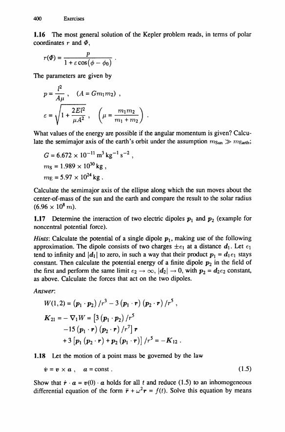
1.16 The most general solution of the Kepler problem reads, in terms of polar coordinates r and iP,

r(P) = p 1 + c: cos ( cf> - c/>o)

The parameters are given by

z2 p= AJ.t'

t:= 2Ez2

1+--2' pA

What values of the energy are possible if the angular momentum is given? Calculate the semimajor axis of the earth's orbit under the assumption msun ~ mEarth;

G = 6.672 X 10-11 m3 kg- 1 s-2 '

ms = 1.989 x 1030 kg ,

mE = 5.97 X 1024 kg .

Calculate the semimajor axis of the ellipse along which the sun moves about the center-of-mass of the sun and the earth and compare the result to the solar radius (6.96 x 108 m).

1.17 Determine the interaction of two electric dipoles p 1 and p2 (example for noncentral potential force).

Hints: Calculate the potential of a single dipole p 1, making use of the following approximation. The dipole consists of two charges ±e1 at a distance d1. Let e1 tend to infinity and ldtl to zero, in such a way that their product p 1 = dt et stays constant. Then calculate the potential energy of a finite dipole p2 in the field of the first and perform the same limit e2 ---> oo, ld2l ---> 0, with p2 = d2e2 constant, as above. Calculate the forces that act on the two dipoles.

Answer:

W(1,2) = (Pt · P2) /r3 - 3 (Pt · r) (P2 · r) /r5 ,

K21 =- Vt W = (3 (Pt · P2) /r5

-15 (Pt · r) (p2 · r) /r7) r + 3 (Pt (P2 · r) + P2 (Pt · r )) /r5 = -K12 .

1.18 Let the motion of a point mass be governed by the law

v = v x a , a = const . (1.5)

Show that r ·a= v(O) ·a holds for all t and reduce (1.5) to an inhomogeneous differential equation of the form r + w2r = j(t). Solve this equation by means


of the substitution rinhom(t) = ct +d. Express the integration constants in terms of the initial values r(O) and v(O). Describe the curve r(t) = r 00m(t) + 1'inhom(t).

Hint:

at x (a2 x a3) = a2 (at · a3) - a3 (at · a2) .

1.19 An iron ball falls vertically onto a hoarizontal plane from which it is reflected. At every bounce it loses the nth fraction of its kinetic energy. Discuss the orbit x = x(t) of the bouncing ball and derive the relation between Xmax and tmax·

Hint: Study the orbit between two successive bounces and sum over previous times.

1.20 Consider the following transformations of the coordinate system:

{t,r}-+{t,r}, {t,r}-+{t,-r}, {t,r}-+{-t,r}, E P T

as well as the transformation P · T that is generated by performing first T and then P. Write these transformations in the form of matrices that act on the fourcomponent vector (!). Show that {E, P, T, PT} form a group.

1.21 Let the potential U(r) of a two-body system be C2 (twice continuously differentiable). For fixed relative angular momentum, under which additional condition on U(r) are there circular orbits? Let Eo be the energy of such an orbit. Discuss the motion for E = Eo+£ for small positive £. Study the special cases

U(r) = rn and U(r) = >..jr .

1.22 Following the methods explained in Sect. 1.26 show the following.

(i) In the northern hemisphere a falling object experiences a southward deviation of second order (in addition to the first-order eastward deviation).

(ii) A stone thrown vertically upward falls down west of its point of departure, the deviation being four times the eastward deviation of the falling stone.

1.23 Let a two-body system be subject to the potential

a U(r) = --

r2

in the relative coordinate r, with positive a. Calculate the scattering orbits r(«.P). For fixed angular momentum what are the values of a for which the particle makes one (two) revolutions about the center of force? Follow and discuss an orbit that collapses to r = 0.

1.24 A pointlike comet of mass m moves in the gravitational field of a sun with mass M and radius R. What is the total cross section for the comet to crash on the sun?

402 Exercises

1.25 Solve the equations of motion for the example of Sect. 1.21.2 (Lorentz force with constant fields) for the case

1.26 Consider the scattering of two identical, pointlike charges with charge e and mass M. What is the motion of the center-of-mass? What is the equation of the relative motion? Choose an inertial system whose origin coincides with the center-of-mass and. whose x-axis is parallel to the direction along which the two particles come in. Which type of solution of the Kepler problem is relevant here? Why can there be no bound state? Study now the central collision of the two particles and discuss the phase portrait in the plane (x,px) as a function of the energy. Sketch the velocity field and the flow.

Chapter 2: The Principles of Canonical Mechanics

2.1 The energy E(q,p) is an integral of a finite, one-dimensional, periodic motion. Why is the portrait symmetric with respect to the q-axis? The surface enclosed by the periodic orbit is

f 1qmax

F(E) = pdq = 2 . pdq . qmm

Show that the change of F(E) with E equals the period T of the orbit, T =

dF(E)jdE, Calculate F and T for the example

E(q,p) = p2 /2m+ mw2q2 /2.

2.2 A weight glides without friction along a plane inclined by the angle a with respect to the horizontal. Study this system by means of d' Alembert's principle.

2.3 A ball rolls without friction on the inside of a circular annulus. The annulus is put upright in the earth's gravitational field. Use d'Alembert's principle to

derive the equation of motion and discuss its solutions.

2.4 A mass point m that can only move along a straight line is tied to the point A by means of a spring. The distance of A to the straight line is l (cf. Fig. 5). Calculate (approximately) the frequency of oscillation of the mass point.

2.5 Two equal masses m are connected by means of a (massless) spring with spring constant x. They move without friction along a rail, their distance being l when the spring is inactive. Calculate the deviations x 1 (t) and x2(t) from the equilibrium positions, for the following initial conditions:

Xt(O) = 0'

X2(0) = [,

±t(O) = vo,

±2(0) = 0.

Chapter 2: The Principles of Canonical Mechanics 403

A

m Fig.S

2.6 Given a function F(xt, ... , x f) that is homogeneous and of degree N in its f variables, show that

1 aF LB.x;=NF. i=l x,

2.7 If in the integral

1X2

J[y] = dx f(y, y') x,

f does not depend explicitly on x, show that

,aJ , y ay' - f(y, y) = const.

Apply this result to L(q, q) = T- U and identify the constant. T is assumed to be a homogeneous quadratic fonn in q.

2.8 Solve the following two problems (whose solutions are well known) by means of variational calculus:

(i) the shortest connection between two points (xt, Yt) and (x2, Y2) in the Euclidean plane;

(ii) the shape of a homogeneous, fine-grained chain suspended at its end points (xt, Yt) and (x2, Y2) in the gravitational field.

Hints: Make use of the result of Exercise 2.7. The equilibrium shape of the chain is detennined by the lowest position of its center of mass. The line element is given by

ds = y'(dx)2 + (dy)2 = .ji+YI2dx.

2.9 Two coupled pendulums can be described by means of the Lagrangian function

(i) Show that the Lagrangian function

404 Exercises

leads to the same equations of motion. Why is this so?

(ii) Show that transforming to the eigenmodes of the system leaves the Lagrange equations form invariant.

2.10 The force acting on a body in three-dimensional space is assumed to be axially symmetric with respect to the z-axis. Show that

(i) its potential has the form U = U(r, z), where { r, <p, z} are cylindrical coordinates,

x = r cos <p , y = r sin <p , z = z ;

(ii) the force always lies in a plane containing the z-axis.

2.11 With respect to an inertial system K0 the Lagrangian function of a particle is

Lo = !mz~- U(zo) .

The frame of reference K has the same origin as K0 but rotates about the latter with constant angular velocity w. Show that the Lagrangian with respect to K reads

m:i:2 m L = - 2- + m:i: · (w X z) + 2(w x :vi - U(z) .

Derive the equations of motion of Sect. 1.25 from this.

2.12 A planar pendulum is suspended such that its point of suspension glides without friction along a horizontal axis. Construct the kinetic and potential energies and a Lagrangian function for this problem.

2.13 A pearl of mass m glides (without friction) along a planar curve s = s(P)

put up vertically. s is the length of arc and P the angle between the tangent to the curve and the horizontal line (see Fig. 6.).

(i) Derive the equation for s(t) for harmonic oscillations.

(ii) What is the relation between s(t) and P(t)? Discuss this relation and the motion that follows from it. What happens in the limit where s can reach its

maximal amplitude?

(iii) From the explicit solution calculate the force of constraint and the effective force that acts on the pearl.

2.14 Geometrical interpretation of the Legendre transformation. Given f(x)

with J"(x) > 0. Construct (Cf)(x) = xf'(x) - f(x) = xz - f(x) = F(x, z), where z = J'(;r). The inverse x = x(z) of the latter exists and so does the Legendre transform of j(x), which is zx(z)- /(x(z)) = Cf(z) = P(z).


mg

L-----------~~----__.x x(z)

Fig.6 Fig. 7

(i) Comparing the graphs of the functions y = f(x) andy= zx (for fixed z) one sees with

8F(x,z) = 0 ax

that x = x(z) is the point where the vertical distance between the two graphs is maximal (see Fig. 7).

(ii) Take the Legendre transform of P(z), i.e. (CP)(z) = zP'(z)- P(z) = zx

P(z) = G(z, x) with P'(z) = x. Identify the straight line y = G(z, x) for fixed z and with x = x(z) show that one has G(z, x)-= f(x). Sketch the picture that one obtains if one keeps x = xo fixed and varies z.

2.15 (i) Let

L(q1, qz, <it, q2, t) = T- U with 2 2

T = L Cik4i4k + L bkqk + a . i,k=l k=l

Under what condition can one construct H(q,p, t) and what are Pt, P2, and H? Confirm that the Legendre transform of H is again L and that

det (a:;q;) det (a:Zm) = 1 ·

Hint: Take dn = 2cn, d12 = d21 = c12 + c21, d22 = 2c22, 11'; =Pi - b;.

(ii) Assume now that L = L(xt = q1, x2 = 42, q1, qz, t) = L(xt, x2, u) with

u ~c(q1 , q2 , t) to be an arbitrary Lagrangian function. We expect the momenta Pi = p;(x1, x2, u) derived from L to be independent functions of x1 and xz, i.e. that there is no function F(p1 (xi, xz, u), P2(XJ, xz, u)) that vanishes identically. Show that, if p1 and P2 were dependent, the determinant of the second derivatives of L with respect to the x1 would vanish.

406 Exercises

Hint: Consider dF/dxt and dFjdx2.

2.16 A particle of mass m is described by the Lagrangian function

L = ~m (±2 + 1l + z2) + ~13 , where 13 is the z-component of angular momentum and w is a constant frequency. Find the equations of motion, write them in terms of the complex variable x + iy and of z, and solve them. Construct the Hamiltonian function and find the kinematical and canonical momenta. Show that the particle has only kinetic energy and that the latter is conserved.

2.17 Invariance under time translations and Noether's theorem. The theorem of E. Noether can be applied to the case of translations in time by means of the following trick. Make t a coordinate-like variable by parametrizing both q and t by q = q(r), t = t(r) and by defining the following Lagrangian function:

-( dq dt)def ( 1 dq )dt L q,t,dr'dr =L 9'dt/drdr't dr'

(i) Show that Hamilton's variational principle applied to L yields the same equations of motion as for L.

(ii) Assume L to be invariant under time translations

h8 (q, t) = (q, t + s) . (2.1)

Apply Noether's theorem to L and find the constant of the motion corresponding to the invariance (2.1).

2.18 A mass point is scattered elastically on a sphere with center P and radius R (see Fig. 8). Show that the physically possible orbit has maximal length.

Hints: Show first that the angles a and f3 must be equal and construct the action integral. Show that any other path AB' n would be shorter than for those points


where the sum of the distances to A and n is constant and equal to the length of the physical orbit.

2.19 (i) Show that canonical transformations leave the physical dimension of the product p;q; unchanged, i.e. [PiQi] = [piqi]. Let~ be the generating function for a canonical transformation. Show that

where H is the Hamiltonian function and t the time.

(ii) In the Hamiltonian function H = l /2m+mw2q2 /2 of the harmonic oscillator introduce the variables

def r= Xt =wymq,

def r=wt,

thus obtaining H = (xf + x~) /2. What is the generating .function ~(x1 , yt) for the canonical transformation x7y that corresponds to the function ~(q, Q) =

~

(mwq2 f2)cot Q? Calculate the matrix Mik = 8xd 8yk and confirm det M = 1 and M JM = J.

2.20 The group SP2J is particularly simple for f = 1, i.e. in two dimensions.

(i) Show that every matrix

M = (att a12) a21 a22

is symplectic if and only if an a22 - a12a21 = 1.

(ii) Therefore, the orthogonal matrices

0 = ( co~ a sin a ) -sma cosa

and the symmetric matrices

5 = ( ~ ~) with xz -l = 1

belong to SP2J· Show that every ME SP2J can be written as a product

M=5·0

of a symmetric matrix 5 with determinant 1 and an orthogonal matrix 0.

2.21 (i) Evaluate the following Poisson brackets for a single particle:

{li,rk}, {l;,pk}, {l;,r}, {l;,p2 }.

(ii) If the Hamiltonian function in its natural form H = T + U is invariant under rotations, what quantities can U depend on?

408 Exercises

2.22 Making use of the Poisson brackets show that for the system H = T+U(r) with U(r) = 1/r and 1 a constant, the vector

A=pxl+~m1/r

is an integral of the motion (Lenz' s vector).

2.23 The motion of a particle of mass m is described by

1 H = 2m (pf + ~) + maq1 , a = const .

Construct the solution of the equations of motion for the initial conditions

qt(O) = xo, q2(0) =Yo, Pt(O) = Px, P2(0) = Py,

making use of Poisson brackets.

2.24 For a three-body system with masses m;, coordinates r;, and momenta P; introduce the following coordinates (Jacobian coordinates):

def lf't = r2- rt

def mt rt + m2r2 lf'2 = r3-

mt+m2

defffitP2 - m2Pt 1rt = ,

mt +m2

der(mt + m2) P3 - m3 (Pt + P2) 1r2 = ,

mt +m2+m3 def

1r3 = Pt + P2 + P3 ·

(relative coordinate of particles 1 and 2)

(relative coordinate of particle 3

and the center of mass of the first two) ,

(center of mass of the three particles),

(i) What is the physical interpretation of the momenta 1r1, 1r2, 1r3?

(ii) How would you define such coordinates for four or more particles?

(iii) Show in at least two (equivalent) ways that the transformation

is canonical.

2.25 Given a Lagrangian function L for which aL/Ot = 0, study only those variations of the orbits qk(t, a) which belong to a fixed energy E = Lk iJk(/)L/[Jqk) - L and whose end points are kept fixed irrespective of the time (h- t1) that the system needs to move from the initial to the end point, i.e.

qk(t, a) with { (I)

qk (tt(a), a)= qk (2)

qk (i2(a), a) = qk for all a . (2.1)


Thus, initial and final times are also varied, ti = ti(o:).

(i) Calculate the variation of I(o:),

dl(o:) I 1M<>) OJ= -d- do: = L (qk(t, o:), «ik(t, o:)) dt .

0: a=O t1(a)

(ii) Show that the variational principle

(2.2)

together with the prescriptions (2.1) is equivalent to the Lagrange equations (the Principle of Euler and Maupertuis).

2.26 The kinetic energy

is assumed to be a positive symmetric quadratic form in the 4i· The orbit in the space spanned by the qk is described by the length of arcs such that T = (ds jdt)2 .

With E = T + U the integral K of Exercise 2.25 can be replaced with an integral over s. Show that the integral principle obtained in this way is equivalent to Fermat's principle of geometric optics,

1X2

b n(:c, v)ds = 0 X1

(n: index of refraction, v: frequency).

2.27 Let H = p2 /2 + U(q), where the potential is such that it has a local minimum at qo. Thus, in an interval q1 < qo < q2 the potential forms a potential well. Sketch a potential with this property and show that there is an interval U(qo) < E ~ Emax where there are periodic orbits. Consider the characteristic equation of Hamilton and Jacobi (2.154). If S(q, E) is a complete integral then t- to= 8Sf8E. Take the integral

I(E)d~r.!._ J pdq 271" IrE

over the periodic orbit rE with energy E (this is the surface enclosed by rE). Write l(E) as an integral over time and show that

2.28 In Exercise 2.27 replace S(q, E) by S(q, I) with I= l(E) as defined there.

410 Exercises

S generates the canonical transformation (q, p, H) -+ (fJ, I, ii = E(ll)). What are the canonical equations in the new variables? Can they be integrated?

2.29 Let H0 = -j /2 + q2 /2. Calculate the integral /(E) defined in Exercise 2.27. Solve the characteristic equation of Hamilton and Jacobi (2.154) and write the solution as S(q,l). Then (J = 8Sf01. Show that (q,p) and (fJ,l) are related by the canonical transformation (2.95) of Sect. 2.24 (ii).

Chapter 3: The Mechanics of Rigid Bodies

3.1 Let two systems of reference K and K be fixed in the center of mass of a rigid body, the axes of the former being fixed in space, those of the latter fixed in the body. If J is the inertia tensor with respect to K and J the one as calculated in K, show that (i) J and J have the same eigenvalues. (Use the characteristic polynomial.)

(ii) K is now assumed to be a system of principal axes of inertia. What is the form of J ? Calculate J for the case of rotation of the body about the 3-axis.

3.2 Two particles with masses mt and m2 are held by a rigid but massless straight connection with length 1. What are the principal axes and what are the moments of inertia?

3.3 The inertia tensor of a rigid body is found to have the form

l;k = ( ~:: ~~ ~ ) , ht = lt2 . 0 0 /33

Determine the three moments of inertia and consider the following special cases.

(i) In = I22 =A, It2 =B. Can 133 be arbitrary?

(ii) Itt = A, I22 = 4A, It2 = 2A. What can you say about 133 ? What is the shape of the body in this example?

3.4 Construct the Lagrangian function for general, force-free motion of a conical top (heigth h, mass M, radius of base circle R). What are the equations of motion? Are there integrals of the motion and what is their physical interpretation?

3.5 Calculate the moments of inertia of a torus filled homogeneously with mass. Its main radius is R; the radius of its section is r.

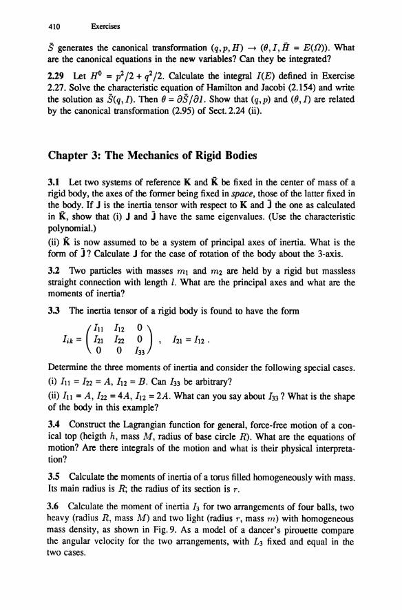
3.6 Calculate the moment of inertia 13 for two arrangements of four balls, two heavy (radius R, mass M) and two light (radius r, mass m) with homogeneous mass density, as shown in Fig. 9. As a model of a dancer's pirouette compare the angular velocity for the two arrangements, with L3 fixed and equal in the two cases.

Chapter 3: The Mechanics of Rigid Bodies 411

Fig.9

b

a

3.7 (i) Let the boundary of a homogeneous body be defined by the formula (in spherical coordinates)

R(B) = Ro(l +a cos B) ,

i.e. g(r, 0, q;) = l!O = const for r ~ R(B) and all 0 and q;, and g(r, 0, q;) = 0 for r > R(B). If M is the total mass, calculate l!O and the moments of inertia.

(ii) Perform the same calculation for a homogeneous body whose shape is given by

R(O) = Ro (1 + ,BY2o(O))

with Yw(B) = J5/16rr(3cos2 0- 1) being the spherical harmonic with l = 2, m = 0. In both examples sketch the body.

3.8 Determine the moments of inertia of a rigid body whose inertia tensor with respect to a system of reference K 1 (fixed in the body) is given by

9 I -J3 8 4 8

J= 1 3 -J3 -4 2 4

-J3 -J3 II -

8 4 8

Can one indicate the relative position of the principal inertia system K0 relative to Kt?

3.9 A ball with radius a is filled homogeneously with mass such that the density is l!O· The total mass is M.

(i) Write the mass density g with respect to a body-fixed system centered in the center of mass and express l!O in terms of M. Let the ball rotate about a point P on its surface (see Fig. 10).

(ii) What is the same density function g(r, t) as seen from a space-fixed system centered on P?

412 Exercises

---Flg.lO

(iii) Give the inertia tensor in the body-fixed system of (i). What is the moment of inertia for rotation about a tangent to the ball in P ?

Hint: Use the step function 8(x) = 1 for x ~ 0, 8(x) = 0 for x < 0.

3.10 A homogeneous circular cylinder with length h, radius r, and mass m rolls along an inclined plane in the earth's gravitational field.

(i) Construct the full kinetic energy of the cylinder and find the moment of inertia relevant to the described motion.

(ii) Construct the Lagrangian function and solve the equation of motion.

3.11 Manifold of motions of the rigid body. A rotation R E S0(3) can be determined by a unit vector rp (the direction about which the rotation takes place) and an angle <p.

(i) Why is the interval 0 :::; <p :::; 1r sufficient for describing every rotation?

(ii) Show that the parameter space (rp, <p) fills the interior of a sphere with radius 1r in R3. This ball is denoted by D2 • Confirm that antipodal points on the ball's surface represent the same rotation.

(iii) There are two types of closed orbit in D2, namely those which can be contracted to a point and those which connect two antipodal points. Show by means of a sketch that every closed curve can be reduced by continuous deformation to either the former or the latter type.

3.12 Calculate the Poisson brackets (3.92-95).

Chapter 4: Relativistic Mechanics

4.1 (i) A neutral 1r meson (1r0) has constant velocity v0 along the x3-direction. Write its energy-momentum vector. Construct the special Lorentz transformation that leads to the particle's rest system.

(ii) The particle decays isotropically into two photons, i.e. with respect to its rest system the two photons are emitted in all directions with equal probability. Study their decay distribution in the laboratory system.

Chapter 4: Relativistic Mechanics 413

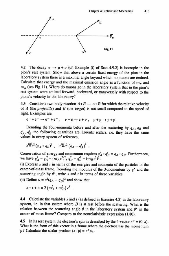
4.2 The decay 1r ---+ J.l + v (cf. Example (i) of Sect. 4.9.2) is isotropic in the pion's rest system. Show that above a certain fixed energy of the pion in the laboratory system there is a maximal angle beyond which no muons are emitted. Calculate that energy and the maximal emission angle as a function of m,. and m,. (see Fig. 11). Where do muons go in the laboratory system that in the pion's rest system were emitted forward, backward, or transversely with respect to the pions's velocity in the laboratory?

4.3 Consider a two-body reaction A+ B ---+ A+ B for which the relative velocity of A (the projectile) and B (the target) is not small compared to the speed of light. Examples are

e-+e----+e-+e-, v+e---+e+v, p+p---+p+p.

Denoting the four-momenta before and after the scattering by qA, qB and q~, q8 the following quantities are Lorentz scalars, i.e. they have the same values in every system of reference,

def2( ')2 t=c qA-qA .

Conservation of energy and momentum requires q~ +q8 = qA +qB. Furthermore, we have q~ = q1 = (mAc2)2 , q~ = q~ = (mBCl-)2 .

(i) Express s and t in terms of the energies and momenta of the particles in the center-of-mass frame. Denoting the modulus of the 3-momentum by q* and the scattering angle by (}*, write s and t in terms of these variables.

(ii) Define u = c2(qA - q8)2 and show that

s+t+u=2(m~+m~)c4 •

4.4 Calculate the variables sand t (as defined in Exercise 4.3) in the laboratory system, i.e. in that system where B is at rest before the scattering. What is the relation between the scattering angle () in the laboratory system and ()* in the center-of-mass frame? Compare to the nonrelativistic expression (1.80).

4.5 In its rest system the electron's spin is described by the 4-vector s" = (0, s). What is the form of this vector in a frame where the electron has the momentum p? Calculate the scalar product ( s · p) = s" Pa.

414 Exercises

4.6 Show that

(i) every lightlike vector z (z2 = 0) can be brought to the form (1,1,0,0) by means of Lorentz transformations;

(ii) every spacelike vector can be transformed to the form (0, zt, 0, 0), where zt = r-;'1. Indicate the necessary transformations in both cases.

4.7 If Ji and Ki denote the generators of rotations and boosts, respectively (cf. Sect. 4.5.2 (iii)) define

deft ( ") deft ( • ) . Ap = 2 Jp + iKp , Bq = 2 Jq - tKq , p, q = 1, 2, 3 .

Making use of the commutation rules (4.59) calculate [Ap, Aq], [Bp, Bq], and [Ap, Bq] and compare to (4.59).

4.8 Study the behavior of Ji and Ki with respect to space inversion, i.e. determine PJip-t, PKiP-t.

4.9 In quantum theory one prefers to use the quantities A clef A clef Ji=iJi, Ki= -iKi.

What are the commutators (4.59) for these matrices? Show that the matrices Ji

are Hermitian, i.e. that <Ji>• = Ji.

4.10 A muon decays predominantly into an electron and two massless neutrinos, J.L- --+ e- + vt + Vl· If the muon is at rest, show that the electron assumes its maximal momentum whenever the neutrinos are emitted parallel to each other. Calculate the maximal and minimal energies of the electron as functions of m,. and me. Answer:

2 2 - m,. +me Cl Emax- 2 ,

m,.

Draw the corresponding momenta in the two cases.

4.11 A particle of mass M is assumed to decay into three particles (1,2,3) with masses mt, m2, m3. Determine the maximal energy of particle 1 in the rest system of the decaying particle as follows. Set

Pt =- f(x)n , P2 = xf(x) , P3 = (1 - x)f(x)n ,

where n is a unit vector and x is a number between 0 and 1. Find the maximum of f(x) from the principle of energy conservation.

Examples:

(i) J.L- --+ e- +III + V2 (cf. Exercise 4.10),

Chapter 5: Geometric Aspects of Mechanics 415

(ii) Neutron decay: n 4 p + e + v.

What is the maximal energy of the electron? What is the value of f3 = lvl/c for the electron? mn- mp = 2.53 me, mp = 1836 me.

4.12 Pions 71'+' 71'- have the mean lifetime T ~ 2.6 X w-8 s and decay predominantly into a muon and a neutrino. Over what distance can they fly, on average, before decaying if their momentum is P1r = x • m1rc with x = 1, 10, or 1000? (m'lr ~ 140MeV fc2 = 2.50 X w-28 kg).

4.13 The free neutron is unstable. Its mean lifetime is r ~ 900 s. How far can a neutron fly on average if its energy is E = w-2 mncl or E = 1014 mncl?

4.14 Show that a free electron cannot radiate a single photon, i.e. the process

cannot take place because of energy and momentum conservation.

Chapter 5: Geometric Aspects of Mechanics

5.1 Let ~ be an exterior k-form, ~ an exterior 1-form. Show that their exterior product is symmetric if k and/or l are even and antisymmetric if both are odd, i.e.

k I k·ll k w 1\ w = (-1) w 1\ w.

5.2 Let x1, x2 , x3 be local coordinates in the Euclidean space R3 , ds2 = Et dxf+ E2 dx~ + EJ dx~ the square of the line element, and et' e2, e3 unit vectors along the coordinate directions. What is the value of dx;(ej), i.e. of the action of the one-form dx; on the unit vector ei?

5.3 Let a= E~=l a;(x)e; be a vector field with a;(x) smooth functions on M.

To every such vector field we associate. a one-form ~a and a two-form ~a such that

1 2 Wa(e) =(a· e) , Wa(e, 7]) =(a· (e X 7])) ·

Show that 3

~a= La;(x)y'E;dx;, i=l

~a= a;(x)~ dx21\ dx3 +cyclic permutations,

5.4 Making use of the results of Exercise 5.3 determine the components of V f in the basis { et' e2, e3}

416 Exercises

Answer: 3 1 8f A v J = I: ro-. -a i e; .

i=t vE; x

5.5 Determine the functions E; for the case of Cartesian, cylindrical, and spherical coordinates. In each case give the components of V f. 5.6 To the force F = (Fi, F2) in the plane we associate the one-form w = F1 dx 1 + H dx2. When we apply w onto a displacement vector, w(e) is the work done by the force. What is the dual *W of the form w? What is its interpretation?

5.7 The Hodge star operator assigns to every k-form w the (n- k)-form *W. Show that

*(*w) = (-l)k-(n-k)w.

5.8 Let E = (E1, Fh,, ~) and B = (B1, B2, B3) be electric and magnetic fields that in general depend on x and t. We assign the following exterior forms to them:

3 def"" .

cp = L...J E;dx' , i=l

w~fB1 dx2 Adx3 +B2dx3 Adx1 +B3dx1 Adx2 •

Write the homogeneous Maxwell equation curl E + iJ / c = 0 as an equation between the forms cp and w.

5.9 If d denotes the exterior derivatives and * the Hodge star operator, the codifferential 6 is defined by

6~f*d*.

Show that L1~rd o 6 + 6 o d, when applied to functions, is the Laplacian operator

5.10 Let

/:; = L w;1 •.. ;k (q;) dxi 1 A ••. A dxi•

il <···<it

be an exterior k-form over a vector space W Let F : V -+ W be a smooth

mapping of the vector space V onto W. Show that the pullback F*(/:; A~) of the exterior product of two such forms is equal to the exterior product of the

pullback of the individual forms (F*/:;) A (F*~).

Chapter 6: Stability and Chaos 417

5.11 With the same assumptions as in Exercise 5.10 show that the exterior derivative and the pullback commute,

d(F*w) = F*(dw).

5.12 Let x and y be Cartesian coordinates in R2 , V = yax and W = xay two vector fields on R2 . Calculate the Lie bracket [V, W). Sketch the vector fields V, W, and [V, W) along circles about the origin.

5.13 Prove the following assertions.

(i) The set of all tangent vectors to the smooth manifold M at the point p E M form a real vector space, denoted by TpM, whose dimension is n = dim M. (ii) If M is Rn, TpM is isomorphic to that space.

5.14 The canonical two-form for a system with two degrees of freedom reads w = I:;= I dq; I\ dp;. Calculate w I\ w and confirm that this product is proportional to the oriented volume element in phase space.

5.15 Let H<1l = p2 /2 + (1 - cos q) and H<2l = p2 /2 + q(q2 - 3)/6 be the Hamiltonian functions for two systems with one degree of freedom. Construct the corresponding Hamiltonian vector fields and sketch them along some of the solution curves.

5.16 Let H = H0 + H' with H0 = (p2 + q2)j2 and H' = c:q3 f3. Construct the Hamiltonian vector fields X Ho and X H and calculate w(X H, X Ho).

5.17 Let Land L' be two Lagrangian functions on TQ for which PL and Pu are regular. The corresponding vector fields and canonical two-forms are XE, X E', w L, and w L'. Show that each of the following assertions implies the other:

(i) L' = L +a, where a: TQ--+ R is a closed one-form, i.e. da = 0;

(ii) XE = XE' and WL = wu. Show that in local coordinates this is the result obtained in Sect. 2.10.

Chapter 6: Stability and Chaos

6.1 Study the two-dimensional linear system ¥ = A¥, where A has one of the

Jordan normal forms

(i) A = ( ~ ~2 ) , (ii) A = ( ~b ! ) , (iii) A = (; ~) .

In all three cases determine the characteristic exponents and the flow (6.13) with s = 0. Suppose the system is obtained by linearizing a dynamical system in the neighborhood of an equilibrium position. (i) corresponds to the situations shown in Figs. 6.2a--c. Draw the analogous pictures for (ii) for (a = 0, b > 0) and (a < 0, b > 0), and for (iii) with .A < 0.

418 Exercises

6.2 The variables a and {3 on the torus T2 = S1 X S1 define the dynamical system

a= a/27r ' /3 = b/27r ' 0::; a, {3 ::; 1 '

where a and bare real constants. Cutting the torus at (a= 1, {3) and at (a, {3 = 1) yields a square of length 1. Draw the solutions with initial condition (ao, f3o) in this square for b fa rational and irrational.

6.3 Show that in an autonomous Hamiltonian system with one degree of freedom (and hence two-dimensional phase space) neighboring trajectories can diverge at most linearly with increasing time.

Hint: Make use of the characteristic equation (2.154) of Hamilton and Jacobi.

6.4 Study the system

41 = -JJq1 - >..q2 + q1 q2

42 = >..qt - {tqz + ( qf - qi) /2 '

where 0 ::; JJ «: 1 is a damping term and>.. with 1>..1 «: 1 is a detuning parameter. Show that if JJ = 0 the system is Hamiltonian. Find a Hamiltonian function for this case. Draw the projection of its phase portraits for >.. > 0 onto the ( q1 , q2)

plane and determine the position and the nature of the critical points. Show that the picture obtained above is structurally unstable when JJ is chosen

to be different from zero and positive, by studying the change of the critical points for wf.O. 6.5 Given the Hamiltonian function on R4

H( ) - 1 ( 2 2) 1 ( 2 2) 1 ( 3 3) q1 , q2, P1 ' P2 - 2 P1 + Pi + 2 q1 + q2 + 3 q1 - q2

show that this system possesses two independent integrals of the motion and sketch the structure of its flow.

6.6 Study the flow of the equations of motion p = q, p = q - q3 - p and determine the position and the nature of its critical points. Two of these are attractors. Determine their basin of attraction by means of the Liapunov function v = p2 /2 - q2 /2 + q4 /4. 6.7 Dynamical systems of the type

t =-au f8q: = -U,x

are called gradient flows. They are quite different from the flows of Hamiltonian systems. Making use of a Liapunov function show that if U has an isolated minimum at q;o. then q;o is an asymptotically stable equilibrium position. Study the example

6.8 Consider the equations of motion

q = p' p = !(1- q2)

Olapter 6: Stability and Olaos 419

of a system with f = 1. Sketch the phase portrait of typical solutions with given energy. Study its critical points.

6.9 By numerical integration find the solutions of the Van der Pool equation (6.36) for initial conditions close to (0,0) and for various values of c: in the interval 0 < c: ~ 0.4. Draw q(t) as a function of time, as in Fig. 6.7. Use the result to find out empirically at what rate the orbit approaches the attractor.

6.10 Choose the straight line p = q as the transverse section for the system (6.36), Fig. 6.6. Determine numerically the points of intersection of the orbit with initial condition (0.01,0) with that line and plot the result as a function of time.

6.11 The system in R2

Xt = Xt '

has a critical point in x1 = 0 = xz. Show that for the linearized system the line x1 = 0 is a stable submanifold and the line xz = 0 an unstable one. Find the corresponding manifolds for the exact system by integrating the latter.

6.12 Study the mapping Xi+l = f(xi) with f(x) = 1 - 2x2• Substitute u = (4/'rr)arcsin J<x + 1)/2 and show that there are no stable fixed points. Calculate numerically 50 000 iterations of this mapping for various initial values xt f 0 and plot the histogram of the points that land in one of the intervals [n/100, (n + 1)/100] with n = -100, -99, ... , +99. Follow the development of two close initial values x1 , x~, and verify that they diverge in the course of the iteration. (For a discussion see Collet, Eckmann 1980.)

6.13 Study the flow of Roessler's model

x = -y- z, iJ = x + ay, z = b+ xz- cz

for a = b = 0.2, c = 5.7 by numerical integration. The graphs of x, y, z as functions of time and their projections onto the (x, y)-plane and the (x, x)-plane are particularly interesting. Consider the Poincare mapping for the transverse section y + z = 0. As x = 0, x has an extremum on the section. Plot the value of the extremum Xi+t as a function of the previous extremum Xi (see also Berge, Pomeau, VJ.dal1984 and references therein).

6.14 Although this is more than an exercise, the reader is strongly encouraged to study the system known as Henon's attractor. It provides a good illustration of chaotic behavior and extreme sensitivity to initial conditions (see also, Berge, Pomeau, Vidal 1984, Sect. 3.2 and Devaney 1986, Sect. 2.6, Exercise 10).

420 Exercises

6.15 Show that

i=exp [i 2: am] = n8mo, (m = 0, ... , n- 1). 0'=1

Use this resalt to prove (6.63), (6.65), and (6.66).

6.16 Show that by a linear substitution y = ax + f3 the system (6.67) can be transformed to Yi+l = 1 - 'YY~. Determine 'Y in terms of Jl and show that y lies in the interval (-1, 1] and 'Yin (0,2] (cf. also Exercise 6.12 above). Making use of this transformed equation derive the values of the first bifurcation points (6.68) and (6.70).

Appendix: Some Mathematical Notions

"Order" and ''Modulo". The symbol O(en) stands for tenns of the order en and higher powers thereof that are being neglected.

Example. If in a Taylor series one wishes to take account only of the first three terms, one writes

(A.l)

This means that the right-hand side is valid up to terms of order x3 and higher. The notation y = x (mod a) means that x and x + na should be identified, n

being any integer. Equivalently, this means that one should add to x or subtract from it the nu~ber a as many times as are necessary to have y fall in a given interval.

Example. Suppose two angles a and f3 are defined in the interval [0, 271"]. The equation a= f(/3) (mod 27r) means that one must add to the value of the function f(/3), or subtract from it, an integer number of terms 271" such that a does not fall outside its interval of definition.

Mappings. A mapping f that maps a set A onto a set B is denoted as follows:

f: A -+ B: a .,.... b . (A.2)

It assigns to a given element a E A the element b E B. The element b is said to be the image and a its preimage.

Examples. (i) The real function sin x maps the real x-axis onto the interval [-1, +1],

sin: R-+ [-1, +1]: x f-+ y = sinx.

(ii) The curve 'Y: x = cos wt, y = sin wt in R2 is a mapping from the real t-axis onto the unit circle S1 in R2,

'Y: Rt -+ S1 : t.,.... (x = coswt, y = sinwt).

A mapping is called surjective if f(A) = B, i.e. if B is covered completely. The mapping is called injective if two distinct elements in A also have distinct images in B, in other words, if every b E B has one and only one original a E A. If it has both properties it is said to be bijective. In this case every element of A has exactly one image in B, and for every element of B there is exactly one preimage in A. In other words the mapping is then one-to-one.

422 Appendix: Some Mathematical Notions

The composition f o g of two mappings f and g means that g should be applied first and then f should be applied to the result of the first mapping, viz.

If g: A ~ B and f: B ~ C , then f o g: A ~ C . (A.3)

Example. Suppose f and g are functions over the reals. Then, withy= g(x) and z = f(y) we have z = (f o g)(x) = f(g(x)).

The identical mapping is often denoted by "id", i.e.

id: A ~ A: a ~---+ a .

Special Properties of Mappings. A mapping f: A ~ B is said to be continuous at the point u E A if for every neighborhood V of its image v = f(u) E B there exists a neighborhood U of u such that f(U) C V. The mapping is continuous if this property holds at every point of A.

Homeomorphisms are bijective mappings f: A ~ B that are such that both f and its inverse f-1 are continuous.

Dijfeomorphisms are differentiable, bijective mappings f that are such that both f and f-1 are smooth (i.e. differentiable, C 00).

Derivatives. Let f(x 1 , x2 , ••• , xn) be a function over the space Rn, { e1, ... , en}, a set of orthogonal unit vectors. The partial derivative with respect to the variable xi is defined as follows:

8f. =lim f(x +he;)- f(x) ax• h--0 h

(A.4)

Thus one takes the derivative with respect to xi while keeping all other arguments xi' ... ' xi-1' xi+ I' ... ' xn fixed.

Collecting all partial derivatives yields a vector field called the gradient,

(A.5)

Since any direction n in Rn can be decomposed in terms of the basis vectors el, ... 'en, one can take the directional derivative off along that direction, viz.

(A.6)

The total differential of the function f(x 1, ••• , xn) is defined as follows:

Bj 1 BJ 2 BJ n df= -dx +-dx + ··· +-dx . 8x1 8x2 axn

(A.7)

Examples. (i) Let f(x, y) = !<x2 + y2) and let (x = r cos¢>, y = r sin¢>) with fixed r and 0 :-:::; ¢> :-:::; 21r be a circle in R2 . The normalized vector tangent to the circle at the point (x, y) is given by v1 = (-sin¢>, cos¢>). Similarly, the normalized normal vector at the same point is given by vn =(cos¢>, sin¢>). The

Appendix: Some Mathematical Notions 423

total differential off is df = xdx + ydy and its directional derivative along Vt

is Vt • V f = -x sin <P + ycos <P = 0; the directional derivative along Vn is given by Vn • V f = x cos <P + y sin <P = r. For an arbitrary unit vector v =(cos a, sin a) we find v · V f = r(cos <Pcos a+ sin <P sin a). For fixed <P the absolute value of this real number becomes maximal if a= c/J(mod7r). Thus, the gradient defines the direction along which the function f grows or falls fastest

(ii) Let U (x, y) = xy be a potential in the plane R2 . The curves along which the potential U is constant (they are called equipotential lines) are obtained by taking U(x, y) = c, with c a constant real number. They are given by y = cfx, i.e. by hyperbolas whose center of symmetry is the origin. Along these curves dU(x, y) = ydx + xdy = 0 because dy = -(cfx2)dx = -(yjx)dx. The gradient is given by VU = (oU fox, oU joy)= (y, x) and is perpendicular to the curves U(x, y) = c at any point (x, y). It is the tangent vector field of another set of curves that obey the differential equation

dy X

dx =y These latter curves are given by y2 - x2 = a.

Differentiability of Functions. The function f(x1 , ••• , xi, ... , xn) is said to be cr with respect to xi if it is r-times continuously differentiable in the argument xi. A function is said to be coo in some or all of its arguments if it is differentiable an infinite number of times. It is then also said to be smooth.

Variables and Parameters. Physical quantities often depend on two kinds of arguments, the variables and the parameters. This distinction is usually made on the basis of a physical picture and, therefore, is not canonical. Generally, variables are dynamical quantities whose time evolution one wishes to study. Parameters, on the other hand, are given numbers that define the system under consideration. In the example of a forced and damped oscillator, the deviation x(t) from the equilibrium position is taken to be the dynamical variable while the spring constant, the damping factor, and the frequency of the driving source are parameters.

Bibliography

Mechanics Textbooks and Exercise Books

Fetter, AL., Walecka, J.D.: Theoretical Mechanics of Particles and Continua (McGraw Hill, New York 1980)

Goldstein, H.: Classical Mechanics (Addison-Wesley, Reading 1980) Honerkarnp, J., Romer, H.: Grundlagen der klassischen Theoretischen Physik (Springer, Berlin, Hei

delberg 1989) Landau, LD., Lifshitz, EM.: Mechanics (Pergamon, Oxford and Addison-Wesley, Reading 1971) Scheck, F., Schtlpf, R.: Mechanik Manual, Aufgaben mit l..Osungen (Springer, Heidelberg, Berlin

1989) Spiegel, M.R.: General Mechanics, Theory and Applications (McGraw Hill, New York 1976)

Some General Mathematical Texts

Arnold, V.I.: Ordinary Differential Equations (M.I.T. Press, Cambridge 1973) Arnold, V.I.: Geometrical Methods in the Theory of Ordinary Differential Equations (Springer, New

York, Berlin, Heidelberg 1983) Flanders, H.: Differential Forms (Academic, New York 1963) Hamermesh, M.: Group Theory and Its Applications to Physical Problems (Addison-Wesley, Reading

1962)

Special Functions and Mathematical Formulae

Abramowitz, M., Stegun, I.A.: Handbook of Mathematical Functions (Dover, New York 1965) Gradshteyn, I.S., Ryzhik, l.M.: Tables of Integrals, Series and Products (Academic, New York 1965)

Chapter 2

Rii.Bmann, H.: Konvergente Reihenentwicklungen in der Swrungstheorie der Himmelsmechanik, Selecta Mathernatica V (Springer, Berlin, Heidelberg 1979)

RiiBrnann, H.: Non-degeneracy in the Perturbation Theory of Integrable Dynamical Systems, in Dodson, M.M., Vickers, J.A.G. (eds.) Number Theory and Dynamical Systems, London Mathematical Society Lecture Note Series 134 (Cambridge University Press 1989)

Chapter 4

Hagedorn, R.: Relativistic Kinematics (Benjamin, New York 1963) Jackson, J.D.: Classical Electrodynamics (Wiley, New York 1975) Sex!, R.U., Urbantke, H.K.: Relativitiit, Gruppen, Teilchen (Springer, Berlin, Heidelberg 1976)

426 Bibliography

Weinberg, S.: Gravitation and Cosmology, Principles and Applications of the General Theory of Relativity (Wiley, New York 1972)

Chapter 5

Abraham, R., Marsden, J.E.: Foundations of Mechanics (Benjamin Cummings, Reading 1978) Arnold, V.I.: Mathematical Methods of Classical Mechanics (Springer, New York, Berlin, Heidelberg

1978) Guillemin, V., Sternberg, S.: Symplectic Techniques in Physics (Cambridge University Press, New

York 1986) O'Neill, B.: Semi-Riemannian Geometry, With Applications to Relativity (Academic, New York 1983) Thirring, W.: A Course in Mathematical Physics, Vol. 1: Classical Dynamical Systems (Springer,

Berlin, Heidelberg 1978)

Chapter 6

Arnold, V.I.: Catastrophe Theory (Springer, Berlin, Heidelberg 1986) Berg~. P., Pomeau, Y., Vidal, C.: Order within Chaos; Towards a Deterministic Approach to Turbu

lence (Wiley, New York 1986) French original (Hermann, Paris 1984) Chirikov, B.V.: A Universal Instability of Many-Dimensional Oscillator Systems, Physics Reports 52,

263 (1979) Collet, P., Eckmann, J.P.: Iterated Maps on the Interval as Dynamical Systems (Birkhliuser, Boston

1980) Devaney, RL.: An Introduction to Chaotic Dynamical Systems (Benjamin Cummings, Reading 1986) Feigenbaum, M.: I. Stat. Phys. 19, 25 (1978) and 21, 669 (1979) Guckenheimer, J., Holmes, P.: Nonlinear Oscillations, Dynamical Systems, and Bifurcations of Vector

Fields (Springer, Berlin, Heidelberg 1983) Henon, M., Heiles, C.: Astron. Journ. 69, 73 (1964) Hirsch, M.W., Smale, S.: Differential Equations, Dynamical Systems and Linear Algebra (Academic,

New York 1974) Palis, J., de Melo, W.: Geometric Theory of Dynamical Systems (Springer, Berlin, Heidelberg 1982) Peitgen, H.O., Richter, P.H.: The Beauty of Fractals, Images of Complex Dynamical Systems (Springer,

Berlin, Heidelberg 1986) Ruelle, D.: D.: Elements of Dif!erenJial Dynamics and Bifurcation Theory (Academic, New York

1989) Schuster, H.G.: Deterministic Chaos, An lnJroduction (Physik-Verlag, Weinheim 1984) Wisdom, J.: Chaotic Behaviour in the Solar System, Nucl. Phys. B (Proc. Suppl.) 2, 391 (1987)

Subject Index

Acceleration 4 Action 88, 308 Action function 308 Action integral 88 Action-angle variables 114, 149,345 Addition of velocities 230 Adiabatic invariants 157 Angular momentum - of rigid body 179 - of single particle 13 Angular-momentum conservation,

principle of 20 Angular velocity 168 Aphelion 46 Apocenter 46 Asymptotic stability 325, 336 Atlas 258 -, complete 259 Attractor 333, 338 -, strange 333,357,369 Atwood's machine 84 Autonomous systems 37 Averaging principle 156 Axial vector 285

Base differential forms 274 Base integral curve 311 Base space 268 Base vector fields 267,271 Basin of attractor 339 Bifurcations 346 -, Hopf 349 -, pitchfork 349 -, saddle-node 348 -, transcritical 348 Body cone 194 Boost, see special Lorentz transformation Bundle chan 269

Canonical equations 98, 115, 297 Canonical one-form 290 Canonical systems 98

Canonical transformations 110.117 -, infinitesimal 133 Canonical two-form 292 Cantor's middle third set 370 Cartan derivative 282 Center 328 Center-of-mass

coordinates 11 momentum 18 motion, principle of 19 system 55

Central force 13 Centrifugal force 51 Chaos 352, 354 Characteristic exponents 324 Characteristic multipliers 344 Chart 257 Children's top 176,201 Circular orbit 16,401 Closed form 292 Commutators

of generators of Lorentz group 228 - of generators of rotation group 109 - of vector fields 272 Composition of mappings 422 Cone -. body 194 - of nutation 194 -, space 194 Conformal group 249 Constant of the motion, see integral

of the motion Constraints 77 Contravariant index 213 Coordinate functions, natural 256 Coordinate manifold 254, 286 Coordinate system (for rigid bodies) -, body-fixed 167 -, intrinsic 167 -, space-fixed 167 Coordinates -, canonical 296 -, cyclic 95,110

428 Subject Index

-, generalized 79 -, local 254, 257 Coriolis force 51,401 Cotangent bundle 254, 273 Cotangent space 253, 273 Coulomb force 8, 62 Coulomb scattering 61,62 Covariantderivative 94 Covariantequation 238 Covariant index 213 Critical elements (of vector fields) 336 Critical points 322, 329 Cross section -, differential 59 -, total 60 Curl 28 Curves on manifolds 264 Cyclic coordinates 95,110

D'Alembert's principle 80 Darboux' s theorem 296 Decomposition theorem 224 Degree of freedom 35 Derivative -, directional 266,422 -, exterior 282 -, exterior in R3 283 -, Lie 272, 299 -, partial 422 -, total 422 -, variational 87 Deterministic motion 36 Diffeomorphism 93, 322, 422 Differential equation with separable

variables 40 Differential form 273 Differential mapping 276 Dilatations 249 Dissipative systems 334 Dynamical systems 318, 322

Eigenfrequencies 160 Energy conservation, principle of 20 Energy function 308 Energy-momentum vector 240 Equilibrium position 142,322 Eulerian angles 183,184 Euler-Lagrange equations 89, 387 Euler's differential equation 87 Euler's equations 188,190 Event, see world point Exterior forms 281 Exterior product 280

Fermat's principle 86,409 Fiber 234, 268 Fiber bundle 234, 268 Fibonacci's numbers 366 Field strengths, tensor of 243 Finite orbit 16,41 Flow -, global 322 -, local 321 -. maximal 321 - in phase space 37 - of a vector field 320 Flow fronts 321 Force -, centrifugal 51 -, conservative 28 - of constraint 80 -, external 7 -, fictitious 5, 51 -, generalized 81 -. internal 7 -, Lorentz 90 Force field 7 Force law, relativistic 238 Form invariance 5, 238 Forms -, canonical, of mechanics 290, 292 -, exterior 281 Fractal .369 Frequency doubling 363 Functions on manifolds 264

Galilei group 24 - proper, orthochronous 23 Galilean space-time 217, 233 Gauge transformations 91,92 Generating function

for canonical transformations 111 - for infinitesimal canonical

transformations 133 Generators

for infinitesimal Lorentz transformations 227 for infinitesimal rotations 104, 108 for infinitesimal symplectic transformations 329

Golden Mean 366 Gradient 422 Gradient flow 344,418 Gravitational constant 8, 10 Gravitational force 8 Group axioms 24,218 Group -. conformal 249

-, Galilei 24 -, Klein's 219,401 -, Lorentz 218 -, Poincar~ 218 -, special orthogonal 106 -, special unitary 261 -, symplectic 119

Hamiltonian density 389 Hamilton-Jacobi differential equation 137 Hamiltonian function - for relativistic motion 248 - for rigid body 199 Hamiltonian systems 98, 298, 334 -, time-dependent 303 Hamiltonian vector field 265 Hamilton's variational Jrinciple 88,387 Hausdorff dimension 370 Hausdorff space 255 Hodge's star operator 284,416 Holonomic constraints 77 Homeomorphism 422 Homogeneity of space 3, 25 Hopf bifurcation 349 Hyperion 372

Impact parameter 58 Impact vector 58 Inertia, moment of 112 Inertia tensor 170 Inertial frame 5 Infinitesimal transformations, see generators Inner product 300 Integrable systems 146 Integral curve -, complete 279 -, maximal 279,321 - of vector fields 278, 320 Integral of the motion 102,134 Intermittency 363 Invariant plane 195 Involution 145 Isotropy of space 3, 25 Iterative mappings 352

Jacobi identity 132, 302 Jacobian coordinates 408 Jacobian matrix 271

KAM theorem 153 KAM tori 153, 3n Kepler ellipse 16

Subject Index 429

Kepler's laws 14, 16 Kirkwood gaps 371,378 Klein-Gordon equation 389 Klein's group 219,401

Laboratory system 55 Lagrange equations 82, 89, 311 Lagrangian density 386 Lagrangian function -, natural form of 83, 94 -, relativistic 247 - for rigid body 198 Lagrangian mechanics in geometric

language 305 Lagrangian two-form 307 Lagrangian vector field 309 Legendre transformation 95,97,312,404 Leibniz's rule 266 Length contraction 245 Lenz's vector 408 Liapunov characteristic exponent 363, 368, 376 Liapunov function 331 Liapunov stability 336 Liapunov stable point 325 Lie algebra

of Lorentz group 228 - of rotation group 109 - of smooth functions 302 Lie-derivative 272,299 Lie group 109 Lie product 302 Light cone 216 Lightlike vectors 216 Limit curve 340 Linear systems 38, 116 Linearization 323, 343 Line element 237 Liouville's theorem 123,299 Logistic equation 358 Lorentz contraction 245 Lorentz force 90, 242 Lorentz group -, homogeneous 218 -, inhomogeneous 218 -, proper orthochronous 220 Lorentz transformations -, proper 220 -, orthochronous 218 -. special 220, 222 Lorentzian space-time manifold 235

Manifold - of coordinates 252

430 Subject Index

-, differentiable 258 -. space-time 217,233 -, symplectic 296 Mapping -, iterative 353 - of manifolds 276 -, Poincar~ 343 Mass -, gravitational 8 -. inertial 4 -,moving 239 -, reduced 12 Mass density 66,165 Mass point 2 Mass shell 242 Massless particles 209 Metric 287 Metric tensor 213 Minkowskian space-time 217, 233 Momentum 6 -, canonically conjugate 95,100,389 -, kinematic 6, 100 Momentum Conservation, principle of 21 Motion reversal 25 Muon 210,240,414

Neutrino 210 Newton's laws 2 Noether's theorem - for space transformations I 02 - for time translations 406 Normal coordinates 161 n-particle system, closed 21,89 Nutation 203

One-form 273 -, canonical, of mechanics 290 Orbital stability 336 Orthochronous transformations 218 Oscillations, small 159 Oscillator, harmonic 30

Parameter 11,423 Parity, see space reflection Panicle 2 Pendulum -, planar 33,41 -, spherical 147 Pendulum chain 390 Pericenter 46 Perihelion 46 -, precession of 72

Period doubling 350 Perturbation theory 150 Phase ponrait 30, 32 Phase space 30, 286 -, extended 38 Photon 208 Pion decay 209,240,415 Poincar~ group 218 Poincar~ mapping 343 Poinsot's construction 195 Poisson bracket 128,300 Poisson's theorem 132 Potential 13,28 Potential force 28 PreCession 181,193 Pressure 9 Principal axes 171 Principle -, Hamilton's 88 - of Euler and Maupertuis 409 Projectile 55 Proper time 3, 26, 236 Pull-back 276

Quasiperiodic motion 147,365

Rapidity 222 Rectification theorem 142 Relative angular momentum 18 Relative momentum 18 Rest energy 240 Rest mass 7, 238 Rest system 224 Rheonomic constraints 78 Rigid rod 180 Rosette orbits 49 Rotation group, see S0(3} Rutherford scattering 61,75

Saddle point 327 Scattering angle 56 Scattering orbits 46, 54 Scleronomic constraints 78 Section 270 Separatrix 34 Sine-Gordon equation 391 Snowflake set 370 S0(3} 106,109,165,261 Soliton 393 SPz1(R} 119,296 Space cone 194 Space reflection 25

Spacelike vectors 216 Special conformal transformations 249 Special Lorentz transformations 220 Special orthogonal group, see S0{3) Special relativity, postulate of 216 Special unitary group, see SU(2) Speed of light 208 Spherical harmonics 68 Stability - of equilibrium positions 325 - of orbits 336 Steiner's theorem 174 SU(2) 109,261 Subcritical bifurcation 349 Summation convention 214 Supercritical bifurcation 349 Symplectic charts 296 Symplectic form 295 Symplectic manifold 296 Symplectic transformations 295, 329 Symplectic vector space 295

Tangent bundle 254, 268 Tangent space 253, 268 Tangent vector 266 Target 55 Tensor fields 287 Tensors -, contravariant 287 -, covariant 287 Thomas precession 229 Three-body problem, restricted 150 Tune dilatation 244 Time reversal 25 Timelike vectors 216 Tippe top 204 Top -, asymmetric 173, 190

Subject Index 431

-, sleeping 202 -, spherical 173,180 -, symmetric 173,180,191,204 Tori -, nonresonant 153, 338 -, resonant 153, 338 Torque 20,373 Torus 261 Translations - in space 22, 135 - in time 23 Transverse section 342 Turning points 41 Two-body system 11,44 Two-form, canonical, of mechanics 292

Uniform rectilinear motion 4 Unitary unimodular group, see SU(2) Units 9

Vander Pool's equation 339 Variable 11,423 Variational calculus 86 Variational derivative 87 Vector field 253, 270, 320 -, complete 321 Velocity 4 Virial 69 Vinual displacement 79 Vinual work 80 Volume form 294

Wave equation 386 Wedge product 280 Winding number 366 World line 211 World point 10,211

Exercises • •

Documents

Transcript of Exercises • •