Munich Personal RePEc Archive

Primary Seat-Belt Laws and Driver

Behavior: Evidence from Accident Data

Bae, Yong-Kyun

Pusan National University, Republic of Korea

14 September 2013

Online at https://mpra.ub.uni-muenchen.de/49823/

MPRA Paper No. 49823, posted 17 Sep 2013 02:50 UTC

Primary Seat-Belt Laws and Driver Behavior: Evidence

from Accident Data ∗

Yong-Kyun Bae †

September 15, 2013

Abstract

This paper investigates the offsetting effect theory, using individual-level accident datato analyze how drivers respond to seat-belt laws. I find that drivers drive their vehiclesmore carefully when more stringent seat-belt laws are in effect. I also find that carefuldriving is not associated with pedestrian involvement in accidents. Using synthetic paneldata, I find that the change in the laws results in an increased number of careful drivers anda decreased number of careless drivers in accidents. The results show that the offsettingeffects are weaker than expected or may not exist in accidents.

Keywords: Offsetting Behavior, Safety Regulation, Seat Belt Laws, Vehicle AccidentsJEL Classification : D01, L62, L51

∗I am grateful to Hugo Benitez-Silva, Lawrence White, Valentina Kachanovskaya, Robert N. Funk, ErinMansfield, and Leah Devi Hallfors for their useful comments and suggestions. I also thank the participants of theEastern Economic Association Annual Meeting 2010 held in Philadelphia. This work was supported by PusanNational University Research Grant, 2012. I bear sole responsibility for any remaining errors.

†Department of Global Studies, Pusan National University, Busandaehang-ro, 63beon-gil 2, Geumjeong-gu,Busan, Korea. Phone: 82-51-510-3358, Fax: 82-51-514-2681, E-mail: ykbae@pusan.ac.kr

1

I. INTRODUCTION

It is widely accepted that mandatory seat belt laws reduce fatalities among drivers who wear seat belts.

However, there have been ongoing discussions regarding the effectiveness of these laws. According to

the offsetting effect theory, suggested by Peltzman (1975), since drivers wearing seat belts feel more

secure, they drive less carefully, and therefore cause more fatal accidents involving pedestrians. If seat-

belt laws resulted in more pedestrian involvement in accidents and the resulting fatalities were sizeable

enough to offset the decrease in the fatalities of drivers and passengers, then seat belt regulation would

be considered ineffective. This paper investigates the existence of the offsetting behavior.

Many earlier studies have investigated the effects of seat-belt laws on the fatality rates of drivers

and passengers. Some have directly tested the effectiveness of the seat belt laws on the fatalities of

the non-occupants who are involved in fatal accidents. These tests show mixed results. Furthermore,

even some supporting results do not provide direct evidence on the relationship between the laws and

the offsetting (or adverse) behavior, even though many factors are appropriately controlled for in the

models. This lack of direct evidence is inevitable when either aggregated state-level or survey data are

used.

My paper uses individual-level accident data. There are several advantages in using individual-

level data for this type of research. First, individual-level accident data can correctly control for het-

erogeneity among drivers and identify each driver’s behavioral differences. Second, the offsetting effect

theory is about a recursive relationship: The laws cause drivers’ adverse behavior, and in turn, the

adverse behavior leads to the frequent involvement of non-occupants in accidents. It is easier to identify

this recursive structure using individual-level data. Third, disaggregate data provides rich details on

individual and accident-specific characteristics, so once panel data is constructed from individual-level

data through an aggregation process, we can easily control for unobservable factors without losing

factors that affect the evolution of number of accidents, such as time trends.

This paper answers three major questions. First, would seat belt laws cause more-aggressive

or less-careful driving behavior? By looking at individual accident data with the specific locations of

crashes, I investigate if there is a direct link between the laws and the behavioral changes. Second, if

2

the change in behavior exists, would the less-careful driving behavior result in more pedestrians and

non-occupant involvement in accidents? Third, how does less-careful driving behavior play a role as

a link between laws and non-occupant involvement? To answer these questions, this paper develops

unique models (both cross-section and panel data models) to identify drivers’ behavioral changes by

observing each individual driver’s response to the law changes, and see if the numbers of accidents

involving less-careful drivers or non-occupants increase.

The offsetting effect theory says that the probability of accidents with protection is greater than

the probability of accidents with no protection. Therefore, the theory is about either an increase or a

decrease in fatality rates of non-occupants because of less-careful driving behavior, which results from

more-stringent seat-belt laws. As a result, some might argue that we cannot test the effect if we only

use individual accident data and that the accident data only consists of a subset of all drivers on the

road, less-careful drivers. Relatively careful drivers are not involved in accidents, so these people argue

that the accident data can only help identify drivers’ behavioral change in the subset of the population,

but not the change in fatality rates.

There are two groups of people on the roads: an accident group and a non-accident group.

People in the accident group are involved in accidents, while people in the non-accident group are not.

We can say that people in the accident group are relatively less careful, on average, than people in

the non-accident group. The offsetting effect theory assumes that the laws make “some drivers” less

careful and that their less-careful driving behavior causes them to have accidents involving pedestrians.

Therefore, these less-careful drivers can be in both the accident and the non-accident group. If the

drivers are in the accident group, they would not affect the number of accidents because they would

already have caused the accidents. As the result of the law change, only the accident type would change

- no pedestrian involvement to pedestrian involvement. Thus, only the accidental damages increase. If

the less-careful drivers are in the non-accident group, some of them would cause their accidents and be

added to the existing accidents1. This implies that these drivers would not have been included in the

accident data, if more-stringent seat-belt laws had not been in effect. The theory implicitly assumes

that there would be more accidents involving pedestrians if drivers became less careful.

1Not all drivers necessarily cause accidents, even if they become less careful when their level of care does notreach a certain threshold. Therefore, only some of the drivers would cause accidents.

3

What if the laws instead make people more careful? If the laws make some people more careful,

then the same thing occurs in the opposite direction. Again, these more-careful drivers can be in both

groups. If they were in the non-accident group, they wouldn’t change anything when they became more

careful because they were already careful enough not to cause an accident. If they were in the accident

group, their more-careful driving behavior made them not cause accidents involving pedestrians. Or even

if they still caused accidents, pedestrians were not involved in accidents. This means that there would

be fewer accidents involving pedestrians if drivers were more careful. In other words, less-careful driving

behavior pushes some additional people, who would otherwise not have been involved in accidents, into

the accident data; more-careful driving behavior pulls some additional people, who otherwise would

have been involved in accidents, out of the data. The necessary condition for this symmetric conclusion

is whether the laws, in fact, change people’s behavior, and if they do, in which direction. If I identify

this behavioral change from the accident data, I could make a conclusion, with consistent logic, that

there must be the same behavioral change from those who are not in the accident data. Therefore, with

only individual accident data, I can still verify the implications of the offsetting theory. Two distinct

questions should be answered through empirical tests. First, can we observe more- or less-careful driving

behavior from the accident data because of the law change? Second, can we use the accident data to

test if the number of careful or careless behavior increases or decreases? If I find that the primary seat

belt laws decreased the number of more-careful drivers and increased the number of less-careful drivers

in accidents, I would conclude that the seat belt laws increased the number of accidents, including fatal

accidents. Then, I could confirm that the offsetting effect theory exists. Otherwise, I could conclude

that the offsetting effects may not exist.

I use two steps to test above arguments. To answer the first question, I compare two groups

of states - states with and without a seat-belt law change - and see if there are behavioral differences

between drivers in the different states. Second, using only accident data, I produce synthetic panel data

to see if the number of accidents increases or not. The main advantage of using the synthetic panel

data is that we can see if the number of careless drivers involved in accidents increases or decreases

when more stringent laws are applied, even if only individual accident data is available. Therefore, the

synthetic panel data provides us to figure out the change in accidents on the road, as if we have data

4

on people who are not involved in accidents too.

I find that there is a greater probability of having relatively more-careful drivers in accidents

in states where stronger seat belt laws are in effect. In fact, people drive more carefully when more

stringent seat-belt laws are in effect. However, drivers are less careful in neighboring states where there

is no change in the laws, so there is a clear difference in behavior between people in the states with and

without the law changes. I also find that careful driving is not associated with pedestrian involvement in

accidents. In terms of the aggregate numbers of accidents, the change in the laws increases the number

of careful drivers and decreases the number of careless drivers in accidents. Since the results show that

there is no relationship between drivers’ careful behavior and pedestrian involvement in accidents, it

is hard to believe that the number of accidents involving non-occupants, at least, would increase when

people drive more carefully. These results show that the offsetting effects are weaker than expected

or may not exist in general. As a policy implication, I recommend seat-belt laws with strong punitive

penalties. Governments can use this policy tool to increase the expected cost of not wearing a seat belt

and thereby cause less-careful drivers to wear seat belts.

The paper consists of five sections. In the next section, I review the literature on offsetting

behavior. Section III discusses empirical strategy and econometric models. The section also discusses

the recursive structure of people’s behavior and the construction of synthetic panel data models. Section

IV describes data and provides summary statistics. Section V discusses estimation results. The last

section draws conclusions and addresses policy implications.

II. LITERATURE

It is widely accepted that seat belt use reduces fatalities among people who wear seat belts. According

to the 2011 survey from the National Highway Traffic Safety Administration (NHTSA), seat belt use

has risen steadily, while there has been a steady decline in passenger vehicle occupant fatalities per mile

traveled2. Most economic literature in this field has focused on whether seat-belt laws have reduced

2NHTSA: Occupant Protection, Traffic Safety Facts, 2011 (DOT HS 811 729). The survey says that, in 2011,

5

aggregate fatalities or not, regardless of the type of individuals involved in accidents. Many papers

(McCarthy (1999), Derrig et al. (2002)) use time series data and analyze whether there is any statis-

tically significant difference before and after seat-belt law enforcement. However, these studies fail to

control for a time trend, and since macro effects unrelated to seat-belt laws also affect fatalities, this is

an important limitation of these studies. The tests, which produce mixed results for offsetting effects,

are only a secondary concern to researchers who focus on aggregate fatality rates.

Other studies try to investigate directly if the offsetting effect in fact exists3. Among others,

Garbacz(1990) finds a positive relationship between seat belt use and non-occupant fatality. Recent

studies use panel data models using state-level data. Evan and Graham (1991) use pooled data from 50

states. They find that there is weak evidence that non-occupant fatalities increase, and they conclude

that offsetting behavior appears to be small relative to lifesaving effects. Cohen and Einav(2003) look

at the effects of the laws on non-occupant fatalities to investigate the offsetting effect. They notice a

potential endogeneity problem of using seat-belt use, and they use seat-belt laws as an instrument for

use. They do not find any significant evidence of compensating behavior. These studies focus on the

factors that affect fatalities and use the increase in the fatality rate as evidence of offsetting behavior.

Some of the empirical studies focus on personal characteristics of individuals. Researchers find

that heterogeneity across individuals is important (Sen & Mizzen (1992 and 2007)). Loeb (1995) uses

monthly accident data in only one state to remove the statewide differences in the laws. He finds that the

state’s seat-belt law results in a reduction in the various driver-involved injury rates. After controlling

for state-specific characteristics, researchers could easily find whether the laws in different states reduce

fatalities, given a fixed number of fatalities. However, it is very difficult to observe an individual

driver’s behavioral change and test if this behavioral change affects fatalities using state-level data.

Furthermore, there is no direct link between behavioral changes and the laws. State-level data obtained

from surveys is subject to serious measurement error concerns and unobserved hetereogeneity given the

21,253 occupants of passenger vehicles (passenger cars, pickup trucks, vans, and SUVs) died in motor vehicletraffic crashes. Among them, 9,439 were restrained. Restraint use was not known for 1,634 occupants. Lookingat only occupants where the restraint status was known 52 percent were unrestrained at the time of the crash.Thinking that seat belt use in the same year was 84 percent, fatal crashes involve much more people not wearingseat belts.

3Earlier studies include Peltzman (1975, 1977), Robertson (1977), Crandall and Graham (1984), Gar-bacz(1990), Evans and Graham (1991), Keeler (1994), and Loeb (1995).

6

lack of control for individual-level characteristics of each driver, each vehicle, and the environmental

conditions surrounding the accidents.

Sobel and Nesbit (2007) use individual-level data to test for individual human responses to

safety improvements within a well-controlled environment. The two authors use data from the National

Association for Stock Car Auto Racing (NASCAR). Their results strongly support the presence of

offsetting behavioral effects. However, NASCAR drivers are constantly pushing safety limits when

they drive, so it is expected that the authors would find a clear offsetting effect among these drivers.

Professional racecar drivers drive on a closed course, and participate in a competition in which the

objective is to beat all other drivers; they are not representative of average drivers on our roads.

Many studies only use data from fatal crashes. Using only fatal crashes may not accurately

measure the effectiveness of a safety regulation and may result in sample selection bias. In order to

remove this bias, some (Levitt et al. (2001)) have proposed that researchers only include crashes in

which someone in a different vehicle dies. Singh and Thayer (1992) use models based on individual-

specific survey data to see if seat belt use affects the number of citations for moving violations. Their

results show that the compensating behavior hypothesis only applies to individuals who are not strongly

risk-averse, and that individual risk preferences are an important dimension. They find that drivers’

risk preferences may be irrelevant to the behavioral change, and that the existence of the offsetting

behavior may not necessarily be what causes increased non-occupant involvement.

My paper does not investigate the effects of seat belt laws on traffic fatalities. The question that

I address is whether I can identify the direct link between the behavioral change due to the laws and

accidental harm, including fatalities. To answer this question, I use individual-level accident data over

a five-year period from the National Highway Traffic and Safety Administration (NHTSA)4.

III. EMPIRICAL STRATEGY AND ECONOMETRIC MODELS

1. Overall Estimation Strategy

4The detailed description of the data is discussed in section VI.

7

Based on the discussion in the introduction section, I address two major questions. First, to identify

behavioral differences with and without the law change, I need to use the same subsets of people with

the same distribution of carefulness on the road: both accident data in different states. I compare

accidents in one state with accidents in its neighboring state. Therefore, I choose two groups of states:

one group of states consists of the states that change their seat-belt laws over the studied period (2004

through 2008), and the other group of states consists of the neighboring states with no change in the

laws during the same period. I call the first group “primary states” and the second group “non-primary

states”. Since both groups are made up of drivers involved in accidents, I can consider these people

equally less careful drivers on average compared to drivers who are not involved in accidents, if there is

no law change in both groups of states. If the primary states change their laws and people’s behavior

changes because of the law change, then the seat-belt laws must have played a role in altering people’s

driving behavior. To see this, I treat the neighboring states as if they also change laws. If drivers of

these two adjacent states showed a different behavioral pattern, I will be able to conclude that the

seat-belt laws do affect drivers’ behavior.

Second, I develop a synthetic panel data model to answer the second question5. This is a

technique that uses independently selected cross-sections over time to produce panel data. The technique

is used when there is no actual panel data or only data for a sub-sample of a population, such as accident

data. Therefore, even though I only have accident data, I can still see if the number of a certain type

of accidents, involving careless or careful drivers, increases or decreases within a panel data framework,

and I can determine whether the primary seat-belt laws change the number of accidents. Assuming

that less-careful drivers would also cause more accidents involving pedestrians, more-careful drivers may

have a greater probability of not having pedestrians involved in their accidents than less-careful drivers.

Therefore, if there are more pedestrians involved in accidents, this could be indirect evidence of more

accidents involving pedestrians because of the seat-belt laws. If the drivers in the subset are not related

5This econometric technique has recently developed and carefully used in the limited settings, depending onthe nature of studies. It is essentially impossible to observe an individual driver’s behavior and his or her responseto seat belt laws over time. Thus, the technique groups drivers whose characteristics are similar into a type. Wethen track the drivers’ behavior over time through these types. So, each type behaves as if it were an individual.For more details, see Deaton (1985), Deaton & Irish (1985), Verbeek & Nijman (1992), and, recently, Bae &Benıtez-Silva (2011)

8

to the cause of accidents, their behavioral change due to the laws may lead to more or less non-occupant

involvement in accidents. Therefore, the change in the number of accidents involving less-careful drivers

and more non-occupant involvement, such as pedestrians, can be verified by the synthetic panel data

model.

2. Behavioral Differences in Accidents

I use police accident data from the National Highway Traffic Safety Administration (NHTSA). The

General Estimates System (GES) in the NHTSA gets its data from a nationally representative proba-

bility sample selected from the estimated six million police-reported crashes that occur annually. The

data essentially consists of police accident reports (PAR). This data contains each detailed crash de-

scription, which includes information on the people and vehicles involved and the detailed description

of the accident, including environmental factors6.

First, I observe each accident that occurred between 2004 and 2008. During the time period,

seven states have changed their seat belt laws from secondary to primary laws. I will therefore focus on

the accidents that occurred in these seven states7. Within a state, accidents occur either before or after

the enforcement date of the primary seat belt law. These are “pre-accidents” and “post-accidents,”

respectively. I test if there are behavioral differences among drivers who have accidents before and after

the enforcement date. Each observation is a driver who is involved in an accident. The observation has

one variable - the zip-code - of the driver’s home address 8. It also tells us when the accident occurred.

The data tells us whether or not the accident occurs under the primary seat-belt law. Since accidents

occur on different dates within a state and across the states, some occur before, and some occur after the

primary seat-belt laws are adopted. I use drivers’ careless behavior to measure the behavioral difference

6Since the GES contains a sample from all accidents, one cannot use this data to see the effects of seat beltlaws on fatalities. This contains accidents with no, minor, or severe injuries, as well as deaths. Therefore, itshould be understood that accidental damages include both lives lost and people injured along with propertydamages.

7The NHTSA changed many variables in 2009 and merged two data sets into one in 2010 and 2011. Therefore,I use data only between 2004 and 2008 to keep the data consistent.

8Some drivers cause accidents in other states rather than their states. They are travelers and commuters.However, the data set does not include information on the exact locations of crashes. There is no reason tobelieve that most drivers experience accidents in other states rather than their states. Thus, drivers’ addressesare used.

9

before and after the enforcement date. Each observation shows whether or not the driver was careless

at the time of crash9. Careless behavior includes talking on, listening to, or dialing a phone; adjusting

climate control, the radio, or a CD; using other devices integral to the vehicle; sleeping, eating, or

drinking; smoking-related distractions; and any other actions that take attention away from driving10.

I will see if driver behavior, measured by careless behavior, is different before and after the enforcement

date of the seat-belt law.

Second, even if the above relationship is statistically significant, the relationship itself doesn’t

provide anything meaningful because we are finding careless drivers among already less-careful drivers.

Therefore, we should compare the same type of subsets, accidents data from seven primary and seven

non-primary (neighboring) states. I select seven neighboring states that did not change the laws over

the same period. I divide accidents again into two groups - pre-accidents and post-accidents - as if

the neighboring states changed the seat belt laws. For example, Mississippi is a primary state that

changed the law from secondary enforcement to primary enforcement on May. 27, 2006, so all accidents

that occurred before this date are pre-accidents, and accidents that occurred after the date are post-

accidents. I choose Louisiana as one of Mississippi’s neighboring states. Louisiana adopted its primary

seat-belt law in 1995, so there was no law change between 2004 and 2008. However, I grouped Louisiana

accidents into pre- and post-accidents. If accidents occurred before May. 27, 2006, then they are pre-

accidents; others are post-accidents. If the drivers in these two states showed the same behavioral

pattern, then we could conclude that the laws failed to change people’s behavior. In addition to these

seven neighboring states, I also randomly choose another seven states11. These states are assigned to

9Some may argue that the GES data is not reliable because the definition of less careful behavior may differfrom accident to accident, depending on where the accidents occur and who records the information. Driversinvolving in accidents may tend to conceal their faulty or careless behavior, if they believe that they cause theaccidents. Taking this into account, if I found that the primary seat belt laws resulted in less-careful behavior,then we could conclude that the offsetting effects would be larger than expected. If the laws led to more carefulbehavior, then the effects would be smaller, even if the effects existed.

10I use the definition of careless behavior from the NHTSA. The GES data contains information on drivers’careless behavior. The distracted data set has a variable, “MDRDSTRD”. This variable identifies all distractionsthat may influence driver performance. Most distractions are caused by drivers, although some distractions arecaused by outside factors, such as non-occupants. However, most of them could have been avoided if drivers hadbeen careful while driving. See also other details from the US Department of Transportation, 2011.

11I use these random states because the neighboring states might be affected by the law change in the primarystates, and two adjacent states might be economically integrated. As we see in the summary statistics, the driversin the primary states are relatively less careful than those in the neighboring or randomly assigned states.

10

each primary state, and accidents are divided into pre- and post-accidents, as if the accidents in these

random states occurred in the primary states. If the relationship between the primary seat belt laws

and careless behavior in these states were similar to that in the primary states, then the offsetting

effect - or any type of statistical relationship - would not prove the impact of the primary seat-belt laws

whatsoever.

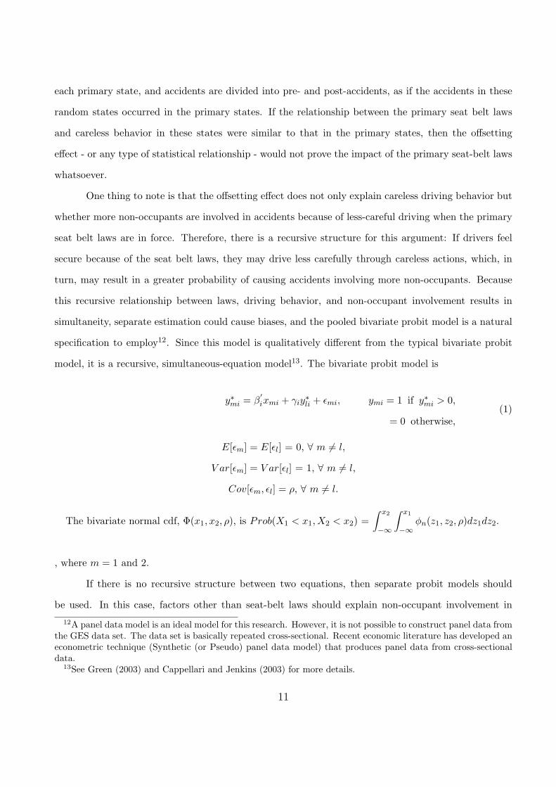
One thing to note is that the offsetting effect does not only explain careless driving behavior but

whether more non-occupants are involved in accidents because of less-careful driving when the primary

seat belt laws are in force. Therefore, there is a recursive structure for this argument: If drivers feel

secure because of the seat belt laws, they may drive less carefully through careless actions, which, in

turn, may result in a greater probability of causing accidents involving more non-occupants. Because

this recursive relationship between laws, driving behavior, and non-occupant involvement results in

simultaneity, separate estimation could cause biases, and the pooled bivariate probit model is a natural

specification to employ12. Since this model is qualitatively different from the typical bivariate probit

model, it is a recursive, simultaneous-equation model13. The bivariate probit model is

y∗mi

= β′

ixmi + γiy

∗li+ ϵmi, ymi = 1 if y∗

mi> 0,

= 0 otherwise,(1)

E[ϵm] = E[ϵl] = 0, ∀ m = l,

V ar[ϵm] = V ar[ϵl] = 1, ∀ m = l,

Cov[ϵm, ϵl] = ρ, ∀ m = l.

The bivariate normal cdf, Φ(x1, x2, ρ), is Prob(X1 < x1, X2 < x2) =

∫x2

−∞

∫x1

−∞ϕn(z1, z2, ρ)dz1dz2.

, where m = 1 and 2.

If there is no recursive structure between two equations, then separate probit models should

be used. In this case, factors other than seat-belt laws should explain non-occupant involvement in

12A panel data model is an ideal model for this research. However, it is not possible to construct panel data fromthe GES data set. The data set is basically repeated cross-sectional. Recent economic literature has developed aneconometric technique (Synthetic (or Pseudo) panel data model) that produces panel data from cross-sectionaldata.

13See Green (2003) and Cappellari and Jenkins (2003) for more details.

11

accidents. As we will see later, the regression results show that there is no recursive structure. The

variance-covariance matrix of the cross-equation error terms is estimated, and the null hypothesis ρ12 = 0

is tested with a Wald test at the 5 percent level. The Wald test shows that there is no correlation

between the error terms14. Therefore, the model shows that non-occupant involvement is not linked to

the primary seat-belt laws through drivers’ careless behavior. Therefore, two separate probit models

must be used to determine the effects of the primary seat belt laws on both careless behavior and

pedestrian involvement.

3. The Number of Accidents

To answer the second question, I produce a synthetic panel data model from the accident data to see

if there is a change in the number of accidents. The synthetic panel model groups drivers into several

cohorts according to their personal characteristics and observes their behavioral changes over time and

across the cohorts. I construct cohorts using gender, states, and four age groups. Each cohort contains

drivers with similar characteristics. For instance, one cohort contains drivers who are all males between

16 and 25 years old who all live in the same state. I observe the number of drivers in this cohort over

time. The number of people in the cohorts may increase or decrease across observations and over time,

so I can consider this numerical change to be the increase or the decrease in a certain type of accidents.

These numbers in cohorts include both careless and careful drivers. Since I need to know whether the

number of careless drivers in a cohort increases or decreases, drivers in a cohort are divided into two

groups: careless drivers and careful drivers. If the numbers of careless and careful drivers increase

and decrease, respectively, then I can conclude that the primary seat belt laws lead to more accidents

involving careless drivers15.

The General Estimates System (GES) accident data is a sample. Therefore, to reach a national

estimate, I should not give all accidents equal weight. The GES says that in order to calculate estimates

of national crash characteristics, data from each police accident report on file must be weighted. The

14χ2(1) = .1391. Prob > χ2 = .7091. Convergence was not achieved, so I limited the number of iteration to 10.15There is a reason why drivers in a cohort are divided into two groups. These drivers are all in accident data.

It is necessary to focus on careful drivers among them because they relatively represent the entire population(all people on the road) better. However, I also calculate the ratio of less-careful drivers to all drivers in myregression. The estimation result is in Table 8.

12

accident data contains a weight for each accident. Therefore, the number of drivers in a cohort in my

model is the weighted number.

Using this grouping, 40 different cohorts are created16. Since there are seven states, the total

number of observation is 280. These observations are used for the synthetic panel data model17.

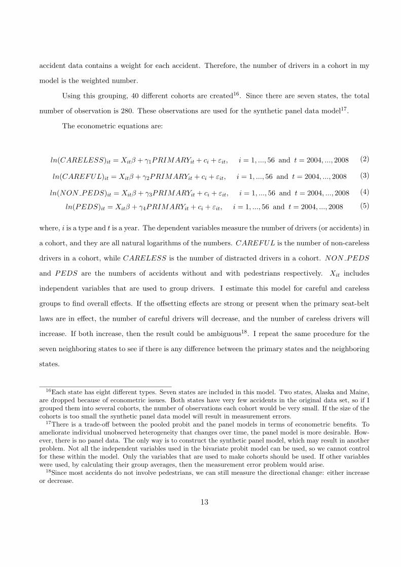
The econometric equations are:

ln(CARELESS)it = Xitβ + γ1PRIMARYit + ci + εit, i = 1, ..., 56 and t = 2004, ..., 2008 (2)

ln(CAREFUL)it = Xitβ + γ2PRIMARYit + ci + εit, i = 1, ..., 56 and t = 2004, ..., 2008 (3)

ln(NON PEDS)it = Xitβ + γ3PRIMARYit + ci + εit, i = 1, ..., 56 and t = 2004, ..., 2008 (4)

ln(PEDS)it = Xitβ + γ4PRIMARYit + ci + εit, i = 1, ..., 56 and t = 2004, ..., 2008 (5)

where, i is a type and t is a year. The dependent variables measure the number of drivers (or accidents) in

a cohort, and they are all natural logarithms of the numbers. CAREFUL is the number of non-careless

drivers in a cohort, while CARELESS is the number of distracted drivers in a cohort. NON PEDS

and PEDS are the numbers of accidents without and with pedestrians respectively. Xit includes

independent variables that are used to group drivers. I estimate this model for careful and careless

groups to find overall effects. If the offsetting effects are strong or present when the primary seat-belt

laws are in effect, the number of careful drivers will decrease, and the number of careless drivers will

increase. If both increase, then the result could be ambiguous18. I repeat the same procedure for the

seven neighboring states to see if there is any difference between the primary states and the neighboring

states.

16Each state has eight different types. Seven states are included in this model. Two states, Alaska and Maine,are dropped because of econometric issues. Both states have very few accidents in the original data set, so if Igrouped them into several cohorts, the number of observations each cohort would be very small. If the size of thecohorts is too small the synthetic panel data model will result in measurement errors.

17There is a trade-off between the pooled probit and the panel models in terms of econometric benefits. Toameliorate individual unobserved heterogeneity that changes over time, the panel model is more desirable. How-ever, there is no panel data. The only way is to construct the synthetic panel model, which may result in anotherproblem. Not all the independent variables used in the bivariate probit model can be used, so we cannot controlfor these within the model. Only the variables that are used to make cohorts should be used. If other variableswere used, by calculating their group averages, then the measurement error problem would arise.

18Since most accidents do not involve pedestrians, we can still measure the directional change: either increaseor decrease.

13

IV. DATA AND SUMMARY STATISTICS

1. Data

I use two sources of data. The first source of data is about the seat-belt laws. There are two types

of law enforcement: primary enforcement, in which occupants can be pulled over and ticketed simply

for not using their seat belts, and secondary enforcement, in which occupants must be stopped for

another violation, like speeding, before they can be ticketed for not using their seat belts19. Thus,

primary enforcement is a much stronger regulatory tool. As of 2013, all U.S. jurisdictions except New

Hampshire have some sort of seat-belt statute, primary or secondary. Many states, such as Connecticut,

New York, and Texas, adopted primary seat belt laws in the mid-1980s, while some states, such as West

Virginia, adopted primary laws more recently (Table 1). Now, 34 states have primary seat belt laws

in effect (Table 1)20, and the coverage of seat belt use differs from state to state. Due to changes in

law enforcement, seat belt use has increased consistently over time; use reached 86 percent in 201221.

However, many states still adopt secondary seat-belt laws.

The second source of data is the GES accident data from the NHTSA. There are several ad-

vantages to using this data. First, it contains detailed information on individual driver’s behavior,

such as careless driving behavior, alcohol consumption, and non-occupant involvement, as well as other

behavioral changes at the time of the crash, before the crash, and after the crash. This information

allows me to observe each driver’s detailed behavior. Second, the data contains vehicle characteris-

tics, such as model year, vehicle age, and vehicle contribution factor. Previous literature shows that

the vehicle age affects drivers’ behavior (Crandall & Graham (1984)), so I identify what model year

vehicles were involved in a particular accident. Third, each observation has a zip code, so I know the

state in which the accident occurred at that particular time. The zip code for each observation is the

main link between the seat belt law in the state and the accident. Furthermore, this data set includes

environmental factors, road conditions, weather conditions, and personal characteristics. These char-

19NHTSA, “Traffic Safety Use in 2008”, DOT HS 811 036.20Even though many states adopt primary seat belt laws, the coverage and the maximum fines differ from state

to state. For instance, Texas charges $ 200, for a seat-belt violation, while many states only charge $ 10.21“Seat Belt Use in 2012 Use Rates in the States and Territories”, NHTSA.

14

acteristics are unique to each observation and are used as control variables to account for individual

(crash-specific) heterogeneity. For instance, even if two crashes occur in the same state on a same date,

These characteristics can explain the variations between the accidents. Controlling for these factors

allows me to see the effects of primary seat belt laws on drivers’ behavior. Otherwise, the coefficient

of the seat belt law would be biased because of the heterogeneity affecting the behavior, even though I

control for state-fixed and year-fixed effects.

Since I focus on the states that have changed their seat belt laws between 2004 and 2008, I

only use accidents that occurred in these states22. Over the time period, more than 82,000 people were

involved in crashes in these states (Appendix D.). Drivers consist of 70 percent of the people (57,700

individuals). Since non-occupants do not affect drivers’ behavioral change in response to the laws, I

only use the observations for drivers.

2. Summary Statistics: Cross-Section Data Model (Probit Model)

Table 2 shows summary statistics for the probit models. This table is for the primary states. Since there

are two equations, two dependent variables are constructed; both are dummy variables. The dependent

variable CARELESS measures whether the driver was distracted at the time of the accident. This

behavior is caused by the driver, not by other people or objects on the road, so the variable directly

measures the driver’s mistakes or careless behavior. If the driver in an accident is careless, then the

value is 1; otherwise, the value is zero. Careless behavior includes the driver’s talking on, listening

to, or dialing a phone; adjusting climate control, the radio, or a CD; eating or drinking; smoking-

related distractions; using or reaching for other devices integral to the vehicle; sleeping; and any other

distractions or inattention23. About 20 percent of the drivers were careless when accidents occurred.

In the second equation, the dependent variable NON OCCUPANTS measures the involvement of

non-occupants - such as pedestrians and bikers - in the accident. If any non-occupant is involved in the

accident, then the value is 1; otherwise, the value is zero. About 1.6 percent of the drivers experienced

22As I pointed out in the previous section, there is a data-matching problem in the GES in later years, so I useaccident data until 2008 in order to classify variables consistently.

23Some drivers were distracted by vehicle occupants, non-occupants, or outside objects at the time of the crash.However, the drivers could have avoided these types of distractions if they had been more attentive. Note thatthis information is self-reported by the driver, occupants, or eyewitnesses.

15

non-occupant-related accidents.

Independent variables include three main factors: individual accident-level, state-fixed, and year-

fixed factors along with the seat belt law24. The main variable PRIMARY is an indicator. If an accident

occurs before the enforcement date in the state, then the value is zero; otherwise, the value is 1. More

than 60 percent of accidents occurred when the primary seat belt laws were in effect.

The average driver age is 38, and 60 percent of the drivers in the sample are males. ALCOHOL

measures whether alcohol is involved in the accident at the time of the crash. If alcohol is involved,

then the value is 1; otherwise the value is zero. Slightly less than 7 percent of accidents were related to

alcohol. STRIKING measures the role of the vehicle in the crash. I include the vehicle age variable,

V EHICLE AGE, to measure drivers’ behavioral differences with regards to how old their vehicles are.

The average vehicle age is 7.6 years. To account for a possible non-linear relationship, I also include

V EHICLE AGE SQ. NIGHT measures when the accident occurs. If the accident occurs between

7:00 p.m. and 5:00 a.m., then the value is 1; otherwise, the value is zero. About 23 percent of the

accidents occurred at night. The variable is correlated with alcohol consumption, which may cause

careless behavior. HIGH POP is a dummy variable that indicates the density of the population. If

the accident occurs in the area with 100,000 residents or more, then the value is 1; otherwise, the value

is zero 25. I expect drivers to act more carefully while driving in highly populated areas.

Many variables that reflect road and weather conditions are included. If the road surface is

dry, then DRY SURFACE is 1; if it is wet, snowy, or icy, then the value is zero. The variable

measures road conditions. About 80 percent of drivers had accidents under good surface conditions.

GOOD WEATHER measures if it is rainy, snowy, sleety, or foggy. If there are no adverse conditions,

the value is 1. LIGHT measures visual conditions. Seventy-two percent of accidents occurred during

daylight. If the accident occurs on the highway, then the variable HIGHWAY has a value of 1.

Most accidents occur on local roads. If the accident occurs in an interchange area, then the value

of INTERCHANGE is 1; otherwise, it is zero. Less than 10 percent of the accidents occurred in

24The definition and the description of each variable is in the appendix.25The dummy variable is used because of data limitations. Furthermore, since each observation has the zip

code that tells us where the vehicle owner lives, the owner’s address and the place the accident occurred will bedifferent. Thus, county-level populations cannot be used in this case. To control for regional population density,the dummy variable would be fine.

16

interchange areas. The variable, SPEED LIMIT , measures the maximum speed limit at the place of

the accident. Since there are different maximum speed limits even within a state, this information helps

determine accident-specific variations. The average speed limit is 44 mph26.

State and year dummies are included in the equations to control for state- and year-fixed factors.

The states that changed their laws are Alaska, Kentucky, Maine, Mississippi, North Carolina, South

Carolina, and Tennessee. North Carolina has the most accidents during the studied time period, Ten-

nessee has the second-highest amounts of accidents, and Alaska has the fewest accidents among these

states27.

The summary statistics for both neighboring and randomly assigned states are in the appendix.

Seven neighboring states are Hawaii, Ohio, New Hampshire, Louisiana, Virginia, Georgia, and Alabama.

The other seven random states are Idaho, Connecticut, New York, Virginia, Pennsylvania, Florida, and

Utah28. There are two fundamental differences between summary statistics. One is that the total

numbers of observation are more in these samples than the sample with the primary states. The other

is that the ratios of the number of accidents with careless drivers to the total number of accidents

in the sample are quite different. Almost 20 percent of the drivers was careless in accidents in the

primary state sample, while it was 15.8 percent in the neighboring state sample. Furthermore, it was

13.7 percent in the random state sample. Therefore, the seven primary states had more accidents with

relatively less careful drivers. This could be one of the reasons why these states changed their laws from

the secondary to primary law enforcement during the years studied.

3. Summary Statistics: Synthetic Panel Data Model

The summary statistics for the primary states are in Table 3, and the summary statistics for the

neighboring states is in the Appendix. The average number of drivers in a cohort is 23,132. This

26Some accidents, though not many, occurred in places without any statutory limits - parking lots or alley -,so the maximum speed limits were zero.

27The GES data is a sampled data from the police accident reports. Therefore, each selected observation hasits own weight to be used to get the national estimate. The frequencies in the sample do not have any meaningif the weight is not taken into account. However, it suffices to use the raw data to see the behavioral differencesamong drivers because I do calculate neither the number of accidents nor fatality rates here. The weights areused when I construct the synthetic panel data model in the later section.

28They were randomly chosen and assigned by STATA, after removing the seven primary states.

17

is a weighted number of drivers. Among them, the numbers of non-careless and careless drivers are

18,411 and 4,720, respectively. The dependent variables are the natural logarithms of these numbers.

I also calculate the ratio of the number of careless drivers to the total number of drivers in a cohort.

If this ratio rises, then more less-careful drivers are involved in accidents. About 24 percent of drivers

are careless drivers; the percentage seems substantial. Since the numbers in cohorts are the weighted

numbers, the accidents involving careless driver behavior might have more weight. I create another

dependent variable to measure the number of accidents involving non-occupants in a cohort. Since

most accidents do not have pedestrians, the number of drivers in accidents with pedestrians is quite

small29.

Most independent variables are the ones used to construct the synthetic panel data. The main

independent variable PRIMARY measures if the primary seat belt laws were in effect at the time of

the accident. Since the observations are annual, each cohort has a value of 1 if the primary seat belt

law changed in that year or in subsequent years; otherwise, the value is zero. The gender and age

variables are all control variables. Year and state dummies are also used to construct the panel data.

To compare the primary states with the neighboring states, I also construct the same panel data with

only neighboring states. They are in the Appendix.

V. EMPIRICAL RESULTS

1. Estimation Results: Cross-Section Data Model (Probit Model)

The estimation results are presented in Tables 4 and 5. The sample for the analysis contains states.

Therefore, the dependent variable might be correlated within a cluster (a state), possibly through un-

observed cluster effects (Wooldridge, 2002). This is true even when some control variables are included,

so I use the standard errors that allow for within-state correlation, relaxing the usual requirement that

29Among 200 observations, 75 observations do not have any driver in accidents with pedestrian involvement.Even though there are 125 remaining observations, the number people in the cohorts are quite small, makingthe estimation results less reliable. The estimation results for non-occupant involvement are only presented forreference.

18

the observations be independent. All the t-values are calculated using a robust variance estimate that

adjusts for within-cluster correlation.

Table 4 shows the estimation results for testing if the primary seat belt laws cause drivers to drive

less carefully, while Table 5 shows the estimation results for testing if the laws cause more accidents

involving non-occupants. They are separately estimated using probit models. To compare drivers’

behavior in different states, three models are estimated: Primary, Neighboring, and Random States.

As we see in the first column, the estimation results show that drivers drive more carefully when a

primary seat-belt law is in effect in a state. Careless behavior is negatively associated with PRIMARY,

and the variable is statistically significant at the 5 percent level. People drive more carefully under

the primary seat-belt law. This finding is surprising because it is the opposite result of what the

offsetting effect theory concludes. The second column shows careless driver behavior in neighboring

states when the seat-belt law changes in these drivers’ neighboring states, which are the same as the

original primary states studied. Careless behavior is now positively associated with PRIMARY, and

the variable is statistically significant at the 1 percent level. It seems that the offsetting effects appear

in states where there is no change in the seat-belt laws. How can we explain this seemingly odd result?

The variable PRIMARY reflects pre- and post-primary seat belt periods in the primary states where

new laws are adopted. From the perspective of the original neighboring states, primary states are their

neighbor states. Therefore, drivers in the states with no law change may be affected by the states with

the law change. Knowing that the neighboring state changes its law on a particular date, the drivers in

a state that does not change its law may tend to drive less carefully30. One possible interpretation is

that the drivers in the seven neighboring states had maintained a higher level of carefulness in driving.

More than 20 percent of the drivers were careless in the primary states, while only 16 percent were

careless in the neighboring states31. Therefore, when the law changed, people in the primary states

became relatively more careful, while people in the neighboring states became relatively less careful.

30Interstate commuters may change their driving behavior once they cross the border of the states. This is notempirically proved. However, this is plausible if we consider a similar situation. With regard to maximum speedlimits, drivers reduce their travel speed as they pass from the roads with higher to those with lower maximumspeed limits.

31This could be the reason why the primary states changed their laws. Compared to the neighboring states,primary states have a higher ratio of careless drivers in accidents.

19

The conclusion is that the primary seat-belt laws change people’s behavior in neighboring states as

well as primary states. However, this must be valid only for the neighboring states. As we see in the

third column, the laws do not affect people’s behavior in the randomly assigned states. I calculate the

marginal effects of the variable PRIMARY , along with other independent variables. The marginal

effects for the dummy variable are explained by the change in the predicted probability for a change in

PRIMARY from 0 to 1. According to the post estimation from Table 4, changing the seat belt laws

from the secondary to the primary decreases the probability driving carelessly by 17.6 percent in the

primary states and increases the probability by 13.4 percent in the neighboring states32.

Among other control variables, careless behavior is caused by neither age nor gender in the

primary states33. In the neighboring states, younger, male drivers are less careful. Alcohol consumption

is positively associated with careless behavior in the neighboring states. The same results are shown

in the random states34 Drunken drivers are often less careful. Therefore, there is a difference in driver

behavior between the primary and the non-primary (neighboring or random) states. Drivers in striking

vehicles in accidents were less careful, and it is statistically significant in all states. The older the

vehicles are, the less careful the drivers are.

The signs of other control variables are what I expected. Careless behavior is found in accidents

that occurred between 7:00 p.m. and 5:00 a.m. Drivers are more careful in highly populated areas.

During the daylight, drivers are less careful. When it is dark, dawn, or dusk, people drive more

carefully. HIGHWAY is positively associated with careless behavior and statistically significant only

in the neighboring states. When drivers drive on highways, they are less careful. People are more

careful in interchange areas. Speed limits are not associated with careless behavior, except for people

in neighboring states. This is a seemingly counterintuitive outcome. Drivers are possibly more careful

32The post estimation results are not reported in this paper.33Most literature shows that young male drivers cause more fatal accidents. My study uses individual-level

accident data. The data includes accidents with all levels of injury and property damage. Therefore, based onthe police-reported accidents, the estimation results show that there is no difference in careless behavior amongmale and female drivers as well as young and old drivers in primary states. Typically, male drivers are less-carefuldrivers. However, if both male and female drivers are equally less careful, then there could be statistically nosignificant difference between genders.

34These randomly assigned states are not related to the primary states at all. Therefore, drivers’ carelessbehavior should be explained by other factors, such as personal and accident-specific characteristics. We confirmthis conjecture from the estimation results in Tables 4 and 5.

20

on the local roads because of frequent obstacles like pedestrians. Drivers may focus on driving when

the roads have lower maximum speed limits. The coefficients of year dummies are not statistically

significant in the primary states, while they are significant in other states. Most state dummies are

statistically significant. For instance, drivers in North Carolina were relatively less careful than drivers

in Maine.

Table 5 shows that primary seat-belt laws are not associated with non-occupant involvement.

The coefficient PRIMARY is not statistically significant at any level. This is also true regardless of

states. Therefore, factors other than primary seat-belt laws must explain non-occupant involvement in

accidents35.

Personal characteristics affect non-occupant involvement. Older drivers cause more accidents

involving non-occupants, and the age variable is statistically significant in all states. Causing accidents

involving non-occupants is not related to gender. Alcohol-related accidents involve fewer pedestrians

and more non-occupants are involved in accidents with striking vehicles. Vehicle age is not associated

with non-occupant involvement. NIGHT is associated with pedestrian involvement. More pedestrians

are involved in accidents in highly populated areas. It is also natural to observe that HIGHWAY is

not statistically associated with NON OCCUPANT since pedestrians are not on the highway. The

coefficient, INTERCHANGE, is negative and statistically significant. That means fewer pedestrians

are involved in accidents that occurred in the interchange areas. This is because most drivers are

more careful when they approach the interchange areas. A higher speed limit is associated with less

pedestrian involvement in both primary and random states; this result implies that most accidents

involving pedestrians occur on roads with lower maximum speed limits, such as local roads. Both year-

and state-dummies are used to control for heterogeneity in years and states.

In summary, I find that the primary seat-belt laws affect people’s behavior and people in different

states respond to the laws differently. This is valid only in the subset of all drivers (the accident

group) on the roads. However, it is still meaningful because I find drivers’ behavioral differences by

comparing three subsets in different states. I also find that primary seat-belt laws are not associated

35We still need to be very careful in deriving a conclusion here. Non-occupant involvement is not related to thelaw change only in this subset of the population. The change in the number of accidents involving pedestriansdue to the laws should be verified in the synthetic panel data model, which will be discussed in the next section.

21

with pedestrian-related accidents. The next section will discuss the effects of the laws on the increase

or decrease in certain types of accidents.

2. Estimation Results: Synthetic Panel Data Model

The estimation results are presented in Tables 6 and 7. The random effect models are used.

In Table 6, the first two synthetic panel models show the estimation results from primary states. The

second two models show the estimation results from neighboring states. The first two models show that

the number of careful drivers increases (first column) and the number of less careful drivers decreases

(second column) when a primary seat-belt law is in effect in the state. The coefficient of the variable

PRIMARY is highly significant at the 1 percent level in the careful group and significant at the 10

percent level in the careless group. If the more stringent seat-belt laws are newly enforced, the number

of careful drivers increases by 99 percent and the number of careless drivers decreases by 26 percent in

accidents. These percentage changes seem quite substantial. However, the result is consistent with the

results from the NHTSA. According to the Centers for Disease Control and Prevention (CDC), seat

belts reduce serious crash-related injuries and deaths by about 50 percent36. Not all careful drivers

prevent accidents involving serious injuries or death. Thus, some can avoid accidents because of their

careful driving behavior. It must be below 50 percent because even more-careful drivers may still cause

accidents, and most accidents include no injury or minor injuries. This result is consistent with the main

estimation result from Tables 4 and 5. Therefore, the estimation results say that when a state adopts a

more stringent seat-belt law, the number of careful drivers increases in both careful and careless groups

on the road. The fit of this model is fairly good, with an R2 close to 85 or 87 percent. In neighboring

states, the number of careful drivers in the careful group decreases, and the variable PRIMARY is

statically significant (third column), while it (fourth column) is not statistically significant. The overall

effects of the primary seat-belt laws on driver behavior in neighboring states is the opposite of the effects

in primary states.

Now, I focus on other independent variables only in the first two columns (Primary States).

Individual characteristics are mostly significant. With regards to MALE, the number of careful male

36Seat Belts Fact Sheet, NHTSA, 2010. http://www.cdc.gov/motorvehiclesafety/seatbelts/facts.html.

22

drivers in the careful group increases, while the number of them in the careless group decreases, so

they are offsetting each other. Therefore, male drivers are more careful in the careful group, but female

drivers are more careful in the careless group. The younger the drivers are in the careful group, the less

careful they are in the careful group. The younger drivers are more careful in the careless group, so

they are also offsetting. Therefore, I can conclude that both gender and age are not factors that affect

the numbers of careful and careless drivers in accidents on roads in the United States. This result is

also consistent with the estimation results from a later model in Table 8. Most year dummies are not

statistically significant in the careful group, but they are statistically significant in the careless group.

This pattern is reversed in the neighboring states. All state-dummies are statistically significant at the

1 percent level. Drivers also behave differently in different groups, the careful or careless groups. These

drivers also offset each other within the groups.

We need to note one thing: the main disadvantage of the synthetic panel model, however, is that

many environmental factors that are used in the probit model are no longer controlled for. However,

even though the model does not control well for unobserved factors, I obtained a consistent result for

drivers’ behavior from different model specifications.

Table 7 shows the effects of the laws on the number of accidents involving non-occupants. I

divide the driver group into two groups: one consisting of drivers whose accidents did not involve

non-occupants (occupant accidents), and one consisting of drivers whose accidents did involve non-

occupants (non-occupant accidents). The variable, NON PEDS, represents the number of accidents

without pedestrians involved, and PEDS represents the number of accidents with pedestrians involved.

The first column tests to see if the laws increase or decrease the number of occupant accidents, while

the second column tests to see if the laws change the number of non-occupant accidents. As we see in

the table, the primary seat belt laws are associated with neither the increase nor the decrease in the

number of pedestrians. The coefficient PRIMARY is not statistically significant at any level37.

37The synthetic panel data model should satisfy a condition in order to use it as a valid model: the numberof observation in a cell should be large enough. Since the number of accidents where pedestrians are involved isquite small, many cohorts do not have any observations. Therefore, the second and the fourth columns have only125 and 143 observations, respectively, because the dependent variable is the natural logarithm of the number ofdrivers (or accidents) involving pedestrians. In this case, the effectiveness of using the synthetic panel model couldbe limited. However, it suffices to show that primary seat-belt laws are not affecting the number of occupant-and non-occupant accidents.

23

I create a new dependent variable to see the overall effects of the primary seat belt laws on driver

behavior and number of accidents. Then, I run the regression using the panel data model used in Table

6. I do this because some variables are offsetting each other. The estimation results are in Table 8.

The new dependent variable CARELESS/TOTAL measures the total number of careless drivers to

the total number of drivers in a cohort. When primary seat-belt laws are in effect, the ratio of careless

drivers on the road decreases in the primary states and increases in the neighboring states. The variable

is statistically significant at the 1 percent level. I also confirm that driver behavior is the opposite in

primary and neighboring states.

In conclusion, the primary seat belt laws are effective in reducing the number of accidents whose

drivers are less careful. However, we need to be very careful in deriving the implications of the offsetting

effects. I have used the accident data. It includes all different types of accidents in terms of severity of

injuries, including no injury in accidents. Therefore, as the offsetting effect theory concludes, we still

do not know if fatal accidents increase or not because of the primary seat belt laws. The GES data also

includes fatal accidents. However, it is not possible to construct panel data only with fatal accidents.

Therefore, it is very important to draw a conclusion with caution: The offsetting effects may not exist

or are weaker than expected, if we include all different types of accidents.

VI. CONCLUDING REMARKS

This paper investigates the effects of the primary seat-belt laws on driver behavior and non-occupant

involvement. I find that the offsetting effects do not exist when I analyze the accidents using all injury

levels. Primary seat belt laws rather reduce the predicted probability of less-careful driving behavior.

The behavior does not even lead to greater non-occupant involvement. Therefore, the overall effect of

the laws is still effective, assuming that the law reduces fatalities among drivers and passengers38.

38A research note (2006) from the NHTSA found that states with primary enforcement laws have lower fatalityrates. According to the note, the passenger vehicle occupant fatality rates were 1.03 per 100 million vehicle milestraveled (VMT) and 10.69 per 100,000 population over the period of study. This compares to 1.21 and 13.13(respectively) for all other states.

24

The estimation results from the synthetic panel model also show consistent outcomes. Both the

probit and the synthetic panel data models show that drivers are more careful because of the stringent

law enforcement. Furthermore, the number of more-careful drivers increases, and the number of less-

careful drivers decreases, when primary seat belt laws are in effect, meaning that people become more

careful, regardless of whether they are careful or careless drivers on the road.

One thing to consider is whether the increase in accidental harm from the offsetting behavior is

big enough to outweigh the reduction in accidental harm from the seat belt laws, even if I assume that the

offsetting behavior really exists or strongly appears. By looking at the descriptive statistics of accident

data (Appendix D), one could find an intuitive idea of the size of accidental harm of non-occupants.

The General Estimates System (GES) has 82,055 individuals who were involved in the accidents that

occurred in the primary states over the period of study39. Pedestrians and cyclists consisted of only

0.92 percent of them (Appendix D.1.). Drivers and passengers consisted of 98.93 percent of the sample.

Therefore, even if the fatality of non-occupants increases because of the offsetting effects, it may not

be sizeable. This becomes clear when I focus on the injury severity levels of non-occupants included in

the sample. Among the 752 non-occupants involved in accidents over the period, only 60 people had a

fatal injury (Appendix D.2.). Seventy-five percent of the drivers might have caused the accidents due

to their possible mistakes or misbehavior (Appendix D.3.). If we include non-motorist vehicle operators

and other or unknown actions, the percentage increases to 90 percent. Only 10 percent of them (or

6 non-occupants out of more than 82,000 people involved in accidents) had a fatal injury when they

did not take any action. This percentage can be explained by drivers’ mistakes or careless (or even

intentionally aggressive) behavior. Even so, there is no guarantee that the seat-belt laws cause this

non-occupant involvement.

From these simple descriptive statistics, it is hard to believe that drivers’ less-careful behavior

causes a substantial increase in the number of more-fatal accidents. However, the data set used in this

paper is from the police accident reports obtained from the NHTSA. These six accidents could be even

sizeable if we converted the number into the weighted sum. This weighted number could have been in

39There was no change in the laws in 2008. In 2009, 4 states changed their laws. By including these four states,we can compare drivers’ behavioral differences between the states with and without the primary seat belt lawover the years of study.

25

the accident data set because of the offsetting effects if any. Therefore, as I pointed out in the previous

section, it is very important to draw a conclusion with caution: The offsetting effects may not exist or

are weaker than expected, if we include all different types of accidents.

Currently, 34 states and the District of Columbia have primary seat-belt laws. Sixteen states

have secondary laws, and New Hampshire has no seat belt law. Some people argue that drivers should

choose whether to wear seat belts as a matter of “personal freedom.”40 However, primary seat belt laws

save the lives of drivers as well as passengers, pedestrians, and bikers. This result, along with earlier

studies, shows that primary seat belt laws play an important role in improving public safety on roads

across the United States41.

It is still true that the laws save drivers’ lives. As of Jan. 1, 2010, a new state law in Georgia,

the Super Speeder Law, went into effect with substantially higher fines of $ 20042. This law may give

drivers stronger motivation to drive more carefully and strengthen the effects of primary seat-belt laws.

Therefore, punitive penalties, such as higher fines, would make the laws much more effective, if used

together.

For future studies, we may test if joint regulation is more effective in promoting public safety.

We can perform this test by comparing different states with and without punitive (financial) penalties,

given that the states have the same level safety enforcement.

Another possible study can augment my paper. The use of cellular phones has been prevalent in

recent years in the United States. Some states have recently prohibited drivers from using their phones

to call or send text messages while driving. Cellular-phone use could be a major distraction and a cause

of careless driving behavior. My current paper does not incorporate this cellular-phone use into the

model. We could therefore test if there is a relationship between primary seat-belt laws, laws banning

cellular phones, and their joint impacts on road safety.

40For instance, the National Motorists Association(NMA) submitted testimony against a 2003 Wisconsin billallowing primary enforcement. Seven years later, the state of Wisconsin passed a primary seat-belt law in 2009.See more details from “http://www.motorists.org/seat-belt-laws/testimony”.

41Not only the seat belt laws improve public safety. Vehicle recall regulation reduces accidental harm. See Bae& Benıtez-Silva (2011 and 2013) for more details.

42See “http://www.safespeedsgeorgia.org/”.

26

Table 1. Primary Seat Belt Laws - States

State Initial Primary Standard Who is Covered? MaximumEffective Seatbelt Enforcement In What Seats? FineDate Laws? Date 1st Offense

Alabama 07/18/91 Yes 12/09/99 15+ years in front seat $ 25Alaska 09/12/90 Yes 05/01/06 16+ years in all seats $ 15Arizona 01/01/91 No 15+ in front seat; 5 through 15 in all seats $ 10Arkansas 07/15/91 Yes 06/03/09 15+ years in front seat $ 25California 01/01/86 Yes 01/01/93 16+ years in all seats $ 20Colorado 07/01/87 No 16+ years in front seat $ 71Connecticut 01/01/86 Yes 01/01/86 7+ years in front seat $ 15Delaware 01/01/92 Yes 06/30/03 16+ years in all seats $ 25DC 12/12/85 Yes 10/01/97 16+ in all seats $ 50Florida 07/01/86 Yes 06/30/09 6+ in front seat; 6 through 17 in all seats $ 30Georgia 09/01/88 Yes 07/01/96 18+ in front seat; 6 through 17 in all seats $ 15Hawaii 12/16/85 Yes 12/16/85 18+ in front seat; 8 through 17 in all seats $ 45Idaho 07/01/86 No 7+ years in all seats $ 10Illinois 01/01/88 Yes 07/03/03 16+ in front seat; 18 and younger in all seats $ 25

if driver is younger than 18 yearsIndiana 07/01/87 Yes 07/01/98 16+ years in all seats $ 25Iowa 07/01/86 Yes 07/01/86 11+ years in front seat $ 25Kansas 07/01/86 Yes 06/10/10 18+ in front seat; 14 through 17 in all seats $ 30Kentucky 07/15/94 Yes 07/20/06 7+ years in all seats; 6 and younger and $ 25

more than 50 inches in all seatsLouisiana 07/01/86 Yes 01/01/95 13+ years in front seat $ 25Maine 12/26/95 Yes 09/20/07 18+ years in all seats $ 50Maryland 07/01/86 Yes 10/01/97 16+ years in front seat $ 50

(effective 10/01/13)Massachusetts 02/01/94 No 13+ years in all seats $ 25Michigan 07/01/85 Yes 04/01/00 16+ years in front seat $ 25Minnesota 08/01/86 Yes 06/09/09 all in front seat; 3 through 10 in all seats $ 25Mississippi 07/01/94 Yes 05/27/06 7+ years in front seat $ 25Missouri 09/28/85 No 16+ years in front seat $ 10Montana 10/01/87 No 6+ years in all seats $ 20Nebraska 01/01/93 No 18+ years in front seat $ 25Nevada 07/01/87 No 6+ years in all seats $ 25New Hampshire n/a No law No law No lawNew Jersey 03/01/85 Yes 05/01/00 18+ in front seat; 8 through 17 in all seats; $ 20

7 and younger and more than 80 poundsNew Mexico 01/01/86 Yes 01/01/86 18+ years in all seats $ 25New York 12/01/84 Yes 12/01/84 16+ years in front seat $ 50North Carolina 10/01/85 Yes 12/01/06 16+ years in all seats $ 25North Dakota 07/14/94 No 18+ years in front seat $ 20Ohio 05/06/86 No 15+ in front seat; 8 through 14 in all seats $ 30Oklahoma 02/01/87 Yes 11/01/97 13+ years in front seat $ 20Oregon 12/07/90 Yes 12/07/90 16+ years in all seats $ 110Pennsylvania 11/23/87 No 18+ in front seat; 8 through 17 in all seats $ 10Rhode Island 06/18/91 Yes 06/30/11 18+ years in all seats $ 40South Carolina 07/01/89 Yes 12/09/05 6+ in front seat; 6+ in rear seat with shoulder belt $ 25South Dakota 01/01/95 No 18+ years in front seat $ 20Tennessee 04/21/86 Yes 07/01/04 16+ years in front seat $ 50Texas 09/01/85 Yes 09/01/85 17+ in front seat; 5 through 16 in all seats; $ 200

4 and younger and 36 in or moreUtah 04/28/86 No 16+ years in all seats $ 45Vermont 01/01/94 No 16+ years in front seat $ 25Virginia 01/01/88 No 16+ years in all seats $ 25Washington 06/11/86 Yes 07/01/02 16+ years in all seats $ 124West Virginia 09/01/93 Yes 07/01/13 8+ in front seat; 8 through 17 in all seats; $ 25Wisconsin 12/01/87 Yes 06/30/09 8+ years in all seats $ 10Wyoming 06/08/89 No 9+ years in all seats $ 25

* Source: Insurance Institute for Highway Safety (IIHS), “http://www.iihs.org/laws/SafetyBeltUse.aspx#OR.”

27

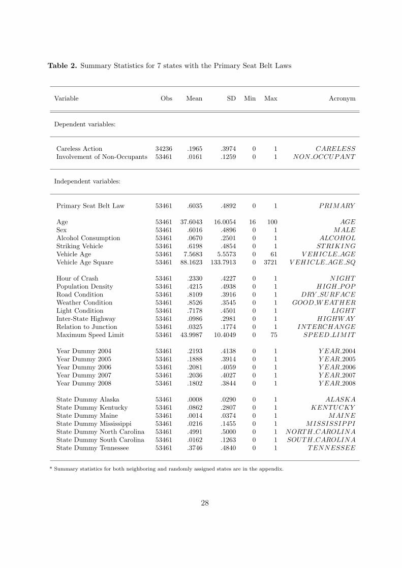
Table 2. Summary Statistics for 7 states with the Primary Seat Belt Laws

Variable Obs Mean SD Min Max Acronym

Dependent variables:

Careless Action 34236 .1965 .3974 0 1 CARELESSInvolvement of Non-Occupants 53461 .0161 .1259 0 1 NON OCCUPANT

Independent variables:

Primary Seat Belt Law 53461 .6035 .4892 0 1 PRIMARY

Age 53461 37.6043 16.0054 16 100 AGESex 53461 .6016 .4896 0 1 MALEAlcohol Consumption 53461 .0670 .2501 0 1 ALCOHOLStriking Vehicle 53461 .6198 .4854 0 1 STRIKINGVehicle Age 53461 7.5683 5.5573 0 61 V EHICLE AGEVehicle Age Square 53461 88.1623 133.7913 0 3721 V EHICLE AGE SQ

Hour of Crash 53461 .2330 .4227 0 1 NIGHTPopulation Density 53461 .4215 .4938 0 1 HIGH POPRoad Condition 53461 .8109 .3916 0 1 DRY SURFACEWeather Condition 53461 .8526 .3545 0 1 GOOD WEATHERLight Condition 53461 .7178 .4501 0 1 LIGHTInter-State Highway 53461 .0986 .2981 0 1 HIGHWAYRelation to Junction 53461 .0325 .1774 0 1 INTERCHANGEMaximum Speed Limit 53461 43.9987 10.4049 0 75 SPEED LIMIT

Year Dummy 2004 53461 .2193 .4138 0 1 Y EAR 2004Year Dummy 2005 53461 .1888 .3914 0 1 Y EAR 2005Year Dummy 2006 53461 .2081 .4059 0 1 Y EAR 2006Year Dummy 2007 53461 .2036 .4027 0 1 Y EAR 2007Year Dummy 2008 53461 .1802 .3844 0 1 Y EAR 2008

State Dummy Alaska 53461 .0008 .0290 0 1 ALASKAState Dummy Kentucky 53461 .0862 .2807 0 1 KENTUCKYState Dummy Maine 53461 .0014 .0374 0 1 MAINEState Dummy Mississippi 53461 .0216 .1455 0 1 MISSISSIPPIState Dummy North Carolina 53461 .4991 .5000 0 1 NORTH CAROLINAState Dummy South Carolina 53461 .0162 .1263 0 1 SOUTH CAROLINAState Dummy Tennessee 53461 .3746 .4840 0 1 TENNESSEE

* Summary statistics for both neighboring and randomly assigned states are in the appendix.

28

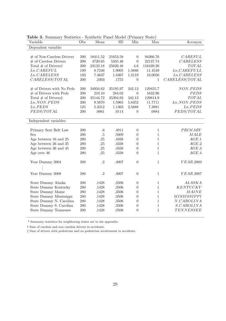
Table 3. Summary Statistics - Synthetic Panel Model (Primary State)Variable Obs Mean SD Min Max Acronym

Dependent variable:

# of Non-Careless Drivers 200 18411.52 21653.58 0 94366.76 CAREFUL# of Careless Drivers 200 4720.65 5335.46 0 22137.74 CARELESSTotal # of Drivers† 200 23132.18 25626.48 4.8 116439.20 TOTALLn CAREFUL 199 8.7246 1.9005 1.5686 11.4549 Ln CAREFULLLn CARELESS 193 7.4637 1.8367 1.2119 10.0050 Ln CARELESSCARELESS/TOTAL 200 .2403 .1755 0 1 CARELESS/TOTAL

# of Drivers with No Peds 200 34934.62 35195.97 342.13 129455.7 NON PEDS# of Drivers with Peds 200 210.10 284.02 0 1632.96 PEDSTotal # of Drivers‡ 200 35144.72 35394.92 342.13 129814.9 TOTALLn NON PEDS 200 9.5670 1.5965 5.8352 11.7711 Ln NON PEDSLn PEDS 125 5.3312 1.1363 2.5688 7.3981 Ln PEDSPEDS/TOTAL 200 .0061 .0114 0 .0884 PEDS/TOTAL

Independent variables:

Primary Seat Belt Law 200 .6 .4911 0 1 PRIMARYSex 280 .5 .5009 0 1 MALEAge between 16 and 25 280 .25 .4338 0 1 AGE 1Age between 26 and 35 280 .25 .4338 0 1 AGE 2Age between 36 and 45 280 .25 .4338 0 1 AGE 3Age over 46 280 .25 .4338 0 1 AGE 4

Year Dummy 2004 280 .2 .4007 0 1 Y EAR 2003...

Year Dummy 2008 280 .2 .4007 0 1 Y EAR 2007

State Dummy Alaska 280 .1428 .3506 0 1 ALASKAState Dummy Kentucky 280 .1428 .3506 0 1 KENTUCKYState Dummy Maine 280 .1428 .3506 0 1 MAINEState Dummy Mississippi 280 .1428 .3506 0 1 MISSISSIPPIState Dummy N. Carolina 280 .1428 .3506 0 1 N CAROLINAState Dummy S. Carolina 280 .1428 .3506 0 1 S CAROLINAState Dummy Tennessee 280 .1428 .3506 0 1 TENNESSEE

* Summary statistics for neighboring states are in the appendix.

† Sum of careless and non careless drivers in accidents.

‡ Sum of drivers with pedestrian and no pedestrian involvement in accidents.

29

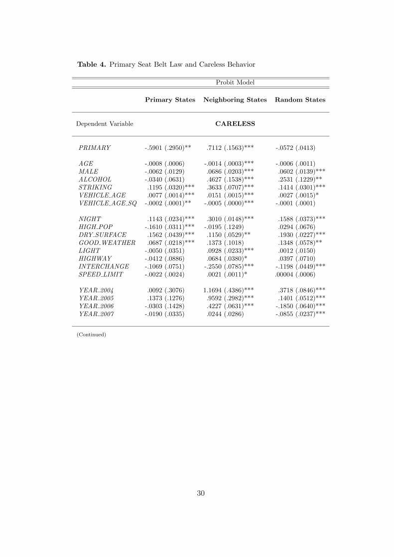
Table 4. Primary Seat Belt Law and Careless Behavior

Probit Model

Primary States Neighboring States Random States

Dependent Variable CARELESS

PRIMARY -.5901 (.2950)** .7112 (.1563)*** -.0572 (.0413)

AGE -.0008 (.0006) -.0014 (.0003)*** -.0006 (.0011)MALE -.0062 (.0129) .0686 (.0203)*** .0602 (.0139)***ALCOHOL -.0340 (.0631) .4627 (.1538)*** .2531 (.1229)**STRIKING .1195 (.0320)*** .3633 (.0707)*** .1414 (.0301)***VEHICLE AGE .0077 (.0014)*** .0151 (.0015)*** .0027 (.0015)*VEHICLE AGE SQ -.0002 (.0001)** -.0005 (.0000)*** -.0001 (.0001)

NIGHT .1143 (.0234)*** .3010 (.0148)*** .1588 (.0373)***HIGH POP -.1610 (.0311)*** -.0195 (.1249) .0294 (.0676)DRY SURFACE .1562 (.0439)*** .1150 (.0529)** .1930 (.0227)***GOOD WEATHER .0687 (.0218)*** .1373 (.1018) .1348 (.0578)**LIGHT -.0050 (.0351) .0928 (.0233)*** .0012 (.0150)HIGHWAY -.0412 (.0886) .0684 (.0380)* .0397 (.0710)INTERCHANGE -.1069 (.0751) -.2550 (.0785)*** -.1198 (.0449)***SPEED LIMIT -.0022 (.0024) .0021 (.0011)* .00004 (.0006)

YEAR 2004 .0092 (.3076) 1.1694 (.4386)*** .3718 (.0846)***YEAR 2005 .1373 (.1276) .9592 (.2982)*** .1401 (.0512)***YEAR 2006 -.0303 (.1428) .4227 (.0631)*** -.1850 (.0640)***YEAR 2007 -.0190 (.0335) .0244 (.0286) -.0855 (.0237)***

(Continued)

30

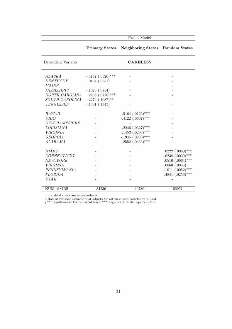
Probit Model

Primary States Neighboring States Random States

Dependent Variable CARELESS

ALASKA -.4157 (.0520)*** - -KENTUCKY .0154 (.0551) - -MAINE - - -MISSISSIPPI -.1076 (.0754) - -NORTH CAROLINA .2458 (.0778)*** - -SOUTH CAROLINA .2274 (.1087)** - -TENNESSEE -.1301 (.1345) - -

HAWAII - -.5164 (.0126)*** -OHIO - -.4122 (.0667)*** -NEW HAMPSHIRE - - -LOUISIANA - -.2246 (.0327)*** -VIRGINIA - -.1453 (.0293)*** -GEORGIA - -.1945 (.0230)*** -ALABAMA - -.2552 (.0436)*** -

IDAHO - - .0222 (.0063)***CONNECTICUT - - -.0238 (.0039)***NEW YORK - - .0516 (.0064)***VIRGINIA - - .0060 (.0056)PENNSYLVANIA - - -.1011 (.0052)***FLORIDA - - -.4841 (.0256)***UTAH - - -

NUM of OBS 34236 40786 66951

† Standard errors are in parentheses.‡ Robust variance estimate that adjusts for within-cluster correlation is used.§ **: Significant at the 5-percent level. ***: Significant at the 1-percent level.

31

Table 5. Primary Seat Belt Law and Pedestrian Involvement

Probit Model

Primary States Neighboring States Random States

Dependent Variable NON OCCUPANT

PRIMARY -.0292 (.0372) .0919 (.0608) .0054 (.0067)

AGE .0050 (.0007)*** .0024 (.0006)*** .0045 (.0007)***MALE -.0056 (.0216) -.0085 (.0275) .0353 (.0279)ALCOHOL -.2302 (.0424)*** -.2001 (.0854)** -.5755 (.0533)***STRIKING .6213 (.0549)*** .5378 (.0168)*** .7055 (.0285)***VEHICLE AGE -.0055 (.0052) .0028 (.0011)** -.0045 (.0035)VEHICLE AGE SQ .0001 (.0004) -.0001 (.0001) .0001 (.0001)

NIGHT .0746 (.0430)* .1080 (.0278)*** .0743 (.0344)**HIGH POP .1719 (.0183)*** .1536 (.0660)** .4653 (.1875)**DRY SURFACE .1670 (.0845)** .1852 (.0450)*** .2178 (.0733)***GOOD WEATHER .0792 (.0864) .0742 (.0543) .0264 (.0855)LIGHT -.1408 (.0187)*** -.0546 (.0171)*** -.0023 (.0594)HIGHWAY .1468 (.0927) .2380 (.1723) -.0591 (.1586)INTERCHANGE -.5535 (.0537)*** -.0827 (.1151) -.5098 (.1153)***SPEED LIMIT -.0245 (.0017)*** -.0290 (.0027) -.0211 (.0083)**

YEAR 2004 -.1288 (.0134)*** .0215 (.0859) -.0798 (.0645)YEAR 2005 -.0621 (.0099)*** .0259 (.0894) -.0809 (.0391)**YEAR 2006 -.1300 (.0228)*** .0396 (.0677) -.0361 (.0350)YEAR 2007 .0139 (.0135) -.0169 (.0399) -.0074 (.0252)

(Continued)

32

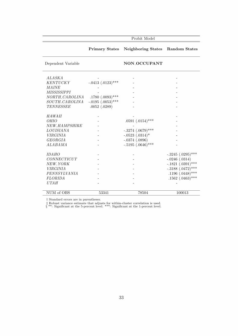
Probit Model

Primary States Neighboring States Random States

Dependent Variable NON OCCUPANT

ALASKA - - -KENTUCKY -.0413 (.0123)*** - -MAINE - - -MISSISSIPPI - - -NORTH CAROLINA .1780 (.0093)*** - -SOUTH CAROLINA -.0195 (.0053)*** - -TENNESSEE .0052 (.0289) - -

HAWAII - - -OHIO - .0591 (.0154)*** -NEW HAMPSHIRE - - -LOUISIANA - -.3274 (.0679)*** -VIRGINIA - -.0523 (.0314)* -GEORGIA - -.0374 (.0896) -ALABAMA - -.5195 (.0646)*** -

IDAHO - - -.3245 (.0295)***CONNECTICUT - - -.0246 (.0314)NEW YORK - - -.1821 (.0391)***VIRGINIA - - -.3188 (.0472)***PENNSYLVANIA - - .1196 (.0448)***FLORIDA - - .1562 (.0463)***UTAH - - -

NUM of OBS 53341 78504 100013

† Standard errors are in parentheses.‡ Robust variance estimate that adjusts for within-cluster correlation is used.§ **: Significant at the 5-percent level. ***: Significant at the 1-percent level.

33

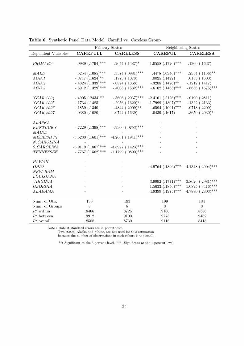
Table 6. Synthetic Panel Data Model: Careful vs. Careless Group

Primary States Neighboring States

Dependent Variables CAREFULL CARELESS CAREFUL CARELESS

PRIMARY .9989 (.1794)*** -.2644 (.1487)* -1.0558 (.1726)*** .1300 (.1637)

MALE .5254 (.1085)*** .3574 (.0981)*** .4478 (.0946)*** .2954 (.1156)**AGE 1 -.3717 (.1624)** .1773 (.1078) .0025 (.1422) .0153 (.1600)AGE 2 -.4324 (.1339)*** -.0824 (.1368) -.3208 (.1426)** -.1212 (.1417)AGE 3 -.5912 (.1329)*** -.4008 (.1532)*** -.6102 (.1465)*** -.6656 (.1675)***

YEAR 2004 -.4905 (.2434)** -.5606 (.2037)*** -2.4161 (.2126)*** -.0190 (.2811)YEAR 2005 -.1734 (.1485) -.2956 (.1620)* -1.7999 (.1807)*** -.1322 (.2133)YEAR 2006 -.1859 (.1340) -.4844 (.2009)** -.6594 (.1091)*** .0718 (.2209)YEAR 2007 -.0380 (.1080) -.0744 (.1639) -.0439 (.1617) .3650 (.2030)*

ALASKA - - - -KENTUCKY -.7229 (.1398)*** -.9300 (.0753)*** - -MAINE - - - -MISSISSIPPI -3.6230 (.1601)*** -4.2661 (.1941)*** - -N CAROLINA - - - -S CAROLINA -3.9119 (.1867)*** -3.8927 (.1423)*** - -TENNESSEE -.7767 (.1562)*** -1.1799 (.0890)*** - -

HAWAII - - - -OHIO - - 4.9764 (.1896)*** 4.1348 (.2904)***NEW HAM - - - -LOUISIANA - - - -VIRGINIA - - 3.9992 (.1771)*** 3.8626 (.2981)***GEORGIA - - 1.5633 (.1856)*** 1.0895 (.3416)***ALABAMA - - 4.9399 (.1975)*** 4.7880 (.2803)***

Num. of Obs. 199 193 199 184Num. of Groups 8 8 8 8R2:within .8466 .8725 .9100 .8386R2:between .9912 .9100 .9778 .9462R2:overall .8508 .8730 .9116 .8418

Note : Robust standard errors are in parentheses.Two states, Alaska and Maine, are not used for this estimationbecause the number of observations in each cohort is too small.

**: Significant at the 5-percent level. ***: Significant at the 1-percent level.

34

Table 7. Synthetic Panel Data Model: Non-Pedestrian vs. Pedestrian Group

Primary States Neighboring States

Dependent Variables NON PEDS PEDS NON PEDS PEDS

PRIMARY .0525 (.0637) .2306 (.2813) -.0842 (.0694) -.0605 (.2226)

MALE .4690 (.0384)*** .5026 (.1457)*** .4118 (.0707)*** .2644 (.1072)**AGE 1 -.1630 (.0538)*** -.0701 (.1903) .0345 (.0821) -.3841 (.1472)***AGE 2 -.3672 (.0482)*** -.5351 (.2230)** -.3575 (.1094)*** -.5772 (.1455)***AGE 3 -.5470 (.0581)*** -.4225 (.1958)** -.5912 (.0848)*** -.8924 (.1470)***

YEAR 2004 .1367 (.0841) .3706 (.3748) -.0604 (.1151) .1931 (.2728)YEAR 2005 .1757 (.0672)*** .1449 (.3141) .0576 (.0810) -.0554 (.2294)YEAR 2006 .1807 (.0558)*** .1331 (.2760) .0196 (.0691) -.0197 (.2067)YEAR 2007 -.0046 (.0613) .4239 (.2338)* .0137 (.0738) .2639 (.1545)*

ALASKA - - - -KENTUCKY -1.3101 (.0412)*** -.5571 (.2171)** - -MAINE - - - -MISSISSIPPI -3.4005 (.0511)*** -2.4554 (.3324)*** - -N CAROLINA - - - -S CAROLINA -3.8466 (.0737)*** -2.4955 (.3054)*** - -TENNESSEE -.5204 (.0554)*** -.6413 (.1905)*** - -

HAWAII - - - -OHIO - - 4.7743 (.1016)*** 2.9639 (.6682)***NEW HAM - - - -LOUISIANA - - - -VIRGINIA - - 3.6391 (.1067)*** 2.0912 (.6714)***GEORGIA - - 1.4244 (.1119)*** .0142 (.6800)ALABAMA - - 5.1465 (.1028)*** 2.5844 (.6742)***

Num. of Obs. 200 125 200 143Num. of Groups 8 8 8 8R2:within .9749 .5050 .9738 .7319R2:between .9888 .8806 .9670 .9041R2:overall .9754 .5206 .9736 .7505

Note : Robust standard errors are in parentheses.Two states, Alaska and Maine, are not used for this estimationbecause the number of observations in each cohort is too small.

**: Significant at the 5-percent level. ***: Significant at the 1-percent level.

35

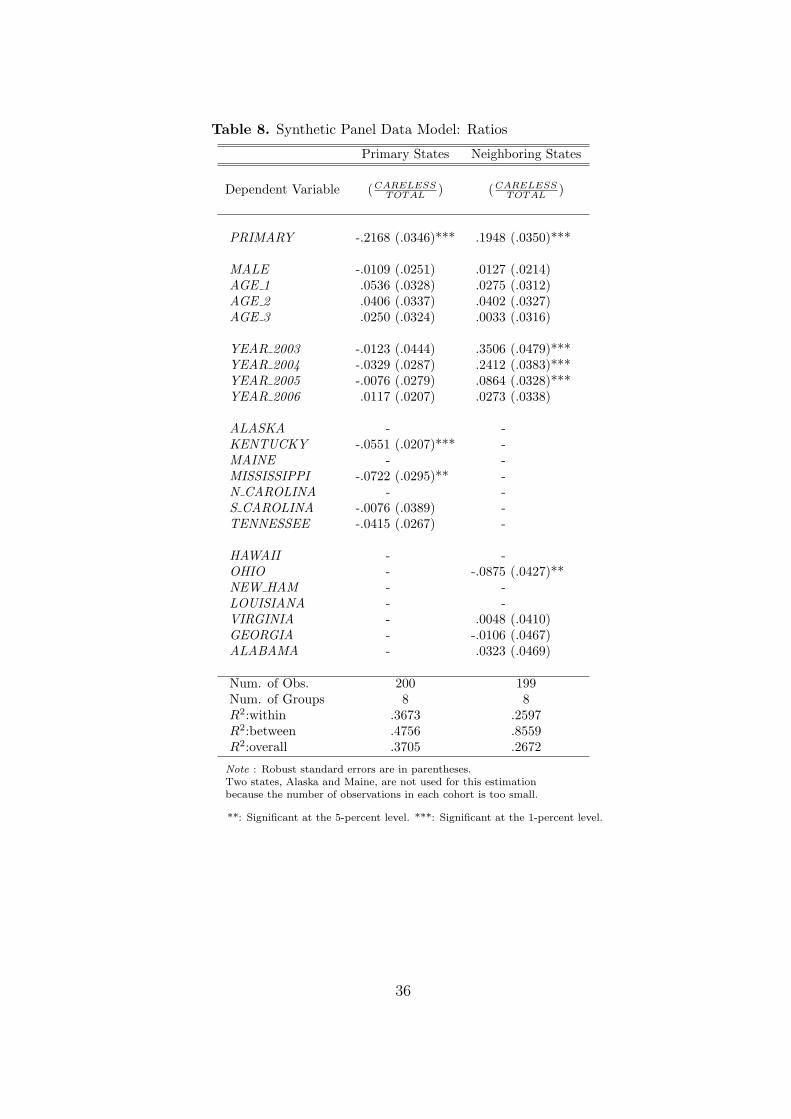
Table 8. Synthetic Panel Data Model: Ratios

Primary States Neighboring States

Dependent Variable (CARELESS

TOTAL) (CARELESS

TOTAL)

PRIMARY -.2168 (.0346)*** .1948 (.0350)***

MALE -.0109 (.0251) .0127 (.0214)AGE 1 .0536 (.0328) .0275 (.0312)AGE 2 .0406 (.0337) .0402 (.0327)AGE 3 .0250 (.0324) .0033 (.0316)

YEAR 2003 -.0123 (.0444) .3506 (.0479)***YEAR 2004 -.0329 (.0287) .2412 (.0383)***YEAR 2005 -.0076 (.0279) .0864 (.0328)***YEAR 2006 .0117 (.0207) .0273 (.0338)

ALASKA - -KENTUCKY -.0551 (.0207)*** -MAINE - -MISSISSIPPI -.0722 (.0295)** -N CAROLINA - -S CAROLINA -.0076 (.0389) -TENNESSEE -.0415 (.0267) -

HAWAII - -OHIO - -.0875 (.0427)**NEW HAM - -LOUISIANA - -VIRGINIA - .0048 (.0410)GEORGIA - -.0106 (.0467)ALABAMA - .0323 (.0469)

Num. of Obs. 200 199Num. of Groups 8 8R2:within .3673 .2597R2:between .4756 .8559R2:overall .3705 .2672

Note : Robust standard errors are in parentheses.Two states, Alaska and Maine, are not used for this estimationbecause the number of observations in each cohort is too small.

**: Significant at the 5-percent level. ***: Significant at the 1-percent level.

36

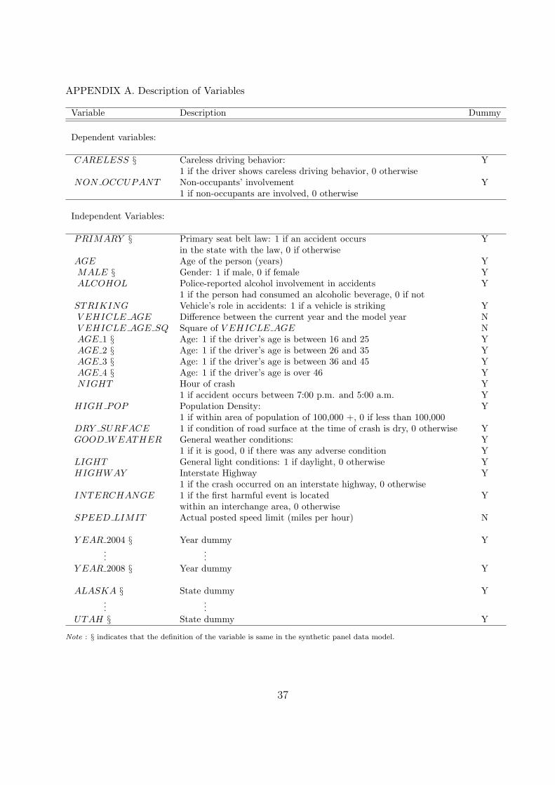
APPENDIX A. Description of Variables

Variable Description Dummy

Dependent variables:

CARELESS § Careless driving behavior: Y1 if the driver shows careless driving behavior, 0 otherwise

NON OCCUPANT Non-occupants’ involvement Y1 if non-occupants are involved, 0 otherwise

Independent Variables:

PRIMARY § Primary seat belt law: 1 if an accident occurs Yin the state with the law, 0 if otherwise

AGE Age of the person (years) YMALE § Gender: 1 if male, 0 if female YALCOHOL Police-reported alcohol involvement in accidents Y

1 if the person had consumed an alcoholic beverage, 0 if notSTRIKING Vehicle’s role in accidents: 1 if a vehicle is striking YV EHICLE AGE Difference between the current year and the model year NV EHICLE AGE SQ Square of V EHICLE AGE NAGE 1 § Age: 1 if the driver’s age is between 16 and 25 YAGE 2 § Age: 1 if the driver’s age is between 26 and 35 YAGE 3 § Age: 1 if the driver’s age is between 36 and 45 YAGE 4 § Age: 1 if the driver’s age is over 46 YNIGHT Hour of crash Y

1 if accident occurs between 7:00 p.m. and 5:00 a.m. YHIGH POP Population Density: Y

1 if within area of population of 100,000 +, 0 if less than 100,000DRY SURFACE 1 if condition of road surface at the time of crash is dry, 0 otherwise YGOOD WEATHER General weather conditions: Y

1 if it is good, 0 if there was any adverse condition YLIGHT General light conditions: 1 if daylight, 0 otherwise YHIGHWAY Interstate Highway Y

1 if the crash occurred on an interstate highway, 0 otherwiseINTERCHANGE 1 if the first harmful event is located Y

within an interchange area, 0 otherwiseSPEED LIMIT Actual posted speed limit (miles per hour) N

Y EAR 2004 § Year dummy Y...

...Y EAR 2008 § Year dummy Y

ALASKA § State dummy Y...

...UTAH § State dummy Y

Note : § indicates that the definition of the variable is same in the synthetic panel data model.

37

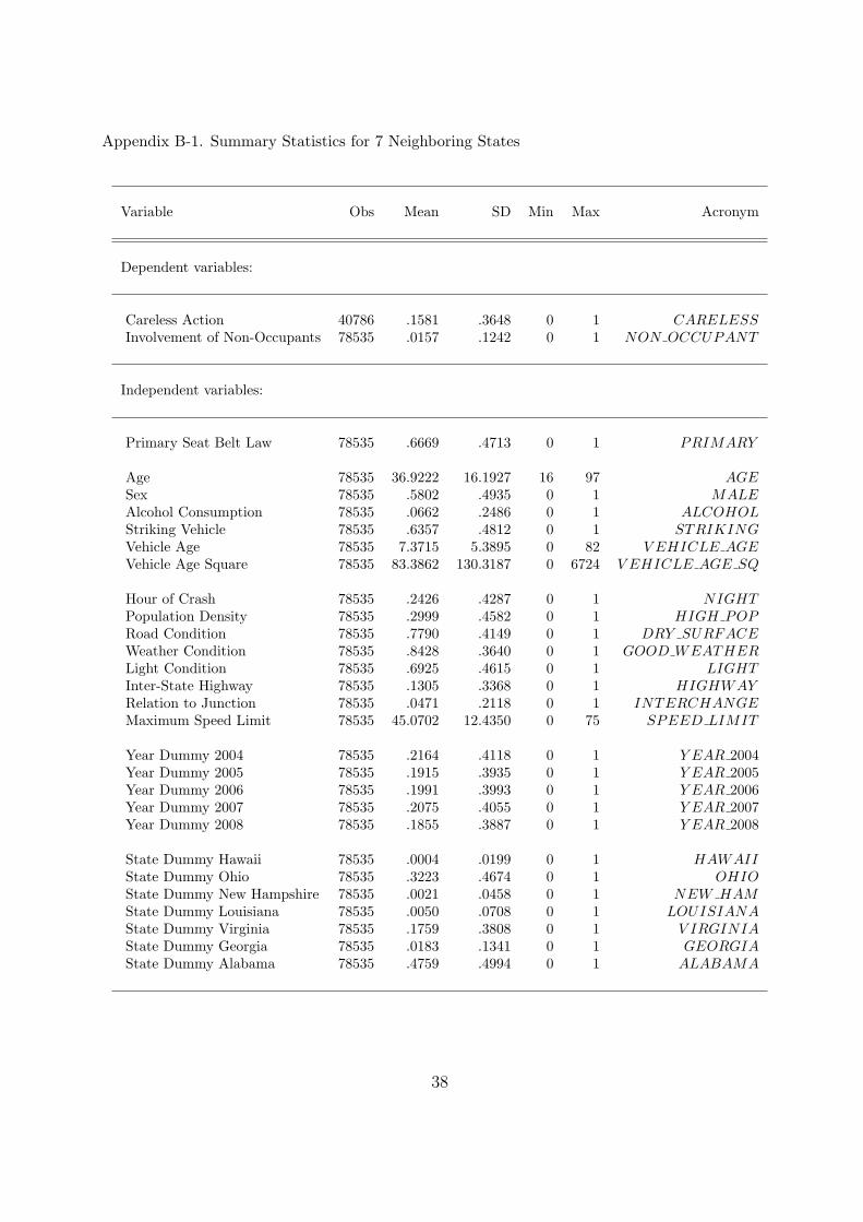
Appendix B-1. Summary Statistics for 7 Neighboring States

Variable Obs Mean SD Min Max Acronym

Dependent variables:

Careless Action 40786 .1581 .3648 0 1 CARELESSInvolvement of Non-Occupants 78535 .0157 .1242 0 1 NON OCCUPANT

Independent variables:

Primary Seat Belt Law 78535 .6669 .4713 0 1 PRIMARY

Age 78535 36.9222 16.1927 16 97 AGESex 78535 .5802 .4935 0 1 MALEAlcohol Consumption 78535 .0662 .2486 0 1 ALCOHOLStriking Vehicle 78535 .6357 .4812 0 1 STRIKINGVehicle Age 78535 7.3715 5.3895 0 82 V EHICLE AGEVehicle Age Square 78535 83.3862 130.3187 0 6724 V EHICLE AGE SQ

Hour of Crash 78535 .2426 .4287 0 1 NIGHTPopulation Density 78535 .2999 .4582 0 1 HIGH POPRoad Condition 78535 .7790 .4149 0 1 DRY SURFACEWeather Condition 78535 .8428 .3640 0 1 GOOD WEATHERLight Condition 78535 .6925 .4615 0 1 LIGHTInter-State Highway 78535 .1305 .3368 0 1 HIGHWAYRelation to Junction 78535 .0471 .2118 0 1 INTERCHANGEMaximum Speed Limit 78535 45.0702 12.4350 0 75 SPEED LIMIT

Year Dummy 2004 78535 .2164 .4118 0 1 Y EAR 2004Year Dummy 2005 78535 .1915 .3935 0 1 Y EAR 2005Year Dummy 2006 78535 .1991 .3993 0 1 Y EAR 2006Year Dummy 2007 78535 .2075 .4055 0 1 Y EAR 2007Year Dummy 2008 78535 .1855 .3887 0 1 Y EAR 2008

State Dummy Hawaii 78535 .0004 .0199 0 1 HAWAIIState Dummy Ohio 78535 .3223 .4674 0 1 OHIOState Dummy New Hampshire 78535 .0021 .0458 0 1 NEW HAMState Dummy Louisiana 78535 .0050 .0708 0 1 LOUISIANAState Dummy Virginia 78535 .1759 .3808 0 1 V IRGINIAState Dummy Georgia 78535 .0183 .1341 0 1 GEORGIAState Dummy Alabama 78535 .4759 .4994 0 1 ALABAMA

38

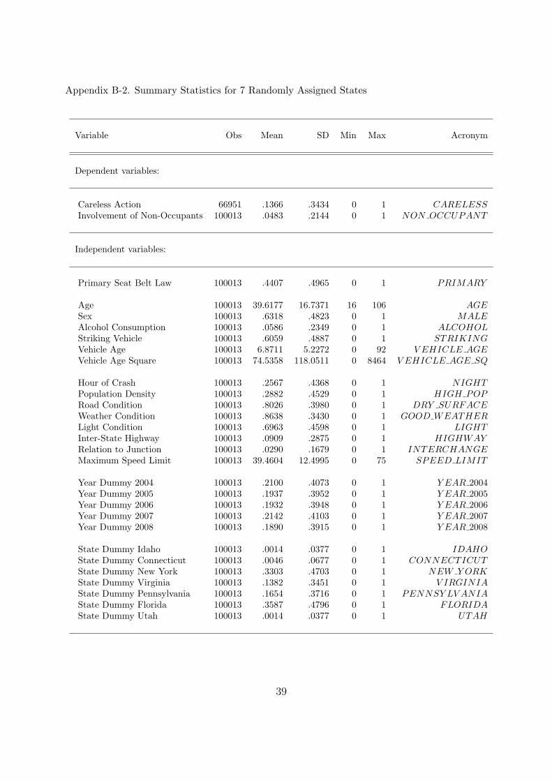
Appendix B-2. Summary Statistics for 7 Randomly Assigned States

Variable Obs Mean SD Min Max Acronym

Dependent variables:

Careless Action 66951 .1366 .3434 0 1 CARELESSInvolvement of Non-Occupants 100013 .0483 .2144 0 1 NON OCCUPANT

Independent variables:

Primary Seat Belt Law 100013 .4407 .4965 0 1 PRIMARY

Age 100013 39.6177 16.7371 16 106 AGESex 100013 .6318 .4823 0 1 MALEAlcohol Consumption 100013 .0586 .2349 0 1 ALCOHOLStriking Vehicle 100013 .6059 .4887 0 1 STRIKINGVehicle Age 100013 6.8711 5.2272 0 92 V EHICLE AGEVehicle Age Square 100013 74.5358 118.0511 0 8464 V EHICLE AGE SQ

Hour of Crash 100013 .2567 .4368 0 1 NIGHTPopulation Density 100013 .2882 .4529 0 1 HIGH POPRoad Condition 100013 .8026 .3980 0 1 DRY SURFACEWeather Condition 100013 .8638 .3430 0 1 GOOD WEATHERLight Condition 100013 .6963 .4598 0 1 LIGHTInter-State Highway 100013 .0909 .2875 0 1 HIGHWAYRelation to Junction 100013 .0290 .1679 0 1 INTERCHANGEMaximum Speed Limit 100013 39.4604 12.4995 0 75 SPEED LIMIT

Year Dummy 2004 100013 .2100 .4073 0 1 Y EAR 2004Year Dummy 2005 100013 .1937 .3952 0 1 Y EAR 2005Year Dummy 2006 100013 .1932 .3948 0 1 Y EAR 2006Year Dummy 2007 100013 .2142 .4103 0 1 Y EAR 2007Year Dummy 2008 100013 .1890 .3915 0 1 Y EAR 2008

State Dummy Idaho 100013 .0014 .0377 0 1 IDAHOState Dummy Connecticut 100013 .0046 .0677 0 1 CONNECTICUTState Dummy New York 100013 .3303 .4703 0 1 NEW Y ORKState Dummy Virginia 100013 .1382 .3451 0 1 V IRGINIAState Dummy Pennsylvania 100013 .1654 .3716 0 1 PENNSY LV ANIAState Dummy Florida 100013 .3587 .4796 0 1 FLORIDAState Dummy Utah 100013 .0014 .0377 0 1 UTAH

39

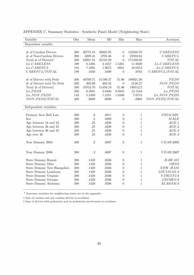
APPENDIX C. Summary Statistics - Synthetic Panel Model (Neighboring State)

Variable Obs Mean SD Min Max Acronym

Dependent variable:

# of Careless Drivers 200 20772.10 29002.95 0 152340.70 CARELESS# of Non-Careless Drivers 200 3209.45 3795.36 0 22592.63 CAREFULTotal # of Drivers† 200 23981.55 32123.29 0 171330.00 TOTALLn CARELESS 199 8.5495 2.1657 1.5261 11.9339 Ln CARELESSLn CAREFUL 184 7.1085 1.9672 .6931 10.0254 Ln CAREFULCAREFUL/TOTAL 199 .1850 .1699 0 .9783 CAREFUL/TOTAL

# of Drivers with Peds 200 46709.71 51196.47 51.96 189921.30 PEDS# of Drivers with No Peds 200 303.99 363.34 0 2146.27 NON PEDSTotal # of Drivers‡ 200 47013.70 51450.19 51.96 190512.5 TOTALLn PEDS 200 9.5091 2.0400 3.9505 12.1544 Ln PEDSLn NON PEDS 143 5.5489 1.2101 1.6506 7.6715 Ln NON PEDSNON PEDS/TOTAL 200 .0069 .0099 0 .0963 NON PEDS/TOTAL

Independent variables:

Primary Seat Belt Law 200 .6 .4911 0 1 PRIMARYSex 280 .5 .5009 0 1 MALEAge between 16 and 25 280 .25 .4338 0 1 AGE 1Age between 26 and 35 280 .25 .4338 0 1 AGE 2Age between 36 and 45 280 .25 .4338 0 1 AGE 3Age over 46 280 .25 .4338 0 1 AGE 4

Year Dummy 2004 280 .2 .4007 0 1 Y EAR 2003...

Year Dummy 2008 280 .2 .4007 0 1 Y EAR 2007

State Dummy Hawaii 280 .1428 .3506 0 1 HAWAIIState Dummy Ohio 280 .1428 .3506 0 1 OHIOState Dummy New Hampshire 280 .1428 .3506 0 1 NEW HAMState Dummy Louisiana 280 .1428 .3506 0 1 LOUISIANAState Dummy Virginia 280 .1428 .3506 0 1 V IRGINIAState Dummy Georgia 280 .1428 .3506 0 1 GEORGIAState Dummy Alabama 280 .1428 .3506 0 1 ALABAMA

* Summary statistics for neighboring states are in the appendix.

† Sum of careless and non careless drivers in accidents.

‡ Sum of drivers with pedestrian and no pedestrian involvement in accidents.

40

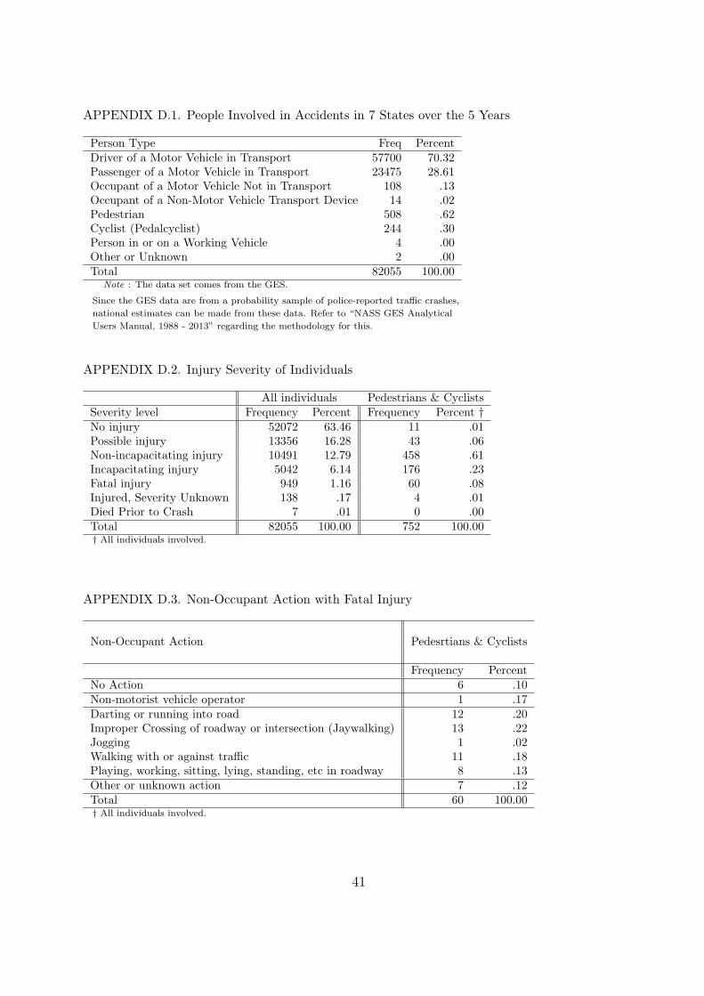
APPENDIX D.1. People Involved in Accidents in 7 States over the 5 Years

Person Type Freq PercentDriver of a Motor Vehicle in Transport 57700 70.32Passenger of a Motor Vehicle in Transport 23475 28.61Occupant of a Motor Vehicle Not in Transport 108 .13Occupant of a Non-Motor Vehicle Transport Device 14 .02Pedestrian 508 .62Cyclist (Pedalcyclist) 244 .30Person in or on a Working Vehicle 4 .00Other or Unknown 2 .00Total 82055 100.00

Note : The data set comes from the GES.

Since the GES data are from a probability sample of police-reported traffic crashes,

national estimates can be made from these data. Refer to “NASS GES Analytical

Users Manual, 1988 - 2013” regarding the methodology for this.

APPENDIX D.2. Injury Severity of Individuals

All individuals Pedestrians & CyclistsSeverity level Frequency Percent Frequency Percent †No injury 52072 63.46 11 .01Possible injury 13356 16.28 43 .06Non-incapacitating injury 10491 12.79 458 .61Incapacitating injury 5042 6.14 176 .23Fatal injury 949 1.16 60 .08Injured, Severity Unknown 138 .17 4 .01Died Prior to Crash 7 .01 0 .00Total 82055 100.00 752 100.00† All individuals involved.

APPENDIX D.3. Non-Occupant Action with Fatal Injury

Non-Occupant Action Pedesrtians & Cyclists

Frequency PercentNo Action 6 .10Non-motorist vehicle operator 1 .17Darting or running into road 12 .20Improper Crossing of roadway or intersection (Jaywalking) 13 .22Jogging 1 .02Walking with or against traffic 11 .18Playing, working, sitting, lying, standing, etc in roadway 8 .13Other or unknown action 7 .12Total 60 100.00† All individuals involved.

41

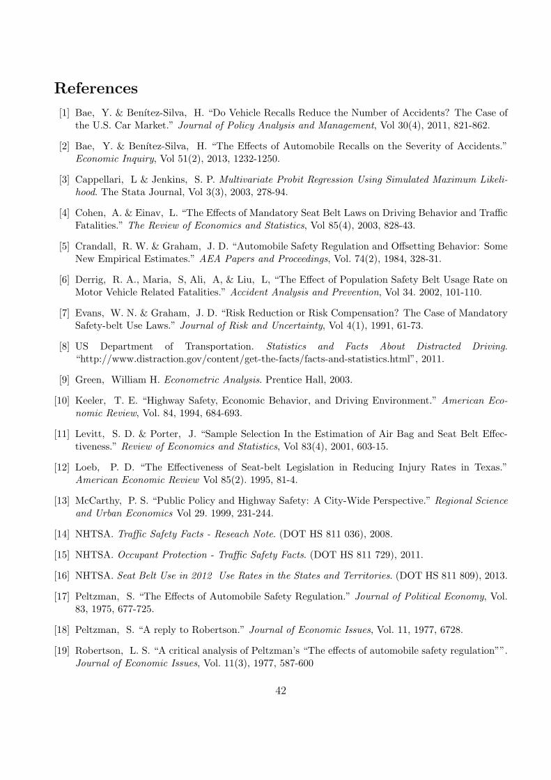
References

[1] Bae, Y. & Benıtez-Silva, H. “Do Vehicle Recalls Reduce the Number of Accidents? The Case ofthe U.S. Car Market.” Journal of Policy Analysis and Management, Vol 30(4), 2011, 821-862.

[2] Bae, Y. & Benıtez-Silva, H. “The Effects of Automobile Recalls on the Severity of Accidents.”Economic Inquiry, Vol 51(2), 2013, 1232-1250.

[3] Cappellari, L & Jenkins, S. P. Multivariate Probit Regression Using Simulated Maximum Likeli-

hood. The Stata Journal, Vol 3(3), 2003, 278-94.

[4] Cohen, A. & Einav, L. “The Effects of Mandatory Seat Belt Laws on Driving Behavior and TrafficFatalities.” The Review of Economics and Statistics, Vol 85(4), 2003, 828-43.

[5] Crandall, R. W. & Graham, J. D. “Automobile Safety Regulation and Offsetting Behavior: SomeNew Empirical Estimates.” AEA Papers and Proceedings, Vol. 74(2), 1984, 328-31.

[6] Derrig, R. A., Maria, S, Ali, A, & Liu, L, “The Effect of Population Safety Belt Usage Rate onMotor Vehicle Related Fatalities.” Accident Analysis and Prevention, Vol 34. 2002, 101-110.

[7] Evans, W. N. & Graham, J. D. “Risk Reduction or Risk Compensation? The Case of MandatorySafety-belt Use Laws.” Journal of Risk and Uncertainty, Vol 4(1), 1991, 61-73.

[8] US Department of Transportation. Statistics and Facts About Distracted Driving.“http://www.distraction.gov/content/get-the-facts/facts-and-statistics.html”, 2011.

[9] Green, William H. Econometric Analysis. Prentice Hall, 2003.

[10] Keeler, T. E. “Highway Safety, Economic Behavior, and Driving Environment.” American Eco-

nomic Review, Vol. 84, 1994, 684-693.

[11] Levitt, S. D. & Porter, J. “Sample Selection In the Estimation of Air Bag and Seat Belt Effec-tiveness.” Review of Economics and Statistics, Vol 83(4), 2001, 603-15.

[12] Loeb, P. D. “The Effectiveness of Seat-belt Legislation in Reducing Injury Rates in Texas.”American Economic Review Vol 85(2). 1995, 81-4.

[13] McCarthy, P. S. “Public Policy and Highway Safety: A City-Wide Perspective.” Regional Science

and Urban Economics Vol 29. 1999, 231-244.

[14] NHTSA. Traffic Safety Facts - Reseach Note. (DOT HS 811 036), 2008.

[15] NHTSA. Occupant Protection - Traffic Safety Facts. (DOT HS 811 729), 2011.

[16] NHTSA. Seat Belt Use in 2012 Use Rates in the States and Territories. (DOT HS 811 809), 2013.

[17] Peltzman, S. “The Effects of Automobile Safety Regulation.” Journal of Political Economy, Vol.83, 1975, 677-725.

[18] Peltzman, S. “A reply to Robertson.” Journal of Economic Issues, Vol. 11, 1977, 6728.

[19] Robertson, L. S. “A critical analysis of Peltzman’s “The effects of automobile safety regulation””.Journal of Economic Issues, Vol. 11(3), 1977, 587-600

42

[20] Sen, A. & Mizzen, B. “Impact of Seat Belt Use on Driving Behavior.” Economic Inquiry, Vol. 30,1992, 649-58.

[21] Sen, A. and Mizzen, B. “Estimating the Impact of Seat Belt Use on Traffic Fatalities: EmpiricalEvidence from Canada.” Canandian Public Policy, Vol 33(3), 2007, 315-35.

[22] Singh, H. & Thayer, M. “Impact of Seat Belt Use on Driving Behavior.” Economic Inquiry, Vol.30(4), 1992, 649-58.

[23] Sobel, R. S. & and Nesbit, T. M. “Automobile Safety Regulation and the Incentive to DriveRecklessly: Evidence from NASCAR.” Southern Economic Journal, Vol 74(1). 2007, 71-84.

[24] Wooldridge, J. M. Econometric Analysis of Cross Section and Panel Data. Cambridge, 2002, MITPress.

43