Auton Agent Multi-Agent Syst (2009) 18:267–294DOI 10.1007/s10458-008-9045-x

Primary and secondary diagnosis of multi-agent planexecution

Femke de Jonge · Nico Roos · Cees Witteveen

Published online: 12 April 2008The Author(s) 2008

Abstract Diagnosis of plan failures is an important subject in both single- and multi-agentplanning. Plan diagnosis can be used to deal with plan failures in three ways: (i) to provideinformation necessary for the adjustment of the current plan or for the development of a newplan, (ii) to point out which equipment and/or agents should be repaired or adjusted to avoidfurther violation of the plan execution, and (iii) to identify the agents responsible for plan-execution failures. We introduce two general types of plan diagnosis: primary plan diagnosisidentifying the incorrect or failed execution of actions, and secondary plan diagnosis thatidentifies the underlying causes of the faulty actions. Furthermore, three special cases ofsecondary plan diagnosis are distinguished, namely agent diagnosis, equipment diagnosisand environment diagnosis.

Keywords Diagnosis · Planning · Multi-agent systems

1 Introduction

In multi-agent planning research there is a tendency to deal with plans that become larger,more detailed and more complex. As complexity grows, the vulnerability of plans for fail-ures will grow correspondingly. Taking appropriate measures to plan failures requires theability to detect the occurrence of failures as well as to determine their causes. Therefore, we

F. de Jonge · N. Roos (B)Department of Computer Science, Universiteit Maastricht, P.O. Box 616, 6200 MD Maastricht,The Netherlandse-mail: roos@micc.unimaas.nl

F. de Jongee-mail: f.dejonge@micc.unimaas.nl

C. WitteveenFaculty EEMCS, Delft University of Technology, P.O. Box 5031, 2600 GA Delft, The Netherlandse-mail: C.Witteveen@tudelft.nl

123

268 Auton Agent Multi-Agent Syst (2009) 18:267–294

consider diagnosis as an integral part of the capabilities of agents in single- and multi-agentsystems.

To illustrate the relevance of plan diagnosis, consider a simple example in which yourluggage did not arrive at the destination when flying from New York to Amsterdam. Afterdetecting this fault, i.e., your luggage did not appear on the arrival belt, you know that theplan of transporting your luggage did not lead to the desired result. Clearly, the normal planexecution has failed and we wish to apply diagnosis to find out why. Given the transport planof your luggage, consisting of actions such as sorting the luggage after check-in, loadingit on the airplane, unloading the luggage, and so on, we apply diagnosis to identify whichof these actions have failed. For instance, sorting the luggage to the right airplane. We willdenote this type of diagnosis as primary plan diagnosis. Primary plan diagnosis focuses ona set of fault behaviors of actions that explain the differences between the expected and theobserved plan execution.

Often, however, it is more interesting to determine the causes behind such faulty actionexecutions. In our example, the failure of the action ‘sorting of luggage’ may be caused by amalfunction of the equipment used. For instance, the component that reads the label attachedto the luggage may make errors. We will denote the diagnosis of these underlying causes assecondary plan diagnosis. Secondary diagnosis can be viewed as a diagnosis of the primarydiagnosis. It informs us for instances about a malfunctioning of the equipment that caused thefaulty behavior of an action performed by it. Beside malfunctioning equipment, secondarydiagnosis may also identify the agents that did not execute an action correctly and changesin the environment that where not anticipated at the time the plan was made. For instance,loading the luggage onto an airplane may fail for a piece of luggage because the personnelforgot to load that piece. Unexpected environment changes (such as the weather) may alsoinfluence the outcome of an action. For instance, very strong turbulence during a flight maycause injuries among passengers and may damage the cargo.

As a special type of secondary diagnosis, we are also able to determine the agents respon-sible for the failed execution of some actions. In our luggage transportation example, themaintenance agent might be responsible for the malfunctioning sensor that reads the labelsof luggage.

In our opinion, diagnosis in general, and secondary diagnosis in particular, enables theagents involved to make specific adjustments to the system or the plan as to manage currentplan-execution failures and to avoid new plan-execution failures. These adjustments can becategorized with regard to their benefits to the general system. Primary diagnosis can con-tribute to plan repair by identifying the failed action and how it failed. Secondary diagnosiscontributes to plan repair by identifying the broken equipment and the misbehaving agents.In particular, information about misbehaving agents may help to adjust the agents, therebycontributing to a better plan execution. Finally, by indicating the agents responsible for planfailures, secondary diagnosis also becomes a valuable tool in evaluating the system and mightbe used to divide costs of repairs and/or changes in the plan amongst the agents.

1.1 Aim, approach and results

In some previous papers [30,24] we have introduced a simple formal framework for plandiagnosis. The framework is based on classical Model-Based Diagnosis (MBD). We haveshown that modeling the world using a set of state variables enables us to view (i) actionsas components, (ii) variables who’s values are set by one action and are inputs of the nextaction as connections between component, and (iii) the whole plan as a system.

123

Auton Agent Multi-Agent Syst (2009) 18:267–294 269

In this framework we restricted diagnosis to primary diagnosis of failing actions in a plan,distinguishing only two health modes for actions: a normal (nor ) and an abnormal (ab) mode.Using the framework we were able to point out some computational differences between twotypes of preferred plan diagnoses: minimum diagnoses and minimal maximum-informativediagnoses (mini-maxi diagnoses). While minimum diagnoses turned out to be difficult tocompute, mini-maxi diagnoses were computable in polynomial time.

We did not, however, investigate a more refined set of fault modes and we could notidentify the causes of failing actions as e.g., executing agents, equipment used to execute anaction, or unforeseen changes of the environment. The purpose of this paper is to extend thisexisting framework in several respects.

First of all, we would like to have a common framework for plan diagnosis to deal withboth primary and secondary diagnosis, where agents, equipment and environment could beidentified as possible sources for plan execution errors. This necessitates us to introducehealth modes for agents, equipment and environment, too. Equipment has health modes indi-cating the normal behavior (nor ), the general unknown but abnormal behavior (ab), andequipment-specific health modes. The label reader in the above example for instance mayhave a health mode indicating that it confuses ‘AMS’ (Amsterdam) with ‘AMM’ (Amman).An agent executing a part of a plan can be viewed as just a special type of equipment. Hence,besides the health modes nor and ab, an agent may have agent-specific health modes forhardware, software, sensor and actor failures.

Remark 1 Beside viewing agents as a special kind of equipment, we may also view agentsas intentional systems (beings). From this perspective, agents may fail to execute an actioncorrectly because of incorrect beliefs or intentions. In such an agent, we may view the agent’sbelief states as health modes.1 The diagnostic model presented in the following sections isalso able to identify these causes of execution failures. Note that identifying belief states ofagents is related to social diagnosis [16,17]. However, social diagnosis does not deal withplans consisting of a partially ordered set of actions.

We also would like to allow health modes for environment objects. Although the purposeof executing a plan is to change the environment in such a way that after the execution the stateof the environment satisfies some goals, the environment may also influence the executionof the plan in unintended ways. For instance very strong turbulence causing damage to frag-ile cargo. Therefore, diagnosis should be able to identify unforeseen environment changesinfluencing the execution of an action. Finally, we also allow for more than two health modesfor actions. Besides the health modes nor , denoting that the action is executed as expected,and ab, denoting that the action execution fails, we allow for several action-specific healthmodes, such as routing error: AMS→AMM for luggage sorting action.

The above extensions needed to deal with primary and secondary diagnosis will cause amajor change of the existing plan diagnosis framework.

First of all, we introduce a uniform representation of actions, agents equipment and theenvironment using a set of state variables. To be able to distinguish different types of diag-noses such as primary diagnosis and three types of secondary diagnosis, namely: agent,equipment and environment diagnosis, we partition these variables into action, agent, equip-ment and environment variables.

1 However, in general we cannot state in advance which beliefs are normal modes and which are faults modessince this may depend on the context.

123

270 Auton Agent Multi-Agent Syst (2009) 18:267–294

Secondly, we introduce events to describe the unforeseen (unplanned) state changes ofvariables. Variables may therefore be viewed a discrete event systems [5] with respect to theunforeseen state changes.2

Finally, we define diagnosis as a set of events changing the states of variables. We make adistinction between two types of diagnosis, namely primary and secondary diagnosis wherethe latter gives the underlying causes of the former. Secondary diagnosis is further dividedinto agent, equipment and environment diagnosis. Moreover as a special form of secondarydiagnosis, we discuss the identification of agents responsible for failures. These agents neednot be the agents executing the plan.

1.2 Organization

The remainder of the paper is organized as follows. In the next section, Sect. 2, we presentsome related work and discuss some related approaches to plan diagnosis. Then, in Sect. 3,we introduce a general framework for plan-diagnosis that enables the identification of dif-ferent causes of plan execution failures as will be described in Sect. 4. In Sect. 5 we illustratethe aspects of our diagnostic model using a large example. Being able to efficiently identifydiagnoses is an important issue. Section 6, discussed preference criteria on diagnoses as wellas some complexity results with respect to the identification of preferred diagnoses. Section 7concludes the paper.

To place our approach in perspective, before introducing the plan and diagnostic model,we first discuss some related work.

2 Related research

Our approach to plan diagnosis can be viewed as an extension of the Model-Based Diagnosis(MBD) to the planning domain. We therefore start with a brief overview of MBD and itsconnection to plans.

2.1 Model-based diagnosis

Classical Model-Based Diagnosis (MBD) assumes a set of connected components usuallywith specific inputs and outputs. A model of the system is used to predict its expectedbehavior. Discrepancies between the observed and the predicted behavior are subsequentlyused to determine a diagnosis. Two forms of diagnosis can be distinguished; abductive [6]and consistency-based diagnosis [23,11]. To apply abductive diagnosis we must be ableto predict the values of all the observed system outputs using a description of the system.Consistency-based diagnosis is a weaker notion of diagnosis. The predictions made usinga consistency-based diagnosis only need to be consistent with the observed values of theobserved system outputs. Hence an abductive diagnosis is more restrictive but also requiresmore information about the system behavior [22]. Especially, one needs to know the behaviorof malfunctioning components. Note that if the later knowledge is known, consistency-baseddiagnosis identifies the same set of diagnosis as abductive diagnosis [10].

We will show that a plan consisting of a partially ordered set of actions can be viewed asa system of connected components. This view enables us to predict the expected behaviorof a plan, observe discrepancies between the predicted and the expected behavior and apply

2 Note that the execution of actions will not be described in terms of events changing the state of a variable.

123

Auton Agent Multi-Agent Syst (2009) 18:267–294 271

consistency-based diagnosis to identify causes. We do not consider abductive diagnosis sincewe need not know the behavior of failing or incorrectly executed actions of a plan.

2.2 (Multi-)agent-based approaches

Similar to our use of MBD as a starting point of plan diagnosis, Birnbaum et al. [2] applyMBD to planning agents relating health modes of agents to outcomes of their planning activ-ities, but not taking into account faults that can be attributed to actions occurring in a plan asa separate source of errors.

de Jonge et al. [8,9] present an approach that directly applies MBD to plan execution.Here, the authors focus on agents each having an individual plan, and on the conflicts thatmay arise between these plans (e.g., if they require the same resource). Actions are viewedas processed, which are modeled as Discrete Event Systems (DES). Diagnosis is applied todetermine those factors that are accountable for future conflicts. The authors, however, do nottake into account dependencies between health modes of actions and do not consider agentsthat collaborate to execute a common plan.

Micalizio and Torasso [19] introduce a distributed monitoring approach for multi-agentplan execution which is similar to the work of de Jonge et al. They also view a plan’s actionsas processes and they also model actions as DESs. Their approach, however, differs fromthe work of [8,9] in that they explicitly incorporate the belief state of the executing agent inthe description of actions. Moreover, they focus on monitoring and diagnosis of the agents’belief states.

In [20] the authors apply this approach to execution of a multi-agent plan and extend theapproach with repair of faults occurring during the execution the plan. They view a plan asa partially order set of actions where each action provides a service required by followingactions. The actions are again modeled as DESs. When an agent detects an action failure, itwill first try to repair its own sub-plan. If this local recovery fails, the team to with the agentbelongs will try to repair the plan.

Kalech and Kaminka [17,18] apply social diagnosis in order to find the cause of ananomalous plan execution by a team of agents. They consider hierarchical plans consistingof so-called behaviors. Such plans do not prescribe a (partial) execution order on a set ofactions. Instead, based on an agent’s observations, beliefs and role, the plan prescribes foreach agent the appropriate behavior to be executed. Each behavior in turn may consist ofprimitive actions to be executed, or of a set of other behaviors to choose from. Social diagno-sis then addresses the issue of determining what went wrong in the joint execution of such aplan by identifying the disagreeing agents and the causes for their selection of incompatiblebehaviors (e.g., belief disagreement, communication errors) based on monitoring the agents’plan execution.

Carver and Lesser [4] and Horling et al. [15] also apply diagnosis to (multi-agent) plans.Their research concentrates on the use of a causal model that can help an agent to refine itsinitial diagnosis of a failing component (called a task) of a plan. As a consequence of usingsuch a causal model, the agent would be able to generate a new, situation-specific plan that isbetter suited to pursue its goal. Diagnosis is based on observations of a component withouttaking into account the consequences of failures of such a component w.r.t. the remainingplan.

In previous work [24,26], the authors show how classical MBD can be applied to identifyabnormally executed actions in a plan consisting of a partially ordered set of actions. Theyproposed to describe the state of the world by a set of variables and the actions as functionsthat modify some of the state variables. This description of the world and the actions together

123

272 Auton Agent Multi-Agent Syst (2009) 18:267–294

with partial observations at different time points, makes it possible to apply classical MBDby viewing (i) actions as components of a system, and (ii) variables set by one action andrequired as inputs by a following action as connections between components. Unlike otherapproaches, this approach does not monitor the execution of all plan steps and does not modelplan steps as processes. Since we do not monitor the execution of plan steps, we only monitorthe effects of the plan execution at some time point, there is nothing to gain by modeling plansteps as processes. We can, however, gain something from modeling the specific health stateof actions, agents and equipment. Below we present an adapted and extended version of ourformalization of plan diagnosis. This formalization enables the handling of the health stateof actions, agents and equipment in much the same way as the approaches of de Jonge et al.[8,9], Kalech and Kaminka [17,18], and Lesser et al. [4,15]. The work of Birnbaum et al. [2]is not covered by the proposed formalization since it focuses on the planning activity insteadof on plan execution.

2.3 Discrete event systems

To model state changes that are not caused by the execution of actions, we propose to viewstate variables as Discrete Event Systems (DESs). This view enables us to describe unknowncauses of state changes by unobserved events where the transition function places restrictionon the state changes that may occur.

In general, Discrete Event Systems are a modeling method of real-world systems based onfinite state machines (FSM) [5]. In a DES a finite set of states describes at some abstractionlevel the state of a real-world system. State changes are caused by events and a transitionfunction specifies the changes triggered by the events. The events are usually observable con-trol events. However, unobservable failure events mays also cause state changes. Diagnosisof a DES aims at identifying the unobserved failure events based on a trace of observableevents [27]. Essentially, this is a form of abductive diagnosis. Note that the trace of observableevents depends on the state of the system and the transition function. Therefore, a DES issometimes viewed as a machine accepting a language of observable and unobservable events.

In order to create a DES modeling a system, one first models the behavior of individualcomponents using DESs. The finite state machines described by the DESs modeling thesecomponents interact by exchanging events. Here, a state transition of a FSM may trigger newevents causing state transitions of other FSMs. To make a diagnosis using the coupled DESstwo main approaches exist. The oldest approach combines the FSMs modeling the compo-nents into a global FSM of the whole system [28]. Unfortunately, the number of states of theglobal finite state machine grows exponentially with the number of components, making itinfeasible for modeling large systems. Therefore, in recent work, instead of creating a singleFSM, methods for making diagnosis directly using the coupled DESs have been proposed inthe literature [1,21].

Remark 2 Although we will propose the use of discrete event systems for describing statechanges of variables caused by unknown events, we will not model plan execution usingDESs. The reason is that an action in a plan is a process that changes the values of variablesdescribing the state of the world. Since actions change the values of variables, they mustbe described by events. Of course we could avoid the combinatorial explosion associatedwith creating one global DES by introducing a DES for each variable (as we will do in thispaper). However, describing actions as events implies ignoring the processing time of actions.Although, in this paper, we consider unit processing times for actions in order to simplify thedescription of our model, there is no principal objection against using non-unit processing

123

Auton Agent Multi-Agent Syst (2009) 18:267–294 273

times of actions. The use of events however to represent actions with non-unit processingtimes, which may also depend on the agents executing the actions, the equipment used theenvironment and the way actions may fail, is quite problematic.

Another reason why we do not model a plan using a DES is because diagnosis of DESsis essentially abductive diagnosis. This implies that we need to know all the different waysin which executing an action may fail. In general, this knowledge is not available.

3 Plans as systems

We consider plan based diagnosis as an extension of model-based diagnosis where the modelis a description of a plan instead of a physical system. In this view the execution of an actionis a component changing the state of the world. Therefore, we will introduce a state-baseddescription of the world. The state-based description is changed by the execution of actionsand by disruptions.

To realize plan diagnosis, we adapt and extend the representation of plans presented in[30,24]. This representation, in which the state of the world is described by a set of variables,has been chosen because it is more suited to plan diagnosis than the traditional plan repre-sentations such as [3,12,13,29] and it also enables us to extend the classical Model-BasedDiagnosis (MBD) approach to the planning domain. Moreover, we wish to study plan diag-nosis independent of any planning approach that is used to generate a plan or that will beused to repair a plan.

We now introduce the building blocks of our plan diagnosis approach. Since our repre-sentation differs from the traditional plan representation, we will relate our representation tostrips.

3.1 Actions, plan operators and plan steps

In the preceding sections we used the term ‘actions’ in a rather informal way. From now onwe will distinguish plan operators O and plan steps S, which are both covered by the term‘actions’.

A plan operator o ∈ O refers to a general description of an action independently of howit is used in a plan. In contrast, a plan step s ∈ S is an instantiation of a plan operator tobe used at a specific point in a plan. One plan operator o ∈ O may therefore have severalinstantiations {s1, . . . , sn} = inst (o) that are used in the same plan. A plan operator fortransporting items may, for instance, be instantiated resulting in a plan step for the transportof a specific container from Rotterdam to New York by ship, and also be instantiated resultingin a plan step for the transport of a passager’s luggage from Washington to Amsterdam byplane.

3.2 States and partial states

In [30], it was shown that by describing the state of the world using objects or variablesinstead of propositions, it becomes possible to apply classical MBD to plan execution. Here,we will take this approach one step further by also introducing variables for agents executingthe plan, the equipment used by the agents and for the plan steps themselves. We explic-itly introduce these variables in order to enable the identification of other health modes ofsteps beside normal and abnormal, and the identification of underlying causes of failing plansteps such as misbehaving agents and malfunctioning equipment. Hence, we assume a finite

123

274 Auton Agent Multi-Agent Syst (2009) 18:267–294

set of variables V that will be used to describe the plan, the agents, the equipment and theenvironment, respectively. The variables V are partitioned into four classes or types: plansteps S, agents A, equipment E and environment variables N . Each variable in v ∈ V isassumed to have a domain Dv of values. The state of the set of variables V = {v1, . . . , vn}at some time point is described by a tuple σ ∈ Dv1 × · · · × Dvn of values. In particular, fourprojections σS , σA, σE and σN of σ are used to denote the state of the plan step variablesS, the agent variables A, the equipment variables E and the environment variables N .

The state σN of the set of environment variables N describes the state of the agents’environment at some point in time. For instance, these state descriptions can represent thelocation of an airplane or the availability of a gate.

The states σS and σE of plan step and equipment variables, describe the health of plansteps and equipment, respectively. Their domains consist of the health modes of the plansteps and equipment. We assume that each of these domains contains at least (i) the valuenor to denote that the plan steps and equipment behave normally, and (ii) the general faultmode ab to denote that the plan steps and equipment behave in an unknown and possiblyabnormal way. Moreover, the domains may contain several more specific fault modes. Forinstance, different types of routing errors for the ‘sort luggage’ action in the example in theIntroduction. Note that beside a variable describing the health state of a piece of equipment, aseparate environment variable must be introduced to describe for instance the location of thepiece of equipment. The equipment variables are reserved for describing the health modesof the equipment.

If an agent is viewed as a special type of equipment, then state σA either describes theagents’ health mode in terms of normal operation nor , general malfunctioning ab, and otherhealth modes denoting hardware, software, sensor and actor failures. If, however, an agentis viewed as an intentional system, the health modes may describe the agent’s beliefs thatdetermine the agent’s execution a planed plan step. Incorrect beliefs may result in an incorrectexecution of a plan step. The actual choice depends on the application domain. If necessary,two variables representing both aspects may be used for each agent.

It will not always be possible to give a complete state description. Therefore, we intro-duce a partial state as an element π ∈ Dvi1

× Dvi2× · · · × Dvik

, where 1 ≤ k ≤ n and1 ≤ i1 < · · · < ik ≤ |V|. We use V (π) to denote the set of variables {vi1 , vi2 , . . . , vik } ⊆ Vspecified in such a state π . The value of a variable v ∈ V (π) in π will be denoted by π(v).The value of an object v ∈ V not occurring in π is said to be unknown (or unpredictable) inπ , denoted by ⊥. Including ⊥ in every value domain Di allows us to consider every partialstate π as an element of D1 × D2 × · · · × D|V|.

Partial states can be ordered with respect to their information content: given values d andd ′, we say that d ≤ d ′ holds iff d = ⊥ or d = d ′. The containment relation � between partialstates is the point-wise extension of ≤: π is said to be contained in π ′, denoted by π � π ′,iff ∀v ∈ V [π(v) ≤ π ′(v)].

Given a subset of variables V ⊆ V , two partial states π , π ′ are said to be V -equivalent,denoted by π =V π ′, if for every v ∈ V , π(v) = π ′(v). We define the partial state π restrictedto a given set V , denoted by π�V , as the state π ′ � π such that V (π ′) = V ∩ V (π).

An important notion in plan diagnosis is the notion of compatibility between partial states.Intuitively, two states π and π ′ are said to be compatible if they could characterize the samestate of the world, that is, there exists a state σ such that π � σ and π ′ � σ . Equivalently, thiscompatibility relation can also be expressed without making a reference to such a state σ sincethe existence of such a state σ clearly implies that for every v ∈ V ar , either π(v) = π ′(v)

or at least one of the values π(v) and π ′(v) is undefined:

123

Auton Agent Multi-Agent Syst (2009) 18:267–294 275

Definition 1 (compatibility relation) Two partial states π and π ′ are said to be compatible,denoted by π ≈ π ′, iff

∀v ∈ V[ π(v) ≤ π ′(v) or π ′(v) ≤ π(v) ].3.3 Goals

An (elementary) goal g of an agent specifies a set of states an agent wants to bring aboutusing a plan. Here, we specify each such a goal g as a constraint, that is, a relation over someproduct Di1 × · · · × Dik of domains. We say that a goal g is satisfied by a partial state π ,denoted by π |= g, if the relation g contains some tuple (partial state) (di1 , di2 , . . . dik ) suchthat (di1 , di2 , . . . dik ) � π . We assume each agent a to have a set Ga of such elementarygoals g ∈ Ga . We use π |= Ga to denote that all goals in Ga hold in π , i.e. for all g ∈ Ga ,π |= g.

3.4 Plan step execution

The execution of a specific plan step s ∈ S may not only change the state of environmentvariables N , but also agent variables A and equipment variables E . We describe such changesinduced by a specific plans step s ∈ S by a function f o:

f o : Ds × (Da1 × · · · × Dai ) × (De1 × · · · × De j ) × (Dn1 × · · · × Dnk ) →(Da′

1× · · · Da′

u) × (De′

1× · · · × De′

v) × (Dn′

1× · · · × Dn′

w)

where

– o is the plan operator of which the plan step s is an instance, that is, s ∈ inst (o),– a1, . . . , ai ∈ A are the execution agents,– e1, . . . , e j ∈ E are the variables describing the health modes of equipment required,– n1, . . . , nk ∈ N are the environment variables required, and– {a′

1, . . . , a′u, e′

1, . . . , e′v, n′

1, . . . , n′w} are agent, equipment and environment variables,

respectively, that are changed by the execution of plan step s.

Each application of the function f o associated with the plan operator o is completelydetermined by a plan step s ∈ inst (o). Therefore, we will use the plan step s to denotethe binding of the variables to the domain parameters of the function f o by domV (s) ={s, a1, . . . , ai , e1, . . . , e j , n1, . . . , nk}. Likewise we denote the binding to the range param-eters by ranV (s) = {a′

1, . . . , a′u, e′

1, . . . , e′v, n′

1, . . . , n′w}.

Remark 3 Note that a plan step is the only variable that cannot be changed by the executionof a plan step. A plan step is executed only once and its health mode determines how it isexecuted. We allow that the values of all other variables can be changed by the execution ofa plan step. In case of equipment, such a change may indicate effect of a maintenance or arepair activity, but also the effect of damaging equipment by operating it outside the operationparameters. The same holds for agents if agents are viewed as a special kind of equipment.3

Also note that the set of variables ranV (s) bound to the range of f o with s ∈ inst (o) maydiffer from the variables domV (s) bound to the domain of f o. This property makes it possi-ble to set the value of a variable independently of its previous value. Finally, note that mostplanning formalisms, such as strips, can be modeled using our formalism for describingplans. The relation with strips will be described in paragraph “The relation with strips”.

3 If, however, agents are viewed as intentional systems, state changes may indicate belief updates.

123

276 Auton Agent Multi-Agent Syst (2009) 18:267–294

agent HAL(status: normal)

transport(status: normal)

goods(location: Rotterdam)

f TRANSPORT

goods(location: New York)

transport(status: normal)

agent HAL(status: normal)

state

state

ship(status: normal)

ship(status: normal)

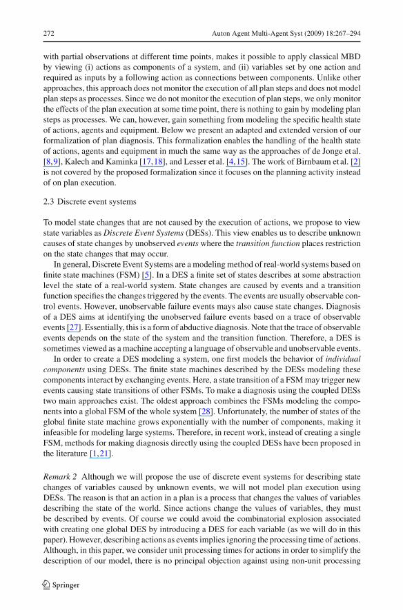
Fig. 1 An action and its state transformation

To distinguish the different types of parameters in a more clear way, we will place semi-colons between them when specifying the function, e.g.:

f TRANSPORT(transport : S; HAL : A; ship : E; goods : N ).

Figure 1 gives an illustration of the our representation of a plan step. It show the applica-tion of the plan step ‘transport’ which is a an instance of a transport plan operator. Theeffect of executing the plan step is that the location of the goods changes. If necessary, wecould also model that the location of the ship and of the executing agent HAL changes too.

The result of a plan step may not always be known if, for instance, the action fails, theagent misbehaves or the equipment malfunctions. Therefore we allow that the plan operatorfunction associated with a plan step maps the value of a variable to ⊥ to denote that the effectof the plan step on this variable is unknown. We will use the health mode ab to indicate themost general abnormal health mode of a plan step, an agent or equipment. If one of the inputparameters of f o has the health mode ab, the outcome of the action execution is assumed tobe unknown. That is,

f o(s, a1, . . . , ai , e1, . . . , e j , n1, . . . , nk) = (⊥, . . . ,⊥)

if s = ab, for some l: al = ab, or for some l: el = ab.In [30,24], it was assumed that the result of a plan step s is unknown (all variables in

its range will take the value ⊥) if one of the variables in the domain v ∈ domV (s) has anunknown value. Here, we relax this restriction allowing the function f o with s ∈ inst (o) tomap to known values if some values in its (environment) domain are unknown.

3.5 Plans

A plan is a tuple P = 〈S,<〉 where S ⊆ S is a subset of the plan steps that need to beexecuted and < is a partial order defined on S × S where s < s′ indicates that the plan steps must finish before the plan step s′ may start. Note that each plan step s ∈ S occurs exactlyonce in the plan P . We will denote the transitive reduction of < by , i.e., is the smallestsub-relation of < such that the transitive closure + of equals <.

123

Auton Agent Multi-Agent Syst (2009) 18:267–294 277

s1 s2

s3 s4

s6

t=3

π0

π2

π3

s8

s5

⊥

s7

π1

t=2

t=1

t=0v2 v3 v4 v5v1

Fig. 2 Plan execution with one abnormal action

We assume that if in a plan P two plan steps s and s′ are independent, in principle theymay be executed concurrently. This means that the precedence relation < at least shouldcapture all resource dependencies that would prohibit concurrent execution of plan steps.Specifically, this implies that the precedence relation <

1. should prohibit simultaneous changes of the same variable v by different plan steps and2. should prohibit changing a variable v by some plan step s while v may also be used as

the input of another plan step s′.

Therefore, we assume < to satisfy the following concurrency requirement4:

If ranV (s) ∩ (domV (s′) ∪ ranV (s)) �= ∅ then s < s′ or s′ < s.

Figure 2 gives an illustration of a plan with one abnormally executed plan step. Since aplan step is applied only once in a plan, for clarity reasons, we replace the function describ-ing the behavior of the corresponding plan operator by the name of the plan step and weuse the color of the plan step to denote its health mode. The arrows relate a plan step si tothe variables it uses as inputs and the variables it modifies as its outputs. In this plan, thedependency relation is specified as s1 s3, s1 s4, s2 s4, s2 s5, s4 s7, s5 s8

and s4 s6. The last dependency has to be included because s6 changes the value of v2

needed by s4. The step s4 shows that not every variable occurring in the domain of a planstep need to be affected by the plan step. Note that in this example the effects of plan steps s6

(variables v1 and v2) and the effect of s8 (variable v4) are unknown because in the examplewe assume that all input variables of a plan step must be known in order to to get a knowneffect. In general, this may depend on the plan step.

4 The simplifying assumption that will be made in the next paragraph makes it possible to simplify theconcurrency requirement. In [25], the simplified concurrency requirement is called Determinism.

123

278 Auton Agent Multi-Agent Syst (2009) 18:267–294

3.6 The relation with strips

The most well known representation of plans is the one introduced with strips [13]. Stripsuses a set of ground instances of atomic propositions to describe the state of the world. Inthe above proposed formalism, we can represent this set of ground instances by introducinga variable for every ground instance of an atomic proposition and by assigning it the variabletrue if it is in the set describing the current state of the world and false otherwise.5

Plan steps in strips change the truth values of some ground instances of atomic proposi-tions. The functions that are associated with plan steps in the above proposed formalism doexactly the same thing. Given the values of some variables, which may represent the truthvalues of ground instances of atomic propositions, the values of a possibly different set ofvariables set; for instance to true or false.

Hence, a plan in the strips notation can be can be transformed to the here proposedformalism.

3.7 Plan execution

For simplicity, we will assume that every plan step in a plan P takes one time unit to execute.We are allowed to observe the execution of a plan P at discrete times t = 0, 1, 2, . . . , k wherek is the depth of the plan, i.e., the longest <-chain of plan steps occurring in P . Let depth P (s)be the depth of plan step s in plan P = 〈A,<〉. Here, depth P (s) = 0 if {s′ | s′ s} = ∅

and depth P (s) = 1+max{depth P (s′) | s′ s}, otherwise. If the context is clear, we oftenwill omit the subscript P . We assume that the plan starts to be executed at time t = 0 and thatconcurrency is fully exploited, i.e., if depth P (s) = k, then execution of s has been completedat time t = k +1. Thus, all plan steps s with depth P (s) = 0 are completed at time t = 1 andevery plan step s with depth P (s) = k will be started at time k and will be completed at timek + 1. It is not difficult to see that, thanks to the above specified concurrency requirement,concurrent execution of plan steps having the same depth leads to a well-defined result.

To model plan execution, we need the notion of a timed state. A timed state is a tuple(π, t) where π is a state and t ≥ 0 a time point. Now, given some timed state (π, t), letus consider the timed state (π ′, t ′) that results by executing plan P on (π, t). To define thisplan execution relation in a precise way, we first need to define the set of plan steps that canbe executed at some time t . But this is easy, since this is the set Pt of all plan steps s withdepth P (s) = t .

Now we can predict the timed state (π ′, t + 1) using the timed state (π, t) and the set Pt

of plan steps to be executed at time t as follows:

– For every plan step s ∈ Pt , the function f o with s ∈ inst (o) determines the values ofthe variables v ∈ ranV (s) bound to the range parameters of f o.

– All remaining variables v not in the range of a plan step s ∈ Pt do not change their valuebetween time points t and t + 1.

Note that the concurrency requirement guarantees that the values of the variables at timepoint t + 1 are well defined.

The following definition formalizes the result of executing the plan steps in Pt :

Definition 2 We say that (π ′, t + 1) is (directly) generated by execution of P from (π, t),abbreviated by (π, t) →P (π ′, t + 1), if the following conditions hold:

5 Note that the proposed transformation need not always be the best possible. It might for instance be betterto introduce a location-variable for every object mentioned in the predicate: location(?object, ?posi tion).

123

Auton Agent Multi-Agent Syst (2009) 18:267–294 279

1. π ′(v) = f o(π � domV (s))(v) for each s ∈ Pt with s ∈ inst (o) and for each v ∈ranV (s).

2. π ′(v) = π(v) for each v �∈ ⋃s∈Pt

ranV (s), that is, the value of any variable not occurringin the range of a plan step in Pt should remain unchanged.

We extend this direct derivability relation to a general derivability relation in a straightforwardway:

Definition 3 For arbitrary values of t ≤ t ′, (π ′, t ′) is said to be (directly or indirectly)generated by execution of P from (π, t), denoted by (π, t) →∗

P (π ′, t ′), iff the followingconditions hold:

1. if t = t ′ then π ′ = π ;2. if t ′ = t + 1 then (π, t) →P (π ′, t ′);3. if t ′ > t + 1 then there exists some state (π ′′, t ′ − 1) such that (π, t) →∗

P (π ′′, t ′ − 1)

and (π ′′, t ′ − 1) →P (π ′, t ′).

Note that the semantics of a plan execution corresponds to the Hoare semantics of program-ming languages [14].

3.8 Dynamic changes of health modes

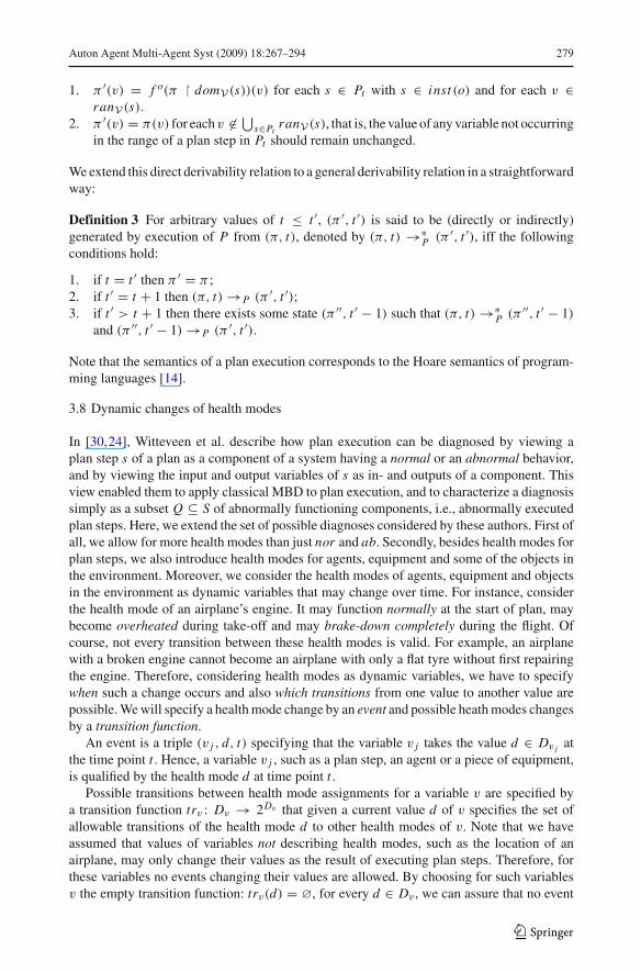
In [30,24], Witteveen et al. describe how plan execution can be diagnosed by viewing aplan step s of a plan as a component of a system having a normal or an abnormal behavior,and by viewing the input and output variables of s as in- and outputs of a component. Thisview enabled them to apply classical MBD to plan execution, and to characterize a diagnosissimply as a subset Q ⊆ S of abnormally functioning components, i.e., abnormally executedplan steps. Here, we extend the set of possible diagnoses considered by these authors. First ofall, we allow for more health modes than just nor and ab. Secondly, besides health modes forplan steps, we also introduce health modes for agents, equipment and some of the objects inthe environment. Moreover, we consider the health modes of agents, equipment and objectsin the environment as dynamic variables that may change over time. For instance, considerthe health mode of an airplane’s engine. It may function normally at the start of plan, maybecome overheated during take-off and may brake-down completely during the flight. Ofcourse, not every transition between these health modes is valid. For example, an airplanewith a broken engine cannot become an airplane with only a flat tyre without first repairingthe engine. Therefore, considering health modes as dynamic variables, we have to specifywhen such a change occurs and also which transitions from one value to another value arepossible. We will specify a health mode change by an event and possible heath modes changesby a transition function.

An event is a triple (v j , d, t) specifying that the variable v j takes the value d ∈ Dv j atthe time point t . Hence, a variable v j , such as a plan step, an agent or a piece of equipment,is qualified by the health mode d at time point t .

Possible transitions between health mode assignments for a variable v are specified bya transition function trv : Dv → 2Dv that given a current value d of v specifies the set ofallowable transitions of the health mode d to other health modes of v. Note that we haveassumed that values of variables not describing health modes, such as the location of anairplane, may only change their values as the result of executing plan steps. Therefore, forthese variables no events changing their values are allowed. By choosing for such variablesv the empty transition function: trv(d) = ∅, for every d ∈ Dv , we can assure that no event

123

280 Auton Agent Multi-Agent Syst (2009) 18:267–294

a1d0 d2d2d1

(v,d2,1) (v,d3,2)a2 d4

t=0 t=1 t=1+ t=2+ t=3

d3

t=2

)( 12 dtrd ∈ )( 23 dtrd ∈v

tr(d0)={d5} tr(d1)={d2,d6} tr(d2)={d3,d6}

d0 d2d1 d3

d4 d6

d5

tr(d5)=∅ tr(d3)=∅

transition function:

d7tr(d4)=∅ tr(d6)={d7} tr(d7)=∅

Fig. 3 A Discrete Event System of the variable v

changes the state of the variable v. Hence, we can simply assume that a transition functiontrv is specified for every variable v.

Remark 4 Note that we might view each variable v j as representing a DES [5]. In this DES,a triple (v j , d, t) describes an unknown event that changes the state of the variable v j , andthe transition function tr j : D j → 2D j describes the transition allowed by DES. Figure 3gives an illustration. The goal of a diagnosis in such systems is to identify these unknownevents (v j , d, t) that have caused the state changes. Also note that plan steps enforce statechanges independently of the transition function tr j .

3.9 Qualifications

In a previous section we have specified the plan derivability relation →∗P that enabled us to

predict a timed state from an earlier timed state not taking into account unforeseen changes inthe values of health modes of variables. Since we have used events to specify such changes, wewill now incorporate the specification of such events in the definition of the plan derivabilityrelation.

First of all, we define a plan qualification, denoted by κ , as a set of events changing thestates of some variables v at specific time points t and thereby causing specific state changesin the plan. Using these qualifications, we (re)define the derivability relation:

Definition 4 Let (π ′′, t) →P (π ′, t + 1) be the direct derivability relation given a plan P ,and let κ be a qualification.

We say that (π ′, t + 1) is (directly) generated by execution of P from (π, t) given thequalification κ , abbreviated by (π, t) →κ;P (π ′, t + 1), iff there exists a state π ′′ such that:

1. for each v j ∈ V: π ′′(v j ) = d if (v j , d, t) ∈ κ , and π ′′(v j ) = π(v j ) otherwise;2. (π ′′, t) →P (π ′, t + 1).

Note that we use an implicit transition from time point t to t + ε with ε approximating 0 inthe definition. During this transition, the variable v j takes the value d .

Again we extend this direct derivability relation to a general derivability relation in astraightforward way to (π, t) →∗

κ;P (π ′, t ′).In the above defined derivability relation given a qualification κ , we did not take into

account whether the state changes specified by κ are unambiguous and are allowed accord-ing to the transition functions trv: Dv → 2Dv . If the state changes are allowed, we say that

123

Auton Agent Multi-Agent Syst (2009) 18:267–294 281

κ induces a sound derivation. Of course, soundness of such a derivation given qualificationκ not only depends on the set of events described by κ but also on the observed state π ofthe world from which the derivation starts and the plan P that is executed.

Definition 5 Let κ be a qualification and let trv: Dv → 2Dv be the transition function of thevariable v. We say that a qualification κ induces a sound derivation (π, t) →∗

κ;P (π ′, t ′) iff:

– (no ambiguity) for no pair of events (v j , d, t1), (v j , d ′, t2) ∈ κ , we have that t1 = t2, and– (allowed transition) for every t ≤ t ′′ < t ′ and for event (v, d, t ′′) ∈ κ ,

if (π, t) →∗κ;P (π ′′, t ′′) →∗

κ;P (π ′, t ′), then d ∈ trv(π′′(v)).

3.10 Default assumptions and plan execution

To predict the effect of executing a plan, we usually start with a partial observation π ofthe state of the world at some time point t . This raises a problem with respect to the healthmodes of plan steps, agents, equipment and possibly some environment variables. Often,these variables v do not belong to the set of observed variables and therefore will be unde-fined in π . Nevertheless, knowledge of the values of these variables is essential for predictingthe specific effects of executing the plan using the derivation relation. Therefore, we assumethat each plan step, agent and equipment variable has a default value specified by a defaultfunction δ. Often the default value will be the value nor . Note that δ maps a variable withouta default value to ⊥. The default values δ(v) can be used to extend a partial observation π toa partial state denoted by δ(π) where default values are assigned to unobserved variables.

Definition 6 Let π be a partial state and let δ: V → ⋃v∈V Dv be a default function speci-

fying the default values of the health mode variables.The partial state extended with default values, denoted by δ(π), is defined as:

∀v ∈ V [δ(π)(v) = δ(v) if π(v) = ⊥; δ(π)(v) = π(v) otherwise].

4 Plan diagnosis

As we stated in the introduction, we will distinguish two forms of plan diagnosis: primarydiagnosis and secondary diagnosis. By making (partial) observations at different time pointsof the ongoing plan execution we may establish that there are discrepancies between theexpected and the observed plan execution. Identifying these discrepancies is called faultdetection. The identified discrepancies indicate that the results of executing one or more plansteps differs from the way they were planned. Identifying these plan steps and, if possible,what went wrong in the plan steps’ execution will be called primary plan diagnosis.

Plan steps may fail because external factors such as changes in the environmental condi-tions (the weather), failing equipment or incorrect beliefs of agents. These external factorsare underlying causes which are important for predicting how the remainder of a plan willbe executed. The secondary plan diagnosis aims at establishing these underlying causes.

We denote an instance of a primary or secondary diagnosis problem by the tuple:

〈P, δ, tr, obs(t), obs(t ′)〉where P = (S,<) is a plan description, δ is a function describing the default values of vari-ables, tr is a set of transition functions trv: Dv → 2Dv for every v ∈ V , and obs(t) = (π, t)and obs(t ′) = (π ′, t ′) are observations of the partial states π and π ′ at time points t and t ′,respectively, where 0 ≤ t < t ′ ≤ depth(P).

123

282 Auton Agent Multi-Agent Syst (2009) 18:267–294

Given such an instance, we would like to identify a suitable qualification κ such that thepredicted state π ′

κ using the derivation (δ(π), t)→∗κ;P (π ′

κ , t ′) corresponds to the observation(π ′, t ′).

We will now discuss suitable qualifications κ to characterize primary and secondarydiagnoses.

4.1 Primary plan diagnosis

In [30,24], we describe how plan execution can be diagnosed by viewing plan steps of aplan as components of a system and by viewing the input and output variables of a planstep as in- and outputs of a component. In this approach, a qualification Q ⊂ S is a subsetof plan steps s qualified as abnormal. Here, such a set Q can be represented by a quali-fication κQ = {(s, ab, depth(s)) | s ∈ Q}. A qualification consisting of a set of events(s, d, depth(s)) with s ∈ S will be called a plan step qualification. To illustrate such a planstep qualification, consider Fig. 2. Suppose plan step s3 is abnormal and generates a resultthat is unpredictable (⊥). Given the qualification κ = {(s3, ab, 1)} and the partially observedstate π0 at time point t = 0, we predict the partial states πi as indicated in Fig. 2, where(π0, t0) →∗

κ;P (πi , ti ) for i = 1, 2, 3. Note that in the example we assume that all inputs of aplan step must have known values in order to have predictable outputs. This implies that theresults of plan steps s6 and s8 cannot be predicted because the values of v1 and of v5 cannotbe predicted at time t = 2. Therefore, π3 contains only the value of v3.

Now consider a plan-diagnosis instance 〈P, δ, tr, obs(t), obs(t ′)〉. In order to obtain a suit-able primary diagnosis, we would like to use the observations obs(t) = (π, t) and obs(t ′) =(π ′, t ′) to infer the health modes of the plan steps occurring in P = (S,<). Assuming anormal execution of P using the function δ to specify default values for variables, we can (par-tially) predict the state of the world at a time point t ′ given the observation obs(t): if all plansteps behave normally, we predict a partial state π ′

∅at time t ′ such that (δ(π), t)→∗

P (π ′∅

, t ′).Therefore, if this assumption holds, the values of the variables that occur in both the predictedstate and the observed state at time t ′ should match, i.e., there should exist a complete stateσ , such that π ′ � σ and π ′

∅� σ . But that implies that π ′ ≈ π ′

∅. If, however, this is not the

case, the execution of some plan steps s must have gone wrong and we have to determine aplan step qualification κ such that the predicted state derived using κ agrees with π ′. Thisis nothing else than a straight-forward extension of the diagnosis concept in MBD to plandiagnosis (cf. [23,7]):

Definition 7 Let 〈P, δ, tr, obs(t), obs(t ′)〉 be a diagnostic instance. Moreover, let the planstep qualification κ be a set of triples (s, d, depth(s)) with s ∈ S and d ∈ Ds , and let κ

induce a sound derivation (δ(π), t)→∗κ;P (π ′

κ , t ′) given the plan P and a transition function

trs: Ds → 2Ds for each plan step s ∈ S.Then κ is said to be a primary plan diagnosis (plan step diagnosis) of a plan-diagnosis

instance 〈P, δ, tr, obs(t), obs(t ′)〉 iff π ′ ≈ π ′κ .

So in a primary plan diagnosis κ , the observed partial state π ′ at time t ′ and the predictedstate π ′

κ at time t ′ assuming the plan step qualification κ agrees upon the values of all variablesV (π ′) ∩ V (π ′

κ ) occurring in both states.

Example 1 Consider again Fig. 2 and suppose that we did not know that plan step s3 wasabnormal and that we observed obs(0) = ((d1, d2, d3, d4), 0) and obs(3) = ((d ′

1, d ′3, d ′

5), 3).Using the normal plan derivation relation starting with obs(0) we will predict a state π ′

∅at

time t = 3 where π ′∅

= (d ′′1 , d ′′

2 , d ′′3 ). If everything is ok, the values of the variables predicted

123

Auton Agent Multi-Agent Syst (2009) 18:267–294 283

as well as observed at time t = 3 should correspond, i.e., we should have d ′j = d ′′

j for j = 1, 3.If, for example, only d ′

1 would differ from d ′′1 , then we could qualify s6 as abnormal, since

then the predicted state at time t = 3 using κ = {(s6, ab, 2)} would be π ′κ = (d ′′

3 ) and thispartial state agrees with the observed state on the value of v3.

Note that for all variables in V (π ′)∩V (π ′κ ), the qualification κ provides an explanation for

the observation π ′ made at time point t ′. Hence, for these variables the qualification providesan abductive diagnosis [6]. For all observed variables in V (π ′) − V (π ′

κ ), no value can bepredicted given the qualification κ . Hence, by declaring them to be unpredictable, possibleconflicts with respect to these variables if a normal execution of all plan steps is assumed,are resolved. This corresponds with the idea of a consistency-based diagnosis [23].

4.2 Secondary plan diagnosis

Plan steps may fail because of unforeseen (environmental) conditions such as being struck bylightning, malfunctioning equipment or incorrect beliefs of agents. Secondary plan diagno-sis aims at identifying the underlying causes of plan step failures. Therefore, secondary plandiagnosis only considers qualifications that change the values of variables not representingplan steps, i.e., the set of variables in V − S.

A secondary qualification κ then is a qualification consisting of triples (v, d, t), wherev ∈ V − S. Note that there may be more than one time point between the execution of theplan step s where the value of the variable v must have been changed by an event and thelatest plan step s′ < s where v was actually used by s′, that is v ∈ ranV (s′) ∩ domV (s′).Since there is no way to determine at which time point between dept (s′) + 1 and depth(s)the event (v, d, t) occurred, we usually choose for t the depth depth(s) of the first plan step swhere the change manifests itself.

Definition 8 Let 〈P, δ, tr, obs(t), obs(t ′)〉 be a diagnostic instance. Moreover, let the planstep qualification κ be a set of triples (v, d, t) with v ∈ V − S and d ∈ Dv , and let κ

induce a sound derivation (δ(π), t)→∗κ;P (π ′

κ , t ′) given the plan P and a transition function

tr j: D j → 2D j for each variable v j ∈ V .Then the qualification κ is said to be a secondary plan diagnosis of a plan-diagnosis

instance 〈P, δ, tr, obs(t), obs(t ′)〉 iff π ′ ≈ π ′κ .

The secondary diagnosis can be divided into agent, equipment and environment diag-nosis depending on whether the variable v in a triple (v, d, t) ∈ κ belongs to A, E or N ,respectively. Note that agent diagnosis is related to social diagnosis described by Kalechand Kaminka [16,17] if the agents’ health modes are used to describe the agents’ incorrectbeliefs.

4.3 Predicting the future

Secondary diagnosis offers an important advantage over primary diagnosis. First of all, sec-ondary diagnosis enables us to determine which future plan steps may also be affected by themalfunctioning agents and equipment, and by unforeseen state changes in the environment.If a piece of equipment breaks down, then all plan steps that require this piece of equipmentwill fail. The state change described by a failure event (v, d, t) ∈ κ persists: π(v) = d at alltime points t ′ ≥ t until another event or a plan step changes v again.

Definition 9 Let 〈P, δ, tr, obs(t), obs(t ′)〉 be a diagnostic instance and let κ be a currentsecondary diagnosis of the plan executed so far. Moreover, let t ′ be the current time point.

123

284 Auton Agent Multi-Agent Syst (2009) 18:267–294

Then the set of future plan steps that will directly be affected given the current diagnosisκ is:

{s ∈ S | v ∈ domV (s), (v, d, t ′′) ∈ κ, d �= nor, t ≤ t ′′ < t ′ ≤ depth(s)}Second, besides identifying the plan steps that will be affected, we can also determine the

goals that can still be reached.

Definition 10 Let 〈P, δ, tr, obs(t), obs(t ′)〉 be a diagnostic instance with obs(t ′) = (π ′, t ′),and let κ be a current secondary diagnosis of the plan executed so far. Moreover, let t ′ be thecurrent time point and let (δ(π)′, t ′) →κ;P (π ′′, depth(P)).

Then the set of goals that can still be realized is given by:

{g ∈ G | π ′′ |= g}4.4 Responsible agents

Besides knowing the underlying cause of plan execution failures, it is also important to knowthe agents responsible for the failures. To illustrate this, reconsidering the example in theintroduction where the agent responsible for the failing luggage sorting action may be themaintenance agent or the airport authorities that reduced the maintenance budget.

We might introduce a responsibility function res mapping a failed plan step, a misbe-having agent and malfunctioning equipment to a responsible agent. Such a function cannothandle more sophisticated forms of responsibility. For instance, a pilot being responsible fora rough landing and the maintenance personnel being responsible for a tire blow-out duringlanding. In both cases the landing plan step is executed in an abnormal way but the respon-sible agent depends on type of abnormal execution. Therefore, we propose a mapping basedon a variable and its health mode.

Definition 11 Let κ be any diagnosis of a plan execution and let

res: V ×⋃

v∈VDv → A

be function assigning responsibility to agents in A.Then for each event (v, d, t) ∈ κ , the responsible agent is determined by: res(v, d).

This failure dependent responsibility may not suffice in all cases. Similar to primary andsecondary diagnosis, we may introduce different levels of responsibility. An air traffic con-troller making an error can be primary responsible for the error. His or her supervisor may besecondary responsible for the error. The airport may be responsible at the third level while theaviation authorities may be responsible at the fourth level. Here, we leave such sophisticatedmodels of responsibility for future research.

5 An example

This section will illustrate the diagnostic model presented in the previous section using a planfor transporting luggage of a passenger form one airport to another. We add to this plan theobservation that luggage is dropped-off at the check-in and the observation at the destinationindicating whether the luggage has arrived. Sometimes there is a discrepancy between ourexpectation about our luggage and that what we observe at the destination. We will use sucha discrepancy to illustrate the diagnostic model presented in this paper.

123

Auton Agent Multi-Agent Syst (2009) 18:267–294 285

5.1 The plan

Figure 4 depicts such a plan at an abstract level. Note that only the states of the variables‘luggage’ and ‘label’ are changed by the plan steps. The state of the other variables are notchanged by the plan steps, they are only used as inputs. Based on the graphical representationof a plan introduced in the previous section, all the variables in the columns to the right of thevariables ‘luggage’ and ‘label’ should actually be placed alongside the variables ‘luggage’and ‘label’. The variables of which the states are not changed by the execution plan steps areplaced near the plan steps that use them as inputs because of the limited width of the page.Note that we have ordered the variables to the right of the variables ‘luggage’ and ‘label’

label luggage

transport to sorting

sort luggage

transport to aircraft

load aircraft

flight

unload aircraft

transport to arrival belt

check-in agent

t=0

my luggage

t=1

t=6

t=5

t=4

t=3

t=2

t=8

t=7

belt

sorter

personnel1 vehicle1

personnel2 lift1

pilot aircraft

personnel3 lift2

personnel4 vehicle2

weather

label

label luggage

transport to sorting

sort luggage

transport to aircraft

load aircraft

flight

unload aircraft

transport to arrival belt

check-in agent

t=0

my luggage

t=1

t=6

t=5

t=4

t=3

t=2

t=8

t=7

belt

sorter

personnel1 vehicle1

personnel2 lift1

pilot aircraft

personnel3 lift2

personnel4 vehicle2

weather

label

Fig. 4 A plan for transporting a passenger’s luggages

123

286 Auton Agent Multi-Agent Syst (2009) 18:267–294

in columns: first a column with agents, then a column with equipment and finally a columnwith other environment variables.

The plan in Fig. 4 only shows the transport of one piece of luggage. An airport handlesof course many pieces of luggage, some for the same flight and some for other flights. Foreach piece of luggage there is a similar plan which may require the same plan steps, the sameagents and the same equipment during its execution. Together these individual plans formthe total plan of luggage handling on an airport.

5.2 Primary diagnosis

Suppose that at our destination we observe the absence of our luggage. Using the plan depictedin Fig. 4, we may determine as our primary diagnosis that one of the eight plan steps musthave been executed abnormally:

κ1 = {(‘label luggage’, ab, 0)},κ2 = {(‘transport to sorting’, ab, 1)},κ3 = {(‘sort luggage’, ab, 2)},κ4 = {(‘transport to aicraft’, ab, 3)},κ5 = {(‘load airplane’, ab, 4)},κ6 = {(‘flight’, ab, 5)},κ7 = {(‘unload aircraft’, ab, 6)},κ8 = {(‘transport to arrival belt’, ab, 7)}

Note that these are all single fault diagnoses; i.e., each diagnosis consist of a single failureevent. Intuitively, we prefer these diagnoses over diagnoses with multiple faults. In the nextsection, we will formalize the intuition.

Having observed the absence of our luggage, we may go to the help desk where, using acommunication network, the service person finds out that your luggage has arrived in Amman(AMM) instead of Amsterdam (AMS). Based on fault models of the different plan steps, wemay determine better primary diagnoses. For instance, the plan step ‘sort luggage’ may haverouted the luggage to the wrong loading platform.

κ = {(‘sort luggage’, ‘routing error: AMS → AMM’, 2)}

Usually finding back someone’s lost luggage will take several hours. Even before informa-tion about the luggage’s location come available, we can already determine a more specific setof primary diagnoses. The transport plan of our luggage is a sub-plan of a much larger plan.In this larger plan, other passengers have also transported their luggage using the same flight.If the luggage of some of these passengers have correctly arrived in Amsterdam, we knowthat the plan step ‘flight’ is executed normally. (Of course, we already knew this because wearrived ourselves at the destination.) Moreover, if the plan steps ‘transport to airplane’, ‘loadairplane’ ‘unload aircraft’ and ‘transport to arrival belt’ are the same plan steps for all theluggage on a flight, then these plan steps have not failed either. Therefore, using the largerplan also enables us to determine a more specific set of primary diagnoses:

κ1 = {(‘labeling luggage’, ab, 0)},κ2 = {(‘transport to sorting’, ab, 1)},κ3 = {(‘sort luggage’, ab, 2)}

123

Auton Agent Multi-Agent Syst (2009) 18:267–294 287

5.3 Secondary diagnosis

Beside identifying the plan steps that may have failed, we may also consider malfunctioningequipment that may have caused the plan steps to fail. For instance, a malfunctioning sensoron the ‘sorter’ may be responsible for routing some of the luggage to the wrong platform.The equipment diagnosis

κ = {(‘sorter’, ‘sensor error: S → M’, 2)}

explains why some pieces of luggage ended up in Amman (AMM) instead of Amsterdam(AMS). It also explain why some pieces of luggage ended up in Laiagam (LGM) instead ofMalargue (LGS). Moreover it enables us to predict that some pieces of luggage will endedup in Hvammstangi (HVM) instead of Municipal (HVS) .

Misbehaving agents may also result in a plan execution failure. The check-in agent maymake errors with the label of the luggage and the personnel transporting the luggage to theairplane may forget a pieces of luggage. Agent diagnosis can be used to identify failingagents.

κ1 = {(‘check-in agent’, ab, 0)},κ2 = {(‘personnel1’, ab, 3)}

A damaged label may also explain why our luggage ended up in Amman instead ofAmsterdam. Environment diagnosis can be used to identify this explanation for our lostluggage.

κ = {(‘label’, ‘damaged’, 2)}

A change in the environment object ‘weather’ may also explain why our luggage did notreach its destination. Unforseen bad weather conditions may force an airplane to deviate toanother airport. This is, however, an adaptation of the plan instead of an incorrect executionof the plan. The plan diagnosis approach described in the paper cannot be used to identifychanges in the plan. It must know the plan that is actually executed. Therefore, this type ofcause cannot be handled by the diagnosis of plan execution we describe here.

5.4 Responsible agents

Usually the agent(s) executing a plan step are responsible for the proper execution of the planstep. Therefore, for every failing plan step, we may assign the responsibility to the executingagents mentioned in Fig. 4. In much the same way we may assign responsibility for failingequipment to either the agent operating it or the agent maintaining it, depending on the typeof fault that occurred. For instance, we can specify that ‘personnel1’ is responsible for a‘crash’ with ‘vehicle1’ while ‘maintenance personnel’ is responsible for an ‘engine failure’of ‘vehicle1’.

In our application domain we are often more interested in who is financially responsi-ble. This gives us a differen type of responsibility assignment. Airlines are responsible forplan executions of their airplanes, ground handling companies are responsible loading theairplanes, air traffic control is responsible for runways, taxi-ways, gate availabilities, and soon and so forth. These types of responsibilities can also be modeled using the responsibilityfunction res.

123

288 Auton Agent Multi-Agent Syst (2009) 18:267–294

6 Preference criteria on diagnoses

As we saw in the example presented in the previous section, both primary and secondarydiagnosis need not provide a unique explanation of observed anomalies. When more thanone diagnosis can be determined, the diagnoses need not all provide the same quality ofexplanation. Intuitively, a primary diagnosis in which one plan step is failing gives a betterexplanation than a primary diagnosis in which all plan steps are failing. This intuition has infact been used in the previous section. In this section we formalize this intuition by definingpreference criteria on diagnoses. Moreover, we analyze time complexity of identifying thepreferred diagnoses.

6.1 The preference criteria

The most common preference criteria on diagnoses are (i) based on the subset relation withrespect to the sets of health mode variables indicating failures (i.e., variables v ∈ S ∪ A ∪ Efor which there are events (v, d, t) ∈ κ such that d �= δ(v)), and (ii) the number of thesehealth mode variables. The intuition behind the first preference criterium is that if failuresoccur independent of each other, and if the probabilities that a failure occurs is less than 0.5,a diagnosis that has a subset of the failures of another diagnosis has a higher probabilityof being correct. A diagnosis in which a subset minimal failures occurs is called minimaldiagnosis:

Definition 12 Let 〈P, δ, tr, obs(t), obs(t ′)〉 be a diagnostic instance.A diagnosis κ is a minimal diagnosis iff for no diagnosis κ ′:

{v ∈ S ∪ A ∪ E | (v, d, t) ∈ κ ′, d �= δ(v)} ⊂ {v ∈ S ∪ A ∪ E | (v, d, t) ∈ κ, d �= δ(v)}The intuition behind the second preference criterium is based on a stronger requirement,

namely that the failure probabilities are very small and that they are more or less of the samemagnitude. In that case, the most probable diagnoses are those having a numerical minimumnumber of failures.

Definition 13 Let 〈P, δ, tr, obs(t), obs(t ′)〉 be a diagnostic instance.A diagnosis κ is a minimum diagnosis iff for no diagnosis κ ′:

|{v ∈ S ∪ A ∪ E | (v, d, t) ∈ κ ′, d �= δ(v)}| < |{v ∈ S ∪ A ∪ E | (v, d, t) ∈ κ, d �= δ(v)}|A third preference criterium on diagnoses is based on the explanative power for diagnoses

[25]. Given an instance of a plan-diagnostic problem 〈P, δ, tr, obs(t), obs(t ′)〉, a diagnosisκ may explain more observations at time point t ′ than a diagnosis κ ′. If the probability thatthe observed value of a variable is correctly predicted given a diagnosis is very small, thenthe diagnosis κ has a higher probability of being correct than the diagnosis κ ′. We say insuch cases that the diagnosis κ is more informative than the diagnosis κ ′ [25]. Given thisinformation order on diagnosis, we can define the maximal-informative diagnoses, whichalso turn out to be maximum-informative diagnosis.

Definition 14 Let 〈P, δ, tr, obs(t), obs(t ′)〉 be a diagnostic instance, and let π ′κ be defined

as: (δ(π), t)→∗κ;P (π ′

κ , t ′).A diagnosis κ is said to be a maximum-informative diagnosis iff for no diagnosis κ ′:

V (π ′κ ) ⊂ V (π ′

κ ′)

Since a maximum-informative diagnosis need not be a minimal diagnosis, the two pref-erence criteria can be combined resulting in minimal maximum-informative (mini-maxi)diagnoses.

123

Auton Agent Multi-Agent Syst (2009) 18:267–294 289

6.2 Complexity issues

In [25] Roos and Witteveen have shown that identifying a minimum diagnosis is an NP-hardproblem while identifying a minimal maximum-informative (mini-maxi) diagnosis can bedone in polynomial time. Identifying a minimum maximum-informative diagnosis, however,is again an NP-hard problem. In this section, we briefly consider some complexity issueswith respect to finding diagnoses in our framework, relating them to the results obtained in[25].

6.2.1 Finding minimum diagnoses

Identifying a minimum diagnosis is also an NP-hard problem for the plan diagnosis modelpresented in this paper: By only considering primary diagnoses and by restricting the healthmodes in a primary diagnosis to nor and ab, the diagnostic problem becomes identical tothe diagnostic problem addressed in [25].

Proposition 1 Finding minimum primary diagnoses is NP-hard.

Proof We transform an instance 〈P, obs(t), obs(t ′)〉 of a diagnostic problem as describedin [25] to a diagnostic instance 〈P, δ, tr, obs(t), obs(t ′)〉 described in this paper. Note thata (minimum) solution to the former diagnostic problem is (minimum) set of plan steps Qqualified as being abnormal.

Given the instance 〈P, obs(t), obs(t ′)〉 with a set of plan steps S and a set of variables V:

– Extend V with the variables {vs | s ∈ S}.– Replace every function f nor

s (v1, . . . , vn) with s ∈ inst (o) by the function f o(vs :S; v1, . . . , vn : N ) where f o(nor : S; d1, . . . , dn : N ) = f nor

s (d1, . . . , dn) and f o(ab :S; d1, . . . , dn : N ) = f ab

s (d1, . . . , dn) = (⊥, . . . ,⊥).– Let δ be specified as follows: δ(vs) = nor for each s ∈ S, and δ(v) = ⊥ otherwise.– tr = {trvs : s ∈ S}, where trvs (nor) = {ab} and trvs (ab) = ∅.

Let 〈P, δ, tr, obs(t), obs(t ′)〉 be the resulting diagnostic instance in our current framework.It is easy to see that a minimum primary diagnosis κ obtained for this instance corresponds toa minimum diagnosis Q = {s | (vs, ab, depth(vs)) ∈ κ} in the framework of [25]. Hence,we can obtain a minimum plan diagnosis Q by reducing the original diagnostic problem tothe primary diagnostic problem described in this paper. Therefore finding primary diagnosesin our current framework is NP-hard, too. ��

6.2.2 Finding mini-maxi diagnoses

A mini-maxi diagnosis can be determined in polynomial time for both primary and secondarydiagnosis. We will show this by simply adapting the polynomial algorithm given in [25]. Let(δ(π), t)→∗

∅;P (π ′∅

, t ′) be a prediction of the state at time point t ′ assuming the absenceof failures (i.e.: κ = ∅) and let π ′ be the observed state at time point t ′. To determine amaximum-informative diagnosis, we first determine the disagreement set V di f of all thosevariables whose values are defined in both the observed state π ′ and the predicted state π ′

∅

at time t ′ but differ:

V di f = {v ∈ V | π ′∅

(v) �= π ′(v), π ′∅

(v) > ⊥, π ′(v) > ⊥}.Next, for i = 1, we collect all plan step variables s ∈ S such that s ∈ Pt ′−i and ranV (s) ∩V di f �= ∅. Subsequently, we add the qualification (s, ab, t ′ − i) to κmax and remove all

123

290 Auton Agent Multi-Agent Syst (2009) 18:267–294

variables ranV (s) form the disagreement set V di f for all the collected plan steps s. Fori = 2, 3, . . . , we iteratively select new plan step variables s ∈ S at times t ′ − i repeating thesame procedure. It can easily be proven that this qualification κmax is a maximum-informativediagnosis.

In order to obtain a mini-maxi diagnosis instead of just a maximum-informative diag-nosis, we have to refine this procedure slightly using the notion of a scope of a variable v

at time point t . The function scope(v, t) returns the smallest set of variables that becomeundefined at time point t ′ if κ = {(v, ab, t ′′)}. If a heath mode variable is set to the valueab by an event at time point t ′′, then every variable in the range of a plan step s ∈ P≥t ′′with v ∈ domV (s) may become undefined. Moreover if a variable in the range of a plan steps ∈ Pt∗ becomes undefined, then so may the variables in the range of the plan steps s′ ∈ P>t∗with ranV (s) ∩ domV (s′) �= ∅.

We can use the function scope(v, t) to remove events from κmax till it becomes a minimaldiagnosis. The resulting diagnosis is mini-maxi diagnosis. Since the whole procedure can beexecuted in polynomial time, a mini-maxi diagnosis can be identified in polynomial time.

Example To illustrate the identification of a mini-maxi diagnosis, we use the scenariodescribed in Sect. 5, in which we observe at t = 8 that our luggage did not reach itsdestination; i.e., V di f = {‘myluggage’}. There is a plan step determining the value ofthe variable ‘my luggage’ at t = 7, namely ‘transport to arrival belt’. Hence, we add(‘transport to arrival belt’, ab, 7) to κmax . Since V di f contains only one variable,

κmax = {(‘transport to arrival belt’, ab, 7)}is a maximum-informative diagnosis. Note that κmax is also a primary diagnosis.

The maximum-informative diagnosis κmax is also mini-maxi diagnoses because no eventcan be removed from κmax without guaranteeing that all variables is V di f are covered. Nowsuppose that we also have to qualify the plan step ‘unload aircraft’ as abnormal; i.e.

κ ′ = {(‘unload luggage’, ab, 6), (‘transport to arrival elt’, ab, 7)}because of some variable v also belonging to V di f . If every variable has an unpredictableeffect whenever one of its inputs is undefined, then κ ′ is maximum-informative diagnosesbut not mini-maxi diagnoses. Instead,

κ ′′ = {(‘unload luggage’, ab, 6)}is a mini-maxi diagnosis since we can eliminate (‘transport to arrival belt’, ab, 7) form κ ′using the function scope(v, t).

The above described procedure gives us one mini-maxi diagnosis for the example ofSect. 5. We can use the function scope(v, t) to identify other mini-maxi diagnosis. Anydiagnosis κ such that

⋃(v,ab,t)∈κ scope(v, t) = ⋃

(v,ab,t)∈κmaxscope(v, t) is also mini-maxi

diagnosis. For instance, the diagnoses:

κ1 = {(‘personel4’, ab, 7)},κ2 = {(‘vehicle2’, ab, 7)},κ3 = {(‘unload luggage’, ab, 6)},κ4 = {(‘personel3’, ab, 6)},κ5 = {(‘lift2’, ab, 2)},and so on, and so forth.

123

Auton Agent Multi-Agent Syst (2009) 18:267–294 291

Note that the diagnoses κ1, κ2, κ4 and κ5, are secondary diagnoses because the variablesmentioned in the diagnoses either belong to A or to E . Also note that the transition func-tion trv(·) always allows a transition to ab for a plan step variable. For other variables suchas ‘personnel4’, we have to verify whether this transition is allowed given the value of thevariable just before the event (‘personel4’, ab, 7).

6.2.3 Dealing with additional health modes

Identifying a diagnosis in which health modes other than nor and ab are used is an NP-hardproblem, even for mini-maxi diagnoses. This does not come as a surprise since identifyingthese diagnoses is a form of abduction, which is a well-known NP-hard problem. We willshow that identifying an arbitrary diagnosis in which health mode variables are qualified withhealth modes other than ab is an NP-hard problem.

Proposition 2 Identifying an arbitrary primary diagnosis is NP-hard.

Proof To prove that a primary diagnosis is NP-hard, we reduce the NP-hard integer par-tition problem (Given a set I of integers and an integer r , find a subset of I whose sumequals r ) to a primary diagnosis problem as follows:

Given an instance (I, r) of integer partition, construct an instance of a primarydiagnosis problem as follows:

– Introduce a plan step variable si and a plan operator oi for every integer i ∈ I .– Introduce a new environment variable v.– For each integer i ∈ I introduce a function f oi , defined as: f oi (nor, d) = (d + i) and

f oi (failure, d) = (d). The plan step si binds the parameters of f oi : domV (si ) = (si , v)

and ranV (si ) = (v).– Let trs j (nor) = {failure, ab}, trs j (failure) = {ab} and trs j (ab) = ∅.– Let P = (S,<) be the plan, where si < s j iff i < j .– Let obs(0) = (π, 0) be an observation such that for every plan step s ∈ S: π(s) = nor

and for the variable v ∈ N : π(v) = 0.– Let the obs(|I |) = (π ′, |I |) be an observation such that π ′(v) = r .

It is not difficult to show that there exists a diagnosis κ such that πκ ≈ π ′ iff the integerpartition problem instance has a solution, i.e., a subset of integers that add up to r . Hence,finding a primary diagnosis is NP-hard. ��Proposition 3 Identifying an arbitrary secondary diagnosis is NP-hard.

Proof To prove that finding a secondary diagnosis is NP-hard, we reduce the 3-SAT prob-lem to the secondary plan diagnosis problem. Consider a 3-SAT instance with variablesU = {u1, . . . , un} and clauses C = {c1, . . . , cm}. Let Lit (ui ) = {ui ,¬ui }.– For every clause c ∈ C , introduce a plan step variable sc, a plan operator oc ∈ O such

that sc ∈ inst (oc), and an environment variable nc. Moreover, let Dnc = {true, f alse}be the domain of nc.

– For every u ∈ U , introduce a variable vu belonging to X . Here, X is either A, E or N .Moreover, let Dvu = {true, f alse} be the domain of vu .

– For each clause c = (xi1 , xi2 , xi3) ∈ C , where xi j ∈ Lit (ui j ) for j = 1, 2, 3, the functionf oc is defined as follows: f oc (nor, d1, d2, d3) = (true) iff a truth assignment I such thatI (ui j ) = d j , for j = 1, 2, 3, satisfies c. The plan step sc binds the parameters of f oc :domV (sc) = (sc, vu1 , vu2 , vu3) and ranV (sc) = (nc).

123

292 Auton Agent Multi-Agent Syst (2009) 18:267–294

– Let trsc (nor) = {ab} and let trsc (ab) = ∅.– Let trnc ( f alse) = trnc (true) = ∅.– Let trvu ( f alse) = {true} and let trvu (true) = ∅.– Let P = (S, ∅) be the plan.– Let the obs(0) = (π, t) be an observation such that for every plan steps s ∈ S: π(s) = nor

and for every variable v ∈ X : π(v) = f alse.– Let the obs(t) = (π ′, 1) be an observation such that for every variable nc: π ′(nc) = true.

It is not difficult to show that there exists a secondary diagnosis κ such that πκ ≈ π ′ iffthe 3-SAT instance is satisfiable. Hence, agent, equipment and environment diagnosis areNP-hard. ��

The above complexity results are of course disappointing. A mini-maxi diagnoses withonly fault modes nor and ab can still be determined in polynomial time. However, identifyingother fault modes than ab is NP-hard even for mini-maxi diagnoses.

In practice things are usually not that bad. First note that for any diagnosis κ there alwaysexists a diagnosis κ∗ = {(v, ab, t) | (v, d, t) ∈ κ, ab ∈ Dv}. We assume for the moment thatagents also have health modes nor and ab. Since a mini-maxi diagnosis is a likely diagnosis,we may expect that κ∗ is a mini-maxi diagnosis. We rather efficiently search for κ given κ∗if κ∗ contains an event (v, ab, t) and there is a variable v′′ ∈ scope(v, t)∩ V di f such that forno other event (v′, ab, t ′) ∈ κ∗, v′′ ∈ scope(v′, t ′). If this condition holds, we can test for allhealth modes d ∈ Dv whether substituting (v, d, t) for (v, ab, t) inκ∗ enables us to predict theobserved values of the variables (scope(v, t)−⋃

(v′,ab,t ′)∈κ∗,v �=v′ scope(v′, ab, t ′))∩ V di f .

If we can predict the values of these variables, then κ∗[(v,d,t)/(v,ab,t)] is a diagnosis and wecan continue searching for refinements of κ∗[(v,d,t)/(v,ab,t)]. So, we can repeat this procedureusing the diagnosis κ∗ in which (v, ab, t) is replaced by (v, d, t) using the disagreement setV di f from which we have removed the variables scope(v, t) − ⋃

(v′,ab,t ′)∈κ∗,v �=v′scope(v′, ab, t ′).

7 Conclusion

This paper describes a generalization of the model for plan diagnosis as presented in [30,24].New in the current approach is (i) the introduction of the concepts of a primary and secondarydiagnosis, (ii) the introduction of variables representing plan steps, agents and equipment,and (iii) the use of discrete event systems to describe the unknown dynamic behavior ofvariables such as equipment over time.

The primary diagnosis identifies failed plan steps and possibly in which way they failed,while the secondary diagnosis addresses the causes for plan step failures by identifying mis-behaving agents and malfunctioning equipment. The latter is an improvement over the plandiagnosis presented in [30,24], where only dependencies between plan step failures could bedescribed using causal rules. An additional feature of the proposed approach is the assign-ment of responsibilities for failures to specific agents. This responsibility assignment makesit possible, for instance, to divide cost of plan repair or to choose between plan repairs basedon the impact on the agents involved.

Based on the results reported in [26], we have shown that finding minimum diagnoses is ingeneral NP-hard. A minimal maximum-informative (mini-maxi) diagnosis can, however, stillbe determined in polynomial time. Unfortunately, however, identifying a mini-maxi diagno-sis containing health modes other than nor and ab is again NP-hard. Finally, we pointed out

123

Auton Agent Multi-Agent Syst (2009) 18:267–294 293

conditions under which we may still identify a mini-maxi diagnosis containing health modesother than nor and ab efficiently.

Some of limitations of our model for plan diagnosis concern

– the identification of differences between the original plan and the executed plan; Weassume that the plan is executed as specified. This assumption enables the identificationof incorrect plan step executions, malfunctioning agents, broken equipment and unfore-seen environment changes using partial observations of world at different time points.

– the identification of temporal constraint violations; To keep the discussion simple, inour model we assume that each plan step requires a unit time. The model also applieswhen plan steps have different durations. However, violations temporal constraints onthe execution of a plan cannot be diagnosed using the current model.

– the modeling of plan steps as atomic entities. Often is suffices to model plan steps asatoms. However, it may sometimes be better to model an plan step as a process [20].

In future work we intend to extend our model cope with some of these limitations. First, weintend to incorporate diagnosis of plan structure violations into the model. Such plan struc-ture violations are e.g., skipping a plan step, duplicating a plan step or swapping the orderof two plan steps in the plan execution. Second, we wish to extend the model with diagnosisof temporal constraint violations. Here, we would like to refine our current plan descriptionalso with information about the time in which a certain plan step has to be executed.

Acknowledgements We thank the reviewers for their comments, which helped us to improve the paper. Thisresearch is supported by the Technology Foundation STW, applied science division of NWO and the technol-ogy programme of the Ministry of Economic Affairs (the Netherlands). Project DIT5780: Distributed ModelBased Diagnosis and Repair.

Open Access This article is distributed under the terms of the Creative Commons Attribution NoncommercialLicense which permits any noncommercial use, distribution, and reproduction in any medium, provided theoriginal author(s) and source are credited.

References

1. Baroni, P., Lamperti, G., Pogliano, P., & Zanella, M. (1999). Diagnosis of large active systems. ArtificialIntelligence, 110, 135–183.

2. Birnbaum, L., Collins, G., Freed, M., & Krulwich, B. (1990). Model-based diagnosis of planning failures.In AAAI 90, pp. 318–323.

3. Blum, A. L., & Furst, M. L. (1997). Fast planning through planning graph analysis. Artificial Intelligence,90, 281–300.

4. Carver, N., & Lesser, V. R. (2003). Domain monotonicity and the performance of local solutions strate-gies for cdps-based distributed sensor interpretation and distributed diagnosis. Autonomous Agents andMulti-Agent Systems, 6(1), 35–76.

5. Cassandras, C. G., & Lafortune, S. (1999). Introduction to discrete event systems. Kluwer AcademicPublishers.

6. Console, L., & Torasso, P. (1990). Hypothetical reasoning in causal models. International Journal ofIntelligence Systems, 5, 83–124.

7. Console, L., & Torasso, P. (1991). A spectrum of logical definitions of model-based diagnosis. Compu-tational Intelligence, 7, 133–141.

8. de Jonge, F., & Roos, N. (2004). Plan-execution health repair in a multi-agent system. In PlanSIG 2004.9. de Jonge, F., Roos, N., & van den Herik, H. J. (2005). Keeping plan execution healthy. In Multi-Agent

Systems and Applications IV: CEEMAS 2005, LNCS 3690, pp. 377–387.10. de Kleer, J., Mackworth, A. K., & Reiter, R. (1992). Characterizing diagnoses and systems. Artificial

Intelligence, 56, 197–222.11. de Kleer, J., & Williams, B. C. (1987). Diagnosing multiple faults. Artificial Intelligence, 32, 97–130.

123

294 Auton Agent Multi-Agent Syst (2009) 18:267–294

12. McDermott, D., et al. (1998). The pddl planning domain definition language. In The AIPS-98 PlanningCompetition Committee.

13. Fikes, R. E., & Nilsson, N. (1971). Strips: A new approach to the application of theorem proving toproblem solving. Artificial Intelligence, 5, 189–208.

14. Hoare, C. A. R. (1969). An axiomatic basis for computer programming. Communications of the ACM,12(10), 576–585.

15. Horling, B., Benyo, B., & Lesser, V. (2001). Using self-diagnosis to adapt organizational structures. InProceedings of the 5th International Conference on Autonomous Agents (pp. 529–536). ACM Press.

16. Kalech, M., & Kaminka, G. A. (2003). On the design of social diagnosis algorithms for multi-agent teams.In IJCAI-03, pp. 370–375.

17. Kalech, M., & Kaminka, G. A. (2005). Diagnosing a team of agents: Scaling-up. In AAMAS 2005,pp. 249–255.

18. Kalech, M., & Kaminka, G. A. (2007). On the design of coordination diagnosis algorithms for theams ofsituated agents. Artificial Intelligence, 171, 491–513.

19. Micalizio, R., & Torasso, P. (2007). On-line monitoring of plan execution: A distributed approach. Knowl-edge-Based Systems, 20, 134–142.

20. Micalizio, R., & Torasso, P. (2007). Team cooperation for plan recovery in multi-agent systems. In Mul-tiagent System Technologies, LNCS 4687, pp. 170–181.

21. Pencolé, Y., & Cordier, M. (2005). A formal framework for the decentralised diagnosis of large scalediscrete event systems and its application to telecommunication networks. Artificial Intelligence, 164,121–170.

22. Poole, D. (1988). Representing knowledge for logic-based diagnosis. In International Conference onFifth Generation Computer Systems, pp. 1282–1290.

23. Reiter, R. (1987). A theory of diagnosis from first principles. Artificial Intelligence, 32, 57–95.24. Roos, N., & Witteveen, C. (2005). Diagnosis of plans and agents. In Multi-Agent Systems and Applications

IV: CEEMAS 2005, LNCS 3690, pp. 357–366.25. Roos, N., & Witteveen, C. (2006). Models and methods for plan diagnosis. In Formal Approaches to

Multi-Agent Systems (FAMAS’06).26. Roos, N., & Witteveen, C. (2008). Models and methods for plan diagnosis. Journal of Autonomous Agents

and Multi-Agent Systems. doi:10.1007/s10458-007-9017-6.27. Sampath, M., Sengupta, R., Lafortune, S., Sinnamohideen, K., & Teneketzis, D. (1995). Diagnosibility

of discrete event systems. IEEE Transactions on Automatic Control, 40, 1555–1575.28. Sampath, M., Sengupta, R., Lafortune, S., Sinnamohideen, K., & Teneketzis, D. (1996). Failure diagnosis

using discrete event models. IEEE Transactions on Control Systems Technology, 4, 105–124.29. Tonino, H., Bos, A., de Weerdt, M., & Witteveen, C. (2002). Plan coordination by revision in collective

agent based systems. Artificial Intelligence, 142, 121–145.30. Witteveen, C., Roos, N., van der Krogt, R., & de Weerdt, M. (2005). Diagnosis of single and multi-agent

plans. In AAMAS 2005, pp. 805–812.

123