Pricing of global and local sources of risk in Russian stock market

Available online at www.sciencedirect.com

sevier.com/locate/emr
Emerging Markets Review 9 (2008) 40–56
www.el

Pricing of global and local sources of riskin Russian stock market☆

Kashif Saleem, Mika Vaihekoski ⁎

Lappeenranta University of Technology, School of Business, Finland

Received 14 March 2007; received in revised form 21 August 2007; accepted 22 August 2007Available online 8 September 2007

Abstract

This paper investigates whether global, local and currency risks are priced in the Russian stock marketusing conditional international asset pricing models. The estimation is conducted using a modified versionof the multivariate GARCH-M framework of De Santis and Gérard [De Santis, G., Gérard, B., 1998, Howbig is the premium for currency risk? Journal of Financial Economics 49, 375–412]. We take US investors'point of view and use a sample period from 1995 to 2006. The results show that the world market risktogether with the currency and local market risks are priced on the Russian stock market.© 2007 Elsevier B.V. All rights reserved.

JEL classification: G12; G15

Keywords: World asset pricing; Conditional; Price of risk; Segmentation; Integration; Currency risk; MultivariateGARCH-M; Russia

1. Introduction

Last two decades have seen a rapid change in the global economic and financial situation;many small and large underdeveloped economies have become recognized as emerging markets.At the same time they have started to receive increasing amounts of global investments spurred by

☆ We are grateful for the comments from Terhi Jokipii and other participants at BOFIT/CEFIRWorkshop on TransitionEconomics, April 2006 in Helsinki, as well as from Johan Knif and other participants of the GSF's Joint Finance Seminar,May 2006 in Helsinki and the participants of the international conference on Emerging Markets Finance & Economics(EMFE), September 2006 in Istanbul, Turkey, and from the anonymous referees. Saleem gratefully acknowledges financialsupport from Liikesivistysrahasto — Foundation for Economic Education.⁎ Corresponding author. P.O. Box 20, 53851 Lappeenranta, Finland. Tel.: +358 5 621 7270; fax: +358 5 621 7299.E-mail addresses: [email protected] (K. Saleem), [email protected] (M. Vaihekoski).

1566-0141/$ - see front matter © 2007 Elsevier B.V. All rights reserved.doi:10.1016/j.ememar.2007.08.002

mailto:[email protected]

mailto:[email protected]

http://dx.doi.org/10.1016/j.ememar.2007.08.002

41K. Saleem, M. Vaihekoski / Emerging Markets Review 9 (2008) 40–56

their higher returns, favorable risk–return opportunities and better diversification alternatives toglobal investors. On the other hand, these markets have raised the issue of what are risk factorsassociated with these markets, as asset pricing models suggest that the high realized returns oughtto be associated with high measures of risk with respect to a number of risk factors.

Prior literature has identified two different fundamental sources of risk that help in explainingthe returns in international stock markets including emerging markets, namely exposure to localand global sources of risks. If the stock markets are fully segmented, the classic CAPM suggeststhat the expected equity returns are a function of only the country-specific local risk. However,due to rapid structural changes in the world economy, increased global trade, introduction of newfinancial trading and information handling techniques, formation of regional economic groups,increased need for foreign investments, and so-called globalization, most of the emerging stockmarkets are in the process of integration and liberalization. Hence, if markets were completeintegrated, the international version of the CAPM suggests that the only systematic source of riskis global market risk. This is due to international investors diversifying their portfolios acrosscountries and as a result, the local (idiosyncratic) country-specific risk is no longer priced similarto company specific non-systematic risk in the traditional CAPM.

However, earlier results from many emerging or smaller developed markets have notsupported the fully integrated international CAPM. It seems that the partially segmented model byErrunza and Losq (1985) is more appropriate for these markets (see, e.g., Nummelin andVaihekoski, 2002, who found the partially segmented model appropriate for the Finnish market).It suggests that both local and world risk factors influence asset returns in equilibrium. This isespecially the case in the emerging markets (see, e.g., Carrieri et al., 2006).

Besides the local and global market risk, currency risk can have very important implicationsfor the portfolio management, the cost of capital of a firm, asset pricing as well as currencyhedging strategies, as any source of risk which is not compensated in terms of expected returnsshould be hedged. However, the pricing of currency risk in the international stock markets is stillan open and controversial issue, as the prior empirical evidence does not give a clear answerwhether or not the currency risk is priced. Jorion (1991) reports that currency risk is not priced inthe US market, while De Santis and Gérard (1998) report opposite results when the price ofcurrency risk is time-varying using data from developed countries. Antell and Vaihekoski (2007),on the other hand, find that the simple, linear specification for time-variation in the price ofcurrency risk may not be sufficient if the country has experienced several currency regimes.

In this paper, we use the conditional asset pricing approach of De Santis and Gérard (1998) tostudy the pricing of global and local market risk, and currency risk on one of the largest emergingstock market, Russia, using data from 1995 to 2006. The purpose of this study is two-fold. First,we study whether US investor should take into account the local risk on the Russian stock market.Second, we study the pricing of currency risk in the Russian market using the simplest, constantspecification for the price of risk. Russia is interesting from the point of view of currency risk,since the Russian currency has always played a major role in the economy.

There are a few studies on financial integration issues and exchange rate related risk inemerging stock markets such as in Latin America (see, e.g., Bailey and Chung, 1995), in Asia(see, e.g., De Santis and Imrohoroglu, 1997; Gérard et al., 2003; Phylaktis and Ravazzolo, 2004),and in Eastern Europe (see, e.g., Mateus, 2004). Similar studies on Russian stock market are stillvery scarce. One exception is Goriaev and Zabotkin (2006) who found partial support for thepricing of currency risk using unconditional framework.

There are also additional reasons why the Russian equity market is worth investigating,namely, its sheer size, future prospective for international investors, and a number of important

42 K. Saleem, M. Vaihekoski / Emerging Markets Review 9 (2008) 40–56

major financial reforms implemented during since the early 1990s.1 Moreover, one can expect itto differ from other emerging markets for various reasons (such as its history, company structure,and institutional features). Furthermore, excellent performance of many Russian companies (e.g.,in the oil industry) has drawn foreign investors' attention resulting in increased foreign ownershipduring the last decade. At the same time Russian policy makers have realized the benefits ofopening the market for foreign investors and started to remove investment barriers. This generallyleads to an increase in the foreign investments as well as higher aggregate market values for theaffected securities.

Overall, we believe Russia's institutional features and our sample period make the Russianstock market an interesting test laboratory for tests of conditional international asset pricingmodels. Our results can shed light on the role of the currency risk and local risk on the pricing ofstocks in countries that are currently emerging from full segmentation and fixed valuation of theircurrencies.

The remainder of the paper is as follows. Section 2 presents the research methodology. Section3 gives a short introduction to the Russian foreign exchange policy and presents the data in thisstudy. Section 4 shows the empirical results. Section 5 concludes.

2. Research methodology

2.1. Theoretical background

We begin our examination with the conditional international capital asset pricing model(ICAPM) consistent with fully integrated capital markets. If world markets are fully integrated,the expected return on all assets should be the same after adjusting for exposure to global sourcesof risk. Hence, in a single-factor-setting, the single relevant source of global risk is a benchmarkportfolio comprised of the world equity market portfolio.

If there are no restrictions on capital movements, allowing domestic investors freely todiversify internationally and foreign investors to invest in local markets, markets are said to belegally integrated. By financial market integration we understand that assets in all markets areexposed to the same set of risk factors with the risk premia on each factor being the same in allmarkets. In this case, e.g., Grauer et al. (1976) and Adler and Dumas (1983) have shown that theglobal value-weighted market portfolio is the relevant risk factor to consider. Assuming thatinvestors do not hedge against exchange rate risks and a risk-free asset exists, the conditionalversion of the international CAPM implies the following restriction for the nominal excess returns

E ri;tþ1jXt

� � ¼ bi;tþ1 Xtð ÞE rm;tþ1jXt

� � ð1Þ

where E[ri,t+1|Ωt] and E[rm,t+ 1|Ωt] are expected returns on asset i and the global market portfolioconditional on investors' information set Ωt available at time t. Both returns are in excess of thelocal risk-free rate of return rft for the period of time from t to t+1. The global market portfoliocomprises all securities in the world in proportion to their capitalization relative to world wealth(see Stulz, 1995). All returns are measured in one numeraire currency.

Since the conditional beta is defined as Cov(ri,t+1,rm,t+1|Ωt]Var(rm,t+1|Ωt)−1, we can use

Eq. (1) to define the ratio E[rm,t+1|Ωt]Var(rm,t+ 1|Ωt)−1. It can be considered as the conditional

1 See, e.g., Anatolyev (2005) and Goriaev and Zabotkin (2006) for recent overviews of the Russian stock marketdevelopment.


price of global market risk λm,t + 1 conditioned on information available at time t.2 It measures thecompensation the representative investor must receive for a unit increase in the variance of themarket return. Now the model gives the following restriction for the expected excess returns forany asset i:

E ri;tþ1jXt

� � ¼ km;tþ1Cov ri;tþ1;rm;tþ1jXt

� � ð2Þ

where the price of market risk should be positive if investors are risk-averse. Since the marketportfolio is also a tradable asset, the model gives the following restriction for the expected excessreturn of the global market portfolio

E rm;tþ1jXt

� � ¼ km;tþ1Var rm;tþ1jXt

� � ð3Þ

As the returns are measured in the numeraire currency, the model also implies that the expectedreturns do not have to be the same for investors coming from different currency areas even thoughthey do not price the currency risk. On the other hand, the price of global market risk is the samefor all investors irrespective of their country of residence.3

However, if some assets deviate from pricing under full integration, their risk-adjusted returnwill differ from the international CAPM. If this is the case, the market price of global risk shouldbe the same for all assets everywhere, after adjusting for the costs arising from the barrierconstraints. Following Errunza and Losq (1985), the pricing equation may include also the localmarket portfolio as a source of local market risk. The pricing equation can be written as follows:

E ri;tþ1jXt

� � ¼ kwm;tþ1Cov ri;tþ1;rwm;tþ1jXt

� �þ klm;tþ1Cov ri;tþ1;r

lm;tþ1jXt

� �ð4Þ

where λm,t +1w and λm,t + 1

l are the conditional prices of world and local market risk.However, any investment in a foreign asset is always a combination of an investment in the

performance of the asset itself and in the movement of the foreign currency relative to the domesticcurrency. Adler and Dumas (1983) show that if the purchasing power parity (PPP) does not hold,investors view real returns differently and they want to hedge against exchange rate risks.4

Specifically, the risk induced by the PPP deviations is measured as the exposure to both the inflationrisk and the currency risk associated with currencies. Assuming that the domestic inflation is non-stochastic over short-period of times, the PPP risk contains only the relative change in the exchangerate between the numeraire currency and the currency of C+1 countries (see, e.g., De Santis and

2 The price of risk is sometimes also called as reward-to-risk, compensation for covariance risk, or aggregate relativerisk aversion measure.3 The price of global market risk is the average of the risk aversion coefficients for each national group, weighted by

their corresponding relative share of global wealth. Note that, in theory, these weights do not have to be the same ifmeasured in different currencies, but lack of arbitrage between currencies is sufficient to give the same λm,t+1.4 Moreover, currency risk may enter indirectly into asset pricing, if companies are exposed to unhedged currency risk

for example through foreign trade and/or foreign debt. Empirical evidence has found conflicting support for the pricing ofthe foreign exchange rate risk (see, e.g., Jorion, 1991; Roll, 1992; De Santis and Gérard, 1997, 1998; Doukas et al.,1999).


Gérard, 1998). In this case the conditional asset pricing model for partially segmented marketsimplies the following restriction for the expected return of asset i in the numeraire currency

Et ri;tþ1

� � ¼ kwm;tþ1Covt ri;tþ1;rwm;tþ1

� �þXCc¼1

kc;tþ1Covt ri;tþ1;fc;tþ1

� �

þ klm;tþ1Covt ri;tþ1;rlm;tþ1

� �; ð5Þ

where λc,t+1 is the conditional price of exchange rate risk for currency c. Vart(·) and Covt(·) are short-hand notations for conditional variance and covariance operators, all conditional on informationΩt.Note that the price of exchange rate risk is not restricted to be positive.

Now, the risk premium, e.g., for the local market risk premium can be written as follows

Et rlm;tþ1

h i¼ kwm;tþ1Covt rlm;tþ1;r

wm;tþ1

� �þ klm;tþ1Vart rlm;tþ1

� �

þXCc¼1

kc;tþ1Covt rlm;tþ1;fc;tþ1

� �; ð6Þ

Finally, assuming that the exchange rate changes are not related to the local equity marketreturn, the currency risk premia can be written as follows

Et fj;tþ1

� � ¼ kwm;tþ1Covt fj;tþ1;rwm;tþ1

� �þXCc¼1

kc;tþ1Covt fj;tþ1;fc;tþ1

� � ð7Þ

Unfortunately, the model above is intractable in practice if C is large. Thus, one can eitherfocus on a subset of currencies or use a more parsimonious measure for the currency risk. Fersonand Harvey (1993) and Harvey (1995) show how one can use a single aggregate exchange riskfactor to proxy for the deviations from the PPP to the model. In this case, the models (5) and (6)boil down to a three-factor models.

2.2. Empirical formulation

To model the investors' conditional expectations we utilize the framework of De Santis andGérard (1998), with the exception that we use constant price of risk specification instead of time-varying, for simplicity and to attain convergence in the estimates.5 The variance and covarianceprocesses are assumed to be time-varying. To do this, they use a multivariate GARCH-in-Meanapproach to model the conditional expectations, covariances, and variances.

Our investigation proceeds from the point of view of an US investor, investing both in thedomestic stock market, and one additional, emerging economy — in this case Russia. Weestimate the model originally using three test assets: world equity market and equity marketindices for the US and Russia. The currency return is also modeled if the currency risk is includedin the tested pricing model. The full empirical model for excess returns in USD is the following:

rwm;tþ1 ¼ kwmhwtþ1 þ ewm;tþ1; ð8Þ

5 The estimation is conducted using a Gauss program originally written by Bruno Gérard. Modifications to the originalprogram are made by the authors.


rUSm;tþ1 ¼ kwmhUS;wtþ1 þ kUSm hUStþ1 þ eUSm;tþ1; ð9Þ

rRFm;tþ1 ¼ kwmhRF;wtþ1 þ kRFm hRFtþ1 þ kFXhRF;FXtþ1 þ eRFm;tþ1; ð10Þ

rFXtþ1 ¼ kwmhFX;wtþ1 þ kFXhFXtþ1 þ eFXm;tþ1; ð11Þ

"tþ1fIID 0;Htþ1ð Þ:

where lambdas are the conditional prices of risk and ɛt+1 is a 4×1 vector of stacked innovations,

i.e., "tþ1 ¼ ewm;tþ1eUSm;tþ1e

RFm;tþ1e

FXm;tþ1

h i0 .Ht+ 1 is the variance–covariance matrix. Eqs. (8)–(11) are

the empirical counterparts to Eqs. (3), (6), and (7).There are several alternatives to specify the four-variate covariance process of ɛt+1. Financial

returns often exhibit features like clustering, time-variation and non-normality. Variance–covariance specifications in the family of (Generalized) Autoregressive Conditional Hetero-skedasticity (henceforth GARCH) capture these features. The drawback of the multivariateextension by Bollerslev et al. (1988) is the large number of parameters to estimate, the difficultiesto obtain a stationary covariance process, and the problems to get a positive-definite (co)variancematrix. Many of these problems can be circumvented by the BEKK (Baba, Engle, Kraft andKroner) parameterization proposed by Engle and Kroner (1995):

Htþ1 ¼ C 0CþA 0 "t" 0t AþB 0HtB; ð12Þ

While specification (12) allows for rich dynamics and a positive-definite covariance matrix,the number of parameters still grows fairly large in higher-dimensional systems. Therefore,parameter restrictions are often imposed, for example diagonality or symmetricity restrictions. Inorder to simplify the estimation process, we adopt the covariance stationary specification of Dingand Engle (2001), and utilized for example by De Santis and Gérard (1997, 1998):

Htþ1 ¼ H0 � ii 0� aa 0� bb 0ð Þ þ aa 0� ete 0t þ bb 0�Ht; ð13Þ

where a and b are vectors containing the diagonal elements of A and B, respectively. H0 is the

unconditional variance–covariance matrix and "t ¼ ewm;teUSm;te

RFm;te

FXm;t

h i0 is a vector of stacked

residuals from the Eqs. (8)–(11).The parameters are estimated by maximum likelihood approach under normal distribution.

However, the returns often show evidence of nonnormal distribution. As a result, in practice, weassume the residuals are conditionally normal following earlier studies and use the quasi-maximum likelihood (QML) approach of Bollerslev and Wooldridge (1992) to calculate thestandard errors. Given that the conditional mean and conditional variance are correctly specified,QML yields consistent and asymptotically normally distributed parameter estimates. We use theBerndt–Hall–Hall–Hausman algorithm for the optimization.


3. Data

3.1. Russian foreign exchange policy

The breakup of the USSR in 1991 marked the beginning of new era for the Russian economy.It had also major effects on the internal and external value of RUB. In mid 1992 ruble's exchangerate was fixed as 125 rubles per one USD. However, Russian economy was severely hit by thehigh inflation and the creditability of the external value of the ruble started to decrease. At first,the central bank tried to defend the currency. The first prominent shock suffered by the ruble wasSeptember 1993 devaluation, when ruble lost its 28% value within one week. Later in 1994, onOctober 11 (Black Tuesday) ruble devalued again 27.5% against USD. The first half of year 1995ended up with further 18.1% decrease in ruble value against dollar.

During the second half of the year 1995 the government of Russia introduced the so-calledcorridor system for the currency as a move towards stabilization of the ruble. RUB was allowed tomove between 4300 and 4900 per USD during the period from July 6 to October 1, but changed toNov. 31 of 1995 and later extended the period to June 1996. By the end of October 1995, the rublehad stabilized and actually appreciated in inflation-adjusted terms. Ruble remained stable duringthe first half of 1996. In May 1996, the government allowed the ruble to depreciate gradually(crawling band). At first the exchange rate band was set to between 5000 and 5600 rubles per US$1. However, later the band moved to 5500 and 6100. Russia also announced the fullconvertibility of ruble on current account basis in June 1996.

Birth of present-day Russian ruble took place on January 1, 1998, with 1000 old rubles equalto one new ruble. As part of economic reforms, Russian government tried to adopt a more fixedexchange rate policy and fixed the ruble's exchange rate at 6.2 rubles to the dollar, allowing it tomove 15% up and down from this level. Unfortunately, the situation surrounding the ruble wasgetting worse, mainly due to the sharp decrease in oil prices, increasing government debt, and theAsian currency crisis in 1997. On August 17th, the Russian government announced a package ofmeasures to cope with the crisis, including a 32.8% devaluation of the ruble's lower end of theexchange range from 7.15 rubles to the dollar to 9.5 rubles to the dollar. On September 9th, thegovernment had to abandon the target zone. From that day, the ruble shifted to a “floatingexchange rate” system.

After the floating decision, RUB experienced at first further depreciations. However, after theturn of the century, the external value of the ruble started to stabilize. It is evident that this is partlydue to the increases in the foreign currency supply on the market due to higher export salesrevenues, thanks to higher oil prices. In 2003, for the first time in the whole post-crisis period, thegrowth in consumer prices was within the limits set by the Government. The gold and foreignexchange reserves of the Russian Federation started to grow steadily. As a result, the situation inthe monetary sphere has remained rather stable and tranquil. In 2006, the ruble became finallyfreely convertible. Fig. 1 shows the development of the RUB/USD exchange rate during thesample period.

3.2. Risk factors and test assets

Our sample period begins from January 1994 and ends in December 2006. The beginning ofthe sample period is dictated by the availability of the MSCI data for Russia. We take the view ofUS investors. Thus, all returns are measured in US dollars. As a proxy for US investors' risk-freereturn measured in USD for month t+1, we use a one-month holding period return on Eurodollar

Fig. 1. Development of the daily exchange rate of Russian ruble in terms of US dollar from 1994 to 2006.


in London calculated from the observation at the end of month t. We use continuouslycompounded montly asset returns throughout the paper. All returns in estimations are inpercentage – not decimal – form.

We employ two types of risk factors in our international asset pricing model to representeconomic risks. Our first risk factor is the global market risk measured using the global equitymarket portfolio. Global market portfolio returns are proxied by the total return on the MorganStanley Capital International (MSCI) world equity market index with reinvested gross dividends.It has been commonly used in earlier studies. Our second source of risk is related to exchange ratechanges. As a proxy for the exchange rate risk, one can test either a global (trade-weighted)currency index or a single bilateral currency exchange rate. In this paper we choose the latterapproach in order to detect if the USD/RUB exchange rate is relevant for the pricing of Russianstocks. If US investors price consider the value of RUB as source for the currency risk, theexchange risk premium should be significantly priced risk factor. In practice, we use continuouslycompounded change in the US dollar value of RUB as a measure of the currency risk.

Initially, we test the model using two test assets in addition to the global market portfolio,namely the US and Russian market portfolios. We do this in order to compare results with theearlier studies, e.g., by De Santis and Gérard (1998). Returns on the US and Russia stock marketsare calculated from the MSCI total return indices.6 Fig. 2 shows their development during thesample period (from US investors point of view).

We can see clearly how the behavior of the Russian market has differed from the global and USmarkets. Russian stock market has way higher volatility and the peaks do not seem to happen atthe same time in the world market. The same result can also be seen from Fig. 3 which shows the24 month rolling correlation between the world and both national stock market returns. Over thewhole sample, the correlation coefficient between the world and the USA market returns is 0.938,

6 As a comparison, we also utilize the RTS index calculated by the RTS Stock Exchange.

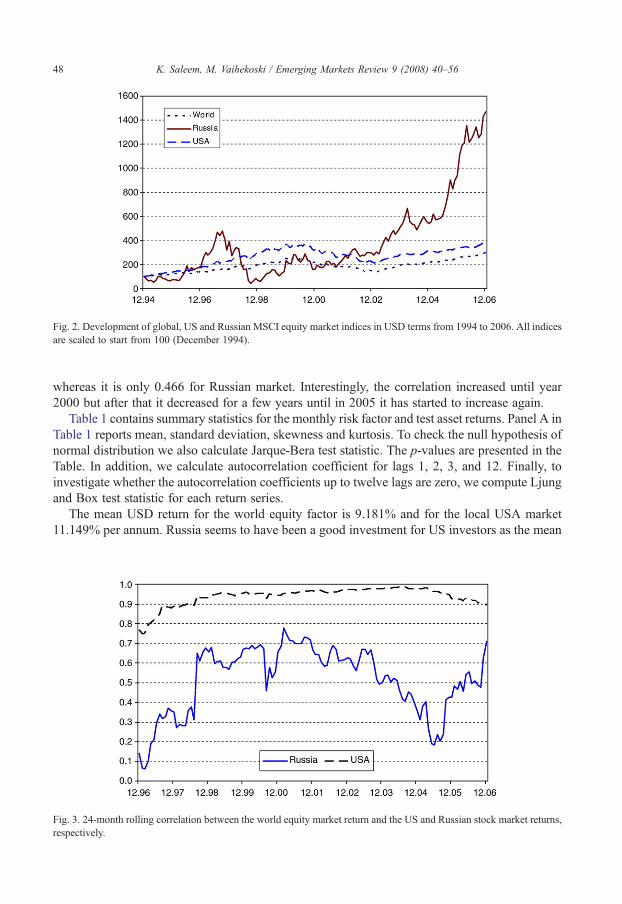
Fig. 2. Development of global, US and Russian MSCI equity market indices in USD terms from 1994 to 2006. All indicesare scaled to start from 100 (December 1994).


whereas it is only 0.466 for Russian market. Interestingly, the correlation increased until year2000 but after that it decreased for a few years until in 2005 it has started to increase again.

Table 1 contains summary statistics for the monthly risk factor and test asset returns. Panel A inTable 1 reports mean, standard deviation, skewness and kurtosis. To check the null hypothesis ofnormal distribution we also calculate Jarque-Bera test statistic. The p-values are presented in theTable. In addition, we calculate autocorrelation coefficient for lags 1, 2, 3, and 12. Finally, toinvestigate whether the autocorrelation coefficients up to twelve lags are zero, we compute Ljungand Box test statistic for each return series.

The mean USD return for the world equity factor is 9.181% and for the local USA market11.149% per annum. Russia seems to have been a good investment for US investors as the mean

Fig. 3. 24-month rolling correlation between the world equity market return and the US and Russian stock market returns,respectively.

Table 1Descriptive statistics for the monthly asset returns

Asset returnseries

Mean Std. dev. Skewness Excesskurtosis

Normality Autocorrelation a

(%) (%) (p-value) ρ1 ρ2 ρ3 ρ12 Q(12) b

Panel A: Summary statisticsWorld market

portfolio9.181 13.746 −0.841 4.233 b0.001 0.035 −0.029 0.049 0.097 0.822

USA 11.149 14.769 −0.743 3.944 b0.001 −0.001 −0.002 0.084 0.102 0.602Russia 22.387 62.826 −1.004 7.347 b0.001 0.129 −0.138 0.041 −0.001 0.257USD/RUB −16.713 21.277 −6.398 50.573 b0.001 0.489⁎ 0.136⁎ 0.199⁎ 0.021⁎ 0.001Risk-free rate

(Eurodollar)4.229 0.540 −0.560 1.801 b0.001 0.968⁎ 0.956⁎ 0.947⁎ 0.644⁎ 0.001

Panel B: Pairwise correlationsWorld USA Russia USD/RUB Rf

World marketportfolio

1 0.938 0.466 0.132 0.030

USA 1 0.431 0.043 0.088Russia 1 0.475 −0.056USD/RUB 1 −0.148Risk-free rate

(Eurodollar)1

Descriptive statistics are calculated for the monthly asset continuously compounded returns. The global market portfolio isproxied by the Morgan Stanley Capital International (MSCI) world equity index. The US market return is proxied by theMSCI US index. The Russian market return is proxied by the MSCI Russia index. All returns are calculated in USD andthey include dividends (i.e., total return). USD/RUB is the logarithmic difference in the USD value of one Ruble. The risk-free rate is proxied by the one-month Eurodollar rate. The mean and standard returns are annualized (multiplied with 12and the square root of 12, respectively). The sample size is 144 monthly observations from January 1995 to December2006. The p-value for the Jarque-Bera test statistic of the null hypothesis of normal distribution is provided in the table.a Autocorrelation coefficients significantly (1%) different from zero are marked with an asterisk (⁎).b The p-value for the Ljung and Box test statistic for the null that autocorrelation coefficients up to 12 lags are zero.


return has been clearly higher 22.387% per annum. The change in the value of Russian currencyin USD terms is −16.713% on average and monthly risk-free rate is 4.229% per annum onaverage during the sample period. The world portfolio has the lowest standard deviation assuggested by its low return. On the other hand, Russia has by far the highest standard deviation(62.826).

The index of kurtosis shows that the unconditional distribution of asset returns has heavier tailsthan the normal for all the risk factors in our sample. The Jarque–Bera test statistics also indicatethat the hypothesis of normality is rejected in all instances. None of the equity market showingevidence of positive first-order autocorrelation, however, US market exhibit negativeautocorrelation indicating a negative or reactive dependency exists for observations in the series.The lack of statistically significant autocorrelations in the return series and Ljung and Box teststatistics might lead us to believe that market indexes need not to correct for spuriousautocorrelation and GARCH specification used in our study is justified.

Panel B reports pair wise correlations among asset returns. All correlations in the table arebelow 0.5 except the correlation between USA and world (the value is 0.94). Further, we foundthe correlation between US stock market and the USD/RUB very close to zero (0.04).


In summary, the descriptive statistics of our data set suggest that Russian stock market hasoffered an attractive opportunity to US investors to diversify their portfolios internationally.

4. Empirical results

4.1. Conditional international CAPM without currency risk

We begin our investigation by testing the international CAPM which assumes full integrationbetween global and local stock markets. In addition, investors are assumed to diversify thecurrency risk away and hence the currency risk is not priced. As a result, we have only one sourceof risk, the global market risk (i.e. Eqs. (2) and (3)). The price of risk is assumed to be constant,

Table 2Conditional fully integrated ICAPM with constant prices of global risk

Full integration

US Russia World

Panel A: Parameter estimatesWorld market price of risk, λw 0.036⁎⁎

(0.022)ai 0.280⁎⁎⁎ 0.389⁎⁎⁎ 0.249⁎⁎⁎

(0.036) (0.096) (0.036)bi 0.950⁎⁎⁎ 0.915⁎⁎⁎ 0.957⁎⁎⁎

(0.013) (0.050) (0.013)

Panel B: Diagnostic testsAverage standardized residual 0.025 0.062 −0.022Standard deviation of z 0.980 1.000 0.990Skewness of z −0.830⁎⁎⁎ −0.520⁎⁎⁎ −0.990⁎⁎⁎Excess kurtosis of z 1.500⁎⁎⁎ 1.240⁎⁎⁎ 2.040⁎⁎⁎

Jarquez–Bera test for normality 27.930⁎⁎⁎ 16.240⁎⁎⁎ 45.260⁎⁎⁎

Q(12) 12.570 7.120 9.110Q2(12) 4.480 9.990 8.170Absolute mean pricing error 3.280 13.040 3.010Likelihood function −8.529

Quasi-maximum likelihood estimates of the conditional international CAPM with constant price of world covariance riskwhere the US and Russia are assumed to be fully integrated to the world market which leads to a single-factor model.

ri;tþ1 ¼ kwmCovt ri;tþ1;rwtþ1

� �þ "i;tþ1;

where λmw denotes the price of world market risk, and the residual ɛt+1∼ IID(0, Ht+1). The conditional covariance matrix

Ht+1 is parameterized as follows

Htþ1 ¼ H0⁎ ii 0 � aa 0 � bb 0ð Þ þ aa 0 ⁎"t"t 0 þ bb 0 ⁎Ht

where a and b are 3×1 vectors of constants and i is an 3×1 unit vector. H0 is the unconditional variance–covariancematrix and ⁎ denotes Hadamard matrix product. The sample size is 144 monthly observations from January 1995 toDecember 2006. QML standard errors are provided in parentheses below parameter estimates. Coefficients significantly(10%, 5% or 1%) different from zero are marked with (⁎), (⁎⁎) or (⁎⁎⁎).

Table 3Conditional partially segmented ICAPM with constant prices of global and local risk

Partial segmentation

US Russia World


(0.016)Local market price of risk, λl 0.001 −0.001

(0.004) (0.004)ai 0.281⁎⁎⁎ 0.389⁎⁎⁎ 0.250⁎⁎⁎

(0.037) (0.099) (0.037)bi 0.950⁎⁎⁎ 0.915⁎⁎⁎ 0.957⁎⁎⁎

(0.013) (0.051) (0.013)

Panel B: Diagnostic testsAverage standardized residual z 0.021 0.071 −0.023Standard deviation of z 0.980 1.000 0.990Skewness of z −0.830⁎⁎⁎ −0.600⁎⁎⁎ −0.990⁎⁎⁎Excess kurtosis of z 1.500⁎⁎⁎ 1.250⁎⁎⁎ 2.040⁎⁎⁎

Jarque-Bera test for normality 28.020⁎⁎⁎ 16.560⁎⁎⁎ 45.220⁎⁎⁎

Q(12) 12.640 7.060 9.120Q2(12) 4.440 9.780 8.150Absolute mean pricing error 3.280 13.050 3.010Likelihood function −8.529

Quasi-maximum likelihood estimates of the conditional international CAPM with constant price of world covariance riskwhere the US and Russia are assumed to be partially segmented to the world market which leads to a two factor model.

ri;tþ1 ¼ kwmCovt ri;tþ1;rwm;tþ1

� �þ klmCovt ri;tþ1;r

lm;tþ1

� �þ "i;tþ1

where λmw denotes the price of world covariance risk and λm

l price of local market risk, and ɛt+1∼ IID(0, Ht+1). Theconditional covariance matrix Ht+1 is parameterized as follows:

Htþ1 ¼ H0T ii 0 � aa 0 � bb 0ð Þ þ aa 0 T"t"t 0 þ bb 0 THt

where a and b are 3×1 vector of constants and i is an 3×1 unit vector.H0 is the unconditional variance–covariance matrixand ⁎ denotes Hadamard matrix product. The sample size is 144 monthly observations from January 1995 to December2006. QML standard errors are provided in parentheses below parameter estimates. Coefficients significantly (10%, 5% or1%) different from zero are marked with (⁎), (⁎⁎) or (⁎⁎⁎).


whereas the variance and covariance terms are time-varying.7 This implies that the conditionalrisk-free rate and conditional mean standard deviation frontier can change in each period, the slopeof the capital market line is fixed. In practice, we test the model using two assets in addition to theglobal market portfolio, namely the US and Russian stock market portfolios. Table 2 shows theresults.

We find the global price of risk to be positive 3.60 (reported value 0.036 due to percentagevalues used) which is consistent with the theory and corresponds to De Santis and Gérard (1998)who found the unconditional market price of risk to be 2.78. However, unlike them, we find the

7 This restriction has been imposed in many studies of the conditional CAPM (see, e.g., Chan et al., 1992).


price of world risk parameter to be significant (p-value 0.022).8 This shows that the world marketrisk is priced using market data from the US and Russia. The variance parameters (ai, bi) arehighly significant, making the variance process clearly time-varying. Moreover, in line withearlier studies variance processes display high persistence and the estimates of the bi coefficients(which link second moments to their lagged values) are considerably larger than thecorresponding estimates of the ai's (which link second moments to their past innovations).

Panel B of Table 2 shows some diagnostic test statistics for the standardized residuals.Theoretically they should be mean zero with unit variance. The results show that the one-factorICAPM performs worst for the Russian stock markets as the mean standardized residual is 0.062.On the other hand, the GARCH model is able to explain some of the non-normality in thedistribution as the coefficients of the excess kurtosis in all cases are lower then the correspondingvalues reported in Table 1. However, overall the GARCHmodel is not able to accommodate all ofthe non-normality as expected since the Jarque-Bera statistic rejects the normality of the residualsfor all markets.9 We also compute the Ljung–Box portmanteau statistic for each series to test thehypothesis of absence of autocorrelation up to order 12. The tests show that the null hypothesiscan not be rejected and that the GARCH(1,1) parameterization that we adopt is satisfactory.

Next we modify our model to allow for partial segmentation specification, where the US andRussia are assumed to be partially segmented to the world market. This corresponds to Eq. (4).Results are presented in Table 3. The variance parameters are of the same magnitude as those inTable 2, and highly significant. The misspecification statistics in Panel B of Table 3 are very muchin line with the corresponding statistics reported in Table 2.

The price of world risk parameter is again found significant at conventional 5% level.Interestingly the local market price of risk coefficients for both the markets are foundinsignificant, 0.001 (p-value 0.867) for the USA, and −0.001 (p-value 0.884) for Russia. Thus,market specific risk does not seem to be priced on either of the markets using the unconditionalapproach. This is a surprising result especially in the case of the Russian stock market as a priorione expects the Russian market to be strongly segmented. However, we have to remember that themodel omits the currency risk which could affect the results from US investors' point of view asthe local risk and currency are partly correlated.

4.2. Conditional international CAPM with currency risk

As stated before, the currencymovements have played an important role in the Russian economy,and for the companies as well as for the investors. This suggests a priori that the foreign exchangeriskmay be priced in the Russian stock market. To test this, we add the currency risk component intoour model (as suggested by Eq. (5)), first without and then with the local risk component.

Table 4 reveals the same story as previously in Table 2 and Table 3 in regards of the global risk.Additionally, we find currency risk priced and highly significant. This indicates that exchange rateexposure, to some extent, is non-diversifiable (systematic risk) and investors are rewarded forbearing such risk.

Finally we test our full model, which estimates the conditional international CAPM withconstant prices of world and currency risk where the US and Russia are assumed to be partially

8 De Santis and Gérard (1998) used eight different country and forex indices, and mention that the little explanatorypower of price of global market risk is due to the cross section of returns that they used.9 As robustness check model is also estimated under the assumption of a multivariate t-distribution for the residuals. It

allows for thicker-than-normal tails, and a higher excess kurtosis. The results are in line with those reported in Table 2.

Table 4Conditional fully integrated ICAPM with constant prices of global and currency risk

Full integration

US Russia ΔRub/$ World


(0.021)Price of currency risk, λfx −0.057⁎⁎⁎

(0.022)ai 0.198⁎ 0.350⁎⁎⁎ 0.531⁎⁎⁎ 0.191⁎⁎⁎

(0.113) (0.116) (0.156) (0.056)bi 0.971⁎⁎⁎ 0. 911⁎⁎⁎ 0.574⁎⁎ 0.971⁎⁎⁎

(0.010) (0.062) (0.134) (0.010)

Panel B: Diagnostic testsAverage standardized residual 0.025 0.158 −0.078 0.006Standard deviation of z 0.960 0.940 0.970 0.980Skewness of z −0.780⁎⁎⁎ −0.820⁎⁎⁎ −8.010⁎⁎⁎ −0.960⁎⁎⁎Excess kurtosis of z 1.400⁎⁎⁎ 2.570⁎⁎⁎ 82.610⁎⁎⁎ 1.850⁎⁎⁎

J-B-test for normality 24.730⁎⁎⁎ 51.790⁎⁎⁎ N99.999⁎⁎⁎ 39.810⁎⁎⁎

Q(12) 13.060 7. 010 8.140 9.930Q2(12) 9.070 15.560 0.130 10.810Absolute mean pricing error 3.320 13.270 1.930 3.080Likelihood function −11.372

Quasi-maximum likelihood estimates of the conditional international CAPM with constant price of world covariance riskand constant price of currency risk where the US and Russia are assumed to be fully integrated to the world market whichleads to a two factor model.


� �þ kcCovt ri;tþ1;fc;tþ1

� �þ "tþ1

where λmw denotes the price of world covariance risk, and λc price of currency risk and ɛt+1∼ IID(0, Ht+1). The

conditional covariance matrix Ht+1 is parameterized as follows:


where a and b are 4×1 vectors of constants and i is an 4×1 unit vector.H0 is the unconditional variance–covariance matrixand ⁎ denotes Hadamard matrix product. The sample size is 144 monthly observations from January 1995 to December2006. QML standard errors are provided in parentheses below parameter estimates. Coefficients significantly (10%, 5% or1%) different from zero are marked with (⁎), (⁎⁎) or (⁎⁎⁎).


segmented to the world market. The model corresponds to the empirical formulation in Eqs. (8)–(11) which leads to a three-factor model for the Russian, and two factor model for the US equitymarket.

Table 5 confirms the results presented in Table 4. However, contrary to the results in Table 3,local market price of risk for Russia is found highly significant (p-value 0.004), indicating that apartially segmented asset pricing specification is better suited for at least Russian market. Its valueis also positive indicating that higher local market volatility increases investors expected returns.In line with the previous research (e.g., De Santis and Gérard, 1998), the same parameter for theUSA is negative and insignificant (p-value 0.472); indicating that the local risk is not needed toprice US stocks.

Table 5Conditional partially segmented ICAPM with constant prices of global, local and currency risk

Partial segmentation

US Russia ΔRub/$ World


(0.019)Price of currency risk, λfx −0.062⁎⁎⁎

(0.019)Local market price of risk, λl −0.005 0.011⁎⁎⁎

(0.007) (0.004)ai 0.197⁎ 0.344⁎⁎⁎ 0.522⁎⁎⁎ 0.192⁎⁎⁎

(0.111) (0.101) (0.151) (0.058)bi 0.971⁎⁎⁎ 0.906⁎⁎⁎ 0.579⁎⁎⁎ 0.971⁎⁎⁎

(0.012) (0.051) (0.115) (0.009)

Panel B: Diagnostic testsAverage standardized residual 0.048 −0.010 −0.060 0.008Standard deviation of z 0.960 0.940 0.970 0.980Skewness of z −0.780⁎⁎⁎ −0.780⁎⁎⁎ −7.980⁎⁎⁎ −0.960⁎⁎⁎Excess kurtosis of z 1.390 2.260⁎⁎⁎ 82.280⁎⁎⁎ 1.870⁎⁎⁎

J-B-test for normality 24.310⁎⁎⁎ 41.680⁎⁎⁎ N99.999⁎⁎⁎ 40.090⁎⁎⁎

Q(12) 12.900 7.260 8.150 10.160Q2(12) 9.600 17.610 0.130 10.850Absolute mean pricing error 3.330 13.040 1.930 3.090Likelihood function −11.339

Quasi-maximum likelihood estimates of the conditional international CAPM with constant price of world covariance riskand constant price of currency risk where the US and Russia are assumed to be partially segmented to the world marketwhich leads to a three-factor model.


� �þ kcCovt ri;tþ1;fc;tþ1

� �þ klm;Covt ri;tþ1;rlm;tþ1

� �þ "i;tþ1

where λmw denotes the price of world covariance risk, λm

l price of local risk and λc price of currency risk and ɛt+1∼ IID(0,Ht+1). The conditional covariance matrix Ht+1 is parameterized as follows:


where a and b are 4×1 vectors of constants and i is an 4×1 unit vector. H0 is the unconditional variance–covariancematrix and ⁎ denotes Hadamard matrix product. The sample size is 144 monthly observations from January 1995 toDecember 2006. QML standard errors are provided in parentheses below parameter estimates. Coefficients significantly(10%, 5% or 1%) different from zero are marked with (⁎), (⁎⁎) or (⁎⁎⁎).


Moreover, the diagnostic tests of our final model lead us to believe that with the inclusion ofcurrency risk factor, the model performs batter; the mean standardized residual is smallest forRussia when the three-factor model is used whereas it seems that the smallest misspecification forthe USA takes places with the one-factor international CAPM. The rest of the diagnostic tests arebasically similar to the earlier tables. GARCH(1,1) specification seems to capture at least partiallythe dynamics of the conditional second moments in the asset returns.

In summary, the empirical analysis suggests a partially segmented model with currency risk asa separate risk factor is suitable for the Russian stock market. Thus our results suggests that whenpricing Russian stocks, US investors should take into account separately local market and


currency risk. Similarly, they should be taken into consideration by the portfolio managers as wellcompanies making decisions about investments in Russia.

5. Summary and conclusions

In this paper we investigate whether global and local market risk as well as the currency risk arepriced in the Russian stock market using conditional international asset pricing models. We usemonthly data from 1995 to 2006. We take the view of US investors and measure all returns in USdollars. Russian stock market offers an interesting test laboratory for many aspects of theinternational asset pricing models. The sample period includes, for example, a gradual liberalizationof the Russian financial markets and several currency regimes starting from fixed and floatingcurrency regimes. Many emerging markets are currently experiencing similar development.

The estimation is conducted using a modified version of the multivariate GARCH-Mframework of De Santis and Gérard (1997, 1998) with constant prices of risk specification. Theapproach allows for conditional variance and covariance processes between analyzed markets.First, we estimate the conditional fully integrated international CAPM and then partiallysegmented asset pricing model. Finally, we add the currency risk into our model.

The results show that the unconditional price of world risk is positive and significant withreasonable values, which is in line with the theory and earlier studies. Our final, three factor showsthat the Russian stock market is at least partly segmented as the local market risk is priced in theRussian, but not on the US market. Positive prices of global and local market risk indicate thatinvestors require higher compensation for higher market volatility. Finally, we also find thecurrency risk to be priced in the Russian stock market.

Our results have important implications for investors, who want to diversify their portfoliosinternationally. When portfolio managers aim to optimize the return–risk relationship, the resultsindicate that at least in the case of Russia, one should account for the local market as well ascurrency risk when calculating the key inputs for the optimization. In addition, the pricing ofexchange rate risk implies that exchange rate exposure is partly non-diversifiable and investorsare compensated for bearing the risk. Finally, the results suggest that one should separate the localmarket and currency risk when analyzing emerging markets, especially Russia.

However, we still believe that modelling of the currency risk in emerging stock markets needsfurther research as earlier studies have found that the role of the currency risk varies over time. Inaddition, when international asset pricing models are tested using data from countries with clearevidence of segmentation, it could be more appropriate to model the integration as a dynamicprocess with local influence. These questions are left for future study.

References

Adler, M., Dumas, B., 1983. International portfolio selection and corporation finance: a synthesis. Journal of Finance 38,925–984.

Anatolyev, S., 2005. A ten-year retrospection of the behavior of Russian stock returns. Bank of Finland. BOFIT DiscussionPapers, vol. 9.

Antell, J., Vaihekoski, M., 2007. International asset pricing models and currency risk: evidence from Finland 1970–2004.Journal of Banking and Finance 31, 2571–2590.

Bailey, W., Chung, Y.P., 1995. Exchange rate fluctuations, political risk, and stock returns: some evidence from anemerging market. Journal of Financial and Quantitative Analysis 30, 541–561.

Bollerslev, T., Engle, R.F., Wooldridge, J.M., 1988. A capital asset pricing model with time-varying covariances. Journalof Political Economy 96, 116–131.


Bollerslev, T., Wooldridge, J.M., 1992. Quasi-maximum likelihood estimation and inference in dynamic models with time-varying covariances. Econometric Reviews 11, 143–172.

Carrieri, F., Errunza, V., Majerbi, B., 2006. Local risk factors in emerging markets: are they separately priced? Journal ofEmpirical Finance 13, 444–461.

Chan, K.C., Karolyi, A.G., Stulz, R., 1992. Global financial markets and the risk premium on U.S. Equity. Journal ofFinancial Economics 32, 137–169.

De Santis, G., Imrohoroglu, S., 1997. Stock returns and volatility in emerging financial markets. Journal of InternationalMoney and Finance 16, 561–579.

De Santis, G., Gérard, B., 1997. International asset pricing and portfolio diversification with time-varying risk. Journal ofFinance 52, 1881–1912.

De Santis, G., Gérard, B., 1998. How big is the premium for currency risk? Journal of Financial Economics 49, 375–412.Ding, Z., Engle, R.F., 2001. Large scale conditional covariance matrix modeling, estimation and testing. Academia

Economic Papers 29, 157–184.Doukas, J., Hall, P.H., Lang, L.H.P., 1999. The pricing of currency risk in Japan. Journal of Banking and Finance 23, 1–20.Engle, R.F., Kroner, K., 1995. Multivariate simultaneous generalized ARCH. Econometric Theory 11, 122–150.Errunza, V., Losq, E., 1985. Internal asset pricing under mild segmentation: theory and tests. Journal of Finance 40, 105–124.Ferson, W., Harvey, C.R., 1993. The risk and predictability of international equity returns. Review of Financial Studies 6,

527–566.Gérard, B., Thanyalakpark, K., Batten, J.A., 2003. Are the East Asian markets integrated? Evidence from the ICAPM.

Journal of Economics and Business 55, 585–607.Goriaev, A., Zabotkin, A., 2006. Risks of investing in the Russian stock market: lessons of the first decade. Emerging

Markets Review 7, 380–397.Grauer, F., Litzenberger, R., Stehle, R., 1976. Sharing rules and equilibrium in an international capital market under

uncertainty. Journal of Financial Economics 3, 233–256.Harvey, C.R., 1995. Predictable risk and return in emerging markets. Review of Financial Studies 8, 773–816.Jorion, P., 1991. The pricing of exchange rate risk in the stock market. Journal of Financial and Quantitative Analysis 26,

363–376.Mateus, T., 2004. The risk and predictability of equity returns of the EU accession countries. Emerging Markets Review 5,

241–266.Nummelin, K., Vaihekoski, M., 2002. International capital markets and Finnish stock returns. European Journal of Finance

8, 322–343.Phylaktis, K., Ravazzolo, F., 2004. Currency risk in emerging equity markets. Emerging Markets Review 5, 317–339.Roll, R., 1992. Industrial structure and the comparative behavior of international stock market indices. Journal of Finance

47, 3–41.Stulz, R.M., 1995. International portfolio choice and asset pricing: an integrative survey. In: Jarrow, R.A., Maksimovic, V.,

Ziemba, W.T. (Eds.), Handbooks in Operations Research and Management Science, 9: Finance. North-Holland,Amsterdam, pp. 201–223.

Pricing of global and local sources of risk in Russian stock market

Documents

Transcript of Pricing of global and local sources of risk in Russian stock market