
Pricing decision and lead time quotation in supply chains with ...
157
HAL Id: tel-01734909 https://tel.archives-ouvertes.fr/tel-01734909 Submitted on 15 Mar 2018 HAL is a multi-disciplinary open access archive for the deposit and dissemination of sci- entific research documents, whether they are pub- lished or not. The documents may come from teaching and research institutions in France or abroad, or from public or private research centers. L’archive ouverte pluridisciplinaire HAL, est destinée au dépôt et à la diffusion de documents scientifiques de niveau recherche, publiés ou non, émanant des établissements d’enseignement et de recherche français ou étrangers, des laboratoires publics ou privés. Pricing decision and lead time quotation in supply chains with an endogenous demand sensitive to lead time and price Abduh-Sayid Albana To cite this version: Abduh-Sayid Albana. Pricing decision and lead time quotation in supply chains with an endogenous demand sensitive to lead time and price. Business administration. Université Grenoble Alpes, 2018. English. NNT : 2018GREAI004. tel-01734909
-
Upload
khangminh22 -
Category
Documents
-
view
3 -
download
0
Transcript of Pricing decision and lead time quotation in supply chains with ...
HAL Id: tel-01734909https://tel.archives-ouvertes.fr/tel-01734909
Submitted on 15 Mar 2018
HAL is a multi-disciplinary open accessarchive for the deposit and dissemination of sci-entific research documents, whether they are pub-lished or not. The documents may come fromteaching and research institutions in France orabroad, or from public or private research centers.
L’archive ouverte pluridisciplinaire HAL, estdestinée au dépôt et à la diffusion de documentsscientifiques de niveau recherche, publiés ou non,émanant des établissements d’enseignement et derecherche français ou étrangers, des laboratoirespublics ou privés.
Pricing decision and lead time quotation in supplychains with an endogenous demand sensitive to lead
time and priceAbduh-Sayid Albana
To cite this version:Abduh-Sayid Albana. Pricing decision and lead time quotation in supply chains with an endogenousdemand sensitive to lead time and price. Business administration. Université Grenoble Alpes, 2018.English. �NNT : 2018GREAI004�. �tel-01734909�

THESEPour obtenir le grade de
DOCTEUR DE LA COMMUNAUTEUNIVERSITE GRENOBLE ALPESSpecialite : GI : Genie Industriel
Arrete ministeriel : 25 mai 2016
Presentee par
Abduh-Sayid ALBANA
These dirigee par Yannick FREIN, Professeur a Grenoble INPet codirigee par Ramzi HAMMAMI, Professeur a Rennes School ofBusiness
preparee au sein du Laboratoire des Sciences pour la Conception,l’Optimisation et la Production de Grenoble (G-SCOP)dans l’Ecole doctorale Ingenierie - Materiaux, Mecanique,Environnement, Energetique, Procedes, Production (I-MEP2)
Choix du prix et du delai de livraisondans une chaıne logistique avec unedemande endogene sensible au delai delivraison et au prix
Pricing Decision and Lead timeQuotation in Supply Chains with anEndogenous Demand Sensitive to Leadtime and Price
These soutenue publiquement le 26/01/2018,devant le jury compose de :
Monsieur Lyes BENYOUCEFProfesseur a Aix-Marseille Universite, PresidentMonsieur Zied JEMAIProfesseur a Ecole Nationale d’Ingenieurs de Tunis, RapporteurMonsieur Faicel HNAIENMaıtre de conferences a l’Universite de Technologie de Troyes, RapporteurMonsieur Jean-Philippe GAYONProfesseur a ISIMA Clermont-Ferrand, ExaminateurMonsieur Yannick FREINProfesseur a Grenoble INP, Directeur de theseMonsieur Ramzi HAMMAMIProfesseur a Rennes School of Business, Co-Encadrant de these

Contents
List of Figures . . . . . . . . . . . . . . . . . . . . . . . . . . . . . . . . . . iiiList of Tables . . . . . . . . . . . . . . . . . . . . . . . . . . . . . . . . . . v
Resume en francais 1
1 Introduction 19
2 Literature review 232.1 The pioneer paper: Palaka et al. (1998) . . . . . . . . . . . . . . . . . 242.2 Single-firm in MTO system . . . . . . . . . . . . . . . . . . . . . . . . 262.3 Multi-firm in MTO system . . . . . . . . . . . . . . . . . . . . . . . . 292.4 Other related papers: the MTS system . . . . . . . . . . . . . . . . . 342.5 Conclusion of literature review . . . . . . . . . . . . . . . . . . . . . . 35
3 Lead time sensitive cost: a production system with demand andproduction cost sensitive to lead time (M/M/1 model) 373.1 The model . . . . . . . . . . . . . . . . . . . . . . . . . . . . . . . . . 373.2 Setting 1: Model with variable lead time and fixed price . . . . . . . 40
3.2.1 Optimal policy with variable lead time and fixed price . . . . 403.2.2 Experiments and insights with fixed price . . . . . . . . . . . . 43
3.3 Setting 2: Model with both lead time and price as decision variables . 463.3.1 Optimal policy with both lead time and price as decision vari-
ables . . . . . . . . . . . . . . . . . . . . . . . . . . . . . . . . 463.3.2 Experiments and insights with variable price . . . . . . . . . . 51
3.4 General model (Setting 3): price is a decision variable; congestion &lateness costs are considered . . . . . . . . . . . . . . . . . . . . . . . 563.4.1 Optimal policy for general model . . . . . . . . . . . . . . . . 563.4.2 Experiments and insights for general model . . . . . . . . . . 57
3.5 Conclusion . . . . . . . . . . . . . . . . . . . . . . . . . . . . . . . . . 63
4 Rejection policy: a lead time quotation and pricing in an M/M/1/Kmake-to-order queue 654.1 General model: M/M/1/K . . . . . . . . . . . . . . . . . . . . . . . . 654.2 The M/M/1/1 model: Analytical solution . . . . . . . . . . . . . . . 69
4.2.1 The M/M/1/1 model: congestion & lateness costs are ignored 694.2.2 The M/M/1/1 model: congestion & lateness costs are considered 72
4.3 Performance of the rejection policy (M/M/1/1) with comparison tothe all-customers’ acceptance policy (M/M/1) . . . . . . . . . . . . . 754.3.1 Effect of lead time-sensitivity . . . . . . . . . . . . . . . . . . 764.3.2 Effect of price-sensitivity . . . . . . . . . . . . . . . . . . . . . 774.3.3 Effect of service level . . . . . . . . . . . . . . . . . . . . . . . 78
i
Contents
4.3.4 Effect of holding cost . . . . . . . . . . . . . . . . . . . . . . . 794.3.5 Effect of lateness penalty cost . . . . . . . . . . . . . . . . . . 79
4.4 The M/M/1/K model: numerical solution and experiments . . . . . . 814.5 Conclusion . . . . . . . . . . . . . . . . . . . . . . . . . . . . . . . . . 83
5 Coordination of upstream-downstream supply chain under priceand lead time sensitive demand: a tandem queue model 875.1 System description (M/M/1–M/M/1) . . . . . . . . . . . . . . . . . . 875.2 Centralized Setting: Model and Experiments . . . . . . . . . . . . . . 895.3 Local & Global Service Level . . . . . . . . . . . . . . . . . . . . . . . 935.4 Modified Centralized: Model and Experiments . . . . . . . . . . . . . 975.5 Decentralized setting (Downstream Leader – Upstream Follower) . . . 101
5.5.1 Upstream decides his own lead time . . . . . . . . . . . . . . . 1025.5.2 Upstream decides his own price . . . . . . . . . . . . . . . . . 109
5.6 Conclusion . . . . . . . . . . . . . . . . . . . . . . . . . . . . . . . . . 118
6 General conclusion 1216.1 Conclusion . . . . . . . . . . . . . . . . . . . . . . . . . . . . . . . . . 1216.2 Future works and perspectives . . . . . . . . . . . . . . . . . . . . . . 123
A Root of cubic equation Q(L) in Proposition 3.3 131
B Expected lateness in a M/M/1/K 133
C Particle Swarm Optimization for M/M/1/K 137
D Experiment with Kopt 139
E Root of cubic equation in Lemma 5.8 143
F Root of cubic equation in Lemma 5.13 145
ii Univ. Grenoble Alpes, 2018
List of Figures
1 Modele file d’attente . . . . . . . . . . . . . . . . . . . . . . . . . . . 12
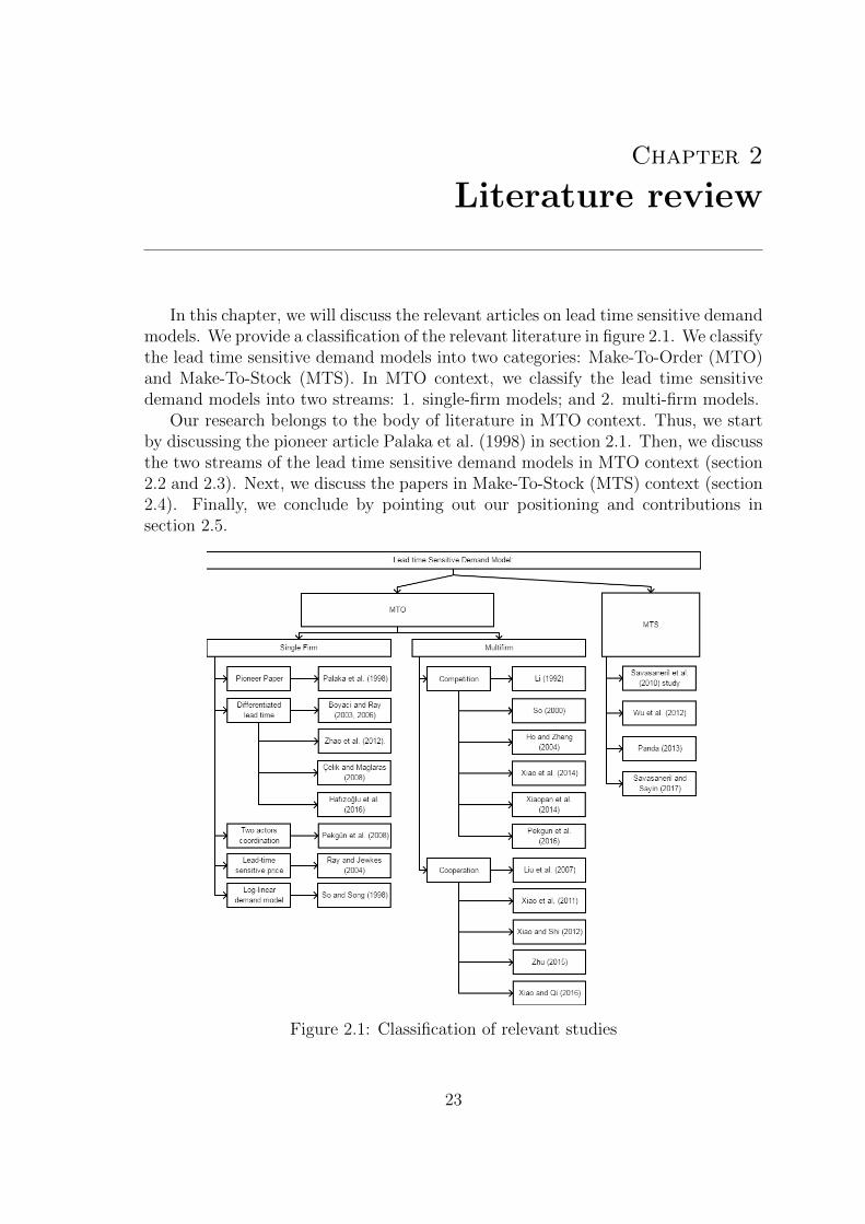
2.1 Classification of relevant studies . . . . . . . . . . . . . . . . . . . . . 23
3.1 Illustration of situations: LB ≤ LNB and LB > LNB . . . . . . . . . . 423.2 Variable cost vs Fixed cost: quoted lead time . . . . . . . . . . . . . 443.3 Effect of b1 with variable and constant cost . . . . . . . . . . . . . . . 523.4 Variation of lead time for increasing values of b2 . . . . . . . . . . . . 543.5 Effect of C2 with variable and constant price . . . . . . . . . . . . . . 553.6 Effect of b1 with variable and constant cost for general model . . . . . 583.7 Variation of lead time for increasing values of b2 in general model . . 603.8 Effect of C2 in general model . . . . . . . . . . . . . . . . . . . . . . . 613.9 Effect of F in general model . . . . . . . . . . . . . . . . . . . . . . . 623.10 Effect of cr in general model . . . . . . . . . . . . . . . . . . . . . . . 63
4.1 M/M/1/K performance as a function of b2 . . . . . . . . . . . . . . . 834.2 M/M/1/K performance as a function of b1 . . . . . . . . . . . . . . . 834.3 M/M/1/K performance as a function of s . . . . . . . . . . . . . . . . 844.4 M/M/1/K performance as a function of F . . . . . . . . . . . . . . . 844.5 M/M/1/K performance as a function of cr . . . . . . . . . . . . . . . 85
5.1 Queuing model . . . . . . . . . . . . . . . . . . . . . . . . . . . . . . 885.2 f(s) in function of s . . . . . . . . . . . . . . . . . . . . . . . . . . . 965.3 s in function of V1/V2 . . . . . . . . . . . . . . . . . . . . . . . . . . . 975.4 Π1,Π2 and Πg with µ1 = µ2 . . . . . . . . . . . . . . . . . . . . . . . 1055.5 Theoritical profit of each actor with µ1 = µ2 . . . . . . . . . . . . . . 1135.6 Real profit of each actor with µ1 = µ2 . . . . . . . . . . . . . . . . . . 114
D.1 Profit in function of K . . . . . . . . . . . . . . . . . . . . . . . . . . 139D.2 Kopt in function of b2 . . . . . . . . . . . . . . . . . . . . . . . . . . . 140D.3 Kopt in function of b1 . . . . . . . . . . . . . . . . . . . . . . . . . . . 141
iii

List of Figures
iv Univ. Grenoble Alpes, 2018
List of Tables
3.1 Effect of demand sensitivity to lead time (b2) with fixed price . . . . . 443.2 Effect of cost sensitivity to lead time (C2) with fixed price . . . . . . 463.3 Effect of demand sensitivity to price (b1) . . . . . . . . . . . . . . . . 513.4 Effect of demand sensitivity to lead time (b2) with variable price . . . 533.5 Effect of cost sensitivity to lead time (C2) with variable price . . . . . 553.6 Effect of demand sensitivity to price (b1) for general model . . . . . . 573.7 Effect of demand sensitivity to lead time (b2) for general model . . . . 593.8 Effect of cost sensitivity to lead time (C2) for general model . . . . . 603.9 Effect of holding cost (F ) for general model . . . . . . . . . . . . . . 613.10 Effect of lateness cost (cr) for general model . . . . . . . . . . . . . . 62
4.1 M/M/1/1 vs M/M/1 for different values of b2 . . . . . . . . . . . . . 774.2 M/M/1/1 vs M/M/1 for different values of b1 . . . . . . . . . . . . . 784.3 M/M/1/1 vs M/M/1 for different values of s . . . . . . . . . . . . . . 784.4 M/M/1/1 vs M/M/1 for different values of F . . . . . . . . . . . . . 794.5 M/M/1/1 vs M/M/1 for different values of cr . . . . . . . . . . . . . 80
5.1 Centralized setting experiment on b1 with µ1 = µ2 . . . . . . . . . . . 915.2 Centralized setting experiment on b2 with µ1 = µ2 . . . . . . . . . . . 925.3 Centralized setting experiment on b1 with µ1 6= µ2 . . . . . . . . . . . 925.4 Centralized setting experiment on b2 with µ1 6= µ2 . . . . . . . . . . . 935.5 Experiment on b1 with µ1 = µ2 for modified centralized setting . . . . 995.6 Experiment on b2 with µ1 = µ2 for modified centralized setting . . . . 1005.7 Experiment on b1 with µ1 > µ2 for modified centralized setting . . . . 1005.8 Experiment on b2 with µ1 > µ2 for modified centralized setting . . . . 1015.9 Verification of local service constraint for centralized setting . . . . . 1015.10 b1 for µ1 = µ2 . . . . . . . . . . . . . . . . . . . . . . . . . . . . . . . 1075.11 b2 for µ1 = µ2 . . . . . . . . . . . . . . . . . . . . . . . . . . . . . . . 1075.12 b1 for µ1 > µ2 . . . . . . . . . . . . . . . . . . . . . . . . . . . . . . . 1085.13 b2 for µ1 > µ2 . . . . . . . . . . . . . . . . . . . . . . . . . . . . . . . 1085.14 b1 for µ1 = µ2 . . . . . . . . . . . . . . . . . . . . . . . . . . . . . . . 1165.15 b2 for µ1 = µ2 . . . . . . . . . . . . . . . . . . . . . . . . . . . . . . . 1165.16 δ2 for µ1 = µ2 . . . . . . . . . . . . . . . . . . . . . . . . . . . . . . . 1175.17 b1 for µ1 > µ2 . . . . . . . . . . . . . . . . . . . . . . . . . . . . . . . 1175.18 b2 for µ1 > µ2 . . . . . . . . . . . . . . . . . . . . . . . . . . . . . . . 1185.19 δ2 for µ1 > µ2 . . . . . . . . . . . . . . . . . . . . . . . . . . . . . . . 118
D.1 Detailed result of Kopt in function of b2 . . . . . . . . . . . . . . . . . 140D.2 Detailed result of Kopt in function of b1 . . . . . . . . . . . . . . . . . 141
v

List of Tables
vi Univ. Grenoble Alpes, 2018
Resume en francais
Chapitre 1 : Introduction
La majeure partie des travaux sur la conception d’une chaıne logistique sup-posent une demande exogene, c’est-a-dire connue a priori (eventuellement par unecaracterisation stochastique) et donc independante des eventuelles decisions priseslors de cette conception. Ces travaux supposent donc en particulier que le prix, fac-teur influencant fortement la demande, est deja fixe. Mais, ces travaux supposentaussi implicitement que la demande n’est pas sensible au delai de livraison ou alorsque ce delai est aussi deja fixe. Or, ces deux hypotheses sont bien sur tres discuta-bles comme nous l’expliquons ci-apres. Precisons tout d’abord que nous definissonsle delai de livraison L comme etant le temps entre l’instant ou le client passe sacommande et le temps ou le produit est disponible pour ce client (Christopher,2011).
Tout d’abord, il est connu depuis longtemps que le delai de livraison proposeaux clients est un facteur de competitivite essentiel, et meme une cle du succesdans de nombreuses industries (Blackburn et Stalk, 1990). La litterature fournit denombreuses illustrations sur la facon dont les entreprises peuvent utiliser ce delaide livraison comme une arme strategique pour obtenir un avantage concurrentiel(Blackburn et al., 1992; Hum et Sim, 1996; Suri, 1998). Geary et Zonnenberg (2000),apres une enquete aupres de 110 entreprises dans cinq grands secteurs manufacturi-ers, relatent que nombre d‘entre elles focalisent leurs efforts sur des ameliorationssur les couts, mais aussi sur les delais de livraison. Baker et al. (2001) indiquentque moins de 10% des clients finaux (BtC) et moins de 30% des clients BtB basentleurs decisions d’achat sur uniquement le prix de vente d’un article.
De plus, il est evident que le delai de livraison est largement impacte par lesdecisions prises lors de la conception de la chaıne. En effet, les decisions de lo-calisation des lieux de production et d’achat des composants ont bien sur un effetdirect sur le delai de production. Les politiques de stockage (quantites et lieuxde stockage) ont aussi un effet direct sur la disponibilite des produits a livrer. Ilnous paraıt donc interessant de travailler sur des modeles dans lesquels on prendexplicitement en compte l’impact du delai de livraison sur la demande. Au-dela dela reduction du delai, il est probablement encore plus important de satisfaire le delaiannonce. La non satisfaction du delai indique peut conduire a de fortes penalites.Selon Savasaneril et al. (2010), les exemples montrant l’importance de delais delivraison fiables sont abondants dans l’industrie. Les auteurs rapportent par ex-emple que le cout de livraisons tardives dans la division des equipements de FMCWellhead pourrait atteindre $ 250 000 par jour et que les penalites de retard dansl’industrie aeronautique vont de $ 10 000 a $ 15 000 et peuvent atteindre $ 1 000 000
1
Resume en francais
par jour. En plus des consequences directes en termes de penalites, une livraisonen retard peut affecter la reputation de l’entreprise et dissuader les clients futurs(Slotnick, 2014). Les entreprises risquent donc de perdre des marches si elles ne sontpas capables de respecter les delais promis (Kapuscinski et Tayur, 2007). Il s’agiradonc de developper des modeles dans lesquels nous choisissons le delai annonce auxclients mais aussi garantissons un niveau de respect de ces delais annonces.
Un temps de livraison plus court peut conduire a une augmentation de la de-mande, mais augmente egalement le risque de retard de livraison, et donc deteriorele niveau de service et augmente le cout de la penalite de retard. Inversement, lastrategie consistant a augmenter le delai annonce conduit a une demande plus faible;cela conduira en effet les clients a commander aux concurrents qui proposent desdelais de livraison plus courts (Ho et Zheng, 2004; Pekgun et al., 2016; So, 2000;Xiao et al., 2014). Et bien sur, une diminution de la demande aura un effet negatifsur les revenus. Par contre, le cote positif de promettre un delai plus long est lapossibilite d’atteindre un niveau de service plus eleve (puisque, d’une part, le delaipromis est plus long et, d’autre part, la demande est plus faible). Il peut egalementdiminuer le cout de stockage des stocks en cours. Ce dernier cout peut etre signi-ficatif dans de nombreuses industries telles que l’automobile et l’electronique. Lafixation du delai est donc en soi le resultat d’un compromis. Par ailleurs, meme sinous avons insiste dans ce qui precede sur l’influence du delai, car encore peu abordedans la litterature, il est bien connu que l’augmentation du prix reduit la demandemais augmente la marge et qu’une baisse du prix augmente cette demande mais audetriment de la marge. Il y a donc aussi un compromis a trouver dans cette fixationdu prix. Il est donc evident que la combinaison du prix propose et du delai promisouvre sur de nouveaux compromis et offre des possibilites pour de nombreux travauxnovateurs.
Il est interessant de noter que tres peu de recherches en gestion des operationsont ete menees dans ce cadre d’une demande sensible aux prix et delai de livrai-son, comme le soulignent Huang et al. (2013). La majorite de cette litterature sesitue dans le contexte �Make-To-Order� (pour les articles en �Make-To-Stock� voirPanda, 2013; Savasaneril et al., 2010; Savasaneril et Sayin, 2017; Wu et al., 2012). Lepapier pionnier sur un modele avec une demande sensible aux delais et prix dans lecontexte du MTO est le papier de Palaka et al. (1998). Dans ce papier, la demandeest supposee etre une fonction lineaire du prix et du delai. Ils considerent 3 vari-ables de decision : le delai promis, la capacite de production et le prix. Ils limitenttout d’abord leur attention a un horizon court terme, et par consequent la capaciteest supposee constante. Les clients sont servis selon le principe du premier arrive,premier servi. Ils supposent que le processus d’arrivee des clients peut etre decritpar un processus de Poisson. En outre, les temps de traitement des commandes desclients sont supposes distribues de maniere exponentielle. Ces hypotheses leur per-mettent d’utiliser un modele M/M/1 pour representer les operations de l’entreprise.Dans la suite de ces travaux, differentes extensions ont ete effectuees dans des cadresmono et multi-entreprise, et nous nous positionnons clairement dans ce courant de
2 Univ. Grenoble Alpes, 2018
Resume en francais
la litterature. Avant de preciser nos contributions, nous analysons rapidement lesextensions les plus importantes issues du travail fondateur de Palaka et al. (1998).Dans le cas mono-entreprise, Pekgun et al. (2008) ont etudie deux modes de prisedes decisions prix et delai, en l’occurrence centralise et decentralise. Ils ont utilise lecadre de Palaka et al. (1998) pour leur modele centralise mais sans tenir compte descouts de stockage et de penalite. Ray et Jewkes (2004) se focalisent sur la recherchedu delai promis optimal dans une situation ou le prix est sensible au delai de livrai-son. Zhao et al. (2012) ont egalement considere cette problematique de fixation dudelai et du prix dans les entreprises de services et les industries �Make-To-Order�.Ils ont considere deux strategies : dans la premiere strategie, les entreprises pro-posent un delai et prix uniques (�uniform quotation mode�) et, dans la seconde, ilsproposent un menu de delais et de prix (�differentiated quotation mode�). Dansle cadre multi-entreprise, Zhu (2015) considere une chaıne logistique composee d’unfournisseur et d’un detaillant face a une demande sensible aux prix et delais. Il estimportant de signaler que le detaillant n’a pas d’operation de production et doncpas de delai propre. Le processus de decision est modelise comme une sequence oule fournisseur determine la capacite et le prix de vente au detaillant, et le detaillantdetermine le prix de vente et le delai de livraison. La recente recherche de Pekgunet al. (2016) est une extension de leur papier precedent (Pekgun et al., 2008).Dans ce papier recent, ils etudient deux entreprises qui se font concurrence sur lesdecisions de prix et de delais dans un marche commun. Une discussion detaillee dela litterature considerant une demande sensible au delai et prix est fourni dans lechapitre 2.
Dans notre etude de la litterature, nous avons trouve quelques faiblesses. Danstous les travaux consideres, le cout de production unitaire est suppose etre constant.De plus, nous n’avons pas trouve de travaux dans lesquels des clients peuvent etrerejetes (notamment si l’entreprise a un carnet de commandes rempli). Enfin, lesquelques travaux considerant plusieurs entreprises se situent dans le cadre de 2entreprises ou une seule a des operations de production (l’autre acteur a un delainul). Concernant la premiere limitation, on sait que dans de nombreuses situationsle cout de production unitaire depend du delai de livraison promis. Les entreprisespeuvent en effet mieux gerer le processus de production et reduire les couts deproduction lorsqu’elles disposent d’un delai plus eleve. Bien sur, la prise en compted’un cout de production sensible au delai pose de nouvelles difficultes surtout sion considere l’hypothese realiste d’une relation non lineaire entre le cout et le delai.L’hypothese qui consiste a accepter tous les clients permet a ces travaux de considererun modele M/M/1 ce qui est bien sur interessant d’un point de vue resolutionanalytique. Mais, accepter les clients, meme avec un nombre eleve de commandesdeja en attente, peut entraıner de longs delais pour ces clients et donc necessite dedefinir un delai important si on veut satisfaire un niveau de service eleve, ce quiconduira a une reduction de la demande. Pratiquement, les entreprises peuventchoisir de rejeter les clients lorsqu’elles ont deja trop de clients. Mais alors, lemodele obtenu sera du type M/M/1/K et la formulation du temps d’attente residuel,
Univ. Grenoble Alpes, 2018 3
Resume en francais
necessaire pour calculer le cout de la penalite pour les clients en retard, n’est pasdisponible dans la litterature. Enfin, il est bien sur interessant de considerer unechaıne logistique comprenant plusieurs acteurs et contrairement a ce qui est presentedans la litterature, il faudrait etudier une situation ou chaque acteur a ses propresoperations de production et donc ses propres delais. Mais a nouveau, un tel modelepose des difficultes nouvelles. En effet, le modele global est plus complexe et si onsouhaite etudier un modele avec decentralisation des decisions, on se heurte a ladifficulte de savoir imposer un taux de service global (qui interesse le client final) apartir des contraintes de service locales.
Le plan de la these decoule naturellement de l’analyse de ces limitations. En effet,apres une etude de litterature (chapitre 2) nous proposons trois extensions: 1. Coutunitaire de production sensible au delai, 2. Politique de rejet de clients a l’aide d’unmodele M/M/1/K, et 3. Etude de la coordination d’une chaıne logistique composeede deux etages a l’aide d’un reseau tandem de type (M/M/1-M/M/1), extensionsdeveloppees dans les chapitres 3, 4 et 5, respectivement. Enfin, nous concluons notretravail dans le chapitre 6.
Chapitre 2 : Revue de litterature
Comme indique dans l’introduction, le papier pionnier est celui de Palaka etal. (1998). Dans ce papier, les auteurs se sont interesses au choix du delai, dela capacite et du prix pour une entreprise ou les clients sont sensibles aux delaispromis. Palaka et al. (1998) considerent une entreprise qui produit avec un mode�make-to-order�. Ils limitent initialement leur etude a un horizon court terme, parconsequent la capacite est supposee constante alors que le prix, le delai promis etla demande sont consideres comme des variables de decision. Comme indique enintroduction, ils ont modelise le systeme par une file d’attente de type M/M/1. Lesclients sont sensibles aux delais et prix, et la demande est naturellement supposeeetre decroissante a la fois en fonction du prix et du delai promis. Plus precisement,la demande maximale est une fonction lineaire et modelisee comme suit:
Λ(P,L) = a− b1P − b2L (1)
ou P = prix du bien/service etabli par l’entreprise, L = delai promis, Λ(P,L) =demande maximale attendue pour le bien/service au prix P et delai promis L, a =demande maximale correspondant a un prix et un delai promis nuls, b1 = sensibilitede la demande au prix, et b2 = sensibilite de la demande au delai promis (b1 etb2 sont positifs). De plus, pour eviter des delais de livraison promis irrealistes, ilsimposent que l’entreprise maintienne un niveau de service minimum (s), ou ce niveaude service est defini comme la probabilite de satisfaire le delai promis. Ce niveau deservice minimum peut etre fixe par l’entreprise elle-meme en reponse aux pressionsconcurrentielles.
L’entreprise etant modelise par une M/M/1 avec un taux de service moyen, µ,et un taux d’arrivee moyen, λ, le nombre de clients moyen du systeme, Ns, est
4 Univ. Grenoble Alpes, 2018
Resume en francais
donne par Ns = λ/(µ − λ) et le temps de sejour dans le systeme, W , est distribuede facon exponentielle avec une moyenne 1/(µ − λ) (Hillier et Lieberman, 2001;Kleinrock, 1975). La probabilite que l’entreprise ne respecte pas le delai de livraisonpromis, L, est donnee par e−(µ−λ)L et le retard moyen d’une commande en retardest de 1/(µ− λ), identique au temps de sejour moyen en raison de la propriete sansmemoire de la distribution exponentielle.
L’objectif de l’entreprise est de maximiser le profit total attendu qui peut etreexprimee par l’equation (2) ci-apres. Dans la fonction objectif, λ(P −m) representele revenu prevu (net des couts directs), ou m est le cout unitaire. Les couts decongestion moyens sont donnes par Fλ/(µ−λ) ou F est le cout de stockage unitaireet λ/(µ− λ) est le nombre moyen de clients dans le systeme. La penalite de retardmoyenne est donnee par cr(λ/(µ− λ))e−(µ−λ)L, ou cr est la penalite par commandepour une unite de temps de retard, le nombre du client en retard etant egal aλe−(µ−λ)L, et le retard moyen etant egal a 1/(µ−λ). Enfin, en notant s le niveau deservice minimum, Palaka et al. (1998) formulent le probleme d’optimisation commesuit:
(PBase) MaximiserP,L,λ
Π(P,L, λ) = (P −m)λ− Fλ
µ− λ− crλ
µ− λe−(µ−λ)L (2)
Sous contraintes λ ≤ a− b1P − b2L (3)
1− e−(µ−λ)L ≥ s (4)
0 ≤ λ ≤ µ (5)
P,L ≥ 0 (6)
La contrainte (3) exige que la demande moyenne, λ, desservie par l’entreprise nedepasse pas la demande generee par le prix, P et le delai indique, L. La contrainte(4) exprime la limite inferieure du niveau de service. La contrainte (5) correspond ala restriction selon laquelle la demande moyenne, λ, est egalement limitee par le tauxde service de l’entreprise, µ. La contrainte (6) exprime les contraintes de positivitedes variables.
Dans leur papier, Palaka et al. (1998) ont montre que la contrainte (3) est serreea l’optimalite. L’entreprise choisira le prix, P , le delai promis, L et le taux dedemande, λ, de sorte que la contrainte λ ≤ Λ(P,L) soit en fait: λ = Λ(P,L). Leprobleme d’optimisation est donc en fait un probleme a 2 variables.
Par contre la contrainte de service (4) dans le modele d’optimisation (PBase) n’estpas obligatoirement serree a l’optimalite. Palaka et al. (1998) ont demontre que lacontrainte de service (4) n’est pas serree si le niveau de service, s, est strictementinferieur a une valeur critique, sc, c’est-a-dire s < 1− b1/(b2cr). En outre, le niveaude service effectif sera donne par max(s, sc) (voir la proposition 2 de Palaka et al.(1998)).
Les solutions du probleme PBase dans les cas serre et non serre, sont:
• La demande optimale λ∗ est donnee par la racine de l’equation cubique ci-
Univ. Grenoble Alpes, 2018 5
Resume en francais
dessous sur l’intervalle [0, µ]:
(a−mb1 − 2λ)(µ− λ)2 = Gµ
Ou G = b2 log x+ Fb1 + crb1/x et x = max{1/(1− s), b1cr/b2},
• Le delai promis optimal L∗ est donne par (log x)/(µ− λ∗), et
• Le prix optimal, P ∗, est obtenu en utilisant la relation P ∗ = (a−λ∗−b2L∗)/b1.
Ce modele de Palaka et al. (1998) a ete a l’origine de nombreux travaux sur lesmodeles de demande sensible au delai dans des entreprises de type MTO.
Dans le cas mono entreprise on peut tout d’abord citer des papiers qui proposentdes delais differencies au client (Boyaci et Ray, 2006 et 2003; Celik et Maglaras,2008; Hafizouglu et al., 2016; Zhao et al., 2012). Pekgun et al. (2008) s’interesse ala coordination de deux services d’une seule entreprise pour decider le prix et le delaipromis. On peut aussi citer Ray et Jewkes (2004) qui modelisent un prix sensibleau delai de livraison, et le papier de So et Song (1998) qui utilisent un modele dedemande log-lineaire. Des descriptions plus detaillees de ces papiers sont fourniesdans la section 2.2 de la these.
Dans le cas multi-entreprise, avec des entreprises en competition, nous avons lescontributions de Ho et Zheng, (2004); Li, (1992); So, (2000); Xiao et al., (2014);Xiaopan et al., (2014); et Pekgun et al. (2016). Toujours pour le cas multi-entreprisemais dans des cas d’entreprises en cooperation, nous avons Liu et al., (2007); Xiao etal., (2011); Xiao et Shi, (2012); Zhu, (2015); et Xiao et Qi, (2016). Des discussionsdetaillees sont fournies dans la section 2.3 de la these.
De cette revue de la litterature, nous avons pu faire les observations suivantes.Tout d’abord, tous les travaux supposent un cout unitaire de production constant.Or pratiquement, les entreprises peuvent mieux gerer leur systeme de productionlorsqu’elles proposent un long delai. Ainsi, nous avons fait une contribution enmodelisant le cout de production en fonction du delai de livraison promis. Parailleurs, dans tous ces travaux tous les clients sont acceptes. Or, cela peut entraınerde longs delais dans le systeme dans certains cas, et donc nous avons etudie une poli-tique avec possibilite de rejets de clients. Enfin, pour les travaux multi-entreprises,il est toujours suppose qu’un des acteurs agit uniquement comme un mediateuravec un delai de livraison egal a zero. Nous avons donc etudie un systeme en tan-dem M/M/1-M/M/1. Notre travail aura pour cadre des systemes MTO, proposantun produit unique avec un prix unique, et un modele de demande lineaire. Nousproposerons trois contributions:
• Introduire un cout de production unitaire qui depend du delai promis,
• Considerer une politique de rejet des clients en utilisant la file M/M/1/K,
• Introduire une chaıne logistique (multi-entreprise) ou les deux acteurs ont unprocessus de production qui mene a reseau M/M/1-M/M/1.
Ces trois problemes sont etudies dans respectivement les chapitres 3, 4 et 5.
6 Univ. Grenoble Alpes, 2018
Resume en francais
Chapitre 3 : Cout sensible aux delais de livraison
Dans le chapitre precedent nous avons presente rapidement les travaux con-siderant un modele de type M/M/1 avec une demande qui depend du prix et dudelai annonce. Nous avons deja souligne que tous ces travaux supposent un coutde production constant. Or, on sait que lorsque le delai de livraison est plus long,l’entreprise peut mieux gerer la production et reduire le cout.
Nous etudions donc la decision de cotation d’un delai et d’un prix en supposantque le cout de production est une fonction decroissante du delai, et ceci dans unsysteme de production MTO. Le systeme est modelise par une M/M/1. La de-mande suit un processus de Poisson de taux d’arrivee moyen λ, qui ne peut pas etresuperieur a la valeur maximale de la demande Λ(P,L) obtenu lorsque le prix, P et ledelai, L, sont proposes aux clients. Comme tres souvent suppose dans la litterature(voir chapitre 2), nous considerons que la demande diminue lineairement avec leprix et le delai promis, Λ(P,L) = a− b1P − b2L ou b1 et b2 sont respectivement lescoefficients de sensibilite au prix et au delai de livraison. La capacite de productionest constante (µ) et le temps de service est reparti exponentiellement.
Revenons sur le cout unitaire. Il est bien connu que dans de nombreuses situa-tions le cout de production unitaire depend des delais promis. Les entreprises quiproposent un delai court a leurs clients, et qui sont donc exposees a un risque eleve,doivent repenser differentes decisions influencant le delai pour reduire le risque au-tant que possible. Cela concerne l’achat d’articles aupres de fournisseurs rapidesmais couteux au lieu de fournisseurs a cout moins cher (par exemple, fournisseurslocaux au lieu de fournisseurs a l’etranger), ou bien la detention d’un stock plus elevede matieres premieres en amont, ou encore l’utilisation de modes de transport plusrapides mais plus couteux. Ces differents exemples montrent que quand des delaispromis sont courts, les actions requises peuvent conduire a des couts de productionunitaire eleves. Ainsi, nous ne considerons pas un cout de production constant, maisun cout de production unitaire (m) decroissant en fonction du delai promis (L), etproposons la fonction non lineaire suivante : m = C1 + C2
L. Cette fonction implique
que l’augmentation du cout de production unitaire resultant d’une diminution uni-taire du delai n’est pas constante (comme dans les fonctions lineaires), mais cetteaugmentation est d’autant plus forte que les delais sont faibles. De toute evidence,le cout de production generalement utilise dans la litterature existante est un casparticulier de notre fonction de cout avec C2 = 0.
Les variables de decision et les parametres de notre probleme sont les memes queceux introduits dans Palaka et al. (1998) avec les parametres de cout de productionsupplementaires: C1 et C2.
L’objectif de l’entreprise est de maximiser le profit total attendu, ce qui equivautau revenu (λP ) – cout de production (λm) – cout de stockage total (Fλ/(µ− λ)) –cout de penalite de retard (cr(λ/(µ − λ))e−(µ−λ)L). Comme explique par Palaka etal. (1998), le cout de retard reflete la remuneration directe versee aux clients pourne pas respecter le delai de livraison indique. Le cout de stockage total est donne
Univ. Grenoble Alpes, 2018 7
Resume en francais
par Fλ/(µ − λ) ou F est le cout de stockage unitaire, et λ/(µ − λ) est l’inventairemoyen. La penalite de retard peut etre donnee par (penalite par travail par unite deretard) × (taux d’arrivee des demandes) × (probabilites qu’un travail soit en retard)× (retard moyen d’une commande en retard). Ainsi, cette penalite de retard est:cr(λ/(µ−λ))e−(µ−λ)L ou cr est la penalite par travail par unite de retard, e−(µ−λ)L estla probabilite qu’un travail soit en retard, et λ/(µ− λ) est le debit × retard moyen(voir Palaka et al. (1998)). Enfin, la firme doit respecter son delai de livraison avecun taux de service minimum (s). La formulation de notre modele general est donneeci-dessous.
MaximiserL,P,λ,m
λ(P −m)− Fλ
µ− λ− crλ
µ− λe−(µ−λ)L (7)
Sous contraintes λ ≤ a− b1P − b2L (8)
1− e−(µ−λ)L ≥ s (9)
λ ≤ µ (10)
m = C1 + C2/L (11)
λ, L, P,m ≥ 0 (12)
La fonction objectif est donnee par l’equation (7). L’equation (8) garantit que le tauxde demande moyen recu par l’entreprise ne peut pas depasser la demande genereepar le prix et le delai promis. L’equation (9) garantit que la probabilite de respecterle delais promis, donnee par 1− e−(µ−λ)L (puisque e−(µ−λ)L est la probabilite qu’untravail soit en retard dans la file d’attente M/M/1), ne doit pas etre inferieure auniveau de service requis. L’equation (10) garantit un regime stable de la M/M/1.L’equation (11) definit la fonction cout de production. Les contraintes de positivitedes variables sont donnees dans l’equation (12).
A partir du modele general ci-dessus, nous considerons trois cas differents : (1)le prix est fixe et les couts de stockage et de retard sont ignores, (2) le prix estegalement une variable de decision (en plus du delai), mais les couts de stockage etde retard sont toujours ignores et (3) le prix est une variable de decision et des coutsde stockage et de retard sont consideres, c’est a dire le modele general ci-dessus.Pour les 2 premiers cas, nous proposons une approche pour trouver analytiquementle delai optimal et le prix optimal (s’il s’agit d’une variable); et pour le 3eme cas,nous developpons une approche numerique pour le resoudre.
Nous resolvons analytiquement le modele lorsque le prix est fixe (cas 1). Dansce contexte, le probleme est formule sous la forme d’un modele d’optimisation nonlineaire sous contraintes avec une seule variable de decision L (P est fixe et lacontrainte (8) sur la demande est serree). Nous avons montre que la fonction de profitest concave en L (voir le lemme 3.2). Dans notre modele, la contrainte de niveaude service (eq. (9)) n’est pas necessairement serree. En effet le compromis entrel’augmentation de la demande (λ) et la reduction du cout de production unitaire(m), en modifiant L sans violer la contrainte de niveau de service, peut conduire ades situations non serrees pour la contrainte de niveau de service (9). Nous avons
8 Univ. Grenoble Alpes, 2018
Resume en francais
etudie ces 2 situations et obtenu la valeur optimale de L comme nous le proposonsdans la proposition 3.1.
Dans le deuxieme cas, nous considerons une situation plus complexe ou le prixP est aussi une variable de decision (en plus du delai L). Nous transformons et for-mulons le probleme en un probleme d’optimisation a deux variables (L et λ), car lacontrainte de la demande est serree (demontree dans lemme 3.1). Nous en deduisonsplusieurs lemmes et propositions qui nous permettent de resoudre le probleme ana-lytiquement comme propose dans la proposition 3.3. Le delai optimal est en fait laracine d’une equation cubique.
Dans le troisieme cas, nous considerons un modele avec trois composantes decouts: le cout de production unitaire (m) mais aussi le cout de stockage unitaire(F ) et le cout de penalite (cr). Ce modele est tres difficile a resoudre analytiquement.Ainsi, nous le resolvons numeriquement avec une meta-heuristique classique telle quel’optimisation par essaims particulaires (PSO).
Nous avons conduit des experiences numeriques et obtenu des resultats interessants.Dans le cas ou le prix est fixe (cas 1), nous constatons que notre modele permetd’avoir des gains significatifs par rapport au modele de base qui ignore la sensibilitedu cout au delai. Ce gain devient plus important lorsque nous prenons en compte leprix en tant que variable de decision (cas 2). Et lorsque nous considerons le retardet le cout de stockage, nous voyons que pour la solution optimale du modele general(cas 3) la contrainte de service est non serree dans tous les cas testes, afin de reduireles couts encourus.
Chapitre 4 : Politique de rejet
La plupart des articles dans la litterature, presentes dans le chapitre 2, utilisentun modele de type M/M/1. Ce modele a l’avantage d’etre facile a resoudre, maisil implique que tous les clients sont acceptes, ce qui peut entraıner de longs tempsde sejour dans le systeme lorsque nous acceptons des clients alors qu’il y a dejabeaucoup de clients en attente et donc necessite de promettre un delai suffisammenteleve si on veut un taux de service satisfaisant. Une alternative consiste a rejeter lesclients lorsqu’il y a deja beaucoup de clients en attente. Cela conduit a premiere vuea diminuer la demande (clients rejetes) mais, en permettant de proposer un delaiplus faible pour les clients acceptes, cela pourrait donner a contrario un effet positifsur la demande. Il nous est donc paru interessant d’etudier cette politique de rejetdes clients au-dela d’un certain nombre de clients deja presents dans le systeme enutilisant un modele M/M/1/K. La demande est rejetee s’il y a deja K clients dansle systeme (K represente la capacite du systeme, c’est-a-dire le nombre maximumde clients dans le systeme, y compris celui en service).
Dans ce chapitre, nous formulons explicitement le probleme de choix du prix etdu delai annonce pour une firme modelisee par une M/M/1/K, face a une demandelineaire basee sur le prix et le delai, en tenant compte du cout de stockage et ducout de penalite de retard. A nouveau, la demande est supposee etre une fonction
Univ. Grenoble Alpes, 2018 9
Resume en francais
decroissante lineaire du prix et du delai de livraison annonce a − b1P − b1L. Lesvariables de decision de notre modele sont donc le prix, le delai promis et la demande.
Contrairement au comportement d’une M/M/1, pour laquelle tous les clientssont acceptes, des clients sont rejetes dans le modele M/M/1/K et nous appellerons(λ) la demande effective. La capacite (taille du systeme) K est supposee constante.La probabilite Pk d’avoir k clients dans le systeme (k = 1, 2, . . . , K) est donnee parl’equation (13) comme dans Gross et al. (2008). PK represente la probabilite de rejetd’un client et (1−PK) la probabilite qu’un client soit accepte. La demande effective(λ) est egale au taux d’arrivee moyen (λ) multiplie par la probabilite d’accepter unclient (1−PK). L’equation (14) donne le nombre moyen de clients dans le systeme,note Ns (voir Gross et al. 2008). Le temps de sejour moyen W (temps total dans lesysteme) est egal a Ns/λ. La probabilite que l’entreprise soit en mesure de respecterle delai de livraison cite (c.-a-d. Pr(W ≤ L)) et la probabilite qu’un travail soiten retard (c.-a-d. Pr(W > L)) sont formulees dans les equations (15) et (16) telqu’indique dans Sztrik (2012).
Pk =1− ρ
1− ρK+1ρk si ρ 6= 1 et Pk =
1
K + 1si ρ = 1 avec ρ =
λ
µ(13)
Ns =ρ
1− ρ− (K + 1)ρK+1
1− ρK+1(14)
Pr(W ≤ L) = 1−K−1∑k=0
Pk1− PK
(k∑i=0
(µL)i
i!e−µL
)(15)
Pr(W > L) =K−1∑k=0
Pk1− PK
(k∑i=0
(µL)i
i!e−µL
)(16)
Afin d’eviter que les entreprises citent des delais de livraison irrealistes, noussupposons que l’entreprise maintient un niveau de service minimum. Ainsi, la prob-abilite de respecter le delai promis doit etre superieure au niveau de service designepar s (c’est-a-dire, nous imposons: Pr(W ≤ L) ≥ s).
L’objectif de l’entreprise est de maximiser le profit. Etant donne que nous con-siderons une penalite de retard et des couts de stockage, le profit de l’entreprise estcalcule comme suit: Profit = Revenus (net du cout direct) – Cout de stockage total– Cout de penalite de retard.
Pour formuler le cout de retard, nous devons calculer le retard moyen d’un travailen retard (RL) dans une file M/M/1/K. Pour ce calcul, nous avons ete confrontes aun obstacle theorique car a notre connaissance, ce resultat n’est pas connu dans lalitterature. Notre travail apporte donc une nouvelle contribution a la litterature dela theorie des files d’attente en calculant explicitement la valeur de RL dans une fileM/M/1/K (voir theoreme 4.1 dans chapitre 4).
Ainsi, a partir du resultat annonce dans le theoreme 4.1 et des equations (13),(14), (15) et (16), nous pouvons maintenant formuler explicitement le probleme dechoix du delai promis et du prix pour une entreprise modelisee par une M/M/1/K,
10 Univ. Grenoble Alpes, 2018
Resume en francais
face a une demande lineaire en fonction du prix et du delai, en tenant compte descouts de penalites et de stockage.
(MK) MaximiserP,L,λ
λ(1− PK)(P −m)− (Ns × F )
− (cr × λ(1− PK)× Pr(W > L)×RL) (17)
Sous contraintes λ ≤ a− b1P − b2L (18)
Pr(W ≤ L) ≥ s (19)
λ, P, L ≥ 0 (20)
Dans le modele (MK), la contrainte (18) impose que la demande moyenne (λ) nepeut pas etre superieure a la demande obtenue avec le prix (P ) et le delai promis(L). La contrainte (19) exprime la contrainte de niveau de service. La contrainte(20) exprime la positivite des variables du modele.
De toute evidence, le modele obtenu (MK) est tres difficile a resoudre analy-tiquement. Donc, nous commencons par considerer le cas de K = 1 (M/M/1/1).Nous considerons deux situations: le cas sans cout de penalite et de stockage, et lecas ou ces couts sont inclus.
Dans le cas sans couts de penalite et de stockage, nous prouvons que la contraintede la demande (equation (18)) et la contrainte de service (eq. (19)) sont serrees al’optimal (voir les lemmes 4.1 et 4.2). Grace a ces deux lemmes, par methodede substitution, nous transformons le modele initial en un modele avec une seulevariable λ. Nous derivons des lemmes et resolvons ce modele analytiquement. Nousproposons notre solution dans la proposition 4.1.
Dans le cas avec couts de penalite et de stockage, nous prouvons que la contraintede la demande (equation (18)) est serree a l’optimalite, mais la contrainte de service(eq. (19)) n’est pas toujours serree. Nous fournissons les conditions caracterisantchaque situation (contrainte de service serree ou non) dans le lemme 4.3. Et nousresolvons le probleme analytiquement comme indique dans la proposition 4.2.
L’expression de la solution optimale, dans le cas K = 1 avec couts de penalite etde stockage, a montre qu’une augmentation de la sensibilite au delai conduit toutd’abord a reduire le delai promis mais devient inutile si elle depasse une certainevaleur de seuil. En effet, au-dela d’une certaine valeur de cette sensibilite, la con-trainte de service devient serree et dans ce cas le delai optimal ne depend plus decette sensibilite. Nous avons egalement observe que lorsque les clients deviennentplus sensibles au prix ou lorsque le cout de la penalite unitaire augmente, l’entreprisepeut reagir en augmentant le delai de livraison.
Ensuite, nous avons compare le profit optimal donne par notre modele M/M/1/1au profit optimal obtenu lorsque l’entreprise est modelisee en tant que file M/M/1(comme dans la litterature). Le systeme M/M/1/1 represente la politique de rejetalors que dans le M/M/1, tous les clients sont acceptes. Nous avons decouvertqu’une politique de rejet de type M/M/1/1 peut etre pour certains cas plus rentableque la politique d’acceptation de tous les clients et ceci meme lorsque les couts destockage et de penalite ne sont pas pris en consideration. Certains de nos resultats
Univ. Grenoble Alpes, 2018 11
Resume en francais
ont montre qu’une augmentation de la sensibilite au delai ou de la sensibilite auxprix favorise la politique de rejet. L’augmentation des couts de stockage s’est reveleeetre l’un des principaux criteres qui rendent la politique de rejet meilleure que lapolitique d’acceptation de tous les clients. Une augmentation du niveau de serviceou des couts de penalite unitaire favorise egalement la politique de rejet mais a unimpact beaucoup plus faible que l’augmentation des couts de stockage unitaire.
Les modeles avec K > 1, n’ont pas pu etre resolus analytiquement. Nous lesavons resolus numeriquement par une approche de type optimisation par essaimsparticulaires (PSO). Nous avons mene des experiences pour comparer les resultatsde notre modele, pour differentes valeurs de K, aux resultats obtenus avec une fileM/M/1 sous differents parametres. Nous avons montre, pour toutes les instancesconsiderees, qu’il y a au moins une valeur de K pour laquelle la politique optimaleobtenue avec la M/M/1/K (politique de rejet) est plus rentable que celle obtenueavec la politique d’acceptation de tous les clients (M/M/1). Dans la plupart descas, on a egalement observe qu’une augmentation de la valeur de K (c’est-a-dire lataille du systeme) a un effet non monotone sur le profit de l’entreprise. En effet, uneaugmentation de K, dans un premier temps ameliore le profit puis ensuite entraıneune diminution.
Chapitre 5 : Coordination de la chaıne logistique :
un modele de M/M/1-M/M/1
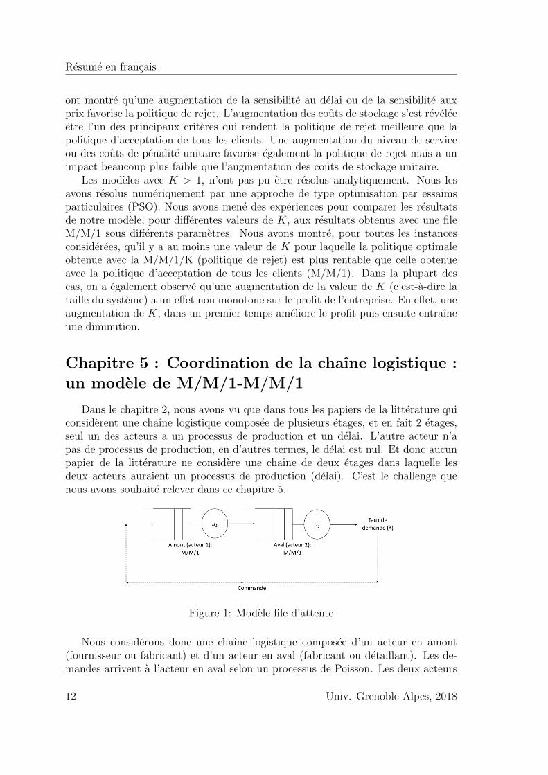
Dans le chapitre 2, nous avons vu que dans tous les papiers de la litterature quiconsiderent une chaıne logistique composee de plusieurs etages, et en fait 2 etages,seul un des acteurs a un processus de production et un delai. L’autre acteur n’apas de processus de production, en d’autres termes, le delai est nul. Et donc aucunpapier de la litterature ne considere une chaıne de deux etages dans laquelle lesdeux acteurs auraient un processus de production (delai). C’est le challenge quenous avons souhaite relever dans ce chapitre 5.
Figure 1: Modele file d’attente
Nous considerons donc une chaıne logistique composee d’un acteur en amont(fournisseur ou fabricant) et d’un acteur en aval (fabricant ou detaillant). Les de-mandes arrivent a l’acteur en aval selon un processus de Poisson. Les deux acteurs
12 Univ. Grenoble Alpes, 2018
Resume en francais
(en amont et en aval) ont une capacite fixe avec un temps de service exponentiel.Ainsi, nous modelisons le systeme comme un reseau en tandem de type M/M/1-M/M/1. Ce systeme est decrit dans la Figure 1.
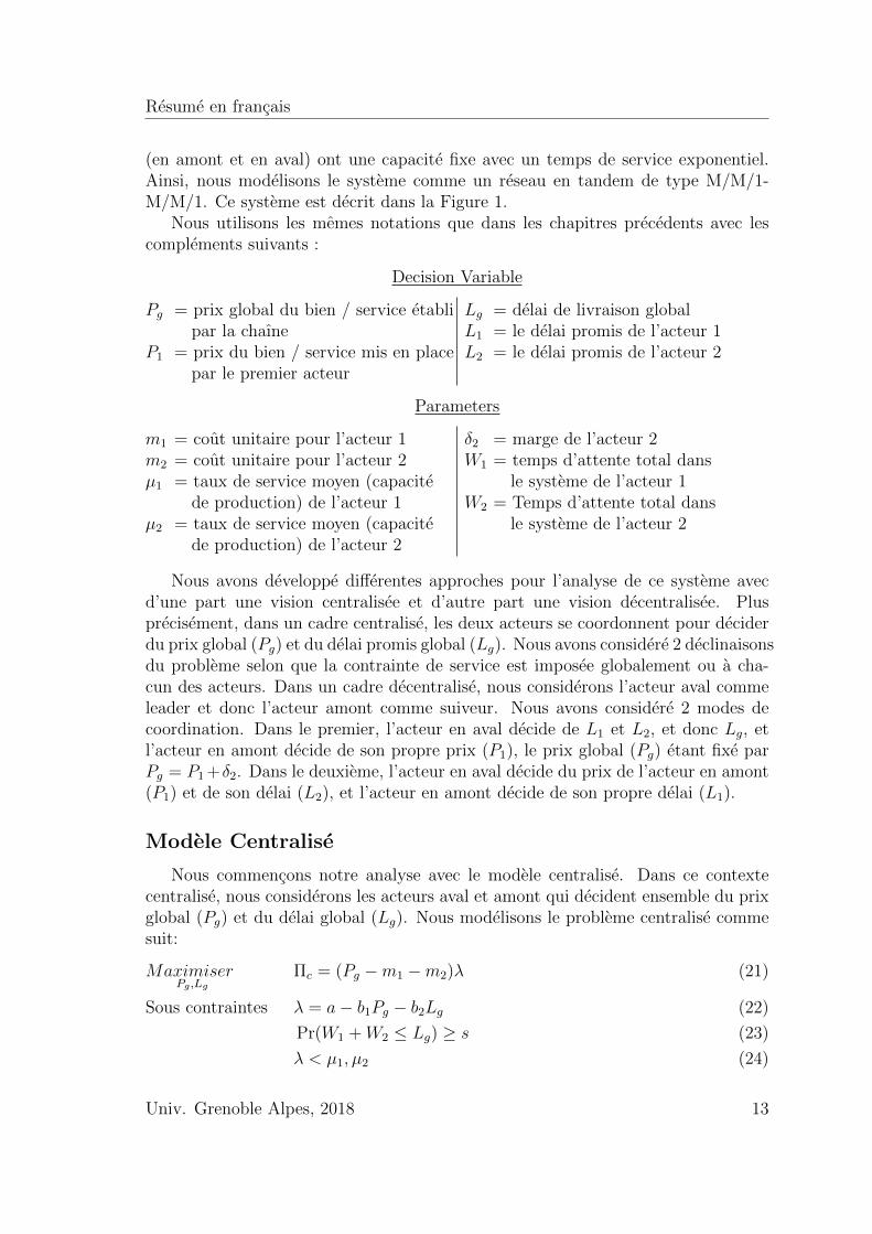
Nous utilisons les memes notations que dans les chapitres precedents avec lescomplements suivants :
Decision Variable
Pg = prix global du bien / service etablipar la chaıne
P1 = prix du bien / service mis en placepar le premier acteur
Lg = delai de livraison globalL1 = le delai promis de l’acteur 1L2 = le delai promis de l’acteur 2
Parameters
m1 = cout unitaire pour l’acteur 1m2 = cout unitaire pour l’acteur 2µ1 = taux de service moyen (capacite
de production) de l’acteur 1µ2 = taux de service moyen (capacite
de production) de l’acteur 2
δ2 = marge de l’acteur 2W1 = temps d’attente total dans
le systeme de l’acteur 1W2 = Temps d’attente total dans
le systeme de l’acteur 2
Nous avons developpe differentes approches pour l’analyse de ce systeme avecd’une part une vision centralisee et d’autre part une vision decentralisee. Plusprecisement, dans un cadre centralise, les deux acteurs se coordonnent pour deciderdu prix global (Pg) et du delai promis global (Lg). Nous avons considere 2 declinaisonsdu probleme selon que la contrainte de service est imposee globalement ou a cha-cun des acteurs. Dans un cadre decentralise, nous considerons l’acteur aval commeleader et donc l’acteur amont comme suiveur. Nous avons considere 2 modes decoordination. Dans le premier, l’acteur en aval decide de L1 et L2, et donc Lg, etl’acteur en amont decide de son propre prix (P1), le prix global (Pg) etant fixe parPg = P1 +δ2. Dans le deuxieme, l’acteur en aval decide du prix de l’acteur en amont(P1) et de son delai (L2), et l’acteur en amont decide de son propre delai (L1).
Modele Centralise
Nous commencons notre analyse avec le modele centralise. Dans ce contextecentralise, nous considerons les acteurs aval et amont qui decident ensemble du prixglobal (Pg) et du delai global (Lg). Nous modelisons le probleme centralise commesuit:
MaximiserPg ,Lg
Πc = (Pg −m1 −m2)λ (21)
Sous contraintes λ = a− b1Pg − b2Lg (22)
Pr(W1 +W2 ≤ Lg) ≥ s (23)
λ < µ1, µ2 (24)
Univ. Grenoble Alpes, 2018 13
Resume en francais
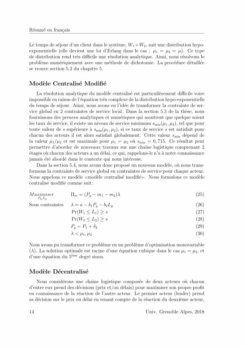
Le temps de sejour d’un client dans le systeme, W1 +W2, suit une distribution hypo-exponentielle (elle devient une loi d’Erlang dans le cas : µ1 = µ2 = µ). Ce typede distribution rend tres difficile une resolution analytique. Ainsi, nous resolvons leprobleme numeriquement avec une methode de dichotomie. La procedure detailleese trouve section 5.2 du chapitre 5.
Modele Centralise Modifie
La resolution analytique du modele centralise est particulierement difficile voireimpossible en raison de l’equation tres complexe de la distribution hypo-exponentielledu temps de sejour. Ainsi, nous avons eu l’idee de transformer la contrainte de ser-vice global en 2 contraintes de service local. Dans la section 5.3 de la these, nousfournissons des preuves analytiques et numeriques qui montrent que quelque soientles taux de service, il existe un niveau de service minimum smin(µ1, µ2), tel que pourtoute valeur de s superieure a smin(µ1, µ2), si ce taux de service s est satisfait pourchacun des acteurs il est alors satisfait globalement. Cette valeur smin depend dela valeur µ1/µ2 et est maximale pour µ1 = µ2 ou smin = 0, 715. Ce resultat peutpermettre d’aborder de nouveaux travaux sur une chaıne logistique comprenant 2etages ou chacun des acteurs a un delai, ce qui, rappelons-le n’a a notre connaissancejamais ete aborde dans le contexte qui nous interesse.
Dans la section 5.4, nous avons donc propose un nouveau modele, ou nous trans-formons la contrainte de service global en contraintes de service pour chaque acteur.Nous appelons ce modele �modele centralise modifie�. Nous formulons ce modelecentralise modifie comme suit:
MaximiserPg ,Lg
Πm = (Pg −m1 −m2)λ (25)
Sous contraintes λ = a− b1Pg − b2Lg (26)
Pr(W1 ≤ L1) ≥ s (27)
Pr(W2 ≤ L2) ≥ s (28)
Pg = P1 + δ2 (29)
λ < µ1, µ2 (30)
Nous avons pu transformer ce probleme en un probleme d’optimisation monovariable(λ). La solution optimale est racine d’une equation cubique dans le cas µ1 = µ2, etd’une equation du 5eme degre sinon.
Modele Decentralise
Nous considerons une chaıne logistique composee de deux acteurs ou chacund’entre eux prend des decisions (prix et/ou delais) pour maximiser son propre profiten connaissance de la reaction de l’autre acteur. Le premier acteur (leader) prendsa decision sur le prix ou delai en tenant compte de la reaction du deuxieme acteur,
14 Univ. Grenoble Alpes, 2018
Resume en francais
alors le second acteur (suiveur) prendra une decision suite a la decision du premieracteur. Ce type de prise de decision est souvent appele �Jeu de Stackelberg�.
Nous avons propose pour cette approche decentralisee deux modes de coordi-nation. Dans les deux scenarios, l’acteur en aval agit comme le leader et l’acteuren amont agit en suiveur. Dans le premier scenario, l’acteur en amont choisit sonpropre delai (L1), mais le prix P1 et le delai de livraison L2 sont decides par l’acteuren aval (acteur 2). Dans le deuxieme scenario, l’acteur en amont (acteur 1) decidede son propre prix (P1) et l’acteur en aval (acteur 2) decide du delai global (L1 +L2).La formulation detaillee et le calcul de chaque modele decentralise se trouvent dansla section 5.5.
A partir de nos experiences, nous voyons qu’en utilisant le premier modeledecentralise (l’acteur en amont decide de son propre delai), le profit global est tresfaible par rapport a celui que l’on peut esperer avec l’approche centralisee. Nousvoyons egalement que le profit de l’acteur en amont est nul. Cela montre que lesacteurs ne se coordonnent pas naturellement de facon satisfaisante. Ainsi, nous pro-posons d’echanger la decision prise par chaque acteur. Dans la deuxieme modele,l’acteur amont (suiveur) decide de son propre prix (P1), et l’acteur aval du delai delivraison L1 et L2, donc Lg. Il est interessant de voir que l’equilibre obtenu est tresproche de la situation ou le profit global est maximum, que ce profit est proche duprofit obtenu en centralise et qu’enfin le reglage du partage des profits peut se faireavec le reglage de la marge de l’acteur aval.
Nous resolvons analytiquement les problemes decentralises et nous fournissonsdes etudes numeriques. Nous avons compare tous les scenarios: centralise, centralisemodifie et les deux modeles decentralises. Le meilleur profit est bien sur celui obtenuavec l’approche centralise. Toutefois, dans la plupart des cas les acteurs de la chaınelogistique ont une certaine autonomie et les scenarios decentralises sont interessants.Nous avons vu que le scenario ou l’acteur en amont choisit son propre prix souscontrainte de delai impose par l’acteur aval est tres interessant.
Chapitre 6 : Conclusion et perspectives
Cette these porte sur l’analyse et l’optimisation de systemes de production dansle cas d’une demande sensible au prix et au delai de livraison promis aux clients.De la revue de la litterature (chapitre 2), on a identifie 3 extensions interessantes:introduire un cout de production unitaire variable; etudier une politique de rejet declients; etudier une chaine composee de 2 etages dans laquelle chacun des acteurs aun delai de production.
Dans la premiere contribution, nous avons resolu le probleme du choix du delaiannonce dans une file d’attente M/M/1 lorsque cout de production est une fonctiondecroissante du delai. Nous avons considere trois situations : (1) le delai est variable,mais le prix est fixe, (2) le prix et le delai sont deux variables de decision, et (3)le prix et le delai sont des variables de decision et le cout de retard et le coutde stockage sont pris en consideration. Nous avons resolu analytiquement les 2
Univ. Grenoble Alpes, 2018 15
Resume en francais
premiers cas et numeriquement le troisieme. Dans le cas 1, nous avons trouvel’expression du delai (L) en fonction des parametres du modele. Mais, dans le cas2, le delai optimal est racine d’une equation cubique. Et, pour le cas 3, nous avonsresolu le modele numeriquement. Nous avons mene des experimentations numeriquesqui montrent que nos modeles conduisent a des gains significatifs par rapport auxmodeles existants ou le cout est suppose etre constant.
Dans la deuxieme contribution, nous avons formule le probleme du choix du delaiet du prix avec possibilite de rejet de clients pour une entreprise modelisee par uneM/M/1/K, face a nouveau a une demande lineaire en fonction des prix et delai, entenant compte du cout de stockage et de la penalite de retard. Afin de determiner lapenalite de retard, nous avons du obtenir un nouveau resultat theorique en calculantexplicitement le temps de sejour residuel au-dela d’un temps donne d’une M/M/1/K.Ce resultat peut etre utilise a l’avenir pour differents problemes de gestion desoperations et de theories de file d’attente. Nous avons montre que dans certainesconfigurations numeriques, la politique de rejet (modelisee par la M/M/1/1) peutetre plus rentable que la politique d’acceptation de tous les clients meme lorsqueles couts de stockage et de penalite ne sont pas pris en consideration. Ceci nousa encourages a etudier des valeurs de K plus elevees, cas que nous avons resolunumeriquement. Nous avons montre sur tous les exemples traites qu’il y a au moinsune valeur de K pour laquelle la M/M/1/K (politique de rejet) est plus rentableque le M/M/1 (la politique d’acceptation de tous les clients). Dans tous les cas, ona egalement observe qu’une augmentation de la valeur de K (c’est-a-dire la tailledu systeme) a un effet non monotone sur le profit de l’entreprise. En effet, dans unpremier temps une augmentation de K ameliore le profit mais ensuite entraıne unediminution.
Dans la derniere contribution, nous avons resolu avec succes (numeriquement) lemodele centralise et le modele dit centralise modifie. Pour ce dernier, nous imposonsdes contraintes locales de service, ce qui a ete possible par la demonstration d’unresultat donnant les conditions pour que la satisfaction de contraintes locales deservice suffisent a la satisfaire globalement. Nous avons aussi introduit et resolu 2modeles decentralises et fait des experiences numeriques.
Nous avons compare les differents scenarios: centralise, centralise modifie et lesdeux modeles decentralises. Si le meilleur profit est bien sur celui obtenu avecl’approche centralisee, nous avons montre l’interet d’un scenario decentralise oul’acteur en amont choisit son propre prix sous contrainte de delai impose par l’acteuraval.
Notre etude peut etre etendue de differentes facons. Par exemple, il seraitinteressant de considerer une autre forme de demande egalement souvent retenuedans la litterature, en l’occurrence le modele de demande Cobb-Douglas (demandeexponentielle decroissante en fonction du delai et du prix). Il serait aussi interessantd’approfondir le cas decentralise en introduisant un systeme incitatif de partage desbenefices notamment dans le scenario ou l’acteur en amont choisit son propre delai(pour eviter un benefice zero de l’acteur en amont). Une autre extension de notre
16 Univ. Grenoble Alpes, 2018
Resume en francais
modele de file d’attente en tandem serait d’inverser les roles de leader-suiveur, avecdonc l’acteur amont en tant que leader et l’aval comme suiveur. Enfin tous sestravaux ont considere une seule firme ou bien 2 firmes en cooperation. On pour-rait egalement envisager une situation de concurrence entre les acteurs des chaıneslogistique.
Univ. Grenoble Alpes, 2018 17

Resume en francais
Univ. Grenoble Alpes, 201818
Chapter 1
Introduction
A large number of firms are using pricing and lead time quotation decisions as astrategic weapon to manage the demand and to maximize the profitability. It is wellknown in the business logistics literature that one of the most important customer-service elements, in addition to price, is the delivery lead time (Sterling and Lambert,1989; Ballou, 1998; Jackson et al., 1986). Along with the price, the delivery lead timehas become a key factor of competitiveness for companies and an important purchasecriterion for many customers (Hammami and Frein, 2013). Since the 90’s, time-basedcompetition has been widely established as a key to success in many industries asreported by Blackburn (1991) and Stalk and Hout (1990). The academic and popularliterature on time-based competition presented ample evidence on how firms can usedelivery lead time as a strategic weapon to gain competitive advantage (Blackburnet al., 1992; Hum and Sim, 1996; Suri, 1998). Geary and Zonnenberg (2000) reportedthat the best in class performers of 110 firms in five major manufacturing sectorsfocus their operations on achieving breakthroughs not only in cost, but also in speed(delivery lead time). Baker et al. (2001) stated that less than 10% of end-consumersand less than 30% of corporate customers base their purchase decisions on an item’sselling price only; the rest also care about other customer-service elements.
Delivery lead time is traditionally defined as the elapsed time between the receiptof customer order and the delivery of this order (Christopher, 2011). Nowadays,firms are more than ever obliged to meet their quoted lead time, that is the deliverylead time announced to the customer. The combination of pricing and lead timequotation implies new trade-offs and offers opportunities for many insights.
For instance, a shorter quoted lead time can lead to an increase in the demandbut also increases the risk of late delivery, which can imply a lower service leveland an increase in the lateness penalty. For many operations sectors, failure ofattaining the quoted lead time might lead to a large amount of penalties. Accordingto Savasaneril et al. (2010), examples that show the importance of reliable lead timequotes are abundant in industry. The authors reported that the cost of late deliveryin the FMC Wellhead Equipment Division may rise up to $250,000 per day andthat the lateness penalties in the aircraft industry starts from $10,000-$15,000 andcan go as high as $1,000,000 per day. In addition to its impact on the cost, thelate delivery may affect the firm’s reputation and deter future customers (Slotnick,2014); companies risk even to lose markets if they are not capable of respecting thequoted lead time (Kapuscinski and Tayur, 2007).
A longer quoted lead time or a higher price generally yields a lower demand,which might have a negative effect on the profitability. This will drive the costumers
19
Chapter 1. Introduction
to order from the competitors who propose shorter quoted lead times and/or lowerprices (Pekgun et al., 2016; Ho and Zheng, 2004; So, 2000; Xiao et al., 2014). Thepositive side of quoting longer lead time is the possibility of attaining higher servicelevel (since, on the one hand, the quoted lead time is longer and, on the other hand,the demand is lower). It can also decrease the in-process inventory holding cost.This latter cost can be significant in many industries such as in automotive andelectronics.
Despite the strategic role of joint pricing and lead time quotation decisions andtheir impacts on demand, the operations management literature has not paid enoughattention to this problem, as reported by Huang et al. (2013). To our knowledge,most of the literature that deals with lead time quotation and pricing under endoge-nous demand (i.e., a demand that depends on quoted lead time and price) considereda Make-To-Order (MTO) context (for the articles that are in Make-To-Stock (MTS)context, see Savasaneril et al., 2010; Savasaneril and Sayin, 2017; Panda, 2013; Wuet al., 2012).
The pioneer paper on lead time quotation and pricing under lead time and pricesensitive demand in MTO context is Palaka et al. (1998). Their research examinedthe lead time setting, pricing decisions, and capacity utilization for a firm servingcustomers that are sensitive to quoted lead times and price. The authors initiallyrestricted their focus to a short time horizon, and hence capacity was assumed tobe constant while price, quoted lead time, and demand were the decision variables.Customers were served on a first come-first served basis. The arrival pattern ofcustomers was modeled by a Poisson process. Further, the processing times of thecustomer orders were assumed to be exponentially distributed. These assumptionsled to the use of an M/M/1 queue to model the firm’s operations. Demand wasassumed to be a linear decreasing function in price and quoted lead time. In thelast part of the paper, the authors considered a capacity expansion case where theyfixed price and modeled demand, lead time, and capacity as decision variables.
Based on Palaka et al. (1998), different extensions have been studied in both sin-gle and multi-firm settings. For instance, in single firm setting, Pekgun et al. (2008)studied the centralization and decentralization of pricing and lead time decisionsbetween production and marketing departments. They used the same framework ofPalaka et al. (1998) for their centralized model but without considering the holdingand penalty costs. Ray and Jewkes (2004) focused on customer lead time man-agement where demand is a function of price and lead time, and where price itselfis sensitive to lead time. Zhao et al. (2012) studied lead time and price quota-tion in service firms and make-to-order manufacturing industries. They consideredtwo strategies: in the first strategy firms offer single lead time and price quotation(uniform quotation mode) and, in the second case they offer a menu of lead timesand prices for customers to choose from (differentiated quotation mode). In themulti-firm setting, Zhu (2015) considered a decentralized supply chain consisting ofa supplier and a retailer facing price- and lead time-sensitive demand. The decisionprocess was modeled as a sequence where supplier determines capacity and whole-
20 Univ. Grenoble Alpes, 2018
Chapter 1. Introduction
sale price, and retailer determines sale price and lead time. Pekgun et al. (2016),which was an extension of Pekgun et al. (2008), studied two firms that compete onprice and lead time decisions in a common market. A detailed discussion of therelevant literature will be developed in chapter 2.
Our review of the literature allowed to identify new perspectives for the problemof lead time quotation and pricing in a stochastic MTO context with endogenousdemand. In particular,
1. The unit production cost was assumed to be constant in most published pa-pers. In practice, the unit production cost generally depends on the quotedlead time. Indeed, the firm can manage better the production process andreduce the production cost by quoting longer lead time to the customers.However, considering a unit production cost as a function of lead time yieldsnew analytical difficulties, especially because the relation between cost andlead time is not linear.
2. In single firm setting, only the M/M/1 queue was used. In M/M/1, all thecustomers are accepted, which might lead to long sojourn times (lead time)in the system. In practice, firms can choose to reject the customers whenthey already have too many customers. Thus, one can consider the use of thecapacitated M/M/1/K queue. However, the formulation of residual waitingtime, which is required to calculate the lateness penalty cost for the overdueclients, is not available in the literature for M/M/1/K.
3. In multi-firm setting, most papers considered that only one actor has produc-tion operations (the other actor has zero lead time). It is more realistic toconsider a supply chain that consists of more than one stage having their ownproduction operations. However, considering a tandem queue is challengingas it leads to a very complex service level constraint.
Based on the observations explained above, we propose three extensions in thisthesis:
• Unit production cost is sensitive to lead time. In the first contribution, we usePalaka et al.’s framework and consider the production cost to be a decreasingfunction in quoted lead time. Indeed, a company can use different ways toreduce lead time (such as buying items from quick response but expensivesubcontractors) but this generally leads to higher production cost. Moreover,a longer lead time can permit a better optimization of production process and,consequently, can lead to a decrease in production cost. The detailed analysisis provided in chapter 3.
• Firm’s operations modeled by an M/M/1/K queue. In the second contribution,we still consider Palaka et al.’s framework but model the firm as an M/M/1/Kqueue, for which demand is rejected if there are already K customers in thesystem. Indeed, our idea is based on the fact that rejecting some customers
Univ. Grenoble Alpes, 2018 21
Chapter 1. Introduction
might help to quote shorter lead time for the accepted ones, which might finallylead to a higher profitability. The detailed discussion is presented in chapter4.
• Two-stage supply chain modeled as a tandem queue (M/M/1-M/M/1). Fi-nally, we study a new setting for the lead time quotation and pricing problemunder endogenous demand as we model the supply chain by two productionstages in a tandem queue. We investigate both the centralized and the decen-tralized settings. This will be the focus of chapter 5.
22 Univ. Grenoble Alpes, 2018
Chapter 2
Literature review
In this chapter, we will discuss the relevant articles on lead time sensitive demandmodels. We provide a classification of the relevant literature in figure 2.1. We classifythe lead time sensitive demand models into two categories: Make-To-Order (MTO)and Make-To-Stock (MTS). In MTO context, we classify the lead time sensitivedemand models into two streams: 1. single-firm models; and 2. multi-firm models.
Our research belongs to the body of literature in MTO context. Thus, we startby discussing the pioneer article Palaka et al. (1998) in section 2.1. Then, we discussthe two streams of the lead time sensitive demand models in MTO context (section2.2 and 2.3). Next, we discuss the papers in Make-To-Stock (MTS) context (section2.4). Finally, we conclude by pointing out our positioning and contributions insection 2.5.
Figure 2.1: Classification of relevant studies
23
Chapter 2. Literature review
2.1 The pioneer paper: Palaka et al. (1998)
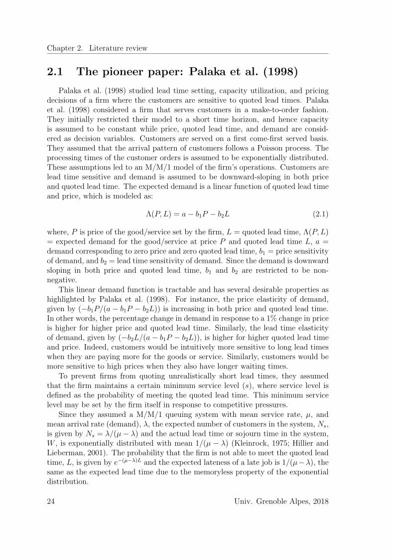
Palaka et al. (1998) studied lead time setting, capacity utilization, and pricingdecisions of a firm where the customers are sensitive to quoted lead times. Palakaet al. (1998) considered a firm that serves customers in a make-to-order fashion.They initially restricted their model to a short time horizon, and hence capacityis assumed to be constant while price, quoted lead time, and demand are consid-ered as decision variables. Customers are served on a first come-first served basis.They assumed that the arrival pattern of customers follows a Poisson process. Theprocessing times of the customer orders is assumed to be exponentially distributed.These assumptions led to an M/M/1 model of the firm’s operations. Customers arelead time sensitive and demand is assumed to be downward-sloping in both priceand quoted lead time. The expected demand is a linear function of quoted lead timeand price, which is modeled as:
Λ(P,L) = a− b1P − b2L (2.1)
where, P is price of the good/service set by the firm, L = quoted lead time, Λ(P,L)= expected demand for the good/service at price P and quoted lead time L, a =demand corresponding to zero price and zero quoted lead time, b1 = price sensitivityof demand, and b2 = lead time sensitivity of demand. Since the demand is downwardsloping in both price and quoted lead time, b1 and b2 are restricted to be non-negative.
This linear demand function is tractable and has several desirable properties ashighlighted by Palaka et al. (1998). For instance, the price elasticity of demand,given by (−b1P/(a− b1P − b2L)) is increasing in both price and quoted lead time.In other words, the percentage change in demand in response to a 1% change in priceis higher for higher price and quoted lead time. Similarly, the lead time elasticityof demand, given by (−b2L/(a− b1P − b2L)), is higher for higher quoted lead timeand price. Indeed, customers would be intuitively more sensitive to long lead timeswhen they are paying more for the goods or service. Similarly, customers would bemore sensitive to high prices when they also have longer waiting times.
To prevent firms from quoting unrealistically short lead times, they assumedthat the firm maintains a certain minimum service level (s), where service level isdefined as the probability of meeting the quoted lead time. This minimum servicelevel may be set by the firm itself in response to competitive pressures.
Since they assumed a M/M/1 queuing system with mean service rate, µ, andmean arrival rate (demand), λ, the expected number of customers in the system, Ns,is given by Ns = λ/(µ− λ) and the actual lead time or sojourn time in the system,W , is exponentially distributed with mean 1/(µ − λ) (Kleinrock, 1975; Hillier andLieberman, 2001). The probability that the firm is not able to meet the quoted leadtime, L, is given by e−(µ−λ)L and the expected lateness of a late job is 1/(µ−λ), thesame as the expected lead time due to the memoryless property of the exponentialdistribution.
24 Univ. Grenoble Alpes, 2018
Chapter 2. Literature review
The firm’s objective is to maximize the expected total profit contribution whichcan be expressed by equation (2.2). In the objective function, λ(P −m) representsthe expected revenue (net of direct costs), where m is the unit direct variable cost.The expected congestion costs are given by Fλ/(µ− λ) where F is the unit holdingcost and λ/(µ−λ) is the expected number of customers in the system. The expectedlateness penalty is given by cr(λ/(µ−λ))e−(µ−λ)L, where cr is the penalty per job perunit lateness, number of overdue client equaled to λe−(µ−λ)L, and expected latenessgiven that a job is late equals to 1/(µ− λ). Finally, Palaka et al. (1998) formulatedthe optimization problem as:
(PBase) MaximizeP,L,λ
Π(P,L, λ) = (P −m)λ− Fλ
µ− λ− crλ
µ− λe−(µ−λ)L (2.2)
Subject to λ ≤ a− b1P − b2L (2.3)
1− e−(µ−λ)L ≥ s (2.4)
0 ≤ λ ≤ µ (2.5)
P,L ≥ 0 (2.6)
Constraint (2.3) ensures that the mean demand, λ, served by the firm did notexceed the demand generated by price, P , and quoted lead time, L. Constraint(2.4) expresses the lower bound on the service level. The service level constraintguarantees that the probability of meeting the quoted lead time (given by 1−e−(µ−λ)L
for an M/M/1 queue), must not be smaller than the minimum required service levels. It is important to note that for Poisson arrivals and exponential service timesassumptions, this form of service constraint is exact. Furthermore, for high servicelevels, it gives a good approximation even for a G/G/s queue (refer to So andSong, 1998). Hence, the model is approximately valid for more general demandand service time characteristics. Constraint (2.5) corresponds to the restriction thatmean demand served, λ, is also bounded by the firm’s processing rate, µ. Constraint(2.6) restricts price and quoted lead times to non-negative values.
In their paper, Palaka et al. (1998) stated that constraint (2.3) is binding atoptimality. The firm will choose price, P , quoted lead time, L, and demand rate,λ, such that λ = Λ(P,L) at optimality. This can be proven by supposing that theoptimal solution is given by price, P ∗, quoted lead time L∗, and demand rate λ∗, andthat λ∗ < Λ(P ∗, L∗). Since the revenues are non-decreasing in P , one could increasethe price to P ′ (while holding the demand rate and quoted lead time constant) untilλ∗ = Λ(P ′, L∗). This change will increase revenues without increasing direct variablecosts and lateness penalties. Therefore, (P ∗, L∗, λ∗) cannot be an optimal solution.
Service level constraint (2.4) in the optimization model (PBase) is not necessarilybinding at optimality. Palaka et al. (1998) stated that the service level constraint(2.4) is non-binding iff the service level, s, is strictly lower than a critical value, sc,that is, s < 1− b1/(b2cr). In addition, the service level is given by max(s, sc).
The solutions of problem PBase in both binding and non-binding cases, as statedby Palaka et al. (1998), are:
Univ. Grenoble Alpes, 2018 25
Chapter 2. Literature review
(a) optimal demand λ∗ is given by the root of cubic equation below on the interval[0, µ]:
(a−mb1 − 2λ)(µ− λ)2 = Gµ
where G = b2 log x+ Fb1 + crb1/x and x = max{1/(1− s), b1cr/b2},
(b) optimal quoted lead time L∗ is given by (log x)/(µ− λ∗), and
(c) optimal price, P ∗, is obtained using the relationship P ∗ = (a− λ∗ − b2L∗)/b1.
This model of Palaka et al. (1998) has been a stepping stone for many recent studies.In the rest of their paper, Palaka et al. (1998) considered the capacity expansion
case where price is fixed. They introduced fractional increase in processing rate (Z),upper bound on capacity expansion (Z), and cost of increasing the processing rateby one job/unit time (ce). The type of capacity expansion that they consider is ashort term nature, e.g., hiring part-time or temporary worker, and running overtime.The capacity expansion is given by µ(1 +Z) with total cost of expansion written asceµZ (for further details see Palaka et al., 1998).
2.2 Single-firm in MTO system
Following Palaka et al. (1998)’s research, several authors dealt with lead timesensitive demand model in MTO single firm. We divide the relevant papers in thissection as papers that propose differentiated lead times to customers, papers thatdealt with coordination between actors in a single firm, papers that model lead timesensitive price, and papers that use log-linear demand model.
Differentiated lead times Papers that propose differentiated lead times to thecustomer are Boyaci and Ray (2003, 2006); Celik and Maglaras (2008); Zhao et al.(2012); and Hafızoglu et al. (2016).
Boyaci and Ray (2003) studied a profit-maximizing firm selling two substitutableproducts in a price and time sensitive market. They considered two type of products:1. regular (slower) product with a given standard industry lead time, and 2. express(faster) product. These products are substitutable and therefore customer demandfor each product depends on the price and delivery time of both products. The twoproducts differ only in their prices and lead times. They assumed that there arededicated capacities for each product. The firm objective is to determine the optimalprice for each product, the quoted lead time for express product, and productioncapacity for each product. They considered the same unit constant operating costfor both regular and express products. They assumed that customers arrive to takedelivery of the products at two separate facilities (one for the regular product andanother for the express) according to a Poisson process. The mean arrival rate(demand) for each of the products is a linear function that depends not only on itsown price and lead time but also price and lead time of the other product. The
26 Univ. Grenoble Alpes, 2018
Chapter 2. Literature review
service time for each product is exponentially distributed and the customers areserved on a first-come first-served basis. The system is modeled as two M/M/1 inparallel. Boyaci and Ray (2003) found that the degree of product differentiationdepends on the values of capacity costs. An increase in capacity cost differentialincreases price differentiation, but decreases time differentiation. They found thatprices can actually decrease when the firm incurs capacity-related costs. The optimalprices depend on the market characteristic.
Boyaci and Ray (2006)’s research is an extension of Boyaci and Ray (2003).However, in this research they assumed that the capacities of both products arefixed. They added a new decision variable instead of capacities which is deliveryreliability (minimum service level s). They introduced a new linear demand modelas a function of price, delivery time and delivery reliabilities of both products. Theirsystem is also modeled as a parallel M/M/1 with constant unit production cost asin Boyaci and Ray (2003). Boyaci and Ray (2006) found that customer preferencestowards delivery times, reliabilities, prices, and the capacity costs have an impacton the firm’s optimal product positioning policy.
Celik and Maglaras (2008) studied the operational and demand control decisionsfaced by a profit-maximizing make-to-order production firm that offers multipleproducts to a market of price and lead time sensitive customers. They emphasizedthree features: 1. the joint use of dynamic pricing and lead time quotation controls tomanage demand; 2. the access to a dual sourcing mode that can be used to expediteorders at a certain cost; and 3. the interaction between the demand controls andthe operational decisions of sequencing and expediting. No production cost wasoccurred. They only considered expediting cost. Demand is assumed to be an N-dimensional non-homogeneous Poisson process with instantaneous rate vector wherethe arrival rate of potential customers is sensitive to price and quoted lead time. Aproposed heuristics and Markov decision process formulation were used to solve theproblem in their study. Unlike Boyaci and Ray (2003, 2006), Celik and Maglaras(2008) considered one or several good(s) offered at multiple (price and lead time)combinations. Their numerical results illustrate the effectiveness of dynamic overstatic pricing, as well as the impact of lead time control policies.
Zhao et al. (2012) analyzed strategies where a firm offers a single lead time andprice (uniform quotation mode (UQM)) or offers a menu of lead times and prices (dif-ferentiated quotation mode (DQM)). They also classified customers into two groups:lead time sensitive (LS) customers who value more the lead time reduction and pricesensitive (PS) customers who value more the price reduction. They assumed thatcostumers for UQM arrive in Poisson process and for DQM in sub-Poisson. UnlikeBoyaci and Ray (2003, 2006), Zhao et al. (2012) modeled the demand as a functionof utility (willingness-to-pay) where the linear utility depend on price and lead time.The service times are exponentially distributed. Thus, they modeled the system asM/M/1 for UQM and parallel M/M/1 for DQM. They considered a constant pro-duction cost. They used their model to determine the optimal quoted lead time,price and service rate (µ). They found that DQM is dominated by UQM when LS
Univ. Grenoble Alpes, 2018 27
Chapter 2. Literature review
customers value a product or service no more than PS customers. Otherwise, whichquotation mode is better depends on multiple factors, such as customer characteris-tics (including lead time reduction valuation and product valuation of a customer,and the proportion of LS customers) and production characteristics (including thedesired service level and service or production cost).
Hafızoglu et al. (2016) studied price and lead time quotation decisions in make-to-order system with two customer classes: (1) contract customers whose orders arealways accepted and fulfilled based on a contract price and lead time agreed on atthe beginning of the time horizon, and (2) spot purchasers who arrive over time andare quoted a price and lead time pair dynamically. The spot customer will placean order or not according on quoted lead time and price proposed. The objectiveis to maximize the long-run expected average profit per unit time, where profitfrom a customer is defined as revenues minus lateness penalties incurred becauseof lead time violations. They did not consider production cost. Hafızoglu et al.(2016) model the dynamic quotation problem of the spot purchasers as an infinitehorizon Markov decision process, given a fixed price and lead time for contractcustomers. They showed that the optimal price and lead time quotation policy isheavily affected by the price/lead time sensitivity of the spot purchasers and thepenalty for missed due dates. When spot purchasers are highly price sensitive, it isoptimal to quote a small fixed price while dynamically changing the lead time. Incontrast, if spot purchasers are highly lead time sensitive, offering zero lead timesand dynamic pricing is optimal.
Two actors’ coordination Pekgun et al. (2008) dealt with coordination betweenmarketing and production departments of a single firm in deciding pricing and leadtime decisions. They studied a firm which serves customers that are sensitive toquoted price and lead time with pricing decisions being made by the marketingand lead time decisions by production departments. In their paper, they assumedthat demand is a linear function of price and lead time, unit production costs areconstant, and the firm system is modeled as M/M/1 queue. They considered twosettings of decision-making: centralized and decentralized settings. In centralizedsetting, lead time quotation and pricing decisions are taken simultaneously. In thissetting, Pekgun et al. (2008) used a simplified version of Palaka et al. (1998)’s modelwhere they don’t consider the lateness penalty and congestion cost. In decentralizedsetting they considered that the decisions are taken sequentially (as a Stackelberggame). Under this setting, Pekgun et al. (2008) developed two cases: 1. productionacts as a leader who decides the quoted lead time and marketing acts as a followerwho decides the price; and 2. marketing acts as a leader who decides the priceand production acts as a follower who decides the quoted lead time. They foundthat inefficiencies are created by the decentralization of the price and lead timedecisions. In the decentralized setting, the total demand generated is larger, leadtimes are longer, quoted prices are lower, and the firm’s profits are lower comparedto the centralized setting. They stated that coordination can be achieved using a
28 Univ. Grenoble Alpes, 2018
Chapter 2. Literature review
transfer price contract with bonus payments.
Lead time sensitive price Ray and Jewkes (2004) modeled an operating systemconsisting of a firm and its customers, where the mean demand rate is a functionof the guaranteed delivery time (quoted lead time) offered to the customers and ofmarket price, where price itself is determined by the length of the delivery-time.Firm’s production system is modeled as M/M/1. They introduced the explicitdependence of price on lead time as an additional relationship. Ray and Jewkes(2004) stated that the new link of price and lead time captures a relationship thatexists in practice. If this relationship is ignored, it could lead to a weak decision.In the latter part of their paper, they incorporated economies of scale by assumingthat the unit operating cost is a decreasing function of the demand rate within acertain volume range.
Log-linear demand model So and Song (1998) studied the impact of using de-livery time guarantees as a competitive strategy in service industries where demandsare sensitive to both price and delivery time. They assumed that delivery reliabilityis crucial, and investment in capacity expansion is plausible in order to maintain ahigh probability of delivering the time guarantee. Thus, their objective is to findthe optimal price, delivery time guarantee, and capacity selection in order to maxi-mize profit. The production costs in So and Song (1998)’s model is assumed to beconstant. So and Song (1998)’s main difference compared to Palaka et al. (1998) istheir demand model. So and Song (1998) modeled the demand as log-linear model(Cobb-Douglas). As for the firm system, they modeled it as M/M/1 similar toPalaka et al. (1998).
2.3 Multi-firm in MTO system
In this subsection, we consider lead time sensitive demand models in MTO systemwith multi-firm. We divide the literature into two groups: competition models andcooperation models.
Competition models In papers dealing competitive firms, we have Li (1992); So(2000); Ho and Zheng (2004); Xiao et al. (2014); Xiaopan et al. (2014); and Pekgunet al. (2016).
Li (1992) studied the role of inventory in response time competition. Their objec-tive is to determine the optimal production/inventory policy and the optimal choicebetween make-to-order and make-to-stock operation. He dealt first with a singlefirm production control in which customers are characterized by their preference ofprice, delivery quality and delivery-time (lead time). The demand from customersarises over time according to a Poisson process with intensity λ. Customers will buyor not buy the product depending on their utility (willingness to pay) where the
Univ. Grenoble Alpes, 2018 29
Chapter 2. Literature review
utility is a function of price, delivery quality, and delivery time. The firm incurs aconstant unit production cost. In the first part of his paper, Li (1992) considered asingle firm, then he extends his work to competitive multi-firm where firms competefor orders in terms of early delivery. The competition they introduced is only intimely delivery rather than price, product, or other aspect of the market. The goalis to show that competition breed a demand for make-to-stock. The competition inLi (1992) can be considered as parallel M/M/1 queue. With lead time uncertainty,they identified three important factors in firm’s decision on production/inventorypolicies: discount, costumer characteristic, and competition. They found that theincentive for make-to-stock decreases when the nature of the market switches in theorder of oligopoly racing, monopoly, and the demand sharing market. They alsofound that delivery-time competition increases the buyer’s welfare while decreasesthe producer’s welfare.
So (2000) developed a stylized model to analyze the impact of using time guar-antees (quoted lead time) on competition. This research is an extension of So andSong (1998). Unlike So and Song (1998) who considered a single firm, So (2000)considered a competition between two firms. This competition is modeled as a par-allel M/M/1 queue where each firm decides price and time guarantee. So (2000)’sdemand model is similar to So and Song (1998). In their study, So (2000) foundthat different firm and market characteristics affect the price and delivery time (leadtime) competition in the market. The equilibrium price and time guarantee deci-sions in an oligopolistic market with identical firms behave in a similar fashion asthe optimal solution in a monopolistic situation from So and Song (1998). However,when there are heterogeneous firms in the market, these firms will exploit theirdistinctive characteristics to differentiate their services. Assuming all other factorsbeing equal, the high capacity firms provide better time guarantees, while firms withlower operating costs offer lower prices, and the differentiation becomes more acuteas demands become more time-sensitive. As time-attractiveness of the market in-creases, firms compete less on price, and the equilibrium prices of the firms increaseas a result.
Ho and Zheng (2004) studied how a firm might choose a delivery time commit-ment to influence its customer expectation, and delivery quality in order to maximizeits market share. They stated that many firms now choose to set customer expec-tation by announcing their maximal delivery time. Customers will be satisfied iftheir perceived delivery times are shorter than their expectations. They considereda firm that serves a population of homogeneous customers who are impatient andsensitive to service delivery time. The firm’s objective is to maximize the demandrate, which is affected by customers’ expectation for the delivery time as well asthe probability that this expectation is being fulfilled. In Ho and Zheng (2004)research, no production cost is incurred. They modeled the whole service deliveryprocess as an M/M/1 queueing system where the arrival (demand) rate depends oncustomer’s utility for the firm’s service. Unlike Zhao et al. (2012), Ho and Zheng(2004)’s customer’s utility for the firm’s service depends on the expected delivery
30 Univ. Grenoble Alpes, 2018
Chapter 2. Literature review
time and service quality. In the first part of their paper, they considered single firm.Then, they considered two firms in duopoly competition where firms compete fora fixed market. The competition is modeled as parallel M/M/1. These two firmscompete in obtaining demand (market share). Ho and Zheng (2004) showed thatthe delivery time commitment game is analogous to a Prisoners’ Dilemma.
Xiao et al. (2014) developed a game theory model of a one-manufacturer andone-retailer supply chain facing an outside integrated chain (a manufacturer) tostudy the price and lead time competition and investigate coordination within theirsupply chain. They considered a make-to-order production mode and consumers aresensitive to retail price and quoted lead time. In one-manufacturer and one-retailersupply chain, the manufacturer decides wholesale price and quoted lead time, thenretailer decides retail price. Here, the retailer has zero lead time. In the integratedchain, the lead time quotation and pricing decision are taken simultaneously by amanufacturer. The demand in Xiao et al. (2014)’s model is a linear function inutility where the utility (willingness-to-pay) itself is sensitive to lead time and price.The unit production cost of both chains are assumed to be constant. Xiao et al.(2014) modeled their problem in Hotelling’s Location Model and the objective foreach chain is to maximize its own profit. Hotelling model is a model introduced byHotelling (1929) where consumer market is conceptualized as a straight line in anideal preference space, with exogenously specified locations for the two brands (i.e.,manufacturer-retailer chain and integrated chain). Xiao et al. (2014) found that thecoordination of the supply chain facing integrated chain harms the integrated chain.In addition, the existence of the outside competitor increases the lead time. Theyalso found the Nash equilibrium of this competition.
Xiaopan et al. (2014) investigated the competition and cooperation in a duopolysetting where two dominant facilities control over a market. The demand faced byeach facility is not only sensitive to its own retail price and guaranteed deliverytime, but also to the differences between the two prices and guaranteed deliverytimes. They analyzed three different competition scenarios where 1. the two facilitiescompete exclusively on retail prices, 2. exclusively on guaranteed delivery times,and 3. both on retail prices and guaranteed delivery times. They also analyzedthree different cooperation scenarios where 1. firms cooperate exclusively on retailprices, 2. exclusively on guaranteed delivery times, and 3. both on retail prices andguaranteed delivery times. In all scenarios, the objective of the firms is to maximizetheir profit. The demand in all scenarios follows Poisson process and it is a linearfunction in price, lead time and sensitivity of switch-over toward price and leadtime difference (similar to Boyaci and Ray, 2003). The market system is modeledas parallel M/M/1 and unit production costs are assumed to be constant. In theirstudy, Xiaopan et al. (2014) found that the competition on retail prices for givenguaranteed delivery times is as same as the Bertrand game, reaching to the Nash-Bertrand equilibrium. Nash-Bertrand equilibrium occurs when both firms set priceequal to unit cost (the competitive price). The equilibrium guaranteed delivery timeof each facility for given retail prices only depends on its own retail price. When
Univ. Grenoble Alpes, 2018 31
Chapter 2. Literature review
price is a decision variable, the gross profits of the facilities increase significantly viacoordinating retail prices.
Pekgun et al. (2016)’s research is an extension of Pekgun et al. (2008). Pekgunet al. (2016) studied two firms that compete on price and lead time decisions in acommon market. They investigated the impact of decentralizing the decisions ofpricing by marketing department and lead time quotation by production depart-ments, with either marketing or production as the leader. They compared scenariosin which none, one, or both of the firms are decentralized. The market system ismodeled as a parallel M/M/1. They found that under intense price competition,firms may suffer from a decentralized structure. In contrast, under intense lead timecompetition, a decentralized strategy with marketing as the leader can not onlyresult in significantly higher profits, but also be the equilibrium strategy. More-over, decentralization may no longer lead to lower prices or longer lead times if theproduction department chooses capacity along with lead time.
Cooperation models In papers dealing with cooperative firms, we have Liu et al.(2007); Xiao et al. (2011); Xiao and Shi (2012); Zhu (2015); and Xiao and Qi (2016).
Liu et al. (2007) studied a decentralized supply chain consisting of a supplierand a retailer facing a price- and lead time-sensitive demand. They constructeda Stackelberg game to analyze the price and lead time decisions by the supplieras leader and the retailer as follower. Upon receiving an order from the retailer,the supplier completes the finished product and delivers it to the retailer (or to thecustomer directly on behalf of the retailer). The product is not unique in the marketand potential customers for the product are sensitive to both price and promised leadtime. This requires the supply chain to offer a competitive retail price and quotedlead time. They assumed the supplier system to be modeled as a single-server queue(M/M/1) with the exponential service time and constant unit production cost. Theretailer has zero lead time because no production process is occurred. They alsoassumed that demand process is Poisson where demand itself is a linear functionin promised lead time and retailer price. They found that decentralized decisionsare inefficient and lead to inferior performance due to the double marginalizationeffect. The decision inefficiency is strongly influenced by market and operationalfactors. Before pursuing a coordination strategy with retailers, a supplier shouldfirst improve his or her own internal operations.
Xiao et al. (2011) investigated coordination of a (global) supply chain consistingof one manufacturer and one retailer via a revenue-sharing contract, where a prod-uct quality assurance policy is provided and the utility of consumer is sensitive toproduct (physical) quality, service quality (i.e., reciprocal of delivery lead time) andretail price. The supply chain operates in a MTO environment and a defective prod-uct is returned to the manufacturer for free re-manufacturing. Consumers return theimperfect products to the manufacturer for re-manufacturing within a guaranteedperiod. Every reworked unit is as good as new after rework and the manufacturer re-quires no rework charges for consumers or the retailer. They considered centralized
32 Univ. Grenoble Alpes, 2018
Chapter 2. Literature review
and decentralized settings. In the centralized setting, all decisions are taken simul-taneously via a moderator or by a higher authority. In the decentralized setting,decisions are taken as a sequence. Manufacturer determines both unit wholesaleprice and quoted lead time, then the retailer determines retail price following thedecision of manufacturer. Consumers arrive at the retailer following a Poisson pro-cess. The order is processed in a first-come-first-served fashion and the productiontime is exponentially distributed. The unit production cost is assumed to be con-stant. The manufacturer follows an M/M/1 system. And the retailer only acts asmediator without production process happen in retailer, thus the retailer lead timeis equal to zero. This demand function is a result of utility function which dependson product physical quality, lead time and return loss. In the decentralized setting,Xiao et al. (2011) found that: 1. a higher defective rate of the final product impliesa higher cost for the manufacturer, 2. the optimal service quality first decreasesand then increases, and 3. the optimal retail price decreases as the defective rateincreases. In the coordinated supply chain, the manufacturer charges the retailer ahigher unit wholesale price.
Xiao and Shi (2012) considered a supply chain consisting of one make-to-order(MTO) manufacturer and one retailer in a price and lead time sensitive market.They developed a Manufacturer-Stackelberg (MS) model with predetermined (ex-ogenous) lead time standard and a MS model with endogenous lead time standard.Following Boyaci and Ray (2003), they assumed that the manufacturer provides twosubstitutable products: regular product and faster product. The difference betweenthe two kinds of products only lies in lead time standard. When a consumer arrivesat the retailer, the consumer determines to buy the regular product or the fasterproduct. Once consumer made an order, the retailer sends the order to the manu-facturer immediately and then the manufacturer sets up production. So, the retailerserves as an intermediary between consumers and the manufacturer. Both playersaim to maximize their long-term average profits. The manufacturer has a dedicatedfacility for each product. Both facilities process orders following a first-come-first-serve service discipline. Each facility is an M/M/1 queuing service system withPoisson arrival and exponential service time. Similar to Boyaci and Ray (2003), theunit production costs (excluding capacity cost) for the two products are identical,but the faster product has a higher unit capacity cost than the regular product.Their demand model is similar to Boyaci and Ray (2003). They found that whenthe lead time sensitivity increases, the players decrease the unit wholesale prices andretail prices for the two products and reduce the lead time standard for the fasterproduct. The manufacturer builds a lower capacity for the regular product while ahigher capacity for the faster product.
Zhu (2015) considered a decentralized supply chain consisting of a supplier and aretailer facing price- and lead time-sensitive demand. The decision process is mod-eled by a Stackelberg game where the supplier, as a leader, determines the capacityand the wholesale price, and the retailer, as a follower, determines the sale priceand lead time. Unlike Liu et al. (2007) who considered either pricing and capac-
Univ. Grenoble Alpes, 2018 33
Chapter 2. Literature review
ity decisions or pricing and lead time decisions, Zhu (2015) studied the integrationof pricing, lead time, and capacity decisions. The supply chain framework of Zhu(2015) is similar to Liu et al. (2007) where the supplier has M/M/1 production sys-tem and retailer has zero lead time. Zhu (2015) found that the integration of pricing,lead time, and capacity decision can significantly reduce the profit loss caused bydouble marginalization. The revenue-sharing and two-part tariff contracts cannotcoordinate the decentralized channel. Instead, a franchise contract with a contingentrebate can achieve channel coordination and a win–win outcome.
Xiao and Qi (2016) studied the equilibrium decisions in the supply chain withan all-unit quantity discount contract. They considered a two-stage supply chainwith one supplier and one manufacturer. The manufacturer faces a Poisson de-mand process where the arrival rate depends on the selling price, the announceddelivery time, and the delivery reliability defined as the probability of satisfying theannounced delivery time. The supplier produces a standard product in MTS mode.The manufacturer purchases standard products from the supplier at a unit wholesaleprice, takes orders from end users, customizes the standard products based on orderspecifications, and delivers the final products to end users. The supplier and themanufacturer maximize their long-term average profit per time unit. They assumedthat the supply chain adopts vendor managed inventory (VMI) mode to manage thesupply chain’s inventory, and the production rate of the supplier is greater than themanufacturer’s service rate (capacity). Under VMI, the effect of resource constrainton the manufacturer can be ignored because the MTS supplier has a greater pro-duction rate than the manufacturer’s capacity and can well control the inventory ofstandard products. Xiao and Qi (2016) used the M/M/1 queuing model to describethe operations of the manufacturer. They considered coordination of a decentralizedsupply chain where supplier decides the wholesale price, and manufacturer decidesjointly the resale price and the quotation of lead time. They considered four sce-narios regarding whether the lead time standard, the delivery reliability standard,and the manufacturer’s capacity are endogenous, and whether the manufacturer’sproduction cost is its private information. They found that an all-unit quantitydiscount scheme can coordinate the supply chain for most cases.
2.4 Other related papers: the MTS system
Other papers related on lead time sensitive demand models are in the MTScontext. Examples include Savasaneril et al. (2010); Wu et al. (2012); Panda (2013);and Savasaneril and Sayin (2017).
Savasaneril et al. (2010) studied a dynamic lead time quotation problem in abase-stock inventory system characterized by lead time sensitive Poisson demandand exponentially distributed service times. They show that the optimal profit isunimodal in the base-stock level. They compare the base-stock system with a make-to-order (MTO) system and show that the lead time quotes are lower in an MTOsystem and that increasing the base-stock level does not necessarily decrease the
34 Univ. Grenoble Alpes, 2018
Chapter 2. Literature review
expected number of customers waiting.Wu et al. (2012) studied the news-vendor problem with endogenous demand
sensitive to price and quoted lead time. The problem is observed in situationswhere a firm orders semi-finished product prior to the selling season and customizesthe product in response to customer orders during the selling season. The totaldemand during the selling season and the lead time required for customization areuncertain. The demand for the product depends not only on the selling price butalso on the quoted lead time. To set the quoted lead time, the firm has to carefullybalance the benefit of increasing demand as the quoted lead time is reduced againstthe cost of increased tardiness.
Panda (2013) dealt with the coordination of a supply chain that consists of amanufacturer and a price setting retailer. The manufacturer offers a single productto the retailer, who faces time and price sensitive demand. Under explicit costin- formation, optimal quantity–price pairs are derived for an integrated scenarioand a decentralized scenario by considering the manufacturer as the Stackelbergleader. The objective of Panda (2013) is to determine price, order quantity andreplenishment cycle length in order to maximize the total profit of the chain. Intheir model, demand is a function of time and price.
Savasaneril and Sayin (2017) addressed the lead time quotation problem of amanufacturer serving multiple customer classes. Customers are sensitive to thequoted lead times and the manufacturer has the flexibility to keep inventory toimprove responsiveness. They model the problem as a Markov decision process andcharacterize the optimal lead time quotation, rationing, and production policies.
2.5 Conclusion of literature review
From the literature review, we make the following observations. First, all papersassume that the unit production cost is a constant. In practice, a firm can managebetter its production system when it quotes longer lead time. Thus, we will extendthe existing models by considering the direct relation between the unit productioncost and the quoted lead time in chapter 3. Second, in the single firm case, the vastmajority of works use the M/M/1 system. Although M/M/1 is the simplest queuingmodel, it has a drawback since all the customers are accepted which might lead tolong sojourn time in the system. Thus, we propose to test whether a new policy,which consists of rejecting customers when there are already a certain number ofcustomers in the system, can be more profitable. We call this policy a rejectionpolicy. The detailed discussion is provided in chapter 4. Third, in the case ofmulti-firm, all works assume that only one of the actors has a production process(queuing system), the other actor only acts as a mediator with a lead time thatequals to zero. Thus, we will introduce a supply chain where the two actors have aproduction system in chapter 5.
In this thesis, we will consider MTO systems, uniform lead time quotation, single-class product, single- class customer, and linear demand model and we will propose
Univ. Grenoble Alpes, 2018 35
Chapter 2. Literature review
three contributions:
1. Introduce a unit production cost that depends on the quoted lead time,
2. Consider a policy allowing to reject the clients by using an M/M/1/K queue,
3. Introduce a supply chain (multi-firm) where the two actors have a productionprocess, which leads to a tandem queue M/M/1-M/M/1.
These three problems are investigated in the following chapters to achieve the PhDobjective.
36 Univ. Grenoble Alpes, 2018
Chapter 3
Lead time sensitive cost: aproduction system with demandand production cost sensitive to
lead time (M/M/1 model)
Some research has been done on M/M/1 queuing systems with lead time- andprice-dependent demand. However, all of the works, presented in chapter 2, assumea constant production cost. It is known that the longer the quoted lead time thebetter the firm can manage the production and reduce the cost. The idea of thispaper stems from this observation. Indeed, we investigate the lead time quotationdecision in an M/M/1 make-to-order queue while assuming the production cost tobe a decreasing function in lead time. We consider three settings: (1) price is fixedand holding and lateness costs are ignored, (2) price is also a decision variable (inaddition to lead time) but holding and lateness costs are ignored, and (3) price isa decision variable and holding and lateness costs are considered. For setting 1 and2, we provide an approach to find analytically the optimal lead time and price (if itis a variable). And for setting 3, we develop a numerical approach to solve the case.We use the optimal solutions to conduct experiments and derive some insights.
3.1 The model
We model the firm as an M/M/1 Make-to-Order queue. Customers arrive andare served in a first-come-first-served fashion. The demand follows a Poisson processof mean arrival rate λ, which cannot be larger than the amount of demand Λ(P,L)obtained when price, P , and lead time, L, are quoted to the customers. As usuallyassumed in the literature (see the aforementioned papers), we consider that the de-mand linearly decreases with price and quoted lead time, Λ(P,L) = a− b1P − b2Lwhere b1 and b2 are the sensitivity coefficients to price and lead time, respectively.The production capacity is constant (µ) and the service time is exponentially dis-tributed.
It is well known that the unit operating cost depends on the quoted lead time inmany situations. In particular, firms that quote short lead time to their customers,and that are consequently exposed to high risk, do not focus only on productioncapacity but rethink the different decisions along the supply chain and align them
37
Chapter 3. Lead time sensitive cost: a production system with demand andproduction cost sensitive to lead time (M/M/1 model)
with the lead time strategy to reduce the risk as much as possible. Examples includebuying items from quick-response but expensive suppliers instead of regular low-costsuppliers (e.g. local suppliers instead of suppliers abroad), holding higher stock ofraw materials in the upstream stages, using faster but more costly transportationmodes (e.g., in the logistics industry, FedEx Express uses airplanes while FedExground uses trucks), and rethinking the production/delivery process by moving thetradeoff toward shorther lead time instead of cheaper production (e.g., less economiesof scale in production, less grouped shipments, etc.). In all these examples, theshorter the quoted lead time the more difficult the required actions become and,consequently, the higher the unit production cost.
Thus, we do not assume a constant production cost but consider the unit pro-duction cost (m) to be a decreasing function in quoted lead time (L). Indeed, m isgiven by the following non-linear function: m = C1 + C2
L. This function implies that
the increase in unit production cost that results from one unit decrease in lead timeis not constant (as in linear functions) but is growing with smallest values of leadtime. In other words, the smaller the value of the lead time the more difficult (and,consequently, the more expensive), its reduction becomes. Clearly, the productioncost usually used in the existing literature is a particular case of our cost functionwith C2 = 0.
The decision variables and parameters for this chapter are given below:
Decision variables:λ : mean arrival rate (demand),L : quoted lead time,P : price of the goods/service,m : unit production cost.
Parameters:a : market potential,b1 : price sensitivity of demand,b2 : lead time sensitivity of demand,µ : mean service rate (production capacity),s : service level defined by company (s ∈ [0, 1]),F : unit holding cost,cr : penalty per job per unit lateness,C1, C2 : production cost parameters.
The firm’s objective is to maximize the total expected profit, which equals torevenue (λP ) – production cost (λm) – expected holding cost (Fλ/(µ − λ)) – ex-pected lateness penalty cost (cr(λ/(µ−λ))e−(µ−λ)L). The lateness cost reflects directcompensation paid to customers for not meeting the quoted lead time. Firm has tomake sure to meet its quoted lead time within a service rate (s). The expected con-gestion cost is given by Fλ/(µ− λ) where F is the unit holding cost, and λ/(µ− λ)is the mean inventory. The expected lateness penalty can be given by (penalty per
38 Univ. Grenoble Alpes, 2018
Chapter 3. Lead time sensitive cost: a production system with demand andproduction cost sensitive to lead time (M/M/1 model)
job per unit lateness) × (throughput rate) × (probability that a job is late) × (ex-pected lateness given that a job is late). Thus, the expected lateness penalty is:cr(λ/(µ − λ))e−(µ−λ)L where cr is the penalty per job per unit lateness, e−(µ−λ)L isthe probability that a job is late and λ/(µ−λ) is the (throughput rate) × (expectedlateness) (see Palaka et al., 1998). The formulation of our general model is givenbelow.
MaximizeL,P,λ,m
λ(P −m)− Fλ
µ− λ− crλ
µ− λe−(µ−λ)L (3.1)
Subject to λ ≤ a− b1P − b2L (3.2)
1− e−(µ−λ)L ≥ s (3.3)
λ ≤ µ (3.4)
m = C1 +C2
L(3.5)
λ, L, P,m ≥ 0 (3.6)
The objective function is given in Equation (3.1). Equation (3.2) ensures thatthe mean demand rate received by the firm cannot exceed the demand generatedby the quoted price and lead time. Equation (3.3) guarantees that the probabilityof meeting the quoted lead time, given by 1 − e−(µ−λ)L (since e−(µ−λ)L is known tobe the probability that a job is late in M/M/1 queue), must not be smaller thanthe required service level. Equation (3.4) guarantees a steady state of the M/M/1.Equation (3.5) defines the production cost function. The non-negativity constraintsare given in Equation (3.6).
As stated before, we consider three settings: (1) Fixed price without holding andlateness penalty cost, (2) Price as decision variable without holding and lateness cost,and (3) Price as decision variable with holding and lateness cost. Before moving tothe solving approach of each setting, we point out the following general result, whichis verified under all settings.
Lemma 3.1. Demand constraint (3.2) is binding and we have λ = a − b1P − b2Lat optimality.
Proof. Suppose that the optimal solution is given by quoted lead time L∗, price P ∗,and demand rate λ∗ such that λ∗ < a − b1P
∗ − b2L∗. The profit increases when L
increases as an increase in L leads to decrease in production cost (m = C1 + C2
L) and
in lateness penalty cost (for setting 3). An increase in L also leads to decreasingthe probability of having late delivery (e−(µ−λ)L). Thus, by keeping price P ∗ anddemand rate λ∗ constant, one could increase the lead time from L∗ to L′ untilλ∗ = a− b1P
∗ − b2L′. This change will increase profit as production cost decreases,
lateness penalty cost decreases, and holding cost stays the same (because λ doesn’tchange), while the service level constraint remains satisfied. Therefore, we wouldget a new solution: P ∗, λ∗, and L′ with a better profit than the supposed optimalsolution, which is impossible. �
Univ. Grenoble Alpes, 2018 39
Chapter 3. Lead time sensitive cost: a production system with demand andproduction cost sensitive to lead time (M/M/1 model)
Given the result of lemma 3.1, we will use λ = a− b1P − b2L for the rest of thischapter. Note also that constraint (3.4) is immediately satisfied if service constraintis satisfied and the lead time is positive. Therefore, constraint (3.4) can be removed.
3.2 Setting 1: Model with variable lead time and
fixed price
In this section, we consider the model when price is fixed (not a decision variable).
3.2.1 Optimal policy with variable lead time and fixed price
We solve analytically the model when price is fixed. By considering the result ofLemma 3.1 and integrating the expression of production cost (m) into the objectivefunction, the problem can be formulated as a constrained non-linear optimizationmodel with a single decision variable L. Indeed, we respectively replace λ and m bya− b1P − b2L and C1 + C2
L. Thus, the model with fixed price becomes equivalent to
the following model.
MaximizeL≥0
f(L) = (a− b1P − b2L)
(P − C1 −
C2
L
)(3.7)
Subject to (µ− a+ b1P )L+ b2L2 ≥ ln
(1
1− s
)(3.8)
L ≤ a− b1P
b2
(3.9)
Equation (3.8) represents the service constraint after rewriting 1− e−(µ−λ)L ≥ sas (µ− λ)L ≥ ln
(1
1−s
). In the rest of the paper, we let γ denote ln
(1
1−s
). Equation
(3.9) guarantees that λ ≥ 0, which is equivalent to L ≤ a−b1Pb2
. In order to solve themodel, we firstly consider the following lemma.
Lemma 3.2. The feasible region of profit f(L) is defined by:[max
{C2
P−C1,a−b1P−µ+
√(a−b1P−µ)2+4b2γ
2b2
}, a−b1P
b2
]Proof. Service level constraint is satisfied iff (µ − a + b1P )L + b2L
2 ≥ γ (see eq.(3.8)). The equation (µ − a + b1P )L + b2L
2 − γ = 0 has a discriminant ∆ =
(µ − a + b1P )2 + 4b2γ and two roots:a−b1P−µ±
√(a−b1P−µ)2+4b2γ
2b2. Thus, the service
level constraint (3.8) is satisfied iff: L ≥ a−b1P−µ+√
(a−b1P−µ)2+4b2γ
2b2, which is positive,
or L ≤ a−b1P−µ−√
(a−b1P−µ)2+4b2γ
2b2, which is negative. Furthermore, we have L ≥ C2
P−C1
(indeed to have a positive profit, we must have cost lower than price: P −C1− C2
L≥
40 Univ. Grenoble Alpes, 2018
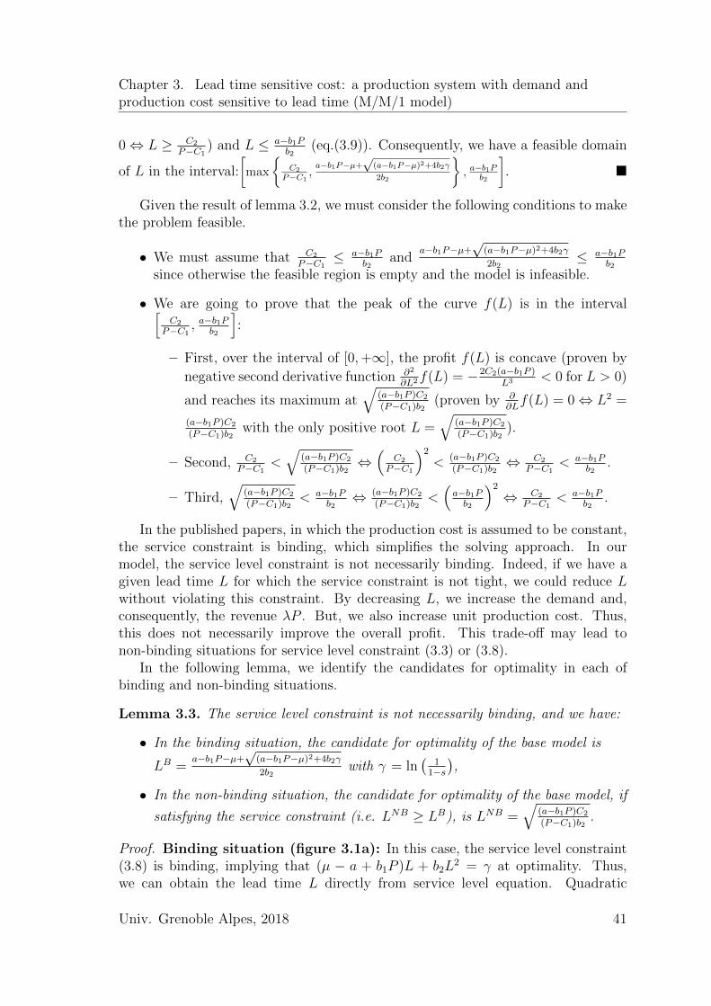
Chapter 3. Lead time sensitive cost: a production system with demand andproduction cost sensitive to lead time (M/M/1 model)
0⇔ L ≥ C2
P−C1) and L ≤ a−b1P
b2(eq.(3.9)). Consequently, we have a feasible domain
of L in the interval:
[max
{C2
P−C1,a−b1P−µ+
√(a−b1P−µ)2+4b2γ
2b2
}, a−b1P
b2
]. �
Given the result of lemma 3.2, we must consider the following conditions to makethe problem feasible.
• We must assume that C2
P−C1≤ a−b1P
b2and
a−b1P−µ+√
(a−b1P−µ)2+4b2γ
2b2≤ a−b1P
b2since otherwise the feasible region is empty and the model is infeasible.
• We are going to prove that the peak of the curve f(L) is in the interval[C2
P−C1, a−b1P
b2
]:
– First, over the interval of [0,+∞], the profit f(L) is concave (proven by
negative second derivative function ∂2
∂L2f(L) = −2C2(a−b1P )L3 < 0 for L > 0)
and reaches its maximum at√
(a−b1P )C2
(P−C1)b2(proven by ∂
∂Lf(L) = 0⇔ L2 =
(a−b1P )C2
(P−C1)b2with the only positive root L =
√(a−b1P )C2
(P−C1)b2).
– Second, C2
P−C1<√
(a−b1P )C2
(P−C1)b2⇔(
C2
P−C1
)2
< (a−b1P )C2
(P−C1)b2⇔ C2
P−C1< a−b1P
b2.
– Third,√
(a−b1P )C2
(P−C1)b2< a−b1P
b2⇔ (a−b1P )C2
(P−C1)b2<(a−b1Pb2
)2
⇔ C2
P−C1< a−b1P
b2.
In the published papers, in which the production cost is assumed to be constant,the service constraint is binding, which simplifies the solving approach. In ourmodel, the service level constraint is not necessarily binding. Indeed, if we have agiven lead time L for which the service constraint is not tight, we could reduce Lwithout violating this constraint. By decreasing L, we increase the demand and,consequently, the revenue λP . But, we also increase unit production cost. Thus,this does not necessarily improve the overall profit. This trade-off may lead tonon-binding situations for service level constraint (3.3) or (3.8).
In the following lemma, we identify the candidates for optimality in each ofbinding and non-binding situations.
Lemma 3.3. The service level constraint is not necessarily binding, and we have:
• In the binding situation, the candidate for optimality of the base model is
LB =a−b1P−µ+
√(a−b1P−µ)2+4b2γ
2b2with γ = ln
(1
1−s
),
• In the non-binding situation, the candidate for optimality of the base model, if
satisfying the service constraint (i.e. LNB ≥ LB), is LNB =√
(a−b1P )C2
(P−C1)b2.
Proof. Binding situation (figure 3.1a): In this case, the service level constraint(3.8) is binding, implying that (µ − a + b1P )L + b2L
2 = γ at optimality. Thus,we can obtain the lead time L directly from service level equation. Quadratic
Univ. Grenoble Alpes, 2018 41
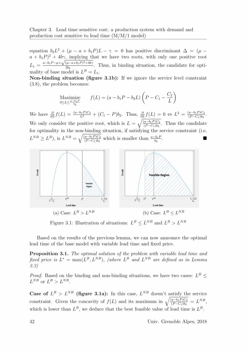
Chapter 3. Lead time sensitive cost: a production system with demand andproduction cost sensitive to lead time (M/M/1 model)
equation b2L2 + (µ − a + b1P )L − γ = 0 has positive discriminant ∆ = (µ −
a + b1P )2 + 4bγ, implying that we have two roots, with only one positive root
L1 =a−b1P−µ+
√(µ−a+b1P )2+4bγ
2b2. Thus, in binding situation, the candidate for opti-
mality of base model is LB = L1.Non-binding situation (figure 3.1b): If we ignore the service level constraint(3.8), the problem becomes:
Maximize0≤L≤a−b1P
b2
f(L) = (a− b1P − b2L)
(P − C1 −
C2
L
)
We have ∂∂Lf(L) = (a−b1P )C2
L2 + (C1 − P )b2. Thus, ∂∂Lf(L) = 0 ⇔ L2 = (a−b1P )C2
(P−C1)b2.
We only consider the positive root, which is L =√
(a−b1P )C2
(P−C1)b2. Thus the candidate
for optimality in the non-binding situation, if satisfying the service constraint (i.e.
LNB ≥ LB), is LNB =√
(a−b1P )C2
(P−C1)b2which is smaller than a−b1P
b2. �
(a) Case: LB > LNB (b) Case: LB ≤ LNB
Figure 3.1: Illustration of situations: LB ≤ LNB and LB > LNB
Based on the results of the previous lemma, we can now announce the optimallead time of the base model with variable lead time and fixed price.
Proposition 3.1. The optimal solution of the problem with variable lead time andfixed price is L∗ = max(LB, LNB), (where LB and LNB are defined as in Lemma3.3)
Proof. Based on the binding and non-binding situations, we have two cases: LB ≤LNB or LB > LNB.
Case of LB > LNB (figure 3.1a): In this case, LNB doesn’t satisfy the service
constraint. Given the concavity of f(L) and its maximum in√
(a−b1P )C2
(P−C1)b2= LNB,
which is lower than LB, we deduce that the best feasible value of lead time is LB.
42 Univ. Grenoble Alpes, 2018
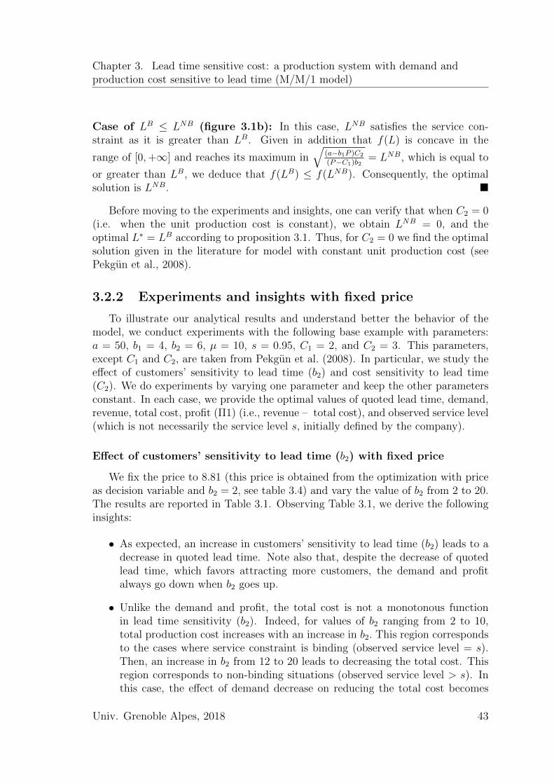
Chapter 3. Lead time sensitive cost: a production system with demand andproduction cost sensitive to lead time (M/M/1 model)
Case of LB ≤ LNB (figure 3.1b): In this case, LNB satisfies the service con-straint as it is greater than LB. Given in addition that f(L) is concave in the
range of [0,+∞] and reaches its maximum in√
(a−b1P )C2
(P−C1)b2= LNB, which is equal to
or greater than LB, we deduce that f(LB) ≤ f(LNB). Consequently, the optimalsolution is LNB. �
Before moving to the experiments and insights, one can verify that when C2 = 0(i.e. when the unit production cost is constant), we obtain LNB = 0, and theoptimal L∗ = LB according to proposition 3.1. Thus, for C2 = 0 we find the optimalsolution given in the literature for model with constant unit production cost (seePekgun et al., 2008).
3.2.2 Experiments and insights with fixed price
To illustrate our analytical results and understand better the behavior of themodel, we conduct experiments with the following base example with parameters:a = 50, b1 = 4, b2 = 6, µ = 10, s = 0.95, C1 = 2, and C2 = 3. This parameters,except C1 and C2, are taken from Pekgun et al. (2008). In particular, we study theeffect of customers’ sensitivity to lead time (b2) and cost sensitivity to lead time(C2). We do experiments by varying one parameter and keep the other parametersconstant. In each case, we provide the optimal values of quoted lead time, demand,revenue, total cost, profit (Π1) (i.e., revenue – total cost), and observed service level(which is not necessarily the service level s, initially defined by the company).
Effect of customers’ sensitivity to lead time (b2) with fixed price
We fix the price to 8.81 (this price is obtained from the optimization with priceas decision variable and b2 = 2, see table 3.4) and vary the value of b2 from 2 to 20.The results are reported in Table 3.1. Observing Table 3.1, we derive the followinginsights:
• As expected, an increase in customers’ sensitivity to lead time (b2) leads to adecrease in quoted lead time. Note also that, despite the decrease of quotedlead time, which favors attracting more customers, the demand and profitalways go down when b2 goes up.
• Unlike the demand and profit, the total cost is not a monotonous functionin lead time sensitivity (b2). Indeed, for values of b2 ranging from 2 to 10,total production cost increases with an increase in b2. This region correspondsto the cases where service constraint is binding (observed service level = s).Then, an increase in b2 from 12 to 20 leads to decreasing the total cost. Thisregion corresponds to non-binding situations (observed service level > s). Inthis case, the effect of demand decrease on reducing the total cost becomes
Univ. Grenoble Alpes, 2018 43
Chapter 3. Lead time sensitive cost: a production system with demand andproduction cost sensitive to lead time (M/M/1 model)
Table 3.1: Effect of demand sensitivity to lead time (b2) with fixed price
b2 Lead time Demand Total cost Profit (Π1) Π1′ Gains Serv. lev. realized
2 2.89 8.96 27.23 51.77 51.77 0.0% 95%
4 1.64 8.18 31.28 40.78 40.78 0.0% 95%
6 1.21 7.51 33.73 32.50 32.50 0.0% 95%
8 0.98 6.93 35.16 25.94 25.94 0.0% 95%
10 0.83 6.41 35.87 20.61 20.61 0.0% 95%
12 0.74 5.92 35.98 16.19 16.19 0.0% 95.03%
14 0.68 5.21 33.39 12.55 12.50 0.4% 96.16%
16 0.64 4.55 30.56 9.58 9.41 1.9% 96.89%
18 0.60 3.94 27.53 7.16 6.81 5.1% 97.38%
20 0.57 3.35 24.35 5.19 4.63 12.1% 97.74%
Figure 3.2: Variable cost vs Fixed cost: quoted lead time
more important than the effect of lead time decrease on increasing the totalcost.
• It is important to note that when b2 becomes significantly large (here, b2 ≥ 12),the model chooses to do better than the required service level (non-bindingsituation). More generally, we observe that the higher the demand sensitivityto lead time the higher the service level. This results is not intuitive sincean increase in lead time sensitivity leads to shorter lead time that is moredifficult to guarantee and, consequently, one can expect that this will lead totight service constraint. In our problem, the model has to quote a short leadtime in order to maintain a certain amount of demand. However, this implies ahigh unit production cost, which may annihilate the gain obtained by reducing
44 Univ. Grenoble Alpes, 2018
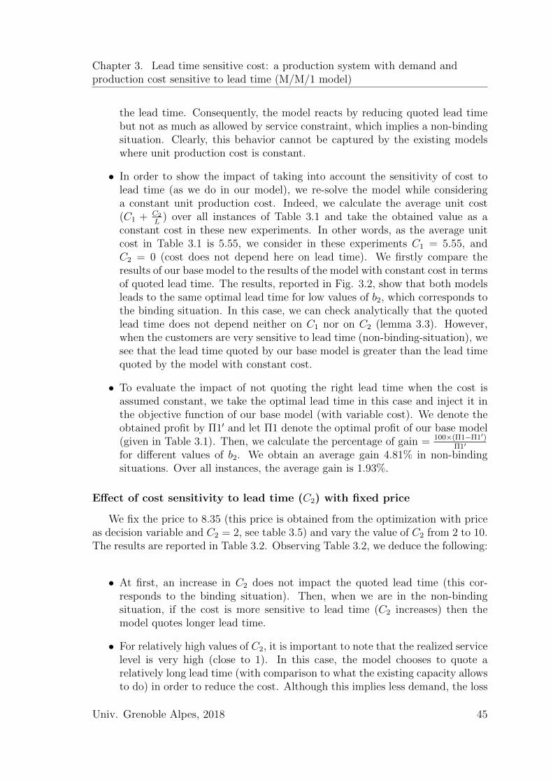
Chapter 3. Lead time sensitive cost: a production system with demand andproduction cost sensitive to lead time (M/M/1 model)
the lead time. Consequently, the model reacts by reducing quoted lead timebut not as much as allowed by service constraint, which implies a non-bindingsituation. Clearly, this behavior cannot be captured by the existing modelswhere unit production cost is constant.
• In order to show the impact of taking into account the sensitivity of cost tolead time (as we do in our model), we re-solve the model while consideringa constant unit production cost. Indeed, we calculate the average unit cost(C1 + C2
L) over all instances of Table 3.1 and take the obtained value as a
constant cost in these new experiments. In other words, as the average unitcost in Table 3.1 is 5.55, we consider in these experiments C1 = 5.55, andC2 = 0 (cost does not depend here on lead time). We firstly compare theresults of our base model to the results of the model with constant cost in termsof quoted lead time. The results, reported in Fig. 3.2, show that both modelsleads to the same optimal lead time for low values of b2, which corresponds tothe binding situation. In this case, we can check analytically that the quotedlead time does not depend neither on C1 nor on C2 (lemma 3.3). However,when the customers are very sensitive to lead time (non-binding-situation), wesee that the lead time quoted by our base model is greater than the lead timequoted by the model with constant cost.
• To evaluate the impact of not quoting the right lead time when the cost isassumed constant, we take the optimal lead time in this case and inject it inthe objective function of our base model (with variable cost). We denote theobtained profit by Π1′ and let Π1 denote the optimal profit of our base model(given in Table 3.1). Then, we calculate the percentage of gain = 100×(Π1−Π1′)
Π1′
for different values of b2. We obtain an average gain 4.81% in non-bindingsituations. Over all instances, the average gain is 1.93%.
Effect of cost sensitivity to lead time (C2) with fixed price
We fix the price to 8.35 (this price is obtained from the optimization with priceas decision variable and C2 = 2, see table 3.5) and vary the value of C2 from 2 to 10.The results are reported in Table 3.2. Observing Table 3.2, we deduce the following:
• At first, an increase in C2 does not impact the quoted lead time (this cor-responds to the binding situation). Then, when we are in the non-bindingsituation, if the cost is more sensitive to lead time (C2 increases) then themodel quotes longer lead time.
• For relatively high values of C2, it is important to note that the realized servicelevel is very high (close to 1). In this case, the model chooses to quote arelatively long lead time (with comparison to what the existing capacity allowsto do) in order to reduce the cost. Although this implies less demand, the loss
Univ. Grenoble Alpes, 2018 45
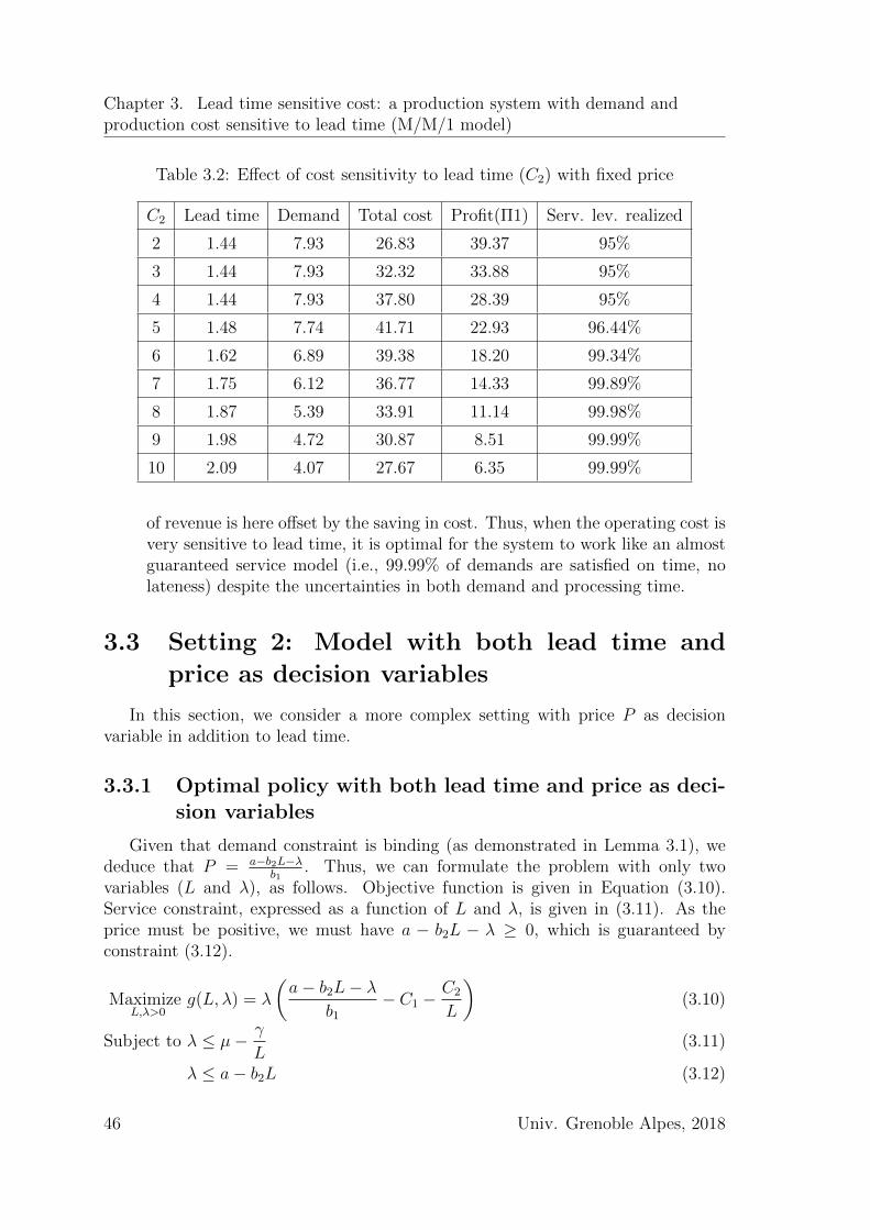
Chapter 3. Lead time sensitive cost: a production system with demand andproduction cost sensitive to lead time (M/M/1 model)
Table 3.2: Effect of cost sensitivity to lead time (C2) with fixed price
C2 Lead time Demand Total cost Profit(Π1) Serv. lev. realized
2 1.44 7.93 26.83 39.37 95%
3 1.44 7.93 32.32 33.88 95%
4 1.44 7.93 37.80 28.39 95%
5 1.48 7.74 41.71 22.93 96.44%
6 1.62 6.89 39.38 18.20 99.34%
7 1.75 6.12 36.77 14.33 99.89%
8 1.87 5.39 33.91 11.14 99.98%
9 1.98 4.72 30.87 8.51 99.99%
10 2.09 4.07 27.67 6.35 99.99%
of revenue is here offset by the saving in cost. Thus, when the operating cost isvery sensitive to lead time, it is optimal for the system to work like an almostguaranteed service model (i.e., 99.99% of demands are satisfied on time, nolateness) despite the uncertainties in both demand and processing time.
3.3 Setting 2: Model with both lead time and
price as decision variables
In this section, we consider a more complex setting with price P as decisionvariable in addition to lead time.
3.3.1 Optimal policy with both lead time and price as deci-sion variables
Given that demand constraint is binding (as demonstrated in Lemma 3.1), wededuce that P = a−b2L−λ
b1. Thus, we can formulate the problem with only two
variables (L and λ), as follows. Objective function is given in Equation (3.10).Service constraint, expressed as a function of L and λ, is given in (3.11). As theprice must be positive, we must have a − b2L − λ ≥ 0, which is guaranteed byconstraint (3.12).
MaximizeL,λ>0
g(L, λ) = λ
(a− b2L− λ
b1
− C1 −C2
L
)(3.10)
Subject to λ ≤ µ− γ
L(3.11)
λ ≤ a− b2L (3.12)
46 Univ. Grenoble Alpes, 2018
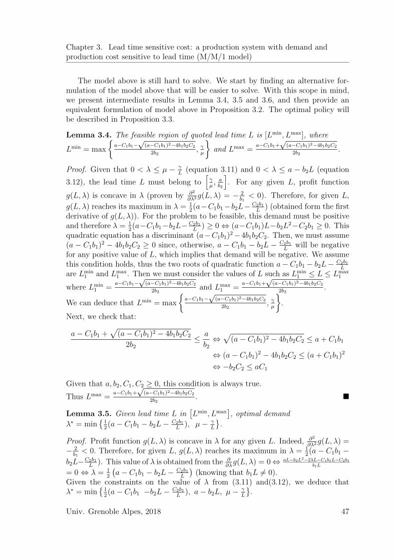
Chapter 3. Lead time sensitive cost: a production system with demand andproduction cost sensitive to lead time (M/M/1 model)
The model above is still hard to solve. We start by finding an alternative for-mulation of the model above that will be easier to solve. With this scope in mind,we present intermediate results in Lemma 3.4, 3.5 and 3.6, and then provide anequivalent formulation of model above in Proposition 3.2. The optimal policy willbe described in Proposition 3.3.
Lemma 3.4. The feasible region of quoted lead time L is [Lmin, Lmax], where
Lmin = max
{a−C1b1−
√(a−C1b1)2−4b1b2C2
2b2, γµ
}and Lmax =
a−C1b1+√
(a−C1b1)2−4b1b2C2
2b2.
Proof. Given that 0 < λ ≤ µ − γL
(equation 3.11) and 0 < λ ≤ a − b2L (equation
3.12), the lead time L must belong to[γµ, ab2
]. For any given L, profit function
g(L, λ) is concave in λ (proven by ∂2
∂λ2g(L, λ) = − 2
b1< 0). Therefore, for given L,
g(L, λ) reaches its maximum in λ = 12(a−C1b1−b2L− C2b1
L) (obtained form the first
derivative of g(L, λ)). For the problem to be feasible, this demand must be positiveand therefore λ = 1
2(a−C1b1−b2L− C2b1
L) ≥ 0⇔ (a−C1b1)L−b2L
2−C2b1 ≥ 0. Thisquadratic equation has a discriminant (a−C1b1)2−4b1b2C2. Then, we must assume(a − C1b1)2 − 4b1b2C2 ≥ 0 since, otherwise, a − C1b1 − b2L − C2b1
Lwill be negative
for any positive value of L, which implies that demand will be negative. We assumethis condition holds, thus the two roots of quadratic function a−C1b1 − b2L− C2b1
L
are Lmin1 and Lmax
1 . Then we must consider the values of L such as Lmin1 ≤ L ≤ Lmax
1
where Lmin1 =
a−C1b1−√
(a−C1b1)2−4b1b2C2
2b2and Lmax
1 =a−C1b1+
√(a−C1b1)2−4b1b2C2
2b2.
We can deduce that Lmin = max
{a−C1b1−
√(a−C1b1)2−4b1b2C2
2b2, γµ
}.
Next, we check that:
a− C1b1 +√
(a− C1b1)2 − 4b1b2C2
2b2
≤ a
b2
⇔√
(a− C1b1)2 − 4b1b2C2 ≤ a+ C1b1
⇔ (a− C1b1)2 − 4b1b2C2 ≤ (a+ C1b1)2
⇔ −b2C2 ≤ aC1
Given that a, b2, C1, C2 ≥ 0, this condition is always true.
Thus Lmax =a−C1b1+
√(a−C1b1)2−4b1b2C2
2b2. �
Lemma 3.5. Given lead time L in[Lmin, Lmax
], optimal demand
λ∗ = min{
12(a− C1b1 − b2L− C2b1
L), µ− γ
L
}.
Proof. Profit function g(L, λ) is concave in λ for any given L. Indeed, ∂2
∂λ2g(L, λ) =
− 2b1< 0. Therefore, for given L, g(L, λ) reaches its maximum in λ = 1
2(a− C1b1 −
b2L−C2b1L
). This value of λ is obtained from the ∂∂λg(L, λ) = 0⇔ aL−b2L2−2λL−C1b1L−C2b1
b1L
= 0 ⇔ λ = 12
(a− C1b1 − b2L− C2b1
L
)(knowing that b1L 6= 0).
Given the constraints on the value of λ from (3.11) and(3.12), we deduce thatλ∗ = min
{12(a− C1b1 −b2L− C2b1
L), a− b2L, µ− γ
L
}.
Univ. Grenoble Alpes, 2018 47
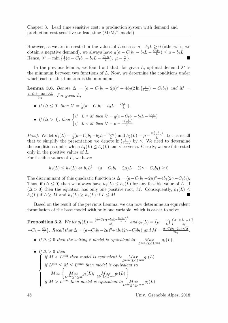
Chapter 3. Lead time sensitive cost: a production system with demand andproduction cost sensitive to lead time (M/M/1 model)
However, as we are interested in the values of L such as a− b2L ≥ 0 (otherwise, weobtain a negative demand), we always have 1
2(a− C1b1 − b2L− C2b1
L) ≤ a− b2L.
Hence, λ∗ = min{
12(a− C1b1 − b2L− C2b1
L), µ− γ
L
}. �
In the previous lemma, we found out that, for given L, optimal demand λ∗ isthe minimum between two functions of L. Now, we determine the conditions underwhich each of this function is the minimum.
Lemma 3.6. Denote ∆ = (a − C1b1 − 2µ)2 + 4b2(2 ln(
11−s
)− C2b1) and M =
a−C1b1−2µ+√
∆2b2
. For given L,
• If (∆ ≤ 0) then λ∗ = 12(a− C1b1 − b2L− C2b1
L),
• If (∆ > 0), then
{if L ≥M then λ∗ = 1
2(a− C1b1 − b2L− C2b1
L)
if L < M then λ∗ = µ− ln( 11−s)L
Proof. We let h1(L) = 12(a−C1b1−b2L− C2b1
L) and h2(L) = µ− ln( 1
1−s)L
. Let us recallthat to simplify the presentation we denote ln
(1
1−s
)by γ. We need to determine
the conditions under which h1(L) ≤ h2(L) and vice versa. Clearly, we are interestedonly in the positive values of L.For feasible values of L, we have:
h1(L) ≤ h2(L)⇔ b2L2 − (a− C1b1 − 2µ)L− (2γ − C2b1) ≥ 0
The discriminant of this quadratic function is ∆ = (a−C1b1−2µ)2 +4b2(2γ−C2b1).Thus, if (∆ ≤ 0) then we always have h1(L) ≤ h2(L) for any feasible value of L. If(∆ > 0) then the equation has only one positive root, M . Consequently, h1(L) ≤h2(L) if L ≥M and h1(L) ≥ h2(L) if L ≤M . �
Based on the result of the previous Lemma, we can now determine an equivalentformulation of the base model with only one variable, which is easier to solve.
Proposition 3.2. We let g1(L) =(a−C1b1−b2L−C2b1
L )2
4b1and g2(L) =
(µ− γ
L
) (a−b2L−µ+ γL
b1
−C1 − C2
L
). Recall that ∆ = (a−C1b1−2µ)2+4b2(2γ−C2b1) and M = a−C1b1−2µ+
√∆
2b2.
• If ∆ ≤ 0 then the setting 2 model is equivalent to: MaxLmin≤L≤Lmax
g1(L),
• If ∆ > 0 then
if M < Lmin then model is equivalent to MaxLmin≤L≤Lmax
g1(L)
if Lmin ≤M ≤ Lmax then model is equivalent to
Max
{Max
Lmin≤L≤Mg2(L), Max
M≤L≤Lmaxg1(L)
}if M > Lmax then model is equivalent to Max
Lmin≤L≤Lmaxg2(L)
48 Univ. Grenoble Alpes, 2018
Chapter 3. Lead time sensitive cost: a production system with demand andproduction cost sensitive to lead time (M/M/1 model)
Proof. According to the previous lemma:
if ∆ ≤ 0 then g(L, λ) reaches its maximum in λ = 12(a−C1b1−b2L− C2b1
L). The feasi-
ble region of quoted lead time L is [Lmin, Lmax]. Replacing λ by 12(a−C1b1−b2L−C2b1
L)
in the objective function, we immediately conclude that the base model becomesequivalent to Max
Lmin<L<Lmaxg1(L).
If ∆ > 0 then we have to consider three situation:
• if M < Lmin1 . Here, λ∗ = 1
2(a − C1b1 − b2L − C2b1
L) over the relevant interval[
Lmin, Lmax]. Hence, the model is equivalent to Max
Lmin≤L≤Lmaxg1(L).
• If Lmin ≤ M ≤ Lmax then we have to consider 2 regions: [Lmin,M ] and
[M,Lmax]. For L ∈ [Lmin,M ], the best feasible value of λ is µ − ln( 11−s)L
,which is positive only for L ≥ Lmin (otherwise, the problem is not relevant).Replacing λ by this value in the objective function, we deduce that, overinterval [Lmin,M ], the base model is equivalent to Max
Lmin≤L<Mg2(L). Over
interval [M,Lmax], we obtain λ = 12(a−C1b1− b2L− C2b1
L) and the base model
is equivalent to MaxM≤L≤Lmax
g1(L). Consequently, when ∆ > 0, the base model
is equivalent to Max
{Max
Lmin≤L<Mg2(L), Max
M≤L≤Lmaxg1(L)
}.
• Case ofM > Lmax.Here, λ∗ = µ− ln( 11−s)L
over the relevant interval[Lmin, Lmax
].
Hence, the model is equivalent to MaxLmin≤L≤Lmax
g2(L).
�
At this stage in proposition 3.2, we have transformed our complex problem intoa set of subproblems with only one variable L. We can now provide the optimalpolicy of lead time quotation and pricing for our setting 2 model.
Proposition 3.3. The optimal result of setting 2 model are:
• If (∆ ≤ 0) or (∆ > 0 and M < Lmin) then the optimal lead time L∗ =
max(√
(C2b1)/b2,γµ
).
• If (∆ > 0 and M > Lmax) then the optimal lead timeL∗ = arg max
x∈{R1,R2,Lmin}∩[Lmin,Lmax]
g2(x), where R1 and R2 are the two potential pos-
itive roots of cubic equation µb2L3 − (aγ − 2µγ + µC2b1 − C1b1γ)L − 2γ(γ −
C2b1) = 0 (this equation has at maximum two positive roots).
Univ. Grenoble Alpes, 2018 49
Chapter 3. Lead time sensitive cost: a production system with demand andproduction cost sensitive to lead time (M/M/1 model)
• If (∆ > 0 and Lmin ≤ M ≤ Lmax) then we let L∗1 = max(√
(C2b1)/b2,M)
and L∗2 = arg maxx∈{R1,R2,Lmin}∩[Lmin,M ]
g2(x). The optimal lead time
L∗ =
{L∗1, if g1(L∗1) ≥ g2(L∗2)L∗2, otherwise
.
In all cases, the optimal price can be easily deduced from this expression P ∗ =a−b2L∗−λ∗
b1.
Proof. Here, we consider following situations:
• Case of (∆ ≤ 0) or (∆ > 0 and M < Lmin). The model here is equivalent toMax
Lmin≤L≤Lmaxg1(L) according to Proposition 3.2. The first derivative of g1(L):
g′1(L) =((a−C1b1)L−b2L2−C2b1)(−b2+
C2b1L2 )
2b1L, implying that there are three extrema.
Two of them are the roots of quadratic equation (a− C1b1)L−b2L2−C2b1 = 0
(i.e., Lmin1 and Lmax
1 ), leading to a null profit. The third extrema, solu-
tion of g′1(L) = 0 is L =√
(C2b1)/b2, leading to positive profit (a−C1b1)2
4b1.
Hence, g1(L) is concave over[Lmin
1 , Lmax], which includes
[Lmin, Lmax
], and
reaches its maximum in√
(C2b1)/b2 ∈[Lmin
1 , Lmax]. However,
√(C2b1)/b2 is
not necessarily feasible (i.e., does not necessarily belong to[Lmin, Lmax
]since
Lmin = max{Lmin
1 , γµ
}).Consequently, L∗ = max
(√(C2b1)/b2,
γµ
).
• Case of (∆ > 0 and M > Lmax). The model is equivalent to MaxLmin≤L≤Lmax
g2(L)
according to Proposition 3.2. g′2(L) = 0⇔ µb2L3−(aγ − 2µγ + µC2b1 − C1b1γ)L−
2γ(γ − C2b1) = 0. Using the properties of cubic equations, if the three rootsare reals, it can be proven that there are at maximum two positive roots(see Appendix A). We denote the two positive roots by R1 and R2. Notethat g2(Lmin) = g2(Lmax) = 0 and that R1 and R2 are not necessarily in[Lmin, Lmax
]. Consequently, L∗ = arg max
x∈{R1,R2,Lmin}∩[Lmin,Lmax]
g2(x).
• Case of (∆ > 0 and Lmin ≤M ≤ Lmax). Model is equivalent to
Max
{Max
Lmin≤L≤Mg2(L), Max
M≤L≤Lmaxg1(L)
}according to Proposition 3.2. On the
one hand, we just demonstrated that g1(L) is concave over[Lmin
1 , Lmax]
and
reaches its maximum in√
(C2b1)/b2. As we have Lmin ≤M ≤ Lmax, we deduce
that the optimal solution of MaxM≤L≤Lmax
g1(L) is L∗1 = max(√
(C2b1)/b2,M)
.
On the other hand, as g2(L) has at maximum two positive extrema R1 andR2, and that g2(Lmin) = g2(M) = 0, we deduce that the optimal solution ofMax
Lmin≤L≤Mg2(L) is L∗2 = arg max
x∈{R1,R2,Lmin}∩[Lmin,M ]
g2(x). Consequently, L∗ = L∗1 if
g1(L∗1) ≥ g2(L∗2) and L∗ = L∗2 otherwises.
�
50 Univ. Grenoble Alpes, 2018
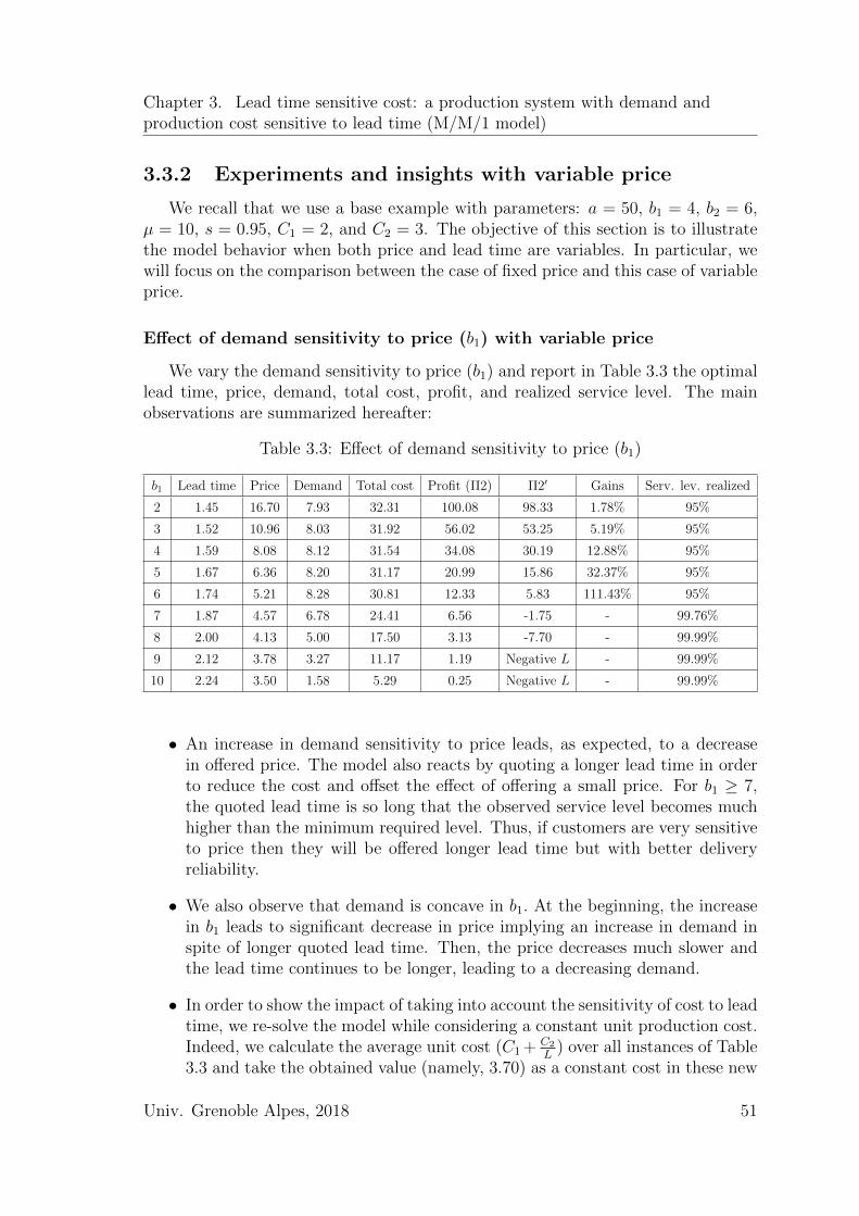
Chapter 3. Lead time sensitive cost: a production system with demand andproduction cost sensitive to lead time (M/M/1 model)
3.3.2 Experiments and insights with variable price
We recall that we use a base example with parameters: a = 50, b1 = 4, b2 = 6,µ = 10, s = 0.95, C1 = 2, and C2 = 3. The objective of this section is to illustratethe model behavior when both price and lead time are variables. In particular, wewill focus on the comparison between the case of fixed price and this case of variableprice.
Effect of demand sensitivity to price (b1) with variable price
We vary the demand sensitivity to price (b1) and report in Table 3.3 the optimallead time, price, demand, total cost, profit, and realized service level. The mainobservations are summarized hereafter:
Table 3.3: Effect of demand sensitivity to price (b1)
b1 Lead time Price Demand Total cost Profit (Π2) Π2′ Gains Serv. lev. realized
2 1.45 16.70 7.93 32.31 100.08 98.33 1.78% 95%
3 1.52 10.96 8.03 31.92 56.02 53.25 5.19% 95%
4 1.59 8.08 8.12 31.54 34.08 30.19 12.88% 95%
5 1.67 6.36 8.20 31.17 20.99 15.86 32.37% 95%
6 1.74 5.21 8.28 30.81 12.33 5.83 111.43% 95%
7 1.87 4.57 6.78 24.41 6.56 -1.75 - 99.76%
8 2.00 4.13 5.00 17.50 3.13 -7.70 - 99.99%
9 2.12 3.78 3.27 11.17 1.19 Negative L - 99.99%
10 2.24 3.50 1.58 5.29 0.25 Negative L - 99.99%
• An increase in demand sensitivity to price leads, as expected, to a decreasein offered price. The model also reacts by quoting a longer lead time in orderto reduce the cost and offset the effect of offering a small price. For b1 ≥ 7,the quoted lead time is so long that the observed service level becomes muchhigher than the minimum required level. Thus, if customers are very sensitiveto price then they will be offered longer lead time but with better deliveryreliability.
• We also observe that demand is concave in b1. At the beginning, the increasein b1 leads to significant decrease in price implying an increase in demand inspite of longer quoted lead time. Then, the price decreases much slower andthe lead time continues to be longer, leading to a decreasing demand.
• In order to show the impact of taking into account the sensitivity of cost to leadtime, we re-solve the model while considering a constant unit production cost.Indeed, we calculate the average unit cost (C1 + C2
L) over all instances of Table
3.3 and take the obtained value (namely, 3.70) as a constant cost in these new
Univ. Grenoble Alpes, 2018 51
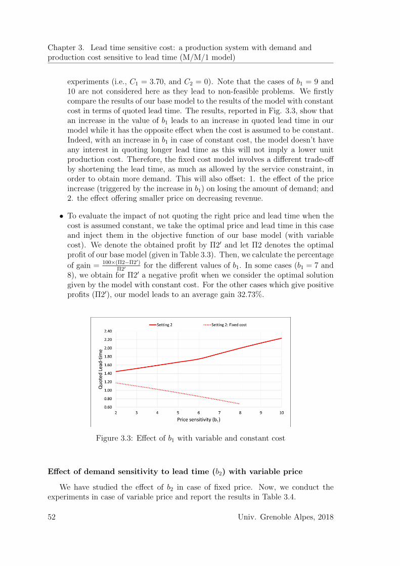
Chapter 3. Lead time sensitive cost: a production system with demand andproduction cost sensitive to lead time (M/M/1 model)
experiments (i.e., C1 = 3.70, and C2 = 0). Note that the cases of b1 = 9 and10 are not considered here as they lead to non-feasible problems. We firstlycompare the results of our base model to the results of the model with constantcost in terms of quoted lead time. The results, reported in Fig. 3.3, show thatan increase in the value of b1 leads to an increase in quoted lead time in ourmodel while it has the opposite effect when the cost is assumed to be constant.Indeed, with an increase in b1 in case of constant cost, the model doesn’t haveany interest in quoting longer lead time as this will not imply a lower unitproduction cost. Therefore, the fixed cost model involves a different trade-offby shortening the lead time, as much as allowed by the service constraint, inorder to obtain more demand. This will also offset: 1. the effect of the priceincrease (triggered by the increase in b1) on losing the amount of demand; and2. the effect offering smaller price on decreasing revenue.
• To evaluate the impact of not quoting the right price and lead time when thecost is assumed constant, we take the optimal price and lead time in this caseand inject them in the objective function of our base model (with variablecost). We denote the obtained profit by Π2′ and let Π2 denotes the optimalprofit of our base model (given in Table 3.3). Then, we calculate the percentage
of gain = 100×(Π2−Π2′)Π2′
for the different values of b1. In some cases (b1 = 7 and8), we obtain for Π2′ a negative profit when we consider the optimal solutiongiven by the model with constant cost. For the other cases which give positiveprofits (Π2′), our model leads to an average gain 32.73%.
Figure 3.3: Effect of b1 with variable and constant cost
Effect of demand sensitivity to lead time (b2) with variable price
We have studied the effect of b2 in case of fixed price. Now, we conduct theexperiments in case of variable price and report the results in Table 3.4.
52 Univ. Grenoble Alpes, 2018
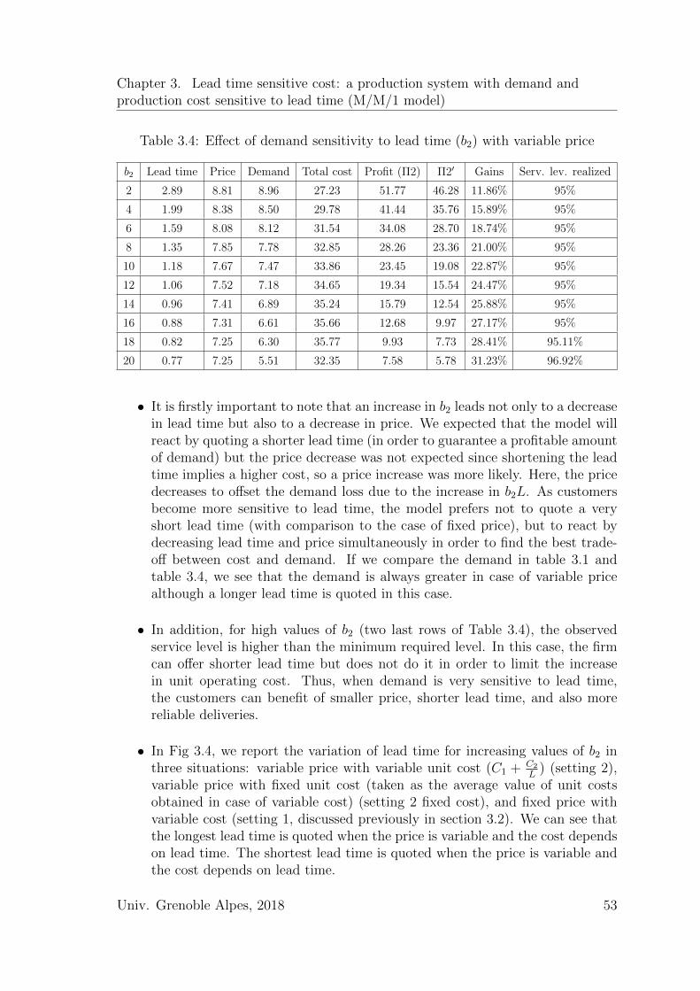
Chapter 3. Lead time sensitive cost: a production system with demand andproduction cost sensitive to lead time (M/M/1 model)
Table 3.4: Effect of demand sensitivity to lead time (b2) with variable price
b2 Lead time Price Demand Total cost Profit (Π2) Π2′ Gains Serv. lev. realized
2 2.89 8.81 8.96 27.23 51.77 46.28 11.86% 95%
4 1.99 8.38 8.50 29.78 41.44 35.76 15.89% 95%
6 1.59 8.08 8.12 31.54 34.08 28.70 18.74% 95%
8 1.35 7.85 7.78 32.85 28.26 23.36 21.00% 95%
10 1.18 7.67 7.47 33.86 23.45 19.08 22.87% 95%
12 1.06 7.52 7.18 34.65 19.34 15.54 24.47% 95%
14 0.96 7.41 6.89 35.24 15.79 12.54 25.88% 95%
16 0.88 7.31 6.61 35.66 12.68 9.97 27.17% 95%
18 0.82 7.25 6.30 35.77 9.93 7.73 28.41% 95.11%
20 0.77 7.25 5.51 32.35 7.58 5.78 31.23% 96.92%
• It is firstly important to note that an increase in b2 leads not only to a decreasein lead time but also to a decrease in price. We expected that the model willreact by quoting a shorter lead time (in order to guarantee a profitable amountof demand) but the price decrease was not expected since shortening the leadtime implies a higher cost, so a price increase was more likely. Here, the pricedecreases to offset the demand loss due to the increase in b2L. As customersbecome more sensitive to lead time, the model prefers not to quote a veryshort lead time (with comparison to the case of fixed price), but to react bydecreasing lead time and price simultaneously in order to find the best trade-off between cost and demand. If we compare the demand in table 3.1 andtable 3.4, we see that the demand is always greater in case of variable pricealthough a longer lead time is quoted in this case.
• In addition, for high values of b2 (two last rows of Table 3.4), the observedservice level is higher than the minimum required level. In this case, the firmcan offer shorter lead time but does not do it in order to limit the increasein unit operating cost. Thus, when demand is very sensitive to lead time,the customers can benefit of smaller price, shorter lead time, and also morereliable deliveries.
• In Fig 3.4, we report the variation of lead time for increasing values of b2 inthree situations: variable price with variable unit cost (C1 + C2
L) (setting 2),
variable price with fixed unit cost (taken as the average value of unit costsobtained in case of variable cost) (setting 2 fixed cost), and fixed price withvariable cost (setting 1, discussed previously in section 3.2). We can see thatthe longest lead time is quoted when the price is variable and the cost dependson lead time. The shortest lead time is quoted when the price is variable andthe cost depends on lead time.
Univ. Grenoble Alpes, 2018 53
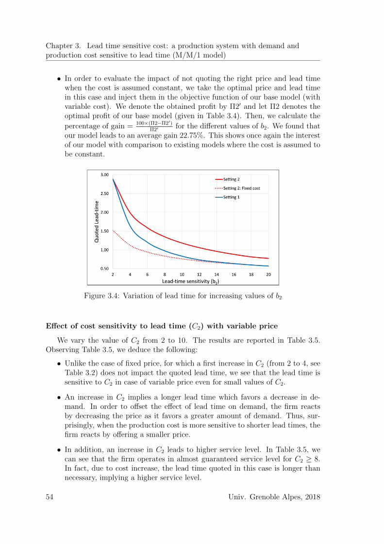
Chapter 3. Lead time sensitive cost: a production system with demand andproduction cost sensitive to lead time (M/M/1 model)
• In order to evaluate the impact of not quoting the right price and lead timewhen the cost is assumed constant, we take the optimal price and lead timein this case and inject them in the objective function of our base model (withvariable cost). We denote the obtained profit by Π2′ and let Π2 denotes theoptimal profit of our base model (given in Table 3.4). Then, we calculate the
percentage of gain = 100×(Π2−Π2′)Π2′
for the different values of b2. We found thatour model leads to an average gain 22.75%. This shows once again the interestof our model with comparison to existing models where the cost is assumed tobe constant.
Figure 3.4: Variation of lead time for increasing values of b2
Effect of cost sensitivity to lead time (C2) with variable price
We vary the value of C2 from 2 to 10. The results are reported in Table 3.5.Observing Table 3.5, we deduce the following:
• Unlike the case of fixed price, for which a first increase in C2 (from 2 to 4, seeTable 3.2) does not impact the quoted lead time, we see that the lead time issensitive to C2 in case of variable price even for small values of C2.
• An increase in C2 implies a longer lead time which favors a decrease in de-mand. In order to offset the effect of lead time on demand, the firm reactsby decreasing the price as it favors a greater amount of demand. Thus, sur-prisingly, when the production cost is more sensitive to shorter lead times, thefirm reacts by offering a smaller price.
• In addition, an increase in C2 leads to higher service level. In Table 3.5, wecan see that the firm operates in almost guaranteed service level for C2 ≥ 8.In fact, due to cost increase, the lead time quoted in this case is longer thannecessary, implying a higher service level.
54 Univ. Grenoble Alpes, 2018
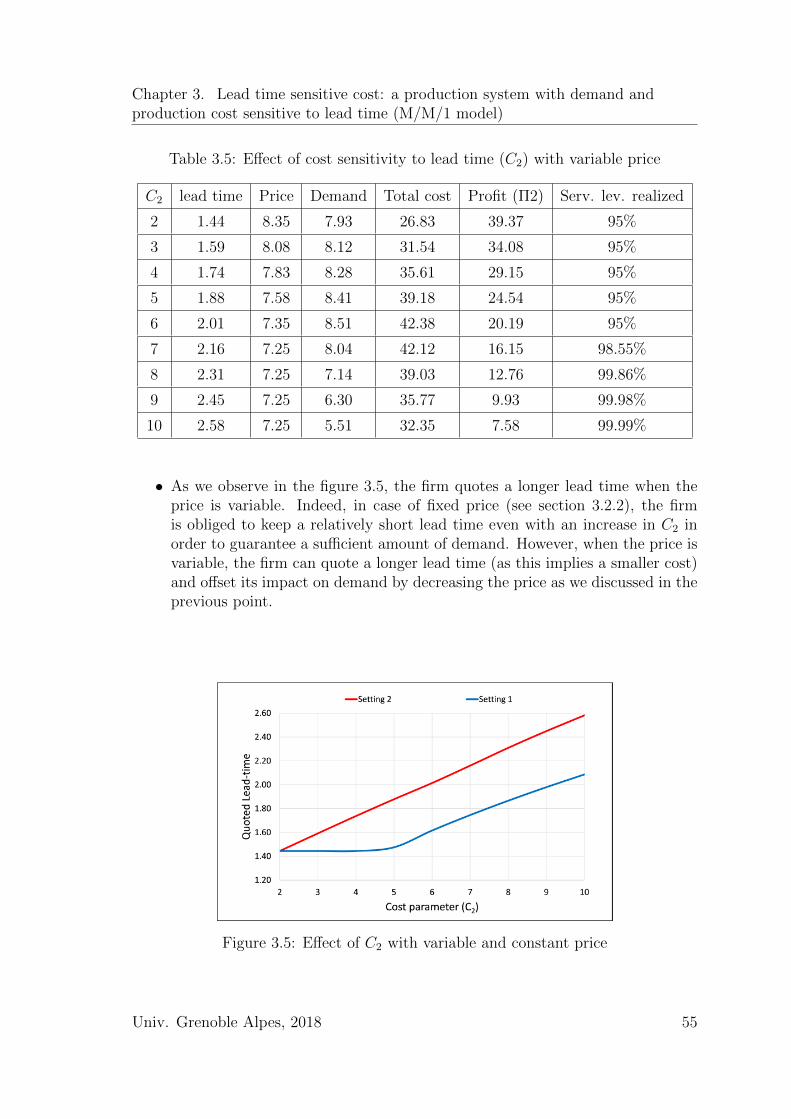
Chapter 3. Lead time sensitive cost: a production system with demand andproduction cost sensitive to lead time (M/M/1 model)
Table 3.5: Effect of cost sensitivity to lead time (C2) with variable price
C2 lead time Price Demand Total cost Profit (Π2) Serv. lev. realized
2 1.44 8.35 7.93 26.83 39.37 95%
3 1.59 8.08 8.12 31.54 34.08 95%
4 1.74 7.83 8.28 35.61 29.15 95%
5 1.88 7.58 8.41 39.18 24.54 95%
6 2.01 7.35 8.51 42.38 20.19 95%
7 2.16 7.25 8.04 42.12 16.15 98.55%
8 2.31 7.25 7.14 39.03 12.76 99.86%
9 2.45 7.25 6.30 35.77 9.93 99.98%
10 2.58 7.25 5.51 32.35 7.58 99.99%
• As we observe in the figure 3.5, the firm quotes a longer lead time when theprice is variable. Indeed, in case of fixed price (see section 3.2.2), the firmis obliged to keep a relatively short lead time even with an increase in C2 inorder to guarantee a sufficient amount of demand. However, when the price isvariable, the firm can quote a longer lead time (as this implies a smaller cost)and offset its impact on demand by decreasing the price as we discussed in theprevious point.
Figure 3.5: Effect of C2 with variable and constant price
Univ. Grenoble Alpes, 2018 55
Chapter 3. Lead time sensitive cost: a production system with demand andproduction cost sensitive to lead time (M/M/1 model)
3.4 General model (Setting 3): price is a deci-
sion variable; congestion & lateness costs are
considered
In this section, we consider the general model (setting 3) that has been explainedin section 3.1. We consider three cost components: unit production cost (m =C1 + C2
L), unit holding cost (F ), and lateness penalty cost (cr).
3.4.1 Optimal policy for general model
As stated in lemma 3.1, the demand constraint (3.2) is tight at optimality. Thus,we have P = (a−b2L−λ)/b1. The service level constraint (3.3) can also be rewritten
as: λ ≤ µ− ln(1/(1−s))L
. Thus, the problem can be rewritten as:
Maximize0≤L≤a−λ
b2
f(L, λ) = λ
(a− b2L− λ
b1
− C1 −C2
L
)− Fλ
µ− λ− crλ
µ− λe−(µ−λ)L
(3.13)
Subject to λ ≤ µ− ln(1/(1− s))L
(3.14)
Lemma 3.7. If service level constraint (3.14) is non-binding then optimal demand
is λ∗ = ln(b2/(b1cr)−C2/(L2cr))L
+µ. If service level (3.14) is binding, optimal demand is
equal to λ∗ = µ− ln(1/(1−s))L
.
Proof. In non-binding situations, we have service level constraint as λ < µ −ln(1/(1−s))
L. This service level constraint (3.14) can be ignored. The optimal lead time
in non-binding situation should respect: ∂∂Lf(L, λ) = λ
(C2
L2 − b2b1
)+crλe
−(µ−λ)L = 0,
which leads to the following demand: λ∗ = ln(b2/(b1cr)−C2/(L2cr))L
+ µ. In binding sit-
uation, from (3.14)we have λ∗ = µ− ln(1/(1−s))L
. �
Then from λ = a − b1P − b2L, we derive the maximum value for L is ab2
(λ =P = 0). Thus, we have the range of L as 0 ≤ L ≤ a/b2. And adding lemma 3.7, weget a single variable optimization problem which is:
Maximize0≤L≤ a
b2
f(L) = λ
(a− b2L− λ
b1
− C1 −C2
L
)− Fλ
µ− λ− crλ
µ− λe−(µ−λ)L (3.15)
where λ =ln(b2/(b1cr)− C2/(L
2cr))
L+ µ (non-binding situation) or
λ = µ− ln(1/(1− s))L
(binding situation)
To find the optimal profit, we have to compare the profit of both binding and non-binding case. Then we should take the maximum one. But, the problem above
56 Univ. Grenoble Alpes, 2018
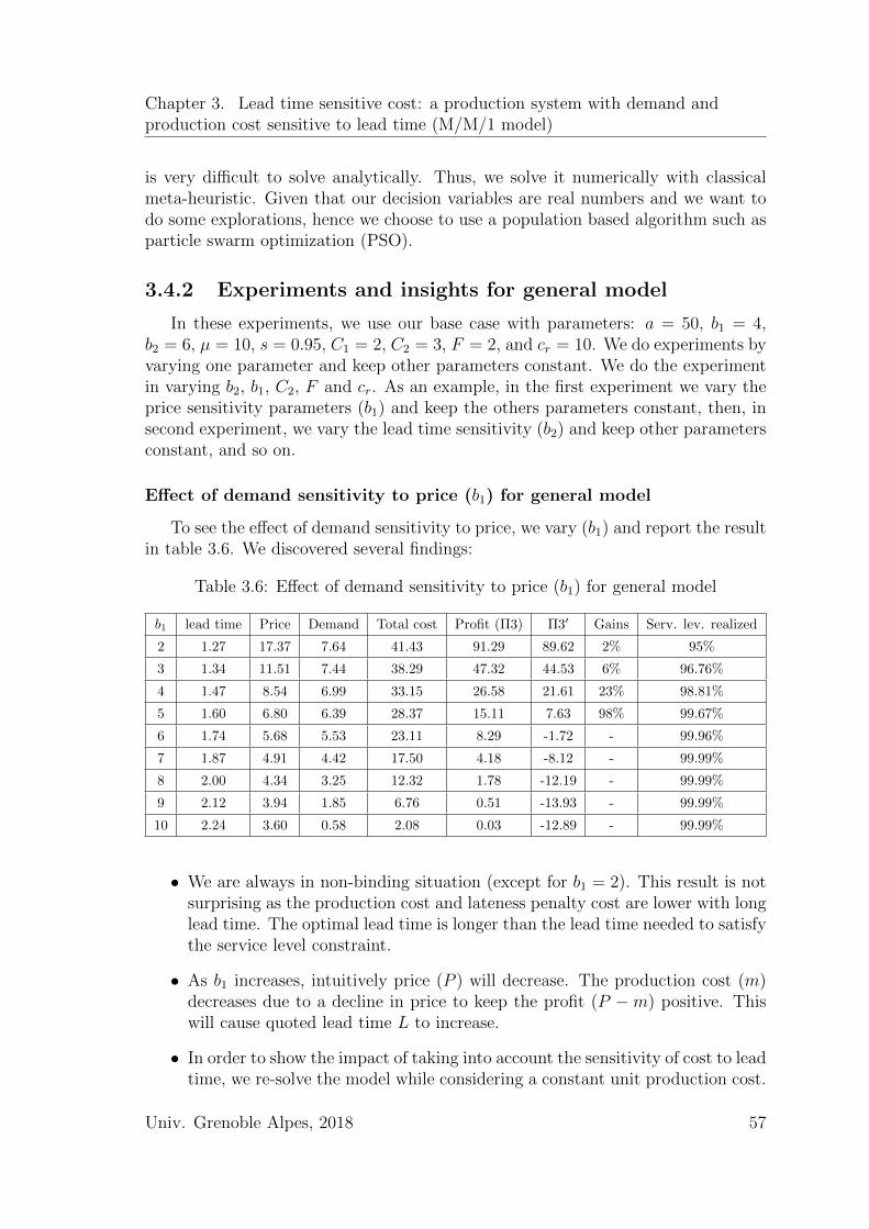
Chapter 3. Lead time sensitive cost: a production system with demand andproduction cost sensitive to lead time (M/M/1 model)
is very difficult to solve analytically. Thus, we solve it numerically with classicalmeta-heuristic. Given that our decision variables are real numbers and we want todo some explorations, hence we choose to use a population based algorithm such asparticle swarm optimization (PSO).
3.4.2 Experiments and insights for general model
In these experiments, we use our base case with parameters: a = 50, b1 = 4,b2 = 6, µ = 10, s = 0.95, C1 = 2, C2 = 3, F = 2, and cr = 10. We do experiments byvarying one parameter and keep other parameters constant. We do the experimentin varying b2, b1, C2, F and cr. As an example, in the first experiment we vary theprice sensitivity parameters (b1) and keep the others parameters constant, then, insecond experiment, we vary the lead time sensitivity (b2) and keep other parametersconstant, and so on.
Effect of demand sensitivity to price (b1) for general model
To see the effect of demand sensitivity to price, we vary (b1) and report the resultin table 3.6. We discovered several findings:
Table 3.6: Effect of demand sensitivity to price (b1) for general model
b1 lead time Price Demand Total cost Profit (Π3) Π3′ Gains Serv. lev. realized
2 1.27 17.37 7.64 41.43 91.29 89.62 2% 95%
3 1.34 11.51 7.44 38.29 47.32 44.53 6% 96.76%
4 1.47 8.54 6.99 33.15 26.58 21.61 23% 98.81%
5 1.60 6.80 6.39 28.37 15.11 7.63 98% 99.67%
6 1.74 5.68 5.53 23.11 8.29 -1.72 - 99.96%
7 1.87 4.91 4.42 17.50 4.18 -8.12 - 99.99%
8 2.00 4.34 3.25 12.32 1.78 -12.19 - 99.99%
9 2.12 3.94 1.85 6.76 0.51 -13.93 - 99.99%
10 2.24 3.60 0.58 2.08 0.03 -12.89 - 99.99%
• We are always in non-binding situation (except for b1 = 2). This result is notsurprising as the production cost and lateness penalty cost are lower with longlead time. The optimal lead time is longer than the lead time needed to satisfythe service level constraint.
• As b1 increases, intuitively price (P ) will decrease. The production cost (m)decreases due to a decline in price to keep the profit (P −m) positive. Thiswill cause quoted lead time L to increase.
• In order to show the impact of taking into account the sensitivity of cost to leadtime, we re-solve the model while considering a constant unit production cost.
Univ. Grenoble Alpes, 2018 57
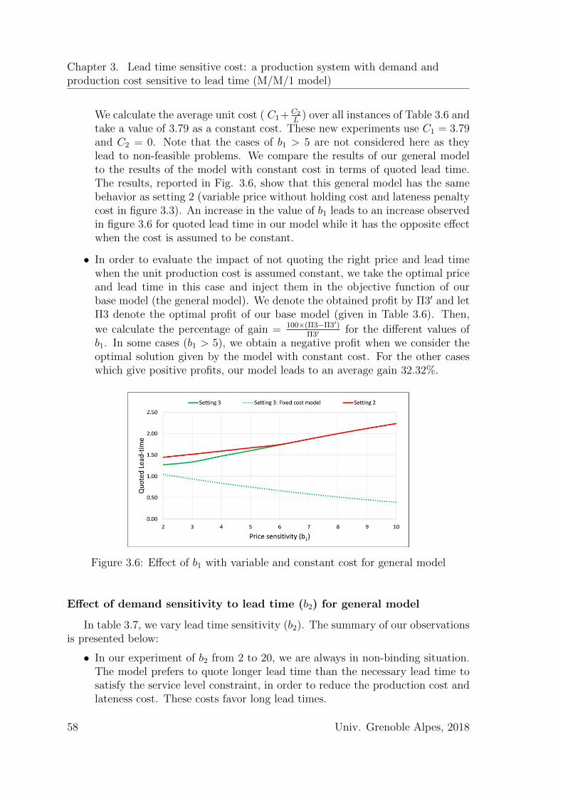
Chapter 3. Lead time sensitive cost: a production system with demand andproduction cost sensitive to lead time (M/M/1 model)
We calculate the average unit cost ( C1+ C2
L) over all instances of Table 3.6 and
take a value of 3.79 as a constant cost. These new experiments use C1 = 3.79and C2 = 0. Note that the cases of b1 > 5 are not considered here as theylead to non-feasible problems. We compare the results of our general modelto the results of the model with constant cost in terms of quoted lead time.The results, reported in Fig. 3.6, show that this general model has the samebehavior as setting 2 (variable price without holding cost and lateness penaltycost in figure 3.3). An increase in the value of b1 leads to an increase observedin figure 3.6 for quoted lead time in our model while it has the opposite effectwhen the cost is assumed to be constant.
• In order to evaluate the impact of not quoting the right price and lead timewhen the unit production cost is assumed constant, we take the optimal priceand lead time in this case and inject them in the objective function of ourbase model (the general model). We denote the obtained profit by Π3′ and letΠ3 denote the optimal profit of our base model (given in Table 3.6). Then,
we calculate the percentage of gain = 100×(Π3−Π3′)Π3′
for the different values ofb1. In some cases (b1 > 5), we obtain a negative profit when we consider theoptimal solution given by the model with constant cost. For the other caseswhich give positive profits, our model leads to an average gain 32.32%.
Figure 3.6: Effect of b1 with variable and constant cost for general model
Effect of demand sensitivity to lead time (b2) for general model
In table 3.7, we vary lead time sensitivity (b2). The summary of our observationsis presented below:
• In our experiment of b2 from 2 to 20, we are always in non-binding situation.The model prefers to quote longer lead time than the necessary lead time tosatisfy the service level constraint, in order to reduce the production cost andlateness cost. These costs favor long lead times.
58 Univ. Grenoble Alpes, 2018
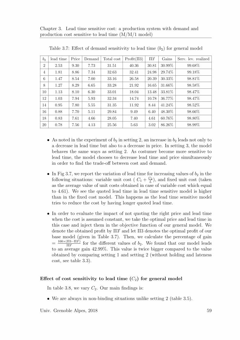
Chapter 3. Lead time sensitive cost: a production system with demand andproduction cost sensitive to lead time (M/M/1 model)
Table 3.7: Effect of demand sensitivity to lead time (b2) for general model
b2 lead time Price Demand Total cost Profit(Π3) Π3′ Gains Serv. lev. realized
2 2.53 9.30 7.73 31.51 40.36 30.81 30.99% 99.68%
4 1.81 8.86 7.34 32.63 32.41 24.98 29.74% 99.18%
6 1.47 8.54 7.00 33.16 26.58 20.39 30.33% 98.81%
8 1.27 8.29 6.65 33.28 21.92 16.65 31.66% 98.58%
10 1.13 8.10 6.30 33.01 18.04 13.48 33.81% 98.47%
12 1.03 7.94 5.93 32.34 14.74 10.78 36.77% 98.47%
14 0.95 7.80 5.55 31.35 11.92 8.44 41.24% 98.52%
16 0.88 7.70 5.11 29.84 9.49 6.40 48.30% 98.66%
18 0.83 7.61 4.66 28.05 7.40 4.61 60.76% 98.80%
20 0.78 7.56 4.13 25.56 5.63 3.02 86.26% 98.99%
• As noted in the experiment of b2 in setting 2, an increase in b2 leads not only toa decrease in lead time but also to a decrease in price. In setting 3, the modelbehaves the same ways as setting 2. As costumer become more sensitive tolead time, the model chooses to decrease lead time and price simultaneouslyin order to find the trade-off between cost and demand.
• In Fig 3.7, we report the variation of lead time for increasing values of b2 in thefollowing situations: variable unit cost ( C1 + C2
L), and fixed unit cost (taken
as the average value of unit costs obtained in case of variable cost which equalto 4.61). We see the quoted lead time in lead time sensitive model is higherthan in the fixed cost model. This happens as the lead time sensitive modeltries to reduce the cost by having longer quoted lead time.
• In order to evaluate the impact of not quoting the right price and lead timewhen the cost is assumed constant, we take the optimal price and lead time inthis case and inject them in the objective function of our general model. Wedenote the obtained profit by Π3′ and let Π3 denotes the optimal profit of ourbase model (given in Table 3.7). Then, we calculate the percentage of gain
= 100×(Π3−Π3′)Π3′
for the different values of b2. We found that our model leadsto an average gain 42.99%. This value is twice bigger compared to the valueobtained by comparing setting 1 and setting 2 (without holding and latenesscost, see table 3.3).
Effect of cost sensitivity to lead time (C2) for general model
In table 3.8, we vary C2. Our main findings is:
• We are always in non-binding situations unlike setting 2 (table 3.5).
Univ. Grenoble Alpes, 2018 59
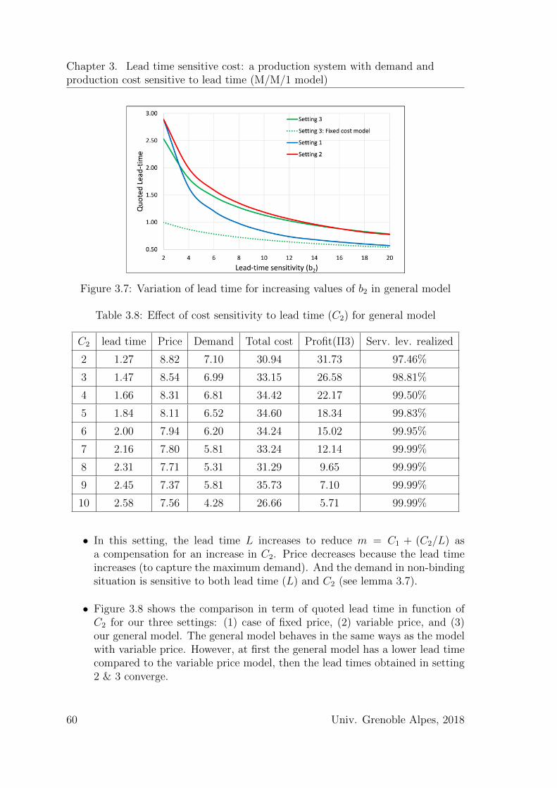
Chapter 3. Lead time sensitive cost: a production system with demand andproduction cost sensitive to lead time (M/M/1 model)
Figure 3.7: Variation of lead time for increasing values of b2 in general model
Table 3.8: Effect of cost sensitivity to lead time (C2) for general model
C2 lead time Price Demand Total cost Profit(Π3) Serv. lev. realized
2 1.27 8.82 7.10 30.94 31.73 97.46%
3 1.47 8.54 6.99 33.15 26.58 98.81%
4 1.66 8.31 6.81 34.42 22.17 99.50%
5 1.84 8.11 6.52 34.60 18.34 99.83%
6 2.00 7.94 6.20 34.24 15.02 99.95%
7 2.16 7.80 5.81 33.24 12.14 99.99%
8 2.31 7.71 5.31 31.29 9.65 99.99%
9 2.45 7.37 5.81 35.73 7.10 99.99%
10 2.58 7.56 4.28 26.66 5.71 99.99%
• In this setting, the lead time L increases to reduce m = C1 + (C2/L) asa compensation for an increase in C2. Price decreases because the lead timeincreases (to capture the maximum demand). And the demand in non-bindingsituation is sensitive to both lead time (L) and C2 (see lemma 3.7).
• Figure 3.8 shows the comparison in term of quoted lead time in function ofC2 for our three settings: (1) case of fixed price, (2) variable price, and (3)our general model. The general model behaves in the same ways as the modelwith variable price. However, at first the general model has a lower lead timecompared to the variable price model, then the lead times obtained in setting2 & 3 converge.
60 Univ. Grenoble Alpes, 2018
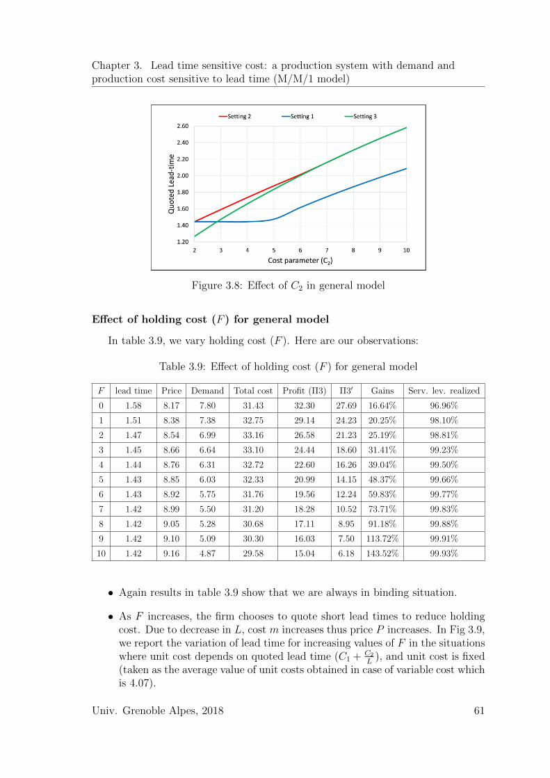
Chapter 3. Lead time sensitive cost: a production system with demand andproduction cost sensitive to lead time (M/M/1 model)
Figure 3.8: Effect of C2 in general model
Effect of holding cost (F ) for general model
In table 3.9, we vary holding cost (F ). Here are our observations:
Table 3.9: Effect of holding cost (F ) for general model
F lead time Price Demand Total cost Profit (Π3) Π3′ Gains Serv. lev. realized
0 1.58 8.17 7.80 31.43 32.30 27.69 16.64% 96.96%
1 1.51 8.38 7.38 32.75 29.14 24.23 20.25% 98.10%
2 1.47 8.54 6.99 33.16 26.58 21.23 25.19% 98.81%
3 1.45 8.66 6.64 33.10 24.44 18.60 31.41% 99.23%
4 1.44 8.76 6.31 32.72 22.60 16.26 39.04% 99.50%
5 1.43 8.85 6.03 32.33 20.99 14.15 48.37% 99.66%
6 1.43 8.92 5.75 31.76 19.56 12.24 59.83% 99.77%
7 1.42 8.99 5.50 31.20 18.28 10.52 73.71% 99.83%
8 1.42 9.05 5.28 30.68 17.11 8.95 91.18% 99.88%
9 1.42 9.10 5.09 30.30 16.03 7.50 113.72% 99.91%
10 1.42 9.16 4.87 29.58 15.04 6.18 143.52% 99.93%
• Again results in table 3.9 show that we are always in binding situation.
• As F increases, the firm chooses to quote short lead times to reduce holdingcost. Due to decrease in L, cost m increases thus price P increases. In Fig 3.9,we report the variation of lead time for increasing values of F in the situationswhere unit cost depends on quoted lead time (C1 + C2
L), and unit cost is fixed
(taken as the average value of unit costs obtained in case of variable cost whichis 4.07).
Univ. Grenoble Alpes, 2018 61
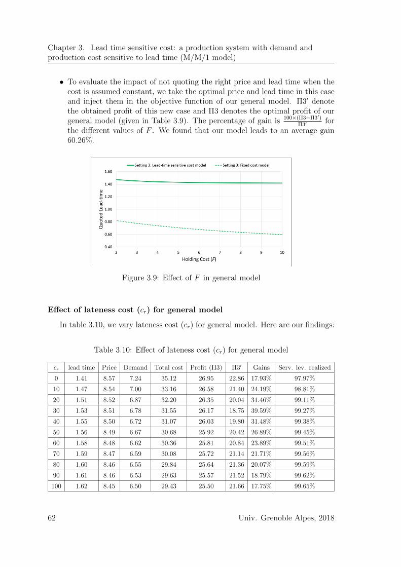
Chapter 3. Lead time sensitive cost: a production system with demand andproduction cost sensitive to lead time (M/M/1 model)
• To evaluate the impact of not quoting the right price and lead time when thecost is assumed constant, we take the optimal price and lead time in this caseand inject them in the objective function of our general model. Π3′ denotethe obtained profit of this new case and Π3 denotes the optimal profit of ourgeneral model (given in Table 3.9). The percentage of gain is 100×(Π3−Π3′)
Π3′for
the different values of F . We found that our model leads to an average gain60.26%.
Figure 3.9: Effect of F in general model
Effect of lateness cost (cr) for general model
In table 3.10, we vary lateness cost (cr) for general model. Here are our findings:
Table 3.10: Effect of lateness cost (cr) for general model
cr lead time Price Demand Total cost Profit (Π3) Π3′ Gains Serv. lev. realized
0 1.41 8.57 7.24 35.12 26.95 22.86 17.93% 97.97%
10 1.47 8.54 7.00 33.16 26.58 21.40 24.19% 98.81%
20 1.51 8.52 6.87 32.20 26.35 20.04 31.46% 99.11%
30 1.53 8.51 6.78 31.55 26.17 18.75 39.59% 99.27%
40 1.55 8.50 6.72 31.07 26.03 19.80 31.48% 99.38%
50 1.56 8.49 6.67 30.68 25.92 20.42 26.89% 99.45%
60 1.58 8.48 6.62 30.36 25.81 20.84 23.89% 99.51%
70 1.59 8.47 6.59 30.08 25.72 21.14 21.71% 99.56%
80 1.60 8.46 6.55 29.84 25.64 21.36 20.07% 99.59%
90 1.61 8.46 6.53 29.63 25.57 21.52 18.79% 99.62%
100 1.62 8.45 6.50 29.43 25.50 21.66 17.75% 99.65%
62 Univ. Grenoble Alpes, 2018
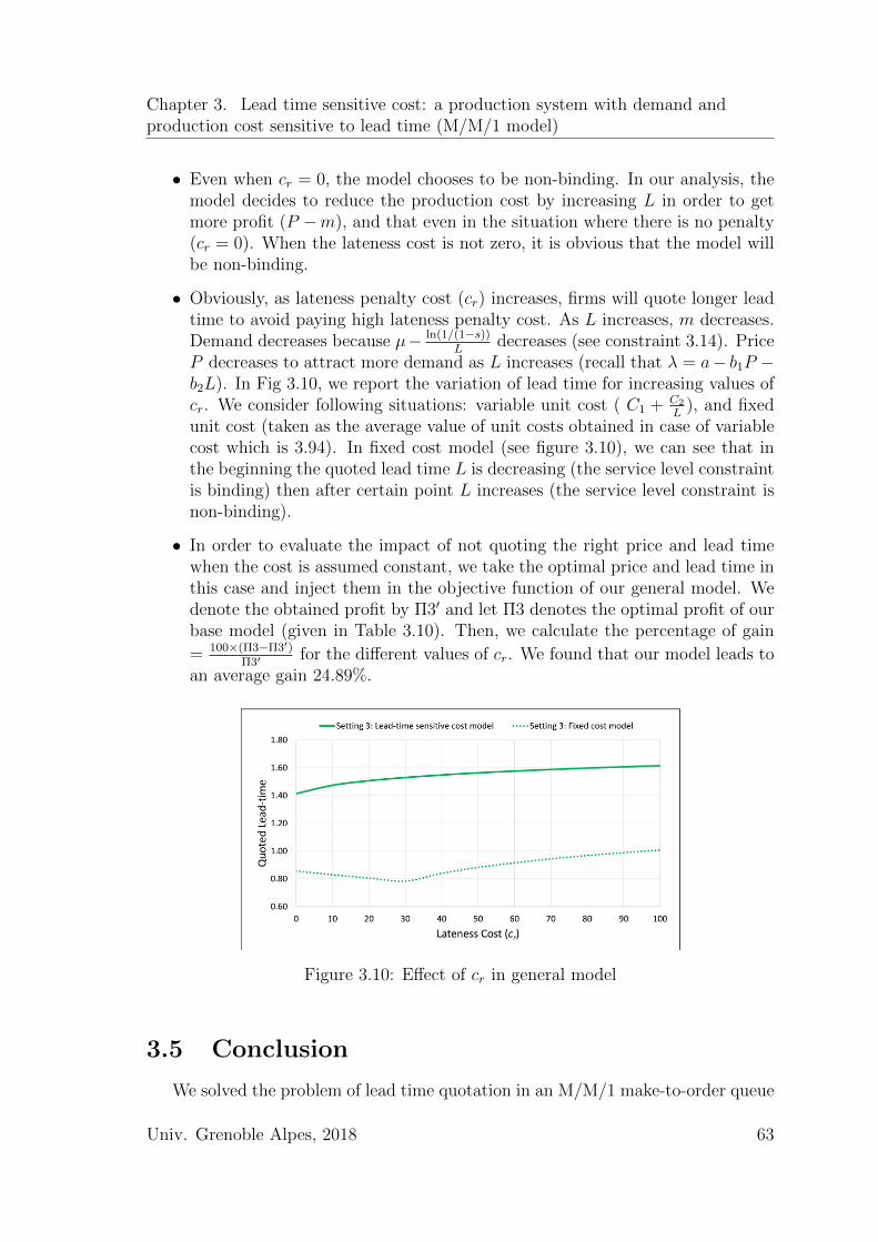
Chapter 3. Lead time sensitive cost: a production system with demand andproduction cost sensitive to lead time (M/M/1 model)
• Even when cr = 0, the model chooses to be non-binding. In our analysis, themodel decides to reduce the production cost by increasing L in order to getmore profit (P −m), and that even in the situation where there is no penalty(cr = 0). When the lateness cost is not zero, it is obvious that the model willbe non-binding.
• Obviously, as lateness penalty cost (cr) increases, firms will quote longer leadtime to avoid paying high lateness penalty cost. As L increases, m decreases.Demand decreases because µ− ln(1/(1−s))
Ldecreases (see constraint 3.14). Price
P decreases to attract more demand as L increases (recall that λ = a− b1P −b2L). In Fig 3.10, we report the variation of lead time for increasing values ofcr. We consider following situations: variable unit cost ( C1 + C2
L), and fixed
unit cost (taken as the average value of unit costs obtained in case of variablecost which is 3.94). In fixed cost model (see figure 3.10), we can see that inthe beginning the quoted lead time L is decreasing (the service level constraintis binding) then after certain point L increases (the service level constraint isnon-binding).
• In order to evaluate the impact of not quoting the right price and lead timewhen the cost is assumed constant, we take the optimal price and lead time inthis case and inject them in the objective function of our general model. Wedenote the obtained profit by Π3′ and let Π3 denotes the optimal profit of ourbase model (given in Table 3.10). Then, we calculate the percentage of gain
= 100×(Π3−Π3′)Π3′
for the different values of cr. We found that our model leads toan average gain 24.89%.
Figure 3.10: Effect of cr in general model
3.5 Conclusion
We solved the problem of lead time quotation in an M/M/1 make-to-order queue
Univ. Grenoble Alpes, 2018 63
Chapter 3. Lead time sensitive cost: a production system with demand andproduction cost sensitive to lead time (M/M/1 model)
while assuming the production cost to be a decreasing function in lead time. We con-sidered three settings: (1) lead time is variable but price is fixed, (2) price and leadtime are both decision variables, and (3) price and lead time are decision variableswhere the lateness and holding costs are considered. We conducted experiments andderived interesting insights.
In case of variable lead time and fixed cost (setting 1), some of our insightsindicated that the higher the demand sensitivity to lead time the higher the servicelevel. This results is not intuitive since an increase in lead time sensitivity leads toshorter lead time that is supposed to be more difficult to guarantee. In addition, thisbehavior cannot be captured by the existing models where the unit operating cost isassumed constant since the service constraint is always binding in this case. We alsofound that when customers are very sensitive to lead time, our model quotes longerlead time than the benchmark model with constant cost. Furthermore, we observedthat when the operating cost is very sensitive to lead time, it can be optimal for thesystem to work like an almost guaranteed service model (i.e., 99.99% of demandsare satisfied on time) despite the uncertainties in both demand and processing time.
When both lead time and price are endogenous variables (Setting 2), our resultsshowed that an increase in the demand sensitivity to price leads to an increasein quoted lead time in our model while it has the opposite effect for models withconstant cost. We also found that when demand is very sensitive to lead time, thecustomers can benefit of smaller price, shorter lead time, and also more reliabledeliveries. Some of our findings showed that, surprisingly, when the operating costis more sensitive to lead time, the firm reacts by offering a smaller price. In addition,we saw that the firm quotes a longer lead time when the price is also a variable (inaddition to lead time) with comparison to the case of fixed price.
When we consider the lateness penalty and holding costs (Setting 3), the modelquotes a longer lead time higher than the service constraint. The model prefers tobe in non-binding situation. Indeed, quoting a longer lead time is favorable as itwill reduce the incurred cost (i.e. production and lateness cost).
From our numerical experiments, we quantified the gain brought by using thesolution of our model versus the solution of the benchmark model where the cost isconstant. In the case where the price is fixed (setting 1), we found that our modelleads to small gains. This prove that there is an impact of not quoting the rightlead time when the cost is assumed to be constant. This impact becomes moresignificant (as the gains become bigger) when we take into account the price as adecision variable (setting 2). And when the lateness and holding costs are included,this gains increase compared to the settings 1 and 2.
64 Univ. Grenoble Alpes, 2018
Chapter 4
Rejection policy: a lead timequotation and pricing in an
M/M/1/K make-to-order queue
All of papers in the literature, presented in chapter 2, use the M/M/1 system.Although M/M/1 is the simplest queuing model, it has a drawback. In M/M/1, allthe customers are accepted, which might lead to long sojourn times (lead time) in thesystem when we accept customer while there are already a lot of customers waiting.Realistically, firms can choose to reject customers when they already have too manycustomers. Thus, we propose a customer’s rejection policy using an M/M/1/Kmodel. Demand is rejected if there are already K customers in the system (Krepresents the system capacity, that is the maximum number of customers in thesystem including the one under service). Our idea, that we want to check in thischapter, is that rejecting some customers might help to quote shorter lead time forthe accepted ones, which might finally lead to a higher profitability.
In this chapter, we explicitly formulate the problem of lead time quotation andpricing for a profit-maximizing firm, modeled as an M/M/1/K system, facing a linearprice- and lead time-dependent demand with the consideration of inventory holdingand lateness penalty costs. In order to formulate the lateness cost, we overcome atheoretical obstacle by calculating the expected lateness given that a job is late in anM/M/1/K queue when a delivery lead time, L, is quoted to the customers (i.e., theexpected sojourn time in the system after L). Then, we bring a second analyticalcontribution by determining the optimal firm’s policy (optimal price and quotedlead time) in case of M/M/1/1. We solve the problem numerically for K > 1.We conduct experiments and use the expression of the optimal solution obtainedfor M/M/1/1 to derive some insights. We also compare the results of our model,firstly for K = 1 and then for different values of K, to the results obtained in theliterature with an M/M/1 queue. We show in different situations that a customerrejection policy, represented by the M/M/1/K, can be better than the all-customers’acceptance policy, represented by the M/M/1, even when the inventory holding andlateness penalty costs are ignored.
4.1 General model: M/M/1/K
We consider a firm operating under a make-to-order M/M/1/K setting. Cus-tomers are served in first-come, first-served basis. The demand arrival is assumed to
65
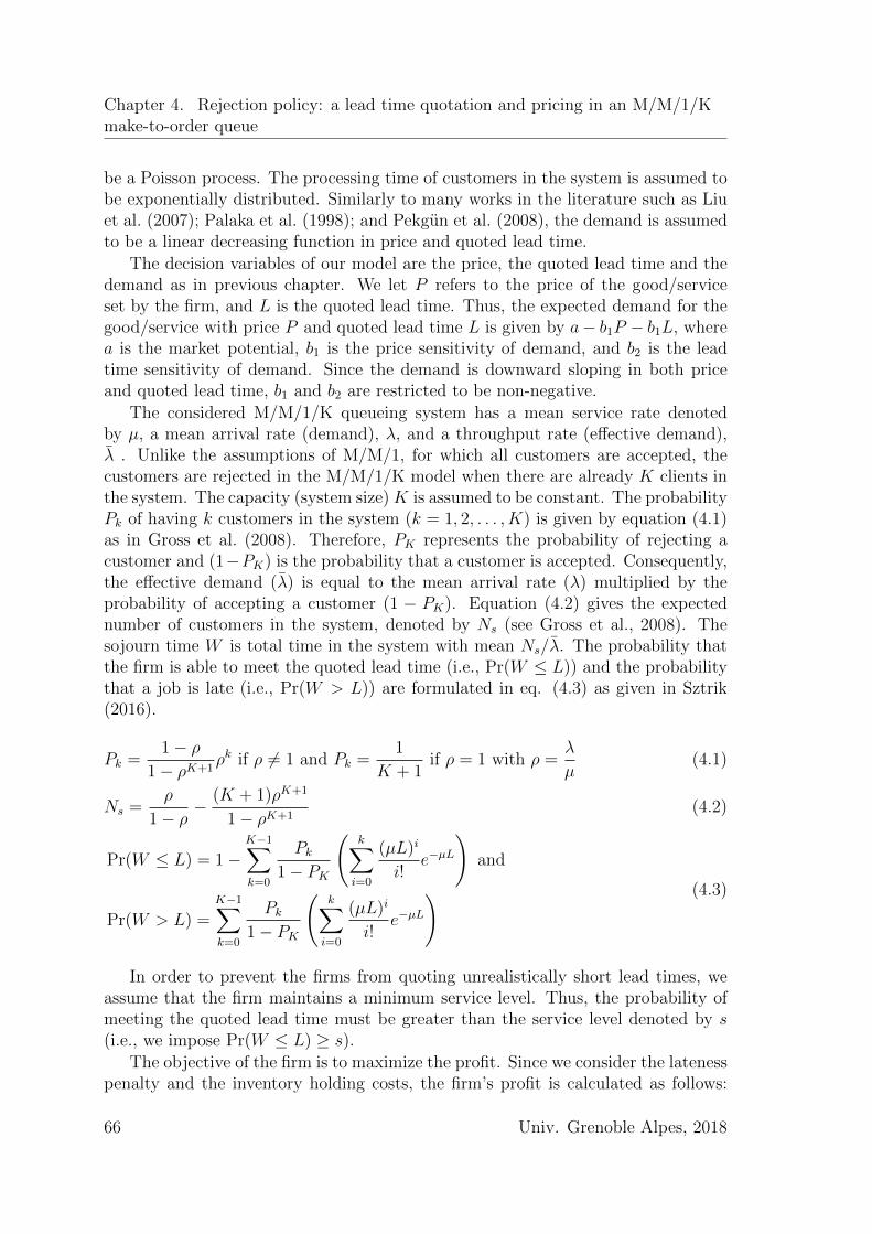
Chapter 4. Rejection policy: a lead time quotation and pricing in an M/M/1/Kmake-to-order queue
be a Poisson process. The processing time of customers in the system is assumed tobe exponentially distributed. Similarly to many works in the literature such as Liuet al. (2007); Palaka et al. (1998); and Pekgun et al. (2008), the demand is assumedto be a linear decreasing function in price and quoted lead time.
The decision variables of our model are the price, the quoted lead time and thedemand as in previous chapter. We let P refers to the price of the good/serviceset by the firm, and L is the quoted lead time. Thus, the expected demand for thegood/service with price P and quoted lead time L is given by a− b1P − b1L, wherea is the market potential, b1 is the price sensitivity of demand, and b2 is the leadtime sensitivity of demand. Since the demand is downward sloping in both priceand quoted lead time, b1 and b2 are restricted to be non-negative.
The considered M/M/1/K queueing system has a mean service rate denotedby µ, a mean arrival rate (demand), λ, and a throughput rate (effective demand),λ . Unlike the assumptions of M/M/1, for which all customers are accepted, thecustomers are rejected in the M/M/1/K model when there are already K clients inthe system. The capacity (system size)K is assumed to be constant. The probabilityPk of having k customers in the system (k = 1, 2, . . . , K) is given by equation (4.1)as in Gross et al. (2008). Therefore, PK represents the probability of rejecting acustomer and (1−PK) is the probability that a customer is accepted. Consequently,the effective demand (λ) is equal to the mean arrival rate (λ) multiplied by theprobability of accepting a customer (1 − PK). Equation (4.2) gives the expectednumber of customers in the system, denoted by Ns (see Gross et al., 2008). Thesojourn time W is total time in the system with mean Ns/λ. The probability thatthe firm is able to meet the quoted lead time (i.e., Pr(W ≤ L)) and the probabilitythat a job is late (i.e., Pr(W > L)) are formulated in eq. (4.3) as given in Sztrik(2016).
Pk =1− ρ
1− ρK+1ρk if ρ 6= 1 and Pk =
1
K + 1if ρ = 1 with ρ =
λ
µ(4.1)
Ns =ρ
1− ρ− (K + 1)ρK+1
1− ρK+1(4.2)
Pr(W ≤ L) = 1−K−1∑k=0
Pk1− PK
(k∑i=0
(µL)i
i!e−µL
)and
Pr(W > L) =K−1∑k=0
Pk1− PK
(k∑i=0
(µL)i
i!e−µL
) (4.3)
In order to prevent the firms from quoting unrealistically short lead times, weassume that the firm maintains a minimum service level. Thus, the probability ofmeeting the quoted lead time must be greater than the service level denoted by s(i.e., we impose Pr(W ≤ L) ≥ s).
The objective of the firm is to maximize the profit. Since we consider the latenesspenalty and the inventory holding costs, the firm’s profit is calculated as follows:
66 Univ. Grenoble Alpes, 2018
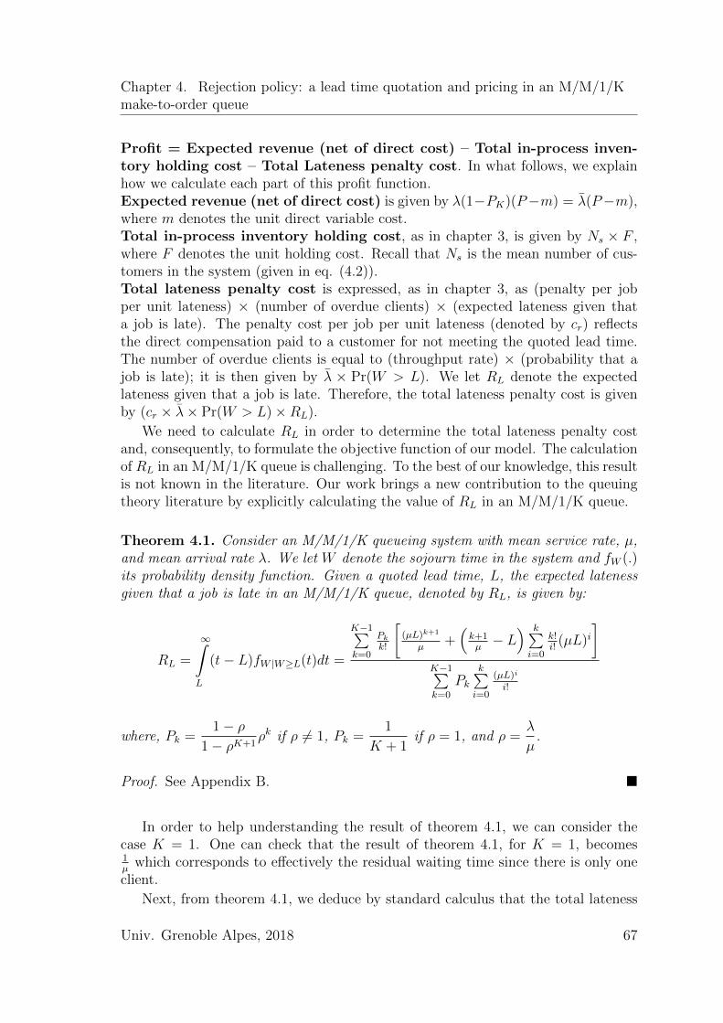
Chapter 4. Rejection policy: a lead time quotation and pricing in an M/M/1/Kmake-to-order queue
Profit = Expected revenue (net of direct cost) – Total in-process inven-tory holding cost – Total Lateness penalty cost. In what follows, we explainhow we calculate each part of this profit function.Expected revenue (net of direct cost) is given by λ(1−PK)(P−m) = λ(P−m),where m denotes the unit direct variable cost.Total in-process inventory holding cost, as in chapter 3, is given by Ns × F ,where F denotes the unit holding cost. Recall that Ns is the mean number of cus-tomers in the system (given in eq. (4.2)).Total lateness penalty cost is expressed, as in chapter 3, as (penalty per jobper unit lateness) × (number of overdue clients) × (expected lateness given thata job is late). The penalty cost per job per unit lateness (denoted by cr) reflectsthe direct compensation paid to a customer for not meeting the quoted lead time.The number of overdue clients is equal to (throughput rate) × (probability that ajob is late); it is then given by λ × Pr(W > L). We let RL denote the expectedlateness given that a job is late. Therefore, the total lateness penalty cost is givenby (cr × λ× Pr(W > L)×RL).
We need to calculate RL in order to determine the total lateness penalty costand, consequently, to formulate the objective function of our model. The calculationof RL in an M/M/1/K queue is challenging. To the best of our knowledge, this resultis not known in the literature. Our work brings a new contribution to the queuingtheory literature by explicitly calculating the value of RL in an M/M/1/K queue.
Theorem 4.1. Consider an M/M/1/K queueing system with mean service rate, µ,and mean arrival rate λ. We let W denote the sojourn time in the system and fW (.)its probability density function. Given a quoted lead time, L, the expected latenessgiven that a job is late in an M/M/1/K queue, denoted by RL, is given by:
RL =
∞∫L
(t− L)fW |W≥L(t)dt =
K−1∑k=0
Pkk!
[(µL)k+1
µ+(k+1µ− L
) k∑i=0
k!i!
(µL)i]
K−1∑k=0
Pkk∑i=0
(µL)i
i!
where, Pk =1− ρ
1− ρK+1ρk if ρ 6= 1, Pk =
1
K + 1if ρ = 1, and ρ =
λ
µ.
Proof. See Appendix B. �
In order to help understanding the result of theorem 4.1, we can consider thecase K = 1. One can check that the result of theorem 4.1, for K = 1, becomes1µ
which corresponds to effectively the residual waiting time since there is only oneclient.
Next, from theorem 4.1, we deduce by standard calculus that the total lateness
Univ. Grenoble Alpes, 2018 67
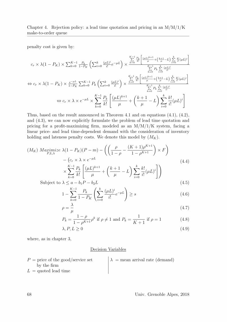
Chapter 4. Rejection policy: a lead time quotation and pricing in an M/M/1/Kmake-to-order queue
penalty cost is given by:
cr × λ(1− PK)×∑K−1
k=0Pk
1−PK
(∑ki=0
(µL)i
i!e−µL
)×
K−1∑k=0
Pkk!
[(µL)k+1
µ+( k+1
µ−L)
k∑i=0
k!i!
(µL)i
]K−1∑k=0
Pkk∑i=0
(µL)i
i!
⇔ cr × λ(1− PK)× e−µL
1−PK
∑K−1k=0 Pk
(∑ki=0
(µL)i
i!
)×
K−1∑k=0
Pkk!
[(µL)k+1
µ+( k+1
µ−L)
k∑i=0
k!i!
(µL)i
]K−1∑k=0
Pkk∑i=0
(µL)i
i!
⇔ cr × λ× e−µL ×K−1∑k=0
Pkk!
[(µL)k+1
µ+
(k + 1
µ− L
) k∑i=0
k!
i!(µL)i
]
Thus, based on the result announced in Theorem 4.1 and on equations (4.1), (4.2),and (4.3), we can now explicitly formulate the problem of lead time quotation andpricing for a profit-maximizing firm, modeled as an M/M/1/K system, facing alinear price- and lead time-dependent demand with the consideration of inventoryholding and lateness penalty costs. We denote this model by (MK).
(MK) MaximizeP,L,λ
λ(1− PK)(P −m)−((
ρ
1− ρ− (K + 1)ρK+1
1− ρK+1
)× F
)−(cr × λ× e−µL
×K−1∑k=0
Pkk!
[(µL)k+1
µ+
(k + 1
µ− L
) k∑i=0
k!
i!(µL)i
]) (4.4)
Subject to λ ≤ a− b1P − b2L (4.5)
1−K−1∑k=0
Pk1− PK
(k∑i=0
(µL)i
i!e−µL
)≥ s (4.6)
ρ =λ
µ(4.7)
Pk =1− ρ
1− ρK+1ρk if ρ 6= 1 and Pk =
1
K + 1if ρ = 1 (4.8)
λ, P, L ≥ 0 (4.9)
where, as in chapter 3,
Decision Variables
P = price of the good/service setby the firm
L = quoted lead time
λ = mean arrival rate (demand)
68 Univ. Grenoble Alpes, 2018
Chapter 4. Rejection policy: a lead time quotation and pricing in an M/M/1/Kmake-to-order queue
Parameters
a = market potentialb1 = price sensitivity of demandb2 = lead time sensitivity of demandµ = mean service rate (production
capacity)m = unit direct variable cost
s = service level set by the companyF = unit holding costcr = penalty cost per job per unit
latenessK = system size (notation added for
this chapter)
In model (MK), constraint (4.5) imposes that the mean demand (λ) cannotbe greater than the demand obtained with price (P ) and quoted lead time (L).Constraint (4.6) expresses the service level constraint. Equality (4.7) gives the valueof ρ. Equality (4.8) calculates the probability of rejecting customers. The non-negativity constraint (4.9) gives the domain of model variables. Clearly, the modelobtained is very hard to solve analytically in the general case. In the followingsection, we show how an analytical solution can be found in case of K = 1 with andwithout lateness penalty and holding costs.
4.2 The M/M/1/1 model: Analytical solution
Solving analytically the general case (MK) seems to be very difficult. So, in thissection, we consider the case of K = 1. We will consider two situations: the casewithout penalty and holding cost; and the case where these costs are included. Forboth cases, we will compare the obtained optimal solution with the optimal solutionof the M/M/1 approach and derive insights in section 4.3.
4.2.1 The M/M/1/1 model: congestion & lateness costs areignored
For K = 1 without lateness penalty and holding costs (cr = 0 and F = 0), it canbe shown by standard calculus that model (MK) is equivalent to model (M
′1) given
below.
(M′
1) MaximizeP,L,λ
(λµ
µ+ λ
)(P −m) (4.10)
Subject to λ ≤ a− b1P − b2L (4.11)
1− e−µL ≥ s (4.12)
λ, P, L ≥ 0 (4.13)
Under its present form, model (M′1) is a three-variables constrained non-linear
optimization model, which is still hard to solve analytically. In order to solve model(M
′1), we firstly reduce the number of variables by using the following lemma.
Univ. Grenoble Alpes, 2018 69
Chapter 4. Rejection policy: a lead time quotation and pricing in an M/M/1/Kmake-to-order queue
Lemma 4.1. The demand constraint is binding (eq. (4.11)) and we have P =a−b2L−λ
b1at optimality.
Proof. We let price P ∗, quoted lead time L∗, and demand rate λ∗ denote the optimalsolution and suppose that λ∗ < a − b1P
∗ − b2L∗. Since the objective function is
increasing in P , one could increase the price from P ∗ to P ′ (while keeping L∗ and λ∗
constant) until λ∗ = a− b1P′ − b2L
∗. This change will increase the profit, which isimpossible since (L∗, P ∗, λ∗) was assumed to be the optimal solution. Consequently,the demand constraint is binding and P = (a− b2L− λ)/b1 at optimality. �
Lemma 4.2. Service constraint (eq. (4.12)) is binding and we have L = ln(1/(1−s))µ
at optimality.
Proof. We let price P ∗, quoted lead time L∗, and demand rate λ∗ denote the optimalsolution and suppose that 1 − e−µL > s ⇔ µL∗ > ln(1/(1 − s)). Since constraint(4.11) is binding (according to lemma 4.1) and demand rate is decreasing in quotedlead time, one could increase λ∗ to λ′ by decreasing L∗ to L′ (while keeping theprice constant) until µL′ = ln(1/(1 − s)). Given that the objective function isincreasing in demand rate λ (assuming the profit is positive), then solution P ∗, L′,and λ′ will increase the profit. This is impossible since P ∗, L∗, and λ∗ is the optimalsolution. Hence, service constraint is binding and implies that L = (ln(1/(1−s)))/µat optimality. �
Now, we will use the results of Lemma 4.1 and 4.2 in order to transform model(M1) into a single variable model. We substitute L by (ln(1/(1−s)))/µ into equation(4.11). Given that constraints (4.11) and (4.12) are tight at optimality, we obtain:
P =aµ− b2 ln(1/(1− s))− λµ
µb1
Price P must be greater than m in order to obtain a positive profit, which impliesthat λ must satisfy λ ≤ a − b2 ln(1/(1−s))
µ− b1m. Thus, substituting L and P by
their values, we get the following equivalent formulation of model (M1) with a singlevariable (λ):
Maximize0≤λ≤a− b2 ln(1/(1−s))
µ−b1m
Π(λ) =λaµ− λb2 ln(1/(1− s))− λ2µ− λmµb1
µb1 + λb1
(4.14)
Clearly, this problem is relevant only when a − b2 ln(1/(1−s))µ
− b1m > 0. We assumethis condition holds.
Proposition 4.1. Assuming a− b2 ln(1/(1−s))µ
−b1m > 0 (otherwise the problem is not
relevant), the optimal solution of the (M/M/1/1) model without penalty and holdingcosts is:
• Optimal lead time: L∗ = ln(1/(1−s))µ
,
70 Univ. Grenoble Alpes, 2018
Chapter 4. Rejection policy: a lead time quotation and pricing in an M/M/1/Kmake-to-order queue
• Optimal price: P ∗ =a−b2 ln(1/(1−s))
µ+µ−√µ2+aµ−b2 ln(1/(1−s))−mµb1b1
,
• Optimal demand: λ∗ = −µ+√µ2 + aµ− b2 ln(1/(1− s))−mµb1
Proof. Firstly, we identify the stationary points of function Π(λ). Let us calculatedΠ(λ)dλ
:dΠ(λ)
dλ= 0⇔ aµ− b2 ln(1/(1− s))−mµb1 − 2λµ− λ2 = 0
The discriminant of this quadratic equation is:
∆ = 4µ2 + 4aµ− 4b2 ln(1/(1− s))− 4mµb1
As it was assumed that a − b2 ln(1/(1−s))µ
− b1m > 0 (since, otherwise, the problem
is not relevant), we deduce that ∆ ≥ 0. Hence, we obtain two real roots (twostationary points):
λ1 = −µ−√µ2 + aµ− b2 ln(1/(1− s))−mµb1
and
λ2 = −µ+√µ2 + aµ− b2 ln(1/(1− s))−mµb1
The first root λ1 is negative and, consequently, non-feasible.We are going to prove that λ2 is feasible (i.e., λ2 ≥ 0 and λ2 ≤ a− b2 ln(1/(1−s))
µ−b1m).
First, we search the condition that allows λ2 ≥ 0 which equals to:
− µ+√µ2 + aµ− b2 ln(1/(1− s))−mµb1 ≥ 0
⇔ aµ− b2 ln(1/(1− s))−mµb1 ≥ 0
⇔ a− b2 ln(1/(1− s))µ
− b1m ≥ 0
Then, we have our second condition λ2 ≤ a− b2 ln(1/(1−s))µ
− b1m which is equivalentto:
− µ+√µ2 + aµ− b2 ln(1/(1− s))−mµb1 ≤ a− b2 ln(1/(1− s))
µ− b1m
⇔ aµ− b2 ln(1/(1− s))−mµb1 ≤(a− b2 ln(1/(1− s))
µ− b1m+ µ
)2
− µ2
⇔ aµ− b2 ln(1/(1− s))−mµb1 ≤(a− b2 ln(1/(1−s))
µ− b1m+
)2
+ 2µ(a− b2 ln(1/(1−s))
µ− b1m
)⇔ a− b2 ln(1/(1−s))
µ− b1m ≤ 2
(a− b2 ln(1/(1−s))
µ− b1m
)+ 1
µ
(a− b2 ln(1/(1−s))
µ− b1m
)2
which is also equivalent to:
−µ ≤ a− b2 ln(1/(1− s))µ
− b1m
Univ. Grenoble Alpes, 2018 71
Chapter 4. Rejection policy: a lead time quotation and pricing in an M/M/1/Kmake-to-order queue
This condition must already be satisfied to verify λ2 ≥ 0. Thus, λ2 is the uniquefeasible stationary point of our problem.We have Π(λ2) = λ2(aµ−b2 ln(1/(1−s))−λ2µ−mµb1)
µb1+λ2b1. Given that a− b2 ln(1/(1−s))
µ− b1m > 0,
one can easily check that Π(λ2) > 0.In addition, lim
λ→0Π(λ) = 0 and lim
λ→a− b2 ln(1/(1−s))µ
−b1mΠ(λ) = 0. Hence, λ2 is the
optimal demand as given in proposition 4.1. The optimal price and profit followimmediately. �
It has been shown when the penalty and holding cost are removed the problemcan be solved analytically. Therefore, we increase the difficulty by considering late-ness penalty and holding cost. We investigate the problem with lateness penaltyand holding cost in the next subsection.
4.2.2 The M/M/1/1 model: congestion & lateness costs areconsidered
With the consideration of penalty and holding costs, the objective function willbe composed by three terms: expected revenue, total congestion costs, and totallateness penalty costs. The formulation of this objective function has been presentedin section 4.1. With K = 1, it can be shown by standard calculus that model (MK)is equivalent to model (M1) given below.
(M1) MaximizeP,L,λ
λ
µ+ λ
(µ(P −m)− F − cre−µL
)(4.15)
Subject to λ ≤ a− b1P − b2L (4.16)
1− e−µL ≥ s (4.17)
λ, P, L ≥ 0 (4.18)
As was demonstrated for the case without penalty and holding costs, demandconstraint (eq. (4.16)) is binding and we have P = a−b2L−λ
b1at optimality (proof
similar to the proof of Lemma 4.1).Substituting price P by its value and rewriting 1− e−µL ≥ s as L ≥ 1
µln(
11−s
),
we obtain the following equivalent formulation of (M1).
MaximizeL,λ
Π(L, λ) =λ[µ(a−b2L−λ)
b1−mµ− F − cre−µL
]µ+ λ
(4.19)
Subject to L ≥ 1
µln
(1
1− s
)(4.20)
L ≤ a− λb2
(4.21)
λ, L ≥ 0 (4.22)
72 Univ. Grenoble Alpes, 2018
Chapter 4. Rejection policy: a lead time quotation and pricing in an M/M/1/Kmake-to-order queue
Note that, in constraint (4.21), we forced lead time L to be smaller than (a−λ)/b2
in order to guarantee that the price is positive according to the expression of P . Incase where the inventory holding and lateness penalty costs are ignored, it is proventhat the service level constraint is binding, which simplifies the solving approach.However, under our setting with holding and penalty costs, the service constraint(constraint (4.20)) is not necessarily binding. Indeed, for large values of unit penaltycost (cr), the achieved service level has to be very high (close to 1) to avoid a highpenalty cost. This means that the achieved service level can be greater than theimposed service level (s). In order to solve the problem, we will now determine inLemma 4.3 when service constraint is binding.
Lemma 4.3. There exists a critical value of service level sc = 1− b2crb1
such as theservice constraint is binding if and only if s ≥ sc.
Proof. We have ∂∂L
Π(λ, L) = −λµ[b2−b1cre−µL]b1(µ+λ)
.Case of s ≥ sc. It can be verified by standard calculus that if s ≥ sc, which isequivalent to 1− e−µL ≥ 1− b2
crb1⇔ b2 − b1cre
−µL ≥ 0, then we have ∂∂L
Π(λ, L) ≤ 0
for the feasible values of L (eq. 4.20-4.21), that is for L ∈[
1µ
ln(
11−s
), a−λb2
]. In this
case, the profit is therefore a decreasing function in L. Hence, the profit maximumcan be obtained from the smallest feasible L. Consequently, if s ≥ sc then theservice level constraint is binding.Case of s < sc. The optimal lead time L∗ must verify ∂
∂LΠ(λ, L) = 0. This
equation has a unique solution, given by 1µ
ln(b1crb2
)= 1
µln(
11−sc
). This solution is
therefore the only candidate for optimality. If s < sc then we have 1µ
ln(
11−sc
)>
1µ
ln(
11−s
), implying that the service constraint is satisfied for the candidate solution
L = 1µ
ln(
11−sc
)and, consequently, the service constraint is not binding. �
Based on the results of lemma 4.3 and expression of P , we can now announcethe optimal solution of lead time quotation and pricing problem in M/M/1/1 withpenalty and holding costs.
Proposition 4.2. Assuming a ≥b2 ln
(max
{1
1−s ,b1crb2
})+b1
(µm+F+cr max
{1−s, b2
b1cr
})µ
(since
otherwise the problem is not relevant), the optimal solution of lead time quotationand pricing problem in M/M/1/1 with penalty and holding costs is the following.
• Optimal lead time:
L∗ =ln(
max{
11−s ,
b1crb2
})µ
,
• Optimal price:
P ∗ =a− b2
µln(
max{
11−s ,
b1crb2
})+µ−
√µ2+aµ−b2 ln
(max
{1
1−s ,b1crb2
})−b1
(µm−F−cr max
{1−s, b2
b1cr
})b1
,
Univ. Grenoble Alpes, 2018 73
Chapter 4. Rejection policy: a lead time quotation and pricing in an M/M/1/Kmake-to-order queue
• Optimal demand:
λ∗ = −µ+
√µ2 + aµ− b2 ln
(max
{1
1−s ,b1crb2
})− b1
(µm− F − cr max
{1− s, b2
b1cr
})Proof. We firstly consider the case of s ≥ sc (i.e., when service constraint is binding)and then turn to the case of s < sc (non-binding situation).Case 1: s ≥ sc. In this case, L∗ = 1
µln(
11−s
)according to the service constraint
(4.20). Substituting L∗ by its value, we transform the problem into a one vari-able optimization model in λ. We use the first derivative condition to obtain thecandidates for optimality.
d
dλΠ(λ) = 0⇔ −λ2 − 2µλ+ aµ− b2 ln
(1
1− s
)− µmb1 − Fb1 − b1cr (1− s) = 0
The discriminant of this quadratic equation in λ is:
∆ = 4µ2 + 4
(aµ− b2 ln
(1
1− s
)− µmb1 − Fb1 − b1cr (1− s)
)The case of ∆ < 0 is not relevant to our study (since, in this case, the profit isdecreasing in λ, implying that the optimal demand and profit are equal to zero orthe problem is infeasible).We focus on the case of ∆ ≥ 0. If ∆ ≥ 0 then we have two roots:
λ1 = −µ+
√µ2 + aµ− b2 ln
(1
1− s
)− µmb1 − Fb1 − b1cr (1− s)
and
λ2 = −µ−
√µ2 + aµ− b2 ln
(1
1− s
)− µmb1 − Fb1 − b1cr (1− s)
Root λ2 is negative, so infeasible. The first root λ1 is positive if and only if
a ≥ b2 ln( 11−s)+b1(µm+F+cr(1−s))
µ. We assume this condition holds (since otherwise
the optimal demand and profit are equal to zero or the problem is infeasible).Under this condition, one can check that λ1 satisfies constraint (4.21). Hence, theonly candidate for optimality is λ1. Given that the profit obtained with λ1 is positiveand that the limits of the objective function in the endpoints do not improve thisprofit, we deduce that the optimal solution of the problem is: L∗ = 1
µln(
11−s
), λ∗ =
λ1.Case 2: s < sc. In this case, service constraint (4.20) is not binding, so can beignored.
∂
∂LΠ(λ, L) = 0⇔ λµ
[b2 − b1cre
−µL] = 0 (the case of λ = 0 is not relevant)
⇔ L =1
µln
(b1crb2
)∂
∂λΠ(λ, L) = 0⇔ aµ− µb2L− µmb1 − Fb1 − b1cre
−µL − 2µλ− λ2 = 0
74 Univ. Grenoble Alpes, 2018
Chapter 4. Rejection policy: a lead time quotation and pricing in an M/M/1/Kmake-to-order queue
Substituting L by 1µ
ln(b1crb2
)in ∂
∂λΠ(λ, L) equation, we obtain:
−λ2 − 2µλ+ aµ− b2 ln
(b1crb2
)− µmb1 − Fb1 − b2 = 0
We focus on the case where the discriminant is positive (since otherwise the problemis not relevant as explained earlier).Under this condition, the equation has two roots:
λ1 = −µ+
√µ2 + aµ− b2 ln
(b1crb2
)− b1
(µm+ F +
b2
b1
)and
λ2 = −µ−
√µ2 + aµ− b2 ln
(b1crb2
)− b1
(µm+ F +
b2
b1
)The second root is always negative, so infeasible. The first root λ1 is positive if
and only if a ≥b2 ln
(b1crb2
)+b1
(µm+F+
b2b1
)µ
. Assuming this condition holds, there is a
unique candidate for optimality(L = 1
µln(b1crb2
), λ = λ1). One can check that this
solution is feasible (satisfies constraint (4.21)). In addition, it leads to a positiveprofit while the limits of the objective function in the endpoints do not give a better
profit. Thus,(
1µ
ln(b1crb2
), λ1
)is the optimal solution.
Note finally that in both cases (binding or non-binding situation), the optimal pricecan be directly obtained by using the expression of P = a−b2L−λ
b1. �
The expression of the optimal quoted lead time in Proposition 4.2 shows thatan increase in lead time-sensitivity b2 can firstly lead to reducing the quoted leadtime, but when b2 becomes greater than (1− s) b1cr, the lead time sensitivity has nomore effect on the quoted lead time. Furthermore, we can deduce that an increase inprice sensitivity (beyond b2
(1−s)cr ) or in the unit lateness penalty cost (beyond b2(1−s)cr )
always favors quoting a longer lead time. Note also that the optimal quoted leadtime does not depend on the unit holding cost F . Finally, the quoted lead time isdecreasing in production capacity (i.e., in mean service rate µ), as expected.
In the next section, we use the analytical result of Proposition 4.1 and 4.2 tocompare the rejection policy, modeled as an M/M/1/1, with the all customers’acceptance policy, M/M/1.
4.3 Performance of the rejection policy (M/M/1/1)
with comparison to the all-customers’ accep-
tance policy (M/M/1)
The fact that rejecting some customers might help to quote shorter lead time for
Univ. Grenoble Alpes, 2018 75
Chapter 4. Rejection policy: a lead time quotation and pricing in an M/M/1/Kmake-to-order queue
the accepted ones raise the question about the interest of the all-customers’ accep-tance policy with comparison to the rejection policy when customers are sensitiveto lead time. The consideration of holding and lateness costs is also expected toimpact on this trade-off. Under different parameters setting, we investigate in thissection whether a customer rejection policy, represented by an M/M/1/1 model, canbe more profitable for the firm than an all-customers’ acceptance policy, representedby an M/M/1 model.
Thus, we compare the performance of our model, where the firm is modeledas an M/M/1/1 queue to two relevant models of the literature where the firm isrepresented by an M/M/1 queue: Palaka et al. (1998) and Pekgun et al. (2008).Both of these models consider a similar framework than the one used in this chapter(but all customers are accepted in their model unlike us). Nevertheless, recall thatPalaka et al. (1998) include holding and lateness penalty costs while Pekgun et al.(2008) ignore such costs. We compare the results of Palaka et al. (1998) to ourresults obtained from model M1 (section 4.2.2) and the results of Pekgun et al.(2008) to our result of model M
′1 (section 4.2.1).
To conduct our experiments, we consider again the base scenario used by Pekgunet al. (2008) with the following setting: market potential (a) = 50, lead time sensi-tivity (b2) = 6, price sensitivity (b1) = 4, production capacity (µ) = 10, service level(s) = 0.95, unit direct variable cost (m) = 5. In the comparison to Palaka et al.(1998), we consider the unit holding (F ) = 2 and the cost per job per unit lateness(cr) = 10. In each experiment, we vary one parameter while keeping the othersconstant, and deduce the relative gain resulting from using the M/M/1/1 model
instead of M/M/1. This gain is given by ProfitM/M/1/1−ProfitM/M/1ProfitM/M/1
× 100. Clearly, a
positive gain means that the rejection policy (M/M/1/1) is better and vice versa.
Note that binding and non-binding situation can be seen from the nb symbol inthe profit (i.e., 36.22nb). The nb means that it is a case in non-binding situation.Otherwise, it is a case in binding situation.
4.3.1 Effect of lead time-sensitivity
First, we study the impact of lead time sensitivity (b2) and report the resultsin Table 4.1. As expected, the M/M/1 is better for small values of b2 whether theholding and penalty costs are considered or not. It is then interesting to note thatan increase in lead time-sensitivity favors the rejection policy, even in the absenceof holding and penalty costs. In M/M/1, all customers are accepted, which leadsto a long time in the system with comparison to M/M/1/1. We can observe inTable 4.1 that the quoted lead time is always longer for M/M/1. Therefore, evenwhen the holding and penalty costs are not considered, the firm cannot quote avery short lead time since, otherwise, the service level cannot be satisfied. Whenthe customers are highly sensitive to lead time, the impossibility of quoting shortlead time in M/M/1 leads to a much smaller demand with comparison to M/M/1/1,which explains why the M/M/1/1 can be better for high values of b2 even without
76 Univ. Grenoble Alpes, 2018
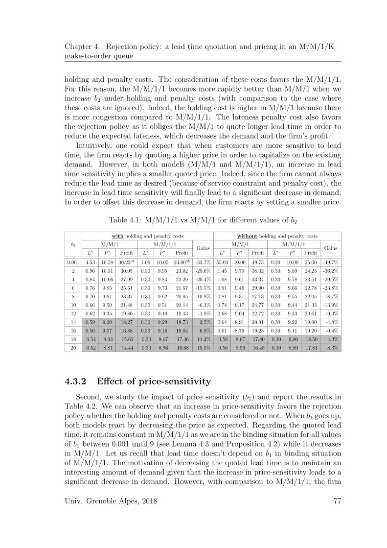
Chapter 4. Rejection policy: a lead time quotation and pricing in an M/M/1/Kmake-to-order queue
holding and penalty costs. The consideration of these costs favors the M/M/1/1.For this reason, the M/M/1/1 becomes more rapidly better than M/M/1 when weincrease b2 under holding and penalty costs (with comparison to the case wherethese costs are ignored). Indeed, the holding cost is higher in M/M/1 because thereis more congestion compared to M/M/1/1. The lateness penalty cost also favorsthe rejection policy as it obliges the M/M/1 to quote longer lead time in order toreduce the expected lateness, which decreases the demand and the firm’s profit.
Intuitively, one could expect that when customers are more sensitive to leadtime, the firm reacts by quoting a higher price in order to capitalize on the existingdemand. However, in both models (M/M/1 and M/M/1/1), an increase in leadtime sensitivity implies a smaller quoted price. Indeed, since the firm cannot alwaysreduce the lead time as desired (because of service constraint and penalty cost), theincrease in lead time sensitivity will finally lead to a significant decrease in demand.In order to offset this decrease in demand, the firm reacts by setting a smaller price.
Table 4.1: M/M/1/1 vs M/M/1 for different values of b2
with holding and penalty costs without holding and penalty costs
M/M/1 M/M/1/1 M/M/1 M/M/1/1b2
L∗ P ∗ Profit L∗ P ∗ ProfitGains
L∗ P ∗ Profit L∗ P ∗ ProfitGains
0.001 4.53 10.58 36.22nb 1.06 10.05 24.00nb -33.7% 55.03 10.00 49.73 0.30 10.00 25.00 -49.7%
2 0.96 10.31 30.95 0.30 9.95 23.02 -25.6% 1.45 9.79 38.02 0.30 9.89 24.25 -36.2%
4 0.84 10.06 27.99 0.30 9.84 22.29 -20.4% 1.08 9.61 33.34 0.30 9.78 23.51 -29.5%
6 0.76 9.85 25.51 0.30 9.73 21.57 -15.5% 0.91 9.46 29.90 0.30 9.66 22.78 -23.8%
8 0.70 9.67 23.37 0.30 9.62 20.85 -10.8% 0.81 9.31 27.13 0.30 9.55 22.05 -18.7%
10 0.66 9.50 21.48 0.30 9.51 20.14 -6.3% 0.74 9.17 24.77 0.30 9.44 21.33 -13.9%
12 0.62 9.35 19.80 0.30 9.40 19.43 -1.8% 0.68 9.04 22.72 0.30 9.33 20.61 -9.3%
14 0.59 9.20 18.27 0.30 9.29 18.73 2.5% 0.64 8.91 20.91 0.30 9.22 19.90 -4.8%
16 0.56 9.07 16.88 0.30 9.18 18.04 6.9% 0.61 8.79 19.28 0.30 9.11 19.20 -0.4%
18 0.54 8.93 15.61 0.30 9.07 17.36 11.2% 0.58 8.67 17.80 0.30 9.00 18.50 4.0%
20 0.52 8.81 14.44 0.30 8.96 16.68 15.5% 0.56 8.56 16.45 0.30 8.89 17.81 8.3%
4.3.2 Effect of price-sensitivity
Second, we study the impact of price sensitivity (b1) and report the results inTable 4.2. We can observe that an increase in price-sensitivity favors the rejectionpolicy whether the holding and penalty costs are considered or not. When b1 goes up,both models react by decreasing the price as expected. Regarding the quoted leadtime, it remains constant in M/M/1/1 as we are in the binding situation for all valuesof b1 between 0.001 until 9 (see Lemma 4.3 and Proposition 4.2) while it decreasesin M/M/1. Let us recall that lead time doesn’t depend on b1 in binding situationof M/M/1/1. The motivation of decreasing the quoted lead time is to maintain aninteresting amount of demand given that the increase in price-sensitivity leads to asignificant decrease in demand. However, with comparison to M/M/1/1, the firm
Univ. Grenoble Alpes, 2018 77
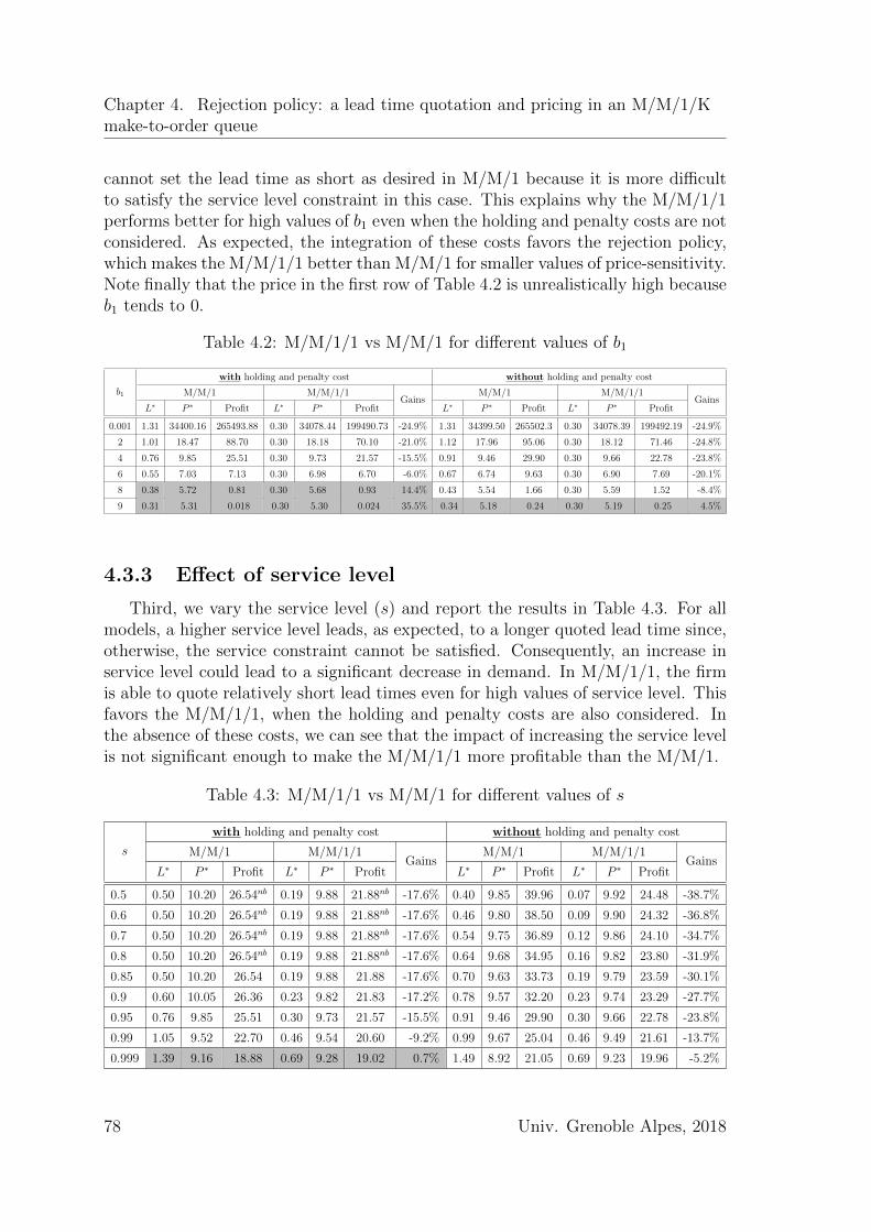
Chapter 4. Rejection policy: a lead time quotation and pricing in an M/M/1/Kmake-to-order queue
cannot set the lead time as short as desired in M/M/1 because it is more difficultto satisfy the service level constraint in this case. This explains why the M/M/1/1performs better for high values of b1 even when the holding and penalty costs are notconsidered. As expected, the integration of these costs favors the rejection policy,which makes the M/M/1/1 better than M/M/1 for smaller values of price-sensitivity.Note finally that the price in the first row of Table 4.2 is unrealistically high becauseb1 tends to 0.
Table 4.2: M/M/1/1 vs M/M/1 for different values of b1
b1
with holding and penalty cost without holding and penalty cost
M/M/1 M/M/1/1Gains
M/M/1 M/M/1/1Gains
L∗ P ∗ Profit L∗ P ∗ Profit L∗ P ∗ Profit L∗ P ∗ Profit
0.001 1.31 34400.16 265493.88 0.30 34078.44 199490.73 -24.9% 1.31 34399.50 265502.3 0.30 34078.39 199492.19 -24.9%
2 1.01 18.47 88.70 0.30 18.18 70.10 -21.0% 1.12 17.96 95.06 0.30 18.12 71.46 -24.8%
4 0.76 9.85 25.51 0.30 9.73 21.57 -15.5% 0.91 9.46 29.90 0.30 9.66 22.78 -23.8%
6 0.55 7.03 7.13 0.30 6.98 6.70 -6.0% 0.67 6.74 9.63 0.30 6.90 7.69 -20.1%
8 0.38 5.72 0.81 0.30 5.68 0.93 14.4% 0.43 5.54 1.66 0.30 5.59 1.52 -8.4%
9 0.31 5.31 0.018 0.30 5.30 0.024 35.5% 0.34 5.18 0.24 0.30 5.19 0.25 4.5%
4.3.3 Effect of service level
Third, we vary the service level (s) and report the results in Table 4.3. For allmodels, a higher service level leads, as expected, to a longer quoted lead time since,otherwise, the service constraint cannot be satisfied. Consequently, an increase inservice level could lead to a significant decrease in demand. In M/M/1/1, the firmis able to quote relatively short lead times even for high values of service level. Thisfavors the M/M/1/1, when the holding and penalty costs are also considered. Inthe absence of these costs, we can see that the impact of increasing the service levelis not significant enough to make the M/M/1/1 more profitable than the M/M/1.
Table 4.3: M/M/1/1 vs M/M/1 for different values of s
s
with holding and penalty cost without holding and penalty cost
M/M/1 M/M/1/1Gains
M/M/1 M/M/1/1Gains
L∗ P ∗ Profit L∗ P ∗ Profit L∗ P ∗ Profit L∗ P ∗ Profit
0.5 0.50 10.20 26.54nb 0.19 9.88 21.88nb -17.6% 0.40 9.85 39.96 0.07 9.92 24.48 -38.7%
0.6 0.50 10.20 26.54nb 0.19 9.88 21.88nb -17.6% 0.46 9.80 38.50 0.09 9.90 24.32 -36.8%
0.7 0.50 10.20 26.54nb 0.19 9.88 21.88nb -17.6% 0.54 9.75 36.89 0.12 9.86 24.10 -34.7%
0.8 0.50 10.20 26.54nb 0.19 9.88 21.88nb -17.6% 0.64 9.68 34.95 0.16 9.82 23.80 -31.9%
0.85 0.50 10.20 26.54 0.19 9.88 21.88 -17.6% 0.70 9.63 33.73 0.19 9.79 23.59 -30.1%
0.9 0.60 10.05 26.36 0.23 9.82 21.83 -17.2% 0.78 9.57 32.20 0.23 9.74 23.29 -27.7%
0.95 0.76 9.85 25.51 0.30 9.73 21.57 -15.5% 0.91 9.46 29.90 0.30 9.66 22.78 -23.8%
0.99 1.05 9.52 22.70 0.46 9.54 20.60 -9.2% 0.99 9.67 25.04 0.46 9.49 21.61 -13.7%
0.999 1.39 9.16 18.88 0.69 9.28 19.02 0.7% 1.49 8.92 21.05 0.69 9.23 19.96 -5.2%
78 Univ. Grenoble Alpes, 2018
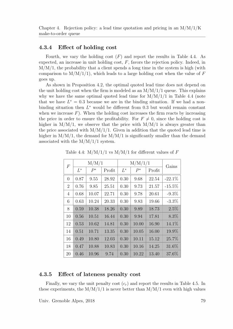
Chapter 4. Rejection policy: a lead time quotation and pricing in an M/M/1/Kmake-to-order queue
4.3.4 Effect of holding cost
Fourth, we vary the holding cost (F ) and report the results in Table 4.4. Asexpected, an increase in unit holding cost, F , favors the rejection policy. Indeed, inM/M/1, the probability that a client spends a long time in the system is high (withcomparison to M/M/1/1), which leads to a large holding cost when the value of Fgoes up.
As shown in Proposition 4.2, the optimal quoted lead time does not depend onthe unit holding cost when the firm is modeled as an M/M/1/1 queue. This explainswhy we have the same optimal quoted lead time for M/M/1/1 in Table 4.4 (notethat we have L∗ = 0.3 because we are in the binding situation. If we had a non-binding situation then L∗ would be different from 0.3 but would remain constantwhen we increase F ). When the holding cost increases the firm reacts by increasingthe price in order to ensure the profitability. For F 6= 0, since the holding cost ishigher in M/M/1, we observe that the price with M/M/1 is always greater thanthe price associated with M/M/1/1. Given in addition that the quoted lead time ishigher in M/M/1, the demand for M/M/1 is significantly smaller than the demandassociated with the M/M/1/1 system.
Table 4.4: M/M/1/1 vs M/M/1 for different values of F
M/M/1 M/M/1/1F
L∗ P ∗ Profit L∗ P ∗ ProfitGains
0 0.87 9.55 28.92 0.30 9.68 22.54 -22.1%
2 0.76 9.85 25.51 0.30 9.73 21.57 -15.5%
4 0.68 10.07 22.71 0.30 9.78 20.61 -9.3%
6 0.63 10.24 20.33 0.30 9.83 19.66 -3.3%
8 0.59 10.38 18.26 0.30 9.89 18.73 2.5%
10 0.56 10.51 16.44 0.30 9.94 17.81 8.3%
12 0.53 10.62 14.81 0.30 10.00 16.90 14.1%
14 0.51 10.71 13.35 0.30 10.05 16.00 19.9%
16 0.49 10.80 12.03 0.30 10.11 15.12 25.7%
18 0.47 10.88 10.83 0.30 10.16 14.25 31.6%
20 0.46 10.96 9.74 0.30 10.22 13.40 37.6%
4.3.5 Effect of lateness penalty cost
Finally, we vary the unit penalty cost (cr) and report the results in Table 4.5. Inthese experiments, the M/M/1/1 is never better than M/M/1 even with high values
Univ. Grenoble Alpes, 2018 79
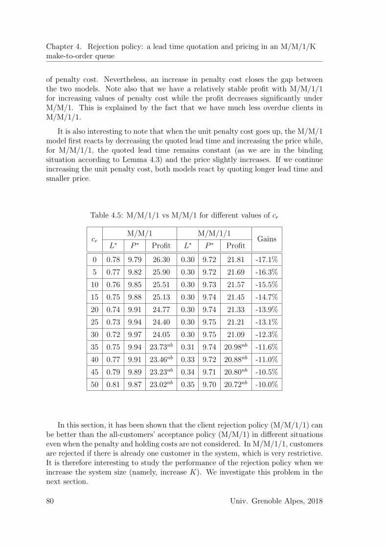
Chapter 4. Rejection policy: a lead time quotation and pricing in an M/M/1/Kmake-to-order queue
of penalty cost. Nevertheless, an increase in penalty cost closes the gap betweenthe two models. Note also that we have a relatively stable profit with M/M/1/1for increasing values of penalty cost while the profit decreases significantly underM/M/1. This is explained by the fact that we have much less overdue clients inM/M/1/1.
It is also interesting to note that when the unit penalty cost goes up, the M/M/1model first reacts by decreasing the quoted lead time and increasing the price while,for M/M/1/1, the quoted lead time remains constant (as we are in the bindingsituation according to Lemma 4.3) and the price slightly increases. If we continueincreasing the unit penalty cost, both models react by quoting longer lead time andsmaller price.
Table 4.5: M/M/1/1 vs M/M/1 for different values of cr
M/M/1 M/M/1/1cr
L∗ P ∗ Profit L∗ P ∗ ProfitGains
0 0.78 9.79 26.30 0.30 9.72 21.81 -17.1%
5 0.77 9.82 25.90 0.30 9.72 21.69 -16.3%
10 0.76 9.85 25.51 0.30 9.73 21.57 -15.5%
15 0.75 9.88 25.13 0.30 9.74 21.45 -14.7%
20 0.74 9.91 24.77 0.30 9.74 21.33 -13.9%
25 0.73 9.94 24.40 0.30 9.75 21.21 -13.1%
30 0.72 9.97 24.05 0.30 9.75 21.09 -12.3%
35 0.75 9.94 23.73nb 0.31 9.74 20.98nb -11.6%
40 0.77 9.91 23.46nb 0.33 9.72 20.88nb -11.0%
45 0.79 9.89 23.23nb 0.34 9.71 20.80nb -10.5%
50 0.81 9.87 23.02nb 0.35 9.70 20.72nb -10.0%
In this section, it has been shown that the client rejection policy (M/M/1/1) canbe better than the all-customers’ acceptance policy (M/M/1) in different situationseven when the penalty and holding costs are not considered. In M/M/1/1, customersare rejected if there is already one customer in the system, which is very restrictive.It is therefore interesting to study the performance of the rejection policy when weincrease the system size (namely, increase K). We investigate this problem in thenext section.
80 Univ. Grenoble Alpes, 2018
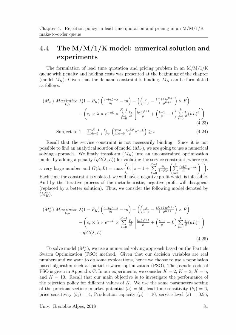
Chapter 4. Rejection policy: a lead time quotation and pricing in an M/M/1/Kmake-to-order queue
4.4 The M/M/1/K model: numerical solution and
experiments
The formulation of lead time quotation and pricing problem in an M/M/1/Kqueue with penalty and holding costs was presented at the beginning of the chapter(model MK). Given that the demand constraint is binding, MK can be formulatedas follows.
(MK) MaximizeL,λ
λ(1− PK)(a−b2L−λ
b1−m
)−((
ρ1−ρ −
(K+1)ρK+1
1−ρK+1
)× F
)−(cr × λ× e−µL ×
K−1∑k=0
Pkk!
[(µL)k+1
µ+(k+1µ− L
) k∑i=0
k!i!
(µL)i])
(4.23)
Subject to 1−∑K−1
k=0Pk
1−PK
(∑ki=0
(µL)i
i!e−µL
)≥ s (4.24)
Recall that the service constraint is not necessarily binding. Since it is notpossible to find an analytical solution of model (MK), we are going to use a numericalsolving approach. We firstly transform (MK) into an unconstrained optimizationmodel by adding a penalty (ηG(λ, L)) for violating the service constraint, where η is
a very large number and G(λ, L) = max
(0,
[s− 1 +
K−1∑k=0
Pk1−PK
(k∑i=0
(µL)i
i!e−µL
)]).
Each time the constraint is violated, we will have a negative profit which is infeasible.And by the iterative process of the meta-heuristic, negative profit will disappear(replaced by a better solution). Thus, we consider the following model denoted by(M∗
K).
(M∗K) Maximize
L,λλ(1− PK)
(a−b2L−λ
b1−m
)−((
ρ1−ρ −
(K+1)ρK+1
1−ρK+1
)× F
)−(cr × λ× e−µL ×
K−1∑k=0
Pkk!
[(µL)k+1
µ+(k+1µ− L
) k∑i=0
k!i!
(µL)i])
−η[G(λ, L)]
(4.25)
To solve model (M∗K), we use a numerical solving approach based on the Particle
Swarm Optimization (PSO) method. Given that our decision variables are realnumbers and we want to do some explorations, hence we choose to use a populationbased algorithm such as particle swarm optimization (PSO). The pseudo code ofPSO is given in Appendix C. In our experiments, we consider K = 2, K = 3, K = 5,and K = 10. Recall that our main objective is to investigate the performance ofthe rejection policy for different values of K. We use the same parameters settingof the previous section: market potential (a) = 50, lead time sensitivity (b2) = 6,price sensitivity (b1) = 4; Production capacity (µ) = 10; service level (s) = 0.95;
Univ. Grenoble Alpes, 2018 81
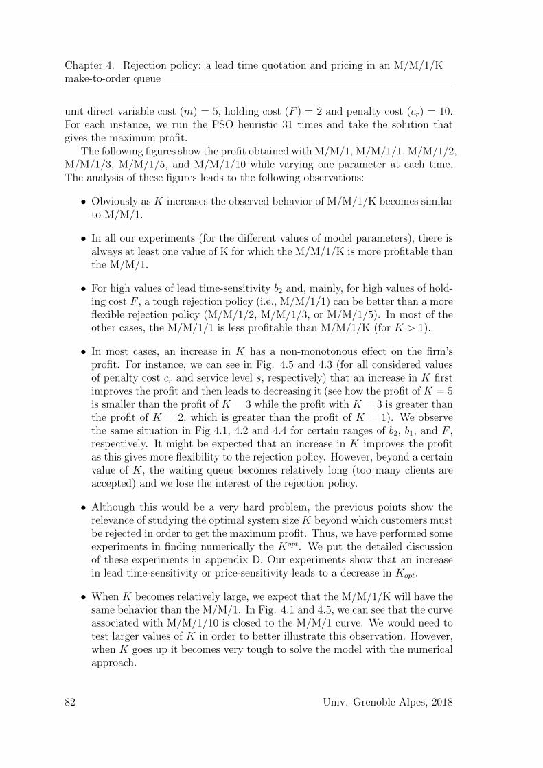
Chapter 4. Rejection policy: a lead time quotation and pricing in an M/M/1/Kmake-to-order queue
unit direct variable cost (m) = 5, holding cost (F ) = 2 and penalty cost (cr) = 10.For each instance, we run the PSO heuristic 31 times and take the solution thatgives the maximum profit.
The following figures show the profit obtained with M/M/1, M/M/1/1, M/M/1/2,M/M/1/3, M/M/1/5, and M/M/1/10 while varying one parameter at each time.The analysis of these figures leads to the following observations:
• Obviously as K increases the observed behavior of M/M/1/K becomes similarto M/M/1.
• In all our experiments (for the different values of model parameters), there isalways at least one value of K for which the M/M/1/K is more profitable thanthe M/M/1.
• For high values of lead time-sensitivity b2 and, mainly, for high values of hold-ing cost F , a tough rejection policy (i.e., M/M/1/1) can be better than a moreflexible rejection policy (M/M/1/2, M/M/1/3, or M/M/1/5). In most of theother cases, the M/M/1/1 is less profitable than M/M/1/K (for K > 1).
• In most cases, an increase in K has a non-monotonous effect on the firm’sprofit. For instance, we can see in Fig. 4.5 and 4.3 (for all considered valuesof penalty cost cr and service level s, respectively) that an increase in K firstimproves the profit and then leads to decreasing it (see how the profit of K = 5is smaller than the profit of K = 3 while the profit with K = 3 is greater thanthe profit of K = 2, which is greater than the profit of K = 1). We observethe same situation in Fig 4.1, 4.2 and 4.4 for certain ranges of b2, b1, and F ,respectively. It might be expected that an increase in K improves the profitas this gives more flexibility to the rejection policy. However, beyond a certainvalue of K, the waiting queue becomes relatively long (too many clients areaccepted) and we lose the interest of the rejection policy.
• Although this would be a very hard problem, the previous points show therelevance of studying the optimal system size K beyond which customers mustbe rejected in order to get the maximum profit. Thus, we have performed someexperiments in finding numerically the Kopt. We put the detailed discussionof these experiments in appendix D. Our experiments show that an increasein lead time-sensitivity or price-sensitivity leads to a decrease in Kopt.
• When K becomes relatively large, we expect that the M/M/1/K will have thesame behavior than the M/M/1. In Fig. 4.1 and 4.5, we can see that the curveassociated with M/M/1/10 is closed to the M/M/1 curve. We would need totest larger values of K in order to better illustrate this observation. However,when K goes up it becomes very tough to solve the model with the numericalapproach.
82 Univ. Grenoble Alpes, 2018
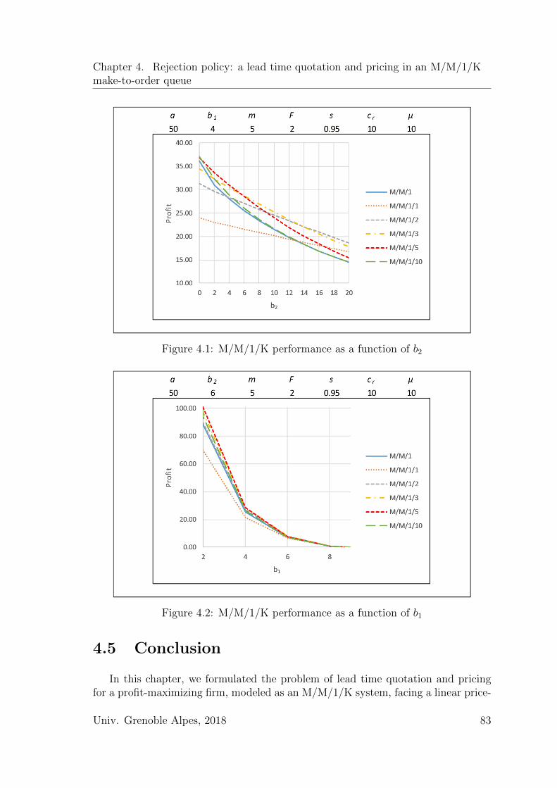
Chapter 4. Rejection policy: a lead time quotation and pricing in an M/M/1/Kmake-to-order queue
Figure 4.1: M/M/1/K performance as a function of b2
Figure 4.2: M/M/1/K performance as a function of b1
4.5 Conclusion
In this chapter, we formulated the problem of lead time quotation and pricingfor a profit-maximizing firm, modeled as an M/M/1/K system, facing a linear price-
Univ. Grenoble Alpes, 2018 83
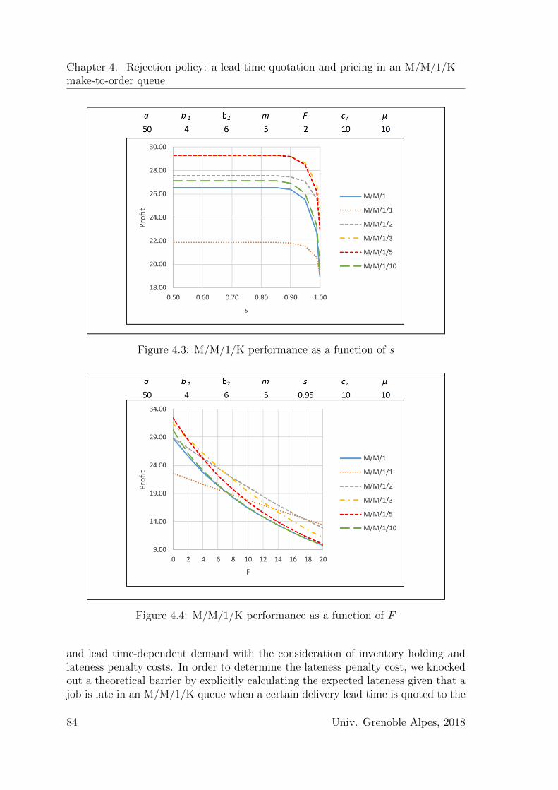
Chapter 4. Rejection policy: a lead time quotation and pricing in an M/M/1/Kmake-to-order queue
Figure 4.3: M/M/1/K performance as a function of s
Figure 4.4: M/M/1/K performance as a function of F
and lead time-dependent demand with the consideration of inventory holding andlateness penalty costs. In order to determine the lateness penalty cost, we knockedout a theoretical barrier by explicitly calculating the expected lateness given that ajob is late in an M/M/1/K queue when a certain delivery lead time is quoted to the
84 Univ. Grenoble Alpes, 2018
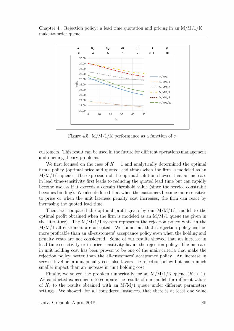
Chapter 4. Rejection policy: a lead time quotation and pricing in an M/M/1/Kmake-to-order queue
Figure 4.5: M/M/1/K performance as a function of cr
customers. This result can be used in the future for different operations managementand queuing theory problems.
We first focused on the case of K = 1 and analytically determined the optimalfirm’s policy (optimal price and quoted lead time) when the firm is modeled as anM/M/1/1 queue. The expression of the optimal solution showed that an increasein lead time-sensitivity first leads to reducing the quoted lead time but can rapidlybecome useless if it exceeds a certain threshold value (since the service constraintbecomes binding). We also deduced that when the customers become more sensitiveto price or when the unit lateness penalty cost increases, the firm can react byincreasing the quoted lead time.
Then, we compared the optimal profit given by our M/M/1/1 model to theoptimal profit obtained when the firm is modeled as an M/M/1 queue (as given inthe literature). The M/M/1/1 system represents the rejection policy while in theM/M/1 all customers are accepted. We found out that a rejection policy can bemore profitable than an all-customers’ acceptance policy even when the holding andpenalty costs are not considered. Some of our results showed that an increase inlead time sensitivity or in price-sensitivity favors the rejection policy. The increasein unit holding cost has been proven to be one of the main criteria that make therejection policy better than the all-customers’ acceptance policy. An increase inservice level or in unit penalty cost also favors the rejection policy but has a muchsmaller impact than an increase in unit holding cost.
Finally, we solved the problem numerically for an M/M/1/K queue (K > 1).We conducted experiments to compare the results of our model, for different valuesof K, to the results obtained with an M/M/1 queue under different parameterssettings. We showed, for all considered instances, that there is at least one value
Univ. Grenoble Alpes, 2018 85
Chapter 4. Rejection policy: a lead time quotation and pricing in an M/M/1/Kmake-to-order queue
of K for which the M/M/1/K (rejection policy) is more profitable than the M/M/1(all customers’ acceptance policy). In most cases, it has also been observed that anincrease in the value of K (i.e., the system size) has a non-monotonous effect on thefirm’s profit. Indeed, an increase in K first improves the profit and then leads todecreasing it.
86 Univ. Grenoble Alpes, 2018
Chapter 5
Coordination ofupstream-downstream supply
chain under price and lead timesensitive demand: a tandem queue
model
In the industrial world nowadays, a competition between enterprises is a compe-tition between supply chains. And different stages of the supply chain are used toresponse the expectation of the clients. Let us take an example of airplane industry,such as Airbus. When an order arrives, Airbus has to quote the right price andlead time that fit the customer needs. Airbus will contact its suppliers, which willquote their price and lead time taking into account some constraints imposed byAirbus. Then, Airbus announces the final price and lead time to the costumer. Thecostumer will then decide on the basis of the lead time and price offered. If we addthe feature of a lead time dependent demand in this supply chain, the problem willbecome complex. Thus it is interesting to study the behavior of such chain and howto quote the right lead time and price under the endogenous demand (demand sen-sitive to price and lead time). In this chapter, we only consider a two-stage supplychain which we model as a tandem queue network (M/M/1-M/M/1).
In chapter 2, we saw several papers in the literature who model different stages ofa supply chain in cooperative firms, such as Liu et al. (2007); Xiao et al. (2011); Xiaoand Shi (2012); Zhu (2015); and Xiao and Qi (2016). However, in this literatureonly one of its actor has a production process and lead time. The other actordoesn’t have production process, in other words, the lead time is zero. Based onour knowledge, no paper considers two stages with both actors having productionprocess (lead time).
5.1 System description (M/M/1–M/M/1)
We consider a two-stage supply chain consisting of an upstream actor (supplieror manufacturer) and a downstream actor (manufacturer or retailer). The demandsarrive at the downstream actor according to a Poisson process. Both actors (up-stream and downstream) have a fixed capacity with exponential service time. Thus,
87
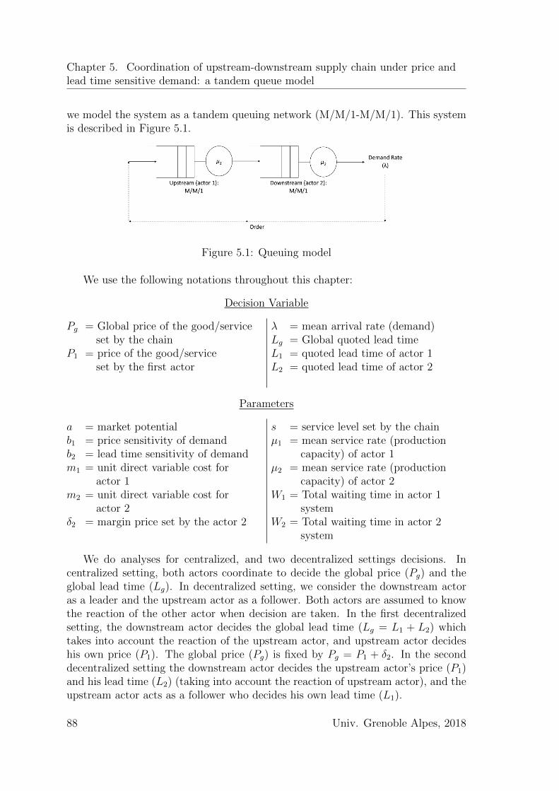
Chapter 5. Coordination of upstream-downstream supply chain under price andlead time sensitive demand: a tandem queue model
we model the system as a tandem queuing network (M/M/1-M/M/1). This systemis described in Figure 5.1.
Figure 5.1: Queuing model
We use the following notations throughout this chapter:
Decision Variable
Pg = Global price of the good/serviceset by the chain
P1 = price of the good/serviceset by the first actor
λ = mean arrival rate (demand)Lg = Global quoted lead timeL1 = quoted lead time of actor 1L2 = quoted lead time of actor 2
Parameters
a = market potentialb1 = price sensitivity of demandb2 = lead time sensitivity of demandm1 = unit direct variable cost for
actor 1m2 = unit direct variable cost for
actor 2δ2 = margin price set by the actor 2
s = service level set by the chainµ1 = mean service rate (production
capacity) of actor 1µ2 = mean service rate (production
capacity) of actor 2W1 = Total waiting time in actor 1
systemW2 = Total waiting time in actor 2
system
We do analyses for centralized, and two decentralized settings decisions. Incentralized setting, both actors coordinate to decide the global price (Pg) and theglobal lead time (Lg). In decentralized setting, we consider the downstream actoras a leader and the upstream actor as a follower. Both actors are assumed to knowthe reaction of the other actor when decision are taken. In the first decentralizedsetting, the downstream actor decides the global lead time (Lg = L1 + L2) whichtakes into account the reaction of the upstream actor, and upstream actor decideshis own price (P1). The global price (Pg) is fixed by Pg = P1 + δ2. In the seconddecentralized setting the downstream actor decides the upstream actor’s price (P1)and his lead time (L2) (taking into account the reaction of upstream actor), and theupstream actor acts as a follower who decides his own lead time (L1).
88 Univ. Grenoble Alpes, 2018
Chapter 5. Coordination of upstream-downstream supply chain under price andlead time sensitive demand: a tandem queue model
5.2 Centralized Setting: Model and Experiments
We start our analysis with the centralized setting. In this centralized setting, weconsider downstream and upstream actors who work together to decide the globalprice (Pg) and global lead time (Lg). We model the centralized problem as follows:
MaximizePg ,Lg≥0
(Pg −m1 −m2)λ (5.1)
Subject to λ = a− b1Pg − b2Lg (5.2)
Pr(W1 +W2 ≤ Lg) ≥ s (5.3)
0 ≤ λ < µ1, µ2 (5.4)
When µ1 6= µ2, the actual lead time (W1 + W2) will follow a hypo-exponentialdistribution (Bolch et al., 2006). Thus, the service constraint (5.3) will be expressedas below:
1− µ2 − λ(µ2 − λ)− (µ1 − λ)
e−(µ1−λ)Lg +µ1 − λ
(µ2 − λ)− (µ1 − λ)e−(µ2−λ)Lg ≥ s
⇔ 1− µ2 − λµ2 − µ1
e−(µ1−λ)Lg +(µ1 − λ)
(µ2 − µ1)e−(µ2−λ)Lg ≥ s
However, if the upstream actor has exactly same capacity as the downstream actor(µ1 = µ2 = µ)(Bolch et al., 2006), the service constraint (5.3) becomes:
1− e−(µ−λ)Lg − e−(µ−λ)Lg(µ− λ)Lg ≥ s
The overall formulation for both problem with µ1 6= µ2 and µ1 = µ2 can be rewrittenas:
MaximizePg ,Lg≥0
Πc(Pg, Lg) = (Pg −m1 −m2)(a− b1Pg − b2Lg) (5.5)
Subject to Pr(W1 +W2 ≤ Lg) ≥ s⇔
1− µ2−a+b1Pg+b2Lgµ2−µ1 e−(µ1−a+b1Pg+b2Lg)Lg
+µ1−a+b1Pg+b2Lgµ2−µ1 e−(µ2−a+b1Pg+b2Lg)Lg ≥ s,
for µ1 6= µ2
1− e−(µ−a+b1Pg+b2Lg)Lg − e−(µ−a+b1Pg+b2Lg)Lg
(µ− a+ b1Pg + b2Lg)Lg ≥ s,
for µ1 = µ2
(5.6)
0 ≤ a− b1Pg − b2Lg < µ1, µ2 (5.7)
Then, we deduce several lemmas.
Lemma 5.1. The profit Πc(Pg, Lg) is concave for any given Lg and Pg.
Univ. Grenoble Alpes, 2018 89
Chapter 5. Coordination of upstream-downstream supply chain under price andlead time sensitive demand: a tandem queue model
Proof. The second derivative of Πc(Pg, Lg) is ∂2
∂Pg2Πc(Pg, Lg) = −2b1 which proves
that the function Πc(Pg, Lg) is concave in Pg for given Lg. The second derivative
of Πc(Pg, Lg) in function of Lg is null ( ∂2
∂Lg2Πc(Pg, Lg) = 0) and ∂2
∂Pg∂LgΠc(Pg, Lg) =
−b2. Hence, the function Πc(Pg, Lg) is concave given that ∂2Πc(Pg ,Lg)
∂Pg2∂2Πc(Pg ,Lg)
∂Lg2−[
∂2Πc(Pg ,Lg)
∂Pg∂Lg
]2
= b22 ≥ 0, ∂2Πc(Pg ,Lg)
∂Pg2≤ 0, and ∂2Πc(Pg ,Lg)
∂Lg2≤ 0 (see Hillier and Lieber-
man, 2001 on how to prove convexity or concavity of functions with several vari-ables) �
Lemma 5.2. service constraint (5.6), for both µ1 6= µ2 and µ1 = µ2, is binding atoptimality.
Proof. Let’s assume that at optimality we have Pg∗ and Lg
∗ which give a service levelsuperior to s (Pr(W1 +W2 ≤ Lg) > s). We have profit of the firm as Πc(Pg
∗, Lg∗). If
we decrease the Lg∗ to Lg
′ (while keeping Pg constant) until Pr(W1 +W2 ≤ Lg) = s,we will get Πc(Pg
∗, Lg∗) < Πc(Pg
∗, Lg′) since the demand has increased. We have a
better solution which is Pg∗ and Lg
′. Thus, service level is binding at optimality.This condition is true with µ1 = µ2 and µ1 6= µ2. �
From lemma 5.2 and constraint (5.6), we can deduce a link between Pg and Lg.For each value of Pg, we can obtain a unique value of Lg. Thus the initial problembecome a single optimization problem in function of Pg. Then, we can find thesolution for profit Πc numerically as proposed in proposition below.
Proposition 5.1. The following single optimization problem (centralized setting):
MaximizePg≥0
Πc(Pg) = (Pg −m1 −m2)(a− b1Pg − b2Lg(Pg))
can be solved with bisection method with the following steps:
1. We fixed a value Pg within the range of (m1 +m2) ≤ Pg ≤ ab1
,
2. We obtain a unique solution of Lg in function of Pg from:
g(Pg, Lg) =
1− s− µ2−a+b1Pg+b2Lg
µ2−µ1 e−(µ1−a+b1Pg+b2Lg)Lg
+µ1−a+b1Pg+b2Lgµ2−µ1 e−(µ2−a+b1Pg+b2Lg)Lg = 0 for µ1 6= µ2
1− s− e−(µ−a+b1Pg+b2Lg)Lg − e−(µ−a+b1Pg+b2Lg)Lg
(µ− a+ b1Pg + b2Lg)Lg = 0 for µ1 = µ2
with the range of a−Pgb1−min[µ1,µ2]
b2< Lg ≤ a−b1Pg
b2.
3. With the obtained Lg, we can calculate Πc(Pg) and use the bisection methodprocedures.
90 Univ. Grenoble Alpes, 2018
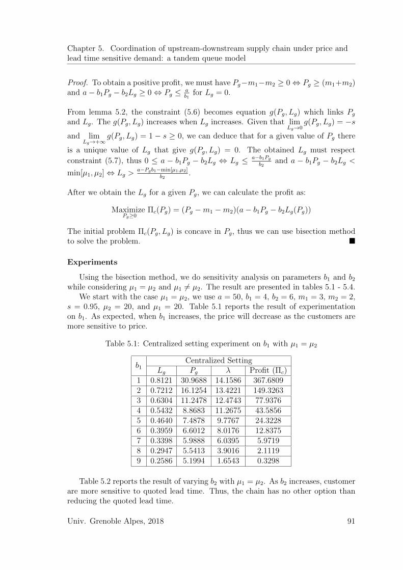
Chapter 5. Coordination of upstream-downstream supply chain under price andlead time sensitive demand: a tandem queue model
Proof. To obtain a positive profit, we must have Pg−m1−m2 ≥ 0⇔ Pg ≥ (m1+m2)and a− b1Pg − b2Lg ≥ 0⇔ Pg ≤ a
b1for Lg = 0.
From lemma 5.2, the constraint (5.6) becomes equation g(Pg, Lg) which links Pgand Lg. The g(Pg, Lg) increases when Lg increases. Given that lim
Lg→0g(Pg, Lg) = −s
and limLg→+∞
g(Pg, Lg) = 1− s ≥ 0, we can deduce that for a given value of Pg there
is a unique value of Lg that give g(Pg, Lg) = 0. The obtained Lg must respect
constraint (5.7), thus 0 ≤ a − b1Pg − b2Lg ⇔ Lg ≤ a−b1Pgb2
and a − b1Pg − b2Lg <
min[µ1, µ2]⇔ Lg >a−Pgb1−min[µ1,µ2]
b2.
After we obtain the Lg for a given Pg, we can calculate the profit as:
MaximizePg≥0
Πc(Pg) = (Pg −m1 −m2)(a− b1Pg − b2Lg(Pg))
The initial problem Πc(Pg, Lg) is concave in Pg, thus we can use bisection methodto solve the problem. �
Experiments
Using the bisection method, we do sensitivity analysis on parameters b1 and b2
while considering µ1 = µ2 and µ1 6= µ2. The result are presented in tables 5.1 - 5.4.We start with the case µ1 = µ2, we use a = 50, b1 = 4, b2 = 6, m1 = 3, m2 = 2,
s = 0.95, µ2 = 20, and µ1 = 20. Table 5.1 reports the result of experimentationon b1. As expected, when b1 increases, the price will decrease as the customers aremore sensitive to price.
Table 5.1: Centralized setting experiment on b1 with µ1 = µ2
b1Centralized Setting
Lg Pg λ Profit (Πc)1 0.8121 30.9688 14.1586 367.68092 0.7212 16.1254 13.4221 149.32633 0.6304 11.2478 12.4743 77.93764 0.5432 8.8683 11.2675 43.58565 0.4640 7.4878 9.7767 24.32286 0.3959 6.6012 8.0176 12.83757 0.3398 5.9888 6.0395 5.97198 0.2947 5.5413 3.9016 2.11199 0.2586 5.1994 1.6543 0.3298
Table 5.2 reports the result of varying b2 with µ1 = µ2. As b2 increases, customerare more sensitive to quoted lead time. Thus, the chain has no other option thanreducing the quoted lead time.
Univ. Grenoble Alpes, 2018 91
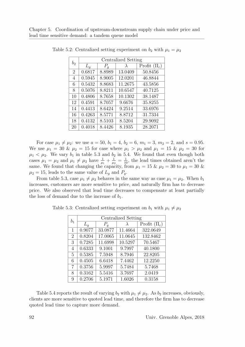
Chapter 5. Coordination of upstream-downstream supply chain under price andlead time sensitive demand: a tandem queue model
Table 5.2: Centralized setting experiment on b2 with µ1 = µ2
b2Centralized Setting
Lg Pg λ Profit (Πc)2 0.6817 8.8989 13.0409 50.84564 0.5945 8.9005 12.0201 46.88446 0.5432 8.8683 11.2675 43.58568 0.5076 8.8211 10.6547 40.712510 0.4806 8.7658 10.1302 38.148712 0.4591 8.7057 9.6676 35.825514 0.4413 8.6424 9.2514 33.697616 0.4263 8.5771 8.8712 31.733418 0.4132 8.5103 8.5204 29.909220 0.4018 8.4426 8.1935 28.2071
For case µ1 6= µ2: we use a = 50, b1 = 4, b2 = 6, m1 = 3, m2 = 2, and s = 0.95.We use µ1 = 30 & µ2 = 15 for case where µ1 > µ2 and µ1 = 15 & µ2 = 30 forµ1 < µ2. We vary b1 in table 5.3 and b2 in 5.4. We found that even though bothcases µ1 = µ2 and µ1 6= µ2 have 1
µ1+ 1
µ2= 1
10, the lead times obtained aren’t the
same. We found that changing the capacity, from µ1 = 15 & µ2 = 30 to µ1 = 30 &µ2 = 15, leads to the same value of Lg and Pg.
From table 5.3, case µ1 6= µ2 behaves in the same way as case µ1 = µ2. When b1
increases, customers are more sensitive to price, and naturally firm has to decreaseprice. We also observed that lead time decreases to compensate at least partiallythe loss of demand due to the increase of b1.
Table 5.3: Centralized setting experiment on b1 with µ1 6= µ2
b1Centralized Setting
Lg Pg λ Profit (Πc)1 0.9077 33.0877 11.4664 322.06492 0.8204 17.0065 11.0645 132.84623 0.7285 11.6998 10.5297 70.54674 0.6333 9.1001 9.7997 40.18005 0.5385 7.5948 8.7946 22.82056 0.4505 6.6418 7.4462 12.22507 0.3756 5.9997 5.7484 5.74688 0.3162 5.5416 3.7697 2.04199 0.2706 5.1971 1.6026 0.3158
Table 5.4 reports the result of varying b2 with µ1 6= µ2. As b2 increases, obviously,clients are more sensitive to quoted lead time, and therefore the firm has to decreasequoted lead time to capture more demand.
92 Univ. Grenoble Alpes, 2018
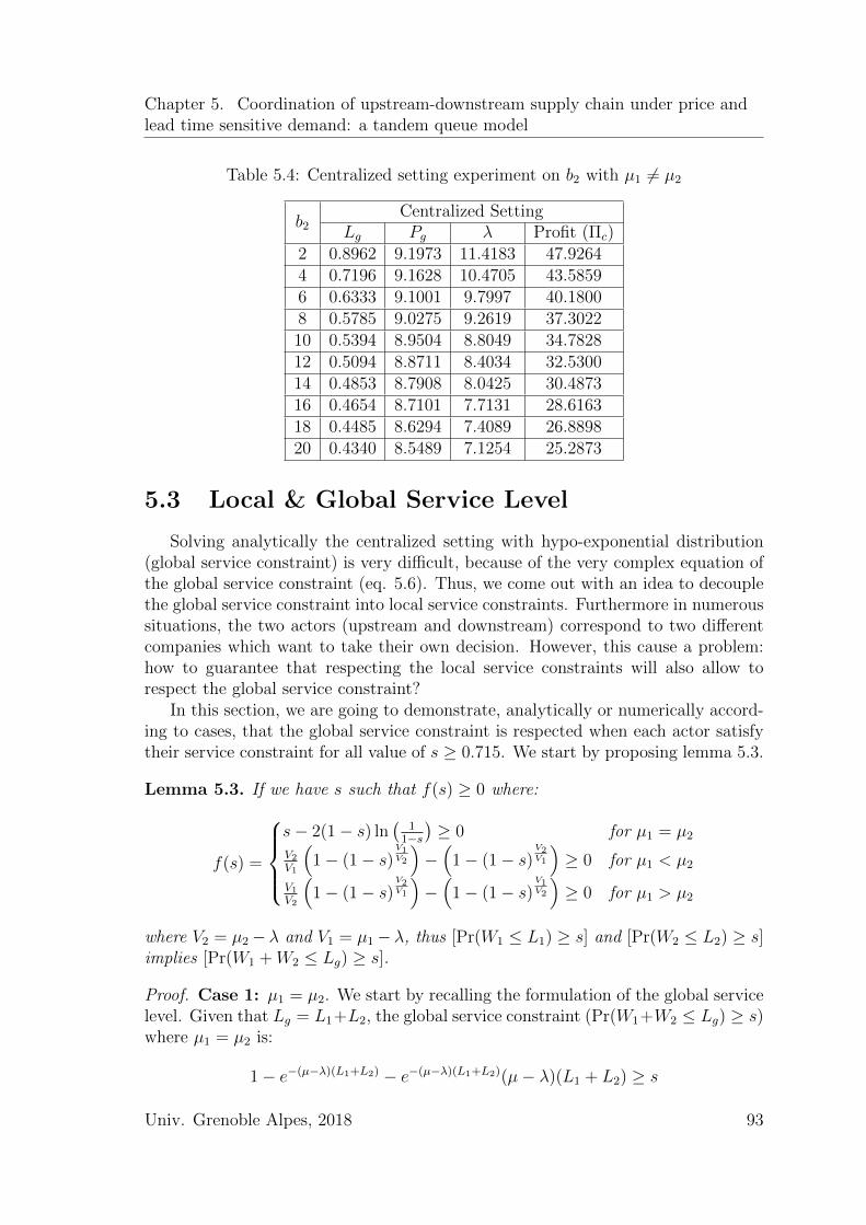
Chapter 5. Coordination of upstream-downstream supply chain under price andlead time sensitive demand: a tandem queue model
Table 5.4: Centralized setting experiment on b2 with µ1 6= µ2
b2Centralized Setting
Lg Pg λ Profit (Πc)2 0.8962 9.1973 11.4183 47.92644 0.7196 9.1628 10.4705 43.58596 0.6333 9.1001 9.7997 40.18008 0.5785 9.0275 9.2619 37.302210 0.5394 8.9504 8.8049 34.782812 0.5094 8.8711 8.4034 32.530014 0.4853 8.7908 8.0425 30.487316 0.4654 8.7101 7.7131 28.616318 0.4485 8.6294 7.4089 26.889820 0.4340 8.5489 7.1254 25.2873
5.3 Local & Global Service Level
Solving analytically the centralized setting with hypo-exponential distribution(global service constraint) is very difficult, because of the very complex equation ofthe global service constraint (eq. 5.6). Thus, we come out with an idea to decouplethe global service constraint into local service constraints. Furthermore in numeroussituations, the two actors (upstream and downstream) correspond to two differentcompanies which want to take their own decision. However, this cause a problem:how to guarantee that respecting the local service constraints will also allow torespect the global service constraint?
In this section, we are going to demonstrate, analytically or numerically accord-ing to cases, that the global service constraint is respected when each actor satisfytheir service constraint for all value of s ≥ 0.715. We start by proposing lemma 5.3.
Lemma 5.3. If we have s such that f(s) ≥ 0 where:
f(s) =
s− 2(1− s) ln
(1
1−s
)≥ 0 for µ1 = µ2
V2V1
(1− (1− s)
V1V2
)−(
1− (1− s)V2V1
)≥ 0 for µ1 < µ2
V1V2
(1− (1− s)
V2V1
)−(
1− (1− s)V1V2
)≥ 0 for µ1 > µ2
where V2 = µ2− λ and V1 = µ1− λ, thus [Pr(W1 ≤ L1) ≥ s] and [Pr(W2 ≤ L2) ≥ s]implies [Pr(W1 +W2 ≤ Lg) ≥ s].
Proof. Case 1: µ1 = µ2. We start by recalling the formulation of the global servicelevel. Given that Lg = L1+L2, the global service constraint (Pr(W1+W2 ≤ Lg) ≥ s)where µ1 = µ2 is:
1− e−(µ−λ)(L1+L2) − e−(µ−λ)(L1+L2)(µ− λ)(L1 + L2) ≥ s
Univ. Grenoble Alpes, 2018 93
Chapter 5. Coordination of upstream-downstream supply chain under price andlead time sensitive demand: a tandem queue model
We have the local service constraints which are:Pr(W1 ≤ L1) ≥ s⇔ e−(µ1−λ)L1 ≤ 1− s and Pr(W2 ≤ L2) ≥ s⇔ e−(µ2−λ)L2 ≤ 1− s.We consider calculations with 1 − s = e−(µ1−λ)L1 and 1 − s = e−(µ1−λ)L2 . Andobviously if we prove that in this case the global service constraint is satisfied, itwill be also verified when 1− s > e−(µ1−λ)L1 and/or 1− s > e−(µ1−λ)L2 . The globalservice level equation is then equivalent to:
1− e−(µ−λ)(L1+L2) − e−(µ−λ)(L1+L2)(µ− λ)(L1 + L2) =
1− (1− s)2 − (µ− λ)(L1 + L2)(1− s)2 ≥ s
With s 6= 1, we can simplify the equation above into:
s− (µ− λ)(L1 + L2)(1− s) ≥ 0
From e−(µ1−λ)L1 = 1− s and e−(µ2−λ)L2 = 1− s, we can deduce:
(µ− λ)(L1 + L2) = 2 ln
(1
1− s
)and therefore:
s− (µ− λ)(L1 + L2)(1− s) = s− 2(1− s) ln
(1
1− s
)≥ 0
Therefore we have proven that if f(s) = s− 2(1− s) ln(
11−s
)≥ 0 the global service
level is respected.
Case 2: µ1 6= µ2. The global service constraint (Pr(W1 + W2 ≤ Lg) ≥ s) whereµ2 − µ1 6= 0 is:
1− µ2 − λµ2 − µ1
e−(µ1−λ)(L1+L2) +µ1 − λµ2 − µ1
e−(µ2−λ)(L1+L2) ≥ s
⇔ 1− µ2 − λµ2 − µ1
e−(µ1−λ)L1e−(µ1−λ)L2 +µ1 − λµ2 − µ1
e−(µ2−λ)L1e−(µ2−λ)L2 ≥ s
Given that the local service constraints are e−(µ1−λ)L1 ≤ 1−s and e−(µ2−λ)L2 ≤ 1−s,we use the same logic as for case µ1 = µ2: we consider the case in which local serviceconstraints are binding (e−(µ1−λ)L1 = 1 − s and e−(µ2−λ)L2 = 1 − s). The obtainedcondition in this case will be obviously a sufficient condition when we will havee−(µ1−λ)L1 < 1 − s and/or e−(µ2−λ)L2 < 1 − s. Thus the global service constraint isequivalent to:
1− µ2 − λµ2 − µ1
e−(µ1−λ)L1e−(µ1−λ)L2 +µ1 − λµ2 − µ1
e−(µ2−λ)L1e−(µ2−λ)L2 =
1− 1− sµ2 − µ1
[(µ2 − λ)e−(µ1−λ)L2 + (µ1 − λ)e−(µ2−λ)L1
]≥ s
94 Univ. Grenoble Alpes, 2018
Chapter 5. Coordination of upstream-downstream supply chain under price andlead time sensitive demand: a tandem queue model
Here, we have two sub-cases: µ2 − µ1 > 0 and µ2 − µ1 < 0.Sub-case 2.1: µ2 − µ1 > 0. We derive from previous inequality:
1− 1− sµ2 − µ1
[(µ2 − λ)e−(µ1−λ)L2 + (µ1 − λ)e−(µ2−λ)L1
]≥ s
⇔ µ2 − µ1 ≥ (µ2 − λ)e−(µ1−λ)L2 + (µ1 − λ)e−(µ2−λ)L1
Recall that we consider e−(µ1−λ)L1 = 1− s which is equivalent to L1 = ln(1/(1−s))µ1−λ and
e−(µ2−λ)L2 = 1− s which is equivalent to L2 = ln(1/(1−s))µ2−λ . Thus we obtain:
µ2 − µ1 − (µ2 − λ)e−(µ1−λ)
ln(1/(1−s))µ2−λ − (µ1 − λ)e
−(µ2−λ)ln(1/(1−s))µ1−λ =
µ2 − µ1 − (µ2 − λ)(1− s)µ1−λµ2−λ − (µ1 − λ)(1− s)
µ2−λµ1−λ ≥ 0
Replace (µ2 − λ) = V2 and (µ1 − λ) = V1, we obtain:
V2 − V1 − V2(1− s)V1V2 − V1(1− s)
V2V1 ≥ 0
⇔ f(s) =V2
V1
(1− (1− s)
V1V2
)−(
1− (1− s)V2V1
)≥ 0
Thus, if f(s) ≥ 0 implies Pr(W1 +W2 ≤ Lg) ≥ s for µ2 > µ1.Sub-case 2.2: µ2−µ1 < 0. Using the same procedure as sub-case 2.1, we will have:
f(s) =V1
V2
(1− (1− s)
V2V1
)−(
1− (1− s)V1V2
)≥ 0
Thus, if f(s) ≥ 0 implies Pr(W1 +W2 ≤ Lg) ≥ s for µ1 > µ2. �
Note that the expressions of f(s) in sub-case 2.1 and 2.2 (in the proof above)are symmetric. Indeed, suppose that we have (µ, µ′) with µ < µ′. If µ1 = µ andµ2 = µ′, we use the expression of f(s) in sub-case 2.1 and obtain a value of s suchthat f(s) = 0 called s1. If µ1 = µ′ and µ2 = µ, we use the expression of f(s) insub-case 2.2 and obtain a value of s such that f(s) = 0 called s2. It is obvious,from the expression of f(s) in both sub-cases, that the obtained value of s is equal(s1 = s2).
From lemma 5.3, we can deduce following corollary.
Corollary 5.1. For s ≥ 0.715, satisfying the local service constraints allows tosatisfy the global service constraint.
Proof. For µ1 = µ2, the condition to verify is: f(s) = s− 2(1− s) ln(
11−s
); we have
dds2f(s) = 2
1−s > 0. This proves that f(s) is convex for µ1 = µ2.
Furthermore ddsf(s) = 0 will result in s0 = 1 − e− 1
2 and f(s0) = 1 − 2e−12 < 0. In
addition, lims→0
s− 2(1− s) ln(
11−s
)= 0 and lim
s→1s− 2(1− s) ln
(1
1−s
)= 1. Therefore,
Univ. Grenoble Alpes, 2018 95
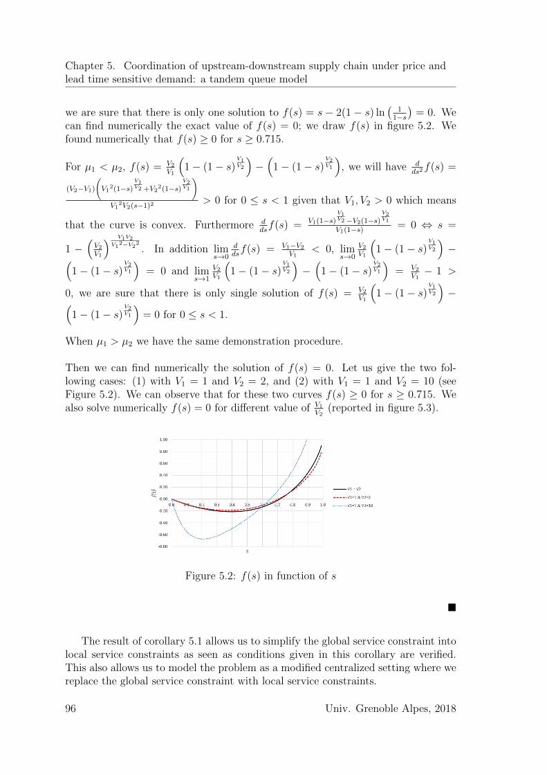
Chapter 5. Coordination of upstream-downstream supply chain under price andlead time sensitive demand: a tandem queue model
we are sure that there is only one solution to f(s) = s− 2(1− s) ln(
11−s
)= 0. We
can find numerically the exact value of f(s) = 0; we draw f(s) in figure 5.2. Wefound numerically that f(s) ≥ 0 for s ≥ 0.715.
For µ1 < µ2, f(s) = V2V1
(1− (1− s)
V1V2
)−(
1− (1− s)V2V1
), we will have d
ds2f(s) =
(V2−V1)
(V1
2(1−s)V1V2 +V2
2(1−s)V2V1
)V1
2V2(s−1)2> 0 for 0 ≤ s < 1 given that V1, V2 > 0 which means
that the curve is convex. Furthermore ddsf(s) = V1(1−s)
V1V2 −V2(1−s)
V2V1
V1(1−s) = 0 ⇔ s =
1 −(V2V1
) V1V2V1
2−V22 . In addition lims→0
ddsf(s) = V1−V2
V1< 0, lim
s→0
V2V1
(1− (1− s)
V1V2
)−(
1− (1− s)V2V1
)= 0 and lim
s→1
V2V1
(1− (1− s)
V1V2
)−(
1− (1− s)V2V1
)= V2
V1− 1 >
0, we are sure that there is only single solution of f(s) = V2V1
(1− (1− s)
V1V2
)−(
1− (1− s)V2V1
)= 0 for 0 ≤ s < 1.
When µ1 > µ2 we have the same demonstration procedure.
Then we can find numerically the solution of f(s) = 0. Let us give the two fol-lowing cases: (1) with V1 = 1 and V2 = 2, and (2) with V1 = 1 and V2 = 10 (seeFigure 5.2). We can observe that for these two curves f(s) ≥ 0 for s ≥ 0.715. Wealso solve numerically f(s) = 0 for different value of V1
V2(reported in figure 5.3).
Figure 5.2: f(s) in function of s
�
The result of corollary 5.1 allows us to simplify the global service constraint intolocal service constraints as seen as conditions given in this corollary are verified.This also allows us to model the problem as a modified centralized setting where wereplace the global service constraint with local service constraints.
96 Univ. Grenoble Alpes, 2018
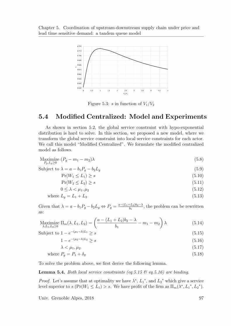
Chapter 5. Coordination of upstream-downstream supply chain under price andlead time sensitive demand: a tandem queue model
Figure 5.3: s in function of V1/V2
5.4 Modified Centralized: Model and Experiments
As shown in section 5.2, the global service constraint with hypo-exponentialdistribution is hard to solve. In this section, we proposed a new model, where wetransform the global service constraint into local service constraints for each actor.We call this model “Modified Centralized”. We formulate the modified centralizedmodel as follows.
MaximizePg ,Lg≥0
(Pg −m1 −m2)λ (5.8)
Subject to λ = a− b1Pg − b2Lg (5.9)
Pr(W1 ≤ L1) ≥ s (5.10)
Pr(W2 ≤ L2) ≥ s (5.11)
0 ≤ λ < µ1, µ2 (5.12)
where Lg = L1 + L2 (5.13)
Given that λ = a− b1Pg− b2Lg ⇔ Pg = a−(L1+L2)b2−λb1
, the problem can be rewrittenas:
Maximizeλ,L1,L2≥0
Πm(λ, L1, L2) =
(a− (L1 + L2)b2 − λ
b1
−m1 −m2
)λ (5.14)
Subject to 1− e−(µ1−λ)L1 ≥ s (5.15)
1− e−(µ2−λ)L2 ≥ s (5.16)
λ < µ1, µ2 (5.17)
where Pg = P1 + δ2 (5.18)
To solve the problem above, we first derive the following lemma.
Lemma 5.4. Both local service constraints (eq.5.15 & eq.5.16) are binding.
Proof. Let’s assume that at optimality we have λ∗, L1∗, and L2
∗ which give a servicelevel superior to s (Pr(W1 ≤ L1) > s. We have profit of the firm as Πm(λ∗, L1
∗, L2∗).
Univ. Grenoble Alpes, 2018 97
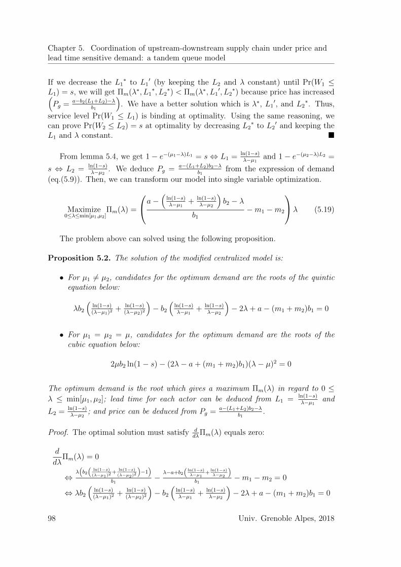
Chapter 5. Coordination of upstream-downstream supply chain under price andlead time sensitive demand: a tandem queue model
If we decrease the L1∗ to L1
′ (by keeping the L2 and λ constant) until Pr(W1 ≤L1) = s, we will get Πm(λ∗, L1
∗, L2∗) < Πm(λ∗, L1
′, L2∗) because price has increased(
Pg = a−b2(L1+L2)−λb1
). We have a better solution which is λ∗, L1
′, and L2∗. Thus,
service level Pr(W1 ≤ L1) is binding at optimality. Using the same reasoning, wecan prove Pr(W2 ≤ L2) = s at optimality by decreasing L2
∗ to L2′ and keeping the
L1 and λ constant. �
From lemma 5.4, we get 1− e−(µ1−λ)L1 = s⇔ L1 = ln(1−s)λ−µ1 and 1− e−(µ2−λ)L2 =
s ⇔ L2 = ln(1−s)λ−µ2 . We deduce Pg = a−(L1+L2)b2−λ
b1from the expression of demand
(eq.(5.9)). Then, we can transform our model into single variable optimization.
Maximize0≤λ≤min[µ1,µ2]
Πm(λ) =
a−(
ln(1−s)λ−µ1 + ln(1−s)
λ−µ2
)b2 − λ
b1
−m1 −m2
λ (5.19)
The problem above can solved using the following proposition.
Proposition 5.2. The solution of the modified centralized model is:
• For µ1 6= µ2, candidates for the optimum demand are the roots of the quinticequation below:
λb2
(ln(1−s)(λ−µ1)2
+ ln(1−s)(λ−µ2)2
)− b2
(ln(1−s)λ−µ1 + ln(1−s)
λ−µ2
)− 2λ+ a− (m1 +m2)b1 = 0
• For µ1 = µ2 = µ, candidates for the optimum demand are the roots of thecubic equation below:
2µb2 ln(1− s)− (2λ− a+ (m1 +m2)b1)(λ− µ)2 = 0
The optimum demand is the root which gives a maximum Πm(λ) in regard to 0 ≤λ ≤ min[µ1, µ2]; lead time for each actor can be deduced from L1 = ln(1−s)
λ−µ1 and
L2 = ln(1−s)λ−µ2 ; and price can be deduced from Pg = a−(L1+L2)b2−λ
b1.
Proof. The optimal solution must satisfy ddλ
Πm(λ) equals zero:
d
dλΠm(λ) = 0
⇔λ(b2(
ln(1−s)(λ−µ1)2
+ln(1−s)(λ−µ2)2
)−1)
b1−
λ−a+b2(
ln(1−s)λ−µ1
+ln(1−s)λ−µ2
)b1
−m1 −m2 = 0
⇔ λb2
(ln(1−s)(λ−µ1)2
+ ln(1−s)(λ−µ2)2
)− b2
(ln(1−s)λ−µ1 + ln(1−s)
λ−µ2
)− 2λ+ a− (m1 +m2)b1 = 0
98 Univ. Grenoble Alpes, 2018

Chapter 5. Coordination of upstream-downstream supply chain under price andlead time sensitive demand: a tandem queue model
For the case µ1 = µ2 = µ, the quintic equation above becomes:
λb2
(ln(1−s)(λ−µ1)2
+ ln(1−s)(λ−µ2)2
)− b2
(ln(1−s)λ−µ1 + ln(1−s)
λ−µ2
)− 2λ+ a− (m1 +m2)b1 = 0
⇔ λb2
(2 ln(1−s)(λ−µ)2
)− b2
(2 ln(1−s)λ−µ
)− 2λ+ a− (m1 +m2)b1 = 0
⇔[λb2
(2 ln(1−s)(λ−µ)2
)− b2
(2 ln(1−s)λ−µ
)− 2λ+ a− (m1 +m2)b1
](λ− µ)2 = 0
⇔ 2µb2 ln(1− s)− (2λ− a+ (m1 +m2)b1)(λ− µ)2 = 0
The optimum demand can be found by comparing the profit Πm(λ) (see eq.(5.19))of each root which respect 0 ≤ λ ≤ min[µ1, µ2]. Let us note that we have notencountered the case where there are several feasible roots. But we still not yetprove that it can not happen.The expression of L1 and L2 can be deduced using lemma 5.4. And the expressionof Pg can be found from the expression of demand (eq.(5.9)). �
Experiments
We do some experiments using the bisection. The parameters explored are b1,and b2. We vary one parameter and fix other parameters. For µ1 and µ2, we definecases where µ1 = µ2 and µ1 6= µ2.
Our first experiment in this section uses µ1 = µ2 = 20 and base parameters are:a = 50, b1 = 4, b2 = 6, m1 = 3, m2 = 2, and s = 0.95. It is obvious that when bothcapacity of the actors are the same, it will result the same waiting time. This leadsto both actors have the same quoted lead time. This can be seen in our result (seeTable 5.5 and 5.6). In table 5.5, as b1 increases, the price decreases. In table 5.6, asb2 increases the lead time decreases. These behaviors are similar to those observedin section 5.2.
Let us point the following interesting finding: the profit, that we get from themodified centralized setting, isn’t too far from the profit of the centralized setting.We use Πc−Πm
Πc× 100% to calculate the loss of using this modified centralized setting
compared to the centralized setting. For the experiment with b1, we get an averageloss of 6.66% and for experiment with b2 we get an average loss of 8.41%.
Table 5.5: Experiment on b1 with µ1 = µ2 for modified centralized setting
b1
Modified Centralized Setting
L1 L2 Pg λ Πm Πc LossServ. Lvl. Real.
Actor 1 Actor 2 Global2 0.4213 0.4213 16.0273 12.8896 142.1375 149.3263 4.81% 95.00% 95.00% 98.25%4 0.3248 0.3248 8.8319 10.7754 41.2901 43.5856 5.27% 95.00% 95.00% 98.25%6 0.2425 0.2425 6.5742 7.6450 12.0349 12.8375 6.25% 95.00% 95.00% 98.25%8 0.1833 0.1833 5.5183 3.6545 1.8940 2.1119 10.32% 95.00% 95.00% 98.25%
In the second experiment, we consider µ1 6= µ2. We use µ1 = 30 & µ2 = 15 forµ1 > µ2 and vice-versa for µ1 < µ2. We only display the results where µ1 > µ2 (see
Univ. Grenoble Alpes, 2018 99
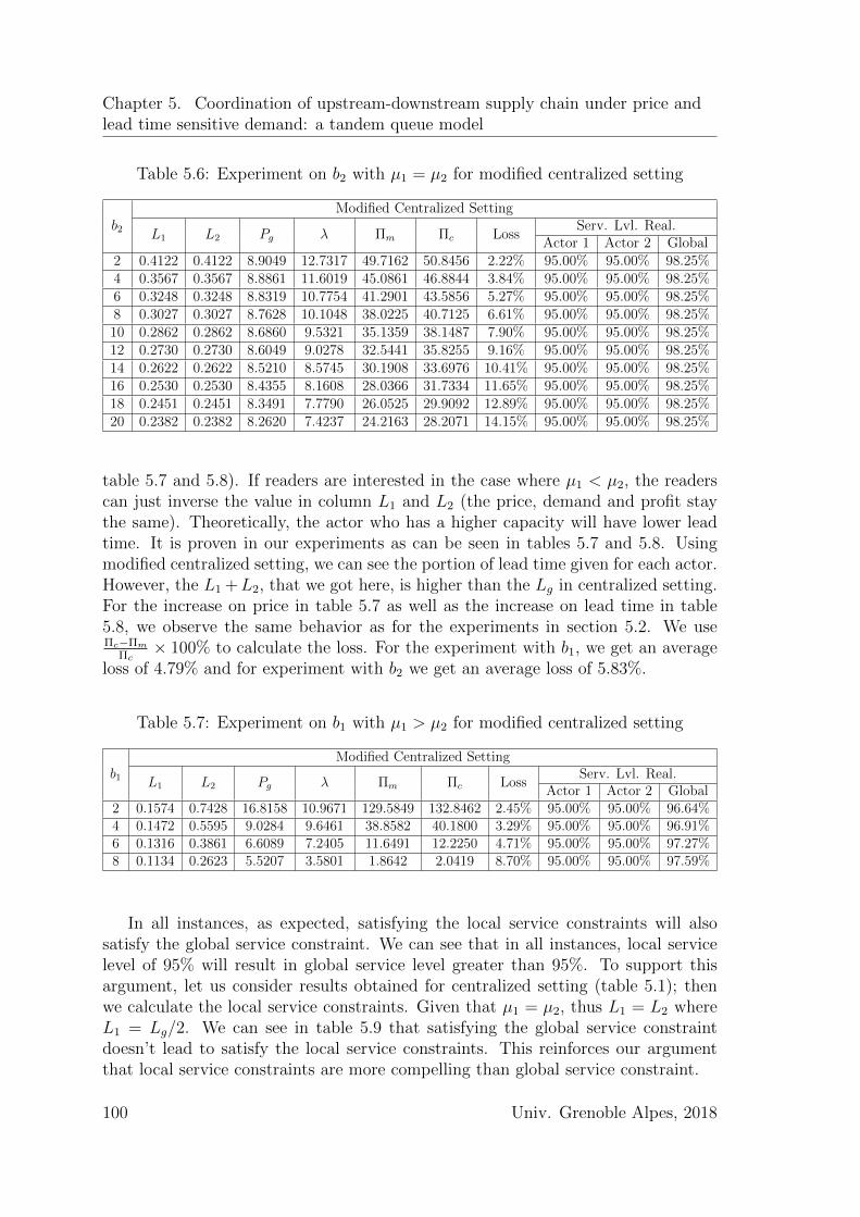
Chapter 5. Coordination of upstream-downstream supply chain under price andlead time sensitive demand: a tandem queue model
Table 5.6: Experiment on b2 with µ1 = µ2 for modified centralized setting
b2
Modified Centralized Setting
L1 L2 Pg λ Πm Πc LossServ. Lvl. Real.
Actor 1 Actor 2 Global2 0.4122 0.4122 8.9049 12.7317 49.7162 50.8456 2.22% 95.00% 95.00% 98.25%4 0.3567 0.3567 8.8861 11.6019 45.0861 46.8844 3.84% 95.00% 95.00% 98.25%6 0.3248 0.3248 8.8319 10.7754 41.2901 43.5856 5.27% 95.00% 95.00% 98.25%8 0.3027 0.3027 8.7628 10.1048 38.0225 40.7125 6.61% 95.00% 95.00% 98.25%10 0.2862 0.2862 8.6860 9.5321 35.1359 38.1487 7.90% 95.00% 95.00% 98.25%12 0.2730 0.2730 8.6049 9.0278 32.5441 35.8255 9.16% 95.00% 95.00% 98.25%14 0.2622 0.2622 8.5210 8.5745 30.1908 33.6976 10.41% 95.00% 95.00% 98.25%16 0.2530 0.2530 8.4355 8.1608 28.0366 31.7334 11.65% 95.00% 95.00% 98.25%18 0.2451 0.2451 8.3491 7.7790 26.0525 29.9092 12.89% 95.00% 95.00% 98.25%20 0.2382 0.2382 8.2620 7.4237 24.2163 28.2071 14.15% 95.00% 95.00% 98.25%
table 5.7 and 5.8). If readers are interested in the case where µ1 < µ2, the readerscan just inverse the value in column L1 and L2 (the price, demand and profit staythe same). Theoretically, the actor who has a higher capacity will have lower leadtime. It is proven in our experiments as can be seen in tables 5.7 and 5.8. Usingmodified centralized setting, we can see the portion of lead time given for each actor.However, the L1 +L2, that we got here, is higher than the Lg in centralized setting.For the increase on price in table 5.7 as well as the increase on lead time in table5.8, we observe the same behavior as for the experiments in section 5.2. We useΠc−Πm
Πc× 100% to calculate the loss. For the experiment with b1, we get an average
loss of 4.79% and for experiment with b2 we get an average loss of 5.83%.
Table 5.7: Experiment on b1 with µ1 > µ2 for modified centralized setting
b1
Modified Centralized Setting
L1 L2 Pg λ Πm Πc LossServ. Lvl. Real.
Actor 1 Actor 2 Global2 0.1574 0.7428 16.8158 10.9671 129.5849 132.8462 2.45% 95.00% 95.00% 96.64%4 0.1472 0.5595 9.0284 9.6461 38.8582 40.1800 3.29% 95.00% 95.00% 96.91%6 0.1316 0.3861 6.6089 7.2405 11.6491 12.2250 4.71% 95.00% 95.00% 97.27%8 0.1134 0.2623 5.5207 3.5801 1.8642 2.0419 8.70% 95.00% 95.00% 97.59%
In all instances, as expected, satisfying the local service constraints will alsosatisfy the global service constraint. We can see that in all instances, local servicelevel of 95% will result in global service level greater than 95%. To support thisargument, let us consider results obtained for centralized setting (table 5.1); thenwe calculate the local service constraints. Given that µ1 = µ2, thus L1 = L2 whereL1 = Lg/2. We can see in table 5.9 that satisfying the global service constraintdoesn’t lead to satisfy the local service constraints. This reinforces our argumentthat local service constraints are more compelling than global service constraint.
100 Univ. Grenoble Alpes, 2018
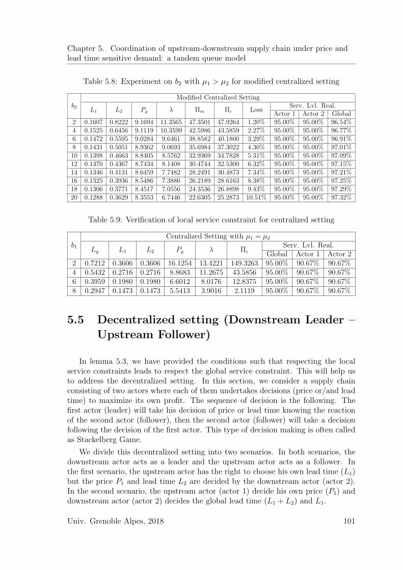
Chapter 5. Coordination of upstream-downstream supply chain under price andlead time sensitive demand: a tandem queue model
Table 5.8: Experiment on b2 with µ1 > µ2 for modified centralized setting
b2
Modified Centralized Setting
L1 L2 Pg λ Πm Πc LossServ. Lvl. Real.
Actor 1 Actor 2 Global2 0.1607 0.8222 9.1694 11.3565 47.3501 47.9264 1.20% 95.00% 95.00% 96.54%4 0.1525 0.6456 9.1119 10.3599 42.5986 43.5859 2.27% 95.00% 95.00% 96.77%6 0.1472 0.5595 9.0284 9.6461 38.8582 40.1800 3.29% 95.00% 95.00% 96.91%8 0.1431 0.5051 8.9362 9.0693 35.6984 37.3022 4.30% 95.00% 95.00% 97.01%10 0.1398 0.4663 8.8405 8.5762 32.9369 34.7828 5.31% 95.00% 95.00% 97.09%12 0.1370 0.4367 8.7434 8.1408 30.4744 32.5300 6.32% 95.00% 95.00% 97.15%14 0.1346 0.4131 8.6459 7.7482 28.2491 30.4873 7.34% 95.00% 95.00% 97.21%16 0.1325 0.3936 8.5486 7.3886 26.2189 28.6163 8.38% 95.00% 95.00% 97.25%18 0.1306 0.3771 8.4517 7.0556 24.3536 26.8898 9.43% 95.00% 95.00% 97.29%20 0.1288 0.3629 8.3553 6.7446 22.6305 25.2873 10.51% 95.00% 95.00% 97.32%
Table 5.9: Verification of local service constraint for centralized setting
b1
Centralized Setting with µ1 = µ2
Lg L1 L2 Pg λ ΠcServ. Lvl. Real.
Global Actor 1 Actor 22 0.7212 0.3606 0.3606 16.1254 13.4221 149.3263 95.00% 90.67% 90.67%4 0.5432 0.2716 0.2716 8.8683 11.2675 43.5856 95.00% 90.67% 90.67%6 0.3959 0.1980 0.1980 6.6012 8.0176 12.8375 95.00% 90.67% 90.67%8 0.2947 0.1473 0.1473 5.5413 3.9016 2.1119 95.00% 90.67% 90.67%
5.5 Decentralized setting (Downstream Leader –
Upstream Follower)
In lemma 5.3, we have provided the conditions such that respecting the localservice constraints leads to respect the global service constraint. This will help usto address the decentralized setting. In this section, we consider a supply chainconsisting of two actors where each of them undertakes decisions (price or/and leadtime) to maximize its own profit. The sequence of decision is the following. Thefirst actor (leader) will take his decision of price or lead time knowing the reactionof the second actor (follower), then the second actor (follower) will take a decisionfollowing the decision of the first actor. This type of decision making is often calledas Stackelberg Game.
We divide this decentralized setting into two scenarios. In both scenarios, thedownstream actor acts as a leader and the upstream actor acts as a follower. Inthe first scenario, the upstream actor has the right to choose his own lead time (L1)but the price P1 and lead time L2 are decided by the downstream actor (actor 2).In the second scenario, the upstream actor (actor 1) decide his own price (P1) anddownstream actor (actor 2) decides the global lead time (L1 + L2) and L1.
Univ. Grenoble Alpes, 2018 101
Chapter 5. Coordination of upstream-downstream supply chain under price andlead time sensitive demand: a tandem queue model
5.5.1 Upstream decides his own lead time
In this setting, the upstream actor decides his own lead time (L1). The upstreamprice (P1) and downstream lead time (L2) are decided by the downstream actor. Inthis setting the global price (Pg) is obtained from P1 plus a fixed margin taken bythe downstream actor (δ2): Pg = P1 + δ2. The formulation for both upstream anddownstream problems are:
Upstream Problem:
MaximizeL1≥0
Π1(L1) = (P1 −m1)λ (5.20)
Subject to λ = a− b1(P1 + δ2)− b2(L1 + L2) (5.21)
Pr(W1 ≤ L1) ≥ s (5.22)
0 ≤ λ < µ1 (5.23)
Downstream Problem:
MaximizeP1,L2≥0
Π2(P1, L2) = (Pg − P1 −m2)λ (5.24)
Subject to λ = a− b1(P1 + δ2)− b2(L1 + L2) (5.25)
Pr(W2 ≤ L2) ≥ s (5.26)
0 ≤ λ < µ2 (5.27)
knowing that Pg = P1 + δ2 (5.28)
Lg = L1 + L2 (5.29)
To solve the problem, we do a backward induction. Thus, we start the analysisby solving the upstream problem.
Upstream Problem
In the upstream problem, L2 and P1 are given by the downstream actor thus theonly option of upstream actor to maximize its profit is to choose his lead time (L1).From here we can deduce lemma 5.5.
Lemma 5.5. The upstream’s service constraint is binding, implying that:
L1(L2, P1) =a−b1(P1+δ2)−b2L2−µ1+
√(µ1−a+b1(P1+δ2)+b2L2)2+4b2 ln( 1
1−s)2b2
Proof. L2 and P1 are given by the downstream actor, the only option of upstreamactor to maximize his profit is to increase demand by reducing his lead time (L1)but in respecting to service constraint. Thus, the upstream’s service level will bebinding. From here we can deduce that:
Pr(W1 ≤ L1) = s⇔ 1− e−(µ1−λ)L1 = s
⇔ (µ1 − a+ b1(P1 + δ2) + b2L2)L1 + b2L12 = ln
(1
1− s
)
102 Univ. Grenoble Alpes, 2018
Chapter 5. Coordination of upstream-downstream supply chain under price andlead time sensitive demand: a tandem queue model
The discriminant of this equation is:
∆ = (µ1 − a+ b1(P1 + δ2) + b2L2)2 + 4b2 ln
(1
1− s
)≥ 0
Thus, we will obtain two roots, knowing that one of the roots is negative. We areonly interested in the positive root which is:
L1(L2, P1) =a−b1(P1+δ2)−b2L2−µ1+
√(µ1−a+b1(P1+δ2)+b2L2)2+4b2 ln( 1
1−s)2b2
�
Having obtained L1 from the upstream, we can move to the downstream problem.
Downstream Problem
The service constraint (Pr(W2 ≤ L2) ≥ s) can be rewritten as: 1− e−(µ2−λ)L2 ≥s ⇔ (µ2 − a + b1(P1 + δ2) + b2(L1 + L2))L2 ≥ ln
(1
1−s
). Then, the problem can be
rewritten as:
MaximizeP1,L2≥0
Π2(P1, L2) = (δ2 −m2)(a− b1(P1 + δ2)− b2(L1 + L2)) (5.30)
Subject to (µ2 − a+ b1(P1 + δ2) + b2(L1 + L2))L2 ≥ ln
(1
1− s
)(5.31)
0 ≤ a− b1(P1 + δ2)− b2(L1 + L2) < µ2 (5.32)
From the problem above, we can deduce several lemmas.
Lemma 5.6. The downstream’s service level is binding.
Proof. Assume that at optimality we have L2∗ and P1
∗ which give (µ2− a+ b1(P1 +δ2)+b2(L1+L2))L2 > ln(1/(1−s)). We have profit of the downstream as Π2(L2
∗, P1∗).
If we decrease the L2∗ to L2
′ (by keeping the P1 constant) until (µ2 − a + b1(P1 +δ2)+ b2(L1 +L2))L2 = ln(1/(1−s)), we will get Π2(L2
∗, P1∗) < Π2(L2
′, P1∗) because
demand has increased. Thus, we will have a better solution which is P1∗ and L2
′. �
Before continuing, let us consider the following remarks:
• The downstream actor’s profit (Π2) is increasing in λ which is proven by Π2 =(δ2 −m2)λ (from eq.(5.24) and eq.(5.28)).
• Demand λ is increasing in function of L2 which is proven by Pr(W2 ≤ L2) = s
⇔ (µ2 − λ)L2 = ln(
11−s
)⇔ λ = µ2 −
ln( 11−s)L2
(from eq.(5.26) and lemma 5.6).
• L1 is an increasing function in λ which is proven by Pr(W1 ≤ L1) = s ⇔(µ1 − λ)L1 = ln
(1
1−s
)⇔ L1 =
ln( 11−s)
µ1−λ (from eq.(5.22) and lemma 5.5).
Univ. Grenoble Alpes, 2018 103
Chapter 5. Coordination of upstream-downstream supply chain under price andlead time sensitive demand: a tandem queue model
• And price P1 decreases when L1, L2, and λ increase which is proven by P1 =1b1
[a− b1δ2 − b2(L1 + L2)− λ] (from eq.(5.25)).
Based on those remarks, we derive the following lemma.
Lemma 5.7. The optimum price P1 proposed by the downstream actor is P1 = m1.
Proof. Suppose that at optimality we have P1∗, λ∗, L1
∗, and L2∗ with P1
∗ > m1; wehave downstream actor’s profit as Π2
∗. If we increase L2∗ to L2
′, keeping the serviceconstraint binding for actor 2, the demand λ will increase thus we would obtainprofit Π2
′ > Π2∗. Because demand increases, L1 will increase if we keep binding the
service constraint for actor 1. As L2, λ, and L1 increase, consequently price P1 willdecrease. But this is possible only until a value of P1 such that P1 = m1 (otherwisethe profit of actor 1 would be negative). Thus, downstream actor can increase L2
to get a better profit until L2 such that it leads to P1 = m1.
�
To illustrate this lemma 5.7, we provide the profit curve in function of L2 foreach actor (Π1 and Π2) and the global profit which is the sum of each actor profit(Πg = Π1 + Π2) (see figure 5.4). The curves are drawn with price:
P1(L2) =
(2ln( 1
1−s)L2
−2µ2+a−b1δ2−b2L2+µ1
)2
−(µ1−a+b1δ2+b2L2)2−4b2 ln( 11−s)
2b1
[2ln( 1
1−s)L2
−2µ2+2µ1
]
which can be obtained from the service constraint (5.31) using lemma 5.6. Weobserve the same behavior for all experiments that we have done. We see that Π2
is increasing in function of L2 given that Π1 ≥ 0. In consequence, the downstreamactor will choose the longer L2 to maximize his own profit. This will lead to zeroprofit for upstream actor (Π1 = 0). And since Π1 = λ(P1 −m1), it means that weeffectively have P1 = m1.
Lemma 5.8. Given that the downstream will propose P1 = m1, for the case µ1 6= µ2
the candidates for optimum L2 will be the solution of the following cubic equation:
(µ2 − µ1)b2L23 + (µ2(µ2 − µ1)− α(µ2 − µ1) + b1m1(µ2 − µ1)− 2b2γ)L2
2
+ γ(µ1 − 2µ2 + α− b1m1)L2 + γ2 = 0
where α = a− b1δ2 and γ = ln(1/(1− s)).The optimum L2 is the root which gives a maximum Π2 in regard to the problemsconstraint.
104 Univ. Grenoble Alpes, 2018
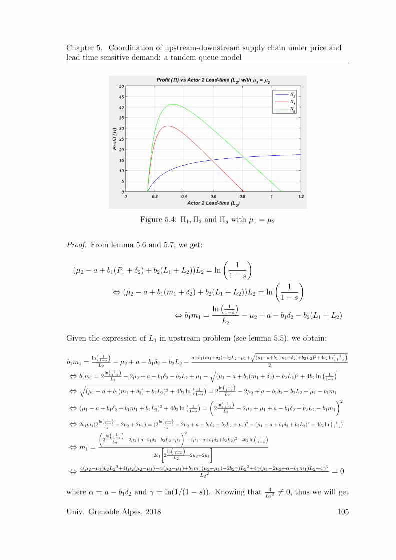
Chapter 5. Coordination of upstream-downstream supply chain under price andlead time sensitive demand: a tandem queue model
Figure 5.4: Π1,Π2 and Πg with µ1 = µ2
Proof. From lemma 5.6 and 5.7, we get:
(µ2 − a+ b1(P1 + δ2) + b2(L1 + L2))L2 = ln
(1
1− s
)⇔ (µ2 − a+ b1(m1 + δ2) + b2(L1 + L2))L2 = ln
(1
1− s
)⇔ b1m1 =
ln(
11−s
)L2
− µ2 + a− b1δ2 − b2(L1 + L2)
Given the expression of L1 in upstream problem (see lemma 5.5), we obtain:
b1m1 =ln( 1
1−s)L2
− µ2 + a− b1δ2 − b2L2 −a−b1(m1+δ2)−b2L2−µ1+
√(µ1−a+b1(m1+δ2)+b2L2)2+4b2 ln( 1
1−s)2
⇔ b1m1 = 2ln( 1
1−s)L2
− 2µ2 + a− b1δ2 − b2L2 + µ1 −√
(µ1 − a+ b1(m1 + δ2) + b2L2)2 + 4b2 ln(
11−s
)⇔
√(µ1 − a+ b1(m1 + δ2) + b2L2)2 + 4b2 ln
(1
1−s
)= 2
ln( 11−s)L2
− 2µ2 + a− b1δ2 − b2L2 + µ1 − b1m1
⇔ (µ1 − a+ b1δ2 + b1m1 + b2L2)2 + 4b2 ln(
11−s
)=
(2
ln( 11−s)L2
− 2µ2 + µ1 + a− b1δ2 − b2L2 − b1m1
)2
⇔ 2b1m1(2ln( 1
1−s)L2
− 2µ2 + 2µ1) = (2ln( 1
1−s)L2
− 2µ2 + a− b1δ2 − b2L2 + µ1)2 − (µ1 − a+ b1δ2 + b2L2)2 − 4b2 ln(
11−s
)
⇔ m1 =
(2ln( 1
1−s)L2
−2µ2+a−b1δ2−b2L2+µ1
)2
−(µ1−a+b1δ2+b2L2)2−4b2 ln( 11−s)
2b1
[2ln( 1
1−s)L2
−2µ2+2µ1
]
⇔ 4(µ2−µ1)b2L23+4(µ2(µ2−µ1)−α(µ2−µ1)+b1m1(µ2−µ1)−2b2γ)L2
2+4γ(µ1−2µ2+α−b1m1)L2+4γ2
L22 = 0
where α = a− b1δ2 and γ = ln(1/(1− s)). Knowing that 4L2
2 6= 0, thus we will get
Univ. Grenoble Alpes, 2018 105
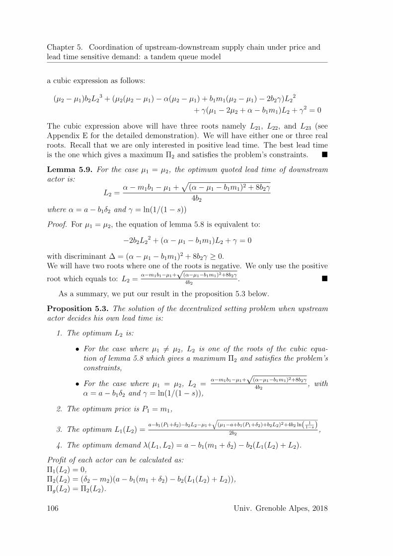
Chapter 5. Coordination of upstream-downstream supply chain under price andlead time sensitive demand: a tandem queue model
a cubic expression as follows:
(µ2 − µ1)b2L23 + (µ2(µ2 − µ1)− α(µ2 − µ1) + b1m1(µ2 − µ1)− 2b2γ)L2
2
+ γ(µ1 − 2µ2 + α− b1m1)L2 + γ2 = 0
The cubic expression above will have three roots namely L21, L22, and L23 (seeAppendix E for the detailed demonstration). We will have either one or three realroots. Recall that we are only interested in positive lead time. The best lead timeis the one which gives a maximum Π2 and satisfies the problem’s constraints. �
Lemma 5.9. For the case µ1 = µ2, the optimum quoted lead time of downstreamactor is:
L2 =α−m1b1 − µ1 +
√(α− µ1 − b1m1)2 + 8b2γ
4b2
where α = a− b1δ2 and γ = ln(1/(1− s))
Proof. For µ1 = µ2, the equation of lemma 5.8 is equivalent to:
−2b2L22 + (α− µ1 − b1m1)L2 + γ = 0
with discriminant ∆ = (α− µ1 − b1m1)2 + 8b2γ ≥ 0.We will have two roots where one of the roots is negative. We only use the positive
root which equals to: L2 =α−m1b1−µ1+
√(α−µ1−b1m1)2+8b2γ
4b2. �
As a summary, we put our result in the proposition 5.3 below.
Proposition 5.3. The solution of the decentralized setting problem when upstreamactor decides his own lead time is:
1. The optimum L2 is:
• For the case where µ1 6= µ2, L2 is one of the roots of the cubic equa-tion of lemma 5.8 which gives a maximum Π2 and satisfies the problem’sconstraints,
• For the case where µ1 = µ2, L2 =α−m1b1−µ1+
√(α−µ1−b1m1)2+8b2γ
4b2, with
α = a− b1δ2 and γ = ln(1/(1− s)),
2. The optimum price is P1 = m1,
3. The optimum L1(L2) =a−b1(P1+δ2)−b2L2−µ1+
√(µ1−a+b1(P1+δ2)+b2L2)2+4b2 ln( 1
1−s)2b2
,
4. The optimum demand λ(L1, L2) = a− b1(m1 + δ2)− b2(L1(L2) + L2).
Profit of each actor can be calculated as:Π1(L2) = 0,Π2(L2) = (δ2 −m2)(a− b1(m1 + δ2)− b2(L1(L2) + L2)),Πg(L2) = Π2(L2).
106 Univ. Grenoble Alpes, 2018
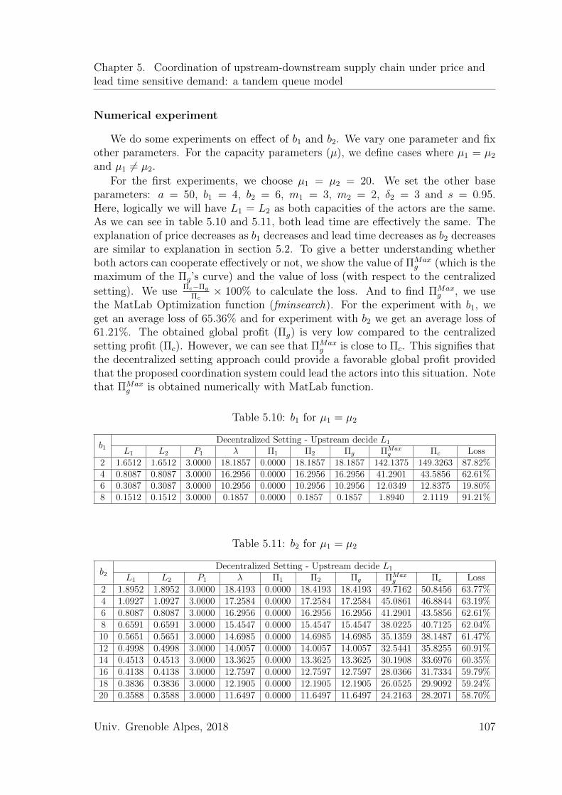
Chapter 5. Coordination of upstream-downstream supply chain under price andlead time sensitive demand: a tandem queue model
Numerical experiment
We do some experiments on effect of b1 and b2. We vary one parameter and fixother parameters. For the capacity parameters (µ), we define cases where µ1 = µ2
and µ1 6= µ2.
For the first experiments, we choose µ1 = µ2 = 20. We set the other baseparameters: a = 50, b1 = 4, b2 = 6, m1 = 3, m2 = 2, δ2 = 3 and s = 0.95.Here, logically we will have L1 = L2 as both capacities of the actors are the same.As we can see in table 5.10 and 5.11, both lead time are effectively the same. Theexplanation of price decreases as b1 decreases and lead time decreases as b2 decreasesare similar to explanation in section 5.2. To give a better understanding whetherboth actors can cooperate effectively or not, we show the value of ΠMax
g (which is themaximum of the Πg’s curve) and the value of loss (with respect to the centralized
setting). We use Πc−ΠgΠc× 100% to calculate the loss. And to find ΠMax
g , we usethe MatLab Optimization function (fminsearch). For the experiment with b1, weget an average loss of 65.36% and for experiment with b2 we get an average loss of61.21%. The obtained global profit (Πg) is very low compared to the centralizedsetting profit (Πc). However, we can see that ΠMax
g is close to Πc. This signifies thatthe decentralized setting approach could provide a favorable global profit providedthat the proposed coordination system could lead the actors into this situation. Notethat ΠMax
g is obtained numerically with MatLab function.
Table 5.10: b1 for µ1 = µ2
b1Decentralized Setting - Upstream decide L1
L1 L2 P1 λ Π1 Π2 Πg ΠMaxg Πc Loss
2 1.6512 1.6512 3.0000 18.1857 0.0000 18.1857 18.1857 142.1375 149.3263 87.82%4 0.8087 0.8087 3.0000 16.2956 0.0000 16.2956 16.2956 41.2901 43.5856 62.61%6 0.3087 0.3087 3.0000 10.2956 0.0000 10.2956 10.2956 12.0349 12.8375 19.80%8 0.1512 0.1512 3.0000 0.1857 0.0000 0.1857 0.1857 1.8940 2.1119 91.21%
Table 5.11: b2 for µ1 = µ2
b2Decentralized Setting - Upstream decide L1
L1 L2 P1 λ Π1 Π2 Πg ΠMaxg Πc Loss
2 1.8952 1.8952 3.0000 18.4193 0.0000 18.4193 18.4193 49.7162 50.8456 63.77%4 1.0927 1.0927 3.0000 17.2584 0.0000 17.2584 17.2584 45.0861 46.8844 63.19%6 0.8087 0.8087 3.0000 16.2956 0.0000 16.2956 16.2956 41.2901 43.5856 62.61%8 0.6591 0.6591 3.0000 15.4547 0.0000 15.4547 15.4547 38.0225 40.7125 62.04%10 0.5651 0.5651 3.0000 14.6985 0.0000 14.6985 14.6985 35.1359 38.1487 61.47%12 0.4998 0.4998 3.0000 14.0057 0.0000 14.0057 14.0057 32.5441 35.8255 60.91%14 0.4513 0.4513 3.0000 13.3625 0.0000 13.3625 13.3625 30.1908 33.6976 60.35%16 0.4138 0.4138 3.0000 12.7597 0.0000 12.7597 12.7597 28.0366 31.7334 59.79%18 0.3836 0.3836 3.0000 12.1905 0.0000 12.1905 12.1905 26.0525 29.9092 59.24%20 0.3588 0.3588 3.0000 11.6497 0.0000 11.6497 11.6497 24.2163 28.2071 58.70%
Univ. Grenoble Alpes, 2018 107
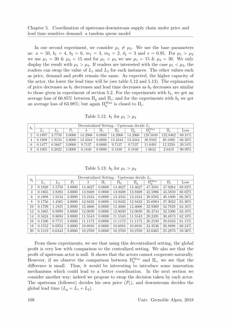
Chapter 5. Coordination of upstream-downstream supply chain under price andlead time sensitive demand: a tandem queue model
In our second experiment, we consider µ1 6= µ2. We use the base parametersas: a = 50, b1 = 4, b2 = 6, m1 = 3, m2 = 2, δ2 = 3 and s = 0.95. For µ1 > µ2
we use µ1 = 30 & µ2 = 15 and for µ1 < µ2 we use µ1 = 15 & µ2 = 30. We onlydisplay the result with µ1 > µ2. If readers are interested with the case µ1 < µ2, thereaders can swap the value of L1 and L2 for each instances. The other values suchas price, demand and profit remain the same. As expected, the higher capacity ofthe actor, the lower the lead time will be (see table 5.12 and 5.13). The explanationof price decreases as b1 decreases and lead time decreases as b2 decreases are similarto those given in experiment of section 5.2. For the experiments with b1, we get anaverage loss of 66.85% between Πg and Πc; and for the experiments with b2 we getan average loss of 63.98%; but again ΠMax
g is closed to Πc.
Table 5.12: b1 for µ1 > µ2
b1Decentralized Setting - Upstream decide L1
L1 L2 P1 λ Π1 Π2 Πg ΠMaxg Πc Loss
2 0.1897 3.7759 3.0000 14.2066 0.0000 14.2066 14.2066 129.5849 132.8462 89.31%4 0.1808 1.9134 3.0000 13.4344 0.0000 13.4344 13.4344 38.8582 40.1800 66.56%6 0.1477 0.5667 3.0000 9.7137 0.0000 9.7137 9.7137 11.6491 12.2250 20.54%8 0.1005 0.2022 3.0000 0.1840 0.0000 0.1840 0.1840 1.8642 2.0419 90.99%
Table 5.13: b2 for µ1 > µ2
b2Decentralized Setting - Upstream decide L1
L1 L2 P1 λ Π1 Π2 Πg ΠMaxg Πc Loss
2 0.1928 5.5758 3.0000 14.4627 0.0000 14.4627 14.4627 47.3501 47.9264 69.82%4 0.1865 2.8283 3.0000 13.9408 0.0000 13.9408 13.9408 42.5986 43.5859 68.02%6 0.1808 1.9134 3.0000 13.4344 0.0000 13.4344 13.4344 38.8582 40.1800 66.56%8 0.1756 1.4565 3.0000 12.9432 0.0000 12.9432 12.9432 35.6984 37.3022 65.30%10 0.1709 1.1825 3.0000 12.4666 0.0000 12.4666 12.4666 32.9369 34.7828 64.16%12 0.1665 0.9999 3.0000 12.0039 0.0000 12.0039 12.0039 30.4744 32.5300 63.10%14 0.1624 0.8694 3.0000 11.5543 0.0000 11.5543 11.5543 28.2491 30.4873 62.10%16 0.1586 0.7715 3.0000 11.1172 0.0000 11.1172 11.1172 26.2189 28.6163 61.15%18 0.1552 0.6953 3.0000 10.6916 0.0000 10.6916 10.6916 24.3536 26.8898 60.24%20 0.1519 0.6343 3.0000 10.2769 0.0000 10.2769 10.2769 22.6305 25.2873 59.36%
From these experiments, we see that using this decentralized setting, the globalprofit is very low with comparison to the centralized setting. We also see that theprofit of upstream actor is null. It shows that the actors cannot cooperate naturally.However, if we observe the comparison between ΠMax
g and Πc, we see that thedifference is small. Thus, it would be interesting to introduce some innovationmechanisms which could lead to a better coordination. In the next section weconsider another way; indeed we propose to swap the decision taken by each actor.The upstream (follower) decides his own price (P1), and downstream decides theglobal lead time (Lg = L1 + L2).
108 Univ. Grenoble Alpes, 2018
Chapter 5. Coordination of upstream-downstream supply chain under price andlead time sensitive demand: a tandem queue model
5.5.2 Upstream decides his own price
In this model we consider a decentralized setting where again the leader is thedownstream actor and follower is the upstream actor. The upstream decides his ownprice (P1), and downstream decides the global lead time (Lg) by deciding his ownlead time (L2) and upstream’s lead time (L1). The global price Pg is obtained fromP1 by Pg = P1 + δ2.
Upstream Problem:
MaximizeP1≥0
Π1(P1) = (P1 −m1)λ (5.33)
Subject to λ = a− b1(P1 + δ2)− b2(L1 + L2) (5.34)
Pr(W1 ≤ L1) ≥ s (5.35)
0 ≤ λ < µ1 (5.36)
Downstream Problem:
MaximizeL1,L2≥0
Π2(L1, L2) = (Pg − P1 −m2)λ (5.37)
Subject to λ = a− b1(P1 + δ2)− b2(L1 + L2) (5.38)
Pr(W2 ≤ l2) ≥ s (5.39)
0 ≤ λ < µ2 (5.40)
knowing that Pg = P1 + δ2 (5.41)
To solve the problems above we use a backward induction, we start by solvingthe upstream problem.
Upstream Problem
The service constraint (Pr(W1 ≤ L1) ≥ s) can be rewritten using the expressionof λ from eq. (5.38) as:
1− e−(µ1−λ)L1 ≥ s⇔ 1− e−(µ1−a+b1(P1+δ2)+b2(L1+L2))L1 ≥ s
⇔ P1 ≥ln( 1
1−s)L1
− µs + a− b1δ2 − b2(L1 + L2)
b1
Then, we have a new formulation of the problem as:
MaximizeP1≥0
Π1(P1) = (P1 −m1)(a− b1(P1 + δ2)− b2(L1 + L2)) (5.42)
Subject to P1 ≥ln( 1
1−s)L1
− µ1 + a− b1δ2 − b2(L1 + L2)
b1
(5.43)
0 ≤ a− b1(P1 + δ2)− b2(L1 + L2) < µ1 (5.44)
Univ. Grenoble Alpes, 2018 109
Chapter 5. Coordination of upstream-downstream supply chain under price andlead time sensitive demand: a tandem queue model
Different from the previous case (section 5.5.1), in this new case (section 5.5.2)the service constraint (5.43) isn’t necessarily binding. Indeed, if we have a given P1
for which the service constraint is not tight, we could reduce P1 without violatingthis constraint. By decreasing P1, we increase (a − b1(P1 + δ2) − b2(L1 + L2)) butwe also decrease (P1−m1). Thus, this does not necessarily improve the profit. Thistrade off complicates the solving approach. Thus, in order to solve the problem, weconsider the following lemma.
Lemma 5.10. If service level is binding, we have: P1 =
ln( 11−s)L1
−µ1+a−b1δ2−b2(L1+L2)
b1.
Otherwise, service level is non-binding and we have: P1 = a−b1(δ2−m1)−b2(L1+L2)2b1
.
Proof. Let us consider the two possible cases: (1) service constraint is binding, and(2) service constraint is non-binding.
Case 1: service constraint is binding. From eq.(5.43), we have immediately:
P1 =
ln( 11−s)L1
−µ1+a−b1δ2−b2(L1+L2)
b1.
Case 2: service constraint is non-binding. We can find P1 directly from theobjective function: Π1(P1) = (P1 −m1)(a− b1(P1 + δ2)− b2(L1 + L2)).Thus, the first derivative in P1 is:
d
dP1
Π1(P1) = 0⇔ a− b1(2P1 + δ2)− b2(L1 + L2) + b1m1 = 0
⇔ P1 =a− b1(δ2 −m1)− b2(L1 + L2)
2b1
�
Having obtained the expression of P1 in both binding and non-binding cases, wemove to the downstream problem.
Downstream Problem
The service constraint (Pr(W2 ≤ l2) ≥ s) can be rewritten as: 1 − e−(µ2−λ)L2 ≥s ⇔ (µ2 − a + b1(P1 + δ2) + b2(L1 + L2))L2 ≥ ln
(1
1−s
). Then the problem can be
rewritten as:
MaximizeL1,L2≥0
Π2(L1, L2) = (δ2 −m2)(a− b1(P1 + δ2)− b2(L1 + L2)) (5.45)
Subject to (µ2 − a+ b1(P1 + δ2) + b2(L1 + L2))L2 ≥ ln
(1
1− s
)(5.46)
0 ≤ a− b1(P1 + δ2)− b2(L1 + L2) < µ2 (5.47)
From the problem above, we deduce several lemmas.
110 Univ. Grenoble Alpes, 2018
Chapter 5. Coordination of upstream-downstream supply chain under price andlead time sensitive demand: a tandem queue model
Lemma 5.11. Service constraint (5.46) is binding at optimality.
Proof. Let’s assume that at optimality we have L2∗ and L1
∗ which give (µ2 − a +b1(P1 +δ2)+b2(L1 +L2))L2 > ln(1/(1−s)). We have profit of the downstream actoras Π2(L2
∗, L1∗). If we decrease the L2
∗ to L2′ (by keeping the L1 constant) until
(µ2 − a + b1(P1 + δ2) + b2(L1 + L2))L2 = ln(1/(1 − s)), we will get Π2(L2∗, L1
∗) <Π2(L2
′, L1∗) because the demand has increased. We have a better solution which
are L2′ and L1
∗. Thus, service level is binding at optimality. �
And taking into account the two expressions of P1 in lemma 5.10, we have thefollowing lemma.
Lemma 5.12. We have two situations based on the uptream’s service level.
• If upstream service level is binding, then
L2(L1) =ln( 1
1−s)ln( 1
1−s)L1
−µ1+µ2
,
P1(L1) =
ln( 11−s)L1
−µ1+a−b1δ2−b2
L1+ln( 1
1−s)ln( 1
1−s)L1
−µ1+µ2
b1
,
λ(L1) = µ1 −ln( 1
1−s)L1
.
• If upstream service level is non-binding, then
L2(L1) =a−b1(δ2+m1)−b2L1−2µ2+
√(2µ2−a+b1(δ2+m1)+b2L1)2+8b2 ln( 1
1−s)2b2
,
P1(L1) =a−b1(δ2−3m1)−b2L1+2µ2−
√(2µ2−a+b1(δ2+m1)+b2L1)2+8b2 ln( 1
1−s)4b1
,
λ(L1) =a−b1(δ2+m1)−b2L1+2µ2−
√(2µ2−a+b1(δ2+m1)+b2L1)2+8b2 ln( 1
1−s)4
Proof. We have two possible situations: (1) upstream service constraint is bindingand (2) upstream service constraint is non-binding.
Case 1: If upstream service constraint is binding.
We have P1 =
ln( 11−s)L1
−µ1+a−b1δ2−b2(L1+L2)
b1from lemma 5.10. The service level of the
downstream is always binding (lemma 5.11), thus the service constraint:
(µ2 − a+ b1(P1 + δ2) + b2(L1 + L2))L2 = ln
(1
1− s
)⇔ L2 =
ln(
11−s
)ln( 1
1−s)L1
− µ1 + µ2
Univ. Grenoble Alpes, 2018 111
Chapter 5. Coordination of upstream-downstream supply chain under price andlead time sensitive demand: a tandem queue model
Then, substitute the expression of L2 into P1(L1, L2), we get:
P1(L1, L2) =
ln( 11−s)L1
− µ1 + a− b1δ2 − b2(L1 + L2)
b1
⇔ P1(L1) =
ln( 11−s)L1
− µ1 + a− b1δ2 − b2
L1 +ln( 1
1−s)ln( 1
1−s)L1
−µ1+µ2
b1
Next, substitute the expression of P1(L1) and L2 into λ(P1, L1, L2), we get:
λ(P1, L1, L2) = a− b1(P1 + δ2)− b2(L1 + L2)⇔ λ(L1) = µ1 −ln(
11−s
)L1
Case 2: If upstream service constraint is non-binding.We have P1 = a−b1(δ2−m1)−b2(L1+L2)
2b1. The service level of the downstream is always
binding (lemma 5.11), thus the service constraint:
(µ2 − a+ b1(P1 + δ2) + b2(L1 + L2))L2 = ln
(1
1− s
)⇔ b2L2
2 + (2µ2 − a+ b1(δ2 +m1) + b2L1)L2 − 2 ln
(1
1− s
)= 0
Given that ∆ = (2µ2− a+ b1(δ2 +m1) + b2L1)2 + 8b2 ln(
11−s
)≥ 0, we get two roots
and we only consider the positive root. Thus we have:
L2 =a−b1(δ2+m1)−b2L1−2µ2+
√(2µ2−a+b1(δ2+m1)+b2L1)2+8b2 ln( 1
1−s)2b2
Then, substitute the expression of L2 into P1(L1, L2), we get:
P1(L1, L2) =(a− b1(δ2 −m1)− b2(L1 + L2))
2b1
⇔ P1(L1) =a−b1(δ2−3m1)−b2L1+2µ2−
√(2µ2−a+b1(δ2+m1)+b2L1)2+8b2 ln( 1
1−s)4b1
Demand of the downstream actor becomes:
λ(P1, L1, L2) = a− b1(P1 + δ2)− b2(L1 + L2)
⇔ λ(P1, L1) =2(a−b1δ2−b2L1)+2b1m1+4µ2−2
√(2µ2−a+b1(δ2+m1)+b2L1)2+8b2 ln( 1
1−s)4
− b1P1
⇔ λ(L1) =a−b1(δ2+m1)−b2L1+2µ2−
√(2µ2−a+b1(δ2−m1)+b2L1)2+8b2 ln( 1
1−s)4
�
112 Univ. Grenoble Alpes, 2018
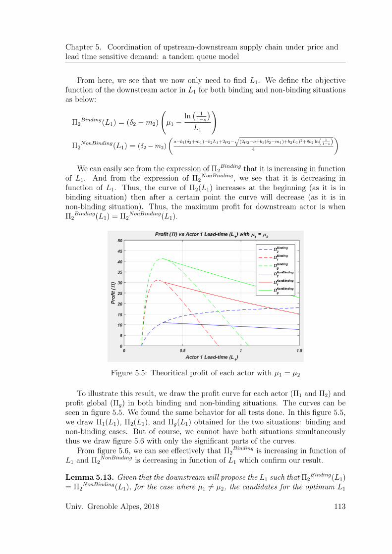
Chapter 5. Coordination of upstream-downstream supply chain under price andlead time sensitive demand: a tandem queue model
From here, we see that we now only need to find L1. We define the objectivefunction of the downstream actor in L1 for both binding and non-binding situationsas below:
Π2Binding(L1) = (δ2 −m2)
(µ1 −
ln(
11−s
)L1
)
Π2NonBinding(L1) = (δ2 −m2)
(a−b1(δ2+m1)−b2L1+2µ2−
√(2µ2−a+b1(δ2−m1)+b2L1)2+8b2 ln( 1
1−s)4
)We can easily see from the expression of Π2
Binding that it is increasing in functionof L1. And from the expression of Π2
NonBinding, we see that it is decreasing infunction of L1. Thus, the curve of Π2(L1) increases at the beginning (as it is inbinding situation) then after a certain point the curve will decrease (as it is innon-binding situation). Thus, the maximum profit for downstream actor is whenΠ2
Binding(L1) = Π2NonBinding(L1).
Figure 5.5: Theoritical profit of each actor with µ1 = µ2
To illustrate this result, we draw the profit curve for each actor (Π1 and Π2) andprofit global (Πg) in both binding and non-binding situations. The curves can beseen in figure 5.5. We found the same behavior for all tests done. In this figure 5.5,we draw Π1(L1), Π2(L1), and Πg(L1) obtained for the two situations: binding andnon-binding cases. But of course, we cannot have both situations simultaneouslythus we draw figure 5.6 with only the significant parts of the curves.
From figure 5.6, we can see effectively that Π2Binding is increasing in function of
L1 and Π2NonBinding is decreasing in function of L1 which confirm our result.
Lemma 5.13. Given that the downstream will propose the L1 such that Π2Binding(L1)
= Π2NonBinding(L1), for the case where µ1 6= µ2, the candidates for the optimum L1
Univ. Grenoble Alpes, 2018 113
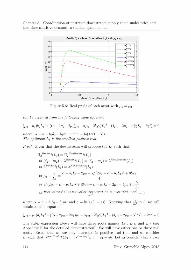
Chapter 5. Coordination of upstream-downstream supply chain under price andlead time sensitive demand: a tandem queue model
Figure 5.6: Real profit of each actor with µ1 = µ2
can be obtained from the following cubic equation:
(µ2−µ1)b2L13 +((α+2µ2−2µ1)µ1−αµ2 +2b2γ)L1
2 +(4µ1−2µ2−α)γL1−2γ2) = 0
where: α = a− b1δ2 − b1m1 and γ = ln(1/(1− s)).The optimum L1 is the smallest positive root.
Proof. Given that the downstream will propose the L1 such that:
Π2Binding(L1) = Π2
NonBinding(L1)
⇔ (δ2 −m2)× λBinding(L1) = (δ2 −m2)× λNonBinding(L1)
⇔ λBinding(L1) = λNonBinding(L1)
⇔ µ1 −γ
L1
=α− b2L1 + 2µ2 −
√(2µ2 − α + b2L1)2 + 8b2γ
4
⇔√
(2µ2 − α + b2L1)2 + 8b2γ = α− b2L1 + 2µ2 − 4µ1 + 4γ
L1
⇔ 8((µ2−µ1)b2L13+((α+2µ2−2µ1)µ1−αµ2+2b2γ)L1
2+(4µ1−2µ2−α)γL1−2γ2)
L12 = 0
where α = a − b1δ2 − b1m1 and γ = ln(1/(1 − s)). Knowing that 8L1
2 > 0, we willobtain a cubic equation:
(µ2−µ1)b2L13 +((α+2µ2−2µ1)µ1−αµ2 +2b2γ)L1
2 +(4µ1−2µ2−α)γL1−2γ2 = 0
The cubic expression above will have three roots namely L11, L12, and L13 (seeAppendix F for the detailed demonstration). We will have either one or three realroots. Recall that we are only interested in positive lead time and we considerL1 such that λNonBinding(L1) = λBinding(L1) = µ1 − γ
L1. Let us consider that a case
114 Univ. Grenoble Alpes, 2018
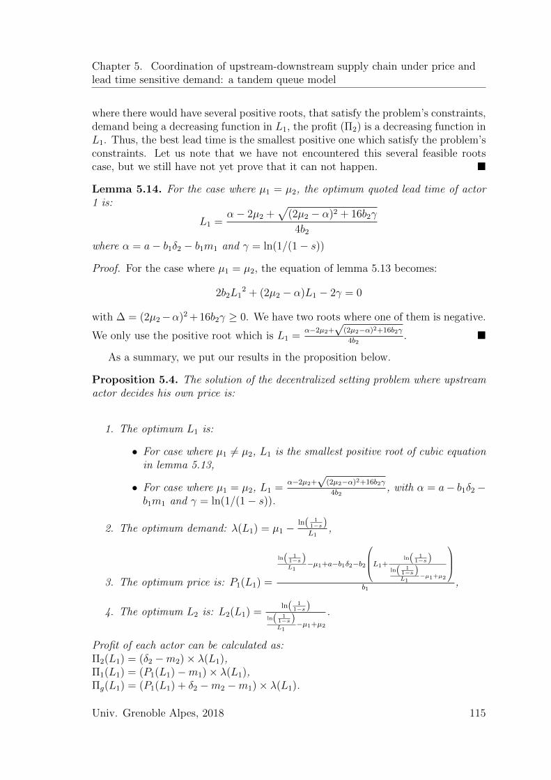
Chapter 5. Coordination of upstream-downstream supply chain under price andlead time sensitive demand: a tandem queue model
where there would have several positive roots, that satisfy the problem’s constraints,demand being a decreasing function in L1, the profit (Π2) is a decreasing function inL1. Thus, the best lead time is the smallest positive one which satisfy the problem’sconstraints. Let us note that we have not encountered this several feasible rootscase, but we still have not yet prove that it can not happen. �
Lemma 5.14. For the case where µ1 = µ2, the optimum quoted lead time of actor1 is:
L1 =α− 2µ2 +
√(2µ2 − α)2 + 16b2γ
4b2
where α = a− b1δ2 − b1m1 and γ = ln(1/(1− s))
Proof. For the case where µ1 = µ2, the equation of lemma 5.13 becomes:
2b2L12 + (2µ2 − α)L1 − 2γ = 0
with ∆ = (2µ2−α)2 + 16b2γ ≥ 0. We have two roots where one of them is negative.
We only use the positive root which is L1 =α−2µ2+
√(2µ2−α)2+16b2γ
4b2. �
As a summary, we put our results in the proposition below.
Proposition 5.4. The solution of the decentralized setting problem where upstreamactor decides his own price is:
1. The optimum L1 is:
• For case where µ1 6= µ2, L1 is the smallest positive root of cubic equationin lemma 5.13,
• For case where µ1 = µ2, L1 =α−2µ2+
√(2µ2−α)2+16b2γ
4b2, with α = a− b1δ2−
b1m1 and γ = ln(1/(1− s)).
2. The optimum demand: λ(L1) = µ1 −ln( 1
1−s)L1
,
3. The optimum price is: P1(L1) =
ln( 11−s)L1
−µ1+a−b1δ2−b2
L1+ln( 1
1−s)ln( 1
1−s)L1
−µ1+µ2
b1
,
4. The optimum L2 is: L2(L1) =ln( 1
1−s)ln( 1
1−s)L1
−µ1+µ2
.
Profit of each actor can be calculated as:Π2(L1) = (δ2 −m2)× λ(L1),Π1(L1) = (P1(L1)−m1)× λ(L1),Πg(L1) = (P1(L1) + δ2 −m2 −m1)× λ(L1).
Univ. Grenoble Alpes, 2018 115
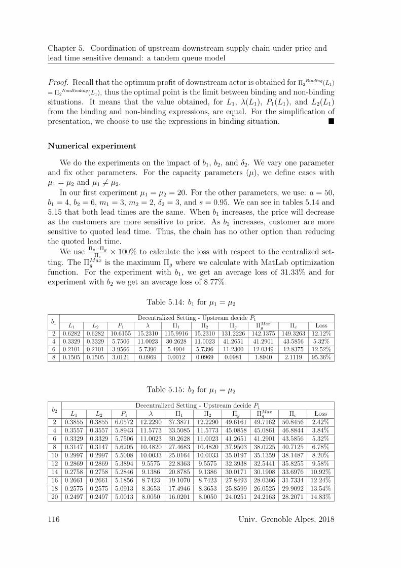
Chapter 5. Coordination of upstream-downstream supply chain under price andlead time sensitive demand: a tandem queue model
Proof. Recall that the optimum profit of downstream actor is obtained for Π2Binding(L1)
= Π2NonBinding(L1), thus the optimal point is the limit between binding and non-binding
situations. It means that the value obtained, for L1, λ(L1), P1(L1), and L2(L1)from the binding and non-binding expressions, are equal. For the simplification ofpresentation, we choose to use the expressions in binding situation. �
Numerical experiment
We do the experiments on the impact of b1, b2, and δ2. We vary one parameterand fix other parameters. For the capacity parameters (µ), we define cases withµ1 = µ2 and µ1 6= µ2.
In our first experiment µ1 = µ2 = 20. For the other parameters, we use: a = 50,b1 = 4, b2 = 6, m1 = 3, m2 = 2, δ2 = 3, and s = 0.95. We can see in tables 5.14 and5.15 that both lead times are the same. When b1 increases, the price will decreaseas the customers are more sensitive to price. As b2 increases, customer are moresensitive to quoted lead time. Thus, the chain has no other option than reducingthe quoted lead time.
We use Πc−ΠgΠc× 100% to calculate the loss with respect to the centralized set-
ting. The ΠMaxg is the maximum Πg where we calculate with MatLab optimization
function. For the experiment with b1, we get an average loss of 31.33% and forexperiment with b2 we get an average loss of 8.77%.
Table 5.14: b1 for µ1 = µ2
b1Decentralized Setting - Upstream decide P1
L1 L2 P1 λ Π1 Π2 Πg ΠMaxg Πc Loss
2 0.6282 0.6282 10.6155 15.2310 115.9916 15.2310 131.2226 142.1375 149.3263 12.12%4 0.3329 0.3329 5.7506 11.0023 30.2628 11.0023 41.2651 41.2901 43.5856 5.32%6 0.2101 0.2101 3.9566 5.7396 5.4904 5.7396 11.2300 12.0349 12.8375 12.52%8 0.1505 0.1505 3.0121 0.0969 0.0012 0.0969 0.0981 1.8940 2.1119 95.36%
Table 5.15: b2 for µ1 = µ2
b2Decentralized Setting - Upstream decide P1
L1 L2 P1 λ Π1 Π2 Πg ΠMaxg Πc Loss
2 0.3855 0.3855 6.0572 12.2290 37.3871 12.2290 49.6161 49.7162 50.8456 2.42%4 0.3557 0.3557 5.8943 11.5773 33.5085 11.5773 45.0858 45.0861 46.8844 3.84%6 0.3329 0.3329 5.7506 11.0023 30.2628 11.0023 41.2651 41.2901 43.5856 5.32%8 0.3147 0.3147 5.6205 10.4820 27.4683 10.4820 37.9503 38.0225 40.7125 6.78%10 0.2997 0.2997 5.5008 10.0033 25.0164 10.0033 35.0197 35.1359 38.1487 8.20%12 0.2869 0.2869 5.3894 9.5575 22.8363 9.5575 32.3938 32.5441 35.8255 9.58%14 0.2758 0.2758 5.2846 9.1386 20.8785 9.1386 30.0171 30.1908 33.6976 10.92%16 0.2661 0.2661 5.1856 8.7423 19.1070 8.7423 27.8493 28.0366 31.7334 12.24%18 0.2575 0.2575 5.0913 8.3653 17.4946 8.3653 25.8599 26.0525 29.9092 13.54%20 0.2497 0.2497 5.0013 8.0050 16.0201 8.0050 24.0251 24.2163 28.2071 14.83%
116 Univ. Grenoble Alpes, 2018
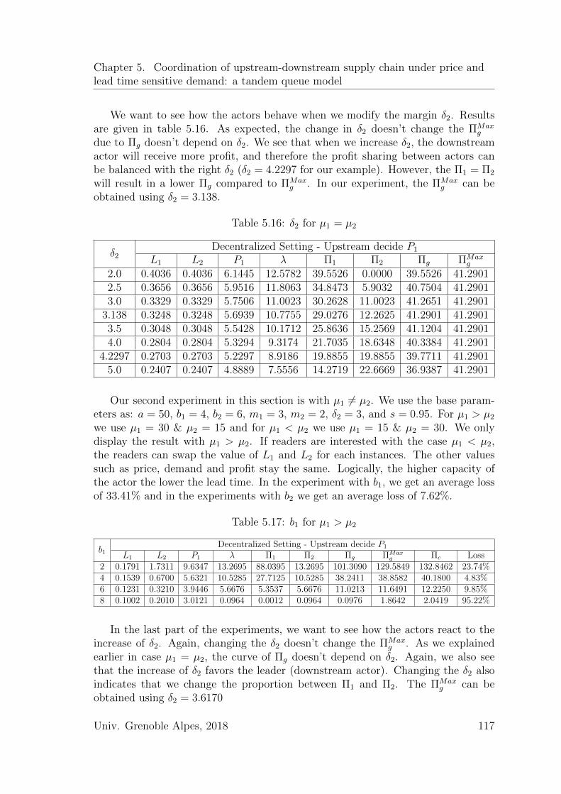
Chapter 5. Coordination of upstream-downstream supply chain under price andlead time sensitive demand: a tandem queue model
We want to see how the actors behave when we modify the margin δ2. Resultsare given in table 5.16. As expected, the change in δ2 doesn’t change the ΠMax
g
due to Πg doesn’t depend on δ2. We see that when we increase δ2, the downstreamactor will receive more profit, and therefore the profit sharing between actors canbe balanced with the right δ2 (δ2 = 4.2297 for our example). However, the Π1 = Π2
will result in a lower Πg compared to ΠMaxg . In our experiment, the ΠMax
g can beobtained using δ2 = 3.138.
Table 5.16: δ2 for µ1 = µ2
δ2Decentralized Setting - Upstream decide P1
L1 L2 P1 λ Π1 Π2 Πg ΠMaxg
2.0 0.4036 0.4036 6.1445 12.5782 39.5526 0.0000 39.5526 41.29012.5 0.3656 0.3656 5.9516 11.8063 34.8473 5.9032 40.7504 41.29013.0 0.3329 0.3329 5.7506 11.0023 30.2628 11.0023 41.2651 41.2901
3.138 0.3248 0.3248 5.6939 10.7755 29.0276 12.2625 41.2901 41.29013.5 0.3048 0.3048 5.5428 10.1712 25.8636 15.2569 41.1204 41.29014.0 0.2804 0.2804 5.3294 9.3174 21.7035 18.6348 40.3384 41.2901
4.2297 0.2703 0.2703 5.2297 8.9186 19.8855 19.8855 39.7711 41.29015.0 0.2407 0.2407 4.8889 7.5556 14.2719 22.6669 36.9387 41.2901
Our second experiment in this section is with µ1 6= µ2. We use the base param-eters as: a = 50, b1 = 4, b2 = 6, m1 = 3, m2 = 2, δ2 = 3, and s = 0.95. For µ1 > µ2
we use µ1 = 30 & µ2 = 15 and for µ1 < µ2 we use µ1 = 15 & µ2 = 30. We onlydisplay the result with µ1 > µ2. If readers are interested with the case µ1 < µ2,the readers can swap the value of L1 and L2 for each instances. The other valuessuch as price, demand and profit stay the same. Logically, the higher capacity ofthe actor the lower the lead time. In the experiment with b1, we get an average lossof 33.41% and in the experiments with b2 we get an average loss of 7.62%.
Table 5.17: b1 for µ1 > µ2
b1Decentralized Setting - Upstream decide P1
L1 L2 P1 λ Π1 Π2 Πg ΠMaxg Πc Loss
2 0.1791 1.7311 9.6347 13.2695 88.0395 13.2695 101.3090 129.5849 132.8462 23.74%4 0.1539 0.6700 5.6321 10.5285 27.7125 10.5285 38.2411 38.8582 40.1800 4.83%6 0.1231 0.3210 3.9446 5.6676 5.3537 5.6676 11.0213 11.6491 12.2250 9.85%8 0.1002 0.2010 3.0121 0.0964 0.0012 0.0964 0.0976 1.8642 2.0419 95.22%
In the last part of the experiments, we want to see how the actors react to theincrease of δ2. Again, changing the δ2 doesn’t change the ΠMax
g . As we explainedearlier in case µ1 = µ2, the curve of Πg doesn’t depend on δ2. Again, we also seethat the increase of δ2 favors the leader (downstream actor). Changing the δ2 alsoindicates that we change the proportion between Π1 and Π2. The ΠMax
g can beobtained using δ2 = 3.6170
Univ. Grenoble Alpes, 2018 117
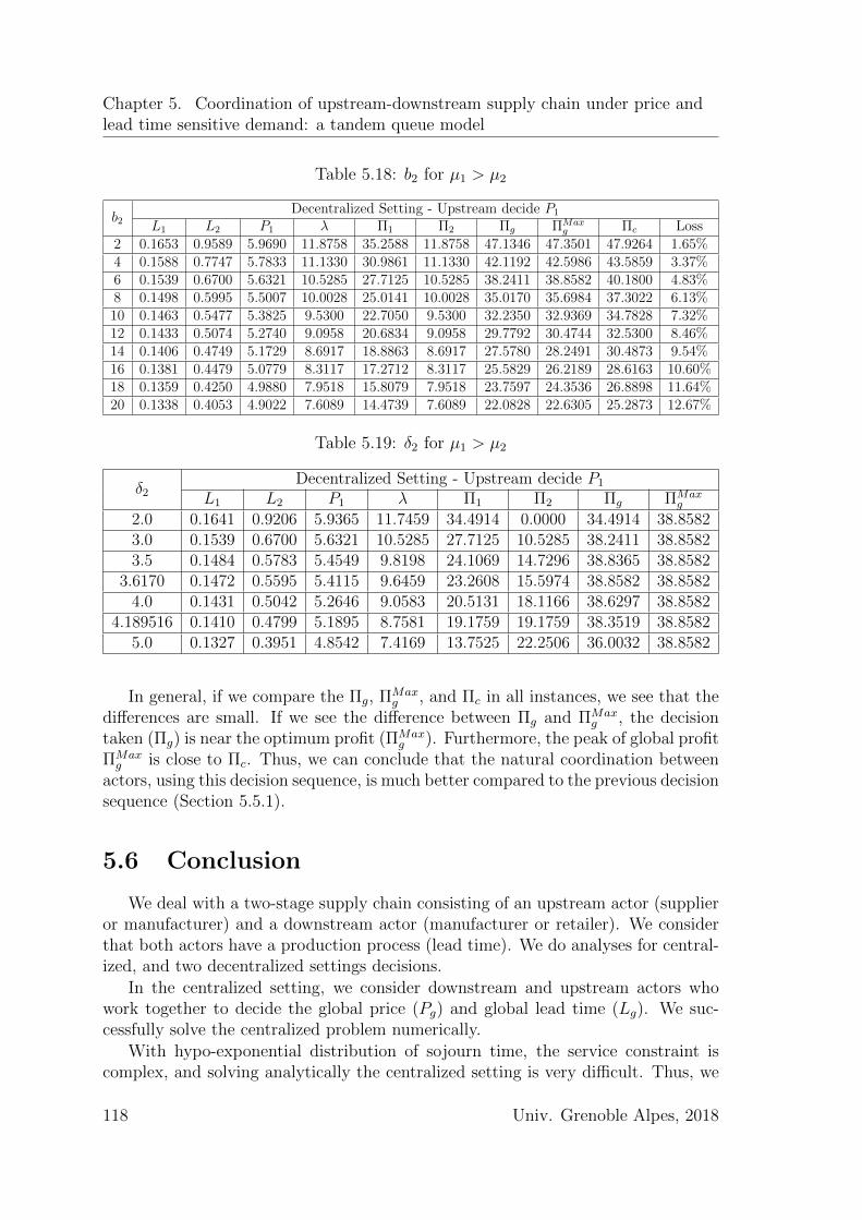
Chapter 5. Coordination of upstream-downstream supply chain under price andlead time sensitive demand: a tandem queue model
Table 5.18: b2 for µ1 > µ2
b2Decentralized Setting - Upstream decide P1
L1 L2 P1 λ Π1 Π2 Πg ΠMaxg Πc Loss
2 0.1653 0.9589 5.9690 11.8758 35.2588 11.8758 47.1346 47.3501 47.9264 1.65%4 0.1588 0.7747 5.7833 11.1330 30.9861 11.1330 42.1192 42.5986 43.5859 3.37%6 0.1539 0.6700 5.6321 10.5285 27.7125 10.5285 38.2411 38.8582 40.1800 4.83%8 0.1498 0.5995 5.5007 10.0028 25.0141 10.0028 35.0170 35.6984 37.3022 6.13%10 0.1463 0.5477 5.3825 9.5300 22.7050 9.5300 32.2350 32.9369 34.7828 7.32%12 0.1433 0.5074 5.2740 9.0958 20.6834 9.0958 29.7792 30.4744 32.5300 8.46%14 0.1406 0.4749 5.1729 8.6917 18.8863 8.6917 27.5780 28.2491 30.4873 9.54%16 0.1381 0.4479 5.0779 8.3117 17.2712 8.3117 25.5829 26.2189 28.6163 10.60%18 0.1359 0.4250 4.9880 7.9518 15.8079 7.9518 23.7597 24.3536 26.8898 11.64%20 0.1338 0.4053 4.9022 7.6089 14.4739 7.6089 22.0828 22.6305 25.2873 12.67%
Table 5.19: δ2 for µ1 > µ2
δ2Decentralized Setting - Upstream decide P1
L1 L2 P1 λ Π1 Π2 Πg ΠMaxg
2.0 0.1641 0.9206 5.9365 11.7459 34.4914 0.0000 34.4914 38.85823.0 0.1539 0.6700 5.6321 10.5285 27.7125 10.5285 38.2411 38.85823.5 0.1484 0.5783 5.4549 9.8198 24.1069 14.7296 38.8365 38.8582
3.6170 0.1472 0.5595 5.4115 9.6459 23.2608 15.5974 38.8582 38.85824.0 0.1431 0.5042 5.2646 9.0583 20.5131 18.1166 38.6297 38.8582
4.189516 0.1410 0.4799 5.1895 8.7581 19.1759 19.1759 38.3519 38.85825.0 0.1327 0.3951 4.8542 7.4169 13.7525 22.2506 36.0032 38.8582
In general, if we compare the Πg, ΠMaxg , and Πc in all instances, we see that the
differences are small. If we see the difference between Πg and ΠMaxg , the decision
taken (Πg) is near the optimum profit (ΠMaxg ). Furthermore, the peak of global profit
ΠMaxg is close to Πc. Thus, we can conclude that the natural coordination between
actors, using this decision sequence, is much better compared to the previous decisionsequence (Section 5.5.1).
5.6 Conclusion
We deal with a two-stage supply chain consisting of an upstream actor (supplieror manufacturer) and a downstream actor (manufacturer or retailer). We considerthat both actors have a production process (lead time). We do analyses for central-ized, and two decentralized settings decisions.
In the centralized setting, we consider downstream and upstream actors whowork together to decide the global price (Pg) and global lead time (Lg). We suc-cessfully solve the centralized problem numerically.
With hypo-exponential distribution of sojourn time, the service constraint iscomplex, and solving analytically the centralized setting is very difficult. Thus, we
118 Univ. Grenoble Alpes, 2018
Chapter 5. Coordination of upstream-downstream supply chain under price andlead time sensitive demand: a tandem queue model
come out with an idea to decouple the global service constraint into local service con-straints. We have proved that for s ≥ 0.715, satisfying the local service constraintsallows to satisfy the global service constraint. Then, we proposed a new model,where we transform the global service constraint into local service constraints foreach actor. We call this model “Modified Centralized”. Based on our experimenta-tions, decouple the global service constraints leads to lower profit (in our experimentswe get approximately 15% of loss compared to the centralized setting).
Thanks to this result, we have been able to model our problem into the decen-tralized setting. We divide the decentralized setting into two scenarios. In bothscenarios, the downstream actor acts as a leader and the upstream actor acts as afollower. In the first scenario, the upstream actor chooses his own lead time (L1)but the price P1 and lead time L2 are decided by the downstream actor (actor 2).In the second scenario, the upstream actor (actor 1) decides his own price (P1) anddownstream actor (actor 2) decides the global lead time (L1 + L2) and L1. Theglobal price (Pg) is obtained from P1 plus a fixed margin taken by the downstreamactor (δ2). We solve the decentralized problems analytically and we provide someexperiments.
In the first scenario (upstream actor decides his own lead time), from the ex-periments we see that the global profit is very low compared to the centralizedsetting. We also see that the profit of upstream actor is null. It shows that theactors cannot cooperate naturally. However, if we observe the comparison betweenmaximum global profit and profit in centralized setting, we see that the differenceis small. This signifies that the decentralized setting approach could provide a fa-vorable global profit in condition that the proposed coordination system could leadthe actors into this situation.
In second scenario (upstream actor decides his own price), the global profit curvedoesn’t depend on the downstream actor’s margin (δ2). We see that the increasein δ2 favors the leader (downstream actor). Changing the δ2 also indicates that wechange the proportion of profit for each actor. The maximum global price can beobtained numerically.
If we compare all scenarios: centralized, modified centralized, and two decentral-ized settings, we can naturally see that the best setting for maximizing the globalprofit is centralized setting. However, in most supply chain actors have a givenautonomy. So in decentralized schemes, we suggest the upstream actor chooses hisown price. This will result in a better profit for both actors and for the profit globalof the chain compared to the other scheme (upstream actors chooses the lead-time).
Univ. Grenoble Alpes, 2018 119
Chapter 5. Coordination of upstream-downstream supply chain under price andlead time sensitive demand: a tandem queue model
120 Univ. Grenoble Alpes, 2018
Chapter 6
General conclusion
6.1 Conclusion
From the literature review, we see at least three weaknesses. First, all worksassume that the unit production cost is a constant. Second, in single firm case allpapers use the M/M/1 system. Although M/M/1 is the simplest queuing model, thefact that all customers are accepted might lead to long sojourn times (lead time) inthe system. Third, in multi-firm all contributions assume that only one of the actorhas production process, the other actor only acts as a mediator with a lead-timeequals to zero.
Thus, in this study, we propose three extensions: 1. Lead-time sensitive produc-tion cost, 2. Customer’s rejection policy using an M/M/1/K model, and 3. Two-stage supply chain coordination using a tandem queue (M/M/1-M/M/1) model. Inthe first contribution, we consider the production cost to be a decreasing functionin lead time. Indeed, a company can use different ways to reduce lead time (such asbuying items from quick response but expensive subcontractors) but this generallyleads to higher production cost. The second contribution, we model the firm as anM/M/1/K queue, for which demand is rejected if there are already K customers inthe system. The last contribution is modeling the system in a tandem queue. Itis more realistic when a supply chain consists of more than one stage and in eachstage there is a production process.
In the first contribution, we solved the problem of lead-time quotation in anM/M/1 make-to-order queue while assuming the production cost to be a decreasingfunction in lead-time. We considered three settings: (1) lead-time is variable butprice is fixed, (2) price and lead-time are both decision variables, and (3) price andlead-time are decision variables where the lateness and holding cost are considered.We solve settings 1 and 2 analytically; and setting 3 numerically. We conductedexperiments and derived interesting insights.
In case of variable lead time and fixed cost (setting 1), some of our insightsindicated that the higher the demand sensitivity to lead time the higher the servicelevel. This results is not intuitive since an increase in lead time sensitivity leads toshorter lead time that is supposed to be more difficult to guarantee. This behaviorcannot be captured by the existing models where the unit operating cost is assumedconstant since the service constraint is always binding in this case.
When both lead time and price are endogenous variables (Setting 2), our resultsshowed that an increase in the demand sensitivity to price leads to an increasein quoted lead time in our model while it has the opposite effect for models with
121
Chapter 6. General conclusion
constant cost. We also found that when demand is very sensitive to lead time, thecustomers can benefit of smaller price, shorter lead time, and also more reliabledeliveries.
When we consider the lateness penalty and holding costs (Setting 3), the modelquotes a longer lead time higher than the one imposed by the service constraint.The model prefers to be in non-binding situation. Indeed, quoting a longer leadtime is favorable as it will reduce the incurred costs (i.e. production and latenesscosts).
From our numerical experiments, we quantified the gain brought by using thesolution of our model versus the solution of the benchmark model where the cost isconstant. In the case where the price is fixed (setting 1), we found that our modelleads to small gains. This proves that there is an impact of not quoting the rightlead time when the cost is assumed to be constant. This impact becomes moresignificant (as the gains become bigger) when we take into account the price as adecision variable (setting 2). And when the lateness and holding costs are included,this gains increase compared to the settings 1 and 2.
In the second contribution, we formulated the problem of lead time quotationand pricing for a profit-maximizing firm, modeled as an M/M/1/K system, facing alinear price- and lead time-dependent demand with the consideration of inventoryholding and lateness penalty costs. In order to determine the lateness penalty cost,we knocked out a theoretical barrier by explicitly calculating the expected latenessgiven that a job is late in an M/M/1/K queue when a certain delivery lead timeis quoted to the customers. This result can be used in the future for differentoperations management and queuing theory problems.
In M/M/1/1 queue, the expression of the optimal solution showed that an in-crease in lead time-sensitivity first leads to reducing the quoted lead time but canrapidly become useless if it exceeds a certain threshold value (since the service con-straint becomes binding). We also deduced that when the customers become moresensitive to price or when the unit lateness penalty cost increases, the firm can reactby increasing the quoted lead time. Based on our comparison of the optimal profitgiven by our M/M/1/1 model to the optimal profit obtained when the firm is mod-eled as an M/M/1 queue (as given in the literature), we found out that a rejectionpolicy can be more profitable than an all-customers’ acceptance policy even whenthe holding and penalty costs are not considered. Some of our results showed thatan increase in lead-time sensitivity or in price-sensitivity favors the rejection policy.The increase in unit holding cost has been proven to be one of the main criteria thatmake the rejection policy better than the all-customers’ acceptance policy.
Then, we solved numerically the M/M/1/K queue (K > 1). We showed thatthere is at least one value of K for which the M/M/1/K (rejection policy) is moreprofitable than the M/M/1 (all customers’ acceptance policy). In most cases, it hasalso been observed that an increase in the value of K (i.e., the system size) has anon-monotonous effect on the firm’s profit. Indeed, an increase in K first improvesthe profit and then leads to decreasing it.
122 Univ. Grenoble Alpes, 2018
Chapter 6. General conclusion
In the last contribution, we deal with a two-stage supply chain consisting of anupstream actor (supplier or manufacturer) and a downstream actor (manufactureror retailer). We consider that both actors have production process (lead time). Wedo analyses for centralized, and two decentralized settings decisions.
In the centralized setting, we consider downstream and upstream actors whowork together to decide the global price (Pg) and global lead time (Lg). We suc-cessfully solve the centralized problem numerically.
With hypo-exponential distribution of sojourn time, the service constraint iscomplex, and solving analytically the centralized setting is very difficult. Thus, wecome out with an idea to decouple the global service constraint into local serviceconstraints. We have proved, from a given value of service level, that satisfying thelocal service constraints allows to satisfy the global service constraint. We proposeda new model with these new constraints, called “Modified Centralized”. Based onour experimentations, decouple the global service constraints naturally leads to lowerprofit, but the difference is not very high.
Thanks to the decoupling result, we have been able to model our problem intothe decentralized setting. We divide the decentralized setting into two scenarios. Inboth scenarios, the downstream actor acts as a leader and the upstream actor actsas a follower. In the first scenario, the upstream actor chooses his own lead time(L1) but the price P1 and lead time L2 are decided by the downstream actor (actor2). In the second scenario, the upstream actor (actor 1) decides his own price (P1)and downstream actor (actor 2) decides the global lead time (L1 + L2) and L1. Wesolve the decentralized problems analytically and we provide some experiments.
If we compare all scenarios: centralized, modified centralized, and two decentral-ized settings, we can naturally see that the best setting for maximizing the globalprofit is centralized setting. However, most supply chains nowadays are decentral-ized. So in decentralized schemes, we suggest the upstream actor chooses his ownprice. This will result in a better profit for both actors and for the profit global ofthe chain compared to the other scheme (upstream actors chooses the lead-time).
6.2 Future works and perspectives
Our study can be extended in different ways. For instance, it would be interestingto investigate the log-linear model of demand. Another extension of our tandemqueue model would be to inverse the role of leader-follower. We could consider theupstream acts as a leader and downstream acts as a follower. Other extensions couldbe: to introduce sharing bonus scheme for the decentralized setting where upstreamactor chooses his own lead-time (this will avoid the zero profit of upstream actor).One could also consider a competition between actors in the multi stage supplychains. We could also consider a new stream of research which considers a dynamiclead time quotation.
Univ. Grenoble Alpes, 2018 123
Chapter 6. General conclusion
124 Univ. Grenoble Alpes, 2018
Bibliography
Albana, A. S., Y. Frein, and R. Hammami2016. Optimal firm’s policy under lead time- and price-dependent demand: in-terest of customers rejection policy. In POMS 27th Annual Conference, Orlando,Florida.
Albana, A. S., R. Hammami, and Y. Frein2017a. Expected lateness in an M/M/1/K queue. Working paper. http://hal.univ-grenoble-alpes.fr/hal-01626006.
Albana, A. S., R. Hammami, and Y. Frein2017b. Impact of lead-time sensitive cost on lead-time quotation and pricingproblems. In 7th IESM Conference, Pp. 474–479, Saarbrucken, Germany.
Albana, A. S., R. Hammami, and Y. Frein2017c. Lead time quotation and pricing in a finite buffer queue with endogenousdemand: Effect of customers’ rejection and buffer capacity sizing. Working paper.
Albana, A. S., R. Hammami, and Y. Frein2017d. Lead time quotation and pricing in a stochastic make-to-order system withlead time-dependent cost and endogenous demand. Submitted to InternationalJournal of Production Economics.
Baker, W., M. Marn, and C. Zawada2001. Price smarter on the net. Harvard business review, 79(2):122–7.
Ballou, R. H.1998. Business Logistics Management, 4th edition. Upper Saddle River, NewJersey: Prentice-Hall.
Blackburn, J. D.1991. Time-based competition: the next battleground in American manufacturing.Homewood, Illinois: Irwin Professional Pub.
Blackburn, J. D., T. Elrod, W. B. Lindsley, and A. J. Zahorik1992. The strategic value of response time and product variety. ManufacturingStrategy – Process and Content. Chapman and Hall, London.
Bolch, G., S. Greiner, H. de Meer, and K. S. Trivedi2006. Queueing networks and Markov chains: modeling and performance evalua-tion with computer science applications, 2nd edition. Hoboken, New Jersey: JohnWiley & Sons.
125
Bibliography
Boyaci, T. and S. Ray2003. Product differentiation and capacity cost interaction in time and pricesensitive markets. Manufacturing & Service operations management, 5(1):18–36.
Boyaci, T. and S. Ray2006. The impact of capacity costs on product differentiation in delivery time,delivery reliability, and price. Production and Operations Management, 15(2):179–197.
Celik, S. and C. Maglaras2008. Dynamic pricing and lead-time quotation for a multiclass make-to-orderqueue. Management Science, 54(6):1132–1146.
Christopher, M.2011. Logistics & supply chain management, 4th edition. Harlow: FT PrenticeHall.
Geary, S. and J. P. Zonnenberg2000. What it means to be best in class. Supply Chain Management Review, V.4,NO.3 (July/Aug. 2000), P. 43-48: ILL.
Gross, D., J. F. Shortle, J. M. Thompson, and C. M. Harris2008. Fundamentals of Queueing Theory, 4th edition. Hoboken, New Jersey: JohnWiley & Sons.
Hafızoglu, A. B., E. S. Gel, and P. Keskinocak2016. Price and lead time quotation for contract and spot customers. OperationsResearch, 64(2):406–415.
Hammami, R. and Y. Frein2013. An optimisation model for the design of global multi-echelon supplychains under lead time constraints. International Journal of Production Reseach,51(9):2760–2775.
Hillier, F. and G. Lieberman2001. Introduction To Operations Research, 7th edition. New York: McGraw Hill.
Ho, T. H. and Y.-S. Zheng2004. Setting customer expectation in service delivery: An integrated marketing-operations perspective. Management Science, 50(4):479–488.
Hotelling, H.1929. Stability in competition. The economic journal, 39(153):41–57.
Huang, J., M. Leng, and M. Parlar2013. Demand functions in decision modeling: A comprehensive survey and re-search directions. Decision Sciences, 44(3):557–609.
126 Univ. Grenoble Alpes, 2018
Bibliography
Hum, S.-H. and H.-H. Sim1996. Time-based competition: literature review and implications for modelling.International Journal of Operations & Production Management, 16(1):75–90.
Irving, R.2013. Beyond the quadratic formula. Washington: Mathematical Association ofAmerica.
Jackson, D. W., J. E. Keith, and R. K. Burdick1986. Examining the relative importance of physical distribution service elements.Journal of Business Logistics, 7(2).
Kapuscinski, R. and S. Tayur2007. Reliable due-date setting in a capacitated mto system with two customerclasses. Operations research, 55(1):56–74.
Kleinrock, L.1975. Queueing systems, volume 1. New York: Wiley.
Li, L.1992. The role of inventory in delivery-time competition. Management Science,38(2):182–197.
Liu, L., M. Parlar, and S. X. Zhu2007. Pricing and lead time decisions in decentralized supply chains. ManagementScience, 53(5):713–725.
Palaka, K., S. Erlebacher, and D. H. Kropp1998. Lead-time setting, capacity utilization, and pricing decisions under lead-time dependent demand. IIE transactions, 30(2):151–163.
Panda, S.2013. Coordinating a manufacturer–retailer chain under time and price dependentdemand rate. International Journal of Management Science and EngineeringManagement, 8(2):84–92.
Pekgun, P., P. M. Griffin, and P. Keskinocak2008. Coordination of marketing and production for price and leadtime decisions.IIE transactions, 40(1):12–30.
Pekgun, P., P. M. Griffin, and P. Keskinocak2016. Centralized versus decentralized competition for price and lead-time sensi-tive demand. Decision Sciences.
Ray, S. and E. M. Jewkes2004. Customer lead time management when both demand and price are leadtime sensitive. European Journal of operational research, 153(3):769–781.
Univ. Grenoble Alpes, 2018 127
Bibliography
Savasaneril, S., P. M. Griffin, and P. Keskinocak2010. Dynamic lead-time quotation for an M/M/1 base-stock inventory queue.Operations research, 58(2):383–395.
Savasaneril, S. and E. Sayin2017. Dynamic lead time quotation under responsive inventory and multiple cus-tomer classes. OR Spectrum, 39(1):95–135.
Schechter, E.2013. The Cubic Formula - Solve Any 3rd Degree Polynomial Equation. https:
//math.vanderbilt.edu/schectex/courses/cubic/.
Slotnick, S. A.2014. Lead-time quotation when customers are sensitive to reputation. Interna-tional Journal of Production Research, 52(3):713–726.
So, K. C.2000. Price and time competition for service delivery. Manufacturing & ServiceOperations Management, 2(4):392–409.
So, K. C. and J.-S. Song1998. Price, delivery time guarantees and capacity selection. European Journalof operational research, 111(1):28–49.
Stalk, G. and T. M. Hout1990. Competing against time: How time-based competition is reshaping globalmar. New York: Free Press.
Sterling, J. U. and D. M. Lambert1989. Customer service research: past, present and future. International journalof physical distribution & materials management, 19(2):2–23.
Suri, R.1998. Quick response manufacturing: a companywide approach to reducing leadtimes. Portland, Oregon: Productivity Press.
Sztrik, J.2016. Basic Queueing Theory: Foundations of System Performance Modeling.Saarbrucken, Germany: GlobeEdit.
Thomopoulos, N. T.2012. Fundamentals of Queuing Systems: Statistical Methods for Analyzing Queu-ing Models. New York: Springer Science & Business Media.
Wu, Z., B. Kazaz, S. Webster, and K.-K. Yang2012. Ordering, pricing, and lead-time quotation under lead-time and demanduncertainty. Production and Operations Management, 21(3):576–589.
128 Univ. Grenoble Alpes, 2018
Bibliography
Xiao, T. and X. Qi2016. A two-stage supply chain with demand sensitive to price, delivery time, andreliability of delivery. Annals of Operations Research, 241(1-2):475–496.
Xiao, T. and J. Shi2012. Price, capacity, and lead-time decisions for a make-to-order supply chainwith two production modes. International Journal of Applied Management Sci-ence, 4(2):107–129.
Xiao, T., J. Shi, and G. Chen2014. Price and leadtime competition, and coordination for make-to-order supplychains. Computers & Industrial Engineering, 68:23–34.
Xiao, T., D. Yang, and H. Shen2011. Coordinating a supply chain with a quality assurance policy via a revenue-sharing contract. International Journal of Production Research, 49(1):99–120.
Xiaopan, L., W. Jianjun, Z. Binghang, and Z. Zongbao2014. Price and guaranteed delivery time competition/cooperation in a duopoly.In Service Systems and Service Management (ICSSSM), 2014 11th InternationalConference on, Pp. 1–6. IEEE.
Zhao, X., K. E. Stecke, and A. Prasad2012. Lead time and price quotation mode selection: uniform or differentiated?Production and Operations Management, 21(1):177–193.
Zhu, S. X.2015. Integration of capacity, pricing, and lead-time decisions in a decentralizedsupply chain. International Journal of Production Economics, 164:14–23.
Univ. Grenoble Alpes, 2018 129
Bibliography
130 Univ. Grenoble Alpes, 2018
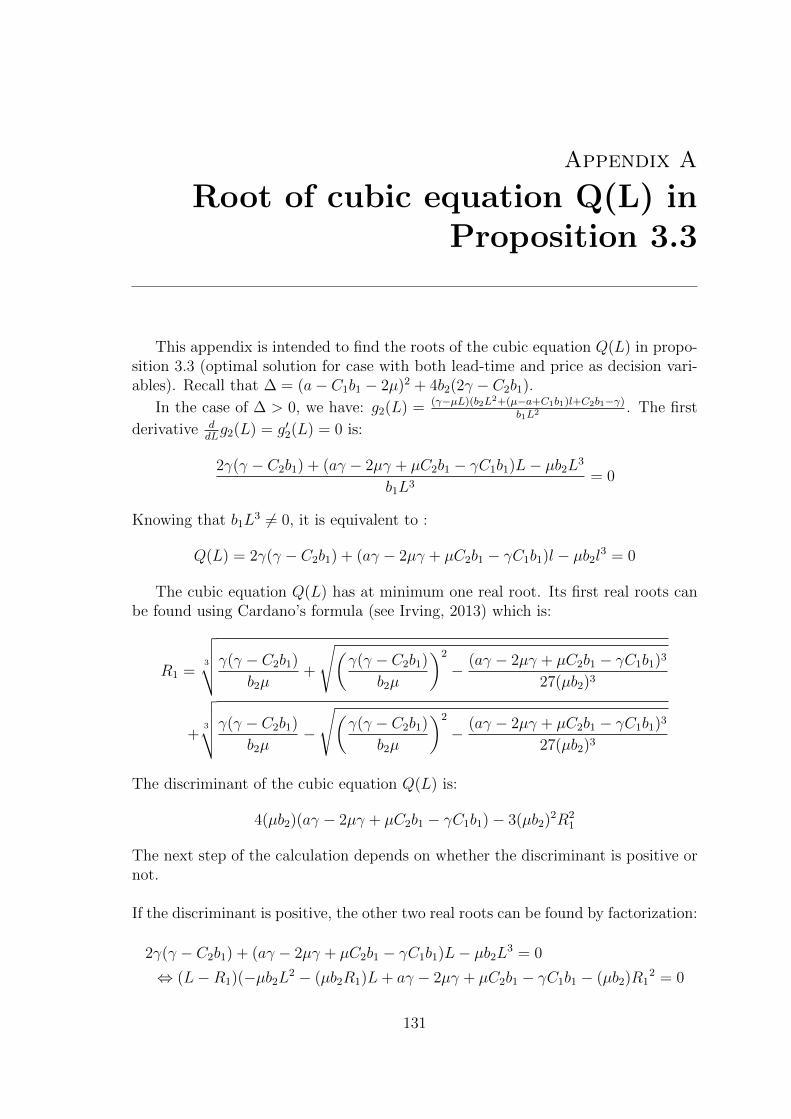
Appendix A
Root of cubic equation Q(L) inProposition 3.3
This appendix is intended to find the roots of the cubic equation Q(L) in propo-sition 3.3 (optimal solution for case with both lead-time and price as decision vari-ables). Recall that ∆ = (a− C1b1 − 2µ)2 + 4b2(2γ − C2b1).
In the case of ∆ > 0, we have: g2(L) = (γ−µL)(b2L2+(µ−a+C1b1)l+C2b1−γ)b1L2 . The first
derivative ddLg2(L) = g′2(L) = 0 is:
2γ(γ − C2b1) + (aγ − 2µγ + µC2b1 − γC1b1)L− µb2L3
b1L3= 0
Knowing that b1L3 6= 0, it is equivalent to :
Q(L) = 2γ(γ − C2b1) + (aγ − 2µγ + µC2b1 − γC1b1)l − µb2l3 = 0
The cubic equation Q(L) has at minimum one real root. Its first real roots canbe found using Cardano’s formula (see Irving, 2013) which is:
R1 =3
√√√√γ(γ − C2b1)
b2µ+
√(γ(γ − C2b1)
b2µ
)2
− (aγ − 2µγ + µC2b1 − γC1b1)3
27(µb2)3
+3
√√√√γ(γ − C2b1)
b2µ−
√(γ(γ − C2b1)
b2µ
)2
− (aγ − 2µγ + µC2b1 − γC1b1)3
27(µb2)3
The discriminant of the cubic equation Q(L) is:
4(µb2)(aγ − 2µγ + µC2b1 − γC1b1)− 3(µb2)2R21
The next step of the calculation depends on whether the discriminant is positive ornot.
If the discriminant is positive, the other two real roots can be found by factorization:
2γ(γ − C2b1) + (aγ − 2µγ + µC2b1 − γC1b1)L− µb2L3 = 0
⇔ (L−R1)(−µb2L2 − (µb2R1)L+ aγ − 2µγ + µC2b1 − γC1b1 − (µb2)R1
2 = 0
131
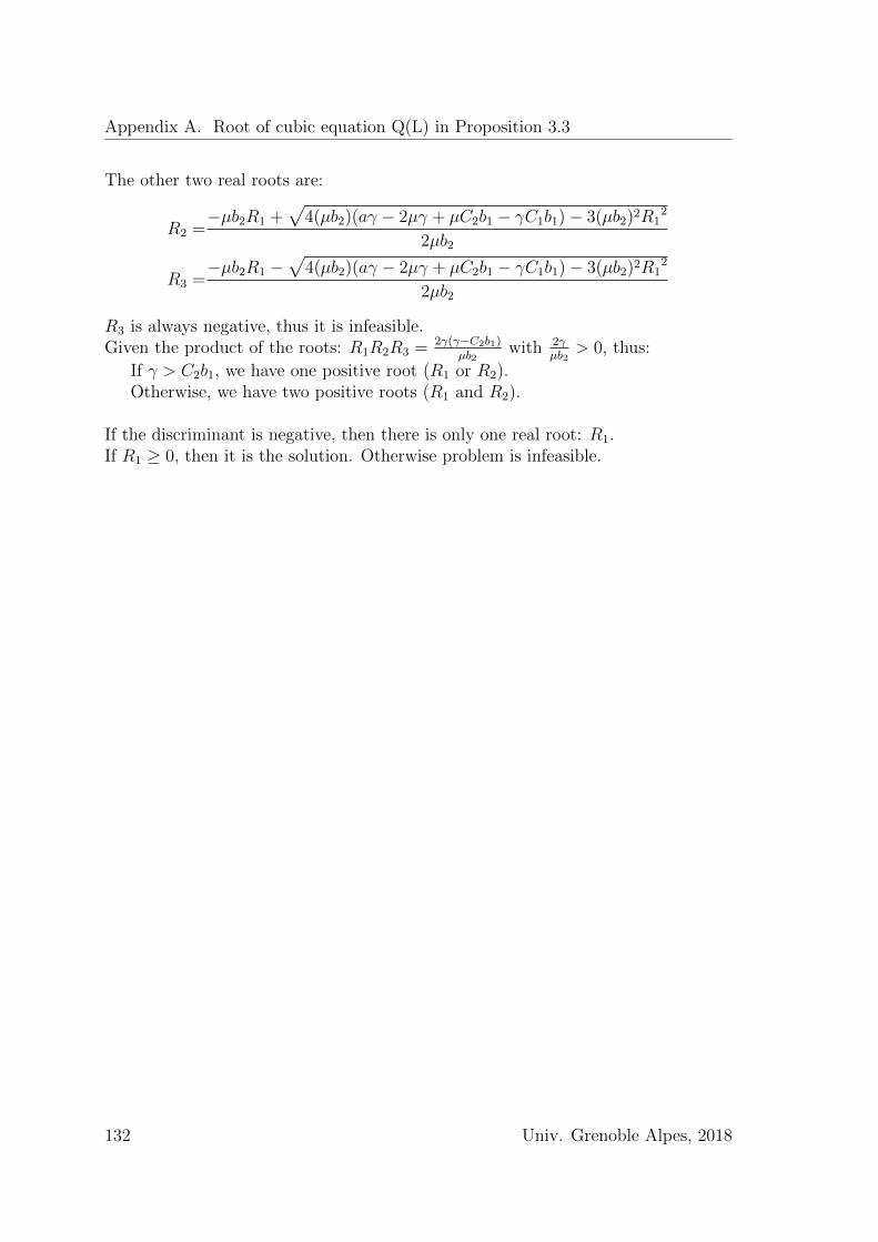
Appendix A. Root of cubic equation Q(L) in Proposition 3.3
The other two real roots are:
R2 =−µb2R1 +
√4(µb2)(aγ − 2µγ + µC2b1 − γC1b1)− 3(µb2)2R1
2
2µb2
R3 =−µb2R1 −
√4(µb2)(aγ − 2µγ + µC2b1 − γC1b1)− 3(µb2)2R1
2
2µb2
R3 is always negative, thus it is infeasible.Given the product of the roots: R1R2R3 = 2γ(γ−C2b1)
µb2with 2γ
µb2> 0, thus:
If γ > C2b1, we have one positive root (R1 or R2).Otherwise, we have two positive roots (R1 and R2).
If the discriminant is negative, then there is only one real root: R1.If R1 ≥ 0, then it is the solution. Otherwise problem is infeasible.
132 Univ. Grenoble Alpes, 2018
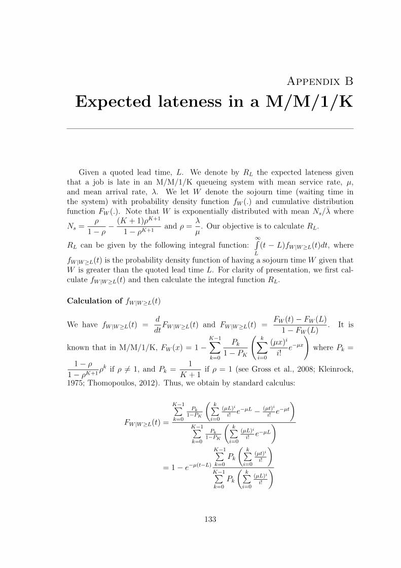
Appendix B
Expected lateness in a M/M/1/K
Given a quoted lead time, L. We denote by RL the expected lateness giventhat a job is late in an M/M/1/K queueing system with mean service rate, µ,and mean arrival rate, λ. We let W denote the sojourn time (waiting time inthe system) with probability density function fW (.) and cumulative distributionfunction FW (.). Note that W is exponentially distributed with mean Ns/λ where
Ns =ρ
1− ρ− (K + 1)ρK+1
1− ρK+1and ρ =
λ
µ. Our objective is to calculate RL.
RL can be given by the following integral function:∞∫L
(t − L)fW |W≥L(t)dt, where
fW |W≥L(t) is the probability density function of having a sojourn time W given thatW is greater than the quoted lead time L. For clarity of presentation, we first cal-culate fW |W≥L(t) and then calculate the integral function RL.
Calculation of fW |W≥L(t)
We have fW |W≥L(t) =d
dtFW |W≥L(t) and FW |W≥L(t) =
FW (t)− FW (L)
1− FW (L). It is
known that in M/M/1/K, FW (x) = 1 −K−1∑k=0
Pk1− PK
(k∑i=0
(µx)i
i!e−µx
)where Pk =
1− ρ1− ρK+1
ρk if ρ 6= 1, and Pk =1
K + 1if ρ = 1 (see Gross et al., 2008; Kleinrock,
1975; Thomopoulos, 2012). Thus, we obtain by standard calculus:
FW |W≥L(t) =
K−1∑k=0
Pk1−PK
(k∑i=0
(µL)i
i!e−µL − (µt)i
i!e−µt
)K−1∑k=0
Pk1−PK
(k∑i=0
(µL)i
i!e−µL
)
= 1− e−µ(t−L)
K−1∑k=0
Pk
(k∑i=0
(µt)i
i!
)K−1∑k=0
Pk
(k∑i=0
(µL)i
i!
)
133
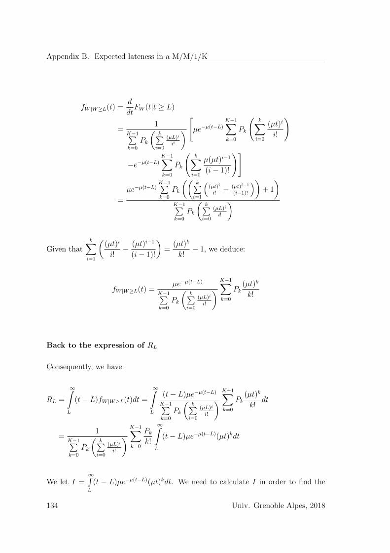
Appendix B. Expected lateness in a M/M/1/K
fW |W≥L(t) =d
dtFW (t|t ≥ L)
=1
K−1∑k=0
Pk
(k∑i=0
(µL)i
i!
) [µe−µ(t−L)
K−1∑k=0
Pk
(k∑i=0
(µt)i
i!
)
−e−µ(t−L)
K−1∑k=0
Pk
(k∑i=0
µ(µt)i−1
(i− 1)!
)]
=
µe−µ(t−L)K−1∑k=0
Pk
((k∑i=1
((µt)i
i!− (µt)i−1
(i−1)!
))+ 1
)K−1∑k=0
Pk
(k∑i=0
(µL)i
i!
)
Given thatk∑i=1
((µt)i
i!− (µt)i−1
(i− 1)!
)=
(µt)k
k!− 1, we deduce:
fW |W≥L(t) =µe−µ(t−L)
K−1∑k=0
Pk
(k∑i=0
(µL)i
i!
) K−1∑k=0
Pk(µt)k
k!
Back to the expression of RL
Consequently, we have:
RL =
∞∫L
(t− L)fW |W≥L(t)dt =
∞∫L
(t− L)µe−µ(t−L)
K−1∑k=0
Pk
(k∑i=0
(µL)i
i!
) K−1∑k=0
Pk(µt)k
k!dt
=1
K−1∑k=0
Pk
(k∑i=0
(µL)i
i!
) K−1∑k=0
Pkk!
∞∫L
(t− L)µe−µ(t−L)(µt)kdt
We let I =∞∫L
(t − L)µe−µ(t−L)(µt)kdt. We need to calculate I in order to find the
134 Univ. Grenoble Alpes, 2018
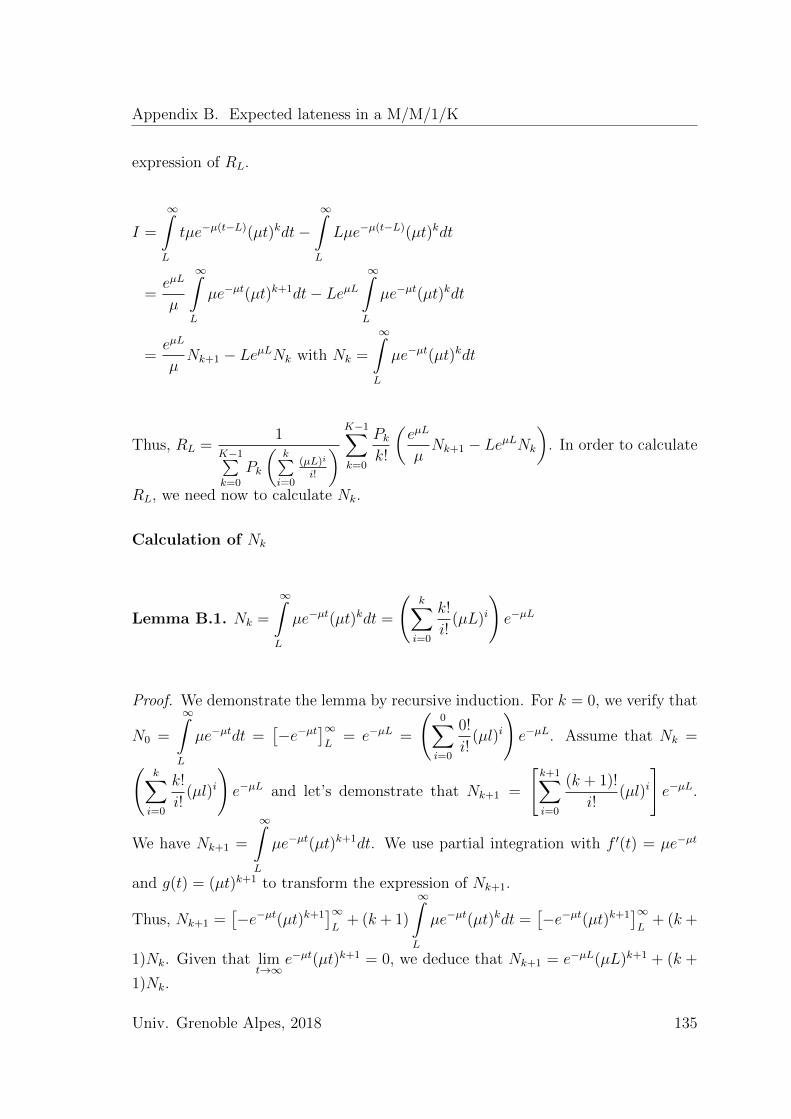
Appendix B. Expected lateness in a M/M/1/K
expression of RL.
I =
∞∫L
tµe−µ(t−L)(µt)kdt−∞∫L
Lµe−µ(t−L)(µt)kdt
=eµL
µ
∞∫L
µe−µt(µt)k+1dt− LeµL∞∫L
µe−µt(µt)kdt
=eµL
µNk+1 − LeµLNk with Nk =
∞∫L
µe−µt(µt)kdt
Thus, RL =1
K−1∑k=0
Pk
(k∑i=0
(µL)i
i!
) K−1∑k=0
Pkk!
(eµL
µNk+1 − LeµLNk
). In order to calculate
RL, we need now to calculate Nk.
Calculation of Nk
Lemma B.1. Nk =
∞∫L
µe−µt(µt)kdt =
(k∑i=0
k!
i!(µL)i
)e−µL
Proof. We demonstrate the lemma by recursive induction. For k = 0, we verify that
N0 =
∞∫L
µe−µtdt =[−e−µt
]∞L
= e−µL =
(0∑i=0
0!
i!(µl)i
)e−µL. Assume that Nk =(
k∑i=0
k!
i!(µl)i
)e−µL and let’s demonstrate that Nk+1 =
[k+1∑i=0
(k + 1)!
i!(µl)i
]e−µL.
We have Nk+1 =
∞∫L
µe−µt(µt)k+1dt. We use partial integration with f ′(t) = µe−µt
and g(t) = (µt)k+1 to transform the expression of Nk+1.
Thus, Nk+1 =[−e−µt(µt)k+1
]∞L
+ (k + 1)
∞∫L
µe−µt(µt)kdt =[−e−µt(µt)k+1
]∞L
+ (k +
1)Nk. Given that limt→∞
e−µt(µt)k+1 = 0, we deduce that Nk+1 = e−µL(µL)k+1 + (k +
1)Nk.
Univ. Grenoble Alpes, 2018 135
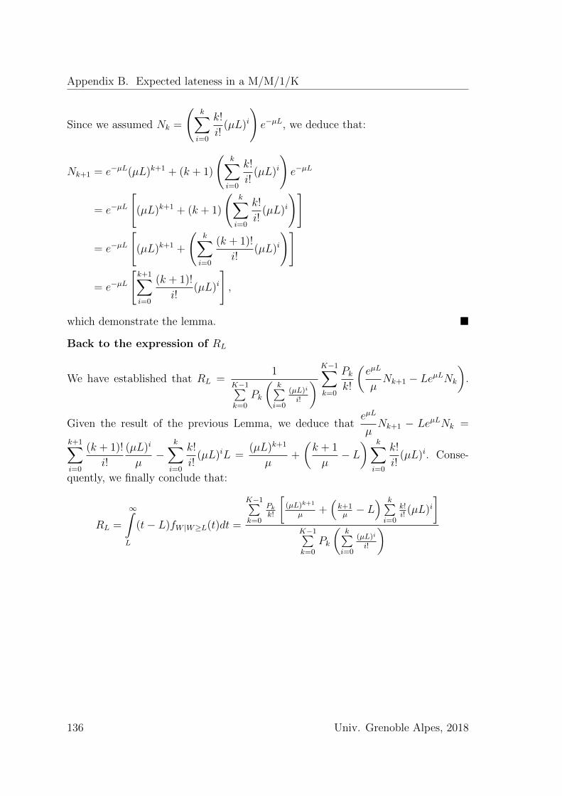
Appendix B. Expected lateness in a M/M/1/K
Since we assumed Nk =
(k∑i=0
k!
i!(µL)i
)e−µL, we deduce that:
Nk+1 = e−µL(µL)k+1 + (k + 1)
(k∑i=0
k!
i!(µL)i
)e−µL
= e−µL
[(µL)k+1 + (k + 1)
(k∑i=0
k!
i!(µL)i
)]
= e−µL
[(µL)k+1 +
(k∑i=0
(k + 1)!
i!(µL)i
)]
= e−µL
[k+1∑i=0
(k + 1)!
i!(µL)i
],
which demonstrate the lemma. �
Back to the expression of RL
We have established that RL =1
K−1∑k=0
Pk
(k∑i=0
(µL)i
i!
) K−1∑k=0
Pkk!
(eµL
µNk+1 − LeµLNk
).
Given the result of the previous Lemma, we deduce thateµL
µNk+1 − LeµLNk =
k+1∑i=0
(k + 1)!
i!
(µL)i
µ−
k∑i=0
k!
i!(µL)iL =
(µL)k+1
µ+
(k + 1
µ− L
) k∑i=0
k!
i!(µL)i. Conse-
quently, we finally conclude that:
RL =
∞∫L
(t− L)fW |W≥L(t)dt =
K−1∑k=0
Pkk!
[(µL)k+1
µ+(k+1µ− L
) k∑i=0
k!i!
(µL)i]
K−1∑k=0
Pk
(k∑i=0
(µL)i
i!
)
136 Univ. Grenoble Alpes, 2018
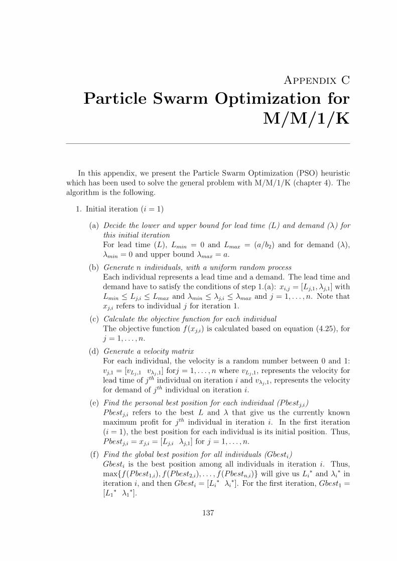
Appendix C
Particle Swarm Optimization forM/M/1/K
In this appendix, we present the Particle Swarm Optimization (PSO) heuristicwhich has been used to solve the general problem with M/M/1/K (chapter 4). Thealgorithm is the following.
1. Initial iteration (i = 1)
(a) Decide the lower and upper bound for lead time (L) and demand (λ) forthis initial iterationFor lead time (L), Lmin = 0 and Lmax = (a/b2) and for demand (λ),λmin = 0 and upper bound λmax = a.
(b) Generate n individuals, with a uniform random processEach individual represents a lead time and a demand. The lead time anddemand have to satisfy the conditions of step 1.(a): xi,j = [Lj,1, λj,1] withLmin ≤ Lj,i ≤ Lmax and λmin ≤ λj,i ≤ λmax and j = 1, . . . , n. Note thatxj,i refers to individual j for iteration 1.
(c) Calculate the objective function for each individualThe objective function f(xj,i) is calculated based on equation (4.25), forj = 1, . . . , n.
(d) Generate a velocity matrixFor each individual, the velocity is a random number between 0 and 1:vj,1 = [vLj ,1 vλj ,1] forj = 1, . . . , n where vLj ,1, represents the velocity forlead time of jth individual on iteration i and vλj ,1, represents the velocityfor demand of jth individual on iteration i.
(e) Find the personal best position for each individual (Pbestj,i)Pbestj,i refers to the best L and λ that give us the currently knownmaximum profit for jth individual in iteration i. In the first iteration(i = 1), the best position for each individual is its initial position. Thus,Pbestj,i = xj,i = [Lj,i λj,1] for j = 1, . . . , n.
(f) Find the global best position for all individuals (Gbesti)Gbesti is the best position among all individuals in iteration i. Thus,max{f(Pbest1,i), f(Pbest2,i), . . . , f(Pbestn,i)} will give us Li
∗ and λi∗ in
iteration i, and then Gbesti = [Li∗ λi
∗]. For the first iteration, Gbest1 =[L1∗ λ1
∗].
137
Appendix C. Particle Swarm Optimization for M/M/1/K
2. Iterations i
(a) While stopping conditions are not satisfied doThe stopping condition for our algorithm is the number of iterations. Weuse 10,000 iterations because no significant improvement is obtained for100,000 iterations.
i. Update the velocity for each individualvj,i+1 = vj,i + r1(Pbestj,i− xj,i) + r2(Gbesti− xj,i) for j = 1, 2, . . . , n,where r1 and r2 are random numbers on interval [0,1].
ii. Update the position for each individualxj,i+1 = xj,i + vj,i+1 for j = 1, 2, . . . , n.
iii. Calculate the objective function for each individualWe use equation (4.25) and obtain f(xj,i+1) for j = 1, 2, . . . , n.
iv. Update the personal best position for each individualIf f(xj,i+1) > f(xj,i) then Pbestj,i+1 = xj,i+1
Else Pbestj,i+1 = xj,ifor j = 1, 2, . . . , n.
v. Update the global best position for all individualsWe calculate max{f(Pbest1,i+1), f(Pbest2,i+1), . . . , f(Pbestn,i+1)} anddeduce Li+1
∗ and λi+1∗. Gbesti+1 = [Li+1
∗ λi+1∗].
vi. Back to step 2.(a).i
138 Univ. Grenoble Alpes, 2018
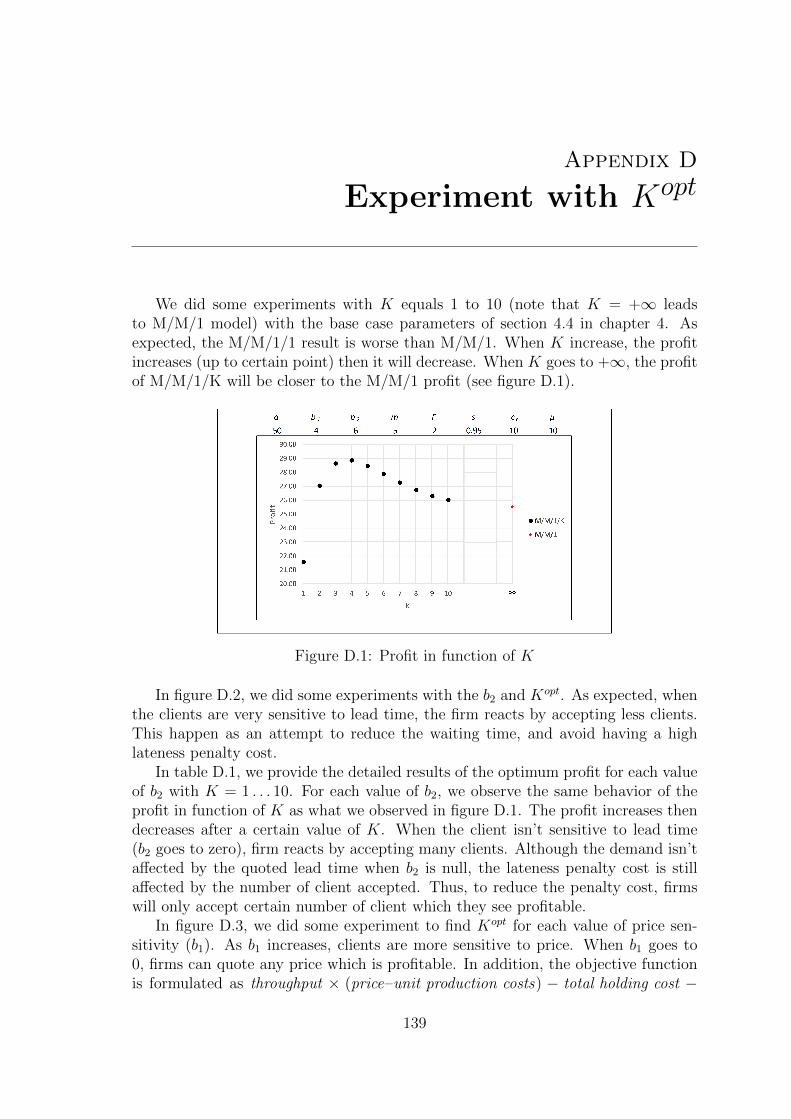
Appendix D
Experiment with Kopt
We did some experiments with K equals 1 to 10 (note that K = +∞ leadsto M/M/1 model) with the base case parameters of section 4.4 in chapter 4. Asexpected, the M/M/1/1 result is worse than M/M/1. When K increase, the profitincreases (up to certain point) then it will decrease. When K goes to +∞, the profitof M/M/1/K will be closer to the M/M/1 profit (see figure D.1).
Figure D.1: Profit in function of K
In figure D.2, we did some experiments with the b2 and Kopt. As expected, whenthe clients are very sensitive to lead time, the firm reacts by accepting less clients.This happen as an attempt to reduce the waiting time, and avoid having a highlateness penalty cost.
In table D.1, we provide the detailed results of the optimum profit for each valueof b2 with K = 1 . . . 10. For each value of b2, we observe the same behavior of theprofit in function of K as what we observed in figure D.1. The profit increases thendecreases after a certain value of K. When the client isn’t sensitive to lead time(b2 goes to zero), firm reacts by accepting many clients. Although the demand isn’taffected by the quoted lead time when b2 is null, the lateness penalty cost is stillaffected by the number of client accepted. Thus, to reduce the penalty cost, firmswill only accept certain number of client which they see profitable.
In figure D.3, we did some experiment to find Kopt for each value of price sen-sitivity (b1). As b1 increases, clients are more sensitive to price. When b1 goes to0, firms can quote any price which is profitable. In addition, the objective functionis formulated as throughput × (price–unit production costs) − total holding cost −
139
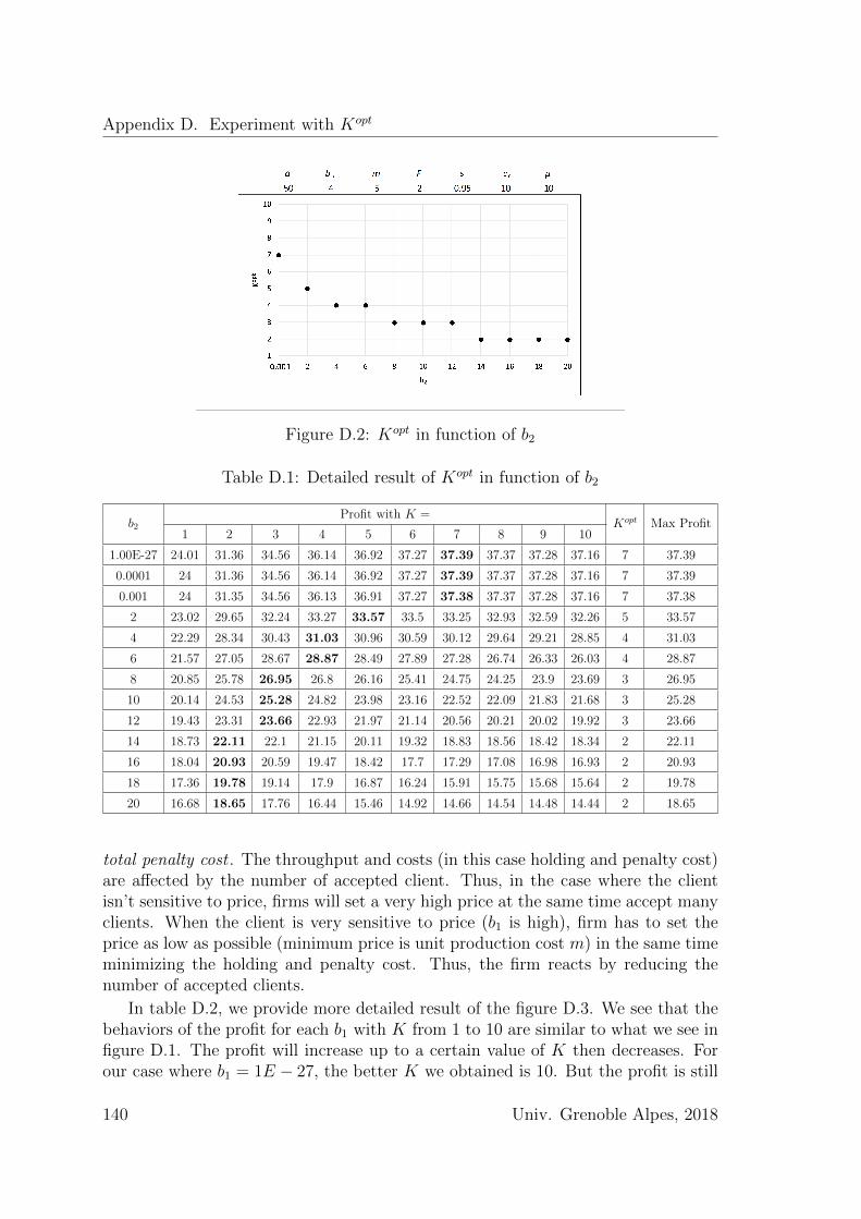
Appendix D. Experiment with Kopt
Figure D.2: Kopt in function of b2
Table D.1: Detailed result of Kopt in function of b2
b2
Profit with K =Kopt Max Profit
1 2 3 4 5 6 7 8 9 10
1.00E-27 24.01 31.36 34.56 36.14 36.92 37.27 37.39 37.37 37.28 37.16 7 37.39
0.0001 24 31.36 34.56 36.14 36.92 37.27 37.39 37.37 37.28 37.16 7 37.39
0.001 24 31.35 34.56 36.13 36.91 37.27 37.38 37.37 37.28 37.16 7 37.38
2 23.02 29.65 32.24 33.27 33.57 33.5 33.25 32.93 32.59 32.26 5 33.57
4 22.29 28.34 30.43 31.03 30.96 30.59 30.12 29.64 29.21 28.85 4 31.03
6 21.57 27.05 28.67 28.87 28.49 27.89 27.28 26.74 26.33 26.03 4 28.87
8 20.85 25.78 26.95 26.8 26.16 25.41 24.75 24.25 23.9 23.69 3 26.95
10 20.14 24.53 25.28 24.82 23.98 23.16 22.52 22.09 21.83 21.68 3 25.28
12 19.43 23.31 23.66 22.93 21.97 21.14 20.56 20.21 20.02 19.92 3 23.66
14 18.73 22.11 22.1 21.15 20.11 19.32 18.83 18.56 18.42 18.34 2 22.11
16 18.04 20.93 20.59 19.47 18.42 17.7 17.29 17.08 16.98 16.93 2 20.93
18 17.36 19.78 19.14 17.9 16.87 16.24 15.91 15.75 15.68 15.64 2 19.78
20 16.68 18.65 17.76 16.44 15.46 14.92 14.66 14.54 14.48 14.44 2 18.65
total penalty cost . The throughput and costs (in this case holding and penalty cost)are affected by the number of accepted client. Thus, in the case where the clientisn’t sensitive to price, firms will set a very high price at the same time accept manyclients. When the client is very sensitive to price (b1 is high), firm has to set theprice as low as possible (minimum price is unit production cost m) in the same timeminimizing the holding and penalty cost. Thus, the firm reacts by reducing thenumber of accepted clients.
In table D.2, we provide more detailed result of the figure D.3. We see that thebehaviors of the profit for each b1 with K from 1 to 10 are similar to what we see infigure D.1. The profit will increase up to a certain value of K then decreases. Forour case where b1 = 1E − 27, the better K we obtained is 10. But the profit is still
140 Univ. Grenoble Alpes, 2018
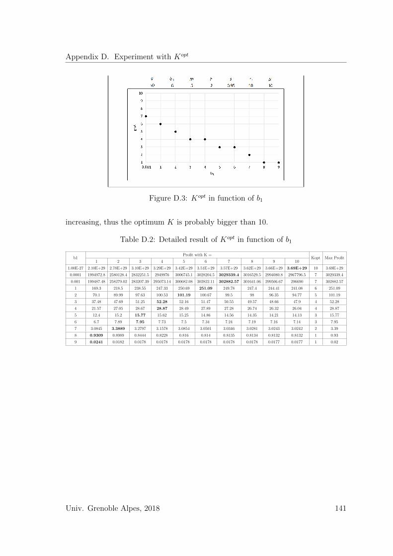
Appendix D. Experiment with Kopt
Figure D.3: Kopt in function of b1
increasing, thus the optimum K is probably bigger than 10.
Table D.2: Detailed result of Kopt in function of b1
b1Profit with K =
Kopt Max Profit1 2 3 4 5 6 7 8 9 10
1.00E-27 2.10E+29 2.78E+29 3.10E+29 3.29E+29 3.42E+29 3.51E+29 3.57E+29 3.62E+29 3.66E+29 3.69E+29 10 3.69E+29
0.0001 1994972.8 2580128.4 2832251.5 2949976 3006745.1 3028204.5 3029339.4 3016529.5 2994080.8 2967796.5 7 3029339.4
0.001 199487.48 258279.02 283207.39 295073.14 300682.08 302822.11 302882.57 301641.06 299506.67 296690 7 302882.57
1 169.3 218.5 238.55 247.33 250.69 251.09 249.78 247.4 244.41 241.08 6 251.09
2 70.1 89.99 97.63 100.53 101.19 100.67 99.5 98 96.35 94.77 5 101.19
3 37.48 47.69 51.25 52.28 52.16 51.47 50.55 49.57 48.66 47.9 4 52.28
4 21.57 27.05 28.67 28.87 28.49 27.89 27.28 26.74 26.32 26.04 4 28.87
5 12.4 15.2 15.77 15.62 15.25 14.86 14.56 14.35 14.21 14.13 3 15.77
6 6.7 7.89 7.95 7.73 7.5 7.34 7.24 7.19 7.16 7.14 3 7.95
7 3.0845 3.3889 3.2797 3.1578 3.0854 3.0501 3.0346 3.0281 3.0243 3.0242 2 3.39
8 0.9309 0.8989 0.8444 0.8228 0.816 0.814 0.8135 0.8134 0.8132 0.8132 1 0.93
9 0.0241 0.0182 0.0178 0.0178 0.0178 0.0178 0.0178 0.0178 0.0177 0.0177 1 0.02
Univ. Grenoble Alpes, 2018 141
Appendix D. Experiment with Kopt
142 Univ. Grenoble Alpes, 2018
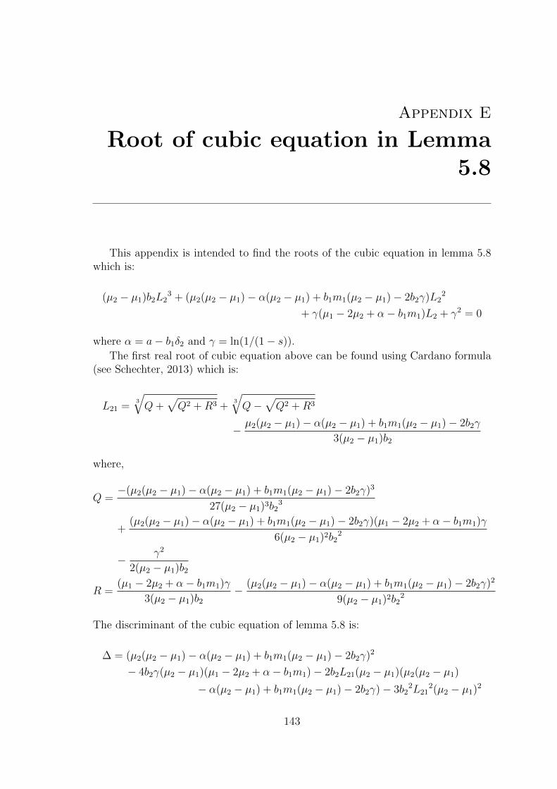
Appendix E
Root of cubic equation in Lemma5.8
This appendix is intended to find the roots of the cubic equation in lemma 5.8which is:
(µ2 − µ1)b2L23 + (µ2(µ2 − µ1)− α(µ2 − µ1) + b1m1(µ2 − µ1)− 2b2γ)L2
2
+ γ(µ1 − 2µ2 + α− b1m1)L2 + γ2 = 0
where α = a− b1δ2 and γ = ln(1/(1− s)).The first real root of cubic equation above can be found using Cardano formula
(see Schechter, 2013) which is:
L21 =3
√Q+
√Q2 +R3 +
3
√Q−
√Q2 +R3
− µ2(µ2 − µ1)− α(µ2 − µ1) + b1m1(µ2 − µ1)− 2b2γ
3(µ2 − µ1)b2
where,
Q =−(µ2(µ2 − µ1)− α(µ2 − µ1) + b1m1(µ2 − µ1)− 2b2γ)3
27(µ2 − µ1)3b23
+(µ2(µ2 − µ1)− α(µ2 − µ1) + b1m1(µ2 − µ1)− 2b2γ)(µ1 − 2µ2 + α− b1m1)γ
6(µ2 − µ1)2b22
− γ2
2(µ2 − µ1)b2
R =(µ1 − 2µ2 + α− b1m1)γ
3(µ2 − µ1)b2
− (µ2(µ2 − µ1)− α(µ2 − µ1) + b1m1(µ2 − µ1)− 2b2γ)2
9(µ2 − µ1)2b22
The discriminant of the cubic equation of lemma 5.8 is:
∆ = (µ2(µ2 − µ1)− α(µ2 − µ1) + b1m1(µ2 − µ1)− 2b2γ)2
− 4b2γ(µ2 − µ1)(µ1 − 2µ2 + α− b1m1)− 2b2L21(µ2 − µ1)(µ2(µ2 − µ1)
− α(µ2 − µ1) + b1m1(µ2 − µ1)− 2b2γ)− 3b22L21
2(µ2 − µ1)2
143
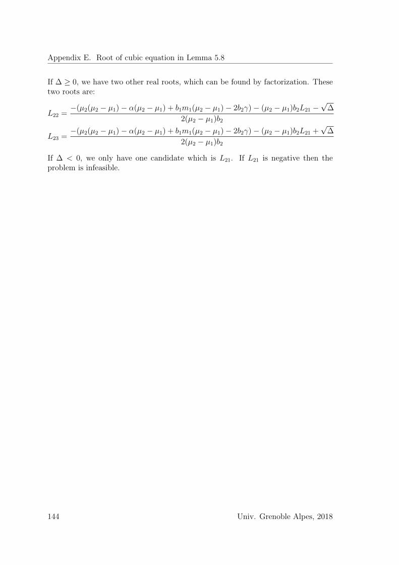
Appendix E. Root of cubic equation in Lemma 5.8
If ∆ ≥ 0, we have two other real roots, which can be found by factorization. Thesetwo roots are:
L22 =−(µ2(µ2 − µ1)− α(µ2 − µ1) + b1m1(µ2 − µ1)− 2b2γ)− (µ2 − µ1)b2L21 −
√∆
2(µ2 − µ1)b2
L23 =−(µ2(µ2 − µ1)− α(µ2 − µ1) + b1m1(µ2 − µ1)− 2b2γ)− (µ2 − µ1)b2L21 +
√∆
2(µ2 − µ1)b2
If ∆ < 0, we only have one candidate which is L21. If L21 is negative then theproblem is infeasible.
144 Univ. Grenoble Alpes, 2018
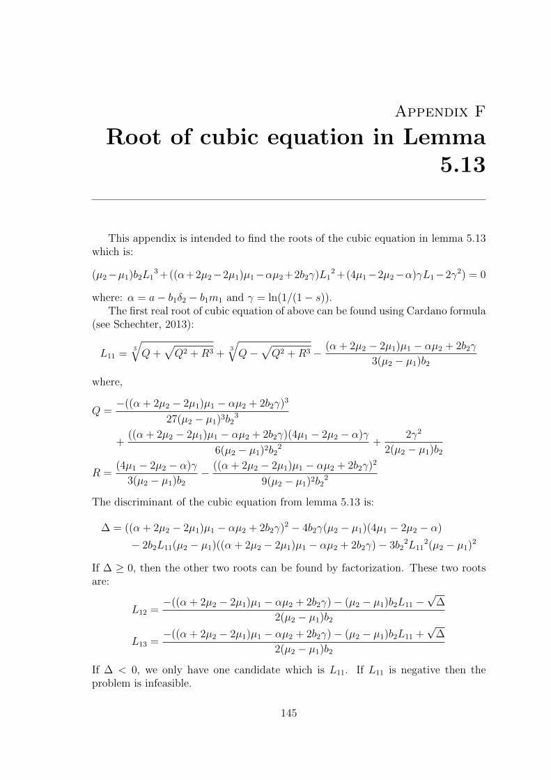
Appendix F
Root of cubic equation in Lemma5.13
This appendix is intended to find the roots of the cubic equation in lemma 5.13which is:
(µ2−µ1)b2L13 +((α+2µ2−2µ1)µ1−αµ2 +2b2γ)L1
2 +(4µ1−2µ2−α)γL1−2γ2) = 0
where: α = a− b1δ2 − b1m1 and γ = ln(1/(1− s)).The first real root of cubic equation of above can be found using Cardano formula
(see Schechter, 2013):
L11 =3
√Q+
√Q2 +R3 +
3
√Q−
√Q2 +R3 − (α + 2µ2 − 2µ1)µ1 − αµ2 + 2b2γ
3(µ2 − µ1)b2
where,
Q =−((α + 2µ2 − 2µ1)µ1 − αµ2 + 2b2γ)3
27(µ2 − µ1)3b23
+((α + 2µ2 − 2µ1)µ1 − αµ2 + 2b2γ)(4µ1 − 2µ2 − α)γ
6(µ2 − µ1)2b22 +
2γ2
2(µ2 − µ1)b2
R =(4µ1 − 2µ2 − α)γ
3(µ2 − µ1)b2
− ((α + 2µ2 − 2µ1)µ1 − αµ2 + 2b2γ)2
9(µ2 − µ1)2b22
The discriminant of the cubic equation from lemma 5.13 is:
∆ = ((α + 2µ2 − 2µ1)µ1 − αµ2 + 2b2γ)2 − 4b2γ(µ2 − µ1)(4µ1 − 2µ2 − α)
− 2b2L11(µ2 − µ1)((α + 2µ2 − 2µ1)µ1 − αµ2 + 2b2γ)− 3b22L11
2(µ2 − µ1)2
If ∆ ≥ 0, then the other two roots can be found by factorization. These two rootsare:
L12 =−((α + 2µ2 − 2µ1)µ1 − αµ2 + 2b2γ)− (µ2 − µ1)b2L11 −
√∆
2(µ2 − µ1)b2
L13 =−((α + 2µ2 − 2µ1)µ1 − αµ2 + 2b2γ)− (µ2 − µ1)b2L11 +
√∆
2(µ2 − µ1)b2
If ∆ < 0, we only have one candidate which is L11. If L11 is negative then theproblem is infeasible.
145
Appendix F. Root of cubic equation in Lemma 5.13
146 Univ. Grenoble Alpes, 2018
Pricing decision and lead time quotation in supply chains with anendogenous demand sensitive to lead time and price
Abstract – Along with the price, the delivery lead time has become a key factor of com-petitiveness for companies and an important purchase criterion for many customers. Nowadays,firms are more than ever obliged to meet their quoted lead time, which is the delivery lead timeannounced to the customers. The combination of pricing and lead time quotation implies newtrade-offs and offers opportunities for many insights. For instance, on the one hand, a shorterquoted lead time can lead to an increase in the demand but also increases the risk of late deliveryand thus may affect the firm’s reputation and deter future customers. On the other hand, a longerquoted lead time or a higher price generally yields a lower demand. Despite the strategic role ofjoint pricing and lead time quotation decisions and their impacts on demand, in the operationsmanagement literature an exogenous demand (a priory a known demand) is generally used in sup-ply chain models, even if the design of the supply chain has a strong impact on lead times (i.e.,sites location, inventory position, etc.) and thus affects the demand. Therefore, we are interestedin the lead time quotation and pricing decisions in a context of endogenous demand (i.e., demandsensitive to price and quoted lead time).The literature dealing with pricing and lead time quotation under an endogenous demand mainlyconsidered a make to order (MTO) context. A pioneer paper, Palaka et al. (1998), investigatedthis issue by modeling the company as an M/M/1 queue, and our work follows their footsteps.Our review of the literature allowed to identify new perspectives for this problem, which led tothree main contributions in this thesis.In our first contribution, using Palaka et al.’s framework, we consider the unit production cost tobe a decreasing function in quoted lead time. In most published papers, the unit production costwas assumed to be constant. In practice, the unit production cost generally depends on the quotedlead time. Indeed, the firm can manage better the production process and reduce the productioncost by quoting longer lead time to the customers.In the second contribution, we still consider Palaka et al.’s framework but model the firm as anM/M/1/K queue, for which demand is rejected if there are already K customers in the system. Inthe literature on single firm setting following Palaka et al.’s research, only the M/M/1 queue wasused, i.e., where all customers are accepted, which might lead to long sojourn times in the system.Our idea is based on the fact that rejecting some customers, might help to quote shorter lead timefor the accepted ones, which might finally lead to a higher profitability, even if in the first glancewe lose some demand.In the third contribution, we study a new framework for the lead time quotation and pricing prob-lem under endogenous demand as we model the supply chain by two production stages in a tandemqueue (M/M/1-M/M/1). In the literature with multi-firm setting, all papers considered that onlyone actor has production operations and the other actor has zero lead time. We investigated boththe centralized and decentralized decision settings.For each problem studied, we formulated a profit-maximization model, where the profit consistsof a revenue minus the production, storage and lateness penalty costs, and provides the optimumresult (analytically or numerically). These resolutions led us to demonstrate new theoretical results(such as the expected lateness in an M/M/1/K, and the sufficient condition required to satisfy theglobal service constraint in a tandem queue by only satisfying the local service constraints). Wealso conducted numerical experiments and derived managerial insights.
Keywords: supply chains, endogenous demand, lead time quotation, pricing, queuing theory

Choix du prix et du delai de livraison dans une chaıne logistique avecune demande endogene sensible au delai de livraison et au prix
Resume – Parallelement au prix, le delai de livraison est un facteur cle de competitivitepour les entreprises. De plus les entreprises sont plus que jamais obligees de respecter ce delaipromis. La combinaison du choix du prix et du delai promis implique de nouveaux compromiset offre de nombreuses perspectives. Un delai plus court peut entraıner une augmentation de lademande, mais augmente egalement le risque de livraison tardive et donc decourager les clients. Acontrario un delai plus long ou un prix plus eleve entraıne generalement une baisse de la demande.Or malgre le role strategique conjoint du prix et des delais et leurs impacts sur la demande, dansla litterature en gestion des operations on suppose tres generalement une demande exogene (fixeea priori) meme si la conception de la chaıne impacte fortement les delais (localisation des sites,positionnement des stocks,..) et donc la demande. Nous nous sommes donc interesses a ces choixde fixation des delais promis et du prix dans un contexte de demande endogene.La litterature traitant du choix du delai et du prix sous demande endogene a principalement con-sidere un contexte de fabrication a la commande (Make to Order). Un papier fondateur de Palakaet al en 1998 a presente cette problematique avec une modelisation de l’entreprise par une filed’attente M/M/1 et nos travaux se placent dans la suite de ce travail. Notre revue de la litteraturea permis d’identifier de nouvelles perspectives et nous proposons trois extensions dans cette these.Dans notre premiere contribution, en utilisant le cadre de Palaka et al, nous considerons que lecout de production est une fonction decroissante du delai. Dans tous les articles publies dans cecontexte, le cout de production unitaire a ete suppose constant. Pourtant en pratique, le coutde production unitaire depend du delai promis, l’entreprise pouvant mieux gerer le processus deproduction et reduire les couts de production en proposant des delais plus longs aux clients.Dans la deuxieme contribution, nous considerons toujours le cadre de Palaka et al, mais modelisonsl’entreprise comme une file d’attente M/M/1/K, pour laquelle la demande est donc rejetee s’il y adeja K clients dans le systeme. Dans la litterature issue du travail de Palaka seule la file d’attenteM/M/1 a ete utilisee, ce qui signifie que tous les clients sont acceptes, ce qui peut entraıner delongues durees de sejour dans le systeme. Notre idee est basee sur le fait que rejeter certains clients,meme si cela peut apparaitre dans un premier temps comme une perte de demande, pourrait aidera proposer un delai plus court pour les clients acceptes, et finalement conduire a une demande etdonc un profit plus eleve.Dans la troisieme contribution nous etudions un nouveau cadre pour le probleme du delai et duprix en fonction de la demande endogene, en modelisant une chaıne logistique composee de deuxetapes de production, modelisee par un reseau de files d’attente tandem (M/M/1-M/M/1). Dansla litterature avec ce cadre multi-entreprise, tous les articles ont considere qu’un seul acteur avaitdes operations de production, l’autre acteur ayant un delai nul. Nous avons etudie les scenarioscentralises et decentralises.Pour chacun des nouveaux problemes nous avons propose des formulations maximisant le profitcompose du revenu diminue des couts de production, de stockage et penalite de retard, et fourni desresolutions optimales, analytiques ou numeriques. Ces resolutions nous ont amenes a demontrerde nouveaux resultats (retard moyen dans une M/M/1/K ; condition pour que des contraintesde service locales permettent d’assurer une contrainte de service globale dans un systeme en tan-dem). Nous avons mene des experiences numeriques pour voir l’influence des differents parametres.
Mots cles: chaınes logistiques, demande endogene, delai de livraison, prix, files d’attente.