Price Transmission in the Cocoa-Chocolate Chain - HAL-SHS

HAL Id: halshs-00552997https://halshs.archives-ouvertes.fr/halshs-00552997

Preprint submitted on 6 Jan 2011

HAL is a multi-disciplinary open accessarchive for the deposit and dissemination of sci-entific research documents, whether they are pub-lished or not. The documents may come fromteaching and research institutions in France orabroad, or from public or private research centers.

L’archive ouverte pluridisciplinaire HAL, estdestinée au dépôt et à la diffusion de documentsscientifiques de niveau recherche, publiés ou non,émanant des établissements d’enseignement et derecherche français ou étrangers, des laboratoirespublics ou privés.

Price Transmission in the Cocoa-Chocolate ChainCatherine Araujo Bonjean, Jean-François Brun

To cite this version:Catherine Araujo Bonjean, Jean-François Brun. Price Transmission in the Cocoa-Chocolate Chain.2011. �halshs-00552997�

https://halshs.archives-ouvertes.fr/halshs-00552997

https://hal.archives-ouvertes.fr

CERDI, Etudes et Documents, E 2010.03

1

Document de travail de la série

Etudes et Documents

E 2010.03

Price Transmission in the Cocoa-Chocolate Chain

Catherine Araujo Bonjean

Chargée de Recherche CNRS

CERDI - Université d’Auvergne

[email protected]

Jean-François Brun

Maître de Conférences

CERDI - Université d’Auvergne

[email protected]

Communication aux 1ères Journées du GDR

Economie du Développement et de la Transition

CERDI-Université d’Auvergne, 2 et 3 juillet 2007

CERDI

65 Bd François Mitterrand

63000 Clermont Ferrand – France

TEL. 33 4 73 17 74 00 FAX. 33 4 73 17 74 28

www.cerdi.org


2

Résumé

Les consommateurs ont souvent l’impression que les prix de détail répondent plus vite

aux augmentations du prix de la matière première qu’aux baisses. Aussi, l’objectif de ce

travail est de tester l’existence d’une transmission asymétrique des fluctuations de prix entre

la matière première, la fève de cacao, et le produit fini, la tablette de chocolat sur le marché

français. Deux formes d’asymétrie, ayant chacune une origine différente, sont recherchées :

d’une part, une asymétrie dans la transmission des chocs positifs et négatifs, potentiellement

liée à l’exercice d’un pouvoir de marché des industriels, et d’autre part, une asymétrie dans la

transmission des grands et des petits chocs de prix liée à la présence de coûts d’ajustement.

Les résultats, obtenus à partir d’une modélisation TAR du déséquilibre de prix par rapport à

leur valeur de long terme, ne permettent pas de rejeter ces hypothèses. Sur la plus grande

partie de la période couverte (1960-2003) le prix de la fève et le prix de la tablette évoluent

indépendamment l’un de l’autre. Toutefois, au moment du boom du cacao (fin 70) le prix de

la tablette répond rapidement à la hausse des cours de la fève tandis qu’à la fin des années 80,

alors que le prix de la fève est retombé à un bas niveau, le prix de la tablette revient lentement

vers l’équilibre.


3

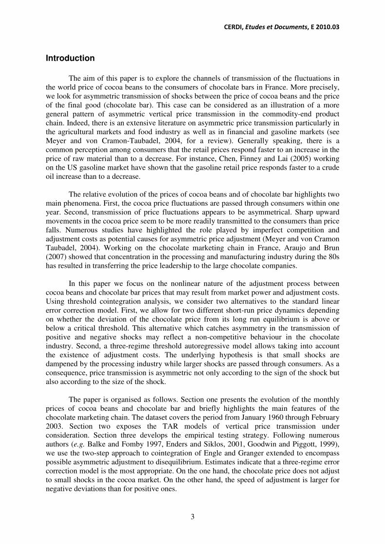
Introduction

The aim of this paper is to explore the channels of transmission of the fluctuations in

the world price of cocoa beans to the consumers of chocolate bars in France. More precisely,

we look for asymmetric transmission of shocks between the price of cocoa beans and the price

of the final good (chocolate bar). This case can be considered as an illustration of a more

general pattern of asymmetric vertical price transmission in the commodity-end product

chain. Indeed, there is an extensive literature on asymmetric price transmission particularly in

the agricultural markets and food industry as well as in financial and gasoline markets (see

Meyer and von Cramon-Taubadel, 2004, for a review). Generally speaking, there is a

common perception among consumers that the retail prices respond faster to an increase in the

price of raw material than to a decrease. For instance, Chen, Finney and Lai (2005) working

on the US gasoline market have shown that the gasoline retail price responds faster to a crude

oil increase than to a decrease.

The relative evolution of the prices of cocoa beans and of chocolate bar highlights two

main phenomena. First, the cocoa price fluctuations are passed through consumers within one

year. Second, transmission of price fluctuations appears to be asymmetrical. Sharp upward

movements in the cocoa price seem to be more readily transmitted to the consumers than price

falls. Numerous studies have highlighted the role played by imperfect competition and

adjustment costs as potential causes for asymmetric price adjustment (Meyer and von Cramon

Taubadel, 2004). Working on the chocolate marketing chain in France, Araujo and Brun

(2007) showed that concentration in the processing and manufacturing industry during the 80s

has resulted in transferring the price leadership to the large chocolate companies.

In this paper we focus on the nonlinear nature of the adjustment process between

cocoa beans and chocolate bar prices that may result from market power and adjustment costs.

Using threshold cointegration analysis, we consider two alternatives to the standard linear

error correction model. First, we allow for two different short-run price dynamics depending

on whether the deviation of the chocolate price from its long run equilibrium is above or

below a critical threshold. This alternative which catches asymmetry in the transmission of

positive and negative shocks may reflect a non-competitive behaviour in the chocolate

industry. Second, a three-regime threshold autoregressive model allows taking into account

the existence of adjustment costs. The underlying hypothesis is that small shocks are

dampened by the processing industry while larger shocks are passed through consumers. As a

consequence, price transmission is asymmetric not only according to the sign of the shock but

also according to the size of the shock.

The paper is organised as follows. Section one presents the evolution of the monthly

prices of cocoa beans and chocolate bar and briefly highlights the main features of the

chocolate marketing chain. The dataset covers the period from January 1960 through February

2003. Section two exposes the TAR models of vertical price transmission under

consideration. Section three develops the empirical testing strategy. Following numerous

authors (e.g. Balke and Fomby 1997, Enders and Siklos, 2001, Goodwin and Piggott, 1999),

we use the two-step approach to cointegration of Engle and Granger extended to encompass

possible asymmetric adjustment to disequilibrium. Estimates indicate that a three-regime error

correction model is the most appropriate. On the one hand, the chocolate price does not adjust

to small shocks in the cocoa market. On the other hand, the speed of adjustment is larger for

negative deviations than for positive ones.


4

1. The cocoa – chocolate chain

The relative evolution, over the period 1960 – 2003, of the world price of cocoa beans1

and the retail price of the chocolate bar in the French market2 highlights two phenomena

(figure 1). First, cocoa beans price fluctuations are passed through chocolate bar price with a

lag of roughly one year. Second, positive shocks in the cocoa price appear to be fully

transmitted to the retail chocolate price. This phenomenon can be especially observed during

the 70s. On the opposite, cocoa price decreases are passed through chocolate price in a lessen

way or are not transmitted at all. For instance, cocoa price experienced a transitory fall during

the years 1965-66 which is not reflected in the chocolate price. The same observation is valid

for the period 1980-84. Moreover, from 1985 until the end of the 90s, the cocoa price

experienced a long lasting phase of decline while the chocolate price stayed at a rather steady

level.

These features of price movements in the cocoa chain suggest the existence of

important lags and asymmetries in price transmission. Increases in the input price seem to be

more fully transmitted to the output price than equivalent decreases.

Figure 1. Cocoa bean and chocolate bar prices (constant euros)

.05

.06

.07

.08

.09

.10

.11

.12

.13

.00

.01

.02

.03

.04

.05

.06

.07

.08

60 65 70 75 80 85 90 95 00

cocoa bean (60 gr)chocolale bar (100gr)

cocoa beans

chocolate bar

Among the different possible causes for asymmetric price transmission, two main

causes have received a special attention in the literature: non-competitive market structure and

adjustment costs which may result in two different types of asymmetry in the adjustment

process.

1 Average of London and New York Stock Exchange prices. Source: International Financial Statistics of the

IMF. 2 This is the retail price of a 100 gr. bar of black chocolate sold on the French market since 1960 (source

INSEE). A 100 gr bar of chocolate contains approximately 60 gr. of cocoa bean. Both prices are in euros.


5

First, asymmetry in the transmission of positive and negative shocks may be due to

imperfect competition in the processing/distribution chain. Agro-food industry is highly

concentrated and processing companies and/or distributors are often accused to exert a market

power. Processing industry may be prompted to pass, more rapidly and more fully, the

increases in the input prices than the decreases, on to the consumers.

This hypothesis of price leadership in the cocoa processing industry has been tested by

Araujo and Brun (2007) in a game theory framework. The authors show that Cote d’Ivoire,

the main cocoa producing country, has lost its market power during the 80s to the benefit of

the cocoa industry which now plays a leading role in price formation.

Indeed the cocoa industry has experienced important changes during the period under

consideration, leading to a significant increase in industry concentration. Every stage of the

cocoa chain -from cocoa bean production to chocolate products distribution- is highly

concentrated. The three largest cocoa producing countries (Cote d’Ivoire, Ghana, Indonesia)

represent more than 70 % of cocoa world production while six multinational companies

control 90 % of the chocolate processing, manufacturing and distribution.

Cocoa processing3 requires large investments. An important movement of

concentration has taken place in the processing industry since the second half of the 80s. At

the world level three companies realize more than 70 % of cocoa processing: Barry Callebaut

(51 %), ADM (11 %), Blommer (9%). Cargill and Cémoi play also an important role, each

representing 6 % of market share4.

At the same time, numerous mergers and acquisitions took place in the manufacturing

industry5. Leading international companies in the chocolate industry are: Barry Callebaut

(24%) Nestlé (21%), Mars (13%), Cadbury (12%), Kraft Foods (10%), Hershey (10%).6 In

France, the chocolate market is dominated by Barry Callebaut (60-70%), Cargill (10-20%)

and Cémoi (10-20%). These companies are vertically integrated and control each stage of the

processing and manufacturing of chocolate.

The distribution sector is also highly concentrated. Hypermarkets and supermarkets

are the major sellers of chocolate products (80%). They sell the quasi totality of the chocolate

bars consumed in France. This sector also experienced an increased concentration during the

last decade.

The high concentration in cocoa processing, manufacturing and distribution may thus

result in non-competitive situations and asymmetric price transmission.

Second, adjustment costs in the packaging and distribution stage of the marketing

process are also a possible cause of asymmetry in price transmission according to the size of

the shocks. Changing prices generate so-called “menu costs” (Barro, 1972). For instance the

costs of reprinting price lists or catalogues may lead to late and asymmetric adjustment of

prices. Fixed adjustment costs are expected to create a price band inside which the retail price

does not adjust to fluctuations in the raw material price as the adjustment cost would exceed

3 Process during which cocoa beans are transformed in nib, liquor, butter, cake and powder.

4 Data concerning 2003.

5 Process that consists in the blending and refining of cocoa liquor, cocoa butter and other ingredients such as

milk and sugar. 6 Source : CNUCED, Infocomm. See also aussi Dorin (2003).


6

the benefit. As a consequence, processors and/or distributors respond to “small” input price

fluctuations by increasing or reducing their margins. The output price will adjust only if the

fluctuations in the input price exceed a critical level. Moreover, the adjustment costs are not

necessarily symmetric with respect to price increases or decreases (Meyer and von Cramon-

Taubael, 2004, Peltzman, 2000, etc).

Non-competitive markets and adjustment costs may thus result in nonlinear price

dynamic. Threshold effects occur on the one side, when large shocks bring about a different

response than small shocks due for instance to the presence of adjustment cost, and on the

other side, when positive shocks (increases in the input price) trigger a different response of

the output price than negative shocks. In the next section we develop a nonlinear model of

price transmission that takes into account these two types of asymmetry.

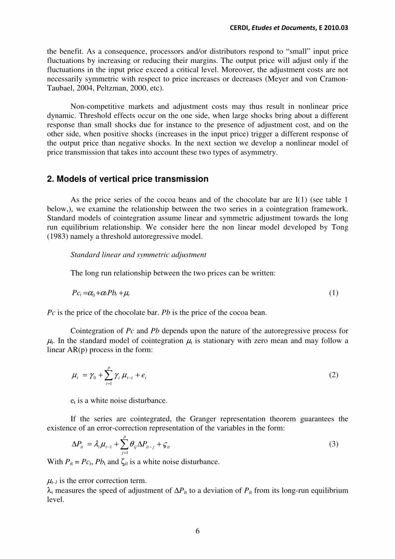
2. Models of vertical price transmission

As the price series of the cocoa beans and of the chocolate bar are I(1) (see table 1

below,), we examine the relationship between the two series in a cointegration framework.

Standard models of cointegration assume linear and symmetric adjustment towards the long

run equilibrium relationship. We consider here the non linear model developed by Tong

(1983) namely a threshold autoregressive model.

Standard linear and symmetric adjustment

The long run relationship between the two prices can be written:

ttt PbPc µαα ++= 10 (1)

Pc is the price of the chocolate bar. Pb is the price of the cocoa bean.

Cointegration of Pc and Pb depends upon the nature of the autoregressive process for

µt. In the standard model of cointegration µt is stationary with zero mean and may follow a

linear AR(p) process in the form:

t

p

i

itit e++= ∑=

−1

0 µγγµ (2)

et is a white noise disturbance.

If the series are cointegrated, the Granger representation theorem guarantees the

existence of an error-correction representation of the variables in the form:

itjit

p

j

ijtiit PP ςθµλ +∆+=∆ −

=

− ∑1

1 (3)

With Pit = Pct, Pbt and ζit is a white noise disturbance.

µt-1 is the error correction term.

λi measures the speed of adjustment of ∆Pit to a deviation of Pit from its long-run equilibrium

level.


7

In this standard error correction model (ECM), adjustment is linear and symmetric: λi

is constant and negative. At every period, a constant proportion of any deviation from the long

run equilibrium is corrected, regardless of the size or the sign of the deviation and the system

moves back towards the equilibrium.

However, as discussed above, different types of market failures may prevent a

continuous and linear adjustment of prices. Threshold cointegration model are thus

considered.

A general threshold adjustment model

If Pc and Pb are characterised by threshold cointegration and asymmetric adjustment,

then the equilibrium error, µt, will follow a self-exciting threshold autoregression (TAR). In

such a model the autoregressive decay depends on the state of the variable of interest, µt-d.

The general form of a TAR(k; p, d) process is given by:

)(

1

)()(

0

j

t

p

i

it

j

i

j

t e++= ∑=

−µγγµ , rj-1 ≤ µt-d < rj (3)

where k is the number of regimes that are separated by k-1 thresholds rj (j = 1 to k-1). In each

regime, µt follows a different linear autoregressive process depending on the value of µt-d. d is

the threshold lag or delay parameter. It represents the delay in the error correction process. et(j)

are zero-mean, constant-variance i.i.d random variables.

The stationarity of the threshold autoregressive process depends crucially on the

behaviour of µt in the outer regimes. The equilibrium error may behave like a random walk

inside the threshold range, but as long as it is mean-reverting in the outer regimes it is a

stationary stochastic process (Balke and Fomby, 1997).

In the remainder of the section, we consider two special cases:

- a two regimes model allowing asymmetric adjustment to deviations in the positive

and negative directions,

- a three regimes model with two asymmetric thresholds which, in addition, takes into

account asymmetry in the correction of large and small deviations.

A TAR model with two regimes

A threshold autoregressive model with one threshold allows asymmetry in price

adjustment to positive and negative deviations from the long run equilibrium. The TAR(2; p,

d) is given by:

<++

≥++

=

−=

−

−=

−

∑

∑

if

if

)2(

1

)2()2(

0

)1(

1

)1()1(

0

τµµρρ

τµµρρ

µ

dtt

p

i

iti

dtt

p

i

iti

t

e

e

(4)


8

τ is the unknown threshold value.

The corresponding error correcting model can be written:

itiit

p

j

ijttittiit PIIP ςθµρµρ +∆+−+=∆ −

=

−− ∑1

1211 )1( (5)

In this representation, the speed of adjustment differs according to whether the

deviation from long run equilibrium is above or below a critical threshold. The speed of

adjustment is given by ρi1 if µt-d is above the threshold level and by ρi2 if µt-d is below the

threshold value.

A TAR model with three regimes

A particular attention is paid to the case where deviations, in the positive and negative

directions, from the long run equilibrium relationship lead to a price response only if they

exceed a specific threshold level. In that case, the cointegrating relationship is inactive inside

a given range and then becomes active once the system gets too far from the equilibrium

band. This situation is captured by a TAR(3; p, d) model:

>++

≤≤++

<++

=

−=

−

−

=

−

−

=

−

∑

∑

∑

2

1

0

21

1

0

1

1

0

if

if

c if

cv

ccv

v

dt

u

t

p

k

kt

u

k

u

dt

m

t

p

k

kt

m

k

m

dt

l

t

p

k

kt

l

k

l

t

µµγγ

µµγγ

µµγγ

µ (6)

vt are zero-mean random disturbances with constant standard deviation.

An equivalent vector error correction representation is given by:

>+∆++

≤≤+∆++

<+∆++

=∆

∑

∑

∑

=

−−

=

−−

−

=

−−

2d-t,3

1

,310

2d-t1,2

1

,210

1,1

1

,110

if

c if

c if

cP

cP

P

P

t

p

k

kitkt

uu

t

p

k

kitkt

mm

dtt

p

k

kitkt

ll

it

µςγµφπ

µςγµφπ

µςγµφπ

(7)

with Pit = Pct, Pbt

The two thresholds c1 and c2 define three price regimes. The parameters φ1, φ2, and φ3,

measure the adjustment speeds of one price to deviations from the equilibrium relationship.

A case often encountered is when φ2 = 0: small deviations from equilibrium are not

corrected (the price series are not cointegrated). Deviation from the equilibrium must reach a

critical level before triggering a price response.


9

If |c1 | ≠ |c2 | the interval [c1, c2] is not symmetric around the origin and deviations in

the positive and negative directions must reach different magnitudes before triggering a price

response. This case is more likely when adjustment costs are asymmetric.

3. Empirical application – testing procedure

We follow the threshold cointegration method introduced by Balke and Fomby (1997)

and developed by Enders and Siklos (2001). It is a two-step approach that extends the Engle

and Granger (1987) testing strategy by permitting asymmetry in the adjustment towards

equilibrium. The first step involves the estimation of the long run equilibrium relationship

between the price of chocolate and the price of cocoa; cointegration tests are then applied to

the equilibrium error. The second step involves testing for nonlinear threshold behaviour. We

consider two non linear autoregressive processes with respectively two and three regimes. In

each case, tests for the difference in parameters across alternative regimes are conducted and

confidence intervals for the threshold values are calculated. We then estimate the asymmetric

error correction model corresponding to the best fit model.

3.1. Testing for no cointegration against linear cointegration

We first test for the order of integration of the price series using Dickey and Fuller

(1981), Phillips and Perron (1988), and Kwiatkowski, Phillips, Schmidt and Shin (1992) tests

(table 1).

Table 1: Unit root tests. monthly data, sample 1960.01 – 2003.02

ADF Prob PP Prob KPSS

Price of the cocoa bean (Pb) -1.88 0.34 -1.84 0.36 0.44***

Price of the chocolate bar (Pc) -2.20 0.49 -2.16 0.51 0.33***

ADF: Augmented Dickey Fuller test. Ho: unit root

PP: Phillips- Perron. Ho: unit root

KPSS: Ho: I(0) ; critical values (Kwiatkowski-Phillips-Schmidt-Shin, 1992, Table 1)

The ADF and PP tests fail to reject the null hypothesis of unit root for both the cocoa

and the chocolate bar price series while the first-differenced price series appear to be

stationary7 (table 1).

Following the two-step method of Engle and Granger (1987) we estimate the long run

relationship between the chocolate and the cocoa price using OLS; the estimated equation is

given in table 2. The Johansen procedure is conducted to test for linear cointegration between

the two price series (table 3).

7 Results not reported here.


10

Table 2. OLS Estimate of the cointegration relationship tttt TPbPc µ+α+α+α= 210

α0 α1 α2 Adj R² SBC AIC

Pc -0.04 0.198 0.002 0.95 -2.93 -2.95

(-6.67) (3.45) (85.5)

T: trend variable

AIC: Akaike Information criterion - SBC: Schwarz criterion

t-Statistics are in parentheses.

Sample: 1960.01 – 2003-02.

Table 3: Cointegration testing results

Trace test:

r=0

Max eigenvalue

r=0

Max eigenvalue and trace test

r=1

35.61

(0.002)

26.18

(0.004)

9.42

(0.16)

H0: no cointegration, intercept and trend in the cointegrating equation, no trend in VAR

The Johansen tests clearly reject the null hypothesis of no cointegration between the

price series of cocoa and of chocolate.

Table 4. OLS Estimate of the autoregressive process

∑−

=−+− +∆++=∆

1

1

1110ˆˆˆ

p

i

tititt eµγµγγµ

γ1 γ2 γ3 γ4 Adj R² SSR AIC White Q(33)

∆µt -0.005 0.39 0.10 0.12 0.25 0.003436 -9.06 8.25 0.103

(-2.13) (8.88) (2.04) (2.65) (0.00)

t-Statistics are in parentheses

SSR: sum of squared residuals

Q(p) is the Ljung-Box statistic.

White's heteroskedasticity test and Pvalue in parenthesis

Table 4 gives the autoregressive process driving the residuals under the hypothesis of

linearity that underlies the standard cointegration tests. The lag order of the linear AR(p) is

selected according to the Akaike and the Schwartz information criteria. The former selects 4

lags while the latter selects 3 lags. An evaluation of autocorrelation patterns for the residuals

led us to adopt a specification with four lags. We also test for the homoskedasticity of the

residuals using the test proposed by White, Engle and Pagan and reject the null of

homoskedasticity.

3.2. Testing for non linearity

We look for non linearity in the equilibrium error µt using two related tests: the non

parametric test of Tsay (1989) and the CUSUM-type test of Petruccelli and Davies (1986).

These two tests are based on predictive residuals (ets) obtained from an arranged

autoregressive process where data are sorted according to the value of the potential threshold


11

variable (µt-d). The sorting process allows to separate the different regimes. The first s cases8

are located below the first threshold and correspond to the first regime. On this sub-sample

the predictive residuals are then orthogonal to the regressors (µts). The following cases fall

into the second regime and the orthogonality between the predictive residuals and the

regressors does not hold any more.

The Tsay’s test is thus an orthogonality test which consists in regressing the predictive

residuals on the explanatory variables. The test statistic is the F-stat associated to the

regression:

ss ttsv

p

v

t ue ++= −

=

∑ 1

1

0 µϖω (8)

The test is run for alternative delays. Tsay (1989) proposes to select as an estimate of

the delay parameter the delay giving the largest F-statistic.

In general the test results depend heavily on the selected AR order and on the starting

point for the arranged autoregression. Following Tsay the start-up for the test is taken to be

10 % of the sample. The selected order of the AR process is four (see above).

The portmanteau test of Petrucelli and Davies (1986) is based on the cumulative sum

of the standardized predictive residuals from the arranged autoregression. The standardized

residuals are normalised by the square root of the residual variance computed recursively. The

standardized and normalized residuals are standard Gaussian so that the P-value of the test

can be evaluated by using an invariant principle for random walk.

Table 5. Nonlinearity tests - ascending order – b=52

d 1 2 3 4 5 6 7 8 9 10 11 12

Tsay 3.26

(0.012)

3.64

(0.006)

2.94

(0.02)

2.89

(0.02)

2.64

(0.03)

2.76

(0.03)

3.09

(0.02)

3.52

(0.008)

3.86

(0.004)

3.81

(0.005)

3.65

(0.006)

3.92

(0.004)

PD 1.54

(0.25)

1.91

(0.11)

2.19

(0.057)

2.12

(0.067)

1.11

(0.54)

1.05

(0.58)

0.66

(0.93)

0.72

(0.88)

0.80

(0.81)

0.92

(0.70)

0.99

(0.64)

0.74

(0.86)

Tsay: F stat and (P-value)

PD: Petruccelli and Davies : t stat and P-value.

Table 5 summarises the results of the portmanteau and the F tests. The F tests with P-

values below 5 % strongly reject (for all d) the null hypothesis of linearity and thus imply the

presence of one or more thresholds. These results contrast with those of the Petruccelli-Davies

test that reject linearity only for d=3 and d=4. This may reflects the superiority of the Tsay’s

test in detecting non linearity (Tsay, 1989).

Given that the hypothesis of linearity is reasonably rejected, we turn to the

identification of the thresholds and the estimation of the threshold autoregressive model.

8 A « case » of data denotes each combination of µt and µt-i. The individual cases of data are ordered according to

the threshold variable (µt-d).


12

3.3. Testing for TAR adjustment with one threshold

We estimate the threshold value (τ) along with the delay parameter (d) and the

autoregressive adjustment process. We follow the methodology of Chan (1993) which

consists to minimize the sum of squared residuals by searching over a set of potential

threshold values for each possible delay parameters. The lagged residuals of the long run

relationship are sorted in ascending order and the largest and smallest 7.5 % of the residuals

are discarded. The remaining 85 % of the residual values are considered as potential

thresholds. The threshold value and the delay parameter yielding the lowest sum of squared

residuals are considered as the appropriate estimate of the threshold value.

The best fit TAR model is presented in table 6. The estimated delay parameter and

threshold value corresponding to the lowest sum of squared error are respectively equal to 11

and –0.08531. To check for robustness we conduct the Enders-Siklos (2001) test of no

cointegration against the alternative of cointegration with threshold adjustment. The test

equation is given by:

∑−

=−−− ε+µ∆γ+µρ−+µρ=µ∆

1

1

1211 )1(p

i

titittttt II (9)

τ : is the threshold value. εt is an iid process with zero mean and constant variance.

It is an indicator function that depends on the level of µt-d:

1=tI if τµ ≥− dt and 0=tI otherwise

The test statistics are the tMAX statistic which is given by the larger t-statistic of ρ1 and

ρ2, and the F-statistic, called Φ stat. Results are given in table 6.

Table 6. OLS Estimate of the TAR(2; 4, 11) model

τ

ρ0 ρ1 ρ2 SSR Φstat

Ho: ρ1 = ρ2 = 0

SupWald

Ho: ρ1 = ρ2

∆µt –0.085831 -0.00 -0.001 -0.033 0.003286 15.12*** 9.66

[-0.0939;

-0.0739] (-2.13) (-0.27) (-3.25)

(0.048)a

t-stat in parenthesis.

99 % asymptotic confidence interval for τ in brackets.

White Heteroskedasticity-Consistent Standard Errors & Covariance.

Critical value for tMAX (Enders and Siklos, 2001, table 2):

90 % : -1.69 ; 95 %: -1.89; 99 %: -2.29

Critical value for Φ (Enders and Siklos, 2001, table 1)

90 % : 5.21 ; 95 %: 6.33 ; 99 %: 9.09 a: Bootstrapped P-value for 1000 replications.

The tMAX test does not reject the null hypothesis of no cointegration while the F-test

does reject the absence of cointegration at the 1% level. The latter test having higher power

(Enders and Siklos, 2001) we conclude that the residual are I(0). We then can test for

symmetric adjustment.


13

Testing linearity versus a threshold alternative involves a non-standard inference

problem as the threshold parameters are not identified under the null hypothesis. In such case

conventional test statistics do not have standard distribution.

To test the null hypothesis of linearity versus the two-regime TAR model we follow

the methodology proposed by Hansen (1996) and calculate the following standard F-statistic:

−==

−=

Γ∈ )(ˆ

)(ˆ~)( with )(sup

ˆ

ˆ~

2

2

2

22

τσ

τσσττ

σ

σσ

τ n

nn

nn

n

nn

n nFFnF

2~σ is the residual variance under the null of linearity.

)(ˆ 2 τσ is the residual variance under the alternative hypothesis of threshold autoregression

calculated over all the possible threshold values.

We follow Hansen (1996) bootstrap procedure to approximate the asymptotic

distribution of F.9 Because there is evidence of heteroskedasticity in εt (White

heteroskedasticity test) we replace the F-statistic F(τ) with a heteroskedascity-consistent

Wald statistic and modify accordingly the bootstrap procedure (Hansen, 1997).

We also use the Hansen (1996) methodology to construct confidence-intervals for the

threshold estimates.

−=

)ˆ(ˆ

)ˆ(ˆ)(~)(

2

22

τσ

τστστ

n

nn

n nLR

)(~ 2 τσ is the residual variance given the true value of the threshold.

)(ˆ 2 τσ is the residual variance given the estimated value of the threshold.

LRn(τ) is the likelihood ratio statistic to test the hypothesis τ = τ0. The β-percent

confidence interval for τ, is given by: { })()(:ˆ βττ cLRn ≤=Γ where c (β) is the β-level

critical value from the asymptotic distribution of LRn(τ). Following Hansen (1997) we use the

convexified region [ ]21ˆ,ˆˆ ττ=Γc

where 1̂τ and 2τ̂ are the minimum and the maximum elements

of Γ.

In the heteroskedastic case, the modified likelihood ratio is:

−=

2

22

*ˆ)(~

)(η

στστ nLRn

and the modified likelihood ratio confidence region is { })()(:ˆ * βττ cLRn ≤=Γ . The nuisance

parameter η is estimated using a polynomial regression (Hansen, 1997).

9 1000 simulations are run replacing the dependant variable by standard normal random draws. For each

bootstrapped series the grid search procedure is used to estimate the threshold value and the Fn(τ) statistic is

computed.


14

Figure 2. Confidence interval for the estimated threshold (1%)

0

2

4

6

8

10

12

14

-.10 -.08 -.06 -.04 -.02 .00 .02 .04 .06 .08 .10

Threshold

Likelihood ratio

The value of the sup-Wald statistic is 9.66 (table 6) and the resulting p-value is 0.048.

Therefore, the null hypothesis of linearity is rejected. The two regimes TAR is thus preferred

to a linear autoregressive process. The estimated threshold is τ = –0.0858 with a 99% asymptotic

confidence interval [-0.0939; -0.0739]. A plot of the adjusted likelihood ratio (LRn*(τ)) is displayed

in figure 2. This figure shows that the threshold estimate is quite precise.

3.4. Testing TAR adjustment with 2 thresholds

A three regimes TAR model is fitted to µt by minimizing the sum of squared residuals

with respect to the threshold and delay parameters, maintaining the lag length at four.

Following Goodwin and Piggott (1999), a two dimensional grid search is used, to estimate the

two thresholds c1 and c2. As a practical matter, we search for the first threshold between 5%

and 95 % of the largest (in absolute value) negative residuals and we search for the second

threshold between 5% and 95 % of the largest positive residuals.

This estimator selects a delay parameter of 11 and produced the TAR model given in

table 7. Three tests are conducted. First, we check the stationnarity of the threshold

autoregressive process with a standard Wald test on White heteroskedasticity consistent

parameters estimates. The bootstrapped p-value is obtained imposing a linear autoregression

with a unit root under the null. The calculated test statistic equals 7.30 and the bootstrapped

P-value is 0.03 (table 7). We thus reject the non-stationnarity hypothesis at conventional

levels.

Second, a test to select the appropriate number of regimes for the TAR model is used.

To test the null hypothesis of a two regimes TAR model versus the alternative of three

regimes, we use the following likelihood ratio statistic:

−=

2

3

2

3

2

223

ˆ

ˆˆ

σ

σσnF

2

2σ̂ is the residual variance from the estimated two-regime TAR model. 2

3σ̂ is the residual variance from the estimated three-regime TAR model.

The value of F23 is 6.25 and the bootstrapped P-value is 0.078. Therefore we do reject

the null of a two-regime TAR model against the alternative of a three-regime TAR model.


15

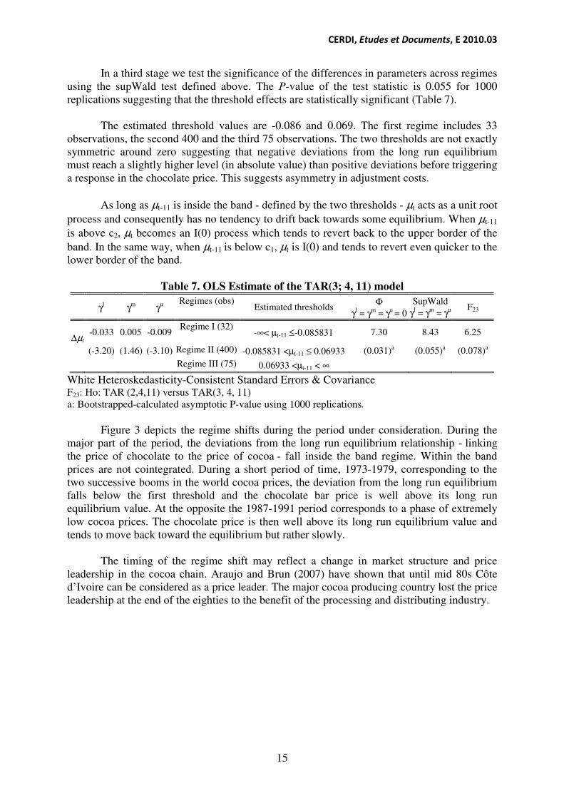
In a third stage we test the significance of the differences in parameters across regimes

using the supWald test defined above. The P-value of the test statistic is 0.055 for 1000

replications suggesting that the threshold effects are statistically significant (Table 7).

The estimated threshold values are -0.086 and 0.069. The first regime includes 33

observations, the second 400 and the third 75 observations. The two thresholds are not exactly

symmetric around zero suggesting that negative deviations from the long run equilibrium

must reach a slightly higher level (in absolute value) than positive deviations before triggering

a response in the chocolate price. This suggests asymmetry in adjustment costs.

As long as µt-11 is inside the band - defined by the two thresholds - µt acts as a unit root

process and consequently has no tendency to drift back towards some equilibrium. When µt-11

is above c2, µt becomes an I(0) process which tends to revert back to the upper border of the

band. In the same way, when µt-11 is below c1, µt is I(0) and tends to revert even quicker to the

lower border of the band.

Table 7. OLS Estimate of the TAR(3; 4, 11) model

γl γm

γu

Regimes (obs) Estimated thresholds

Φ

γl = γm

= γu = 0

SupWald

γl = γm

= γu F23

∆µt -0.033 0.005 -0.009

Regime I (32) -∞< µt-11 ≤-0.085831 7.30 8.43 6.25

(-3.20) (1.46) (-3.10) Regime II (400) -0.085831 <µt-11 ≤ 0.06933 (0.031)a (0.055)

a (0.078)a

Regime III (75) 0.06933 <µt-11 < ∞

White Heteroskedasticity-Consistent Standard Errors & Covariance F23: Ho: TAR (2,4,11) versus TAR(3, 4, 11)

a: Bootstrapped-calculated asymptotic P-value using 1000 replications.

Figure 3 depicts the regime shifts during the period under consideration. During the

major part of the period, the deviations from the long run equilibrium relationship - linking

the price of chocolate to the price of cocoa - fall inside the band regime. Within the band

prices are not cointegrated. During a short period of time, 1973-1979, corresponding to the

two successive booms in the world cocoa prices, the deviation from the long run equilibrium

falls below the first threshold and the chocolate bar price is well above its long run

equilibrium value. At the opposite the 1987-1991 period corresponds to a phase of extremely

low cocoa prices. The chocolate price is then well above its long run equilibrium value and

tends to move back toward the equilibrium but rather slowly.

The timing of the regime shift may reflect a change in market structure and price

leadership in the cocoa chain. Araujo and Brun (2007) have shown that until mid 80s Côte

d’Ivoire can be considered as a price leader. The major cocoa producing country lost the price

leadership at the end of the eighties to the benefit of the processing and distributing industry.


16

Figure 3. Timing of regime switching

1

2

3

4

60 65 70 75 80 85 90 95 00

middle upper lower

3.4. Short run dynamics

The error correction model for the chocolate bar shows that the chocolate price

displays asymmetric error correction toward long run equilibrium (table 8). The price of

chocolate adjusts faster to negative shocks than to positive shocks. In the middle regime the

coefficient for the error correction term is not significantly different from 0. Deviations of the

chocolate price from its long run equilibrium thus have to reach a critical level before

adjustment operates. For small deviations the chocolate and the cocoa prices move

independently one from each other.

Table 8. OLS Estimate of the error correction model

π0 φl φm

φu

Wald

φl = φm

= φu=0

Wald

φl = φm

= φu

Wald

φl = φu

∆Pct 0.00 -0.027 0.001 -0.008 7.87 4.86 3.66

(4.09) (-2.81) (0.29) (-2.94) (0.00) (0.01) (0.06)

White Heteroskedasticity-Consistent Standard Errors & Covariance

The Wald tests reject the different null hypothesis of linear and symmetric adjustment.

Concluding remarks

The tests clearly reject linear cointegration between the price of cocoa beans and the

price of chocolate bar. The results tend to favour a three regimes error correction model. Most

of the time, the price of chocolate does not adjust to changes in the price of cocoa beans. This

may partly be explained by excessive adjustment costs and stocks management.

Two periods of adjustment are identified corresponding on the one hand, to an

historical cocoa boom on the world market, and on the other hand, to a sharp decline in the

cocoa price and, at the same time, to an increased concentration in the chocolate industry. In

the first case, the chocolate price responded rather quickly to the disequilibrium. In the second

case, the chocolate price reverted slowly to the equilibrium band. This asymmetry in the pass

through of large price shocks to consumers may reflect a non-competitive market structure.


17

References

Abdulai A. (2000), “Spatial Price Transmission and Asymmetry in the Ghanaian Maize

Market”, Journal of Development Economics, vol.63: 327-349.

Araujo Bonjean C. and J.-F. Brun (2007), « Pouvoir de marché dans la filière cacao :

l’hypothèse de Prébish et Singer revisitée», Economie et Prévision (forthcoming).

Balke N.S. and T.B. Fomby (1997), “Threshold Cointegration”, International Economic

Review, vol. 38, No3.: 627-645.

Barro R.J. (1972), “A theory of monopolistic price adjustment”, Review of Economic Studies,

39: 17-26.

Chan K.S. (1990), “Testing for threshold autoregression”, The Annals of Statistics, vol.18,

No.4: 1886-1894.

Chan K.S. (1993), “Consistency and Limiting Distribution of the Least Squares Estimator of a

Threshold Autoregressive Model”, The Annals of Statistics, vol. 21, No. 1: 520 -533.

Chen L.H., M. Finney and K.S. Lai (2005), “A Threshold Cointegration Analysis of

Asymmetric Price transmission from Crude Oil to Gasoline Pries”, Economic Letters, 89:

233-239.

Enders W. and P.L. Siklos (2001), “Cointegration and Threshold Adjustment”, Journal of

Business and Economics Statistics, vol. 19, No.2: 166-176.

Enders W., B.L. Falk and P. Siklos (2007), “A threshold model of real U.S. GDP and the

problem of constructing confidence intervals in TAR models”, Berkeley Electronic Press.

Goodwin B.K. and M.T. Holt (1999), “Price Transmission and Asymmetric Adjustment in the

US Beef Sector”, American Journal of Agricultural Economics, 81, august: 630-637.

Hansen B.E. (1999), “The grid bootstrap and the autoregressive model”, The Review of

Economics and Statistics, 81 (4): 594-607.

Hansen B.E. (1997), “Inference in TAR model”, Studies in nonlinear dynamics and

econometrics, Vol. 2, No.1: 1-14.

Hansen B.E. (1996), “inference when a nuisance parameter is not identified under the null

hypothesis”, Econometrica, Vol.64, No. 2:413-430.

Healy S. (2005). « La baisse du prix des produits agricoles: conséquences pour les pays

africains », Notes et Etudes Economiques, Ministère de l’Agriculture, No.23 : 21-54.

Meyer J. and S. von Cramon-Taubadel (2004), « Asymmetric Price transmission: a survey »,

Journal of Agricultural Economics, vol. 55, No.3: 581-611.

Obstfeld M. and A.M. Taylor (1997), “Nonlinear Aspects of Goods-Market Arbitrage and

Adjustment: Heckscher’s Commodity Points Revisited”, Journal of the Japanese and

International Economies, 11: 441-479.

Peltzman S. (2000), “Prices rise faster than they fall”, Journal of Political Economy, vol. 108,

No3: 466-502.

Petruccelli J.D. and N. Davies (1986), “A portmanteau test for self-exciting threshold

autoregressive-type nonlinearity in time series”, Biometrika, vol. 73, No.3: 687-694.

Tsay R.S. (1989), “Testing and Modelling Threshold Autoregressive Processes”, Journal of

the American Statistical Association, vol. 84, No.405: 231-240.

Price Transmission in the Cocoa-Chocolate Chain - HAL-SHS

Documents

Transcript of Price Transmission in the Cocoa-Chocolate Chain - HAL-SHS