Price Setting in Forward-Looking Customer Markets

Emi Nakamura and Jon Steinsson∗

Harvard University

First Draft: February 16, 2005

This Version: September 5, 2005

Abstract

We propose a new explanation for price rigidity. We show that if consumers form habits in

individual goods, then firms face a time-inconsistency problem. The consumers’ habits imply

that low prices in the future help attract customers in the present. Firms would therefore like to

promise low prices in the future. But when the future arrives they have an incentive to exploit

consumers’ habits and price gouge. In this model, unlike the standard no-habit model, nominal

price rigidity is an equilibrium outcome. Equilibrium price rigidity can be sustained because

rigid prices help firms overcome the time-inconsistency problem. If customers have incomplete

information about firms’ desired prices, the optimal policy for the firm is to commit to a “price

cap”. Our model therefore provides an explanation for the simultaneous existence of a rigid

regular price and frequent sales, a pattern that is difficult to reconcile with existing menu cost

models or price rigidity. Our model also explains survey evidence on firms’ fears of adverse

customer reactions to price changes, the fact that firms make open commitments to customers

not to change their prices, the tendency of price rigidity to increase with the frequency of repeat

purchases and the tendency of prices to be more rigid to existing customers than new customers.

Keywords: Time-inconsistency, Price Rigidity, Habit Formation, Asymmetric Information.

JEL Classification: E30∗We would like to thank Alberto Alesina, Susanto Basu, Daniel Benjamin, Michael Katz, David Laibson, Greg

Mankiw, Alice Nakamura, Ariel Pakes, Ricardo Reis, Kenneth Rogoff, Julio Rotemberg, Michael Woodford andseminar participants at Harvard for valuable comments and discussions.

1 Introduction

A consumer’s past purchases of a particular product often exert a strong positive influence on his

current demand for this product. Such time non-separability of preferences arise for many different

reasons. Some goods are addictive while consumers develop a sense of “brand-loyalty” to others.

Consumers favor some products that they have used in the past because of compatibility with other

equipment while they favor other products because the quality of competing products is unknown

to them. And consumers continue using some products simply because of the large transaction

costs associated with switching to a competitor (e.g., another bank or another internet service

provider).

For all these reasons, it is common for consumers to be partially locked into purchasing a

particular product once they have begun purchasing it. Similar lock-in effects are common when

firms purchase from suppliers. Blinder et al. (1998) note that 85% of all goods and services in the

U.S. non-farm business sector are sold to ‘regular customers’ and that 70% of these are business-

to-business transactions. Shapiro and Varian (1999, ch. 5 and 6) present a detailed discussion of

the importance of lock-in in business-to-business transactions.

In this paper, we study the implications that this has for firm price setting. Following Ravn

et al. (2005), we formalize the time non-separability of consumer demand with a model of good-

specific habits. We interpret this good-specific habit as providing a reduced form specification for

the effects of the various types of switching costs described above as well as capturing the type

of addiction studied by Becker and Murphy (1988). We solve for the consumer’s demand curve

given these preferences and assuming rational expectations. We show that consumer demand is

forward-looking; consumer demand depends negatively not only of the current price of the product

but also of the consumer’s expectations about the good’s future prices.

The forward-looking nature of consumer demand implies that firms face a time-inconsistency

problem. Since consumers’ current demand depends negatively on expected future prices of the

product as well as its current price, firms would like to promise that they will keep their prices

low in the future. However, when the future arrives and consumers are locked in, the firms have

an incentive to renege on their earlier promises and price gouge. The consumers understand these

incentives and don’t take the firms’ promises at face value unless the firms are able to make

1

credible commitments. We show that if firms are not able to make credible commitments this

time-inconsistency problem leads them to set prices that are sub-optimally high both from a profit

perspective and from the perspective of overall welfare.

The model we analyze is a model of “customer markets”. The seminal paper on customer mar-

kets is Phelps and Winter (1970).1 An important drawback of the earlier literature on customer

markets is that customers’ demand curves are not derived from the behavior of forward-looking,

optimizing agents. We show that the conclusions of the customer markets literature change sub-

stantially once the forward-looking nature of customers is taken into account. Most importantly,

in the earlier literature, firms do not face a time-inconsistency problem.

Explaining price rigidity was a major motivation for the original development of customer

markets models. According to Okun’s (1981) “invisible handshake” version of the customer markets

idea, firms have implicit agreements with their customers not to take advantage of tight market

conditions by raising their price in exchange for stable prices in weak markets. This view of price

rigidity finds strong support in the views of firm managers. When managers of U.S. manufacturing

firms were asked why they don’t change their prices more often than they do, by far the most

frequent answer they gave was that they feared that this would “antagonize” their customers

(Blinder et al., 1998). Similar surveys in a host of other countries have since confirmed that the

most important reason cited by firm managers for price rigidity is that they are loathe to “damage

customer relations” by changing their prices.2

The problem with this explanation for price rigidity has been that the customer markets lit-

erature has not provided a convincing rationale for why firms enter into these implicit contracts

with their customers. Our model suggests that the reason may be that firms are trying to build

and maintain a reputation for not taking advantage of locked-in customers. In other words, prices

may be rigid because firms are trying to “commit to a sticky price”. In section 4, we show that

firms benefit from the ability to set rigid nominal prices since this partially alleviates their time-1Other contributions include Okun (1981), Bils (1989), Rotemberg and Woodford (1991, 1995) and Bagwell (2004).2See Apel et al. (2004) for a survey of Swedish firms; Hall et al. (1997) for U.K. firms; Amirault et al. (2004) for

Canadian firms; and Fabiani et al. (2004) for a meta-study of surveys of firms in Belgium, Germany, Spain, France,Italy, Luxembough, the Netherlands, Austria and Portugal. A consistent finding across these surveys is that firmsrate implicit and explicit contracts as the most important (or, in a few cases, among the most important) sources ofprice rigidity. In contrast, menu-costs and information costs typically rank rather low among the reasons for pricerigidity. Fabiani et al. (2004) is particularly noteworthy due to its size (over 10,000 respondents) and scope (ninecountries and many different sectors).

2

inconsistency problem. An equilibrium exists in our model in which firms commit to rigid nominal

prices. In this equilibrium, firms are induced not to deviate from otherwise time-inconsistent ac-

tions by the threat that a deviation would damage their reputation and trigger an adverse shift in

consumer expectations about future prices. In section 6, we present numerous quotes from firms’

marketing rhetoric in which they promise customers not to increase prices, sometimes with the

stated goal of not adversely affecting consumers’ expectations about future prices.

The time-inconsistency problem that firms face implies that there is a fundamental difference

between our model and the more standard “no-habit” model. In the no-habit model, there is only

one equilibrium and that equilibrium does not entail nominal price rigidity. In our model, there are

many equilibrium price paths associated with reputational equilibria, all of which are preferred to

the discretionary equilibrium. Whether price rigidity arises thus becomes a question of equilibrium

selection, as in Hall (2005). One might argue that reputational equilibria are hard to achieve

since they require that customers understand the firm’s pricing rule. However, a commitment

to a constant price seems particularly simple for a firm to convey. Moreover, barriers to price

adjustment, such as menu costs, can help firms commit to price rigidity. Analogous mechanisms

that help firms make state-contingent commitments are less available.

In section 5, we consider an extension of our basic model in which variables that affect the firm’s

pricing problem—such as its marginal costs and the demand for its products—are unobservable or

too costly for the firm’s customers to observe. In the standard no-habit model, this is irrelevant

since it is unnecessary for the consumer to understand the firm’s optimization problem. However,

in the habit model, asymmetric information limits the variables that it is possible, even in principle,

for the firm to make commitments contingent on. We use the results of Athey et al. (2004) to

show that the firm’s optimal pricing policy under this kind of asymmetric information is to commit

to a “price cap”. Under this policy, the firm acts with discretion when its desired price is low,

but when its desired price is high the firm sets its price equal to the price cap. The price cap

has the beneficial effect that it lowers the customers’ expectations about future prices and thereby

increases demand. Given plausible assumptions about the process followed by the desired price

and the extent of informational asymmetries, the firm’s price will be “stuck” at the price cap a

significant fraction of the time. It will, however, frequently drop below the price cap and exhibit

much more flexibility when it is not at the price cap.

3

Our model therefore has the following empirical prediction: Goods prices should spend a signif-

icant portion of their time at a rigid upper bound. Below this upper bound, they should be much

more flexible. As the reader is no doubt aware from casual observation, two of the most salient

features of retail price series are the existence of a “regular” price, which remains unchanged for

long periods of time, and frequent “sales”—i.e., brief periods during which the price drops below

its regular price before returning back to the old regular price.3 In section 6, we document these

features of retail prices formally using the Dominick’s Finer Foods dataset provided by the Univer-

sity of Chicago Graduate School of Business. We furthermore show that sales prices are about 8

times more flexible than regular prices.

To date, price rigidity and the existence of frequent sales have been studied separately. On

the one hand, there is a large literature in macroeconomics about price rigidity. Theoretical work

seeking to understand price rigidity has focused on the notion that there may be costs associated

with changing prices.4 Several features of retail price data are however difficult to reconcile with

existing models of menu costs. These include the incredible number of sales observed in retail price

data and the fact that prices frequently return to the old regular price after sales. However, the

combination of a price cap rule and menu costs that only apply to changes in the “regular price” is

consistent with the data. In a model without habit, a menu cost that does not apply to temporary

price changes yields the counterfactual prediction that “reverse sales” should occur as frequently

as sales.

On the other hand, there is a large literature in applied microeconomics and industrial organi-

zation documenting the existence of frequent sales and seeking to understand why they arise.5 An

important idea in this literature is that sales may be used to price discriminate. However, these

models cannot account for the existence of a rigid regular price that truncates the price distribution

from above. Our model is the only model of rational agents we are aware of that is consistent with

both rigid regular prices and frequent sales.6

3See figures 1-3 for examples of this pattern.4Empirical studies of price rigidity include Carlton (1986), Cecchetti (1986), Kashyap (1995), Blinder et al. (1998),

Bils and Klenow (2004), Klenow and Kryvtsov (2005) and Konieczny and Skrzypacz (2005). Contributions to theliterature on menu costs include Barro (1972), Akerlof and Yellen (1985), Mankiw (1985), Caplin and Spulber (1987)and Golosov and Lucas (2005).

5Contributions to the literature on sales include Salop (1977), Varian (1980), Salop and Stiglitz (1982), Conlisket al. (1984), Lazear (1986), Pashigian and Bowen (1991), Warner and Barsky (1995), Aguirregabiria (1999), Hoskenet al. (20000), Pesendorfer (2002), Chevalier et al. (2003) and Hendel and Nevo (2003).

6Rotemberg (2004) presents a model in which consumers become angry if they perceive firm pricing to be unfair.

4

In section 6, we discuss a number of existing empirical results that support our model of price

rigidity. In particular, we discuss experimental evidence supporting the notion that prices are

stickier in customer markets. We also discuss empirical work showing that prices to new customers

are less rigid than prices to old customers.

We build heavily on recent work by Ravn et al. (2005). While the primary focus of their

paper is a model of good specific external habits, they also derive consumer demand in the case

of good specific internal habits. They note that in the internal habits model the firm faces a time

inconsistency problem but leave for future research a detailed analysis of the firm’s pricing problem

in this case. Our paper focuses on analyzing this problem.

The paper proceeds as follows: In section 2, we derive the demand curve for consumers that

form habits in individual goods. In section 3, we discuss the time-inconsistency problem faced by

firms and solve for the optimal pricing rule in the polar cases of fully state-contingent commitment

and complete discretion. In section 4, we show that firms benefit from price rigidity and that price

rigidity is therefore an equilibrium outcome of our model. In section 5, we derive the optimal

pricing policy of the firm when it has private information about its desired price. In section 6, we

present empirical evidence supporting our model. Section 7 concludes.

2 Demand When Consumers Have Good Specific Internal Habits

Consider an economy in which there are a continuum of firms of measure one each of which produces

a differentiated good. Consumers’ preferences over the consumption of these goods are given by

E0

∞∑t=0

βtU(Ct),

where

Ct =[∫ 1

0(ct(z)− γct−1(z))

θt−1θt dz

] θtθt−1

, (1)

ct(z) denotes the consumption of good z at time t and θt is the consumers’ elasticity of demand at

time t. This utility function implies that consumers’ utility from the consumption of any particular

good is not only a function of their current consumption of that good. It also depends on their past

consumption of that good. In other words, the consumer has a habit in each of the differentiated

He shows how this model is consistent with both price rigidity and temporary sales.

5

goods. The parameter γ ≥ 0 is a measure of the degree of this good-specific habit.7 For simplicity

we choose a specification of utility in which the consumer’s elasticity of demand is only a function

of time. The time variation in the consumer’s elasticity of demand should be viewed as a stand-in

for all the time varying features of demand that affect the firm’s optimal price and that are not

explicitly modeled.

Theoretical work on habit formation has largely focused on models in which consumers form

habits in their total level of consumption rather than forming a habit in a particular good. Constan-

tinides (1990) and Fuhrer (2000) consider a model in which consumers’ utility from consumption

depends on past values of their own consumption (internal habit). Abel (1990) and Campbell and

Cochrane (1999) instead study models in which consumers are “catching up with the Joneses”—i.e.,

their utility from consumption depends on past values of aggregate consumption (external habit).

The consequences of consumers forming habits in individual goods has until recently not received

much attention, to our knowledge. In a recent paper, Ravn et al. (2005) study the consequences

of external habit in specific goods for the cyclicality of markups. Ravn et al. (2005) also derive

consumer demand in the case of internal habit, but leave a detailed analysis of the firm’s pricing

problem in this case for future research. In contrast we focus on the case of good specific internal

habit. The only other paper we are aware of that considers good-specific internal habit is Becker

and Murphy’s (1988) model of rational addiction. While our model is formally a model of addictive

goods, we interpret it as also capturing in a reduced form way “switching costs” of the type discussed

in Klemperer (1995).

The consumers face two types of decisions about consumption. They must decide how much to

spend on consumption at each point in time and they must decide how to allocate their spending at

each point between the different goods. These two problems may be analyzed separately. We focus

on the allocation of spending across goods at a particular point in time. Given a state contingent

path for total consumption {Ct+j}∞j=0, the consumers seek to minimize their expenditures. Formally,

7By assuming that γ ≥ 0, we are focusing on goods for which a consumer’s past purchases exert a positive influenceon current demand. While this is true for many goods, there also exist goods for which a consumer’s purchases inthe recent past negatively influence current demand. This is true, e.g., for durable goods. For such goods, equations(1) and (2) with γ < 0 may imply a reasonable reduced form model for consumer demand. To the extent that this isthe case, the results of our model hold for this class of goods as well as the class of goods we focus on. See footnotes17 and 19 for a more detailed discussion of what our model implies in the γ < 0 case.

6

the consumers choose ct(z) to minimize

Et

∞∑j=0

Mt,t+j

∫ 1

0pt+j(z)ct+j(z)dz

subject to {Ct+j}∞j=0, where Mt,t+j denotes the stochastic discount factor that the consumers use

to value future cash flows.

The solution to this optimization problem implies that consumer demand for good z is

ct(z) = γct−1(z) + Ct

(Et∑∞

j=0 γjMt,t+jpt+j(z)Pt

)−θt

, (2)

where Pt denotes the price level.8 Notice that when γ = 0 and θt is a constant, this demand

curve reduces to the iso-elastic Dixit-Stiglitz demand curve. When γ 6= 0, demand differs from this

simple benchmark in two ways. First, demand at time t depends on last period’s demand. Second,

current demand is influenced not only by the current price but also by the consumer’s expectations

about the future price of the good. The intuition for these two effects is straight-forward. When

the consumer has a habit, his utility depends directly on his consumption in the last period. His

demand today therefore depends on his consumption last period. However, the consumer also

understands that by consuming a particular good today he is increasing his habit in the good,

thereby increasing his future demand for it. As a consequence, the consumer’s demand today is

affected by how costly it will be to feed his habit in the future, i.e., his demand will depend on his

expectations about the future price of the good.

3 Price Setting by Firms

For simplicity we adopt the setting of monopolistic competition. Since each firm faces a downward

sloping demand curve—equation (2)—it is able to set the price of the good it produces. Firms are

indexed by z. Firm z seeks to maximize its value,

E0

∞∑t=0

M0,t[pt(z)ct(z)−WtLt(z)], (3)

subject to the constraint that it produces at least as much as it sells,

ct(z) ≤ Atf(Lt(z)), (4)8Pt is the index of individual prices that has the property that PtCt is the minimum expenditure required to

achieve a utility level Ct. Pt is also the Lagrange multiplier in the consumer’s constrained expenditure minimizationproblem.

7

and subject to the demand for its product, given by equation (2). Here At denotes an exogenous

technology factor, Lt(z) denotes the firm’s labor demand and Wt denotes the wage paid by the firm

to its employees.

An important consequence of consumers having good-specific internal habits is that the firm

faces a time-inconsistency problem when setting its price. Since consumer demand depends neg-

atively on expected future prices of the product as well as its current price, the firm would like

to be able to affect the consumer’s expectations by promising a low price in the future. However,

when the future arrives, the firm has an incentive to renege on its earlier promise by charging a

high price. The consumers understand these incentives and don’t take the firm’s promises at face

value unless the firm is able to make a credible commitment. In this section, we focus on the two

polar cases: full commitment to a state-contingent rule and complete discretion. In sections 4 and

5 we explore some intermediate cases.

Solving analytically for optimal behavior under discretion is difficult since the constraints im-

posed on the firm’s optimization problem by its inability to commit are complicated. We therefore

resort to approximation methods of the sort that are widely used in monetary economics (see, e.g.,

Woodford, 2003; and Benigno and Woodford, 2004). We approximate the firm’s problem around its

steady state solution under full commitment to a state-contingent rule and assume that exogenous

shocks and the habit coefficient, γ, are small. In addition, we make several simplifying assumptions

about functional form: We assume that the firm’s production function is linear; that Mt,t+j = βj ;

that Ct and Pt are constant; and that Wt, At and θt are i.i.d. The details of our derivations are

presented in appendix A.

When the firm is able to commit to a fully state contingent rule it chooses to set its price such

that

pt(z) = St + εt, (5)

where hatted variables denote percentage deviations from steady state of the corresponding un-

hatted variables, St denotes marginal costs and εt = −θt/(θ − 1) denotes shocks to demand.9 We

define Φt ≡ St + εt and refer to Φt as the firm’s desired price.9For robustness, in appendix A we also drive the exact solution to the firm’s problem under commitment without

imposing the simplifying assumptions discussed above but instead assuming that θt is a constant. In this case, theprice of the good also varies one for one in percentage terms with marginal costs.

8

Notice that the firm’s desired pricing policy does not exhibit any real rigidity.10 This contrasts

with the results of earlier customer market models such as those in Phelps and Winter (1970) and

Rotemberg and Woodford (1991, 1995) in which the consumer demand function is not derived from

micro-foundations. In these papers, firms optimally vary their price less than one for one with

marginal costs. Thus, markups vary countercyclically.

One of the ideas earlier customer markets models meant to capture in a reduced form way was

that consumers face switching costs. In these models, firms can invest in a “customer base” by

lowering their current price. New customers are then reluctant to switch to another firm since

this entails that they incur a switching cost. Each firm’s customer base is therefore a slow moving

variable. When firms are hit by a shock to marginal costs they are reluctant to raise their price

since a higher price would erode their customer base. As a consequence of this, firm prices exhibit

real rigidity.11

The crucial difference between our model and earlier customer markets models is that in our

model consumers realize that their demand in future periods depends on their actions in the current

period. This entails that consumers decide to become customers of a particular firm not only based

on the current price of the firm’s product but also based on their expectations about its future

prices. In contrast, the earlier customer market literature assumes that changes in a firm’s market

share are a function only of the firm’s current price, which is not consistent with the interpretation

that consumer’s reluctance to switch is due to switching costs. Surely consumers realize that if

they become customers of a particular firm they will become partially locked into that relationship

in the future. Equation (5) shows that, given the consumption aggregator (1), it is optimal for a

firm facing forward looking consumers to let its price vary one-for-one in percentage terms with

marginal costs.

Next, consider the optimal pricing strategy of a firm that is not able to make time-inconsistent

commitments. In appendix A, we show that, to a first order approximation, the “discretionary”

pricing rule chosen by such a firm is

pt(z) =γ

θ − 1+ St + εt, (6)

10We define real rigidity as a situation in which the pricing decisions of different firms are strategic complements.11Ravn et al. (2005) show that a model in which consumers have good-specific external habit yields the consumer

demand function assumed in the earlier customer markets literature.

9

where hatted variables again denote the percentage difference from the steady state under commit-

ment. The positive constant term in this equation implies that producers of habit-forming goods

set higher prices on average if they are not able to make time-inconsistent commitments. Their

inability to make commitments leads them to exploit the habit of their customers to a greater

extent than is optimal. The higher price implies a lower demand and lower profits for the firm.

The higher price, of course, also hurts consumers. The firm’s inability to make time-inconsistent

commitments therefore leads to lower social welfare as well as lower profits for the firm.12

The idea that firms have an incentive to price gouge when consumers are locked into a relation-

ship with the firm is not new. This idea has been explored in Cremer (1984), Farell and Shapiro

(1989), Klemperer (1995), Bagwell (2004) and Caminal (2004). All these papers differ in significant

ways from our paper. None of them explore how lock-in effects can lead to price rigidity as we do in

section 4. Nor do they discuss optimal firm behavior when the firm’s desired price is unobservable

to its customers as we do in section 5.

4 Equilibrium Price Rigidity

Our results in section 3 imply that the ability to make price commitments is valuable to a firm since

it alleviates the firm’s time-inconsistency problem. This raises a familiar question: How does the

firm make credible commitments? One approach is for the firm to build a reputation for offering

low prices.13 A key difference between our model and the standard “no-habit” model is that in

our model there exist a multitude of equilibria in which the firm is induced not to deviate from

otherwise time-inconsistent actions by the threat that a deviation would damage its reputation and

trigger an adverse shift in consumers’ expectations about its future prices.

One pricing rule that, in principle, may be sustained by a firm’s reputation is the fully state-

contingent commitment rule described in section 3. However, equilibria involving much simpler

pricing rules also exist in our model. In particular, equilibria exist in which the firm sets rigid12In discussing the commitment case, we emphasized that it is optimal for the firm to vary its price one-for-one in

percentage terms with marginal costs. While equation (6) seems to indicate that the same is true in the discretioncase, we would like to caution that, in contrast to the commitment case, this result holds only approximately in thediscretion case. While the solution to the commitment case is exact, the solution to the discretion case and all thecases considered later in the paper rely on an approximation. In these cases, the fact that the firm’s price variesone-for-one with marginal costs follows from the assumption that the habit coefficient is small.

13We discuss other commitment mechanisms below.

10

prices. To show formally that such equilibria exist, we must show that the the firm can attain

higher profits if it is able to fix its price for multiple periods than it can attain under discretion.14

Consider a firm that is identical to the one analyzed in section 3 except that it is able to fix its

price for two periods. Assume that the firm is otherwise not able to make any time-inconsistent

commitments about its pricing policy. In appendix A we show that the optimal pricing policy of

such a firm is

pt(z) =γ

(θ − 1)(1 + β)+

11 + β

(St + εt). (7)

This policy differs in two ways from the pricing behavior of a firm that follows the discretionary

pricing policy. The benefit that comes from fixing the price for two periods is that the average level

of the price is lower than under complete discretion. The average price is lower because the firm

recognizes that a high price in period t raises consumer’s expectations about the price in period

t+1 and therefore raises the consumer’s cost of forming a habit in the good. Since this lowering of

the average price brings the average price closer to what it would be under commitment to a fully

state-contingent rule, the firm’s profits are higher in this case than they are under discretion.

The cost of fixing the price for more than one period is that the firm is not able to respond

optimally to fluctuations in marginal costs and demand. Instead of responding one-for-one in

percentage terms to such variations, the firm only changes its price by 1/(1 + β) percent for each

percentage deviation in marginal costs and demand. The simple intuition for this result is that the

firm is choosing a price that is appropriate not only for the current period but for the entire period

during which the price is fixed and it is discounting the future by a factor β. This feature of the

firm’s pricing policy lowers its profits relative to what they are under discretion.

Whether it is beneficial for the firm to be able to fix its price for more than one period therefore

depends on the relative strength of these two effects. In appendix A we show that it is beneficial

for the firm to be able to fix its price for two periods if

γ2 >β(θ − 1)2

2 + βvar(St + εt). (8)

This expression has a straight-forward interpretation. It says that being able to commit to a fixed

price for two periods yields higher profits if the size of the habit coefficient—i.e., the strength of

the habit—is large relative to the variability of marginal costs and demand.14The existence of such equilibria also relies on the discount factor of the firm being close enough to one, as is

standard in trigger-strategy equilibria.

11

We have analyzed the simple case of a firm that is able to fix its price for two periods. The

results above can, however, easily be extended to the case of a firm that is able to fix its price

for n periods. Another simplifying assumption employed above is that the aggregate price level is

constant. This assumption is also easily relaxed. Commiting to a fixed nominal price is beneficial

to the firm as long as variations in the price level are not too large.15

The fact that the fixed price policy is preferable to the discretionary policy from the firm’s

perspective means that price rigidity is an equilibrium outcome of our model. In this equilibrium

the firm commits to a sticky price and the threat of consumer beliefs reverting to the discretionary

equilibrium induces the firm to follow through on its commitment.

A fundamental difference between our model and the standard “no-habit” model thus arises

with respect to the viability of equilibria involving nominal rigidity. Our model has a multiplicity

of equilibria, some of which involve nominal rigidity. In contrast, the no-habit model has a unique

equilibrium and this equilibrium does not entail nominal price rigidity. The equilibrium is unique

because consumers’ expectations about the firm’s future prices don’t affect current demand. Shifts

in these expectations don’t affect the firm’s profits. Threats of such shifts therefore cannot be used

to sustain a range of equilibria.

The presence of nominal price rigidity in the set of equilibrium outcomes of our model has an

important parallel in the recent literature on wage stickiness. Hall (2005) shows that nominal wage

stickiness can also arise as an equilibrium outcome in search models of the labor market. Hall’s

results follow from the fact that the outcome of the bargain between workers and firms, once they

have been matched, is indeterminate in such models.

We have analyzed three equilibria of our model: commitment to a fully state contingent rule,

complete discretion and an equilibrium in which the price is fixed for two periods. Clearly, many

other equilibria exist. Wether price rigidity arises therefore becomes a question of equilibrium

selection. The equilibrium most prefered by the firm is the fully state contingent commitment

rule—equation (5). However, conveying such a complicated commitment to consumers may be

difficult and poses a risk of misunderstandings that may lead to adverse shifts in consumer beliefs.15Notice that given a similar condition to condition (8), consumers also prefer the two period fixed price policy—

equation (7)—to the discretionary price policy—equation (6). The fact that the average price is lower makes con-sumers better off. The effect of lowering the variability of prices is however ambiguous. If the habit is large enoughrelative to the variability of price, the first effect will outway the second effect.

12

Furthermore, it may not be possible, even in principle, for a firm to commit to such a rule if the

firm’s marginal costs and demand are unobservable. A simpler, less risky pricing rule may therefore

arise in the market such as sticky price rule described above or the price cap rule discussed in section

5.

Reputational equilibria of the kind discussed above provide a rational interpretation for the

notion of “implicit contracts” discussed informally by Okun (1981) and found by Blinder et al.

(1998) to be an important source of price rigidity. In Blinder et al. (1998), 64.5% of firms report

that they have implicit contracts with their consumers and an overwhelming majority of these firms

(79%) indicate that these implicit contracts are an important source of price rigidity. Surveys in

many other countries have since confirmed this result (see footnote 2). Furthermore, the punishment

phase of such reputation equilibria provides an interpretation for consumers’ adverse reactions to

price increases, not justified by observable increases in costs. Consumers often perceive such price

increases as “unfair” (see, e.g., Kahneman et al., 1986; and Rotemberg, 2002 and 2004). In the

reputational equilibria, it is exactly these types of price increases that lead to adverse reactions by

customers.

Aside from repuation, there are a number of other mechanisms that a firm has at its disposal to

make commitments. Menu costs and other barriers to price changes, can help a firm commit not to

change its prices. Levy et al. (1997) present evidence that supermarkets face physical, managerial

and communication-related costs of changing prices. Since it is optimal for firms to economize on

such costs, it may be impractical for them to commit to a state-contingent rule. The menu cost

will tilt the firm’s incentives away from changing its price and therefore make it more likely that

the firm’s current price will not change in the near future. Just as in the simple case analyzed

above, such price rigidity implies that a price increase in period t raises consumer’s expectations

about the price in the near future and therefore raises the consumer’s cost of forming a habit in

the good. Menu costs and other barriers to price changes can therefore be beneficial to a firm since

they reduce the firm’s incentive to take advantage of locked in customers.

One reason why one might be skeptical of menu costs as an explanation of price rigidity is

that one might think that technologies exits that make changing prices easy and cheap (see, e.g.,

Dutta et al., 1999). However, the argument above suggests that firms might have an incentive to

intentionally adopt technologies and an organizational structure that makes changing prices costly

13

as part of a commitment not to take advantage of locked in customers. In most models of price

rigidity, it is assumed that firms are forced to change their price infrequently. In such models price

rigidity hurts the firms, although their losses are only second order (see Akerlof and Yellen, 1985;

and Mankiw, 1985). Our model suggests that firms would actually like to be able to commit to

change prices infrequently if state-contingent commitments are not possible.16

Another approach to making credible commitments is for the firm to sign binding contracts with

its customers. Much like reputation formation, explicit contracts are an imperfect commitment

mechanism. Contracts are costly to write, interpret and enforce. Furthermore, these costs rise with

the length and complexity of the contract. Such costs can explain why empirical evidence suggests

that fixed price contracts are quite common in one form or another in interactions between firms

and their customers. Blinder et al. (1998) presents evidence to this effect. In their sample, 65% of

firms had a meaningful volume of contracts that specified a fixed nominal price and 57% of these

firms indicated that such nominal contracts were an important source of price rigidity. Explicit

contracts have since been found to rank among the most important sources of price rigidity in many

other countries (see footnote 2).17

5 Optimal Policy under Asymmetric Information

Many components of a typical firm’s marginal costs and demand are either unobservable or very

costly for a consumer to observe. In section 3, we show that in a complete information setting the

firm’s desired pricing policy under full commitment is a function of the firm’s marginal costs and

its demand. If marginal costs and demand are unobservable, it is not possible, even in principle,

for a firm to commit to such a rule since there is no way for consumers to verify whether the firm

deviates from this rule or not. This observation raises the question: What is the optimal pricing16Nishimura (2000) also discusses possible benefits of price rigidity. His argument for the benefits of price rigidity

is however quite different.17All the results of this section and section 3 hold not only when γ ≥ 0 but also for γ < 0. As we mentioned

in footnote 7, the demand curve—equation (2)—with γ < 0 may be interpreted as describing consumer demand forgoods for which consumer’s purchases in the recent past negatively affect their current demand. Durable goods areexamples of such goods. In this case the firm faces a slightly different time-inconsistency problem. It would like tobe able to commit not to lower its price in the immediate future since expectations of low future prices will leadconsumers to delay their purchases. This implies that firms again have an incentive to make repricing costly in orderto make it more credible that they will not “take advantage of past customers” by lowering their price.

14

policy for the firm when it has private information about its desired price?18

It turns out that this question is formally related to the problem studied by Athey et al. (2004).

They study the time-inconsistency problem of a central bank that has private information about

the state of the economy. Using methods developed by Abreu et al. (1990), they are able to show

that under relatively mild restrictions this type of problem has a surprisingly simple solution. In

this section, we use the results of Athey et al. (2004) to show that the firm’s optimal policy when

it has private information about its desired price is to commit to a “price cap”. More specifically,

when the firm’s desired price is relatively low it acts with discretion but when the desired price

is high enough that discretionary price setting would entail a price above the price cap it sets its

price equal to the price cap. Athey et al. (2004) refer to this as bounded discretion. The level of

the price cap depends on the severity of the time-inconsistency problem, which in turn depends

on the strength of the habit that consumers develop in the firm’s good. The more severe is the

time-inconsistency problem, the lower is the price cap.

Formally, we show in appendix B that:

I. If γ > −Φ, the firm sets a constant price.

II. If γ < −Φ, the firm’s optimal policy is to commit to a price cap.

Here Φ < 0 is the lowest possible realization of the firm’s desired price. Let p∗(Φ; z) denote the

static best response of a firm with desired price equal to Φ. If a firm’s desired price is lower than

Φ∗, the firm sets its price equal to p∗(Φ; z). However, whenever the firm’s desired price is higher

than Φ∗, the firm sets its price equal to the static best response of a firm with desired price equal

to Φ∗, i.e., p∗(Φ∗; z). This pricing policy can be written more succinctly as

p(z) =

p∗(Φ; z) if Φ ∈ [Φ, Φ∗]

p∗(Φ∗; z) if Φ ∈ [Φ∗,¯Φ].

(9)

In appendix B, we show that the cutoff level of the firm’s desired price, Φ∗, is decreasing in γ.

Thus, the firm’s desire to limit its discretion increases with the severity of the time-inconsistency

problem.18For simplicity, in this section we assume that the firm’s private information is the only impediment it faces to

making commitments about its pricing policy.

15

19

The results above show that the firm’s optimal pricing policy when it has private information

about its desired price is one in which its price is upward rigid at a price cap. Below this cap

the firm’s price is flexible. Even a casual look at time series of goods prices reveals that exactly

these features—a rigid price cap and frequent and flexible sales—appear to be salient features of

goods prices. In section 6, we provide formal empirical evidence that shows that these empirical

predictions of our model are indeed prominent features of retail prices.

Notice also that we have shown that the price cap policy is the best policy from the firm’s

perspective of all policies that do not depend on the firm’s contemporaneous desired price. This

policy is therefore more desirable for the firm than the fixed price policy we discussed in section

4. This provides a rationale for why firms that are unable to make complicated commitments

may choose a price cap policy even if their inability to commit is not strictly due to asymmetric

information. Moreover, consumers also have an incentive to move from the discretionary equilibrium

to the price cap policy since it lowers the average price of the good.

Here we have derived results for the simple case in which the consumer cannot observe any of

the variables that the firm would like to make its price depend on. Our results can, however, be

extended to a setting in which the consumer observes some such variables but not others. In this

case, the variables that the consumer observes are state variables and thefirm-ptiomal pricing rule

is a price cap that depends on these variables.

6 Empirical Evidence

In this section we present several different types of empirical evidence supporting our model of price

rigidity. We first present two kinds of new evidence on price rigidity: evidence from retail price

data on the behavior of regular prices and sale prices and evidence on company announcements

about their future prices. We then discuss three sets of existing evidence supporting our model.19As with the earlier sections, the results of this section may also be extended to the case of γ < 0. In this case

the optimal pricing policy from the firm’s perspective is a “price floor” rather than a price cap. This is because inthe γ < 0 case the firm’s time-inconsistency problem leads firms to set too low prices rather than too high prices (seefootnote 17).

16

6.1 New Evidence from Retail Prices

In section 5, we show that our model has the following empirical prediction: Goods prices should

spend a significant portion of their time at a rigid upper bound. Below this upper bound, they

should exhibit much more flexibility. In tables 1 and 2, we use weekly price data from the Dominick’s

Finer Foods (DFF) dataset provided by the University of Chicago Graduate School of Business to

show that these predictions are indeed borne out by data on retail goods prices.20 More precisely,

the results presented in tables 1 and 2 along with the fact that we very rarely observe “reverse-

sales”—i.e., brief periods during which the price of a good rises above its regular price and then

returns back to the regular price—show that: i) The regular price of a good remains fixed for long

periods of time, but during this time the good frequently goes on sale for brief periods; ii) Regular

prices are a sticky upper bound for the price of a good; iii) Prices generally return to their old

regular price after sales; and iv) Sale prices are more than 8 times more flexible than regular prices.

For robustness, the statistics in tables 1 and 2 are presented separately for each of 26 categories of

goods. Hosken and Reiffen (2004) document similar qualitative results to (i) and (ii) for a panel of

monthly data from 30 U.S. metropolitan areas.

The concept of a “regular price” is familiar in the literature on retail prices. Chevalier et al.

(2003) comment,

In general, pricing at DFF (and, we believe, at all supermarkets) is characterized by

temporary discounting. Prices frequently drop to a temporary sale price and return

again to the “normal” price. The path of prices for a typical good (9.5 ounce Triscuit

crackers) in our study can be seen in Figure 1. Notice that, during the 7.5 years of our

study, Triscuits appear to have only eight “regular prices”. Upward deviations from the

regular price are virtually nonexistant; temporary downward deviations are frequent.

The labeling of promotions in the Dominick’s dataset is, however, somewhat undependable.21 More-

over, what we typically view as a sale—i.e., a short-term decrease in prices relative to a recurrent20DFF is the second-largest supermarket chain in the Chicago metropolitan area with approximately 100 stores

and a 25% market share. DFF provided the University of Chicago Graduate School of Business (GSB) with weeklystore-level scanner data, available at http://gsbwww.uchicago.edu/kilts/research/db/dominicks/. See Chevalier etal. (2003) for a more detailed description of this data set. We use data from store number 126 since the data fromthis store has the least missing data points.

21According the University of Chicago GSB website describing the data, “if the variable is set it indicates apromotion, if it is not set, there might still be a promotion that week”.

17

upper bound—is more closely related to the time series behavior of prices than the presence of a

promotion. We therefore identify sales directly from observations on prices as periods when the

price drops for a short period and then returns to either a previously occurring regular price or to

a new regular price that reoccurs soon after.22 The “sales filter” used to identify sales is described

in detail in appendix C. To give the reader a feel for this procedure, we present several figures

showing the original and “regular price” series for popular items in appendix C. The figures show

that the regular price series generated by this procedure corresponds well with our intuition about

how to define a sale. The price series have infrequent adjustments in regular prices and frequent

sales. When no recurring regular price can be identified from the data, the sales filter simply sets

the regular price equal to the observed price. Thus, a continuously adjusting price series would

have the regular price always equal to the actual price—i.e., no sales—with a regular price change

in every period.

A very irregular pattern of sales, such as the one near the end of Figure 2, is not identified by

the sales filter. The sales filter is, thus, somewhat conservative in assigning variation in prices to

sales rather than the regular price. This tendency biases us away from finding a high frequency of

sales, and a low frequency of price adjustment of regular prices—two of the key findings discussed in

this section. Another comforting fact about our procedure is that the qualitative findings (i)- (iv)

are not at all sensitive to the exact parameters used in the sales filter. Furthermore, Hosken and

Reiffen (2004) document very similar qualitative results for (i) and (ii) using an entirely different

data set and a different procedure for identifying sales.

The first column of Table 1 presents the fraction of weeks in which the price of the good was

equal to the regular price. One minus this number is the fraction of time the good was on sale. By

our measure, sales occur about 13% of the time. The first column of table 2 establishes furthermore

that this regular price often remains fixed for significant periods of time—the frequency of price

adjustment of regular prices is 6.1% or less in more than half of the categories.

The pricing dynamics observed in the data are hard to reconcile with the standard menu cost

model of price rigidity. In this model, the firm should always readjust the regular price when a sale

ends. Yet, after a large number of sales, the price returns to the original regular price. Column 2 of22This procedure has the advantage over the procedure suggested in Hosken and Reiffen (2004)—of defining sales

as percentage deviations from the modal price—that it can accomodate variation in the regular price witin a yearand allows for sales that last more than one period.

18

table 1 shows that for most products the price of the product returns to the original regular price

over 90 percent of the time following a sale.23 Given the high frequency of sales in retail data, this

statistic implies that the opportunity to adjust a price following a sale is often forgone. Indeed the

condition that the price returns to the original price following a price decrease is sometimes use

as a criterion for identifying a sale in other papers in the literature (see, e.g., Hosken and Reiffen,

2004Hosken and Reiffen (2004)).

The observed pricing dynamics are also difficult to reconcile with the existing literature on sales.

An important explanation for sales in the industrial organization literature is price discrimination

(see, e.g., Varian, 1980). The intuition for this theory of sales is that sales allow for price discrim-

ination between shoppers with different price elasticities. However, these models do not provide

an explanation for the existence of a rigid regular price that truncates the price distribution from

above unless consumer valuations are also truncated from above.

The results in table 2 show that sale prices are considerably more variable than regular prices.

The fourth column of table 2 reports the number of unique sale values as a fraction of the total

number of weeks spent on sale. This statistic would equal 1 if there were a unique sale price in

every period and would approach zero if only one sale price was ever visited. The median value of

this fraction across categories is 43%. In contrast, the fraction of unique regular price values as a

fraction of total time at regular prices is about 10 time smaller—4.5% or less for the majority of

items.24 The data are not, therefore, consistent with the idea that the price always returns to a

particular sale price when the product goes on sale.

A slightly different way of analyzing the relative rigidity of sale prices is to look at the tendency

of prices to adjust while the product is on sale versus at other times. Recall that our procedure

for identifying sales allows for sales that last for more than one week. Multi-week sales account

for somewhat less than half of sales in most categories. The first two columns of table 2 compare

the frequency of price adjustment for regular prices versus sale prices during multi-week sales, not

including the price changes at the start and end of the sale. The frequency of price adjustment

during sales is about 8 times as high as the frequency of adjustment of the regular price. Existing23This is not by construction. Our sales filter allows for sales that do not return to the original price following the

sale, as we discuss in C.24An even higher fraction of sale prices are unique if the prices are defined in terms of percent off the regular price,

or an absolute amount off the regular price.

19

menu cost models of price rigidity do not provide any reason why the price of a good should be

more flexible when it is on sale. As we showed in section 5, this pricing pattern is however a natural

implication of our model. Again, these empirical facts do not arise from the particular approach

used to identify sales, since our algorithm does not make any assumptions about the dynamics of

prices during a sale.

From the perspective of the customer markets model presented in this paper, this pattern of

pricing reflects the fact that the firm chooses to commit to a sticky regular price. Indeed, many

retail stores choose to employ observably less permanent technologies for posting sale versus regular

prices. This suggests that menu costs may be smaller for temporary price changes than for changes

in the regular price. However, a model with such differential menu costs on its own is not fully

consistent with the data since it implies that we should observe reverse sales as frequently as we

observe sales. The model presented in section 5 shows that committing to a sticky regular price,

but allowing sale prices to fluctuate, is preferable from the perspective of the firm to fixing its price

for multiple periods or other types of pricing rules that do not depend on costs. Indeed, the results

of Section 5 imply that this pricing rule is close to optimal in the class of all possible rules if the

cost and demand factors affecting the optimal pricing of a supermarket are unobservable (or costly

to observe) for consumers.

6.2 New Evidence from Company Announcements

If barriers to price adjustment are a hindrance to firms, why do firms self-impose restrictions to

their future prices? On May 23 2002, Marvel CEO Bill Jemas began a pricing conference with the

statement: “Read my lips, we will not raise prices.” On Oct 9 2000, Revlon Inc. announced as

part of its new terms of trade a “commitment not to raise prices for its retail partners in 2001”.

On Dec 1 2004, Apple Computer “flatly denied a report that...[it] was planning to raise prices for

songs bought on the popular iTunes online music store...‘These rumors aren’t true,’ said Apple

spokeswoman Natalie Sequerira. ‘We have multiyear agreements with the labels and our prices

remain 99c a track.’ ” On Aug 24 2004, B. Muthuraman, managing director of Tata Steel said,

“We will not increase prices for both our direct customers as well as our retail customers til March

2005.” These examples were collected from news articles and company webpages on the internet.

A number of similar examples from the steel industry, power and electricity, petroleum and gas,

20

telephone services, internet service providers and other industrial and consumer goods industries

are presented in table 3.

In some cases, an explanation is provided. The large fence manufacturer Sarel states:

Sarel...has had no price increases for more than five years and no price changes are

expected in the forseeable future.... When [the customers have] made their choice, the

exceptional stability of our prices means that they know not only that they’re getting

superb value for their money today, but also that they will continue to do so in the

future.

A small photofinishing company “Color Express” states:

Once we publish our price list, our track record proves that we commit to those prices:

it’s not uncommon to maintain prices for one or two years barring significant increases

in the paper industry. Take a look at other published prices, and you will find revi-

sions sometimes as frequently as every 3-6 months. Even if the competitions prices are

“slashed”, doesn’t it make you wonder?

Though far from conclusive, these anecdotes provide concrete examples of firms “committing to a

sticky price”, sometimes for the stated purpose of affecting consumers’ future price expectations.25

6.3 Survey Evidence on the Reasons for Price Rigidity

An important source of evidence on price rigidity and the reasons for price rigidity is surveys. An

influential survey on price rigidity was conducted by Blinder et al. (1998) for U.S. manufacturing

firms. Blinder et al. interviewed managers at about 200 firms and asked them how often they

changed their prices and why they didn’t change them more often. This type of study has since

been conduced in a host of other countries using similar methodology and in some cases with a

much larger sample size than Blinder et al.’s original survey (see footnote 2).

The results of these surveys are strikingly similar across countries. A major conclusion of these

studies is that the primary reason why firms seem to be reluctant to change their prices is because

their customers don’t like price variability rather than because such variability is costly for the

firm independent of customer reactions. The importance of customer-based explanations for price25Another potential explanation for firms pre-announcing their prices is collusion.

21

rigidity is reflected in robustly high scores for the ‘implicit contracts’ explanation for price rigidity

and the robustly low scores for the menu cost and firm information cost explanations. Follow up

questions in Blinder’s survey also strongly suggest that the main concern that firms have with

changing their prices is antagonizing customers.

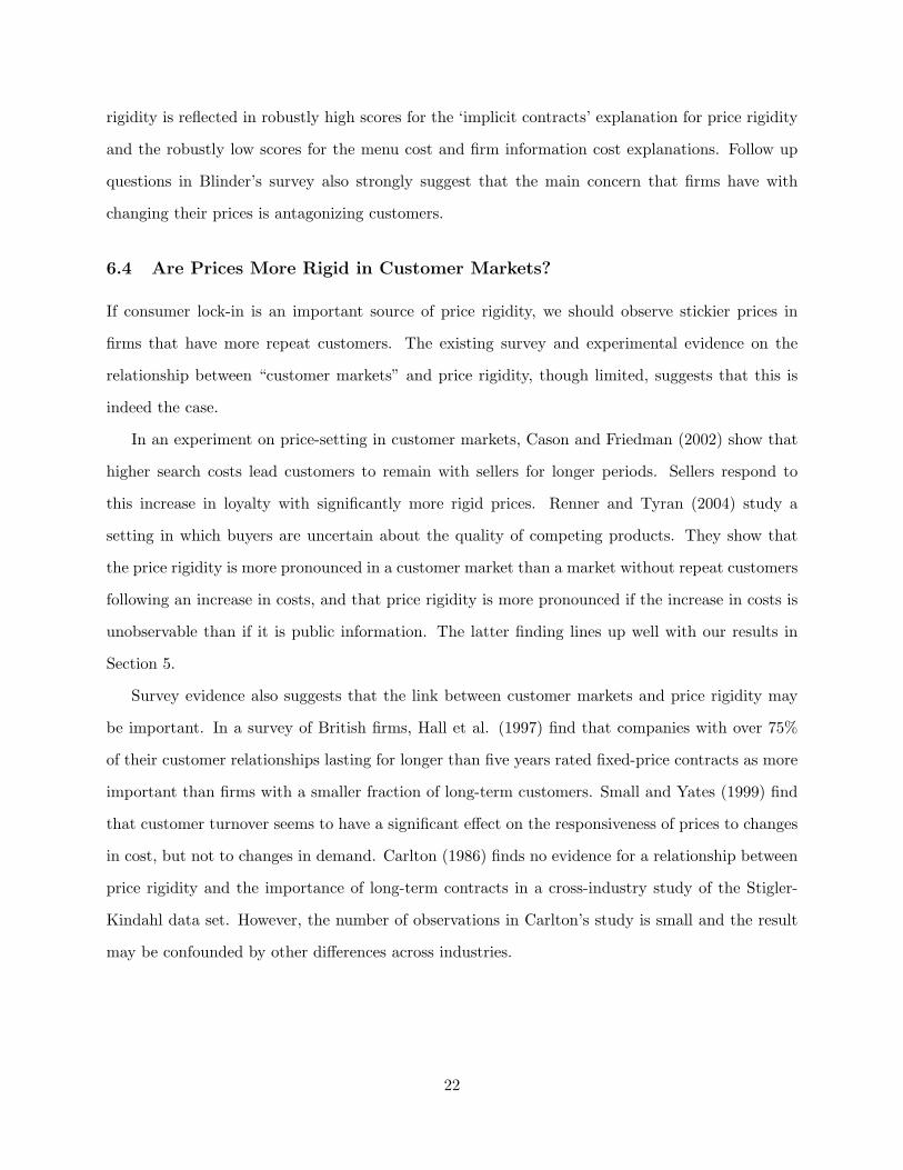
6.4 Are Prices More Rigid in Customer Markets?

If consumer lock-in is an important source of price rigidity, we should observe stickier prices in

firms that have more repeat customers. The existing survey and experimental evidence on the

relationship between “customer markets” and price rigidity, though limited, suggests that this is

indeed the case.

In an experiment on price-setting in customer markets, Cason and Friedman (2002) show that

higher search costs lead customers to remain with sellers for longer periods. Sellers respond to

this increase in loyalty with significantly more rigid prices. Renner and Tyran (2004) study a

setting in which buyers are uncertain about the quality of competing products. They show that

the price rigidity is more pronounced in a customer market than a market without repeat customers

following an increase in costs, and that price rigidity is more pronounced if the increase in costs is

unobservable than if it is public information. The latter finding lines up well with our results in

Section 5.

Survey evidence also suggests that the link between customer markets and price rigidity may

be important. In a survey of British firms, Hall et al. (1997) find that companies with over 75%

of their customer relationships lasting for longer than five years rated fixed-price contracts as more

important than firms with a smaller fraction of long-term customers. Small and Yates (1999) find

that customer turnover seems to have a significant effect on the responsiveness of prices to changes

in cost, but not to changes in demand. Carlton (1986) finds no evidence for a relationship between

price rigidity and the importance of long-term contracts in a cross-industry study of the Stigler-

Kindahl data set. However, the number of observations in Carlton’s study is small and the result

may be confounded by other differences across industries.

22

6.5 Are Prices More Rigid for Existing Customers?

Another empirical implication of the model presented in sections 2-5 (more precisely, a slight ex-

tension of that model) is that if it is possible to price discriminate between new and old customers,

prices for new customers should not exhibit the same degree of rigidity as prices for existing cus-

tomers. This is because the firm does not face a time inconsistency problem vis-a-vis its new

customers since the new customers are not yet locked in by past purchases. The practive of main-

taining fixed prices for existing customers when prices for new customers are changed is referred

to as “grandfathering” old prices for existing customers. This practice has been studied in the

economics literature are for housing rents and long distance phone services. Genesove (2003) shows

that the rent on an apartment is about twice as likely to change when a new tenant moves in as

when an old tenant signs a new lease. Epling (2002) shows that long distance telephone companies

often maintain fixed prices for existing customers when they change prices for new customers.

The results of Carlton (1986) also suggest more rigidity to existing customers. Carlton uses

the Stigler-Kindahl data set to show that prices for a particular buyer are rigid for long periods of

time and contrasts this with the results of Stigler and Kindahl (1970). Stigler and Kindahl show

that price indexes of average transaction prices are quite flexible. Together these two facts strongly

suggest that prices for existing customers are more rigid than prices for new customers for the

Stigler-Kindahl data.

7 Concluding Remarks

In this paper, we show that time non-separabilities in consumer demand imply that firms face a

time-inconsistency problem when they are choosing prices. They would like to promise low prices

in the future. But when the future arrives they have an incentive to take advantage of consumers’

habits and price gouge. In this model, price rigidity arises as an equilibrium outcome. Moreover,

firms may benefit from menu costs since they help firms commit not to price gouge. The firms’

optimal policy is to commit to a state-contingent pricing policy. However, there are various reasons

why this pricing rule may not be selected in the market. One reason is that the firms’ marginal costs

and demand may not be observable. Another reason is that it may be costly to write complicated

contracts or commit to a complicated pricing rule.

23

If firms have private information about their desired prices, the optimal pricing policy is to

commit to a price cap. Our model therefore implies that prices should spend a significant portion

of their time at a rigid upper bound. Below this upper bound, they should be much more flexible.

As we show in section 6, the behavior of retail prices bears a striking resemblance to this price cap

policy. In contrast, the combination of a rigid regular price and frequent sales is difficult to explain

within standard models of menu costs. Our model also provides an explanation for the tendency

of firms to cite adverse customer reations as an important reason for price rigidity, the tendency of

prices to be more rigid in customer markets, and the tendency of prices to existing consumers to

be more rigid than prices to new consumers.

24

A Solutions to Firm Optimization

A.1 Exact Solution in the Case of Full Commitment

Under the assumption of full commitment with a constant elasticity of demand θ, the firm’s prob-

lem can be solved analytically without any simplifying assumptions. The firm seeks to maximize

equation (3) subject to equations (2) and (4). A Lagrangian for this constrained optimization

problem is

L0 = E0

∞∑t=0

M0,t[pt(z)ct(z)−WtLt(z)− St(ct(z)−Atf(Lt(z)))

−Ψt(−pt(z) + PtC1θt (ct(z)− γct−1(z))−

1θ − γMt,t+1(Pt+1C

1θt+1(ct+1(z)− γct(z))−

1θ )],

where St and Ψt denote Lagrange multipliers. The first order conditions of this problem are

Ψt = −ct(z),

St =Wt

Atf ′(Lt(z)),

1θ(Ψt − γΨt−1)PtC

1θt (ct(z)− γct−1(z))−

1+θθ = −pt(z) + St

+γ

θEt[Mt,t+1(Ψt+1 − γΨt)Pt+1C

1θt+1(ct+1(z)− γct(z))−

1+θθ ],

and a transversality condition.26 Manipulation of these equations and equation (2) yields

pt(z) =θ

θ − 1St.

Notice that this equation implies that under full commitment the firm sets prices in exactly the

same way as it would if consumers did not have good specific habits.

A.2 A Derivation of a 2nd Order Approximation to the Firm’s Value

Given the simplifying assumption that the firm’s production function is linear we can substitute it

into the expression for the firm’s value and get

E0

∞∑t=0

βt[pt(z)ct(z)− Wt

Atct(z)],

26Throughout the paper we focus on bounded solutions. The transversality condtions of the various dynamicoptimization problems solved in the paper always hold for all bounded solutions. We therefore ignore transversalityconditions elsewhere in the paper.

25

where we have also replace M0,t by βt. The analysis in section A.1 implies that in the steady state

with full commitment

p(z) =θ

θ − 1W

A,

where variables without subscripts denote steady state values. Notice furthermore that equation

(1) implies that C = (1− γ)c(z) and equation (2) implies that (1− γβ)P = p(z). A second order

Taylor series approximation of the value of the firm around the steady state of the solution in

section A.1 is given by

E0

∞∑t=0

βt[c(z)(pt(z)− p(z)) +

1θp(z)(ct(z)− c(z)) + (pt(z)− p(z))(ct(z)− c(z))

−θ − 1θ

(Wt −W )(ct(z)− c(z)) +θ − 1

θ(At −A)(ct(z)− c(z))

]+ ex. terms +O(||ξ||3),(10)

where “ex. terms” stands for terms that are exogenous to the firm’s decision problem, ξ stands for

a vector of the exogenous variables and O(||ξ||3) denotes higher order terms.

The exposition of our results is simplified if we make a change of variables. Let ct(z) =

log(ct(z)/c(z)) and define hatted versions of all other variables in the same way. Making use

of the fact that

ct(z) = c(z)(

1 + ct(z) +12ct(z)

)+O(||ξ||3),

we can rewrite equation (10) as

E0

∞∑t=0

p(z)c(z)βt[(

pt(z) +12p2

t (z))

+1θ

(ct(z) +

12c2t (z)

)+ pt(z)ct(z)− θ − 1

θStct(z)

]+ex. terms +O(||ξ||3), (11)

where St = (Wt − At).

A.3 Firm Behavior in the Case of Full Commitment

Assuming that the habit parameter γ is small, a second order approximation of consumer demand

is given by(ct(z) +

12c2t (z)

)− γct−1(z)− 1 + θ

2θ(1− γ)c2t (z)− ct(z)θt =

−θ(1− γ − γβ)pt(z)− θ

2p2

t (z) + γβEtct+1(z) +O(||ξ, γ||3). (12)

26

We can rearrange this equation so that it says that

11− γ − γβ

ct(z)− γ

1− γ − γβct−1(z)− γβ

1− γ − γβEtct+1(z) = −θpt(z)− 1

21

1− γ − γβc2t (z)

+12

1 + θ

θ(1− γ)(1− γ − γβ)c2t (z) +

11− γ − γβ

ct(z)θt −12

θ

1− γ − γβp2

t (z) +O(||ξ, γ||3).

Now notice that equation (11) may be written

E0

∞∑t=0

p(z)c(z)βt[1θ

(1

1− γ − γβct(z)− γ

1− γ − γβct−1(z)− γβ

1− γ − γβct+1(z)

)+(

pt(z) +12p2

t (z))

+1θ

12c2t (z) + pt(z)ct(z)− θ − 1

θStct(z)

]+ ex. terms +O(||ξ, γ||3).

Substituting consumer demand into this expression now yields

E0

∞∑t=0

p(z)c(z)βt[1θ

(−1

21

1− γ − γβ

(c2t (z)− 1 + θ

θ(1− γ)c2t (z)− 2ct(z)θt + θp2

t (z)))

+12p2

t (z)

+1θ

12c2t (z) + pt(z)ct(z)− θ − 1

θStct(z)

]+ ex. terms +O(||ξ, γ||3). (13)

In the last two steps of this derivation we have assumed that the firm solves its problem from the

“timeless perspective” (see Woodford, 2003, and Benigno and Woodford, 2004). In this problem,

this assumption amounts to assuming that the firm is able to make its commitment at least one

period before its policy takes effect so as to be able to affect consumer expectations about its policy

in the first period. If we assumed that the firm did not optimize from the timeless perspective,

the expression above would have an extra ct(z) term in the first period which would imply that

the firm would behave differently in the first period compared with all subseqent periods. The

special aspects of the firm’s behavior in the first period would reflect the fact that it was taking

past expectations as given in the first period while it was seeking to affect future expectations by

its commitment. We assume that the firm optimizes from the timeless perspective simply in order

to be able to abstract from any special behavoir of the firm in the first period.

If we now multiply expression (13) by (1− γ)(1− γ − γβ), use consumer demand to substitute

for ct(z) and simplify, we get that

E0

∞∑t=0

p(z)c(z)βt[1− θ

2p2

t (z)− θtpt(z) + (θ − 1)Stpt(z)]

+ ex. terms +O(||ξ, γ||3).

Setting the derivative of this with respect to pt(z) equal to zero shows that the firm’s optimal

pricing policy under full commitment to a state-contingent rule is

pt(z) = St −1

θ − 1θt.

27

up to an error of order O(||ξ, γ||2).

A.4 Firm Behavior in the Case of Complete Discretion

While consumer demand is again given by equation (12) in the case of full discretion, the firm must

take the expectations of the consumers as given when it chooses how to set its price. We guess that

equilibrium consumption may be represented by

ct = a1 + a2St +O(||ξ, γ||2),

where a1 and a2 are undetermined coefficients. Since St is i.i.d., we have that

Etct+1 = a1 +O(||ξ, γ||2).

Notice that we need only use a first order approximation to the expectations of the agents since

these expectations are multiplied by γ in equation (12) and we are assuming that γ is small. If we

now plug this into the equation for consumer demand, equation (12), we get that(ct(z) +

12c2t (z)

)− γct−1(z)− 1 + θ

2θ(1− γ)c2t (z)− ct(z)θt =

−θ(1− γ − γβ)pt(z)− θ

2p2

t (z) + γβa1 +O(||ξ, γ||3).

Slight manipulation of this equation yields

−θpt(z) =1

1− γ − γβct(z)− γ

1− γ − γβct−1(z)− γβa1

1− γ − γβ+

12

11− γ − γβ

c2t (z)

−12

1 + θ

θ(1− γ)(1− γ − γβ)c2t (z)− 1

1− γ − γβct(z)θt +

12

θ

1− γ − γβp2

t (z) +O(||ξ, γ||3).

Notice that equation (11) implies that

E0

∞∑t=0

p(z)c(z)βt[pt(z) +

1θ

(1

1− γ − γβct(z)− γ

1− γ − γβct−1(z)

)− γ

θ

11− γ − γβ

ct(z)

+12p2

t (z) +1θ

12c2t (z) + pt(z)ct(z)− θ − 1

θStct(z)

]+ ex. terms +O(||ξ||3)

Using consumer demand to eliminate the first two terms in the above equation we get that

E0

∞∑t=0

p(z)c(z)βt[−γ

θ

11− γ − γβ

ct(z)− 12

1θ

11− γ − γβ

c2t (z) +

12

1 + θ

θ2(1− γ)(1− γ − γβ)c2t (z)

+1θ

11− γ − γβ

ct(z)θt −12

11− γ − γβ

p2t (z) +

12p2

t (z) +12

1θc2t (z) + pt(z)ct(z)

−θ − 1θ

Stct(z)]

+ ex. terms +O(||ξ, γ||3).

28

Next we multiply the above equation by (1− γ)(1− γ − γβ), use consumer demand to substitute

for ct(z) and simplify. This yields

E0

∞∑t=0

p(z)c(z)βt[γpt(z)− 1

2(θ − 1)p2

t (z)− θtpt(z) + (θ − 1)Stpt(z)]

+ ex. terms +O(||ξ, γ||3).

Here we use the fact that a1 is of order O(||ξ, γ||). Setting the derivative of this with respect to

pt(z) equal to zero yields

pt(z) =γ

θ − 1+ St −

1θ − 1

θt, (14)

up to an error of order O(||ξ, γ||2).

A.5 Firm Behavior when Prices are Fixed for Two Periods

Let’s next consider a case in which the firm is able to keep its price fixed for two periods. In a period

t in which the firm is able to change its price, both the firm and consumers know that the price in

period t+1 will be the same as the price at time t, i.e., they know that pt+1(z) = pt(z). This implies

that ct+1(z) = ct(z)+O(||ξ, γ||2). The price set by the firm at time t therefore affects the consumer’s

expectations about outcomes in period t+1. The firm, however, takes the consumer’s expectations

about outcomes at t + 1 + j for j ≥ 1 as given. We guess that Etct+1+j(z) = a1 + O(||ξ, γ||2)

is appropriate. All this implies that the demand curve of the consumers imposes the following

constraints on the firm at time t:(ct(z) +

12c2t (z)

)− 1 + θ

2θ(1− γ)c2t (z)− ct(z)θt = −θ(1− γ − γβ)pt(z)− θ

2p2

t (z) + γβct(z)

+s.o.ex.terms +O(||ξ, γ||3),

(ct+1(z) +

12c2t (z)

)− γct(z)− 1 + θ

2θ(1− γ)c2t (z)− ct(z)θt+1 = −θ(1− γ − γβ)pt(z)− θ

2p2

t (z)

+s.o.ex.terms +O(||ξ, γ||3),

Etct+2(z)− γct+1(z) = −θEtpt+2(z) + s.o.ex.terms +O(||ξ, γ||3),

Etct+j(z) = −θEtpt+j(z) + s.o.ex.terms +O(||ξ, γ||3),

for j ≥ 2, where s.o.ex.terms stands for “second order exogenous terms”.

29

A second order approximation of the value of the firm is again given by expression (11). In this

case expression (11) can be written

p(z)c(z)(

pt(z) +1θ

1− γβ

1− γ − γβct(z)− 1

θ

γ

1− γ − γβct(z) +

12p2

t (z) +12

1θc2t (z) + pt(z)ct(z)

−θ − 1θ

Stct(z))

+ p(z)c(z)β(

pt(z) +1θ

1− γ

1− γ − γβct+1(z) +

12p2

t (z) +12

1θc2t (z) + pt(z)ct(z)

)+p(z)c(z)β2

(Etpt+2(z) +

1θEtct+2(z)− γ

θct(z)

)+ p(z)c(z)βj

(Etpt+j(z) +

1θEtct+j(z)

)+ex.terms +O(||ξ, γ||3),

for j > 2. Next we plug the constraints implied by the demand curve into this expression. After

we multiply the result by (1− γ)(1− γ − γβ), this yields

p(z)c(z)(−γ

θct(z) +

1 + θ

2θ2c2t (z) +

1θct(z)θt + pt(z)ct(z)− θ − 1

θStct(z)

)+p(z)c(z)β

(1 + θ

2θ2c2t (z) + pt(z)ct(z)

)+ ex.terms +O(||ξ, γ||3).

If we now use the demand curve to eliminate ct(z) we get

p(z)c(z)(

γpt(z)− 12(1 + β)(θ − 1)p2

t (z)− θtpt(z) + (θ − 1)Stpt(z))

+ex.terms +O(||ξ, γ||3).

Setting the derivative of this with respect to pt(z) equal to zero yields

pt(z) =γ

(θ − 1)(1 + β)+

11 + β

St −1

1 + β

1θ − 1

θt +O(||ξ, γ||2). (15)

A.6 Comparison of Profits

Next we would like to compare the profits of a firm that is not able to make any time-inconsistent

commitments and a firm that is able to fix its price for two periods. The expectation of the stream

of profits of a firm is

E0

∞∑t=0

p(z)c(z)βt[1− θ

2p2

t (z)− θtpt(z) + (θ − 1)Stpt(z)]

+ ex. terms +O(||ξ, γ||3).

Using equation (14) we can derive that, ignoring exogenous terms and terms of higher than second

order, the expected profit of a firm that optimizes under discretion is

E0ΠD =p(z)c(z)1− β

θ − 12

[−(

γ

θ − 1

)2

+ var(St) +1

(θ − 1)2var(θt)

].

30

Similarly, using equation (15) we can derive that the expected profit of a firm that is able to fix its

price for two periods is

E0ΠF =p(z)c(z)1− β

θ − 12

[−(

γ

(θ − 1)(1 + β)

)2

+1 + 2β

(1 + β)2(var(St) +

1(θ − 1)2

var(θt))

].

Comparing these expressions we get that E0ΠF > E0ΠD if

γ2 >β(θ − 1)2

2 + β(var(St) +

1(θ − 1)2

var(θt)).

B Results when Firms have Private Information

We begin by deriving the function in our model that correponds to R(xt, µt, θt) in Athey et al.

(2004). Notice that a second order approximation of the value of the firm may be written

E0

∞∑t=0

p(z)c(z)βt[pt(z) +

1θ

(1

1− γ − γβct(z)− γ

1− γ − γβct−1(z)

)− γ

θ

11− γ − γβ

ct(z)

+12p2

t (z) +1θ

12c2t (z) + pt(z)ct(z)− θ − 1

θStct(z)

]+ ex. terms +O(||ξ||3)

and consumer demand may be written

−θpt(z) =1

1− γ − γβct(z)− γ

1− γ − γβct−1(z)− γβ

1− γ − γβEtct+1(z) +

12

11− γ − γβ

c2t (z)

−12

1 + θ

θ(1− γ)(1− γ − γβ)c2t (z)− 1

(1− γ − γβ)ct(z)θt +

12

θ

1− γ − γβp2

t (z) +O(||ξ, γ||3).

Using consumer demand to eliminate the first two terms in the expression for the value of the firm

given above we get

E0

∞∑t=0

p(z)c(z)βt[−γ

θ

11− γ − γβ

ct(z) +1θ

γβ

1− γ − γβEtct+1(z)− 1

21θ

11− γ − γβ

c2t (z)

+12

1 + θ

θ2(1− γ)(1− γ − γβ)c2t (z) +

1θ(1− γ − γβ)

ct(z)θt −12

11− γ − γβ

p2t (z) +

12p2

t (z)

+12

1θc2t (z) +

12

1θc2t (z) + pt(z)ct(z)− θ − 1

θStct(z)

]+ ex. terms +O(||ξ, γ||3).

Next we multiply through by (1 − γ − γβ)(1 − γ), use the demand curve to eliminate ct(z) and

focus only on terms that are affected by the firm’s action at time t. This yields

R(Et−1pt(z), pt(z), St) = p(z)c(z)[γpt(z)− γEt−1pt(z)− 1

2(θ − 1)p2

t (z)− θtpt(z) + (θ − 1)Stpt(z)]

+ex. terms +O(||ξ, γ||3). (16)

31

This is the function in our model that corresponds to R(xt, µt, θt) in Athey et al. (2004). Mapping

our notation into the notation used by Athey et al. (2004) we get that: xt = Et−1pt(z), µt = pt(z)

and θt = St − θt/(1 − θ) ≡ Φt. In the notation used by Athey et al. (2004), the firm’s objective

function is

R(xt, µt, θt) = γµt − γxt −12(θ − 1)µ2

t + (θ − 1)θtµt.

Notice that this function satisfies all the conditions required for the propositions in Athey et

al. (2004) to be valid. Specifically, Rx(xt, µt, θt) = −γ < 0, Rµθ(xt, µt, θt) = θ − 1 > 0 and

Rµµ(xt, µt, θt) = −(θ − 1) < 0.

The main difference between our results and the results in Athey et al. (2004) is that they

consider a model in which R(xt, µt, θt) is the social welfare function, i.e. it is the objective of all the

agents in the model. The fact that R(xt, µt, θt) in Athey et al. (2004) is the social welfare function

entails that the resulting policy is socially optimal. Here we use the objective of the firm as our

R(xt, µt, θt), which means that the resulting policy is not socially optimal but rather the best policy

from the perspective of the firm. The proofs in Athey et al. (2004) do not rely on R(xt, µt, θt)

being a social welfare function. Only their interpretation as solving for the socially optimal policy

relies on this.

Given equation (16) and the following monotone hazard conditions: (1−P (Φt))/p(Φt) is strictly

decreasing in Φt and P (Φt)/p(Φt) is strictly increasing in Φt, Proposition 1 in Athey et al. (2004)

shows that the pricing policy that is optimal from the perspective of the firm is static. Here p(Φt)

and P (Φt) denote the pdf and cdf of Φt, respectively. We assume that Φt ∈ [Φ,¯Φ].

Furthermore, Proposition 2 in Athey et al. (2004) shows that the firm’s best pricing policy is

either a constant price or it is a policy of bounded discretion, i.e.,

p(z) =

p∗(Φ; z) if Φ ∈ [Φ, Φ∗]

p∗(Φ∗; z) if Φ ∈ [Φ∗,¯Φ]

(17)

where p∗(Φ; z) denotes the static best response of a firm with a desired price equal to Φ and

Φ ≤ Φ∗ ≤ ¯Φ.

To complete the description of the policy most prefered by the firm, we must calculate four

things: 1) Under what conditions does the firm prefer a constant price? 2) What is the optimal

constant price from the firm’s perspective? 3-4) When the firm prefers to set its price according

32

to equation (17), what is the optimal cutoff point Φ∗ and what is the firm’s static best response

p∗(Φ; z)?

The remainder of this section draws heavily on appendix D in Athey et al. (2004). First, notice

that the static best reponse of the firm solves Rp(z)(Ep(z), p(z), Φ) = 0. The solution is

p∗(Φ, z) =γ

θ − 1+ Φ. (18)

If the firm’s pricing policy is of the form (17), then

Ep(z) =∫ Φ∗

Φp∗(Φ, z)p(Φ)dΦ +

∫ ¯Φ

Φ∗p∗(Φ∗, z)p(Φ)dΦ.

Using equation (18) to plug in for p∗(Φ, z) in this equation we get that

Ep(z) =γ

θ − 1−∫ ¯

Φ

Φ∗(Φ− Φ∗)p(Φ)dΦ.

Athey et al. (2004) show that the objective of the firm,∫

R(Ep(z), p(z), Φ)p(Φ)dΦ may be written

R(Ep(z), p∗(Φ, z), Φ) +∫ Φ∗

ΦRΦ(Ep(z), p∗(Φ, z), Φ)[1− P (Φ)]dΦ

+∫ ¯

Φ

Φ∗RΦ(Ep(z), p∗(Φ∗, z), Φ)[1− P (Φ)]dΦ.

Since RΦ(Ep(z), p(z), Φ) = (θ − 1)p(z), this expression simplifies to

γ

∫ ¯Φ

Φ∗(Φ− Φ∗)p(Φ)dΦ + (θ − 1)

∫ Φ∗

ΦΦ[1− P (Φ)]dΦ + (θ − 1)

∫ ¯Φ

Φ∗Φ∗[1− P (Φ)]dΦ + ex. terms.

Differentiating this with respect to Φ∗ and setting the resulting expression equal to zero yields

−γ

∫ ¯Φ

Φ∗p(Φ)dΦ + (θ − 1)

∫ ¯Φ

Φ∗[1− P (Φ)]dΦ = 0,

which is equivalent to

−γ[1− P (Φ∗)] + (θ − 1)∫ ¯

Φ

Φ∗[1− P (Φ)]dΦ = 0.

When Φ∗ <¯Φ, 1− P (Φ∗) > 0, so this last equation is equivalent to

−γ + (θ − 1)∫ ¯

Φ

Φ∗

1− P (Φ)p(Φ)

p(Φ)1− P (Φ∗)

dΦ = 0. (19)

Notice that the second term on the left hand side of this equaiton is the conditional mean of

(1 − P (Φ))/p(Φ) over the interval [Φ∗,¯Φ]. Since (1 − P (Φ))/p(Φ) is strictly decreasing in Φ∗

33

(monotone hazard assumption), its conditional mean is also strictly decreasing in Φ∗. This implies

that equation (19) has at most one interior solution. Since the expression on the left hand side of

equation (19) is decreasing in both γ and Φ∗, it is furthermore the case that Φ∗ is decreasing in γ.

We have shown that equation (19) has at most one interior solutions. To show that such a

solution in fact exists we must show that the left hand side of this equation is negative for Φ∗ close¯Φ and positive for Φ∗ = Φ. Notice that when Φ∗ → ¯Φ, (1−P (Φ))/p(Φ) → 0. This implies that for

γ > 0 and Φ∗ close enough to ¯Φ, the left hand side of equation (19) is strictly less than zero. When

Φ∗ = ¯Φ, equation (19) is not defined. However, Φ∗ = ¯Φ is a solution to the equation above equation

(19). However, since the expression on the left hand side of that equation is strictly negative for

Φ∗ <¯Φ in the neighborhood of ¯Φ, this is not a local maximum.

Athey et al. (2004) show that at Φ∗ = Φ the left hand side of equation (19) becomes −γ − Φ.

Since Φ < 0, this is positive for γ ∈ (0,−Φ). So, there is an interior solution in this case. When

γ > −Φ there is no interior solution to equation (19). This implies that for this range of γ the

firm’s best policy is a constant price.

Finally, when γ > −Φ the firm chooses its constant price to maximize

∫ ¯Φ

ΦR(Ep(z), p(z), Φ)p(Φ)dΦ

subject to Ep(z) = p(z). The solution to this problem is p(z) = 0.

C The Sales Filter

Let pt denote the observed price at time t and rt denote the “regular” price at time t. The sales

filter has 6 steps for each time period which should be considered in order (i.e. step 1 has precedence

over step 2, etc.). However, for the first time period, the algorithm implementing the filter should

start at step 3 (the first step not to refer to rt−1). The steps of the filter are:

0. If pt = rt−1, then rt = rt−1.

1. If pt > rt−1, then rt = pt.

2. If rt−1 ∈ {pt+1, ..., pt+J}, then rt = rt−1.

3. If the set {pt, pt+1, ..., pt+L} has K or more different elements, then rt = pt.

34

4. Define pmax = max{pt, pt+1, ..., pt+L} and tmax = time max{pt, pt+1, ..., pt+L}. If pmax ∈

{ptmax , ptmax+1, ..., ptmax+L}, then rt = pmax.

5. rt = pt.

The filter has three parameters to be chosen by its user: J and K. We chose these parameters to

be J = 8, K = 3, L = 3.

The filter identifies sales as brief period of time when the price of the good drops below its

regular price before returning to its old regular price or a new reoccuring regular price. A simpler

filter would only identify sales as cases when the price returns to the original regular price. However,

our filter counts brief discounts followed by changes in the regular price as sales.

The parameters J , K and L determine how conservative the filter is at assigning price variation

to sales rather than variation in the regular price. If, e.g., J = K = L = 3 any price change lasting

longer than 3 periods is counted as a change in the regular price and any time 3 or more prices are

seen in four consecutive periods the filter assigns variation in the price to variation in the regular

price, not sales. This means that if two different sales with different sales prices happen with one

or two periods in between all the variation in price is assigned to the regular price. If J , K and L

are assigned higher values, longer and more irregular sales within a short period are allowed.

The parameters we use imply that the maximum duration of sales is 3 periods if the price

returns to the original “regular price” following a sale (i.e., a v-shaped sale) and 7 periods if the

price returns to a new recurring regular price following the sale.

Perhaps the best way to convince the reader that our sales filter correctly identifies sales is

to show what happens when we apply the filter to a few price series. Figures 1-3 provide three

examples. In each figure we plot the price of a good and the regular price shifted up by $1. Two

things stand out: 1) Most of the time, the filter works very well. It filters out all sales and only

sales. 2) The filter is somewhat conservative in assigning price variation to sales rather than the

regular price. In particular, very irregular patterns of sales are attributed to variation in the regular

price rather than variation in the sale price. The most striking example of this is the price of Diet

Coke in the period form last 1995 to mid 1996. During this period, the price of Diet Coke varied

rather eratically and the sales filter was unable to identify a stable regular price. This type of error

tends to increase the frequency of price changes and the number of unique values in the regular

price series. Both of these effects work against the results we present in section 6.

35

References

Abel, A. B. (1990): “Asset Prices under Habit Formation and Catching up with the Joneses,”American Economic Review, 80(2), 38–42.

Abreu, D., D. Pearce, and E. Stacchetti (1990): “Toward a Theory of Discounted RepeatedGames with Imperfect Monitoring,” Econometrica, 58(5), 1041–1063.

Aguirregabiria, V. (1999): “The Dynamics of Markups and Inventories in Retail Firms,” Reviewof Economic Studies, 66, 275–308.

Akerlof, G. A., and J. L. Yellen (1985): “A Near-Rational Model of the Business Cycle withWage and Price Inertia,” Quarterly Journal of Economics, 100(Supplement), 823–838.

Amirault, D., C. Kwan, and G. Wilkinson (2004): “A Survey of the Price-Setting Behaviorof Canadian Companies,” Bank of Canada Review, winter 2004–2005, 29–40.

Apel, M., R. Friberg, and K. Hallsten (2004): “Micro Foundations of Macroeconomic PriceAdjustment: Survey Evidence from Swedish Firms,” Forthcoming in the Journal of Money,Credit and Banking.

Athey, S., A. Atkeson, and P. J. Kehoe (2004): “The Optimal Degree of Discretion inMonetary Policy,” NBER Working Paper No. 10109.

Bagwell, K. (2004): “Countercyclical Pricing in Customer Markets,” Economica, 71(284), 519–542.

Barro, R. (1972): “A Theory of Monopolistic Price Adjustment,” Review of Economic Studies,39, 17–26.

Becker, G. S., and K. M. Murphy (1988): “A Theory of Rational Addiction,” Journal ofPolitical Economics, 96(4), 675–700.

Benigno, P., and M. Woodford (2004): “Inflation Stabilization and Welfare: The Case of aDistorted Steady State,” NBER Working Paper No. 10838.

Bils, M. (1989): “Pricing in a Customer Market,” Quarterly Journal of Economics, 104(4), 699–718.

Bils, M., and P. J. Klenow (2004): “Some Evidence on the Importance of Sticky Prices,”Journal of Political Economics, 112(5), 947–985.

Blinder, A. S., E. R. D. Canetti, D. E. Lebow, and J. B. Rudd (1998): Asking AboutPrices. Russell Sage Foundation, New York, New York.

Caminal, R. (2004): “Pricing Cyclical Goods,” Working Paper, Institut d’Asalisi Economica.

Campbell, J. Y., and J. H. Cochrane (1999): “By Force of Habit: A Consumption-BasedExplanation of Aggregate Stock Market Behavior,” Journal of Political Economics, 107(2), 206–251.

Caplin, A. S., and D. F. Spulber (1987): “Menu Costs and the Neutrality of Money,” QuarterlyJournal of Economics, 102(4), 703–725.

36

Carlton, D. W. (1986): “The Rigidity of Prices,” American Economic Review, 76, 637–658.

Cason, T. N., and D. Friedman (2002): “A Laboratory Study of Customer Markets,” Advancesin Economic Analysis and Policy, 2(1), Article 1.

Cecchetti, S. G. (1986): “The Frequency of Price Adjustment: A Study of the Newsstand Pricesof Magazines,” Journal of Econometrics, 31, 255–274.

Chevalier, J. A., A. K. Kashyap, and P. E. Rossi (2003): “Why Don’t Prices Rise DuringPeak Demand Periods? Evidence from Scanner Data,” American Economic Review, 93(1), 15–37.

Conlisk, J., E. Gerstner, and J. Sobel (1984): “Cyclic Pricing by a Durable Goods Monop-olist,” Quarterly Journal of Economics, 99, 489–505.

Constantinides, G. M. (1990): “Habit Formation: A Resolution of the Equity Premium Puzzle,”Journal of Political Economics, 98(3), 519–543.

Cremer, J. (1984): “On the Economics of Repeat Buying,” RAND Journal of Economics, 15(3),396–403.

Diewert, E., and K. J. Fox (1999): “Can Measurement Error Explain the Productivity Para-dox?,” Canadian Journal of Economics, 32(2), 251–280.

Dutta, S., M. Bergen, D. Levy, and R. Venable (1999): “Menu Costs, Posted Prices andMultiproduct Retailers,” Journal of Money Credit and Banking, 31(4), 683–703.

Epling, N. M. (2002): “Price Discrimination amid Heterogeneous Switching Costs: A CompetitiveStrategy of the Long Distance Telephony Fringe,” Working Paper, Yale University.

Fabiani, S., M. Druant, I. Hernando, C. Kwapil, B. Landau, C. Loupias, F. Martins,

T. Matha, R. Sabbatini, H. Stahl, and A. Stokman (2004): “The Pricing Behavior ofFirms in the Euro Area: New Survey Evidence,” Paper Presented at Conference on “InflationPersistence in the Euro Area” at the European Central Bank.

Farell, J., and C. Shapiro (1989): “Optimal Contracts with Lock-In,” American EconomicReview, 79, 51–68.

Fuhrer, J. (2000): “Habit Formation in Consumption and Its Implications for Monetary-PolicyModels,” American Economic Review, 90(3), 367–390.

Genesove, D. (2003): “The Nominal Rigidity of Apartment Rents,” Review of Economics andStatistics, 85(4), 844–853.

Golosov, M., and R. E. Lucas (2005): “Menu Costs and Phillips Curves,” Working Paper,Massachusetts Unstitute of Technology.

Hall, R. E. (2005): “Employment Fluctuations with Equilibrium Wage Stickiness,” AmericanEconomic Review, 95(1), 50–65.

Hall, S., M. Walsh, and T. Yates (1997): “How do UK Companies set prices?,” Bank ofEngland Quarterly Bulletin, pp. 180–192.

37

Hendel, I., and A. Nevo (2003): “Measuring the Implications of Sales and Consumer StockpilingBehavior,” Working Paper, University of Wisconsin.

Hosken, D., D. Matsa, and D. Reiffen (2000): “How do Retailers Adjust Prices?: Evidencefrom Store-Level Data,” Working Paper, Federal Trade Commission.

Hosken, D., and D. Reiffen (2004): “Patterns of Retail Price Variation,” Rand Journal ofEconomics, 35(1), 128–146.

Kahneman, D., J. L. Knetsch, and R. Thaler (1986): “Fairness as a Constraint on ProfitSeeking: Entitlements in the Market,” American Economic Review, 76(4), 728–741.

Kashyap, A. K. (1995): “Sticky Prices: New Evidence from Retail Catalogs,” Quarterly Journalof Economics, 110, 245–274.

Klemperer, P. (1995): “Competition when Consumers have Switching Costs: An Overview withApplications to Industrial Organization, Macroeconomics, and International Trade,” Review ofEconomic Studies, 62, 515–539.

Klenow, P. J., and O. Kryvtsov (2005): “State-Dependent or Time-Dependent Pricing: DoesIt Matter for Recent U.S. Inflation,” Working Paper, Stanford University.

Konieczny, J. D., and A. Skrzypacz (2005): “Inflation and Price Setting in a Natural Experi-ment,” Journal of Monetary Economics, 52(3), 621–632.

Lazear, E. P. (1986): “Retail Pricing and Clearance Sales,” American Economic Review, 76,14–32.

Levy, D., M. Bergen, S. Dutta, and R. Venable (1997): “The Magnitude of Menu Costs:Direct Evidence of From Large U.S. Supermarket Chains,” Quarterly Journal of Economics,112(3), 791–825.

Mankiw, N. G. (1985): “Small Menu Costs and Large Business Cycles: A Macroeconomic Modelof Monopoly,” Quarterly Journal of Economics, 100, 529–539.

Nishimura, K. (2000): “Gains from Price Rigidity,” The Japanese Economic Review, 51(1), 95–110.

Okun, A. M. (1981): Prices and Quantities: A Macroeconomic Analysis. Brookings Institution,Washington, DC.

Pashigian, P. B., and B. Bowen (1991): “Why Are Products Sold on Sales? Explanation ofPricing Regularities,” Quarterly Journal of Economics, 106, 1015–1038.

Pesendorfer, M. (2002): “Retail Sales: A Study of Pricing Behavior in Supermarkets,” Journalof Business, 75(1), 33–66.

Phelps, E. S., and S. G. Winter (1970): “Optimal Price Policy under Atomistic Competition,”in Microeconomic Foundations of Employment and Inflation Theory, ed. by E. S. Phelps, NewYork, New York. W.W. Norton.

Ravn, M., S. Schmitt-Grohe, and M. Uribe (2005): “Deep Habits,” Review of EconomicStudies, forthcoming.

38

Renner, E., and J.-R. Tyran (2004): “Price Rigidity in Customer Markets: An EmpiricalStudy,” Journal of Economic Behavior and Organization, 55(4), 575–593.

Rotemberg, J. J. (2002): “Customer Anger at Price Increases, Time Variation in the Frequencyof Price Changes and Monetary Policy,” NBER Working Paper No. 9320.

(2004): “Fair Pricing,” NBER Working Paper No. 10915.

Rotemberg, J. J., and M. Woodford (1991): “Markups and the Business Cycle,” in NBERMacroeconomics Annual, ed. by O. J. Blanchard, and S. Fischer, Cambridge, Mass. MIT Press.

(1995): “Oligopolistic Pricing and the Effects of Aggregate Demand on Economic Ac-tivity,” in Frontiers of Business Cycle Research, ed. by T. F. Cooley, Princeton, New Jersey.Princeton University Press.

Salop, S. C. (1977): “The Noisy Monpolist: Imperfect Information, Price Dispersion and PriceDiscrimination,” Review of Economic Studies, 44, 393–406.

Salop, S. C., and J. E. Stiglitz (1982): “The Theory of Sales: A Simple Model of PriceDispersion with Identical Agents,” American Economic Review, 72, 1121–1130.

Shapiro, C., and H. R. Varian (1999): Information Rules. Harvard Business School Press,Boston, MA.

Small, I., and T. Yates (1999): “What makes prices sticky? Some survey evidence for theUnited Kingdom,” Bank of England Quarterly Bulletin.

Stigler, G., and J. Kindahl (1970): The Behavior of Industrial Prices. Columbia UniversityPress, New York, NY.

Varian, H. R. (1980): “A Model of Sales,” American Economic Review, 70, 651–659.

Warner, E. J., and R. B. Barsky (1995): “The Timing and Magnitude of Retail Store Mark-downs: Evidence from weekends and Holidays,” Quarterly Journal of Economics, 110, 321–352.

Woodford, M. (2003): Interest and Prices. Princton University Press, Princeton, NJ.

39

Table 1: Descriptive Statistics on Retail Price Adjustment

Product Fraction of Weeks Fraction of Salesat the that Return to the

Regular Price Regular Price

Analgesics 0.954 0.926(0.001) (0.008)

Bath Soap 0.921 0.938(0.003) (0.014)

Bathroom Tissues 0.825 0.937(0.004) (0.007)

Beer 0.758 0.925(0.003) (0.005)

Bottled Juices 0.831 0.956(0.002) (0.003)

Canned Soup 0.892 0.957(0.001) (0.003)

Canned Tuna 0.882 0.947(0.002) (0.006)

Cereals 0.931 0.947(0.001) (0.005)

Cheese 0.812 0.945(0.002) (0.003)

Cigarettes 0.995 0.897(0.001) (0.040)

Cookies 0.868 0.958(0.001) (0.003)

Crackers 0.837 0.968(0.002) (0.004)

Dish Detergent 0.886 0.969(0.002) (0.004)

Fabric Softeners 0.904 0.947(0.002) (0.006)

Front-end-candies 0.896 0.968(0.002) (0.004)

Frozen Dinners 0.768 0.963(0.004) (0.004)

Frozen Entrees 0.845 0.961(0.001) (0.002)

Continued on next page

Continued from last page

Product Fraction of Weeks Fraction of Salesat the that Return to the

Regular Price Regular Price

Frozen Juices 0.813 0.966(0.002) (0.004)

Grooming Products 0.889 0.929(0.001) (0.004)

Laundry Detergents 0.908 0.951(0.002) (0.005)

Oatmeal 0.907 0.970(0.003) (0.007)

Paper Towels 0.836 0.946(0.004) (0.007)

Refrigirated Juices 0.766 0.934(0.003) (0.005)

Shampoos 0.900 0.935(0.002) (0.004)

Snack Crackers 0.827 0.947(0.002) (0.004)

Soaps 0.871 0.952(0.003) (0.006)

Soft Drinks 0.750 0.957(0.001) (0.001)

Toothbrushes 0.871 0.935(0.002) (0.006)

Toothpastes 0.887 0.936(0.002) (0.005)

Median 0.871 0.947

Note: Standard Errors are in parentheses. The total number of observations is 985,022.The regular price and sale prices of a good are identified using the sales filter that isdiscribed in appendix C. Estimates are based on pooled data from each category.

Table 2: Adjustment of Regular versus Sale Prices

Frequency of Number of Unique Prices as aPrice Change Fraction of Total Weeks

Product Regular Prices Sale Prices Regular Prices Sales Prices

Analgesics 0.036 0.411 0.035 0.578(0.001) (0.013) (0.001) (0.019)

Bath Soap 0.026 0.354 0.031 0.531(0.002) (0.025) (0.002) (0.047)

Bathroom Tissues 0.110 0.491 0.064 0.359(0.003) (0.014) (0.004) (0.029)

Beer 0.063 0.200 0.040 0.195(0.001) (0.006) (0.002) (0.016)

Bottled Juices 0.084 0.454 0.053 0.404(0.001) (0.006) (0.002) (0.014)

Canned Soup 0.058 0.418 0.042 0.464(0.001) (0.007) (0.001) (0.016)

Canned Tuna 0.069 0.304 0.046 0.331(0.002) (0.008) (0.003) (0.013)

Cereals 0.069 0.528 0.061 0.668(0.001) (0.010) (0.001) (0.014)

Cheeses 0.111 0.530 0.080 0.395(0.001) (0.005) (0.007) (0.010)

Cigarettes 0.036 — 0.053 0.580(0.001) (0.001) (0.037)

Cookies 0.046 0.500 0.034 0.426(0.001) (0.005) (0.001) (0.009)

Crackers 0.065 0.445 0.044 0.349(0.001) (0.008) (0.002) (0.013)

Dish Detergent 0.054 0.453 0.047 0.434(0.001) (0.011) (0.002) (0.018)

Fabric Softeners 0.057 0.404 0.045 0.495(0.001) (0.011) (0.003) (0.023)

Front-end-Candies 0.028 0.344 0.024 0.338(0.001) (0.008) (0.001) (0.016)

Frozen Dinners 0.066 0.551 0.040 0.432(0.002) (0.011) (0.003) (0.022)

Frozen Entrees 0.054 0.495 0.039 0.446(0.001) (0.006) (0.001) (0.007)

Continued on next page

Continued from last page

Frequency of Number of Unique Prices as aPrice Change Fraction of Total Weeks

Product Regular Prices Sale Prices Regular Prices Sales Prices

Frozen Juices 0.081 0.522 0.051 0.344(0.002) (0.009) (0.002) (0.011)

Grooming Products 0.034 0.497 0.036 0.442(0.001) (0.007) (0.001) (0.011)

Laundry Detergents 0.061 0.425 0.049 0.538(0.001) (0.009) (0.003) (0.027)

Oatmeal 0.071 0.530 0.062 0.607(0.002) (0.019) (0.004) (0.029)

Paper Towels 0.086 0.482 0.045 0.301(0.003) (0.015) (0.004) (0.023)

Refrigerated Juices 0.133 0.635 0.089 0.447(0.002) (0.008) (0.005) (0.016)

Shampoos 0.043 0.443 0.038 0.443(0.001) (0.010) (0.001) (0.013)

Snack Crackers 0.073 0.529 0.051 0.428(0.001) (0.007) (0.002) (0.013)

Soaps 0.051 0.510 0.039 0.449(0.002) (0.011) (0.003) (0.026)

Soft Drinks 0.076 0.652 0.042 0.309(0.001) (0.004) (0.001) (0.006)

Toothbrushes 0.049 0.406 0.045 0.403(0.001) (0.011) (0.002) (0.016)

Toothpastes 0.056 0.492 0.048 0.443(0.001) (0.009) (0.001) (0.013)

Median 0.061 0.487 0.045 0.434

Note: Standard Errors are in parentheses. The total number of observations is 985,022.The regular price and sale prices of a good are identified using the sales filter that isdescribed in appendix C. The frequency of price change is calculated by dividing the totalnumber of price changes by the total number of weeks. The statistics in columns three andfour are calculated by first dividing the number of unique regular or sale prices observed fora product by the total number of weeks at the regular price or on sale and then averagingwithin categories.

Table 3: Evidence of Price Commitments

Company Industry Company Description Date QuoteIndustrialAuto SuppliersSteelIndian Steel Alliance steel organization represents 5

leading steelmakers5-Mar-04 Steelmakers in India will not increase prices of hot rolled steel coils until end of

June even if input costs rise during this period, the chairman of an industry body (Indian Steel Alliance) said on Thursday

Tata Steel steel India 24-Aug-04 B Muthuraman, managing director, Tata Steel, said: “We will not increase prices for both our direct customers as well as retail customers till March 2005.” Tata Steel announcement assumed significance against the backdrop of rising global steel prices and large international steel companies like Arcelor and Posco already annoucing price hikes for the next quarter.

Other Siemens equipment 31-Dec-69 Siemens make a commitment not to increase the price for the service indefinitely

Pioneer Hi-Bred International

agricultural products

29-Sep-98 announced it will not raise prices of its corn and soybean seed products in calendar year 1999, due to the "challenging economic conditions faced by US and Canadian farmers"

Sarel, brand of Schneider Electric

fences 1-Jun-01 Accompanying the catalogue is a new price list, the most important feature of which is what hasn't changed - the prices! In fact, Sarel, a brand of Schneider Electric, has had no price increases for more than five years, and no price changes are expected in the foreseeable future.

"Our new catalogue and stable prices both, in their own way, demonstrate our commitment to enclosure users," said Brian O'Donoghue, marketing manager.

"We have made a substantial investment in ensuring that our catalogue guides customers toward the most appropriate and most economical enclosure choices.

When they've made their choice, the exceptional stability of our prices means that they know not only that they're getting superb value for money today, but also that they will continue to do so in the future."

Computer Related

Web HostingTech trade Internet Services

web hosting 29-Jan-05 Price Freeze Guarantee. Same price. Forever.

Infinity Hosting web hosting 29-Jan-05 Price Promise: the price you paid when you opened your account iw the price you will always pay. No price increases no extra charges ever….No contract…cancel your hosting account…at any time

hostup.com web hosting 29-Jan-05 we will never, ever increase the pricing of hosting plans…you will always pay the same fee for your hosting account

A1-hosting web hosting 1-Dec-04 Life Time Price Guarantee…there will be no Price increases for the life of the time that you host with us

Cloch web hosting 1-Dec-04 Price Promise: Cloch Internet will not raise the price of your hosting plan, even if the price increases for new customers

BurningBulb.net web hosting 3-Dec-04 Price Freeze Guarantee. Our clients take comfort in knowing that regardless of our future pricing policies, their monthly fee will always remain the same. As our policies change for future accounts, current accounts continue to host at the same monthly fee charged at the time their account was setup.

Other DSLExtreme internet

services3-Dec-04 Price Freeze Guarantee…Choose one of our exclusive Price Freeze Guarantee

subscriptions. Clients who select this option will enjoy one low price for as long as they choose to keep the service. Your Price will never go up!

Optimum Online cable internet Nov-04 Cablevision Systems Corp. has announced that it will freeze prices for its Optimum Online high-speed Internet service in 2005. The announcement comes when the number of customers for that service has increased despite stepped-up competition, including discount prices, from phone companies including Verizon Communications.

Comodo internet security

30-Oct-04 "We want to assure all our customers that our prices remain frozen,"; states Paul Tourret, Managing Director of Comodo Limited,"We launched Instant SSL several months ago as the market leader in low-cost, fully validated, fully supported high quality SSL Certificates. The recent price increases from Thawte and GeoTrust only strengthen our unique position in this market - through Instant SSL we ensure that high quality SSL webserver security will remain affordable.";

Power and ElectricityElectric UtilitiesPowerco utility 4-Jan-02 Powerco, New Zealand’s third largest electricity and gas utility has implemented a

12 month voluntary price freeze from 1 April 2002 for its electricity lines charges for all its residential consumers in the central and lower North Island.

npower utility 29-Jan-05 With npower you’ll see no increase in your electricity and gas prices throughout the whole of 2005, providing there are no increases imposed by any governmental, statutory or licensing authority.

Bangor Hydro-Electric Company

utility State of Maine utility 10-Jul-96 commitment not to raise prices

Oil and GasBord Gais utility Bord Gáis Éireann (Bord

Gáis) is a statutory body that was established under the 1976 Gas Act. The company is responsible for the transmission, distribution and supply of natural gas in Ireland. Bord Gáis, which is wholly owned by the Irish Government, employs over 800 staff and is headquartered at Gasworks Road, Cork.

29-Jun-00 Despite substantial increases in the supply cost of natural gas during the year, prices to consumers were not increased, in line with the company's commitment to maintain prices at existing levels until at least 2003. Natural gas prices for residential customers have not been increased since the mid-1980s.

Chinese Petroleum Corp

gas and oil Taiwan 1-Apr-04 "will not raise prices before May 20"

Petron Corporation diesel ? 2003 promised not to increase its prices any further for the rest of the year

Gazprom gas and oil Russia's oil and gas giant 3-Nov-99 Gazprom, Russia's oil and gas giant, does not intend to raise natural gas prices for its Russian clients this year, chairman of the company's board of directors Rem Vyakhirev said.

Other

ABB utility supplier ABB is a leader in power and automation technologies that enable utility and industry customers to improve performance while lowering environmental impact. The ABB Group of companies operates in around 100 countries and employs around 105,000 people.

25-May-04 In order to further strengthen our ties with our OEM customers, ABB will not be increasing prices on OEM medium voltage products. We will maintain the current price levels through the end of 2004, barring any further drastic changes in material costs

PharmaceuticalsGlaxosmithKline pharmaceutic

alJul-02 will not raise wholesale prices of HIV drugs until January 2004. This will help low-

income people who are uninsured or underinsured and rely on state programs and federal funding for their medications

Pfizer pharmaceutical

Mar-02 2 year freeze on anti-retrovirals

PublishingInspec bibliographic

servicesInspec is the leading English-language bibliographic information service providing access to the world's scientific and technical literature in physics, electrical engineering, electronics, communications, control engineering, computers and computing, information technology, production, manfacturing and mechanical engineering.

2001 INSPEC is pleased to announce a price freeze for 2002. This means no price increase for standalone customers and some networking customers will see a slight decrease.

Serials Solutions library services

Serials Solutions Inc. provides complete e-journal access services to over 1000 libraries worldwide

19-Aug-03 Seattle, WA – August 19, 2003. Serials Solutions, Inc. announced today that it is freezing its 2003 price schedule and offering additional price breaks to keep services accessible for all libraries.

Consumer Goods

DHA Lighting lighting 24-Jun-05 DHA Lighting has frozen prices on all products this year. The leading manufacturer of gobos, moving lighting effects, projection slides and creator of the Digital Light Curtain is holding its 2002 prices into 2003.

Marvel comic books 23-May-02 Marvel CEO Bill Jemas began today's press conference by swiping a line from Bush the Elder and declaring, "Read my lips, we will not raise prices." The hastily called conference call with the comic press was arranged to provide a quick Marvel response to price increases on 20 books announced by DC Comics earlier in the week. Though Jemas did note that many companies traditionally took advantage of price hikes by the competition to raise prices on their own goods, he promised "that unless something drastic happens to the contrary, we will hold price indefinitely."

Jaguar auto 15/10/1998 Speaking today at the Sydney International Motor Show 1998 industry day, Mr Danny Rezek, managing director of Jaguar Australia, said that:"Since its inception in 1922, Jaguar Cars has espoused a philosophy of offering customers excellent value for money. Jaguar Australia's commitment to this philosophy is evident in our announcement today of a price freeze on all Jaguar models for the next six months. This price freeze is testimony to our serious commitment to ensure our customers continue to receive best-in-class value," said Mr Rezek.

Mitsubishi South Africa auto 23-Jun-05 Mitsubishi recently announced that it will not increase its prices for the remainder of 2001 and will only look at increasing prices in 2002.

Revlon consumer goods

9-Oct-00 Revlon Inc. (NYSE: REV) today announced an innovative change to the way it does business with its U.S. retail partners to drive market growth and emphasize mutual success.In addition to the trade terms, the Company also announced a commitment not to raise prices for its retail partners in 2001.

Needham Junction ice cream

retail 5-May-04 In an article investigating the likelihood of future ice cream price increases: Around the middle of April…Turransky hiked the price of a small soft-serve ice cream cone...Turransky…stressed that he works with a printed menu, that he's already printed this season's and he won't be raising prices again

Apple Computer Inc ipod music 1-Dec-04 Apple Computer Inc. on Friday flatly denied a report that the computer maker was planning to raise prices for songs bought on its popular iTunes online music store... "These rumors aren't true," said Apple spokeswoman Natalie Sequeira. "We have multiyear agreements with the labels and our prices remain 99c a track."

Consumer ServicesTelephoneIllonois Bell Telephone Company

telephone 6/26/2004 Price protection which guarantees no price increases for the duration of the 12, 24, or 36 month plan

Bell telephone 6/10/2004 SBC and other Bells have pledged not to increase wholesale prices until 2005

Citzens Communications co

telephone 6/23/1905 proposed agreement to purchase lines in rural Colorado: proposal included guarantee to "maintain current prices for at least a year"

Cell PhoneCantel Amigo cell phone Canada cell phone 11/13/1997 price guarantee: We promise no price increases and the flexibility to change plans

if you need to, no long term contract

HealthcarePalmetto Health healthcare integrated healthcare delivery

system6/18/1996 Following merger, "guarantees that the new system will have no price increases

for five years"BUPA Ireland healthcare BUPA Ireland is part of

BUPA, a global health and care organisation with members in over 190 countries. BUPA have been committed to Irish healthcare for more than 15 years.BUPA Ireland is a not-for-profit organisation.

7/9/2002 will not be increasing prices to customers this year

Other (Small)Color Express film 1/1/2005 Our published price list is one of our commitments. We provide consistent, "no

surprises" pricing for our customers.

Once we publish our price list, our track record proves that we commit to those prices; it's not uncommon to maintain prices for one to two years barring significant increases in the paper industry. Take a look at other published prices, and you will find revisions sometimes as frequently as every 3 - 6 months. Even if the competition's prices are "slashed", doesn't it make you wonder?

Bravo Software software Sep-02 This feature is called "Price Lock". Price Lock will allow you to purchase additional add-ons for the same price as when you joined the program. No price increases ever, for as long as you are a Customer Care member.

Satin Ivy Laundry Service

laundry Jan-05 We offer a personalised service at affordable prices. Once accepted, our prices are set for 12 months – in fact we rarely increase prices even then, unless the purchase price of linen is increased.

Robins School of Motoring

driving instruction

1/1/2005 On the FAQ page:

Q. How often do you increase your prices?A. I try to keep my rates as competitive as possible and rarely increase prices, this will depend mainly on the increase in the price of fuel and the general economy, over the last two years I have only increased my prices once by £1

University ProcurementMonash University procurement procurement of information

technologiesOct-04 The Universit requires that Suppliers provide a firm price period of at least twelve

(12) months from the date of execution of a formal agreement…During the firm price period the Supplier guarantees not to increase prices….

Harvard University procurement office products procurement from Staples

1/1/2005 * Information based on an interview with the Harvard procurement manager:

Staples prices fixed during the year for top 200(?) products

The solid line is the price of Nabisco Premium Saltines. The dotted line is the regular price of Nabisco Premium Saltines shifted up by $1.

Jan90 Jan92 Jan94 Jan960.5

1

1.5

2

2.5

3

3.5Figure 1: Nabisco Premium Saltines 16oz

The solid line is the price of Diet Coke 2L. The dotted line is the regular price of Diet Coke 2L shifted up by $1.

Jan90 Jan92 Jan94 Jan960.5

1

1.5

2

2.5

3Figure 2: Diet Coke 2L

The solid line is the price of Nabisco Premium Saltines. The dotted line is the regular price of Nabisco Premium Saltines shifted up by $1.

Jan90 Jan92 Jan94 Jan960.5

1

1.5

2

2.5

3

3.5

4

4.5

5Figure 3: Kraft Singles 16oz