Prediction of the spread of highly pathogenic avian influenza using a multifactor network: Part 1...

This article appeared in a journal published by Elsevier. The attachedcopy is furnished to the author for internal non-commercial researchand education use, including for instruction at the authors institution

and sharing with colleagues.

Other uses, including reproduction and distribution, or selling orlicensing copies, or posting to personal, institutional or third party

websites are prohibited.

In most cases authors are permitted to post their version of thearticle (e.g. in Word or Tex form) to their personal website orinstitutional repository. Authors requiring further information

regarding Elsevier’s archiving and manuscript policies areencouraged to visit:

http://www.elsevier.com/authorsrights

http://www.elsevier.com/authorsrights

Author's personal copy

Research Paper

Prediction of the spread of highly pathogenic avianinfluenza using a multifactor network: Part1 e Development and application of computationalfluid dynamics simulations of airborne dispersion

Il-Hwan Seo a,d, In-Bok Lee a,*, Oun-Kyung Moon b, Nam-Su Jung c,Hyung-Jin Lee a, Se-Woon Hong a, Kyeong-Seok Kwon a, Jessie P. Bitog a

aDepartment of Rural Systems Engineering, Research Institute for Agriculture and Life Sciences,

College of Agriculture and Life Sciences, Seoul National University, 599, Gwanakno, Gwanakgu,

Seoul 151-921, Republic of KoreabAnimal and Plant Quarantine Agency, Veterinary Epidemiology Division, 175 Anyang-ro, Manan-gu, Anyang-si,

Gyeonggi-do 480-757, Republic of KoreacDepartment of Rural Construction Engineering, College of Industrial Sciences, Kongju National University,

56 Gongjudaehak-ro, Gongju-si, Chungcheongnam-do 314-701, Republic of KoreadCenter for Green Eco Engineering, Institute of Green Bio Science and Technology, Seoul National University, 1200,

Shin-ri, Daehwa-myeon, Pyeongchang-gun, Gangwon-do 232-916, Republic of Korea

a r t i c l e i n f o

Article history:

Received 15 July 2013

Received in revised form

14 January 2014

Accepted 27 February 2014

Published online 28 March 2014

Keywords:

Aerosol

Dispersion modelling

GIS

Livestock disease

Wind frequency

Highly pathogenic avian influenza (HPAI) virus can be spread rapidly, resulting in high

mortality and severe economic damage to the poultry industry. A prediction of HPAI

dispersion is challenging considering various spread factors, such as indirect transmission

by airborne spread as well as direct transmission through contact by humans, vehicles,

wild animals, and migratory birds. Because of the complexity of the spread of HPAI, it is

difficult to provide prompt treatments against epidemics. Moreover, there is little infor-

mation on the airborne spread of the HPAI virus because of the limitations of field ex-

periments for determining the mechanism of the spread of the disease due to the difficulty

of making accurate measurements in the presence of unstable and uncontrollable weather

conditions. In this study, CFD (computational fluid dynamics) was used to estimate the

dispersion of the virus attached to aerosols produced by livestock using a GIS (geographical

information system) to model a three-dimensional specific topography that includes the

farm location, road network, and related facilities. The CFD simulation was conducted to

predict the dispersion of virus from source farms according to various wind conditions.

The weather conditions during the period of interest were analysed using CFD simulations

to complete a frequency matrix form. The results were used as background data, to be used

to take preventive measures against HPAI occurrences and spread based on the multifactor

network process introduced in Part II.

ª 2014 IAgrE. Published by Elsevier Ltd. All rights reserved.

* Corresponding author. Tel.: þ82 2 880 4586; fax: þ82 2 873 2087.E-mail address: [email protected] (I.-B. Lee).

Available online at www.sciencedirect.com

ScienceDirect

journal homepage: www.elsevier .com/locate/ issn/15375110

b i o s y s t em s e n g i n e e r i n g 1 2 1 ( 2 0 1 4 ) 1 6 0e1 7 6

http://dx.doi.org/10.1016/j.biosystemseng.2014.02.0131537-5110/ª 2014 IAgrE. Published by Elsevier Ltd. All rights reserved.


1. Introduction

Highly pathogenic avian influenza (HPAI) is a highly conta-

gious virus that affects mortality and egg production in the

poultry industry. There is a high risk of HPAI outbreaks in

Korea because of frequent human and supply exchanges with

neighbouring South-East-Asian countries where HPAI has

often occurred. Furthermore, the habitats of migratory birds

in the infected regions of Korea are located near the poultry

industry. There have been fourmajor HPAI outbreaks in Korea

since 2000. They have resulted in much economic damage,

including the costs of disease control, compensation for

farmers, and decline in the related industries. During the 2008

HPAI epidemic, 8.46 million birds within 950 poultry farms

were culled, with an economic loss of at least 575 million US$,

including direct costs (compensation for farmers) and indirect

damages (the poultry industry, including feed, circulation,

and processed food) from April to May (Woo, Lee, Hwang, Lee,

& Kim, 2008). It was recently reported that long-term exposure

and close contact with HPAI-infected poultry has produced a

mutation in the virus strain that can be transmitted among

humans (Hayden & Croisier, 2005; Koopmans et al., 2004;

Ungchusak et al., 2005; Yang, Halloran, Sugimoto, & Longini,

2007). Dozens of victims of avian influenza were reported in

China and Taiwan in 2013, and airborne dispersion was

strongly presumed to be the main mechanism for the spread

of the avian influenza virus.

HPAI can be spread very quickly through livestock farms

and cannot be controlled only by vaccine protection because

of genetic diversity andmutation of the virus. Therefore, early

preventive measures against epidemics are the most impor-

tantmethod of reducing the damage of an outbreak.Migratory

birds are major candidates for the long-distance dispersal of

zoonotic pathogens (Gaidet et al., 2010), and HPAI viruses have

been frequently detected in wild birds (Kim et al., 2012). When

HPAI initially occurs, it can be spread farm-to-farm for short

distances by means of direct and indirect transmissions.

Direct transmission of HPAI involves mechanical movements

of viruses between farms through humans, vehicles, and wild

and domestic animals, while indirect transmission involves

the airborne transmission of HPAI virus. Airborne trans-

mission has been verified by field experiments (Spekreijse,

Bouma, Koch, & Stegeman, 2011; Tsukamoto et al., 2007).

During an HPAI outbreak, general disease control in Korea

has been conducted by preventing direct transmission using

the slaughter of animals, access control, and disinfection for

0.5 km, 3 km, and 10 km from the infected farm. However, the

criteria for these disinfection ranges are unclear, and this

Nomenclature

C13, C23 constants with values of 1.44 and 1.92

C33 constant for the ratio of the horizontal and

perpendicular velocity components to the

gradient direction

Cm empirical constant of the turbulence model

(approximately 0.09)

Fwind weighting factor for the frequency of wind

conditions during the research period (%)

Gk turbulent kinetic energy generated by mean

velocity gradients (kg m�1 s�2)

Gb turbulent kinetic energy generated by buoyancy

(kg m�1 s�2)

k turbulent kinetic energy (m2 s�2)

MCFD pathogen-laden aerosol concentration from

infected farms and affecting nearby farms

arranged in a 39 by 39 matrix form during the

research period (mg m�3)

Mwind distribution of aerosol concentrations generated

from the infected farm at a steady-state condition

without a change in the wind speed and direction

(mg m�3)

MRoad distribution of aerosol concentrations generated

from the road through livestock-related vehicles

(mg m�3)

Pt possibility of airborne HPAI spread on the time

period t(%)

Pt�1 HPAI infection possibility in the poultry house on

the (t � 1)th day (%)

t time (s)

u velocity at a height of z m (m s�1)

u* fiction velocity (m s�1)

YM fluctuating dilation of the compressible

turbulence in the overall dissipation rate

(kg m�1 s�2)

z0 height of the surface roughness (m)

d boundary layer depth (m).

3 turbulent dissipation rate (m2 s�3)

k von Karman constant

m viscosity (kg m�1 s�1)

r density (kg m�3)

qe characteristic angle (60� for triangular and 90� fortetragonal angles)

qmax, qmin maximum and minimum side angle of each

mesh (�)

Abbreviations

APQA Animal and Plant Quarantine Agency in Korea

CFD computational fluid dynamics

FMD foot-and-mouth disease

GIS geographical information system

HPAI highly pathogenic avian influenza

PCR polymerase chain reaction

PM10 particulatematter less than 10 mm in aerodynamic

diameter

TCID50 tissue culture median infective dose for influenza

infection

TIN triangular irregular network

TSP total suspended particle

UDF user-defined function

b i o s y s t em s e ng i n e e r i n g 1 2 1 ( 2 0 1 4 ) 1 6 0e1 7 6 161


strategy has sometimes been unsuccessful in preventing the

spread of disease. It is quite likely that a considerable amount

of HPAI virus could be spread by means of a variety of

mechanisms to neighbouring farms, including vehicle move-

ment, frequent farm-related human contact, wild animals

(including migratory birds), and the airborne transmission of

the HPAI virus (Jewell, Kypraios, Christley, & Roberts, 2009).

To trace the infection route for preventive measures, a

multifactor HPAI network is required to explain both the

direct and indirect disease transmissions during HPAI out-

breaks. Using an expected spread route of HPAI, estimated by

themultifactor HPAI network, counter plans can be suggested

to address disease control and prevention of HPAI occur-

rences. There are three challenging tasks for designing the

multifactor HPAI network: 1) a decision to determine the

factors to be included in the model in various ways, through

direct and indirect transmission obtained by epidemiological

investigation and field measurements; 2) background data for

the airborne spread of HPAI, which is not available in field

experiments due to the difficulty in making accurate mea-

surements and the risk of disease spread; and 3) the estima-

tion of weight factors between each transmission route in the

network.

To solve these difficulties, an HPAI spread model that

contains stochastic concepts and engineering approacheswas

developed by a specific epidemiological investigation during

HPAI outbreaks based. Study of a network model could

explain a long-distance HPAI spread by person and vehicle

movements, which are not limited by the distances between

the farms. Airflow patterns formed from a specific geograph-

ical configuration and the local weather conditions could

explain the airborne spread of HPAI on a regional basis.

Despite of its importance as a public health problem, the

airborne spread of HPAI was little known until recently (Fiegel,

Clarke, & Edwards, 2006), although the possibility of airborne

disease transmission was suggested by many research groups

from the 1930s to the 1980s based on contested epidemiolog-

ical support (Weber & Stilianakis, 2008). Pathogens are emitted

in aerosol form during the coughing of infected animals and

are also dispersed from the excrement on the floor surfaces.

Aerosol containing virus can be suspended in the air for long

periods and can infect other animals via the respiratory tract.

Airborne disease transmission is possible because a single

aerosol particle in the 1e10 mm in size range has a calculated

103e107 virons, which satisfies 0.67 TCID50 (tissue culture

median infective dose) for influenza infection (Weber &

Stilianakis, 2008). Fine aerosols that are generated by cough-

ing from infected animals and by excrements infected by

avian influenza can directly penetrate into the lower respira-

tory tract, resulting in disease infection and spread (DFG,

2008). Therefore, the influenza virus can be spread in the air

by adhesion to aerosols (Cox et al., 2005; Hayden & Palese,

2002; Treanor, 2004; Wright & Webster, 2001).

There are a few research studies that have attempted to

directly prove the mechanism of airborne transmission

quantitatively using field experiments by detecting avian

influenza viruses (Chen et al., 2009; Tsukamoto et al., 2007).

However, these field experiments have relied on laboratory

experiments in highly quarantined situations or using epide-

miological investigations. Although field experiments on virus

spread are highly important, it is very difficult to achieve the

goal of studying the real phenomena because of the many

difficulties in working with viruses, such as 1) the lack of

ability of experimental techniques to capture and test

airborne viruses that are attached to aerosols floating through

an invisible airflow pattern, 2) an extremely low probability to

detect viruses from aerosol samples that have a low concen-

tration in the air, and 3) uncontrollable and unpredictable

weather conditions involving many variables.

Stochastic models have been used to predict and analyse

the airborne spread of disease. Stochastic models solve the

probability functions that represent the complex character-

istics of viruses, including the infection rates and spread

routes. A stochastic agent-based discrete-time simulation

model was suggested by Germann, Kadau, Longini, and

Macken (2006) to statistically calculate the average number

of secondary infections produced by a single unit using the

concept of the basic reproductive number. Kim, Hwang,

Zhang, Sen, and Ramanathan (2008) analysed a trend in

HPAI spread in Korea by evaluating the mutual relations in a

multi-agent model, including the quarantine range, incuba-

tion period, and infection probability. However, these sto-

chastic models estimated the disease spread based on

subjective assumptions of the main constants, including

diffusion coefficients and contact frequencies, which are

important for solving the probability functions. The value of

each constant related with direct and indirect transmission of

an avian influenza (AI) virus has not been clearly established.

Recently, numerical simulation models have been shown

to predict and to estimate disease transmission routes

(Krumkamp et al., 2009; Mayer, Reiczigel, & Rubel, 2008;

Mikkelsen et al., 2003; Sørensen, Jensen, Mikkelsen, Mackay,

& Donaldson, 2001). A Lagrangian particle dispersion model

was used to calculate the distribution of a pathogen-attached

aerosol concentration by tracking the particle trajectories

from an infected source farm (Mayer et al., 2008). An atmo-

spheric dispersion model was also developed to evaluate the

airborne spread of foot-and-mouth disease (FMD) virus, which

can be dispersed by direct contact between animals, livestock

products, and mechanical transmission through vehicles of

infection. The results based on the numerical models showed

that topographical information and weather conditions were

major factors that influence the airborne spread of virus

through an airflow pattern. This finding is very important in

Korea because most of the livestock farms in the country are

located in mountainous and hilly areas with complex topog-

raphy and this could be used to develop strategies that could

avoid virus dispersion to neighbouring villages.

Meso-scale meteorological models have been effectively

used to calculate the pollutant dispersion using satellite im-

ages and a synoptic meteorology; however, the resolution of

themethod is appropriate for large areas. Gaussian dispersion

models have been used to predict pollutant dispersion in the

meteorological models based on steady conditions but they

are not sufficient when considering complex airflow patterns

and topography. The accuracy of a Gaussian-based model is

largely dependent on the width of the plume dispersion,

which results in a large error in the pollutant distribution in

complex terrains. It is also difficult to apply regional and

temporal variations in a Gaussian model due to the


https://www.researchgate.net/publication/6368504_Impact_of_Different_Husbandry_Conditions_on_Contact_and_Airborne_Transmission_of_H5N1_Highly_Pathogenic_Avian_Influenza_Virus_to_Chickens?el=1_x_8&enrichId=rgreq-c95a1d58-4883-4993-8028-072f68d7774b&enrichSource=Y292ZXJQYWdlOzI2MTE4NDA4MztBUzoxNzEyNTYxMDQxMDM5MzZAMTQxNzg0MjA0NTY3Nw==


assumption of having a horizontally uniformly distributed

concentration. However, computational fluid dynamics (CFD)

has a significant advantage when solving an airflow pattern

using the modelling of specific meteorological and topo-

graphical information. This is important in Korea, where

livestock farms are typically located around mountainous or

hilly regions. CFD modelling using complex terrain has been

studied recently to predict aerosol dispersion from reclaimed

land (Seo et al., 2010) and odour dispersion from livestock

farms (Hong et al., 2011a, 2011b). Therefore, it was thought

likely that CFD could be used to solve the airflow patterns

required to predict airborne HPAI spread between poultry

farms and livestock-related facilities.

In this study, there are two parts: Part I focuses on devel-

oping a CFD model to estimate the airborne spread of HPAI

virus as an indirect transmission. The airborne spread of HPAI

was investigated according to changes in wind speed, wind

direction, and the characteristics of infected farms. In Part II a

multifactor HPAI network was developed using indirect

airborne transmission via and direct transmission through

mutual connections between farms obtained using epidemi-

ological investigations and field surveys. The resulting model

combined the routes of disease spread via different di-

mensions of connectivity between farms and the diffusivity

from farms, and as a consequence the uncertainty in the HPAI

spread model can be minimised.

The objective this part of our work was to develop and

apply a CFD simulationmodel for predicting the airborneHPAI

spread based on the specific geographical and meteorological

information. A large number of theoretical and technical

methods were used to solve three-dimensional specific

airflow patterns, such as three-dimensional complex

topography from geographical information system (GIS) data,

atmospheric boundary layers, and vertical profiles for turbu-

lent and wind speeds. The airborne HPAI spread was simu-

lated by injecting pathogen-laden aerosols from various

sources, including infected farms and the roads to nearby

livestock farms. The CFD-computed results for the pathogen-

laden aerosol concentrations were used to construct a

weighting matrix database according to a combination of

various wind directions and wind speeds. The CFDmodel that

predicted the airborne HPAI spread was applied to the 2008

HPAI outbreak in Korea by means of frequency analysis under

wind conditions. The constructed database was also con-

verted to raw data for use in predicting the airborne spread

HPAI in a multifactor network.

2. Materials and methods

2.1. Research site

A research site for analysing the airborne HPAI spread while

considering climate and topography was located in Kimje-si,

Jeollabuk-do, Korea, where an HPAI outbreak occurred in

2008. Poultry farms for broiler, layer chicken, breeding

chicken, Korean native chickens, and ducks were located in

this region, including several mixed-feed factories and

slaughter houses. Thus, substantial movement of livestock-

related vehicles, humans, and livestock products is observed

in this area. Farms for the study were selected based on the

specific epidemiological investigation conducted by the Ani-

mal and Plant Quarantine Agency (APQA) in Korea during the

2008 HPAI outbreak at the research site. A total number of 39

Fig. 1 e Satellite image for the research site in Yongji-myeon, Kimje-si, Jeollabuk-do, Korea (35�5002300N, 126�5805400E) andpoultry farms, including 8 where outbreaks occurred (O), 5 positive (P), and 26 farms suspicious (S) for HPAI; the occurred

and positive farms are represented by large circles.


https://www.researchgate.net/publication/210250511_CFD_modelling_of_livestock_odour_dispersion_over_complex_terrain_part_I_Topographical_modelling?el=1_x_8&enrichId=rgreq-c95a1d58-4883-4993-8028-072f68d7774b&enrichSource=Y292ZXJQYWdlOzI2MTE4NDA4MztBUzoxNzEyNTYxMDQxMDM5MzZAMTQxNzg0MjA0NTY3Nw==


farms was selected, including 8 farms in which had clinical

signs of HPAI, 5 diagnosed with a positive reaction to HPAI

pathogens from samples, and 26 suspected farms, whichwere

located close to the HPAI-infected farms (Fig. 1).

Figure 2 shows the locations of the research farms, which

are categorised by time-periodic occurrences and notification

of HPAI. The first HPAI outbreak in 2008 was on two poultry

farms located in the south-eastern area in April 1e5 (1st

outbreak) by means of clinical signs and the diagnosis of the

HPAI pathogen using the polymerase chain reaction (PCR)

method. Then, second and third outbreaks occurred during

April 9e12 and 16e20, respectively, and were notified by

means of a positive reaction for an HPAI pathogen and a

suspicion of HPAI (Lee et al., 2008). The direction of spread

followed the westerly wind direction that occurred during the

outbreak. Therefore, it was necessary to find the relationship

between the airborne spread of HPAI and the prevailing

meteorological conditions using a specific airflow pattern at

the research site by means of CFD simulation.

The prevailing wind is a westerly direction there is a

stronger westerly wind occurs. Data from the last 20 years, is

shown in Fig. 3 with a series of wind roses formed from three-

hourly data measured by the weather station in Gun-San. The

daily trend shows an easterly prevailing wind from midnight

to 9 A.M.; thewind is shifted from easterly to westerly during 9

A.M.e12 P.M. when the ground temperature is increased by

solar radiation. From noon to 9 P.M., a westerly wind prevails

and wind speeds are increased with less clam periods. From 9

A.M. to 9 P.M., is the time to perform livestock-related tasks,

such as feeding and management, feed supply, livestock

shipment, cleaning, disinfection, and excrement treatment,

which results in frequent livestock-related movements of

humans and vehicles. Because the ventilation rate usually

increases during the day, there is a high risk that airborne

HPAI can spread from an infected farm to neighbouring farms

in a westerly wind direction through increased wind speeds.

Then, the wind shifts from westerly to easterly during the

period 9 P.M. to midnight after the ground has cooled down.

2.2. Simulation tools and theoretical backgrounds

CFD simulation can be divided into three sub-processes 1) pre-

processing, to construct a computational domain, mesh

design, and boundaries; 2) main-processing, to calculate the

mass, momentum, and energy equivalent equations within

each mesh; and 3) post-processing to analyse the computed

results. A geographic information system (GIS) was used to

realise specific airflow using CFD based on three-dimensional

complex topography. This process is important for finding the

characteristics of the airflow that affect the accuracy of

dispersion modelling in the CFD simulation because a nu-

merical map from a GIS includes not only topographical in-

formation in a region but also land use, including

mountainous, hilly, urban, rural, and agricultural areas.

ARCGIS (version 9.2, ESRI Inc., Redlands, CA, USA) was used to

control the numerical map; then, various programs, including

AUTOCAD (version 2006, Autodesk, San Rafael, CA, USA) and

RHINOCEROS (version 3.0, McNeel, Seattle, WA, USA), were

used to design a three-dimensional surface for CFD simulation

divided by different areas according to the land use situations.

GAMBIT (version 2.3, ANSYS Inc., Canonsburg, PA, USA)

was used to make a computational domain, a mesh design for

the analysis of the internal fluid dynamics, and boundary

conditions for each surface. A modeller’s experience, tech-

nique, and know-how are very important in making the mesh

design, considering that the density and stability of the mesh

affects the accuracy of the CFD simulation in a sensitive way.

An overall computational domain was created by a three-

dimensional volume based on the specific rendering result

of the numerical map. The size of the computational domain

was determined by the height or width of the obstacles, which

researchers have studied using wind tunnel experiments

(Bournet & Boulard, 2010; Franke et al., 2004; Hefny & Ooka,

2009; Tominaga et al., 2008). In Fig. 4 an integrated sugges-

tion is presented of the computational domain from an illus-

tration of the longest recommended distances against the

height and width of the obstacles among the references. The

computational domain used in this study was designed for a

large area and it considered the height of the farm area and

the mountainous areas following the appropriate guidelines.

The surface mesh on the complex topography was gener-

ated to estimate the aerosol spread based on the previous

related research. Because truncation errors can occur with a

sudden change in mesh size between nearby cells, a value of

1.1 was used for any reduction and expansion ratio between

the cells. It should be noted that Franke et al. (2004) suggested

a 1:3 ratio. The stability of the mesh design was evaluated by

the amount of skewness in the meshes from an equiangular

skew, as shown in Eq. (1). When skewness was <0.85 in

hexahedron meshes and 0.9 in tetrahedron meshes, the re-

sults can be expected to be reliable (Fluent Manual, 2008).

Qs ¼ max

�qmax � qe

180� qe;qe � qmin

qe

�(1)

where, qmax is the maximum side angle of each mesh, qmin is

Fig. 2 e Tendency of HPAI spread between farms during

the 2008 outbreak in Kimje-si, Korea.



the minimum side angle of each mesh, and qe is the charac-

teristic angle of the regular polygons, with a value of 60� in the

triangular and 90� in the tetragonal meshes.

The mesh design, including the number, shape, and den-

sity of the mesh, can be empirically changed according to the

purpose and importance of the simulation with respect to

how the phenomenon should be realised or simplified. When

densemeshes and a large number ofmeshes are used in a CFD

simulation, a more reliable result can be obtained, but the

computational time can also be increased, resulting in

resource limitations of the computing system. The guideline

for mesh design that was validated by Seo et al. (2010) was

implemented. TGRID (version 5.0, ANSYS Inc., Canonsburg,

PA, USA) was used to effectively create a volumetric mesh

based on the mesh design for a complex ground surface.

The wind environment, including wind speed, direction,

and turbulent intensity, is the most important factor for

estimating the airborne spread of pathogen-laden aerosols. A

standard ke3 turbulence model was used in this research

while considering the physical characteristics, accuracy re-

quirements, and computation time. The standard ke3 turbu-

lence model suggested by Launder and Spalding (1974) is

known as an economical and reasonablemodel in engineering

fields. It has been used in CFD simulations for estimating the

regional spread of pollutants and aerosols (Li & Guo, 2008;

Milliez & Carissimo, 2007; Sabatino, Buccolieri, Pulvirenti, &

Britter, 2007; Seo et al., 2010). The standard ke3 model solves

the turbulent kinetic energy (k) and turbulent dissipation rate

(3) based on the semi-empirical constants from field experi-

ments, as presented in Eqs. (2) and (3). To arrive at reliable

wind conditions compared to the real situation, vertical pro-

files for wind and turbulence conditionswere designed using a

user-defined functions (UDFs). The turbulent kinetic energy

and dissipation rate were calculated by means of the friction

velocity and surface roughness, as shown in Eqs. (4)e(6).

rvkvt

¼ v

vxi

��mþ mt

sk

�vkvxi

�þ Gk þ Gb � r3� YM (2)

rv3

vt¼ v

vxi

��mþ mt

s3

�v3

vxi

�þ C13

3

kðGk þ C33GbÞ � C23r

32

k(3)

UðzÞ ¼ u�klog

�zz0

�(4)

k ¼ u2�ffiffiffiffiffiffiCm

p �1� z

d

�(5)

3 ¼ u3�

kz

�1� z

d

�(6)

where r is the density (kg m�3), k is the turbulent kinetic en-

ergy (m2 s�2), t is the time, m is the viscosity (kg m�1 s�1), Gk is

the turbulent kinetic energy generated by mean velocity gra-

dients (kg m�1 s�2), Gb is the turbulent kinetic energy gener-

ated by buoyancy (kg m�1 s�2), 3 is the turbulent dissipation

Fig. 3 e Wind conditions by 3-h intervals averaged over the last 20 years in Gunsan-si: upper labels refer to the 24 h clock.

Fig. 4 e Proposed design suggestions for the computational

domain based on the height (H) and width (W) of obstacles

integrated by the longest distances (from studies by

Bournet & Boulard, 2010; Franke et al., 2004; Hefny & Ooka,

2009; Tominaga et al., 2008).



rate (m2 s�3), YM is the fluctuating dilation of the compressible

turbulence in the overall dissipation rate (kg m�1 s�2), C13 is a

constant that equals 1.44, C23 is a constant that equals 1.92, C33

is a constant for the ratio of the horizontal and perpendicular

velocity components to the gradient direction, u is the velocity

at a height of z m (m s�1), u* is the fiction velocity (m s�1), k is

the von Karman constant, z0 is the height of the surface

roughness (m), Cm is the empirical constant of the turbulence

model (approximately 0.09), and d is the boundary layer depth

(m).

2.3. Method

Figure 5 illustrates themethod to estimate the airborne spread

of HPAI. The epidemiological data from the 2008 outbreak on

vehicle and human movement for the multifactor network

were used. The airborne spread of HPAI was simulated by

means of a CFD model that included pathogen-laden aerosol

dispersion grafted to a wind frequency analysis. The purpose

of the multifactor network is to analyse the HPAI spread

tendency during the outbreak based on various scenarios, and

help suggest effective preventive measures against an HPAI

pandemic by the development of a forecasting system and

analysis of a hub farm that significantly affects the spread of

HPAI spread by its close connectivity with nearby farms.

The CFD computational domain was 5.6 km in diameter in

Kimje-si, Jeollabuk-do, Korea, including 39 poultry farms on

which the 2008 HPAI outbreak occurred. A numerical map,

including the research area, was used to make a three-

dimensional surface that considered the complex topog-

raphy. A contour line was extracted from the numerical map

using AUTOCAD; then, a triangular irregular network (TIN)

was created using SKETCHUP (version 8, Trimble, Sunnyvale,

CA, USA). The created TIN was imported to RHINOCEROS to

make a three-dimensional surface using the drape option and

dividing it into subparts according to topographical

classifications, such as lakes, roads, farms, and mountainous

areas. The divided surfaces were imported in GAMBIT to

prepare a design for the surface mesh.

Specific mesh design methods were used to enhance the

mesh quality and to reduce the total number of meshes, to

reduce the computational time. Dense meshes were designed

in the important area for fluid dynamics, such as hilly or

mountainous areas and source areas, which can significantly

affect the modelling results. The surface mesh was used to

make a volumetric mesh that included the overall computa-

tional domain using TGRID, which is a useful simulation tool

for designing mesh for complicated configurations and verti-

cal surface extrusions. Considering the guidelines for the

recommended heights to account for the obstacles, the

computational domain was 800 m in height, which is 10 times

higher than the obstacles, such as the livestock houses and

mountains. The designed mesh in the computational domain

was moved to FLUENT to simulate the airborne HPAI spread

from an infected livestock farm to nearby farms according to a

combination three wind speeds and eight wind directions.

The total number of cases of CFD models was 960, which

included 24 wind environments and source areas, with 39

farms and a main road.

Reliable values for the aerosol size, aerosol density, wind

conditions, turbulence characteristics, porosity of wooden

area, surface roughness height, and other factors were

entered into the CFD model by means of theoretical and

empirical considerations. The aerosols generated from the

livestock house are likely to be mixtures of feed particles,

feathers, skin fragments, and bran particles from the litter

surface. It is very challenging to simultaneously model parti-

cle mixtures; thus, only the feed particles were considered to

mainly form the livestock aerosols based on the field mea-

surements conducted by Seo et al. (2011). The concentrations

of aerosols generated by poultry farms are altered by many

variables, such as the farm size, farm type, poultry type,

Fig. 5 e Flowchart of the research procedure and sources of data for predicting HPAI spread using a multifactor network.



poultry age, season, ventilation method, floor type, and

operating conditions. Therefore, a representative aerosol

concentration for a general poultry house was investigated

and based on previous research and empirical results from

field monitoring this was used in the CFD model. Takai et al.

(1998) measured inhalable dust in poultry houses which

resulted in an average value of 3600 mg m�3 in aerosol con-

centration. Choi et al. (2006) have provided concentrations of

total suspended particle (TSP) fora typical Korean windowless

broiler house; 3670 mg m�3, on average, ranging from 465 to

6873 mg m�3 with poultry age. The size of the largest aerosols

emitted through a ventilation fan from a livestock house were

PM10 (particulate matter less than 10 mm in aerodynamic

diameter), which is the general size and shape of feed parti-

cles investigated by scanning electron microscope (SEM), JSM

5410LV, JEOL, Tokyo, Japan (Seo et al., 2011). Therefore, the

aerosol concentration of 3600 mg m�3 was used in the CFD

model with a value of 1388 kg m�3 as aerosol density,

considering the feed density measured by a gas pycnometer

(IQI, InstruQuest Inc., Coconut Creek, FL, USA). For the aerosol

concentration generated from the adjacent road, the value of

116.4 mg m�3 was used, following the work of Seo et al. (2011),

who measured the real-time aerosol concentration and its

size distribution according to distance from the road when

livestock-related vehicles, checked by video analysis, passed

by an aerosol spectrometer (1.109, Grimm Inc., Ainring,

Germany).

Deposition of aerosols emitted from the poultry farm were

considered using vertical volumes with a 0.5 m height from

the ground surface bymeans of a sink term. This removed the

incoming aerosol concentration into the volume using UDF, as

suggested by Seo et al. (2010). Surface roughness generates

turbulence near the ground reducing the windward wind

speed, which results in a change in the vertical wind profile.

The surface roughness was applied with a value of 0.0002 for

the lakes and road, 0.25 for the agricultural area, and 1.0 for

the forest (Wieringa, Davenport, Grimmond, & Oke, 2001). The

airborne HPAI spread was estimated using CFD based on the

weather data during the 2008 HPAI outbreak. Three wind

speeds (3, 5, 7 m s�1) and eight wind directions (E, W, S, N, SE,

SW, NE, NW) were simulated individually; these speeds and

directions were change continuously with the frequency of a

sinusoidal curve (by �25�), which is similar to the assumption

made with general Gaussian atmospheric dispersion models.

A linear interpolation was then used to analyse the airborne

spread of HPAI over the experimental period (Table 1).

The dispersion tendency of airborne pathogen-laden

aerosols was estimated and saved to a database of CFD-

computed results according to a combination of environ-

mental conditions. A grafting algorithm was developed to

combine a CFD-computed database of airborne HPAI spread

transformed by matrix form and weighting factors for

weather conditions bymeans of frequency analysis during the

specific research period.

The airborne HPAI spread from an infected farm to a

neighbouring farm was estimated by CFD simulation and

compared with the dispersion tendency found in the 2008

HPAI outbreak using the weather frequency data found during

the outbreak. The airborne spread of HPAI in matrix form can

be directly used as raw data for the multifactor network,

combining indirect airborne spread and direct contact spread

via human and livestock vehicles, which is discussed in Part II

of this research.

3. Results and discussion

3.1. Computational domain for CFD simulation

A numerical map, on the scale of 1:5,000, for the research re-

gion was prepared from the GIS information supported by the

National Geographic Information Institute, Korea. The nu-

merical map contained the network of roads, rivers, tribu-

taries, buildings, livestock facilities, geographical feathers,

and administrative districts information. The exact positions

of the road, river, and livestock houses for the disease

spreadingmodel were located by the building and contour line

layers compared to the satellite photograph and farm address.

A total of 39 research farms were selected for modelling for

the specific epidemiological investigation during the 2008

HPAI outbreak in Korea, which required securing detailed in-

formation on those farms. The location of the farms can be

identified by means of a comparison between a numerical

map and a satellite photograph. It is not efficient to model

each poultry house using the CFD simulation because of the

size of the overall computational domain. Each infected farm

was simplified as a circular source based on the location in-

formation, considering the size variance with the overall

computational domain.

A volume size of the source represented an emission rate

of pathogen-laden aerosols from the infected farms by means

of a fixed value for the aerosol concentration in the volume,

which could be spread through a computed airflow field using

CFD. The volume size of each farm was proportionally

adjusted based on the investigated data of the poultry

numbers from a field survey, as shown in Table 2. The poultry

numbers of the 39 farms showed 25,100 birds on average,

Table 1 e Input and boundary conditions for CFDanalysis.

Pre-processing Designed domain 5.6 km Diameter

800 m Height from the

ground surface

Mesh types Hexagedron/prism

Number of

meshes

6,784,362

Main module Wind condition Wind velocity: 3, 5, 7 m s�1

Wind direction: N, NE, E,

SE, S, SW, W, NW

Number of farms 39 (8 outbreak, 5 positive,

26 prevention

Turbulence model Standard ke3 model

Surface roughness Road, lake: 0.0002 m

Agricultural surface: 0.25 m

Forest: 1.0 m (porous media)

Aerosol

concentration

Broiler house: 3600 mg m�3

Adjacent road: 116.4 mg m�3

UDF modules Source term for deposition

Wind profile at the

boundary surfaces

Wind frequency



ranging from a minimum of 4000 to a maximum of 151,000

birds investigated by APQA. The farm labelled S-13 in the GIS

information, which included 25,000 birds, was initially chosen

as a standard farm in size, and the number of chicken houses

in S-13 was investigated and compared with the field survey.

The circle that contains all of the chicken houses in S-13 was

used as the standard for the volume size in the farm source for

calculating the volume ratio of the remaining farm sources in

terms of the poultry number ranging from 0.16 to 6.04,

compared to the standard volume size in S-13. By entering the

exact volume ratio in RHINOCEROS during partitioning of the

computational domain, the aerosol concentrations emitted

from the infected farms were considered to be fixed values

that change by the poultry number of the farms.

A triangular irregular network (TIN) was created to make a

three-dimensional surface from the contour lines in a nu-

merical map using SCETCHUP, as shown in Fig. 6. TIN was

essential for CFD modelling of airflow fields because it could

change two-dimensional line information from the contour

lines into three-dimensional surface information for a mesh

design. During the TIN process, parts of the flat areas, such as

the agricultural field and lake, were aberrantly distorted due

to large triangles, while some nodes were connected with far

away nodes inside one large contour line without a change in

elevation. To solve the distortion problem on the ground

surface, artificial lines were created within the large contours

by changing their size proportionally at the same elevation to

make more dense triangles. The three-dimensional surface

was divided into subparts following the overlapped lines for

topographical classification using RHINOCEROS.

Wooded areas, including forest and mountain, can signif-

icantly affect the airflow field and should be considered in the

CFD simulation. A leafy tree or a dense forest can change the

surface airflow field by increasing the surface roughness and

can be used as a wind break for aerosol dispersion. To

consider the effect of the wind break, the wooden area was

also divided into subparts on the computation domain and

was assumed to be a porous media. An aerodynamic porosity

of 91.76% and a drag coefficient (Cd) of 0.55 were used as

characteristic values for the porous media based on the wind

tunnel test for wind breaks conducted by Bitog et al. (2011). A

source term in the momentum equation was applied to the

wooden area using a viscous resistance coefficient and an

inertial resistance coefficient. The viscous resistance coeffi-

cient calculated a decrease in the pressure by the fluid velocity

with the assumption of laminar flow inside the porous media

using Darcy’s law. The inertial resistance coefficient repre-

sents the decrease in the pressure by the length following the

fluid flow direction.

Thewooded areaswere not classified in the numericalmap

except for a mountainous region and was distributed

sporadically. Therefore, a wooded area was divided from the

computational domain by comparing it to the relevant satel-

lite photograph, as shown in Fig. 7. The dividing lines were

considered to be obtuse angles with longer than 10 m of a

Table 2 e Volume ratio of each farm according to the number of poultry being raised.

Farm label Poultry numbers Volume ratio Farm label Poultry numbers Volume ratio

O-1 151,000 6.04 S-8 10,000 0.4

O-2 61,000 2.44 S-9 4000 0.16

O-3 11,400 0.456 S-10 20,000 0.8

O-4 12,700 0.508 S-11 14,000 0.56

O-5 30,900 1.236 S-12 16,000 0.64

O-6 40,000 1.6 S-13 25,000 1 (Standard)

O-7 20,000 0.8 S-14 32,000 1.28

O-8 16,000 0.64 S-15 14,900 0.596

P-1 30,000 1.2 S-16 6000 0.24

P-2 36,000 1.44 S-17 17,000 0.68

P-3 13,000 0.52 S-18 13,000 0.52

P-4 60,000 2.4 S-19 18,000 0.72

P-5 15,100 0.604 S-20 27,000 1.08

S-1 4000 0.16 S-21 16,400 0.656

S-2 13,500 0.54 S-22 18,800 0.752

S-3 42,000 1.68 S-23 9000 0.36

S-4 40,000 1.6 S-24 11,000 0.44

S-5 18,000 0.72 S-25 15,000 0.6

S-6 16,000 0.64 S-26 21,000 0.84

S-7 41,000 1.64

Fig. 6 e Three-dimensional ground surface of the

triangular irregular network (TIN) overlapped by the

numerical map with roads, lakes, and contour lines.



segment length in the lines for the mesh design. For simpli-

fication of the CFD model, it was assumed that all of the trees

had a value of 5m in height, and differences in the species and

planting densities were ignored. The road information in the

numerical map was represented by a line. To make a surface

source, the road lines were copied under the assumption of a

10 m width and were simplified into gentle curves to divide

the computational domain as shown in Fig. 8.

3.2. Development of the CFD model for airborne HPAIspread

Themesh structurewas designed using GAMBIT following the

guideline used by Seo et al. (2010), which ranged between 5 m

and 30 m in mesh size. This was validated from the concen-

tration of aerosol spread found over the reclaimed land. A

dense mesh size was used for significant areas, such as farm

sources, roads, and wooded areas. A size function technique

was used to save the total amount of mesh by means of

changing the size of the mesh with a certain increase or

decrease in the ratios based on a standard point, line, or sur-

face. The density of the mesh was adjusted by a coarser mesh

while using the size function technique, which increased the

size of themesh by 10% between adjacent meshes that ranged

from 5m to 30m in the flat area; this procedure resulted in not

only saved on the total amount of mesh but also maintained

the accuracy of the hydrodynamic modelling. The overall

computational domain was designed as a cylinder shape to

control the boundary conditions at the side surfaces by

windward inlets and leeward outlets, as shown in Fig. 9. The

total number of meshes at the three-dimensional ground

surfaces was 173,958, with a maximum skewness number of

0.714. This is relevant in terms of the of mesh stability criteria

suggested by the Fluent Manual (2008).

The vertical volume of themeshwas designed using TGRID

while considering dense meshes that were near to the ground

surface and that can enhance the CFD accuracy. Based on the

mesh guideline as previously discussed, the size of the first

mesh from the ground surface should be larger than the sur-

face roughness andmore than threemeshes should be used at

a 3m height for analysis of the aerosol concentration from the

Fig. 7 e Satellite photograph showing the wooden area around the livestock farm area (left) and the simplification process

using topographical classification in the numerical map.

Fig. 8 e Simplified road surfaces divided from the

computational domain using RHIOCEROS.

Fig. 9 e The three-dimensional volumetric computational

domain, considering 16 side surfaces for changes in the

boundary conditions according to 8 different wind

directions.



infected livestock building, while considering the location of

the ventilation fan and the entrance. The size of the firstmesh

used in the CFD model was 0.25 m but this size was gradually

increased in the vertical direction by representing a dense

mesh near the ground surface and a vertical coarser mesh. A

volume at a 0.5 m height from the ground surface was

assigned as a sink volume for aerosol deposition near the

ground activated by UDF. A volume from the ground to a 5 m

height was used for farm sources by a fixed value of aerosol

concentration and a wooden area by porosity. The total

amount of volumetric mesh was 6,784,362 using 35 vertical

meshes at an 860 m height size increment using a geometric

growth method, as shown in Fig. 10.

3.3. Aerosol dispersion modelling for construction ofdatabase matrices

Figure 11 shows the example of CFD-computed results for

aerosol dispersion from different source farms with a 3 m s�1

wind speed and an NW wind direction. The leeward direction

aerosol concentration distribution was changed by the wind

direction and the topographic characteristics. The strength of

the aerosol concentration was increased by the size of the

source farm; aerosol concentrations generated from the O-2

and O-6 farms were dispersed further and were stronger than

from the O-8 farm due to their differences in size. A total of

960 cases with a combination of 40 sources, 3 wind speeds,

and 8 wind directions were computed independently by the

CFD simulation.

CFD-computed pathogen-laden aerosol concentrations

were tabulated from sources of 39 farms and roads in a hori-

zontal axis to neighbouring farms in a vertical axis by amatrix

form according to eight wind speeds and three wind di-

rections, as illustrated in Fig. 12, to provide a sample among 24

matrices of the wind conditions based on the 960 CFD-

computed results. The horizontal axis shows source farms

that are assumed to be HPAI-infected farms, and the vertical

axis shows the effect of airborne HPAI spreading to the

neighbouring farms (it is standardised by a range of 0e1).

There is little information on the decision criteria required for

aerosol concentrations carrying airborne diseases through

dispersion; the value of 20 mg m�3 was assumed to be an in-

fectious exposure concentration based on the previous com-

parison between CFD prediction using random concentrations

ranging from 10 to 100 mg m�3 and spread tendency from the

epidemiological investigation report of the 2008 outbreak. The

infection probability valuemeans the possibility that the farm

can be infected by HPAI through airborne spread. The colour

in Fig. 12 was divided into four steps, including a weak caution

of less than 0.1 (white), a light alert with the range 0.1e0.3

(light grey), a strong alert with the range 0.3e1.0 (dark grey),

and an extreme danger ofmore than 1.0 (black). The range can

be easily changed by a researcher’s consideration after more

specific research on airborne virus transmission.

The distributions of aerosol concentrations generated from

each farm were simulated by the farm size, as defined by the

poultry numbers and airflow patterns related with complex

topography and wind conditions. It was assumed that a spe-

cific concentration of accumulated aerosol from the sources

represents the possibility of HPAI disease spread, which was

converted into a percentage with the range 0e1. The effect of

aerosol spread from the vehicle movement on the road was

calculated by the proximity between the road and farm and

resulted in a value of less than 0.1 because the emissions rate

from the road was only 3.2% compared with the infected

farms. An HPAI spread possibility shows a high value in the

farm located in the windward direction and a low value in the

leeward direction from sources, according to the wind speeds

and directions. However, wind is characterised by succes-

sional changes in wind speed and direction. Thus, it is not

sufficient to predict the airborneHPAI spread bymeans of only

one CFD-computed result under stable wind conditions. The

effects of wind frequency should be analysed and connected

to a CFD simulation based on the meteorological data.

3.4. Wind frequency analysis

Airborne HPAI spreading from an infected farm to neigh-

bouring farms was predicted from the CFD-computed back-

ground data with 960 combinations among 39 poultry houses

during the 2008 HPAI outbreak from April 1e20 in Kimje-si.

During the period, the meteorological data showed an

average temperature of 12.2 �C, which ranged from a mini-

mum of 3.6 �C to amaximum of 24.2 �C, and a wind velocity of

2.1 m s�1 (an hourly average), which ranged from 0 to

7.8 m s�1. It was assumed that there are no airborne spread of

HPAI during calm and rainy periods. Finally, 403 meteorolog-

ical data were chosen after a deduction of 77 h due to calm

(54 h) and precipitation (23 h) periods among the 480 h of the

whole period. Table 3 represents the wind frequency

Fig. 10 e Mesh design of the computational domain that is 5.6 km in diameter and 0.86 km in height.



distribution of the wind conditions using data from the

Meteorological Administration Agency, Korea, which was

recorded as 1-h averaged values for the 480 h covering the

research period. Among various meteorological data, time,

wind speed, wind direction, and precipitation were utilised in

the frequency analysis by a 16 by 8matrix. Themeteorological

matrix was transformed to the 8 by 3 matrix with the same

combination used for CFD simulation by multiplying a

weighting factor; e.g., the frequency of the NNEwind direction

was divided in half, and each half frequency was added to N

and NE, as shown in Table 4.

For application of the transformed wind frequency table

the 960 CFD cases were arranged into 24matrices according to

the combinations of three wind speeds and eight wind di-

rections. These matrices were then unified into the final ma-

trix and represented the possibility of HPAI spread between

farms using Eq. (8). The HPAI spread prediction can be calcu-

lated using Eq. (9), which adds the possibility of HPAI spread

multiplied by the daily weighting factors and the road through

the vehicle movements. The possibility of airborne HPAI

spread was accumulated until it exceeded the standard con-

centration assumed by HPAI infection, showing a value of 1.

This value was maintained until the end of the research

period.

MCFD ¼X

Mwind � Fwind (8)

Pt ¼ fðMCFD � Pt�1Þ þ ðMRoadÞg � t (9)

In Eqs. (8) and (9), MCFD is a pathogen-laden aerosol con-

centration from infected farms and affecting nearby farms

arranged in a 39 by 39 matrix form during the research period

(mg m�3), Mwind is the distribution of aerosol concentrations

Fig. 11 e Distribution of HPAI-laden aerosol concentrations from source farms (O-2, O-6, O-8) with a wind speed of 3 m sL1

and a wind direction from the NW.

Fig. 12 e CFD-computed aerosol concentration distribution for the wind direction N and the wind speed 3 m sL1; different

colours represent the disease spread by weak (light grey), moderate (dark grey), and strong (black) possibilities based on

standard accumulated aerosol concentrations.



generated from the infected farm at a steady-state condition

without a change in the wind speed and direction (mg m�3),

Fwind is the weighting factor for the frequency of wind con-

ditions during the research period (%), Pt is the possibility of

airborne HPAI spread on the time period t(%), Pt�1 is an HPAI

infection possibility in the poultry house on the (t � 1)th day

(%), MRoad is the distribution of aerosol concentrations

generated from the road through livestock-related vehicles,

and t is the time period.

3.5. Development of algorithm for predicting airbornespread of HPAI

The occurrence of HPAI and its propagation pathway during

the 2008 HPAI outbreak was analysed by a specific epidemio-

logical investigation. In general, the clinical signs of HPAI,

such as changes in mortality rate, cough, decreased egg pro-

duction, and decrease in feed consumption, can be recognised

by farmers 5 days after the first occurrence of HPAI. However,

it is difficult to recognise an HPAI outbreak from the clinical

signs that occur in only a small number of poultry. At the first

stage of an HPAI outbreak, the disease was spread to a large

number of poultry without recognising the clinical signs due

to the incubation period, and it was transferred to nearby

farms through airborne transmission and direct contact

transmission by livestock-related human and vehicle move-

ments. After notification of the HPAI outbreak, the recognition

period of the other farms was drastically decreased by early

reports of the clinical signs, by means of concern for the

possibility of HPAI inflow from infected farms. An estimated

infection period (EI period) was assumed at 4 days before

confirmation of the HPAI disease by a PCR test, and a possible

inflow period (PI period) was assumed by 8 days before the EI

period following the comment from APQA. An evaluation

guideline was compared according to the standard data and

wind frequency analysis method to compare the HPAI prop-

agation pathway between the CFD-computed prediction and

epidemiological investigation. Three different standard dates

were considered from the epidemiological investigation by an

HPAI confirmation date, a first day of the EI period and a first

day of the PI period. The wind frequency analysis was con-

ducted by three different divisions of the overall research

period: the whole period, four divided periods following the

spread trend, and daily analysis. The algorithm for the pre-

diction of airborne HPAI spread followed the steps described

below (illustrated by Fig. 13):

1) Construction of a matrix database computed by CFD

simulation according to 3 wind speeds, 8 wind directions,

and 40 sources, including 39 farms and a road;

2) Frequency analysis of the wind conditions by the wind

speed, direction, and precipitation from meteorological

data during the research period;

3) Converting wind conditions into a 3 by 8 table for the wind

weighting factor using the conversion algorithm;

4) Combining the CFD-computed matrix database and wind

weighting factor table for the prediction of the airborne

HPAI spread; and

5) Calculation of the matrix for the accumulated probability

of HPAI occurrences on farms using MATLAB.

3.6. Validation of the prediction model for airbornespread of HPAI

Previous research related to the airborne spread of HPAI has

concerned Gaussian-based simulations, which suggests

approximate distributions of aerosol or gas concentrations.

Most of these studies could not find a specific criterion for the

possibility of infection through airborne transmission and

showed the dispersion of the aerosol or gas distribution from

one infected farm under a steady-state condition. However,

the airborne HPAI spread occurred by a pathogen-laden

aerosol generated from one infected farm at the first stage

but involved multiple infected farms in later stages. In this

study, it was assumed that the farms were infected by HPAI

and emitted pathogens as infected farms when the accumu-

lated aerosol concentration exceeded the criterion concen-

tration. With the passage of time, the number of infected

farms was increased, which resulted in a geometrical

Table 3 e Frequency distribution of the wind conditions during the research period measured by the MeteorologicalAdministration Agency, Korea.

Wind speed (m s�1) N NNE NE ENE E ESE SE SSE S SSW SW WSW W WNW NW NNW

1 7 3 2 4 1 4 13 4 3 6 2 2 6 3 6 10

2 13 3 5 6 8 7 10 22 6 2 0 2 5 10 6 15

3 2 1 0 5 9 4 6 10 1 4 1 2 7 7 13 20

4 2 0 1 6 5 3 1 1 1 2 1 0 2 12 11 11

5 1 0 0 1 4 2 0 0 0 0 1 1 0 3 9 11

6 0 0 0 0 0 0 0 0 0 0 0 1 1 1 5 10

7 0 0 0 0 0 0 0 0 0 1 0 0 0 2 1 2

8 0 0 0 0 0 0 0 0 1 0 0 1 3 0 0 1

Table 4 e Transformation of the wind conditions for combining the CFD-computed results with the wind frequency.

Wind speed (m s�1) N NE E SE S SW W NW

3 10.00% 3.75% 6.88% 11.35% 7.08% 2.50% 6.46% 11.98%

5 2.40% 0.10% 1.15% 0.21% 0.00% 0.42% 0.83% 5.52%

7 1.35% 0.00% 0.00% 0.00% 0.31% 0.31% 1.35% 2.92%



increment of HPAI spread to neighbouring farms. However,

there is very little research on how much pathogen-laden

aerosol can affect HPAI infection by means of the respiration

of animals based on field experiments. There is a large un-

certainty in the HPAI infection depending on the farms, even

though the poultry are exposed to high concentrations of

aerosols, because of variations in the ventilation system, farm

operation method, hygienic condition, containing ratio of

pathogens in aerosols, and physical conditions of poultry.

When the averaged aerosol concentrations for the infection

criteria were assumed to be 10, 20, 30, and 50 mg m�3, the

standard deviations between CFD-computed timeline of

airborne HPAI spread and the recorded HPAI propagation

timeline during the outbreak were shown to be 0.764, 0.581,

0.966, and 1.206 based the epidemiological investigation.

Therefore, an accumulated concentration of 20 mg m�3 was

chosen as a criterion for airborne HPAI infection.

The computed results for airborne HPAI spread were

compared with the propagation results of the investigation of

the 2008 HPAI outbreak using the nine combinations with

three standard dates (confirmation, estimated infection, and

possible inflow periods) and three wind frequency divisions.

Table 5 shows the errors between the results of the epidemi-

ological investigation and the CFD-predicted values for

airborne HPAI spread through the farms. When the whole

period was used for weather frequency analysis, the error

compared to the epidemiological investigation was 4.52 days

on average, while the error was 5.29 days based on the daily

weather frequency analysis, which resulted in an 18.9%

increased error. The higher possibility of airborne HPAI spread

could be predicted by a specific windward direction when the

aerosol concentration was accumulated daily at the specific

wind direction or wind speed. The CFD prediction result was

overestimated because of the accumulation of the daily

airborne HPAI spread during the overall research period. The

CFD prediction using four divided periods for the weather

frequency analysis showed the most similar result with an

error of 4.45 days. Finally, the prediction result in terms of the

PI period and the four divided weather frequency data was

shown to be the closest prediction to the epidemiological re-

sults among the nine combinations based on the average er-

rors and standard deviations.

Figure 14 shows the propagation of HPAI disease by means

of airborne transmission during four divided periods during

the 2008 HPAI outbreak in Kimje-si. Therewere two farms that

were initially infected that were located in the south-west

segment of the computational domain. The propagation

pathway was in a north-east direction following the principle

wind direction during the research period; there were north-

erly, north-westerly, and westerly winds with a wind fre-

quency of 55.1%. During the first stage, when just two farms

were infected, the airborne HPAI spread was slow. The prop-

agation rate increased after additional farms were infected

because the emission sources of the pathogen-laden aerosols

were increased. Therefore, appears important to conduct

preventive measures against HPAI disease in the infected

farms at an earlier stage as possible. Following prediction of

airborne HPAI spread using the developedmodel, to minimise

the damage from the HPAI outbreak possible infected farms

Fig. 13 e Schematic diagram of the algorithm for predicting airborne spread of HPAI, combining frequency analysis wind

conditions and CFD-computed results.

Table 5 e Comparison of the CFD-computed airborneHPAI spread prediction with the epidemiological resultsfrom the HPAI outbreak in Kimje-si in 2008, based on thedifference in the standard day, including HPAIconfirmation, estimated infection (EI), and possibleinflow (PI) days.

Standards PI day EI day Confirmation day

Whole period 4.43 (3.09) 4.57 (3.01) 4.57 (2.94)

Four divided

periods

4.12 (2.51) 4.74 (3.19) 4.48 (2.82)

Daily analysis 4.42 (3.22) 5.52 (4.07) 5.93 (4.29)



should be controlled by slaughtering, cutting off entrances,

isolation, and disinfection.

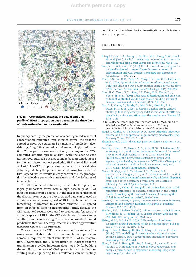
A specific comparison of the propagation pathways be-

tween the epidemiological investigation and the CFD-

computed prediction was analysed to check the geograph-

ical locations of farms with overestimated and under-

estimated infections in terms of the HPAI confirmation days.

The underestimated locations, as shown in the light blue

circle in Fig. 14, stand for the distance of farms (O-4, O-5, O-8,

and S-02) from the initial infected farms (O-1 and P-5) and the

farm (O-7) far away from the northwest principal wind. These

underestimated locations had less of an effect on the

pathogen-laden aerosol from the initial and additionally

infected farms. As a result, the HPAI infections occurred more

rapidly than the predicted airborne HPAI spread. This

outcome means that the HPAI infection was caused by other

factors, such as direct contact transmission, which is stronger

than airborne transmission. This result provides an illustra-

tion of the important limitations of the one-factor prediction

of HPAI spread and also provides an opportunity to make a

multifactor network for HPAI spread, including both indirect

airborne and direct contact transmissions of HPAI disease

between farms. The overestimated locations, as shown in the

dark red circles in Fig. 15, were located along the principle

wind direction and resulted in a significant effect by the

pathogen-laden aerosol from the infected farms. The over-

estimated locations were close to the road, affecting the

nearby farms from aerosols released by livestock vehicle

movements. The assumption of continuous aerosol emission

from a road could affect the overestimation compared to the

actual conditions by the intermittent movement of livestock

vehicles. Therefore, the weighting factors for the strength of

the road emissions must be controlled by the researchers

according to the field conditions.

4. Conclusions

The CFDmodel for airborne spread of HPAI was developed not

only using specific topography and obstacles, including live-

stock farms, vehicle movement, wooden area, and topo-

graphical classifications, but also connecting weather

Fig. 14 e CFD-predicted airborne propagation of HPAI disease from two initial infected farms during the 2008 HPAI outbreak

in Korea during Apr. 1st to Apr. 20th, 2008.



frequency data. By the prediction of a pathogen-laden aerosol

concentration generated from infected farms, the airborne

spread of HPAI was calculated by means of prediction algo-

rithm grafting CFD simulation and meteorological informa-

tion. This algorithm was used not only to compare the CFD-

computed airborne spread of HPAI with the specific case

during HPAI outbreak but also to make background database

for the multifactor network predicting HPAI spread discussed

on Part II. The CFD-computed simulation can provide valuable

data for predicting the possible infected farms from airborne

HPAI spread, which results in early control of HPAI propaga-

tion by effective preventive measures and the isolation of

infected farms.

The CFD-predicted data can provide data for epidemio-

logically important farms with a high possibility of HPAI

infection resulting in a decrease in the risk of transmission of

the disease. Moreover, the CFD-predicted data can be used as

a database for airborne spread of HPAI combined with the

forecasting information to estimate airborne HPAI spread

from an infected farm to neighbouring farms. Because the

CFD-computed results were used to predict and forecast the

airborne spread of HPAI, the CFD calculation process can be

omitted from the forecasting. This omission provides for rapid

predictions that could be very effective in selecting preventive

measures against HPAI outbreaks.

The accuracy of the CFD prediction should be enhanced by

using more reliable data for how much pathogen-laden

aerosol is required to infect animals with HPAI via respira-

tion. Nevertheless, the CFD prediction of indirect airborne

transmission provides important data, not only for building

the multifactor network of HPAI spread, but also for demon-

strating how engineering CFD simulations can be usefully

combined with epidemiological investigations while taking a

scientific approach.

r e f e r e n c e s

Bitog, J. P., Lee, I.-B., Hwang, H.-S., Shin, M.-H., Hong, S.-W., Seo, I.-H., et al. (2011). A wind tunnel study on aerodynamic porosityand windbreak drag. Forest Science and Technology, 7(1), 8e16.

Bournet, P., & Boulard, T. (2010). Effect of ventilator configurationon the distributed climate of greenhouses: a review ofexperimental and CFD studies. Computers and Electronics inAgriculture, 74, 195e217.

Chen, P. S., Lin, C. K., Tsai, F. T., Yang, C. Y., Lee, C. H., Liao, Y. S.,et al. (2009). Quantification of airborne influenza and avianinfluenza virus in a wet poultry market using a filter/real-timeqPCR method. Aerosol Science and Technology, 43(4), 290e297.

Choi, H. C., Yeon, G. Y., Song, J. I., Kang, H. S., Kwon, D. J.,Yoo, Y. H., et al. (2006). Dust spatial distribution and emissionof tunnel ventilated windowless broiler building. Journal ofLivestock Housing and Environment., 12(3), 145e152.

Cox, S. J., Voyce, C., Parida, S., Reid, S. M., Hamblin, P. A.,Paton, D. J., et al. (2005). Protection against direct-contactchallenge following emergency FMD vaccination of cattle andthe effect on virus excretion from the oropharynx. Vaccine, 23,1106e1113.

DFG, Deutsche Forschungsgemeinschaft. (2008). MAK- und BAT-Werte-Liste 2008 e Senatskommission zur Prufunggesundheitsschadlicher ArbeitstoffeeMitteilung 44.

Fiegel, J., Clarke, R., & Edwards, D. A. (2006). Airborne infectiousdisease and the suppression of pulmonary bioaerosols. DrugDiscovery Today, 11(1e2), 51e57.

Fluent Manual. (2008). Fluent user guide. version 6.3. Lebanon, N.H.,USA.

Franke, J., Hirsch, C., Jensen, A. G., Krus, H. W., Schatzmann, M.,Westbury, P. S., et al. (2004). Recommendations of the use ofCFD in wind engineering. In J. P. A. J. van Beeck (Ed.),Proceedings of the international conference on urban windengineering and building aerodynamics: COST action C14-impact ofwind and storm on city life and built environment. May 5e7,C.1.1eC.1.11, Rhode-Saint-Genese, Belgium.

Gaidet, N., Cappelle, J., Takekawa, J. Y., Prosser, D. J.,Iverson, S. A., Douglas, D. C., et al. (2010). Potential spread ofhighly pathogenic avian influenza H5N1 by wildfowl: dispersalranges and rates determined from large-scale satellitetelemetry. Journal of Applied Ecology, 1e11.

Germann, T. C., Kadau, K., Longini, I. M., & Macken, C. A. (2006).Mitigation strategies for pandemic influenza in the UnitedStates. Proceedings of the National Academy of Sciences of theUnited States of America, 103(15), 5935e5940.

Hayden, F., & Croisier, A. (2005). Transmission of avian influenzaviruses to and between humans. The Journal of InfectiousDiseases, 192, 1311e1314.

Hayden, F. G., & Palese, P. (2002). Influenza virus. In D. Richman,R. Whitley, & F. Hayden (Eds.), Clinical virology (2nd ed.) (pp.891e920). Washington, DC: ASM Press.

Hefny, M. M., & Ooka, R. (2009). CFD analysis of pollutantdispersion around buildings: effect of cell geometry. Buildingand Environment, 44, 1699e1706.

Hong, S., Lee, I., Hwang, H., Seo, I., Bitog, J. P., Kwon, K., et al.(2011a). CFD modelling of livestock odour dispersion overcomplex terrain, part I: topographical modelling. BiosystemsEngineering, 108, 253e264.

Hong, S., Lee, I., Hwang, H., Seo, I., Bitog, J. P., Kwon, K., et al.(2011b). CFD modelling of livestock odour dispersion overcomplex terrain, part II: dispersion modelling. BiosystemsEngineering, 108, 265e279.

Fig. 15 e Comparison between the actual and CFD-

predicted HPAI propagation days based on the three days

of underestimation and overestimation.



Jewell, C. P., Kypraios, T., Christley, R. M., & Roberts, G. O. (2009). Anovel approach to real-time risk prediction for emerginginfectious diseases: a case study in avian influenza H5N1.Preventive Veterinary Medicine, 91, 19e28.

Kim, H.-Y., Lee, Y.-J., Park, C.-K., Oem, J.-K., Lee, O.-S., Kang, H.-M., et al. (2012). Highly pathogenic avian influenza (H5N1)outbreaks in wild birds and poultry, South Korea. EmergingInfectious Diseases, 18(3), 480e483.

Kim, T.-H., Hwang, W.-C., Zhang, A. D., Sen, S., & Ramanathan, M.(2008). Multi-agent model analysis of the containmentstrategy for avian influenza (AI) in South Korea. In Proceedingsof the 2008 IEEE international conference on bioinformatics andbiomedicine (pp. 335e338).

Koopmans, M., Wilbrink, B., Conyn, M., Natrop, G., van derNat, H., Vennema, H., et al. (2004). Transmission of H7N7 avianinfluenza A virus to human beings during a large outbreak incommercial poultry farms in the Netherlands. The Lancet, 363,587e593.

Krumkamp, R., Hans-Peter, D., Ralf, R., Amena, A., Annette, K., &Martin, E. (2009). Impact of public health interventions incontrolling the spread of SARS: modelling of interventionscenarios. International Journal of Hygiene and EnvironmentalHealth., 212(1), 67e75.

Launder, B. E., & Spalding, D. B. (1974). The numericalcomputation of turbulent flows. Computer Methods in AppliedMechanics and Engineering, 3(2), 269e289.

Lee, S. J., Lee, S. D., Jeong, S. K., Ha, J. K., Jeong, J. W., Kim, I. Y.,et al. (2008). Highly pathogenic avian influenza in Korea in 2008.Animal and Plant Quarantine Agency (APQA). Report number11-1541002-000013-01 (in Korean).

Li, Y., & Guo, Y. (2008). Numerical simulation of aeolian dustysand transport in a marginal desert region at the earlyentrainment stage. Geomorphology, 100(3e4), 335e344.

Mayer, D., Reiczigel, J., & Rubel, F. (2008). A Lagrangian particlemodel to predict the airborne spread of foot-and-mouthdisease virus. Atmospheric Environment, 42, 466e479.

Mikkelsen, T., Alexandersen, S., Astrup, P., Champion, H. J.,Donaldson, A. I., Dunderley, F. N., et al. (2003). Investigation ofairborne foot-and-mouth disease virus transmission duringlow-wind conditions in the early phase of the UK 2001epidemic. Atmospheric Chemistry and Physics, 3, 2101e2110.

Milliez, M., & Carissimo, B. (2007). Numerical simulations ofpollutant dispersion in an idealized urban area, for differentmeteorological conditions. Boundary-Layer Meteorology, 122(2),321e342.

Sabatino, S. D., Buccolieri, R., Pulvirenti, B., & Britter, R. (2007).Simulations of pollutant dispersion within idealised urban-type geometries with CFD and integral models. AtmosphericEnvironment, 41(37), 8316e8329.

Seo, I.-H., Lee, I.-B., Moon, O.-K., Hong, S.-W., Hwang, H.-S.,Bitog, J. P., et al. (2011). Aerodynamic approaches for theprediction of spread the HPAI (highly pathogenic avianinfluenza) on aerosol. Journal of the Korean Society of AgriculturalEngineers, 53(1), 29e36.

Seo, I.-H., Lee, I.-B., Shin, M.-H., Lee, G.-Y., Hwang, H.-S., Hong, S.-W., et al. (2010). Numerical prediction of fugitive dustdispersion on reclaimed land in Korea. Transactions of theASABE, 53(3), 891e901.

Sørensen, J. H., Jensen, C.Ø., Mikkelsen, T., Mackay, D. K. L., &Donaldson, A. I. (2001). Modelling the atmospheric dispersionof foot-and-mouth disease virus for emergency preparedness.Physics and Chemistry of the Earth, Part B: Hydrology, Oceans andAtmosphere, 26(2), 93e97.

Spekreijse, D., Bouma, A., Koch, G., & Stegeman, J. A. (2011).Airborne transmission of a highly pathogenic avianinfluenza virus strain H5N1 between groups of chickensquantified in an experimental setting. Veterinary Microbiology,152, 88e95.

Takai, H., Pedersen, S., Johnsen, J. O., Metz, H. M., GrootKoerkamp, P. W. G., Uenk, G. H., et al. (1998). Concentrationsand emissions of airborne dust in livestock buildings inNorthern Europe. Journal of Agricultural Engineering Research, 70,59e77.

Tominaga, Y., Mochida, A., Yoshie, R., Kataoka, H., Nozu, T.,Yoshikawa, M., et al. (2008). AIJ guidelines for practicalapplications of CFD to pedestrian wind environment aroundbuildings. Journal of Wind Engineering and IndustrialAerodynamics, 96, 1749e1761.

Treanor, J. J. (2004). Influenza virus. In G. L. Mandell, J. E. Bennett,& R. Dolin (Eds.), Mandell, Douglas, and Bennett’s principles andpractice of infectious diseases (6th ed.) (pp. 2060e2085). ChurchillLivingstone.

Tsukamoto, K., Imada, T., Tanimura, N., Okamatsu, M., Mase, M.,Mizuhara, T., et al. (2007). Impact of different husbandryconditions on contact and airborne transmission of H5N1highly pathogenic avian influenza virus to chickens.Summarized from Avian Diseases, 51(1), 129e132.

Ungchusak, K., Auewarakul, P., Dowell, S. F., Kitphati, R.,Auwanit, W., Puthavathana, P., et al. (2005). Probable person-to-person transmission of avian influenza A (H5N1). The NewEngland Journal of Medicine, 352(4), 333e340.

Weber, T. P., & Stilianakis, N. I. (2008). Inactivation of influenza aviruses in the environment and modes of transmission: acritical review. Journal of Infection, 57(5), 361e373.

Wieringa, J., Davenport, A. G., Grimmond, C. S. B., & Oke, T. R.(2001). New revision of Davenport roughness classification. InProceedings of the 3rd European & African conference on windengineering (p. 8). Eindhoven, Netherlands, July 2001.

Woo, B.-J., Lee, H.-W., Hwang, Y.-J., Lee, J.-M., & Kim, J.-N. (2008).An economic impact and countermeasure policies of highlypathogenic avian influenza. Report for Korea Rural EconomicInstitute (p. 102).

Wright, P. F., & Webster, R. G. (2001). Orthomyxoviruses. InD. M. Knipe, & P. M. Howley (Eds.), Fields virology (4th ed.) (pp.1533e1579). Philadelphia: Lippincott Williams & Wilkins.

Yang, Y., Halloran, M. E., Sugimoto, J. D., & Longini, I. M. (2007).Detecting human-to-human transmission of avian influenzaA (H5N1). Emerging Infectious Diseases, 13(9), 1348e1353.


Prediction of the spread of highly pathogenic avian influenza using a multifactor network: Part 1...

Documents

Transcript of Prediction of the spread of highly pathogenic avian influenza using a multifactor network: Part 1...