Predicting the Demand for Central Bank Digital Currency

Bank of Canada staff working papers provide a forum for staff to publish work-in-progress research independently from the Bank’s Governing Council. This research may support or challenge prevailing policy orthodoxy. Therefore, the views expressed in this paper are solely those of the authors and may differ from official Bank of Canada views. No responsibility for them should be attributed to the Bank. ISSN 1701-9397 ©2021 Bank of Canada

Staff Working Paper/Document de travail du personnel — 2021-65

Last updated: December 20, 2021

Predicting the Demand for Central Bank Digital Currency: A Structural Analysis with Survey Data by Jiaqi Li

Banking and Payments Department Bank of Canada, Ottawa, Ontario, Canada K1A 0G9

[email protected]

i

Acknowledgements I am grateful to Jonathan Chiu and Yu Zhu for constructive feedback and useful guidance throughout the development of this paper. I want to thank Kim Huynh for helpful suggestions at various stages of this project and the Economic Research and Analysis team of the Currency Department at the Bank of Canada for providing the cleaned payment survey data. I thank Shutao Cao, Heng Chen, Marie-Hélène Felt, Sofia Lu, Adi Mordel and Yaz Terajima for sharing their knowledge about the datasets. I am also grateful to Matteo Benetton (discussant), Rod Garratt, Paul Grieco, Charles Kahn, Katrin Tinn (discussant) and my Bank of Canada colleagues for their insightful comments. Finally, I thank the seminar participants at the following conferences and seminars for their useful feedback: Bank of Canada seminars, Research Workshop by Bank of Canada and Payments Canada, SNB-CIF Conference on Cryptoassets and Financial Innovation, CEA Annual Conference, International Cash Conference by Deutsche Bundesbank, Asian Meeting of the Econometric Society, China Meeting of the Econometric Society, EARIE Annual Conference, and ECB virtual seminar.

ii

Abstract This paper predicts households’ demand for a central bank digital currency (CBDC) with different design attributes by applying a structural demand model to a unique Canadian survey dataset. CBDC and its close alternatives, cash and demand deposits, are viewed as product bundles of different attributes. I estimate households’ preferences towards these attributes from how they allocate their liquid assets between cash and demand deposits. The estimated preferences are used to predict the demand for CBDC with a set of design attributes and quantify the impacts of CBDC design choices on CBDC demand. Under a baseline design for CBDC, the aggregate CBDC holdings out of households’ liquid assets could range from 4 to 52%, depending on whether households would perceive CBDC to be closer to cash or deposits. I find that important design attributes include budgeting usefulness, anonymity, bundling of bank services and rate of return.

Topics: Central bank research, Digital currencies and fintech JEL codes: E50, E58

1 Introduction

Many central banks around the world are contemplating the issuance of a central bank

digital currency (CBDC), a digital form of central-bank-issued money. According to a Bank

for International Settlements (BIS) survey in 2020, 86% of central banks are engaging in

CBDC work and 14% have already reached the pilot stage.1 To decide whether to issue a

CBDC,2 a central bank needs to consider three important questions: What would be the

demand for CBDC? How would the design attributes of CBDC affect the demand? To what

extent would CBDC impact the demand for cash and deposits? This paper helps answer

these questions empirically.

Serving as a store-of-value asset and a payment instrument, CBDC is an alternative to

cash and demand deposits. According to a recent BIS report, one foundational principle

for CBDC issuance is that CBDC should complement and co-exist with cash and deposits

(BIS, 2020). This paper represents the first attempt to empirically quantify households’

potential CBDC holdings relative to cash and demand deposits, the impacts of different

design attributes on CBDC holdings, and the extent to which CBDC may crowd out the

demand for cash and deposits.

While there is emerging theoretical literature on the implications of CBDC (e.g., Andol-

fatto, 2021; Williamson, 2021b; Chiu et al., 2020; Brunnermeier and Niepelt, 2019; Keister

and Sanches, 2019), the lack of data on CBDC poses a constraint to the empirical work. This

paper provides a framework to predict the potential demand for CBDC relative to its close

alternatives, cash and demand deposits. The key idea is to view CBDC, cash, and demand

deposits as product bundles of different attributes based on a structural demand model. I

estimate households’ preferences for the attributes by applying the model to survey data on

the existing products. Provided that the estimated preferences remain the same after CBDC

issuance, I can predict the demand for CBDC based on its design attributes and how much

households value each attribute, and study how the CBDC demand would be affected by

different design attributes.

More specifically, a household obtains an utility from holding each product, which de-

1Respondents to the BIS survey include 21 advanced economies and 44 emerging market economies,covering 91% of the world economic output (Boar and Wehrli, 2021). Examples of retail CBDC pilotsinclude the DCEP in China, the e-krona in Sweden, and the e-peso in Uruguay.

2This paper focuses on the retail CBDC that is available to the general public and can be used for retailtransactions. For some countries including Canada, the motivation for considering the issuance of a retailCBDC is in part driven by declining cash usage as documented in Engert, Fung and Segendorff (2019),which could lead to financial exclusion of certain groups of people, and in part as a response to the potentialrisks posed by privately issued e-money (e.g., Adrian and Mancini-Griffoli, 2019; Brunnermeier, James andLandau, 2019; Zhu and Hendry, 2019). For other motivations for issuing CBDC, see Kahn, Rivadeneyra andWong (2018), Engert and Fung (2017), and Fung and Halaburda (2016), among others.

1

pends on the attributes of the product, the household characteristics, and the product fixed

effect that captures the average impact of unobserved households’ idiosyncratic preferences.

Without CBDC, the household decides how to allocate the endowment of liquid assets be-

tween cash and demand deposits based on the relative utilities from holding cash and de-

posits, which in turn depend on the differences in the product attributes. Using a unique

Canadian survey dataset that contains households’ cash and deposit shares out of their liquid

assets and the product attributes of cash and deposits, I can estimate households’ preferences

towards each product attribute.

To predict the demand for CBDC with a certain design, apart from the chosen design

attributes of CBDC and the estimated preference parameter for each attribute, I also need to

make assumptions on the CBDC-specific effects that consist of the impacts of the household

characteristics and the CBDC fixed effect on the utilities for holding CBDC. The effects

related to the household characteristics reflect how households from a given demographic

group would value CBDC relative to cash and demand deposits, while the CBDC fixed

effect reflects the average impact of households’ idiosyncratic preferences on their utilities

for CBDC. In the counterfactual analyses, I assume these CBDC-specific effects can range

from being cash-like, in which case households would perceive CBDC to be closer to cash,

to being deposit-like, in which case they would perceive CBDC to be closer to deposits.

I find that under a baseline design for CBDC, where CBDC is non-interest-bearing, un-

bundled with bank services, and achieves 70% of cash budgeting usefulness and anonymity,

the total CBDC holdings out of households’ liquid assets could range from 4–52% of their

liquid assets. The exact level of CBDC demand in this range depends on the assumptions

for CBDC-specific effects. The lower (upper) bound prediction is obtained when assuming

CBDC-specific effects are cash-like (deposit-like).3 Since a median household only holds

around 4% of their liquid assets in cash, the demand for CBDC would also be low if house-

holds perceive CBDC to be closer to cash. Similarly, this paper finds that households with

higher income, older age, or that are home owners tend to hold more CBDC balance if

CBDC-specific effects are more cash-like, since these groups tend to hold more cash.

Unlike the predicted level of CBDC demand, the percentage change in CBDC demand

in response to a change in a given attribute would rely much less on CBDC-specific effects.

By studying the impacts of different design attributes, this paper provides useful insights

on how much each design attribute would matter for CBDC demand. I find that important

design attributes include usefulness for budgeting, anonymity, bundling of bank services, and

rate of return, which are ranked in a decreasing order of importance, except for the rate of

3With more information on whether households would perceive CBDC to be closer to cash or deposits,it could be possible to take a stance on the CBDC-specific effects and thus narrow down this range.

2

return whose impact depends on the magnitude of the rate change.4

I measure the impact of each product attribute using the percentage change in CBDC

demand in response to a change in the given attribute relative to the baseline design, while

keeping everything else unchanged. I find that reducing the budgeting usefulness of CBDC

from 70% of cash usefulness to deposit usefulness would lower CBDC demand by around

7–14%, depending on different assumptions for CBDC-specific effects. Reducing CBDC

anonymity from 70% of cash anonymity to 0% like deposits would lower CBDC demand by

around 5–10%. If CBDC becomes bundled with bank services, its demand would increase

by around 4–8%. Finally, increasing the CBDC rate from 0% to 0.1% could raise its demand

by around 10–23%.5 The estimated model also allows for studying the impacts of changes

in CBDC designs where a combination of different attributes change at the same time. For

example, moving from a cryptocurrency design with a full degree of cash anonymity to the

Sand Dollar design with a low level of anonymity could reduce CBDC demand by around

6–10%.

In this framework, the demand for CBDC comes from households’ liquid assets, so it is

natural to examine the crowding-out effects of CBDC on the demand for cash and deposits.

Since a higher demand for CBDC tends to reduce cash and deposit demand by more, CBDC-

specific effects also play a large role here. When CBDC-specific effects are deposit-like (cash-

like), CBDC with a baseline design can reduce the demand for deposits and cash each by

around 52% (4%) on average across households.

The empirical literature on CBDC is scarce. To the best of my knowledge, there are

two empirical papers on CBDC (Bijlsma et al., 2021; Huynh et al., 2020). Huynh et al.

(2020) focuses on consumers’ choices of using CBDC to pay at the point of sale. They study

consumers’ payment choices among cash, debit cards, and credit cards and use the estimated

demand parameters to predict the adoption and usage of CBDC as a new payment instru-

ment. In contrast, this paper focuses on households’ potential holdings of CBDC, taking

into account the role of CBDC as both a store-of-value asset and a payment instrument.

Predicting the potential holdings of CBDC is important for understanding how much CBDC

would affect bank deposits, which are a relatively low-cost and stable funding source for

banks. Bijlsma et al. (2021) conducted a survey on the adoption and usage intention for

hypothetical CBDC accounts in the Netherlands. In the absence of a CBDC or a concrete

design for CBDC, this survey approach is challenging because the results would rely heav-

ily on people’s understanding of CBDC based on a broad description for CBDC. The key

4Other product attributes that are studied in this paper include cost of use, ease of use/convenience,security, capability of online purchase, and merchant acceptance.

5The median demand deposit rate after tax was around 0.08% across households during 2010–2017.Therefore, the change of 0.1 percentage points in CBDC interest rate is a large change.

3

difference here is that I use households’ preferences that are revealed from their allocation decisions on cash and demand deposits to predict their potential holdings of CBDC with aset of design attributes.

The paper is also related to the growing literature on how CBDC could affect bank deposits and thus financial intermediation (e.g., Andolfatto, 2021; Garratt and Zhu, 2021; Chiu et al., 2020; Keister and Sanches, 2019).6 This literature often assumes CBDC to be

a perfect substitute for deposits and focuses on the rate of return differences, which directly implies the substitution pattern between the demand for deposits and CBDC. That is, the one that offers a lower rate of return would face a zero demand. In contrast, this paper models CBDC as an imperfect substitute for deposits, where CBDC can differ from deposits

in a variety of product attributes, including the rate of return. In doing so, the paper provides empirical evidence on the extent to which the demand for CBDC would be affected by different design attributes of CBDC.7 Since the demand for CBDC would come from the liquid assets like deposits, the paper also sheds light on the crowding-out effect of CBDC on the demand for deposits under different CBDC designs.

The rest of this paper is organized as follows. Section 2 describes the structural demand model and then introduces CBDC into the model. Section 3 discusses the data sources and how to measure different product attributes using the survey data. Section 4 shows the estimated demand parameters. Section 5 uses the estimated model to predict the demand

for CBDC relative to cash and demand deposits, the crowding-out effects on the demand for cash and deposits, the impacts of different design choices on CBDC demand, and the CBDC holdings across different demographic groups. Section 6 concludes.

6Existing theoretical literature also looks at the impact of CBDC on financial stability (e.g., Fernandez-Villaverde et al., 2021; Williamson, 2021a; Schilling, Fernandez-Villaverde and Uhlig, 2020; Brunnermeier and Niepelt, 2019; Skeie, 2019), monetary policy (e.g., Davoodalhosseini, 2021; Jiang and Zhu, 2021; Bordo and Levin, 2017), macroeconomic volatility (e.g., Barrdear and Kumhof, 2021; Ferrari, Mehl and Stracca, 2020), and welfare (e.g., Assenmacher et al., 2021; Williamson, 2021b; Piazzesi and Schneider, 2020). For policy discussions on the macro implications of CBDC issuance, see Davoodalhosseini, Rivadeneyra and Zhu (2020), Garcıa et al. (2020), Berentsen and Schar (2018), Mancini-Griffoli et al. (2018), Meaning et al. (2018), Engert and Fung (2017), etc.

7There are a few theoretical papers focusing on certain design features of CBDC, such as anonymity and security in Agur, Ari and Dell’Ariccia (2021), automation of personal loss recovery via an expiry date onoffline CBDC balances proposed in Kahn, van Oordt and Zhu (2021), and asymmetric privacy between thereceiver and the sender of money in Tinn and Dubach (2021). Kahn, Rivadeneyra and Wong (2020) look atthe trade-offs between safety and convenience of digital currencies in general, which provides guidance forthe design of CBDC. For policy discussions on the technical design choices and the design principles, seeAllen et al. (2020), Auer and Bohme (2020), Kumhof and Noone (2018), etc.

4

2 Model

Section 2.1 introduces a logit demand model to study how households allocate their liquid

assets between cash and demand deposits. I use this structural demand model to study

asset allocation because households’ utilities are modeled in terms of the product attributes,

which facilitates the counterfactual analysis of introducing a CBDC with a set of design

attributes. The model can be equivalently written in terms of an asset allocation problem

with money-in-the-utility assumptions and a constant-elasticity-of-substitution (CES) utility

function, as shown in Appendix A.1.

Section 2.2 introduces CBDC and discusses how to predict the potential demand for

CBDC based on a logit model and a nested logit model. Under the logit model, there are

no common factors that drive the unobserved idiosyncratic preferences for CBDC, cash, and

deposits. In contrast, the nested logit model allows CBDC to be a closer substitute for cash

(deposits) due to the correlated idiosyncratic preferences for CBDC and cash (deposits).

Appendix A.2 shows that the nested logit model can be equivalently represented by an asset

allocation problem with money-in-the-utility assumptions and a nested CES utility function.

2.1 Logit Model of Cash and Deposit Demand

Assume each household i is endowed with wi,t dollars in period t. For each dollar, household

i chooses to hold it in cash c or demand deposits d. Household i’s indirect utility u for

product j ∈ c, d depends on the product attributes xi,j,t, household characteristics zi,t, a

product-specific constant ηj, and an i.i.d. utility shock εi,j,t:

ui,j,t = α′xi,j,t + γ ′jzi,t + ηj + εi,j,t = Vi,j,t + εi,j,t (1)

where Vi,j,t ≡ α′xi,j,t +γ ′jzi,t + ηj is the observable part of the indirect utility. The vector α

consists of the preference parameters for the product attributes. Parameters γj reflect the

effects of household characteristics on the utility for holding product j. The utility shock εi,j,t

captures the unobserved idiosyncratic preferences and the constant ηj reflects the average

impact of these unobserved preferences on the utility for product j. In the presence of ηj,

the mean of the unobserved part of the utility εi,j,t is zero.

Since the utility shock εi,j,t is randomly drawn from a given distribution, even if the

observed utility for holding the one dollar in cash is higher, that is, Vi,c,t > Vi,d,t, there is a

probability that the unobserved portion of the utility for deposits εi,d,t is sufficiently higher

to overcome the lower Vi,d,t such that household i chooses to hold it in deposits instead. Let

f(εi,t) denote the joint density of the random vector εi,t = (εi,c,t, εi,d,t). The probability that

5

household i chooses product j is:

Pi,j,t =

∫ε

I(εi,k,t − εi,j,t < Vi,j,t − Vi,k,t ∀ k 6= j)f(εi,t)dεi,t (2)

where k denotes the product other than j and I(.) is an indicator that equals one if the

condition inside the brackets is true and zero otherwise. Assuming the i.i.d. utility shock

follows a Type I extreme value distribution, the choice probability of holding the one dollar

in product j is:

Pi,j,t =exp(Vi,j,t)

exp(Vi,c,t) + exp(Vi,d,t)∈ (0, 1) (3)

where j ∈ c, d. When the observed attributes of product j improves such that the observed

utility Vi,j,t increases, the probability of choosing product j also increases, given everything

else remains the same.

With the endowment of wi,t dollars, household i makes wi,t number of choices. By the

law of large numbers, the probability Pi,j,t of holding the one dollar in asset j is equivalent

to the share si,j,t ≡ qi,j,twi,t

of asset j out of the liquid asset wi,t, where qi,j,t denotes the balance

of asset j and wi,t = qi,c,t + qi,d,t is the total liquid asset (sum of cash and demand deposit

balances) held by household i.8 After taking the difference between the logs of deposit and

cash shares, the log of deposit-to-cash ratio can be written as:

lnqi,d,tqi,c,t

= Vi,d,t − Vi,c,t = α′(xi,d,t − xi,c,t) + (γd − γc)′zi,t + ηd − ηc (4)

which depends on the difference between the observed utilities for deposits and cash. This

utility difference in turn depends on the differences in the product attributes (xi,d,t −xi,c,t),the household characteristics zi,t, and the difference in the product-specific constants (ηd −ηc).

The choice probability (2) shows that only the utility difference matters for households’

choices, so the effects of household characteristics can only be identified if they are product-

specific (i.e., γd 6= γc). Since different values of γd and γc that result in the same differences

(γd − γc) will give the same choices, the overall level of (γd − γc) needs to be set and the

same applies to (ηd−ηc). I follow a common approach to normalize the parameters for cash,

8The interpretation of choice probabilities as asset shares is also used in Wang et al. (2020) and Xiao(2020). They assume that each agent is endowed with one dollar and makes a discrete choice among differentassets. They point out that this one-dollar one-choice assumption can be interpreted as a situation whereagents make multiple discrete choices for their one-dollar endowment and the probability of choosing eachasset can be interpreted as the portfolio weight. Similarly, Ellickson, Grieco and Khvastunov (2020) studythe discrete choice for each unit of the consumer’s grocery expenditure and the probability for choosing aparticular store is interpreted as the share of the consumer’s expenditure spent at that store.

6

γc and ηc, to zero. After this normalization, the estimated ηd reflects the average impact of

the unobserved idiosyncratic preferences on the utility for deposits relative to cash and the

estimated γd reflects the effects of household characteristics zi,t on the utility for deposits

relative to cash.

2.2 Introducing CBDC

To predict the demand for CBDC, one key step is to calculate each household’s observed

utility Vi,cbdc,t for CBDC. Provided that the estimated preference parameters α remain the

same after CBDC issuance, the utility for CBDC can be calculated using the CBDC at-

tributes xi,cbdc and the assumptions on the CBDC-specific effects (i.e., γcbdc and ηcbdc) as

below:

Vi,cbdc,t = α′xi,cbdc + γ ′cbdczi,t + ηcbdc (5)

In the counterfactual analyses, I assume these CBDC-specific effects, γcbdc and ηcbdc, can

range from being cash-like (i.e., taking the normalized parameter values for cash γc = 0 and

ηc = 0) to deposit-like (i.e., taking the estimated values for deposits γd and ηd). In reality,

the parameters γcbdc and ηcbdc could lie outside this range, but this paper does not consider

these cases that require extrapolation. Instead, it predicts the potential demand for CBDC

relative to cash and demand deposits by focusing on the values of γcbdc and ηcbdc in between

the corresponding values for cash and deposits.

If households perceive CBDC to be closer to cash (deposits), then the CBDC-specific

effects are likely to be more cash-like (deposit-like). More specifically, assuming γcbdc = γc

implies that the household characteristics have identical effects on the utilities for cash and

CBDC. In other words, households from a given demographic group would equally value

CBDC and cash. Assuming ηcbdc = ηc means that the average impact of the unobserved

idiosyncratic preferences on the utility for CBDC is identical to that for cash. In contrast,

assuming γcbdc = γd and ηcbdc = ηd implies that the household characteristics and the

unobserved idiosyncratic preferences have identical effects on the utilities for deposits and

CBDC.

2.2.1 Predictions Based on Logit Model

Apart from the observed utility Vi,cbdc,t (5), another key component for predicting the demand

for CBDC is the distribution of the random utility shock εi,j,t, where j ∈ c, d, cbdc. This

section introduces CBDC into the logit demand model described in Section 2.1, where εi,j,t

is assumed to be i.i.d Type I extreme value. After CBDC issuance, household i allocates

the endowment of the liquid asset wi,t into CBDC, cash, and demand deposits. With the

7

distributional assumption on εi,j,t, the probability of allocating each dollar of the endowment

wi,t into CBDC, or equivalently, the share of CBDC holding, is:

si,cbdc,t =exp(Vi,cbdc,t)

exp(Vi,c,t) + exp(Vi,d,t) + exp(Vi,cbdc,t)(6)

A higher observed utility Vi,cbdc,t leads to a larger share of CBDC holding, keeping everything

else the same. Given that wi,t is unaffected by the CBDC issuance, the demand for CBDC

comes from the substitution away from cash and deposits.9 In this logit framework, the

demand for CBDC draws proportionally from cash and deposits so that the deposit-to-cash

ratio remains unchanged as in (4).

This independence of irrelevant alternatives (IIA) property – the deposit-to-cash ratio be-

ing unaffected by the introduction of CBDC – is due to the assumption that the unobserved

factors are i.i.d. across products. The resulting substitution patterns can be restrictive in

some cases. For example, supposing CBDC and deposits are perfect substitutes, the de-

mand for CBDC should only draw from deposits while cash demand is unaffected. However,

this perfect substitute case cannot be captured in the logit framework. Even if CBDC and

deposits have an identical observed utility, they are still imperfect substitutes due to the un-

observed idiosyncratic preferences. To allow for different degrees of substitutability between

CBDC and the existing products and thus more flexible substitution patterns, Section 2.2.2

introduces a nested logit framework which avoids the IIA property.

2.2.2 Predictions Based on Nested Logit Model

This section introduces CBDC into a nested logit framework to capture more general sub-

stitution patterns. The unobserved utilities εi,t = (εi,c,t, εi,d,t, εi,cbdc,t) that capture the id-

iosyncratic preferences are now jointly distributed as generalized extreme value and can be

correlated across products that are closer substitutes. Suppose CBDC and deposits are

closer substitutes due to the correlated unobserved utilities, then the demand for CBDC

would mainly draw from deposits. This section discusses, in turn, the cases where CBDC is

a closer substitute for deposits or cash.

9In this paper, the liquid asset only consists of cash and demand deposits because they are close alter-natives to CBDC. The assumption that the liquid asset holding is unaffected by CBDC issuance is realisticas long as the CBDC interest rate is lower than the deposit rate, in which case the introduction of CBDCis unlikely to cause substitution away from other types of liquid assets into CBDC. For the counterfactualanalyses in Section 5, I assume that CBDC is non-interest-bearing under the baseline design.

8

Case I. CBDC as a closer substitute for deposits

Suppose the unobserved utilities for CBDC and deposits are correlated and hence they are in

the same nest Bd cbdc. This could be because households value the feature of digital payments,

which cannot be identified empirically since there are no data on their perceptions towards

this feature. Since CBDC and deposits can both be used for digital payments, this feature

could drive the correlation between their unobserved utilities. The probability of household

i allocating each dollar into CBDC is the conditional probability of choosing CBDC from

the nest Bd cbdc multiplied by the probability of choosing the nest Bd cbdc:

Pi,cbdc,t =exp

(Vi,cbdc,tτd

)exp

(Vi,cbdc,tτd

)+ exp

(Vi,d,tτd

)︸︷︷︸

Prob(j=cbdc|j∈Bd cbdc)

[exp

(Vi,cbdc,tτd

)+ exp

(Vi,d,tτd

)]τd[exp

(Vi,cbdc,tτd

)+ exp

(Vi,d,tτd

)]τd+ exp (Vi,c,t)︸︷︷︸

Prob(j∈Bd cbdc)

(7)

where τd ≡√

1− ρd cbdc ∈ (0, 1] is an inverse measure of the correlation ρd cbdc ∈ [0, 1)

between the unobserved utilities for deposits and CBDC. The observed utilities for CBDC

and deposits are scaled by a factor of 1τd

. Intuitively, this is because a positive correlation

between their unobserved utilities implies a greater role of the observed utilities in explaining

the choices between deposits and CBDC.10 When the unobserved utilities are uncorrelated

(i.e., τd = 1), this reduces to the logit model where the CBDC share (7) would be identical

to (6).

Due to the correlated unobserved utilities within the nest, cash and deposits no longer

substitute proportionally into CBDC. Appendix B.1 shows that the deposit-to-cash ratios′i,d,ts′i,c,t

after CBDC issuance becomes:

s′i,d,ts′i,c,t

=

[1 + exp

(Vi,cbdc,t − Vi,d,t

τd

)]τd−1 si,d,tsi,c,t

(8)

wheresi,d,tsi,c,t

= exp (Vi,d,t − Vi,c,t) is the deposit-to-cash ratio before the CBDC issuance. When

CBDC is a perfect substitute for deposits (i.e., Vi,cbdc,t = Vi,d,t and τd approaches 0), the

deposit-to-cash ratio after CBDC issuance is reduced by a half, since half of the deposits

would be substituted into CBDC while cash is unaffected. Appendix B.1 shows that when 0 <

τd < 1, the deposit-to-cash ratios′i,d,ts′i,c,t

becomes smaller than that before the CBDC issuance,

10A higher correlation between the unobserved utilities for deposits and CBDC lowers the variance of(εi,cbdc,t − εi,d,t). Let Var(εi,d,t) = Var(εi,cbdc,t) = σ2 denote the variance of the unobserved utilities, wherethe logit model implicitly scales the utilities for all products such that the unobserved utilities have a

variance of σ2 = π2

6 . Under the logit model, Var(εi,cbdc,t − εi,d,t) = 2σ2, while under the nested logit model,Var(εi,cbdc,t − εi,d,t) = 2σ2 − 2σ2ρd cbdc = 2σ2(1− ρd cbdc), which is reduced by a factor of (1− ρd cbdc).

9

since the demand for CBDC draws more than proportionally from deposits. Furthermore,

the crowding-out effect on deposits is stronger if CBDC has a higher observed utility than

deposits (i.e., Vi,cbdc,t − Vi,d,t > 0), as shown in Appendix B.1.

How the correlation impacts the CBDC share depends on the difference in the observed

utilities for CBDC and deposits, as shown in Appendix B.1. When the observed utility

for CBDC is higher than that for deposits, it is ambiguous how the correlation affects the

CBDC share. On the one hand, a higher correlation ρd cbdc makes CBDC and deposits

more substitutable and thus leads to greater substitution from deposits to CBDC when

(Vi,cbdc,t − Vi,d,t) > 0, which tends to raise the CBDC share. On the other hand, the higher

correlation implies that the demand for CBDC would mainly draw from its closer substi-

tute, deposits. As the cash demand is reduced by less, the share that can be allocated to

deposits and CBDC is smaller, which tends to reduce the CBDC share. In contrast, when

(Vi,cbdc,t − Vi,d,t) 6 0, the former effect reinforces the latter and it is unambiguous that a

higher correlation reduces the CBDC share.

Case II. CBDC as a closer substitute for cash

Suppose CBDC and cash are closer substitutes along the unobserved dimensions and hence

they are in the same nest. One example of the unobserved factor could be that people value

the central-bank-issued money. Since CBDC and cash are both issued by the central bank

and this feature cannot be identified empirically due to the lack of data, this can lead to

a positive correlation between the unobserved utilities for CBDC and cash. Appendix B.2

shows that in this case, the deposit-to-cash ratio after CBDC issuance becomes:

s′i,d,ts′i,c,t

=

[1 + exp

(Vi,cbdc,t − Vi,c,t

τc

)]1−τc si,d,tsi,c,t

(9)

where τc ≡√

1− ρc cbdc ∈ (0, 1] is an inverse measure of the correlation ρc cbdc ∈ [0, 1) between

the unobserved utilities for CBDC and cash. Appendix B.2 shows that the deposit-to-cash

ratio is greater than or equal to that before CBDC issuance, since the demand for CBDC

mainly draws from its closer substitute, which is cash in this case.

How the CBDC share changes with the correlation depends on the sign of the observed

utility difference, as shown in Appendix B.2. If the observed utility for CBDC is higher than

that for cash, it is ambiguous how the CBDC share is affected by the correlation. On the one

hand, when (Vi,cbdc,t − Vi,c,t) is positive, a higher correlation ρc cbdc tends to raise the CBDC

share by making CBDC and cash more substitutable. On the other hand, as the demand

for CBDC draws mainly from its closer substitute (i.e., cash), deposits become less affected

10

and thus the total share of CBDC and cash is lower, which tends to lower the CBDC share.

In contrast, when (Vi,cbdc,t − Vi,c,t) 6 0, the former effect is reversed and the CBDC share

unambiguously decreases in ρc cbdc.

3 Data

This paper uses the Canadian Financial Monitor (CFM) survey and the Methods-of-Payment

(MOP) survey. The former is a syndicated survey run by Ipsos, while the latter is a Bank

of Canada survey. The CFM survey provides detailed information on households’ deposit

and cash holdings and has some repeated cross sections.11 The MOP survey is a cross-

sectional dataset and has two components: a survey questionnaire that contains information

on people’s perceptions towards different payment features, and a payment diary that records

detailed transaction-level data for each respondent during a three-day period.

In this paper, cash is measured as the sum of cash in wallet and the precautionary holding

of cash. The paper focuses on the sample period of 2010–2017 for the CFM data because

the survey questions on cash holdings are consistent across years during this period.12 It

focuses on the demand deposits, which can be readily used for transactions and thus are

a close alternative to CBDC. Therefore, deposits are measured by the sum of chequing,

chequing/saving, and saving account balances for each household. Figure 10 in Appendix C.1

shows the usage of all the bank account types that are classified in the CFM data. Detailed

information on the measures of cash and deposit holdings can be found in Appendix C.1.1

and C.1.2.

The MOP survey in 2013 consisted of three subsamples, one of which was formed by

recruiting the respondents who had recently filled out the CFM survey. These two datasets

are matched using the common ID documented by the survey company Ipsos.13 Apart from

11Although CFM has repeated observations for some households, this panel dimension is not intentional.There is a high attrition rate, so the survey company recruits new participants to maintain a nationallyrepresentative survey in each year, as discussed in Chen, Felt and Huynh (2014).

12During 2010–2017, the question on cash in wallet is: “How much cash do you have in your purse orwallet right now?” and the question on precautionary cash holding is: “(On average), how much cash onhand does your household hold for emergencies, or other precautionary reasons?”. Note that the phrase “onaverage” is included in the question for 2010–2012, while it is not included for 2013–2017. This difference isless of a concern after controlling for the year fixed effects. The results are robust to using the sample periodof 2013–2017 only.

13Note that the MOP survey questions are addressed to a given individual, while the CFM is a household-level survey where the questions are often addressed to a given household. Without having data on everyone’sperceptions in the same household, this paper assumes that the individual’s perceptions are representativeof the given household and would affect the household’s asset allocation decision. Felt (2017) also usesinformation from both the CFM and MOP data in 2013 to study the influence of the spouse on a person’spayment method usage in Chapter 3, adopting the method proposed in Felt (2020) to deal with the unob-

11

the product attributes, household characteristics can also affect the utilities from holding

cash and deposits. When estimating the demand parameters in Section 4, this paper also

includes household income, household head age and education, household size, home owner-

ship, whether the household has a female head, region, rural area, whether there is internet

access at work, households’ attitudes towards investing in the stock market, the extent to

which they feel difficulty in paying off debt, and whether anyone from the household was

behind debt obligations in the past year. These variables are from the CFM data except for

the internet access which is from the MOP survey questionnaire. Table 7 in Appendix C.5

shows the summary statistics of the key variables of interest.

To predict the demand for CBDC with a set of design attributes and assess how different

attributes would affect the demand for CBDC, a key step is to estimate households’ prefer-

ences for these product attributes. This paper uses the MOP survey to measure most of the

product attributes, including the cost of use, ease of use/convenience, security, anonymity,

usefulness for budgeting, capability of online purchase, and merchant acceptance rate. In

addition, rate of return and bundling of bank services are measured using the CANNEX and

CFM data, respectively. The details for each attribute are discussed below.

Rate of Return

The return on deposits tends to differ across households as they save at different banks. One

unique feature of the CFM data is that there is information on the main financial institution

of a given household.14 I use this information together with the bank-level deposit rates

from CANNEX to construct the household-specific deposit rates.15 However, among the

main financial institutions on the CFM choice list that households can choose from, only the

big six and Laurentian Bank have the demand deposit rates available from CANNEX during

the sample period. Hence, I use the rates for these seven banks and assume the deposit rates

of other banks to be the average across these seven banks.16

served behavior of the person’s spouse in a given household due to the lack of data. In contrast, this paperfocuses on decisions at the household level.

14Details on the construction of the main financial institution for each household can be found in AppendixC.1.3.

15Mulligan and Sala-i-Martin (2000) use the marginal tax rate facing each household to proxy for the rateof return, assuming households face the same pretax interest rate. However, they only have three differentmarginal tax rates in their dataset (1989 Survey of Consumer Financial for the US). In addition, the marginaltax rates do not provide much more information once income is controlled for. Attanasio, Guiso and Jappelli(2002) avoid this problem using the regional variation in the interest rates for their cross-sectional datasetof Italian households during 1989–1995. In contrast, this paper uses the cross-bank and over-time variationinstead, since there are no data for the Canadian deposit rates at a regional level.

16The results in this paper are robust to dropping the households whose main financial institutions arenot the big six or Laurentian Bank, accounting for about 33% of the observations. More information about

12

Since the interest earned on savings is taxed at the same marginal rate as income, I

multiply the net interest rate by one minus the marginal tax rate on household income using

the federal and provincial income tax rates during 2010–2017 published on the website of the

Government of Canada. Figure 12 in Appendix C.3 shows the average deposit rates across

households over the period of 2010–2017.

Cost, Ease of Use, and Security

To measure the cost, ease of use, and security features of cash and deposits, I use the

respondents’ ratings for each of these features from the MOP survey questionnaire. For a

given payment feature, each individual chooses a rating from one to five on a Likert scale

for each of the payment instruments, including cash, debit card, and credit card.17 For

instance, the survey question on cost asks people how costly they think it is (or would be)

to use each payment instrument, taking fees and interest payments into account. Similarly,

the questions on ease of use and security ask people how easy or hard and how risky or

secure it is (or would be) to use each payment instrument, respectively. I use the debit card

ratings to measure the cost, ease, and security of using deposits to make payments. Table

6 in Appendix C.5 shows that most people perceive cash to be a very low-cost, easy-to-use,

and secure payment instrument compared to other payment instruments in the MOP 2013

survey.

Following Arango, Huynh and Sabetti (2015), I standardize the ratings by the respon-

dent’s overall level of perceptions over cash, debit card, and credit card for each payment

feature. For example, a respondent who rates 5, 2, 2 for the ease-of-use feature of cash,

debit card, and credit card, respectively, has a standardized rating of 5/9 for cash and thus

perceives cash to be easier to use compared to a respondent who rates 5 for all three payment

instruments.18

Bundling of Bank Services

Deposits are often bundled with other services provided by banks. To capture this comple-

mentarity between deposits and other bank services, this paper uses households’ attitudes

the demand deposit rates from CANNEX can be found in Appendix C.3.17The ratings for each feature are also available for prepaid card, mobile payment application, the tap and

go feature of a credit/debit card, online payment account (e.g., PayPal), and online payment from a creditcard/bank account.

18Instead of standardising by the overall perception across all payment instruments as in Arango, Huynhand Sabetti (2015), I calculate the overall perception across cash, debit card, and credit card, which aremost frequently used, as shown in Figure 11 in Appendix C.1.4. The perceptions based on usage experienceare likely to be more informative.

13

towards other services provided by their banks in the CFM survey. More specifically, each

household can choose a number from one (strongly disagree) to ten (strongly agree) for the

statement, “I would go to my bank for any financial planning advice.” The scale of these

ratings is adjusted from 1–10 to 0–5, where ratings below (and including) five on the original

scale are treated as zero. This is because households that disagree with or are neutral about

the statement should be indifferent between holding cash and deposits when considering this

feature. The more they value the services provided by their banks, the more utility they

would obtain from holding deposits.

Since deposits are exclusively tied to the bank, unlike cash that can be obtained through

banks or other sources, they tend to have a higher degree of bundling with bank services than

cash. For simplicity of interpretation, I assume this feature takes a value of one for deposits

and zero for cash. The exact numbers do not matter because the impact of this feature is

identified by interacting with households’ attitudes towards bank services and the degree of

bundling for deposits relative to cash only scales up/down the preference parameter. In the

counterfactual analysis, I look at the changes in the degree of bundling for CBDC relative

to the degrees for cash and deposits.

Anonymity and Usefulness for Budgeting

Cash tends to be more anonymous and useful for budgeting than deposits. When using cash

to make payments, the user’s identity does not need to be revealed and the transactions would

be traceless. The latter implies that it would be impossible to use the transaction patterns

to determine the user’s identity. People may perceive cash to be useful for budgeting because

cash gives a signal of the remaining budget via a glance into one’s pocket (von Kalckreuth,

Schmidt and Stix, 2014) or serves as a commitment device to avoid overspending (Hernandez,

Jonker and Kosse, 2017). With online and mobile banking, deposits may also be useful for

budgeting to some extent. However, this still requires some extra effort in terms of logging

into the mobile app or memorizing the pre-set budget. Given that cash has higher levels of

anonymity and budgeting usefulness, I set these two features to take a value of one for cash

and zero for deposits.19

To identify the impacts of these features on households’ utilities, these features are com-

bined with individuals’ perceptions of importance towards these features from the MOP

survey questionnaire. More specifically, the survey asks each respondent to choose a rat-

ing from one (not at all important) to seven (very important) for anonymity (in terms of

19Similar to the discussion on the bundling feature, there is no need to assume that deposits are not usefulfor budgeting at all by taking a value of zero. The prior is that cash is more useful for budgeting thandeposits, which is confirmed by the empirical results in Section 4.

14

not having to provide the name/information) and budgeting usefulness, respectively, when

considering which payment method to use. The scale of the ratings is adjusted from 1–7 to

0–6 by subtracting one from the original ratings. This is because the rating of one on the

original scale means that people think the given feature is not important at all, in which case

they should be indifferent from holding cash or deposits when considering these features. If

people think anonymity and budgeting usefulness are more important, they should obtain

more utility from holding cash relative to deposits.

Online Purchase Capability

Since cash cannot be used for online purchases while deposits can, this online purchase

capability feature takes a value of one for deposits and zero for cash. To identify its im-

pact on households’ utilities, it is combined with households’ online transaction frequency.

Households that shop online more often should obtain more utility from holding deposits.

From the MOP payment diary in 2013, each respondent records their transactions over a

three-day period. A transaction is counted as online whenever the purchase is made online

using a computer or a smartphone/tablet.20 For each respondent, the online transaction

frequency is calculated as the number of online transactions over the total number of trans-

actions recorded by this individual.

Card Unacceptance Rate

To calculate the cards’ unacceptance rate using the MOP payment diary, I divide the number

of transactions where debit/credit cards are not accepted or the store is cash-only by the

total number of transactions recorded for each respondent.21 What matters for households’

allocation between cash and deposits is not the aggregate-level merchant acceptance for cash

or cards, but rather their own experience of the acceptance rate after optimizing which

stores to visit. For example, if households prefer to visit the stores that do not accept cards

after taking into account the factors such as the store location and the quality of the goods,

they are likely to obtain more utility from holding cash and thus hold more cash relative to

deposits.

20Other choice categories for the location of purchase include at a store, over the phone, to another person,and by mail.

21The MOP survey questionnaire also provides information on merchant acceptance. Appendix C.2 ex-plains why this paper uses the information from the MOP payment diary to measure this feature.

15

4 Demand Estimation

This section estimates the demand-side parameters based on the logit model described in

Section 2.1 and shows the estimated preference parameters and the relative importance of

each attribute in explaining households’ allocation of liquid assets between cash and deposits.

The demand-side parameters (i.e., α, γd, and ηd) are estimated using the log of deposit-to-

cash ratio (4) derived from the logit model:22

lnqi,d,tqi,c,t

= α′(xi,d,t − xi,c,t) + γ ′dzi,t + ηd + εi,t (10)

The vector xi,j,t consists of different product attributes that are household-specific (i.e.,

interest rate, cost of use, ease of use, security, and card unacceptance rate), as well as the

attributes that have no variation over households (i.e., bundling of bank services, anonymity,

usefulness for budgeting, and online purchase capability) and are identified using the related

household-specific variables, as discussed in Section 3. The parameters γd reflect the effects

of household characteristics on the utility for deposits relative to cash and the deposit-specific

constant ηd reflects the average impact of the unobserved idiosyncratic preferences on the

utility for deposits relative to cash, as discussed in Section 2.1.

Table 1 shows the estimated preference parameters α for different product attributes and

the deposit-specific constant ηd. The latter is the constant term in the regression, which is

positive as shown in Table 1 and thus increases the utility from holding deposits relative to

cash. The effects γd of the household characteristics on the utilities of deposits relative to

cash can be found in Table 8 in Appendix D.

From the last column in Table 1, when the post-tax deposit rate rises by 0.1 percentage

points, the deposit-to-cash ratio increases by around 21.9%. This means when the median

post-tax deposit rate across households increases from 0.08% to 0.18%, the median deposit-

to-cash ratio increases from 23 to 28. This semi-elasticity is estimated using the variation in

deposit rates from the big six banks and Laurentian Bank, for which the data are available.

Since there is not much over-time variation in the deposit rates for some of the big six banks,

the fixed effects of groups of banks are applied. More specifically, I include the indicators

for the two largest banks by assets (i.e., TD and RBC), the indicator of the small bank

(i.e., Laurentian Bank), and the indicator of banks that are not the big six or Laurentian

Bank. The bundling of bank services also has a significant positive effect on the deposit-to-

22This paper focuses on the intensive margin and does not study the extensive margin in terms of whetherto hold an asset, because it is difficult to know whether the zero asset holdings are true values or dueto non-responses (i.e., missing values) in the survey data. There are around 7% (15%) of household-yearobservations with zero or missing cash (demand deposit) balances.

16

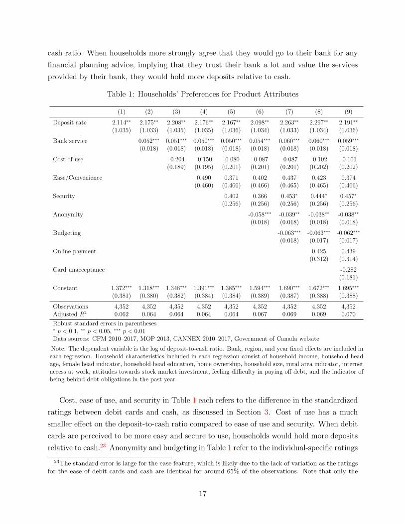
cash ratio. When households more strongly agree that they would go to their bank for any

financial planning advice, implying that they trust their bank a lot and value the services

provided by their bank, they would hold more deposits relative to cash.

Table 1: Households’ Preferences for Product Attributes

(1) (2) (3) (4) (5) (6) (7) (8) (9)

Deposit rate 2.114∗∗ 2.175∗∗ 2.208∗∗ 2.176∗∗ 2.167∗∗ 2.098∗∗ 2.263∗∗ 2.297∗∗ 2.191∗∗

(1.035) (1.033) (1.035) (1.035) (1.036) (1.034) (1.033) (1.034) (1.036)

Bank service 0.052∗∗∗ 0.051∗∗∗ 0.050∗∗∗ 0.050∗∗∗ 0.054∗∗∗ 0.060∗∗∗ 0.060∗∗∗ 0.059∗∗∗

(0.018) (0.018) (0.018) (0.018) (0.018) (0.018) (0.018) (0.018)

Cost of use -0.204 -0.150 -0.080 -0.087 -0.087 -0.102 -0.101(0.189) (0.195) (0.201) (0.201) (0.201) (0.202) (0.202)

Ease/Convenience 0.490 0.371 0.402 0.437 0.423 0.374(0.460) (0.466) (0.466) (0.465) (0.465) (0.466)

Security 0.402 0.366 0.453∗ 0.444∗ 0.457∗

(0.256) (0.256) (0.256) (0.256) (0.256)

Anonymity -0.058∗∗∗ -0.039∗∗ -0.038∗∗ -0.038∗∗

(0.018) (0.018) (0.018) (0.018)

Budgeting -0.063∗∗∗ -0.063∗∗∗ -0.062∗∗∗

(0.018) (0.017) (0.017)

Online payment 0.425 0.439(0.312) (0.314)

Card unacceptance -0.282(0.181)

Constant 1.372∗∗∗ 1.318∗∗∗ 1.348∗∗∗ 1.391∗∗∗ 1.385∗∗∗ 1.594∗∗∗ 1.690∗∗∗ 1.672∗∗∗ 1.695∗∗∗

(0.381) (0.380) (0.382) (0.384) (0.384) (0.389) (0.387) (0.388) (0.388)

Observations 4,352 4,352 4,352 4,352 4,352 4,352 4,352 4,352 4,352Adjusted R2 0.062 0.064 0.064 0.064 0.064 0.067 0.069 0.069 0.070

Robust standard errors in parentheses∗ p < 0.1, ∗∗ p < 0.05, ∗∗∗ p < 0.01Data sources: CFM 2010–2017, MOP 2013, CANNEX 2010–2017, Government of Canada website

Note: The dependent variable is the log of deposit-to-cash ratio. Bank, region, and year fixed effects are included ineach regression. Household characteristics included in each regression consist of household income, household headage, female head indicator, household head education, home ownership, household size, rural area indicator, internetaccess at work, attitudes towards stock market investment, feeling difficulty in paying off debt, and the indicator ofbeing behind debt obligations in the past year.

Cost, ease of use, and security in Table 1 each refers to the difference in the standardized

ratings between debit cards and cash, as discussed in Section 3. Cost of use has a much

smaller effect on the deposit-to-cash ratio compared to ease of use and security. When debit

cards are perceived to be more easy and secure to use, households would hold more deposits

relative to cash.23 Anonymity and budgeting in Table 1 refer to the individual-specific ratings

23The standard error is large for the ease feature, which is likely due to the lack of variation as the ratingsfor the ease of debit cards and cash are identical for around 65% of the observations. Note that only the

17

on the importance of anonymity and budgeting usefulness as payment features, respectively.

Given that cash is anonymous while deposits are not, when people think anonymity is more

important, they would obtain more utility from holding cash and hence would hold more cash

relative to deposits. Similarly, the table shows that when people think budgeting usefulness

is more important, they would hold more cash relative to deposits. This is consistent with

the prior that cash is more useful for budgeting than deposits.24

Online payment frequency measured by the fraction of transactions made online has a

positive effect on the deposit-to-cash ratio, as expected. Since cash cannot be used to make

online purchases, the more frequently households shop online, the more deposits they will

hold relative to cash. However, the coefficient is not significant, which is likely due to the

lack of variation in the online transaction frequency across households as only around 12%

of people made online purchases during a three-day period in the MOP 2013 payment diary.

Card unacceptance in Table 1 refers to the fraction of transactions where the store is cash-

only or the cards are not accepted at the individual level. As shown in the table, the card

unacceptance rate has a negative effect on the deposit-to-cash ratio.

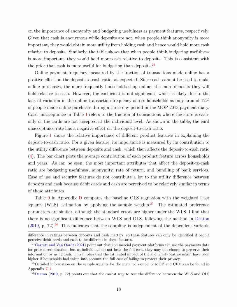
Figure 1 shows the relative importance of different product features in explaining the

deposit-to-cash ratio. For a given feature, its importance is measured by its contribution to

the utility difference between deposits and cash, which then affects the deposit-to-cash ratio

(4). The bar chart plots the average contribution of each product feature across households

and years. As can be seen, the most important attributes that affect the deposit-to-cash

ratio are budgeting usefulness, anonymity, rate of return, and bundling of bank services.

Ease of use and security features do not contribute a lot to the utility difference between

deposits and cash because debit cards and cash are perceived to be relatively similar in terms

of these attributes.

Table 9 in Appendix D compares the baseline OLS regression with the weighted least

squares (WLS) estimation by applying the sample weights.25 The estimated preference

parameters are similar, although the standard errors are higher under the WLS. I find that

there is no significant difference between WLS and OLS, following the method in Deaton

(2019, p. 72).26 This indicates that the sampling is independent of the dependent variable

difference in ratings between deposits and cash matters, so these features can only be identified if peopleperceive debit cards and cash to be different in these features.

24Garratt and Van Oordt (2021) point out that commercial payment platforms can use the payments datafor price discrimination, but as individuals do not bear the full cost, they may not choose to preserve theirinformation by using cash. This implies that the estimated impact of the anonymity feature might have beenhigher if households had taken into account the full cost of failing to protect their privacy.

25Detailed information on the sample weights for the matched sample of MOP and CFM can be found inAppendix C.4.

26Deaton (2019, p. 72) points out that the easiest way to test the difference between the WLS and OLS

18

Figure 1: Relative Importance of Different Product Attributes

-.2

-.1

0

.1

.2

Rate of

retur

n

Bank s

ervice

Cost o

f use

Ease/c

onve

nienc

e

Securi

ty

Anony

mity

Budge

ting u

seful

ness

Online

paym

ent

Card un

acce

ptanc

e

Data sources: CFM 2010–2017, MOP 2013, CANNEX 2010–2017, Government of Canada websiteNote: The bar chart shows the relative importance of different product attributes in explaining the deposit-to-cash ratio by plotting the contribution of each attribute to the utility difference between deposits andcash, where the y-axis is in utils. For each attribute x, the bar is computed as the attribute differencebetween deposits and cash multiplied by the corresponding preference parameter α(xi,d,t − xi,c,t) that isaveraged across households and years.

conditional on the explanatory variables, in which case weighting is unnecessary and harmful

for precision (Solon, Haider and Wooldridge, 2013).

The adjusted R squared in Table 1 is only around 0.07 and the correlation between the

predicted deposit-to-cash ratio and the data values is around 0.28, which indicates that

it is difficult to have precise predictions for each household due to a lot of variability in

the deposit-to-cash ratios across households. Since the counterfactual analyses focus on

the aggregate CBDC share instead of aiming to precisely predict each household’s CBDC

holding, I check how well the model can predict the aggregate deposit-to-cash ratio. More

specifically, I look at the out-of-sample model fit by estimating the model using data from

2010–2013 only and predicting the aggregate deposit-to-cash ratio during 2014–2017 using

the estimated model. Figure 2 plots the predicted values of the aggregate deposit-to-cash

estimators is to use an auxiliary regression approach. More specifically, this is done by (1) adding the sampleweight and the interaction terms between each explanatory variable and the sample weight into the baselineregression and (2) using an F-test to test the joint significance of these added variables. If the null that thesevariables are jointly zero cannot be rejected, then there is no significant difference between WLS and OLS.Using this method, the P-value is 0.21 and hence the null cannot be rejected at the 5% level.

19

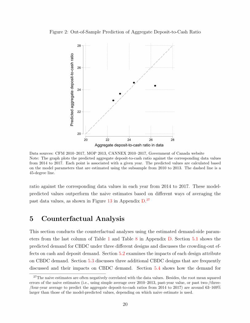
Figure 2: Out-of-Sample Prediction of Aggregate Deposit-to-Cash Ratio

20

22

24

26

28

Pred

icte

d ag

greg

ate

depo

sit-t

o-ca

sh ra

tio

20 22 24 26 28

Aggregate deposit-to-cash ratio in data

Data sources: CFM 2010–2017, MOP 2013, CANNEX 2010–2017, Government of Canada websiteNote: The graph plots the predicted aggregate deposit-to-cash ratio against the corresponding data valuesfrom 2014 to 2017. Each point is associated with a given year. The predicted values are calculated basedon the model parameters that are estimated using the subsample from 2010 to 2013. The dashed line is a45-degree line.

ratio against the corresponding data values in each year from 2014 to 2017. These model-

predicted values outperform the naive estimates based on different ways of averaging the

past data values, as shown in Figure 13 in Appendix D.27

5 Counterfactual Analysis

This section conducts the counterfactual analyses using the estimated demand-side param-

eters from the last column of Table 1 and Table 8 in Appendix D. Section 5.1 shows the

predicted demand for CBDC under three different designs and discusses the crowding-out ef-

fects on cash and deposit demand. Section 5.2 examines the impacts of each design attribute

on CBDC demand. Section 5.3 discusses three additional CBDC designs that are frequently

discussed and their impacts on CBDC demand. Section 5.4 shows how the demand for

27The naive estimates are often negatively correlated with the data values. Besides, the root mean squarederrors of the naive estimates (i.e., using simple average over 2010–2013, past-year value, or past two-/three-/four-year average to predict the aggregate deposit-to-cash ratios from 2014 to 2017) are around 63–169%larger than those of the model-predicted values, depending on which naive estimate is used.

20

CBDC differs across social demographic groups.

5.1 Demand for CBDC

I predict the potential demand for CBDC if it were issued in 2017 and to what extent it could

affect the demand for cash and deposits based on the logit model in Section 5.1.1 and nested

logit model in Section 5.1.2. The demand for CBDC is measured by the aggregate CBDC

share, which is the total CBDC holdings over the total liquid assets held by households.

This section shows the CBDC demand under three different designs, that is, deposit design,

cash design, and baseline design.

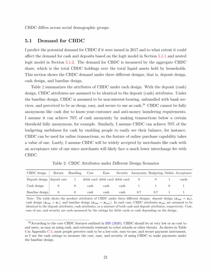
Table 2 summarizes the attributes of CBDC under each design. With the deposit (cash)

design, CBDC attributes are assumed to be identical to the deposit (cash) attributes. Under

the baseline design, CBDC is assumed to be non-interest-bearing, unbundled with bank ser-

vices, and perceived to be as cheap, easy, and secure to use as cash.28 CBDC cannot be fully

anonymous like cash due to know-your-customer and anti-money laundering requirements.

I assume it can achieve 70% of cash anonymity by making transactions below a certain

threshold fully anonymous, for example. Similarly, I assume CBDC can achieve 70% of the

budgeting usefulness for cash by enabling people to easily see their balance, for instance.

CBDC can be used for online transactions, so the feature of online purchase capability takes

a value of one. Lastly, I assume CBDC will be widely accepted by merchants like cash with

an acceptance rate of one since merchants will likely face a much lower interchange fee with

CBDC.

Table 2: CBDC Attributes under Different Design Scenarios

CBDC design Return Bundling Cost Ease Security Anonymity Budgeting Online Acceptance

Deposit design deposit rate 1 debit card debit card debit card 0 0 1 cards

Cash design 0 0 cash cash cash 1 1 0 1

Baseline design 0 0 cash cash cash 0.7 0.7 1 1

Note: The table shows the product attributes of CBDC under three different designs: deposit design (xcbdc = xd),cash design (xcbdc = xc), and baseline design (xcbdc = xbase). In each case, CBDC attributes xcbdc are assumed to beidentical to the deposit attributes, cash attributes, or a mixture of both cash and deposit attributes, respectively. Cost,ease of use, and security are each measured by the ratings for debit cards or cash depending on the design.

28According to the core CBDC features outlined in BIS (2020), CBDC should be at very low or no cost toend users, as easy as using cash, and extremely resistant to cyber attacks or other threats. As shown in Table6 in Appendix C.5, most people perceive cash to be a low-cost, easy-to-use, and secure payment instrument,so I use the cash ratings to measure the cost, ease, and security of using CBDC to make payments underthe baseline design.

21

5.1.1 Predicted Demand for CBDC under Logit Model

The utility Vi,cbdc,t for CBDC (5) consists of three main components: how households value

different attributes of CBDC captured by α′xi,cbdc,t, how households with different char-

acteristics value CBDC captured by γ ′cbdczi,t, and the average impact of the unobserved

idiosyncratic preferences captured by ηcbdc. To calculate the utility for CBDC and thus pre-

dict the demand for CBDC, I assume the CBDC-specific effects range from being cash-like

(i.e., γcbdc = γc = 0 and ηcbdc = ηc = 0) to being deposit-like (i.e., γcbdc = γd and ηcbdc = ηd),

as discussed in Section 2.2. Therefore, Figure 3 shows the aggregate CBDC shares against

the values of γcbdc/γd and ηcbdc/ηd, ranging from zero to one. Each graph plots the aggregate

CBDC shares under the three designs shown in Table 2.

There are three main findings from Figure 3. First, when CBDC-specific effects are

cash-like (deposit-like), the aggregate CBDC share is around 4% (52%). Intuitively, since a

median household holds around 96% of their liquid assets in deposit and 4% in cash in the

CFM data, if CBDC-specific effects are closer to being deposit-like, implying that households

would perceive CBDC to be closer to deposit, they would also hold more CBDC.

Second, the two components of the CBDC-specific effects, that is, the demographics-

related effects γcbdc and the CBDC fixed effect ηcbdc, are equally important in determining

the potential level of CBDC demand. The upper panel shows that as γcbdc approaches γd,

the aggregate CBDC share increases from around 16% to 52% (4% to 17%) conditional on

ηcbdc = ηd (ηcbdc = ηc). Similarly, the lower panel shows that as ηcbdc approaches ηd, the

aggregate CBDC share increases from around 17% to 52% (4% to 16%), conditional on

γcbdc = γd (γcbdc = γc).

Third, the aggregate CBDC shares under the cash design are the highest among the

three designs mainly due to the higher levels of anonymity and budgeting usefulness under

the cash design. Although the deposit design is better in terms of the rate of return and

bundling of bank services, it is not enough to compensate for its low level of anonymity and

budgeting usefulness, so the CBDC demand is lower under the deposit design.

A higher demand for CBDC implies larger crowding-out effects on the demand for de-

posits and cash. Under the logit model, the demand for CBDC draws proportionally from

deposits and cash, so the percentage drops in deposit and cash demand are identical. Fig-

ure 14 in Appendix D shows that the mean percentage drop in deposits and cash across

households is around 4% (52%) when CBDC-specific effects are cash-like (deposit-like).

22

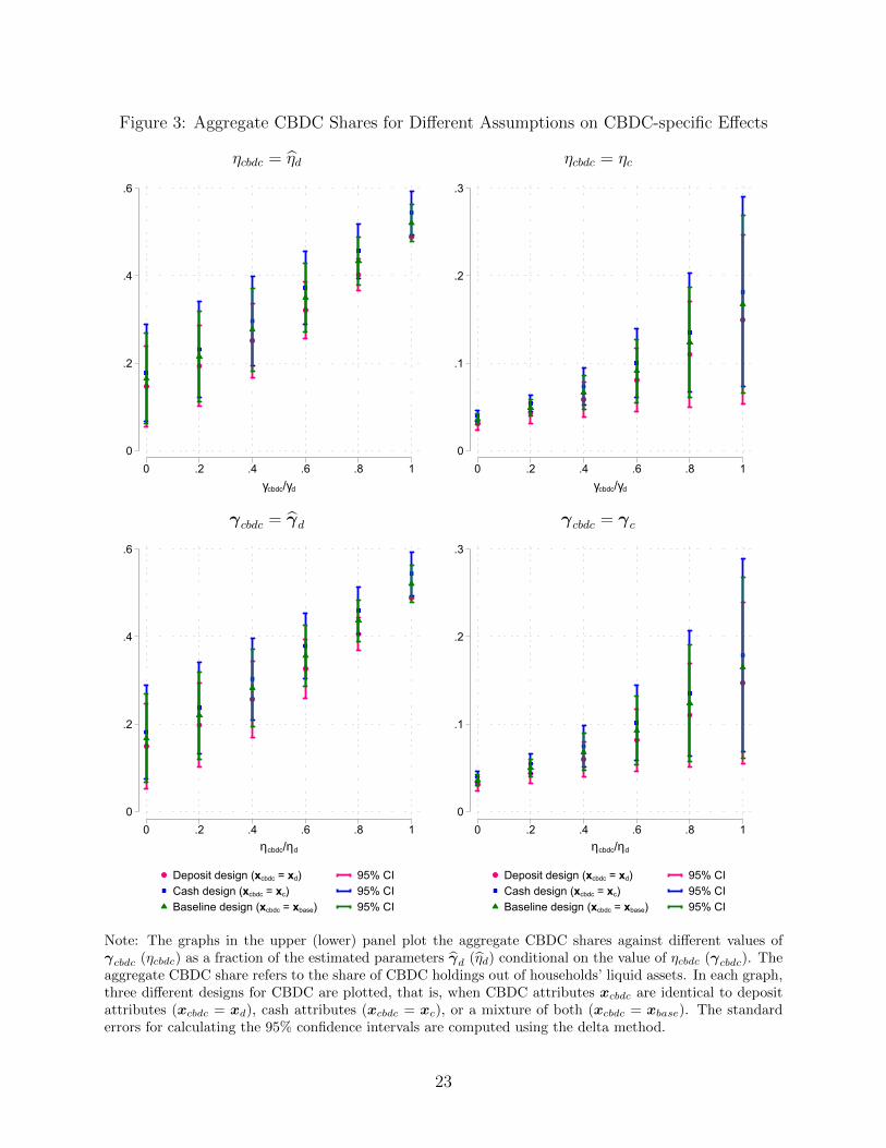
Figure 3: Aggregate CBDC Shares for Different Assumptions on CBDC-specific Effects

ηcbdc = ηd

0

.2

.4

.6

0 .2 .4 .6 .8 1γcbdc/γd

Deposit design (xcbdc = xd) 95% CICash design (xcbdc = xc) 95% CIBaseline design (xcbdc = xbase) 95% CI

ηcbdc = ηc

0

.1

.2

.3

0 .2 .4 .6 .8 1γcbdc/γd


γcbdc = γd

0

.2

.4

.6

0 .2 .4 .6 .8 1ηcbdc/ηd


γcbdc = γc

0

.1

.2

.3

0 .2 .4 .6 .8 1ηcbdc/ηd


Note: The graphs in the upper (lower) panel plot the aggregate CBDC shares against different values ofγcbdc (ηcbdc) as a fraction of the estimated parameters γd (ηd) conditional on the value of ηcbdc (γcbdc). Theaggregate CBDC share refers to the share of CBDC holdings out of households’ liquid assets. In each graph,three different designs for CBDC are plotted, that is, when CBDC attributes xcbdc are identical to depositattributes (xcbdc = xd), cash attributes (xcbdc = xc), or a mixture of both (xcbdc = xbase). The standarderrors for calculating the 95% confidence intervals are computed using the delta method.

23

5.1.2 Predicted Demand for CBDC under Nested Logit Model

Under the logit model, CBDC is treated as a distinct product in the sense that households

possess a unique set of unobserved idiosyncratic preferences for CBDC. In other words,

there are no common factors driving the unobserved idiosyncratic preferences for different

products. This assumption is relaxed in this section, so that CBDC can be a closer substitute

for deposits or cash due to the correlated idiosyncratic preferences, as discussed in Section

2.2.2. This section examines to what extent the predictions from the logit model are robust

to the correlated unobserved utilities across products.

Figure 4 plots the aggregate CBDC shares against different levels of correlation ranging

from 0 to 0.99, assuming the unobserved utility for CBDC is correlated with that for deposits

(left panel) or cash (right panel). A higher correlation between the unobserved utilities for

CBDC and deposits (cash) implies greater substitutability between CBDC and deposits

(cash). When the correlation is zero, the predictions are identical to those based on the logit

model. Each graph plots the aggregate CBDC shares under the deposit design, the cash

design, and the baseline design.

There are three main implications from Figure 4. First, the predicted aggregate CBDC

shares are robust to a wide range of correlation coefficients. When the correlation is below

0.8, the level changes in the aggregate CBDC shares across different levels of correlation are

small, conditional on a given CBDC design.

Second, the impact of the correlation on the aggregate CBDC share depends on the

utility difference between CBDC and its closer substitute, as discussed in Section 2.2.2. For

example, under the deposit design in the first graph, CBDC and deposits have the same

observed utility, as both the design of CBDC and the CBDC-specific effects are identical

to those of deposits. In this case, as ρd cbdc increases, cash is reduced by less as CBDC

demand draws more than proportionally from deposits. As a consequence, the remaining

asset share that can be allocated to CBDC and deposits is smaller, which leads to a lower

CBDC share. This effect can be reversed (reinforced) by the substitution between CBDC

and deposits when CBDC has a higher (lower) observed utility than deposits. Under the

cash design or the baseline design, CBDC has a higher observed utility than deposits due

to better anonymity and budgeting usefulness features, so a higher ρd cbdc that makes them

more substitutable can lead to greater substitution from deposits into CBDC and hence a

higher aggregate CBDC share.

In contrast, in the bottom right graph, CBDC with the deposit design or the baseline

design has a lower observed utility than that with the cash design, so a higher ρc cbdc leads to

greater substitution from CBDC into cash and larger drops in the CBDC shares compared

to the drop under the cash design. Apart from the design, the CBDC-specific effects can also

24

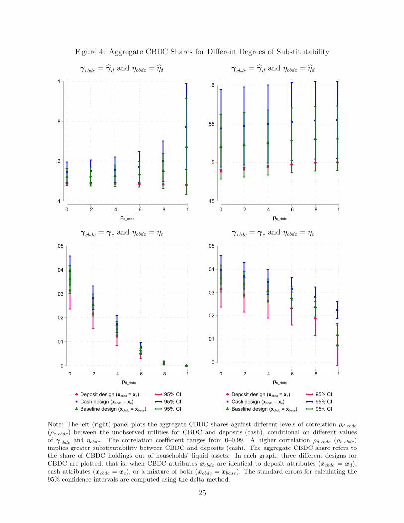
Figure 4: Aggregate CBDC Shares for Different Degrees of Substitutability

γcbdc = γd and ηcbdc = ηd

.4

.6

.8

1

0 .2 .4 .6 .8 1ρd_cbdc



.45

.5

.55

.6

0 .2 .4 .6 .8 1ρc_cbdc


γcbdc = γc and ηcbdc = ηc

0

.01

.02

.03

.04

.05

0 .2 .4 .6 .8 1ρd_cbdc



0

.01

.02

.03

.04

.05

0 .2 .4 .6 .8 1ρc_cbdc


Note: The left (right) panel plots the aggregate CBDC shares against different levels of correlation ρd cbdc(ρc cbdc) between the unobserved utilities for CBDC and deposits (cash), conditional on different valuesof γcbdc and ηcbdc. The correlation coefficient ranges from 0–0.99. A higher correlation ρd cbdc (ρc cbdc)implies greater substitutability between CBDC and deposits (cash). The aggregate CBDC share refers tothe share of CBDC holdings out of households’ liquid assets. In each graph, three different designs forCBDC are plotted, that is, when CBDC attributes xcbdc are identical to deposit attributes (xcbdc = xd),cash attributes (xcbdc = xc), or a mixture of both (xcbdc = xbase). The standard errors for calculating the95% confidence intervals are computed using the delta method.

25

lead to an observed utility difference. The bottom left graph shows that when CBDC has a

much lower observed utility than deposits due to the CBDC-specific effects being cash-like

(i.e., γcbdc = γc and ηcbdc = ηc), there is greater substitution from CBDC to deposits and

the aggregate CBDC share approaches zero as ρd cbdc increases.

Third, the correlation ρc cbdc between the unobserved utilities for CBDC and cash has

a much smaller impact compared to ρd cbdc. The right panel of Figure 4 shows that the

level changes in aggregate CBDC shares are small even when ρc cbdc approaches one. This is

because households only hold a small fraction of their liquid assets in cash. Hence, even if

CBDC has a much higher observed utility than cash due to the CBDC-specific effects being

deposit-like (i.e., γcbdc = γd and ηcbdc = ηd), the greater substitution from cash into CBDC

as ρc cbdc increases would not add much extra demand for CBDC, as shown in the top right

graph.

Similar to the logit model, the crowding-out effects on the demand for deposits and

cash depend a lot on CBDC-specific effects. Suppose CBDC has a baseline design and is a

closer substitute to deposits. The left panels of Figure 15 and 16 in Appendix D show that

when CBDC-specific effects are cash-like, deposit and cash demand would only be reduced

by around 0–4%. In contrast, when CBDC-specific effects are deposit-like, the demand for

deposits (cash) can be crowded out by around 52–70% (15–52%), as ρd cbdc increases from 0

to 0.99.

When CBDC is a closer substitute to cash, the crowding out on deposit demand is

robust to changes in the correlation ρc cbdc, whereas the crowding out on cash demand is

more sensitive to ρc cbdc, as shown in the right panels of Figure 15 and 16 in Appendix D.

Intuitively, the latter is because people only hold a small amount of cash, so even a small

level change can be a large percentage change. As ρc cbdc increases from 0 to 0.99, implying

that CBDC and cash become more substitutable, deposit (cash) demand would be reduced

by 50–52% (52–100%) when CBDC-specific effects are deposit-like, and 0–4% (4–26%) when

CBDC-specific effects are cash-like.

5.2 The Impacts of CBDC Design Attributes

In this section, I quantify how each design attribute would impact CBDC demand. While

CBDC-specific effects (i.e., γcbdc and ηcbdc) play a large role in determining the exact level of

CBDC demand, this section shows that the impacts of the design attributes on the percentage

changes in CBDC demand would rely much less on these assumptions.

The predicted impacts of attributes from both the logit and nested logit models are

shown in this section. When the unobserved utilities for CBDC and deposits are correlated

26

under the nested logit model, the impact of a given attribute on CBDC demand is larger.

Intuitively, when CBDC and deposits are closer substitutes, any attribute change will lead

to greater substitution between the two. Hence, the predictions based on the logit model

can be viewed as a lower bound.

The correlation ρc cbdc between the unobserved utilities for CBDC and cash has a much

smaller impact on the impacts of design attributes compared to ρd cbdc, so the results are not

shown in this section. Intuitively, a higher correlation ρc cbdc increases the substitutability

between CBDC and cash, which leads to greater substitution from cash into CBDC if CBDC

has better attributes than cash. However, this would not add much to the CBDC demand

since people tend to hold a small amount of cash.

I find that except for the rate of return whose impact depends on the magnitude of the

rate change, the most important attribute is budgeting usefulness, followed by anonymity

and bundling of bank services. This is consistent with Figure 1, which shows that these

attributes are relatively more important in explaining the allocation between deposits and

cash. The rest of this section discusses the impact of each attribute in turn.

CBDC Interest Rate

Figure 5 shows how changes in the CBDC interest rate would impact the aggregate CBDC

shares (upper panel) and the percentage changes in aggregate CBDC shares relative to those

under the baseline design (lower panel), conditional on the CBDC-specific effects (i.e., γcbdc

and ηcbdc) and the correlation ρd cbdc between the unobserved utilities for CBDC and deposits.

The range 0–0.1% is chosen because the median (75th percentile) deposit rate after tax is

around 0.08% (0.1%) across households during 2010–2017.

The upper panel of Figure 5 shows that as the CBDC rate increases from 0% to 0.1%,

the aggregate CBDC share increases from 52% to 57% (3.6% to 4.4%), when CBDC-specific

effects are deposit-like (cash-like) under the logit model. As can be seen, the predicted

levels of CBDC demand differ a lot depending on CBDC-specific effects. To summarize the

impacts of the CBDC interest rate across different assumptions on CBDC-specific effects, I

look at the percentage changes in the aggregate CBDC shares relative to the shares under

the baseline design in the lower panel.

As shown in the lower panel of Figure 5, when CBDC is non-interest-bearing as in the

baseline design, there is a zero percentage change in the aggregate CBDC share. Based on

the logit model where ρd cbdc = 0, as the CBDC rate rises to 0.1%, the aggregate CBDC share

increases by around 10% (23%) if CBDC-specific effects are deposit-like (cash-like). The 0.1

percentage point increase in CBDC rate is a large change as most households face a post-tax

deposit rate that is below 0.1%. When the correlation is high (e.g., ρd cbdc = 0.75), the

27

Figure 5: The Impact of Rate of Return on CBDC Demand


.45

.5

.55

.6

.65

.7

0 .025 .05 .075 .1CBDC interest rate (%)

scbdc for ρd_cbdc = 0 95% CIscbdc for ρd_cbdc = 0.75 95% CI


0

.02

.04

.06


scbdc for ρd_cbdc = 0 95% CIscbdc for ρd_cbdc = 0.75 95% CI


0

10

20

30

40


%∆ in scbdc for ρd_cbdc = 0 95% CI%∆ in scbdc for ρd_cbdc = 0.75 95% CI


0

50

100

150



Note: The graph plots the aggregate CBDC share scbdc (upper panel) and the percentage change %∆ in theaggregate CBDC share scbdc relative to the baseline value (lower panel) for different levels of CBDC interestrate ranging from 0% to 0.1%, conditional on different values of γcbdc and ηcbdc. In each graph, two differentlevels of the correlation ρd cbdc between the unobserved utilities for CBDC and deposits are plotted. Thestandard errors for calculating the 95% confidence intervals are computed using the delta method.

28

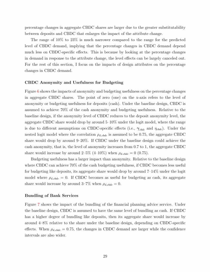
percentage changes in aggregate CBDC shares are larger due to the greater substitutability

between deposits and CBDC that enlarges the impact of the attribute change.

The range of 10% to 23% is much narrower compared to the range for the predicted

level of CBDC demand, implying that the percentage changes in CBDC demand depend

much less on CBDC-specific effects. This is because by looking at the percentage changes

in demand in response to the attribute change, the level effects can be largely canceled out.

For the rest of this section, I focus on the impacts of design attributes on the percentage

changes in CBDC demand.

CBDC Anonymity and Usefulness for Budgeting

Figure 6 shows the impacts of anonymity and budgeting usefulness on the percentage changes

in aggregate CBDC shares. The point of zero (one) on the x-axis refers to the level of

anonymity or budgeting usefulness for deposits (cash). Under the baseline design, CBDC is

assumed to achieve 70% of the cash anonymity and budgeting usefulness. Relative to the

baseline design, if the anonymity level of CBDC reduces to the deposit anonymity level, the

aggregate CBDC share would drop by around 5–10% under the logit model, where the range

is due to different assumptions on CBDC-specific effects (i.e., γcbdc and ηcbdc). Under the

nested logit model where the correlation ρd cbdc is assumed to be 0.75, the aggregate CBDC

share would drop by around 9–20%. If CBDC under the baseline design could achieve the

cash anonymity, that is, the level of anonymity increases from 0.7 to 1, the aggregate CBDC

share would increase by around 2–5% (4–10%) when ρd cbdc = 0 (0.75).

Budgeting usefulness has a larger impact than anonymity. Relative to the baseline design

where CBDC can achieve 70% of the cash budgeting usefulness, if CBDC becomes less useful

for budgeting like deposits, its aggregate share would drop by around 7–14% under the logit

model where ρd cbdc = 0. If CBDC becomes as useful for budgeting as cash, its aggregate

share would increase by around 3–7% when ρd cbdc = 0.

Bundling of Bank Services

Figure 7 shows the impact of the bundling of the financial planning advice service. Under

the baseline design, CBDC is assumed to have the same level of bundling as cash. If CBDC

has a higher degree of bundling like deposits, then its aggregate share would increase by

around 4–8% relative to the share under the baseline design, depending on CBDC-specific

effects. When ρd cbdc = 0.75, the changes in CBDC demand are larger while the confidence

intervals are also wider.

29

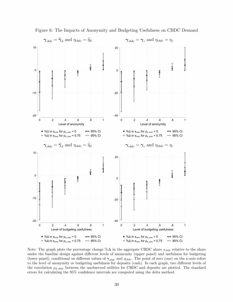
Figure 6: The Impacts of Anonymity and Budgeting Usefulness on CBDC Demand


-20

-10

0

10

0 .2 .4 .6 .8 1Level of anonymity



-40

-20

0

20

0 .2 .4 .6 .8 1Level of anonymity



-20

-10

0

10

0 .2 .4 .6 .8 1Level of budgeting usefulness



-40

-20

0

20

0 .2 .4 .6 .8 1Level of budgeting usefulness


Note: The graph plots the percentage change %∆ in the aggregate CBDC share scbdc relative to the shareunder the baseline design against different levels of anonymity (upper panel) and usefulness for budgeting(lower panel), conditional on different values of γcbdc and ηcbdc. The point of zero (one) on the x-axis refersto the level of anonymity or budgeting usefulness for deposits (cash). In each graph, two different levels ofthe correlation ρd cbdc between the unobserved utilities for CBDC and deposits are plotted. The standarderrors for calculating the 95% confidence intervals are computed using the delta method.

30

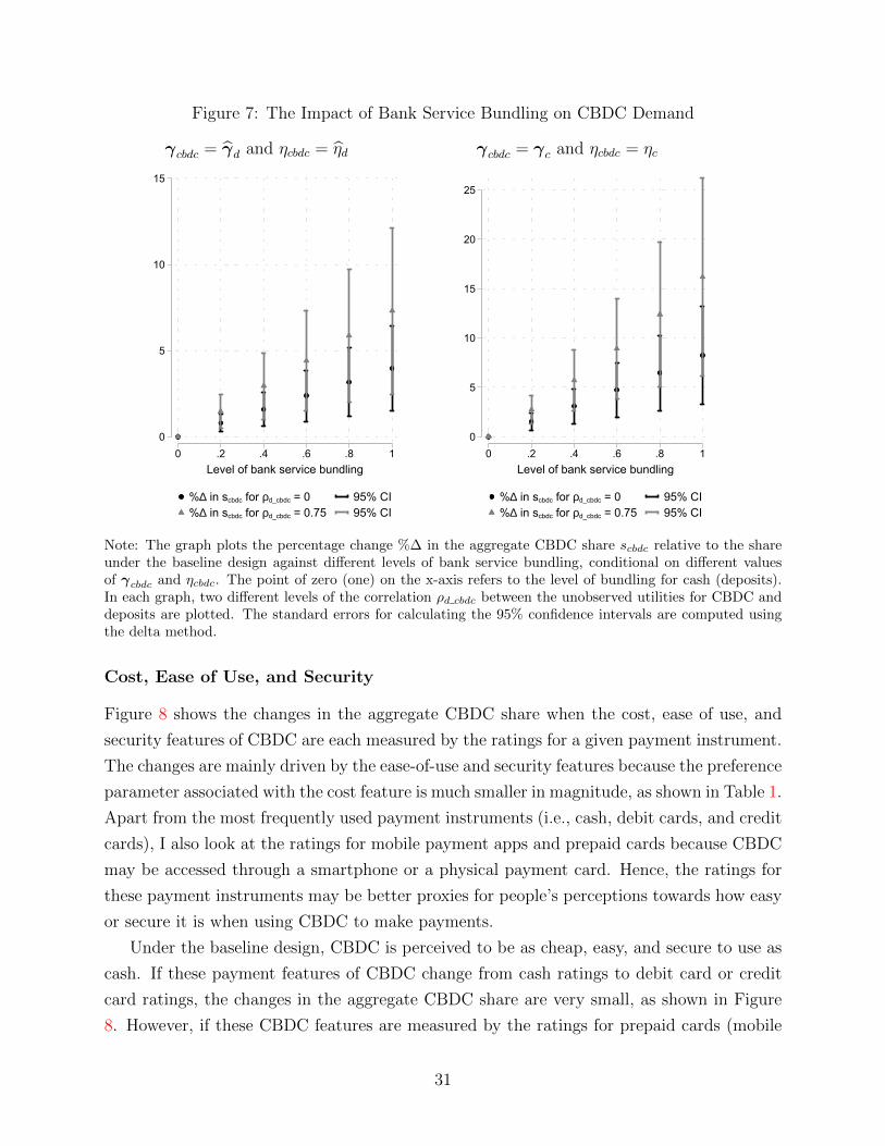
Figure 7: The Impact of Bank Service Bundling on CBDC Demand


0

5

10

15

0 .2 .4 .6 .8 1Level of bank service bundling



0

5

10

15

20

25

0 .2 .4 .6 .8 1Level of bank service bundling


Note: The graph plots the percentage change %∆ in the aggregate CBDC share scbdc relative to the shareunder the baseline design against different levels of bank service bundling, conditional on different valuesof γcbdc and ηcbdc. The point of zero (one) on the x-axis refers to the level of bundling for cash (deposits).In each graph, two different levels of the correlation ρd cbdc between the unobserved utilities for CBDC anddeposits are plotted. The standard errors for calculating the 95% confidence intervals are computed usingthe delta method.

Cost, Ease of Use, and Security

Figure 8 shows the changes in the aggregate CBDC share when the cost, ease of use, and

security features of CBDC are each measured by the ratings for a given payment instrument.

The changes are mainly driven by the ease-of-use and security features because the preference

parameter associated with the cost feature is much smaller in magnitude, as shown in Table 1.

Apart from the most frequently used payment instruments (i.e., cash, debit cards, and credit

cards), I also look at the ratings for mobile payment apps and prepaid cards because CBDC

may be accessed through a smartphone or a physical payment card. Hence, the ratings for

these payment instruments may be better proxies for people’s perceptions towards how easy

or secure it is when using CBDC to make payments.

Under the baseline design, CBDC is perceived to be as cheap, easy, and secure to use as

cash. If these payment features of CBDC change from cash ratings to debit card or credit

card ratings, the changes in the aggregate CBDC share are very small, as shown in Figure

8. However, if these CBDC features are measured by the ratings for prepaid cards (mobile

31

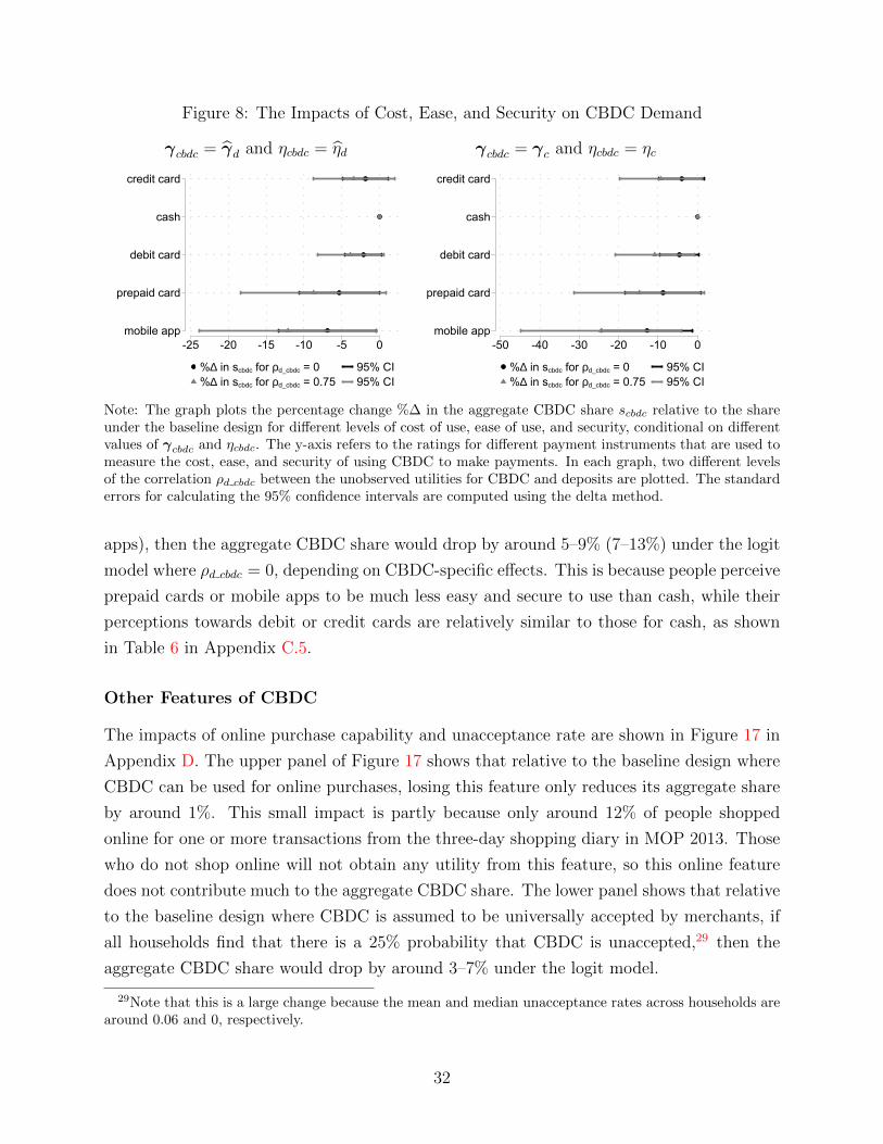
Figure 8: The Impacts of Cost, Ease, and Security on CBDC Demand


credit card

cash

debit card

prepaid card

mobile app-25 -20 -15 -10 -5 0



credit card

cash

debit card

prepaid card

mobile app-50 -40 -30 -20 -10 0


Note: The graph plots the percentage change %∆ in the aggregate CBDC share scbdc relative to the shareunder the baseline design for different levels of cost of use, ease of use, and security, conditional on differentvalues of γcbdc and ηcbdc. The y-axis refers to the ratings for different payment instruments that are used tomeasure the cost, ease, and security of using CBDC to make payments. In each graph, two different levelsof the correlation ρd cbdc between the unobserved utilities for CBDC and deposits are plotted. The standarderrors for calculating the 95% confidence intervals are computed using the delta method.

apps), then the aggregate CBDC share would drop by around 5–9% (7–13%) under the logit

model where ρd cbdc = 0, depending on CBDC-specific effects. This is because people perceive

prepaid cards or mobile apps to be much less easy and secure to use than cash, while their

perceptions towards debit or credit cards are relatively similar to those for cash, as shown

in Table 6 in Appendix C.5.

Other Features of CBDC

The impacts of online purchase capability and unacceptance rate are shown in Figure 17 in

Appendix D. The upper panel of Figure 17 shows that relative to the baseline design where

CBDC can be used for online purchases, losing this feature only reduces its aggregate share

by around 1%. This small impact is partly because only around 12% of people shopped

online for one or more transactions from the three-day shopping diary in MOP 2013. Those

who do not shop online will not obtain any utility from this feature, so this online feature

does not contribute much to the aggregate CBDC share. The lower panel shows that relative

to the baseline design where CBDC is assumed to be universally accepted by merchants, if

all households find that there is a 25% probability that CBDC is unaccepted,29 then the

aggregate CBDC share would drop by around 3–7% under the logit model.

29Note that this is a large change because the mean and median unacceptance rates across households arearound 0.06 and 0, respectively.

32

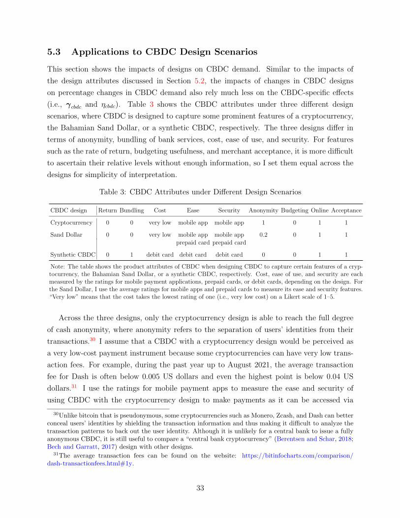
5.3 Applications to CBDC Design Scenarios

This section shows the impacts of designs on CBDC demand. Similar to the impacts of

the design attributes discussed in Section 5.2, the impacts of changes in CBDC designs

on percentage changes in CBDC demand also rely much less on the CBDC-specific effects

(i.e., γcbdc and ηcbdc). Table 3 shows the CBDC attributes under three different design

scenarios, where CBDC is designed to capture some prominent features of a cryptocurrency,

the Bahamian Sand Dollar, or a synthetic CBDC, respectively. The three designs differ in

terms of anonymity, bundling of bank services, cost, ease of use, and security. For features

such as the rate of return, budgeting usefulness, and merchant acceptance, it is more difficult

to ascertain their relative levels without enough information, so I set them equal across the

designs for simplicity of interpretation.

Table 3: CBDC Attributes under Different Design Scenarios

CBDC design Return Bundling Cost Ease Security Anonymity Budgeting Online Acceptance

Cryptocurrency 0 0 very low mobile app mobile app 1 0 1 1

Sand Dollar 0 0 very low mobile app mobile app 0.2 0 1 1

prepaid card prepaid card

Synthetic CBDC 0 1 debit card debit card debit card 0 0 1 1

Note: The table shows the product attributes of CBDC when designing CBDC to capture certain features of a cryp-tocurrency, the Bahamian Sand Dollar, or a synthetic CBDC, respectively. Cost, ease of use, and security are eachmeasured by the ratings for mobile payment applications, prepaid cards, or debit cards, depending on the design. Forthe Sand Dollar, I use the average ratings for mobile apps and prepaid cards to measure its ease and security features.“Very low” means that the cost takes the lowest rating of one (i.e., very low cost) on a Likert scale of 1–5.

Across the three designs, only the cryptocurrency design is able to reach the full degree

of cash anonymity, where anonymity refers to the separation of users’ identities from their

transactions.30 I assume that a CBDC with a cryptocurrency design would be perceived as

a very low-cost payment instrument because some cryptocurrencies can have very low trans-

action fees. For example, during the past year up to August 2021, the average transaction

fee for Dash is often below 0.005 US dollars and even the highest point is below 0.04 US

dollars.31 I use the ratings for mobile payment apps to measure the ease and security of

using CBDC with the cryptocurrency design to make payments as it can be accessed via

30Unlike bitcoin that is pseudonymous, some cryptocurrencies such as Monero, Zcash, and Dash can betterconceal users’ identities by shielding the transaction information and thus making it difficult to analyze thetransaction patterns to back out the user identity. Although it is unlikely for a central bank to issue a fullyanonymous CBDC, it is still useful to compare a “central bank cryptocurrency” (Berentsen and Schar, 2018;Bech and Garratt, 2017) design with other designs.

31The average transaction fees can be found on the website: https://bitinfocharts.com/comparison/dash-transactionfees.html#1y.

33

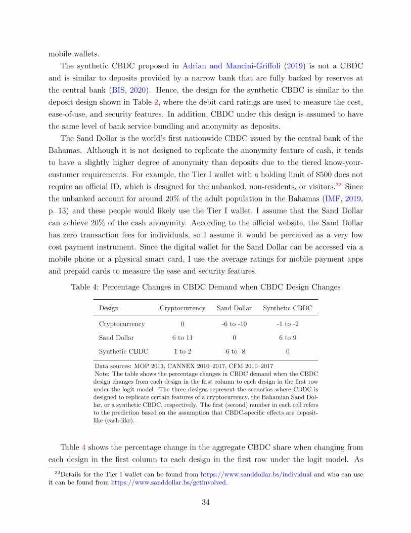
https://bitinfocharts.com/comparison/dash-transactionfees.html#1y

https://bitinfocharts.com/comparison/dash-transactionfees.html#1y

mobile wallets.

The synthetic CBDC proposed in Adrian and Mancini-Griffoli (2019) is not a CBDC

and is similar to deposits provided by a narrow bank that are fully backed by reserves at

the central bank (BIS, 2020). Hence, the design for the synthetic CBDC is similar to the

deposit design shown in Table 2, where the debit card ratings are used to measure the cost,

ease-of-use, and security features. In addition, CBDC under this design is assumed to have

the same level of bank service bundling and anonymity as deposits.

The Sand Dollar is the world’s first nationwide CBDC issued by the central bank of the

Bahamas. Although it is not designed to replicate the anonymity feature of cash, it tends

to have a slightly higher degree of anonymity than deposits due to the tiered know-your-

customer requirements. For example, the Tier I wallet with a holding limit of $500 does not

require an official ID, which is designed for the unbanked, non-residents, or visitors.32 Since

the unbanked account for around 20% of the adult population in the Bahamas (IMF, 2019,

p. 13) and these people would likely use the Tier I wallet, I assume that the Sand Dollar

can achieve 20% of the cash anonymity. According to the official website, the Sand Dollar

has zero transaction fees for individuals, so I assume it would be perceived as a very low

cost payment instrument. Since the digital wallet for the Sand Dollar can be accessed via a

mobile phone or a physical smart card, I use the average ratings for mobile payment apps

and prepaid cards to measure the ease and security features.

Table 4: Percentage Changes in CBDC Demand when CBDC Design Changes

Design Cryptocurrency Sand Dollar Synthetic CBDC

Cryptocurrency 0 -6 to -10 -1 to -2

Sand Dollar 6 to 11 0 6 to 9

Synthetic CBDC 1 to 2 -6 to -8 0

Data sources: MOP 2013, CANNEX 2010–2017, CFM 2010–2017Note: The table shows the percentage changes in CBDC demand when the CBDCdesign changes from each design in the first column to each design in the first rowunder the logit model. The three designs represent the scenarios where CBDC isdesigned to replicate certain features of a cryptocurrency, the Bahamian Sand Dol-lar, or a synthetic CBDC, respectively. The first (second) number in each cell refersto the prediction based on the assumption that CBDC-specific effects are deposit-like (cash-like).

Table 4 shows the percentage change in the aggregate CBDC share when changing from

each design in the first column to each design in the first row under the logit model. As

32Details for the Tier I wallet can be found from https://www.sanddollar.bs/individual and who can useit can be found from https://www.sanddollar.bs/getinvolved.

34

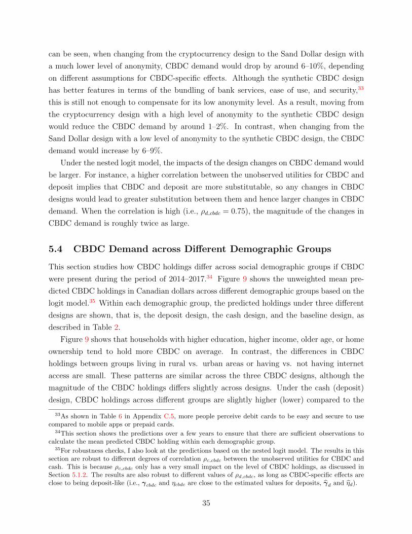
https://www.sanddollar.bs/individual

https://www.sanddollar.bs/getinvolved

can be seen, when changing from the cryptocurrency design to the Sand Dollar design with

a much lower level of anonymity, CBDC demand would drop by around 6–10%, depending

on different assumptions for CBDC-specific effects. Although the synthetic CBDC design

has better features in terms of the bundling of bank services, ease of use, and security,33

this is still not enough to compensate for its low anonymity level. As a result, moving from

the cryptocurrency design with a high level of anonymity to the synthetic CBDC design

would reduce the CBDC demand by around 1–2%. In contrast, when changing from the

Sand Dollar design with a low level of anonymity to the synthetic CBDC design, the CBDC

demand would increase by 6–9%.

Under the nested logit model, the impacts of the design changes on CBDC demand would

be larger. For instance, a higher correlation between the unobserved utilities for CBDC and

deposit implies that CBDC and deposit are more substitutable, so any changes in CBDC

designs would lead to greater substitution between them and hence larger changes in CBDC

demand. When the correlation is high (i.e., ρd cbdc = 0.75), the magnitude of the changes in

CBDC demand is roughly twice as large.

5.4 CBDC Demand across Different Demographic Groups

This section studies how CBDC holdings differ across social demographic groups if CBDC

were present during the period of 2014–2017.34 Figure 9 shows the unweighted mean pre-

dicted CBDC holdings in Canadian dollars across different demographic groups based on the

logit model.35 Within each demographic group, the predicted holdings under three different

designs are shown, that is, the deposit design, the cash design, and the baseline design, as

described in Table 2.

Figure 9 shows that households with higher education, higher income, older age, or home

ownership tend to hold more CBDC on average. In contrast, the differences in CBDC

holdings between groups living in rural vs. urban areas or having vs. not having internet

access are small. These patterns are similar across the three CBDC designs, although the

magnitude of the CBDC holdings differs slightly across designs. Under the cash (deposit)

design, CBDC holdings across different groups are slightly higher (lower) compared to the

33As shown in Table 6 in Appendix C.5, more people perceive debit cards to be easy and secure to usecompared to mobile apps or prepaid cards.

34This section shows the predictions over a few years to ensure that there are sufficient observations tocalculate the mean predicted CBDC holding within each demographic group.

35For robustness checks, I also look at the predictions based on the nested logit model. The results in thissection are robust to different degrees of correlation ρc cbdc between the unobserved utilities for CBDC andcash. This is because ρc cbdc only has a very small impact on the level of CBDC holdings, as discussed inSection 5.1.2. The results are also robust to different values of ρd cbdc, as long as CBDC-specific effects areclose to being deposit-like (i.e., γcbdc and ηcbdc are close to the estimated values for deposits, γd and ηd).

35

baseline design, since the cash (deposit) design is better (worse) in terms of anonymity and

budgeting usefulness features.

Figure 9: CBDC holdings in Canadian Dollars across Demographic Groups

Household Head Education

0

2,000

4,000

6,000

8,000

Grade 9

-13 or

below

Commun

ity C

olleg

e

Diplom

a

Underg

radua

te

Post-g

radua

te

Deposit design Baseline design Cash design

Household Income

0

2,000

4,000

6,000

8,000

Less

than

30K

30-60

K

60-10

0K

More th

an 10

0K

Deposit design Baseline design Cash designHousehold Head Age

0

2,000

4,000

6,000

Under

3435

-4445

-5455

-64

65 or

olde

r


Home Ownership

0

2,000

4,000

6,000

Owner

Renter

Deposit design Baseline design Cash designRural vs Urban

0

2,000

4,000

6,000

Urban

Rural


Internet Access at Work

0

2,000

4,000

6,000

No Inte

rnet

Intern

et


Note: The bar charts show the unweighted mean predicted CBDC holdings across households and over theperiod of 2014–2017 for different demographic groups. For a given demographic group, the predicted CBDCholdings under three different designs are plotted. The CBDC holdings are predicted from the logit modelbased on the assumption that CBDC-specific effects are deposit-like. The predicted CBDC holdings aredeflated by CPI in each year.

36

Since the observed utility for CBDC depends on both the design and the CBDC-specific

effects (i.e., γcbdc and ηcbdc), the patterns being similar across the designs indicates that they are driven by the CBDC-specific effects. Figure 9 assumes that CBDC-specific effects are

deposit-like (i.e., γcbdc = γd and ηcbdc = ηd), implying that households tend to perceive CBDC

to be closer to deposits. In this case, if households in a given demographic group prefer to hold more deposits, they would also want to hold more CBDC. Figure 18 in Appendix D shows that the types of households that tend to hold more CBDC in Figure 9 also hold more deposits during 2014–2017 in the CFM data. Similarly, Figure 19 in Appendix D shows that households with older age, higher income, or home ownership tend to hold more cash in the data. I find that when assuming CBDC-specific effects are cash-like (i.e., γcbdc = γc and ηcbdc = ηc), those groups also tend to hold more CBDC in this case, as shown in Figure 20 in Appendix D.

The patterns in Figure 9 are robust to different time periods (or years) except for the level of education and are robust to different ways of summarizing the CBDC holdings (e.g., median or weighted mean holdings). This section examined the holdings of CBDC instead of the shares because the latter is entangled with the effects of wealth. For example, households in older age groups tend to hold more CBDC, but they also have more liquid assets. If the two effects cancel out each other, the CBDC shares between the older and younger age groups should be similar. If this wealth effect dominates, households in older age groups that hold more CBDC balances can have lower CBDC shares. I find that when assuming that CBDC-specific effects are deposit-like, there is not much difference in CBDC shares across different demographic groups. In contrast, when assuming that CBDC-specific effects are cash-like, households with higher education, higher income, home ownership, or internet access at work tend to have lower CBDC shares.

6 Conclusions

This paper provides a framework to empirically quantify the potential demand for CBDC relative to cash and demand deposits. Using a structural demand model, households decide how to allocate their liquid assets between cash and deposits based on the relative utilities from holding cash and deposits, which in turn depend on the differences in the product attributes between the two. I then estimate households’ preferences for the product attributes using a unique Canadian survey dataset that contains households’ asset holdings and the product attributes of cash and demand deposits. Provided that these estimated preference parameters remain the same after CBDC issuance, they can be used to predict the demand for CBDC with a set of chosen design attributes and quantify the impacts of the design

37

choices on CBDC demand.

I find that under a baseline design for CBDC, where CBDC is non-interest-bearing,

unbundled with bank services, and achieves 70% of cash budgeting usefulness and anonymity,

the total CBDC holdings out of households’ liquid assets could range from 4–52%. To pin

down the exact level of CBDC demand in this range, I need to make assumptions on the

CBDC-specific effects that consist of two equally important components, the demographics-

related effects and the CBDC fixed effect. The former captures how households from a given

demographic group would value CBDC relative to cash and demand deposits, while the latter

captures the average impact of the unobserved idiosyncratic preferences on the utilities for

CBDC. With more information from survey data, it could be possible to take a stance on

these effects and thus narrow down the range of the estimates.

In this paper, CBDC can differ from deposits and cash in a variety of product attributes,

which allows for analyzing the impacts of CBDC design choices. By studying the percentage

change in CBDC demand in response to the change in a given attribute, the level effects

would largely be canceled out and thus CBDC-specific effects would matter much less. In

doing so, I find that some attributes are more important for CBDC demand, which include

budgeting usefulness, anonymity, bundling of bank services, and rate of return.

38

References

Adrian, Tobias, and Tommaso Mancini-Griffoli. 2019. “The rise of digital money.”

IMF Fintech Notes 19/01, International Monetary Fund.

Agur, Itai, Anil Ari, and Giovanni Dell’Ariccia. 2021. “Designing cen-

tral bank digital currencies.” Journal of Monetary Economics. Available at:

https://doi.org/10.1016/j.jmoneco.2021.05.002.

Allen, Sarah, Srdjan Capkun, Ittay Eyal, Giulia Fanti, Bryan A Ford, James

Grimmelmann, Ari Juels, Kari Kostiainen, Sarah Meiklejohn, Andrew Miller,

et al. 2020. “Design choices for central bank digital currency: Policy and technical con-

siderations.” National Bureau of Economic Research Working Paper 27634.

Andolfatto, David. 2021. “Assessing the impact of central bank digital currency on private

banks.” The Economic Journal, 131(634): 525–540.

Arango, Carlos, Kim P Huynh, and Leonard Sabetti. 2015. “Consumer payment

choice: Merchant card acceptance versus pricing incentives.” Journal of Banking & Fi-

nance, 55: 130–141.

Assenmacher, Katrin, Aleksander Berentsen, Claus Brand, and

Nora Lamersdorf. 2021. “A unified framework for CBDC design: Re-

muneration, collateral haircuts and quantity constraints.” Available at:

https://www.snb.ch/en/ifor/research/conf/other academic conferences/id/sem 2021 05 20.

Attanasio, Orazio P, Luigi Guiso, and Tullio Jappelli. 2002. “The demand for money,

financial innovation, and the welfare cost of inflation: An analysis with household data.”

Journal of Political Economy, 110(2): 317–351.

Auer, Raphael, and Rainer Bohme. 2020. “The technology of retail central bank digital

currency.” BIS Quarterly Review March pp.85-100.

Barrdear, John, and Michael Kumhof. 2021. “The macroeconomics of central

bank digital currencies.” Journal of Economic Dynamics and Control. Available at:

https://doi.org/10.1016/j.jedc.2021.104148.

Bech, Morten L, and Rodney J Garratt. 2017. “Central bank cryptocurrencies.” BIS

Quarterly Review September 2017.

Berentsen, Aleksander, and Fabian Schar. 2018. “The case for central bank electronic

money and the non-case for central bank cryptocurrencies.” Available at SSRN 3194981.

39

Bijlsma, Michiel, Carin van der Cruijsen, Nicole Jonker, and Jelmer Reijerink.

2021. “What triggers consumer adoption of central bank digital currency?” De Neder-

landsche Bank Working Paper No. 709.

BIS. 2020. “Central bank digital currencies: foundational principles and core features.” Joint

work by Bank of Canada, European Central Bank, Bank of Japan, Sveriges Riksbank,

Swiss National Bank, Bank of England, Board of Governors Federal Reserve System, and

Bank for International Settlements. Available at: https://www.bis.org/publ/othp33.pdf.

Boar, Codruta, and Andreas Wehrli. 2021. “Ready, steady, go? - Results of the third

BIS survey on central bank digital currency.” BIS Papers No 114.

Bordo, Michael D, and Andrew T Levin. 2017. “Central bank digital currency and the

future of monetary policy.” National Bureau of Economic Research Working Paper 23711.

Brunnermeier, Markus K, and Dirk Niepelt. 2019. “On the equivalence of private and

public money.” Journal of Monetary Economics, 106: 27–41.

Brunnermeier, Markus K, Harold James, and Jean-Pierre Landau. 2019. “The

digitalization of money.” National Bureau of Economic Research Working Paper 26300.

Chen, Heng, Marie-Helene Felt, and Kim P Huynh. 2014. “Retail payment inno-

vations and cash usage: Accounting for attrition using refreshment samples.” Bank of

Canada Working Paper 2014-27.

Chiu, Jonathan, Seyed Mohammadreza Davoodalhosseini, Janet Hua Jiang, and

Yu Zhu. 2020. “Bank market power and central bank digital currency: Theory and

quantitative assessment.” Available at SSRN 3331135.

Davoodalhosseini, Seyed Mohammadreza. 2021. “Central bank digital currency

and monetary policy.” Journal of Economic Dynamics and Control. Available at:


Davoodalhosseini, Seyed Mohammadreza, Francisco Rivadeneyra, and Yu Zhu.

2020. “CBDC and monetary policy.” Bank of Canada Staff Analytical Notes 2020-4.

Deaton, Angus. 2019. The analysis of household surveys: A microeconometric approach to

development policy. World Bank Publications.

Drechsler, Itamar, Alexi Savov, and Philipp Schnabl. 2017. “The deposits channel

of monetary policy.” The Quarterly Journal of Economics, 132(4): 1819–1876.

40

Ellickson, Paul B, Paul LE Grieco, and Oleksii Khvastunov. 2020. “Measuring

competition in spatial retail.” The RAND Journal of Economics, 51(1): 189–232.

Engert, Walter, and Ben Siu-Cheong Fung. 2017. “Central bank digital currency:

Motivations and implications.” Bank of Canada Staff Discussion Paper No. 2017-16.

Engert, Walter, Ben Fung, and Bjorn Segendorff. 2019. “A tale of two countries:

Cash demand in Canada and Sweden.” Bank of Canada Staff Discussion Paper 2019-7.

Felt, Marie-Helene. 2017. “Three essays on identification and estimation using sample

combination in a missing data context.” PhD diss. Carleton University.

Felt, Marie-Helene. 2020. “On the identification of joint distributions using marginals and

aggregates.” Economics Letters, 194: 109431.

Fernandez-Villaverde, Jesus, Daniel Sanches, Linda Schilling, and Harald Uhlig.

2021. “Central bank digital currency: Central banking for all?” Review of Economic

Dynamics, 41: 225–242.

Ferrari, Massimo Minesso, Arnaud Mehl, and Livio Stracca. 2020. “Central bank

digital currency in an open economy.” ECB Working Paper No. 2488.

Fung, Ben SC, and Hanna Halaburda. 2016. “Central bank digital currencies: A frame-

work for assessing why and how.” Bank of Canada Staff Discussion Paper No. 2016-22.

Garcıa, Alejandro, Bena Lands, Xuezhi Liu, and Joshua Slive. 2020. “The potential

effect of a central bank digital currency on deposit funding in Canada.” Bank of Canada

Staff Analytical Note 2020-15.

Garratt, Rodney J, and Haoxiang Zhu. 2021. “On interest-bearing central bank digital

currency with heterogeneous banks.” Available at SSRN 3802977.

Garratt, Rodney J, and Maarten RC Van Oordt. 2021. “Privacy as a public good: a

case for electronic cash.” Journal of Political Economy, 129(7): 000–000.

Hernandez, Lola, Nicole Jonker, and Anneke Kosse. 2017. “Cash versus debit card:

The role of budget control.” Journal of Consumer Affairs, 51(1): 91–112.

Huynh, Kim, Jozsef Molnar, Oleksandr Shcherbakov, and Qinghui Yu. 2020.

“Demand for payment services and consumer welfare: The introduction of a central bank

digital currency.” Bank of Canada Staff Working Paper 2020-7.

41

IMF. 2019. “The Bahamas: Technical note on financial inclusion, retail payments, and SME

finance.” IMF Country Report No. 19/201.

Jiang, Janet Hua, and Yu Zhu. 2021. “Monetary policy pass-through with central bank

digital currency.” Bank of Canada Staff Working Paper 2021-10.

Kahn, Charles M, Francisco Rivadeneyra, and Tsz-Nga Wong. 2018. “Should the

central bank issue e-money?” Bank of Canada Staff Working Paper 2018-58.

Kahn, Charles M, Francisco Rivadeneyra, and Tsz-Nga Wong. 2020. “Eggs in one

basket: Security and convenience of digital currencies.” Federal Reserve Bank of St. Louis

Working Paper 2020-032A.

Kahn, Charles M, Maarten RC van Oordt, and Yu Zhu. 2021. “Best before? Expiring

central bank digital currency and loss recovery.” Working Paper.

Keister, Todd, and Daniel R Sanches. 2019. “Should central banks issue digital cur-

rency?” Federal Reserve Bank of Philadelphia Working Paper 19-26.

Kolenikov, Stanislav. 2014. “Calibrating survey data using iterative proportional fitting

(raking).” The Stata Journal, 14(1): 22–59.

Kumhof, Michael, and Clare Noone. 2018. “Central bank digital currencies - design

principles and balance sheet implications.” Bank of England Staff Working Paper No.

725.

Kurlat, Pablo. 2019. “Deposit spreads and the welfare cost of inflation.” Journal of Mon-

etary Economics, 106: 78–93.

Mancini-Griffoli, Tommaso, Maria Soledad Martinez Peria, Itai Agur, Anil Ari,

John Kiff, Adina Popescu, and Celine Rochon. 2018. “Casting light on central bank

digital currency.” IMF Staff Discussion Notes 18-08.

Meaning, Jack, Ben Dyson, James Barker, and Emily Clayton. 2018. “Broadening

narrow money: monetary policy with a central bank digital currency.” Bank of England

Working Paper No.724.

Mulligan, Casey B, and Xavier Sala-i-Martin. 2000. “Extensive margins and the de-

mand for money at low interest rates.” Journal of Political Economy, 108(5): 961–991.

Perraudin, William RM, and Bent E Sørensen. 2000. “The demand for risky assets:

Sample selection and household portfolios.” Journal of Econometrics, 97(1): 117–144.

42

Piazzesi, Monika, and Martin Schneider. 2020. “Credit lines, bank deposits or CBDC?

Competition and efficiency in modern payment systems.” Working Paper, Stanford Uni-

versity.

Schilling, Linda, Jesus Fernandez-Villaverde, and Harald Uhlig. 2020. “Central

bank digital currency: When price and bank stability collide.” National Bureau of Eco-

nomic Research Working Paper 28237.

Skeie, David R. 2019. “Digital currency runs.” Available at SSRN 3294313.

Solon, Gary, Steven J. Haider, and Jeffrey Wooldridge. 2013. “What are we weighting

for?” National Bureau of Economic Research Working Paper 18859.

Tinn, Katrin, and Christophe Dubach. 2021. “Central bank digital currency with asym-

metric privacy.” Available at SSRN 3787088.

Vincent, K. 2013. “Methods-of-payment survey: Sample calibration analysis.” Bank of

Canada Technical Report No. 103.

von Kalckreuth, Ulf, Tobias Schmidt, and Helmut Stix. 2014. “Using cash to monitor

liquidity: Implications for payments, currency demand, and withdrawal behavior.” Journal

of Money, Credit and Banking, 46(8): 1753–1786.

Wang, Yifei, Toni M Whited, Yufeng Wu, and Kairong Xiao. 2020. “Bank market

power and monetary policy transmission: Evidence from a structural estimation.” National

Bureau of Economic Research Working Paper No.27258.

Williamson, Stephen D. 2021a. “Central bank digital currency and flight

to safety.” Journal of Economic Dynamics and Control. Available at:


Williamson, Stephen D. 2021b. “Central bank digital currency: Welfare and policy impli-

cations.” Available at: https://sites.google.com/site/1954stephenwilliamson/2-working-

papers.

Xiao, Kairong. 2020. “Monetary transmission through shadow banks.” The Review of

Financial Studies, 33(6): 2379–2420.

Zhu, Yu, and Scott Hendry. 2019. “A framework for analyzing monetary policy in an

economy with e-money.” Bank of Canada Staff Working Paper 2019-1.

43

Appendices

A Asset Allocation Problem

Section A.1 shows that the log of deposit-to-cash ratio (4) derived from the logit model can

also be derived from an asset allocation problem with a constant-elasticity-of-substitution

(CES) utility function. Section A.2 shows that the predictions from the nested logit model

in Section 2.2.2 can be equivalently derived from an asset allocation problem with a nested

CES utility function.

A.1 CES Utility

With the money-in-the-utility assumptions, households obtain the utility from holding cash

c and deposits d since they can use the money holdings to facilitate transactions. Each

household i maximizes the following CES utility function:36

ui,t(qi,c,t, qi,d,t,xi,c,t,xi,d,t, zi,t) =[νi,c,tq

θi,c,t + νi,d,tq

θi,d,t

] 1θ (11)

subject to a budget constraint:

qi,c,t + qi,d,t = wi,t (12)

where θ ∈ (0, 1] is the substitution parameter and the estimate of the share parameter νi,j,t

depends on the product attributes xi,j,t and the household characteristics zi,t for product

j ∈ c, d. The interest on deposits or the opportunity cost of holding cash is included in

the product attributes xi,j,t. The cash and deposit holdings are denoted by qi,c,t and qi,d,t,

respectively. This type of budget constraint, where wealth wi,t is allocated between different

assets, follows Perraudin and Sørensen (2000). When θ approaches 0, the utility function

becomes Cobb-Douglas. When θ is equal to one, the two assets are perfect substitutes, in

which case if νi,j,t from asset j is higher, then the entire wealth wi,t will be allocated to this

asset.

Let λ denote the Lagrange multiplier associated with the budget constraint. Taking the

first order conditions with respect to qi,j,t gives:

1

θ

[νi,c,tq

θi,c,t + νi,d,tq

θi,d,t

] 1θ−1νi,j,tθq

θ−1i,j,t = λ ∀ j ∈ c, d (13)

36See Kurlat (2019) and Drechsler, Savov and Schnabl (2017) for this type of asset allocation problem.

44

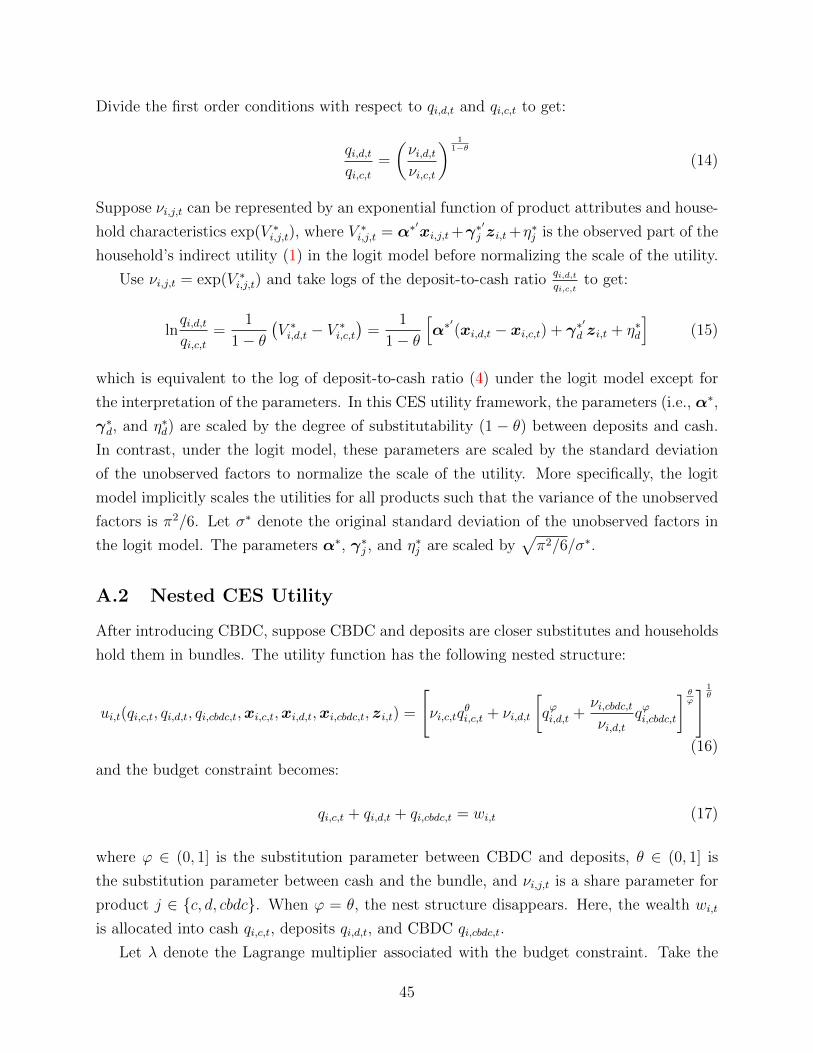
Divide the first order conditions with respect to qi,d,t and qi,c,t to get:

qi,d,tqi,c,t

=

(νi,d,tνi,c,t

) 11−θ

(14)

Suppose νi,j,t can be represented by an exponential function of product attributes and house-

hold characteristics exp(V ∗i,j,t), where V ∗i,j,t = α∗′xi,j,t+γ

∗′j zi,t+η∗j is the observed part of the

household’s indirect utility (1) in the logit model before normalizing the scale of the utility.

Use νi,j,t = exp(V ∗i,j,t) and take logs of the deposit-to-cash ratioqi,d,tqi,c,t

to get:

lnqi,d,tqi,c,t

=1

1− θ(V ∗i,d,t − V ∗i,c,t

)=

1

1− θ

[α∗′(xi,d,t − xi,c,t) + γ∗

′

d zi,t + η∗d

](15)

which is equivalent to the log of deposit-to-cash ratio (4) under the logit model except for

the interpretation of the parameters. In this CES utility framework, the parameters (i.e., α∗,

γ∗d, and η∗d) are scaled by the degree of substitutability (1 − θ) between deposits and cash.

In contrast, under the logit model, these parameters are scaled by the standard deviation

of the unobserved factors to normalize the scale of the utility. More specifically, the logit

model implicitly scales the utilities for all products such that the variance of the unobserved

factors is π2/6. Let σ∗ denote the original standard deviation of the unobserved factors in

the logit model. The parameters α∗, γ∗j , and η∗j are scaled by√π2/6/σ∗.

A.2 Nested CES Utility

After introducing CBDC, suppose CBDC and deposits are closer substitutes and households

hold them in bundles. The utility function has the following nested structure:

ui,t(qi,c,t, qi,d,t, qi,cbdc,t,xi,c,t,xi,d,t,xi,cbdc,t, zi,t) =

[νi,c,tq

θi,c,t + νi,d,t

[qϕi,d,t +

νi,cbdc,tνi,d,t

qϕi,cbdc,t

] θϕ

] 1θ

(16)

and the budget constraint becomes:

qi,c,t + qi,d,t + qi,cbdc,t = wi,t (17)

where ϕ ∈ (0, 1] is the substitution parameter between CBDC and deposits, θ ∈ (0, 1] is

the substitution parameter between cash and the bundle, and νi,j,t is a share parameter for

product j ∈ c, d, cbdc. When ϕ = θ, the nest structure disappears. Here, the wealth wi,t

is allocated into cash qi,c,t, deposits qi,d,t, and CBDC qi,cbdc,t.

Let λ denote the Lagrange multiplier associated with the budget constraint. Take the

45

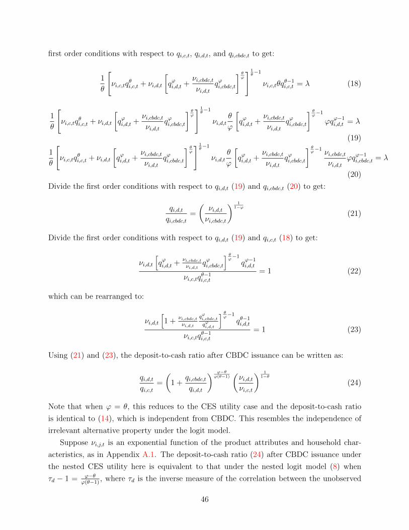
first order conditions with respect to qi,c,t, qi,d,t, and qi,cbdc,t to get:

1

θ

[νi,c,tq

θi,c,t + νi,d,t

[qϕi,d,t +

νi,cbdc,tνi,d,t

qϕi,cbdc,t

] θϕ

] 1θ−1

νi,c,tθqθ−1i,c,t = λ (18)

1

θ

[νi,c,tq

θi,c,t + νi,d,t

[qϕi,d,t +

νi,cbdc,tνi,d,t

qϕi,cbdc,t

] θϕ

] 1θ−1

νi,d,tθ

ϕ

[qϕi,d,t +

νi,cbdc,tνi,d,t

qϕi,cbdc,t

] θϕ−1

ϕqϕ−1i,d,t = λ

(19)

1

θ

[νi,c,tq

θi,c,t + νi,d,t

[qϕi,d,t +

νi,cbdc,tνi,d,t

qϕi,cbdc,t

] θϕ

] 1θ−1

νi,d,tθ

ϕ

[qϕi,d,t +

νi,cbdc,tνi,d,t

qϕi,cbdc,t

] θϕ−1νi,cbdc,tνi,d,t

ϕqϕ−1i,cbdc,t = λ

(20)

Divide the first order conditions with respect to qi,d,t (19) and qi,cbdc,t (20) to get:

qi,d,tqi,cbdc,t

=

(νi,d,tνi,cbdc,t

) 11−ϕ

(21)

Divide the first order conditions with respect to qi,d,t (19) and qi,c,t (18) to get:

νi,d,t

[qϕi,d,t +

νi,cbdc,tνi,d,t

qϕi,cbdc,t

] θϕ−1qϕ−1i,d,t

νi,c,tqθ−1i,c,t

= 1 (22)

which can be rearranged to:

νi,d,t

[1 +

νi,cbdc,tνi,d,t

qϕi,cbdc,tqϕi,d,t

] θϕ−1qθ−1i,d,t

νi,c,tqθ−1i,c,t

= 1 (23)

Using (21) and (23), the deposit-to-cash ratio after CBDC issuance can be written as:

qi,d,tqi,c,t

=

(1 +

qi,cbdc,tqi,d,t

) ϕ−θϕ(θ−1)

(νi,d,tνi,c,t

) 11−θ

(24)

Note that when ϕ = θ, this reduces to the CES utility case and the deposit-to-cash ratio

is identical to (14), which is independent from CBDC. This resembles the independence of

irrelevant alternative property under the logit model.

Suppose νi,j,t is an exponential function of the product attributes and household char-

acteristics, as in Appendix A.1. The deposit-to-cash ratio (24) after CBDC issuance under

the nested CES utility here is equivalent to that under the nested logit model (8) when

τd − 1 = ϕ−θϕ(θ−1) , where τd is the inverse measure of the correlation between the unobserved

46

utilities for similar products under the nested logit.

It can be seen from Appendix A.1 that the deposit-to-cash ratio before the CBDC issuance

is(νi,d,tνi,c,t

) 11−θ

. Hence, similar to the prediction from the nested logit model (8), the deposit-

to-cash ratio after the CBDC issuance is a fraction of that before the CBDC issuance, where

the fraction depends on how CBDC is valued against deposits (indicated byqi,cbdc,tqi,d,t

) and the

degree of substitutability between CBDC and deposits ϕ−θϕ(θ−1) .

B Choice Probabilities under Nested Logit Model

This section shows the probabilities of holding each dollar in each asset/product under the

nested logit model, where the choice probabilities are interpreted as the portfolio shares as

discussed in Section 2.1. It also shows how the deposit-to-cash ratio and the CBDC share

are affected by the correlation between the unobserved utilities for similar products. This

section shows the cases when CBDC is a closer substitute for deposits and cash in turn.

B.1 CBDC and Deposits are Closer Substitutes

Suppose CBDC and deposits are in the same nest Bd cbdc, then the deposit share is the

conditional probability of choosing deposits from the nestBd cbdc multiplied by the probability

of choosing the nest Bd cbdc:

s′i,d,t =exp

(Vi,d,tτd

)exp

(Vi,cbdc,tτd

)+ exp

(Vi,d,tτd

)︸︷︷︸

Prob(j=d|j∈Bd cbdc)

[exp

(Vi,cbdc,tτd

)+ exp

(Vi,d,tτd

)]τd[exp

(Vi,cbdc,tτd

)+ exp

(Vi,d,tτd

)]τd+ exp (Vi,c,t)︸︷︷︸

Prob(j∈Bd cbdc)

(25)

and the cash share is:

s′i,c,t =exp (Vi,c,t)[

exp(Vi,cbdc,tτd

)+ exp

(Vi,d,tτd

)]τd+ exp (Vi,c,t)

(26)

where τd ≡√

1− ρd cbdc ∈ (0, 1] is an inverse measure of the correlation ρd cbdc ∈ [0, 1)

between the unobserved utilities for deposits and CBDC.

Divide the deposit share (25) by the cash share (26) to get the deposit-to-cash ratio after

47

CBDC issuance:

s′i,d,ts′i,c,t

=exp

(Vi,d,tτd

) [exp

(Vi,d,tτd

)+ exp

(Vi,cbdc,tτd

)]τd−1exp (Vi,c,t)

= exp (Vi,d,t − Vi,c,t) exp

(Vi,d,tτd− Vi,d,t

)[exp

(Vi,d,tτd

)+ exp

(Vi,cbdc,tτd

)]τd−1=

[1 + exp


τd

)]τd−1exp (Vi,d,t − Vi,c,t)

(27)

where exp (Vi,d,t − Vi,c,t) =si,d,tsi,c,t

is the deposit-to-cash ratio before the CBDC issuance, as

can be seen from (4). Since[1 + exp

(Vi,cbdc,t−Vi,d,t

τd

)]> 1 and (τd − 1) 6 0, the fraction is

0 <[1 + exp

(Vi,cbdc,t−Vi,d,t

τd

)]τd−16 1. As a consequence,

s′i,d,ts′i,c,t

6 si,d,tsi,c,t

.

To see how the inverse correlation measure τd affects the deposit-to-cash ratio, differen-

tiate (27) with respect to τd to get:

∂s′i,d,ts′i,c,t

∂τd=

[1 + exp


τd

)]τd−1ln

(1 + exp


τd

))si,d,tsi,c,t

+ (τd − 1)

[1 + exp


τd

)]τd−2exp


τd

)(−Vi,cbdc,t − Vi,d,t

τ 2d

)si,d,tsi,c,t

=

(1 +

si,cbdc,ts′i,d,t

)τd−1si,d,tsi,c,t

[ln

(1 +

si,cbdc,ts′i,d,t

)+ (τd − 1)

1

1 +si,cbdc,ts′i,d,t

∂si,cbdc,ts′i,d,t

∂τd

]

=s′i,d,ts′i,c,t

[ln

(1 +

si,cbdc,ts′i,d,t

)+ (τd − 1)

1



∂τd

](28)

As can be seen from (28), how the deposit-to-cash ratio changes with τd depends on how the

CBDC-to-deposit ratiosi,cbdc,ts′i,d,t

= exp(Vi,cbdc,t−Vi,d,t

τd

)changes with τd:


∂τd= exp


τd

)(−Vi,cbdc,t − Vi,d,t

τ 2d

)(29)

which in turn depends on the sign of the observed utility difference (Vi,cbdc,t − Vi,d,t). When

Vi,cbdc,t−Vi,d,t > 0, the deposit-to-cash ratio increases in τd. In contrast, when Vi,cbdc,t−Vi,d,t <0, the deposit-to-cash ratio can decrease in τd.

Since the asset shares sum to one, i.e., s′i,c,t + s′i,d,t + si,cbdc,t = 1, divide this identity by

48

s′i,d,t and rearrange to write the CBDC share si,cbdc,t in terms of the deposit-to-cash ratio:

si,cbdc,t =

si,cbdc,ts′i,d,t

1 +s′i,c,ts′i,d,t

+si,cbdc,ts′i,d,t

(30)

To see how si,cbdc,t changes with τd, differentiate si,cbdc,t (30) with respect to τd:

∂si,cbdc,t∂τd

=

∂si,cbdc,t

s′i,d,t

∂τd


+si,cbdc,ts′i,d,t

−si,cbdc,ts′i,d,t(


+si,cbdc,ts′i,d,t

)2−(s′i,d,t

s′i,c,t

)−2 ∂ s′i,d,ts′i,c,t

∂τd+∂si,cbdc,ts′i,d,t

∂τd

=∂si,cbdc,ts′i,d,t

∂τd

1 +s′i,c,ts′i,d,t(


+si,cbdc,ts′i,d,t

)2 +∂s′i,d,ts′i,c,t

∂τd

si,cbdc,ts′i,d,t

(s′i,d,ts′i,c,t

)−2(


+si,cbdc,ts′i,d,t

)2(31)

Define Λ ≡(


+si,cbdc,ts′i,d,t

)and substitute (28) into (31) to get:

∂si,cbdc,t∂τd


∂τd


Λ2+

si,cbdc,ts′i,d,t

(s′i,d,ts′i,c,t

)−2Λ2

s′i,d,ts′i,c,t

[ln

(1 +

si,cbdc,ts′i,d,t

)+ (τd − 1)

1



∂τd

]


∂τd

1

Λ2


+

(s′i,d,ts′i,c,t

)−1(τd − 1)s′i,d,tsi,cbdc,t

+ 1

+

si,cbdc,ts′i,d,t

(s′i,d,ts′i,c,t

)−1Λ2

ln

(1 +

si,cbdc,ts′i,d,t

)


∂τd

1

Λ2


1 +(τd − 1)s′i,d,tsi,cbdc,t

+ 1

+

si,cbdc,ts′i,d,t

s′i,c,ts′i,d,t

Λ2ln

(1 +

si,cbdc,ts′i,d,t

)(32)

Since τd ∈ (0, 1] ands′i,d,tsi,cbdc,t

> 0, the term

(1 + (τd−1)

s′i,d,t

si,cbdc,t+1

)is positive. Hence, the sign of

the derivative∂si,cbdc,t∂τd

depends on how the CBDC-to-deposit ratiosi,cbdc,ts′i,d,t

changes with τd

(29), which in turn depends on the sign of the observed utility difference (Vi,cbdc,t − Vi,d,t).When Vi,cbdc,t − Vi,d,t > 0, it is ambiguous how the CBDC share changes with τd. When

Vi,cbdc,t − Vi,d,t 6 0, it is unambiguous that the CBDC share increases in τd.

49

B.2 CBDC and Cash are Closer Substitutes

If CBDC and cash are in the same nest, following similar steps in B.1, the deposit-to-cash

ratio after CBDC issuance is:

s′i,d,ts′i,c,t

=

[1 + exp


τc

)]1−τcexp (Vi,d,t − Vi,c,t) (33)

where τc ≡√

1− ρc cbdc ∈ (0, 1] is an inverse measure of the correlation ρc cbdc ∈ [0, 1)

and exp (Vi,d,t − Vi,c,t) =si,d,tsi,c,t

is the deposit-to-cash ratio before the CBDC issuance. Since[1 + exp

(Vi,cbdc,t−Vi,c,t

τc

)]> 1 and (1 − τc) > 0, the factor

[1 + exp

(Vi,cbdc,t−Vi,c,t

τc

)]1−τc> 1.

As a consequence,s′i,d,ts′i,c,t

> si,d,tsi,c,t

.

To see how the inverse correlation measure τc affects the deposit-to-cash ratio, differen-

tiate (33) with respect to τc and simplify to get:

∂s′i,d,ts′i,c,t

∂τc=s′i,d,ts′i,c,t

[−ln

(1 +

si,cbdc,ts′i,c,t

)+ (1− τc)

1

1 +si,cbdc,ts′i,c,t

∂si,cbdc,ts′i,c,t

∂τc

](34)

wheresi,cbdc,ts′i,c,t

= exp(Vi,cbdc,t−Vi,c,t

τc

)and the derivative of

si,cbdc,ts′i,c,t

with respect to τc is:

∂si,cbdc,ts′i,c,t

∂τc= exp


τc

)(−Vi,cbdc,t − Vi,c,t

τ 2c

)(35)

As can be seen from (34), how the deposit-to-cash ratio changes with τc depends on how the

CBDC-to-cash ratiosi,cbdc,ts′i,c,t

changes with τc (35), which in turn depends on how the observed

utility for CBDC compares with that for cash. When Vi,cbdc,t−Vi,c,t > 0, the deposit-to-cash

ratio unambiguously decreases in τc. When Vi,cbdc,t − Vi,c,t < 0, the deposit-to-cash ratio can

increase in τc.

Divide the identity s′i,c,t + s′i,d,t + si,cbdc,t = 1 by s′i,c,t and rearrange to write the CBDC

share si,cbdc,t in terms of the deposit-to-cash ratio:

si,cbdc,t =

si,cbdc,ts′i,c,t

1 +s′i,d,ts′i,c,t

+si,cbdc,ts′i,c,t

(36)

50

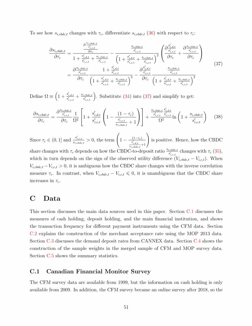
To see how si,cbdc,t changes with τc, differentiate si,cbdc,t (36) with respect to τc:

∂si,cbdc,t∂τc

=

∂si,cbdc,t

s′i,c,t

∂τc


+si,cbdc,ts′i,c,t

−si,cbdc,ts′i,c,t(


+si,cbdc,ts′i,c,t

)2∂ s′i,d,ts′i,c,t

∂τc+∂si,cbdc,ts′i,c,t

∂τc

=∂si,cbdc,ts′i,c,t

∂τc

1 +s′i,d,ts′i,c,t(


+si,cbdc,ts′i,c,t

)2 − ∂s′i,d,ts′i,c,t

∂τc

si,cbdc,ts′i,c,t(


+si,cbdc,ts′i,c,t

)2(37)

Define Ω ≡(


+si,cbdc,ts′i,c,t

). Substitute (34) into (37) and simplify to get:

∂si,cbdc,t∂τc

=∂si,cbdc,ts′i,c,t

∂τc

1

Ω2


1− (1− τc)s′i,c,tsi,cbdc,t

+ 1

+

si,cbdc,ts′i,c,t

s′i,d,ts′i,c,t

Ω2ln

(1 +

si,cbdc,ts′i,c,t

)(38)

Since τc ∈ (0, 1] ands′i,c,tsi,cbdc,t

> 0, the term

(1− (1−τc)

s′i,d,t

si,cbdc,t+1

)is positive. Hence, how the CBDC

share changes with τc depends on how the CBDC-to-deposit ratiosi,cbdc,ts′i,c,t

changes with τc (35),

which in turn depends on the sign of the observed utility difference (Vi,cbdc,t − Vi,c,t). When

Vi,cbdc,t−Vi,c,t > 0, it is ambiguous how the CBDC share changes with the inverse correlation

measure τc. In contrast, when Vi,cbdc,t − Vi,c,t 6 0, it is unambiguous that the CBDC share

increases in τc.

C Data

This section discusses the main data sources used in this paper. Section C.1 discusses the

measures of cash holding, deposit holding, and the main financial institution, and shows

the transaction frequency for different payment instruments using the CFM data. Section

C.2 explains the construction of the merchant acceptance rate using the MOP 2013 data.

Section C.3 discusses the demand deposit rates from CANNEX data. Section C.4 shows the

construction of the sample weights in the merged sample of CFM and MOP survey data.

Section C.5 shows the summary statistics.

C.1 Canadian Financial Monitor Survey

The CFM survey data are available from 1999, but the information on cash holding is only

available from 2009. In addition, the CFM survey became an online survey after 2018, so the

51

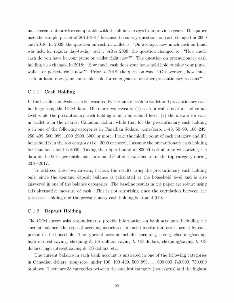
most recent data are less comparable with the offline surveys from previous years. This paper

uses the sample period of 2010–2017 because the survey questions on cash changed in 2009

and 2018. In 2009, the question on cash in wallet is, “On average, how much cash on hand

was held for regular day-to-day use?”. After 2009, the question changed to: “How much

cash do you have in your purse or wallet right now?”. The question on precautionary cash

holding also changed in 2018: “How much cash does your household hold outside your purse,

wallet, or pockets right now?”. Prior to 2018, the question was, “(On average), how much

cash on hand does your household hold for emergencies, or other precautionary reasons?”.

C.1.1 Cash Holding

In the baseline analysis, cash is measured by the sum of cash in wallet and precautionary cash

holdings using the CFM data. There are two caveats: (1) cash in wallet is at an individual

level while the precautionary cash holding is at a household level; (2) the answer for cash

in wallet is in the nearest Canadian dollar, while that for the precautionary cash holding

is in one of the following categories in Canadian dollars: none/zero, 1–49, 50–99, 100–249,

250–499, 500–999, 1000–2999, 3000 or more. I take the middle point of each category and if a

household is in the top category (i.e., 3000 or more), I assume the precautionary cash holding

for that household is 3000. Taking the upper bound at $3000 is similar to winsorizing the

data at the 96th percentile, since around 4% of observations are in the top category during

2010–2017.

To address these two caveats, I check the results using the precautionary cash holding

only, since the demand deposit balance is calculated at the household level and is also

answered in one of the balance categories. The baseline results in the paper are robust using

this alternative measure of cash. This is not surprising since the correlation between the

total cash holding and the precautionary cash holding is around 0.98.

C.1.2 Deposit Holding

The CFM survey asks respondents to provide information on bank accounts (including the

current balance, the type of account, associated financial institution, etc.) owned by each

person in the household. The types of account include: chequing, saving, chequing/saving,

high interest saving, chequing & US dollars, saving & US dollars, chequing/saving & US

dollars, high interest saving & US dollars, etc.

The current balance in each bank account is answered in one of the following categories

in Canadian dollars: non/zero, under 100, 100–499, 500–999, ..., 600,000–749,999, 750,000

or above. There are 38 categories between the smallest category (none/zero) and the highest

52

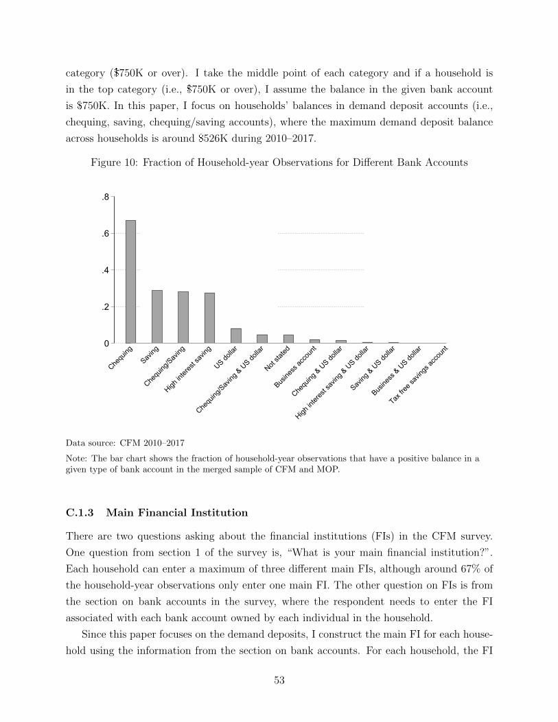
category ($750K or over). I take the middle point of each category and if a household is

in the top category (i.e., $750K or over), I assume the balance in the given bank account

is $750K. In this paper, I focus on households’ balances in demand deposit accounts (i.e.,

chequing, saving, chequing/saving accounts), where the maximum demand deposit balance

across households is around $526K during 2010–2017.

Figure 10: Fraction of Household-year Observations for Different Bank Accounts

0

.2

.4

.6

.8

Chequ

ing

Saving

Chequ

ing/Sav

ing

High in

teres

t sav

ing

US dolla

r

Chequ

ing/Sav

ing & U

S dolla

r

Not sta

ted

Busine

ss ac

coun

t

Chequ

ing & U

S dolla

r

High in

teres

t sav

ing & U

S dolla

r

Saving

& US do

llar

Busine

ss & U

S dolla

r

Tax fre

e sav

ings a

ccou

nt

Data source: CFM 2010–2017

Note: The bar chart shows the fraction of household-year observations that have a positive balance in agiven type of bank account in the merged sample of CFM and MOP.

C.1.3 Main Financial Institution

There are two questions asking about the financial institutions (FIs) in the CFM survey.

One question from section 1 of the survey is, “What is your main financial institution?”.

Each household can enter a maximum of three different main FIs, although around 67% of

the household-year observations only enter one main FI. The other question on FIs is from

the section on bank accounts in the survey, where the respondent needs to enter the FI

associated with each bank account owned by each individual in the household.

Since this paper focuses on the demand deposits, I construct the main FI for each house-

hold using the information from the section on bank accounts. For each household, the FI

53

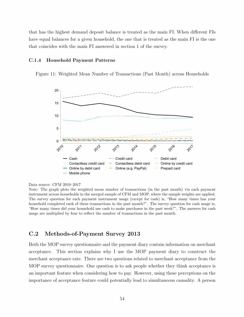
that has the highest demand deposit balance is treated as the main FI. When different FIs

have equal balances for a given household, the one that is treated as the main FI is the one

that coincides with the main FI answered in section 1 of the survey.

C.1.4 Household Payment Patterns

Figure 11: Weighted Mean Number of Transactions (Past Month) across Households

0

5

10

15

20

2010

2011

2012

2013

2014

2015

2016

2017

Cash Credit card Debit cardContactless credit card Contactless debit card Online by credit cardOnline by debit card Online (e.g. PayPal) Prepaid cardMobile phone

Data source: CFM 2010–2017Note: The graph plots the weighted mean number of transactions (in the past month) via each paymentinstrument across households in the merged sample of CFM and MOP, where the sample weights are applied.The survey question for each payment instrument usage (except for cash) is, “How many times has yourhousehold completed each of these transactions in the past month?”. The survey question for cash usage is,“How many times did your household use cash to make purchases in the past week?”. The answers for cashusage are multiplied by four to reflect the number of transactions in the past month.

C.2 Methods-of-Payment Survey 2013

Both the MOP survey questionnaire and the payment diary contain information on merchant

acceptance. This section explains why I use the MOP payment diary to construct the

merchant acceptance rate. There are two questions related to merchant acceptance from the

MOP survey questionnaire. One question is to ask people whether they think acceptance is

an important feature when considering how to pay. However, using these perceptions on the

importance of acceptance feature could potentially lead to simultaneous causality. A person

54

that prefers to use deposits to pay and hence holds more deposits may think acceptance is

more important.

Another question from the survey questionnaire is to ask people whether they think a

given payment instrument is widely accepted. The categories that people can choose from

include: rarely accepted, occasionally accepted, often accepted, almost always accepted, and

not sure. These perceptions tend to be less informative than the acceptance rate calculated

using the payment diary because the perceptions of acceptance are not the only determinant

for which stores people want to visit. They will also consider factors such as the location

and the quality of the goods. For example, when some people perceive debit cards to be less

widely accepted, this does not necessarily mean they would hold more cash and use cash

to pay since they can avoid the cash-only stores or they may prefer to shop in the stores

that accept cards anyway. In contrast, the card acceptance rates experienced by individuals

through their own transactions tend to result from the individuals’ optimal decisions in

terms of which stores to visit, which are likely to matter more for their allocation between

deposits and cash. Therefore, this paper uses the information from the MOP payment diary

to construct the individual-level acceptance rate.

C.3 CANNEX Deposit Rates

CANNEX data are at a bank-product-week level. I average the weekly rates to get the

annual rates. I use the deposit products from the high interest chequing category classified

in CANNEX, because they are likely to be the most relevant for the demand deposit rates.

Other categories of deposit products during the sample period include daily interest savings

which are non-chequable and offer much higher deposit rates, daily interest chequing which

tend to have rates close to zero throughout the sample period, daily interest investment for

large balances, and senior and junior accounts that target particular groups of people. The

high interest chequing accounts offer different tiers of interest rates, where the rate is higher

for a larger balance. I take the average rate across different tiers to get the deposit rate of a

given product. Each of the banks that I use has one product in this high interest chequing

category except for CIBC which has two. To get the deposit rate at a bank-year level for

CIBC, I average the deposit rates across the two products.

The deposit rates for the high interest chequing accounts are available for the big six,

Laurentian Bank, Alterna Bank, Alterna Savings, and Manulife Bank over the sample period

of 2010–2017. However, the latter three are not on the CFM choice list, so I use the deposit

rates for the big six and Laurentian Bank which can be matched to the CFM data.

55

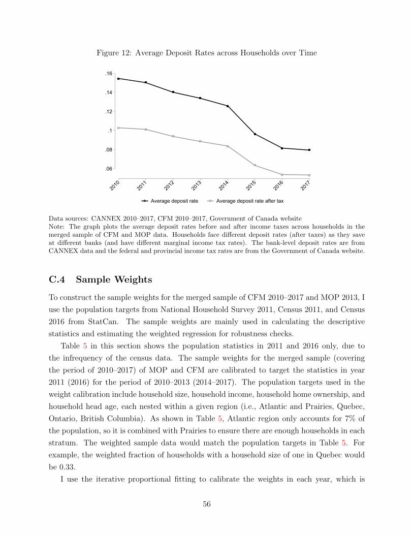
Figure 12: Average Deposit Rates across Households over Time

.06

.08

.1

.12

.14

.16

2010

2011

2012

2013

2014

2015

2016

2017

Average deposit rate Average deposit rate after tax

Data sources: CANNEX 2010–2017, CFM 2010–2017, Government of Canada websiteNote: The graph plots the average deposit rates before and after income taxes across households in themerged sample of CFM and MOP data. Households face different deposit rates (after taxes) as they saveat different banks (and have different marginal income tax rates). The bank-level deposit rates are fromCANNEX data and the federal and provincial income tax rates are from the Government of Canada website.

C.4 Sample Weights

To construct the sample weights for the merged sample of CFM 2010–2017 and MOP 2013, I

use the population targets from National Household Survey 2011, Census 2011, and Census

2016 from StatCan. The sample weights are mainly used in calculating the descriptive

statistics and estimating the weighted regression for robustness checks.

Table 5 in this section shows the population statistics in 2011 and 2016 only, due to

the infrequency of the census data. The sample weights for the merged sample (covering

the period of 2010–2017) of MOP and CFM are calibrated to target the statistics in year

2011 (2016) for the period of 2010–2013 (2014–2017). The population targets used in the

weight calibration include household size, household income, household home ownership, and

household head age, each nested within a given region (i.e., Atlantic and Prairies, Quebec,

Ontario, British Columbia). As shown in Table 5, Atlantic region only accounts for 7% of

the population, so it is combined with Prairies to ensure there are enough households in each

stratum. The weighted sample data would match the population targets in Table 5. For

example, the weighted fraction of households with a household size of one in Quebec would

be 0.33.

I use the iterative proportional fitting to calibrate the weights in each year, which is

56

commonly used in sample calibration as documented in Kolenikov (2014) and Vincent (2013).

The first step is to specify the initial weights. I use the population totals over the number of

households in the sample for each income-region category as initial weights. Using population

totals over the number of households in the sample to generate the same initial weight for

everyone does not affect the raking procedure and gives the same calibrated weights. The

second step is to update the sample weights for each targeted demographic category in turn

such that the weighted totals (of households) match the population counts in the given

demographic category. The second step is repeated until the distances between the weighted

totals and the population totals are minimized for all the targeted demographic categories.

57

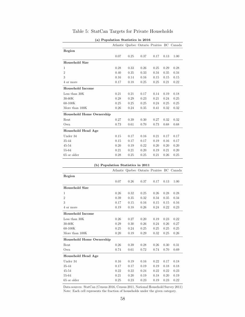
Table 5: StatCan Targets for Private Households

(a) Population Statistics in 2016

Atlantic Quebec Ontario Prairies BC Canada

Region

0.07 0.25 0.37 0.17 0.13 1.00

Household Size

1 0.28 0.33 0.26 0.25 0.29 0.28

2 0.40 0.35 0.33 0.34 0.35 0.34

3 0.16 0.14 0.16 0.15 0.15 0.15

4 or more 0.17 0.18 0.25 0.25 0.21 0.22

Household Income

Less than 30K 0.21 0.21 0.17 0.14 0.19 0.18

30-60K 0.28 0.29 0.23 0.21 0.24 0.25

60-100K 0.25 0.25 0.25 0.24 0.25 0.25

More than 100K 0.26 0.24 0.35 0.41 0.32 0.32

Household Home Ownership

Rent 0.27 0.39 0.30 0.27 0.32 0.32

Own 0.73 0.61 0.70 0.73 0.68 0.68

Household Head Age

Under 34 0.15 0.17 0.16 0.21 0.17 0.17

35-44 0.15 0.17 0.17 0.19 0.16 0.17

45-54 0.20 0.19 0.22 0.20 0.20 0.20

55-64 0.21 0.21 0.20 0.19 0.21 0.20

65 or older 0.28 0.25 0.25 0.21 0.26 0.25

(b) Population Statistics in 2011

Atlantic Quebec Ontario Prairies BC Canada

Region

0.07 0.26 0.37 0.17 0.13 1.00

Household Size

1 0.26 0.32 0.25 0.26 0.28 0.28

2 0.39 0.35 0.32 0.34 0.35 0.34

3 0.17 0.15 0.16 0.15 0.15 0.16

4 or more 0.19 0.18 0.26 0.24 0.22 0.23

Household Income

Less than 30K 0.26 0.27 0.20 0.19 0.23 0.22

30-60K 0.29 0.30 0.26 0.24 0.26 0.27

60-100K 0.25 0.24 0.25 0.25 0.25 0.25

More than 100K 0.20 0.19 0.29 0.32 0.25 0.26

Household Home Ownership

Rent 0.26 0.39 0.28 0.26 0.30 0.31

Own 0.74 0.61 0.72 0.74 0.70 0.69

Household Head Age

Under 34 0.16 0.19 0.16 0.22 0.17 0.18

35-44 0.17 0.17 0.19 0.19 0.18 0.18

45-54 0.22 0.22 0.24 0.22 0.22 0.23

55-64 0.21 0.20 0.19 0.18 0.20 0.19

65 or older 0.25 0.23 0.23 0.19 0.23 0.22

Data sources: StatCan (Census 2016, Census 2011, National Household Survey 2011)Note: Each cell represents the fraction of households under the given category.

58

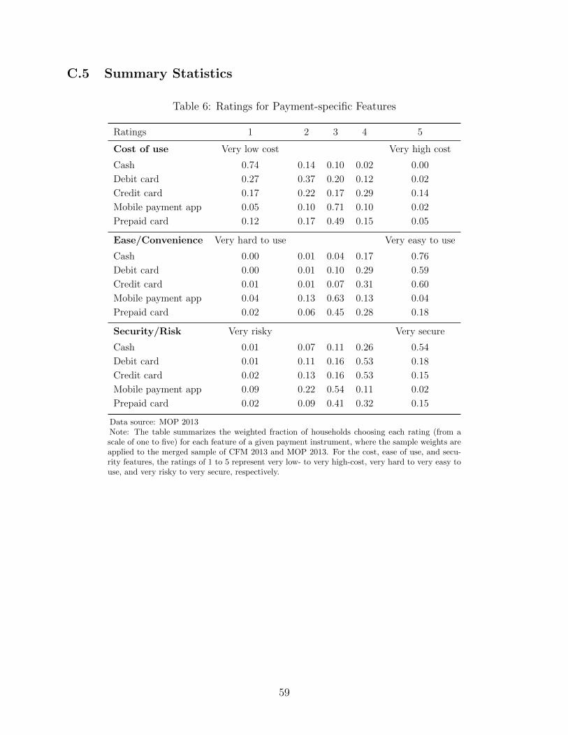
C.5 Summary Statistics

Table 6: Ratings for Payment-specific Features

Ratings 1 2 3 4 5

Cost of use Very low cost Very high cost

Cash 0.74 0.14 0.10 0.02 0.00

Debit card 0.27 0.37 0.20 0.12 0.02

Credit card 0.17 0.22 0.17 0.29 0.14

Mobile payment app 0.05 0.10 0.71 0.10 0.02

Prepaid card 0.12 0.17 0.49 0.15 0.05

Ease/Convenience Very hard to use Very easy to use

Cash 0.00 0.01 0.04 0.17 0.76

Debit card 0.00 0.01 0.10 0.29 0.59

Credit card 0.01 0.01 0.07 0.31 0.60


Prepaid card 0.02 0.06 0.45 0.28 0.18

Security/Risk Very risky Very secure

Cash 0.01 0.07 0.11 0.26 0.54

Debit card 0.01 0.11 0.16 0.53 0.18

Credit card 0.02 0.13 0.16 0.53 0.15


Prepaid card 0.02 0.09 0.41 0.32 0.15

Data source: MOP 2013Note: The table summarizes the weighted fraction of households choosing each rating (from ascale of one to five) for each feature of a given payment instrument, where the sample weights areapplied to the merged sample of CFM 2013 and MOP 2013. For the cost, ease of use, and secu-rity features, the ratings of 1 to 5 represent very low- to very high-cost, very hard to very easy touse, and very risky to very secure, respectively.

59

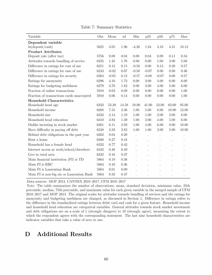
Table 7: Summary Statistics

Variable Obs Mean sd Min p25 p50 p75 Max

Dependent variableln(deposit/cash) 5025 3.05 1.96 -4.20 1.84 3.10 4.31 10.13

Product AttributesDeposit rate (after tax) 5756 0.08 0.04 0.00 0.04 0.09 0.11 0.34

Attitudes towards bundling of service 6235 1.45 1.76 0.00 0.00 1.00 3.00 5.00

Difference in ratings for cost of use 6251 0.12 0.15 -0.50 0.00 0.13 0.20 0.57

Difference in ratings for ease of use 6243 -0.02 0.07 -0.50 -0.07 0.00 0.00 0.36

Difference in ratings for security 6264 -0.05 0.12 -0.57 -0.08 -0.07 0.00 0.57

Ratings for anonymity 6296 4.10 1.72 0.00 3.00 4.00 6.00 6.00

Ratings for budgeting usefulness 6279 3.70 1.82 0.00 3.00 4.00 5.00 6.00

Fraction of online transactions 5910 0.03 0.09 0.00 0.00 0.00 0.00 1.00

Fraction of transactions cards unaccepted 5910 0.06 0.14 0.00 0.00 0.00 0.00 1.00

Household CharacteristicsHousehold head age 6332 52.28 14.58 18.00 41.00 53.00 63.00 95.00

Household income 6208 7.55 3.36 1.00 5.00 8.00 10.00 12.00

Household size 6332 2.14 1.19 1.00 1.00 2.00 3.00 8.00

Household head education 6310 3.82 1.39 1.00 2.00 4.00 5.00 6.00

Dislike investing in stock market 6261 6.11 2.93 1.00 4.00 6.00 9.00 10.00

Have difficulty in paying off debt 6248 3.33 2.82 1.00 1.00 2.00 5.00 10.00

Behind debt obligations in the past year 6202 0.04 0.20 . . . . .

Rent a home 6200 0.27 0.44 . . . . .

Household has a female head 6332 0.77 0.42 . . . . .

Internet access at work/school/elsewhere 6332 0.40 0.49 . . . . .

Live in rural area 6332 0.16 0.37 . . . . .

Main financial institution (FI) is TD 5864 0.18 0.38 . . . . .

Main FI is RBC 5864 0.16 0.36 . . . . .

Main FI is Laurentian Bank 5864 0.01 0.09 . . . . .

Main FI is non-big six or Laurentian Bank 5864 0.33 0.47 . . . . .

Data sources: MOP 2013, CANNEX 2010–2017, CFM 2010–2017Note: The table summarizes the number of observations, mean, standard deviation, minimum value, 25thpercentile, median, 75th percentile, and maximum value for each given variable in the merged sample of CFM2010–2017 and MOP 2013. The original scales for attitudes towards bundling of services and the ratings foranonymity and budgeting usefulness are changed, as discussed in Section 3. Difference in ratings refers tothe difference in the standardized ratings between debit card and cash for a given feature. Household incomeand household head education are categorical variables. General attitudes towards stock market investmentand debt obligations are on a scale of 1 (strongly disagree) to 10 (strongly agree), measuring the extent towhich the respondent agrees with the corresponding statement. The last nine household characteristics areindicator variables that take a value of zero or one.

D Additional Results

60

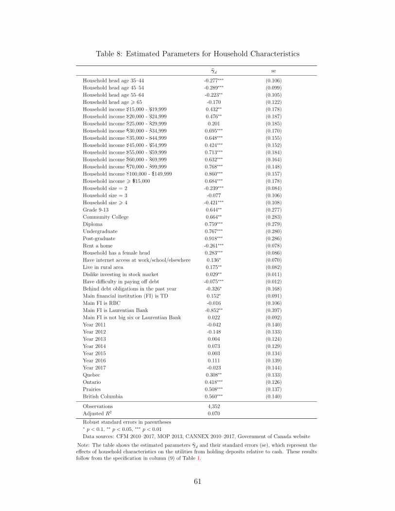
Table 8: Estimated Parameters for Household Characteristics

γd se

Household head age 35–44 -0.277∗∗∗ (0.106)

Household head age 45–54 -0.289∗∗∗ (0.099)

Household head age 55–64 -0.223∗∗ (0.105)

Household head age > 65 -0.170 (0.122)

Household income $15,000 - $19,999 0.432∗∗ (0.178)

Household income $20,000 - $24,999 0.476∗∗ (0.187)

Household income $25,000 - $29,999 0.201 (0.185)

Household income $30,000 - $34,999 0.695∗∗∗ (0.170)







Household income > $15,000 0.684∗∗∗ (0.178)

Household size = 2 -0.239∗∗∗ (0.084)

Household size = 3 -0.077 (0.106)

Household size > 4 -0.421∗∗∗ (0.108)

Grade 9-13 0.644∗∗ (0.277)

Community College 0.664∗∗ (0.283)

Diploma 0.759∗∗∗ (0.279)

Undergraduate 0.767∗∗∗ (0.280)

Post-graduate 0.918∗∗∗ (0.286)

Rent a home -0.261∗∗∗ (0.078)

Household has a female head 0.283∗∗∗ (0.086)

Have internet access at work/school/elsewhere 0.136∗ (0.070)

Live in rural area 0.175∗∗ (0.082)

Dislike investing in stock market 0.029∗∗ (0.011)

Have difficulty in paying off debt -0.075∗∗∗ (0.012)

Behind debt obligations in the past year -0.326∗ (0.168)

Main financial institution (FI) is TD 0.152∗ (0.091)

Main FI is RBC -0.016 (0.106)

Main FI is Laurentian Bank -0.852∗∗ (0.397)

Main FI is not big six or Laurentian Bank 0.022 (0.092)

Year 2011 -0.042 (0.140)

Year 2012 -0.148 (0.133)

Year 2013 0.004 (0.124)

Year 2014 0.073 (0.129)

Year 2015 0.003 (0.134)

Year 2016 0.111 (0.139)

Year 2017 -0.023 (0.144)

Quebec 0.308∗∗ (0.133)

Ontario 0.418∗∗∗ (0.126)

Prairies 0.508∗∗∗ (0.137)

British Columbia 0.560∗∗∗ (0.140)

Observations 4,352

Adjusted R2 0.070

Robust standard errors in parentheses∗ p < 0.1, ∗∗ p < 0.05, ∗∗∗ p < 0.01

Data sources: CFM 2010–2017, MOP 2013, CANNEX 2010–2017, Government of Canada website

Note: The table shows the estimated parameters γd and their standard errors (se), which represent theeffects of household characteristics on the utilities from holding deposits relative to cash. These resultsfollow from the specification in column (9) of Table 1.

61

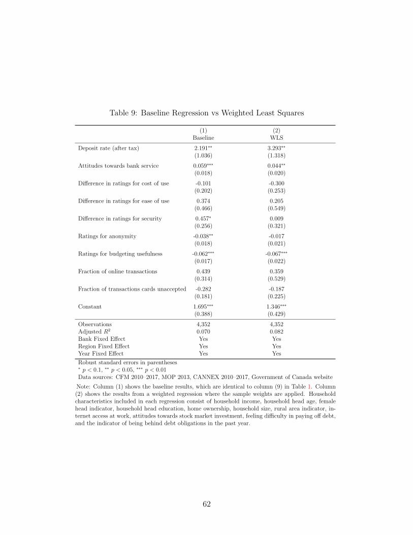
Table 9: Baseline Regression vs Weighted Least Squares

(1) (2)Baseline WLS

Deposit rate (after tax) 2.191∗∗ 3.293∗∗

(1.036) (1.318)

Attitudes towards bank service 0.059∗∗∗ 0.044∗∗

(0.018) (0.020)

Difference in ratings for cost of use -0.101 -0.300(0.202) (0.253)

Difference in ratings for ease of use 0.374 0.205(0.466) (0.549)

Difference in ratings for security 0.457∗ 0.009(0.256) (0.321)

Ratings for anonymity -0.038∗∗ -0.017(0.018) (0.021)

Ratings for budgeting usefulness -0.062∗∗∗ -0.067∗∗∗

(0.017) (0.022)

Fraction of online transactions 0.439 0.359(0.314) (0.529)

Fraction of transactions cards unaccepted -0.282 -0.187(0.181) (0.225)

Constant 1.695∗∗∗ 1.346∗∗∗

(0.388) (0.429)

Observations 4,352 4,352Adjusted R2 0.070 0.082Bank Fixed Effect Yes YesRegion Fixed Effect Yes YesYear Fixed Effect Yes Yes

Robust standard errors in parentheses∗ p < 0.1, ∗∗ p < 0.05, ∗∗∗ p < 0.01Data sources: CFM 2010–2017, MOP 2013, CANNEX 2010–2017, Government of Canada website

Note: Column (1) shows the baseline results, which are identical to column (9) in Table 1. Column(2) shows the results from a weighted regression where the sample weights are applied. Householdcharacteristics included in each regression consist of household income, household head age, femalehead indicator, household head education, home ownership, household size, rural area indicator, in-ternet access at work, attitudes towards stock market investment, feeling difficulty in paying off debt,and the indicator of being behind debt obligations in the past year.

62

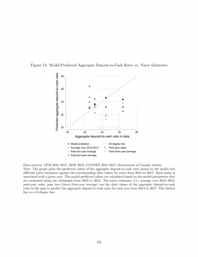
Figure 13: Model-Predicted Aggregate Deposit-to-Cash Ratio vs. Naive Estimates

20

22

24

26

28

Pred

icte

d ag

greg

ate

depo

sit-t

o-ca

sh ra

tio

20 22 24 26 28

Aggregate deposit-to-cash ratio in data

Model prediction 45-degree lineAverage over 2010-2013 Past-year valuePast two-year average Past three-year averagePast four-year average

Data sources: CFM 2010–2017, MOP 2013, CANNEX 2010–2017, Government of Canada websiteNote: The graph plots the predicted values of the aggregate deposit-to-cash ratio based on the model anddifferent naive estimates against the corresponding data values for years from 2014 to 2017. Each point isassociated with a given year. The model-predicted values are calculated based on the model parameters thatare estimated using the subsample from 2010 to 2013. The naive estimates (i.e., average over 2010–2013,past-year value, past two-/three-/four-year average) use the data values of the aggregate deposit-to-cashratio in the past to predict the aggregate deposit-to-cash ratio for each year from 2014 to 2017. The dashedline is a 45-degree line.

63

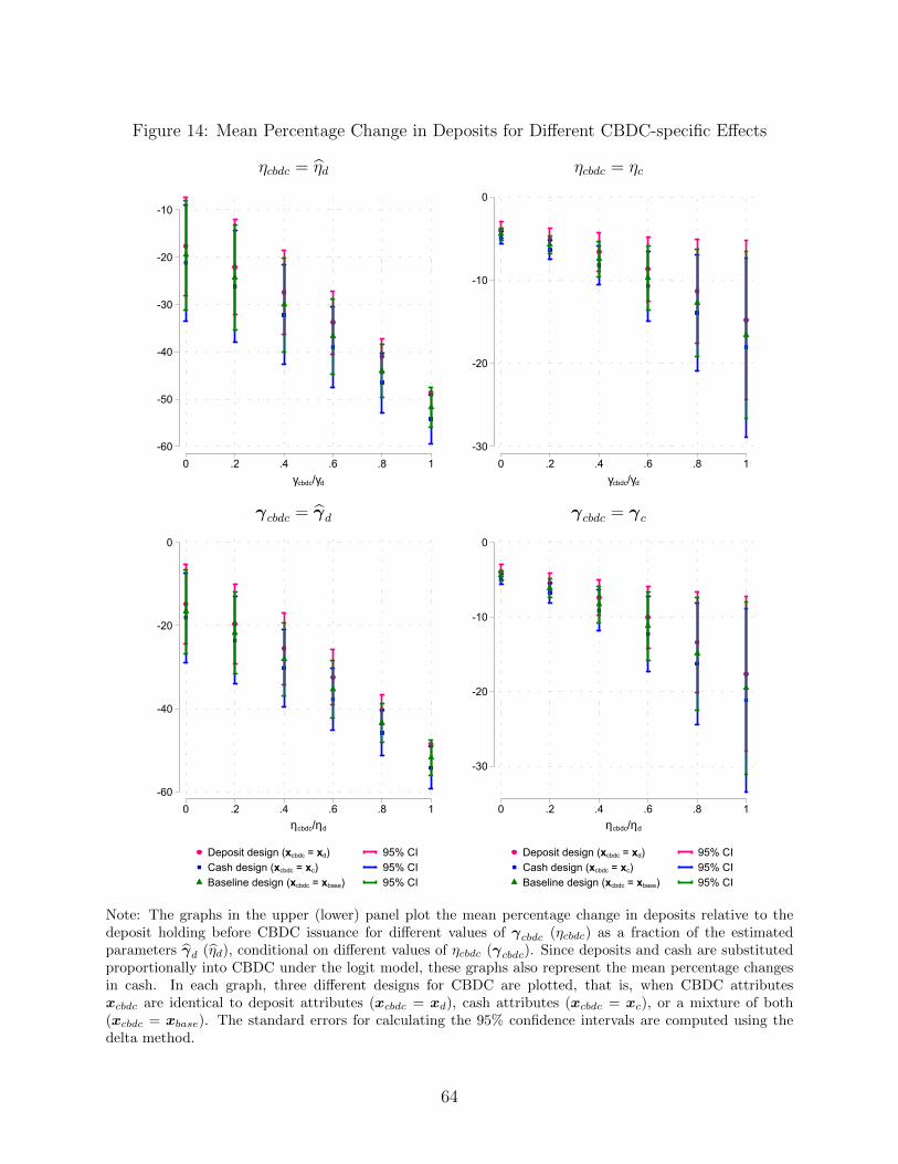
Figure 14: Mean Percentage Change in Deposits for Different CBDC-specific Effects

ηcbdc = ηd

-60

-50

-40

-30

-20

-10

0 .2 .4 .6 .8 1γcbdc/γd


ηcbdc = ηc

-30

-20

-10

0

0 .2 .4 .6 .8 1γcbdc/γd


γcbdc = γd

-60

-40

-20

0

0 .2 .4 .6 .8 1ηcbdc/ηd


γcbdc = γc

-30

-20

-10

0

0 .2 .4 .6 .8 1ηcbdc/ηd


Note: The graphs in the upper (lower) panel plot the mean percentage change in deposits relative to thedeposit holding before CBDC issuance for different values of γcbdc (ηcbdc) as a fraction of the estimatedparameters γd (ηd), conditional on different values of ηcbdc (γcbdc). Since deposits and cash are substitutedproportionally into CBDC under the logit model, these graphs also represent the mean percentage changesin cash. In each graph, three different designs for CBDC are plotted, that is, when CBDC attributesxcbdc are identical to deposit attributes (xcbdc = xd), cash attributes (xcbdc = xc), or a mixture of both(xcbdc = xbase). The standard errors for calculating the 95% confidence intervals are computed using thedelta method.

64

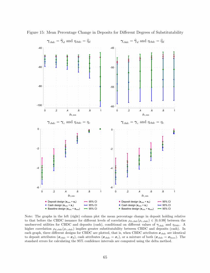
Figure 15: Mean Percentage Change in Deposits for Different Degrees of Substitutability


-100

-80

-60

-40

0 .2 .4 .6 .8 1ρd_cbdc



-60

-55

-50

-45

0 .2 .4 .6 .8 1ρc_cbdc



-6

-4

-2

0

0 .2 .4 .6 .8 1ρd_cbdc



-6

-4

-2

0

0 .2 .4 .6 .8 1ρc_cbdc


Note: The graphs in the left (right) column plot the mean percentage change in deposit holding relativeto that before the CBDC issuance for different levels of correlation ρd cbdc(ρc cbdc) ∈ [0, 0.99] between theunobserved utilities for CBDC and deposits (cash), conditional on different values of γcbdc and ηcbdc. Ahigher correlation ρd cbdc(ρc cbdc) implies greater substitutability between CBDC and deposits (cash). Ineach graph, three different designs for CBDC are plotted, that is, when CBDC attributes xcbdc are identicalto deposit attributes (xcbdc = xd), cash attributes (xcbdc = xc), or a mixture of both (xcbdc = xbase). Thestandard errors for calculating the 95% confidence intervals are computed using the delta method.

65

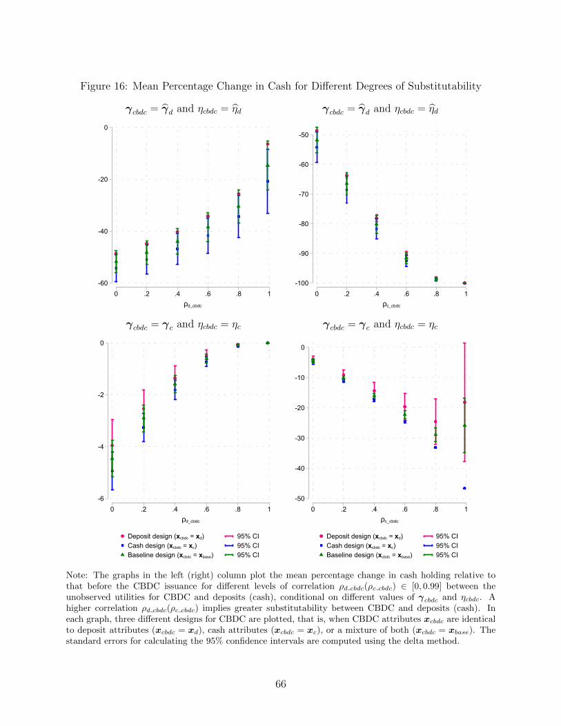
Figure 16: Mean Percentage Change in Cash for Different Degrees of Substitutability


-60

-40

-20

0

0 .2 .4 .6 .8 1ρd_cbdc



-100

-90

-80

-70

-60

-50

0 .2 .4 .6 .8 1ρc_cbdc



-6

-4

-2

0

0 .2 .4 .6 .8 1ρd_cbdc



-50

-40

-30

-20

-10

0

0 .2 .4 .6 .8 1ρc_cbdc


Note: The graphs in the left (right) column plot the mean percentage change in cash holding relative tothat before the CBDC issuance for different levels of correlation ρd cbdc(ρc cbdc) ∈ [0, 0.99] between theunobserved utilities for CBDC and deposits (cash), conditional on different values of γcbdc and ηcbdc. Ahigher correlation ρd cbdc(ρc cbdc) implies greater substitutability between CBDC and deposits (cash). Ineach graph, three different designs for CBDC are plotted, that is, when CBDC attributes xcbdc are identicalto deposit attributes (xcbdc = xd), cash attributes (xcbdc = xc), or a mixture of both (xcbdc = xbase). Thestandard errors for calculating the 95% confidence intervals are computed using the delta method.

66

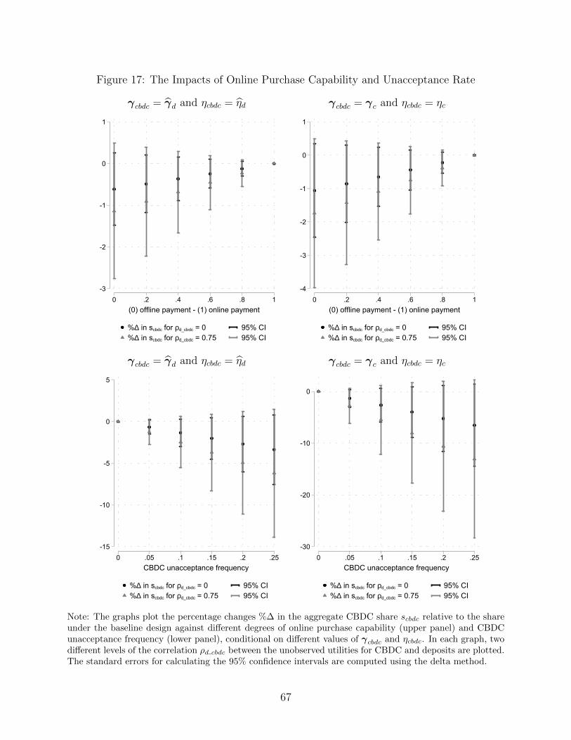
Figure 17: The Impacts of Online Purchase Capability and Unacceptance Rate


-3

-2

-1

0

1

0 .2 .4 .6 .8 1(0) offline payment - (1) online payment



-4

-3

-2

-1

0

1

0 .2 .4 .6 .8 1(0) offline payment - (1) online payment



-15

-10

-5

0

5

0 .05 .1 .15 .2 .25CBDC unacceptance frequency



-30

-20

-10

0

0 .05 .1 .15 .2 .25CBDC unacceptance frequency


Note: The graphs plot the percentage changes %∆ in the aggregate CBDC share scbdc relative to the shareunder the baseline design against different degrees of online purchase capability (upper panel) and CBDCunacceptance frequency (lower panel), conditional on different values of γcbdc and ηcbdc. In each graph, twodifferent levels of the correlation ρd cbdc between the unobserved utilities for CBDC and deposits are plotted.The standard errors for calculating the 95% confidence intervals are computed using the delta method.

67

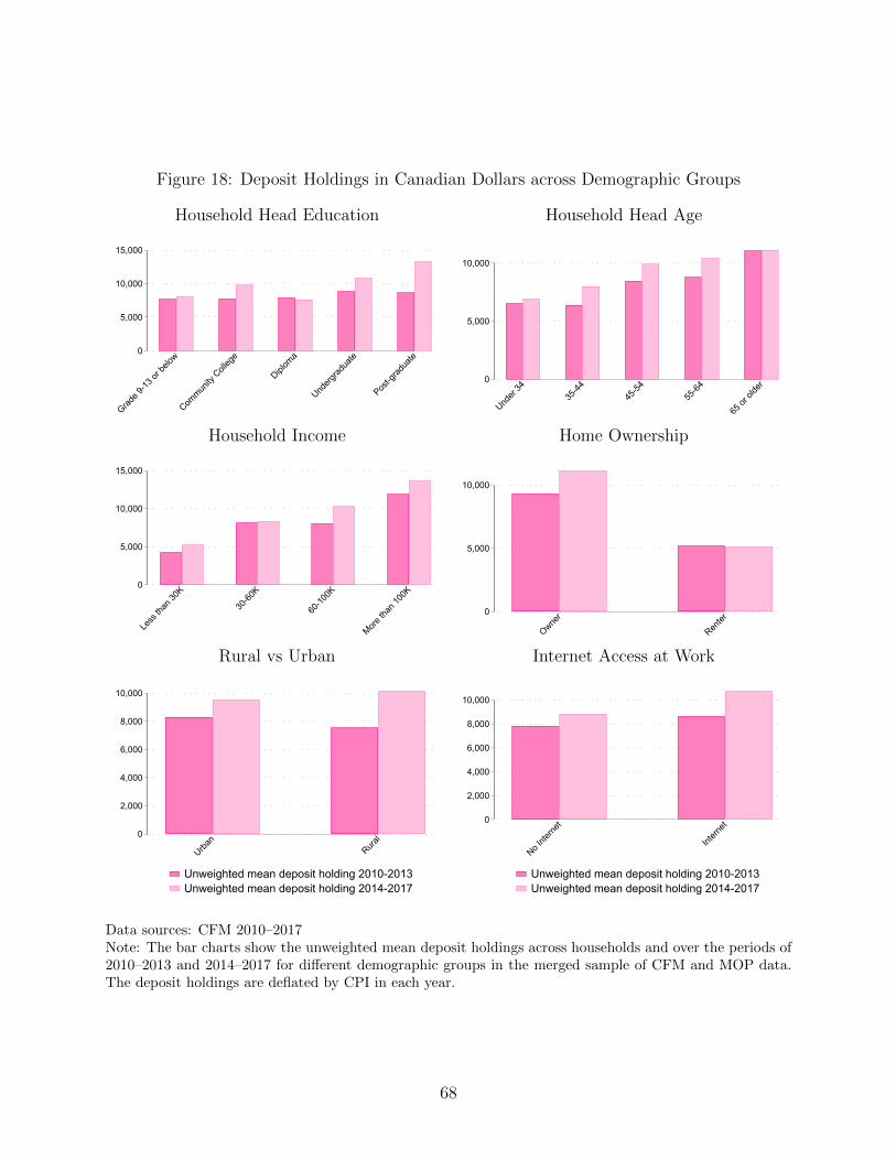
Figure 18: Deposit Holdings in Canadian Dollars across Demographic Groups


0

5,000

10,000

15,000

Grade 9

-13 or

below

Commun

ity C

olleg

e

Diplom

a

Underg

radua

te

Post-g

radua

te

Unweighted mean deposit holding 2010-2013Unweighted mean deposit holding 2014-2017

Household Head Age

0

5,000

10,000

Under

3435

-4445

-5455

-64

65 or

olde

r


Household Income

0

5,000

10,000

15,000

Less

than

30K

30-60

K

60-10

0K

More th

an 10

0K


Home Ownership

0

5,000

10,000

Owner

Renter


Rural vs Urban

0

2,000

4,000

6,000

8,000

10,000

Urban

Rural



0

2,000

4,000

6,000

8,000

10,000

No Inte

rnet

Intern

et


Data sources: CFM 2010–2017Note: The bar charts show the unweighted mean deposit holdings across households and over the periods of2010–2013 and 2014–2017 for different demographic groups in the merged sample of CFM and MOP data.The deposit holdings are deflated by CPI in each year.

68

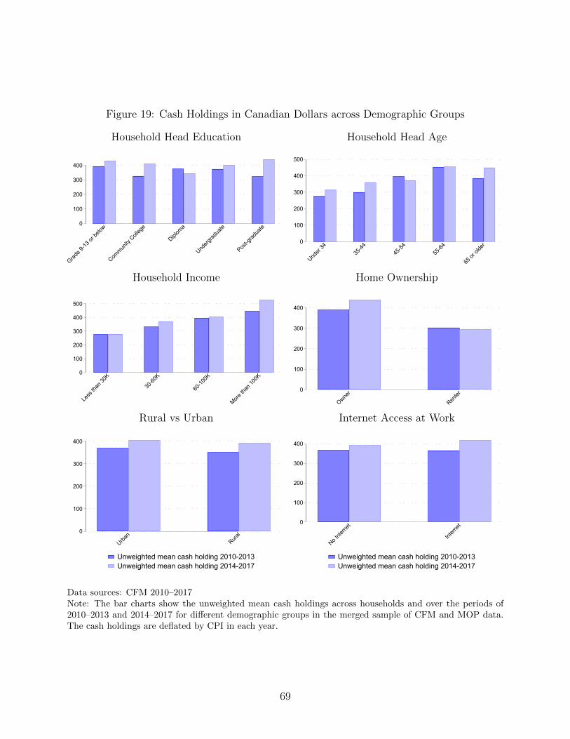
Figure 19: Cash Holdings in Canadian Dollars across Demographic Groups


0

100

200

300

400

Grade 9

-13 or

below

Commun

ity C

olleg

e

Diplom

a

Underg

radua

te

Post-g

radua

te

Unweighted mean cash holding 2010-2013Unweighted mean cash holding 2014-2017

Household Head Age

0

100

200

300

400

500

Under

3435

-4445

-5455

-64

65 or

olde

r


Household Income

0

100

200

300

400

500

Less

than

30K

30-60

K

60-10

0K

More th

an 10

0K


Home Ownership

0

100

200

300

400

Owner

Renter


Rural vs Urban

0

100

200

300

400

Urban

Rural



0

100

200

300

400

No Inte

rnet

Intern

et


Data sources: CFM 2010–2017Note: The bar charts show the unweighted mean cash holdings across households and over the periods of2010–2013 and 2014–2017 for different demographic groups in the merged sample of CFM and MOP data.The cash holdings are deflated by CPI in each year.

69

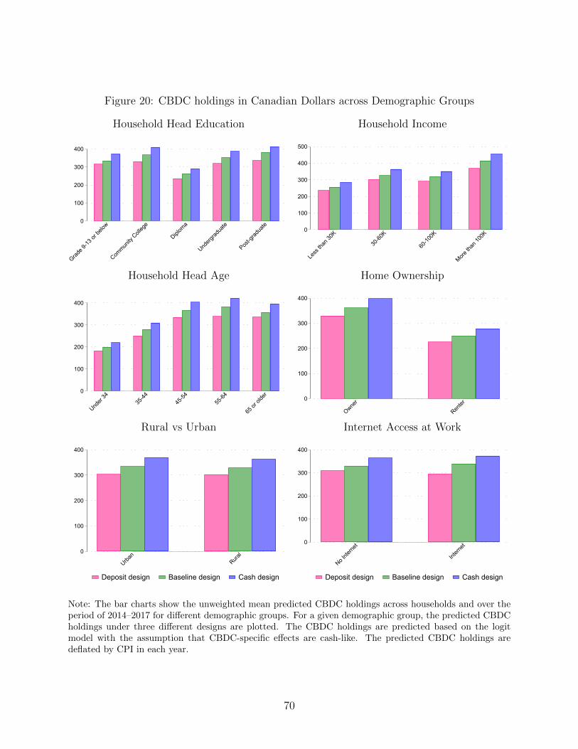
Figure 20: CBDC holdings in Canadian Dollars across Demographic Groups


0

100

200

300

400

Grade 9

-13 or

below

Commun

ity C

olleg

e

Diplom

a

Underg

radua

te

Post-g

radua

te


Household Income

0

100

200

300

400

500

Less

than

30K

30-60

K

60-10

0K

More th

an 10

0K

Deposit design Baseline design Cash designHousehold Head Age

0

100

200

300

400

Under

3435

-4445

-5455

-64

65 or

olde

r


Home Ownership

0

100

200

300

400

Owner

Renter

Deposit design Baseline design Cash designRural vs Urban

0

100

200

300

400

Urban

Rural



0

100

200

300

400

No Inte

rnet

Intern

et


Note: The bar charts show the unweighted mean predicted CBDC holdings across households and over theperiod of 2014–2017 for different demographic groups. For a given demographic group, the predicted CBDCholdings under three different designs are plotted. The CBDC holdings are predicted based on the logitmodel with the assumption that CBDC-specific effects are cash-like. The predicted CBDC holdings aredeflated by CPI in each year.

70

Predicting the Demand for Central Bank Digital Currency

Documents

Transcript of Predicting the Demand for Central Bank Digital Currency