University of Wollongong University of Wollongong

Research Online Research Online

Faculty of Engineering and Information Sciences - Papers: Part A

Faculty of Engineering and Information Sciences

2017

Predicting concentrations of fine particles in enclosed vessels using a Predicting concentrations of fine particles in enclosed vessels using a

camera based system and CFD simulations camera based system and CFD simulations

L Lulbadda Waduge University of Greenwich

S Zigan University of Greenwich

Luke Stone University of Wollongong, les019@uowmail.edu.au

A Belaidi University of Greenwich

P Garcia-Trinanes University of Greenwich

Follow this and additional works at: https://ro.uow.edu.au/eispapers

Part of the Engineering Commons, and the Science and Technology Studies Commons

Recommended Citation Recommended Citation Lulbadda Waduge, L; Zigan, S; Stone, Luke; Belaidi, A; and Garcia-Trinanes, P, "Predicting concentrations of fine particles in enclosed vessels using a camera based system and CFD simulations" (2017). Faculty of Engineering and Information Sciences - Papers: Part A. 6373. https://ro.uow.edu.au/eispapers/6373

Research Online is the open access institutional repository for the University of Wollongong. For further information contact the UOW Library: research-pubs@uow.edu.au

Predicting concentrations of fine particles in enclosed vessels using a camera Predicting concentrations of fine particles in enclosed vessels using a camera based system and CFD simulations based system and CFD simulations

Abstract Abstract One of the main challenges in industries handling biomass is the consequence of the particle breakage of pelletised biomass in smaller fractions which can lead to fine particles smaller 500 ¿m that can form dust clouds in the handling and storing equipment. These dust clouds present potential health and safety hazards as well as dust explosion hazards to plant operators because the airborne dust can occur in high concentrations close to the dust explosion limits of the biomass material, during the filling process of storage silos. Preventing dust explosions and the damage of plant infrastructures requires a profound understanding of the particle/air dynamics in the dust cloud circulating in the storage silo. The limited access to the storage facilities as well as the silo size requires a detailed study of the particle/air dynamics at different scales. Lab scale experiments were conducted as a first step to establishing a new optical method for measuring particle concentrations. A small scale experimental rig was fed centrally with different sized wood pellets and a single camera and a laser was utilised to capture the dust concentration in different areas of the silo. According to the experimental results, a higher mass concentration of dust was observed near the silo wall as well as near the main particle jet. However, the mass concentrations were below the explosive limits at the area in between main particle jet and silo wall. These experimental results were then feeding into a 2D CFD simulation representing the particle dynamics in the laser sheet (2D plane). Qualitative findings show a good agreement of the particle/air dynamics between experiments and simulations.

Disciplines Disciplines Engineering | Science and Technology Studies

Publication Details Publication Details Lulbadda Waduge, L. L., Zigan, S., Stone, L. E., Belaidi, A. & Garcia-Trinanes, P. (2017). Predicting concentrations of fine particles in enclosed vessels using a camera based system and CFD simulations. Process Safety and Environmental Protection, 105 262-273.

This journal article is available at Research Online: https://ro.uow.edu.au/eispapers/6373

1

Predicting concentrations of fine particles in enclosed vessels using a

camera based system and CFD simulations

L. L. Lulbadda Waduge*, S. Zigan †,Luke E. Stone♦, A. Belaidi† and P. García-

Triñanes*,

* The Wolfson Centre for Bulk Solids Handling Technology

† Department of Mechanical Manufacturing and Design Engineering

University of Greenwich, Central Avenue, Chatham Maritime, Kent ME4 4TB

♦ Faculty of Engineering and Information Sciences, University of Wollongong, Northfields

Avenue, Wollongong, N.S.W, 2522, Australia

e-mail: L.L.LulbaddaWaduge@greenwich.ac.uk, web page: www.bulksolids.com/

e-mail: s.zigan@gre.ac.uk, e-mail: h.belaidi@greenwich.ac.uk,

e-mail: P.GarciaTrinanes@greenwich.ac.uk

Abstract

Biomass generates a increasing interest as renewable fuel and industries handling biomass

show fast levels of growths over the last decade and, yet, several challenges remain in the

handling, transporting and storing of biomass such as wood pellets. One challenge is the

consequence of the particle breakage of pelletised biomass in smaller fractions which can

lead to fine particles smaller 500 microns which can form dust clouds in the handling and

storing equipment. These dust clouds present potential health and safety hazards as well as

dust explosion hazards to plant operators because during the filling process of storage silos

the airborne dust can occur in high concentrations close to the dust explosion limits of the

2

biomass material. Preventing dust explosions and the damage of plant infrastructures

requires a profound understanding of the particle/ air dynamics in the dust cloud circulating

in the storage silo. The limited access to the storage facilities as well as the silo size require a

detailed study of the particle/ air dynamics at different scales. Lab scale experiments were

conducted as a first step to establish a new optical method for measuring particle

concentrations. A small scale experimental rig was fed centrally with different sized wood

pellets and a single camera and a laser was utilised to capture the dust concentration in

different areas of the silo. These experimental results were then feeding into a 2D CFD

simulation representing the particle dynamics in the laser sheet (2D plane). Qualitative

findings show a good agreement of the particle/ air dynamics between experiments and

simulations.

Keywords

Laser, optical method, dust explosions, CFD, experimental, storage silos, particle dynamics

Introduction

Dust explosions are a major concern of industries handling combustible bulk materials

containing fractions of fines (particles smaller than 355 µm). Dust explosion risks are present

in many industries (e.g. power, chemical and food industries) handling wood and paper

products, grain and flour, metal products or pulverized coal to mention just few (Frank 2004).

The consequences of dust explosions in industrial facilities can be severe for the work force

and plant operators as such explosions can cause fatalities, injuries and facility damage e.g. to

the storage silos (U.S. CSB 2010).

Dust explosions in storage silos occur in the presence of an ignition source capable of

igniting an explosive fuel mixture atmosphere. In the presence of favourable conditions such

as dust concentration and air turbulence levels inside the silo, explosions hazards are

increased. When dust concentrations in the circulating air inside a closed vessel is within the

range of around 300 g/m3 to 1500 g/m

3 with a narrow particle size distribution (of between 10

to 40 microns) the highest propensity for dust explosions is present. The quantification of

dust concentrations and particle size distributions in the atmosphere-fuel mixture in the

storage silo can provide a baseline for evaluating dust explosions risks not only for storage

silos but also for industrial facilities in general (Davis et al. 2011, p.839).

3

The dust concentrations in silos depends on equipment parameters e.g. the operation mode of

the silo (e.g. filling or emptying) and material parameters e.g. the natural variations of the

particle size distribution in the material handled. Some materials, such as biomass/ wood

pellets, tend to dust significantly.

The environmental parameters such as temperature and air humidity have to be added to the

list of material and equipment parameters when evaluating the amount of airborne fines in

storage silos. The large number of parameters influencing the concentration of airborne dust

can cause variations of up to 30 percent between filling and discharge cycles. The large

variations of dust concentrations with time in the industrial process require a detailed study of

the particle settling behaviour which can be best studied using small scale experiments and

simulation approaches such as Computational Fluid Dynamics (CFD). For verifying and

validating CFD models the simulation results need to be compared with experimental data

(Klippel et al. 2014). Researcher e.g. (Réthoré et al. 2014), (Wang et al. 2016) and (Krueger

et al. 2015) suggest the use of optical methods such as using a single camera for measuring

the settling of particles in a silo during the filling process and evaluating the particle

displacements by correlating digital images. The displacement of fines following air currents

in the silo can be estimated from the images as successive positions over time. Based on

averaged images it is possible to track temporal dust evolutions in the silo. For the

illumination of dust particles in a plane, a laser light source is recommended (Gouesbet et al.

2015).

This paper explores the possibility of verifying and validating CFD models using a bench

scale dustiness tester and a single camera system with a laser source to illuminate particles.

Materials and methods

Wood pellets produced from compacted sawdust contain a wide particle size distribution

(Oveisi et al. 2013).

4

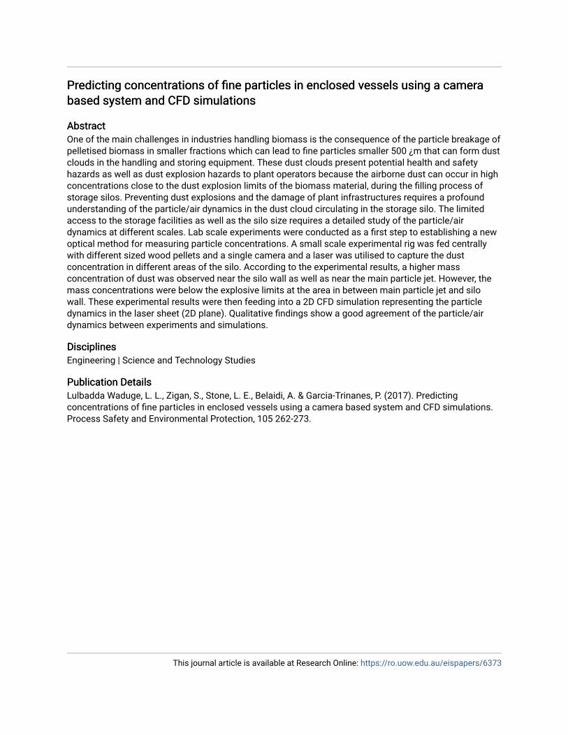
Figure 1 : SEM (Scanning Electron Microscope) Images of wood dust samples with various sizes (a) size range from 60-90

µ m (b) size range from 100-125µm (c) size range from 300 to 355 µm

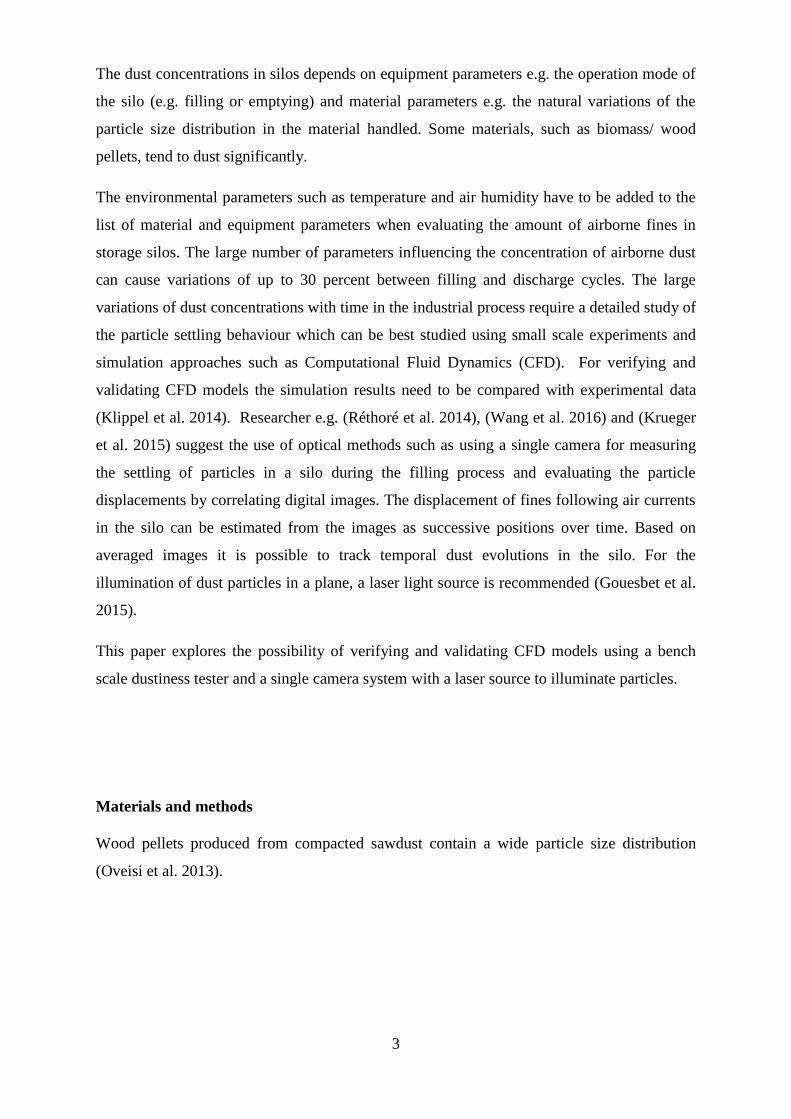
The wood pellets were sieved into different fractions. The coarser particle fractions had a

particle size ranging from 3.15 to 4.75 mm (obtained from sieving the material with a

Rotex® size analyser/ Apex screener (Allen 2003). The smaller particle fractions passed a

sieve of 500 µm. The fines (particles below 355 µm) are shown in Figure 1. The coarse and

small size particle fractions are shown in Figure 2. The material used in the experiments had

a mass ratio of coarse to fine material of 10:1.

Figure 2: The material used in the experiment is a mixture of coarse (a) and fine (b) particles mixed with the mass ratio of

10:1.

The material used in the experiments was investigated further as the CFD simulation setup

required more data for input parameters. Fines were prepared through sieving wood pellet

dust through a 355 and then a 63 micron sieve before being analysed in a Gradex sieve

system. A sample of the coarse particles (3.15 to 4.75 mm) was prepared by mixing fines in

a ratio of 10 grams of coarse material to 1 gram of fine material to obtain the same mixture

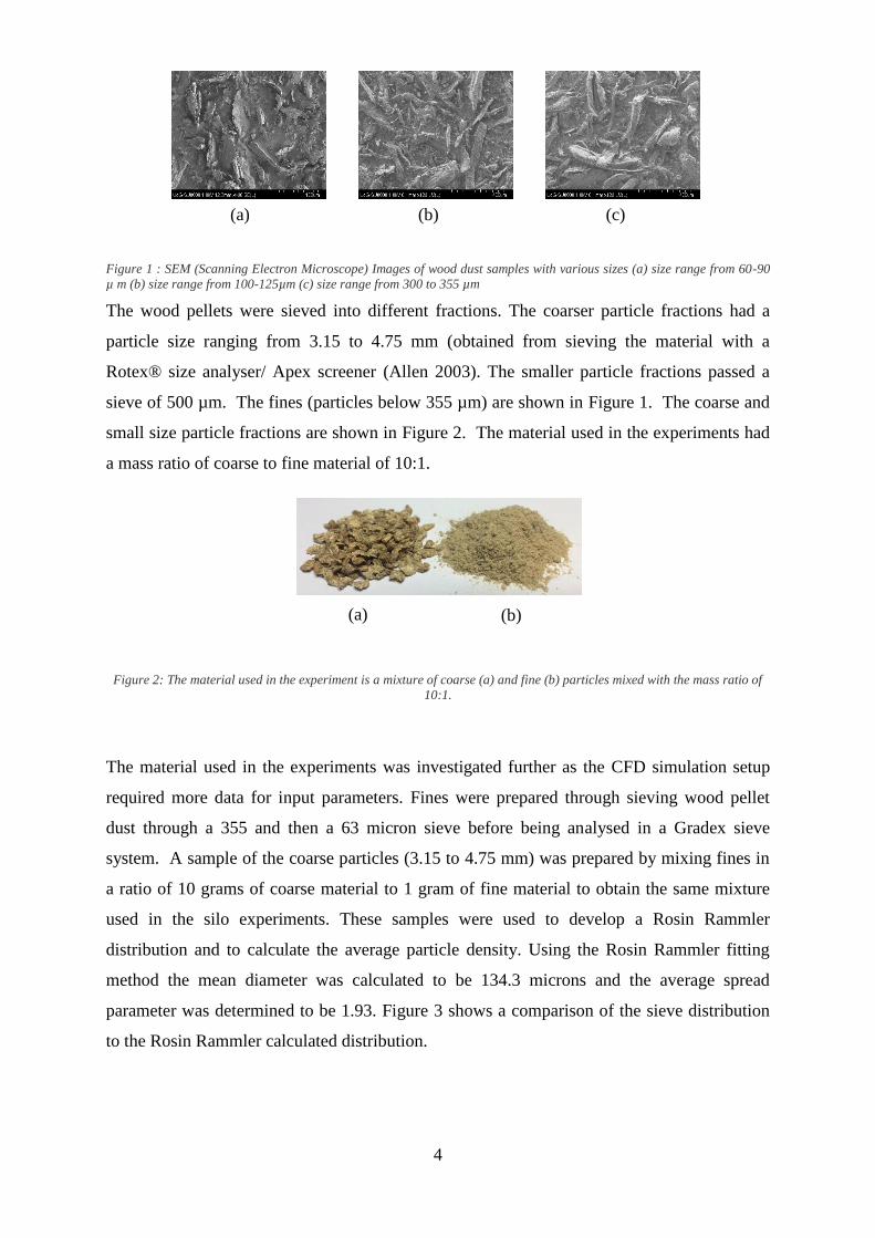
used in the silo experiments. These samples were used to develop a Rosin Rammler

distribution and to calculate the average particle density. Using the Rosin Rammler fitting

method the mean diameter was calculated to be 134.3 microns and the average spread

parameter was determined to be 1.93. Figure 3 shows a comparison of the sieve distribution

to the Rosin Rammler calculated distribution.

(a) (b) (c)

(a) (b)

5

Figure 3: Rosin Rammler Distribution Fitted to Sieve Particle Size Results

After conducting density measurements using a pycnometer the level of compressibility of

the material is demonstrated through differences in calculated densities. This variation is due

to the material having a cellular nature, which causes porosity in the particles; at high

pressures, these pores are compressed leading to a lower volume occupied by the material

and therefore a decrease in calculated density. For the simulation, the lower density of 1460

kg/m3 was used for fine and coarse materials.

Experimental set up

Wood pellets were fed centrally at a flowrate of (82 g/s) into a cylindrical silo of 1200mm x

400mm (height x diameter) shown in Figure 4. The air was extracted at four extraction ports

equally spaced on the top of the experimental silo and the flow rate of 0.04 𝑙/𝑠 from each

port matched the volumetric flow rate of air entering the silo during the filling process. The

separation of fines from the main particle jet was examined at the end of the experiment by

collecting the retained fines in different areas at the silo bottom.

A 500mW 532nm (bright green colour) laser (Coherent® DPSS 532) was used for creating a

thin vertical light sheet. The vertical laser sheet was obtained by projecting a linear laser

beam through a horizontal glass rod 8mm in diameter. A Nikon D800E with Nikon AF-S

NIKKOR 16-35mm lens was used to capture the video footage of the circulating dust in the

experimental silo in a symmetry plane as shown in Figure 4.

6

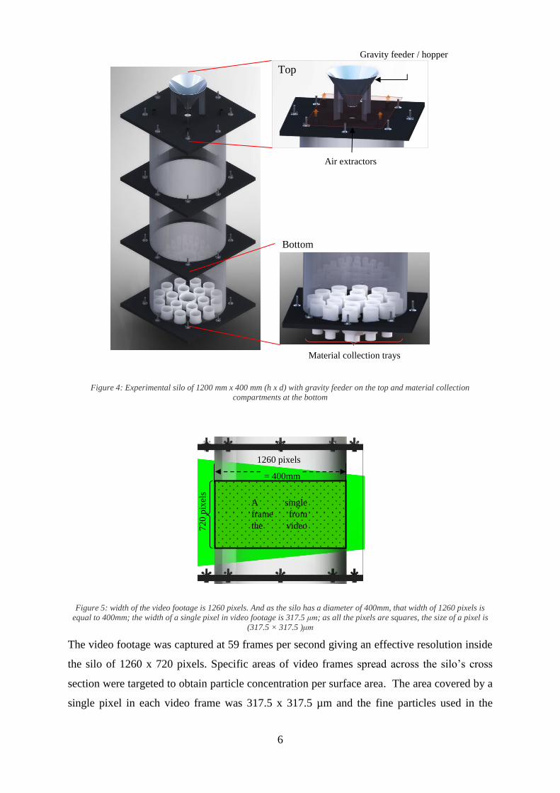
Figure 4: Experimental silo of 1200 mm x 400 mm (h x d) with gravity feeder on the top and material collection

compartments at the bottom

Figure 5: width of the video footage is 1260 pixels. And as the silo has a diameter of 400mm, that width of 1260 pixels is

equal to 400mm; the width of a single pixel in video footage is 317.5 μm; as all the pixels are squares, the size of a pixel is

(317.5 × 317.5 )μm

The video footage was captured at 59 frames per second giving an effective resolution inside

the silo of 1260 x 720 pixels. Specific areas of video frames spread across the silo’s cross

section were targeted to obtain particle concentration per surface area. The area covered by a

single pixel in each video frame was 317.5 x 317.5 µm and the fine particles used in the

Top

Gravity feeder / hopper

Air extractors

Bottom

Material collection trays

1260 pixels

= 400mm

72

0 p

ixel

s

A single

frame from

the video

footage

7

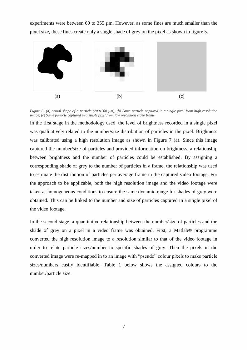
experiments were between 60 to 355 µm. However, as some fines are much smaller than the

pixel size, these fines create only a single shade of grey on the pixel as shown in figure 5.

Figure 6: (a) actual shape of a particle (200x200 µm), (b) Same particle captured in a single pixel from high resolution

image, (c) Same particle captured in a single pixel from low resolution video frame.

In the first stage in the methodology used, the level of brightness recorded in a single pixel

was qualitatively related to the number/size distribution of particles in the pixel. Brightness

was calibrated using a high resolution image as shown in Figure 7 (a). Since this image

captured the number/size of particles and provided information on brightness, a relationship

between brightness and the number of particles could be established. By assigning a

corresponding shade of grey to the number of particles in a frame, the relationship was used

to estimate the distribution of particles per average frame in the captured video footage. For

the approach to be applicable, both the high resolution image and the video footage were

taken at homogeneous conditions to ensure the same dynamic range for shades of grey were

obtained. This can be linked to the number and size of particles captured in a single pixel of

the video footage.

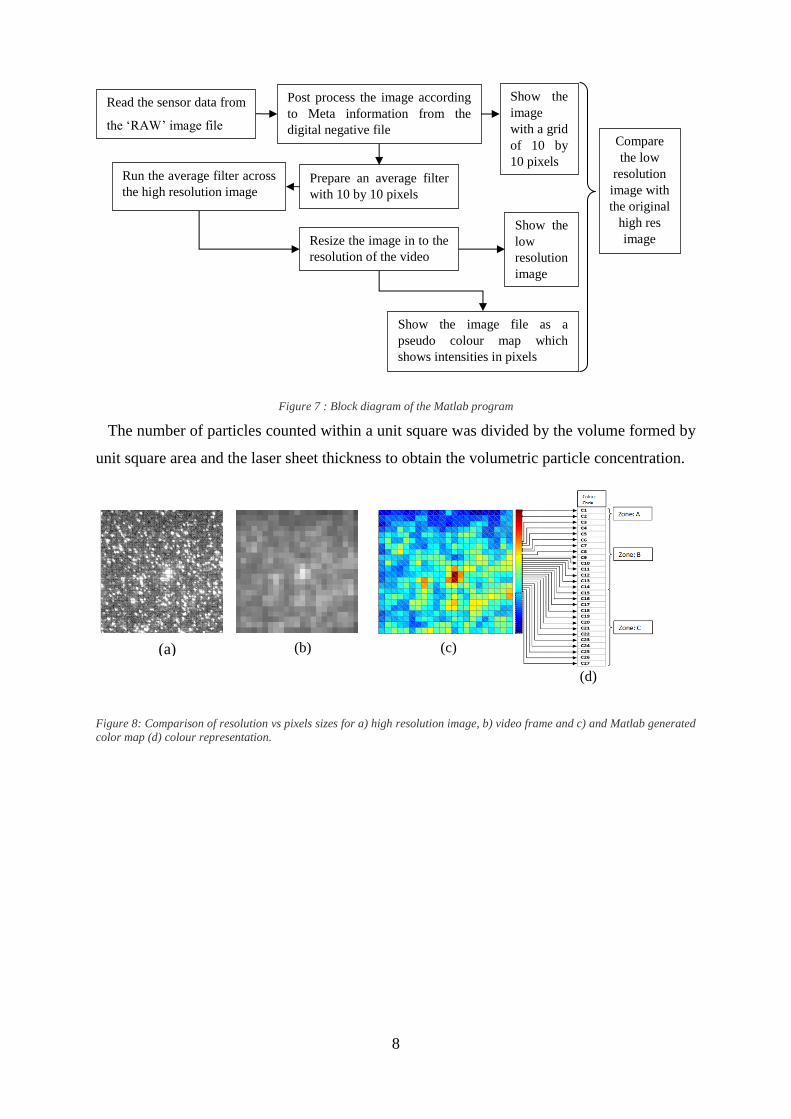
In the second stage, a quantitative relationship between the number/size of particles and the

shade of grey on a pixel in a video frame was obtained. First, a Matlab® programme

converted the high resolution image to a resolution similar to that of the video footage in

order to relate particle sizes/number to specific shades of grey. Then the pixels in the

converted image were re-mapped in to an image with “pseudo” colour pixels to make particle

sizes/numbers easily identifiable. Table 1 below shows the assigned colours to the

number/particle size.

(a) (b) (c)

8

Figure 7 : Block diagram of the Matlab program

The number of particles counted within a unit square was divided by the volume formed by

unit square area and the laser sheet thickness to obtain the volumetric particle concentration.

Figure 8: Comparison of resolution vs pixels sizes for a) high resolution image, b) video frame and c) and Matlab generated

color map (d) colour representation.

Read the sensor data from

the ‘RAW’ image file

Post process the image according

to Meta information from the

digital negative file

Prepare an average filter

with 10 by 10 pixels

Run the average filter across

the high resolution image

Resize the image in to the

resolution of the video

Show the image file as a

pseudo colour map which

shows intensities in pixels

Compare

the low

resolution

image with

the original

high res

image

Show the

image

with a grid

of 10 by

10 pixels

Show the

low

resolution

image

(a) (b) (c) 2 4 6 8 10 12 14 16 18 20 22

2

4

6

8

10

12

14

16

18

20

22

0.3

0.4

0.5

0.6

0.7

0.8

0.9

(d)

9

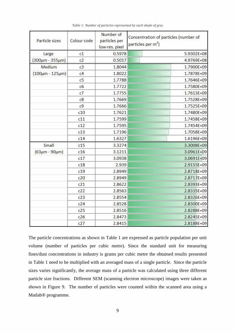
Table 1: Number of particles represented by each shade of grey

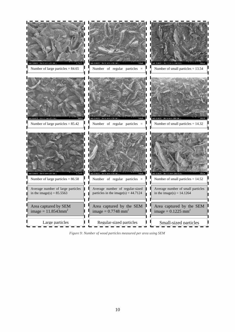
The particle concentrations as shown in Table 1 are expressed as particle population per unit

volume (number of particles per cubic metre). Since the standard unit for measuring

fines/dust concentrations in industry is grams per cubic metre the obtained results presented

in Table 1 need to be multiplied with an averaged mass of a single particle. Since the particle

sizes varies significantly, the average mass of a particle was calculated using three different

particle size fractions. Different SEM (scanning electron microscope) images were taken as

shown in Figure 9. The number of particles were counted within the scanned area using a

Matlab® programme.

10

Small-sized particles Large particles Regular-sized particles

Number of small particles = 13.54

Number of small particles = 14.32

Number of small particles = 14.52

Number of large particles = 84.65

Number of large particles = 85.42

Number of large particles = 86.58

Number of regular particles =

39.93

Number of regular particles =

46.24

Number of regular particles =

47.95

Average number of small particles

in the image(s) = 14.1264

Average number of large particles

in the image(s) = 85.5563

Average number of regular-sized

particles in the image(s) = 44.7124

Area captured by SEM

image = 11.8543mm2

Area captured by the SEM

image = 0.7748 mm2

Area captured by the SEM

image = 0.1225 mm2

Figure 9: Number of wood particles measured per area using SEM

11

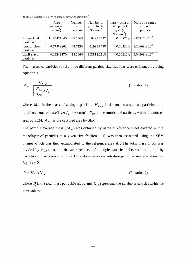
Table 2 : Extrapolation for number of particles in 900mm2.

Area

measured

(mm2)

Number

of

particles

Number of

particles in

900mm2

mass (total) of

each particle

types (in

900mm2)

Mass of a single

particle (in

grams)

Large-sized

particles 11.85431840 85.5563 6495.5797 0.00575 g 8.85217 x 10

-7

regular-sized

particles 0.77488362 44.7124 51931.8758 0.00422 g 8.12603 x 10

-8

small-sized

particles 0.12246170 14.1264 103818.2518 0.00212 g 2.04203 x 10

-8

The masses of particles for the three different particle size fractions were estimated by using

equation 1.

L

SEM

CA

TotalPs

AA

N

MM (Equation 1)

where PsM is the mass of a single particle, TotalM is the total mass of all particles on a

reference squared tape/layer LA = 900mm2, CAN is the number of particles within a captured

area by SEM, SEMA is the captured area by SEM.

The particle average mass ( PsM ) was obtained by using a reference sheet covered with a

monolayer of particles at a given size fraction. CAN was then estimated using the SEM

images which was then extrapolated to the reference area AL. The total mass in AL was

divided by NCA to obtain the average mass of a single particle. This was multiplied by

particle numbers shown in Table 1 to obtain mass concentration per cubic metre as shown in

Equation 2.

PVPsc NMP (Equation 2)

where cP is the total mass per cubic metre and PVN represents the number of particles within the

same volume.

12

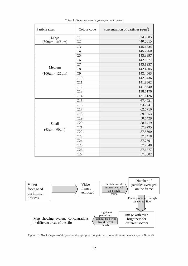
Table 3: Concentrations in grams per cubic metre.

Particle sizes Colour code concentration of particles (g/m3)

Large (300μm - 355μm)

C1 524.9505 C2 440.5615

Medium

(100μm - 125μm)

C3 145.4534 C4 145.2760

C5 143.3897

C6 142.8577

C7 143.1237

C8 142.4305

C9 142.4063

C10 142.0436

C11 141.8662

C12 141.8340

C13 138.6176

C14 131.6126

Small

(63μm - 90μm)

C15 67.4031 C16 63.2241

C17 62.6710

C18 59.5353

C19 58.6429

C20 58.6419

C21 57.9795

C22 57.8600

C23 57.8418

C24 57.7891

C25 57.7648

C26 57.6777

C27 57.5602

Video

footage of

the filling

process

Video

frames

extracted

Particles on all

frames overlaid

on a single

frame

Number of

particles averaged

on the frame

Frame processed through

an average filter

Image with even

brightness for

different sectors

Brightness

plotted as a

contour map with

five different

levels

Map showing average concentrations

in different areas of the silo

Figure 10: Block diagram of the process steps for generating the dust concentration contour maps in Matlab®

13

Video frames were captured over a period of time and superimposed to provide enough data

sets for image analysis. The frames were analysed using the Matlab® program as shown in

Figure 10. Then a contour map was established to show the different levels of dust

concentration. In the final step, levels of brightness were identified and matched with the

data obtained in table 3 to show the dust distribution in grams per cubic meter.

Simulation setup

CFD was coupled with the Discrete Element Method (DEM) in the commercial software

package ANSYS/ Fluent (Package) to predict particle concentrations in a 2D plane (similar to

the laser sheet) in the experimental set up. The obtained particle concentrations were then

qualitatively verified by direct comparison with results obtained from the optical

measurements in the experimental silo.

As the case study is a comparison to the laser sheet a 2D simulation was sufficient for a direct

comparison, additionally, it is assumed that the flow is symmetric and therefore only half of

the silo is required for this simulation. After developing the 2D geometry, the mesh was

calculated. To ensure that the results are independent of the mesh; a sensitivity study was

undertaken. The study revealed that the overall appearance of the velocity profile inside the

silo stayed the same and that only a small variance in the maximum velocity was observed.

Finally, due to the small variance between the two finest meshes a mesh size of 38402

elements was used for the final simulation. The results of this study are outlined in Table 4.

Table 4: Mesh Sensitivity Results

Mesh

Parameters

Coarse

[10 mm]

Medium

[5 mm]

Fine

[2.5 mm]

Very Fine

[1.5 mm]

Elements 2400 9623 38402 106569

Simulation

Duration

1hr 14 minutes 1hr 50 mins 3 hr 6 minutes 6 hr 40 mins

Maximum

Velocity

0.954 m/s 0.893 m/s 0.844 m/s 0.848 m/s

Error (Relative

to Finest Mesh)

12.50% 5.31% 0.47% 0%

14

Figure 11: Velocity profiles for each mesh tested in the sensitivity study

The simplification of the 2D simulation results in a total mass flow rate of 0.041 kg/s. Due to

the computational expense of having millions of particles in a simulation the mass flow rate

of 0.041 kg/s has been separated into two mass flow rates, 0.0369 kg/s for the coarse material

and 0.0041kg/s for the fines. Although the fines make up 0.0041 kg/s of the mass flow rate in

the experiments, this was modified to a mass flow rate of 0.00041 kg/s in order to decrease

the number of particles in the simulation. This can be justified by the main aim of this case

study being a qualitative investigation.

The simulation used a transient pressure based solver with the coupled pressure – velocity

scheme with gravity set to 9.81 m/s2 in the negative Y direction. Air viscosity was calculated

using the K-Epsilon Realisable model with Standard Wall Functions, the discrete phase was

used to track particles with unsteady particle tracking with each fluid time step. Two-way

turbulence coupling was also used to ensure the particles would influence the air and generate

the velocity profile inside the silo. The simulation used a time step size of 0.001 seconds and

35 iterations per time step.

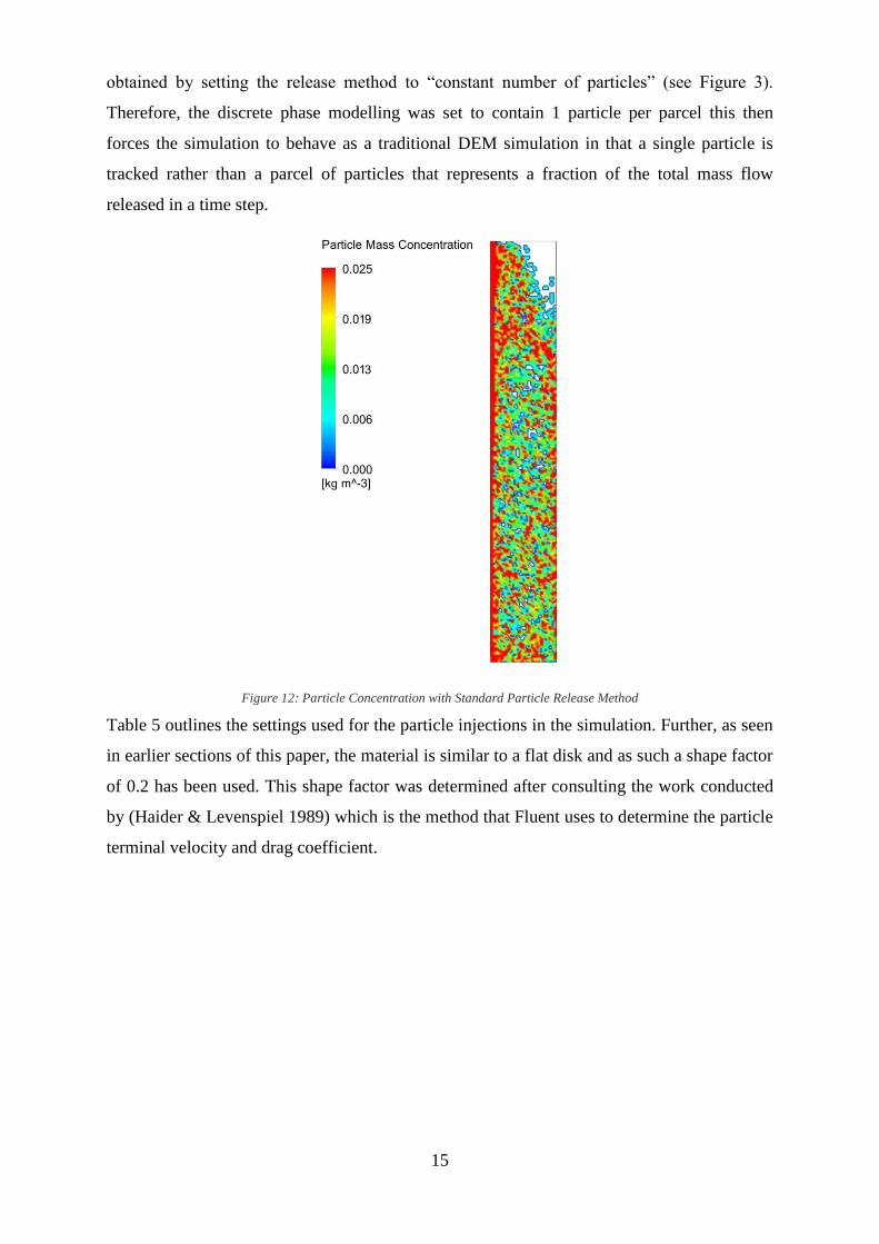
After investigating different parcel release methods it was found that the “standard” method

did not show the same results as observed in the experiments and that a better result was

15

obtained by setting the release method to “constant number of particles” (see Figure 3).

Therefore, the discrete phase modelling was set to contain 1 particle per parcel this then

forces the simulation to behave as a traditional DEM simulation in that a single particle is

tracked rather than a parcel of particles that represents a fraction of the total mass flow

released in a time step.

Figure 12: Particle Concentration with Standard Particle Release Method

Table 5 outlines the settings used for the particle injections in the simulation. Further, as seen

in earlier sections of this paper, the material is similar to a flat disk and as such a shape factor

of 0.2 has been used. This shape factor was determined after consulting the work conducted

by (Haider & Levenspiel 1989) which is the method that Fluent uses to determine the particle

terminal velocity and drag coefficient.

16

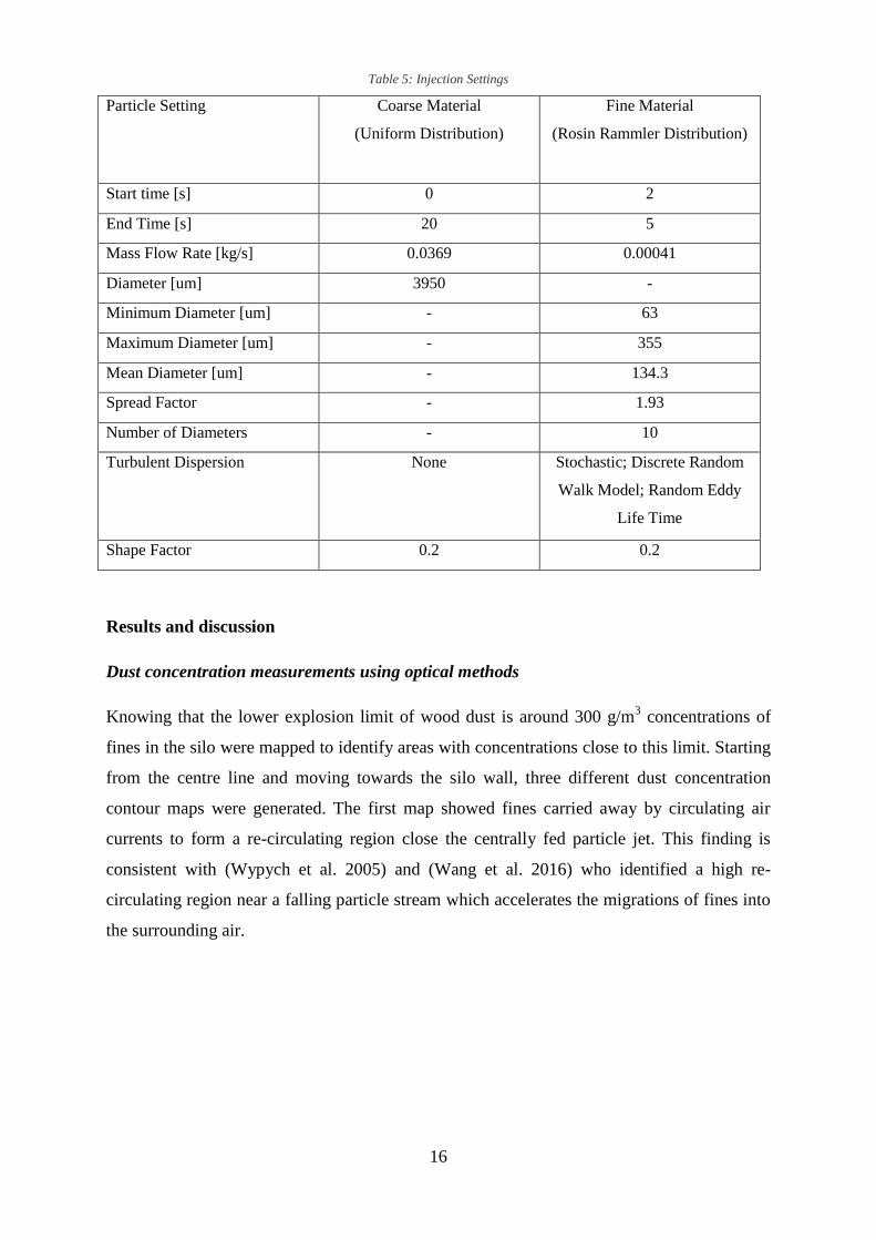
Table 5: Injection Settings

Particle Setting Coarse Material

(Uniform Distribution)

Fine Material

(Rosin Rammler Distribution)

Start time [s] 0 2

End Time [s] 20 5

Mass Flow Rate [kg/s] 0.0369 0.00041

Diameter [um] 3950 -

Minimum Diameter [um] - 63

Maximum Diameter [um] - 355

Mean Diameter [um] - 134.3

Spread Factor - 1.93

Number of Diameters - 10

Turbulent Dispersion None Stochastic; Discrete Random

Walk Model; Random Eddy

Life Time

Shape Factor 0.2 0.2

Results and discussion

Dust concentration measurements using optical methods

Knowing that the lower explosion limit of wood dust is around 300 g/m3 concentrations of

fines in the silo were mapped to identify areas with concentrations close to this limit. Starting

from the centre line and moving towards the silo wall, three different dust concentration

contour maps were generated. The first map showed fines carried away by circulating air

currents to form a re-circulating region close the centrally fed particle jet. This finding is

consistent with (Wypych et al. 2005) and (Wang et al. 2016) who identified a high re-

circulating region near a falling particle stream which accelerates the migrations of fines into

the surrounding air.

17

Figure 13: Dust concentration(s) near the particle jet at a particle feeding rate of 81.87 g/s; (a) Cropped image from

averaged frame of the video footage. (b) Contour map of dust concentration(s) near the particle jet. (c) Position of image

which cropped from the average frame.

The dust concentration contour map shown in Figure 13 depicts another area of high dust

accumulation of around 440 g/m3 close to the wall. The particles observed in this area are

mostly fines, the larger particles dropped out from the airstream already and settled on the

heap.

The upward moving air near the silo wall gradually reduces its velocity with entrained

particles gradually settling to the bottom (Rani et al. 2015). These settling particles are

continuously charged by fresh fines from the main falling stream. (Zhang et al. 2013) showed

that the particle charges increase with decreasing particle diameter e.g. wood pellets of

around 212μm showed a specific charge density of −24.77μC/kg. Wood particles are charged

even more when coming in contact with the silo wall (e.g. steel silos for storing wood pellets)

as the work function is higher between particles and a steel plate (Hussain et al. 2013). This

highly, negatively, charged particles form a solid like network with similar distances between

them and can create a potentially explosive fuel like mixture in the presence of a spark or

other ignition sources.

C1 : 524.9505 g/m3

2/3 between C2 and C3 : 342.1921 g/m3

C10 : 142.0436 g/m3

C27 : 57.5602 g/m3

Area with very low dust concentration

103.505 mm

183.515 mm

Position of the frame (a)

(b)

(c)

18

Figure 14: Dust concentration(s) near the silo wall (a) Cropped image from averaged frame of the video footage. (b)

Contour map of dust concentration(s) near the particle jet. (c) Position of image which cropped from the average frame.

Figure 14 depicts a dust concentration contour map between the silo centre line and the silo

wall which clearly shows less particles in the frame than in the other two dust concentration

contour maps.

The obtained dust concentration distribution in the experimental silo was then compared with

CFD results by (Rani et al. 2015). Since the materials used were different and the silos had

different dimensions only qualitative information can be derived from this comparison. Rani

et al. 2015 simulated the dust concentration distribution in a cylindrical silo of 5m x 1.6m

(height x diameter) and obtained dust concentration near the centrally falling particle stream

of around 600 g/m3

and near the wall of around 200 g/m3. In this study the dust concentration

measured at the centre line of the silo was about 525 g/m3

and near the silo wall of about 440

g/m3. Dust concentrations near the silo centre line were quite similar but those close to the

wall were a factor of two higher.

Silo

wall

C2 : 440.5615 g/m3

C5 : 143.3897 g/m3

C16 : 63.2241 g/m3

C27 : 57.5602 g/m3

Area with very low dust concentration

Position of the frame

109.22 mm

52.3875 mm

(a)

(b)

(c)

19

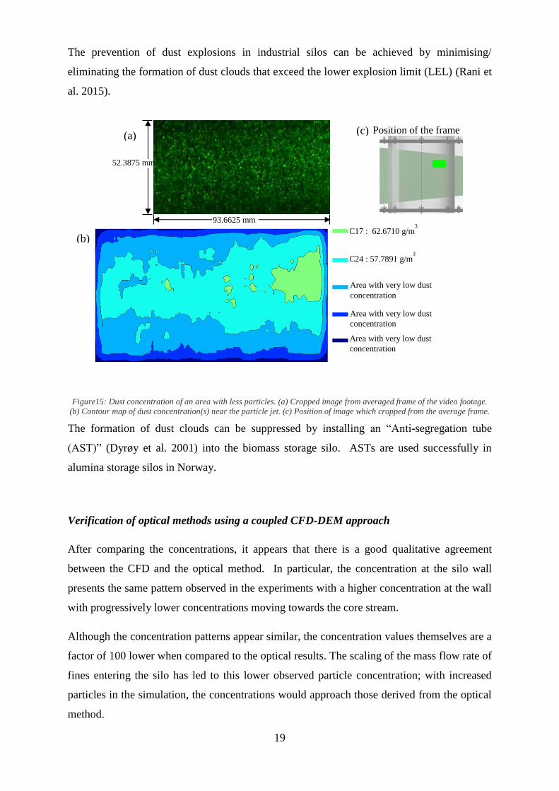
The prevention of dust explosions in industrial silos can be achieved by minimising/

eliminating the formation of dust clouds that exceed the lower explosion limit (LEL) (Rani et

al. 2015).

Figure15: Dust concentration of an area with less particles. (a) Cropped image from averaged frame of the video footage.

(b) Contour map of dust concentration(s) near the particle jet. (c) Position of image which cropped from the average frame.

The formation of dust clouds can be suppressed by installing an “Anti-segregation tube

(AST)” (Dyrøy et al. 2001) into the biomass storage silo. ASTs are used successfully in

alumina storage silos in Norway.

Verification of optical methods using a coupled CFD-DEM approach

After comparing the concentrations, it appears that there is a good qualitative agreement

between the CFD and the optical method. In particular, the concentration at the silo wall

presents the same pattern observed in the experiments with a higher concentration at the wall

with progressively lower concentrations moving towards the core stream.

Although the concentration patterns appear similar, the concentration values themselves are a

factor of 100 lower when compared to the optical results. The scaling of the mass flow rate of

fines entering the silo has led to this lower observed particle concentration; with increased

particles in the simulation, the concentrations would approach those derived from the optical

method.

C17 : 62.6710 g/m3

C24 : 57.7891 g/m3

Area with very low dust

concentration

Area with very low dust

concentration

Area with very low dust

concentration

Position of the frame

93.6625 mm

52.3875 mm

(a)

(b)

(c)

20

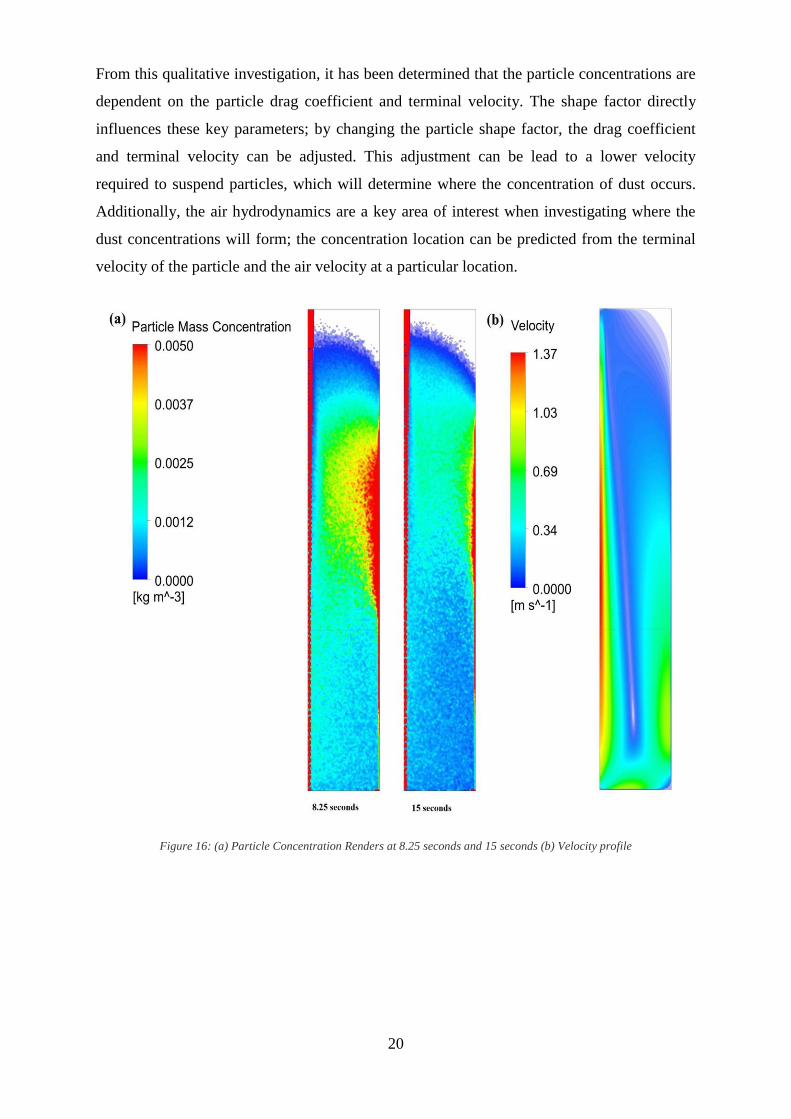
From this qualitative investigation, it has been determined that the particle concentrations are

dependent on the particle drag coefficient and terminal velocity. The shape factor directly

influences these key parameters; by changing the particle shape factor, the drag coefficient

and terminal velocity can be adjusted. This adjustment can be lead to a lower velocity

required to suspend particles, which will determine where the concentration of dust occurs.

Additionally, the air hydrodynamics are a key area of interest when investigating where the

dust concentrations will form; the concentration location can be predicted from the terminal

velocity of the particle and the air velocity at a particular location.

Figure 16: (a) Particle Concentration Renders at 8.25 seconds and 15 seconds (b) Velocity profile

21

Conclusions

Dust explosions during the handling and storing of biomass such as wood pellet present a

high risk to plant operators and can cause serious structural damages. The ability to evaluate

and manage the risks of dust explosions in large scale biomass storage facilities largely

depends on a profound understanding of dust mobility in the vessel. The dust mobility can be

studied using simulation approaches such as CFD which requires validation data from

existing installations or experimental data.

This paper proposes an analytical method to create dust concentration contour maps which

give a clear indication how the concentration is distributed in the silo. To obtain

concentration contour maps, wood pellets with different particle sizes and wood dust were

fed centrally into an experimental silo. A camera system captured the particle dynamics and

the video footage was analysed using a Matlab® programme. The obtained dust

concentration contour maps showed a high dust concentration near the silo centre line (falling

particle jet) and the silo wall. Although the concentration patterns appear similar in the

simulation and experiments, the concentration values in the simulation are a factor of 100

lower when compared to the optical results. The values near the silo wall were more realistic

with the newly proposed optical method than the simulation. This can be partly explained by

the fact that this method captures better the particles dynamics near the silo wall. Particle

concentrations of 440 g/m3

were measured near the silo wall which represents a high dust

explosion risk with the presence of an ignition source. The dust settles near the silo wall and

because of particle-particle and particle-wall interactions the fines are continuously charged.

These charged particles could create a solid like network between the particles which creates

a stable atmosphere fuel mixture leading to an even higher dust explosion risk. From this

qualitative investigation, it has been determined that the particle concentrations are dependent

on the particle drag coefficient and terminal velocity. The values obtained for terminal

velocity were similar between experiments and simulations. Further developments of the

CFD model for obtaining quantitative results will include the introduction of an

experimentally based particle shape factor and running the CFD simulation on a higher

capacity computer. This would allow for a greater number of particles to be used in the

simulation. A large-scale investigation should be undertaken to ensure that the simulation is

scalable.

22

Acknowledgement:

With great gratitude we would like to thank Gexcon AS - DSEAR, Fire and Explosion

Consultants (www.gexcon.com/) and the University of Greenwich for funding this research

and the research support team at The Wolfson Centre.

References:

Allen, T., 2003. Powder Sampling and Particle Size Determination, Elsevier. Available at:

https://books.google.com/books?hl=en&lr=&id=5NgqTf9L63kC&pgis=1 [Accessed

April 27, 2016].

Scott G. D., Hinze, P.C., Hansen, O.R., Wingerden, K., 2011. Does your facility have a dust

problem: Methods for evaluating dust explosion hazards. Journal of Loss Prevention in

the Process Industries, 24(6), pp.837–846.

Dyrøy, A., 2006. Quantification and mitigation of segregation in the handling of alumina in

aluminium production, internal report.

Frank, W.L., 2004. Dust explosion prevention and the critical importance of housekeeping.

Process Safety Progress, 23(3), pp.175–184. Available at:

http://www.scopus.com/inward/record.url?eid=2-s2.0-

10244267547&partnerID=tZOtx3y1 [Accessed April 27, 2016].

Gouesbet, G., Gréhan, G., 2015. Laser-based optical measurement techniques of discrete

particles: A review [invited keynote]. International Journal of Multiphase Flow, 72,

pp.288–297.

Haider, A. & Levenspiel, O., 1989. Drag coefficient and terminal velocity of spherical and

nonspherical particles. Powder Technology, 58(1), pp.63–70. Available at:

http://www.sciencedirect.com/science/article/pii/0032591089800087 [Accessed May 27,

2016].

Hussain, T. et al., 2013. A novel sensing technique for measurement of magnitude and

polarity of electrostatic charge distribution across individual particles. International

journal of pharmaceutics, 441(1-2), pp.781–789. Available at:

23

http://www.sciencedirect.com/science/article/pii/S0378517312009428.

Klippel, A., Schmidt, M., Muecke, O., Krause, U., 2014. Dust concentration measurements

during filling of a silo and CFD modeling of filling processes regarding exceeding the

lower explosion limit. Journal of Loss Prevention in the Process Industries, 29, pp.122–

137. Available at:

http://www.sciencedirect.com/science/article/pii/S0950423014000291.

Krueger, B., Wirtz, S., Scherer, V., 2015. Measurement of drag coefficients of non-spherical

particles with a camera-based method. Powder Technology, 278, pp.157–170.

Oveisi, E., Lau, A., Sokhansanj, S., Lim, C.J., Bi, X., Larsson, S., Melin, S., 2013. Breakage

behavior of wood pellets due to free fall. Powder Technology, 235, pp.493–499.

Rani, S.I., Aziz, B.A. & Gimbun, J., 2015. Analysis of dust distribution in silo during axial

filling using computational fluid dynamics: Assessment on dust explosion likelihood.

Process Safety and Environmental Protection, 96, pp.14–21.

Réthoré, J., Morestin, F., Lafarge, L., Valverde, P., 2014. 3D displacement measurements

using a single camera. Optics and Lasers in Engineering, 57, pp.20–27.

U.S. CSB, 2010. Investigation Report, COMBUSTIBLE DUST HAZARD STUDY. U. S.

Chemical Safety and Hazard Investigation Board. Available at:

http://www.csb.gov/assets/1/19/dust_final_report_website_11-17-06.pdf.

Wang,Y., Ren X., Zhao J., Chu Z., Cao Y., Yang Y., Duan M., Fan H., Qu X, 2016.

Experimental study of flow regimes and dust emission in a free falling particle stream.

Powder Technology, 292, pp.14–22.

Wypych, P., Cook, D., Cooper, P., 2005. Controlling dust emissions and explosion hazards in

powder handling plants. Chemical Engineering and Processing: Process Intensification,

44(2), pp.323–326.

Zhang, L., Hou, J., Bi, X., 2013. Triboelectric charging behavior of wood particles during

pellet handling processes. Journal of Loss Prevention in the Process Industries, 26(6),

pp.1328–1334.