Precomputed Shadow Fields for Dynamic Scenes

Kun Zhou Yaohua Hu Stephen Lin Baining Guo Heung-Yeung Shum

Microsoft Research Asia

Abstract

We present a soft shadow technique for dynamic scenes with mov-ing objects under the combined illumination of moving local lightsources and dynamic environment maps. The main idea of our tech-nique is to precompute for each scene entity a shadow field thatdescribes the shadowing effects of the entity at points around it.The shadow field for a light source, called a source radiance field(SRF), records radiance from an illuminant as cube maps at sam-pled points in its surrounding space. For an occluder, an object oc-clusion field (OOF) conversely represents in a similar manner theocclusion of radiance by an object. A fundamental difference be-tween shadow fields and previous shadow computation concepts isthat shadow fields can be precomputed independent of scene con-figuration. This is critical for dynamic scenes because, at any giveninstant, the shadow information at any receiver point can be rapidlycomputed as a simple combination of SRFs and OOFs according tothe current scene configuration. Applications that particularly bene-fit from this technique include large dynamic scenes in which manyinstances of an entity can share a single shadow field. Our tech-nique enables low-frequency shadowing effects in dynamic scenesin real-time and all-frequency shadows at interactive rates.

Keywords: soft shadow, area lighting, environment lighting, videotexture lighting, precomputed source radiance, precomputed visi-bility.

1 Introduction

Soft shadows that arise from area light sources add striking realismto a computer generated scene. Computing this lighting effect forinteractive applications, however, is difficult because of the com-plex dependence of soft shadows on light sources and scene geom-etry. To make the problem tractable, earlier techniques mostly dealwith small or point-like area sources. Recently, researchers havedeveloped techniques such as precomputed radiance transfer (PRT)(e.g., [Sloan et al. 2002; Ng et al. 2003]) for the special case of dis-tant illumination represented by environment maps. The problemof efficient shadow computation under the combined illuminationof general local light sources and environment maps remains un-solved.

Computing soft shadows is even more challenging for dynamicscenes such as shown in Fig. 1, where objects, local light sources,and the environment map are all in motion. With traditional meth-ods based on shadow maps [Williams 1978] and shadow volumes[Crow 1977], computational costs increase rapidly as the numbersof objects and light sources increase. The high run-time expensecannot be reduced by precomputation, since shadow maps and vol-umes are determined with respect to a specific arrangement of lightsand occluders. With PRT, dynamic scenes present an even greaterproblem because the pre-computed transfer matrices are only valid

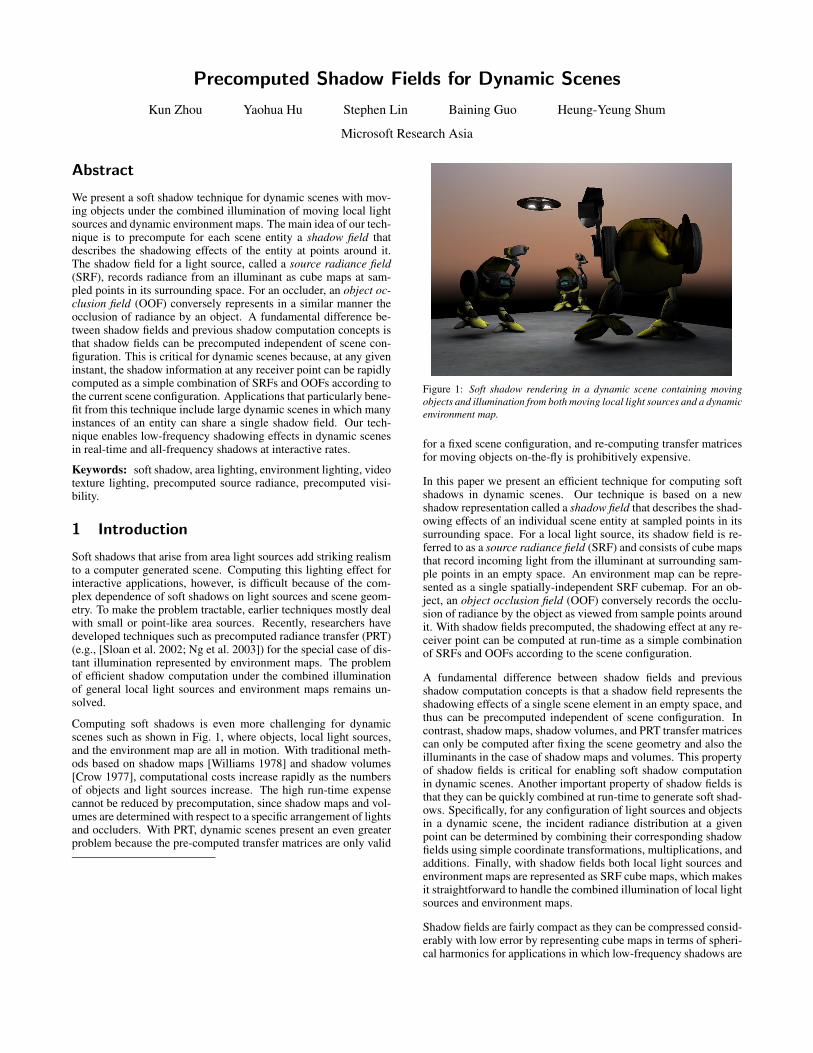
Figure 1: Soft shadow rendering in a dynamic scene containing moving

objects and illumination from both moving local light sources and a dynamic

environment map.

for a fixed scene configuration, and re-computing transfer matricesfor moving objects on-the-fly is prohibitively expensive.

In this paper we present an efficient technique for computing softshadows in dynamic scenes. Our technique is based on a newshadow representation called a shadow field that describes the shad-owing effects of an individual scene entity at sampled points in itssurrounding space. For a local light source, its shadow field is re-ferred to as a source radiance field (SRF) and consists of cube mapsthat record incoming light from the illuminant at surrounding sam-ple points in an empty space. An environment map can be repre-sented as a single spatially-independent SRF cubemap. For an ob-ject, an object occlusion field (OOF) conversely records the occlu-sion of radiance by the object as viewed from sample points aroundit. With shadow fields precomputed, the shadowing effect at any re-ceiver point can be computed at run-time as a simple combinationof SRFs and OOFs according to the scene configuration.

A fundamental difference between shadow fields and previousshadow computation concepts is that a shadow field represents theshadowing effects of a single scene element in an empty space, andthus can be precomputed independent of scene configuration. Incontrast, shadow maps, shadow volumes, and PRT transfer matricescan only be computed after fixing the scene geometry and also theilluminants in the case of shadow maps and volumes. This propertyof shadow fields is critical for enabling soft shadow computationin dynamic scenes. Another important property of shadow fields isthat they can be quickly combined at run-time to generate soft shad-ows. Specifically, for any configuration of light sources and objectsin a dynamic scene, the incident radiance distribution at a givenpoint can be determined by combining their corresponding shadowfields using simple coordinate transformations, multiplications, andadditions. Finally, with shadow fields both local light sources andenvironment maps are represented as SRF cube maps, which makesit straightforward to handle the combined illumination of local lightsources and environment maps.

Shadow fields are fairly compact as they can be compressed consid-erably with low error by representing cube maps in terms of spheri-cal harmonics for applications in which low-frequency shadows are

sufficient, and using wavelets for all-frequency applications. Fur-thermore, soft shadows can be directly rendered from compressedSRFs and OOFs. For low-frequency shadowing, dynamic scenescontaining numerous objects can be rendered in real time. Forall-frequency shadows, real-time rendering can be achieved for re-lighting of static scenes. Dynamic all-frequency shadowing withmoving, non-rotating light sources and objects can be rendered atinteractive rates.

The use of shadow fields especially benefits applications such asgames, which often contain many instances of a given light sourceor object in a scene, such as street lamps and vehicles on a road. Asingle shadow field can represent multiple instances of a given en-tity, which promotes efficient storage and processing. This shadowfield technique is also particularly advantageous for user interactionwith a scene, such as in lighting design which requires immediatevisualization of local light source rearrangements.

The remainder of this paper is organized as follows. The follow-ing section reviews related work and highlights the contributions ofshadow fields. Section 3 describes the representation and precom-putation of shadow fields, and also the method for combining themto determine the incident radiance distribution at a scene point. InSection 4, we present the soft shadow rendering framework, includ-ing the basic algorithm and acceleration techniques. Results andapplications are shown in Section 5, and the paper concludes withsome discussion of future work in Section 6.

2 Related Work

Soft Shadow Generation: Soft shadow techniques are generallybased on combining multiple shadow maps (e.g., [Heckbert andHerf 1997; Agrawala et al. 2000]) or extending shadow volumes(e.g., [Assarsson and Akenine-Moller 2003]). There also exist re-lated methods that gain speed by computing “fake”, geometricallyincorrect soft shadows (e.g., [Chan and Durand 2003; Wyman andHansen 2003]). These techniques have become increasingly effi-cient in recent years, but they share the common restriction that theilluminants must be point-like or small area sources. Environmentmaps cannot be efficiently handled.

For a dynamic scene, shadow map and volume computation esca-lates significantly with greater scene complexity and needs to be re-peated for each frame. This rendering load cannot be alleviated byprecomputation, since shadow maps and volumes are determinedwith respect to a specific arrangement of lights and occluders, forwhich there exists numerous possible configurations. In our ap-proach, we decouple lighting and visibility by modeling the effectsof illuminants and occluders individually, which allows precompu-tation that is independent of arrangement.

A radiosity-based approach [Drettakis and Sillion 1997] has beenpresented for rendering soft shadows and global illumination byidentifying changes in hierarchical cluster links as an object moves.With this technique, the corresponding changes in only coarse shad-ows have been demonstrated at interactive rates, and it is unclearhow to handle multiple moving objects that may affect the appear-ance of one another.

PRT for Static Scenes: PRT provides a means to efficiently ren-der global illumination effects such as soft shadows and interreflec-tions from an object onto itself. Most PRT algorithms facilitateevaluation of the shading integral by computing a double productbetween BRDF and transferred lighting that incorporates visibilityand global illumination [Sloan et al. 2002; Kautz et al. 2002; Lehti-nen and Kautz 2003] or between direct environment lighting anda transport function that combines visibility and BRDF [Ng et al.

2003]. Instead of employing double product integral approxima-tions, Ng et al. [2004] propose an efficient triple product waveletalgorithm in which lighting, visibility, and reflectance propertiesare separately represented, allowing high resolution lighting effectswith view variations. In our proposed method, we utilize this tripleproduct formulation to combine BRDFs with multiple instances oflighting and occlusions.

PRT methods focus on transferring distant illumination from en-vironment maps to an object. To handle dynamic local illumina-tion, they would require lighting to be densely sampled over theobject at run time, which would be extremely expensive. In a tech-nique for reducing surface point sampling of illumination, Annen etal. [2004] approximate the incident lighting over an object by inter-polating far fewer samples using gradients of spherical harmoniccoefficients. Complex local illumination with moving occluderscan often induce frequent, time-varying fluctuations in these gra-dients, which may necessitate prohibitively dense sampling for all-frequency shadow rendering in dynamic scenes.

PRT for Dynamic Scenes: The idea of sampling occlusion in-formation around an object was first presented by Ouhyoung etal. [1996], and later for scenes with moving objects, Mei etal. [2004] efficiently rendered shadows using precomputed visibil-ity information for each object with respect to uniformly sampleddirections. By assuming parallel lighting from distant illuminants,some degree of shadow map precomputation becomes manageablefor environment maps. For dynamic local light sources, however,precomputation of shadow maps nevertheless remains infeasible.

Sloan et al. [2002] present a neighborhood-transfer technique thatrecords the soft shadows and reflections cast from an object ontosurrounding points in the environment. However, it is unclear howneighborhood-transfers from multiple objects can be combined. Inour technique, the overall occlusion of a point by multiple objectsis well defined by simple operations on the respective OOFs.

PRT methods for deformable objects have suggested partial solu-tions for dynamic lighting. James and Fatahaltian [2003] computeand interpolate transfer vectors for several key frames of given an-imations, and render the pre-animated models under environmentmaps in real time. This method, however, does not generalize wellto dynamic scenes that contain moving local light sources and nu-merous degrees of freedom. Kautz et al. [2004] propose a hemi-spherical rasterizer that computes the self-visibility for each ver-tex on the fly; however, this approach would incur heavy renderingcosts for a complex scene containing many objects.

Light Field Models of Illuminants: To facilitate rendering withcomplex light sources, such as flashlights and shaded lamps, lightfield representations of these illuminants have been obtained fromglobal illumination simulations [Heidrich et al. 1998] or by physi-cal acquisition [Goesele et al. 2003]. The acquired illuminants arethen used with photon tracing for off-line rendering. Our work iscomplementary with this line of work since their light field modelscan be resampled into SRFs for interactive rendering of shadows.

3 Shadow Fields

To deal with scenes with dynamic illumination conditions producedby light sources and objects in motion, we employ shadow fieldsto represent their illumination and occlusion effects. In this sec-tion, we detail the precomputation of source radiance fields and ob-ject occlusion fields, describe how these fields are combined to ob-tain the incident radiance distribution of soft shadows for arbitraryscene configurations, and then discuss the sampling and compres-sion schemes used for efficient storage and rendering of shadowfields.

(Rq,θq,Φq)

q

o

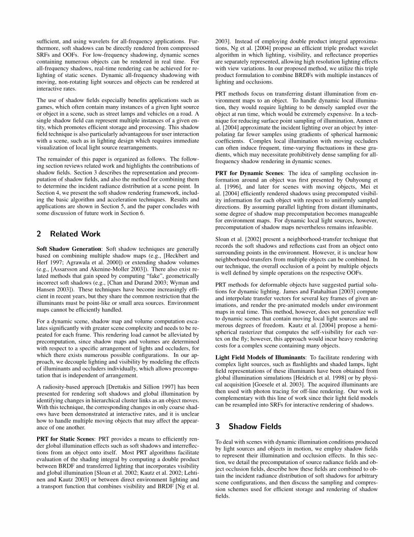
Figure 2: Shadow field sampling. Left: Radial and angular sampling

(R,θ ,φ ) of cubemap positions on concentric shells. The bounding sphere

of the scene entity is shown in blue. Right: The sampled cube map (θin,φin)

of point q.

3.1 SRF and OOF Precomputation

The effect of a light source or occluding object can be expressed asa field in the space that surrounds it. For a local light source Li, itsradiated illumination at an arbitrary point (x,y,z) in the scene can beexpressed as a 6D plenoptic function P(x,y,z,θin,φin, t) [McMillanand Bishop 1995], where (θin,φin) is the incident illumination di-rection and t denotes time. Reparameterizing the position (x,y,z) aspolar coordinates (Rp,θp,φp) with respect to the local frame of thelight source and removing the time dependency, a source radiancefield can be represented as the 5D function S(Rp,θp,φp,θin,φin),or equivalently as cube maps (θin,φin) as a function of position(Rp,θp,φp). Occlusion fields can be expressed similarly, but repre-senting alpha values instead of radiance intensities.

The SRF of each light source and the OOF of each local object isindividually precomputed at sampled locations in its surroundingspace as illustrated in Fig. 2. While optimal sampling densitiescould potentially be established from a detailed analysis, we insteadallow the user to empirically determine for each shadow field theradial and angular sampling densities that result in an acceptablelevel of error.

Distant illumination represented in an environment map is handledas a special light source with a shadow field Sd that is independentof spatial location and may undergo changes such as rotations. Dis-tant lighting is noted as being farther away from any scene pointthan any local entity. The self-occlusion of an object at a surfacepoint p can similarly be expressed as a special object occlusion fieldOp that is precomputed at sampled points on an object’s surface andis considered the closest entity to any point on the object.

3.2 Incident Radiance Computation

With movement of light sources and objects, lighting and visibil-ity can change rapidly within a scene and vary significantly amongdifferent scene points. For efficient rendering of soft shadow at agiven point, the SRFs and OOFs of illuminants and objects must bequickly combined according to the scene configuration to solve forthe incident radiance distribution.

To determine the contribution of a light source to the incident ra-diance distribution of a soft shadow point, the visibility of thelight source from the point needs to be computed with respect tothe occluding objects in the scene. While this conventionally re-quires tracing rays between the illuminant and the point, it can beefficiently calculated by some simple operations on precomputedshadow fields. First, the fields induced by the illuminant and sceneobjects are aligned to their scene positions and orientations usingcoordinate transformations. The distances of these scene entitiesfrom the shadow point are then sorted from near to far. To avoid am-biguity in this distance sort, we do not allow the bounding spheres

O3

O1

S1

S3

p

Sd

Op

O2 S2

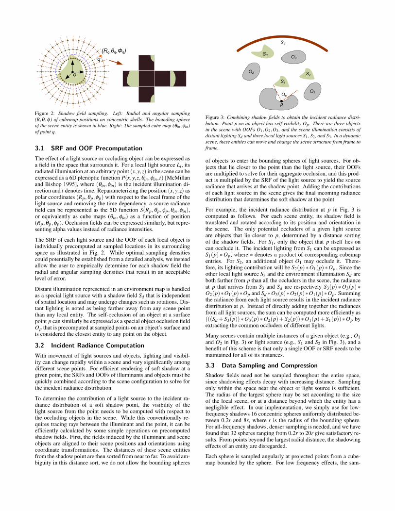
Figure 3: Combining shadow fields to obtain the incident radiance distri-

bution. Point p on an object has self-visibility Op. There are three objects

in the scene with OOFs O1,O2,O3, and the scene illumination consists of

distant lighting Sd and three local light sources S1, S2, and S3. In a dynamic

scene, these entities can move and change the scene structure from frame to

frame.

of objects to enter the bounding spheres of light sources. For ob-jects that lie closer to the point than the light source, their OOFsare multiplied to solve for their aggregate occlusion, and this prod-uct is multiplied by the SRF of the light source to yield the sourceradiance that arrives at the shadow point. Adding the contributionsof each light source in the scene gives the final incoming radiancedistribution that determines the soft shadow at the point.

For example, the incident radiance distribution at p in Fig. 3 iscomputed as follows. For each scene entity, its shadow field istranslated and rotated according to its position and orientation inthe scene. The only potential occluders of a given light sourceare objects that lie closer to p, determined by a distance sortingof the shadow fields. For S1, only the object that p itself lies oncan occlude it. The incident lighting from S1 can be expressed asS1(p) ∗Op, where ∗ denotes a product of corresponding cubemapentries. For S2, an additional object O1 may occlude it. There-fore, its lighting contribution will be S2(p)∗O1(p)∗Op. Since theother local light source S3 and the environment illumination Sd areboth farther from p than all the occluders in the scene, the radianceat p that arrives from S3 and Sd are respectively S3(p) ∗O3(p) ∗O2(p)∗O1(p)∗Op and Sd ∗O3(p)∗O2(p)∗O1(p)∗Op. Summingthe radiance from each light source results in the incident radiancedistribution at p. Instead of directly adding together the radiancesfrom all light sources, the sum can be computed more efficiently as(((Sd + S3(p)) ∗O3(p) ∗O2(p)+ S2(p)) ∗O1(p)+ S1(p)) ∗Op byextracting the common occluders of different lights.

Many scenes contain multiple instances of a given object (e.g., O1

and O2 in Fig. 3) or light source (e.g., S1 and S2 in Fig. 3), and abenefit of this scheme is that only a single OOF or SRF needs to bemaintained for all of its instances.

3.3 Data Sampling and Compression

Shadow fields need not be sampled throughout the entire space,since shadowing effects decay with increasing distance. Samplingonly within the space near the object or light source is sufficient.The radius of the largest sphere may be set according to the sizeof the local scene, or at a distance beyond which the entity has anegligible effect. In our implementation, we simply use for low-frequency shadows 16 concentric spheres uniformly distributed be-tween 0.2r and 8r, where r is the radius of the bounding sphere.For all-frequency shadows, denser sampling is needed, and we havefound that 32 spheres ranging from 0.2r to 20r give satisfactory re-sults. From points beyond the largest radial distance, the shadowingeffects of an entity are disregarded.

Each sphere is sampled angularly at projected points from a cube-map bounded by the sphere. For low frequency effects, the sam-

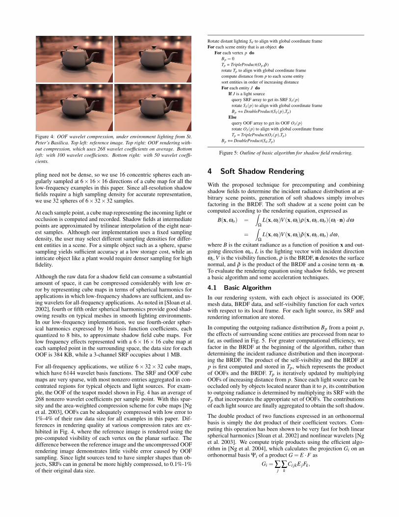
Figure 4: OOF wavelet compression, under environment lighting from St.

Peter’s Basilica. Top left: reference image. Top right: OOF rendering with-

out compression, which uses 268 wavelet coefficients on average. Bottom

left: with 100 wavelet coefficients. Bottom right: with 50 wavelet coeffi-

cients.

pling need not be dense, so we use 16 concentric spheres each an-gularly sampled at 6×16×16 directions of a cube map for all thelow-frequency examples in this paper. Since all-resolution shadowfields require a high sampling density for accurate representation,we use 32 spheres of 6×32×32 samples.

At each sample point, a cube map representing the incoming light orocclusion is computed and recorded. Shadow fields at intermediatepoints are approximated by trilinear interpolation of the eight near-est samples. Although our implementation uses a fixed samplingdensity, the user may select different sampling densities for differ-ent entities in a scene. For a simple object such as a sphere, sparsesampling yields sufficient accuracy at a low storage cost, while anintricate object like a plant would require denser sampling for highfidelity.

Although the raw data for a shadow field can consume a substantialamount of space, it can be compressed considerably with low er-ror by representing cube maps in terms of spherical harmonics forapplications in which low-frequency shadows are sufficient, and us-ing wavelets for all-frequency applications. As noted in [Sloan et al.2002], fourth or fifth order spherical harmonics provide good shad-owing results on typical meshes in smooth lighting environments.In our low-frequency implementation, we use fourth-order spher-ical harmonics expressed by 16 basis function coefficients, eachquantized to 8 bits, to approximate shadow field cube maps. Forlow frequency effects represented with a 6× 16× 16 cube map ateach sampled point in the surrounding space, the data size for eachOOF is 384 KB, while a 3-channel SRF occupies about 1 MB.

For all-frequency applications, we utilize 6× 32× 32 cube maps,which have 6144 wavelet basis functions. The SRF and OOF cubemaps are very sparse, with most nonzero entries aggregated in con-centrated regions for typical objects and light sources. For exam-ple, the OOF of the teapot model shown in Fig. 4 has an average of268 nonzero wavelet coefficients per sample point. With this spar-sity and the area-weighted compression scheme for cube maps [Nget al. 2003], OOFs can be adequately compressed with low error to1%-4% of their raw data size for all examples in this paper. Dif-ferences in rendering quality at various compression rates are ex-hibited in Fig. 4, where the reference image is rendered using thepre-computed visibility of each vertex on the planar surface. Thedifference between the reference image and the uncompressed OOFrendering image demonstrates little visible error caused by OOFsampling. Since light sources tend to have simpler shapes than ob-jects, SRFs can in general be more highly compressed, to 0.1%-1%of their original data size.

Rotate distant lighting Sd to align with global coordinate frame

For each scene entity that is an object do

For each vertex p do

Bp = 0

Tp = TripleProduct(Op ,ρ)

rotate Tp to align with global coordinate frame

compute distance from p to each scene entity

sort entities in order of increasing distance

For each entity J do

If J is a light source

query SRF array to get its SRF SJ(p)

rotate SJ(p) to align with global coordinate frame

Bp += DoubleProduct(SJ(p),Tp)

Else

query OOF array to get its OOF OJ(p)

rotate OJ(p) to align with global coordinate frame

Tp = TripleProduct(OJ(p),Tp)

Bp += DoubleProduct(Sd ,Tp)

Figure 5: Outline of basic algorithm for shadow field rendering.

4 Soft Shadow Rendering

With the proposed technique for precomputing and combiningshadow fields to determine the incident radiance distribution at ar-bitrary scene points, generation of soft shadows simply involvesfactoring in the BRDF. The soft shadow at a scene point can becomputed according to the rendering equation, expressed as

B(x,ωo) =∫

ΩL(x,ωi)V (x,ωi)ρ(x,ωi,ωo)(ωi ·n) dω

=∫

ΩL(x,ωi)V (x,ωi)ρ(x,ωi,ωo) dω,

where B is the exitant radiance as a function of position x and out-going direction ωo, L is the lighting vector with incident directionωi, V is the visibility function, ρ is the BRDF, n denotes the surfacenormal, and ρ is the product of the BRDF and a cosine term ωi ·n.To evaluate the rendering equation using shadow fields, we presenta basic algorithm and some acceleration techniques.

4.1 Basic Algorithm

In our rendering system, with each object is associated its OOF,mesh data, BRDF data, and self-visibility function for each vertexwith respect to its local frame. For each light source, its SRF andrendering information are stored.

In computing the outgoing radiance distribution Bp from a point p,the effects of surrounding scene entities are processed from near tofar, as outlined in Fig. 5. For greater computational efficiency, wefactor in the BRDF at the beginning of the algorithm, rather thandetermining the incident radiance distribution and then incorporat-ing the BRDF. The product of the self-visibility and the BRDF atp is first computed and stored in Tp, which represents the productof OOFs and the BRDF. Tp is iteratively updated by multiplyingOOFs of increasing distance from p. Since each light source can beoccluded only by objects located nearer than it to p, its contributionto outgoing radiance is determined by multiplying its SRF with theTp that incorporates the appropriate set of OOFs. The contributionsof each light source are finally aggregated to obtain the soft shadow.

The double product of two functions expressed in an orthonormalbasis is simply the dot product of their coefficient vectors. Com-puting this operation has been shown to be very fast for both linearspherical harmonics [Sloan et al. 2002] and nonlinear wavelets [Nget al. 2003]. We compute triple products using the efficient algo-rithm in [Ng et al. 2004], which calculates the projection Gi on anorthonormal basis Ψi of a product G = E ·F as

Gi = ∑j∑k

Ci jkE jFk,

where Ci jk =∫

S2 Ψi(ω)Ψ j(ω)Ψk(ω)dω are tripling coefficients.

In determining the soft shadows of a scene point, the computationrequired for each scene entity consists of a table query with in-terpolation, a rotation, and a double product for light sources ora triple product for objects. Since table queries with interpolationand double products are fast, computational costs principally arisefrom rotations and triple products. For a spherical harmonic basis,rotations can be efficiently computed using the rotation function inDirectX. For a wavelet basis, rotations are computationally expen-sive, so we consequently do not support rotations of local entitiesin all frequency applications. Rotations of a wavelet environmentmap, however, are efficiently supported since only a single rotationof its cube map is needed to update the environment lighting in theentire scene. To efficiently handle wavelet rotations for a local en-tity, wavelet projections could be precomputed at sampled rotationsof a shadow field, but at a large expense in storage.

The complexity of triple products for N spherical harmonic basis

functions in complex form is O(N5/2) as noted in [Ng et al. 2004].Since we use only low-order spherical harmonic projections in realform [Sloan et al. 2002], the number of nonzero tripling coefficientsis small (25 for third order and 77 for fourth order). For a waveletbasis, we use the sublinear-time algorithm presented in [Ng et al.2004].

4.2 Acceleration

To accelerate rendering, we employ a two-stage culling techniqueand utilize a lazy updating of occlusions.

Culling: Visibility culling is performed on two levels. With respectto the viewer, we cull vertices that do not contribute to screen pixels.With respect to each remaining vertex p, we cull entities that donot contribute to its radiance. Such entities exhibit at least one ofthe following three conditions. First, the bounding sphere of theentity is under the local horizon plane of the vertex. Second, thebounding sphere of the entity is occluded by the inscribed spheresof closer entities. Third, the entity is far enough away from p to bedisregarded. This distance is set according to ‖ p−o ‖> ε ·r, whereo is the origin of the entity’s coordinate frame, r is the radius of itsbounding sphere, and ε · r is the maximum sampling radius of theshadow field. In our implementation, ε is set to 8 for low-frequencyapplications and 20 for all-frequency applications.

Lazy Occlusion Updating: If only light sources are moving in thescene, we can cache the visibility at each vertex with respect to eachlight source. In this way, as long as the occluders for a specific lightsource remain unchanged, the cached visibility can be reused; oth-erwise, the visibility is recomputed and cached. This accelerationscheme is particularly useful for interactive lighting design applica-tions, and can typically reduce rendering costs by a factor of 20.

5 Applications and Results

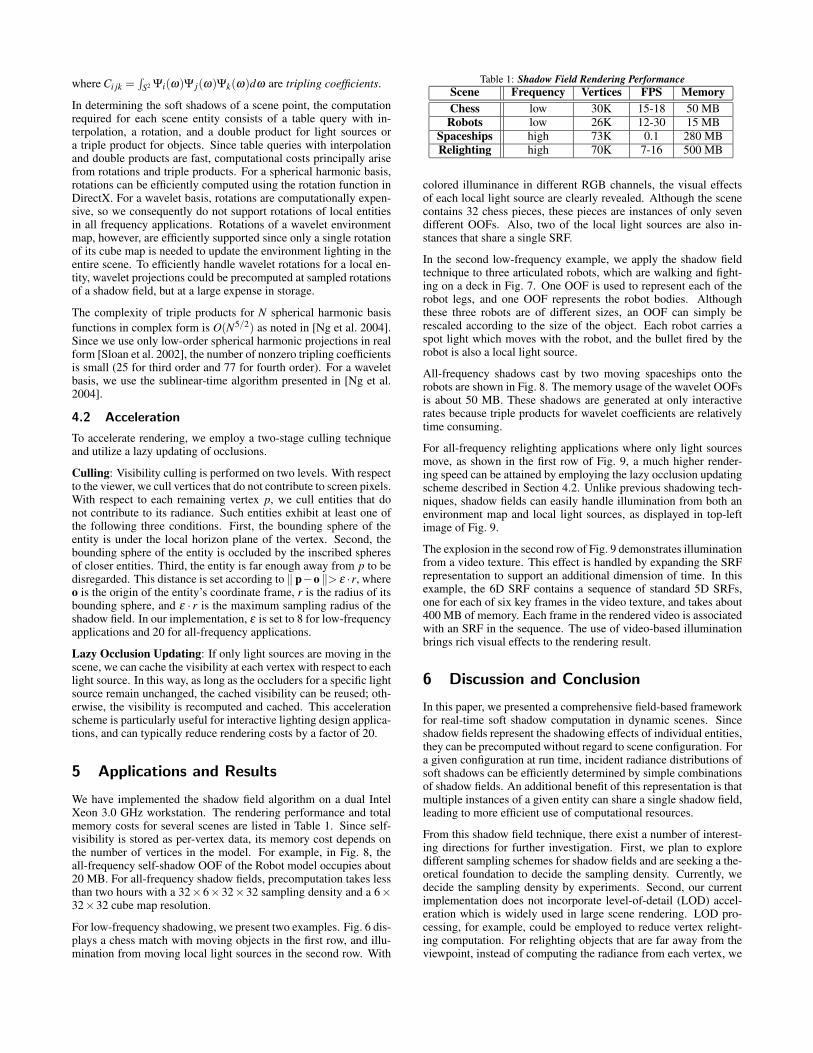
We have implemented the shadow field algorithm on a dual IntelXeon 3.0 GHz workstation. The rendering performance and totalmemory costs for several scenes are listed in Table 1. Since self-visibility is stored as per-vertex data, its memory cost depends onthe number of vertices in the model. For example, in Fig. 8, theall-frequency self-shadow OOF of the Robot model occupies about20 MB. For all-frequency shadow fields, precomputation takes lessthan two hours with a 32×6×32×32 sampling density and a 6×32×32 cube map resolution.

For low-frequency shadowing, we present two examples. Fig. 6 dis-plays a chess match with moving objects in the first row, and illu-mination from moving local light sources in the second row. With

Table 1: Shadow Field Rendering Performance

Scene Frequency Vertices FPS Memory

Chess low 30K 15-18 50 MB

Robots low 26K 12-30 15 MB

Spaceships high 73K 0.1 280 MB

Relighting high 70K 7-16 500 MB

colored illuminance in different RGB channels, the visual effectsof each local light source are clearly revealed. Although the scenecontains 32 chess pieces, these pieces are instances of only sevendifferent OOFs. Also, two of the local light sources are also in-stances that share a single SRF.

In the second low-frequency example, we apply the shadow fieldtechnique to three articulated robots, which are walking and fight-ing on a deck in Fig. 7. One OOF is used to represent each of therobot legs, and one OOF represents the robot bodies. Althoughthese three robots are of different sizes, an OOF can simply berescaled according to the size of the object. Each robot carries aspot light which moves with the robot, and the bullet fired by therobot is also a local light source.

All-frequency shadows cast by two moving spaceships onto therobots are shown in Fig. 8. The memory usage of the wavelet OOFsis about 50 MB. These shadows are generated at only interactiverates because triple products for wavelet coefficients are relativelytime consuming.

For all-frequency relighting applications where only light sourcesmove, as shown in the first row of Fig. 9, a much higher render-ing speed can be attained by employing the lazy occlusion updatingscheme described in Section 4.2. Unlike previous shadowing tech-niques, shadow fields can easily handle illumination from both anenvironment map and local light sources, as displayed in top-leftimage of Fig. 9.

The explosion in the second row of Fig. 9 demonstrates illuminationfrom a video texture. This effect is handled by expanding the SRFrepresentation to support an additional dimension of time. In thisexample, the 6D SRF contains a sequence of standard 5D SRFs,one for each of six key frames in the video texture, and takes about400 MB of memory. Each frame in the rendered video is associatedwith an SRF in the sequence. The use of video-based illuminationbrings rich visual effects to the rendering result.

6 Discussion and Conclusion

In this paper, we presented a comprehensive field-based frameworkfor real-time soft shadow computation in dynamic scenes. Sinceshadow fields represent the shadowing effects of individual entities,they can be precomputed without regard to scene configuration. Fora given configuration at run time, incident radiance distributions ofsoft shadows can be efficiently determined by simple combinationsof shadow fields. An additional benefit of this representation is thatmultiple instances of a given entity can share a single shadow field,leading to more efficient use of computational resources.

From this shadow field technique, there exist a number of interest-ing directions for further investigation. First, we plan to exploredifferent sampling schemes for shadow fields and are seeking a the-oretical foundation to decide the sampling density. Currently, wedecide the sampling density by experiments. Second, our currentimplementation does not incorporate level-of-detail (LOD) accel-eration which is widely used in large scene rendering. LOD pro-cessing, for example, could be employed to reduce vertex relight-ing computation. For relighting objects that are far away from theviewpoint, instead of computing the radiance from each vertex, we

Figure 6: A chess match. The first row shows moving objects; the second

row shows moving local light sources.

Figure 7: Articulated robots. Left: walking; Right: fighting.

could compute radiance from only a sparse set of vertices and in-terpolate their colors for other vertices. Third, we currently handleonly direct lighting, and we are interested in examining methodsfor incorporating radiance from interreflections into our framework.Another area of future work is to capture shadow fields of actuallight sources and objects, which could allow shadowing effects tobe generated from light field models of these entities.

Acknowledgements

The authors would like to thank Wei Zhou for designing and ani-mating the 3D models and for video production. Many thanks toDr. Chunhui Mei and Prof. Jiaoying Shi for useful discussionsabout their work. Thanks to Paul Debevec for the light probe data.The authors are grateful to the anonymous reviewers for their help-ful suggestions and comments.

References

AGRAWALA, M., RAMAMOORTHI, R., HEIRICH, A., AND MOLL, L. 2000. Efficient

image-based methods for rendering soft shadows. In SIGGRAPH ’00, 375–384.

ANNEN, T., KAUTZ, J., DURAND, F., AND SEIDEL, H.-P. 2004. Spherical harmonic

gradients for mid-range illumination. In Euro. Symp. on Rendering, 331–336.

ASSARSSON, U., AND AKENINE-MOLLER, T. 2003. A geometry-based soft shadow

volume algorithm using graphics hardware. In SIGGRAPH ’03, 511–520.

CHAN, E., AND DURAND, F. 2003. Rendering fake soft shadows with smoothies. In

Euro. Symp. on Rendering, 208–218.

CROW, F. C. 1977. Shadow algorithms for computer graphics. In Computer Graphics

(Proceedings of SIGGRAPH 77), vol. 11, 242–248.

DRETTAKIS, G., AND SILLION, F. X. 1997. Interactive update of global illumination

using a line-space hierarchy. In SIGGRAPH ’97, 57–64.

Figure 8: All frequency shadows from moving spaceships.

Figure 9: Relighting and light design. Top left: relighting with both an

environment map and a local light source; Top right: multiple local light

sources; Bottom: a local light source represented by a video texture.

GOESELE, M., GRANIER, X., HEIDRICH, W., AND SEIDEL, H.-P. 2003. Accurate

light source acquisition and rendering. In SIGGRAPH ’03, 621–630.

HECKBERT, P., AND HERF, M. 1997. Simulating soft shadows with graphics hard-

ware. Tech. Rep. CMU-CS-97-104, Carnegie Mellon University.

HEIDRICH, W., KAUTZ, J., SLUSALLEK, P., AND SEIDEL, H.-P. 1998. Canned

lightsources. In Rendering Techniques ’98, Eurographics, 293–300.

JAMES, D., AND FATAHALTIAN, K. 2003. Precomputing interactive dynamic de-

formable scenes. In SIGGRAPH ’03, 879–887.

KAUTZ, J., SLOAN, P., AND SNYDER, J. 2002. Fast, arbitrary brdf shading for low-

frequency lighting using spherical harmonics. In Euro. Workshop on Rendering,

291–296.

KAUTZ, J., LEHTINEN, J., AND AILA, T. 2004. Hemispherical rasterization for

self-shadowing of dynamic objects. In Euro. Symp. on Rendering, 179–184.

LEHTINEN, J., AND KAUTZ, J. 2003. Matrix radiance tranfer. In Symp. on Interactive

3D Graphics, 59–64.

MCMILLAN, L., AND BISHOP, G. 1995. Plenoptic modeling: an image-based ren-

dering system. In SIGGRAPH ’95, 39–46.

MEI, C., SHI, J., AND WU, F. 2004. Rendering with spherical radiance transport

maps. In Eurographics ’04, 281–290.

NG, R., RAMAMOORTHI, R., AND HANRAHAN, P. 2003. All-frequency shadows

using non-linear wavelet lighting approximation. In SIGGRAPH ’03, 376–381.

NG, R., RAMAMOORTHI, R., AND HANRAHAN, P. 2004. Triple product wavelet

integrals for all-frequency relighting. In SIGGRAPH ’04, 477–487.

OUHYOUNG, M., CHUANG, Y.-Y., AND LIANG, R.-H. 1996. Reusable Radiosity

Objects. Computer Graphics Forum 15, 3, 347–356.

SLOAN, P., KAUTZ, J., AND SNYDER, J. 2002. Precomputed radiance transfer

for real-time rendering in dynamic, low-frequency lighting environments. In SIG-

GRAPH ’02, 527–536.

WILLIAMS, L. 1978. Casting curved shadows on curved surfaces. In Computer

Graphics (Proceedings of SIGGRAPH 78), vol. 12, 270–274.

WYMAN, C., AND HANSEN, C. 2003. Penumbra maps: Approximate soft shadows

in real-time. In Euro. Symp. on Rendering, 202–207.