
Precision measurement instruments for machinery's ...
131
Precision measurement instruments for machinery’s mechanical compliance: design and operation Measurement instruments for physics-based calibration of advanced manufacturing machinery NIKOLAS ALEXANDER THEISSEN, THEISSEN(AT)KTH.SE Doctoral Thesis in Production Engineering School of Industrial Engineering and Management KTH Royal Institute of Technology Stockholm, Sweden 2021
-
Upload
khangminh22 -
Category
Documents
-
view
0 -
download
0
Transcript of Precision measurement instruments for machinery's ...
Precision measurement instruments for machinery’smechanical compliance: design and operation
Measurement instruments for physics-based calibration of advanced manufacturingmachinery
NIKOLAS ALEXANDER THEISSEN, THEISSEN(AT)KTH.SE
Doctoral Thesis in Production EngineeringSchool of Industrial Engineering and Management
KTH Royal Institute of TechnologyStockholm, Sweden 2021
Principal supervisorProf. Andreas Archenti, KTH Royal Institute of Technology, Sweden
Co-supervisorsProf. Amir Rashid, KTH Royal Institute of Technology, SwedenProf. Lihui Wang, KTH Royal Institute of Technology, Sweden
OpponentProf. Alexander H. Slocum, Massachusetts Institute of Technology, U.S.A.
Grading committeeDr. Anke Günther, ETH Zürich, SwitzerlandProf. Rikard Söderberg, Chalmers University of Technology, SwedenDr. Hélène Mainaud-Durand, CERN, Switzerland
Advance reviewerProf. Sofia Ritzén, KTH Royal Institute of Technology, Sweden
KTH School of Industrial Engineeringand ManagementSE-114 28 StockholmSWEDEN TRITA-ITM-AVL 2021:47ISBN 978-91-8040-068-8
Akademisk avhandling som med tillstånd av Kungl Tekniska högskolan framläggestill offentlig granskning för avläggande av doktorsexamen i industriell produktionfredag den 2021-12-17 klockan 10.00 i F3, Kungliga Tekniska högskolan, Lindsted-tsvägen 26, Stockholm.
© Nikolas Alexander Theissen, theissen(at)kth.se, December 2021
Tryck: Universitetsservice US AB
Abstract
Precision Measurement Instruments (PMIs) for machinery’s mechanical complianceare tools to quantify mechanical load as well as length for measurement ranges of0.1 µm to 10 m at uncertainty levels of 0.1 µm to 100 µm while exerting mechanicalloads. The quantity values of mechanical load and length can be used to identifycompliance, which is a relationship describing mechanical loads to a change ingeometry and vice versa.
This work is based on and contributes to research in the field of quasi-staticcompliance measurements of machine tools and industrial robots. In this context,quasi-static means to experimentally measure as close as possible to the intendedindustrial use case, which results in the quantification of positioning accuracy un-der slow movements. These data can be utilised to gain an improved understandingof the machinery’s operational behaviour and via calibration, in combination withon- or off-line compensation, the performance of the machinery can be improved.This approach contradicts ISO standard recommendations for compliance measure-ments, as quasi-static measurements can be affected by several superimposed errors.The influence of these errors can be minimised through the design and operationof the PMI. Metrologists and engineers have defined precision engineering designprinciples to create accurate and precise PMI. Furthermore, the author has sum-marised complementary precision engineering operation principles of PMI to ensurereproducible compliance measurements under movement.
This doctoral thesis summarises and applies precision engineering design as wellas operation principles to develop quasi-static compliance measurements throughthe Loaded Double Ball Bar - 3 Dimensional (LDBB-3D) and LDBB - 3 Dimen-sional Dynamic. These principles are exemplified in a case study on quasi-staticelasto-geometric measurement of a machine tool by employing the designed LDBB-3D. The results contribute to the understanding of the opportunities and limitationsof PMI for experimental compliance measurements for model calibration1 and va-lidation.
Keywords: Measurement instruments, Machine tools, Industrial robots
1Model calibration is detailed in the author’s licentiate thesis: Theissen, Nikolas Alexander(2019). Physics-based modelling and measurement of advanced manufacturing machinery’s posi-tioning accuracy. Stockholm: Universitetsservice US AB (TRITA-ITM-AVL, 2019:40).
iii

iv ABSTRACT

Sammanfattning
Precisionsmätinstrument (PMI) för maskins mekaniska styvhet är verktyg för attkvantifiera mekanisk belastning liksom längd för mått på 0.1 µm till 10 m vid osäker-hetsnivåer från 0.1 µm till 100 µm medan mekaniska belastningar utövas. Måtten avmekanisk belastning och längd kan användas för att identifiera styvhet, relationenvilken beskriva mekanisk belastning till ändring av geometrin och vice versa.
Detta arbete baserar på och bidrar till forskningen inom området kvasi-statiskstyvhets mätningar av verktygsmaskiner och industrirobotar. I detta samman-hang, kvasi-statisk betyder att experimentellt mäta så nära det avsedda industrielltillämpning som möjligt, vilket resulterar i kvantifiering av positioneringsnoggrann-het under långsamma rörelser. Dessa data kan användas för att få en bättre förstå-else för maskinens driftsbeteende och via kalibrering i kombination med on- elleroff-line kompensationen kan maskinens prestanda förbättras. Detta tillvägagångs-sätt strider mot ISO-standard rekommendationer för styvhets mätningar, eftersomkvasi-statiska mätningar kan påverkas av flera överlagrade fel. Påverkan av dessafel kan minimeras genom design och drift av PMI. Metrologer och ingenjörer hardefinierat precisions ingenjörs design principer för att skapa noggranna och repe-terbara PMI. Ytterligare, har författaren sammanfattat kompletterande precisionsingenjörs drift principer för att säkerställa reproducerbara efterlevnadsmätningarunder rörelse.
Denna doktorsavhandling sammanfattar och tillämpar såväl precisions ingenjörsdesign som drift principer för att utveckla kvasi-statisk styvhets mätningar genomden Loaded Double Ball Bar - 3 Dimensioner (LDBB - 3D) och LDBB - 3 Dimen-sioner Dynamisk. Dessa principer exemplifieras i en fallstudie om elasto-geometriskmätning av en verktygsmaskin genom att använda den designade LDBB-3D. Re-sultaten är avsedda att bidra till förståelsen av möjligheterna och begränsningarnaför PMI för experimentell styvhetsmätningar för modellkalibrering2 och validering.
Nyckelord: Mätinstrument, Verktygsmaskiner, Industrirobotar
2Model calibration is detailed in the author’s licentiate thesis: Theissen, Nikolas Alexander(2019). Physics-based modelling and measurement of advanced manufacturing machinery’s posi-tioning accuracy. Stockholm: Universitetsservice US AB (TRITA-ITM-AVL, 2019:40).
v

vi SAMMANFATTNING

Acknowledgements
Dear reader,Firstly, I would like to express my sincere gratitude, appreciation, and admirationfor my supervisor Prof. Andreas Archenti. To learn from Andreas Archenti has beenthe opportunity to work on interesting topics in multi-national and interdisciplinaryteams, to understand the meaning of being an independent researcher and to de-velop myself beyond research. Thank you for your unique performance as a mentor,human, and friend. I would like to express my gratitude towards my co-supervisorsProf. Amir Rashid for your indefatigable patience and Prof. Lihui Wang for yourextensive network. To my genuinely appreciated colleagues and collaborators inresearch as well as simply, search:
To Theodoros Laspas, Károly Szipka, Katherine Gonzalez, Péter Troll, and EleonoraIunusova for being the best possible office cohabitants. Without you, this would havenot been possible.
To Bita Daemi, Robert Tomkowski, Bernd Peukert, Tomas Österlind, and Mo-hammed Abdullah for sharing their expertise and scientific attitude with me. Pleasestay the educative, supportive, and open supervisors you are.
To Jan Stamer, Anton Kviberg, Mikael Johansson, Kevin Karlsson, and TomaszOciepa for their work, patience, ingeniousness. Thank you for your guidance.
To my fellow PhD students, colleagues at ITM and IIP, PhD student councilmembers, gym buddies, BBQ buddies, Svensk klassiker vänner, friends, and familyfor making my PhD studies one of the most hospitable environments I ever had thepleasure to work in.
To our collaborators in international projects such as Asier Barrios at IDEKOS.COOP, Professor Soichi Ibaraki at Hiroshima University, Alexandre Ambiehl andSebastien Garnier at the University of Nantes as well as in national projects Ste-fan Cedergren at GKN Trollhättan, Jeroen Derkx and Jens Andersson at ABB inVästerås for the fruitful cooperation.
I wish to carry and keep the spirit of reliability, honesty, respect, and accountabilitythat you thought and shared with me for the rest of my life.
vii

viii ACKNOWLEDGEMENTS
To KTH, DMMS, XPRES, SMART, VINNOVA and the European Research Coun-cil for the financial support of this work.
And finally, to you my dear reader, I am looking forward to our discussions.
Nikolas Alexander TheissenStockholm, 2021-06-03

ix
Good research practices are based on fundamental principles of researchintegrity...
Reliability in ensuring the quality of research, reflected in the design,the methodology, the analysis and the use of resources.
Honesty in developing, undertaking, reviewing, reporting and commu-nicating research in a transparent, fair, full and unbiased way.
Respect for colleagues, research participants, society, ecosystems, cul-tural heritage and the environment.
Accountability for the research from idea to publication, for its man-agement and organisation, for training, supervision and mentoring, andfor its wider impacts.
The European Code of Conduct for Research IntegrityAll European Academies 2017

x ACKNOWLEDGEMENTS

Table of contents
Abstract iii
Sammanfattning v
Acknowledgements vii
Table of contents xi
List of figures xiii
List of tables xv
Acronyms xvii
Sign conventions xix
1 Introduction 11.1 Background . . . . . . . . . . . . . . . . . . . . . . . . . . . . . . . . 31.2 Motivation . . . . . . . . . . . . . . . . . . . . . . . . . . . . . . . . 51.3 Research questions . . . . . . . . . . . . . . . . . . . . . . . . . . . . 61.4 Research methodology . . . . . . . . . . . . . . . . . . . . . . . . . . 61.5 Thesis delimitation . . . . . . . . . . . . . . . . . . . . . . . . . . . . 81.6 Thesis outline . . . . . . . . . . . . . . . . . . . . . . . . . . . . . . . 101.7 Sustainable development . . . . . . . . . . . . . . . . . . . . . . . . . 101.8 Publications . . . . . . . . . . . . . . . . . . . . . . . . . . . . . . . . 12
2 Precision engineering design principles 172.1 History and mechanical design . . . . . . . . . . . . . . . . . . . . . 192.2 Structure . . . . . . . . . . . . . . . . . . . . . . . . . . . . . . . . . 212.3 Abbe principle . . . . . . . . . . . . . . . . . . . . . . . . . . . . . . 242.4 Kinematic and quasi-kinematic design . . . . . . . . . . . . . . . . . 262.5 Direct displacement transducers . . . . . . . . . . . . . . . . . . . . . 292.6 Metrology frames . . . . . . . . . . . . . . . . . . . . . . . . . . . . . 302.7 Bearings . . . . . . . . . . . . . . . . . . . . . . . . . . . . . . . . . . 31
xi

xii TABLE OF CONTENTS
2.8 Drives and carriages . . . . . . . . . . . . . . . . . . . . . . . . . . . 332.9 Thermal effects . . . . . . . . . . . . . . . . . . . . . . . . . . . . . . 342.10 Control system . . . . . . . . . . . . . . . . . . . . . . . . . . . . . . 382.11 Error compensation . . . . . . . . . . . . . . . . . . . . . . . . . . . 402.12 Uncertainty budget . . . . . . . . . . . . . . . . . . . . . . . . . . . . 41
3 Precision engineering operation principles 453.1 Machine base coordinate system transformation . . . . . . . . . . . . 463.2 Transient measurement data . . . . . . . . . . . . . . . . . . . . . . . 493.3 Error separation . . . . . . . . . . . . . . . . . . . . . . . . . . . . . 493.4 Mechanical base load reference . . . . . . . . . . . . . . . . . . . . . 54
4 LDBB-3D: Machine tool elasto-geometric measurement 59
5 Discussion and conclusion 63
6 Outlook and future work 69
Bibliography 71
Appended publications 85
List of figures
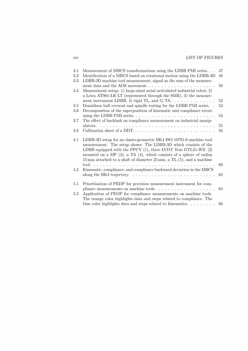
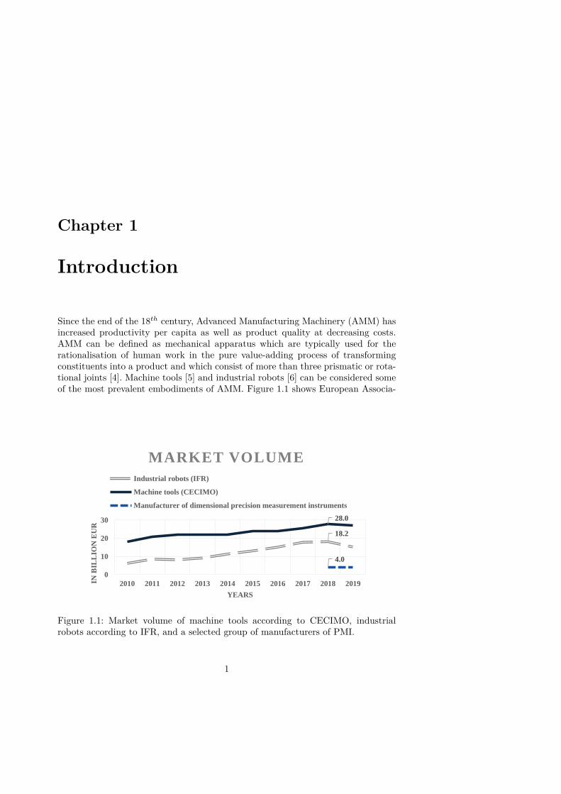
1.1 Market volume of machine tools according to CECIMO, industrial robotsaccording to IFR, and a selected group of manufacturers of PMI. . . . . 1
1.2 Machine accuracy and machining accuracy. . . . . . . . . . . . . . . . . 41.3 Thesis outline in a figure. . . . . . . . . . . . . . . . . . . . . . . . . . . 7
2.1 Conceptual measurement setups. . . . . . . . . . . . . . . . . . . . . . . 182.2 PEDP as a part of the mechanical design process based on [1, 2]. The
bullet points on the right-hand side highlight the activities, while thearrows indicate the aim of each phase. . . . . . . . . . . . . . . . . . . . 20
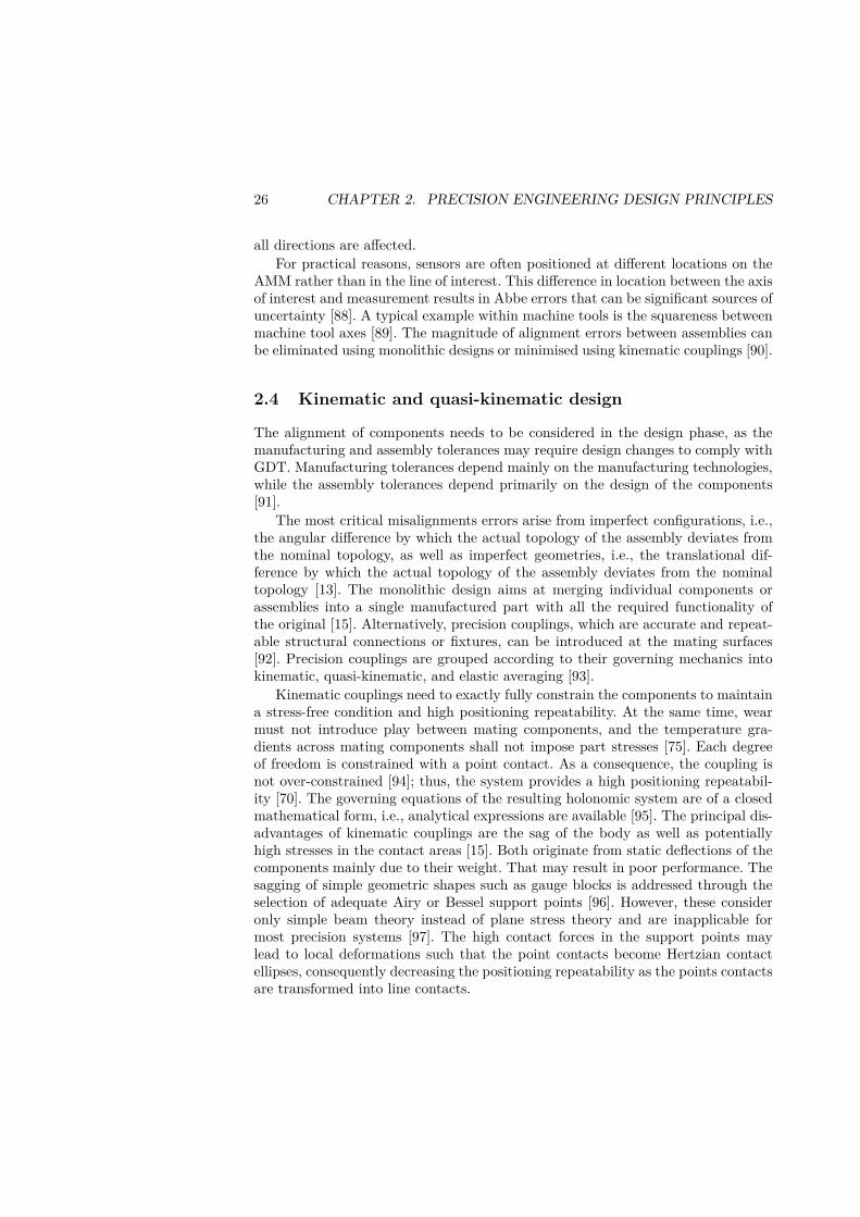
2.3 Conceptual MF of the LDBB-3D and LDBB-3DD. . . . . . . . . . . . . 212.4 Visualisation of trilateration for the MF. . . . . . . . . . . . . . . . . . . 232.5 Examples of the Abbe principle. . . . . . . . . . . . . . . . . . . . . . . 252.6 Visualisation of the kinematic constraints of the TL. The point con-
straints are highlighted in orange. . . . . . . . . . . . . . . . . . . . . . . 272.7 Visualisation of the kinematic constraints of the MF. The point, line,
and planar constraints are highlighted in orange, green, and red. . . . . 282.8 The metrology and force loop of the LDBB-3D. . . . . . . . . . . . . . . 302.9 Side view of the LDBB-3DD: 1. Helical coil spring, 2. Parallel pre-
stressed PEA, 3. IEPE force sensor. . . . . . . . . . . . . . . . . . . . . 322.10 Thermal heat transfer, internal and external heat sources and sinks and
their relationship with AMM. . . . . . . . . . . . . . . . . . . . . . . . . 352.11 Steady state heat field due to power loss of the DDT and a thermo-
mechanical deformation due to a temperature increase by by 10 °C. . . . 362.12 MF of the LDBB-3D and one of the thermocouples mounted on the table
of a machine tool. . . . . . . . . . . . . . . . . . . . . . . . . . . . . . . 382.13 Closed-loop control for the magnitude of the force of the LDBB and
LDBB-3D via the PPCV. . . . . . . . . . . . . . . . . . . . . . . . . . . 392.14 LDBB-3D, force orientation and resulting magnitude error as a function
of the radial offset for a uni-dimensional force vector. . . . . . . . . . . . 432.15 LDBB-3D, relative uncertainty in the identified Cartesian stiffness based
on the combined standard uncertainty for deflection and force measure-ment. . . . . . . . . . . . . . . . . . . . . . . . . . . . . . . . . . . . . . 44
xiii
xiv LIST OF FIGURES
3.1 Measurement of MBCS transformations using the LDBB PMI series. . . 473.2 Identification of a MBCS based on rotational motion using the LDBB-3D. 483.3 LDBB-3D machine tool measurement; signal as the sum of the measure-
ment data and the AOS movement. . . . . . . . . . . . . . . . . . . . . . 503.4 Measurement setup: 1) large-sized serial articulated industrial robot, 2)
a Leica AT901-LR LT (represented through the SMR), 3) the measure-ment instrument LDBB, 4) rigid TL, and 5) TA. . . . . . . . . . . . . . 52
3.5 Donaldson ball reversal and spindle testing for the LDBB PMI series. . 533.6 Decomposition of the superposition of kinematic and compliance errors
using the LDBB PMI series. . . . . . . . . . . . . . . . . . . . . . . . . . 543.7 The effect of backlash on compliance measurement on industrial manip-
ulators. . . . . . . . . . . . . . . . . . . . . . . . . . . . . . . . . . . . . 553.8 Calibration sheet of a DDT. . . . . . . . . . . . . . . . . . . . . . . . . . 56
4.1 LDBB-3D setup for an elasto-geometric BK4 ISO 10791-6 machine toolmeasurement. The setup shows: The LDBB-3D which consists of theLDBB equipped with the PPCV (1), three LVDT Tesa GTL21-W® [3]mounted on a MF (3), a TA (4), which consists of a sphere of radius15 mm attached to a shaft of diameter 25 mm, a TL (5), and a machinetool. . . . . . . . . . . . . . . . . . . . . . . . . . . . . . . . . . . . . . . 60
4.2 Kinematic, compliance, and compliance backward deviation in the MBCSalong the BK4 trajectory. . . . . . . . . . . . . . . . . . . . . . . . . . . 62
5.1 Prioritisation of PEDP for precision measurement instrument for com-pliance measurements on machine tools. . . . . . . . . . . . . . . . . . . 64
5.2 Application of PEOP for compliance measurements on machine tools.The orange color highlights data and steps related to compliance. Theblue color highlights data and steps related to kinematics. . . . . . . . . 66

List of tables
2.1 List of uncertainty contributors for the LDBB-3D. . . . . . . . . . . . . 44
4.1 Compliance in X-, Y-, and Z-axis in terms of mean over velocity. . . . . 61
xv


Acronyms
ABMA American Bearing Manufacturers AssociationAL Apparent LoadAMM Advanced Manufacturing MachineryAOS Angular Overshoot
CAM Computer Aided ManufacturingCCW Counter-ClockwiseCECIMO European Association of the Machine Tool IndustriesCFRP Carbon Fibre Reinforced PlasticsCMM Coordinate Measurement MachineCNC Computer Numerical ControlCW Clockwise
DDT Direct Displacement TransducerDOF Degree of Freedom
EE End Effector
FE Finite ElementFRF Frequency Response Function
GDT Geometric Dimension and Tolerance
IEPE Integrated Electronics Piezo-ElectricIFR International Federation of Robotics
KPI Key Performance Indicator
LDBB Loaded Double Ball BarLDBB-3DD Loaded Double Ball Bar - 3 Dimensional DynamicLDBB-3D Loaded Double Ball Bar - 3 DimensionalLT Laser TrackerLVDT Linear Variable Differential Transformer
xvii

xviii ACRONYMS
MAP Measurement Application PointMBCS Machine Base Coordinate SystemMBLR Mechanical Base Load ReferenceMBS Multibody SystemMF Metrology Frame
NCCP Non-Contact Capacitive ProbeNMI National Metrology Institute
OEM Original Equipment Manufacturer
PEA Piezo-Electric ActuatorPEDP Precision Engineering Design PrinciplesPEOP Precision Engineering Operation PrinciplesPKM Parallel Kinematic Mechanism/MachinePMI Precision Measurement InstrumentPPCV Proportional Pressure Control Valve
RQ Research Question
SDG Sustainable Development GoalSKM Serial Kinematic Mechanism/MachineSMR Spherically Mounted Retroreflector
TA Tool AdaptorTCP Tool Centre PointTL Table LinkTSRS Tele Surgical Robotic Systems
UN United Nations
VCS Volumetric Compensation SystemVIM International Vocabulary of Metrology

Sign conventions
A, a Scalaraaa Vectoraaa Unit vectorAAA MatrixaHTMHTMHTM b Homogeneous transformation from b into a|| • ||2 Euclidean norm|| • ||2 Least squares approximation•−1 Inverse operator•T Transpose operator
xix

Chapter 1
Introduction
Since the end of the 18th century, Advanced Manufacturing Machinery (AMM) hasincreased productivity per capita as well as product quality at decreasing costs.AMM can be defined as mechanical apparatus which are typically used for therationalisation of human work in the pure value-adding process of transformingconstituents into a product and which consist of more than three prismatic or rota-tional joints [4]. Machine tools [5] and industrial robots [6] can be considered someof the most prevalent embodiments of AMM. Figure 1.1 shows European Associa-
18.2
28.0
4.0
0
10
20
30
2010 2011 2012 2013 2014 2015 2016 2017 2018 2019IN B
ILL
ION
EU
R
YEARS
MARKET VOLUME
Industrial robots (IFR)
Machine tools (CECIMO)
Manufacturer of dimensional precision measurement instruments
Figure 1.1: Market volume of machine tools according to CECIMO, industrialrobots according to IFR, and a selected group of manufacturers of PMI.
1
2 CHAPTER 1. INTRODUCTION
tion of the Machine Tool Industries (CECIMO)’s market volume of machine tools,the global market volume of industrial manipulators, according to the InternationalFederation of Robotics (IFR), and some manufacturers of their Precision Measure-ment Instrument (PMI), e.g. Hexagon, Mitutoyo, and Renishaw. The importanceof AMM is partly founded in the ability to realise numerous accurate and precisemanufacturing processes while providing modern manufacturing environments withthe flexibility to adapt to global trends, e.g., smaller lot sizes as a result of higherdegrees of customisation. Hence, knowledge on AMM’s accuracy for optimal opera-tion can be critical for a variety of industries such as automotive, aeronautical, andconsumer electronics.
Dependent on the reference source, accuracy is a qualitative [7] and quantitative[8] measure of the closeness of agreement between a test result and the acceptedreference value [9]. In metrology and engineering there exist several definitionsand standards on and related to accuracy, e.g., the International Vocabulary ofMetrology (VIM) [7] or ISO 230 [10], ISO 13041 [11], ISO 10791 [12]. This workmainly considers positioning accuracy, i.e., the difference between a commandedposition and the barycentre of the attained average of positions [8]. In productionengineering, positioning accuracy is a quantitative measure of how closely AMMcan position the Tool Centre Point (TCP) with respect to the workpiece. It is ameasure of "how AMMs move?" (kinematics), "how much AMMs deflect?" (statics),"how much AMMs vibrate?" (dynamics), and "how much AMMs expand or contractdue to a change in temperature?" (thermo-elasticity) [13]. This directly affects thegeometric dimensions and surface properties of the parts, i.e., how closely the partsmatch their design drawings. This idea is visualised in Figure 1.2.
The research of the Precision Engineering and Metrology group at the Depart-ment for Production Engineering at KTH uses PMI to quantify the performanceof the AMM under quasi-static conditions. Quasi-static conditions are emulatedthrough slow movements, which are meant to resemble the intended industrial ap-plication. The data of these measurements are used for calibration in combinationwith compensation to improve the performance of AMM. Thus, the successful util-isation of AMM depends also on the availability of the right PMI.
PMI for machinery’s compliance are devices to quantify mechanical load, i.e.,force and torque, as well as length, e.g., distance, position, and orientation, for mea-surement ranges of 0.1 µm to 10 m at uncertainty levels of 0.1 µm to 100 µm whileexerting mechanical loads. The term precision in the context of this work is basedon the quantitative definition by Gao [14]. Another definition of the term precisioncould be, that unpredictable deviations from a desired result being as small as isphysically and economically possible [15]. This is not to be confused with the termprecision1 in the VIM [7]. The measurement ranges indicate the absolute value of thedifference between the extreme quantity values of the measurable interval, e.g., lasertrackers are commonly stated to be able to measure up to a distance of 50 m. In-
1The closeness of agreement between a test result and the accepted reference value obtainedby replicated specified conditions [7].
1.1. BACKGROUND 3
strumental measurement uncertainty is the component of measurement uncertaintyarising from a measuring instrument or measuring system, e.g., laser trackers arecommonly stated to be able to measure with a base instrumental uncertainty of15 µm + 6 µm m−1 distance from the instrument. The quantity values of lengthand mechanical load can be used to identify compliance, which is a relationship re-lating mechanical loads to a change in geometry and vice versa. Its inverse is termedstiffness. The relative importance of stiffness compared to other physics-based errorsources depends on the AMM as well as its application.
In the context of AMM and this thesis, Precision Engineering Design Principles(PEDP) as well as Precision Engineering Operation Principles (PEOP) refer toa set of best practices to ensure the accuracy and precision of the instrument aswell as reproducible measurements through its operation. PEDP are establishedrules or good practices for application in the mechanical design process to minimiserandom and systematic measurement errors of a process [7]. The collection of PEDPis based on notable works related to precision engineering and design, such as theworks of Abbe [16], McKeown [17], and Schellekens et al. [18]. While PEOPs reducemeasurement uncertainty and separate the errors from the reference objects of thePMI or superimposed ones from the AMM from the measurand, i.e., the error sourceof the AMM under investigation. The collection of PEOP is based on the author’sexperience in the field of quasi-static compliance measurements.
Finally, physics-based calibration is the process of defining mathematical rep-resentations that describe the position or pose, i.e., the combined position andorientation [8], of one or several bodies of the machine tool or robot with modelparameters that relate a commanded pose to the actual pose considering the effectsof the kinematics, thermo-elasticity, statics, and dynamics. Then, to experimentallymeasure data, which can be used to identify and implement these model parame-ters for the optimised operation of the machinery [19]. Physics-based calibration isdescribed in the author’s licentiate thesis [4].
1.1 Background
Accuracy and repeatability2 have played crucial roles in the development of severaltechnological milestones [20]. From the author’s point of view, the development ofAMM and PMI has taken place conjointly for at least the past three centuries.
In the 1780s, John Wilkinson contributed to the 1st industrial revolution withthe boring technology for the pistons of James Watt’s steam engines; ensuring acircularity of about 2.5 mm [21]. Unfortunately, little is known about which PMIWilkinson used to verify the parts. Potentially Wilkinson used a micrometre screwgauge, which was invented by William Gascoigne in the 17th century, as an en-hancement of the Vernier calliper. In 1915, Carl Edvard Johansson contributed tothe 2nd industrial revolution by supplying the measurement artefacts to gauge theinterchangeability of the parts on Henry Ford’s assembly lines; ensuring a parallelity
2Also referred to as precision [7].

4 CHAPTER 1. INTRODUCTION
Process plan Machine
accuracy
Machining
Accuracy
Workpiece
material
Process
technologyFixturing
Cutting
tool
Wear
Thermo-
elasticity
StaticsDynamics
Kinematics
Volumetric
Accuracy
GD&THuman
factor
Figure 1.2: Machine accuracy and machining accuracy.
and orthogonality of about 0.01 mm. In the early 1950s, several works in the USApromoted the development of Computer Numerical Control (CNC) machine toolswhich contributed to the 3rd industrial revolution by providing machines, whichcould ensure concentric run-outs of less than 0.01 mm for the jet engines. At thesame time, the first Coordinate Measurement Machine (CMM) was developed bythe British company Ferranti [22]. This machine only had two axes. But CMMsquickly evolved with the first three axes models appearing in the 1960s. Semi-conductor and machine tool industries contributed to the 4th industrial revolutionby the development of lithography machines for the production of computer chips;ensuring transistor gates sizes in the range of 0.01 µm. While the development ofPMI evolves around the development of scanning probe microscopy, e.g., atomicforce or scanning tunnelling [23].
In manufacturing, accuracy is important for the design as well as for the oper-ation of AMM, and the verification of the produced parts. Improved accuracy ofAMM can arguably lead to increased energy efficiency, e.g., motors with decreasedconcentric run-outs. Or it can lead to a higher degree of suitability due to reducedscrap rates, e.g., for AMM with higher accuracy at invariant Geometric Dimensionand Tolerances (GDTs) the process capability increases. And it can lead to reduced
1.2. MOTIVATION 5
material consumption, e.g., the wall thickness of products such as aluminium canscan be further reduced, but this is cost-prohibitive due to the GDT of the diesin the forming process. Nowadays, manufacturers and customers usually require amachine accuracy in terms of positioning, pose, and path accuracy in the range of1 −50 µm for machine tools and 0.5 −5.0 mm for industrial robots [24, 25]. In thecontext of this work, the positioning, pose, and path accuracy of the sole AMM istermed machine accuracy [26]. This is not to be confused with machining accuracy;the "minimal achievable deviation of the actual value of a cutting tool from the tar-get value set by the NC" considering the interaction with the process, fixtures etc.,cf. Figure 1.2 [26].
1.2 Motivation
This doctoral thesis aims to outline the opportunities and limitations of experimen-tal compliance measurements of machine tools under movement. The opportunitiesand limitations are instantiated through the application of PMI on machine tools.In that, the thesis provides a comprehensive overview and applies PEDP as well asPEOP to develop the LDBB-3D.
From the author’s point of view, this knowledge can be valuable for meteo-rologists and experimental scientists as well as for engineers across the companyhierarchy. Meteorologists can identify potentials for improvement to develop thestate-of-the-art in terms of accuracy and repeatability of future PMI for machinecompliance under movement. In the design offices of the AMM’s Original Equip-ment Manufacturers (OEMs), these PMI could arguably be used for the validationand improvement of the finite element models for the co-simulation of the mechan-ics and control system. They can also use the PEDPs to improve their designs. Thiscan decrease the length of the product design phase [27]. The process planner canuse the knowledge about the accuracy to optimise the tool trajectories for reducedscrap rates [28]. One can use the data to make inferences on the machine health[29] of components such as bearings, or gauge the capability of a machine for a taskknowing its machine accuracy [10, 8]. The production manager can use the knowl-edge about the accuracy to derive economic Key Performance Indicators (KPIs)such as the operation time or scrap rate to support the decision making process forreorganisations or changes of value streams [30].
Archenti first introduced the concept of elastically linked systems for quasi-staticmeasurements in 2011 [31]. Archenti and Nicolescu exemplified the concept throughthe application of the Loaded Double Ball Bar (LDBB) for the accuracy analysisof machine tools [32]. This work supports further investigations under the conceptof elastically linked systems and quasi-static compliance measurements throughthe development of PMI for compliance in three-dimensional Cartesian space formachine tools and industrial manipulators.
6 CHAPTER 1. INTRODUCTION
1.3 Research questions
Based on the preceding introduction on the importance of AMM’s accuracy and itsrelation to PMI, the following research questions are defined and addressed in thisthesis:
RQ. 1. What are the most important precision engineering design principles forprecision measurement instruments to ensure accurate and repeatable compliancemeasurements on machine tools, in particular for the LDBB - 3 Dimensional?
RQ. 2. What are the most important precision engineering operation principles toensure accurate and repeatable compliance measurements on machine tools?
1.4 Research methodology
Researchers need to to identify and understand the limitations of the applied theo-ries, methods, and personal bias. From the author’s point of view, research method-ology comprises: (i) a philosophy or epistemology, a preconception on how knowl-edge is created, (ii) an approach to logical reasoning, a reasonable sequence ofthinking for the verification or falsification of the answer the research questions,(iii) a research method, which is the strategical approach to obtain accurate infor-mation on the subject. These elements are top-down interlinked. For instance, someepistemologies, approaches and methods are mutually exclusive.
The research methodology for this work follows aspects of positivism and post-positivism using inductive reasoning to scrutinise the approach to answer the re-search questions in combination with quantitative experimentation to gather dataabout the positioning accuracy of AMM. Positivism and post-positivism are bothbased on empiricism. Positivism requires knowledge to be derived from phenomena,which are natural and perceivable with one’s senses, as well as testable [33]. For thiswork, this means that for the quantification of positioning accuracy only researchworks and experiments are considered that are in accordance with internationalstandardisation and metrology bodies, besides the aspect of static and quasi-statictesting. Further, the author is convinced that theories, background, knowledge andvalues of the researcher influence what is observed. This relates to post-positivismand means that there exists a conscious or unconscious bias for the researcher [34].The studies of the author have been financed by projects related to AMM, thus theauthor might be prone to present the positioning accuracy of AMM in a favourablemanner. Hence, to systematically compensate for the bias of the researcher, falsifica-tion needs to be present throughout the research work. Meaning that the potentialaccuracy improvements presented as results throughout this work should be ques-tioned with respect to their reliability. Falsification is another important aspect inthe author’s epistemology and an idea of post-positivism developed by Karl Popper[35]. It questions the idea of the absolute truth as if a statement were impossibleto falsify it should be considered pseudo-science.
1.4. RESEARCH METHODOLOGY 7
Chapter 2
Precision Engineering Design Principles
1. Structure
2. Abbe principle
3. Kinematic and quasi-kinematic design
4. Direct displacement transducers
5. Metrology frames
6. Bearings
7. Drives and carriages
8. Thermal effects
9. Control systems
10. Uncertainty budgets
11. Error compensation
Chapter 3
Precision Engineering Operation Principles
1. Machine base coordinate system
transformation
2. Transient measurement data
3. Error separation
4. Mechanical base load reference
Chapter 4
LDBB-3D: Machine tool elasto-geometric
measurement
𝐾𝑋 =
𝑘𝑥𝑥 𝑘𝑥𝑦 𝑘𝑥𝑧𝑘𝑦𝑥 𝑘𝑦𝑦 𝑘𝑦𝑧𝑘𝑧𝑥 𝑘𝑧𝑦 𝑘𝑧𝑧
Figure 1.3: Thesis outline in a figure.

8 CHAPTER 1. INTRODUCTION
The research approach to logical reasoning follows the inductive paradigm,meaning that the research attempts to infer from a sample to the population, i.e.,the formulation of generalisations based on the observed phenomena. In the con-text of this work means to question how the author has ensured that the AMMunder investigation is a representative specimen for its kind. While this inductivereasoning may be persuasive, its arguments are not necessarily valid. Inductive rea-soning can yield a wrong conclusion even if the hypotheses are objectively true.For example, while all the machine tools presented in this work are Parallel Kine-matic Mechanism/Machines (PKMs), they may differ significantly in their design.They may use different drive trains. Some of which may exhibit non-linear stiffnesscharacteristics, while others do not. This contrasts with the principles of deduc-tive reasoning, as only an incorrect hypothesis can lead to an incorrect conclusionin deductive reasoning [36]. The research contribution of this work utilises experi-ments, demonstrations of the cause-effect relationship when systematically varyinga particular factor cetaris paribus, quantitative methods and numerical evaluationsof the results of the experiments. Meaning, that by following the procedures ofinternational standardisation and metrology bodies, the author tried to achieve ahigh degree of error separation to provide reliable figures. One additional remark,it would be more accurate to talk about apparent compliance and positioning accu-racy throughout this whole work, because the effect of the control system has notbeen quantified.
1.5 Thesis delimitation
Based on the title of this work, there exists a wide range of potential content thata reader may expect. This section intends to outline what is not included in thisreport and why it is not.
From the author’s point of view, PEDPs are an integral part of the mechanicaldesign process of PMI. Design and development engineers apply use PEDPs tocheck the feasibility of a product in the product definition, conceptual design, andproduct development phases [37]. Nevertheless, the work does not elaborate on themechanical design process. Particularly, as the author has only applied PEDPs anddesign methodologies for the creation of PMI for the measurement of machinery’scompliance, and neither established a PEDP nor a design methodology. But, theauthor has collected and created PEOP. Some of which, may have already beendocumented for dimensional PMI for machine tool kinematic measurements. Theintroduced PEDP and PEOP are not solely valid for PMI, they are also applicablefor instance to AMM. Based on the author’s presented terminology, certain typesof CMM would qualify to be both a PMI and an AMM.
Furthermore, this work omits the iterations of geometry and material selectionas a result of solid mechanics and thermo-elasticity finite element analysis of thedeveloped PMI, but only presents a list of uncertainty contributors which are aresult of this process. Also, material selection methodology is not covered in this
1.5. THESIS DELIMITATION 9
work. For an extensive work on the topic, please refer to works such as Timoshenko[38] and Ashby [39]. The author considers the topic to be of equal importance, butalso already well described in literature.
One could argue that the PEOP can be considered incomplete, as auxiliaryactions such as calibration, maintenance, and cleaning can be more crucial to thecorrectness of the measurand than the operation during the actual measurement.Nevertheless, this work covers no aspect related to the degradation of the PMI’sperformance over time, neither in terms of the short-term such as drift nor thelong-term time horizon.
Furthermore, metrology is based on traceability, uncertainty, and calibration [7].In the context of metrology, calibration is defined as operation that, under specifiedconditions, in a first step, establishes a relation between the quantity values withmeasurement uncertainties provided by measurement standards and correspondingindications with associated measurement uncertainties and, in a second step, usesthis information to establish a relation for obtaining a measurement result from anindication [7]. This is work can not claim that the created LDBB-3D and LoadedDouble Ball Bar - 3 Dimensional Dynamic (LDBB-3DD) are calibrated PMI. Butthey are used for physics-based calibration in accordance with the definition fromindustrial robotics [19, 4]. From the author’s point of view, the documented im-provement in positioning accuracy reported via calibrated PMI, see [40], providesa pragmatic validity to the physics-based calibration and its PMI.
From an industrial point of view, on-machine integration, data fusion, absolutemeasurement, smartness connectivity, and user-friendliness are important aspectsof PMI [4]. Particularly with regard to user-friendliness, the author can rely onlyon little data, as the proposed PMI have only been used by two groups of masterthesis students. From the author’s point of view, several of these factors could beconsidered more valuable by industry rather than the uncertainty associated withthe measurement.
The thesis focuses on machine accuracy, not machining accuracy [9], i.e., notconsidering the interaction with the process. That there can exist a significantdifference between the machine and machining accuracy is crucial for the quality ofthe finished product. The AMM models focus on physics-based aspects of machineaccuracy; meaning that this work does not elaborate on the importance of controlstrategies and controllers for machine accuracy.
Also, the thesis does not explain different measurement procedures nor the iden-tification and implementation of model parameters which also do have an importanteffect. This will be covered by another member of the Precision Engineering andMetrology group at the Department for Production Engineering at KTH in early2022.

10 CHAPTER 1. INTRODUCTION
1.6 Thesis outline
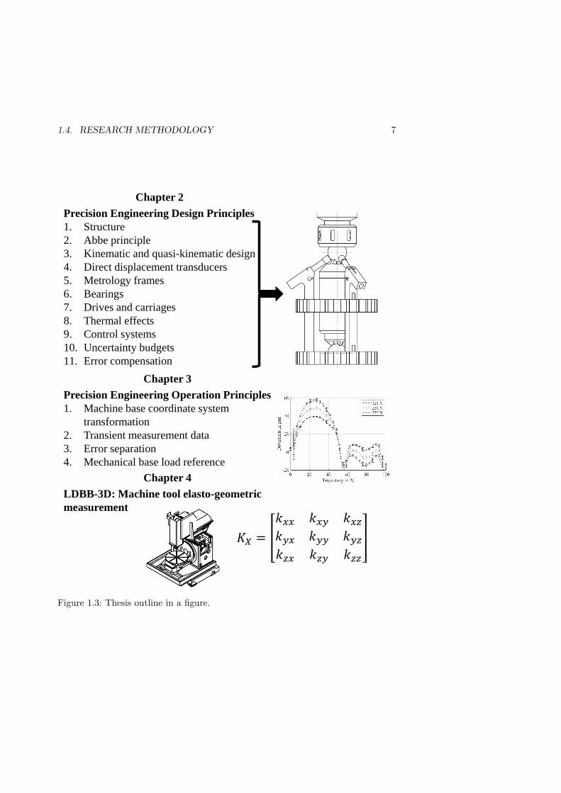
This thesis is organised into four main chapters: Chapter 1 Introduction, Chapter 2Precision engineering design principles, Chapter 3 Precision engineering operationprinciples, and Chapter 4 LDBB-3D: Machine tool elasto-geometric measurement.Chapters 2 and 3 are the corpus of this work, as they review the state-of-the-artof the PEDPs as well as PEOPs of which are necessary to create PMI for thecompliance measurement of AMM. Chapter 2 starts with a contextualisation ofPEDPs as a part of the mechanical design process and explains their developmentat hand of notable publications over the last century. Then, each subsection focusesindividually on the PEDP and explains their application in the design of PMI formachinery’s compliance at the example of the LDBB-3D. Furthermore, it elaboratesthe importance of aspects such as trilateration. Chapter 3 outlines PEOP which arebased on data transformation into the Machine Base Coordinate System (MBCS),error separation techniques, the handling of transient measurement data, and theapplication of a mechanical base load reference in loaded testing. Like in the pre-ceding chapter, each subsection focuses individually on a PEOP and explain theirapplication. Then, Chapter 4 exemplifies a quasi-static elasto-geometric of a 5-axismachine tool using the LDBB-3D. The data are used to identify the complianceof the machine tool as well as to quantify the kinematic errors along the circulartrajectory. The thesis is concluded by the Chapters 5 Discussion and conclusion,in which the preceding chapters are summarised to answer the Research Questions(RQs). Chapter 6 Outlook and future work proposes a plan to create measurementinstruments for the factories of the future as well as software to utilise the potentialof physics-based calibration of AMM.
1.7 Sustainable development
Engineers as well as researchers need to be aware of the limitations of science andtechnology to fulfil their ethical responsibility and to contribute to the sustainabledevelopment of society [41]. Sustainable development is development that meets theneeds of the present without compromising the ability of future generations to meettheir own needs. [42]. For this purpose the United Nations (UN) has developed theSustainable Development Goals (SDGs). There are 17 SDGs which were adoptedby all United Nations Member States in 2015 and provide a shared blueprint forpeace and prosperity for people and the planet, now and into the future [43]. Itfollows a concise qualitative assessment of the different impacts, that this researchwork may have on the SDGs. Only SDGs with a direct and indirect contributionare considered [44].
SDG 3. Good health and well-being
Tele Surgical Robotic Systemss (TSRSs) allow surgeons to perform surgical op-erations from remote locations with enhanced comfort, dexterity and accuracy [45].
1.7. SUSTAINABLE DEVELOPMENT 11
TSRS are capable to assist in a wide range of surgeries such orthopaedic, gynae-cological, cardiovascular, and general surgery [46] with several applications suchas laparoscopic procedures [47], eye surgery [48], and fracture manipulation [49].The introduction of robotic technology has revolutionized operation theatres but itsmultidisciplinary nature and high associated costs pose significant challenges. Nev-ertheless, low cost TSRS solutions seem distant [50]. Thus, cost reductions for TSRShave great potential for future research. One potential cost reduction comes fromeconomies of scales through the application of off-the-shelf industrial manipulatorsas the prices of equipment such as da Vinci, Mirosurge or SOFIE are around 1-2million USD [45]. For this purpose, KTH has been exploiting physics-based calibra-tion of industrial manipulators in combination with on- and off-line compensationto improve the positioning accuracy of industrial manipulators [4]. The author or-ganises a research visit to exchange knowledge about TSRS and the physics-basedcalibration of industrial manipulators to improve the alignment in the repositioningof bone fractures. This directly contributes to Target 3.8 as one core idea of TSRSis to give access to quality essential health-care services by providing the serviceof skilled surgeons beyond the border of popular urban areas remotely into ruralareas.
SDG 4. Quality Education
One may claim that the main outcome of this work is not measurement instru-ments, algorithms or classic scientific contributions but the PhD student them-self.This work promoted education through courses, summer projects, and theses un-der the # Sharp Cut (Cut) platform. The #Cut platform is an approach for themodelling and simulation of manufacturing processes and machinery. The #Cutplatform has a technology development roadmap which is redefined on an annualbasis with a forecast for the next three years. Summer projects and thesis are de-fined jointly with the roadmap to provide high-quality tasks to the students. Thiscontributes indirectly to Target 4.4 to substantially increase the number of youthand adults who have relevant skills, including technical and vocational skills, foremployment, decent jobs and entrepreneurship as most of our projects are industryoriented.
SDG 10. Reduce inequality
Furthermore, #Cut is an open software and hardware platform, as all designedmeasurements instruments and algorithms are published on GitHub. This con-tributes directly to Target 10.2 to empower and promote the social, economic andpolitical inclusion of all, irrespective of age, sex, disability, race, ethnicity, origin,religion or economic or other status.
12 CHAPTER 1. INTRODUCTION
SDG 12. Sustainable Consumption
The author’s research focuses on precision measurement instruments for ma-chinery’s compliance and physics-based calibration. From an industrial applicationpoint of view, the results of this work contribute to an increased positioning accu-racy of machine tool and industrial manipulators [4]. This directly contributes toTarget 12.5 to substantially reduce waste generation through prevention, reduction.However, it neglects recycling and reuse. Unfortunately, the direct and indirect con-tributions are just an efficiency development in accordance with the linear economy.
From the systems perspective, it is arguable, that the mentioned performanceincreases might lead to an overall increase in resource consumption showing re-bounds effects due to an induced increase in production. This rebound effect hasbeen observed for greenhouse gas emissions and the EU regulations on vehicle’sfuel efficiency [51]. Thus, it put forth the need to shift to a circular economy [52].However, from the author’s point of view, without the right mindset and legisla-tion, even the circular economy might just become yet another efficiency increasesubjected to the same rebound effect.
1.8 Publications
There are three publications appended to this compilation thesis. The appendedpublications referred to as Paper A-C are important to answer the RQs. Thepublications referred to as Paper D-G are further contributions to physics-basedcalibration of AMM.
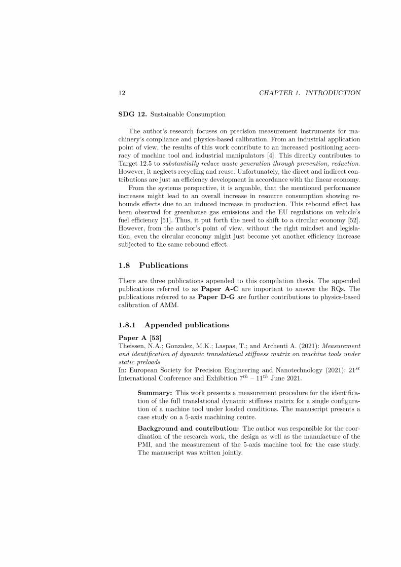
1.8.1 Appended publicationsPaper A [53]Theissen, N.A.; Gonzalez, M.K.; Laspas, T.; and Archenti A. (2021): Measurementand identification of dynamic translational stiffness matrix on machine tools understatic preloadsIn: European Society for Precision Engineering and Nanotechnology (2021): 21st
International Conference and Exhibition 7th – 11th June 2021.
Summary: This work presents a measurement procedure for the identifica-tion of the full translational dynamic stiffness matrix for a single configura-tion of a machine tool under loaded conditions. The manuscript presents acase study on a 5-axis machining centre.Background and contribution: The author was responsible for the coor-dination of the research work, the design as well as the manufacture of thePMI, and the measurement of the 5-axis machine tool for the case study.The manuscript was written jointly.
1.8. PUBLICATIONS 13
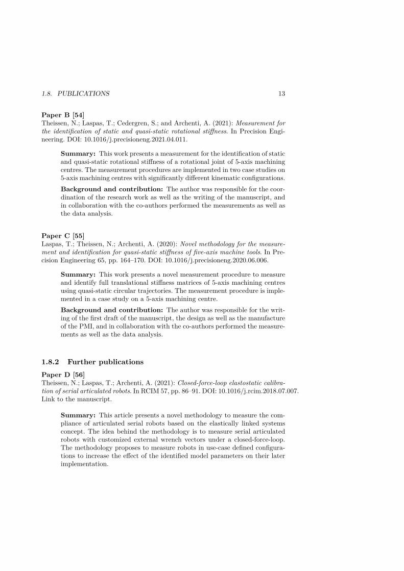
Paper B [54]Theissen, N.; Laspas, T.; Cedergren, S.; and Archenti, A. (2021): Measurement forthe identification of static and quasi-static rotational stiffness. In Precision Engi-neering. DOI: 10.1016/j.precisioneng.2021.04.011.
Summary: This work presents a measurement for the identification of staticand quasi-static rotational stiffness of a rotational joint of 5-axis machiningcentres. The measurement procedures are implemented in two case studies on5-axis machining centres with significantly different kinematic configurations.Background and contribution: The author was responsible for the coor-dination of the research work as well as the writing of the manuscript, andin collaboration with the co-authors performed the measurements as well asthe data analysis.
Paper C [55]Laspas, T.; Theissen, N.; Archenti, A. (2020): Novel methodology for the measure-ment and identification for quasi-static stiffness of five-axis machine tools. In Pre-cision Engineering 65, pp. 164–170. DOI: 10.1016/j.precisioneng.2020.06.006.
Summary: This work presents a novel measurement procedure to measureand identify full translational stiffness matrices of 5-axis machining centresusing quasi-static circular trajectories. The measurement procedure is imple-mented in a case study on a 5-axis machining centre.Background and contribution: The author was responsible for the writ-ing of the first draft of the manuscript, the design as well as the manufactureof the PMI, and in collaboration with the co-authors performed the measure-ments as well as the data analysis.
1.8.2 Further publicationsPaper D [56]Theissen, N.; Laspas, T.; Archenti, A. (2021): Closed-force-loop elastostatic calibra-tion of serial articulated robots. In RCIM 57, pp. 86–91. DOI: 10.1016/j.rcim.2018.07.007.Link to the manuscript.
Summary: This article presents a novel methodology to measure the com-pliance of articulated serial robots based on the elastically linked systemsconcept. The idea behind the methodology is to measure serial articulatedrobots with customized external wrench vectors under a closed-force-loop.The methodology proposes to measure robots in use-case defined configura-tions to increase the effect of the identified model parameters on their laterimplementation.
14 CHAPTER 1. INTRODUCTION
Background and contribution: The author was responsible for the writ-ing of the manuscript, and in collaboration with the co-authors performedthe measurements as well as the data analysis.
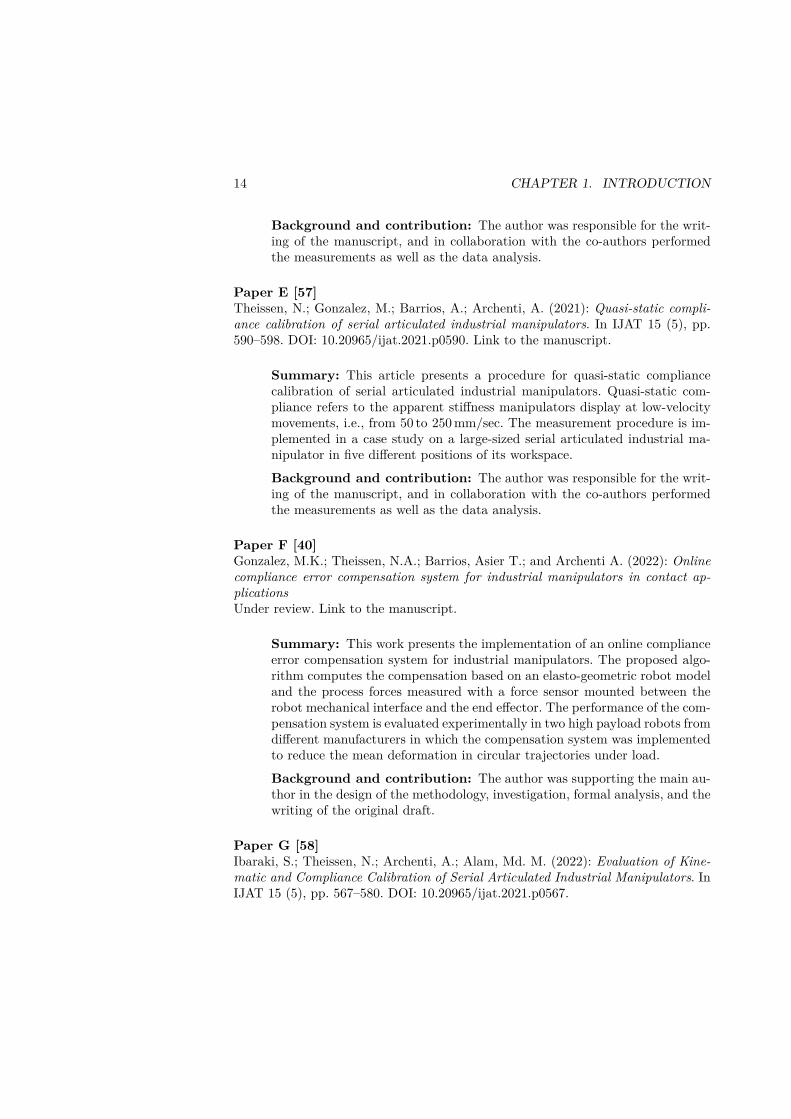
Paper E [57]Theissen, N.; Gonzalez, M.; Barrios, A.; Archenti, A. (2021): Quasi-static compli-ance calibration of serial articulated industrial manipulators. In IJAT 15 (5), pp.590–598. DOI: 10.20965/ijat.2021.p0590. Link to the manuscript.
Summary: This article presents a procedure for quasi-static compliancecalibration of serial articulated industrial manipulators. Quasi-static com-pliance refers to the apparent stiffness manipulators display at low-velocitymovements, i.e., from 50 to 250 mm/sec. The measurement procedure is im-plemented in a case study on a large-sized serial articulated industrial ma-nipulator in five different positions of its workspace.
Background and contribution: The author was responsible for the writ-ing of the manuscript, and in collaboration with the co-authors performedthe measurements as well as the data analysis.
Paper F [40]Gonzalez, M.K.; Theissen, N.A.; Barrios, Asier T.; and Archenti A. (2022): Onlinecompliance error compensation system for industrial manipulators in contact ap-plicationsUnder review. Link to the manuscript.
Summary: This work presents the implementation of an online complianceerror compensation system for industrial manipulators. The proposed algo-rithm computes the compensation based on an elasto-geometric robot modeland the process forces measured with a force sensor mounted between therobot mechanical interface and the end effector. The performance of the com-pensation system is evaluated experimentally in two high payload robots fromdifferent manufacturers in which the compensation system was implementedto reduce the mean deformation in circular trajectories under load.
Background and contribution: The author was supporting the main au-thor in the design of the methodology, investigation, formal analysis, and thewriting of the original draft.
Paper G [58]Ibaraki, S.; Theissen, N.; Archenti, A.; Alam, Md. M. (2022): Evaluation of Kine-matic and Compliance Calibration of Serial Articulated Industrial Manipulators. InIJAT 15 (5), pp. 567–580. DOI: 10.20965/ijat.2021.p0567.

1.8. PUBLICATIONS 15
Summary: This work presents measurement schemes of end effector poses,it outlines kinematic and compliant models of serial articulated industrial ma-nipulators to quantify the positioning accuracy. This paper aims to presentstate-of-the-art technical issues and future research directions for the im-plementation of model-based numerical compensation schemes for industrialrobots.Background and contribution: The author was supporting the main au-thor in the design of the methodology, investigation, formal analysis, and thewriting of the original draft.

Chapter 2
Precision engineering designprinciples
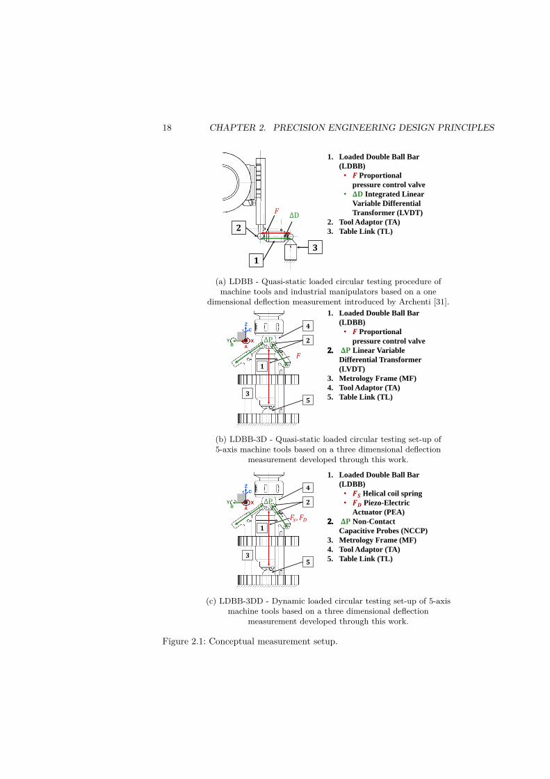
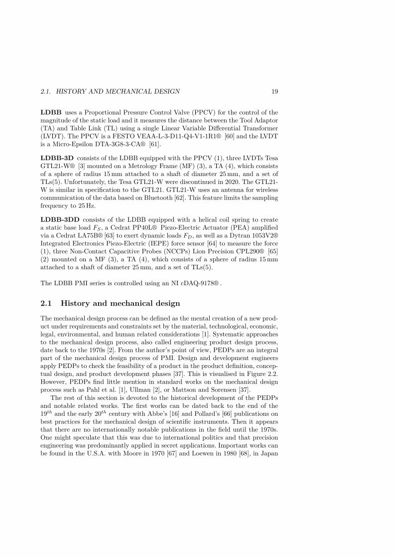
The goal of precision engineering design is to create a [product or] process forwhich the outcomes are deterministic and controllable over a range of operation,with unpredictable deviations from a desired result being as small as is physicallyand economically possible [15]. The deviations from the desired result are definedthrough accuracy and precision. Accuracy is the closeness of agreement betweena measured quantity value and a true quantity value of a measurand. This is alsoreferred to as trueness when considered as a quantitative concept [7, 9]. Precision isthe closeness of agreement between indications or measured quantity values obtainedby replicate measurements on the same or similar objects under specified conditions,also referred to as repeatability [7]. PEDP are established rules or good practicesfor application in the mechanical design process to minimise random and system-atic measurement errors of a PMI and its associated measurement processes [15].This chapter starts with the historical development of PEDP, summarises them,outlines their application, and finishes with a list of uncertainty contributors forthe created LDBB-3D as well as LDBB-3DD. The term LDBB PMI series com-prises the LDBB, LDBB-3D, and LDBB-3DD, see Figure 2.1. The LDBB is usedfor quasi-static loaded circular testing of machine tools and industrial manipulatorsbased on a one dimensional deflection measurement [32]. The LDBB-3D is used forquasi-static loaded circular testing of 5-axis machine tools based on a three di-mensional deflection measurement, as can be seen in Paper B [54] and Paper C[55]. The LDBB-3DD is used for dynamic loaded circular testing of 5-axis machinetools which is also based on a three dimensional deflection measurement, please seePaper A [53]. Both the LDBB-3D and LDBB-3DD were developed as a part ofthis work. All aforementioned PMI are meant to measure the mechanical stiffness ofAMM. The mechanical stiffness of a system can be defined as its capacity to sustainloads, which result in a change of its geometry [59]. The conceptual measurementsetup employed by the LDBB PMI series can be seen in Figure 2.1.
17
18 CHAPTER 2. PRECISION ENGINEERING DESIGN PRINCIPLES
Quasi-static loaded circular
testing of machine tools and
industrial manipulators based
on a one dimensional deflection
measurement
developed by Archenti and
Nicolescu
1. Loaded Double Ball Bar
(LDBB)
• 𝑭 Proportional
pressure control valve
• 𝚫𝐃 Integrated Linear
Variable Differential
Transformer (LVDT)
2. Tool Adaptor (TA)
3. Table Link (TL)
Quasi-static and dynamic
loaded circular testing of 5-axis
machine tools based on a three
dimensional deflection
measurement
developed through this work
1. Loaded Double Ball Bar
(LDBB)
2. Non-Contact Capacitive
Probe (NCCP)
3. Metrology Frame (MF)
4. Tool Adaptor (TA)
5. Table Link (TL)
Y
Z
X
C
AB
ΔD
(a) LDBB - Quasi-static loaded circular testing procedure ofmachine tools and industrial manipulators based on a one
dimensional deflection measurement introduced by Archenti [31].
Quasi-static loaded circular
testing of machine tools and
industrial manipulators based
on a one dimensional deflection
measurement
developed by Archenti and
Nicolescu
1. Loaded Double Ball Bar
(LDBB)
• 𝑭 Proportional
pressure control valve
• 𝚫𝐃 Integrated Linear
Variable Differential
Transformer (LVDT)
2. Tool Adaptor (TA)
3. Table Link (TL)
Quasi-static and dynamic
loaded circular testing of 5-axis
machine tools based on a three
dimensional deflection
measurement
developed through this work
1. Loaded Double Ball Bar
(LDBB)
• 𝑭 Proportional
pressure control valve
2. 𝚫𝐏 Linear Variable
Differential Transformer
(LVDT)
3. Metrology Frame (MF)
4. Tool Adaptor (TA)
5. Table Link (TL)
Y
Z
X
C
AB
ΔD
ΔP
(b) LDBB-3D - Quasi-static loaded circular testing set-up of5-axis machine tools based on a three dimensional deflection
measurement developed through this work.
Quasi-static loaded circular
testing of machine tools and
industrial manipulators based
on a one dimensional deflection
measurement
developed by Archenti and
Nicolescu
1. Loaded Double Ball Bar
(LDBB)
• 𝑭 Proportional
pressure control valve
• 𝚫𝐃 Integrated Linear
Variable Differential
Transformer (LVDT)
2. Tool Adaptor (TA)
3. Table Link (TL)
Quasi-static and dynamic
loaded circular testing of 5-axis
machine tools based on a three
dimensional deflection
measurement
developed through this work
1. Loaded Double Ball Bar
(LDBB)
• 𝑭𝑺 𝐇elical coil spring
• 𝑭𝑫 Piezo-Electric
Actuator (PEA)
2. 𝚫𝐏 Non-Contact
Capacitive Probes (NCCP)
3. Metrology Frame (MF)
4. Tool Adaptor (TA)
5. Table Link (TL)
Y
Z
X
C
AB
𝑠, 𝐷
ΔD
ΔP
(c) LDBB-3DD - Dynamic loaded circular testing set-up of 5-axismachine tools based on a three dimensional deflection
measurement developed through this work.
Figure 2.1: Conceptual measurement setup.
2.1. HISTORY AND MECHANICAL DESIGN 19
LDBB uses a Proportional Pressure Control Valve (PPCV) for the control of themagnitude of the static load and it measures the distance between the Tool Adaptor(TA) and Table Link (TL) using a single Linear Variable Differential Transformer(LVDT). The PPCV is a FESTO VEAA-L-3-D11-Q4-V1-1R1® [60] and the LVDTis a Micro-Epsilon DTA-3G8-3-CA® [61].
LDBB-3D consists of the LDBB equipped with the PPCV (1), three LVDTs TesaGTL21-W® [3] mounted on a Metrology Frame (MF) (3), a TA (4), which consistsof a sphere of radius 15 mm attached to a shaft of diameter 25 mm, and a set ofTLs(5). Unfortunately, the Tesa GTL21-W were discontinued in 2020. The GTL21-W is similar in specification to the GTL21. GTL21-W uses an antenna for wirelesscommunication of the data based on Bluetooth [62]. This feature limits the samplingfrequency to 25 Hz.
LDBB-3DD consists of the LDBB equipped with a helical coil spring to createa static base load FS , a Cedrat PP40L® Piezo-Electric Actuator (PEA) amplifiedvia a Cedrat LA75B® [63] to exert dynamic loads FD, as well as a Dytran 1053V2®Integrated Electronics Piezo-Electric (IEPE) force sensor [64] to measure the force(1), three Non-Contact Capacitive Probes (NCCPs) Lion Precision CPL290® [65](2) mounted on a MF (3), a TA (4), which consists of a sphere of radius 15 mmattached to a shaft of diameter 25 mm, and a set of TLs(5).
The LDBB PMI series is controlled using an NI cDAQ-9178® .
2.1 History and mechanical design
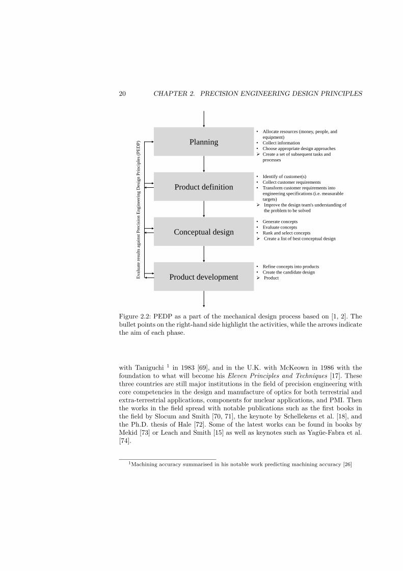
The mechanical design process can be defined as the mental creation of a new prod-uct under requirements and constraints set by the material, technological, economic,legal, environmental, and human related considerations [1]. Systematic approachesto the mechanical design process, also called engineering product design process,date back to the 1970s [2]. From the author’s point of view, PEDPs are an integralpart of the mechanical design process of PMI. Design and development engineersapply PEDPs to check the feasibility of a product in the product definition, concep-tual design, and product development phases [37]. This is visualised in Figure 2.2.However, PEDPs find little mention in standard works on the mechanical designprocess such as Pahl et al. [1], Ullman [2], or Mattson and Sorensen [37].
The rest of this section is devoted to the historical development of the PEDPsand notable related works. The first works can be dated back to the end of the19th and the early 20th century with Abbe’s [16] and Pollard’s [66] publications onbest practices for the mechanical design of scientific instruments. Then it appearsthat there are no internationally notable publications in the field until the 1970s.One might speculate that this was due to international politics and that precisionengineering was predominantly applied in secret applications. Important works canbe found in the U.S.A. with Moore in 1970 [67] and Loewen in 1980 [68], in Japan
20 CHAPTER 2. PRECISION ENGINEERING DESIGN PRINCIPLES
Planning
• Allocate resources (money, people, and
equipment)
• Collect information
• Choose appropriate design approaches
➢ Create a set of subsequent tasks and
processes
Product definition
Conceptual design
Product developmentEv
alu
ate
resu
lts
agai
nst
Pre
cisi
on
En
gin
eeri
ng
Des
ign
Pri
nci
ple
s (P
ED
P)
• Identify of customer(s)
• Collect customer requirements
• Transform customer requirements into
engineering specifications (i.e. measurable
targets)
➢ Improve the design team's understanding of
the problem to be solved
• Generate concepts
• Evaluate concepts
• Rank and select concepts
➢ Create a list of best conceptual design
• Refine concepts into products
• Create the candidate design
➢ Product
Figure 2.2: PEDP as a part of the mechanical design process based on [1, 2]. Thebullet points on the right-hand side highlight the activities, while the arrows indicatethe aim of each phase.
with Taniguchi 1 in 1983 [69], and in the U.K. with McKeown in 1986 with thefoundation to what will become his Eleven Principles and Techniques [17]. Thesethree countries are still major institutions in the field of precision engineering withcore competencies in the design and manufacture of optics for both terrestrial andextra-terrestrial applications, components for nuclear applications, and PMI. Thenthe works in the field spread with notable publications such as the first books inthe field by Slocum and Smith [70, 71], the keynote by Schellekens et al. [18], andthe Ph.D. thesis of Hale [72]. Some of the latest works can be found in books byMekid [73] or Leach and Smith [15] as well as keynotes such as Yagüe-Fabra et al.[74].
1Machining accuracy summarised in his notable work predicting machining accuracy [26]
2.2. STRUCTURE 21
Z X
Y
(a) MF top view.
Z
XY
𝟏75
(b) MF side view and section view.
Figure 2.3: Conceptual MF of the LDBB-3D and LDBB-3DD.
2.2 Structure
Mechanical structures position and orient their components, and they change theseposes under forces and moments as a result of their change in geometry [75]. Themost important mechanical properties of structures are the geometry and the ma-terial.
In general, symmetry facilitates the design (simplified and reduced models),manufacture (repetitive features and programming), as well as operation (system-atic behaviour). Hence, symmetry must be included to the maximum extent inthe component, system, and system environment. The selection of an asymmetricdesign should be carefully assessed [72].
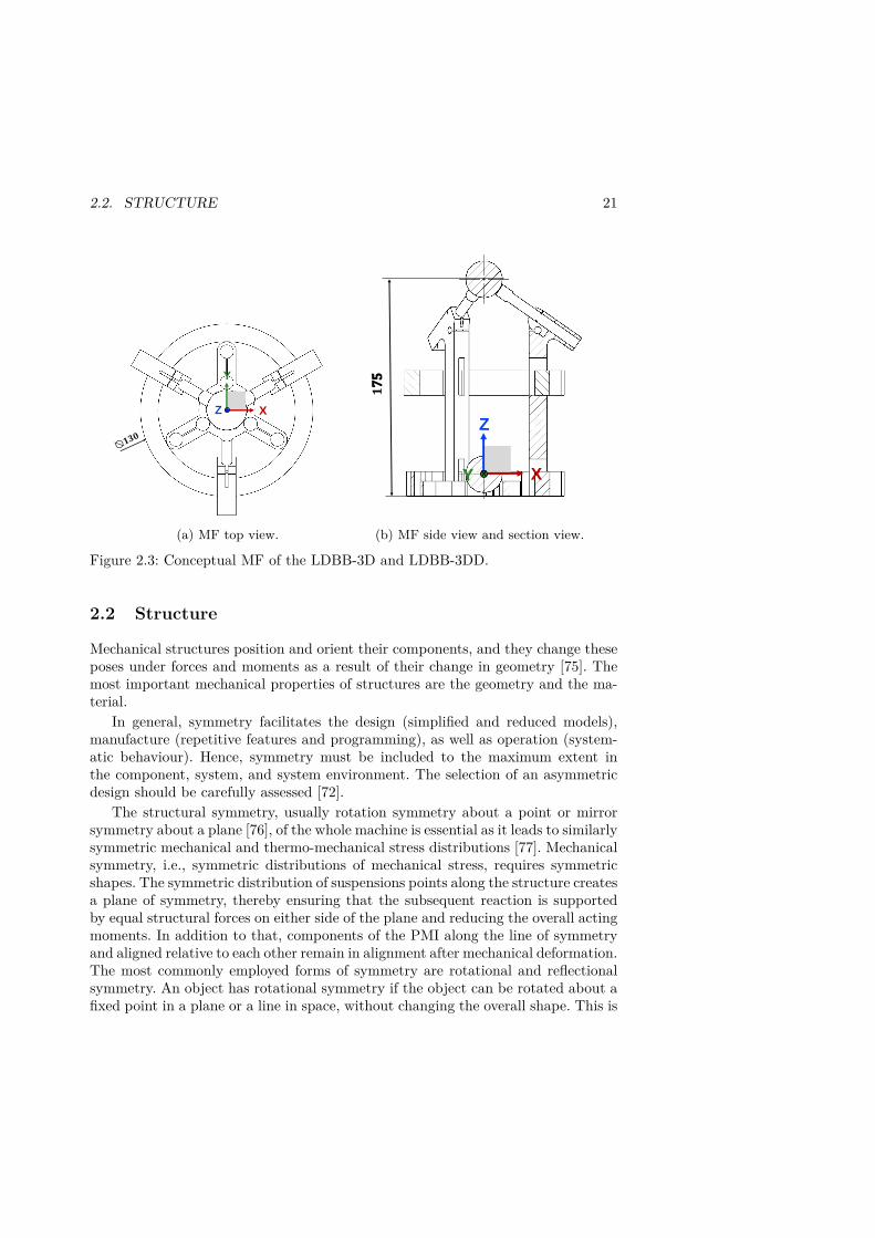
The structural symmetry, usually rotation symmetry about a point or mirrorsymmetry about a plane [76], of the whole machine is essential as it leads to similarlysymmetric mechanical and thermo-mechanical stress distributions [77]. Mechanicalsymmetry, i.e., symmetric distributions of mechanical stress, requires symmetricshapes. The symmetric distribution of suspensions points along the structure createsa plane of symmetry, thereby ensuring that the subsequent reaction is supportedby equal structural forces on either side of the plane and reducing the overall actingmoments. In addition to that, components of the PMI along the line of symmetryand aligned relative to each other remain in alignment after mechanical deformation.The most commonly employed forms of symmetry are rotational and reflectionalsymmetry. An object has rotational symmetry if the object can be rotated about afixed point in a plane or a line in space, without changing the overall shape. This is
22 CHAPTER 2. PRECISION ENGINEERING DESIGN PRINCIPLES
visualised in Figure 2.3a for the MF of the LDBB-3D and LDBB-3DD. An objecthas reflectional symmetry, also referred to as line or mirror symmetry, if there is aline in a plane or a plane in space, which divides it into two pieces that are mirrorimages of each other. This is visualised in Figure 2.3b for one of the three legs of theMF of the LDBB-3D and LDBB-3DD. There exist further forms of basic structuresymmetry such as translational symmetry (moving every point of the object by thesame distance without changing its overall shape), and scale symmetry (expandingor contracting every point of the object by the same amount without changing itsoverall shape), as well as a group of combinational structure symmetry such ashelical symmetry, glide reflection, and roto-reflection [76]. However, these forms ofbasic and combinational structure symmetry are of less importance for mechanicaland thermo-mechanical stress distributions.
Thermo-mechanical symmetry, i.e., symmetric distributions of thermo-mechanicalstress, requires equal time constants on all subsystems of the PMI to create a ho-mogeneous heat and consequently distortion field to avoid thermal bending [78].Important thermo-elastic system properties are thermal inertia, which is the prod-uct of thermal conductivity k and the specific heat capacity cp, which describeshow fast a system transfers heat, as well as the coefficient of thermal expansion α,which describes the geometry change due to temperature [79]. Thermo-mechanicalsymmetry may most likely be achieved as a result of symmetric shapes, as thermalconductivity, specific heat capacity, and the coefficient of thermal expansion arematerial properties. However, this approach is not exclusive. Namely, one can com-bine materials with a positive (aluminium) and negative (Carbon Fibre ReinforcedPlastics (CFRP)) linear expansion coefficient [78]. Furthermore, the designer caninfluence the internal but not the external heat sources. One can reduce the gener-ated heat by replacing components with ones that have higher efficiency rates or byreducing friction through different lubrication. Due to that fact, several PMIs areequipped with external sensors to measure temperature, humidity, and pressure tocompensate or qualify the measurement results.
For the LDBB-3D symmetry is most important for the MF and the TA. TheMF positions and aligns the tips of the Direct Displacement Transducers (DDTs),i.e., LVDTs for the created LDBB-3D, and NCCPs for the created LDBB-3DD, onthe centre of the TA. The uncertainty resulting from the offset to common origincan be reduced selecting angles of 120° in the X-Y plane, i.e., 90° between thesensor axes, and an angle θ of 35° in the X-Z plane, see Figure 2.3b [80]. For this,the offset from the radial probing direction as well as the offset from the spherecentre, i.e., the common origin of the DDTs, are the most critical features [80]. TheLVDTs are equipped with planar steel tips with a diameter D of 10 mm to keepthe Measurement Application Point (MAP) on the same axis under movement anddeflection of the AMM. The term MAP is more commonly referred to as Point ofInterest. For a machine tool, the diameter of the tips could have been significantlylower, e.g., down to 4 mm for most applications.
PMI which employ DDTs, usually employ trilateration or triangulation, cf.Bringmann and Knapp [81]. Trilateration is the process of determining the location
2.2. STRUCTURE 23
Z X
Y𝑃1 𝑃3
𝑃2
𝑅1
𝑅2
𝑅3
𝐷1
𝐷2𝐷3
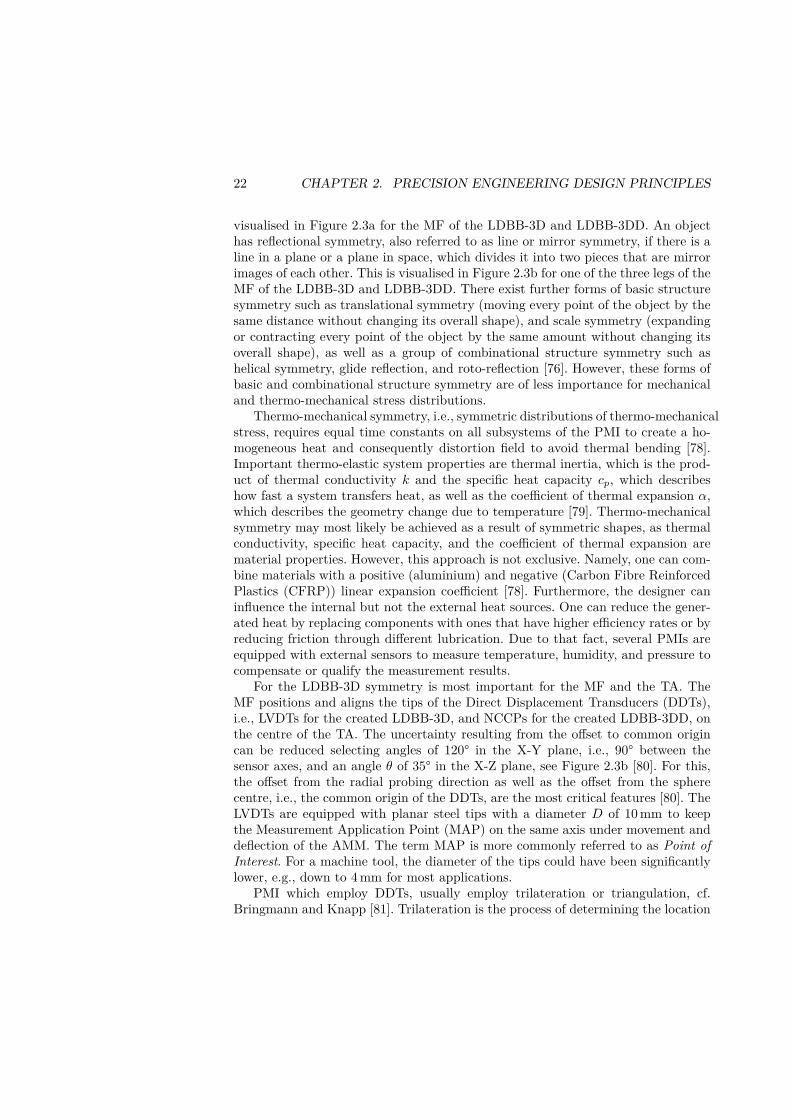
Figure 2.4: Visualisation of trilateration for the MF.
of a measurement point in space from known distances to the suspension points aswell as the position of the suspension points [82]. As implied by the first syllableof these methods, PMI employing these require three or more DDTs. A PMI withthree DDTs yields exactly one unique solution to transform the data from the co-ordination system of the PMI into the MBCS. This concept is visualised in Figure2.4. The circles inscribed by the radii from the suspension points of the individualDDTs intersect in exactly one point, i.e., the origin of the coordinate system. Inthe home configuration the TA should be positioned equally with respect to thesuspension point of the DDTs, i.e., R1 = R2 = R3; once, the AMM starts to moveor deflects due to the induced mechanical loads, the TA starts moving relativelywith respect to P1 = P2 = P3. Nevertheless, there will be exactly one solutionfor the data transformation. Ideally the distances are equal and time-invariant to

24 CHAPTER 2. PRECISION ENGINEERING DESIGN PRINCIPLES
minimise the transformation error.One could also consider using two DDTs, which yields two potential solutions or
using four or more sensors [83]. If the PMI were to employ two sensors, additionalinformation would be required to identify the correct solution. For instance, onecan add indicative features to the movement employed for the identification of theMBCS, see more in Section 3.1. If the PMI were to employ more sensors than three,the results might be similar while the investment costs and operational complexitywould increase [80].
The TA features a sphere with invariant radius of 30 mm. According to DIN5401 [84], which is connected to ISO 3290-1:2014, spheres of that radius can beproduced up to grade G20, i.e., with a tolerance in diameter of ± 11.5 µm, alterna-tively the American Bearing Manufacturers Association (ABMA) standard definestolerances of ± 12.5 µm for a corresponding grade G25 sphere. The LDBB PMIseries features steel balls for general industrial use. Thus, it needs to be assumedthat each measurement contains an error component that is attributable to theimperfect shape of the sphere. It is possible to manufacture spheres according tomuch tighter tolerance on their roundness, e.g., the IBS Spindle Error Analyzer®features spheres with a roundness of less than ±25 nm [85]. The employment ofsuch spheres can reduce the complexity in understanding the measurement data aswell as the time required to perform a measurement. Alternatively, one needs toemploy error separation methods such as the Ball Reversal Method to quantify thecontribution of the sphericity on the measurand, see Section 3 [86].
The MF for the LDBB-3D and LDBB-3DD is made from the same material andfeatures similar sizes on all components to achieve equal time constants, while atthe same time all measurements are meant to be supported with external sensorsto qualify the measurement results. Material selection is a decisive factor in thesuccessful design, manufacture, and operation of PMI. For the LDBB PMI seriesthe components are made from tool steel Toolox 33® [87].
2.3 Abbe principle
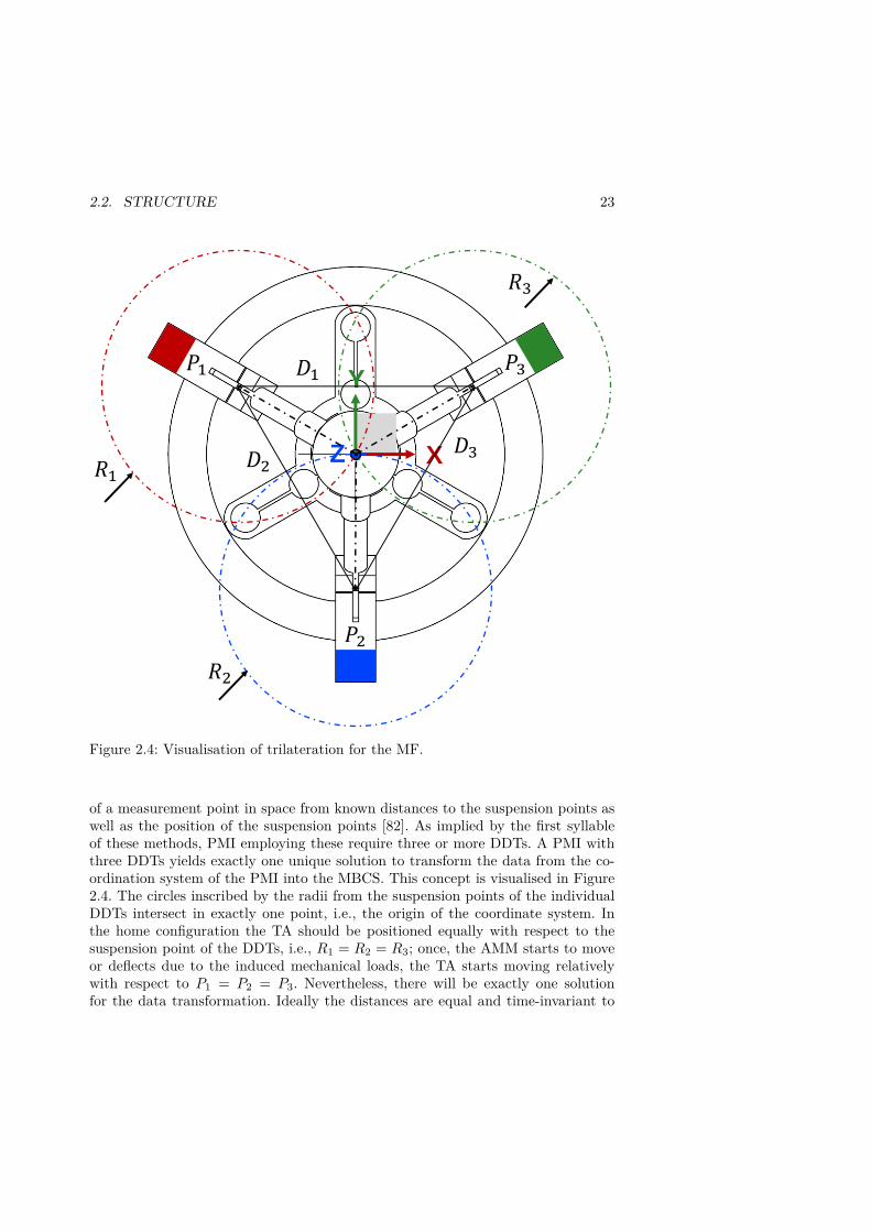
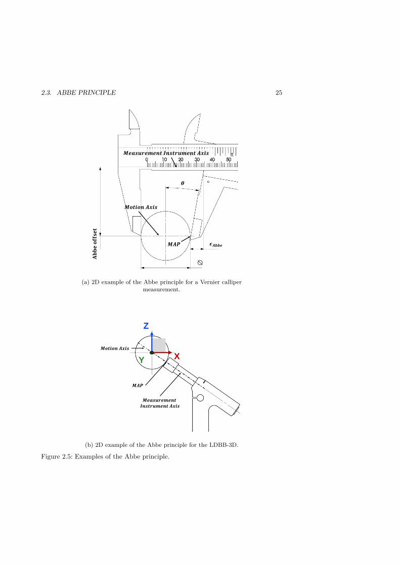
The Abbe alignment principle states that "when measuring the displacement of aspecified point [MAP], it is not sufficient to have the axis of the probe [Measure-ment Instrument Axis] parallel to the direction of motion [Motion Axis], the axisshould also be aligned with (pass-through) the point" [16]. One could argue that if themoving body were error free then there would be no Abbe error. However, thereare always motion errors and the Abbe error is proportional to the Abbe offset.This is visualised in Figure 2.5a for the measurement of a circular workpiece witha Vernier calliper and Figure 2.5b for a measurement with the LDBB-3D. In thelatter example, the Abbe offset and error still exist. However, they are significantlyreduced as the line of motion of the sensing head and the measurement instrumentaxis are significantly more collinear than in the Vernier calliper example. Further-more, Figure 2.5a only shows a two dimensional example, but in Cartesian space
2.3. ABBE PRINCIPLE 25
𝑴𝑨𝑷
𝑴𝒆𝒂𝒔𝒖𝒓𝒆𝒎𝒆𝒏𝒕 𝑰𝒏𝒔𝒕𝒓𝒖𝒎𝒆𝒏𝒕 𝑨𝒙𝒊𝒔
𝑴𝒐𝒕𝒊𝒐𝒏 𝑨𝒙𝒊𝒔
𝝐𝑨𝒃𝒃𝒆
𝐀𝐛𝐛𝐞𝐨𝐟𝐟𝐬𝐞𝐭
⦰
(a) 2D example of the Abbe principle for a Vernier callipermeasurement.
Z
XY
𝑴𝑨𝑷
𝑴𝒐𝒕𝒊𝒐𝒏 𝑨𝒙𝒊𝒔
𝑴𝒆𝒂𝒔𝒖𝒓𝒆𝒎𝒆𝒏𝒕𝑰𝒏𝒔𝒕𝒓𝒖𝒎𝒆𝒏𝒕 𝑨𝒙𝒊𝒔
(b) 2D example of the Abbe principle for the LDBB-3D.
Figure 2.5: Examples of the Abbe principle.
26 CHAPTER 2. PRECISION ENGINEERING DESIGN PRINCIPLES
all directions are affected.For practical reasons, sensors are often positioned at different locations on the
AMM rather than in the line of interest. This difference in location between the axisof interest and measurement results in Abbe errors that can be significant sources ofuncertainty [88]. A typical example within machine tools is the squareness betweenmachine tool axes [89]. The magnitude of alignment errors between assemblies canbe eliminated using monolithic designs or minimised using kinematic couplings [90].
2.4 Kinematic and quasi-kinematic design
The alignment of components needs to be considered in the design phase, as themanufacturing and assembly tolerances may require design changes to comply withGDT. Manufacturing tolerances depend mainly on the manufacturing technologies,while the assembly tolerances depend primarily on the design of the components[91].
The most critical misalignments errors arise from imperfect configurations, i.e.,the angular difference by which the actual topology of the assembly deviates fromthe nominal topology, as well as imperfect geometries, i.e., the translational dif-ference by which the actual topology of the assembly deviates from the nominaltopology [13]. The monolithic design aims at merging individual components orassemblies into a single manufactured part with all the required functionality ofthe original [15]. Alternatively, precision couplings, which are accurate and repeat-able structural connections or fixtures, can be introduced at the mating surfaces[92]. Precision couplings are grouped according to their governing mechanics intokinematic, quasi-kinematic, and elastic averaging [93].
Kinematic couplings need to exactly fully constrain the components to maintaina stress-free condition and high positioning repeatability. At the same time, wearmust not introduce play between mating components, and the temperature gra-dients across mating components shall not impose part stresses [75]. Each degreeof freedom is constrained with a point contact. As a consequence, the coupling isnot over-constrained [94]; thus, the system provides a high positioning repeatabil-ity [70]. The governing equations of the resulting holonomic system are of a closedmathematical form, i.e., analytical expressions are available [95]. The principal dis-advantages of kinematic couplings are the sag of the body as well as potentiallyhigh stresses in the contact areas [15]. Both originate from static deflections of thecomponents mainly due to their weight. That may result in poor performance. Thesagging of simple geometric shapes such as gauge blocks is addressed through theselection of adequate Airy or Bessel support points [96]. However, these consideronly simple beam theory instead of plane stress theory and are inapplicable formost precision systems [97]. The high contact forces in the support points maylead to local deformations such that the point contacts become Hertzian contactellipses, consequently decreasing the positioning repeatability as the points contactsare transformed into line contacts.
2.4. KINEMATIC AND QUASI-KINEMATIC DESIGN 27
Z X
Y
Z
X
Y
Z
XY
Figure 2.6: Visualisation of the kinematic constraints of the TL. The point con-straints are highlighted in orange.
When this is the case, couplings based on quasi-kinematics and elastic averagingcan be considered. Quasi-kinematic, also called pseudo-kinematic, couplings aredesigns with convex and grooved mates resulting in line type contacts. This isvisualised in Figures 2.6 and 2.7. Although these designs are over-constrained, theyare nearly kinematic, and they ensure uniform thermo-mechanical deformations[93]. They are less expensive to manufacture than kinematic couplings and allow forslightly higher precision also at a larger scale [93]. The principle of elastic averagingfollows from the requirement of mating surfaces with capacities to carry higherloads and exhibit higher contact stiffness [70]. The line or area type connectionslead to a distribution of the contact pressure on more than the ideally requiredcontact points, which forces geometric congruences and is over-constrained [93].
For the LDBB-3D quasi-kinematic design is most important for the assembly ofthe MF and the positioning of the TL. The design is intended to create a repeat-able repositioning of the components, which contributes to deterministic systembehaviour, ergo it reduces random setup errors. The most important mating sur-faces of the TL exist between its centring ring, the sphere, and the table of themachine tool. The centring ring features a variation of the three V-shaped grooveskinematic coupling [70]. This is also called a Maxwell kinematic coupling [98]. Usu-ally, the three V-shaped grooves are oriented towards the centre of the part, in thiscase, they are orientated tangentially with respect to the surface of the sphere. Eachof the three v-grooves provides two contact points for a total of six kinematic con-straints in the plane, see Figure 2.6. Thus, it could be considered a quasi-kinematiccoupling. The standard Maxwell coupling is thermally stable due to its symmetryas the curved surfaces can expand or contract in unison in the V-grooves; this is

28 CHAPTER 2. PRECISION ENGINEERING DESIGN PRINCIPLES
𝐷𝑒𝑡𝑎𝑖𝑙 𝐴5: 1
Z X
Y
𝐴
Z
X
Y
Figure 2.7: Visualisation of the kinematic constraints of the MF. The point, line,and planar constraints are highlighted in orange, green, and red.
not the case for the centring ring. The centring ring constrains the movement ofthe sphere in the X-Y plane, while the force loop between the machine tool tableand the LDBB constrain the motion along the Z-axis, see Figure 2.6 and 2.9.
The mating surfaces of the MF exist between its legs as well as the upperand lower centring rings. The legs X- and Y-axis positions are centred by two V-shaped grooves which mate with two line contacts with the lower centring ring, seeFigure 2.7 left-hand side green; and the Z-axis position is constrained by a planarcontact, see Figure 2.7 left-hand side red. The rotations around the Z-axis axis areconstrained by two point contacts on the inner circumference, see Figure 2.7 left-hand side yellow. The upper centring features wedges to impose two additional linecontacts which are intended to minimise the influence of orientation errors closerto the measurement point, see Figure 2.7 right-hand green.
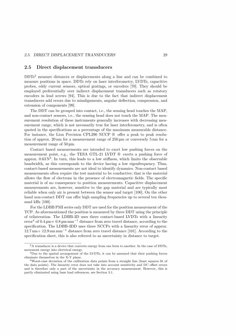
2.5. DIRECT DISPLACEMENT TRANSDUCERS 29
2.5 Direct displacement transducers
DDTs2 measure distances or displacements along a line and can be combined tomeasure positions in space. DDTs rely on laser interferometry, LVDTs, capacitiveprobes, eddy current sensors, optical gratings, or encoders [70]. They should beemployed preferentially over indirect displacement transducers such as rotatoryencoders in lead screws [94]. This is due to the fact that indirect displacementtransducers add errors due to misalignments, angular deflection, compression, andextension of components [99].
The DDT can be grouped into contact, i.e., the sensing head touches the MAP,and non-contact sensors, i.e., the sensing head does not touch the MAP. The mea-surement resolution of these instruments generally increases with decreasing mea-surement range, which is not necessarily true for laser interferometry, and is oftenquoted in the specifications as a percentage of the maximum measurable distance.For instance, the Lion Precision CPL290 NCCP ® offer a peak to peak resolu-tion of approx. 20 nm for a measurement range of 250 µm or conversely 5 nm for ameasurement range of 50 µm.
Contact based measurements are intended to exert low pushing forces on themeasurement point, e.g., the TESA GTL-21 LVDT ® exerts a pushing force ofapprox. 0.63 N3. In turn, this leads to a low stiffness, which limits the observablebandwidth, as this corresponds to the device having a low eigenfrequency. Thus,contact-based measurements are not ideal to identify dynamics. Non-contact basedmeasurements often require the test material to be conductive; that is the materialallows the flow of electrons in the presence of electromagnetic fields. The specificmaterial is of no consequence to position measurements. Capacitive displacementmeasurements are, however, sensitive to the gap material and are typically mostreliable when only air is present between the sensor and target [100]. On the otherhand non-contact DDT can offer high sampling frequencies up to several ten thou-sand kHz [100].
For the LDBB PMI series only DDT are used for the position measurement of theTCP. As aforementioned the position is measured by three DDT using the principleof trilateration. The LDBB-3D uses three contact-based LVDTs with a linearityerror4 of 0.4 µm+ 0.8 µm mm−1 distance from zero travel distance, according to thespecification. The LDBB-3DD uses three NCCPs with a linearity error of approx.12.7 nm+ 12.9 nm mm−1 distance from zero travel distance [101]. According to thespecification sheet, this is also referred to as uncertainty in distance to target.
2A transducer is a device that converts energy from one form to another. In the case of DDTs,movement energy into electrical energy.
3Due to the spatial arrangement of the LVDTs, it can be assumed that their pushing forceseliminate themselves in the X-Y plane.
4Worst-case deviation of the calibration data points from a straight line (least squares fit ofthe data points). The linearity error does not take into account sensitivity and DC offset errorsand is therefore only a part of the uncertainty in the accuracy measurement. However, this ispartly eliminated using base load references, see Section 3.1.

30 CHAPTER 2. PRECISION ENGINEERING DESIGN PRINCIPLES
Y
Z
X
C
AB
Figure 2.8: The metrology and force loop of the LDBB-3D.
The measurement range also limits the applications, as for the LVDTs at 2 mmand the NCCPs at 0.25 mm are sufficient to measure a machine tool under move-ment. However, to perform the same measurement with the NCCPs at 0.05 mmmeasurement range is not possible, as this range will probably be exceeded by thecombined kinematic and compliance deviations.
2.6 Metrology frames
The components and assemblies within a PMI form force and thermal loops aswell as the metrology loop, these are also called frames [18]. The force and thermalloop contain all components which are in the flow of mechanical and thermal loads.The metrology loops contain all components required to perform measurements.An alternative definition is given as "the metrology loop is a structural loop of allelements from the end effector to the workpiece for which dimensional changes wouldnot be detected by the measurement process" [15]. These loops should be separatedfrom one and another so that the metrology frame can maintain a precise spatialrelationship also under operational conditions over time. Measurement errors can be

2.7. BEARINGS 31
minimised by maintaining a rigid metrology loop. Furthermore, the effect of forcesand heat on the force and thermal loop must be minimised. One approach to realisethis is the application of symmetry, and another is error compensation, see Section2.11. These can be applied jointly. This idea can be visualised for the LDBB-3Dand LDBB-3DD at hand of Figure 2.8. The mechanical stiffness of machine toolsis commonly modelled as two elastically coupled rigid bodies in terms of the TCPand the workpiece [102]. This means that both the force and the deflection needto express the relative movement between the TCP and the workpiece but shallnot deform itself by inducing those loads. Thus, the LDBB-3D and LDBB-3DDinduce loads directly between the TCP and the machine tool table, see Figure 2.8.In Figure 2.8 the force loop is highlighted in blue. The metrology loops must beisolated from these loads. Thus, the MF is mounted rigidly on the machine tooltable, but not in the flow of forces. In Figure 2.8 the metrology loop is highlightedin green.
The LDBB and LDBB-3D induce loads by controlling the pressure in the cham-ber using a PPCV. The proportional valve and its measurement systems are notaffected by this static load, as the load is not exerted on them. In the case of theLDBB-3DD, this is different as the force measurement is performed as close as pos-sible to the TCP. The force sensor inside the LDBB-3DD is mounted between theTCP on the one and the PEA and the helical coil spring on the other, see Figure2.9. Alternatively, one could consider mounting the force sensor on the machinetool. However, these solutions have been disregarded as no feasible solution couldbe found without compromising the stiffness of the AMM.
One further consideration could be the influence of electromagnetic fields, whichliterature has suggested that this influence can be considered negligible for com-pliance measurements of AMM [103], and vibrations. Vibration isolation is theconcept of minimising adverse effects on the performance of the PMI by reduc-ing the transfer of internal and external vibrations to and among the componentsof the system. One needs to analyse vibration transmissibility, for long-durationvibrations and short-duration shocks, from mechanics and acoustics to select anddimension passive and or active isolation techniques.
2.7 Bearings
The mechanical system of a PMI consists of components and assemblies of individ-ual bodies or links (e.g., housings, suspensions systems, axes of movement) whichare coupled by joints (e.g., springs, dampers, gears, bearings, motors) [104]. Jointsconnect to either two or more adjacent links, in which cases these structures canbe considered Serial Kinematic Mechanism/Machines (SKMs) [105] or PKMs [106].Joints enable relative translational and rotational movement in either one or severalspatial Degree of Freedom (DOF). The most common joints have a single DOF andcan thusly be classified as either prismatic or revolute joints:
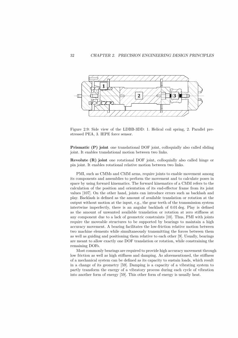
32 CHAPTER 2. PRECISION ENGINEERING DESIGN PRINCIPLES
𝟐 𝟑
𝟏
Figure 2.9: Side view of the LDBB-3DD: 1. Helical coil spring, 2. Parallel pre-stressed PEA, 3. IEPE force sensor.
Prismatic (P) joint one translational DOF joint, colloquially also called slidingjoint. It enables translational motion between two links.
Revolute (R) joint one rotational DOF joint, colloquially also called hinge orpin joint. It enables rotational relative motion between two links.
PMI, such as CMMs and CMM arms, require joints to enable movement amongits components and assemblies to perform the movement and to calculate poses inspace by using forward kinematics. The forward kinematics of a CMM refers to thecalculation of the position and orientation of its end-effector frame from its jointvalues [107]. On the other hand, joints can introduce errors such as backlash andplay. Backlash is defined as the amount of available translation or rotation at theoutput without motion at the input, e.g., the gear teeth of the transmission systemintertwine imperfectly, there is an angular backlash of 0.01 deg. Play is definedas the amount of unwanted available translation or rotation at zero stiffness atany component due to a lack of geometric constraints [10]. Thus, PMI with jointsrequire the moveable structures to be supported by bearings to maintain a highaccuracy movement. A bearing facilitates the low-friction relative motion betweentwo machine elements while simultaneously transmitting the forces between themas well as guiding and positioning them relative to each other [9]. Usually, bearingsare meant to allow exactly one DOF translation or rotation, while constraining theremaining DOFs.
Most commonly bearings are required to provide high accuracy movement throughlow friction as well as high stiffness and damping. As aforementioned, the stiffnessof a mechanical system can be defined as its capacity to sustain loads, which resultin a change of its geometry [59]. Damping is a capacity of a vibrating system topartly transform the energy of a vibratory process during each cycle of vibrationinto another form of energy [59]. This other form of energy is usually heat.
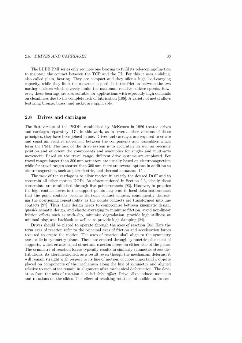
2.8. DRIVES AND CARRIAGES 33
The LDBB PMI series only requires one bearing to fulfil its telescoping-functionto maintain the contact between the TCP and the TL. For this it uses a sliding,also called plain, bearing. They are compact and they offer a high load-carryingcapacity, while they limit the movement speed. It is the friction between the twomating surfaces which severely limits the maximum relative surface speeds. How-ever, these bearings are also suitable for applications with especially high demandson cleanliness due to the complete lack of lubrication [108]. A variety of metal alloysfeaturing bronze, brass, and nickel are applicable.
2.8 Drives and carriages
The first version of the PEDPs established by McKeown in 1986 treated drivesand carriages separately [17]. In this work, as in several other versions of thoseprinciples, they have been joined in one. Drives and carriages are required to createand constrain relative movement between the components and assemblies whichform the PMI. The task of the drive system is to accurately as well as preciselyposition and or orient the components and assemblies for single- and multi-axismovement. Based on the travel range, different drive systems are employed. Fortravel ranges longer than 300 mm actuators are usually based on electromagnetismwhile for travel ranges shorter than 300 mm there are several options in addition toelectromagnetism, such as piezoelectric, and thermal actuators [15].
The task of the carriage is to allow motion in exactly the desired DOF and toconstrain all other motion DOFs. As aforementioned in Section 2.3, ideally thoseconstraints are established through five point-contacts [93]. However, in practicethe high contact forces in the support points may lead to local deformations suchthat the point contacts become Hertzian contact ellipses, consequently decreas-ing the positioning repeatability as the points contacts are transformed into linecontacts [97]. Thus, their design needs to compromise between kinematic design,quasi-kinematic design, and elastic averaging to minimise friction, avoid non-linearfriction effects such as stick-slip, minimise degradation, provide high stiffness atminimal play, and backlash as well as to provide high damping [24].
Drives should be placed to operate through the axes of reaction [94]. Here theterm axes of reaction refer to the principal axes of friction and acceleration forcesrequired to create the motion. The axes of reaction shall align to the symmetryaxes or lie in symmetry planes. These are created through symmetric placement ofsupports, which creates equal structural reaction forces on either side of the plane.The symmetry of reaction forces typically results in similarly symmetric stress dis-tributions. As aforementioned, as a result, even though the mechanism deforms, itwill remain straight with respect to its line of motion; or more importantly, objectsplaced on components of the mechanism along the line of symmetry and alignedrelative to each other remain in alignment after mechanical deformation. The devi-ation from the axis of reaction is called drive offset. Drive offset induces momentsand rotations on the slides. The effect of resulting rotations of a slide on its con-

34 CHAPTER 2. PRECISION ENGINEERING DESIGN PRINCIPLES
trollability is minimised, if both the drive- and measurement-axis are at the sameside of the centre of rotation [109].
For PMIs it may be necessary to fine adjust the motion also through non-influencing couplings and clamps [17]. The fine adjustment usually relies on thepositioning of a component using a screw mechanism, or positioning using an ex-ternal means followed by clamping. Also, non-influencing couplings should be usedin linear and rotary drives to avoid over-constraining and to provide maximumsmoothness of motion.
In precision systems, frictionless guiding systems are commonly preferred, suchas flexures, air bearings, and magnetic levitation. The absence of friction betweenmechanical components present benefits such as infinite resolution, high accuracy,repeatability, speed, lack of wear, and no use of lubricants. Flexure systems arealso used when the connection between elements involves decoupling or isolationfrom dimensional changes of the supports. Pneumatic (air bearings) and magneticlevitation consist of creating vertical forces that counteract the weight of the part.This vertical force can be controlled to attenuate frame vibrations and increasestiffness. The correct application of those principles facilitates the creation of nano-positioning systems, which are essential in many areas including high-precisionmachining, scanning probe microscopes, nano-manipulation, and photolithography[110].
For the LDBB PMI series no drives or carriages are employed.
2.9 Thermal effects
For several decades, it has been argued that thermal effects in PMIs can have asignificant contribution to the system’s accuracy [111]. Thermal effects in PMIs canlead to random changes in the system’s kinematics; excessive temperature changesmay also affect its statics and dynamics. Thus, thermal effects need to be eliminated,minimised, stabilised against, or compensated for [78].
Thermal effects and their influence on the PMI, also called thermo-elasticity[79], are complex fields of study. There are two key aspects of thermal effects forthe design of PMI [15]. The first is that temperature gradients cause expansion ofmaterials and can lead to distortions and strains not accounted for in the design.The second key aspect is that thermo-elasticity is complex due to time horizons ofdays rather than hours to measure a steady-state response [112], the difficulty toimplement sensors effectively to obtain robust measurements, the non-linearity ofmathematical models as well as the numerous sources which can cause the changein the heat field [113]. The sources are differentiated into system internal and ex-ternal, as illustrated in Figure 2.10. Internal sources are only present during theoperation of the machine. Namely, thermal power loss and active cooling systems.External sources are the factory environmental temperature on the macro scale aswell as temperature fluxes due to open factory gates on the mesoscale. These change
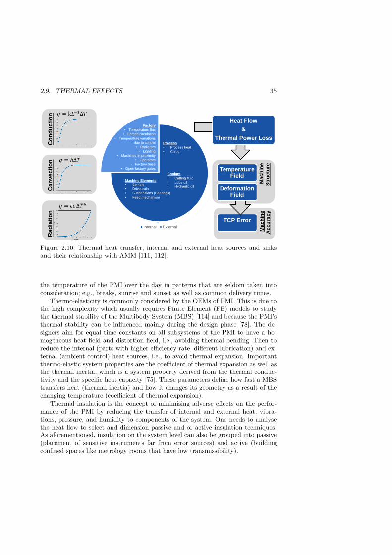
2.9. THERMAL EFFECTS 35
Ma
ch
ine
Ac
cu
rac
y
Ma
ch
ine
Str
uc
ture
TemperatureField
TCP Error
Machine Elements
• Spindle
• Drive train
• Suspensions (Bearings)
• Feed mechanism
Coolant
• Cutting fluid
• Lube oil
• Hydraulic oil
Process
• Process heat
• Chips
Factory
• Temperature flux
• Forced circulation
• Temperature variations
due to control
• Radiators
• Lighting
• Machines in proximity
• Operators
• Factory base
• Open factory gates
Internal External
Co
nve
cti
on 𝑞 = ℎΔ𝑇
Rad
iati
on
𝑞 = 𝜖𝜎Δ𝑇4
Co
nd
uc
tio
n 𝑞 = k𝐿−1Δ𝑇Heat Flow
&
Thermal Power Loss
Deformation Field
Figure 2.10: Thermal heat transfer, internal and external heat sources and sinksand their relationship with AMM [111, 112].
the temperature of the PMI over the day in patterns that are seldom taken intoconsideration; e.g., breaks, sunrise and sunset as well as common delivery times.
Thermo-elasticity is commonly considered by the OEMs of PMI. This is due tothe high complexity which usually requires Finite Element (FE) models to studythe thermal stability of the Multibody System (MBS) [114] and because the PMI’sthermal stability can be influenced mainly during the design phase [78]. The de-signers aim for equal time constants on all subsystems of the PMI to have a ho-mogeneous heat field and distortion field, i.e., avoiding thermal bending. Then toreduce the internal (parts with higher efficiency rate, different lubrication) and ex-ternal (ambient control) heat sources, i.e., to avoid thermal expansion. Importantthermo-elastic system properties are the coefficient of thermal expansion as well asthe thermal inertia, which is a system property derived from the thermal conduc-tivity and the specific heat capacity [75]. These parameters define how fast a MBStransfers heat (thermal inertia) and how it changes its geometry as a result of thechanging temperature (coefficient of thermal expansion).
Thermal insulation is the concept of minimising adverse effects on the perfor-mance of the PMI by reducing the transfer of internal and external heat, vibra-tions, pressure, and humidity to components of the system. One needs to analysethe heat flow to select and dimension passive and or active insulation techniques.As aforementioned, insulation on the system level can also be grouped into passive(placement of sensitive instruments far from error sources) and active (buildingconfined spaces like metrology rooms that have low transmissibility).

36 CHAPTER 2. PRECISION ENGINEERING DESIGN PRINCIPLES
20.01°𝐶
20.02°𝐶
6µ𝑚
17µ𝑚
Figure 2.11: Steady state heat field due to power loss of the DDTs and a thermo-mechanical deformation due to a temperature increase by by 10 °C.
The goal of passive thermal insulation is to provide a thermally inert or resis-tive path (reduce heat flow) such that the internal temperature is isolated fromthe external temperature. Of course, this insulation has limitations; if the exteriortemperature is kept constant for an infinite length of time, the interior temperaturewill become equal to the exterior temperature. Thus, passive thermal insulation ismost effective when temperature changes are cyclic at high frequencies. Althoughpassive thermal insulation is often adequate and is a cost-effective way to limitthe thermal effects on a precision system, it may, however, not be sufficient withincreased performance requirements, high constant heat loads, or low-frequencythermal fluctuations [111].
Consequently, an active thermal insulation system can be an effective alter-native for providing the ability to isolate a system with increased thermal ratechanges. Active thermal insulation uses methods to either heat up or cool downa system by forcing fluid flow (water cooling, ventilation fan, etc.) and/or usingthermo-electrical systems (electrical heaters, Peltier coolers, etc.). Some companiescan provide temperature control within 0.1 °C for metrology facilities at a consid-erable cost [15]. Such facilities are often maintained at positive pressures with closeattention to the flow into and out of the room.
Then, there is thermo-elastic error compensation [78]. Models of the thermo-
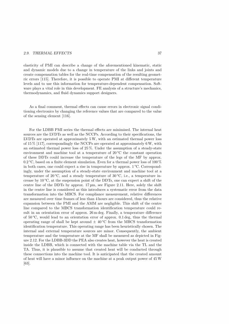
2.9. THERMAL EFFECTS 37
elasticity of PMI can describe a change of the aforementioned kinematic, staticand dynamic models due to a change in temperature of the links and joints andcreate compensation tables for the real-time compensation of the resulting geomet-ric errors [115]. Therefore, it is possible to operate PMI at different temperaturelevels and to use this information for temperature-dependent compensation. Soft-ware plays a vital role in this development. FE analysis of a structure’s mechanics,thermodynamics, and fluid dynamics support designers.
As a final comment, thermal effects can cause errors in electronic signal condi-tioning electronics by changing the reference values that are compared to the valueof the sensing element [116].
For the LDBB PMI series the thermal effects are minimised. The internal heatsources are the LVDTs as well as the NCCPs. According to their specifications, theLVDTs are operated at approximately 5 W, with an estimated thermal power lossof 15 % [117], correspondingly the NCCPs are operated at approximately 6 W, withan estimated thermal power loss of 25 %. Under the assumption of a steady-stateenvironment and machine tool at a temperature of 20 °C the constant operationof these DDTs could increase the temperature of the legs of the MF by approx.0.2 °C, based on a finite element simulation. Even for a thermal power loss of 100 %in both cases, one could expect a rise in temperature by approx. 1 °C. Correspond-ingly, under the assumption of a steady-state environment and machine tool at atemperature of 20 °C, and a steady temperature of 30 °C, i.e., a temperature in-crease by 10 °C, at the suspension point of the DDTs, one can expect a shift of thecentre line of the DDTs by approx. 17 µm, see Figure 2.11. Here, solely the shiftin the centre line is considered as this introduces a systematic error from the datatransformation into the MBCS. For compliance measurement, relative differencesare measured over time frames of less than 4 hours are considered, thus the relativeexpansion between the PMI and the AMM are negligible. This shift of the centreline compared to the MBCS transformation identification temperature could re-sult in an orientation error of approx. 26 m deg. Finally, a temperature differenceof 50 °C, would lead to an orientation error of approx. 0.1 deg, thus the thermaloperating range of shall be kept around ± 40 °C from the MBCS transformationidentification temperature. This operating range has been heuristically chosen. Theinternal and external temperature sources are minor. Consequently, the ambienttemperature and the temperature at the MF shall be measured as depicted in Fig-ure 2.12. For the LDBB-3DD the PEA also creates heat, however the heat is createdinside the LDBB, which is connected with the machine table via the TL and theTA. Thus, it is plausible to assume that created heat will be conducted throughthese connections into the machine tool. It is anticipated that the created amountof heat will have a minor influence on the machine at a peak output power of 45 W[63].
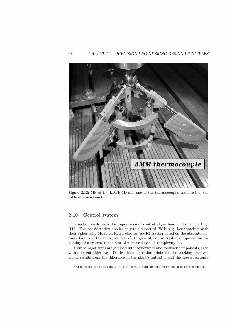
38 CHAPTER 2. PRECISION ENGINEERING DESIGN PRINCIPLES
𝑨𝑴𝑴 𝒕𝒉𝒆𝒓𝒎𝒐𝒄𝒐𝒖𝒑𝒍𝒆
Figure 2.12: MF of the LDBB-3D and one of the thermocouples mounted on thetable of a machine tool.
2.10 Control system
This section deals with the importance of control algorithms for target tracking[118]. This consideration applies only to a subset of PMIs, e.g., laser trackers withtheir Spherically Mounted Retroreflector (SMR) tracing based on the absolute dis-tance laser and the rotary encoders5. In general, control systems improve the ca-pability of a system at the cost of increased system complexity [15].
Control algorithms are grouped into feedforward and feedback components, eachwith different objectives. The feedback algorithm minimises the tracking error eT ,which results from the difference in the plant’s output x and the user’s reference
5Also, image processing algorithms are used for this depending on the laser tracker model.
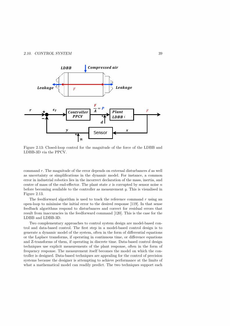
2.10. CONTROL SYSTEM 39
𝑳𝑫𝑩𝑩
𝑳𝑫𝑩𝑩
𝐹
𝑪𝒐𝒎𝒑𝒓𝒆𝒔𝒔𝒆𝒅 𝒂𝒊𝒓
𝑳𝒆𝒂𝒌𝒂𝒈𝒆𝑳𝒆𝒂𝒌𝒂𝒈𝒆
𝐹𝝐𝑻
𝒚
𝒓
𝒅
𝑷𝒍𝒂𝒏𝒕𝑪𝒐𝒏𝒕𝒓𝒐𝒍𝒍𝒆𝒓
𝑭
𝑨= 𝑷
𝑷𝑷𝑪𝑽
𝒏
𝒙
Figure 2.13: Closed-loop control for the magnitude of the force of the LDBB andLDBB-3D via the PPCV.
command r. The magnitude of the error depends on external disturbances d as wellas uncertainty or simplifications in the dynamic model. For instance, a commonerror in industrial robotics lies in the incorrect declaration of the mass, inertia, andcentre of mass of the end-effector. The plant state x is corrupted by sensor noise nbefore becoming available to the controller as measurement y. This is visualised inFigure 2.13.
The feedforward algorithm is used to track the reference command r using anopen-loop to minimise the initial error to the desired response [119]. In that sensefeedback algorithms respond to disturbances and correct for residual errors thatresult from inaccuracies in the feedforward command [120]. This is the case for theLDBB and LDBB-3D.
Two complementary approaches to control system design are model-based con-trol and data-based control. The first step in a model-based control design is togenerate a dynamic model of the system, often in the form of differential equationsor the Laplace transforms, if operating in continuous time, or difference equationsand Z-transforms of them, if operating in discrete time. Data-based control designtechniques use explicit measurements of the plant response, often in the form offrequency response. The measurement itself becomes the model on which the con-troller is designed. Data-based techniques are appealing for the control of precisionsystems because the designer is attempting to achieve performance at the limits ofwhat a mathematical model can readily predict. The two techniques support each

40 CHAPTER 2. PRECISION ENGINEERING DESIGN PRINCIPLES
other, as increasingly sophisticated models can be created to explain the measureddata, and thus ultimately influence the electro-mechanical design of the plant [15].
2.11 Error compensation
The positioning accuracy of PMIs is a consequence of kinematic, static, dynamic,and thermo-elastic induced errors. These together with the performance of thecontrol system are commonly referred to as the main error sources [13]. Some of themost common errors are imperfect geometries and configurations, the distance orangle by which the actual body or topology deviates from the ideal one; deflections,the deformation of the structure due to its stiffness and external forces; as well asthermo-mechanical errors, the change of the aforementioned due to a temperaturechange.
Systematic, or deterministic [72], errors can be compensated, i.e., corrected inorder to minimise uncertainty and positioning accuracy. This idea is utilised inSiemens Volumetric Compensation System (VCS) ®, ABB Absolute Accuracy ® ,and the virtual CMM [121]. In general, this concept can be implemented in termsof:
Continuous compensation in the path generation of the controller through closed-loop control based on sensor data, e.g., force/torque, and the plant model. Alsocalled on-line compensation [122].
Discrete compensation in the code, e.g., machine code or task program, gen-eration of the post-processors using through simulation of the disturbances. Alsocalled off-line compensation [123].
Result compensation for measurements in a measurement report, i.e., onlythe result of measurement is corrected by the known deviation [13].
An example for continuous compensation is the externally guided motion ofindustrial manipulators using for example laser trackers [124]. In this case, thelaser tracker provides corrective information about the translational component inCartesian space to minimise positioning accuracy. Another common example is aforce deformation compensation system [40]. These systems calculate the deflectionat the TCP using a compliant model of the AMM as well as measured forces andtorques. The efficiency of such systems depends on the uncertainty of the measure-ment instruments, the communication performance of the controller of the AMM,e.g., usually around 1 ms for machine tools and 4 ms for industrial robots, as wellas the model of the AMM. These are usually lumped parameter models6. Lumpedparameter models simplify spatially distributed physical characteristics by agglom-erating them in discrete spatial positions. In this context, an advantage of lumped
6Also called lumped element models or lumped component models.
2.12. UNCERTAINTY BUDGET 41
parameter models is that they are less computationally intensive which makes themmore suitable for the implementation onto industrial controllers [125].
An example for discrete compensation can be found in research and some Com-puter Aided Manufacturing (CAM) software to use force prediction models andcalibrated machine tool models, i.e., which are usually integrated into customisedpost-processors, to compensate for anticipated tool path deviations [28]. In thiscase, usually fewer points along a trajectory are compensated, e.g., industrial ma-nipulators using on-line compensation are corrected according to the controller’scycle time while for off-line compensation usually the points that form the trajec-tory are compensated in the tool path generation step. Off-line compensation doesnot require additional sensors, but it requires an accurate force prediction model.
Result compensation is most commonly applied to sensitive measurement instru-ments such as CMMs or laser-based measurement instruments. Result compensa-tion usually minimises the measurement uncertainty through a thermo-elastic modelof the measurement instruments and temperature measurements of the measure-ment instruments as well as ambient conditions, e.g., ambient pressure, humidity,and temperature.
In the case of the LDBB PMI series there exists no error compensation.
2.12 Uncertainty budget
An uncertainty budget is defined as a statement of a measurement uncertainty,of the components of that measurement uncertainty, and of their calculation andcombination [7]. This concept is also known as error budget [72]. In the context ofmetrology the term error is an idealized concept, as neither the true value of themeasurand nor the difference from it can be known [126]. Thus, this work adeptsthe more recent designation of uncertainty budget. The function of the uncertaintybudget is to quantify the systematic and random uncertainty components of PMIs[7]. Uncertainty budgeting was not included by McKeown [17]. But Schellekenset al. [18] included repeatability in their work. In 1992, Slocum [70] included theerror budget in his work to account deterministically for systematic and randomerrors. Information on the evaluation of uncertainty in measurement data can befound in [101]. In the case of the LDBB-3D, a list of uncertainty contributors issummarised in Table 2.1. These contributors and their evaluation are explained inthe following sections:
Magnitude of the force uncertainty in the control of the magnitude of the staticforce to push between the two objects.The static force exerted by the LDBB results from a feed forward signal whichconverts the commanded force into pressure using a proportional valve. The pro-portional valve is equipped with a controller and sensor to reduce the effect of noiseand disturbances on the load setting. The error in the voltage command is constant.Thus, the uncertainty of the load setting is high at small loads, i.e., approximately
42 CHAPTER 2. PRECISION ENGINEERING DESIGN PRINCIPLES
1.4% at a load of 100 N, and decreases at higher loads, i.e., approximately 0.01% ata load of 750 N. The maximum load is limited to approximately 750 N dependenton the supply of compressed air. The standard uncertainty of the static load settingUSL as a function of the commanded static load NC,SL is given by the followingfunction:
USL = −0.0008 · NC,SL + 1.035 (2.1)
Orientation of the force uncertainty in the orientation of the force vector.The AMM needs to position the TA with respect to the metrology frame as wellas the employed manufacturing technology to locate the centre of TL relative tothe MF. This is visualised in Figure 2.14. The radial offset between the centres ofthe TA and TL introduces a systematic error in the orientation and consequentlythe magnitude of the force in the Cartesian coordinate system. The magnitude ofthe orientation and force error are also plotted in Figure 2.14. The radial offset isa result of the GDT of the MF, the eccentricity of the TA as well as TL, and thepositioning accuracy of the machine tool. The GDT of the MF have been assessedwith a CMM and contribute less than 10 µm. The eccentricity of each sphere isassumed to contribute with 25 µm. The applicable range of machine tools can beassumed to have a positioning accuracy in the range of 1-50 µm [24]. Thus, the radialoffset can be assumed to be less than 110 µm. Thus, the standard uncertainty ofthe orientation of the force vector of the static load setting USO is assumed tocontribute with as a function of the commanded static load NC,SL is given by thefollowing function:
USO = 0.0006 · NC,SL (2.2)
Magnitude of the deflection uncertainty in the magnitude of the measured de-flections.The centre of the TA and MF coincide in a point which is designed to be 70 mmabove and in the centre of the top ring of the MF. The further the centre of theTA travels from the centre of the MF the bigger the error in positioning accuracybecomes. To quantify this uncertainty contributor the machine tool control instruc-tion was to move along vertices of a line at different distances of 1:1:20, 30, 50, 100,150 µm. These movements were measured using a Renishaw XL80 ® laser interfer-ometer as well as the MF equipped with LVDT. Each measurement was repeatedfive times. The resulting uncertainty of the measured deflection Uδx in µm as afunction of distance d is given by the following function:
Uδx = 0.04 · d + 0.05 (2.3)
As expected, the error increases, approximately linearly, with the distance to thecentre of the MF. The domain from 0 to 20 µm has been measured with a step
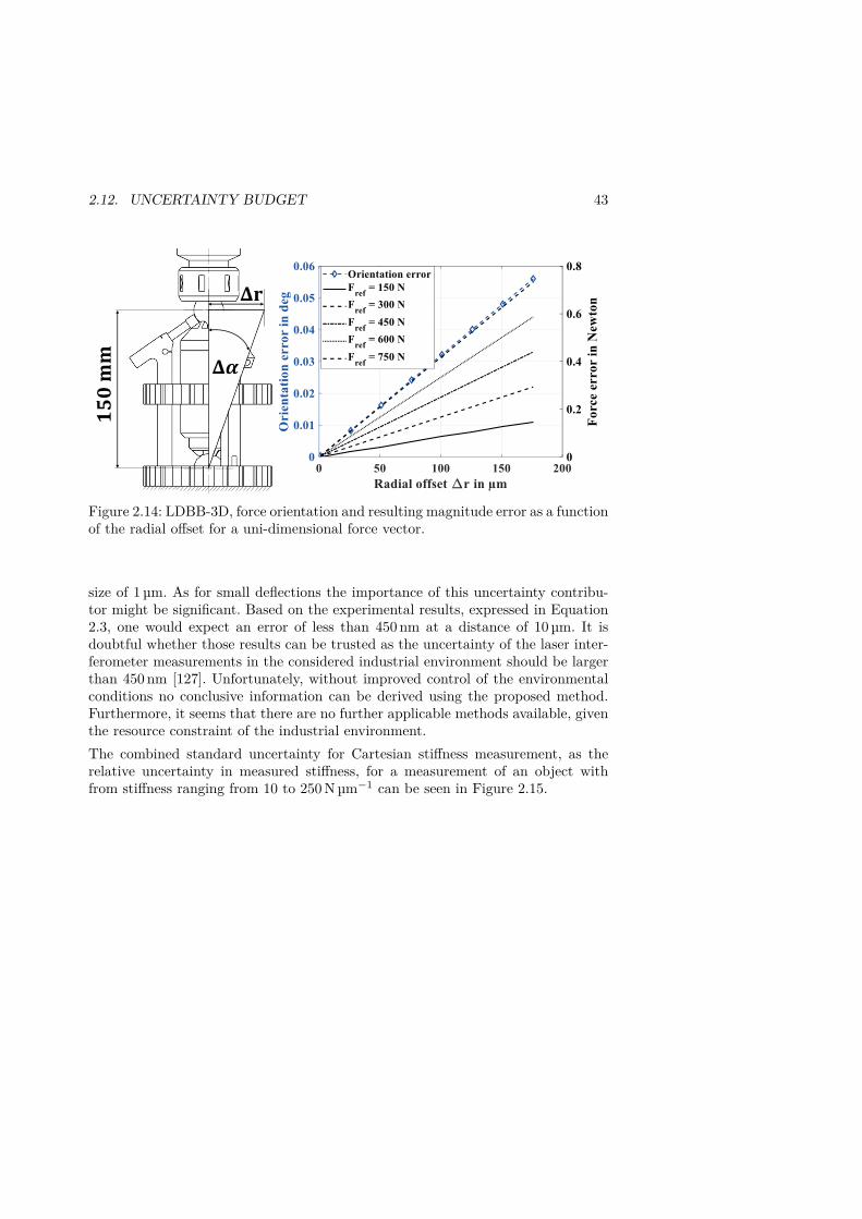
2.12. UNCERTAINTY BUDGET 43
𝟏𝟓𝟎𝐦𝐦
𝚫𝐫
𝚫𝜶
Figure 2.14: LDBB-3D, force orientation and resulting magnitude error as a functionof the radial offset for a uni-dimensional force vector.
size of 1 µm. As for small deflections the importance of this uncertainty contribu-tor might be significant. Based on the experimental results, expressed in Equation2.3, one would expect an error of less than 450 nm at a distance of 10 µm. It isdoubtful whether those results can be trusted as the uncertainty of the laser inter-ferometer measurements in the considered industrial environment should be largerthan 450 nm [127]. Unfortunately, without improved control of the environmentalconditions no conclusive information can be derived using the proposed method.Furthermore, it seems that there are no further applicable methods available, giventhe resource constraint of the industrial environment.The combined standard uncertainty for Cartesian stiffness measurement, as therelative uncertainty in measured stiffness, for a measurement of an object withfrom stiffness ranging from 10 to 250 N µm−1 can be seen in Figure 2.15.
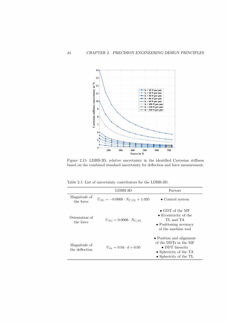
44 CHAPTER 2. PRECISION ENGINEERING DESIGN PRINCIPLES
200 300 400 500 600 700Force in N
4
5
6
7
8
9
10
11
12
13
14
Car
tesi
an s
tiff
ness
uncertainty
in %
k = 10 N per µmk = 20 N per µmk = 30 N per µmk = 40 N per µmk = 50 N per µmk = 100 N per µmk = 150 N per µmk = 250 N per µm
Figure 2.15: LDBB-3D, relative uncertainty in the identified Cartesian stiffnessbased on the combined standard uncertainty for deflection and force measurement.
Table 2.1: List of uncertainty contributors for the LDBB-3D.
LDBB-3D FactorsMagnitude of
the force USL = −0.0008 · NC,SL + 1.035 • Control system
Orientation ofthe force USO = 0.0006 · NC,SL
• GDT of the MF• Eccentricity of the
TL and TA• Positioning accuracy
of the machine tool
Magnitude ofthe deflection Uδx = 0.04 · d + 0.05
• Position and alignmentof the DDTs in the MF
• DDT linearity• Sphericity of the TA• Sphericity of the TL

Chapter 3
Precision engineering operationprinciples
PEOPs have been developed to ensure reproducible experimental compliance mea-surements of AMM. The aim of PEOPs is to reduce the measurement uncertaintyand to separate superimposed errors from the reference objects of the PMI or theAMM from the measurand. This chapter focuses exclusively on the PEOPs for theLDBB PMI series such as the importance of the measurement procedure for theidentification of the MBCS transformation, the avoidance of transient measure-ment data, different approaches of error separation as well as the importance forthe selection of the Mechanical Base Load Reference (MBLR). The collection ofPEOP is based on the author’s experience in the field of quasi-static compliancemeasurements of AMM. Nevertheless, these PEOPs have general validity and findapplication in different commercial PMIs. Namely, the transformation of the datainto the MBCS is important for R-test devices [128] as well as with any laser trackermeasurement of industrial manipulators [129]. The avoidance of transient measure-ment data is common with the measurement of quasi-static AMM, e.g., circulartesting [130]. The topic of error separation is important across several industriessuch as metalworking, optics, experimental science, and metrology. These methodshave general applicability but are unfortunately often regarded as secrets of a craftwhich inhibits their dispersion across shop floors [86]. A typical example is the test-ing of circular run-out of machine tool spindles to separate the eccentricity of thereference object representing the TCP from the actual run-out [131].
Other aspects such as the utility value of the data in terms of model parametersobservability and sensitivity are also important for the selection of measurementconfiguration or trajectories; however, these aspects are already covered in [4].
45
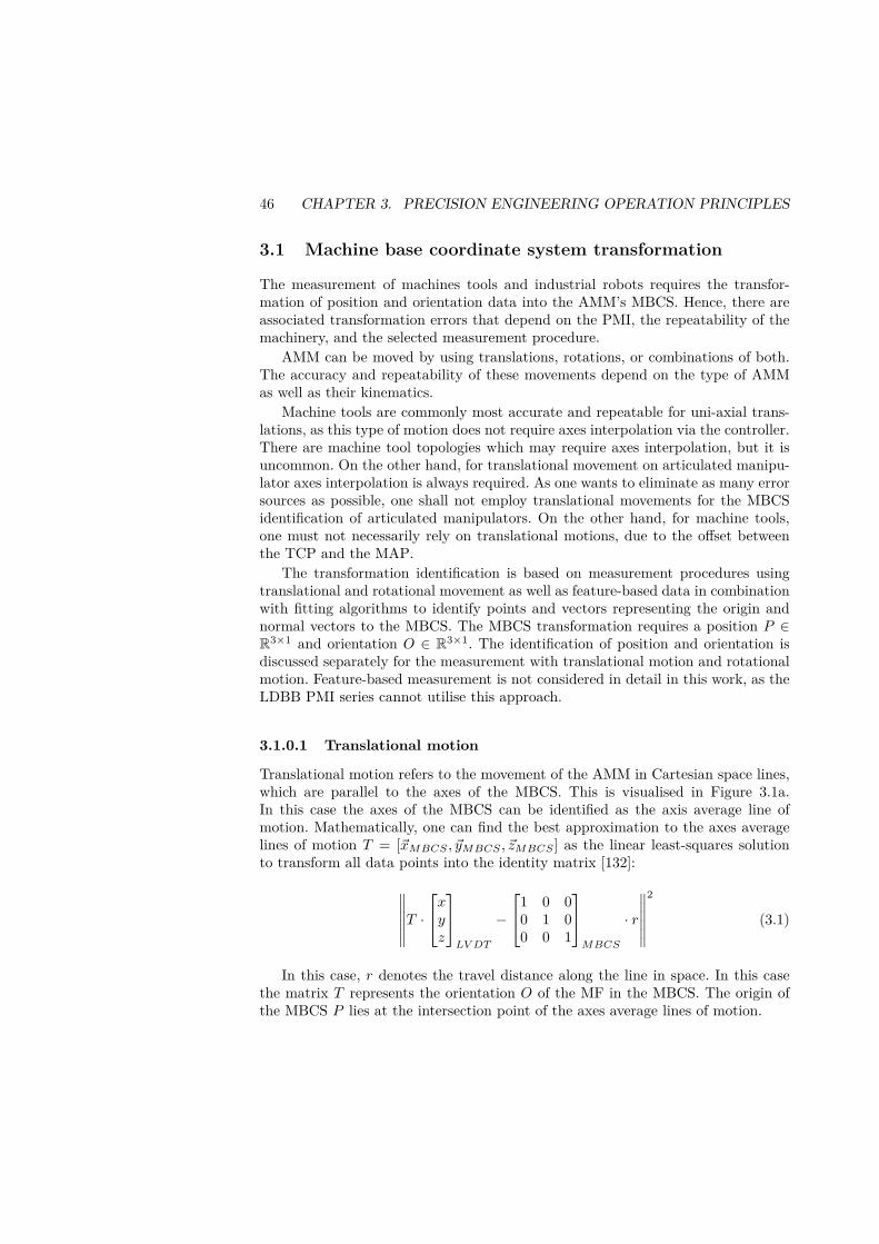
46 CHAPTER 3. PRECISION ENGINEERING OPERATION PRINCIPLES
3.1 Machine base coordinate system transformation
The measurement of machines tools and industrial robots requires the transfor-mation of position and orientation data into the AMM’s MBCS. Hence, there areassociated transformation errors that depend on the PMI, the repeatability of themachinery, and the selected measurement procedure.
AMM can be moved by using translations, rotations, or combinations of both.The accuracy and repeatability of these movements depend on the type of AMMas well as their kinematics.
Machine tools are commonly most accurate and repeatable for uni-axial trans-lations, as this type of motion does not require axes interpolation via the controller.There are machine tool topologies which may require axes interpolation, but it isuncommon. On the other hand, for translational movement on articulated manipu-lator axes interpolation is always required. As one wants to eliminate as many errorsources as possible, one shall not employ translational movements for the MBCSidentification of articulated manipulators. On the other hand, for machine tools,one must not necessarily rely on translational motions, due to the offset betweenthe TCP and the MAP.
The transformation identification is based on measurement procedures usingtranslational and rotational movement as well as feature-based data in combinationwith fitting algorithms to identify points and vectors representing the origin andnormal vectors to the MBCS. The MBCS transformation requires a position P ∈R3×1 and orientation O ∈ R3×1. The identification of position and orientation isdiscussed separately for the measurement with translational motion and rotationalmotion. Feature-based measurement is not considered in detail in this work, as theLDBB PMI series cannot utilise this approach.
3.1.0.1 Translational motion
Translational motion refers to the movement of the AMM in Cartesian space lines,which are parallel to the axes of the MBCS. This is visualised in Figure 3.1a.In this case the axes of the MBCS can be identified as the axis average line ofmotion. Mathematically, one can find the best approximation to the axes averagelines of motion T = [xMBCS , yMBCS , zMBCS ] as the linear least-squares solutionto transform all data points into the identity matrix [132]:∥∥∥∥∥∥T ·
xyz
LV DT
−
1 0 00 1 00 0 1
MBCS
· r
∥∥∥∥∥∥2
(3.1)
In this case, r denotes the travel distance along the line in space. In this casethe matrix T represents the orientation O of the MF in the MBCS. The origin ofthe MBCS P lies at the intersection point of the axes average lines of motion.
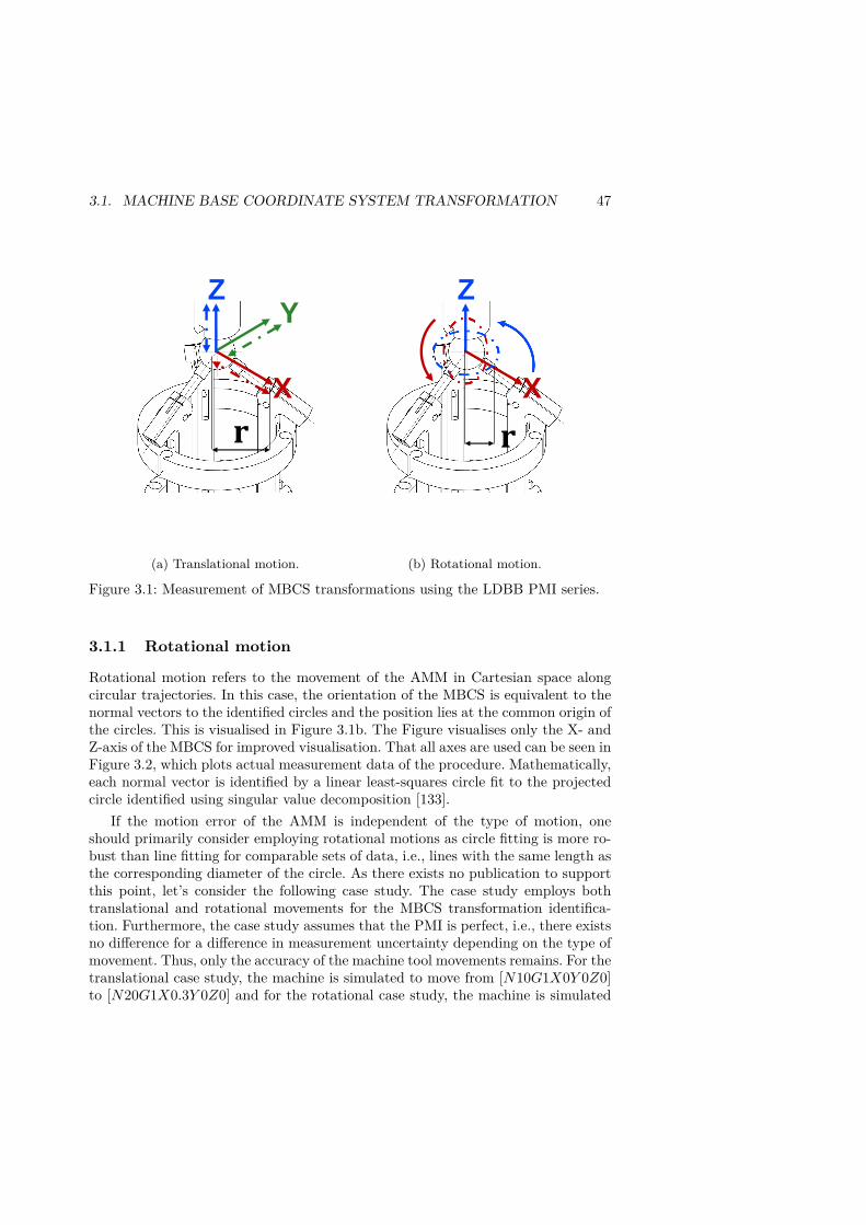
3.1. MACHINE BASE COORDINATE SYSTEM TRANSFORMATION 47
Z
X
Y
𝐫
(a) Translational motion.
Z
X
𝐫
(b) Rotational motion.
Figure 3.1: Measurement of MBCS transformations using the LDBB PMI series.
3.1.1 Rotational motion
Rotational motion refers to the movement of the AMM in Cartesian space alongcircular trajectories. In this case, the orientation of the MBCS is equivalent to thenormal vectors to the identified circles and the position lies at the common origin ofthe circles. This is visualised in Figure 3.1b. The Figure visualises only the X- andZ-axis of the MBCS for improved visualisation. That all axes are used can be seen inFigure 3.2, which plots actual measurement data of the procedure. Mathematically,each normal vector is identified by a linear least-squares circle fit to the projectedcircle identified using singular value decomposition [133].
If the motion error of the AMM is independent of the type of motion, oneshould primarily consider employing rotational motions as circle fitting is more ro-bust than line fitting for comparable sets of data, i.e., lines with the same length asthe corresponding diameter of the circle. As there exists no publication to supportthis point, let’s consider the following case study. The case study employs bothtranslational and rotational movements for the MBCS transformation identifica-tion. Furthermore, the case study assumes that the PMI is perfect, i.e., there existsno difference for a difference in measurement uncertainty depending on the type ofmovement. Thus, only the accuracy of the machine tool movements remains. For thetranslational case study, the machine is simulated to move from [N10G1X0Y 0Z0]to [N20G1X0.3Y 0Z0] and for the rotational case study, the machine is simulated
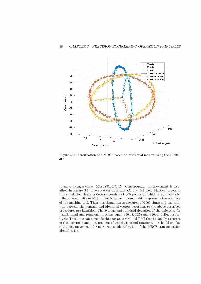
48 CHAPTER 3. PRECISION ENGINEERING OPERATION PRINCIPLES
27
Figure 3.2: Identification of a MBCS based on rotational motion using the LDBB-3D.
to move along a circle [G2X0Y 0Z0R0.15]. Conceptually, this movement is visu-alised in Figure 3.1. The rotation directions G2 and G3 yield identical errors inthis simulation. Each trajectory consists of 300 points on which a normally dis-tributed error with σ(10, 3) in µm is super-imposed, which represents the accuracyof the machine tool. Then this simulation is executed 100 000 times and the rota-tion between the nominal and identified vectors according to the above-describedprocedures are identified. The average and standard deviation of the difference fortranslational and rotational motions equal σ(0.48, 0.25) and σ(0.40, 0.20), respec-tively. Thus, one can conclude that for an AMM and PMI that is equally accuratein the movement and measurement of translations and rotations, one should employrotational movements for more robust identification of the MBCS transformationidentification.
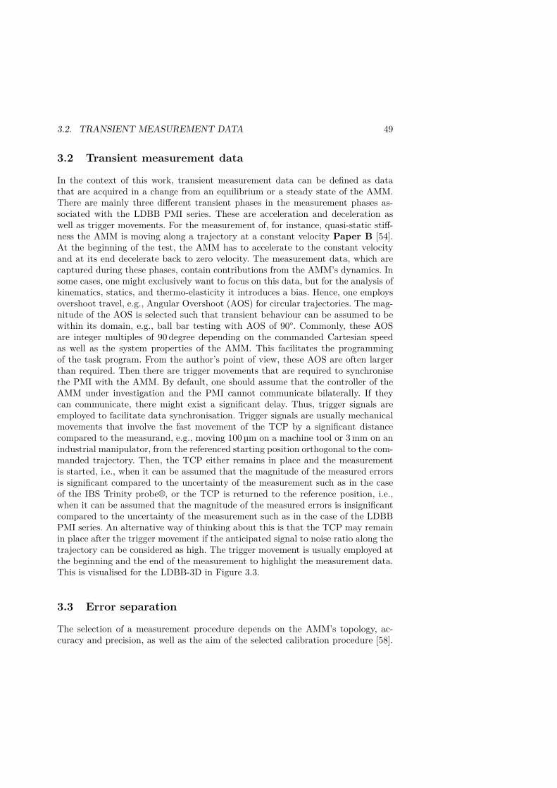
3.2. TRANSIENT MEASUREMENT DATA 49
3.2 Transient measurement data
In the context of this work, transient measurement data can be defined as datathat are acquired in a change from an equilibrium or a steady state of the AMM.There are mainly three different transient phases in the measurement phases as-sociated with the LDBB PMI series. These are acceleration and deceleration aswell as trigger movements. For the measurement of, for instance, quasi-static stiff-ness the AMM is moving along a trajectory at a constant velocity Paper B [54].At the beginning of the test, the AMM has to accelerate to the constant velocityand at its end decelerate back to zero velocity. The measurement data, which arecaptured during these phases, contain contributions from the AMM’s dynamics. Insome cases, one might exclusively want to focus on this data, but for the analysis ofkinematics, statics, and thermo-elasticity it introduces a bias. Hence, one employsovershoot travel, e.g., Angular Overshoot (AOS) for circular trajectories. The mag-nitude of the AOS is selected such that transient behaviour can be assumed to bewithin its domain, e.g., ball bar testing with AOS of 90°. Commonly, these AOSare integer multiples of 90 degree depending on the commanded Cartesian speedas well as the system properties of the AMM. This facilitates the programmingof the task program. From the author’s point of view, these AOS are often largerthan required. Then there are trigger movements that are required to synchronisethe PMI with the AMM. By default, one should assume that the controller of theAMM under investigation and the PMI cannot communicate bilaterally. If theycan communicate, there might exist a significant delay. Thus, trigger signals areemployed to facilitate data synchronisation. Trigger signals are usually mechanicalmovements that involve the fast movement of the TCP by a significant distancecompared to the measurand, e.g., moving 100 µm on a machine tool or 3 mm on anindustrial manipulator, from the referenced starting position orthogonal to the com-manded trajectory. Then, the TCP either remains in place and the measurementis started, i.e., when it can be assumed that the magnitude of the measured errorsis significant compared to the uncertainty of the measurement such as in the caseof the IBS Trinity probe®, or the TCP is returned to the reference position, i.e.,when it can be assumed that the magnitude of the measured errors is insignificantcompared to the uncertainty of the measurement such as in the case of the LDBBPMI series. An alternative way of thinking about this is that the TCP may remainin place after the trigger movement if the anticipated signal to noise ratio along thetrajectory can be considered as high. The trigger movement is usually employed atthe beginning and the end of the measurement to highlight the measurement data.This is visualised for the LDBB-3D in Figure 3.3.
3.3 Error separation
The selection of a measurement procedure depends on the AMM’s topology, ac-curacy and precision, as well as the aim of the selected calibration procedure [58].

50 CHAPTER 3. PRECISION ENGINEERING OPERATION PRINCIPLES
Start
point
CW
𝑪𝑾 𝒅𝒂𝒕𝒂 𝟐𝝅Start
point
CCW𝑺𝒊𝒈𝒏𝒂𝒍 𝟑𝝅
𝑨𝑶𝑺𝝅
𝟐𝑨𝑶𝑺
𝝅
𝟐
Figure 3.3: LDBB-3D machine tool measurement; signal as the sum of the mea-surement data and the AOS movement.
Any measurement procedure has its advantages and disadvantages. Common disad-vantages are that the result of the measurement itself is a superposition of severalerror sources. This section focuses on the separation of the error sources under in-vestigation from other superimposed contributions such as the movement of otheractuated joints of the AMM or the reference objects of the PMI.
3.3.1 Direct measurement and indirect measurementMeasurement methods for AMM can be classified as direct and indirect [13]. Directmethods measure individual structural loop components, i.e., measurement of theresultant movement of the actuation of a single translational or rotational joint.Indirect methods measure the combined movement of several structural loops com-ponents. For instance circular trajectories on machine tools and straight lines onindustrial manipulators. According to ISO 230-1 [10], a structural loop is defined asan assembly of mechanical components which maintain a relative position betweentwo specified objects. In a typical machine tool, the structural loop includes thespindle, the bearings and the spindle housing, the guideways and frame, the drivesand the ball screws, and the tool and work-holding fixtures. In a typical industrialmanipulator, the structural loop includes the base plate, the links, and the EndEffector (EE) [134].
As aforementioned, direct measurements allow the identification of a singlestructural loop component without any contribution from other components. In thecase of direct measurements, one of the most favourable and widely adopted directmeasuring methods is laser interferometer, which combined with special optics is
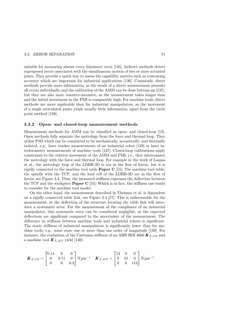
3.3. ERROR SEPARATION 51
suitable for measuring almost every kinematic error [135]. Indirect methods detectsuperposed errors associated with the simultaneous motion of two or more actuatedjoints. They provide a quick way to assess the capability metrics such as contouringaccuracy which are important for industrial applications [136]. Commonly, directmethods provide more information, as the result of a direct measurement presentsall errors individually and the calibration of the AMM can be done bottom-up [137],but they are also more resource-intensive, as the measurement takes longer timeand the initial investment in the PMI is comparably high. For machine tools, directmethods are more applicable than for industrial manipulators, as the movementof a single articulated joints yields usually little information, apart from the circlepoint method [138].
3.3.2 Open- and closed-loop measurement methodsMeasurement methods for AMM can be classified as open- and closed-loop [13].Open methods fully separate the metrology from the force and thermal loop. Theyutilise PMI which can be considered to be mechanically, acoustically, and thermallyisolated, e.g., laser tracker measurements of an industrial robot [129] or laser in-terferometry measurements of machine tools [127]. Closed-loop calibrations applyconstraints to the relative movement of the AMM and PMI, i.e., they interconnectthe metrology with the force and thermal loop. For example in the work of Laspaset al., the metrology loop of the LDBB-3D is not in the flow of forces, but it isrigidly connected to the machine tool table Paper C [55]. The machine tool table,the spindle with the TCP, and the load cell of the LDBB-3D are in the flow offorces, see Figure 3.4. Thus, the measured stiffness expresses the deflection betweenthe TCP and the workpiece Paper C [55]. Which is in fact, the stiffness one wantsto consider for the machine tool model.
On the other hand, the measurement described in Theissen et al. is dependenton a rigidly connected table link, see Figure 3.4 [57]. This is unfavourable for themeasurement, as the deflection of the structure locating the table link will intro-duce a systematic error. For the measurement of the compliance of an industrialmanipulator, this systematic error can be considered negligible, as the expecteddeflections are significant compared to the uncertainty of the measurement. Thedifference in stiffness between machine tools and industrial robots is significant.The static stiffness of industrial manipulators is significantly lower than for ma-chine tools; e.g., some state one or more than one order of magnitude [139]. Forinstance, the evaluation of the Cartesian stiffness of an ABB IRB 4600 KKKX,IM anda machine tool KKKX,MT yield [140]:
KKKX,IM =
0.14 0 00 0.11 00 0 0.3
N µm−1 KKKX,MT =
13 0 00 16 00 0 113
N µm−1
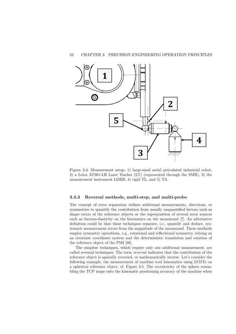
52 CHAPTER 3. PRECISION ENGINEERING OPERATION PRINCIPLES
𝟏
𝟐
𝟑
𝟒
𝟓
Figure 3.4: Measurement setup: 1) large-sized serial articulated industrial robot,2) a Leica AT901-LR Laser Tracker (LT) (represented through the SMR), 3) themeasurement instrument LDBB, 4) rigid TL, and 5) TA.
3.3.3 Reversal methods, multi-step, and multi-probeThe concept of error separation utilises additional measurements, directions, orsymmetries to quantify the contribution from usually unquantified factors such asshape errors of the reference objects or the superposition of several error sourcessuch as thermo-elasticity on the kinematics on the measurand [7]. An alternativedefinition could be that these techniques separate, i.e., quantify and deduce, sys-tematic measurement errors from the magnitude of the measurand. These methodsemploy symmetry operations, e.g., rotational and reflectional symmetry, relying onan invariant coordinate system and the deterministic translation and rotation ofthe reference object of the PMI [86].
The simplest techniques, which require only one additional measurement, arecalled reversal techniques. The term reversal indicates that the contribution of thereference object is spatially reversed, or mathematically inverse. Let’s consider thefollowing example, the measurement of machine tool kinematics using LVDTs ona spherical reference object, cf. Figure 3.5. The eccentricity of the sphere resem-bling the TCP maps onto the kinematic positioning accuracy of the machine when
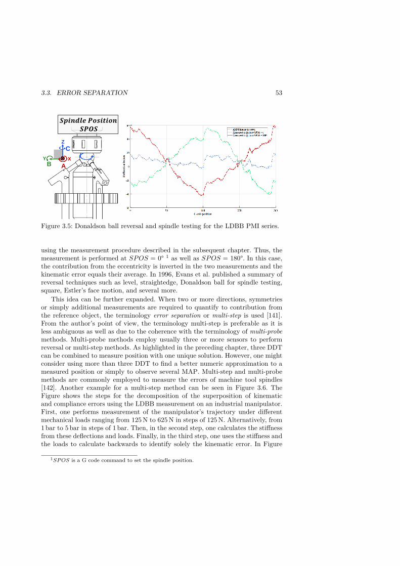
3.3. ERROR SEPARATION 53
Y
Z
X
C
AB
𝑺𝒑𝒊𝒏𝒅𝒍𝒆 𝑷𝒐𝒔𝒊𝒕𝒊𝒐𝒏𝑺𝑷𝑶𝑺
Figure 3.5: Donaldson ball reversal and spindle testing for the LDBB PMI series.
using the measurement procedure described in the subsequent chapter. Thus, themeasurement is performed at SPOS = 0° 1 as well as SPOS = 180°. In this case,the contribution from the eccentricity is inverted in the two measurements and thekinematic error equals their average. In 1996, Evans et al. published a summary ofreversal techniques such as level, straightedge, Donaldson ball for spindle testing,square, Estler’s face motion, and several more.
This idea can be further expanded. When two or more directions, symmetriesor simply additional measurements are required to quantify to contribution fromthe reference object, the terminology error separation or multi-step is used [141].From the author’s point of view, the terminology multi-step is preferable as it isless ambiguous as well as due to the coherence with the terminology of multi-probemethods. Multi-probe methods employ usually three or more sensors to performreversal or multi-step methods. As highlighted in the preceding chapter, three DDTcan be combined to measure position with one unique solution. However, one mightconsider using more than three DDT to find a better numeric approximation to ameasured position or simply to observe several MAP. Multi-step and multi-probemethods are commonly employed to measure the errors of machine tool spindles[142]. Another example for a multi-step method can be seen in Figure 3.6. TheFigure shows the steps for the decomposition of the superposition of kinematicand compliance errors using the LDBB measurement on an industrial manipulator.First, one performs measurement of the manipulator’s trajectory under differentmechanical loads ranging from 125 N to 625 N in steps of 125 N. Alternatively, from1 bar to 5 bar in steps of 1 bar. Then, in the second step, one calculates the stiffnessfrom these deflections and loads. Finally, in the third step, one uses the stiffness andthe loads to calculate backwards to identify solely the kinematic error. In Figure
1SP OS is a G code command to set the spindle position.
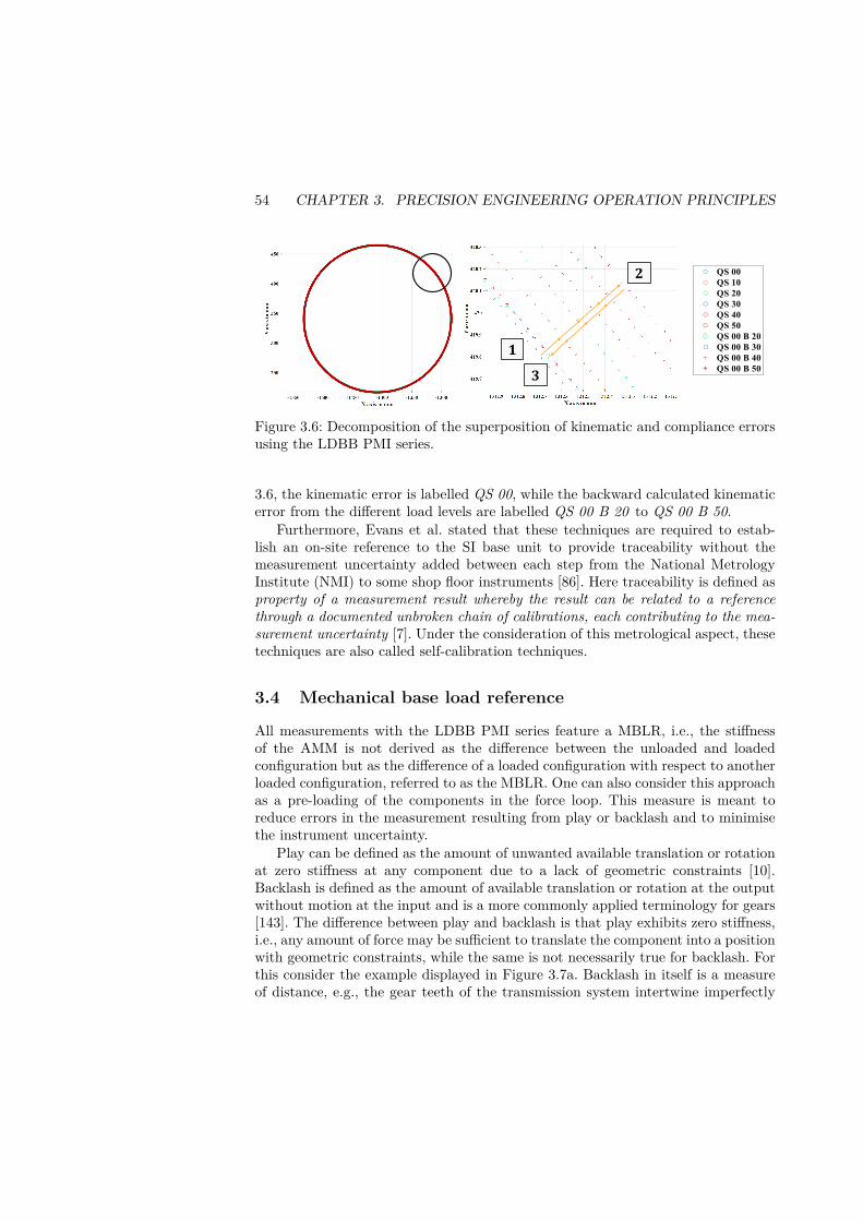
54 CHAPTER 3. PRECISION ENGINEERING OPERATION PRINCIPLES
𝟏
𝟐
𝟑
Figure 3.6: Decomposition of the superposition of kinematic and compliance errorsusing the LDBB PMI series.
3.6, the kinematic error is labelled QS 00, while the backward calculated kinematicerror from the different load levels are labelled QS 00 B 20 to QS 00 B 50.
Furthermore, Evans et al. stated that these techniques are required to estab-lish an on-site reference to the SI base unit to provide traceability without themeasurement uncertainty added between each step from the National MetrologyInstitute (NMI) to some shop floor instruments [86]. Here traceability is defined asproperty of a measurement result whereby the result can be related to a referencethrough a documented unbroken chain of calibrations, each contributing to the mea-surement uncertainty [7]. Under the consideration of this metrological aspect, thesetechniques are also called self-calibration techniques.
3.4 Mechanical base load reference
All measurements with the LDBB PMI series feature a MBLR, i.e., the stiffnessof the AMM is not derived as the difference between the unloaded and loadedconfiguration but as the difference of a loaded configuration with respect to anotherloaded configuration, referred to as the MBLR. One can also consider this approachas a pre-loading of the components in the force loop. This measure is meant toreduce errors in the measurement resulting from play or backlash and to minimisethe instrument uncertainty.
Play can be defined as the amount of unwanted available translation or rotationat zero stiffness at any component due to a lack of geometric constraints [10].Backlash is defined as the amount of available translation or rotation at the outputwithout motion at the input and is a more commonly applied terminology for gears[143]. The difference between play and backlash is that play exhibits zero stiffness,i.e., any amount of force may be sufficient to translate the component into a positionwith geometric constraints, while the same is not necessarily true for backlash. Forthis consider the example displayed in Figure 3.7a. Backlash in itself is a measureof distance, e.g., the gear teeth of the transmission system intertwine imperfectly
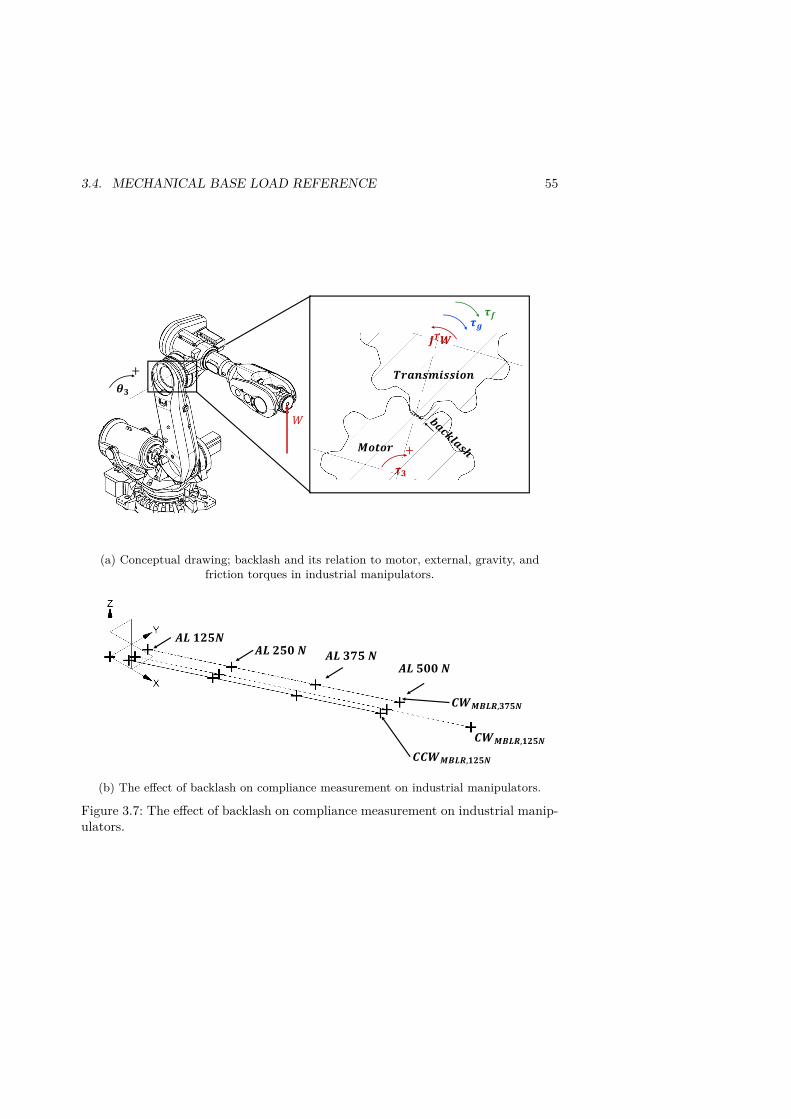
3.4. MECHANICAL BASE LOAD REFERENCE 55
(a) Conceptual drawing; backlash and its relation to motor, external, gravity, andfriction torques in industrial manipulators.
𝑪𝑾𝑴𝑩𝑳𝑹,𝟏𝟐𝟓𝑵
𝑪𝑪𝑾𝑴𝑩𝑳𝑹,𝟏𝟐𝟓𝑵
𝑪𝑾𝑴𝑩𝑳𝑹,𝟑𝟕𝟓𝑵
𝑨𝑳 𝟏𝟐𝟓𝑵𝑨𝑳 𝟐𝟓𝟎 𝑵 𝑨𝑳 𝟑𝟕𝟓 𝑵
𝑨𝑳 𝟓𝟎𝟎 𝑵
(b) The effect of backlash on compliance measurement on industrial manipulators.
Figure 3.7: The effect of backlash on compliance measurement on industrial manip-ulators.
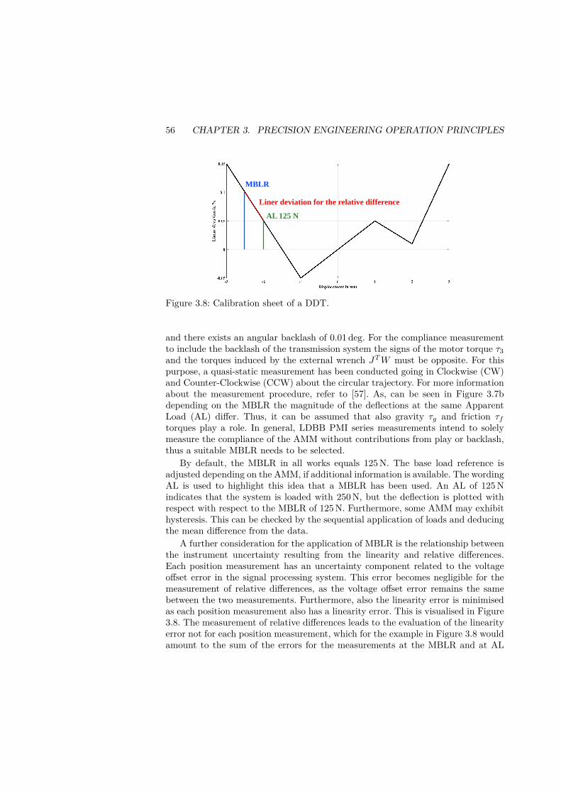
56 CHAPTER 3. PRECISION ENGINEERING OPERATION PRINCIPLES
MBLR
AL 125 N
Liner deviation for the relative difference
Figure 3.8: Calibration sheet of a DDT.
and there exists an angular backlash of 0.01 deg. For the compliance measurementto include the backlash of the transmission system the signs of the motor torque τ3and the torques induced by the external wrench JT W must be opposite. For thispurpose, a quasi-static measurement has been conducted going in Clockwise (CW)and Counter-Clockwise (CCW) about the circular trajectory. For more informationabout the measurement procedure, refer to [57]. As, can be seen in Figure 3.7bdepending on the MBLR the magnitude of the deflections at the same ApparentLoad (AL) differ. Thus, it can be assumed that also gravity τg and friction τf
torques play a role. In general, LDBB PMI series measurements intend to solelymeasure the compliance of the AMM without contributions from play or backlash,thus a suitable MBLR needs to be selected.
By default, the MBLR in all works equals 125 N. The base load reference isadjusted depending on the AMM, if additional information is available. The wordingAL is used to highlight this idea that a MBLR has been used. An AL of 125 Nindicates that the system is loaded with 250 N, but the deflection is plotted withrespect with respect to the MBLR of 125 N. Furthermore, some AMM may exhibithysteresis. This can be checked by the sequential application of loads and deducingthe mean difference from the data.
A further consideration for the application of MBLR is the relationship betweenthe instrument uncertainty resulting from the linearity and relative differences.Each position measurement has an uncertainty component related to the voltageoffset error in the signal processing system. This error becomes negligible for themeasurement of relative differences, as the voltage offset error remains the samebetween the two measurements. Furthermore, also the linearity error is minimisedas each position measurement also has a linearity error. This is visualised in Figure3.8. The measurement of relative differences leads to the evaluation of the linearityerror not for each position measurement, which for the example in Figure 3.8 wouldamount to the sum of the errors for the measurements at the MBLR and at AL

3.4. MECHANICAL BASE LOAD REFERENCE 57
125 N, but as the difference of these measurements. This minimises the measurementuncertainty for the deflection measurement.


Chapter 4
LDBB-3D: Machine toolelasto-geometric measurement
This chapter presents a case study of the simultaneous measurement of kinematicand compliance errors of a 5-axis machining centre using the LDBB-3D for a BK4test according to ISO10791-6 [144]. The combination of kinematic and complianceinvestigation may also be referred to as elasto-geometric [145]. The BK4 test ismeant to quantify the kinematic errors for circular interpolation motion by simul-taneous five-axis control. This tests is more commonly known under the term rotaryaxis test or simply R-Test [146]. This chapter presents an elasto-geometric versionof the BK4 test, i.e., compliance errors are superimposed onto the kinematic errors.The measurement uses the LDBB-3D, designed in accordance with the PEDPs asdescribed in Chapter 2, to induce and measure the elasto-geometric errors alongthe circular trajectory. Then, the PEOPs, as described in Chapter 3, are utilisedto accurately and precisely identify the kinematic errors and the compliance of themachine tool at the TCP. The measurement setup can be seen in Figure 4.1.
The section provides a concise summary of the measurement procedure and itsresults:
Once the force and metrology loops are prepared, i.e., the transformation into theMBCS as well as the position difference between the TA and TL are identified,one needs to identify the eccentricity of the TA. By employing the ball reversal forspindle testing technique [86].
Then the loads are applied between the TA and TL, and the machine conductscircular trajectories by simultaneously rotating the C-axis in CCW and CW direc-tion for 360° from the initial position with an AOS of 5° and the A-axis in CCWand CW direction for 20° from the initial position with an AOS of 5°.
The MBLR equals 250 N the ALs are equal to 125 N, 250 N, and 375 N.
59

60CHAPTER 4. LDBB-3D: MACHINE TOOL ELASTO-GEOMETRIC
MEASUREMENT
Proportional pressure control valve
Linear Variable Differential Transformer (LVDT)
𝟏
𝟐
𝟐
𝟑
𝐹
Δ𝑃
𝟒
𝟓
𝟔
Figure 4.1: LDBB-3D setup for an elasto-geometric BK4 ISO 10791-6 machinetool measurement. The setup shows: The LDBB-3D which consists of the LDBBequipped with the PPCV (1), three LVDTs Tesa GTL21-W® [3] mounted on a MF(3), a TA (4), which consists of a sphere of radius 15 mm attached to a shaft ofdiameter 25 mm, a TL(5), and a machine tool.
The measurement was conducted at a feed rate of 1500 deg/min1. The results arevisualised in Figure 4.2 for each of the Cartesian components in the MBCS. The X-axis label of Figure 4.2 reads trajectory in % as the C- and A-axis are simultaneously
1A video of the test can be accessed under the following link: youtube.com

61
Table 4.1: Compliance in X-, Y-, and Z-axis in terms of mean over velocity.
ComplianceFeed rate in deg/min X-axis in N µm−1 Y-axis in N µm−1 Z-axis in N µm−1
3000 14 12 1056000 8 4 54
actuated; However, over different movement ranges. Namely 360° and 20°. One canfind a detailed description of the measurement procedure in Paper B and C[54, 55].
The average error and its standard deviation between the kinematic referencemeasurement and the corresponding kinematic component in the X-axis equals 2 µmand 2 µm, in the Y-axis equals 2 µm and 1 µm, and in the Z-axis equals 2 µm and1 µm, cf. Figure 4.2 the data with the labels Kinematic and Comp. B Mean. Inaddition to that, the stiffness at the TCP can be identified. The Cartesian stiffnesshas been calculated according to Laspas et al. Paper C [55]. The results can beseen in Equation 4.1:
KKK =
131710 ± 1 0 00 1624
10 ± 1 00 0 113125
100 ± 6
N µm−1 (4.1)
The stiffness along the main diagonal of the translational Cartesian stiffnessmatrix are not represented as a single scalar value. As the position of the TCPchanges in the workspace, so changes the configuration of the machine tool, andconsequently the stiffness at the TCP. Thus, the results are presented in terms ofthe mean, minimum, and maximum stiffness for each main diagonal component,e.g., the component kxx has a mean, minimum, and maximum stiffness of 13, 10,and 17 N µm−1. The uncertainty in Equation 4.1 is stated at a confidence with acoverage factor of k = 2 for normally distributed data.
It seems feasible that one can simultaneously quantify kinematics and compli-ance of a machine tool employing loaded circular testing and the developed LDBB-3D. However, at least one additional measurement is required, as one needs toperform at least two measurements to identify the stiffness of the machine tool.
Further tests were conducted at feed rates of 3000 and 6000 deg/min. The re-sulting stiffness is presented in Table 4.1.
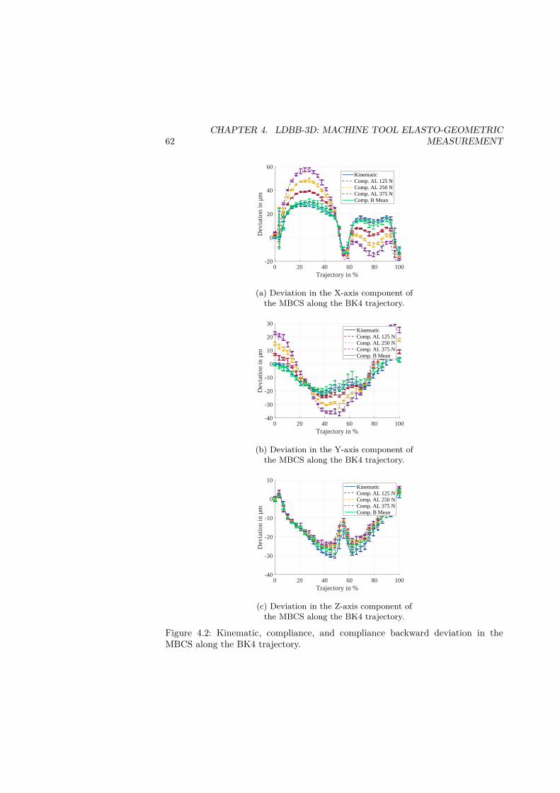
62CHAPTER 4. LDBB-3D: MACHINE TOOL ELASTO-GEOMETRIC
MEASUREMENT
0 20 40 60 80 100Trajectory in %
-20
0
20
40
60
Dev
iatio
n in
µm
KinematicComp. AL 125 NComp. AL 250 NComp. AL 375 NComp. B Mean
(a) Deviation in the X-axis component ofthe MBCS along the BK4 trajectory.
0 20 40 60 80 100Trajectory in %
-40
-30
-20
-10
0
10
20
30
Dev
iatio
n in
µm
KinematicComp. AL 125 NComp. AL 250 NComp. AL 375 NComp. B Mean
(b) Deviation in the Y-axis component ofthe MBCS along the BK4 trajectory.
0 20 40 60 80 100Trajectory in %
-40
-30
-20
-10
0
10
Dev
iatio
n in
µm
KinematicComp. AL 125 NComp. AL 250 NComp. AL 375 NComp. B Mean
(c) Deviation in the Z-axis component ofthe MBCS along the BK4 trajectory.
Figure 4.2: Kinematic, compliance, and compliance backward deviation in theMBCS along the BK4 trajectory.
Chapter 5
Discussion and conclusion
This work presents a collection of PEDP, which are based on notable works in thefield of precision engineering, as well as PEOP, which are based on the author’sexperience in the field of quasi-static compliance measurements. From the author’spoint of view, these principles form an important part of the basis for the cre-ation of PMI for the compliance measurements of AMM. Hence, their applicationwas exemplified through the design of the LDBB-3D and its application on a ma-chine tool quasi-static elasto-geometric measurement in Chapter 4. The quasi-staticelasto-geometric measurement identifies the compliance as well as kinematic errorsof the machine tool. Other application examples which focus on the measurementof compliance can be seen in the appended publications Paper B and Paper C.They show the application of the LDBB-3D to measure and identify quasi-staticstiffness matrices of machine tools. In addition to that, Paper A showed the ap-plication of the LDBB-3DD to measure and identify the dynamic stiffness matrixof a static machine tool.
The PMIs for compliance measurement require two essential requirements. Theseare the ability to exert a controllable mechanical load while measuring the deflec-tion in terms of distance, position, or orientation. Based on the author’s experiencethrough the development of this work, the peer review of other works, and thereverse engineering of available PMI, the author proposes a coarse prioritisation ofPEDP for PMI for compliance measurements to answer RQ. 1. The PEDPs aregrouped into primary and secondary principles. Primary principles directly supportthe aforementioned two essential requirements. While secondary principles eitherindirectly support the aforementioned two essential requirements or directly sup-port other requirements such as allow for a range of motion of ± 1 mm, has a firsteigen-frequency higher than 50 Hz, or has an operating temperature range 5 to50 °C. In this context, the word directly means that independent of the candidatedesign of the PMI for compliance measurement, the accuracy and repeatability willbe affected and indirectly means that it might be affected.
The PEDPs Structure, Abbe, and Kinematic design determine the position and
63
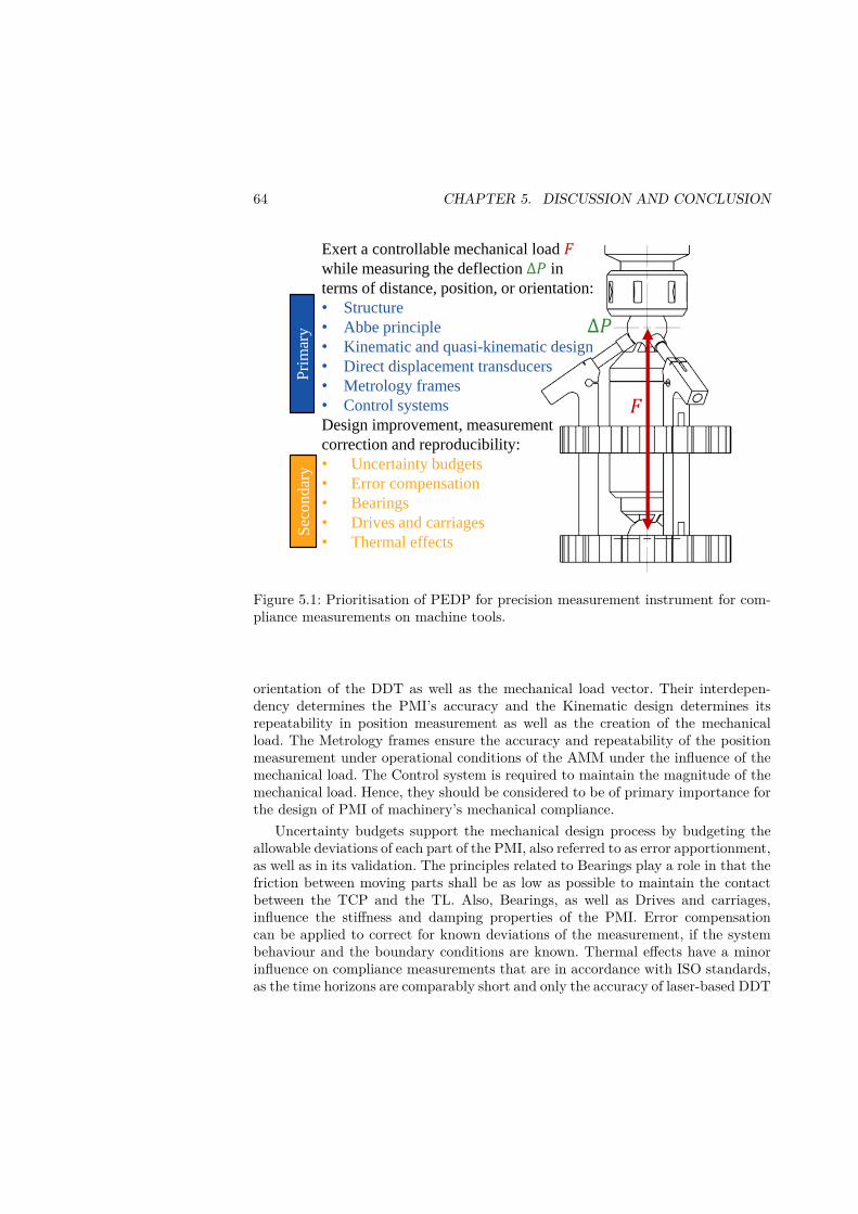
64 CHAPTER 5. DISCUSSION AND CONCLUSION
Exert a controllable mechanical load 𝐹while measuring the deflection Δ𝑃 in
terms of distance, position, or orientation:
• Structure
• Abbe principle
• Kinematic and quasi-kinematic design
• Direct displacement transducers
• Metrology frames
• Control systems
Design improvement, measurement
correction and reproducibility:
• Uncertainty budgets
• Error compensation
• Bearings
• Drives and carriages
• Thermal effects
𝐹
Δ𝑃S
eco
nd
ary
Pri
mar
y
Figure 5.1: Prioritisation of PEDP for precision measurement instrument for com-pliance measurements on machine tools.
orientation of the DDT as well as the mechanical load vector. Their interdepen-dency determines the PMI’s accuracy and the Kinematic design determines itsrepeatability in position measurement as well as the creation of the mechanicalload. The Metrology frames ensure the accuracy and repeatability of the positionmeasurement under operational conditions of the AMM under the influence of themechanical load. The Control system is required to maintain the magnitude of themechanical load. Hence, they should be considered to be of primary importance forthe design of PMI of machinery’s mechanical compliance.
Uncertainty budgets support the mechanical design process by budgeting theallowable deviations of each part of the PMI, also referred to as error apportionment,as well as in its validation. The principles related to Bearings play a role in that thefriction between moving parts shall be as low as possible to maintain the contactbetween the TCP and the TL. Also, Bearings, as well as Drives and carriages,influence the stiffness and damping properties of the PMI. Error compensationcan be applied to correct for known deviations of the measurement, if the systembehaviour and the boundary conditions are known. Thermal effects have a minorinfluence on compliance measurements that are in accordance with ISO standards,as the time horizons are comparably short and only the accuracy of laser-based DDT
65
is significantly dependent on heat fields. Thus, these principles can be consideredto be of secondary importance.
Thus, the author’s answer to RQ. 1 is that all PEDPs as defined by McKeown,and developed through other notable works such as Slocum, Schellekens et al., andYagüe-Fabra et al., need to be considered for a PMI to perform accurate and repeat-able compliance measurements on machine tools. However, only Structure, Abbeprinciple, Kinematic design, Direct displacement transducers, Metrology frames,and the Control system directly contribute to the accuracy and repeatability of thePMI, see Figure 5.1. While Uncertainty budgets, Error compensation, Bearings,Drives and carriages, and Thermal effects are less important for the design of PMIfor compliance measurements. This is exemplified through the design of both theLDBB-3D and LDBB-3DD.
This work only presents one candidate design, namely the LDBB-3D, for a PMIfor compliance measurements on machine tools. The author has created alternativeconceptual designs, which employ different technological solutions to the require-ments. Nevertheless, the author would argue that the coarse prioritisation of thePEDPs remains the same independent of the candidate design. But it is hard to ar-gue which of these PEDPs needs to be prioritised individually to ensure a successfuldesign. For this purpose Table 2.1 in Chapter 2 states a list of uncertainty contrib-utors, their magnitude, and their relation to error sources so that one can prioritisethe minimisation of the remaining uncertainty contributors to further develop theaccuracy and repeatability of the presented PMI for compliance measurements.
Furthermore, there is the remaining dependency on the measurement procedureand the related PEOPs. As, the raw measurement data need to be processed toidentify the part which constitutes the deflections due to the compliance of theAMM. This has been presented in the case study in Chapter 4, the PMI accuratelymeasures the movement of the TCP, but only the application of error separationallows to attribute the movement into its constituents, which are the kinematicsand compliance of the AMM and the eccentricity of the TA. Concerning RQ. 2, theauthor’s answer is that all PEOPs as defined in Chapter 3 need to be consideredto perform accurate and repeatable compliance measurements on AMM. However,which ones are applicable to a measurement procedure can be roughly grouped asdepicted in Figure 5.2. Thus, the selection of the right PEOP from the collectionoutlined in Chapter 3 depends on the objective of the measurement procedure.MBCS transformation and a MBLR should always be used. MBCS transformationexpresses all quantities into the same coordinate system, which is the one usedfor modelling, simulation, and the generation of G-code. The MBLR can be usedto identify the part of the deflection caused by the compliance of the machinery.On the other hand, Error separation can fulfil the same function, but is usuallyused if additional information should be identifiable from the data. For instanceChapter 4 showed that the LDBB-3D can be used to perform quasi-static elasto-geometric measurement of machine tools. The handling of Transient measurementdata is required for any quasi-static compliance measurements, i.e., under slowAMM motions.
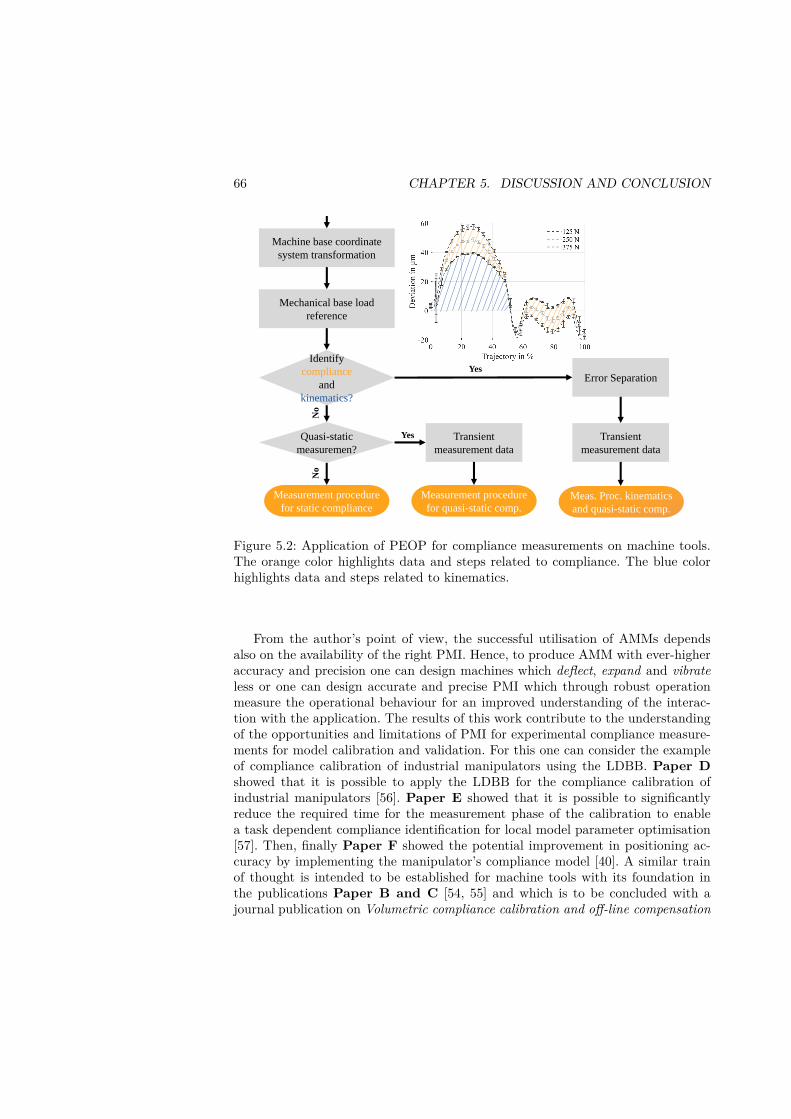
66 CHAPTER 5. DISCUSSION AND CONCLUSION
No
Yes
Machine base coordinate
system transformation
Mechanical base load
reference
Identify
compliance
and
kinematics?
Measurement procedure
for static compliance
Error Separation
Quasi-static
measuremen?
Transient
measurement data
Yes
Measurement procedure
for quasi-static comp.
Transient
measurement data
Meas. Proc. kinematics
and quasi-static comp.
No
Figure 5.2: Application of PEOP for compliance measurements on machine tools.The orange color highlights data and steps related to compliance. The blue colorhighlights data and steps related to kinematics.
From the author’s point of view, the successful utilisation of AMMs dependsalso on the availability of the right PMI. Hence, to produce AMM with ever-higheraccuracy and precision one can design machines which deflect, expand and vibrateless or one can design accurate and precise PMI which through robust operationmeasure the operational behaviour for an improved understanding of the interac-tion with the application. The results of this work contribute to the understandingof the opportunities and limitations of PMI for experimental compliance measure-ments for model calibration and validation. For this one can consider the exampleof compliance calibration of industrial manipulators using the LDBB. Paper Dshowed that it is possible to apply the LDBB for the compliance calibration ofindustrial manipulators [56]. Paper E showed that it is possible to significantlyreduce the required time for the measurement phase of the calibration to enablea task dependent compliance identification for local model parameter optimisation[57]. Then, finally Paper F showed the potential improvement in positioning ac-curacy by implementing the manipulator’s compliance model [40]. A similar trainof thought is intended to be established for machine tools with its foundation inthe publications Paper B and C [54, 55] and which is to be concluded with ajournal publication on Volumetric compliance calibration and off-line compensation
67
for machine tools. Concerning model validation, it needs to be highlighted thatexperimental measurements are costly compared to finite element simulations. Atthe current uncertainties displayed in Figure 2.15, measurements with less than5% uncertainty in the Cartesian stiffness value can only be expected for nominalstiffness of less than 50 N µm−1. Based on the list of uncertainty contributors forthe LDBB-3D, the author suggest to improve PMI for compliance measurement ofAMM by employing similar dimensional measurement instruments, but increasingtheir ability to exert accurate mechanical load vectors.
Furthermore, one needs to consider the compromise which have to be foundbetween the sometimes diametric opposites of theory (metrology) and practice (itsapplication in industry). Metrologists focus on traceability, uncertainty, and cali-bration, while industry focuses on high productivity and low costs. From the puremetrological point of view, the joint set of requirements is usually mutually exclu-sive. At the same time, PMI need to be adaptable to cope with metrology trendssuch as automated uncertainty analysis, large volume coordinate metrology, highdata density, and an ever higher accuracy as well as industry trends such as on-machine integrability, data fusion, absolute measurement, smartness, connectivityand user-friendliness [147]. From an industrial point of view, the resulting PMI needto address the customer requirements within the limits of time, quality, and cost.Namely, the LDBB-3DD employs expensive equipment to measure the dynamicstiffness of a machine tool. These investments render the proposed method onlyapplicable to machine tool designers rather than the machine tool users.
While these requirements are by no means exhaustive or detailed they do provideguidelines which contemporary PMI should follow in order to provide a high utilityvalue for the industry and society as well as science by meeting metrology rules andgood practices.

Chapter 6
Outlook and future work
This work together with the author’s licentiate thesis [4] have argued that theapplication of PMI for the calibration of AMM may have a considerable impacton positioning accuracy. This in turn can lead to added value through off-line andon-line compensation. The foundation described in this thesis as well as in theappended and published papers is meant to be used in the following years for thefollowing activities:
Development of further PMI to support the calibration of AMM, especiallyfor the application on 3-axis machine tools
Calibration procedures that yield potentially higher improvements of the posi-tioning accuracy or lower time and investment requirements for the measurementprocedure
Customised post processors to include the knowledge about calibrated AMMto improve the positioning accuracy
For the development of the customised post processors, there are several chal-lenges beyond the difficulties of the calibration and validation procedures. There isa significant amount of required work for the parsing of the G-code to allow oper-ability across different controllers for AMM. In addition to that, one should aim fora free software solution, which usually requires some additional work.
In addition to that, the author will spend time on the investigation of theuncertainty budget for the Frequency Response Function (FRF) measurement withthe LDBB-3DD. Thus far, it appears that the statement of uncertainty budgets isan uncommon practice for FRF measurements of AMM, while in civil engineeringit is not an uncommon practice [148]. This is probably due to the significantlydifferent bandwidth of several kHz for AMM and several 10th of Hz for buildings.
69

Bibliography
[1] G. Pahl, Ken Wallace, and Luciënne Blessing. Engineering design: A system-atic approach. Springer, London, 3rd ed. edition, 2007. ISBN 9781846283192.
[2] David G. Ullman. The Mechanical Design Process // The mechanical designprocess. McGraw-Hill series in mechanical engineering. McGraw-Hill HigherEducation, Boston, 4th ed. edition, 2010. ISBN 978-0-07-297574-1.
[3] theissen. Gtl 21 probe, 2021. URL https://tesatechnology.com/en-gb/products/palpeurs-de-mesure/palpeurs-axiaux-standards/standard-probes-gt21-%C2%B1-1-mm,-4,3-mm-bolt-travel_p47267.htm.
[4] Nikolas Alexander Theissen. Physics-based modelling and measurement ofadvanced manufacturing machinery’s accuracy: Machine tools and industrialmanipulators - Position, pose and path accuracies. Licentiate, KTH RoyalInstitute of Technology, Stockholm, 2019.
[5] European Association of the Machine Tool Industries. Research & innovation- cecimo. URL https://www.cecimo.eu/policy/reserach-innovation/.
[6] International Federation of Robotics. History, 2018. URL https://ifr.org/robot-history.
[7] Joint Committee for Guides in Metrology. International vocabularyof metrology - basic and general concepts and associated terms (vim),2012. URL https://www.bipm.org/utils/common/documents/jcgm/JCGM_200_2012.pdf.
[8] International Organization for Standardization. Iso 9283:1998 manipulatingindustrial robots - performance criteria and related test methods, 2012.
[9] Sami Chatti and Tullio Tolio. CIRP Encyclopedia of Production Engineering.Springer Berlin Heidelberg, Berlin, Heidelberg, 2019. ISBN 978-3-642-35950-7. doi: 10.1007/978-3-642-35950-7.
71
72 BIBLIOGRAPHY
[10] International Organization for Standardization. Iso 230-1:2012 test code formachine tools — part 1: Geometric accuracy of machines operating underno-load or quasi-static conditions, 2012.
[11] International Organization for Standardization. Iso 13041-2:2008 test condi-tions for numerically controlled turning machines and turning centres - part2: Geometric tests for machines with a vertical workholding spindle, .
[12] International Organization for Standardization. Iso 10791-1:2015 test con-ditions for machining centres – part 1: Geometric tests for machines withhorizontal spindle (horizontal z-axis), .
[13] H. Schwenke, W. Knapp, H. Haitjema, A. Weckenmann, R. Schmitt,and F. Delbressine. Geometric error measurement and compensation ofmachines—an update. CIRP Annals - Manufacturing Technology, 57(2):660–675, 2008. ISSN 00078506. doi: 10.1016/j.cirp.2008.09.008.
[14] Wei Gao. Precision nanometrology: Sensors and measuring systems fornanomanufacturing / Wei Gao. Springer series in advanced manufacturing.Springer, London, 2010. ISBN 9781849962544.
[15] R. K. Leach and S. T. Smith, editors. Basics of precision engineering. Taylor& Francis a CRC title part of the Taylor & Francis imprint a member ofthe Taylor & Francis Group the academic division of T&F Informa plc, BocaRaton, 2018. ISBN 9781498760850.
[16] Ernst Abbe. Messapparate fur physiker. Instrumentenkunde, (10):446–448,1890.
[17] P. A. McKeown. High precision manufacturing and the british economy.Proceedings of the Institution of Mechanical Engineers, Part B: Managementand engineering manufacture, 200(3):147–165, 1986. ISSN 0263-7146.
[18] P. Schellekens, N. Rosielle, H. Vermeulen, M. Vermeulen, S. Wetzels, andW. Pril. Design for precision: Current status and trends. CIRP Annals, 47(2):557–586, 1998. ISSN 00078506. doi: 10.1016/S0007-8506(07)63243-0.
[19] Benjamin Mooring, Zvi S. Roth, and Morris R. Driels. Fundamentals ofmanipulator calibration. Wiley, New York, 1991. ISBN 0471508640.
[20] S. Sartori and G. X. Zhang. Geometric error measurement and compensationof machines. CIRP Annals - Manufacturing Technology, 44(2):599–609, 1995.ISSN 00078506. doi: 10.1016/S0007-8506(07)60507-1.
[21] Simon Winchester. The perfectionists: How precision engineers created themodern world. Harper an imprint of HarperCollinsPublishers, New York,first edition edition, 2018. ISBN 0062652559.
BIBLIOGRAPHY 73
[22] Faro Arm Probing & Accessories | Renishaw Probing & Styli | CMM En-closures. The history of the coordinate measuring machine, 2014. URLhttps://www.cmm-solutions.co.uk/contact-us/cmm-history/.
[23] J. Corbett, P. A. McKeown, G. N. Peggs, and R. Whatmore. Nanotechnology:International developments and emerging products. CIRP Annals, 49(2):523–545, 2000. ISSN 00078506. doi: 10.1016/S0007-8506(07)63454-4.
[24] Christian Brecher and Manfred Weck. Werkzeugmaschinen Fertigungssys-teme. Springer Berlin Heidelberg, Berlin, Heidelberg, 2017. ISBN 978-3-662-46566-0. doi: 10.1007/978-3-662-46567-7.
[25] Bruno Siciliano and Oussama Khatib, editors. Springer Handbook ofRobotics. Springer Science+Business Media, Berlin, Heidelberg, 2008.ISBN 9783540239574. doi: 10.1007/978-3-540-30301-5. URL http://site.ebrary.com/lib/alltitles/docDetail.action?docID=10284823.
[26] Collge International Pour Letude Scientifique Techniques De Production DesMcanique. Wrterbuch der fertigungstechnik: Trennende verfa. Springer, [Placeof publication not identified], softcover reprint of the original 1st ed. 2004edition, 2014. ISBN 978-3-642-62382-0.
[27] Y. Altintas, C. Brecher, M. Weck, and S. Witt. Virtual machine tool. CIRPAnnals, 54(2):115–138, 2005. ISSN 00078506. doi: 10.1016/S0007-8506(07)60022-5.
[28] Karoly Szipka, Paul Dax, Andreas Archenti, Florian Degen, and MikaelHedlind. Integration of machining system capability information into a caxsoftware environment for complex tool trajectory prediction. Procedia CIRP,72:1239–1244, 2018. ISSN 22128271. doi: 10.1016/j.procir.2018.03.015.
[29] Károly Szipka. Uncertainty Management for Automated Diagnostics of Pro-duction Machinery. PhD thesis, KTH, Production Engineering, 2020.
[30] Klaus Erlach. Value Stream Design. Springer Berlin Heidelberg, Berlin, Hei-delberg, 2013. ISBN 978-3-642-12568-3. doi: 10.1007/978-3-642-12569-0.
[31] Andreas Archenti, editor. A Computational Framework for Control of Ma-chining System Capability: From Formulation to Implementation. Stockholmand Sweden, 2011. ISBN 978-91-7501-162-2.
[32] Andreas Archenti and Mihai Nicolescu. Accuracy analysis of machine toolsusing elastically linked systems. CIRP Annals - Manufacturing Technology,62(1):503–506, 2013. ISSN 00078506. doi: 10.1016/j.cirp.2013.03.100.
[33] George Lichtheim. The concept of ideology. History and Theory, 4(2):164,1965. ISSN 00182656. doi: 10.2307/2504150.
74 BIBLIOGRAPHY
[34] Neil Murray and David Beglar. Inside track: Writing dissertations and theses.Inside track. Pearson Longman, Harlow England and New York, 2009. ISBN0273721704.
[35] Paul Arthur Schilpp. The philosophy of Karl Popper, volume v14 of TheLibrary of living philosophers. Open Court, La Salle, Ill., 1974. ISBN0875481426.
[36] A. C. Grayling. An introduction to philosophical logic. Blackwell Pub, Malden,Mass, 3rd ed., 16th printing edition, 2013. ISBN 0631199829.
[37] Christopher A. Mattson and Carl David Sorensen. Product development:Principles and tools for creating desirable and transferable designs / Christo-pher A. Mattson, Carl D. Sorensen. Springer, Cham, Switzerland, 2020. ISBN9783030148997.
[38] Stephen Timoshenko. History of strength of materials: With a brief account ofthe history of theory of elasticity and theory of structures / Stephen P. Tim-oshenko. Dover and London : Constable, New York, 1983. ISBN 0486611876.
[39] M. F. Ashby. Materials selection in mechanical design, fourth edition. Else-vier, Burlington, Mass, 4th ed. edition, 2011. ISBN 1856176630.
[40] Monica Katherine Gonzalez, Nikolas Alexander Theissen, Asier Barrios, andAndreas Archenti. Online compliance error compensation system for indus-trial manipulators in contact applications: Submitted for review. 2022.
[41] Sveriges Riksdag Utbildningsdepartementet. Högskoleförordning(1993:100), 1993. URL https://www.riksdagen.se/sv/dokument-lagar/dokument/svensk-forfattningssamling/hogskoleforordning-1993100_sfs-1993-100.
[42] Gro Harlem Brundtland. Report of the world commission on environmentanddevelopment: Our common future, 1987.
[43] Jeffrey D. Sachs, Guido Schmidt-Traub, Mariana Mazzucato, Dirk Messner,Nebojsa Nakicenovic, and Johan Rockström. Six transformations to achievethe sustainable development goals. Nature Sustainability, 2(9):805–814, 2019.doi: 10.1038/s41893-019-0352-9.
[44] Patrick Schroeder, Kartika Anggraeni, and Uwe Weber. The relevance ofcircular economy practices to the sustainable development goals. Journal ofIndustrial Ecology, 23(1):77–95, 2019. ISSN 1088-1980. doi: 10.1111/jiec.12732.
[45] Mehdi Khosrow-Pour. Encyclopedia of information science and technology.IGI Global (701 E. Chocolate Avenue, Hershey, Pennsylvania, 17033, USA),Hershey, Pa., 2005. ISBN 978-1591405535.
BIBLIOGRAPHY 75
[46] Anthony R. Lanfranco, Andres E. Castellanos, Jaydev P. Desai, andWilliam C. Meyers. Robotic surgery: a current perspective. Annals of surgery,239(1):14–21, 2004. ISSN 0003-4932. doi: 10.1097/01.sla.0000103020.19595.7d.
[47] Murilo Marques Marinho, Bruno Vilhena Adorno, Kanako Harada, KyoichiDeie, Anton Deguet, Peter Kazanzides, Russell H. Taylor, and Mitsuishi Ma-muro. A unified framework for the teleoperation of surgical robots in con-strained workspaces. 2019.
[48] Yushiro Tomiki, Murilo Marinho, Yusuke Kurose, Kanako Harade, and Mit-suishi Mamuro. On the use of general-purpose serial-link manipulators ineye surgery: June 28-july 1, 2017, maison glad jeju, jeju, korea. In URAI2017, 2017. URL http://ieeexplore.ieee.org/servlet/opac?punumber=7983000.
[49] G. Dagnino, I. Georgilas, P. Tarassoli, R. Atkins, and S. Dogramadzi.Design and real-time control of a robotic system for fracture manipula-tion. In 2015 37th annual international conference of the IEEE Engineer-ing in Medicine and Biology Society (EMBC), Piscataway, NJ, 2015. IEEE.ISBN 9781424492695. URL http://ieeexplore.ieee.org/servlet/opac?punumber=7302811.
[50] Giuseppe Turchetti, Ilaria Palla, Francesca Pierotti, and Alfred Cuschieri.Economic evaluation of da vinci-assisted robotic surgery: a systematic review.Surgical endoscopy, 26(3):598–606, 2012. doi: 10.1007/s00464-011-1936-2.
[51] COMM/DG/UNIT. Transport emissions - climate action - european commis-sion, 2019. URL https://ec.europa.eu/clima/policies/transport_en.
[52] Joachim H. Spangenberg, Alastair Fuad-Luke, and Karen Blincoe. Design forsustainability (dfs): the interface of sustainable production and consumption.Journal of Cleaner Production, 18(15):1485–1493, 2010. ISSN 09596526. doi:10.1016/j.jclepro.2010.06.002.
[53] Nikolas Alexander Theissen, Monica Katherine Gonzalez, Theodoros Laspas,and Andreas Archenti. Measurement and identification of dynamic transla-tional stiffness matrix on machine tools under static preloads. In EUSPENGA 21st International Conference and Exhibition 7th – 11th June 2021.
[54] Nikolas Alexander Theissen, Theodoros Laspas, Stefan Cedergren, and An-dreas Archenti. Measurement for the identification of static and quasi-staticrotational stiffness. Precision Engineering, 72:215–223, 2021. ISSN 01416359.doi: 10.1016/j.precisioneng.2021.04.011.
[55] Theodoros Laspas, Nikolas Alexander Theissen, and Andreas Archenti. Novelmethodology for the measurement and identification for quasi-static stiffness
76 BIBLIOGRAPHY
of five-axis machine tools. Precision Engineering, 65:164–170, 2020. ISSN01416359. doi: 10.1016/j.precisioneng.2020.06.006.
[56] Nikolas Alexander Theissen, Theodoros Laspas, and Andreas Archenti.Closed-force-loop elastostatic calibration of serial articulated robots. Roboticsand Computer-Integrated Manufacturing, 57:86–91, 2019. ISSN 07365845. doi:10.1016/j.rcim.2018.07.007.
[57] Nikolas Alexander Theissen, Monica Katherine Gonzalez, Asier Barrios, andAndreas Archenti. Quasi-static compliance calibration of serial articulatedindustrial manipulators. International Journal of Automation Technology, 15(5):590–598, 2021. ISSN 1881-7629. doi: 10.20965/ijat.2021.p0590.
[58] Soichi Ibaraki, Nikolas Alexander Theissen, Andreas Archenti, and Md. Mok-tadir Alam. Evaluation of kinematic and compliance calibration of serial ar-ticulated industrial manipulators. International Journal of Automation Tech-nology, 15(5):567–580, 2021. ISSN 1881-7629. doi: 10.20965/ijat.2021.p0567.
[59] Eugene I. Rivin. Handbook on stiffness & damping in mechanical design.ASME Press, New York, 2010. ISBN 9780791802939.
[60] Festo AG & Co. Proportional pressure control valve veaa-l-3-d11-q4-v1-1r1, 2021. URL https://www.festo.com/us/en/a/download-document/datasheet/8046905.
[61] Micro-Epsilon. indusensor-lvdt, 2017. URL https://www.micro-epsilon.com/download/products/cat-indu-lvdt/dax--induSENSOR-LVDT-Taster--en-us.html.
[62] Bluetooth - wikipedia, 7/4/2021. URL https://en.wikipedia.org/wiki/Bluetooth.
[63] Parallel pre-stressed actuator - ppa40l - cedrat technologies, 7/5/2021. URLhttps://www.cedrat-technologies.com/en/products/product/PPA40L.html.
[64] Series 1053|force sensor|dytran, 7/5/2021. URL https://www.dytran.com/Model-1053V1-IEPE-Force-Sensor-P1716.
[65] Lion Precision. User manual | cpl190/cpl290 | lion precision, 2020.URL https://www.lionprecision.com/user-manual-cpl190cpl290/#PowerSpecs.
[66] Alan F.C. Pollard. The mechanical design of scientific instruments. Journalof the Royal Society of Arts, 1922.
[67] Wayne R. Moore. Foundations of mechanical accuracy. Moore Special ToolCo, 1970.

BIBLIOGRAPHY 77
[68] E. G. Loewen. Metrology problems in general engineering: A comparison withprecision engineering. CIRP Annals, 29(2):451–453, 1980. ISSN 00078506.doi: 10.1016/S0007-8506(16)30138-X.
[69] Norio Taniguchi. Current status in, and future trends of, ultraprecision ma-chining and ultrafine materials processing. CIRP Annals, 32(2):573–582, 1983.ISSN 00078506. doi: 10.1016/S0007-8506(07)60185-1.
[70] Alexander H. Slocum. Precision machine design. Prentice Hall, EnglewoodCliffs, N.J, [nachdr.] edition, 1992. ISBN 0136909183.
[71] S. T. Smith. Foundations of Ultra-Precision Mechanism Design, volume 2 ofDevelopments in Nanotechnology. C R C Press LLC and Taylor & FrancisGroup [distributor], Boca Raton and Florence, repr edition, Oct. 1994. ISBN2884490019.
[72] Layton Carter Hale. Principles and techniques for designing precision ma-chines. Doctoral, CA, USA, 1999.
[73] Samir Mekid. Introduction to Precision Machine Design and Error As-sessment. Mechanical and Aerospace Engineering Series. Taylor and Fran-cis, Hoboken, 2008. ISBN 9780849378867. URL http://gbv.eblib.com/patron/FullRecord.aspx?p=1388901.
[74] Jose A. Yagüe-Fabra, Wei Gao, Andreas Archenti, Edward Morse, and AlkanDonmez. Scalability of precision design principles for machines and instru-ments. CIRP Annals, 2021. ISSN 00078506. doi: 10.1016/j.cirp.2021.05.004.
[75] Hans-Christian Möhring, Christian Brecher, Eberhard Abele, Jürgen Fleis-cher, and Friedrich Bleicher. Materials in machine tool structures. CIRPAnnals, 64(2):725–748, 2015. ISSN 00078506. doi: 10.1016/j.cirp.2015.05.005.
[76] Zhi Yong Ma, Pei En Feng, Jian Zhang, and Ling Bin Zeng. Research on me-chanics symmetry ontology. In S. I. Ao, editor, The 2008 International Con-ference of Applied and Engineering Mathematics, Lecture notes in engineeringand computer science, pages 1478–1486, Hong Kong, 2008. IAENG. ISBN9789881701237. URL http://iaeng.org/publication/WCE2008/WCE2008_pp1478-1486.pdf.
[77] L. Uriarte, M. Zatarain, D. Axinte, J. Yagüe-Fabra, S. Ihlenfeldt, J. Eguia,and A. Olarra. Machine tools for large parts. CIRP Annals, 62(2):731–750,2013. ISSN 00078506. doi: 10.1016/j.cirp.2013.05.009.
[78] Josef Mayr, Jerzy Jedrzejewski, Eckart Uhlmann, M. Alkan Donmez, Wolf-gang Knapp, Frank Härtig, Klaus Wendt, Toshimichi Moriwaki, Paul Shore,Robert Schmitt, Christian Brecher, Timo Würz, and Konrad Wegener. Ther-mal issues in machine tools. CIRP Annals, 61(2):771–791, 2012. ISSN00078506. doi: 10.1016/j.cirp.2012.05.008.
78 BIBLIOGRAPHY
[79] Witold Nowacki. Thermoelasticity. Pergamon, Oxford, 2nd ed. edition, 1986.ISBN 0080247679.
[80] Eugen Trapet, Juan-José Aguilar Martín, José-Antonio Yagüe, Henny Spaan,and Vit Zelený. Self-centering probes with parallel kinematics to verifymachine-tools. Precision Engineering, 30(2):165–179, 2006. ISSN 01416359.doi: 10.1016/j.precisioneng.2005.07.002.
[81] B. Bringmann and W. Knapp. Model-based ‘chase-the-ball’ calibration of a5-axes machining center. CIRP Annals, 55(1):531–534, 2006. ISSN 00078506.doi: 10.1016/S0007-8506(07)60475-2.
[82] True-range multilateration, 10/03/2021. URL https://en.wikipedia.org/wiki/True-range_multilateration.
[83] Paweł Majda and Joanna Jastrzębska. Measurement uncertainty of gen-eralized stiffness of machine tools. Measurement, 170:108692, 2021. ISSN02632241. doi: 10.1016/j.measurement.2020.108692.
[84] Deutsches Institut fur Normung. Balls for rolling bearings and general indus-trial use, 2002.
[85] International Organization for Standardization. Iso 1101:2017 geometricalproduct specifications (gps) — geometrical tolerancing — tolerances of form,orientation, location and run-out, 2017.
[86] Chris J. Evans, Robert J. Hocken, and W. Tyler Estler. Self-calibration:Reversal, redundancy, error separation, and ‘absolute testing’. CIRP Annals,45(2):617–634, 1996. ISSN 00078506. doi: 10.1016/S0007-8506(07)60515-0.
[87] SSAB. The pre-hardened, exceptionally clean tool and engineeringsteel, 8/19/2021. URL https://www.ssab.com/products/brands/toolox/products/toolox-33.
[88] G. X. Zhang. A study on the abbe principle and abbe error. CIRP Annals,38(1):525–528, 1989. ISSN 00078506. doi: 10.1016/S0007-8506(07)62760-7.
[89] Károly Szipka, Andreas Archenti, Gregory W. Vogl, and M. Alkan Donmez.Identification of machine tool squareness errors via inertial measurements.CIRP Annals, 68(1):547–550, 2019. ISSN 00078506. doi: 10.1016/j.cirp.2019.04.070.
[90] J. B. Bryan. The abbé principle revisited: An updated interpretation.Precision Engineering, 1(3):129–132, 1979. ISSN 01416359. doi: 10.1016/0141-6359(79)90037-0.
BIBLIOGRAPHY 79
[91] Paulo Flores. A methodology for quantifying the kinematic position errorsdue to manufacturing and assembly tolerances. Strojniški vestnik – Journalof Mechanical Engineering, 57(06):457–467, 2011. ISSN 00392480. doi: 10.5545/sv-jme.2009.159.
[92] Chris Evans. Precision engineering: An evolutionary view. 1989. ISBN1871315018.
[93] Martin L. Culpepper. Design and Application of Compliant Quasi-KinematicCouplings. Doctor of philosophy in mechanical engineering, MassachusettsInstitute of Technology, Massachusetts, USA, 2000.
[94] P. A. McKeown. The role of precision engineering in manufacturing of thefuture. CIRP Annals, 36(2):495–501, 1987. ISSN 00078506. doi: 10.1016/S0007-8506(07)60751-3.
[95] Holonomic constraints, 14/03/2021. URL https://en.wikipedia.org/wiki/Holonomic_constraints.
[96] David Dornfeld and Dae-Eun Lee. Precision manufacturing. Springer, NewYork, NY, 2008. ISBN 0387324674. URL http://deposit.dnb.de/cgi-bin/dokserv?id=2813547&prov=M&dok_var=1&dok_ext=htm.
[97] Gerard Johannes Pieter Nijsse. Linear motion systems: A modular ap-proach for improved straightness performance. DUP, Delft, 2001. ISBN 978-9040721878.
[98] Alexander Slocum. Kinematic couplings: A review of design principles andapplications. International Journal of Machine Tools and Manufacture, 50(4):310–327, 2010. ISSN 08906955. doi: 10.1016/j.ijmachtools.2009.10.006.
[99] Y. Y. Chen, R. C. Wu, F. C. Wang, and J. Y. Yen. Sensor layouts for along-stroke nano-positioning stage. In 2014 Proceedings of the SICE AnnualConference (SICE), pages 432–437. IEEE, 9/9/2014 - 9/12/2014. ISBN 978-4-9077-6446-3. doi: 10.1109/SICE.2014.6935203.
[100] Jon S. Wilson. Sensor technology handbook. Elsevier, Amsterdam and Boston,2005. ISBN 0750677295.
[101] Joint Committee for Guides in Metrology. Evaluation of measurement data:Guide to the expression of uncertainty in measurement.
[102] Christian Brecher, Dennis Rempel, Hans-Martin Eckel, and Marcel Fey. Ein-fluss dynamischer prozesslasten auf das betriebs- und verschleisverhalten: Ab-bildung dynamischer kräfte gestattet prufstandversuche an werkzeugmaschi-nenkomponenten. VDI-Z, (9), 2017.
80 BIBLIOGRAPHY
[103] Sebastian Böhl, Sascha Weikert, and Konrad Wegener. Improving robust-ness of capacitive displacement measurements against electromagnetic dis-turbances in machine tool environments. Lamdamap, 13:1, 2019.
[104] Olivier Andre Bauchau. Flexible multibody dynamics, volume v. 176 of Solidmechanics and its applications, 0925-0042. Springer, Dordrecht, 2011. ISBN978-94-007-0334-6. doi: 10.1007/978-94-007-0335-3.
[105] Hexagon Manufacturing Intelligence. Portable measuring arms, 23/03/2021.URL https://www.hexagonmi.com/products/portable-measuring-arms.
[106] Renishaw plc. Renishaw: Equator™ gauging system, 23/03/2021. URLhttps://www.renishaw.com/en/equator-gauging-system--12595.
[107] Kevin M. Lynch and Frank C. Park. Modern Robotics: Mechanics, Plan-ning, and Control. Cambridge University Press, Cambridge, 2017. ISBN9781107156302.
[108] Gustav Niemann, Hans Winter, and Bernd-Robert Höhn. Maschinen-elemente. Springer, Berlin, 3. aufl. edition, 2001. ISBN 3540658165.
[109] G. Otten, T.J.A. de Vries, J. van Amerongen, A. M. Rankers, and E. W.Gaal. Linear motor motion control using a learning feedforward con-troller. IEEE/ASME Transactions on Mechatronics, 2(3):179–187, 1997.ISSN 10834435. doi: 10.1109/3516.622970.
[110] Jung-Jae Kim, Young-Man Choi, Dahoon Ahn, Beomseok Hwang, Dae-GabGweon, and Jaehwa Jeong. A millimeter-range flexure-based nano-positioningstage using a self-guided displacement amplification mechanism. Mechanismand Machine Theory, 50:109–120, 2012. ISSN 0094114X. doi: 10.1016/j.mechmachtheory.2011.11.012.
[111] J. Bryan. International status of thermal error research (1990). CIRP Annals,39(2):645–656, 1990. ISSN 00078506. doi: 10.1016/S0007-8506(07)63001-7.
[112] C. Brecher, P. Hirsch, and M. Weck. Compensation of thermo-elastic machinetool deformation based on control internal data. CIRP Annals, 53(1):299–304,2004. ISSN 00078506. doi: 10.1016/S0007-8506(07)60702-1.
[113] T. Holkup, H. Cao, P. Kolář, Y. Altintas, and J. Zelený. Thermo-mechanicalmodel of spindles. CIRP Annals, 59(1):365–368, 2010. ISSN 00078506. doi:10.1016/j.cirp.2010.03.021.
[114] Rui Li and Yang Zhao. Dynamic error compensation for industrial robot basedon thermal effect model. Measurement, 88:113–120, 2016. ISSN 02632241. doi:10.1016/j.measurement.2016.02.038.

BIBLIOGRAPHY 81
[115] Janine Glänzel, Steffen Ihlenfeldt, C. Christian Naumann, and Matthias Putz.Decoupling of fluid and thermo-elastic simulations on machine tools usingcharacteristic diagrams. Procedia CIRP, 62:340–345, 2017. ISSN 22128271.doi: 10.1016/j.procir.2016.06.068.
[116] Jin-Hyeon Lee and Seung-Han Yang. Statistical optimization and assessmentof a thermal error model for cnc machine tools. International Journal ofMachine Tools and Manufacture, 42(1):147–155, 2002. ISSN 08906955. doi:10.1016/S0890-6955(01)00110-9.
[117] Roland Unruh, Frank Schafmeister, and Joachim Bocker. 11kw, 70khz llcconverter design with adaptive input voltage for 98% efficiency in an mmc.In 2020 IEEE 21st Workshop on Control and Modeling for Power Electronics(COMPEL), pages 1–8. IEEE, 1192020. ISBN 978-1-7281-7160-9. doi: 10.1109/COMPEL49091.2020.9265771.
[118] Robert Munnig Schmidt. The design of high performance mechatronics: High-tech functionality by multidisciplinary system integration. Delft UniversityPress, Amsterdam, 2nd revised edition edition, 2014. ISBN 978-1614993674.
[119] Makoto Iwasaki, Kenta Seki, and Yoshihiro Maeda. High-precision motioncontrol techniques: A promising approach to improving motion performance.IEEE Industrial Electronics Magazine, 6(1):32–40, 2012. ISSN 1932-4529.doi: 10.1109/MIE.2012.2182859.
[120] Gene F. Franklin, J. David Powell, and Abbas Emami-Naeini. Feedback con-trol of dynamic systems. Pearson, Upper Saddle River (N.J.), 7th editionedition, 2015. ISBN 9780133496598.
[121] Michael Trenk, Matthias Franke, and Heinrich Schwenke. The “virtual cmm”a software tool for uncertainty evaluation–practical application in an accred-ited calibration lab. Proc. of ASPE: Uncertainty Analysis in Measurementand Design, 9:68–75, 2004.
[122] Tomas Olsson, Mathias Haage, Henrik Kihlman, Rolf Johansson, Klas Nils-son, Anders Robertsson, Mats Björkman, Robert Isaksson, Gilbert Ossbahr,and Torgny Brogårdh. Cost-efficient drilling using industrial robots with high-bandwidth force feedback. Robotics and Computer-Integrated Manufacturing,26(1):24–38, 2010. ISSN 07365845. doi: 10.1016/j.rcim.2009.01.002.
[123] Alexandr Klimchik, Dmitry Bondarenko, Anatol Pashkevich, Sébastien Briot,and Benoît Furet. Compliance error compensation in robotic-based milling.283:197–216. doi: 10.1007/978-3-319-03500-0{\textunderscore}13.
[124] Zheng Wang, Runan Zhang, and Patrick Keogh. Real-time laser tracker com-pensation of robotic drilling and machining. Journal of Manufacturing andMaterials Processing, 4(3):79, 2020. doi: 10.3390/jmmp4030079.
82 BIBLIOGRAPHY
[125] R. Neugebauer, B. Denkena, and K. Wegener. Mechatronic systems formachine tools. CIRP Annals, 56(2):657–686, 2007. ISSN 00078506. doi:10.1016/j.cirp.2007.10.007.
[126] Károly Szipka. Modelling and Management of Uncertainty in ProductionSystems: From Measurement to Decision, volume 2018:37 of TRITA-ITM-AVL. KTH Royal Institute of Technology, Stockholm, 2018.
[127] W. Knapp. Measurement uncertainty and machine tool testing. CIRP Annals,51(1):459–462, 2002. ISSN 00078506. doi: 10.1016/S0007-8506(07)61560-1.
[128] S. Weikert. R-test, a new device for accuracy measurements on five axismachine tools. CIRP Annals, 53(1):429–432, 2004. ISSN 00078506. doi:10.1016/S0007-8506(07)60732-X.
[129] Albert Nubiola and Ilian A. Bonev. Absolute calibration of an abb irb 1600robot using a laser tracker. Robotics and Computer-Integrated Manufacturing,29(1):236–245, 2013. ISSN 07365845. doi: 10.1016/j.rcim.2012.06.004.
[130] International Organization for Standardization. Iso 230-4:2005 test code formachine tools – part 4: Circular tests for numerically controlled machine tools,.
[131] E. Abele, Y. Altintas, and C. Brecher. Machine tool spindle units. CIRPAnnals, 59(2):781–802, 2010. ISSN 00078506. doi: 10.1016/j.cirp.2010.05.002.
[132] Stephen Boyd and Lieven Vandenberghe. Introduction to Applied LinearAlgebra. Cambridge University Press, 2019. ISBN 9781316518960. doi:10.1017/9781108583664.
[133] Izhak Bucher. Circle fit. URL https://www.mathworks.com/matlabcentral/fileexchange/5557-circle-fit.
[134] International Organization for Standardization. Iso 8373:2012 robots androbotic devices – vocabulary, .
[135] R. H. Schmitt, M. Peterek, E. Morse, W. Knapp, M. Galetto, F. Härtig,G. Goch, B. Hughes, A. Forbes, and W. T. Estler. Advances in large-scalemetrology – review and future trends. CIRP Annals, 65(2):643–665, 2016.ISSN 00078506. doi: 10.1016/j.cirp.2016.05.002.
[136] Gonzalez Monica, Hosseini Arian, Theissen Nikolas Alexander, and ArchentiAndreas. Quasi-static loaded circular testing of serial articulated industrialmanipulators. In ISR 2020; 52th International Symposium on Robotics, pages1–6, 2020.

BIBLIOGRAPHY 83
[137] Károly Szipka, Theodoros Laspas, and Andreas Archenti. Measurement andanalysis of machine tool errors under quasi-static and loaded conditions. Pre-cision Engineering, 2017. ISSN 01416359. doi: 10.1016/j.precisioneng.2017.07.011.
[138] Jorge Santolaria, Javier Conte, Marcos Pueo, and Carlos Javierre. Rotationerror modeling and identification for robot kinematic calibration by circlepoint method. Metrology and Measurement Systems, 21(1):85–98, 2014. ISSN0860-8229. doi: 10.2478/mms-2014-0009.
[139] H. Zhang, J. Wang, G. Zhang, and Z. Gan. Machining with flexible ma-nipulator: Toward improving robotic machining performance: 2005 ieee/asmeinternational conference on advanced intelligent mechatronics [proceedings]monterey, ca, july 24-28, 2005. 2005.
[140] Arian Hosseini. Modelling and Measurement of Industrial Manipulators forHigh-Precision Contact Applications. Master of science, KTH Royal Instituteof Technology, Stockholm, Sweden, 2019.
[141] Eric R. Marsh, David A. Arneson, and Donald L. Martin. A comparison ofreversal and multiprobe error separation. Precision Engineering, 34(1):85–91,2010. ISSN 01416359. doi: 10.1016/j.precisioneng.2009.03.001.
[142] Han Haitjema. Revisiting the multi-step method: Enhanced error separationand reduced amount of measurements. CIRP Annals, 64(1):491–494, 2015.ISSN 00078506. doi: 10.1016/j.cirp.2015.03.001.
[143] Mohamed Slamani, Albert Nubiola, and Ilian A. Bonev. Modeling and assess-ment of the backlash error of an industrial robot. Robotica, 30(7):1167–1175,2012. ISSN 0263-5747. doi: 10.1017/S0263574711001287.
[144] International Organization for Standardization. Iso 10791-6:2007 test condi-tions for machining centres - part 6: Accuracy of speeds and interpolations,.
[145] Kaveh Kamali, Ahmed Joubair, Ilian A. Bonev, and Pascal Bigras. Elasto-geometrical calibration of an industrial robot under multidirectional externalloads using a laser tracker. In IEEE International Conference on Robotics andAutomation (ICRA), 2016. URL http://ieeexplore.ieee.org/servlet/opac?punumber=7478842.
[146] Soichi Ibaraki, Yu Nagai, Hisashi Otsubo, Yasutaka Sakai, Shigeki Morimoto,and Yosuke Miyazaki. R-test analysis software for error calibration of five-axis machine tools – application to a five-axis machine tool with two rotaryaxes on the tool side –. International Journal of Automation Technology, 9(4):387–395, 2015. ISSN 1881-7629. doi: 10.20965/ijat.2015.p0387.

84 BIBLIOGRAPHY
[147] International Electrotechnical Commission. Factory of the future, 2015. URLhttps://www.iec.ch/whitepaper/futurefactory/.
[148] Yan-Chun Ni, Feng-Liang Zhang, Heung-Fai Lam, and Siu-Kui Au. Fastbayesian approach for modal identification using free vibration data, partii—posterior uncertainty and application. Mechanical Systems and SignalProcessing, 70-71:221–244, 2016. ISSN 08883270. doi: 10.1016/j.ymssp.2015.06.009.
Appended publications
Paper A
Theissen, N.A.; Gonzalez, M.K.; Laspas, T.; and Archenti A. (2021): Measurementand identification of dynamic translational stiffness matrix on machine tools understatic preloadsIn: European Society for Precision Engineering and Nanotechnology (2021): 21st
International Conference and Exhibition 7th – 11th June 2021.
Summary: This work presents a measurement procedure for the identifica-tion of the full translational dynamic stiffness matrix for a single configura-tion of a machine tool under loaded conditions. The manuscript presents acase study on a 5-axis machining centre.
Background and contribution: The author was responsible for the coor-dination of the research work, the design as well as the manufacture of thePMI, and the measurement of the 5-axis machine tool for the case study.The manuscript was written jointly.
85
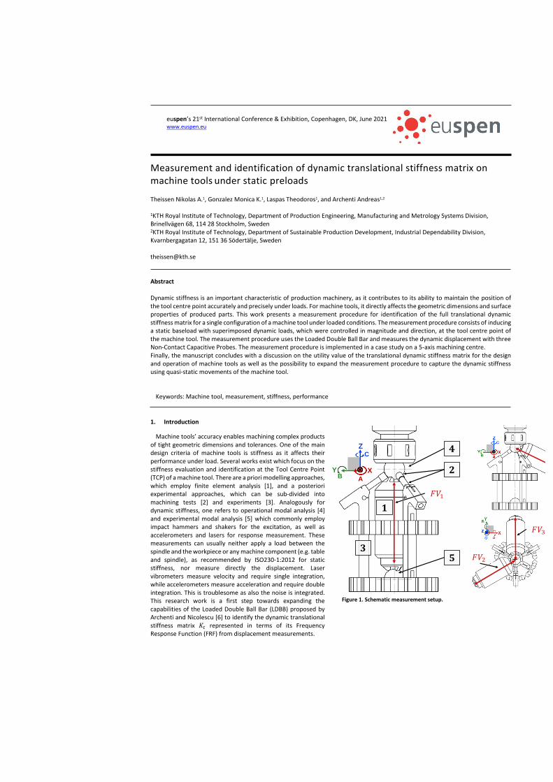
euspen’s 21st International Conference & Exhibition, Copenhagen, DK, June 2021 www.euspen.eu
Measurement and identification of dynamic translational stiffness matrix on machine tools under static preloads
Theissen Nikolas A.1, Gonzalez Monica K.1, Laspas Theodoros1, and Archenti Andreas1,2
1KTH Royal Institute of Technology, Department of Production Engineering, Manufacturing and Metrology Systems Division, Brinellvägen 68, 114 28 Stockholm, Sweden 2KTH Royal Institute of Technology, Department of Sustainable Production Development, Industrial Dependability Division, Kvarnbergagatan 12, 151 36 Södertälje, Sweden
Abstract
Dynamic stiffness is an important characteristic of production machinery, as it contributes to its ability to maintain the position of the tool centre point accurately and precisely under loads. For machine tools, it directly affects the geometric dimensions and surface properties of produced parts. This work presents a measurement procedure for identification of the full translational dynamic stiffness matrix for a single configuration of a machine tool under loaded conditions. The measurement procedure consists of inducing a static baseload with superimposed dynamic loads, which were controlled in magnitude and direction, at the tool centre point of the machine tool. The measurement procedure uses the Loaded Double Ball Bar and measures the dynamic displacement with three Non-Contact Capacitive Probes. The measurement procedure is implemented in a case study on a 5-axis machining centre. Finally, the manuscript concludes with a discussion on the utility value of the translational dynamic stiffness matrix for the design and operation of machine tools as well as the possibility to expand the measurement procedure to capture the dynamic stiffness using quasi-static movements of the machine tool.
Keywords: Machine tool, measurement, stiffness, performance
1. Introduction
Machine tools’ accuracy enables machining complex products of tight geometric dimensions and tolerances. One of the main design criteria of machine tools is stiffness as it affects their performance under load. Several works exist which focus on the stiffness evaluation and identification at the Tool Centre Point (TCP) of a machine tool. There are a priori modelling approaches, which employ finite element analysis [1], and a posteriori experimental approaches, which can be sub-divided into machining tests [2] and experiments [3]. Analogously for dynamic stiffness, one refers to operational modal analysis [4] and experimental modal analysis [5] which commonly employ impact hammers and shakers for the excitation, as well as accelerometers and lasers for response measurement. These measurements can usually neither apply a load between the spindle and the workpiece or any machine component (e.g. table and spindle), as recommended by ISO230-1:2012 for static stiffness, nor measure directly the displacement. Laser vibrometers measure velocity and require single integration, while accelerometers measure acceleration and require double integration. This is troublesome as also the noise is integrated. This research work is a first step towards expanding the capabilities of the Loaded Double Ball Bar (LDBB) proposed by Archenti and Nicolescu [6] to identify the dynamic translational stiffness matrix 𝐾𝑡 represented in terms of its Frequency Response Function (FRF) from displacement measurements.
Figure 1. Schematic measurement setup.
Y
Z
X
C
AB
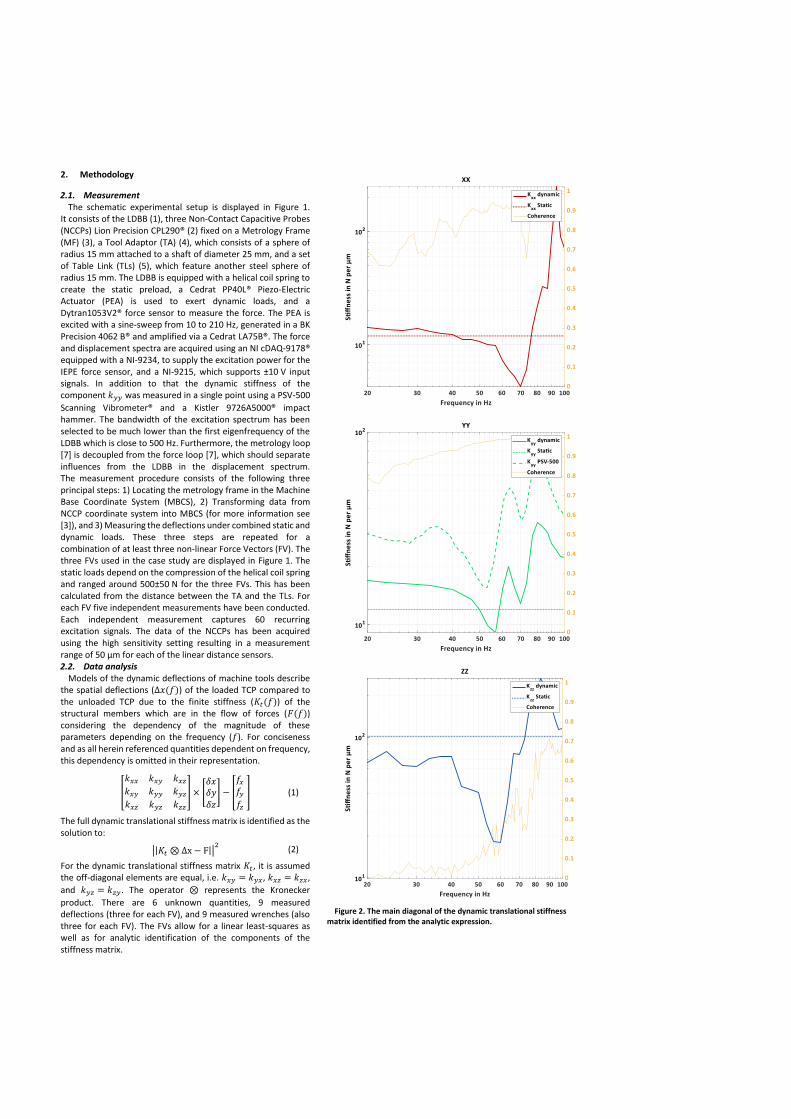
2. Methodology
2.1. Measurement The schematic experimental setup is displayed in Figure 1.
It consists of the LDBB (1), three Non-Contact Capacitive Probes (NCCPs) Lion Precision CPL290® (2) fixed on a Metrology Frame (MF) (3), a Tool Adaptor (TA) (4), which consists of a sphere of radius 15 mm attached to a shaft of diameter 25 mm, and a set of Table Link (TLs) (5), which feature another steel sphere of radius 15 mm. The LDBB is equipped with a helical coil spring to create the static preload, a Cedrat PP40L® Piezo-Electric Actuator (PEA) is used to exert dynamic loads, and a Dytran1053V2® force sensor to measure the force. The PEA is excited with a sine-sweep from 10 to 210 Hz, generated in a BK Precision 4062 B® and amplified via a Cedrat LA75B®. The force and displacement spectra are acquired using an NI cDAQ-9178® equipped with a NI-9234, to supply the excitation power for the IEPE force sensor, and a NI-9215, which supports ±10 V input signals. In addition to that the dynamic stiffness of the component 𝑘𝑦𝑦 was measured in a single point using a PSV-500
Scanning Vibrometer® and a Kistler 9726A5000® impact hammer. The bandwidth of the excitation spectrum has been selected to be much lower than the first eigenfrequency of the LDBB which is close to 500 Hz. Furthermore, the metrology loop [7] is decoupled from the force loop [7], which should separate influences from the LDBB in the displacement spectrum. The measurement procedure consists of the following three principal steps: 1) Locating the metrology frame in the Machine Base Coordinate System (MBCS), 2) Transforming data from NCCP coordinate system into MBCS (for more information see [3]), and 3) Measuring the deflections under combined static and dynamic loads. These three steps are repeated for a combination of at least three non-linear Force Vectors (FV). The three FVs used in the case study are displayed in Figure 1. The static loads depend on the compression of the helical coil spring and ranged around 500±50 N for the three FVs. This has been calculated from the distance between the TA and the TLs. For each FV five independent measurements have been conducted. Each independent measurement captures 60 recurring excitation signals. The data of the NCCPs has been acquired using the high sensitivity setting resulting in a measurement range of 50 µm for each of the linear distance sensors. 2.2. Data analysis
Models of the dynamic deflections of machine tools describe the spatial deflections (Δ𝑥(𝑓)) of the loaded TCP compared to the unloaded TCP due to the finite stiffness (𝐾𝑡(𝑓)) of the structural members which are in the flow of forces ( (𝑓)) considering the dependency of the magnitude of these parameters depending on the frequency (𝑓). For conciseness and as all herein referenced quantities dependent on frequency, this dependency is omitted in their representation.
[
𝑘𝑥𝑥 𝑘𝑥𝑦 𝑘𝑥𝑧𝑘𝑥𝑦 𝑘𝑦𝑦 𝑘𝑦𝑧𝑘𝑥𝑧 𝑘𝑦𝑧 𝑘𝑧𝑧
] × [𝛿𝑥𝛿𝑦𝛿𝑧
] − [
𝑓𝑥𝑓𝑦𝑓𝑧
] (1)
The full dynamic translational stiffness matrix is identified as the solution to:
||𝐾𝑡 ⊗Δx − F||
(2)
For the dynamic translational stiffness matrix 𝐾𝑡, it is assumed the off-diagonal elements are equal, i.e. 𝑘𝑥𝑦 = 𝑘𝑦𝑥, 𝑘𝑥𝑧 = 𝑘𝑧𝑥,
and 𝑘𝑦𝑧 = 𝑘𝑧𝑦. The operator ⊗ represents the Kronecker
product. There are 6 unknown quantities, 9 measured deflections (three for each FV), and 9 measured wrenches (also three for each FV). The FVs allow for a linear least-squares as well as for analytic identification of the components of the stiffness matrix.
Figure 2. The main diagonal of the dynamic translational stiffness
matrix identified from the analytic expression.
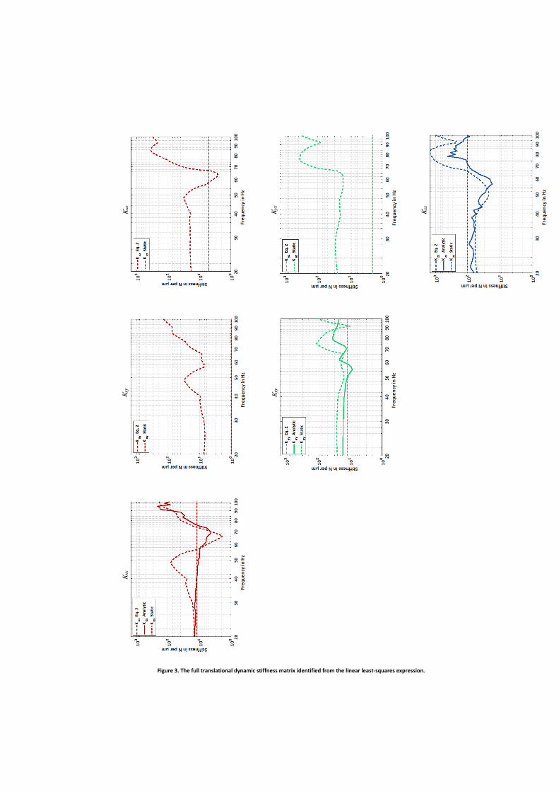
Kxz
Kyz
Kzz
Kxy
Kyy
Kxx
Figure 3. The full translational dynamic stiffness matrix identified from the linear least-squares expression.
3. Results
The case study uses a 5-axis milling machine, kinematic configuration wC'A'bYXZ(C)t, with a rotary tilting table, equipped with a tandem drive on the A-axis [8]. Figure 2 displays the analytic solutions for the components 𝑘𝑥𝑥, 𝑘𝑦𝑦, and 𝑘𝑧𝑧. For all
three components the dynamic and static stiffness as well as the coherence are displayed in the same graph. For 𝑘𝑥𝑥, 𝑘𝑦𝑦, and
𝑘𝑧𝑧 there exist differences of respectively 1 Nµm-1 (10%), 4 Nµm-
1 (30%), and 27 Nµm-1 (30%) up to 40 Hz compared to the static stiffness reference. The static stiffness has been measured according to [9]. Then the stiffness drops in the bandwidth of 50 to 70 Hz depending on the direction. This, per theory, is the bandwidth in which the first eigenfrequencies of machine tools can be expected. The coherence functions for the components 𝑘𝑥𝑥 and 𝑘𝑦𝑦 are reasonably good, while the coherence for the
𝑘𝑧𝑧 component is unsatisfactory. It is assumed that this is due to the fact that the Z-axis stiffness is about ten times bigger than for the X- and Y-axis. Nevertheless, the magnitude of the identified 𝑘𝑧𝑧 component has some relevance with respect to the static stiffness reference. For comparison, the 𝑘𝑦𝑦
component was additionally measured with a scanning vibrometer and an impact hammer, see Figure 2 PSV-500. The identified FRFs share similar characteristics but are different in magnitude. This is probably due to the fact that the sensitivity of the force sensors in both measurements differ by almost exactly a factor 100 and that the data in the comparative measurement has not been transformed into the MBCS. Furthermore, it should be heeded that the proposed measurement with the LDBB exerts a static base load, which is assumed to result in a change in stiffness, while the comparative measurements with the PSV-500 exert no static base load. The standard deviations are omitted in all plots, as these are always less than 1 Nµm-1, i.e. hard to visualise. Figure 3 displays the full translational dynamic stiffness matrix. The sub figures visualise the identified components as solutions according to Equation 2, as well as the analytic solutions and static references displayed in Figure 2. The components of the main diagonal exhibit the same trend, but 𝑘𝑥𝑥, 𝑘𝑦𝑦, and 𝑘𝑧𝑧 differ respectively by 1 Nµm-1 (8%), 9 Nµm-1
(56%), and 35 Nµm-1 (40%) up to 40 Hz compared to the analytic solution. Coincidentally, the linear least-squares solution to 𝑘𝑦𝑦
is a close match to the comparative measurements up to 55 Hz, i.e. their magnitudes differ on average by 3 Nµm-1 (10%). The components 𝑘𝑥𝑦, 𝑘𝑥𝑧, and 𝑘𝑦𝑧 differ by 5 Nµm-1 (85%), 15 Nµm-
1 (75%), and 26 Nµm-1 (93%) and have the same sign up to 40 Hz compared to the static stiffness reference. The components 𝑘𝑥𝑧 and 𝑘𝑦𝑧 exceed the expected magnitudes and are bigger than
𝑘𝑥𝑥 and 𝑘𝑦𝑦. Additionally, above 40 Hz sign changes take place
for 𝑘𝑥𝑦 and 𝑘𝑥𝑧. This is signs are omitted in Figure 3 as all
quantities are plotted on a logarithmic scale.
4. Conclusion
This work presents a measurement and identification procedure for the full translational dynamic stiffness matrix of a machine tool using the LDBB and additional measurement instruments. As can be observed from the measurement results displayed in Figure 2 and Figure 3, the proposed method yields reasonable estimates for main diagonal entries of the full translational stiffness matrix, but further work needs to be conducted to provide reliable estimates of the off-diagonal elements. A comparison of measured and simulated eigenfrequencies could be considered a prudent validation for the proposed method; however, accurate simulations of machine tools are exclusively reserved to the manufacturers.
Additionally, the investments in the measurement instruments used renders the proposed method only applicable to machine tool design rather than machine tool users, e.g. process planning. Future works focus on improving the method to identify the full translational stiffness matrix for a subset of the workspace. Further future work shall focus on providing an uncertainty budget for the proposed measurement procedure, as it is uncertain how the machine tool kinematics and thermal drifts influence the measurement results.
5. Acknowledgement
The authors would like to thank VINNOVA (Sweden’s innovation agency) and the SMART advanced manufacturing cluster for funding this research as a part of the COMACH project (Grant Agreement ID: S0120-COMACH). The authors would like to also express their gratitude to the Center for Design and Management of Manufacturing Systems as well as Excellence in Production Research for their financial support.
References
[1] Kono D, Mizuno S, Muraki Tand Nakaminami M. A machine tool motorized spindle with hybrid structure of steel and carbon fiber composite [online]. CIRP Annals, 2019, 68(1), 389-392. ISSN 00078506. Available under: doi:10.1016/j.cirp.2019.04.022
[2] Sarhan A and Matsubara A. Investigation about the characterization of machine tool spindle stiffness for intelligent CNC end milling [online]. Robotics and Computer-Integrated Manufacturing, 2015, 34, 133-139. ISSN 07365845.
[3] Laspas T, Theissen N and Archenti A. Novel methodology for the measurement and identification for quasi-static stiffness of five-axis machine tools [online]. Precision Engineering, 2020, 65, 164-170. ISSN 01416359. Available under: doi:10.1016/j.precisioneng.2020.06.006
[4] Zaghbani I and Songmene V. Estimation of machine-tool dynamic parameters during machining operation through operational modal analysis [online]. International Journal of Machine Tools and Manufacture, 2009, 49(12-13), 947-957. ISSN 0890-6955. Available under: doi:10.1016/j.ijmachtools.2009.06.010
[5] Pedrammehr S, Farrokhi H, Rajab A, Pakzad S, Mahboubkhah M, Ettefagh M and Sadeghi M. Modal Analysis of the Milling Machine Structure through FEM and Experimental Test [online]. Advanced Materials Research, 2011, 383-390, 6717-6721. Available under: doi:10.4028/www.scientific.net/AMR.383-390.6717
[6] Archenti A and Nicolescu M. Accuracy analysis of machine tools using Elastically Linked Systems [online]. CIRP Annals, 2013, 62(1), 503-506. ISSN 00078506. Available under: doi:10.1016/j.cirp.2013.03.100
[7] Leach, R.K. and S.T. SMITH, Hg. Basics of precision engineering. Boca Rato: CRC Press, Taylor & Francis Group, 2018. ISBN 978-1-4987-6085-0.
[8] Schwenke H, Knapp W, Haitjema H, Weckenmann A, Schmitt R and Delbressine F. Geometric error measurement and compensation of machines—An update [online]. CIRP Annals - Manufacturing Technology, 2008, 57(2), 660-675. ISSN 00078506. Available under: doi:10.1016/j.cirp.2008.09.008
[9] Theissen N, Laspas T, Szipka K and Archenti A Measurement and identification of translational stiffness matrix for static loads in machine tools. In: Virtual International Conference 2020, 2020.

90 BIBLIOGRAPHY
Paper B
Laspas, T.; Theissen, N.; Archenti, A. (2020): Measurement for the identification ofstatic and quasi-static rotational stiffness. In Precision Engineering 65, pp. 164–170.DOI: 10.1016/j.precisioneng.2020.06.006.
Summary: This work presents a measurement for the identification of staticand quasi-static rotational stiffness of a rotational joint of 5-axis machiningcentres. The measurement procedures are implemented in two case studies on5-axis machining centres with significantly different kinematic configurations.
Background and contribution: The author was responsible for the coor-dination of the research work as well as the writing of the manuscript, andin collaboration with the co-authors performed the measurements as well asthe data analysis.
Measurement for the identification of static and quasi-static rotational stiffness
Nikolas Theissena,∗, Theodoros Laspasa, Stefan Cedergrena,c, Andreas Archentia,b
aKTH Royal Institute of Technology, Department of Production Engineering, Measurement and Metrology Systems Division, Stockholm, SwedenbKTH Royal Institute of Technology, Department of Sustainable Production Development, Industrial Dependability Division, Sodertalje, Sweden
cGKN Aerospace Sweden AB, Trollhattan, Sweden
Abstract
Machine tool calibration can be employed to optimise tool path trajectories through on- and off-line compensation of anticipateddeflections, which result from a process plan, and to assess the machine tools capability to comply with the geometric dimensionsand tolerances of a process plan.
This work presents a measurement for the identification of static and quasi-static rotational stiffness of a rotational joint of 5-axismachining centres. This work shall serve as a basis towards the calibration of translational as well as rotational stiffness of 5-axismachining centres. The novelty of this work lies partly in the measurement procedure for the quasi-static rotational stiffness, whichrelies on multiple circular trajectories, as well as in the comparison of the static and quasi-static rotational stiffness of machine tools,which is usually identified using finite element approaches. The measurement procedure for the static rotational stiffness consistsof inducing a static load directly, from an overhead factory crane, to a single rotational joint and measuring its deflection withboth three Linear Variable Differential Transformers (LVDTs) as well as three Non-Contact Capacitive Probes (NCCPs). While themeasurement for the quasi-static rotational stiffness induces quasi-static loads indirectly from the Loaded Double Ball Bar, withdifferent magnitudes and radii from the axis of rotation, between the tool centre point and the machine tool table. The quasi-staticmeasurement procedure measures the deflection with both three LVDTs as well as three NCCPs while the spindle tracks circulartrajectories inscribed by the movement of the rotary axis. The measurement procedures are implemented in two case studies on5-axis machining centres with significantly different kinematic configurations to be able to highlight and discuss the limitationsof the applicability of the method. The presented method works well for machining centres with symmetric and acceptably withasymmetric structures due to the corresponding symmetry of the deflection field.
Finally, the manuscript concludes with a contextualisation of the introduced measurement procedure towards fully calibratedmachine tool models, i.e. translation and rotation as well as static and dynamic, which together with customised post-processorsand process models, might form the future basis of a stiffness volumetric compensation system.
Keywords: Machine Tools, Rotational Stiffness, Measurement
1. Introduction
The accuracy of physics-based calibrated machine tools [1]can be optimised through on- and off-line compensation [2].Particularly off-line compensation can be considered a value-adding feature as it applies to all machine tools, i.e. the onesalready installed (approx. $ 1 trillion USD [3]) as well as thosein production, because the compensation takes place on a PCduring the process planning phase. An example of an on-linecompensation system is Siemens’s Volumetric CompensationSystem (VCS) ® for the compensation of machine tool kine-matics [4], which could be expanded to include compliance[5]. Physics-based calibration aims to lift the level of accuracycloser to the level of repeatability of a piece of machinery us-ing a set of deterministic functions to describe the kinematics,static, dynamics, and thermo-elasticity [1]. This may also in-crease its range of potential applications, as it is both a machine
∗Corresponding author. Brinellvaegen 68, SE-114 28 Stockholm, SwedenEmail address: [email protected] (Nikolas Theissen)
tool’s accuracy as well as repeatability that enable the machin-ing of complex parts with tight Geometric Dimension and Tol-erance (GDT). Machine tool calibration can also be used forcapability assessment [6]. In the given context, capability as-sessment focuses on representing and communicating the ap-plicability of machinery for a task in terms of requirementson metrics used by industrial practitioners. One such metric ispositioning accuracy, which measures the closeness between acommanded and an attained position of a machine. Positioningaccuracy depends on the machine’s kinematics, statics, dynam-ics, and thermo-elasticity [7]. Hence, capability assessment en-ables one to evaluate a machine tool’s suitability for a giventask. Furthermore, the measurement data used for the calibra-tion, can also be used as auxiliary information to Finite Element(FE) modelling for the validation of machine tool designs [8].
One of the main design criteria of machine tools is stiffnesswhich affects their performance under load [9]. High stiffnessis important to precisely maintain the pose between the ToolCenter Point (TCP) with respect to the workpiece during man-ufacturing. It directly affects the GDT compliance of machined
Preprint submitted to Elsevier February 19, 2021

Y
X
Z
A
B
C
1
3
2
(a)
Y
X
Z
A
B
C
6 7 9
10
4
5
8
(b)
Figure 1: Measurement set-ups: In (a) is shown the static measurement set-up using the overhead crane (1) connected to a suspension point on the machine tooltable (2), and the metrology frame with LVDTs (3). In (b) shows a part of the quasi-static measurement set-up using the NCCPs (4), mounted on the metrologyframe (5) with its data acquisition system (6, 7), as well as the Loaded Double Ball Bar (8), its Tool Adapter (9), and the Table Link (10). The Machine BaseCoordinate System is indicated in the lower left-hand corner.
parts, i.e. how closely the part matches the design specification.The stiffness of a mechanical system can be defined as its ca-pacity to sustain loads, which result in a change of its geometry[10]. For this investigation the machine tool’s structural com-ponents are in static equilibrium, the forces and torques neithercause an acceleration nor are they caused by an acceleration[11], and quasi-static equilibrium, the forces and torques causea slow and periodic load with a frequency lower than 0.5 Hz[10], with their environment.
Machining centres with five axes have revolute joints in ad-dition to the prismatic joints. Those revolute joints are usuallymutually orthogonal to increase the capability, e.g. ability tomachine free form surfaces, or flexibility, e.g. the number ofset-ups can be reduced. The revolute joints may be coupled tothe prismatic joints or hold the workpiece in place. The rota-tional stiffness of those rotational joints contributes to the stiff-ness between the TCP and the workpiece. The work of Konoet al. has shown that the contribution of rotational joints can besignificant [12]. Thus, it should be considered when perform-ing machine tool calibration. ISO230-1:2012 provides guide-lines for the measurement and evaluation of machine tool staticcompliance for rotary axis [13]. It is proposed to induce a loadand measure between the spindle and the table or any machinecomponent and to express the resulting calculated compliancein µm N−1 at a specified distance.
This work proposes to use quasi-static circular trajectoriesfor the measurement of the joint stiffness, given in Nm/ deg tofacilitate the calculation of deflections more accurately in thewhole workspace. It complements the investigation of Konoet al. by comparing machine tools with significantly different
kinematic chains to assess the importance of the structural loop[7]. It compares static and quasi-static rotational stiffness. And,it expands the work of Laspas et al. [14] on the calibration oftranslational stiffness of 5-axis machining centres by account-ing for the contribution of the rotational joints. In this work, thestatic stiffness is identified using direct measurements, i.e. datarepresenting a single structural loop component without anycontribution from other components [13]. On the other hand,the quasi-static stiffness is identified using indirect measure-ments, data containing superposed errors associated with thesimultaneous motion of two or more machine axes [13]. Themeasurement procedures are implemented in two case studieson 5-axis machining centres with significantly different kine-matic configurations to be able to highlight and discuss the lim-itations of the applicability of the method. The two case studiesare hereafter referred to as case A. and B. In both cases the ro-tary A-axis carries the additional rotational Degree of Freedom(DOF). The most significant difference between the case studiesis the symmetry in the suspension of the A-axis.
2. Methodology
This section describes the measurement devices, measure-ment procedures, and data processing for the measurement andidentification of the static and quasi-static rotational stiffness ofa single rotary joint of a 5-axis machining centre. The sectionstarts with a description of the static followed by the quasi-staticprocedure. The quasi-static procedure builds on the the staticprocedure. The quasi-static procedure requires more steps andis thus divided into several detailed subsections.
2
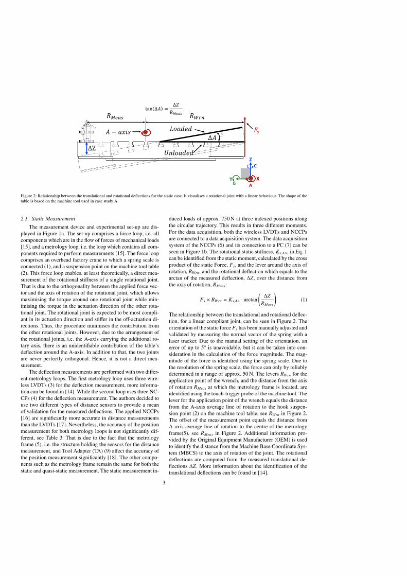
Y
Z
X
C
AB
ΔZ
𝑅𝑀𝑒𝑎𝑠 𝑅𝑊𝑟𝑛
tan Δ𝐴 =Δ𝑍
𝑅𝑀𝑒𝑎𝑠
𝐿𝑜𝑎𝑑𝑒𝑑 𝐹𝑠𝐴 − 𝑎𝑥𝑖𝑠
𝑈𝑛𝑙𝑜𝑎𝑑𝑒𝑑
Δ𝐴
Figure 2: Relationship between the translational and rotational deflections for the static case. It visualises a rotational joint with a linear behaviour. The shape of thetable is based on the machine tool used in case study A.
2.1. Static Measurement
The measurement device and experimental set-up are dis-played in Figure 1a. The set-up comprises a force loop, i.e. allcomponents which are in the flow of forces of mechanical loads[15], and a metrology loop, i.e. the loop which contains all com-ponents required to perform measurements [15]. The force loopcomprises an overhead factory crane to which a spring scale isconnected (1), and a suspension point on the machine tool table(2). This force loop enables, at least theoretically, a direct mea-surement of the rotational stiffness of a single rotational joint.That is due to the orthogonality between the applied force vec-tor and the axis of rotation of the rotational joint, which allowsmaximising the torque around one rotational joint while min-imising the torque in the actuation direction of the other rota-tional joint. The rotational joint is expected to be most compli-ant in its actuation direction and stiffer in the off-actuation di-rections. Thus, the procedure minimises the contribution fromthe other rotational joints. However, due to the arrangement ofthe rotational joints, i.e. the A-axis carrying the additional ro-tary axis, there is an unidentifiable contribution of the table’sdeflection around the A-axis. In addition to that, the two jointsare never perfectly orthogonal. Hence, it is not a direct mea-surement.
The deflection measurements are performed with two differ-ent metrology loops. The first metrology loop uses three wire-less LVDTs (3) for the deflection measurement, more informa-tion can be found in [14]. While the second loop uses three NC-CPs (4) for the deflection measurement. The authors decided touse two different types of distance sensors to provide a meanof validation for the measured deflections. The applied NCCPs[16] are significantly more accurate in distance measurementsthan the LVDTs [17]. Nevertheless, the accuracy of the positionmeasurement for both metrology loops is not significantly dif-ferent, see Table 3. That is due to the fact that the metrologyframe (5), i.e. the structure holding the sensors for the distancemeasurement, and Tool Adapter (TA) (9) affect the accuracy ofthe position measurement significantly [18]. The other compo-nents such as the metrology frame remain the same for both thestatic and quasi-static measurement. The static measurement in-
duced loads of approx. 750 N at three indexed positions alongthe circular trajectory. This results in three different moments.For the data acquisition, both the wireless LVDTs and NCCPsare connected to a data acquisition system. The data acquisitionsystem of the NCCPs (6) and its connection to a PC (7) can beseen in Figure 1b. The rotational static stiffness, Ks,AA, in Eq. 1can be identified from the static moment, calculated by the crossproduct of the static Force, Fs, and the lever around the axis ofrotation, RWrn, and the rotational deflection which equals to thearctan of the measured deflection, ∆Z, over the distance fromthe axis of rotation, RMeas:
Fs × RWrn = Ks,AA · arctan(
∆ZRMeas
)(1)
The relationship between the translational and rotational deflec-tion, for a linear compliant joint, can be seen in Figure 2. Theorientation of the static force Fs has been manually adjusted andvalidated by measuring the normal vector of the spring with alaser tracker. Due to the manual setting of the orientation, anerror of up to 5° is unavoidable, but it can be taken into con-sideration in the calculation of the force magnitude. The mag-nitude of the force is identified using the spring scale. Due tothe resolution of the spring scale, the force can only by reliablydetermined in a range of approx. 50 N. The levers RWrn for theapplication point of the wrench, and the distance from the axisof rotation RMeas at which the metrology frame is located, areidentified using the touch-trigger probe of the machine tool. Thelever for the application point of the wrench equals the distancefrom the A-axis average line of rotation to the hook suspen-sion point (2) on the machine tool table, see RWrn in Figure 2.The offset of the measurement point equals the distance fromA-axis average line of rotation to the centre of the metrologyframe(5), see RMeas in Figure 2. Additional information pro-vided by the Original Equipment Manufacturer (OEM) is usedto identify the distance from the Machine Base Coordinate Sys-tem (MBCS) to the axis of rotation of the joint. The rotationaldeflections are computed from the measured translational de-flections ∆Z. More information about the identification of thetranslational deflections can be found in [14].
3
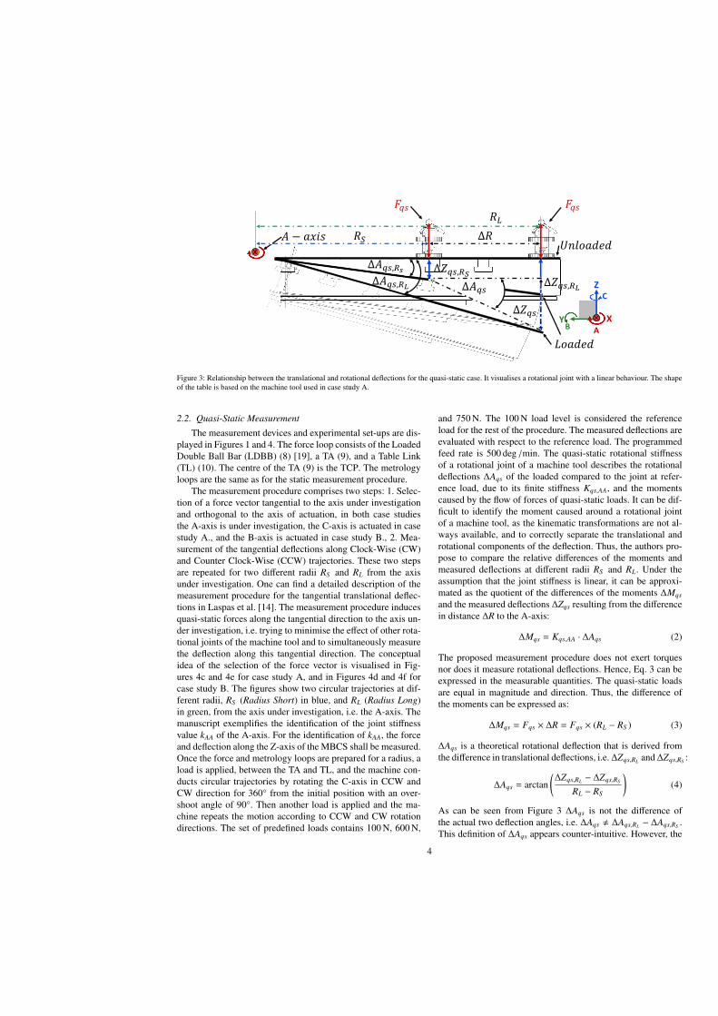
Δ𝑍𝑞𝑠,𝑅𝐿
𝐴 − 𝑎𝑥𝑖𝑠 𝑅𝑆
𝑅𝐿
Y
Z
X
C
AB
𝑈𝑛𝑙𝑜𝑎𝑑𝑒𝑑
𝐿𝑜𝑎𝑑𝑒𝑑
𝐹𝑞𝑠𝐹𝑞𝑠
Δ𝑅
Δ𝑍𝑞𝑠
Δ𝐴𝑞𝑠,𝑅𝑠Δ𝐴𝑞𝑠,𝑅𝐿
Δ𝑍𝑞𝑠,𝑅𝑆Δ𝐴𝑞𝑠
Figure 3: Relationship between the translational and rotational deflections for the quasi-static case. It visualises a rotational joint with a linear behaviour. The shapeof the table is based on the machine tool used in case study A.
2.2. Quasi-Static Measurement
The measurement devices and experimental set-ups are dis-played in Figures 1 and 4. The force loop consists of the LoadedDouble Ball Bar (LDBB) (8) [19], a TA (9), and a Table Link(TL) (10). The centre of the TA (9) is the TCP. The metrologyloops are the same as for the static measurement procedure.
The measurement procedure comprises two steps: 1. Selec-tion of a force vector tangential to the axis under investigationand orthogonal to the axis of actuation, in both case studiesthe A-axis is under investigation, the C-axis is actuated in casestudy A., and the B-axis is actuated in case study B., 2. Mea-surement of the tangential deflections along Clock-Wise (CW)and Counter Clock-Wise (CCW) trajectories. These two stepsare repeated for two different radii RS and RL from the axisunder investigation. One can find a detailed description of themeasurement procedure for the tangential translational deflec-tions in Laspas et al. [14]. The measurement procedure inducesquasi-static forces along the tangential direction to the axis un-der investigation, i.e. trying to minimise the effect of other rota-tional joints of the machine tool and to simultaneously measurethe deflection along this tangential direction. The conceptualidea of the selection of the force vector is visualised in Fig-ures 4c and 4e for case study A, and in Figures 4d and 4f forcase study B. The figures show two circular trajectories at dif-ferent radii, RS (Radius Short) in blue, and RL (Radius Long)in green, from the axis under investigation, i.e. the A-axis. Themanuscript exemplifies the identification of the joint stiffnessvalue kAA of the A-axis. For the identification of kAA, the forceand deflection along the Z-axis of the MBCS shall be measured.Once the force and metrology loops are prepared for a radius, aload is applied, between the TA and TL, and the machine con-ducts circular trajectories by rotating the C-axis in CCW andCW direction for 360° from the initial position with an over-shoot angle of 90°. Then another load is applied and the ma-chine repeats the motion according to CCW and CW rotationdirections. The set of predefined loads contains 100 N, 600 N,
and 750 N. The 100 N load level is considered the referenceload for the rest of the procedure. The measured deflections areevaluated with respect to the reference load. The programmedfeed rate is 500 deg /min. The quasi-static rotational stiffnessof a rotational joint of a machine tool describes the rotationaldeflections ∆Aqs of the loaded compared to the joint at refer-ence load, due to its finite stiffness Kqs,AA, and the momentscaused by the flow of forces of quasi-static loads. It can be dif-ficult to identify the moment caused around a rotational jointof a machine tool, as the kinematic transformations are not al-ways available, and to correctly separate the translational androtational components of the deflection. Thus, the authors pro-pose to compare the relative differences of the moments andmeasured deflections at different radii RS and RL. Under theassumption that the joint stiffness is linear, it can be approxi-mated as the quotient of the differences of the moments ∆Mqs
and the measured deflections ∆Zqs resulting from the differencein distance ∆R to the A-axis:
∆Mqs = Kqs,AA · ∆Aqs (2)
The proposed measurement procedure does not exert torquesnor does it measure rotational deflections. Hence, Eq. 3 can beexpressed in the measurable quantities. The quasi-static loadsare equal in magnitude and direction. Thus, the difference ofthe moments can be expressed as:
∆Mqs = Fqs × ∆R = Fqs × (RL − RS ) (3)
∆Aqs is a theoretical rotational deflection that is derived fromthe difference in translational deflections, i.e. ∆Zqs,RL and ∆Zqs,RS :
∆Aqs = arctan(∆Zqs,RL − ∆Zqs,RS
RL − RS
)(4)
As can be seen from Figure 3 ∆Aqs is not the difference ofthe actual two deflection angles, i.e. ∆Aqs , ∆Aqs,RL − ∆Aqs,RS .This definition of ∆Aqs appears counter-intuitive. However, the
4
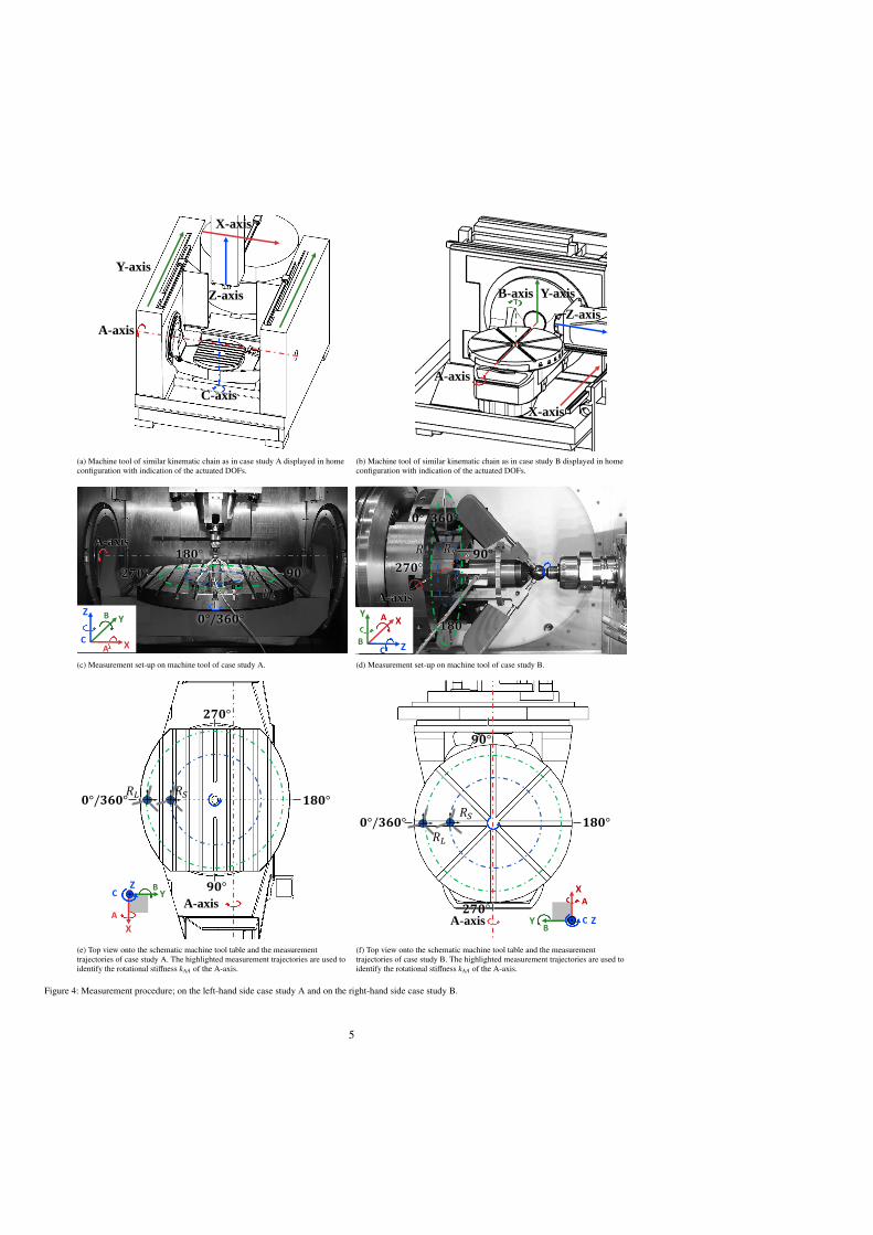
A-axis
C-axis
Y-axis
Z-axis
X-axis
(a) Machine tool of similar kinematic chain as in case study A displayed in homeconfiguration with indication of the actuated DOFs.
A-axis
B-axis Y-axis
Z-axis
X-axis
(b) Machine tool of similar kinematic chain as in case study B displayed in homeconfiguration with indication of the actuated DOFs.
X
YZ
A
B
C
A-axis
𝟗𝟎°
𝟏𝟖𝟎°
𝟐𝟕𝟎°
𝑅𝐿
𝑅𝑆
𝟎°/𝟑𝟔𝟎°
(c) Measurement set-up on machine tool of case study A.
A-axis
𝟗𝟎°
𝟏𝟖𝟎°
𝟐𝟕𝟎°
𝑅𝐿 𝑅𝑆
𝟎°/𝟑𝟔𝟎°
Z
XY
C
A
B
(d) Measurement set-up on machine tool of case study B.
𝟗𝟎°
𝟏𝟖𝟎°
𝟐𝟕𝟎°
𝟎°/𝟑𝟔𝟎°𝑅𝐿 𝑅𝑆
A-axis
X
YZ
A
BC
(e) Top view onto the schematic machine tool table and the measurementtrajectories of case study A. The highlighted measurement trajectories are used toidentify the rotational stiffness kAA of the A-axis.
A-axis
𝟗𝟎°
𝟏𝟖𝟎°
𝟐𝟕𝟎°
𝟎°/𝟑𝟔𝟎°𝑅𝐿
𝑅𝑆
Z
X
Y C
A
B
(f) Top view onto the schematic machine tool table and the measurementtrajectories of case study B. The highlighted measurement trajectories are used toidentify the rotational stiffness kAA of the A-axis.
Figure 4: Measurement procedure; on the left-hand side case study A and on the right-hand side case study B.
5

quantities ∆Aqs,RL and ∆Aqs,RS are both unknown as the deflec-tion measurements, i.e. ∆Zqs,RL and ∆Zqs,RS , contain transla-tional and rotational components as well as due to their de-pendency on the distance from the A-axis, i.e. RL and RS . Acomparison of ∆Aqs and ∆Aqs,RL − ∆Aqs,RS , which is based onthe identified quasi-static joint stiffness values, yielded differ-ences in the order of up to 40 µ deg, i.e. a difference of approx.3%. Further information on the calculation and attribution ofthe quantity ∆ZR,qs = ∆Zqs,RL − ∆Zqs,RS can be found in the fol-lowing section. Thus, the authors propose to approximate thequasi-static joint stiffness by:
Kqs,AA ≈Fqs × (RL − RS )
arctan(
∆Zqs,RL−∆Zqs,RSRL−RS
) (5)
Equation 5 is only true for small ∆Z as the relative pose be-tween the metrology loop and the MBCS changes as the tabledeflects, see Figure 3. This introduces a systematic error. Theangular deflections for both case studies are less than 10 m°.This introduces negligible transformation errors of less than0.02 %. The orientation and magnitude of the quasi-static force,Fqs, is defined through the load and orientation of the LDBBand the rotational deflections are computed from the measuredtranslational deflections ∆Zqs,RL and ∆Zqs,RS as well as the dis-tance between the radii RS and RL. The relationship betweenthe rotational and translational deflections can be deduced fromFigure 3. The radii RS and RL are identified using the touch-trigger probe of the machine. Information about the transforma-tion and counter-rotation of the translational deflections as wellas treatment of the CCW and CW rotations trajectories can befound in [14].
3. Results and Discussion
3.1. Case study A.
Case study A uses a 5-axis milling machine, kinematic con-figuration [wC’A’bYXZ(C)t], with a rotary tilting table, equippedwith a tandem drive on the A-axis [7]. It is assumed that the tan-dem drive on the A-axis leads to a symmetric deflection field.
The measured translational deflections of the machine tooltable as a result of the static loading can be seen in Figure 5a.Figure 5a shows the average measured ∆Z for three differentmoments as measured by the LVDTs and NCCPs. The mea-sured ∆Z differ on average by 0.3 µm. All quantities have beenmeasured in three independent measurements. The uncertaintyis significant compared to the measurand. The mean transla-tional deflections of the TCP as a result of the loading alongthe CW and CCW circular trajectories can be seen in Figure 6a.All quantities have been measured in three independent mea-surements. The figure shows the mean translational deflectionsin the direction of the Z-axis of the MBCS. It includes the de-flections as measured by the LVDTs and the NCCPs at a loadof 600 N and 750 N. The initial distances of the radii RS and RL
from the axis of rotation of the A-axis are 50 mm and 500 mm.As the force is constant, one can assume the corresponding mo-ments at RL to be ten times bigger than the moments at RS .
The maximum difference between measured deflections by theLVDTs and NCCPs equals 2.2 µm. That is a significant dif-ference. However, for the same set of data, the average differ-ence between measured deflections equals 0.1 µm. This is dueto the fact that the greatest difference exists between the mea-surements at 750 N at RL close to the C-axis positions 0/360°and 180°. One can see that there are discrete jumps in the mea-sured data at these positions. It is assumed that the jumps arenot solely measurement errors or noise, but fundamentally a re-sult of the mechanics of the machine tool. The jumps can beobserved in both data sets for the unloaded and loaded mea-surements. The jumps are position-dependent, i.e. close to thetransition points of the quadrants, though they are not neces-sarily symmetrically distributed about them and the jumps onlyoccur at RL, the data sets at RS are smooth. Hence, it is assumedthat the jumps are a result of the super-imposed motion of theX-, Y-, and C-axis. It is difficult to attribute it to an individualerror of a single axis, though it appears that a pitch error ofthe X-axis contributes significantly. These ideas are supportedby additional measurement data from a Renishaw XM 60® aswell as a IBS Trinity System®. In general, the measurementdata from the LVDTs and NCCPs are similar in pattern andmagnitude. Though their mean difference at the measurementof 750 N at RS is close to 1.4 µm. This difference would stillfall within the expanded uncertainty of the measurement pro-cedures; that is under the consideration of normal distributionsand a coverage factor of k = 2, see Table 3. The following sec-tion describes how the translational deflections in Figure 6 havebeen attributed to the deflection of the rotary joints. As afore-mentioned, the authors propose to compare the relative differ-ences of the moments and measured deflections at different radiiRS and RL. The moments at different radii RS and RL can beseen in Figure 7. The relative difference of the translational de-flections, i.e. ∆ZR,qs = ∆Zqs,RL − ∆Zqs,RS , can be seen in Figure8. Considering Figure 7 and 8, one can see that the deflectionsare proportional to the moments. Both follow a trigonometricshape along the circular trajectory.
The moments are highest at C-axis positions of 0° and 180°,as these have the biggest levers from the axis of rotation, seeFigure 7a. However, the centre of the A-axis is offset by approx.100 mm from the C-axis center of rotation. Thus, the momentat C-axis position of 0°, i.e. magnitude of the lever 600 mm, isroughly 1.5 times bigger than the moment at C-axis positionof 180°, i.e. magnitude of the lever 400 mm. Hence, one wouldexpect the deflections at the C-axis position of 0° to be maximaloverall. Due to the discrete jumps at these C-axis positions, onecan hardly determine the actual deflections.
For a linear joint behaviour as described in Equation 5, therelative rotational deflections equal to zero when the relativemoments equal to zero and vice versa. Hence, it can be assumedthat the contribution of the rotational stiffness to the measureddeflections is the sole peak to peak value a of the trigonometricshape, see Figure 8. It is assumed that the axis offset c resultsfrom another rotational stiffness, which should be modelled foran additional DOF. Thus, for the subsequent calculation of therotational stiffness, only the peak to peak value a of the trigono-metric shape of the relative difference of the translational de-
6
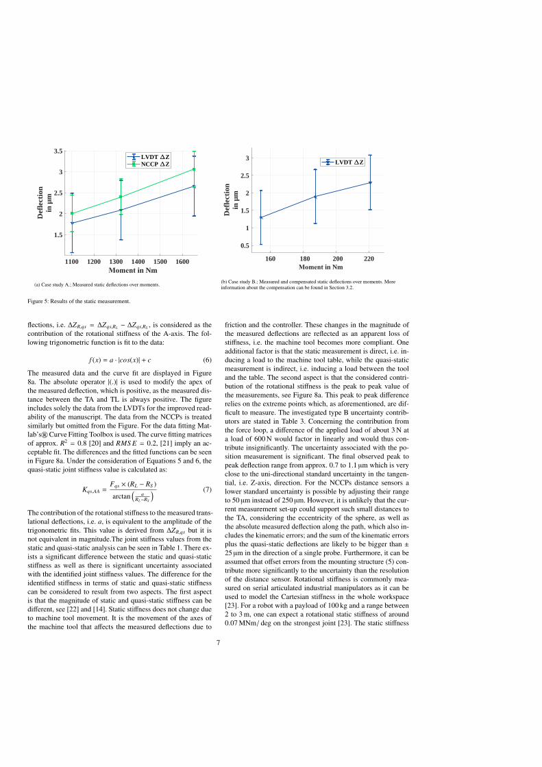
1100 1200 1300 1400 1500 1600Moment in Nm
1.5
2
2.5
3
3.5
Def
lect
ion
in µ
m
LVDT ZNCCP Z
(a) Case study A.; Measured static deflections over moments.
160 220180 200 Moment in Nm
0.5
1
1.5
2
2.5
3
Def
lect
ion
in µ
m
LVDT Z
(b) Case study B.; Measured and compensated static deflections over moments. Moreinformation about the compensation can be found in Section 3.2.
Figure 5: Results of the static measurement.
flections, i.e. ∆ZR,qs = ∆Zqs,RL − ∆Zqs,RS , is considered as thecontribution of the rotational stiffness of the A-axis. The fol-lowing trigonometric function is fit to the data:
f (x) = a · |cos(x)| + c (6)
The measured data and the curve fit are displayed in Figure8a. The absolute operator |(.)| is used to modify the apex ofthe measured deflection, which is positive, as the measured dis-tance between the TA and TL is always positive. The figureincludes solely the data from the LVDTs for the improved read-ability of the manuscript. The data from the NCCPs is treatedsimilarly but omitted from the Figure. For the data fitting Mat-lab’s®Curve Fitting Toolbox is used. The curve fitting matricesof approx. R2 = 0.8 [20] and RMS E = 0.2, [21] imply an ac-ceptable fit. The differences and the fitted functions can be seenin Figure 8a. Under the consideration of Equations 5 and 6, thequasi-static joint stiffness value is calculated as:
Kqs,AA =Fqs × (RL − RS )
arctan(
aRL−RS
) (7)
The contribution of the rotational stiffness to the measured trans-lational deflections, i.e. a, is equivalent to the amplitude of thetrigonometric fits. This value is derived from ∆ZR,qs but it isnot equivalent in magnitude.The joint stiffness values from thestatic and quasi-static analysis can be seen in Table 1. There ex-ists a significant difference between the static and quasi-staticstiffness as well as there is significant uncertainty associatedwith the identified joint stiffness values. The difference for theidentified stiffness in terms of static and quasi-static stiffnesscan be considered to result from two aspects. The first aspectis that the magnitude of static and quasi-static stiffness can bedifferent, see [22] and [14]. Static stiffness does not change dueto machine tool movement. It is the movement of the axes ofthe machine tool that affects the measured deflections due to
friction and the controller. These changes in the magnitude ofthe measured deflections are reflected as an apparent loss ofstiffness, i.e. the machine tool becomes more compliant. Oneadditional factor is that the static measurement is direct, i.e. in-ducing a load to the machine tool table, while the quasi-staticmeasurement is indirect, i.e. inducing a load between the tooland the table. The second aspect is that the considered contri-bution of the rotational stiffness is the peak to peak value ofthe measurements, see Figure 8a. This peak to peak differencerelies on the extreme points which, as aforementioned, are dif-ficult to measure. The investigated type B uncertainty contrib-utors are stated in Table 3. Concerning the contribution fromthe force loop, a difference of the applied load of about 3 N ata load of 600 N would factor in linearly and would thus con-tribute insignificantly. The uncertainty associated with the po-sition measurement is significant. The final observed peak topeak deflection range from approx. 0.7 to 1.1 µm which is veryclose to the uni-directional standard uncertainty in the tangen-tial, i.e. Z-axis, direction. For the NCCPs distance sensors alower standard uncertainty is possible by adjusting their rangeto 50 µm instead of 250 µm. However, it is unlikely that the cur-rent measurement set-up could support such small distances tothe TA, considering the eccentricity of the sphere, as well asthe absolute measured deflection along the path, which also in-cludes the kinematic errors; and the sum of the kinematic errorsplus the quasi-static deflections are likely to be bigger than ±25 µm in the direction of a single probe. Furthermore, it can beassumed that offset errors from the mounting structure (5) con-tribute more significantly to the uncertainty than the resolutionof the distance sensor. Rotational stiffness is commonly mea-sured on serial articulated industrial manipulators as it can beused to model the Cartesian stiffness in the whole workspace[23]. For a robot with a payload of 100 kg and a range between2 to 3 m, one can expect a rotational static stiffness of around0.07 MNm/ deg on the strongest joint [23]. The static stiffness
7
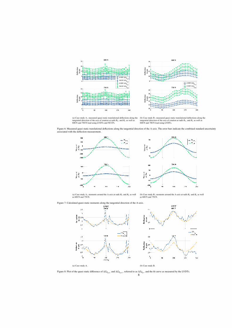
4
6
8
10
12
Def
lect
ion
in µ
m
600 N
LVDT ZRqs,S
NCCP ZRqs,S
LVDT ZRqs,L
NCCP ZRqs,L
0 90 180 270 3604
6
8
10
12
14
Def
lect
ion
in µ
m
750 N
(a) Case study A.; measured quasi-static translational deflections along thetangential direction of the axis of rotation at radii RS , and RL as well as600 N and 700 N load using LVDTs and NCCPs.
8
10
12
14
16
Def
lect
ion
in µ
m
600 N
LVDT ZRqs,S
LVDT ZRqs,L
0 90 180 270 36010
12
14
16
18
20
Def
lect
ion
in µ
m
750 N
(b) Case study B.; measured quasi-static translational deflections along thetangential direction of the axis of rotation at radii RS , and RL as well as600 N and 700 N load using LVDTs.
Figure 6: Measured quasi-static translational deflections along the tangential direction of the A-axis. The error bars indicate the combined standard uncertaintyassociated with the deflection measurement.
(a) Case study A.; moments around the A-axis at radii RS and RL as wellas 600 N and 750 N.
(b) Case study B.; moments around the A-axis at radii RS and RL as wellas 600 N and 750 N.
Figure 7: Calculated quasi-static moments along the tangential direction of the A-axis.
(a) Case study A. (b) Case study B.
Figure 8: Plot of the quasi-static difference of ∆ZRqs,L and ∆ZRqs,S , referred to as ∆ZRqs , and the fit curve as measured by the LVDTs.8
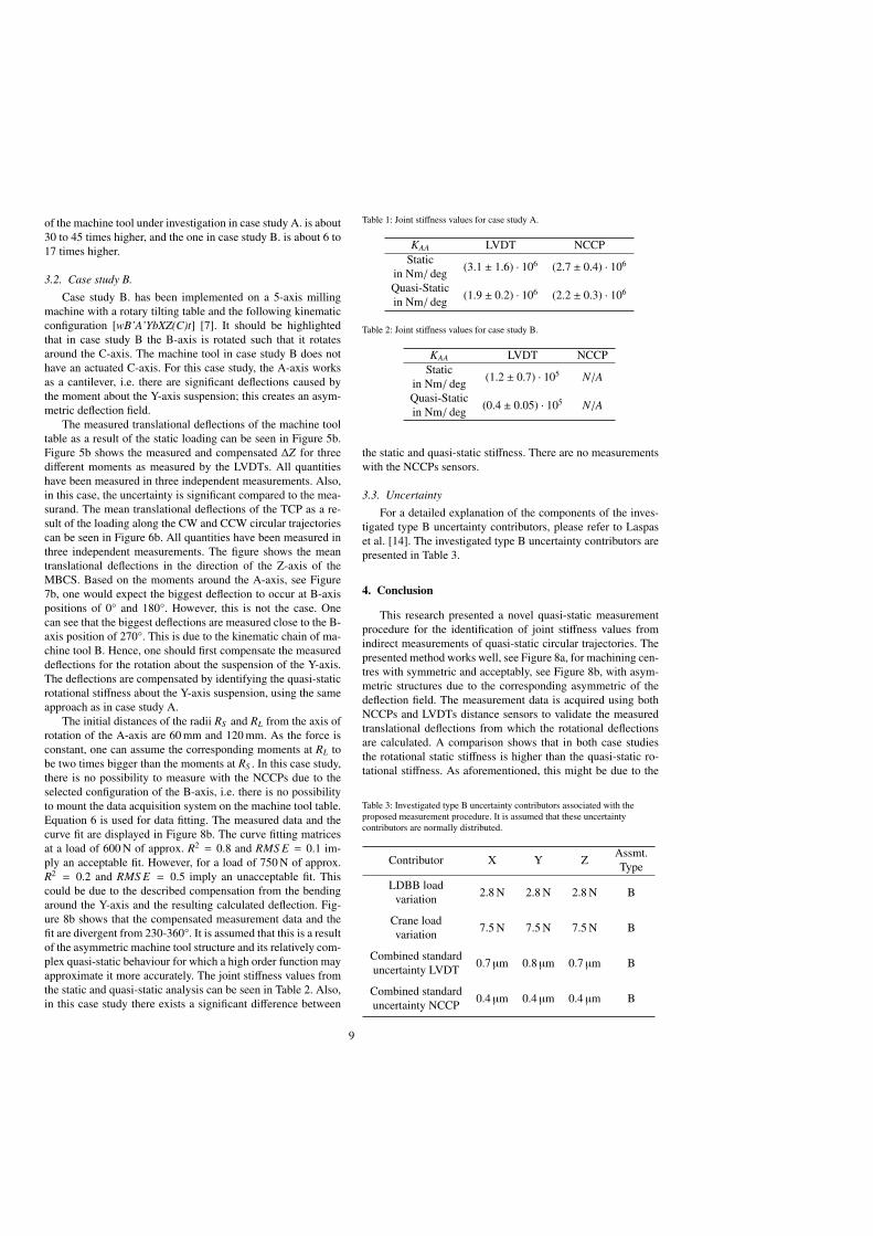
of the machine tool under investigation in case study A. is about30 to 45 times higher, and the one in case study B. is about 6 to17 times higher.
3.2. Case study B.
Case study B. has been implemented on a 5-axis millingmachine with a rotary tilting table and the following kinematicconfiguration [wB’A’YbXZ(C)t] [7]. It should be highlightedthat in case study B the B-axis is rotated such that it rotatesaround the C-axis. The machine tool in case study B does nothave an actuated C-axis. For this case study, the A-axis worksas a cantilever, i.e. there are significant deflections caused bythe moment about the Y-axis suspension; this creates an asym-metric deflection field.
The measured translational deflections of the machine tooltable as a result of the static loading can be seen in Figure 5b.Figure 5b shows the measured and compensated ∆Z for threedifferent moments as measured by the LVDTs. All quantitieshave been measured in three independent measurements. Also,in this case, the uncertainty is significant compared to the mea-surand. The mean translational deflections of the TCP as a re-sult of the loading along the CW and CCW circular trajectoriescan be seen in Figure 6b. All quantities have been measured inthree independent measurements. The figure shows the meantranslational deflections in the direction of the Z-axis of theMBCS. Based on the moments around the A-axis, see Figure7b, one would expect the biggest deflection to occur at B-axispositions of 0° and 180°. However, this is not the case. Onecan see that the biggest deflections are measured close to the B-axis position of 270°. This is due to the kinematic chain of ma-chine tool B. Hence, one should first compensate the measureddeflections for the rotation about the suspension of the Y-axis.The deflections are compensated by identifying the quasi-staticrotational stiffness about the Y-axis suspension, using the sameapproach as in case study A.
The initial distances of the radii RS and RL from the axis ofrotation of the A-axis are 60 mm and 120 mm. As the force isconstant, one can assume the corresponding moments at RL tobe two times bigger than the moments at RS . In this case study,there is no possibility to measure with the NCCPs due to theselected configuration of the B-axis, i.e. there is no possibilityto mount the data acquisition system on the machine tool table.Equation 6 is used for data fitting. The measured data and thecurve fit are displayed in Figure 8b. The curve fitting matricesat a load of 600 N of approx. R2 = 0.8 and RMS E = 0.1 im-ply an acceptable fit. However, for a load of 750 N of approx.R2 = 0.2 and RMS E = 0.5 imply an unacceptable fit. Thiscould be due to the described compensation from the bendingaround the Y-axis and the resulting calculated deflection. Fig-ure 8b shows that the compensated measurement data and thefit are divergent from 230-360°. It is assumed that this is a resultof the asymmetric machine tool structure and its relatively com-plex quasi-static behaviour for which a high order function mayapproximate it more accurately. The joint stiffness values fromthe static and quasi-static analysis can be seen in Table 2. Also,in this case study there exists a significant difference between
Table 1: Joint stiffness values for case study A.
KAA LVDT NCCPStatic
in Nm/ deg (3.1 ± 1.6) · 106 (2.7 ± 0.4) · 106
Quasi-Staticin Nm/ deg (1.9 ± 0.2) · 106 (2.2 ± 0.3) · 106
Table 2: Joint stiffness values for case study B.
KAA LVDT NCCPStatic
in Nm/ deg (1.2 ± 0.7) · 105 N/A
Quasi-Staticin Nm/ deg (0.4 ± 0.05) · 105 N/A
the static and quasi-static stiffness. There are no measurementswith the NCCPs sensors.
3.3. Uncertainty
For a detailed explanation of the components of the inves-tigated type B uncertainty contributors, please refer to Laspaset al. [14]. The investigated type B uncertainty contributors arepresented in Table 3.
4. Conclusion
This research presented a novel quasi-static measurementprocedure for the identification of joint stiffness values fromindirect measurements of quasi-static circular trajectories. Thepresented method works well, see Figure 8a, for machining cen-tres with symmetric and acceptably, see Figure 8b, with asym-metric structures due to the corresponding asymmetric of thedeflection field. The measurement data is acquired using bothNCCPs and LVDTs distance sensors to validate the measuredtranslational deflections from which the rotational deflectionsare calculated. A comparison shows that in both case studiesthe rotational static stiffness is higher than the quasi-static ro-tational stiffness. As aforementioned, this might be due to the
Table 3: Investigated type B uncertainty contributors associated with theproposed measurement procedure. It is assumed that these uncertaintycontributors are normally distributed.
Contributor X Y ZAssmt.Type
LDBB loadvariation 2.8 N 2.8 N 2.8 N B
Crane loadvariation 7.5 N 7.5 N 7.5 N B
Combined standarduncertainty LVDT 0.7 µm 0.8 µm 0.7 µm B
Combined standarduncertainty NCCP 0.4 µm 0.4 µm 0.4 µm B
9
machine tool movement as well as the measurements being dif-ferent. The static measurement is direct, i.e. inducing a loadto the machine tool table, while the quasi-static measurementis indirect, i.e. inducing a load between the tool and the table.Thus, the apparent lower stiffness can be a result of the longerforce loop. i.e. more component interfaces in the force loop,in the quasi-static measurement. In addition to that, the quasi-static joint stiffness value is approximated through the measure-ment of the translational deflections, but the correct attributionof translational and rotational components in the measurementis complex. Hence, this type of measurement does not allowfor the most accurate identification of the machine tool’s stiff-ness, but it might reflect more realistically the apparent stiffnessone can expect during machining. Furthermore, the comparisonshows that additional work is required to comprehensively ex-plain the difference in magnitude of the identified stiffness val-ues. For this investigation, not only the length of the force loopsbut also the type, i.e. open and closed, shall be investigated ingreater detail. The manuscript at hand and [14] have introducedmeasurement methods to assess the translational and rotationalquasi-static deflections in the whole workspace of a 5-axis ma-chining centre. Fully calibrated machine tool stiffness models,i.e. translation and rotation as well as static and dynamic stiff-ness, can be established using the introduced measurement pro-cedure with the metrology frame, which uses the NCCPs sen-sors, and a force loop which is able to exert a dynamic load ontop of the static base load. Thus, for future work, it is intendedto use the described approaches to identify and model the nec-essary DOF to create a volumetric compliance compensationwhich shall be used in a case study on an off-line compensatedprocess plan to assess the utility of the proposed calibrated ma-chine tool models.
5. Declaration of competing interest
The authors declare that they have no known competing fi-nancial interests or personal relationships that could have ap-peared to influence the work reported in this paper.
Acknowledgements
The authors would like to thank VINNOVA (Sweden’s in-novation agency) and the SMART advanced manufacturing clus-ter for funding this research as a part of the COMACH project(Grant Agreement ID: S0120-COMACH). The authors wouldlike to also express their gratitude to the Center for Design andManagement of Manufacturing Systems as well as Excellencein Production Research for their financial support.
References
[1] Nikolas A. Theissen. Physics-based modelling and measurement of ad-vanced manufacturing machinery’s accuracy: Machine tools and indus-trial manipulators - Position, pose and path accuracies. Licentiate, KTHRoyal Institute of Technology, Stockholm, 2019.
[2] C. Brecher, P. Hirsch, and M. Weck. Compensation of thermo-elasticmachine tool deformation based on control internal data. CIRP Annals,53(1):299–304, 2004. ISSN 00078506. doi: 10.1016/S0007-8506(07)60702-1.
[3] Karoly Szipka. Uncertainty Management for Automated Diagnostics ofProduction Machinery, volume 2020:29 of TRITA-ITM-AVL. KTH RoyalInstitute of Technology, Stockholm, 2020. ISBN 978-91-7873-558-7.
[4] Siemens AG. Siemens volumetric compensation system,2009. URL http://www.volumetric.com.br/cases/
volumetric-compensation-system.pdf.[5] Dirk Jahn, Mirco Vitr, and Rouven Meidlinger. Position dependent com-
pliance compensation in a machine tool, 2006. WIPO WO 2008/011845A1 filed 28.07.2006 and issued 31.01.2008.
[6] Andreas Archenti and Mihai Nicolescu. Accuracy analysis of machinetools using elastically linked systems. CIRP Annals - ManufacturingTechnology, 62(1):503–506, 2013. ISSN 00078506. doi: 10.1016/j.cirp.2013.03.100.
[7] H. Schwenke, W. Knapp, H. Haitjema, A. Weckenmann, R. Schmitt,and F. Delbressine. Geometric error measurement and compensation ofmachines—an update. CIRP Annals - Manufacturing Technology, 57(2):660–675, 2008. ISSN 00078506. doi: 10.1016/j.cirp.2008.09.008.
[8] Y. Altintas, C. Brecher, M. Weck, and S. Witt. Virtual machine tool.CIRP Annals, 54(2):115–138, 2005. ISSN 00078506. doi: 10.1016/
S0007-8506(07)60022-5.[9] Christian Brecher and Manfred Weck. Werkzeugmaschinen Ferti-
gungssysteme. Springer Berlin Heidelberg, Berlin, Heidelberg, 2017.ISBN 978-3-662-46566-0. doi: 10.1007/978-3-662-46567-7.
[10] Eugene I. Rivin. Handbook on stiffness & damping in mechanical design.ASME Press, New York, 2010. ISBN 0791802930.
[11] Dietmar Gross. Technische Mechanik. Springer-Lehrbuch. Springer,Berlin and Heidelberg, 13., aktualisierte auflage edition, 2016. ISBN366249471X.
[12] Daisuke Kono, Yuki Moriya, and Atsushi Matsubara. Influence of rotaryaxis on tool-workpiece loop compliance for five-axis machine tools. Pre-cision Engineering, 49:278–286, 2017. ISSN 01416359. doi: 10.1016/
j.precisioneng.2017.02.016. URL http://www.sciencedirect.com/
science/article/pii/S0141635917300958.[13] International Organization for Standardization. Iso 230-1:2012 test code
for machine tools — part 1: Geometric accuracy of machines operatingunder no-load or quasi-static conditions.
[14] Theodoros Laspas, Nikolas Theissen, and Andreas Archenti. Novelmethodology for the measurement and identification for quasi-static stiff-ness of five-axis machine tools. Precision Engineering, 65:164–170,2020. ISSN 01416359. doi: 10.1016/j.precisioneng.2020.06.006.
[15] P. Schellekens, N. Rosielle, H. Vermeulen, M. Vermeulen, S. Wetzels, andW. Pril. Design for precision: Current status and trends. CIRP Annals,47(2):557–586, 1998. ISSN 00078506. doi: 10.1016/S0007-8506(07)63243-0.
[16] Cpl190/290 — lion precision non contact displacement sensors,2020-07-30. URL https://www.lionprecision.com/products/
capacitive-sensors/cpl190-290/.[17] Gtl w 21 — hexagon tesa lvdt, 2020-08-
03. URL https://tesatechnology.com/en-gb/
products/measuring-probes-and-display-units/
usb-or-wireless-measuring-probes_f43698.htm.[18] Eugen Trapet, Juan-Jose Aguilar Martın, Jose-Antonio Yague, Henny
Spaan, and Vit Zeleny. Self-centering probes with parallel kinematicsto verify machine-tools. Precision Engineering, 30(2):165–179, 2006.ISSN 01416359. doi: 10.1016/j.precisioneng.2005.07.002.
[19] Andreas Archenti, editor. A Computational Framework for Controlof Machining System Capability: From Formulation to Implementation.Stockholm and Sweden, 2011. ISBN 978-91-7501-162-2.
[20] Coefficient of determination - wikipedia, 2020-07-30. URL https://
en.wikipedia.org/wiki/Coefficient_of_determination.[21] Root-mean-square deviation - wikipedia, 2020-07-30. URL https://
en.wikipedia.org/wiki/Root-mean-square_deviation.[22] Nikolas A. Theissen, Theodoros Laspas, Karoly Szipka, and Andreas
Archenti. Measurement and identification of translational stiffness ma-trix for static loads in machine tools. In Virtual International Conference2020, 2020.
[23] Alexandr Klimchik, Benoit Furet, Stephane Caro, and Anatol Pashkevich.
10

Identification of the manipulator stiffness model parameters in industrialenvironment. Mechanism and Machine Theory, 90:1–22, 2015. ISSN0094114X. doi: 10.1016/j.mechmachtheory.2015.03.002.
11

102 BIBLIOGRAPHY
Paper C
Laspas, T.; Theissen, N.; Archenti, A. (2020): Novel methodology for the measure-ment and identification for quasi-static stiffness of five-axis machine tools. In Pre-cision Engineering 65, pp. 164–170. DOI: 10.1016/j.precisioneng.2020.06.006.
Summary: This work presents a novel measurement procedure to measureand identify full translational stiffness matrices of 5-axis machining centresusing quasi-static circular trajectories. The measurement procedure is imple-mented in a case study on a 5-axis machining centre.
Background and contribution: The author was responsible for the writ-ing of the first draft of the manuscript, the design as well as the manufactureof the PMI, and in collaboration with the co-authors performed the measure-ments as well as the data analysis.

Novel methodology for the measurement and identification for quasi-static stiffness offive-axis machine tools
Theodoros Laspasa,∗, Nikolas Theissena, Andreas Archentia
aKTH Royal Institute of Technology, Department of Production Engineering, Stockholm,Sweden
Abstract
Stiffness is an important characteristic of production machinery, as it contributes to its ability to precisely maintain the pose betweena tool center point with respect to a workpiece under load. For machine tools, it directly affects the geometric dimensions and surfaceproperties of the parts, i.e. how closely the parts match their design drawings. This work presents a novel measurement procedureto measure and identify full translational stiffness matrices of 5-axis machining centers using quasi-static circular trajectories. Themeasurement procedure consists of inducing quasi-static loads, which vary in magnitude and direction, at the tool center pointof the machine tool using the Loaded Double Ball Bar and measuring the displacement with three Linear Variable DifferentialTransformers while the spindle tracks the circular trajectories inscribed by the movement of the rotary axis. The work outlinesand quantifies the main components of the uncertainty budget related to the measurement of the translational stiffness matrices.The measurement procedure is implemented in a case study on a 5-axis machining center. Finally, the manuscript concludes witha discussion on the utility value of the translational stiffness matrix for the design and operation of machine tools as well as thepossibility to expand the measurement procedure to a calibration procedure for 5-axis machining centers to analyse the translationaland rotational stiffness.
Keywords: Machine Tools, Stiffness, Measurement
1. Introduction
Machine tools are essential for technologically developedsocieties. Their accuracy enables machining of complex prod-ucts with tight tolerances. This is apparent in economic dataprovided by European Association of the Machine Tool Indus-tries (CECIMO) according to which the world machine toolproduction currently equals approximately 80 billion euros [1].
One of the main design criteria of machine tools is staticstiffness which affects their performance under load [2]. Highstiffness is important to precisely maintain the pose betweenthe Tool Center Point (TCP) with respect to the workpiece dur-ing manufacturing. It directly affects the dimensional and ge-ometric accuracy of machined parts, i.e. how closely the partmatches the design specification [3]. The stiffness of a mechan-ical system can be defined as its capacity to sustain loads, whichresult in a change of its geometry [4]. Its inverse is termedcompliance [5]. For this investigation the machine tool’s struc-tural components are in quasi-static equilibrium with their en-vironment. An alternative definition is given by Rivin [4] whostates: ”quasi-static is the analysis of bodies subjected to forcesand torques for a very slow loading process under a periodicloading with a frequency lower than 0.5 Hz”. The stiffness atthe TCP is modelled using Hooke’s law in general tensor form[6, 7]:
FFF = KtKtKt ×∆X∆X∆X (1)
∗Corresponding author. Brinellvaegen 68, SE-114 28 Stockholm, SwedenEmail address: [email protected] (Theodoros Laspas)
Several works exist which focus on the stiffness evaluationand identification at the TCP of a machine tool. There are a pri-ori modelling approaches employing Finite Element (FE) anal-ysis [8] and a posteriori experimental approaches [9]. This workfocuses on the experimental approaches, which can be furtherdivided into machining tests [10] and experiments [2]. ISO230-1:2012 provides guidelines for the measurement and evaluationof machine tool static compliance and hysteresis [11]. The mea-surement consists of applying a quasi-static load between thespindle and the workpiece or any machine component (e.g. ta-ble and spindle) and measuring the displacements for each axis.The limitation of the process is the measurement of deflectionssolely in the direction of the applied force ignoring possiblecross stiffness effects. Further experimental works such as Aga-piou and others usually can only span a comparatively smallsubset of the machine workspace as the measurement methodis static [12, 13].
This research work is a first step towards expanding the con-cept of Elastically Linked Systems (ELS) proposed by Archentiand Nicolescu [14] to identify the Cartesian translational stiff-ness matrix KtKtKt.
KtKtKt =
kxx kxy kxz
kyx kyy kyz
kzx kzy kzz
(2)
Preprint submitted to Elsevier June 4, 2020

1
2
3
5
6
74
Figure 1: Experimental setup for the measurement of the Cartesian translational stiffness matrix in two linearly independentmeasurement setups. The pictures on the left- and right-hand sides shows the principle loading in Z- and Y-axis directions. Thethird linearly independent setup is akin to the picture on the right-hand side.
2. Methodology
This section describes the measurement device and proce-dure as well as the data analysis to identify the Cartesian trans-lational stiffness matrix as a linear least-squares fit solution tothe measured deflections and the induced quasi-static loads.
2.1. Measurement deviceThe measurement device and experimental setup are dis-
played in Figure 1. It consists of two systems; the first is theLoaded Double Ball Bar (LDBB) (1), a Tool Adapter (TA) (3),which consists of a steel sphere of radius 15 mm attached to asteel shaft of diameter 25 mm with an overhang from the spin-dle of approx. 200 mm (including toolholder), and a set of Ta-ble Links (TLs) (4,7), which in Figure 1 is an additional steelsphere of radius 15 mm mounted on the table with a washerand a nut; the second is a metrology frame (5) holding threecontact-type wireless Linear Variable Differential Transform-ers (LVDTs) probes (2) equipped with flat tip inserts (6). Themain specifications of the linear probes are listed in Table 1.For the data acquisition, the wireless probes are connected to adata acquisition system, not in the picture. Furthermore, Figure1 omits the control system of the LDBB which allows the con-trol of the supplied air pressure. The design of the metrologyframe and probing concept is inspired by the work of Trapetet al. [15]. Figure 1 shows two of the three linearly indepen-dent setups. The third setup can be considered to be similar tothe right hand-side picture but rotated by approximately 120°about the Z-axis, see Figure 3.
2.2. Measurement procedureThe measurement procedure comprises five steps: 1. Selec-
tion of a force vector, 2. Locating of the TL, 3. Transforma-
Table 1: Specifications of linear probes.
Attribute SpecificationMeasurement principle LVDTTip insert material SteelTip insert diameter 10 mmRange ±2 mmResolution 0.1 µmMax linearity error 0.4 µm + 0.8 × L∗ µmRepeatability 0.1 µmMeasuring force 0.63 N∗ L in mm
tion identification of probes orientation in Machine Base Co-ordinate System (MBCS), 4. Evaluation of the accuracy of thetransformation, and 5. Measurement of the Clock-Wise (CW)and Counter Clock-Wise (CCW) trajectories. These five stepsare repeated for at least three linearly independent force vectors[16], i.e. no one force vector can be written as a linear combi-nation of the other force vectors. The measurement procedureis highlighted in Figure 2.
The first force vector shall be aligned coaxial to the Z-axisof the MBCS. This setup is shown in Figure 1 and schemat-ically represented in Figure 3 including a visualisation of thecircular trajectory. The coaxiality with the Z-axis facilitates themeasurement of three linearly independent force vectors andit leads to maximum deflections in the direction of the Z-axis,which are small compared to the X- and Y-axis of the machinetool, see Figure 1. The Z-axis of the machine tool is usually thestiffest as only small moments, which are independent of theoverhang of the TCP, are induced into the structure. For the two
2
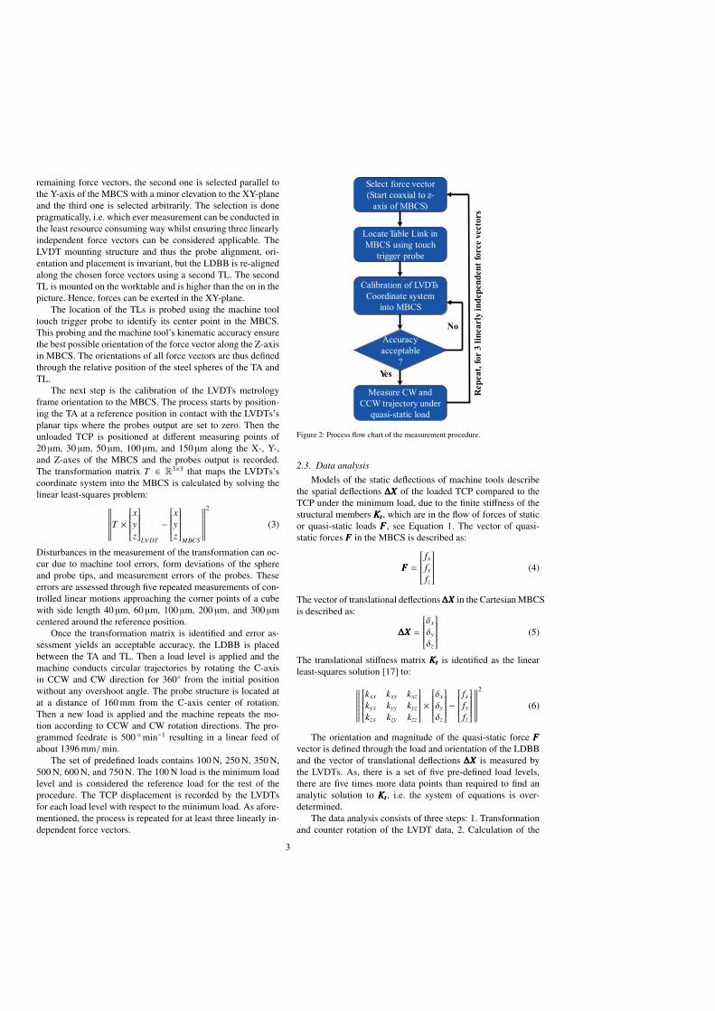
remaining force vectors, the second one is selected parallel tothe Y-axis of the MBCS with a minor elevation to the XY-planeand the third one is selected arbitrarily. The selection is donepragmatically, i.e. which ever measurement can be conducted inthe least resource consuming way whilst ensuring three linearlyindependent force vectors can be considered applicable. TheLVDT mounting structure and thus the probe alignment, ori-entation and placement is invariant, but the LDBB is re-alignedalong the chosen force vectors using a second TL. The secondTL is mounted on the worktable and is higher than the on in thepicture. Hence, forces can be exerted in the XY-plane.
The location of the TLs is probed using the machine tooltouch trigger probe to identify its center point in the MBCS.This probing and the machine tool’s kinematic accuracy ensurethe best possible orientation of the force vector along the Z-axisin MBCS. The orientations of all force vectors are thus definedthrough the relative position of the steel spheres of the TA andTL.
The next step is the calibration of the LVDTs metrologyframe orientation to the MBCS. The process starts by position-ing the TA at a reference position in contact with the LVDTs’splanar tips where the probes output are set to zero. Then theunloaded TCP is positioned at different measuring points of20 µm, 30 µm, 50 µm, 100 µm, and 150 µm along the X-, Y-,and Z-axes of the MBCS and the probes output is recorded.The transformation matrix T ∈ R3×3 that maps the LVDTs’scoordinate system into the MBCS is calculated by solving thelinear least-squares problem:
∥∥∥∥∥∥∥∥T ×
xyz
LVDT
−xyz
MBCS
∥∥∥∥∥∥∥∥
2
(3)
Disturbances in the measurement of the transformation can oc-cur due to machine tool errors, form deviations of the sphereand probe tips, and measurement errors of the probes. Theseerrors are assessed through five repeated measurements of con-trolled linear motions approaching the corner points of a cubewith side length 40 µm, 60 µm, 100 µm, 200 µm, and 300 µmcentered around the reference position.
Once the transformation matrix is identified and error as-sessment yields an acceptable accuracy, the LDBB is placedbetween the TA and TL. Then a load level is applied and themachine conducts circular trajectories by rotating the C-axisin CCW and CW direction for 360° from the initial positionwithout any overshoot angle. The probe structure is located atat a distance of 160 mm from the C-axis center of rotation.Then a new load is applied and the machine repeats the mo-tion according to CCW and CW rotation directions. The pro-grammed feedrate is 500 ° min−1 resulting in a linear feed ofabout 1396 mm/min.
The set of predefined loads contains 100 N, 250 N, 350 N,500 N, 600 N, and 750 N. The 100 N load is the minimum loadlevel and is considered the reference load for the rest of theprocedure. The TCP displacement is recorded by the LVDTsfor each load level with respect to the minimum load. As afore-mentioned, the process is repeated for at least three linearly in-dependent force vectors.
Locate Table Link inMBCS using touch
trigger probe
Calibration of LVDTsCoordinate system
into MBCS
Accuracyacceptable
?
Measure CW andCCW trajectory under
quasi-static load
Select force vector(Start coaxial to z-
axis of MBCS)
No
Yes
Repeat,for3linearlyindependentforcevectors
Figure 2: Process flow chart of the measurement procedure.
2.3. Data analysisModels of the static deflections of machine tools describe
the spatial deflections ∆X∆X∆X of the loaded TCP compared to theTCP under the minimum load, due to the finite stiffness of thestructural members KtKtKt, which are in the flow of forces of staticor quasi-static loads FFF, see Equation 1. The vector of quasi-static forces FFF in the MBCS is described as:
FFF =
fx
fyfz
(4)
The vector of translational deflections ∆X∆X∆X in the Cartesian MBCSis described as:
∆X∆X∆X =
δx
δy
δz
(5)
The translational stiffness matrix KtKtKt is identified as the linearleast-squares solution [17] to:
∥∥∥∥∥∥∥∥
kxx kxy kxz
kyx kyy kyz
kzx kzy kzz
×δx
δy
δz
−
fx
fyfz
∥∥∥∥∥∥∥∥
2
(6)
The orientation and magnitude of the quasi-static force FFFvector is defined through the load and orientation of the LDBBand the vector of translational deflections ∆X∆X∆X is measured bythe LVDTs. As, there is a set of five pre-defined load levels,there are five times more data points than required to find ananalytic solution to KtKtKt, i.e. the system of equations is over-determined.
The data analysis consists of three steps: 1. Transformationand counter rotation of the LVDT data, 2. Calculation of the
3

mean differences of the measured trajectories, and 3. Identifica-tion of the Cartesian translational stiffness matrix KtKtKt as a linearleast-squares solution to Equation 1.
In the first step all the measured deflections by the LVDTsare transformed into the MBCS according to:
xyz
MBCS
= T ×xyz
LVDT
(7)
T is the transformation matrix which calibrates LVDTs’s outputinto the MBCS. The transformed deflections express the loadinduced deviations of the TCP with respect to the reference po-sition of the TCP under the minimum load.
Then the data set is filtered for the circles by cutting off
the data set at the trigger motions. The trigger motion is a con-trolled linear motion of 100 µm in positive and then negativeZ-axis direction, i.e. the loaded TCP moves from and returns tothe set origin. The data acquisition system captures data fromthe LVDTs at a rate of 20 Hz. The measurement procedure wasperformed at a feedrate of 500 ° min−1 (which corresponds toa feedrate of 1396 mm/min for the linear axis). Based on theselected distance from the C-axis center and the feed velocitythis results in circular trajectories of approximately n = 860data points. The transformation in Equation 7 is only valid forthe start and end point as the mounting structure of the LVDTsrotates with the C-axis of the machine. Hence, the data needs tobe rotated with c = [0 · · · 2π] ∈ Rn×1, i.e. the actuation variableof the C-axis, about the Z-axis according to:
xi
yi
zi
MBCS
= Rot(z, ci) × T ×xi
yi
zi
LVDT
(8)
The index i ∈ Nn×1 refers to the measurement points. Posi-tive direction of rotation is considered along CCW and negativealong CW. The data measured with a CW rotation has to be ro-tated positively about the Z-axis, while the data measured witha CCW rotation has to be rotated negatively about the Z-axis,see Figure 3. The same counter-rotation is applied to the ini-tially measured force vector Fini to calculate the force vectorsFi along the trajectory:
FFF i = Rot(z, ci) × FFF ini (9)
As aforementioned, circular trajectories have been measuredfor both CW and CCW rotation directions, at loads of 100 N,250 N, 350 N, 500 N, 600 N, and 750 N. The vector of load in-duced differences ∆X∆X∆Xi, j,k is calculated for each point along thetrajectory, load level, and rotation direction according to:
∆X∆X∆Xi, j,k =
δxi, j,k
δyi, j,k
δzi, j,k
=
xi, j,k
yi, j,k
zi, j,k
−xi, j=1,kyi, j=1,kzi, j=1,k
(10)
In Equation 10 index i = 1...n where n = 860 represents thepoints along the circular trajectory, j defines the load levels withj = 1 corresponding to the minimum load of 100 N and j = 6corresponding to the maximum load at 750 N, k = 1, 2 defining
0° / 360°
90°270°
180°
CCWCWYX
Z
(a) Macroscopic view of the machine tool and the measurement system.Highlighted are the CW and CCW directions, MBCS orientation (notposition), and the C axis positions of 0°, 90°, 180°and 270°
0/360
90
180
270
CCW
YX
Z
(b) Measurement setup 1 - principal force direction in Z-axis.
CW
Δℎ
0/360
90
180
270
YX
Z
(c) Measurement setup 2 - principal force direction in Y- axis.
Δℎ
Δc
0/360
90
180
270
YX
Z
(d) Measurement setup 3 - principal load direction in X-axis.
TL start point
TA trajectoryTA start point
Force vector
TL trajectory
Figure 3: View of the machine tool including measurement system of the threemeasurement setups. Principal force directions stated are at C=0° position.4
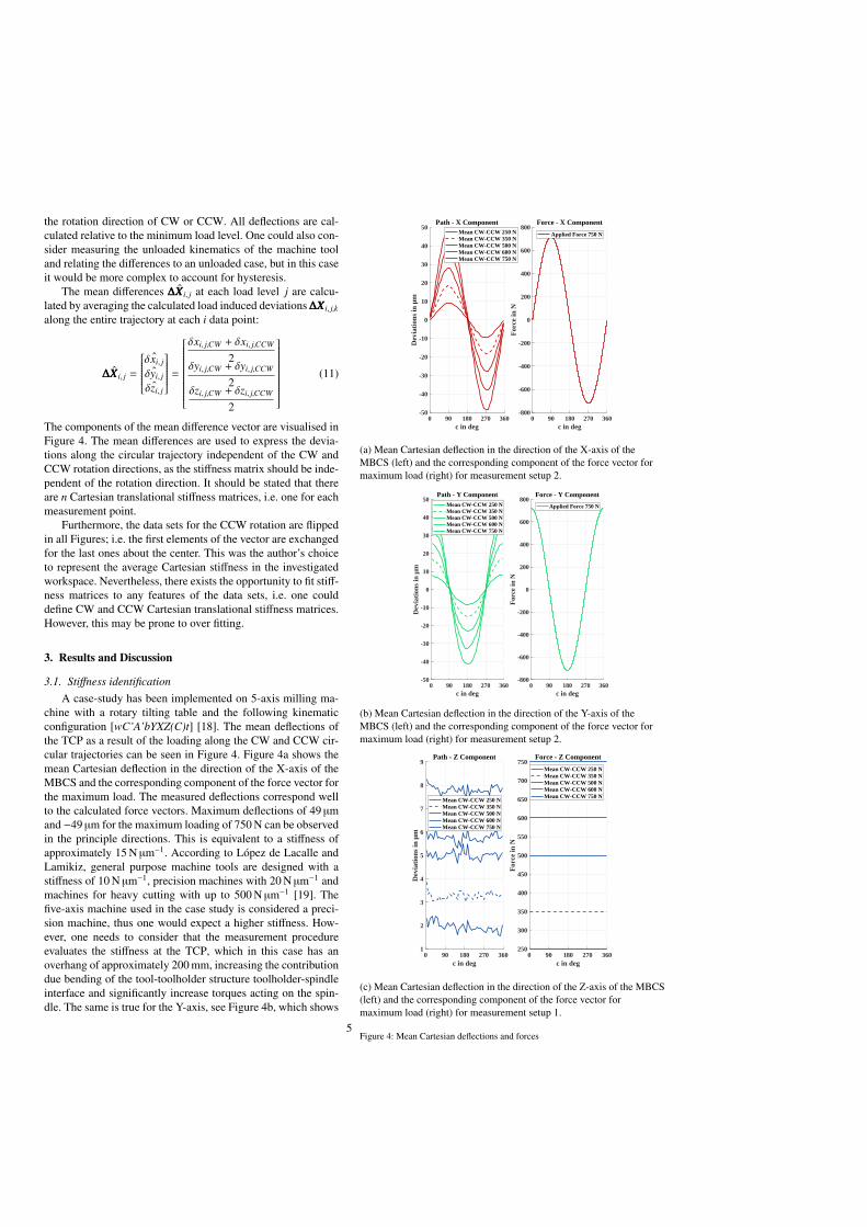
the rotation direction of CW or CCW. All deflections are cal-culated relative to the minimum load level. One could also con-sider measuring the unloaded kinematics of the machine tooland relating the differences to an unloaded case, but in this caseit would be more complex to account for hysteresis.
The mean differences ˆ∆X∆X∆Xi, j at each load level j are calcu-lated by averaging the calculated load induced deviations ∆X∆X∆Xi, j,k
along the entire trajectory at each i data point:
ˆ∆X∆X∆Xi, j =
ˆδxi, jˆδyi, jˆδzi, j
=
δxi, j,CW + δxi, j,CCW
2δyi, j,CW + δyi, j,CCW
2δzi, j,CW + δzi, j,CCW
2
(11)
The components of the mean difference vector are visualised inFigure 4. The mean differences are used to express the devia-tions along the circular trajectory independent of the CW andCCW rotation directions, as the stiffness matrix should be inde-pendent of the rotation direction. It should be stated that thereare n Cartesian translational stiffness matrices, i.e. one for eachmeasurement point.
Furthermore, the data sets for the CCW rotation are flippedin all Figures; i.e. the first elements of the vector are exchangedfor the last ones about the center. This was the author’s choiceto represent the average Cartesian stiffness in the investigatedworkspace. Nevertheless, there exists the opportunity to fit stiff-ness matrices to any features of the data sets, i.e. one coulddefine CW and CCW Cartesian translational stiffness matrices.However, this may be prone to over fitting.
3. Results and Discussion
3.1. Stiffness identificationA case-study has been implemented on 5-axis milling ma-
chine with a rotary tilting table and the following kinematicconfiguration [wC’A’bYXZ(C)t] [18]. The mean deflections ofthe TCP as a result of the loading along the CW and CCW cir-cular trajectories can be seen in Figure 4. Figure 4a shows themean Cartesian deflection in the direction of the X-axis of theMBCS and the corresponding component of the force vector forthe maximum load. The measured deflections correspond wellto the calculated force vectors. Maximum deflections of 49 µmand −49 µm for the maximum loading of 750 N can be observedin the principle directions. This is equivalent to a stiffness ofapproximately 15 N µm−1. According to Lopez de Lacalle andLamikiz, general purpose machine tools are designed with astiffness of 10 N µm−1, precision machines with 20 N µm−1 andmachines for heavy cutting with up to 500 N µm−1 [19]. Thefive-axis machine used in the case study is considered a preci-sion machine, thus one would expect a higher stiffness. How-ever, one needs to consider that the measurement procedureevaluates the stiffness at the TCP, which in this case has anoverhang of approximately 200 mm, increasing the contributiondue bending of the tool-toolholder structure toolholder-spindleinterface and significantly increase torques acting on the spin-dle. The same is true for the Y-axis, see Figure 4b, which shows
0 90 180 270 360c in deg
-50
-40
-30
-20
-10
0
10
20
30
40
50
Dev
iati
ons
in µ
m
Path - X ComponentMean CW-CCW 250 NMean CW-CCW 350 NMean CW-CCW 500 NMean CW-CCW 600 NMean CW-CCW 750 N
0 90 180 270 360c in deg
-800
-600
-400
-200
0
200
400
600
800
For
ce in
N
Force - X Component
Applied Force 750 N
(a) Mean Cartesian deflection in the direction of the X-axis of theMBCS (left) and the corresponding component of the force vector formaximum load (right) for measurement setup 2.
0 90 180 270 360c in deg
-50
-40
-30
-20
-10
0
10
20
30
40
50
Dev
iati
ons
in µ
m
Path - Y ComponentMean CW-CCW 250 NMean CW-CCW 350 NMean CW-CCW 500 NMean CW-CCW 600 NMean CW-CCW 750 N
0 90 180 270 360c in deg
-800
-600
-400
-200
0
200
400
600
800
For
ce in
N
Force - Y Component
Applied Force 750 N
(b) Mean Cartesian deflection in the direction of the Y-axis of theMBCS (left) and the corresponding component of the force vector formaximum load (right) for measurement setup 2.
0 90 180 270 360c in deg
1
2
3
4
5
6
7
8
9
Dev
iati
ons
in µ
m
Path - Z Component
Mean CW-CCW 250 NMean CW-CCW 350 NMean CW-CCW 500 NMean CW-CCW 600 NMean CW-CCW 750 N
0 90 180 270 360c in deg
250
300
350
400
450
500
550
600
650
700
750
For
ce in
N
Force - Z Component
Mean CW-CCW 250 NMean CW-CCW 350 NMean CW-CCW 500 NMean CW-CCW 600 NMean CW-CCW 750 N
(c) Mean Cartesian deflection in the direction of the Z-axis of the MBCS(left) and the corresponding component of the force vector formaximum load (right) for measurement setup 1.
Figure 4: Mean Cartesian deflections and forces5

Figure 5: The magnitudes of the elements of the translational stiffness matrices plotted over the azimuth angle of the rotation around the Z-axis of the machine tool.
maximum deflections of 43 µm and −42 µm for the maximumloading of 750 N in the principle directions, i.e. a stiffness ofapprox. 17 N µm−1. As aforementioned, the stiffness in the di-rection of the Z-axis is much higher than both in X- and Y-axisas only forces with very small levers are acting. Figure 4c showsa maximum deflection of approximately 8 µm for the maximumloading of 750 N in the principle Z-axis direction. This is equiv-alent to a stiffness of approximately 94 N µm−1, one would haveexpected roughly 100 N µm−1 [2]. The data in Figure 4 havebeen measured in different setups, i.e. when the forces in thedirection of the X- and Y-axis are maximal then the force in thedirection of the Z-axis would be minimal and vice versa. Thefollowing stiffness matrix quantifies the maximum and mini-mum elements of the identified translational stiffness matrices:
KtKtKt =
9 · · · 15 −8 · · · 0 −18 · · · 5−3 · · · 2 10 · · · 15 −10 · · · 1012 · · · 20 11 · · · 32 80 · · · 87
N µm−1 (12)
The minima and maxima have been calculated from the meanmagnitudes of the elements of the translational stiffness matri-ces. All elements for all n stiffness matrices are displayed inFigure 5.
An analytic solution for the elements of the main diago-nal of the stiffness matrix, i.e. kxx,ana, kyy,ana, and kzz,ana, can befound in the vertices of the trajectories, as these yield uni-axialforces and deflections:
FFF =
kxx,ana × δxkyy,ana × δykzz,ana × δz
(13)
From Equation 12 we can see that the resulting analyticsolutions for kxx,ana ≈ 15 N µm−1, kyy,ana ≈ 17 N µm−1, andkzz,ana ≈ 94 N µm−1, are not necessarily included in the uncon-strained linear least-squares fitted solutions. This is interesting,but it is not uncommon that the analytic and the fitted solutionsare similar, but not equivalent [20].
All elements on the main diagonal are positive, as one wouldexpect [4]. Some cross coupling terms are negative, which isalso expected. However, the elements kxz and kyz change frompositive to negative, which is unexpected. It appears to be an er-ror associated with two aspects of the measurement procedure.First, most elements that exert a deterministic pattern in Figure5, e.g. kxz and kyz, resemble trigonometric functions. One canassume this to be a consequence of the relative engagement ofLDBB, TA, and TL as the steel spheres are eccentric with re-spect to each other and TA sphere is eccentric to the spindleaxis. This is further analysed in the subsequent section aboutUncertainty. This effect is reinforced by the small change in theposition of the TCP due to the applied load, i.e. with each in-crease in load level the relative engagement increases the unde-sired contributions. For the loading in the direction of the Z-axisthese are the components in the X- and Y-axis, i.e. kxz and kyz.
Furthermore, this investigation omits the importance of therotational stiffness of the A- and C-axis. The torques around therotational axes change constantly, but their effect is only sub-sumed into the translational stiffness matrix. Thus, one shouldrather talk about the apparent Cartesian translational stiffnessmatrix. Future works can further investigate this, by introducingthe machine tool model of both Cartesian and rotational stiff-ness and measuring the deflections at different distances from
6
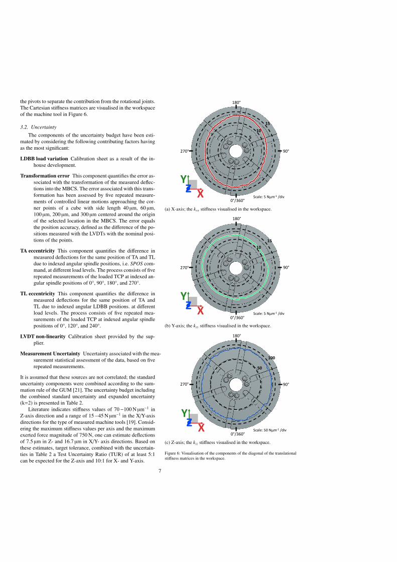
the pivots to separate the contribution from the rotational joints.The Cartesian stiffness matrices are visualised in the workspaceof the machine tool in Figure 6.
3.2. Uncertainty
The components of the uncertainty budget have been esti-mated by considering the following contributing factors havingas the most significant:
LDBB load variation Calibration sheet as a result of the in-house development.
Transformation error This component quantifies the error as-sociated with the transformation of the measured deflec-tions into the MBCS. The error associated with this trans-formation has been assessed by five repeated measure-ments of controlled linear motions approaching the cor-ner points of a cube with side length 40 µm, 60 µm,100 µm, 200 µm, and 300 µm centered around the originof the selected location in the MBCS. The error equalsthe position accuracy, defined as the difference of the po-sitions measured with the LVDTs with the nominal posi-tions of the points.
TA eccentricity This component quantifies the difference inmeasured deflections for the same position of TA and TLdue to indexed angular spindle positions, i.e. SPOS com-mand, at different load levels. The process consists of fiverepeated measurements of the loaded TCP at indexed an-gular spindle positions of 0°, 90°, 180°, and 270°.
TL eccentricity This component quantifies the difference inmeasured deflections for the same position of TA andTL due to indexed angular LDBB positions. at differentload levels. The process consists of five repeated mea-surements of the loaded TCP at indexed angular spindlepositions of 0°, 120°, and 240°.
LVDT non-linearity Calibration sheet provided by the sup-plier.
Measurement Uncertainty Uncertainty associated with the mea-surement statistical assessment of the data, based on fiverepeated measurements.
It is assumed that these sources are not correlated; the standarduncertainty components were combined according to the sum-mation rule of the GUM [21]. The uncertainty budget includingthe combined standard uncertainty and expanded uncertainty(k=2) is presented in Table 2.
Literature indicates stiffness values of 70−100 N µm−1 inZ-axis direction and a range of 15−45 N µm−1 in the X/Y-axisdirections for the type of measured machine tools [19]. Consid-ering the maximum stiffness values per axis and the maximumexerted force magnitude of 750 N, one can estimate deflectionsof 7.5 µm in Z- and 16.7 µm in X/Y- axis directions. Based onthese estimates, target tolerance, combined with the uncertain-ties in Table 2 a Test Uncertainty Ratio (TUR) of at least 5:1can be expected for the Z-axis and 10:1 for X- and Y-axis.
YXZ
0°/360°
90°
180°
270°
Scale: 5 Nμm-1 /div
15
10
5
(a) X-axis; the kxx stiffness visualised in the workspace.
YXZ
0°/360°
90°
180°
270°
15
5
Scale: 5 Nμm-1 /div
10
(b) Y-axis; the kyy stiffness visualised in the workspace.
YXZ
100
50
0°/360°
90°
180°
270°
Scale: 50 Nμm-1 /div
(c) Z-axis; the kzz stiffness visualised in the workspace.
Figure 6: Visualisation of the components of the diagonal of the translationalstiffness matrices in the workspace.
7
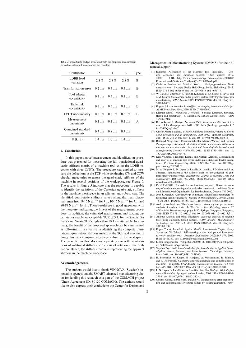
Table 2: Uncertainty budget associated with the proposed measurementprocedure. Standard uncertainties are rounded.
Contributor X Y Z Type
LDBB loadvariation 2.8 N 2.8 N 2.8 N B
Transformation error 0.2 µm 0.3 µm 0.3 µm B
Tool adaptereccentricity 0.2 µm 0.3 µm 0.1 µm B
Table linkeccentricity 0.3 µm 0.3 µm 0.1 µm B
LVDT non-linearity 0.6 µm 0.6 µm 0.6 µm B
Measurementuncertainty 0.1 µm 0.1 µm 0.1 µm A
Combined standarduncertainty 0.7 µm 0.8 µm 0.7 µm
U (k=2) 1.4 µm 1.6 µm 1.4 µm
4. Conclusion
In this paper a novel measurement and identification proce-dure was presented for measuring the full translational quasi-static stiffness matrix of a machine tool using the LDBB to-gether with three LVDTs. The procedure was applied to mea-sure the deflections at the TCP while conducting CW and CCWcircular trajectories to assess the quasi-static stiffness of themachine in several positions of the workspace, see Figure 6.The results in Figure 5 indicate that the procedure is capableto identify the variations of the Cartesian quasi-static stiffnessin the machine workspace in an efficient and robust way. Theidentified quasi-static stiffness values along the main diago-nal range from 9-15 N µm−1 for kxx, 10-15 N µm−1 for kyy, and80-87 N µm−1 for kzz. These results are in good agreement withthe literature, indicating the fitness of the measurement proce-dure. In addition, the estimated measurement and loading un-certainties enable an acceptable TUR of 5:1, for the Z-axis. Forthe X- and Y-axis TURs higher than 10:1 are attainable. In sum-mary, the benefit of the proposed approach can be summarisedas following: It is effective in identifying the complete trans-lational quasi-static stiffness matrix at the TCP and efficient indoing this in a comparatively large subset of the workspace.The presented method does not separately assess the contribu-tions of rotational stiffness of the axis of rotation in the eval-uation. Hence, the stiffness matrix is representing the apparentstiffness in the machine workspace.
Acknowledgements
The authors would like to thank VINNOVA (Sweden’s in-novation agency) and the SMART advanced manufacturing clus-ter for funding this research as a part of the COMACH project(Grant Agreement ID: S0120-COMACH). The authors wouldlike to also express their gratitude to the Center for Design and
Management of Manufacturing Systems (DMMS) for their fi-nancial support.[1] European Association of the Machine Tool Industries. Cec-
imo economic and statistical toolbox: Third quarter 2019,2020. URL https://www.cecimo.eu/wp-content/uploads/2020/01/
Economic-and-Statistical-Toolbox-Q3-2019-FINAL.pdf.[2] Christian Brecher and Manfred Weck. Werkzeugmaschinen Ferti-
gungssysteme. Springer Berlin Heidelberg, Berlin, Heidelberg, 2017.ISBN 978-3-662-46566-0. doi: 10.1007/978-3-662-46567-7.
[3] W. Gao, H. Haitjema, F. Z. Fang, R. K. Leach, C. F. Cheung, E. Savio, andJ. M. Linares. On-machine and in-process surface metrology for precisionmanufacturing. CIRP Annals, 2019. ISSN 00078506. doi: 10.1016/j.cirp.2019.05.005.
[4] Eugene I. Rivin. Handbook on stiffness & damping in mechanical design.ASME Press, New York, 2010. ISBN 0791802930.
[5] Dietmar Gross. Technische Mechanik. Springer-Lehrbuch. Springer,Berlin and Heidelberg, 13., aktualisierte auflage edition, 2016. ISBN366249471X.
[6] R. Hooke and J. Martyn. Lectiones Cutlerianae, or a collection of lec-tures. John Martyn printer, 1679. URL https://books.google.se/books?id=XeU5QzqCz6AC.
[7] Olivier Andre Bauchau. Flexible multibody dynamics, volume v. 176 ofSolid mechanics and its applications, 0925-0042. Springer, Dordrecht,2011. ISBN 978-94-007-0334-6. doi: 10.1007/978-94-007-0335-3.
[8] Reimund Neugebauer, Christian Scheffler, Markus Wabner, and CarstenZwingenberger. Advanced calculation of static and dynamic stiffness inmechatronic machine tools. International Journal of Mechatronics andManufacturing Systems, 4(3/4):370, 2011. ISSN 1753-1039. doi: 10.1504/IJMMS.2011.041478.
[9] Karoly Szipka, Theodoros Laspas, and Andreas Archenti. Measurementand analysis of machine tool errors under quasi-static and loaded condi-tions. Precision Engineering, 2017. ISSN 01416359. doi: 10.1016/j.precisioneng.2017.07.011.
[10] M. A. Salgado, L. N. Lopez de Lacalle, A. Lamikiz, J. Munoa, and J. A.Sanchez. Evaluation of the stiffness chain on the deflection of end-mills under cutting forces. International Journal of Machine Tools andManufacture, 45(6):727–739, 2005. ISSN 08906955. doi: 10.1016/j.ijmachtools.2004.08.023.
[11] ISO 230-1:2012. Test code for machine tools — part 1: Geometric accu-racy of machines operating under no-load or quasi-static conditions. Stan-dard, International Organization for Standardization, Geneva, CH, 2012.
[12] John S. Agapiou. A methodology to measure joint stiffness parameters fortoolholder-spindle interfaces. Journal of Manufacturing Systems, 24(1):13–20, 2005. ISSN 02786125. doi: 10.1016/S0278-6125(05)80003-2.
[13] Andreas Archenti and Theodoros Laspas. Accuracy and performanceanalysis of machine tools. In Wei Gao, editor, Metrology, volume 62of Precision Manufacturing, pages 1–30. Springer Singapore, Singapore,2019. ISBN 978-981-10-4912-5. doi: 10.1007/978-981-10-4912-5 7-1.
[14] Andreas Archenti and Mihai Nicolescu. Accuracy analysis of machinetools using elastically linked systems. CIRP Annals - ManufacturingTechnology, 62(1):503–506, 2013. ISSN 00078506. doi: 10.1016/j.cirp.2013.03.100.
[15] Eugen Trapet, Juan-Jose Aguilar Martın, Jose-Antonio Yague, HennySpaan, and Vit Zeleny. Self-centering probes with parallel kinematicsto verify machine-tools. Precision Engineering, 30(2):165–179, 2006.ISSN 01416359. doi: 10.1016/j.precisioneng.2005.07.002.
[16] Linear independence - wikipedia, 2020-03-06. URL https://en.wikipedia.org/wiki/Linear independence.
[17] Stephen Boyd and Lieven Vandenberghe. Introduction to Applied LinearAlgebra: Vectors, Matrices, and Least Squares. Cambridge UniversityPress, 2018. doi: 10.1017/9781108583664.
[18] H. Schwenke, W. Knapp, H. Haitjema, A. Weckenmann, R. Schmitt,and F. Delbressine. Geometric error measurement and compensation ofmachines—an update. CIRP Annals - Manufacturing Technology, 57(2):660–675, 2008. ISSN 00078506. doi: 10.1016/j.cirp.2008.09.008.
[19] L. N. Lopez de Lacalle and A. Lamikiz. Machine Tools for High Perfor-mance Machining. Springer London, London, 2009. ISBN 978-1-84800-379-8. doi: 10.1007/978-1-84800-380-4.
[20] Chunhe Gong, Jingxia Yuan, and Jun Ni. Nongeometric error identifica-tion and compensation for robotic system by inverse calibration. Inter-
8

national Journal of Machine Tools and Manufacture, 40(14):2119–2137,2000. ISSN 08906955. doi: 10.1016/S0890-6955(00)00023-7.
[21] Joint Committee for Guides in Metrology. Evaluation of measurementdata: Guide to the expression of uncertainty in measurement, 2008.
9