Supporting Information for:

Precipitating Polyelectrolyte-Surfactant

Systems by Admixing a Nonionic Surfactant –

a Case of Cononsurfactancy

Leonardo Chiappisi,∗,†,‡ Stephen David Leach,† and Michael Gradzielski∗,†

Stranski Laboratorium fur Physikalische Chemie und Theoretische Chemie, Institut fur

Chemie, Strasse des 17. Juni 124, Sekr. TC7, Technische Universitat Berlin, D-10623

Berlin, Germany, and Institut Max von Laue - Paul Langevin, Large Scale Structures

Group, 71 avenue des Martyrs - 38042 Grenoble Cedex 9

E-mail: leonardo.chiappisi@tu-berlin.de; michael.gradzielski@tu-berlin.de

Contents

1 Experimental details S2

2 Additional results S7

2.1 Pictures of Samples . . . . . . . . . . . . . . . . . . . . . . . . . . . . . . S7

2.2 Additional phase diagrams . . . . . . . . . . . . . . . . . . . . . . . . . . S8

2.3 Molecular weight of complexes . . . . . . . . . . . . . . . . . . . . . . . . S10

∗To whom correspondence should be addressed†Technische Universitat Berlin‡Institut Laue - Langevin

S1

Electronic Supplementary Material (ESI) for Soft Matter.This journal is © The Royal Society of Chemistry 2017

2.4 Additional ITC titrations . . . . . . . . . . . . . . . . . . . . . . . . . . . S11

2.5 Neutron small-angle scattering (SANS) results . . . . . . . . . . . . . . . S14

2.5.1 Analysis of SANS patterns from chitosan - C18:1E9Ac and C18:1E9

complexes . . . . . . . . . . . . . . . . . . . . . . . . . . . . . . . S14

2.5.2 Analytical expression for SANS Data analysis . . . . . . . . . . . S19

2.6 Characterization of pure surfactant mixtures . . . . . . . . . . . . . . . . S24

2.7 Ionization degree of pure components . . . . . . . . . . . . . . . . . . . . S28

1 Experimental details

Table S1: Densities, scattering length densities (SLD), and volumes (v used in for the de-scription of the SANS experimental results. SLDs and densities are obtained consideringsolvent-exchangeable protons.

Compound Density / g cm−3 SLD / 10−4 nm−2 v / nm3

Acetic acid buffer 1.10 6.27 —Chitosan 1.17 2.86 0.223C18:1 0.85 -0.36 0.494(OCH2CH2)9OCH2COOH 1.23 0.99 0.600(OCH2CH2)9OH 1.19 0.82 0.576

Light scattering Static (SLS) and dynamic (DLS) light scattering measurements were

performed simultaneously on the mixed micelle solutions on the same compact ALV/CGS-

3 instrument, equipped with a He-Ne laser with a wavelength of λ = 632.8 nm. The results

are reported in section 2.6 of the supporting information. Experiments were performed at

scattering angles θ ranging from 20◦ to 130◦ set with an ALV-SP 125 goniometer. Pseudo-

cross correlation functions were recorded using an ALV 5000/E multiple-τ correlator. All

measurements were carried out at 25.0(1) ◦C in a thermostatted toluene bath.

Absolute scattering intensities were obtained using toluene as a standard, where a

Rayleigh ratio of 1.340×10−5 cm−1 for 25 ◦C and 632.8 nm was used.1 Isotropic scattering

S2

is observed from the mixed micelle solutions investigated, and the forward scattering

intensity I(0) is obtained from the average of the intensities recorded between 20◦ to

130◦. The apparent molecular weight of the micelles of a solution of concentration c, is

obtained by means of the following relation:

Mappw =

I(0)

KLc(S1)

with KL being the optical constant:

KL =4π2

λ4NA

n20

(dn

dc

)2

(S2)

where NA is the Avogadro constant, n0 is the refractive index of the solvent and dn/dc ≈

0.119 cm3 g−1 is the refractive index increment. Due the high concentration of acetic

acid/sodium acetate in the buffer, there is no need to take into account the scattering

structure factor for the surfactant micelle solution.2 The micelle aggregation numbers

were obtained neglecting the free surfactant concentration, as justified by the very low

cmc of ∼ 6 · 10−6molL−1 for C18:1E9CH2COOH.

The mean decay rate Γ(q) was obtained from the field autocorrelation function:3

g(1)(τ, q) = exp(−Γ(q)τ

) (1 +

µ2

2τ 2)

(S3)

where τ and µ2 are the delay time and the second moment around the mean, respec-

tively. The apparent diffusion coefficient is obtained as Dapp = Γ(q)/q2, from which the

hydrodynamic radius (Rh) was obtained, applying the Stokes-Einstein relation:

Rh =kbT

6πη0Dapp

(S4)

with η0 being the solvent viscosity.

S3

Zeta-potential determination The electrophoretic mobility µe of the mixed micelles

was determined on a Malvern Zetasizer Nano Z, equipped with a He-Ne laser (633 nm).

The ζ-potential of the mixed micelles was calculated as:

ζ =3µeη

2ε0εrf(κa)(S5)

with η being the fluid viscosity, ε0 the vacuum permittivity, εr the relative permittivity,

and f(κa) is the Henry function approximated by:4

f(κa) =16 + 18κa+ 3(κa)2

16 + 18κa+ 2(κa)2(S6)

where κ is the inverse Debye length while a is the particle size approximated by its

hydrodynamic radius.

1H-NMR of surfactants The 1H-NMR spectrum of C18:1E9CH2COOH and C18:1E9

solubilized in CDCl3 was recorded on a Brucker Avance II spectrometer operating at 400

MHz. The spectra are reported in Figs. S1 and S2. From the integral of the different

peaks, we deduced that the alkyl chain is a 3:1 mixture of oleyl and palmitic alcohol, while

on average 8.8 EO units per surfactant chains are present. The degree of carboxymethy-

lation is of ∼ 0.9, in agreement with previous results from pH titrations.2 In Table S2

the predicted and experimentally determined integrals of the 1H-NMR peaks. In each

spectrum one unidentified peak is present: for C18:1E9CH2COOH a very broad peak is

observed at δ = 5.6 ppm, representing 3.5 % of the hydrogens in the sample; for C18:1E9

a singlet at 3.3 ppm, representing 2 % of the hydrogens in the sample, is present.

S4

7.0 6.5 6.0 5.5 5.0 4.5 4.0 3.5 3.0 2.5 2.0 1.5 1.0 0.5 ppm

3.00

22.20

2.16

2.89

2.15

35.24

1.77

1.52

2.94

solv

ent

CD

Cl 3

a

bc

d

e

f

g

h

CH3-(CH2)6-CH2-CH=CH-CH2-(CH2)5-CH2-CH2-O-(CH2CH2O)8.8-CH2-COOH

CH3-(CH2)13-CH2-CH2-O-(CH2CH2O)8.8-CH2-COOH

a

bcd

ee

fgh

h75 mol%

25 mol%

g

Figure S1: 1H-NMR spectrum (400 MHz, CDCl3) of C18:1E9CH2COOH.

7.0 6.5 6.0 5.5 5.0 4.5 4.0 3.5 3.0 2.5 2.0 1.5 1.0 0.5 ppm

3.00

22.43

2.09

3.14

1.43

1.95

34.52

1.57

CH3-(CH2)6-CH2-CH=CH-CH2-(CH2)5-CH2-CH2-O-(CH2CH2O)8.8-H

CH3-(CH2)13-CH2-CH2-O-(CH2CH2O)8.8-H

a

bbc

dd

ef

g

g75 mol%

25 mol%

a

b

c

f

d

e

f

g

Figure S2: 1H-NMR spectrum (400 MHz, CDCl3) of C18:1E9.

S5

Table S2: Characterization of 1H-NMR spectra from C18:1E9CH2COOH (left) and C18:1E9

(right). Chemical shift δ is given in ppm, in parentheses the letter used for their identi-fication in Figs. S1 and S2 is provided. Experimentally Iexp and calculated Ical integralsare normalized with respect to the three hydrogen of the terminal CH3 group.

δ Iexp Ical

0.9 (h) 3.0 31.2 (g) 22.2 231.5 (f) 2.2 22.0 (e) 2.9 33.4 (d) 2.1 2∼3.6 (c) 35.2 35.24.2 (b) 1.8 1.85.3 (a) 1.5 1.5

δ Iexp Ical

0.9 (g) 3.0 31.2 (f) 22.4 231.5 (e) 2.1 22.0 (d) 3.1 33.4 (c) 2.0 2∼3.6 (b) 34.5 35.25.3 (a) 1.6 1.5

S6

2 Additional results

2.1 Pictures of Samples

Cloudy Precipitate

Clear solutionTranslucent solution

Solid-like precipitate

Figure S3: Picture of two samples in within the two-phase region, with a total chitosancontent of 0.3 wt%, Z = 0.2, χ = 0.4, and pH 5.0 on the left and ca. 10 on the right.Picture evidence a homogenous, cloudy precipitate with a clear surnatant at high pH,while the formation of a solid-like precipitate in equilibrium with a translucent solution.The sample on the left, at pH 5 was gently shaken before taking the picture in order todisperse the precipitate.

S7

2.2 Additional phase diagrams

3.5

4.0

4.5

5.0

5.5

6.0

6.5

7.0

7.5

0.0 0.2 0.4 0.6 0.8 1.0

pH

1.0-[C18:1E9CH2COOH]/Cmax

105

106

107

108

109

Mw

/ g

mol

-1

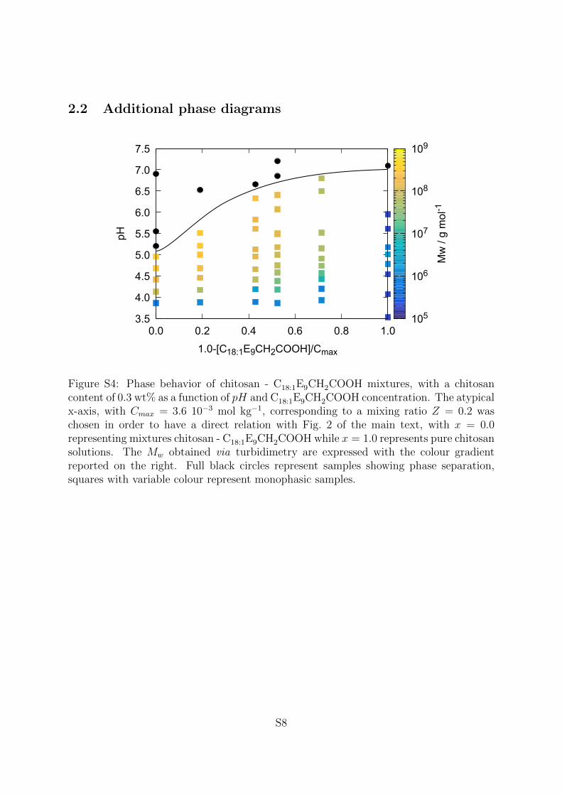
Figure S4: Phase behavior of chitosan - C18:1E9CH2COOH mixtures, with a chitosancontent of 0.3 wt% as a function of pH and C18:1E9CH2COOH concentration. The atypicalx-axis, with Cmax = 3.6 10−3 mol kg−1, corresponding to a mixing ratio Z = 0.2 waschosen in order to have a direct relation with Fig. 2 of the main text, with x = 0.0representing mixtures chitosan - C18:1E9CH2COOH while x = 1.0 represents pure chitosansolutions. The Mw obtained via turbidimetry are expressed with the colour gradientreported on the right. Full black circles represent samples showing phase separation,squares with variable colour represent monophasic samples.

S8

0

0.1

0.2

0.3

0.4

0.5

0.6

0.7

0 0.2 0.4 0.6 0.8 1

Z =

([C

18:1

E9]

+ [C

18:1

E9C

H2C

OO

H])

/[CH

-NH

3]

χ = [C18:1E9]/([C18:1E9] + [C18:1E9CH2COOH])

105

106

107

108

109

Mw

/ g

mol

-1

1Φ

2Φ

0

0.1

0.2

0.3

0.4

0.5

0.6

0.7

0 0.2 0.4 0.6 0.8 1

Z =

([C

18:1

E9]

+ [C

18:1

E9C

H2C

OO

H])

/[CH

-NH

3]

χ = [C18:1E9]/([C18:1E9] + [C18:1E9CH2COOH])

105

106

107

108

109

Mw

/ g

mol

-12Φ

1Φ

Figure S5: Phase behavior of chitosan - C18:1E9CH2COOH and C18:1E9 mixtures, with achitosan content of 0.3 wt%, pH = 4.0 on the top and 4.75 on the bottom, as a functionof Z and χ. The Mw obtained via turbidimetry are expressed with the colour gradientreported on the right. Full black circles represent samples showing phase separation,squares with variable colour represent monophasic samples. Dashed lines represent com-position values with constant C18:1E9CH2COOH content, i.e. constant charge ratio.

S9

2.3 Molecular weight of complexes

In table S3 the molecular weight of the complexes reported in Fig. 1 of the main text

are reported. The molecular weights were obtained via turbidimetric measurements, as

described in the experimental section of the main text.

Table S3: Molecular weights determined by turbidity measurements for the aggregates ofchitosan (0.3 wt%), at variable pH and χ as reported in Fig. 1 of the main text.

χ pH Mw / g mol−1 χ pH Mw / g mol−1 χ pH Mw / g mol−1

0.00 3.5 6.4·105 0.45 3.8 3.7·105 0.80 5.5 1.4·106

0.00 3.7 5.5·105 0.45 4.1 5.4·106 0.80 6.0 1.6·106

0.00 3.9 1.1·107 0.45 4.2 3.8·107 0.80 6.2 1.4·106

0.00 4.0 2.3·107 0.45 4.3 8.9·107 0.80 6.6 1.4·106

0.00 4.1 3.5·107 0.45 6.3 7.3·107 0.80 6.9 6.7·107

0.00 4.3 5.4·107 0.45 6.5 1.1·107

0.00 4.4 7.1·107 0.45 6.8 7.7·106 0.91 3.4 8.5·104

0.00 4.6 9.3·107 0.91 3.7 6.0·104

0.00 4.8 1.1·108 0.91 4.0 2.5·105

0.00 5.1 1.3·108 0.64 3.6 1.9·106 0.91 4.2 1.3·106

0.64 3.9 3.1·106 0.91 4.3 1.7·106

0.64 4.0 6.4·106 0.91 4.6 1.6·106

0.14 3.7 4.9·104 0.64 6.3 8.0·106 0.91 4.7 1.7·106

0.14 4.0 2.1·107 0.64 6.8 2.8·106 0.91 5.0 1.7·106

0.14 4.1 7.9·107 0.91 5.5 2.8·106

0.14 4.2 1.3·108 0.91 5.9 3.0·106

0.14 4.3 1.8·108 0.72 3.7 2.4·106 0.91 6.2 4.0·106

0.14 4.5 2.5·108 0.72 4.0 1.2·106 0.91 6.3 2.4·106

0.14 4.6 3.3·108 0.72 4.2 1.2·107 0.91 6.5 2.8·106

0.14 4.7 3.7·108 0.72 5.9 1.2·106 0.91 6.8 4.8·106

0.14 4.9 4.1·108 0.72 6.2 5.6·105

0.14 5.1 4.4·108 0.72 6.3 6.3·105 1.00 3.5 2.2·106

0.14 5.2 4.7·108 0.72 6.5 5.8·105 1.00 3.7 2.3·106

0.72 6.7 4.7·106 1.00 4.0 2.1·106

1.00 4.1 2.2·106

0.33 3.9 1.1·106 0.80 3.4 7.4·105 1.00 4.3 2.1·106

0.33 4.3 4.4·107 0.80 3.6 1.1·106 1.00 4.5 2.3·106

0.33 4.5 1.3·108 0.80 3.8 1.4·106 1.00 4.8 2.3·106

0.32 3.6 9.4·105 0.80 4.0 1.5·106 1.00 5.3 2.3·106

0.32 3.8 1.8·106 0.80 4.2 2.6·106 1.00 6.6 2.5·106

0.32 4.0 8.0·106 0.80 4.3 2.7·106

0.32 4.2 6.7·107 0.80 4.6 2.0·106

0.32 4.2 1.3·108 0.80 4.9 1.8·106

0.32 4.4 1.9·108 0.80 5.1 1.4·106

S10

2.4 Additional ITC titrations

In Fig. S6 the excess mixing heats and according fits for experiments performed at pH

3.75, 4.00, 4.25, 4.50, 4.75, and 5.00 are reported. The obtained parameters are given in

Table S4. Fits were performed using Eqs. 4 and 5 reported in the main text.

S11

-1.0

-0.5

0.0

0.5

-2.0

0.0

2.0

4.0

6.0 Z=0.2 - pH 3.75

2.0

4.0

6.0no chitosan - pH 3.75

Z=0.2 - pH 4.00

no chitosan - pH 4.00

-1.0

-0.5

0.0

0.5

-2.0

0.0

2.0

4.0

6.0 Z=0.2 - pH 4.25

2.0

4.0

no chitosan - pH 4.25

Z=0.2 - pH 4.50

no chitosan - pH 4.50

-1.0

-0.5

0.0

0.5

0 0.2 0.4 0.6 0.8 1

-2.0

0.0

2.0

4.0

6.0 Z=0.2 - pH 4.75

2.0

4.0

no chitosan - pH 4.75

0.2 0.4 0.6 0.8 1

χ = [C18:1E9]/([C18:1E9] + [C18:1E9CH2COOH]

Z=0.2 - pH 5.00

no chitosan - pH 5.00

h E(χ

)q o

bs(χ

)q o

bs(χ

)h E

(χ)

q obs

(χ)

q obs

(χ)

h E(χ

)q o

bs(χ

)q o

bs(χ

)

Figure S6: ITC results obtained for titrations performed between pH 3.75 to pH 5.0. qobsare the integrated heats given in kJ mol−1; empty circles are titrations of C18:1E9 intoC18:1E9CH2COOH (q1), empty squares are titrations of C18:1E9CH2COOH into C18:1E9

(q2). Dotted and broken lines are best fits with a common set of parameters for q1 andq2 via Eqs. 4 and 5 in the main text. The excess mixing enthalpies are also reportedin kJ mol−1 from titration without (hZ=∞E (χ), dotted line) and with chitosan (hZ=0.2

E (χ),broken line); the excess chitosan-surfactant interaction (HE(χ)) is represented as thickfull line.

S12

Table S4: Fit parameters obtained from ITC. For each investigated pH, the coefficients of the polyno-mial used in Eq. 2 of the main text with the uncertainties arising from the fitting procedure is reported.The coefficients used for calculating the excess chitosan-surfactant interaction (HE(χ)) are obtained asthe difference between the coefficients for the excess mixing enthalpy obtained in the presence of chitosanhZ=0.2E (χ) and without chitosan hZ=∞

E (χ).

pH = 3.75 pH = 4.0 pH = 4.25

hZ=∞E (χ) ρ0 4.35·103 8·102 ρ0 3.91·103 6·102 ρ0 2.60·103 1·102

ρ1 -3.10·104 9·103 ρ1 -6.16·103 7·103 ρ1 -4.71·103 1·103

ρ2 1.48·105 4·104 ρ2 -3.53·103 3·104 ρ2 3.10·104 4·103

ρ3 -3.23·105 8·104 ρ3 7.47·104 6·104 ρ3 -5.28·104 6·103

ρ4 3.29·105 8·104 ρ4 -1.36·105 7·104 ρ4 2.85·104 3·103

ρ5 -1.25·105 3·104 ρ5 7.49·104 3·104 ρ5 — —ρ6 -3.97·102 6·101 ρ6 — — ρ6 — —

hZ=0.2E (χ) ρ0 2.23·103 1·103 ρ0 8.96·102 5·102 ρ0 8.49·102 1·103

ρ1 -1.70·104 1·104 ρ1 -7.40·102 6·103 ρ1 -4.23·103 1·104

ρ2 6.85·104 6·104 ρ2 -5.49·103 3·104 ρ2 5.12·104 5·104

ρ3 -9.64·104 1·105 ρ3 1.96·104 7·104 ρ3 -1.72·105 9·104

ρ4 2.91·104 1·105 ρ4 -1.62·104 8·104 ρ4 2.46·105 1·105

ρ5 2.60·104 5·104 ρ5 9.29·103 4·104 ρ5 -1.19·105 4·104

ρ6 2.31·102 8·101 ρ6 3.60·102 2·102 ρ6 4.25·102 2·102

HE(χ) ρ0 -2.12·103 2·103 ρ0 -3.02·103 1·103 ρ0 -1.76·103 1·103

ρ1 1.40·104 2·104 ρ1 5.42·103 1·104 ρ1 4.85·102 1·104

ρ2 -7.91·104 9·104 ρ2 -1.96·103 6·104 ρ2 2.01·104 5·104

ρ3 2.26·105 2·105 ρ3 -5.51·104 1·105 ρ3 -1.19·105 1·105

ρ4 -3.00·105 2·105 ρ4 1.20·105 1·105 ρ4 2.17·105 1·105

ρ5 1.51·105 8·104 ρ5 -6.56·104 7·104 ρ5 -1.19·105 4·104

ρ6 6.28·102 1·102 ρ6 3.60·102 2·102 ρ6 4.25·102 2·102

pH = 4.5 pH = 4.75 pH = 5.0

hZ=∞E (χ) ρ0 1.29·103 2·102 ρ0 4.49·103 2·102 ρ0 5.33·103 2·103

ρ1 2.82·103 1·103 ρ1 -1.82·104 2·103 ρ1 -2.97·104 2·104

ρ2 6.43·103 5·103 ρ2 5.78·104 6·103 ρ2 1.27·105 8·104

ρ3 -1.31·104 7·103 ρ3 -6.51·104 9·103 ρ3 -2.67·105 2·105

ρ4 6.60·103 4·103 ρ4 2.64·104 4·103 ρ4 2.95·105 2·105

ρ5 — — ρ5 — — ρ5 -1.32·105 8·104

ρ6 — — ρ6 — — ρ6 -6.54·102 2·102

hZ=0.2E (χ) ρ0 3.59·103 6·102 ρ0 9.09·103 2·103 ρ0 2.51·103 1·103

ρ1 -3.81·104 7·103 ρ1 -9.34·104 2·104 ρ1 -2.36·104 1·104

ρ2 2.09·105 3·104 ρ2 4.62·105 6·104 ρ2 1.90·105 5·104

ρ3 -5.21·105 8·104 ρ3 -1.07·106 1·105 ρ3 -5.81·105 1·105

ρ4 6.16·105 8·104 ρ4 1.17·106 1·105 ρ4 7.70·105 1·105

ρ5 -2.69·105 4·104 ρ5 -4.78·105 4·104 ρ5 -3.59·105 4·104

ρ6 7.02·102 7·101 ρ6 8.01·102 1·102 ρ6 6.45·102 2·102

HE(χ) ρ0 2.30·103 8·102 ρ0 4.61·103 2·103 ρ0 -2.82·103 3·103

ρ1 -4.09·104 9·103 ρ1 -7.51·104 2·104 ρ1 6.19·103 3·104

ρ2 2.03·105 4·104 ρ2 4.05·105 7·104 ρ2 6.23·104 1·105

ρ3 -5.07·105 8·104 ρ3 -1.00·106 1·105 ρ3 -3.14·105 3·105

ρ4 6.09·105 9·104 ρ4 1.14·106 1·105 ρ4 4.75·105 3·105

ρ5 -2.69·105 4·104 ρ5 -4.78·105 4·104 ρ5 -2.27·105 1·105

ρ6 7.02·102 7·101 ρ6 8.01·102 1·102 ρ6 1.30·103 4·102

S13

2.5 Neutron small-angle scattering (SANS) results

2.5.1 Analysis of SANS patterns from chitosan - C18:1E9Ac and C18:1E9 com-

plexes

10-4

10-3

10-2

10-1

100

101

102

103

104

0.01 0.1 1

I(q)

/ cm

-1

χ = 0.0, pH = 3.53.73.83.94.04.14.34.44.65.0

0.01 0.1 1q / nm-1

pH = 4.0, χ = 1.00.90.80.70.60.50.40.30.20.10.0

Figure S7: Neutron small-angle scattering (SANS) patterns recorded on V4 at theHelmholtz Zentrum Berlin arising from chitosan chitosan - C18:1E9Ac and C18:1E9 mix-tures, with a chitosan content of 0.3 wt%, χ = 0.0, Z = 0.2, and variable pH (on the left)and at pH = 4.0, Z = 0.2, and variable χ (on the right). Curves scaled for an improvedreadability are given in the main text.

SANS patterns arising from chitosan - C18:1E9Ac and C18:1E9 mixtures are reported

in Fig. S9. The data can be quantitatively described using the scattering models de-

scribed in detail elsewhere.2 Briefly, three structural models are employed (all analytical

expressions are also given in the next section of the supporting information):

(i) when no or only weak interactions between chitosan and the surfactant micelle

are present, no evidence for supramolecular aggregation is found. The scattering pat-

terns of a randomly decorated polymer network or independently distributed surfactant

S14

micelles and polymer chains in the solution, i.e., no interaction present, are identical.

Accordingly, the scattering curves obtained at low pH for χ = 0.0 and at high χ for pH

= 4.0 were described as a linear superposition of the scattering pattern arising from the

chitosan chains, treated as gaussian coils (Eq. S17), and the surfactant micelles, treated

as elongated core-shell micelles (Eq. S7).2,5 The different contributions and the resulting

calculated scattering curve are shown in Fig. S8.

(ii) when moderate interactions between chitosan and the surfactant micelle are

present. The formation of aggregates with aligned micelles embedded in a chitosan net-

work is found.2,6 The scattering patterns were described using a model of N aligned

core-shell ellipsoids (the micelles) contained in an homogeneous cylinder (the complexed

chitosan).2,7 The scattering form factor is given in Eq. S18. A mass-fractal structure

factor with a dimensionality of three is used to take into account the aggregation of the

cylindrical subunits (Eq. S23). The model was applied to described the scattering curves

from samples with χ = 0 and 3.7 < pH < 4.3, and for pH = 4.0 and 0.5 < χ < 1.

(iii) when strong interactions between chitosan and the surfactant micelle are present

the aggregates are found to be collapsed into a core-corona structure, with a core formed

by densely packed surfactant micelles surrounded by a stabilizing polymer corona,2,6

a model initially developed by Berret et al .8 As the size of the micelle and that of

the supramolecular aggregate differ by two orders of magnitude (3.5 vs. 150 nm), the

scattering form factor can be expressed as the sum of a term arising from dense packed

micelles (core-shell ellipsoids with an hard sphere structure factor) and a term from

the formed supramolecular structure (a homogeneous core-shell sphere).2,6 Analytical

expressions used for the calculations are given in the next section. The model was applied

to described the scattering curves from samples with χ = 0 and pH > 4.05, and for pH

= 4.0 and χ = 1.

Note that samples found at the border line between the structural picture ii (one-

S15

10-4

10-3

10-2

10-1

100

101

0.1 1

Gauss chain

Bkg.

Micelle

I(q)

/ cm

-1

q / nm-1

χ = 0.0, pH = 3.5

10-4

10-3

10-2

10-1

100

101

102

103

104

0.01 0.1 1

Bkg.I(

q) /

cm-1

q / nm-1

pH = 4.3, χ = 0.0

Model ii

Model iii

Figure S8: Representative calculations of the SANS patterns. On the left, the scatteringcurve of a mixture representative for case (i), when no no or weak interaction is present,and the SANS pattern is given by the sum of the contribution of the chitosan gaussianchain (red), the surfactant micelles (blue), and the incoherent background (gray). Onthe right, the scattering pattern representative for chitosan - surfactant mixtures wherethe structures described case (ii) and case (iii) coexists. All models are explained in theprevious page of the text.

dimensional complex) and iii (core-corona suprastrucure) were described using both mod-

els (a representative calculation is given in Fig. S8). Calculated curves and experimental

data are reported in Fig. 5 of the main text and in Fig. S9. The parameters used for the

calculation of the scattering curves are reported in Table S5.

S16

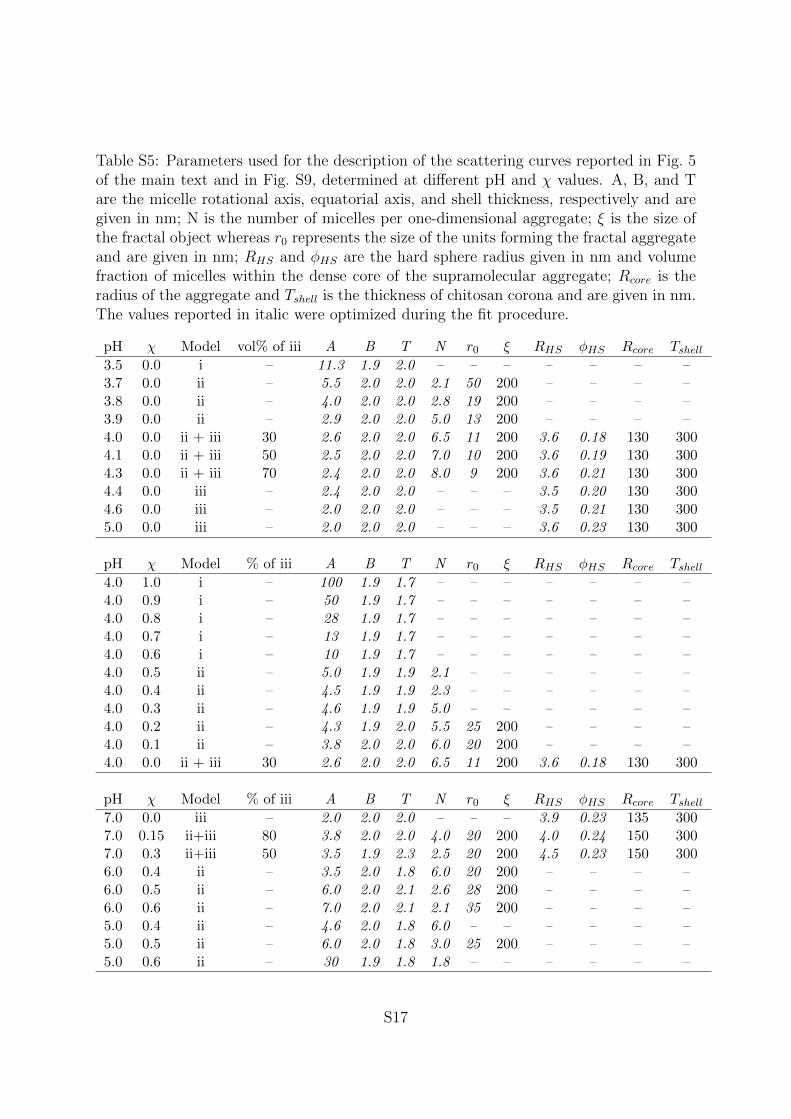
Table S5: Parameters used for the description of the scattering curves reported in Fig. 5of the main text and in Fig. S9, determined at different pH and χ values. A, B, and Tare the micelle rotational axis, equatorial axis, and shell thickness, respectively and aregiven in nm; N is the number of micelles per one-dimensional aggregate; ξ is the size ofthe fractal object whereas r0 represents the size of the units forming the fractal aggregateand are given in nm; RHS and φHS are the hard sphere radius given in nm and volumefraction of micelles within the dense core of the supramolecular aggregate; Rcore is theradius of the aggregate and Tshell is the thickness of chitosan corona and are given in nm.The values reported in italic were optimized during the fit procedure.

pH χ Model vol% of iii A B T N r0 ξ RHS φHS Rcore Tshell3.5 0.0 i – 11.3 1.9 2.0 – – – – – – –3.7 0.0 ii – 5.5 2.0 2.0 2.1 50 200 – – – –3.8 0.0 ii – 4.0 2.0 2.0 2.8 19 200 – – – –3.9 0.0 ii – 2.9 2.0 2.0 5.0 13 200 – – – –4.0 0.0 ii + iii 30 2.6 2.0 2.0 6.5 11 200 3.6 0.18 130 3004.1 0.0 ii + iii 50 2.5 2.0 2.0 7.0 10 200 3.6 0.19 130 3004.3 0.0 ii + iii 70 2.4 2.0 2.0 8.0 9 200 3.6 0.21 130 3004.4 0.0 iii – 2.4 2.0 2.0 – – – 3.5 0.20 130 3004.6 0.0 iii – 2.0 2.0 2.0 – – – 3.5 0.21 130 3005.0 0.0 iii – 2.0 2.0 2.0 – – – 3.6 0.23 130 300

pH χ Model % of iii A B T N r0 ξ RHS φHS Rcore Tshell4.0 1.0 i – 100 1.9 1.7 – – – – – – –4.0 0.9 i – 50 1.9 1.7 – – – – – – –4.0 0.8 i – 28 1.9 1.7 – – – – – – –4.0 0.7 i – 13 1.9 1.7 – – – – – – –4.0 0.6 i – 10 1.9 1.7 – – – – – – –4.0 0.5 ii – 5.0 1.9 1.9 2.1 – – – – – –4.0 0.4 ii – 4.5 1.9 1.9 2.3 – – – – – –4.0 0.3 ii – 4.6 1.9 1.9 5.0 – – – – – –4.0 0.2 ii – 4.3 1.9 2.0 5.5 25 200 – – – –4.0 0.1 ii – 3.8 2.0 2.0 6.0 20 200 – – – –4.0 0.0 ii + iii 30 2.6 2.0 2.0 6.5 11 200 3.6 0.18 130 300

pH χ Model % of iii A B T N r0 ξ RHS φHS Rcore Tshell7.0 0.0 iii – 2.0 2.0 2.0 – – – 3.9 0.23 135 3007.0 0.15 ii+iii 80 3.8 2.0 2.0 4.0 20 200 4.0 0.24 150 3007.0 0.3 ii+iii 50 3.5 1.9 2.3 2.5 20 200 4.5 0.23 150 3006.0 0.4 ii – 3.5 2.0 1.8 6.0 20 200 – – – –6.0 0.5 ii – 6.0 2.0 2.1 2.6 28 200 – – – –6.0 0.6 ii – 7.0 2.0 2.1 2.1 35 200 – – – –5.0 0.4 ii – 4.6 2.0 1.8 6.0 – – – – – –5.0 0.5 ii – 6.0 2.0 1.8 3.0 25 200 – – – –5.0 0.6 ii – 30 1.9 1.8 1.8 – – – – – –

S17

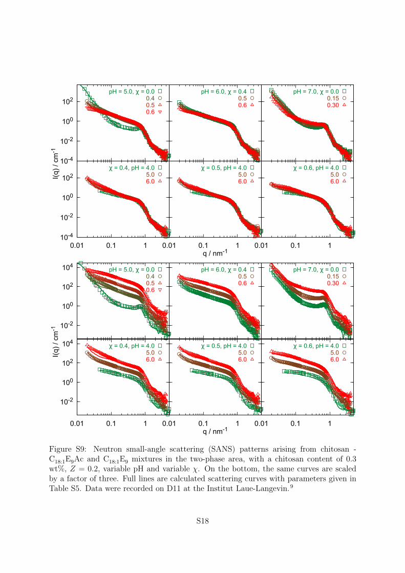
10-4

10-2

100

102

I(q)

/ cm

-1

pH = 5.0, χ = 0.00.40.50.6

pH = 6.0, χ = 0.40.50.6

pH = 7.0, χ = 0.00.150.30

10-4

10-2

100

102

0.01 0.1 1

χ = 0.4, pH = 4.05.06.0

0.01 0.1 1q / nm-1

χ = 0.5, pH = 4.05.06.0

0.01 0.1 1

χ = 0.6, pH = 4.05.06.0

10-2

100

102

104

I(q)

/ cm

-1

pH = 5.0, χ = 0.00.40.50.6

pH = 6.0, χ = 0.40.50.6

pH = 7.0, χ = 0.00.150.30

10-2

100

102

104

0.01 0.1 1

χ = 0.4, pH = 4.05.06.0

0.01 0.1 1q / nm-1

χ = 0.5, pH = 4.05.06.0

0.01 0.1 1

χ = 0.6, pH = 4.05.06.0

Figure S9: Neutron small-angle scattering (SANS) patterns arising from chitosan -C18:1E9Ac and C18:1E9 mixtures in the two-phase area, with a chitosan content of 0.3wt%, Z = 0.2, variable pH and variable χ. On the bottom, the same curves are scaledby a factor of three. Full lines are calculated scattering curves with parameters given inTable S5. Data were recorded on D11 at the Institut Laue-Langevin.9

S18

2.5.2 Analytical expression for SANS Data analysis

All expression are also reported in the supporting information of Ref. 2 and are reported

here for the sake of completeness.

Surfactant Micelle The scattering arising from the surfactant micelles is described

using a core-shell ellipsoidal model.10 The scattering form factor is given by:

PCS(q) =

∫ 1

0

|F (q, cosα)|2d cosα (S7)

with α being the angle formed by the scattering vector and the rotational axis of the

ellipsoid. F (q, cosα) is the scattering amplitude and is given by

F (q, cosα) = (SLDc − SLDsh)Vc

[3j1(xc)

xc

]+(SLDsh − SLD

)Vt

[3j1(xt)

xt

](S8)

with SLDsh and SLD being the scattering length densities of the micellar shell and of

the medium, respectively. The scattering length density of the shell was obtained as the

volume average of the SLDs of the hydrophylic part of the surfactant and the solvent.

j1(x) is the first order spherical Bessel function:

j1(x) =sin(x)− x cos(x)

x2(S9)

xc and xt are given by:

xc = q√A2 cosα2 +B2(1− cosα2) (S10)

xt = q√

(A+ T )2 cosα2 + (B + T )2(1− cosα2) (S11)

S19

and the volumes of the core and of the particle are

Vc =4

3πAB2 (S12)

Vt =4

3π(A+ T )(B + T )2 (S13)

The particle number density was calculated from the micellar core as

1N =3φc

4πAB2(S14)

with phic being the volume fraction of the C18:1 units. φc was obtained from the vol-

ume fractions of the ionic and nonionic surfactant and the volumes of hydrophilic and

hydrophobic part of the surfactant reported in Table S1. The aggregation number from

the volume of the hydrophobic tail of the surfactant (vc)

Nagg =4πAB2

3vc(S15)

The water content of the shell was calculated as

φshellw =Vsh −Naggvs

Vsh(S16)

with Vsh = Vt − Vc being the volume of the hydrated shell and vs the average volume of

the surfactant headgroup.

Chitosan chains The scattering arising from chitosan is described with a gaussian

chain model:11

I(q) = 2 · I(0)chie−q

2Rg2 + q2Rg2 − 1

q4Rg4(S17)

S20

with I(0)chi and Rg being the forward scattering intensity and the radius of gyration of

the polymer chain, respectively. In the calculations, the values of I(0)chi of 20-40 cm−1

and Rg ∼ 250 nm, determined for pure chitosan solutions in Ref. 2 were used.

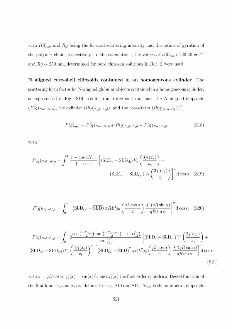
N aligned core-shell ellipsoids contained in an homogeneous cylinder The

scattering form factor for N-aligned globular objects contained in a homogeneous cylinder,

as represented in Fig. S10, results from three contributions: the N aligned ellipsoids

(P (q)Nob−Nob), the cylinder (P (q)Cyl−Cyl), and the cross-term (P (q)Nob−Cyl):7

P (q)agg = P (q)Nob−Nob + P (q)Cyl−Cyl + P (q)Nob−Cyl (S18)

with

P (q)Nob−Nob =

∫ 1

0

1− cos zNmic

1− cos z

[(SLDc − SLDsh)Vc

(3j1(xc)

xc

)+

(SLDsh − SLDcyl)Vt

(3j1(xt)

xt

)]2d cosα (S19)

P (q)Cyl−Cyl =

∫ 1

0

[(SLDcyl − SLD

)πRL2j0

(qL cosα

2

)J1 (qR sinα)

qR sinα

]2d cosα (S20)

P (q)Nob−Cyl =

∫ 1

0

2cos(z Nmic

2

)sin(z Nmic+z

2

)− sin

(z2

)sin(z2

) [(SLDc − SLDsh)Vc

(3j1(xc)

xc

)+

(SLDsh − SLDcyl)Vt

(3j1(xt)

xt

)]·[(

SLDcyl − SLD)2πRL2j0

(qL cosα

2

)J1 (qR sinα)

qR sinα

]d cosα

(S21)

with z = qD cosα, j0(x) = sin(x)/x and J1(x) the first-order cylindrical Bessel function of

the first kind. xc and xt are defined in Eqs. S10 and S11. Nmic is the number of ellipsoids

S21

2R

LD

Figure S10: Schematic representation of the structure formed by stiff polyelectrolytesand weakly charged macroions. Such a structure can be approximated with a particlesin a cylinder model, characterized by an overall extension L, a radius R and a spacingbetween the centers of the objects of D.

per cylinder and D the spacing between their centers. The scattering length densities

were calculated assuming an anhydrous micellar core, a micellar core composed of water

and the hydrophilic part of the surfactant, and the cylinder being made of chitosan and

solvent. The amount of chitosan in the cylinder is calculated in such a way that charge

neutrality is reached within the cylinder. The number density of the cylinders is obtained

assuming all surfactant being involved in the complex:

1Ncyl =1N

Nmic

=3φc

4πNmicAB2(S22)

A mass-fractal structure factor is used to describe the supramolecular aggregation of

the cylindrical building blocks:2

S(q)agg = 1 +3 sin (3 arctan(qξ))

(qr0)3[1 + 1

q2ξ2

] (S23)

Densely packed micelles in a supramolecular core-shell structure The scatter-

ing pattern arising from a supramolecular core-shell structure formed by a core of densely

S22

packed micelles glued together by chitosan and stabilized by a chitosan shell was obtained

as:2

I(q) = 1NSAPSA(q) + 1NPCS(q)SHS(q) (S24)

with PSA(q) being the scattering form factor of a homogeneous core-shell sphere, SHS(q)

is the hard-sphere structure factor:12

SHS(q) =(1− 1NC0(q)

)−1(S25)

with

1NC0(q) =Λ

x3(sinx− x cosx) +

Υ

x3

((2

x2− 1

)x cosx+ 2 sinx− 2

x

)−ΛφHS

2x3

[24

x3+ 4

(1− 6

x2

)sinx−

(1− 12

x2+

24

x4

)x cosx

](S26)

with x = 2RSq, Λ = −24φHS

(1+2φHS

(1−φHS)2

)2and Υ = 36

(φHS

2+φHS

(1−φHS)2

)2.

Given the large difference in size between the surfactant micelle and the supramolecu-

lar aggregate, the micelle-aggregate cross-term was neglected. The scattering form factor

of the supramolecular aggregate is obtained as:

PSA(q) =

[V SAc

(SLDSA

c − SLDSAsh

) 3 sinωc − 3ωc cosωcωc3

+

V SAt

(SLDSA

sh − SLD) 3 sinωsh − 3ωsh cosωsh

ω3sh

]2(S27)

with SLDSAc , SLDSA

sh , V SAc and V SA

t being the scattering length densities of the core and

the shell of the supraaggregate, and the volume of the core and the total volume of the

SA, respectively. ωc = qRSAc and ωsh = qRSA

sh with RSAc and RSA

s being the radii of

the core and the shell of the supraaggregate, respectively. For the calculation a normal

distribution of RSAc with a relative standard deviation 0.3 was assumed.

S23

The number of micelles in the supraaggregate core was obtained combining the radius

of the supraaggregate and the hard-sphere radius and volume fraction:

Nmic =

⟨RSAc

3⟩

R3HS

φHS (S28)

Accordingly, the supraaggregate number density is given by:

1NSA =1N

Nmic

=3φc

4πNmicAB2(S29)

The scattering length density of the core of the supraaggregate was calculated as the

volume weighted average of the components (surfactants, chitosan, and solvent):

SLDSAc =

NmicNagg (vc + vs)

4/3πRSAc

3 SLDsurf +φchχ

chicorevch

4/3πRSAc

3 SLDchi+(4/3πRSA

c3 −NmicNagg (vc + vs)− φchχchicorevch

)4/3πRSA

c3 SLDsolv (S30)

and the scattering length density of the shell of the supraaggregate as

SLDSAsh =

φchχchish vch

4/3πRSAs

3 − 4/3πRSAc

3SLDchi+

(4/3πRSA

s3 − 4/3πRSA

c3 − φchχchish vch

)4/3πRSA

s3 − 4/3πRSA

c3 SLDsolv

(S31)

2.6 Characterization of pure surfactant mixtures

The mixing behavior of the ionic C18:1E9CH2COOH and the nonionic C18:1E9 was in-

vestigated both from a thermodynamic and structural perspective. The excess mixing

enthalpy were determined via calorimetric titrations (Eqs. 3 and 4 of the main text) and

are reported in Fig. S11. Given the chemical similarity of the surfactant, we made use

of the regular solution theory for the description of the thermodynamics of the mixing

S24

0.0

0.2

0.4

0.6

0.8

1.0

0.0 0.2 0.4 0.6 0.8 1.0

ΔH

mix

/ kJ

mol

-1

χ = [C18:1E9]/([C18:1E9] + [C18:1E9CH2COOH]

pH = 3.75pH = 4.00pH = 4.25pH = 4.50pH = 4.75pH = 5.00

Figure S11: Mixing enthalpies determined at a total surfactant concentration of ∼10−3molL−1 and at variable pH, as a function of non-ionic surfactant content χ. Fulllines are fits according to Eq. S34. Arrow indicates effect of increasing pH.

-1.4

-1.2

-1.0

-0.8

-0.6

-0.4

-0.2

0.0

0.0 0.2 0.4 0.6 0.8 1.0

ΔG

mix

/ kJ

mol

-1

χ = [C18:1E9]/([C18:1E9] + [C18:1E9CH2COOH]

pH = 3.75pH = 4.00pH = 4.25pH = 4.50pH = 4.75pH = 5.00

Figure S12: Gibbs free energy of mixing determined at a total surfactant concentrationof ∼ 10−3molL−1 and at variable pH, as a function of non-ionic surfactant content χ.

S25

process. Accordingly, the molar mixing entropy for ideal mixing is given by:13

T∆Sm = −RT [χ lnχ+ (1− χ) ln(1− χ)] (S32)

with R being the ideal gas constant and T the absolute temperature. The combination

of experimentally determined mixing enthalpy (Fig. S11) and calculated mixing entropy

leads to the mixing free energy (Fig. S12). The mixing enthalpy can be expressed as a

polynomial expansion:

∆Hm = χ(1− χ)∑i=1

Ai(2χ− 1)i−1 (S33)

Developing the series only to its first term leads to the simple expression ∆Hm = Aχ(1−

χ), also known as the Porter equation.14 Given the slight asymetric shape of the excess

mixing enthalpy curves, with the maximum around 0.6, Eq. S33 was developed up to the

second term, leading to

∆Hm = χ(1− χ) [A+B(2χ− 1)] (S34)

The free energy of mixing was described as:15

∆Gm/RT = βχ(1− χ) (S35)

The mixing enthalpy and the free energy of mixing were fitted with Eqs. S34 and S35,

respectively. The obtained values are reported in Table S6. All mixing processes are

slightly endothermic, as also found in several surfactant/lipid mixtures.16 However, the

enthalpic contribution is compensated by the mixing entropy, resulting in an exergonic

process, i.e. fully miscible micelles are formed, as expected from the chemical similarity

of both headgroup and tail (see Fig. S12). Although the simple, first order development

S26

Table S6: Parameters used for the description of the mixing enthalpy and mixing freeenergy of the ionic C18:1E9CH2COOH and the nonionic C18:1E9 surfactant.

pH A / J mol−1 B / J mol−1 β3.75 2200 ± 30 460 ± 70 -2.03 ± 0.034.00 3220 ± 50 900 ± 100 -1.62 ± 0.034.25 3100 ± 20 1500 ± 40 -1.66 ± 0.044.50 3000 ± 20 1500 ± 50 -1.70 ± 0.054.75 3400 ± 20 1400 ± 60 -1.55 ± 0.045.00 3400 ± 60 1250 ± 100 -1.55 ± 0.04

of the free energy reported in Eq. S35 does not capture the whole complexity of the

system, it offers a useful approach for comparing the β parameter with values found in

similar systems. In fact, the values for this system of −2 < β < −1.5 fall within the usual

range of anionic-nonionic ethoxylated surfactant mixtures.15 With increasing pH, i.e. with

increasing charge density of the ionic species, the process becomes more endothermic and

more asymmetric, as evidenced also by the increasing values of A and B of Eq. S34. This

observation can be explained by the fact that with increasing degree of ionization of the

surfactants, a larger difference between the headgroups is observed: the area per molecule

at the core-shell interface of the surfactant micelle for C18:1E9CH2COOH increases from

59 to 69 A2 when pH is varied between 2.7 and 6.2.5 As a comparison, the headgroup

area of C16E9 at the air-water interface is 53 A2.17

The headgroup size difference is also clearly visible in the micelle aggregation numbers

and hydrodynamic radii, as determined by static and dynamic light scattering, respec-

tively (see Fig. S13). With increasing nonionic surfactant content the micelles grow in

size, with an hydrodynamic radius increasing from ca. 5 to almost 25 nm, and the ag-

gregation number increasing from ca. 200 to above 3000 molecules per micelle. This is a

consequence of an effective decrease of headgroup area requirement, resulting in a larger

packing parameter. Almost no differences are observed between mixtures at pH 4.5 and

5.0, while the growth process takes place at lower χ for the more weakly charged system

at pH 4.0. The results are in good agreement with previous SANS experiments per-

S27

formed on C18:1E9CH2COOH between pH 2.5 and 10, showing a transition from rodlike

to globular micelles upon acidification.5

0

5

10

15

20

25

0.0 0.2 0.4 0.6 0.8 1.0

Rh

/ nm

χ = [C18:1E9]/([C18:1E9] + [C18:1E9CH2COOH]

pH = 4.00pH = 4.50pH = 5.00

102

103

104

0.0 0.2 0.4 0.6 0.8 1.0N

agg

χ = [C18:1E9]/([C18:1E9] + [C18:1E9CH2COOH]

pH = 4.00pH = 4.50pH = 5.00

Figure S13: Hydrodynamic radius (left) and aggregation number (right) determined vialight scattering experiments at a total surfactant concentration of 1 wt% and at variablepH, as a function of non-ionic surfactant content χ.

To probe the ionization condition of the micellar aggregate ζ-potential experiments

were carried out and are reported in Fig. S14. The different pH has no effect on the

determined ζ-potential values, as the additional charges arising from the increased degree

of ionization of C18:1E9CH2COOH are compensated by condensed counterions. Moreover,

two regions can be identified in the evolution of the ζ-potential with χ: below χ = 0.4,

where a ζ-potential value of ca. -25 mV is determined; and for χ > 0.4, where the

potential approaches zero, till a neutral surface is obtained for χ = 1, i.e., the pure

nonionic surfactant. Similar values are found in other ionic/nonionic mixed micellar

systems determined at salt content ∼ 0.2 M, as it was in our case.18,19

2.7 Ionization degree of pure components

In Fig. S15 the degree of ionization of chitosan and C18:1E9CH2COOH as a function of

pH is reported. Titration were performed adding a 0.1 mol L−1 standard NaOH solution

to a 1 wt% solution of chitosan or C18:1E9CH2COOH in the presence of 1 mol L−1 HCl.

S28

-40

-35

-30

-25

-20

-15

-10

-5

0

5

0.0 0.2 0.4 0.6 0.8 1.0

Zet

a P

oten

tial /

mV

χ = [C18:1E9]/([C18:1E9] + [C18:1E9CH2COOH]

pH = 4.00pH = 4.50pH = 5.00

Figure S14: ζ-potential determined at a total surfactant concentration of 1 wt% and atdifferent pH, as a function of non-ionic surfactant content χ.

0.0

0.2

0.4

0.6

0.8

1.0

2 3 4 5 6 7 8

Degreeofionization

pH

C18:1E9CH2COOH

Chitosan

Figure S15: Degree of ionization of Chitosan and C18:1E9CH2COOH in H2O as a functionof pH obtained from potentiometric titration.

S29

References

(1) Itakura, M.; Shimada, K.; Matsuyama, S.; Saito, T.; Kinugasa, S. A convenient

method to determine the Rayleigh ratio with uniform polystyrene oligomers. J.

Appl. Polym. Sci. 2006, 99, 1953–1959.

(2) Chiappisi, L.; Prevost, S.; Grillo, I.; Gradzielski, M. Chitosan/alkylethoxy carboxy-

lates: A surprising variety of structures. Langmuir 2014, 30, 1778–1787.

(3) Frisken, B. J. Revisiting the Method of Cumulants for the Analysis of Dynamic

Light-Scattering Data. Appl. Opt. 2001, 40, 4087.

(4) Swan, J. W.; Furst, E. M. A simpler expression for Henry’s function describing the

electrophoretic mobility of spherical colloids. J. Colloid Interface Sci. 2012, 388,

92–94.

(5) Schwarze, M.; Chiappisi, L.; Prevost, S.; Gradzielski, M. Oleylethoxycarboxylate

An efficient surfactant for copper extraction and surfactant recycling via micellar

enhanced ultrafiltration. J. Colloid Interface Sci. 2014, 421, 184–190.

(6) Chiappisi, L.; Prevost, S.; Grillo, I.; Gradzielski, M. From Crab Shells to Smart

Systems: ChitosanAlkylethoxy Carboxylate Complexes. Langmuir 2014, 30, 10608–

10616.

(7) Chiappisi, L.; Prevost, S.; Gradzielski, M. Form factor of cylindrical superstructures

composed of globular particles. J. Appl. Crystallogr. 2014, 47, 827–834.

(8) Berret, J.-F.; Herve, P.; Aguerre-Chariol, O.; Oberdisse, J. Colloidal Complexes

Obtained from Charged Block Copolymers and Surfactants: A Comparison between

Small-Angle Neutron Scattering, Cryo-TEM, and Simulations. J. Phys. Chem. B

2003, 107, 8111–8118.

S30

(9) Gradzielski, M.; Chiappisi, L.; Hoffmann, I.; Schweins, R.; Simon, M.; Yalcinkaya, H.

Interconnecting charged microemulsion droplets via oppositely charged polyelec-

trolyte - effect of polyelectrolyte structure. 2016.

(10) Bendedouch, D.; Chen, S. H. Effect of an attractive potential on the interparticle

structure of ionic micelles at high salt concentration. J. Phys. Chem. 1984, 88,

648–652.

(11) Debye, P. Molecular-weight Determination by Light Scattering. J. Phys. Colloid

Chem. 1947, 51, 18–32.

(12) Baba-Ahmed, L.; Benmouna, M.; Grimson, M. J. Elastic Scattering from Charged

Colloidal Dispersions. Phys. Chem. Liq. 1987, 16, 235–238.

(13) Hoffmann, H.; Poessnecker, G.; Possnecker, G. The Mixing Behavior of Surfactants.

Langmuir 1994, 10, 381–389.

(14) Porter, A. W. On the vapour-pressures of mixtures. Trans. Faraday Soc. 1920, 16,

336.

(15) Rosen, M. J. Surfactants and interfacial phenomena surfactants and interfacial phe-

nomena, 3rd ed.; John Wiley & Sons, Inc.: Hoboken, New Jersey., 2004; p 455.

(16) Heerklotz, H.; Seelig, J. Titration calorimetry of surfactantmembrane partitioning

and membrane solubilization. Biochim. Biophys. Acta - Biomembr. 2000, 1508,

69–85.

(17) Elworthy, P. H.; Macfarlane, C. B. Surface activity of a series of synthetic non-ionic

detergents. J. Pharm. Pharmacol. 1962, 14, 100T–102T.

(18) Tokiwa, F. Solubilization behavior of mixed surfactant micelles in connection with

their zeta potentials. J. Colloid Interface Sci. 1968, 28, 145–148.

S31

(19) Micheau, C.; Schneider, A.; Girard, L.; Bauduin, P. Evaluation of ion separation

coefficients by foam flotation using a carboxylate surfactant. Colloids Surfaces A

Physicochem. Eng. Asp. 2015, 470, 52–59.

S32