Power inline control in ready mix concrete

manufacturing

Bogdan Cazacliu Ifsttar

with the participation of

Isaak Cheikh Ifsttar, data mining

Jean-Marc Paul Ifsttar, data acquisition

Fabbris Faber Eqiom - for the in-situ data

Chafika Dantec Univ. Artois – organizer of the Round Robin test

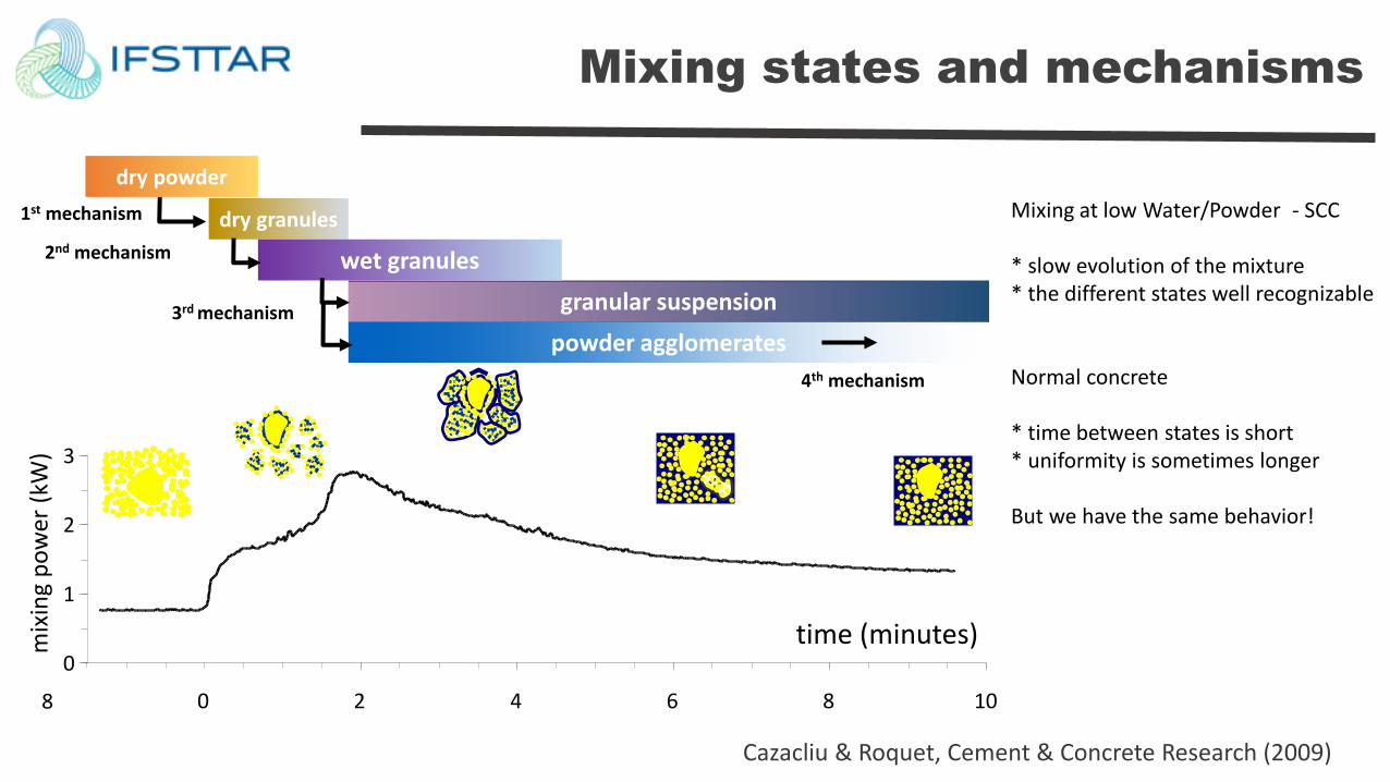
Mixing states and mechanisms m

ixin

g p

ow

er (

kW)

0

1

2

3

0 2 4 6 8 10

time (minutes)

8

dry granules

granular suspension

wet granules

dry powder

powder agglomerates

1st mechanism

2nd mechanism

3rd mechanism

4th mechanism

Cazacliu & Roquet, Cement & Concrete Research (2009)

Mixing at low Water/Powder - SCC * slow evolution of the mixture * the different states well recognizable Normal concrete * time between states is short * uniformity is sometimes longer

But we have the same behavior!

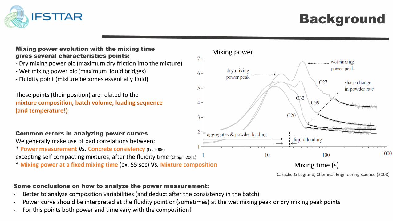
Background

Cazacliu & Legrand, Chemical Engineering Science (2008)

Some conclusions on how to analyze the power measurement:

- Better to analyze composition variabilities (and deduct after the consistency in the batch) - Power curve should be interpreted at the fluidity point or (sometimes) at the wet mixing peak or dry mixing peak points - For this points both power and time vary with the composition!

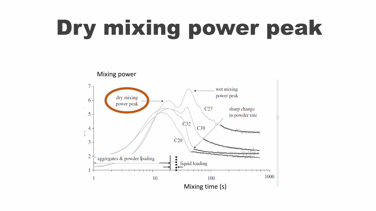
Mixing power

Mixing time (s)

Mixing power evolution with the mixing time

gives several characteristics points:

- Dry mixing power pic (maximum dry friction into the mixture) - Wet mixing power pic (maximum liquid bridges) - Fluidity point (mixture becomes essentially fluid) These points (their position) are related to the mixture composition, batch volume, loading sequence (and temperature!) Common errors in analyzing power curves

We generally make use of bad correlations between: * Power measurement Vs. Concrete consistency (Le, 2006)

excepting self compacting mixtures, after the fluidity time (Chopin 2001)

* Mixing power at a fixed mixing time (ex. 55 sec) Vs. Mixture composition

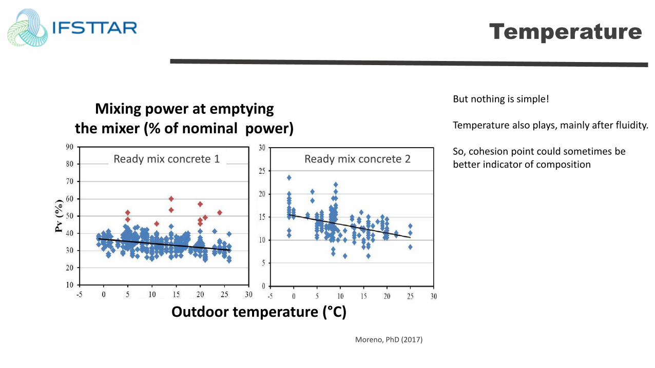
Temperature

Moreno, PhD (2017)

But nothing is simple! Temperature also plays, mainly after fluidity. So, cohesion point could sometimes be better indicator of composition

Outdoor temperature (°C)

Mixing power at emptying the mixer (% of nominal power)

Ready mix concrete 2 Ready mix concrete 1

Sand moisture

And the aggregates initial moisture: For sand, this could mainly be a problem of probe calibration (see PN BAP reports) but the high variability is demonstrated to be introduced by the coarse aggregates initial moisture (Le 2006) !

Mix

ing

po

we

r at

em

pty

ing

the

mix

er

(% o

f n

om

inal

po

we

r)

Sand initial moisture (%)

Moreno, PhD (2017)

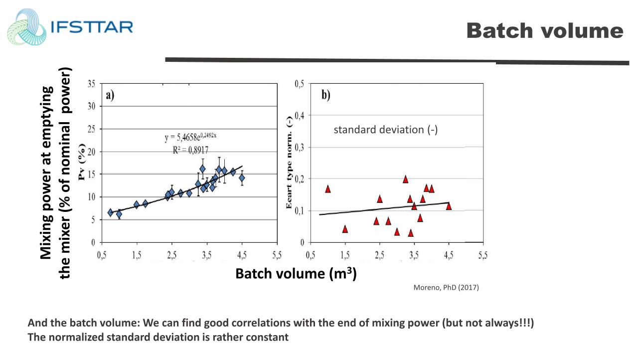
Batch volume

And the batch volume: We can find good correlations with the end of mixing power (but not always!!!) The normalized standard deviation is rather constant

Mix

ing

po

we

r at

em

pty

ing

the

mix

er

(% o

f n

om

inal

po

we

r)

Batch volume (m3) Moreno, PhD (2017)

standard deviation (-)

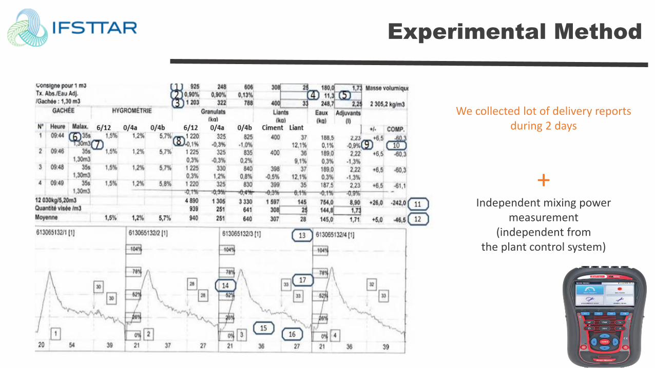
Experimental Method

We collected lot of delivery reports during 2 days

+ Independent mixing power

measurement (independent from

the plant control system)

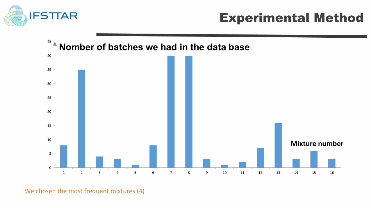
Experimental Method

We chosen the most frequent mixtures (4)

0

5

10

15

20

25

30

35

40

45

1 2 3 4 5 6 7 8 9 10 11 12 13 14 15 16

Mixture number

Mixing power

Mixing time (s)

Dry mixing power peak

Mixing power

Mixing time (s)

Dry mixing power peak

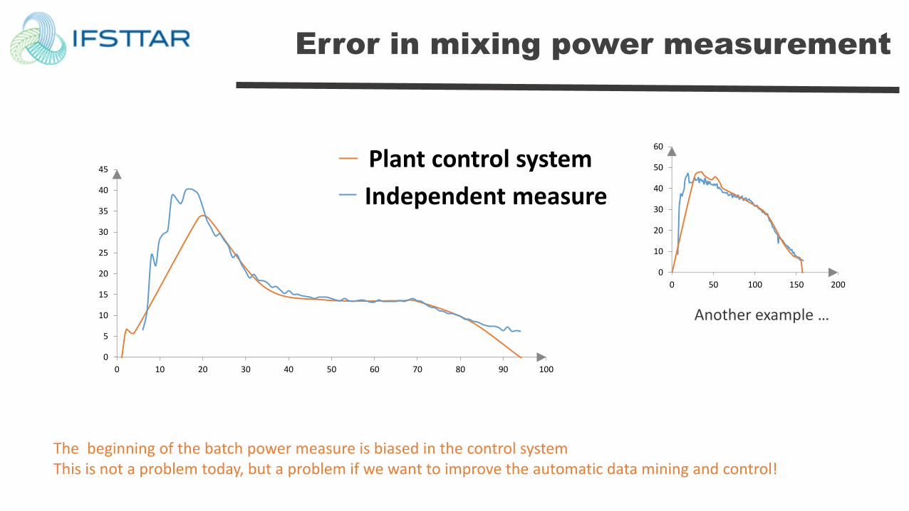
Error in mixing power measurement

The beginning of the batch power measure is biased in the control system This is not a problem today, but a problem if we want to improve the automatic data mining and control!

0

5

10

15

20

25

30

35

40

45

0 10 20 30 40 50 60 70 80 90 100

Bons Pesésmesure MetrelPlant control system

Independent measure

0

10

20

30

40

50

60

0 50 100 150 200

Another example …

Nominal volume and real volume of the batch

Concrete from the previous batch is still in the new batch after emptying. Excepting the first batch of a truck ! The quantity of concrete still present in the mixer is a control system parameter (more exactly, a small mixing power is fixed)

0

10

20

30

40

50

60

8800 8900 9000 9100 9200 9300 9400

Time (s)

Batches for one same truck

Mixing power (kW) – independent measure

Real volume Vs. Mixing power dry peak

Good correlation between the dry mixing pic and the batch volume (of coarse for the independent measure)

R² = 0,985

0

10

20

30

40

50

0 0,5 1 1,5 2

Dry Mixing power pic (kW) – mixture 1

Batch nominal volume (m3)

It works much better when we use the real volume of the batch (we made a mass correction in the batches)

R² = 0,994

0

10

20

30

40

50

0 0,5 1 1,5 2

Batch real volume (m3)

still have large standard deviation

Batch real mass

It seems that the final fluidity of the concrete plays! Indeed, the mixture still in the mixer for the new batch is fluid not granular!

0

10

20

30

40

50

0 0,5 1 1,5 2

Low consistency concrete

High consistency concrete

Dry Mixing power pic (kW) – 4 mixtures

Batch real volume (m3)

0

10

20

30

40

50

0 1000 2000 3000 4000 5000

Batch “real” mass (kg) – with a correction for the

initially fluid mixture

This curve could be use to retrofit the real volume. This will correct the data obtained with the fluidity point

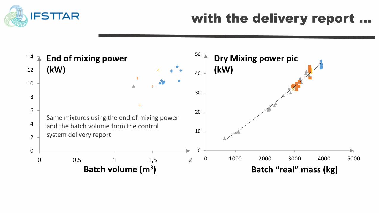
with the delivery report …

Same mixtures using the end of mixing power and the batch volume from the control system delivery report

0

2

4

6

8

10

12

14

0 0,5 1 1,5 2

End of mixing power (kW)

Batch volume (m3)

0

10

20

30

40

50

0 1000 2000 3000 4000 5000

Batch “real” mass (kg)

Dry Mixing power pic (kW)

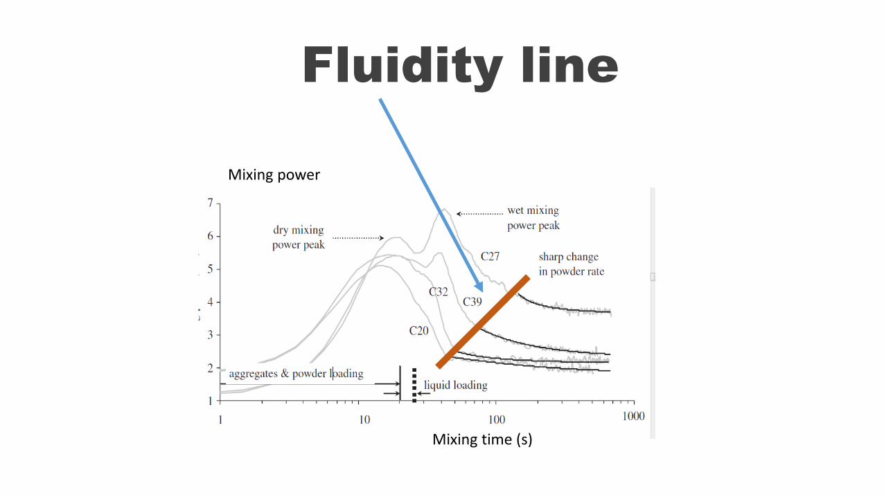
Mixing power

Mixing time (s)

Fluidity line

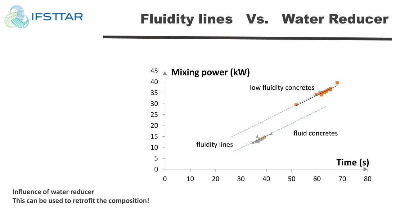
Fluidity lines Vs. Water Reducer

Influence of water reducer This can be used to retrofit the composition!

low fluidity concretes

fluid concretes

0

5

10

15

20

25

30

35

40

45

0 10 20 30 40 50 60 70 80

Time (s)

fluidity lines

Mixing power (kW)

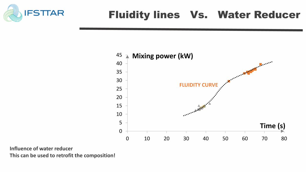
Fluidity lines Vs. Water Reducer

Influence of water reducer This can be used to retrofit the composition!

0

5

10

15

20

25

30

35

40

45

0 10 20 30 40 50 60 70 80

Time (s)

FLUIDITY CURVE

Mixing power (kW)

Fluidity power Vs. Water / Powder

How to measure the real water proportion in a batch?

Fluidity power (kW)

0

5

10

15

20

25

30

35

40

45

50

0 0,1 0,2 0,3 0,4 0,5 0,6 0,7 0,8

Water / Powder

Fluidity line Vs. Filling ratio

The batch volume is influent, but can be corrected

Fluidity power (kW)

Fluidity time 10

11

12

13

14

15

16

17

20 25 30 35 40 45 50

Filling ratio = 90%

Filling ratio = 100%

Filling ratio > 100%

5

6

7

8

9

10

20 25 30 35 40 45 50

Volume independent fluidity line?

Fluidity power per unit volume (kW/m3)

Fluidity time

Conclusion

FLUIDITY CURVE separate two zones in the (Mixing Power – Mixing Time) space - at short mixing time the mixture is not uniform - at longer mixing time the concrete become uniform (but continue to structure under mixing!)

This is a powerful concept to determine the real W/P value into a batch mixer However, the filling ratio change drastically the behavior: this can be corrected The DRY MIXING POWER PEAK gives accurately the filling ratio Other mix-design parameters could be determined by using the WET MIXING POWER CURVE