Powell - Beginning Database Design (2006)
496
-
Upload
stiki-indonesia -
Category
Documents
-
view
1 -
download
0
Transcript of Powell - Beginning Database Design (2006)

Beginning Database Design
Gavin Powell
01_574906 ffirs.qxd 10/28/05 11:43 PM Page iii

Beginning Database Design
01_574906 ffirs.qxd 10/28/05 11:43 PM Page i

01_574906 ffirs.qxd 10/28/05 11:43 PM Page ii

Beginning Database Design
Gavin Powell
01_574906 ffirs.qxd 10/28/05 11:43 PM Page iii
Beginning Database DesignPublished byWiley Publishing, Inc.10475 Crosspoint BoulevardIndianapolis, IN 46256www.wiley.com
Copyright © 2006 by Wiley Publishing, Inc., Indianapolis, Indiana
Published by Wiley Publishing, Inc., Indianapolis, Indiana
Published simultaneously in Canada
ISBN-13: 978-0-7645-7490-0ISBN-10: 0-7645-7490-6
Manufactured in the United States of America
10 9 8 7 6 5 4 3 2 1
1B/RV/RR/QV/IN
Library of Congress Control Number is available from the publisher.
No part of this publication may be reproduced, stored in a retrieval system or transmitted in any form or by any means, electronic, mechanical, photocopying, recording, scanning or otherwise, except as permittedunder Sections 107 or 108 of the 1976 United States Copyright Act, without either the prior written permis-sion of the Publisher, or authorization through payment of the appropriate per-copy fee to the CopyrightClearance Center, 222 Rosewood Drive, Danvers, MA 01923, (978) 750-8400, fax (978) 646-8600. Requests to the Publisher for permission should be addressed to the Legal Department, Wiley Publishing, Inc., 10475 Crosspoint Blvd., Indianapolis, IN 46256, (317) 572-3447, fax (317) 572-4355, or online at http://www.wiley.com/go/permissions.
LIMIT OF LIABILITY/DISCLAIMER OF WARRANTY: THE PUBLISHER AND THE AUTHOR MAKENO REPRESENTATIONS OR WARRANTIES WITH RESPECT TO THE ACCURACY OR COMPLETENESSOF THE CONTENTS OF THIS WORK AND SPECIFICALLY DISCLAIM ALL WARRANTIES, INCLUDINGWITHOUT LIMITATION WARRANTIES OF FITNESS FOR A PARTICULAR PURPOSE. NO WARRANTYMAY BE CREATED OR EXTENDED BY SALES OR PROMOTIONAL MATERIALS. THE ADVICE ANDSTRATEGIES CONTAINED HEREIN MAY NOT BE SUITABLE FOR EVERY SITUATION. THIS WORK ISSOLD WITH THE UNDERSTANDING THAT THE PUBLISHER IS NOT ENGAGED IN RENDERINGLEGAL, ACCOUNTING, OR OTHER PROFESSIONAL SERVICES. IF PROFESSIONAL ASSISTANCE ISREQUIRED, THE SERVICES OF A COMPETENT PROFESSIONAL PERSON SHOULD BE SOUGHT.NEITHER THE PUBLISHER NOR THE AUTHOR SHALL BE LIABLE FOR DAMAGES ARISING HERE-FROM. THE FACT THAT AN ORGANIZATION OR WEBSITE IS REFERRED TO IN THIS WORK AS ACITATION AND/OR A POTENTIAL SOURCE OF FURTHER INFORMATION DOES NOT MEAN THATTHE AUTHOR OR THE PUBLISHER ENDORSES THE INFORMATION THE ORGANIZATION ORWEBSITE MAY PROVIDE OR RECOMMENDATIONS IT MAY MAKE. FURTHER, READERS SHOULD BEAWARE THAT INTERNET WEBSITES LISTED IN THIS WORK MAY HAVE CHANGED OR DISAP-PEARED BETWEEN WHEN THIS WORK WAS WRITTEN AND WHEN IT IS READ.
For general information on our other products and services or to obtain technical support, please contact ourCustomer Care Department within the U.S. at (800) 762-2974, outside the U.S. at (317) 572-3993 or fax (317)572-4002.
Wiley also publishes its books in a variety of electronic formats. Some content that appears in print may notbe available in electronic books.
Trademarks: Wiley, the Wiley logo, Wrox, the Wrox logo, Programmer to Programmer, and related trade dressare trademarks or registered trademarks of John Wiley & Sons, Inc. and/or its affiliates, in the United States andother countries, and may not be used without written permission. All other trademarks are the property of theirrespective owners. Wiley Publishing, Inc., is not associated with any product or vendor mentioned in this book.
01_574906 ffirs.qxd 10/28/05 11:43 PM Page iv

This book is dedicated to Jacqueline — my fondest pride and joy.
01_574906 ffirs.qxd 10/28/05 11:43 PM Page v

About the AuthorGavin Powell has a Bachelor of Science degree in Computer Science, with numerous professionalaccreditations and skills (including Microsoft Word, PowerPoint, Excel, Windows 2000, ERWin, andPaintshop, as well as Microsoft Access, Ingres, and Oracle relational databases, plus a multitude ofapplication development languages). He has almost 20 years of contracting, consulting, and hands-oneducating experience in both software development and database administration roles. He has workedwith all sorts of tools and languages, on various platforms over the years. He has lived, studied, andworked on three different continents, and is now scratching out a living as a writer, musician, and familyman. He can be contacted at [email protected] or [email protected]. His Web siteat http://www.oracledbaexpert.com offers information on database modeling, database software, andmany development languages. Other titles by this author include Oracle Data Warehouse Tuning for 10g(Burlington, MA: Digital Press, 2005), Oracle 9i: SQL Exam Cram 2 (1Z0-007) (Indianapolis: Que, 2004),Oracle SQL: Jumpstart with Examples (Burlington, MA: Digital Press, 2004), Oracle Performance Tuning for 9i and 10g (Burlington, MA: Digital Press, 2003), ASP Scripting (Stephens City, VA: Virtual TrainingCompany, 2005), Oracle Performance Tuning (Stephens City, VA: Virtual Training Company, 2004), OracleDatabase Administration Fundamentals II (Stephens City, VA: Virtual Training Company, 2004), OracleDatabase Administration Fundamentals I (Stephens City, VA: Virtual Training Company, 2003), andIntroduction to Oracle 9i and Beyond: SQL & PL/SQL (Stephens City, VA: Virtual Training Company, 2003).
01_574906 ffirs.qxd 10/28/05 11:43 PM Page vi

CreditsSenior Acquisitions EditorJim Minatel
Development EditorKevin Shafer
Technical EditorDavid Mercer
Production EditorPamela Hanley
Copy EditorSusan Hobbs
Editorial ManagerMary Beth Wakefield
Production ManagerTim Tate
Vice President & Executive Group PublisherRichard Swadley
Vice President and PublisherJoseph B. Wikert
Project CoordinatorMichael Kruzil
Graphics and Production SpecialistsJonelle BurnsCarrie A. FosterDenny HagerJoyce HaugheyJennifer HeleineAlicia B. South
Quality Control TechniciansLaura AlbertLeeann HarneyJoe Niesen
Proofreading and IndexingTECHBOOKS Production Services
01_574906 ffirs.qxd 10/28/05 11:43 PM Page vii

01_574906 ffirs.qxd 10/28/05 11:43 PM Page viii
Contents
Introduction xvii
Part I: Approaching Relational Database Modeling 1
Chapter 1: Database Modeling Past and Present 3
Grasping the Concept of a Database 4Understanding a Database Model 5
What Is an Application? 5The Evolution of Database Modeling 6
File Systems 7Hierarchical Database Model 8Network Database Model 8Relational Database Model 9
Relational Database Management System 11The History of the Relational Database Model 11
Object Database Model 12Object-Relational Database Model 14
Examining the Types of Databases 14Transactional Databases 15Decision Support Databases 15Hybrid Databases 16
Understanding Database Model Design 16Defining the Objectives 17Looking at Methods of Database Design 20
Summary 21
Chapter 2: Database Modeling in the Workplace 23
Understanding Business Rules and Objectives 24What Are Business Rules? 25The Importance of Business Rules 26
Incorporating the Human Factor 27People as a Resource 27Talking to the Right People 29Getting the Right Information 30
02_574906 ftoc.qxd 10/28/05 11:37 PM Page ix
Contents
Dealing with Unfavorable Scenarios 32Computerizing a Pile of Papers 32Converting Legacy Databases 33Homogenous Integration of Heterogeneous Databases 33Converting from Spreadsheets 33Sorting Out a Messed-up Database 34
Summary 34
Chapter 3: Database Modeling Building Blocks 35
Information, Data and Data Integrity 37Understanding the Basics of Tables 37
Records, Rows, and Tuples 39Fields, Columns and Attributes 40Datatypes 42
Simple Datatypes 42Complex Datatypes 46Specialized Datatypes 47
Constraints and Validation 47Understanding Relations for Normalization 48
Benefits of Normalization 49Potential Normalization Hazards 49
Representing Relationships in an ERD 49Crows Foot 50One-to-One 51One-to-Many 52Many-to-Many 53Zero, One, or Many 55Identifying and Non-Identifying Relationships 57
Understanding Keys 58Primary Keys 59Unique Keys 59Foreign Keys 60Understanding Referential Integrity 63
Understanding Indexes 64What Is an Index? 65Alternate Indexing 65Foreign Key Indexing 65Types of Indexes 66Different Ways to Build Indexes 68
Introducing Views and Other Specialized Objects 69Summary 70Exercises 70
x
02_574906 ftoc.qxd 10/28/05 11:37 PM Page x

Contents
Part II: Designing Relational Database Models 71
Chapter 4: Understanding Normalization 73
What Is Normalization? 74The Concept of Anomalies 74Dependency, Determinants, and Other Jargon 76Defining Normal Forms 80
Defining Normal Forms the Academic Way 80Defining Normal Forms the Easy Way 81
1st Normal Form (1NF) 821NF the Academic Way 821NF the Easy Way 83
2nd Normal Form (2NF) 892NF the Academic Way 892NF the Easy Way 89
3rd Normal Form (3NF) 963NF the Academic Way 963NF the Easy Way 97
Beyond 3rd Normal Form (3NF) 103Why Go Beyond 3NF? 104Beyond 3NF the Easy Way 104
One-to-One NULL Tables 104Beyond 3NF the Academic Way 107
Boyce-Codd Normal Form (BCNF) 1084th Normal Form (4NF) 1115th Normal Form (5NF) 116Domain Key Normal Form (DKNF) 121
Summary 122Exercises 122
Chapter 5: Reading and Writing Data with SQL 123
Defining SQL 124The Origins of SQL 125SQL for Different Databases 125
The Basics of SQL 126Querying a Database Using SELECT 127
Basic Queries 127Filtering with the WHERE Clause 130Precedence 132Sorting with the ORDER BY Clause 134
xi
02_574906 ftoc.qxd 10/28/05 11:37 PM Page xi
Contents
Aggregating with the GROUP BY Clause 135Join Queries 137Nested Queries 141Composite Queries 143
Changing Data in a Database 144Understanding Transactions 144Changing Database Metadata 145
Summary 148Exercises 149
Chapter 6: Advanced Relational Database Modeling 151
Understanding Denormalization 152Reversing Normal Forms 152
Denormalizing Beyond 3NF 153Denormalizing 3NF 157Denormalizing 2NF 160Denormalizing 1NF 161
Denormalization Using Specialized Database Objects 162Denormalization Tricks 163
Understanding the Object Model 165Introducing the Data Warehouse Database Model 167Summary 169Exercises 170
Chapter 7: Understanding Data Warehouse Database Modeling 171
The Origin of Data Warehouses 172The Relational Database Model and Data Warehouses 173Surrogate Keys in a Data Warehouse 174Referential Integrity in a Data Warehouse 174
The Dimensional Database Model 175What Is a Star Schema? 176What Is a Snowflake Schema? 178
How to Build a Data Warehouse Database Model 182Data Warehouse Modeling Step by Step 183How Long to Keep Data in a Data Warehouse? 183Types of Dimension Tables 184Understanding Fact Tables 190
Summary 191Exercises 192
xii
02_574906 ftoc.qxd 10/28/05 11:37 PM Page xii

Contents
Chapter 8: Building Fast-Performing Database Models 193
The Needs of Different Database Models 194Factors Affecting OLTP Database Model Tuning 194Factors Affecting Client-Server Database Model Tuning 195Factors Affecting Data Warehouse Database Model Tuning 196Understanding Database Model Tuning 197
Writing Efficient Queries 198The SELECT Command 200Filtering with the WHERE Clause 202The HAVING and WHERE Clauses 204Joins 205Auto Counters 206
Efficient Indexing for Performance 206Types of Indexes 207How to Apply Indexes in the Real World 207When Not to Use Indexes 209
Using Views 210Application Caching 211Summary 212Exercises 213
Part III: A Case Study in Relational Database Modeling 215
Chapter 9: Planning and Preparation Through Analysis 217
Steps to Creating a Database Model 219Step 1: Analysis 219Step 2: Design 220Step 3: Construction 220Step 4: Implementation 220
Understanding Analysis 221Analysis Considerations 222Potential Problem Areas and Misconceptions 224
Normalization and Data Integrity 224More Normalization Leads to Better Queries 224Performance 224Generic and Standardized Database Models 225
Putting Theory into Practice 225Putting Analysis into Practice 225Company Objectives 226
xiii
02_574906 ftoc.qxd 10/28/05 11:37 PM Page xiii
Contents
Case Study: The OLTP Database Model 229Establishing Company Operations 229Discovering Business Rules 232
Case Study: The Data Warehouse Model 243Establishing Company Operations 244Discovering Business Rules 248
Project Management 253Project Planning and Timelines 253Budgeting 255
Summary 256Exercises 257
Chapter 10: Creating and Refining Tables During the Design Phase 259
A Little More About Design 260Case Study: Creating Tables 262
The OLTP Database Model 262The Data Warehouse Database Model 265
Case Study: Enforcing Table Relationships 269Referential Integrity 269Primary and Foreign Keys 270Using Surrogate Keys 271Identifying versus Non-Identifying Relationships 272Parent Records without Children 272Child Records with Optional Parents 273The OLTP Database Model with Referential Integrity 274The Data Warehouse Database Model with Referential Integrity 279
Normalization and Denormalization 282Case Study: Normalizing an OLTP Database Model 283
Denormalizing 2NF 284Denormalizing 3NF 285Denormalizing 1NF 286Denormalizing 3NF Again 287Deeper Normalization Layers 289
Case Study: Backtracking and Refining an OLTP Database Model 295Example Application Queries 298
Case Study: Refining a Data Warehouse Database Model 308Summary 316Exercises 317
xiv
02_574906 ftoc.qxd 10/28/05 11:37 PM Page xiv
Contents
Chapter 11: Filling in the Details with a Detailed Design 319
Case Study: Refining Field Structure 320The OLTP Database Model 320The Data Warehouse Database Model 323
Understanding Datatypes 329Simple Datatypes 329ANSI (American National Standards Institute) Datatypes 330Microsoft Access Datatypes 331Specialized Datatypes 331Case Study: Defining Datatypes 332
The OLTP Database Model 332The Data Warehouse Database Model 336
Understanding Keys and Indexes 338Types of Indexes 339What, When, and How to Index 342When Not to Create Indexes 342Case Study: Alternate Indexing 343
The OLTP Database Model 343The Data Warehouse Database Model 345
Summary 352Exercises 352
Chapter 12: Business Rules and Field Settings 353
What Are Business Rules Again? 354Classifying Business Rules in a Database Model 355
Normalization, Normal Forms, and Relations 355Classifying Relationship Types 356Explicitly Declared Field Settings 357Storing Code in the Database 358
Stored Procedure 360Stored Function 362Event Trigger 363External Procedure 364Macro 364
Case Study: Implementing Field Level Business Rules in a Database Model 364Table and Relation Level Business Rules 364Individual Field Business Rules 364
Field Level Business Rules for the OLTP Database Model 364Field Level Business Rules for the Data warehouse Database Model 370
xv
02_574906 ftoc.qxd 10/28/05 11:37 PM Page xv
Contents
Encoding Business Rules 373Encoding Business Rules for the OLTP Database Model 373Encoding Business Rules for the Data Warehouse Database Model 374
Summary 379
Part IV: Advanced Topics 381
Chapter 13: Advanced Database Structures and Hardware Resources 383
Advanced Database Structures 384What and Where? 384
Views 384Materialized Views 384Indexes 385Clusters 385Auto Counters 385Partitioning and Parallel Processing 385
Understanding Views 386Understanding Materialized Views 387Understanding Types of Indexes 390
BTree Index 391Bitmap Index 392Hash Keys and ISAM Keys 393Clusters, Index Organized Tables, and Clustered Indexes 393
Understanding Auto Counters 393Understanding Partitioning and Parallel Processing 393
Understanding Hardware Resources 396How Much Hardware Can You Afford? 396How Much Memory Do You Need? 396
Understanding Specialized Hardware Architectures 396RAID Arrays 397Standby Databases 397Replication 399Grids and Computer Clustering 400
Summary 401
Glossary 403
Appendix A: Exercise Answers 421
Appendix B: Sample Databases 435
Index 443
xvi
02_574906 ftoc.qxd 10/28/05 11:37 PM Page xvi
Introduction
This book focuses on the relational database model from a beginning perspective. The title is, therefore,Beginning Database Design. A database is a repository for data. In other words, you can store lots of infor-mation in a database. A relational database is a special type of database using structures called tables.Tables are linked together using what are called relationships. You can build tables with relationshipsbetween those tables, not only to organize your data, but also to allow later retrieval of information fromthe database.
The process of relational database model design is the method used to create a relational database model.This process is mathematical in nature, but very simple, and is called normalization. With the process ofnormalization are a number of distinct steps called Normal Forms. Normal Forms are: 1st Normal Form(1NF), 2nd Normal Form (2NF), 3rd Normal Form (3NF), Boyce-Codd Normal Form (BCNF), 4th NormalForm (4NF), 5th Normal Form (5NF), and Domain Key Normal Form (DKNF). That is quite a list. Thisbook presents the technical details of normalization and Normal Forms, in addition to presenting a lay-man’s version of normalization. Purists would argue that this approach is sacrilegious. The problemwith normalization is that it is so precise by attempting to cater to every possible scenario. The result isthat normalization is often misunderstood and quite frequently ignored. The result is poorly designedrelational database models. A simplified version tends to help bridge a communication gap, and perhapsprepare the way for learning the precise definition of normalization, hopefully lowering the incline ofthe learning curve.
Traditionally, relational database model design (and particularly the topic of normalization), has beenmuch too precise for commercial environments. There is an easy way to interpret normalization, and thisbook contains original ideas in that respect.
You should read this book because these ideas on relational database model design and normalizationtechniques will help you in your quest for perhaps even just a little more of an understanding as to howyour database works. The objective here is to teach you to make much better use of that wonderfulresource you have at your fingertips — your personal or company database.
Who This Book Is ForPeople who would benefit from reading this book would be anyone involved with database technology,from the novice all the way through to the expert. This includes database administrators, developers, datamodelers, systems or network administrators, technical managers, marketers, advertisers, forecasters,planners — anyone. This book is intended to explain to the people who actually make use of databasedata (such as in a data warehouse) to make forecasting predictions for market research and otherwise.This book is intended for everyone. If you wanted some kind of clarity as to the funny diagrams you findin your Microsoft Access database (perhaps built for you by a programmer), this book will do it for you. If you want to know what on earth is all that stuff in the company SQL-Server or Oracle database, thisbook is a terrific place to start — giving just enough understanding without completely blowing yourmind with too much techno-geek-speak.
03_574906 flast.qxd 10/28/05 11:42 PM Page xvii

Current Head
What This Book CoversThe objective of this book is to provide an easy to understand, step-by-step, simple explanation ofdesigning and building relational database models. Plenty of examples are offered, and even a multiplechapter case study scenario is included, really digging into and analyzing all the details. All the scary,deep-level technical details are also here—hopefully with enough examples and simplistic explanatorydetail to keep you hooked and absorbed, from cover to cover.
As with all of the previous books by this author, this book presents something that appears to beimmensely complex in a simplistic and easy to understand manner. The profligate use of examplesand step-by-step explanations builds the material into the text.
How This Book Is StructuredThis book is divided into four parts. Each part contains chapters with related material. The book beginsby describing the basics behind relational database modeling. It then progresses onto the theory withwhich relational database models are built. The third part performs a case study across four entire chap-ters, introducing some new concepts, as the case study progresses. In Part IV, new concepts described inthe case study chapters are not directly related to relational database modeling theory. The last partdescribes some advanced topics.
It is critical to read the parts in the order in which they appear in the book. Part I examines historicalaspects, describing why the relational database model became necessary. Part II goes through all the the-ory grounding relational database modeling. You need to know why the relational database model wasdevised (from Part I), to fully understand theory covered in Part II. After all the history and theories areunderstood, you can begin with the case study in Part III. The case study applies all that you havelearned from Part I and Part II, particularly Part II. Part IV contains detail some unusual information,related to previous chapters by expanding into rarely used database structures and hardware resourceusage.
Note that the content of this book is made available “as is.” The author assumes noresponsibility or liability for any mishaps as a result of using this information, inany form or environment.
To find further information, the easiest place to search is the Internet. Search for aterm such as “first normal form,” or “1st normal form,” or “1NF,” in search enginessuch as http://www.yahoo.com. Be aware that not all information will be currentand might be incorrect. Verify by crosschecking between multiple references. If noresults are found using Yahoo, try the full detailed listings on http://www.google.com. Try http://www.amazon.com and http://www.barnesandnoble.com whereother relational database modeling titles can be found.
xviii
Introduction
03_574906 flast.qxd 10/28/05 11:42 PM Page xviii
Current Head
This book contains a glossary, allowing for the rapid look up of terms without having to page throughthe index and the book to seek explicit definitions.
❑ Part I: Approaching Relational Database Modeling — Part I examines the history of relationaldatabase modeling. It describes the practical needs the relational database model fulfilled. Alsoincluded are details about dealing with people, extracting information from people and existingsystems, problematic scenarios, and business rules.
❑ Chapter 1: Database Modeling Past and Present — This chapter introduces basic conceptsbehind database modeling, including the evolution of database modeling, differenttypes of databases, and the very beginnings of how to go about building a databasemodel.
❑ Chapter 2: Database Modeling in the Workplace — This chapter describes how to approachthe designing and building of a database model. The emphasis is on business rules andobjectives, people and how to get information from them, plus handling of awkwardand difficult existing database scenarios.
❑ Chapter 3: Database Modeling Building Blocks — This chapter introduces the buildingblocks of the relational database model by discussing and explaining all the variousparts and pieces making up a relational database model. This includes tables, relation-ships between tables, and fields in tables, among other topics.
❑ Part II: Designing Relational Database Models — Part II discusses relational database modelingtheory formally, and in detail. Topics covered are normalization, Normal Forms and their appli-cation, denormalization, data warehouse database modeling, and database model performance.
❑ Chapter 4: Understanding Normalization — This chapter examines the details of the nor-malization process. Normalization is the sequence of steps (normal forms) by which arelational database model is both created and improved upon.
❑ Chapter 5: Reading and Writing Data with SQL — This chapter shows how the relationaldatabase model is used from an application perspective. A relational database modelcontains tables. Records in tables are accessed using Structured Query Language (SQL).
❑ Chapter 6: Advanced Relational Database Modeling — This chapter introduces denormal-ization, the object database model, and data warehousing.
❑ Chapter 7: Understanding Data Warehouse Database Modeling — This chapter discussesdata warehouse database modeling in detail.
❑ Chapter 8: Building Fast-Performing Database Models — This chapter describes various fac-tors affecting database performance tuning, as applied to different database modeltypes. If performance is not acceptable, your database model does not service the end-users in an acceptable manner.
❑ Part III: A Case Study in Relational Database Modeling — The case study applies all the formal the-ory learned in Part I and Part II—particularly Part II. The case study is demonstrated across fourentire chapters, introducing some new concepts as the case study progresses. The case study is asteady, step-by-step learning process, using a consistent example relational database model foran online auction house company. The case study introduces new concepts, such as analysis anddesign of database models. Analysis and design are non-formal, loosely defined processes, andare not part of relational database modeling theory.
xix
Introduction
03_574906 flast.qxd 10/28/05 11:42 PM Page xix

Current Head
❑ Chapter 9: Planning and Preparation Through Analysis — This chapter analyzes a relationaldatabase model for the case study (the online auction house company) from a companyoperational capacity (what a company does for a living). Analysis is the process ofdescribing what is required of a relational database model — discovering what is theinformation needed in a database (what all the basic tables are).
❑ Chapter 10: Creating and Refining Tables During the Design Phase — This chapter describesthe design of a relational database model for the case study. Where analysis describeswhat is needed, design describes how it will be done. Where analysis described basictables in terms of company operations, design defines relationships between tables, bythe application of normalization and Normal Form, to analyzed information.
❑ Chapter 11: Filling in the Details with a Detailed Design — This chapter continues thedesign process for the online auction house company case study — refining fields intables. Field design refinement includes field content, field formatting, and indexing on fields.
❑ Chapter 12: Business Rules and Field Settings — This chapter is the final of four chapterscovering the case study design of the relational database model for the online auctionhouse company. Business rules application to design encompasses stored procedures,as well as specialized and very detailed field formatting and restrictions.
❑ Part IV: Advanced Topics —Part IV contains a single chapter that covers details on advanceddatabase structures (such as materialized views), followed by brief information on hardwareresource usage (such as RAID arrays).
❑ Appendices — Appendix A contains exercise answers for all exercises found at the end of manychapters ion this book. Appendix B contains a single Entity Relationship Diagram (ERD) formany of the relational database models included in this book.
What You Need to Use This BookThis book does not require the use on any particular software tool — either database vendor-specific orfront-end application tools. The topic of this book is relational database modeling, meaning the contentof the book is not database vendor-specific. It is the intention of this book to provide non-database ven-dor specific subject matter. So if you use a Microsoft Access database, dBase database, Oracle Database,MySQL, Ingres, or any relational database — it doesn’t matter. All of the coding in this book is writtenintentionally to be non-database specific, vendor independent, and as pseudo code, most likely match-ing American National Standards Institute (ASNI) SQL coding standards.
You can attempt to create structures in a database if you want, but the scripts may not necessarily workin any particular database. For example, with Microsoft Access, you don’t need to create scripts to createtables. Microsoft Access uses a Graphical User Interface (GUI), allowing you to click, drag, drop, andtype in table and field details. Other databases may force use of scripting to create tables.
The primary intention of this book is to teach relational database modeling in a step-by-step process. It isnot about giving you example scripts that will work in any relational database. There is no such thing asuniversally applicable scripting — even with the existence of ANSI SQL standards because none of therelational database vendors stick to ANSI standards.
xx
Introduction
03_574906 flast.qxd 10/28/05 11:42 PM Page xx

Current Head
This book is all about showing you how to build the database model — in pictures of Entity RelationshipDiagrams (ERDs). All you need to read and use this book are your eyes, concentration, and fingers toturn the pages.
Any relational database can be used to create the relational database models in this book. Some adapta-tion of scripts is required if your chosen database engine does not have a GUI table creation tool.
ConventionsTo help you get the most from the text and keep track of what’s happening, a number of conventions areused throughout the book.
Examples that you can download and try out for yourself generally appear in a box like this:
Example title
This section gives a brief overview of the example.
SourceThis section includes the source code.
Source codeSource codeSource code
OutputThis section lists the output:
Example outputExample outputExample output
Try It OutTry It Out is an exercise you should work through, following the text in the book.
1. They usually consist of a set of steps.
2. Each step has a number.
3. Follow the steps through one by one.
How It WorksAfter each Try It Out, the code you’ve typed is explained in detail.
xxi
Introduction
03_574906 flast.qxd 10/28/05 11:42 PM Page xxi
Current Head
Tips, hints, tricks, and asides to the current discussion are offset and placed in italics like this.
As for styles in the text:
❑ New terms and important words are italicized when introduced.
❑ Keyboard strokes are shown like this: Ctrl+A.
❑ File names, URLs, and code within the text are shown like so: persistence.properties.
❑ Code is presented in two different ways:
In code examples we highlight new and important code with a gray background.
The gray highlighting is not used for code that’s less important in the presentcontext, or has been shown before.
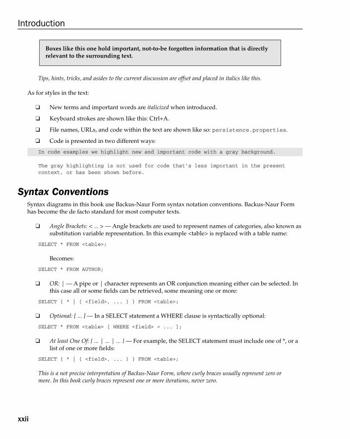
Syntax ConventionsSyntax diagrams in this book use Backus-Naur Form syntax notation conventions. Backus-Naur Formhas become the de facto standard for most computer texts.
❑ Angle Brackets: < ... > — Angle brackets are used to represent names of categories, also known assubstitution variable representation. In this example <table> is replaced with a table name:
SELECT * FROM <table>;
Becomes:
SELECT * FROM AUTHOR;
❑ OR: | — A pipe or | character represents an OR conjunction meaning either can be selected. Inthis case all or some fields can be retrieved, some meaning one or more:
SELECT { * | { <field>, ... } } FROM <table>;
❑ Optional: [ ... ] — In a SELECT statement a WHERE clause is syntactically optional:
SELECT * FROM <table> [ WHERE <field> = ... ];
❑ At least One Of: { ... | ... | ... } — For example, the SELECT statement must include one of *, or alist of one or more fields:
SELECT { * | { <field>, ... } } FROM <table>;
This is a not precise interpretation of Backus-Naur Form, where curly braces usually represent zero ormore. In this book curly braces represent one or more iterations, never zero.
Boxes like this one hold important, not-to-be forgotten information that is directlyrelevant to the surrounding text.
xxii
Introduction
03_574906 flast.qxd 10/28/05 11:42 PM Page xxii

Current Head
xxiii
Introduction
ErrataEvery effort has been made to ensure that there are no errors in the text or in the code; however, no oneis perfect, and mistakes do occur. If you find an error in one of our books, such as a spelling mistake orfaulty piece of code, your feedback would be greatly appreciated. By sending in errata you may saveanother reader hours of frustration and at the same time you will be helping us provide even higherquality information.
To find the errata page for this book, go to http://www.wrox.com and locate the title using the Search boxor one of the title lists. On the book details page, click the Book Errata link. On this page you can view allerrata that has been submitted for this book and posted by Wrox editors. A complete book list includinglinks to each book’s errata is also available at www.wrox.com/misc-pages/booklist.shtml.
If you don’t spot “your” error on the Book Errata page, go to www.wrox.com/contact/techsupport.shtml and complete the form there to send the error you have found. The information will be checkedand, if appropriate, a message will be posted to the book’s errata page and the problem will be fixed insubsequent editions of the book.
p2p.wrox.comFor author and peer discussion, join the P2P forums at p2p.wrox.com. The forums are a Web-based sys-tem for you to post messages relating to Wrox books and related technologies and interact with otherreaders and technology users. The forums offer a subscription feature to e-mail you topics of interest ofyour choosing when new posts are made to the forums. Wrox authors, editors, other industry experts,and your fellow readers are present on these forums.
At http://p2p.wrox.com you will find a number of different forums that will help you not only asyou read this book, but also as you develop your own applications. To join the forums, follow thesesteps:
1. Go to p2p.wrox.com and click the Register link.
2. Read the terms of use and click Agree.
3. Complete the required information to join as well as any optional information you want to pro-vide and click Submit.
You will receive an e-mail with information describing how to verify your account and complete thejoining process.
You can read messages in the forums without joining P2P, but you must join to post your own messages.
After you join, you can post new messages and respond to messages other users post. You can read mes-sages at any time on the Web. If you would like to have new messages from a particular forum e-mailedto you, click the Subscribe to this Forum icon by the forum name in the forum listing.
For more information about how to use the Wrox P2P, be sure to read the P2P FAQs for answers to ques-tions about how the forum software works as well as many common questions specific to P2P and Wroxbooks. To read the FAQs, click the FAQ link on any P2P page.
03_574906 flast.qxd 10/28/05 11:42 PM Page xxiii

03_574906 flast.qxd 10/28/05 11:42 PM Page xxiv

Beginning Database Design
03_574906 flast.qxd 10/28/05 11:42 PM Page xxv

03_574906 flast.qxd 10/28/05 11:42 PM Page xxvi
Part I
Approaching RelationalDatabase Modeling
In this Part:
Chapter 1: Database Modeling Past and Present
Chapter 2: Database Modeling in the Workplace
Chapter 3: Database Modeling Building Blocks
04_574906 pt01.qxd 10/28/05 11:44 PM Page 1

04_574906 pt01.qxd 10/28/05 11:44 PM Page 2
1Database Modeling Past and Present
“...a page of history is worth a volume of logic.” (Oliver Wendell Holmes)
Why a theory was devised and how it is now applied, can be more significant than the theory itself.
This chapter gives you a basic grounding in database model design. To begin with, you need tounderstand simple concepts, such as the difference between a database model and a database. Adatabase model is a blueprint for how data is stored in a database and is similar to an architecturalapproach for how data is stored — a pretty picture commonly known as an entity relationship dia-gram (a database on paper). A database, on the other hand, is the implementation or creation of aphysical database on a computer. A database model is used to create a database.
In this chapter, you also examine the evolution of database modeling. As a natural progression ofimprovements in database modeling design, the relational database model has evolved into whatit is today. Each step in the evolutionary development of database modeling has solved one ormore problems.
The final step of database modeling evolution is applications and how they affect a database modeldesign. An application is a computer program with a user-friendly interface. End-users use interfaces(or screens) to access data in a database. Different types of applications use a database in differentways — this can affect how a database model should be designed. Before you set off to figure out adesign strategy, you must have a general idea of the kind of applications your database will serve.Different types of database models underpin different types of applications. You must understandwhere different types of database models apply.
It is essential to understand that a well-organized design process is paramount to success. Also, agoal to drive the design process is equally as important as the design itself. There is no sense design-ing or even building something unless the target goal is established first, and kept foremost in mind.
This chapter, being the first in this book, lays the groundwork by examining the most basic conceptsof database modeling.
05_574906 ch01.qxd 10/28/05 11:41 PM Page 3
By the end of this chapter, you should understand why the relational database model evolved. You willcome to accept that the relational database model has some shortcomings, but after many years it isstill the most effective of available database modeling design techniques, for most application types.You will also discover that variations of the relational database model depend on the application type,such as an Internet interface, or a data warehouse reporting system.
In this chapter, you learn about the following:
❑ The definition of a database
❑ The definition of a database model
❑ The evolution of database modeling
❑ The hierarchical and network database models
❑ The relational database model
❑ The object and object-relational database models
❑ Database model types
❑ Database design objectives
❑ Database design methods
Grasping the Concept of a DatabaseA database is a collection of information — preferably related information and preferably organized. Adatabase consists of the physical files you set up on a computer when installing the database software.On the other hand, a database model is more of a concept than a physical object and is used to create thetables in your database. This section examines the database, not the database model.
By definition, a database is a structured object. It can be a pile of papers, but most likely in the modernworld it exists on a computer system. That structured object consists of data and metadata, with metadatabeing the structured part. Data in a database is the actual stored descriptive information, such as all the names and addresses of your customers. Metadata describes the structure applied by the database to the customer data. In other words, the metadata is the customer table definition. The customer tabledefinition contains the fields for the names and addresses, the lengths of each of those fields, anddatatypes. (A datatype restricts values in fields, such as allowing only a date, or a number). Metadataapplies structure and organization to raw data.
Figure 1-1 shows a general overview of a database. A database is often represented graphically by acylindrical disk, as shown on the left of the diagram. The database contains both metadata and raw data.The database itself is stored and executed on a database server computer.
4
Chapter 1
05_574906 ch01.qxd 10/28/05 11:41 PM Page 4
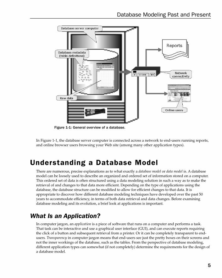
Figure 1-1: General overview of a database.
In Figure 1-1, the database server computer is connected across a network to end-users running reports,and online browser users browsing your Web site (among many other application types).
Understanding a Database ModelThere are numerous, precise explanations as to what exactly a database model or data model is. A databasemodel can be loosely used to describe an organized and ordered set of information stored on a computer.This ordered set of data is often structured using a data modeling solution in such a way as to make theretrieval of and changes to that data more efficient. Depending on the type of applications using thedatabase, the database structure can be modified to allow for efficient changes to that data. It is appropriate to discover how different database modeling techniques have developed over the past 50years to accommodate efficiency, in terms of both data retrieval and data changes. Before examiningdatabase modeling and its evolution, a brief look at applications is important.
What Is an Application?In computer jargon, an application is a piece of software that runs on a computer and performs a task. That task can be interactive and use a graphical user interface (GUI), and can execute reports requiring the click of a button and subsequent retrieval from a printer. Or it can be completely transparent to end-users. Transparency in computer jargon means that end-users see just the pretty boxes on their screens andnot the inner workings of the database, such as the tables. From the perspective of database modeling, different application types can somewhat (if not completely) determine the requirements for the design ofa database model.
5
Database Modeling Past and Present
05_574906 ch01.qxd 10/28/05 11:41 PM Page 5

An online transaction processing (OLTP) database is usually a specialized, highly concurrent (shareable)architecture requiring rapid access to very small amounts of data. OLTP applications are often wellserved by rigidly structured OLTP transactional database models. A transactional database model isdesigned to process lots of small pieces of information for lots of different people, all at the same time.
On the other side of the coin, a data warehouse application that requires frequent updates and extensivereporting must have large amounts of properly sorted data, low concurrency, and relatively lowresponse times. A data warehouse database modeling solution is often best served by implementing adenormalized duplication of an OLTP source database.
Figure 1-2 shows the same image as in Figure 1-1, except that in Figure 1-2, the reporting and onlinebrowser applications are made more prominent. The most important point to remember is that databasemodeling requirements are generally determined by application needs. It’s all about the applications.End-users use your applications. If you have no end-users, you have no business.
Figure 1-2: Graphic image of an application.
The Evolution of Database ModelingThe various data models that came before the relational database model (such as the hierarchical databasemodel and the network database model) were partial solutions to the never-ending problem of how tostore data and how to do it efficiently. The relational database model is currently the best solution for both storage and retrieval of data. Examining the relational database model from its roots can help youunderstand critical problems the relational database model is used to solve; therefore, it is essential thatyou understand how the different data models evolved into the relational database model as it is today.
6
Chapter 1
05_574906 ch01.qxd 10/28/05 11:41 PM Page 6
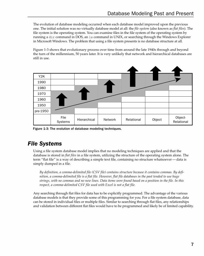
The evolution of database modeling occurred when each database model improved upon the previousone. The initial solution was no virtually database model at all: the file system (also known as flat files). Thefile system is the operating system. You can examine files in the file system of the operating system byrunning a dir command in DOS, an ls command in UNIX, or searching through the Windows Explorerin Microsoft Windows. The problem that using a file system presents is no database structure at all.
Figure 1-3 shows that evolutionary process over time from around the late 1940s through and beyondthe turn of the millennium, 50 years later. It is very unlikely that network and hierarchical databases arestill in use.
Figure 1-3: The evolution of database modeling techniques.
File SystemsUsing a file system database model implies that no modeling techniques are applied and that thedatabase is stored in flat files in a file system, utilizing the structure of the operating system alone. Theterm “flat file” is a way of describing a simple text file, containing no structure whatsoever — data issimply dumped in a file.
By definition, a comma-delimited file (CSV file) contains structure because it contains commas. By defi-nition, a comma-delimited file is a flat file. However, flat file databases in the past tended to use hugestrings, with no commas and no new lines. Data items were found based on a position in the file. In thisrespect, a comma-delimited CSV file used with Excel is not a flat file.
Any searching through flat files for data has to be explicitly programmed. The advantage of the variousdatabase models is that they provide some of this programming for you. For a file system database, datacan be stored in individual files or multiple files. Similar to searching through flat files, any relationshipsand validation between different flat files would have to be programmed and likely be of limited capability.
Y2K
1990
1980
1970
1960
1950
pre-1950
FileSystems
Hierarchical Network Relational ObjectObject-
Relational
7
Database Modeling Past and Present
05_574906 ch01.qxd 10/28/05 11:41 PM Page 7
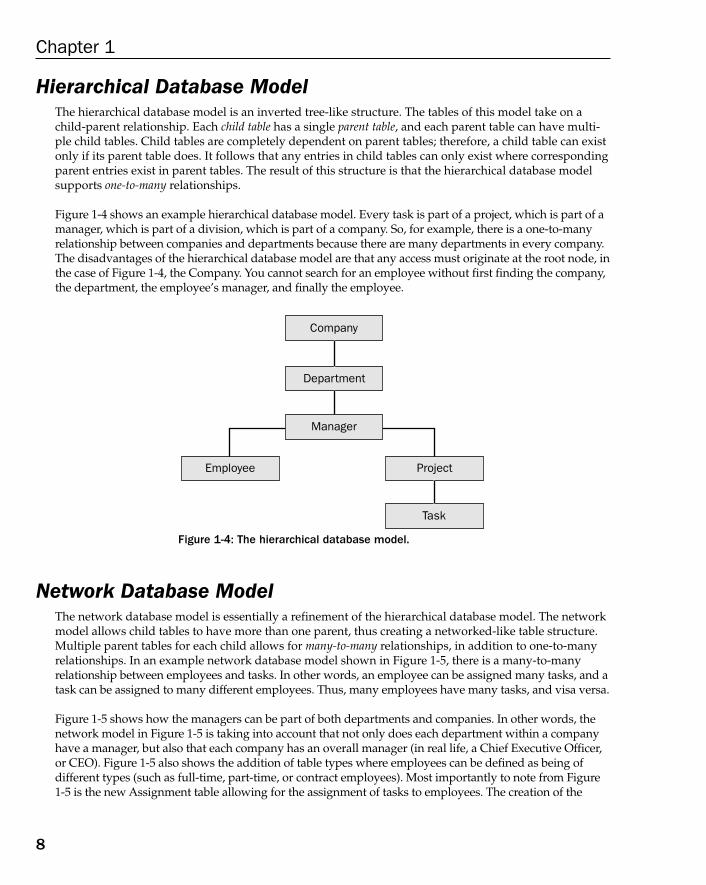
Hierarchical Database ModelThe hierarchical database model is an inverted tree-like structure. The tables of this model take on achild-parent relationship. Each child table has a single parent table, and each parent table can have multi-ple child tables. Child tables are completely dependent on parent tables; therefore, a child table can existonly if its parent table does. It follows that any entries in child tables can only exist where correspondingparent entries exist in parent tables. The result of this structure is that the hierarchical database modelsupports one-to-many relationships.
Figure 1-4 shows an example hierarchical database model. Every task is part of a project, which is part of amanager, which is part of a division, which is part of a company. So, for example, there is a one-to-manyrelationship between companies and departments because there are many departments in every company.The disadvantages of the hierarchical database model are that any access must originate at the root node, inthe case of Figure 1-4, the Company. You cannot search for an employee without first finding the company,the department, the employee’s manager, and finally the employee.
Figure 1-4: The hierarchical database model.
Network Database ModelThe network database model is essentially a refinement of the hierarchical database model. The networkmodel allows child tables to have more than one parent, thus creating a networked-like table structure.Multiple parent tables for each child allows for many-to-many relationships, in addition to one-to-manyrelationships. In an example network database model shown in Figure 1-5, there is a many-to-manyrelationship between employees and tasks. In other words, an employee can be assigned many tasks, and atask can be assigned to many different employees. Thus, many employees have many tasks, and visa versa.
Figure 1-5 shows how the managers can be part of both departments and companies. In other words, thenetwork model in Figure 1-5 is taking into account that not only does each department within a companyhave a manager, but also that each company has an overall manager (in real life, a Chief Executive Officer,or CEO). Figure 1-5 also shows the addition of table types where employees can be defined as being of different types (such as full-time, part-time, or contract employees). Most importantly to note from Figure1-5 is the new Assignment table allowing for the assignment of tasks to employees. The creation of the
Company
Department
Employee Project
Task
Manager
8
Chapter 1
05_574906 ch01.qxd 10/28/05 11:41 PM Page 8
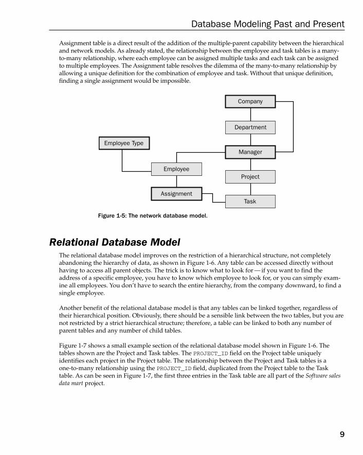
Assignment table is a direct result of the addition of the multiple-parent capability between the hierarchicaland network models. As already stated, the relationship between the employee and task tables is a many-to-many relationship, where each employee can be assigned multiple tasks and each task can be assignedto multiple employees. The Assignment table resolves the dilemma of the many-to-many relationship byallowing a unique definition for the combination of employee and task. Without that unique definition,finding a single assignment would be impossible.
Figure 1-5: The network database model.
Relational Database ModelThe relational database model improves on the restriction of a hierarchical structure, not completelyabandoning the hierarchy of data, as shown in Figure 1-6. Any table can be accessed directly withouthaving to access all parent objects. The trick is to know what to look for — if you want to find theaddress of a specific employee, you have to know which employee to look for, or you can simply exam-ine all employees. You don’t have to search the entire hierarchy, from the company downward, to find asingle employee.
Another benefit of the relational database model is that any tables can be linked together, regardless oftheir hierarchical position. Obviously, there should be a sensible link between the two tables, but you arenot restricted by a strict hierarchical structure; therefore, a table can be linked to both any number of parent tables and any number of child tables.
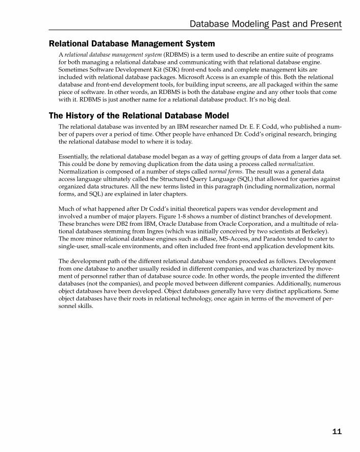
Figure 1-7 shows a small example section of the relational database model shown in Figure 1-6. Thetables shown are the Project and Task tables. The PROJECT_ID field on the Project table uniquely identifies each project in the Project table. The relationship between the Project and Task tables is a one-to-many relationship using the PROJECT_ID field, duplicated from the Project table to the Tasktable. As can be seen in Figure 1-7, the first three entries in the Task table are all part of the Software salesdata mart project.
Employee
Employee Type
Assignment
Project
Task
Company
Department
Manager
9
Database Modeling Past and Present
05_574906 ch01.qxd 10/28/05 11:41 PM Page 9
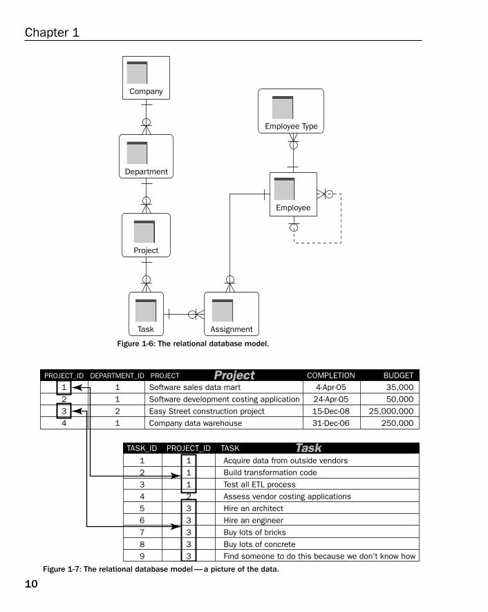
Figure 1-6: The relational database model.
Figure 1-7: The relational database model — a picture of the data.
123456789
111233333
Acquire data from outside vendorsBuild transformation codeTest all ETL processAssess vendor costing applicationsHire an architectHire an engineerBuy lots of bricksBuy lots of concreteFind someone to do this because we don’t know how
1234
1121
4-Apr-0524-Apr-0515-Dec-0831-Dec-06
35,00050,000
25,000,000250,000
Software sales data martSoftware development costing applicationEasy Street construction projectCompany data warehouse
TASK_ID PROJECT_ID TASK
PROJECT_ID DEPARTMENT_ID PROJECT COMPLETION BUDGET
TaskTask
ProjectProject
Company
Department
Employee Type
Assignment
Project
Task
Employee
10
Chapter 1
05_574906 ch01.qxd 10/28/05 11:41 PM Page 10
Relational Database Management SystemA relational database management system (RDBMS) is a term used to describe an entire suite of programsfor both managing a relational database and communicating with that relational database engine.Sometimes Software Development Kit (SDK) front-end tools and complete management kits areincluded with relational database packages. Microsoft Access is an example of this. Both the relationaldatabase and front-end development tools, for building input screens, are all packaged within the samepiece of software. In other words, an RDBMS is both the database engine and any other tools that comewith it. RDBMS is just another name for a relational database product. It’s no big deal.
The History of the Relational Database ModelThe relational database was invented by an IBM researcher named Dr. E. F. Codd, who published a num-ber of papers over a period of time. Other people have enhanced Dr. Codd’s original research, bringingthe relational database model to where it is today.
Essentially, the relational database model began as a way of getting groups of data from a larger data set.This could be done by removing duplication from the data using a process called normalization.Normalization is composed of a number of steps called normal forms. The result was a general dataaccess language ultimately called the Structured Query Language (SQL) that allowed for queries againstorganized data structures. All the new terms listed in this paragraph (including normalization, normalforms, and SQL) are explained in later chapters.
Much of what happened after Dr Codd’s initial theoretical papers was vendor development andinvolved a number of major players. Figure 1-8 shows a number of distinct branches of development.These branches were DB2 from IBM, Oracle Database from Oracle Corporation, and a multitude of rela-tional databases stemming from Ingres (which was initially conceived by two scientists at Berkeley).The more minor relational database engines such as dBase, MS-Access, and Paradox tended to cater to single-user, small-scale environments, and often included free front-end application development kits.
The development path of the different relational database vendors proceeded as follows. Developmentfrom one database to another usually resided in different companies, and was characterized by move-ment of personnel rather than of database source code. In other words, the people invented the differentdatabases (not the companies), and people moved between different companies. Additionally, numerousobject databases have been developed. Object databases generally have very distinct applications. Someobject databases have their roots in relational technology, once again in terms of the movement of per-sonnel skills.
11
Database Modeling Past and Present
05_574906 ch01.qxd 10/28/05 11:41 PM Page 11
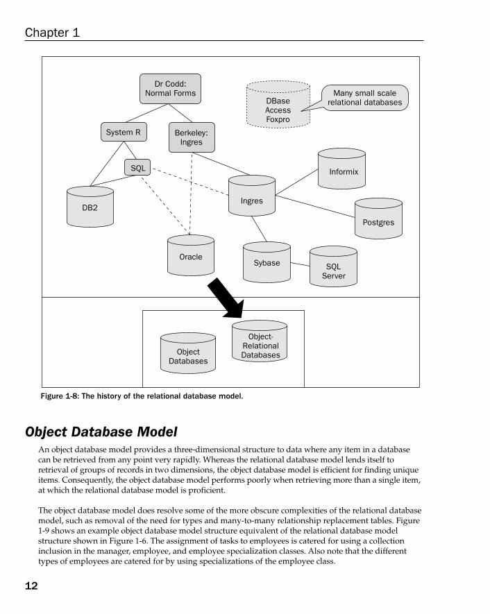
Figure 1-8: The history of the relational database model.
Object Database ModelAn object database model provides a three-dimensional structure to data where any item in a databasecan be retrieved from any point very rapidly. Whereas the relational database model lends itself toretrieval of groups of records in two dimensions, the object database model is efficient for finding uniqueitems. Consequently, the object database model performs poorly when retrieving more than a single item,at which the relational database model is proficient.
The object database model does resolve some of the more obscure complexities of the relational databasemodel, such as removal of the need for types and many-to-many relationship replacement tables. Figure1-9 shows an example object database model structure equivalent of the relational database model structure shown in Figure 1-6. The assignment of tasks to employees is catered for using a collectioninclusion in the manager, employee, and employee specialization classes. Also note that the differenttypes of employees are catered for by using specializations of the employee class.
Dr Codd:Normal Forms
DBaseAccessFoxpro
Informix
Postgres
Ingres
SQL
DB2
System R Berkeley:Ingres
SQLServer
SybaseOracle
ObjectDatabases
Object-RelationalDatabases
Many small scalerelational databases
12
Chapter 1
05_574906 ch01.qxd 10/28/05 11:41 PM Page 12
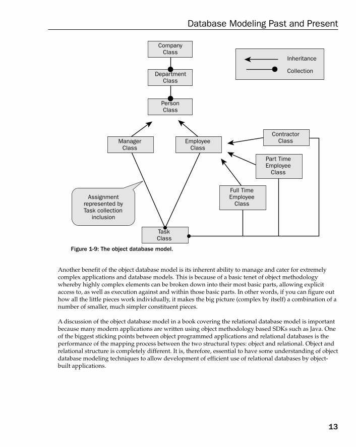
Figure 1-9: The object database model.
Another benefit of the object database model is its inherent ability to manage and cater for extremelycomplex applications and database models. This is because of a basic tenet of object methodologywhereby highly complex elements can be broken down into their most basic parts, allowing explicitaccess to, as well as execution against and within those basic parts. In other words, if you can figure outhow all the little pieces work individually, it makes the big picture (complex by itself) a combination of anumber of smaller, much simpler constituent pieces.
A discussion of the object database model in a book covering the relational database model is importantbecause many modern applications are written using object methodology based SDKs such as Java. Oneof the biggest sticking points between object programmed applications and relational databases is theperformance of the mapping process between the two structural types: object and relational. Object andrelational structure is completely different. It is, therefore, essential to have some understanding of objectdatabase modeling techniques to allow development of efficient use of relational databases by object-built applications.
CompanyClass
Inheritance
CollectionDepartmentClass
PersonClass
ManagerClass
EmployeeClass
TaskClass
ContractorClass
Part TimeEmployee
Class
Full TimeEmployee
ClassAssignment
represented byTask collection
inclusion
13
Database Modeling Past and Present
05_574906 ch01.qxd 10/28/05 11:41 PM Page 13
Object-Relational Database ModelThe object database model is somewhat spherical in nature, allowing access to unique elements anywherewithin a database structure, with extremely high performance. The object database model performsextremely poorly when retrieving more than a single data item. The relational database model, on theother hand, contains records of data in tables across two dimensions. The relational database model is bestsuited for retrieval of groups of data, but can also be used to access unique data items fairly efficiently.The object-relational database model was created in answer to conflicting capabilities of relational andobject database models.
Essentially, object database modeling capabilities are included in relational databases, but not the otherway around. Many relational databases now allow binary object storage and limited object method codingcapabilities, with varying degrees of success. The biggest issue with storage of binary objects in a relationaldatabase is that potentially large objects are stored in what is actually a small-scale structural element as asingle field-record entry in a table. This is not always strictly the case because some relational databasesallow storage of binary objects in separate disk files outside the table’s two-dimensional record structures.
The evolution of database modeling began with what was effectively no database model whatsoever withfile system databases, evolving on to hierarchies to structure, networks to allow for special relationships,onto the relational database model allowing for unique individual element access anywhere in thedatabase. The object database model has a specific niche function at handling high-speed application ofsmall data items within large highly complex data sets. The object-relational model attempts to includethe most readily accountable aspects of the object database model into the structure of the relationaldatabase model, with varying (and sometimes dubious) degrees of success.
Examining the Types of DatabasesAt this stage, we need to branch into both the database and application arenas because the choice ofdatabase modeling strategy is affected by application requirements. After all, the reason a databaseyou build a database is to service some need. That need is influenced by one or more applications.Applications should present user-friendly interfaces to end-users. End-users should not be expected toknow anything at all about database modeling. The objective is to provide something useful to a banker,an insurance sales executive, or anyone else most likely not in the computer industry, and probably noteven in a technical field. You need to take into account the function of what a database achieves, ratherthan the complicated logic that goes into designing the specific database.
Databases functionally fall into three general categories:
❑ Transactional
❑ Decision support system (DSS)
❑ Hybrid
14
Chapter 1
05_574906 ch01.qxd 10/28/05 11:41 PM Page 14

Transactional DatabasesA transactional database is a database based on small changes to the database (that is, small transactions).The database is transaction-driven. In other words, the primary function of the database is to add newdata, change existing data, delete existing data, all done in usually very small chunks, such as individualrecords.
The following are some examples of transactional databases:
❑ Client-Server database — A client-server environment was common in the pre-Internet days wherea transactional database serviced users within a single company. The number of users couldrange from as little as one to thousands, depending on the size of the company. The critical factorwas actually a mixture of both individual record change activity and modestly sized reports.Client-server database models typically catered for low concurrency and low throughput at thesame time because the number of users was always manageable.
❑ OLTP database — OLTP databases cause problems with concurrency. The number of users thatcan be reached over the Internet is an unimaginable order of magnitude larger than that of anyin-house company client-server database. Thus, the concurrency requirements for OLTPdatabase models explode well beyond the scope of previous experience with client-serverdatabases. The difference in scale can only be described as follows:
❑ Client-server database — A client-server database inside a company services, for example,1,000 users. A company of 1,000 people is unlikely to be corporate and global, so all usersare in the same country, and even likely to be in the same city, perhaps even in andaround the same office. Therefore, the client-server database services 1,000 people, 8hours per day, 5 days a week, perhaps 52 weeks a year. The standard U.S. work year isestimated at a maximum of about 2,000 hours per year. That’s a maximum of 2,000 hoursper year, per person. Also, consider how many users will access the database at exactlythe same millisecond. The answer is probably 1! You get the picture.
❑ OLTP database — An OLTP database, on the other hand, can have millions of potentialusers, 24 hours per day, 365 days per year. An OLTP database must be permanentlyonline and concurrently available to even in excess of 1,000 users every millisecond.Imagine if half a million people are watching a home shopping network on televisionand a Web site appears offering something for free that everyone wants. How manypeople hit the Web site at once and make demands on the OLTP database behind thatWeb site? The quantities of users are potentially staggering. This is what an OLTPdatabase has to cater to — enormously high levels of concurrent database access.
Decision Support DatabasesDecision support systems are commonly known as DSS databases, and they do just that — they supportdecisions, generally more management-level and even executive-level decision-type of objectives.Following are some DSS examples:
❑ Data warehouse database — A data warehouse database can use the same data modeling approach as atransactional database model. However, data warehouses often contain many years of historicaldata to provide effective forecasting capabilities. The result is that data warehouses can becomeexcessively large, perhaps even millions of times larger than their counterpart OLTP source
15
Database Modeling Past and Present
05_574906 ch01.qxd 10/28/05 11:41 PM Page 15
databases. The OLTP database is the source database because the OLTP database is the databasewhere all the transactional information in the data warehouse originates. In other words, as databecomes not current in an OLTP database, it is moved to a data warehouse database. Note the useof the word “moved,” implying that the data is copied to the data warehouse and deleted from theOLTP database. Data warehouses need specialized relational database modeling techniques.
❑ Data mart — A data mart is essentially a small subset of a larger data warehouse. Data marts aretypically extracted as small sections of data warehouses, or created as small section data chunksduring the process of creating a much larger data warehouse database. There is no reason why a data mart should use a different database modeling technique than that of its parent datawarehouse.
❑ Reporting database — A reporting database is often a data warehouse type database, but containingonly active (and not historical or archived) data. A simple reporting database is of small sizecompared to a data warehouse database, and likely to be much more manageable and flexible.
Data warehouse databases are typically inflexible because they can get so incredibly large.
Hybrid DatabasesA hybrid database is simply a mixture containing both OLTP type concurrency requirements and data warehouse type throughput requirements. In less-demanding environments (or in companies runningsmaller operations), a smaller hybrid database is often a more cost-effective option, simply because thereis one rather than two databases — fewer machines, fewer software licenses, fewer people, the list goes on.
This section has described what a database does. The function of the database can determine the way inwhich the database model is built. The following section goes back to the database model design process,but approaching it from a conceptual perspective.
Understanding Database Model DesignDo you really need to design stuff? When designing a computer system or a database model, you mightwonder why you need to design it. And exactly what is design? Design is to writing software like whatarchitecture is to civil engineering. Architects learn all the arty stuff such as where the bathrooms go andhow many bathrooms there are, and whether or not there are bathrooms. If the architecture were left tothe civil engineers, they might forget the bathrooms or leave the occupants of the completed structurewith Portaloos or outhouses.
Civil engineers ensure that it all stands up without falling down on our heads. Architects make it habitable.So, where does that lead us with software, database modeling, and having to design the database model?Essentially, the design process involves putting your ideas on paper before actually constructing yourobject, and perhaps experimenting with moving parts and pieces around a bit just to see what they looklike. Civil engineers are not in the habit of erecting millions of tons of precast concrete slabs into the formsof bridges and skyscrapers and then moving bits around (such as whole corners and sections of structures)just to see what the changes look like. You see my point. You must design it and build it on paper first. Youcould use something like a computer-aided design (CAD) package to sort out the seeing what it looks likestage. In terms of the database model, you must design it before you build it and then start filling it withdata and hooking it up to applications.
16
Chapter 1
05_574906 ch01.qxd 10/28/05 11:41 PM Page 16
Database design is so important because all applications written against that database model design arecompletely dependent on the structure of that underlying database. If the database model must bealtered at a later stage, everything constructed based on the database model probably must be changedand perhaps even completely rewritten. That’s all the applications — and I mean all of them! That canget very expensive and time consuming. Design the database model in the same way that you woulddesign an application — using tools, flowcharts, pretty pictures, Entity Relationship Diagrams (ERDs),and anything else that might help to ensure that what you intend to build is not only what you need, butalso will actually work, and preferably work without ever breaking.
Of course, liability issues place far more stringent requirements on the process of design for architectsand civil engineers when building concrete structures than that compared with computer systems. Justimagine how much it costs to build a skyscraper! Skyscrapers can take 10 years to build. The cost inwages alone is probably in the hundreds of millions. A computer system, however, and database modelthat ultimately turns into a complete dud as a result of poor planning and design can cost a companymore money than it is prepared to spend and perhaps more than a company is even able to lose.
Design is the process of ensuring that it all works without actually building it. Design is a little like testingsomething on paper before spending thousands of hours building it in possibly the wrong way.
Design is needed to ensure that it works before spending humungous amounts of money finding outthat it doesn’t. The idea is to fix as many teething problems and errors in the design. Fixing the design ismuch easier than fixing a finished product. A design on paper costs a fraction of what building andimplementing the real thing would cost. Waste a small amount of money in planning, rather than losemore than can be afforded when it’s too late to fix it.
Defining the ObjectivesDefining objectives is probably the single most important task done in planning any project, be it askyscraper or a database model. You could, of course, just start anywhere and dive right into the projectwith your eyes shut. But that is not planning. The more you plan what you are going to do, the morelikely the final result will fit your requirements.
Aside from planning, you must know what to plan in the first place. Defining the objectives is the basicstep of defining how you are going to get from A to B.
So, now that you know you have to plan your steps, you also have to know what the steps are that you areplanning for (be those steps the final result or smaller steps in between). There are, of course, a number ofpoints to guide the establishment of design objectives for a proper relational database model design:
❑ Aim for a well-structured database model — A well-structured database model is simple, easy toread, and easy to comprehend. If your company has a database model made up of 50 pieces ofA4-sized paper taped to an entire wall, and links between tables taking 20 minutes to trace, youhave a problem. That problem is poor structure. If you are interviewed as a contractor to sortout a problem like this, you might be faced with a Herculean task.
❑ Data integrity — Integrity is a set of rules in a database model, ensuring that data is not lostwithin the database, and that data is only destroyed when it should be.
17
Database Modeling Past and Present
05_574906 ch01.qxd 10/28/05 11:41 PM Page 17
❑ Support both planned queries and ad-hoc or unplanned queries — The fewer ad-hoc queries, the better,of course, and in some circumstances (such as very high-concurrency OLTP databases), ad-hocqueries might have to be banned altogether, or perhaps shifted to a more appropriate data warehouse platform.
An ad-hoc query is a query that is submitted to the database by a non-programmer such as a sales executive. People who are not programmers are not expected to know how to build the most elegant solution to a query and will often write queries quite to the contrary.
❑ Ad-hoc queries can cause serious performance issues. Customer-facing applications that requiremillisecond response times (which depend solely on a high-performance OLTP database) do notget along well with ad-hoc queries. Don’t risk losing your customers and wind up with no busi-ness to speak of. Do not allow anyone to do anything ad-hoc in an application-controlled OLTPdatabase.
❑ Support the objectives of the business — Highly normalized table structures do not necessarily rep-resent business structures directly. Denormalized, data warehouse, fact-dimensional structurestend to look a lot more like a business operationally. The latter is acceptable because a datawarehouse is much more likely to be subjected to ad-hoc queries by management, businessplanning, and executive staff. Subjecting a customer-facing OLTP database to ad-hoc activitycould be disastrous for operational effectiveness of the business. In other words, don’t normal-ize a database model simply because the rules of normalization state this is the accepted prac-tice. Different types of databases, and even different types of application, are often better servedwith less application of normalization.
❑ Provide adequate performance for any required change activity — Be it single record changes in anOLTP database or high-speed batch operations in a data warehouse (or both), this is important.
❑ Each table in a database model should preferably represent a single subject or topic — Don’t over-designa database model. Don’t create too many tables. OLTP databases can thrive on more detail andmore tables, but not always. Data warehouses can fall apart when data is divided up into toomany tables.
❑ Future growth must always be a serious consideration — Some databases can grow at astronomicalrates. Where data warehouse growth is potentially predictable from one load to the next, some-times OLTP database growth can surprise you with sudden interest in an Internet site becauseof advertising, or just blind luck. When a sudden jump in online user interest increases load onan OLTP database astronomically, however, a database model that is not designed for potentialastronomical growth could lose all newly acquired customers just as quickly as their interestwas gained — overnight!
The computer jargon term commonly used to assess the potential future growth of a computer system isscalability. Is it scalable?
❑ Future changes can be accommodated for, but potential structural changes can be difficult to allow for —Parts of the various different types of database models naturally allow extension and enhancement. Some parts do not allow future changes easily. Some arguments for future growthstate that more granularity and normalization are essential to allow for future growth, whereasother opinions can state exactly the opposite. This objective can often depend on companyrequirements. The problem with allowing for future growth in a database model is that it ismuch easier to allow for database size growth by adding new data. Adding new metadata
18
Chapter 1
05_574906 ch01.qxd 10/28/05 11:41 PM Page 18
structures is also not necessarily a problem. On the contrary, changing existing structures cancause serious problems, particularly where relationships between tables change, and even sometimes simply adding new fields to tables. Any table changes can affect applications. Thebest way to deal with this issue is to code applications generically, but generic coding can affectoverall performance. Other ways are to black box SQL database access code either in applicationsor the database.
The term “black box” implies chunks of code that can function independently, where changes made toone part of a piece of software will not affect others.
❑ Minimize dependence between applications and database model structures if you expectchange. This makes it easier to change and enhance both database model and application codein the future.
Changes to underlying database model structure can cause huge maintenance costs. Minimizing dependence between application database access code and database model structures might help this process, but this can result in inefficient generic coding. No matter what, database model changes nearlyalways result in unpleasant application code changes. The important point is to build the applicationproperly as well as the database model. Changes are unavoidable in applications when a database modelis altered, but they can be adequately planned for.
Catering to all these objectives could cause you a real headache in designing your database model. Theyare only guidelines with possibilities both good and bad, and then all only potentially arising at onepoint or another. However, the positive results from using good database model design objectives are asfollows:
❑ From an operational perspective, the most important objective is fulfilling the needs of applica-tions. OLTP applications require rapid response times on small transactions and high concur-rency levels — in other words, lots and lots of users, all doing the same stuff and at exactly thesame time. A data warehouse has different requirements, of course, and a hybrid type ofdatabase a mixture of both.
❑ Queries should be relatively easy to code without producing errors because of lack of dataintegrity or poor table design. Table and relationship structures must be correct.
❑ The easier applications can be built, the better. In general, the less co-dependence betweendatabase model and application, the better. In tightly controlled OLTP application environmentswhere no ad-hoc activity is permitted, this is easy. Where end-users are allowed to interact moredirectly with the database such as in a data warehouse, this becomes more difficult.
❑ Changing data and metadata is always an issue, and from an operational perspective, datachanges are more important. Changing table structures would be nice if it were always easy, butmetadata changes tend to affect applications adversely no matter how unglued applications anddatabase structures are.
Strive for the best you can in the given circumstances, budget, and requirements.
That’s ideally where you want to be when your database model design is built, implemented, and applications using your database are running and performing their tasks up to the operational expectationsof the business. In other words, you are in business and business has improved substantially both inturnover and efficiency after your company has invested large sums of money in computerization.
19
Database Modeling Past and Present
05_574906 ch01.qxd 10/28/05 11:41 PM Page 19
Looking at Methods of Database DesignSo far, you have looked at why a design process is required and why you need to define objectives togive the design process a goal at which to aim. So, the question you might be asking is how do you goabout designing a database model?
There are various methodologies available for designing database models. Each of these differentapproaches consists of a number of steps. The following sequence of steps to database model designseems the most sensible for a book such as this.
❑ Requirements analysis — Collect information about the nature of the data, features required, andany specialized needs such as expected output responses. This step covers what is needed, sosimply analyze it and write it down. Talk to the customer and company employees to get a bet-ter idea of exactly what they need.
❑ Conceptual design — This is where you get to use the fancy graphical tools and draw the prettypictures — Entity Relationship Diagrams (ERDs). This step includes creation of tables, fieldswithin those tables, and relationships between the tables. This step also includes normalization.Later chapters describe all aspects of conceptual design. Figure 1-10 shows a simple ERD for anonline store selling books.
❑ Logical design — Create database language commands to generate table definitions. Some toolsused for creating ERDs allow generation of data definition language (DDL) scripting; however,they are likely to generate generic scripts. Be sure that you check anything generated before exe-cuting in any specific database engine.
Data definition language (DDL) is made of the commands used to change metadata in a database, suchas creating tables, changing tables, and dropping tables.
❑ Physical design — Adjust database language commands to alter the database model for theunderlying physical attributes of tables. For example, you might want to store large binaryobjects in separate, underlying files to that of standard relational record-field data.
❑ Tuning phase — This step includes items such as appropriate indexing, further normalization, oreven denormalization, security features, and anything else not covered by the previous steps.
These separate steps are interchangeable, repeatable, iterative, and really anything-able, according to vari-ous different approaches used for different database engines and different database designer personalpreferences. Some designers may even put some of these steps into single steps and divide others upinto more detailed sets of subset steps. In other words, this is all open to interpretation. The only thingI do insist that should be universal is that you draw the ERDs and build tables well before you buildmetadata table creation code, placing visual design prior to physical implementation.
20
Chapter 1
05_574906 ch01.qxd 10/28/05 11:41 PM Page 20
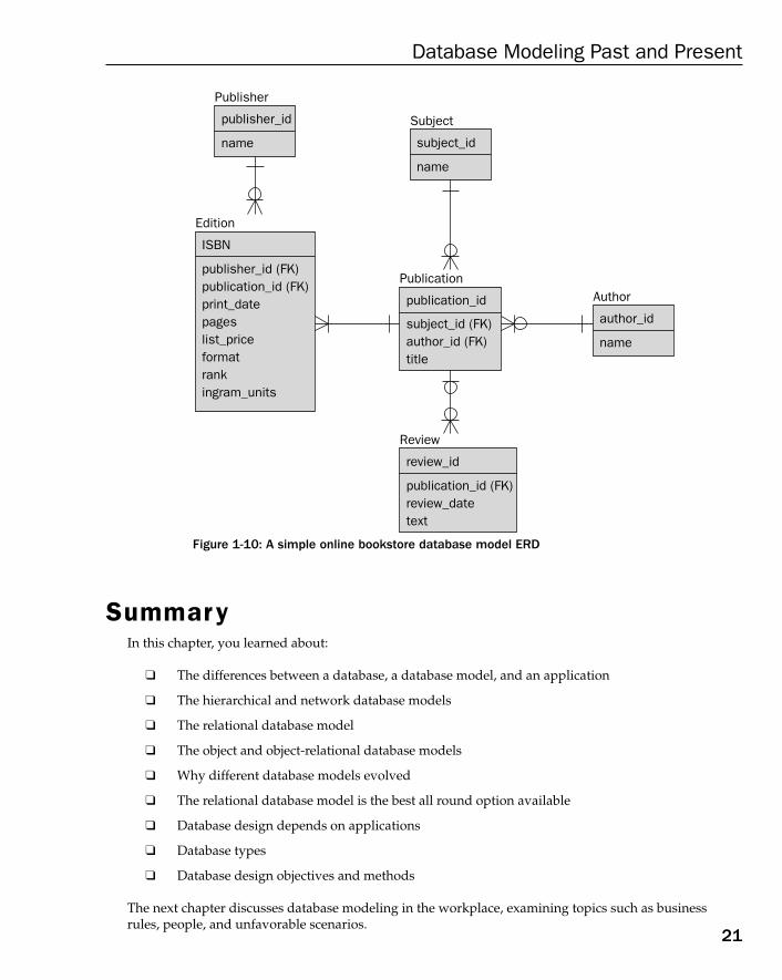
Figure 1-10: A simple online bookstore database model ERD
SummaryIn this chapter, you learned about:
❑ The differences between a database, a database model, and an application
❑ The hierarchical and network database models
❑ The relational database model
❑ The object and object-relational database models
❑ Why different database models evolved
❑ The relational database model is the best all round option available
❑ Database design depends on applications
❑ Database types
❑ Database design objectives and methods
The next chapter discusses database modeling in the workplace, examining topics such as businessrules, people, and unfavorable scenarios.
Publisher
publisher_id
name
Edition
ISBN
publisher_id (FK)publication_id (FK)print_datepageslist_priceformatrankingram_units
Publication
publication_id
subject_id (FK)author_id (FK)title
Review
review_id
publication_id (FK)review_datetext
Subject
subject_id
name
Author
author_id
name
21
Database Modeling Past and Present
05_574906 ch01.qxd 10/28/05 11:41 PM Page 21

05_574906 ch01.qxd 10/28/05 11:41 PM Page 22
2Database Modeling in the
Workplace
“A common mistake that people make when trying to design something completely foolproof is tounderestimate the ingenuity of complete fools.” (Douglas Adams)
The only fool is the data model designer who assumes to know all.
Chapter 1 described database model design history, the different types of applications, and howthose applications affect the basic structure of a database model. This chapter expands on thatoverall perspective by describing how to approach database modeling.
Data modeling in the workplace includes the modeling (or design) of a company’s operations.Business rules are sometimes by definition a gray area, but they attempt to define how a businessoperates — that is, what a company does to earn its keep. There can be a distinct differencebetween end-user interpretation of operations and the interpretation of a database modeler. Bothinterpretations are usually correct, but simply formulated from a different perspective.
People are so important to a database model designer. Those people are nearly always end-users.It is important for a database modeler to find out what people need. People skills are required. Theend-users have all the facts, especially if a database does not yet exist. If a database already exists,that existing database might be useful, might even be a hindrance, or both. There can be differentapproaches when dealing with people (both technical people and non-technical people) when trying to create a database design, either in a consulting or more permanent role. Getting correctinformation from the right people is critical to the pre-design process. A database is built for acompany that will use it. Build for the people who will use it.
You might need to build for developers or end-users, or even both. It depends on who gets accessto that database. A database modeler must know who to get information from, and what types of employee roles give what types of information. Whereas an employee may be microcosmic, amanager could be macrocosmic. That’s a little akin to the difference between a weather report foryour local town and the entire country. For example, manager and employee perspectives can bevery different. A database designer must understand that management level has a birds-eye viewand employees have a more localized perspective to fill in the details for you.
06_574906 ch02.qxd 10/28/05 11:36 PM Page 23
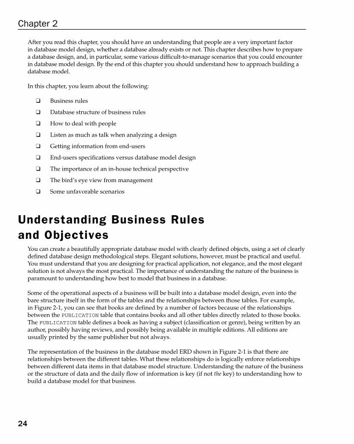
After you read this chapter, you should have an understanding that people are a very important factor in database model design, whether a database already exists or not. This chapter describes how to preparea database design, and, in particular, some various difficult-to-manage scenarios that you could encounterin database model design. By the end of this chapter you should understand how to approach building adatabase model.
In this chapter, you learn about the following:
❑ Business rules
❑ Database structure of business rules
❑ How to deal with people
❑ Listen as much as talk when analyzing a design
❑ Getting information from end-users
❑ End-users specifications versus database model design
❑ The importance of an in-house technical perspective
❑ The bird’s eye view from management
❑ Some unfavorable scenarios
Understanding Business Rules and Objectives
You can create a beautifully appropriate database model with clearly defined objects, using a set of clearlydefined database design methodological steps. Elegant solutions, however, must be practical and useful.You must understand that you are designing for practical application, not elegance, and the most elegantsolution is not always the most practical. The importance of understanding the nature of the business isparamount to understanding how best to model that business in a database.
Some of the operational aspects of a business will be built into a database model design, even into thebare structure itself in the form of the tables and the relationships between those tables. For example, in Figure 2-1, you can see that books are defined by a number of factors because of the relationshipsbetween the PUBLICATION table that contains books and all other tables directly related to those books.The PUBLICATION table defines a book as having a subject (classification or genre), being written by anauthor, possibly having reviews, and possibly being available in multiple editions. All editions are usually printed by the same publisher but not always.
The representation of the business in the database model ERD shown in Figure 2-1 is that there are relationships between the different tables. What these relationships do is logically enforce relationshipsbetween different data items in that database model structure. Understanding the nature of the businessor the structure of data and the daily flow of information is key (if not the key) to understanding how tobuild a database model for that business.
24
Chapter 2
06_574906 ch02.qxd 10/28/05 11:36 PM Page 24
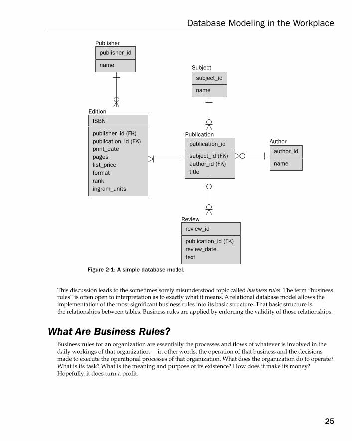
Figure 2-1: A simple database model.
This discussion leads to the sometimes sorely misunderstood topic called business rules. The term “businessrules” is often open to interpretation as to exactly what it means. A relational database model allows theimplementation of the most significant business rules into its basic structure. That basic structure is the relationships between tables. Business rules are applied by enforcing the validity of those relationships.
What Are Business Rules?Business rules for an organization are essentially the processes and flows of whatever is involved in thedaily workings of that organization — in other words, the operation of that business and the decisionsmade to execute the operational processes of that organization. What does the organization do to operate?What is its task? What is the meaning and purpose of its existence? How does it make its money?Hopefully, it does turn a profit.
Publisher
publisher_id
name Subject
subject_id
name
Author
author_id
name
Publication
publication_id
subject_id (FK)author_id (FK)title
Review
review_id
publication_id (FK)review_datetext
Edition
ISBN
publisher_id (FK)publication_id (FK)print_datepageslist_priceformatrankingram_units
25
Database Modeling in the Workplace
06_574906 ch02.qxd 10/28/05 11:36 PM Page 25
Business rules essentially have great scope for definition and redefinition, even in a single organization.Essentially, business rules cover the following aspects of an organization:
❑ Any types of organizational policies of any form and at all levels of the organization
❑ Any types of calculations or formulas (such as loan amortization calculations for a mortgagelending company)
❑ Any types of regulations (such as rules applied because of legal requirements, self-imposedrestrictions, or industry-standard requirements)
Simple business rules can be implemented in a database model by creating relationships between tables.For example, in Figure 2-1, a book (PUBLICATION) requires at least one author. This relationship isenforced in the diagram as being one and only one author who can have zero, one, or many publications.
In Figure 2-1, the relationship between the PUBLICATION and AUTHOR tables determines that an authorcan exist, but the author does not have to have any books published. On the contrary, a publication cannot exist unless it has an author. This relationship is somewhat sensible because if an author neverwrote a book, the book never existed.
It could, of course, be argued that an unpublished author is not an author by trade; however, that is aminor detail. The point is that the relationship forces the database model to accept only books that haveactually been written by someone, on the basis that a book written by no one has never been writtenbecause no one wrote it. The enforcement of entry of author prior to the name of the book helps toensure that the book does actually exist in the real world. This is how a database model can help toimplement simple business rules. The business rule is that a non-existent book cannot be entered intothe database.
Other business rules can be implemented and enforced using coding and other specialized constrainttypes. Coding implies programming code, in whatever language is appropriate. Constraints are thingsthat place restrictions on values stored in a database. For example, field values in table records can bevalidated for each entry. Only allowing a field to take on the value M or F to represent Male or Female isanother example of business rule application because there is no such gender that is not male or female.
The Importance of Business RulesI have had conversations with managers along the lines of, “no business rules in the database please,” or, “asmany business rules in the database as possible please.” Both of these statements are nonsensical because bothdo not apply to a certain extent. A relational database model cannot avoid defining some business rulessimply because of the existence of relationships between tables and enforcement of referential integrity.
And then there is individual field validation, such as allowing or prohibiting NULL values on individualfields. On the other hand, any type of complex validation processing may require the use of database-stored procedures or method coding (in an object database) to provide comprehensive business rule vali-dation in the database.
A stored procedure (also sometimes called a “database procedure”) is a chunk of code stored within andexecuted from within a database, typically on data stored in a database, but not always.
26
Chapter 2
06_574906 ch02.qxd 10/28/05 11:36 PM Page 26

Implementing business rules using stored procedures can be used to provide comprehensive accommodation of business rules; however, it is not a recommended path to good database performancefor a relational database. On the contrary, storing chunks of code as methods is the best route for anobject database because of the black box effect of the object data model.
The term “black box” implies chunks of code that can function independently, where changes made toone part of a piece of software, will not affect others.
Because this book is essentially about designing good relational database models, the object aspect issomewhat irrelevant. Perhaps it merely reinforces that complex business logic should be left to the application if developers must resort to database procedural code to enforce it. Most especially, avoidtriggers and database events for enforcing relationships between tables.
A trigger can also be called a database event trigger or a database rule. A trigger is a chunk of code that executes when a specified event occurs. For example, adding a new record to a table can be used to trigger an event. Referring to Figure 2-1 again, adding a new author could fire a trigger making a logentry into a logging or auditing table. Unless you are building an expert system, do not to use this typeof database-automated response coding for the application of database model level complex businessrules. You will likely get serious performance deficiencies if you do not heed this particular warning.
Incorporating the Human FactorWhat is meant by the human factor? You cannot create a database model without the involvement of thepeople who will ultimately use that database model. It is of no consequence if they are technical peoplesuch as computer programmers, or end-users such as executives wanting forecast plans from a datawarehouse. There is only one important thing to remember about company employees: as a whole, theyknow their business, how it operates, and how it works.
Many database model designers with vast experience can often go into a new company and draw on pastexperiences that they gained in similar organizations. This is nearly always the case for experienceddesigners, but there are often exceptional situations in any company that even experience can’t prepare for.
You can find out exactly what is needed by talking to the people who will use the database model youare about to design for them. Talk to their developers and their end-users. Your first task is to talk withand listen to company personnel. By talking and listening, you can discover how to design a betterdatabase model for them
People as a ResourceThe people the database model is being built for can often tell you the most about what should be in themodel, and sometimes even how pieces within that model should relate to each other. Remember, however,that those people are usually non-technical and know nothing about database model design. The databasedesigner applies technical skills to the thoughts and statements of the users (be that verbal or writtendown). Both users and designers have equal weight to add to this process.
In fact, even though I keep stressing the point of listening (always assuming the customer is right),essentially the users are people who you (the designer) gathers information from as to how the modelshould be designed and what should be in it — even down to the size and datatypes of fields in tables.
27
Database Modeling in the Workplace
06_574906 ch02.qxd 10/28/05 11:36 PM Page 27
Ultimately, you (the designer) are 95 percent responsible for figuring out the design and building thedatabase model. The end-users can give you many small pointers. From their perspective, it all makessense. From your perspective, information from end-users can often feel like a stream of jumbled-upfacts. It is your job to un-jumble everything and to make complete sense of it. Take time to think.Remember, design is largely a planning process, and thinking about various options is a big part of thatplanning process.
All you really need to do is to organize everything into sequences of logical, mathematical steps. Thoselogical bits and pieces get placed into a logically structured database model. It is the database designer’sresponsibility to figure out all this logical organization. It is not that the end-users do not know their business, but they are likely to think of it in terms of priorities and how they react to different situations —plus how important each task on their desk is related to the importance of the running of their business.
There also may be indirect effects in play as well where a specific employee thinks something is importantbecause he or she has been managed and motivated in a specific direction. Of course, it is likely that themanager or even the manager’s manager is aware of the importance of a specific task, but a lower-levelemployee may not be aware of why something is significant or not. Everything is subjective at this stage.The database designer must be objective, clinical, analytical, and (above all) precise.
So, now you have an impression of perhaps what people (being end-users, employees within a company)can tell you about the database model you are about to design. Perhaps you have also been made awarethat some things company employees tell you can be misleading. If people are misleading you, it is morethan likely that they are explaining something to you in a specific case type of scenario. That specific casescenario is the way they see it as specific to their particular business, company, the city they work and livein, or any number of other reasons.
Designing a database model is an abstraction of specifics. Abstraction is a logical or mathematical process,designed to make handling of specific situations much easier. Abstraction attempts to compartmentalizedifferent activities, ultimately processing at the compartment level, and not the activity level. What in abusiness environment could be two distinctly different things could be identical when properlyabstracted.
So, what does all that jargon mean? For example, a car salesman may picture selling a Ford and selling aChevy as two distinctly different processes. Fords and Chevys could be in different lots. They could havedifferent service agreements. There could be many other differences as well. From the perspective of the database modeler, however, both Ford and Chevy are automobiles, they are both either automatictransmissions or stick-shift, and they are both sold.
Whereas end-users see specifics, database model designers should look for common elements for abstraction.
Once again, you as the data modeler are ultimately responsible for designing their database. The databasemodel designer has the final say on what a database model should do and what it should look like. This is important to remember. Even though managers and employees alike understand their specific roles, not only could their perspective on tasks and procedures be microcosmic in nature, but also they couldmisunderstand the concept that some abstraction is required to create an effective and efficient databasemodel. A database model must take all special circumstances into account, but it must remain abstract. To reiterate an important point, what could seem like a special circumstance or situation for an end-usercould very well be easily catered for by a future database model — essentially an abstraction of special circumstances.
28
Chapter 2
06_574906 ch02.qxd 10/28/05 11:36 PM Page 28

Take into account everything people tell you, but don’t get sidetracked, misled, or confused because the database model designer’s perspective is much more abstract than that of an end-user. End-user perspectives are either at ground level or operationally based. A database model is a logical (and evenmathematical) abstraction that tries to accommodate for all possible circumstances, within reason, of course. Otherwise, the database model will be more complex than sometimes it is possible for applications to find useful. Have you ever encountered a database model design in a company, coveringan entire wall? This harbors potential for a scary situation.
Talking to the Right PeopleThere are different types of people. Some people are more technically aware than others; however, this doesnot imply that those who are technically aware are your best source of information. In my experience, thepeople with the most knowledge of a business are usually the managers, usually executive level in smallcompanies, and somewhere in the middle in larger companies. In a small company, executive-level peopleare easy to access. In a larger company, getting executive time is difficult (if not impossible) and probablynot effective for your purposes. For large companies, the best option is the high-level managers with agood overall picture of the business. These people can allocate the database designer more time than people further down on the scale who know the business well, perhaps someone who has both technicaland business operational skills.
As a database model designer, your entry point is the person who you bill and who signs your check.You may see this person only once. Even if your recruiter is in the Human Resources (HR) department,be sure that you get the recruiter’s help right off the bat in getting introductions to who might be able tohelp you best in your quest to create the most appropriate database model design possible.
A database designer must talk to different types of people on multiple levels and in multiple skills arenas,in the same company. It is beneficial to get a balance of levels and skills to help get a better overall pictureof requirements. There can be quite a distinct contrast between the perspective of management and that ofthe nitty-gritty details of employees on the floor getting their hands dirty in specific job functions.Obviously, how much detail is required is largely dependent on how complex the business is and also onhow much of that complexity is to be computerized.
For example, a simple invoicing system requiring only that bills be sent out excluding details of what isbeing sent out makes a simple book retailer require the same data modeling complexity as that of an autoparts manufacturer. Of course, if the evolving application is to include part numbers, colors, materials ofwhich items are made, correct parts for different types of cars, how things are made, precise measurements,the list goes on — there is a complexity issue. How complicated can selling books get? Quite typically, retailis simplistic when it comes to computerization. Manufacturing can be extremely complex, especially whenparts and pieces manufactured are custom-made as well as off-the-shelf.
The more complexity a database model requires, the more questions you must ask. The more questionsthere are to ask, the larger the amount of detail and potential layering within the structure of a designsolution. In conclusion, the more questions you have, the more people you might want to talk to, and,thus, the more people in different roles you will probably need to talk to as well. Take a breath!
Perhaps the central theme of database modeling (especially for relational database modeling in OLTPdatabases) is that abstraction is the order of the day. Greater levels of abstraction are more often neededwhen special-case scenarios crop up frequently. The more special-case scenarios you get, the more likelyyou will begin to observe similarities between those supposedly opposing special-case scenarios. Yourobjective is to create a single set of tables and relationships to cover as much of the operational functioning
29
Database Modeling in the Workplace
06_574906 ch02.qxd 10/28/05 11:36 PM Page 29
of a company as possible. If a separate set of tables is created for every special-case scenario, you will havetoo many tables and, therefore, no reduction in complexity (probably what the company was aiming at bycomputerizing). An extremely complex database model is not the objective. Application developers andend-users need simplicity. Without adequate simplicity, your database model design might be impossibleto use, particularly in the case of end-users and a data warehouse.
The job of a database modeler is simplicity through abstraction. Abstraction is this sense of the word is theamalgamation of different aspects of company operations into a succinct set of tables and relationshipsjoining those tables together. One simple rule is the more people you talk to about how to build theirdatabase model, the more likely you get a general overall picture (also the more likely you can get completely confused). The higher up the management scale you get, the more of a global picture you get.The problem with the management level is that they can leave out crucial details. Therefore, you must talkto the regular employees in specific job functions as well. Some managers might be able to point you atthe right employees with whom you should talk.
Overall, the number of people you must talk to depends on how complex the required database modelshould be. With simple database models, you can sometimes get away with using the elements of apaper-based system alone to build a database model.
In more technical companies that include computer personnel skills (such as programmers, systems anddatabase administrators, and so on), these people can possibly provide you with the most valuable ofinput; however, technical people can also be obstructive. Technical people, even in-house technical people, often do not have a clear perspective in terms of what end-users might need. In fact, more oftenthan not, in-house technical people are less aware of end-user needs within a company than consultingpeople. Outside consulting help can often give a fresh perspective.
Getting the Right InformationWhen it comes to getting the right information, the question that should perhaps first be asked is, “Whatis the right information?” Do you know the correct information? As an outsider, the answer is “probablynot.” As an insider, the answer is “perhaps.” There is a distinct advantage in using outside people to doessentially a task that not only treads on people’s toes, but also has the threat of introducing change. No one likes change. An in-house employee cannot reach across departments, asking 101 people 101 questions, from all over the company, without having to negotiate large tangled knots of political red tape.
Politics within companies is not always the case; however, environments that are difficult to deal with are common. Sometimes a consultant can either drive the process, or help get around the obstacles.Another (perhaps more quirky) fact is that the more a consultant costs, the more significant the consultant is to the company in terms of the relative cost perspective. Obviously, the higher the cost, thehigher the approval-rated signature is for the consultant’s bill (thus, the higher the level of managementthe consultant deals with and, therefore, the more likely that consultant will be effective). Obviously, allof this depends on company size, composition, political issues...the list is endless. On the contrary, inmany situations, in-house people are the best option.
Don’t get a completely negative opinion of company politics. Political maneuvering has its purpose. The larger companies get, the more complex people issues and the human factor can become. Simplechain of command can often be misconstrued as politicking. In other words, politics is not always asunproductive as you might think. Every facet of a situation has its purpose. If a situation is wholly negative, perhaps you should attempt to use it to your own advantage in getting the job done.
30
Chapter 2
06_574906 ch02.qxd 10/28/05 11:36 PM Page 30
Getting the right information is really an extension of talking to the right people, in that the correct detailcomes from the mouths of the people who know how a company functions operationally. This is not aderogatory statement. The database designer must figure out what should and should not be listened to,and taken into account. Some company employees have a birds-eye view; others have a detailed pictureof specific aspects of how a company makes its living on a daily basis.
Another way to look at it is this. The more people you talk to in a greater number of sections and levelsof a company, the more likely you (as a database model designer) will get a better perspective, perhapseven to the point of being able to dissimilate between correct and incorrect information and advise. Thedanger of talking to far too many people, taking account of some and not implementing suggestions andor requests of others, could certainly ruffle some feathers (not to mention completely confusing thedatabase model designer). The situation might even be a delicate balance between producing a goodstructure and not upsetting anyone. Strike a balance. The database model must be correct, but it also hasto be acceptable to the users. If there really are special scenarios, maintain them as special cases and notabstractions. Abstraction will save a database model from complexity, but could also make it unusable.
Finally, if you are an outside consultant, bear in mind that what you think is correct and what you thinkis incorrect may not be the reality of the situation. You could be completely wrong. Try not to ruffle anyfeathers while analyzing for and building your database model design because you want people to useyour database. There is no point in building a database design if it is not accepted because people simplydon’t like you. Strive to be liked, as well as achieving technical aims, and your efforts are unlikely to bewasted. Many technical people think that being liked is unimportant. They are wrong!
It’s not what you know, it’s who you know. It’s also not what you say, but how you say it!
Never assume that you know more than in-house employees, but also realize that you do have someexperience; otherwise, you would not be there. A combination of your skills and the knowledge of otherscan help you build a good database model design. Balance all perspectives and opinions to find the bestsolution. That solution should also be agreeable to as many of the participants as possible (includingyourself). You as the database designer are important as well because ultimately you designed it andyou are responsible for it. When you know you are correct, insist gently (but firmly), but also acquiescewhen someone else might be correct. Consider all possibilities and don’t let your own ego get in the way of your own success. Ensuring that a database model design comes into enthusiastic use is just asimportant as making sure the design is correct.
Above all, listen! Listen, learn, and examine every piece of information you are given. If a piece of information is not given, ask for it. If a snippet of information is essential and one person does not orcannot provide it, ask another. Achieve your objectives, but be careful not to tread on people’s toes. Thematerial discussed here can be found in a sales handbook. It is all basic common sense, and, yes, it islargely selling — selling yourself, your skills, your experience, and your ideas. When building a databasemodel for a company, be it a brand new concept or a rebuild of something that is already there, you arepotentially introducing change. Some people inside the company may react badly to potential change. Beaware of that, work around it, and work with it.
31
Database Modeling in the Workplace
06_574906 ch02.qxd 10/28/05 11:36 PM Page 31
Dealing with Unfavorable ScenariosQuite often, the best environment for which to design is a completely non-computerized environment.Common in many database model design projects are what can only be called “unfavorable” and sometimeseven “ugly” scenarios. Sometimes those ugly scenarios have to do with people. Those are best avoided;however, there are some commonly encountered situations where the people involved are only too willingto assist you in helping themselves out of a difficult database model problem.
With any existing database model and any type of conversion, be it from a legacy database on a mainframe, a paper-based system, or even a spreadsheet program, get as much information as possibleon what the new database model is supposed to achieve. Work backward from that point.
Computerizing a Pile of PapersThis can, in some ways, be the easiest problem to solve, and also, in some ways, the most difficult. Thefact is nothing exists in the way of a computerized database and quite often the paper pile and itsattached trail can show you (in great detail) exactly how the database model should look. Paper-basedsystems are sometimes very accurate and very detailed. They must also take all possibilities intoaccount, and have been designed for all possible eventualities over many years.
A problematic situation with a paper-based system is that it has often not been meticulously designed, andhas more or less grown into what it is because of necessity. The obvious result is a complete nightmare ofdifferent types of paper with a lot of duplicated information, conflicting information, and a whole plethoraof potential problems. In this extreme situation, you can use the basic format of paper documents to buildbasic table structures and possibly establish the operational aspects of the business.
Sometimes it is possible to find one person in an organization who knows how it all works. Sometimesit’s up to you to figure it out. In an extreme situation of total confusion, it is best to approach a databasemodel design cautiously and get some kind of verification from people who understand operationalfunctioning of the business. These people likely enjoy applying their knowledge to the creation of adatabase model. And better still, they also understand your database model design much better when itcomes to final handover to the client. Further still, they might even point out other factors such as fieldadditions and special cases that as an outsider you would never be able to see.
The easiest way through a paper system is to collect as much printed material as you can and then startcategorizing it. This task might be easier if you can find someone in the organization who can help youthrough this categorization process. Just be sure that the person actually does know about both thepaper system and the operational function of the business. Someone who doesn’t know zip could wellconfuse the heck out of you. Also, exchanging them later on for someone who is in the know could rufflefeathers. Choose wisely if you have a choice. Ask the manager or executive who hired you to pick theperson. Ensure that it is the executive who wanted you in the company. You don’t want to get involvedin any petty politicking.
Computerizing a pile of papers always looks like a daunting task. It isn’t! In fact, it is very possible thatby the time a company decides to computerize a paper system, the company will be more than willing toassist you in this most daunting of tasks because they might very well be trying to get rid of all thosepesky pieces of paper they are constantly having to fill in and correct.
32
Chapter 2
06_574906 ch02.qxd 10/28/05 11:36 PM Page 32
Converting Legacy DatabasesConverting legacy databases can often be the most difficult of tasks. Sometimes the databases are partiallyinaccessible or difficult to access at best. Sometimes the databases may even be in existence using networkor even hierarchical database modeling techniques. These database model structures can be extremelylarge and complex and, therefore, very difficult to decipher.
As with a paper system, find someone who knows all about the database to help you; otherwise, dig into the database yourself, allow plenty of time for analysis, and verify structure. In the worst case, analyze applications as well as the database model to confirm the operational functionality of thedatabase and that it actually does what it should do. It could very well be the case that a new databasemodel is required because the legacy database and software was incorrectly built in the first place, orthat requirements have drastically changed since its inception. If things have changed, you should findsomeone or something that makes these differences very obvious, either inside or outside of the databaseand applications, or both. It’s better to find an expert in the company first. Once again, you will getmuch farther, much faster, and with much more ease, by talking to people and asking questions.
Homogenous Integration of Heterogeneous DatabasesIn scientific terms, a heterogeneous system is a system consisting of dissimilar parts. And, obviously, ahomogenous system is the complete opposite consisting of similar parts, or parts being of a uniform structurethroughout. In terms of database models, some of the much more sophisticated (largely very expensive)database engines allow for the creation of homogenous integration of heterogeneous databases. In otherwords, it is possible to transparently link multiple types of databases, using different database engines, perhaps even including legacy databases, and really any type of database that can be catered for withwhichever database is being used to perform the integration. The idea is to retrieve data from the controlling database, the one establishing the homogeneous, seamless, transparent interface, and managedata in any number of underlying databases.
These maps or overlying homogeneous structures usually require what are called gateways, which areessentially database links from one database to another. The link is passed through a specialized driver,which allows the controlling database to talk to another database. Typically, these gateways arerestricted to access only the commonly used databases. Any connections or gateways to older networkor hierarchical databases could be implemented by manual coding. That is complicated and probablynot worth the development effort.
The fact is this — all computer software, including databases and their incorporated database models,have a fixed life cycle. That life cycle is the cycle of usefulness within acceptable limits of cost effectiveness.There comes a point where older legacy software is either too expensive to maintain or can be easilyreplaced. At that point, there is simply no reason to retain and not rewrite older software. Other than that,older legacy software and databases (depending on how old they are) can present enormous problems formanagement in finding people to maintain those older systems.
Converting from SpreadsheetsSpreadsheets are always fun at first because they look like flat files. When looking into spreadsheet files,however, you can find all sorts of complexities with formulas on multiple levels and even multiplerelated sheets. Paper-based and legacy-system spreadsheets require analysis, requirements specificationsof what should exist, and preferably the person who built the spreadsheet.
33
Database Modeling in the Workplace
06_574906 ch02.qxd 10/28/05 11:36 PM Page 33
The benefit of converting something like a spreadsheet into a database model is that the spreadsheet islikely to be a lot less complex than a mainframe-based legacy network database or a paper-based system.The reason why is likely to be because the company keeps losing copies of the spreadsheet or spreadsheets.Loss can occur from bad hardware, but most likely they occur because of human error caused by accidentaldeletions or copying. People lose things all the time. Spreadsheet or any single-user based system, unlessits something built in a legacy piece of software like dBase, is unlikely to present too much history; however, complexity is certainly a possibility.
Sorting Out a Messed-up DatabaseSorting out a messed-up database implies that there is a relational database in existence, but that thedatabase model is a complete mess. Expect to find invalid data, orphaned records, and other such wonderful problems. Once again, establish what is needed first before starting to go through it willy-nilly.After you establish what the records are supposed to look like, you might even find that there are only afew minor structural errors or relationship errors that can be easily repaired.
Even though a task like this can seem daunting, it really only has two very distinct steps. First, establishand build the correct structure. If the company has decided that the existing structure is problematic, thecompany probably has plenty of ideas on how to fix it. The company probably also knows who can giveyou all the correct information. Second, copy data across to new tables, if necessary.
SummaryIn this chapter, you learned about:
❑ Business rules are partially built into a relational database model design
❑ Talk to users to get the information you need
❑ Abstraction requires management perspective
❑ Assess the culture of in-house technical people to understand their perspective
❑ Higher-level personnel in small companies are more accessible than those in large companies
❑ Different types of people in different roles can give differing perspectives
❑ Talk to the right people to get the right information in a specific topic area
❑ Unfavorable scenarios are difficult conversion situations, but not necessarily as daunting as they seem
The next chapter begins the discussion of the technical details of the relational database model itself byintroducing all the various terms and concepts, the building blocks of the relational database model.
34
Chapter 2
06_574906 ch02.qxd 10/28/05 11:36 PM Page 34
3Database Modeling
Building Blocks
“Well begun is half done.” (Aristotle)
Begin at the beginning by starting with the simple pieces.
This chapter introduces the building blocks of the relational database model by discussing andexplaining all the various parts and pieces making up a relational database model. For example,a table is probably the most important piece in the puzzle of the relational database model, wherefields or fields in tables are perhaps of less significance but still essential to the semantics of themodel as a whole.
So far, this book has covered the historical evolution of database models, how different applica-tions and end-user needs affect database type, the basics of the art of database design, plus varioushuman factors influencing design. Before describing how a data model is built, you must knowwhat all the pieces are. You need a basic knowledge of all the parts and pieces constituting the relational database model. This chapter describes all those parts and pieces needed for future chapters, which will cover the process of creating and refining relational database models.
In a book such as this, the objective is to teach an understanding of the relational database modelby whatever means necessary. Previous chapters have used approaches such as a history ofdatabase models to describe the benefits and reasons for the evolution of the relational databasemodel, as it exists today. Various aspects of this book have already gone into some detail todescribe some basic and fundamental concepts, with deliberate succinctness.
At this point, this book could jump straight into the workings of the normalization process usingnormal forms. Normalization is used to granularize and organize data for use in a database. It isalso assumed, having purchased this book, that the concept of a table in a relational databasemodel is completely unfamiliar to you. So, I shall have to err on the side of caution and proceed to devote this entire chapter to describing all the various parts and pieces of what makes up a relational database model. You have to begin with the elements that make up the relationaldatabase model before proceeding to learn how to create relational database models.
07_574906 ch03.qxd 11/4/05 10:48 AM Page 35
If you have all the details in this chapter committed to memory and well understood, you can skip it ifyou are really strapped for time. However, I do recommend you read this chapter in its entirety. Thereare concepts, ideas, and object aspects of data modeling described in this chapter that you will not findin most books of this nature. I have taken the liberty of expanding on the basic structure of the relationaldatabase model and adding little bits and pieces here and there such as materialized views and autocounter sequences. For example, even though materialized views are not a part of the normalization process used to create a relational database model, materialized views can have a most profound effecton the behavior of data warehouses, particularly in the area of performance.
The process of normalization and the application of normal forms are covered in detail in Chapter 4. Allyou have to know at this stage is that normalization is the method or formula used to divide data upinto separate tables — according to a bunch of rules. So, when the term normalization is mentioned,simply assume it implies that new tables are being created or more streamlined versions of existingtables are being devised.
Views are included in this chapter. A view is not the same thing as a materialized view, which are relegated to a final section covering specialized objects. Materialized views and auto counters are included. As a performance tuner, I don’t believe in using views for anything other than security purposes, and I still wouldn’t recommend even that practice. Views are often used by developers to prototype or speed up development. The result is usually drastically poor performance in production. I prefer not to promote the use of views in general. In addition, views can be used to get around or skirtpoor database model design. Like I said, I prefer not to suggest use of views too strongly, by reason ofpast experience.
This chapter describes all the pieces that compose the relational database model. All of the constituentsof the relational database model help to create an organized logical structure for managing data in adatabase. The organized logical structure is a relational database model.
In this chapter, you learn about the following:
❑ Information, data, and data integrity
❑ Tables
❑ Fields, columns, and attributes
❑ Rows, records, and tuples
❑ Datatypes
❑ Validation and NULL values
❑ Relations, relationships, and some normalization
❑ Entity Relationship Diagrams (ERDs)
❑ Primary and foreign keys
❑ Referential integrity
❑ Indexes
❑ Specialized objects (views and materialized views)
So, arm in arm and onward we shall go! Let’s begin with a conceptual perspective.
36
Chapter 3
07_574906 ch03.qxd 11/4/05 10:48 AM Page 36
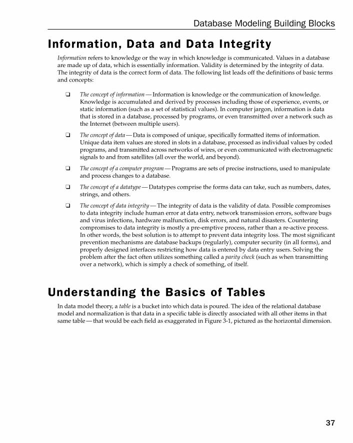
Information, Data and Data IntegrityInformation refers to knowledge or the way in which knowledge is communicated. Values in a databaseare made up of data, which is essentially information. Validity is determined by the integrity of data.The integrity of data is the correct form of data. The following list leads off the definitions of basic termsand concepts:
❑ The concept of information — Information is knowledge or the communication of knowledge.Knowledge is accumulated and derived by processes including those of experience, events, orstatic information (such as a set of statistical values). In computer jargon, information is datathat is stored in a database, processed by programs, or even transmitted over a network such asthe Internet (between multiple users).
❑ The concept of data — Data is composed of unique, specifically formatted items of information.Unique data item values are stored in slots in a database, processed as individual values by codedprograms, and transmitted across networks of wires, or even communicated with electromagneticsignals to and from satellites (all over the world, and beyond).
❑ The concept of a computer program — Programs are sets of precise instructions, used to manipulateand process changes to a database.
❑ The concept of a datatype — Datatypes comprise the forms data can take, such as numbers, dates,strings, and others.
❑ The concept of data integrity — The integrity of data is the validity of data. Possible compromisesto data integrity include human error at data entry, network transmission errors, software bugsand virus infections, hardware malfunction, disk errors, and natural disasters. Countering compromises to data integrity is mostly a pre-emptive process, rather than a re-active process.In other words, the best solution is to attempt to prevent data integrity loss. The most significantprevention mechanisms are database backups (regularly), computer security (in all forms), andproperly designed interfaces restricting how data is entered by data entry users. Solving theproblem after the fact often utilizes something called a parity check (such as when transmittingover a network), which is simply a check of something, of itself.
Understanding the Basics of TablesIn data model theory, a table is a bucket into which data is poured. The idea of the relational databasemodel and normalization is that data in a specific table is directly associated with all other items in thatsame table — that would be each field as exaggerated in Figure 3-1, pictured as the horizontal dimension.
37
Database Modeling Building Blocks
07_574906 ch03.qxd 11/4/05 10:48 AM Page 37
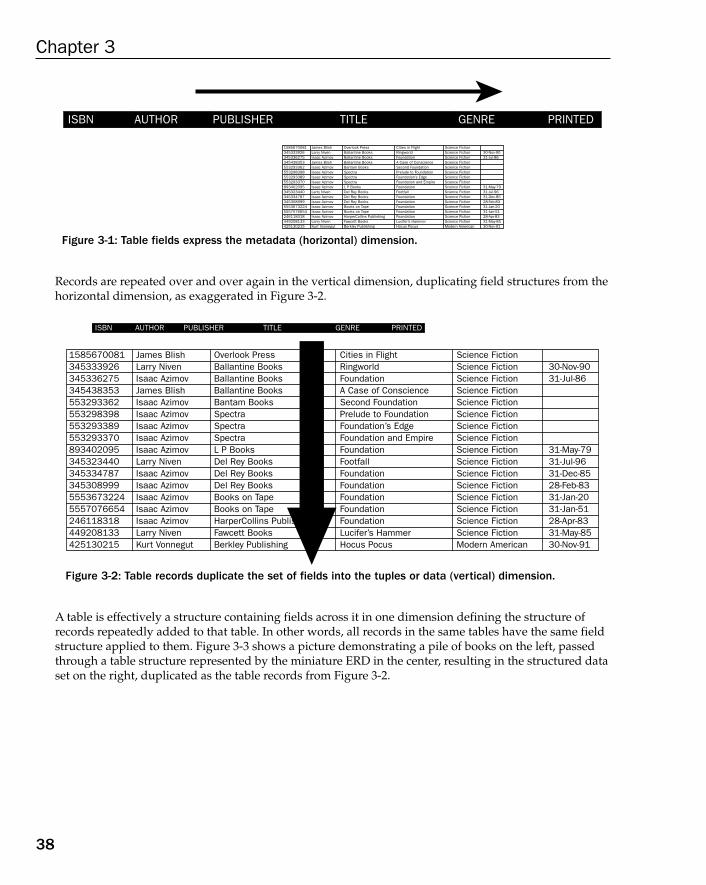
Figure 3-1: Table fields express the metadata (horizontal) dimension.
Records are repeated over and over again in the vertical dimension, duplicating field structures from thehorizontal dimension, as exaggerated in Figure 3-2.
Figure 3-2: Table records duplicate the set of fields into the tuples or data (vertical) dimension.
A table is effectively a structure containing fields across it in one dimension defining the structure ofrecords repeatedly added to that table. In other words, all records in the same tables have the same fieldstructure applied to them. Figure 3-3 shows a picture demonstrating a pile of books on the left, passedthrough a table structure represented by the miniature ERD in the center, resulting in the structured dataset on the right, duplicated as the table records from Figure 3-2.
ISBN AUTHOR PUBLISHER TITLE GENRE PRINTED
158567008134533392634533627534543835355329336255329839855329338955329337089340209534532344034533478734530899955536732245557076654246118318449208133425130215
James BlishLarry NivenIsaac AzimovJames BlishIsaac AzimovIsaac AzimovIsaac AzimovIsaac AzimovIsaac AzimovLarry NivenIsaac AzimovIsaac AzimovIsaac AzimovIsaac AzimovIsaac AzimovLarry NivenKurt Vonnegut
Overlook PressBallantine BooksBallantine BooksBallantine BooksBantam BooksSpectraSpectraSpectraL P BooksDel Rey BooksDel Rey BooksDel Rey BooksBooks on TapeBooks on TapeHarperCollins PublishingFawcett BooksBerkley Publishing
Cities in FlightRingworldFoundationA Case of ConscienceSecond FoundationPrelude to FoundationFoundation’s EdgeFoundation and EmpireFoundationFootfallFoundationFoundationFoundationFoundationFoundationLucifer’s HammerHocus Pocus
Science FictionScience FictionScience FictionScience FictionScience FictionScience FictionScience FictionScience FictionScience FictionScience FictionScience FictionScience FictionScience FictionScience FictionScience FictionScience FictionModern American
30-Nov-9031-Jul-86
31-May-7931-Jul-9631-Dec-8528-Feb-8331-Jan-2031-Jan-5128-Apr-8331-May-8530-Nov-91
38
Chapter 3
07_574906 ch03.qxd 11/4/05 10:48 AM Page 38
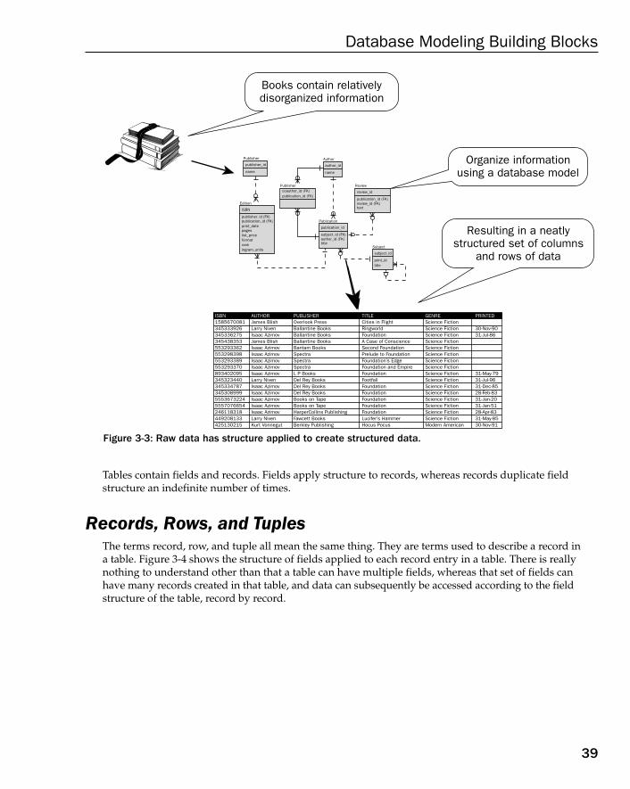
Figure 3-3: Raw data has structure applied to create structured data.
Tables contain fields and records. Fields apply structure to records, whereas records duplicate fieldstructure an indefinite number of times.
Records, Rows, and TuplesThe terms record, row, and tuple all mean the same thing. They are terms used to describe a record in a table. Figure 3-4 shows the structure of fields applied to each record entry in a table. There is reallynothing to understand other than that a table can have multiple fields, whereas that set of fields canhave many records created in that table, and data can subsequently be accessed according to the fieldstructure of the table, record by record.
Books contain relativelydisorganized information
1585670081
Publisher
publisher_id
name
34533392634533627534543835355329336255329839855329338955329337089340209534532344034533478734530899955536732245557076654246118318449208133425130215
James BlishLarry NivenIsaac AzimovJames BlishIsaac AzimovIsaac AzimovIsaac AzimovIsaac AzimovIsaac AzimovLarry NivenIsaac AzimovIsaac AzimovIsaac AzimovIsaac AzimovIsaac AzimovLarry NivenKurt Vonnegut
Overlook PressBallantine BooksBallantine BooksBallantine BooksBantam BooksSpectraSpectraSpectraL P BooksDel Rey BooksDel Rey BooksDel Rey BooksBooks on TapeBooks on TapeHarperCollins PublishingFawcett BooksBerkley Publishing
Cities in FlightRingworldFoundationA Case of ConscienceSecond FoundationPrelude to FoundationFoundation’s EdgeFoundation and EmpireFoundationFootfallFoundationFoundationFoundationFoundationFoundationLucifer’s HammerHocus Pocus
Science FictionISBN AUTHOR PUBLISHER TITLE GENRE PRINTED
Science FictionScience FictionScience FictionScience FictionScience FictionScience FictionScience FictionScience FictionScience FictionScience FictionScience FictionScience FictionScience FictionScience FictionScience FictionModern American
30-Nov-9031-Jul-86
31-May-7931-Jul-9631-Dec-8528-Feb-8331-Jan-2031-Jan-5128-Apr-8331-May-8530-Nov-91
Author
author_id
name
Subject
subject_id
print_idtitle
Publication
publication_id
subject_id (FK)author_id (FK)title
Review
review_id
publication_id (FK)review_id (FK)text
Publishercoauthor_id (FK)publication_id (FK)
Edition
ISBN
publisher_id (FK)publication_id (FK)print_datepageslist_priceformatrankingram_units
Organize informationusing a database model
Resulting in a neatlystructured set of columns
and rows of data
39
Database Modeling Building Blocks
07_574906 ch03.qxd 11/4/05 10:48 AM Page 39
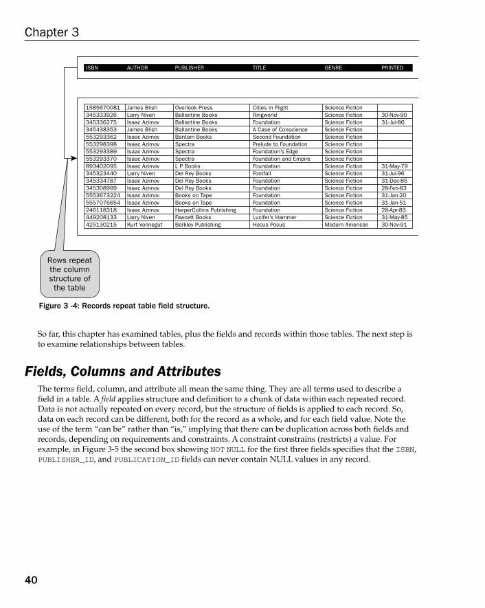
Figure 3 -4: Records repeat table field structure.
So far, this chapter has examined tables, plus the fields and records within those tables. The next step isto examine relationships between tables.
Fields, Columns and AttributesThe terms field, column, and attribute all mean the same thing. They are all terms used to describe afield in a table. A field applies structure and definition to a chunk of data within each repeated record.Data is not actually repeated on every record, but the structure of fields is applied to each record. So,data on each record can be different, both for the record as a whole, and for each field value. Note theuse of the term “can be” rather than “is,” implying that there can be duplication across both fields andrecords, depending on requirements and constraints. A constraint constrains (restricts) a value. Forexample, in Figure 3-5 the second box showing NOT NULL for the first three fields specifies that the ISBN,PUBLISHER_ID, and PUBLICATION_ID fields can never contain NULL values in any record.
Rows repeatthe columnstructure ofthe table
158567008134533392634533627534543835355329336255329839855329338955329337089340209534532344034533478734530899955536732245557076654246118318449208133425130215
James BlishLarry NivenIsaac AzimovJames BlishIsaac AzimovIsaac AzimovIsaac AzimovIsaac AzimovIsaac AzimovLarry NivenIsaac AzimovIsaac AzimovIsaac AzimovIsaac AzimovIsaac AzimovLarry NivenKurt Vonnegut
Overlook PressBallantine BooksBallantine BooksBallantine BooksBantam BooksSpectraSpectraSpectraL P BooksDel Rey BooksDel Rey BooksDel Rey BooksBooks on TapeBooks on TapeHarperCollins PublishingFawcett BooksBerkley Publishing
Cities in FlightRingworldFoundationA Case of ConscienceSecond FoundationPrelude to FoundationFoundation’s EdgeFoundation and EmpireFoundationFootfallFoundationFoundationFoundationFoundationFoundationLucifer’s HammerHocus Pocus
Science Fiction
ISBN AUTHOR PUBLISHER TITLE GENRE PRINTED
Science FictionScience FictionScience FictionScience FictionScience FictionScience FictionScience FictionScience FictionScience FictionScience FictionScience FictionScience FictionScience FictionScience FictionScience FictionModern American
30-Nov-9031-Jul-86
31-May-7931-Jul-9631-Dec-8528-Feb-8331-Jan-2031-Jan-5128-Apr-8331-May-8530-Nov-91
40
Chapter 3
07_574906 ch03.qxd 11/4/05 10:48 AM Page 40
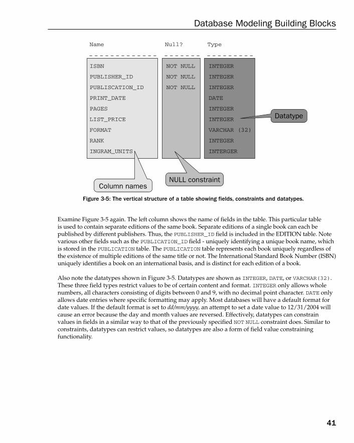
Figure 3-5: The vertical structure of a table showing fields, constraints and datatypes.
Examine Figure 3-5 again. The left column shows the name of fields in the table. This particular table is used to contain separate editions of the same book. Separate editions of a single book can each be published by different publishers. Thus, the PUBLISHER_ID field is included in the EDITION table. Notevarious other fields such as the PUBLICATION_ID field - uniquely identifying a unique book name, whichis stored in the PUBLICATION table. The PUBLICATION table represents each book uniquely regardless ofthe existence of multiple editions of the same title or not. The International Standard Book Number (ISBN)uniquely identifies a book on an international basis, and is distinct for each edition of a book.
Also note the datatypes shown in Figure 3-5. Datatypes are shown as INTEGER, DATE, or VARCHAR(32).These three field types restrict values to be of certain content and format. INTEGER only allows wholenumbers, all characters consisting of digits between 0 and 9, with no decimal point character. DATE onlyallows date entries where specific formatting may apply. Most databases will have a default format fordate values. If the default format is set to dd/mm/yyyy, an attempt to set a date value to 12/31/2004 willcause an error because the day and month values are reversed. Effectively, datatypes can constrain values in fields in a similar way to that of the previously specified NOT NULL constraint does. Similar toconstraints, datatypes can restrict values, so datatypes are also a form of field value constraining functionality.
Name
ISBN
PUBLISHER_ID
PUBLISCATION_ID
PRINT_DATE
PAGES
LIST_PRICE
FORMAT
RANK
INGRAM_UNITS
Null?
NOT NULL
NOT NULL
NOT NULL
Type
INTEGER
INTEGER
INTEGER
DATE
INTEGER
INTEGER
VARCHAR (32)
INTEGER
INTERGER
Column namesNULL constraint
Datatype
41
Database Modeling Building Blocks
07_574906 ch03.qxd 11/4/05 10:48 AM Page 41

Whereas fields apply structure to records, datatypes apply structure and restrictions to fields and valuesin those fields.
DatatypesThere are many different types of datatypes, which vary often more in name than anything else withrespect to different database engines. This section describes all different variations of datatypes, butwithout targeting any specific vendor database engine.
Datatypes can be divided into three separate sections:
❑ Simple datatypes — These are datatypes applying a pattern or value limitation on a single valuesuch as a number.
❑ Complex datatypes — These include any datatypes bridging the gap between object and relational databases, including items such as binary objects and collection arrays. Specifics oncomplex datatypes are not strictly necessary for this book as they are more object-oriented thanrelational in nature.
❑ Specialized datatypes — These are present in more advanced relational databases catering toinherently structured data such as XML documents, spatial data, multimedia objects and evendynamically definable datatypes.
Simple DatatypesSimple datatypes include basic validation and formatting requirements placed on to individual values.This includes the following:
❑ Strings — A string is a sequence of one or more characters. Strings can be fixed-length strings orvariable-length strings:
❑ Fixed-length strings — A fixed-length string will always store the specified length declaredfor the datatype. The value is padded with spaces even when the actual string value isless than the length of the datatype length. For example, the value NY in a CHAR(3) vari-able would be stored as NY plus a space character. Fixed-length strings are generallyonly used for short length strings because a variable-length string (discussed next)requires storage of both value and length. Fixed-length strings are also more efficient forensuring fixed record lengths of key values. Figure 3-6 shows an FXCODE field represent-ing a foreign exchange currency code, always returning three characters even when thecurrency code is less than three characters in length. A case in point is the defunct cur-rency code DM (Deutsche Marks, German currency), returning DM plus a space character,yielding a total of three characters.
42
Chapter 3
07_574906 ch03.qxd 11/4/05 10:48 AM Page 42

Figure 3-6: Fixed-length strings and variable-length strings.
❑ Variable-length strings — A variable-length string allows storage into a datatype as theactual length of the string, as long as a maximum limit is not exceeded. The length of the string is variable because when storing a string of length less than the width specified by the datatype, the string is not padded (as is the case for fixed-lengthstrings). Only the actual string value is stored. Storing the string XXX into a variablelength string datatype of ten characters in length stores the three characters only, andnot three characters padded by seven spaces. Different databases use different namingconventions for variable-length string datatypes. VARCHAR(n) or TEXT(n) are commonnaming formats for variable-length strings. Figure 3-6 shows variable-length strings oncountry names (COUNTRY), returning only the names of the countries and no paddingout to maximum length as for fixed-length strings.
“DM” returnedas “DM ”
COUNTRY is variablelength returning only
the value in the column
SQL> select country||’,’||fxcode||’,’||currency
Gambia, GMD, Dalasi
Ghana, GHC, Cedis
Guinea, GNF, Francs
Guatemala, GTQ, Quetzales
Germany, DM , Deutsche Marks
Guyana, GYD, Dollars
COUNTRY||’,’||FXCODE||’,’||CURRENCY
2 from country
3 where fxcode is not null
4 and country like ‘G%’;
FXCODE is a fixedlength, 3 character string
43
Database Modeling Building Blocks
07_574906 ch03.qxd 11/4/05 10:48 AM Page 43
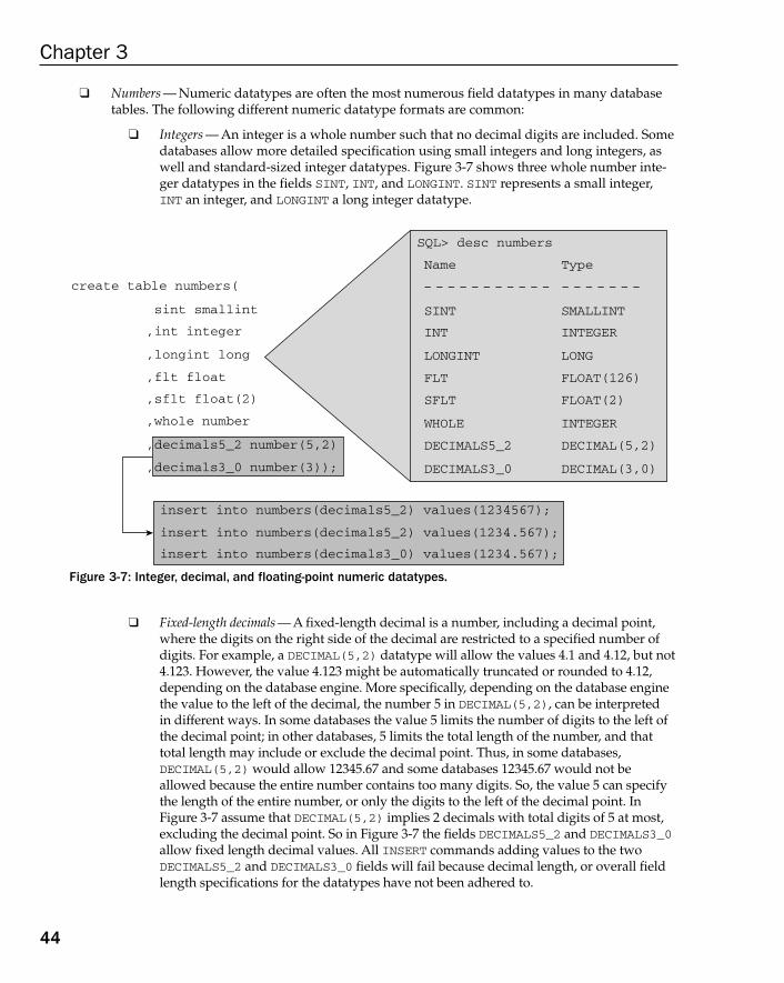
❑ Numbers — Numeric datatypes are often the most numerous field datatypes in many databasetables. The following different numeric datatype formats are common:
❑ Integers — An integer is a whole number such that no decimal digits are included. Somedatabases allow more detailed specification using small integers and long integers, aswell and standard-sized integer datatypes. Figure 3-7 shows three whole number inte-ger datatypes in the fields SINT, INT, and LONGINT. SINT represents a small integer,INT an integer, and LONGINT a long integer datatype.
Figure 3-7: Integer, decimal, and floating-point numeric datatypes.
❑ Fixed-length decimals — A fixed-length decimal is a number, including a decimal point,where the digits on the right side of the decimal are restricted to a specified number ofdigits. For example, a DECIMAL(5,2) datatype will allow the values 4.1 and 4.12, but not4.123. However, the value 4.123 might be automatically truncated or rounded to 4.12,depending on the database engine. More specifically, depending on the database enginethe value to the left of the decimal, the number 5 in DECIMAL(5,2), can be interpreted in different ways. In some databases the value 5 limits the number of digits to the left of the decimal point; in other databases, 5 limits the total length of the number, and thattotal length may include or exclude the decimal point. Thus, in some databases, DECIMAL(5,2) would allow 12345.67 and some databases 12345.67 would not beallowed because the entire number contains too many digits. So, the value 5 can specifythe length of the entire number, or only the digits to the left of the decimal point. InFigure 3-7 assume that DECIMAL(5,2) implies 2 decimals with total digits of 5 at most,excluding the decimal point. So in Figure 3-7 the fields DECIMALS5_2 and DECIMALS3_0allow fixed length decimal values. All INSERT commands adding values to the two DECIMALS5_2 and DECIMALS3_0 fields will fail because decimal length, or overall fieldlength specifications for the datatypes have not been adhered to.
create table numbers(
SQL> desc numbers
Name Type
SINT SMALLINT
INT INTEGER
LONGINT LONG
FLT FLOAT(126)
SFLT FLOAT(2)
WHOLE INTEGER
DECIMALS5_2 DECIMAL(5,2)
DECIMALS3_0 DECIMAL(3,0)
sint smallint
,int integer
,longint long
,flt float
,sflt float(2)
,whole number
,decimals5_2 number(5,2)
,decimals3_0 number(3));
insert into numbers(decimals5_2) values(1234567);
insert into numbers(decimals5_2) values(1234.567);
insert into numbers(decimals3_0) values(1234.567);
44
Chapter 3
07_574906 ch03.qxd 11/4/05 10:48 AM Page 44
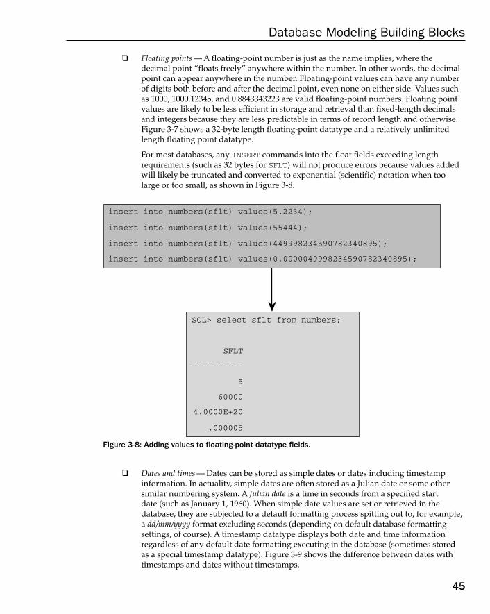
❑ Floating points — A floating-point number is just as the name implies, where the decimal point “floats freely” anywhere within the number. In other words, the decimalpoint can appear anywhere in the number. Floating-point values can have any numberof digits both before and after the decimal point, even none on either side. Values suchas 1000, 1000.12345, and 0.8843343223 are valid floating-point numbers. Floating pointvalues are likely to be less efficient in storage and retrieval than fixed-length decimalsand integers because they are less predictable in terms of record length and otherwise.Figure 3-7 shows a 32-byte length floating-point datatype and a relatively unlimitedlength floating point datatype.
For most databases, any INSERT commands into the float fields exceeding lengthrequirements (such as 32 bytes for SFLT) will not produce errors because values addedwill likely be truncated and converted to exponential (scientific) notation when toolarge or too small, as shown in Figure 3-8.
Figure 3-8: Adding values to floating-point datatype fields.
❑ Dates and times — Dates can be stored as simple dates or dates including timestampinformation. In actuality, simple dates are often stored as a Julian date or some othersimilar numbering system. A Julian date is a time in seconds from a specified start date (such as January 1, 1960). When simple date values are set or retrieved in thedatabase, they are subjected to a default formatting process spitting out to, for example,a dd/mm/yyyy format excluding seconds (depending on default database formatting settings, of course). A timestamp datatype displays both date and time informationregardless of any default date formatting executing in the database (sometimes storedas a special timestamp datatype). Figure 3-9 shows the difference between dates withtimestamps and dates without timestamps.
insert into numbers(sflt) values(5.2234);
SQL> select sflt from numbers;
SFLT
5
60000
4.0000E+20
.000005
insert into numbers(sflt) values(55444);
insert into numbers(sflt) values(449998234590782340895);
insert into numbers(sflt) values(0.0000049998234590782340895);
45
Database Modeling Building Blocks
07_574906 ch03.qxd 11/4/05 10:48 AM Page 45
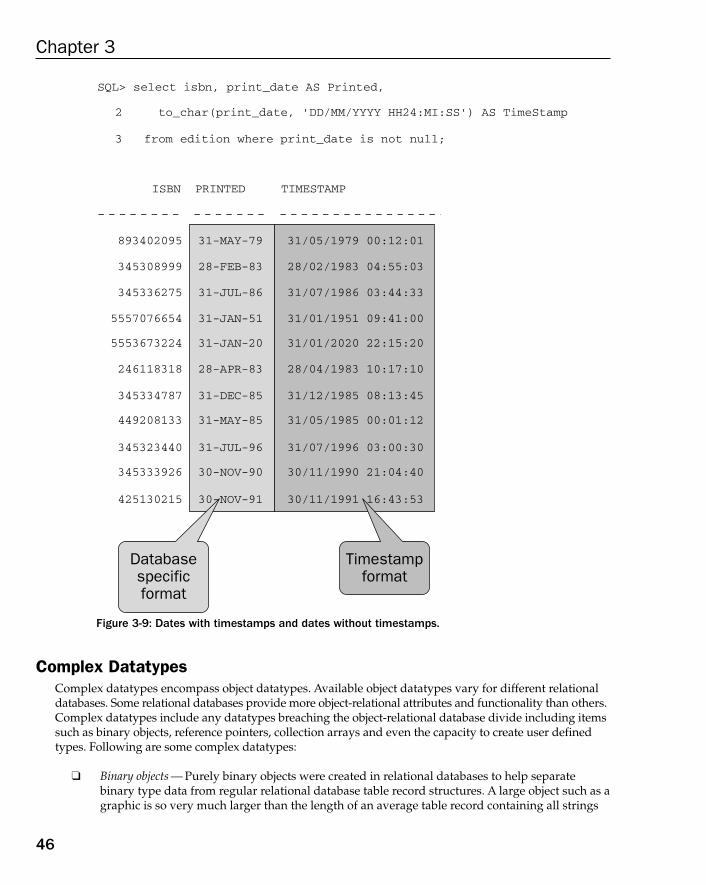
Figure 3-9: Dates with timestamps and dates without timestamps.
Complex DatatypesComplex datatypes encompass object datatypes. Available object datatypes vary for different relationaldatabases. Some relational databases provide more object-relational attributes and functionality than others.Complex datatypes include any datatypes breaching the object-relational database divide including itemssuch as binary objects, reference pointers, collection arrays and even the capacity to create user definedtypes. Following are some complex datatypes:
❑ Binary objects — Purely binary objects were created in relational databases to help separatebinary type data from regular relational database table record structures. A large object such as agraphic is so very much larger than the length of an average table record containing all strings
SQL> select isbn, print_date AS Printed,
2 to_char(print_date, ‘DD/MM/YYYY HH24:MI:SS’) AS TimeStamp
3 from edition where print_date is not null;
ISBN PRINTED TIMESTAMP
893402095
345308999
345336275
5557076654
5553673224
246118318
345334787
449208133
345323440
345333926
425130215
31-MAY-79
28-FEB-83
31-JUL-86
31-JAN-51
31-JAN-20
28-APR-83
31-DEC-85
31-MAY-85
31-JUL-96
30-NOV-90
30-NOV-91
31/05/1979 00:12:01
28/02/1983 04:55:03
31/07/1986 03:44:33
31/01/1951 09:41:00
31/01/2020 22:15:20
28/04/1983 10:17:10
31/12/1985 08:13:45
31/05/1985 00:01:12
31/07/1996 03:00:30
30/11/1990 21:04:40
30/11/1991 16:43:53
Databasespecificformat
Timestampformat
46
Chapter 3
07_574906 ch03.qxd 11/4/05 10:48 AM Page 46
and numbers. Storage issues can become problematic. Relational databases use many differenttypes of underlying disk storage techniques to make the management of records in tables moreefficient. A typical record in a table may occupy at most 2 KB (sometimes known as a page orblock), and often much less. Even the smallest of graphic objects used in Web site applicationseasily exceeds the size of a record — and each record in a table could have a unique graphicobject. Therefore, storing a graphic object with each record in the underlying operating systemblock structure completely ruins any kind of specialized storage structure performance tunedfor simple table record strings and numbers storage. Binary objects were created to physicallyseparate binary values from traditional table record values. The obvious extension to this concept was creation of binary objects to store anything in binary format, reducing storage,even items such as large strings, sound files, video, XML documents . . . the list goes on.
❑ Reference pointers — In the C programming language, a reference pointer is a variable containingan address on disk or in memory of whatever the programmer wants to point at. A pointer provides the advantage of not having to specify too much in advance with respect to how manybytes the pointer value occupies. Some relational databases allow the use of pointers where apointer points to an object or file stored externally to the database, pointing from a field within atable, to the object stored outside the database. Only the address of the externally stored objectis stored in the table field. This minimizes structural storage effects on relational tables as oftenis the result of storing binary objects in table records. Pointers are generally used for pointing tostatic binary objects. A static object does not change very often.
❑ Collection arrays — Some relational databases allow creation of what an object database wouldcall a collection. A collection is a set of values repeated structurally (values are not necessarily thesame) where the array is contained within another object, and can only be referenced from thatobject. In the case of a relational database, the containment factor is the collection being a fieldin the table. Collection arrays can have storage structures defined in alternative locations totable fields as for binary objects, but do not have to be as such. Collection arrays, much like program arrays, can be either fixed length or dynamic. A dynamic array is a variable-lengtharray, and is actually a pointer. When using a fixed-length array, the programmer must specifythe length of the array before using it.
❑ User-defined types — Some relational databases allow programmable or even on-the-fly creationof user-defined types. A user-defined type allows the creation of new types. Creation of a newtype means that user-defined datatypes can be created by programmers, even using other user-defined types. It follows that fields can be created in tables where those fields have user-defined datatypes.
Specialized DatatypesSpecialized datatypes take into account datatypes that are intended for contained complex data objects.These specialized datatypes allow types with contained inherent structure (such as XML documents,spatial data, and multimedia objects).
Constraints and ValidationRelational databases allow constraints, which restrict values that are allowed to be stored in table fields.Some relational databases allow the minimum of constraints necessary to define a database as being arelational database. Some relational databases allow other constraints in addition to the basics. In general,constraints are used to restrict values in tables, make validation checks on one or more fields in a table, oreven check values between fields in different tables. Following are some examples of constraints:
47
Database Modeling Building Blocks
07_574906 ch03.qxd 11/4/05 10:48 AM Page 47

❑ NOT NULL— This is the simplest of field level constraints, making sure that a value must alwaysbe entered into a field when a record is added or changed.
❑ Validation check — Similar to a NOT NULL constraint, a validation checking type of constraintrestricts values in fields when a record is added or changed in a table. A check validation constraint can be as simple as making sure a field allowing only M for Male or F for Female, willonly ever contain those two possible values. Otherwise, check validation constraints can becomefairly complex in some relational databases, perhaps allowing inclusion of user written functions running SQL scripting.
❑ Keys — Key constraints include primary keys, foreign keys, and unique keys. All these key typesare discussed briefly later on in this chapter and further in later chapters in this book. Key con-straints allow the checking and validation of values between fields in different tables. Primaryand foreign keys are essentially the implementation of relationships between parent and childtables. Those relationships or relations are the source of the term relational database.
Some relational databases allow constraints to be specified at both the field level or for an entire table asa whole, depending on the type of constraint.
Understanding Relations for NormalizationBy dictionary definition, the term normalization means to make normal in terms of causing something to conform to a standard, or to introduce consistency with respect to style and content. In terms of relational database modeling, that consistency becomes a process of removing duplication in data,among other factors. Removal of duplication tends to minimize redundancy. Minimization of redundancy implies getting rid of unneeded data present in particular places, or tables.
In reality, normalization usually manages to divide information into smaller, more manageable parts,preferably not too small. The most obvious redundancies can usually be removed without getting toodeeply mathematical about everything. Commercially speaking, primary objectives are usually to savespace and organize data for usability and manageability, without sacrificing performance. All this is oftena juggling act and commonly partially ironed out by trial and error. Additionally the demands of intenselybusy applications and end-user needs can tend to necessitate breaking the rules of normalization in many ways to meet performance requirements. Rules are usually broken simply by not applying everypossible layer of normalization. Normal Forms beyond 3rd Normal Form are often ignored and sometimes even 3rd Normal Form itself is discounted.
Normalization can be described as being one of introduction of granularity, removal of duplication, orminimizing of redundancy, or simply the introduction of tables, all of which place data into a betterorganized state.
Normalization is an incremental process. In other words, each Normal Form layer adds to whateverNormal Forms have already been applied. For example, 2nd Normal Form can only be applied to tablesin 1st Normal Form, and 3rd Normal Form only applied to tables in 2nd Normal Form, and so on. EachNormal Form is a refinement of the previous Normal Form. Similarly 3rd Normal cannot be applied totables in 4th Normal Form because by definition tables in 4th Normal Form are cumulatively already in3rd Normal Form.
48
Chapter 3
07_574906 ch03.qxd 11/4/05 10:48 AM Page 48
Benefits of NormalizationEffectively minimizing redundancy is another way of describing removal of duplication. The effect ofremoving duplication is as follows:
❑ Physical space needed to store data is reduced.
❑ Data becomes better organized.
❑ Normalization allows changes to small amounts of data (namely single records) to be made toone table at once. In other words, a single table record is updated when a specific item is added,changed, or removed from the database. You don’t have to search through an entire database tochange a single field value in a single record, just the table.
Potential Normalization HazardsThere are potential problems in taking this redundancy minimization process too far. Some detailed aspectsof the positive effects of normalization mentioned previously can have negative side effects, and sometimeseven backfire, depending on the application focus of the database. Performance is always a problem with too much granularity caused by over-application of normalization. Very demanding concurrencyOLTP databases can be very adversely affected by too much granularity. Data warehouses often requirenon-technical end-user access and over-granularity tends to make table structure more technically orientedto the point of being impossible to interpret by end-users. Keep the following in mind:
❑ Physical space is not nearly as big a concern as it used to be, because disk space is one of the cheapest cost factors to consider (unless, of course, when dealing with a truly huge datawarehouse).
❑ Too much minimization of redundancy implies too much granularity and too many tables. Toomany tables can lead to extremely huge SQL join queries. The more tables in a SQL join query,the slower queries execute. Performance can be so drastically affected as to make applicationscompletely useless.
❑ Better organization of data with extreme amounts of redundancy minimization can actuallyresult in more complexity, particularly if end-users are exposed to database model structure.The deeper the level of normalization, the more mathematical the model becomes, making the model “techie-friendly” and thus very “user-unfriendly.” Who is accessing the database,end-users or OLTP applications?
Tables are connected to each other with relationships. Examine what a relationship is and how it can berepresented.
Representing Relationships in an ERDTables can have various types of relationships between them. The different types of inter-table relation-ships that can be formed between different tables can be best described as displayed in EntityRelationship Diagrams (ERDs).
49
Database Modeling Building Blocks
07_574906 ch03.qxd 11/4/05 10:48 AM Page 49
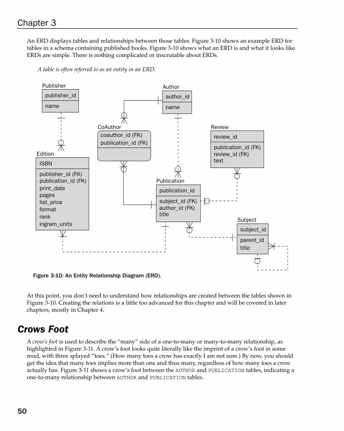
An ERD displays tables and relationships between those tables. Figure 3-10 shows an example ERD fortables in a schema containing published books. Figure 3-10 shows what an ERD is and what it looks like.ERDs are simple. There is nothing complicated or inscrutable about ERDs.
A table is often referred to as an entity in an ERD.
Figure 3-10: An Entity Relationship Diagram (ERD).
At this point, you don’t need to understand how relationships are created between the tables shown inFigure 3-10. Creating the relations is a little too advanced for this chapter and will be covered in laterchapters, mostly in Chapter 4.
Crows FootA crow’s foot is used to describe the “many” side of a one-to-many or many-to-many relationship, ashighlighted in Figure 3-11. A crow’s foot looks quite literally like the imprint of a crow’s foot in somemud, with three splayed “toes.” (How many toes a crow has exactly I am not sure.) By now, you shouldget the idea that many toes implies more than one and thus many, regardless of how many toes a crowactually has. Figure 3-11 shows a crow’s foot between the AUTHOR and PUBLICATION tables, indicating aone-to-many relationship between AUTHOR and PUBLICATION tables.
Publisher
publisher_id
name
Author
author_id
name
Subject
subject_id
parent_idtitle
Publication
publication_id
subject_id (FK)author_id (FK)title
Review
review_id
publication_id (FK)review_id (FK)text
CoAuthorcoauthor_id (FK)publication_id (FK)
Edition
ISBN
publisher_id (FK)publication_id (FK)print_datepageslist_priceformatrankingram_units
50
Chapter 3
07_574906 ch03.qxd 11/4/05 10:48 AM Page 50
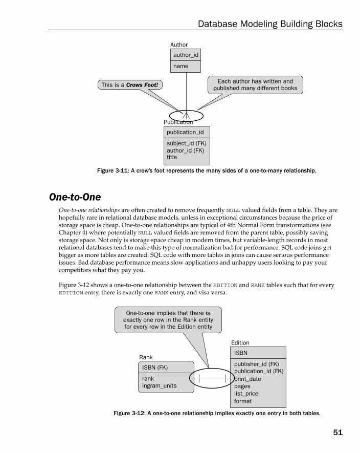
Figure 3-11: A crow’s foot represents the many sides of a one-to-many relationship.
One-to-OneOne-to-one relationships are often created to remove frequently NULL valued fields from a table. They arehopefully rare in relational database models, unless in exceptional circumstances because the price ofstorage space is cheap. One-to-one relationships are typical of 4th Normal Form transformations (seeChapter 4) where potentially NULL valued fields are removed from the parent table, possibly saving storage space. Not only is storage space cheap in modern times, but variable-length records in most relational databases tend to make this type of normalization bad for performance. SQL code joins getbigger as more tables are created. SQL code with more tables in joins can cause serious performanceissues. Bad database performance means slow applications and unhappy users looking to pay your competitors what they pay you.
Figure 3-12 shows a one-to-one relationship between the EDITION and RANK tables such that for everyEDITION entry, there is exactly one RANK entry, and visa versa.
Figure 3-12: A one-to-one relationship implies exactly one entry in both tables.
Edition
ISBN
publisher_id (FK)publication_id (FK)print_datepageslist_priceformat
Rank
One-to-one implies that there isexactly one row in the Rank entityfor every row in the Edition entity
ISBN (FK)
rankingram_units
Author
author_id
name
Publication
publication_id
subject_id (FK)author_id (FK)title
This is a Crows Foot!Each author has written and
published many different books
51
Database Modeling Building Blocks
07_574906 ch03.qxd 11/4/05 10:48 AM Page 51
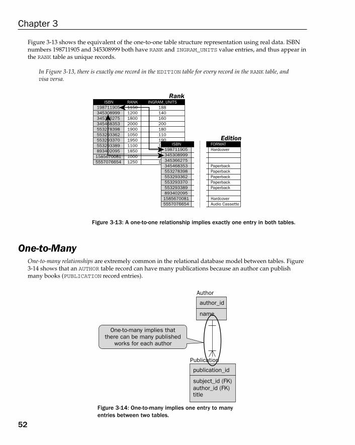
Figure 3-13 shows the equivalent of the one-to-one table structure representation using real data. ISBNnumbers 198711905 and 345308999 both have RANK and INGRAM_UNITS value entries, and thus appear inthe RANK table as unique records.
In Figure 3-13, there is exactly one record in the EDITION table for every record in the RANK table, andvisa versa.
Figure 3-13: A one-to-one relationship implies exactly one entry in both tables.
One-to-ManyOne-to-many relationships are extremely common in the relational database model between tables. Figure3-14 shows that an AUTHOR table record can have many publications because an author can publishmany books (PUBLICATION record entries).
Figure 3-14: One-to-many implies one entry to many entries between two tables.
Author
author_id
name
Publication
publication_id
subject_id (FK)author_id (FK)title
One-to-many implies thatthere can be many published
works for each author
198711905345308999345366275345468353553278398553293362553293370553293389893402095
15856700815557076654
11501200180020001900105019501100185010001250
188140
Rank
Edition
1602001801101901111
ISBN RANK INGRAM_UNITS
19871190534530899934536627534546835355327839855329336255329337055329338989340209515856700815557076654
Hardcover
PaperbackPaperbackPaperbackPaperbackPaperback
HardcoverAudio Cassette
ISBN FORMAT
52
Chapter 3
07_574906 ch03.qxd 11/4/05 10:48 AM Page 52
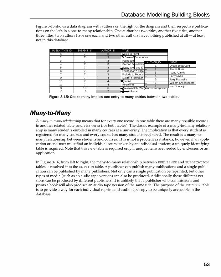
Figure 3-15 shows a data diagram with authors on the right of the diagram and their respective publica-tions on the left, in a one-to-many relationship. One author has two titles, another five titles, anotherthree titles, two authors have one each, and two other authors have nothing published at all — at leastnot in this database.
Figure 3-15: One-to-many implies one entry to many entries between two tables.
Many-to-ManyA many-to-many relationship means that for every one record in one table there are many possible recordsin another related table, and visa versa (for both tables). The classic example of a many-to-many relation-ship is many students enrolled in many courses at a university. The implication is that every student isregistered for many courses and every course has many students registered. The result is a many-to-many relationship between students and courses. This is not a problem as it stands; however, if an appli-cation or end-user must find an individual course taken by an individual student, a uniquely identifyingtable is required. Note that this new table is required only if unique items are needed by end-users or anapplication.
In Figure 3-16, from left to right, the many-to-many relationship between PUBLISHER and PUBLICATIONtables is resolved into the EDITION table. A publisher can publish many publications and a single publi-cation can be published by many publishers. Not only can a single publication be reprinted, but othertypes of media (such as an audio tape version) can also be produced. Additionally those different ver-sions can be produced by different publishers. It is unlikely that a publisher who commissions andprints a book will also produce an audio tape version of the same title. The purpose of the EDITION tableis to provide a way for each individual reprint and audio tape copy to be uniquely accessible in thedatabase.
123456791011812
77777777771516
223333344467
Cities in FlightA Case of ConscienceFoundationSecond FoundationFoundation and EmpireFoundation’s EdgePrelude to FoundationLucifer’s HammerFootfallRingworldThe Complete Works of ShakespeareHocus Pocus
PUBLICATION_ID SUBJECT_ID AUTHOR_ID TITLE
1
56
Orson Scott CardJames BlishIsaac AzimovLarry NivenJerry PournelleWilliam ShakespeareKurt Vonnegut
AUTHOR_ID NAME
234
7
53
Database Modeling Building Blocks
07_574906 ch03.qxd 11/4/05 10:48 AM Page 53
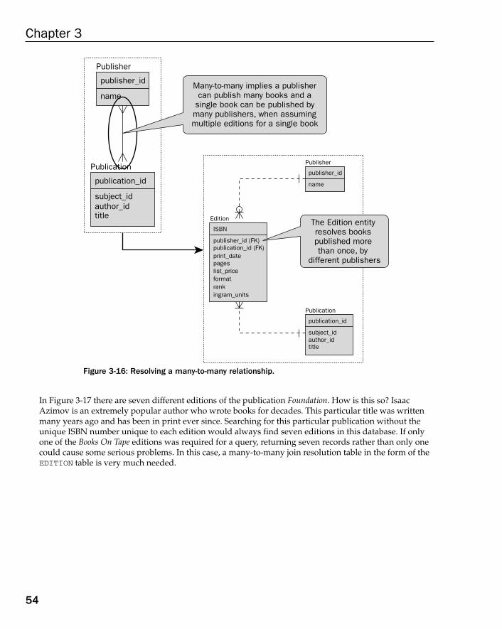
Figure 3-16: Resolving a many-to-many relationship.
In Figure 3-17 there are seven different editions of the publication Foundation. How is this so? IsaacAzimov is an extremely popular author who wrote books for decades. This particular title was writtenmany years ago and has been in print ever since. Searching for this particular publication without theunique ISBN number unique to each edition would always find seven editions in this database. If onlyone of the Books On Tape editions was required for a query, returning seven records rather than only onecould cause some serious problems. In this case, a many-to-many join resolution table in the form of theEDITION table is very much needed.
Publisher
publisher_id
name
Publisher
publisher_id
name
Publication
publication_id
subject_idauthor_idtitle
Publication
publication_id
subject_idauthor_idtitle
Edition
ISBN
publisher_id (FK)publication_id (FK)print_datepageslist_priceformatrankingram_units
Many-to-many implies a publishercan publish many books and a
single book can be published bymany publishers, when assumingmultiple editions for a single book
The Edition entity resolves books published more than once, by
different publishers
54
Chapter 3
07_574906 ch03.qxd 11/4/05 10:48 AM Page 54
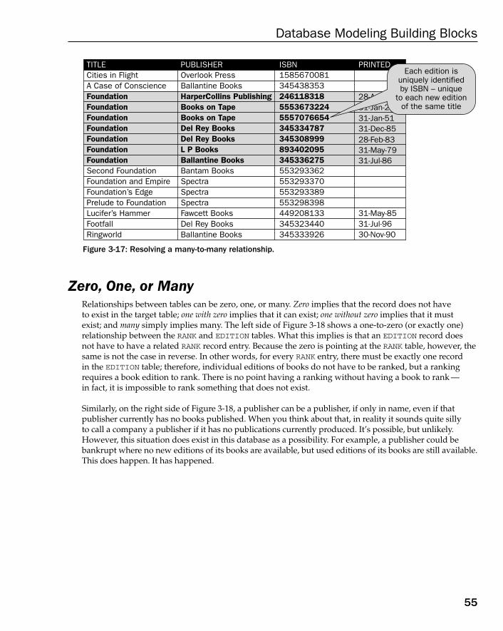
Figure 3-17: Resolving a many-to-many relationship.
Zero, One, or ManyRelationships between tables can be zero, one, or many. Zero implies that the record does not have to exist in the target table; one with zero implies that it can exist; one without zero implies that it must exist; and many simply implies many. The left side of Figure 3-18 shows a one-to-zero (or exactly one)relationship between the RANK and EDITION tables. What this implies is that an EDITION record does not have to have a related RANK record entry. Because the zero is pointing at the RANK table, however, thesame is not the case in reverse. In other words, for every RANK entry, there must be exactly one record in the EDITION table; therefore, individual editions of books do not have to be ranked, but a rankingrequires a book edition to rank. There is no point having a ranking without having a book to rank —in fact, it is impossible to rank something that does not exist.
Similarly, on the right side of Figure 3-18, a publisher can be a publisher, if only in name, even if that publisher currently has no books published. When you think about that, in reality it sounds quite sillyto call a company a publisher if it has no publications currently produced. It’s possible, but unlikely.However, this situation does exist in this database as a possibility. For example, a publisher could bebankrupt where no new editions of its books are available, but used editions of its books are still available.This does happen. It has happened.
158567008134543835324611831855536732245557076654345334787345308999893402095345336275553293362553293370553293389553298398449208133345323440345333926
Overlook PressBallantine BooksHarperCollins PublishingBooks on TapeBooks on TapeDel Rey BooksDel Rey BooksL P BooksBallantine BooksBantam BooksSpectraSpectraSpectraFawcett BooksDel Rey BooksBallantine Books
Cities in FlightA Case of ConscienceFoundationFoundationFoundationFoundationFoundationFoundationFoundationSecond FoundationFoundation and EmpireFoundation’s EdgePrelude to FoundationLucifer’s HammerFootfallRingworld
ISBNPUBLISHERTITLE PRINTED
28-Apr-8331-Jan-20
31-Dec-8531-Jan-51
28-Feb-8331-May-7931-Jul-86
31-May-8531-Jul-9630-Nov-90
Each edition isuniquely identifiedby ISBN – unique
to each new editionof the same title
55
Database Modeling Building Blocks
07_574906 ch03.qxd 11/4/05 10:48 AM Page 55
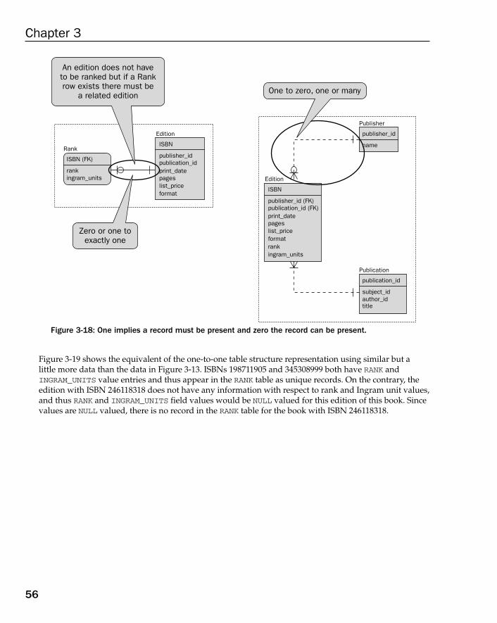
Figure 3-18: One implies a record must be present and zero the record can be present.
Figure 3-19 shows the equivalent of the one-to-one table structure representation using similar but a little more data than the data in Figure 3-13. ISBNs 198711905 and 345308999 both have RANK andINGRAM_UNITS value entries and thus appear in the RANK table as unique records. On the contrary, theedition with ISBN 246118318 does not have any information with respect to rank and Ingram unit values,and thus RANK and INGRAM_UNITS field values would be NULL valued for this edition of this book. Sincevalues are NULL valued, there is no record in the RANK table for the book with ISBN 246118318.
Publisher
publisher_id
name
Publication
publication_id
subject_idauthor_idtitle
Rank
ISBN (FK)
rankingram_units Edition
ISBN
publisher_id (FK)publication_id (FK)print_datepageslist_priceformatrankingram_units
Edition
ISBN
publisher_idpublication_idprint_datepageslist_priceformat
One to zero, one or many
An edition does not haveto be ranked but if a Rankrow exists there must be
a related edition
Zero or one toexactly one
56
Chapter 3
07_574906 ch03.qxd 11/4/05 10:48 AM Page 56
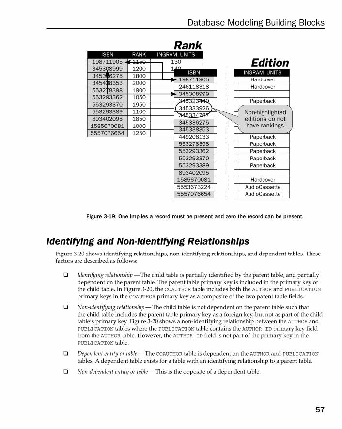
Figure 3-19: One implies a record must be present and zero the record can be present.
Identifying and Non-Identifying RelationshipsFigure 3-20 shows identifying relationships, non-identifying relationships, and dependent tables. Thesefactors are described as follows:
❑ Identifying relationship — The child table is partially identified by the parent table, and partiallydependent on the parent table. The parent table primary key is included in the primary key ofthe child table. In Figure 3-20, the COAUTHOR table includes both the AUTHOR and PUBLICATIONprimary keys in the COAUTHOR primary key as a composite of the two parent table fields.
❑ Non-identifying relationship — The child table is not dependent on the parent table such that the child table includes the parent table primary key as a foreign key, but not as part of the childtable’s primary key. Figure 3-20 shows a non-identifying relationship between the AUTHOR andPUBLICATION tables where the PUBLICATION table contains the AUTHOR_ID primary key fieldfrom the AUTHOR table. However, the AUTHOR_ID field is not part of the primary key in the PUBLICATION table.
❑ Dependent entity or table — The COAUTHOR table is dependent on the AUTHOR and PUBLICATIONtables. A dependent table exists for a table with an identifying relationship to a parent table.
❑ Non-dependent entity or table — This is the opposite of a dependent table.
198711905345308999345306275345438353553278398553293362553293370553293389893402095
15856700815557076654
11501200180020001900105019501100185010001250
130140
ISBN RANK INGRAM_UNITSRankRank
EditionEdition198711905246118318345308999345323440345333926345334787345336275345338353449208133553278398553293362
11501200180020001900105019501100185010001250
ISBN RANK INGRAM_UNITS
553293370553293389893402095158567008155536732245557076654
HardcoverHardcover
Paperback
PaperbackPaperbackPaperbackPaperbackPaperback
HardcoverAudioCassetteAudioCassette
Non-highlightededitions do nothave rankings
57
Database Modeling Building Blocks
07_574906 ch03.qxd 11/4/05 10:48 AM Page 57
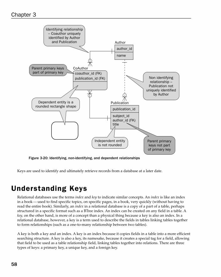
Figure 3-20: Identifying, non-identifying, and dependent relationships
Keys are used to identify and ultimately retrieve records from a database at a later date.
Understanding KeysRelational databases use the terms index and key to indicate similar concepts. An index is like an index in a book — used to find specific topics, on specific pages, in a book, very quickly (without having toread the entire book). Similarly, an index in a relational database is a copy of a part of a table, perhapsstructured in a specific format such as a BTree index. An index can be created on any field in a table. Akey, on the other hand, is more of a concept than a physical thing because a key is also an index. In a relational database, however, a key is a term used to describe the fields in tables linking tables togetherto form relationships (such as a one-to-many relationship between two tables).
A key is both a key and an index. A key is an index because it copies fields in a table into a more efficientsearching structure. A key is also a key, its namesake, because it creates a special tag for a field, allowingthat field to be used as a table relationship field, linking tables together into relations. There are threetypes of keys: a primary key, a unique key, and a foreign key.
Author
author_id
name
Publication
publication_id
subject_idauthor_id (FK)title
CoAuthorcoauthor_id (FK)publication_id (FK)
Dependent entity is arounded rectangle shape
Parent primary keyspart of primary key
Identifying relationship– Coauthor uniquelyidentified by Author
and Publication
Non identifyingrelationship –Publication not
uniquely identifiedby Author
Parent primarykeys not partof primary key
Independent entityis not rounded
58
Chapter 3
07_574906 ch03.qxd 11/4/05 10:48 AM Page 58
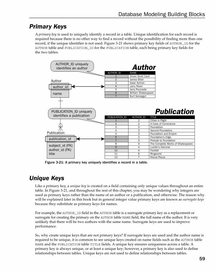
Primary KeysA primary key is used to uniquely identify a record in a table. Unique identification for each record isrequired because there is no other way to find a record without the possibility of finding more than onerecord, if the unique identifier is not used. Figure 3-21 shows primary key fields of AUTHOR_ID for theAUTHOR table and PUBLICATION_ID for the PUBLICATION table, each being primary key fields for the two tables.
Figure 3-21: A primary key uniquely identifies a record in a table.
Unique KeysLike a primary key, a unique key is created on a field containing only unique values throughout an entiretable. In Figure 3-21, and throughout the rest of this chapter, you may be wondering why integers areused as primary keys rather than the name of an author or a publication, and otherwise. The reason whywill be explained later in this book but in general integer value primary keys are known as surrogate keysbecause they substitute as primary keys for names.
For example, the AUTHOR_ID field in the AUTHOR table is a surrogate primary key as a replacement or surrogate for creating the primary on the AUTHOR table NAME field, the full name of the author. It is veryunlikely that there will be two authors with the same name. Surrogate keys are used to improve performance.
So, why create unique keys that are not primary keys? If surrogate keys are used and the author name isrequired to be unique, it is common to see unique keys created on name fields such as the AUTHOR tableNAME and the PUBLICATION table TITLE fields. A unique key ensures uniqueness across a table. Aprimary key is always unique, or at least a unique key; however, a primary key is also used to definerelationships between tables. Unique keys are not used to define relationships between tables.
123456789101112
223333344467
Cities in FlightA Case of ConscienceFoundationSecond FoundationFoundation and EmpireFoundation’s EdgePrelude to FoundationThe Complete Works of ShakespeareLucifer’s HammerFootfallRingworldHocus Pocus
PUBLICATION_ID AUTHOR_ID TITLE
1
56
Orson Scott CardJames BlishIsaac AzimovLarry NivenJerry PournelleWilliam ShakespeareKurt Vonnegut
AUTHOR_ID NAME
234
7
PublicationPublication
AuthorAuthor
Author
author_id
name
Publication
publication_id
subject_id (FK)author_id (FK)title
PUBLICATION_ID uniquelyidentifies a publication
AUTHOR_ID uniquelyidentifies an author
59
Database Modeling Building Blocks
07_574906 ch03.qxd 11/4/05 10:48 AM Page 59
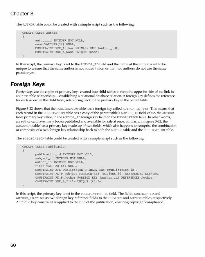
The AUTHOR table could be created with a simple script such as the following:
CREATE TABLE Author(
author_id INTEGER NOT NULL,name VARCHAR(32) NULL,CONSTRAINT XPK_Author PRIMARY KEY (author_id),CONSTRAINT XUK_A_Name UNIQUE (name)
);
In this script, the primary key is set to the AUTHOR_ID field and the name of the author is set to beunique to ensure that the same author is not added twice, or that two authors do not use the samepseudonym.
Foreign KeysForeign keys are the copies of primary keys created into child tables to form the opposite side of the link inan inter-table relationship — establishing a relational database relation. A foreign key defines the referencefor each record in the child table, referencing back to the primary key in the parent table.
Figure 3-22 shows that the PUBLICATION table has a foreign key called AUTHOR_ID (FK). This means thateach record in the PUBLICATION table has a copy of the parent table’s AUTHOR_ID field value, the AUTHORtable primary key value, in the AUTHOR_ID foreign key field on the PUBLICATION table. In other words,an author can have many books published and available for sale at once. Similarly, in Figure 3-22, the COAUTHOR table has a primary key made up of two fields, which also happens to comprise the combinationor composite of a two foreign key relationship back to both the AUTHOR table and the PUBLICATION table.
The PUBLICATION table could be created with a simple script such as the following:
CREATE TABLE Publication(
publication_id INTEGER NOT NULL,subject_id INTEGER NOT NULL,author_id INTEGER NOT NULL,title VARCHAR(64) NULL,CONSTRAINT XPK_Publication PRIMARY KEY (publication_id), CONSTRAINT FK_P_Subject FOREIGN KEY (subject_id) REFERENCES Subject, CONSTRAINT FK_P_Author FOREIGN KEY (author_id) REFERENCES Author,CONSTRAINT XUK_P_Title UNIQUE (title)
);
In this script, the primary key is set to the PUBLICATION_ID field. The fields SUBJECT_ID andAUTHOR_ID are set as two foreign key reference fields to the SUBJECT and AUTHOR tables, respectively.A unique key constraint is applied to the title of the publication, ensuring copyright compliance.
60
Chapter 3
07_574906 ch03.qxd 11/4/05 10:48 AM Page 60
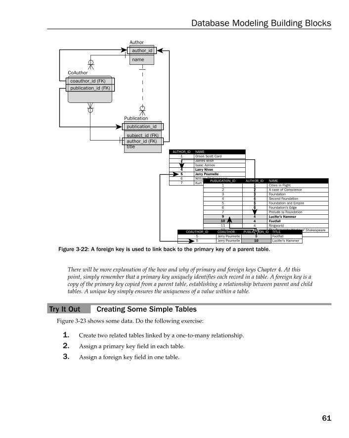
Figure 3-22: A foreign key is used to link back to the primary key of a parent table.
There will be more explanation of the how and why of primary and foreign keys Chapter 4. At thispoint, simply remember that a primary key uniquely identifies each record in a table. A foreign key is acopy of the primary key copied from a parent table, establishing a relationship between parent and childtables. A unique key simply ensures the uniqueness of a value within a table.
Try It Out Creating Some Simple TablesFigure 3-23 shows some data. Do the following exercise:
1. Create two related tables linked by a one-to-many relationship.
2. Assign a primary key field in each table.
3. Assign a foreign key field in one table.
1234567
Orson Scott CardJames BlishIsaac AzimovLarry NivenJerry PournelleWilliam ShakespeareKurt Vonnegut
AUTHOR_ID NAME
1234567
AUTHOR_ID1234567
Cities in FlightA case of ConscienceFoundationSecond FoundationFoundation and EmpireFoundation’s EdgePrelude to Foundation
47
Lucifer’s HammerFootfallRingworldThe Complete Works of Shakespeare
PUBLICATION_ID NAME
1112
Jerry PournelleJerry Pournelle
COAUTHOR55
COAUTHOR_ID PUBLICATION_IDFootfallLucifer’s Hammer
TITLE
44
910
910
Author
author_id
name
Publication
publication_id
subject_id (FK)author_id (FK)title
CoAuthor
coauthor_id (FK)publication_id (FK)
61
Database Modeling Building Blocks
07_574906 ch03.qxd 11/4/05 10:48 AM Page 61
Figure 3-23: Band names, tracks, and silly descriptions.
How It WorksYou are asked for two tables from three fields. One table has one field and the other table has two fields.The three fields are conveniently arranged. Look for a one-to-many relationship by finding duplicatedvalues. The data is inconveniently and deliberately unsorted.
1. The first column contains the names of numerous different bands (musical groups) and the second column a track or song name. Typically, different bands or musical groups create manytracks. A one-to-many relationship exists between the band names and track names.
2. Band names in the first column are duplicated. Track names and descriptions are not. This supports the solution already derived in step 1.
3. Band names are the only duplicated values, so they make up the table on the parent side of theone-to-many relationship. The other two columns make up the table on the child side of therelationship.
4. The track name must identify the track uniquely. The description is just silly.
Figure 3-24 shows three viable solutions with Option 3 being the better of all of the three options becausesurrogate keys are used for the primary and foreign keys. Option 2 is better than Option 1 because inOption 2 the one-to-many relationship is a non-identifying relationship, where the primary key on theTRACK table is not composite key.
Nirvana
Nirvana
Nirvana
Nirvana
Stone Temple Pilots
Greetings From Limbo
Greetings From Limbo
Pearl Jam
Pearl Jam
Pearl Jam
Foo FightersGreetings From LimboRed Hot Chili Peppers
Red Hot Chili Peppers
Red Hot Chili Peppers
Red Hot Chili PeppersSoundgarden
Red Hot Chili PeppersRed Hot Chili Peppers
Come As You Are
About A Girl
The Man Who Sold The World
Polly
The Right Line
Greetings From Limbo
Fatal
Immortality
Around The Bend
AshesMy Friends
Suck My Kiss
University Speaking
Under The Bridge
OthersideCalifornication
Bass reverb
Lots of lovely bass
Sell out!
Who’s that?
Country groove
The Wizard of Oz
Deadly
Just imagine
Nuts!
HeavyHmmm
No thanks
OK
Where’s that confounded bridge?
Hmmm againHot and dry
BAND NAME TRACK DESCRIPTION
62
Chapter 3
07_574906 ch03.qxd 11/4/05 10:48 AM Page 62
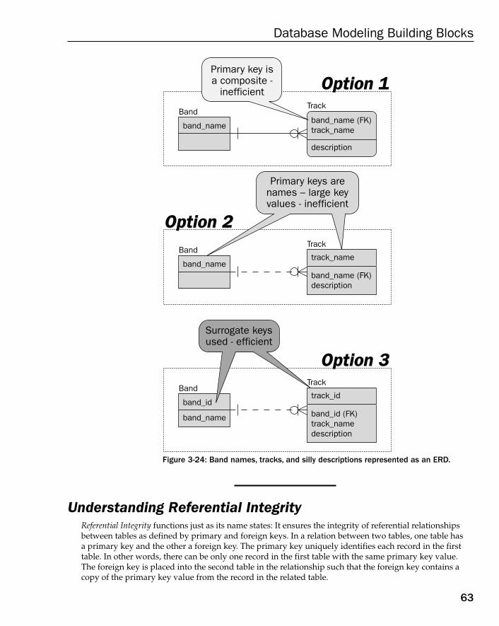
Figure 3-24: Band names, tracks, and silly descriptions represented as an ERD.
Understanding Referential IntegrityReferential Integrity functions just as its name states: It ensures the integrity of referential relationshipsbetween tables as defined by primary and foreign keys. In a relation between two tables, one table hasa primary key and the other a foreign key. The primary key uniquely identifies each record in the firsttable. In other words, there can be only one record in the first table with the same primary key value.The foreign key is placed into the second table in the relationship such that the foreign key contains acopy of the primary key value from the record in the related table.
Band
band_name
Track
band_name (FK)track_name
description
Option 1Option 1
Band
band_name
Track
band_name (FK)description
track_name
Option 2Option 2
Band
band_id
band_name
Track
band_id (FK)track_namedescription
track_id
Option 3Option 3
Primary key isa composite -
inefficient
Primary keys arenames – large keyvalues - inefficient
Surrogate keysused - efficient
63
Database Modeling Building Blocks
07_574906 ch03.qxd 11/4/05 10:48 AM Page 63
So, what is Referential Integrity? Referential Integrity ensures the integrity of relationships between pri-mary and foreign key values in related tables. Most relational database engines use what are often calledconstraints. Primary and foreign keys are both constraints. Remember, a constraint is a piece of metadatadefined for a table defining restrictions on values. A primary key constraint forces the primary key fieldto be unique. A primary key constraint is also forced to make checks against any foreign key constraintsreferenced back to that primary key constraint. Referencing (or referential) foreign key constraints can bein any table, including the same table as the primary key constrained field referenced by the foreign key(a self join). A foreign key constraint uses its reference to refer back to a referenced table, containing theprimary key constraint, to ensure that the two values in the primary key field and foreign key fieldmatch.
Simply put, primary and foreign keys automatically verify against each other. Primary and foreign keyreferences are the connections establishing and enforcing Referential Integrity between tables. There aresome specific circumstances to consider in terms of how Referential Integrity is generally enforced:
A primary key table is assumed to be a parent table and a foreign key table a child table.
❑ When adding a new record to a child table, if a foreign key value is entered, it must exist in therelated primary key field of the parent table.
Foreign key fields can contain NULL values. Primary key field values can never contain NULL values asthey are required to be unique.
❑ When changing a record in a parent table if the primary key is changed, the change must be cascaded to all foreign key valued records in any related child tables. Otherwise, the change tothe parent table must be prohibited.
The term “cascade” implies that changes to data in parent tables are propagated to all child tables containing foreign key field copies of a primary key from a parent table.
❑ When changing a record in a child table, a change to a foreign key requires that a related primary key must be checked for existence, or changed first. If a foreign key is changed to NULL,no primary key is required. If the foreign key is changed to a non-NULL value, the foreign keyvalue must exist as a primary key value in the related parent table.
❑ When deleting a parent table record then related foreign key records in child tables must eitherbe cascade deleted or deleted from child tables first.
Understanding IndexesIndexes are not really part and parcel of the relational database model itself; however, indexes are soimportant to performance and overall database usability that they simply have to be introduced without going into the nitty-gritty of how each different type of index functions internally. It is importantto understand the fundamentals of indexes and their different types and attributes to get a basic understanding as to why exactly indexing is so important for relational databases in general.
64
Chapter 3
07_574906 ch03.qxd 11/4/05 10:48 AM Page 64
What Is an Index?An index is usually and preferably a copy of a very small section of table, such as a single field, and preferably a short length field. The act of creating an index physically copies one or more fields to beindexed into a separate area of disk other than that of the table. In some databases, indexes can be stored in a file completely separated from that of the table. Different databases are structured differently on a physical level. The important factor is the underlying physical separation. When a table is accessed, aprocess usually called an Optimizer decides whether to access the table alone, scanning all the records in thetable, or if it is faster to read the much smaller index in conjunction with a very small section of the table.
All relational databases have some type of SQL execution optimization process. It is usually called theOptimizer.
An index essentially behaves like an index in the back of a book or the table of contents at the front of abook. When searching for details on a specific topic, it is much easier to find the term in the index ortable of contents first, and then use a page reference number to find the information within the pages ofthe text. Reading the entire book every time you want to find a definition for a single term would be fartoo time-consuming to be useful, probably making the book completely useless as a reference. Mosttechnical books are used as reference guides in one form or another.
Following are some things to be avoided when indexing:
❑ Creating too many indexes — Too many indexes on a table can result in very slow database changeresponses. This is because every change to a table updates every index attached to it, as well as thetable. The more indexes created for a table, the more physical changes are required.
❑ Indexing too many fields — Indexing too many fields not only makes the use of the indexes byqueries more complex, but also makes the indexes too large physically. An index must be relatively much smaller than a table, and should be created on as few fields from that table asis possible.
Alternate IndexingAlternate indexing really comes from the terms “alternate index,” “secondary index,” “tertiary index,” orjust plain “indexing.” Specific use of terminology depends on the database in use. These terms all meanthe same thing. Alternate indexes are an alternate to the primary relational structure organized by primary and foreign key indexes. Alternate indexes are alternate because they are in addition to primaryand foreign key indexes and exist as alternate sorting methods to those provided by primary and foreignkeys. By definition, the unique key indexes described in a previous section of this chapter are essentiallyalternate indexes, as well as being unique constraints.
Foreign Key IndexingRelationships between tables such as that between the AUTHOR and PUBLICATION tables shown in Figure3-21 can allow the foreign key in the child table not only to be duplicated (one-to-many) but also to be NULLvalued in the child table (one-to-zero, one or many). In other words, in Figure 3-21, each author can havemultiple publications or an author does not have to have any publications at all. Because foreign keys areallowed to be NULL valued and do not have to be unique, indexes must be created on those foreign keyfields manually.
65
Database Modeling Building Blocks
07_574906 ch03.qxd 11/4/05 10:48 AM Page 65
Because primary keys must be unique, a relational database should automatically create internal uniqueindexes on primary keys.
Commands similar to the following commands could be used to create indexes on foreign key fields, forthe CREATE TABLE command on the PUBLICATION table shown previously in this chapter:
CREATE INDEX XFK_P_Author ON Publication(author_id);CREATE INDEX XFK_P_Publisher ON Publication(subject_id);
Types of IndexesIt is important to have a brief understanding of different types of indexing available in relationaldatabases. Some of the smaller-scale database engines (such as dBase, Paradox, and MS Access) mightoffer little or no variation on index types allowed, generally using BTree type indexing. Types of indexesin various relational database engines are as follows:
❑ BTree index — BTree means “binary tree” and, if drawn out on a piece of paper, a BTree indexlooks like an upside down tree. The tree is called “binary” because binary implies two optionsunder each branch node: branch left and branch right. The binary counting system of numberscontains two digits, namely 0 and 1. The result is that a binary tree only ever has two options asleafs within each branch — at least that is the theory, not being precisely the case in all databases.BTree indexes are sometimes improperly named as they are not actually binary meaning two —branches can have more than two leafs contained within them. Naming conventions are largelyimmaterial in this situation. Essentially, a BTree consists of a root node, branch nodes, and ultimately leaf nodes containing the indexed field values in the ending (or leaf) nodes of the tree.Some BTree construction and searching methods in some databases are highly efficient for bothreading and changing of data, automatically changing the structure of the BTree index withoutany overflow.
Overflow is bad for indexing because changes are placed outside of the optimized index structure.Enough changes and overflow can destroy the efficiency of an index, eventually rendering it useless anddrastically deteriorating rather than generally improving table access performance.
Figure 3-25 shows an example of what a typical relational database BTree index might look like.
❑ Bitmap index — A Bitmap index contains binary representations for each record using 0’s and 1’s.Bitmap indexes are often misused and are extremely vulnerable to overflow over long periodsof time. Values cannot be slotted into the existing Bitmap index structure as readily as can bedone when updating a BTree index. Figure 3-26 shows a graphical type structure of the internalmachinations of a Bitmap index where two bitmaps are created for two values of M for maleand F for female. When M is encountered, the M bitmap is set to 1 and the F bitmap is set to 0.In general, Bitmap indexes can be disappointing, even in environments where they are suppos-edly highly beneficial.
66
Chapter 3
07_574906 ch03.qxd 11/4/05 10:48 AM Page 66
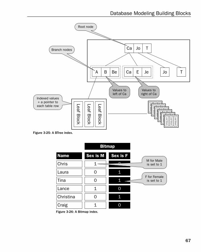
Figure 3-25: A BTree index.
Figure 3-26: A Bitmap index.
Name
Chris
Laura
Tina
Lance
Christina
Craig
Sex is M
1
0
0
1
0
1
Sex is F
Bitmap
0
1
1
0
1
0
M for Maleis set to 1
F for Femaleis set to 1
Ca Jo T
A B Be Ca E Je Jo T
Leaf Block
Leaf Block
Leaf Block
Leaf Block
Leaf Block
Leaf Block
Leaf Block
Leaf Block
Leaf Block
Leaf Block
Leaf Block
Leaf Block
Leaf Block
Leaf Block
Leaf Block
Leaf Block
Leaf Block
Leaf Block
Leaf Block
Leaf Block
Leaf Block
Root node
Branch nodes
Indexed values+ a pointer toeach table row
Values toleft of Ca
Values toright of Ca
67
Database Modeling Building Blocks
07_574906 ch03.qxd 11/4/05 10:48 AM Page 67

❑ ISAM index — Indexed Sequential Access Method (ISAM) uses a simple structure with a list ofrecord numbers. ISAM indexes are used in various database engines. ISAM indexes are bestused for static data as their internal list structure prohibits easy changes, making themextremely vulnerable to index overflow.
❑ Hash table — A hash table is a copy of data but rearranged into a different and more efficientlyaccessed order depending on a hashing algorithm. For example, a hashing algorithm takes astring and creates a number from that string. The number created by a specific string is alwaysthe same and is thus placed in a position in an index, sorted based on the hash-calculated value.Hash indexes can be highly efficient for read access, but are best avoided when subjected to anykind of data changes. Hash tables are likely to overflow worse than Bitmap indexes becausethere is absolutely no scope whatsoever for changes. The only way to push record changes fromtable to index is by regenerating the entire hash table index.
❑ Index Organized Table — An Index Organized Table (IOT) builds a table in the sorted order of anindex, typically using a BTree index. IOTs can actually work fairly well in many types ofdatabases, but you must remember that index record length is much longer than normalbecause index leaf blocks contain all fields in the entire record length of a table. Also, if the IOTis not read in indexed order, obviously all records in the table are read, and thus the index isignored. Because the table is built in the structure of an index, however, not reading the table inIOT indexed order could be seriously problematic for performance.
Different Ways to Build IndexesIndexes can usually be built in various different ways to accommodate however they might be used. Onceagain, some relational databases allow all of these options, some allow some, and some allow none.
❑ Ascending or descending index — An index can be built sorted in a normally ascending order(such as A, B, C) or in descending order (such as C, B, A).
❑ Unique index — Indexes values must be unique (can’t contain duplicate values).
❑ Non-unique index — Non-unique indexes contain duplicated or repeated values in the index.
It is normal to create both unique indexes and non-unique indexes.
❑ Composite index — Indexes can be built on more than a single field and are known as compositefield indexes, multiple field indexes, or just plain old composite indexes. The most efficient typeof index is a single field index containing an integer.
❑ Compressed indexes — Some databases allow compression of composite indexes where repeatedprefix values are effectively indexed within the index, removing duplications within prefixedindexed fields. In other words, a composite index containing three fields can be accessed usinga single value of the first field.
❑ Reverse key indexes — This is a really weird and unusual one. Only a very select few databasesallow building of indexes such that indexed field values are stored as reverse strings. Whenadding gazillions of records at once to the same index in a very busy database, adding sequen-tial index values (not reversed) adds many records all at once to the same physical space in theindex. The result is what some relational databases call locking and other relational databases
68
Chapter 3
07_574906 ch03.qxd 11/4/05 10:48 AM Page 68
call hot blocking. The result is the same — gridlock! Reverse keys make the index values notsequential in terms of where they are physically written to disk. The result is no locking, no hotblocking, no gridlock, and, thus, much better performance.
Other than tables, keys, and indexes, there are other types of objects. These other object types are more eas-ily defined as data management objects and only loosely definable as data modeling objects. Managementof data is the administration process occurring on a production system, long after completion of the datamodeling process.
Introducing Views and Other SpecializedObjects
So far in this chapter, topics covered have included tables, relationships between tables, and indexesattached to tables. You should understand the basic structure of a table, and that the relationshipsbetween tables are determined by primary keys in parent tables linked to foreign keys in child tables.Foreign keys are copies of primary key field values from parent tables. Indexing is important to under-stand not directly from a modeling perspective, but that indexes are used to superimpose a differentorder on top of the order created by the very structure of the relationships between tables, imposed byprimary and foreign keys.
Other than all these wonderful indexing things, there are further possibilities within relational databasesthat some database engines allow and some do not. It is important to know that specialized objects existas options for expansion to a relational database model, as extensions to both the underlying physicalstructure of a database and the overlying logical structure (the tables and indexes). Following are a fewexamples:
❑ Views — A view is essentially a query definition and does not contain any data. A view is not aphysical copy of data and does not contain any data itself. A view is merely a logical overlay ofexisting tables. Every execution against a view executes the query contained within the viewagainst all underlying tables. The danger with using views is filtering a query against a view,expecting to read a very small portion of a very large table. Any filtering should be done withinthe view because any filtering against the view itself is applied after the query in the view hascompleted execution. Views are typically useful for speeding up the development process butin the long run can completely kill database performance.
❑ Materialized views — Materialized views are available in some very large capacity type relationaldatabases. A materialized view materializes underlying physical data by making a physical copy of data from tables. So, unlike a view as described previously, when a query is executedagainst a materialized view, the materialized view is physically accessed rather than the underlying tables. The objective is to free the underlying tables for other uses, effectively creatingtwo separate physical copies. Materialized views are often used to aggregate large data setsdown to smaller sized data sets, in data warehouses and data marts. The biggest potential problem with materialized views is how often they are refreshed and brought up to date withany changes to their underlying tables. Another attribute of materialized views is the ability ofsome database engines to allow a query directed at an underlying table to be automatically redirected to a physically much smaller materialized view, sometimes called automated queryrewrite. Queries can be automatically rewritten by the query Optimizer if the query rewrite canhelp to increase query performance.
69
Database Modeling Building Blocks
07_574906 ch03.qxd 11/4/05 10:48 AM Page 69
❑ Clusters — Clusters are used in very few databases and have been somewhat superceded bymaterialized views. In the past, clusters were used to pre-create physical copies of entire fieldlevel sections of heavily accessed tables, especially in SQL joins. Unlike materialized views, clusters do not allow for automatic refresh and are normally manually maintained.
❑ Sequences and auto counters — An auto counter field is a special datatype, sometimes called a non-static internal function, allowing automated generation of sequential number values (thus theterm “sequence”). Typically, auto counters are used for primary key surrogate key generation oninsertion of new records into a table.
❑ Partitioning and parallel processing — Some databases allow physical splitting of tables into separate partitions, including parallel processing on multiple partitions and individual opera-tions on individual partitions. One particularly efficient aspect of partitioning is the capabilitywhen querying a table to read fewer than all the partitions making up a table, perhaps even asingle partition.
SummaryIn this chapter, you learned about:
❑ Building tables containing fields, datatypes, and simple validation
❑ The different types of relationships between tables
❑ Representing relations in ERDs
❑ Defining referential integrity relationships between tables using primary and foreign keys
❑ The types and uses of indexes
❑ The types and uses of specialized objects such as views, materialized views, and auto counters
The next chapter discusses the very heart of the relational database model by examining the process ofnormalization through the application of normal forms.
Exercises1. Write two CREATE TABLE commands for the tables in Option 3 of Figure 3-24. Make sure that all
primary key, foreign key, and any potentially necessary unique keys are included.
2. Write CREATE INDEX commands to create all indexes on any foreign keys indicated in the CREATE TABLE command written for the previous question.
70
Chapter 3
07_574906 ch03.qxd 11/4/05 10:48 AM Page 70
Part II
Designing RelationalDatabase Models
In this Part:
Chapter 4: Understanding Normalization
Chapter 5: Reading and Writing Data with SQL
Chapter 6: Advanced Relational Database Modeling
Chapter 7: Understanding Data Warehouse Database Modeling
Chapter 8: Building Fast-Performing Database Models
08_574906 pt02.qxd 10/28/05 11:43 PM Page 71

08_574906 pt02.qxd 10/28/05 11:43 PM Page 72
4UnderstandingNormalization
“There are two rules in life: Rule #1: Don’t sweat the small stuff. Rule #2: Everything is small stuff.” (Finn Taylor)
Life is as complicated as we make it — normalization can be simplified.
This chapter examines the detail of the normalization process. Normalization is the sequence of steps by which a relational database model is both created and improved upon. The sequence ofsteps involved in the normalization process is called Normal Forms. Essentially, Normal Formsapplied during a process of normalization allow creation of a relational database model as a step-by-step progression.
Previous chapters have examined history and applications, plus various other factors involved indatabase model design. Chapter 3 introduced all the parts and pieces involved in a relationaldatabase model. This chapter now uses the terminology covered in Chapter 3 and explains how to build a relational database model. Subsequent chapters examine more advanced details of relational database modeling such as denormalization and SQL, both of which depend on a goodunderstanding of normalization.
This chapter describes the precise steps involved in creation of relational database models. These steps are the 1st, 2nd, and 3rd Normal Forms, plus the rarely commercially implementedBoyce-Codd, 4th, 5th, and Domain Key Normal Forms. The Normal Forms steps are the progressivesteps in the normalization process.
In this chapter, you learn about the following:
❑ Anomalies
❑ Dependency and determinants
❑ Normalization
❑ A layman’s method of understanding normalization
09_574906 ch04.qxd 11/4/05 10:46 AM Page 73
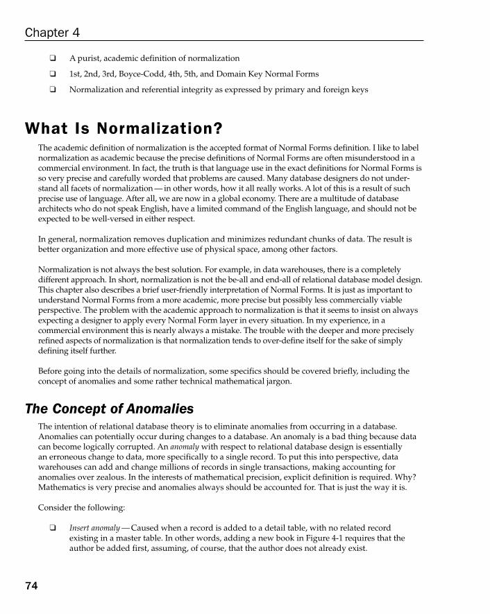
❑ A purist, academic definition of normalization
❑ 1st, 2nd, 3rd, Boyce-Codd, 4th, 5th, and Domain Key Normal Forms
❑ Normalization and referential integrity as expressed by primary and foreign keys
What Is Normalization?The academic definition of normalization is the accepted format of Normal Forms definition. I like to labelnormalization as academic because the precise definitions of Normal Forms are often misunderstood in acommercial environment. In fact, the truth is that language use in the exact definitions for Normal Forms isso very precise and carefully worded that problems are caused. Many database designers do not under-stand all facets of normalization — in other words, how it all really works. A lot of this is a result of such precise use of language. After all, we are now in a global economy. There are a multitude of database architects who do not speak English, have a limited command of the English language, and should not beexpected to be well-versed in either respect.
In general, normalization removes duplication and minimizes redundant chunks of data. The result isbetter organization and more effective use of physical space, among other factors.
Normalization is not always the best solution. For example, in data warehouses, there is a completely different approach. In short, normalization is not the be-all and end-all of relational database model design.This chapter also describes a brief user-friendly interpretation of Normal Forms. It is just as important tounderstand Normal Forms from a more academic, more precise but possibly less commercially viable perspective. The problem with the academic approach to normalization is that it seems to insist on alwaysexpecting a designer to apply every Normal Form layer in every situation. In my experience, in a commercial environment this is nearly always a mistake. The trouble with the deeper and more preciselyrefined aspects of normalization is that normalization tends to over-define itself for the sake of simplydefining itself further.
Before going into the details of normalization, some specifics should be covered briefly, including theconcept of anomalies and some rather technical mathematical jargon.
The Concept of AnomaliesThe intention of relational database theory is to eliminate anomalies from occurring in a database.Anomalies can potentially occur during changes to a database. An anomaly is a bad thing because datacan become logically corrupted. An anomaly with respect to relational database design is essentially an erroneous change to data, more specifically to a single record. To put this into perspective, data warehouses can add and change millions of records in single transactions, making accounting foranomalies over zealous. In the interests of mathematical precision, explicit definition is required. Why?Mathematics is very precise and anomalies always should be accounted for. That is just the way it is.
Consider the following:
❑ Insert anomaly — Caused when a record is added to a detail table, with no related record existing in a master table. In other words, adding a new book in Figure 4-1 requires that theauthor be added first, assuming, of course, that the author does not already exist.
74
Chapter 4
09_574906 ch04.qxd 11/4/05 10:46 AM Page 74
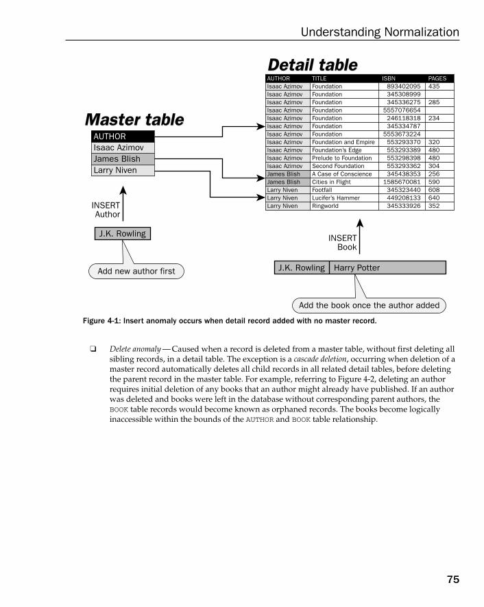
Figure 4-1: Insert anomaly occurs when detail record added with no master record.
❑ Delete anomaly — Caused when a record is deleted from a master table, without first deleting allsibling records, in a detail table. The exception is a cascade deletion, occurring when deletion of amaster record automatically deletes all child records in all related detail tables, before deletingthe parent record in the master table. For example, referring to Figure 4-2, deleting an authorrequires initial deletion of any books that an author might already have published. If an authorwas deleted and books were left in the database without corresponding parent authors, theBOOK table records would become known as orphaned records. The books become logicallyinaccessible within the bounds of the AUTHOR and BOOK table relationship.
Isaac AzimovIsaac AzimovIsaac AzimovIsaac AzimovIsaac AzimovIsaac AzimovIsaac AzimovIsaac AzimovIsaac AzimovIsaac AzimovIsaac AzimovJames BlishJames BlishLarry NivenLarry NivenLarry Niven
J.K. Rowling
J.K. Rowling
Harry Potter
INSERTBook
Add the book once the author added
Add new author first
FoundationFoundationFoundationFoundationFoundationFoundationFoundationFoundation and EmpireFoundation’s EdgePrelude to FoundationSecond FoundationA Case of ConscienceCities in FlightFootfallLucifer’s HammerRingworld
893402095345308999345336275
5557076654246118318345334787
5553673224553293370553293389553298398553293362345438353
1585670081345323440449208133345333926
435
285
234
320480480304256590608640352
AUTHOR TITLE ISBN PAGES
Isaac AzimovJames BlishLarry Niven
AUTHOR
INSERTAuthor
Master tableMaster table
Detail tableDetail table
75
Understanding Normalization
09_574906 ch04.qxd 11/4/05 10:46 AM Page 75
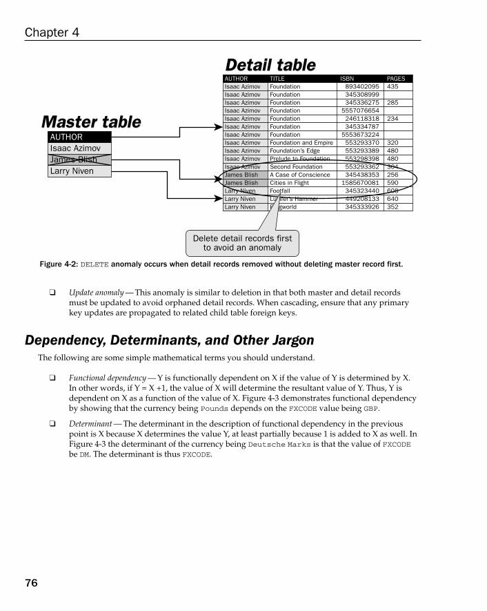
Figure 4-2: DELETE anomaly occurs when detail records removed without deleting master record first.
❑ Update anomaly — This anomaly is similar to deletion in that both master and detail recordsmust be updated to avoid orphaned detail records. When cascading, ensure that any primarykey updates are propagated to related child table foreign keys.
Dependency, Determinants, and Other JargonThe following are some simple mathematical terms you should understand.
❑ Functional dependency — Y is functionally dependent on X if the value of Y is determined by X.In other words, if Y = X +1, the value of X will determine the resultant value of Y. Thus, Y isdependent on X as a function of the value of X. Figure 4-3 demonstrates functional dependencyby showing that the currency being Pounds depends on the FXCODE value being GBP.
❑ Determinant — The determinant in the description of functional dependency in the previouspoint is X because X determines the value Y, at least partially because 1 is added to X as well. InFigure 4-3 the determinant of the currency being Deutsche Marks is that the value of FXCODEbe DM. The determinant is thus FXCODE.
Isaac AzimovIsaac AzimovIsaac AzimovIsaac AzimovIsaac AzimovIsaac AzimovIsaac AzimovIsaac AzimovIsaac AzimovIsaac AzimovIsaac AzimovJames BlishJames BlishLarry NivenLarry NivenLarry Niven
FoundationFoundationFoundationFoundationFoundationFoundationFoundationFoundation and EmpireFoundation’s EdgePrelude to FoundationSecond FoundationA Case of ConscienceCities in FlightFootfallLucifer’s HammerRingworld
893402095345308999345336275
5557076654246118318345334787
5553673224553293370553293389553298398553293362345438353
1585670081345323440449208133345333926
435
285
234
320480480304256590608640352
AUTHOR TITLE ISBN PAGES
Isaac AzimovJames BlishLarry Niven
AUTHORMaster tableMaster table
Detail tableDetail table
Delete detail records firstto avoid an anomaly
76
Chapter 4
09_574906 ch04.qxd 11/4/05 10:46 AM Page 76
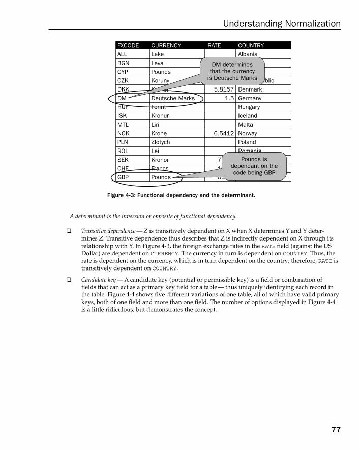
Figure 4-3: Functional dependency and the determinant.
A determinant is the inversion or opposite of functional dependency.
❑ Transitive dependence — Z is transitively dependent on X when X determines Y and Y deter-mines Z. Transitive dependence thus describes that Z is indirectly dependent on X through itsrelationship with Y. In Figure 4-3, the foreign exchange rates in the RATE field (against the USDollar) are dependent on CURRENCY. The currency in turn is dependent on COUNTRY. Thus, therate is dependent on the currency, which is in turn dependent on the country; therefore, RATE istransitively dependent on COUNTRY.
❑ Candidate key — A candidate key (potential or permissible key) is a field or combination offields that can act as a primary key field for a table — thus uniquely identifying each record inthe table. Figure 4-4 shows five different variations of one table, all of which have valid primarykeys, both of one field and more than one field. The number of options displayed in Figure 4-4is a little ridiculous, but demonstrates the concept.
FXCODEALLBGNCYPCZKDKKDMHUFISKMTLNOKPLNROLSEKCHEGBP
CURRENCYLekeLevaPoundsKorunyKrenerDeutsche MarksForintKronurLiriKroneZlotychLeiKronorFrancsPounds
COUNTRYAlbania
PublicDenmarkGermanyHungaryIcelandMaltaNorwayPolandRomania
RATE
5.81571.5
6.5412
7.00010.000.538
RATE
DM determinesthat the currency
is Deutsche Marks
Pounds isdependant on thecode being GBP
77
Understanding Normalization
09_574906 ch04.qxd 11/4/05 10:46 AM Page 77

Figure 4-4: A table with five and possibly more candidate keys.
❑ Full functional dependence — This situation occurs where X determines Y, but X combined with Z does not determine Y. In other words, Y depends on X and X alone. If Y depends on X withanything else, there is not full functional dependence. Essentially X, the determinant, cannot bea composite key. A composite key contains more than one field (the equivalent of X with Z).Figure 4-5 shows that POPULATION is dependent on COUNTRY but not on the combination ofRATE and COUNTRY. Therefore, there is full functional dependency between POPULATION andCOUNTRY because RATE is irrelevant to POPULATION. Conversely, there is not full functionaldependence between POPULATION and the combination of COUNTRY and RATE.
Customer
customer_id
customercurrency_codecurrencyexchange_rateaddress
Customer
currency_codecustomer
customer_idcurrencyexchange_rateaddress
Customer
currencycustomer_idaddress
customercurrency_codeexchange_rate
Customer
address
customer_idcustomercurrency_codecurrencyexchange_rate Customer
customer
customer_idcurrency_codecurrencyexchange_rateaddress
Customer
customer_idcustomercurrency_codecurrencyexchange_rateaddress
78
Chapter 4
09_574906 ch04.qxd 11/4/05 10:46 AM Page 78
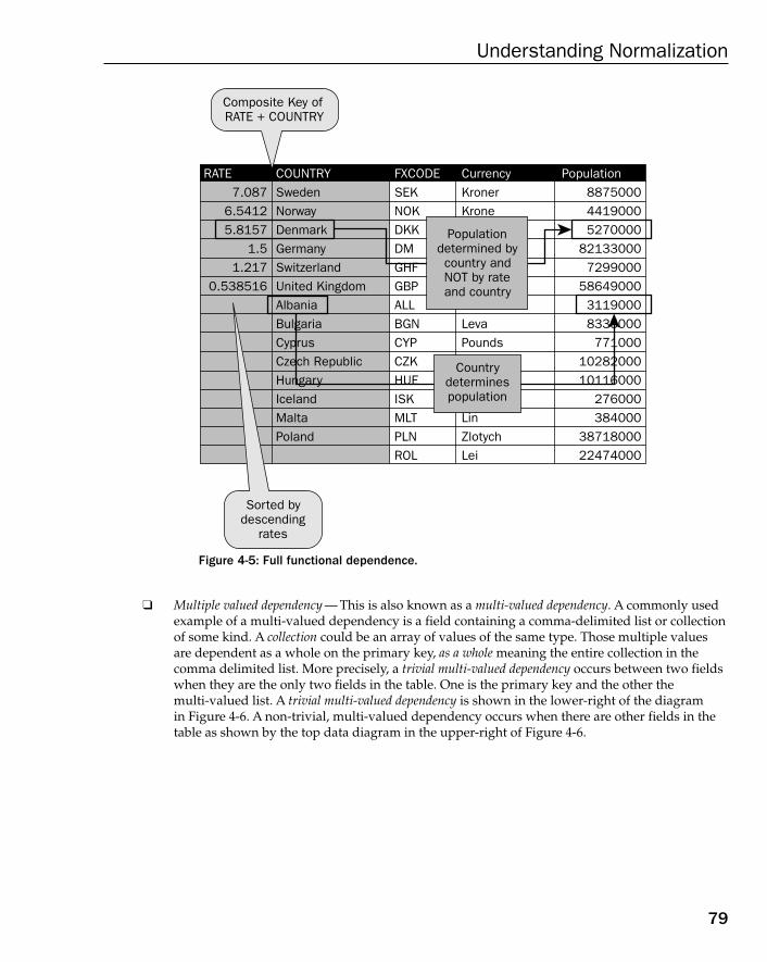
Figure 4-5: Full functional dependence.
❑ Multiple valued dependency — This is also known as a multi-valued dependency. A commonly usedexample of a multi-valued dependency is a field containing a comma-delimited list or collectionof some kind. A collection could be an array of values of the same type. Those multiple valuesare dependent as a whole on the primary key, as a whole meaning the entire collection in thecomma delimited list. More precisely, a trivial multi-valued dependency occurs between two fieldswhen they are the only two fields in the table. One is the primary key and the other the multi-valued list. A trivial multi-valued dependency is shown in the lower-right of the diagramin Figure 4-6. A non-trivial, multi-valued dependency occurs when there are other fields in thetable as shown by the top data diagram in the upper-right of Figure 4-6.
Rate7.087
6.54125.8157
1.51.217
0.538516
RATE COUNTRYSwedenNorwayDenmarkGermanySwitzerlandUnited KingdomAlbaniaBulgariaCyprusCzech RepublicHungaryIcelandMaltaPoland
CurrencyKronerKrone
LevaPounds
LinZlotychLei
FXCODESEKNOKDKKDMGHFGBPALLBGNCYPCZKHUEISKMLTPLNROL
Population887500044190005270000
821330007299000
5864900031190008335000
7710001028200010116000
276000384000
3871800022474000
Population
Composite Key of RATE + COUNTRY
Sorted bydescending
rates
Populationdetermined bycountry andNOT by rateand country
Countrydeterminespopulation
79
Understanding Normalization
09_574906 ch04.qxd 11/4/05 10:46 AM Page 79
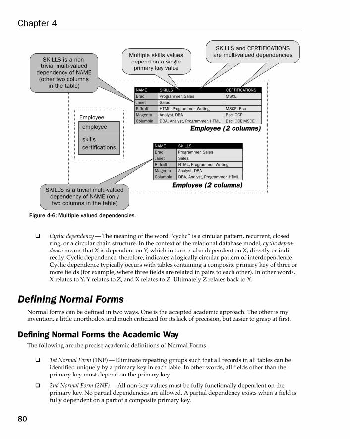
Figure 4-6: Multiple valued dependencies.
❑ Cyclic dependency — The meaning of the word “cyclic” is a circular pattern, recurrent, closedring, or a circular chain structure. In the context of the relational database model, cyclic depen-dence means that X is dependent on Y, which in turn is also dependent on X, directly or indi-rectly. Cyclic dependence, therefore, indicates a logically circular pattern of interdependence.Cyclic dependence typically occurs with tables containing a composite primary key of three ormore fields (for example, where three fields are related in pairs to each other). In other words,X relates to Y, Y relates to Z, and X relates to Z. Ultimately Z relates back to X.
Defining Normal FormsNormal forms can be defined in two ways. One is the accepted academic approach. The other is myinvention, a little unorthodox and much criticized for its lack of precision, but easier to grasp at first.
Defining Normal Forms the Academic WayThe following are the precise academic definitions of Normal Forms.
❑ 1st Normal Form (1NF) — Eliminate repeating groups such that all records in all tables can beidentified uniquely by a primary key in each table. In other words, all fields other than the primary key must depend on the primary key.
❑ 2nd Normal Form (2NF) — All non-key values must be fully functionally dependent on the primary key. No partial dependencies are allowed. A partial dependency exists when a field isfully dependent on a part of a composite primary key.
NAMEBradJanetRiffraffMagentaColumbia
SKILLSProgrammer, SalesSalesHTML, Programmer, WritingAnalyst, DBADBA, Analyst, Programmer, HTML
RATEMSCE
MSCE, BscBsc, OCPBsc, OCP, MSCE
CERTIFICATIONS
NAMEBradJanetRiffraffMagentaColumbia
SKILLSProgrammer, SalesSalesHTML, Programmer, WritingAnalyst, DBADBA, Analyst, Programmer, HTML
Employee (2 columns)Employee (2 columns)
Employee (2 columns)Employee (2 columns)
Employee
employee
skillscertifications
SKILLS is a non-trivial multi-valued
dependency of NAME(other two columns
in the table)
SKILLS is a trivial multi-valueddependency of NAME (onlytwo columns in the table)
Multiple skills valuesdepend on a singleprimary key value
SKILLS and CERTIFICATIONSare multi-valued dependencies
80
Chapter 4
09_574906 ch04.qxd 11/4/05 10:46 AM Page 80

❑ 3rd Normal Form (3NF) — Eliminate transitive dependencies, meaning that a field is indirectlydetermined by the primary key. This is because the field is functionally dependent on anotherfield, whereas the other field is dependent on the primary key.
❑ Boyce-Codd Normal Form (BCNF) — Every determinant in a table is a candidate key. If there isonly one candidate key, 3NF and BCNF are one and the same.
❑ 4th Normal Form (4NF) — Eliminate multiple sets of multivalued dependencies.
❑ 5th Normal Form (5NF) — Eliminate cyclic dependencies. 5NF is also known as ProjectionNormal Form (PJNF).
❑ Domain Key Normal Form (DKNF) — DKNF is the ultimate application of normalization and ismore a measurement of conceptual state, as opposed to a transformation process in itself.
The irritating thing about all this precise language is that it can be extremely confusing. Most of normalization is essentially common sense. For example, most experienced database modelers, architects, designers, programmers, whatever you want to call them — can actually figure out 1NFs,2NFs, and 3NFs simply by looking at a set of data. Anything else is usually ignored. Experienced architects often have an understanding of how to apply common generic database modeling structuresto often repetitive or classifiable business operational structures.
Maintenance of data with respect to accessing of individual records in a database can be more effectivelyand easily managed using “beyond 3NF.” Any querying, however, is adversely affected by too manytables. In some cases, the performance factor can be completely debilitating, making a database useless.Additionally, even in highly accurate, single-record update environments, the extra functionality and accuracy given by beyond 3NF structures (BCNF, 4NF, 5NF, DKNF) can always be provided byapplication coding and SQL code to find those individual records.
Is “beyond 3NF” unnecessary? It might be, but probably in many commercial situations it is unnecessary. Remember that application SDKs are just as powerful as database engine structural andfunctional capabilities. Extreme implementation of normalization using layers beyond 3NF tends toplace too much functionality into the database. Why not use the best of both worlds — both databaseand application capabilities? Use the database to store data and allow applications to manipulate andverify data to a certain extent.
Defining Normal Forms the Easy WayMany modern-day commercial relational database implementations do not go beyond the implementationof 3NF. This is often true of OLTP databases and nearly always true in properly designed data warehousedatabases. Application of Normal Forms beyond that of 3NF tends to produce too many tables, resulting intoo many tables in SQL joins. Bigger joins result in poor performance. In general, good performance ismuch more important than granular perfection in relational database design.
How can normalization be made simple? Why is it easy? I like to offer a simplified interpretation of normalization just to get the novice started. In a perfect world, most relational database model designsare very similar. As a result, much of the basic database design for many applications from accounting tomanufacturing (and anything else you can think of) is all more or less the same. Some of the commonfactors are separation of repeated fields in master-detail relationships using 1NF, pushing static data intonew tables using 2NF, and doing various interesting things with 3NF (such as uniquely identifying repetitions between many-to-many relationships).
81
Understanding Normalization
09_574906 ch04.qxd 11/4/05 10:46 AM Page 81
Normalization is, for the most part, easy and mostly common sense with some business knowledgethrown in. There are, of course, numerous exceptional circumstances and special cases where my basicinterpretation of normalization does fill all needs 100 percent. In these situations, parts of the morerefined academic interpretation can be used.
The following defines the Normal Forms in an easy to understand manner:
❑ 1st Normal Form (1NF) — Removes repeating fields by creating a new table where the originaland new table are linked together with a master-detail, one-to-many relationship. For example,a master table could contain parent records representing all the ships owned by a cruise line. Adetail table would contain detail records, such as all the passengers on a cruise to the Caribbean.Create primary keys on both tables where the detail table will have a composite primary keycontaining the master table primary key field as the prefix field of its primary key. That prefixfield is also a foreign key back to the master table.
❑ 2nd Normal Form (2NF) — Performs a seemingly similar function to that of 1NF, but creates atable where repeating values (rather than repeating fields as for 1NF) are removed to a newtable. The result is a many-to-one relationship rather than a one-to-many relationship, createdbetween the original and the new tables. The new table gets a primary key consisting of a singlefield. The master table contains a foreign key pointing back to the primary key of the new table.That foreign key is not part of the primary key in the original table.
❑ 3rd Normal Form (3NF) — It is difficult to explain 3NF without using a mind bogglingly confusingtechnical definition. Elimination of a transitive dependency implies creation of a new table forsomething indirectly dependent on the primary key in an existing table. There are a multitude ofways in which 3NF can be interpreted.
❑ Beyond 3NF — Many modern relational database models do not extend beyond 3NF. Sometimes3NF is not used at all. The reason why is because of the generation of too many tables and theresulting complex SQL code joins, with resulting terrible database response times. One commoncase that bears mentioning is removal of potentially NULL valued fields into new tables, creatinga one-to-one relationship. In modern high-end relational database engines with variable recordlengths, this is largely irrelevant. Disk space is cheap and, as already stated, increased numbersof tables leads to bigger SQL joins and poorer performance.
Now let’s examine 1NF in detail.
1st Normal Form (1NF)The following sections define 1NF academically and then demonstrate an easier way.
1NF the Academic Way1NF does the following.
❑ Eliminates repeating groups.
❑ Defines primary keys.
❑ All records must be identified uniquely with a primary key. A primary key is unique and thusno duplicate values are allowed.
82
Chapter 4
09_574906 ch04.qxd 11/4/05 10:46 AM Page 82
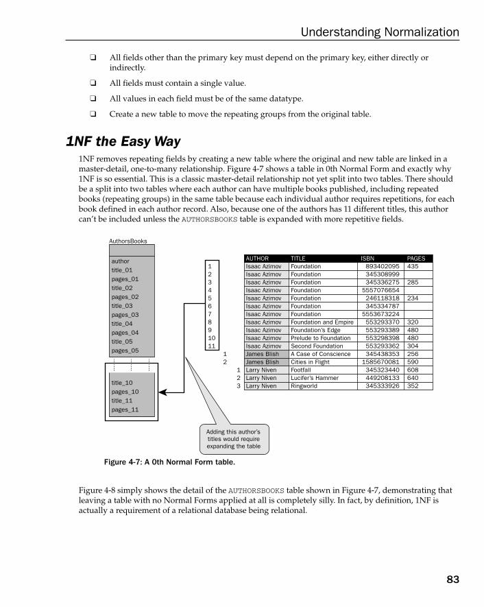
❑ All fields other than the primary key must depend on the primary key, either directly or indirectly.
❑ All fields must contain a single value.
❑ All values in each field must be of the same datatype.
❑ Create a new table to move the repeating groups from the original table.
1NF the Easy Way1NF removes repeating fields by creating a new table where the original and new table are linked in amaster-detail, one-to-many relationship. Figure 4-7 shows a table in 0th Normal Form and exactly why1NF is so essential. This is a classic master-detail relationship not yet split into two tables. There shouldbe a split into two tables where each author can have multiple books published, including repeatedbooks (repeating groups) in the same table because each individual author requires repetitions, for eachbook defined in each author record. Also, because one of the authors has 11 different titles, this authorcan’t be included unless the AUTHORSBOOKS table is expanded with more repetitive fields.
Figure 4-7: A 0th Normal Form table.
Figure 4-8 simply shows the detail of the AUTHORSBOOKS table shown in Figure 4-7, demonstrating thatleaving a table with no Normal Forms applied at all is completely silly. In fact, by definition, 1NF is actually a requirement of a relational database being relational.
Isaac AzimovIsaac AzimovIsaac AzimovIsaac AzimovIsaac AzimovIsaac Azimov
AuthorsBooks
authortitle_01pages_01title_02pages_02title_03pages_03title_04pages_04title_05pages_05
title_10pages_10title_11pages_11
Isaac AzimovIsaac AzimovIsaac AzimovIsaac AzimovIsaac AzimovJames BlishJames BlishLarry NivenLarry NivenLarry Niven
FoundationFoundationFoundationFoundationFoundationFoundationFoundationFoundation and EmpireFoundation’s EdgePrelude to FoundationSecond FoundationA Case of ConscienceCities in FlightFootfallLucifer’s HammerRingworld
893402095345308999345336275
5557076654246118318345334787
5553673224553293370553293389553298398553293362345438353
1585670081345323440449208133345333926
435
285
234
320480480304256590608640352
AUTHOR TITLE ISBN PAGES1234567891011
12
Adding this author’stitles would requireexpanding the table
123
83
Understanding Normalization
09_574906 ch04.qxd 11/4/05 10:46 AM Page 83
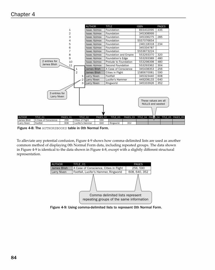
Figure 4-8: The AUTHORSBOOKS table in 0th Normal Form.
To alleviate any potential confusion, Figure 4-9 shows how comma-delimited lists are used as anothercommon method of displaying 0th Normal Form data, including repeated groups. The data shown in Figure 4-9 is identical to the data shown in Figure 4-8, except with a slightly different structural representation.
Figure 4-9: Using comma-delimited lists to represent 0th Normal Form.
James BlishLarry Niven
A Case of Conscience, Cities in FlightFootfall, Lucifer’s Hammer, Ringworld
256, 590608, 640, 352
AUTHOR TITLE_01 PAGES
Comma delimited lists representrepeating groups of the same information
Isaac AzimovIsaac AzimovIsaac AzimovIsaac AzimovIsaac AzimovIsaac AzimovIsaac AzimovIsaac AzimovIsaac AzimovIsaac AzimovIsaac AzimovJames BlishJames BlishLarry NivenLarry NivenLarry Niven
FoundationFoundationFoundationFoundationFoundationFoundationFoundationFoundation and EmpireFoundation’s EdgePrelude to FoundationSecond FoundationA Case of ConscienceCities in FlightFootfallLucifer’s HammerRingworld
893402095345308999345336275
5557076654246118318345334787
5553673224553293370553293389553298398553293362345438353
1585670081345323440449208133345333926
435
285
234
320480480304256590608640352
AUTHOR TITLE ISBN PAGES
James BlishLarry Niven
A Case of ConscienceFootfall
Cities of FlightLucifer’s Hammer
256608
AUTHOR TITLE_01 PAGES_01 TITLE_02590640
PAGES_02
1234567891011
12
2 entries forJames Blish
3 entries forLarry Niven
123
Ringworld
TITLE_03
352
PAGES_03 TITLE_04 PAGES_04 TITLE_05 PAGES_05
These values are allNULLS and wasted
84
Chapter 4
09_574906 ch04.qxd 11/4/05 10:46 AM Page 84

Figure 4-10 shows the application of 1NF, removing repeating fields by creating a new table where theoriginal and new table are linked in a master-detail, one-to-many relationship.
Figure 4-10: 1NF normalization master-detail tables forAUTHORSBOOKS.
In Figure 4-11, primary keys are created on both tables where the detail table has a composite primarykey. The composite primary key contains the master table primary key field as the prefix field of its primary key. Therefore, the prefix field AUTHOR on the BOOK table is the foreign key pointing back to themaster table AUTHOR.
Figure 4-11: Primary keys and the foreign key pointer.
Author
author
Book
author (FK)titleisbn
pages
Author
author
Book
titleisbnpages
85
Understanding Normalization
09_574906 ch04.qxd 11/4/05 10:46 AM Page 85
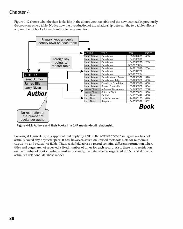
Figure 4-12 shows what the data looks like in the altered AUTHOR table and the new BOOK table, previouslythe AUTHORSBOOKS table. Notice how the introduction of the relationship between the two tables allowsany number of books for each author to be catered for.
Figure 4-12: Authors and their books in a 1NF master-detail relationship.
Looking at Figure 4-12, it is apparent that applying 1NF to the AUTHORSBOOKS in Figure 4-7 has not actually saved any physical space. It has, however, saved on unused metadata slots for numerousTITLE_nn and PAGES_nn fields. Thus, each field across a record contains different information wheretitles and pages are not repeated a fixed number of times for each record. Also, there is no restriction on the number of books. Perhaps most importantly, the data is better organized in 1NF and it now isactually a relational database model.
Isaac AzimovIsaac AzimovIsaac AzimovIsaac AzimovIsaac AzimovIsaac AzimovIsaac AzimovIsaac AzimovIsaac AzimovIsaac AzimovIsaac AzimovJames BlishJames BlishLarry NivenLarry NivenLarry Niven
FoundationFoundationFoundationFoundationFoundationFoundationFoundationFoundation and EmpireFoundation’s EdgePrelude to FoundationSecond FoundationA Case of ConscienceCities in FlightFootfallLucifer’s HammerRingworld
893402095345308999345336275
5557076654246118318345334787
5553673224553293370553293389553298398553293362345438353
1585670081345323440449208133345333926
435
285
234
320480480304256590608640352
AUTHOR TITLE ISBN PAGES
Isaac AzimovJames BlishLarry Niven
AUTHOR
AuthorAuthor
BookBookNo restriction onthe number of
books per author
Foreign keypoints to
master table
Primary keys uniquelyidentify rows on each table
86
Chapter 4
09_574906 ch04.qxd 11/4/05 10:46 AM Page 86
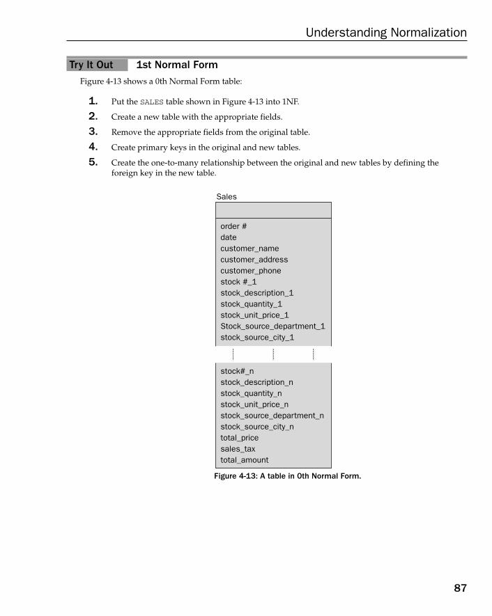
Try It Out 1st Normal FormFigure 4-13 shows a 0th Normal Form table:
1. Put the SALES table shown in Figure 4-13 into 1NF.
2. Create a new table with the appropriate fields.
3. Remove the appropriate fields from the original table.
4. Create primary keys in the original and new tables.
5. Create the one-to-many relationship between the original and new tables by defining the foreign key in the new table.
Figure 4-13: A table in 0th Normal Form.
Sales
order #datecustomer_namecustomer_addresscustomer_phonestock #_1stock_description_1stock_quantity_1stock_unit_price_1Stock_source_department_1stock_source_city_1
stock#_nstock_description_nstock_quantity_nstock_unit_price_nstock_source_department_nstock_source_city_ntotal_pricesales_taxtotal_amount
87
Understanding Normalization
09_574906 ch04.qxd 11/4/05 10:46 AM Page 87

How It Works1NF requires removal of repeating groups into a new table.
1. The SALES table contains orders with lines on each order represented by each stock item on theorder. It would help having the data in this situation, but previous examples and exercises havealready shown data, so this is unnecessary. At this point, understanding of concepts is important.
2. Figure 4-14 shows the desired 1NF transformation.
Figure 4-14: 1NF transformation of the SALES table in Figure 4-13.
Figure 4-14 shows repeated sales order item entries in the form of stock item entries removed to the SALE_ORDER_ITEM table, linking back to the renamed SALE_ORDER table, renamed from the original SALES table. The two tables are linked by a one-to-many relationship between the SALE_ORDERand SALE_ORDER_ITEM tables using the primary key on the SALE_ORDER table, duplicated to theSALE_ORDER_ITEM table as the ORDER# (FK) field, part of the SALE_ORDER_ITEM table primary key.
Sales
order #datecustomer_namecustomer_addresscustomer_phonestock #_1stock_description_1stock_quantity_1stock_unit_price_1stock_source_department_1stock_source_city_1
stock#_nstock_description_nstock_quantity_nstock_unit_price_nstock_source_department_nstock_source_city_ntotal_pricesales_taxtotal_amount
Sales_Order
order #
datecustomer_namecustomer_addresscustomer_phonetotal_pricesales_taxtotal_amount
Sales_Order_Item
order# (FK)stock#
stock_descriptionstock_quantitystock_unit_pricestock_source_departmentstock_source_city
1st NF
Transform
1st NF
Transform
88
Chapter 4
09_574906 ch04.qxd 11/4/05 10:46 AM Page 88
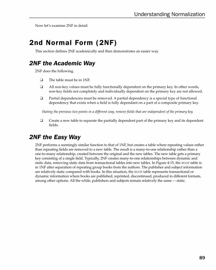
Now let’s examine 2NF in detail.
2nd Normal Form (2NF)This section defines 2NF academically and then demonstrates an easier way.
2NF the Academic Way2NF does the following.
❑ The table must be in 1NF.
❑ All non-key values must be fully functionally dependent on the primary key. In other words,non-key fields not completely and individually dependent on the primary key are not allowed.
❑ Partial dependencies must be removed. A partial dependency is a special type of functionaldependency that exists when a field is fully dependant on a part of a composite primary key.
Stating the previous two points in a different way, remove fields that are independent of the primary key.
❑ Create a new table to separate the partially dependent part of the primary key and its dependentfields.
2NF the Easy Way2NF performs a seemingly similar function to that of 1NF, but creates a table where repeating values ratherthan repeating fields are removed to a new table. The result is a many-to-one relationship rather than aone-to-many relationship, created between the original and the new tables. The new table gets a primarykey consisting of a single field. Typically, 2NF creates many-to-one relationships between dynamic andstatic data, removing static data from transactional tables into new tables. In Figure 4-15, the BOOK table isin 1NF after separation of repeating group books from the authors. The publisher and subject informationare relatively static compared with books. In this situation, the BOOK table represents transactional ordynamic information where books are published, reprinted, discontinued, produced in different formats,among other options. All the while, publishers and subjects remain relatively the same — static.
89
Understanding Normalization
09_574906 ch04.qxd 11/4/05 10:46 AM Page 89

Figure 4-15: The BOOK table is in 1NF.
Figure 4-16 shows the initial stage of the application of 2NF, removing static publisher and subject information from the more dynamic BOOK transaction table.
In Figure 4-17, many-to-one relationships are established between dynamic and static tables, namelyBOOK to PUBLISHER and BOOK to SUBJECT tables. When applying 1NF, one-to-many relationships areestablished between master and detail tables, as shown in Figure 4-10 and Figure 4-11. Application of2NF establishes the same relationship, except it is easier to understand the slight difference by callingthat relationship a many-to-one relationship. Mathematically, a one-to-many relationship is identical to amany-to-one relationship; however, 1NFs and 2NFs are completely different because the one-to-manyrelationship is established for a completely different reason.
Isaac AzimovIsaac AzimovIsaac AzimovIsaac AzimovIsaac AzimovIsaac AzimovIsaac AzimovIsaac AzimovIsaac AzimovIsaac AzimovIsaac AzimovJames BlishJames BlishLarry NivenLarry NivenLarry Niven
FoundationFoundationFoundationFoundationFoundationFoundationFoundationFoundation and EmpireFoundation’s EdgePrelude to FoundationSecond FoundationA Case of ConscienceCities in FlightFootfallLucifer’s HammerRingworld
L P BooksBel Rey BooksBallantine BooksBooks on TapeHaperCollins PublisherDel Rey BooksBooks on TapeSpectraSpectraSpectraBantam BooksBallatine BooksOverlook PressDel Rey BooksFawcett BooksBallantine Books
435
285
234
320480480304256590608640352
AUTHOR TITLE PUBLISHERAddress, contact, phoneAddress, contact, phoneAddress, contact, phoneAddress, contact, phoneAddress, contact, phoneAddress, contact, phoneAddress, contact, phoneAddress, contact, phoneAddress, contact, phoneAddress, contact, phoneAddress, contact, phoneAddress, contact, phoneAddress, contact, phoneAddress, contact, phoneAddress, contact, phoneAddress, contact, phone
ADDRESSScience FictionScience FictionScience FictionScience FictionScience FictionScience FictionScience FictionScience FictionScience FictionScience FictionScience FictionScience FictionScience FictionScience FictionScience FictionScience Fiction
SUBJECTPAGES
Book
author (FK)titleisbn
pagespublisherpublisher_addresspublisher_contactpublisher_phonesubjectfictionnon-fiction
Author
author
Publisherdata is static
Subject datais static
Many books foreach publisher
Many books foreach publisher
90
Chapter 4
09_574906 ch04.qxd 11/4/05 10:46 AM Page 90
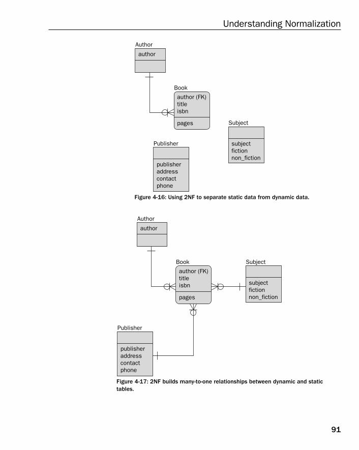
Figure 4-16: Using 2NF to separate static data from dynamic data.
Figure 4-17: 2NF builds many-to-one relationships between dynamic and statictables.
Author
author
SubjectBook
author (FK)titleisbn subject
fictionnon_fiction
Publisher
publisheraddresscontactphone
pages
Author
author
Subject
Book
author (FK)titleisbn
subjectfictionnon_fiction
Publisher
publisheraddresscontactphone
pages
91
Understanding Normalization
09_574906 ch04.qxd 11/4/05 10:46 AM Page 91
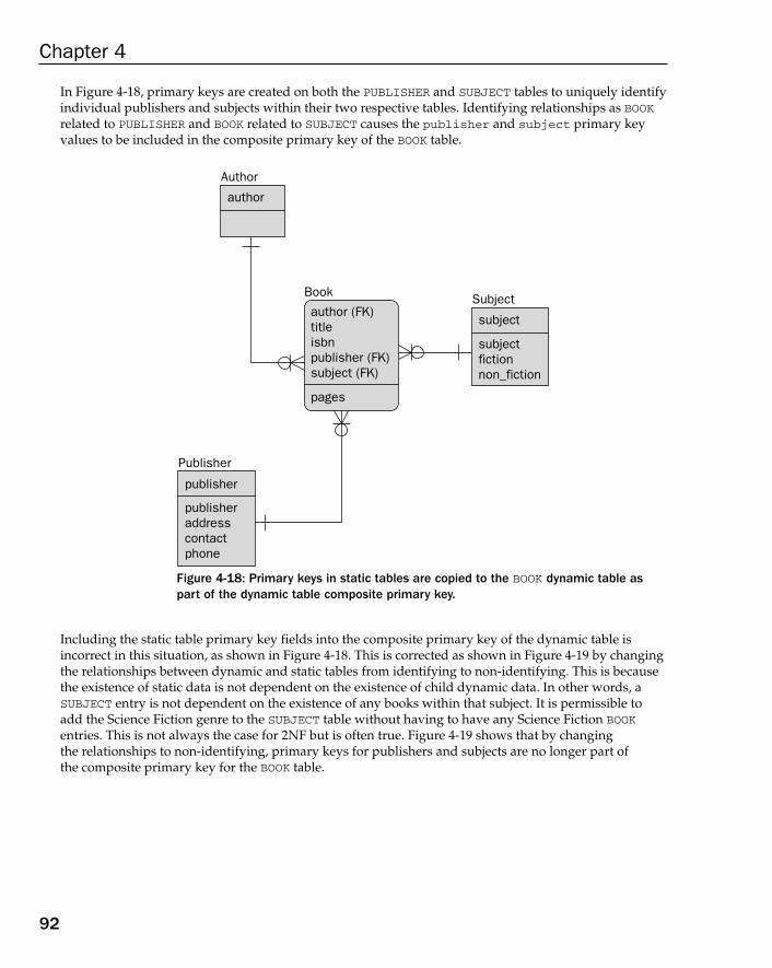
In Figure 4-18, primary keys are created on both the PUBLISHER and SUBJECT tables to uniquely identifyindividual publishers and subjects within their two respective tables. Identifying relationships as BOOKrelated to PUBLISHER and BOOK related to SUBJECT causes the publisher and subject primary keyvalues to be included in the composite primary key of the BOOK table.
Figure 4-18: Primary keys in static tables are copied to the BOOK dynamic table aspart of the dynamic table composite primary key.
Including the static table primary key fields into the composite primary key of the dynamic table isincorrect in this situation, as shown in Figure 4-18. This is corrected as shown in Figure 4-19 by changingthe relationships between dynamic and static tables from identifying to non-identifying. This is becausethe existence of static data is not dependent on the existence of child dynamic data. In other words, aSUBJECT entry is not dependent on the existence of any books within that subject. It is permissible toadd the Science Fiction genre to the SUBJECT table without having to have any Science Fiction BOOKentries. This is not always the case for 2NF but is often true. Figure 4-19 shows that by changing the relationships to non-identifying, primary keys for publishers and subjects are no longer part ofthe composite primary key for the BOOK table.
Author
author
SubjectBook
author (FK)titleisbnpublisher (FK)subject (FK)
subject
subject
fictionnon_fiction
Publisher
publisher
publisher
addresscontactphone
pages
92
Chapter 4
09_574906 ch04.qxd 11/4/05 10:46 AM Page 92
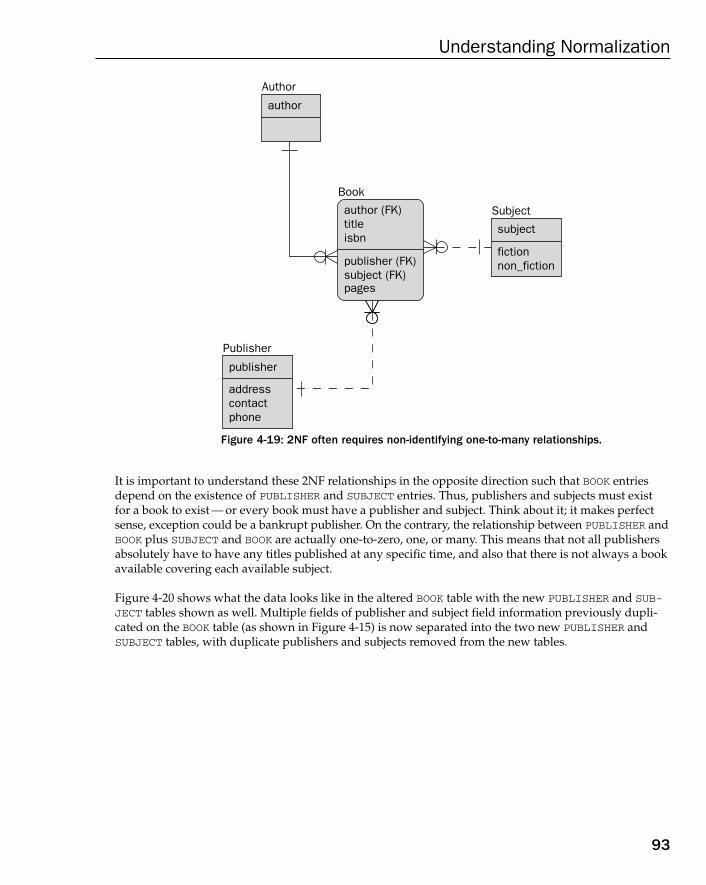
Figure 4-19: 2NF often requires non-identifying one-to-many relationships.
It is important to understand these 2NF relationships in the opposite direction such that BOOK entriesdepend on the existence of PUBLISHER and SUBJECT entries. Thus, publishers and subjects must existfor a book to exist — or every book must have a publisher and subject. Think about it; it makes perfectsense, exception could be a bankrupt publisher. On the contrary, the relationship between PUBLISHER andBOOK plus SUBJECT and BOOK are actually one-to-zero, one, or many. This means that not all publishersabsolutely have to have any titles published at any specific time, and also that there is not always a bookavailable covering each available subject.
Figure 4-20 shows what the data looks like in the altered BOOK table with the new PUBLISHER and SUB-JECT tables shown as well. Multiple fields of publisher and subject field information previously dupli-cated on the BOOK table (as shown in Figure 4-15) is now separated into the two new PUBLISHER andSUBJECT tables, with duplicate publishers and subjects removed from the new tables.
Author
author
Subject
Book
author (FK)titleisbn
publisher (FK)subject (FK)
subject
fictionnon_fiction
Publisher
publisher
addresscontactphone
pages
93
Understanding Normalization
09_574906 ch04.qxd 11/4/05 10:46 AM Page 93
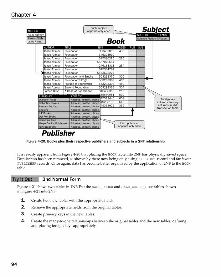
Figure 4-20: Books plus their respective publishers and subjects in a 2NF relationship.
It is readily apparent from Figure 4-20 that placing the BOOK table into 2NF has physically saved space.Duplication has been removed, as shown by there now being only a single SUBJECT record and far fewerPUBLISHER records. Once again, data has become better organized by the application of 2NF to the BOOKtable.
Try It Out 2nd Normal FormFigure 4-21 shows two tables in 1NF. Put the SALE_ORDER and SALE_ORDER_ITEM tables shown in Figure 4-21 into 2NF:
1. Create two new tables with the appropriate fields.
2. Remove the appropriate fields from the original tables.
3. Create primary keys in the new tables.
4. Create the many-to-one relationships between the original tables and the new tables, definingand placing foreign keys appropriately.
Isaac AzimovIsaac AzimovIsaac AzimovIsaac AzimovIsaac AzimovIsaac AzimovIsaac AzimovIsaac AzimovIsaac AzimovIsaac AzimovIsaac AzimovJames BlishJames BlishLarry NivenLarry NivenLarry Niven
FoundationFoundationFoundationFoundationFoundationFoundationFoundationFoundation and EmpireFoundation’s EdgePrelude to FoundationSecond FoundationA Case of ConscienceCities in FlightFootfallLucifer’s HammerRingworld
893402095345308999345336275
5557076654246118318345334787
5553673224553293370553293389553298398553293362345438353
1585670081345323440449208133345333926
435
285
234
320480480304256590608640352
AUTHOR TITLE ISBN PAGES PUB SUB
Isaac AzimovJames BlishLarry Niven
AUTHOR
Science FictionSUBJECT
FictionCLASS
BookBook
PublisherPublisher
SubjectSubject
Overlook PressBallantine BooksBantam BooksSpectraL P BooksDel Rey BooksBooks on TapeHarperCollins PublishersFawcett Books
PUBLISHERAddress, contact, phoneAddress, contact, phoneAddress, contact, phoneAddress, contact, phoneAddress, contact, phoneAddress, contact, phoneAddress, contact, phoneAddress, contact, phoneAddress, contact, phone
ADDRESS
Each subjectappears only once
Each publisherappears only once
Foreign keycolumns are onlycolumns in 2NFtransaction table
94
Chapter 4
09_574906 ch04.qxd 11/4/05 10:46 AM Page 94
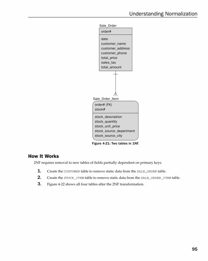
Figure 4-21: Two tables in 1NF.
How It Works2NF requires removal to new tables of fields partially dependent on primary keys.
1. Create the CUSTOMER table to remove static data from the SALE_ORDER table.
2. Create the STOCK_ITEM table to remove static data from the SALE_ORDER_ITEM table.
3. Figure 4-22 shows all four tables after the 2NF transformation.
Sale_Order
order#
datecustomer_namecustomer_addresscustomer_phonetotal_pricesales_taxtotal_amount
Sale_Order_Item
order# (FK)stock#
stock_descriptionstock_quantitystock_unit_pricestock_source_departmentstock_source_city
95
Understanding Normalization
09_574906 ch04.qxd 11/4/05 10:46 AM Page 95
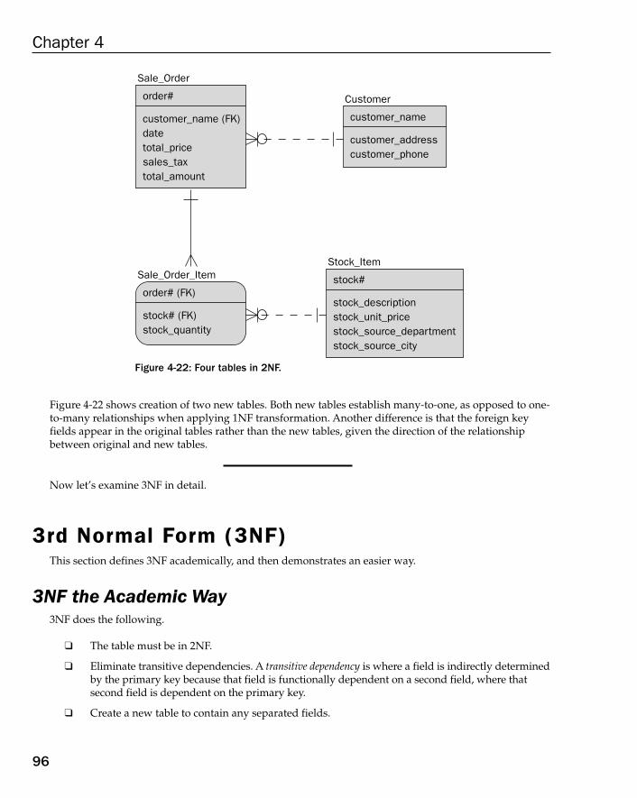
Figure 4-22: Four tables in 2NF.
Figure 4-22 shows creation of two new tables. Both new tables establish many-to-one, as opposed to one-to-many relationships when applying 1NF transformation. Another difference is that the foreign keyfields appear in the original tables rather than the new tables, given the direction of the relationshipbetween original and new tables.
Now let’s examine 3NF in detail.
3rd Normal Form (3NF)This section defines 3NF academically, and then demonstrates an easier way.
3NF the Academic Way3NF does the following.
❑ The table must be in 2NF.
❑ Eliminate transitive dependencies. A transitive dependency is where a field is indirectly determinedby the primary key because that field is functionally dependent on a second field, where that second field is dependent on the primary key.
❑ Create a new table to contain any separated fields.
Sale_Order
order#
customer_name (FK)datetotal_pricesales_taxtotal_amount
Stock_Item
stock#
stock_descriptionstock_unit_pricestock_source_departmentstock_source_city
Sale_Order_Item
order# (FK)
stock# (FK)stock_quantity
Customer
customer_name
customer_addresscustomer_phone
96
Chapter 4
09_574906 ch04.qxd 11/4/05 10:46 AM Page 96

3NF the Easy Way3NF is an odd one and can often cause confusion. In basic terms, every field in a table that is not a keyfield must be directly dependent on the primary key. There are number of different ways to look at 3NF,and this section goes through them one by one.
Figure 4-23 shows one of the easiest interpretations of 3NF where a many-to-many relationship presentsthe possibility that more than one record will be returned using a query joining both tables.
Figure 4-23: Resolving a many-to-many relationship into a new table.
Figure 4-24 shows employees and tasks from the 2NF version on the left of the diagram in Figure 4-23.Employees perform tasks in their daily routines, doing their jobs. If you were searching for the employeeColumbia, three tasks would always be returned. Similarly, if searching for the third task shown inFigure 4-24, two employees would always be returned. A problem would arise with this situation whensearching for an attribute specific to a particular assignment where an assignment is a single taskassigned to a single employee. Without the new ASSIGNMENT table created by the 3NF transformationshown in Figure 4-23, finding an individual assignment would be impossible.
Employee
employee
Task
task
Assignment
employee (FK)task (FK)
Employee
employee
Task
task
Join query can yieldduplicate rows
Gives access tounique assignments
3rd NFTransform3rd NFTransform
97
Understanding Normalization
09_574906 ch04.qxd 11/4/05 10:46 AM Page 97

Figure 4-24: A many-to-many relationship finds duplicate records when unique recordsare sought.
Another way to look at 3NF is as displayed in Figure 4-25, where fields common to more than one tablecan be moved to a new table, as shown by the creation of the FOREIGN_EXCHANGE table. At first, thislooks like a 2NF transformation because fields not dependent on the primary key are removed to thenew table; however, currencies should be conceived as being dependent upon location. Both CUSTOMERand SUPPLIER have addresses and, thus, there are transitive dependencies between currencies, throughaddresses (location), ultimately to customers and suppliers. Customers and suppliers use specific currencies depending on what country they are located in. Figure 4-25 shows a 3NF transformationallowing removal of common information from the CUSTOMER and SUPPLIER tables for two reasons:
❑ Currency coding and rate information does not depend on CUSTOMER and SUPPLIER primarykeys, even though which currency they use does depend on who the customer or supplier are,based on the country in which they do business.
❑ The CURRENCY and EXCHANGE_RATE fields in the pre-transformation tables are transitivelydependant on CUSTOMER and SUPPLIER primary keys because they depend on theCURRENCY_CODE, which in turn does depends on addresses.
TaskTask
EmployeeEmployeeNAMEALLBradJanetRiffraffMagentaColumbia
TITLEProgrammerSales personHTML coderAnalystDBA
HIRED1-Feb-031-Jan-001-Apr-041-Sep-041-Sep-04
SALARY50K30K65K75K
105K
TASKALLAnalyze accounting applicationBuild data warehouse databaseCode website HTML pagesBuild XML generators for websites
2 employees,1 task
1 employee,3 tasks
1 to 1
98
Chapter 4
09_574906 ch04.qxd 11/4/05 10:46 AM Page 98
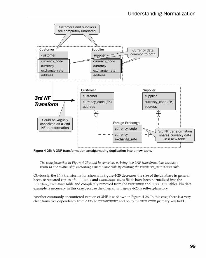
Figure 4-25: A 3NF transformation amalgamating duplication into a new table.
The transformation in Figure 4-25 could be conceived as being two 2NF transformations because amany-to-one relationship is creating a more static table by creating the FOREIGN_EXCHANGE table.
Obviously, the 3NF transformation shown in Figure 4-25 decreases the size of the database in generalbecause repeated copies of CURRENCY and EXCHANGE_RATE fields have been normalized into the FOREIGN_EXCHANGE table and completely removed from the CUSTOMER and SUPPLIER tables. No dataexample is necessary in this case because the diagram in Figure 4-25 is self-explanatory.
Another commonly encountered version of 3NF is as shown in Figure 4-26. In this case, there is a veryclear transitive dependency from CITY to DEPARTMENT and on to the EMPLOYEE primary key field.
Customer
customer
currency_code (FK)address
Customer
customer
currency_codecurrencyexchange_rateaddress
Supplier
supplier
currency_codecurrencyexchange_rateaddress
Supplier
supplier
currency_code (FK)address
Foreign Exchange
currency_code
currencyexchange_rate
Customers and suppliersare completely unrelated
3rd NFTransform3rd NFTransform
Currency datacommon to both
3rd NF transformationshares currency data
in a new table
Could be vaguelyconceived as a 2ndNF transformation
99
Understanding Normalization
09_574906 ch04.qxd 11/4/05 10:46 AM Page 99
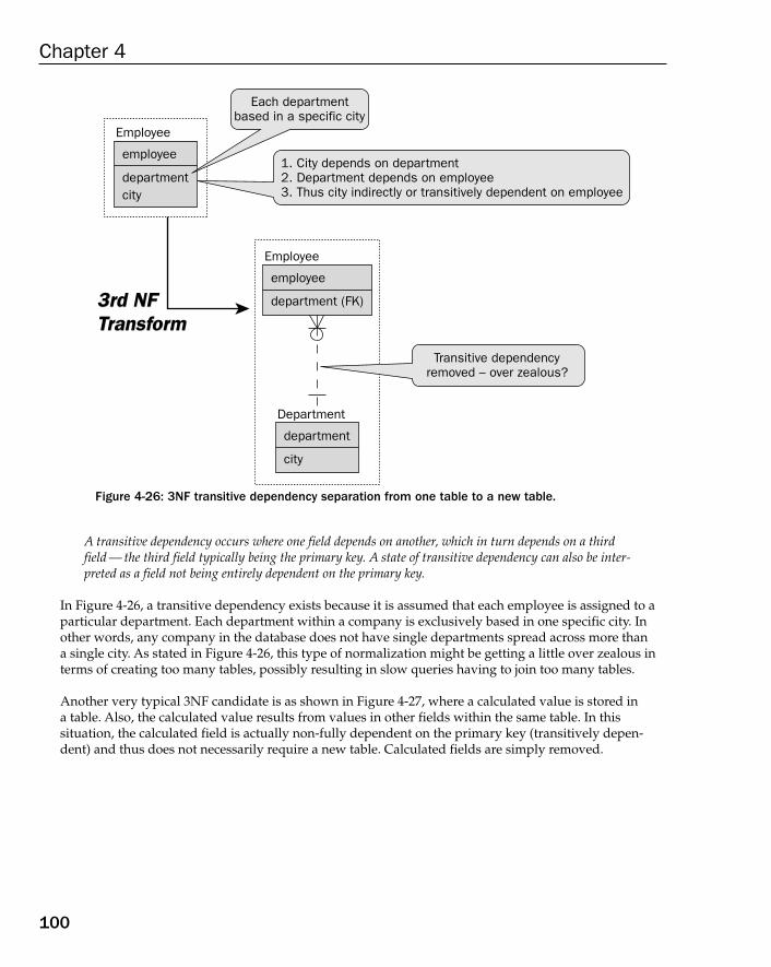
Figure 4-26: 3NF transitive dependency separation from one table to a new table.
A transitive dependency occurs where one field depends on another, which in turn depends on a thirdfield — the third field typically being the primary key. A state of transitive dependency can also be inter-preted as a field not being entirely dependent on the primary key.
In Figure 4-26, a transitive dependency exists because it is assumed that each employee is assigned to aparticular department. Each department within a company is exclusively based in one specific city. Inother words, any company in the database does not have single departments spread across more thana single city. As stated in Figure 4-26, this type of normalization might be getting a little over zealous interms of creating too many tables, possibly resulting in slow queries having to join too many tables.
Another very typical 3NF candidate is as shown in Figure 4-27, where a calculated value is stored in a table. Also, the calculated value results from values in other fields within the same table. In this situation, the calculated field is actually non-fully dependent on the primary key (transitively depen-dent) and thus does not necessarily require a new table. Calculated fields are simply removed.
Employee
employee
departmentcity
Employee
employee
department (FK)
Department
department
city
Each departmentbased in a specific city
1. City depends on department2. Department depends on employee3. Thus city indirectly or transitively dependent on employee
Transitive dependencyremoved – over zealous?
3rd NFTransform3rd NFTransform
100
Chapter 4
09_574906 ch04.qxd 11/4/05 10:46 AM Page 100
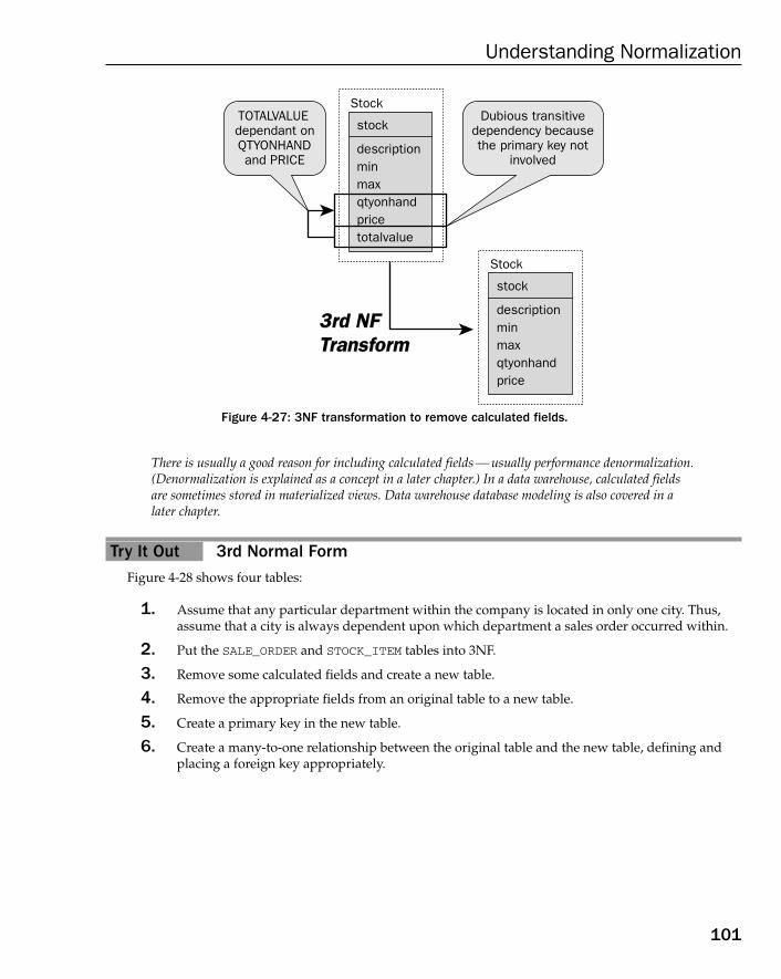
Figure 4-27: 3NF transformation to remove calculated fields.
There is usually a good reason for including calculated fields — usually performance denormalization.(Denormalization is explained as a concept in a later chapter.) In a data warehouse, calculated fieldsare sometimes stored in materialized views. Data warehouse database modeling is also covered in alater chapter.
Try It Out 3rd Normal FormFigure 4-28 shows four tables:
1. Assume that any particular department within the company is located in only one city. Thus,assume that a city is always dependent upon which department a sales order occurred within.
2. Put the SALE_ORDER and STOCK_ITEM tables into 3NF.
3. Remove some calculated fields and create a new table.
4. Remove the appropriate fields from an original table to a new table.
5. Create a primary key in the new table.
6. Create a many-to-one relationship between the original table and the new table, defining andplacing a foreign key appropriately.
TOTALVALUEdependant onQTYONHANDand PRICE
Stock
stock
descriptionminmaxqtyonhandpricetotalvalue
Stock
stock
descriptionminmaxqtyonhandprice
3rd NFTransform3rd NFTransform
Dubious transitivedependency becausethe primary key not
involved
101
Understanding Normalization
09_574906 ch04.qxd 11/4/05 10:46 AM Page 101
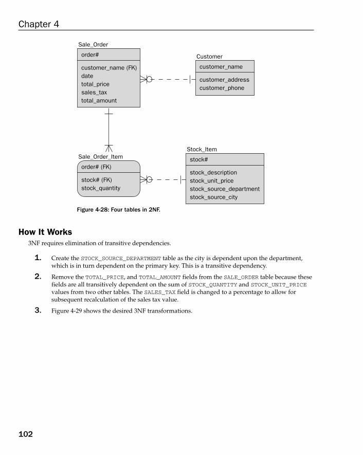
Figure 4-28: Four tables in 2NF.
How It Works3NF requires elimination of transitive dependencies.
1. Create the STOCK_SOURCE_DEPARTMENT table as the city is dependent upon the department,which is in turn dependent on the primary key. This is a transitive dependency.
2. Remove the TOTAL_PRICE, and TOTAL_AMOUNT fields from the SALE_ORDER table because thesefields are all transitively dependent on the sum of STOCK_QUANTITY and STOCK_UNIT_PRICEvalues from two other tables. The SALES_TAX field is changed to a percentage to allow for subsequent recalculation of the sales tax value.
3. Figure 4-29 shows the desired 3NF transformations.
Sale_Order
order#
customer_name (FK)datetotal_pricesales_taxtotal_amount
Stock_Item
stock#
stock_descriptionstock_unit_pricestock_source_departmentstock_source_city
Sale_Order_Item
order# (FK)
stock# (FK)stock_quantity
Customer
customer_name
customer_addresscustomer_phone
102
Chapter 4
09_574906 ch04.qxd 11/4/05 10:46 AM Page 102
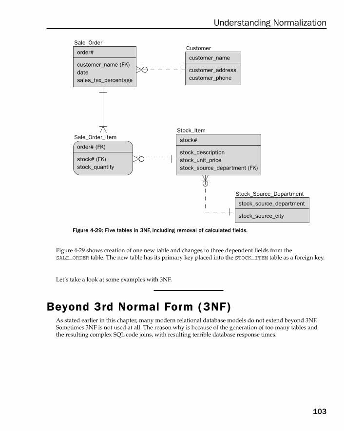
Figure 4-29: Five tables in 3NF, including removal of calculated fields.
Figure 4-29 shows creation of one new table and changes to three dependent fields from theSALE_ORDER table. The new table has its primary key placed into the STOCK_ITEM table as a foreign key.
Let’s take a look at some examples with 3NF.
Beyond 3rd Normal Form (3NF)As stated earlier in this chapter, many modern relational database models do not extend beyond 3NF.Sometimes 3NF is not used at all. The reason why is because of the generation of too many tables andthe resulting complex SQL code joins, with resulting terrible database response times.
Sale_Order
order#
customer_name (FK)datesales_tax_percentage
Stock_Item
stock#
stock_descriptionstock_unit_pricestock_source_department (FK)
Stock_Source_Department
stock_source_department
stock_source_city
Sale_Order_Item
order# (FK)
stock# (FK)stock_quantity
Customer
customer_name
customer_addresscustomer_phone
103
Understanding Normalization
09_574906 ch04.qxd 11/4/05 10:46 AM Page 103

Why Go Beyond 3NF?The objective of naming this section “Beyond 3rd Normal Form [3NF”] is to, in a small way, show the possible folly of using Normal Forms beyond 3NF. The biggest problems with going beyond 3NF arecomplexity and performance issues. Too much granularity actually introduces complexity, especially in a relational database. After all, a relational structure is not an object structure. Object structures becomemore simplistic as they are further reduced. Object database reduction is equivalent to the extremes ofnormalization in a relational database.
Extreme reduction in a relational database has the opposite effect to that of an object database whereeverything gets far to complex — even more complicated than is possible to manage. Extreme forms ofreduction are not of benefit to the relational database model. Additionally, in a relational database themore normalization that is used then the greater the number of tables. The greater the number of tables,the larger SQL query joins become. The larger joins become the poorer database performance.
Extreme levels of granularity in relational database modeling are a form of mathematical perfection.These extremes rarely apply in fast-paced commercial environments. Commercial operations requirethat a job is done efficiently and cost effectively. Perfection in database model design is a side issue tothat of making a profit.
Beyond 3NF the Easy WayIn this section, you begin with the easy way, and not the academic way, as previously. Beyond 3NF areBoyce-Codd normal form (BCNF), 4NF, 5NF, and Domain Key Normal Form (DKNF). Yoiks! That’s justone or two Normal Forms to deal with. It always seems so inconceivable that relational database modelscan become so horribly complicated. After all, the essentials are by and large covered by 1NF and 2NF,with occasional need for 3NF transformations.
The specifics of Boyce-Codd normal form (BCNF), 4NF, 5NF, and DKNF will be covered later in thischapter.
One-to-One NULL TablesFigure 4-30 shows removal of two often to be NULL valued fields from a table called EDITION, creatingthe new table called RANK. The result is a zero or one-to-one relationship between the RANK and EDITIONtables. This implies that if a RANK record exists, then a corresponding EDITION record must exist as well.In the opposite case, however, an EDITION record can exist where a RANK record does not have to exist.This opposite case, accounts for an edition of a publication having no RANK and INGRAM_UNITS values.A recently published publication will rarely have any statistical information.
104
Chapter 4
09_574906 ch04.qxd 11/4/05 10:46 AM Page 104
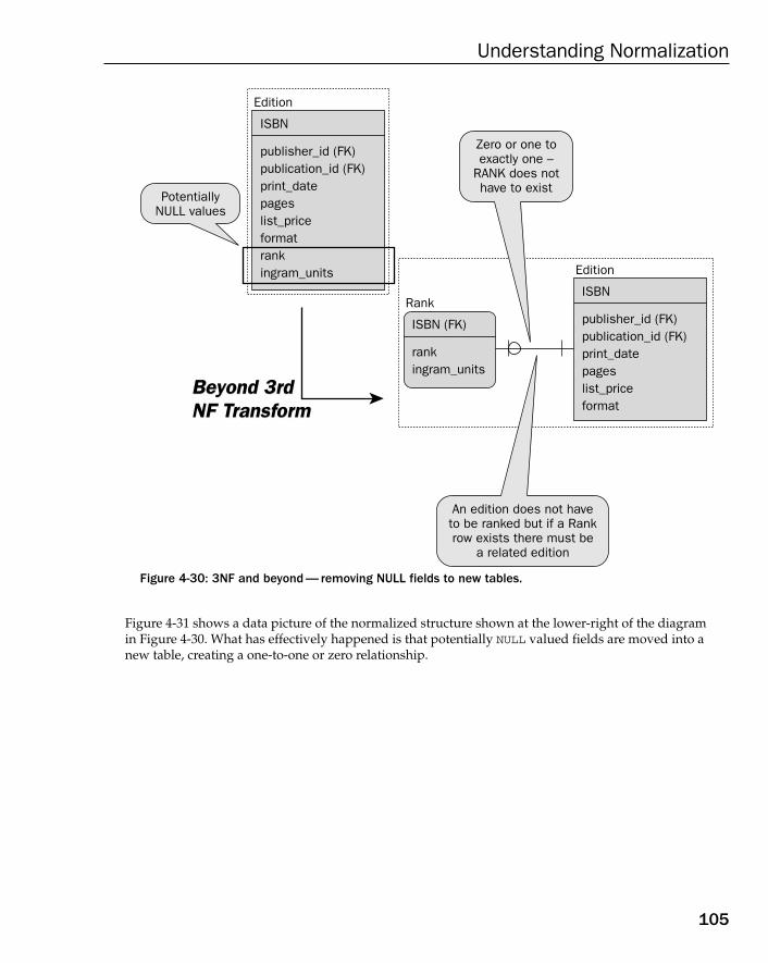
Figure 4-30: 3NF and beyond — removing NULL fields to new tables.
Figure 4-31 shows a data picture of the normalized structure shown at the lower-right of the diagram in Figure 4-30. What has effectively happened is that potentially NULL valued fields are moved into anew table, creating a one-to-one or zero relationship.
PotentiallyNULL values
Edition
ISBN
publisher_id (FK)publication_id (FK)print_datepageslist_priceformatrankingram_units Edition
ISBN
publisher_id (FK)publication_id (FK)print_datepageslist_priceformat
Rank
ISBN (FK)
rankingram_units
Zero or one toexactly one –
RANK does nothave to exist
An edition does not haveto be ranked but if a Rankrow exists there must be
a related edition
Beyond 3rdNF TransformBeyond 3rdNF Transform
105
Understanding Normalization
09_574906 ch04.qxd 11/4/05 10:46 AM Page 105
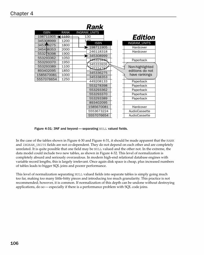
Figure 4-31: 3NF and beyond — separating NULL valued fields.
In the case of the tables shown in Figure 4-30 and Figure 4-31, it should be made apparent that the RANKand INGRAM_UNITS fields are not co-dependent. They do not depend on each other and are completelyunrelated. It is quite possible that one field may be NULL valued and the other not. In the extreme, thedata model could include two new tables, as shown in Figure 4-32. This level of normalization is completely absurd and seriously overzealous. In modern high-end relational database engines with variable record lengths, this is largely irrelevant. Once again disk space is cheap, plus increased numbersof tables leads to bigger SQL joins and poorer performance.
This level of normalization separating NULL valued fields into separate tables is simply going much too far, making too many little-bitty pieces and introducing too much granularity. This practice is not recommended; however, it is common. If normalization of this depth can be undone without destroyingapplications, do so — especially if there is a performance problem with SQL code joins.
198711905345308999345306275345438353553278398553293362553293370553293389893402095
15856700815557076654
11501200180020001900105019501100185010001250
130140
ISBN RANK INGRAM_UNITSRankRank
EditionEdition198711905246118318345308999345323440345333926345334787345336275345338353449208133553278398553293362
11501200180020001900105019501100185010001250
ISBN RANK INGRAM_UNITS
553293370553293389893402095158567008155536732245557076654
HardcoverHardcover
Paperback
PaperbackPaperbackPaperbackPaperbackPaperback
HardcoverAudioCassetteAudioCassette
Non-highlightededitions do nothave rankings
106
Chapter 4
09_574906 ch04.qxd 11/4/05 10:46 AM Page 106
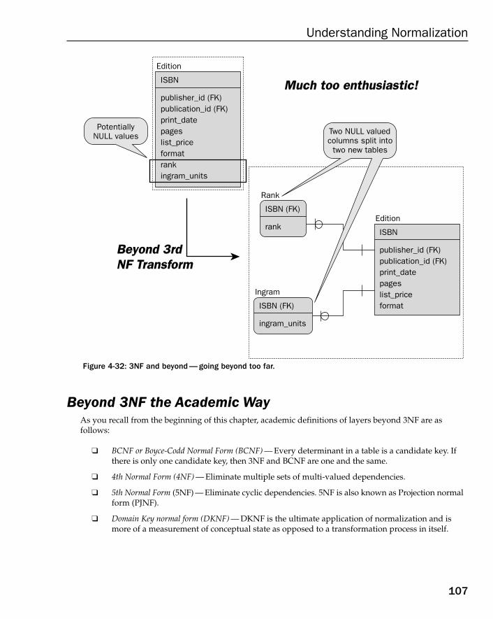
Figure 4-32: 3NF and beyond — going beyond too far.
Beyond 3NF the Academic WayAs you recall from the beginning of this chapter, academic definitions of layers beyond 3NF are as follows:
❑ BCNF or Boyce-Codd Normal Form (BCNF) — Every determinant in a table is a candidate key. Ifthere is only one candidate key, then 3NF and BCNF are one and the same.
❑ 4th Normal Form (4NF) — Eliminate multiple sets of multi-valued dependencies.
❑ 5th Normal Form (5NF) — Eliminate cyclic dependencies. 5NF is also known as Projection normalform (PJNF).
❑ Domain Key normal form (DKNF) — DKNF is the ultimate application of normalization and ismore of a measurement of conceptual state as opposed to a transformation process in itself.
PotentiallyNULL values
Edition
ISBN
publisher_id (FK)publication_id (FK)print_datepageslist_priceformatrankingram_units
Edition
ISBN
publisher_id (FK)publication_id (FK)print_datepageslist_priceformat
Rank
ISBN (FK)
rank
Ingram
ISBN (FK)
ingram_units
Two NULL valuedcolumns split into
two new tables
Beyond 3rdNF TransformBeyond 3rdNF Transform
Much too enthusiastic!Much too enthusiastic!
107
Understanding Normalization
09_574906 ch04.qxd 11/4/05 10:46 AM Page 107

Boyce-Codd Normal Form (BCNF)BCNF does the following.
❑ A table must be in 3NF.
❑ A table can have only one candidate key.
A candidate key has potential for being a table’s primary key. A table is not allowed more than one primary key because referential integrity requires it as such. It would be impossible to check foreign keysagainst more than one primary key. Referential integrity would be automatically invalid, unenforceable,and, thus, there would be no relational database model.
BCNF is an odd one because it is a little like a special case of 3NF. BCNF requires that every determinantin a table is a candidate key. If there is only one candidate key, 3NF and BCNF are the same. What doesthis mean? A determinant is a field whose value may depend other fields for their values. And sometables can be uniquely identified by more than one field or combination of fields. Each one of these is apotential primary key that can uniquely identify records in a table, and, thus, they are candidate keys, orpotential primary keys.
This is where BCNF gets interesting because most examples of BCNF (and, in fact, any level of normaliza-tion beyond 3NF) utilize generally highly complex, multiple table, multiple many-to-many join resolutionissues. You will get to those nasty, horribly complicated examples — just not yet.
The left side of the diagram in Figure 4-33 shows an example of a table with both a surrogate key and anatural key. Surrogate keys are added to tables to replace natural keys because surrogate keys are moreefficient and easier to manage than natural keys. The other problem is that the original primary key (thenatural key) needs a unique qualifier on it to ensure that it is not duplicated. Two customers with thesame name could cause a problem when it comes to sending them both an invoice at the end of themonth. The right side of the diagram in Figure 4-33 shows a BCNF breakdown into an innumerate multiple of tables created from the original table, for any values that are potentially unique. This is whatthe purest form of BCNF essentially requires. It is a little bit ridiculous.
108
Chapter 4
09_574906 ch04.qxd 11/4/05 10:47 AM Page 108
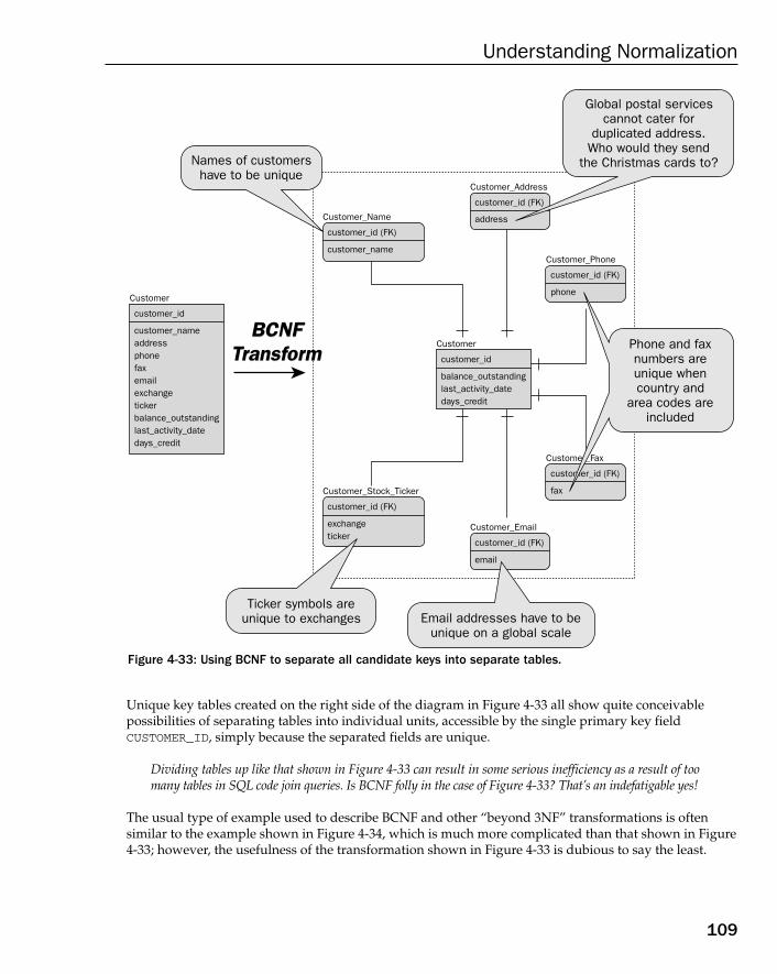
Figure 4-33: Using BCNF to separate all candidate keys into separate tables.
Unique key tables created on the right side of the diagram in Figure 4-33 all show quite conceivable possibilities of separating tables into individual units, accessible by the single primary key field CUSTOMER_ID, simply because the separated fields are unique.
Dividing tables up like that shown in Figure 4-33 can result in some serious inefficiency as a result of toomany tables in SQL code join queries. Is BCNF folly in the case of Figure 4-33? That’s an indefatigable yes!
The usual type of example used to describe BCNF and other “beyond 3NF” transformations is often similar to the example shown in Figure 4-34, which is much more complicated than that shown in Figure4-33; however, the usefulness of the transformation shown in Figure 4-33 is dubious to say the least.
Customer
customer_id
balance_outstandinglast_activity_datedays_credit
Customer
customer_id
customer_nameaddressphonefaxemailexchangetickerbalance_outstandinglast_activity_datedays_credit
Customer_Stock_Ticker
customer_id (FK)
exchangeticker
Customer_Name
customer_id (FK)
customer_name
Customer_Email
customer_id (FK)
Customer_Address
customer_id (FK)
address
Customer_Fax
customer_id (FK)
fax
Customer_Phone
customer_id (FK)
phone
BCNFTransform
BCNFTransform
Names of customershave to be unique
Email addresses have to beunique on a global scale
Ticker symbols areunique to exchanges
Global postal servicescannot cater for
duplicated address.Who would they send
the Christmas cards to?
Phone and faxnumbers areunique whencountry and
area codes areincluded
109
Understanding Normalization
09_574906 ch04.qxd 11/4/05 10:47 AM Page 109
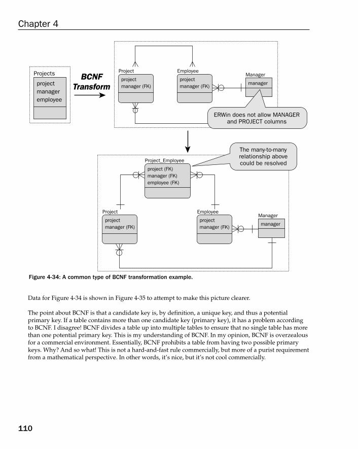
Figure 4-34: A common type of BCNF transformation example.
Data for Figure 4-34 is shown in Figure 4-35 to attempt to make this picture clearer.
The point about BCNF is that a candidate key is, by definition, a unique key, and thus a potential primary key. If a table contains more than one candidate key (primary key), it has a problem accordingto BCNF. I disagree! BCNF divides a table up into multiple tables to ensure that no single table has morethan one potential primary key. This is my understanding of BCNF. In my opinion, BCNF is overzealousfor a commercial environment. Essentially, BCNF prohibits a table from having two possible primarykeys. Why? And so what! This is not a hard-and-fast rule commercially, but more of a purist requirementfrom a mathematical perspective. In other words, it’s nice, but it’s not cool commercially.
Manager
manager
Projects
projectmanageremployee
Project
projectmanager (FK)
Employee
projectmanager (FK)
Manager
manager
Project
projectmanager (FK)
Project_Employee
project (FK)manager (FK)employee (FK)
Employee
projectmanager (FK)
ERWin does not allow MANAGERand PROJECT columns
The many-to-manyrelationship abovecould be resolved
BCNFTransform
BCNFTransform
110
Chapter 4
09_574906 ch04.qxd 11/4/05 10:47 AM Page 110
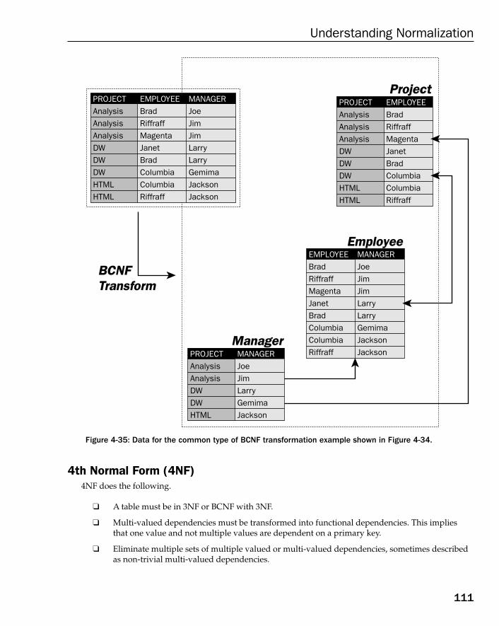
Figure 4-35: Data for the common type of BCNF transformation example shown in Figure 4-34.
4th Normal Form (4NF)4NF does the following.
❑ A table must be in 3NF or BCNF with 3NF.
❑ Multi-valued dependencies must be transformed into functional dependencies. This impliesthat one value and not multiple values are dependent on a primary key.
❑ Eliminate multiple sets of multiple valued or multi-valued dependencies, sometimes describedas non-trivial multi-valued dependencies.
ProjectProject
EmployeeEmployee
ManagerManagerPROJECTALLAnalysisAnalysisDWDWHTML
MANAGERJoeJimLarryGemimaJackson
EMPLOYEEBradRiffraffMagentaJanetBradColumbiaColumbiaRiffraff
MANAGERJoeJimJimLarryLarryGemimaJacksonJackson
PROJECTALLAnalysisAnalysisAnalysisDWDWDWHTMLHTML
EMPLOYEEBradRiffraffMagentaJanetBradColumbiaColumbiaRiffraff
BCNFTransformBCNFTransform
PROJECTALLAnalysisAnalysisAnalysisDWDWDWHTMLHTML
EMPLOYEEBradRiffraffMagentaJanetBradColumbiaColumbiaRiffraff
MANAGERJoeJimJimLarryLarryGemimaJacksonJackson
111
Understanding Normalization
09_574906 ch04.qxd 11/4/05 10:47 AM Page 111
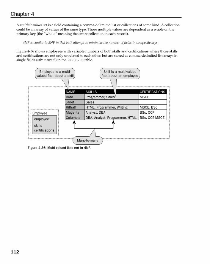
A multiple valued set is a field containing a comma-delimited list or collections of some kind. A collectioncould be an array of values of the same type. Those multiple values are dependent as a whole on the primary key (the “whole” meaning the entire collection in each record).
4NF is similar to 5NF in that both attempt to minimize the number of fields in composite keys.
Figure 4-36 shows employees with variable numbers of both skills and certifications where those skillsand certifications are not only unrelated to each other, but are stored as comma-delimited list arrays insingle fields (take a breath) in the EMPLOYEE table.
Figure 4-36: Multi-valued lists not in 4NF.
Employee
employee
skillscertifications
NAMEBradJanetRiffraffMagentaColumbia
SKILLSProgrammer, SalesSalesHTML, Programmer, WritingAnalyst, DBADBA, Analyst, Programmer, HTML
CERTIFICATIONSMSCE
MSCE, BScBSc, OCPBSc, OCP, MSCE
Employee is a multi-valued fact about a skill
Many-to-many
Skill is a multi-valuedfact about an employee
112
Chapter 4
09_574906 ch04.qxd 11/4/05 10:47 AM Page 112
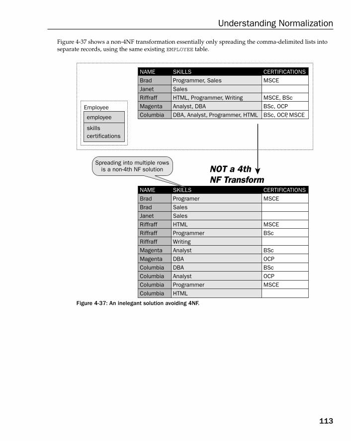
Figure 4-37 shows a non-4NF transformation essentially only spreading the comma-delimited lists intoseparate records, using the same existing EMPLOYEE table.
Figure 4-37: An inelegant solution avoiding 4NF.
NOT a 4thNF TransformNOT a 4thNF Transform
Employee
employee
skillscertifications
NAMEBradJanetRiffraffMagentaColumbia
SKILLSProgrammer, SalesSalesHTML, Programmer, WritingAnalyst, DBADBA, Analyst, Programmer, HTML
CERTIFICATIONSMSCE
MSCE, BScBSc, OCPBSc, OCP, MSCE
NAMEBradBradJanetRiffraffRiffraffRiffraffMagentaMagentaColumbiaColumbiaColumbiaColumbia
SKILLSProgramerSalesSalesHTMLProgrammerWritingAnalystDBADBAAnalystProgrammerHTML
CERTIFICATIONSMSCE
MSCEBSc
BScOCPBScOCPMSCE
Spreading into multiple rowsis a non-4th NF solution
113
Understanding Normalization
09_574906 ch04.qxd 11/4/05 10:47 AM Page 113
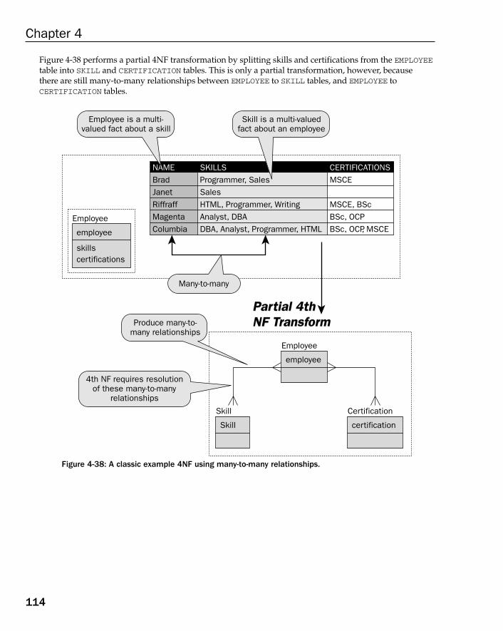
Figure 4-38 performs a partial 4NF transformation by splitting skills and certifications from the EMPLOYEEtable into SKILL and CERTIFICATION tables. This is only a partial transformation, however, because there are still many-to-many relationships between EMPLOYEE to SKILL tables, and EMPLOYEE to CERTIFICATION tables.
Figure 4-38: A classic example 4NF using many-to-many relationships.
Partial 4thNF TransformPartial 4thNF Transform
Employee
employee
skillscertifications
NAMEBradJanetRiffraffMagentaColumbia
SKILLSProgrammer, SalesSalesHTML, Programmer, WritingAnalyst, DBADBA, Analyst, Programmer, HTML
CERTIFICATIONSMSCE
MSCE, BScBSc, OCPBSc, OCP, MSCE
Produce many-to-many relationships
Employee is a multi-valued fact about a skill
Many-to-many
Skill is a multi-valuedfact about an employee
Skill
Skill
Certification
certification
Employee
employee
4th NF requires resolutionof these many-to-many
relationships
114
Chapter 4
09_574906 ch04.qxd 11/4/05 10:47 AM Page 114
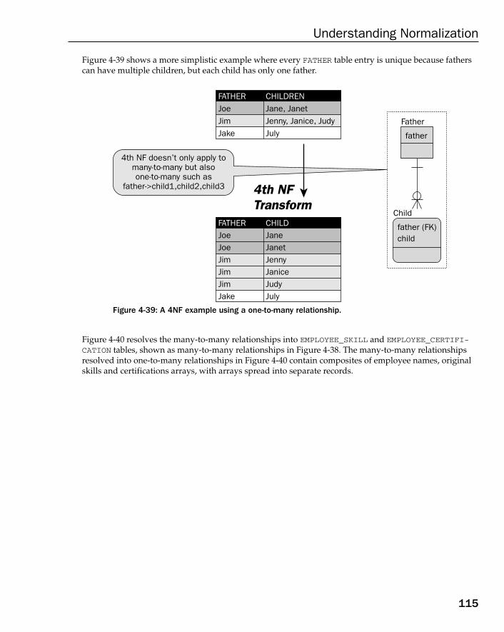
Figure 4-39 shows a more simplistic example where every FATHER table entry is unique because fatherscan have multiple children, but each child has only one father.
Figure 4-39: A 4NF example using a one-to-many relationship.
Figure 4-40 resolves the many-to-many relationships into EMPLOYEE_SKILL and EMPLOYEE_CERTIFI-CATION tables, shown as many-to-many relationships in Figure 4-38. The many-to-many relationshipsresolved into one-to-many relationships in Figure 4-40 contain composites of employee names, originalskills and certifications arrays, with arrays spread into separate records.
4th NF doesn’t only apply tomany-to-many but alsoone-to-many such as
father->child1,child2,child3 4th NFTransform4th NFTransform
Father
father
Child
father (FK)child
FATHERJoeJimJake
CHILDRENJane, JanetJenny, Janice, JudyJuly
FATHERJoeJoeJimJimJimJake
CHILDJaneJanetJennyJaniceJudyJuly
115
Understanding Normalization
09_574906 ch04.qxd 11/4/05 10:47 AM Page 115
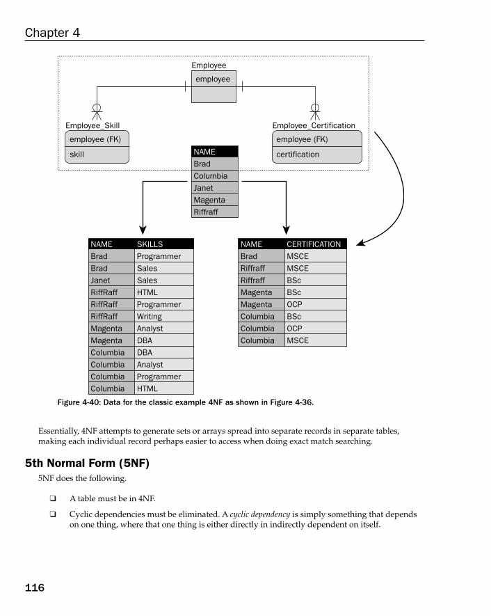
Figure 4-40: Data for the classic example 4NF as shown in Figure 4-36.
Essentially, 4NF attempts to generate sets or arrays spread into separate records in separate tables, making each individual record perhaps easier to access when doing exact match searching.
5th Normal Form (5NF)5NF does the following.
❑ A table must be in 4NF.
❑ Cyclic dependencies must be eliminated. A cyclic dependency is simply something that dependson one thing, where that one thing is either directly in indirectly dependent on itself.
Employee
employee
skill
Employee_Skill
employee (FK)
skill
Employee_Certification
employee (FK)
certification
NAMEBradBradJanetRiffRaffRiffRaffRiffRaffMagentaMagentaColumbiaColumbiaColumbiaColumbia
SKILLSProgrammerSalesSalesHTMLProgrammerWritingAnalystDBADBAAnalystProgrammerHTML
NAMEBradRiffraffRiffraffMagentaMagentaColumbiaColumbiaColumbia
CERTIFICATIONMSCEMSCEBScBScOCPBScOCPMSCE
NAMEBradColumbiaJanetMagentaRiffraff
116
Chapter 4
09_574906 ch04.qxd 11/4/05 10:47 AM Page 116
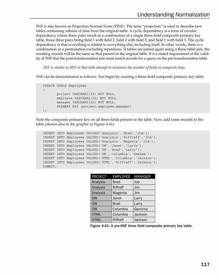
5NF is also known as Projection Normal Form (PJNF). The term “projection” is used to describe newtables containing subsets of data from the original table. A cyclic dependency is a form of circular dependency where three pairs result as a combination of a single three-field composite primary keytable, those three pairs being field 1 with field 2, field 2 with field 3, and field 1 with field 3. The cyclicdependency is that everything is related to everything else, including itself. In other words, there is acombination or a permutation excluding repetitions. If tables are joined again using a three-table join, theresulting records will be the same as that present in the original table. It is a stated requirement of the valid-ity of 5NF that the post-transformation join must match records for a query on the pre-transformation table.
5NF is similar to 4NF in that both attempt to minimize the number of fields in composite keys.
5NF can be demonstrated as follows. You begin by creating a three-field composite primary key table:
CREATE TABLE Employees(
project VARCHAR2(32) NOT NULL,employee VARCHAR2(32) NOT NULL,manager VARCHAR2(32) NOT NULL,PRIMARY KEY (project,employee,manager)
);
Note the composite primary key on all three fields present in the table. Now, add some records to thetable (shown also in the graphic in Figure 4-41):
INSERT INTO Employees VALUES(‘Analysis’,’Brad’,’Joe’);INSERT INTO Employees VALUES(‘Analysis’,’Riffraff’,’Jim’);INSERT INTO Employees VALUES(‘Analysis’,’Magenta’,’Jim’);INSERT INTO Employees VALUES(‘DW’,’Janet’,’Larry’);INSERT INTO Employees VALUES(‘DW’,’Brad’,’Larry’);INSERT INTO Employees VALUES(‘DW’,’Columbia’,’Gemima’);INSERT INTO Employees VALUES(‘HTML’,’Columbia’,’Jackson’);INSERT INTO Employees VALUES(‘HTML’,’Riffraff’,’Jackson’);COMMIT;
Figure 4-41: A pre-5NF three field composite primary key table.
PROJECTALLAnalysisAnalysisAnalysisDWDWDWHTMLHTML
EMPLOYEEBradRiffraffMagentaJanetBradColumbiaColumbiaRiffraff
MANAGERJoeJimJimLarryLarryGemimaJacksonJackson
117
Understanding Normalization
09_574906 ch04.qxd 11/4/05 10:47 AM Page 117
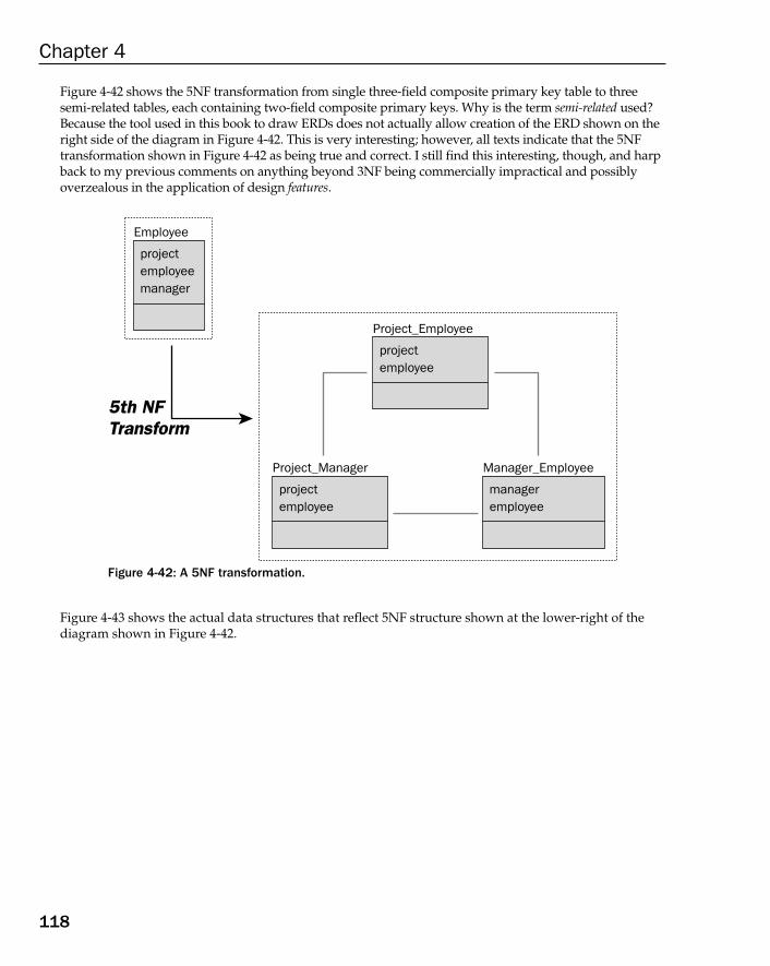
Figure 4-42 shows the 5NF transformation from single three-field composite primary key table to threesemi-related tables, each containing two-field composite primary keys. Why is the term semi-related used?Because the tool used in this book to draw ERDs does not actually allow creation of the ERD shown on theright side of the diagram in Figure 4-42. This is very interesting; however, all texts indicate that the 5NFtransformation shown in Figure 4-42 as being true and correct. I still find this interesting, though, and harpback to my previous comments on anything beyond 3NF being commercially impractical and possiblyoverzealous in the application of design features.
Figure 4-42: A 5NF transformation.
Figure 4-43 shows the actual data structures that reflect 5NF structure shown at the lower-right of thediagram shown in Figure 4-42.
5th NFTransform5th NFTransform
Employee
projectemployeemanager
Project_Employee
projectemployee
Project_Manager
projectemployee
Manager_Employee
manageremployee
118
Chapter 4
09_574906 ch04.qxd 11/4/05 10:47 AM Page 118

Figure 4-43: 5NF transformations sometimes remove duplicates.
Going further with the table-creation commands and record-insertion commands for each of the threeseparate 5NF tables, note that all records added are exactly the same as for adding to the pre-5NF table,with any duplicate records removed. Create the PROJECT_EMPLOYEE table and add records:
CREATE TABLE Project_Employee(
project VARCHAR2(32) NOT NULL,employee VARCHAR2(32) NOT NULL,PRIMARY KEY (project, employee)
);
INSERT INTO Project_Employee VALUES(‘Analysis’,’Brad’);INSERT INTO Project_Employee VALUES(‘Analysis’,’Riffraff’);INSERT INTO Project_Employee VALUES(‘Analysis’,’Magenta’);INSERT INTO Project_Employee VALUES(‘DW’,’Janet’);INSERT INTO Project_Employee VALUES(‘DW’,’Brad’);INSERT INTO Project_Employee VALUES(‘DW’,’Columbia’);INSERT INTO Project_Employee VALUES(‘HTML’,’Columbia’);INSERT INTO Project_Employee VALUES(‘HTML’,’Riffraff’);COMMIT;
PROJECTALLAnalysisAnalysisAnalysisDWDWDWHTMLHTML
EMPLOYEEBradRiffraffMagentaJanetBradColumbiaColumbiaRiffraff
PROJECTALLAnalysisAnalysisDWDWHTML
MANAGERJoeJimLarryGemimaJackson
MANAGERALLGemimaJacksonJacksonJimJimJoeLarryLarry
EMPLOYEEColumbiaColumbiaRiffraffMagentaRiffraffBradBradJanet
Someduplicaterows wereremoved
119
Understanding Normalization
09_574906 ch04.qxd 11/4/05 10:47 AM Page 119
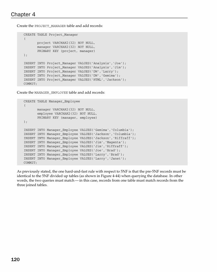
Create the PROJECT_MANAGER table and add records:
CREATE TABLE Project_Manager(
project VARCHAR2(32) NOT NULL,manager VARCHAR2(32) NOT NULL,PRIMARY KEY (project, manager)
);
INSERT INTO Project_Manager VALUES(‘Analysis’,’Joe’);INSERT INTO Project_Manager VALUES(‘Analysis’,’Jim’);INSERT INTO Project_Manager VALUES(‘DW’,’Larry’);INSERT INTO Project_Manager VALUES(‘DW’,’Gemima’);INSERT INTO Project_Manager VALUES(‘HTML’,’Jackson’);COMMIT;
Create the MANAGER_EMPLOYEE table and add records:
CREATE TABLE Manager_Employee(
manager VARCHAR2(32) NOT NULL,employee VARCHAR2(32) NOT NULL,PRIMARY KEY (manager, employee)
);
INSERT INTO Manager_Employee VALUES(‘Gemima’,’Columbia’);INSERT INTO Manager_Employee VALUES(‘Jackson’,’Columbia’);INSERT INTO Manager_Employee VALUES(‘Jackson’,’Riffraff’);INSERT INTO Manager_Employee VALUES(‘Jim’,’Magenta’);INSERT INTO Manager_Employee VALUES(‘Jim’,’Riffraff’);INSERT INTO Manager_Employee VALUES(‘Joe’,’Brad’);INSERT INTO Manager_Employee VALUES(‘Larry’,’Brad’);INSERT INTO Manager_Employee VALUES(‘Larry’,’Janet’);COMMIT;
As previously stated, the one hard-and-fast rule with respect to 5NF is that the pre-5NF records must beidentical to the 5NF divided up tables (as shown in Figure 4-44) when querying the database. In otherwords, the two queries must match — in this case, records from one table must match records from thethree joined tables.
120
Chapter 4
09_574906 ch04.qxd 11/4/05 10:47 AM Page 120
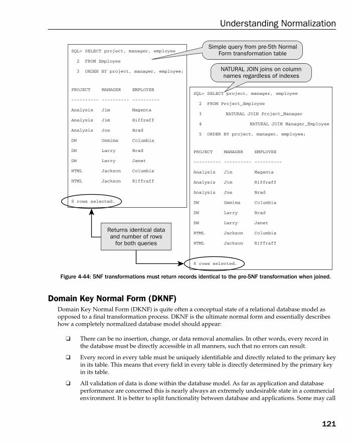
Figure 4-44: 5NF transformations must return records identical to the pre-5NF transformation when joined.
Domain Key Normal Form (DKNF)Domain Key Normal Form (DKNF) is quite often a conceptual state of a relational database model asopposed to a final transformation process. DKNF is the ultimate normal form and essentially describeshow a completely normalized database model should appear:
❑ There can be no insertion, change, or data removal anomalies. In other words, every record inthe database must be directly accessible in all manners, such that no errors can result.
❑ Every record in every table must be uniquely identifiable and directly related to the primary keyin its table. This means that every field in every table is directly determined by the primary keyin its table.
❑ All validation of data is done within the database model. As far as application and database performance are concerned this is nearly always an extremely undesirable state in a commercialenvironment. It is better to split functionality between database and applications. Some may call
SQL> SELECT project, manager, employee
2 FROM Employee 3 ORDER BY project, manager, employee;
PROJECT
----------
Analysis
Analysis
Analysis
DW
DW
DW
HTML
HTML
8 rows selected.
MANAGER
----------
Jim
Jim
Joe
Gemima
Larry
Larry
Jackson
Jackson
EMPLOYEE
----------
Magenta
Riffraff
Brad
Columbia
Brad
Janet
Columbia
Riffraff
SQL> SELECT project, manager, employee
2 FROM Project_Employee 3 NATURAL JOIN Project_Manager
4 NATURAL JOIN Manager_Employee
5 ORDER BY project, manager, employee;
PROJECT
----------
Analysis
Analysis
Analysis
DW
DW
DW
HTML
HTML
8 rows selected.
MANAGER
----------
Jim
Jim
Joe
Gemima
Larry
Larry
Jackson
Jackson
EMPLOYEE
----------
Magenta
Riffraff
Brad
Columbia
Brad
Janet
Columbia
Riffraff
Returns identical dataand number of rows
for both queries
Simple query from pre-5th NormalForm transformation table
NATURAL JOIN joins on columnnames regardless of indexes
121
Understanding Normalization
09_574906 ch04.qxd 11/4/05 10:47 AM Page 121

this business rules. It is generally common knowledge that some business rule implementationis often most effectively divided up between database and applications.
DKNF is an ideal form and an ultimate or final form of relational database normalization. This level ofnormalization is more mathematically perfect and has beauty in its granular simplicity. In an objectdatabase model, this approach is perfectly suited where individual data items are only ever accessed asunique elements (primary keys) and records are never accessed in groups. In a relational database modelwhere commercially most databases require not only exact matches but also range searching for report-ing, this level of intensity in normalization nearly always has a seriously negative impact on generaldatabase and application performance, and thus a negative effect on end-user satisfaction. End-user satisfaction is the objective of any application. If it isn’t, it should be because they usually pay the bills!
SummaryIn this chapter, you learned about:
❑ What normalization is, its benefits and potential hazards
❑ A layman’s method of understanding normalization
❑ A purist, academic definition of normalization
❑ How referential integrity is maintained using primary and foreign keys
❑ Normal Forms from 1st through to 5th, including Boyce-Codd Normal Form and Domain KeyNormal Form
❑ Special terminology used in Normal Forms
The next chapter discusses some advanced relational database modeling techniques, including denormalization, special tricks used for different database model types, followed by introductions to the object database model and data warehouse database modeling.
Exercises1. Write five CREATE TABLE commands for the tables in Figure 4-29. Ensure that all primary key,
foreign key, and any potentially necessary unique keys are included.
2. Write CREATE INDEX commands to create all indexes on any foreign keys indicated in the CREATE TABLE commands written for the previous question.
122
Chapter 4
09_574906 ch04.qxd 11/4/05 10:47 AM Page 122
5Reading and Writing Data
with SQL
“Any sufficiently advanced technology is indistinguishable from magic.” (Arthur C. Clarke)
SQL helps to explain relational database modeling. None of this is magic, and is much easier to understandthan you might think.
This chapter shows how the relational database model is used from an application perspective.There is little point in understanding something, such as relational database modeling, withoutseeing it applied in some way, no matter how simple. With that in mind, this chapter looks at howa database model is accessed when it contains data in a database. A relational database model con-tains tables, and the records in those tables are accessed using Structured Query Language (SQL).SQL is used to create the database access sections of applications. When a database model is correctly designed, creation of SQL code is a simple process. Great difficulties in coding of SQLqueries in particular can often indicate serious database model design flaws.
This book is all about relational database modeling; therefore, it is necessary to explain only the basis of SQL in this book as pertaining directly to helping in the understanding of relationaldatabase modeling. How can describing the basic details of SQL help with the understanding ofrelational database modeling? The answer to this question is very simple. SQL uses a relationaldatabase model to change data in a database, and to retrieve data from that database. SQLessentially applies all the structures created by the relational database modeling process. SQL —and particularly SQL queries and their simplicity — is a direct result of the underlying structure ofa database model. In other words, the better and more appropriate a database model is, the easierbuilding SQL code for applications will be. Another way to look at this is that a database model ismost easily utilized by applications, when matching application structure. It makes perfect senseto describe the basics of using SQL because it demonstrates the use of a relational database modelin action.
10_574906 ch05.qxd 11/4/05 10:47 AM Page 123
In this chapter, you learn about the following:
❑ What SQL is
❑ The origins of SQL
❑ Many types of queries
❑ Changing data in tables
❑ Changing table structure
Defining SQLSQL is a non-procedural language used for accessing field and record values in relational database tables.
A procedural programming language is a language where there can be dependencies between sequentialcommands. For example, when setting a variable X = 1 on a line, that variable X can be used to referencethe value 1, as the variable X in subsequent lines of programming code. A non-procedural programminglanguage does not allow communication between different lines of programming code. Non-procedurallanguages also do not allow use of procedures. A procedure allows intra-program communication by passing values in and out of procedures.
Keep in mind the following when considering what SQL is.
❑ SQL is structured in the sense that it is used to access structured data, in a structured manner, orretrieve data from organized structures. Those organized structures are tables.
❑ Use of the word “language” implies a computer programming language. Computer programminglanguages are often used to get information from a computer.
❑ A non-procedural language essentially submits a single command, with a questioning or queryingtype nature. SQL is a non-procedural language consisting of single commands, where thedatabase itself does a lot of the work in deciding how to get that information. On the otherhand, a procedural language contains blocks of commands. Those blocks of commands aresequences of distinct steps, typically where each successive step is dependent on the result ofthe previous command in the sequence.
❑ In most relational databases, SQL does have the capability to function in a limited proceduralfashion, allowing the programmer to determine partially how a database is accessed.Traditionally, SQL procedural code is used to write what are called stored procedures, triggers,database events, or database procedures. There are other names for these code blocks, depending onthe database in use. Procedural SQL code is generally simplistic and can sometimes allow theinclusion of basic programming constructs such as IF statements, CASE statements, and so on.
So, SQL is a simple non-procedural programming language allowing single line commands. These single-line commands are used to access data stored in database table structures.
124
Chapter 5
10_574906 ch05.qxd 11/4/05 10:47 AM Page 124
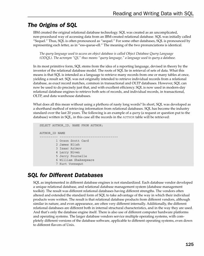
The Origins of SQLIBM created the original relational database technology. SQL was created as an uncomplicated, non-procedural way of accessing data from an IBM-created relational database. SQL was initially called“Sequel.” Thus, SQL is often pronounced as “sequel.” For some other databases, SQL is pronounced byrepresenting each letter, as in “ess-queue-ell.” The meaning of the two pronunciations is identical.
The query language used to access an object database is called Object Database Query Language(ODQL). The acronym “QL” thus means “query language,” a language used to query a database.
In its most primitive form, SQL stems from the idea of a reporting language, devised in theory by theinventor of the relational database model. The roots of SQL lie in retrieval of sets of data. What thismeans is that SQL is intended as a language to retrieve many records from one or many tables at once,yielding a result set. SQL was not originally intended to retrieve individual records from a relationaldatabase, as exact record matches, common in transactional and OLTP databases. However, SQL cannow be used to do precisely just that, and with excellent efficiency. SQL is now used in modern-day relational database engines to retrieve both sets of records, and individual records, in transactional,OLTP, and data warehouse databases.
What does all this mean without using a plethora of nasty long words? In short, SQL was developed asa shorthand method of retrieving information from relational databases. SQL has become the industrystandard over the last 20 years. The following is an example of a query (a request or question put to thedatabase) written in SQL, in this case all the records in the AUTHOR table will be retrieved:
SELECT AUTHOR_ID, NAME FROM AUTHOR;
AUTHOR_ID NAME---------- --------------------------------
1 Orson Scott Card2 James Blish3 Isaac Azimov4 Larry Niven5 Jerry Pournelle6 William Shakespeare7 Kurt Vonnegut
SQL for Different DatabasesSQL as implemented in different database engines is not standardized. Each database vendor developeda unique relational database, and relational database management system (database managementtoolkit). The result was different relational databases having different strengths. The vendors oftenaltered and extended the standard form of SQL to take advantage of the way in which their individualproducts were written. The result is that relational database products from different vendors, althoughsimilar in nature, and even appearance, are often very different internally. Additionally, the differentrelational databases are different both in internal structural characteristics, and in the way they are used.And that’s only the database engine itself. There is also use of different computer hardware platformsand operating systems. The larger database vendors service multiple operating systems, with com-pletely different versions of the database software, applicable to different operating systems, even downto different flavors of Unix.
125
Reading and Writing Data with SQL
10_574906 ch05.qxd 11/4/05 10:47 AM Page 125
Many of the smaller-scale database engines such as dBase and MSAccess are only written for a singleplatform and operating system. In the case of dBase and MSAccess, that system is PC-based, runningthe Windows operating system.
So, what are the basics of SQL?
The Basics of SQLThe basics of SQL consist of a number of parts. This section briefly introduces what simple SQL can do.As you read through this chapter, each is explained individually by example.
❑ Query commands — Querying a database is performed with a single command called the SELECTcommand. The SELECT command creates queries, and has various optional clauses that includeperforming functions such as filtering and sorting. Queries are used to retrieve data from tablesin a database. There are various ways in which data can be retrieved from tables:
Some database engines refer to SQL commands as SQL statements. Don’t get confused. The two termsmean exactly the same thing. I prefer the term “command.” This is merely a personal preference on mypart. The term “clause” is usually applied to subset parts of commands.
❑ Basic query — The most simple of queries retrieves all records from a single table.
❑ Filtered query — A filtered query uses a WHERE clause to include or exclude specific records.
❑ Sorted query — Sorting uses the ORDER BY clause to retrieve records in a specific sortedorder.
❑ Aggregated query — The GROUP BY clause allows summarizing, grouping, or aggregatingof records into summarized record sets. Typically, aggregated queries contain fewerrecords than the query would produce, if the GROUP BY clause were not used. A HAVINGclause can be used to filter in, or filter out, records in the resulting summarized aggregated record set. In other words, the HAVING clause filters the results of the GROUPBY clause, and not the records retrieved before aggregation.
❑ Join query — A join query joins tables together, returning records from multiple tables.Joins can be performed in various ways, including inner joins and outer joins.
❑ Nested queries — A nested query is also known as a subquery, which is a query containedwithin another query (a parent or calling query). Nesting implies that subqueries can benested in multiple layers and thus a subquery itself can also be a calling query of anothersubquery.
❑ Composite queries — A composite query is a query that merges multiple query resultstogether, most often using the UNION keyword.
❑ Data change commands — The following commands are used to change data in tables in adatabase.
❑ INSERT— The INSERT command is used to add new records to a table.
❑ UPDATE— The UPDATE command allows changes to one or more records in a table, at once.
❑ DELETE— The DELETE command allows deletion of one or more records from a table,at once.
126
Chapter 5
10_574906 ch05.qxd 11/4/05 10:47 AM Page 126
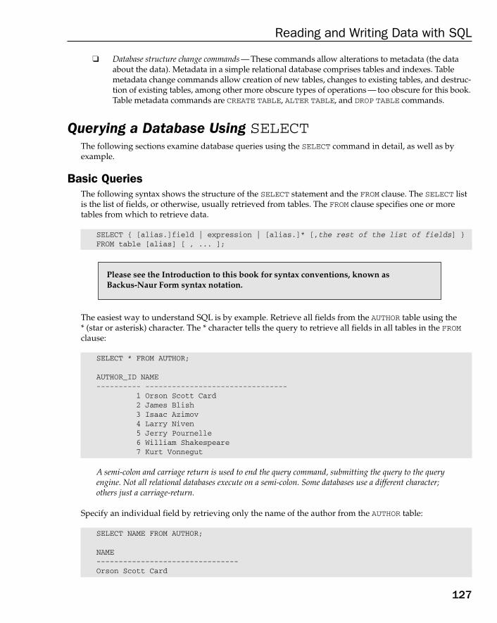
❑ Database structure change commands — These commands allow alterations to metadata (the dataabout the data). Metadata in a simple relational database comprises tables and indexes. Tablemetadata change commands allow creation of new tables, changes to existing tables, and destruc-tion of existing tables, among other more obscure types of operations — too obscure for this book.Table metadata commands are CREATE TABLE, ALTER TABLE, and DROP TABLE commands.
Querying a Database Using SELECTThe following sections examine database queries using the SELECT command in detail, as well as byexample.
Basic QueriesThe following syntax shows the structure of the SELECT statement and the FROM clause. The SELECT listis the list of fields, or otherwise, usually retrieved from tables. The FROM clause specifies one or moretables from which to retrieve data.
SELECT { [alias.]field | expression | [alias.]* [,the rest of the list of fields] }FROM table [alias] [ , ... ];
The easiest way to understand SQL is by example. Retrieve all fields from the AUTHOR table using the* (star or asterisk) character. The * character tells the query to retrieve all fields in all tables in the FROMclause:
SELECT * FROM AUTHOR;
AUTHOR_ID NAME---------- --------------------------------
1 Orson Scott Card2 James Blish3 Isaac Azimov4 Larry Niven5 Jerry Pournelle6 William Shakespeare7 Kurt Vonnegut
A semi-colon and carriage return is used to end the query command, submitting the query to the queryengine. Not all relational databases execute on a semi-colon. Some databases use a different character;others just a carriage-return.
Specify an individual field by retrieving only the name of the author from the AUTHOR table:
SELECT NAME FROM AUTHOR;
NAME--------------------------------Orson Scott Card
Please see the Introduction to this book for syntax conventions, known as Backus-Naur Form syntax notation.
127
Reading and Writing Data with SQL
10_574906 ch05.qxd 11/4/05 10:47 AM Page 127
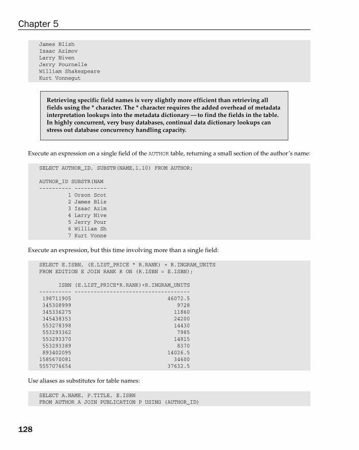
James BlishIsaac AzimovLarry NivenJerry PournelleWilliam ShakespeareKurt Vonnegut
Execute an expression on a single field of the AUTHOR table, returning a small section of the author’s name:
SELECT AUTHOR_ID, SUBSTR(NAME,1,10) FROM AUTHOR;
AUTHOR_ID SUBSTR(NAM---------- ----------
1 Orson Scot2 James Blis3 Isaac Azim4 Larry Nive5 Jerry Pour6 William Sh7 Kurt Vonne
Execute an expression, but this time involving more than a single field:
SELECT E.ISBN, (E.LIST_PRICE * R.RANK) + R.INGRAM_UNITSFROM EDITION E JOIN RANK R ON (R.ISBN = E.ISBN);
ISBN (E.LIST_PRICE*R.RANK)+R.INGRAM_UNITS---------- ------------------------------------198711905 46072.5345308999 9728345336275 11860345438353 24200553278398 14430553293362 7985553293370 14815553293389 8370893402095 14026.5
1585670081 346005557076654 37632.5
Use aliases as substitutes for table names:
SELECT A.NAME, P.TITLE, E.ISBNFROM AUTHOR A JOIN PUBLICATION P USING (AUTHOR_ID)
Retrieving specific field names is very slightly more efficient than retrieving allfields using the * character. The * character requires the added overhead of metadatainterpretation lookups into the metadata dictionary — to find the fields in the table.In highly concurrent, very busy databases, continual data dictionary lookups canstress out database concurrency handling capacity.
128
Chapter 5
10_574906 ch05.qxd 11/4/05 10:47 AM Page 128
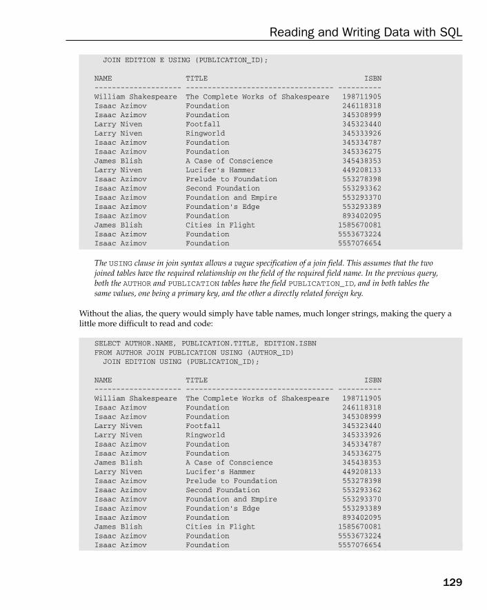
JOIN EDITION E USING (PUBLICATION_ID);
NAME TITLE ISBN-------------------- ---------------------------------- ----------William Shakespeare The Complete Works of Shakespeare 198711905Isaac Azimov Foundation 246118318Isaac Azimov Foundation 345308999Larry Niven Footfall 345323440Larry Niven Ringworld 345333926Isaac Azimov Foundation 345334787Isaac Azimov Foundation 345336275James Blish A Case of Conscience 345438353Larry Niven Lucifer’s Hammer 449208133Isaac Azimov Prelude to Foundation 553278398Isaac Azimov Second Foundation 553293362Isaac Azimov Foundation and Empire 553293370Isaac Azimov Foundation’s Edge 553293389Isaac Azimov Foundation 893402095James Blish Cities in Flight 1585670081Isaac Azimov Foundation 5553673224Isaac Azimov Foundation 5557076654
The USING clause in join syntax allows a vague specification of a join field. This assumes that the twojoined tables have the required relationship on the field of the required field name. In the previous query,both the AUTHOR and PUBLICATION tables have the field PUBLICATION_ID, and in both tables thesame values, one being a primary key, and the other a directly related foreign key.
Without the alias, the query would simply have table names, much longer strings, making the query alittle more difficult to read and code:
SELECT AUTHOR.NAME, PUBLICATION.TITLE, EDITION.ISBNFROM AUTHOR JOIN PUBLICATION USING (AUTHOR_ID)
JOIN EDITION USING (PUBLICATION_ID);
NAME TITLE ISBN-------------------- ---------------------------------- ----------William Shakespeare The Complete Works of Shakespeare 198711905Isaac Azimov Foundation 246118318Isaac Azimov Foundation 345308999Larry Niven Footfall 345323440Larry Niven Ringworld 345333926Isaac Azimov Foundation 345334787Isaac Azimov Foundation 345336275James Blish A Case of Conscience 345438353Larry Niven Lucifer’s Hammer 449208133Isaac Azimov Prelude to Foundation 553278398Isaac Azimov Second Foundation 553293362Isaac Azimov Foundation and Empire 553293370Isaac Azimov Foundation’s Edge 553293389Isaac Azimov Foundation 893402095James Blish Cities in Flight 1585670081Isaac Azimov Foundation 5553673224Isaac Azimov Foundation 5557076654
129
Reading and Writing Data with SQL
10_574906 ch05.qxd 11/4/05 10:47 AM Page 129
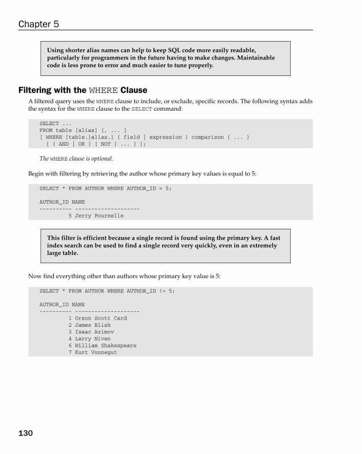
Filtering with the WHERE ClauseA filtered query uses the WHERE clause to include, or exclude, specific records. The following syntax addsthe syntax for the WHERE clause to the SELECT command:
SELECT ...FROM table [alias] [, ... ][ WHERE [table.|alias.] { field | expression } comparison { ... }
[ { AND | OR } [ NOT ] ... ] ];
The WHERE clause is optional.
Begin with filtering by retrieving the author whose primary key values is equal to 5:
SELECT * FROM AUTHOR WHERE AUTHOR_ID = 5;
AUTHOR_ID NAME---------- --------------------
5 Jerry Pournelle
Now find everything other than authors whose primary key value is 5:
SELECT * FROM AUTHOR WHERE AUTHOR_ID != 5;
AUTHOR_ID NAME---------- --------------------
1 Orson Scott Card2 James Blish3 Isaac Azimov4 Larry Niven6 William Shakespeare7 Kurt Vonnegut
This filter is efficient because a single record is found using the primary key. A fastindex search can be used to find a single record very quickly, even in an extremelylarge table.
Using shorter alias names can help to keep SQL code more easily readable, particularly for programmers in the future having to make changes. Maintainablecode is less prone to error and much easier to tune properly.
130
Chapter 5
10_574906 ch05.qxd 11/4/05 10:47 AM Page 130
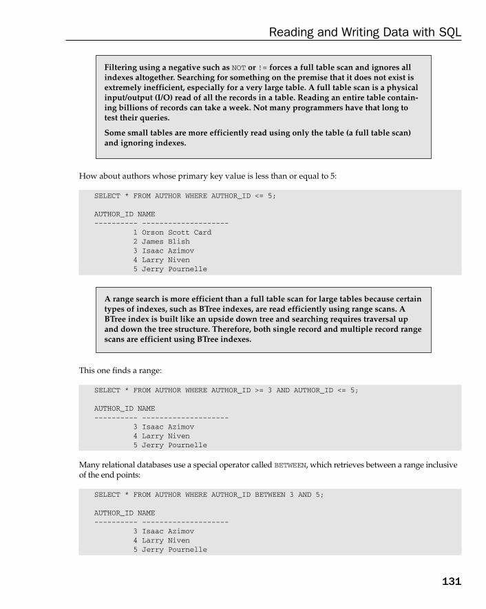
How about authors whose primary key value is less than or equal to 5:
SELECT * FROM AUTHOR WHERE AUTHOR_ID <= 5;
AUTHOR_ID NAME---------- --------------------
1 Orson Scott Card2 James Blish3 Isaac Azimov4 Larry Niven5 Jerry Pournelle
This one finds a range:
SELECT * FROM AUTHOR WHERE AUTHOR_ID >= 3 AND AUTHOR_ID <= 5;
AUTHOR_ID NAME---------- --------------------
3 Isaac Azimov4 Larry Niven5 Jerry Pournelle
Many relational databases use a special operator called BETWEEN, which retrieves between a range inclusiveof the end points:
SELECT * FROM AUTHOR WHERE AUTHOR_ID BETWEEN 3 AND 5;
AUTHOR_ID NAME---------- --------------------
3 Isaac Azimov4 Larry Niven5 Jerry Pournelle
A range search is more efficient than a full table scan for large tables because certaintypes of indexes, such as BTree indexes, are read efficiently using range scans. ABTree index is built like an upside down tree and searching requires traversal upand down the tree structure. Therefore, both single record and multiple record rangescans are efficient using BTree indexes.
Filtering using a negative such as NOT or != forces a full table scan and ignores allindexes altogether. Searching for something on the premise that it does not exist isextremely inefficient, especially for a very large table. A full table scan is a physicalinput/output (I/O) read of all the records in a table. Reading an entire table contain-ing billions of records can take a week. Not many programmers have that long totest their queries.
Some small tables are more efficiently read using only the table (a full table scan)and ignoring indexes.
131
Reading and Writing Data with SQL
10_574906 ch05.qxd 11/4/05 10:47 AM Page 131
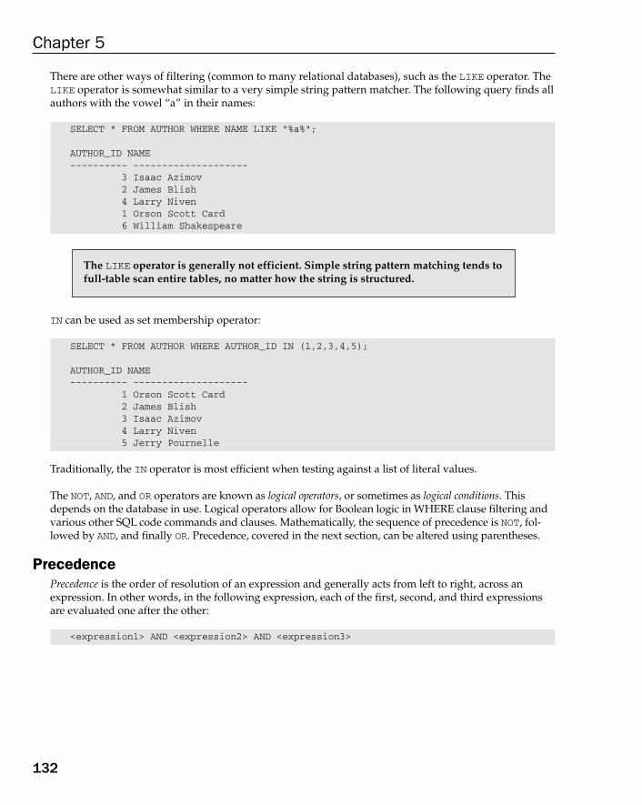
There are other ways of filtering (common to many relational databases), such as the LIKE operator. TheLIKE operator is somewhat similar to a very simple string pattern matcher. The following query finds allauthors with the vowel “a” in their names:
SELECT * FROM AUTHOR WHERE NAME LIKE “%a%”;
AUTHOR_ID NAME---------- --------------------
3 Isaac Azimov2 James Blish4 Larry Niven1 Orson Scott Card6 William Shakespeare
IN can be used as set membership operator:
SELECT * FROM AUTHOR WHERE AUTHOR_ID IN (1,2,3,4,5);
AUTHOR_ID NAME---------- --------------------
1 Orson Scott Card2 James Blish3 Isaac Azimov4 Larry Niven5 Jerry Pournelle
Traditionally, the IN operator is most efficient when testing against a list of literal values.
The NOT, AND, and OR operators are known as logical operators, or sometimes as logical conditions. Thisdepends on the database in use. Logical operators allow for Boolean logic in WHERE clause filtering andvarious other SQL code commands and clauses. Mathematically, the sequence of precedence is NOT, fol-lowed by AND, and finally OR. Precedence, covered in the next section, can be altered using parentheses.
PrecedencePrecedence is the order of resolution of an expression and generally acts from left to right, across anexpression. In other words, in the following expression, each of the first, second, and third expressionsare evaluated one after the other:
<expression1> AND <expression2> AND <expression3>
The LIKE operator is generally not efficient. Simple string pattern matching tends tofull-table scan entire tables, no matter how the string is structured.
132
Chapter 5
10_574906 ch05.qxd 11/4/05 10:47 AM Page 132
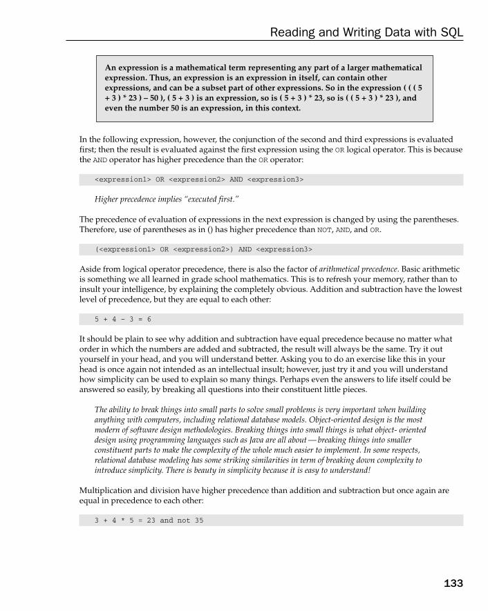
In the following expression, however, the conjunction of the second and third expressions is evaluatedfirst; then the result is evaluated against the first expression using the OR logical operator. This is becausethe AND operator has higher precedence than the OR operator:
<expression1> OR <expression2> AND <expression3>
Higher precedence implies “executed first.”
The precedence of evaluation of expressions in the next expression is changed by using the parentheses.Therefore, use of parentheses as in () has higher precedence than NOT, AND, and OR.
(<expression1> OR <expression2>) AND <expression3>
Aside from logical operator precedence, there is also the factor of arithmetical precedence. Basic arithmeticis something we all learned in grade school mathematics. This is to refresh your memory, rather than toinsult your intelligence, by explaining the completely obvious. Addition and subtraction have the lowestlevel of precedence, but they are equal to each other:
5 + 4 – 3 = 6
It should be plain to see why addition and subtraction have equal precedence because no matter whatorder in which the numbers are added and subtracted, the result will always be the same. Try it outyourself in your head, and you will understand better. Asking you to do an exercise like this in yourhead is once again not intended as an intellectual insult; however, just try it and you will understandhow simplicity can be used to explain so many things. Perhaps even the answers to life itself could beanswered so easily, by breaking all questions into their constituent little pieces.
The ability to break things into small parts to solve small problems is very important when buildinganything with computers, including relational database models. Object-oriented design is the mostmodern of software design methodologies. Breaking things into small things is what object- orienteddesign using programming languages such as Java are all about — breaking things into smaller constituent parts to make the complexity of the whole much easier to implement. In some respects, relational database modeling has some striking similarities in term of breaking down complexity tointroduce simplicity. There is beauty in simplicity because it is easy to understand!
Multiplication and division have higher precedence than addition and subtraction but once again areequal in precedence to each other:
3 + 4 * 5 = 23 and not 35
An expression is a mathematical term representing any part of a larger mathematicalexpression. Thus, an expression is an expression in itself, can contain other expressions, and can be a subset part of other expressions. So in the expression ( ( ( 5+ 3 ) * 23 ) – 50 ), ( 5 + 3 ) is an expression, so is ( 5 + 3 ) * 23, so is ( ( 5 + 3 ) * 23 ), andeven the number 50 is an expression, in this context.
133
Reading and Writing Data with SQL
10_574906 ch05.qxd 11/4/05 10:47 AM Page 133
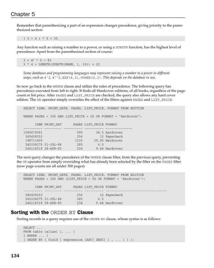
Remember that parenthesizing a part of an expression changes precedence, giving priority to the paren-thesized section:
( 3 + 4 ) * 5 = 35
Any function such as raising a number to a power, or using a SUBSTR function, has the highest level ofprecedence. Apart from the parenthesized section of course:
3 + 42 * 5 = 833 * 4 + LENGTH(SUBSTR(NAME, 1, 10)) = 22
Some databases and programming languages may represent raising a number to a power in differentways, such as 4^2, 4^^2, EXP(4,2), POWER(4,2). This depends on the database in use.
So now go back to the WHERE clause and utilize the rules of precedence. The following query has precedence executed from left to right. It finds all Hardcover editions, of all books, regardless of the pagecount or list price. After PAGES and LIST_PRICE are checked, the query also allows any hard cover edition. The OR operator simply overrides the effect of the filters against PAGES and LIST_PRICE:
SELECT ISBN, PRINT_DATE, PAGES, LIST_PRICE, FORMAT FROM EDITION
WHERE PAGES < 300 AND LIST_PRICE < 50 OR FORMAT = “Hardcover”;
ISBN PRINT_DAT PAGES LIST_PRICE FORMAT---------- --------- ---------- ---------- --------------1585670081 590 34.5 Hardcover345438353 256 12 Paperback198711905 1232 39.95 Hardcover345336275 31-JUL-86 285 6.5246118318 28-APR-83 234 9.44 Hardcover
The next query changes the precedence of the WHERE clause filter, from the previous query, preventingthe OR operator from simply overriding what has already been selected by the filter on the PAGES filter(now page counts are all under 300 pages):
SELECT ISBN, PRINT_DATE, PAGES, LIST_PRICE, FORMAT FROM EDITIONWHERE PAGES < 300 AND (LIST_PRICE < 50 OR FORMAT = ‘Hardcover’);
ISBN PRINT_DAT PAGES LIST_PRICE FORMAT---------- --------- ---------- ---------- --------------------------------345438353 256 12 Paperback345336275 31-JUL-86 285 6.5246118318 28-APR-83 234 9.44 Hardcover
Sorting with the ORDER BY ClauseSorting records in a query requires use of the ORDER BY clause, whose syntax is as follows:
SELECT ...FROM table [alias] [, ... ][ WHERE ... ][ ORDER BY { field | expression [ASC| DESC] [ , ... ] } ];
134
Chapter 5
10_574906 ch05.qxd 11/4/05 10:47 AM Page 134

The ORDER BY clause is optional.
Sorting with the ORDER BY clause allows resorting into an order other than the natural physical orderthat records were originally added into a table. This example sorts by AUTHOR_ID, contained within thename of the author (the NAME field):
SELECT * FROM AUTHOR ORDER BY NAME, AUTHOR_ID;
AUTHOR_ID NAME---------- -------------------
3 Isaac Azimov2 James Blish5 Jerry Pournelle7 Kurt Vonnegut4 Larry Niven1 Orson Scott Card6 William Shakespeare
Different databases allow different formats for ORDER BY clause syntax. Some formats are more restric-tive than others.
Aggregating with the GROUP BY ClauseAn aggregated query uses the GROUP BY clause to summarize repeating groups of records into aggregationsof those groups. The following syntax adds the syntax for the GROUP BY clause:
SELECT ...FROM table [alias] [, ... ][ WHERE ... ]
[ GROUP BY expression [, ... ] [ HAVING condition ] ][ ORDER BY ... ];
The GROUP BY clause is optional.
Some databases allow special expansions to the GROUP BY clause, allowing creation of rollup and cubicquery output, even to the point of creating highly complex spreadsheet or On-Line Analytical process(OLAP) type analytical output rollups create rollup totals, such as subtotals for each grouping in anested groups query. Cubic output allows for reporting such as cross-tabbing and similar cross sectionsof data. Lookup OLAP, rollup and cubic data on the Internet for more information. OLAP is animmense topic in itself and detailed explanation does not belong in this book.
Some queries, depending on data retrieved, whether tables or indexes are read,which clause are used — can be sorted without use of the ORDER BY clause. It is rarebut it is possible. Using the ORDER BY clause in all situations can be inefficient.
135
Reading and Writing Data with SQL
10_574906 ch05.qxd 11/4/05 10:47 AM Page 135

A simple application of the GROUP BY clause is to create a summary, as in the following example, creatingan average price for all editions, printed by each publisher:
SELECT P.NAME AS PUBLISHER, AVG(E.LIST_PRICE)FROM PUBLISHER P JOIN EDITION E USING (PUBLISHER_ID)GROUP BY P.NAME;
PUBLISHER AVG(E.LIST_PRICE)-------------------------------- -----------------Ballantine Books 8.49666667Bantam Books 7.5Books on Tape 29.97Del Rey Books 6.99Fawcett Books 6.99HarperCollins Publishers 9.44L P Books 7.49Overlook Press 34.5Oxford University Press 39.95Spectra 7.5
In this example, an average price is returned for each publisher. Individual editions of books are summa-rized into each average, for each publisher; therefore, individual editions of each book are not returnedas separate records because they are summarized into the averages.
The next example selects only the averages for publishers, where that average is greater than 10:
SELECT P.NAME AS PUBLISHER, AVG(E.LIST_PRICE)FROM PUBLISHER P JOIN EDITION E USING (PUBLISHER_ID)GROUP BY P.NAMEHAVING AVG(E.LIST_PRICE) > 10;
PUBLISHER AVG(E.LIST_PRICE)-------------------------------- -----------------Books on Tape 29.97Overlook Press 34.5Oxford University Press 39.95
The AS clause in the preceding query renames a field in a query.
The above example filters out aggregated records.
Note the sequence of the different clauses in the previous syntax. The WHERE clauseis always executed first, and the ORDER BY clause is always executed last. It followsthat the GROUP BY clause always appears after a WHERE clause, and always before anORDER BY clause.
136
Chapter 5
10_574906 ch05.qxd 11/4/05 10:47 AM Page 136
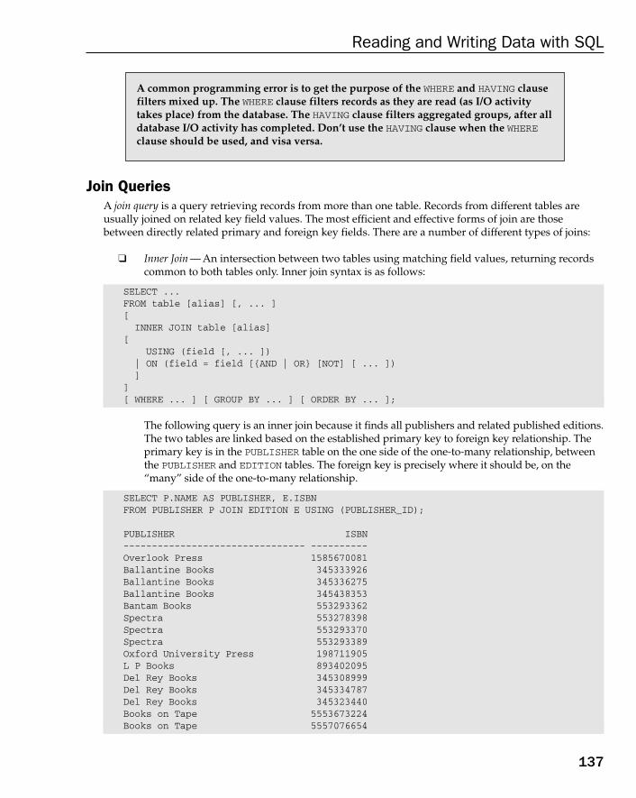
Join QueriesA join query is a query retrieving records from more than one table. Records from different tables are usually joined on related key field values. The most efficient and effective forms of join are thosebetween directly related primary and foreign key fields. There are a number of different types of joins:
❑ Inner Join — An intersection between two tables using matching field values, returning recordscommon to both tables only. Inner join syntax is as follows:
SELECT ...FROM table [alias] [, ... ][
INNER JOIN table [alias][
USING (field [, ... ])| ON (field = field [{AND | OR} [NOT] [ ... ])]
][ WHERE ... ] [ GROUP BY ... ] [ ORDER BY ... ];
The following query is an inner join because it finds all publishers and related published editions.The two tables are linked based on the established primary key to foreign key relationship. Theprimary key is in the PUBLISHER table on the one side of the one-to-many relationship, betweenthe PUBLISHER and EDITION tables. The foreign key is precisely where it should be, on the“many” side of the one-to-many relationship.
SELECT P.NAME AS PUBLISHER, E.ISBNFROM PUBLISHER P JOIN EDITION E USING (PUBLISHER_ID);
PUBLISHER ISBN-------------------------------- ----------Overlook Press 1585670081Ballantine Books 345333926Ballantine Books 345336275Ballantine Books 345438353Bantam Books 553293362Spectra 553278398Spectra 553293370Spectra 553293389Oxford University Press 198711905L P Books 893402095Del Rey Books 345308999Del Rey Books 345334787Del Rey Books 345323440Books on Tape 5553673224Books on Tape 5557076654
A common programming error is to get the purpose of the WHERE and HAVING clausefilters mixed up. The WHERE clause filters records as they are read (as I/O activitytakes place) from the database. The HAVING clause filters aggregated groups, after alldatabase I/O activity has completed. Don’t use the HAVING clause when the WHEREclause should be used, and visa versa.
137
Reading and Writing Data with SQL
10_574906 ch05.qxd 11/4/05 10:47 AM Page 137
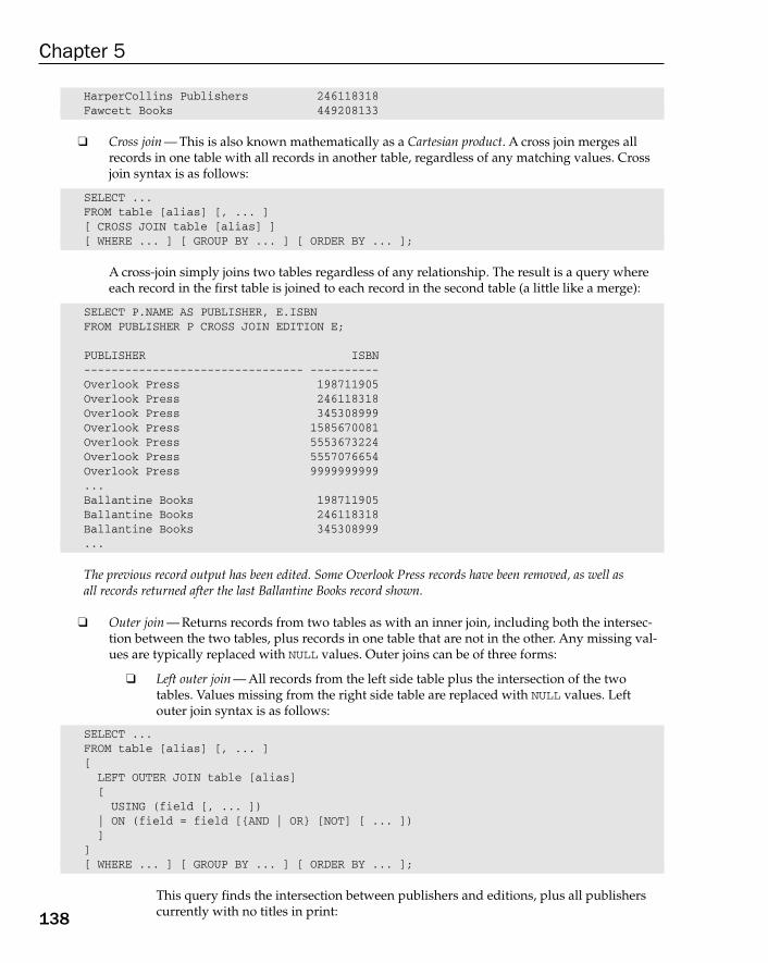
HarperCollins Publishers 246118318Fawcett Books 449208133
❑ Cross join — This is also known mathematically as a Cartesian product. A cross join merges allrecords in one table with all records in another table, regardless of any matching values. Crossjoin syntax is as follows:
SELECT ...FROM table [alias] [, ... ][ CROSS JOIN table [alias] ][ WHERE ... ] [ GROUP BY ... ] [ ORDER BY ... ];
A cross-join simply joins two tables regardless of any relationship. The result is a query whereeach record in the first table is joined to each record in the second table (a little like a merge):
SELECT P.NAME AS PUBLISHER, E.ISBNFROM PUBLISHER P CROSS JOIN EDITION E;
PUBLISHER ISBN-------------------------------- ----------Overlook Press 198711905Overlook Press 246118318Overlook Press 345308999Overlook Press 1585670081Overlook Press 5553673224Overlook Press 5557076654Overlook Press 9999999999...Ballantine Books 198711905Ballantine Books 246118318Ballantine Books 345308999...
The previous record output has been edited. Some Overlook Press records have been removed, as well asall records returned after the last Ballantine Books record shown.
❑ Outer join — Returns records from two tables as with an inner join, including both the intersec-tion between the two tables, plus records in one table that are not in the other. Any missing val-ues are typically replaced with NULL values. Outer joins can be of three forms:
❑ Left outer join — All records from the left side table plus the intersection of the twotables. Values missing from the right side table are replaced with NULL values. Leftouter join syntax is as follows:
SELECT ...FROM table [alias] [, ... ][
LEFT OUTER JOIN table [alias][
USING (field [, ... ])| ON (field = field [{AND | OR} [NOT] [ ... ])]
][ WHERE ... ] [ GROUP BY ... ] [ ORDER BY ... ];
This query finds the intersection between publishers and editions, plus all publisherscurrently with no titles in print:138
Chapter 5
10_574906 ch05.qxd 11/4/05 10:47 AM Page 138
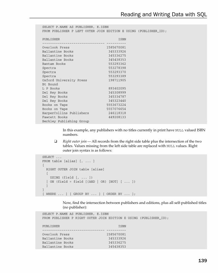
SELECT P.NAME AS PUBLISHER, E.ISBNFROM PUBLISHER P LEFT OUTER JOIN EDITION E USING (PUBLISHER_ID);
PUBLISHER ISBN-------------------------------- ----------Overlook Press 1585670081Ballantine Books 345333926Ballantine Books 345336275Ballantine Books 345438353Bantam Books 553293362Spectra 553278398Spectra 553293370Spectra 553293389Oxford University Press 198711905Bt BoundL P Books 893402095Del Rey Books 345308999Del Rey Books 345334787Del Rey Books 345323440Books on Tape 5553673224Books on Tape 5557076654HarperCollins Publishers 246118318Fawcett Books 449208133Berkley Publishing Group
In this example, any publishers with no titles currently in print have NULL valued ISBNnumbers.
❑ Right outer join — All records from the right side table plus the intersection of the twotables. Values missing from the left side table are replaced with NULL values. Rightouter join syntax is as follows:
SELECT ...FROM table [alias] [, ... ][
RIGHT OUTER JOIN table [alias][
USING (field [, ... ])| ON (field = field [{AND | OR} [NOT] [ ... ])]
][ WHERE ... ] [ GROUP BY ... ] [ ORDER BY ... ];
Now, find the intersection between publishers and editions, plus all self-published titles(no publisher):
SELECT P.NAME AS PUBLISHER, E.ISBNFROM PUBLISHER P RIGHT OUTER JOIN EDITION E USING (PUBLISHER_ID);
PUBLISHER ISBN-------------------------------- ----------Overlook Press 1585670081Ballantine Books 345333926Ballantine Books 345336275Ballantine Books 345438353
139
Reading and Writing Data with SQL
10_574906 ch05.qxd 11/4/05 10:47 AM Page 139

Bantam Books 553293362Spectra 553278398Spectra 553293389Spectra 553293370Oxford University Press 198711905L P Books 893402095Del Rey Books 345323440Del Rey Books 345334787Del Rey Books 345308999Books on Tape 5553673224Books on Tape 5557076654HarperCollins Publishers 246118318Fawcett Books 449208133
9999999999
In this example, books without a publisher would have NULL valued publishing houseentries.
❑ Full outer join — The intersection plus all records from the right side table not in the leftside table, in addition to all records from the left side table not in the right side table.Full outer join syntax is as follows:
SELECT ...FROM table [alias] [, ... ][
FULL OUTER JOIN table [alias][
USING (field [, ... ])| ON (field = field [{AND | OR} [NOT] [ ... ])]
][ WHERE ... ] [ GROUP BY ... ] [ ORDER BY ... ];
This query finds the full outer join, effectively both the left and the right outer joins atthe same time:
SELECT P.NAME AS PUBLISHER, E.ISBNFROM PUBLISHER P FULL OUTER JOIN EDITION E USING (PUBLISHER_ID);
PUBLISHER ISBN-------------------------------- ----------Overlook Press 1585670081Ballantine Books 345333926Ballantine Books 345336275Ballantine Books 345438353Bantam Books 553293362Spectra 553278398Spectra 553293370Spectra 553293389Oxford University Press 198711905Bt BoundL P Books 893402095Del Rey Books 345308999Del Rey Books 345334787Del Rey Books 345323440Books on Tape 5553673224
140
Chapter 5
10_574906 ch05.qxd 11/4/05 10:47 AM Page 140
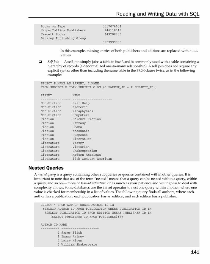
Books on Tape 5557076654HarperCollins Publishers 246118318Fawcett Books 449208133Berkley Publishing Group
9999999999
In this example, missing entries of both publishers and editions are replaced with NULLvalues.
❑ Self Join — A self join simply joins a table to itself, and is commonly used with a table containing ahierarchy of records (a denormalized one-to-many relationship). A self join does not require anyexplicit syntax other than including the same table in the FROM clause twice, as in the followingexample:
SELECT P.NAME AS PARENT, C.NAMEFROM SUBJECT P JOIN SUBJECT C ON (C.PARENT_ID = P.SUBJECT_ID);
PARENT NAME---------------- ---------------------Non-Fiction Self HelpNon-Fiction EsotericNon-Fiction MetaphysicsNon-Fiction ComputersFiction Science FictionFiction FantasyFiction DramaFiction WhodunnitFiction SuspenseFiction LiteratureLiterature PoetryLiterature VictorianLiterature ShakespearianLiterature Modern AmericanLiterature 19th Century American
Nested QueriesA nested query is a query containing other subqueries or queries contained within other queries. It isimportant to note that use of the term “nested” means that a query can be nested within a query, withina query, and so on — more or less ad infinitum, or as much as your patience and willingness to deal withcomplexity allows. Some databases use the IN set operator to nest one query within another, where onevalue is checked for membership in a list of values. The following query finds all authors, where eachauthor has a publication, each publication has an edition, and each edition has a publisher:
SELECT * FROM AUTHOR WHERE AUTHOR_ID IN(SELECT AUTHOR_ID FROM PUBLICATION WHERE PUBLICATION_ID IN(SELECT PUBLICATION_ID FROM EDITION WHERE PUBLISHER_ID IN
(SELECT PUBLISHER_ID FROM PUBLISHER)));
AUTHOR_ID NAME---------- --------------------
2 James Blish3 Isaac Azimov4 Larry Niven6 William Shakespeare
141
Reading and Writing Data with SQL
10_574906 ch05.qxd 11/4/05 10:47 AM Page 141

Some databases also allow use of the EXISTS keyword. The EXISTS keyword returns a Boolean Trueresult if the result is positive (it exists), or False otherwise. Where the IN operator includes expressionson both sides, the EXISTS operator has an expression only on the right side of the comparison. The nextquery finds all authors where the author exists as a foreign key AUTHOR_ID value in the PUBLISHER table:
SELECT * FROM AUTHOR WHERE EXISTS(SELECT AUTHOR_ID FROM PUBLICATION);
AUTHOR_ID NAME---------- --------------------
1 Orson Scott Card2 James Blish3 Isaac Azimov4 Larry Niven5 Jerry Pournelle6 William Shakespeare7 Kurt Vonnegut
It is often also possible to pass a cross checking or correlation value into a subquery, such as in the following case using EXISTS. The query is a slightly more complex variation on the previous one wherethe AUTHOR_ID value, for each record found in the AUTHOR table, is passed to the subquery, and used bythe subquery, to match with a PUBLISHER record:
A correlation between a calling query and a subquery is a link where variables in calling query and subquery are expected to contain the same values. The correlation link is usually a primary key to for-eign key link — but it doesn’t have to be.
SELECT * FROM AUTHOR WHERE EXISTS(SELECT AUTHOR_ID FROM PUBLICATION WHERE AUTHOR_ID = AUTHOR.AUTHOR_ID);
AUTHOR_ID NAME---------- --------------------
2 James Blish3 Isaac Azimov4 Larry Niven6 William Shakespeare7 Kurt Vonnegut
Sometimes a correlation can be established between the calling query and subquery, using the IN operatoras well as the EXISTS operator, although this is not as common. The next query is almost identical to theprevious query, except that it uses the IN operator:
SELECT * FROM AUTHOR WHERE AUTHOR_ID IN(SELECT AUTHOR_ID FROM PUBLICATION WHERE AUTHOR_ID = AUTHOR.AUTHOR_ID);
AUTHOR_ID NAME---------- --------------------
2 James Blish3 Isaac Azimov4 Larry Niven6 William Shakespeare7 Kurt Vonnegut
142
Chapter 5
10_574906 ch05.qxd 11/4/05 10:47 AM Page 142
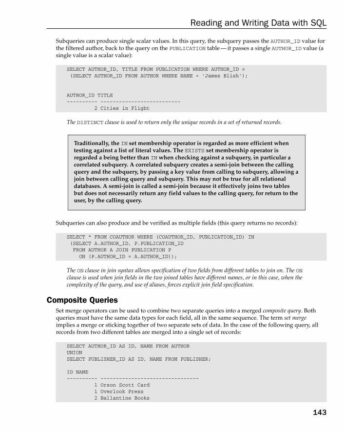
Subqueries can produce single scalar values. In this query, the subquery passes the AUTHOR_ID value forthe filtered author, back to the query on the PUBLICATION table — it passes a single AUTHOR_ID value (asingle value is a scalar value):
SELECT AUTHOR_ID, TITLE FROM PUBLICATION WHERE AUTHOR_ID =(SELECT AUTHOR_ID FROM AUTHOR WHERE NAME = ‘James Blish’);
AUTHOR_ID TITLE---------- --------------------------
2 Cities in Flight
The DISTINCT clause is used to return only the unique records in a set of returned records.
Subqueries can also produce and be verified as multiple fields (this query returns no records):
SELECT * FROM COAUTHOR WHERE (COAUTHOR_ID, PUBLICATION_ID) IN(SELECT A.AUTHOR_ID, P.PUBLICATION_IDFROM AUTHOR A JOIN PUBLICATION P
ON (P.AUTHOR_ID = A.AUTHOR_ID));
The ON clause in join syntax allows specification of two fields from different tables to join on. The ONclause is used when join fields in the two joined tables have different names, or in this case, when thecomplexity of the query, and use of aliases, forces explicit join field specification.
Composite QueriesSet merge operators can be used to combine two separate queries into a merged composite query. Bothqueries must have the same data types for each field, all in the same sequence. The term set mergeimplies a merge or sticking together of two separate sets of data. In the case of the following query, allrecords from two different tables are merged into a single set of records:
SELECT AUTHOR_ID AS ID, NAME FROM AUTHORUNIONSELECT PUBLISHER_ID AS ID, NAME FROM PUBLISHER;
ID NAME---------- --------------------------------
1 Orson Scott Card1 Overlook Press2 Ballantine Books
Traditionally, the IN set membership operator is regarded as more efficient whentesting against a list of literal values. The EXISTS set membership operator isregarded a being better than IN when checking against a subquery, in particular acorrelated subquery. A correlated subquery creates a semi-join between the callingquery and the subquery, by passing a key value from calling to subquery, allowing ajoin between calling query and subquery. This may not be true for all relationaldatabases. A semi-join is called a semi-join because it effectively joins two tablesbut does not necessarily return any field values to the calling query, for return to theuser, by the calling query.
143
Reading and Writing Data with SQL
10_574906 ch05.qxd 11/4/05 10:47 AM Page 143
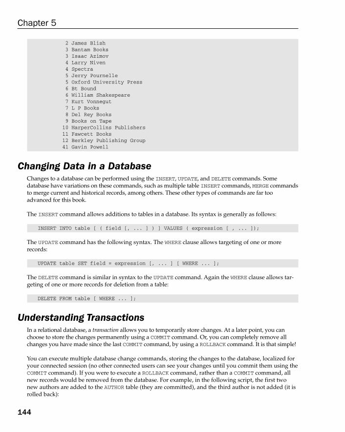
2 James Blish3 Bantam Books3 Isaac Azimov4 Larry Niven4 Spectra5 Jerry Pournelle5 Oxford University Press6 Bt Bound6 William Shakespeare7 Kurt Vonnegut7 L P Books8 Del Rey Books9 Books on Tape
10 HarperCollins Publishers11 Fawcett Books12 Berkley Publishing Group41 Gavin Powell
Changing Data in a DatabaseChanges to a database can be performed using the INSERT, UPDATE, and DELETE commands. Somedatabase have variations on these commands, such as multiple table INSERT commands, MERGE commandsto merge current and historical records, among others. These other types of commands are far tooadvanced for this book.
The INSERT command allows additions to tables in a database. Its syntax is generally as follows:
INSERT INTO table [ ( field [, ... ] ) ] VALUES ( expression [ , ... ]);
The UPDATE command has the following syntax. The WHERE clause allows targeting of one or morerecords:
UPDATE table SET field = expression [, ... ] [ WHERE ... ];
The DELETE command is similar in syntax to the UPDATE command. Again the WHERE clause allows tar-geting of one or more records for deletion from a table:
DELETE FROM table [ WHERE ... ];
Understanding TransactionsIn a relational database, a transaction allows you to temporarily store changes. At a later point, you canchoose to store the changes permanently using a COMMIT command. Or, you can completely remove allchanges you have made since the last COMMIT command, by using a ROLLBACK command. It is that simple!
You can execute multiple database change commands, storing the changes to the database, localized foryour connected session (no other connected users can see your changes until you commit them using theCOMMIT command). If you were to execute a ROLLBACK command, rather than a COMMIT command, allnew records would be removed from the database. For example, in the following script, the first twonew authors are added to the AUTHOR table (they are committed), and the third author is not added (it isrolled back):
144
Chapter 5
10_574906 ch05.qxd 11/4/05 10:47 AM Page 144
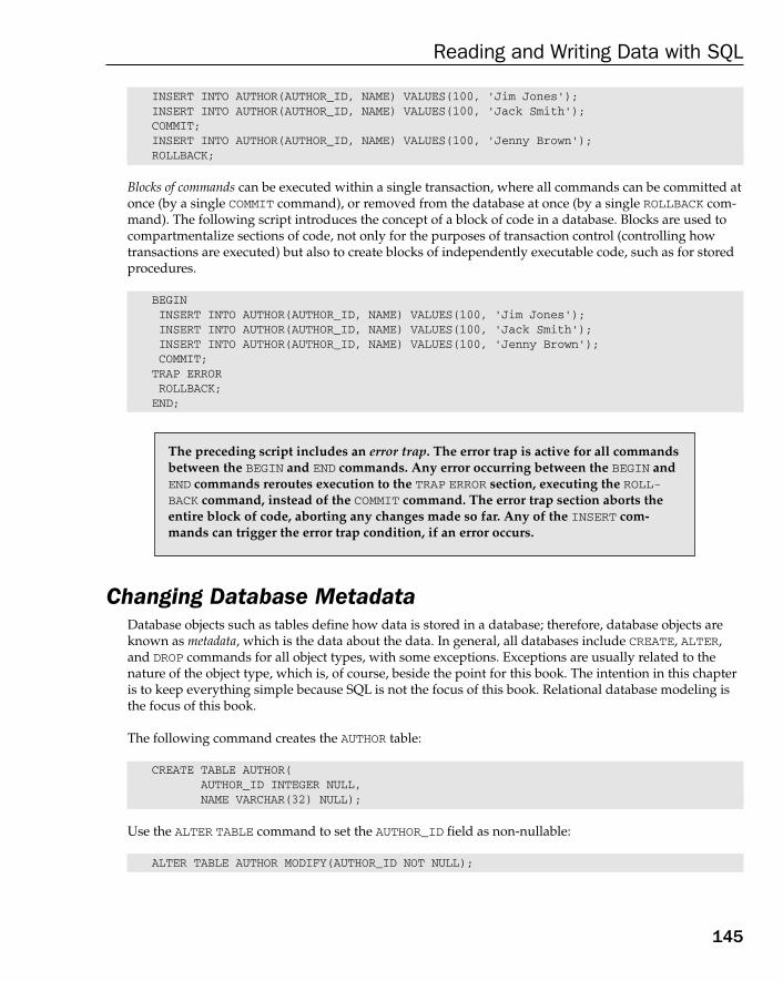
INSERT INTO AUTHOR(AUTHOR_ID, NAME) VALUES(100, ‘Jim Jones’);INSERT INTO AUTHOR(AUTHOR_ID, NAME) VALUES(100, ‘Jack Smith’);COMMIT;INSERT INTO AUTHOR(AUTHOR_ID, NAME) VALUES(100, ‘Jenny Brown’);ROLLBACK;
Blocks of commands can be executed within a single transaction, where all commands can be committed atonce (by a single COMMIT command), or removed from the database at once (by a single ROLLBACK com-mand). The following script introduces the concept of a block of code in a database. Blocks are used tocompartmentalize sections of code, not only for the purposes of transaction control (controlling howtransactions are executed) but also to create blocks of independently executable code, such as for storedprocedures.
BEGININSERT INTO AUTHOR(AUTHOR_ID, NAME) VALUES(100, ‘Jim Jones’);INSERT INTO AUTHOR(AUTHOR_ID, NAME) VALUES(100, ‘Jack Smith’);INSERT INTO AUTHOR(AUTHOR_ID, NAME) VALUES(100, ‘Jenny Brown’);COMMIT;
TRAP ERRORROLLBACK;
END;
Changing Database MetadataDatabase objects such as tables define how data is stored in a database; therefore, database objects areknown as metadata, which is the data about the data. In general, all databases include CREATE, ALTER,and DROP commands for all object types, with some exceptions. Exceptions are usually related to thenature of the object type, which is, of course, beside the point for this book. The intention in this chapteris to keep everything simple because SQL is not the focus of this book. Relational database modeling isthe focus of this book.
The following command creates the AUTHOR table:
CREATE TABLE AUTHOR(AUTHOR_ID INTEGER NULL,NAME VARCHAR(32) NULL);
Use the ALTER TABLE command to set the AUTHOR_ID field as non-nullable:
ALTER TABLE AUTHOR MODIFY(AUTHOR_ID NOT NULL);
The preceding script includes an error trap. The error trap is active for all commandsbetween the BEGIN and END commands. Any error occurring between the BEGIN andEND commands reroutes execution to the TRAP ERROR section, executing the ROLL-BACK command, instead of the COMMIT command. The error trap section aborts theentire block of code, aborting any changes made so far. Any of the INSERT com-mands can trigger the error trap condition, if an error occurs.
145
Reading and Writing Data with SQL
10_574906 ch05.qxd 11/4/05 10:47 AM Page 145
Use the DROP TABLE and CREATE TABLE commands to recreate the AUTHOR table with two constraints:
DROP TABLE AUTHOR;CREATE TABLE AUTHOR (
AUTHOR_ID INTEGER PRIMARY KEY NOT NULL,NAME VARCHAR(32) UNIQUE NOT NULL);
This CREATE TABLE command creates the PUBLICATION table, including a foreign key (REFERENCESAUTHOR), pointing back to the primary key field on the AUTHOR table:
CREATE TABLE PUBLICATION(PUBLICATION_ID INTEGER PRIMARY KEY NOT NULL,AUTHOR_ID INTEGER REFERENCES AUTHOR NOT NULL,TITLE VARCHAR(64) UNIQUE NOT NULL);
A relational database should automatically create an index for a primary key and a unique key field. Thereason is simple to understand. When adding a new record, a primary key or unique key must be checkedfor uniqueness. What better way to maintain unique key values than an index? However, foreign key fieldsby their very nature can be both NULL valued and duplicated in a child table. Duplicates can occur because,in its most simple form, a foreign key field is usually on the “many” side of a one-to-many relationship. Inother words, there are potentially many different publications for each author. Many authors often writemore than one book. Additionally, a foreign key value could potentially be NULL valued. An author doesnot necessarily have to have any publications, currently in print. Creating an index on a foreign key field isnot automatically controlled by a relational database. If an index is required for a foreign key field, thatindex should be manually created:
CREATE INDEX XFK_PUBLICATION_AUTHOR ON PUBLICATION (AUTHOR_ID);
Indexes can also be altered and dropped using the ALTER INDEX and DROP INDEX commands, respectively.
In general, database metadata change commands are a lot more comprehensive than just creating, alter-ing, and dropping simple tables and indexes. Then again, it is not necessary to bombard you with toomuch scripting in this book.
Try It Out Creating Tables and ConstraintsFigure 5-1 shows the tables of the online bookstore database model. Create all tables, including primaryand foreign key constraints:
1. It is important to create the table in the correct sequence because some tables depend on theexistence of others.
2. The PUBLISHER, AUTHOR, and SUBJECT tables can be created first because they are at the top ofdependency hierarchies.
3. Next, create the PUBLICATION table.
4. Then create the EDITION, REVIEW, and COAUTHOR tables.
146
Chapter 5
10_574906 ch05.qxd 11/4/05 10:47 AM Page 146
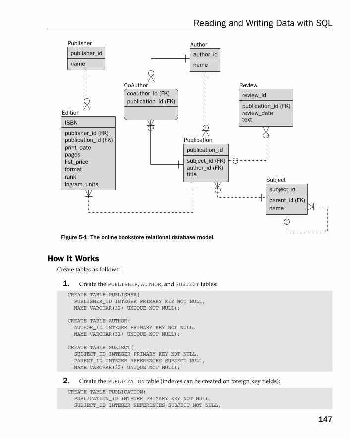
Figure 5-1: The online bookstore relational database model.
How It WorksCreate tables as follows:
1. Create the PUBLISHER, AUTHOR, and SUBJECT tables:
CREATE TABLE PUBLISHER(PUBLISHER_ID INTEGER PRIMARY KEY NOT NULL,NAME VARCHAR(32) UNIQUE NOT NULL);
CREATE TABLE AUTHOR(AUTHOR_ID INTEGER PRIMARY KEY NOT NULL,NAME VARCHAR(32) UNIQUE NOT NULL);
CREATE TABLE SUBJECT(SUBJECT_ID INTEGER PRIMARY KEY NOT NULL,PARENT_ID INTEGER REFERENCES SUBJECT NULL,NAME VARCHAR(32) UNIQUE NOT NULL);
2. Create the PUBLICATION table (indexes can be created on foreign key fields):
CREATE TABLE PUBLICATION(PUBLICATION_ID INTEGER PRIMARY KEY NOT NULL,SUBJECT_ID INTEGER REFERENCES SUBJECT NOT NULL,
Publisher
publisher_id
name
Author
author_id
name
Subject
subject_id
parent_id (FK)name
Publication
publication_id
subject_id (FK)author_id (FK)title
Review
review_id
publication_id (FK)review_datetext
CoAuthorcoauthor_id (FK)publication_id (FK)
Edition
ISBN
publisher_id (FK)publication_id (FK)print_datepageslist_priceformatrankingram_units
147
Reading and Writing Data with SQL
10_574906 ch05.qxd 11/4/05 10:47 AM Page 147
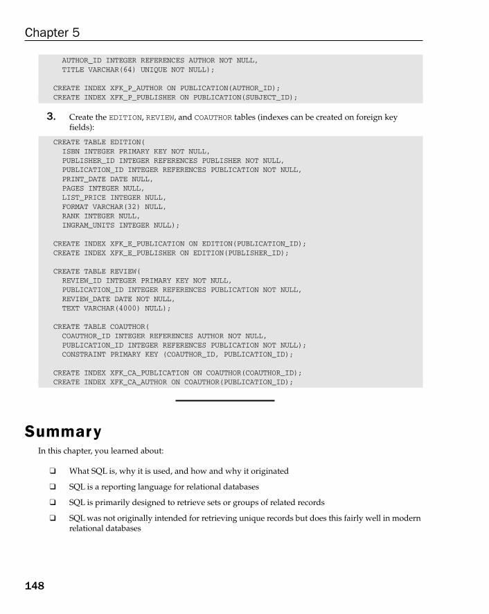
AUTHOR_ID INTEGER REFERENCES AUTHOR NOT NULL,TITLE VARCHAR(64) UNIQUE NOT NULL);
CREATE INDEX XFK_P_AUTHOR ON PUBLICATION(AUTHOR_ID);CREATE INDEX XFK_P_PUBLISHER ON PUBLICATION(SUBJECT_ID);
3. Create the EDITION, REVIEW, and COAUTHOR tables (indexes can be created on foreign keyfields):
CREATE TABLE EDITION(ISBN INTEGER PRIMARY KEY NOT NULL,PUBLISHER_ID INTEGER REFERENCES PUBLISHER NOT NULL,PUBLICATION_ID INTEGER REFERENCES PUBLICATION NOT NULL,PRINT_DATE DATE NULL,PAGES INTEGER NULL,LIST_PRICE INTEGER NULL,FORMAT VARCHAR(32) NULL,RANK INTEGER NULL,INGRAM_UNITS INTEGER NULL);
CREATE INDEX XFK_E_PUBLICATION ON EDITION(PUBLICATION_ID);CREATE INDEX XFK_E_PUBLISHER ON EDITION(PUBLISHER_ID);
CREATE TABLE REVIEW(REVIEW_ID INTEGER PRIMARY KEY NOT NULL,PUBLICATION_ID INTEGER REFERENCES PUBLICATION NOT NULL,REVIEW_DATE DATE NOT NULL,TEXT VARCHAR(4000) NULL);
CREATE TABLE COAUTHOR(COAUTHOR_ID INTEGER REFERENCES AUTHOR NOT NULL,PUBLICATION_ID INTEGER REFERENCES PUBLICATION NOT NULL);CONSTRAINT PRIMARY KEY (COAUTHOR_ID, PUBLICATION_ID);
CREATE INDEX XFK_CA_PUBLICATION ON COAUTHOR(COAUTHOR_ID);CREATE INDEX XFK_CA_AUTHOR ON COAUTHOR(PUBLICATION_ID);
SummaryIn this chapter, you learned about:
❑ What SQL is, why it is used, and how and why it originated
❑ SQL is a reporting language for relational databases
❑ SQL is primarily designed to retrieve sets or groups of related records
❑ SQL was not originally intended for retrieving unique records but does this fairly well in modernrelational databases
148
Chapter 5
10_574906 ch05.qxd 11/4/05 10:47 AM Page 148
❑ There are many different types of queries used for extracting and presenting information to theuser in different ways
❑ There are three specific commands (INSERT, UPDATE, and DELETE) used for changing records intables
❑ Tables and indexes can themselves be changed using table and index database metadata changingcommands
❑ There are some simple ways of building better written, more maintainable, and faster performingSQL code commands
Above all, this chapter has shown how the relational database model is used from an application perspective. There is little point in understanding something such as relational database modeling with-out seeing it applied in some way, no matter how simple.
The next chapter returns to the topic of relational database modeling by presenting some advanced rela-tional database modeling techniques.
ExercisesUse the ERD in Figure 5-1 to help you answer these questions.
1. Find all records and fields in the EDITION table.
2. Find all ISBN values in the EDITION table, for all FORMAT=’Hardcover ‘books.
3. Do the same query, but sort records by LIST_PRICE contained within FORMAT.
4. Which of the two expressions 3 + 4 * 5, and (3 + 4) * 5 yields the greater value?
5. Find the sum of all LIST_PRICE values in the EDITION table, for each publisher.
6. Join the SUBJECT and PUBLICATION tables on the SUBJECT_ID field, as an intersection.
7. Find the intersection of subjects and publications, where subjects do not necessarily have tohave publications.
8. Find subjects with publications, using a semi-join, in two different ways.
149
Reading and Writing Data with SQL
10_574906 ch05.qxd 11/4/05 10:47 AM Page 149

10_574906 ch05.qxd 11/4/05 10:47 AM Page 150
6Advanced RelationalDatabase Modeling
“A computer lets you make more mistakes faster than any invention in human history — with thepossible exceptions of hand guns and tequila.” (Mitch Ratliffe)
Acts of overzealousness in application of normalization techniques can sometimes be partially rectified byusing denormalization, aspects of the object-relational database model, and maybe even a data warehouse.
Remember your first job? The first thing your new boss said to you might have been something of thisnature. “Forget everything you learned in college. Here we do what’s necessary to get the job done.
Sometimes we have to break the rules.”
This chapter expands on the concepts of relational database modeling, normalization, and NormalForms. This chapter introduces denormalization, the object database model, and data warehousing.These topics are all related to normalization in one way or another.
Understanding how to build normalized table structures is all well and good; however, withoutknowledge of how to undo those granular structures through denormalization, you will not beable to understand other essential topics of database modeling, such as data warehousing.
This chapter bridges the gap between creating properly normalized table structures, and ultimatelycreating adequately performing table structures. Good performance services applications in a usablemanner. Usability is all important. Modern-day applications are often built using object-orientedSDKs; therefore, this chapter includes a brief introduction to object modeling theory. Additionally,data warehouses are essential to maintaining performance of active OLTP databases, to providinggood projections and forecasting facilities for end-users. An introduction to data warehousing isincluded here as a primer for further detail later on in this book.
In this chapter, you learn about the following:
❑ Denormalization
❑ Denormalization by reversing of Normal Forms
❑ Denormalization using specialized database objects
11_574906 ch06.qxd 10/28/05 11:39 PM Page 151
❑ The object database model
❑ The data warehouse database model
Let’s begin this chapter by examining the topic of denormalization.
Understanding DenormalizationDenormalization is often (but not always) the opposite of normalization. (See Chapter 4 for a discussion ofnormalization.) Denormalization can be applied to a database model to create data warehouse or reportingonly type tables. Denormalization is also sometimes required as a solution to reviving dying OLTPapplications that exhibit dreadful performance. This can be a result of past profligate use of normalizationin the development of database models and applications. Too much granularity in normalization can cause as many problems as it solves. So, denormalization often attempts to reverse granularity, created byover-application of Normal Forms during the normalization process.
Reversing Normal FormsDenormalization is often a reversal of the processing performed by normalization; therefore, it is essential when describing denormalization to understand the steps (Normal Forms) contained withinnormalization. Take a look at the definitions of normalization once again, as a reminder:
❑ 1st Normal Form (1NF) — Remove repeating fields by creating a new table. The original and newtables are linked together with a master-detail, one-to-many relationship. Also create primary keyson both tables. 1NF does not require definition of the detail table primary key, but so what? Thedetail table has a composite primary key containing the master table primary key field, as the pre-fix field of its primary key. That prefix field is also a foreign key back to the master table.
❑ 2nd Normal Form (2NF) — Perform a seemingly similar function to that of 1NF; however, create a table where repeating values rather than repeating fields are removed to a new table. Theresult is a many-to-one relationship, rather than a one-to-many relationship as for 1NF, createdbetween the original and the new tables. The new table gets a primary key consisting of a singlefield. The master table contains a foreign key pointing back to the primary key of the new table.That foreign key is not part of the primary key in the original table.
❑ 3rd Normal Form (3NF) — Eliminate transitive dependencies. A field is transitively dependent on the primary key if it is indirectly determined by the primary key. In other words, the field isfunctionally dependent on another field, where the other field is dependent on the primary key. Insome cases, elimination of a transitive dependency implies creation of a new table for somethingindirectly dependent on the primary key in an existing table. There are numerous methods ofinterpreting 3NF.
❑ Beyond 3rd Normal Form — Many modern relational database models do not extend beyond 3NF.Sometimes 3NF is not used at all. The reason why is because of the generation of too many tablesand the resulting complex SQL code joins, with resulting dreadful database response times. Diskspace is cheap and, as already stated, increased numbers of tables leads to bigger SQL joins andpoorer performance. The other point to note about Boyce-Codd Normal Form (BCNF), 4th NormalForm (4NF), 5th Normal Form (5NF), and Domain Key Normal Form (DKNF) levels of normaliza-tion is that they tend to place a lot of business functionality (business rules) into database tables.This is often unnecessary because modern day application SDKs are more than capable of dealingwith this type of complex processing. Let applications do the number crunching and leave thedatabase to storing data, not processing data or applying too many rules to data.
152
Chapter 6
11_574906 ch06.qxd 10/28/05 11:39 PM Page 152
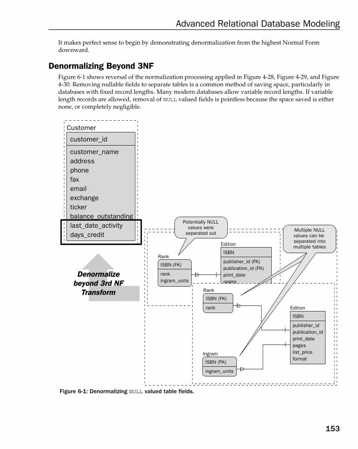
It makes perfect sense to begin by demonstrating denormalization from the highest Normal Form downward.
Denormalizing Beyond 3NFFigure 6-1 shows reversal of the normalization processing applied in Figure 4-28, Figure 4-29, and Figure4-30. Removing nullable fields to separate tables is a common method of saving space, particularly indatabases with fixed record lengths. Many modern databases allow variable record lengths. If variablelength records are allowed, removal of NULL valued fields is pointless because the space saved is eithernone, or completely negligible.
Figure 6-1: Denormalizing NULL valued table fields.
Customer
customer_id
customer_nameaddressphonefaxemailexchangetickerbalance_outstandinglast_date_activitydays_credit
Edition
ISBN
publisher_id (FK)publication_id (FK)print_datepages
Rank
ISBN (FK)
rankingram_units
Edition
ISBN
publisher_idpublication_idprint_datepageslist_priceformat
Rank
ISBN (FK)
rank
Ingram
ISBN (FK)
ingram_units
Denormalizebeyond 3rd NF
Transform
Denormalizebeyond 3rd NF
Transform
Multiple NULLvalues can be separated intomultiple tables
Potentially NULLvalues were
separated out
153
Advanced Relational Database Modeling
11_574906 ch06.qxd 10/28/05 11:39 PM Page 153
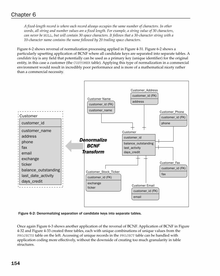
A fixed-length record is where each record always occupies the same number of characters. In otherwords, all string and number values are a fixed length. For example, a string value of 30 characters, can never be NULL, but will contain 30 space characters. It follows that a 30-character string with a 10-character name contains the name followed by 20 trailing space characters.
Figure 6-2 shows reversal of normalization processing applied in Figure 4-31. Figure 6-2 shows a particularly upsetting application of BCNF where all candidate keys are separated into separate tables. Acandidate key is any field that potentially can be used as a primary key (unique identifier) for the originalentity, in this case a customer (the CUSTOMER table). Applying this type of normalization in a commercialenvironment would result in incredibly poor performance and is more of a mathematical nicety ratherthan a commercial necessity.
Figure 6-2: Denormalizing separation of candidate keys into separate tables.
Once again Figure 6-3 shows another application of the reversal of BCNF. Application of BCNF in Figure4-32 and Figure 4-33 created three tables, each with unique combinations of unique values from the PROJECTS table on the left. Accessing of unique records in the PROJECT table can be handled with application coding more effectively, without the downside of creating too much granularity in tablestructures.
Customer
customer_id
customer_nameaddressphonefaxemailexchangetickerbalance_outstandinglast_date_activitydays_credit
Customer
customer_id
balance_outstandinglast_activitydays_credit
Customer_Stock_Ticker
customer_id (FK)
exchangeticker
Customer_Phone
customer_id (FK)
phone
Customer_Address
customer_id (FK)
address
Customer Email
customer_id (FK)
Customer_Fax
customer_id (FK)
fax
Customer Name
customer_id (FK)
customer_name
DenormalizeBCNF
Transform
DenormalizeBCNF
Transform
154
Chapter 6
11_574906 ch06.qxd 10/28/05 11:39 PM Page 154
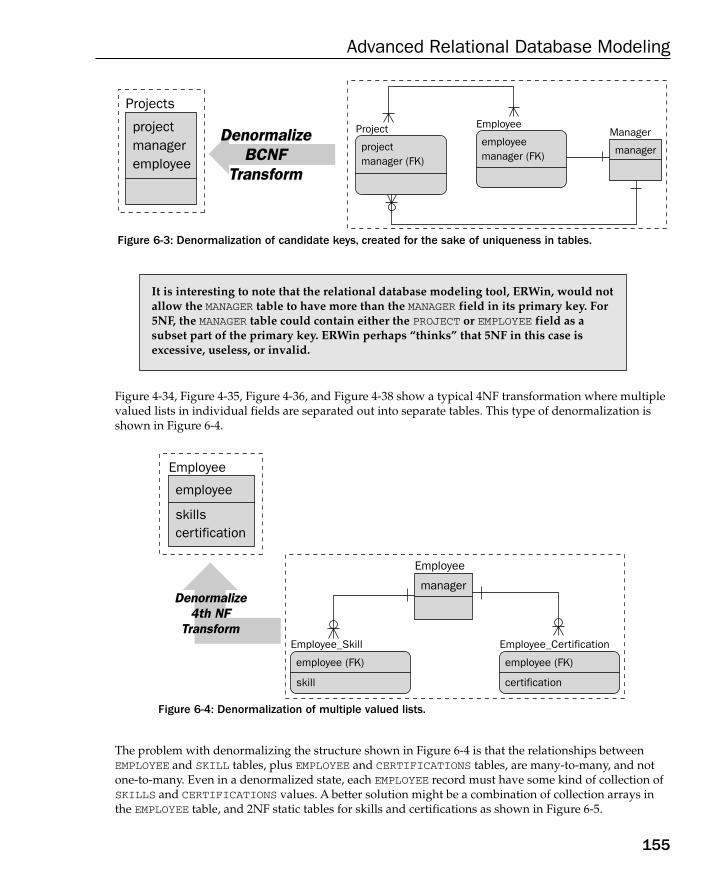
Figure 6-3: Denormalization of candidate keys, created for the sake of uniqueness in tables.
Figure 4-34, Figure 4-35, Figure 4-36, and Figure 4-38 show a typical 4NF transformation where multiplevalued lists in individual fields are separated out into separate tables. This type of denormalization isshown in Figure 6-4.
Figure 6-4: Denormalization of multiple valued lists.
The problem with denormalizing the structure shown in Figure 6-4 is that the relationships betweenEMPLOYEE and SKILL tables, plus EMPLOYEE and CERTIFICATIONS tables, are many-to-many, and notone-to-many. Even in a denormalized state, each EMPLOYEE record must have some kind of collection ofSKILLS and CERTIFICATIONS values. A better solution might be a combination of collection arrays inthe EMPLOYEE table, and 2NF static tables for skills and certifications as shown in Figure 6-5.
Employee
manager
Employee
employee
skillscertification
Denormalize4th NF
Transform
Denormalize4th NF
TransformEmployee_Certification
employee (FK)
certification
Employee_Skill
employee (FK)
skill
It is interesting to note that the relational database modeling tool, ERWin, would notallow the MANAGER table to have more than the MANAGER field in its primary key. For5NF, the MANAGER table could contain either the PROJECT or EMPLOYEE field as a subset part of the primary key. ERWin perhaps “thinks” that 5NF in this case isexcessive, useless, or invalid.
Projects
projectmanageremployee
Manager
manager
Employee
employeemanager (FK)
Project
projectmanager (FK)
DenormalizeBCNF
Transform
DenormalizeBCNF
Transform
155
Advanced Relational Database Modeling
11_574906 ch06.qxd 10/28/05 11:39 PM Page 155
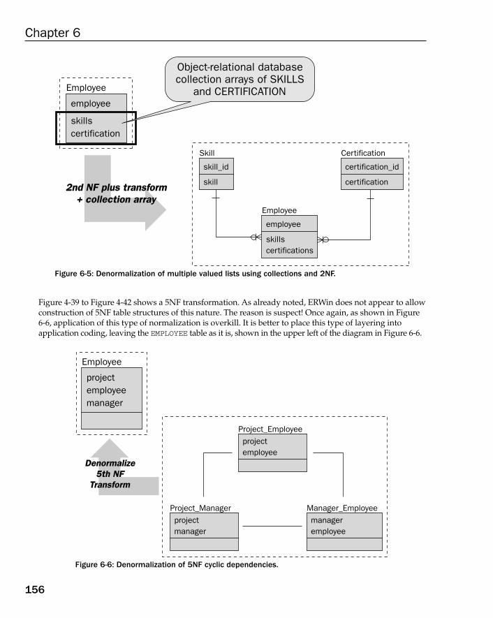
Figure 6-5: Denormalization of multiple valued lists using collections and 2NF.
Figure 4-39 to Figure 4-42 shows a 5NF transformation. As already noted, ERWin does not appear to allowconstruction of 5NF table structures of this nature. The reason is suspect! Once again, as shown in Figure6-6, application of this type of normalization is overkill. It is better to place this type of layering into application coding, leaving the EMPLOYEE table as it is, shown in the upper left of the diagram in Figure 6-6.
Figure 6-6: Denormalization of 5NF cyclic dependencies.
Employee
projectemployeemanager
Denormalize5th NF
Transform
Denormalize5th NF
Transform
Project_Managerprojectmanager
Manager_Employeemanageremployee
Project_Employeeprojectemployee
Employee
employee
skillscertification
Skill
skill_id
skill
Certification
certification_id
certification
Employee
employee
skillscertifications
2nd NF plus transform+ collection array
2nd NF plus transform+ collection array
Object-relational databasecollection arrays of SKILLS
and CERTIFICATION
156
Chapter 6
11_574906 ch06.qxd 10/28/05 11:39 PM Page 156

Denormalizing 3NFThe role of 3NF is to eliminate what are called transitive dependencies. A transitive dependency is where afield is not directly determined by the primary key, but indirectly determined by the primary key,through another field.
Most of the Normal Form layers beyond 3NF are often impractical in a commercial environment becauseapplications can often do better at that level. What happens in reality is that 3NF occupies a gray area,fitting in between what should not be done in the database model (beyond 3NF), and what should donein the database model (1NF and 2NF).
There are a number of different ways of interpreting 3NF, as shown in Figure 4-21, Figure 4-23, Figure4-24, and Figure 4-25. All of these example interpretations of 3NF are completely different. Figure 6-7shows the denormalization of a many-to-many join resolution table. As a general rule, a many-to-manyjoin resolution table is usually required by applications when it can be specifically named, as for theASSIGNMENT table shown in Figure 6-7. If it was nonsensical to call the new table ASSIGNMENT, and itwas called something such as EMPLOYEE_TASK, chances are that the extra table is unnecessary. Quiteoften these types of tables are created without forethought as to application requirements. If a table likethis is not essential to application requirements, it is probably unnecessary. The result of too many newtables is more tables in joins and slower queries.
Figure 6-7: Denormalize unnecessary 3NF many-to-many join resolution tables.
Employee
employee
Denormalize3rd NF
Transform
Denormalize3rd NF
Transform
Task
task
Employeeemployee
Tasktask
Assignment
employee (FK)task (FK)
Employee Task
157
Advanced Relational Database Modeling
11_574906 ch06.qxd 10/28/05 11:39 PM Page 157
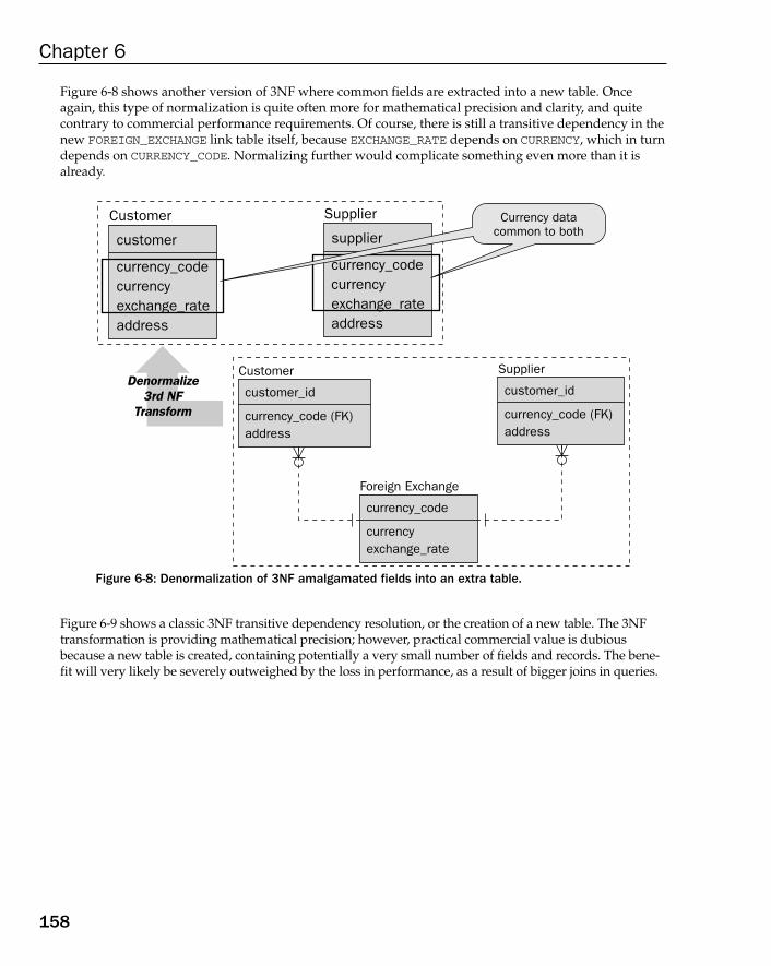
Figure 6-8 shows another version of 3NF where common fields are extracted into a new table. Onceagain, this type of normalization is quite often more for mathematical precision and clarity, and quitecontrary to commercial performance requirements. Of course, there is still a transitive dependency in thenew FOREIGN_EXCHANGE link table itself, because EXCHANGE_RATE depends on CURRENCY, which in turndepends on CURRENCY_CODE. Normalizing further would complicate something even more than it isalready.
Figure 6-8: Denormalization of 3NF amalgamated fields into an extra table.
Figure 6-9 shows a classic 3NF transitive dependency resolution, or the creation of a new table. The 3NFtransformation is providing mathematical precision; however, practical commercial value is dubiousbecause a new table is created, containing potentially a very small number of fields and records. The bene-fit will very likely be severely outweighed by the loss in performance, as a result of bigger joins in queries.
Denormalize3rd NF
Transform
Denormalize3rd NF
Transform
Customer
customer
currency_codecurrencyexchange_rateaddress
Supplier
supplier
currency_codecurrencyexchange_rateaddress
Customer
customer_id
currency_code (FK)address
Foreign Exchange
currency_code
currencyexchange_rate
Supplier
customer_id
currency_code (FK)address
Currency datacommon to both
158
Chapter 6
11_574906 ch06.qxd 10/28/05 11:39 PM Page 158
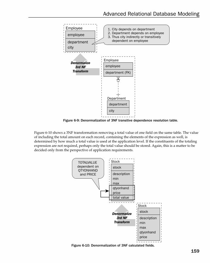
Figure 6-9: Denormalization of 3NF transitive dependence resolution table.
Figure 6-10 shows a 3NF transformation removing a total value of one field on the same table. The valueof including the total amount on each record, containing the elements of the expression as well, is determined by how much a total value is used at the application level. If the constituents of the totalingexpression are not required, perhaps only the total value should be stored. Again, this is a matter to bedecided only from the perspective of application requirements.
Figure 6-10: Denormalization of 3NF calculated fields.
Denormalize3rd NF
Transform
Denormalize3rd NF
Transform
Stock
stock
descriptionminmaxqtyonhandpricetotal value
Stock
stock
descriptionminmaxqtyonhandprice
TOTALVALUEdependent onQTYONHANDand PRICE
Denormalize3rd NF
Transform
Denormalize3rd NF
Transform
Employee
employee
departmentcity
Employee
employee
department (FK)
Department
department
city
1. City depends on department2. Department depends on employee3. Thus city indirectly or transitively dependent on employee
159
Advanced Relational Database Modeling
11_574906 ch06.qxd 10/28/05 11:39 PM Page 159

Denormalizing 2NFThe role of 2NF is to separate static data into separate tables, removing repeated static values from transactional tables. Figure 6-11 shows an example of over-application of 2NF. The lower right of the diagram shows an extreme of four tables, created from what is essentially a more-than-adequately normalized COMPANY table at the upper left of the diagram.
Figure 6-11: Denormalization of 2NF into a single static table.
Listing
listing
exchange (FK)ticker
Classification
classification
Exchange
exchange
classification (FK)
Company
company
listing (FK)addressphonefaxemail
Company
company
listing (FK)addressphonefaxemail
Listing
listing
classificationexchangeticker
Company
company
addressphonefaxemailclassificationexchangeticker
Company is static data-too much normalization
Insanely overnormalized
Over normalization
160
Chapter 6
11_574906 ch06.qxd 10/28/05 11:39 PM Page 160
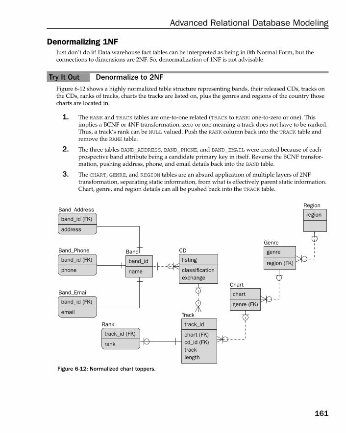
Denormalizing 1NFJust don’t do it! Data warehouse fact tables can be interpreted as being in 0th Normal Form, but the connections to dimensions are 2NF. So, denormalization of 1NF is not advisable.
Try It Out Denormalize to 2NFFigure 6-12 shows a highly normalized table structure representing bands, their released CDs, tracks onthe CDs, ranks of tracks, charts the tracks are listed on, plus the genres and regions of the country thosecharts are located in.
1. The RANK and TRACK tables are one-to-one related (TRACK to RANK: one-to-zero or one). Thisimplies a BCNF or 4NF transformation, zero or one meaning a track does not have to be ranked.Thus, a track’s rank can be NULL valued. Push the RANK column back into the TRACK table andremove the RANK table.
2. The three tables BAND_ADDRESS, BAND_PHONE, and BAND_EMAIL were created because of eachprospective band attribute being a candidate primary key in itself. Reverse the BCNF transfor-mation, pushing address, phone, and email details back into the BAND table.
3. The CHART, GENRE, and REGION tables are an absurd application of multiple layers of 2NF transformation, separating static information, from what is effectively parent static information.Chart, genre, and region details can all be pushed back into the TRACK table.
Figure 6-12: Normalized chart toppers.
Chart
chart
genre (FK)
Region
region
Genre
genre
region (FK)
Track
track_id
chart (FK)cd_id (FK)tracklength
Band
band_id
name
CD
listing
classificationexchange
Band_Address
band_id (FK)
address
Band_Phone
band_id (FK)
phone
Band_Email
band_id (FK)
Rank
track_id (FK)
rank
161
Advanced Relational Database Modeling
11_574906 ch06.qxd 10/28/05 11:39 PM Page 161
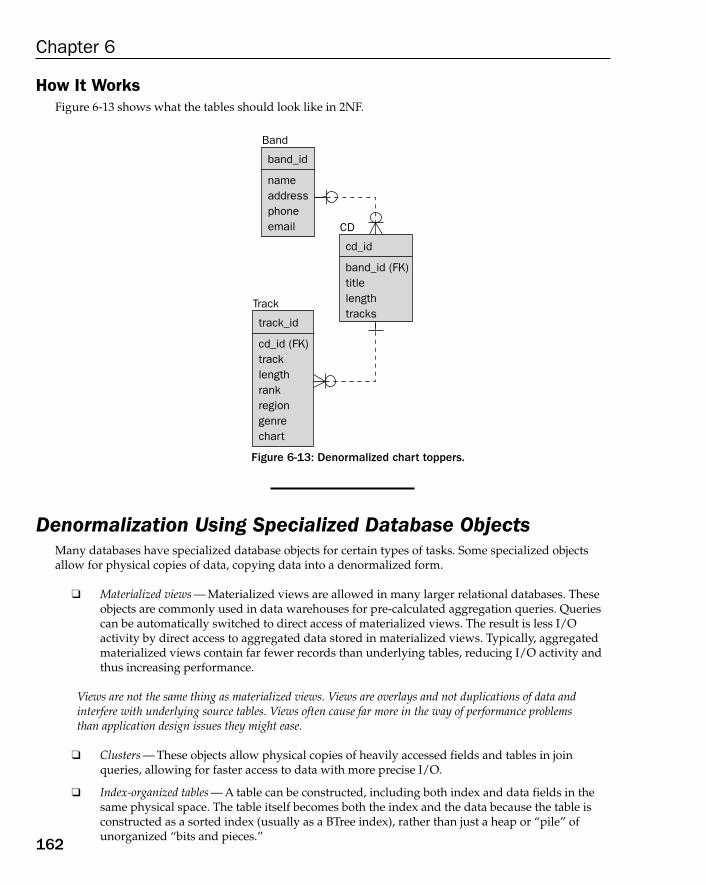
How It WorksFigure 6-13 shows what the tables should look like in 2NF.
Figure 6-13: Denormalized chart toppers.
Denormalization Using Specialized Database ObjectsMany databases have specialized database objects for certain types of tasks. Some specialized objectsallow for physical copies of data, copying data into a denormalized form.
❑ Materialized views — Materialized views are allowed in many larger relational databases. Theseobjects are commonly used in data warehouses for pre-calculated aggregation queries. Queriescan be automatically switched to direct access of materialized views. The result is less I/O activity by direct access to aggregated data stored in materialized views. Typically, aggregatedmaterialized views contain far fewer records than underlying tables, reducing I/O activity andthus increasing performance.
Views are not the same thing as materialized views. Views are overlays and not duplications of data andinterfere with underlying source tables. Views often cause far more in the way of performance problemsthan application design issues they might ease.
❑ Clusters — These objects allow physical copies of heavily accessed fields and tables in joinqueries, allowing for faster access to data with more precise I/O.
❑ Index-organized tables — A table can be constructed, including both index and data fields in thesame physical space. The table itself becomes both the index and the data because the table isconstructed as a sorted index (usually as a BTree index), rather than just a heap or “pile” ofunorganized “bits and pieces.”
CD
cd_id
band_id (FK)titlelengthtracks
Track
track_id
cd_id (FK)tracklengthrankregiongenrechart
Band
band_id
nameaddressphoneemail
162
Chapter 6
11_574906 ch06.qxd 10/28/05 11:39 PM Page 162
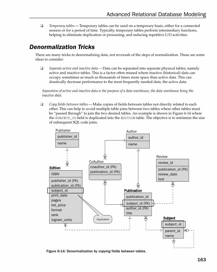
❑ Temporary tables — Temporary tables can be used on a temporary basis, either for a connectedsession or for a period of time. Typically, temporary tables perform intermediary functions,helping to eliminate duplication or processing, and reducing repetitive I/O activities.
Denormalization TricksThere are many tricks to denormalizing data, not reversals of the steps of normalization. These are someideas to consider:
❑ Separate active and inactive data — Data can be separated into separate physical tables, namelyactive and inactive tables. This is a factor often missed where inactive (historical) data canoccupy sometimes as much as thousands of times more space than active data. This can drastically decrease performance to the most frequently needed data, the active data.
Separation of active and inactive data is the purpose of a data warehouse, the data warehouse being theinactive data.
❑ Copy fields between tables — Make copies of fields between tables not directly related to eachother. This can help to avoid multiple table joins between two tables where other tables mustbe “passed through” to join the two desired tables. An example is shown in Figure 6-14 where the SUBJECT_ID field is duplicated into the EDITION table. The objective is to minimize the sizeof subsequent SQL code joins.
Figure 6-14: Denormalization by copying fields between tables.
Publisher
publisher_id
name
Author
author_id
name
Review
review_id
publication_id (FK)review_datetext
SubjectSubject
subject_id
parent_idname
PublicationPublication
publication_id
subject_id (FK)author_id (FK)title
EditionEdition
ISBN
publisher_id (FK)publication_id (FK)subject_idprint_datepageslist_priceformatrankingram_units
CoAuthorcoauthor_id (FK)publication_id (FK)
Duplication
163
Advanced Relational Database Modeling
11_574906 ch06.qxd 10/28/05 11:39 PM Page 163

❑ Summary fields in parent tables — This can help to avoid costly grouping joins, but real-timeupdates can cause serious problems with hot blocks. Examples are shown in Figure 6-15. Again,the objective is to minimize the size of subsequent SQL code joins, and to provide summary val-ues without having to constantly add all the details, from multiple records in a detail table.
A hot block is a very busy part of the database accessed much too often by many different sessions.
Figure 6-15: Denormalization using summary fields in parent tables.
❑ Separate heavily and lightly accessed fields — Much like separating inactive and active data at thetable level, tables containing fields with vastly different rates of access can be separated. Thisavoids continual physical scanning of rarely used data field values, especially when those values do not contain NULLs. This is one potentially sensible use of 4NF in terms of separation of tables into two tables, related by one-to-one relationships.
Publisher
publisher_id
name
Author
author_id
nametotal_publications
Review
review_id
publication_id (FK)review_datetext
Subject
subject_id
parent_idname
PublicationPublication
publication_id
subject_id (FK)author_id (FK)titleaverage_pricetotal_editions
EditionEdition
ISBN
publisher_id (FK)publication_id (FK)subject_idprint_datepageslist_priceformatrankingram_units
CoAuthorcoauthor_id (FK)publication_id (FK)
Average
164
Chapter 6
11_574906 ch06.qxd 10/28/05 11:39 PM Page 164
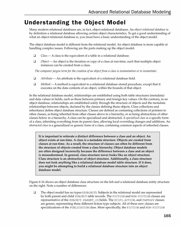
Understanding the Object ModelMany modern relational databases are, in fact, object-relational databases. An object-relational database isby definition a relational database allowing certain object characteristics. To get a good understanding ofwhat an object-relational database is, you must have a basic understanding of the object model.
The object database model is different from the relational model. An object database is more capable athandling complex issues. Following are the parts making up the object model:
❑ Class — A class is the equivalent of a table in a relational database.
❑ Object — An object is the iteration or copy of a class at run-time, such that multiple objectinstances can be created from a class.
The computer jargon term for the creation of an object from a class is instantiation or to instantiate.
❑ Attribute — An attribute is the equivalent of a relational database field.
❑ Method — A method is equivalent to a relational database stored procedure, except that it executes on the data contents of an object, within the bounds of that object.
In the relational database model, relationships are established using both table structures (metadata) and data values in fields, such as those between primary and foreign key values. On the contrary, in anobject database, relationships are established solely through the structure of objects and the metadatarelationships between objects, declared by the classes defining those objects. Class collections and inheritance define object database structure. Classes are defined as containing collections of pointers toother classes, as being inherited from other classes above in a hierarchy, or as being abstractions of otherclasses below in a hierarchy. A class can be specialized and abstracted. A specialized class is a specific formof a class, inheriting everything from its parent class, allowing local overriding changes and additions. Anabstracted class is a generalized or generic form of a class, containing common aspects of inherited classes.
Figure 6-16 shows an object database class structure on the left and a relational database entity structureon the right. Note a number of differences:
❑ The object model has no types (SUBJECT). Subjects in the relational model are represented by both parent and child SUBJECT table records. The FICTION and NON-FICTION classes arerepresentative of the SUBJECT.PARENT_ID fields. The SCIFI, ACTION, and FANTASY classes are genres, representing three different fiction type subjects. All of these new classes are specializations of the PUBLICATION class. More specifically, the FICTION and NON-FICTION
It is important to reiterate a distinct difference between a class and an object. Anobject exists at run-time. A class is a metadata structure. Objects are created fromclasses at run-time. As a result, the structure of classes can often be different fromthe structure of objects created from a class hierarchy. Object database models are often designed incorrectly because the difference between a class and an objectis misunderstood. In general, class structure never looks like an object structure.Class structure is an abstraction of object structure. Additionally, a class structuredoes not look anything like a relational database model table structure. If it does,you might be attempting to build a relational database structure into an objectdatabase model.
165
Advanced Relational Database Modeling
11_574906 ch06.qxd 10/28/05 11:39 PM Page 165
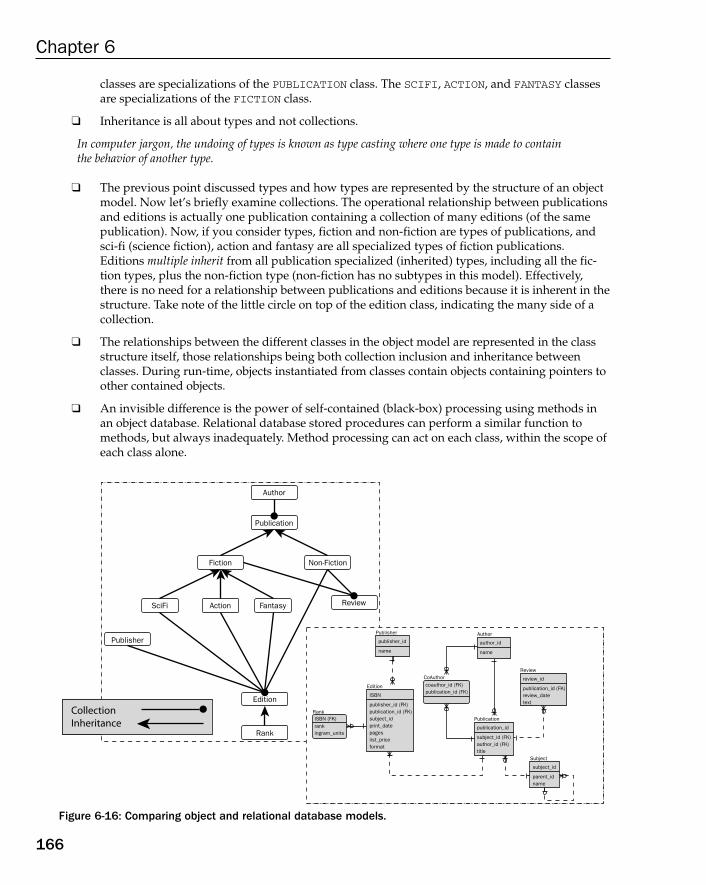
classes are specializations of the PUBLICATION class. The SCIFI, ACTION, and FANTASY classesare specializations of the FICTION class.
❑ Inheritance is all about types and not collections.
In computer jargon, the undoing of types is known as type casting where one type is made to containthe behavior of another type.
❑ The previous point discussed types and how types are represented by the structure of an objectmodel. Now let’s briefly examine collections. The operational relationship between publicationsand editions is actually one publication containing a collection of many editions (of the samepublication). Now, if you consider types, fiction and non-fiction are types of publications, andsci-fi (science fiction), action and fantasy are all specialized types of fiction publications.Editions multiple inherit from all publication specialized (inherited) types, including all the fic-tion types, plus the non-fiction type (non-fiction has no subtypes in this model). Effectively,there is no need for a relationship between publications and editions because it is inherent in thestructure. Take note of the little circle on top of the edition class, indicating the many side of acollection.
❑ The relationships between the different classes in the object model are represented in the classstructure itself, those relationships being both collection inclusion and inheritance betweenclasses. During run-time, objects instantiated from classes contain objects containing pointers toother contained objects.
❑ An invisible difference is the power of self-contained (black-box) processing using methods inan object database. Relational database stored procedures can perform a similar function tomethods, but always inadequately. Method processing can act on each class, within the scope ofeach class alone.
Figure 6-16: Comparing object and relational database models.
Publisher
publisher_id
name
Author
author_id
name
Review
review_id
publication_id (FK)review_datetext
Subject
subject_id
parent_idname
Publication
publication_id
subject_id (FK)author_id (FK)title
Edition
ISBN
publisher_id (FK)publication_id (FK)subject_idprint_datepageslist_priceformat
CoAuthorcoauthor_id (FK)publication_id (FK)
Rank
rankingram_units
ISBN (FK)
Author
Publication
Non-Fiction
Review
Fiction
Action Fantasy
Edition
Rank
SciFi
Publisher
CollectionInheritance
166
Chapter 6
11_574906 ch06.qxd 10/28/05 11:39 PM Page 166
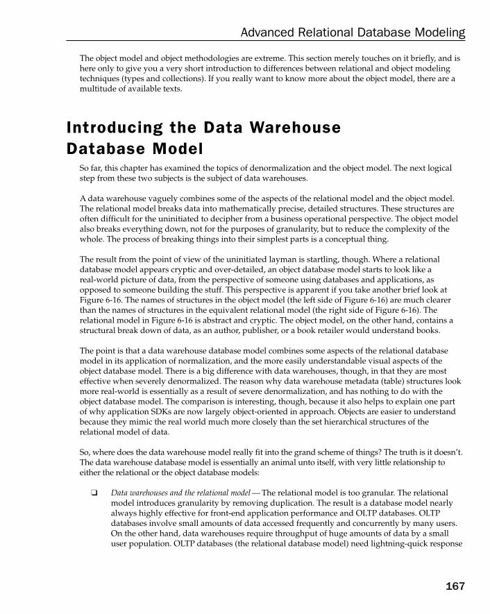
The object model and object methodologies are extreme. This section merely touches on it briefly, and ishere only to give you a very short introduction to differences between relational and object modelingtechniques (types and collections). If you really want to know more about the object model, there are amultitude of available texts.
Introducing the Data Warehouse Database Model
So far, this chapter has examined the topics of denormalization and the object model. The next logicalstep from these two subjects is the subject of data warehouses.
A data warehouse vaguely combines some of the aspects of the relational model and the object model.The relational model breaks data into mathematically precise, detailed structures. These structures areoften difficult for the uninitiated to decipher from a business operational perspective. The object modelalso breaks everything down, not for the purposes of granularity, but to reduce the complexity of thewhole. The process of breaking things into their simplest parts is a conceptual thing.
The result from the point of view of the uninitiated layman is startling, though. Where a relationaldatabase model appears cryptic and over-detailed, an object database model starts to look like a real-world picture of data, from the perspective of someone using databases and applications, asopposed to someone building the stuff. This perspective is apparent if you take another brief look atFigure 6-16. The names of structures in the object model (the left side of Figure 6-16) are much clearerthan the names of structures in the equivalent relational model (the right side of Figure 6-16). The relational model in Figure 6-16 is abstract and cryptic. The object model, on the other hand, contains astructural break down of data, as an author, publisher, or a book retailer would understand books.
The point is that a data warehouse database model combines some aspects of the relational databasemodel in its application of normalization, and the more easily understandable visual aspects of theobject database model. There is a big difference with data warehouses, though, in that they are mosteffective when severely denormalized. The reason why data warehouse metadata (table) structures lookmore real-world is essentially as a result of severe denormalization, and has nothing to do with theobject database model. The comparison is interesting, though, because it also helps to explain one partof why application SDKs are now largely object-oriented in approach. Objects are easier to understandbecause they mimic the real world much more closely than the set hierarchical structures of the relational model of data.
So, where does the data warehouse model really fit into the grand scheme of things? The truth is it doesn’t.The data warehouse database model is essentially an animal unto itself, with very little relationship toeither the relational or the object database models:
❑ Data warehouses and the relational model — The relational model is too granular. The relationalmodel introduces granularity by removing duplication. The result is a database model nearlyalways highly effective for front-end application performance and OLTP databases. OLTPdatabases involve small amounts of data accessed frequently and concurrently by many users.On the other hand, data warehouses require throughput of huge amounts of data by a smalluser population. OLTP databases (the relational database model) need lightning-quick response
167
Advanced Relational Database Modeling
11_574906 ch06.qxd 10/28/05 11:39 PM Page 167
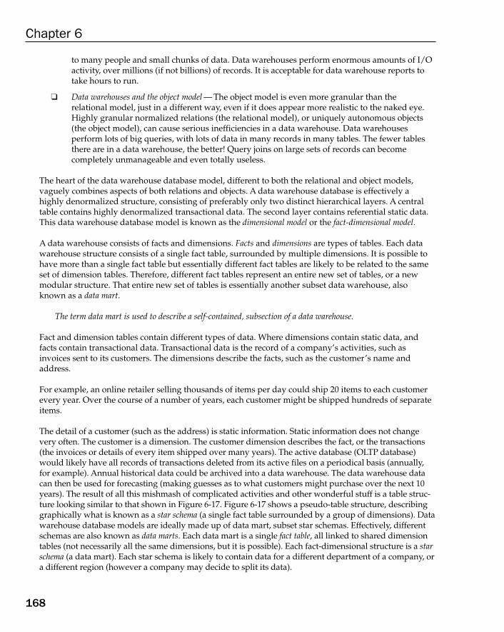
to many people and small chunks of data. Data warehouses perform enormous amounts of I/Oactivity, over millions (if not billions) of records. It is acceptable for data warehouse reports totake hours to run.
❑ Data warehouses and the object model — The object model is even more granular than the relational model, just in a different way, even if it does appear more realistic to the naked eye.Highly granular normalized relations (the relational model), or uniquely autonomous objects(the object model), can cause serious inefficiencies in a data warehouse. Data warehouses perform lots of big queries, with lots of data in many records in many tables. The fewer tablesthere are in a data warehouse, the better! Query joins on large sets of records can become completely unmanageable and even totally useless.
The heart of the data warehouse database model, different to both the relational and object models,vaguely combines aspects of both relations and objects. A data warehouse database is effectively ahighly denormalized structure, consisting of preferably only two distinct hierarchical layers. A centraltable contains highly denormalized transactional data. The second layer contains referential static data.This data warehouse database model is known as the dimensional model or the fact-dimensional model.
A data warehouse consists of facts and dimensions. Facts and dimensions are types of tables. Each datawarehouse structure consists of a single fact table, surrounded by multiple dimensions. It is possible tohave more than a single fact table but essentially different fact tables are likely to be related to the sameset of dimension tables. Therefore, different fact tables represent an entire new set of tables, or a newmodular structure. That entire new set of tables is essentially another subset data warehouse, alsoknown as a data mart.
The term data mart is used to describe a self-contained, subsection of a data warehouse.
Fact and dimension tables contain different types of data. Where dimensions contain static data, andfacts contain transactional data. Transactional data is the record of a company’s activities, such asinvoices sent to its customers. The dimensions describe the facts, such as the customer’s name andaddress.
For example, an online retailer selling thousands of items per day could ship 20 items to each customerevery year. Over the course of a number of years, each customer might be shipped hundreds of separateitems.
The detail of a customer (such as the address) is static information. Static information does not changevery often. The customer is a dimension. The customer dimension describes the fact, or the transactions(the invoices or details of every item shipped over many years). The active database (OLTP database)would likely have all records of transactions deleted from its active files on a periodical basis (annually,for example). Annual historical data could be archived into a data warehouse. The data warehouse datacan then be used for forecasting (making guesses as to what customers might purchase over the next 10years). The result of all this mishmash of complicated activities and other wonderful stuff is a table struc-ture looking similar to that shown in Figure 6-17. Figure 6-17 shows a pseudo-table structure, describinggraphically what is known as a star schema (a single fact table surrounded by a group of dimensions). Datawarehouse database models are ideally made up of data mart, subset star schemas. Effectively, differentschemas are also known as data marts. Each data mart is a single fact table, all linked to shared dimensiontables (not necessarily all the same dimensions, but it is possible). Each fact-dimensional structure is a starschema (a data mart). Each star schema is likely to contain data for a different department of a company, ora different region (however a company may decide to split its data).
168
Chapter 6
11_574906 ch06.qxd 10/28/05 11:39 PM Page 168
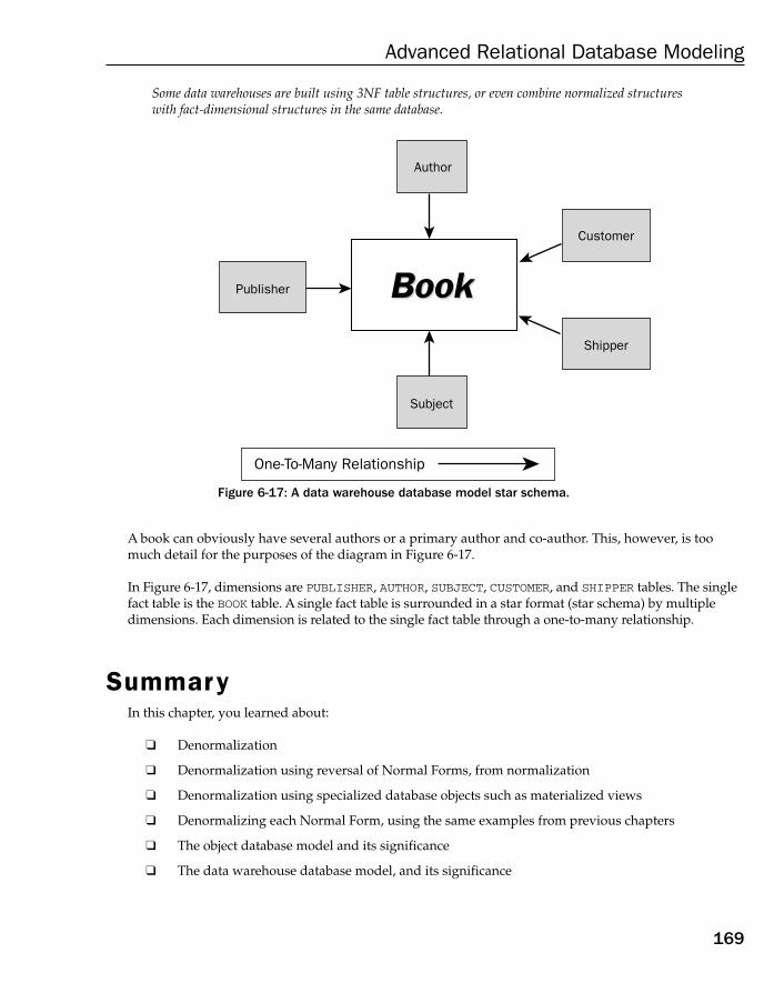
Some data warehouses are built using 3NF table structures, or even combine normalized structureswith fact-dimensional structures in the same database.
Figure 6-17: A data warehouse database model star schema.
A book can obviously have several authors or a primary author and co-author. This, however, is toomuch detail for the purposes of the diagram in Figure 6-17.
In Figure 6-17, dimensions are PUBLISHER, AUTHOR, SUBJECT, CUSTOMER, and SHIPPER tables. The singlefact table is the BOOK table. A single fact table is surrounded in a star format (star schema) by multipledimensions. Each dimension is related to the single fact table through a one-to-many relationship.
SummaryIn this chapter, you learned about:
❑ Denormalization
❑ Denormalization using reversal of Normal Forms, from normalization
❑ Denormalization using specialized database objects such as materialized views
❑ Denormalizing each Normal Form, using the same examples from previous chapters
❑ The object database model and its significance
❑ The data warehouse database model, and its significance
Publisher
Customer
Shipper
Author
Subject
One-To-Many Relationship
BookBook
169
Advanced Relational Database Modeling
11_574906 ch06.qxd 10/28/05 11:39 PM Page 169
This chapter has described some advanced database modeling topics, including denormalization, objectdatabase modeling, and data warehouse modeling. A brief grasp of object modeling is important tounderstanding the basics of object-relational databases. Denormalization is essential to understandingnot only database performance but also the topic area of data warehousing database modeling. Datawarehousing is very important to modern-day databases and is a large topic in itself. The next chaptercovers data warehouse database modeling in detail.
ExercisesUse the ERD in Figure 6-12 to help you answer these questions.
1. Create a temporary table called BAND2, joining the four tables BAND, BAND_ADDRESS, BAND_PHONE,and BAND_EMAIL together. Use a CREATE TABLE command. In the same CREATE TABLE command,add the records from the four tables into the new BAND2 temporary table. Some databases allowthis; others do not. A database not allowing insertion of records on table creation requires creationof the table, and subsequent population of the new table with INSERT commands, from selectedrecords.
2. Drop the BAND table using a DROP TABLE command and rename the BAND2 table to BAND, usingan ALTER TABLE ... RENAME command. A database not allowing a table rename commandwould require that the BAND2 table be copied to the BAND table, including data, either includedwith the CREATE TABLE BAND command, or with INSERT commands. Afterward, the BAND2temporary table can be dropped using a DROP TABLE command.
170
Chapter 6
11_574906 ch06.qxd 10/28/05 11:39 PM Page 170

7Understanding Data
Warehouse DatabaseModeling
“Intuition becomes increasingly valuable in the new information society precisely because there isso much data.” (John Naisbitt)
Data warehouses need special treatment and a special type of approach to database modeling, simply becausethey can get so unmanageably large.
Chapter 6 introduced the data warehouse database model, amongst other advanced relationaldatabase modeling techniques. Chapter 6 briefly compared data warehouse modeling relative toboth the relational database model, and the object database model. In addition, a brief descriptioncovered star schemas. This chapter delves deeply into the details of the database warehousedatabase model.
Expanding the relational database model to include the data warehouse database model may seem a little obtuse; however, in the modern, computerized, commercial world, there is probably morephysical disk space occupied by data warehouse database installations as a whole. Data warehousedatabases are usually physically much larger on average. Something larger is generally much moreexpensive and likely just as important as OLTP databases, if not more so. A bigger database costsmore money to build and maintain; therefore, data warehouse data modeling is just as important asrelational database modeling for OLTP and transactional databases.
This chapter discusses data warehouse database modeling in detail, preferably without bombardingyou with too much complexity all at once. Data warehouse data model design is a semi-normalizationapproach to relational database model design. Because many existing databases are data warehouses,inclusion of this chapter in this book, at this point, is critical.
12_574906 ch07.qxd 11/4/05 10:48 AM Page 171

In this chapter, you learn about the following:
❑ The origin of data warehouses
❑ How data warehouses require a specialized database model
❑ Star and snowflake schemas
❑ Facts and dimensions
❑ The fact-dimensional database model
❑ How to create a data warehouse database model
❑ The contents of a data warehouse database model
The Origin of Data WarehousesData warehouses were originally devised because existing databases were being subjected to conflictingrequirements. Conflict arose between operational use and decision-support requirements as follows:
❑ Operational use — Operational use of a database requires a precise, accurate, and instant pictureof data in a database. This includes all day-to-day operations in the functional running of a business. When a customer comes through the door, asks for a specific part, for a specific automobile, for a specific year, the part is searched for in a database. After the customer makesthe purchase, they are invoiced. When the customer pays, the transaction is processed throughbank accounts, and otherwise. All of this is operational-type activity. Response is instantaneous(or as near to instantaneous as possible) and it is all company to customer-direct trading activity.The operations aspect of a company is the heart of its business.
❑ Decision-support use — Where operational use divides data based on business function, decision-support requires division of database data based on subject matter. Operational use requiresaccess to specific items such as a specific part for a specific automobile, for a specific customer.Decision-support use requirements might be a summary of which parts were ordered on whichdates, not necessarily by whom. A decision-support database presents reports, such as all partsin stock, plus all parts ordered, over the period of a whole year. The result could be a projectionof when new parts should be ordered. The report allows company employees to cater forrestocking of popular items.
There is a big difference between requirements for operational and decision-support databases. Operationalsystems require instant responses on small amounts of information. Decision-support systems need accessto large amounts of data (large portions of a database), allowing for good all-round estimates as to futureprospects for a company. The invention of data warehouses was inevitable to reduce conflict betweensmall transactional (OLTP databases) and large historical analytical reporting requirements (data warehouses).
172
Chapter 7
12_574906 ch07.qxd 11/4/05 10:48 AM Page 172
The demands of the modern global economy and the Internet dictate that end user operational applicationsare required to be active 24/7, 365 days a year. There is no window for any type of batch activity becausewhen people are asleep in Europe, others are awake down under in Australia. The global economy requiresinstant and acceptable servicing of the needs of a global user population.
In reality, the most significant difference between OLTP databases and data warehouses extends all the way down to the hardware layer. OLTP databases need highly efficient sharing of critical resourcessuch as onboard memory (RAM), and have very small I/O requirements. Data warehouses are completely opposite. Data warehouses can consume large portions of RAM by transferring between diskand memory, in detriment to an OLTP database running on the same machine. Where OLTP databasesneed resource sharing, data warehouses need to hog those resources for extended periods of time. So, adata warehouse hogs machine resources. An OLTP database attempts to share those same resources. It islikely to have unacceptable response times because of a lack of basic I/O resources for both databasetypes. The result, therefore, is a requirement for a complete separation between operational (OLTP) anddecision-support (data warehouse) activity. This is why data warehouses exist!
The Relational Database Model and Data WarehousesThe traditional OLTP (transactional) type of relational database model does not cater for data warehouserequirements. The relational database model is too granular. “Granular” implies too many little pieces.Processing through all those little-bitty pieces is too time consuming for large transactions, joining allthose pieces together. Similar to the object database model, the relational database model removes duplication and creates granularity. This type of database model is efficient for front-end applicationperformance, involving small amounts of data that are accessed frequently and concurrently by manyusers at once. This is what an OLTP database does.
Data warehouses, on the other hand, need throughput of huge amounts of data by relatively very fewusers. Data warehouses process large quantities of data at once, mainly for reporting and analytical processing. Also, data warehouses are regularly updated, but usually in large batch operations. OLTPdatabases need lightning-quick response to many individual users. Data warehouses perform enormousamounts of I/O activity over copious quantities of data; therefore, the needs of OLTP and data warehousedatabases are completely contrary to each other, down to the lowest layer of hardware resource usage.
Hardware resource usage is the most critical consideration. Software rests quite squarely on the shouldersof your hardware. Proper use of memory (RAM), disk storage, and CPU time to manage everything is thecritical layer for all activity. OLTP and data warehouse database differences extend all the way down tothis most critical of layers. OLTP databases require intensely sharable hardware structures (commonlyknown as concurrency), needing highly efficient use of memory and processor time allocations. Data warehouses need huge amounts of disk space, processing power as well, but all dedicated to long-runningprograms (commonly known as batch operations or throughput).
A data warehouse database simply cannot cope using a standard OLTP database relational databasemodel. Something else is needed for a data warehouse.
173
Understanding Data Warehouse Database Modeling
12_574906 ch07.qxd 11/4/05 10:48 AM Page 173
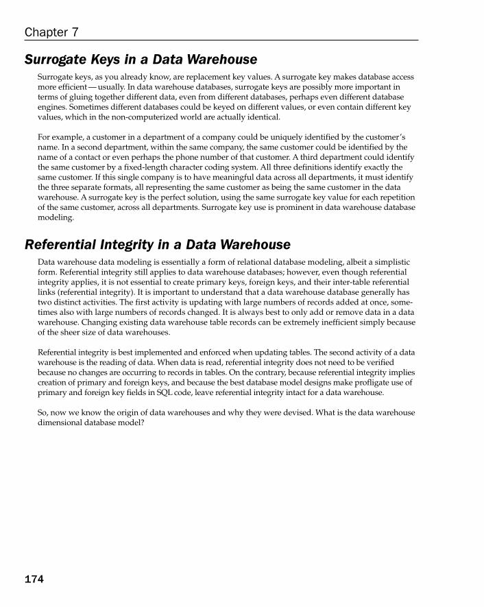
Surrogate Keys in a Data WarehouseSurrogate keys, as you already know, are replacement key values. A surrogate key makes database accessmore efficient — usually. In data warehouse databases, surrogate keys are possibly more important interms of gluing together different data, even from different databases, perhaps even different databaseengines. Sometimes different databases could be keyed on different values, or even contain different keyvalues, which in the non-computerized world are actually identical.
For example, a customer in a department of a company could be uniquely identified by the customer’sname. In a second department, within the same company, the same customer could be identified by thename of a contact or even perhaps the phone number of that customer. A third department could identifythe same customer by a fixed-length character coding system. All three definitions identify exactly thesame customer. If this single company is to have meaningful data across all departments, it must identifythe three separate formats, all representing the same customer as being the same customer in the datawarehouse. A surrogate key is the perfect solution, using the same surrogate key value for each repetitionof the same customer, across all departments. Surrogate key use is prominent in data warehouse databasemodeling.
Referential Integrity in a Data WarehouseData warehouse data modeling is essentially a form of relational database modeling, albeit a simplisticform. Referential integrity still applies to data warehouse databases; however, even though referentialintegrity applies, it is not essential to create primary keys, foreign keys, and their inter-table referentiallinks (referential integrity). It is important to understand that a data warehouse database generally hastwo distinct activities. The first activity is updating with large numbers of records added at once, some-times also with large numbers of records changed. It is always best to only add or remove data in a datawarehouse. Changing existing data warehouse table records can be extremely inefficient simply becauseof the sheer size of data warehouses.
Referential integrity is best implemented and enforced when updating tables. The second activity of a datawarehouse is the reading of data. When data is read, referential integrity does not need to be verifiedbecause no changes are occurring to records in tables. On the contrary, because referential integrity impliescreation of primary and foreign keys, and because the best database model designs make profligate use ofprimary and foreign key fields in SQL code, leave referential integrity intact for a data warehouse.
So, now we know the origin of data warehouses and why they were devised. What is the data warehousedimensional database model?
174
Chapter 7
12_574906 ch07.qxd 11/4/05 10:48 AM Page 174
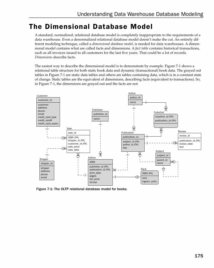
The Dimensional Database ModelA standard, normalized, relational database model is completely inappropriate to the requirements of adata warehouse. Even a denormalized relational database model doesn’t make the cut. An entirely dif-ferent modeling technique, called a dimensional database model, is needed for data warehouses. A dimen-sional model contains what are called facts and dimensions. A fact table contains historical transactions,such as all invoices issued to all customers for the last five years. That could be a lot of records.Dimensions describe facts.
The easiest way to describe the dimensional model is to demonstrate by example. Figure 7-1 shows a relational table structure for both static book data and dynamic (transactional) book data. The grayed outtables in Figure 7-1 are static data tables and others are tables containing data, which is in a constant stateof change. Static tables are the equivalent of dimensions, describing facts (equivalent to transactions). So,in Figure 7-1, the dimensions are grayed out and the facts are not.
Figure 7-1: The OLTP relational database model for books.
Customer
customer_id
Shipper
shipper_id
shipperaddressphoneemail
customeraddressphoneemailcredit_card_typecredit_card#credit_card_expiry
Sale
sale_id
ISBN (FK)shipper_id (FK)customer_id (FK)sale_pricesale_date
Edition
ISBN
publisher_id (FK)publication_id (FK)print_datepageslist_priceformat
Publisher
publisher_id
name
Publication
publication_id
subject_id (FK)author_id (FK)title
Author
author_id
name
Review
review_id
publication_id (FK)review_datetext
Subject
subject_id
parent_idname
CoAuthor
coauthor_id (FK)
publication_id (FK)
Rank
ISBN (FK)
rankingram_units
175
Understanding Data Warehouse Database Modeling
12_574906 ch07.qxd 11/4/05 10:48 AM Page 175
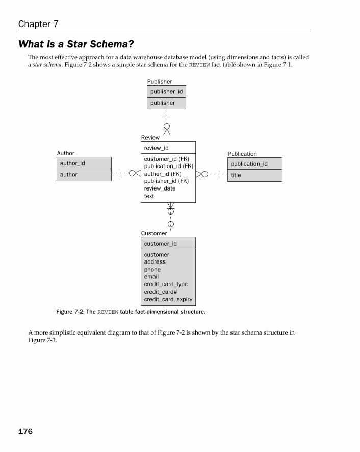
What Is a Star Schema?The most effective approach for a data warehouse database model (using dimensions and facts) is calleda star schema. Figure 7-2 shows a simple star schema for the REVIEW fact table shown in Figure 7-1.
Figure 7-2: The REVIEW table fact-dimensional structure.
A more simplistic equivalent diagram to that of Figure 7-2 is shown by the star schema structure inFigure 7-3.
Review
review_id
customer_id (FK)publication_id (FK)author_id (FK)publisher_id (FK)review_datetext
Customer
customer_id
customeraddressphoneemailcredit_card_typecredit_card#credit_card_expiry
Author
author_id
author
Publisher
publisher_id
publisher
Publication
publication_id
title
176
Chapter 7
12_574906 ch07.qxd 11/4/05 10:48 AM Page 176
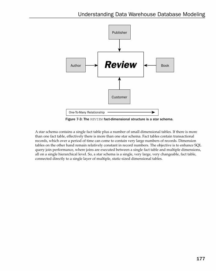
Figure 7-3: The REVIEW fact-dimensional structure is a star schema.
A star schema contains a single fact table plus a number of small dimensional tables. If there is morethan one fact table, effectively there is more than one star schema. Fact tables contain transactionalrecords, which over a period of time can come to contain very large numbers of records. Dimensiontables on the other hand remain relatively constant in record numbers. The objective is to enhance SQLquery join performance, where joins are executed between a single fact table and multiple dimensions,all on a single hierarchical level. So, a star schema is a single, very large, very changeable, fact table, connected directly to a single layer of multiple, static-sized dimensional tables.
Author Book
Publisher
Customer
One-To-Many Relationship
ReviewReview
177
Understanding Data Warehouse Database Modeling
12_574906 ch07.qxd 11/4/05 10:48 AM Page 177
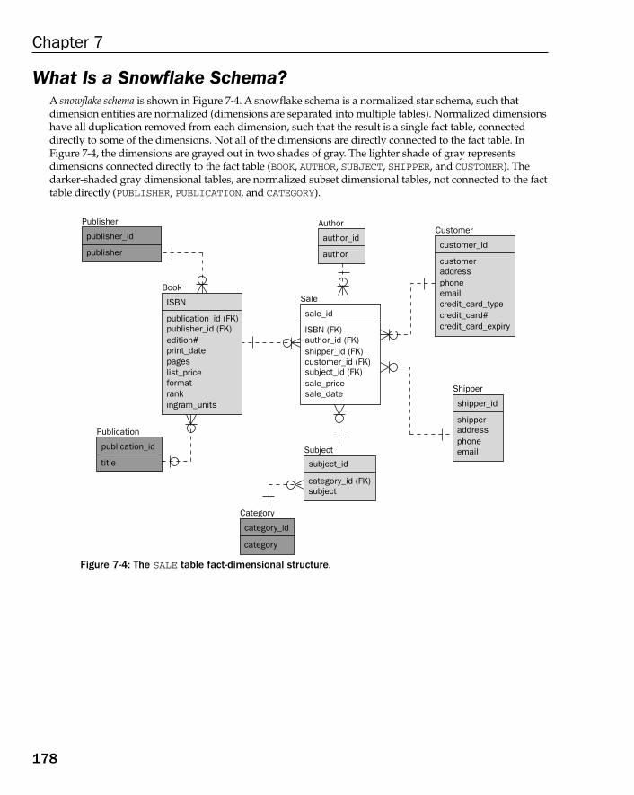
What Is a Snowflake Schema?A snowflake schema is shown in Figure 7-4. A snowflake schema is a normalized star schema, such thatdimension entities are normalized (dimensions are separated into multiple tables). Normalized dimensionshave all duplication removed from each dimension, such that the result is a single fact table, connecteddirectly to some of the dimensions. Not all of the dimensions are directly connected to the fact table. InFigure 7-4, the dimensions are grayed out in two shades of gray. The lighter shade of gray representsdimensions connected directly to the fact table (BOOK, AUTHOR, SUBJECT, SHIPPER, and CUSTOMER). Thedarker-shaded gray dimensional tables, are normalized subset dimensional tables, not connected to the facttable directly (PUBLISHER, PUBLICATION, and CATEGORY).
Figure 7-4: The SALE table fact-dimensional structure.
Customer
customer_id
Shipper
shipper_id
shipperaddressphoneemail
customeraddressphoneemailcredit_card_typecredit_card#credit_card_expiry
Book
ISBN
publication_id (FK)publisher_id (FK)edition#print_datepageslist_priceformatrankingram_units
Sale
sale_id
ISBN (FK)author_id (FK)shipper_id (FK)customer_id (FK)subject_id (FK)sale_pricesale_date
Publisher
publisher_id
publisher
Author
author_id
author
Publication
publication_id
titleSubject
subject_id
category_id (FK)subject
Category
category_id
category
178
Chapter 7
12_574906 ch07.qxd 11/4/05 10:48 AM Page 178

A more simplistic equivalent diagram to that of Figure 7-4 is shown by the snowflake schema in Figure 7-5.
Figure 7-5: The SALE fact-dimensional structure is a snowflake schema.
The problem with snowflake schemas isn’t too many tables but too many layers. Data warehouse facttables can become incredibly large, even to millions, billions, even trillions of records. The critical factorin creating star and snowflake schemas, instead of using standard “nth” Normal Form layers, is decreasingthe number of tables in SQL query joins. The more tables in a join, the more complex a query, the slowerit will execute. When fact tables contain enormous record counts, reports can take hours and days, notminutes. Adding just one more table to a fact-dimensional query join at that level of database size couldmake the query run for weeks. That’s no good!
Book
Publication
Publisher
Customer
Shipper
Author
Subject
One-To-Many Relationship
SaleSale
Category
179
Understanding Data Warehouse Database Modeling
12_574906 ch07.qxd 11/4/05 10:48 AM Page 179
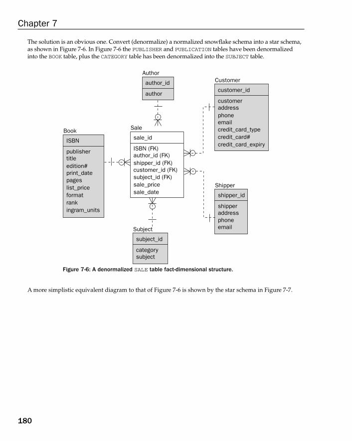
The solution is an obvious one. Convert (denormalize) a normalized snowflake schema into a star schema,as shown in Figure 7-6. In Figure 7-6 the PUBLISHER and PUBLICATION tables have been denormalizedinto the BOOK table, plus the CATEGORY table has been denormalized into the SUBJECT table.
Figure 7-6: A denormalized SALE table fact-dimensional structure.
A more simplistic equivalent diagram to that of Figure 7-6 is shown by the star schema in Figure 7-7.
Sale
sale_id
ISBN (FK)author_id (FK)shipper_id (FK)customer_id (FK)subject_id (FK)sale_pricesale_date
Customer
customer_id
customeraddressphoneemailcredit_card_typecredit_card#credit_card_expiry
Shipper
shipper_id
shipperaddressphoneemail
Author
author_id
author
Book
ISBN
publishertitleedition#print_datepageslist_priceformatrankingram_units
Subject
subject_id
categorysubject
180
Chapter 7
12_574906 ch07.qxd 11/4/05 10:48 AM Page 180
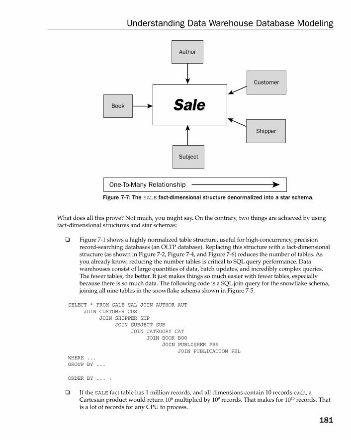
Figure 7-7: The SALE fact-dimensional structure denormalized into a star schema.
What does all this prove? Not much, you might say. On the contrary, two things are achieved by usingfact-dimensional structures and star schemas:
❑ Figure 7-1 shows a highly normalized table structure, useful for high-concurrency, precisionrecord-searching databases (an OLTP database). Replacing this structure with a fact-dimensionalstructure (as shown in Figure 7-2, Figure 7-4, and Figure 7-6) reduces the number of tables. Asyou already know, reducing the number tables is critical to SQL query performance. Data warehouses consist of large quantities of data, batch updates, and incredibly complex queries.The fewer tables, the better. It just makes things so much easier with fewer tables, especiallybecause there is so much data. The following code is a SQL join query for the snowflake schema,joining all nine tables in the snowflake schema shown in Figure 7-5.
SELECT * FROM SALE SAL JOIN AUTHOR AUTJOIN CUSTOMER CUS
JOIN SHIPPER SHPJOIN SUBJECT SUB
JOIN CATEGORY CATJOIN BOOK BOO
JOIN PUBLISHER PBSJOIN PUBLICATION PBL
WHERE ...GROUP BY ...
ORDER BY ... ;
❑ If the SALE fact table has 1 million records, and all dimensions contain 10 records each, aCartesian product would return 106 multiplied by 109 records. That makes for 1015 records. Thatis a lot of records for any CPU to process.
Book
Customer
Shipper
Author
Subject
One-To-Many Relationship
SaleSale
181
Understanding Data Warehouse Database Modeling
12_574906 ch07.qxd 11/4/05 10:48 AM Page 181
A Cartesian product is a worse-case scenario.
❑ Now look at the next query.
SELECT * FROM SALE SAL JOIN AUTHOR AUTJOIN CUSTOMER CUS
JOIN SHIPPER SHPJOIN SUBJECT SUB
JOIN BOOK BOOWHERE ...GROUP BY ...
ORDER BY ... ;
❑ Using the star schema from Figure 7-7, assuming the same number of records, a join occursbetween one fact table and six dimensional tables. That is a Cartesian product of 106 multiple by 106, resulting in 1012 records returned. The difference between 1012 and 1015 is three deci-mals. Three decimals is not just three zeroes and thus 1,000 records. The difference is actually1,000,000,000,000,000 – 1,000,000,000,000 = 999,000,000,000,000. That is effectively just a little lessthan 1015. The difference between six dimensions and nine dimensions is more or less infinite,from the perspective of counting all those zeros. Fewer dimensions make for faster queries.That’s why it is so essential to denormalize snowflake schemas into star schemas.
❑ Take another quick glance at the snowflake schema in Figure 7-4 and Figure 7-5. Then examinethe equivalent denormalized star schema in Figure 7-6 and Figure 7-7. Now put yourself intothe shoes of a hustled, harried and very busy executive — trying to get a quick report. Think asan end-user, one only interested in results. Which diagram is easier to decipher as to contentand meaning? The diagram in Figure 7-7 is more complex than the diagram in Figure 7-5? Afterall, being an end-user, you are probably not too interested in understanding the complexities ofhow to build SQL join queries. You have bigger fish to fry. The point is this: The less complexthe table structure, the easier it will be to use. This is because a star schema is more representa-tive of the real world than a snowflake schema. Look at it this way. A snowflake schema is more deeply normalized than a star schema, and, therefore, by definition more mathematical.Something more mathematical is generally of more use to a mathematician than it is to an exec-utive manager. The executive is trying to get a quick overall impression of whether his companywill sell more cans of lima beans, or more cans of string beans, over the course of the next tenyears. If you are a computer programmer, you will quite probably not agree with this analogy.
That tells us the very basics of data warehouse database modeling. How can a data warehouse databasemodel be constructed?
How to Build a Data Warehouse Database Model
Now you know how to build star schemas for data warehouse database models. As you can see, a starschema is quite different from a standard relational database model (Figure 7-1). The next step is toexamine the process, or the steps, by which a data warehouse database model can be built.
182
Chapter 7
12_574906 ch07.qxd 11/4/05 10:48 AM Page 182
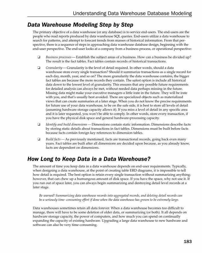
Data Warehouse Modeling Step by StepThe primary objective of a data warehouse (or any database) is to service end-users. The end-users are thepeople who read reports produced by data warehouse SQL queries. End-users utilize a data warehouse tosearch for patterns, and attempt to forecast trends from masses of historical information. From that per-spective, there is a sequence of steps in approaching data warehouse database design, beginning with theend-user perspective. The end-user looks at a company from a business process, or operational perspective:
❑ Business processes — Establish the subject areas of a business. How can a business be divided up?The result is the fact tables. Fact tables contain records of historical transactions.
❑ Granularity — Granularity is the level of detail required. In other words, should a data warehouse store every single transaction? Should it summarize transactions as a single record foreach day, month, year, and so on? The more granularity the data warehouse contains, the biggerfact tables are because the more records they contain. The safest option is include all historicaldata down to the lowest level of granularity. This ensures that any possible future requirementsfor detailed analysis can always be met, without needed data perhaps missing in the future.Missing data might make your executive managers a little irate in the future. They will be iratewith you, and that’s usually best avoided. There are specialized objects such as materializedviews that can create summaries at a later stage. When you do not know the precise requirementsfor future use of your data warehouse, to be on the safe side, it is best to store all levels of detail(assuming hardware storage capacity allows it). If you miss a level of detail in any specific areaand it is later requested, you won’t be able to comply. In other words, store every transaction, ifyou have the physical disk space and general hardware-processing capacity.
❑ Identify and build dimensions — Dimensions contain static information. Dimensions describe factsby storing static details about transactions in fact tables. Dimensions must be built before factsbecause facts contain foreign key references to dimension tables.
❑ Build facts — As previously mentioned, facts are transactional records, going back even manyyears. Fact tables are built after all dimensions are decided upon because, as you already know,facts are dependent on dimensions.
How Long to Keep Data in a Data Warehouse?The amount of time you keep data in a data warehouse depends on end-user requirements. Typically,when designing a data warehouse, at the point of creating table ERD diagrams, it is impossible to tellhow detail is required. The best option is retain every single transaction without summarizing anything;however, that can chew up a humungous amount of disk space. If you have the space, why not use it. Ifyou run out of space later, you can always begin summarizing and destroying detail level records at alater stage.
Be warned! Summarizing data warehouse records into aggregated records, and deleting detail records canbe a seriously time- consuming effort if done when the data warehouse has grown to be extremely large.
Data warehouses sometimes retain all data forever. When a data warehouse becomes too difficult tomanage, there will have to be some deletion of older data, or summarizing (or both). It all depends onhardware storage capacity, the power of computers, and how much you can spend on continuallyexpanding the capacity of existing hardware. Upgrading a large data warehouse to new hardware andsoftware can also be very time-consuming.
183
Understanding Data Warehouse Database Modeling
12_574906 ch07.qxd 11/4/05 10:48 AM Page 183

Types of Dimension TablesThe data warehouse database models for the REVIEW and SALE tables, shown previously in this chapter,are actually inadequate. Many data warehouse databases have standard requirements based on how end-users need to analyze data. Typical additions to data warehouse databases are dimensions such asdates, locations, and products. These extra dimensions can be built from most types of transactional data.
Any types of transactions involving products or services are usually dated, such as orders, invoices, or payments. Therefore, every transaction can be placed (or dated) into specific periods. Locations can usuallybe assessed either generally or in detail from customers, suppliers, shippers, and other company’s that con-tact is had with. The REVIEW and SALE fact tables shown in Figure 7-2 and Figure 7-4 both contain datefields (REVIEW.REVIEW_DATE and SALE.SALE_DATE). A date or timestamp dimension might look some-thing similar to that shown in Figure 7-8. Date fields in the tables would be replaced with identifiers asshown in Figure 7-9. Note how the date values in the TIME table, as shown in Figure 7-8, are reconstitutedin a specific time window period, such as MONTH, QUARTER, and YEAR.
Figure 7-8: A time dimension entity.
Figure 7-9 shows fact tables for both book reviews and sales, where the date fields have been replacedwith foreign key links to the TIME table. The result of this is that facts can be analyzed by month, quarter,and year. In this case, removing the date fields from the fact tables has actually decreased the detaillevel. Now data can only be analyzed by month. Months are the lowest level of detail. To retain the ability to analyze on a daily basis, or with further detail such as hours and minutes, either the TIME tableshould be expanded to accommodate more detail periods, or the date fields should be retained in thefact tables.
Another commonly used dimension involves locations, which can be states, cities, countries, continents,regions, and others. Location details for review and sale facts can be gleaned from customer and shipperaddress details. The resulting LOCATION table would look something like that shown in Figure 7-10.Some silly fields have been added just to give this conversation a little color. The equivalent star schemachanges are shown in Figure 7-11.
Time
time_id
monthquarteryear
184
Chapter 7
12_574906 ch07.qxd 11/4/05 10:48 AM Page 184
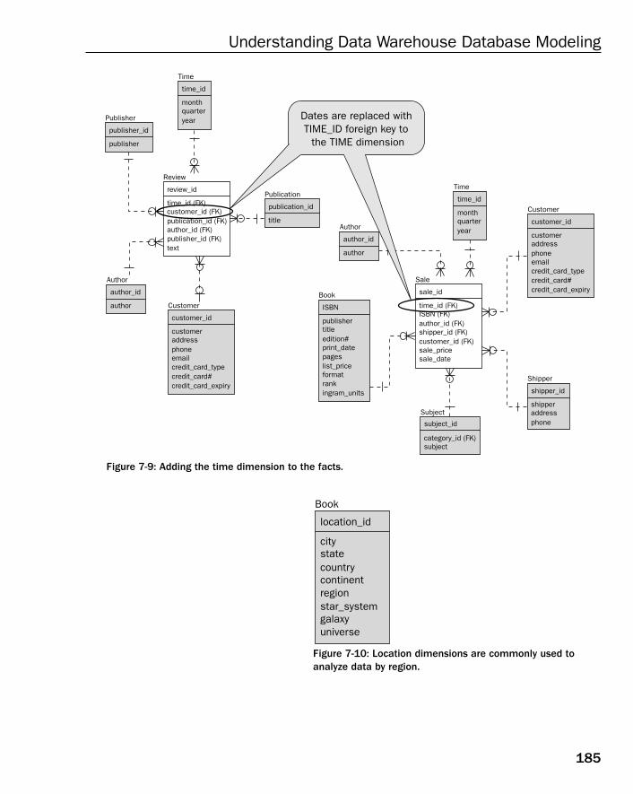
Figure 7-9: Adding the time dimension to the facts.
Figure 7-10: Location dimensions are commonly used toanalyze data by region.
Book
location_id
citystatecountrycontinentregionstar_systemgalaxyuniverse
Customer
customer_id
customeraddressphoneemailcredit_card_typecredit_card#credit_card_expiry
Review
review_id
time_id (FK)customer_id (FK)publication_id (FK)author_id (FK)publisher_id (FK)text
Book
ISBN
publishertitleedition#print_datepageslist_priceformatrankingram_units
Sale
sale_id
time_id (FK)ISBN (FK)author_id (FK)shipper_id (FK)customer_id (FK)sale_pricesale_date
Publisher
publisher_id
publisher
Author
author_id
author
Publication
publication_id
title
Subject
subject_id
category_id (FK)subject
Time
time_id
monthquarteryear
Author
author_id
author
Time
time_id
monthquarteryear
Customer
customer_id
customeraddressphoneemailcredit_card_typecredit_card#credit_card_expiry
Shipper
shipper_id
shipperaddressphone
Dates are replaced with TIME_ID foreign key to
the TIME dimension
185
Understanding Data Warehouse Database Modeling
12_574906 ch07.qxd 11/4/05 10:48 AM Page 185
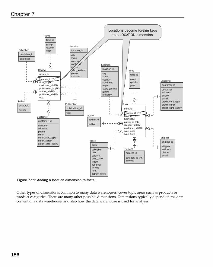
Figure 7-11: Adding a location dimension to facts.
Other types of dimensions, common to many data warehouses, cover topic areas such as products orproduct categories. There are many other possible dimensions. Dimensions typically depend on the datacontent of a data warehouse, and also how the data warehouse is used for analysis.
Location
location_id
citystatecountrycontinentregionstart_systemgalaxyuniverse
Customer
customer_id
customeraddressphoneemailcredit_card_typecredit_card#credit_card_expiry
Review
review_id
time_id (FK)location_id (FK)
customer_id (FK)publication_id (FK)author_id (FK)publisher_id (FK)text
Book
ISBN
publishertitleedition#print_datepageslist_priceformatrankingram_units
Sale
sale_id
location_id (FK)time_id (FK)ISBN (FK)author_id (FK)shipper_id (FK)customer_id (FK)sale_pricesale_date
Publisher
publisher_id
publisher
Author
author_id
author
Publication
publication_id
title
Subject
subject_id
category_id (FK)subject
Time
time_id
monthquarteryear
Author
author_id
author
Time
time_id
monthquarteryear
Customer
customer_id
customeraddressphoneemailcredit_card_typecredit_card#credit_card_expiry
Shipper
shipper_id
shipperaddressphoneemail
Locations become foreign keysto a LOCATION dimension
Location
location_id
citystatecountrycontinentregionstart_systemgalaxyuniverse
186
Chapter 7
12_574906 ch07.qxd 11/4/05 10:48 AM Page 186
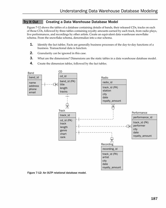
Try It Out Creating a Data Warehouse Database ModelFigure 7-12 shows the tables of a database containing details of bands, their released CDs, tracks on eachof those CDs, followed by three tables containing royalty amounts earned by each track, from radio plays,live performances, and recordings by other artists. Create an equivalent data warehouse snowflakeschema. From the snowflake schema, denormalize into a star schema.
1. Identify the fact tables. Facts are generally business processes of the day-to-day functions of abusiness. Transactional data is function.
2. Granularity can be ignored in this case.
3. What are the dimensions? Dimensions are the static tables in a data warehouse database model.
4. Create the dimension tables, followed by the fact tables.
Figure 7-12: An OLTP relational database model.
Track
track_id
cd_id (FK)tracklengthgenrechartrank
Band
band_id
addressphone
name
CD
cd_id
band_id (FK)titlelengthtracks
Radio
radio_id
track_id (FK)stationcitydateroyalty_amount
Performance
performance_id
Recording
recording_id
track_id (FK)performercitydateroyalty_amount
track_id (FK)artistcitydateroyalty_amount
187
Understanding Data Warehouse Database Modeling
12_574906 ch07.qxd 11/4/05 10:48 AM Page 187
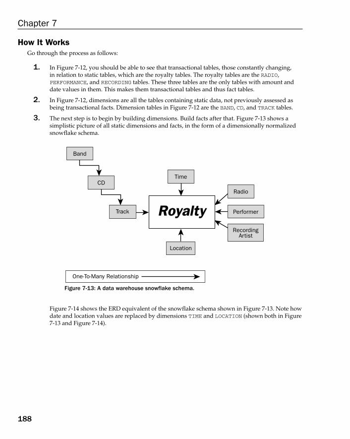
How It WorksGo through the process as follows:
1. In Figure 7-12, you should be able to see that transactional tables, those constantly changing, in relation to static tables, which are the royalty tables. The royalty tables are the RADIO, PERFORMANCE, and RECORDING tables. These three tables are the only tables with amount anddate values in them. This makes them transactional tables and thus fact tables.
2. In Figure 7-12, dimensions are all the tables containing static data, not previously assessed asbeing transactional facts. Dimension tables in Figure 7-12 are the BAND, CD, and TRACK tables.
3. The next step is to begin by building dimensions. Build facts after that. Figure 7-13 shows a simplistic picture of all static dimensions and facts, in the form of a dimensionally normalizedsnowflake schema.
Figure 7-13: A data warehouse snowflake schema.
Figure 7-14 shows the ERD equivalent of the snowflake schema shown in Figure 7-13. Note howdate and location values are replaced by dimensions TIME and LOCATION (shown both in Figure7-13 and Figure 7-14).
Band
CD
Track
Time
Location
Radio
Performer
RecordingArtist
RoyaltyRoyalty
One-To-Many Relationship
188
Chapter 7
12_574906 ch07.qxd 11/4/05 10:48 AM Page 188
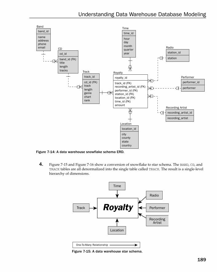
Figure 7-14: A data warehouse snowflake schema ERD.
4. Figure 7-15 and Figure 7-16 show a conversion of snowflake to star schema. The BAND, CD, andTRACK tables are all denormalized into the single table called TRACK. The result is a single-levelhierarchy of dimensions.
Figure 7-15: A data warehouse star schema.
Track
Time
Location
Radio
Performer
RecordingArtist
RoyaltyRoyalty
One-To-Many Relationship
Track
track_id
cd_id (FK)tracklengthgenrechartrank
Time
time_id
hourdaymonthquarteryear
Band
band_id
addressphone
name
email CD
cd_id
band_id (FK)titlelengthtracks
Radio
station_id
station
Performer
performer_id
Recording Artist
recording_artist_id
performer
recording_artist
Royalty
royalty_id
track_id (FK)recording_artist_id (FK)performer_id (FK)station_id (FK)location_id (FK)time_id (FK)amount
Location
location_id
citycountystatecountry
189
Understanding Data Warehouse Database Modeling
12_574906 ch07.qxd 11/4/05 10:48 AM Page 189
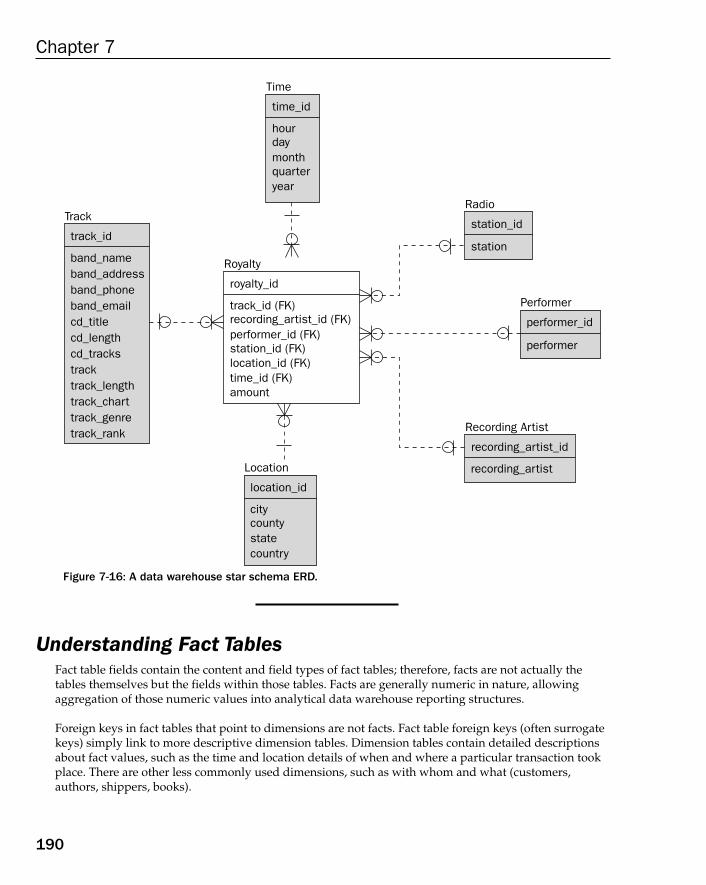
Figure 7-16: A data warehouse star schema ERD.
Understanding Fact TablesFact table fields contain the content and field types of fact tables; therefore, facts are not actually thetables themselves but the fields within those tables. Facts are generally numeric in nature, allowingaggregation of those numeric values into analytical data warehouse reporting structures.
Foreign keys in fact tables that point to dimensions are not facts. Fact table foreign keys (often surrogatekeys) simply link to more descriptive dimension tables. Dimension tables contain detailed descriptionsabout fact values, such as the time and location details of when and where a particular transaction tookplace. There are other less commonly used dimensions, such as with whom and what (customers,authors, shippers, books).
Track
track_id
band_nameband_addressband_phoneband_emailcd_titlecd_lengthcd_trackstracktrack_lengthtrack_charttrack_genretrack_rank
Time
time_id
hourdaymonthquarteryear
Radio
station_id
station
Performer
performer_id
Recording Artist
recording_artist_id
performer
recording_artist
Royalty
royalty_id
track_id (FK)recording_artist_id (FK)performer_id (FK)station_id (FK)location_id (FK)time_id (FK)amount
Location
location_id
citycountystatecountry
190
Chapter 7
12_574906 ch07.qxd 11/4/05 10:48 AM Page 190
Fact tables can contain detailed transactional histories, summaries (aggregations), or both. Details and aggregations can be separated into different fact tables. Many relational databases allow use ofmaterialized views to contain fact table aggregations, containing less detailed aggregations of theirunderlying fact tables.
One of the most significant factors with fact tables, specifically because of their potentially enormoussize, is how fact tables are changed. How is data changed in fact tables? Fact tables can be added to orchanged, and even deleted from. The least obstructive changes to fact tables are done by adding newdata, preferably during low end-user activity time windows. Deletion from fact tables is necessary whenupgrading to more summarized details, or perhaps deletion of old data that is no longer useful. Facttables are thus regarded as being additive, semi-additive, or non-additive. The most efficient data warehouses are those that never change, containing only non-additive fact tables. Additive tables aremore practical because the more current data warehouse facts are, the more useful they should becomefor analysis.
SummaryIn this chapter, you learned about:
❑ The importance of understanding the origin of data warehouses, especially why they wereinvented and how they are used
❑ The inadequacy of the transactional (OLTP) database model for producing forecasts and predictions from huge amounts of out of date data because an OLTP database model has toomuch granularity
❑ Specialized database modeling techniques required by data warehouses in the form of facts anddimensions
❑ Star schemas as single dimensional layers and how they provide best efficiency and clarity toend-users
❑ Snowflake schemas as normalized, less efficient forms of star schemas
❑ Variable data, the transactions or history of company transactional activities that compose facts
❑ How dimensions contain static, descriptive data; dimensional data describes fact data
❑ How dimensions describe the facts by normalizing only static (dimensional) data, preferably ina single dimensional layer
❑ How fact-dimensional or dimensional database modeling is either a star schema or a snowflakeschema
❑ Data warehouses containing one or more fact tables, linked to the same dimensions, or a subsetof the dimensions
❑ The various steps and processes used in the creation of a data warehouse database model
❑ The contents of a data warehouse database and model are both static and historical
❑ Static (dimensional) data changes infrequently
❑ Historical or archived data (factual) is continually added to, and can grow enormously over time
191
Understanding Data Warehouse Database Modeling
12_574906 ch07.qxd 11/4/05 10:48 AM Page 191

This chapter has described the specialized database modeling techniques required for the building ofdata warehouses. The next chapter examines one of the most important factors of database modeling —performance. If a database underperforms, a company can lose customers and, in extreme situations,lose all its customers. Guess what happens after that? Look, no job!
ExercisesUse the ERDs in Figure 7-14 and Figure 7-16 to help you answer these questions:
1. Create scripts to create tables for the snowflake schema in Figure 7-14.
2. Change the tables created for the previous question, converting the snowflake schema in Figure7-14 to the star schema in Figure 7-16. Use CREATE TABLE and DROP TABLE commands.
192
Chapter 7
12_574906 ch07.qxd 11/4/05 10:48 AM Page 192

8Building Fast-Performing
Database Models
“Man is a slow, sloppy, and brilliant thinker; the machine is fast, accurate, and stupid.” (William M. Kelly)
Man is ingenious. Only by instructing a database properly will it perform well.
Much of the information in this chapter has already been discussed, perhaps even analyzed, andoften alluded to, in previous chapters of this book. This chapter is intended to take everything youhave learned so far (all the theory) and begin the process of putting it into practice. This chapterdescribes various factors affecting database performance tuning, as applied to different databasemodel types. Anything obviously repeated from a previous chapter should be considered as beingdoubly significant, with respect to database modeling. Database performance is the most importantfactor as far as any database or database model is concerned. If performance is not acceptable, yourdatabase model does not service the end-users in an acceptable manner. End-users are your clientsand thus the most important people in your life — at least as far as your database is concerned.
A client can be a direct customer or an indirect customer. An indirect client could be someoneelse’s customer — your customer’s client.
Previous chapters have explained database modeling theory. This chapter forms a bridge betweendatabase modeling and related theoretical concepts described in the previous chapters, and a largeongoing case study in chapters to follow this chapter. The following chapters dig into the practicalaspects of database modeling by describing and demonstrating the full process of thinking about,analyzing, designing and building a database model in a real world environment.
By the end of this chapter, you should have a slightly less theoretical and slightly more real-worldpicture of database modeling techniques.
13_574906 ch08.qxd 10/28/05 11:40 PM Page 193
In this chapter, you learn about the following:
❑ Factors affecting tuning of different types of database models
❑ All the detail on writing efficient queries
❑ Helping database performance by using appropriate indexing
❑ Views
❑ Application caching
The Needs of Different Database ModelsPerformance tuning of different database model types depends solely on what the database is servicing,in terms of applications connected to that database. All the theory about tuning database models hasbeen discussed in previous chapters. Essentially, everything needs to be tied together. All the theory youhave so far been bombarded with is now explained from the point of view of why and how it used.
Different database model types are tuned in different ways. In general, a database model can be tunedbased on what its dependant applications require. It comes down to what the end-users need. The twoextreme ends of the scale are the OLTP database model and the data warehouse database model. The following sections break down the aspects of different types of databases based on the performance survival needs of the different database model types.
Factors Affecting OLTP Database Model TuningAn OLTP database services the Internet. The primary characteristics of OLTP databases are as follows:
❑ Large user population — OLTP databases have an immeasurably large user population, all tryingto get at the same information at once.
❑ Very high concurrency — Concurrency implies a very high degree of sharing of the same information.
❑ Large database size — OLTP databases have small to large databases, depending on applicationtype and user population. A large globally available online book retailer might have a multitudeof servers all over the world. A site advertising local night spots for only a single city, in a spe-cific country, has local appeal and, thus, potentially far less information.
❑ Reaction time — Real-time, instantaneous reaction to database changes and activities are essential. Ifyou withdraw cash from an ATM at your bank and then check your statement online in an hour orso, you would expect to see the transaction. Similarly, if you purchase something online, youwould hope to see the transaction on your credit card account within minutes, if not seconds.
❑ Small transactions — Users retrieve single records or very small joins.
❑ Granularity — Many OLTP database models are highly normalized structures, but this is often a mistake. OLTP databases allow access to small chunks of data; however, the problem is thatsometimes those small chunks of data can actually equate to large multiple table joins caused byexcessive normalization. If a table structure is normalized to the point of catering for all businessrules in the table structure, performance problems may well arise, even for users seeking to view
194
Chapter 8
13_574906 ch08.qxd 10/28/05 11:40 PM Page 194
10 to 20 records on a single screen. A prime example of this is a user logging onto a bank accounta getting bank statement. If all the information on a single sheet of paper (a short Web page) is ina multitude of tables, that user could become seriously irritated with all the data glued together(if it takes more than seven seconds for a response). Thousands of other users could be accessingthe same data at the same time.
❑ Manageability — This is usually possible but quite often difficult. OLTP database user populationsare generally globally based, round the clock and 365 days a year. This can make managing anOLTP database complex and awkward.
❑ Service window — As already stated, OLTP databases must be alert, awake, and ready for usepermanently. This is an ideal, but many service providers sell themselves based on the ability toprovide availability at slightly less than 100 percent. Less than 100 percent service time allowsfor small servicing windows of time.
Factors Affecting Client-Server Database Model TuningThere are plenty of client-server environments servicing small numbers of users in the range of tens ofusers or even less. The primary characteristics of client-server databases are as follows:
❑ Small user population — A company can be small or large, on local- or wide-area networks.Predicting and measuring internal company use is much easier than trying to cater to OLTPdatabase capacity requirements.
❑ Low level of concurrency — Company-wide client-server databases have measurable user popula-tions. These populations can be extremely small or relatively large, but it is a quantifiable servicerequirement because of being a measurable user population. OLTP database requirements areactually quantifiable; however, for OLTP databases, user populations are immeasurably larger,but OLTP database use can often have sudden increases (or decreases), even occasional massivespikes (jumps in end-users). Client-server database concurrency levels are much more predictablethan OLTP databases. Predictability implies the ability to prepare for and cater to applicationrequirements more easily.
❑ Database size — Client-server databases are usually small in size. Anything too large, and aclient-server architecture simply won’t be able to cope with requirements. One solution to overuse of client-server architectures is extremely costly hardware. At that stage, costs can probablybe reduced by implementing OLTP and data warehouse architectural approaches.
❑ Reaction time — Client-server reaction times are generally acceptable as real-time for singlerecord user interface actions, and perhaps minutes for reporting requirements.
❑ Small and large transactions — Client-server environments combine both small and large transac-tions in the form of user interface connectivity to data, plus reporting needs, which are smallenough to manage at the same time. This type of service is possible because both user popula-tion numbers and concurrency requirement levels are low.
❑ Granularity — All items of data are often relatively small and table structures can be more math-ematical in nature. Client-server databases can even incorporate large quantities of business rulestructure into table structures by utilizing very high levels of normalization, beyond 3NFs.
195
Building Fast-Performing Database Models
13_574906 ch08.qxd 10/28/05 11:40 PM Page 195
Once again application of high-level normalization is, in my opinion, often more mathematical thanpractical. Let applications do the number crunching and leave the database to store the data. Don’t puttoo much processing into the database. It is quite possible, but can become very complicated to manage,change, and administer. Modern application SDKs are more than capable of intense processing andnumber crunching. The purpose of a relational database is to store and apply structure to data. Objectdatabases manage processing inside database objects well. Relational databases do not!
❑ Manageability — Data is fairly easily manageable not only because parameters are small andquantifiable but also because everyone goes home at night, giving plenty of down time formaintenance.
❑ Service window — See this same explanation in the previous section, “Factors Affecting OLTPDatabase Model Tuning.”
Factors Affecting Data Warehouse Database Model Tuning
Data warehouses are all about seriously large amounts of data and a very few — often very technicallychallenging — application environments:
❑ Minimal user population — Administrators, developers, and analytical-type end-users typicallyaccess data warehouses. Those analytical end-users are usually knowledgeable and executive ormiddle-management level. One of the primary purposes of storing lots and lots of old data in adata warehouse is to help with forecasting for the future. This type of user population finds thistype of information extremely useful.
❑ Very low concurrency — There is very little data sharing in a data warehouse. Most activity isread-only, or bulk updates to fact tables, when the database is not being used for reporting andanalysis. Concurrency is not really an issue.
❑ Frightening database size — Data warehouses can become incredibly large. Administrators anddevelopers must decide how much detail to retain, when to remove data, when to summarize,and what to summarize. A lot of these decisions are done during production when the data ware-house is in use. It is very difficult to predict what will be needed in design and developmentphases. Ad-hoc queries can cause serious problems if a data warehouse is very large. User educa-tion in relation to how to code proper joins may be essential; otherwise, provision of efficiencyproviding structures such as pre-built joins and aggregations in materialized views can help.
Materialized views copy data, allowing access to physical copies of data and avoiding underlying tableaccess, expensive joins, and aggregations. A relational database allowing use of materialized views usessomething called query rewrite. Query rewrite is where requested access to a table in a query, is poten-tially replaced with access to a much smaller, and more efficient materialized view. I/O and processingactivity are substantially reduced. Query performance is helped enormously.
❑ Reaction time — Data warehouse reaction times are acceptable as hours and perhaps even longer.Reaction times depend on various factors, such as data warehouse database physical size, com-plexity of end-user reporting and analytical requests, granularity of data, and general end-userunderstanding of the scale of data warehouses.
196
Chapter 8
13_574906 ch08.qxd 10/28/05 11:40 PM Page 196
❑ Incredibly large transactions — Users retrieve large amounts of data, using both simple reportingand highly complex analytical techniques. The fewer tables in joins, the better. Updates are bestperformed periodically in large batch operations.
❑ Very low granularity — A star schema is the best route to adopt for a data warehouse because itminimizes on the potential numbers of tables in joins. A star schema contains a single large facttable connected to a single layer of very small, descriptive, static dimensional tables. Very smalltables can be joined with a single very large table fairly efficiently. When joins involve morethan one very large table, serious performance problems can arise.
❑ Very demanding manageability — Because of their size, extremely large databases can becomedifficult to manage. The larger a database becomes, the more time and hardware resourcesneeded to use and alter that data. Demanding manageability is gradually replaced with moresophisticated means of handling sheer database sized, such as hugely expensive hardware andspecial tricks (such as clustering, partitioning, parallel processing, and materialized views). Datawarehouses are, more often than not, largely read-only structures. This gives far more flexibility,allowing for more available options to cope with a very demanding physical database size.
❑ Service window — Data warehouse service windows are generally not an issue because end-userusage is driven by occasional bursts of furious I/O activity, but generally not constant usage aswith an OLTP database. Most I/O activity is read-only. This, of course, depends on the real-timecapability of a data warehouse. Real-time reporting requirements in a data warehouse complicateeverything substantially, requiring constant real-time updating.
One way to alleviate performance issues with data warehouses is the use of data marts. A data mart is asubsection of a larger single data warehouse. A large data warehouse can consist of a number of verylarge fact tables, linked to the same dimensions. A data mart can be pictured as a single large fact table(perhaps one or two fact table star schemas) linked to a single set of dimensions.
Understanding Database Model TuningThe biggest problem with database model tuning is that it really must be done during the design phase, and preferably before any development is complete. This is the case as far as tables and theirinter-relationships are concerned. Data warehouses are largely read-only and are not as restrictive withproduction-phase changes. Data warehouses are mostly read-only type environments. Read-only environments can take advantage of specialized database structures, which overlay, duplicate, and summarize data in tables. Materialized views are used extensively in data warehouses and even someOLTP databases. A materialized view allows for copying of table data, either as individual tables or joins.The result is a physical copy of data. Queries then execute against the materialized view copy, which isbuilt based on the requirements of a single query or a group of queries. The result is better performance.
Tuning a database model is the most difficult and expensive option because SQL code depends on thestructure of the underlying database model; extensive application code changes can result. The databasemodel underpins and supports everything else. Changes to a database model can cause major applicationchanges, obviously applying after development of application code. The point is that database model tuning changes (such as changes to underlying tables) can affect everything else. Changing everythingfrom database model up is very expensive because everything is dependent on the database model.Everything must be changed. This is why it is so important to get the database model correct before development begins. Unfortunately, we don’t live in an ideal world, but we can strive for it. Big changesto database model table structure can often result in what amounts to full rewrites of application software.
197
Building Fast-Performing Database Models
13_574906 ch08.qxd 10/28/05 11:40 PM Page 197
An effective way to performance-tune a database model after development is complete, is the creation ofalternate indexing. Stored procedures can also help by compartmentalizing, speeding up and organizingwhat already exists.
When it comes to database model tuning, at the worst and most expensive end of the scale are normalization, denormalization, changes to referential integrity and table structure, and anything else thatchanges the basic table structure. At best, and with minimal intrusion on existing tables and relationships,alternate indexing, materialized views, clustering, and other such tricks, can help to enhance a databasemodel, without messing around with critical underlying table structure. Database objects such as materialized views and clustering help to circumvent table changes by creating copies and overlays ofexisting table structures, without affecting those existing tables, and obviously avoiding changes to anydependent application coding already written, tested, debugged, and in general use in a production environment. The down side to overlaying and copying is that there is a limit to how many things such as materialized views that can be created. Too much can hinder rather than help performance.
So, now you know why OLTP databases need less granularity, some denormalization, and small quantitiesof data. The same applies with the other extreme in that data warehouses need highly denormalized (simple) table structures to minimize table numbers in join queries, thus not severely impeding data warehouse reporting performance.
Writing Efficient QueriesEfficient SQL code is primarily about efficient queries using the SELECT command. The SELECT commandallows use of a WHERE clause, reducing the amount of data read. The WHERE clause is used to return (or notreturn) specific records. The UPDATE and DELETE commands can also have a WHERE clause and, thus, theycan also be performance-tuned with respect to WHERE clause use, reducing the amount of data accessed.
Performance tuning of the INSERT command to add records to a database is often the job of both developers and administrators. This is because end-users usually add data to a database through the useof applications. Metadata change commands such as (CREATE TABLE and ALTER TABLE) are moredatabase administration. Thus, INSERT commands and metadata commands and not relevant to this text.
In an OLTP (transactional) database, small transactions and high concurrency are the most importantaspects. Accuracy of SQL code and matching indexes is critical. In data warehouses, large queries andbatch updates are prevalent. Therefore, in data warehouses, large complex queries are executed againstas few tables as possible, minimizing on the number of tables in join queries. Joining too many tables atonce in a query can have the most significant impact on query performance of all, in both OLTP and datawarehouse databases. Data warehouses simply exacerbate problems because of huge data quantities.
There are some general philosophical rules of thumb to follow when performance-tuning SQL code:
❑ Database model design supports SQL code — The quality of SQL code depends completely on the quality of database model design, not only from a perspective of correct levels of normalizationand denormalization, but also from the point of view of using appropriate structures. For example, a data warehouse database model design is needed for a data warehouse because over-normalized, granular, deep normal form tables, often used in OLTP databases, are completelyinappropriate to the very large transactions, across many tables, required by data warehouses.
198
Chapter 8
13_574906 ch08.qxd 10/28/05 11:40 PM Page 198
❑ The KISS Rule (Keep It Simple and Stupid) — Any type of program code broken into simple,(preferably independent) pieces is always easier “to wrap your head around.” Simple SQLcommands with simple clauses are easy to write and easy to tune. Longer and more complicatedqueries are more difficult to write, and it’s more difficult to get them to produce the properresults. Performance tuning is an additional step. If you have to tune some big nasty queriesbecause they are running too slow, well, what can I say? If you had kept it simple, making them run faster would probably be a lot easier, and a lot more possible. Simplify first if over-complexity is an issue. In the very least, simplicity can help you understand precisely what aquery is doing, without giving you a headache just staring at lines of meaningless SQL code.
❑ Good table structure allows for easy construction of SQL code — Be aware of anything controlling the way or manner in which SQL code is constructed and written, other than, of course, thedatabase model. In an ideal table structure, SQL code should be written directly from those table structures, or as subsets of it, not the other way around. Writing SQL code should not be difficult. You should not get a constant impression (a nagging doubt or hunch) that tablestructure doesn’t quite fit. The structure of the database model should make for easy of SQLcode construction. After all, SQL code supports applications. Don’t forget that SQL code rests on the database table structure. If there is any kind of mismatch between application requirementsand database structure, there is likely something wrong with the database model. Performance-tuning SQL code in a situation such as this will likely be a serious problem.
❑ Breaking down into the smallest pieces — Break down the construction of SQL code commands,such as queries and DML commands (INSERT, UPDATE, and DELETE). Do not break down non-query and non-DML type commands. For example, do not continually connect and disconnectfrom a database for every single code snippet of SQL database access executed. Either connectfor a period of time, for each user, or connect at the start and end of sessions. On the other hand,make extensive use of subqueries if it helps to making coding easier. You can always merge sub-queries back into the parent query later on.
There are a set of specific ways in which the most basic elements of SQL code can be constructed to ensuregood processing performance. There are a number of general areas that are important to the most basicrules of query performance tuning. Examine how each factor is affected by the underlying structure of thedatabase model:
❑ The SELECT command — This includes how many tables are involved in SELECT commands. Thesefactors have a highly significant impact on performance of queries. The more granular a databasemodel, the more tables retrieved from at once. The manner in which fields are retrieved can alsoaffect performance, but table numbers in joins are more significant, especially in larger databases.
❑ The WHERE clause — This includes how records are filtered. Comparison conditions dictate that a WHERE clause is applied to records, such as only to retrieve records with the vowel “a” in anauthor’s name. A comparison condition is the main factor determining the construction of aWHERE clause. There are different types of comparison conditions. The manner in which records
The most important thing to remember is that the SQL code, and its potential to exe-cute with acceptable speed, is completely dependant on the underlying structure ofa database model. Queries are quite literally constructed from the tables and therelationships between those tables.
199
Building Fast-Performing Database Models
13_574906 ch08.qxd 10/28/05 11:40 PM Page 199
are filtered in a query can affect the way in which a query executes. The result is a highly signifi-cant impact on performance. Indexing has a very significant affect on how well WHERE clause fil-tering performs.
❑ The GROUP BY clause — The GROUP BY clause is used to aggregate records into summarizedgroups of records retrieved from a database. Groupings are best achieved as a direct mappingonto one-to-many relationships between tables. Materialized views are commonly used in datawarehouse to pre-calculate and pre-store GROUP BY clause aggregations.
❑ Joins — A join query retrieves records from multiple tables, joining tables based on related fieldvalues between those tables. Typically, relationships are based on referential integrity establishedbetween primary and foreign keys, in two tables. Perhaps the most significant factor in makingqueries execute at an acceptable speed is how tables are joined, and how many tables are in joins(as stated previously). When considering a database model design, the more granular a databasemodel is (the more tables you have and the more it is broken down into small pieces), the largerthe number of tables will be in join queries. In a data warehouse, this is generally much more significant because data warehouses contain huge volumes of data; however, even in OTLPdatabases, with a multitude of miniscule-sized transactions, large joins with ten or more tables can kill performance just as effectively as more than two large tables for a join query in a datawarehouse.
Joins are important to performance. The database model design can have a most profound effect on joinquery performance if the database model has too many little-bitty tables (too much granularity or normalization).
The SELECT CommandThe SELECT command is used to query the database. There are a number of points to remember whenintending to build efficient queries:
❑ Querying all fields — Retrieving specific field names is very slightly more efficient than retrievingall fields using the * character. The * character requires the added overhead of metadata interpret-ation lookups into the metadata dictionary — to find the fields in the table. In highly concurrent,very busy databases (OLTP databases), continual data dictionary lookups can stress out databaseconcurrency handling capacity. Consider the following query:
SELECT NAME FROM AUTHOR;
This is faster than this query:
SELECT * FROM AUTHOR;
❑ Reading indexes — If there is an index, use it. Reading field values directly from an index withoutreading a table at all is faster because the index occupies less physical space. There is, therefore,less I/O activity. In the ERD snippet shown in Figure 8-1, reading the EDITION table, with the following query should be able to force a direct read of the index because primary keys are automatically indexed. The ISBN field is the primary key for the EDITION table.
SELECT ISBN FROM EDITION;
200
Chapter 8
13_574906 ch08.qxd 10/28/05 11:40 PM Page 200
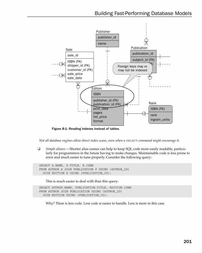
Figure 8-1: Reading indexes instead of tables.
Not all database engines allow direct index scans, even when a SELECT command might encourage it.
❑ Simple aliases — Shorter alias names can help to keep SQL code more easily readable, particu-larly for programmers in the future having to make changes. Maintainable code is less prone toerror and much easier to tune properly. Consider the following query:
SELECT A.NAME, P.TITLE, E.ISBNFROM AUTHOR A JOIN PUBLICATION P USING (AUTHOR_ID)
JOIN EDITION E USING (PUBLICATION_ID);
This is much easier to deal with than this query:
SELECT AUTHOR.NAME, PUBLICATION.TITLE, EDITION.ISBNFROM AUTHOR JOIN PUBLICATION USING (AUTHOR_ID)
JOIN EDITION USING (PUBLICATION_ID);
Why? There is less code. Less code is easier to handle. Less is more in this case.
Sale
sale_id
ISBN (FK)shipper_id (FK)customer_id (FK)sale_pricesale_date
Edition
ISBN
publisher_id (FK)publication_id (FK)print_datepageslist_priceformat
Publisher
publisher_id
name
publication_id
Publication
subject_id (FK)author_id (FK)title
Rank
ISBN (FK)
rankingram_units
Foreign keys may ormay not be indexed
201
Building Fast-Performing Database Models
13_574906 ch08.qxd 10/28/05 11:40 PM Page 201

Filtering with the WHERE ClauseThe WHERE clause can be used either to include wanted records or exclude unwanted records (or both).The WHERE clause can be built in specific ways, allowing for faster execution of SQL code. Use of theWHERE clause can be applied to tune SQL statements simply by attempting to match WHERE clause specifications to indexes, sorted orders, and physical ordering in tables. In other words, filter accordingto how the metadata is constructed.
The WHERE clause is used to filter records and can, therefore, be placed in all three of SELECT, UPDATE,and DELETE commands.
There are numerous points to keep in mind when building efficient filtering:
❑ Single record searches — The best filters utilize a primary key on a single table, preferably finding a single record only, or a very small number of records. This query finds the only authorwith primary key identifier as 10:
SELECT * FROM AUTHOR WHERE AUTHOR_ID = 10;
❑ Record range searches — Using the >, >=, <, and <= operators executes range searching. Rangesearches are not as efficient as using equality with an = operator. A group of rows rather than asingle row are targeted. Range searching can still use indexing and is fairly efficient. This queryfinds the range of all author records, with identifiers between 5 and 10, inclusive:
SELECT * FROM AUTHOR WHERE AUTHOR_ID >= 5 AND AUTHOR_ID <= 10;
❑ Negative WHERE clauses — Negative filters using NOT, !=, or <> (an operator that is different indifferent databases) try to find something that is not there. Indexes are ignored and the entiretable is read. This query reads all records, excluding only the record with author identifier as 10:
SELECT * FROM AUTHOR WHERE AUTHOR_ID != 10;
❑ The LIKE operator — Beware of the LIKE operator. It usually involves a full scan of a table andignores indexing. If searching for a small number of records, this could be extremely inefficient.When searching for 10 records in 10 million, it is best to find those 10 records only using something like equality, and not pull them from all 10 million records, because all those 10 million records are read. The following query finds all authors with the vowel “a” in theirnames, reading the entire table:
SELECT * FROM AUTHOR WHERE NAME LIKE ‘%a%’;
❑ Functions in the WHERE clause — Any type of functional expression used in a WHERE clause mustbe used carefully. Functions are best not to be used where you expect a SQL statement to usean index. In the following query, the function will prohibit use on an index created on thePRINT_DATE field:
SELECT * FROM EDITION WHERE TO_CHAR(PRINT_DATE,’DD-MON-YYYY’)=’01-JAN-2005’;
202
Chapter 8
13_574906 ch08.qxd 10/28/05 11:40 PM Page 202
Utilize the index by not applying the function to a field in a table, but using the literal value onthe opposite side of the expression:
SELECT * FROM EDITION WHERE PRINT_DATE=TO_DATE(‘01-JAN-2005’,’DD-MON-YYYY’);
❑ Small and large tables — Very small tables are often more efficiently read by reading only thetable, and not the index plus the table. The same applies when large portions of a single tableare read. If enough of the table is read at once, the index may as well be ignored. Reading anindex involves scanning an index and then passing pointers through to a table, scanning thetable with index values found. When enough of the table is read, index scanning activity to findtable records can become more time-consuming than reading only the table (ignoring the index).
❑ Composite index field sequence — In many databases, the sequence of fields in a WHERE clause candetermine if an index is matched or missed. For example, create a composite index with threefields, indexed as follows:
CREATE INDEX CAK_EDITION_1 ON EDITION (PUBLISHER_ID, PUBLICATION_ID, ISBN);
When a table is accessed with the following WHERE clause, the index will be used because allfields are included, and in the indexed field sequence:
SELECT ... WHERE PUBLISHER_ID=1 AND PUBLICATION=10 AND ISBN=’1555583059’;
When a table is accessed with the following WHERE clauses, the composite index may not beused (depending on the database):
SELECT ... WHERE ISBN=’1555583059’ AND PUBLISHER_ID=1 AND PUBLICATION=10;SELECT ... WHERE ISBN=’1555583059’;SELECT ... WHERE PUBLISHER_ID=1;
Some databases may allow index use of composite indexes for the previous queries, but it is unusual.
The first query above does not match the sequence of indexed fields. The second query containsonly the last field in the index. The last query contains only the first field in the index.
❑ IN and EXISTS set operators —IN is often used to test a single value against a list of literal values, as in the following query:
SELECT * FROM AUTHOR WHERE AUTHOR_ID IN (1,2,3,4,5);
EXISTS is used to check against a dynamic set of values, such as that produced by a subquery,as in the following example:
SELECT * FROM AUTHOR WHERE EXISTS(SELECT AUTHOR_ID FROM PUBLICATION);
IN and EXISTS can be efficient, depending on how they are used. In other words, performing an IN check against a non-indexed field forces a full table scan. The IN operator query abovechecks literal values against a primary key and, thus, uses an index. The EXISTS operator fullscans two tables. This can be made more efficient by incorporating a WHERE clause in bothqueries and by using a correlation between the calling query and subquery.
203
Building Fast-Performing Database Models
13_574906 ch08.qxd 10/28/05 11:41 PM Page 203
❑ Using AND and OR—AND and OR allow logical combination of multiple expressions, such as in aWHERE clause:
SELECT * FROM AUTHOR
WHERE NAME LIKE ‘%a%’ OR (AUTHOR_ID >= 5 AND AUTHOR_ID <= 10);
Matching indexes where AND and OR operators are used is important because anything missingin an index field use could result in a full table scan.
Some databases allow for use of specialized built-in functions, very similar to regular programming CASE statements. Sometimes these CASE statement, much like functions, can beused to more efficiently replace expressions logically joined with AND and OR operators. TheUNION clause is another option to consider. UNION merges two separate queries into a single setof records and can be equivalent to an OR logical operation.
The HAVING and WHERE ClausesA common programming error is to get the purposes of the WHERE and HAVING clause filters mixed up.The WHERE clause filters records as they are read from the database (as I/O activity takes place). TheHAVING clause (part of the GROUP BY clause) filters aggregated groups, after all database I/O activityhas completed. Don’t use the HAVING clause when the WHERE clause could be used more efficiently, andvisa versa. In the following example, the PUBLISHER_ID restriction in the HAVING clause can be movedto the WHERE clause:
SELECT ISBN, PUBLISHER_ID, AVG(LIST_PRICE)FROM EDITION GROUP BY ISBNHAVING PUBLISHER_ID > 5 AND AVG(LIST_PRICE) > 10;
Move the PUBLISHER_ID restriction from the HAVING clause, to the WHERE clause, as shown by the fol-lowing altered query:
SELECT ISBN, PUBLISHER_ID, AVG(LIST_PRICE)FROM EDITION WHERE PUBLISHER_ID > 5GROUP BY ISBNHAVING AVG(LIST_PRICE) > 10;
Why move the condition from the HAVING clause to the WHERE clause? As already stated, the WHEREclause executes filtering at the time that I/O activity occurs. In other words, WHERE clause filtering usingthe second query above, should under ideal circumstances, not even read records with PUBLISHER_IDless than or equal to 5. Leaving the PUBLISHER_ID filter in the HAVING clause will not limit I/O activitybecause the HAVING clause is only applied after all WHERE clause filtering, and thus I/O activity has beencompleted. Ensuring that any filtering that can be placed into the WHERE clause — is in the WHERE clause,and not in the HAVING clause — ensures best execution efficiency, in most cases.
204
Chapter 8
13_574906 ch08.qxd 10/28/05 11:41 PM Page 204
JoinsChapter 5 provided a large quantity of information on joins. This section briefly examines joins, purelyfrom a performance-tuning perspective. There are various different types of joins. Some join types can beclassified with inherently good performance. Some join types might need a little manual help. Some jointypes can be stubbornly difficult to tune. Different join types and their tuning attributes can be describedas follows:
❑ Inner join — An inner join is an intersection between two tables. The join is usually performedbetween two referential integrity keys in those two tables. Intersections are the most efficienttypes of joins because they match records between two tables based on equality (an = sign). Thefollowing query joins the PUBLISHER and EDITION tables, based on the primary and foreign keylink between the two tables (one-to-many relationship). The tables are shown in Figure 8-1.
SELECT P.NAME AS Publisher, E.ISBNFROM PUBLISHER P JOIN EDITION E USING (PUBLISHER_ID);
A self-join is a special type of intersection where records on multiple hierarchical levels, stored in a singletable, are returned as a hierarchical structure.
❑ Outer join — An inner join returns an intersection between two tables. An outer join returns theopposite of an inner join. An outer join returns all records in one table, which are excluded fromthe other table. Profligate use of outer joins in queries could indicate a possibly over-granulardatabase model. Tuning outer joins is inherently more difficult than tuning inner joins becauseouter joins are more complex to write. The following query returns the intersection betweenPUBLISHER and EDITION, as well as all publishers currently with no titles in print (the outerpart of the outer join):
SELECT P.NAME AS Publisher, E.ISBNFROM PUBLISHER P LEFT OUTER JOIN EDITION E USING (PUBLISHER_ID);
❑ Cross join — A cross join is a Cartesian product, joining every record in one table to every recordin another table, regardless of any meaningful referential integrity connection of keys betweenthe two tables, or any other field connection. Obviously, cross joins will be slow, depending onthe number of records in both tables, relative to each other, and in total number of records. The following query returns all publishers with all editions regardless of any PUBLICATION to EDITION relationship. In other words, every book is returned with every publisher, regardless ofwho published the book. Even if a particular publisher did not publish a particular book, a recordis still returned containing completely unrelated publishers and books (those books belonging toother publishers, or perhaps even no publisher whatsoever — self-published books).
SELECT P.NAME AS Publisher, E.ISBNFROM PUBLISHER P CROSS JOIN EDITION E;
The most important factor for performance tuning joins is minimizing the number of tables in a join, inall types of database models
Any poorly coded join will likely be inefficient. In data warehouses, inefficient joins can easily have disas-trous performance effects because of the sheer quantities of data. OLTP databases can also be crippled tothe point of uselessness, but it is less likely because of smaller physical database size. One particular project I contracted on in the past, however, had a miniscule 10 GB database and joins composed of 15tables or more in each query. Short Web page listings of 10 records were taking 30 seconds to return a
205
Building Fast-Performing Database Models
13_574906 ch08.qxd 10/28/05 11:41 PM Page 205
response to their customers. After I spent two months persuading developers how to speed up their software, they took about a week to fix. The Web site subsequently turned those 30-second waits into lessthan a half a second. Internet surfers typically lose interest in Web sites taking longer than seven seconds to react.
There are some basic rules when attempting to tune SQL code joins:
❑ Apply largest filters first — Filter from largest tables first to reduce records joined. Retrieve tablesin order from the most highly filtered table downward, preferably the largest table has the mostfiltering applied. It is essential to reduce record numbers from large tables as much as possiblebefore joining them to other tables. The most highly filtered table is the table having the smallestpercentage of its records retrieved; preferably, the largest table is filtered the most.
❑ Use indexes — Try to write code to utilize indexes wherever possible, except for very small tables.Small tables can sometimes be more efficiently read, ignoring any indexing on the small table.Small tables are often read by ignoring indexes. Sometimes even large tables are best read byignoring indexing, especially in cases where a larger percentage of the bigger table is read.
❑ Nested subquery semi-joins — It is possible to tune or merely simplify joins (for easier tuning) by using nested layers of subqueries. This type of tuning is much more applicable to highly normalized OLTP database models, and does not apply to denormalized data warehousedatabase models.
Auto CountersMany relational databases have some kind of automated counter or auto counter. An auto counter is aspecific database object used to count integer values, usually from 1 upwards. Auto counters are oftenused by a database to fill primary key surrogate key integer values. In the old and dirty days, before the invention of auto counters, items such as unique surrogate keys were either not used or stored in asingle central system metadata table. A single central system data table is potentially disastrous in highlyconcurrent environments, resulting in a serious hot block problem on that system data table. A hot blockproblem is where enormous quantities of queries access the same physical area of the disk, all at the sametime (concurrently). Multiple operations compete for the same resources. Eventually resources becomescarce and performance suffers.
This section expanded on details provided in Chapter 5 by going into detail of performance tuning ofSQL code, queries in particular. Poorly designed table structures ultimately equate to queries, which arequite likely impossible to tune up to an acceptable level of performance. Well-designed table structurespropagate into high-performance queries. Indexing is also important to query performance, and overalldatabase model performance.
Efficient Indexing for PerformanceMost important, always be more circumspect about creating an index rather than not creating an index.Many databases get so convoluted and mixed up with over-indexing that, after long periods of time, noone knows who created what — and why. Never be afraid of not creating an index. It follows that youshould not always assume that an existing index should exist, simply because it does exist.
206
Chapter 8
13_574906 ch08.qxd 10/28/05 11:41 PM Page 206
Types of IndexesSome databases allow different types of indexing. In relational databases, one index type is most commonlyused. That index type is usually some form of binary tree index (BTree). Other index types are nearlyalways rare and only applicable in specialized cases. Be aware of the needs of, and consequences for,using special types of indexing such as ISAM, hash, or bitmap indexing.
Different database engines use index structures and methods in different ways. Some examples are warranted here. Where one database engine allows creation of separate physical ISAM indexes, anotherdatabase may use an ISAM algorithm to access a BTree index. Some databases allow creation of hashindexes as separate physical structures; others only allow application of hashing algorithms to all fieldsin an entire table. Some database engines allow creation of BTree indexes both as an index, and as a sorting sequence on an entire table. The table itself, and all its fields, become a BTree index (known as aclustered index or an index organized table).
They have very specialized applications and are not commonly used. Also, be aware that these less commonly used index types are often subject to overflow when changes are made to source tables.In reality, unusual types of indexes can often be subject to performance-crippling forms of overflow.Overflow is where an index has its performance created index structure completely diverted from andpartially undone, by data changes to tables. Most of these unusual types of indexes are more often thatnot for read-only type environments, and should generally be implemented and applied with great careand forethought beforehand.
Database administrators should always keep a watchful eye on indexing in a database. Of course, thereis never really available time, but when an application is released it is always best to re-examine allindexing. Quite often, developers will create many indexes, sometimes each creating their own sets ofindexes, for the same application. The result is over-indexing. Too many indexes on a table create a performance problem. Effectively, executing a table change command (INSERT, UPDATE, or DELETE) on a table executes the same command on all of its indexes in addition to just the table. For example, inserting a single record into a table with four indexes comprises five changes to the database.
How to Apply Indexes in the Real WorldThere are various ways in which indexes can be applied, generally dependent on the function of thetable for which an index is created:
❑ No index — Data in a table is heap structured (in a heap or disorganized pile). Both small andlarge tables can benefit from having no indexing. Small tables may be best accessed as a whole,rather than with table and index, because they access a small amount of physical space. Largetables could very well only be read in their entirety based on application requirements. Whyindex a table when indexes are never used? It is even sometimes beneficial to drop referentialintegrity keys and indexes.
❑ Static data — Small static data tables are often better off without indexing. Be aware of twopotential problems: removing foreign key indexes can cause serious locking problems that candrastically hamper performance; and highly complex joins with many tables usually benefitfrom all tables having indexes, particularly unique primary key indexes, even on small statictables.
207
Building Fast-Performing Database Models
13_574906 ch08.qxd 10/28/05 11:41 PM Page 207
❑ Dynamic data — Dynamic data is data that changes all the time (transactional data). These indexesare changed frequently, are subject to overflow, and require frequent refreshing. Be acutelyaware of the type of index used for dynamic data. The default index type for a particulardatabase is usually the best option for dynamic data. This index type is usually some form ofbinary tree indexing structure. Other index types involving pre-calculated structures such asISAM, hash tables, and bitmaps will overflow almost immediately when subject to change.
Overflow of an index is seriously ugly for performance. Index overflow happens to certain types ofindexes where any changes to data in tables cannot be slotted into the proper physical point in the original structure of the index. This is because of the way in which certain index types are constructed.The result of overflow and a lot of data changes could be query I/O quite literally bouncing all over diskstorage trying to find data. This can cause serious performance problems.
❑ Read only reporting index — Unlike dynamic data indexing, read-only data is much more flexiblewith respect to index types, because data is not subject to change. Read-only indexing is speciallydesigned for read only queries, often in data warehouses. Types of indexing in this category arepre-built structures subject to overflow but highly efficient when used for read only I/O activity.Index types proficient as read-only indexes (bitmaps, clusters, hash tables) are ineffective inhighly dynamic environments.
❑ Unique and non-unique indexes — A unique index is an index allowing only a single value in a table.Be careful when creating unique indexes because every insertion or update to a uniquely indexedfield (or fields) requires a scan of the entire index space (to verify a value as unique). A non-uniqueindex allows more than one record with the same value and is typical of foreign key indexes.Unique indexing is better for performance and is typical of primary keys. A unique index is betterfor performance because subset index searching can be used to find single records, in theory making for less I/O, and less traversal through index structures.
❑ Single field versus multiple field indexes — Multiple field indexes are generally known as compositefield indexes. Single field indexes are more efficient than composite multiple field indexes. The simple fact is the fewer fields, the less to search through. Also, fewer fields means the index isrelatively much smaller than its parent table. The bigger the relative difference in size betweentable and index, the more effective the index is at reducing I/O, especially for larger tables.
❑ Datatypes to index — Integers are always best. An integer is a whole number with no digits to theright of the decimal point. Any other datatypes are nearly always flexible in terms of both lengthand content. Fixed-length strings are not quite as efficient as integers but they can be good optionsfor index construction if the strings are a few characters, such as with use of codes. Quite often,codes are used to represent structures, such as code names for states in the United States. For example, NY represents the state of New York and CA represents California. Numbers are still better because there are 10 possible digits. Character strings have 26 different variations for the letters of the alphabet, plus 10 possible digits (strings are alphanumeric and can contain numeralsas well), plus all sorts of punctuation and other odd characters.
❑ Sacrificing referential integrity for performance — Sometimes this is a good idea, but most often it is not. Dropping of foreign key indexing can cause serious locking issues. Referential integrityuses primary and foreign keys to validate relationships between records in related tables. Ifthere is a lot of validation occurring, and a table containing a foreign key has no foreign keyindex, the child table could be frequently fully scanned, resulting in huge competition for theentire table rather than just the index.
208
Chapter 8
13_574906 ch08.qxd 10/28/05 11:41 PM Page 208
❑ Optimizing with alternate indexes — Alternate indexing is often referred to as secondary indexing.Alternate indexing includes any indexes created against tables in a database model, which arenot part of referential integrity constraints. Quite often, the need for alternate indexing is a mismatch between the database model and functionality required by applications. Excessivealternate indexing could indicate the database model not catering to application needs. Reportingor data warehousing application requirements will usually cause further demand for alternateindexing.
When Not to Use IndexesPossibly the most important question is when should an index not be created? There are some circumstanceswhere indexes can be detrimental to performance and sometimes those indexes should not exist.Sometimes (in fact, quite frequently), it is better for query performance for indexes to be ignored, and the entire table be read. The following explains when indexes should be avoided.
❑ A table with a small number of fields may not benefit from an index if a large percentage of itsrecords are always retrieved from it. Creating an index will not prevent full table scans. Notethat removing primary key or foreign keys is not a good idea.
❑ Small static data tables are often small enough to be read as a table scan rather than an indexscan, plus a point into a table. Let’s explain by example. Underlying I/O activity in the operatingsystem (UNIX, Windows, Linux, and many others) is read in what are sometimes called blocks orpages. These pages can be many sizes, but usually at the database level the pages become 2 KB, 4KB, 8 KB, 16 KB, and sometimes even 32 KB pages. The point to understand is that if a table has asmall enough number of records, to occupy a single physical page, why read an index and pointto a table? Reading the index and the table is reading two pages, when reading the table onlyconstitutes an I/O on a single page only.
❑ Often, tables created for reporting or during data warehouse periodical appending (batchupdates) may already be in the required physical order.
❑ Indexes should usually be created on a small percentage of the fields in a table. Large compositeindexes may be relatively large compared with the table. The relative size between index andtable is important. The larger the ratio of index to table physical size, the less helpful the indexwill be in terms of decreasing physical space to be read. Fields containing NULL values mayexacerbate this effect. It may be faster to read the entire table, rather than a large composite fieldindex, containing a lot of NULL values. Why create indexes with every field for a composite? Itis, of course, acceptable to create a duplicate valued index on less than all the fields desired bythe composite field structure. Sometimes a partial index is more efficient than no index, and alsomore efficient than the complete field set for a composite field index.
That’s indexing. Indexes are important to database modeling and overall database performance as awhole, even to the point of not using indexing under certain circumstances. Overuse of indexing canhinder performance just as easily as not using indexing where indexing should be used.
What about using views?
209
Building Fast-Performing Database Models
13_574906 ch08.qxd 10/28/05 11:41 PM Page 209
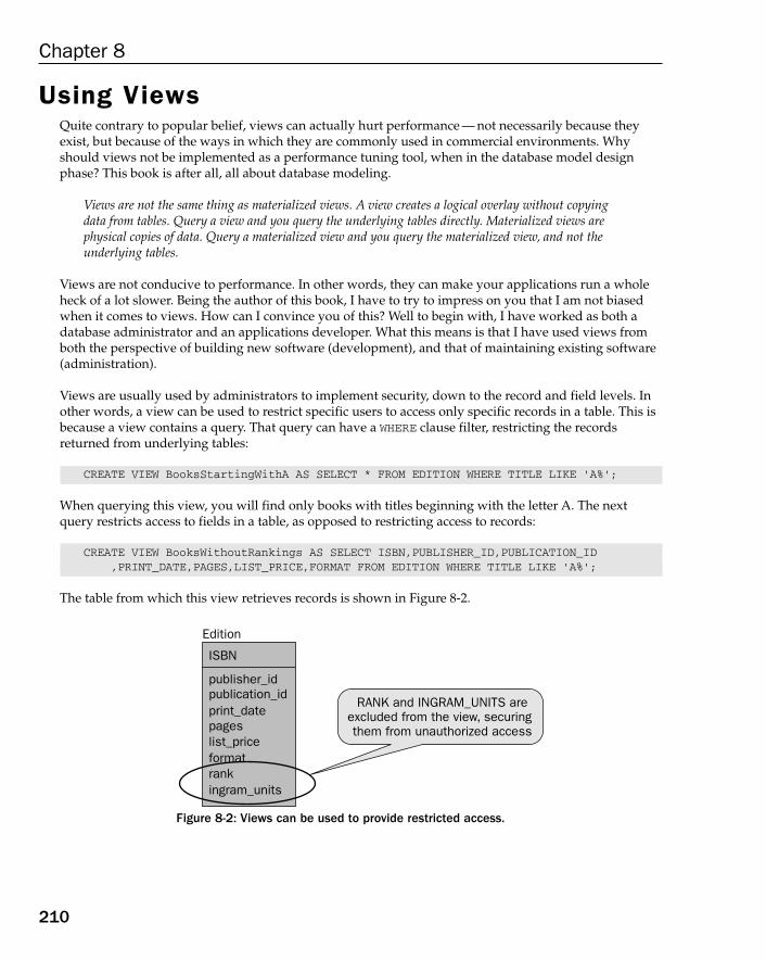
Using ViewsQuite contrary to popular belief, views can actually hurt performance — not necessarily because theyexist, but because of the ways in which they are commonly used in commercial environments. Whyshould views not be implemented as a performance tuning tool, when in the database model designphase? This book is after all, all about database modeling.
Views are not the same thing as materialized views. A view creates a logical overlay without copyingdata from tables. Query a view and you query the underlying tables directly. Materialized views arephysical copies of data. Query a materialized view and you query the materialized view, and not theunderlying tables.
Views are not conducive to performance. In other words, they can make your applications run a wholeheck of a lot slower. Being the author of this book, I have to try to impress on you that I am not biasedwhen it comes to views. How can I convince you of this? Well to begin with, I have worked as both adatabase administrator and an applications developer. What this means is that I have used views fromboth the perspective of building new software (development), and that of maintaining existing software(administration).
Views are usually used by administrators to implement security, down to the record and field levels. Inother words, a view can be used to restrict specific users to access only specific records in a table. This isbecause a view contains a query. That query can have a WHERE clause filter, restricting the recordsreturned from underlying tables:
CREATE VIEW BooksStartingWithA AS SELECT * FROM EDITION WHERE TITLE LIKE ‘A%’;
When querying this view, you will find only books with titles beginning with the letter A. The nextquery restricts access to fields in a table, as opposed to restricting access to records:
CREATE VIEW BooksWithoutRankings AS SELECT ISBN,PUBLISHER_ID,PUBLICATION_ID,PRINT_DATE,PAGES,LIST_PRICE,FORMAT FROM EDITION WHERE TITLE LIKE ‘A%’;
The table from which this view retrieves records is shown in Figure 8-2.
Figure 8-2: Views can be used to provide restricted access.
Edition
ISBN
publisher_idpublication_idprint_datepageslist_priceformat rankingram_units
RANK and INGRAM_UNITS areexcluded from the view, securing them from unauthorized access
210
Chapter 8
13_574906 ch08.qxd 10/28/05 11:41 PM Page 210
The only way to access the RANK and INGRAM_UNITS field is by accessing the table directly in the followingquery:
SELECT * FROM EDITION;
Obviously, if you do not want particular users accessing ranks and Ingram numbers, you can restrictaccess to the table, allowing general access to the view only. End-users can only access the view.
Different types of security access are required by different users. End-users only get to access data from theviews that are specifically built for them; therefore, an executive-level manager can see all fields, for allrecords, in tables a non-management employee would be prohibited from looking at (such as employeesalaries). Employees seeing each other’s salaries can cause morale problems. Then again, an executive maysimply access different information, perhaps wanting factual business-applicable information, avoidingtechnical details.
The problem with views is that they slow things down because they are often used by developers, oradministrators, to make application coding easier. So, the issue is that there is absolutely nothing wrongwith using views. The real problem is that views are very often inappropriately used. This is a highlysignificant consideration. You can never, ever assume that everyone having access to a database knowsand understands everything about everything. And you, as a database modeler, cannot expect it even ofyourself. Look at it this way. If executive managers use data warehouse reporting, they probably knowas much about the internal workings of your database as you know about executive management —Nothing!
Views are database objects even if they are only logical overlays. If they are used in a database, they doeffectively become a part of the database model because they tend to break things down, even if only in a logical and not a physical sense. When considering views and database model performance, keep an eye on use of views. The more you allow the use of views by developers and the general user popula-tion, the more you must monitor and performance-tune those views. If managing those views becomesan overwhelming task you may eventually be faced with a difficult task to resolve performance problem.
In my 20 years of development and administration experience, I’ve found that the best way to avoid abuse,misuse, and misunderstood use of views is to avoid using views altogether. That is my philosophicalapproach and is by no means an absolute rule.
Be careful using views. Views have very specific roles and the biggest danger is misuse of views.
Another interesting topic to discuss is application caching.
Application CachingApplication caching is where data can be stored in the memory of a client computer. That client computercan even be on the other side of the world, using an Internet browser. Application caching is significantto database model performance because the best things to cache are static tables.
In any database, it can sometimes be an effective performance-tuning method to cache static data, oreven index structures, even dynamic table indexes. This caching process can be implemented on thedatabase server, within the server, on an application server, and even in the application itself, even as faras a front-end application passed to a multitude of unknown users over the Internet (in a browser).
211
Building Fast-Performing Database Models
13_574906 ch08.qxd 10/28/05 11:41 PM Page 211

For OLTP databases, just the static data tables can be cached, even perhaps some dynamic table indexes aswell. Caching makes perfect sense for OLTP databases because very high levels of sharing are prevalent(high concurrency). For example, an online bookstore might perform much better for a user buying booksif all recently accessed static files, by that specific user, were cached as soon as the user logged in.Sometimes, even partially static files can be preloaded into an application such as an online bookstore.Common types of structures in this category for online bookstores as likely candidates for online browsercaching are wish lists, the contents of a shopping cart, previously purchased items, and the list goes on.
Caching of any form is completely useless in data warehouses because fact tables are usually so incrediblyhuge in comparison with dimensions. Also, tables are accessed infrequently and by very few users atonce. For data warehouses, quantities of data in each table have much more significant impact. Cachinglarge data warehouse tables in memory would fill hardware resource capacities rapidly. Data warehousesare simply I/O intensive and that is all there is to it.
SummaryIn this chapter, you learned about:
❑ Factors affecting tuning of OLTP database models
❑ Factors affecting tuning of client-server database models
❑ Factors affecting tuning of data warehouse database models
❑ Writing efficient queries using the SELECT command, the WHERE clause and joins
❑ Auto counters and surrogate keys
❑ The type of indexes useful for performance
❑ Index types and how they apply in reality
❑ When not to use indexing
❑ Performance problems caused by views down the road
❑ Application caching used to reduce database demand and network activity
This chapter linked the theory presented in previous chapters with case study and database modeling inpractice, to be presented in chapters to follow this chapter. This linking process has been done using themost critical factor to all database installations — performance. If the database and its attached applicationsdo not perform up to scratch, end-users will not be happy, and will probably go elsewhere, or find anotheremployee to replace you. Performance tuning is a highly complex topic and this chapter has barelyscratched the surface. The intention of this chapter has been to attempt to give a very brief mentalimpression of how database modeling theory might be applied in the real world, perhaps attempting totweak a subconscious change in your train of thought, as you read through this book. In other words, theapproach in this chapter is changing the direction of this book from theory into practice, in small steps.The idea is to make it all a little easier to absorb.
212
Chapter 8
13_574906 ch08.qxd 10/28/05 11:41 PM Page 212
ExercisesAnswer the following questions:
1. Which of these apply to OLTP databases?
a. Large transactions
b. High concurrency
c. Frequent servicing opportunities
d. Real-time response to end-users
2. Which of these apply to data warehouse databases?
a. Lots of users
b. High concurrency
c. Very large database
d. High granularity
3. Which aspect of a query affects performance most profoundly? Select the most appropriateanswer.
a. WHERE clause filtering
b. Sorting with the ORDER BY clause
c. Aggregating with the GROUP BY clause
d. The number of tables in join queries
e. The number of fields in join queries
4. Assume that there 1,000,000 records in a table. One record has AUTHOR_ID = 50. AUTHOR_ID asthe primary key. Which is the fastest query?
a. SELECT * FROM AUTHOR WHERE AUTHOR_ID != 50;
b. SELECT * FROM AUTHOR WHERE AUTHOR_ID = 50;
213
Building Fast-Performing Database Models
13_574906 ch08.qxd 10/28/05 11:41 PM Page 213

13_574906 ch08.qxd 10/28/05 11:41 PM Page 214
Part III
A Case Study inRelational Database
Modeling
In this Part:
Chapter 9: Planning and Preparation Through Analysis
Chapter 10: Creating and Refining Tables During the Design Phase
Chapter 11: Filling in the Details with a Detailed Design
Chapter 12: Business Rules and Field Settings
14_574906 pt03.qxd 10/28/05 11:47 PM Page 215

14_574906 pt03.qxd 10/28/05 11:47 PM Page 216

9Planning and Preparation
Through Analysis
“The temptation to form premature theories upon insufficient data is the bane of our profession.”(Sherlock Holmes)
“It almost looks like analysis were the third of those impossible professions in which one can bequite sure of unsatisfying results. The other two, much older-established, are the bringing up of
children and the government of nations.” (Sigmund Freud)
Rocket science is an exact science. Analysis is by no means an exact science.
In planning this book, I thought of just that — planning. Where would the human race be withoutplanning? Probably still up in the trees hanging from gnarly branches, shouting “Aaark!” everynow and again. Previous chapters in this book have examined not only the theory of how to createa relational database model but also some other interesting topics, such as the history of it all, andwhy these things came about.
At this stage, why the relational database model was devised should make some sense. Additionally,different applications cause a need for different variations on the same theme, leading to the invention of specialized data warehouse database models. A data warehouse database model isdenormalized to the point of being more or less totally unrecognizable when compared to an OLTP(transactional) type relational database model structure. ERDs for OLTP and data warehousedatabase models only appear similar. The two are completely different in structure because thedata warehouse database model is completely denormalized. This is why it is so important to present both OLTP and data warehouse database models in this book. Both are relevant, and bothrequire intensive planning and preparation to ensure useful results.
This chapter begins a case study where theoretical information (absorbed from previous chapters)is applied in a practical real-world scenario. This chapter (and the next three following chapters)uses practice to apply theory presented in the first seven chapters. Why? Theory and practice aretwo completely different things. Theory describes and expounds on a set of rules, attempting toquantify and explain the real world in a formal manner, with formal methods. Formal methods areessentially a precise mathematical expression as a methodology. A methodology is an approach asapplied to a real-world scenario. In this book, the desired result is usable underlying structure — arelational database model.
15_574906 ch09.qxd 11/4/05 10:49 AM Page 217
Without placing a set of rules into practice, in a recognizable form, from start to finish, understanding oftheory is often lost through memorization. In other words, there is no point learning something by heartwithout actually having a clear understanding of what you are learning, and why you are learning it.Using a case study helps to teach by application of theory.
This might all seem a little silly, but I have always found that a little understanding lends itself to notrequiring my conscious mind to mindlessly memorize everything about a topic. I prefer to understandrather than memorize. I find that understanding makes me much more capable of applying what I havelearned in not-yet-encountered scenarios. By understanding a multiple-chapter case study, you shouldlearn how everything fits together.
So far, you have read about history, some practical application, and lots and lots of theory. Even someadvanced stuff (such as data warehousing and performance) has been skimmed over briefly. What’s thepoint of all this information, crammed into your head, without any kind of demonstration? The act ofdemonstrating is exactly how this book proceeds from here on in with a progressive, fictitious case studyexample. There are plenty of examples in previous chapters, but it’s all been little pieces. This chapterstarts the development of a larger case study example. The idea is to demonstrate and describe the process of creating a database model for an entire application. And it starts at the very beginning. Theonly assumptions made are that everyone knows how to work the mouse, and we all know what a computer is. This chapter begins the process of creating appropriate database models for an OLTPdatabase and a data warehouse. The specific company type will be an online auctioning Web site. Onlineauctions have high concurrent activity (OLTP activity), and a large amount of potential historical trans-actions (data warehouse activity).
This chapter begins with the very basics. The very basics are not getting out a piece of paper and drawingtable structures, or installing your favorite ERD tool and getting to it. The very beginning of databasemodel design (and any software project for that matter) is drawing up a specific analysis of what is actually needed. You should talk to people and analyze what software should be built, if any. There are, of course, other important factors. How much is it going to cost? How long will it take? The intention ofthis chapter is to subliminally give a message of focusing on how to obtain the correct information, fromthe right people. The goal is to present information as structure.
By the time you have completed reading this chapter, you should have a good understanding of the analytical process, not only for database modeling, but also as applicable for any software developmentprocess. More importantly, you should get a grip on the importance of planning. It is possible to builda bridge without drawing, designing, and architecting. An engineer could avoid doing lots of nasty complicated mathematical civil engineering calculations. What about planning that bridge? Imagine abridge that is built from the ground up with no planning. Whoever pays the engineer to build the bridgeis probably prudent to ask the builder to be the first to walk across it.
In this chapter, you learn about the following:
❑ The basics of analysis and design
❑ The steps in the analysis process
❑ Common problem areas and misconceptions associated with analysis
❑ The value of following a paper trail
218
Chapter 9
15_574906 ch09.qxd 11/4/05 10:49 AM Page 218

❑ How to create a database model to cover objectives
❑ How to refine a database model using business rules
❑ How to apply everything learned so far with a comprehensive case study
Steps to Creating a Database ModelBefore beginning in earnest with the case study example, you need to sidestep a little over the course ofthis and the next few chapters. There is an abundance of information covering the systematized process(the “what and how”) of building a database model.
The building of a database model can be divided up into distinct steps (as can any software developmentprocess). These steps can be loosely defined as follows:
1. Analysis
2. Design
3. Construction
4. Implementation
Take a brief look at each of these in a bit more detail.
Step 1: AnalysisAnalyzing a situation or company is a process of initial fact-finding through interviews with end-users. Ifthere are technical computer staff members on hand, with the added bonus of inside company operationalknowledge, interview them as well.
A proper analysis cannot be achieved by interviewing just the technical people. An all-around picture ofa client or scenario is required. End-users are those who will eventually use what you are building. Theend-users are more important! A database system is built for applications. Technical people program theapplications. End-users are the ultimate recipients of whatever you are providing as the databasedesigner or modeler.
As stated previously, analysis is more about what is required, not how it will be provided. What will thedatabase model do to fulfill requirements? How it will fulfill requirements is a different issue. Analysisessentially describes a business. What does the company do to earn its keep? If a company manufacturestires for automobiles, it very likely does such things as buying rubber, steel, and nylon for reinforcement,purchasing valves, advertising its tires, and selling tires, among a myriad of other things. Analysis helpsto establish what a company does to get from raw materials to finished product. In the case of the tiremanufacturer, the raw materials are rubber, steel, nylon, and valves. The finished products are the tires.
Analysis is all about what a company does for a living? This equates to analyzing what are the tables inthe database? And what are the most basic and essential relationships between those tables?
219
Planning and Preparation Through Analysis
15_574906 ch09.qxd 11/4/05 10:49 AM Page 219
Analysis defines general table structure. An auction Web site might contain a seller table and a biddertable. You must know what tables should generally contain in terms of information content. Should boththe seller and bidder tables contain addresses of sellers and bidders respectively? Analysis merelydefines. Analysis does not describe how many fields should be used for an address, or what datatypesthose fields should be. Analysis simply determines that an address field actually exists, and, obviously,which table or tables require address information.
Step 2: DesignDesign involves using what was discovered during analysis, and figuring out how those analyzedthings can be catered for, with the software tools available. The analysis stage decided what should becreated. The design stage applies more precision by deciding how tables should be created. Thisincludes the tables, their fields, and datatypes. Most importantly, it includes how everything is linkedtogether.
Analysis defines tables, information in tables, and basic relationships between tables. The linking togetheraspect of the design stage is, in its most basic form, the precise definition of referential integrity. Referentialintegrity is a design process because it enforces relationships between tables. The initial establishment ofinter-table relationships is an analysis process, not one of designs.
In other words, analysis defines what is to be done; design organizes how it’s done. The design stageintroduces database modeling refinement processing, such as normalization and denormalization. Interms of application construction, the design stage begins to define front-end user “bits and pieces” suchas reports and graphical user interface (GUI) screens.
Build the tables graphically, add fields, define datatypes, and apply referential integrity. Refine throughuse of processes such as normalization and denormalization.
Step 3: ConstructionIn this stage, you build and test code. For a database model, you build scripts to create tables, referentialintegrity keys, indexes, and anything else such as stored procedures. In other words, with this step, youbuild scripts to create tables and execute them.
Step 4: ImplementationThis is the final step in the process. Here you create a production database. In other words, it is at thisstage of the process that you actually put it all into practice.
This book is primarily concerned with the analysis stage but partially with thedesign stage as well. As already stated, construction is all about testing and verification. Implementation is putting it into production. This book is aboutdatabase modeling — analysis and design. The construction and implementationphases are largely irrelevant to this text; however, it is important to understand that analysis and design do not complete the entire building process. Physical construction and implementation are required to achieve an end result.
220
Chapter 9
15_574906 ch09.qxd 11/4/05 10:49 AM Page 220
The case study example introduced later in this chapter is all about analyzing what is needed for adatabase model — the analysis stage of the process. Let’s turn our attention to analysis. What is analysisand how can you go about the process of analyzing for a database model?
Understanding AnalysisAs you have learned, analysis is the beginning point in the building of a good relational database model.Analysis is about the operational factors of a company, the business of a company. It is not about the technical aspects of the computer system. It is not about the database model, or what the administrators,or programmers want, and would like to see. The analyst must understand the business. Participationfrom people in the business — the company employees, both technical and non-technical (end-users),even up to and including executive management level — is critical to success. On the other hand, completecontrol cannot be passed to the company. Some companies develop software using only temporarily hiredstaff, with no in-house technical involvement whatsoever. This can result in an entirely end-user orienteddatabase model. There needs to be a balance between both technical and non-technical input.
It is important to understand that the analysis stage is a requirements activity. What is needed? Whenbuilding a database model, an application or a software product, it is important to understand that there is a process to figuring what is in a database. What tables do you need? In computer jargon, theseprocesses are often called methodologies (a set of rules) by which a builder of computer systems gets fromA to B (from doodles on scrap paper, to a useful computer system) A lot of people have spent manyyears mulling over these sets of rules, refining and redefining, giving anyone and everyone a series ofsometimes easy or sometimes incredibly complex steps to follow, in getting from A to B.
Normalization is a methodology. Normalization is a complex set of rules for refining relational databasetable structures. Dividing up the database model design process into separate steps of analysis, design, construction, and implementation, is also a methodology.
The best database models are produced by paying attention to detail in the analysis stage. It is importantto understand exactly what is needed before jumping in and “just getting to it.” If changes are requiredat a later stage of development, changes can be added at a later stage; however, making changes to adatabase model used in a production system can be extremely problematic, so much so as to not be an option. This is because applications are usually dependent on a database and therefore usually dependent on the database model.
Analysis is planning. It is doubly important to plan for a database model. The reason is that the databasemodel forms the basis of all database-driven applications, quite often for an entire company. In the case ofan off-the-shelf product, that database model could drive duplicated and semi-customized applications forhundreds and even thousands of companies. Getting the database model right in the first place is critical.The more that is understood about requirements in the analysis stage, the better a database model andproduct will ultimately be produced.
Some database modeling and design tools allow generation of table scripts into different database engines.The tool used for database modeling in this book is called ERWin. ERWin can be used to generate table creation scripts for a number of database engines. Microsoft Access has its own built-in ERD modeling tool.Database models can generally be designed using pretty pictures in a graphical database modeling tool,such as ERWin. Building a database model using pretty pictures and fancy graphics packages allows for an
221
Planning and Preparation Through Analysis
15_574906 ch09.qxd 11/4/05 10:49 AM Page 221
analytical mindset and approach, ignoring some of the more technical details when performing analysis.Deep-level technical aspects (such as field datatypes and precise composition) can actually muddy the perspective of analysis by including too much complexity at the outset.
Analysis is about what is needed. Design is about how to provide what is needed by an already com-pleted analysis.
In the case of a rewrite of an existing system (reconstruction of an existing database model), analysissimply includes the old system in interviews and discussions with end-users and technical staff. If a system is being rewritten, it is likely that the original system is inadequate, for one or more reasons. Theanalysis process should be partially performed to enlighten as to exactly what is missing, incorrect, orinadequate.
End-users are likely to tell you what they cannot do with the existing system. End-users are also likely tohave a long list of what they would like. A conservative approach on the part of the analyst is to assesswhat enhancements and new features are most important. This is because one of the most important features of the analysis stage is how much it is all going to cost. The more work that is done, the more itwill cost.
Technical staffers, such as programmers and administrators, are likely to tell you what is wrong. Theycan also tell you how they “got around” inadequacies, such as what “kludges” they used.
A “kludge” is a term often used by computer programmers to describe a clumsy or inelegant solution toa problem. The result is often a computer system consisting of a number of poorly matched elements.
Analysis ConsiderationsBecause the analysis stage is a process of establishing and quantifying what is needed, you should keepin mind several factors and considerations, including the following:
❑ Overall objectives — These include the objectives of a company when creating a database modelWhat should be in the database model? What is the expected result? What should be achieved?For example, is it a new application or a rewrite?
❑ Company operations — These include the operations of a company in terms of what the companydoes to make its keep. How can all this be computerized?
❑ Business rules — This is the heart of the analysis stage, describing what has been analyzed andwhat needs to be created to design the database model. What tables are needed and what arethe basic relationships between those tables?
❑ Planning and timelines — A project plan and timeline are useful for larger projects. Project planstypically include who does what and when. More sophisticated plans integrate multiple tasks,sharing them among many people, and ensuring that dependencies are catered for. For example,if task B requires completion of task A, the same person can do both tasks A and B. If there is nodependency, two people can do both tasks A an B at the same time.
222
Chapter 9
15_574906 ch09.qxd 11/4/05 10:49 AM Page 222

❑ Budgeting — How much will it cost? Is it cost effective? Is it actually worth it? Is it affordable?Will it give the company an edge over the competition without bankrupting the company beforebeing able to bring that competitive edge to market? This includes the following considerations:
❑ Hiring help costs money — Do you need hired help? Help is expensive. Are skilled per-sonnel available? Is recruitment required? Are expensive consultants required?
❑ Hardware costs — Hardware requirements in terms of speed and capacity should beassessed. Concurrency in terms of number and size of processors, on-board RAM, specialized hardware (RAID arrays), and network bandwidth are important factors forOLTP databases. Storage space projections and I/O performance are very significant for data warehouses.
❑ Maintenance — Ease of future maintenance implies lower long-term costs.
❑ Training — End-users and programmers must know how to use what is being created.Otherwise, it may be difficult at best to apply, if not completely useless. If a databasedesigner introduces a new database engine such as Oracle Database into a company,training is a requirement, and must be budgeted for. Technical training can be extremelyexpensive and time-consuming.
❑ Other factors — Other less-noticed (but not less-relevant) factors include the following:
❑ Duplication of data — Avoid duplication of data (if performance is not sacrificed) andexcessive granularity. Excessive granularity is often a result of over-normalization.Over-normalization can make SQL code much more complex to write, more difficult tomake it perform acceptably, and much more problematic and expensive to maintain.
Excessive application of normalization removes potential for error in data (referential integrity violations). It also makes for ERDs with hundreds of tables and a lot of head-scratching on the part ofprogrammers. Over-normalization is perfection to a database designer, and a programmer’s nightmare.Relational database model design is a means to an end, not a process in itself. In other words, build adatabase model for programmers and end-users. Don’t build a database model based on a mathematicalprecept of perfection because ultimately only the database modeler can understand it. Keep the objectivein mind. That objective is to service application requirements and give the company an edge, but not tomake life difficult for everyone involved.
❑ Read-only or read-write — Is a database read-only or is full read-write access required?Data warehouse databases are often partially read-only. Some parts of OLTP databasesare can be somewhat read only, usually only where static data is concerned. Specializedmethods can be applied to static tables, allowing for more flexibility in OLTP databases.
Not surprising, the considerations for the overall objectives, company operations, business rules, planning and timeliness, and budgeting all can serve as an outline for the analysis process. In fact, laterin this chapter, the development of the case study example incorporates each of these considerations.Before you get to the case study example, see what potential problems lurk in the darkness when analyzing a company database model.
The “Other Factors” mentioned in the previous list are covered in detail in this chapter. These factorsrelate to topics already covered in previous chapters of this book.
223
Planning and Preparation Through Analysis
15_574906 ch09.qxd 11/4/05 10:49 AM Page 223
Potential Problem Areas and MisconceptionsThere are a number of negative factors worth considering and remembering, when analyzing a companydatabase model. These include the following:
❑ Normalization and data integrity
❑ More normalization leads to better queries
❑ Performance
❑ Generic and standardized database models
Let’s take a closer look.
Normalization and Data IntegrityMany analysts put forward the opinion that applying all levels of normalization through use of all available normal forms ensures no lost data (redundancy), and no referential integrity mismatches(orphaned records). A database is an information repository. Poor application programming or poordatabase use produces problematic data. Highly normalized database models can help ensure betterdata integrity, but the database model itself does not produce the problem. Application programmersand end-users cause the problem by making coding errors and incorrect changes in a database.
More Normalization Leads to Better QueriesThis is another opinion put forward by many analysts. Some statements that might be made could be ofthe following forms:
❑ “Problem queries are often the result of an inadequate (denormalized) database structure.”
❑ “It is much easier to write faster queries and updates against a normalized database structure.”
My opinion is completely opposite on both counts. Denormalized structures lead to faster queries andthey are easier for end-users to write. Denormalized tables tend to match a business more accuratelyfrom an operational perspective. In other words, the busy executives writing those ad-hoc queries canunderstand the tables and how tables relate to each other.
Building queries with lots of tables results in huge join queries. Join queries can be very complicated notonly to write, but also to make them execute in less than a week (sarcasm intended). For the databasenovice end-user, writing highly complex join queries is really too much to expect. It simply isn’t fair.Even for experienced programmers, building a join query against a DKNF level normalized databasemodel often borders on the ridiculous. For example, 15 tables in a single join query against a databasecontaining a paltry 1 GB taking 30 seconds is completely unacceptable. I have seen this in the past.
Database modeling should not be approached as an expression of mathematical perfection, but more as a means to an end. The means is the database model. The end is to service the users. The end is not toproduce the most granularly perfect database model if it does not service the required needs.
PerformanceSome analysts state that the performance of a computer, its applications, and its database model areirrelevant to the analysis of a business. I disagree with this approach completely. I have seen applicationsand entire server environments thrown on the garbage pile of history because they were not built with
224
Chapter 9
15_574906 ch09.qxd 11/4/05 10:49 AM Page 224
performance foremost in mind, from the very beginning. Performance is always important. Analyzinga database model without performance in mind is like buying a new boat when you can’t afford it — ahole in the water for throwing money into.
All SQL code depends on underlying table structure and table contents, even back to table identificationand table information content. All this stuff is decided on in the analysis phase. Decisions made duringanalysis absolutely affect performance in the long term. Database and application performance is farfrom unimportant.
Generic and Standardized Database ModelsBeware of generic database models or a model that is accepted as a standard for a particular industry or application. Generic database models are often present in purchased, perhaps semi-customizableapplications. Generic models cater to a large variety of applications. If you are investing in a databasemodel of your own, you may as well build a company-specific database model. Generic models oftenhave a lot of scope that does not apply to the requirements of a specific company. In other words, yourdatabase might have many empty, useless tables. Unused tables are not really a problem technically,but they can cause serious confusion for programmers and end-users. The other downside to a genericmodel is that it may not cater exactly to all your needs, and will very likely require modification anyway.
Standardized database models, particular to a specific industry and perhaps accepted as the norm, are also dangerous because they are likely to be very out of date. As for generic models, standardizedmodels are also likely to contain superfluous tables, with all the possible problems and inadequacies thatgo with it. Once again, if you are building a database model, you may as well invest in the real thing andcustom build it for your company and your specific applications; however, narrowing of scope couldbuild inflexibility and ultimately limitations into the system. It’s all about achieving a good balance.
It’s now time to get to the business of why you are here, why I am writing this book, and why you are sobusily reading this chapter. How do you begin to put theory into practice? Start by analyzing.
Putting Theory into PracticeFor the remainder of this chapter (and much of what is in the three chapters that follow), you build upona case study example in an effort to put theory into practice. Recall from the beginning of this chapterthat the case study involves a fictitious online auction house. This chapter performs the analysis stage ofthe case study. What does a database model need? What is in it?
Putting Analysis into PracticeAs you learned at the beginning of this chapter, the first step in putting the database modeling processinto practice is analysis. Discover and quantify what exactly it is that the company does to make endsmeet. Remember that to perform a proper analysis, you must keep the following in mind:
❑ Company objectives
❑ Company operations
❑ Business rules
225
Planning and Preparation Through Analysis
15_574906 ch09.qxd 11/4/05 10:49 AM Page 225
❑ Planning and timelines
❑ Budgeting
You perform the analysis stage for your case study by examining each of the items in the list. The follow-ing discussion begins with an examination of company objectives for the online auction house; however,once you have established what those objectives are, you then branch off a bit. You examine companyoperations and business rules in two separate contexts: one for an OLTP database, and one for a data warehouse model. By the end of the chapter, however, you’ll converge back into a discussion ofplanning, timelines, and budgeting for your overall case study example.
So, let’s find out exactly what the objectives of our online auction house really are.
Company ObjectivesThe most important objective is that the company actually turns a profit. After all, without profit, you haveno company! In addition, the overall objective of software is always to provide a service to customers. Foryour online auction house, the customers are the sellers and bidders. Sellers list items for auction. Biddersplace bids on listed items, hoping to win the auction.
After users are serviced adequately, if the business idea is a viable possibility, it has a better chance ofsucceeding in the commercial marketplace. A computer system would give a company an edge over itscompetition. Using the Internet, an online auction house is extremely likely to reach far more potentialcustomers than an offline auction house. This would make it possible for the auction house to market far less expensive products, in very much larger quantities. Obviously, commissions would be lower.After all, world-famous auction houses such as Sotheby’s auction only multimillion-dollar items, such as rare works of art. An online auction house can make good profitability, however, out of much higherquantities, all the while auctioning much cheaper items.
So, an online auction house has a very large potential market of sellers and buyers. Technically, this makesthe usage capacity of this database highly shareable (concurrent) between thousands of users, if not more.An OLTP database model structure is, therefore, desirable. Also, it is valuable to the auction house (andperhaps many of its selling clientele) to understand trends. Trends and forecasting can be established usingforecasts and projects into archived data sets. Archived data can be stored conveniently and efficientlyusing a specialized data warehouse database.
Technical objectives for this company would be to provide a data model for a highly concurrent OLTPdatabase, plus an I/O intense data warehouse data model as well.
One additional factor concerns already existing software and database modeling, already used by theonline auction house, for example. If the company is already computerized, already existing softwareand models can be used as a basis for creating new software.
Once again, a word of warning: If software is being rewritten, is the existing software inadequate? If so,why? Would using characteristics of existing software simply propagate existing problems into newsoftware?
Before tackling the two different database models, take a moment to think about how you can define theoperations of your online auction house.
226
Chapter 9
15_574906 ch09.qxd 11/4/05 10:49 AM Page 226
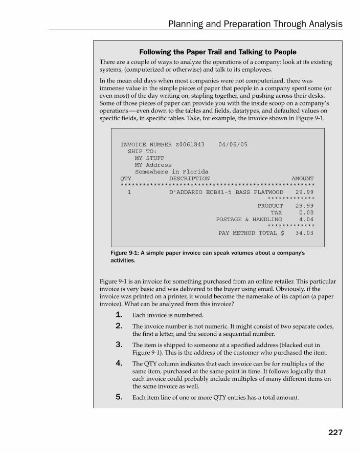
227
Planning and Preparation Through Analysis
Following the Paper Trail and Talking to People There are a couple of ways to analyze the operations of a company: look at its existingsystems, (computerized or otherwise) and talk to its employees.
In the mean old days when most companies were not computerized, there wasimmense value in the simple pieces of paper that people in a company spent some (oreven most) of the day writing on, stapling together, and pushing across their desks.Some of those pieces of paper can provide you with the inside scoop on a company’soperations — even down to the tables and fields, datatypes, and defaulted values onspecific fields, in specific tables. Take, for example, the invoice shown in Figure 9-1.
Figure 9-1: A simple paper invoice can speak volumes about a company’sactivities.
Figure 9-1 is an invoice for something purchased from an online retailer. This particularinvoice is very basic and was delivered to the buyer using email. Obviously, if theinvoice was printed on a printer, it would become the namesake of its caption (a paperinvoice). What can be analyzed from this invoice?
1. Each invoice is numbered.
2. The invoice number is not numeric. It might consist of two separate codes,the first a letter, and the second a sequential number.
3. The item is shipped to someone at a specified address (blacked out inFigure 9-1). This is the address of the customer who purchased the item.
4. The QTY column indicates that each invoice can be for multiples of thesame item, purchased at the same point in time. It follows logically thateach invoice could probably include multiples of many different items onthe same invoice as well.
5. Each item line of one or more QTY entries has a total amount.
INVOICE NUMBER z0061843 04/06/05 SHIP TO: MY STUFF MY Address Somewhere in FloridaQTY DESCRIPTION AMOUNT***************************************************** 1 D’ADDARIO ECB81-5 BASS FLATWOOD 29.99 ************* PRODUCT 29.99 TAX 0.00 POSTAGE & HANDLING 4.04 ************* PAY METHOD TOTAL $ 34.03
15_574906 ch09.qxd 11/4/05 10:49 AM Page 227
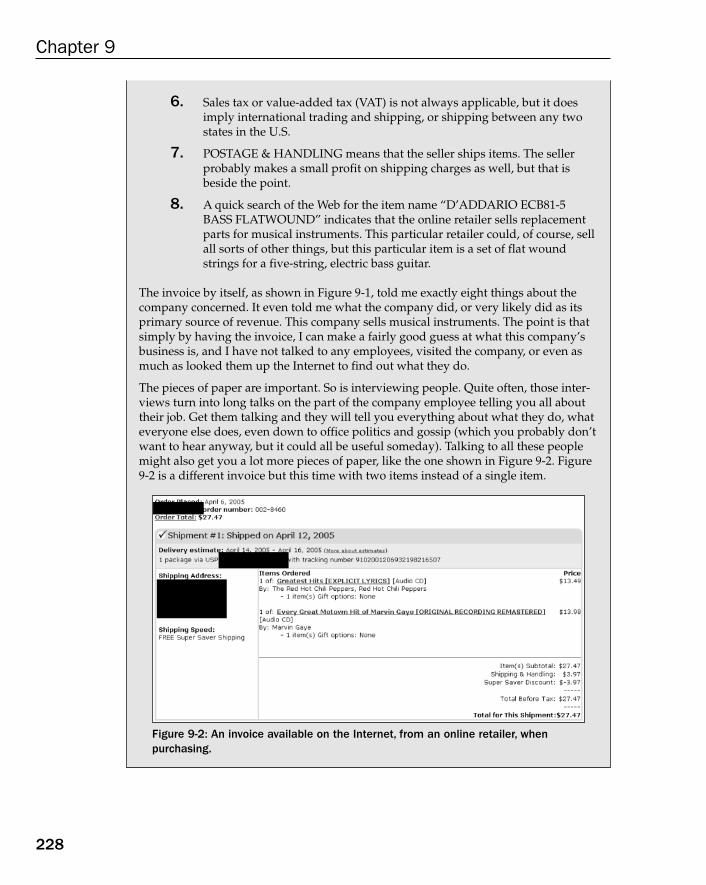
228
Chapter 9
6. Sales tax or value-added tax (VAT) is not always applicable, but it doesimply international trading and shipping, or shipping between any twostates in the U.S.
7. POSTAGE & HANDLING means that the seller ships items. The sellerprobably makes a small profit on shipping charges as well, but that isbeside the point.
8. A quick search of the Web for the item name “D’ADDARIO ECB81-5BASS FLATWOUND” indicates that the online retailer sells replacementparts for musical instruments. This particular retailer could, of course, sellall sorts of other things, but this particular item is a set of flat woundstrings for a five-string, electric bass guitar.
The invoice by itself, as shown in Figure 9-1, told me exactly eight things about thecompany concerned. It even told me what the company did, or very likely did as itsprimary source of revenue. This company sells musical instruments. The point is thatsimply by having the invoice, I can make a fairly good guess at what this company’sbusiness is, and I have not talked to any employees, visited the company, or even asmuch as looked them up the Internet to find out what they do.
The pieces of paper are important. So is interviewing people. Quite often, those inter-views turn into long talks on the part of the company employee telling you all abouttheir job. Get them talking and they will tell you everything about what they do, whateveryone else does, even down to office politics and gossip (which you probably don’twant to hear anyway, but it could all be useful someday). Talking to all these peoplemight also get you a lot more pieces of paper, like the one shown in Figure 9-2. Figure9-2 is a different invoice but this time with two items instead of a single item.
Figure 9-2: An invoice available on the Internet, from an online retailer, whenpurchasing.
15_574906 ch09.qxd 11/4/05 10:49 AM Page 228
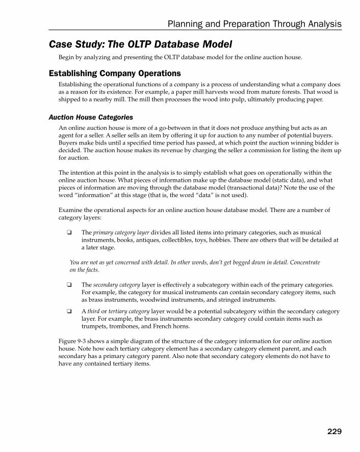
Case Study: The OLTP Database ModelBegin by analyzing and presenting the OLTP database model for the online auction house.
Establishing Company OperationsEstablishing the operational functions of a company is a process of understanding what a company doesas a reason for its existence. For example, a paper mill harvests wood from mature forests. That wood isshipped to a nearby mill. The mill then processes the wood into pulp, ultimately producing paper.
Auction House CategoriesAn online auction house is more of a go-between in that it does not produce anything but acts as anagent for a seller. A seller sells an item by offering it up for auction to any number of potential buyers.Buyers make bids until a specified time period has passed, at which point the auction winning bidder isdecided. The auction house makes its revenue by charging the seller a commission for listing the item upfor auction.
The intention at this point in the analysis is to simply establish what goes on operationally within theonline auction house. What pieces of information make up the database model (static data), and whatpieces of information are moving through the database model (transactional data)? Note the use of theword “information” at this stage (that is, the word “data” is not used).
Examine the operational aspects for an online auction house database model. There are a number of category layers:
❑ The primary category layer divides all listed items into primary categories, such as musical instruments, books, antiques, collectibles, toys, hobbies. There are others that will be detailed ata later stage.
You are not as yet concerned with detail. In other words, don’t get bogged down in detail. Concentrateon the facts.
❑ The secondary category layer is effectively a subcategory within each of the primary categories.For example, the category for musical instruments can contain secondary category items, suchas brass instruments, woodwind instruments, and stringed instruments.
❑ A third or tertiary category layer would be a potential subcategory within the secondary categorylayer. For example, the brass instruments secondary category could contain items such as trumpets, trombones, and French horns.
Figure 9-3 shows a simple diagram of the structure of the category information for our online auctionhouse. Note how each tertiary category element has a secondary category element parent, and each secondary has a primary category parent. Also note that secondary category elements do not have tohave any contained tertiary items.
229
Planning and Preparation Through Analysis
15_574906 ch09.qxd 11/4/05 10:49 AM Page 229
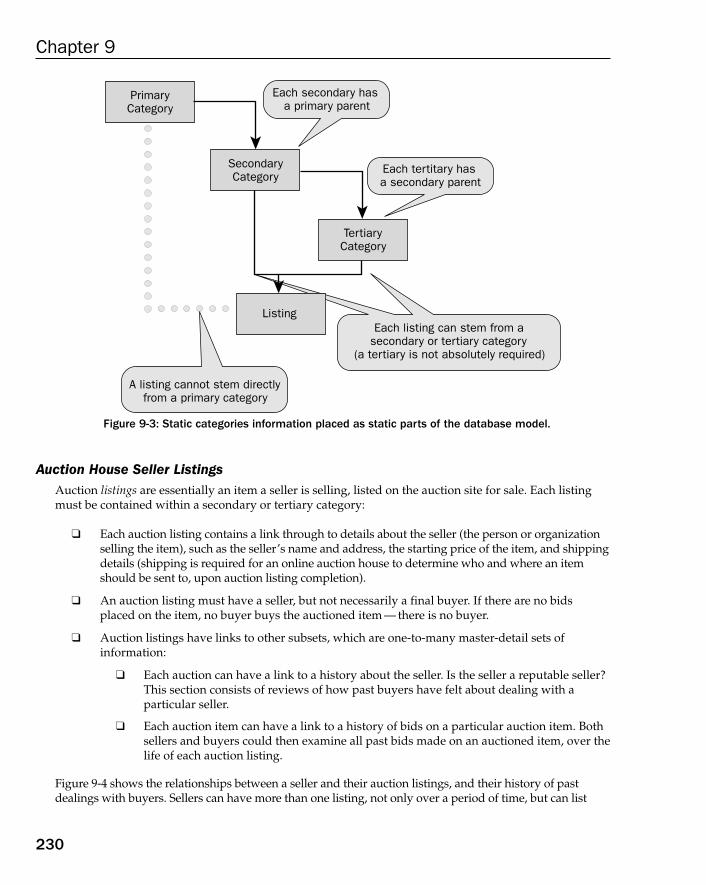
Figure 9-3: Static categories information placed as static parts of the database model.
Auction House Seller ListingsAuction listings are essentially an item a seller is selling, listed on the auction site for sale. Each listingmust be contained within a secondary or tertiary category:
❑ Each auction listing contains a link through to details about the seller (the person or organizationselling the item), such as the seller’s name and address, the starting price of the item, and shippingdetails (shipping is required for an online auction house to determine who and where an itemshould be sent to, upon auction listing completion).
❑ An auction listing must have a seller, but not necessarily a final buyer. If there are no bidsplaced on the item, no buyer buys the auctioned item — there is no buyer.
❑ Auction listings have links to other subsets, which are one-to-many master-detail sets of information:
❑ Each auction can have a link to a history about the seller. Is the seller a reputable seller?This section consists of reviews of how past buyers have felt about dealing with a particular seller.
❑ Each auction item can have a link to a history of bids on a particular auction item. Bothsellers and buyers could then examine all past bids made on an auctioned item, over thelife of each auction listing.
Figure 9-4 shows the relationships between a seller and their auction listings, and their history of past dealings with buyers. Sellers can have more than one listing, not only over a period of time, but can list
PrimaryCategory
SecondaryCategory
TertiaryCategory
Each secondary has a primary parent
Each tertitary has a secondary parent
A listing cannot stem directlyfrom a primary category
ListingEach listing can stem from a
secondary or tertiary category (a tertiary is not absolutely required)
230
Chapter 9
15_574906 ch09.qxd 11/4/05 10:49 AM Page 230
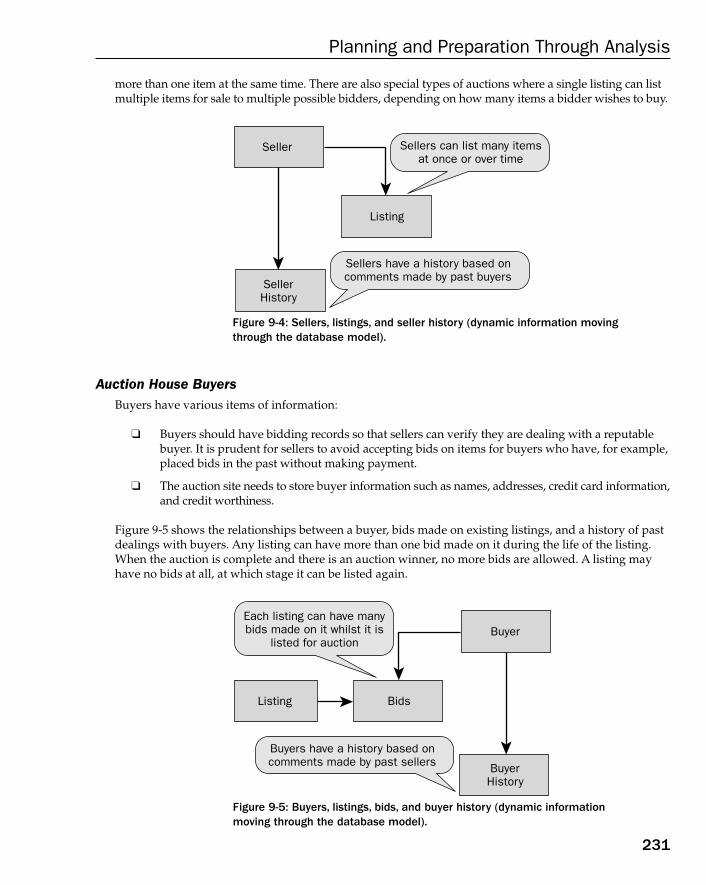
more than one item at the same time. There are also special types of auctions where a single listing can listmultiple items for sale to multiple possible bidders, depending on how many items a bidder wishes to buy.
Figure 9-4: Sellers, listings, and seller history (dynamic information movingthrough the database model).
Auction House BuyersBuyers have various items of information:
❑ Buyers should have bidding records so that sellers can verify they are dealing with a reputablebuyer. It is prudent for sellers to avoid accepting bids on items for buyers who have, for example,placed bids in the past without making payment.
❑ The auction site needs to store buyer information such as names, addresses, credit card information,and credit worthiness.
Figure 9-5 shows the relationships between a buyer, bids made on existing listings, and a history of pastdealings with buyers. Any listing can have more than one bid made on it during the life of the listing.When the auction is complete and there is an auction winner, no more bids are allowed. A listing mayhave no bids at all, at which stage it can be listed again.
Figure 9-5: Buyers, listings, bids, and buyer history (dynamic information moving through the database model).
Buyer
BidsListing
Buyers have a history based oncomments made by past sellers
Each listing can have manybids made on it whilst it is
listed for auction
BuyerHistory
Seller
Listing
Sellers have a history based oncomments made by past buyers
Sellers can list many itemsat once or over time
SellerHistory
231
Planning and Preparation Through Analysis
15_574906 ch09.qxd 11/4/05 10:49 AM Page 231
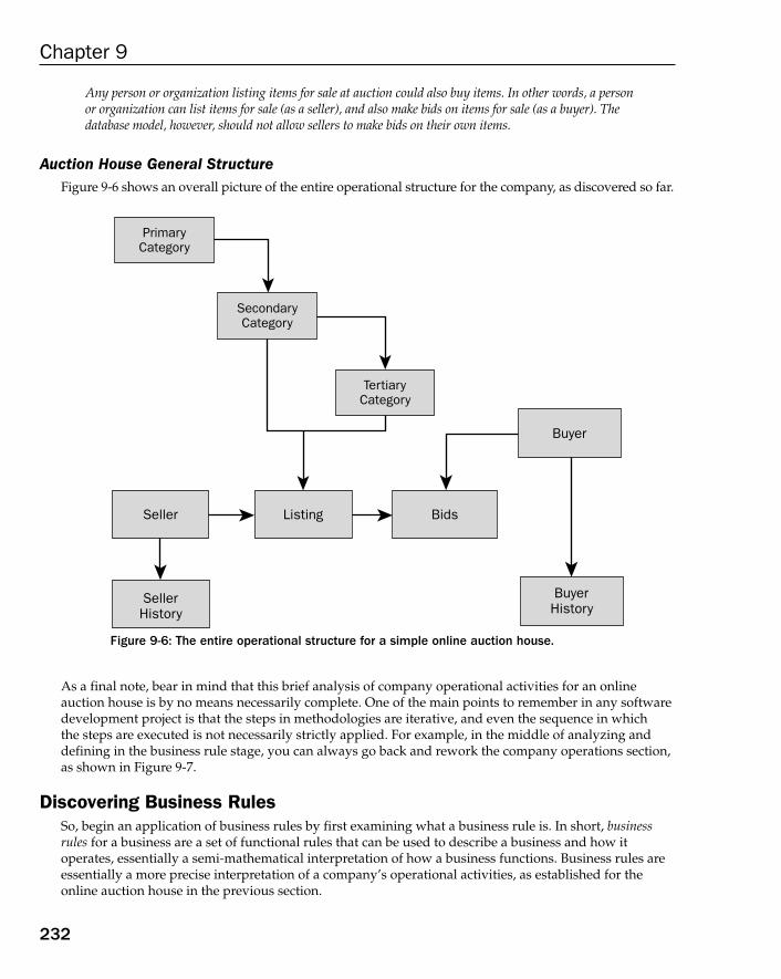
Any person or organization listing items for sale at auction could also buy items. In other words, a personor organization can list items for sale (as a seller), and also make bids on items for sale (as a buyer). Thedatabase model, however, should not allow sellers to make bids on their own items.
Auction House General StructureFigure 9-6 shows an overall picture of the entire operational structure for the company, as discovered so far.
Figure 9-6: The entire operational structure for a simple online auction house.
As a final note, bear in mind that this brief analysis of company operational activities for an online auction house is by no means necessarily complete. One of the main points to remember in any softwaredevelopment project is that the steps in methodologies are iterative, and even the sequence in which the steps are executed is not necessarily strictly applied. For example, in the middle of analyzing anddefining in the business rule stage, you can always go back and rework the company operations section,as shown in Figure 9-7.
Discovering Business RulesSo, begin an application of business rules by first examining what a business rule is. In short, businessrules for a business are a set of functional rules that can be used to describe a business and how it operates, essentially a semi-mathematical interpretation of how a business functions. Business rules areessentially a more precise interpretation of a company’s operational activities, as established for theonline auction house in the previous section.
Buyer
BidsListing
BuyerHistory
Seller
SellerHistory
PrimaryCategory
SecondaryCategory
TertiaryCategory
232
Chapter 9
15_574906 ch09.qxd 11/4/05 10:49 AM Page 232

The business rules of a company, when applied to a database model, become that database model. Thebusiness rules are the tables, relationships between those tables, and even the constraint rules (in addition to referential integrity constraints) in a database. In fact, the application of normalization to aset of initial company data tables is a more and more complex application of business rules to that company data environment. Normalization is the application of business rules.
Figure 9-7: Iterative steps in the analysis methodology.
Figure 9-8 shows some very simple example business rules. In Figure 9-8, there are many categories ofinstruments listed for auction. Each separate category of instruments (such as brass instruments, or thebrass section) has numerous instruments (such as a trumpet, trombone, or sousaphone).
Figure 9-8: A one-to-many relationship is a business rule.
Brass
brass_id
category_id (FK)brassmanufacturerin_stock
Stringed Instrument
stringed_id
category_id (FK)stringed_instrumentmanufacturerin_stocknumber_of_strings
Woodwind
woodwind_id
Percussion
percussion_id
category_id (FK)percussionmanufacturerin_stockfree_snare_drum
Category
category_id
category
category_id (FK)woodwindmanufacturerin_stockused_or_new
Each category has manysubcategories, in turn having many individual instruments
One-to-many business rulesOne-to-many business rules
Company Operations
Overall Objectives
Business Rules
Budgeting
Planning and Timeline
Other Factors
All these steps can be reworked in any order.Obviously rework means rework of all subsequent
steps, if there are any dependencies
233
Planning and Preparation Through Analysis
15_574906 ch09.qxd 11/4/05 10:49 AM Page 233
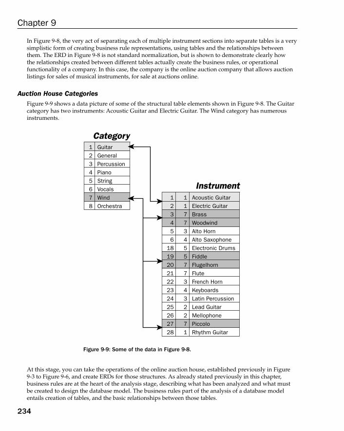
In Figure 9-8, the very act of separating each of multiple instrument sections into separate tables is a verysimplistic form of creating business rule representations, using tables and the relationships betweenthem. The ERD in Figure 9-8 is not standard normalization, but is shown to demonstrate clearly how the relationships created between different tables actually create the business rules, or operational functionality of a company. In this case, the company is the online auction company that allows auctionlistings for sales of musical instruments, for sale at auctions online.
Auction House CategoriesFigure 9-9 shows a data picture of some of the structural table elements shown in Figure 9-8. The Guitarcategory has two instruments: Acoustic Guitar and Electric Guitar. The Wind category has numerousinstruments.
Figure 9-9: Some of the data in Figure 9-8.
At this stage, you can take the operations of the online auction house, established previously in Figure9-3 to Figure 9-6, and create ERDs for those structures. As already stated previously in this chapter, business rules are at the heart of the analysis stage, describing what has been analyzed and what mustbe created to design the database model. The business rules part of the analysis of a database modelentails creation of tables, and the basic relationships between those tables.
12345678
GuitarGeneralPercussionPianoStringVocalsWindOrchestra
1 2 3 4 5 61819202122232425262728
11773455773432271
Acoustic GuitarElectric GuitarBrassWoodwindAlto HornAlto SaxophoneElectronic DrumsFiddleFlugelhornFluteFrench HornKeyboardsLatin PercussionLead GuitarMellophonePiccoloRhythm Guitar
CategoryCategory
InstrumentInstrument
234
Chapter 9
15_574906 ch09.qxd 11/4/05 10:49 AM Page 234

The overall aim of analysis is merely to define rather than specify with precision; therefore, analysis doesnot describe how many fields should be used for an address, for example, or what datatypes those fieldsshould be. Analysis simply determines that an address field actually exists, and obviously which table ortables address information is required within.
Starting with the categories static structures in Figure 9-3, the ERD section in Figure 9-10 caters effectivelyto the category hierarchical structure, and the link to the table containing auction listings. The LISTINGtable has all the details for the master side of a master — detail table that depicts table design, including adescription, listing table number reference (LISTING#), dates, prices, bids, and winning bidder details.
Figure 9-10: An ERD version of the category hierarchical structure of Figure 9-3.
As can be seen in Figure 9-10, the process of analysis is beginning to become one of partial definition, without specifics, of course, where individual fields are defined for different attributes of specific operations.Figure 9-11 and Figure 9-12 show some sample data (including surrogate key fields), to be represented bythe ERD in Figure 9-10.
Listing
listing#descriptionimagestart_dateend_datestarting_pricereserve_pricebuy_now_pricenumber_of_bidswinning_pricebuyer
Category_Primary
primary
Category_Tertiary
tertiary
Category_Secondary
secondary
235
Planning and Preparation Through Analysis
15_574906 ch09.qxd 11/4/05 10:49 AM Page 235
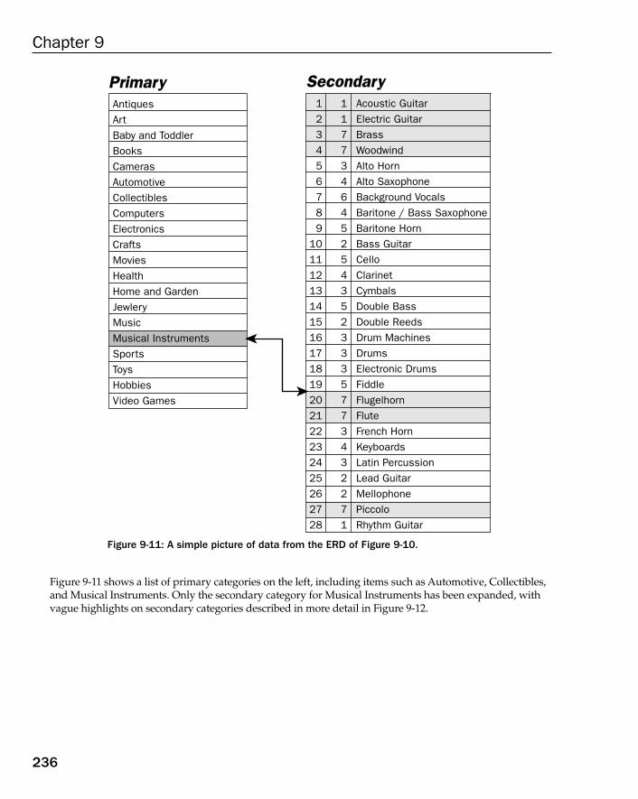
Figure 9-11: A simple picture of data from the ERD of Figure 9-10.
Figure 9-11 shows a list of primary categories on the left, including items such as Automotive, Collectibles,and Musical Instruments. Only the secondary category for Musical Instruments has been expanded, withvague highlights on secondary categories described in more detail in Figure 9-12.
AntiquesArtBaby and ToddlerBooksCamerasAutomotiveCollectiblesComputersElectronicsCraftsMoviesHealthHome and GardenJewleryMusicMusical InstrumentsSportsToysHobbiesVideo Games
1 2 3 4 5 6789
10111213141516171819202122232425262728
1177346452543523335773432271
Acoustic GuitarElectric GuitarBrassWoodwindAlto HornAlto SaxophoneBackground VocalsBaritone / Bass SaxophoneBaritone HornBass GuitarCelloClarinetCymbalsDouble BassDouble ReedsDrum MachinesDrumsElectronic DrumsFiddleFlugelhornFluteFrench HornKeyboardsLatin PercussionLead GuitarMellophonePiccoloRhythm Guitar
PrimaryPrimary SecondarySecondary
236
Chapter 9
15_574906 ch09.qxd 11/4/05 10:49 AM Page 236
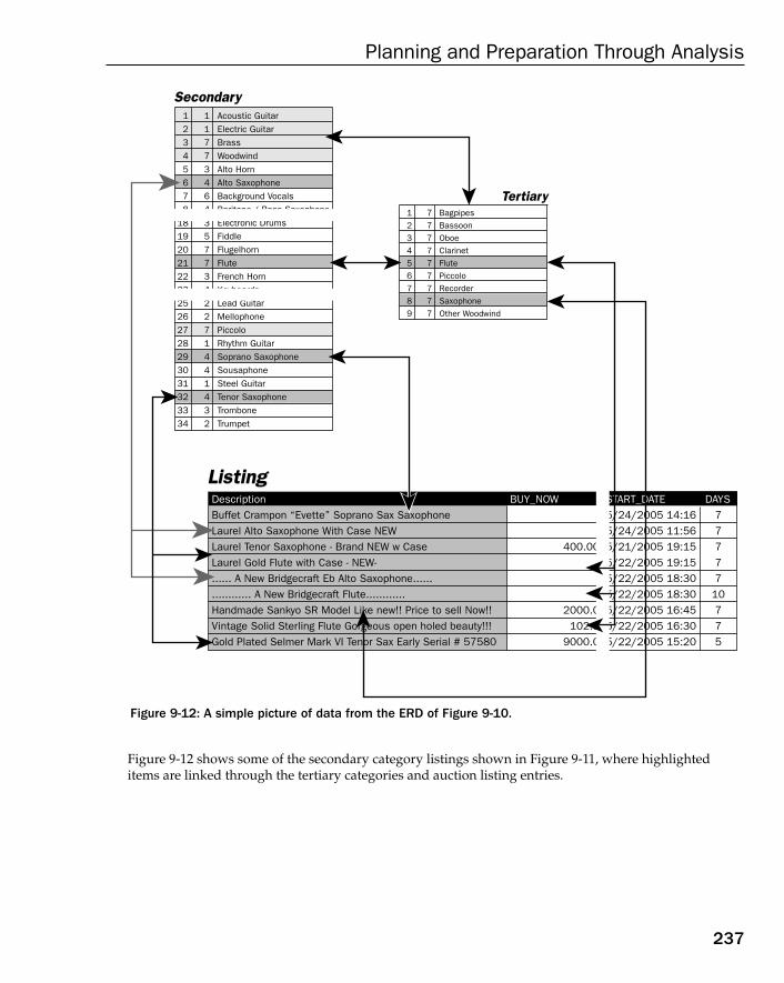
Figure 9-12: A simple picture of data from the ERD of Figure 9-10.
Figure 9-12 shows some of the secondary category listings shown in Figure 9-11, where highlighteditems are linked through the tertiary categories and auction listing entries.
1 2 3 4 5 678
18192021222325262728293031323334
117734643577342271441432
Acoustic GuitarElectric GuitarBrassWoodwindAlto HornAlto SaxophoneBackground VocalsBaritone / Bass SaxophoneElectronic DrumsFiddleFlugelhornFluteFrench HornKeyboardsLead GuitarMellophonePiccoloRhythm GuitarSoprano SaxophoneSousaphoneSteel GuitarTenor SaxophoneTromboneTrumpet
SecondarySecondary
1 2 3 4 5 6
789
777777777
BagpipesBassoonOboeClarinetFlutePiccoloRecorderSaxophoneOther Woodwind
ListingListing
TertiaryTertiary
DescriptionBuffet Crampon “Evette” Soprano Sax SaxophoneLaurel Alto Saxophone With Case NEWLaurel Tenor Saxophone - Brand NEW w CaseLaurel Gold Flute with Case - NEW-...... A New Bridgecraft Eb Alto Saxophone.................. A New Bridgecraft Flute............Handmade Sankyo SR Model Like new!! Price to sell Now!!Vintage Solid Sterling Flute Gorgeous open holed beauty!!!Gold Plated Selmer Mark VI Tenor Sax Early Serial # 57580
BUY_NOW
400.00
2000.00 102.50 9000.00
START_DATE5/24/2005 14:165/24/2005 11:565/21/2005 19:155/22/2005 19:155/22/2005 18:305/22/2005 18:305/22/2005 16:455/22/2005 16:305/22/2005 15:20
DAYS7777710775
237
Planning and Preparation Through Analysis
15_574906 ch09.qxd 11/4/05 10:49 AM Page 237
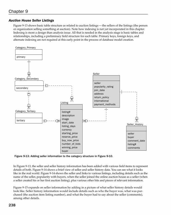
Auction House Seller ListingsFigure 9-13 shows basic table structure as related to auction listings — the sellers of the listings (the personor organization selling something at auction). Note how indexing is not yet incorporated in this chapter.Indexing is more a design than analysis issue. All that is needed in the analysis stage is basic tables andrelationships, including a preliminary field structure for each table. Primary keys, foreign keys, and alternate indexing are not required at this early point in the process of database model creation.
Figure 9-13: Adding seller information to the category structure in Figure 9-10.
In Figure 9-13, the seller and seller history information has been added with various field items to representdetails of both. Figure 9-14 shows a brief view of seller and seller history data. You can see what it lookslike in the real world. Figure 9-14 shows the seller and links to various listings, including details such as thename of the seller, popularity with buyers, when the seller joined the online auction house as a seller (whena seller created his or her first auction listing), plus various other bits and pieces of relevant information.
Figure 9-15 expands on seller information by adding in a picture of what seller history details wouldlook like. Seller history information would include details such as who the buyer was, what was pur-chased (the auction item listing number), and what the buyer had to say about the seller (comments),among other details.
Category_Primary
primary
Listing
listing#descriptionimagestart_datelisting_dayscurrencystarting_pricereserve_pricebuy_now_pricenumber_of_bidswinning_pricebuyer
Seller
sellerpopularity_ratingjoin_dateaddressreturn_policyinternationalpayment_methods
Seller_History
sellerbuyercomment_datelisting#comments
Category_Tertiary
tertiary
Category_Secondary
secondary
238
Chapter 9
15_574906 ch09.qxd 11/4/05 10:49 AM Page 238
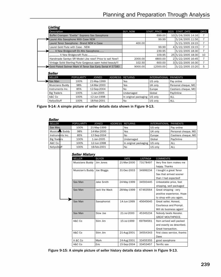
Figure 9-14: A simple picture of seller details data shown in Figure 9-13.
Figure 9-15: A simple picture of seller history details data shown in Figure 9-13.
Seller HistorySeller History
SellerSeller
SELLERMusicians Buddy
Musician’s Buddy
Sax Man
Sax Man
Sax Man
Sax Man
A&C Co
A&C Co
A &C CoA&C Co
BUYERJim Jones
Joe Bloggs
Jake Smith
Jack the Wack
Saxophonist
Slow Joe
Slim Jim
Slim Jim
MarkEric
DATE21-Mar-2000
31-Dec-2003
24-May-1999
28-May-1999
14-Jun-1999
21-Jul-2000
15-Jul-1999
21-Aug-2001
24-Aug-200115-Sep-2004
LISTING#73178497
34999234
34593445
67463564
45645645
45345234
69784561
34554343
3345535533453457
COMMENTSVery fine item makes mehappy. ThanksI bought a great Tenor Sax that arrived soonerthan I had expected!Unbeatable price, fastshipping, well packagedGreat shipping - verypositive experience. Hopeto shop with you again.Great seller, Honest, Courteous and Prompt.Will do business again!Nobody beats Kessler.GREAT MOUTHPIECE.Item arrived well packedand exactly as described.Great transaction.first class service, thanksDavegood saxophoneTerrific sax
SELLERSax ManMusicians BuddyInstruments Inc.Big TradersA&C CoKellysStuff
POPULARITY100%98%85%100%100%100%
JOINED21-May-199914-Mar-200012-Sep-20041-Jan-200512-Jun-199818-Feb-2001
ADDRESS RETURNSYesYesNoUndamagedIn original packagingNo
INTERNATIONALUS onlyUK onlyEuropeGlobalUS onlyUS only
PAYMENTSPay onlinePersonal cheque, MOCashiers cheque, MOPayOnlineALLALL
ListingListing
SellerSeller
DescriptionBuffet Crampon “Evette” Soprano Sax SaxophoneLaurel Alto Saxophone With Case NEWLaurel Tenor Saxophone - Brand NEW w CaseLaurel Gold Flute with Case - NEW-...... A New Bridgecraft Eb Alto Saxophone.................. A New Bridgecraft Flute............Handmade Sankyo SR Model Like new!! Price to sell Now!!Vintage Solid Sterling Flute Gorgeous open holed beauty!!!Gold Plated Selmer Mark VI Tenor Sax Early Serial # 57580
BUY_NOW
400.00
2000.00 102.50 9000.00
START_PRICE 699.00 99.99
99.99 239.95 109.95 4800.00 600.00 12500.00
BIDS 10
4
25 2 3
START_DATE5/24/2005 14:165/24/2005 11:565/21/2005 19:155/22/2005 19:155/22/2005 18:305/22/2005 18:305/22/2005 16:455/22/2005 16:305/22/2005 15:20
DAYS77777
10775
SELLERSax ManMusicians BuddyInstruments Inc.Big TradersA&C CoKellysStuff
POPULARITY100%98%85%
100%100%100%
JOINED21-May-199914-Mar-200012-Sep-20041-Jan-200512-Jun-199818-Feb-2001
ADDRESS RETURNSYesYesNoUndamagedIn original packagingNo
INTERNATIONALUS onlyUK onlyEuropeGlobalUS onlyUS only
PAYMENTSPay onlinePersonal cheque, MOCashiers cheque, MOPayOnlineALLALL
239
Planning and Preparation Through Analysis
15_574906 ch09.qxd 11/4/05 10:49 AM Page 239
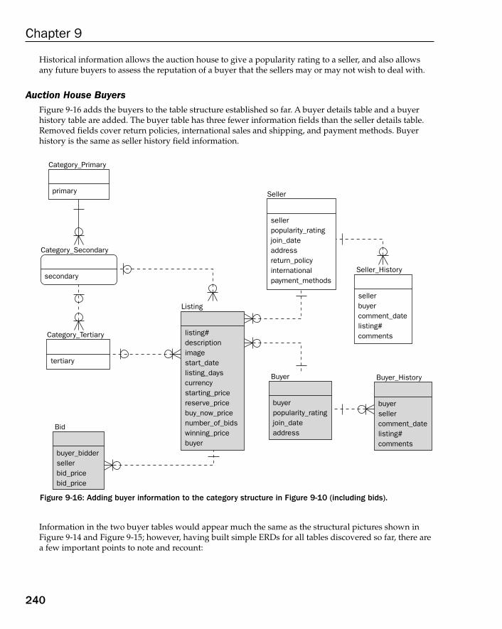
Historical information allows the auction house to give a popularity rating to a seller, and also allowsany future buyers to assess the reputation of a buyer that the sellers may or may not wish to deal with.
Auction House BuyersFigure 9-16 adds the buyers to the table structure established so far. A buyer details table and a buyerhistory table are added. The buyer table has three fewer information fields than the seller details table.Removed fields cover return policies, international sales and shipping, and payment methods. Buyerhistory is the same as seller history field information.
Figure 9-16: Adding buyer information to the category structure in Figure 9-10 (including bids).
Information in the two buyer tables would appear much the same as the structural pictures shown inFigure 9-14 and Figure 9-15; however, having built simple ERDs for all tables discovered so far, there area few important points to note and recount:
Category_Primary
primary
Category_Secondary
secondary
Category_Tertiary
tertiary
Bid
buyer_biddersellerbid_pricebid_price
Listing
listing#descriptionimagestart_datelisting_dayscurrencystarting_pricereserve_pricebuy_now_pricenumber_of_bidswinning_pricebuyer
Buyer
buyerpopularity_ratingjoin_dateaddress
Seller
sellerpopularity_ratingjoin_dateaddressreturn_policyinternationalpayment_methods
Seller_History
sellerbuyercomment_datelisting#comments
Buyer_History
buyersellercomment_datelisting#comments
240
Chapter 9
15_574906 ch09.qxd 11/4/05 10:49 AM Page 240

❑ Separating buyers and sellers — In any auction model, a buyer can actually also be a seller (biddingon their own items should be prohibited). It might seem sensible to merge the buyer and sellertables, and also merge the two history tables together. Traditionally, in many database models,any types of customer and supplier details are generally separated. This is usually because theyare not one and the same, from the perspective of content, as opposed to a structural point ofview. In an auctioning database model, separating buyers from sellers is likely to be the most sensible option, simply because it is probably the norm (not always the case) that the buyers areunlikely to be sellers, and visa versa. Obviously, with normalization applied during the designphase (discussed in Chapter 10), it may make sense to separate buyers, sellers, and buyer-sellers(auctioneers who both buy and sell), all into three separate tables.
❑ Referential integrity keys — All the most basic relationships have been established between thedifferent tables. Identifying appropriate primary and foreign keys is more a design issue thanan analysis issue. Keys will be established in Chapter 10, which covers design.
❑ Category hierarchy — In some situations, separating static tables (such as the three categorytables) may not be the most efficient option. There may be a case for merging all categories intoa single table. The single table would contain all three category levels using specialized parentand child fields, for each category record. Because this is once again a design issue and not ananalysis issue, it is covered in Chapter 10.
Try It Out Analyzing an OLTP Database ModelCreate a simple analytical-level OLTP database model for a Web site. This Web site allows creation offree classified ads for musicians and bands. Here’s a simplistic approach:
1. Identify the operations of the company.
2. Draw up a picture of basic tables.
3. Establish simple relationships.
4. Create basic fields within each table.
How It WorksFigure 9-17 shows some basic information categories, both static and transactional in nature. Instrumentsand skills statically describe relatively static musicians (musicians come and go, skills and instrumentclassifications do not). This probably makes musicians dynamic transactional information. A band has aspecific genre such as playing rock music, punk, classic rock, and so on. Thus, the band is dynamic andthe genre is static. The classified advertisement itself is most certainly dynamic in nature.
Just in case you are wondering where all this stuff is going (the three points justmentioned), these factors are all design issues, not analysis issues. This chapterdeals with the analytical process of discovering basic contents of the auctioningdatabase model. Chapter 10 deals with design issues. The objective of these casestudy directed chapters is to introduce a data model in a manner that covers eachconcept step-by-step, making details easy to understand and absorb.
241
Planning and Preparation Through Analysis
15_574906 ch09.qxd 11/4/05 10:49 AM Page 241
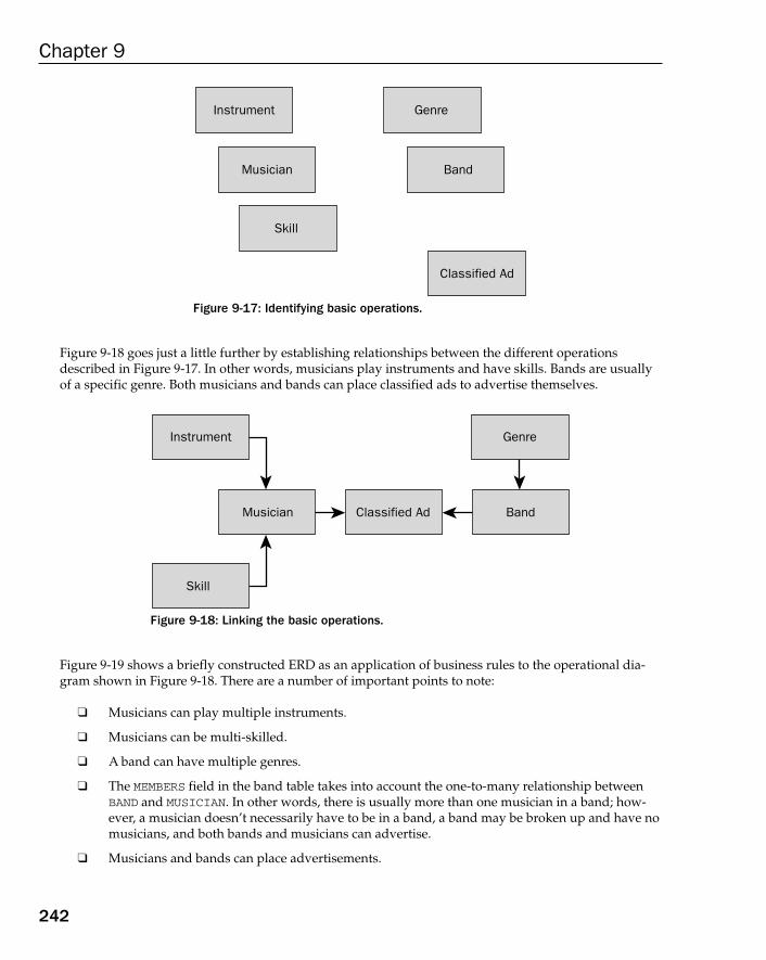
Figure 9-17: Identifying basic operations.
Figure 9-18 goes just a little further by establishing relationships between the different operationsdescribed in Figure 9-17. In other words, musicians play instruments and have skills. Bands are usuallyof a specific genre. Both musicians and bands can place classified ads to advertise themselves.
Figure 9-18: Linking the basic operations.
Figure 9-19 shows a briefly constructed ERD as an application of business rules to the operational dia-gram shown in Figure 9-18. There are a number of important points to note:
❑ Musicians can play multiple instruments.
❑ Musicians can be multi-skilled.
❑ A band can have multiple genres.
❑ The MEMBERS field in the band table takes into account the one-to-many relationship betweenBAND and MUSICIAN. In other words, there is usually more than one musician in a band; how-ever, a musician doesn’t necessarily have to be in a band, a band may be broken up and have nomusicians, and both bands and musicians can advertise.
❑ Musicians and bands can place advertisements.
Instrument Genre
Musician Classified Ad Band
Skill
Instrument
Musician
Skill
Genre
Band
Classified Ad
242
Chapter 9
15_574906 ch09.qxd 11/4/05 10:49 AM Page 242
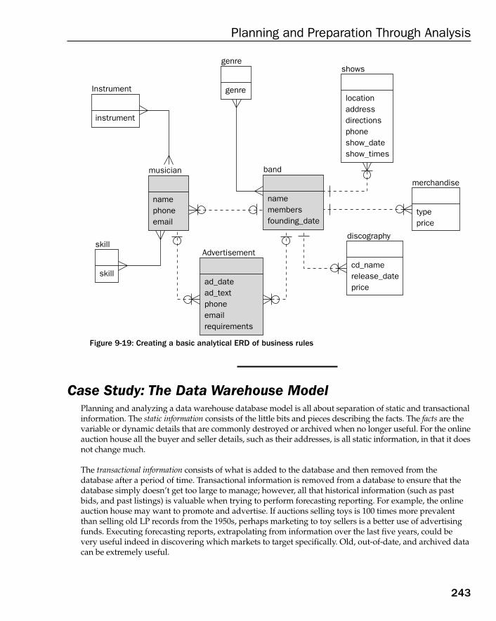
Figure 9-19: Creating a basic analytical ERD of business rules
Case Study: The Data Warehouse ModelPlanning and analyzing a data warehouse database model is all about separation of static and transactionalinformation. The static information consists of the little bits and pieces describing the facts. The facts are thevariable or dynamic details that are commonly destroyed or archived when no longer useful. For the onlineauction house all the buyer and seller details, such as their addresses, is all static information, in that it doesnot change much.
The transactional information consists of what is added to the database and then removed from thedatabase after a period of time. Transactional information is removed from a database to ensure that thedatabase simply doesn’t get too large to manage; however, all that historical information (such as pastbids, and past listings) is valuable when trying to perform forecasting reporting. For example, the onlineauction house may want to promote and advertise. If auctions selling toys is 100 times more prevalentthan selling old LP records from the 1950s, perhaps marketing to toy sellers is a better use of advertisingfunds. Executing forecasting reports, extrapolating from information over the last five years, could bevery useful indeed in discovering which markets to target specifically. Old, out-of-date, and archived datacan be extremely useful.
Instrument
instrument
musician
namephoneemail
skill
skill
Advertisement
ad_datead_textphoneemailrequirements
band
namemembersfounding_date
genre
genre
shows
locationaddressdirectionsphoneshow_dateshow_times
merchandise
typeprice
discography
cd_namerelease_dateprice
243
Planning and Preparation Through Analysis
15_574906 ch09.qxd 11/4/05 10:49 AM Page 243
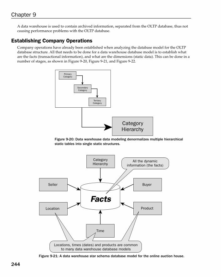
A data warehouse is used to contain archived information, separated from the OLTP database, thus notcausing performance problems with the OLTP database.
Establishing Company OperationsCompany operations have already been established when analyzing the database model for the OLTPdatabase structure. All that needs to be done for a data warehouse database model is to establish whatare the facts (transactional information), and what are the dimensions (static data). This can be done in anumber of stages, as shown in Figure 9-20, Figure 9-21, and Figure 9-22.
Figure 9-20: Data warehouse data modeling denormalizes multiple hierarchicalstatic tables into single static structures.
Figure 9-21: A data warehouse star schema database model for the online auction house.
Seller
CategoryHierarchy
Time
Location
Buyer
Product
FactsFacts
All the dynamicinformation (the facts)
Locations, times (dates) and products are commonto many data warehouse database models
PrimaryCategory
SecondaryCategory
TertiaryCategory
CategoryHierarchy
244
Chapter 9
15_574906 ch09.qxd 11/4/05 10:49 AM Page 244
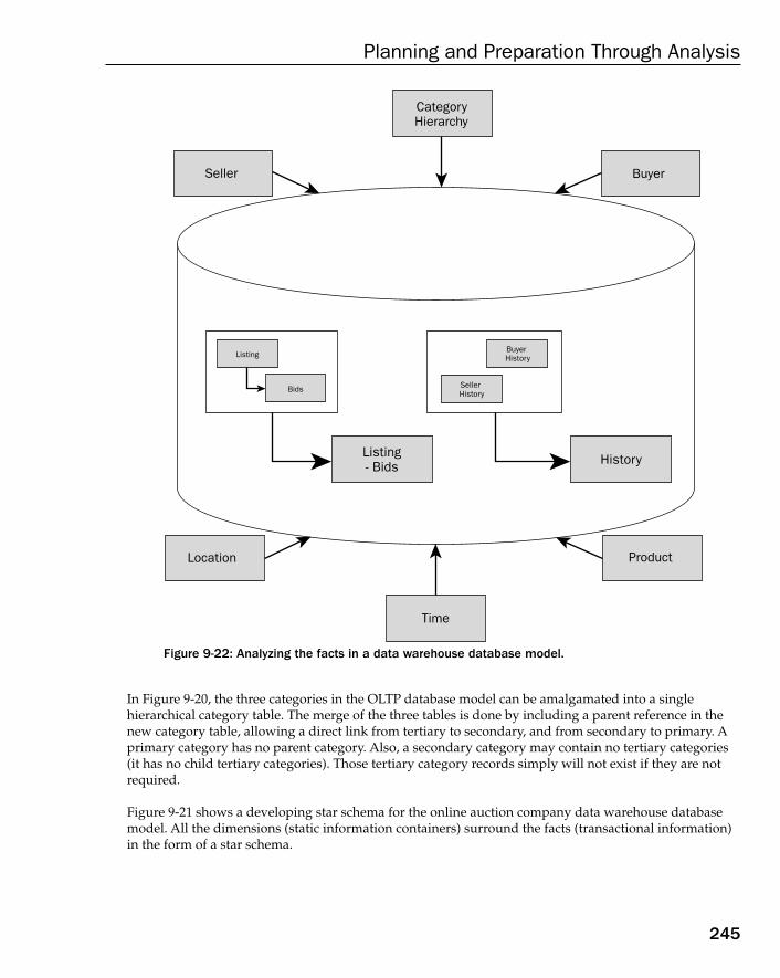
Figure 9-22: Analyzing the facts in a data warehouse database model.
In Figure 9-20, the three categories in the OLTP database model can be amalgamated into a single hierarchical category table. The merge of the three tables is done by including a parent reference in thenew category table, allowing a direct link from tertiary to secondary, and from secondary to primary. Aprimary category has no parent category. Also, a secondary category may contain no tertiary categories(it has no child tertiary categories). Those tertiary category records simply will not exist if they are notrequired.
Figure 9-21 shows a developing star schema for the online auction company data warehouse databasemodel. All the dimensions (static information containers) surround the facts (transactional information)in the form of a star schema.
Seller
CategoryHierarchy
Time
Location
Buyer
Product
Listing
Bids
Listing- Bids
Buyer History
Seller History
History
245
Planning and Preparation Through Analysis
15_574906 ch09.qxd 11/4/05 10:49 AM Page 245
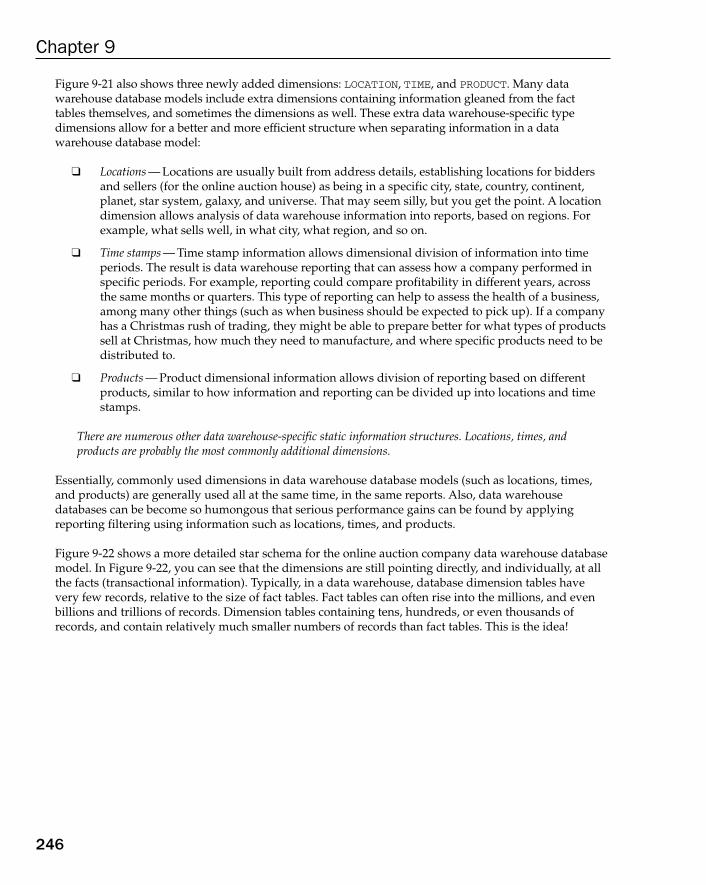
Figure 9-21 also shows three newly added dimensions: LOCATION, TIME, and PRODUCT. Many data warehouse database models include extra dimensions containing information gleaned from the fact tables themselves, and sometimes the dimensions as well. These extra data warehouse-specific typedimensions allow for a better and more efficient structure when separating information in a data warehouse database model:
❑ Locations — Locations are usually built from address details, establishing locations for biddersand sellers (for the online auction house) as being in a specific city, state, country, continent,planet, star system, galaxy, and universe. That may seem silly, but you get the point. A locationdimension allows analysis of data warehouse information into reports, based on regions. Forexample, what sells well, in what city, what region, and so on.
❑ Time stamps — Time stamp information allows dimensional division of information into timeperiods. The result is data warehouse reporting that can assess how a company performed inspecific periods. For example, reporting could compare profitability in different years, acrossthe same months or quarters. This type of reporting can help to assess the health of a business,among many other things (such as when business should be expected to pick up). If a companyhas a Christmas rush of trading, they might be able to prepare better for what types of productssell at Christmas, how much they need to manufacture, and where specific products need to bedistributed to.
❑ Products — Product dimensional information allows division of reporting based on differentproducts, similar to how information and reporting can be divided up into locations and timestamps.
There are numerous other data warehouse-specific static information structures. Locations, times, andproducts are probably the most commonly additional dimensions.
Essentially, commonly used dimensions in data warehouse database models (such as locations, times,and products) are generally used all at the same time, in the same reports. Also, data warehousedatabases can be become so humongous that serious performance gains can be found by applyingreporting filtering using information such as locations, times, and products.
Figure 9-22 shows a more detailed star schema for the online auction company data warehouse databasemodel. In Figure 9-22, you can see that the dimensions are still pointing directly, and individually, at allthe facts (transactional information). Typically, in a data warehouse, database dimension tables havevery few records, relative to the size of fact tables. Fact tables can often rise into the millions, and evenbillions and trillions of records. Dimension tables containing tens, hundreds, or even thousands ofrecords, and contain relatively much smaller numbers of records than fact tables. This is the idea!
246
Chapter 9
15_574906 ch09.qxd 11/4/05 10:49 AM Page 246
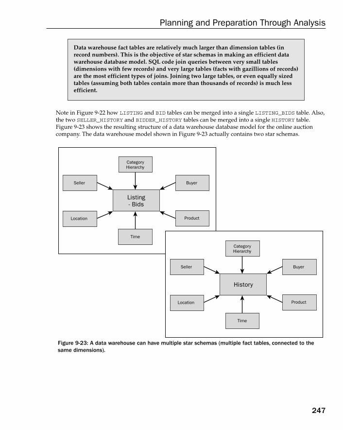
Note in Figure 9-22 how LISTING and BID tables can be merged into a single LISTING_BIDS table. Also,the two SELLER_HISTORY and BIDDER_HISTORY tables can be merged into a single HISTORY table.Figure 9-23 shows the resulting structure of a data warehouse database model for the online auctioncompany. The data warehouse model shown in Figure 9-23 actually contains two star schemas.
Figure 9-23: A data warehouse can have multiple star schemas (multiple fact tables, connected to thesame dimensions).
Seller
CategoryHierarchy
Time
Location
Buyer
Product
Listing- Bids
Seller
CategoryHierarchy
Time
Location
Buyer
Product
History
Data warehouse fact tables are relatively much larger than dimension tables (inrecord numbers). This is the objective of star schemas in making an efficient datawarehouse database model. SQL code join queries between very small tables(dimensions with few records) and very large tables (facts with gazillions of records)are the most efficient types of joins. Joining two large tables, or even equally sizedtables (assuming both tables contain more than thousands of records) is much lessefficient.
247
Planning and Preparation Through Analysis
15_574906 ch09.qxd 11/4/05 10:49 AM Page 247
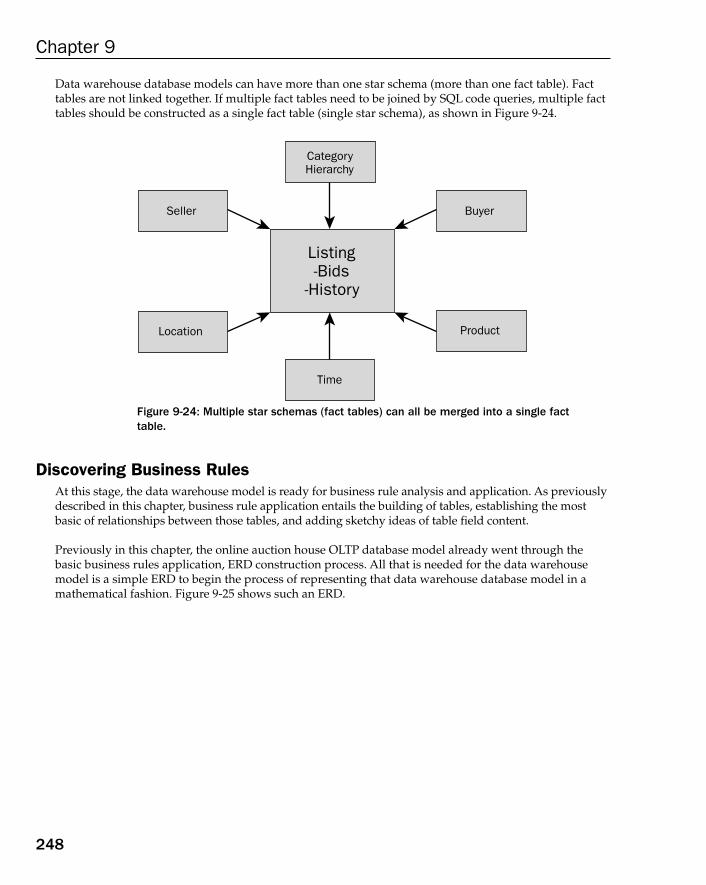
Data warehouse database models can have more than one star schema (more than one fact table). Facttables are not linked together. If multiple fact tables need to be joined by SQL code queries, multiple facttables should be constructed as a single fact table (single star schema), as shown in Figure 9-24.
Figure 9-24: Multiple star schemas (fact tables) can all be merged into a single facttable.
Discovering Business RulesAt this stage, the data warehouse model is ready for business rule analysis and application. As previouslydescribed in this chapter, business rule application entails the building of tables, establishing the mostbasic of relationships between those tables, and adding sketchy ideas of table field content.
Previously in this chapter, the online auction house OLTP database model already went through thebasic business rules application, ERD construction process. All that is needed for the data warehousemodel is a simple ERD to begin the process of representing that data warehouse database model in amathematical fashion. Figure 9-25 shows such an ERD.
Seller
CategoryHierarchy
Time
Location
Buyer
Product
Listing-Bids
-History
248
Chapter 9
15_574906 ch09.qxd 11/4/05 10:49 AM Page 248
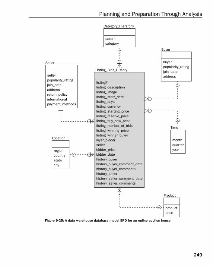
Figure 9-25: A data warehouse database model ERD for an online auction house.
Seller
sellerpopularity_ratingjoin_dateaddressreturn_policyinternationalpayment_methods
Location
regioncountrystatecity
Time
monthquarteryear
Product
productprice
Buyer
buyerpopularity_ratingjoin_dateaddress
Listing_Bids_History
listing#listing_descriptionlisting_imagelisting_start_datelisting_dayslisting_currencylisting_starting_pricelisting_reserve_pricelisting_buy_now_pricelisting_number_of_bidslisting_winning_pricelisting_winner_buyerluyer_biddersellerbidder_pricebidder_datehistory_buyerhistory_buyer_comment_datehistory_buyer_commentshistory_sellerhistory_seller_comment_datehistory_seller_comments
Category_Hierarchy
parentcategory
249
Planning and Preparation Through Analysis
15_574906 ch09.qxd 11/4/05 10:49 AM Page 249
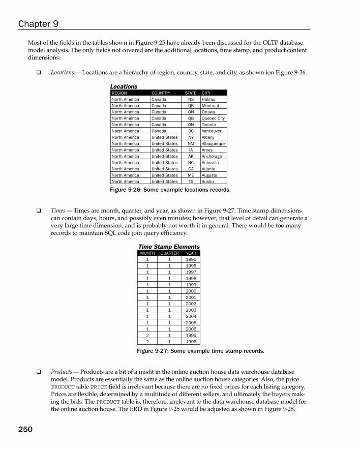
Most of the fields in the tables shown in Figure 9-25 have already been discussed for the OLTP databasemodel analysis. The only fields not covered are the additional locations, time stamp, and product contentdimensions:
❑ Locations — Locations are a hierarchy of region, country, state, and city, as shown ion Figure 9-26.
Figure 9-26: Some example locations records.
❑ Times — Times are month, quarter, and year, as shown in Figure 9-27. Time stamp dimensionscan contain days, hours, and possibly even minutes; however, that level of detail can generate avery large time dimension, and is probably not worth it in general. There would be too manyrecords to maintain SQL code join query efficiency.
Figure 9-27: Some example time stamp records.
❑ Products — Products are a bit of a misfit in the online auction house data warehouse databasemodel. Products are essentially the same as the online auction house categories. Also, the pricePRODUCT table PRICE field is irrelevant because there are no fixed prices for each listing category.Prices are flexible, determined by a multitude of different sellers, and ultimately the buyers mak-ing the bids. The PRODUCT table is, therefore, irrelevant to the data warehouse database model forthe online auction house. The ERD in Figure 9-25 would be adjusted as shown in Figure 9-28.
Time Stamp ElementsTime Stamp ElementsMONTH
11111111111122
QUARTER11111111111111
YEAR19951996199719981999200020012002200320042005200619951996
LocationsLocationsREGIONNorth AmericaNorth AmericaNorth AmericaNorth AmericaNorth AmericaNorth AmericaNorth AmericaNorth AmericaNorth AmericaNorth AmericaNorth AmericaNorth AmericaNorth AmericaNorth America
COUNTRYCanadaCanadaCanadaCanadaCanadaCanadaUnited StatesUnited StatesUnited StatesUnited StatesUnited StatesUnited StatesUnited StatesUnited States
STATENSQBONQBONBCNYNMIAAKNCGAMETX
CITYHalifaxMontrealOttawaQuebec CityTorontoVancouverAlbanyAlbuquerqueAmesAnchorageAshevilleAtlantaAugustaAustin
250
Chapter 9
15_574906 ch09.qxd 11/4/05 10:49 AM Page 250
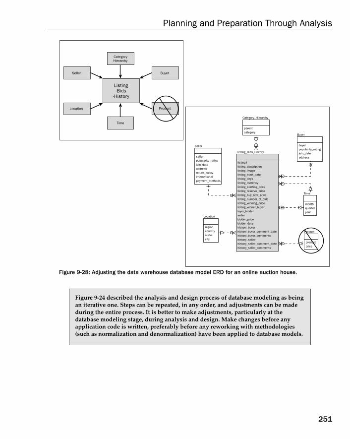
Figure 9-28: Adjusting the data warehouse database model ERD for an online auction house.
Figure 9-24 described the analysis and design process of database modeling as beingan iterative one. Steps can be repeated, in any order, and adjustments can be madeduring the entire process. It is better to make adjustments, particularly at thedatabase modeling stage, during analysis and design. Make changes before anyapplication code is written, preferably before any reworking with methodologies(such as normalization and denormalization) have been applied to database models.
Seller
CategoryHierarchy
Time
Location
Buyer
Product
Listing-Bids
-History
Seller
sellerpopularity_ratingjoin_dateaddressreturn_policyinternationalpayment_methods
Location
regioncountrystatecity
Time
monthquarteryear
Buyer
buyerpopularity_ratingjoin_dateaddress
Listing_Bids_History
listing#listing_descriptionlisting_imagelisting_start_datelisting_dayslisting_currencylisting_starting_pricelisting_reserve_pricelisting_buy_now_pricelisting_number_of_bidslisting_winning_pricelisting_winner_buyerluyer_biddersellerbidder_pricebidder_datehistory_buyerhistory_buyer_comment_datehistory_buyer_commentshistory_sellerhistory_seller_comment_datehistory_seller_comments
Product
productprice
Category_Hierarchy
parentcategory
251
Planning and Preparation Through Analysis
15_574906 ch09.qxd 11/4/05 10:49 AM Page 251
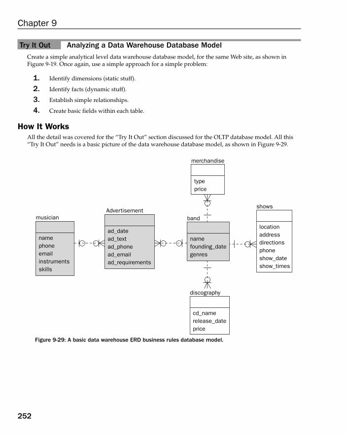
Try It Out Analyzing a Data Warehouse Database ModelCreate a simple analytical level data warehouse database model, for the same Web site, as shown inFigure 9-19. Once again, use a simple approach for a simple problem:
1. Identify dimensions (static stuff).
2. Identify facts (dynamic stuff).
3. Establish simple relationships.
4. Create basic fields within each table.
How It WorksAll the detail was covered for the “Try It Out” section discussed for the OLTP database model. All this“Try It Out” needs is a basic picture of the data warehouse database model, as shown in Figure 9-29.
Figure 9-29: A basic data warehouse ERD business rules database model.
musician
namephoneemailinstrumentsskills
band
namefounding_dategenres
shows
locationaddressdirectionsphoneshow_dateshow_times
Advertisement
ad_datead_textad_phonead_emailad_requirements
discography
cd_namerelease_dateprice
merchandise
typeprice
252
Chapter 9
15_574906 ch09.qxd 11/4/05 10:49 AM Page 252

The ADVERTISEMENT table is decided on being the fact table. The MUSICIAN table is a single layer facttable. The BAND, MERCHANDISE, SHOWS, and DISCOGRAPHY tables constitute a two-layer dimensionalhierarchy.
There are some gray areas between static and dynamic information in this situation. There are otherways of building this data warehouse database model.
Project ManagementWhen it comes to planning and establishing timelines, there are some remarkably good project-planningsoftware tools available. When planning any software project, including a database model design, thereis often more than one person involved in a project. This excludes the planner. If not using a softwaretool, and multiple people are to perform multiple overlapping, interdependent tasks, you could end upwith lots of drawings, and an awfully full garbage can. These things change. Plans can change. Peopleget sick and go on vacation. They find new jobs. Sometimes people simply don’t show up at all! In otherwords, expect things to change.
The fact is when it comes to planning, establishing timelines, and budgeting there is no enforceable or reasonably useful applicable set of rules and steps. It just doesn’t exist. In any planning process (includingbudgeting), for any type of project, there is no way to accurately predict to any degree of mathematicalcertainty. None of us can really read the future. Planning, establishing timelines, and budgeting entail aflexible process, which is almost entirely dependant on the expertise, and past experience, of the planner.And then again, if changes and unexpected snags or events are not anticipated, a project can very quicklyspiral out of control.
Project Planning and TimelinesA software development company can meet with its financial demise by not allowing enough time in project plans. It is quite common in the software development field for project-tender budgets from multiple companies to be as much as 50 times different. In other words, the difference in dollar estimatesbetween the lowest and highest bidders can be enormous. This indicates guesswork. It is often the casethat the most inexperienced companies put in the lowest bids. The highest bids are probably greedy.Those between the average and the highest are probably the most realistic. Also, they are likely to make aprofit, and thus be around to support very expensive software tools, say, 5 to 10 years from now.
As already stated, there is much research into project planning in general. Unfortunately, few, if anyquantifiable and useful results have been obtained. Expert level assessment based on past experience ofexperts, is usually the best measure of possibilities.
There is an International Standards Institute (ISO) model called the “ISO 9000-3 Model.” This modelis used more to give a method of quality assurance against the final product, of, say, an analysis of adatabase model. This ISO model does not give a set of instructions as to how to go about performinganalysis process itself, but rather presents a method of validation after the fact.
253
Planning and Preparation Through Analysis
15_574906 ch09.qxd 11/4/05 10:49 AM Page 253
The accuracy of a planned budget is dependent on the experience of the planner. Database designers,administrators, and programmers think that their project managers and planners do nothing. They arewrong. The planners take all the risk, make all the wild guesses; the programmers get to write all thatmathematically precise programming code. So, the next time you see your project manager in a coldsweat, you know why. It’s not your job on the line — it’s theirs.
Here are some interesting — and sometimes amusing — terms, often used to describe planning, budgeting,and project management:
❑ “Why did the chicken cross the road?” — This is a well-known quotation about a now unfortu-nately discontinued software development consultancy company. This company was famousfor producing enormous amounts of paper. Lots of paper can help to make more profit for thesoftware development company. The more paper produced, the more useless waffle. However,the more paper produced, the less likely something has been overlooked, and the more likelythe plan and budget are accurate. The other problem with lots of paper is no one has time toread it, and doesn’t really want to either.
❑ “Get someone with a great, big, long signature and a serious title to sign off on it ASAP.” — This one isalso called “passing the buck.” That buck has to stop somewhere, and the higher up, the better,and preferably not with the planner. The planner has enough things to think about withoutworrying about whether their wildest guesses will bear fruit, or simply crash and burn.
❑ “Don’t break it if it’s already fixed.” — If something is working properly, why change it?
❑ “Use information in existing systems, be they computerized or on paper.” — Existing structures canusually tell more about a company that its people can. There is, however, a danger that if a sys-tem is being replaced, there is probably something very wrong with the older system.
❑ “Try not to reinvent the wheel.” — When planning on building software or a new database model,use other people’s ideas if they are appropriate. Of course, beware of outdated ideas. Do thor-ough research. The Internet is an excellent source of freely available ideas, both old and new.
❑ “More resources do not mean faster work.” — The more people involved in a project, the more con-fusion. Throwing more bodies at a project can just as likely make a project impossible to man-age, as it can make it go faster.
Figure 9-30 shows a pretty picture of what a project timeline might look like, containing multiple people,multiple skills levels, multiple tasks (both overlapping and interdependent). Project timelines canbecome incredibly complicated. Simplify, if possible. Too much interdependency can lead to problems ifone area overruns on time limitations. Keep something spare in terms of people, available hours, andotherwise. Expect changes. Plan with some resources in reserve.
Figure 9-30 shows five separate tasks in a simplistic project-timeline Gantt chart. Task 1 is assigned toJim. There is no time conflict between Task 2 and Task 3, and can both be assigned to Joe (one person).Task 3 and Task 4 overlap between both Janet and Joe, in more ways than one. Joe is going to be verybusy indeed. A project manager would allow overlap where the person doing the assigned tasks isknown to be capable of multiple concurrent activities.
254
Chapter 9
15_574906 ch09.qxd 11/4/05 10:49 AM Page 254
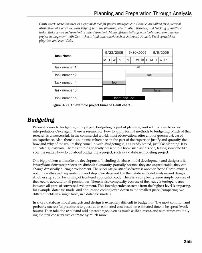
Gantt charts were invented as a graphical tool for project management. Gantt charts allow for a pictorialillustration of a schedule, thus helping with the planning, coordination between, and tracking of multipletasks. Tasks can be independent or interdependent. Many off-the-shelf software tools allow computerizedproject management with Gantt charts (and otherwise), such as Microsoft Project, Excel spreadsheetplug-ins, and even Visio.
Figure 9-30: An example project timeline Gantt chart.
BudgetingWhen it comes to budgeting for a project, budgeting is part of planning, and is thus open to expert interpretation. Once again, there is research on how to apply formal methods to budgeting. Much of thatresearch is unsuccessful. In the commercial world, most observations offer a lot of guesswork based on experience. Also, there is an intense reluctance on the part of the experts to justify and quantify thehow and why of the results they come up with. Budgeting is, as already stated, just like planning. It iseducated guesswork. There is nothing to really present in a book such as this one, telling someone likeyou, the reader, how to go about budgeting a project, such as a database modeling project.
One big problem with software development (including database model development and design) is itsintangibility. Software projects are difficult to quantify, partially because they are unpredictable, they canchange drastically during development. The sheer complexity of software is another factor. Complexity isnot only within each separate unit and step. One step could be the database model analysis and design.Another step could be writing of front-end application code. There is a complexity issue simply because ofthe need to account for all possibilities. There is also complexity because of the heavy interdependencebetween all parts of software development. This interdependence stems from the highest level (comparing,for example, database model and application coding) even down to the smallest piece (comparing two different fields in a single table, in a database model).
In short, database model analysis and design is extremely difficult to budget for. The most common andprobably successful practice is to guess at an estimated cost based on estimated time to be spent (workhours). Then take the result and add a percentage, even as much as 50 percent, and sometimes multiply-ing the first conservative estimate by much more.
Task Name
Task number 1
5/23/2005
Task number 2
Task number 4
Task number 3
Task number 5
M T W Th F
5/30/2005
M T W Th F
6/6/2005
M T W Th F
Jim
Joe
Joe
Janet
Janet and Joe
255
Planning and Preparation Through Analysis
15_574906 ch09.qxd 11/4/05 10:49 AM Page 255
A number of detail areas already have been discussed previously in this chapter:
❑ Hiring help costs money — Hired help in the form of software development expertise can be astro-nomically expensive.
❑ Hardware costs — Hardware can be cheap to incredibly expensive. Generally, more expensivehardware leads to the following scenarios:
❑ Expensive hardware can help to alleviate software costs, but usually in the form of hiding performance problems. Sloppy database design and software development canbe overcome by upgrading hardware. If growth is expected, and the hardware selectedis ever outgrown, costly problems could be the result. The temptation when usingexpensive hardware is to not worry too much about building database and softwareapplications properly. Fast-performing hardware lets you get away with a lot of things.
❑ Expensive hardware is complicated. Hiring people to set up and maintain that complexitycan be extremely expensive. Simplistic and cheap hardware requires less training andlower skills levels. Less-skilled labor is much cheaper.
❑ Maintenance — Maintenance is all about complexity and quality. The more complex somethingis, the more difficult it is to maintain. Somewhat unrelated, but just as important, poor qualityresults in a lot more maintenance. Indirectly, maintenance is related to the life of a databasemodel, and ultimately applications. How long will they last, how long will something be useful,and help to turn a profit? There is a point where constant maintenance is outweighed by doing acomplete rewrite. In other words, sometimes rebuilding databases and software applicationsfrom scratch can save money, rather than continuing to maintain older software that has seen somany changes that it is no longer cost-effective to maintain.
❑ Training — Training affects all levels, from technical staff to unknown huge quantities of end-userson the Internet. Obviously, you don’t want to have to train Internet users located at far-flung partsof the globe. Attempting to train Internet users is pointless. People lose interest in applications thatare difficult to use. You might as well start again in this case. Training in-house staff is different.The higher the complexity, the more training is involved. Training costs money — sometimes a lotof money!
SummaryIn this chapter, you learned about:
❑ The basics of analysis and design of a database model
❑ A usable set of semi-formal steps, for the database modeling analysis process
❑ Some common problem areas and misconceptions that can arise
❑ How talking, listening, and following a paper trail can be of immense value
❑ How to create a database model to cover objectives for both an OLTP and a data warehousedatabase model
256
Chapter 9
15_574906 ch09.qxd 11/4/05 10:49 AM Page 256
❑ How to refine a database model using the application of business rules, through basic analysis,creating both an OLTP and a data warehouse database model
❑ How to apply everything learned so far with a comprehensive case study, creating both anOLTP and a data warehouse database model
This chapter has attempted to apply everything learned in previous chapters, by going through themotions of beginning with the process of creating a database model. An online auction company hasbeen used as the case study example.
Chapter 10 expands on the analysis process (simplistic in this chapter at best) and design with moredetail provided for the OLTP and database warehouse database models, as presented analytically in thischapter. The idea is to build things step-by-step, with as much planning as possible. This chapter hasbegun that database model building process, as the first little step in the right direction.
ExercisesUse the ERDs in Figure 9-19 and Figure 9-29 to help you answer these questions.
1. Create scripts to create tables for the OLTP database model Figure 9-19. Create the tables in theproper order by understanding the relationships between the tables.
2. Create scripts to create tables for the data warehouse database model Figure 9-29. Once again,create the tables in the proper order by understanding the relationships between the tables.
257
Planning and Preparation Through Analysis
15_574906 ch09.qxd 11/4/05 10:49 AM Page 257

15_574906 ch09.qxd 11/4/05 10:49 AM Page 258

10Creating and Refining Tables
During the Design Phase
“Everything in the world must have design or the human mind rejects it. But in addition, it musthave purpose or the human conscience shies away from it.” (John Steinbeck)
Analysis is all about what needs to done. Design does it!
This chapter builds on and expands on the basic analytical process and structure discovered duringthe case study approach in Chapter 9, which covered analysis. Analysis is the process of discoveringwhat needs to be done. Analysis is all about the operations of a company, what it does to make a living. Design is all about how to implement that which was analyzed into a useful database model.
This chapter passes from the analysis phase into the design phase by discovering through a casestudy example how to build and relate tables in a relational database model.
By the end of this chapter, you will have a much deeper understanding of how database modelsare created and designed. This chapter teaches you how to begin the implementation of what wasanalyzed (discovered) in Chapter 9. In short, implementation is the process of creating tables, andsticking those tables together with appropriate relationships.
In this chapter, you learn about the following:
❑ Database model design
❑ The difference between analysis and design
❑ Creating tables
❑ Enforcing inter-table relationships and referential integrity
❑ Normalization without going too far
❑ Denormalization without going too far
16_574906 ch10.qxd 11/4/05 10:46 AM Page 259
A Little More About DesignWhen designing a database model, the intention is to refine database model structure for reasons ofmaintaining data integrity, good performance, and adaptations to specific types of applications, such asa data warehouse. A data warehouse database model requires a different basic table structure than anOLTP database model, mostly for reasons of acceptable reporting performance.
Performance is not exclusively a programming or implementation construction or even a testing or“wait until it’s in production” activity. Performance should be included at the outset in both analysis anddesign stages. This is particularly important for database model analysis and design for two reasons:
❑ Redesigning a database model after applications are written will change applications (a littlelike a rewrite — a complete waste of time and money).
❑ There is simply no earthly reason or excuse to not build for performance right from the beginningof the development process. If this is not possible, you might want additional expertise in theform of specialized personnel. Hiring a short-term consultant at the outset of a development project could save enormous amounts of maintenance, rewriting, redevelopment costs, and timein the future.
Business events and operations discovered in the analysis stage should be utilized to drive the designprocess, which consists of refining table pictures and ERDs already drawn. For larger projects, thedesign stage can also consist of detailed technical specifications. Technical specifications are used by programmers and administrators to create databases and programming code.
Essentially, the beginning of the design process marks the point where the thought processes of analystsand programmers begin to mix. In the analysis stage, the approach was one of a business operation (abusiness-wide view) of a company. In the design stage, it starts to get more technical.
When designing a database model, you should begin thinking about a database model from the perspective of how applications will use that database model. In other words, when considering how tobuild fact and dimensional table structures in a data warehouse database model, consider how reportswill be structured. Consider how long those reports will take to run. For a data warehouse, not only arethe table contents and relationships important, but factors such as reconstruction of data using materializedviews and alternate indexing can help with the building and performance of data warehouse reporting.
Relational database model design includes the following:
❑ Refine Database Models — At this stage of the game, most of this is about normalization anddenormalization.
❑ Finalization and Approval — This includes finalization (and most especially, approval) of businessand technical design issues. You need to get it signed off for two reasons:
❑ Software development involves large amounts of investment in both money and time.Management, and probably even executive management approval and responsibility, isrequired. A designer does not need this level of worry, but may need some powerful cloutto back up the development process. Other departments and managers getting in the wayof the development process could throw your schedule and budget for a complete loop.
260
Chapter 10
16_574906 ch10.qxd 11/4/05 10:46 AM Page 260

Every project needs a sponsor and champion; otherwise, there is no point in progressing.
❑ You need to cover your back. You also need to be sure that you are going in the rightdirection because you may very well not be. There is usually a good reason why your boss is your boss, and it usually has a lot do with him or her having a lot moreexperience. Experience is always valuable. It is extremely likely that this person will help you get things moving when you need, such as when you need information and help from other departments.
So, it’s not really about passing the buck up the ladder. It’s really about getting a job done. The strongerapproval and support for a project, the better the chance of success — unless, of course, it’s your money.In that case, it’s your problem! So, pinch those pennies. Of course, some entrepreneurs say that thesecrets to making money are all about cash flow, spending it, and not stashing it in the bank for a rainyday. Be warned, however, that software development is a very expensive and risky venture!
So, the design stage is the next stage following the analysis stage. Design is a process of figuring out howto implement what was discovered during the analysis stage. As described in Chapter 9, analysis isabout what needs to be done. Design is about how it should be done. The design stage deals with thefollowing aspects of database model creation:
❑ More precise tables, including practical application of normalization.
❑ Establishment of primary and foreign key fields.
❑ Enforcement of referential integrity by establishing and quantifying precise relationshipsbetween tables, using primary and foreign key fields.
❑ Denormalization in the design stage (the sooner the better), particularly in the case of datawarehouse table structures.
❑ Alternate and extra indexing in addition to that of referential integrity, primary and foreignkeys; however, alternate indexing is more advanced (detailed) design, and is discussed inChapter 11.
❑ Advanced database structures, such as materialized views, and some specialized types of indexing. Similar to alternate indexing, this is also more advanced (detailed) design, and is discussed in Chapter 11.
❑ Precise field definitions, structure, and their respective datatypes (again advanced design).
The intention of this chapter is to focus on the firm and proper establishment of inter-table relationships,through the application of normalization and denormalization for both OLTP and data warehousedatabase models. This process is performed as a case study, continuing with the use of the online auctioncompany introduced in Chapter 9.
Let’s create some tables.
261
Creating and Refining Tables During the Design Phase
16_574906 ch10.qxd 11/4/05 10:46 AM Page 261
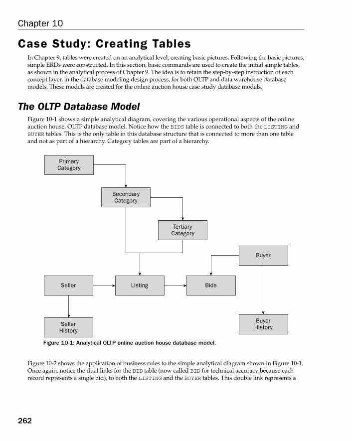
262
Chapter 10
Case Study: Creating TablesIn Chapter 9, tables were created on an analytical level, creating basic pictures. Following the basic pictures,simple ERDs were constructed. In this section, basic commands are used to create the initial simple tables,as shown in the analytical process of Chapter 9. The idea is to retain the step-by-step instruction of eachconcept layer, in the database modeling design process, for both OLTP and data warehouse database models. These models are created for the online auction house case study database models.
The OLTP Database ModelFigure 10-1 shows a simple analytical diagram, covering the various operational aspects of the onlineauction house, OLTP database model. Notice how the BIDS table is connected to both the LISTING andBUYER tables. This is the only table in this database structure that is connected to more than one tableand not as part of a hierarchy. Category tables are part of a hierarchy.
Figure 10-1: Analytical OLTP online auction house database model.
Figure 10-2 shows the application of business rules to the simple analytical diagram shown in Figure 10-1.Once again, notice the dual links for the BID table (now called BID for technical accuracy because eachrecord represents a single bid), to both the LISTING and the BUYER tables. This double link represents a
PrimaryCategory
SecondaryCategory
TertiaryCategory
BuyerHistory
Listing
SellerHistory
Seller Bids
Buyer
16_574906 ch10.qxd 11/4/05 10:46 AM Page 262
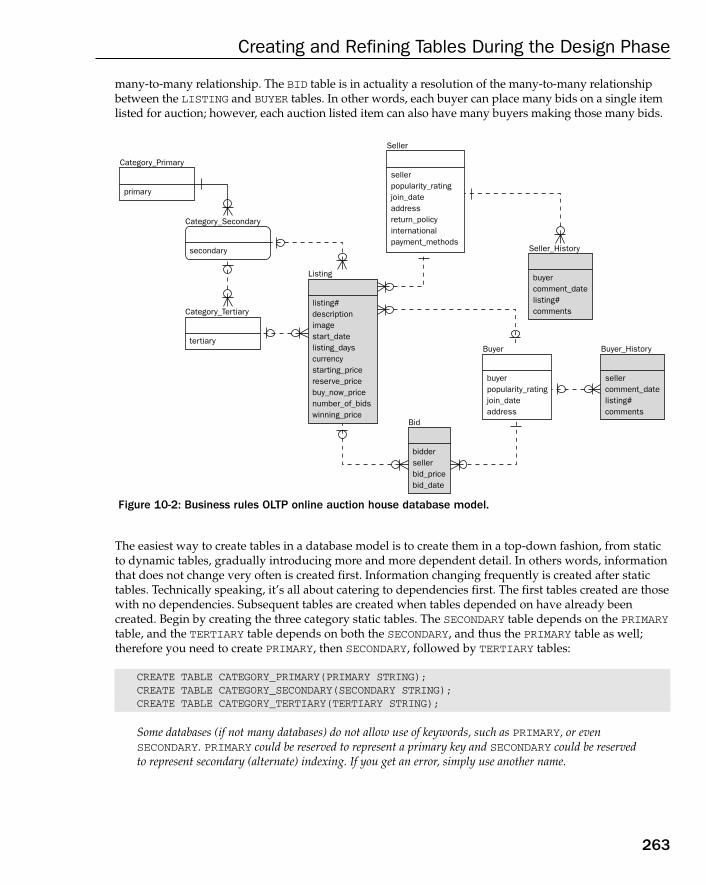
263
Creating and Refining Tables During the Design Phase
many-to-many relationship. The BID table is in actuality a resolution of the many-to-many relationshipbetween the LISTING and BUYER tables. In other words, each buyer can place many bids on a single itemlisted for auction; however, each auction listed item can also have many buyers making those many bids.
Figure 10-2: Business rules OLTP online auction house database model.
The easiest way to create tables in a database model is to create them in a top-down fashion, from staticto dynamic tables, gradually introducing more and more dependent detail. In others words, informationthat does not change very often is created first. Information changing frequently is created after statictables. Technically speaking, it’s all about catering to dependencies first. The first tables created are thosewith no dependencies. Subsequent tables are created when tables depended on have already been created. Begin by creating the three category static tables. The SECONDARY table depends on the PRIMARYtable, and the TERTIARY table depends on both the SECONDARY, and thus the PRIMARY table as well;therefore you need to create PRIMARY, then SECONDARY, followed by TERTIARY tables:
CREATE TABLE CATEGORY_PRIMARY(PRIMARY STRING);CREATE TABLE CATEGORY_SECONDARY(SECONDARY STRING);CREATE TABLE CATEGORY_TERTIARY(TERTIARY STRING);
Some databases (if not many databases) do not allow use of keywords, such as PRIMARY, or even SECONDARY. PRIMARY could be reserved to represent a primary key and SECONDARY could be reservedto represent secondary (alternate) indexing. If you get an error, simply use another name.
Listing
listing#descriptionimagestart_datelisting_dayscurrencystarting_pricereserve_pricebuy_now_pricenumber_of_bidswinning_price
Seller
sellerpopularity_ratingjoin_dateaddressreturn_policyinternationalpayment_methods
Seller_History
buyercomment_datelisting#comments
Buyer_History
sellercomment_datelisting#comments
Buyer
buyerpopularity_ratingjoin_dateaddress
Bid
biddersellerbid_pricebid_date
Category_Primary
primary
Category_Tertiary
tertiary
Category_Secondary
secondary
16_574906 ch10.qxd 11/4/05 10:46 AM Page 263

264
Chapter 10
The SELLER and BUYER tables are also static. According to the ERD shown in Figure 10-2 they are notdependencies. So you can create the SELLER and BUYER tables next:
CREATE TABLE SELLER(
SELLER STRING,POPULARITY_RATING INTEGER,JOIN_DATE DATE,ADDRESS STRING,RETURN_POLICY STRING,INTERNATIONAL STRING,PAYMENT_METHODS STRING
);
CREATE TABLE BUYER(
BUYER STRING,POPULARITY_RATING INTEGER,JOIN_DATE DATE,ADDRESS STRING
);
In these table creation script sections, I have begun to use de-formalized datatypes, such as STRING(representing text strings of any length), plus DATE for dates, and INTEGER for whole numbers.
Next, you can create the two history tables because the SELLER and BUYER tables are now available.Note how the SELLER_HISTORY table does not have a SELLER field, because this is implied by the directparent relationship to the SELLER table. The same applies to the BUYER_HISTORY table, containing theSELLER field only.
CREATE TABLE SELLER_HISTORY(
BUYER STRING,COMMENT_DATE DATE,LISTING# STRING,COMMENTS STRING
);
CREATE TABLE BUYER_HISTORY(
SELLER STRING,COMMENT_DATE DATE,LISTING# STRING,COMMENTS STRING
);
Next, create the LISTING table:
16_574906 ch10.qxd 11/4/05 10:46 AM Page 264
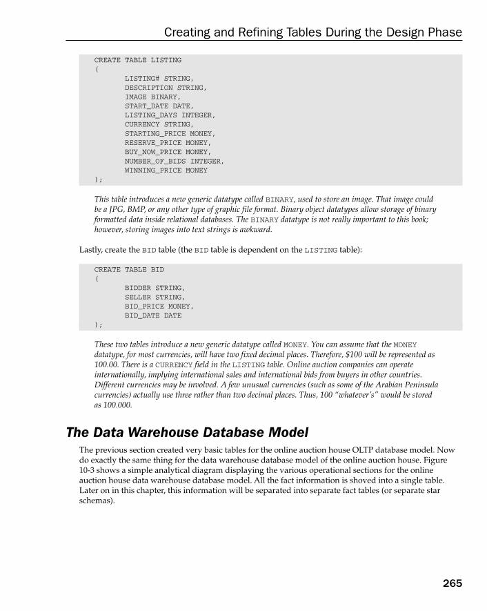
265
Creating and Refining Tables During the Design Phase
CREATE TABLE LISTING(
LISTING# STRING,DESCRIPTION STRING,IMAGE BINARY,START_DATE DATE,LISTING_DAYS INTEGER,CURRENCY STRING,STARTING_PRICE MONEY,RESERVE_PRICE MONEY,BUY_NOW_PRICE MONEY,NUMBER_OF_BIDS INTEGER,WINNING_PRICE MONEY
);
This table introduces a new generic datatype called BINARY, used to store an image. That image couldbe a JPG, BMP, or any other type of graphic file format. Binary object datatypes allow storage of binaryformatted data inside relational databases. The BINARY datatype is not really important to this book;however, storing images into text strings is awkward.
Lastly, create the BID table (the BID table is dependent on the LISTING table):
CREATE TABLE BID(
BIDDER STRING,SELLER STRING,BID_PRICE MONEY,BID_DATE DATE
);
These two tables introduce a new generic datatype called MONEY. You can assume that the MONEYdatatype, for most currencies, will have two fixed decimal places. Therefore, $100 will be represented as100.00. There is a CURRENCY field in the LISTING table. Online auction companies can operate internationally, implying international sales and international bids from buyers in other countries.Different currencies may be involved. A few unusual currencies (such as some of the Arabian Peninsulacurrencies) actually use three rather than two decimal places. Thus, 100 “whatever’s” would be storedas 100.000.
The Data Warehouse Database ModelThe previous section created very basic tables for the online auction house OLTP database model. Nowdo exactly the same thing for the data warehouse database model of the online auction house. Figure10-3 shows a simple analytical diagram displaying the various operational sections for the online auction house data warehouse database model. All the fact information is shoved into a single table.Later on in this chapter, this information will be separated into separate fact tables (or separate starschemas).
16_574906 ch10.qxd 11/4/05 10:46 AM Page 265

Figure 10-3: Analytical data warehouse online auction house database model.
Multiple star schemas within a single data warehouse are sometimes known as individual data marts.
Figure 10-4 shows the application of business rules to the simple analytical diagram shown in Figure10-3 for the data warehouse database model. Once again, you must take table dependencies intoaccount.
It is significant to observe how the three category tables, shown in Figure 10-2 (the OLTP databasemodel), have been merged into a single hierarchical category table (CATEGORY_HIERARCHY) in the data warehouse model shown in Figure 10-4. This is a form of denormalization, used especially in data warehouse databases to simplify and compress dimensional information use.
CategoryHierarchy
Time
Seller
Location
Buyer
Listing-Bids
-History
Listing-Bids
-History
266
Chapter 10
16_574906 ch10.qxd 11/4/05 10:46 AM Page 266
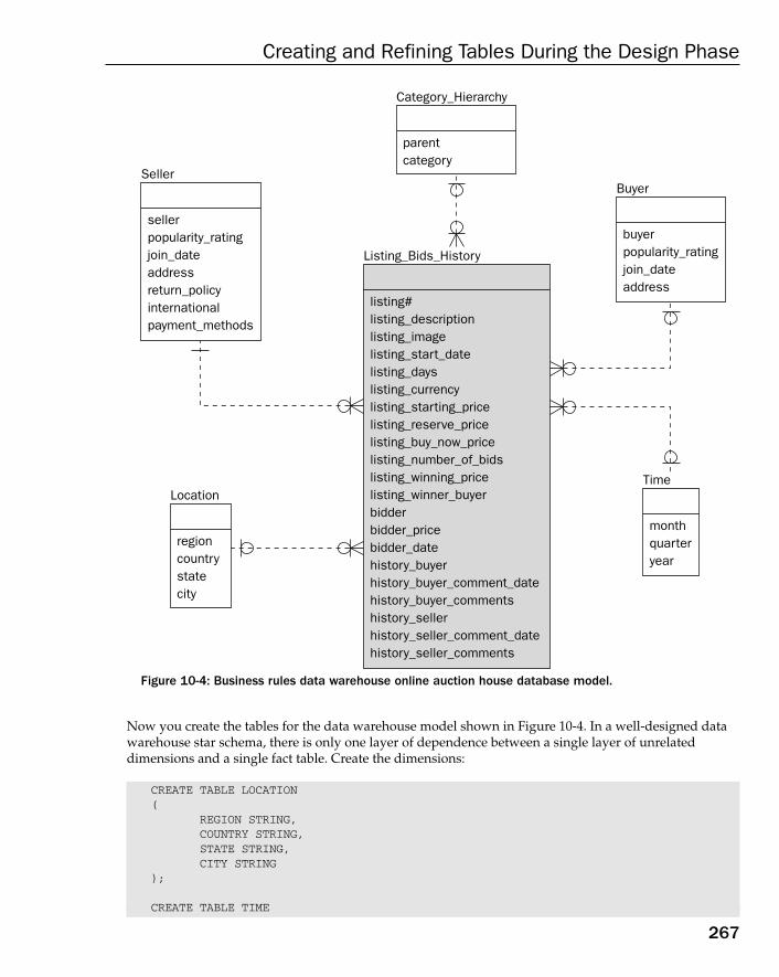
267
Creating and Refining Tables During the Design Phase
Figure 10-4: Business rules data warehouse online auction house database model.
Now you create the tables for the data warehouse model shown in Figure 10-4. In a well-designed datawarehouse star schema, there is only one layer of dependence between a single layer of unrelateddimensions and a single fact table. Create the dimensions:
CREATE TABLE LOCATION(
REGION STRING,COUNTRY STRING,STATE STRING,CITY STRING
);
CREATE TABLE TIME
Seller
sellerpopularity_ratingjoin_dateaddressreturn_policyinternationalpayment_methods
Category_Hierarchy
parentcategory
Buyer
buyerpopularity_ratingjoin_dateaddress
Location
regioncountrystatecity
Time
monthquarteryear
Listing_Bids_History
listing#listing_descriptionlisting_imagelisting_start_datelisting_dayslisting_currencylisting_starting_pricelisting_reserve_pricelisting_buy_now_pricelisting_number_of_bidslisting_winning_pricelisting_winner_buyerbidderbidder_pricebidder_datehistory_buyerhistory_buyer_comment_datehistory_buyer_commentshistory_sellerhistory_seller_comment_datehistory_seller_comments
16_574906 ch10.qxd 11/4/05 10:46 AM Page 267
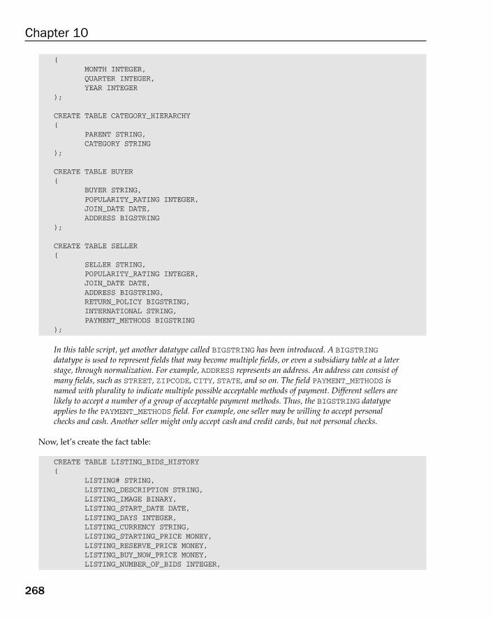
268
Chapter 10
(MONTH INTEGER,QUARTER INTEGER,YEAR INTEGER
);
CREATE TABLE CATEGORY_HIERARCHY(
PARENT STRING,CATEGORY STRING
);
CREATE TABLE BUYER(
BUYER STRING,POPULARITY_RATING INTEGER,JOIN_DATE DATE,ADDRESS BIGSTRING
);
CREATE TABLE SELLER(
SELLER STRING,POPULARITY_RATING INTEGER,JOIN_DATE DATE,ADDRESS BIGSTRING,RETURN_POLICY BIGSTRING,INTERNATIONAL STRING,PAYMENT_METHODS BIGSTRING
);
In this table script, yet another datatype called BIGSTRING has been introduced. A BIGSTRINGdatatype is used to represent fields that may become multiple fields, or even a subsidiary table at a laterstage, through normalization. For example, ADDRESS represents an address. An address can consist ofmany fields, such as STREET, ZIPCODE, CITY, STATE, and so on. The field PAYMENT_METHODS isnamed with plurality to indicate multiple possible acceptable methods of payment. Different sellers arelikely to accept a number of a group of acceptable payment methods. Thus, the BIGSTRING datatypeapplies to the PAYMENT_METHODS field. For example, one seller may be willing to accept personalchecks and cash. Another seller might only accept cash and credit cards, but not personal checks.
Now, let’s create the fact table:
CREATE TABLE LISTING_BIDS_HISTORY(
LISTING# STRING,LISTING_DESCRIPTION STRING,LISTING_IMAGE BINARY,LISTING_START_DATE DATE,LISTING_DAYS INTEGER,LISTING_CURRENCY STRING,LISTING_STARTING_PRICE MONEY,LISTING_RESERVE_PRICE MONEY,LISTING_BUY_NOW_PRICE MONEY,LISTING_NUMBER_OF_BIDS INTEGER,
16_574906 ch10.qxd 11/4/05 10:46 AM Page 268

269
Creating and Refining Tables During the Design Phase
LISTING_WINNING_PRICE MONEY,LISTING_WINNER_BUYER STRING,BIDDER MONEY,BIDDER_PRICE MONEY,BIDDER_DATE DATE,HISTORY_BUYER STRING,HISTORY_BUYER_COMMENT_DATE DATE,HISTORY_BUYER_COMMENTS BIGSTRING,HISTORY_SELLER STRING,HISTORY_SELLER_COMMENT_DATE DATE,HISTORY_SELLER_COMMENTS BIGSTRING
);
This fact table shows the source of all fields as being listing, bidder, buyer history, and seller history.Tables have been created for the OLTP and data warehouse database models for the online auctionhouse. The next step is to establish and enforce referential integrity.
Case Study: Enforcing Table RelationshipsReferential integrity maintains and enforces the data integrity of relationships between tables. In otherwords, referential integrity ensures that where a child table record exists, the parent table record exists as well.
Referential IntegrityIn Figure 10-2, you cannot delete a SELLER record without deleting all the seller’s listings first. If theseller is deleted, their listings become orphaned records. An orphaned record is term applied to a recordnot findable within the logical table structure of a database model. Essentially, the seller’s name andaddress details are stored in the SELLER table and not in the LISTING table. If the seller record wasdeleted, any of their listings are useless because you don’t know who is selling it. Similarly, if buyerinformation with winning bids were deleted, the seller wouldn’t know who to mail it to. Referentialintegrity, through the use of primary and foreign keys, acts to ensure that the following activities areprohibited:
❑ INSERT check — A child record cannot be added to a child table unless the parent record exists inthe parent table.
❑ UPDATE check — Parent and child table records cannot have their linking key field valueschanged, unless both are changed simultaneously (“simultaneously” implies within the sametransaction).
❑ DELETE check — A parent table record cannot be deleted when a child table record exists, unlessall related child table records are deleted first.
❑ DELETE CASCADE check — A parent table record can be deleted if all child records are deletedfirst. This is known as a cascading delete. Cascade deletion is rarely implemented because it can result in serious data loss (usually through operator or programmer error). Additionally,cascade deletions can cause serious locking conflicts because large numbers of child recordscould have to be deleted, when deleting a parent record. This type of locking problem can occurwhen a parent record has many records in child tables, through a multiple level table structure.
16_574906 ch10.qxd 11/4/05 10:46 AM Page 269
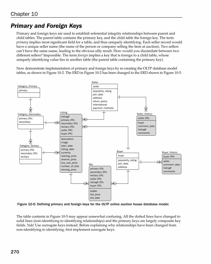
Primary and Foreign KeysPrimary and foreign keys are used to establish referential integrity relationships between parent andchild tables. The parent table contains the primary key, and the child table the foreign key. The term primary implies most significant field for a table, and thus uniquely identifying. Each seller record wouldhave a unique seller name (the name of the person or company selling the item at auction). Two sellerscan’t have the same name, leading to the obvious silly result. How would you dissimilate between twodifferent sellers? Impossible. The term foreign implies a key that is foreign to a child table, whoseuniquely identifying value lies in another table (the parent table containing the primary key).
Now demonstrate implementation of primary and foreign keys by re-creating the OLTP database modeltables, as shown in Figure 10-2. The ERD in Figure 10-2 has been changed to the ERD shown in Figure 10-5.
Figure 10-5: Defining primary and foreign keys for the OLTP online auction house database model.
The table contents in Figure 10-5 may appear somewhat confusing. All the dotted lines have changed tosolid lines (non-identifying to identifying relationships) and the primary keys are largely composite keyfields. Yuk! Use surrogate keys instead. Before explaining why relationships have been changed fromnon-identifying to identifying, first implement surrogate keys.
Seller_History
Seller
seller
popularity_ratingjoin_dateaddressreturn_policyinternationalpayment_methods
seller (FK)
buyercomment_datelisting#comments
Buyer_History
buyer (FK)
sellercomment_datelisting#comments
Buyer
buyer
popularity_ratingjoin_dateaddress
Category_Primary
primary
Category_Secondary
primary (FK)secondary
Category_Tertiary
primary (FK)secondary (FK)tertiary
Listing
listing#primary (FK)secondary (FK)tertiary (FK)seller (FK)buyer (FK)
descriptionimagestart_datelisting_datecurrencystarting_pricereserve_pricebuy_now_pricenumber_of_bidswinning_price
Bid
primary (FK)secondary (FK)tertiary (FK)seller (FK)listing# (FK)buyer (FK)
bidderbid_pricebid_date
270
Chapter 10
16_574906 ch10.qxd 11/4/05 10:46 AM Page 270

Using Surrogate KeysFigure 10-6 shows the same model as shown in Figure 10-5, except with surrogate keys added. The onlytable without a surrogate primary key field is the LISTING table, still using the LISTING# field as its pri-mary key. LISTING# is likely to be some type of auto counter anyway, and so a surrogate key is not nec-essary in this case. Figure 10-6 still has composite primary key fields.
Figure 10-6: Using surrogate keys as primary keys with identifying relationships.
One important point about Figure 10-6 is that the three category tables, plus the buyer and seller table,have additional identifier fields as primary keys (for example, BUYER.BUYER_ID). However, these tablesstill have their original primary key fields, now no longer as the primary key (for example, BUYER.BUYER).The identifiers have become surrogates (replacements) for the original string datatype names.
Identifying relationships in Figure 10-6 imply that a child table record is specifically identified by a parenttable record, through the connection between parent table primary key, and child table foreign key.
Seller_History
Seller
seller_id
sellerpopularity_ratingjoin_dateaddressreturn_policyinternationalpayment_methods
seller_id (FK)
buyercomment_datelisting#comments
Buyer_History
buyer_id (FK)
sellercomment_datelisting#comments
Buyer
buyer_id
buyerpopularity_ratingjoin_dateaddress
Category_Primary
primary_id
primary
secondary
Category_Secondary
primary_id (FK)secondary_id
Category_Tertiary
primary_id (FK)secondary_id (FK)tertiary_id
tertiary
Listing
primary_id (FK)secondary_id (FK)tertiary_id (FK)seller_id (FK)buyer_id (FK)listing#
descriptionimagestart_datelisting_datecurrencystarting_pricereserve_pricebuy_now_pricenumber_of_bidswinning_price
Bid
primary_id (FK)secondary_id (FK)tertiary_id (FK)seller_id (FK)buyer_id (FK)listing# (FK)
bidderbid_pricebid_date
271
Creating and Refining Tables During the Design Phase
16_574906 ch10.qxd 11/4/05 10:46 AM Page 271
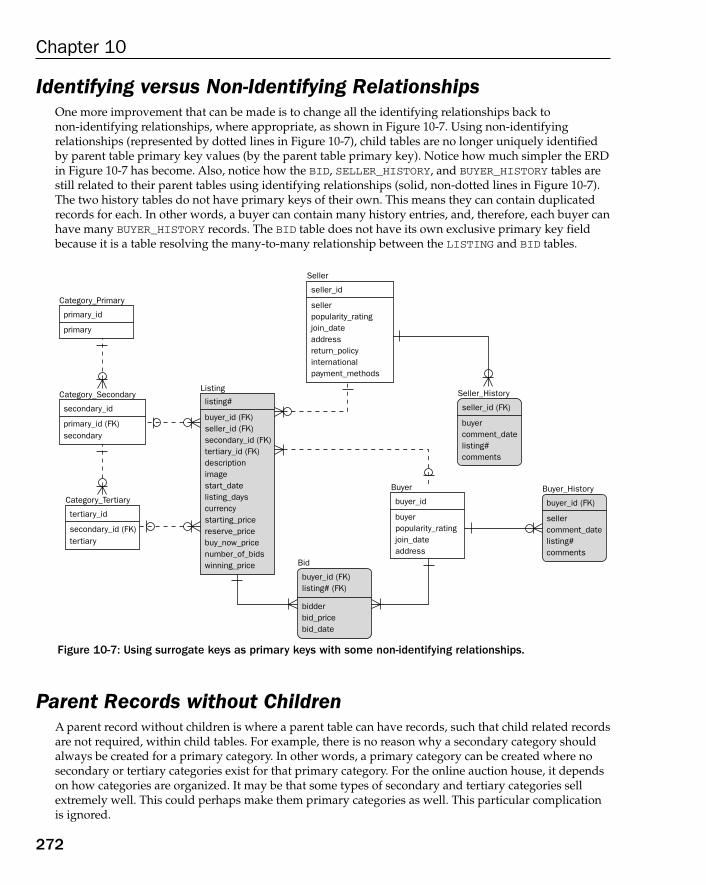
272
Chapter 10
Identifying versus Non-Identifying RelationshipsOne more improvement that can be made is to change all the identifying relationships back to non-identifying relationships, where appropriate, as shown in Figure 10-7. Using non-identifying relationships (represented by dotted lines in Figure 10-7), child tables are no longer uniquely identifiedby parent table primary key values (by the parent table primary key). Notice how much simpler the ERDin Figure 10-7 has become. Also, notice how the BID, SELLER_HISTORY, and BUYER_HISTORY tables arestill related to their parent tables using identifying relationships (solid, non-dotted lines in Figure 10-7).The two history tables do not have primary keys of their own. This means they can contain duplicatedrecords for each. In other words, a buyer can contain many history entries, and, therefore, each buyer canhave many BUYER_HISTORY records. The BID table does not have its own exclusive primary key fieldbecause it is a table resolving the many-to-many relationship between the LISTING and BID tables.
Figure 10-7: Using surrogate keys as primary keys with some non-identifying relationships.
Parent Records without ChildrenA parent record without children is where a parent table can have records, such that child related recordsare not required, within child tables. For example, there is no reason why a secondary category shouldalways be created for a primary category. In other words, a primary category can be created where nosecondary or tertiary categories exist for that primary category. For the online auction house, it dependson how categories are organized. It may be that some types of secondary and tertiary categories sellextremely well. This could perhaps make them primary categories as well. This particular complicationis ignored.
Seller_History
Seller
seller_id
sellerpopularity_ratingjoin_dateaddressreturn_policyinternationalpayment_methods
seller_id (FK)
buyercomment_datelisting#comments
Buyer_History
buyer_id (FK)
sellercomment_datelisting#comments
Buyer
buyer_id
buyerpopularity_ratingjoin_dateaddress
Category_Primary
primary_id
primary
secondary
Category_Secondary
secondary_id
primary_id (FK)
tertiary
Category_Tertiary
tertiary_id
secondary_id (FK)
Listing
buyer_id (FK)seller_id (FK)secondary_id (FK)tertiary_id (FK)descriptionimagestart_datelisting_dayscurrencystarting_pricereserve_pricebuy_now_pricenumber_of_bidswinning_price Bid
buyer_id (FK)listing# (FK)
bidderbid_pricebid_date
listing#
16_574906 ch10.qxd 11/4/05 10:46 AM Page 272
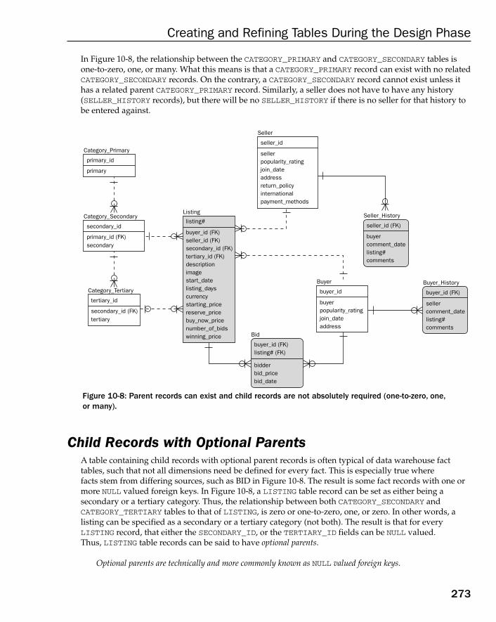
273
Creating and Refining Tables During the Design Phase
In Figure 10-8, the relationship between the CATEGORY_PRIMARY and CATEGORY_SECONDARY tables isone-to-zero, one, or many. What this means is that a CATEGORY_PRIMARY record can exist with no relatedCATEGORY_SECONDARY records. On the contrary, a CATEGORY_SECONDARY record cannot exist unless ithas a related parent CATEGORY_PRIMARY record. Similarly, a seller does not have to have any history(SELLER_HISTORY records), but there will be no SELLER_HISTORY if there is no seller for that history tobe entered against.
Figure 10-8: Parent records can exist and child records are not absolutely required (one-to-zero, one,or many).
Child Records with Optional ParentsA table containing child records with optional parent records is often typical of data warehouse facttables, such that not all dimensions need be defined for every fact. This is especially true where facts stem from differing sources, such as BID in Figure 10-8. The result is some fact records with one ormore NULL valued foreign keys. In Figure 10-8, a LISTING table record can be set as either being a secondary or a tertiary category. Thus, the relationship between both CATEGORY_SECONDARY and CATEGORY_TERTIARY tables to that of LISTING, is zero or one-to-zero, one, or zero. In other words, alisting can be specified as a secondary or a tertiary category (not both). The result is that for every LISTING record, that either the SECONDARY_ID, or the TERTIARY_ID fields can be NULL valued. Thus, LISTING table records can be said to have optional parents.
Optional parents are technically and more commonly known as NULL valued foreign keys.
Seller_History
Seller
seller_id
sellerpopularity_ratingjoin_dateaddressreturn_policyinternationalpayment_methods
seller_id (FK)
buyercomment_datelisting#comments
Buyer_History
buyer_id (FK)
sellercomment_datelisting#comments
Buyer
buyer_id
buyerpopularity_ratingjoin_dateaddress
Category_Primary
primary_id
primary
secondary
Category_Secondary
secondary_id
primary_id (FK)
tertiary
Category_Tertiary
tertiary_id
secondary_id (FK)
Listing
buyer_id (FK)seller_id (FK)secondary_id (FK)tertiary_id (FK)descriptionimagestart_datelisting_dayscurrencystarting_pricereserve_pricebuy_now_pricenumber_of_bidswinning_price Bid
buyer_id (FK)listing# (FK)
bidderbid_pricebid_date
listing#
16_574906 ch10.qxd 11/4/05 10:46 AM Page 273
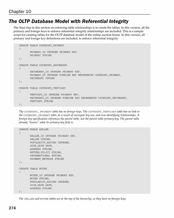
274
Chapter 10
The OLTP Database Model with Referential IntegrityThe final step in this section on enforcing table relationships is to create the tables. In this version, all theprimary and foreign keys to enforce referential integrity relationships are included. This is a samplescript for creating tables for the OLTP database model of the online auction house. In this version, all primary and foreign key definitions are included, to enforce referential integrity:
CREATE TABLE CATEGORY_PRIMARY(
PRIMARY_ID INTEGER PRIMARY KEY,PRIMARY STRING
);
CREATE TABLE CATEGORY_SECONDARY(
SECONDARY_ID INTEGER PRIMARY KEY,PRIMARY_ID INTEGER FOREIGN KEY REFERENCES CATEGORY_PRIMARY,SECONDARY STRING
);
CREATE TABLE CATEGORY_TERTIARY(
TERTIARY_ID INTEGER PRIMARY KEY,SECONDARY_ID INTEGER FOREIGN KEY REFERENCES CATEGORY_SECONDARY,TERTIARY STRING
);
The CATEGORY_ PRIMARY table has no foreign keys. The CATEGORY_TERTIARY table has no link tothe CATEGORY_PRIMARY table, as a result of surrogate key use, and non-identifying relationships. Aforeign key specification references the parent table, not the parent table primary key. The parent tablealready “knows” what its primary key field is.
CREATE TABLE SELLER(
SELLER_ID INTEGER PRIMARY KEY,SELLER STRING,POPULARITY_RATING INTEGER,JOIN_DATE DATE,ADDRESS STRING,RETURN_POLICY STRING,INTERNATIONAL STRING,PAYMENT_METHODS STRING
);
CREATE TABLE BUYER(
BUYER_ID INTEGER PRIMARY KEY,BUYER STRING,POPULARITY_RATING INTEGER,JOIN_DATE DATE,ADDRESS STRING
);
The SELLER and BUYER tables are at the top of the hierarchy, so they have no foreign keys.
16_574906 ch10.qxd 11/4/05 10:46 AM Page 274
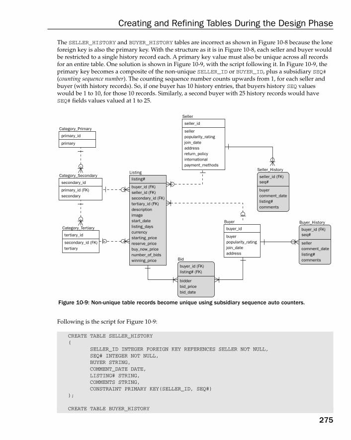
275
Creating and Refining Tables During the Design Phase
The SELLER_HISTORY and BUYER_HISTORY tables are incorrect as shown in Figure 10-8 because the loneforeign key is also the primary key. With the structure as it is in Figure 10-8, each seller and buyer wouldbe restricted to a single history record each. A primary key value must also be unique across all recordsfor an entire table. One solution is shown in Figure 10-9, with the script following it. In Figure 10-9, theprimary key becomes a composite of the non-unique SELLER_ID or BUYER_ID, plus a subsidiary SEQ#(counting sequence number). The counting sequence number counts upwards from 1, for each seller andbuyer (with history records). So, if one buyer has 10 history entries, that buyers history SEQ valueswould be 1 to 10, for those 10 records. Similarly, a second buyer with 25 history records would haveSEQ# fields values valued at 1 to 25.
Figure 10-9: Non-unique table records become unique using subsidiary sequence auto counters.
Following is the script for Figure 10-9:
CREATE TABLE SELLER_HISTORY(
SELLER_ID INTEGER FOREIGN KEY REFERENCES SELLER NOT NULL,SEQ# INTEGER NOT NULL,BUYER STRING,COMMENT_DATE DATE,LISTING# STRING,COMMENTS STRING,CONSTRAINT PRIMARY KEY(SELLER_ID, SEQ#)
);
CREATE TABLE BUYER_HISTORY
Seller_History
Seller
seller_id
sellerpopularity_ratingjoin_dateaddressreturn_policyinternationalpayment_methods
seller_id (FK)seq#
buyercomment_datelisting#comments
Buyer_History
buyer_id (FK)seq#
sellercomment_datelisting#comments
Buyer
buyer_id
buyerpopularity_ratingjoin_dateaddress
Category_Primary
primary_id
primary
secondary
Category_Secondary
secondary_id
primary_id (FK)
tertiary
Category_Tertiary
tertiary_id
secondary_id (FK)
Listing
buyer_id (FK)seller_id (FK)secondary_id (FK)tertiary_id (FK)descriptionimagestart_datelisting_dayscurrencystarting_pricereserve_pricebuy_now_pricenumber_of_bidswinning_price Bid
buyer_id (FK)listing# (FK)
bidderbid_pricebid_date
listing#
16_574906 ch10.qxd 11/4/05 10:46 AM Page 275
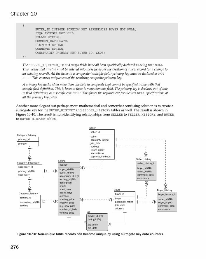
276
Chapter 10
(BUYER_ID INTEGER FOREIGN KEY REFERENCES BUYER NOT NULL,SEQ# INTEGER NOT NULLSELLER STRING,COMMENT_DATE DATE,LISTING# STRING,COMMENTS STRING,CONSTRAINT PRIMARY KEY(BUYER_ID, SEQ#)
);
The SELLER_ID, BUYER_ID and SEQ# fields have all been specifically declared as being NOT NULL.This means that a value must be entered into these fields for the creation of a new record (or a change toan existing record). All the fields in a composite (multiple field) primary key must be declared as NOTNULL. This ensures uniqueness of the resulting composite primary key.
A primary key declared on more than one field (a composite key) cannot be specified inline with that specific field definition. This is because there is more than one field. The primary key is declared out-of-lineto field definitions, as a specific constraint. This forces the requirement for the NOT NULL specifications ofall the primary key fields.
Another more elegant but perhaps more mathematical and somewhat confusing solution is to create asurrogate key for the BUYER_HISTORY and SELLER_HISTORY tables as well. The result is shown inFigure 10-10. The result is non-identifying relationships from SELLER to SELLER_HISTORY, and BUYERto BUYER_HISTORY tables.
Figure 10-10: Non-unique table records can become unique by using surrogate key auto counters.
Seller_History
Seller
seller_id
sellerpopularity_ratingjoin_dateaddressreturn_policyinternationalpayment_methods
seller_history_id
buyer_id (FK)seller_id (FK)comment_datecomments
Buyer_History
buyer_history_id
seller_id (FK)buyer_id (FK)comment_datecomments
Buyer
buyer_id
buyerpopularity_ratingjoin_dateaddress
Category_Primary
primary_id
primary
secondary
Category_Secondary
secondary_id
primary_id (FK)
tertiary
Category_Tertiary
tertiary_id
secondary_id (FK)
Listing
buyer_id (FK)seller_id (FK)secondary_id (FK)tertiary_id (FK)descriptionimagestart_datelisting_dayscurrencystarting_pricereserve_pricebuy_now_pricenumber_of_bidswinning_price Bid
bidder_id (FK)listing# (FK)
bid_pricebid_date
listing#
16_574906 ch10.qxd 11/4/05 10:46 AM Page 276
As a reminder, a non-identifying relationship is when the parent table primary key is not part of the pri-mary key in the child table. A child table record is not specifically or uniquely identified by a child tablerecord.
Further changes in Figure 10-10 are as follows:
❑ The addition of the relationships between SELLER to BUYER_HISTORY tables, and BUYER toSELLER_HISTORY tables. Every history record of seller activity is related to something pur-chased from that seller (by a buyer). The same applies to buyers.
❑ A buyer can be a seller as well, and visa versa. This database model is beginning to look a littlemessy.
Following is the script for changes introduced in Figure 10-10:
CREATE TABLE SELLER_HISTORY(
SELLER_HISTORY_ID INTEGER PRIMARY KEY,SELLER_ID INTEGER FOREIGN KEY REFERENCES SELLER,BUYER_ID INTEGER FOREIGN KEY REFERENCES BUYER,COMMENT_DATE DATE,COMMENTS STRING
);
CREATE TABLE BUYER_HISTORY(
BUYER_HISTORY_ID INTEGER PRIMARY KEY,BUYER_ID INTEGER FOREIGN KEY REFERENCES BUYER,SELLER_ID INTEGER FOREIGN KEY REFERENCES SELLER,COMMENT_DATE DATE,COMMENTS STRING
);
Figure 10-11 shows further refinement for the BID table. Essentially, this section has included some specific analysis-design reworking. Some things can’t be assessed accurately by simple analysis. Don’tmistake the fiddling with relationships, and specific fields, for primary and foreign keys as normalizationor denormalization. Note, however, that some extensive normalization has occurred merely by the establishment of one-to-many relationships. This normalization activity has actually been performed froman analytical perspective.
277
Creating and Refining Tables During the Design Phase
16_574906 ch10.qxd 11/4/05 10:46 AM Page 277

278
Chapter 10
Figure 10-11: Refining the BID table and related tables.
Figure 10-11 has essentially redefined the BID table and made a few other small necessary changes. Thesechanges all make analytical sense and don’t need normalization. Potential buyers place bids on auctionlistings, but do not necessarily win the auction; however, the history of all bids for a listing needs to beretained. The BID table, therefore, contains all bids for a listing, including all losing bids and the final winning bid. The final winning bid is recorded as the winning bid, by setting the BUYER_ID field in theLISTING table. As a result, a losing buyer is not stored in the LISTING table as a buyer because he or sheis only a bidder (a buyer is only a bidder who wins the listing). The results are as follows:
❑ LISTING to BID is one-to-zero, one, or many — A listing that has just been listed is likely to haveno bids. Also, an unpopular listing may have no bids placed over the life of the auction listing.It is still a listing, but it has no bids.
❑ BUYER to LISTING is zero or one to zero, one, or many — A losing buyer is only a bidder and not thewinning bidder. Losing bidders are not entered into the LISTING table as buyers because theylost the auction.
You don’t actually have to apply the rules of normalization, using Normal Forms, tocreate a first pass of a database model. So far, it’s all been common sense. This is oneof the reasons why these final chapters are presented as a case study example. Thiscase study is not an application of theory, by applying normalization and NormalForms, to a bucket of information. A bucket of information implies a whole pile ofthings thrown into a heap, on the floor in front of you.
Seller_History
Seller
seller_id
sellerpopularity_ratingjoin_dateaddressreturn_policyinternationalpayment_methods
seller_history_id
buyer_id (FK)seller_id (FK)comment_datecomments
Buyer_History
buyer_history_id
seller_id (FK)buyer_id (FK)comment_datecomments
Buyer
buyer_id
buyerpopularity_ratingjoin_dateaddress
Category_Primary
primary_id
primary
secondary
Category_Secondary
secondary_id
primary_id (FK)
tertiary
Category_Tertiary
tertiary_id
secondary_id (FK)
Listing
buyer_id (FK)seller_id (FK)secondary_id (FK)tertiary_id (FK)descriptionimagestart_datelisting_dayscurrencystarting_pricereserve_pricebuy_now_pricenumber_of_bidswinning_price Bid
bidder_id (FK)listing# (FK)
bid_pricebid_date
listing#
16_574906 ch10.qxd 11/4/05 10:46 AM Page 278
❑ BUYER to BID is one-to-one or many (zero is not allowed) — A bid cannot exist without a potentialbuyer. This item is not a change, but listed as a reinforcing explanation of said relationshipsbetween BID, BUYER, and LISTING tables.
The result is the following script for creating the LISTING and BID tables:
CREATE TABLE LISTING(
LISTING# STRING PRIMARY KEY,BUYER_ID INTEGER FOREIGN KEY REFERENCES BUYER WITH NULL,SELLER_ID INTEGER FOREIGN KEY REFERENCES SELLER,SECONDARY_ID INTEGER FOREIGN KEY REFERENCES CATEGORY_SECONDARY WITH NULL,TERTIARY_ID INTEGER FOREIGN KEY REFERENCES CATEGORY_TERTIARY WITH NULL,DESCRIPTION STRING,IMAGE BINARY,START_DATE DATE,LISTING_DAYS INTEGER,CURRENCY STRING,STARTING_PRICE MONEY,RESERVE_PRICE MONEY,BUY_NOW_PRICE MONEY,NUMBER_OF_BIDS INTEGER,WINNING_PRICE MONEY
);
The BUYER_ID field is specified as a WITH NULL foreign key, indicating that LISTING records onlycontain the BUYER_ID for the winning bidder. If no one bids, then a LISTING record will never have aBUYER_ID value. The SECONDARY_ID and TERTIARY_ID category fields are also listed as WITHNULL foreign key fields because either is allowed (not both).
CREATE TABLE BID(
BIDDER_ID INTEGER FOREIGN KEY REFERENCES BIDDER,LISTING# INTEGER FOREIGN KEY REFERENCES LISTING,BID_PRICE MONEY,BID_DATE DATE,CONSTRAINT PRIMARY KEY(BIDDER_ID, LISTING#)
);
CREATE TABLE commands would have to be preceded by DROP TABLE commands for all tables, preferablyin reverse order to that of creation. Some databases will allow changes to primary and foreign keys usingALTER TABLE commands. Some databases even allow these changes directly into an ERD GUI tool.Microsoft Access allows these changes to be made very easily, using a GUI.
The Data Warehouse Database Model with Referential Integrity
The data warehouse database model for the online auction house is altered slightly in Figure 10-12, including addition of surrogate primary keys to all tables. All of the dimensional-fact table relationships arezero or one, to zero, one, or many. This indicates that the fact table contains a mixture of multiple factsources (multiple transaction types, including listings, bids, and histories). Essentially, a fact table does not
279
Creating and Refining Tables During the Design Phase
16_574906 ch10.qxd 11/4/05 10:46 AM Page 279
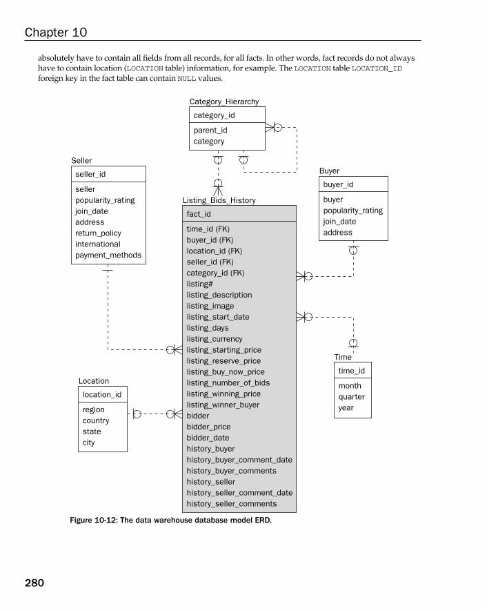
280
Chapter 10
absolutely have to contain all fields from all records, for all facts. In other words, fact records do not alwayshave to contain location (LOCATION table) information, for example. The LOCATION table LOCATION_IDforeign key in the fact table can contain NULL values.
Figure 10-12: The data warehouse database model ERD.
Seller
seller_id
sellerpopularity_ratingjoin_dateaddressreturn_policyinternationalpayment_methods
Location
location_id
regioncountrystatecity
Time
time_id
monthquarteryear
Category_Hierarchy
category_id
parent_idcategory
Listing_Bids_History
fact_id
time_id (FK)buyer_id (FK)location_id (FK)seller_id (FK)category_id (FK)listing#listing_descriptionlisting_imagelisting_start_datelisting_dayslisting_currencylisting_starting_pricelisting_reserve_pricelisting_buy_now_pricelisting_number_of_bidslisting_winning_pricelisting_winner_buyerbidderbidder_pricebidder_datehistory_buyerhistory_buyer_comment_datehistory_buyer_commentshistory_sellerhistory_seller_comment_datehistory_seller_comments
Buyer
buyer_id
buyerpopularity_ratingjoin_dateaddress
16_574906 ch10.qxd 11/4/05 10:46 AM Page 280
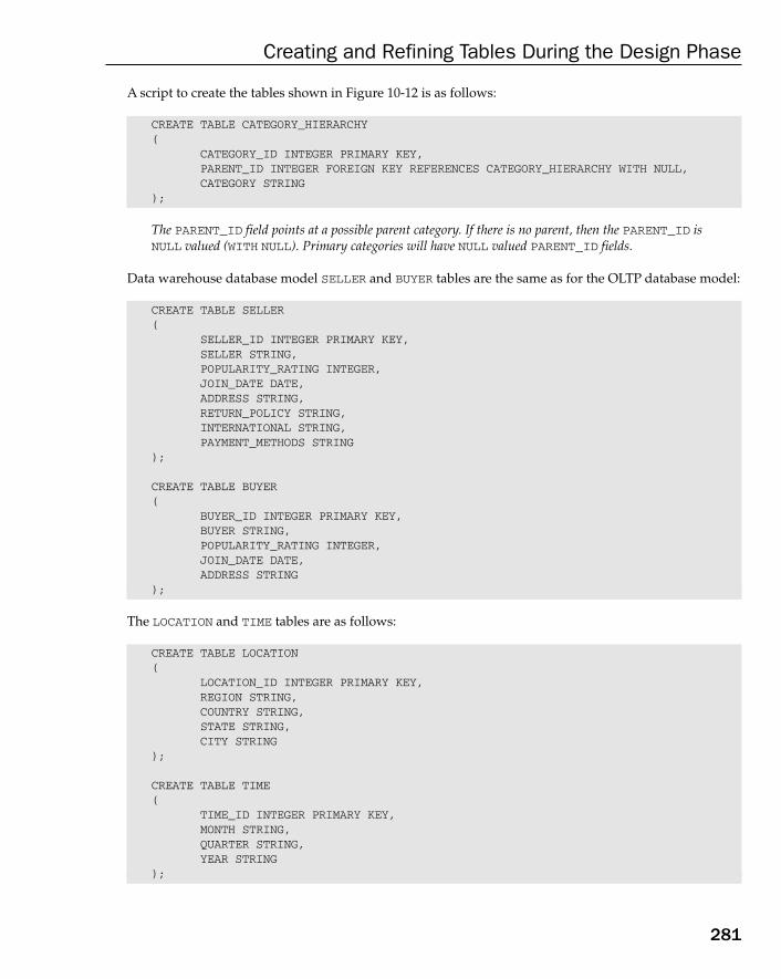
A script to create the tables shown in Figure 10-12 is as follows:
CREATE TABLE CATEGORY_HIERARCHY(
CATEGORY_ID INTEGER PRIMARY KEY,PARENT_ID INTEGER FOREIGN KEY REFERENCES CATEGORY_HIERARCHY WITH NULL,CATEGORY STRING
);
The PARENT_ID field points at a possible parent category. If there is no parent, then the PARENT_ID isNULL valued (WITH NULL). Primary categories will have NULL valued PARENT_ID fields.
Data warehouse database model SELLER and BUYER tables are the same as for the OLTP database model:
CREATE TABLE SELLER(
SELLER_ID INTEGER PRIMARY KEY,SELLER STRING,POPULARITY_RATING INTEGER,JOIN_DATE DATE,ADDRESS STRING,RETURN_POLICY STRING,INTERNATIONAL STRING,PAYMENT_METHODS STRING
);
CREATE TABLE BUYER(
BUYER_ID INTEGER PRIMARY KEY,BUYER STRING,POPULARITY_RATING INTEGER,JOIN_DATE DATE,ADDRESS STRING
);
The LOCATION and TIME tables are as follows:
CREATE TABLE LOCATION(
LOCATION_ID INTEGER PRIMARY KEY,REGION STRING,COUNTRY STRING,STATE STRING,CITY STRING
);
CREATE TABLE TIME(
TIME_ID INTEGER PRIMARY KEY,MONTH STRING,QUARTER STRING,YEAR STRING
);
281
Creating and Refining Tables During the Design Phase
16_574906 ch10.qxd 11/4/05 10:46 AM Page 281
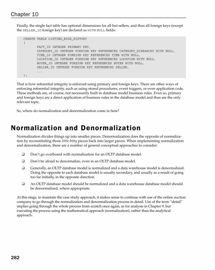
282
Chapter 10
Finally, the single fact table has optional dimensions for all but sellers, and thus all foreign keys (exceptthe SELLER_ID foreign key) are declared as WITH NULL fields:
CREATE TABLE LISTING_BIDS_HISTORY(
FACT_ID INTEGER PRIMARY KEY,CATEGORY_ID INTEGER FOREIGN KEY REFERENCES CATEGORY_HIERARCHY WITH NULL,TIME_ID INTEGER FOREIGN KEY REFERENCES TIME WITH NULL,LOCATION_ID INTEGER FOREIGN KEY REFERENCES LOCATION WITH NULL,BUYER_ID INTEGER FOREIGN KEY REFERENCES BUYER WITH NULL,SELLER_ID INTEGER FOREIGN KEY REFERENCES SELLER,...
);
That is how referential integrity is enforced using primary and foreign keys. There are other ways ofenforcing referential integrity, such as using stored procedures, event triggers, or even application code.These methods are, of course, not necessarily built in database model business rules. Even so, primaryand foreign keys are a direct application of business rules in the database model and thus are the onlyrelevant topic.
So, where do normalization and denormalization come in here?
Normalization and DenormalizationNormalization divides things up into smaller pieces. Denormalization does the opposite of normaliza-tion by reconstituting those little-bitty pieces back into larger pieces. When implementing normalizationand denormalization, there are a number of general conceptual approaches to consider:
❑ Don’t go overboard with normalization for an OLTP database model.
❑ Don’t be afraid to denormalize, even in an OLTP database model.
❑ Generally, an OLTP database model is normalized and a data warehouse model is denormalized.Doing the opposite to each database model is usually secondary, and usually as a result of goingtoo far initially, in the opposite direction.
❑ An OLTP database model should be normalized and a data warehouse database model shouldbe denormalized, where appropriate.
At this stage, to maintain the case study approach, it makes sense to continue with use of the online auctioncompany to go through the normalization and denormalization process in detail. Use of the term “detail”implies going through the whole process from scratch once again, as for analysis in Chapter 9, but executing the process using the mathematical approach (normalization), rather than the analyticalapproach.
16_574906 ch10.qxd 11/4/05 10:46 AM Page 282
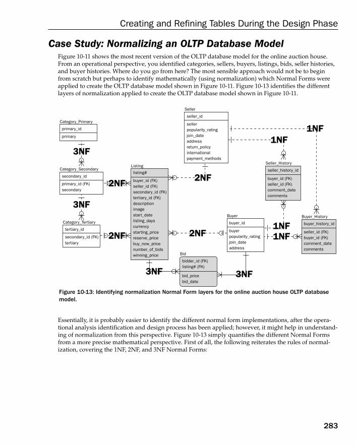
283
Creating and Refining Tables During the Design Phase
Case Study: Normalizing an OLTP Database ModelFigure 10-11 shows the most recent version of the OLTP database model for the online auction house.From an operational perspective, you identified categories, sellers, buyers, listings, bids, seller histories,and buyer histories. Where do you go from here? The most sensible approach would not be to beginfrom scratch but perhaps to identify mathematically (using normalization) which Normal Forms wereapplied to create the OLTP database model shown in Figure 10-11. Figure 10-13 identifies the differentlayers of normalization applied to create the OLTP database model shown in Figure 10-11.
Figure 10-13: Identifying normalization Normal Form layers for the online auction house OLTP databasemodel.
Essentially, it is probably easier to identify the different normal form implementations, after the opera-tional analysis identification and design process has been applied; however, it might help in understand-ing of normalization from this perspective. Figure 10-13 simply quantifies the different Normal Formsfrom a more precise mathematical perspective. First of all, the following reiterates the rules of normal-ization, covering the 1NF, 2NF, and 3NF Normal Forms:
Seller_History
Seller
seller_id
sellerpopularity_ratingjoin_dateaddressreturn_policyinternationalpayment_methods
seller_history_id
buyer_id (FK)seller_id (FK)comment_datecomments
Buyer_History
buyer_history_id
seller_id (FK)buyer_id (FK)comment_datecomments
Buyer
buyer_id
buyerpopularity_ratingjoin_dateaddress
Category_Primary
primary_id
primary
secondary
Category_Secondary
secondary_id
primary_id (FK)
tertiary
Category_Tertiary
tertiary_id
secondary_id (FK)
Listing
buyer_id (FK)seller_id (FK)secondary_id (FK)tertiary_id (FK)descriptionimagestart_datelisting_dayscurrencystarting_pricereserve_pricebuy_now_pricenumber_of_bidswinning_price Bid
bidder_id (FK)listing# (FK)
bid_pricebid_date
listing#
3NF3NF
3NF3NF
3NF3NF 3NF3NF
2NF2NF
2NF2NF 2NF2NF1NF1NF
1NF1NF1NF1NF
1NF1NF
2NF2NF
16_574906 ch10.qxd 11/4/05 10:46 AM Page 283
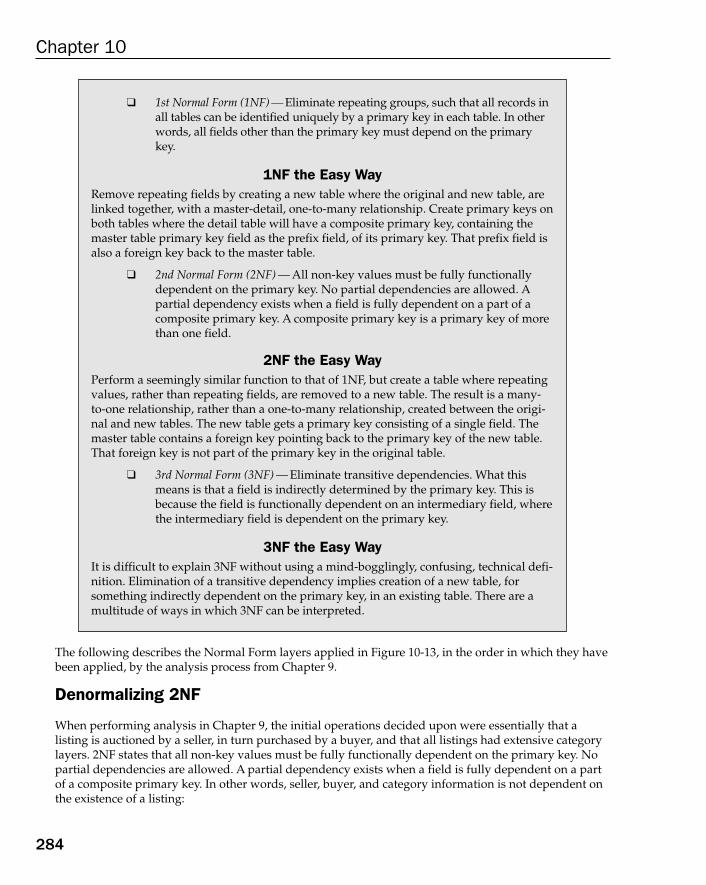
284
Chapter 10
The following describes the Normal Form layers applied in Figure 10-13, in the order in which they havebeen applied, by the analysis process from Chapter 9.
Denormalizing 2NF
When performing analysis in Chapter 9, the initial operations decided upon were essentially that a listing is auctioned by a seller, in turn purchased by a buyer, and that all listings had extensive categorylayers. 2NF states that all non-key values must be fully functionally dependent on the primary key. Nopartial dependencies are allowed. A partial dependency exists when a field is fully dependent on a partof a composite primary key. In other words, seller, buyer, and category information is not dependent onthe existence of a listing:
❑ 1st Normal Form (1NF) — Eliminate repeating groups, such that all records inall tables can be identified uniquely by a primary key in each table. In otherwords, all fields other than the primary key must depend on the primarykey.
1NF the Easy WayRemove repeating fields by creating a new table where the original and new table, arelinked together, with a master-detail, one-to-many relationship. Create primary keys onboth tables where the detail table will have a composite primary key, containing themaster table primary key field as the prefix field, of its primary key. That prefix field isalso a foreign key back to the master table.
❑ 2nd Normal Form (2NF) — All non-key values must be fully functionallydependent on the primary key. No partial dependencies are allowed. Apartial dependency exists when a field is fully dependent on a part of acomposite primary key. A composite primary key is a primary key of morethan one field.
2NF the Easy WayPerform a seemingly similar function to that of 1NF, but create a table where repeatingvalues, rather than repeating fields, are removed to a new table. The result is a many-to-one relationship, rather than a one-to-many relationship, created between the origi-nal and new tables. The new table gets a primary key consisting of a single field. Themaster table contains a foreign key pointing back to the primary key of the new table.That foreign key is not part of the primary key in the original table.
❑ 3rd Normal Form (3NF) — Eliminate transitive dependencies. What thismeans is that a field is indirectly determined by the primary key. This isbecause the field is functionally dependent on an intermediary field, wherethe intermediary field is dependent on the primary key.
3NF the Easy WayIt is difficult to explain 3NF without using a mind-bogglingly, confusing, technical defi-nition. Elimination of a transitive dependency implies creation of a new table, forsomething indirectly dependent on the primary key, in an existing table. There are amultitude of ways in which 3NF can be interpreted.
16_574906 ch10.qxd 11/4/05 10:46 AM Page 284

285
Creating and Refining Tables During the Design Phase
❑ A seller can exist in the database, without having any current listings. This assumes a seller registerswith the auction house, even if never having listed something for sale. The seller is simply notready yet.
❑ A buyer can exist, also without any current listings, by registering as a user.
❑ Category hierarchies are created, but there do not have to be any listings within those specificcategories, at any specific point in time. The auction company would be wasting energy by creating unused categories.
The new tables and relationships created at this stage are as shown in Figure 10-14, including LISTINGto SELLER, LISTING to BUYER, and LISTING to CATEGORY inter-table relationships. The LISTING table isessentially divided up into four different tables: LISTING, SELLER, BUYER, and CATEGORY.
Figure 10-14: Identifying 2NF normalization for the online auction house OLTP database model.
Denormalizing 3NFThe next thing decided on in analysis was that there were multiple category layers. The CATEGORY tableshown in Figure 10-14 vaguely demonstrates a transitive dependency. The parent of a category is dependent on the name of the category, and the category name is dependent on the primary key. Thus,PARENT_ID is dependent on CATEGORY, which is in turn dependent on CATEGORY_ID. Therefore, PARENT_ID is transitively dependent on CATEGORY_ID.
3NF requires that all transitive dependencies be removed by creating a new table. The resulting three-table structure is obviously not a direct application of 3NF, but the transitive dependency isremoved, as shown by the three-level hierarchical structure, of the three category tables shown in Figure10-15 (CATEGORY_PRIMARY, CATEGORY_SECONDARY, and CATEGORY_TERTIARY). The two relationships of CATEGORY_SECONDARY to LISTING, and CATEGORY_TERTIARY to LISTING, are somewhat cosmetic
Seller
seller_id
sellerpopularity_ratingjoin_dateaddressreturn_policyinternationalpayment_methods
Buyer
buyer_id
buyerpopularity_ratingjoin_dateaddress
category
Category
category_id
parent_id
Listing
category_id (FK)buyer_id (FK)seller_id (FK)descriptionimagestart_datelisting_dayscurrencystarting_pricereserve_pricebuy_now_pricenumber_of_bidswinning_price
listing#
2NF2NF
2NF2NF
2NF2NF
16_574906 ch10.qxd 11/4/05 10:46 AM Page 285
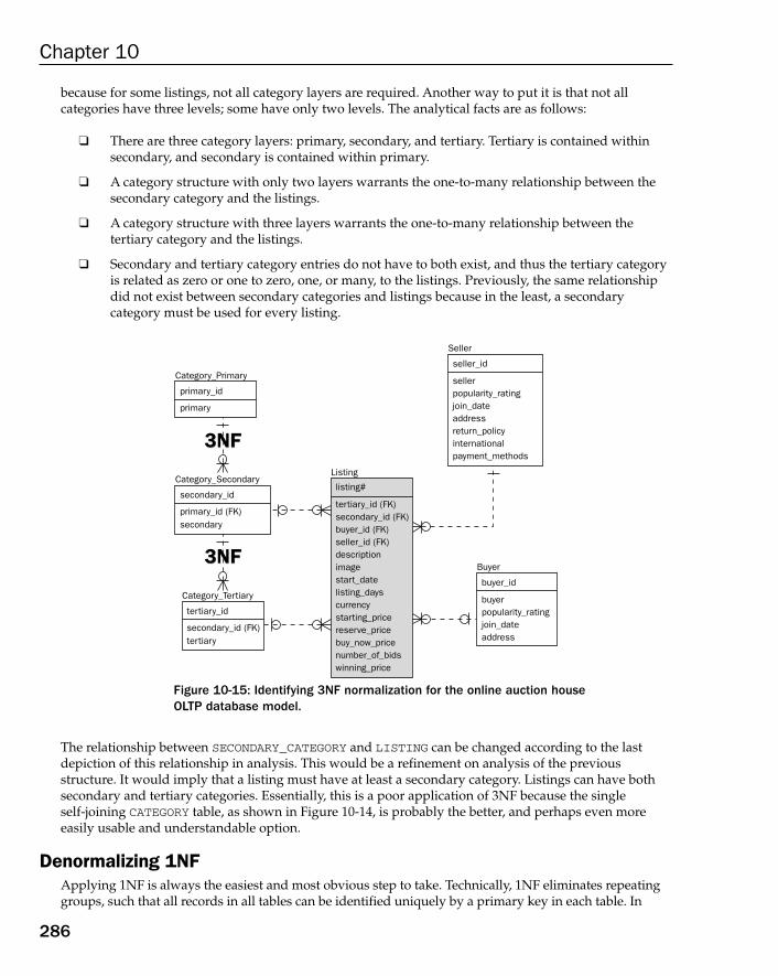
286
Chapter 10
because for some listings, not all category layers are required. Another way to put it is that not all categories have three levels; some have only two levels. The analytical facts are as follows:
❑ There are three category layers: primary, secondary, and tertiary. Tertiary is contained withinsecondary, and secondary is contained within primary.
❑ A category structure with only two layers warrants the one-to-many relationship between thesecondary category and the listings.
❑ A category structure with three layers warrants the one-to-many relationship between the tertiary category and the listings.
❑ Secondary and tertiary category entries do not have to both exist, and thus the tertiary categoryis related as zero or one to zero, one, or many, to the listings. Previously, the same relationshipdid not exist between secondary categories and listings because in the least, a secondary category must be used for every listing.
Figure 10-15: Identifying 3NF normalization for the online auction house OLTP database model.
The relationship between SECONDARY_CATEGORY and LISTING can be changed according to the lastdepiction of this relationship in analysis. This would be a refinement on analysis of the previous structure. It would imply that a listing must have at least a secondary category. Listings can have bothsecondary and tertiary categories. Essentially, this is a poor application of 3NF because the single self-joining CATEGORY table, as shown in Figure 10-14, is probably the better, and perhaps even more easily usable and understandable option.
Denormalizing 1NFApplying 1NF is always the easiest and most obvious step to take. Technically, 1NF eliminates repeatinggroups, such that all records in all tables can be identified uniquely by a primary key in each table. In
Seller
seller_id
sellerpopularity_ratingjoin_dateaddressreturn_policyinternationalpayment_methods
Buyer
buyer_id
buyerpopularity_ratingjoin_dateaddress
Category_Primary
primary_id
primary
secondary
Category_Secondary
secondary_id
primary_id (FK)
tertiary
Category_Tertiary
tertiary_id
secondary_id (FK)
Listing
tertiary_id (FK)secondary_id (FK)buyer_id (FK)seller_id (FK)descriptionimagestart_datelisting_dayscurrencystarting_pricereserve_pricebuy_now_pricenumber_of_bidswinning_price
listing#
3NF3NF
3NF3NF
16_574906 ch10.qxd 11/4/05 10:46 AM Page 286
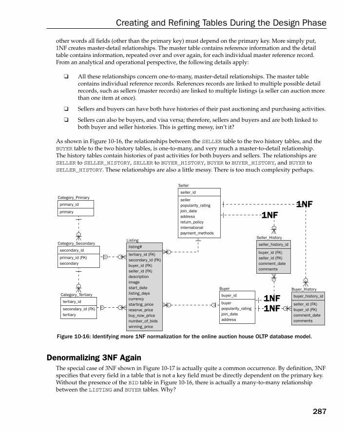
287
Creating and Refining Tables During the Design Phase
other words all fields (other than the primary key) must depend on the primary key. More simply put,1NF creates master-detail relationships. The master table contains reference information and the detailtable contains information, repeated over and over again, for each individual master reference record.From an analytical and operational perspective, the following details apply:
❑ All these relationships concern one-to-many, master-detail relationships. The master table contains individual reference records. References records are linked to multiple possible detailrecords, such as sellers (master records) are linked to multiple listings (a seller can auction morethan one item at once).
❑ Sellers and buyers can have both have histories of their past auctioning and purchasing activities.
❑ Sellers can also be buyers, and visa versa; therefore, sellers and buyers and are both linked toboth buyer and seller histories. This is getting messy, isn’t it?
As shown in Figure 10-16, the relationships between the SELLER table to the two history tables, and theBUYER table to the two history tables, is one-to-many, and very much a master-to-detail relationship. The history tables contain histories of past activities for both buyers and sellers. The relationships areSELLER to SELLER_HISTORY, SELLER to BUYER_HISTORY, BUYER to BUYER_HISTORY, and BUYER toSELLER_HISTORY. These relationships are also a little messy. There is too much complexity perhaps.
Figure 10-16: Identifying more 1NF normalization for the online auction house OLTP database model.
Denormalizing 3NF AgainThe special case of 3NF shown in Figure 10-17 is actually quite a common occurrence. By definition, 3NFspecifies that every field in a table that is not a key field must be directly dependent on the primary key.Without the presence of the BID table in Figure 10-16, there is actually a many-to-many relationshipbetween the LISTING and BUYER tables. Why?
Seller_History
Seller
seller_id
sellerpopularity_ratingjoin_dateaddressreturn_policyinternationalpayment_methods
seller_history_id
buyer_id (FK)seller_id (FK)comment_datecomments
Buyer_History
buyer_history_id
seller_id (FK)buyer_id (FK)comment_datecomments
Buyer
buyer_id
buyerpopularity_ratingjoin_dateaddress
Category_Primary
primary_id
primary
secondary
Category_Secondary
secondary_id
primary_id (FK)
tertiary
Category_Tertiary
tertiary_id
secondary_id (FK)
Listing
tertiary_id (FK)secondary_id (FK)buyer_id (FK)seller_id (FK)descriptionimagestart_datelisting_dayscurrencystarting_pricereserve_pricebuy_now_pricenumber_of_bidswinning_price
listing#
1NF1NF
1NF1NF1NF1NF
1NF1NF
16_574906 ch10.qxd 11/4/05 10:46 AM Page 287
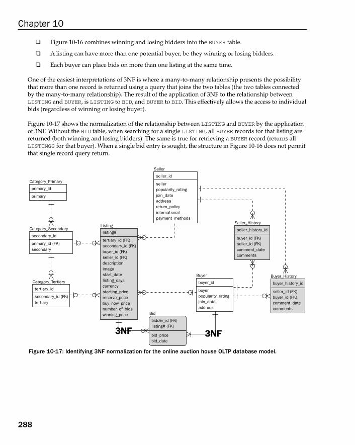
288
Chapter 10
❑ Figure 10-16 combines winning and losing bidders into the BUYER table.
❑ A listing can have more than one potential buyer, be they winning or losing bidders.
❑ Each buyer can place bids on more than one listing at the same time.
One of the easiest interpretations of 3NF is where a many-to-many relationship presents the possibilitythat more than one record is returned using a query that joins the two tables (the two tables connectedby the many-to-many relationship). The result of the application of 3NF to the relationship betweenLISTING and BUYER, is LISTING to BID, and BUYER to BID. This effectively allows the access to individualbids (regardless of winning or losing buyer).
Figure 10-17 shows the normalization of the relationship between LISTING and BUYER by the applicationof 3NF. Without the BID table, when searching for a single LISTING, all BUYER records for that listing arereturned (both winning and losing bidders). The same is true for retrieving a BUYER record (returns allLISTINGS for that buyer). When a single bid entry is sought, the structure in Figure 10-16 does not permitthat single record query return.
Figure 10-17: Identifying 3NF normalization for the online auction house OLTP database model.
Seller_History
Seller
seller_id
sellerpopularity_ratingjoin_dateaddressreturn_policyinternationalpayment_methods
seller_history_id
buyer_id (FK)seller_id (FK)comment_datecomments
Buyer_History
buyer_history_id
seller_id (FK)buyer_id (FK)comment_datecomments
Buyer
buyer_id
buyerpopularity_ratingjoin_dateaddress
Category_Primary
primary_id
primary
secondary
Category_Secondary
secondary_id
primary_id (FK)
tertiary
Category_Tertiary
tertiary_id
secondary_id (FK)
Listing
tertiary_id (FK)secondary_id (FK)buyer_id (FK)seller_id (FK)descriptionimagestart_datelisting_dayscurrencystarting_pricereserve_pricebuy_now_pricenumber_of_bidswinning_price Bid
bidder_id (FK)listing# (FK)
bid_pricebid_date
listing#
3NF3NF 3NF3NF
16_574906 ch10.qxd 11/4/05 10:46 AM Page 288
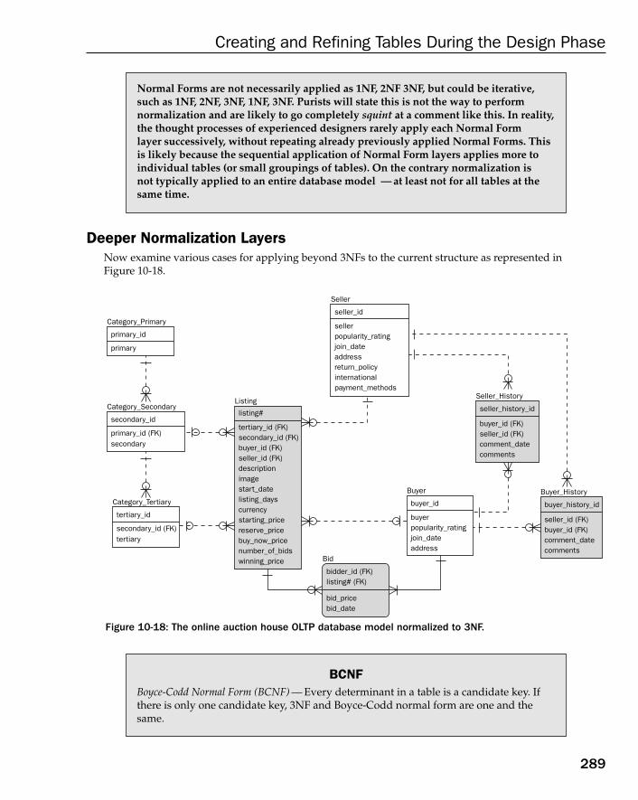
BCNFBoyce-Codd Normal Form (BCNF) — Every determinant in a table is a candidate key. Ifthere is only one candidate key, 3NF and Boyce-Codd normal form are one and thesame.
289
Creating and Refining Tables During the Design Phase
Deeper Normalization LayersNow examine various cases for applying beyond 3NFs to the current structure as represented in Figure 10-18.
Figure 10-18: The online auction house OLTP database model normalized to 3NF.
Seller_History
Seller
seller_id
sellerpopularity_ratingjoin_dateaddressreturn_policyinternationalpayment_methods
seller_history_id
buyer_id (FK)seller_id (FK)comment_datecomments
Buyer_History
buyer_history_id
seller_id (FK)buyer_id (FK)comment_datecomments
Buyer
buyer_id
buyerpopularity_ratingjoin_dateaddress
Category_Primary
primary_id
primary
secondary
Category_Secondary
secondary_id
primary_id (FK)
tertiary
Category_Tertiary
tertiary_id
secondary_id (FK)
Listing
tertiary_id (FK)secondary_id (FK)buyer_id (FK)seller_id (FK)descriptionimagestart_datelisting_dayscurrencystarting_pricereserve_pricebuy_now_pricenumber_of_bidswinning_price Bid
bidder_id (FK)listing# (FK)
bid_pricebid_date
listing#
Normal Forms are not necessarily applied as 1NF, 2NF 3NF, but could be iterative,such as 1NF, 2NF, 3NF, 1NF, 3NF. Purists will state this is not the way to perform normalization and are likely to go completely squint at a comment like this. In reality,the thought processes of experienced designers rarely apply each Normal Form layer successively, without repeating already previously applied Normal Forms. Thisis likely because the sequential application of Normal Form layers applies more toindividual tables (or small groupings of tables). On the contrary normalization is not typically applied to an entire database model — at least not for all tables at thesame time.
16_574906 ch10.qxd 11/4/05 10:46 AM Page 289
290
Chapter 10
Denormalizing BCNFA table is allowed to have only one possible candidate key. A candidate key is a candidate to be a primary key. Personally, I have found BCNF a bit of an odd one, even a little obsessive. Go back toChapter 4 and take a quick peek at Figure 4-33. In Figure 4-33, it should be clear if you read the calloutsin the graphic that any field which is potentially unique for each record, that field can be a primary key.This is quite a common occurrence. In fact, quite often when replacing a traditional primary key with asurrogate key auto counter, one instantly violates BCNF. I have never seen a relational database thatphysically allows Data Definition Language (DDL) commands that permits the creation of a table withmore than one primary key per table. Using a CREATE TABLE command or even a table-design GUI(such as in Microsoft Access) more than one primary key is simply not an option. In other words, yourMicrosoft Access table-modeling GUI and your Oracle or SQL Server database DDL commands will notallow creation of a table violating BCNF, with more than one primary key.
Looking at Figure 10-18 again, for the online auction house OLTP database model, you could applyBCNF to all of the SELLER, BUYER, LISTING, and both the history tables as shown in Figure 10-19.
Figure 10-19 provokes the following commentary:
❑ Separating out sellers and buyers, as well as names and addresses, is sensible from a mathemati-cal perspective; however, from a practically applicable commercial perspective, it simply createslots of tables to join. Additionally, the possibility of having two people or companies with thesame name is unlikely, but it is possible. From a mathematical and data integrity perspective,allowing duplicate names is a problem, such as the wrong data going to the wrong person. For abank, that would be libelous.
4NF4th Normal Form (4NF) — Eliminate multiple sets of multi-valued dependencies.
SNF5th Normal Form (5NF) — Eliminate cyclic dependencies. 5NF is also known as projec-tion normal form (PJNF).
DKNFDomain Key Normal Form (DKNF) — This is the ultimate application of normalizationand is more a measurement of conceptual state, as opposed to a transformation processin itself. DKNF will, therefore, be ignored for the purposes of the online auction housecase study example.
Beyond 3NF the Easy WayMany commercial relational database models do not extend beyond 3NF. Sometimes3NF is not used. The simple rule is not to make a rule out of it. Commerce requires flexibility, not rigidity. The reason why is because of the generation of too many tables,and the resulting complex SQL code joins, with resulting terrible database responsetimes. One common case that bears mentioning is removal of potentially NULL valuedfields into new tables, creating a one-to-one relationship. In modern high-end relationaldatabase engines, with variable record lengths, separating often times NULL valuedfields from more actively used fields is largely irrelevant. Disk space is cheap and, asalready stated, increased numbers of tables leads to bigger SQL joins and poorer performance.
16_574906 ch10.qxd 11/4/05 10:46 AM Page 290
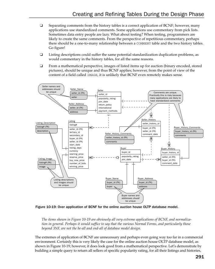
291
Creating and Refining Tables During the Design Phase
❑ Separating comments from the history tables is a correct application of BCNF; however, manyapplications use standardized comments. Some applications use commentary from pick lists.Sometimes data entry people are lazy. What about testing? When testing, programmers arelikely to create the same comments. From the perspective of repetitious commentary, perhapsthere should be a one-to-many relationship between a COMMENT table and the two history tables.Go figure!
❑ Listing descriptions could suffer the same potential standardization duplication problems, aswould commentary in the history tables, for all the same reasons.
❑ From a mathematical perspective, images of listed items up for auction (binary encoded, storedpictures), should be unique and thus BCNF applies; however, from the point of view of the content of a field called IMAGE, it is unlikely that BCNF even remotely makes sense.
Figure 10-19: Over application of BCNF for the online auction house OLTP database model.
The items shown in Figure 10-19 are obviously all very extreme applications of BCNF, and normaliza-tion in general. Perhaps it would suffice to say that the various Normal Forms, and particularly thosebeyond 3NF, are not the be-all and end-all of database model design.
The extremes of application of BCNF are unnecessary and perhaps even going way too far in a commercialenvironment. Certainly this is very likely the case for the online auction house OLTP database model, asshown in Figure 10-19; however, it does look good from a mathematical perspective. Let’s demonstrate bybuilding a simple query to return all sellers of specific popularity rating, for all their listings and histories,
Seller_History
Seller
seller_id
popularity_ratingjoin_datereturn_policyinternationalpayment_methods
seller_history_id
buyer_id (FK)seller_id (FK)comment_date
Buyer_History
buyer_history_id
seller_id (FK)buyer_id (FK)comment_date
Buyer
buyer_id
popularity_ratingjoin_date
Seller_Name
seller_id (FK)
seller
Buyer_Name
buyer_id (FK)
buyer
Buyer_Address
buyer_id (FK)
address
Seller_History_Comments
seller_history_id (FK)
comments
Buyer_History_Comments
buyer_history_id (FK)
comments
Seller_Address
seller_id (FK)
address
Listing_Description
listing# (FK)
description
Listing_Image
listing# (FK)
image
Listing
seller_id (FK)tertiary_idsecondary_idbuyer_id (FK)seller_id (FK)start_datelisting_dayscurrencystarting_pricereserve_pricebuy_now_pricenumber_of_bidswinning_price
listing#
Listing descriptionsand images should
be unique
Seller names andaddresses should
be unique
Buyer names andaddresses should
be unique
Comments are unique.Practically this is risky becausemany applications are likely tohave standardized comments
16_574906 ch10.qxd 11/4/05 10:46 AM Page 291
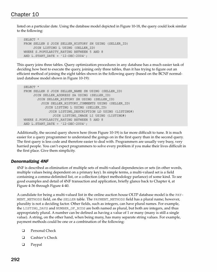
292
Chapter 10
listed on a particular date. Using the database model depicted in Figure 10-18, the query could look similarto the following:
SELECT * FROM SELLER S JOIN SELLER_HISTORY SH USING (SELLER_ID)
JOIN LISTING L USING (SELLER_ID)WHERE S.POPULARITY_RATING BETWEEN 5 AND 8AND L.START_DATE = ‘12-DEC-2004’;
This query joins three tables. Query optimization procedures in any database has a much easier task ofdeciding how best to execute the query, joining only three tables, than it has trying to figure out an efficient method of joining the eight tables shown in the following query (based on the BCNF normal-ized database model shown in Figure 10-19):
SELECT * FROM SELLER S JOIN SELLER_NAME SN USING (SELLER_ID)
JOIN SELLER_ADDRESS SA USING (SELLER_ID)JOIN SELLER_HISTORY SH USING (SELLER_ID)
JOIN SELLER_HISTORY_COMMENTS USING (SELLER_ID)JOIN LISTING L USING (SELLER_ID)
JOIN LISTING_DESCRIPTION LD USING (LISTING#)JOIN LISTING_IMAGE LI USING (LISTING#)
WHERE S.POPULARITY_RATING BETWEEN 5 AND 8AND L.START_DATE = ‘12-DEC-2004’;
Additionally, the second query shown here (from Figure 10-19) is far more difficult to tune. It is mucheasier for a query programmer to understand the goings on in the first query than in the second query.The first query is less code and therefore easier to deal with. Programmers are usually very busy, veryharried people. You can’t expect programmers to solve every problem if you make their lives difficult inthe first place. Give them simplicity.
Denormalizing 4NF4NF is described as elimination of multiple sets of multi-valued dependencies or sets (in other words,multiple values being dependent on a primary key). In simple terms, a multi-valued set is a field containing a comma-delimited list, or a collection (object methodology parlance) of some kind. To seegood examples and detail of 4NF transaction and application, briefly glance back to Chapter 4, at Figure 4-36 through Figure 4-40.
A candidate for being a multi-valued list in the online auction house OLTP database model is the PAY-MENT_METHODS field, on the SELLER table. The PAYMENT_METHODS field has a plural name; however, plurality is not a deciding factor. Other fields, such as integers, can have plural names. For example, the LISTING_DAYS and NUMBER_OF_BIDS are both named as plural, but both are integers, and thusappropriately plural. A number can be defined as having a value of 1 or many (many is still a singlevalue). A string, on the other hand, when being many, has many separate string values. For example,payment methods could be one or a combination of the following:
❑ Personal Check
❑ Cashier’s Check
❑ Paypal
16_574906 ch10.qxd 11/4/05 10:46 AM Page 292
293
Creating and Refining Tables During the Design Phase
❑ Western Union
❑ Cash
❑ Visa
❑ MasterCard
❑ American Express
So, the PAYMENT_METHODS field for a specific listing could be something like this:
Cashier’s Check, Western Union, Visa, MasterCard
This string is a comma-delimited list. A comma-delimited list is by definition a multi-valued set. Amulti-valued set is thus a set, or a single item containing more than one possible value. 4NF demands thatcomma delimited strings should be split up. In the case of an online auction house, it is likely that thePAYMENT_METHODS field would only be used for online display. Then again, the list could be split inapplications. For example, the string value Visa determines that a specific type of credit card is acceptable, perhaps processing payment through an online credit card payment service for Visa creditcards. 4NF would change the OLTP database model in Figure 10-18 to that shown in Figure 10-20.
Figure 10-20: Applying 4NF to the OLTP database model.
Seller_History
Seller
seller_id
sellerpopularity_ratingjoin_dateaddressreturn_policyinternational
seller_history_id
buyer_id (FK)seller_id (FK)comment_datecomments
Buyer_History
buyer_history_id
seller_id (FK)buyer_id (FK)comment_datecomments
Buyer
buyer_id
buyerpopularity_ratingjoin_dateaddress
Category_Primary
primary_id
primary
secondary
Seller_Payment_Methods
seller_id (FK)
payment method
Category_Secondary
secondary_id
primary_id (FK)
tertiary
Category_Tertiary
tertiary_id
secondary_id (FK)
Listing
seller_id (FK)tertiary_id (FK)secondary_id (FK)buyer_id (FK)descriptionimagestart_datelisting_dayscurrencystarting_pricereserve_pricebuy_now_pricenumber_of_bidswinning_price Bid
bidder_id (FK)listing# (FK)
bid_pricebid_date
listing#
16_574906 ch10.qxd 11/4/05 10:46 AM Page 293
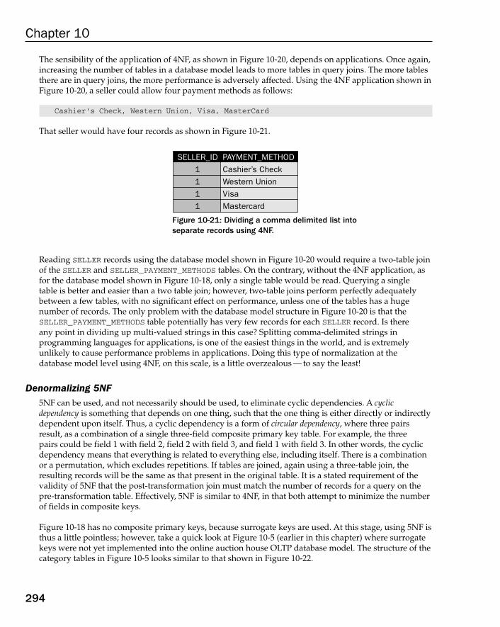
The sensibility of the application of 4NF, as shown in Figure 10-20, depends on applications. Once again,increasing the number of tables in a database model leads to more tables in query joins. The more tablesthere are in query joins, the more performance is adversely affected. Using the 4NF application shown inFigure 10-20, a seller could allow four payment methods as follows:
Cashier’s Check, Western Union, Visa, MasterCard
That seller would have four records as shown in Figure 10-21.
Figure 10-21: Dividing a comma delimited list into separate records using 4NF.
Reading SELLER records using the database model shown in Figure 10-20 would require a two-table joinof the SELLER and SELLER_PAYMENT_METHODS tables. On the contrary, without the 4NF application, asfor the database model shown in Figure 10-18, only a single table would be read. Querying a single table is better and easier than a two table join; however, two-table joins perform perfectly adequatelybetween a few tables, with no significant effect on performance, unless one of the tables has a huge number of records. The only problem with the database model structure in Figure 10-20 is that theSELLER_PAYMENT_METHODS table potentially has very few records for each SELLER record. Is there any point in dividing up multi-valued strings in this case? Splitting comma-delimited strings in programming languages for applications, is one of the easiest things in the world, and is extremelyunlikely to cause performance problems in applications. Doing this type of normalization at thedatabase model level using 4NF, on this scale, is a little overzealous — to say the least!
Denormalizing 5NF5NF can be used, and not necessarily should be used, to eliminate cyclic dependencies. A cyclic dependency is something that depends on one thing, such that the one thing is either directly or indirectlydependent upon itself. Thus, a cyclic dependency is a form of circular dependency, where three pairsresult, as a combination of a single three-field composite primary key table. For example, the three pairs could be field 1 with field 2, field 2 with field 3, and field 1 with field 3. In other words, the cyclicdependency means that everything is related to everything else, including itself. There is a combinationor a permutation, which excludes repetitions. If tables are joined, again using a three-table join, theresulting records will be the same as that present in the original table. It is a stated requirement of thevalidity of 5NF that the post-transformation join must match the number of records for a query on thepre-transformation table. Effectively, 5NF is similar to 4NF, in that both attempt to minimize the numberof fields in composite keys.
Figure 10-18 has no composite primary keys, because surrogate keys are used. At this stage, using 5NF isthus a little pointless; however, take a quick look at Figure 10-5 (earlier in this chapter) where surrogatekeys were not yet implemented into the online auction house OLTP database model. The structure of thecategory tables in Figure 10-5 looks similar to that shown in Figure 10-22.
SELLER_ID1111
PAYMENT_METHODCashier’s CheckWestern UnionVisaMastercard
294
Chapter 10
16_574906 ch10.qxd 11/4/05 10:46 AM Page 294
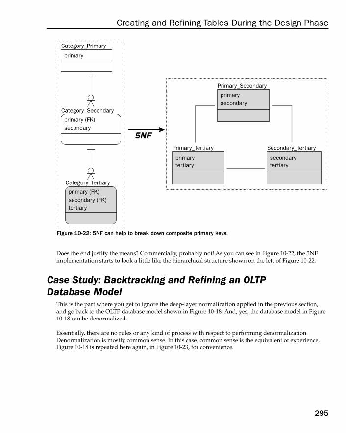
Figure 10-22: 5NF can help to break down composite primary keys.
Does the end justify the means? Commercially, probably not! As you can see in Figure 10-22, the 5NFimplementation starts to look a little like the hierarchical structure shown on the left of Figure 10-22.
Case Study: Backtracking and Refining an OLTP Database Model
This is the part where you get to ignore the deep-layer normalization applied in the previous section,and go back to the OLTP database model shown in Figure 10-18. And, yes, the database model in Figure10-18 can be denormalized.
Essentially, there are no rules or any kind of process with respect to performing denormalization.Denormalization is mostly common sense. In this case, common sense is the equivalent of experience.Figure 10-18 is repeated here again, in Figure 10-23, for convenience.
5NF5NF
Category_Primary
primary
secondary
Category_Secondary
primary (FK)
secondary (FK)
Category_Tertiary
primary (FK)
tertiary
Primary_Secondary
primarysecondary
Primary_Tertiary
primarytertiary
Secondary_Tertiary
secondarytertiary
295
Creating and Refining Tables During the Design Phase
16_574906 ch10.qxd 11/4/05 10:46 AM Page 295
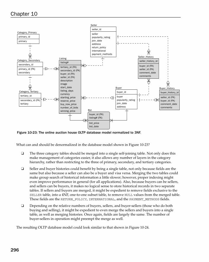
Figure 10-23: The online auction house OLTP database model normalized to 3NF.
What can and should be denormalized in the database model shown in Figure 10-23?
❑ The three category tables should be merged into a single self-joining table. Not only does thismake management of categories easier, it also allows any number of layers in the category hierarchy, rather than restricting to the three of primary, secondary, and tertiary categories.
❑ Seller and buyer histories could benefit by being a single table, not only because fields are thesame but also because a seller can also be a buyer and visa versa. Merging the two tables couldmake group search of historical information a little slower; however, proper indexing mighteven improve performance in general (for all applications). Also, because buyers can be sellers,and sellers can be buyers, it makes no logical sense to store historical records in two separatetables. If sellers and buyers are merged, it might be expedient to remove fields exclusive to theSELLER table, into a 4NF, one-to-one subset table, to remove NULL values from the merged table.These fields are the RETURN_POLICY, INTERNATIONAL, and the PAYMENT_METHODS fields.
❑ Depending on the relative numbers of buyers, sellers, and buyer-sellers (those who do bothbuying and selling), it might be expedient to even merge the sellers and buyers into a singletable, as well as merging histories. Once again, fields are largely the same. The number of buyer-sellers in operation might preempt the merge as well.
The resulting OLTP database model could look similar to that shown in Figure 10-24.
Seller_History
Seller
seller_id
sellerpopularity_ratingjoin_dateaddressreturn_policyinternationalpayment_methods
seller_history_id
buyer_id (FK)seller_id (FK)comment_datecomments
Buyer_History
buyer_history_id
seller_id (FK)buyer_id (FK)comment_datecomments
Buyer
buyer_id
buyerpopularity_ratingjoin_dateaddress
Category_Primary
primary_id
primary
secondary
Category_Secondary
secondary_id
primary_id (FK)
tertiary
Category_Tertiary
tertiary_id
secondary_id (FK)
Listing
tertiary_id (FK)secondary_id (FK)buyer_id (FK)seller_id (FK)descriptionimagestart_datelisting_dayscurrencystarting_pricereserve_pricebuy_now_pricenumber_of_bidswinning_price Bid
buyer_id (FK)listing# (FK)
bid_pricebid_date
listing#
296
Chapter 10
16_574906 ch10.qxd 11/4/05 10:46 AM Page 296
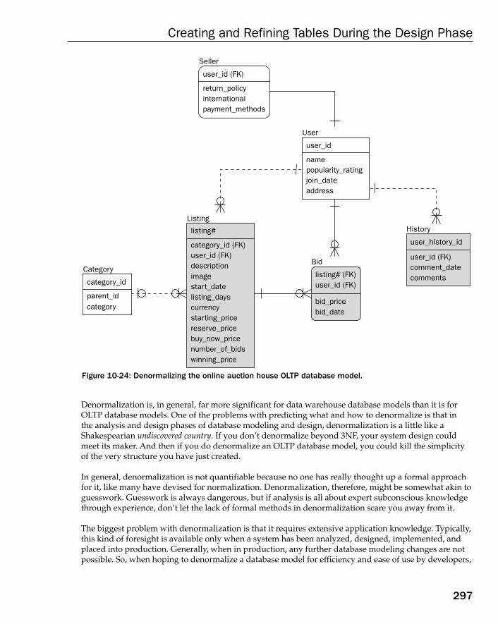
Figure 10-24: Denormalizing the online auction house OLTP database model.
Denormalization is, in general, far more significant for data warehouse database models than it is forOLTP database models. One of the problems with predicting what and how to denormalize is that inthe analysis and design phases of database modeling and design, denormalization is a little like aShakespearian undiscovered country. If you don’t denormalize beyond 3NF, your system design couldmeet its maker. And then if you do denormalize an OLTP database model, you could kill the simplicityof the very structure you have just created.
In general, denormalization is not quantifiable because no one has really thought up a formal approachfor it, like many have devised for normalization. Denormalization, therefore, might be somewhat akin toguesswork. Guesswork is always dangerous, but if analysis is all about expert subconscious knowledgethrough experience, don’t let the lack of formal methods in denormalization scare you away from it.
The biggest problem with denormalization is that it requires extensive application knowledge. Typically,this kind of foresight is available only when a system has been analyzed, designed, implemented, andplaced into production. Generally, when in production, any further database modeling changes are notpossible. So, when hoping to denormalize a database model for efficiency and ease of use by developers,
History
User
user_id
namepopularity_ratingjoin_dateaddress
Seller
user_id (FK)
return_policyinternationalpayment_methods
user_history_id
user_id (FK)comment_datecomments
category
Category
category_id
parent_id
Listing
category_id (FK)user_id (FK)descriptionimagestart_datelisting_dayscurrencystarting_pricereserve_pricebuy_now_pricenumber_of_bidswinning_price
Bid
listing# (FK)user_id (FK)
bid_pricebid_date
listing#
297
Creating and Refining Tables During the Design Phase
16_574906 ch10.qxd 11/4/05 10:46 AM Page 297
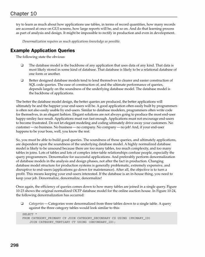
298
Chapter 10
try to learn as much about how applications use tables, in terms of record quantities, how many recordsare accessed at once on GUI screens, how large reports will be, and so on. And do that learning processas part of analysis and design. It might be impossible to rectify in production and even in development.
Denormalization requires as much applications knowledge as possible.
Example Application QueriesThe following state the obvious:
❑ The database model is the backbone of any application that uses data of any kind. That data ismost likely stored in some kind of database. That database is likely to be a relational database ofone form or another.
❑ Better designed database models tend to lend themselves to clearer and easier construction ofSQL code queries. The ease of construction of, and the ultimate performance of queries,depends largely on the soundness of the underlying database model. The database model isthe backbone of applications.
The better the database model design, the better queries are produced, the better applications will ultimately be and the happier your end-users will be. A good application often easily built by programmersis often not also easily usable by end-users. Similar to database modelers, programmers often write codefor themselves, in an elegant fashion. Elegant solutions are not always going to produce the most end-userhappy-smiley face result. Applications must run fast enough. Applications must not encourage end-usersto become frustrated. Do not let elegant modeling and coding ultimately drive away your customers. Nocustomer — no business. No business — no company. No company — no job! And, if your end-user happens to be your boss, well, you know the rest.
So, you must be able to build good queries. The soundness of those queries, and ultimately applications,are dependent upon the soundness of the underlying database model. A highly normalized databasemodel is likely to be unsound because there are too many tables, too much complexity, and too manytables in joins. Lots of tables and lots of complex inter-table relationships confuse people, especially thequery programmers. Denormalize for successful applications. And preferably perform denormalizationof database models in the analysis and design phases, not after the fact in production. Changingdatabase model structure for production systems is generally problematic, extremely expensive, and disruptive to end-users (applications go down for maintenance). After all, the objective is to turn aprofit. This means keeping your end-users interested. If the database is an in-house thing, you need tokeep your job. Denormalize, denormalize, denormalize!
Once again, the efficiency of queries comes down to how many tables are joined in a single query. Figure10-23 shows the original normalized OLTP database model for the online auction house. In Figure 10-24,the following denormalization has occurred:
❑ Categories — Categories were denormalized from three tables down to a single table. A queryagainst the three category tables would look similar to this:
SELECT * FROM CATEGORY_PRIMARY CP JOIN CATEGORY_SECONDARY CS USING (PRIMARY_ID)
JOIN CATEGORY_TERTIARY CT USING (SECONDARY_ID);
16_574906 ch10.qxd 11/4/05 10:46 AM Page 298
299
Creating and Refining Tables During the Design Phase
A query against the single category table could be constructed as follows:
SELECT * FROM CATEGORY;
If the single category table was required to display a hierarchy, a self join could be used (somedatabase engines have special syntax for single-table hierarchical queries):
SELECT P.CATEGORY, C.CATEGORY FROM CATEGORY P JOIN CATEGORY C ON(P.CATEGORY_ID = C.CATEGORY_ID)ORDER BY P.CATEGORY, C.CATEGORY;
Denormalizing categories in this way is probably a very sensible idea for the OLTP databasemodel of the online auction house.
❑ Users — Sellers and buyers were partially denormalized into users, where 4NF normalizationwas used to separate seller details from buyers. Using the normalized database model in Figure10-23 to find all listings for a specific seller, the following query applies (joining two tables andapplying a WHERE clause to the SELLER table):
SELECT * FROM SELLER S JOIN LISTING L USING (SELLER_ID)WHERE S.SELLER = “Joe Soap”;
Once again, using the normalized database model in Figure 10-23, the following query finds allexisting bids, on all listings, for a particular buyer (joining three tables and applying a WHEREclause to the BUYER table):
SELECT * FROM LISTING L JOIN BID BID USING (LISTING#)
JOIN BUYER B USING (BUYER_ID)WHERE B.BUYER = “Jim Smith”;
Using the denormalized database model in Figure 10-24, this query finds all listings for a spe-cific seller (the SELLER and USER tables are actually normalized):
SELECT * FROM USER U JOIN SELLER S USING (SELLER_ID)
JOIN LISTING L USING (USER_ID)WHERE U.NAME = “Joe Soap”;
This query is actually worse for the denormalized database model because it joins three tablesinstead of two. And again, using the denormalized database model in Figure 10-24, the follow-ing query finds all existing bids on all listings for a particular buyer:
SELECT * FROM LISTING L JOIN BID BID USING (LISTING#)
JOIN USER U USING (USER_ID)WHERE U.NAME = “Jim Smith”AND U.USER_ID NOT IN (SELECT USER_ID FROM SELLER);
16_574906 ch10.qxd 11/4/05 10:46 AM Page 299
300
Chapter 10
This query is also worse for the denormalized version because not only does it join three tables,but additionally performs a semi-join (and an anti semi-join at that). An anti semi-join is a nega-tive search. A negative search tries to find what is not in a table, and therefore must read allrecords in that table. Indexes can’t be used at all and, thus, a full table scan results. Full tablescans can be I/O heavy for larger tables.
It should be clear to conclude that denormalizing the BUYER and SELLER tables into the USERand normalized SELLER tables (as shown in Figure 10-24) is probably quite a bad idea! At leastit appears that way from the perspective of query use; however, an extra field could be added tothe USER table to dissimilate between users and buyers, in relation to bids and listings (a personperforming both buying and selling will appear in both buyer and seller data sets). The extrafield could be used as a base for very efficient indexing or even something as advanced as parti-tioning. Partitioning physically breaks tables into separate physical chunks. If the USER tablewere partitioned between users and sellers, reading only sellers from the USER table would onlyperform I/O against a partition containing sellers (not buyers). It is still not really very sensibleto denormalize the BUYER and SELLER table into the USER table.
❑ Histories — The two history tables were denormalized into a single table, as shown in Figure10-24. Executing a query using the normalized database model in Figure 10-23 to find the history for a specific seller, could be performed using a query like the following:
SELECT * FROM SELLER S JOIN SELLER_HISTORY SH USING (SELLER_ID)WHERE S.SELLER = “Joe Soap”;
Finding a history for a specific seller using the denormalized database model shown in Figure10-24 could use a query like this:
SELECT * FROM USER U JOIN HISTORY H (USER_ID)WHERE U.NAME = “Joe Soap”AND U.USER_ID IN (SELECT USER_ID FROM SELLER);
Once again, as with denormalization of SELLER and BUYER tables into the USER table, denormal-izing the SELLER_HISTORY and BUYER HISTORY tables into the HISTORY table, might actuallybe a bad idea. The first query above joins two tables. The second query also joins two tables, butalso executes a semi-join. This semi-join is not as bad as for denormalization of users, whichused an anti semi-join; however, this is still effectively a three-way join.
So, you have discovered that perhaps the most effective, descriptive, and potentially efficient databasemodel for the OLTP online auction house is as shown in Figure 10-25. The only denormalization makingsense at this stage is to merge the three separate category hierarchy tables into the single self-joiningCATEGORY table. Buyer, seller, and history information is probably best left in separate tables.
16_574906 ch10.qxd 11/4/05 10:46 AM Page 300

Denormalization is rarely effective for OLTP database models for anything between 1NF and 3NF; however (and this very important), remember that previously in this chapter you read about layers ofnormalization beyond 3NF (BCNF, 4NF, 5NF and DKNF). None of these intensive Normal Forms haveso far been applied to the OLTP database model for the online auction house. As of Figure 10-23, youbegan to attempt to backtrack on previously performed normalization, by denormalizing. You beganwith the 3NF database model as shown in Figure 10-23. In other words, any normalization beyond 3NFwas simply ignored, having already been proved to be completely superfluous and over the top for thisparticular database model.
Figure 10-25: The online auction house OLTP database model, 3NF, partially denormalized.
The only obvious issue still with the database model as shown in Figure 10-25 is that the BUYER_HIS-TORY and SELLER_HISTORY tables have both BUYER_ID and SELLER_ID fields. In other words, both his-tory tables are linked (related) to both of the BUYER and SELLER tables. It therefore could make perfectsense to denormalize not only the category tables, but the history tables as well, leave BUYER andSELLER tables normalized, and separate, as shown in Figure 10-26.
Seller_History
Seller
seller_id
sellerpopularity_ratingjoin_dateaddressreturn_policyinternationalpayment_methods
seller_history_id
buyer_id (FK)seller_id (FK)comment_datecomments
Buyer_History
buyer_history_id
seller_id (FK)buyer_id (FK)comment_datecomments
Buyer
buyer_id
buyerpopularity_ratingjoin_dateaddress
category
Category
category_id
parent_id
Listing
category_id (FK)buyer_id (FK)seller_id (FK)descriptionimagestart_datelisting_dayscurrencystarting_pricereserve_pricebuy_now_pricenumber_of_bidswinning_price
Bid
bidder_id (FK)listing# (FK)
bid_pricebid_date
listing#
301
Creating and Refining Tables During the Design Phase
16_574906 ch10.qxd 11/4/05 10:46 AM Page 301
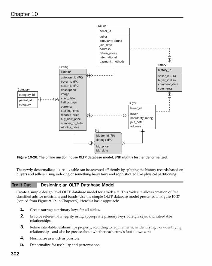
302
Chapter 10
Figure 10-26: The online auction house OLTP database model, 3NF, slightly further denormalized.
The newly denormalized HISTORY table can be accessed efficiently by splitting the history records based onbuyers and sellers, using indexing or something hairy fairy and sophisticated like physical partitioning.
Try It Out Designing an OLTP Database ModelCreate a simple design level OLTP database model for a Web site. This Web site allows creation of freeclassified ads for musicians and bands. Use the simple OLTP database model presented in Figure 10-27(copied from Figure 9-19, in Chapter 9). Here’s a basic approach:
1. Create surrogate primary keys for all tables.
2. Enforce referential integrity using appropriate primary keys, foreign keys, and inter-table relationships.
3. Refine inter-table relationships properly, according to requirements, as identifying, non-identifyingrelationships, and also be precise about whether each crow’s foot allows zero.
4. Normalize as much as possible.
5. Denormalize for usability and performance.
History
Seller
seller_id
sellerpopularity_ratingjoin_dateaddressreturn_policyinternationalpayment_methods
history_id
seller_id (FK)buyer_id (FK)comment_datecomments
Buyer
buyer_id
buyerpopularity_ratingjoin_dateaddress
category
Category
category_id
parent_id
Listing
category_id (FK)buyer_id (FK)seller_id (FK)descriptionimagestart_datelisting_dayscurrencystarting_pricereserve_pricebuy_now_pricenumber_of_bidswinning_price
Bid
bidder_id (FK)listing# (FK)
bid_pricebid_date
listing#
16_574906 ch10.qxd 11/4/05 10:46 AM Page 302
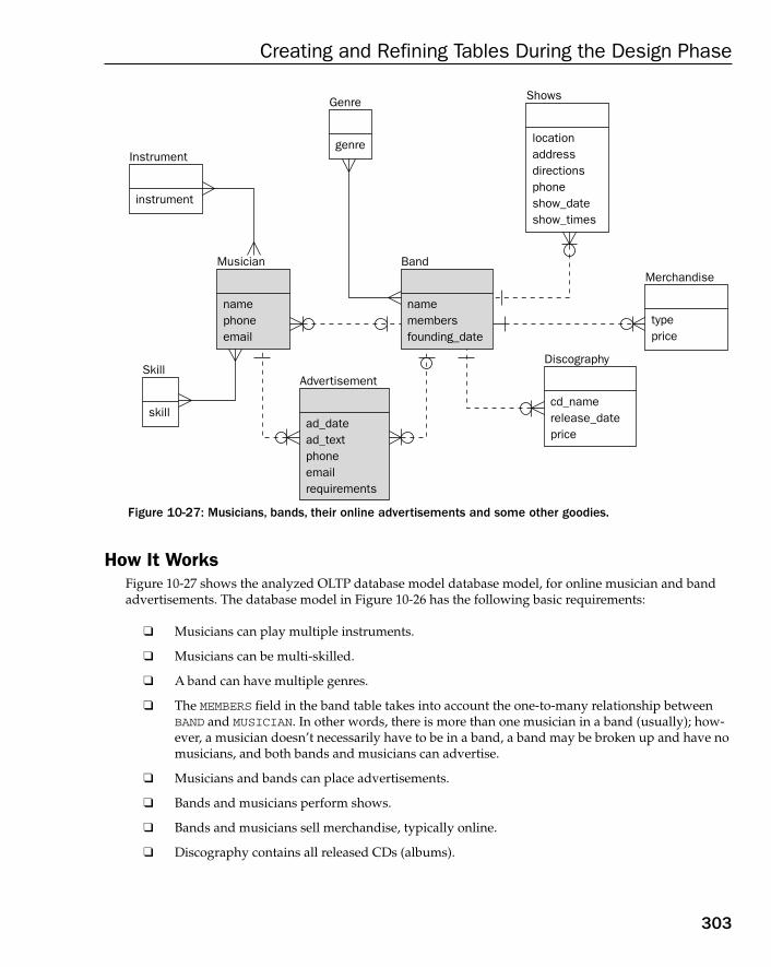
Figure 10-27: Musicians, bands, their online advertisements and some other goodies.
How It WorksFigure 10-27 shows the analyzed OLTP database model database model, for online musician and bandadvertisements. The database model in Figure 10-26 has the following basic requirements:
❑ Musicians can play multiple instruments.
❑ Musicians can be multi-skilled.
❑ A band can have multiple genres.
❑ The MEMBERS field in the band table takes into account the one-to-many relationship betweenBAND and MUSICIAN. In other words, there is more than one musician in a band (usually); how-ever, a musician doesn’t necessarily have to be in a band, a band may be broken up and have nomusicians, and both bands and musicians can advertise.
❑ Musicians and bands can place advertisements.
❑ Bands and musicians perform shows.
❑ Bands and musicians sell merchandise, typically online.
❑ Discography contains all released CDs (albums).
Instrument
instrument
Skill
skill
Genre
genre
Musician
namephoneemail
Band
namemembersfounding_date
Discography
cd_namerelease_dateprice
Merchandise
typeprice
Shows
locationaddressdirectionsphoneshow_dateshow_times
Advertisement
ad_datead_textphoneemailrequirements
303
Creating and Refining Tables During the Design Phase
16_574906 ch10.qxd 11/4/05 10:46 AM Page 303
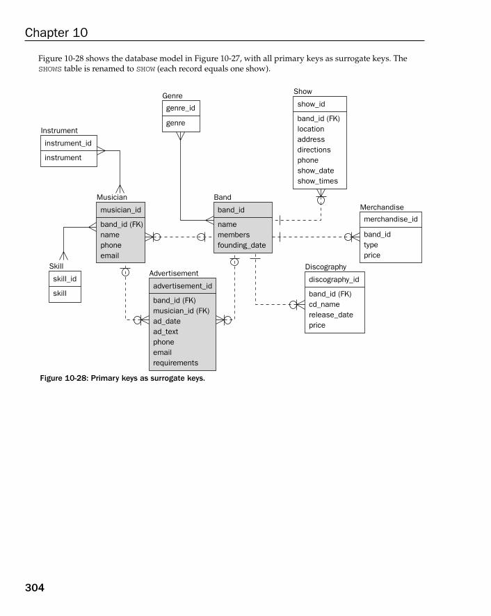
304
Chapter 10
Figure 10-28 shows the database model in Figure 10-27, with all primary keys as surrogate keys. TheSHOWS table is renamed to SHOW (each record equals one show).
Figure 10-28: Primary keys as surrogate keys.
Instrument
instrument
instrument_id
Skill
skill
skill_id
Genre
genre
genre_id
Musician
band_id (FK)namephoneemail
musician_id
Band
namemembersfounding_date
band_id
Discography
band_id (FK)cd_namerelease_dateprice
discography_id
Merchandise
band_idtypeprice
merchandise_id
Show
band_id (FK)locationaddressdirectionsphoneshow_dateshow_times
show_id
Advertisement
band_id (FK)musician_id (FK)ad_datead_textphoneemailrequirements
advertisement_id
16_574906 ch10.qxd 11/4/05 10:46 AM Page 304
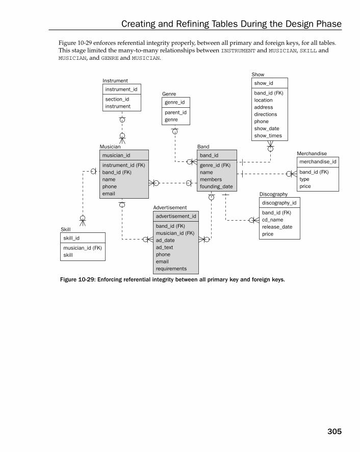
305
Creating and Refining Tables During the Design Phase
Figure 10-29 enforces referential integrity properly, between all primary and foreign keys, for all tables.This stage limited the many-to-many relationships between INSTRUMENT and MUSICIAN, SKILL andMUSICIAN, and GENRE and MUSICIAN.
Figure 10-29: Enforcing referential integrity between all primary key and foreign keys.
Instrument
section_idinstrument
instrument_id
Skill
musician_id (FK)skill
skill_id
Genre
parent_idgenre
genre_id
Musician
instrument_id (FK)band_id (FK)namephoneemail
musician_id
Band
genre_id (FK)namemembersfounding_date
band_id
Discography
band_id (FK)cd_namerelease_dateprice
discography_id
Merchandise
band_id (FK)typeprice
merchandise_id
Show
band_id (FK)locationaddressdirectionsphoneshow_dateshow_times
show_id
Advertisement
band_id (FK)musician_id (FK)ad_datead_textphoneemailrequirements
advertisement_id
16_574906 ch10.qxd 11/4/05 10:46 AM Page 305
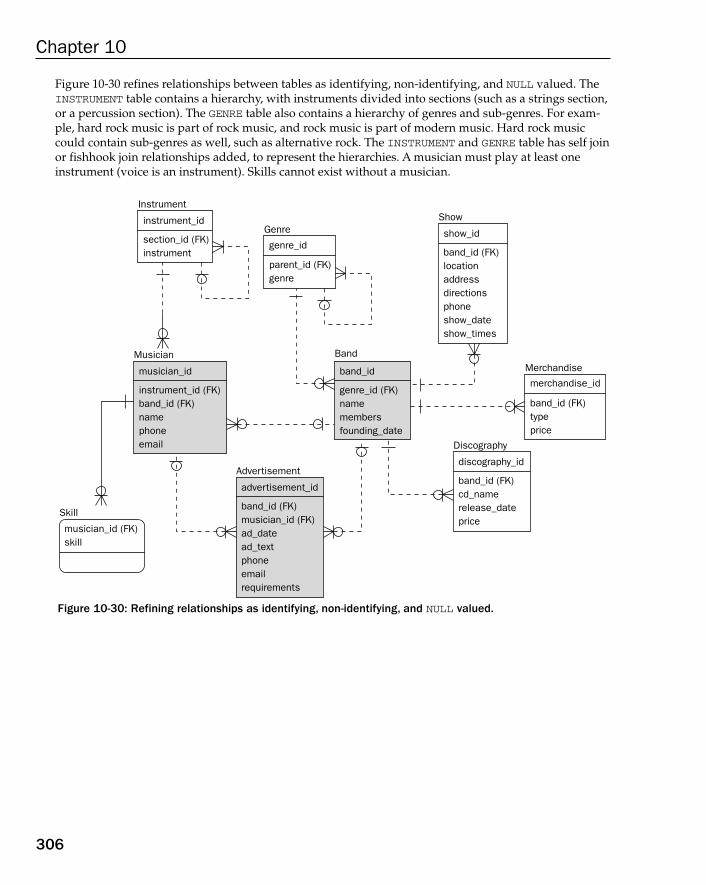
306
Chapter 10
Figure 10-30 refines relationships between tables as identifying, non-identifying, and NULL valued. TheINSTRUMENT table contains a hierarchy, with instruments divided into sections (such as a strings section,or a percussion section). The GENRE table also contains a hierarchy of genres and sub-genres. For exam-ple, hard rock music is part of rock music, and rock music is part of modern music. Hard rock musiccould contain sub-genres as well, such as alternative rock. The INSTRUMENT and GENRE table has self joinor fishhook join relationships added, to represent the hierarchies. A musician must play at least oneinstrument (voice is an instrument). Skills cannot exist without a musician.
Figure 10-30: Refining relationships as identifying, non-identifying, and NULL valued.
Instrument
section_id (FK)instrument
instrument_id
Skill
musician_id (FK)skill
Genre
parent_id (FK)genre
genre_id
Musician
instrument_id (FK)band_id (FK)namephoneemail
musician_id
Band
genre_id (FK)namemembersfounding_date
band_id
Discography
band_id (FK)cd_namerelease_dateprice
discography_id
Merchandise
band_id (FK)typeprice
merchandise_id
Show
band_id (FK)locationaddressdirectionsphoneshow_dateshow_times
show_id
Advertisement
band_id (FK)musician_id (FK)ad_datead_textphoneemailrequirements
advertisement_id
16_574906 ch10.qxd 11/4/05 10:46 AM Page 306
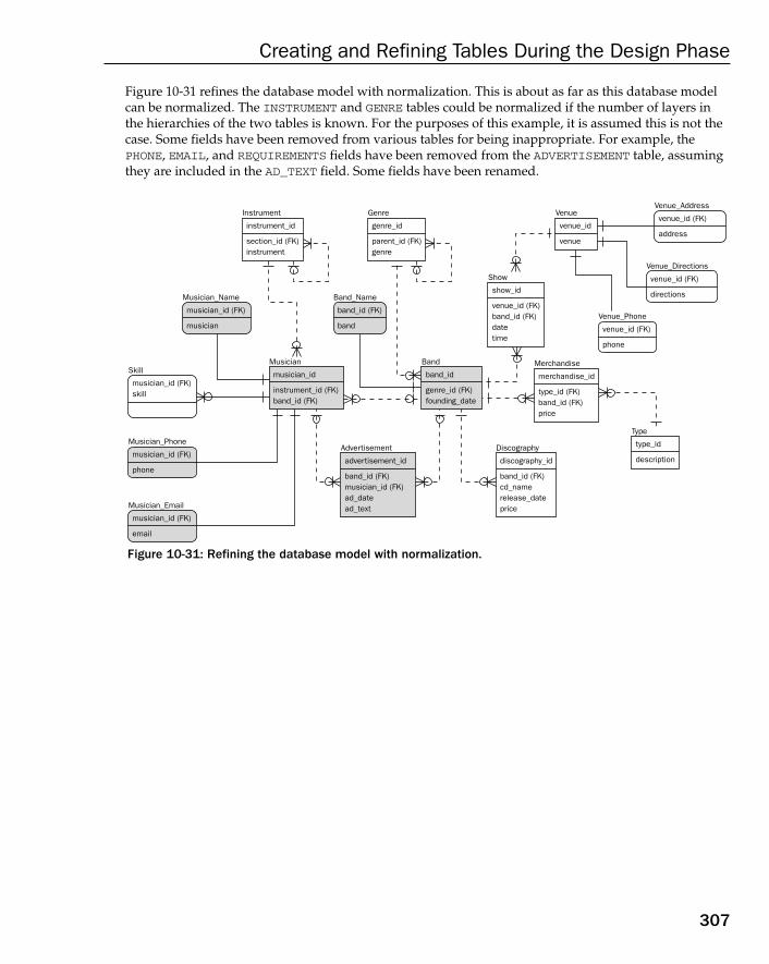
307
Creating and Refining Tables During the Design Phase
Figure 10-31 refines the database model with normalization. This is about as far as this database modelcan be normalized. The INSTRUMENT and GENRE tables could be normalized if the number of layers inthe hierarchies of the two tables is known. For the purposes of this example, it is assumed this is not thecase. Some fields have been removed from various tables for being inappropriate. For example, thePHONE, EMAIL, and REQUIREMENTS fields have been removed from the ADVERTISEMENT table, assumingthey are included in the AD_TEXT field. Some fields have been renamed.
Figure 10-31: Refining the database model with normalization.
Skill
musician_id (FK)skill
Musician_Phone
musician_id (FK)
phone
Venue_Phone
venue_id (FK)
phone
Venue_Directions
venue_id (FK)
directions
Venue_Address
venue_id (FK)
address
Musician_Name
musician_id (FK)
musician
Band_Name
band_id (FK)
band
Musician
musician_id
instrument_id (FK)band_id (FK)
Band
band_id
genre_id (FK)founding_date
Instrument
instrument_id
section_id (FK)instrument
Genre
genre_id
parent_id (FK)genre
Venue
venue_id
venue
Type
type_id
descriptionAdvertisement
advertisement_id
band_id (FK)musician_id (FK)ad_datead_text
Discography
discography_id
band_id (FK)cd_namerelease_dateprice
Merchandise
merchandise_id
type_id (FK)band_id (FK)price
Show
show_id
venue_id (FK)band_id (FK)datetime
Musician_Email
musician_id (FK)
16_574906 ch10.qxd 11/4/05 10:46 AM Page 307
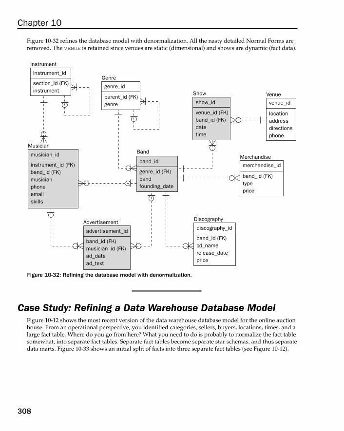
Figure 10-32 refines the database model with denormalization. All the nasty detailed Normal Forms areremoved. The VENUE is retained since venues are static (dimensional) and shows are dynamic (fact data).
Figure 10-32: Refining the database model with denormalization.
Case Study: Refining a Data Warehouse Database ModelFigure 10-12 shows the most recent version of the data warehouse database model for the online auctionhouse. From an operational perspective, you identified categories, sellers, buyers, locations, times, and alarge fact table. Where do you go from here? What you need to do is probably to normalize the fact tablesomewhat, into separate fact tables. Separate fact tables become separate star schemas, and thus separatedata marts. Figure 10-33 shows an initial split of facts into three separate fact tables (see Figure 10-12).
Instrument
section_id (FK)instrument
instrument_idGenre
parent_id (FK)genre
genre_id
Musician
instrument_id (FK)band_id (FK)musicianphoneemailskills
musician_id Band
genre_id (FK)bandfounding_date
band_id
Discography
band_id (FK)cd_namerelease_dateprice
discography_id
Merchandise
band_id (FK)typeprice
merchandise_id
Venue
locationaddressdirectionsphone
venue_id
Show
venue_id (FK)band_id (FK)datetime
show_id
Advertisement
band_id (FK)musician_id (FK)ad_datead_text
advertisement_id
308
Chapter 10
16_574906 ch10.qxd 11/4/05 10:46 AM Page 308
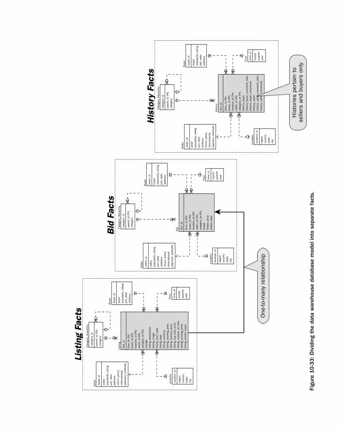
One
-to-m
any
rela
tions
hip
List
ing
Fact
sLi
stin
g Fa
cts
Sel
ler
selle
r_id
selle
rpo
pula
rity_
ratin
gjo
in_d
ate
addr
ess
retu
rn_p
olic
yin
tern
atio
nal
paym
ent_
met
hods
Loca
tion
loca
tion_
id
regi
onco
untr
yst
ate
city
Tim
e
time_
id
mon
thqu
arte
rye
ar
Cat
egor
y_H
iera
rchy
cate
gory
_id
pare
nt_i
d (F
K)
cate
gory
List
ing
fact
_id
time_
id (
FK)
buye
r_id
(FK
)lo
catio
n_id
(FK
)se
ller_
id (FK
)ca
tego
ry_i
d (F
K)
listin
g#lis
ting_
desc
riptio
nlis
ting_
imag
elis
ting_
star
t_da
telis
ting_
days
listin
g_cu
rren
cylis
ting_
star
ting_
pric
elis
ting_
rese
r ve_
pric
elis
ting_
buy_
now
_pric
elis
ting_
num
ber_
of_b
ids
listin
g_w
inni
ng_p
rice
listin
g_w
inne
r_bu
yer
Buy
er
buye
r_id
buye
rpo
pula
rity_
ratin
gjo
in_d
ate
addr
ess
Sel
ler
selle
r_id
selle
rpo
pula
rity_
ratin
gjo
in_d
ate
addr
ess
retu
rn_p
olic
yin
tern
atio
nal
paym
ent_
met
hods
Loca
tion
loca
tion_
id
regi
onco
untr
yst
ate
city
Tim
e
time_
id
mon
thqu
arte
rye
ar
Cat
egor
y_H
iera
rchy
cate
gory
_id
pare
n t_i
d (F
K)
cate
gory
Bid fa
ct_i
d
time_
id (FK
)bu
yer_
id (
FK)
loca
tion_
id (FK
)se
ller_
id (
FK)
cate
gory
_id
(FK
)bi
dder
bidd
er_p
rice
bidd
er_d
ate
Buy
er
buye
r_id
buye
rpo
pula
rity_
ratin
gjo
in_d
ate
addr
ess
Bid
Fac
tsB
id F
acts
Sel
ler
selle
r_id
selle
rpo
pula
rity_
ratin
gjo
in_d
ate
addr
ess
retu
rn_p
olic
yin
tern
atio
nal
paym
ent_
met
hods
Loca
tion
loca
tion_
id
regi
onco
untr
yst
ate
city
Tim
e
time_
id
mon
thqu
arte
rye
ar
Cat
egor
y_H
iera
rchy
cate
gory
_id
pare
nt_i
d (F
K)
cate
gory
His
tory
fact
_id
time_
id (
FK)
buye
r_id
(FK
)lo
catio
n_id
(FK
)se
ller_
id (
FK)
cate
gory
_id
(FK
)hi
stor
y_bu
yer
hist
ory_
buye
r_co
mm
ent_
date
hist
ory_
buye
r_co
mm
ents
hist
ory_
selle
rhi
stor
y_se
ller_
com
men
t_da
tehi
stor
y_se
ller_
com
men
ts
Buy
er
buye
r_id
buye
rpo
pula
rity_
ratin
gjo
in_d
ate
addr
ess
His
tory
Fac
tsH
isto
ry F
acts
His
torie
s pe
rtai
n to
selle
r s a
nd b
uyer
s on
ly
Figu
re 1
0-3
3: D
ivid
ing
the
data
war
ehou
se d
atab
ase
mod
el in
to s
epar
ate
fact
s.
16_574906 ch10.qxd 11/4/05 10:46 AM Page 309
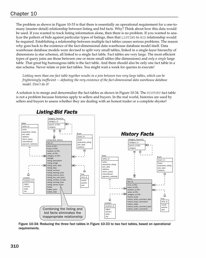
The problem as shown in Figure 10-33 is that there is essentially an operational requirement for a one-to-many (master-detail) relationship between listing and bid facts. Why? Think about how this data wouldbe used. If you wanted to track listing information alone, then there is no problem. If you wanted to ana-lyze the pattern of bids against particular types of listings, then that LISTING to BID relationship wouldbe required. Establishing a relationship between multiple fact tables causes serious problems. The reasonwhy goes back to the existence of the fact-dimensional data warehouse database model itself. Data warehouse database models were devised to split very small tables, linked in a single-layer hierarchy ofdimensions (a star schema), all linked to a single fact table. Fact tables are very large. The most efficienttypes of query joins are those between one or more small tables (the dimensions) and only a single largetable. That great big humungous table is the fact table. And there should also be only one fact table in astar schema. Never relate or join fact tables. You might wait a week for queries to execute!
Linking more than one fact table together results in a join between two very large tables, which can befrighteningly inefficient — defeating the very existence of the fact-dimensional data warehouse databasemodel. Don’t do it!
A solution is to merge and denormalize the fact tables as shown in Figure 10-34. The HISTORY fact tableis not a problem because histories apply to sellers and buyers. In the real world, histories are used bysellers and buyers to assess whether they are dealing with an honest trader or a complete shyster!
Figure 10-34: Reducing the three fact tables in Figure 10-33 to two fact tables, based on operationalrequirements.
Listing-Bid FactsListing-Bid Facts
Seller
seller_id
sellerpopularity_ratingjoin_dateaddressreturn_policyinternationalpayment_methods
Location
location_id
regioncountrystatecity
Time
time_id
monthquarteryear
Category_Hierarchy
category_id
parent_id (FK)category
Listing_Bids_History
fact_id
time_id (FK)buyer_id (FK)location_id (FK)seller_id (FK)category_id (FK)listing#listing_descriptionlisting_imagelisting_start_datelisting_dayslisting_currencylisting_starting_pricelisting_reserve_pricelisting_buy_now_pricelisting_number_of_bidslisting_winning_pricelisting_winner_buyerbidderbidder_pricebidder_date
Buyer
buyer_id
buyerpopularity_ratingjoin_dateaddress
Seller
seller_id
sellerpopularity_ratingjoin_dateaddressreturn_policyinternationalpayment_methods
Location
location_id
regioncountrystatecity
Time
time_id
monthquarteryear
Category_Hierarchy
category_id
parent_id (FK)category
History
fact_id
time_id (FK)buyer_id (FK)location_id (FK)seller_id (FK)category_id (FK)history_buyerhistory_buyer_comment_datehistory_buyer_commentshistory_sellerhistory_seller_comment_datehistory_seller_comments
Buyer
buyer_id
buyerpopularity_ratingjoin_dateaddress
History FactsHistory Facts
Combining the listing andbid facts eliminates the
inappropriate relationship
310
Chapter 10
16_574906 ch10.qxd 11/4/05 10:46 AM Page 310
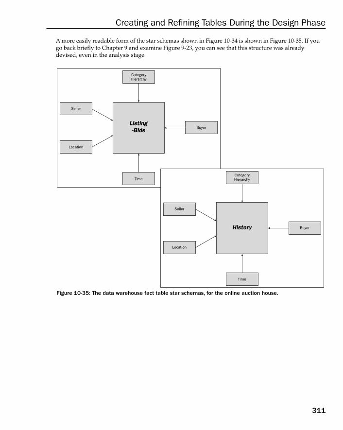
Creating and Refining Tables During the Design Phase
A more easily readable form of the star schemas shown in Figure 10-34 is shown in Figure 10-35. If yougo back briefly to Chapter 9 and examine Figure 9-23, you can see that this structure was alreadydevised, even in the analysis stage.
Figure 10-35: The data warehouse fact table star schemas, for the online auction house.
CategoryHierarchy
Time
Seller
Location
BuyerListing-Bids
Listing-Bids
Buyer
CategoryHierarchy
Time
Seller
Location
HistoryHistory
311
16_574906 ch10.qxd 11/4/05 10:46 AM Page 311
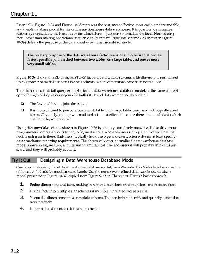
312
Chapter 10
Essentially, Figure 10-34 and Figure 10-35 represent the best, most effective, most easily understandable,and usable database model for the online auction house data warehouse. It is possible to normalize further by normalizing the heck out of the dimensions — just don’t normalize the facts. Normalizingfacts (other than making operational fact table splits into multiple star schemas, as shown in Figure10-34) defeats the purpose of the data warehouse dimensional-fact model.
Figure 10-36 shows an ERD of the HISTORY fact table snowflake schema, with dimensions normalizedup to gazoo! A snowflake schema is a star schema, where dimensions have been normalized.
There is no need to detail query examples for the data warehouse database model, as the same conceptsapply for SQL coding of query joins for both OLTP and data warehouse databases:
❑ The fewer tables in a join, the better.
❑ It is more efficient to join between a small table and a large table, compared with equally sizedtables. Obviously, joining two small tables is most efficient because there isn’t much data (whichshould be logical by now).
Using the snowflake schema shown in Figure 10-36 is not only completely nuts, it will also drive yourprogrammers completely nuts trying to figure it all out. And end-users simply won’t know what theheck is going on in there. End-users, typically in-house type end-users, often write (or at least specify)data warehouse reporting requirements. The obsessively over-normalized data warehouse databasemodel shown in Figure 10-36 is quite simply impractical. The end-users it will probably think it is justscary, and they will probably avoid it.
Try It Out Designing a Data Warehouse Database ModelCreate a simple design level data warehouse database model, for a Web site. This Web site allows creationof free classified ads for musicians and bands. Use the not-so-well-refined data warehouse databasemodel presented in Figure 10-37 (copied from Figure 9-29, in Chapter 9). Here’s a basic approach:
1. Refine dimensions and facts, making sure that dimensions are dimensions and facts are facts.
2. Divide facts into multiple star schemas if multiple, unrelated fact sets exist.
3. Normalize dimensions into a snowflake schema. This can help to identify and quantify dimensionsmore precisely.
4. Denormalize dimensions into a star schema.
The primary purpose of the data warehouse fact-dimensional model is to allow thefastest possible join method between two tables: one large table, and one or morevery small tables.
16_574906 ch10.qxd 11/4/05 10:46 AM Page 312
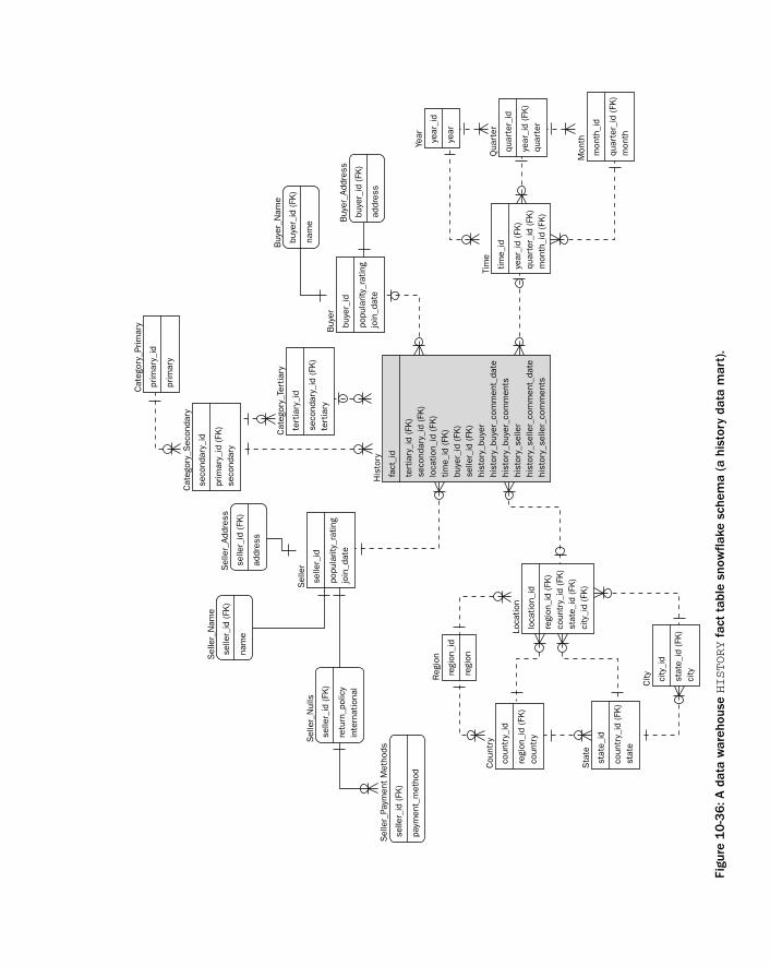
His
tory
fact
_id
tert
iar y
_id
(FK
)se
cond
ary_
id (FK
)lo
catio
n_id
(FK
)tim
e_id
(FK
)bu
yer_
id (FK
)se
ller_
id (FK
)hi
stor
y_bu
yer
hist
ory_
buye
r_co
mm
ent_
date
hist
ory_
buye
r_co
mm
ents
hist
ory_
selle
rhi
stor
y_se
ller_
com
men
t_da
tehi
stor
y_se
ller_
com
men
ts
Loca
tion
loca
tion_
id
regi
on_i
d (F
K)
coun
try_
id (FK
)st
ate_
id (FK
)ci
ty_i
d (F
K)
City city
_id
stat
e_id
(FK
)ci
ty
Sta
te
stat
e_id
coun
try_
id (FK
)st
ate
Cou
ntry
coun
try_
id
regi
on_i
d (F
K)
coun
try
Sel
ler
selle
r_id
popu
larit
y_ra
ting
join
_dat
e
Cat
egor
y_S
econ
dary
seco
ndar
y_id
prim
ary_
id (FK
)se
cond
ary
Cat
egor
y_Te
rtia
ry
ter t
iary
_id
seco
ndar
y_id
(FK
)te
r tia
r yB
uyer
buye
r_id
popu
larit
y_ra
ting
join
_dat
e
Tim
e
time_
id
year
_id
(FK
)qu
arte
r_id
(FK
)m
onth
_id
(FK
)
Qua
rter
quar
ter_
id
year
_id
(FK
)qu
arte
r
Mon
th
mon
th_i
d
quar
ter_
id (FK
)m
onth
Yea r year
_id
year
Buy
er_N
ame
buye
r_id
(FK
)
nam
e Buy
er_A
ddre
ss
buye
r_id
(FK
)
addr
ess
Cat
egor
y_Pr
imar
y
prim
ary_
id
prim
ary
Sel
ler_
Nul
ls
selle
r_id
(FK
)
retu
rn_p
olic
yin
tern
atio
nal
Sel
ler_
Paym
ent
Met
hods
selle
r_id
(FK
)
paym
ent_
met
hod
Sel
ler_
Nam
e
selle
r_id
(FK
)
nam
e
Sel
ler_
Addr
ess
selle
r_id
(FK
)
addr
ess
Reg
ion
regi
on_i
d
regi
on
Figu
re 1
0-3
6: A
dat
a w
areh
ouse
HISTORY
fact
tab
le s
now
flake
sch
ema
(a h
isto
ry d
ata
mar
t).
16_574906 ch10.qxd 11/4/05 10:46 AM Page 313

314
Chapter 10
Figure 10-37: Musicians, bands, their online advertisements, and some other goodies.
How It WorksFigure 10-37 shows the analyzed data warehouse database model, for online musician and band advertisements. The most significant requirement is to ultimately produce a single star schema, if a single star schema is possible. Also add any dimensional and fact information shown as additional inFigure 10-32. Figure 10-37 shows that the SHOW table is actually fact information, not dimensional.
Examine Figure 10-37 once more. Think about the records in the tables. Yes, many advertisements arepossible. However, a simple search of the Internet on Web sites such as www.themode.com andwww.ticketmaster.com will reveal to you the sheer volume of advertisements, musicians, bands,shows, discography (released CDs), and venues. Figure 10-38 takes another slant on this data warehousedatabase model by rolling all of these tables into a single fact table.
Musician
musician_id
musicianphoneemailinstrumentsskills
Advertisement
advertisement_id
band_id (FK)musician_id (FK)ad_datead_text
Band
band_id
bandfounding_dategenre
Discography
discography_id
band_id (FK)cd_namerelease_dateprice
Merchandise
merchandise_id
band_id (FK)typeprice
Show
show_id
venue_id (FK)band_id (FK)venuedatetime
Venue
venue_id
venueaddressdirectionsphone
16_574906 ch10.qxd 11/4/05 10:46 AM Page 314
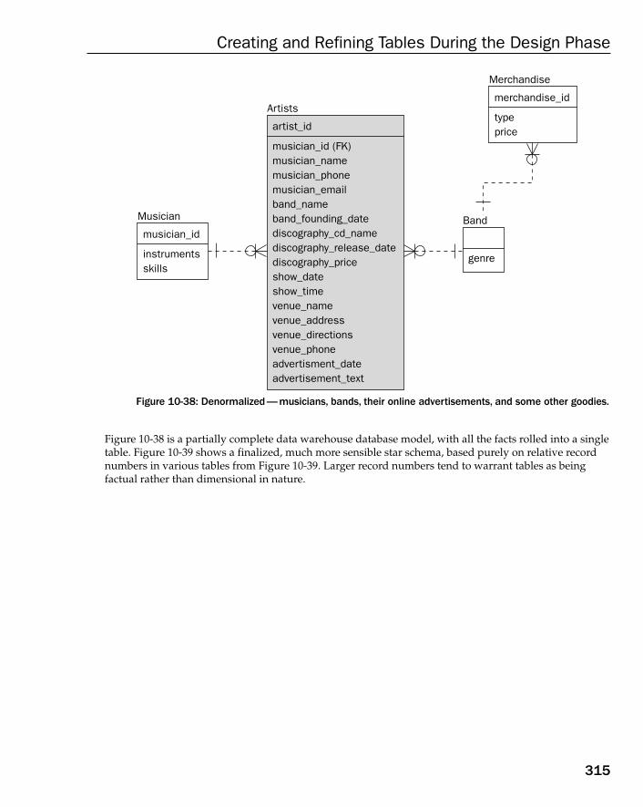
Figure 10-38: Denormalized—musicians, bands, their online advertisements, and some other goodies.
Figure 10-38 is a partially complete data warehouse database model, with all the facts rolled into a singletable. Figure 10-39 shows a finalized, much more sensible star schema, based purely on relative recordnumbers in various tables from Figure 10-39. Larger record numbers tend to warrant tables as being factual rather than dimensional in nature.
Artists
artist_id
musician_id (FK)musician_namemusician_phonemusician_emailband_nameband_founding_datediscography_cd_namediscography_release_datediscography_priceshow_dateshow_timevenue_namevenue_addressvenue_directionsvenue_phoneadvertisment_dateadvertisement_text
Musician
musician_id
instrumentsskills
Merchandise
merchandise_id
typeprice
Band
genre
315
Creating and Refining Tables During the Design Phase
16_574906 ch10.qxd 11/4/05 10:46 AM Page 315
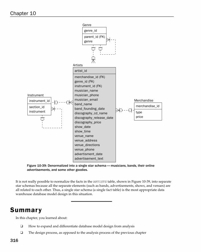
Figure 10-39: Denormalized into a single star schema — musicians, bands, their onlineadvertisements, and some other goodies.
It is not really possible to normalize the facts in the ARTISTS table, shown in Figure 10-39, into separatestar schemas because all the separate elements (such as bands, advertisements, shows, and venues) areall related to each other. Thus, a single star schema (a single fact table) is the most appropriate datawarehouse database model design in this situation.
SummaryIn this chapter, you learned about:
❑ How to expand and differentiate database model design from analysis
❑ The design process, as opposed to the analysis process of the previous chapter
Artists
artist_id
merchandise_id (FK)genre_id (FK)instrument_id (FK)musician_namemusician_phonemusician_emailband_nameband_founding_datediscography_cd_namediscography_release_datediscography_priceshow_dateshow_timevenue_namevenue_addressvenue_directionsvenue_phoneadvertisment_dateadvertisement_text
Instrument
instrument_id
section_idinstrument
Merchandise
merchandise_id
typeprice
Genre
genre_id
parent_id (FK)genre
316
Chapter 10
16_574906 ch10.qxd 11/4/05 10:46 AM Page 316
❑ How to create and refine tables
❑ How to enforce and refine inter-table relationships and referential integrity
❑ Normalization (without going too far)
❑ Denormalization (without going too far)
❑ The folly of normalization beyond 3NFs, for both OLTP and data warehouse databases
❑ Providing for application usability, flexibility, and performance in database modeling
❑ How to ensure applications translate into happy end-users (without happy end-users, there isno profit, and, thus, no company)
This chapter has primarily expanded on Chapter 9, from analysis (what to do), into design (how to solveit). Once again, the online auction house database model has been expanded on, and detailed further bythe design process, as the continuing case study. Chapter 11 digs even further into the design process bydescribing and specifying fields within each table, along with datatypes and indexing. The discussion onindexing is especially about alternate (secondary) indexing.
ExercisesUse the ERDs in Figure 10-32 and Figure 10-39 to help you answer these questions:
1. Create scripts to create tables for the OLTP database model shown in Figure 10-32. Create thetables in the proper order by understanding the relationships between the tables.
2. Create scripts to create tables for the data warehouse database model shown in Figure 10-39.Once again, create the tables in the proper order by understanding the relationships betweenthe tables.
317
Creating and Refining Tables During the Design Phase
16_574906 ch10.qxd 11/4/05 10:46 AM Page 317

16_574906 ch10.qxd 11/4/05 10:46 AM Page 318

11Filling in the Details with
a Detailed Design
“Digging ever deeper gives clarity to definition, and definition of clarity.” (Gavin Powell)
The further you go the more you discover.
This chapter provides the details on the internal structure of tables in terms of fields, field content,field formatting, and indexing on fields. This chapter digs a little deeper into the case study mate-rial presented in the previous two chapters. Chapter 9 introduced a database model in its infancy,by analyzing what needed to be done. Chapter 10 unearthed structural detail by describing howtables are built and how they are joined together.
This chapter delves into the details of the tables themselves, by designing the precise content andstructure of individual fields. Indexing is included at this stage because indexes are created againstspecific table fields. An index is not quite the same thing as a key, such as a primary key. A pri-mary key is required to be unique across all records in a table; therefore, many database enginesusually create an automatic unique index for that primary key (which helps performance bychecking for uniqueness). Foreign keys, on the other hand, do not have to be unique, and even themost sophisticated of relational databases does not automatically create indexes on foreign keys.This is intentional of course. If an index is required on a foreign key field (which it more often thannot is), an index must be manually created for that foreign key.
By the end of this chapter, you will have a good understanding of how best to structure fields,their datatype formats, how, when and where those formats apply. Also, you will have a betterconceptual understanding of foreign key indexing and alternate (secondary) indexing.
In this chapter, you learn about the following:
❑ Refining field structure and content in tables
❑ Using datatypes
❑ The difference between simple datatypes, ANSI datatypes, Microsoft Access datatypesand some specialized datatypes
17_574906 ch11.qxd 10/28/05 11:38 PM Page 319
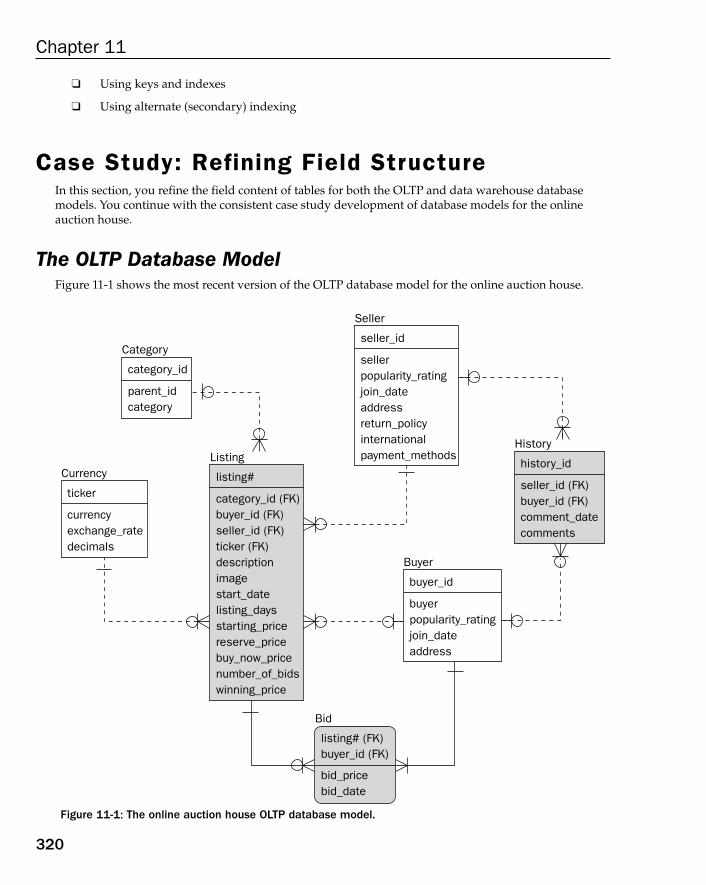
❑ Using keys and indexes
❑ Using alternate (secondary) indexing
Case Study: Refining Field StructureIn this section, you refine the field content of tables for both the OLTP and data warehouse databasemodels. You continue with the consistent case study development of database models for the online auction house.
The OLTP Database ModelFigure 11-1 shows the most recent version of the OLTP database model for the online auction house.
Figure 11-1: The online auction house OLTP database model.
History
history_id
seller_id (FK)buyer_id (FK)comment_datecomments
Listing
listing#
category_id (FK)buyer_id (FK)seller_id (FK)ticker (FK)descriptionimagestart_datelisting_daysstarting_pricereserve_pricebuy_now_pricenumber_of_bidswinning_price
Category
category_id
parent_idcategory
Currency
ticker
currencyexchange_ratedecimals
Seller
seller_id
sellerpopularity_ratingjoin_dateaddressreturn_policyinternationalpayment_methods
Buyer
buyer_id
buyerpopularity_ratingjoin_dateaddress
Bid
listing# (FK)buyer_id (FK)
bid_pricebid_date
320
Chapter 11
17_574906 ch11.qxd 10/28/05 11:38 PM Page 320
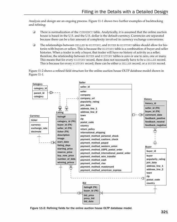
Analysis and design are an ongoing process. Figure 11-1 shows two further examples of backtrackingand refining:
❑ There is normalization of the CURRENCY table. Analytically, it is assumed that the online auctionhouse is based in the U.S. and the U.S. dollar is the default currency. Currencies are separatedbecause there can be a fair amount of complexity involved in currency exchange conversions.
❑ The relationships between SELLER to HISTORY, and BUYER to HISTORY tables should allow for his-tories with buyers or sellers. This is because the HISTORY table is a combination of buyer and sellerhistories. When a trader is only a buyer, that trader will have no history of activity as a seller;therefore, the relationship between BUYER and HISTORY tables is zero or one to zero, one or many.This means that for every HISTORY record, there does not necessarily have to be a SELLER record.This is because for every HISTORY record, there can be either a SELLER record, or a BUYER record.
Figure 11-2 shows a refined field structure for the online auction house OLTP database model shown inFigure 11-1.
Figure 11-2: Refining fields for the online auction house OLTP database model.
History
history_id
seller_id (FK)buyer_id (FK)comment_datefeedback_positivefeedback_neutralfeedback_negative
Listing
listing#
category_id (FK)buyer_id (FK)seller_id (FK)ticker (FK)descriptionimagestart_datelisting_daysstarting_pricereserve_pricebuy_now_pricenumber_of_bidswinning_prince
Category
category_id
parent_idcategory
Currency
ticker
currencyexchange_ratedecimals
Seller
seller_id
sellercompanycompany_urlpopularity_ratingjoin_dateaddress_line_1address_line_2townzippostal_codecountryreturn_policyinternational_shippingpayment_method_personal_checkpayment_method_cashiers_checkpayment_method_paypalpayment_method_western_unionpayment_method_USPS_postal_orderpayment_method_international_postal_orderpayment_method_wire_transferpayment_method_cashpayment_method_visapayment_method_mastercardpayment_method_american_express
Buyer
buyer_id
buyerpopularity_ratingjoin_dateaddress_line_1address_line_2townzippostal_codecountryBid
listing# (FK)buyer_id (FK)
bid_priceproxy_bidbid_date
321
Filling in the Details with a Detailed Design
17_574906 ch11.qxd 10/28/05 11:38 PM Page 321
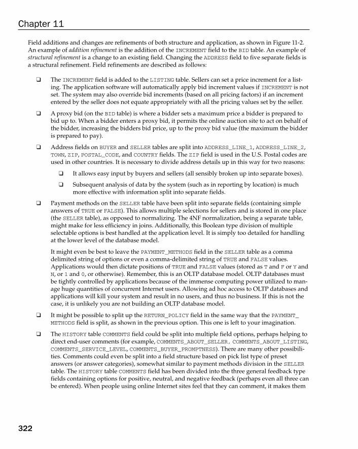
Field additions and changes are refinements of both structure and application, as shown in Figure 11-2.An example of addition refinement is the addition of the INCREMENT field to the BID table. An example ofstructural refinement is a change to an existing field. Changing the ADDRESS field to five separate fields isa structural refinement. Field refinements are described as follows:
❑ The INCREMENT field is added to the LISTING table. Sellers can set a price increment for a list-ing. The application software will automatically apply bid increment values if INCREMENT is notset. The system may also override bid increments (based on all pricing factors) if an incremententered by the seller does not equate appropriately with all the pricing values set by the seller.
❑ A proxy bid (on the BID table) is where a bidder sets a maximum price a bidder is prepared tobid up to. When a bidder enters a proxy bid, it permits the online auction site to act on behalf ofthe bidder, increasing the bidders bid price, up to the proxy bid value (the maximum the bidderis prepared to pay).
❑ Address fields on BUYER and SELLER tables are split into ADDRESS_LINE_1, ADDRESS_LINE_2,TOWN, ZIP, POSTAL_CODE, and COUNTRY fields. The ZIP field is used in the U.S. Postal codes areused in other countries. It is necessary to divide address details up in this way for two reasons:
❑ It allows easy input by buyers and sellers (all sensibly broken up into separate boxes).
❑ Subsequent analysis of data by the system (such as in reporting by location) is muchmore effective with information split into separate fields.
❑ Payment methods on the SELLER table have been split into separate fields (containing simpleanswers of TRUE or FALSE). This allows multiple selections for sellers and is stored in one place(the SELLER table), as opposed to normalizing. The 4NF normalization, being a separate table,might make for less efficiency in joins. Additionally, this Boolean type division of multipleselectable options is best handled at the application level. It is simply too detailed for handlingat the lower level of the database model.
It might even be best to leave the PAYMENT_METHODS field in the SELLER table as a commadelimited string of options or even a comma-delimited string of TRUE and FALSE values.Applications would then dictate positions of TRUE and FALSE values (stored as T and F or Y andN, or 1 and 0, or otherwise). Remember, this is an OLTP database model. OLTP databases mustbe tightly controlled by applications because of the immense computing power utilized to man-age huge quantities of concurrent Internet users. Allowing ad hoc access to OLTP databases andapplications will kill your system and result in no users, and thus no business. If this is not thecase, it is unlikely you are not building an OLTP database model.
❑ It might be possible to split up the RETURN_POLICY field in the same way that the PAYMENT_METHODS field is split, as shown in the previous option. This one is left to your imagination.
❑ The HISTORY table COMMENTS field could be split into multiple field options, perhaps helping todirect end-user comments (for example, COMMENTS_ABOUT_SELLER, COMMENTS_ABOUT_LISTING,COMMENTS_SERVICE_LEVEL, COMMENTS_BUYER_PROMPTNESS). There are many other possibili-ties. Comments could even be split into a field structure based on pick list type of presetanswers (or answer categories), somewhat similar to payment methods division in the SELLERtable. The HISTORY table COMMENTS field has been divided into the three general feedback typefields containing options for positive, neutral, and negative feedback (perhaps even all three canbe entered). When people using online Internet sites feel that they can comment, it makes them
322
Chapter 11
17_574906 ch11.qxd 10/28/05 11:38 PM Page 322
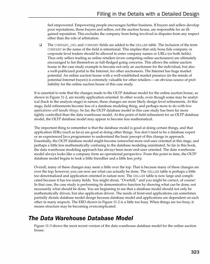
feel empowered. Empowering people encourages further business. If buyers and sellers developpoor reputations, those buyers and sellers, not the auction house, are responsible for an ill-gained reputation. This excludes the company from being involved in disputes from any respectother than the role of arbitration.
❑ The COMPANY_URL and COMPANY fields are added to the SELLER table. The inclusion of the termCOMPANY in the name of the field is intentional. This implies that only bona fide company or corporate level traders should be allowed to enter company names or URLs (or both fields).Thus only sellers trading as online retailers (even competing online auctioneers) are ultimatelyencouraged to list themselves as full-fledged going concerns. This allows the online auctionhouse in the case study example to become not only an auctioneer for the individual, but also a well-publicized portal to the Internet, for other auctioneers. The Internet has huge marketpotential. An online auction house with a well-established market presence (in the minds ofpotential Internet buyers) is extremely valuable for other retailers — an obvious source of prof-itability for the online auction house of this case study.
It is essential to note that the changes made to the OLTP database model for the online auction house, asshown in Figure 11-2, are mostly application-oriented. In other words, even though some may be analyt-ical (back to the analysis stage) in nature, these changes are more likely design level refinements. At thisstage, field refinements become less of a database modeling thing, and perhaps more to do with howapplications will handle things. So far, the OLTP database model in this case study has been far moretightly controlled than the data warehouse model. At this point of field refinement for an OLTP databasemodel, the OLTP database model may appear to become less mathematical.
The important thing to remember is that the database model is good at doing certain things, and thatapplication SDKs (such as Java) are good at doing other things. You don’t need to be a database expertor an experienced Java programmer to understand the basic precept of this change in approach.Essentially, the OLTP database model might become somewhat more end-user oriented at this stage, andperhaps a little less mathematically confusing to the database modeling uninitiated. So far in this book,the data warehouse modeling approach has always been more end-user oriented. The data warehousemodel always looks like a company from an operational perspective. From this point in time, the OLTPdatabase model begins to look a little friendlier and a little less geeky.
Overall, many of these changes may seem a little over the top. That is because many of these changes areover the top; however, you can now see what can actually be done. The SELLER table is perhaps a littletoo denormalized and application oriented in nature now. The SELLER table is now large and compli-cated because it has too many fields. You might shout, “Overkill,” and you might be correct, of course!In that case, the case study is performing its demonstrative function by showing what can be done, notnecessarily what should be done. You are beginning to see that a database model should not only bemathematically driven, but also application driven. The needs of front-end applications can sometimespartially dictate database model design because database model and applications are dependent on eachother in many respects. The ERD shown in Figure 11-2 is a little too busy. When things are too busy, itmeans structure may be becoming overcomplicated.
The Data Warehouse Database ModelFigure 11-3 shows the most recent version of the data warehouse database model for the online auctionhouse.
323
Filling in the Details with a Detailed Design
17_574906 ch11.qxd 10/28/05 11:38 PM Page 323
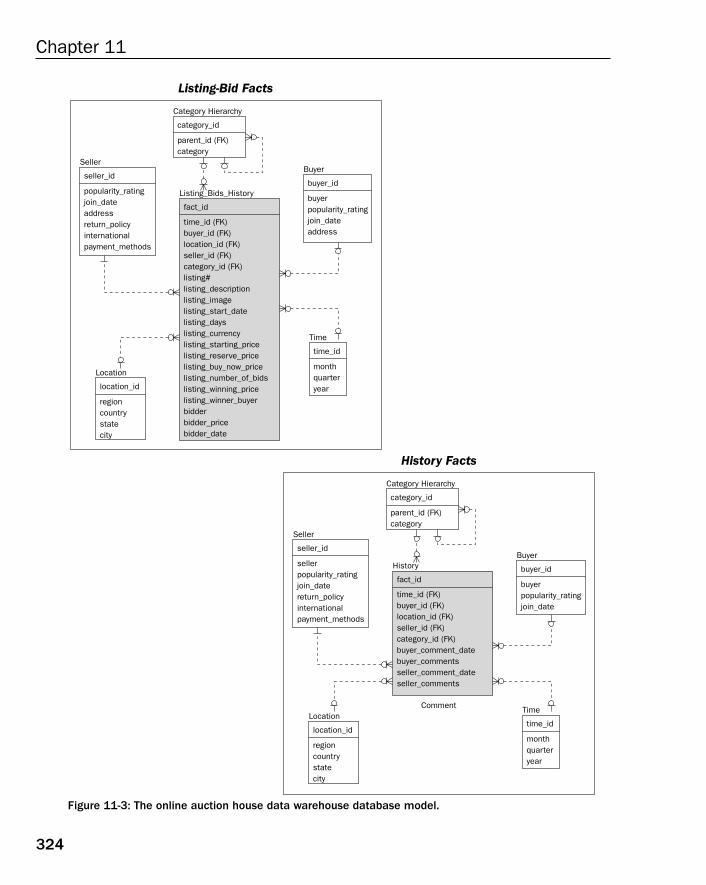
Figure 11-3: The online auction house data warehouse database model.
Category Hierarchy
Listing-Bid Facts
category_id
parent_id (FK)category
Seller
seller_id
popularity_ratingjoin_dateaddress return_policyinternationalpayment_methods
Buyer
buyer_id
buyerpopularity_ratingjoin_dateaddress
Listing_Bids_History
fact_id
time_id (FK)buyer_id (FK)location_id (FK)seller_id (FK)category_id (FK)listing#listing_descriptionlisting_imagelisting_start_datelisting_dayslisting_currencylisting_starting_pricelisting_reserve_pricelisting_buy_now_pricelisting_number_of_bidslisting_winning_pricelisting_winner_buyerbidderbidder_pricebidder_date
Time
time_id
monthquarteryear
Location
location_id
regioncountrystatecity
History Facts
Category Hierarchy
category_id
parent_id (FK)category
Seller
seller_id
sellerpopularity_ratingjoin_date return_policyinternationalpayment_methods
Buyer
buyer_id
buyerpopularity_ratingjoin_date
History
Comment
fact_id
time_id (FK)buyer_id (FK)location_id (FK)seller_id (FK)category_id (FK)buyer_comment_datebuyer_commentsseller_comment_dateseller_comments
Time
time_id
monthquarteryear
Location
location_id
regioncountrystatecity
324
Chapter 11
17_574906 ch11.qxd 10/28/05 11:38 PM Page 324
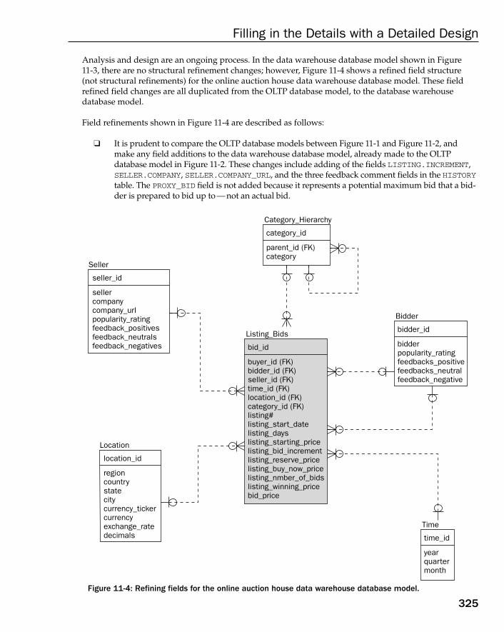
Analysis and design are an ongoing process. In the data warehouse database model shown in Figure11-3, there are no structural refinement changes; however, Figure 11-4 shows a refined field structure(not structural refinements) for the online auction house data warehouse database model. These fieldrefined field changes are all duplicated from the OLTP database model, to the database warehousedatabase model.
Field refinements shown in Figure 11-4 are described as follows:
❑ It is prudent to compare the OLTP database models between Figure 11-1 and Figure 11-2, andmake any field additions to the data warehouse database model, already made to the OLTPdatabase model in Figure 11-2. These changes include adding of the fields LISTING.INCREMENT,SELLER.COMPANY, SELLER.COMPANY_URL, and the three feedback comment fields in the HISTORYtable. The PROXY_BID field is not added because it represents a potential maximum bid that a bid-der is prepared to bid up to — not an actual bid.
Figure 11-4: Refining fields for the online auction house data warehouse database model.
Seller
seller_id
sellercompanycompany_urlpopularity_ratingfeedback_positivesfeedback_neutralsfeedback_negatives
Location
location_id
regioncountrystatecitycurrency_tickercurrencyexchange_ratedecimals
Category_Hierarchy
category_id
parent_id (FK)category
Bidder
bidder_id
bidderpopularity_ratingfeedbacks_positivefeedbacks_neutralfeedback_negative
Listing_Bids
bid_id
buyer_id (FK)bidder_id (FK)seller_id (FK)time_id (FK)location_id (FK)category_id (FK)listing#listing_start_datelisting_dayslisting_starting_pricelisting_bid_incrementlisting_reserve_pricelisting_buy_now_pricelisting_nmber_of_bidslisting_winning_pricebid_price
Time
time_id
yearquartermonth
325
Filling in the Details with a Detailed Design
17_574906 ch11.qxd 10/28/05 11:38 PM Page 325
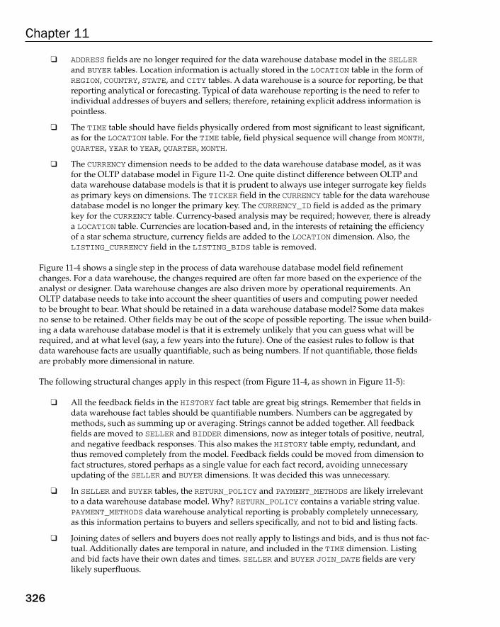
❑ ADDRESS fields are no longer required for the data warehouse database model in the SELLERand BUYER tables. Location information is actually stored in the LOCATION table in the form ofREGION, COUNTRY, STATE, and CITY tables. A data warehouse is a source for reporting, be thatreporting analytical or forecasting. Typical of data warehouse reporting is the need to refer toindividual addresses of buyers and sellers; therefore, retaining explicit address information ispointless.
❑ The TIME table should have fields physically ordered from most significant to least significant,as for the LOCATION table. For the TIME table, field physical sequence will change from MONTH,QUARTER, YEAR to YEAR, QUARTER, MONTH.
❑ The CURRENCY dimension needs to be added to the data warehouse database model, as it wasfor the OLTP database model in Figure 11-2. One quite distinct difference between OLTP anddata warehouse database models is that it is prudent to always use integer surrogate key fieldsas primary keys on dimensions. The TICKER field in the CURRENCY table for the data warehousedatabase model is no longer the primary key. The CURRENCY_ID field is added as the primarykey for the CURRENCY table. Currency-based analysis may be required; however, there is alreadya LOCATION table. Currencies are location-based and, in the interests of retaining the efficiencyof a star schema structure, currency fields are added to the LOCATION dimension. Also, theLISTING_CURRENCY field in the LISTING_BIDS table is removed.
Figure 11-4 shows a single step in the process of data warehouse database model field refinementchanges. For a data warehouse, the changes required are often far more based on the experience of theanalyst or designer. Data warehouse changes are also driven more by operational requirements. AnOLTP database needs to take into account the sheer quantities of users and computing power needed to be brought to bear. What should be retained in a data warehouse database model? Some data makesno sense to be retained. Other fields may be out of the scope of possible reporting. The issue when build-ing a data warehouse database model is that it is extremely unlikely that you can guess what will berequired, and at what level (say, a few years into the future). One of the easiest rules to follow is thatdata warehouse facts are usually quantifiable, such as being numbers. If not quantifiable, those fields are probably more dimensional in nature.
The following structural changes apply in this respect (from Figure 11-4, as shown in Figure 11-5):
❑ All the feedback fields in the HISTORY fact table are great big strings. Remember that fields indata warehouse fact tables should be quantifiable numbers. Numbers can be aggregated bymethods, such as summing up or averaging. Strings cannot be added together. All feedbackfields are moved to SELLER and BIDDER dimensions, now as integer totals of positive, neutral,and negative feedback responses. This also makes the HISTORY table empty, redundant, andthus removed completely from the model. Feedback fields could be moved from dimension tofact structures, stored perhaps as a single value for each fact record, avoiding unnecessaryupdating of the SELLER and BUYER dimensions. It was decided this was unnecessary.
❑ In SELLER and BUYER tables, the RETURN_POLICY and PAYMENT_METHODS are likely irrelevantto a data warehouse database model. Why? RETURN_POLICY contains a variable string value.PAYMENT_METHODS data warehouse analytical reporting is probably completely unnecessary, as this information pertains to buyers and sellers specifically, and not to bid and listing facts.
❑ Joining dates of sellers and buyers does not really apply to listings and bids, and is thus not fac-tual. Additionally dates are temporal in nature, and included in the TIME dimension. Listingand bid facts have their own dates and times. SELLER and BUYER JOIN_DATE fields are verylikely superfluous.
326
Chapter 11
17_574906 ch11.qxd 10/28/05 11:38 PM Page 326
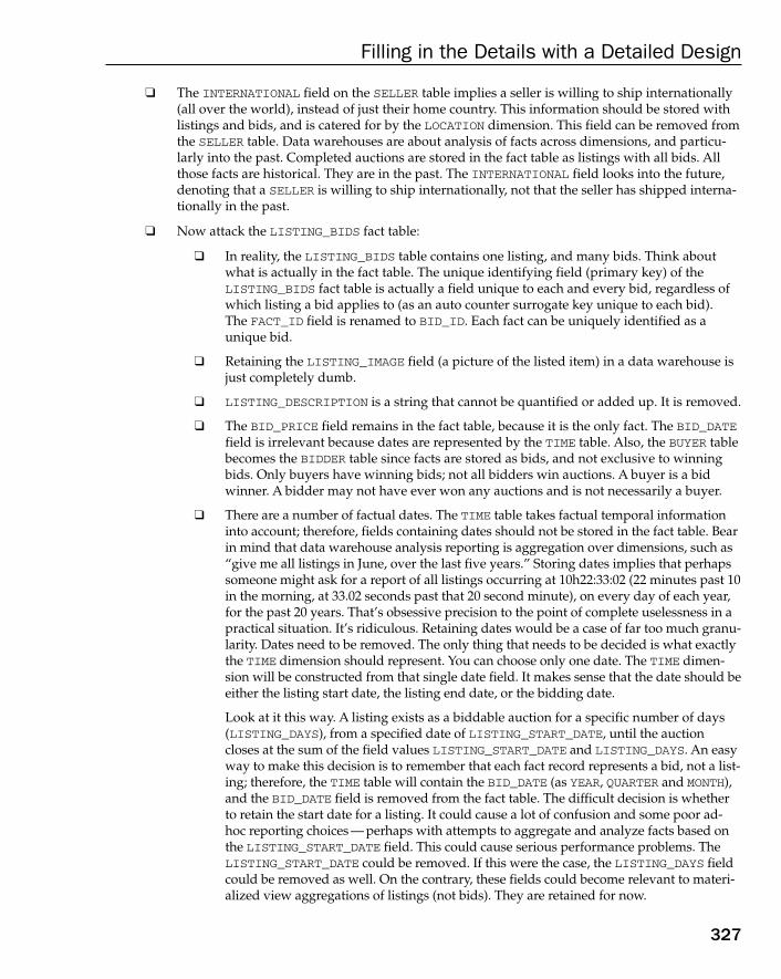
❑ The INTERNATIONAL field on the SELLER table implies a seller is willing to ship internationally(all over the world), instead of just their home country. This information should be stored withlistings and bids, and is catered for by the LOCATION dimension. This field can be removed fromthe SELLER table. Data warehouses are about analysis of facts across dimensions, and particu-larly into the past. Completed auctions are stored in the fact table as listings with all bids. Allthose facts are historical. They are in the past. The INTERNATIONAL field looks into the future,denoting that a SELLER is willing to ship internationally, not that the seller has shipped interna-tionally in the past.
❑ Now attack the LISTING_BIDS fact table:
❑ In reality, the LISTING_BIDS table contains one listing, and many bids. Think aboutwhat is actually in the fact table. The unique identifying field (primary key) of theLISTING_BIDS fact table is actually a field unique to each and every bid, regardless ofwhich listing a bid applies to (as an auto counter surrogate key unique to each bid). The FACT_ID field is renamed to BID_ID. Each fact can be uniquely identified as aunique bid.
❑ Retaining the LISTING_IMAGE field (a picture of the listed item) in a data warehouse isjust completely dumb.
❑ LISTING_DESCRIPTION is a string that cannot be quantified or added up. It is removed.
❑ The BID_PRICE field remains in the fact table, because it is the only fact. The BID_DATEfield is irrelevant because dates are represented by the TIME table. Also, the BUYER tablebecomes the BIDDER table since facts are stored as bids, and not exclusive to winningbids. Only buyers have winning bids; not all bidders win auctions. A buyer is a bid winner. A bidder may not have ever won any auctions and is not necessarily a buyer.
❑ There are a number of factual dates. The TIME table takes factual temporal informationinto account; therefore, fields containing dates should not be stored in the fact table. Bearin mind that data warehouse analysis reporting is aggregation over dimensions, such as“give me all listings in June, over the last five years.” Storing dates implies that perhapssomeone might ask for a report of all listings occurring at 10h22:33:02 (22 minutes past 10in the morning, at 33.02 seconds past that 20 second minute), on every day of each year,for the past 20 years. That’s obsessive precision to the point of complete uselessness in apractical situation. It’s ridiculous. Retaining dates would be a case of far too much granu-larity. Dates need to be removed. The only thing that needs to be decided is what exactlythe TIME dimension should represent. You can choose only one date. The TIME dimen-sion will be constructed from that single date field. It makes sense that the date should beeither the listing start date, the listing end date, or the bidding date.
Look at it this way. A listing exists as a biddable auction for a specific number of days(LISTING_DAYS), from a specified date of LISTING_START_DATE, until the auctioncloses at the sum of the field values LISTING_START_DATE and LISTING_DAYS. An easyway to make this decision is to remember that each fact record represents a bid, not a list-ing; therefore, the TIME table will contain the BID_DATE (as YEAR, QUARTER and MONTH),and the BID_DATE field is removed from the fact table. The difficult decision is whetherto retain the start date for a listing. It could cause a lot of confusion and some poor ad-hoc reporting choices — perhaps with attempts to aggregate and analyze facts based onthe LISTING_START_DATE field. This could cause serious performance problems. TheLISTING_START_DATE could be removed. If this were the case, the LISTING_DAYS fieldcould be removed as well. On the contrary, these fields could become relevant to materi-alized view aggregations of listings (not bids). They are retained for now.
327
Filling in the Details with a Detailed Design
17_574906 ch11.qxd 10/28/05 11:38 PM Page 327
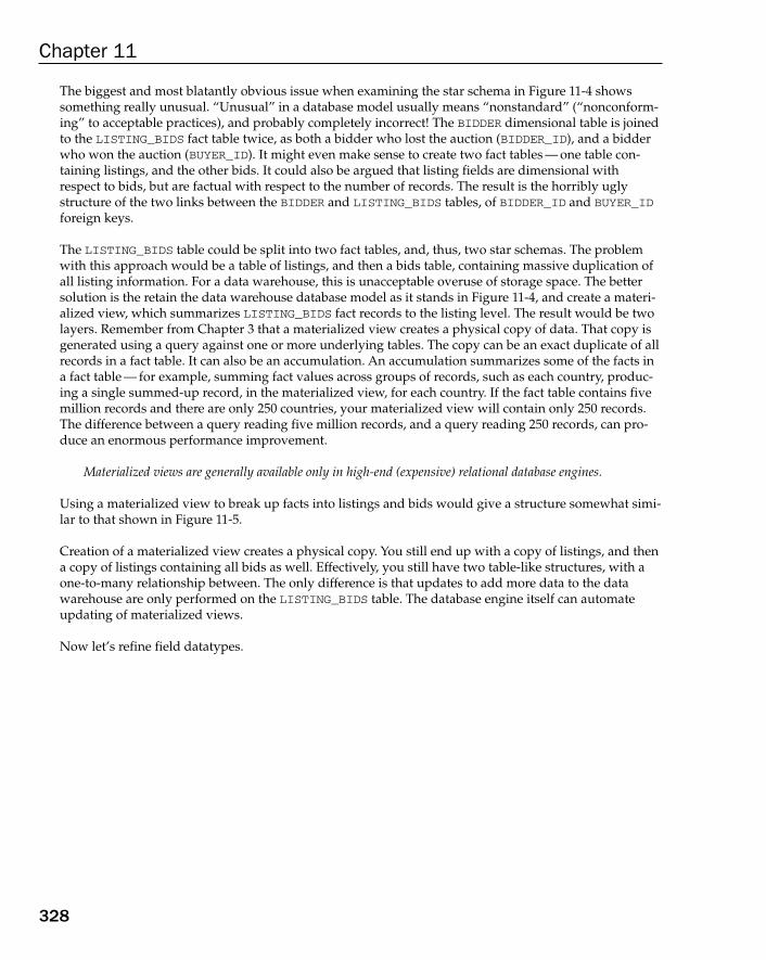
The biggest and most blatantly obvious issue when examining the star schema in Figure 11-4 showssomething really unusual. “Unusual” in a database model usually means “nonstandard” (“nonconform-ing” to acceptable practices), and probably completely incorrect! The BIDDER dimensional table is joinedto the LISTING_BIDS fact table twice, as both a bidder who lost the auction (BIDDER_ID), and a bidderwho won the auction (BUYER_ID). It might even make sense to create two fact tables — one table con-taining listings, and the other bids. It could also be argued that listing fields are dimensional withrespect to bids, but are factual with respect to the number of records. The result is the horribly uglystructure of the two links between the BIDDER and LISTING_BIDS tables, of BIDDER_ID and BUYER_IDforeign keys.
The LISTING_BIDS table could be split into two fact tables, and, thus, two star schemas. The problemwith this approach would be a table of listings, and then a bids table, containing massive duplication ofall listing information. For a data warehouse, this is unacceptable overuse of storage space. The bettersolution is the retain the data warehouse database model as it stands in Figure 11-4, and create a materi-alized view, which summarizes LISTING_BIDS fact records to the listing level. The result would be twolayers. Remember from Chapter 3 that a materialized view creates a physical copy of data. That copy isgenerated using a query against one or more underlying tables. The copy can be an exact duplicate of allrecords in a fact table. It can also be an accumulation. An accumulation summarizes some of the facts ina fact table — for example, summing fact values across groups of records, such as each country, produc-ing a single summed-up record, in the materialized view, for each country. If the fact table contains fivemillion records and there are only 250 countries, your materialized view will contain only 250 records.The difference between a query reading five million records, and a query reading 250 records, can pro-duce an enormous performance improvement.
Materialized views are generally available only in high-end (expensive) relational database engines.
Using a materialized view to break up facts into listings and bids would give a structure somewhat simi-lar to that shown in Figure 11-5.
Creation of a materialized view creates a physical copy. You still end up with a copy of listings, and thena copy of listings containing all bids as well. Effectively, you still have two table-like structures, with aone-to-many relationship between. The only difference is that updates to add more data to the datawarehouse are only performed on the LISTING_BIDS table. The database engine itself can automateupdating of materialized views.
Now let’s refine field datatypes.
328
Chapter 11
17_574906 ch11.qxd 10/28/05 11:38 PM Page 328

Figure 11-5: Refining facts and dimensions using materialized views to replace fact hierarchicalstructures.
Understanding DatatypesA datatype is a format applied to a field. That format sets the field to be restricted as something. Numbers,dates, and strings are the most commonly used datatypes. In general, values in fields are made up asequence of one or more characters. When you type your name on the keyboard of your computer, youget a sequence of characters appearing on your screen.
Simple DatatypesSimple datatypes are numbers, dates, and strings. A string is an alphanumeric sequence of characters. Analphanumeric string can contain any character, including both numbers and alpha characters. An alphacharacter is any letter character on your keyboard. An alphanumeric character is any character on yourkeyboard, including numbers, letters and even all the funky characters like those things you get whenyou press a number key across the top of the keyboard, with the shift key pressed down. For example,Shift+2 gives you the “@” character (the “at” character).
Keyboards might be different in different countries.
ng
quartermonth
Listing_Bids
bid_id
buyer_id (FK)bidder_id (FK)seller_id (FK)time_id (FK)location_id (FK)catgory_id (FK)listing#listing_start_datelisting_dayslisting_starting_pricelisting_bid_incrementlisting_reserve_pricelisting_buy_now_pricelisting_number_of_bidslisting_winning_pricebid_price
Listings
listing#
buyer_idseller_idtime_idlocation_idcategory_idlisting_start_datelisting_dayslisting_starting_pricelisting_bid_incrementlisting_reserve_pricelisting_by_now_pricelisting_number_of_bidslisting_winning_price
Seller
seller_id
sellercompanycompany_urlpopularity_ratingfeedback_positivefeedback_neutralfeedback_negative
Location
location_id
regioncountrystatecitycurrency_tickercurrencyexchange_ratedecimals
Category_Hierarchy
category_id
parent_id (FK)category
A LISTINGS materializedview overlays and duplicatesLISTING_BIDS fact records
329
Filling in the Details with a Detailed Design
17_574906 ch11.qxd 10/28/05 11:38 PM Page 329
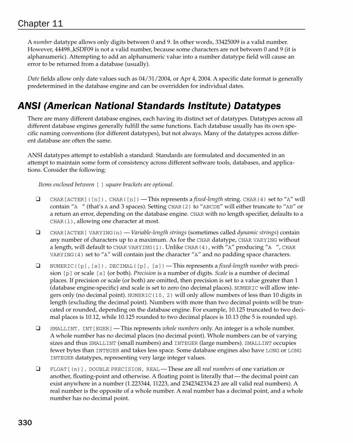
A number datatype allows only digits between 0 and 9. In other words, 33425009 is a valid number.However, 44498.,kSDF09 is not a valid number, because some characters are not between 0 and 9 (it isalphanumeric). Attempting to add an alphanumeric value into a number datatype field will cause anerror to be returned from a database (usually).
Date fields allow only date values such as 04/31/2004, or Apr 4, 2004. A specific date format is generallypredetermined in the database engine and can be overridden for individual dates.
ANSI (American National Standards Institute) DatatypesThere are many different database engines, each having its distinct set of datatypes. Datatypes across alldifferent database engines generally fulfill the same functions. Each database usually has its own spe-cific naming conventions (for different datatypes), but not always. Many of the datatypes across differ-ent database are often the same.
ANSI datatypes attempt to establish a standard. Standards are formulated and documented in anattempt to maintain some form of consistency across different software tools, databases, and applica-tions. Consider the following:
Items enclosed between [ ] square brackets are optional.
❑ CHAR[ACTER]([n]), CHAR([n])— This represents a fixed-length string. CHAR(4) set to “A” willcontain “A “ (that’s A and 3 spaces). Setting CHAR(2) to “ABCDE” will either truncate to “AB” ora return an error, depending on the database engine. CHAR with no length specifier, defaults to aCHAR(1), allowing one character at most.
❑ CHAR[ACTER] VARYING(n)— Variable-length strings (sometimes called dynamic strings) containany number of characters up to a maximum. As for the CHAR datatype, CHAR VARYING without a length, will default to CHAR VARYING(1). Unlike CHAR(4), with “A” producing “A “, CHARVARYING(4) set to “A” will contain just the character “A” and no padding space characters.
❑ NUMERIC([p],[s]), DECIMAL([p], [s])— This represents a fixed-length number with preci-sion [p] or scale [s] (or both). Precision is a number of digits. Scale is a number of decimalplaces. If precision or scale (or both) are omitted, then precision is set to a value greater than 1(database engine-specific) and scale is set to zero (no decimal places). NUMERIC will allow inte-gers only (no decimal point). NUMERIC(10, 2) will only allow numbers of less than 10 digits inlength (excluding the decimal point). Numbers with more than two decimal points will be trun-cated or rounded, depending on the database engine. For example, 10.125 truncated to two deci-mal places is 10.12, while 10.125 rounded to two decimal places is 10.13 (the 5 is rounded up).
❑ SMALLINT, INT[EGER]— This represents whole numbers only. An integer is a whole number. A whole number has no decimal places (no decimal point). Whole numbers can be of varyingsizes and thus SMALLINT (small numbers) and INTEGER (large numbers). SMALLINT occupiesfewer bytes than INTEGER and takes less space. Some database engines also have LONG or LONGINTEGER datatypes, representing very large integer values.
❑ FLOAT[(n)], DOUBLE PRECISION, REAL— These are all real numbers of one variation oranother, floating-point and otherwise. A floating point is literally that — the decimal point canexist anywhere in a number (1.223344, 11223, and 2342342334.23 are all valid real numbers). Areal number is the opposite of a whole number. A real number has a decimal point, and a wholenumber has no decimal point.
330
Chapter 11
17_574906 ch11.qxd 10/28/05 11:38 PM Page 330
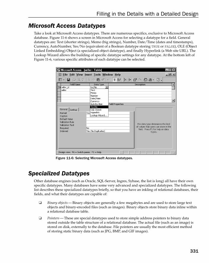
Microsoft Access DatatypesTake a look at Microsoft Access datatypes. There are numerous specifics, exclusive to Microsoft Accessdatabase. Figure 11-6 shows a screen in Microsoft Access for selecting a datatype for a field. Generaldatatypes are: Text (shorter strings), Memo (big strings), Number, Date/Time (dates and timestamps),Currency, AutoNumber, Yes/No (equivalent of a Boolean datatype storing TRUE or FALSE), OLE (ObjectLinked Embedding) Object (a specialized object datatype), and finally Hyperlink (a Web site URL). TheLookup Wizard allows the building of specific datatype settings for any datatype. At the bottom left ofFigure 11-6, various specific attributes of each datatype can be selected.
Figure 11-6: Selecting Microsoft Access datatypes.
Specialized DatatypesOther database engines (such as Oracle, SQL-Server, Ingres, Sybase, the list is long) all have their ownspecific datatypes. Many databases have some very advanced and specialized datatypes. The followinglist describes these specialized datatypes briefly, so that you have an inkling of relational databases, theirfields, and what their datatypes are capable of:
❑ Binary objects — Binary objects are generally a few megabytes and are used to store large textobjects and binary-encoded files (such as images). Binary objects store binary data inline withina relational database table.
❑ Pointers — These are special datatypes used to store simple address pointers to binary datastored outside the table structure of a relational database. The actual file (such as an image) isstored on disk, externally to the database. File pointers are usually the most efficient methodof storing static binary data (such as JPG, BMP, and GIF images).
331
Filling in the Details with a Detailed Design
17_574906 ch11.qxd 10/28/05 11:38 PM Page 331
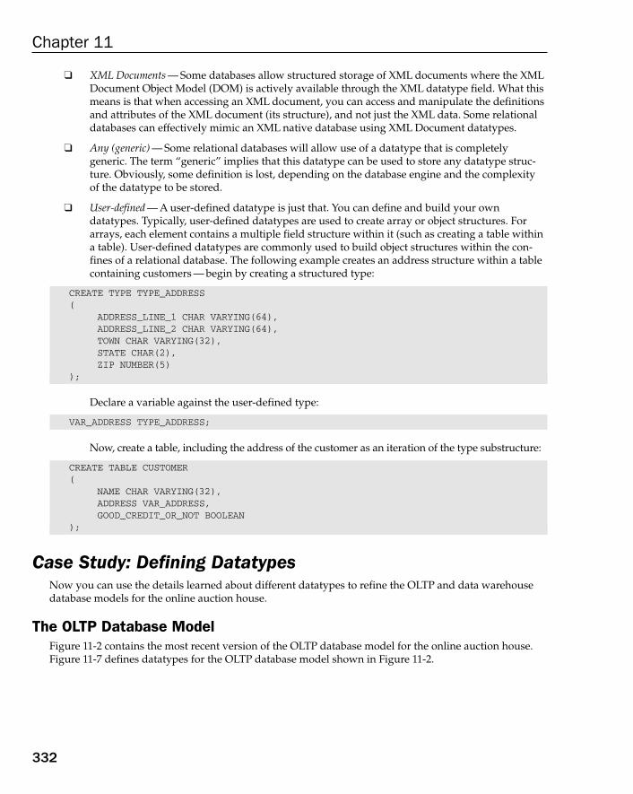
❑ XML Documents — Some databases allow structured storage of XML documents where the XMLDocument Object Model (DOM) is actively available through the XML datatype field. What thismeans is that when accessing an XML document, you can access and manipulate the definitionsand attributes of the XML document (its structure), and not just the XML data. Some relationaldatabases can effectively mimic an XML native database using XML Document datatypes.
❑ Any (generic) — Some relational databases will allow use of a datatype that is completelygeneric. The term “generic” implies that this datatype can be used to store any datatype struc-ture. Obviously, some definition is lost, depending on the database engine and the complexityof the datatype to be stored.
❑ User-defined — A user-defined datatype is just that. You can define and build your owndatatypes. Typically, user-defined datatypes are used to create array or object structures. Forarrays, each element contains a multiple field structure within it (such as creating a table withina table). User-defined datatypes are commonly used to build object structures within the con-fines of a relational database. The following example creates an address structure within a tablecontaining customers — begin by creating a structured type:
CREATE TYPE TYPE_ADDRESS(
ADDRESS_LINE_1 CHAR VARYING(64),ADDRESS_LINE_2 CHAR VARYING(64),TOWN CHAR VARYING(32),STATE CHAR(2),ZIP NUMBER(5)
);
Declare a variable against the user-defined type:
VAR_ADDRESS TYPE_ADDRESS;
Now, create a table, including the address of the customer as an iteration of the type substructure:
CREATE TABLE CUSTOMER(
NAME CHAR VARYING(32),ADDRESS VAR_ADDRESS,GOOD_CREDIT_OR_NOT BOOLEAN
);
Case Study: Defining DatatypesNow you can use the details learned about different datatypes to refine the OLTP and data warehousedatabase models for the online auction house.
The OLTP Database ModelFigure 11-2 contains the most recent version of the OLTP database model for the online auction house.Figure 11-7 defines datatypes for the OLTP database model shown in Figure 11-2.
332
Chapter 11
17_574906 ch11.qxd 10/28/05 11:38 PM Page 332
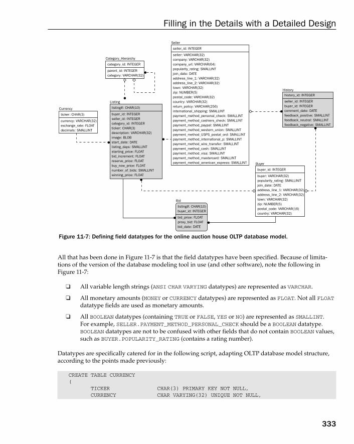
Figure 11-7: Defining field datatypes for the online auction house OLTP database model.
All that has been done in Figure 11-7 is that the field datatypes have been specified. Because of limita-tions of the version of the database modeling tool in use (and other software), note the following inFigure 11-7:
❑ All variable length strings (ANSI CHAR VARYING datatypes) are represented as VARCHAR.
❑ All monetary amounts (MONEY or CURRENCY datatypes) are represented as FLOAT. Not all FLOATdatatype fields are used as monetary amounts.
❑ All BOOLEAN datatypes (containing TRUE or FALSE, YES or NO) are represented as SMALLINT. For example, SELLER.PAYMENT_METHOD_PERSONAL_CHECK should be a BOOLEAN datatype.BOOLEAN datatypes are not to be confused with other fields that do not contain BOOLEAN values,such as BUYER.POPULARITY_RATING (contains a rating number).
Datatypes are specifically catered for in the following script, adapting OLTP database model structure,according to the points made previously:
CREATE TABLE CURRENCY(
TICKER CHAR(3) PRIMARY KEY NOT NULL,CURRENCY CHAR VARYING(32) UNIQUE NOT NULL,
History
history_id: INTEGER
seller_id: INTEGERbuyer_id: INTEGERcomment_date: DATEfeedback_positive: SMALLINTfeedback_neutral: SMALLINTfeedback_negative: SMALLINT
Listing
listing#: CHAR(10)
buyer_id: INTEGERseller_id: INTEGERcategory_id: INTEGERticker: CHAR(3)description: VARCHAR(32)image: BLOBstart_date: DATElisting_days: SMALLINTstarting_price: FLOATbid_increment: FLOATreserve_price: FLOATbuy_now_price: FLOATnumber_of_bids: SMALLINTwinning_price: FLOAT
Category_Hierarchy
category_id: INTEGER
parent_id: INTEGERcategory: VARCHAR(32)
Currency
ticker: CHAR(3)
currency: VARCHAR(32)exchange_rate: FLOATdecimals: SMALLINT
Seller
seller_id: INTEGER
seller: VARCHAR(32)company: VARCHAR(32)company_url: VARCHAR(64)popularity_rating: SMALLINTjoin_date: DATEaddress_line_1: VARCHAR(32)address_line_2: VARCHAR(32)town: VARCHAR(32)zip: NUMBER(5)postal_code: VARCHAR(32)country: VARCHAR(32)return_policy: VARCHAR(256)international_shipping: SMALLINTpayment_method_personal_check: SMALLINTpayment_method_cashiers_check: SMALLINTpayment_method_paypal: SMALLINTpayment_method_western_union: SMALLINTpayment_method_USPS_postal_ord: SMALLINTpayment_method_international_p: SMALLINTpayment_method_wire_transfer: SMALLINTpayment_method_cash: SMALLINTpayment_method_visa: SMALLINTpayment_method_mastercard: SMALLINTpayment_method_american_express: SMALLINT Buyer
buyer_id: INTEGER
buyer: VARCHAR(32)popularity_rating: SMALLINITjoin_date: DATEaddress_line_1: VARCHAR(32)address_line_2: VARCHAR(32)town: VARCHAR(32)zip: NUMBER(5)postal_code: VARCHAR(16)country: VARCHAR(32)
Bid
listing#: CHAR(10)buyer_id: INTEGER
bid_price: FLOATproxy_bid: FLOATbid_date: DATE
333
Filling in the Details with a Detailed Design
17_574906 ch11.qxd 10/28/05 11:38 PM Page 333

EXCHANGE_RATE FLOAT NOT NULL,DECIMALS SMALLINT NULL
);
CREATE TABLE BUYER(
BUYER_ID INTEGER PRIMARY KEY NOT NULL,BUYER CHAR VARYING(32) UNIQUE NOT NULL,POPULARITY_RATING SMALLINT NULL,JOIN_DATE DATE NOT NULL,ADDRESS_LINE_1 CHAR VARYING(32) NULL,ADDRESS_LINE_2 CHAR VARYINGR(32) NULL,TOWN CHAR VARYING(32) NULL,ZIP NUMERIC(5) NULL,POSTAL_CODE CHAR VARYING(16) NULL,COUNTRY CHAR VARYING(32) NULL
);
CREATE TABLE CATEGORY(
CATEGORY_ID INTEGER PRIMARY KEY NOT NULL,PARENT_ID INTEGER FOREIGN KEY REFERENCES CATEGORY WITH NULL,CATEGORY CHAR VARYING(32) NOT NULL
);
CREATE TABLE SELLER(
SELLER_ID INTEGER PRIMARY KEY NOT NULL,SELLER CHAR VARYING(32) UNIQUE NOT NULL,COMPANY CHAR VARYING(32) UNIQUE NOT NULL,COMPANY_URL CHAR VARYING(64) UNIQUE NOT NULL,POPULARITY_RATING SMALLINT NULL,JOIN_DATE DATE NOT NULL,ADDRESS_LINE_1 CHAR VARYING(32) NULL,ADDRESS_LINE_2 CHAR VARYING(32) NULL,TOWN CHAR VARYING (32) NULL,ZIP NUMERIC(5) NULL,POSTAL_CODE CHAR VARYING (32) NULL,COUNTRY CHAR VARYING(32) NULL,RETURN_POLICY CHAR VARYING(256) NULL,INTERNATIONAL_SHIPPING BOOLEAN NULL,PAYMENT_METHOD_PERSONAL_CHECK BOOLEAN NULL,PAYMENT_METHOD_CASHIERS_CHECK BOOLEAN NULL,PAYMENT_METHOD_PAYPAL BOOLEAN NULL,PAYMENT_METHOD_WESTERN_UNION BOOLEAN NULL,PAYMENT_METHOD_USPS_POSTAL_ORDER BOOLEAN NULL,PAYMENT_METHOD_INTERNATIONAL_POSTAL_ORDER BOOLEAN NULL,PAYMENT_METHOD_WIRE_TRANSFER BOOLEAN NULL,PAYMENT_METHOD_CASH BOOLEAN NULL,PAYMENT_METHOD_VISA BOOLEAN NULL,PAYMENT_METHOD_MASTERCARD BOOLEAN NULL,PAYMENT_METHOD_AMERICAN_EXPRESS BOOLEAN NULL
);
CREATE TABLE LISTING
334
Chapter 11
17_574906 ch11.qxd 10/28/05 11:38 PM Page 334

(LISTING# CHAR(10) PRIMARY KEY NOT NULL,CATEGORY_ID INTEGER FOREIGN KEY REFERENCES CATEGORY NOT NULL,BUYER_ID INTEGER FOREIGN KEY REFERENCES BUYER WITH NULL,SELLER_ID INTEGER FOREIGN KEY REFERENCES SELLER WITH NULL,TICKER CHAR(3) NULL,DESCRIPTION CHAR VARYING(32) NULL,IMAGE BINARY NULL,START_DATE DATE NOT NULL,LISTING_DAYS SMALLINT NOT NULL,STARTING_PRICE MONEY NOT NULL,BID_INCREMENT MONEY NULL,RESERVE_PRICE MONEY NULL,BUY_NOW_PRICE MONEY NULL,NUMBER_OF_BIDS SMALLINT NULL,WINNING_PRICE MONEY NULL
);
CREATE TABLE BID(
LISTING# CHAR(10) PRIMARY KEY NOT NULL,BUYER_ID INTEGER FOREIGN KEY REFERENCES BUYER NOT NULL,BID_PRICE MONEY NOT NULL,PROXY_BID MONEY NULL,BID_DATE DATE NOT NULL, CONSTRAINT PRIMARY KEY (LISTING#, BUYER_ID)
);
The primary key for the BID table is declared out of line with field definitions because it is a compositeof two fields.
CREATE TABLE HISTORY(
HISTORY_ID INTEGER PRIMARY KEY NOT NULL,SELLER_ID INTEGER FOREIGN KEY REFERENCES SELLER WITH NULL,BUYER_ID INTEGER FOREIGN KEY REFERENCES BUYER WITH NULL,COMMENT_DATE DATE NOT NULL,FEEDBACK_POSITIVE SMALLINT NULL,FEEDBACK_NEUTRAL SMALLINT NULL,FEEDBACK_NEGATIVE SMALLINT NULL
);
Some field names in Figure 11-7 are truncated by the ERD tool. The previous script has full field names.
A number of points are worth noting in the previous script:
❑ Some fields are declared as being unique (UNIQUE). For example, the BUYER table has a surro-gate key as its primary key; however, the name of the buyer must still be unique within thebuyer table. You can’t allow two buyers to have the same name. Therefore, the BUYER.BUYERfield (the name of the buyer) is declared as being unique.
❑ Some fields (other than primary keys and unique fields) are specified as being NOT NULL. Thismeans that there is no point in having a record in that particular table, unless there is an entryfor that particular field. NOT NULL is the restriction that forces an entry.
335
Filling in the Details with a Detailed Design
17_574906 ch11.qxd 10/28/05 11:38 PM Page 335
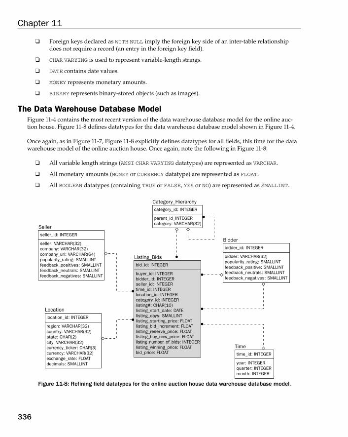
❑ Foreign keys declared as WITH NULL imply the foreign key side of an inter-table relationshipdoes not require a record (an entry in the foreign key field).
❑ CHAR VARYING is used to represent variable-length strings.
❑ DATE contains date values.
❑ MONEY represents monetary amounts.
❑ BINARY represents binary-stored objects (such as images).
The Data Warehouse Database ModelFigure 11-4 contains the most recent version of the data warehouse database model for the online auc-tion house. Figure 11-8 defines datatypes for the data warehouse database model shown in Figure 11-4.
Once again, as in Figure 11-7, Figure 11-8 explicitly defines datatypes for all fields, this time for the datawarehouse model of the online auction house. Once again, note the following in Figure 11-8:
❑ All variable length strings (ANSI CHAR VARYING datatypes) are represented as VARCHAR.
❑ All monetary amounts (MONEY or CURRENCY datatype) are represented as FLOAT.
❑ All BOOLEAN datatypes (containing TRUE or FALSE, YES or NO) are represented as SMALLINT.
Figure 11-8: Refining field datatypes for the online auction house data warehouse database model.
Bidderbidder_id: INTEGER
bidder: VARCHAR(32)popularity_rating: SMALLINTfeedback_positive: SMALLINTfeedback_neutrals: SMALLINTfeedback_negatives: SMALLINT
Category_Hierarchycategory_id: INTEGER
parent_id_INTEGERcategory: VARCHAR(32)
Sellerseller_id: INTEGER
seller: VARCHAR(32)company: VARCHAR(32)company_url: VARCHAR(64)popularity_rating: SMALLINTfeedback_positives: SMALLINTfeedback_neutrals: SMALLINTfeedback_negatives: SMALLINT
Locationlocation_id: INTEGER
region: VARCHAR(32)country: VARCHAR(32)state: CHAR(2)city: VARCHAR(32)currency_ticker: CHAR(3)currency: VARCHAR(32)exchange_rate: FLOATdecimals: SMALLINT
Timetime_id: INTEGER
year: INTEGERquarter: INTEGERmonth: INTEGER
Listing_Bidsbid_id: INTEGER
buyer_id: INTEGERbidder_id: INTEGERseller_id: INTEGERtime_id: INTEGERlocation_id: INTEGERcategory_id: INTEGERlisting#: CHAR(10)listing_start_date: DATElisting_days: SMALLINTlisting_starting_price: FLOATlisting_bid_increment: FLOATlisting_reserve_price: FLOATlisting_buy_now_price: FLOATlisting_number_of_bids: INTEGERlisting_winning_price: FLOATbid_price: FLOAT
336
Chapter 11
17_574906 ch11.qxd 10/28/05 11:38 PM Page 336

Once again, datatypes are changed in the following script to adapt to the points previously made:
CREATE TABLE CATEGORY(
CATEGORY_ID INTEGER PRIMARY KEY NOT NULL,PARENT_ID INTEGER FOREIGN KEY REFERENCES CATEGORY WITH NULL,CATEGORY CHAR VARYING(32) NOT NULL
);
CREATE TABLE SELLER(
SELLER_ID INTEGER PRIMARY KEY NOT NULL,SELLER CHAR VARYING(32) UNIQUE NOT NULL,COMPANY CHAR VARYING(32) UNIQUE NOT NULL,COMPANY_URL CHAR VARYING(64) UNIQUE NOT NULL,POPULARITY_RATING SMALLINT NULL,FEEDBACK_POSITIVES SMALLINT NULL,FEEDBACK_NEUTRALS SMALLINT NULL,FEEDBACK_NEGATIVES SMALLINT NULL
);
CREATE TABLE BIDDER(
BIDDER_ID INTEGER PRIMARY KEY NOT NULL,BIDDER CHAR VARYING(32) UNIQUE NOT NULL,POPULARITY_RATING SMALLINT NULL
);
CREATE TABLE LOCATION(
LOCATION_ID INTEGER PRIMARY KEY NOT NULL,REGION CHAR VARYING(32) NOT NULL,COUNTRY CHAR VARYING(32) NOT NULL,STATE CHAR(2) NULL,CITY CHAR VARYING(32) NOT NULL,CURRENCY_TICKER CHAR(3) UNIQUE NOT NULL,CURRENCY CHAR VARYING(32) UNIQUE NOT NULL,EXCHANGE_RATE FLOAT NOT NULL,DECIMALS SMALLINT NULL
);
CREATE TABLE TIME(
TIME_ID INTEGER PRIMARY KEY NOT NULL,YEAR INTEGER NOT NULL,QUARTER INTEGER NOT NULL,MONTH INTEGER NOT NULL
);
CREATE TABLE LISTING_BIDS(
LISTING# CHAR(10) PRIMARY KEY NOT NULL,BID_ID INTEGER FOREIGN KEY REFERENCES BID NOT NULL,BUYER_ID INTEGER FOREIGN KEY REFERENCES BUYER WITH NULL,
337
Filling in the Details with a Detailed Design
17_574906 ch11.qxd 10/28/05 11:38 PM Page 337
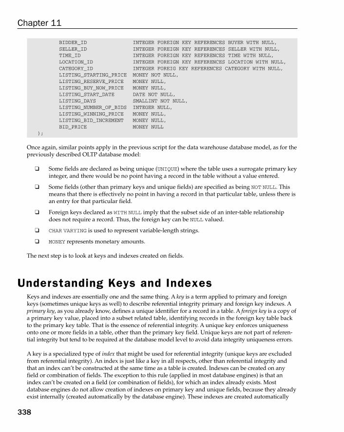
BIDDER_ID INTEGER FOREIGN KEY REFERENCES BUYER WITH NULL,SELLER_ID INTEGER FOREIGN KEY REFERENCES SELLER WITH NULL,TIME_ID INTEGER FOREIGN KEY REFERENCES TIME WITH NULL,LOCATION_ID INTEGER FOREIGN KEY REFERENCES LOCATION WITH NULL,CATEGORY_ID INTEGER FOREIG KEY REFERENCES CATEGORY WITH NULL,LISTING_STARTING_PRICE MONEY NOT NULL,LISTING_RESERVE_PRICE MONEY NULL,LISTING_BUY_NOW_PRICE MONEY NULL,LISTING_START_DATE DATE NOT NULL,LISTING_DAYS SMALLINT NOT NULL,LISTING_NUMBER_OF_BIDS INTEGER NULL,LISTING_WINNING_PRICE MONEY NULL,LISTING_BID_INCREMENT MONEY NULL,BID_PRICE MONEY NULL
);
Once again, similar points apply in the previous script for the data warehouse database model, as for thepreviously described OLTP database model:
❑ Some fields are declared as being unique (UNIQUE) where the table uses a surrogate primary keyinteger, and there would be no point having a record in the table without a value entered.
❑ Some fields (other than primary keys and unique fields) are specified as being NOT NULL. Thismeans that there is effectively no point in having a record in that particular table, unless there isan entry for that particular field.
❑ Foreign keys declared as WITH NULL imply that the subset side of an inter-table relationshipdoes not require a record. Thus, the foreign key can be NULL valued.
❑ CHAR VARYING is used to represent variable-length strings.
❑ MONEY represents monetary amounts.
The next step is to look at keys and indexes created on fields.
Understanding Keys and IndexesKeys and indexes are essentially one and the same thing. A key is a term applied to primary and foreignkeys (sometimes unique keys as well) to describe referential integrity primary and foreign key indexes. Aprimary key, as you already know, defines a unique identifier for a record in a table. A foreign key is a copy ofa primary key value, placed into a subset related table, identifying records in the foreign key table backto the primary key table. That is the essence of referential integrity. A unique key enforces uniquenessonto one or more fields in a table, other than the primary key field. Unique keys are not part of referen-tial integrity but tend to be required at the database model level to avoid data integrity uniqueness errors.
A key is a specialized type of index that might be used for referential integrity (unique keys are excludedfrom referential integrity). An index is just like a key in all respects, other than referential integrity andthat an index can’t be constructed at the same time as a table is created. Indexes can be created on anyfield or combination of fields. The exception to this rule (applied in most database engines) is that anindex can’t be created on a field (or combination of fields), for which an index already exists. Mostdatabase engines do not allow creation of indexes on primary key and unique fields, because they alreadyexist internally (created automatically by the database engine). These indexes are created automatically
338
Chapter 11
17_574906 ch11.qxd 10/28/05 11:38 PM Page 338
because primary and unique keys are both required to be unique. The most efficient method of verifyinguniqueness of primary and unique keys (on insertion of a new record into a table) is an automatically cre-ated index, by the database, on those primary and unique key fields.
Indexes created on tables (not on primary keys or foreign keys) are generally known as alternate or sec-ondary keys. They are named as such because they are additional or secondary to referential integrity keys.
As far as database modeling is concerned, alternate indexing is significant because it is largely dependenton application requirements, how applications use a database model, and most often apply to reporting.Reports are used to get information from a database in bulk. If existing database model indexing (pri-mary and foreign keys) does not cater to the sorting needs of reports, extra indexes (in addition to thatcovered by primary and foreign keys) are created. In fact, alternate indexing is quite common in OLTPdatabase environments because OLTP database model structure is often normalized too much for eventhe smallest on-screen listings (short reports). Reporting tends to denormalize tables and spit out sets ofdata from joins of information gathered from multiple tables at once.
Let’s begin by briefly examining different types of indexing from an analytical and design perspective.
Types of IndexesFrom an analytical and design perspective, there are a number of approaches to indexing:
❑ No Indexes — Tables with no indexing are heap-structured. All data is dumped on the disk as it is added, regardless of any sorting. It is much like overturning a bucket full of sand and simplytipping the sand onto the floor in a nice neat pile. Assume something absurd, and say the bucketwas really big, and you were Jack in Jack and the Beanstalk. Say the pile of sand was 50 feethigh when the giant overturned the bucket of sand. Finding a coin in that monstrous heap ofsand, without a metal detector, means sifting through all of the sand by hand, until you find thecoin. Assuming that you are doing the searching, you are not the giant, and the coin is small,you might be at it for a while. Using a metal detector would make your search much easier. Thepile of sand is a little like a table containing gazillions of records. The metal detector is a littlelike an index on that great big unorganized table. The coin is a single record you are searching for.You get my drift.
❑ Static Table Indexes — A static table is a table containing data that doesn’t change very often —if at all. Additionally, static tables are quite often very small, containing small numbers of fieldsand records. It is often more efficient for queries to simply read the entire table, rather than readparts of the index, and a small section of the table. Figure 11-9 shows the latest versions of bothof the OLTP database model and the data warehouse database model for the online auction house.Dynamic (facts in the data warehouse database model) are highlighted in gray. The static tablesare not highlighted. For example, the BIDDER table in the data warehouse database model, atthe bottom of Figure 11-9, has a primary key field and two other fields. Creating any furtherindexing on this table would be over-designing this table, and ultimately a complete waste ofresources. Try not to create alternate indexing on static data tables. It is usually pointless!
❑ Dynamic Table Indexes — The term “dynamic” implies consistent and continual change. Dynamictables change all the time (fact tables are dynamic; dimension tables are static). Indexing ondynamic tables should expect changes to data. The indexes are subject to overflow. As a result,indexes may require frequent rebuilding. Indexing should be used for dynamic data because ofthe nature of potential for change in data.
339
Filling in the Details with a Detailed Design
17_574906 ch11.qxd 10/28/05 11:38 PM Page 339
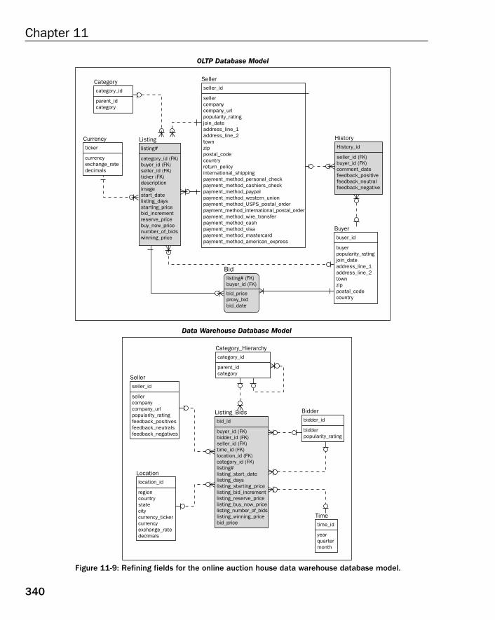
Figure 11-9: Refining fields for the online auction house data warehouse database model.
OLTP Database Model
Listinglisting#
category_id (FK)buyer_id (FK)seller_id (FK)ticker (FK)descriptionimagestart_datelisting_daysstarting_pricebid_incrementreserve_pricebuy_now_pricenumber_of_bidswinning_price
HistoryHistory_id
seller_id (FK)buyer_id (FK)comment_datefeedback_positivefeedback_neutralfeedback_negative
Sellerseller_id
sellercompanycompany_urlpopularity_ratingjoin_dateaddress_line_1address_line_2townzippostal_codecountryreturn_policyinternational_shippingpayment_method_personal_checkpayment_method_cashiers_checkpayment_method_paypalpayment_method_western_unionpayment_method_USPS_postal_orderpayment_method_international_postal_orderpayment_method_wire_transferpayment_method_cashpayment_method_visapayment_method_mastercardpayment_method_american_express
Buyerbuyer_id
buyerpopularity_ratingjoin_dateaddress_line_1address_line_2townzippostal_codecountry
Currencyticker
currencyexchange_ratedecimals
Categorycategory_id
parent_idcategory
Bidlisting# (FK)buyer_id (FK)
bid_priceproxy_bidbid_date
Data Warehouse Database Model
Bidderbidder_id
bidderpopularity_rating
Category_Hierarchycategory_id
parent_idcategory
Sellerseller_id
sellercompanycompany_urlpopularity_ratingfeedback_positivesfeedback_neutralsfeedback_negatives
Locationlocation_id
regioncountrystatecitycurrency_tickercurrencyexchange_ratedecimals
Timetime_id
yearquartermonth
Listing_Bidsbid_id
buyer_id (FK)bidder_id (FK)seller_id (FK)time_id (FK)location_id (FK)category_id (FK)listing#listing_start_datelisting_dayslisting_starting_pricelisting_bid_incrementlisting_reserve_pricelisting_buy_now_pricelisting_number_of_bidslisting_winning_pricebid_price
340
Chapter 11
17_574906 ch11.qxd 10/28/05 11:38 PM Page 340

For example, the LISTING_BIDS fact table shown in Figure 11-9 changes drastically when large amounts of data are added, perhaps even as much as on a daily basis. Additionally, theLISTING_BIDS table contains data from multiple dynamic sources, namely listings and pastbids on those listings. Reporting will not only need to retrieve listings with bids but also listingswithout bids. Even more complexity is needed because reporting will sort records retrievedbased on factors such as dates, locations, amounts, and the list goes on. In the OLTP databasemodel shown at the top of the diagram in Figure 11-9, the LISTING, BID, and HISTORY tablesare also highly dynamic structures. If OLTP database reporting is required (extremely likely),alternate indexing will probably to be needed in the OLTP database model dynamic tables, aswell as for the data warehouse model.
Two issues are important:
❑ OLTP database model — Inserting a new record into a table with, for example, fiveindexes, submits six physical record insertions to the database (one new table recordand five new index records). This is inefficient. Indexing is generally far more real-timedynamic in OLTP databases than for data warehouses, and is better kept under tightcontrol by production administrators.
❑ Data warehouse database model — Complex and composite indexing is far more commonlyused in data warehouse database models, partially because of denormalization and par-tially because of the sheer diversity and volume of fact data. Data warehouses containdynamic fact tables, much like OLTP databases; however, there is a distinct difference.OLTP dynamic tables are updated in real-time. Data warehouse dynamic fact tables areusually updated from one or more OLTP databases (or other sources) in batch mode.Batch mode updates imply periodical mass changes. Those periodical updates could beonce a day, once per month, or otherwise. It all depends on the needs of people usingdata warehouse reporting.
Data warehouses tend to utilize specialized types of indexing. Specialized indexes areoften read-only in nature (making data warehouse reporting very much more efficient).Read-only data has little or no conflict with other requests to a database, other than con-currently running reports reading disk storage.
Where data warehouses are massive in terms of data quantities, OLTP databases areheavy on concurrency (simultaneous use). The result is that OLTP databases focus onprovision of real-time accurate service, and data warehouses focus on processing oflarge chunks of data, for small numbers of users, on occasion. Some of the large andmore complex database engines allow many variations on read-only indexing, and pre-constructed queries for reporting, such as clustering of tables, compacted indexingbased on highly repetitive values (bitmaps), plus other special gadgets like materializedviews.
There is one last thing to remember about alternate indexing — the critical factor. Iftables in a database model (static and dynamic) have many indexes, there could beone of two potential problems: the native referential structure of the database modelis not catering to applications (poor database modeling could be the issue); andindexing has either been loosely controlled by administrators, such as developersbeing allowed to create indexing on a production database server, whenever theyplease. Clean up redundant indexing! The more growth in your database, the moreoften you might have to clean out unused indexing.
341
Filling in the Details with a Detailed Design
17_574906 ch11.qxd 10/28/05 11:38 PM Page 341
What, When, and How to IndexThere are a number of points to consider when trying to understand what to index, when to index it,and how to build those indexes:
❑ Tables with few fields and few records do not necessarily benefit from having indexes. This isbecause an index is actually a pointer, plus whatever field values are indexed (field values areactually copied into the index). An index is a copy of all records in a table and must usually be relatively smaller than the table, both in terms of record length (number of fields), and thenumber of records in the table.
❑ In partial contradiction to the previous point, tables with few fields and large numbers ofrecords can benefit astronomically from indexing. Indexes are usually specially constructed in away that allows fast access to a few records in a table, after reading on a small physical portionof the index. For example, most database engines use BTree (binary tree) indexes. A BTree indexis an upside-down tree structure. Special traversal algorithms (an algorithm is another name fora small, but often complex, computer program that solves a problem) through that tree structurecan access records by reading extremely small portions of the index. Small portions of a massiveindex can be read because of the internal structure of a BTree index, and specialized algorithmsaccessing the index.
❑ The two previous points beg the following additional comments. Large composite indexes con-taining more than one field in a table may be relatively large compared with the table. Not onlyis physical size of composite indexing an issue but also the complexity of the index itself. Asthose rapid traversals mentioned in the previous point become more complex algorithmically,the more complex an index becomes. The more fields a composite index contains, the less usefulit becomes. Also, field datatypes are an issue for indexing. Integer values are usually the mostefficient datatypes for indexing, simply because there are only ten different digits (0 to 9, asopposed to A to Z, and all the other funky characters when indexing strings).
Relative physical size difference between index and table is likely the most significant factor when con-sidering building multiple field (composite) indexes. The smaller the ratio between index and table physi-cal size, the more effective an index will be. After all, the main objective of creating indexes is betterefficiency of access to data in a database.
❑ Try to avoid indexing NULL field values. In general, NULL values are difficult to index if they areincluded in an index at all (some index types do not include NULL values in indexes, when anindex is created). The most efficient types of indexes are unique indexes containing integers.
❑ Tables with few records, regardless of the number of fields, can suffer from serious performancedegradation — the table is over-indexed if an index is created. This is not always the case,though. It is usually advisable to manually create indexes on foreign keys fields of small, staticdata tables. This helps avoid hot block issues with referential integrity checks where a foreignkey table, containing no index on the foreign key field, are full table scanned by primary keytable referential integrity verification. In highly concurrent OLTP databases, this can become aserious performance issue.
When Not to Create IndexesSome alternate indexing is usually created during the analysis and design stages. One of the biggest issueswith alternate indexing is that it is often created after the fact (after analysis and design) — quite often
342
Chapter 11
17_574906 ch11.qxd 10/28/05 11:38 PM Page 342
in applications development and implementation, and even when a system is in production. Alternateindexing is often reactive rather than preemptive in nature, usually in response to reporting require-ments, or OLTP GUI application programs that do not fit the existing underlying database model struc-ture (indicating possible database model inadequacies).
There are a number of points to consider as far as not creating indexes:
❑ When considering the creation of a new index, don’t be afraid of not creating that index at all.Do not always assume that an existing index should exist, simply because it does exist. Don’t be afraid of destroying existing indexes.
❑ When considering use of unusual indexes (such as read-only type indexing), be aware of theirapplications. The only index type amenable to data changes is a standard index (usually a BTreetype index).
Some database engines only allow a single type of indexing and will not even allow you to entertain theuse of more sophisticated indexing strategies such as read-only indexing like bitmaps.
❑ When executing data warehouse reporting, tables often contain records already sorted in thecorrect physical order. This is common because data warehouse tables are often added byappending (added to the end of), where records are copied from sources (for example, an OLTPdatabase), on, for example, a daily basis, and probably in the order of dates. Don’t re-createindexes where sorting has already been performed by the nature of structure and table recordappending processing, into a data warehouse.
❑ Production administrators should monitor existing indexing. Quite often, individual indexes areredundant, and even completely forgotten about. Redundant indexes place additional strain oncomputing power and resources. Destroy them if possible! Be especially vigilant of unusual andweird and unusual index types (such as bitmaps, clusters, indexes created on expressions, andclustering).
It is just as important to understand when and what not to index, as it is to understand what should beindexed.
Case Study: Alternate IndexingAs stated previously in this chapter, alternate indexes are created in addition to referential integrityindexes. Use the case study in this book to examine the OLTP and data warehouse database models onceagain.
The OLTP Database ModelMany database engines do not automatically create indexes on foreign keys, like they do for primaryand unique keys. This is because foreign keys are not required to be unique. Manual creation of indexesfor all foreign keys within a database model is sometimes avoided, if not completely forgotten. They areoften forgotten because developers and administrators are unaware that database engines do not createthem automatically, as is done for primary and unique keys.
You may need to create indexes on foreign keys, manually because constant referential integrity checks willuse indexes for both primary and foreign keys, when referential integrity checks are performed. Referentialintegrity checks are made whenever a change is made that might affect the status of primary-to-foreign
343
Filling in the Details with a Detailed Design
17_574906 ch11.qxd 10/28/05 11:38 PM Page 343
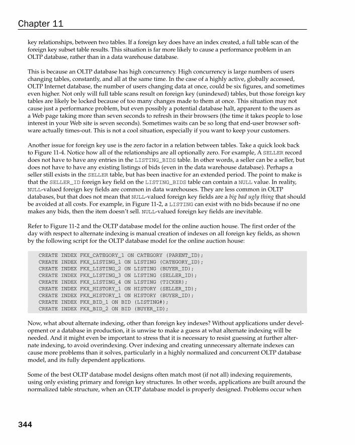
key relationships, between two tables. If a foreign key does have an index created, a full table scan of theforeign key subset table results. This situation is far more likely to cause a performance problem in anOLTP database, rather than in a data warehouse database.
This is because an OLTP database has high concurrency. High concurrency is large numbers of userschanging tables, constantly, and all at the same time. In the case of a highly active, globally accessed,OLTP Internet database, the number of users changing data at once, could be six figures, and sometimeseven higher. Not only will full table scans result on foreign key (unindexed) tables, but those foreign keytables are likely be locked because of too many changes made to them at once. This situation may notcause just a performance problem, but even possibly a potential database halt, apparent to the users as a Web page taking more than seven seconds to refresh in their browsers (the time it takes people to loseinterest in your Web site is seven seconds). Sometimes waits can be so long that end-user browser soft-ware actually times-out. This is not a cool situation, especially if you want to keep your customers.
Another issue for foreign key use is the zero factor in a relation between tables. Take a quick look back to Figure 11-4. Notice how all of the relationships are all optionally zero. For example, A SELLER recorddoes not have to have any entries in the LISTING_BIDS table. In other words, a seller can be a seller, butdoes not have to have any existing listings of bids (even in the data warehouse database). Perhaps aseller still exists in the SELLER table, but has been inactive for an extended period. The point to make isthat the SELLER_ID foreign key field on the LISTING_BIDS table can contain a NULL value. In reality,NULL-valued foreign key fields are common in data warehouses. They are less common in OLTPdatabases, but that does not mean that NULL-valued foreign key fields are a big bad ugly thing that shouldbe avoided at all costs. For example, in Figure 11-2, a LISTING can exist with no bids because if no onemakes any bids, then the item doesn’t sell. NULL-valued foreign key fields are inevitable.
Refer to Figure 11-2 and the OLTP database model for the online auction house. The first order of theday with respect to alternate indexing is manual creation of indexes on all foreign key fields, as shownby the following script for the OLTP database model for the online auction house:
CREATE INDEX FKX_CATEGORY_1 ON CATEGORY (PARENT_ID);CREATE INDEX FKX_LISTING_1 ON LISTING (CATEGORY_ID);CREATE INDEX FKX_LISTING_2 ON LISTING (BUYER_ID);CREATE INDEX FKX_LISTING_3 ON LISTING (SELLER_ID);CREATE INDEX FKX_LISTING_4 ON LISTING (TICKER);CREATE INDEX FKX_HISTORY_1 ON HISTORY (SELLER_ID);CREATE INDEX FKX_HISTORY_1 ON HISTORY (BUYER_ID);CREATE INDEX FKX_BID_1 ON BID (LISTING#);CREATE INDEX FKX_BID_2 ON BID (BUYER_ID);
Now, what about alternate indexing, other than foreign key indexes? Without applications under devel-opment or a database in production, it is unwise to make a guess at what alternate indexing will beneeded. And it might even be important to stress that it is necessary to resist guessing at further alter-nate indexing, to avoid overindexing. Over indexing and creating unnecessary alternate indexes cancause more problems than it solves, particularly in a highly normalized and concurrent OLTP databasemodel, and its fully dependent applications.
Some of the best OLTP database model designs often match most (if not all) indexing requirements,using only existing primary and foreign key structures. In other words, applications are built around thenormalized table structure, when an OLTP database model is properly designed. Problems occur when
344
Chapter 11
17_574906 ch11.qxd 10/28/05 11:38 PM Page 344
reporting (or even short on-screen listings joining more than one table) are required in applications. Thisis actually quite common.
A buyer might want to examine history records for a specific seller, to see if the seller is honest. Thiswould at the bare minimum require a join between SELLER and HISTORY tables. Similarly, a seller exam-ining past bids made by a buyer, would want to join tables, such as BUYER, BID and LISTING. Even so,with joins between SELLER and LISTING tables (or BUYER, BID and LISTING tables), all joins will be exe-cuted using primary and foreign key relationships. As it appears, no alternate indexing is required forthese joins just mentioned. For these types of onscreen reports, the database model itself is providing thenecessary key structures. Problems do not arise with joins when the database model maps adequately toapplication requirements.
Problems do, however, appear when a user wants to sort results. For example, a buyer might want to sort areport of the SELLER and HISTORY tables join, by a date value, such as the date of each comment madeabout the seller. That would be the COMMENT_DATE on the HISTORY table, as in the following query:
SELECT S.SELLER, H.COMMENT_DATE,H.FEEDBACK_POSITIVE, H.FEEDBACK_NEUTRAL, H.FEEDBACK_NEGATIVE
FROM SELLER S JOIN HISTORY H USING (SELLER_ID)ORDER BY H.COMMENT_DATE ASCENDING;
It is conceivable that an alternate index could be created on the HSITORY.COMMENT_DATE field. As alreadystated, this can be very difficult to assess in analysis and design and is best left for later implementationphases. The reason why is because perhaps the GUI will offer a user different sorting methods (such asby COMMENT_DATE, by combinations of SELLER table fields and the HISTORY.COMMENT_DATE field, inunknown orders). You can never accurately predict what users will want. Creating alternate indexing for possible reporting, or even brief OLTP database on-screen listing is extremely difficult without devel-oper, programmer, administrator, and, most important, customer feedback.
The Data Warehouse Database ModelRefer to Figure 11-4 and the data warehouse database model for the online auction house. Once again, as for the OLTP database model, create indexes on all foreign key fields in the data warehouse databasemodel:
CREATE INDEX FKX_CATEGORY_HIERARCHY_1 ON CATEGORY_HIERARCHY (PARENT_ID);CREATE INDEX FKX_LISTING_BIDS_1 ON LISTING (BUYER_ID);CREATE INDEX FKX_LISTING_BIDS_2 ON LISTING (BIDDER_ID);CREATE INDEX FKX_LISTING_BIDS_3 ON LISTING (SELLER_ID);CREATE INDEX FKX_LISTING_BIDS_4 ON LISTING (TIME_ID);CREATE INDEX FKX_LISTING_BIDS_5 ON LISTING (LOCATION_ID);CREATE INDEX FKX_LISTING_BIDS_6 ON LISTING (CATEGORY_ID);
Foreign key indexes are only needed to be created on the LISTING_BIDS fact table, and the CATEGORY_HIERARCHY tables. Categories are stored in a hierarchy and, thus, a pointer to each parent category isstored in the PARENT_ID field (if a parent exists). The fact table is the center of the data warehousedatabase model star schema, and, thus, is the only table (other than categories) containing foreign keys.
Creating alternate indexing for a data warehouse database model might be a little easier to guess at, ascompared to an OLTP database model; however, data warehouse reporting is often ad-hoc (created onthe fly) when the data warehouse is in production.
345
Filling in the Details with a Detailed Design
17_574906 ch11.qxd 10/28/05 11:38 PM Page 345
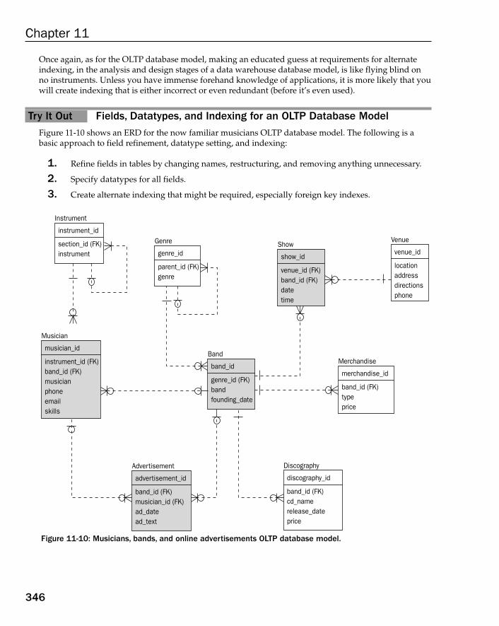
Once again, as for the OLTP database model, making an educated guess at requirements for alternateindexing, in the analysis and design stages of a data warehouse database model, is like flying blind onno instruments. Unless you have immense forehand knowledge of applications, it is more likely that youwill create indexing that is either incorrect or even redundant (before it’s even used).
Try It Out Fields, Datatypes, and Indexing for an OLTP Database ModelFigure 11-10 shows an ERD for the now familiar musicians OLTP database model. The following is abasic approach to field refinement, datatype setting, and indexing:
1. Refine fields in tables by changing names, restructuring, and removing anything unnecessary.
2. Specify datatypes for all fields.
3. Create alternate indexing that might be required, especially foreign key indexes.
Figure 11-10: Musicians, bands, and online advertisements OLTP database model.
Instrument
instrument_id
section_id (FK)instrument
Genre
genre_id
parent_id (FK)genre
Venue
venue_id
locationaddressdirectionsphone
Merchandise
merchandise_id
band_id (FK)typeprice
Band
band_id
genre_id (FK)bandfounding_date
Show
show_id
venue_id (FK)band_id (FK)datetime
Musician
musician_id
instrument_id (FK)band_id (FK)musicianphoneemailskills
Advertisement
advertisement_id
band_id (FK)musician_id (FK)ad_datead_text
Discography
discography_id
band_id (FK)cd_namerelease_dateprice
346
Chapter 11
17_574906 ch11.qxd 10/28/05 11:38 PM Page 346
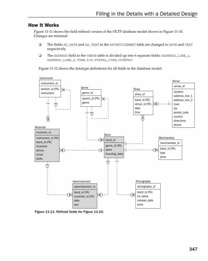
How It WorksFigure 11-11 shows the field-refined version of the OLTP database model shown in Figure 11-10.Changes are minimal:
❑ The fields AD_DATE and AD_TEXT in the ADVERTISEMENT table are changed to DATE and TEXTrespectively.
❑ The ADDRESS field in the VENUE table is divided up into 6 separate fields: ADDRESS_LINE_1,ADDRESS_LINE_2, TOWN, ZIP, POSTAL_CODE, COUNTRY.
Figure 11-12 shows the datatype definitions for all fields in the database model.
Figure 11-11: Refined fields for Figure 11-10.
Instrument
instrument_id
section_id (FK)instrument
Genre
genre_id
parent_id (FK)genre
Venue
venue_id
locationaddress_line_1address_line_2townzippostal_codecountrydirectionsphone
Merchandise
merchandise_id
band_id (FK)typeprice
Band
band_id
genre_id (FK)bandfounding_date
Show
show_id
band_id (FK)venue_id (FK)datetime
Musician
musician_id
instrument_id (FK)band_id (FK)musicianphoneemailskills
Advertisement
advertisement_id
band_id (FK)musician_id (FK)datetext
Discography
discography_id
band_id (FK)cd_namerelease_dateprice
347
Filling in the Details with a Detailed Design
17_574906 ch11.qxd 10/28/05 11:38 PM Page 347

Figure 11-12: Figure 11-11 with datatypes specified.
As discussed previously in this chapter, alternate indexing is best avoided in database analysis anddesign stages because there are too many unknown factors; however, foreign keys can be indexed for themusicians OLTP database model as follows:
CREATE INDEX FKX_INSTRUMENT_1 ON INSTRUMENT (SECTION_ID);CREATE INDEX FKX_GENRE_1 ON GENRE (PARENT_ID);CREATE INDEX FKX_SHOW_1 ON SHOW (BAND_ID);CREATE INDEX FKX_SHOW_2 ON SHOW (VENUE_ID);CREATE INDEX FKX_MERCHANDISE_1 ON MERCHANDISE (BAND_ID);CREATE INDEX FKX_DISCOGRAPHY_1 ON DISCOGRAPHY (BAND_ID);CREATE INDEX FKX_BAND_1 ON BAND (GENRE_ID);CREATE INDEX FKX_MUSICIAN_1 ON MUSICIAN (INSTRUMENT_ID);CREATE INDEX FKX_MUSICIAN_2 ON (BAND_ID);CREATE INDEX FKX_ADVERTISEMENT_1 ON ADVERTISEMENT (BAND_ID);CREATE INDEX FKX_ ADVERTISEMENT _1 ON ADVERTISEMENT (MUSICIAN_ID);
Instrument
instrument_id: INTEGER
section_id: INTEGRinstrument: VARCHAR(32)
Genre
genre_id: INTEGER
parent_id: INTEGERgenre: VARCHAR(32)
Venue
venue_id: INTEGER
location: VARCHAR(32)address_line_1: VARCHAR(32)address_line_2: VARCHAR(32)town: VARCHAR(32)zip: NUMBER(5)postal_code: VARCHAR(32)country: VARCHAR(32)directions: VARCHAR(1024)phone: VARCHAR(32)
Merchandise
merchandise_id: INTEGER
band_id: INTEGERtype: VARCHAR(32)price: FLOAT
Band
band_id: INTEGER
genre_id: INTEGERband: VARCHAR(32)founding_date: DATE
Show
show_id: INTEGER
band_id: INTEGERvenue_id: INTEGERdate: DATEtime: VARCHAR(16)
Musician
musician_id: INTEGER
instrument_id: INTEGERband_id: INTEGERmusician: VARCHAR(32)phone: VARCHAR(32)email: VARCHAR(32)skills: VARCHAR(256)
Advertisement
advertisement_id: INTEGER
band_id: INTEGERmusician_id: INTEGERdate: DATEtext: VARCHAR(246)
Discography
discography_id: INTEGER
band_id: INTEGERcd_name: VARCHAR(32)release_date: DATEprice: FLOAT
348
Chapter 11
17_574906 ch11.qxd 10/28/05 11:38 PM Page 348

Try It Out Fields, Datatypes, and Indexing for a Data Warehouse Database Model
Figure 11-13 shows an ERD for the now familiar musicians data warehouse database model. Here’s abasic approach to field refinement, datatype setting and indexing:
1. Refine fields in tables by changing names, restructuring, and removing anything unnecessary.
2. Specify datatypes for all fields.
3. Create alternate indexing that might be required, especially foreign key indexes.
Figure 11-13: Musicians, bands, their online advertisements data warehouse database model.
Genre
genre_id
parent_id (FK)genre
Merchandise
merchandise_id
typeprice
Instrument
instrument_id
section_id (FK)instrument
Artists
artist_id
merchandise_id (FK)genre_id (FK)instrument_id (FK)musician_namemusician_phonemusician_emailband_nameband_founding_datediscography_cd_namediscography_release_datediscography_priceshow_dateshow_timevenue_namevenue_addressvenue_directionsvenue_phoneadvertisement_dateadvertisement_text
349
Filling in the Details with a Detailed Design
17_574906 ch11.qxd 10/28/05 11:38 PM Page 349
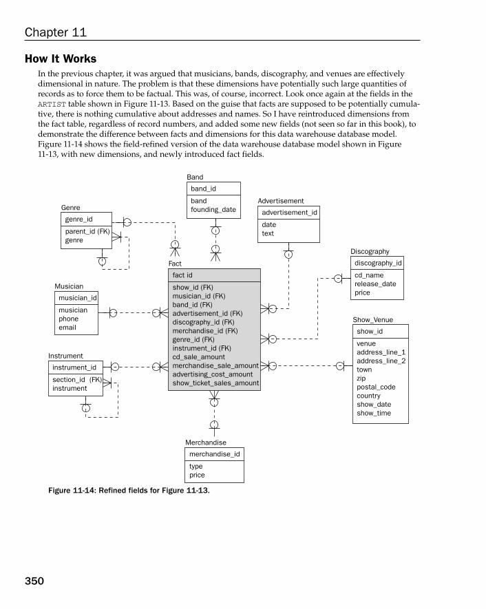
How It WorksIn the previous chapter, it was argued that musicians, bands, discography, and venues are effectivelydimensional in nature. The problem is that these dimensions have potentially such large quantities ofrecords as to force them to be factual. This was, of course, incorrect. Look once again at the fields in theARTIST table shown in Figure 11-13. Based on the guise that facts are supposed to be potentially cumula-tive, there is nothing cumulative about addresses and names. So I have reintroduced dimensions fromthe fact table, regardless of record numbers, and added some new fields (not seen so far in this book), todemonstrate the difference between facts and dimensions for this data warehouse database model.Figure 11-14 shows the field-refined version of the data warehouse database model shown in Figure11-13, with new dimensions, and newly introduced fact fields.
Figure 11-14: Refined fields for Figure 11-13.
Fact
fact id
show_id (FK)musician_id (FK)band_id (FK)advertisement_id (FK)discography_id (FK)merchandise_id (FK)genre_id (FK)instrument_id (FK)cd_sale_amountmerchandise_sale_amountadvertising_cost_amountshow_ticket_sales_amount
Advertisement
advertisement_id
datetext
Band
band_id
bandfounding_dateGenre
genre_id
parent_id (FK)genre
Musician
musician_id
musicianphoneemail
Instrument
instrument_id
section_id (FK)instrument
Merchandise
merchandise_id
typeprice
Discography
discography_id
cd_namerelease_dateprice
Show_Venue
show_id
venueaddress_line_1address_line_2townzippostal_codecountryshow_dateshow_time
350
Chapter 11
17_574906 ch11.qxd 10/28/05 11:38 PM Page 350
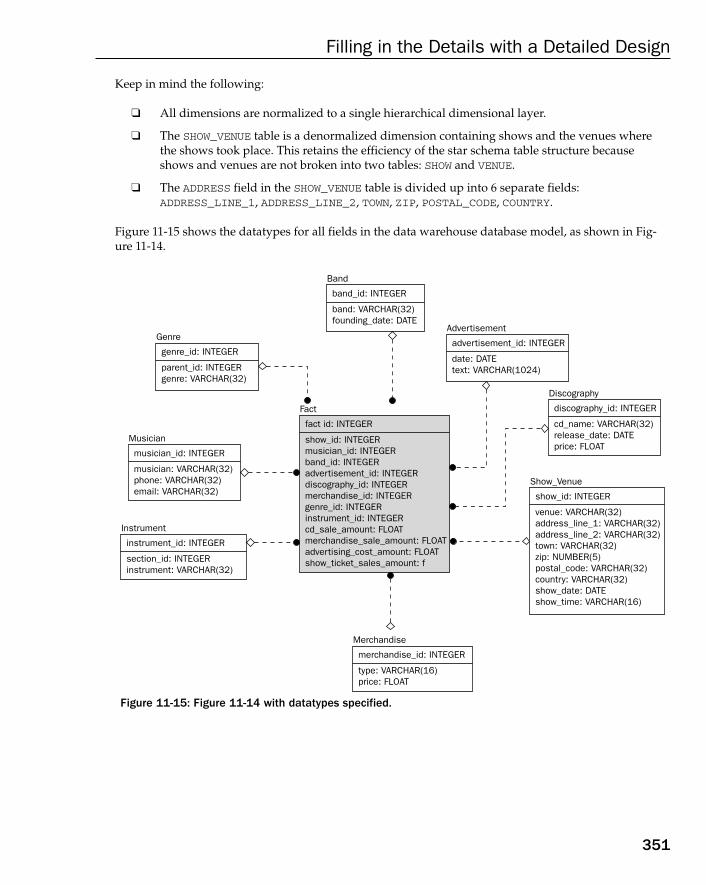
Keep in mind the following:
❑ All dimensions are normalized to a single hierarchical dimensional layer.
❑ The SHOW_VENUE table is a denormalized dimension containing shows and the venues wherethe shows took place. This retains the efficiency of the star schema table structure becauseshows and venues are not broken into two tables: SHOW and VENUE.
❑ The ADDRESS field in the SHOW_VENUE table is divided up into 6 separate fields:ADDRESS_LINE_1, ADDRESS_LINE_2, TOWN, ZIP, POSTAL_CODE, COUNTRY.
Figure 11-15 shows the datatypes for all fields in the data warehouse database model, as shown in Fig-ure 11-14.
Figure 11-15: Figure 11-14 with datatypes specified.
Fact
fact id: INTEGER
show_id: INTEGERmusician_id: INTEGERband_id: INTEGERadvertisement_id: INTEGERdiscography_id: INTEGERmerchandise_id: INTEGERgenre_id: INTEGERinstrument_id: INTEGERcd_sale_amount: FLOATmerchandise_sale_amount: FLOATadvertising_cost_amount: FLOATshow_ticket_sales_amount: f
Advertisement
advertisement_id: INTEGER
date: DATEtext: VARCHAR(1024)
Band
band_id: INTEGER
band: VARCHAR(32)founding_date: DATE
Genre
genre_id: INTEGER
parent_id: INTEGERgenre: VARCHAR(32)
Musician
musician_id: INTEGER
musician: VARCHAR(32)phone: VARCHAR(32)email: VARCHAR(32)
Instrument
instrument_id: INTEGER
section_id: INTEGERinstrument: VARCHAR(32)
Merchandise
merchandise_id: INTEGER
type: VARCHAR(16)price: FLOAT
Discography
discography_id: INTEGER
cd_name: VARCHAR(32)release_date: DATEprice: FLOAT
Show_Venue
show_id: INTEGER
venue: VARCHAR(32)address_line_1: VARCHAR(32)address_line_2: VARCHAR(32)town: VARCHAR(32)zip: NUMBER(5)postal_code: VARCHAR(32)country: VARCHAR(32)show_date: DATEshow_time: VARCHAR(16)
351
Filling in the Details with a Detailed Design
17_574906 ch11.qxd 10/28/05 11:38 PM Page 351
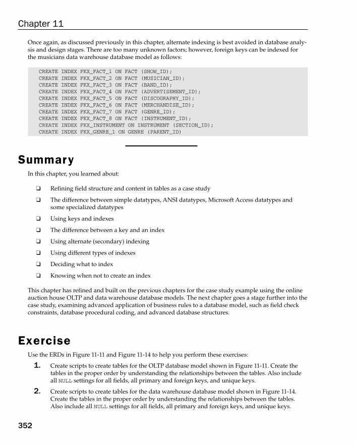
Once again, as discussed previously in this chapter, alternate indexing is best avoided in database analy-sis and design stages. There are too many unknown factors; however, foreign keys can be indexed forthe musicians data warehouse database model as follows:
CREATE INDEX FKX_FACT_1 ON FACT (SHOW_ID);CREATE INDEX FKX_FACT_2 ON FACT (MUSICIAN_ID);CREATE INDEX FKX_FACT_3 ON FACT (BAND_ID);CREATE INDEX FKX_FACT_4 ON FACT (ADVERTISEMENT_ID);CREATE INDEX FKX_FACT_5 ON FACT (DISCOGRAPHY_ID);CREATE INDEX FKX_FACT_6 ON FACT (MERCHANDISE_ID);CREATE INDEX FKX_FACT_7 ON FACT (GENRE_ID);CREATE INDEX FKX_FACT_8 ON FACT (INSTRUMENT_ID);CREATE INDEX FKX_INSTRUMENT ON INSTRUMENT (SECTION_ID);CREATE INDEX FKX_GENRE_1 ON GENRE (PARENT_ID)
SummaryIn this chapter, you learned about:
❑ Refining field structure and content in tables as a case study
❑ The difference between simple datatypes, ANSI datatypes, Microsoft Access datatypes andsome specialized datatypes
❑ Using keys and indexes
❑ The difference between a key and an index
❑ Using alternate (secondary) indexing
❑ Using different types of indexes
❑ Deciding what to index
❑ Knowing when not to create an index
This chapter has refined and built on the previous chapters for the case study example using the onlineauction house OLTP and data warehouse database models. The next chapter goes a stage further into thecase study, examining advanced application of business rules to a database model, such as field checkconstraints, database procedural coding, and advanced database structures.
ExerciseUse the ERDs in Figure 11-11 and Figure 11-14 to help you perform these exercises:
1. Create scripts to create tables for the OLTP database model shown in Figure 11-11. Create thetables in the proper order by understanding the relationships between the tables. Also includeall NULL settings for all fields, all primary and foreign keys, and unique keys.
2. Create scripts to create tables for the data warehouse database model shown in Figure 11-14.Create the tables in the proper order by understanding the relationships between the tables.Also include all NULL settings for all fields, all primary and foreign keys, and unique keys.
352
Chapter 11
17_574906 ch11.qxd 10/28/05 11:38 PM Page 352
12Business Rules and
Field Settings
“In business or in life, don’t follow the wagon tracks too closely.” (H. Jackson Brown)
Database modeling analysis and design are an art form. Use your imagination and you might find that,sometimes rules are made to be bent — if not broken altogether
This chapter covers the deepest layer of implementation into a database model — business rules.Business rules are implemented into a database model by creating tables, establishing relationshipsbetween tables, identifying fields, their datatypes, and various other factors including things suchas validation. Field settings including display formats, input maskings, default values, and checkconstraints are included. There is also a brief section on applying business rules by way of storingcode in the database model.
This chapter is the last of four chapters using the case study example of the online auction house.By reading through the last few chapters and this one, you should have a good idea of the analysisand design process for both OLTP and data warehouse database models, all the way through fromstart to finish.
By the end of this chapter, you should know how to apply field setting business rules in theextreme, and also that this extreme might be best left to application Software Development Kits(SDKs). Application SDKs are much more powerful than database modeling methods when itcomes to number crunching, and some of the more detailed aspects of database modeling.
In this chapter, you learn about the following:
❑ Database model business rules classification
❑ Implementation of business rules can be implemented as table and relations (linksbetween tables) design
❑ Using individual field settings as applications of deeper level business rules
❑ Using stored database code to implement highly complex business rules
18_574906 ch12.qxd 10/28/05 11:42 PM Page 353
What Are Business Rules Again?When applied as a database model, the business rules of a company become the structure of thatdatabase model. The most basic implementation of business rules in a database model, are the tables,relationships between those tables, and even constraint rules, such as validation checks. Validationchecks apply to individual fields. For example, a field called SEX can be restricted to having values of Mfor Male and F for Female. Insisting that a field only be set to M or F is a business rule, applied to thefield SEX. Now I should have your full attention!
The application of normalization and Normal Forms to a set of not yet normalized data tables, applies a progressively more complex implementation of business rules, as you apply the successive NormalForm layers to the data set — 1NF, 2NF, 3NF, and so on.
As already seen previously in this book, a definition of the term business rules appears to be somewhatopen to debate. Technically speaking, business rules require that intra-table and inter-table validation beplaced into a database model. Database implementation of business rules includes validation for someor all fields in tables. Even any type of coding stored and executed within the bounds of a databaseengine is, technically speaking, business rules implementation. So business rules are not just about nor-malization, Normal Forms, and field validation checks. Business rules are also about stored procedures.
Number crunching is computer jargon for large quantities of extremely complex calculations.
An object database model can encapsulate processing into class methods. A relational database can usestored (database) procedures and event or rule triggers to perform a similar function to that of objectclass methods. For the purposes of efficiency, it is usually best to avoid business rules in the database,unless they are included within the relationship structure of the database itself. You don’t want to go toofar in forcing business rules implementation into a database model. The most efficient implementation of business rules in a database model is anything non-coded and non-field-specific validation (valida-tion checks or CHECK constraints). The only business rules that should absolutely be implemented in adatabase model is referential integrity (primary keys, foreign keys, and their representative inter-tablerelationships). Other layers can be, but are not strictly necessary.
So, it should be clear that implementing all types and layers of business rules into a database model maynot the most prudent approach. As already stated, the most effective and efficient implementation ofbusiness rules in a database model is that of referential integrity. Other, deeper and more complex layersof business rules implementation are more often than not far more effectively managed in application
A stored procedure is a chunk of code stored in a database — ostensibly to executeagainst data stored in one or more tables. In other words, the function of a storedprocedure should be directly associated with some data in a database. On the con-trary, the function of a stored procedure is not always directly associated with datain a database. This would not be an implementation of business rules. Businessrules in a database model imply company operations as applied to data. In otherwords, not all stored procedures are an implementation of business rules. Storedprocedures can implement number crunching as well.
354
Chapter 12
18_574906 ch12.qxd 10/28/05 11:42 PM Page 354
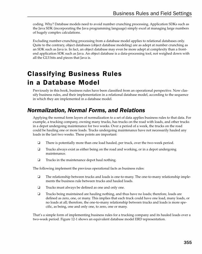
coding. Why? Database models need to avoid number crunching processing. Application SDKs such asthe Java SDK (incorporating the Java programming language) simply excel at managing large numbersof hugely complex calculations.
Excluding number-crunching processing from a database model applies to relational databases only.Quite to the contrary, object databases (object database modeling) are as adept at number crunching asan SDK such as Java is. In fact, an object database may even be more adept at complexity than a front-end application SDK such as Java. An object database is a data-processing tool, not weighed down withall the GUI bits and pieces that Java is.
Classifying Business Rules in a Database Model
Previously in this book, business rules have been classified from an operational perspective. Now clas-sify business rules, and their implementation in a relational database model, according to the sequencein which they are implemented in a database model.
Normalization, Normal Forms, and RelationsApplying the normal form layers of normalization to a set of data applies business rules to that data. Forexample, a trucking company, owning many trucks, has trucks on the road with loads, and other trucksin a depot undergoing maintenance for two weeks. Over a period of a week, the trucks on the roadcould be hauling one or more loads. Trucks undergoing maintenance have not necessarily hauled anyloads in the last two weeks. These points are important:
❑ There is potentially more than one load hauled, per truck, over the two-week period.
❑ Trucks always exist as either being on the road and working, or in a depot undergoing maintenance.
❑ Trucks in the maintenance depot haul nothing.
The following implement the previous operational facts as business rules:
❑ The relationship between trucks and loads is one-to-many. The one-to-many relationship imple-ments the business rule between trucks and hauled loads.
❑ Trucks must always be defined as one and only one.
❑ Trucks being maintained are hauling nothing, and thus have no loads; therefore, loads aredefined as zero, one, or many. This implies that each truck could have one load, many loads, orno loads at all; therefore, the one-to-many relationship between trucks and loads is more spe-cific, as being, one and only one, to zero, one or many.
That’s a simple form of implementing business rules for a trucking company and its hauled loads over atwo-week period. Figure 12-1 shows an equivalent database model ERD representation.
355
Business Rules and Field Settings
18_574906 ch12.qxd 10/28/05 11:42 PM Page 355
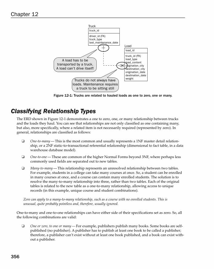
Figure 12-1: Trucks are related to hauled loads as one to zero, one or many.
Classifying Relationship TypesThe ERD shown in Figure 12-1 demonstrates a one to zero, one, or many relationship between trucksand the loads they haul. You can see that relationships are not only classified as one containing many,but also, more specifically, where a related item is not necessarily required (represented by zero). In general, relationships are classified as follows:
❑ One-to-many — This is the most common and usually represents a 1NF master detail relation-ship, or a 2NF static-to-transactional referential relationship (dimensional to fact table, in a datawarehouse database model).
❑ One-to-one — These are common of the higher Normal Forms beyond 3NF, where perhaps lesscommonly used fields are separated out to new tables.
❑ Many-to-many — This relationship represents an unresolved relationship between two tables.For example, students in a college can take many courses at once. So, a student can be enrolledin many courses at once, and a course can contain many enrolled students. The solution is toresolve the many-to-many relationship into three, rather than two tables. Each of the originaltables is related to the new table as a one-to-many relationship, allowing access to uniquerecords (in this example, unique course and student combinations).
Zero can apply to a many-to-many relationship, such as a course with no enrolled students. This isunusual, quite probably pointless and, therefore, usually ignored.
One-to-many and one-to-one relationships can have either side of their specifications set as zero. So, allthe following combinations are valid:
❑ One or zero, to one or many — For example, publishers publish many books. Some books are self-published (no publisher). A publisher has to publish at least one book to be called a publisher;therefore, a publisher can’t exist without at least one book published, and a book can exist with-out a publisher.
Loadload_id
truck_id (FK)load_typeload_contentorigination_citydestination_cityorigination_datedestination_dateweight
Trucktruck_id
driver_id (FK)truck_typelast_maintenance_date
A load has to betransported by a truck.A load can’t drive itself!
Trucks do not always haveloads. Maintenance requires
a truck to be sitting still
356
Chapter 12
18_574906 ch12.qxd 10/28/05 11:42 PM Page 356

❑ One to zero, one, or many — In this case, a publisher does not have to publish any books to be calleda publisher. Also, self-publishing is not allowed — perhaps the author becomes the publisher.
❑ One or zero to one, many, or zero — In this case, a publisher is called a publisher, even if no booksare published. Also, self-publishing with no publisher is allowed.
All these combinations apply to one-to-one relationships, as for one-to-many relationships, except thatmany is prohibited.
You can see that business rules are implemented in a relational database model using normalization(Normal Forms), the relationships established between tables, and even down to the specific valueallowances, by the ends of each relationship (the crow’s foot).
Explicitly Declared Field SettingsThis topic area includes NULL values, uniqueness, and individual field settings (validation checks areincluded). You begin with NULL values and uniqueness, as these are simple:
❑ NULL and default values —NULL value requirements can be set for each field and are usuallycoded in data definition language (DDL) commands as NULL, NOT NULL, or WITH NULL. Thedefault setting is usually NULL for any field with nothing specified. WITH NULL is often not nec-essary. This is not the case for all database engines. Ingres 6.04 defaulted to NOT NULL, requiringexplicit declaration of WITH NULL to allow NULL values into fields. NULL simply means that afield does not have to have a value entered when a record is inserted into (or updated in) atable. NOT NULL is completely the opposite and always requires a value. If inserting or updating,a field specified as NOT NULL is not specified (insertion), or is set to NULL (updating), an errorshould be returned by the database.
❑ Default values — This is an interesting one because when a record is added to a table, if nothingis specified for a NOT NULL set field, then the default value is added to the NOT NULL field. Thiscan somewhat restrict the purpose of specifying a field as NOT NULL. For example, a primary keyfield is always NOT NULL by default. Setting a default insertion value for an auto counter surro-gate primary key field not specified in an insertion could ignore the auto counter, and producean out of sequence, or worse, a duplicated surrogate key value. Default value settings are moreoften utilized in power-user type database engines such as Microsoft Access, rather than SQLServer or Oracle Database.
A power user is a user who is between an end-user and an expert computer programmer, in terms ofknowing how to use a computer. An end-user uses a computer as a tool to solve business problems. Acomputer programmer writes the software that end-users make use of. A power user is someone inbetween, typically an end-user who writes his or her own software.
❑ Uniqueness — This is simply a declaration of a field as being a unique key. You have seen these specifications before in this book where a non-surrogate unique field is declared as beingUNIQUE. For example, a table of customers, using a surrogate primary key auto counter integerCUSTOMER_ID, with a customer name, would not want to store customers having the samename. That could make things confusing, to say the least. The customer’s name field would bedeclared as being unique.
❑ Validation Check — These settings are sometimes called check constraints. All they do is to checkthe value in a field when a new record is added, or an existing record is changed. The validation
357
Business Rules and Field Settings
18_574906 ch12.qxd 10/28/05 11:42 PM Page 357
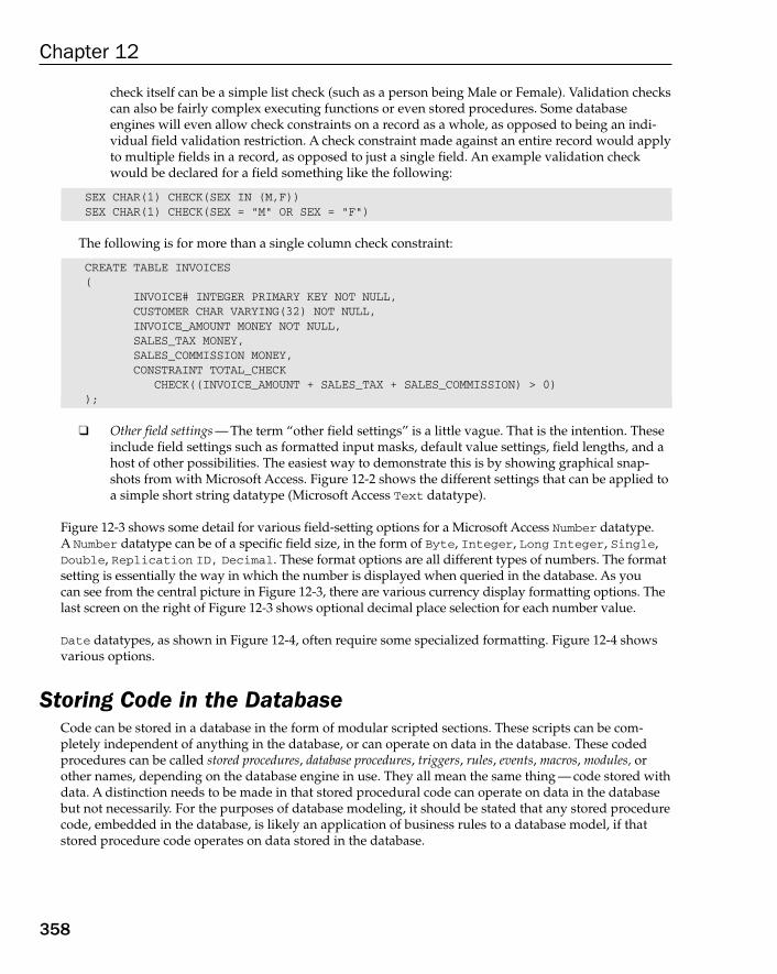
check itself can be a simple list check (such as a person being Male or Female). Validation checkscan also be fairly complex executing functions or even stored procedures. Some databaseengines will even allow check constraints on a record as a whole, as opposed to being an indi-vidual field validation restriction. A check constraint made against an entire record would applyto multiple fields in a record, as opposed to just a single field. An example validation checkwould be declared for a field something like the following:
SEX CHAR(1) CHECK(SEX IN (M,F))SEX CHAR(1) CHECK(SEX = “M” OR SEX = “F”)
The following is for more than a single column check constraint:
CREATE TABLE INVOICES(
INVOICE# INTEGER PRIMARY KEY NOT NULL,CUSTOMER CHAR VARYING(32) NOT NULL,INVOICE_AMOUNT MONEY NOT NULL,SALES_TAX MONEY,SALES_COMMISSION MONEY,CONSTRAINT TOTAL_CHECK
CHECK((INVOICE_AMOUNT + SALES_TAX + SALES_COMMISSION) > 0));
❑ Other field settings — The term “other field settings” is a little vague. That is the intention. Theseinclude field settings such as formatted input masks, default value settings, field lengths, and ahost of other possibilities. The easiest way to demonstrate this is by showing graphical snap-shots from with Microsoft Access. Figure 12-2 shows the different settings that can be applied toa simple short string datatype (Microsoft Access Text datatype).
Figure 12-3 shows some detail for various field-setting options for a Microsoft Access Number datatype.A Number datatype can be of a specific field size, in the form of Byte, Integer, Long Integer, Single,Double, Replication ID, Decimal. These format options are all different types of numbers. The formatsetting is essentially the way in which the number is displayed when queried in the database. As youcan see from the central picture in Figure 12-3, there are various currency display formatting options. Thelast screen on the right of Figure 12-3 shows optional decimal place selection for each number value.
Date datatypes, as shown in Figure 12-4, often require some specialized formatting. Figure 12-4 showsvarious options.
Storing Code in the DatabaseCode can be stored in a database in the form of modular scripted sections. These scripts can be com-pletely independent of anything in the database, or can operate on data in the database. These codedprocedures can be called stored procedures, database procedures, triggers, rules, events, macros, modules, orother names, depending on the database engine in use. They all mean the same thing — code stored withdata. A distinction needs to be made in that stored procedural code can operate on data in the databasebut not necessarily. For the purposes of database modeling, it should be stated that any stored procedurecode, embedded in the database, is likely an application of business rules to a database model, if thatstored procedure code operates on data stored in the database.
358
Chapter 12
18_574906 ch12.qxd 10/28/05 11:42 PM Page 358
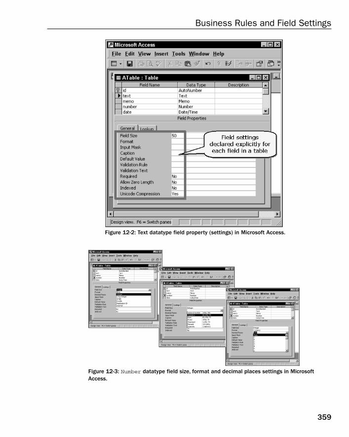
Figure 12-2: Text datatype field property (settings) in Microsoft Access.
Figure 12-3: Number datatype field size, format and decimal places settings in MicrosoftAccess.
359
Business Rules and Field Settings
18_574906 ch12.qxd 10/28/05 11:42 PM Page 359
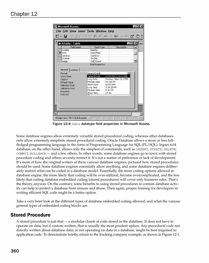
Figure 12-4: Date datatype field properties in Microsoft Access.
Some database engines allow extremely versatile stored procedural coding, whereas other databasesonly allow extremely simplistic stored procedural coding. Oracle Database allows a more or less full-fledged programming language in the form of Programming Language for SQL (PL/SQL). Ingres 6.04database, on the other hand, allows only the simplest of commands, such as INSERT, UPDATE, DELETE,COMMIT, ROLLBACK— and a few others. In other words, some database engines go to town with storedprocedure coding and others severely restrict it. It’s not a matter of preference or lack of development.It’s more of how the original writers of these various database engines, pictured how stored proceduresshould be used. Some database engines essentially allow anything, and some database engines deliber-ately restrict what can be coded in a database model. Essentially, the more coding options allowed indatabase engine, the more likely that coding will be over-utilized, become overcomplicated, and the lesslikely that coding database embedded coding (stored procedures) will cover only business rules. That’sthe theory, anyway. On the contrary, some benefits to using stored procedures to contain database activ-ity can help to protect a database from misuse and abuse. Then again, proper training for developers inwriting efficient SQL code might be a better option.
Take a very brief look at the different types of database embedded coding allowed, and what the variousgeneral types of embedded coding blocks are.
Stored Procedure A stored procedure is just that — a modular chunk of code stored in the database. It does not have tooperate on data, but if custom-written, that is usually the most prudent option. Any procedural code notdirectly written about database data, or not operating on data in a database, might be best migrated toapplication code. To demonstrate briefly, return to the trucking company example, as shown in Figure 12-1.
360
Chapter 12
18_574906 ch12.qxd 10/28/05 11:42 PM Page 360
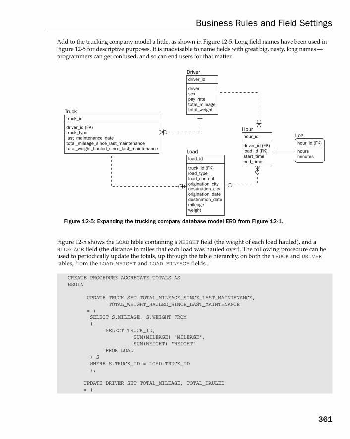
Add to the trucking company model a little, as shown in Figure 12-5. Long field names have been used inFigure 12-5 for descriptive purposes. It is inadvisable to name fields with great big, nasty, long names —programmers can get confused, and so can end users for that matter.
Figure 12-5: Expanding the trucking company database model ERD from Figure 12-1.
Figure 12-5 shows the LOAD table containing a WEIGHT field (the weight of each load hauled), and aMILEGAGE field (the distance in miles that each load was hauled over). The following procedure can beused to periodically update the totals, up through the table hierarchy, on both the TRUCK and DRIVERtables, from the LOAD.WEIGHT and LOAD MILEAGE fields.
CREATE PROCEDURE AGGREGATE_TOTALS ASBEGIN
UPDATE TRUCK SET TOTAL_MILEAGE_SINCE_LAST_MAINTENANCE,TOTAL_WEIGHT_HAULED_SINCE_LAST_MAINTENANCE
= (SELECT S.MILEAGE, S.WEIGHT FROM(
SELECT TRUCK_ID,SUM(MILEAGE) “MILEAGE”,SUM(WEIGHT) “WEIGHT”
FROM LOAD) SWHERE S.TRUCK_ID = LOAD.TRUCK_ID);
UPDATE DRIVER SET TOTAL_MILEAGE, TOTAL_HAULED= (
Driverdriver_id
driversexpay_ratetotal_mileagetotal_weight
Loadload_id
truck_id (FK)load_typeload_contentorigination_citydestination_cityorigination_datedestination_datemileageweight
Trucktruck_id
driver_id (FK)truck_typelast_maintenance_datetotal_mileage_since_last_maintenancetotal_weight_hauled_since_last_maintenance
Hourhour_id
driver_id (FK)load_id (FK)start_timeend_time
Loghour_id (FK)
hoursminutes
361
Business Rules and Field Settings
18_574906 ch12.qxd 10/28/05 11:42 PM Page 361
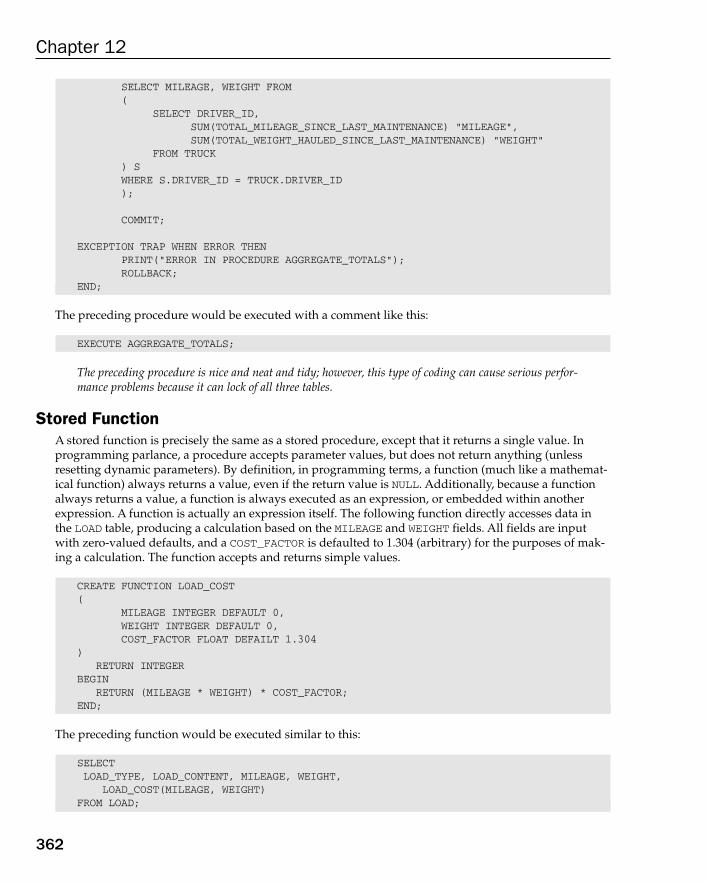
SELECT MILEAGE, WEIGHT FROM(
SELECT DRIVER_ID,SUM(TOTAL_MILEAGE_SINCE_LAST_MAINTENANCE) “MILEAGE”,SUM(TOTAL_WEIGHT_HAULED_SINCE_LAST_MAINTENANCE) “WEIGHT”
FROM TRUCK) SWHERE S.DRIVER_ID = TRUCK.DRIVER_ID);
COMMIT;
EXCEPTION TRAP WHEN ERROR THENPRINT(“ERROR IN PROCEDURE AGGREGATE_TOTALS”);ROLLBACK;
END;
The preceding procedure would be executed with a comment like this:
EXECUTE AGGREGATE_TOTALS;
The preceding procedure is nice and neat and tidy; however, this type of coding can cause serious perfor-mance problems because it can lock of all three tables.
Stored Function A stored function is precisely the same as a stored procedure, except that it returns a single value. In programming parlance, a procedure accepts parameter values, but does not return anything (unlessresetting dynamic parameters). By definition, in programming terms, a function (much like a mathemat-ical function) always returns a value, even if the return value is NULL. Additionally, because a functionalways returns a value, a function is always executed as an expression, or embedded within anotherexpression. A function is actually an expression itself. The following function directly accesses data inthe LOAD table, producing a calculation based on the MILEAGE and WEIGHT fields. All fields are inputwith zero-valued defaults, and a COST_FACTOR is defaulted to 1.304 (arbitrary) for the purposes of mak-ing a calculation. The function accepts and returns simple values.
CREATE FUNCTION LOAD_COST(
MILEAGE INTEGER DEFAULT 0,WEIGHT INTEGER DEFAULT 0,COST_FACTOR FLOAT DEFAILT 1.304
)RETURN INTEGER
BEGINRETURN (MILEAGE * WEIGHT) * COST_FACTOR;
END;
The preceding function would be executed similar to this:
SELECTLOAD_TYPE, LOAD_CONTENT, MILEAGE, WEIGHT,
LOAD_COST(MILEAGE, WEIGHT)FROM LOAD;
362
Chapter 12
18_574906 ch12.qxd 10/28/05 11:42 PM Page 362
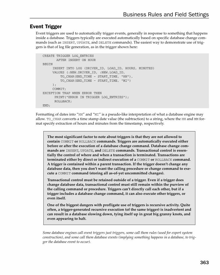
Event Trigger Event triggers are used to automatically trigger events, generally in response to something that happensinside a database. Triggers typically are executed automatically based on specific database change com-mands (such as INSERT, UPDATE, and DELETE commands). The easiest way to demonstrate use of trig-gers is that of log file generation, as in the trigger shown here:
CREATE TRIGGER LOG_ENTRIESAFTER INSERT ON HOUR
BEGININSERT INTO LOG (DRIVER_ID, LOAD_ID, HOURS, MINUTES)VALUES (:NEW.DRIVER_ID, :NEW.LOAD_ID,
TO_CHAR(END_TIME – START_TIME, “HH”),TO_CHAR(END_TIME – START_TIME, “MI”)
);COMMIT;
EXCEPTION TRAP WHEN ERROR THENPRINT(“ERROR IN TRIGGER LOG_ENTRIES”);ROLLBACK;
END;
Formatting of dates into “HH” and “MI” is a pseudo-like interpretation of what a database engine mayallow. TO_CHAR converts a time stamp date value (the subtraction) to a string, where the HH and MM for-mat specify extraction of hours and minutes from the timestamp, respectively.
Some database engines call event triggers just triggers, some call them rules (used for expert systemconstruction), and some call them database events (implying something happens in a database, to trig-ger the database event to occur).
The most significant factor to note about triggers is that they are not allowed to contain COMMIT or ROLLBACK commands. Triggers are automatically executed eitherbefore or after the execution of a database change command. Database change com-mands are INSERT, UPDATE, and DELETE commands. Transactional control is essen-tially the control of where and when a transaction is terminated. Transactions areterminated either by direct or indirect execution of a COMMIT or ROLLBACK command.A trigger is contained within a parent transaction. If the trigger doesn’t change anydatabase data, then you don’t want the calling procedure or change command to exe-cute a COMMIT command (storing all as-of-yet uncommitted changes).
Transactional control must be retained outside of a trigger. Even if a trigger doeschange database data, transactional control must still remain within the purview ofthe calling command or procedure. Triggers can’t directly call each other, but if atrigger includes a database change command, it can also execute other triggers, oreven itself.
One of the biggest dangers with profligate use of triggers is recursive activity. Quiteoften, a trigger-generated recursive execution (of the same trigger) is inadvertent andcan result in a database slowing down, tying itself up in great big granny knots, andeven appearing to halt.
363
Business Rules and Field Settings
18_574906 ch12.qxd 10/28/05 11:42 PM Page 363
External Procedure External procedures are very similar to stored procedures, except they are written a non-database-specific programming language. External procedures are a chunk of code written in a language notnative to the database engine (such as Java or C++). However, external procedures are still executedfrom within the database engine itself, perhaps on data within the database.
Macro A macro is a little like a pseudo-type series of commands, typically not really a programming language,and sometimes a sequence of commands built from GUI-based actions (such as those seen on the Filemenu in Microsoft Access). In other words, a highly computer-literate person, who is not a programmer,stores a sequence of mouse clicks and software tool executed steps, stores them in a file, to be executedat some other time.
Now get back to the case study, and continue with more in depth business model development, for theOLTP and data warehouse database models — using the online auction house.
Case Study: Implementing Field LevelBusiness Rules in a Database Model
The whole objective of this chapter is to show very detailed application of business rules into a databasemodel. This can be placing too much detail into a database model. It might be too much detail becausethis type of business rules implementation is nearly always much more effectively and efficiently han-dled by application SDK programming languages. Typically, this level of business rules implementationinto a database model can overcomplicate a database model, and quite often lead to serious performanceproblems, and serious difficulty in the day-to-day maintenance of production level databases.
Table and Relation Level Business RulesIn the case study so far in previous chapters, all factors for both OLTP and data warehouse databasemodels, for all table and relational level business rules have already been covered in detail. This meansthat for both OLTP and data warehouse database models, for the online auction house, all the tables andrelationships between them have been analyzed and designed. There is nothing more to do in thisrespect, as it’s already been done. In other words, everything to do with normalization, Normal Forms,relations, relation types classification, referential integrity, primary and foreign keys, is already com-pleted. No more need be said at this point.
Individual Field Business RulesIndividual field business rules for case study data modeling in the previous chapter has been partiallycovered. NULL settings and UNIQUE keys are catered for already. Default values, validation checks, andother settings (such as formatting and input maskings) are not yet covered.
Field Level Business Rules for the OLTP Database ModelFigure 12-6 shows the most recent version of the ERD for the OLTP database model, for the online auction house. Figure 12-6 shows that a CURRENT_PRICE field has been added to the LISTING table to
364
Chapter 12
18_574906 ch12.qxd 10/28/05 11:42 PM Page 364
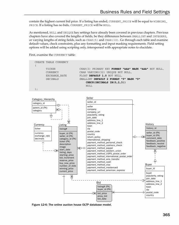
contain the highest current bid price. If a listing has ended, CURRENT_PRICE will be equal to WINNING_PRICE. If a listing has no bids, CURRENT_PRICE will be NULL.
As mentioned, NULL and UNIQUE key settings have already been covered in previous chapters. Previouschapters have also covered the lengths of fields, be they differences between SMALLINT and INTEGERS,or varying lengths of string fields, such as CHAR(5) and CHAR(10). Go through each table and examinedefault values, check constraints, plus any formatting and input masking requirements. Field settingoptions will be added using scripting only, interspersed with appropriate notes to elucidate.
First, examine the CURRENCY table:
CREATE TABLE CURRENCY(
TICKER CHAR(3) PRIMARY KEY FORMAT “AAA” MASK “AAA” NOT NULL,CURRENCY CHAR VARYING(32) UNIQUE NOT NULL,EXCHANGE_RATE FLOAT DEFAULT 1.0 NOT NULL,DECIMALS SMALLINT DEFAULT 2 FORMAT “9” MASK “9”
CHECK(DECIMALS IN(0,2,3))NULL
);
Figure 12-6: The online auction house OLTP database model.
Listinglisting#
buyer_id (FK)seller_id (FK)category_id (FK)ticker (FK)descriptionimagestart_datelisting_daysstarting_pricebid_incrementreserve_pricebuy_now_pricenumber_of_bidswinning_pricecurrent_price
Historyhistory_id
seller_id (FK)buyer_id (FK)comment_datefeedback_positivefeedback_neutralfeedback_negative
Sellerseller_id
sellercompanycompany_urlpopularity_ratingjoin_dateaddress_line_1address_line_2townzippostal_codecountryreturn_policyinternational_shippingpayment_method_personal_checkpayment_method_cashiers_checkpayment_method_paypalpayment_method_western_unionpayment_method_USPS_postal_orderpayment_method_international_postal_orderpayment_method_wire_transferpayment_method_cashpayment_method_visapayment_method_mastercardpayment_method_american_express
Buyerbuyer_id
buyerpopularity_ratingjoin_dateaddress_line_1address_line_2townzippostal_codecountry
Currencyticker
currencyexchange_ratedecimals
Category_Hierarchycategory_id
parent_id (FK)category
Bidlisting# (FK)buyer_id (FK)
bid_priceproxy_bidbid_date
365
Business Rules and Field Settings
18_574906 ch12.qxd 10/28/05 11:42 PM Page 365
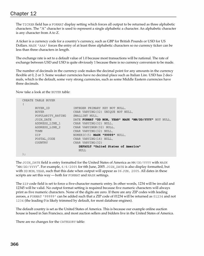
The TICKER field has a FORMAT display setting which forces all output to be returned as three alphabeticcharacters. The “A” character is used to represent a single alphabetic a character. An alphabetic characteris any character from A to Z.
A ticker is a currency code for a country’s currency, such as GBP for British Pounds or USD for USDollars. MASK “AAA” forces the entry of at least three alphabetic characters so no currency ticker can beless than three characters in length.
The exchange rate is set to a default value of 1.0 because most transactions will be national. The rate ofexchange between USD and USD is quite obviously 1 because there is no currency conversion to be made.
The number of decimals in the currency code makes the decimal point for any amounts in the currencyflexible at 0, 2 or 3. Some weaker currencies have no decimal place such as Italian Lire. USD has 2 deci-mals, which is the default, some very strong currencies, such as some Middle Eastern currencies havethree decimals.
Now take a look at the BUYER table:
CREATE TABLE BUYER(
BUYER_ID INTEGER PRIMARY KEY NOT NULL,BUYER CHAR VARYING(32) UNIQUE NOT NULL,POPULARITY_RATING SMALLINT NULL,JOIN_DATE DATE FORMAT “DD MON, YEAR” MASK “MM/DD/YYYY” NOT NULL,ADDRESS_LINE_1 CHAR VARYING(32) NULL,ADDRESS_LINE_2 CHAR VARYINGR(32) NULL,TOWN CHAR VARYING(32) NULL,ZIP NUMERIC(5) MASK “99999” NULL,POSTAL_CODE CHAR VARYING(16) NULL,COUNTRY CHAR VARYING(32)
DEFAULT “United States of America”NULL
);
The JOIN_DATE field is entry formatted for the United States of America as MM/DD/YYYY with MASK“MM/DD/YYYY”. For example, 6/6/2005 for 6th June, 2005. JOIN_DATE is also display formatted, butwith DD MON, YEAR, such that this date when output will appear as 06 JUN, 2005. All dates in thesescripts are set this way — both for FORMAT and MASK settings.
The ZIP code field is set to force a five-character numeric entry. In other words, 1234 will be invalid and12345 will be valid. No output format setting is required because five numeric characters will alwaysprint as five numeric characters. None of the digits are zero. If there are any ZIP codes with leadingzeroes, a FORMAT “99999” can be added such that a ZIP code of 01234 will be returned as 01234 and not1234 (the leading 0 is likely trimmed by default, for most database engines).
The default country is set as the United States of America. This is because our example online auctionhouse is based in San Francisco, and most auction sellers and bidders live in the United States of America.
There are no changes for the CATEGORY table:
366
Chapter 12
18_574906 ch12.qxd 10/28/05 11:42 PM Page 366
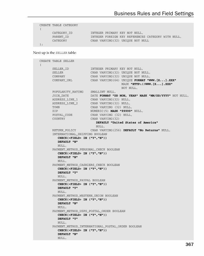
CREATE TABLE CATEGORY(
CATEGORY_ID INTEGER PRIMARY KEY NOT NULL,PARENT_ID INTEGER FOREIGN KEY REFERENCES CATEGORY WITH NULL,CATEGORY CHAR VARYING(32) UNIQUE NOT NULL
);
Next up is the SELLER table:
CREATE TABLE SELLER(
SELLER_ID INTEGER PRIMARY KEY NOT NULL,SELLER CHAR VARYING(32) UNIQUE NOT NULL,COMPANY CHAR VARYING(32) UNIQUE NOT NULL,COMPANY_URL CHAR VARYING(64) UNIQUE FORMAT “WWW.[X...].XXX”
MASK “HTTP://WWW.[X...].XXX”NOT NULL,
POPULARITY_RATING SMALLINT NULL,JOIN_DATE DATE FORMAT “DD MON, YEAR” MASK “MM/DD/YYYY” NOT NULL,ADDRESS_LINE_1 CHAR VARYING(32) NULL,ADDRESS_LINE_2 CHAR VARYING(32) NULL,TOWN CHAR VARYING (32) NULL,ZIP NUMERIC(5) MASK “99999” NULL,POSTAL_CODE CHAR VARYING (32) NULL,COUNTRY CHAR VARYING(32)
DEFAULT “United States of America”NULL,
RETURN_POLICY CHAR VARYING(256) DEFAULT “No Returns” NULL,INTERNATIONAL_SHIPPING BOOLEAN
CHECK(<FIELD> IN (“Y”,”N”))DEFAULT “N”NULL,
PAYMENT_METHOD_PERSONAL_CHECK BOOLEANCHECK(<FIELD> IN (“Y”,”N”))DEFAULT “N”NULL,
PAYMENT_METHOD_CASHIERS_CHECK BOOLEANCHECK(<FIELD> IN (“Y”,”N”))DEFAULT “Y”NULL,
PAYMENT_METHOD_PAYPAL BOOLEANCHECK(<FIELD> IN (“Y”,”N”))DEFAULT “Y”NULL,
PAYMENT_METHOD_WESTERN_UNION BOOLEANCHECK(<FIELD> IN (“Y”,”N”))DEFAULT “N”NULL,
PAYMENT_METHOD_USPS_POSTAL_ORDER BOOLEANCHECK(<FIELD> IN (“Y”,”N”))DEFAULT “Y”NULL,
PAYMENT_METHOD_INTERNATIONAL_POSTAL_ORDER BOOLEANCHECK(<FIELD> IN (“Y”,”N”))DEFAULT “N”NULL,
367
Business Rules and Field Settings
18_574906 ch12.qxd 10/28/05 11:42 PM Page 367

PAYMENT_METHOD_WIRE_TRANSFER BOOLEANCHECK(<FIELD> IN (“Y”,”N”))DEFAULT “N”NULL,
PAYMENT_METHOD_CASH BOOLEANCHECK(<FIELD> IN (“Y”,”N”))DEFAULT “N”NULL,
PAYMENT_METHOD_VISA BOOLEANCHECK(<FIELD> IN (“Y”,”N”))DEFAULT “N”NULL,
PAYMENT_METHOD_MASTERCARD BOOLEANCHECK(<FIELD> IN (“Y”,”N”))DEFAULT “N”NULL,
PAYMENT_METHOD_AMERICAN_EXPRESS BOOLEANCHECK(<FIELD> IN (“Y”,”N”))DEFAULT “N”NULL
);
In the COMPANY_URL field, the FORMAT and MASK settings are slightly different in that the MASK settingrequires the prefix HTTP://. Both format and mask settings will force a URL to be “WWW.[X...].XXX”where the “X” character represents an alphanumeric string (not alphabetic as for “A”), and the “[X...]”implies that a string of one or more alphanumeric characters is allowed. XXX at the end of the stringrestricts to three characters, such as “COM” or “BIZ.” There is also “TV,” which is two characters but, forthe purposes of simplicity, this format sticks to three characters.
Dates, ZIP code and COUNTRY default values are set as before.
RETURN_POLICY is defaulted as “No Returns”, implying that most sellers do not want things returned.In reality this is unlikely, of course.
All BOOLEAN datatype fields are set as CHECK(<FIELD> IN (“Y”,”N”)) and DEFAULT”N”. This ispseudo code and the field names are monstrously long. Thus, <FIELD> should be replaced with theactual field name. The CHECK constraint forces a “Y” or “N” entry, as opposed to “T” or “F”, “1” or “0”.Technically, this is only relevant to entry, and display as BOOLEAN datatypes are generally stored inter-nally as 1 or 0 anyway. Also the default is set to “N,” implying that if a field is not entered, it is set to“N,” rather than left as NULL valued.
Now tackle the LISTING table:
CREATE TABLE LISTING(
LISTING# CHAR(10) PRIMARY KEY NOT NULL,CATEGORY_ID INTEGER FOREIGN KEY REFERENCES CATEGORY NOT NULL,BUYER_ID INTEGER FOREIGN KEY REFERENCES BUYER WITH NULL,SELLER_ID INTEGER FOREIGN KEY REFERENCES SELLER WITH NULL,TICKER CHAR(3) FOREIGN KEY REFERENCES CURRENCY WITH NULL,DESCRIPTION CHAR VARYING(32) NULL,
368
Chapter 12
18_574906 ch12.qxd 10/28/05 11:42 PM Page 368
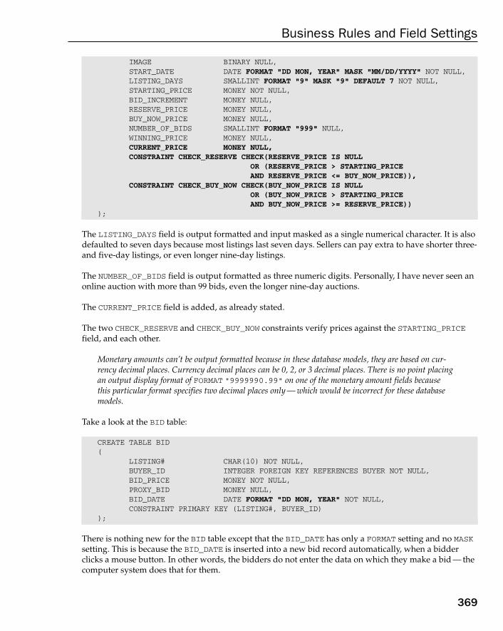
IMAGE BINARY NULL,START_DATE DATE FORMAT “DD MON, YEAR” MASK “MM/DD/YYYY” NOT NULL,LISTING_DAYS SMALLINT FORMAT “9” MASK “9” DEFAULT 7 NOT NULL,STARTING_PRICE MONEY NOT NULL,BID_INCREMENT MONEY NULL,RESERVE_PRICE MONEY NULL,BUY_NOW_PRICE MONEY NULL,NUMBER_OF_BIDS SMALLINT FORMAT “999” NULL,WINNING_PRICE MONEY NULL,CURRENT_PRICE MONEY NULL,CONSTRAINT CHECK_RESERVE CHECK(RESERVE_PRICE IS NULL
OR (RESERVE_PRICE > STARTING_PRICEAND RESERVE_PRICE <= BUY_NOW_PRICE)),
CONSTRAINT CHECK_BUY_NOW CHECK(BUY_NOW_PRICE IS NULLOR (BUY_NOW_PRICE > STARTING_PRICEAND BUY_NOW_PRICE >= RESERVE_PRICE))
);
The LISTING_DAYS field is output formatted and input masked as a single numerical character. It is alsodefaulted to seven days because most listings last seven days. Sellers can pay extra to have shorter three-and five-day listings, or even longer nine-day listings.
The NUMBER_OF_BIDS field is output formatted as three numeric digits. Personally, I have never seen anonline auction with more than 99 bids, even the longer nine-day auctions.
The CURRENT_PRICE field is added, as already stated.
The two CHECK_RESERVE and CHECK_BUY_NOW constraints verify prices against the STARTING_PRICEfield, and each other.
Monetary amounts can’t be output formatted because in these database models, they are based on cur-rency decimal places. Currency decimal places can be 0, 2, or 3 decimal places. There is no point placingan output display format of FORMAT “9999990.99” on one of the monetary amount fields becausethis particular format specifies two decimal places only — which would be incorrect for these databasemodels.
Take a look at the BID table:
CREATE TABLE BID(
LISTING# CHAR(10) NOT NULL,BUYER_ID INTEGER FOREIGN KEY REFERENCES BUYER NOT NULL,BID_PRICE MONEY NOT NULL,PROXY_BID MONEY NULL,BID_DATE DATE FORMAT “DD MON, YEAR” NOT NULL,CONSTRAINT PRIMARY KEY (LISTING#, BUYER_ID)
);
There is nothing new for the BID table except that the BID_DATE has only a FORMAT setting and no MASKsetting. This is because the BID_DATE is inserted into a new bid record automatically, when a bidderclicks a mouse button. In other words, the bidders do not enter the data on which they make a bid — thecomputer system does that for them.
369
Business Rules and Field Settings
18_574906 ch12.qxd 10/28/05 11:42 PM Page 369
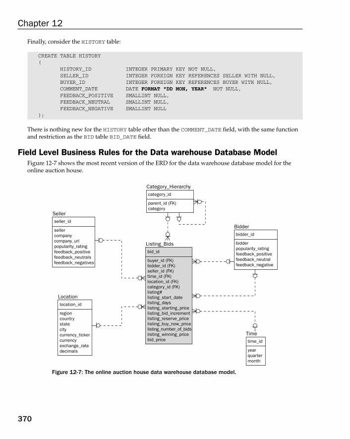
Finally, consider the HISTORY table:
CREATE TABLE HISTORY(
HISTORY_ID INTEGER PRIMARY KEY NOT NULL,SELLER_ID INTEGER FOREIGN KEY REFERENCES SELLER WITH NULL,BUYER_ID INTEGER FOREIGN KEY REFERENCES BUYER WITH NULL,COMMENT_DATE DATE FORMAT “DD MON, YEAR” NOT NULL,FEEDBACK_POSITIVE SMALLINT NULL,FEEDBACK_NEUTRAL SMALLINT NULL,FEEDBACK_NEGATIVE SMALLINT NULL
);
There is nothing new for the HISTORY table other than the COMMENT_DATE field, with the same functionand restriction as the BID table BID_DATE field.
Field Level Business Rules for the Data warehouse Database ModelFigure 12-7 shows the most recent version of the ERD for the data warehouse database model for theonline auction house.
Figure 12-7: The online auction house data warehouse database model.
Bidderbidder_id
bidderpopularity_ratingfeedback_positivefeedback_neutralfeedback_negative
Category_Hierarchycategory_id
parent_id (FK)category
Sellerseller_id
sellercompanycompany_urlpopularity_ratingfeedback_positivefeedback_neutralsfeedback_negatives
Locationlocation_id
regioncountrystatecitycurrency_tickercurrencyexchange_ratedecimals
Timetime_id
yearquartermonth
Listing_Bidsbid_id
buyer_id (FK)bidder_id (FK)seller_id (FK)time_id (FK)location_id (FK)category_id (FK)listing#listing_start_datelisting_dayslisting_starting_pricelisting_bid_incrementlisting_reserve_pricelisting_buy_now_pricelisting_number_of_bidslisting_winning_pricebid_price
370
Chapter 12
18_574906 ch12.qxd 10/28/05 11:42 PM Page 370
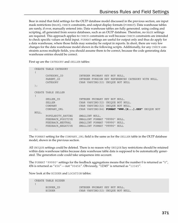
Bear in mind that field settings for the OLTP database model discussed in the previous section, are inputmask restrictions (MASK), CHECK constraints, and output display formats (FORMAT). Data warehouse tablesare rarely, if ever, manually entered into. Data warehouse tables are fully generated. using coding andscripting, all generated from source databases, such as an OLTP database. Therefore, no MASK settingsare required. This approach applies to CHECK constraints as well because CHECK constraints are intendedto check specific values on field input. FORMAT settings are useful for output only and thus do apply fora data warehouse, where those fields may someday be output in reports. In short, there are very fewchanges for the data warehouse model shown in the following scripts. Additionally, for any CHECK con-straints across multiple fields, you should assume them to be correct, because the code generating datawarehouse entries should be correct.
First up are the CATEGORY and SELLER tables:
CREATE TABLE CATEGORY(
CATEGORY_ID INTEGER PRIMARY KEY NOT NULL,PARENT_ID INTEGER FOREIGN KEY REFERENCES CATEGORY WITH NULL,CATEGORY CHAR VARYING(32) UNIQUE NOT NULL
);
CREATE TABLE SELLER(
SELLER_ID INTEGER PRIMARY KEY NOT NULL,SELLER CHAR VARYING(32) UNIQUE NOT NULL,COMPANY CHAR VARYING(32) UNIQUE NOT NULL,COMPANY_URL CHAR VARYING(64) FORMAT “WWW.[X...].XXX” UNIQUE NOT
NULL,POPULARITY_RATING SMALLINT NULL,FEEDBACK_POSITIVE SMALLINT FORMAT “99990” NULL,FEEDBACK_NEUTRAL SMALLINT FORMAT “99990” NULL,FEEDBACK_NEGATIVE SMALLINT FORMAT “99990” NULL
);
The FORMAT setting for the COMPANY_URL field is the same as for the SELLER table in the OLTP databasemodel, shown in the previous section.
All UNIQUE settings could be deleted. There is no reason why UNIQUE key restrictions should be retainedwithin data warehouse tables because data warehouse table data is supposed to be automatically gener-ated. The generation code could take uniqueness into account.
The FORMAT “99990” settings for the feedback aggregations means that the number 0 is returned as “0”,456 is returned as “456” — not “00456”. Obviously, “12345” is returned as “12345”.
Now look at the BIDDER and LOCATION tables:
CREATE TABLE BIDDER(
BIDDER_ID INTEGER PRIMARY KEY NOT NULL,BIDDER CHAR VARYING(32) UNIQUE NOT NULL,
371
Business Rules and Field Settings
18_574906 ch12.qxd 10/28/05 11:42 PM Page 371
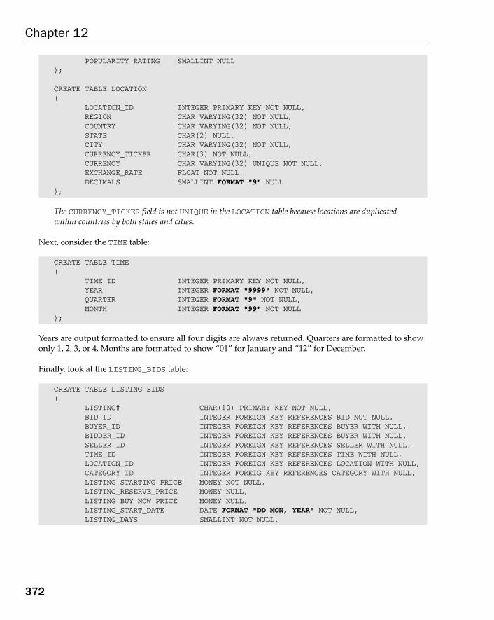
POPULARITY_RATING SMALLINT NULL);
CREATE TABLE LOCATION(
LOCATION_ID INTEGER PRIMARY KEY NOT NULL,REGION CHAR VARYING(32) NOT NULL,COUNTRY CHAR VARYING(32) NOT NULL,STATE CHAR(2) NULL,CITY CHAR VARYING(32) NOT NULL,CURRENCY_TICKER CHAR(3) NOT NULL,CURRENCY CHAR VARYING(32) UNIQUE NOT NULL,EXCHANGE_RATE FLOAT NOT NULL,DECIMALS SMALLINT FORMAT “9” NULL
);
The CURRENCY_TICKER field is not UNIQUE in the LOCATION table because locations are duplicatedwithin countries by both states and cities.
Next, consider the TIME table:
CREATE TABLE TIME(
TIME_ID INTEGER PRIMARY KEY NOT NULL,YEAR INTEGER FORMAT “9999” NOT NULL,QUARTER INTEGER FORMAT “9” NOT NULL,MONTH INTEGER FORMAT “99” NOT NULL
);
Years are output formatted to ensure all four digits are always returned. Quarters are formatted to showonly 1, 2, 3, or 4. Months are formatted to show “01” for January and “12” for December.
Finally, look at the LISTING_BIDS table:
CREATE TABLE LISTING_BIDS(
LISTING# CHAR(10) PRIMARY KEY NOT NULL,BID_ID INTEGER FOREIGN KEY REFERENCES BID NOT NULL,BUYER_ID INTEGER FOREIGN KEY REFERENCES BUYER WITH NULL,BIDDER_ID INTEGER FOREIGN KEY REFERENCES BUYER WITH NULL,SELLER_ID INTEGER FOREIGN KEY REFERENCES SELLER WITH NULL,TIME_ID INTEGER FOREIGN KEY REFERENCES TIME WITH NULL,LOCATION_ID INTEGER FOREIGN KEY REFERENCES LOCATION WITH NULL,CATEGORY_ID INTEGER FOREIG KEY REFERENCES CATEGORY WITH NULL,LISTING_STARTING_PRICE MONEY NOT NULL,LISTING_RESERVE_PRICE MONEY NULL,LISTING_BUY_NOW_PRICE MONEY NULL,LISTING_START_DATE DATE FORMAT “DD MON, YEAR” NOT NULL,LISTING_DAYS SMALLINT NOT NULL,
372
Chapter 12
18_574906 ch12.qxd 10/28/05 11:42 PM Page 372
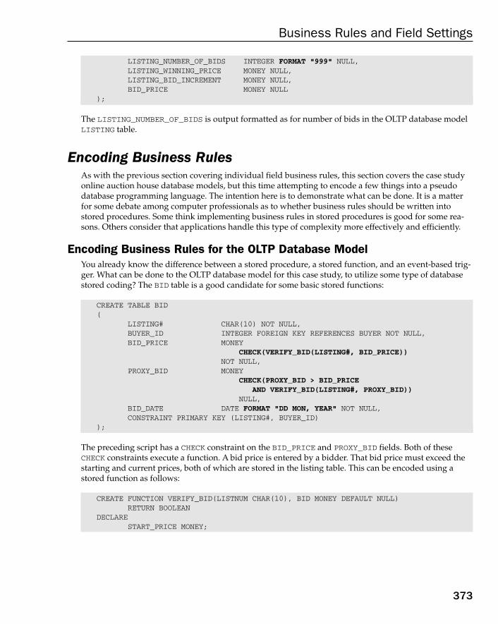
LISTING_NUMBER_OF_BIDS INTEGER FORMAT “999” NULL,LISTING_WINNING_PRICE MONEY NULL,LISTING_BID_INCREMENT MONEY NULL,BID_PRICE MONEY NULL
);
The LISTING_NUMBER_OF_BIDS is output formatted as for number of bids in the OLTP database modelLISTING table.
Encoding Business RulesAs with the previous section covering individual field business rules, this section covers the case studyonline auction house database models, but this time attempting to encode a few things into a pseudodatabase programming language. The intention here is to demonstrate what can be done. It is a matterfor some debate among computer professionals as to whether business rules should be written intostored procedures. Some think implementing business rules in stored procedures is good for some rea-sons. Others consider that applications handle this type of complexity more effectively and efficiently.
Encoding Business Rules for the OLTP Database ModelYou already know the difference between a stored procedure, a stored function, and an event-based trig-ger. What can be done to the OLTP database model for this case study, to utilize some type of databasestored coding? The BID table is a good candidate for some basic stored functions:
CREATE TABLE BID(
LISTING# CHAR(10) NOT NULL,BUYER_ID INTEGER FOREIGN KEY REFERENCES BUYER NOT NULL,BID_PRICE MONEY
CHECK(VERIFY_BID(LISTING#, BID_PRICE))NOT NULL,
PROXY_BID MONEYCHECK(PROXY_BID > BID_PRICE
AND VERIFY_BID(LISTING#, PROXY_BID))NULL,
BID_DATE DATE FORMAT “DD MON, YEAR” NOT NULL, CONSTRAINT PRIMARY KEY (LISTING#, BUYER_ID)
);
The preceding script has a CHECK constraint on the BID_PRICE and PROXY_BID fields. Both of theseCHECK constraints execute a function. A bid price is entered by a bidder. That bid price must exceed thestarting and current prices, both of which are stored in the listing table. This can be encoded using astored function as follows:
CREATE FUNCTION VERIFY_BID(LISTNUM CHAR(10), BID MONEY DEFAULT NULL)RETURN BOOLEAN
DECLARESTART_PRICE MONEY;
373
Business Rules and Field Settings
18_574906 ch12.qxd 10/28/05 11:42 PM Page 373

CURR_PRICE MONEY;BEGIN
REMARK --- Throw out bids that are incorrectly passed inIF LISTING# IS NULL OR BID IS NULL OR BID <= 0 THEN RETURN FALSE;
REMARK –-- bidding price (including proxy bids) must exceed starting priceREMARK –-- if current price is NULL, otherwise must exceed current price
SELECT STARTING_PRICE, CURRENT_PRICEINTO START_PRICE, CURR_PRICEFROM LISTING WHERE LISTING# = LISTNUM;
IF CURR_PRICE IS NULL THENIF BID <= START_PRICE THEN RETURN FALSE;
ELSEIF BID <= CURR_PRICE THEN RETURN FALSE;
END IF;
RETURN TRUE;
END;
The preceding script applies to both normal (regular) bids and to proxy bids as well. A proxy bid mustalways be greater than the current bid price; otherwise, the proxy bid is just a normal bid. A proxy bid iswhere a buyer sets a maximum price that they will bid to. Whenever other bidders place bids, the systemautomatically increments the highest bid price with the current increment, until the proxy bid is reached. If the competing bidder exceeds the proxy bid, the other buyer becomes the current highest bidder.
Encoding Business Rules for the Data Warehouse Database ModelIn short, there is nothing that you would want to attach to a data warehouse database model in the formof database model embedded coding, acting on the database model structures. It would simply be con-trary to the existence of a data warehouse.
Try It Out Field Level Business Rules for an OLTP Database ModelFigure 12-8 shows an ERD for the musicians OLTP database model. Here’s a basic approach to businessrules field settings:
1. Individual field business rules (including defaults, CHECK constraints, display formats, andinput masks)
2. Encoding business rules using some kind of stored database coding, if and where appropriate(usually CHECK constraint functions)
374
Chapter 12
18_574906 ch12.qxd 10/28/05 11:42 PM Page 374
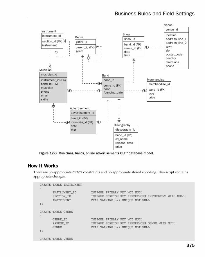
Figure 12-8: Musicians, bands, online advertisements OLTP database model.
How It WorksThere are no appropriate CHECK constraints and no appropriate stored encoding. This script containsappropriate changes:
CREATE TABLE INSTRUMENT(
INSTRUMENT_ID INTEGER PRIMARY KEY NOT NULL,SECTION_ID INTEGER FOREIGN KEY REFERENCES INSTRUMENT WITH NULL,INSTRUMENT CHAR VARYING(32) UNIQUE NOT NULL
);
CREATE TABLE GENRE(
GENRE_ID INTEGER PRIMARY KEY NOT NULL,PARENT_ID INTEGER FOREIGN KEY REFERENCES GENRE WITH NULL,GENRE CHAR VARYING(32) UNIQUE NOT NULL
);
CREATE TABLE VENUE
Musicianmusician_id
instrument_id (FK)band_id (FK)musicianphoneemailskills
Advertisementadvertisement_id
band_id (FK)musician_id (FK)datetext
Bandband_id
genre_id (FK)bandfounding_date
Venuevenue_id
locationaddress_line_1address_line_2townzippostal_codecountrydirectionsphone
Merchandisemerchandise_id
band_id (FK)typeprice
Showshow_id
band_id (FK)venue_id (FK)datetime
Genregenre_id
parent_id (FK)genre
Instrumentinstrument_id
section_id (FK)instrument
Discographydiscography_id
band_id (FK)cd_namerelease_dateprice
375
Business Rules and Field Settings
18_574906 ch12.qxd 10/28/05 11:42 PM Page 375

(VENUE_ID INTEGER PRIMARY KEY NOT NULL,LOCATION CHAR VARYING(32) UNIQUE NOT NULL,ADDRESS_LINE_1 CHAR VARYING(32) NOT NULL,ADDRESS_LINE_2 CHAR VARYING(32) NULL,TOWN CHAR VARYING(32) NOT NULL,ZIP NUMBER(5) FORMAT “99999” MASK “99999” NULL,POSTAL_CODE CHAR VARYING(32) NULL,COUNTRY CHAR VARYING(32) NULL,DIRECTIONS MEMO NULL,PHONE CHAR VARYING(32) NULL
);
CREATE TABLE MERCHANDISE(
MERCHANDISE_ID INTEGER PRIMARY KEY NOT NULL,BAND_ID INTEGER FOREIGN KEY REFERENCES BAND NOT NULL,TYPE CHAR VARYING(32) UNIQUE NOT NULL,PRICE MONEY FORMAT “$9,999,990.99” MASK “9999990.00” NOT NULL
);
CREATE TABLE DISCOGRAPHY(
DISCOGRAPHY_ID INTEGER PRIMARY KEY NOT NULL,BAND_ID INTEGER FOREIGN REFERENCES BAND NOT NULL,CD_NAME CHAR VARYING(32) NOT NULL,RELEASE_DATE DATE FORMAT “DD MON, YEAR” MASK “MM/DD/YYYY” NOT NULL,PRICE MONEY FORMAT “$9,999,990.99” MASK “9999990.00” NOT NULL
);
CREATE TABLE SHOW(
SHOW_ID INTEGER PRIMARY KEY NOT NULL,BAND_ID INTEGER FOREIGN KEY REFERENCES BAND NOT NULL,VENUE_ID INTEGER FOREIGN KEY REFERENES VENUE NOT NULL,DATE DATE FORMAT “DD MON, YEAR” MASK “MM/DD/YYYY” NOT NULL,TIME CHAR VARYING(16)
FORMAT “90:90:90” MASK “90:90:90”NOT NULL
);
CREATE TABLE BAND(
BAND_ID INTEGER PRIMARY KEY NOT NULL,GENRE_ID INTEGER FOREIGN KEY REFERENCES GENRE NOT NULL,BAND CHAR VARYING(32) UNIQUE NOT NULL,FOUNDING_DATE DATE FORMAT “DD MON, YEAR” MASK “MM/DD/YYYY” NOT NULL
);
CREATE TABLE MUSICIAN(
MUSICIAN_ID INTEGER PRIMARY KEY NOT NULL,INSTRUMENT_ID INTEGER FOREIGN KEY REFERENCES INSTRUMENT NOT NULL,BAND_ID INTEGER FOREIGN KEY REFERENCES BAND WITH NULL,MUSICIAN CHAR VARYING(32) UNIQUE NOT NULL,PHONE CHAR VARYING(32) NULL,
376
Chapter 12
18_574906 ch12.qxd 10/28/05 11:42 PM Page 376
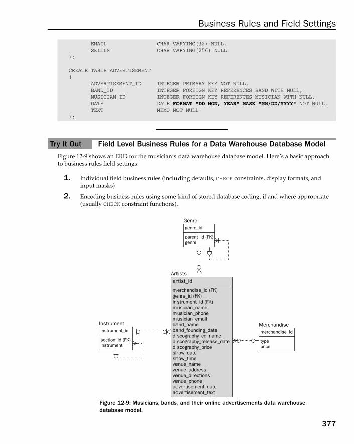
EMAIL CHAR VARYING(32) NULL,SKILLS CHAR VARYING(256) NULL
);
CREATE TABLE ADVERTISEMENT(
ADVERTISEMENT_ID INTEGER PRIMARY KEY NOT NULL,BAND_ID INTEGER FOREIGN KEY REFERENCES BAND WITH NULL,MUSICIAN_ID INTEGER FOREIGN KEY REFERENCES MUSICIAN WITH NULL,DATE DATE FORMAT “DD MON, YEAR” MASK “MM/DD/YYYY” NOT NULL,TEXT MEMO NOT NULL
);
Try It Out Field Level Business Rules for a Data Warehouse Database ModelFigure 12-9 shows an ERD for the musician’s data warehouse database model. Here’s a basic approachto business rules field settings:
1. Individual field business rules (including defaults, CHECK constraints, display formats, andinput masks)
2. Encoding business rules using some kind of stored database coding, if and where appropriate(usually CHECK constraint functions).
Figure 12-9: Musicians, bands, and their online advertisements data warehousedatabase model.
Artistsartist_id
merchandise_id (FK)genre_id (FK)instrument_id (FK)musician_namemusician_phonemusician_emailband_nameband_founding_datediscography_cd_namediscography_release_datediscography_priceshow_dateshow_timevenue_namevenue_addressvenue_directionsvenue_phoneadvertisement_dateadvertisement_text
Genregenre_id
parent_id (FK)genre
Merchandisemerchandise_id
typeprice
Instrumentinstrument_id
section_id (FK)instrument
377
Business Rules and Field Settings
18_574906 ch12.qxd 10/28/05 11:42 PM Page 377
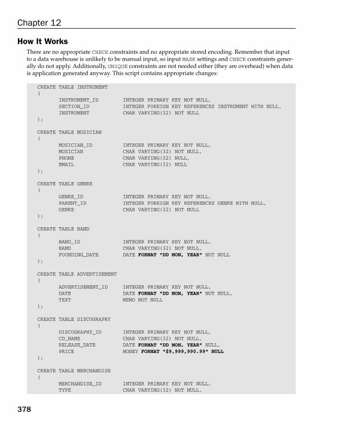
How It WorksThere are no appropriate CHECK constraints and no appropriate stored encoding. Remember that inputto a data warehouse is unlikely to be manual input, so input MASK settings and CHECK constraints gener-ally do not apply. Additionally, UNIQUE constraints are not needed either (they are overhead) when datais application generated anyway. This script contains appropriate changes:
CREATE TABLE INSTRUMENT(
INSTRUMENT_ID INTEGER PRIMARY KEY NOT NULL,SECTION_ID INTEGER FOREIGN KEY REFERENCES INSTRUMENT WITH NULL,INSTRUMENT CHAR VARYING(32) NOT NULL
);
CREATE TABLE MUSICIAN(
MUSICIAN_ID INTEGER PRIMARY KEY NOT NULL,MUSICIAN CHAR VARYING(32) NOT NULL,PHONE CHAR VARYING(32) NULL,EMAIL CHAR VARYING(32) NULL
);
CREATE TABLE GENRE(
GENRE_ID INTEGER PRIMARY KEY NOT NULL,PARENT_ID INTEGER FOREIGN KEY REFERENCES GENRE WITH NULL,GENRE CHAR VARYING(32) NOT NULL
);
CREATE TABLE BAND(
BAND_ID INTEGER PRIMARY KEY NOT NULL,BAND CHAR VARYING(32) NOT NULL,FOUNDING_DATE DATE FORMAT “DD MON, YEAR” NOT NULL
);
CREATE TABLE ADVERTISEMENT(
ADVERTISEMENT_ID INTEGER PRIMARY KEY NOT NULL,DATE DATE FORMAT “DD MON, YEAR” NOT NULL,TEXT MEMO NOT NULL
);
CREATE TABLE DISCOGRAPHY(
DISCOGRAPHY_ID INTEGER PRIMARY KEY NOT NULL,CD_NAME CHAR VARYING(32) NOT NULL,RELEASE_DATE DATE FORMAT “DD MON, YEAR” NULL,PRICE MONEY FORMAT “$9,999,990.99” NULL
);
CREATE TABLE MERCHANDISE(
MERCHANDISE_ID INTEGER PRIMARY KEY NOT NULL,TYPE CHAR VARYING(32) NOT NULL,
378
Chapter 12
18_574906 ch12.qxd 10/28/05 11:42 PM Page 378
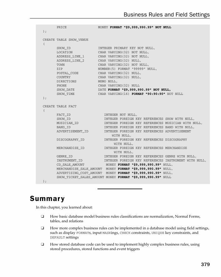
PRICE MONEY FORMAT “$9,999,990.99” NOT NULL);
CREATE TABLE SHOW_VENUE(
SHOW_ID INTEGER PRIMARY KEY NOT NULL,LOCATION CHAR VARYING(32) NOT NULL,ADDRESS_LINE_1 CHAR VARYING(32) NOT NULL,ADDRESS_LINE_2 CHAR VARYING(32) NULL,TOWN CHAR VARYING(32) NOT NULL,ZIP NUMBER(5) FORMAT “99999” NULL,POSTAL_CODE CHAR VARYING(32) NULL,COUNTRY CHAR VARYING(32) NULL,DIRECTIONS MEMO NULL,PHONE CHAR VARYING(32) NULLSHOW_DATE DATE FORMAT “$9,999,990.99” NOT NULL,SHOW_TIME CHAR VARYING(16) FORMAT “90:90:90” NOT NULL
);
CREATE TABLE FACT(
FACT_ID INTEGER NOT NULL,SHOW_ID INTEGER FOREIGN KEY REFERENCES SHOW WITH NULL,MUSICIAN_ID INTEGER FOREIGN KEY REFERENCES MUSICIAN WITH NULL,BAND_ID INTEGER FOREIGN KEY REFERENCES BAND WITH NULL,ADVERTISEMENT_ID INTEGER FOREIGN KEY REFERENCES ADVERTISEMENT
WITH NULL,DISCOGRAPHY_ID INTEGER FOREIGN KEY REFERENCES DISCOGRAPHY
WITH NULL,MERCHANDISE_ID INTEGER FOREIGN KEY REFERENCES MERCHANDISE
WITH NULL,GENRE_ID INTEGER FOREIGN KEY REFERENCES GENRE WITH NULL,INSTRUMENT_ID INTEGER FOREIGN KEY REFERENCES INSTRUMENT WITH NULL,CD_SALE_AMOUNT MONEY FORMAT “$9,999,990.99” NULL,MERCHANDISE_SALE_AMOUNT MONEY FORMAT “$9,999,990.99” NULL,ADVERTISING_COST_AMOUNT MONEY FORMAT “$9,999,990.99” NULL,SHOW_TICKET_SALES_AMOUNT MONEY FORMAT “$9,999,990.99” NULL
);
SummaryIn this chapter, you learned about:
❑ How basic database model business rules classifications are normalization, Normal Forms,tables, and relations
❑ How more complex business rules can be implemented in a database model using field settings,such as display FORMATs, input MASKings, CHECK constraints, UNIQUE key constraints, andDEFAULT settings
❑ How stored database code can be used to implement highly complex business rules, usingstored procedures, stored functions and event triggers
379
Business Rules and Field Settings
18_574906 ch12.qxd 10/28/05 11:42 PM Page 379

This chapter ends the case study of the OLTP and data warehouse database models using the online auc-tion house. This chapter has refined the implementation of business rules to the hilt by applying field-level attributes and settings as being part of table field structure. Additionally, very advanced businessrules can be applied using stored database coding (encoding). The next chapter discusses hardwareresources, as applied to database modeling.
380
Chapter 12
18_574906 ch12.qxd 10/28/05 11:42 PM Page 380

Part IV
Advanced Topics
In this Part:
Chapter 13: Advanced Database Structures and Hardware Resources
19_574906 pt04.qxd 10/28/05 11:49 PM Page 381

19_574906 pt04.qxd 10/28/05 11:49 PM Page 382
13Advanced Database
Structures and HardwareResources
This final chapter of this book wraps up the database modeling design process, delving a bit intosome advanced aspects of the implementation process. Implementation is essentially the actualdatabase building process. When you build a database, as opposed to just the database model, youcreate the database itself. During the database-creation process, implementing the database model,you might want to consider various other factors. These other factors include specialized databasemodel structures (other than tables and indexes). Additionally, there are certain hardware issuessuch as how big of a computer do you need? Other than hardware, there are certain databaseinstallation issues to consider, with respect to configuration. Configuration can affect various fac-tors, such as how fast your database ultimately performs. Or how much recoverability do youneed? How often should backups be executed?
Configuration is computer jargon used to describe the way in which a computer system, or partthereof (such as a database) is installed and set up. For example, when you start up a Windows com-puter, all your desktop icons are part of the configuration of you starting up your computer. Whatthe desktop icons are, and where on your desktop they are placed, are stored in a configuration fileon your computer somewhere. When you start up your computer, the Windows software retrievesthat configuration file, interprets its contents, and displays all your icons on the screen for you.
This chapter essentially appears at the culmination of database model analysis and design; how-ever, its contents should in the very least be considered as a part of the design process, beforegoing ahead and purchasing hardware, and creating the physical database itself.
By the end of this chapter, you will realize that database modeling is not just about creating tables,getting the correct relationships between them, and doing lots of hairy stuff with fields. Betweenthe database modeling phase and the creation of a database, you might want to consider material-ized views for a data warehouse, for example. Or, perhaps you might consider a specialized typeof hardware configuration using something called a RAID array.
In this chapter,you learn about the following:
20_574906 ch13.qxd 10/28/05 11:40 PM Page 383
❑ Views
❑ Materialized views
❑ Different types of indexes
❑ Auto counters
❑ Partitioning and parallel processing
❑ Hardware factors (including memory usage, as applied to OLTP or data warehouse databases)
❑ RAID arrays
❑ Standby databases
❑ Replication
❑ Grid computing and clustering
Advanced Database StructuresThis section covers those logical objects in a relational database, either overlaying one or more tables ormaking duplicates of records in one or more tables. Objects of interest are views, materialized views,index types and clustering, auto counters, and, finally, partitioning and parallel processing.
What and Where?“What and where” implies what objects can be used, and in which scenarios. These specialized objectsdo fall under the guise of database modeling design because they are generally used to enhance adatabase model, and its attendant applications, in one way or another. Enhancements imply easierusability, easier access, controlled access, better performance, and the list goes on. Examine the practicalapplications of each of these additional specialized database objects in turn, in terms of where they canand should be used.
ViewsA view overlays underlying records in tables. It does not copy records from tables. A view contains aquery that reads underlying tables when the view is accessed, and is accessed in a query in exactly thesame way that a table is.
Views can cause performance problems because they are often inappropriately used. The most appropri-ate use of views is to implement table and field level security. You can restrict users to examining onlyspecific fields in a table, for example. One of the most problematic uses of views is to ease and speed thedevelopment process. What typically happens is that developers will use a view, and filter over the topof the view with WHERE clauses. If the view executes a full table scan, even a single record retrieved froma view accessing 1 million records from an underlying table will still effectively read all 1 millionrecords. That’s a serious waste of resources!
Materialized ViewsA materialized view copies records from one or more underlying tables. Unlike a view, when a query isexecuted against a materialized view, the materialized view is physically accessed, rather than theunderlying tables.
384
Chapter 13
20_574906 ch13.qxd 10/28/05 11:40 PM Page 384
Materialized views aggregate large data sets down to smaller sized hierarchical layers. Materializedviews are nearly always utilized in data warehouses and data marts. They can also be used to make simple duplicates for backup and performance separation of data sets.
Views are not the same as materialized views. Views are logical overlays of tables, without actuallyphysically copying data. Materialized views are duplications of data. Views will always interfere withunderlying source tables; materialized views will not, unless being refreshed. Views often cause far morein the way of performance problems than the application design issues that they might seek to ease.
IndexesThe standard use index in relational databases is a BTree (binary tree) index. A BTree index allows for rapidtree traversal searching through an upside-down tree structure. Reading a single record from a verylarge table using a BTree index, can often result in a few block reads — even when index and table are millions of blocks in size. Bitmap indexes allow rapid searches into heavily duplicated field values,such as M for Male and F for Female. Another type of index is called either a clustered index, or an index-organized table (IOT), depending on the database engine. An IOT or a clustered index is a table sorted andstored in the structure of a BTree index.
BTree indexes should be used in most cases, especially for unique key values. Bitmap indexes and clus-tered indexes are best suited for read-only databases such as data warehouses. In general, any indexstructure other than a BTree index is subject to overflow. Overflow is where any changes made to tables(such as adding new records) will not have records added into the original index structure, but rathertacked onto the end. Subsequent searches will likely bounce all over the disk — unpleasant for perfor-mance to say the least.
ClustersA cluster allows a single table or multiple table partial copy of records, from underlying tables. Clustersare usually used for read-only applications in data warehouses.
Clusters have been somewhat superseded by materialized views. Also, a cluster is not the same as aclustered index or IOT. A cluster creates physical clustered copies of tables. A clustered index does thesame thing, except with an index and a table.
Auto CountersAn auto counter allows automated generation of sequences of numbers, usually one after the other, suchas 101, 102, 103, and so on. Some database engines call auto counters sequences. Auto counters are usuallyused to generate surrogate primary key field values.
Partitioning and Parallel ProcessingPartitioning allows splitting of physical table spaces into separate physical chunks. Typically, parallel process-ing functions best when executing against multiple physical table partitions concurrently (simultaneously).
Partitioning and parallel processing can be advantageous for both OLTP and data warehouse databases;however, it is most commonly used in large data warehouses. Partitioning and parallel processing aresuited to fairly large amounts of data to realize performance improvements.
Non-BTree indexes, materialized views, clusters, and partitioning are specialized database object struc-tures. They are generally only available in high-end relational database engines, such as SQL Server,Ingres, Oracle, and DB2.
385
Advanced Database Structures and Hardware Resources
20_574906 ch13.qxd 10/28/05 11:40 PM Page 385
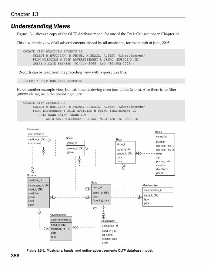
Understanding ViewsFigure 13-1 shows a copy of the OLTP database model for one of the Try It Out sections in Chapter 12.
This is a simple view of all advertisements, placed by all musicians, for the month of June, 2005:
CREATE VIEW MUSICIAN_ADVERTS AS SELECT M.MUSICIAN, M.PHONE, M.EMAIL, A.TEXT “Advertisement”FROM MUSICIAN M JOIN ADVERTISEMENT A USING (MUSICIAN_ID)WHERE A.DATE BETWEEN “01-JUN-2005” AND “30-JUN-2005”;
Records can be read from the preceding view with a query like this:
SELECT * FROM MUSICIAN_ADVERTS;
Here’s another example view, but this time retrieving from four tables (a join). Also there is no filter(WHERE clause) as in the preceding query:
CREATE VIEW ADVERTS AS SELECT M.MUSICIAN, M.PHONE, M.EMAIL, A.TEXT “Advertisement”FROM INSTRUMENT I JOIN MUSICIAN M USING (INSTRUMENT_ID)
JOIN BAND USING (BAND_ID)JOIN ADVERTISEMENT A USING (MUSICIAN_ID, BAND_ID);
Figure 13-1: Musicians, bands, and online advertisements OLTP database model.
Instrument
instrument_id
section_id (FK)instrument
Genre
genre_id
parent_id (FK)genre
Venue
venue_id
locationaddress_line_1address_line_2townzippostal_codecountrydirectionsphone
Merchandise
merchandise_id
band_id (FK)typeprice
Band
band_id
genre_id: (FK)bandfounding_date
Show
show_id
band_id (FK)venue_id (FK)datetime
Musician
musician_id
instrument_id (FK)band_id (FK)musicianphoneemailskills
Advertisement
advertisement_id
band_id (FK)musician_id (FK)datetest
Discography
discograpy_id
band_id (FK)cd_namerelease_dateprice
386
Chapter 13
20_574906 ch13.qxd 10/28/05 11:40 PM Page 386

This query reads all the records from the previous view:
SELECT * FROM ADVERTS;
The following query reads one or only a few records from the view, but because it is reading a view, theunderlying view will read all records from the table. This is extremely inefficient and a complete wasteof processing time.
SELECT * FROM ADVERTS WHERE MUSICIAN = “Jim Bean”;
The preceding query, reading records from the ADVERTS query, is a perfect example of misuse of views.These next example views are a more applicable application of use of views, where fields are restricted:
CREATE VIEW MUSICIANS_PRIVATE AS SELECT M.MUSICIAN, M.PHONE, M.EMAIL, B.BANDFROM MUSICIAN M JOIN BAND USING (BAND_ID);
CREATE VIEW MUSICIANS_PUBLIC AS SELECT M.MUSICIAN, B.BANDFROM MUSICIAN M JOIN BAND USING (BAND_ID);
The first view above is for the private use of musicians, allowing access to phone numbers and emailaddresses of all musicians. The second query is restricted, where only bands and their associated musi-cians can be examined. In other words, you don’t want the general public to have complete access to theprivate phone numbers and email addresses of all musicians. This is a much more sensible use of views.What you would then want to do is to grant and revoke specific access rights to different types of users,as shown in the following command, which removes all access privileges from all users, for all tablesand views:
REVOKE ALL FROM MUSICIAN, BAND;
A command such as the following allows only musicians and bands to examine their own personal data(MUSICIANS and BANDS are database users):
GRANT SELECT ON MUSICIANS_PRIVATE TO MUSICIANS, BANDS;
The following command allows all of the general public to look at only the publicly available fields andrecords (personal information is excluded):
GRANT SELECT ON MUSICIANS_PUBLIC TO EVERYONE;
Understanding Materialized ViewsMaterialized views are most often used to create hierarchical structures of aggregation in data ware-house databases. Figure 13-2 shows an enhanced copy of the data warehouse database model for one of the Try It Out sections in Chapter 11. Figure 13-2 is enhanced by the addition of the data warehousestandard TIME and LOCATION dimensions.
387
Advanced Database Structures and Hardware Resources
20_574906 ch13.qxd 10/28/05 11:40 PM Page 387
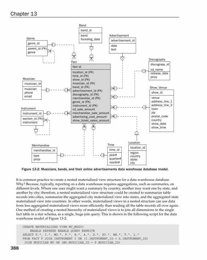
Figure 13-2: Musicians, bands, and their online advertisements data warehouse database model.
It is common practice to create a nested materialized view structure for a data warehouse database.Why? Because, typically, reporting on a data warehouse requires aggregations, such as summaries, ondifferent levels. Where one user might want a summary by country, another may want one by state, andanother by city; therefore, a nested materialized view structure could be created to summarize tablerecords into cities, summarize the aggregated city materialized view into states, and the aggregated statematerialized view into countries. In other words, materialized views in a nested structure can use datafrom less aggregated materialized views more efficiently than reading all the table records all over again.One method of creating a nested hierarchy of materialized views is to join all dimensions to the singlefact table in a star schema, as a single, huge join query. This is shown in the following script for the datawarehouse model of Figure 13-2:
CREATE MATERIALIZED VIEW MV_MUSICENABLE REFRESH ENABLE QUERY REWRITE
SELECT F.*, I.*, MU.*, F.*, B.*, A.*, D.*, SV.*, ME.*, T.*, L.*FROM FACT F JOIN INSTRUMENT I ON (I.INSTRUMENT_ID = A.INSTRUMENT_ID)JOIN MUSICIAN MU ON (MU.MUSICIAN_ID = F.MUSICIAN_ID)
Fact
fact id
location_id (FK)time_id (FK)show_id (FK)musician_id (FK)band_id (FK)advertisement_id (FK)discography_id (FK)merchandise_id (FK)genre_id (FK)instrument_id (FK)cd_sale_amountmerchandise_sale_amountadvertising_cost_amountshow_ticket_sales_amount
Advertisement
advertisement_id
datetext
Band
band_id
bandfounding_dateGenre
genre_id
parent_id (FK)genre
Musician
musician_id
musicianphoneemail
Time
time_id
year#quarter#month#
Location
location_id
regioncountrystatecity
Instrument
instrument_id
section_id (FK)instrument
Merchandise
merchandise_id
typeprice
Discography
discograpy_id
cd_namerelease_dateprice
Show_Venue
show_id
venueaddress_line_1address_line_2townzippostal_codecountryshow_dateshow_time
388
Chapter 13
20_574906 ch13.qxd 10/28/05 11:40 PM Page 388
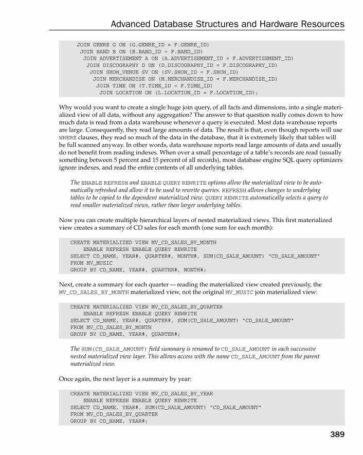
JOIN GENRE G ON (G.GENRE_ID = F.GENRE_ID)JOIN BAND B ON (B.BAND_ID = F.BAND_ID)JOIN ADVERTISEMENT A ON (A.ADVERTISEMENT_ID = F.ADVERTISEMENT_ID)JOIN DISCOGRAPHY D ON (D.DISCOGRAPHY_ID = F.DISCOGRAPHY_ID)JOIN SHOW_VENUE SV ON (SV.SHOW_ID = F.SHOW_ID)JOIN MERCHANDISE ON (M.MERCHANDISE_ID = F.MERCHANDISE_ID)JOIN TIME ON (T.TIME_ID = F.TIME_ID)JOIN LOCATION ON (L.LOCATION_ID = F.LOCATION_ID);
Why would you want to create a single huge join query, of all facts and dimensions, into a single materi-alized view of all data, without any aggregation? The answer to that question really comes down to howmuch data is read from a data warehouse whenever a query is executed. Most data warehouse reportsare large. Consequently, they read large amounts of data. The result is that, even though reports will useWHERE clauses, they read so much of the data in the database, that it is extremely likely that tables will be full scanned anyway. In other words, data warehouse reports read large amounts of data and usuallydo not benefit from reading indexes. When over a small percentage of a table’s records are read (usuallysomething between 5 percent and 15 percent of all records), most database engine SQL query optimizersignore indexes, and read the entire contents of all underlying tables.
The ENABLE REFRESH and ENABLE QUERY REWRITE options allow the materialized view to be auto-matically refreshed and allow it to be used to rewrite queries. REFRESH allows changes to underlyingtables to be copied to the dependent materialized view. QUERY REWRITE automatically selects a query toread smaller materialized views, rather than larger underlying tables.
Now you can create multiple hierarchical layers of nested materialized views. This first materializedview creates a summary of CD sales for each month (one sum for each month):
CREATE MATERIALIZED VIEW MV_CD_SALES_BY_MONTHENABLE REFRESH ENABLE QUERY REWRITE
SELECT CD_NAME, YEAR#, QUARTER#, MONTH#, SUM(CD_SALE_AMOUNT) “CD_SALE_AMOUNT”FROM MV_MUSICGROUP BY CD_NAME, YEAR#, QUARTER#, MONTH#;
Next, create a summary for each quarter — reading the materialized view created previously, theMV_CD_SALES_BY_MONTH materialized view, not the original MV_MUSIC join materialized view:
CREATE MATERIALIZED VIEW MV_CD_SALES_BY_QUARTERENABLE REFRESH ENABLE QUERY REWRITE
SELECT CD_NAME, YEAR#, QUARTER#, SUM(CD_SALE_AMOUNT) “CD_SALE_AMOUNT”FROM MV_CD_SALES_BY_MONTHGROUP BY CD_NAME, YEAR#, QUARTER#;
The SUM(CD_SALE_AMOUNT) field summary is renamed to CD_SALE_AMOUNT in each successivenested materialized view layer. This allows access with the name CD_SALE_AMOUNT from the parentmaterialized view.
Once again, the next layer is a summary by year:
CREATE MATERIALIZED VIEW MV_CD_SALES_BY_YEARENABLE REFRESH ENABLE QUERY REWRITE
SELECT CD_NAME, YEAR#, SUM(CD_SALE_AMOUNT) “CD_SALE_AMOUNT”FROM MV_CD_SALES_BY_QUARTERGROUP BY CD_NAME, YEAR#;
389
Advanced Database Structures and Hardware Resources
20_574906 ch13.qxd 10/28/05 11:40 PM Page 389

And, finally, comes a summary of all CD sales, for each CD, regardless of year, month, or quarter:
CREATE MATERIALIZED VIEW MV_CD_SALES_BY_CDENABLE REFRESH ENABLE QUERY REWRITE
SELECT CD_NAME, SUM(CD_SALE_AMOUNT) “CD_SALE_AMOUNT”FROM MV_CD_SALES_BY_YEARGROUP BY CD_NAME;
When a query is executed reading records from the FACT table, joining with dimensions, the material-ized views will be read because query rewrite changes the query, reading a materialized view, notunderlying tables. Consider this query:
SELECT CD_NAME, YEAR#, SUM(CD_SALE_AMOUNT)FROM FACT F JOIN DISCOGRAPHY ON (D.DISCOGRAPHY_ID = F. DISCOGRAPHY_ID)
JOIN TIME T ON (T.TIME_ID = F.TIME_ID)GROUP BY CD_NAME, YEAR#;
The preceding query may actually be executed as the following query, if the database engine allowsQUERY REWRITE:
SELECT CD_NAME, YEAR#, CD_SALE_AMOUNTFROM MV_SALES_BY_YEAR;
The previous query reads summary records from the materialized view in the nested materialized viewstructure, reading the MV_SALES_BY_YEAR materialized view. If there are 1 million fact records, spreadover a period of 5 years, with 20 different CDs, the preceding query only reads 100 records instead of 1 million records. That is a seriously reduced quantity of I/O activity, don’t you think? That is the pri-mary benefit of using materialized views.
Understanding Types of IndexesThe easiest way to understanding different indexes, how they work and where they apply, is perhaps toshow you how some of the different index types work.
Let’s repeat the concepts of materialized views and query rewrite, just to make surethat the benefits of using materialized views are fully understood. Materializedviews create copies of data, even of each other. When reading a materialized view,the materialized view copy is read, not underlying tables, or any other underlyingmaterialized views. Query rewrite allows a query against an underlying table, to besatisfied by reading a materialized view. It rewrites the query internally in thedatabase engine (it automatically rewrites the query for you). Remember, a material-ized view copies data from underlying structures; a view does not. A view contains aquery to be executed whenever the view is accessed, reading underlying structures(tables). A materialized view creates copies of data; a view does not!
390
Chapter 13
20_574906 ch13.qxd 10/28/05 11:40 PM Page 390
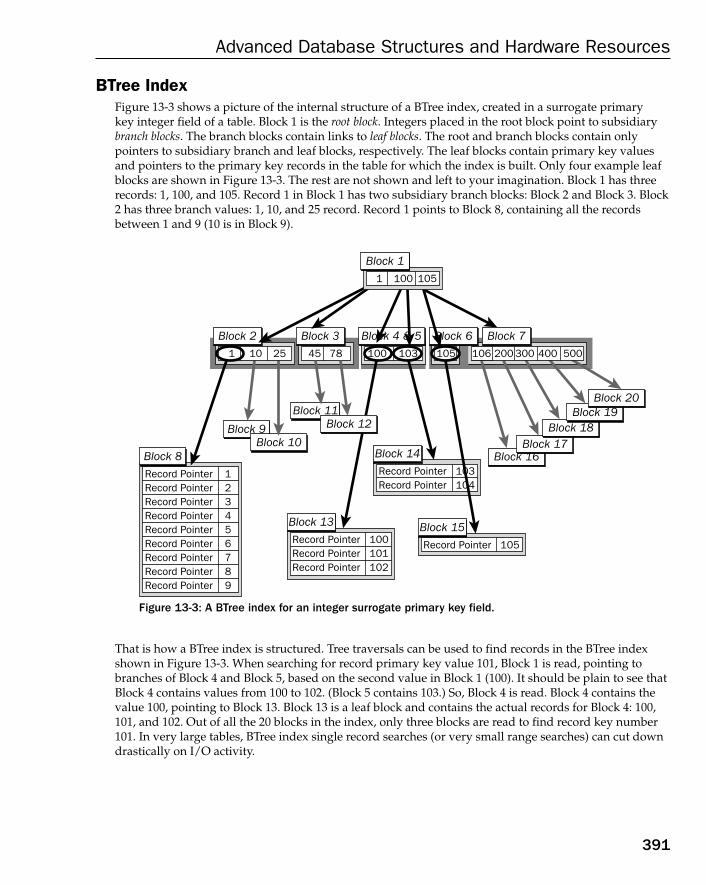
BTree IndexFigure 13-3 shows a picture of the internal structure of a BTree index, created in a surrogate primary key integer field of a table. Block 1 is the root block. Integers placed in the root block point to subsidiarybranch blocks. The branch blocks contain links to leaf blocks. The root and branch blocks contain onlypointers to subsidiary branch and leaf blocks, respectively. The leaf blocks contain primary key valuesand pointers to the primary key records in the table for which the index is built. Only four example leafblocks are shown in Figure 13-3. The rest are not shown and left to your imagination. Block 1 has threerecords: 1, 100, and 105. Record 1 in Block 1 has two subsidiary branch blocks: Block 2 and Block 3. Block2 has three branch values: 1, 10, and 25 record. Record 1 points to Block 8, containing all the recordsbetween 1 and 9 (10 is in Block 9).
Figure 13-3: A BTree index for an integer surrogate primary key field.
That is how a BTree index is structured. Tree traversals can be used to find records in the BTree indexshown in Figure 13-3. When searching for record primary key value 101, Block 1 is read, pointing tobranches of Block 4 and Block 5, based on the second value in Block 1 (100). It should be plain to see thatBlock 4 contains values from 100 to 102. (Block 5 contains 103.) So, Block 4 is read. Block 4 contains thevalue 100, pointing to Block 13. Block 13 is a leaf block and contains the actual records for Block 4: 100,101, and 102. Out of all the 20 blocks in the index, only three blocks are read to find record key number101. In very large tables, BTree index single record searches (or very small range searches) can cut downdrastically on I/O activity.
1
Record PointerRecord PointerRecord PointerRecord PointerRecord PointerRecord PointerRecord PointerRecord PointerRecord Pointer
123456789
Block 8
Record PointerRecord PointerRecord Pointer
100101102
Block 13
Record PointerRecord Pointer
103104
Block 14
1 10 25
Block 2
45 78
Block 3
100 103
Block 4 & 5
105 106 200 300 400 500
Block 6 Block 7
Record Pointer 105
Block 15
Block 9Block 10
Block 11
Block 16Block 17
Block 18Block 19
Block 20
Block 12
1 100 105
Block 1
391
Advanced Database Structures and Hardware Resources
20_574906 ch13.qxd 10/28/05 11:40 PM Page 391
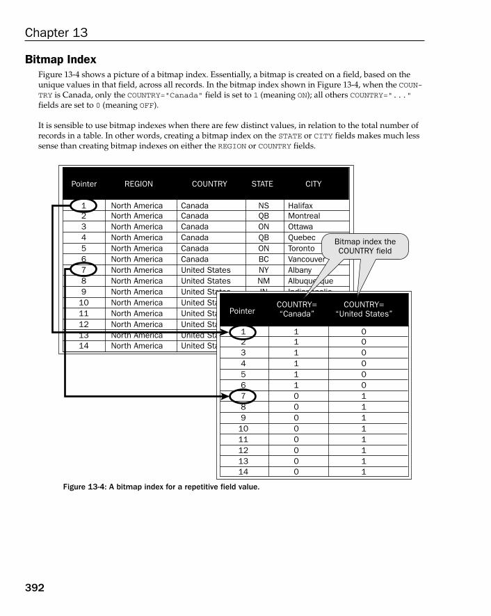
Bitmap IndexFigure 13-4 shows a picture of a bitmap index. Essentially, a bitmap is created on a field, based on theunique values in that field, across all records. In the bitmap index shown in Figure 13-4, when the COUN-TRY is Canada, only the COUNTRY=”Canada” field is set to 1 (meaning ON); all others COUNTRY=”...”fields are set to 0 (meaning OFF).
It is sensible to use bitmap indexes when there are few distinct values, in relation to the total number ofrecords in a table. In other words, creating a bitmap index on the STATE or CITY fields makes much lesssense than creating bitmap indexes on either the REGION or COUNTRY fields.
Figure 13-4: A bitmap index for a repetitive field value.
Pointer REGION
1234567891011121314
North AmericaNorth AmericaNorth AmericaNorth AmericaNorth AmericaNorth AmericaNorth AmericaNorth AmericaNorth AmericaNorth AmericaNorth AmericaNorth AmericaNorth AmericaNorth America
CanadaCanadaCanadaCanadaCanadaCanadaUnited StatesUnited StatesUnited States
NSQBONQBONBCNYNMIN
United StatesUnited StatesUnited StatesUnited StatesUnited States
HalifaxMontrealOttawaQuebecTorontoVancouverAlbanyAlbuquerqueIndianapolis
COUNTRY STATE CITY
PointerCOUNTRY=“Canada”
COUNTRY=“United States”
123456789
1011121314
11111100000000
00000011111111
Bitmap index theCOUNTRY field
392
Chapter 13
20_574906 ch13.qxd 10/28/05 11:40 PM Page 392
Hash Keys and ISAM KeysThere are other, less commonly used indexes, such as hash keys and Indexed Sequential Access Method(ISAM) keys. Both are somewhat out of date in the larger-scale relational database engines; however,Microsoft Access does make use of a mixture of ISAM/BTree indexing techniques, in its JET database.Both ISAM and hash indexes are not good for heavily changing data because their structures will over-flow with newly introduced records. Similar to bitmap indexes, hash and ISAM keys must be rebuilt regularly to maintain their advantage in processing speed advantage. Frequent rebuilds minimize onperformance killing overflow.
Clusters, Index Organized Tables, and Clustered IndexesClusters are used to contain fields from tables, usually a join, where the cluster contains a physical copyof a small portion of the fields in a table — perhaps the most commonly accessed fields. Essentially, clus-ters have been somewhat superseded by materialized views. A clustered index (index organized table,or IOT) is a more complex type of a cluster where all the fields in a single table are reconstructed, not ina usual heap structure, but in the form of a BTree index. In other words, for an IOT, the leaf blocks in thediagram shown in Figure 13-3 would contain not only the indexed field value, but also all the rest of thefields in the table (not just the primary key values).
Understanding Auto CountersSequences are commonly used to create internally generated (transparent) counters for surrogate pri-mary keys. Auto counters are called sequences in some database engines. This command would create asequence object:
CREATE SEQUENCE BAND_ID_SEQUENCE START=1 INCREMENT=1 MAX=INFINITY;
Then you could use the previous sequence to generate primary keys for the BAND table (see Figure 13-1),as in the following INSERT command, creating a new band called “The Big Noisy Rocking Band.”
INSERT INTO BAND (BAND_ID, GENRE_ID, BAND, FOUNDING_DATE)VALUES(
BAND_ID_SEQUENCE.NEXT,(SELECT GENRE_ID FROM GENRE WHERE GENRE=”Rock”),“The Big Noisy Rocking Band”, 25-JUN-2005
);
Understanding Partitioning and Parallel ProcessingPartitioning is just that — it partitions. It separates tables into separate physical partitions. The idea isthat processing can be executed against individual partitions and even in parallel against multiple parti-tions at the same time. Imagine a table with 1 million records. Reading those 1 million records can takean inordinately horrible amount of time; however, dividing that 1 million record table into 100 separatephysical partitions can allow queries to read much fewer records. This, of course, assumes that recordsare read within the structure of partition separation. As in previous sections of this chapter, the easiestway to explain partitioning, what it is, and how it works, is to just demonstrate it. The diagram in Fig-ure 13-5 shows the splitting of a data warehouse fact table in separate partitions.
393
Advanced Database Structures and Hardware Resources
20_574906 ch13.qxd 10/28/05 11:40 PM Page 393

Figure 13-5: Splitting a data warehouse table into separate physical partitions.
Factfact_id
location_id (FK)time_id (FK)show_id (FK)musician_id (FK)band_id (FK)advertisement_id (FK)discography_id (FK)merchandise_id (FK)genre_id (FK)instrument_id (FK)cd_sale_amountmerchandise_sale_amountadvertising_cost_amountshow_ticket_sales_amount
Genregenre_id
parent_idgenre
Bandband_id
bandfounding_date
Advertisementadvertisement_id
datetext
Discographydiscography_id
cd_namerelease_dateprice
Show_Venueshow_id
venueaddress_line_1address_line_2townzippostal_codecountryshow_dateshow_time
Merchandisemerchandise_id
typeprice
Instrumentinstrument_id
section_idinstrument
Musicianmusician_id
musicianphoneemail
Facts
Factfact_id
show_id (FK)musician_id (FK)band_id (FK)advertisement_id (FK)discography_id (FK)merchandise_id (FK)genre_id (FK)instrument_id (FK)cd_sale_amountmerchandise_sale_amountadvertising_cost_amountshow_ticket_sales_amount
Partition 1 Factfact_id
show_id (FK)musician_id (FK)band_id (FK)advertisement_id (FK)discography_id (FK)merchandise_id (FK)genre_id (FK)instrument_id (FK)cd_sale_amountmerchandise_sale_amountadvertising_cost_amountshow_ticket_sales_amount
Partition 2
Factfact_id
show_id (FK)musician_id (FK)band_id (FK)advertisement_id (FK)discography_id (FK)merchandise_id (FK)genre_id (FK)instrument_id (FK)cd_sale_amountmerchandise_sale_amountadvertising_cost_amountshow_ticket_sales_amount
Partition 3
Factfact_id
show_id (FK)musician_id (FK)band_id (FK)advertisement_id (FK)discography_id (FK)merchandise_id (FK)genre_id (FK)instrument_id (FK)cd_sale_amountmerchandise_sale_amountadvertising_cost_amountshow_ticket_sales_amount
Partition 4
Factfact_id
show_id (FK)musician_id (FK)band_id (FK)advertisement_id (FK)discography_id (FK)merchandise_id (FK)genre_id (FK)instrument_id (FK)cd_sale_amountmerchandise_sale_amountadvertising_cost_amountshow_ticket_sales_amount
Partition 5
394
Chapter 13
20_574906 ch13.qxd 10/28/05 11:40 PM Page 394
In some database engines, you can even split materialized views into partitions, in the same way astables can be partitioned. The fact table shown in Figure 13-5 is (as fact tables should be) all referencingsurrogate primary keys, as foreign keys to dimensions. It is easier to explain some of the basics of parti-tioning using the materialized view created earlier in this chapter. The reason is because the materializedview contains the descriptive dimensions, as well as the surrogate key integer values. In other words,even though not technically correct, it is easier to demonstrate partitioning on dimensional descriptions,such as a region of the world (North America, South America, and so on), as opposed to partitioningbased on an inscrutable LOCATION_ID foreign key value. This is the materialized view created earlier:
CREATE MATERIALIZED VIEW MV_MUSICENABLE REFRESH ENABLE QUERY REWRITE
SELECT F.*, I.*, MU.*, F.*, B.*, A.*, D.*, SV.*, ME.*, T.*, L.*FROM FACT A JOIN INSTRUMENT I ON (I.INSTRUMENT_ID = A.INSTRUMENT_ID)JOIN MUSICIAN MU ON (MU.MUSICIAN_ID = F.MUSICIAN_ID)JOIN GENRE G ON (G.GENRE_ID = F.GENRE_ID)JOIN BAND B ON (B.BAND_ID = F.BAND_ID)JOIN ADVERTISEMENT A ON (A.ADVERTISEMENT_ID = F.ADVERTISEMENT_ID)JOIN DISCOGRAPHY D ON (D.DISCOGRAPHY_ID = F.DISCOGRAPHY_ID)JOIN SHOW_VENUE SV ON (SV.SHOW_ID = F.SHOW_ID)JOIN MERCHANDISE ON (M.MERCHANDISE_ID = F.MERCHANDISE_ID)JOIN TIME ON (T.TIME_ID = F.TIME_ID)JOIN LCOATION ON (L.LOCATION_ID = F.LOCATION_ID);
Now, partition the materialized view based on regions of the world — this one is called a list partition:
CREATE TABLE PART_MV_REGIONAL PARTITION BY LIST (REGION)(
PARTITION PART_AMERICAS VALUES (“North America”,”South America”),PARTITION PART_ASIA VALUES (“Middle East”,”Far East”,”Near East”),PARTITION PART_EUROPE VALUES (“Europe”,”Russian Federation”),PARTITION PART_OTHER VALUES (DEFAULT)
) AS SELECT * FROM MV_MUSIC;
The DEFAULT option implies all regions not in the ones listed so far.
Another type of partition is a range partition where each separate partition is limited by a range of values, for each partition. This partition uses the release date of CDs stored in the field called DISCOGRAPHY.RELEASE_DATE:
CREATE TABLE PART_CD_RELEASE PARTITION BY RANGE (RELEASE_DATE)(
PARTITION PART_2002 VALUES LESS THAN (1-JAN-2003),PARTITION PART_2003 VALUES LESS THAN (1-JAN-2004),PARTITION PART_2004 VALUES LESS THAN (1-JAN-2005),PARTITION PART_2005 VALUES LESS THAN (MAXIMUM),
) AS SELECT * FROM MV_MUSIC;
The MAXIMUM option implies all dates into the future, from January 1, 2005, and beyond the year 2005.
You can also create indexes on partitions. Those indexes can be created as locally identifiable to each par-tition, or globally to all partitions created for a table, or materialized view. That is partitioning. There areother more complex methods of partitioning, but these other methods are too detailed for this book.
395
Advanced Database Structures and Hardware Resources
20_574906 ch13.qxd 10/28/05 11:40 PM Page 395

That’s all you need to know about advanced database structures. Take a quick peek at the physical sideof things in the guise of hardware resources.
Understanding Hardware ResourcesThis section briefly examines some facts about hardware, including some specialized database serverarchitectural structures, such as RAID arrays and Grid computing.
How Much Hardware Can You Afford?Windows computers are cheap, but they have a habit of breaking. UNIX boxes (computers are oftencalled “boxes”) are expensive and have excellent reliability. I have heard of cases of UNIX servers run-ning for years, with no problems whatsoever. Typically, a computer system is likely to remain stable aslong as it is not tampered with. The simple fact is that Windows boxes are much more easily tamperedwith than UNIX boxes, so perhaps Windows machines have an undeserved poor reputation, as far asreliability is concerned.
How Much Memory Do You Need?OLTP databases are memory- and processor-intensive. Data warehouse databases are I/O-intensive, andother than heavy processing power, couldn’t care less how much RAM is allocated. The heavy type ofmemory usage for a relational database usually has a lot to do with concurrency and managing the loadof large number of users, accessing your database all at the same time. That’s all about concurrency andmuch more applicable to OLTP databases, rather than data warehouse databases. For an OLTP database,quite often the more RAM you have, the better. Note, however, that sizing up buffer cache values to themaximum amount of RAM available is pointless, even for an OLTP database. The more RAM allocatedfor use by a database, the more complex those buffers become for a database to manage.
In short, data warehouses do not need a lot of memory to temporarily store the most heavily used tablesin the database into RAM. There is no point, as data warehouses tend to read lots of data from lots oftables, occasionally. RAM is not as important in a data warehouse as it is in an OLTP database.
Now, briefly examine some specialized aspects of hardware usage, more from an architectural perspective.
Understanding Specialized HardwareArchitectures
This section examines the following:
❑ RAID arrays
❑ Standby databases
❑ Replication
❑ Grids and computer clustering
396
Chapter 13
20_574906 ch13.qxd 10/28/05 11:40 PM Page 396
RAID ArraysThe acronym RAID stands for Redundant Array of Inexpensive Disks. That means a bunch of small,cheap disks. Some RAID array hardware setups are cheap. Some are astronomically expensive. You getwhat you pay for, and you can purchase what suits your requirements. RAID arrays can give huge per-formance benefits for both OLTP and data warehouse databases.
Some of the beneficial factors of using RAID arrays are recoverability (mirroring), fast random access(striping and multiple disks with multiple bus connections — higher throughput capacity), and parallelI/O activity where more than one disk can be accessed at the same time (concurrently). There are numer-ous types of RAID array architectures, with the following being the most common:
❑ RAID 0 — RAID 0 is striping. Striping splits files into pieces, spreading them over multipledisks. RAID 0 gives fast random read and write access, and is thus appropriate for OLTP data-bases. Rapid recoverability and redundancy is not catered for. RAID 0 is a little risky because oflack of recoverability. Data warehouses that need to be highly contiguous (data on disk is all inone place) are not catered for by random access; however, RAID 0 can sometimes be appropriatefor data warehouses, where large I/O executions utilize parallel processing, accessing manydisks simultaneously.
❑ RAID 1 — RAID 1 is mirroring. Mirroring makes multiple copies of files, duplicating databasechanges at the I/O level on disk. Mirroring allows for excellent recoverability capabilities. RAID1 can sometimes cause I/O bottleneck problems because of all the constant I/O activity associ-ated with mirroring, especially with respect to frequently written tables — creating mirrored hotblocks. A hot block is a block in a file that is accessed more heavily than the hardware can copewith. Everything is trying to read and write that hot block at the same time. RAID 1 can pro-vide recoverability for OLTP databases, but can hurt performance. RAID 1 is best used in data warehouses where mirroring allows parallel read execution, of more than one mirror, at thesame time.
❑ RAID 0+1 — RAID 0+1 combines the best of both worlds from RAID 0 and RAID 1 — using bothstriping and mirroring. Both OLTP and data warehouse I/O performance will be slowed some-what, but RAID 0+1 can provide good all-around recoverability and performance, perhapsoffering the best of both worlds, for both OLTP and data warehouse databases.
❑ RAID 5 — RAID 5 is essentially a minimized form of mirroring, duplicating only parity and notthe real data. RAID 5 is effective with expensive RAID architectures, containing large chunks ofpurpose-built, RAID-array contained, onboard buffering RAM memory.
Those are some of the more commonly implemented RAID array architectures. It is not necessary foryou to understand the details but more important that you know this stuff actually exists.
Standby DatabasesA standby database is a failover database. A standby database has minimal activity, usually only addingnew records, changing existing records, and deleting existing records. Some database engines do allowfor more sophisticated standby database architectures, but once again, the intention in this chapter is toinform you of the existence of standby databases.
397
Advanced Database Structures and Hardware Resources
20_574906 ch13.qxd 10/28/05 11:40 PM Page 397
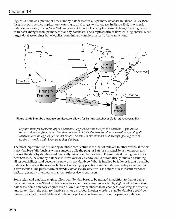
Figure 13-6 shows a picture of how standby databases work. A primary database in Silicon Valley (SanJose) is used to service applications, catering to all changes to a database. In Figure 13-6, two standbydatabases are used, one in New York and one in Orlando. The simplest form of change tracking is usedto transfer changes from primary to standby databases. The simplest form of transfer is log entries. Mostlarger database engines have log files, containing a complete history of all transactions.
Figure 13-6: Standby database architecture allows for instant switchover (failover) recoverability.
Log files allow for recoverability of a database. Log files store all changes to a database. If you had torecover a database from backup files that are a week old, the database could be recovered by applying allchanges stored in log files (for the last week). The result of one week-old cold backups, plus log entriesfor the last week, would be an up-to-date database.
The most important use of standby database architecture is for that of failover. In other words, if the pri-mary database fails (such as when someone pulls the plug, or San Jose is struck by a monstrous earth-quake), the standby database automatically takes over. In the case of Figure 13-6, if the big one strucknear San Jose, the standby database in New York or Orlando would automatically failover, assuming all responsibilities, and become the new primary database. What is implied by failover is that a standbydatabase takes over the responsibilities of servicing applications, immediately — perhaps even within a few seconds. The purest form of standby database architecture is as a more or less instant responsebackup, generally intended to maintain full service to end-users.
Some relational database engines allow standby databases to be utilized in addition to that of being just a failover option. Standby databases can sometimes be used as read-only, slightly behind, reportingdatabases. Some database engines even allow standby databases to be changeable, as long as structureand content from the primary database is not disturbed. In other words, a standby database could con-tain extra and additional tables and data, on top of what is being sent from the primary database.
New York
SlaveDatabase
StandbyDatabase
Log Entry
Transfer
Log Entry Transfer
PrimaryDatabase Orlando
San Jose
398
Chapter 13
20_574906 ch13.qxd 10/28/05 11:40 PM Page 398
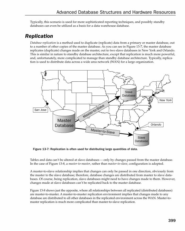
Typically, this scenario is used for more sophisticated reporting techniques, and possibly standbydatabases can even be utilized as a basis for a data warehouse database.
ReplicationDatabase replication is a method used to duplicate (replicate) data from a primary or master database, outto a number of other copies of the master database. As you can see in Figure 13-7, the master databasereplicates (duplicate) changes made on the master, out to two slave databases in New York and Orlando.This is similar in nature to standby database architecture, except that replication is much more powerful,and, unfortunately, more complicated to manage than standby database architecture. Typically, replica-tion is used to distribute data across a wide area network (WAN) for a large organization.
Figure 13-7: Replication is often used for distributing large quantities of data.
Tables and data can’t be altered at slave databases — only by changes passed from the master database.In the case of Figure 13-8, a master-to-master, rather than master-to-slave, configuration is adopted.
A master-to-slave relationship implies that changes can only be passed in one direction, obviously fromthe master to the slave database; therefore, database changes are distributed from master to slave data-bases. Of course, being replication, slave databases might need to have changes made to them. However,changes made at slave databases can’t be replicated back to the master database.
Figure 13-8 shows just the opposite, where all relationships between all replicated (distributed databases)are master-to-master. A master-to-master replication environment implies that changes made to anydatabase are distributed to all other databases in the replicated environment across the WAN. Master-to-master replication is much more complicated than master-to-slave replication.
New York
SlaveDatabase
SlaveDatabase
Master-to-Slav
e
Master-to-Slave
MasterDatabase Orlando
San Jose
399
Advanced Database Structures and Hardware Resources
20_574906 ch13.qxd 10/28/05 11:40 PM Page 399
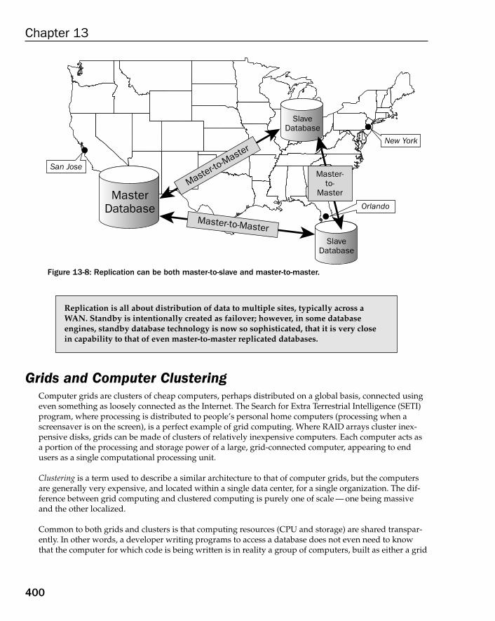
Figure 13-8: Replication can be both master-to-slave and master-to-master.
Grids and Computer ClusteringComputer grids are clusters of cheap computers, perhaps distributed on a global basis, connected usingeven something as loosely connected as the Internet. The Search for Extra Terrestrial Intelligence (SETI)program, where processing is distributed to people’s personal home computers (processing when ascreensaver is on the screen), is a perfect example of grid computing. Where RAID arrays cluster inex-pensive disks, grids can be made of clusters of relatively inexpensive computers. Each computer acts asa portion of the processing and storage power of a large, grid-connected computer, appearing to endusers as a single computational processing unit.
Clustering is a term used to describe a similar architecture to that of computer grids, but the computersare generally very expensive, and located within a single data center, for a single organization. The dif-ference between grid computing and clustered computing is purely one of scale — one being massiveand the other localized.
Common to both grids and clusters is that computing resources (CPU and storage) are shared transpar-ently. In other words, a developer writing programs to access a database does not even need to knowthat the computer for which code is being written is in reality a group of computers, built as either a grid
Replication is all about distribution of data to multiple sites, typically across aWAN. Standby is intentionally created as failover; however, in some databaseengines, standby database technology is now so sophisticated, that it is very close in capability to that of even master-to-master replicated databases.
New York
SlaveDatabase
SlaveDatabase
Master-to-Master
Master-to-Master
MasterDatabase Orlando
San JoseMaster-
to-Master
400
Chapter 13
20_574906 ch13.qxd 10/28/05 11:40 PM Page 400
or a cluster. Grid Internet-connected computers could be as much as five years old, which is geriatric fora computer — especially a personal computer. They might have all been purchased in a yard sale. If thereare enough senior computers, and they are connected properly, the grid itself could contain enormouscomputing power.
Clustered architectures are used by companies to enhance the power of their databases. Grids, on theother hand, are often used to help processing for extremely large and complex problems that perhapseven a super computer might take too long to solve.
SummaryIn this chapter, you learned about:
❑ Views and how to create them
❑ Sensible and completely inappropriate uses of views
❑ Materialized views and how to create them
❑ Nested materialized views and QUERY REWRITE
❑ Different types of indexes (including BTree indexes, bitmap indexes, and clustering)
❑ Auto counters and sequences
❑ Partitioning and parallel processing
❑ Creating list and range partitions
❑ Partitioning materialized views
❑ Hardware factors (including memory usage as applied to OLTP or data warehouse databases)
❑ RAID arrays for mirroring (recoverability) and striping (performance)
❑ Standby databases for recoverability and failover
❑ Replication of databases to cater to distribution of data
❑ Grid computing and clustering to harness as much computing power as possible
This chapter has moved somewhat beyond the realm of database modeling, examining specializeddatabase objects, some brief facts about hardware resources, and finally some specialized database architectures.
401
Advanced Database Structures and Hardware Resources
20_574906 ch13.qxd 10/28/05 11:40 PM Page 401

20_574906 ch13.qxd 10/28/05 11:40 PM Page 402
Glossary
1st Normal Form (1NF) — Eliminate repeating groups, such that all records in all tables can beidentified uniquely, by a primary key in each table. In other words, all fields other than the pri-mary key must depend on the primary key. All Normal Forms are cumulative. (See NormalForms.)
1st Normal Form made easy — Remove repeating fields by creating a new table, where the origi-nal and new tables are linked together with a master-detail, one-to-many relationship. Create pri-mary keys on both tables, where the detail table will have a composite primary key, containing the master table primary key field as the prefix field of its primary key. That prefix field is also aforeign key back to the master table.
2nd Normal Form (2NF) — All non-key values must be fully functionally dependent on the pri-mary key. No partial dependencies are allowed. A partial dependency exists when a field is fullydependant on a part of a composite primary key. All Normal Forms are cumulative. (See NormalForms.)
2nd Normal Form made easy — Performs a seemingly similar function to that of 1st Normal Form,but creates a table, where repeating values (rather than repeating fields) are removed to a new table.The result is a many-to-one relationship rather than a one-to-many relationship (see 1st NormalForm), created between the original (master table) and the new tables. The new table gets a primarykey consisting of a single field. The master table contains a foreign key pointing back to the primarykey of the new table. That foreign key is not part of the primary key in the original table.
3rd Normal Form (3NF) — Eliminate transitive dependencies. What this means is that a field isindirectly determined by the primary key because the field is functionally dependent on anotherfield, where the other field is dependent on the primary key. All Normal Forms are cumulative.(See Normal Forms.)
3rd Normal Form made easy — Elimination of a transitive dependency, which implies creation ofa new table, for something indirectly dependent on the primary key in an existing table.
4th Normal Form (4NF) — Eliminate multiple sets of multi-valued dependencies. All NormalForms are cumulative. (See Normal Forms.)
21_574906 glos.qxd 10/28/05 11:39 PM Page 403
5th Normal Form (5NF) — Eliminate cyclic dependencies. This is also known as Projection Normal Form(PJNF). All Normal Forms are cumulative. (See Normal Forms.)
Abstraction — In computer jargon, this implies something created to generalize a number of otherthings. It is typically used in object models, where an abstract class caters to the shared attributes andmethods of inherited classes.
Active data — Information in a database constantly accessed by applications, such as today’s transac-tions, in an OLTP database.
Ad-hoc query — A query sent to a database by an end-user or power user, just trying to get some infor-mation quickly. Ad-hoc queries are subjected to a database where the content, structure, and perfor-mance of said query, are not necessarily catered for by the database model. The result could be aperformance problem, and in extreme cases, even an apparent database halt.
Aggregated query — A query using a GROUP BY clause to create a summary set of records (smaller num-ber of records).
Algorithm — A computer program (or procedure) that is a step-by-step procedure, solving a problem, ina finite number of steps.
Alternate index — An alternate to the primary relational structure of a table, determined by primary andforeign key indexes. Alternate indexes are “alternate” because they are in addition to primary and for-eign key indexes, existing as alternate sorting methods to those provided by primary and foreign keys.
Analysis — The initial fact-finding process discovering what is to be done by a computer system.
Anomaly — With respect to relational database design, essentially an erroneous change to data, morespecifically to a single record.
ANSI — American National Standards Institute.
Application — A front-end tool used by developers, in-house staff, and end-users to access a database.
Ascending index — An index built sorted in a normally ascending order, such as A, B, C.
Attribute — The equivalent of a relational database field, used more often to describe a similar low-levelstructure in object structures.
Auto counter — Allows automated generation of sequences of numbers, usually one after the other, suchas 101, 102, 103, and so on. Some database engines call these sequences.
Backus-Naur form — A syntax notation convention.
BETWEEN— Verifies expressions between a range of two values.
Binary object — Stores data in binary format, typically used for multimedia (images, sound, and so on).
Bitmap index — An index containing binary representations for each record using 0’s and 1’s. For exam-ple, a bitmap index creates two bitmaps for two values of M for Male and F for Female. When M isencountered, the M bitmap is set to 1 and the F bitmap is set to 0.
404
Glossary
21_574906 glos.qxd 10/28/05 11:39 PM Page 404
Black box — Objects or chunks of code that can function independently, where changes made to one partof a piece of software will not affect others.
Boyce-Codd Normal Form (BCNF) — Every determinant in a table is a candidate key. If there is only onecandidate key, then 3rd Normal Form and Boyce-Codd Normal Form are one and the same. All NormalForms are cumulative. (See Normal Forms.)
BTree index — A binary tree. If drawn out on a piece of paper, a BTree index looks like an upside-downtree. The tree is called “binary” because binary implies two options under each branch node: branch left and branch right. The binary counting system of numbers contains two digits, namely 0 and 1. Theresult is that a binary tree only ever has two options as leafs within each branch. A BTree consists of aroot node, branch nodes and ultimately leaf nodes containing the indexed field values in the ending (or leaf) nodes of the tree.
Budget — A determination of how much something will cost, whether it is cost-effective, whether it isworth the cost, whether it is affordable, and whether it gives the company an edge over the competitionwithout bankrupting the company.
Business processes — The subject areas of a business. The method by which a business is divided up. Ina data warehouse, the subject areas become the fact tables.
Business rules — The processes and flow of whatever is involved in the daily workings of an organiza-tion. The operation of that business and the decisions made to execute the operational processes of thatorganization.
Cache — A term commonly applied to buffering data into fast access memory, for subsequent high-speed retrieval.
Candidate key — Also known as a potential key, or permissible key. A field or combination of fields, whichcan act as a primary key field for a table. A candidate key uniquely identifies each record in the table.
Cartesian product — A mathematical term describing a set of all the pairs that can be constructed from agiven set. Statistically it is known as a combination, not a permutation. In SQL jargon, a Cartesian Productis also known as a cross join.
Cascade — Changes to data in parent tables are propagated to all child tables, containing foreign keyfield copies of a primary key from the parent table.
Cascade delete — A deletion that occurs when the deletion of a master record automatically deletes allchild records in child-related tables, before deleting the record in the master table.
Central Processing Unit (CPU) — The processor (chip) in your computer.
Check constraint — A constraint attached to a field in a database table, as a metadata field setting, andused to validate a given input value.
Class — An object methodology term for the equivalent of a table in a relational database.
Client-server — An environment that was common in the pre-Internet days where a transactional data-base serviced users within a single company. The number of users could range from as little as one to
405
Glossary
21_574906 glos.qxd 10/28/05 11:39 PM Page 405
thousands, depending on the size of the company. The critical factor was actually a mixture of both individual record change activity and modestly sized reports. Client-server database models typicallycatered for low concurrency and low throughput at the same time, because the number of users wasalways manageable.
Cluster — Allows a single table or multiple table partial copy of records, from underlying tables.Materialized views have superseded clusters.
Clustered index — See Index organized table.
Coding — Programming code, in whatever language is appropriate. For example, C is a programminglanguage.
Column — See Field.
COMMIT— Completes a transaction by storing all changes to a database.
Complex datatype — Typically used in object structures, consisting of a number of fields.
Composite index — Indexes that can be built on more than a single field. Also known as composite fieldindexes or multiple field indexes.
Composite key — A primary key, unique key, or foreign key consisting of more than one field.
Concurrent — More than one process executed at the same time means two processes are executingsimultaneously, or more than one process accessing the same piece of data at the same time.
Configuration — A computer term used to describe the way in which a computer system (or partthereof, such as a database) is installed and set up. For example, when you start up a Windows com-puter, all of your desktop icons are part of the configuration (of you starting up your computer). Whatthe desktop icons are, and where on your desktop they are placed, are stored in a configuration file onyour computer somewhere. When you start up your computer, the Windows software retrieves that configuration file, interprets it contents, and displays all your icons on the screen for you.
Constraint — A means to constrain, restrict, or apply rules both within and between tables.
Construction — A stage at which you build and test code. For a database model, you build scripts to create tables, referential integrity keys, indexes, and anything else such as stored procedures.
Cross join — See Cartesian product.
Crow’s foot — Used to describe the many sides of a one-to-many or many-to-many relationship. A crowsfoot looks quite literally like the imprint of a crow’s foot in some mud, with three splayed toes.
Cyclic dependency — In the context of the relational database model, X is dependent on Y, which in turnis also dependent on X, directly or indirectly. Cyclic dependence, therefore, indicates a logically circularpattern of interdependence. Cyclic dependence typically occurs with tables containing a composite pri-mary key with three or more fields, where, for example, three fields are related in pairs to each other. Inother words, X relates to Y, Y relates to Z, and X relates to Z.
406
Glossary
21_574906 glos.qxd 10/28/05 11:39 PM Page 406
Data — A term applied to organized information.
Data Definition Language (DDL) — Commands used to change metadata. In some databases, thesecommands require a COMMIT command; in other database engines, this is not the case. When a COMMITcommand is not required, these commands automatically commit any pending changes to the database,and cannot be rolled back.
Data Manipulation Language (DML) — Commands that change data in a database. These commandsare INSERT, UPDATE, and DELETE. Changes can be committed permanently using the COMMIT command,and undone using the ROLLBACK command. These commands do not commit automatically.
Data mart — A subset part of a data warehouse. Typically, a data mart is made up of a single start schema(a single fact table).
Data warehouse — A large transactional history database used for predictive and planning reporting.
Database — A collection of information, preferably related information, and preferably organized.
Database block — A physical substructure within a database and the smallest physical unit in whichdata is stored on disk.
Database event — See Trigger.
Database model — A model used to organize and apply structure to other disorganized information.
Database procedure — See Stored procedure.
Datatype — Restricts values in fields, such as allowing only a date or a number.
Datestamp — See Timestamp.
DDL — See Data Definition Language.
Decimal — Datatypes that contain decimal or non-floating-point real numbers.
Decision Support System (DSS) — Commonly known as DSS databases, these support decisions, gener-ally more management-level and even executive-level decision-type of objectives.
DEFAULT— A setting used as an optional value for a field in a record, when a value is not specified.
DELETE— A command that can be used to remove one, some, or all rows from a table.
Delete anomaly — A record cannot be deleted from a master table unless all sibling records are deletedfirst.
Denormalization — Most often the opposite of normalization, more commonly used in data warehouseor reporting environments. Denormalization decreases granularity by reversing normalization, and otherwise.
407
Glossary
21_574906 glos.qxd 10/28/05 11:39 PM Page 407
Dependency — Something relies on something else.
Descending index — An index sorted in a normally descending order (such as in C, B, A).
Design — Analysis discovers what needs to be done. Design figures out how what has been analyzed,can and should be done.
Determinant — Determines the value of another value. If X determines the value Y (at least partially),then X determines the value of Y, and is thus the determinant of Y.
Dimension table — A descriptive or static data table in a data warehouse.
DISTINCT clause — A query SELECT command modifier for retrieving unique rows from a set of records.
DML — See Data Manipulation Language.
Domain Key Normal Form (DKNF) — The ultimate application of normalization. This is more a mea-surement of conceptual state, as opposed to a transformation process in itself. All Normal Forms arecumulative. (See Normal Forms.)
DSS — See Decision Support System.
Dynamic data — Data that changes significantly, over a short period of time.
Dynamic string — See Variable length string.
End-user — Ultimate users of a computer system. The clients and staff of a company who actually usesoftware to perform business functions (such as sales people, accountants, and busy executives).
Entity — A relational database modeling term for a table.
Entity Relationship Diagram (ERD) — A diagram that represents the structural contents (the fields) intables for an entire schema, in a database. Additionally included are schematic representations of rela-tionships between entities, represented by various types of relationships, plus primary and foreign keys.
Event Trigger — See Trigger.
Expression — In mathematical terms, a single or multi-functional (or valued) value, ultimately equatingto a single value, or even another expression.
External procedure — Similar to stored procedures, except they are written in non-database-specific programming language. External procedures are chunks of code written in a language not native to thedatabase engine, such as Java or C++; however, external procedures are still executed from within thedatabase engine itself, perhaps on data within the database.
Fact table — The biggest table in a data warehouse, central to a Star schema, storing the transactionalhistory of a company.
Fact-dimensional structure — See Star schema.
408
Glossary
21_574906 glos.qxd 10/28/05 11:39 PM Page 408
Field — Part of a table division that imposes structure and datatype specifics onto each of the field val-ues in a record.
Field list — This is the part of a SELECT command listing fields to be retrieved by a query. When morethan one field is retrieved, then the fields become a list of fields, or field list.
Fifth Normal Form — See 5th Normal Form.
File system — A term used to describe the files in a database at the operating system level.
Filtered query — See Filtering.
Filtering — Retrieve a subset of records, or remove a subset of records from the source. Filtering is donein SQL using the WHERE clause for basic query records retrieved, and using the HAVING clause to removegroups from an aggregated query.
First Normal Form — See 1st Normal Form.
Fixed-length records — Every record in a table must have the same byte-length. This generally prohibitsuse of variable-length datatypes such as variable-length strings.
Fixed length string — The CHAR datatype is a fixed-length string. For example, setting a CHAR(5)datatype to “ABC” will force padding of spaces on to the end of the string up to five characters (“ABC “).
Flat file — A term generally applying to an unstructured file, such as a text file.
Floating point — A real number where the decimal point can be anywhere in the number.
Foreign key — A type of constraint where columns contain copies of primary key values, uniquely iden-tified in parent entities, representing the child or sibling side of what is most commonly a one-to-manyrelationship.
Formal method — The application of a theory, a set of rules, or a methodology. Used to quantify andapply structure to an otherwise completely disorganized system. Normalization is a formal method usedto create a relational database model.
Format display setting — A field setting used to determine the display format of the contents of a field.For example, the datatype definition of INTEGER $9,999,990.99, when set to the value 500, will bedisplayed as $500.00 (format models can be database specific).
FROM clause — The part of a query SELECT command that determines tables retrieved from, and howtables are joined (when using the JOIN, ON, and USING clauses).
Front-end — Customer facing software. Usually, applications either purchased, online over the Internet,or in-house as custom-written applications.
Full Functional dependence — X determines Y, but X combined with Z does not determine Y. In otherwords, Y depends on X and X alone. If Y depends on X with anything else then there is not full func-tional dependence. (See Functional dependency.)
409
Glossary
21_574906 glos.qxd 10/28/05 11:39 PM Page 409
Full outer join — A query finding the combination of intersection, plus records in the left-sided table,but not in the right-sided table, and records in the right-sided table, not in the left (a combination of bothleft and right outer joins).
Function — A programming unit or expression returning a single value, also allowing determinant val-ues to be passed in as parameters. Thus, parameter values can change the outcome or return result ofa function. The beauty of a function is that it is self-contained and can thus be embedded into an expression.
Functional dependence — Y is functionally dependent on X if the value of Y is determined by X. In otherwords if Y = X +1, the value of X will determine the resultant value of Y. Thus, Y is dependent on X as afunction of the value of X. Functional dependence is the opposite of determinance. (See Full Functionaldependence.)
Generic database model — A database model usually consisting of a partial set of metadata, about meta-data; in other words, tables that contain tables which contain data. In modern-day, large, and very busydatabases, this can be extremely inefficient.
Granularity — The depth of detail stored, typically applied to a data warehouse. The more granularitythe data warehouse contains, the bigger fact tables become because the more records they contain. Thesafest option is include all historical data down to the lowest level of granularity. This ensures that anypossible future requirements for detailed analysis can always be met, without needed data perhapsmissing in the future (assuming hardware storage capacity allows it).
Grid computing — Clusters of cheap computers, perhaps distributed on a global basis, connected usingeven something as loosely connected as the Internet.
GROUP BY clause — A clause in the query SELECT command used to aggregate and summarize recordsinto aggregated groups of fewer records.
Hash index — A hashing algorithm is used to organize an index into a sequence, where each indexedvalue is retrievable based on the result of the hash key value. Hash indexes are efficient with integer val-ues, but are usually subject to overflow as a result of changes.
Heterogeneous system — A computer system consisting of dissimilar elements or parts. In database par-lance, this implies a set of applications and databases, where database engines are different. In otherwords, a company could have a database architecture consisting of multiple database engines, such asMicrosoft Access, Sybase, Oracle, Ingres, and so on. All databases, regardless of type, are meldedtogether into a single (apparently one and the same) transparent database-application architecture.
Hierarchical database model — An inverted tree-like structure. The tables of this model take on a child-parent relationship. Each child table has a single parent table, and each parent table can have multiplechild tables. Child tables are completely dependent on parent tables; therefore, a child table can onlyexist if its parent table does. It follows that any entries in child tables can only exist where correspondingparent entries exist in parent tables. The result of this structure is that the hierarchical database modelcan support one-to-many relationships, but not many-to-many relationships.
Homogeneous system — Everything is the same, such as database engines, application SDKs, and so on.
410
Glossary
21_574906 glos.qxd 10/28/05 11:39 PM Page 410
Hot block — A small section of disk that, when accessed too frequently, can cause too much competitionfor that specific area. It can result in a serious slow-down in general database and application performance.
Hybrid database — A database installation mixing multiple types of database architectures. Typically,the mix is including both OLTP (high concurrency) and data warehouse (heavy reporting) into the samedatabase. (See Online Transaction Processing.)
Identifying relationship — The child table is partially identified by the parent table, and partiallydependent on the parent table. The parent table primary key is included in the primary key of the childtable. In other words, if the child record exists, then the foreign key value, in the child table, must be setto something other than NULL. So, you can’t create the child record unless the related parent recordexists. In other words, the child record can’t exist without a related parent record.
Implementation — The process of creating software from a design of that software. A physical databaseis an implementation of a database model.
Inactive data — Inactive data is information passed from an OLTP database to a data warehouse, wherethe inactive data is not used in the customer facing OLTP database on a regular basis. Inactive data isused in data warehouses to make projections and forecasts, based on historical company activities. (SeeOnline Transaction Processing.)
Index — Usually (and preferably) a copy of a very small section of table, such as a single field, andpreferably a short-length field.
Index Organized Table (IOT) — Build a table in the sorted order of an index, typically using a BTreeindex. It is also called a clustered index in some database engines because data is clustered into the formand structure of a BTree index.
Indexed Sequential Access Method (ISAM) index — A method that uses a simple structure with a listof record numbers. When reading the records from the table, in the order of the index, the indexedrecord numbers are read, accessing the records in the table using pointers between index and tablerecords.
In-house — A term applied to something occurring or existing within a company. An in-house applica-tion is an application serving company employees only. An intranet application is generally in-housewithin a company, or within the scope of its operational capacity.
Inline constraint — A constraint created when a field is created and applies to a single field.
Inner join — An SQL term for an intersection, where records from two tables are selected, but onlyrelated rows are retrieved, and joined to each other.
Input mask setting — A field setting used to control the input format of the contents of a field. Forexample, the datatype definition of INTEGER $990.99, will not accept an input of 5000, but will acceptan input of 500.
INSERT— The command that allows addition of new records to tables.
Insert anomaly — A record cannot be added to a detail table unless the record exists in the master table.
411
Glossary
21_574906 glos.qxd 10/28/05 11:39 PM Page 411
Integer — A whole number. For example, 555 is an integer, but 55.43 is not.
Internet Explorer — A Microsoft Windows tool used to gain access to the Internet.
Intersection — A term from mathematical set theory describing items common to two sets (existing inboth sets).
IOT — See Index Organized Table.
Iterative — In computer jargon, a process can be repeated over and over again. When there is more thanone step, all steps can be repeated, sometimes in any order.
Java — A powerful and versatile programming language, often used to build front-end applications, butnot restricted as such.
Join — A joined query implies that the records from more than a single record source (table) are mergedtogether. Joins can be built in various ways including set intersections, various types of outer joins, andotherwise.
Key — A specialized field determining uniqueness, or application of referential integrity through use ofprimary and foreign keys.
KISS rule — “Keep it simple stupid.”
Kluge — A term often used by computer programmers to describe a clumsy or inelegant solution to aproblem. The result is often a computer system consisting of a number of poorly matched elements.
Left outer join — A query finding the combination of intersection, plus records in the left-sided table butnot in the right-sided table.
Legacy system — A database or application using an out-of-date database engine or application tools.Some legacy systems can be as much as 30, or even 40 years old.
Linux — An Open Source operating system with similarities to both UNIX and Microsoft Windows.
Location dimension — A standard table used within a data warehouse, constructed from fact tableaddress information, created to facilitate queries dividing up facts based on regional values (such ascountries, cities, states, and so on).
Macro — A pseudo-type series of commands, typically not really a programming language, and some-times a sequence of commands built from GUI-based commands (such as those seen on the File menu inMicrosoft Access). Macros are not really programming language-built but more power-user, GUI driven-built sequences of steps.
Many-to-many — This relationship represents an unresolved relationship between two tables. For exam-ple, students in a college can take many courses at once. So, a student can be enrolled in many courses atonce, and a course can contain many enrolled students. The solution is resolve the many-to-many rela-tionship into three, rather than two, tables. Each of the original tables is related to the new table as a one-to-many relationship, allowing access to unique records (in this example, unique course and studentcombinations).
412
Glossary
21_574906 glos.qxd 10/28/05 11:39 PM Page 412
Materialized view — A physically preconstructed view of data containing data copied into the material-ized view. Materialized views can be highly efficient in read-only environments and are often used forreplication, distribution and in data warehouses.
Metadata — The tables and the fields defining the structure of the data; the data about the data.
Method — The equivalent to a relational database stored procedure, except that it executes on the datacontents of an object, within the bounds of that object.
Microsoft Windows — The Microsoft Windows operating system.
Multi-valued dependency — A field containing a comma-delimited list or collection of some kind. A col-lection could be an array of values of the same type. Those multiple values are dependent as a whole onthe primary key, the whole meaning the entire collection in the comma-delimited list. Each individualvalue is not dependent on the primary key.
Nested query — A query executed from within another query. In theory, queries can be nested up to anynumber of hierarchical layers. The only limitation is on complexity and the abilities of the programmer.
Network — A system of connected computers. A local area network (LAN) is contained within a singlecompany, in a single office. A wide area network (WAN) is generally distributed across a geographicalarea — even globally. The Internet is a very loosely connected network, meaning that it is usable by any-one and everyone.
Network database model — Essentially a refinement of the hierarchical database model. The networkmodel allows child tables to have more than one parent, thus creating a networked-like table structure.Multiple parent tables for each child allow for many-to-many relationships, in addition to one-to-manyrelationships.
Non trivial multi-valued dependency — A multi-valued dependency with more than two fields in thetable. (See Multi valued dependency.)
Non-identifying relationship — The child table is not dependent on the parent table, such that the childtable includes the parent table primary key as a foreign key, but not as part of the child table’s primarykey. In other words, the parent record does not require, that a related record, exists in the child table. Aforeign key field can contain a NULL value, and it can’t be a part of the primary key because a primarykey requires uniqueness.
Normal Forms — The steps contained within the process of Normalization. Normal Forms are cumulative,such that a database model in 3rd Normal Form is in both 2nd and 1st Normal Forms, but not Boyce-Codd(can be the same as 3rd Normal Form), 4th, 5th Normal Form, or Domain Key Normal Form.
Normalization — The process of simplifying the structure of data. Normalization increases granularityand Granularity is the scope of a definition for any particular thing. The more granular a data model is,the easier it becomes to manage, up to a point, depending, of course, on the application of the databasemodel.
NOT NULL constraint — A constraint that implies a field must have a value placed into it; otherwise, anerror is returned.
413
Glossary
21_574906 glos.qxd 10/28/05 11:39 PM Page 413

NULL— A field that has never been initialized with any value. A NULL field setting allows a field to con-tain nothing when a record is created or changed in a table.
Number — A numeric datatype allowing only numbers of various formats.
Number crunching — Computer jargon for large quantities of extremely complex calculations.
Object — In object methodology, the creation (instantiation) of a class at run-time, such that multipleobject instances can be created from a class. An object is also a generic term applied to anything tangible,such as a table in a relational database.
Object database model — A model that provides a three-dimensional structure to data where any itemin a database can be retrieved from any point very rapidly. Whereas the relational database model lendsitself to retrieval of groups of records in two dimensions, the object database model is very efficient forfinding unique items. Consequently, the object database model performs very poorly when retrievingmore than a single item, at which the relational database model is very good.
Object-relational database model — The object-relational database model includes minimal aspects of theobject database model into the relational database model. In some respects, the object-relational databasemodel was created in answer to conflicting capabilities of relational and object database models — and alsoas a commercial competitor to the object database model. The object database model is somewhat sphericalin nature, allowing access to unique elements anywhere within a database structure, with extremely highperformance. The object database model performs extremely poorly when retrieving more than a singledata item. The relational database model, on the other hand, contains records of data in tables across twodimensions. The relational database model is best suited for retrieval of groups of data but can also be usedto access unique data items fairly efficiently.
OLAP — See Online Analytical Processing.
OLTP — See Online Transaction Processing.
ON clause — The ON clause is an ANSI standard join format that allows exact field join specificationswhen you want to include one or more fields in a join, which have different names in different tables.
One-to-many relationship — The relationship between two tables dictated by having one record in onetable, and many related records in another table.
One-to-one relationship — The relationship between two tables dictated by having one record in eachtable, and not more than one record in either table, related back to the other table.
Online Analytical Processing (OLAP) — A functionality that provides rapid interactive analysis of datainto multiple dimensions, usually involving extremely large databases. The objective of analysis is tohighlight trends, patterns and exceptions.
Online Transaction Processing OLTP) — Databases that were devised to cater for the enormous concur-rency requirements of Internet (online) applications. OLTP databases cause problems with concurrency.The number of users that can be reached over the Internet is an unimaginable order of magnitude largerthan that of an in-house company client-server database. Thus, the concurrency requirements for OLTPdatabase models explodes — well beyond the scope of previous experience with client-server databases.
414
Glossary
21_574906 glos.qxd 10/28/05 11:39 PM Page 414
Operating system — The lowest level of software on a computer, generally managing the interface andthe hardware. Windows, UNIX, and Linux are all operating systems.
Operations — A term describing what a company does to make a profit.
Optimizer — A term applied to a process, within a database engine, that attempts to find the fastestmethod of executing a SQL command against a database.
ORDER BY clause — Query SELECT command adjustment allowing resorting (reordering) of records asthey are returned from a query to a database.
Outer join — An intersection plus rows outside the intersection, in one table and not in the other table ofa join.
Overflow — A situation where new data is added to a table or index, but outside of the most effectivestructure, making subsequent reads potentially very inefficient. Certain types of indexes are subject tooverflow.
Paper trail — The pieces of paper a company produces, and those passing through it, while it conductsits day-to-day affairs. A company in the process of performing its day-to-day business is likely to have apaper trail of orders, invoices, bills, checks, and so on. Analysis can gain copious amounts of informationfrom a company paper trail. Following the paper trail is a very useful method of gathering analyticaldetails of the business operational processes of a company.
Parallel processing — Execution of more than one thing at the same time, typically using multiple CPUs(but not always). Additionally, parallel processing used in hand with partitioning can result in somevery effective performance improvements.
Partitioning — Physical splitting of tables into separate sections (partitions), including parallel process-ing on multiple partitions and individual operations on individual partitions. One particularly efficientaspect is the capability when querying a table to read fewer than all the partitions making up a table,perhaps even a single partition. This is also known as partition pruning.
Performance — Performance is a measure of how fast a database services applications, and ultimatelyend-users.
Planning — A process whereby a project plan and timeline are used for larger projects. Project plans typically include, who does what and when. More sophisticated plans integrate multiple tasks, sharingthem out among many people, ensuring dependencies are catered for. For example, if task B requirescompletion of task A, the same person can do both tasks A and B. If there is no dependency, two peoplecan do both tasks A an B at the same time.
Power-user — A user who is between an end-user and an expert computer programmer, in terms ofknowing how to use a computer. An end-user uses a computer as a tool to solve business problems. A computer programmer writes the software that end-users make use of. A power user is someone inbetween, typically an end-user who writes his or her own software.
Precedence — The order of resolution of an expression, and generally acts from left to right, across anexpression.
415
Glossary
21_574906 glos.qxd 10/28/05 11:39 PM Page 415
Primary key — A key uniquely identifying each row in a table. The entity on the many side of the rela-tionship has a foreign key. The foreign key column contains primary key values of the entity on the oneside of the relationship.
Projection Normal Form (PJNF) — See 5th Normal Form.
Query — A statement interrogating the database and returning information. Most often tables are inter-rogated and records from those tables are returned. Queries can be both simple and complex. A query isexecuted using the SQL SELECT command.
Random access memory (RAM) — The memory chips inside your computer. RAM provides an ultra-fast buffering storage area between CPU (the processor) and your I/O devices (disks).
RDBMS — See Relational Database Management System.
Record — A repetition of a field structure across a table. Records repeat field structure in a table, whereeach repeated field can (and sometimes should) have a different value. Tables are divided into fields andrecords. Fields impose structure and datatype specifics onto each of the field values, in each record.
Redundant Array of Inexpensive Disks (RAID) — A bunch of small, cheap disks. A RAID array is agroup of disks used together as a single unit logical disk. RAID arrays can help with storage capacity,recoverability and performance, using what are called mirroring and striping. Mirroring creates dupli-cate copies of all physical data. Striping breaks data into many small pieces, where those small piecescan be accessed in parallel.
Referential integrity — A process (usually contained within a relational database model) of validationbetween related primary and foreign key field values. For example, a foreign key value cannot be addedto a table unless the related primary key value exists in the parent table. Similarly, deleting a primarykey value necessitates removing all records in subsidiary tables, containing that primary key value inforeign key fields. Additionally, it follows that preventing the deletion of a primary key record is notallowed if a foreign key exists elsewhere.
Relational Database Management System (RDBMS) — A system that uses a database that containstables with data. The management system part is the part allowing you access to that database, and thepower to manipulate both the database and the data contained within it.
Relational database model — A model that provides a two-dimensional structure to data. The relationaldatabase model more or less throws out the window the concept and restriction of a hierarchical struc-ture, but does not completely abandon data hierarchies. Any table can be accessed directly with havingto access all parent objects. Precise data values (such as primary keys) are required to facilitate skirtingthe hierarchy (to find individual records) in specific tables.
Replication — A method used to duplicate (replicate) and distribute data from a primary or masterdatabase, out to a number of other copies of the master database. Those copies can be fully dependentslave databases, or even other master databases, capable of passing their own changes back.
Right outer join — A query finding the combination of intersection, plus records in the right-sided table,but not in the left-sided table.
416
Glossary
21_574906 glos.qxd 10/28/05 11:39 PM Page 416
ROLLBACK— This command undoes any database changes not yet committed to the database using theCOMMIT command.
SDK — Software development kit is a tool containing a programming language (Java, for example).SDKs are often used to build applications software.
Secondary Index — See Alternate index.
SELECT command — A command used to execute a query on a database. A SELECT command containsall the fields to be retrieved from tables. Additionally, a SELECT command can have optional additionsused to perform special alterations to queries, such as filtering using a WHERE clause, and sorting usingan ORDER BY clause.
Self join — Joins records in a table to the same table. Typically used for a table containing hierarchicallystructured records, such as a family tree.
Semi-join — Join two tables using a subquery, but not necessarily returning any field values to the call-ing query. Semi-joins occur when using IN and EXISTS operators.
Sequence — Allows automated generation of sequences of numbers, usually one after the other, such as101, 102, 103, and so on. Some database engines call these auto counters.
Simple datatype — A term used to describe the most basic of datatypes, containing a simple value, suchas an integer or a string.
Snowflake schema — A data warehouse, single fact table structure, with dimension tables in multiplelayered hierarchies of dimensional tables.
Sorted query — See ORDER BY clause.
SQL — See Structured Query Language.
Standby database — A failover database. A standby database has minimal activity, usually only addingnew records, changing existing records, and deleting existing records. Some database engines, however,allow standby databases to be utilized as secondary, active database platforms.
Star schema — A single fact table surrounded by a single hierarchical layer of dimensional tables, in adata warehouse database.
Static data — Data that does not change significantly.
Stored function — The same as a stored procedure, except that it returns a single value.
Stored procedure — Also called a database procedure, a chunk of code stored within and executed fromwithin a database, typically on data stored in a database (but not always).
String — A simple datatype containing a sequence of alphanumeric characters.
417
Glossary
21_574906 glos.qxd 10/28/05 11:39 PM Page 417
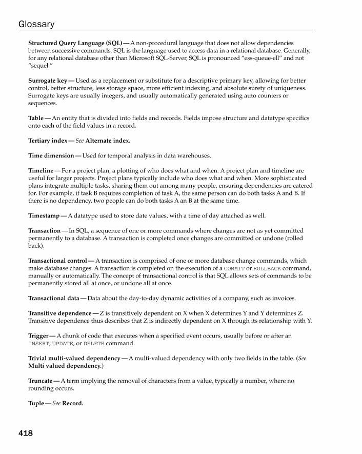
Structured Query Language (SQL) — A non-procedural language that does not allow dependenciesbetween successive commands. SQL is the language used to access data in a relational database. Generally,for any relational database other than Microsoft SQL-Server, SQL is pronounced “ess-queue-ell” and not“sequel.”
Surrogate key — Used as a replacement or substitute for a descriptive primary key, allowing for bettercontrol, better structure, less storage space, more efficient indexing, and absolute surety of uniqueness.Surrogate keys are usually integers, and usually automatically generated using auto counters orsequences.
Table — An entity that is divided into fields and records. Fields impose structure and datatype specificsonto each of the field values in a record.
Tertiary index — See Alternate index.
Time dimension — Used for temporal analysis in data warehouses.
Timeline — For a project plan, a plotting of who does what and when. A project plan and timeline areuseful for larger projects. Project plans typically include who does what and when. More sophisticatedplans integrate multiple tasks, sharing them out among many people, ensuring dependencies are cateredfor. For example, if task B requires completion of task A, the same person can do both tasks A and B. Ifthere is no dependency, two people can do both tasks A an B at the same time.
Timestamp — A datatype used to store date values, with a time of day attached as well.
Transaction — In SQL, a sequence of one or more commands where changes are not as yet committedpermanently to a database. A transaction is completed once changes are committed or undone (rolledback).
Transactional control — A transaction is comprised of one or more database change commands, whichmake database changes. A transaction is completed on the execution of a COMMIT or ROLLBACK command,manually or automatically. The concept of transactional control is that SQL allows sets of commands to bepermanently stored all at once, or undone all at once.
Transactional data — Data about the day-to-day dynamic activities of a company, such as invoices.
Transitive dependence — Z is transitively dependent on X when X determines Y and Y determines Z.Transitive dependence thus describes that Z is indirectly dependent on X through its relationship with Y.
Trigger — A chunk of code that executes when a specified event occurs, usually before or after anINSERT, UPDATE, or DELETE command.
Trivial multi-valued dependency — A multi-valued dependency with only two fields in the table. (SeeMulti valued dependency.)
Truncate — A term implying the removal of characters from a value, typically a number, where norounding occurs.
Tuple — See Record.
418
Glossary
21_574906 glos.qxd 10/28/05 11:39 PM Page 418
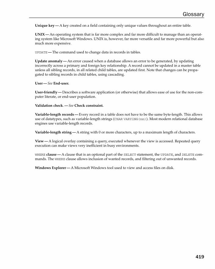
Unique key — A key created on a field containing only unique values throughout an entire table.
UNIX — An operating system that is far more complex and far more difficult to manage than an operat-ing system like Microsoft Windows. UNIX is, however, far more versatile and far more powerful but alsomuch more expensive.
UPDATE— The command used to change data in records in tables.
Update anomaly — An error caused when a database allows an error to be generated, by updatingincorrectly across a primary and foreign key relationship. A record cannot be updated in a master tableunless all sibling records, in all related child tables, are updated first. Note that changes can be propa-gated to sibling records in child tables, using cascading.
User — See End-user.
User-friendly — Describes a software application (or otherwise) that allows ease of use for the non-com-puter literate, or end-user population.
Validation check. — See Check constraint.
Variable-length records — Every record in a table does not have to be the same byte-length. This allowsuse of datatypes, such as variable-length strings (CHAR VARYING(nn)). Most modern relational databaseengines use variable-length records.
Variable-length string — A string with 0 or more characters, up to a maximum length of characters.
View — A logical overlay containing a query, executed whenever the view is accessed. Repeated queryexecution can make views very inefficient in busy environments.
WHERE clause — A clause that is an optional part of the SELECT statement, the UPDATE, and DELETE com-mands. The WHERE clause allows inclusion of wanted records, and filtering out of unwanted records.
Windows Explorer — A Microsoft Windows tool used to view and access files on disk.
419
Glossary
21_574906 glos.qxd 10/28/05 11:39 PM Page 419

21_574906 glos.qxd 10/28/05 11:39 PM Page 420

AExercise Answers
This appendix contains all the answers to the exercises appearing at the ends of chapters.
Chapter 3
Exercise 1 solution
Two CREATE TABLE commands:
CREATE TABLE Band(
band_id INTEGER NOT NULL,band_name VARCHAR(32) NULL,CONSTRAINT XPK_Band PRIMARY KEY (band_id),CONSTRAINT XUK_B_Name UNIQUE (band_name)
);
CREATE TABLE Track(
track_id INTEGER NOT NULL,band_id INTEGER NOT NULL,track_name VARCHAR(32) NULL,description VARCHAR(256) NULL,CONSTRAINT XPK_Track PRIMARY KEY (track_id), CONSTRAINT FK_T_Band FOREIGN KEY (band_id) REFERENCES Band,CONSTRAINT XUK_T_Name UNIQUE (track_name)
);
Exercise 2 solution
One CREATE INDEX command:
CREATE INDEX XFK_T_Band ON Track(band_id);
22_574906 appa.qxd 10/28/05 11:38 PM Page 421

Chapter 4
Exercise 1 solution
Five CREATE TABLE commands are shown here. Note that the order in which tables are created is impor-tant, as assignment of foreign key columns requires that primary keys in parent tables already exist:
CREATE TABLE Customer(
customer_name VARCHAR(32) PRIMARY KEY,customer_address VARCHAR(256),customer_phone VARCHAR(32)
);
CREATE TABLE Stock_Source_Department(
stock_source_department VARCHAR(32) PRIMARY KEY,stock_source_city VARCHAR(32) NOT NULL
);
CREATE TABLE Stock_Item(
stock# INTEGER PRIMARY KEY,stock_source_department VARCHAR(32) NOT NULL
REFERENCES Stock_Source_Department,stock_description VARCHAR(256),stock_unit_price FLOAT
);
CREATE TABLE Sale_Order(
order# INTEGER PRIMARY KEY,customer_name VARCHAR(32) REFERENCES Customer,dte DATE,sales_tax_percentage FLOAT
);CREATE TABLE Sale_Order_Item(
order# INTEGER PRIMARY KEY,stock# INTEGER NOT NULL REFERENCES Sale_Order,stock_quantity INTEGER
);
Note how the PRIMARY KEY and FOREIGN KEY specifications are included within thespecification of the column. These are called in line constraint definitions. This is adifferent method of definition from that of exercises in Chapter 3. Chapter 3 useswhat are called out of line constraint definitions. Inline constraint definitions canonly be used for constraints on single columns. For example, a multiple column primary key would have to be defined as an out of line constraint. It is also possibleto define primary and foreign key constraints using an ALTER TABLE command tochange a table specification, after the table has already been created.
422
Appendix A
22_574906 appa.qxd 10/28/05 11:38 PM Page 422

Exercise 2 solution
Three CREATE INDEX commands to create indexes on foreign keys:
CREATE INDEX XFK_SI_SSD ON Stock_Item (stock_source_department);CREATE INDEX XFK_SO_C ON Sale_Order (customer_name);CREATE INDEX XFK_SOI_SI ON Sale_Order_Item (stock#);
Chapter 5
Exercise 1 solution
There are two possible answers:
SELECT * FROM EDITION;
SELECT ISBN,PUBLISHER_ID,PUBLICATION_ID,PRINT_DATE,PAGES,LIST_PRICE,FORMAT,RANK,UNITS FROM EDITION;
Exercise 2 solutionSELECT ISBN FROM EDITION WHERE FORMAT=’Hardcover’;
Exercise 3 solutionSELECT ISBN FROM EDITION WHERE FORMAT=’Hardcover’ ORDER BY FORMAT, LIST_PRICE;
Exercise 4 solution
3 + 4 * 5 = 23, and (3 + 4 ) * 5 = 35. The second expression yields the greater value.
Exercise 5 solutionSELECT PUBLISHER_ID, SUM(LIST_PRICE) FROM EDITION GROUP BY PUBLISHER_ID;
Exercise 6 solutionSELECT * FROM SUBJECT S JOIN PUBLICATION P USING (SUBJECT_ID);
Exercise 7 solutionSELECT * FROM SUBJECT S LEFT OUTER JOIN PUBLICATION P USING (SUBJECT_ID);
Exercise 8 solutionSELECT * FROM SUBJECT WHERE SUBJECT_ID IN (SELECT SUBJECT_ID FROM PUBLICATION);
SELECT * FROM SUBJECT WHERE EXISTS(SELECT SUBJECT_ID FROM PUBLICATION
WHERE SUBJECT_ID = SUBJECT.SUBJECT_ID);
423
Exercise Answers
22_574906 appa.qxd 10/28/05 11:38 PM Page 423
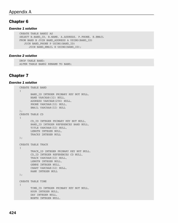
Chapter 6
Exercise 1 solutionCREATE TABLE BAND2 ASSELECT B.BAND_ID, B.NAME, A.ADDRESS, P.PHONE, E.EMAILFROM BAND B JOIN BAND_ADDRESS A USING(BAND_ID)
JOIN BAND_PHONE P USING(BAND_ID)JOIN BAND_EMAIL E USING(BAND_ID);
Exercise 2 solutionDROP TABLE BAND;ALTER TABLE BAND2 RENAME TO BAND;
Chapter 7
Exercise 1 solutionCREATE TABLE BAND(
BAND_ID INTEGER PRIMARY KEY NOT NULL,NAME VARCHAR(32) NULL,ADDRESS VARCHAR(256) NULL,PHONE VARCHAR(32) NULL,EMAIL VARCHAR(32) NULL
);CREATE TABLE CD(
CD_ID INTEGER PRIMARY KEY NOT NULL,BAND_ID INTEGER REFERENCES BAND NULL,TITLE VARCHAR(32) NULL,LENGTH INTEGER NULL,TRACKS INTEGER NULL
);
CREATE TABLE TRACK(
TRACK_ID INTEGER PRIMARY KEY NOT NULL,CD_ID INTEGER REFERENCES CD NULL,TRACK VARCHAR(32) NULL,LENGTH INTEGER NULL,GENRE INTEGER NULL,CHART VARCHAR(32) NULL,RANK INTEGER NULL
);
CREATE TABLE TIME(
TIME_ID INTEGER PRIMARY KEY NOT NULL,HOUR INTEGER NULL,DAY INTEGER NULL,MONTH INTEGER NULL,
424
Appendix A
22_574906 appa.qxd 10/28/05 11:38 PM Page 424

QUARTER INTEGER NULL,YEAR INTEGER NULL
);
CREATE TABLE LOCATION(
LOCATION_ID INTEGER PRIMARY KEY NOT NULL,CITY VARCHAR(32) NULL,COUNTY VARCHAR(32) NULL,STATE VARCHAR(32) NULL,COUNTRY VARCHAR(32) NULL
);
CREATE TABLE RADIO(
STATION_ID INTEGER PRIMARY KEY NOT NULL,STATION VARCHAR(32) NULL
);
CREATE TABLE PERFORMER(
PERFORMER_ID INTEGER PRIMARY KEY NOT NULL,PERFORMER VARCHAR(32) NULL
);
CREATE TABLE RECORDINGARTIST(
RECORDING_ARTIST_ID INTEGER PRIMARY KEY NOT NULL,RECORDING_ARTIST VARCHAR(32) NULL
);
CREATE TABLE ROYALTY(
ROYALTY_ID INTEGER PRIMARY KEY NOT NULL,TRACK_ID INTEGER REFERENCES TRACK NULL,RECORDING_ARTIST_ID INTEGER REFERENCES RECORDINGARTIST NULL,PERFORMER_ID INTEGER REFERENCES PERFORMER NULL,STATION_ID INTEGER REFERENCES RADIO NULL,LOCATION_ID INTEGER REFERENCES LOCATION NULL,TIME_ID INTEGER REFERENCES TIME NULL,AMOUNT FLOAT NOT NULL
);
Exercise 2 solutionCREATE TABLE TEMP AS
SELECT B.NAME AS BAND_NAME, B.ADDRESS AS BAND.ADDRESS, B.PHONE AS BAND_PHONE, B.EMAIL AS BAND_EMAIL, CD.TITLE AS CD_TITLE, CD.LENGTH AS CD_LENGTH, CD.TRACKS AS CD_TRACKS,T.TRACK, T.LENGTH AS TRACK_LENGTH, T.GENRE AS TRACK_GENRE, T.CHART AS TRACK_CHART, T.RANK AS TRACK_RANK
FROM BAND B JOIN CD CD JOIN TRACK T;
--
425
Exercise Answers
22_574906 appa.qxd 10/28/05 11:38 PM Page 425
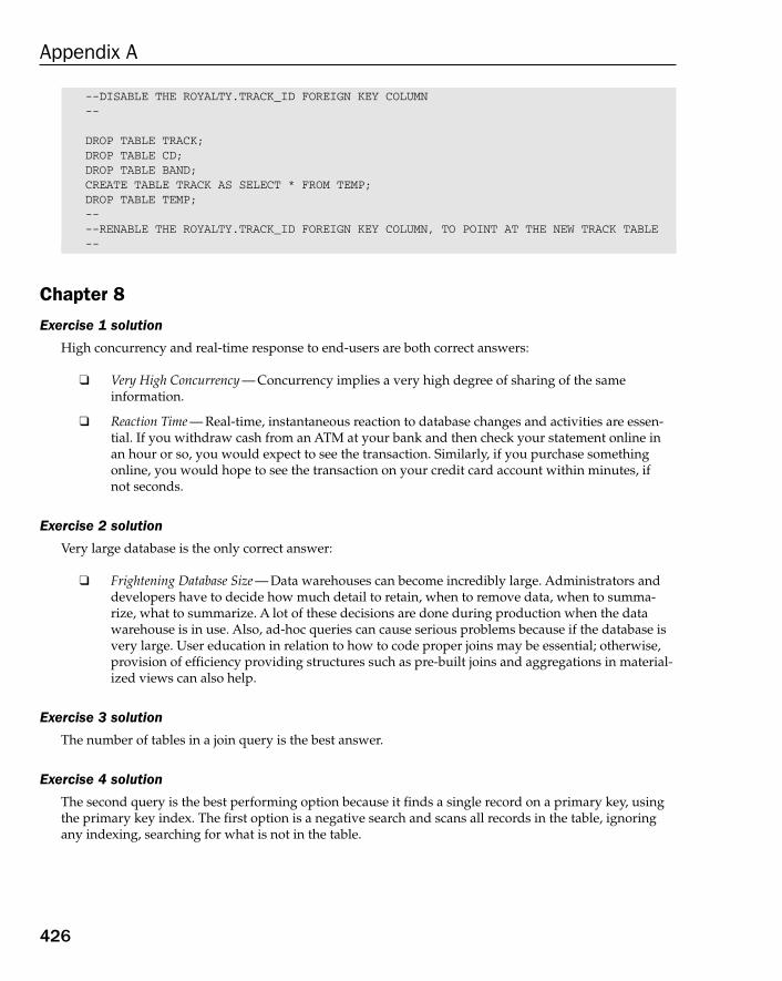
--DISABLE THE ROYALTY.TRACK_ID FOREIGN KEY COLUMN--
DROP TABLE TRACK;DROP TABLE CD;DROP TABLE BAND;CREATE TABLE TRACK AS SELECT * FROM TEMP;DROP TABLE TEMP;----RENABLE THE ROYALTY.TRACK_ID FOREIGN KEY COLUMN, TO POINT AT THE NEW TRACK TABLE--
Chapter 8
Exercise 1 solution
High concurrency and real-time response to end-users are both correct answers:
❑ Very High Concurrency — Concurrency implies a very high degree of sharing of the same information.
❑ Reaction Time — Real-time, instantaneous reaction to database changes and activities are essen-tial. If you withdraw cash from an ATM at your bank and then check your statement online inan hour or so, you would expect to see the transaction. Similarly, if you purchase somethingonline, you would hope to see the transaction on your credit card account within minutes, if not seconds.
Exercise 2 solution
Very large database is the only correct answer:
❑ Frightening Database Size — Data warehouses can become incredibly large. Administrators anddevelopers have to decide how much detail to retain, when to remove data, when to summa-rize, what to summarize. A lot of these decisions are done during production when the datawarehouse is in use. Also, ad-hoc queries can cause serious problems because if the database isvery large. User education in relation to how to code proper joins may be essential; otherwise,provision of efficiency providing structures such as pre-built joins and aggregations in material-ized views can also help.
Exercise 3 solution
The number of tables in a join query is the best answer.
Exercise 4 solution
The second query is the best performing option because it finds a single record on a primary key, usingthe primary key index. The first option is a negative search and scans all records in the table, ignoringany indexing, searching for what is not in the table.
426
Appendix A
22_574906 appa.qxd 10/28/05 11:38 PM Page 426

Chapter 9
Exercise 1 solutionCREATE TABLE INSTRUMENT(INSTRUMENT VARCHAR(32) NULL);
CREATE TABLE SKILL(SKILL VARCHAR(32) NULL);
CREATE TABLE GENRE(GENRE VARCHAR(32) NULL);
CREATE TABLE MUSICIAN(
NAME VARCHAR(32) NULL,PHONE VARCHAR(32) NULL,EMAIL VARCHAR(32) NULL
);
CREATE TABLE SHOWS(
LOCATION VARCHAR(32) NULL,ADDRESS VARCHAR(32) NULL,DIRECTIONS VARCHAR(32) NULL,PHONE VARCHAR(32) NULL,SHOW_DATE DATE NULL,SHOW_TIMES VARCHAR(32) NULL
);
CREATE TABLE MERCHANDISE(
TYPE VARCHAR(32) NULL,PRICE FLOAT NULL
);
CREATE TABLE DISCOGRAPHY(
CD_NAME VARCHAR(32) NULL,RELEASE_DATE DATE NULL,PRICE FLOAT NULL
);
CREATE TABLE BAND(
NAME VARCHAR(32) NULL,MEMBERS VARCHAR(32) NULL,FOUNDING_DATE DATE NULL
);
CREATE TABLE ADVERTISEMENT(
AD_DATE DATE NULL,AD_TEXT VARCHAR(1000) NULL,PHONE VARCHAR(32) NULL,EMAIL VARCHAR(32) NULL,REQUIREMENTS VARCHAR(1000) NULL
);
427
Exercise Answers
22_574906 appa.qxd 10/28/05 11:38 PM Page 427
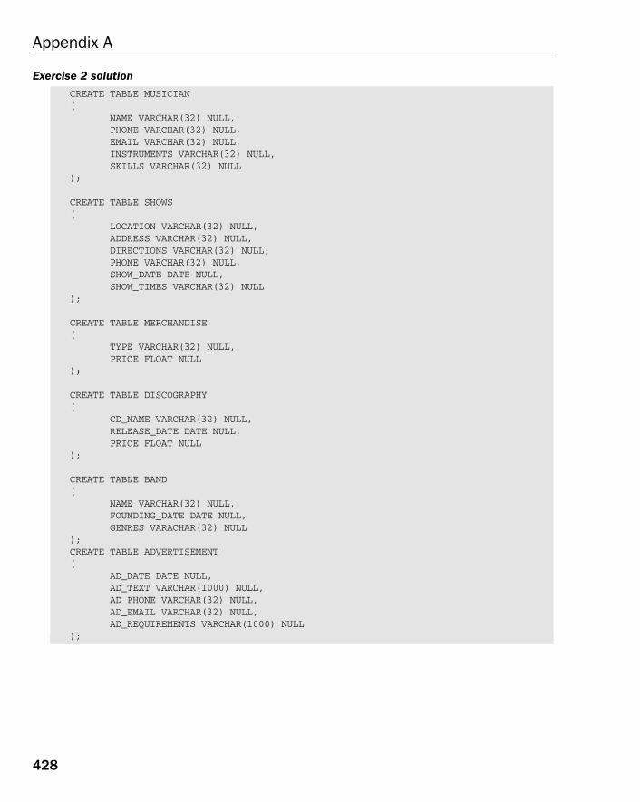
Exercise 2 solutionCREATE TABLE MUSICIAN(
NAME VARCHAR(32) NULL,PHONE VARCHAR(32) NULL,EMAIL VARCHAR(32) NULL,INSTRUMENTS VARCHAR(32) NULL,SKILLS VARCHAR(32) NULL
);
CREATE TABLE SHOWS(
LOCATION VARCHAR(32) NULL,ADDRESS VARCHAR(32) NULL,DIRECTIONS VARCHAR(32) NULL,PHONE VARCHAR(32) NULL,SHOW_DATE DATE NULL,SHOW_TIMES VARCHAR(32) NULL
);
CREATE TABLE MERCHANDISE(
TYPE VARCHAR(32) NULL,PRICE FLOAT NULL
);
CREATE TABLE DISCOGRAPHY(
CD_NAME VARCHAR(32) NULL,RELEASE_DATE DATE NULL,PRICE FLOAT NULL
);
CREATE TABLE BAND(
NAME VARCHAR(32) NULL,FOUNDING_DATE DATE NULL,GENRES VARACHAR(32) NULL
);CREATE TABLE ADVERTISEMENT(
AD_DATE DATE NULL,AD_TEXT VARCHAR(1000) NULL,AD_PHONE VARCHAR(32) NULL,AD_EMAIL VARCHAR(32) NULL,AD_REQUIREMENTS VARCHAR(1000) NULL
);
428
Appendix A
22_574906 appa.qxd 10/28/05 11:38 PM Page 428

Chapter 10
Exercise 1 solutionCREATE TABLE INSTRUMENT(
INSTRUMENT_ID INTEGER PRIMARY KEY,SECTION_ID INTEGER FOREIGN KEY REFERENCES INSTRUMENT WITH NULL,INSTRUMENT STRING NOT NULL
);
INSTRUMENT is NOT NULL, because there is no point in storing an instrument without a name.
CREATE TABLE GENRE(
GENRE_ID INTEGER PRIMARY KEY,PARENT_ID INTEGER FOREIGN KEY REFERENCES GENRE WITH NULL,GENRE STRING NOT NULL
);
CREATE TABLE VENUE(
VENUE_ID INTEGER PRIMARY KEY,VENUE STRING NOT NULL,ADDRESS STRING NULL,DIRECTIONS STRING NULL,PHONE STRING NULL
);
The field for the name of the VENUE should be VENUE, not LOCATION. It is thus changed in the preced-ing script.
CREATE TABLE BAND(
BAND_ID INTEGER PRIMARY KEY,GENRE_ID INTEGER FOREIGN KEY REFERENCES GENRE,BAND STRING NOT NULL,FOUNDING_DATE DATE NULL
);
CREATE TABLE MERCHANDISE(
MERCHANDISE_ID INTEGER PRIMARY KEY,BAND_ID INTEGER FOREIGN KEY REFERENCES BAND,TYPE STRING NOT NULL,PRICE MONEY NULL
);
CREATE TABLE DISCOGRAPHY(
DISCOGRAPHY_ID INTEGER PRIMARY KEY,BAND_ID INTEGER FOREIGN KEY REFERENCES BAND,
429
Exercise Answers
22_574906 appa.qxd 10/28/05 11:38 PM Page 429

CD_NAME STRING NOT NULL,RELEASE_DATE DATE NULL,PRICE MONEY NULL
);
CREATE TABLE SHOW(
SHOW_ID INTEGER PRIMARY_KEY,VENUE_ID INTEGER FOREIGN KEY REFERENCES VENUE,BAND_ID INTEGER FOREIGN KEY REFERENCES BAND,DATE DATE NULL,TIME STRING NULL
);
CREATE TABLE MUSICIAN(
MUSICIAN_ID INTEGER PRIMARY KEY,INSTRUMENT_ID INTEGER FOREIGN KEY REFERENCES INSTRUMENT,BAND_ID INTEGER FOREIGN KEY REFERENCES BAND,MUSICIAN STRING NOT NULL,PHONE STRING NULL,EMAIL STRING NULL,SKILLS STRING NULL
);
CREATE TABLE ADVERTISEMENT(
ADVERTISEMENT_ID INTEGER PRIMARY KEY,BAND_ID INTEGER FOREIGN KEY REFERENCES BAND,MUSICIAN_ID INTEGER FOREIGN KEY REFERENCES MUSICIAN,AD_DATE DATE NULL,AD_TEXT BIGSTRING NULL
);
Exercise 2 solutionCREATE TABLE INSTRUMENT(
INSTRUMENT_ID INTEGER PRIMARY KEY,SECTION_ID INTEGER FOREIGN KEY REFERENCES INSTRUMENT WITH NULL,INSTRUMENT STRING NOT NULL
);
CREATE TABLE GENRE(
GENRE_ID INTEGER PRIMARY KEY,PARENT_ID INTEGER FOREIGN KEY REFERENCES GENRE WITH NULL,GENRE STRING NOT NULL
);
CREATE TABLE MERCHANDISE(
MERCHANDISE_ID INTEGER PRIMARY KEY,TYPE STRING NOT NULL,
430
Appendix A
22_574906 appa.qxd 10/28/05 11:38 PM Page 430

PRICE MONEY NULL);
CREATE TABLE ARTISTS(
ARTIST_ID INTEGER PRIMARY KEY,MERCHANDISE_ID INTEGER FOREIGN KEY REFERENCES MERCHANDISE WITH NULL,GENRE_ID INTEGER FOREIGN KEY REFERENCES GENRE WITH NULL,INSTRUMENT_ID INTEGER FOREIGN KEY REFERENCES INSTRUMENT WITH NULL,MUSICIAN_NAME STRING NULL,MUSICIAN_PHONE STRING NULL,MUSICIAN_EMAIL STRING NULL,BAND_NAME STRING NULL,BAND_FOUNDING_DATE DATE NULL,DISCOGRAPHY_CD_NAME STRING NULL,DISCOGRAPHY_RELEASE_DATE DATE NULL,DISCOGRAPHY_PRICE MONEY NULL,SHOW_DATE DATE NULL,SHOW_TIME STRING NULL,VENUE_NAME STRING NULL,VENUE_ADDRESS STRING NULL,VENUE_DIRECTIONS BIGSTRING NULL,VENUE_PHONE STRING NULL,ADVERTISEMENT_DATE DATE NULL,ADVERTISEMENT_TEXT BIGSTRING NULL
);
Chapter 11
Exercise 1 solutionCREATE TABLE INSTRUMENT(
INSTRUMENT_ID INTEGER PRIMARY KEY NOT NULL,SECTION_ID INTEGER FOREIGN KEY REFERENCES INSTRUMENT WITH NULL,INSTRUMENT CHAR VARYING(32) NOT NULL
);
CREATE TABLE GENRE(
GENRE_ID INTEGER PRIMARY KEY NOT NULL,PARENT_ID INTEGER FOREIGN KEY REFERENCES GENRE WITH NULL,GENRE CHAR VARYING(32) NOT NULL
);
CREATE TABLE VENUE(
VENUE_ID INTEGER PRIMARY KEY NOT NULL,LOCATION CHAR VARYING(32) NOT NULL,ADDRESS_LINE_1 CHAR VARYING(32) NOT NULL,ADDRESS_LINE_2 CHAR VARYING(32) NULL,TOWN CHAR VARYING(32) NOT NULL,ZIP NUMBER(5) NULL,
431
Exercise Answers
22_574906 appa.qxd 10/28/05 11:38 PM Page 431

POSTAL_CODE CHAR VARYING(32) NULL,COUNTRY CHAR VARYING(32) NULL,DIRECTIONS MEMO NULL,PHONE CHAR VARYING(32) NULL
);
CREATE TABLE MERCHANDISE(
MERCHANDISE_ID INTEGER PRIMARY KEY NOT NULL,BAND_ID INTEGER FOREIGN KEY REFERENCES BAND NOT NULL,TYPE CHAR VARYING(32) NOT NULL,PRICE MONEY NOT NULL
);
CREATE TABLE DISCOGRAPHY(
DISCOGRAPHY_ID INTEGER PRIMARY KEY NOT NULL,BAND_ID INTEGER FOREIGN REFERENCES BAND NOT NULL,CD_NAME CHAR VARYING(32) NOT NULL,RELEASE_DATE DATE NULL,PRICE MONEY NULL
);
CREATE TABLE SHOW(
SHOW_ID INTEGER PRIMARY KEY NOT NULL,BAND_ID INTEGER FOREIGN KEY REFERENCES BAND NOT NULL,VENUE_ID INTEGER FOREIGN KEY REFERENES VENUE NOT NULL,DATE DATE NOT NULL,TIME CHAR VARYING(16) NOT NULL
);
CREATE TABLE BAND(
BAND_ID INTEGER PRIMARY KEY NOT NULL,GENRE_ID INTEGER FOREIGN KEY REFERENCES GENRE NOT NULL,BAND CHAR VARYING(32) NOT NULL,FOUNDING_DATE DATE NOT NULL
);
CREATE TABLE MUSICIAN(
MUSICIAN_ID INTEGER PRIMARY KEY NOT NULL,INSTRUMENT_ID INTEGER FOREIGN KEY REFERENCES INSTRUMENT NOT NULL,BAND_ID INTEGER FOREIGN KEY REFERENCES BAND WITH NULL,MUSICIAN CHAR VARYING(32) NOT NULL,PHONE CHAR VARYING(32) NULL,EMAIL CHAR VARYING(32) NULL,SKILLS CHAR VARYING(256) NULL
);
CREATE TABLE ADVERTISEMENT(
ADVERTISEMENT_ID INTEGER PRIMARY KEY NOT NULL,BAND_ID INTEGER FOREIGN KEY REFERENCES BAND WITH NULL,
432
Appendix A
22_574906 appa.qxd 10/28/05 11:38 PM Page 432

MUSICIAN_ID INTEGER FOREIGN KEY REFERENCES MUSICIAN WITH NULL,DATE DATE NOT NULL,TEXT MEMO NOT NULL
);
The Microsoft Access MEMO datatype is used to represent very large strings.
Exercise 2 solutionCREATE TABLE INSTRUMENT(
INSTRUMENT_ID INTEGER PRIMARY KEY NOT NULL,SECTION_ID INTEGER FOREIGN KEY REFERENCES INSTRUMENT WITH NULL,INSTRUMENT CHAR VARYING(32) NOT NULL
);
CREATE TABLE MUSICIAN(
MUSICIAN_ID INTEGER PRIMARY KEY NOT NULL,MUSICIAN CHAR VARYING(32) NOT NULL,PHONE CHAR VARYING(32) NULL,EMAIL CHAR VARYING(32) NULL
);
CREATE TABLE GENRE(
GENRE_ID INTEGER PRIMARY KEY NOT NULL,PARENT_ID INTEGER FOREIGN KEY REFERENCES GENRE WITH NULL,GENRE CHAR VARYING(32) NOT NULL
);
CREATE TABLE BAND(
BAND_ID INTEGER PRIMARY KEY NOT NULL,BAND CHAR VARYING(32) NOT NULL,FOUNDING_DATE DATE NOT NULL
);
CREATE TABLE ADVERTISEMENT(
ADVERTISEMENT_ID INTEGER PRIMARY KEY NOT NULL,DATE DATE NOT NULL,TEXT MEMO NOT NULL
);
CREATE TABLE DISCOGRAPHY(
DISCOGRAPHY_ID INTEGER PRIMARY KEY NOT NULL,CD_NAME CHAR VARYING(32) NOT NULL,RELEASE_DATE DATE NULL,PRICE MONEY NULL
);
CREATE TABLE MERCHANDISE(
433
Exercise Answers
22_574906 appa.qxd 10/28/05 11:38 PM Page 433

MERCHANDISE_ID INTEGER PRIMARY KEY NOT NULL,TYPE CHAR VARYING(32) NOT NULL,PRICE MONEY NOT NULL
);
CREATE TABLE SHOW_VENUE(
SHOW_ID INTEGER PRIMARY KEY NOT NULL,LOCATION CHAR VARYING(32) NOT NULL,ADDRESS_LINE_1 CHAR VARYING(32) NOT NULL,ADDRESS_LINE_2 CHAR VARYING(32) NULL,TOWN CHAR VARYING(32) NOT NULL,ZIP NUMBER(5) NULL,POSTAL_CODE CHAR VARYING(32) NULL,COUNTRY CHAR VARYING(32) NULL,DIRECTIONS MEMO NULL,PHONE CHAR VARYING(32) NULLSHOW_DATE DATE NOT NULL,SHOW_TIME CHAR VARYING(16) NOT NULL
);
VENUE is changed to LOCATIONCREATE TABLE FACT(
FACT_ID INTEGER NOT NULL,SHOW_ID INTEGER FOREIGN KEY REFERENCES SHOW WITH NULL,MUSICIAN_ID INTEGER FOREIGN KEY REFERENCES MUSICIAN WITH NULL,BAND_ID INTEGER FOREIGN KEY REFERENCES BAND WITH NULL,ADVERTISEMENT_ID INTEGER FOREIGN KEY REFERENCES ADVERTISEMENT
WITH NULL,DISCOGRAPHY_ID INTEGER FOREIGN KEY REFERENCES DISCOGRAPHY
WITH NULL,MERCHANDISE_ID INTEGER FOREIGN KEY REFERENCES MERCHANDISE
WITH NULL,GENRE_ID INTEGER FOREIGN KEY REFERENCES GENRE WITH NULL,INSTRUMENT_ID INTEGER FOREIGN KEY REFERENCES INSTRUMENT WITH NULL,CD_SALE_AMOUNT MONEY NULL,MERCHANDISE_SALE_AMOUNT MONEY NULL,ADVERTISING_COST_AMOUNT MONEY NULL,SHOW_TICKET_SALES_AMOUNT_MONEY NULL
);
434
Appendix A
22_574906 appa.qxd 10/28/05 11:38 PM Page 434
BSample Databases
This appendix contains what should the most sensible versions of some of the more complete ERDdatabase model diagrams, as presented in this book. This appendix is intended merely as a refer-ence of database model ERDs.
Following is a summary of the ERDs included in this appendix.
❑ Figure B-1 shows the book publication OLTP ERD.
❑ Figure B-2 shows the book publication reviews data warehouse ERD.
❑ Figure B-3 shows the book publication sales data warehouse ERD.
❑ Figure B-4 shows the musicians, bands, and advertisements OLTP ERD.
❑ Figure B-5 shows the musicians, bands, and advertisements data warehouse ERD.
❑ Figure B-6 shows the online auction house OLTP ERD.
❑ Figure B-7 shows the online auction house data warehouse ERD.
23_574906 appb.qxd 10/28/05 11:43 PM Page 435
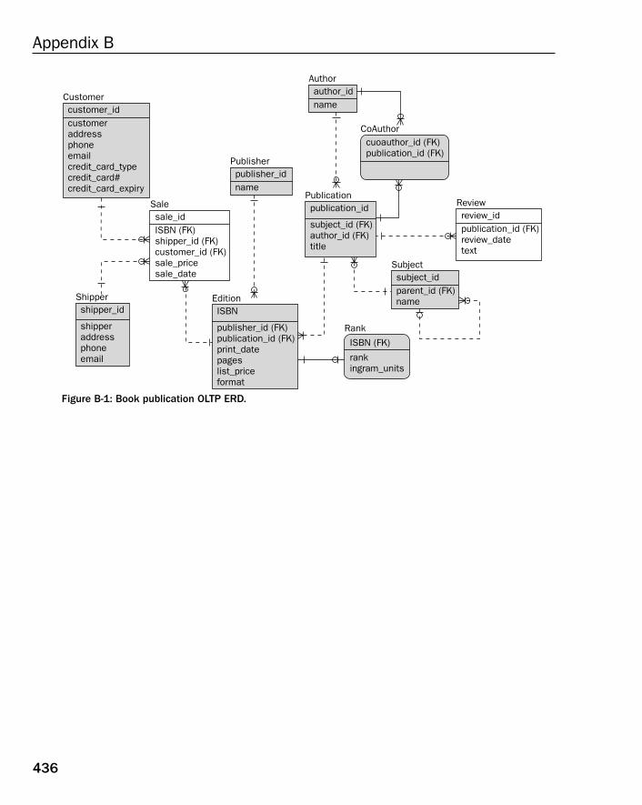
Figure B-1: Book publication OLTP ERD.
Customercustomer_idcustomeraddressphoneemailcredit_card_typecredit_card#credit_card_expiry
Publisherpublisher_idname
Subjectsubject_idparent_id (FK)name
Reviewreview_idpublication_id (FK)review_datetext
Salesale_idISBN (FK)shipper_id (FK)customer_id (FK)sale_pricesale_date
Publicationpublication_id
subject_id (FK)author_id (FK)title
Shippershipper_id
shipperaddressphoneemail
EditionISBN
publisher_id (FK)publication_id (FK)print_datepageslist_priceformat
Authorauthor_idname
CoAuthorcuoauthor_id (FK)publication_id (FK)
Rank
ISBN (FK)
rankingram_units
436
Appendix B
23_574906 appb.qxd 10/28/05 11:43 PM Page 436
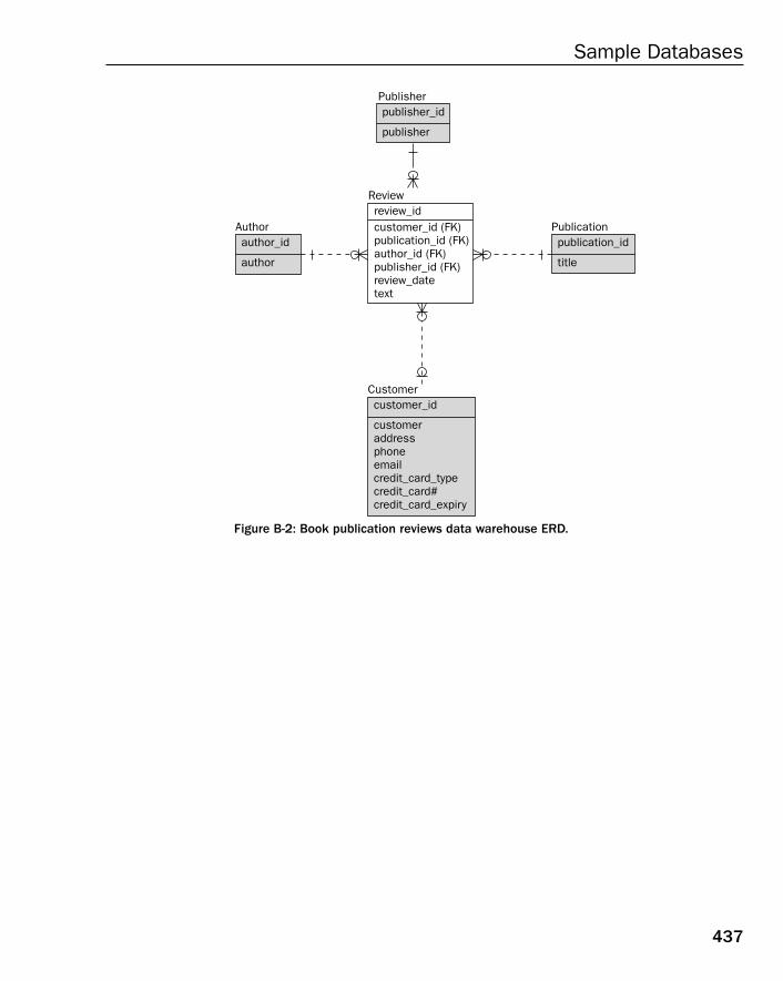
Figure B-2: Book publication reviews data warehouse ERD.
Reviewreview_idcustomer_id (FK)publication_id (FK)author_id (FK)publisher_id (FK)review_datetext
publisher
Publisherpublisher_id
Authorauthor_id
author
Publicationpublication_id
title
Customercustomer_id
customeraddressphoneemailcredit_card_typecredit_card#credit_card_expiry
437
Sample Databases
23_574906 appb.qxd 10/28/05 11:43 PM Page 437
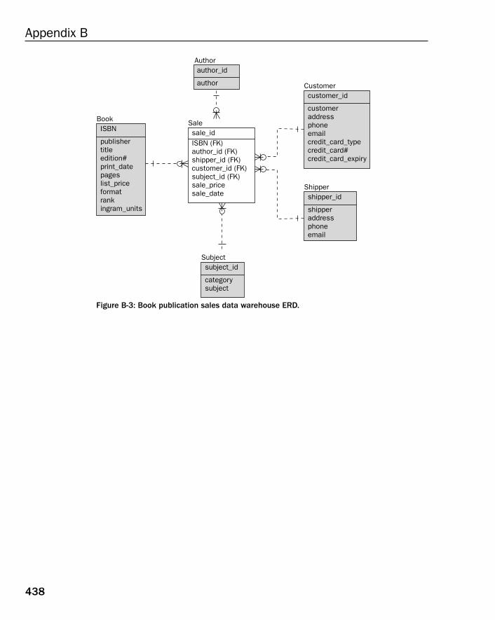
Figure B-3: Book publication sales data warehouse ERD.
Salesale_idISBN (FK)author_id (FK)shipper_id (FK)customer_id (FK)subject_id (FK)sale_pricesale_date
author
Authorauthor_id
BookISBN
publishertitleedition#print_datepageslist_priceformatrankingram_units
Customercustomer_id
customeraddressphoneemailcredit_card_typecredit_card#credit_card_expiry
Subjectsubject_id
categorysubject
Shippershipper_id
shipperaddressphoneemail
438
Appendix B
23_574906 appb.qxd 10/28/05 11:43 PM Page 438
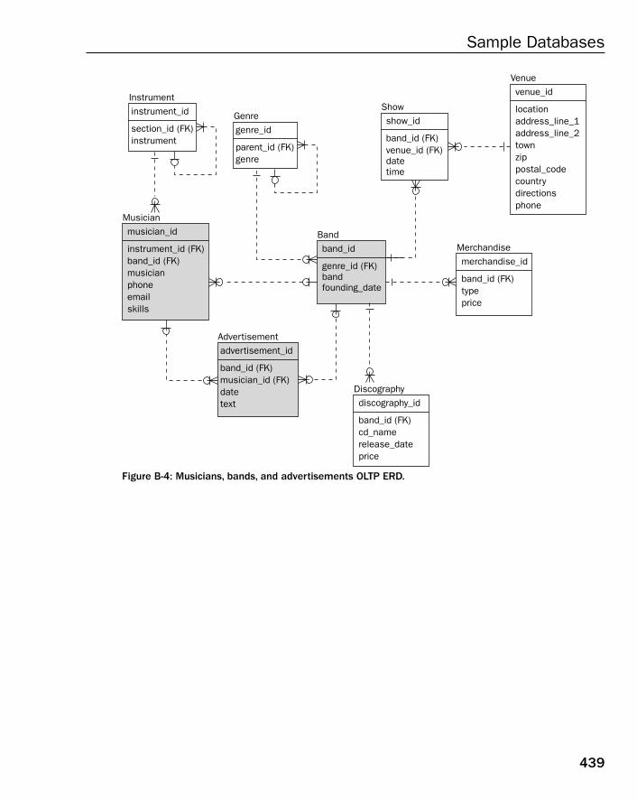
Figure B-4: Musicians, bands, and advertisements OLTP ERD.
Musicianmusician_id
instrument_id (FK)band_id (FK)musicianphoneemailskills
Advertisementadvertisement_id
band_id (FK)musician_id (FK)datetext
Bandband_id
genre_id (FK)bandfounding_date
Venuevenue_id
locationaddress_line_1address_line_2townzippostal_codecountrydirectionsphone
Merchandisemerchandise_id
band_id (FK)typeprice
Showshow_id
band_id (FK)venue_id (FK)datetime
Genregenre_id
parent_id (FK)genre
Instrumentinstrument_id
section_id (FK)instrument
Discographydiscography_id
band_id (FK)cd_namerelease_dateprice
439
Sample Databases
23_574906 appb.qxd 10/28/05 11:43 PM Page 439
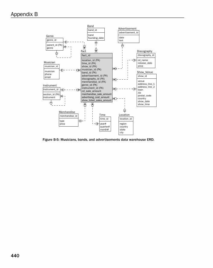
Figure B-5: Musicians, bands, and advertisements data warehouse ERD.
Factfact_id
location_id (FK)time_id (FK)show_id (FK)musician_id (FK)band_id (FK)advertisement_id (FK)discography_id (FK)merchandise_id (FK)genre_id (FK)instrument_id (FK)cd_sale_amountmerchandise_sale_amountadvertising_cost_amountshow_ticket_sales_amount
Genregenre_id
parent_id (FK)genre
Bandband_id
bandfounding_date
Advertisementadvertisement_id
datetext
Discographydiscography_id
cd_namerelease_dateprice
Show_Venueshow_id
venueaddress_line_1address_line_2townzippostal_codecountryshow_dateshow_time
Merchandisemerchandise_id
typeprice
Timetime_id
year#quarter#month#
Locationlocation_id
regioncountrystatecity
Instrumentinstrument_id
section_id (FK)instrument
Musicianmusician_id
musicianphoneemail
440
Appendix B
23_574906 appb.qxd 10/28/05 11:43 PM Page 440
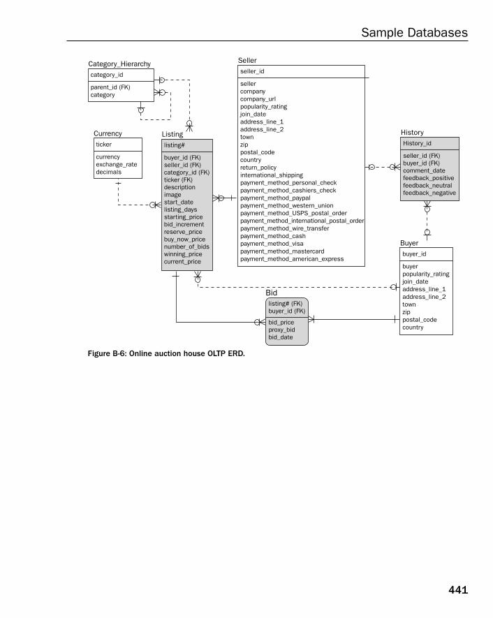
Figure B-6: Online auction house OLTP ERD.
Listinglisting#
buyer_id (FK)seller_id (FK)category_id (FK)ticker (FK)descriptionimagestart_datelisting_daysstarting_pricebid_incrementreserve_pricebuy_now_pricenumber_of_bidswinning_pricecurrent_price
HistoryHistory_id
seller_id (FK)buyer_id (FK)comment_datefeedback_positivefeedback_neutralfeedback_negative
Sellerseller_id
sellercompanycompany_urlpopularity_ratingjoin_dateaddress_line_1address_line_2townzippostal_codecountryreturn_policyinternational_shippingpayment_method_personal_checkpayment_method_cashiers_checkpayment_method_paypalpayment_method_western_unionpayment_method_USPS_postal_orderpayment_method_international_postal_orderpayment_method_wire_transferpayment_method_cashpayment_method_visapayment_method_mastercardpayment_method_american_express
Buyerbuyer_id
buyerpopularity_ratingjoin_dateaddress_line_1address_line_2townzippostal_codecountry
Currencyticker
currencyexchange_ratedecimals
Category_Hierarchycategory_id
parent_id (FK)category
Bidlisting# (FK)buyer_id (FK)
bid_priceproxy_bidbid_date
441
Sample Databases
23_574906 appb.qxd 10/28/05 11:43 PM Page 441
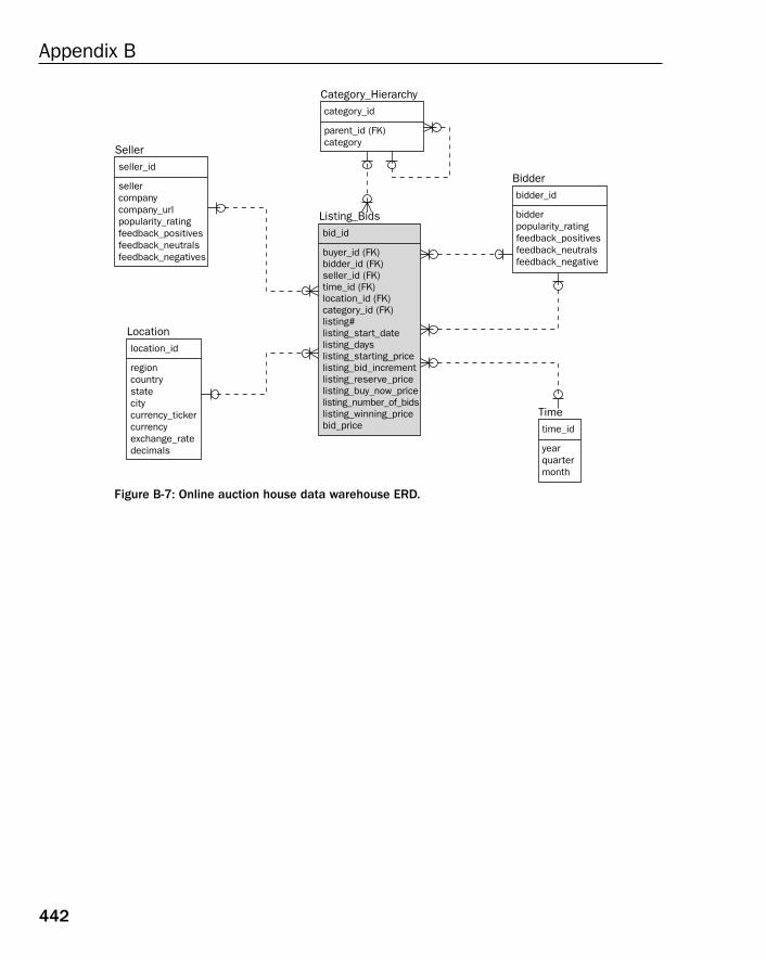
Figure B-7: Online auction house data warehouse ERD.
Bidderbidder_id
bidderpopularity_ratingfeedback_positivesfeedback_neutralsfeedback_negative
Category_Hierarchycategory_id
parent_id (FK)category
Sellerseller_id
sellercompanycompany_urlpopularity_ratingfeedback_positivesfeedback_neutralsfeedback_negatives
Locationlocation_id
regioncountrystatecitycurrency_tickercurrencyexchange_ratedecimals
Timetime_id
yearquartermonth
Listing_Bidsbid_id
buyer_id (FK)bidder_id (FK)seller_id (FK)time_id (FK)location_id (FK)category_id (FK)listing#listing_start_datelisting_dayslisting_starting_pricelisting_bid_incrementlisting_reserve_pricelisting_buy_now_pricelisting_number_of_bidslisting_winning_pricebid_price
442
Appendix B
23_574906 appb.qxd 10/28/05 11:43 PM Page 442

Index
24_574906 bindexbob.qxd 10/28/05 11:46 PM Page 443

24_574906 bindexbob.qxd 10/28/05 11:46 PM Page 444

Inde
x
Index
SYMBOLS AND NUMERICS* (asterisk)
performance issues, 200SELECT queries, 127, 128
() (parentheses), 134; (semicolon), 1271NF (1st Normal Form)
denormalization, 161described, 82–88, 403tables, 284, 286–287
2NF (2nd Normal Form)denormalization, 160, 161–162described, 403functional dependencies, 89–96tables, 284–285
3NF (3rd Normal Form)data warehouses, 169denormalization, 157–159described, 96–103, 403tables, 284, 285–286, 287–288
4NF (4th Normal Form)denormalization, 155–156described, 107, 111–116tables, 292–294
5NF (5th Normal Form)denormalization, 156described, 107, 116–121, 404tables, 294–295
Aabstracted class, 165abstraction, 28–30, 404access
frequency, separating fields by, 164views, restricting, 210–211
Access (Microsoft)datatypes, 331field-setting options, 358, 359
active datadescribed, 404and inactive data, separating, 163
adding table values, validation check, 48addition, 133, 322ad-hoc queries
database design support, 18described, 404
aggregated query, 126, 135–137, 404algorithm
described, 404table, hashing, 68
aliasesshort, improving SQL performance with, 201table names, substituting in SELECT query,
128–130ALTER TABLE command, 145alternate indexing
described, 65, 404foreign keys, 345, 348–352optimizing performance, 209post-development database, tuning, 198
24_574906 bindexbob.qxd 10/28/05 11:46 PM Page 445
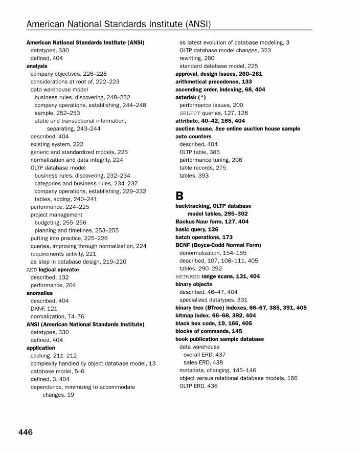
American National Standards Institute (ANSI)datatypes, 330defined, 404
analysiscompany objectives, 226–228considerations at root of, 222–223data warehouse model
business rules, discovering, 248–252company operations, establishing, 244–248sample, 252–253static and transactional information,
separating, 243–244described, 404existing system, 222generic and standardized models, 225normalization and data integrity, 224OLTP database model
business rules, discovering, 232–234categories and business rules, 234–237company operations, establishing, 229–232tables, adding, 240–241
performance, 224–225project management
budgeting, 255–256planning and timelines, 253–255
putting into practice, 225–226queries, improving through normalization, 224requirements activity, 221as step in database design, 219–220
AND logical operatordescribed, 132performance, 204
anomaliesdescribed, 404DKNF, 121normalization, 74–76
ANSI (American National Standards Institute)datatypes, 330defined, 404
applicationcaching, 211–212complexity handled by object database model, 13database model, 5–6defined, 3, 404dependence, minimizing to accommodate
changes, 19
as latest evolution of database modeling, 3OLTP database model changes, 323rewriting, 260standard database model, 225
approval, design issues, 260–261arithmetical precedence, 133ascending order, indexing, 68, 404asterisk (*)
performance issues, 200SELECT queries, 127, 128
attribute, 40–42, 165, 404auction house. See online auction house sampleauto counters
described, 404OLTP table, 385performance tuning, 206table records, 275tables, 393
Bbacktracking, OLTP database
model tables, 295–302Backus-Naur form, 127, 404basic query, 126batch operations, 173BCNF (Boyce-Codd Normal Form)
denormalization, 154–155described, 107, 108–111, 405tables, 290–292
BETWEEN range scans, 131, 404binary objects
described, 46–47, 404specialized datatypes, 331
binary tree (BTree) indexes, 66–67, 385, 391, 405bitmap index, 66–68, 392, 404black box code, 19, 166, 405blocks of commands, 145book publication sample database
data warehouseoverall ERD, 437sales ERD, 438
metadata, changing, 145–146object versus relational database models, 166OLTP ERD, 436
446
American National Standards Institute (ANSI)
24_574906 bindexbob.qxd 10/28/05 11:46 PM Page 446
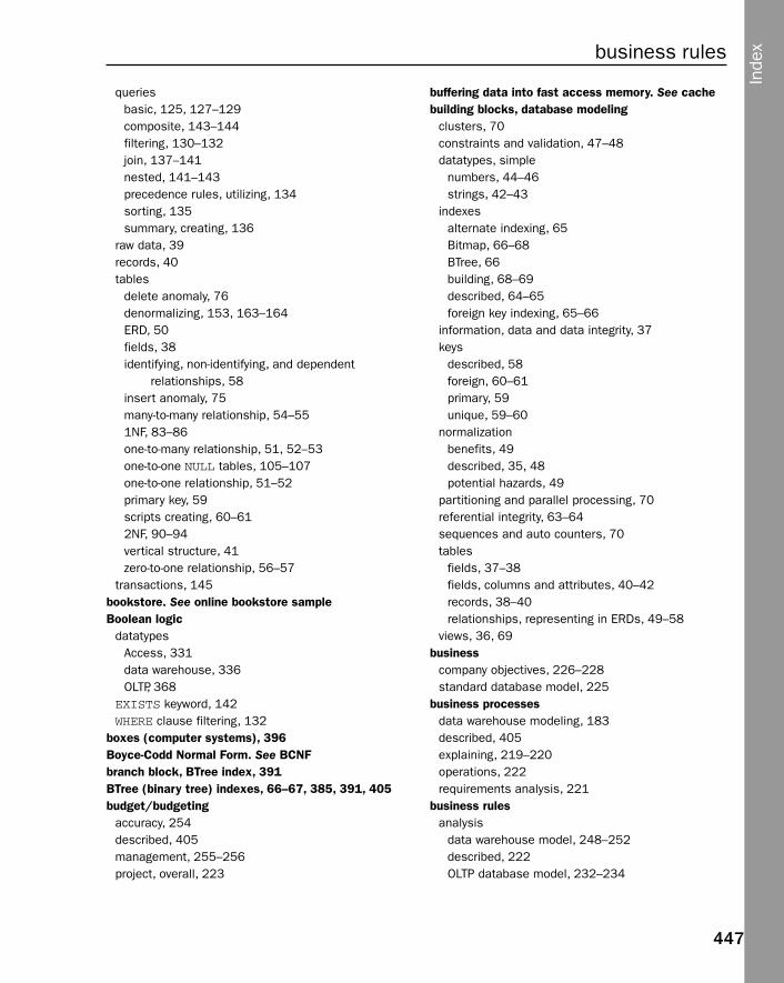
queriesbasic, 125, 127–129composite, 143–144filtering, 130–132join, 137–141nested, 141–143precedence rules, utilizing, 134sorting, 135summary, creating, 136
raw data, 39records, 40tables
delete anomaly, 76denormalizing, 153, 163–164ERD, 50fields, 38identifying, non-identifying, and dependent
relationships, 58insert anomaly, 75many-to-many relationship, 54–551NF, 83–86one-to-many relationship, 51, 52–53one-to-one NULL tables, 105–107one-to-one relationship, 51–52primary key, 59scripts creating, 60–612NF, 90–94vertical structure, 41zero-to-one relationship, 56–57
transactions, 145bookstore. See online bookstore sampleBoolean logic
datatypesAccess, 331data warehouse, 336OLTP, 368
EXISTS keyword, 142WHERE clause filtering, 132
boxes (computer systems), 396Boyce-Codd Normal Form. See BCNFbranch block, BTree index, 391BTree (binary tree) indexes, 66–67, 385, 391, 405budget/budgeting
accuracy, 254described, 405management, 255–256project, overall, 223
buffering data into fast access memory. See cachebuilding blocks, database modeling
clusters, 70constraints and validation, 47–48datatypes, simple
numbers, 44–46strings, 42–43
indexesalternate indexing, 65Bitmap, 66–68BTree, 66building, 68–69described, 64–65foreign key indexing, 65–66
information, data and data integrity, 37keys
described, 58foreign, 60–61primary, 59unique, 59–60
normalizationbenefits, 49described, 35, 48potential hazards, 49
partitioning and parallel processing, 70referential integrity, 63–64sequences and auto counters, 70tables
fields, 37–38fields, columns and attributes, 40–42records, 38–40relationships, representing in ERDs, 49–58
views, 36, 69business
company objectives, 226–228standard database model, 225
business processesdata warehouse modeling, 183described, 405explaining, 219–220operations, 222requirements analysis, 221
business rulesanalysis
data warehouse model, 248–252described, 222OLTP database model, 232–234
447
business rules
Inde
x
24_574906 bindexbob.qxd 10/28/05 11:46 PM Page 447

business rules (continued)code, storing in database
described, 358–360event triggers, 363external procedures, 364macro, 364stored function, 362stored procedure, 360–362
described, 354–355, 405encoding
data warehouse database model, 374OLTP database model, 373–374
field leveldata warehouse database model,
370–373, 377–379described, 364OLTP database model, 364–370, 374–377
fields, explicitly declared, 357–358normalization, normal forms,
and relations, 355–356OLTP database model analysis
described, 232–233one-to-many, 233–234tables, online auction house sample, 262–265
relationship types, classifying, 356–357table and relation level, 364workplace database modeling, 24–27
CC programming language, 47cache
application, 211defined, 405OLTP databases, 212
calculations, complex, 354candidate keys
BCNFdenormalization, 154–155described, 81, 107, 108–111, 405tables, 290–292
generally, 77–78, 405Cartesian product, 138, 205cascade
defined, 405records, 64update anomaly, 76
cascade deletedescribed, 75–76, 405referential integrity check, 269
categoriesbusiness rules, 234–237company operations, 229–230denormalizing, 298–299functional, 14hierarchy, 241, 245, 262layers, 285–286
Central Processing Unit (CPU), 405changesINSERT, UPDATE, and DELETE commands, 144removing latest unsaved (ROLLBACK command),
144–145storing permanently (COMMIT command), 144–145validation check, 48
changes, temporarily storing. See transactionscheck constraints, 357–358, 405child tables
cascading records to, 64foreign keys, 60, 64hierarchical database model, 8many-to-many relationships, network database
model, 8–9with optional parent tables, 273
classdefined, 165, 405methods, encapsulating processing, 354object versus, 165relationships between, 166
classified ads for musicians. See online musicians sample
client-server database modeldescribed, 15, 405–406performance tuning, 195–196scale, OLTP versus, 15
clumsy or inelegant solution, 222clustering, computer, 400–401clusters
denormalization, 162described, 70, 406indexes and, 393performance tuning, 198tables, 385
Codd, Dr. E.F. (inventor of relational database), 11
448
business rules (continued)
24_574906 bindexbob.qxd 10/28/05 11:46 PM Page 448

code, storing in databasedescribed, 358–360event triggers, 363external procedures, 364macro, 364stored function, 362stored procedure, 360–362
codingbusiness rules, 26defined, 406
collectionillustrated, 13multiple valued dependency
defined, 413eliminating with 4NF, 115–116, 155–156primary key, 79–80
operational relationship, 166collection strings, 47column
business rulesdata warehouse database model,
370–373, 377–379described, 364OLTP database model, 364–370, 374–377
data warehouse database sample, 349–352described, 37–38, 40–42, 409explicitly declared, 357–358indexing too many, 65OLTP database sample, 346–348restricting values
constraints, 47–48datatype, 4
structuredata warehouse database model, 323–329OLTP database model, 320–323
validation, 26combination, Cartesian product, 405comma-delimited list
multiple valued dependency, 79–80, 413non-normalized data, displaying, 84splitting up, 4NF, 293
comments, separating in BCNF, 290COMMIT transaction, 406company objectives, 226–228
company operations, establishingdata warehouse model analysis, 244–248OLTP database auction sample
buyers, 231–232categories, 229–230general structure, 232seller listings, 230–231
composite field index, 208composite index
building, 68described, 406WHERE clause filtering, 203
composite keydescribed, 406full functional dependence, 78–79
composite queries, 143–144compressed indexes, 68computer grids and clustering, 400–401computer systems (boxes), 396conceptual design, 20concurrency/concurrent
client-server database, 195data warehouse database, 196described, 406hardware, 173OLTP database, 194, 198, 344querying all fields, 200
configuration, 383, 406constraints
business rules, 26described, 406referential integrity, ensuring, 64validation, 47–48
construction step, 220, 406copying
database replication, 399–400fields between tables, 163
correlation calling query and subquery, 142–143CPU (Central Processing Unit), 405CREATE command, 145CREATE TABLE command, 146credit card strings, splitting up in 4NF, 293cross join, 138, 205crow’s foot (“many” side of one-to-many or
many-to-many relationship) table relationship, 50–51, 406
449
crow’s foot table relationship
Inde
x
24_574906 bindexbob.qxd 10/28/05 11:46 PM Page 449

currenciesdatatypes
Access, 331data warehouse database, 336, 338OLTP database, 265, 333
field settings, 365–366normalizing table, 321table dependencies, 77
cyclic dependencydescribed, 80, 81, 406eliminating in 5NF
denormalization, 156described, 107, 116–121, 404tables, 294–295
Ddata
active, 163, 404described, 4, 407dynamic
defined, 408indexing, 207table indexing, 339
information, data and data integrity, 37integrity, 17raw, 38–39SQL change commands, 126static
caching, 211–212data warehouse, 168, 243described, 417indexing, 207, 209, 339transactional information, separating, 243–244
data definition language (DDL), 20, 407data integrity, 37Data Manipulation Language (DML), 407data mart
to alleviate performance issues, 197within data warehouse, 168–169decision support, 16described, 407snowflake schema, 313
data warehouse databaseanalysis
business rules, discovering, 248–252company operations, establishing, 244–248
sample, 252–253static and transactional information,
separating, 243–244appending, indexing reports, 209caching, 212datatypes, 336–338decision support, 15–16, 407described, 167–169, 407dimensional database
building step-by-step, 183described, 175fact tables, 190–191snowflake schema, 178–182star schema, 176–177table types, 184–186time to keep data, 183
encoding business rules, 374fields
business rules, 370–373, 377–379sample, 349–352structure, 323–329
hybrid database, 16indexes
creating, 345–346sample, 349–352
materialized views, 387–390memory needs, 395operational use and decision-support
requirements, 172–173referential integrity
described, 174online auction house sample, 279–282
relational database model and, 173sample ERD
book publication reviews, 437book publication sales, 438musicians, bands, and advertisements, 440online auction house, 442
surrogate keys, 174tables
child records with optional parents, 273creating, 265–269partitioning and parallel processing, 385referential integrity, 279–282refining, 308–316
450
currencies
24_574906 bindexbob.qxd 10/28/05 11:46 PM Page 450

databasedefined, 407evolution, 3, 407SQL languages for different brands, 125–126structure change, 127
database block, 407database concept, 4–5database event, 27, 418database model
application, 3, 5–6decision support databases, 15–16, 407defined, 3, 407design
importance, 16–17methods, 20–21objectives, defining, 17–19
evolution of, 6–7file systems, 7functional categories, 14hierarchical, 8hybrid databases, 16network, 8–9object database model, 12–13object-relational database model, 14relational
benefits, 9diagram illustrating, 9–10history, 11–12RDBMS, 11
transactional databases, 15database procedures. See stored proceduresdatabase rule, 27, 418datatype
Access, 331ANSI, 330complex
binary objects, 46–47collection strings, 47described, 46, 406reference pointers, 47user-defined types, 47
described, 4, 329, 407fields that may become multiples
(BIGSTRING), 268formatting, 41
indexing, 208OLTP database model
field, specifying, 333–335sample, 346–348
samples definingdata warehouse database model, 336–338OLTP database model, 332–336
simpledescribed, 329–330numbers, 44–46strings, 42–43
specialized, 47, 331–332dataware database
defined, 6performance tuning
design phase, 197–198factors, 196–197
datesAccess datatype, 331join table, 366simple datatypes, 329–330
dates and times, 45–46datestamp. See timestampDDL (data definition language), 20, 407decimal, 44, 407Decision Support System (DSS),
15–16, 172–173, 407default values, 357, 407delete anomaly, 75–76, 407DELETE command
described, 126, 144, 407filtering with WHERE clause, 198older data in data warehouse, 183referential integrity, preserving, 269
denormalizationactive and inactive data, separating, 163described, 152, 407heavily and lightly access fields, separating, 164nullable fields, removing, 152, 153–157OLTP database model
refining, 308rules, 295–298
performance tuning, 198, 224specialized database objects, 162–163summary fields and parent tables, 164
451
denormalization
Inde
x
24_574906 bindexbob.qxd 10/28/05 11:46 PM Page 451

denormalization (continued)tables
BCNF, 290–2921NF, 152, 161, 284, 286–2872NF, 160, 161–162, 284–2853NF, 157–159, 284, 285–286, 287–288beyond 3NF, 289–2904NF, 292–2945NF, 294–295
dependenciescyclic
denormalization, 156described, 80, 81, 4065NF, 107, 116–121, 404tables, 294–295
defined, 408functional
described, 76, 410determinant and, 77full, 78–792NF, 89–96
multiple valued dependencydenormalizing 4NF, 155–156described, 79–80, 413eliminating with 4NF, 115–116normal form, 81
transitive dependence, 77dependent entity or table, 57, 58descending order, indexing, 68, 404, 408design
database modelimportance, 16–17methods, 20–21objectives, defining, 17–19
dataware database model performance tuning, 197–198
defined, 408OLTP database model sample, 302–308steps, 220
detail record, adding without master record, 74–75, 411
determinantBCNF normalization
denormalization, 154–155described, 107, 108–111, 405tables, 290–292
defined, 408normalization generally, 76–77
dimension tabledescribed, 168, 408identifying and building, 183
dimensional databasebuilding step-by-step, 183described, 175fact tables, 190–191snowflake schema, 178–182star schema, 176–177table types, 184–186time to keep data, 183
DISTINCT clause, 408division precedence, 133DKNF (Domain Key Normal Form),
107, 121–122, 408DML (Data Manipulation Language), 407DOM (Document Object Model), 332DOS file system, examining, 7DROP TABLE command, 146DSS (Decision Support System),
15–16, 172–173, 407duplication
avoiding, 223removing through normalization
academic way, 80–81analytical perspective, 277–278anomalies, 74–76BCNF, 108–111, 290–292benefits, 49beyond 3NF, 289–290building blocks, database modeling, 35business rules, 355–356candidate keys, 77–78data integrity, 224data warehouse database model, 308–312dependencies, 78–80described, 11, 48, 73–74, 413determinant, 76–77DKNF, 121–122easy way, 81–82excessive, 2231NF, 82–88, 284, 286–2874NF, 111–116, 292–2945NF, 116–121, 294–295as methodology, 221OLTP database, 307one-to-one NULL tables, 104–107performance tuning, 198
452
denormalization (continued)
24_574906 bindexbob.qxd 10/28/05 11:46 PM Page 452

potential hazards, 492NF, 89–96, 284–285star schema, turning into snowflake
schema, 178–1813NF, 96–103, 284, 285–286, 287–288
dynamic datadefined, 408indexing, 207table indexing, 339
dynamic stringsANSI datatype, 330described, 43, 419
Eemployee database sample
composite table, 117denormalizing table, 155–157, 159–160dependencies, multiple valued, 80normalizing table
BCNF, 110–1115NF, 118–1214NF, 112–1163NF, 97–98, 101–103
encoding business rulesdata warehouse database model, 374OLTP database model, 373–374
end-usersanalysis, 222data modeling for, 23defined, 408needs, listening to
company objectives, 226importance of, 27–28invoices, 227–228
number ofclient-server database, 195data warehouse database, 196OLTP database, 194
performance, 193power user versus, 357
entity, ERD. See tablesERDs (Entity Relationship Diagrams)
conceptual design, 20defined, 3, 408simple database model, 25
error trap, 145errors. See anomaliesERWin database modeling tool
described, 221–2225NF tables, 155, 156
event. See stored proceduresevent triggers, 27, 363, 418excluding specific records, 130–132existing system
analysis, 222usefulness, 254
expression, 202–203, 408external procedures
code, storing in database, 364described, 408
Ffact tables
building, 183child records with optional parents, 273data mart as, 197described, 168, 408dimensional database, 175, 190–191, 247location dimension, 185–186multiple joined by SQL code queries, 248online auction sample
creating during design phase, 268–269normalizing, 308–312with referential integrity, 279–282
snowflake schema, 179star schema, 177time dimension, 184–185
fact-dimensional structure. See star schemafailover database, 397–399, 417fear of indexing, overcoming, 206field
business rulesdata warehouse database model,
370–373, 377–379described, 364OLTP database model, 364–370, 374–377
data warehouse database sample, 349–352described, 37–38, 40–42, 409explicitly declared, 357–358indexing too many, 65
453
field
Inde
x
24_574906 bindexbob.qxd 10/28/05 11:46 PM Page 453
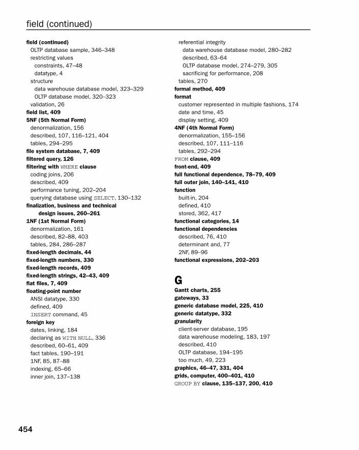
field (continued)OLTP database sample, 346–348restricting values
constraints, 47–48datatype, 4
structuredata warehouse database model, 323–329OLTP database model, 320–323
validation, 26field list, 4095NF (5th Normal Form)
denormalization, 156described, 107, 116–121, 404tables, 294–295
file system database, 7, 409filtered query, 126filtering with WHERE clause
coding joins, 206described, 409performance tuning, 202–204querying database using SELECT, 130–132
finalization, business and technical design issues, 260–261
1NF (1st Normal Form)denormalization, 161described, 82–88, 403tables, 284, 286–287
fixed-length decimals, 44fixed-length numbers, 330fixed-length records, 409fixed-length strings, 42–43, 409flat files, 7, 409floating-point number
ANSI datatype, 330defined, 409INSERT command, 45
foreign keydates, linking, 184declaring as WITH NULL, 336described, 60–61, 409fact tables, 190–1911NF, 85, 87–88indexing, 65–66inner join, 137–138
referential integritydata warehouse database model, 280–282described, 63–64OLTP database model, 274–279, 305sacrificing for performance, 208
tables, 270formal method, 409format
customer represented in multiple fashions, 174date and time, 45display setting, 409
4NF (4th Normal Form)denormalization, 155–156described, 107, 111–116tables, 292–294
FROM clause, 409front-end, 409full functional dependence, 78–79, 409full outer join, 140–141, 410function
built-in, 204defined, 410stored, 362, 417
functional categories, 14functional dependencies
described, 76, 410determinant and, 772NF, 89–96
functional expressions, 202–203
GGantt charts, 255gateways, 33generic database model, 225, 410generic datatype, 332granularity
client-server database, 195data warehouse modeling, 183, 197described, 410OLTP database, 194–195too much, 49, 223
graphics, 46–47, 331, 404grids, computer, 400–401, 410GROUP BY clause, 135–137, 200, 410
454
field (continued)
24_574906 bindexbob.qxd 10/28/05 11:46 PM Page 454

Hhardware
computer grids and clustering, 400–401computer systems (boxes), 396costs, 223, 256failover database, 397–399memory needs, 396RAID, 397replication, 399–400resource usage, data warehouses reducing, 173
hash index, 68, 393, 410HAVING and WHERE clauses, mixing up, 204heavily and lightly access fields, separating, 164help, hiring, 223, 256heterogeneous databases
described, 410homogenous integration, 33
hierarchical database model, 7, 8, 410homogenous system, 33, 410hot block/hot blocking
defined, 164, 411indexes, 69
human factor, database modelinginformation, getting correct, 30–31people, talking to right, 29–30resource, people as, 27–28
hybrid databases, 16, 411hyperlink, 331
IIBM, 125identifying relationship
described, 411non-identifying relationship versus
1NF, 92–93OLTP database, 306tables, 272
tables, 57, 58image, datatype storing (BINARY), 265implementation, 220–221, 411inactive data
active, separating, 163described, 411
including specific recordsdescribed, 130–132performance, improving, 202–204
Index Organized Table (IOT), 68, 393, 411Indexed Sequential Access Method. See ISAMindexes. See also metadata
altering, 146alternate
described, 65, 404foreign keys, 345, 348–352optimizing performance, 209post-development database, tuning, 198
approaches, 339–341bad times to create, 342–343bitmap, 66–68, 392BTree, 66, 385, 391building, 68–69caching, 211–212clustered, 393composite
building, 68described, 406WHERE clause filtering, 203
data warehouse database model,345–346, 349–352
denormalization, 162described, 64–65, 338–339, 411dropping, 146foreign key indexing, 65–66hash keys and ISAM keys, 393joins, 206non-unique, 68, 208OLTP database model, 343–348partitions, 395performance tuning
bad places to use, 209fear, overcoming, 206real-world applications, 207–209types, 207
primary key and unique key field, 146reading, improving performance, 200–201what to index, when to index it,
and how to build, 342industry standard database model, 225
455
industry standard database model
Inde
x
24_574906 bindexbob.qxd 10/28/05 11:46 PM Page 455
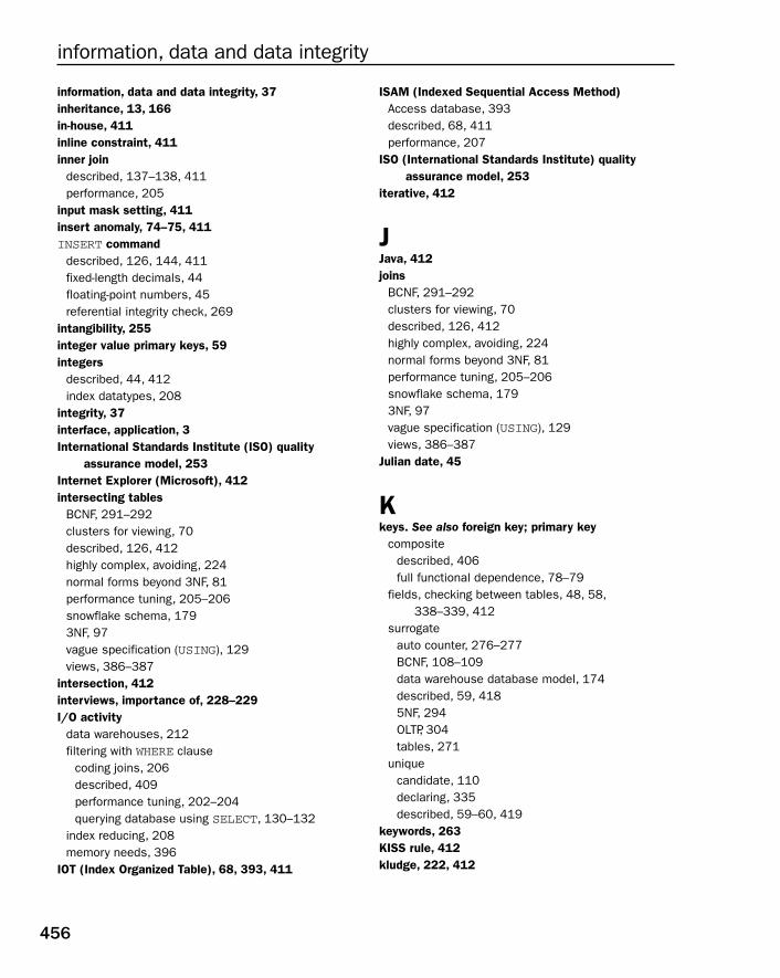
information, data and data integrity, 37inheritance, 13, 166in-house, 411inline constraint, 411inner join
described, 137–138, 411performance, 205
input mask setting, 411insert anomaly, 74–75, 411INSERT command
described, 126, 144, 411fixed-length decimals, 44floating-point numbers, 45referential integrity check, 269
intangibility, 255integer value primary keys, 59integers
described, 44, 412index datatypes, 208
integrity, 37interface, application, 3International Standards Institute (ISO) quality
assurance model, 253Internet Explorer (Microsoft), 412intersecting tables
BCNF, 291–292clusters for viewing, 70described, 126, 412highly complex, avoiding, 224normal forms beyond 3NF, 81performance tuning, 205–206snowflake schema, 1793NF, 97vague specification (USING), 129views, 386–387
intersection, 412interviews, importance of, 228–229I/O activity
data warehouses, 212filtering with WHERE clause
coding joins, 206described, 409performance tuning, 202–204querying database using SELECT, 130–132
index reducing, 208memory needs, 396
IOT (Index Organized Table), 68, 393, 411
ISAM (Indexed Sequential Access Method)Access database, 393described, 68, 411performance, 207
ISO (International Standards Institute) quality assurance model, 253
iterative, 412
JJava, 412joins
BCNF, 291–292clusters for viewing, 70described, 126, 412highly complex, avoiding, 224normal forms beyond 3NF, 81performance tuning, 205–206snowflake schema, 1793NF, 97vague specification (USING), 129views, 386–387
Julian date, 45
Kkeys. See also foreign key; primary key
compositedescribed, 406full functional dependence, 78–79
fields, checking between tables, 48, 58,338–339, 412
surrogateauto counter, 276–277BCNF, 108–109data warehouse database model, 174described, 59, 4185NF, 294OLTP, 304tables, 271
uniquecandidate, 110declaring, 335described, 59–60, 419
keywords, 263KISS rule, 412kludge, 222, 412
456
information, data and data integrity
24_574906 bindexbob.qxd 10/28/05 11:46 PM Page 456
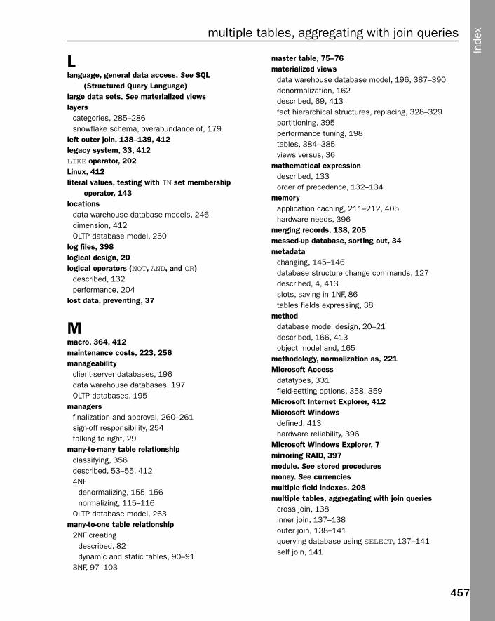
Llanguage, general data access. See SQL
(Structured Query Language)large data sets. See materialized viewslayers
categories, 285–286snowflake schema, overabundance of, 179
left outer join, 138–139, 412legacy system, 33, 412LIKE operator, 202Linux, 412literal values, testing with IN set membership
operator, 143locations
data warehouse database models, 246dimension, 412OLTP database model, 250
log files, 398logical design, 20logical operators (NOT, AND, and OR)
described, 132performance, 204
lost data, preventing, 37
Mmacro, 364, 412maintenance costs, 223, 256manageability
client-server databases, 196data warehouse databases, 197OLTP databases, 195
managersfinalization and approval, 260–261sign-off responsibility, 254talking to right, 29
many-to-many table relationshipclassifying, 356described, 53–55, 4124NF
denormalizing, 155–156normalizing, 115–116
OLTP database model, 263many-to-one table relationship
2NF creatingdescribed, 82dynamic and static tables, 90–91
3NF, 97–103
master table, 75–76materialized views
data warehouse database model, 196, 387–390denormalization, 162described, 69, 413fact hierarchical structures, replacing, 328–329partitioning, 395performance tuning, 198tables, 384–385views versus, 36
mathematical expressiondescribed, 133order of precedence, 132–134
memoryapplication caching, 211–212, 405hardware needs, 396
merging records, 138, 205messed-up database, sorting out, 34metadata
changing, 145–146database structure change commands, 127described, 4, 413slots, saving in 1NF, 86tables fields expressing, 38
methoddatabase model design, 20–21described, 166, 413object model and, 165
methodology, normalization as, 221Microsoft Access
datatypes, 331field-setting options, 358, 359
Microsoft Internet Explorer, 412Microsoft Windows
defined, 413hardware reliability, 396
Microsoft Windows Explorer, 7mirroring RAID, 397module. See stored proceduresmoney. See currenciesmultiple field indexes, 208multiple tables, aggregating with join queries
cross join, 138inner join, 137–138outer join, 138–141querying database using SELECT, 137–141self join, 141
457
multiple tables, aggregating with join queries
Inde
x
24_574906 bindexbob.qxd 10/28/05 11:46 PM Page 457

multiple valued dependencydescribed, 79–80, 413eliminating with 4NF
denormalizing, 155–156normalizing, 115–116
normal form, 81multiplication precedence, 133
Nname fields in table, 41natural keys, BCNF, 108–109negative clauses, WHERE clause filtering, 202negative filtering, 131nested materialized view structure, 388–389nested queries
described, 413INSERT command, 126joins, 206querying database using SELECT, 141–143
network database model, 7, 8–9, 413non-dependent entity or table, 57–58non-identifying relationships
identifying relationships versus1NF, 92–93OLTP database, 306tables, 272
tables, 57, 58non-procedural language, SQL as, 124non-static internal functions. See auto countersnon-unique index
described, 68performance, 208
normal forms, reversing. See denormalizationnormalization
analytical perspective, 277–278anomalies, 74–76benefits, 49building blocks, database modeling, 35business rules, 355–356candidate keys, 77–78data integrity, 224data warehouse database model, 308–312dependencies, 78–80described, 11, 48, 73–74, 413determinant, 76–77excessive, 223
forms explainedacademic way, 80–81BCNF, 108–111DKNF, 121–122easy way, 81–825NF, 116–1211NF, 82–884NF, 111–116one-to-one NULL tables, 104–1072NF, 89–963NF, 96–103
as methodology, 221OLTP database, 307performance tuning, 198potential hazards, 49star schema, turning into snowflake
schema, 178–181tables
BCNF, 290–292beyond 3NF, 289–2905NF, 294–2951NF, 284, 286–2874NF, 292–2942NF, 284–2853NF, 284, 285–286, 287–288
NOT logical operatordescribed, 132performance, 204
NOT NULL constraint, 335, 413NULL valued fields
described, 414explicitly declared, 357foreign key, 64, 65indexing, 342normalization beyond 3NF, 82one-to-one tables, 104–107removing from table, 51–52
nullable fields, denormalization, 153–157number crunching, 354–355, 414numbers
Access datatypedescribed, 331field-setting options, 358, 359
ANSI datatype, 330dates and times, 45–46described, 44–46, 414fixed-length, 44, 330
458
multiple valued dependency
24_574906 bindexbob.qxd 10/28/05 11:46 PM Page 458
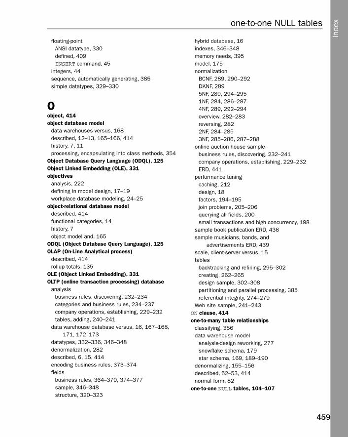
floating-pointANSI datatype, 330defined, 409INSERT command, 45
integers, 44sequence, automatically generating, 385simple datatypes, 329–330
Oobject, 414object database model
data warehouses versus, 168described, 12–13, 165–166, 414history, 7, 11processing, encapsulating into class methods, 354
Object Database Query Language (ODQL), 125Object Linked Embedding (OLE), 331objectives
analysis, 222defining in model design, 17–19workplace database modeling, 24–25
object-relational database modeldescribed, 414functional categories, 14history, 7object model and, 165
ODQL (Object Database Query Language), 125OLAP (On-Line Analytical process)
described, 414rollup totals, 135
OLE (Object Linked Embedding), 331OLTP (online transaction processing) database
analysisbusiness rules, discovering, 232–234categories and business rules, 234–237company operations, establishing, 229–232tables, adding, 240–241
data warehouse database versus, 16, 167–168,171, 172–173
datatypes, 332–336, 346–348denormalization, 282described, 6, 15, 414encoding business rules, 373–374fields
business rules, 364–370, 374–377sample, 346–348structure, 320–323
hybrid database, 16indexes, 346–348memory needs, 395model, 175normalization
BCNF, 289, 290–292DKNF, 2895NF, 289, 294–2951NF, 284, 286–2874NF, 289, 292–294overview, 282–283reversing, 2822NF, 284–2853NF, 285–286, 287–288
online auction house samplebusiness rules, discovering, 232–241company operations, establishing, 229–232ERD, 441
performance tuningcaching, 212design, 18factors, 194–195join problems, 205–206querying all fields, 200small transactions and high concurrency, 198
sample book publication ERD, 436sample musicians, bands, and
advertisements ERD, 439scale, client-server versus, 15tables
backtracking and refining, 295–302creating, 262–265design sample, 302–308partitioning and parallel processing, 385referential integrity, 274–279
Web site sample, 241–243ON clause, 414one-to-many table relationships
classifying, 356data warehouse model
analysis-design reworking, 277snowflake schema, 179star schema, 169, 189–190
denormalizing, 155–156described, 52–53, 414normal form, 82
one-to-one NULL tables, 104–107
459
one-to-one NULL tables
Inde
x
24_574906 bindexbob.qxd 10/28/05 11:46 PM Page 459

one-to-one table relationshipsclassifying, 356described, 51–52, 414
On-Line Analytical process (OLAP)described, 414rollup totals, 135
online auction house sampleapplication queries, 298–300business rules
buyers, adding, 240–241categories, 234–237normalization, 232–233one-to-many relationships, 233–234seller listings, 238–239
company objectives, 226–228data warehouse
business rules, 248–251, 370–373company operations, 244–248datatypes, 336–338ERD, 324, 442facts, dividing into, 309–311fields, refining, 325–329, 340–341indexing, 345referential integrity, 279–282tables, creating, 265–269
datatypes, 332, 333–335OLTP database
analytical model, 262–263, 320buyers, 231–232categories, 229–230child records with optional parents, 273encoding business rules, 373–374ERD, 441field level business rules, 364–365, 364–370fields, refining, 321–3234NF, 293–294general structure, 232identifying versus non-identifying relationships, 272indexing, 344–345normalizing overview, 283parent records without children, 273primary and foreign keys, 270referential integrity, 274–279seller listings, 230–231surrogate keys, 271tables, creating, 264–2653NF, 285–291
online bookstore sampledata warehouse database
snowflake schema, 178–180star schema, 169, 176–177, 181time and location dimensions, 185–186
OLTP relational database model ERD, 175simple database model ERD, 21table
BCNF, 109candidate keys, 78creating, 146–148denormalizing, 153–154, 158, 159dependencies, 77, 791NF, 87–882NF, 94–963NF, 99–101
online musicians sampleauto counter, 393classified ad Web site, 241–243data warehouse model
analyzing, 252–253creating, 187–190denormalized, 315–316designing, 312ERD, 440fact table, 313–314field level business rules, 377–379fields, datatypes, and indexing, 349–352partitioning, 394–395
OLTP database modeldenormalization, 308designing, 302–303ERD, 439field level business rules, 374–377fields, datatypes, and indexing, 346–348identifying, non-identifying, and NULL valued
relationships, 306materialized views, 388–390normalization, 307primary keys as surrogate keys, 304referential integrity, 305views, 386–387
tablescreating simple, 61–63denormalizing, 161–162
online transaction processing database. See OLTP database
460
one-to-one table relationships
24_574906 bindexbob.qxd 10/28/05 11:46 PM Page 460
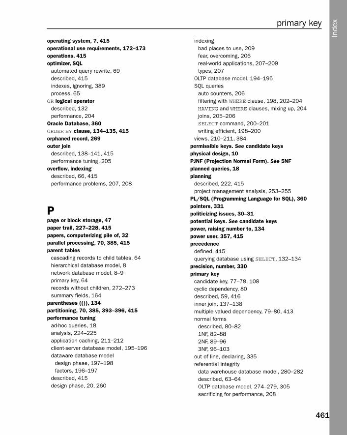
operating system, 7, 415operational use requirements, 172–173operations, 415optimizer, SQL
automated query rewrite, 69described, 415indexes, ignoring, 389process, 65
OR logical operatordescribed, 132performance, 204
Oracle Database, 360ORDER BY clause, 134–135, 415orphaned record, 269outer join
described, 138–141, 415performance tuning, 205
overflow, indexingdescribed, 66, 415performance problems, 207, 208
Ppage or block storage, 47paper trail, 227–228, 415papers, computerizing pile of, 32parallel processing, 70, 385, 415parent tables
cascading records to child tables, 64hierarchical database model, 8network database model, 8–9primary key, 64records without children, 272–273summary fields, 164
parentheses (()), 134partitioning, 70, 385, 393–396, 415performance tuning
ad-hoc queries, 18analysis, 224–225application caching, 211–212client-server database model, 195–196dataware database model
design phase, 197–198factors, 196–197
described, 415design phase, 20, 260
indexingbad places to use, 209fear, overcoming, 206real-world applications, 207–209types, 207
OLTP database model, 194–195SQL queries
auto counters, 206filtering with WHERE clause, 198, 202–204HAVING and WHERE clauses, mixing up, 204joins, 205–206SELECT command, 200–201writing efficient, 198–200
views, 210–211, 384permissible keys. See candidate keysphysical design, 10PJNF (Projection Normal Form). See 5NFplanned queries, 18planning
described, 222, 415project management analysis, 253–255
PL/SQL (Programming Language for SQL), 360pointers, 331politicizing issues, 30–31potential keys. See candidate keyspower, raising number to, 134power user, 357, 415precedence
defined, 415querying database using SELECT, 132–134
precision, number, 330primary key
candidate key, 77–78, 108cyclic dependency, 80described, 59, 416inner join, 137–138multiple valued dependency, 79–80, 413normal forms
described, 80–821NF, 82–882NF, 89–963NF, 96–103
out of line, declaring, 335referential integrity
data warehouse database model, 280–282described, 63–64OLTP database model, 274–279, 305sacrificing for performance, 208
461
primary key
Inde
x
24_574906 bindexbob.qxd 10/28/05 11:46 PM Page 461
primary key (continued)SELECT query, filtered with WHERE clause, 130, 198as surrogate keys
data warehouse database, 338OLTP database, 304
tables, 270unique indexes, 68
problem, 222processes, business
data warehouse modeling, 183described, 405explaining, 219–220operations, 222requirements analysis, 221
productsdata warehouse database models, 246OLTP database model, 250tables, arranging by date, 184–186
programming, file system databases, 7Programming Language for SQL (PL/SQL), 360project management analysis
budgeting, 255–256planning and timelines, 253–255
Projection Normal Form (PJNF). See 5NF
Qquery
ad-hoc, 18, 404aggregated, 126, 135–137, 404automated query rewrite, 69defined, 416improving through normalization
analysis, 224tables, number of, 81
INSERT command, 126SELECT
aggregating with GROUP BY clause, 135–137basic, 127–130composite queries, 143–144filtering with WHERE clause, 130–132, 198multiple tables, aggregating with join queries,
137–141, 206nested queries, 141–143, 413precedence, 132–134sorting with ORDER BY clause, 134–135
SQL commands, 126
RRAID (Redundant Array of Inexpensive
Disks), 397, 416RAM (random access memory)
defined, 416OLTP databases, 173
range of valuesscans, 131searches, WHERE clause filtering, 202
RDBMS (Relational Database Management System), 11, 416
reaction timeclient-server database, 195data warehouse database, 196OLTP database, 194
read only reporting index, 208read-only environments. See also data warehouse
databaseanalysis stage, 223standby databases, 398
read-write databases, 223record
auto counters, 275cascade, 64child with optional parents, 273described, 38–39, 416excluding specific, 130–132fixed-length, 409orphaned, 269parent without children, 273repeating groups, 135–137single, searching, 202variable-length, 153, 419
redundancy, minimizing. See normalizationRedundant Array of Inexpensive
Disks (RAID), 397, 416reference pointers, 47referential integrity
building blocks, database modeling, 63–64data warehouse database model
described, 174tables for online auction house sample, 279–282
defined, 416OLTP database model
keys, 241, 305tables, 274–279
462
primary key (continued)
24_574906 bindexbob.qxd 10/28/05 11:46 PM Page 462
performance tuning, 198sacrificing for performance, 208tables, 269
relation levels, business rules, 364Relational Database Management System
(RDBMS), 11, 416relational database model
benefits, 9data warehouse database model, 173described, 416diagram illustrating, 9–10history, 3, 6–7, 11–12messed-up, sorting out, 34RDBMS, 11SQL and, 123
relations, business rules, 355–356relationship types, business rules classifying,
356–357relationships, ERDs showing
crow’s foot (“many” side of one-to-many or many-to-many relationship), 50–51
dependent entity or table, 57, 58described, 49–50many-to-many, 53–55non-dependent entity or table, 57–58non-identifying relationship, 57, 58one-to-many, 52–53one-to-one, 51–52zero, one, or many, 55–57
repeating groups of records, 135–137replication
hardware, 399–400method, 416
reporting database, 16reports, decision-support database, 172requirements analysis activity, 20, 221resource, people as
optimizing, 254workplace database modeling, 27–28
reverse key indexes, 68–69right information, getting, 30–31right outer join, 139–140, 416ROLLBACK, 417root block, BTree index, 391rows, 39–40rules. See business rules; stored procedures
SSDK (Software Development Kit)
tools, 11, 353, 355, 4172NF (2nd Normal Form)
denormalization, 160, 161–162described, 403functional dependencies, 89–96tables, 284–285
security, views, 210–211SELECT command
aggregating with GROUP BY clause, 135–137basic, 127–130composite queries, 143–144described, 417filtering with WHERE clause, 130–132, 198multiple tables, aggregating with join queries,
137–141nested queries, 141–143performance tuning, 198, 199, 200–201precedence, 132–134sorting with ORDER BY clause, 134–135
self join, 141, 205, 417self-contained (black-box) processing, 166semicolon (;), 127semi-join, 417semi-related tables, 5NF transformation, 118sequences, auto counters and, 70, 393, 417sequential number values. See auto countersservice transactions, 184–186service window
client-server databases, 196data warehouse databases, 197OLTP databases, 195
set operatorsmembership operator, 132merge operators, 143–144WHERE clause filtering, 203
simple datatype, 417single field indexes, 208single record searches, 202size
client-server databases, 195data warehouse database, 196OLTP databases, 194table, filtering with WHERE clause, 203
463
size
Inde
x
24_574906 bindexbob.qxd 10/28/05 11:46 PM Page 463

snowflake schemadata warehouse history data mart, 313described, 417dimensional database, 178–182
software development, intangibility of, 255Software Development Kit (SDK) tools, 11, 353,
355, 417sorted query
described, 417INSERT command, 126ORDER BY clause, 134–135, 415
special-case scenarios, 29–30specialized class, 165specialized database objects, 162–163spreadsheets, converting from, 33–34SQL (Structured Query Language)
changes to a database (INSERT, UPDATE, andDELETE commands), 144
data change commands, 126database structure change commands, 127described, 124, 418for different databases, 125–126joins
clusters for viewing, 70huge queries, as normalization hazard, 49normal forms beyond 3NF, 81performance tuning, 205–206
metadata, changing, 145–146optimizer, 65origins, 125performance tuning
auto counters, 206difficulty of, 197filtering with WHERE clause, 198, 202–204HAVING and WHERE clauses, mixing up, 204joins, 205–206SELECT command, 200–201writing efficient, 198–200
query commands, 126relational database modeling and, 123SELECT queries
aggregating with GROUP BY clause, 135–137basic, 127–130composite queries, 143–144filtering with WHERE clause, 130–132multiple tables, aggregating with join queries,
137–141
nested queries, 141–143precedence, 132–134sorting with ORDER BY clause, 134–135
transactions, 144–145standardized models, 225standby (failover) database, 397–399, 417star schema
data warehouse databasesanalysis, 245–247, 311data mart, 168–169static data, 244tables, 265–267
described, 417dimensional database, 176–177
static datacaching, 211–212data warehouse, 168, 243described, 417indexing, 207, 209, 339transactional information, separating, 243–244
storage, binary object, 47stored function
code, storing in database, 362described, 417
stored proceduresbusiness rules, implementing, 26–27code, storing in database, 358, 360–362described, 417function, 354methods versus, 166
stringsdatatypes
Access, 331ANSI, 330data warehouse, 333, 338OLTP database, 333simple, 329–330
described, 42–43, 417fixed-length, 42–43, 409pattern matcher, filtering with LIKE operator, 132variable-length
ANSI datatype, 330described, 43, 419
striping RAID, 397structural refinement, 322Structured Query Language. See SQLsubject area of business. See business processes
464
snowflake schema
24_574906 bindexbob.qxd 10/28/05 11:46 PM Page 464

subjects, 165–166subqueries. See nested queriesSUBSTR function, precedence, 134subtraction, 133summary
fields and parent tables, denormalizing, 164GROUP BY clause, creating with, 136
surrogate keysauto counter, 276–277BCNF, 108–109data warehouse database model, 174described, 59, 4185NF, 294OLTP, 304tables, 271
Ttables. See also keys; metadata
abstraction, 28–30attributes, 40–42business rules, 364child records with optional parents, 273data warehouse database model
creating, 265–269referential integrity, 279–282refining, 308–316
described, 418dimensional database
fact, 190–191handling, 184–186
fields, 37–38, 40–42identifying versus non-identifying relationships, 272joins, minimizing, 205normalization and denormalization
BCNF, 290–292beyond 3NF, 289–290described, 2825NF, 294–2951NF, 284, 286–2874NF, 292–2942NF, 284–2853NF, 284, 285–286, 287–288
OLTP database modelanalysis, 240–241backtracking and refining, 295–302creating, 262–265
design sample, 302–308identifying, non-identifying, and NULL valued, 306referential integrity, 274–279
parent records without children, 272–273partitioning, 393–396primary and foreign keys, 270records
described, 38–39unique identification (primary key), 59
referential integrity, 269relationships, showing in ERDs
business rules, 26crow’s foot (“many” side of one-to-many or
many-to-many relationship), 50–51dependent entity or table, 57, 58described, 49–50identifying relationship, 57, 58many-to-many, 53–55non-dependent entity or table, 57–58non-identifying relationship, 57, 58one-to-many, 52–53one-to-one, 51–52zero, one, or many, 55–57
rows, 39–40splitting into rate partitions, 70, 415SQL code, easy construction of, 199structure, performance tuning, 198surrogate keys, 271temporary, denormalization, 163tuples, 39–40
technical specifications, 260temporary tables, denormalizing, 1633NF (3rd Normal Form)
data warehouses, 169denormalization, 157–159described, 96–103, 403tables, 284, 285–286, 287–288
throughput, 173timelines
described, 222, 418project management analysis, 253–255
times, 45–46timestamp
Access datatype, 331data warehouse database models, 246described, 45–46, 418OLTP database model, 250
465
timestamp
Inde
x
24_574906 bindexbob.qxd 10/28/05 11:46 PM Page 465

training costs, 223, 256transactional control, 418transactional data, 243, 418transactional databases
client-server model, 15, 405–406database model, 15defined, 6
transactionsCOMMIT, 406described, 144–145, 418dimension tables handling, 184–186event triggers, 363size
client-server, 195data warehouse database, 197OLTP database, 194, 198
static information, separating, 243–244transitive dependence
described, 82, 418normalizing, 77, 813NF, 96–103
transparency, 5, 400–401trigger, 27, 418. See also stored procedurestrivial multi-valued dependency, 79–80, 418trucking company sample database
event trigger, 363field settings, adding, 361–362relationship types, 356stored function, 362
truncate, 418tuning. See performance tuningtuning phase, 10tuples, 39–40type casting, 166
Uunfavorable scenarios
heterogeneous databases, homogenous integration, 33
legacy databases, converting, 33messed-up database, sorting out, 34papers, computerizing pile of, 32spreadsheets, converting from, 33–34
unique indexdescribed, 68performance, 208
unique keyscandidate key, 110declaring, 335described, 59–60, 419
UNIXdescribed, 419file system, examining, 7hardware reliability, 396
update anomaly, 76, 419UPDATE command
described, 126, 144, 419filtering with WHERE clause, 198referential integrity, preserving, 174, 269
usersanalysis, 222data modeling for, 23defined, 408denormalizing, 299–300needs, listening to
company objectives, 226importance of, 27–28invoices, 227–228
number ofclient-server database, 195data warehouse database, 196OLTP database, 194
performance, 193power user, 357user-defined datatype, 332user-defined types, 47user-friendly, 419
Vvalidation
check, explicitly declared field settings, 357–358constraints and, 47–48DKNF, 121–122
valuechecking between fields in different tables
described, 48, 58, 338–339, 412foreign, 60–61primary, 59unique, 59–60
constraints, business rules and, 26entry, requiring (NOT NULL constraint), 48repeated structurally (collection arrays), 47
466
training costs
24_574906 bindexbob.qxd 10/28/05 11:46 PM Page 466
variable-length recordsdescribed, 419NULL valued fields, no need to remove, 153
variable-length stringsANSI datatype, 330described, 43, 419
viewsbuilding blocks, database modeling, 36described, 69, 419performance tuning, 210–211, 384sample, 386–387
WWAN database replication, 399–400Web site, 241–243. See also online auction
house sample; online bookstore sample; online musicians sample
WHERE clause filteringcomparison conditions, 199–200described, 419functional expressions, 202–203HAVING clauses, mixing up, 204indexes, sorted orders, and physical ordering,
202–204Windows (Microsoft)
defined, 413hardware reliability, 396
Windows Explorer (Microsoft), 7
workplace database modelingbusiness rules, 24–27described, 23–24human factor
resource, people as, 27–28right information, getting, 30–31talking to right people, 29–30
objectives, 24–25unfavorable scenarios
heterogeneous databases, homogenous integration, 33
legacy databases, converting, 33messed-up database, sorting out, 34papers, computerizing pile of, 32spreadsheets, converting from, 33–34
XXML documents, 332
Zzero factor, table relations, 344zero table relationship, 55–57zip code field, validating, 366
467
zip code field, validating
Inde
x
24_574906 bindexbob.qxd 10/28/05 11:46 PM Page 467
Take your library wherever you go.Now you can access more than 70 complete Wrox books online, wherever you happen to be! Every diagram, description, screen capture, and code sample is available with your subscription to the Wrox Reference Library. For answers when and where you need them, go to wrox.books24x7.com and subscribe today!
Programmer to ProgrammerTM
• ASP.NET • C#/C++ • Database • General • Java• Mac• Microsoft Office
• .NET • Open Source • PHP/MySQL • SQL Server • Visual Basic • Web• XML
Find books on
www.wrox.com
24_574906 bindexbob.qxd 10/28/05 11:46 PM Page 478