Poverty in India A CHRONOLOGICAL REVIEW ON MEASUREMENT AND IDENTIFICATION 

Kaushik Ranjan Bandyopadhyay 

  

1

Contents 1. Introduction 2. Definition and Measurement of Income Poverty in India

2.1 The Working Group Poverty Line (1962) 2.2 Task Force Poverty Line (1979) 2.3 Expert Group Methodology (1993) 2.4 The Great Indian Poverty Debate: A Snapshot 2.5 The Latest Estimate of Poverty by the Expert Group of the Planning

Commission Formed in 2009: Salient Features

3. Identification of the Poor in India’s Five Year Plans 3.1 Identification of Poor in the Eighth Five Year Plan (1992-97) 3.2 Identification of the Poor in the Ninth Five Year Plan (1997-2002) 3.3 Identification of the Poor in the Tenth Five Year Plan (2002-2007) 3.4 Recommendations of the Expert Group on the methodology for conducting

the BPL Census for Eleventh Five Year Plan (2007-12): Salient Features

Annexure

I State Specific Poverty Lines in Rural Areas (1973-74 to 1993-94) II State Specific Poverty Lines in Urban Areas (1973-74 to 1993-94) III State-Specific Poverty Lines in 1999-2000 IV State Specific Poverty Ratio and Number of Poor in 1973-74 V State Specific Poverty Ratio and Number of Poor in 1977-78 VI State Specific Poverty Ratio and Number of Poor in 1983 VII State Specific Poverty Ratio and Number of Poor in 1987-88 VIII State Specific Poverty Ratio and Number of Poor in 1993-94 IX State Specific Poverty Ratio and Number of Poor in 1999-2000 (30 day Recall Period) X State Specific Poverty Ratio and Number of Poor in 1999-2000 (7 day Recall Period) XI State Specific Poverty Ratio and Number of Poor in 2004-05 (Uniform Recall Period) XII State Specific Poverty Ratio and Number of Poor in 2004-05 (Mixed Recall Period) XIII Poverty Lines and State Specific Poverty Head Count Ratio for 2004-05 (Tendulkar

Committee) XIV Poverty Lines and State Specific Poverty Head Count Ratio for 1993-94 (Tendulkar

Committee) XV Select Measures of Poverty: A Brief Description

2

Poverty and Human Well-being in India: A Chronological Review on Measurement and Identification

1. Introduction Of the many afflictions and adversaries humans have to fight, poverty is perhaps the most

stubborn and deeply ingrained within the society. Poverty is broadly defined as unacceptable

deprivation of well-being which is multidimensional. Thus, an objective assessment of poverty

should essentially recognize its multidimensionality (economic and otherwise). To remain poor

also implies to remain hungry, to live without adequate shelter and clothing, to remain sick and

not cared for, to remain illiterate and so on1. Moreover, people living in poverty tend to be

highly vulnerable to adverse events outside their control and lead an existence denied of the

basic access to a meaningful life.

Poverty can be either ‘absolute’ or ‘relative’. Absolute poverty is described in terms of

the inability to satisfy one’s basic minimum needs that are necessary to maintain a minimum

essential standard of living, say minimum essential level of food and nutrition. It is ‘relative’

when it refers to the position of a household or an individual in relation to the distribution of

average income or consumption in a specific region or economy. Poverty could be a ‘temporary’

phenomenon due to, say, old age, disease, natural disaster, war or any other misfortune, or it

could be of a ‘permanent’ nature attributed to structural factors that might be carried forward

over generations.

India recognized the challenge of poverty and made its removal the central aim of its

economic planning. Yet, it is also distressingly true that Indian efforts have met with a limited

degree of success than what was originally anticipated. Regardless of which figure one chooses

for drawing the poverty line, there is little doubt in the fact a very significant share of Indian

population still lives in abject poverty. In fact the heart of the debate in the literature on Indian

poverty lies in its measurement and in its successive refinements over time since the very

inception of the process that was initiated by the Planning Commission way back in 1962.

However the official estimate of poverty in India brought out periodically by the Planning

Commission relied on micro-level household consumer expenditure survey carried out by

National Sample Survey Organization and using household expenditure as a proxy for income.

1. World Bank (2001).

3

The notion of poverty as multidimensional phenomena does not seem to have received the due

attention that it otherwise deserves.

In the light of this brief backdrop the current monograph delves into a chronological

examination of the definition and measurement of poverty in India and also explores the

multidimensionality in the deprivation of well-being by considering three pivotal parameters

namely adequacy with respect to food, health and education.

2. Definition and Measurement of Poverty in India: A Chronological Examination

Since independence two major studies had been carried out in India that was aimed at defining

poverty and fixing the poverty line. The first study was carried out in 1962 by a Working Group

and the other in 1979 by a Task Force.

2.1 The Working Group Poverty Line (1962)

The Planning Commission, in 1962, constituted a Working Group consisting of eminent

economists, statisticians, nutritionists, among others. The Working Group deliberated on the

question of what should be regarded as the nationally desirable minimum level of consumer

expenditure and in July 1962 recommended the following2.

(a) The national minimum for each household of 5 persons (4 adult consumption units)

should not be less than Rs.100 per month in terms of 1960-61 prices or Rs.20 per capita.

For urban areas, this figure will have to be raised to Rs.125 per capita to cover the higher

prices of the physical volume of commodities on which the national minimum is

calculated.

(b) This national minimum excludes expenditure on health and education, both of which

are expected to be provided by the State according to the Constitution and in the light of

its other commitments.

2. ‘Perspective of Development: 1961-1976 Implications of Planning for a Minimum Level of Living’, in

Bardhan and Srinivasan (1974).

4

(c) An element of subsidy in urban housing will have to be included after taking Rs.10

per month, or 10 per cent as the rent element payable from the proposed national

minimum of Rs.100 per month.

This minimum level of expenditure was almost universally accepted and widely used as the

poverty line in the 1960s and 1970s despite the fact that the details of the calculation based on

which the minimum norm of Rs. 20 per person per month was set was not clear.

Researchers, in their attempt to find out the nexus between calorie norm and the poverty

line ended up finding out that there might, at the most, be a remote connection of the poverty

line with the calorie norms of the Indian Council of Medical research (ICMR). Notable among

them is Rudra (1974) who made an attempt to demonstrate the statistical discrepancies in the

calculation of the poverty line by the Working Group, terming its (Rs. 20 per capita per month)

origin as somewhat of a mystery and underscored that the basis of its acceptance is obscure.3

Dandekar and Rath (1971) made an attempt to link calorie norm to poverty line and

pointed out that daily intake of 2250 calories per person could be considered as adequate under

the Indian conditions both in rural and urban areas.4 They estimated from the National Sample

Survey data on consumer expenditure that monthly per capita expenditure of Rs. 14.20 in rural

areas and Rs. 22.60 in urban areas, both at 1960-61 prices is sufficient to meet the per capita

daily calorie requirement of 2250. Thus they observed that their estimates of rural poverty line

was substantially lower than the Working Group poverty line; their rural poverty line (Rs. 14.20)

being 71 per cent of the working group poverty line. They eventually decided to scale it up to

Rs.15.20 per capita per month. Their estimated urban poverty line (Rs. 22.60) was, however,

close to the working group poverty line and hence they decided to round it off to Rs.22.50 per

capita per month.

Amartya Sen (1974) underscored that the Working Group report apparently precluded

from the ambit of their considerations the fact that nutritional requirements in terms of calories

are age, sex, and occupation-specific and that nutritional requirements are likely to vary across

rural and urban areas. The rural population is more likely to be engaged in manual activities that

demand a higher calorie intake than urban population who are primarily engaged in moderate or

sedentary activities. Furthermore, although the poverty line developed by the Working Group

3. Ashok Rudra, ‘Minimum Level of Living: A Statistical Examination’, in Bardhan and Srinivasan, 1974. 4. The Task Force constituted later in 1979, however, noted that the calorie requirement of 2250 per person

per day, as mentioned by Dandekar and Rath (Dandekar and Rath, 1971), “seems to refer to the lower limit of the range of 2250 to 2300 calories per capita per day on the average at retail level estimated by P. V. Sukhatme, (Sukhatme, 1965, p 23).

5

had considered nutrition, they did not specify any particular nutritional norm nor any set of

prices as justification for the choice of the poverty line.5

The Task Force (1979) whose estimates replaced that of the Working Group stated that

the Working Group appeared to have taken into account the recommendation of balanced diet

made by the Nutrition Advisory Committee of the Indian Council of Medical Research (ICMR)

in 1958 to arrive at the conclusion that in order to provide the minimum nutritional diet in terms

of calorie intake, and to allow for a modest degree of non-food items, the minimum consumption

expenditure per household of 5 persons at the national level should not be less than Rs.100 per

month at 1960-61 prices, i.e., Rs. 20 per capita per month. In view of the higher cost of living in

the urban areas, the Working Group suggested raising the minimum expenditure there to Rs.25

per capita per month. Accordingly, the minimum expenditure in rural areas corresponded to

Rs.18.90 per capita per month6.

Furthermore, the Working Group poverty line was derived on the implicit assumption

that the State would subsidize some of the welfare expenditures particularly of the poor. The

poverty line determined as per capita consumption expenditure of Rs. 20 per month was based

on the assumption that the State would subsidize the health and education expenditure of the

people.

2.1.1 The Estimates of Poverty using Working Group Poverty Line

The Working Group poverty line was widely used in the 1960s and 1970s to estimate the

poverty ratio or head count ratio (i.e., the ratio of the number of poor to the total population,

expressed as percentage). Those who estimated the poverty ratio in rural and urban areas using

this poverty line include V. M. Dandekar and Nilkantha Rath, Amartya Sen, Pranab Bardhan, B

S Minhas, I Z Bhatty, T N Srinivasan, Montek Singh Ahluwalia, among others. Some of them,

for example, Bardhan, and at a later stage Ahluwalia converted this national level poverty line

into state-specific poverty lines, with the help of state-specific price indices. As a result of the

differences in the price indices, the splitting of this national level poverty line of Rs. 20 per

capita per month, into sectors such as rural and urban, and within each area among the states,

5. Amartya Sen, ‘Poverty, Inequality and Unemployment’, in Bardhan and Srinivasan (1974). 6. Government of India, 1979, p 5.

6

yielded varying numbers resulting from the variety of the price inflators (or deflators, as is

commonly used). The rural and urban poverty lines worked out by Bardhan is per capita

consumption expenditure of Rs.15 per month in rural areas and Rs.18 per month in the urban

areas. Minhas and in a separate attempt Bhatty, used this poverty line to estimate the incidence

of poverty among occupation classes of the rural population. Some of these studies are briefly

illustrated below.

Ahluwalia (1978) decomposed the national poverty line into state-specific poverty lines

and used these state-specific poverty lines to estimate state-wise poverty ratios. He used the

estimated poverty series in the rural areas to find out the factors which affect rural poverty,

besides the impact of income and prices on changes in poverty.7

The poverty ratio makes no distinction within the broad category of the poor depending

upon their actual level of consumption and deprivation. For this reason, the poverty ratio fails to

capture the depth or severity of poverty or in other words and fails to answer the question- how

poor the poor are? In order to address the intensity of poverty Amartya Sen (1974) 8 tried to

associate the incidence of poverty with the phenomenon of equity and proposed an alternative

measure of poverty which is superior to the poverty ratio (i.e. head-count ratio) and the standard

measure of relative inequality. This measure of intensity of poverty is known as Sen’s index

(the measure is explained in the Appendix).

Bhatty9 estimated state-wise head count poverty ratio and Sen’s index and for different

occupation classes of the population in rural areas applying a range of poverty lines to

demonstrate the sensitivity of income. According to the level of poverty ratio, Bhatty

categorized the states into high, medium and low level of poverty. The poverty ratios based on

the working group poverty line shows:

(a) Gujarat, Tamil Nadu, Madhya Pradesh and Rajasthan are highly poor states.

(b) Uttar Pradesh, Kerala, Orissa, Maharashtra and Karnataka are medium poor states.

(c) Bihar, Andhra Pradesh, Assam, West Bengal, Punjab and Haryana are low poor

states.

7. Ahluwalia (1978). 8. Amartya Sen, ‘Poverty, Inequality and Unemployment’, in Bardhan and Srinivasan (1974). 9. I Z Bhatty, ‘Inequality and Poverty in Rural India’, in Bardhan and Srinivasan (1974).

7

Bhatty estimated poverty ratio for different occupation groups of the population in rural areas

such as cultivators, agricultural labourers and non-agricultural workers from the Working Group

poverty line of Rs.20 per capita per month and the NSS consumer expenditure distribution.

These were estimated for the year 1968-69 and are given in Table 1.

Table 1

Occupation-Specific Poverty Ratio in 1968-69

Category of Occupation Poverty Ratio 1. Cultivators 39.31 2. Agricultural Labourers 56.21 3. Non- Agricultural Workers 39.55 4. All Households 42.43

Source: Tables 11 to 14 in Bardhan and Srinivasan, 1974, pp 318-319

The poverty ratio among the agricultural labourers (56.21 per cent) in 1968-69 is about

one-third more than the national rural poverty ratio (42.43 per cent), which is the poverty ratio

obtained for all rural households, including the agricultural labour households.

2.2 Task Force Poverty Line (1979)

The Planning Commission on 30th July, 1977, constituted a Task Force on Projections of

Minimum Needs and Effective Consumption Demand under the Chairmanship of Dr Y. K.

Alagh. The job of the Task Force was : “to examine the existing structural studies on

consumption patterns and standards of living and the minimum needs with particular reference

to the poorer sections of the population for the nation as a whole, and its different regions

separately by rural and urban areas; on the basis of the above studies, to forecast the national and

regional structure and pattern of consumption levels and standards for the end of the Sixth Plan

and subsequent perspective plan taking into consideration the basic minimum needs as well as

effective consumption demand"10.

The Task Force defined the poverty line as per capita consumption expenditure level, which

meets the average per capita daily calorie requirement of 2400 kcal in rural areas and 2100 kcal

10. Government of India, 1979, p 4.

8

in urban areas along with the associated quantum of expenditure on non-food items such as

clothing, shelter, transport, education, health care, etc. The average calorie requirement was

calculated from the projected population (for the year 1982-83) by age, sex and activity and the

associated calorie norm recommended by the Nutrition Expert Group (1968) of the Indian

Council of Medical Research (ICMR)11.

The Nutrition Expert Group (NEG) categorized the population into- (a) children in terms of

age; (b) adolescents in terms of age and sex; and (c) workers by sex. The age, sex and activity

structure of the population was derived from: (a) the population estimates of the Expert Group

on Population (1977)12, (b) census occupational structure13, and (c) usual status participation

rates14. The workers were grouped into heavy, moderate and sedentary. The pregnant and

lactating women were allowed additional calories. This is how age, sex and occupational

differentials in the calorie requirement of the population were captured in the average norms.

The monetary requirements for meeting these calorie norms (2400 kcal per capita per day

in rural areas and 2100 kcal per capita per day in urban areas) along with other non-food

necessities as mentioned above had been designated as the poverty lines pertaining to rural and

urban areas. The Task Force utilised the 28th Round National Sample Survey (NSS) data on

household consumer expenditure (pertaining to 1973-74) and estimated that, on an average,

consumer expenditure of Rs.49.09 and Rs.56.64 per capita per month per capita per month meets

the calorie requirement of 2400 kcal and 2100 kcal per capita per day in rural and urban areas

respectively. Based on the observed consumer behavior in 1973-74 the estimated poverty lines

had been observed to conform to a consumption basket, which, besides satisfying the above

calorie norm, also meets a minimum of non-food requirements such as clothing, shelter,

transport, education, health care, etc. Since the consumption was evaluated at 1973-74 prices,

the poverty lines were also measured in terms of the prices prevailing in that year.

11. The relevance of the year is that it was the terminal year of a Five Year Plan which was prepared but not

implemented due to change in the Government. This was the Sixth Five Year Plan, 1978-83, which gave way for the Sixth Five Year Plan, 1980-85.

12. The Expert Group was a joint initiative of the Perspective Planning Division of the Planning Commission and the Office of the Registrar General, Census of India.

13. Derived from the 1971 Census. 14. Based on NSS data on Employment and Unemployment pertaining to 27th Round (1972-73).

9

2.2.1 Updation of the Poverty Line based on Task Force Report

The poverty lines for later years were estimated by updating the 1973-74 poverty lines.

The updation was initially carried out from the price inflation implicit in the Wholesale Price

Index (WPI). The use of WPI was, however, contested on the grounds that it constitutes of a

range of items (nearly half its weight) which are not meant for private consumption and that the

consumers buy goods at retail and not at wholesale prices. This prompted the Planning

Commission to constitute another Study Group on Estimation of Poverty Line during the

Seventh Five Year Plan (1985-90)15. This Study Group recommended the use of implicit private

consumption deflator of the National Accounts Statistics (NAS) of the Central Statistical

Organization (CSO) for updation of the 1973-74 poverty lines for use in later years. CSO in

their National Accounts Statistics publish the estimates of private consumption expenditure at

current and constant prices. The ratio between the two yields the implicit consumption deflator.

2.2.2 Computation of Poverty Ratio by the Task Force

The number of people living below the poverty line was estimated from the percentage

distribution of people in different expenditure classes obtained from the NSS data on household

consumer expenditure. The information was, however, not utilized directly by the Task force but

used after making some adjustment. The NSS distribution of private consumption was adjusted

proportionately so that the total consumption arising from the NSS data corresponded to the total

consumption estimates of National Accounts Statistics (NAS) derived by the Central Statistical

Organization (CSO). Using the poverty line and the adjusted distribution of persons by

expenditure classes for the reference year the percentage of population living below the poverty

line (i.e., the poverty ratio) was estimated. Considering the projected population of the year, the

number of poor people was estimated by using the aforementioned percentage.

Thus, the salient feature of the method of poverty estimation by the Task Force is that the

poverty line is at national level, and the NSS consumption expenditure was pro-rata adjusted to

CSO consumption across all expenditure groups of the population. In fine, the Task Force

15. Government of India (1984).

10

estimated the national poverty line in rural and urban areas and recommended a methodology to

estimate the poverty in the rural and urban areas but at the national level.

However the Planning Commission in order to come out with official estimates of

poverty at the state level not only used the Task Force poverty line, which is at the national level

(in rural and urban areas), as it is to all the states but also adjusted the NSS consumption

distribution of the states pro-rata to the NAS consumption levels across all expenditure classes

of the population. This decision of the Planning Commission, which was completely outside the

purview of the Task Force recommendation, however, was extensively debated at a later stage.

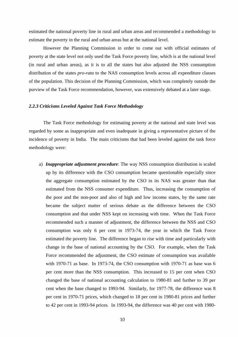
2.2.3 Criticisms Leveled Against Task Force Methodology

The Task Force methodology for estimating poverty at the national and state level was

regarded by some as inappropriate and even inadequate in giving a representative picture of the

incidence of poverty in India. The main criticisms that had been leveled against the task force

methodology were:

a) Inappropriate adjustment procedure: The way NSS consumption distribution is scaled

up by its difference with the CSO consumption became questionable especially since

the aggregate consumption estimated by the CSO in its NAS was greater than that

estimated from the NSS consumer expenditure. Thus, increasing the consumption of

the poor and the non-poor and also of high and low income states, by the same rate

became the subject matter of serious debate as the difference between the CSO

consumption and that under NSS kept on increasing with time. When the Task Force

recommended such a manner of adjustment, the difference between the NSS and CSO

consumption was only 6 per cent in 1973-74, the year in which the Task Force

estimated the poverty line. The difference began to rise with time and particularly with

change in the base of national accounting by the CSO. For example, when the Task

Force recommended the adjustment, the CSO estimate of consumption was available

with 1970-71 as base. In 1973-74, the CSO consumption with 1970-71 as base was 6

per cent more than the NSS consumption. This increased to 15 per cent when CSO

changed the base of national accounting calculation to 1980-81 and further to 39 per

cent when the base changed to 1993-94. Similarly, for 1977-78, the difference was 8

per cent in 1970-71 prices, which changed to 18 per cent in 1980-81 prices and further

to 42 per cent in 1993-94 prices. In 1993-94, the difference was 40 per cent with 1980-

11

81 as base, which rose to 62 per cent when the base was changed to 1993-94. The CSO

consumption in 1999-2000 is available only at 1993-94 prices and it is 76 per cent more

than NSS consumption. If the Task Force method was continued to be applied to

estimate poverty, then with 40 per cent adjustment factor in 1993-94, the poverty ratio

would have been about 12 per cent; with 62 per cent adjustment factor the poverty in

1993-94 would have been 7 per cent. Likewise, if the NSS consumption distribution of

1999-2000 is scaled up by 76 per cent (which is the difference with CSO consumption)

then poverty in 1999-2000 becomes less than 5 per cent.

(b) Choice of deflators to represent price changes in the poverty line: The choice of

wholesale price index (WPI) in the updation of the national poverty line and its uniform

application in rural and urban areas has been contested by many. The alternative index

that could ideally be considered is the consumer price index (CPI), which is available

for both rural and urban areas. Hence, the use of the CPIs in the rural and urban areas

allows the opportunity to capture the regional price differentials. Despite the fact that

WPI included items, about 30 per cent of its aggregate weight which are not meant for

private consumption, the exclusion of CPIs as deflators by the Task Force was

ostensibly due to two primary reasons. First, CPI pertaining to rural areas i.e. consumer

price index of agricultural labourers (CPIAL) during 1973-74 was available with a

base-year of 1960 which in turn was based on the family living survey of 1957.

Likewise, CPI pertaining to urban areas i.e. consumer price index of industrial workers

(CPIIW) was also available with 1960 as base. On the contrary, WPI was available

with 1970-71 as base. Second, the lag in the release of the CPIAL and CPIIW was

much more as compared to that of the WPI.

(c) Use of a fixed consumption basket over time: It had often been argued by many that

the consumption basket of 1973-74 could have changed with lapse of time possibly due

to changes in income, prices, and above all, tastes and preferences of the consumers.

However, changing the consumption basket has its flip side too as such a change would

render the poverty estimates inter-temporally non-comparable. In view of this flip side,

the Expert Group constituted in 1989 to replace the Task Force poverty line, preferred

not to tinker with the consumption basket.

(d) Use of a fixed consumption basket state-wise/regionally: Choice of a uniform

consumption basket for all the states despite marked difference in state-wise/regional

12

consumption pattern has also been extensively debated. However, doing away with this

choice also has its flip side.

2.3 Expert Group Methodology (1993)

The Planning Commission constituted an expert group in September, 1989 for estimating the

proportion and number of poor under the chairmanship of professor D. T. Lakdawala to "look

into the methodology for estimation of poverty and to re-define the poverty line, if necessary"16.

After nearly four years of its constitution, the expert group submitted its Report in July 1993.

This was followed by another four years of deliberations and in March 1997 the Prime Minister

accepted the recommendations of the expert group with minor modifications. Some of the salient

features in the report submitted by the expert group are as follows:

i. The group decided to retain the poverty line defined by the Task force

ii. The group recommended that the Task Force poverty line (which is expressed as monthly

per capita consumption expenditure of Rs. 49.09 in rural areas and Rs. 56.64 in urban

areas, both at 1973-74 prices) should be adopted as the base line.

iii. The group disaggregated the national level rural and urban poverty lines as defined by

the Task Force into state-specific poverty lines.

Since (iii) is the only value addition to the Task Force by the Expert Group, the next three sub-

sections are devoted to a discussion of the methodology of disaggregating the national poverty

line into state-specific poverty lines. As a reason for its endorsement of the existing task force

approach the expert group argued that “some degree of arbitrariness is inherent in the choice of

any base year” and stated that since “much systematic work has already been done with the base

year 1973-74, the group is in favour of continuing it as a base year for estimating the poverty

line”.

16. Government of India (1993), p 1.

13

2.3.1 Rural Poverty Lines

The expert group disaggregated the national rural poverty line of Rs. 49.09 in 1973-74 into state-

specific poverty lines using state-specific price indices of 1973-74 and inter-state price

differential. The state-specific price indices in 1973-74 were worked out by averaging the state-

specific food and non-food price indices of Consumer Price Index of Agricultural Labourers

(CPIAL), using their respective weights in the consumption basket of the poor at national

level.17 The inter-state price differential was worked out by constructing Fisher's Index (the

geometric mean of Laspayer’s and Paasche’s index) which provides the cost of a fixed

consumption basket for the states from the quantity and value of consumption of each item.18

The state-specific rural poverty lines in 1973-74 had been updated for use in later years

by state-specific price indices, which were constructed as weighted average of (a) food (b) fuel

and light, (c) clothing and footwear and (d) miscellaneous, of CPIAL, averaged by their

respective weights in the consumption basket of the poor in 1973-74 at national level.19

2.3.2 Urban Poverty Lines

The national urban poverty line of Rs. 56.64 in 1973-74 was disaggregated into state-specific

poverty lines using state-specific price indices of 1973-74 and inter-state price differential. The

state-specific price indices were constructed from the consumer price index of industrial workers

(CPIIW) and the inter-state price differential was captured through Fisher's Index.20 The state-

specific CPIIWs were worked out by averaging the indices of (a) food (b) fuel and light (c)

housing (d) clothing, bedding and footwear and (e) miscellaneous using their respective weights

in the consumption basket of the poor at national level in 1973-74.21

17. The weight of food and non-food was considered as 81.28 per cent and 18.72 per cent respectively. 18. The index was constructed from NSS 18th Round (February 1963 to January 1964) data on consumer

expenditure and computed for 40th to 60th percentile of the population. 19. The weights of food, fuel and light, clothing and footwear and miscellaneous in the consumption basket of

the 40th to 60th percentile of the population at national level in 1973-74 (NSS 28th Round) were 81.28 per cent, 6.15 per cent, 3.72 per cent and 8.85 per cent respectively.

20. The CPI for industrial workers which are available for 50 centers (subsequently for 70 centers) is mapped into State/UT level.

21. The weights of food, fuel and light, housing, clothing, bedding and footwear and miscellaneous in the consumption basket of 40th to 60th percentile of the population at national level in 1973-74 (NSS 28th Round) are 74.63 per cent, 6.71 per cent, 2.52 per cent, 2.86 per cent and 13.28 per cent respectively.

14

The state specific price indices for the later years were constructed in a similar way and

using these price indices the state-specific poverty lines of 1973-74 had been updated.

The expert group also suggested use of simple average of state-specific consumer price

indices of Industrial Workers (especially weighted, as mentioned above) and Consumer Price

Index of Urban Non-Manual Employees to estimate and update the state-wise urban poverty

lines of 1973-74. The Planning Commission, however, dropped the Consumer Price Index of

Urban Non-Manual Employees and made use of only the weighted Consumer Price Index of

Industrial Workers for this purpose.22

2.3.3. The National Poverty Line

The expert group estimated the state-specific poverty lines, but not specifically the poverty lines

at the national level. The national poverty lines under the expert group method were worked out

as an interpolated value from the national level expenditure distribution obtained from the NSS

consumer expenditure data and the national level poverty ratio. The national level poverty ratio

was estimated as the average of state-wise poverty ratios.

2.3.4 Computation of Poverty Ratio using Expert Group Method

The method of estimating the poverty ratio (i.e., the ratio of the number of poor to the total

population, expressed as percentage) as delineated in the Expert Group method and which

continued to be used by the Planning Commission afterwards to estimate the poverty ratio is

described below.

The expert group calculated the state-specific poverty ratios in the rural and urban areas

on the basis of state-specific poverty lines (in the rural and urban areas derived in the manner as

explained above) and the state-specific distribution of persons by expenditure groups in the rural

and urban areas obtained from the NSS data on consumer expenditure. Unlike the task force,

which adjusted the NSS consumption to NAS on a pro-rata basis, the expert group used

unadjusted NSS consumption distribution. The aggregate poverty ratio of the state was worked

out by combining the rural and urban poverty ratios. The expert group further recommended that

poverty ratio at the national level should be computed as an average of state-wise poverty ratios

22. The rate of increase of Consumer Price Index of Urban Non-Manual Employees has been faster than that of

the CPI of Industrial Workers. The exclusion of CPI of Urban Non-Manual Employees imply a lower rate of increase of the urban poverty line and hence a lower level of urban poverty.

15

and that the state-wise poverty ratios should be computed only from the large sample surveys of

consumer expenditure of the NSS.23

However, due to non-availability of state level prices, the expert group could estimate the

poverty lines and the poverty ratios only for eighteen states and union territories (UTs). The

poverty ratios in the remaining states/UTs were equated with one of these eighteen states/UTs

based on the criteria of physical contiguity and similarity in economic profile.

Since March 1997 the government adopted the expert group methodology (with a minor

modification in the method of computing urban poverty lines as mentioned before) for poverty

estimation as the basis for computing the official estimates of poverty in India. By making use of

the expert group method the planning commission estimated the poverty ratios in rural and urban

areas for the states and UTs pertaining to 1973-74, 1977-78, 1983, 1987-88 and 1993-94.24

These were the years for which the large sample survey consumer expenditure data are available

from the NSS. Later on, the estimates of poverty were also made for 1999-2000 by making use

of the NSS 55th Round consumer expenditure data.25 It deserves to be mentioned at this juncture

that the planning commission is the nodal agency in the Government of India for estimation of

poverty and for this reason the estimates of poverty made by it are the official estimates of

poverty. These official estimates of poverty are utilised in deciding the allocations of food and

funds across sectors and regions.

Annexure tables I and II provide the state-wise poverty lines in rural and urban areas for

the years 1973-74, 1977-78, 1983, 1987-88 and 1993-94 respectively. Annexure tables IV to

VIII indicate the state-wise official poverty ratios and number of poor in rural and urban areas in

the states and for the states as a whole for each of the aforementioned years.

Although the methodological alterations in poverty estimation are likely to have

perceptible influence on the absolute level of poverty for each year; the changes in the poverty

over the years are less likely to get affected on that count. Thus, the switch over from the task

force to the expert group methodology resulted in the lowering of absolute level of poverty for a

particular year, but it did not lead to any significant variation in the incidence of poverty over

time. Even, the state-wise composition of the number of poor, which is a critical component in

deciding the inter-state allocation of the funds that flows from the central government to finance

23. The sample sizes of the large surveys exceed hundred thousand families and the surveys are conducted

once in approximately five years. On the contrary the small or thin sample surveys are conducted annually and with a much reduced sample size.

24. Government of India, Press Information Bureau, 11 March, 1997. 25. Government of India, Press Information Bureau, 22 February, 2001.

16

the poverty alleviation programmes, remained more or less insulated from the methodological

changes. 26

However, the efforts to measure the changes in the incidence of poverty in the late 1990s

sparked off a fresh debate due to alterations in the procedure of data collection on consumer

expenditure pertaining to NSS 55th round. As a consequence, the estimate of poverty derived

from the NSS consumer expenditure data of 1999-2000 (NSS 55th Round) became non-

comparable with the earlier poverty estimates. This makes it all the more essential to delineate

the estimation of poverty based on NSS 55th Round data on consumer expenditure.

2.3.5 Official Poverty Estimates for 1999-200027

The computation of official poverty estimates for 1999-2000 need elucidation because

the method of data collection in the NSS 55th Round is quite different from the earlier rounds of

large sample survey, where the data were collected using a uniform recall period of 30-days for

all items of consumption (though data were collected for some of the non-food items using

reference periods of both 30 days and 365 days from the same household). The NSSO in the 55th

Round collected the consumption expenditure data from the households in the following

manner:

i. The data on consumption of food items (including pan, tobacco and intoxicants)

were collected by using two different recall period of 7-days and 30-days from

the same households, in that order.

ii. The consumption expenditure data in respect of selected non-food items, such as

clothing, footwear, medical (institutional) and durable goods were collected using

365-day recall period.

iii. In case of the remaining non-food items, the consumption expenditure data were

collected using 30-day recall period.

26. Andhra Pradesh is the only state which faced a substantial cut in the allocation of funds under poverty

alleviation programme due to lowering in the poverty ratio in the expert group method, vis-à-vis the task force method. In fact the share of poor in Andhra Pradesh, as per expert group method, was nearly 70 per cent lower than that in the task force method. The share of the number of poor in Karnataka, Madhya Pradesh, Maharashtra and Orissa according to the expert group method was lower by around 5 to 10 per cent from that pertaining to task force method. The consequential reduction in the assistance under the poverty alleviation programmes in these states was however averted at the intervention of the Committee of the National Development Council (NDC), the highest policy making body of the country, comprising of the Chief Ministers of all the states and the UTs, with the Prime Minister as its chairman.

27. This section draws on Saxena (2001).

17

On the basis of data collected, the NSSO generated two different estimates of

consumption in the 55th Round. The 7-day recall data on food and 30/365 day recall data on

non-food was termed as 7-day recall data, and the 30-day recall data on food and 30/365-day

recall data on non-food was termed as 30-day recall data.

The planning commission estimated poverty from both distributions reported by the

NSSO, using the expert group methodology. State specific poverty lines have been estimated

using the original state specific poverty lines identified by the expert group and updating them to

1999-2000 prices using the CPIAL for rural households and the CPIIW for urban households.

These poverty lines are given in Annexure Table III. The poverty lines were then used in

conjunction with each of the two consumption distributions to estimate the percentage of people

below the poverty line (poverty ratio) for each state. As in the past, separate estimates were made

for rural and urban areas for each state, which were then combined into a state level estimate.

Annexure Tables IX and X shows the poverty ratio and the number of poor for rural, urban and

total for the 30 day and 7 day recall period.

The official estimate of poverty made by the planning commission for the year 1999-

2000 (based on 30 day recall period) indicates a sharp decline in the poverty ratio in the 1990s.

That there has been a decline in poverty during the 1990s does not seem to have generated many

disputes. But to what extent could the decline be attributed to non-comparability of consumer

expenditure data on account of changes in data collection methodology of data from 1993-94 to

1999-2000 has been the subject matter of an intense debate, both within and outside the country.

This has made the assessment of the extent of poverty reduction in the 1990s increasingly

complicated with a plethora of views depending on the data used and corrections made to take

into account the problems of comparability. The following section describes in a nutshell the

essence of the debate drawing primarily from the compilation volume of Deaton and Kozel

(2005). 28

28. Deaton and Kozel (2005) provide an extensive coverage of the debate.

18

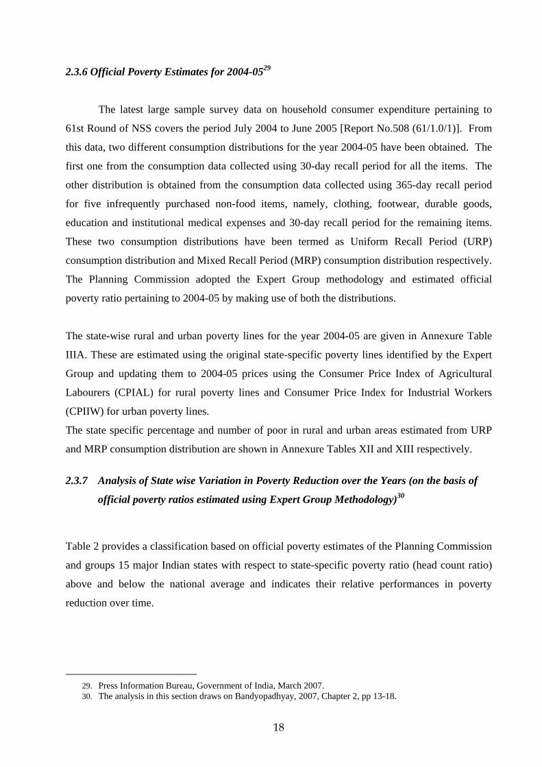
2.3.6 Official Poverty Estimates for 2004-0529

The latest large sample survey data on household consumer expenditure pertaining to

61st Round of NSS covers the period July 2004 to June 2005 [Report No.508 (61/1.0/1)]. From

this data, two different consumption distributions for the year 2004-05 have been obtained. The

first one from the consumption data collected using 30-day recall period for all the items. The

other distribution is obtained from the consumption data collected using 365-day recall period

for five infrequently purchased non-food items, namely, clothing, footwear, durable goods,

education and institutional medical expenses and 30-day recall period for the remaining items.

These two consumption distributions have been termed as Uniform Recall Period (URP)

consumption distribution and Mixed Recall Period (MRP) consumption distribution respectively.

The Planning Commission adopted the Expert Group methodology and estimated official

poverty ratio pertaining to 2004-05 by making use of both the distributions.

The state-wise rural and urban poverty lines for the year 2004-05 are given in Annexure Table

IIIA. These are estimated using the original state-specific poverty lines identified by the Expert

Group and updating them to 2004-05 prices using the Consumer Price Index of Agricultural

Labourers (CPIAL) for rural poverty lines and Consumer Price Index for Industrial Workers

(CPIIW) for urban poverty lines.

The state specific percentage and number of poor in rural and urban areas estimated from URP

and MRP consumption distribution are shown in Annexure Tables XII and XIII respectively.

2.3.7 Analysis of State wise Variation in Poverty Reduction over the Years (on the basis of

official poverty ratios estimated using Expert Group Methodology)30

Table 2 provides a classification based on official poverty estimates of the Planning Commission

and groups 15 major Indian states with respect to state-specific poverty ratio (head count ratio)

above and below the national average and indicates their relative performances in poverty

reduction over time.

29. Press Information Bureau, Government of India, March 2007. 30. The analysis in this section draws on Bandyopadhyay, 2007, Chapter 2, pp 13-18.

19

The states could be grouped into four categories on the basis of poverty ratio in the initial year

(1973-74), the rate of decline in poverty over three decades, 1973-74 to 2004-05, and other

characteristics, like, size of the state, income and population31.

Category I: Bihar, Orissa and Madhya Pradesh

These three states turned out as the perennially poor ones. Although, the average level of

poverty of these states reduced significantly in absolute terms from 62.6 percent in 1973-74 to

about 38 per cent in 2004-05 (as per the official estimates) but, as per the recent estimate of

poverty for 2004-05, one in every three poor in the country belongs to these three states as

compared to a concentration of one in every four poor in 1973-74. This could be attributed partly

to a higher rate of population growth but largely to lower rate of poverty reduction vis-à-vis other

states.

Category II: Uttar Pradesh, Maharashtra, West Bengal, Assam

Except for Assam which has experienced a substantial poverty reduction from 1993-94 to

2004-05, the pace of poverty reduction in these states has generally been relatively slow and the

level of per capita income has also not been adequate to facilitate such a process.

Category III: Andhra Pradesh, Karnataka, Kerala and Tamil Nadu

These states belong to the southern zone of the country and have witnessed substantial

reduction in poverty as indicated by a decline in the poverty ratio from 53.3 per cent in 1973-74

to 19.5 percent in 2004-05. Along with increase in per capita income, which contributed

substantially to poverty reduction, the population growth in these states also declined

concomitantly and led to a higher rate of poverty reduction overtime. These four states were

home to 24 per cent of the country’s poor in 1973-74. In 2004-05 only 15.24 per cent of the

country’s poor belonged to these states.

31. For similar pattern of categorization carried out earlier see Dutta and Sharma, 2002.

20

Table 2: Relative Performance of Fifteen Major States in Poverty Reduction over three decades

(States have been sorted according to the poverty ratio as reported by the Planning Commission in the order of higher to lower value)

1973-74 (54.88% -All India)States with poverty ratio above national

average States with poverty ratio below

national average Orissa, West Bengal, Bihar, Madhya Pradesh, Kerala, Uttar Pradesh, Tamil Nadu

Karnataka, Maharashtra, Assam, Andhra Pradesh, Gujarat, Punjab, Rajasthan, Haryana

1983-84 (44.48%- All India)Orissa, Bihar, West Bengal, Tamil Nadu,

Madhya Pradesh, Uttar Pradesh Maharashtra, Assam, Kerala, Karnataka, Rajasthan, Gujarat, Andhra Pradesh, Haryana, Punjab

1993-94 (35.97%- All India)Bihar, Orissa, Madhya Pradesh, Assam, Uttar Pradesh, Maharashtra

West Bengal, Tamilnadu, Karnataka, Rajasthan, Kerala, Haryana, Gujarat, Andhra Pradesh, Punjab

2004-05 (27.5%)- All India)Orissa, Bihar, Madhya Pradesh, Uttar Pradesh, Maharashtra

Karnataka, West Bengal, Tamilnadu, Rajasthan, Assam, Gujarat, Andhra Pradesh, Kerala, Haryana, Punjab

For 2004-05 the URP consumption distribution has been used here for sake of comparison

Category IV: Gujarat, Haryana, Punjab and Rajasthan

The poverty ratio in these states was lower than the national average in 1973-74 and

ranged from 28 per cent in Punjab to 48.1 per cent in Gujarat. This category comprised states

with both high and low per capita incomes in the initial period (1973-74), but registered a higher

growth in the intervening period. The decline in the poverty ratio has been the highest in this

group of states. According to the latest official poverty estimate of 2004-05 these states are much

below the national average, with poverty ratio ranging from 8.4 percent for Punjab to 22.1

percent for Rajasthan.

A crucial observation that could be made from the movement of poverty ratio is that for

the states which had higher poverty ratios to begin with, the rate of decline in poverty had been

slower. This is brought out strongly by the fact that the position of Bihar, Orissa and Madhya

Pradesh, as per the latest official estimate of poverty ratio for 2004-05, is almost the same as

their position three decades back in 1973-74. The poverty ratio in each of these states is still

lying much above the national average. Similarly, Gujarat, Punjab and Haryana, which had

21

poverty ratios much below the national average as of 1973-74, are still at the lower end in terms

of poverty as of 2004-05.

There has been a lot of debate around the intensity of antipoverty effectiveness of growth

in the pre-reform and post-reform period in India. Based on the years for which official poverty

estimates are available, two separate time-periods have been considered – 1983-84 to 1993-94

(which encompasses a major part of the decade prior to economic reform of 1991) and 1993-94

to 2004-05, which projects post-reform performance. The anti-poverty effectiveness of growth

for each of the fifteen major states could be broadly understood by comparing their compound

annual rate of decline in poverty ratio with per capita income growth per annum (as shown in

figs. 1and 2).

As evident from figs. 1 and 2, the states which appear to have registered an increase in

anti-poverty effectiveness in consonance with per capita income growth in the post-reform

period (1993-94 to 2004-05) are Assam, Haryana, Karnataka, Kerala, Maharashtra, Punjab and

Tamilnadu. Assam and Haryana had been able to successfully reverse a rising trend in poverty

in the pre-reform period to a significant decrease in poverty in the post-reform period. For other

states, there has either been a moderate increase in anti-poverty effectiveness in post-reform

period or effectiveness has been maintained at nearly the same level in the pre-and post-reform

period. The states which have seemingly registered a decline in effectiveness are Andhra

Pradesh, Bihar, Gujarat, Madhya Pradesh, Orissa, Rajasthan, Uttar Pradesh and West Bengal. As

indicated by the decline in gradient and flattening of trend line in figure 2, there has been a

general decline in anti-poverty effectiveness in the post-reform period as compared to the pre-

reform period.

Source: F(2007) and

has exp

For both Figured CSO for Per C

Bihar and O

perienced a

e 1 and Figure Capita Income

Orissa have

marginal d

2, Poverty Ra(Per Capita NS

e registered

decline in e

22

atio is based onSDP) Growth.

a phenome

effectivenes

n Planning Com

enal decline

ss in the po

mmission (200

in effectiv

ost-reform p

02) and Plannin

eness. Andh

period. Wh

ng Commission

hra Pradesh

hat is worth

n

h

h

23

noticing in the figures, however, is that with the exception of Assam and Maharashtra, all the

states that belong to category I and category II have experienced a decline in terms of anti-

poverty effectiveness in the post-reform period. The economic reform process does not seem to

have yielded benefit for the chronically poor states like Bihar, Madhya Pradesh, Uttar Pradesh

and Orissa both in terms of per capita income growth and decline in poverty. Moreover, Gujarat,

a prosperous state belonging to Category IV, which has performed well both in terms of income

growth and poverty reduction throughout the pre-reform period has registered a decline in anti-

poverty effectiveness in the post-reform period.

2.4 The Great Indian Poverty Debate: A Snapshot

Deaton and Kozel (2005) is a compilation of a good number of papers focusing on the debate on

reduction (or otherwise) of poverty especially in the post-economic reform period in India (i.e.

after 1991). The debate on Indian poverty estimates is not only relevant in the Indian context but

it has quite aptly generated a global interest because of the implications and importance of

India’s poverty measurement and the methodological challenges and dilemmas associated

therewith for the world as a whole. The extent of confusion that has been created due to lack of

clarity on the basic conceptual underpinnings especially with respect to the identification of the

poor undoubtedly inspired awe and wonder both locally as well as globally.

The issues that are central to the debate on the poverty in the nineties primarily includes - the

right way in which to resolve conflicts concerning in particular the adjustment of the estimated

household consumption levels of NSSO with that pertaining to NAS (which has been captured

partly in section 1.2.3), the right choice of recall period in surveys concerning household

consumption, the appropriate choice of initial poverty line, and the appropriate means for

adjusting that poverty line to account for variations in purchasing power over space and time in

order to maintain its substantive invariance. These issues are discussed briefly here.

The Debate on Adjustments

An issue that was of central concern in the debate especially after the task force report, as

discussed before, and continued in the nineties is whether estimates of household per capita con-

sumption based on national sample survey should be “corrected” for the estimates of average

24

private consumption based on the national accounts data. It has been argued by most of the

contributors to this debate in Deaton and Kozel (2005) that national accounts data because of

some serious problems are highly unlikely to reflect upon the level of consumption of poorer

persons in India. Notable among these contributions is a classic paper written in the late eighties

by B.S. Minhas32 and contained in the aforesaid edited volume. The paper lays out the issues that

have dominated the contemporary debate that includes the differential definition and coverage of

NAS and NSS consumption, differences in timing, and the heavy reliance in national accounting

practice on various “rates and ratios” that link observable but irrelevant quantities to the relevant

but unobservable ones. Minhas underscored that these ratios are in principle derived from

surveys, for example surveys that link the earnings of those employed in services to the value

added in the service sector, but are frequently many years, often decades, out of date. The use of

outdated “rates and ratios” in an economy undergoing growth and structural development will

typically lead to systematic trend errors in the accounts. A prime example is the netting out of

intermediate production from value-added, which is frequently done using some fixed ratio. But

the degree of intermediation tends to grow as the economy becomes more complex and more

monetized, so that the rate of growth of GDP and of consumption will be systematically

overstated in a growing economy. The points raised by Minhas have been endorsed indirectly by

Kulshreshtha and Kar33 and Sundaram and Tendulkar34 which are also contained in this edited

volume. Kulshreshtha and Kar documented the growing discrepancy between the two sources,

from 5 percent in 1957–58 to more than 38 percent in 1993–94, and noted that the discrepancy

for non-food is both larger and more rapidly growing than the discrepancy for food. Although

there were some exceptions, the general finding was same as Minhas that when there is a

discrepancy, it is the National Accounts estimates that are typically less plausible and more

likely to be in error. They underscored that there is nothing in their findings that would “render

the NSSO data on household consumption expenditure unfit for measurement of poverty

incidence.” Sundaram and Tendulkar reported on the findings of a joint CSO-NSSO exercise

concerned with the cross-validation of the two sets of estimates. They drew particular attention

to the fact that revisions for some categories in NAS are often so large as to cast serious doubt on

the estimates in general. They also underscored that survey data should be preferred because they

32. Minhas, B. S., ‘Validation of large-scale sample survey data: case of NSS household consumption

expenditure,’ in Deaton and Kozel (2005). 33. Kulshrestha, A. C. and Aloke Kar, ‘Consumer expenditure from the National Accounts and National

Sample Survey,’ in Deaton and Kozel (2005). 34. Sundaram, K., and Suresh Tendulkar, ‘NAS-NSS estimates of private consumption for poverty estimation:

a further comparative examination,” in Deaton and Kozel (2005).

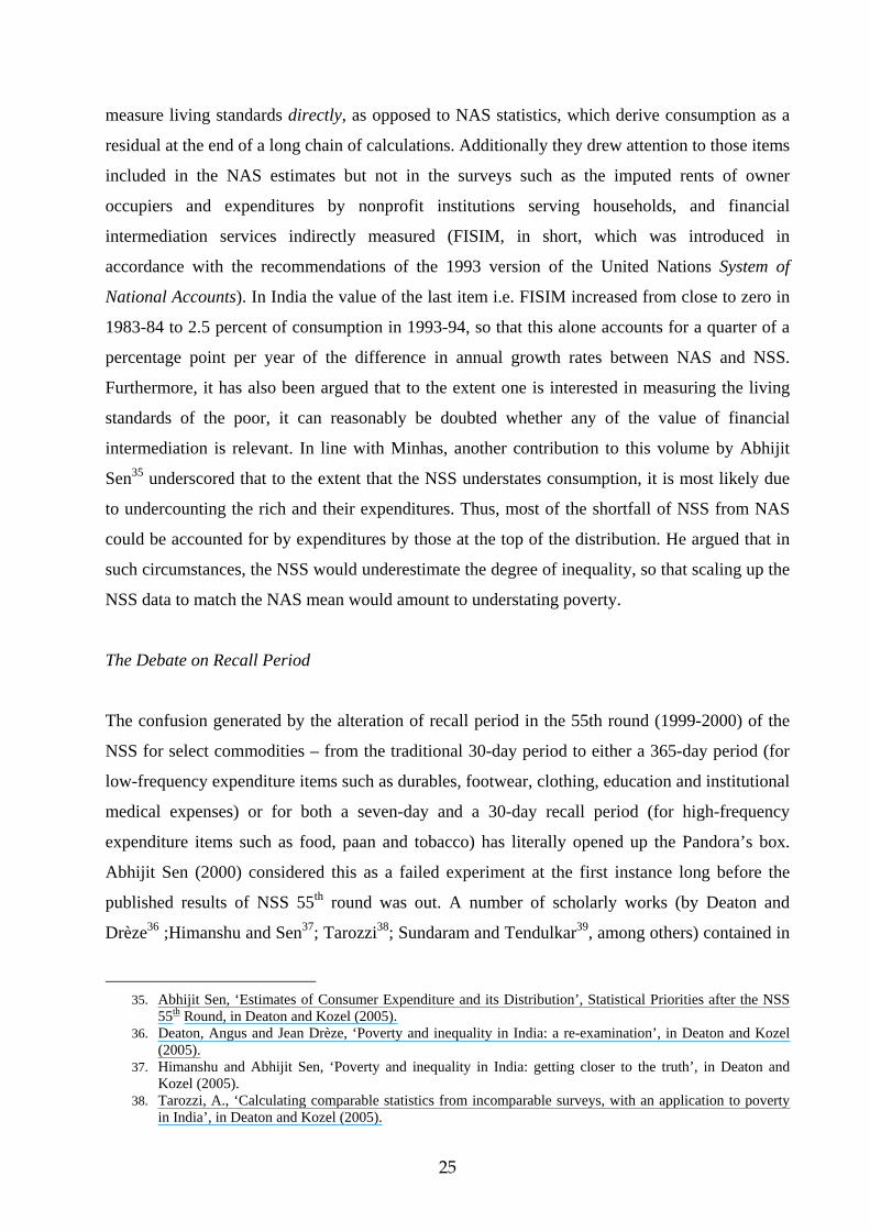
25

measure living standards directly, as opposed to NAS statistics, which derive consumption as a

residual at the end of a long chain of calculations. Additionally they drew attention to those items

included in the NAS estimates but not in the surveys such as the imputed rents of owner

occupiers and expenditures by nonprofit institutions serving households, and financial

intermediation services indirectly measured (FISIM, in short, which was introduced in

accordance with the recommendations of the 1993 version of the United Nations System of

National Accounts). In India the value of the last item i.e. FISIM increased from close to zero in

1983-84 to 2.5 percent of consumption in 1993-94, so that this alone accounts for a quarter of a

percentage point per year of the difference in annual growth rates between NAS and NSS.

Furthermore, it has also been argued that to the extent one is interested in measuring the living

standards of the poor, it can reasonably be doubted whether any of the value of financial

intermediation is relevant. In line with Minhas, another contribution to this volume by Abhijit

Sen35 underscored that to the extent that the NSS understates consumption, it is most likely due

to undercounting the rich and their expenditures. Thus, most of the shortfall of NSS from NAS

could be accounted for by expenditures by those at the top of the distribution. He argued that in

such circumstances, the NSS would underestimate the degree of inequality, so that scaling up the

NSS data to match the NAS mean would amount to understating poverty.

The Debate on Recall Period

The confusion generated by the alteration of recall period in the 55th round (1999-2000) of the

NSS for select commodities – from the traditional 30-day period to either a 365-day period (for

low-frequency expenditure items such as durables, footwear, clothing, education and institutional

medical expenses) or for both a seven-day and a 30-day recall period (for high-frequency

expenditure items such as food, paan and tobacco) has literally opened up the Pandora’s box.

Abhijit Sen (2000) considered this as a failed experiment at the first instance long before the

published results of NSS 55th round was out. A number of scholarly works (by Deaton and

Drèze36 ;Himanshu and Sen37; Tarozzi38; Sundaram and Tendulkar39, among others) contained in

35. Abhijit Sen, ‘Estimates of Consumer Expenditure and its Distribution’, Statistical Priorities after the NSS

55th Round, in Deaton and Kozel (2005). 36. Deaton, Angus and Jean Drèze, ‘Poverty and inequality in India: a re-examination’, in Deaton and Kozel

(2005). 37. Himanshu and Abhijit Sen, ‘Poverty and inequality in India: getting closer to the truth’, in Deaton and

Kozel (2005). 38. Tarozzi, A., ‘Calculating comparable statistics from incomparable surveys, with an application to poverty

in India’, in Deaton and Kozel (2005).

26

the volume by Deaton and Kozel proposed variegated adjustments to achieve comparability

between the resulting consumption estimates of the 55th round and those derived on the basis of

previous rounds. However, the premises underlying the different adjustments that have been

made are numerous, and their respective plausibility is also not straightforward to assess.

The corrections suggested by Deaton40 and Tarozzi41 relied on the fact that an important section

of the questionnaire remained unaltered between the 50th and 55th rounds and could be used as a

basis of comparison between them. These include items that are neither “high-frequency” nor

“low-frequency” and for which a 30-day reporting period had been used in all the previous

rounds. This group of “30-day” goods comprises six broad categories, fuel and light,

miscellaneous goods, miscellaneous services, non-institutional medical expenses, rent, and

consumer cesses and taxes which accounts for more than 20 percent of all rural household

expenditures, and more in urban areas. Importantly, expenditure on these items has also been

observed to be highly correlated with total household expenditure. In other words, their exercise

evinced that there exists a part of expenditure that is consistently measured across the surveys

and is also highly correlated with total expenditure whose direct measurement could not be

trusted in the 55th round. Thus Deaton used the 50th round data to calculate the probability of

being poor as a function of household per capita expenditure on the 30-day goods. This estimated

probability was then used for the 55th round and used together with the (inflation-adjusted)

expenditures on the 30-day goods in that round to estimate for each household a probability that

it is poor according to the procedures and definitions of the 50th round. Adding up these

probabilities over all households provided an estimate of the fraction in poverty as it would have

been measured had the 55th round questionnaire been identical to that in the 50th round.

Sundaram and Tendulkar compared the 30-day reports from the employment and

unemployment survey42 with the comparable 30-day expenditures from the consumption

expenditure survey and found that, at least at the mean, there was a reasonably good match. They

39. Sundaram, K., and S. Tendulkar, ‘Poverty Outcomes in India in the 1990s’, in Deaton and Kozel (2005). 40. Deaton, A, ‘Adjusted Indian Poverty Estimates for 1999/2000’, in Deaton and Kozel (2005). 41. Tarozzi, A., ‘Calculating comparable statistics from incomparable surveys, with an application to poverty

in India’, in Deaton and Kozel (2005). 42. The NSSO introduced a new, abbreviated (one-page) questionnaire on consumers’ expenditure that was

used for the households in the sample pertaining to employment and unemployment survey for the 55th round. The reporting period for this supplementary survey is 30-days for all of the “high” and “intermediate” frequency goods, so that, in principle, these data can be used instead of the data on food, pan and tobacco in the consumer expenditure survey, avoiding any contamination of the 30-day reports by the inclusion of the 7-day recall in the questionnaire.

43. Deaton and Kozel (2005), p 9.

27

used this evidence to argue that the 30-day reports in the main consumption expenditure survey

were more or less accurate, at least on average, in spite of the presence of the potentially

contaminating 7-day recall questions. They further noted that the 50th round had solicited

expenditures on low frequency items, clothing, durables, educational expenses, and institutional

medical expenditures for both 30-days and 365-days. Hence, if total expenditure for the 50th

round were reconstructed using the latter, it would be possible to construct a notionally

consistent measure of per capita expenditure in both 50th and 55th rounds, and hence arrive at

consistent estimates of poverty. Based on the mixed reference periods for the 50th round (365

days for low frequency and 30 days for everything else) they estimated that rural poverty in

1993–94 was 34 percent and that this had fallen to 29 percent in 1999–2000. The decline

estimated by them was about half of the official one and much less than Deaton’s estimated

decline, which was nearly seventy percent of the official one. For urban households, they

estimated poverty in 1993–94 as 26 percent and observed that it had fallen to 23 percent in

1999–2000, which is only about a third of the official decline, whereas Deaton’s estimate

confirmed 85 percent of it. Sundaram and Tendulkar also extended their results to the major

states to investigate what had happened to the poverty rates of different social and economic

groups and observed that while some of the most vulnerable groups (scheduled castes,

agricultural labourers, and urban casual labourers) had poverty reductions in line with those of

the general population, others, such as the scheduled tribes, had been left behind.

Himanshu and Sen questioned both these studies. Beginning from the 50th round estimates of

total expenditure from the “mixed” reference period (365 days for the low-frequency items and

30 days for everything else), they followed Deaton (who used total expenditure from the

“uniform” reference period of 30-days), and calculated the probability of being poor conditional

on expenditures on the consistently measured 30-day goods. Turning to the (contaminated) 55th

round, they repeated the calculation of probability of being poor conditional on the consistently

measured 30-day goods and calculated poverty from total expenditure from 30-day responses for

all but low frequency items, and 365-day responses for the latter. Their calculation indicated that

the contaminated “probability of being poor” function was actually above the schedule from the

50th round. Thus if food expenditures were indeed biased upwards in the 55th round, Deaton’s

stability assumption would become questionable, for example because the food Engel curve has

shifted, with people at the same total expenditure level spending less on food relative to other

things, such as the consistently-measured 30-day goods. If so, assessing poverty decline by

looking at the increase in those expenditures will overstate the decline in poverty.

28

Himanshu and Sen also criticised Sundaram and Tendulkar’s justification for their use of

uncorrected 30-day expenditures for food, pan, and tobacco and produced new estimates using

their own set of corrections. They use the following procedure. For each category of consumers’

expenditure, they calculated three possible estimates:

(a) the mean from the consumer’s expenditure section of the questionnaire,

(b) the mean from the corresponding category from the employment-unemployment section of

the questionnaire

(c) a “counterfactual” based on extrapolation to the 55th round of results from the 53rd and 56th

rounds. (The 54th round was only a half-year survey, and appears to be unreliable.)

Given that the estimates from the employment-unemployment part of the survey are likely to be

biased down (because the categories are broadly aggregated), they first took whichever was

larger of (b) and (c), and second, choose the smaller of this and the original estimate (a). Their

estimate of the mean was thus the smaller of (a) and whichever the larger was of (b) and (c).

Himanshu and Sen’s final estimates were in line with Sen’s original view, that there had been

very little decline in headcount poverty in India in the 1990s. Using comparable mixed reference

periods for both rounds, they estimated that between the 50th and 55th rounds the rural

headcount ratio fell by only 2.7 percentage points, from 31.9 percent to 29.1 percent, and the

urban head-count ratio by 3.1 percentage points, from 29.2 percent to 26.1 percent. These

estimates defined the “pessimistic” pole in the Indian poverty debate.

The Indian experience clearly demonstrates that it cannot be assumed that individual

respondents will give an internally consistent picture of their consumption over distinct time

periods. It may not also be the case that consumer self-reports concerning consumption will be

monotonically distorted in the sense that a shorter recall period (or a longer one) will always

entail a more accurate report. It cannot also be assumed that asking of other questions side-by-

side will not “contaminate” the answers to any one of the questions asked.

Deaton and Kozel in their edited volume also reported the work of the “working group on non-

sampling errors” which observed that when seven-day estimates, 30-day estimates, and a “gold

standard” based on daily visits accompanied by direct measurement were compared in a

29

randomised trial, the seven-day estimates were on average 23 per cent higher than the 30-day

estimates, but that the 30-day estimates were “for many important commodities” more accurate

than the seven-day estimates.43 Although this evidence has very little direct relevance to the case

where different recall periods are applied side-by-side in a single questionnaire it is certainly

matter of serious concern. The reality at the heart of the confusion lies in the fact that

respondents do not necessarily behave rationally always. Rather, the responses suggest presence

of some kind of cognitive, interpretative or communicative approximations or distortions. And it

is very difficult to rectify these distortions by bringing them under the ambit of any theoretical

framework. Such corrections could only be carried out through careful empirical observations.

From the aforesaid discussion it needs to be reiterated that the 1993 expert group established its

original poverty lines on the basis of the “traditional” 30-day recall period. Any alteration in the

recall period (as in the 55th round) has clearly unveiled not only the risks of incomparability of

the consumption estimates generated in different years, but also the incompatibility between the

resulting consumption estimates with the altered recall period and the conceptual foundation of

the previously established poverty lines.

Debate on the Depiction of the Poverty Line44

Assessing poverty essentially comprises at the first instance the task of identifying the poor. The

task of identification in turn involves the choice of conceptual and empirical criteria for the

same. Thus in the assessment of income or consumption poverty, the identification criteria

typically comprises the delineation of a poverty line (or lines) and of a particular method of

empirically estimating the income or consumption of individuals to be compared to the invariant

poverty line (or lines).

The poverty line chosen in earlier official efforts in India was more of a direct nature and was

chosen on the ground that in a particular base year (1973-74) it possessed a specific relation to

the actual achievements of human beings as conceived in a particular way (namely, in terms of

calorific adequacy, as judged by the Planning Commission’s Task Force). It is important to note

that the Task Force tried to provide a rational basis for the poverty lines selected. Although the

44. This debate and the next debate on nutritional equivalence draws largely on an analysis carried out by

Reddy (2007).

30

appropriateness of the calorific standard for human achievement is contestable and has been

extensively debated (the next debate focuses on the calorie adequacy); there is hardly any doubt

about the fact that it did provide a benchmark and that the Planning Commission did give due

importance to this benchmark in the measurement of poverty. Later, however, the methodology

delineated by the expert group, as illustrated before, has been applied uniformly across time and

across regions for determining the poverty line(s) and official poverty ratio(s) by the Planning

Commission. But a debate also cropped up around the latter approach that specified a set of

poverty lines in an indirect manner by questioning its aptness and invariance over time and

space.45

In this context, it is essential to contrast the two approaches that have usually been followed in

setting the poverty line

(1) Apply as the poverty line in a specific time period the consumer expenditure of the

particular section of the surveyed population in that same time period which consumed

foods possessing a calorie content equivalent to a selected calorific norm.

(2) Apply as the poverty line in a specific time period a previously identified poverty line,

updated (if necessary) in accordance with a specified price index.

The first approach maintains a substantive human achievement interpretation for the poverty line

in each period of time by construction and is referred to as direct approach. The second approach

or the indirect approach relies on a retrospective human achievement interpretation for the

poverty line. However, the second approach becomes more relevant only if the chosen price

index maintains real purchasing power appropriately over time. In India these two approaches to

the setting of a poverty line coincide in the base year (i.e. 1973-74 in case of India’s official

poverty estimates) for the obvious reason that no updation exercise is involved there. But for the

subsequent years such equivalence is possible only under exceptional circumstance, when the

price index is constructed in such a manner that it takes some specific value which could lead to

such equivalence, but that is merely coincidental. Thus, in reality, poverty lines constructed in

accordance with the two methods are going to diverge from one another and such divergence

could even be substantial. This is precisely what has happened in Indian context. The official

poverty lines have been constructed by the Planning Commission by adopting the indirect

45. Some notable contributors to this debate include Palmer-Jones and Sen (2001), U. Patnaik (2004; 2005;

2006) and S. Subramanian (2005).

31

approach. However, poverty lines constructed in accordance with the direct approach turned out

to be considerably higher than the official poverty line and the difference only increased over

time.

Adopting a direct approach may be difficult and debatable in the Indian context (illustrated in the

light of the next debate). But one also has to go along with the fact that the indirect approach

followed in India has its share of problems. The apparently simple idea of fixing the base year in

which the poverty line is defined and updating it for future estimation of poverty line hides the

very fact that it may not be possible to decide on the appropriate price index for the updation

exercise unless one ensures that the poverty line for the more recent year possesses the

substantive interpretation that it should otherwise have. In this light, Subramanian (2005) has pointed out that the rate of increase of the all-India

wholesale price of cereals has mostly remained above the increase of the rural poverty line that

has been updated according to the officially prescribed method. The picture is also not simple in

terms of evidences on calorie intakes. Meenakshi and Viswanathan46 in the edited volume by

Deaton and Kozel underscored that in the recent period “the contribution of milk, edible oils and

processed foods to total calories has increased”, even among poorer persons. On the other hand,

total calorie intake at the official poverty line (constructed by adopting indirect method) has

decreased. In another study Mehta and Venkatraman (2000) reported that between 1973-74 and

1993-94 although the share of expenditure attributable to edible oils, vegetables, meats, fish,

eggs, etc, increased substantially, due to increases in the prices of these products, real

consumption appears to have increased negligibly. On the contrary, Sen (2005) emphasised that

“the per capita consumption of fats in the country has increased by more than 50 per cent

between 1972-73 and 1999-2000 and this growth has accelerated in recent years”.

Debate on Nutritional Equivalence47

Without a well-researched and carefully done study it is difficult to establish any definitive

relationship between the improvement in diversity and attendant quality of diet and the quantity

of calories consumed by a poor person. Thus it cannot be necessarily assumed at the first

instance that the improvement in diversity and attendant quality of diet will exactly compensate

nutritionally the decrease in calories consumed by poorer persons. At the same time meeting

46. Meenakshi, J. V., and B. Vishwanathan, ‘Calorie deprivation in rural India, 1983–1999/2000’, in Deaton and Kozel (2005).

47. This section draws largely on Reddy (2007).

32

calorie adequacy norms cannot be considered as sufficient means of ensuring nutritional

adequacy. Rather, the assessment of nutritional adequacy requires a more comprehensive

approach and expertise. However, the narrowly food-energy-centric approach towards official

measurement of poverty in the past by the Indian planners failed to consider the essence of the

comprehensive approach that the appropriate judgment of nutritional equivalence demands.

The official poverty lines in India were founded on the assumption of a particular diversified

food consumption pattern of a section of the population with food energy intake corresponding to

the calorie norms in the base year. However, the approaches to presuming the food consumption

pattern beforehand (usually referred to as inductive approaches) and multiplying that by a scalar

factor in order to meet the calorie norms basically amounts to considering the actual

consumption pattern of a certain section of the population as decisive. Lancaster and Ray (2005)

and Sen (2005) argued that the official approach to the construction of poverty lines in India had

been following a similar procedure. However, such approaches are conceptually weaker for a

host of reasons which are illustrated below.

The food consumption pattern of any specific section of the population may reflect economic

duress as well as tastes or prices. Further, changes in the specified population’s food

consumption pattern can result from increases or decreases in real income as well as from

temporal variations in tastes or prices severely complicating the interpretation of poverty lines

constructed at different times with reference to the “same” population (as pointed out by

defenders of the prevailing indirect approach to the setting of the Indian poverty lines). If no non-

inductive criterion whatever is applied to judge the appropriateness of the consumption pattern

assumed to be required to attain the nutritional (or non-nutritional) norms, then there is simply

no way to avoid these difficulties. Hence, the direct approach to the establishment of the poverty

line in India is rather unsatisfactory, as is the indirect approach, and those who privilege the

former as providing the “correct” estimates of poverty in India should also be questioned.

The exercise of poverty assessment ultimately involves evaluative judgments, although these

must be appropriately supported by empirical facts. To mechanically privilege the latter over the

former – as is systematically done in the wholly inductive approach to poverty line construction

may not be appropriate. A more justifiable approach would be able to draw a synergy between

evaluative judgments and empirical evidence concerning preferences and opportunities carefully.

33

Furthermore, the absence of an unchanging yardstick makes the exercise of poverty

measurement problematic. A systematic approach to the monitoring of poverty across space and

time demands application of a yardstick that is invariant with respect to time and also amenable

in a contextually sensitive manner.

2.5 The Latest Estimate of Poverty by Expert Group of the Planning Commission formed in

2009: Salient Features48

In view of the criticism that had been leveled against the official poverty estimates from time to

time, the Planning Commission set up another expert group under the chairmanship of Professor

Suresh Tendulkar in 2009 to address these issues and to suggest a new poverty line and poverty

estimates. The expert group suggested a new methodology to arrive at state wise and all‐India

rural and urban poverty lines for 2004‐05 based on the latest available 61st round of National

Sample Survey (NSS) on household consumer expenditure.

Following are the salient features of the proposed poverty lines: 1. The estimates of poverty will continue to be based on private household consumer expenditure

of Indian households as collected by the National Sample Survey (NSS) Organization (NSSO).

2. Poverty lines won’t be linked to a calorie intake norm

3. Mixed Reference Period (MRP) based estimates of consumption expenditure has been used as

the basis for future poverty lines as against the previous practice of using Uniform reference

period (URP) estimates of consumption expenditure.

4. In the interest of continuity as well as in view of the consistency with broad external validity

checks with respect to nutritional, educational and health outcomes, the expert group decided to

recommend MRP‐equivalent of urban PLB corresponding to 25.7 per cent urban headcount ratio

(estimated urban share of the poor population) in 2004‐05 as the new reference PLB to be

provided to rural as well as urban population in all the states after adjusting it for within‐state

urban‐relative‐to‐rural and rural and urban state‐relative‐to‐all‐India price differentials. In other

words, the new poverty lines seek to enable rural as well as urban population in all the states to

afford the recommended all‐India urban PLB after taking due account of within‐state rural urban

and inter‐state differentials (rural and urban) incorporating observed consumer behaviour both at

48. This section draws largely on Government of India (2009b).

34

the all‐India and state levels. The expert group also validated the proposed poverty lines by

checking the adequacy of actual private expenditure per capita near the poverty lines on food,

education and health by comparing them with normative expenditures consistent with nutritional,

educational and health outcomes. Actual private expenditures reported by households near the

new poverty lines on these items were found to be adequate at the all‐India level in both the rural

and the urban areas and for most of the states.

7. The proposed reference PLB takes into account all items of consumption (except transport and

conveyance) for construction of price indices. Separate allowance for private expenditure on

transport and conveyance has been made in the recommended poverty lines.

8. The price indices proposed by the expert group are based on the household‐level unit values

(approximated price data) obtained from the 61st round (July 2004 to June 2005) of NSS on

household consumer expenditure survey for food, fuel and light, clothing and footwear at the

most detailed level of disaggregation and hence much closer to the actual prices paid by the

consumers in rural and urban areas. Price indices for health and education were also obtained

from unit level data from related National Sample Surveys. The proposed price indices (Fisher

Ideal indices) incorporate both the observed all‐India and the state level consumption patterns in

the weighting structure of the price indices. For rent and conveyance, actual expenditure share

for these items had been used to adjust the poverty line for each state.

9. The new poverty lines have been generated for all the states including the north‐eastern states.

However, in the absence of adequate data, the expert group has suggested use of poverty line of

the neighboring states for union territories.

The expert group underscored that except for the urban all‐India headcount ratio for 2004‐05

which was used to derive the all‐India reference poverty line basket, all other headcount ratios –

rural all‐India and for rural and urban populations of the states for 2004‐05 are based on the new

reference basket and new price indices, and hence are not comparable and must not be compared

to the earlier announced official headcount ratios using the earlier official poverty lines and

out‐dated price indices.

By adopting the above procedure the expert group estimated the all‐India rural headcount ratio as

41.8 per cent pertaining to 2004-05 which is around 13 per cent higher than official estimate

35

arrived at by the planning commission using the previous expert group method (28.3 per cent)

(see annexure table XIII for the poverty lines and state specific poverty headcount ratio for 2004-

05, as estimated by the new expert group). Furthermore as the new estimate is not comparable

with previous estimates of poverty due to procedural modification it would be necessary to

re‐estimate poverty for the previous years. In view of that, the new expert group carried out a

preliminary exercise for the year 1993‐94 in order to broadly make a two‐point comparison of

changes in poverty ratios. The exercise revealed that poverty at all India level in 1993‐94 as 50.1

per cent in rural areas, 31.8 per cent in urban areas and 45.3 per cent in the country as a whole.

On the contrary, the official poverty estimates pertaining to 1993‐94 were 37.2 per cent in rural

areas, 32.6 per cent in urban areas and 36.0 per cent at the all India level respectively (see

annexure table XIV for the poverty lines and state specific poverty headcount ratio for 1993-94,

as estimated by the new expert group). It could, however, be observed that that although the

proposed methodology led to a higher estimate of poverty for 2004-05 and also for the 1993-94

the percentage point decline between 1993‐94 and 2004‐05 is not different from percentage point

decline using the old expert group methodology.

3. Identification of the Poor in India’s Five Year Plans49

The Ministry of Rural Development of the Government of India, in association with the

State Governments identifies the poor households for selection of beneficiaries under the

poverty alleviation programmes. The identification of the poor is distinct from the estimation of

the incidence of poverty, for which the Planning Commission is the nodal agency in the

Government of India, as already mentioned before. The poverty ratio is a macro estimate that is

used to determine the various dimensions of the policies and programmes in order to improve

the quality of life (especially that of the poor). In this respect, the ratio is used as a parameter in

designing of the anti-poverty programme as a component of the overall planning and

development strategy of the country. The macro parameters, particularly the investment and the

other broader economic and social requirements is usually determined in conformity with the

policies regarding poverty alleviation (broadly determined on the basis of poverty ratio) and

judgments on other social and human development parameters through a Input-Output based

consistency-cum-investment planning model.

49. This section draws largely from Government of India (2009a).

36

On the contrary, the BPL (Below Poverty Line) estimates are arrived at from the census

of the rural households through the country. The actual identification of the beneficiary under

the anti-poverty programme is made through a complete census of rural households known as

BPL census which provide the real location of the poor families who are to be targeted. The

identification of poor constitutes a critical component of poverty alleviation since these are the

families who are targeted for state assistance for the income and employment generating anti-

poverty programmes and the social welfare programmes. The BPL census is conducted at an

interval of approximately five years, generally on the eve of a five year plan. This is known as

BPL (below poverty line) census.

The first two BPL censuses were conducted in 1991-92 (at the beginning of the Eighth

Five Year Plan, which covered the period 1992-97) and 1996-97 (at the beginning of the Ninth

Five Year Plan, which covered the period 1997-2002). Both the census yielded the estimate of

percentage and number of poor households at village, block, district and state level. Another

method was devised in 2002 with the intention of use in the Tenth Five year Plan (2002-2007).

This method, albeit novel as compared to its earlier vintages, has been criticized on various

counts.

For BPL Census pertaining to Eleventh Five Year Plan, Ministry of Rural Development

constituted an Expert Group to recommend a suitable methodology for identification of rural

household living below the poverty line. The Expert Group had a wide range of discussion with the

representatives of civil society, government Officials, Expert in the field. The Expert Group

submitted its final report to the Ministry on 21st August 2009 and is under consideration of the

Ministry of Rural Development for devising the methodology of conducting the census.

3.1 Identification of Poor in the Eighth Five Year Plan (1992-97)

The BPL census in 1991-92 was conducted by making use of the rural poverty line derived by

the Task Force in 1991-92, which was then used by the Planning Commission in bringing out the

official poverty estimates. The task force rural poverty line was not used directly but was

converted into per family basis by using the information on average size of rural household

obtained from the NSS consumer expenditure survey data (observed as around 5 members per

family). This family based poverty line, expressed in terms of monthly consumption

expenditure, was further converted into annual consumption expenditure. Equating the savings

propensity of the poor to zero, this consumption was treated as income. Thus the poverty line so

derived is based on family rather than a person and income rather than consumption. This

37

national level rural poverty line was then applied uniformly to rural areas of all the states in the

country to separate the poor families from the non-poor in the BPL census.

The identified poor families through the lenses of this census far exceeded the poverty

ratio estimated by the Planning Commission. The number of poor identified in the BPL census

was almost twice of that estimated from the official poverty ratio estimated by the Planning

Commission.

The foremost problem with the 1991-92 BPL Census lies in the choice of income to track

the level of living of the population. The Planning Commission had been using consumption

expenditure in place of income as it had always considered the former as more appropriate for

analysis of level of living than the later for two primary reasons. First, expenditure data reflect

more accurately people's actual level of living while income data are more concerned with

people's potential level of living. Second, expenditure data are considered more reliable than

income data as the latter often underestimates people's potential level of living due to much

longer reference period (one year) for recalling one's income correctly (especially in the case of

poor people with no regular permanent source of income). The reference period for expenditure

is usually one month, except for expenditures on consumer durables. Moreover, income in kind

such as, the consumption of own-produce is often valued at producer prices which results in

people's actual level of living being underestimated.

The complexity of computing the household income is well known. Household income

estimates are universally considered as less reliable than consumption estimates. In India, even a

specialized institution such as CSO and NSS with technically competent staff has not attempted

the estimates of household income. On the contrary, BPL census is conducted by locally

available staff of rural development agencies (such as village level workers, school teachers,

etc.), who are not professionally qualified or experienced to investigate household incomes.

Therefore, considerable non-sampling errors are inevitable. Besides, there is an inherent upward

bias with the BPL census as people know beforehand that this census is going to decide the

category of families as poor or non-poor for anti-poverty government assistance.

Despite the aforesaid complexity of computing income, the 1991-92 BPL Census used

the income of the family, albeit the job of assessment of the income of poor families is much less

cumbersome as compared to that of the rich families. Moreover, the problem of family based

38

fixed poverty line compounded the problems for large families with small income per head, and

also for smaller families with large income per head. This may be illustrated with an example.

Consider two families, A and B. Family-A consists of ten persons and each one earns Rs. 1,500.

The family income is 10 x Rs. 1,500 = Rs. 15,000. Since the total income of the family

(Rs. 15,000) exceeds the poverty line (Rs. 11,000), Family-A is considered as non-poor. From

the family-based poverty line of Rs. 11,000 in 1991-92, the poverty line per person works out to

Rs. 2,200 (= Rs. 11,000/5). Therefore, it would be a mistake to count this family as non-poor

since the income of each person in this family (Rs. 1,500) is well below Rs. 2,200. Now consider

the opposite case of Family-B, which has two persons, each earning Rs. 4,500 per year. The total

income of Family-B during the year is Rs. 9,000. Since this is less than the poverty line (Rs.

11,000), Family-B is counted as poor. Again, a mistake is committed; as Family-B is not poor

since its income per head (Rs. 4,500) exceeds the poverty line per head (Rs. 2,200). Thus, the

above procedure of identifying the poor based on the family poverty line declares a person with

monthly income of Rs. 1,500 as non-poor, but a person with monthly income of Rs. 4,500 as

poor.

In other words, the usage of income for measuring the poverty line inherently led to a

mix up of the non-poor and poor and the estimates of the percentage of BPL households

obtained from the census of rural families in 1991-92 were found to be far more than that

obtained from the rural poverty estimates made by the Planning Commission on the basis of

NSS consumer expenditure data using the Expert Group method.

In order to eliminate the aforementioned problems the procedure of conducting the BPL

census was changed in 1996-97 in substantial measure. First, the income concept was changed to

consumption. Second, the poverty line was changed from the household to person basis. Third,

before administering the questionnaire, a set of exclusion criteria was adopted to eliminate

ineligible families.

39

3.2 Identification of the Poor in the Ninth Five Year Plan (1997-2002)

The BPL census in 1996-97 was conducted in two stages. First, on the basis of certain

exclusion criteria50 such as, threshold level of income and ownership of land, building, consumer

durables and agricultural implements some families were declared as non-poor. In the second

stage, the total consumption, both purchased from the market and home grown, were gathered

from the remaining families by interview method. The total consumption of the family was then

divided by the total number of persons in the family, treating all the members (adult, adolescent

and children) as identical units. The method eventually yielded the per capita consumption of the

family. If the per capita consumption of the family fell below the money value of the poverty

line (which was worked out at the state level using the Expert Group methodology and used by

the Planning Commission to estimate the poverty ratio) then the family was counted as poor and

included in the BPL group.

The revised methodology, however, led to considerable reduction of the gap between the

percentage of the BPL households in 1996-97 and the estimate of rural poverty made by the

Planning Commission in 1993-94 although the bias could not be completely removed.

3.3 Identification of the Poor in the Tenth Five Year Plan (2002-2007)

During the Tenth Five Year Plan an innovative approach was adopted in the matter of

identification of poor families. The identification process was based on thirteen indicators of

well-being. For each of these thirteen indicators, the households were awarded a score in a five

point scale as 0, 1, 2, 3 and 4; the scores being inversely related to the poverty and deprivation of

the household. A low score indicate a higher level of poverty and deprivation and vice-versa.

The lower the score of the household, the greater is the chance of selection as a beneficiary.

The thirteen indicators of level of living chosen were: (a) Land Holding (b) Shelter (c)

Clothing (d) Food Security (e) Sanitation (f) Ownership of Consumer Durables (g) Education (h)

Labour Characteristics (i) Occupation category (j) Children’s status (k) Indebtedness (l)

Migration (m) Preference towards State Assistance.

50. The exclusion criteria is if the family operates more than two hectares of land, has a pucca house, if any

resident member of the family has annual income from salary/self-employment exceeding Rs. 20,000 per annum (Rs. 1,700 per month), or if the family possesses a Television set, Refrigerator, Ceiling Fan, Motor Cycle/Scooter, Three-Wheeler, or if the family owns a Tractor, Power Tiller, Combined Thresher/Harvester, then the family is summarily excluded from the BPL group.

40

For each household, the scores from these 13 indicators were summed up to get the

aggregate score of the household, which could range from zero to 52. The households were

chosen for assistance according to their scores. The household with the least score was selected

for assistance first. Then the household with next lowest score got selected. This way, the

household with the highest score would be chosen last.

This method did not make use of the poverty line (used in the Seventh, 1985-90 and

Eighth Plan, 1992-97) or a mix of poverty line and exclusion criteria (used in the Ninth Plan,

1997-2002). The method did not also yield the estimate of percentage of households living

below the poverty line (obtained in the Eighth and Ninth Plan). In fine, this method did not use

the poverty cut-off point to quantify the number of poor families. It rather underscored the

attainment (or otherwise) of several socio-economic indicators that governs the well-being of

population and ranked the households as per their access to these indicators. Furthermore, the

choice of beneficiaries in an anti-poverty programme according to the consecutively higher

score made the selection procedure contingent upon a concept of relative poverty, rather than

absolute poverty as was the case earlier in the Eighth and Ninth Plans. However, in this respect

also, the likelihood of choosing non-poor as the beneficiary cannot be ruled out since households

with low score may not always necessarily be poor.

The methodology of BPL census 2002, therefore, allowed grading of the rural

households in descending order based on a thirteen socio-economic indicators. The State

Governments had been allowed freedom to select the bottom most families of the poor

households such that the total percentage of families selected could be in consonance with the

number of BPL households estimated by the Planning Commission. A margin of ten percent

had been allowed over and above the Planning Commission’s estimate. The cut-off points were

allowed to be determined by the State Governments and could be at the district, block and any

other level.

This method was devised for selection of beneficiary families during the Tenth Plan

period (2002-2007). The surveys on this method (BPL Census, 2002) have been conducted. But,

this method of identifying families had not been made operational initially due to a temporary

stay by the Hon’ble Supreme Court.

The score based methodology of BPL Census 2002 has been criticized from several

quarters and on various counts. First, a number of parameters in the score based methodology

(for example, provision of toilets in the rural houses, housing, and education status of the

children of the rural families) creates disincentives for the rural families in accessing these

benefits because of the potential fear that is generated in their minds that revealing these

41

information might lead to their potential exclusion from the BPL list. Second, as there was no

fixed quota in terms of selection of beneficiaries, most panchayats usually recommended a large

number of names. However, many of these names were replaced later at the upper tier of

administration by names of those with higher political or bureaucratic clout. Since the power of

panchayats and gram sabhas was only confined to recommending names, the final decision on

selection of potential BPL beneficiaries was in the hands of a few powerful bureaucrats at the

upper tier. Thus, the entire selection process turned out to be top-down, non-transparent and

encouraged corruption. Third, it was difficult to capture information on deprivations on some

parameters like availability of clothes, food security, preference for assistance, etc. with a high

level of objectivity as these parameters were neither clearly observable nor directly verifiable in

nature. Most of the 13 criteria, as mentioned above, are such that cheating or giving false

answers could not be easily checked. Fourth, when the poor raised voices against their non-

inclusion they were often told that the list was full and their inclusion would be contingent upon

a listed beneficiary’s death. And finally, the inappropriate assessment in requirement for staff for

doing a comprehensive survey led to the consequence that in actual practice often detailed survey

was skipped, and the survey sheets were filled up within the office itself.51

3.4 Report of the Expert Group on the methodology for conducting the BPL Census for

Eleventh Five Year Plan (2007-12): Salient Features 52

The Ministry of Rural Development had constituted an Expert Group in early 2009 to

recommend on the methodology of carrying out the BPL census pertaining to the Eleventh Five

Year Plan. The group submitted its final report in August 2009. In view of the problems with the

BPL Survey 2002, as briefly stated above, the expert group proposed a three-fold approach to

identifying rural poor households: (a) to identify those who need to be automatically excluded;

(b) to ensure that the poorest and most vulnerable sections who would otherwise get left out are

automatically included; and (c) to grade the rest of the households and identify the poorest

amongst them so that the total number of the poor {including (b)} is the same as conveyed to the

panchayats by the district authorities. The approach was suggested with the expectation that this

would facilitate programme delivery and direct targeted schemes to the most deserving sections

of the poor. The following paragraphs are devoted to brief elaboration of each of these

components.

51. This paragraph largely draws on GoI (2009a). 52. This section is based on GoI (2009a).

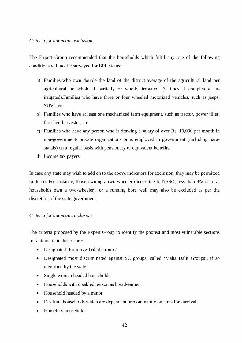
42

Criteria for automatic exclusion

The Expert Group recommended that the households which fulfil any one of the following

conditions will not be surveyed for BPL status:

a) Families

who own double the land of the district

average of the agricultural land per

agricultural household

if partially or wholly irrigated (3 times if completely un-

irrigated).Families who have three or four wheeled motorized vehicles, such as jeeps,

SUVs, etc.

b) Families who have at least one mechanized farm equipment, such as tractor, power tiller,

thresher, harvester, etc.

c) Families who have any person who is drawing a salary of over Rs. 10,000 per month in

non-government/ private organizations or is employed in government (including para-

statals) on a regular basis with pensionary or equivalent benefits.

d) Income tax payers

In case any state may wish to add on to the above indicators for exclusion, they may be permitted

to do so. For instance, those owning a two-wheeler (according to NSSO, less than 8% of rural

households own a two-wheeler), or a running bore well may also be excluded as per the

discretion of the state government.

Criteria for automatic inclusion

The criteria proposed by the Expert Group to identify the poorest and most vulnerable sections

for automatic inclusion are:

• Designated ‘Primitive Tribal Groups’

• Designated most discriminated against SC groups, called ‘Maha Dalit Groups’, if so

identified by the state

• Single women headed households

• Households with disabled person as bread-earner

• Household headed by a minor

• Destitute households which are dependent predominantly on alms for survival

• Homeless households

43

• Any member of the household is a bonded labourer

For the rest of the population, the Expert Group proposed a scoring for the ranking on a scale of

ten is as follows:

A. SC/ST: 3 points; Denotified Tribes, and Designated ‘Most Backward Castes’: 2

points; Muslim/OBC: 1 point.

B. Landless agricultural worker: 4 points; agricultural labourer (with some land): 3

points; casual workers: 2 points; self-employed artisans or self-employed fisher folk

(including those employed by others in such professions): 2 points.

C. No adult (above thirty years of age) has studied up to class 5 in the household: 1 point

D. Any member of the household has TB, leprosy, disability, mental illness or HIV

AIDS: 1 point.

E. Household headed by an old person of age 60 and above: 1 point.

Those achieving highest marks would be included first, followed by the next high score, and

so on, till one reaches the number to be identified by the panchayats. It is likely that on a

scale of 1 to 10, a large number of families would get the same score. Some members of the

Expert Group felt that it may create operational problems for providing assistance under

various programmes and suggested that families may be ranked on a scale of 100 instead of

10. The Group however eventually decided in favour of the top score of 10 because the

scheme has to be so simple that everyone in a village could calculate his/her own score even

before the survey. Increasing the score to 100 would require adding more indicators than five

which are suggested here, and it would lead to the same kind of problems that were

encountered with the 13 point survey of 2002.

In case many households get similar marks, the special category group such as SC/ST may be

placed at the top, followed by landless agricultural labourers in the sequence. Thus the

priority amongst households with the same marks will be as follows:

SC/ST landless agricultural labourers

Other landless agricultural labourers

SC/ST agricultural labourers (with some land)

Other agricultural labourers (with some land), and so on.

44

References Ahluwalia, M. S., ‘Rural Poverty and Agricultural Performance in India’, Journal of Development Studies, April 1978. Bandyopadhyay, K.R., Poverty Alleviation and Pro-poor Growth in India, New Delhi: Asian Institute of Transport Development, 2007. Bardhan, P. K., and T N Srinivasan (eds.) Poverty and Income Distribution in India, Calcutta: Indian Statistical Publishing Society, 1974. Council for Social Development (CSD), India Social Development Report, New Delhi: Oxford University Press, 2006. Dandekar, V.M. and N. Rath, Poverty in India, 1971, (Pune: Indian School of Political Economy). Datta, K.L. and Savita Sharma, Facets of Indian Poverty, New Delhi: Concept Publishing, 2002. Deaton, Angus and Valerie Kozel, The Great Indian Poverty Debate, Delhi: MacMillan, 2005. Deaton, Angus and Jean Dreze, ‘India’s Food Puzzle: Growth, Poverty and Malnutrition’, paper presented at the International Conference on Microeconomics of Growth in India, organized by ICRIER at New Delhi on December, 2006. Government of India, ‘Task Force on Projections of Minimum Needs and Effective Consumption Demand’, Perspective Planning Division, Planning Commission, 1979. Government of India, ‘Study Group on Estimation of Poverty Line’, Perspective Planning Division, Planning Commission, 1984. Government of India, ‘Report of the Expert Group on Estimation of Proportion and Number of Poor’, Perspective Planning Division, Planning Commission, 1993. Government of India, ‘Report of the Expert Group on the Methodology for the BPL Census 2009’, Economic and Monitoring Wing, Ministry of Rural Development, Government of India, August, 2009. Government of India, ‘Report of the Expert Group to Review the Methodology for Estimation of Poverty’, Planning Commission, November, 2009. Lancaster, G. and R. Ray, ‘On Setting the Poverty Line Based on Estimated Nutrient Prices: Condition of Socially Disadvantaged Groups During the Reform Period’, Economic and Political Weekly, January 1, 2005. Mehta, J. and S. Venkatraman, ‘Poverty Statistics: Bermicide’s Feast’, Economic and Political Weekly, July 1, 2000. Ministry of Health and Family Welfare, ‘Report of the National Commission on Macroeconomics and Health’, Government of India, New Delhi, August 2005.

45

P.V. Sukhatme, Feeding India’s Growing Millions, New York: Asia Publishing House, 1965. Palmer-Jones, R. and K. Sen, ‘On India’s Poverty Puzzles and the Statistics of Poverty’, Economic and Political Weekly, January 20, 2001. Patnaik, U., ‘Poverty and Neo-Liberalism in India’, Rao Bahadur Kale Memorial Lecture delivered at Gokhale Institute of Politics and Economics, Pune, February 3, 2006. Patnaik, U., ‘The Republic of Hunger’, Public Lecture on the occasion of the 50 Birthday of Safdar Hashmi, organized by the Safdar Hashmi Memorial Trust, April 10, 2004, New Delhi. Patnaik, U., “Theorizing Food Security and Poverty in the Era of Economic Reforms,” Public Lecture in the series “Freedom from hunger”, India International Center, New Delhi, April 12, 2005. Planning Commission, National Human Development Report 2001, Government of India, March 2002, <available at: http://planningcommission.nic.in/reports/genrep/nhdrep/nhdreportf.htm>.

Reddy, Sanjay G., ‘Indian Poverty Estimates: How Great is the Debate?’, January 30, 2007 <Available at SSRN: http://ssrn.com/abstract=959861>. Sen, Pronab, ‘‘Of Calories and Things: Reflections on Nutritional Norms, Poverty Lines and Consumption Behaviour in India’, Economic and Political Weekly, October 22, 2005. Saxena, N. C., ‘Poverty Estimates for 1999-2000’, Planning Commission, New Delhi, 2001. Sen, Amartya, ‘Development as Capability Expansion’, Journal of Development Planning, Vol.19, pp.41-58, 1989.

Subramanian, S., ‘Unraveling a Conceptual Muddle: India’s Poverty Statistics in the Light of Basic Demand Theory’, EPW, January 1, 2005. World Bank, World Development Report, Washington DC: World Bank, 2001.

46

Annexure I State Specific Poverty Lines in Rural Areas (1973-74 to 1993-94)

(Rs. Monthly Per Capita)

States/UTs 1973-74 1977-78 1983-84 1987-88 1993-94 1. Andhra Pradesh 41.71 50.88 72.66 91.94 163.02 2. Assam 49.82 60.29 98.32 127.44 232.05 3. Bihar 57.68 58.93 97.48 120.36 212.16 4. Goa 50.47 58.07 88.24 115.61 194.94 5. Gujarat 47.10 54.70 83.29 115.00 202.11 6. Haryana 49.95 59.37 88.57 122.90 233.79 7. Himachal Pradesh 49.95 59.37 88.57 122.90 233.79 8. Jammu & Kashmir 46.59 61.53 91.75 124.33 * 9. Karnataka 47.24 51.95 83.31 104.46 186.63 10. Kerala 51.68 58.88 99.35 130.61 243.84 11. Madhya Pradesh 50.20 56.26 83.59 107.00 193.10 12. Maharashtra 50.47 58.07 88.24 115.61 194.94 13. Orissa 46.87 58.89 106.28 121.42 194.03 14. Punjab 49.95 59.37 88.57 122.90 233.79 15. Rajasthan 50.96 57.54 80.24 117.52 215.89 16. Tamil Nadu 45.09 56.62 96.15 118.23 196.53 17. Uttar Pradesh 48.92 54.21 83.85 114.57 213.01 18. West Bengal 54.49 63.34 105.55 129.21 220.74 19. Dadra & N. Haveli 50.47 58.07 88.24 115.61 194.94 20. Delhi 49.95 59.37 88.57 122.90 233.79 21. All-India 49.63 56.84 89.50 115.20 205.84

N.B.: The poverty line (implicit) at all-India level is worked out from the expenditure class-wise distribution of persons and the poverty ratio at all-India level. The poverty ratio at all-India level is obtained as weighted average of the state-wise poverty ratio.

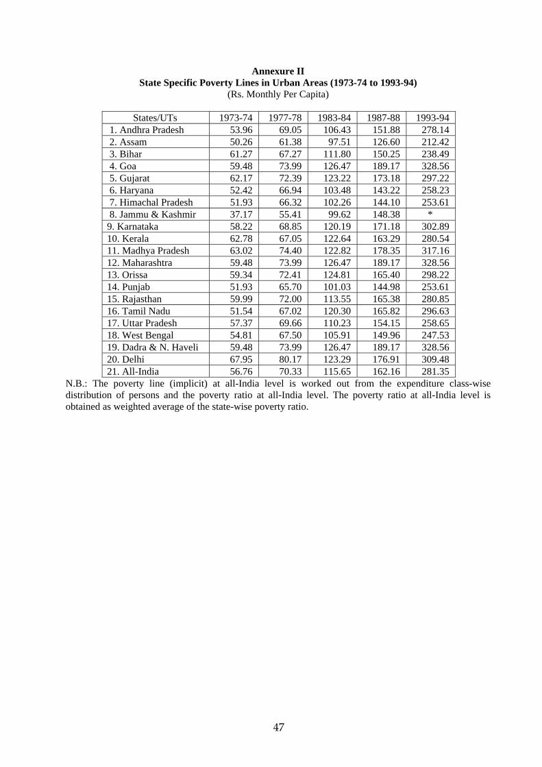
47

Annexure II State Specific Poverty Lines in Urban Areas (1973-74 to 1993-94)

(Rs. Monthly Per Capita)

States/UTs 1973-74 1977-78 1983-84 1987-88 1993-94 1. Andhra Pradesh 53.96 69.05 106.43 151.88 278.14 2. Assam 50.26 61.38 97.51 126.60 212.42 3. Bihar 61.27 67.27 111.80 150.25 238.49 4. Goa 59.48 73.99 126.47 189.17 328.56 5. Gujarat 62.17 72.39 123.22 173.18 297.22 6. Haryana 52.42 66.94 103.48 143.22 258.23 7. Himachal Pradesh 51.93 66.32 102.26 144.10 253.61 8. Jammu & Kashmir 37.17 55.41 99.62 148.38 * 9. Karnataka 58.22 68.85 120.19 171.18 302.89 10. Kerala 62.78 67.05 122.64 163.29 280.54 11. Madhya Pradesh 63.02 74.40 122.82 178.35 317.16 12. Maharashtra 59.48 73.99 126.47 189.17 328.56 13. Orissa 59.34 72.41 124.81 165.40 298.22 14. Punjab 51.93 65.70 101.03 144.98 253.61 15. Rajasthan 59.99 72.00 113.55 165.38 280.85 16. Tamil Nadu 51.54 67.02 120.30 165.82 296.63 17. Uttar Pradesh 57.37 69.66 110.23 154.15 258.65 18. West Bengal 54.81 67.50 105.91 149.96 247.53 19. Dadra & N. Haveli 59.48 73.99 126.47 189.17 328.56 20. Delhi 67.95 80.17 123.29 176.91 309.48 21. All-India 56.76 70.33 115.65 162.16 281.35

N.B.: The poverty line (implicit) at all-India level is worked out from the expenditure class-wise distribution of persons and the poverty ratio at all-India level. The poverty ratio at all-India level is obtained as weighted average of the state-wise poverty ratio.

48

Annexure III

State-Specific Poverty Lines in 1999-2000 (Rs. per capita per month)

No. States/UTs Rural Urban 1 Andhra Pradesh 262.94 457.40 2 Assam 365.43 343.99 3 Bihar 333.07 379.78 4 Gujarat 318.94 474.41 5 Haryana 362.81 420.20 6 Himachal Pradesh 367.45 420.20 7 Karnataka 309.59 511.44 8 Kerala 374.79 477.06 9 Madhya Pradesh 311.34 481.65 10 Maharashtra 318.63 539.71 11 Orissa 323.92 473.12 12 Punjab 362.68 388.15 13 Rajasthan 344.03 465.92 14 Tamil Nadu 307.64 475.60 15 Uttar Pradesh 336.88 416.29 16 West Bengal 350.17 409.22 17 Delhi 362.68 505.45 All India# 327.56 454.11

Note: The poverty line (implicit) at all-India level is worked out from the expenditure class-wise distribution of persons and the poverty ratio at all-India level. The poverty ratio at all-India level is obtained as the weighted average of the state-wise poverty ratio.

49

Annexure IIIA

State-Specific Poverty Lines in 2004-05 (Rs. per capita per month)

S.No. State/U.T.'s Rural Urban

1 Andhra Pradesh 292.95 542.89 2 Assam 387.64 378.84 3 Bihar 354.36 435.00 4 Chhattisgarh 322.41 560.00 5 Delhi 410.38 612.91 6 Goa 362.25 665.90 7 Gujarat 353.93 541.16 8 Haryana 414.76 504.49 9 Himachal Pradesh 394.28 504.49

10 Jammu & Kashmir 391.26 553.77 11 Jharkhand 366.56 451.24 12 Karnataka 324.17 599.66 13 Kerala 430.12 559.39 14 Madhya Pradesh 327.78 570.15 15 Maharashtra 362.25 665.90 16 Orissa 325.79 528.49 17 Punjab 410.38 466.16 18 Rajasthan 374.57 559.63 19 Tamil Nadu 351.86 547.42 20 Uttar Pradesh 365.84 483.26 21 Uttarakhand 478.02 637.67 22 West Bengal 382.82 449.32 23 Dadra & N. Haveli 362.25 665.90

All-India * 356.30 538.60 * The poverty line (implicit) at all-India level is worked out from the expenditure class-wise distribution of persons (based on URP-consumption, that is, consumption data collected from 30 –day recall period for all items) and the poverty ratio at all-India level. The poverty ratio at all-India is obtained as the weighted average of the state-wise poverty ratio.

50

Annexure IV State Specific Poverty Ratio and Number of Poor in 1973-74

(Poverty Ratio is Per Cent; No of Poor is in Thousands)

Rural Urban Total State/UTs Poverty

Ratio Number of Poor

Poverty Ratio

Number of Poor

Poverty Ratio

Number of Poor

1. Andhra Pradesh 48.41 17821 50.61 4748 48.86 22569 2. Arunachal Pradesh 52.67 257 36.92 9 51.93 266 3. Assam 52.67 7637 36.92 546 51.21 8183 4. Bihar 62.99 33652 52.96 3405 61.91 37057 5. Goa 46.85 316 37.69 100 44.26 416 6. Gujarat 46.35 9461 52.57 4381 48.15 13842 7. Haryana 34.23 3008 40.18 824 35.36 3832 8. Himachal Pradesh 27.42 938 13.17 35 26.39 973 9. Jammu & Kashmir 45.51 1841 21.32 207 40.83 2048 10. Karnataka 55.14 12840 52.53 4227 54.47 17067 11. Kerala 59.19 11136 62.74 2416 59.79 13552 12. Madhya Pradesh 62.66 23121 57.65 4509 61.78 27630 13. Maharashtra 57.71 21084 43.87 7658 53.24 28742 14. Manipur 52.67 511 36.92 75 49.96 586 15. Meghalaya 52.67 488 36.92 64 50.20 552 16. Mizoram 52.67 162 36.92 20 50.32 182 17. Nagaland 52.67 265 36.92 25 50.81 290 18. Orissa 67.28 14224 55.62 1223 66.18 15447 19. Punjab 28.21 3047 27.96 1002 28.15 4049 20. Rajasthan 44.76 10141 52.13 2710 46.14 12851 21. Sikkim 52.67 109 36.92 10 50.86 119 22. Tamil Nadu 57.43 17260 49.40 6692 54.94 23952 23. Tripura 52.67 788 36.92 66 51.00 854 24. Uttar Pradesh 56.53 44999 60.09 8574 57.07 53573 25. West Bengal 73.16 25796 34.67 4134 63.43 29930 26. A & N Island 57.43 59 49.40 15 55.56 74 27. Chandigarh 27.96 7 27.96 77 27.96 84 28. Dadra & N. Haveli 46.85 37 37.69 1 46.55 38 29. Delhi 24.44 106 52.23 2178 49.61 2284 30. Lakshadweep 59.19 18 62.74 3 59.68 21 31. Pondicherry 57.43 161 49.40 113 53.82 274 32. All India 56.44 261290 49.01 60046 54.88 321336

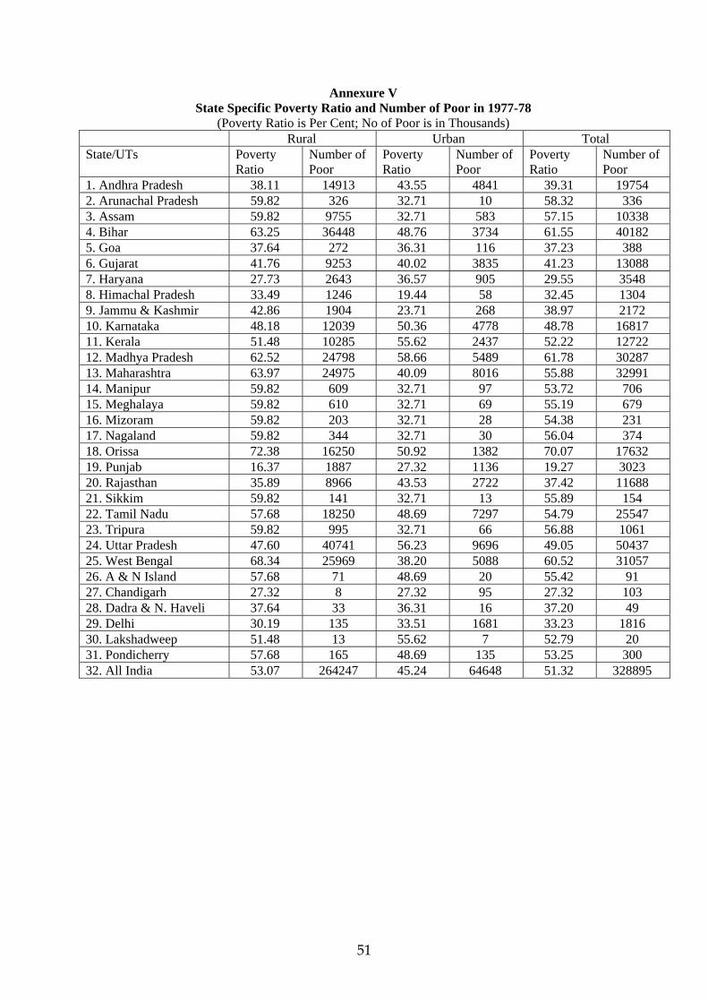
51

Annexure V State Specific Poverty Ratio and Number of Poor in 1977-78

(Poverty Ratio is Per Cent; No of Poor is in Thousands) Rural Urban Total State/UTs Poverty

Ratio Number of Poor

Poverty Ratio

Number of Poor

Poverty Ratio

Number of Poor

1. Andhra Pradesh 38.11 14913 43.55 4841 39.31 19754 2. Arunachal Pradesh 59.82 326 32.71 10 58.32 336 3. Assam 59.82 9755 32.71 583 57.15 10338 4. Bihar 63.25 36448 48.76 3734 61.55 40182 5. Goa 37.64 272 36.31 116 37.23 388 6. Gujarat 41.76 9253 40.02 3835 41.23 13088 7. Haryana 27.73 2643 36.57 905 29.55 3548 8. Himachal Pradesh 33.49 1246 19.44 58 32.45 1304 9. Jammu & Kashmir 42.86 1904 23.71 268 38.97 2172 10. Karnataka 48.18 12039 50.36 4778 48.78 16817 11. Kerala 51.48 10285 55.62 2437 52.22 12722 12. Madhya Pradesh 62.52 24798 58.66 5489 61.78 30287 13. Maharashtra 63.97 24975 40.09 8016 55.88 32991 14. Manipur 59.82 609 32.71 97 53.72 706 15. Meghalaya 59.82 610 32.71 69 55.19 679 16. Mizoram 59.82 203 32.71 28 54.38 231 17. Nagaland 59.82 344 32.71 30 56.04 374 18. Orissa 72.38 16250 50.92 1382 70.07 17632 19. Punjab 16.37 1887 27.32 1136 19.27 3023 20. Rajasthan 35.89 8966 43.53 2722 37.42 11688 21. Sikkim 59.82 141 32.71 13 55.89 154 22. Tamil Nadu 57.68 18250 48.69 7297 54.79 25547 23. Tripura 59.82 995 32.71 66 56.88 1061 24. Uttar Pradesh 47.60 40741 56.23 9696 49.05 50437 25. West Bengal 68.34 25969 38.20 5088 60.52 31057 26. A & N Island 57.68 71 48.69 20 55.42 91 27. Chandigarh 27.32 8 27.32 95 27.32 103 28. Dadra & N. Haveli 37.64 33 36.31 16 37.20 49 29. Delhi 30.19 135 33.51 1681 33.23 1816 30. Lakshadweep 51.48 13 55.62 7 52.79 20 31. Pondicherry 57.68 165 48.69 135 53.25 300 32. All India 53.07 264247 45.24 64648 51.32 328895

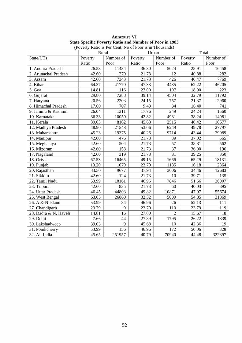
52

Annexure VI

State Specific Poverty Ratio and Number of Poor in 1983 (Poverty Ratio is Per Cent; No of Poor is in Thousands)

Rural Urban Total State/UTs Poverty

Ratio Number of Poor

Poverty Ratio

Number of Poor

Poverty Ratio

Number of Poor

1. Andhra Pradesh 26.53 11434 36.30 5024 28.91 16458 2. Arunachal Pradesh 42.60 270 21.73 12 40.88 282 3. Assam 42.60 7343 21.73 426 40.47 7769 4. Bihar 64.37 41770 47.33 4435 62.22 46205 5. Goa 14.81 116 27.00 107 18.90 223 6. Gujarat 29.80 7288 39.14 4504 32.79 11792 7. Haryana 20.56 2203 24.15 757 21.37 2960 8. Himachal Pradesh 17.00 707 9.43 34 16.40 741 9. Jammu & Kashmir 26.04 1311 17.76 249 24.24 1560 10. Karnataka 36.33 10050 42.82 4931 38.24 14981 11. Kerala 39.03 8162 45.68 2515 40.42 10677 12. Madhya Pradesh 48.90 21548 53.06 6249 49.78 27797 13. Maharashtra 45.23 19375 40.26 9714 43.44 29089 14. Manipur 42.60 476 21.73 89 37.02 565 15. Meghalaya 42.60 504 21.73 57 38.81 562 16. Mizoram 42.60 158 21.73 37 36.00 196 17. Nagaland 42.60 319 21.73 31 39.25 350 18. Orissa 67.53 16465 49.15 1666 65.29 18131 19. Punjab 13.20 1679 23.79 1185 16.18 2864 20. Rajasthan 33.50 9677 37.94 3006 34.46 12683 21. Sikkim 42.60 124 21.73 10 39.71 135 22. Tamil Nadu 53.99 18161 46.96 7846 51.66 26007 23. Tripura 42.60 835 21.73 60 40.03 895 24. Uttar Pradesh 46.45 44803 49.82 10871 47.07 55674 25. West Bengal 63.05 26860 32.32 5009 54.85 31869 26. A & N Island 53.99 84 46.96 26 52.13 111 27. Chandigarh 23.79 9 23.79 110 23.79 119 28. Dadra & N. Haveli 14.81 16 27.00 2 15.67 18 29. Delhi 7.66 44 27.89 1795 26.22 1839 30. Lakshadweep 39.03 9 45.68 10 42.36 19 31. Pondicherry 53.99 156 46.96 172 50.06 328 32. All India 45.65 251957 40.79 70940 44.48 322897

53

Annexure VII State Specific Poverty Ratio and Number of Poor in 1987-88

(Poverty Ratio is Per Cent; No of Poor is in Thousands) Rural Urban Total State/UTs Poverty

Ratio Number of Poor

Poverty Ratio

Number of Poor

Poverty Ratio

Number of Poor

1. Andhra Pradesh 20.92 9638 40.11 6405 25.86 16043 2. Arunachal Pradesh 39.35 275 9.94 8 36.22 283 3. Assam 39.35 7353 9.94 222 36.21 7575 4. Bihar 52.63 37023 48.73 5070 52.13 42093 5. Goa 17.64 131 35.48 165 24.52 296 6. Gujarat 28.67 7413 37.26 4822 31.54 12236 7. Haryana 16.22 1886 17.99 651 16.64 2537 8. Himachal Pradesh 16.28 727 6.29 25 15.45 752 9. Jammu & Kashmir 25.70 1411 17.47 285 23.82 1695 10. Karnataka 32.82 9681 48.42 6180 37.53 15861 11. Kerala 29.10 6164 40.33 2684 31.79 8848 12. Madhya Pradesh 41.92 20002 47.09 6429 43.07 26430 13. Maharashtra 40.78 18689 39.78 10938 40.41 29627 14. Manipur 39.35 483 9.94 46 31.35 529 15. Meghalaya 39.35 518 9.94 30 33.92 548 16. Mizoram 39.35 146 9.94 25 27.52 170 17. Nagaland 39.35 349 9.94 18 34.43 366 18. Orissa 57.64 14998 41.63 1595 55.58 16593 19. Punjab 12.60 1709 14.67 808 13.20 2517 20. Rajasthan 33.21 10497 41.92 3793 35.15 14290 21. Sikkim 39.35 131 9.94 4 36.06 136 22. Tamil Nadu 45.80 16180 38.64 6927 43.39 23107 23. Tripura 39.35 849 9.94 35 35.23 884 24. Uttar Pradesh 41.10 42974 42.96 10679 41.46 53653 25. West Bengal 48.30 22337 35.08 6024 44.72 28361 26. A & N Island 45.80 83 38.64 26 43.89 109 27. Chandigarh 14.67 8 14.67 76 14.67 84 28. Dadra & N. Haveli 67.11 79 - - 67.11 79 29. Delhi 1.29 10 13.56 1015 12.41 1025 30. Lakshadweep 29.10 7 40.33 10 34.95 17 31. Pondicherry 45.80 133 38.64 172 41.46 305 32. All India 39.09 231879 38.20 75169 38.86 307049

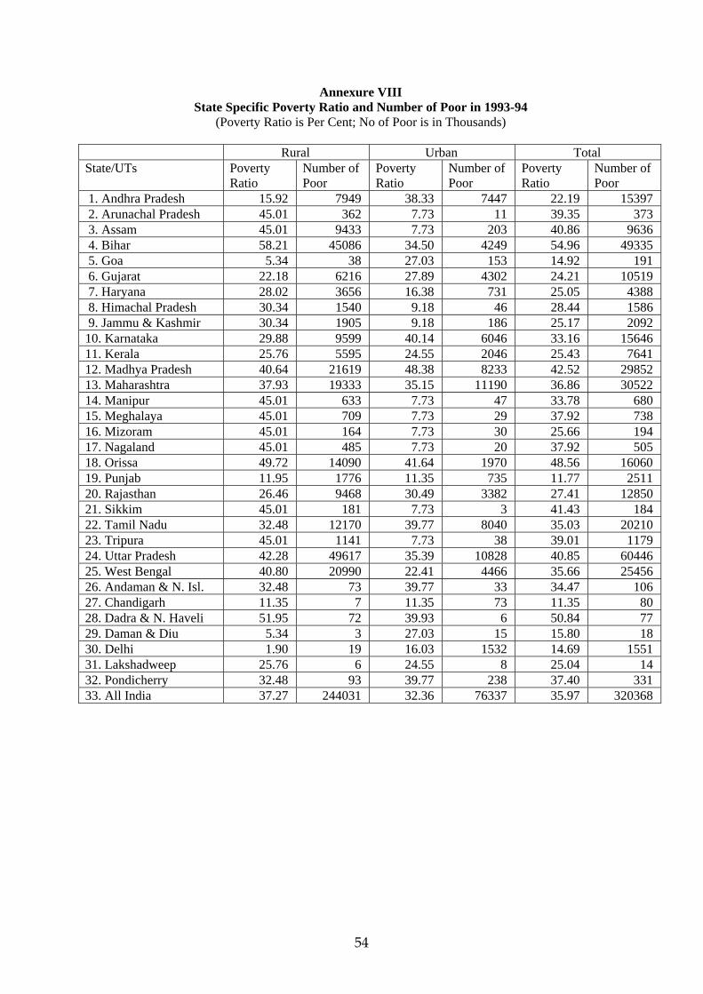
54

Annexure VIII State Specific Poverty Ratio and Number of Poor in 1993-94

(Poverty Ratio is Per Cent; No of Poor is in Thousands)

Rural Urban Total State/UTs Poverty

Ratio Number of Poor

Poverty Ratio

Number of Poor

Poverty Ratio

Number of Poor

1. Andhra Pradesh 15.92 7949 38.33 7447 22.19 15397 2. Arunachal Pradesh 45.01 362 7.73 11 39.35 373 3. Assam 45.01 9433 7.73 203 40.86 9636 4. Bihar 58.21 45086 34.50 4249 54.96 49335 5. Goa 5.34 38 27.03 153 14.92 191 6. Gujarat 22.18 6216 27.89 4302 24.21 10519 7. Haryana 28.02 3656 16.38 731 25.05 4388 8. Himachal Pradesh 30.34 1540 9.18 46 28.44 1586 9. Jammu & Kashmir 30.34 1905 9.18 186 25.17 2092 10. Karnataka 29.88 9599 40.14 6046 33.16 15646 11. Kerala 25.76 5595 24.55 2046 25.43 7641 12. Madhya Pradesh 40.64 21619 48.38 8233 42.52 29852 13. Maharashtra 37.93 19333 35.15 11190 36.86 30522 14. Manipur 45.01 633 7.73 47 33.78 680 15. Meghalaya 45.01 709 7.73 29 37.92 738 16. Mizoram 45.01 164 7.73 30 25.66 194 17. Nagaland 45.01 485 7.73 20 37.92 505 18. Orissa 49.72 14090 41.64 1970 48.56 16060 19. Punjab 11.95 1776 11.35 735 11.77 2511 20. Rajasthan 26.46 9468 30.49 3382 27.41 12850 21. Sikkim 45.01 181 7.73 3 41.43 184 22. Tamil Nadu 32.48 12170 39.77 8040 35.03 20210 23. Tripura 45.01 1141 7.73 38 39.01 1179 24. Uttar Pradesh 42.28 49617 35.39 10828 40.85 60446 25. West Bengal 40.80 20990 22.41 4466 35.66 25456 26. Andaman & N. Isl. 32.48 73 39.77 33 34.47 106 27. Chandigarh 11.35 7 11.35 73 11.35 80 28. Dadra & N. Haveli 51.95 72 39.93 6 50.84 77 29. Daman & Diu 5.34 3 27.03 15 15.80 18 30. Delhi 1.90 19 16.03 1532 14.69 1551 31. Lakshadweep 25.76 6 24.55 8 25.04 14 32. Pondicherry 32.48 93 39.77 238 37.40 331 33. All India 37.27 244031 32.36 76337 35.97 320368

55

Annexure IX State Specific Poverty Ratio and Number of Poor in 1999-2000

(Poverty Ratio is Per Cent; No of Poor is in Thousands) (30-day Recall period)

S.No. States/UTs Rural Urban Total

Poverty Ratio

Number of Poor

Poverty Ratio

Number of Poor

Poverty Ratio

Number of Poor

1 Andhra Pradesh 11.05 58.13 26.63 60.88 15.77 119.012 Arunachal Pradesh 40.04 3.8 7.47 0.18 33.47 3.983 Assam 40.04 92.17 7.47 2.38 36.09 94.554 Bihar 44.3 376.51 32.91 49.13 42.6 425.645 Goa 1.35 0.11 7.52 0.59 4.4 0.76 Gujarat 13.17 39.8 15.59 28.09 14.07 67.897 Haryana 8.27 11.94 9.99 5.39 8.74 17.348 Himachal Pradesh 7.94 4.84 4.63 0.29 7.63 5.129 Jammu & Kashmir 3.97 2.97 1.98 0.49 3.48 3.46

10 Karnataka 17.38 59.91 25.25 44.49 20.04 104.411 Kerala 9.38 20.97 20.27 20.07 12.72 41.0412 Madhya Pradesh 37.06 217.32 38.44 81.22 37.43 298.5413 Maharashtra 23.72 125.12 26.81 102.87 25.02 227.9914 Manipur 40.04 6.53 7.47 0.66 28.54 7.1915 Meghalaya 40.04 7.89 7.47 0.34 33.87 8.2316 Mizoram 40.04 1.4 7.47 0.45 19.47 1.8517 Nagaland 40.04 5.21 7.47 0.28 32.67 5.4918 Orissa 48.01 143.69 42.83 25.4 47.15 169.0919 Punjab 6.35 10.2 5.75 4.29 6.16 14.4920 Rajasthan 13.74 55.06 19.85 26.78 15.28 81.8321 Sikkim 40.04 2 7.47 0.04 36.55 2.0522 Tamil Nadu 20.55 80.51 22.11 49.97 21.12 130.4823 Tripura 40.04 12.53 7.47 0.49 34.44 13.0224 Uttar Pradesh 31.22 412.01 30.89 117.88 31.15 529.8925 West Bengal 31.85 180.11 14.86 33.38 27.02 213.4926 A & N Island 20.55 0.58 22.11 0.24 20.99 0.8227 Chandigarh 5.75 0.06 5.75 0.45 5.75 0.5128 Dadra & Nagar Haveli 17.57 0.3 13.52 0.03 17.14 0.3329 Daman & Diu 1.35 0.01 7.52 0.05 4.44 0.0630 Delhi 0.4 0.07 9.42 11.42 8.23 11.4931 Lakshadweep 9.38 0.03 20.27 0.08 15.6 0.1132 Pondicherry 20.55 0.64 22.11 1.77 21.67 2.41

   All India 27.09 1932.43 23.62 670.07 26.1 2602.5

56

Annexure X State Specific Poverty Ratio and Number of Poor in 1999-2000

(Poverty Ratio is Per Cent; No of Poor is in Thousands) (7-day Recall period)

S.No. States/UTs Rural Urban Total

Poverty Ratio

No. of Poor

Poverty Ratio

No. of Poor

Poverty Ratio

No. of Poor

1 Andhra Pradesh 9.15 48.14 24.48 55.96 13.79 104.12 Arunachal Pradesh 34 3.23 6.29 0.15 28.41 3.383 Assam 34 78.27 6.29 2 30.64 80.274 Bihar 38 322.96 29.23 43.64 36.69 366.65 Goa 2.8 0.23 5.03 0.4 3.9 0.626 Gujarat 12.2 36.87 13.76 24.8 12.78 61.667 Haryana 7.71 11.13 8.02 4.33 7.79 15.468 Himachal Pradesh 7.61 4.63 3.95 0.24 7.27 4.889 Jammu & Kashmir 4.14 3.1 1.7 0.42 3.53 3.52

10 Karnataka 13.64 47.02 22.33 39.35 16.58 86.3611 Kerala 8.14 18.2 17.91 17.73 11.14 35.9312 Madhya Pradesh 34.58 202.78 35.46 74.93 34.81 277.713 Maharashtra 20.71 109.25 25.23 96.81 22.61 206.0514 Manipur 34 5.54 6.29 0.56 24.21 6.115 Meghalaya 34 6.7 6.29 0.29 28.75 6.9916 Mizoram 34 1.19 6.29 0.38 16.5 1.5717 Nagaland 34 4.42 6.29 0.24 27.73 4.6618 Orissa 43.98 131.63 40.33 23.92 43.38 155.5519 Punjab 5.31 8.53 5.4 4.03 5.34 12.5620 Rajasthan 12.22 48.97 18.8 25.36 13.88 74.3321 Sikkim 34 1.7 6.29 0.04 31.03 1.7422 Tamil Nadu 18.68 73.19 20.27 45.81 19.26 11923 Tripura 34 10.64 6.29 0.41 29.24 11.0524 Uttar Pradesh 28.75 379.41 29.04 110.82 28.82 490.2325 West Bengal 27.24 154.04 13.83 31.06 23.43 185.126 A & N Island 18.68 0.52 20.27 0.22 19.13 0.7527 Chandigarh 5.4 0.06 5.4 0.42 5.4 0.48

28 Dadra & Nagar Haveli 15.31 0.26 10.89 0.02 14.84 0.28

29 Daman & Diu 2.8 0.02 5.03 0.04 3.92 0.0530 Delhi 0.63 0.12 5.38 6.52 4.75 6.6431 Lakshadweep 8.14 0.02 17.91 0.07 13.72 0.132 Pondicherry 18.68 0.58 20.27 1.62 19.83 2.2

All India 24.02 1713.35 21.59 612.57 23.33 2325.92

57

Annexure XI State Specific Poverty Ratio and Number of Poor in 2004-05

(Poverty Ratio is Per Cent; No of Poor is in Thousands) (Uniform Recall Period*)

Rural Urban Total State/UTs Poverty

Ratio Number of Poor

Poverty Ratio

Number of Poor

Poverty Ratio

Number of Poor

1 Andhra Pradesh 11.2 64.70 28.0 61.40 15.8 126.10 2 Arunachal Pradesh 22.3 1.94 3.3 0.09 17.6 2.03 3 Assam 22.3 54.50 3.3 1.28 19.7 55.77 4 Bihar 42.1 336.72 34.6 32.42 41.4 369.15 5 Chhattisgarh 40.8 71.50 41.2 19.47 40.9 90.96 6 Delhi 6.9 0.63 15.2 22.30 14.7 22.93 7 Goa 5.4 0.36 21.3 1.64 13.8 2.01 8 Gujarat 19.1 63.49 13.0 27.19 16.8 90.69 9 Haryana 13.6 21.49 15.1 10.60 14.0 32.10 10 Himachal Pradesh 10.7 6.14 3.4 0.22 10.0 6.36 11 Jammu & Kashmir 4.6 3.66 7.9 2.19 5.4 5.85 12 Jharkhand 46.3 103.19 20.2 13.20 40.3 116.39 13 Karnataka 20.8 75.05 32.6 63.83 25.0 138.89 14 Kerala 13.2 32.43 20.2 17.17 15.0 49.60 15 Madhya Pradesh 36.9 175.65 42.1 74.03 38.3 249.68 16 Maharashtra 29.6 171.13 32.2 146.25 30.7 317.38 17 Manipur 22.3 3.76 3.3 0.20 17.3 3.95 18 Meghalaya 22.3 4.36 3.3 0.16 18.5 4.52 19 Mizoram 22.3 1.02 3.3 0.16 12.6 1.18 20 Nagaland 22.3 3.87 3.3 0.12 19.0 3.99 21 Orissa 46.8 151.75 44.3 26.74 46.4 178.49 22 Punjab 9.1 15.12 7.1 6.50 8.4 21.63 23 Rajasthan 18.7 87.38 32.9 47.51 22.1 134.89 24 Sikkim 22.3 1.12 3.3 0.02 20.1 1.14 25 Tamil Nadu 22.8 76.50 22.2 69.13 22.5 145.62 26 Tripura 22.3 6.18 3.3 0.20 18.9 6.38 27 Uttar Pradesh 33.4 473.00 30.6 117.03 32.8 590.03 28 Uttarakhand 40.8 27.11 36.5 8.85 39.6 35.96 29 West Bengal 28.6 173.22 14.8 35.14 24.7 208.36 30 A & N Islands 22.9 0.60 22.2 0.32 22.6 0.92 31 Chandigarh 7.1 0.08 7.1 0.67 7.1 0.74 32 Dadra & N. Haveli 39.8 0.68 19.1 0.15 33.2 0.84 33 Daman & Diu 5.4 0.07 21.2 0.14 10.5 0.21 34 Lakshadweep 13.3 0.06 20.2 0.06 16.0 0.11 35 Pondicherry 22.9 0.78 22.2 1.59 22.4 2.37 All-India 28.3 2209.24 25.7 807.96 27.5 3017.20

*In Uniform Recall Period (URP) consumption the consumer expenditure data for all the items are collected from 30-day recall period. Notes: 1. Poverty Ratio of Assam is used for Sikkim, Arunachal Pradesh, Meghalaya, Mizoram, Manipur, Nagaland and Tripura. 2. Poverty Line of Maharashtra and expenditure distribution of Goa is used to estimate poverty ratio of Goa. 3. Poverty Ratio of Tamil Nadu is used for Pondicherry and A & N Island. 4. Urban Poverty Ratio of Punjab used for both rural and urban poverty of Chandigarh. 5. Poverty Line of Maharashtra and expenditure distribution of Dadra & Nagar Haveli is used to estimate poverty ratio of Dadra & Nagar Haveli. 6. Poverty Ratio of Goa is used for Daman & Diu. 7. Poverty Ratio of Kerala is used for Lakshadweep.

58

Annexure XII State Specific Poverty Ratio and Number of Poor in 2004-05

(Poverty Ratio is Per Cent; No of Poor is in Thousands) (Mixed Recall Period*)

Rural Urban Total State/UTs Poverty

Ratio Number of Poor

Poverty Ratio

Number of Poor

Poverty Ratio

Number of Poor

1 Andhra Pradesh 7.5 43.21 20.7 45.50 11.1 88.71 2 Arunachal Pradesh 17.0 1.47 2.4 0.07 13.4 1.54 3 Assam 17.0 41.46 2.4 0.93 15.0 42.39 4 Bihar 32.9 262.92 28.9 27.09 32.5 290.01 5 Chhattisgarh 31.2 54.72 34.7 16.39 32.0 71.11 6 Delhi 0.1 0.01 10.8 15.83 10.2 15.83 7 Goa 1.9 0.13 20.9 1.62 12.0 1.74 8 Gujarat 13.9 46.25 10.1 21.18 12.5 67.43 9 Haryana 9.2 14.57 11.3 7.99 9.9 22.56 10 Himachal Pradesh 7.2 4.10 2.6 0.17 6.7 4.27 11 Jammu & Kashmir 2.7 2.20 8.5 2.34 4.2 4.54 12 Jharkhand 40.2 89.76 16.3 10.63 34.8 100.39 13 Karnataka 12.0 43.33 27.2 53.28 17.4 96.60 14 Kerala 9.6 23.59 16.4 13.92 11.4 37.51 15 Madhya Pradesh 29.8 141.99 39.3 68.97 32.4 210.97 16 Maharashtra 22.2 128.43 29.0 131.40 25.2 259.83 17 Manipur 17.0 2.86 2.4 0.14 13.2 3.00 18 Meghalaya 17.0 3.32 2.4 0.12 14.1 3.43 19 Mizoram 17.0 0.78 2.4 0.11 9.5 0.89 20 Nagaland 17.0 2.94 2.4 0.09 14.5 3.03 21 Orissa 39.8 129.29 40.3 24.30 39.9 153.59 22 Punjab 5.9 9.78 3.8 3.52 5.2 13.30 23 Rajasthan 14.3 66.69 28.1 40.50 17.5 107.18 24 Sikkim 17.0 0.85 2.4 0.02 15.2 0.87 25 Tamil Nadu 16.9 56.51 18.8 58.59 17.8 115.10 26 Tripura 17.0 4.70 2.4 0.14 14.4 4.85 27 Uttar Pradesh 25.3 357.68 26.3 100.47 25.5 458.15 28 Uttarakhand 31.7 21.11 32.0 7.75 31.8 28.86 29 West Bengal 24.2 146.59 11.2 26.64 20.6 173.23 30 A & N Islands 16.9 0.44 18.8 0.27 17.6 0.71 31 Chandigarh 3.8 0.04 3.8 0.36 3.8 0.40 32 Dadra & N. Haveli 36.0 0.62 19.2 0.16 30.6 0.77 33 Daman & Diu 1.9 0.03 20.8 0.14 8.0 0.16 34 Lakshadweep 9.6 0.04 16.4 0.05 12.3 0.09 35 Pondicherry 16.9 0.58 18.8 1.34 18.2 1.92 All-India 21.8 1702.99 21.7 682.00 21.8 2384.99

*In Mixed Recall Period (MRP) consumption the consumer expenditure data for five non-food items, namely, clothing, footwear, durable goods, education and institutional medical expenses are collected from 365-day recall period and the consumption data for the remaining items are collected from 30-day recall period. Note: Same as Annexure Table XI

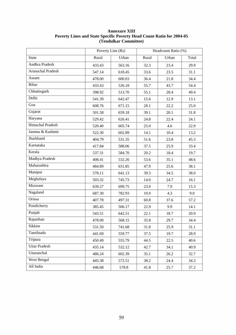
59

Annexure XIII Poverty Lines and State Specific Poverty Head Count Ratio for 2004-05

(Tendulkar Committee) Poverty Line (Rs) Headcount Ratio (%)

State Rural Urban Rural Urban Total

Andhra Pradesh 433.43 563.16 32.3 23.4 29.9 Arunachal Pradesh 547.14 618.45 33.6 23.5 31.1 Assam 478.00 600.03 36.4 21.8 34.4 Bihar 433.43 526.18 55.7 43.7 54.4 Chhattisgarh 398.92 513.70 55.1 28.4 49.4 Delhi 541.39 642.47 15.6 12.9 13.1 Goa 608.76 671.15 28.1 22.2 25.0 Gujarat 501.58 659.18 39.1 20.1 31.8 Haryana 529.42 626.41 24.8 22.4 24.1 Himachal Pradesh 520.40 605.74 25.0 4.6 22.9 Jammu & Kashmir 522.30 602.89 14.1 10.4 13.2 Jharkhand 404.79 531.35 51.6 23.8 45.3 Karnataka 417.84 588.06 37.5 25.9 33.4 Kerala 537.31 584.70 20.2 18.4 19.7 Madhya Pradesh 408.41 532.26 53.6 35.1 48.6 Maharashtra 484.89 631.85 47.9 25.6 38.1 Manipur 578.11 641.13 39.3 34.5 38.0 Meghalaya 503.32 745.73 14.0 24.7 16.1 Mizoram 639.27 699.75 23.0 7.9 15.3 Nagaland 687.30 782.93 10.0 4.3 9.0 Orissa 407.78 497.31 60.8 37.6 57.2 Pondicherry 385.45 506.17 22.9 9.9 14.1 Punjab 543.51 642.51 22.1 18.7 20.9 Rajasthan 478.00 568.15 35.8 29.7 34.4 Sikkim 531.50 741.68 31.8 25.9 31.1 Tamilnadu 441.69 559.77 37.5 19.7 28.9 Tripura 450.49 555.79 44.5 22.5 40.6 Uttar Pradesh 435.14 532.12 42.7 34.1 40.9 Uttaranchal 486.24 602.39 35.1 26.2 32.7 West Bengal 445.38 572.51 38.2 24.4 34.3 All India 446.68 578.8 41.8 25.7 37.2

60

Annexure XIV Poverty Lines and State Specific Poverty Head Count Ratio for 1993-94

(Tendulkar Committee) Poverty Line (Rs) Poverty HCR

Rural Urban Rural Urban Total Andhra Pradesh 244.1 282.0 48.1 35.2 44.6 Arunachal Pradesh 285.1 297.1 60.0 22.6 54.5 Assam 266.3 306.8 54.9 27.7 51.8 Bihar 236.1 266.9 62.3 44.7 60.5 Chhattisgarh 229.1 283.5 55.9 28.1 50.9 Delhi 315.4 320.3 16.2 15.7 15.7 Goa 316.2 306.0 25.5 14.6 20.8 Gujarat 279.4 320.7 43.1 28.0 37.8 Haryana 294.1 312.1 40.0 24.2 35.9 Himachal Pradesh 272.7 316.0 36.7 13.6 34.6 Jammu & Kashmir 289.1 281.1 32.5 6.9 26.3 Jharkhand 227.7 304.1 65.9 41.8 60.7 Karnataka 266.9 294.8 56.6 34.2 49.5 Kerala 286.5 289.2 33.9 23.9 31.3 Madhya Pradesh 232.5 274.5 49.0 31.8 44.6 Maharashtra 268.6 329.0 59.3 30.3 47.8 Manipur 322.3 366.3 64.4 67.2 65.1 Meghalaya 284.1 393.4 38.0 23.0 35.2 Mizoram 316.5 355.7 16.6 6.3 11.8 Nagaland 381.7 409.6 20.1 21.8 20.4 Orissa 224.2 279.3 63.0 34.5 59.1 Pondicherry 220.3 264.3 28.1 32.4 30.9 Punjab 286.9 342.3 20.3 27.2 22.4 Rajasthan 271.9 300.5 40.8 29.9 38.3 Sikkim 266.6 362.2 33.0 20.4 31.8 Tamilnadu 252.6 288.2 51.0 33.7 44.6 Tripura 275.8 316.6 34.3 25.4 32.9 Uttar Pradesh 244.3 281.3 50.9 38.3 48.4 Uttaranchal 249.5 306.7 36.7 18.7 32.0 West Bengal 235.5 295.2 42.5 31.2 39.4 All India 50.1 31.8 45.3 Note: The estimates for Chhattisgarh, Madhya Pradesh, Bihar, Jharkhand, Uttar Pradesh and Uttaranchal are for states as they exist after bifurcation in 2001. The estimates for 1993-94 have been calculated from the unit data using district and state boundaries of the divided states in 1993-94.

61

Annexure XV

Select Measures of Poverty

Three measures of poverty (1) the head count ratio (HCR) which indicates the proportion of the

population below poverty line in terms of a given norm. This is the most widely used measure in

India. (2) The poverty gap index (PGI) which indicates the ratio of the aggregate poverty gap of

all poor households to the minimum normative aggregate expenditure for the entire (poor as well

as non-poor) population (poverty line multiplied by the total population). This is described as

the depth measure of poverty. (3) James Foster, Joel Greer and Erik Thorbecke, popularly known

as FGT which has its components, namely, the head count ratio, the (squared) poverty gap ratio

and the relative inequality amongst the poor as measured by the squared coefficient of variation.

The Headcount Approach

This approach entails the computation of poverty line, defining in a specific way, the number of

poor, and expressing the ratio of persons below the poverty line, to the total number of people in

a particular society. In other words, if the number of persons below the poverty line is ‘q’ and the

total population be ‘n’ then the head count ratio (H) will be: H= q/n

Amartya Sen finds two drawbacks in the headcount measure: firstly, the ratio does not

take into account the extent of the shortfall of income of those below the ‘poverty line’, i.e., if

the income of all below the poverty line is reduced without affecting the income of those above

this line, it will not register any effort whatsoever on the headcount measure and secondly, it is

insensitive to the distribution of income among the poor. For example, transfer of income form a

poor to non-poor will again have no effect on the headcount measure.

Poverty Gap Measure

The other measure – the poverty gap – is defined as the ratio of the average income below the

poverty line. In this approach, the aggregate shortfall of income of all the poor below the

specified poverty line is calculated.

Let (y1, y2, y3, … yn) be the vector of incomes,

z is the poverty line,

n is the total numbers of persons of which q are poor,

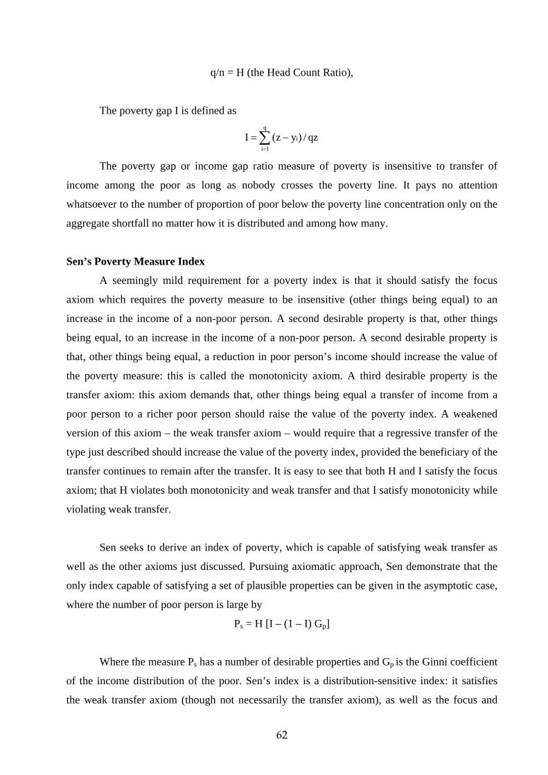
62

q/n = H (the Head Count Ratio),

The poverty gap I is defined as

∑=

−=q

1i

i qz/)yz(I

The poverty gap or income gap ratio measure of poverty is insensitive to transfer of

income among the poor as long as nobody crosses the poverty line. It pays no attention

whatsoever to the number of proportion of poor below the poverty line concentration only on the

aggregate shortfall no matter how it is distributed and among how many.

Sen’s Poverty Measure Index

A seemingly mild requirement for a poverty index is that it should satisfy the focus

axiom which requires the poverty measure to be insensitive (other things being equal) to an

increase in the income of a non-poor person. A second desirable property is that, other things

being equal, to an increase in the income of a non-poor person. A second desirable property is

that, other things being equal, a reduction in poor person’s income should increase the value of

the poverty measure: this is called the monotonicity axiom. A third desirable property is the

transfer axiom: this axiom demands that, other things being equal a transfer of income from a

poor person to a richer poor person should raise the value of the poverty index. A weakened

version of this axiom – the weak transfer axiom – would require that a regressive transfer of the

type just described should increase the value of the poverty index, provided the beneficiary of the

transfer continues to remain after the transfer. It is easy to see that both H and I satisfy the focus

axiom; that H violates both monotonicity and weak transfer and that I satisfy monotonicity while

violating weak transfer.

Sen seeks to derive an index of poverty, which is capable of satisfying weak transfer as

well as the other axioms just discussed. Pursuing axiomatic approach, Sen demonstrate that the

only index capable of satisfying a set of plausible properties can be given in the asymptotic case,

where the number of poor person is large by

Ps = H [I – (1 – I) Gp]

Where the measure Ps has a number of desirable properties and Gp is the Ginni coefficient

of the income distribution of the poor. Sen’s index is a distribution-sensitive index: it satisfies

the weak transfer axiom (though not necessarily the transfer axiom), as well as the focus and

63

monotonicity axioms, and presents a comprehensive picture of poverty by utilizing data on the

incidence of poverty (H), the depth of poverty (I) and the extend of inequality in the distribution

of poor income (via Gp). Sen’s index also satisfies symmetry, which requires that the value of the

poverty index should be invariant with respect to a permutation of income across individuals.

James Foster, Joel Greer and Erik Thorbecke’s Poverty Measure Index

A measure advanced by Foster, Greer and Thorbecke in 1984 is additively decomposable

apart from satisfying the desirable properties suggested by Sen. The measure popularly known as

FGT index and is given by:

Let

H= q/n

be the head count ratio and

∑=

−=q

i

i qzyzI1

/)(

be the poverty gap (income-gap) ratio,

and ∑=

−=q

ipipp qyyyC

1

22 /)(

Where ∑=

=q

iip qyy

1

/

Then FGT = H[I2+(1-I)2C2p]

Finally the squared co-efficient of variation C2 is the measure of inequality ‘corresponding’ to P

in the sense that C2 is obtained when n and y (the mean of y) are substituted for q and z in the

definition of P.