pOtypuT RESUME - ERIC
335
P . 10 1,47, 540 AUTHOR' INSTITUTION r SPONS* , AGENCY PUB DATE OTE f 'AV,AILABLE FROM FDFS PRICE DESCRIPTOFS r IDENTIFIEF.S ABSTRACT pOtypuT RESUME Mott, Frank \'.1 And OtherS Years for Decision: A Longitudinal Study-of *he .Educational, Labor Ma.ket. and Family ExPerieices'of ,Young Women, 1968 to 1973. Volume Four.. Ohio State.Univ., Columbus". Center for Human Rgspurce 1. CE 01'3 811 Research. . Employment and Training' Administration (DO14, Washington, D.C.. Nov' 77 .366p.; For related documents see ED 049 376, ED 812, and ED 094 135 ; Parts of document may be -marginally.legible due to. small type The Ohio State University, College of Administrailk. Science, Center for Human Resource Research; 1375 Perry Street, Stlite 585,, Columbus,-Ohio 43210 ($0.80) 1F-$0.83 HC-$19.41 Plus Postage. Adademic Aspiration; Adolescents; Career'Choice% Career Planning; College Attendance,; Demography;, Divorce; *Educational Experience; *Employment Experience; Employment Opportunities; 'Employment - Patterns;. Employment Problems; *Family-Influence; Family Problems; Females; FinanCial Probleme;-Income; Life Style; Longitudinal Studies; Migration; Mcithp_rs;-- 'National :Surveys; Occupational Aspiration;. . Occupational Mobility; Sex Differences;.StatistiCal tudies;:- Wages; *Working Women; Young Adults United. States .. Utilizing the National Longitudinal Surveys of 5,'159 young women aged fourteen to twenty-four from 1968 to 1973, the .study reports on the educational, labor sarket and family experiences of young women. The content is,in seven chapters. Chapter 1 describes - the data bape and pOsents an overvievoof changes in the women s life patterns over the stud/ period. 'Chapter 2 examines college attendance. and thejactiors associated .with desires and expectations for,higher education and the quality, of the institution a woman attendt. Chapter 3 studies the 4bor force dynamics associated with withdrawal from and. reentry intd the labor force when a woman bears-her Chapter 4 explores the characteristicb of young wowen that are associated with the choice of an itypipal occupation. Chapter 5 examines determinents of average 'hourly eagningsof young women with . focus'on the impact of training, and on.differences in .wage structures by sex. Chapter 0 analyzei causes and ,consequences o,f migtation' for the economic welfare of.yoeng-women and their families. Chapter 7 examines some of the deterilinants' of marital. disruption and its economic consequences. (Eighty - eight, tables and thirteen figures are included. The 1968 and 1973 survey fOrms are appended.) (EN) .? . / , .. . . I Lo...urnents acquired by 'ERIC include Many informal unpublished materials not available from other sources .E.-I-.: makes every,", effort to obtain' the best copy available. Nevertheless,. Items of marginal reproducibility are often encountered a.--.. this atfects.the qutlity of the rrucrofiche and hardcopy reproductions ERIC makes available via the ERIC Document Reproduction Service EDRS). Li...RL is not responsible for the quality of the original document. Reproductions supplied.by EDRS are the belt that can be made from the original. .
-
Upload
khangminh22 -
Category
Documents
-
view
2 -
download
0
Transcript of pOtypuT RESUME - ERIC

P .
10 1,47, 540
AUTHOR'
INSTITUTION
rSPONS*
,AGENCY
PUB DATEOTE
f
'AV,AILABLE FROM
FDFS PRICEDESCRIPTOFS
r
IDENTIFIEF.S
ABSTRACT
pOtypuT RESUME
Mott, Frank \'.1 And OtherSYears for Decision: A Longitudinal Study-of *he.Educational, Labor Ma.ket. and Family ExPerieices'of,Young Women, 1968 to 1973. Volume Four..Ohio State.Univ., Columbus". Center for Human Rgspurce
1.
CE 01'3 811
Research. .
Employment and Training' Administration (DO14,Washington, D.C..Nov' 77
.366p.; For related documents see ED 049 376, ED812, and ED 094 135 ; Parts of document may be
-marginally.legible due to. small typeThe Ohio State University, College of Administrailk.Science, Center for Human Resource Research; 1375Perry Street, Stlite 585,, Columbus,-Ohio 43210($0.80)
1F-$0.83 HC-$19.41 Plus Postage.Adademic Aspiration; Adolescents; Career'Choice%Career Planning; College Attendance,; Demography;,Divorce; *Educational Experience; *EmploymentExperience; Employment Opportunities; 'Employment -
Patterns;. Employment Problems; *Family-Influence;Family Problems; Females; FinanCial Probleme;-Income;Life Style; Longitudinal Studies; Migration; Mcithp_rs;--
'National :Surveys; Occupational Aspiration;. .
Occupational Mobility; Sex Differences;.StatistiCaltudies;:- Wages; *Working Women; Young AdultsUnited. States
..
Utilizing the National Longitudinal Surveys of 5,'159young women aged fourteen to twenty-four from 1968 to 1973, the .studyreports on the educational, labor sarket and family experiences ofyoung women. The content is,in seven chapters. Chapter 1 describes -
the data bape and pOsents an overvievoof changes in the women s lifepatterns over the stud/ period. 'Chapter 2 examines college attendance.and thejactiors associated .with desires and expectations for,highereducation and the quality, of the institution a woman attendt. Chapter3 studies the 4bor force dynamics associated with withdrawal fromand. reentry intd the labor force when a woman bears-herChapter 4 explores the characteristicb of young wowen that areassociated with the choice of an itypipal occupation. Chapter 5examines determinents of average 'hourly eagningsof young women with
.
focus'on the impact of training, and on.differences in .wage structuresby sex. Chapter 0 analyzei causes and ,consequences o,f migtation' forthe economic welfare of.yoeng-women and their families. Chapter 7examines some of the deterilinants' of marital. disruption and itseconomic consequences. (Eighty - eight, tables and thirteen figures areincluded. The 1968 and 1973 survey fOrms are appended.) (EN)
.?
./ , .. .
.
ILo...urnents acquired by 'ERIC include Many informal unpublished materials not available from other sources .E.-I-.: makes every,",
effort to obtain' the best copy available. Nevertheless,. Items of marginal reproducibility are often encountered a.--.. this atfects.thequtlity of the rrucrofiche and hardcopy reproductions ERIC makes available via the ERIC Document Reproduction Service EDRS).Li...RL is not responsible for the quality of the original document. Reproductions supplied.by EDRS are the belt that can be made fromthe original. .
YEARS FOR pECISION:
4
VOLUME FOURNovember 1977
,
)
US S OripARTMENT OF HEALTH.EDUCATION &WELFARENATIONAL INSTITUTEI5F
EDUCATION
7.415, DocumiNT HAS BEEN REPRO-0OCE0 EXACTLY AS RECEIVED FROMSHE PERSONOR OROANIZATtON ORIGIN.?LYING t T POINTS OF VIEW OR OPINIONSStATE0 00 NOT NECESSARILY REPRE-
. SENT OFFICIAL NATIONAL INSTITUTE OF
EOUCKTION FOSITION OR POLICY
A longitudinal study of the_educational, labor market' andfamily experienced of 'young women,
1968 to 197'3
tti
. Frank L. Mott --Steven H. Sandell'David Shapiro
,Patricia K. BritoTimothy J. CarrRex C. JohnsonCarol L. JuseniusPeter,J. KoenigSylvia F. Moore
I
..tv
' Center for Human Resource ResearchCollege of Adminibtrattlie ScienceThe Ohio'State UniVersity?. .
Columbus,,Ohio
This report was prepared under a contract with the Employment and,Training Administration, p.b. @apartment of Labor,,under the authorityor the Comprehensive Employment and Training Act. Researchers,undertaking such ptojects under Government sponsorship are encouragedtoexpress their own judgments. Interpretations or viewliOintsin this document do not nedessarily, represent. the official position or
.policy,of the Department of Labor. .
.
-"L...
° FOREWORD:
. ,.
-Ebrmore than a decadetheCenter for\ Human Resource Research ofThe Ohio State University, and the tJ :S.. Bureau of the Census,.under*separate contracts.with the ,Pmployment and TrainingcAdminidirttion ofthe 'U.S. tepartmentof tabor, have been engaged in the NationalLongitudinal SurVeW(NI.,$)'of labor market experience. Tour subsets ofthe United States civilian population are being studied: ,young "i;en whoat the inception of the study were 14 to 24 years of age; a-counterpartgroup of young women; women 30 tb 44 years of age; and men. 45 to 5y. .
-years of age.-,-These groups were selected because each is confronted.
with special labor market problema that are Challenging to policymakers: for the middle-aged, men, problems,of skill obsolescence and .
deteriorating health that may make reemployment difficulty jobs arelost; for the older group of women, problems associated with reentry
to the labor market after children are in school or grown; and for theyoung men and women, the-problems revolving aroiuid'occupational choice,.preparatiop for work and the often difficult period of accommodation-tothe labor market when formal-schooling has been completed'.
FC:each'.of these four population groups a national probabilitysample, of the noniristitutional civilian population was drawn by theCensus Bureau in 1966; interviews have been conducted periodically by
Census enutherators.utilising questfonnaires'prepared by the Center fOrHuman Resource Resegarchi, Originally contemplated as. covering a five -year period, the surveys have been so successful and attrition so smallthat they havo.been continued beyond the initially planned expiration'dates.. As of the.end of .1977, tilt older cohort of men had beeninterviewed in 1966,, 1967, 1968 (mail), 1969, 1971; 1973 (telephone),1975 (telephone) and 976; the older cohort of women in 1967, 1968-(mail),-'1969, 1971, 1972, 1974 ( telephone), 1976 (telephone) and 1977;
the young women annually between 1968 and 1Q73 and in 1975'(telephorie)and 1977 (telephone); and the young men annually between 196eand 1971,in 1973 and 1975 by telephone, andgain in person in 1976. In early .
1978, a Personal interview with the yoUng women will complete a decadeof interviews with all four cohorts.
Current plaxiS,dall fdr,relatively brief telephone surveys of the? -.existing samples in the twelfth .and fourteenth years, and a longerface-to-face interview the fifteenth year Thus; the'final-'interviewAof_the two mat groUps is scheduled ;Or 1981', while thecorresponding surveys for the older and younger cohorts of women willtake place in 82 and 1983, respeetivetY. The Bureau of the Censuswill continue le responsible for the 'field work and .data- reduction.
4
In ,additiolit4on the basis 9f a questionnaire survei-dfiall knownusers of npAiteiiha a ecommendation bran interdisciplinary panel
kof eXperts, the Departtet of Labor has deaided to begin interviews -
. .. ,
toii .

,
with two new Cohorts Of youth. The new cohorts ale being design d Itopermit a repliai.tiOn of much .of the .S.Palysis.mad of the earlicohorts of yoUng women and young men and also tc, allow an ev Oft, 'n of
the expanded employment and training programs for youth leg ,lat d bythe 1977 aNendm'ents to the Comprehensive EMidoyment'and Tr,ini Act.To these ends, a'national probability sample will be dra , co sistingOf 6,000'young women and 6,000 young men between the ag s.of 14 and.21, with overrepresentation of blacks, Hispanics, add, conc,icallydisadvantaged whites'.'
According to current plans, the new sample. o yo h will beinterviewed fOr the firSt time in November 3Y-gi Th Center for Human,Resource Research will enter into a subcontrac wi a survey researchorganization for designing'the sample; copdu in: the field wOr , andpreparing the data tiles. This organivatio is o be selected n.th'e
. basis of thg recommendation of panel,of/,xpe is who will hreviewed prOposals submitced by a n of chi organizati ns.
/r / . ,. . ",,-
A substantiar body of literature has lreadY appearedbased upon.,r/
-'othe NLS data. 'Seventeen volumes of , mp ehensive repos have beenpublished on surveys conducted thro 1 97?. These have appeared'under the titles of The Pre- etir,at Years (middl -aged men:. four.Volumes); Dual Careers mature ,,, en four volume ) ; Years for'Decision (young women: three velum: ); andCare Thresholds (youngmen; six. lumes). In addition, ,,vex 200 repo is on specific topics
/5have beerCpre ared by ,itatf ombe s or the Center for Humad-ResoUrceResearch and other research, . t rough:Alt the country who have acquired'public-use versions -of
tLS apes..',
.c.- ! ,,./' The present s 'beed on stile siirveys.6f;young women through
I .
I. .
1973. Itdiffer. from'. g "reviouse,volumes,WIhe-Years for Decisionseries in two m 41or wais.-./First, iileiiher attempts to ceirer allatpects oft theddia coinprehensi4ely nor focuses. on a singleenarrow : . .
topic.- Rather;eit gOnsiss.of a Olt of,interielatedstuolies,on toprcs.kthat are conceived tobe'impOrtantdifi'undei-stapdingAhe edUcatipnal, \
-labor marketand i'Fily/experiences bf youpg.women, Second, ;Estherthan relying:entirely On tabUlar analytis as have most of the,prpviOup-volimes, all,of'/, he tpters except the introduqory one- employmultiVariate statis ical techniques. -
. -. , /, ..,.,
.,/
,
14hile ,adept ng sole responsib4litylfor.whaever limitations the 'volulie May'have, we wishAto acknoyAdge oQ debt to.i. large'number of '4perponi wit Out:whose contribution ri.O.therthe overall study: nor thepresehi iv
.
eivould have been po aible: The fime"acknOwledgeMentmusgo Jj the several thousand embers_bf the 'sample whose generousc9ppera6 n in repeated Intervies'has 15ovidddrthe rani materials for
,pdP.endeavor .,--
1
. " .
.,",,.,
, =1 .. . .
e'..'
i' ,t/veil:al officials of the,tmployment'and Training A4Minisera ionj e. /
/ , il .yyave een/very helpful over the_years in providing
itSlAgestions r the, /
;' $I4,
411 '
r
r

designof the NLS and in reviewing carefully the preliminary draftsof-our yepots. We wish to acknowledge.especially.the continuoussupport and encoura ementof Howard Rosen, Director of the Office oResearch'and pevelo ment, and the valuable advice provided by Stuart . , .Garfinkle, J cob Sc 'ffman, Rose Wiener, and Ellen Sehgal, who haveat-various times over the years served'as monitors of the NLS project.In addition, a number of individuals in the Bureau of Labor Statisticsread portions Of the manuscript and provided us with numerous helpful..comments.
.. 4The research st ff of the Center for, Human Reource Research has
enjoyed the continuo s expert and friendly collaboration-of personnelof the'Bur2au of the Census, who have "been responsible for developingthe sadples, tonduct ng all of the inter ews, coding and editing thedata, apd preparing the initial versions f the computer tapes. We .
should like to acknowledge especially our debt to Earle Gerson, Chief-.of4he Demographic Surveys Division and t his predecessors DanielLevine and, Robert Pearl; to Robert Mangold, Chief of the Longitudinal,Surveys Branch; to Aerie Argana, his immediate predecessor; and 'totheir colleagues Sha on Fondelie , Patjlealy Carrol Kindel, Dorothy
. Kpger, and Thomas Sc pp. These re the individuali in the Census,Buread.with whomme ave had i ediate contact inthe recent past. Inaddition, we lksifto express our appreciation to Kenneth Frail of the
dlia
Field Division for directing the data c011ection;'to David Lipprabtb and.Eleanor Brown and th ir.staff of the Systems Division for editing andcoding the intervie schedules; and to Kenneth Kaplan and ReginaldMasapo for the prep ration of the computer tapes.
.' .. -The process of revising the computer tapes received from the
Census Blireau and-p oducing all of the tables and regressions incor-porated in this vol erWas the responsibility of the Data ProceSiThgUnit of the Center oll'Humantlesource Research under the direction ofCarOl Sheets and he . predecessor Robert Shondel. Especial' thanks go,to Janie Campanizzil, Rufua:Milsted; Jack Schrull,,R. Barry Shuman, PamSparrow, Tom Steednan, Keith Stober, Ron.Taylor, and Pete Tomasek whoSeprogramming and other technical assistance were of invaluable assistanceto Ads in preparing this particular report.
Herbert S. Parnes provided us with his continuing guidance apdadvice: We alsoiowe debts of gratitude to our colleagues-Stan Benecki,.Stever Hills, Gilbert Neste' and Lois Shaw of the Center who, generously
' provided of their time ii carefully, yeviewing the various drafts of ,
this volume.' In addition,,thanks go out to 6,ur ex-co eagues John T.P.Grasso,Andrew I. Kohen'anU Richard Shortlidge whOpro ided ,
,
helpful 'comments. In addition to, the, research assist ce mentionedin'the specific*chapters We would like to particularly acknowledgethe work of R. Jean Haurin and Ellen. Mumma who, over a period of manymonths, carried out thethapkless task of coordinating, fact checking, .
proofing. and editing this 3.r.91 e.
'/,
V
V

Final , the authors 'are..espeCially indebted to Jeanie Barnes,
who iMpeccibly typed endless,ver4ons of this report, always with atight deadine and always -with a smile. Her ability to translate.unreadable scribbles into the English' lanfuage-was nothing short ofmiraculous. For her skillftl assistance we are most grateful.
/
.
4
7
roo
.
Frank MottNovember 1977
.
.
P
ti
4
r
1,1
FOREWORD
TABLE 'F CO
o.
.. ..... ...Page
CHAPTER 1: INTRODUCTION AND C CLUSIONS . 4 -. '''' .' 1PLAN OF'TAt VOLUME ....... ..... .). .\. . . ,,, .
1, .'.THE NATIONAL LONGITUDIN iliRVEYS.OF yo G WOMEN 2
The ;Sapiple . . . . . . . . . . . .....)Nattire of the Data
*, a 4
1968 To 1973: 'A DESCRI TIVE OVERVIEW-,. . .. . . .(.
ChaNLes in Houser; d and Farm y. . .
Changes in. Labor orce Participation . . ' 14Changes in Other/Work -Related 'Characteristi s.- . . , 19Some Perspectiv s on Attitude Changes 21Highlights of e Volume and Some Policy Imp ic.ations. 24.
.
CHAPTER 2: YOUNG WOMEN AND HIGHEj:EDUGATION , .. .... . . . "35 ,,
_;NTWIDUCTION 35AN ECONOMIC 49.15E OF HIGHER EDUCATION NROLLMENTr ., . .
, 36.. The Decisi to Attend College ) 36
The Quali y.o -,the College, Attended` 37EXPIRICAL AN S1S .° 110
. ° 38t. The Dem d for Higher cation. 38
, Th90Eho ce of College :. 46
\
. , .CONCLUSION 48
...
'
CHAFTER 3:, W -AND MOTHERHOOD: THE DYIAMICS. OF LABOR FOR, P T1CIPATION SURROUNDING TAE FIRST/BIRTH 65
=4, INTRODUCTION-* . . . . . 65, .. ,
Th Data Set '-' 68LABOR RCE BEHAVIOR SURROUNDING THE FIRST' BIRTH.: , A-
..-
''' DES IPTIVE OVERVIEW. : 2 70, .
SOME ERSPECTIVESJ ON LABOR FORCE 'AND FERTILITY INTERACTION.. , .4WORK AND MOTHERHOOD: AN ECONOMIC FRAMEWORK .'. ... . . 83 .-,
/ Some klultivariate ReSults' -'
THE EFFEC"i OF EMPLOYMENT DISGONTINUITYON WAGES ANDv-: /OCCUPATIONAf, STATUS ,
,,,_,
ONCLUSION .. C .. .%.' .. : .... .., .
.... ,... ..
..
.
ER.-4: OCCUPATIONAL'EXPECTOIONS FOR:AGEL55,:-% .. . .... .-'. .. 113.-"
: -." ,.. .... . ...',. . 113 :
OCCUPATIONAL PREFERiNCE:- TYPICAL VS. ATYPICAL OCCUPATIONS:: 113The Importance of OccupaOonal.SegregatiOn . . :. . . 114 %
"The Empirical Model. :-. .,
. 117 .
iMpiri6a1 Results t' .119I. - ,-, FeMili al- Enyironment . i 120L :Educational arid tabor Mirket Experience\. .
1
i
s. .313:Potential Labor Market InvolveMent . . ...., - . . e' . in,Comparison "of'Race/EduCation Groups . 130
I a
INTRODUCTION
88
94'
-3.06'
.,

.f,
.
7
CHAPTER i; (Continued)
OCCUPATIONAL PREFERENCES ANIPOCCUATIPNAI, OUTLOOK /SUMMARY AND CONCLUSIONS
CKAPYER5: INVESTMENTS IN: HUMAN CAPITAL AND THE EARI NGS OF
0
aEmpirical.Estimatas
WAGE DIFFERENCEBY SEX AND THE EFFECTSINVESTMENTS IN TRAINING
Empirical. EstimatesWage -Gap An41/41.ysis
--,\SUMARY AN DI CONCLUSIONS
.NOUNG WOMEVPOSTSCHOOL-INVESTMENTS IN HUMAN CAPITALWAGE EQUATIONS FOR YOUNG. WOMEN
SpecificationStratificatioA': . .. ...
POSTSCHOOL,
CHAPTER 6: THE GEOGRAPHIC MOBILITY OF YOUNGWOMEN AND THEIR
Page
131137
,
149149
151151
154156
161162165 .
`.166
. FAMILIES, 177.
INTRODUCTION' ..177THE THEORY OF FAMILY MIGRATION ' -'177.
The Model . 'a 1771 UnemplOyment, UhemPloyment Compensation; and the
Stopensity to Migrate,.
The College Experience and the Propensity toMigraeFamily-Income and the Migration Decision
EMPIRICAL TESTS ;.
The Likelihood of Migration. .
The Effect of Migration on EarhingsSUMMARY AND CONCLUSIONS
179. 180. 186
181
181189
192
4:7;7207
208210
212221
221223
.227
228:
'228
CHAPTER 7: MARITAL DISRUPTION: CAUSES AND CONSEQUENCES .
INTRODUCTIONSome Data and Analytical Constraints
THE MARITAL DISRUPTION PROCESS_Some Multivariate Results
THE SOCIOECONOMIC CONSEQUENCES OF MARITAL DISRUPTION. .
The Transition process: The, Income/FactorChanges in Labor Force Participation levels. . =
Work and TrainingWork and Welfare . . .... . ... .
Some Multiviriate Results-.Predisruption laborforce behaviorPostdisruption labor-force behavior
SUMMARY.AND coNcpbsioNs 231
' "rAPPENDIXES -? '. 1
IX A: S Linp, INTERVIEWING AND ESTIMATINGPRO EDURES
ENDIX B: INT VIEW SCHEDULES25'263,

s ,
- TABLES AND FIGURES
e
I TABLES
1.1 Change in Household' Structure between 1968-and 1973,by Race A
1.2 Change in Marital StatUs between 1968 and 1973; by,,-Raoe
. 3
1.6
1-.7-
1.8
1.9
"C./
Household Structure fbr Selected Age Groups in 19680
,and 1973, by Race
Marital Stat:lis for aelebted Age Groups in 1968 And,1973, by Race
30-
Change in Parental Status between 1968.and 1973, byRace
Parental status forSelected,Age Groups 'in 1968 and1973, by Race
Parental Status and Labor\Force sitionf 1968aba 1973, by Race -
Labor Force Participation.Rates.for Selected_geGroups in 1968 and 1973, by Race and Parental Status
.
OccnpatiOnal,Distribution-for.belpeted Age Groups in,
1968 and 1973, by Race
enComparison ot,Joh Satisfaction in 1968 and 1973; byRace -
1.11 percentage of Women with Positive Reactions to Work/ Role. for. Won in 1968 and 1972, by Age and :
Conditions of Work.
.. .,
.
1112 Comparison of-Percentage of Women-Who Feel It Is.. Acceptable, to Work Ptilftime,C.If:Their.Husbands
Agree, 1968. and 1972, by Rape -', -.
') .
-1A.1 Nopinterview Rate, by Noninterview Reason, Selecte
.i Characteristics of'Respondes in 1968.andRaoe.
.
2.1 Si C' 3.1Probability of Desired, Expected and ActU o ege_. Attendance for White Young Women) by Ability and
Average Family Income_ .,..
_2)
8
11
12,1,4
13
16
18 *,
.
20
22
23.
25'
30
:41
ix
.

2.2
2, 3
2A.1
a
ProA
., .
'Page.
.
'ability 6f Desired, Expected and Actual College .111C
tendande for-Black'Young Women, by.Ability and,erage Family Income . 0.! 43. .
Ratio Of Actual to DesLred College Attendance' forYoung Women, by Ability, Average FaMily Income,and Race
°
Determinants of Desired, Expected an Actual CollegeAttendancelfor White Young. Women in High School in1968: Regression Results .
24,2 De-term inants of Desired, 'Expected and Actual CollegeAttendance for White Young Wdmen in High School in .-.
1968 and Never Married in Year Following High'School Graduation: Regression Results
2A.3 Deerminafits of Desired, Expected and Actual CollegeAttendancefor Black Young WoMen in High School in1968: Regression Results
-'2A-4 Determinants Of Desired, Expected and Actual College----,
. Attendance f,4* Black Young Women ill High School in'1960-and never Married in Year'Following HighSchboi Gradllatioh: /Regression Results
,,.
2.t.: 5 Means (Standard Devi4ionsl ror Determinants of- Desired, Expected and httial College Attendance
.,
2A.6 Determinants o f Actual lollege Attendance.for WhiteHigh Schooi!Seniors in 1968, 1969 an .1970:
... . ....,v
Regression Results
2A.7 Mean,tStandard Deviations) for Determinants 6t*,',..Actual College Attenlence for Whitejagh School -
.,-
Seniors ..
.,.., 'o. .
,
2A . 841.
,
Determinants of College Quality Purchased by Whiteoung Women pepolIing Any College AttendancebetWeentO68 and4970:. Regression Results
/
2A.9' Determinants of ColIegeYoung Women /Reporting
between l968 and 1970Regression Results.
2A.IQ Means (Standard Deviations) for Determinants of
CollegeQualfty, purchased by White Young Wome
Quality Purchased by WhitAny College Attendance'or Before the Initial Su
x
S
1
55)
57
58
59
60
. 63 J.
64
4
-(

0
. .
,Median Number of Months between Lust Prebirth Job,Birth, and First Podtbirth Job, by EdudationalAttainMeht and 118,Ce
,Ferti14.tyExcpectations, by Educational Attainment,
Work Status, and Race: ;071.
.,'Father's Educational Attainment, by Respondent's.4ducati6nal Attainment and Race: 1968
3.4 , 'Husband's Educatiorial Attainment, by Respondent'sEducational Attainment and Race: 1968
1 AO.
littsb-s*.nd''s Mean Earnings, by Husband's Educational
Attainmeqt and Race: 1968
tebt and Savings itatus, by Family Status, EducationalAttainment,-and, Race: 1971
3.7. RelatiOnship between Total Fertility'Expectations.and Fertility Ideals; by Race: 1971 ,
. ,.
31?,* anadjusted'-And Adjusted RatioS bf,Holirly Rate of Payat First Postbirth Job to 'Hourly Rate of Pay at
Pie iz
66
77
Last Prebirth.Job, by Babe: Multiple ,Classification. Analysis -'
. ,
3.9 Unadjusted and Ad ttft Ratios.of OccupationalStatliC (Bose Index) at First Pdstbirth'Joh to
- . Occupational StAtusat....Last prebirth JOb, by Race:-- Multiple CiassifiCatidn Analysid .
3A-1- '-.Unad3usted and AdduCted Proportions of Respondents inthe Labor FoE0 13 to 18 Months Before First Birth,
Fiat: 'M4iple Classification Analysis t .107-,-,
3A:2 Unadjusted and,AdjusteciProportiona of Respondents inthe Labor Force.6 to 12 Months Before First Birth,by Race: Multiple Classification Analysis 108 -
,Unaijutted ai1d:Adjuste4 Proportides bf RespOndlta xnthe Labor'Force b to, onths Before First Birth, byRade:". Multiple Classifi ion Analysis'' _ _109
3A.4 lUnadjusted'and Adjusted Proportions of Respondents inthe...LabOrForce 5 Months After First Birth,, by
Rade:, Multiple .Classification Analysis . . 110
80:
81
82
.
98
c
r Pa s
AU
'3A.5 Unadjusted and Adjusted Proportions of Respondents in.'the Labor Force 6 to 12 Months After First Birth;' by -Race.: Multiple Classification ,4.nalSriis 111
',. - ., .
4.1 Sex-typing ofOccupation Desired for Age 3, by,
..
-Educational Expectations and Rate, 1968 and 1973 115.
... . ., 4.2 Unadjusted and Adjusted Percentages of Young.Wodpn
Choosing an Atypical Occupation,'by Selected - .
.7, ..
Characteristics of Familial invironment; Race,' 0. ''''.
and Educational:Expectations; :Multiple: Classification Analysis . .121
, --li Unadjusted and Adjusted Percentages .of. YoungWomen
.
.
Choosing an Atypical Occupation; by Selected.
. Measures of Experience, ReIe, and Educational *.,Expectatio :'Multiple Classification Analysis' 124.
..
4.4. Un usted and AdjUstedsPercentages of Young __.
......... ........ .Women...Choosing an Atypical Occupation ,by Selected__
-/
- Measures of Potential Labor Market fnvolvement,--- d___. u
Rice,and.Educatiopal Expectations: Mul ipleClassification Analysis ,
---- 128
. _4.5 Occupational Expectation fer-Age 35, as Reported'.in 1968 and 1973 y-,Educational Expectation's cand. liace -',
,
.'.
.s, . .. ,
r' 4.6 _OcCapational-ProJections for Occupations Expected..-----
_--.--- t at Age 35, by Year in Which Prpjection Was Milde:
133
134
4.7 Atypical Occupatlohal 4spirations ,for' Age 35, ,.) t,''
Reported in 198a and 1973., by Educational ,:-- -( {
Expectations and Race .
,.
' 136 illrI
r V .`,
. . 0 )...
( 4A.1 Unadjusted and AdjuttedPrcentages of Black.Noncollege Wonien Choosrhg an Atypical Occupation:','
1
Multiple,Classification4Analysis' .
.
.- , , .,
4A.2 Unadjusted and.Adjustpd Percentages' Q ack 'CollegeWomed Chooging an Atypical Occupati -MultiplaClassification .Analysit
I,
.
.4A3 Unadjusted and Adjusted Percentagesof WhiteNonco)I-60-Woten-Choosing an Atypical Occupation:_Multiple Classification Analysis,
-14.6
5.1 '%,0.4ags;tedvVariable Means for Young Women, by. Race anir ,
Plans to Work at Age 35 4' 1551'1 - 4
12'. .... -
0'
41)
5.2 Regre-Variab es,
O
Page
efficients.Relating Ln Wage to Selectedby Race and Plans o,Work at Age 35 ,157
. 163:
5.3 Selected Variable MeansSex
5A.--- 1973 Wage Equations forRegression Results
and Standard Devihtidns,"1.
by
Young Women, by Race:172
5A.2 Varibble Means and Standard Deviations, by Sex' ,----1
.
5A.3.OCcupational'DistrIbution by Sex
:-45
% 6
5A.4 Wage-NEquations by Sex: Regression ResultS;--'
6.1 of Selected Variables on the ProbabilityMigration between 1968 and 1973; 1968'and 1971 and-1§73': Logit Resultt.
of White ReSpondents'Aamilies Whobetween 1968 am:1'197,3,-bl Respondent'sAkStatus, Job Te re; and College Location :4187
c,
Net Effectsof Familyand 1970,
6.2 Percentage
MigratedEmployme
.4itso
.4-
173
.174
1/.5 ,;z,1.
184
Percentage.of White Respondents' Families.Migrated between 1968 and 1970, by EmploymeStatus of ResponHeht_.andHusband
6.4 Percentale'orWlite Respondents' Families Who. Migrated between 1971,and'1973, by Employmentt
Status of Respondent and Husband
. AP6.5," Differences ,in Growth of Migrant AnEnal Far
Ain:1961i dollars) and in Weeks Worked pe Yearbetween 1969 and 1967, by Marital Statu
0. Regression Results .
6A.1
187
l87.
The Likelihood of Family Migration:between. 1968 and1973: Logit.Results
,''
6A.2. The Likelihood,of Family Migration between 1968 and1970 and bet'ween 1971 and 1973: Logit Results .
6A.3' 0Summary Statistics forDeterminanta of FamilyMigration Equations (Appendix Tables.4.1 and 6A.2).. 200
- ... .
.
190
198
1-?9,
6A.4 150icentage Wpose Postpollege Residence Is Different
-frOm HighSchool Re4dence, by Residence at Age 14,1G011ege Location and Marital Status'. '201
r
.13. AS

A
3j ;
: Page .
. ..
6A-6 Change in Husband's and Respondent's LaborMarketEarnings between 1969 and 1973 by Respondent'sarital Status and Year of Migration: RegressionResults . , 202 .
. 6A.6 Change in Family Earnings 1969 to 1973, by Year ofMigratibn on Husbands and Safe's Variables: , /
Regression Results . 403
6A.7 Change ink Husband's, Wife's and Family's Earnings,.by Reaspn for Migration: Regression Results
6A.8 Change in Weeks Worked by Wife 1969 to 1973, by'Year of Migration and Reason for Migration:
204.
`Regression Results' 205. .
6A.9 Summary Statistics for Change in garnings.andWife's Weeks Worked Equations(Appendix Tables6.A.5 -to 6A.8)
7.1 Characteristics of Marital Disruption and Reference-
206 .
Groups at Time T, by Rade . 213d
...
7.2 Unadjusted and Adjusted Proportions of RespondentsExperiencing a Marital Disruption between 1968 and1973,by Race and Selected Edonomic Characteristics:
.
Multiple Classification Analysis 215
/_.7,3 Unadjusted and Adjusted Proportions cif Respondents
Experiencing a Idarital Disruption between 1968and 1973, by Rase and Seledted Sociodemographic .
Characteristics: .Multiple Classification Analysis . 218
'Mean Incdme Characteristics of Respondents re. .
experiencing a Marital Disruption at Time T, T. 1and T 4-'2, by Race
7.5 Labor Force Status for Marital Disruption andReference Groups at T + 1, by Race and LaborForce Status at T .
7.6 Labor-Force Status and Employment Plaiacteristicsat T + 1,, by Training fn Year,Preceding,T
7.7 Percentages of Marital Disruptionand,Refetence GroupsReceiving Welfare,,by Race andSeledited'InCome--Characteristics at T, T + 1, and'T + 2 .
xiv
14 .
222,
. 4
226
229.
230

7A.1
.
7A:2
.7A.3.
7A.5"
' 7A.6F,
:..,
I,
IAA1
7A.8
A
7A.9
7A.10
Page, 7-, .
. .
'Unadjusted anti Adjusted ProportiOts of Respondents,,.
.
ExperiedCing a Marital Disruption between.1968 and.1973,:by Race: MUltiple_classif#ation Analysis 241
.
--: oMean and Median Income and Earnings Estimates for
Marital Disruption Group at T, T +'1, and T + 2,by Race '245 -
m 1* ..
Unadjusted and Adjusted Proportions of Pop4ation .', eligible for Marital Disruption in Labor Force at'
Time T, by Aace: Multiple Classification Analysis 246y
Unadjusted and Adjusted Proportions' of Reference ,Group in Labor Force at Time T, by Race: Multiple ,
.Clasification Analysis 248.
;
UnadjUSted and Adjusted.Proportions of Marital,Disruption Group in.Labor,Force at Time T;'byRace: Multiple Classification Analysis 250
Unadjusted and Adjusted ProportionS of Marital '-Disruption Group in the Labor Force at Time T + 1,by Race: Multiple ClassifiCation Analysis al52..,.
Unadjusted and Adjusted Proportions of.KaritalDisruption Group in;Labor Force at Time'T + 2.1
. .
by Race: 'Multiple Classification Analysis 254,.. :
Number of Respon is Experiencing a MaritalDisruption by Ye. of Disruption and Race
Number of Respondents Experiencing a Marital'Disruption by Type of Disruption,, Year ofDisruption, and Race
Number of Respondents for Reference,Group by,Year_of Selectiod and-Race .
,.
256
256
. 256
FIGURES 41
F
1.1 (A and B) Trends in Selected SocodemographicCharacteristics for White and Black WOmeno.1968 to 1973 6
A and B) Tre4ds in Saiected'Socioehonomic Characteristics
for White and.plack.Women, 1968 to 1973 15
xv
15
Arer.rW
Pa e
3.1 Labor Force Participation Rates Before andAfter First Birth, by Rice *-
3.2 (A.and B) Percentage in Labor Force, Pel-centage Employed,.and Percentage Employed and at Work, Before
. and After First:Birth, by Race,,/
3:3' 'Unemployment Rates Before and4fterFirst ,
Birth, by Race
Percentage Woiking 35 Ho s or More-Per Weekof Respondents Emplo d and At Work,-Before'and After First Bi , by:Race
II
3:5 . Labor Force Participation Rates Before andAfter Fitst'Birth, by EdUcational Attainmeptand.RaCe
-3:6 (A and B) Adjusted Labor F ceParticipation Rates, byIncomeLess Respondent's Earnings (Adjusted'
67
72
75
to 1967 dollars) and Race 9.0
3.7 (A and B) Adjusted Labor Force Participation Rates; by,
Potential Hourly Wage (Adjusted to1967'dopers) and Race 91.
-
3.8 -(A and B) Adjusted Laboi Force Participation Rates, by'Educational Attainment and Race
.
'Experience-Wage Profile's for Young -White'Women by Plans t8-Work at Age 5 (assuming
12 years of school, an IQ of 100, zero tenure,no health.problems, residence in a non=SouthSMSA, and employment in a private sector job anot covered by a collective bargainingagreement) 159
5.2 Experience-Wage Profiles for White)"StronglyAttasChed" Young Women aid Youne.Men ('assuming
years of schooling, an IQ ,of 100, zero.
tenure,'t&idence in a.non-South SMSA,'andemployment in e private sector'job not,coveredby a collective bargaining agreement), 164,
N -. . .
ir 741 Labor Force. Participation Ratof Respondents/ -
Experiending Marital Distuption'atT - 1T,. T + 1,' and T+'2, by Race and Pr4sence.bf
. ''Children: 225: .
k
,
..
P'
47
41.
.7
CHAPTER 1.
INTRODUCTION AND CONCLUSIONS
Frank -Mott
s, -,. ...k., .. .
ThIrtyyears ago, a volume focusing on the labor'market activity of:,.
young" omgn would probably have, been prefaced by a statement pointingto'such work as a transitory,activity between school and assuming the .
family,reapansibilitiea of marriage. Women who maintained a continuing ...
lifetime attachment to the-labor force'were exceptions to the norm,. ,
Thus, counseling and gaidancCfor young women Of' high school and,posthigh school age .were predicated on the assumption that their labor.
.
market 'activity would, generail.y speaking, be temporary.(-
. r, What this volume will demOnstrate is that thedogma of'an earlier
generation would. be counterprodUctOe for young women reaching adulthood411-the seventies. :While the iroman graduating from high schdol or ,
college in 1977 will in all likelihood marry and have a couple of /
children-, she will Aso probably spend a major portion of her life at P7work in the labor market. To be Sure, foll most_women,:the'birth of afirst chi.l.d will be associated Nrith a withdrawZrfrom the labor force,
'1" but only temporarili. For a variety of reasons-, sl,maen will probably _.
maintain ties to the labor force to a degree unparalleled in .the ',
history of this country. To fail to make this clear.tO the" current-_generation of young women_approachibg adulthood is to do lidisservice
"'both to the,and to the society at ,large., tie adolescentwoman must ,
Z1,.
be encouraged ta acquire job related skills that will Serve, her.for a... ..,,,t.,lifetime of work activity. ,
, i-
.
:
- fPLAN OF. 1E VOLUME ,.
I.-. ,fil'
The studies in this volume provide the empirical pasisfoi- iindAiTPY:relabdration of the thesis presented aboveBased on a comprehensiveset of data obtained through"personal interVieys with a national sampleof young women over the period 1968 t0.1973, they all focus either/*aspects of the labor_market-experience of the current generation 0,:tYyoungwomen or on acet's of their lives that have SUbstintialrelationships to their labor market activity. %-. ,
.
The remainder of this chapterdescribes the data base anctresentsan overview of the patterns of change in the -lives Of the younrwomenover the Five year period covered by the study:as well -as highlightsfrom the various chapters. Chapter 2 examineS.an aspectoT the prepa-ration fotithe world of York- .college attendance. More<Specifipally,
-it,investigates"the factors associated with.detires and,eXpeCtitions,,'tor higher educatiOn, aavell as actual college.attendanCe7'-The,factorsdetermining the qualityof the institution'avotan-attenda'are.alsoexplored. These are important topiCs since they 4vp-prigOund
. eg
:7 '
4
I
U
.`'.
/e
'
implications forte future labormarke behavior a d experience,of,
the young women. .--e .
e,
1
-Chapter 3. Focuses On the labor force dynam ics gsociated Itith*
withdrawal ffom-and' reentry into the labor'f,orcewh n a.woMan.bears,
her first. child. This chapter studiesAn great detail a point in the.life cycle that has ieretofore l'en examined only s perficiallY, andsutigeStS sevval.socioeconomic rationales for the d ffer,ences between
white and bl .6k behavior patterns. It also provide diamatic eVIdenCe
rt
if
,
of the stro e,,. labor force attachment 'of many young others.. %1= "''
.,
s.,,
. Shift,40g somewhat from-cur4ent to prospective abor force . .
activities;; Chapter 4 explores the characteristics,of young women that
traditi.onaIly considered to be a , "male, occupation." The chapter alsoare associated, with the chOice of an "atypical occ pation,.i.e,:,°'onelit
a. - 4
seeks to,astentain whether young women are anticiPa ing kinds of workin whichuture demand is expected to' be strong. Al 0 employing the
longer time. span, Chapter 5 addresses the question ofbether inveatment.
''' in 'on-the-job.training is related to-an expectation of long -term-attachment, t6. the labor force, That is, are women who a4icipate,extensiVe lifetime'labOr force attachment more likely than their lesscommitted counterparts'to :Cake jobs with larger training components,
(and lower initial Wages)?
Chapter,6 analyzes some of the,causes as well as the consequencesof m'igration for the economic welfare_ef young women and their families.
''The importance of this topic is indicated by the fact that about one-third of the young women' ere living in a,different county Ormetropolitan area in 1973'than an 1968. ,
Maritaf disruption is another,,phenomenon that affects the livesof surpr'singly'large numbers of young women."About 12 percent of thewhite w9 eh and.more than 30 percent. of'the black who were married atany time between 1968 and 1.9V experienced separation dr,di!'vorce
,during that, five-year period. ,,, Chapter 7 e amines softie of the determi-
nants of marital disruption, and also analyzes in some detail the 4
Sh07.7t rug comomic consequences ,for',the women and their children. The
-.1ongitudinalnature of the data make them ideal for this kind) of
analysis, for one can'follow the same young women from an intact ,
marriage, through the disruption transitioh ptocess, and intql-the
early phases of postdisruption life,. -, Y
,=,,, 1a i
:.TifE NATIONAL LONGIT i. INA_SURITSYS OF YOUNG WOMEN
-
. '..'.
The Sample . t.-
..
"rIn. early 1968, the U.S. Bureau of the,Census, under contract withtheTployment, and Trgining Administration of the U.S. Department'of
Labor, interviewed a ntitionally xePresentative cross=section of 5,159.
4
1:8
40006.
0
I
young woMlp aged 14 to 24, including 3,638 white and 1,459 blackrespohdent1.1 Black women were deliberately oversampled to providee. suffiaiently'large number of blacks for statistically reliebleracial comparisons-2 These women were reinterviewed each year thrOugh1973. The interviews. included extensive batteries of questionsrelating to their education, employment, family life and a host ofother characteristics that were hypothesized to affect or reflectlabor market experience.3
As of the 1973 survey, fully'4,424 of the original 5,159respondents were still being interviewed, representing 85.8 percent, ofthe original sample--86.5 percent of the whites and 84.3 perden ofthe blacks. Thus, reflecting the diligent field work of the ureau ofthe Census, attrition from the sample has been relatively, ow and nomajor noaresponse biases aresknown to exist. Appendi able 1A.1presents in some detail the relatively minor"variat. ns in response,rates by selec-Ated characteristics for this sampl between 1968 and1973.
Reflecting the sampling procedures utilized by the Bureau of theCensus; both the separate black and white samples as well as thecombined race sample must be appropriately weighted in order to provideaccurate population estimates. For this'reasbn, unless otherwisespecifiedall.of the tabular and multivariate analysesAn'this volumegre.based;Onweighted data. pwever,in'all of the tabular-a0 multi-variate maerial the "number of respondents" refers to the unveightednumber of4Oung- women in the sample studied.'
iMP
t
1:The' riterviews with these young women have continued beyond the .
1973 inte iew round. .Relatively,brief telephone, interviews Ave beenaccompli`ccompliled in 1975 'and 1977 and a lengthy personal interview will be '
complete fin 1978. Additiona interviews with this cohort are beingcontemplaed for 1979, .1981 end
illle la:tic:mai Longitudinal veyS also include.continuing:intervie with three other horts: men 45 to 59 and 14 to 24 years.of age w en first intervie edin 1966, and women aged 30 to 44 years
,' when,fir't interviewed in Sbe The National Longitudinal SurveysHandbook, Center for human Resource Research, The Ohio State University,August 1976, for a coinplete;description of these surveys.:,
Vq:,. .°#
2 It;Fcir;a detailed description of the sampling, interviewing and
estimatOg prOpedUress, see Appendix A: The overall sample also .
include 62 respondents of races other than white or black who are .-includ i '.nanalyses of this volume.
3&eCoilPlete interview schedules for the1968.and 1973 surveysare it luded at the end of the volume.
19.
. -

Mature of:the Data
S
O
The uniqteness*of the National Longitudinal Surveys r the.
-panel nature of the'data; that is, information-is provide. number of points in -time fpr the same group'oirespondents it
is possible to examine in some detail the dynamiCs of a y g woman'sactivities. For example, from an employment perspectiv "one,canfolloWa woMan job by job through. the 1968 to 1973 period. ne can also view
;changes in her educational activities and in her f ily and household4': .-status. Obviously, all of these and other behav or patterns can bejuxtaposed,'deperiding on one's 'research inter ts, with.a view toascertaining the relationships that exist b t at a given point in.-time and over time. In this context, the ongitudinal character ofthe data permits one to go' much furthe in establishing directions ofcausation than is possible with cross-sectional data. For example, thefact .that attitudes or psychological o1entations measured at pile point
i4 time are related to subsequent behavior increases the likelihood thatthe attitude is conditioning rather than merely reflecting the,behavior. ,
number Of the chapters in this volume take advantage of thisun4q4e longitudinal dimension Cf.the.data set. The chapter on collegeattendance'foliows young women from their final high school year '
through the early posthigh-school years, comparing the likelihood of .,
college attendance for women withbdifferent bkgroun&ipharacteristicg.The following' chapter, which Focuses oh work activity surroundingfirst birth event, examines the ability of women to attain theirprebirth wage and occupational'status in thei'r first postbirth.job;an analysis that is possible only with a data set which follows the samewomen over a period of time.
Chapter 6, which examines the socioeconomic determinants -and.consequences of geogrAplac mobility, also utilizes longitudinal aspectsof the data set by comparing locational characteristics ofthe,samewomen at.l.ifferent points in time, examining in particular, income andwork-related characteristics of the respondents before and after theJTIOVes. Without the "temporal dimensions Of the data' set, much of this
, analysis would not be possible. FinalIk,teNESUta make it possibleto'examine in great detail gocipeconomic determinants and consequencesof the marital diSruption process. Thus. most of the analyses in this'wlume are heavily contingent on the availability of pahel data anid, assuch, could not have been as successfully accomplished with standard
.cross-sectional data and methodological procedures.
1968 to 1973:, A DESCRIPTIVE OVERVIEWI
For a substantial portion of the-cOhort of young women under .
consideration in this volute,-the Years.between,1968 and 1973 reprgt'ent_a period of maturation.. The youngest five -year age.group, all of
r

A
-whom Are in,their teens when the stucly-began, were 19 to 23 in 1973'Thus, for Many of these women, thefiNce-year interval encompassedleaving school% labor market entry, marriage or the forming_of otherpermatent relakionships, and childbearing.
. ,
In:additionto this maturational prodeYt, the .1968 to 1973'peridd is often felt°to,be a' periodsOf Significant social changewhich might be'evidenced by changes ih family formation patterns, workbehavior, and attitudes ,for women, -of a given age. For tlie reasem,
s addition to highlighting overall trendy for the entire NLS youngss, woman's cohort over the half decade;separate Comparisons are made,' ;where appropriate; between women whd were 20 to 24 in 1968rand'those
of the same ages in 1973..
Changes.in Household- and Family,,Statusts
4.
-Figure 1.1 highlights in a'summary tanner many tf the maturational4patterns of change. The proportion o'f the 'cohort enrolled in schoo
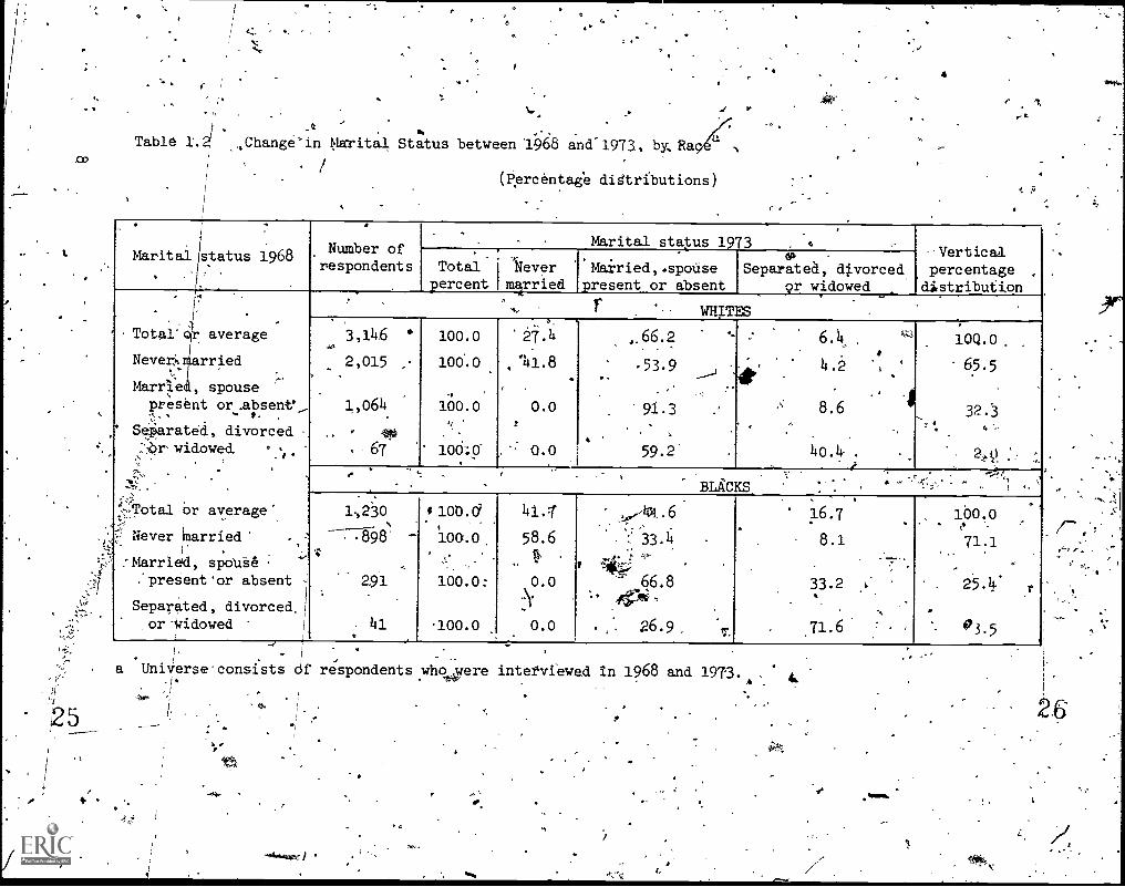
declined from 52.1 to-43.4 percent for the white young'women and from,48.2'to 13:3 percent or\their black .counterparts.4 Parallering'this,decline, there were majo shifts'in'household and-maritallmtterns, asevidenced by. the, sharp decline in the proportions of young3women livingwith their parents andthe concomitaht,increase in the perC'entages whowere married. As may be noted in Tables 1.1 and 1.2, there aresignificant racial variations insome of these changestWhereas in1968 the household compositions and marital statuses of.the young blackand White womeh are somewhat similar, by 1973 there are dramatic,.-distincti.ons. In 1973, 42 percent of the black women had never 'teen ..married and ,17 percent were ,eit4er itparated, divordeed or widowed,Compared 'with only 27 and 6 Vercenp, respectively, for the white women...
' Whereas two -thirds'of,the white Women are in an.intactdarriage, onlytwo-fifths of the black women are living with husbands. 15arallel,differences between blacks and whites: are evident in the data on house-
.
hold stitue. Black women in 1'973 are somewhat more likely than whiteto' be _living with their-parents and we twice_ as likely to be' in a;living 'arrangement'that does nOt'include'either parents qr a husband:,These data suggest ttat from the perspective of living arrangements,-
"..te transition to adulthood for the average black woman may be farmore complex than eor rter whitecOlinterpart. They also suggest that'substantially'grater proporions of yeung adult black women need .
'employment as a*primary means of supporting themselyes during thisdifficult transitional period.
. .
,
4Because of the many social and economic differences between the
black and white young women, virtually all of the discussioh in thisand subsequdnt chapters Will be baied on separate racial Tlyses. '
i .
. 4.
21

.4
. -V& E . ...
A.f.
° ; n
air, ,. MF:,;=.--- , t( and,B) Tredds in. Selected Sciode graphic aracterPstics
for White anf Bak lomen, 1963-to 1973
90
So
70
50
ho
. 30
20a
ry00W
r
700
66
10
0
90
80
50
30s
10
6
0
-4
e
Win "PES, ( A )
, 4
/4
'Moved in
Ever- .
arried
Children
Live with- arenas
Enrolled---in school
past- year
x
44.1.4.44.
I 1 )
1968 1969
I
.
Pcilled in. ..
Moved 'in pastI -1-- year',
1970 1971 1972 1973
BLACKS( (
Childry. -
Ever-.married
.
b
Slirvey Year*
*44
ti
O

r
'Table 1.1 'Change in Household Structure between 1968 and 1973,,by Racea
(Percentagedistributions)
. \
Household status 1968
'
...
a.
w.
:Bumper ofs-spondentsrespondents
Household status 1973Vertical
percentagedistribution
Totalpercent
Lived withpaientsb .
1.,* ed withStsband.
.,0
Other
.., .
4TotalPor averamN.
Lived with parentsb
Lived. with husband
.Other
_
Total or average
Lived *th parentsb
Lived with. husband
Other)
...._
WHITES
3,146 ,
.1.930, 981
235.
100.-"0
-100.0
100.0
100.0
'
.
20.5
31.6
2.2
2:-.W
64.,2
.3 f
,90.3
57.9
15.4
16.1
7.5
N.9.7
t, 100.0
62.2
- 10.0
. BLACKS v
1,230,
796
:. :239
195
100.0
100.0
100...0
100.0
28.6
40.5
.6.4
10..4
t'
-
: 39.1
31.3
67..9
32.6.-.
'
,.
.
32.2
28.2_
25.7
. 57.0
, 100.6-
63.2.
20.9
15.8,
,.
-,
a
b
23
. ,.,
Universe consists of respondents, who mere interviewed in 1968 and"1973Indludes veri-Rball percentages'Uess than 2 perodht). of respondents living with parents)and husband. . J
.
4.
e
,
7,
.24-
I '
%.
Table 1.2 ,,Change' in Marital Status between 1968 and" 1973, by,Ba
(Percentage didtributions)
2
_
1
Ma rit al status 1968.
i
Number ofrespondents
.
Marital status 1973Vertical
percentage ,
distribu-Eion
Totalpercent
Never ''Mairied,.spousemarried present or absent
e13-
Separated, divorcedsr widowed
Total" average
Neveri, rried
MarrZe , spousepresent or
._absent',
p. .
Seiarated, divorcedwidowed. * /
.
..!1Z.'.
.
..
-Total or average.,,
Never married' .:..,
Married, spouse:present'or absent ,
Separated, divorced.or Widowed
I
_ *
... r WHTTES
.0.
3,146
2,015
1,064.
44$
. 67
,*
100.0
100.0
100.0
.'
100'..0
0
'27.4
'41.8
, .
0.0
.: 0.0*
..66.2
.53.9
..'
91.3
59.2
**
.
---i
. :'
:
.
\
.6 4
4.2
8.6
-
40.4
.
.
I
.
",
,-4
'
10Q.0
65.5
.
32.3O
, 2,t1 ', -
e . e
. tBLACKS
,. .
.
.
,230
.898
291
. hl
-
,
0 100.0i
100.0
100.0:
100.0
41.758.6
.
0.0A. .
.
0.0
,,h4..6..- -
- .. 33.4.,..
66.84.7..ti ,
26.9 'T
.
16.7
8.1
.
33.2
J1.6
.
.
,
. 100.0,... '.
71.1. .
25.4.
03.5
.
a Universe'consists Of respondents who were interviewed in 1968 and 1973.1 A A
o.
0
-.11414.1407 /

'r.
e
While a comparison of statuses at just two points in-time fiveYears.apart is an obvioui-simplification of the dynamics of 'change,there is one other major point.worth noting in Tables 1.1 and 1.2.Whereas black women were less likely to move into a.marriage duringthe hilf decade, they were much more.likely to move out of marriage.About one-tentheof the white women who *ere married in 1968-were-either separated, widowed or divorced in 3,973, compared with one=thirdt .
of their black counterparts. This large and.growing group requiresspecial employment-related assistanoe,3a fact highlighted in Chapter 7.
.Tables 1.3 and 1.4 suggest that these cohort trends in changesin family and Marital status represent more than.justan agingProcess.Comparing-black and white young women who were 20 to 24 yearvof, agein 1968"With women the same age in 197.3, certain secular trends maybe noted. There appears to he a trend t'bward delayed marriages as,indicated by higher proportions never married in 1973 and lower pro-portions married and living with their husbands. Also, the proportionof women age 20,to 24 who were separated or diVorced increased over thefive year period. All of-these changes are consistent 'with' thesignifi.cantly greater proportions of white'and black women living in ."other"' household relationships--nOt yith parents or a husband. Indeed.-
1973, about 19'percent of white and fully a third of black 20 to 24'yea.? old women were not living with either their parents or theirspouse.. On average; these women presumably may have a greater needfor self'earned income than women living inother householdarrangements.
Paralleling.these rather dramatic change; in household and maritalstatus.are Sharp increases in the percentage of women with children.FigureIA:depicts the overall trend,-and Table 1.5 describes thepattern'in greater detail. The percentage of white'women who have hadat:least one child increases from slightly under one-fourth to Aboutone -half during the five-year period, and the corresponding proportionof black women increases from one -thirAb aboi, two- thirds. The dataindicate that this-childbearing period: is far from camplete - -consistent._With the knowledge that'the youngest women in'the stuay,are only 19years of age as of 1973. Over 60 percent of the white and 50 percent '4of'the black women yhb had no children in 1968 still had notgiV4n birthby 1973.
kg. -,
Table 1.6 indicates somewhat more fully the demographic transition.process these women are ,currently undergoing. : Only about 6 percent of'those white women who were 15 to 19 in 1968 had borne a child as ofthat date. By 1973, about 36 percent of this grouRrhad-boime at leaStone child. Shifting momentarily.from one age.. group_ toanother,-between 1968 arid 1973, the-proportion of *omen who were mothersamong those who were 20 to 24 in 1960 increased from about 43 to71.percent, .. , . - ....
.
.
Whereas the above represents the'increase in motherhood due to4-
. , .
aging per se, a not surprising phenamenon, the secular change for*,.
k .....,

Table1.3 Household Structure for Selected.Age Groups in 1968.and ).973, bk Raeea
(Percentage.diOtributions)
,
Houaenold structure
.
1.968,.; 1973 ".,
"Age 15-19 lAge'20-24
.
Age 204204r
Age 252- 29%,
,
. WHITES
Number of respqndentd 1,571 1,301 1,571 1,301
7fotal percent - 10,p) 100.0 100.0 100.0
Lived with parentsb . 86.0 28:9 26-9 7.0
Lived with husband, 9.0 . 58.1 54.3 80.2
Other' 4.9 13.0 18.7 12.8
.. .
BLACKS
Number of respondents 686 426 686 426
Total Idercent 100.0 1Q9.0 100.0 100.0
LivectviwitA parentsb 80.9 34.9 33.7 - 16.2
Lived-with husbard . 7.7. .14140 32.9 51.2
Oth- ' 11.4 24.1 33.5 32.6
t ,a Universe consists of respondents who were interviewed in 1968 and
'1973. .. .
b Includes very small percentages of respondents,living with parents
anthhusband.
'10
.N
F

Table 1.4 .,Marital Status for Selected Age Groups in 1968 and
' 1973, by Racea
(Percentage distributions)
Mpiri:tal status
.
1 68 1973'.
Age 15-19 Age 20-24 Age 20-24 Age 25-22
,1W.
Number of respondents
Total percent
Never -mArried
Married, 5ponsepresent or absent
.....
SPparated,,divorcedor widowed .
. .. ss
Nly.mbPr of respondents. .
Total uPrcAnt .
-%
Never married
Wrried, spousP .
present orabsefit -
Separated, divorc*Mor widowed ' 1 .
WHITESIr.
.
.
1,571'
100.0
88.6
10.7
n.8,
/
1,301
10d.0
34.1,
61.8
,('4.0
,
,
,
1;571
100.0
37.8
56.5
5.8
1,301
100.0,
10.p:4
81.9
8.0
-BLACKS. .
.
.
686
100.0 .
88.6
10.7
.
.0.7 -:-.
,426
100.0
14.1
48.0
'
7.9
686
100.0
52.9
35.5
11.6
#426
300.0
22.7'
53.7
23,5.
- 4
a.vniverse consists ntrespnndPnts interviewed in 1968 and 1971.
A
.44
2911
a

.30
Table 1.5 --Change.in'Paren-qal Status between 1968 and 1973, by Racea
(Percentage distributidns.). .
P ar e n t al status i 968lumber ofreSpohdents
.
.Parental status 1973 . ..vertical
'percentage_
distribution1
*tel.percent
No,
ciiiidreh'
_
Youhgest'presahool(0 to 4.)
'Youngestschool age , ,
(age 5' or pver)-
. ,
,
Total or average-
No children. .
Youngest preschool(age 0-4) :
Youngest school age".(age 5 or over)
,
. .
Total or average; ''v
No children
Youngest preschool(age 0-4)
Youngest school d'ge(age 5 or, over): '-'
.
7-. ., WHITES . .
_,
.
3'4.45
2,436
.
691.
38
100.b
100:0
106:0
100.0
50.3
'63.8
1.3.
0.0
'42.1
36.0- 4;
64.1.
57.3
.
%
-
-7.7
0.2 ,
34.6
42.1,
..
. .
, - .
1000 .
78.4
;..
:'21.1
.
o-.5
-. BLACKS . -
-
.
1,229
847. .:
.
. ./.. 369 ''
.
.
13/./
'
100.0-
100.0-
100.0.
100.0
35.4
50.9
, 3.3
.0.0
52.8
48.7,....
,
63.5
, 10:4
,
11.8
: 0.4
33.2
.
89:6
.
.
--
:
. 100.0
.67`5
. ,
.
31%1.
.
1..3
a Universe consists of respondehts'who were interviewed in 1968 and.1973%'
-
ti
40.
.31

4
A
V
Table.1.6 Earehtai 'Status for Selected Age- Groups in 1968 and1973, by Racea
' I,.
(Percentage distributions).
.
sstatusParental tatus.
,968.
Age 15-19 lAge 20-24. Age 20 -24 Age 25 -29.
..
.
Number of respondents
Total percent'
No children
YOungest preschool.(age 0-4)
e - .
youngest school age(age 5 or over)
.
.
.
Number of respondenis
Total percent
No children'
Youngest preschool:. .
(age 0-4) '
Youngest school age(age 5 or over)
. WHIMS
1.570
100.
94.3.
5.6
0.1
17
.
1,301
.100.0
57.4
41.3.
1.2
1,570
100.0-
64.2
34%5
'..
1.3
\
1.,301-
100.0
28.9
55.5
---
15.6. ,
BLACKS
-686
100.0
82.8
17.2
0.0
.
,425
100.0
42.8,
54.1.
3:1
686
100.0,
41.6
.
55.2
. 6.2
425
100.0
23.2
53.2.
'23.5
a Universe consists of respondents who were interviewed.in 1968'and,1973.
32
V
-
13
/0

given age group over the five-year period Is actually in the oppositedirktion. Among white women, the proportion of 20 to 24 yearoldswithout children increased fairly sharply from 57 to'64 percent,cwth1stent with the marriage and household information noted earlier.This trend towards.childlesSnes or a later average age for child-bearing has major impliCations for tI'e proportion of young adultwomen who can be expected to seek emplOyment now and in the yearsahead.
While the longitudinal dimensions of the NLS do not permitmeasuring secular changes in the fertility patterns of women age 25to 29 1973, there is one IMDbrtent'point concerning this group
/- worth noting. Since the average black woman in the original 14-to24-year-old ,cohort began her childbearing, at a somewhat earlier 8,g9,4-she. is now further, along in her Family building process than. herwhite counterpart. That is, az examination of the distribution of25 -to 29-year-old black and white women by parent statui-indicatesthat even though a slightly higher proportion of-the black women haveborne a child by 1973; a significantly higher proportion of thosewith children now have a youngest child of school age (about 31percent for black 25- to 29-year-old women compared with only'22percent for the White women). This evidence strongly supports thenotion (documented in some detail in Chapter 3) that this generationof black women intend to have only,a limited number of children-andeither are or soon will be seeking meaningful employment opportunitiesfor a lifetime of work.
Changes in Labor Force Participation
Whereas the association between childbearingand 'employment statusmay be noted from the overall'labor force participation rates and thepercentages of women with children described in Figpres 1.1 and 1.2, .1the impact of the birth event and of changei in child'status may be .
more directly noted in Table 1,7, Women who were without children bothin 196a and 1973 had by far the sharpest increases in labor forceparticipation during the period. In 1968 _their rates were onlymoderate, reflecting their younger. &ye-rage age end, greater schoolefirallment`rates. By 1973, the majority of these women had entered _
employment. IP all likelihood, many in this group will show significantbut tempbrary declines in their labor force parti ipation in the
aring years'. White73 evidenced sharp
cateaoryah all these ,
immediate years ahead as they enter their childwomenwho had their first child between 1968 anddeclines in participation. whereas black-Women in thevidenced a modest increase in participation: Even'thwomen had A child of Preschool aae ix the home, about 42 ercent ofthe .
white women and 57 percent of the black were in the labor force at the'time of their 1973'interview. This croup is analyzed in-Iftail inChapter 3. Finally, women, who had their first, child before 1968hadminor increases in participation during the period, 'pertly reflecting
t),ile aging of their youngest child. White labor force participation
3:3

Figure
100
ao
70
60
513
GO
h0tf)
3 0 )-4-)
20
C' 10nt:1
0a )-sca 90 - 145
80to
(,)sm GO -a)a.
506-
.
-1.2 (A and B) Trends in Selected Socioeconomic Characteristicsfor White and Black Women, 1-968 to 1973
....
In labor force
Planto work
at age 35
Emptoyed-r-full time.
EidiCKS (B)
Plan to work- at age' 35
labor force
/4030 -
10-
I01966
Employed/full time:7
01.k'
I.
1969 1970 1971 1 19726 1973afigh-
Survey Year
34
ip
15
.1
fl
4,4

35
R 0e
Table 1.7 19,e1-ental Status and Labor Force Transition between 1968 and 1973, by Race;
:.-_.:
Faiental stalus.
.-
.
.
, ., -
Humber of.
respondent's
.,,
Total'percent
.
CompaAs9n of 19681973 labcir-f914ce
is______1( -cet-'Thut*:9ns).
00 1968f In 71 968
in 197319r6 1973
andatet:Us, .
;
Labor forceparticipation rate
,
Out 1968out 1973
In 1968I
in 197319681973
: ''
Change1968.-1973
i,
Total or average
Had no -children by 1973. -
Had first child betweeni3 1968 and' 1973
, '
'Had first child before1968 '-
.
Total or average
,Had no 'children b 197j
Had first child b ween,'1968 and 1973
Had first child' before- 1968
.
)
WHITES "' .
.
.3,127
'1,518
. . .
W1
708'
-100.0
100.0
100.0-
100.0
29.4
40,5
o
]A.9
22.4
16.5
8.3. .
> 3441
"12.9
'2,57.0
114.o'
24:2
.
42.4
.
31.1
37.3
26.81
22.3
47:6
45.5
60.9
35.2
.
60.4
77,8
41.7
44.7
+12.8
+32.3
-19.2r
+ 90.5
\
. BLACKS .-
1,215'
421
411
., 1.,
383
.
104.0
_1'00.0
100:0
_ .
100:0
.
29.9
41.3
26.6:
,,ft
Al..4
13.9
6:9
. -17.(;--
, 17.9 .
;24.3'
r :ID. .
2 41
'25.1
3 ,9'
2;./ 8
30.3
35:6
45.8-61.8
36.7'
41%4'56.9
53.5
71.1
.
57.0
+16:o
, +34.4
+ 9.5
. .
+ 3.5.
-a 6niverseconsists of respondents wfio were interviewed In 1968 and 1973.
36
o
:

00
rates for this group i4creased about 9 percentage points compared witha more modest increasef 3 percentage points Ybr the blacks.
The' longitudinal character of the data set may be utilized. toprobe somewhat further into the dynamics of this labor force transition.For'example, while the labortor66 participation ratefor all whitewomen in the sample. increased by about 13 ?nts between-the 1968 arid-1973 interview dates, in' actuality about 1 percent of the women werein the labor force in 1968 and out in 1973. Conversely, 29 percent were'out in 1968 but' hart entered by 1973.. For the black women, labor forceparticipation increased by l&points representing a "netting out' of
- the 30 percent who entered the'labor tOrce and 14 percent who exited.These estimates are, of course, gross understatements of the actualPlows into and out of the -labor force during the period, as a givenindividual could well have had numerous such moves during the *five-yearperiod. -
The above patterns are useful for describing the general natureof the gesocfati-On between work and childbearing. They also demonstrate,'that whenever one generalizes about such patterns for a group asdiverse as'a full cross-seqtion-of young women, onetmust be.awarethat there are "substantial numbers of individuals whose experiencesrun counter to the described pattern. It may well be that thesedivergent grpiaps, from program and policy perspectives, representindividuals with spe9ial and different needs. For example, it is notunreasonable to speculate that the 15 percent of all white women and27 percent of all black women who gave birth toga first child between1968 and 1973and entered the labor force during that period representWomen with a very high commitment or strong economic need to work. Assuch, they may well be especially worthy of careful analysis.
Much of the above discussion has highlighted changes in both,
demographic and labor force ,characteristics of.young women askociatedwith the maturation pto ss as well -secular changes. The oberall
_.,
ISClabor force particip on-changes citeeiargely reflect changes in --
hougehold and family structure: Focusing once agafh somewhat morenarrowly on the.20-'to 24-year-old groups in 1968 and 1973, some ratherdramatic short term'secular changes may be'noted:- The overallrlaborforce participation rate for white 20 to 24 year olds increased fromSbout56.-to 66 percent in the short five-7year period (Table 1.8).It is to be noted thatthis secular chnage does not reflect a demo-'',graphic phenomenon but rather,a dramatic 11 point increase in theparticipation' rate of 20-7.to 24-year-o14 women with children betweenthe survey agtes. .A.,..smaller, but still )alotatiletrend:was eviden4p for-black women., Th4s, independent_of,all the demographic factors notedearlier, there have been 'major changes in the willingness and desire ofyoung women with children to participate in the labor force.
.,-.
.; .
/ _Several secular trends have been documented or at least:alludedto above. They include apparent changes in patterns of household iind
. .
c.
3
c
17

Table 1.8 Labor Force Participation RatesiCor Selected Age I,
Groups in 1968 and 1973, by Race and Parental Statusa-
Parental status
..
,
1968 1973
Age 15:) Age 20 -24
.
Age 20-24] Age .25-29
Nuinber of respondents.
:Total or average
-Child on survey date
Na child on surveydate' .
Number of respondentsr.
Total or average.
Child on survey date
No child on surveydate
WHITES .
1,564
42.4
36.6
42.7
1,290 e.
57.8
34.4
7.5
1,564
p5.7
45.5
77.0
.
1,290
53.4
41.1
84:2
BLACKS
679
38.2
52.2
35.2
,
419
'60.5
51.4
7.4.7
679
62.8
57.2.
71.2
419
61.7
-, 57.2
*76.9'
Universe consists of respondents who Were interviewed in 1968 and1973.
18
O
34
r
AW
family relationships, changes in childbearing patterns as well assecular increases in working propene,itieg. All of'these factorsundoubtedly represent components of the generally acknowledged movement
./towards greater equality betWeen the.sexes in the rights and
/responsibilities of.adulthood.
;
Changes in Other Work-Related Characteristics
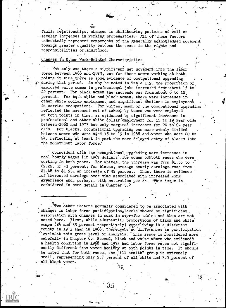
Not only was there a 0.-gnificant net movemeht.into the laborforce between 1968 and X1973, but for those woMen working at both
L points in time there is some, evidence of occupational upgrading#, during that period. As Ay be noted in Table 1.9, the prOportion of
employed white women ih professional jobs increased frdm about 15 to22 percent. For black women the increase was from.aboUt 6 to 12,percent. For bqth white and black women, there were increases in.other white collar employment, and significant declines in employment .
in service occupations. For whites, much of the occupational upgradingreflected the movement out of school by Women who were employedat both.points in time, as evidenced by significant increases inprofessional and other white Collar employment for 15 to 12 year oldsbetween-1968 and 1973 but only marginal increases for 20 to `N4 yearolds. For blacks, occupational upgrading was more evenly dividedbetween women wHo were aged 15 to 19 in .1968 andwomen who were 20 to.24, reflecting at least in part the more delayed entry of blacks intothe nonstudent labor force.'
I
Coincident with the occupational,upgrading were increases inreal hourly wages (in 1967 dollars).fd?. women ofthoth races who wereworkingin both years. For whiten, the increase was from $1.55 to$2.22, or-43 percent; for blacks, average hourly earnings. rose from$1.48 to$1.95, an increase of 32 percent. Thus, there is evidenceHof increased earnings over time associated with-increased workexperience and, perhaps, with maturation per se. This issue isconsidered in some detail in Chapter 5.5
- 5WO other factors normally considered to be associated with
changes in labor force partidipation,levels'showed no significant,
association with.changes in-:Work in overview tables and thus are not. noted here. First, while substantial proportions of black and whitewomen (24 and 33 percent respectively) were `living in a-differentcounty in 1973 than in 1968, there,weremo differences In participation'levels-let this gross levei of analysis. This issue is .Considered morecarefully in Chapter.6.e. Second, black and white women who evidenceda health condition in;1968.and 1?73 had labor force rates not signifi-cantly different -from women healthy at both Points-in time. It shouldbe noted that for both races, the.;'ill health" group is extremelysmall, representing only.2.7 percent of all'white.and 3.5 percent ofall-black women.
3.9
19-
1
4

1 0
O
4u
Table 1.9 Occupational Distribution for Selected'Age groups'in 1968 and 1973, by Race
(Percentage distributions).A ov
. ,
Occupational ,
distribution.
. All respondents,
.
...Aga 15-19 in 1968 Age 20-24 in 1968
1968 1973'
Change1968-1973
1968-- l
1973 Change , 19681968-1973 1
1973, Change1968-r73
'.
.
Number of respondentsTotal percent s.
Professional .
Other white collarBlue collar .'
Service
.
NUMber of respondents. Total percent-Professi dal .
Other- it allar '
Blue collarSet/lee
..11TES825
100.0'15.5
4.4.7
10.529:3
825
100.022.152.711.214 0
,
+6.6+ 8.o'
.+ 0.7
.-15.3,
364
too,o'
4.144:69,7
41.6
364
100.015.256.5''11.1
-x(.3
+11.1+11.9+.1.4 :
-24.3 :
' 415,
100.025.447.311.8135.5
415100.Q.29.348:411.610.7
+ 34'+ 1.1- 0.2- 4.8
.
. BLACKS.
27306.0-6.234.321.4
37.9
273:100.0011...7
39.821.8,26.4
-
+ 5.5 ,
+ 5.5.-. + 0.4
-1'1.5
103I.Op.o_2.1
,36.316,6
4.5.0
_ 103
.1643.0
, 7.144.321.7
26.8
--.;
+ 5.0+ 8.0+ 5.1
-18.2 .
155
100.09.6
33.125.531.5
155100.015.536.323.5
- 24.7
+ 5.9+ 3.2- 2.0- 6.8
a Universe' consists of respondents who. were interviewed and,:employed in 1968 and 1973.
4
4'
t
.
I -
Some Perspectives on Attitude Changes
There is very little. evidence of unhappiriess with-work among:thosewomen in our sample with the most extensive work attachment. Focusingon those women employed in 1968 and 1973, fully 90,:percentlpf the whiteand 85 percent of the blaci women said they liked their-'19§8 jobs
(Table-1.10). There were only minor changes in-these feelings'between r.1968 and 1975 as the proportion who liked their jobs "very much"declined about 10 percentitge points during that period, being offsetby a corresponding rise in the proportion who,liked their jOS"somewhat." Also at the disaggregated level, it is of\soge interestto note that whereas fewer than 10 percent of those whO liked ,their-jobs in 1968 disliked their jobs in 1973, more than 80'percent of thosewho 'had disliked their jobs in 1968 liked them in 1973. Mere was nodifference in he responses of 15to 19 year olds in 1968 and 20 to 24year .olds in his regard.). There.are several possible explanations forthis. Fi unhappy workers are probably more likely to leave thelabor for e if they have the option to do so. Second, unhappy workersundoilbtedly are more likely to change jobs in a search for moresatisfactory working conditdan.
In addition to the Specific feelingi'of job satisfactiOn of theworking group of women, there is evidence of profound change between1968 and 1972 in the.attitudes of young womentoWard the propriety of-aabor market activity on the part of mothers of young children.6 'Onemight anticipate salted shift toward more positiie-sttitudes about workamong Young women as they mature, marry, and gain work experience.
. However, of greatest interest is theclueation'of whether there aresecular.forces at.wdrkwhich have caused U6men with the same charac-teristics to be more positively disposedtowafd Fork icutside the home.Table 1.11 provides sonde' dr c evidence in this regard. :Within agiven year (either 1968or 1972), ere,is only weak evidence of .
shifts towards'MoreTositive work attitudes as one move's fromioungerto older respondents. However, if one co.pperes 18 to 21 or 21 to 24year'olds across years, there are large shifts towards more positiveattitudes. For example, the proportion who believe that it is all,right for a young mother to work if the husband aDidwife agree increased
- .
06These are.the only two years in which this series of work
attitude items were asked. ThequeStions read as follows: "Now I'd
like for- you'tO. think about i,family.where there is'a mother, a fatherwho works f411 time and several children under school age. A,trusted#relative 'who can care for the children lives nearby. In this family-siluation,'how do you feel about-the mother taking a full time job.outside the home? (a) If'it is absolutely necessary to make ends meet.(b) If she prefers to work:and her husband agrees .(c)' If she prefersto work, but her husband does not particularly like
42
. .
. 21
.r.
t
0

Table 1.10 Comparison of Job Satisfaction in'i968 and 1973, by.Racea'b
(Percentage disirib
.
;.
Feelings about1968 job
,
Number ofrespOndentt
-%.
Feelings about 1973. job Verticalp9rcentagedistribution
Totalpercen
Likemuch
Likemewhat
Dislike-
.
Total or average
Like much
..Like somewhat'''.
Dislike I
Total or average
Like'much'
Like` somewhat
Dislike
-
.
: o
512 :,
307 .
155
50
100.0
100.0
100.0
100.0
1.256.3
42,2'
46.7
39.6
36.3.
46.5.'.,,-400'38.9
9.2
7.4
111.3
14.4
100.0'
60.4
, 29.6
. .10.0
'
* . BLACKS .
-..,
200
108
'65 '
27'
s
100.0
100.0.
100.0
100.9
46.7
53.5
35.7.
42.6
42.5
35.5
57.9
38.4.
.
11.1
11.0
6.4
19.0
100.0
54.9
29.8
15.6
_,
4 a Universe consists ofrespondbhis'who were-employed in 1968 and 1973:b Job satisfactidn is based on responses to the question: "How do you
feel about the job you have now?"
sw,
22
.1
0
,t
43.
4
\.
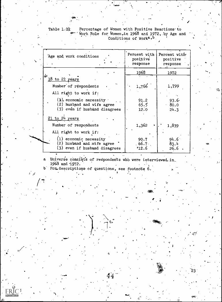
Table 14 Percentage of Women with Positive Reactions-to14ork Role for Women,in 1968 and 1972,-by Age and --,
Conditions of Workasb
.
Age and work conditions
.i .
.
Percent withpositiveresponse
Percent with,
positiveresponse
.. 1968 1972
18 to 21 years
Number of respondents . 1,766 1,799
All right to work if:
(1). economic necessity 91.2 93.6(2) husband and wife agree 65.5 80.0(3) even if husband disagrees 12:0 24.3
21 to 24 years .
Number of respondents 1,362 1,839
All right to work if:.
.
(1) economic necessity 90.7 94.6"--- (2) husband sand .wife agree-
. 66.7. 83.4(3) even if husband disagrees '12.6 26.6 .
A
a Universe consists of reSponderits whb were interviewed.in_1968 and 1972.
, .
b' Fot.descrdptioris of questions, see footnote 6.
6.
.44"23'
..
s

o
froth 66 to 80 percent for 18 to 21 year olds and'from 67 to 83 percentfor Rl to 24 year olds_in the four-year period, Large increases alsooccur in the item asking if it is all right to work even if the husbanddisagrees. -
°Table 1.12, -which focuses more narrowly on the responses ofever- married women, shows the same trends. When the queStion is whether
0... labor'market activity by the mother of young children is.appropriateif her husband agrees, the proportions of positive responses among(the same) white women increased sharply from about 68.to 85 percent '
over the four. -year Period', The same' pattern was found when married 15to 19 and 20 to 24,year olds were examined separately. Less dramatic "*-
i
)
creases occurred. for black women, reflecting the - higher level'ofp 4tive respbnses by these women in 1968., It is also of some interest .
to note that whereas -only 12 percent of the white women whO gave apositive response in 1968,had shifted to a negatiYe response by 1972,fully 79 percentof those who had a negative attitude in 1968 hadchanged their positions by 1972, All of this suggests that there aresocial forces at work that are altering women's basic perceptions oftheir role toward a stronger work orientation. That these attitudechanges are reflected in actual behavior will be evident from theanalyses in several of the_following chapters\
'Highlights of the Volume and Some Polley Implications
. o ,..,-
The( research presented in this volume focuses,' directly and -.
indirectly, on questiOns associated with the prospective lifetimework activities of women who are in their early adult years. It is
. clear that a' slab,stantial proportion of all such women, for varyingreasons, will spend a major part of their lives in the labor force.This volume Considers several factors associated with this trend,including the.educational and ti-aiping experiences of women now
'reachingreachihg adulthood, rationales associated with work attachment duringthe early years ofi'marriage, and the implications of marital breakdown
of family mobility, patterns for work and career.;.
. . . .
In several important ways, the potential quality,of the liffetimework-experience is contingent on the respondent's background. Not onlydo parental factoYs directly affect the quantity and quality of a youngwoman's educational experiences (Chapter 2), thdy also have's. signifi7
.cant effect on the typeof career path a woman plans to follow (Chapter_1)t. In addition, the direct-impact of parents on a daughter'sdubational desires, expectatiOhs and actual experiences will
ultimately alter both the quantity and quality of her adult work(. behavior. \ .
. .
is,--..-
We have found, not unexpectedly, that social class background,particularly parental income; is'a powerful determinant both of thelikelihood of college attendance and of the quality of the collegeattended. This social class factor operates by affecting a youth's
. .
24
3 &
, 45

4
T6le 1.12 Comparison of, Percentageoff
Women Who Feel It'IsAcceptable to. Work Full Time If Their Husbands Agree,
1968 and 1972, by_Racea,b
Attitude 19684
4,
Number ofrespondents
Percent with positive'attitude in 1972
Verticalpercentagedistribution
..
'
'Total or average .
4 _
Positive attitude
Negative attitude
,.
Total or, average
Positive attitude
.Negative attitude"
-WHITES.
1,151.
7$7
_e364
.85.2.
88.0'4190
- 79.3 .
.
100.0
57.6.
, 32.4
BLACKS
3434e V.%
296-
k7
91.4 .
93;3
-- 81.3
(100.0,
90..86.1
13.8
.... . .
.
a Umiverse consists of ever-married respondents who were interviewed in 4
190 and 1972. .
. ..
b See footnote 6 for full definition of question. ."Negative Attitude"includes a small'numter of "no opinions" or "Don't khows.w ,
,. i.
a.
4
4 6'
441
4.
25.
4),, .

o
educational desires and, more directly, by determining at leastpartially her ability to afford college.
.c....,.....,
. _Whereas the above'conclusion is pefhaps no surprising, what is
'of more than academic interest is the rather striking fact thatthe .
lesser likelihood of black -youth to desire and actually attend collegecan be fully explained by the different socioeconomic characteristics .
of the two racial groups. 'In other words, a black:young woman withsocioeconomic background characteristics similar to the average whiteyouth is, if anything, more likely tO desire to attend and actually.attena.college. '
. .
4.,
As a ceirollaryto this economic theme, there is evidence tha'-the parental incolerfactor-becomes even more dominant, as a'predictor'of.college attendance during periods of high unemployment. Thus, allthe evidence in this volume is.highly consistent with thestho6gbt thatequality,of education, particularly at the college level, might be'-fUr-therd through. income subsidizing measures which would enable'mord.students from low income environments to attend college. This statementis relevant not only with regard to attendance per se, but'equally withregard.to a youth's ability to attend college commensurate with herability.
1.
_Moving from'the dynamics' of the educational attainmedt.process into
tri
the early years of work attachment, the imports: e of socioeconomicfactors continues to be evident. Whereas virt llkalltWomen work at. .
some point after leaving.School but before the, birth of their firstchild% major racial 'and socioeconomic.differefices begin to appear as
. ,
the birth event 'approaches ('Chapter 3). First, black_young women,particularly 'the-better educated, are much more likely than white '
women.to be out, of the labor force for only a short time in connectionvitth the birth'of their first-child. In addition, the black woman not, .
only'returns to the work force more,quickly,but is' Mach more likely,toseek full-time employment when she does return': Indeed, over 80 percentof the black-women who return ,to the labor'force ultimately work, at ', .
least 35 hours a week. This is as high ajoroportion working Pull time/as.before-the,birth. Also, for)bOth black and white women w returnto the labor force, the better edUcatedare mucli better abl teimprove'lon the wages and,occupatiOnal status of theirprebirth..job*
, We have already notea that, if given theootion tlac women will.
seek moi'e and higher titian-VT education. This eduCation,'in turn,enhances their ability not only to maintain closer tieth.with the work
enjoy superidf occupational status' and remunqation$As clear,evidence of a selectivity prodess:'woMenning higher salaries in the labor, market-are more likely
.
their work ties. Convetsely, women with the least ecdhomicpowerthe 1Ns educated and skilled- -are least likely to
foree,but tIndeed, thercapable oftb maintainbargaini
find-and maintain employment at a reasonable wage level.
While it is_evident that a substantial proportion of all women plan'to have extensive ties with the-labbr market, the research repbrted i4
26,'47
'a
1
.

-t
Chapter 4 indicates that-there still are extensive labor .marketinformation lags tharimpede appropriate career decisions. In,general,when queried aboutetheir occupational plans for age 35, women tendea'to mention'only a limited number of Occupations, most of,tirhich are 6
jobs that have been traditionally held by women. Thus, it appearsthat the "Women's. liberation"moyement has:not yet made-significantinroads into the career thinking of young women. Moreover, some of.these traditionally female occupations represent econoticallyirrational choiceSunder existing circumstances. For example, amongthe college educated,..about one-third of he white women and almost a'quarter of the black plan to be in a teach g.profession by the timethey reach age 35. °This is an occupational area which currently does'.not offerthe best j41911rspects. There i , hciwever, some cause for.:optimism in this regard; between 1968 and 1 3 therewere decreasesin the proportions planning to,enter teaching as a career, perhapsreflecting a salutary' effect-.of maturation On,a young woman's -sophisticationlaout the world of work.
The fact that women are to.a greater degree planning more extensivecommitments to the labor force than had been true in the pa'st has major0implications, some of which are highlighted in Chapter 5. One mayexpect that young women will display a greater willingness to acceptoccupational' training for general as wellmas specific job skills even oat the cost of lower-initlal wages. In other words, there is evidencet 't women with stronger prospectiVe ateachments to the labor force aremore willing to accept lower initial wages as a price they, must pair. for4 current job:providing training and thereby promising higher. .lifetim.earnings.
Parenthetically, it is useful to speculate. about the possibleofR this increasing level "of work activity among young women for
the wo0 prospects of subsequent generations. To the extent that we4are now witnessing a secular change in the likely.iifetime work
patterns of women, supply and demand patterns for specific occupations--may.be different-in the future than theg.'have_been in the past. Forexample, most women have traditionally withdrawn from the labor, forceduring the family folmative years, sometimes returning 'for a "secondcareer as their youngest child .ages. These traditional patternsOf ,labor _force participation opened up .many job-slots for newgraduates in-an occupation like teaching.- fib the extent that the,current;generation of women will no longer interrupt their.dareerswhen children are born, 4obs a/Llable for new entrants into tile lalpormarketerowill-become more limi In times of high unemployment as atApresent, this si,tuatiohJs lik y to'be exacerbated for women willhave -a greater_tendency to ' ang on,"..to their 'jobs, in the justified
fear that if't4ey94t they-would, have a more difficult timeseeking to return to work.,-
,While'the'teaching profession, is-admittedly a rather extreme' illustration of this phenomenon, many.othe occupations, even tholewith relatively strong growth potential, could have been cited. The ,
4
t.
f
27'
A
O

. ,
4A a \
fundamental point is that; at least ;for the transition generation:\., ,major changes'in women's labor forCetwithdrawal patterns may well be
_ closely'associatecrwith greater labor force entry problems and, .r
concomitantly, higher levels of youth unemployment. Within this.
context'it is useful to emphasize once more the lesson to be learned-)41%,,,4,4
.--P-- .
*****f frOm Chapter 4; career' guidance must' make women aware of a 'broaderrange of posIsible jobs and careers than has traditionally been thecase. This would increase the..Dgxibi/ity of young women in seekingjobs or formulating career ideai during,a period when many-of the
,traditional avenues of employment offer only limdted'prospects fort... ._ .
sucCess. ... . -
,. .
Two other major events in the lives of many young adult women-- -migration and marital disruption-64o have major implications for .
their labor fOrde behavior. Chapter 6 highlights the major negativeiupact that the family tigrationadeeision can have on both the wife'sattachment' to. labor force as well as her annual earnings.. he, ,
research suggests that migration not only reduces the wife's' ings.
on average, but, as a iderect result qg this reduction, reduces tad, .
, 'family earnings as well. In other*ords, the increased-earnings of 4:the husband that accompany migrationdo not, on the average; compenSatefor t4,loss of earnings of the 'wife. From a purely economic . .
perspective one might thus queStioh the desirability of many moves.However, Ve results are consistentViihthe idea that economics maywell not be,',-the major motivating force behind many families' movesl-at
... ,
fleastj.nthe S
4O, rub.. 4
,,, :tPL. .-,:'. .Whereas migratiOn'tenda,toto' be, with reduced leyels of
'work attachmekti C aPter%T shows c;9arly that the-process of marital464 disrupt' geGnex. I# increases attachments to the work force,
- , partiCii 3, go white women. Thus, the ability to find meaningfuleMploym nab el 4endat least'partiallyto,CoMpensate fOr the.: -
loss of a' usb d's earnings...-4Vbe tepialtssliwst that' white womenare'able compensate for- 'lei 'ath'alf.of.theit husbands'' earnings -
loss thr g4 employment a.fer 'Sru/itipn; thelcorresponding statistic..i., for blaCk.women'is only about 15 perceh-C. Pe.ily as a result of this
increase in earnings, white family.i'dco e after the marital disruption'- (on a per capita- basis) rapidllfappips. es treUsruption levels=, This A
1 .- recovery is-not apparent fOr black'f. vies. Job related training4 to,
which white women also apparently 1- avbeyi reater access, contributes to
this ability to cope economically, as *men who receive training ire theyear immediately preceding a marital disruption tend to have higherearnings. as well as lower levels ofunemployAlent in the year fol49wingthe disruptionvent.
,. ''l' /.
.
,...
As noted.earlier, work discontinuities associated with childbirth, tend increasingly to be brief
VWork discontinuities and entry
patterns associated with migration and marital disruption are twoadditiorial.phenOmena which affect iirge numbers of women and whichare associated with a deSire'and'need !or momunerLtive eMployment.,:o
- 'What should be readily apparent is *tat/Whereas most young adult women4....
28
4'9.
4,
Na

I
. Aikt
work, they also commonly encounter life cycle events which'require atleast a brief interruption in employment. Me"tepver, many of these,women wish the discontinuity to be brief,. The more effectiVstheguid nce, training, and other work-related information young womencespecially'those with limited formal education) - receive, the greaterthe likelihood that the actual pattern of.work interruptions willmatch their needs and desires.
#
. yx
OP s
(
4
I
414
V
4
. .29
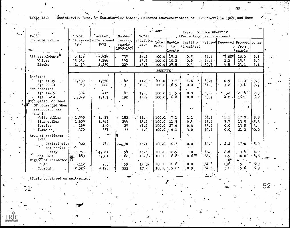
U.)
4
Table 1A.1 Noninterview Rate, by Noninterview RP-Neon, Selected Characteristics of Respondenti in 1968, and Race
,
-.
1968Characteristics
.
Numberinterviewed
1968
.
'Number.interviewed
1973
Numberleavingsample1968-1973
Totalattritior
rate
- Reason for noninterview
(Percentagedistributions)
'
Totalpercent
Unable Institu-to Itionalized
locate1
Refused Deceased.
Droppedfromsamples
Other
?
)
All respOndents b
WhitesBlacks
Enrolled.
Age 14-15,Age 20-24
Not enrolledAge 14-29
.. Age 20-24CCupation of headdf househo).d when
respondent wasage 14
, White cbllarBlue collarService :
Farm.. s-,
Area of residence .
SMSA .
Central cityNot centalcity
Not SMSARegi6rof residence
SouthNonsouth
5459'3,6381,459
.
4,4243,1461 1230
. 735.492
229
.....
14.2,
13.515.7
10040_100.0100.0
z,-;7,4111ITESI
15.2 I 0.5'
10.2 f 0.625.8 i OA
56.664.6
39.7
. `'3.p..
2.24:8
.
18.015.423.1
6.7
6.96.1
-1,532253
- .
504- .1,349'
.
1,599'1,609,
169-370
9001% .
1,2511,483
1,112
2,526
4350_-222
417
1,157
.-
-
1,417
1,365140
337
.-:'
764
'4,0571,321
.
9532.,193
1 82
31
87,
192/
i 182.,
244
29
j 33
*,..,436
194
,162.
159
333.
11.9
'12.3
17.314.2 ,
S'11.415.217.28.9
15,1
15';5
10.5.°.
14.3,
1.2
-'
100.0100.0
100.0100.0
.
,
100.0,
100.0--11.51000100.0
100.0
100.0100.0
100.0100.0
4
13.7.6.5
0
11.56.8
.
,7.1
27.6-,6.1
-
.
10.3
12.9
6.8-
12.6.9.0'
1.60:0
0.00.0
..
1.10.4
0.0.
.
3.0
..
0.0
1.00.64°'
0-.0
.0.9'
.
-
63.7
-61.3
63.266.7
.
0
63.7
65.655.2
69.7
a
64.0
63.966.o .
.
64.8'64.6-
0.5
3.2
- 1,14.2
1.1
3.70.00.0,
-. 2.2
- 2.61.9
-
,go3.0'
_
11.019.4
:21.8-16:1
.
17.0.
13.5 ,e5.313.8 -21.2
-
17:6
13.4-16.0'
15.115.6
9.3
9.7
2.36.2
.
9.9
3.4
`0.0
5.9.
6.2
8.6
6%9
6.9
(Table continued on next page.)
51
t.

o
' Table 1A.1 Continued
' 111
1968
Characteristics
',-
Numberinterviewed
1968
Number
interviewed1973
, .
Number Totalleaving attritionsample' rate1968-1973
. Reason for noninterview
(Percentage distributions)
Totalpercefti
t
I
Unable; Institu- Tefused1Deceased't"o l' dto 1 1 na ize
locates
Droppedfrom
samples
Other
Marital status. Married, spolise
.WHITES
present 1.154 1,015 '139 12.0 100.0 10.8 0.0 64.o 3.6 18.0-- r3.6Never married 2,345 2, 415 330 14.1 .. 100.0 10.3 0.9 .66.7 0.9 13.3 7.9Other 139 116 23 a6-:5 100.0 4.3 0.0 39.1 13.9 30.4 13.0Dependents .
'--- Child 802 709 11.6 100.0 rt.8 0.0:. 61.3 ,6%5 -18.3 .No hild 2,836 2;437 399 34.1 100.0 9.8 d:8 65.14 1.3 114.8 8 oLives wi h arents-Yes 2,250- 1,930. -320 14.2 100.0 .10.6 0.9 65.0 0.9 14.7 7.8-No 1,378 1,208' 170 12.3 100.0 9.4 0.0 64.1 4.7 16.5_ 5.Number of years in
1968 residence-'Less' than 1'
year. 381 329 52 13.6 160,0 11.5 0.0 481 7.7 23.1 9.6-1-4 years5-9 years
590 ,
370500
308.
90
6215.3
16.8 -
100.0Am.()
12.2.8.1'
0.01.6
61.156.5
1.1 20.0 -
22.65.6
N6.510 or .more
years 568 496 "T 12.7 100.Q -15.3 0.0 6 5.. 3 .0.0. 5.6All life. 1;699 1,489 210. 12.4 -10.0 8.1 1.0 , 72.4, 10.0 7.1Years of schooling'completed
l
EnrolledLess than
13 years 1,325 1464 161 12.2 100u0 10.7 1.9. 1.2 11.98 8.713 or morei
p.6_11!460 41)8 52 11.3 100.0' 9.6 0.0 65.4 0.04' 13.5 11.5
(Table continued on next-1540
4
,,r4
5.4

Table 1A.1 Continued.4
1968Charactristics
Numberinterviewed
1968
AYmaiber 'Number
interviewed" leaving19, 73 sample
ti968-1973
Totalattrition
'rate
Rason for noninterview
(Percentage distributions)
Totalpercent
Unablgto
Institu-tionalized
locate
Refused Deceased Droppedfrom
samplea
Other
Not enrolledLess than12years
12 years13 or moreyears
EnrolledAge'14-19
Age 20-24Ndt.earolled
.4e 14-19Age 20-2
Occupation ofheadof household whenrespondent wasage 14White collarBlue collar '
ServiceFarm 0
Area of residenceSMSA"
Centralcity
Not centralcity'
NOt SALSA
";--t'.
(Table continued on nextOr;
4971,030
326
-ho6
881
28"-A.
149
39
WHITES
18.54,5-
2.0
100.0100.0
1(70.0
16.54.0
5.1
0.00.0
- ,
0.0
BLICKS
, 51.4 -;
75.8
59.0
2.24.0
2.6
26.4
11.43.334.7
*10.3
666
50
255
488
332658
%
236.229
689
176
593
580.
1974o8
296549
190209 f.
560
1i9520
. .
page.) .
86 12.9
5 10.0
58, 22:78o I 16.4
36
109 16.,6
46 19.520 8.7
129 *,f
111,7
27 II 15.3. '?
12.3-71
100.0100.0
100.0100.0
1(16.0100.0
100.0100.0
100.0,
100.0i0o.o
37.2
27.6/2.5
25.023.9
'37.030.0
3_6.3
'33.3
39.7
0.0c
1.70.0
0.00.9.
0.0b. o ,
39.745:b
36.1.'45.g
32.6
0:0 4T.3. -
0.0 22.232.9
4.7
0.0
7.5 ,
.2.83.74.3
o.o'
5.4
3:74.1
18.6.
22.428.8A
,
36.1,
21:745.6
4.7
8.66.3
.
24 . 0
33.3 r 7.417.8 '4.1.
I
.!
eor.

1 Si
Table 1A.1 Continued:,,
Number'1968interviewed
Characteristics1968
Numberinterviewed
1973
Numberleavingsample
1968-19n
Totalattrition
rate
Reason for :oni.ttrrview(Pernentage distributions)
Total Unablepercent to
locate
Institu -
tibnalizedRefused Deceased Dropped
fromsamplea
BLACKS
Regionof residence''South 1 972 841 131 13.5 100.0 28.2 0.0 33.6 6.9 25.2Nonsouth 486 388 98 20.2 100.0 2204 1.0 18.0 2.0 20.4
Marital status .. 4,
' Married, spouse!present 4 310. 263 47 15.2 100.0 23.4 4).0 48.9 6.4, 17.0
Never married 1,060 898 162 '15.3 100.0 29.0 0.6 37.7 3.7 23.5Other ' 89 69 20 22.5 .100.0 5.0 .0.0 35.0 10.0 35.0.
CependentsChild : 451 383 . 15.1 100.0 '2540 0.0 41.2 7.'4 17.6No child 1,008 847 161 16.0 loo.o. 26.1 0,6 39.1 3.7 25.5
Lives with parenisYet 944 794 4150 15:9 100.0 30.0' 4440.0 37.3 4.0 22.0No 508-- 76." 15.0 100.0 18.4 1.3 f 46.1 6.6 22.4
Number of years 1.-11.
1968 residence`
,432
Less than 1 .4year 115 -- 95' 20, 17.4 , 100.0 15.0 5.0 35.0 . 5.0 .25.0
1-.4, years 151 117 314- -2.5- 1000 29.4 ; 0.0 5.9 20.65 -9 years 113 *'96 17 15.0 100.0 . c c c10.or moreyears -211 175 -36 17'.1" 100.0 19.4 o.b -27.8 2.8 47:2_
' All life 861 739.. 12? 142. 27.0 42.6 5.7 18to ..
-
(Table continued'on riext page.)
r
r
Other
6.1-6.1
'4.35.6
5.0
8.85.0
6.7
'5;3.1
15.00:0'
_
2,86.6
I
"re

Table 1A.1 Continued
3"
1968Chargcteristics
,Numberinterviewed
1968
Numberinterviewed
19.73
Numberleavingsample
1968-1973
TotalReason for nonintervieW )
(Percentage distributions)
attritionrate
Totalpercent
Unable Institu-to tionalized
locate
Refused Deceased Droppedfrom.'
sample-
Other
Years of schoolingcompletedEnrolled
Less than13 years
13 ormoreyears
Not enrolledLesb than
12 Years12 years13' or more,
years
BLACKS
'629
366304
552
73
297247.
61
77
l4
69
57,
12
12.2
16.1
OP
100.0 37:7 0.0 36.4 5.2 18.2 2.6
100.0 c *c, c. c c
sr
100.0 21.6 0.0 34.8 5.8, 29.0 5.8
100.0 15.8 1.g . 49.1 1.8 21.1-- 10.-
100
aJAny respondent who was not interviewed for two consecutive surveys was dropped froth the
b Includes.aital1 number 131' non Whites boner than"blacki."
c Percent* distribution not shown where base represents lesS,han 20 respondents.
1 .
e
1-1r.
sample.

INTRODUCTION
, The exteh of women's postsecondary schooling is an'important'aspect of their struggle for equality in the United States.,Theaccomplishments of adult women-are limited by,thair past aduqational. .
achievements, It is wll known that higher educational attainmentis associated with greater labor force participation, lower unemploy-ment, and. higher earnings. Thus, an examination of the education-related decisions of today's young women,provides one basis forpredicting their future position in American society. '
a
CHAPTER 2
YOUNG WOMEN AND HIGHER EDUCATION
4,6
Steven H..
Sandell and Rex C. Johnson
A
The National'Whgitudinal tirveys,phow thatopyhile 78 percent ofwhite and 76 percent of black youhg women in high school in 1968expressed 4 desire to receive some higher eduqation, only '52 percentof the white and 34 percent of the blacks young women actually enteredcollege the year after their senior year in high school. ft is ofobvious importance in_ establishing 8dUcational policy to determine theimPortance of ,socioeconomic. background and Ability_as determinants ofcollege attendance: In the first place, low entrance rates forpersons from low income families might suggest policies -that would easethe financial burdens-of college attendance for prospective studentsfrom these families'. Second, examining the likelihood of,collegeattendance of YOung women in VaribusAlracisal'and ability groups isA necessary first step,in evaluating the use of society's higheieducation41 resources:
. In-this chapter,' we examine two aspects"Oi; theicollege attenddecisionlof young women. First, we analyzp,the effectrof race,mental ahility,tparental edUcation, and fatily income on the desire -d,expected, and actudI'college attendance.fOr young women wo_yere.enrolled in high school in 1968, 1969 qr 1970. Second,',for.Whitewomen actUallyenrolled in college, we examine the relatiOnship betweenattributes. of the college (e.g., selectiyity and student/faculty ratio)and the student's personal characteristics and family background.1
. .
Economic theory is used tOdevelopfmoci4la for,,he individual'sdemand for College attendance and quality educationat the collegelevel. The developed_framework 'demonstrates that if;Et. woman chobsesthe quality anciquantity of hell education irk order to maximize the
. 1' L f,,.
1 1;
.
,Small. *samplesize precluded a s ler analysi7,for blacks.; .
I
S.

a'
'S
present value-ofher future earnings stream, the.education decision4 depend on her Mental ability, on the educational attainment of A
her parents? an on. her family's. firiancial resources. .If "romen of'higher ability can make better Ase of education (both number of years.and quality, of educatibnal inputs), they at. mote likely to attendcollege and pay for higher quality educatfOnal inputs. In addition,college'admission standards will liMit the access of 'low abilitystudents to high quality institutions'. Parental ,education is
positively associated with the taste tor education of-young women,,If capital Market imperfections'make financing more expensive forwomen from low income faiailies,-these individuals are less likely onaverage' to attend college and, if they de,'are ltsa likely to attend .
the more expensive,'Iligher quality college's.
. ..
The paper is' orgapized_in the following manner. The first section'o 'elaborates the econbmic model. In the following section, regression ,
analysis is used to examine the yOung women's demands for postsecondaryeducation.. This section is followed by,some conclusions..'w-
-
a, '
AN ECONOMIC MODEL OF HIGHER EDUCATION- OTA,Mil7NT
The Decision to Attend' College
From an economic perspective, an individual wicollege education If the anticipated rate orreturnthe costs otfundS' used in the inveStment.2 In thiexamine the effect's of ability,,differenqes in'famacircumstances ancrtuitiOn subsidies' on the demand 'f.
If womehlwitif.greater abiiity.are better able"5.
-of eduCatIorijnte increased fahOr market'producti*',earnings), t;ifn the,higPer the person's, native tite
zreeter will, a the rate of reiiirfi to an incrementAlsO,if scholarships are awarded on the basis of,4with higher ability are able to reap a'higkier rate
. obtaining thelsaMe education at a lower(private) dfi. 4, ,
Imperfeqiens in the capital market exist partcapital cannit be `used as' collatieral,,and because th
uncertainty'abOut'ths future earningSof any given
t .
)( , II
The edpegelinvestment decision is assumed to
'both the yoUrg,wo4an and Aar parents. '4:1f course, c
Acontains preterit and future consumption benefits.
,.benefits
1 invest in 1_,
is higher hallt,
framework, wecany finandia
il-1
r places n
d convert, a unity '(hence, higher
ligence, thewait Ofeducation.
f return by rrect cost. 17.
. 7y because human .1re is conside ableitdividual. I
to e independent of the imvestmentaspect!for^thexem inderldf the'presemb analysis.
.
.r(62
. .
be decided on
attend9 it thes
and ignoe
by,. ,
ee
1'
t
C
.a 'person is able to, finance her education from her own or her family'ssavings, exercising this optidn will reduce the cost of education, sincethe interest foregone for an incremental unit of funds.i.s lower thanthe'priee she would have to pay for fluids from commercial sources.Hence,\Ithe probability of college attendance,shoula be positively _
correldted with parental family income and negatively correlated-with'family si4e.
.t
Since for any given level of postcollege earnings, the rate ofretur .to'the investment in education is inversely related;to thedirect cost of college, tuition subsidies (from_state or privatesources) that lower the direCt cost of a college education will havea positive effect on enrollment. In addition, such subsidies shouldhave a greater positive inducement on the enrollment behavior of'youngwomen from poor families, since they are otherwise likely to financetheir educations by borrowing.
The Quality of the College Attended°
It is well known that institutions of- higher learning differ both* in the educational benefits they impart %their students and in'thetuition they charge. Thus, young women and their families have todecide not only the n ber of years of education to obtain, but thequality of education hey should acquire. The same economic frameworkused above to examin the decision to attend college can be extendedto examine the choi e of which college to attend. That-is, to theextent'that variations'in the quality 'of education have differentiMplications for persons with different,characteristics, the simpleeconomic model should enable us to predict the college choices.ofyoung women. At
Alte :
Since higher ability women are liker"o0receive greater nefitdfrom educational inputs than lowerability,womenorwe expect,the former'.to'dfsire to attend higher quality' colleges. Haute ,(1.972)), for example,
roundthat number of years., of schooling and_ability are complementary
4 in affecting labor market earnings.. In addition', to-the 6c-tent that '
high ability persons can obtain scholarshiPs enabling themHto purchaSequality educational inputs at reduced prices, ability and theacquisition of qualityeducation,will be correlated.
It is uell known that colleges, partinlarly those ofihighquality, deny, admissions,to somewomenwhcvould be eager to attend:In economic'terms thee colleges have excess demand for Taaces intheir freshman classes. Often the college rations the availableplaces' using admission requirements /selecting 'Students on! thebasis of their ability or past:-achietnetents. Thus otherreasonfor the expected correlation between college quality ability,becoMet apparent. -
-,.....
. , 3 ?
I This is offset sbmel.rhat since scholarships and government -'
guaranteed low interest sl,ent are often awarded on the basis of need.
i
II ,
l'-'.
I ' !I .1 4 '-'sr, ,, 1 I
.
-4
, ,,' ,, 631
I i i..vf ,
7
1

a
If, fOr the reasons mentioned earlier,-the costs of financinghigher education are higher for poor families than for high incomefamilies, the economic model predicts. that, prospective collegestudents from low income.ramilies are less likely to attend-the moree4ensive, higher quality colleges.- This would be expected even inthe absence of any differences in the future benefit streams. ,Finally,parental educational attainment may be,expectedto be positively,'associated with young women's acquisition of college quality bothbecause it'may reflect the parental influence on young women'sacquired taste for higher education and be cruse it may affect the amount.of s sidy the daughter will receive outof.any given fathily income.
EMPIRICAL ANALYSIS
The empirical analysis involves estimating demand'fbnbtions forcollege attendance. First, the determinants 9f desired and expectedcollege attendance are examined for the young women-who were highschool students at the time of the initial survey in'1966. Then thefactors influencing the fulfillment of these desires and expectationsare investigated using data on actual college attendance from the .
later (1969-1971) surveys: For women actually enrolled in college,we examine the.relationship between attributes of the college (e.g.,selectivity; studenttfaculty ratio) and the student's personal.
. characteristics end family background.
The 'Demand for Higher Education.
-41094-
, /. .
...
.
The basic regression)model for the decision td enroll in &liegev
ig:4,5 i s e,
, e,
1 (1) COLLWAEi = A + bIQi + cEDUCATIdNi + 4INCOMEi + fSIhLINGSi
+ 4. ?i,............ ...)i
'
4 '. The implicit assumption is mad.etganie'supply of places incollegeis infinitely elastic. That is, perSons who are willing to..make th requisite expenditure will'be admit edto--some college. Ifthe ass ption is not valid,.the interpretat on of;theregressiop .
coeffic'ent for our1 measure of ability would be altered slightly,reflect-ng an admisplonsiconstraint. .
5dther factors have been incl'Uded'inIi-evious,stddieS of ,
educatil=a1 aspire-04ns and attainment.. The'curriculum, encouragement by, parents and tea
irk the Ome, ,high7.ighool ,quality, etc.' Sinc
-introduce behaviorail aspects (i.e., studentreceiVel more encouraement), they have beeneconomi
38
erinclude: high sC,hool
herNreading Materialmanly of these variables
With.greater ability °
xcludld from'the simple
I ;
,-
Z6
4

'where;
fee.
I%
1
4
cO is a dummy variable with the value of one if theLLEGE
-respondent actually attends (or desires or %Elects toattend) dollege and zero otherwise;
Is a constant;
° Eli is a measure of the respondent's mental ability duringhigh selpol;
..
..e- .
.,EDOCCATIONi
is the number of years of education of the respondents. father (or head of household);
INCOME.a.
SIBLINGS.1
U.
a
is the income of thd respondent'S'°(parental) family;6
is the n bdr of siblings et`the respondent;
represent,equation;
the unexplained residual in the regression
c, d, and f represerit the least squares regressors associated'Iri-thRi!'EDUCATION-0INCONIE-and SIBLINGSi,
respectively...
.
:i The full regression-results for'all three dependent Variables, as,presented in Appendix Tables 2A..1 through 2A.14, aregenerally consistentwith economic theOry. Young women from families with greater.financiaP
.resources are likely tg receive-larger parental.subsidies toiard.their'college educations, and face a lower; effective rate of interest on"-their investment. Hence, we expect and usually, observe) a negative,'effect of number of siblings andqi, positive coefficient on Averagefamily te,youngwomen.1 However, forour Sample ofAlackswe observe an une A esign on the regressioncoefficient of numberof siblings. This . ght not refute Oe'theory, hOwdter, for many,iempir.ical studies-have suggested distinct attitudinal and behavioral-
, differences between the races. It may be that a greater number of ', siblings in the black respondent's family is' associated with a low,standard of living, and that thisbackground heightens the-individual's ' ,
aspirations (hence-, college orientation). _,--
1, . .
1
Itis afparenhaemarriageis, for some women, anc,AlternAlve ,
fto going to college. Hence, marital status the year after graduation1 :. '
(.0,,
A F. .....f. f 0- ', o1 2 ',
'6Since Permanerit income is
fiX1120.1 capacity thWcur"renireported _family income'(in,1967
0.**
-o
o
°a more appropriate measure of parentalIncome, our,mea.sure is the-average
,
dollars)for the available survey years.A ° I
39
2
I...)
,
:.
k, f2
from high school is not an apprppriate variable in a model that isintended tO explain college attendance. This becomes clear whenour.analysis is restricted to women who were single the'year afterhigh.chool (Appendix Table 2A.5) For this sample ot'whites, 57 s,
percent enrolled in college the year after'completing high school,4 compared-with 52 percent of the sampl not controlled for marital-* status. For blacks, the eorresnOndineproportiOns are 38 And 34
. .
..percent. These are considered to be altbrnative sample specifIcationsfor the analysis. use of underlying behavioral assumptions, the 46
remainder of, our dis ssion refers to. analysis of samples unrestrictedby. marital status . s .
As expected, for both groups we observe a significant positiveeffect of our measure of the respondent's mental ability. We interpretthe pogitive coefficient for,mother's and father's educational
,
attainment as representing the transmittal of,a positive taste foreducation from parents to children. A., ,--
A ""To examine the effect of the mothers' and fathers' educational
attainment on the college attendancgof their 'daughters, these measureswere entered separately and jointly in the demand-fo-collegeregressione. When mother's education is added to temand equationsthat-already. contain father's education and-family income as explanatoryvariables, the regression coefficients of.these variables are reduced 4"in sl.ze for whites. In contrast, for blacks, the coefficient offather's education is ,reduced-, but the'family income coefficient is,unaltered by thp inclusion of the additional explanatorY variable.The most appropriate model specificatiohis ambiguouS,with respect toparental education. In the remainder of this paper, mother''s.education
.is used exclusively. .
.
1
Table 2.1 displays' probabilities of desiring, expecting, andactually attending College for,white young women, comptited from the 0
. regression analysis reported in=- Appendix Table,2A.1. TI-16e .probabili-
ties are useful in simplifying and illuminating '.the implications oftile analysis, 'For example, among white women -with "two siblings, a ',
-midfSeX who has completeA 12` years. of schoOling and parental fatly,
income of $9,000, thoSe with 10 ability (IQ =-90) are-on,average about0 half as likely to attend college as those' with high-ability (36 versus
'p percent). Makingia;similarteomparisonholding'ability constant atIQ = 1104and,examining'theProhabillty of attendanae7at various levelsof average family,incOMe, we .find that Increasing income from $9,006.t§ $17,006 mpAps only e, modeSt increase of 8 percentage points, in till'.
probability of actually attendinecollege.1, 4 i I_ 1, ,
. AnotheXAteresting comparison is. the difference in'the behavior. of the income variable'iti'affecting the desire'for.collegerrthe _
expectation of attenc4ng, and,actual attendance. For a'given IQ = 110,"the difference betyeenjthe probabilities Of desiring and expecting '
college4',
iis .07,when family income is $9,0100.bilt this difference isre-duced to .03 for respOndents of the same ability coming from families .'
i
f
?'
*.
-1 1 11
: , b 1 a
,cg
, `,
66'I
.Ally`
1`

-1.
Tabl4 2.1 Probability of Desired, Expected and Actual College Attenaance,for White Young Women,bar Ability and Average Family Incomea,b
".
:Average,family
IQ income.
Family' income $9,000.
1
Famil income = $13,000
.,
i
'Family income = $17,00
Pr(Desire)
Pr(Expect)
Pr'
(Actual)..1
(Desire)? ,
ect)
Pr(Act141)
.Pii
(Desire)
Pr.(Expect)
Pr'(Actual)
= 90
''?Q- a 110
IQ = 130 .
65
79
.94
.59
.72
.86
.36a
.54 '
.73
:68
.82
,.97
.64
77, 91
.40
- .58: r
;.77
-
.-71
.85
.99
.68
.82
..96
.44
.62
.81
. .
a Computations based on mother's education = 12 years, re pondent's siblings =2 and regression,coefficients reported in Appendix Table 2A.1.
b Universe consists,of women enrolled in high school in 1.68:1 '
68

r..
r
-1$1
t
.-with average income of $17,000. When we compareatkie difference in
-probability betweensexpeCting to attend college and actually attending,holding IQ constant at 110, this difference increases on average as .
:
income.increases., For the respondent coming from a $9,000 income 1
'i family, the difference in probabilities'is .18. This'same,comparison,for the tespondent with an average family income if $17,00Xis :20.
'ILWhile these differences are not large they are systematic, suggesting 1
a linkage between family income, attitude formation (the desire for ..
college),and college attendance.
,
Thediffeiences in probabilities of desiring and 'actually attending -..
college for a given ability.are highly stable-as income varies.. For .
a woman with an IQ of 90, the difference is about .28 regardless ofthe level of-family income; for an IQ of 110, the diffewnce is about.24 regardless of income; and-for anIQ of 130, this differential falls
, to about .20. Individuals from 1;7-income families might simply bedicouraged (Perhaps mistakenly) at the prospects of financing collegeattendance. This may-ha-so represe a fundamental difference inattitude about the -value of education.
Displayed in Table.2.2 are the corresponding mean probabilitiesblacks. The usefulness of these tables is that we can essign the
same characteristics to both races and then compare the racialdifferences in the effects of those characteristics on the dependentvariables. yhese calculations indicate that black 7young,women atemore likely than their white counterparts to desire and expect college,attendance for every income/ability group. The same.is true for allbut'one case in the probability of actually attending. Also, the-changes in the probabilities due.to changes in income and abilitydiffer from those observed in whites in several respects. For blacks,a 20 point increment in.IQ is associated with a 12 percentagepoiptincrepein the probability of desiring college, and '15 "percentagepoint increase in the probabilities of expecting And 'actuallyattending college. For whites, the same improvement in ability is
"associated With 14, 13, and 18 percent increases in the probability'-of desiring,, expecting, and actually attending college, respectively.For blacks, irrespective of thd level of ability., a 0,000 increase in
income increases the probability of-attending-College by 11percentage points, whereas for. whites, the increase is .only-4 percentage -
points. Onthe other hand, a $4,000 increase in pinny income increasesthe probability of desiring college by.3 Rercentfor both-racial'groups, regardless of ievel of ability.
7
In Table .3 we divide the probability Aactually attendingpoile0 byhd probability of disiring to attend colleefor.selectedability and income groups. These,stati#.ics can be interpretedas theproportion of those persons degirihg C011ege who actually attend. Itcan be seen clearly from this table that_persons with higher. familyincome and higher ability are more likely to realize their 'higheredUcational aspirations than are other young women. .'
_42
PrI 7
V
.18
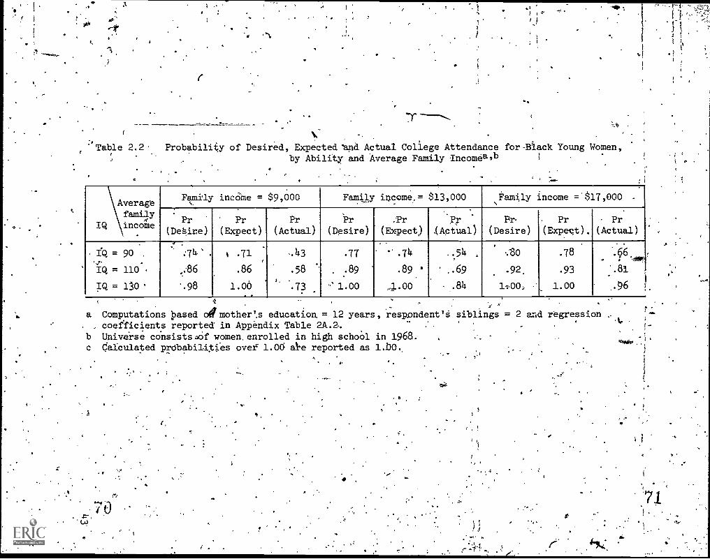
Table 2.2
I
Probability of Desired, Expected -aria Actual College Attendance for -Black Young Women,by Ability and Average Family ncomealb
Averagefamiy
IQ income
\ Family income = $9,000...
Family income ,= $13 000 Family income ='$17,000 .
.
Pr(De4ire)
Pr(Expect)
Pr
(Actual)Pr
(Desire)
.'Pr
(Expect)PF
.(Actual)
Pr(Desire)
. Pr(Expect).
Pr(Actual)
IQ = 90 .
-r.
IQ = 110
IQ = 130
:74-* .
,..86
'.98
w .71 :
.86
1.00
-.43
.58
.73-
.77
. :89
-' 1.00
e' .74
89
4.00
..54
..69
.84
.-80
.92,
ioo,
.78
.93
1.00
..66
-
".81
..96
4
a Computations eased Armotherl.s education = 12 years, resp.ondentlgcoefficients reported in Appendix Table 2A.2.
b Universe consistsoof women, enrolled in high school in 1968.c Calculated prObabiliXies over 1.06 al-e reported as 1.1)0.
0
siblings = 2 and regression
, a.
S
71.!

.
I
1
Table 2.3 .Ratio of Actual to pesired.College Attendance for
i Young Women, by Alq.lity, Average Family Income,rnd Race,b
AverageIQ Family.
Income
Family income= $9,000
1Famfly income=.$13,060
.
amily, income'=. $17:000 ,
.
WHITES ..
.
IQ = 90 . :55 .59.. .
1.62
IQ ="110 .68 z '' .71 .73
IQ = 130 . .78. .79 1.82
, BLACKS
IQ, = 90 ,58 .70 :.83 . .
IQ = 110 .67 . . .78 ,-.88
IQ, = 130 . .74 .. ,84.
-;.96.
a Computations based on -Tables 2.1 and 2.2.b Universe consists of women enrolled in high school in 1968.
44

't1
G
lAppendix Table 2A.6 presents separate regression analyses of thedeterminanis.of actual college'attendance for white young women who werehigh schoorseniors 1968,,1969 tnd 197Q.7 The estimates of thedemand-for-education model 'appear to be different for the three years,,particularly between 1968 and 1969, on the one hand,,itnd 1970, cm ,theother. Parental educational attainment (a iastetactor). seems to bemare important in 1968 while the'variable,representing the financialcapacity of the family (family income and number of siblings) arehighlry significaht in 1970, although they were st4isticAlly indiS-tinguishable from zero in 1968. The respondent's mental ability seemsto have a smaller effect on college attendance in1970 than,. in the twopreious years. We hypothesize that changing economic conditions overthe period (higher inflation, unemployment and-interdit rates) resulted
)
in greater importance of family financial resources in college'attendance- decisions by 1970. A variant of the demand model used toet this `hypothesis is lo interact a dummy variable indicating highschool senior status ;970 with the variables for family income andnumber of siblings and td include these interactions in a sample of allhigh school students in 1968. Significance tests8 were used to reject --the null hypothesis (the effeCts'of the variables on 1970 seniors areindistinguishable from theireffects on 1968 and 1969 seniors). Thus,we find support, for the hypothests that college attendance decisionsare sensitive to, short -run economic conditions.
'Too few sample cases preclude separate year analyses for blackwomen.
.8The test forthe difference in regresSion coefficients in the
same estimating equation is:
CA _ CB
-V varcA +.Varcp. -,?(COVCi,CB)
whereCA and C ' are the two .coefficients, *0
VercA and VarcB, are the i'driancei-of the respective coefficierits,
and COVcA,cp,' is the covariance weep the two coefficients,.
Applying this test,'for which the source is Theil (1971,.E.: 138), to,the difference in the effect of'family income on actual collegeattendance for 1970 seniors'and 1968/196 seniors yields q,t-statistic
. of 2.136 which is significant-at the 5 percent level (tw6-tail test)..The same test. for the diffeience in the effect of number of siblingsyields a t-value Of -2.42, significant at the 5 percent level. .
o
0
^,..fie:41,
...45'
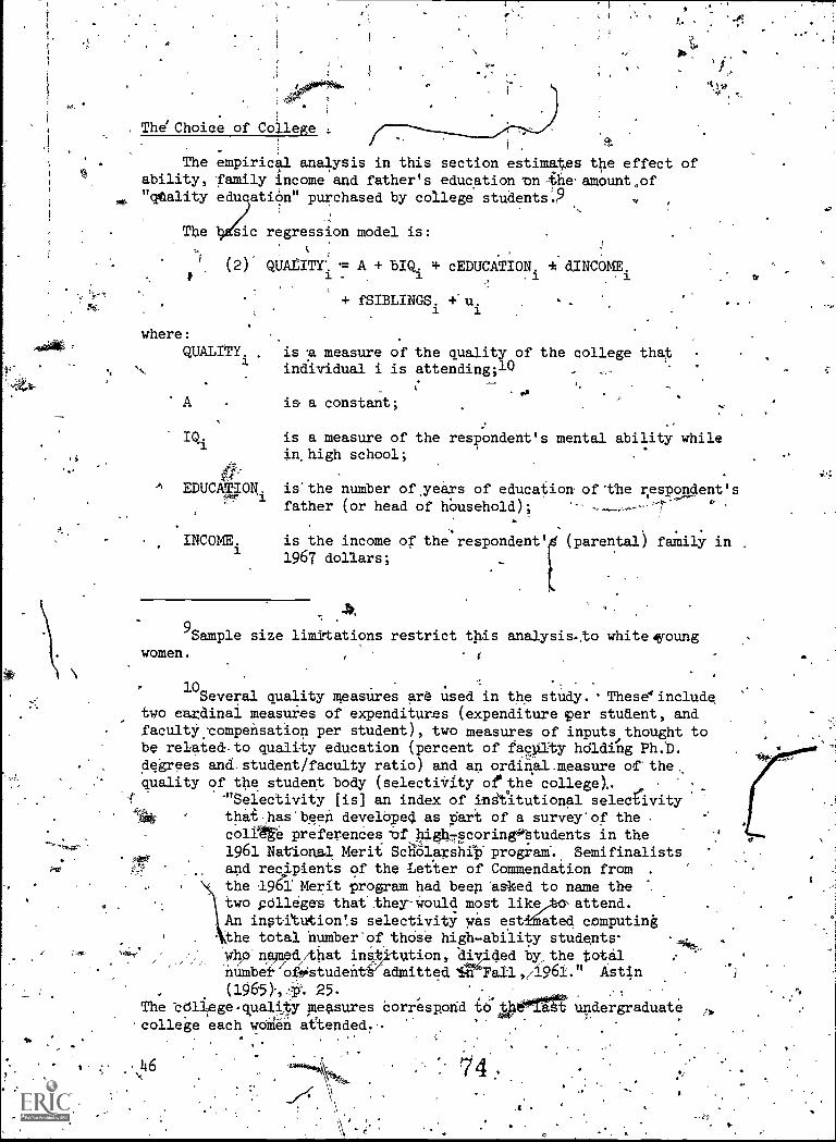
,
The Choice of College
1,-.1- ,
. ,,,4;
I i 1
A. ,`$
i,
4 , w
The empirical analysis in this section estimates the effect ofability, family income and father's education Tni-the amountof"qtality educatiOn" purchased by college students Q ,
The sic regression model is:
t 1(2)' QUALITY*. 7-.- A + + cEDUCATION. *dINCOME1.
. .1
+ fSIBLINGS. u.1 1
where:
QUALITY. . is 'a measure of the quality of the college thatA individual i is attending;lQ
eis a constant;A .
IQi is a measure of the respondent's mental ability whilein high school;
m EDUCAthIONi isthe number of.years of education of'the respondent'sfather (or head of hbusehold);
INCOME.1
is the income of the respondent' (parental) family in1967 dollars;
9Sample size limitations restrict this analysis..to whiteffoungwomen.
10Several quality measures are used in the study. 'Theseinclude
two cardinal measures of expenditures (expenditure per student, andfacultycompensation per student), two measures of inputs thought tobe relatedto quality education (percent of faspIty hdlding Ph.b.degrees and.student/faculty ratio) and an ordikal.measure of thequality of the student body (selectiVity of the college),.
-"Selectivity [is] an index of institutional selectivitythathas'been develOped as part of a survey-of thecolltre preferences ior,high7scorinestudents in the1961 National Merit SchOlarshrpprogram". Semifinalistsand recipients of the Letter of Commendation from .
the 961' Merit program had beep 'asked to name thetwo p011eges that:they-Would most like,tev'attend.
An inatitution!s selectivity was est±thated computingthe total humber'of thOse high-ability students.
Wh.,53'n.p.m ied/that institution, divided by,, the totalnumber'bf,estudenticadmitted Astin(1965).,,Ii% 25.
The bd4ege quality pleasures Correspond t6 thee aSt undergraduatecollege each wOMen attended.
74.t
a-

I
1
SIBLINGSi is the number-of-the respondent's sihdpgs
ui represents the unexplained residual inetheregression eqUation;
b, c, d and f are the'least squares regressors assogiated withIgi,HEDOCATION,,INCOMEi and SIBLINGSi
reppectively::.
.i
tilesI
The effect of the yarijables differs dependingI,
up n the measureused to repretent.college qAlity. Nevertheless, we observe a consis -'
,tent relationship between a young woman's ability, her family's income.,and the college she attends.11 Wealthy families consistently buybetter college education for their daughters than do poor familidt;young-womenwith high ability obtain better educations-Mtn their,lesa.intedigent peers: Mother's eduCation is. not a significantpredidtor of. any of our measures of college quality, and 141 one case(expenditures perstudent) the number-of-siblings variable producesan estimate that is contrary to theoretical expectations.12
N. ,
Using regression results that examine student expenditures forcollege education, the sensitivity of tuition spending, with respectto family income and ability canBe compared with the sensitivity cifcollege quality purchased with respect to these same varlables.13 Othermeaningful chservationsthat'can be made from these estimations include 1'the amount students pay for college education for various levels offamily income and ability, and hgw much the college is willing tosubsidize them. For example, concentrating on the renet tuition,-an additional'$1,000 of family income
4 ,
ressioni forassociated with
-Ptegres-ion results are reported in Appendix Table 2A..8.Ts,'
12.It is useful to inquire whether the st istically weak results
that. have been obtained for the correlates. 6 college qiality areprimarily°explained by' the small size of our, ample.,..f.Accordingly,.
'we have estimated the determinants of the quality of college attended
for a larger sample that includes. Women who had attended.6ollegebefore thesurveyperi6S. Sinc&data on parentil.family income for _
these students Wereeften unavailable, we used mother's edueatiog andfather'veducation reppsent socioeconomic status.. These results,eporged in Appendix TaIle 2A,5, imply that the statistic.1 significancef. some of the determinants of college quality (e.g.; ability) would.
t.
improve if the sample were.larger;
13Thettre,gressi-O,n-r
4.!
are reported in Appendix Table 2A.,
75
1
O
c
.

'3
.1
t
S$31 more in tuition expenditures by young Women and a 10 point in rease:7`
\/ ',
1 '1'
in IQ is assipciatepAth $62 more in tuition expeons s. An additi nal;
,, year of mother's education is associated with $47 o additional t itionpaid by young women?
i
;
:i.,1 :
. i.-,
,z,,,-
t The differencplbetween expenditure pe/: student d tuition p idper student is the subsidy received by each student 'n attendance. This _
subsidy comes pred Minantly Proi tax revenue for pub9.ic colleges, while,a portion of,the s bsidyfor private college students is obtained fromprivate donations. The regression results can beused.tolexplore;howthis subsidy'differ amongistudentsly sex, family rpcome.and abiliity.
. In 1967 dollar's, tie mean'expenditure per student was $2,159 for'llenan t,721 for women (Appendix Table 2A.10).14 Since womell paid'anaverage net tuitio of $653 compared to1694 for men, they received anaverage yearly sub Jay of $1,068 compared to $1,465 for men. 1
i
These rdsultsished some additional light on earnings 'differencesby se4. Since menoon average attend higher quality colleges than,1women, controllingionly for the number of years pf aducatiod inearnings'function+ill tend to overstate the difference in male- female
.earnings after "controlling fOr education.' FurtherMore, !if ourresults are.amilicable to older cohorts of men and women, the findingthat the returrto)education for married women is less thap that! or.married men may-be4d4e in part to differences in the qualgty-of theeducation that.the,gexes'obtained. _.
.. i
., 1
,I a. 0 1
..
CONCLUSIONS .
. 1
v,
.
The decisions of young women to enter collegesAas well as theirchoice of college,lseem to be consistent with the economic inves4ent
. 0 As
model. White women's desired, expected 'and actual college attendanceare related positi'vely to their parents' educational attainment,1 'hillyincome,' and their own mental 'ability, ana'related negalively to _t
.
tirnumber of siblingsi. Similar, but statistically weaker findings e .
**-\\L
btairied for black women, with the exception of the'effeet of number.siblings. .A significant And positive relationship exists between
, young women's mental ability, family income and various measures of thequality of the college attended by White women.
.,.
.The importance of socioeconomic background as a determinant of
.
_I the education decisions of young women is byWs'study,, .
Not only is low family income associatedwi-qh:la lowerprVabilityof college attendance, it often implies attendance
1)
at lower quality',
1 k. ,
14 .
.1:
See.Sandell (1977) for a more,complete analysis of the.acquisi-Y.' tion of College quality by young men. Sample summary statistics for a
comparable group Of young.men are reported in the Appendix.
48

! ...,
'
,
(1
t
, ' 41 .
institutions. A good deal of the lower actual college attendanIce 0blacks thin whites can be explained by the lover pdrental, earnipgs amongblack's. Thus it seems that investment in_college education by bothwhite and plackwomen would be increased if financjal con'Straints.werelesaened, .
-4-4,.....;.
1
. .
. 1 The data haVe supported the hypothesis that t. demand for,1
college attendance among young women is influenced aggregate)/ ,
ecopomic conditions. Family.ipcome availableforfinancing eduCationis demonstrated tobe significantly more important in 'the attendancedecisions for high'school seniors in 1970 than in a968 and 19.69: Weposit that this finding is the result of increasing uncertainty:infamily finances over the peridd due to rising. unemployment, inflationan anterest rates. . .,...,
4 '=4
. Finally, the study documents the importance of parental edUcationalattainment as a factor affecting the desired, expected and actual /college attendance ofayoung women. If young women Whose parents arenot college graduates do not receive the prerequisitaencourLgeMent.financial support from their parental families to seek highereducation, their teachers, their peers, and, perhaps, the governmenthavOgn important role to play.
S.
"\
A
0 I.
...ne
a
49 O
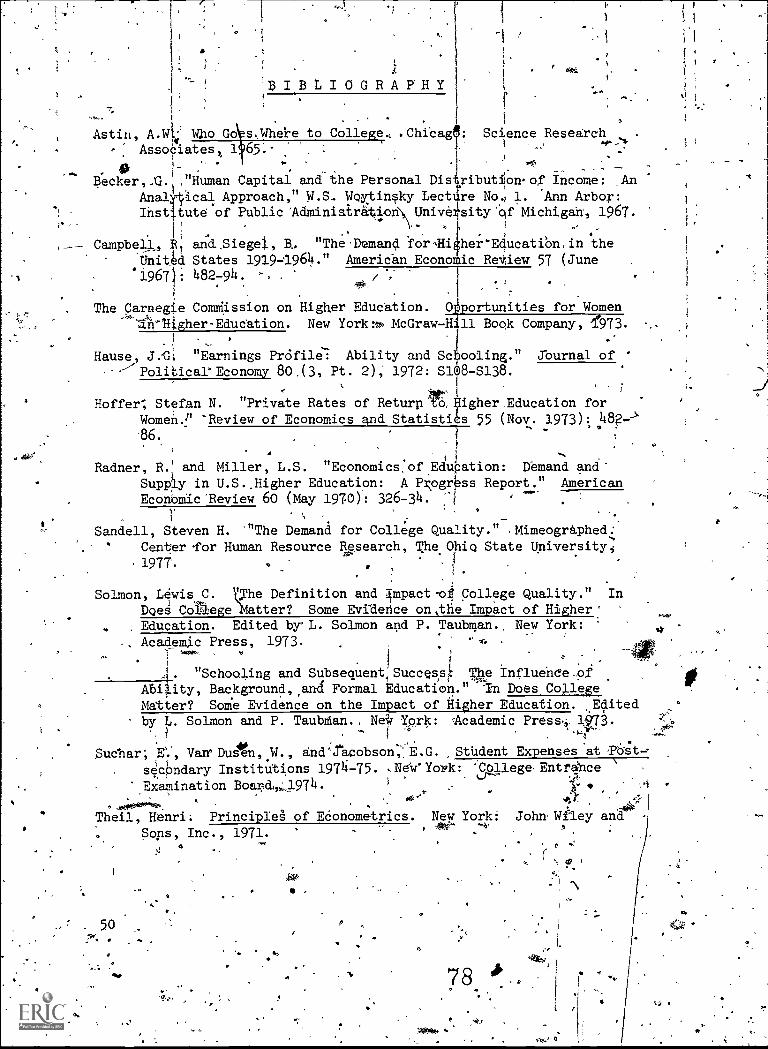
1BIBLIOGRAPH Y
.., i ,
Astin, A.W-4;' Who Go s.Whei-e to College., .Chi'cal: Science Research .
, Asso?iatest 1 65.- .
1
- ... .
1' .1=-
.... 0;
.,-
_ ... .__...,
Becker,G. ,"Human Capital and the Personal Disiribution.of Income: AnAnalytical Approach," W.S. Woytinsky Lectrre No.1 1. *Ann Arbor:
Institute of Public 'Administration Unive sity 'of Michigan, 1967.1
\ ''i
. , i
,--- Campbell, andSiege1, B, "The'Demand 'for,Hi her'Education,in the
Unit. a States 1919=1964." American Econo is Review 57 (June1967: 482-94. '-. .
. .
0.
1
The Carnegie Comiission on Higher Education. Opportunities for Women
an-RigherEdudation. New Yorkm, McGraw-Hr 11 Book Company, f973.. .
Hause, J..G1 "Earnings PrOfile: Ability and Sc ooling." journal of '
--"' Political° Economy 80.(3, Pt. 2); 1972: S1 8-S138.
Hoffer; Stefan N. "Private Rates of Returplt Vigher_Education forWomen.' 'Review of Economics and Statistics 55 (Nov. 1973):
.
86.
Radner, R.' and Miller, L.S. "Economics:ofEdu ation: Demand and
Supply in U.S..Higher Education: A Pogr ss Report." American1
1Economic - Review 60 (May 1970): 326-34. :1
. i.
Sandell, Steven H. '"The Demand for College Quality." , Mimeographed;,
Center Tor Human Resource Research, The Ohio, State University;, .
. 197T. . '
Solmon, Lewis C. he Definition and Impact-o4 College Quality." In
Does Col liege 'Matter? Some Evidence on ,the Impact of Higher:Education. Edited by' L. Solmon and P. Taubman., New York:
Academic Press, 1973..
-/:1. .... . ,, i .
11 1
: :.
, . "Schooling and Subsequent;Success Influenee-pfAbi.ity, Background,.ana Formal Education." "In Does College
Matter? Some Evidence on the Impact of Higher Education. .Editedby L. Solmon and P. Taubtan.. Neva York: .Academic Press.,_1973.
f ta
40. .
Sudhar; E'., Van'Dusen,.W., and'Acobson,i E.G. .Stadent Expenses at ,PO'st-,- 1
.secondary Institutions 1974-75. ,NeW'York: 'C011ege. Entrdnce
Examination Boar;,1974. ,..
. .
Theil, Henri: Principles of Econometrics. New York: John, Wfley an, 44 P
50
a
4r
Sons, Inc., 1971.
O
r
LI

. ,
Taubman, Pau7 and Wales,. Terence. "Mental Ability and Higher-'Educational Attainment in the Twentieth Century.'! In Education, 4Income, and Human Behavior. Edited by F...Thomas Juster, New
,York.:,..McGraw-Hill Book Cpmpany,.1975.
Wachtel, Paul.. "The Returns to Investment in Higher ducation:' Another;View." PIn Education, Income, and Human Behavior. Edited; by .
'F' Thomas Juster. New York: McGraw-Hill Book Company, 1975.
Wales T. "The Effect of College guality,on Earnings: Results from' NBER-Thorndike Data." Journal of Human Resources 8 (Swirlier ';
306-17.-
-,t
AV.
o
0
1
6
t
9
*V;
1..
"s

ADMISSIONS SELECTIVITY
. .
COLLEGE
,
EDUCATION
GLOSSAT'Y.
An index of-inStitutidnal aelectivitYthat has been,-developed as part' of survey -of the cdilege. preferencesof high-scoring:students in'the 1961 Natibnal MeritScholai'ship Program. SemifinaliSts and recipients ofZ,the Letter of Commendation from the.1961 Merit programhad been asked to nine the two colleges that they wouldmost like to attend.' An institution's selectivity wasestimated computing the total number of those high - abilitystudents who named that institution; divided by the totalnumber of students admit d in Fall, 1961.,
A dummy variable with the value of one if the respondent'actualTY-attends (or desii'es or expects to attend) collegeand zero'otherwise.
4.
The highest year of "regular School completed bY therespondent's father'(orshead of household) - frbm 0 to 18 -as of the surveY,week in 1968. "Regular" schools includegraded public, private, and parochial°61kmentary andsecondlyy schools;..,colleges; universities; an professional
EXPENDITURES PER STUDENT
The expendituAs made by *the college per full -time students.
FACULTY, COMPENSATION PER STUDENT-
The compenSaion/awarded the-full-time facultygoler full-timestudent at he college. k
FACULTY/STUDENT RAT i0
Tie ratio f full-time faculty per full-time student at the'college..
'FATHER'S EDUCATION
52
1'
The highest year.of 'regUlar" schoolfcompleted by therespondent's father - fr* 0 to 18 - as of the surveyweekin'1968, "Regular" schdols.include graOd public private,and pardchibl elementary and secondary ,schools; colleges; -.
universitiesji and professional schools.' I ,.....v4'.
: :#1
If
0
' It
* "
.
ar.

. at
;
FULL -TIME STUDENT
.
Full-time,studen* and one-half of the part - time studentsattending the-..co lege. s. - _ .
. GROSS.TUITION .
. ,
The amount ofcfUll-time college tuition.
INCOME''"
The average4eported family iricome.(in 1967 dollars) forthe available survey years.
A measure of the respondent's mental ability diiring high .
school (.taken from the high school record)..,,
40THER'S EDUCATION
..,
The highest year of "regular" school completed by the .
respondent's mother- - from 0 to 18 - as of the survey weekin 1968; . "Regular"-schools include graded public,.kriV-Ite,
. and parochial elementary and secondary schools; colleges;.0
uniVersities; and.professidnal school's. .
NET TUITION , .-------
,The_ainount of full-Itime college tuition-less the aft+ of. -
,financial aid. .
PERCENT FACULTY HOLDIAG-PH.D.'S
The percentage of the full-time fatuity at the college.which holds a Ph.D. degreeor the equivalent. :
t QUALITY
.i ,,, 'A measure-Of.the quality of the college attended byrespondent.. The quality measures include two cardinal
)
. measures of expenditures (expenditures' per studevt and.faculty compensation per Student), two measures of inNtsthought to be related tp quality education (percentt.df
. faculty holding Ph.D. degrees and Student/faculty ratio).,and in ordinal measure of the quality" of the 'student body
. ..
. (Selectivity of college)..
/---: - , -1:-- .
. .-- The college quality measurescorrespon406-the la$t. undergraduatecollege:eac'h woman attended.
.
Cr
0
.41
3.
53
r

1\SIBLINGS
Al The number of siblings-of the respondent as of the surveyweek in 19'68'. )"
cr
.111o,e
M A
- * -
1'
,f
o_
s41.
82.
,

O
110
*..
Table 2A.1 'Determinants of0Desired, ected and.Actual College AttendanCe for...pite Young Women in High School,
.
in 1968: Regression Res.dltsa
r
(t-values in parentheses)
.11- ,, ,Dependent variables ,
Independent .
-variables4. Desirecollege
.Expect-college
Actual-
collegeattendance
Desirecollege
-
Expectcollege
ACtualcollegeattendance
.
Actual
'collegeattendance'
Actualcollegeattendance,
,Fitherts educationA
MAker's education
A've'rage Family. ineome, 1967-1970(in 1967 thousandof dollars)
..- 1
Number of siblingsiii:1968
,IQ x 10-240i.
..
constttnt ".
, . -
.
-
.
-033' I
4.44)***
.007 .,--,
.
"( 2.10)**
--.012' -
(-1.44) '
.7379,
( 5.81)***.-.431
(-3,05) .
.
.038( 4,77)***
.
.012
(.3.68)***
-..014
(-1:66)**-.....
.690
( 5.25)' ***
-.570
( -3.80)
1-
4
.049-
( 5.59)***
.
. .010( 2:63)***
-.010(-1.05Y
:942
( 6.51)***-1.15k 0.
(-6.99)
.b18 .
( 3.11)***.
4---- :
'.
-007 1
(-2.14)**
..
--.013 '
(-15 ).782
(6:34)*4*-.319,-
(-2.31) V
.-
.046 d("4:28)4A*
. '
.011.( 3.20***
-7014 .
(71.66),**-.743
( 5,71)***-.472
(-3:24)
.039
(,5.84)**1,
.007
( 1.77)**.
-1.004f1
(-0.96),
.992
( 6.96)***-1.056(r.6.62)
.028
( 3.65)***.032. :
-( 3.24)***
. .
'.005
( 1,20'
-.007(-0.76)
.914
*6,37)***--1.194
(-7.29)
.
.
.018
( 5c30)***
-:016
'(-1.68)** .
1.120..( 7.74)***.,
-:849(-5.32)
-112 (adjustedl-.. .
F-ratio
4,,
' .15
27.7***
':17..
33.3***
.20
3E1.4***
.
.13
24.8***
..17
.32.0***;
-,.20
39.3***:,
.21
:34.0**
'' .16
38:8***
NAberof respondents = 612. J . .
a Summary statistics are reported inAppendix Table 2A.5,-.All vaqabres are defined in _the Glossary. 't .7.-_ .. ,..'
** Skgnificant at the:5,perceht level.*** %Significantatfthe 1 percent level.
%
<1.

ON
.. ...-
Table 2A.2 Det rminants of Desired, Expected'and Actual Colfkge Attendance for White Young Women in HighSch00%in 1968 and Never Married the Yea- Following High SchOol-qaduation:, Regression Resultsa
. ,
0-.1
Av.(trvalues, in parentheses)
Independentvariablesb
. .. -
Dependeftt variables
Desirecollege.
Expedt:college
Actualcollege --
attendance
. DesOrecollege
Expect .
collegeActualcollege
attendance
Actualcollege
attendance.
Actual'college
attendance
Father's educat1on. --....
,
Mother's educatj.on.
'Average family
income, '1967 -_970(in 1967 thousandsof dollars) 1° )
Number of siblings i
in 1968' 1
:IQ x 10-2 :''
Constant
.
.036( 4.72)***,,
.
.006( 2.01)**
, ,
,-.01 ) ,
(-1.93)**. .672
( 5.32e**-.383, -,
(,-2.67)
v
,
.041
( 5.00)***
.011 -
( 3.43)*f*.
-.021 ,
(-2.39)**.685
(75.08)***
,555 c
(-3:62)'
, .055
( 5.92)***
..44
.005
1, 1.20).
.
-.014
(-21.39)14
.894 ,
(5.80)***-1.04,( -6.07)
.014
( 2.39)**41
.008'
( 2:50)414*
-.017 --.
(-2.04)**.767'
( 6.0$)***'
-.248.
(-1.74)
.025.
( 3.95)***
%
.011
( 3.20)***
-.021
(-2.35)***.763
(4. 5.71)***...,.451
(-2:99)
.038.
( 5.30)414*.
,7
,'
.003
(.0.78).
. .
-., 013
(-lip _k..4.14,.9
(.6.47)***-.946
( -5.50)
.023
( .88)***.941
(.3.88)***, ,
,...%
-.. :
!.001.
( 0.13)
-.012
.876
( 5.72)***-1.105
( -6.33)
.
.014
( 3183)***
.. .
019-.(-1.88)**1-.109 . ,
7-17)*4*
-:739-4.30)
R2 (adjusted)
F-ratio. II'e.
-17.,
27.6*44
.
-0 .20'.
-34.04**
.
.19 .
3?.4*** .
.14 -.
22.8***
.4-.18:
'31.2***
.18-.i
' 430:4***1 .
.20 1.2" .14..
-..,
27,9*** ' 29.6***
'
Number of .respondents4=a 'Summat-y statisbils are pbrted -in Appendix 'Table 2A.5.b All variables arcs define in the Glossary.
iiw :-**. Sibtficant'at.t110 percent level. -.
*** Significant at tfie 1 percent le41.5.
*OrY
*'dt
.5*
6.
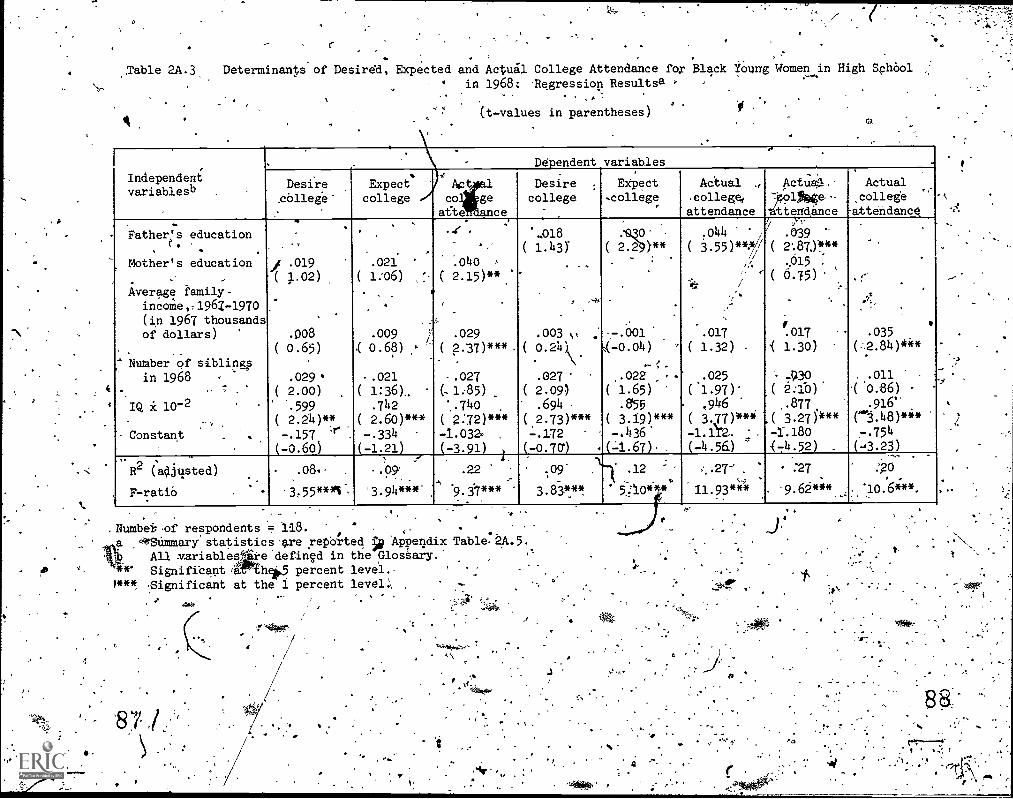
. Is
A
. t.
- C. .
Table 2A.3 Determinants of Desirdd, Expected and Actui1 College Attendance for Black Yourrg Women in High School
\,--in 1968: 'Regression Resultsa '
- . . .,.-.
(t-values in parentheses)
Independenivariablesb
. . . .
- Dependent variables
Desirecollege-
..
.Expect
collegeApt
co ge
atte ante
Desirecollege
,
Expect-.college
Actual .,
.college,
attendance
Actua:l..
"01e--tttehdance
Actualcollege
-attendance
Father's education.
Mother's education,.. ,
Average family-incoMe,196Z-1970(in 1967 thousandsof dollars)
. ..
.' Number of siblings
in 1968 ,
- 7
IQ X 10-2 '
.
Constant
.
j, .019
.( 1.02)
.
.Q08
( 0.65)
.029 0
( 2.00)
599( 2.24)**
-.157 'r -.
(-0.60)
. -
'
.021
( 1:06) !.
.-
.009
4 o 68)
.021
( 1:36)..
.742
( 2.60)***
-.334(-1.21)
./ ,
.040
( 2.15)** .'
.
.029
?.37)***,
.027(-. 1:85)
'..740
( 2:72)*4*
- 1.032® ,
(-391)
...018
( 1.43i
.,
.003 ..
( 0.24)\
.027
( 2.09).694
( 2.73)***
-.172(-0.7U) .(=.1.67),
. 0-
( 2.2 )**- :
.
-:-.001
4-o.o4) ',
- -,'
.022 .
( 1.65)
.8'55
( 3.19)***-.436.
.
.044.( 3.55)*ty//
d-'
/
.
,.
.017
( 1.32)
.025
(*1.97)'.946
( 3.77)**4 ''.(
-1.1i12- .
(-4.56)
// ..-
.039( 2-.87,)***
,615 :
( 0-.75)
''
,.017
i 1.30)
"-. .430
( 2:1'0',.877
3.27)'***
-1.180
-(74.52) -
,
.035
L2.84)*4*
. .011
.( 0.86) -
.916-(n.48)***
.-.754
(-6.23)
.
2 :
R (410,34sted)
F-ratio.08.- .
.3,55***%.
-.29-
'3.94***"
4.
.22
'9.3***
109" :Lk' .12
3.83!**, .:10*r
,',.27' .
.
11.93***
:27
'9.62"*..
:20. ,
'10.6***,
_Numbell.of respondents 7 118. .
a ,AvStirarnary statisticsgre repOrted Appendix Table.2A.5.
Vip! All variablestire'detingd in the Glosiary."
4** Significant larE145 percent level.*** ,Significant at the 1 percent ,
.1%
s
.
Oltatisse
. .
lo,
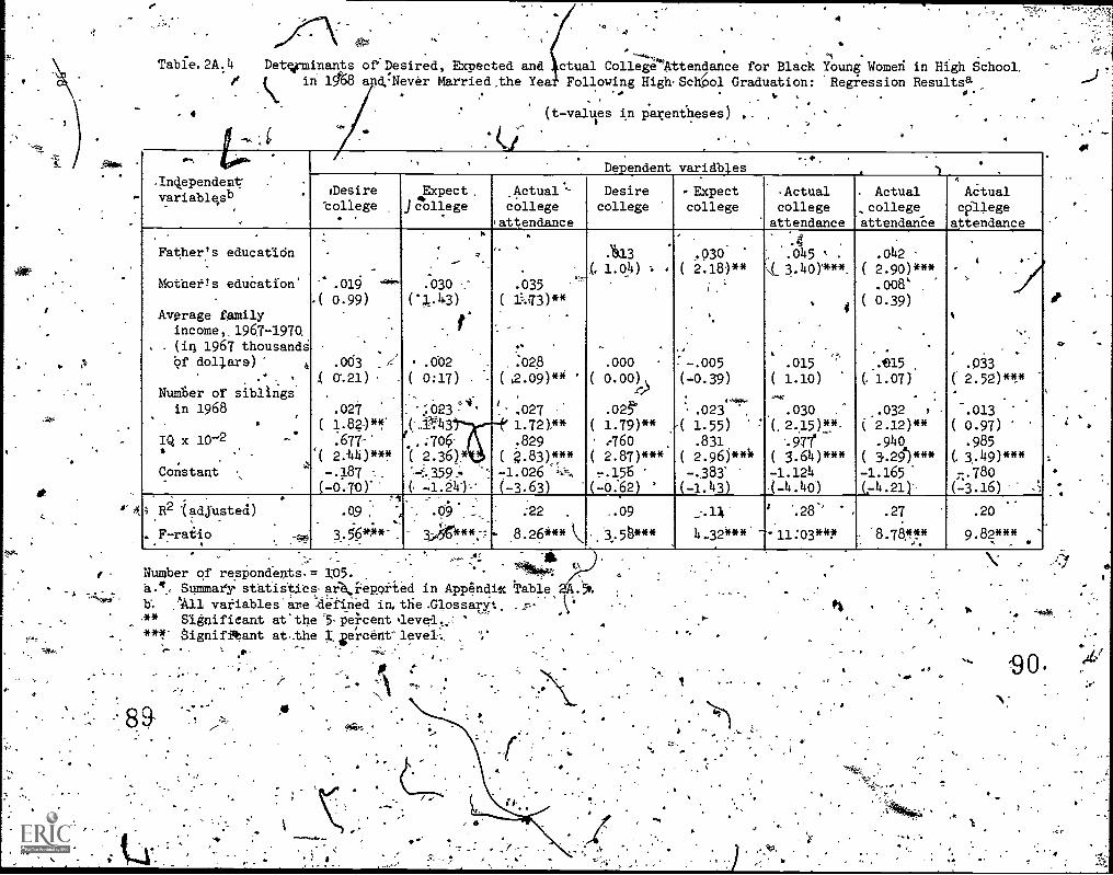
I' A
8
-
Tabie,2A14 Detminants of Desired; Expected and ctual College*Attendance for Black Young Womeri in High School.M in 1068 a,d.:Never Married,the Yea Following HighSchol Graduation: Regression Resultsa
0--
(t -values in parentleses)
1
tiii.- i
Ing nti'ependevariable.sb .
,
f. .
.
.
Dependent variables.
'
aDesire
college'
Expect,JCbollege
Actual -college
'attendance
Desirecollege
Expectcollege
Actualcollege
attendance
. Actual
..college
attendarice
.1
Actualcpflegeattendance
_ .
Father's educatidn
,
Mothefos education
Average familyincome,,1967-1970.
. . (ix 1967 thousandSof dollars) 4
.' . ,
. - .
Number of siblingsin 1968
IQ x 10-2 -.s
.
.
Constant %
.
-
_
.019
( 0.99).
.
. ,
.003 .7-..002X 0%21)
.
.027
( ]..8?)**
.677-
'( 2.444)",
-.387 -..
(-0.70)
. "
'
-
.030 '.-
(..11.3)
( 0:17).
: -.023 "4'
(-..i4
I . ;706.-
.( 2.36)*
--.f.359..: '.
(' -1.24.)".
.
.
.035'''---
( 1'M73)**,
. .. 028
( 12.09)*4 '
.
'- .027 '1.72)."
.829
( .83)***
-1.026 '11:
(-3.63)
.
.1.113
L 1.04) -. .
-
.000
( 0.00),41)
.02'( 1.79)**
(760
( 2.87)***..,-.156
(-0:62) '
.
.030( 2.18)**
I.'
.
'
:-.005(-0.39)
'' .023
-( 1.55)
.831
( 2.96)***
-.383'(-1.43)
. .4 .
L .045 .
q 8.404".
. 4
.
. ,.015
( 1.10)
.030 ..
(. 2.15)**-
'.977.
( 3.0) ***-1.124(..4.40)
.042
( 2.90)***
-0084( 0.39)
. .
.415.(1.07)
.
.032 1 .
( 2.12)**.940
( 3.29)***-1.165(-4.21)'-
.
.
, .
.033
( 2.52)",*
.013
( 0.97)
.985(. 3,49)***
7..780
(-3.16)
_
--!:.
.
";. R2 '(adjusted)
F7ratio-..
,i
.Q9 : ",. -. ,
9'-3.564'4.. -
.
. .--
*-;
;22
- 8.26***
..09
3.58***
..:.IA'
14..32*** ---
' '.28` ,
11:03***
.27
8.78*
.20
9.82 *** ...
Number of respondents.= 105.Summafy statistics-arki-eporied in Appendix Table 2A.
variables' are .de-tined in, the .GlossarYt.
3" Significant at' the `5 percent deve41:**it 8ignifAant at..the tiercent-1evel-._ ao
A
J.
-9o.

Table 2A.5
On.
Means (Standard Deviations) fovr Determinants of Desix0, Expected and Actual.College Attendance
.
,Sample ,
Variabledescription .
description. .
Whites inhip school.
an .068.
Whites inhigh school
in -1968
Blacks inhigh school' int 19.68
..
Blacks dn,high school
in 1968(uhmarried)°
Desire-col-lege-attendance, (dummy coded '1'
if the respondent desires edtmationbeyond high school) ,, .
.
.
Expect college_atten ce (durmy coded-'1'if,the respondent xpects educationbeyond high scilool ---7 -
8A
Actual college attendance (dummy CbcAd '1'.f the respOndent attends college -the .:1
year following grade12)c .
Father's education, .
_
Mother's educaiion- .
Average family's income, 1967-1970,-(in
1967 dollars) .
.
0.780.42)
-
0720.45)-
,
0.520.50)
11.68( 3.24)
11.76
"( 2,38)
.34882.04-(5568.28)
107.30C 1322)
2.96..
. ...1.97)
612
.
0.80'
0.40)
0..75
0.44),
0.57
0.50)
,11.87
3.-.:21)
4.814
( ,--.38)
12312.43(5582:26)
107.71.(1' 13.24)
2.94
C 1.96)
537
?
)
.
,
.'
0.760.43)
0.610.46)
.
;
0.340.48).8.57
3%62)
"7"9-71+
.( 2.71)
644930(31j.5,61
89.o2_
( 16.1 7)
5\11(' 3.18) .
118
-
. 0-76.
0.43)
'
0.70a46)
,
0.38b.49)--,8.73
( 3.70)9..96
(, 2.66)
6628.59(3571%90)f^
IQ -
.
4
/v
.
.___
Number-of siblings in 1968
,,_ .
Number 1.,,f respondents :.
89,41 ,
( 16.33).4.90
.
3.153
109
-" ra ,kAll-variables-are-.defined_in the
b- Not mai.r/ed the year-,following h-_
a.
c
at ion.
4.
}
4
-
o
Jf
5
-

Table 2A.,6 Determinants of Actual College Attendance for White High School Seni ts in 1968,1969 and 1970.; RegreSsion Resultga
V(t-values in parenthese)
Independent variablesb
.
. , i .
Year as high school senior
1968 1969 1970 1968 -1970
, ...--_
Mother's education ...
-
Average family income, 2967=1970.4in.
1967 thousands of dollars) 4........ 4
.-:
Number Of siblings in 1964i
.
IQ x 1072 ' /.y
'
Average family income for '1970 Onibrs,(in. 1967\thousElnds of dollars)
.
Merage family income for 1968 and 1969 lseniors (in,...1967 thousands of dollars)
.
Number' of siblings for t.,9 414ors0 A . , ..
.057
c 3.73):***
.
- .002(- 0.28)
.021
( 1.25)1.939
( 4.23)***
.
. : .
,
,s+.....,...r
- .037 .
( 2.4A***. J,
.014
( 2.24)11-'.001 ..
(- 0.04) ,
.949 '
-( 3.58)***
.
.
,
....
-1.10\(- .3.76
/
.051 1
( 3.416)461*
'
.017.
f--2.44) **-',032(--, 2.15)**
..79l
( 3.2 )4t....:T
1
1,. I....1
I
i
11't
N
.
-1.:.037
(- 3.60)
.049
( 5.634.
.
,950( .6.59)***
.:017
,.,( 3.46)At*
.007
-
.
.-'007
( .r.Q.59)
-1.182(- 7.17
**
-
Mt, .t
87)**031
S3)***
'
number of sibling.s.for-1968 and, 1969-- .
seniors,
_4.)
,Constant . \.
,4,
,
-1.283(- 4:64)
.,
'
. .
ii2 (adjulted).
AZ;atiq .
`Number of, respondents
.19 :
': 12:2***
193 k. .
.20
13.8**,
,209 ,\-----. -
1.,
.20 I
.0
3.0***'
213 I.
.20 4
26:9***
/ 612
-,
. ,
..
Means* (standaid deviations) 'for determinants of actual college attendance for high school. .
seniors samples dl-p reported in Appendix Table 2A.7.All varihbles'are defined ..4,, the Glossary.
...
'.
c
Significant at the 5 percent level.Significhnt at the 1 percent level:
I
4
9 2' y
me,
a
4
e ,
.1
O
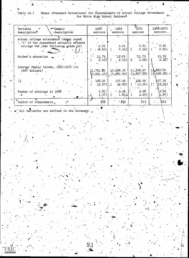
/
Table 2A.7 Means (Standard Deviations) for Determinants of Actual College Attendancefor White High School Seniorsa
, .Variable .4` Sampledescriptions zdescriptiOn
1968 ,"
seniors; 1969seniors
1'N970
seniors
1968-11970
seniors
Actual college attendanceN
(dnimy coded'.'1' if the respondent actually attendscollege the year following grade 2)
i
..
*001.....--° /"' '.,
Mother's education?
.
t
Average family income, 1967-1970 (in1967 dollars)
.
. , .
IQ.
.
Number of siblings in 1968,..0
,
0.55( , ,4.50)
.
-- 11.74( 2..42-)'
,.
1,791.t2
5,931.15)
.
: 108.24
( 13.97)
2:83'A 1.97)
..
e .
0.51( 0.50)
'11:79( 2:53)
12,298.32
4(5,985.59)
107.09
( 12.82)
3.06( 1.81).
a
0.51( 0.50)
.
11.70{- 2.23)
11,548.97
(?{,857.88)
. ,
3,06.59
( '13.04)
. 2.98( 2.09)
.
(
1
(5
. (
,0.520.50)
11:7
2:38y
,
882:*04
568.28) i
07.30
1.3',22).
2.'96
.97)
Nuber of respondents - -.°'/ . T93 - /q,9 213 . 612
. .;;C:All variables are defined in the Glossag.
6
:-
I '
4.
} .
c
I
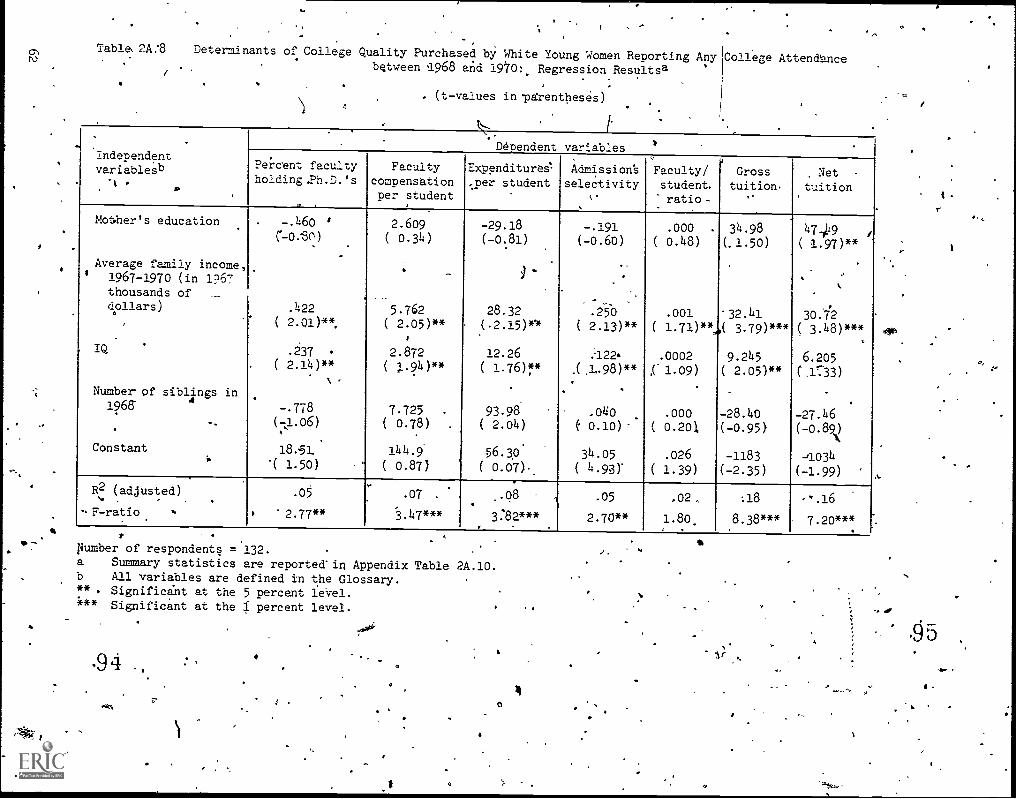
Table 2A:8 Determinants of College Quality Purchased by White Young Women Reporting Anybetween '1968 and 1970:. Regression Resultsa
. (t-values in bp&entheses)
College Attendance
.
-
Independentvariablesb
't A
.*Dependent variables
Percent facultyholding.Ph.D.'s
.._ .
Facultycompensationper student
ExPenditures.-
,..per student
Admission's
selectivityc'
.
,,
Faculty/student.
ratio
Gross
tuition., Net
tuition
Mot,her's education
Average family income,1967-1970 (in 1?67thousands of __
dollars)llars)
. IQ.
Number of siblings in1968-
.
Constant
-.460 8
C-0:80). .
.422
( 2.01)".
.237
( 2.14)**
-.778(-J..06)
.
18..51
"( 1.50)
(
(
(
(
(
2.609
0.34)
. _
5.762
2.05)**
2.872
194)**
7.725 .
0.78) .
144.9
0.87)
-29.18
(-0.81)
.
) -
28.32
(-2.15)**
12.26
( 1.76)7*
.
93.98( 2.04)
.
56.30
( 0.07)
-.191( -0.60)
.
.2500( 2.13)**
.122j ,L.98)**
.
.040
( 0.10)-
34.05
( 4.93)-
(
(
,(
(
(
.000
0.48)
.001
1.71)**4(
.0002
1.09)
.0000.201
.026
1.39)
34.98
(.1.50)
'32.41
3.79)***
9.245
( 2.05)**
-28.40
(-0.95)
-1183
(-2.35)
47419 ,
( 1.97)**
,.
30. 72
( 3.48)***
6.205
(.]n3)
..
-27.46
(-0.89)
11034
(-1.99).
R2 (adjusted),.. ,
.F-ratio 6
.05
2.77**
,. .
.07 -
3.47***.
..081
3:82***
.05
2.70**
.02.
1.80.
:18
8.38***
.
,,.16
' 7.20***
}lumber of respondents = 132.a Summary statistics are reported-in Appendix Table 2A.10.b All variables are defined in the Glossary.** Significant at the 5 percent leVel."* Significant at the I percent level.
948-

Table* 2A . 9
/
.,
Determinants of College Quality Purchased by White YoungWomen Reportillg Any College Attendancebetween 1968 and../19,70 or Before the Initial. Survey: Regression ReSultsa-
(t-values in parentheses)
4
. -
f
Independentvaria4e-sa
.
..
'Dependent variables
Percent facultyholding Eh.D.'s
..- ...4......,.
.
Facultycompensationper student-
.., .
Expendituresper'student
-
Admissionsselectivity
,
Faulty/ 4
student.
ratio '''
." ,,r:,,itton
.
Nettuition
Mother's eddcatiOn,
.
.
Father's education
..
IQ,. .
Number of siblings,in 1968
. .
. ,,
Constant*
/
-.255(-0.57)
,f.121 -2-
(, 3.33)***
.176
( 2.257**.
..
-.948
(-1.81)**
14.64
.( 1.61).
.
' -1.135 '.
(-0.17)
16.0Q'( 3.22)***
3.665( 3.17)***o
.-
13.10'*( 1,69)
-21.30(-0.16)
.
-19.96
(-.557)
.
61.64 .
('2.251**
'4'14.93
( 2.35)***
58.50.
( 1.37)
-563.4'\(-0'.76)
. -.291.
(-1.17)
/
.884 1,
(.4.75)***
'.168
( 3/a8)**
.
.
.068,'
(` 0.24)
/22.61
( L...,50) l
-.000 k,',41.58
(-0:
.
:0.,
02
2'.,82)***:(:)-:83)***
,0003 ..
'( 2P.24**
.
..
:001 -
( 6..95)
:009
(9.58)
q 2-25)tt.
,
c'^1-.39.204
;,-,
}'9,764V3.04)**
, , .
;,'', .
--40{o;..314).
4 '`' 4
1'2482
(=-3;06)
4-5.58
(.2-361*4g
.
42.82
( 2.97)***a
-.1.256( 2.16)**
.
-5.601(-0.25)...
--1374 .
(-3.52)--, ,
R2 (adjusted)
F-rdtib
:075
'6.0647**
.
.11
8.3t***
.045 /
3.95***
,.15 !
'11.96***
. ,
'.'.06
.1:16***
.
,..5
, ii.Ot**.
.14
-10.88***
46.NuMber of respondents =.249.
Summary statistics reported'in Appendix Table 2A.10,All variables are defined in the Glosiary.Significant at the 5 percent level:Significant at the 1 percent lev'el.
Ab**
*i*
.

Table 2A:I0
,.'aa, ...
k.
Means (Standard Deviations) for Determinants of College QualityPurchased,b1 White Young Womena
/
.Sample
description
Variable t,
description'...
.,
White young womenreporting any .
college attendancebetween 1968 and1971 {Table 2A.8)
.
White young women,reporting any
college attendancebetween 1968 end
1971 O. before theinitial survey(Tablei.A.9)
White young memreport3,ng any
collegeattendance
between 1966 and'1971 (reference-unweighted'data).-
Percent faculty holding Ph.D.'s
acuity compensation. pee student
-E penditure per student-
\ Ad issions selectivity
cFa ty/student ratio
.
Gross tuition...
Net to tuition (gross.iuition less"
.anY s holarships and fe1144-shdps eneved b therespon ent)
."Mother's eaucatio\
s.
Father's educati,
Average'family i cbme, 1967-1970(in 1967 dolla s) (1965:1970for young Men)
IQ , -...
Number of sibli gs *in 1968
. 1 '''
'Numl5en of respohdents _
1
.
-
*
44.01
( '14.45).608.29
'( 195.96)
1.,72p.67.( 923.12)
49.31
' ( 8.07).06
.( .02)
' 716:28( 635. )
653.16( 646.74)
12,69
' ( 2.34)12.72
( 3.08)
A.14,230.04
(6,260.79)- 114.87
( 11.91)2.38
( 1.70)
152 1
,
.
-.,
'
4.17( 13.74)
622.93(. 206.28)
1,831.07.(1,098.22)' 49.83_
( 7.:9026)
.( . .02).
665.56( 589.04)
.
587.31( '610.03)
r2.75,( : 2.27)
12.99( 2.98)
NAc
115.19
( 11.16)2.191:61)
249
-
-
47.42.
15.43)
' 662.99 .
C.253.15)23158.62(1,382.96)
51.71f3.56),
NANA
776.54( 650.27) 4
.is."
694.11.
( -656.ol) (. 12.31
( 2.48)
12.40 ,
( 3.30)
11,564.67
(5,709.41).113.46.
( 12.63). 2.34
- ( -1.75).
335.
ar.,1.
All variables are defined in the Glossary,. . . ---
b 'Sburces of th Measure of College Used in the Stildy.' The value 9f.each dependent variable, corresponds.--to the last undergradAie institution attended by the respondent. Qross
Ptuition an4 net tuitions are obtained from the National Longitu,dinal?Sury ys. The.selectivity'index was obtained from Alexander Astin, Who,Goes Where to C llege. Chibaed:Science Research Associates, 1965. Percent of full-time-equivalent.facu ty holcli giPh.D.'s, pxpeniitures per fp11-time-equivalent student, and full-time =equivalent tudentsperlfull-time-equivalent faculty Caere obtained from American Junior.Colleget, 8t ed.;American Universities and Colleges,,10th ed.; American Council on EdUciztion,\Xa eton,1 .C.,.1968, or State Approved, Schools of Professional, Practical and Applied Nu s g:National League for Nursing, New.York, 1968. /Faculty compensation perfull-tiincequivalent student was obtained from: "Report bn the Economic Status of the P ess1971-197," AtericansAssociation of University Profe ors Bulletin, June 1972 or Juniorand Community Colleges); or "Rdorsonthe Economic S atus of the Profession, 1 68-1969f"Americ Association of University Pro?essors Bulleti , June 1972 (for Cale es
panand. I,
.. ,universitTCO other than junior and community" colleges.)I
.(2 The fatilily income variable iS excluded in thiS sample to expand tht°nuMher cif bsetvations ...
to _include college attendees before the initial surveli.,., w' - I ...:
. ', , .
O
48

f
CHAPTER '3j
WORK AND MOTHERHOOD: T E DYNAMICS OF LABOR FORCE 'PARtCIPATIONSURRO DING .THE FIRST BIRTH .
Frank L. M tt and David Shapiro*
lb
Ott
INTRODUCTION , ,.
, One major manifestation.,of\the changing position of women inAmerican society, has been the increasing propensity of women at allkages.to participate'actively in the labpr force. Indeed, the overalllabor fdrce participgtion rate fOr women has increased from 37.8, \
percent td46.4 percent airing th 15-year period between 1960 and ....7__
1975.1 . . '.
. . , ..
Traditionally, women tended tO work primarily in the years-immediately after.leaving schoo.I. \They then withdrew from.the labor'force either wheri they married or as they approached the birth of theirfirst child, SoMe Foten, would sUbsequ4ntly r'eturn,to the work forcewhen their last child reached school age; 'others would remain Out ofth- 4,,e.b6i- force. In recent years, this traditional patterhhas been *
changing: Aligner'..proportionof Women'are returning to the, labor force,_:. and increag,EgrProportions young Women remain out of the labor forcefor ohly short +periods of Mime in connection with the birth of their
, children. 11. a result, *ween'1960 aid 197.5 -the labor 'force partici-, :,-
pation rate for womenyfth children Under the age of three 'more thandou'W.ed, from 15.3.to:341.11 percent.
.
* "' °
While feMalelabot.force participation' leve31 at all life,cyclepoints are-higheFethan theyhave'been in past decades, the birth of thefirst child stL11 remains a major transition point for many women.Reflectfrig the'birth event and the subsequent presence of an infant,substantial,riumbers of.young women withdraw from the labor force.However, aa-our data will, demonetrate, thisThenomenon is apparently .
of a moreAemporary natule than has been true in the past. The
heaverage woman now'stays in he Tabor-force until three.or four monthsbetpre,the birth, and in many instances returns soon after the birth
. (Table.3.1 and Figure,3.1).. . 0
,
*The authors wish to thank Jean Haurin for her outstandingresearch, assistance on this chapter.
.,,1Hayhe (1974), and Hayghe.(1975)...-A
,
*. . ,.., 0 .,. ' 4 0' 'I
.2Ibid7:-
,
4 ,,
, -
65I
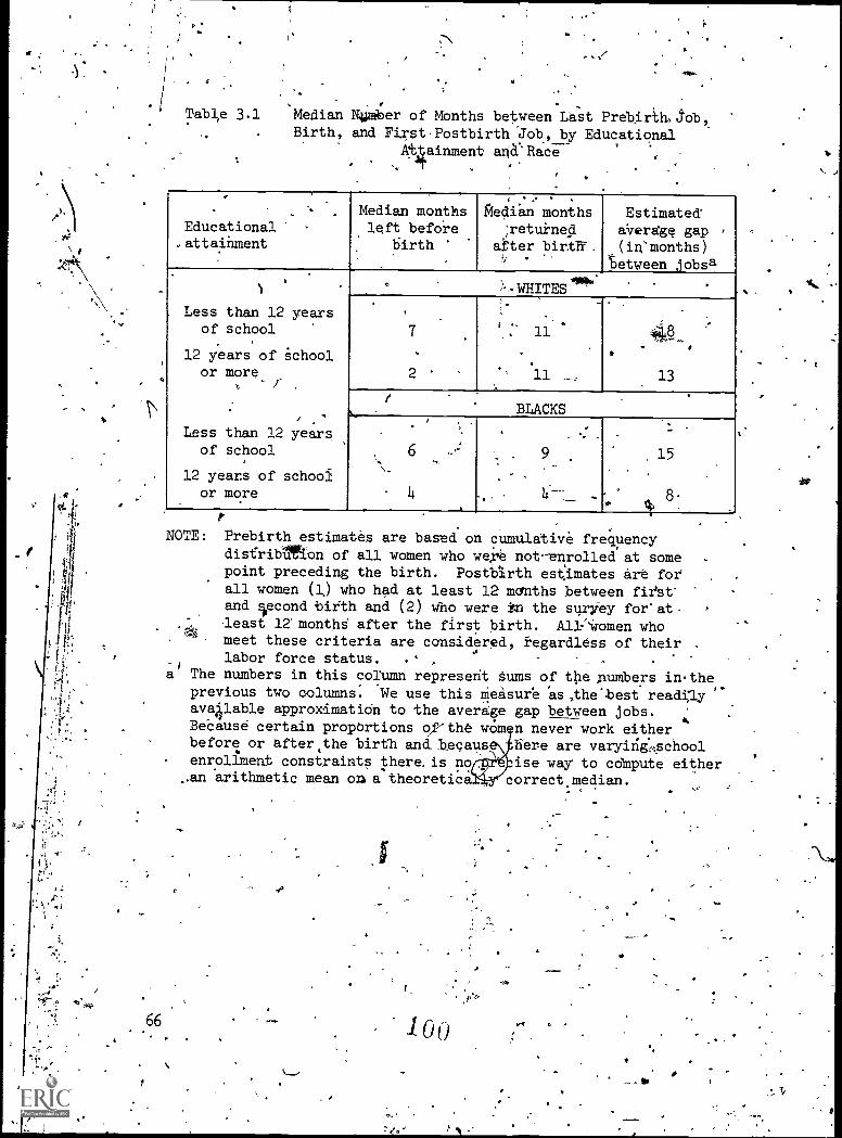
P
Table 3.1 Median Number of Months between Last Prebirh.Job,Birth, and First.Postbirth "Job, by Educational
Attainment ana'Race
.
-.
'. .
Educational,attaihment
. .
Median monthsleft before
birth
Median months;returned
after birth .
i
Estimatedaverage gap(in'months)
between jobsa
1
Less than 12 yearsof school
12 years of schoolor more
/ .
Less than 12 yearsof school
12 years of school'
or more
. .
:',WHITES.
,
7
.
2
; -11
11 ____,
.,.
.
8. .
.
13
,/
.
BLACKS
6
4
-'"
'
9
-
4 _____
.
.-
-0
_
15. _
8.'40
NOTE: Prebirth estimates are based on cumulative frequencydisfribiltion of all women who were not enrolled at somepoint preceding the birth. Postbsirth estimates Are forall women (1) who had at least 12 months between fist'and second tdith and (2) who were tn the suryey for' atleast 12' months after the first birth. All-'iromen whomeet these criteria are considered, regardless of theirlabor force status. ,
t
a The numbers in this column represent Sums of the numbers intheprevious two columns. We use this measure 'as ,the'best read5ly
.
.ava4lable approximation to the average gap between jobs. .:
Bebausd certain proportions cf-the won n never work eitherbefore or after the birth and begaua\ here are varyirii.schoolenrollment constraints there, is no, lse way to compute either
.an arithmetic mean one. theoretic correctmedian.. . . ,.
66, -1 u
41.
-

r
to .
Figure 3.1
c)
(
I
Labor Force Partidipation Ratesore and AfterFirstBirth, byTtace'
4.
Months Bpfbre or After'First Birth
NOTEr fimited to respondents not enrolled.in school at relevant surveydat'6.
o
67

,
This chapter has several objettives, all of fiwhiCh are related tothe overriding objective of clarifytg: both descriptively andanalyticAlly, the patterns of labor force withdrawal andreentryassociated with,the firsttirth. First, patterns of labOroreeactivity surrounding this birth are describedin greater'detail than ..
has hitherto been available. Then, since ajoung woman's ideas about ;/'
childbearing perhaps represent a somewhat longer time perspective, thapatternsof her current 1abOr force activity tare *examined within the,
ik.context of her fertility ideals and expectations. That is, if the- data suggest consistency between current work patterns and prospectivefertility behavior,:it is not unreasonable to hypothesize a certainedommOncausality. Thus, if women' with lower fertility'expectations'are also more likely to be working ill the months immediately folloyin
t their first birth, this evidenced csonsistency'is suggestive of higher
-probabilities of working for these you.4g women in the years ahead.
The concluding tedtions theA fOrCus on interpretitig young women's1,abor force activity, both cross-sectionally andaongitudibally, from.,a more straightforward economic perspective. The discussionwill fdcus
, on suggesting ways in which varying disciplinary perspectives from betheconomics and sociology may be useful for interpreting,divergentpatterns Of work activity between whited and blacks and between womenfrom different socideconomi origins. ".
The Data SetA
Constraints iffipoedbithe available data necessitate usingd ifferent subsets ofWOmen forth two distinctly different analyseswithinthis,ch'aptr. The section of the analysis focusing on laborforce and fertility interaction use's responses to questions, from the.1971 survey which asked women aboui'he number of children they expectto have as well,as the number of,chfIdren they consider ideal.' Thus,the reference point for that part of the analysis is the 1971 int*view.',
''.date. Also, since analogies are drawn between that research and theresearch of the remaining sections df the chapter, which focus onwomen before. and. after, their first,15irthN, the analysis of .fertility
ideals and expectations is leisted to women with exactly one child.
. In both the desciiptive* overview section and the section vhich,
provides the analysis of the labor force acti-,4ity of,these.young women,
virtually all the analyses focus on the,11,40q_,women in the sample. who../had their first birth at some point betw4en v6he1968 and 1913 inter-,_
Views:3,4 The data set for'these analyses was eopstruCted utilizing
3For a more detailed statement about attrition within the cohort-
.
qr.
between 1968 and 1973, see Chapter 1.
4By focusing on the one-parity group, we ve relating information. .
.
Afor a group of women o for-the most part can be assumed to be fecund.
I1
.68 .
102

ti
r
a pooled cross7sectiozitechnique. On ny giVen interview date -a .
womans status, in relationship. to her first birth can b determinedby matching the interview date with the date of birth of jper firstchild: For example, ,if shwa interviewed on .March T969, and herFirst birth was on April 1, 1970, 'she was 13 months (-13 months) befOre.her jist birth at
-her 1969 interview.. ter status in-
relationship to. her f'irst.birth can bq measured as of every interviewdate between 1968 and 1973. The particular woman in the abovexample might have been 25 %months before her first birth at the1968 'interview, 13 monthS jbefore the birth in 1969, 1 'months befc4",ein 1970, 11 months after the first birth.in 1971; and so,forth.5
.
Oneyery one of the interview dates; We.J1dt only are aware of thewOman's:precise fertility'status, but in addition we also have a°considerable amount of information about her work status From the'above example,' it should be apparent that many of the women in thesample could provide detailed labor ,force status information' fen-several: interview dates_both before and after the first birth, . Thus,
tiLe 1,405 wol7len vho had a, firs,t, birth betweenk 1968 and 1973 were'able to provide an effective sample which included Many more thanjust 1,405 points in time. . Becauge of this, it'w-6.7g-P6SSible todeVelop a large and highly detailedwork 'pattern for women not onlyat 411 stages` of pregnancy but also fdr every month immediately)5ollowing. the birth of a first chtld.6
Finally,' one brief section of this chapter, which compares youngwomen's ,wages and occupational status on their first job after 'theirfirst birth with their last job before the- ,birth, uldlizes the paneldimensions of the data set. In this sectiop, job characteris ics forthe same women before and afteer the birth "are matched. ti Thus, whqreas
Thus, exp6ctations, for this t(specific group may be assume to -be
maximally associated with prospective,reality, to the extent,that ex-loectations are indeed associated.with subsequent ferality,behavip.E.
,5From. the perspective of the postfirst birth analyses in this *.
.
cApt'er., a Woman ,is colliider'ed as haying a postfir0 birth status onlyuntil she''has her secondbirth. .fihus, if on a'given interview date a
,twomah already had her -Second birth, that particular interview datewaS no longer considered twithin scope for this particular analysis forthat woman. Of courses if earlier interview".dates.preceded the second 'birth, those points in time were included-in this analysis. Also, theanalysis was limited to women who were nOterilolied Tri-S-ChOOT-on therelevant interview dates. *.
6Aco parison of labor force participation -curves for women hiivi
their firs . biith at different points during'the 'flve-yearperiod. 'indicates no apparent bias from using this technique.
1 03

P7`-`" '''''
111
the pooled data used 'for most of the research of this chapter comparedifferent women at varigus points before and .after the'first birth, thecomparison of wage and occupational status will focus on identical .'individuals at the two points'in time.
.
LABOR FORCE BEHAVIOR SURROUNDING THE FIRST "BIRTn.' A DESCRIPTIVEOVERVIEW
.,,,
The monthssurrounding the first birth represent the life cycle.Point when female'labor.force participation rates are at'a minimum.As'may 1p 'noted in Figure 3.1, labor force participation levels forboth black and white women begiha decline durjng the. early months of
.
pregnancy; from rates approaching 80 percent at the beginning of .
pregnancy,.they:diop to 50 percent aboutthree'to four months...beforethe birth and plumMet to20 percent for whites and 40'petcent forblacks near the:,birth event.? I, is'of some interest_to note thatwhile the ratesdo,incleed decline sharply in the months'preceding
,
7The interested reader may note that labor,force participation.rates, ethploymeht rates and unemployment rates cited in M.%-chapter.are systematically several point's higher thameitimates for comparablepopulation groups in the Decennial Census. This iS.true for both.,'black and2white respondentsWhile exactly comparable'population._groups to those used'in this chapter cannot be found in any Cenius'or Current Population Report,,crude coMparliOns can be made-bycomparing NLS and 1976 Census (U.S. Bureau of the Cehsus, 1970) labor,fOrce statistics for'ever-married one- parity women 2Q to 24' years ofage who have children under the ageof three. The NLS labor forceparticipation rate for all'such women was 42.9 percent compared with03/4.5 percent for the Decennial Census. Of the. 8.4 percentage Point.difference, 5.4 percent,were in the employed part time, with ajob butdid'-not work, and unemployed.eategories, For black.womeh, all,of thedifferencen rates (an NLS labor force participation rate Of 62.9compared with a Census rate of'52.7) can `be attributable to those thre4categories.
dit the basis of this information, several ration ales for heAifferences in the rate levels are suggested; (1) our analys4C,:ex-'cludes a 8mall number of women enrolled in schoo4who have lower levelsof work attachment; (2) all of the NLS i tervrews are with the_respondent herself who may be more likel'y.t regall marginal work-activities than would another household member--who sometimes respondsfor the woman herself in both the Decennial Census and the Current 4.PopulationSurwey; and finally, (3) over the years the NLS Tespondentsmay have acquired a 'sensitiyity" to the standard labor force series ofqUestions they are asked. .Given the respondent'S awareness.of themajor objective; of the NLS interviews, she may makea greater,effort torecall Work activities of,a marginal nature.
70
104-6

./'
f- -the'birth, at virtually ail points there,nonetheless are.substantial,numbers of women who choose to remain in the labor force. .
,
... This fact should of course be mediatedby the knowledge'that in'the months iMmediately around the birth event, actual work aFtivity,is significantly laelow labor' force participation levels,. As may benoted in-Figures ,.2A and 3.2B, for both black and, white women, theactual proportion of women at work-in the month,following -the,birth,is below 10 percent, even though the percent- employed (withli job
`and, either at work or not at work) is around 20 percenf. vre laborforce participation rates at...that point in time are even highercloseto-40.percent for black woman anda little over 20 percent for white,women. . .
.
s 'Following the birth event, black and white labor forceparticipation rates begin.to rise.- White labor force particAtationrates, rise to approximately the 40 percerit level'wherels back rates'increase to between 50 and 60 percent. However, as mOy be noted in,Figure '3%3 a not;inconsequentialyart of the difference' between thebloc" -k and-white rates -- reflects higher--levels-of black. Unemployment;
many more black women are seeking but unable to find work (this. iso.true before as well'asafter the birth).
Infaddition t6 the. fact that the average black woman is modefikely, to be working, br looking for work, there are Major racial.differences in the extentiof postbirth labor force attactrment. As naybe noted in Figure 3.l-, whereas there are.no.significant diCferences..in average hours worked..between employed (.and at work),black and ,white,
women before the birth, the average emploled black-woman is much morelikely to betworking full time (35 hoUrs or more) after the birth1,,hiereas the percentage of white.women working full time after thebirth.is between 50 and 55, nearly 70 perCent of employed black worrierr,are working full timdOmmediately after the birthi_and the rate risesto about '8Q percept a year afte?th6.birth. .
a
The overall racial' contralt'in*Finre 3.1 disguises some majorvariations by educational lev'els. As may be noted in Figurethere are distinct differences in participation levels lietween th
different race:education groups in the prebirth interval; as laborforce rates are loWeist fOr the black'lid *hite respondents with less".,than 12 mearsof gfter the birth, black women with' .2 or more,years of.school return to the labor force in substantially grAfrerproPortions than do any of4he'other groups. At. six Months after thebirth, over-60 percent of black women with at least a high schooldiploma are in the labox force compared -With abb-Tit 50 percent :-for.
black 21.ropbuts and about 40,percent, for the two white education .
categories. Table 3.1'.shows that the better-educated black.womenreturn to the.,latpx",force sooner than.do the other race-eduCatio
groups. The averageblack woman with 12.ormo/te'years ofsohoOlspends about, 8 months without a job due to the hirth compared withbetween-13 and 18 months for the other ''ace- education groups.
a
.
4
10,)-1 o ,

-
ke
0
0
00
a. 70
Figures 3.2 (A and
70
6o
50.
40
30
20
10
6o
5a
4o
r
( 30
20
10
0
O
Percentage in Latorr-Force, Percentage EmPl.c5Yed,
Percentage tmplpyed and at Work, Before andAfter First Birth, by Race
.4
:
's N'At** 1'
s
V
4
WHITES (A)
-
s
In labor force
1paoyed, Employed ana at work
z
/.
- ,
BLACKS (B)
In labor force
Employed
j',19vfe Employed and atwork
I
-5 5-
O - Months Befbre or After Firitlirth
NOTE: Limited to respondent0 s not enrolled in school:at relevant survey date.
4,.4
72
s
. ,106
/

I
M
`wF'
'Figure 3.3
40
3b
10
A
I
Unemployment Rates, Before and. After First. Birth, by Race
N,_
----BLACKS
.
1. - I 1 t A c' - t
-20 . -15 -:10 -5 0 5 it) 15 *20
Months Veore or After.First Birth
NOTE: .Limited to respondents not enrolled in school at relevant surveydate.
107.
4
73 :
.
9
-

4
.
5,4415
Figure 3.4
90
480
0
s.0 .
Percentage Working 55 Hours or More Per_ _Week of Respondents
Employed and At Work, Before and After Firs Birth, by Race
..
/BLACKS
146
. 5
WH:TES
-20 -15 -10 -5 0 5 10 15
Months Befdre or AfterFirst Birth
NOTE:__ Limited to respondents not enrolled in .school at relevantsurvey
date. Also, the denominator references the actual hours worked in
the relevant survey week.-:
714
°
44
y T.
(
108

0 0
`.69
5o
R..
'V
ho0
0
'30
. 'Figure 3.5
30O.43
90
8o
70
20
1- 10
A
Labor Farce Participation Rates Before. and' After FirstBirth, by Educational Attainment and Race
/
.
BLACKS-S(Graduate)
BLACKS'(Dropout)
WHITES'(Graduate)
7:
WHITES.(Dropout)
I I 1 I 1
/-25 -20 -15 -10 -5 0., 5 '10. -
,Njonths Befpra or After First Birth
Irr
ro
NOTE: Limited to respondentt not enrolled in school at relevant surveydate. 4 ,... .
75
109a 1 '

-
b ,
.1
.
! It alSo of some int rest to notet(Figure 3.5) that the group,
with the; second highest pos birth participation levels and propensityto return rapidly are the lacks .with less than 12 years of school,.
suggest4g generally highe levels of black labor forge -part] iPa-tion
colloFing the first birth. All of the-above:data-SU-ggest that thereare distinct variations by race in labor forte behavior following the.first .birth., j
v
7
SOME PERSPECTIVES ON LABO FORCE AND litdiTILITY INTERACTION, : . '.
.
.
.,,
, .
Without belaboring tie question opthe direction of causalitybetween fertility' arld'lab r fortebeha ior it seems reasonable tosuggest that a young women's decisions Roncerning fertility, and workwill, be made within a common framework. ° That- is, a woman may be
.,-' eXciecfed4to make decisionS concerning ,?/- future fertility behavior
which are consistent witOler prOspelt ve and current labor force,
. behavior as well as with her other ego omic'circumstance6. Thus, one
can hypothesizethat,.eve ping else' eing equal, greater fertilityexpectations will be associated with lesser. propensity to work..
!\
I.,.
The preceding sectioh hoWe4.higner levels of labor force'
participation for blacks co paredlyith whites: Table 3.2 providesfertility expectation data enerallYconsistehi with the labor farce
4data, as young "one-*parity bl ck woMen have distinctly lower fertility'
expectations thin their Fhit counterParts.9 ..
.
Sameof the fdctor's which' ifferentially affect female blackand white labor force partici a 'Onjand, presumably, fertility
8It, should be emphasized'that. icAusatoa,in most of "this analysis.
,,is' not implied.tb. be in only'One_airection. %Whileye frequently seemto imply causation in, much'of what we, write, we wish to reiterate that
the interrelationships among the,wOrk, fertility and other socio-economic Variables--adding'in the dithe.nsion of time--are far morecomplex than can be handled within sPaCeand'time constraints of thischapter. ,
. ,
'S6.. 4 Cf9- ,-.: , , *
mplicit in this discussion is the assumption that there are high
correlatibns between fertility expectatIonsandrospectiva fertility .
behavior, While obviously we d-annot answer this 4uestion regarding,the long,un,oidlave,some evidence that the:assdcidtion does indeedhold in the short*run: Between 1971 and 19.73,5,1isercen't of the .one-paritywhite wamen who expected three Or more Child.rWiliad Anadditiondl child compared with 36 percent j*,t11.crsdyho dxpeated atotal of.two children and 14 percent for those expecting only one.
. n .
Similar but less pronounced, patterns were evidenced among the black,,,,,
one-parity *omen'. , . ,- --. .
76
110. r I`A II..
.
41 4, 1,6?
41' 3.1,
a
Fe °
ti

1
41
b.
Table 3.2 ;Fertility Expectations, by Educational Attainment,, i Current Work Status, and Race: 41971h
v.
1
Educational attianment6and current w or status
.
,
.Numb'er of
r espondents
.
Total. number of
children erected
Totalpercent .1.
'1 3 or2 1 more
..
Total or aveWorkingNot worlcing
sc
Less than 12'yearsWorking
. -Not worine
12 yearof,s61*bl'. Working,
., Not working
-,. .
Total or tcrer
Working' Not working
Less than 12 4ears.ofWorkingNot working
-12 yea s of schoolWorld
1g_'11,,V-100.0
4 Not working
a
,?,-
.:
rt
,l
.
of school
T.
or more.'
.
.
,
school,I
.
or More
WHITES , 7--
.,
560 100.0'250 abo.o310 100.0
!.
131 100.0.,
10 100.081 , 100.0'
7429 , 100.0200 100.0.,229 100.0
12.115.59.5
13.8'
20.19.9
11.614.4
9.3
'48.71
45.9i.50%8
4.5,6
38.749.8
49.5.47.'7
51.
39.2
38,6
39.7
40,641:140.3'
38.8
38.039.4
',
ABLACKS .
242 .
-.152,.
90
. 86 -41 .
' 45
: J.6.
45 ,
:100.0
100.0100.0
100A100.0,
100.0
100.0.'
100.0
29.0
32.123.3,
28.828.129.7
'29.3
33.319..0
'40.4
36.91,
46.8
40.2
34.946.3
40,5:37.848.1/,
30.6
31.030.0
31.0
36.924.1
30.528'.9
342
,a The universe is restricted to one-parity respondents who were riotenrolled in S hool'in"197t.'s
A4
J.
77,

c
hehaqor);will be noted within'a standard economic labor-s 'ply'fram4Tork in the section to follow. However, there are czrtain
NOspects of the racial differential .which can perhaps/he 10%erpretedmore readily by incorporating' several temporal dime sions First, .
At all education levels, black young women come fro /poor -r backgrounds.than whSte yOung wqmen. This is supported by the d a i Table 3.3
whic show that ,black young women' at all education /10; ls.havefathers who on average have less education than th 'fath rs of white
young women. Thus, to the extent that newly forme.//yo g familiei, are
able. to gain an economic foothold through intergenerati nal trapsfer1
.
payments, young white f4milies would probably on aVerage be m 0favorably endowed.. k
, 1
', It ,is also of some interest to note that the;larg,stfnter-generational'disparities are.for the young.women,with the highesteducation; less than 30 percent of white young women with some collegehave fathers with less than a high school degree,compared with almosttwo-thirds for young black women. Thus, to the extent,.that young
4), women-obtain financial assistance from their parents' generation, Wewould expect the greatest relative handicap to exist among the better
educated black omen:
. I/;\ addi thisi.ntergenerational dimension, the average,young black Married woman at all educational levels is likely to havea husband who has less education than the husband of her white counter-
part (Table'3.4). Since-a husband't education is directly associatedwith his current and prospective-earnings, the average young blackwoman would have a greater need to work (and concomitantly; reducefertility behavior) in-order to attain a given family income level.Also, to the extent that black young mothers are more likely to beeither separated, divorced or never Married, 'there is a greaterincentive for the black woman t ork. Indeed, as of the -time of the
w men fell in the "no husband
present" categoy compared with only '10 percent of the white women.first birth, 46 pei-cent of the bla
Further, as may to noted, in le 3.'5, black husbands within a
given educational category ear d less than their white counterparts,which probably reflects discrimination in labor mdrkets.10 All'of the
above factors are consistent With the higher working propensities and,:,lower fertility expectations,ofing black compared with,,young' white
. mothers. Moreover as a'reSult m the same factors, black familiesat all educational levels are less likely, to have money in savings than
- their white counterparts and, at the higher educational levels, are
more likely to have: ccumulated debts; perhaps. reflecting in'part thegreater relative gap in ihterge4ratj.onal mobility for black compared
with white daughtert at the higher educational levels (Table.3-6).
1 0See,for example, Becker (1971).
. 4
' 78 . 9
112
rt.
I" 4.
tA
. ,
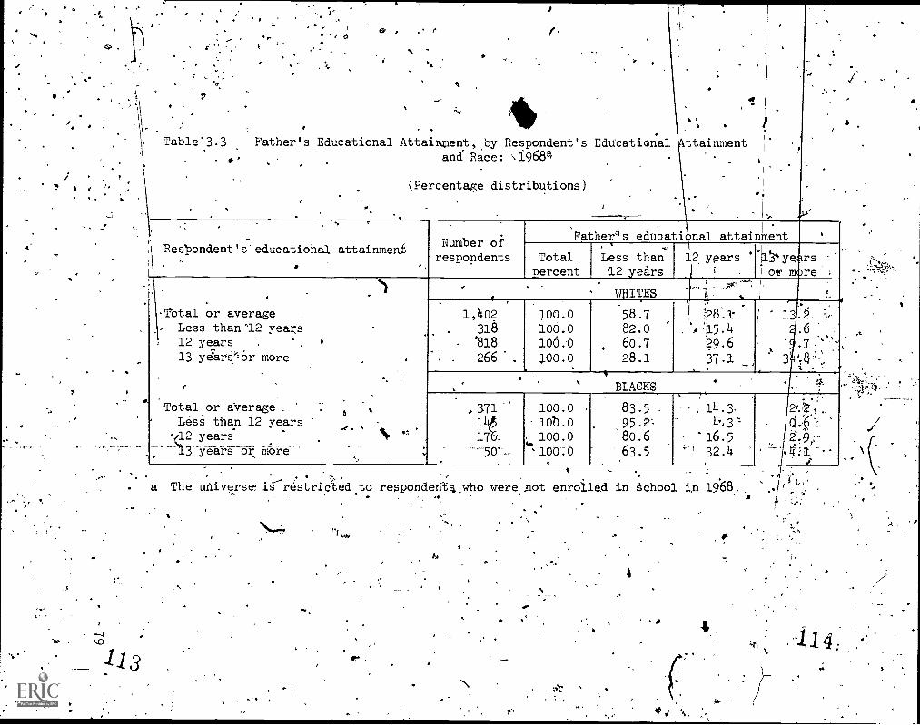
, .
&r r 1.
Table'3.3.
Father's Educational Attainment, by Respondent's Educationaland:Race: \19684
.
ttainment
4 (Percentage distributions)
4 Respondent's'educational attainmentNumber ofrespondents
iFather "s educational attainment
Totalpercent
-Total or averageLess than'12 years12 years13 5,JarOr more
1,402
. 318
'818-
, 266 .
100.0100.0100.0
100.0
t
113
Total or average .
LesS than 12 yearsyears
13 years or moreS
371
14$17
-50' --
100.0100..0
100.0
100:0
A
a The tu'iiverse: iS--restriAed to respondents..who were enrolled in tchool in 19'68.,.
Less than12 years
WHITES
58.7
82.060.728.1
BLACKS
83.595.280.6
63.5
rs
()l m re ;
;15.429.6
37.1
(
1 .2.
.6
.7:
3
4
i
14'1
'16.532.4
4
4'114

a
I
1
Table 3.4. -HUsband.'s Educational Attainment by Respondent' ducationalAttainmen&end Ra-e:' .19
l(Parceniage.distri*igns)
Resporkflent's
educationalattainment
r
um er of..
respondents,:i
,-
--% .
.
u an 's educational'iattainment,
Tote4.
!.percent,Less t*12 years
12 --'-ears 13 yearsor more
.
i'Total or averageLess' than 12 years'
12 years13 years Jr2r-more.
.
Total or averageLess thgh'12:,years12 years _
13 years or more
.i. ."-.
RTES, ',
ev. 329
539-
206
/
100.0. log.°.100.Q
100.
25 7.25.754:1
11.84..,:,...,4.
46.9
40.4
58.5 *27.2'
27.45.6 .
23.7 -
V...8 -
k., . i
. 100.0.....)
10070400.-0
100..0.
BLACKS
.46-5.
-72.5:
'.
- ,27.4
:1_4,-:0,
'
"-
i-
40.823.859.045.7
.
12.7
3.713.640.3
279
142
101.
36
,,
80. .
115-
fe.
r
b
I
O
e .

9,
. .
---------------------nt 3-7-51'.------Hanes---Eartring. , y Husband-Ls Educa-b-iona-. ,
., '', Attainmnt and Rade: 190i
" Husband':
educational,attainmentAn-
O
Total or AVeraRe .
.Liess than 12-yeas12 years13 years or more
/Th Total or averageLe3s than 12:years
\All.responden/t One-parity respondent: I
Number'Of, Meanresnoriderns, earnings
Numberrespondents
Mean
WHITES
1,041: t $5,190' I 367
%T\ ..291 4,379 106'
473, - 5,551 169277-- 5,339 '92
$5,4804,395,7275,961
. BLACKS.
.
3,664 I 88
2,866 6 394,188
129.
4,769 20, .,
265
-139
5
3,7872,717
3,8715,265
_ _
tu3I I I
s."
cite r , r -
s
S
A!

S
I
ti
4 -J.,
I 111'
Table 3.6 ,Debt and 'Savings-Status, by Family &rat
.0
Educational_ Attainment, and Race:$
.1971a
, . 4110,
Educationalattaipmerit
.-,
Percent with debts Percent with savings,
All families,
sig- -
spouse resent.
.
All families Married-.r .
spouse _present
Number of IPercearespondentsi
, sNumber'
responV4ts
.
Percent.
Number ofrespondents-
Percent-$
Number ofrespondents
Percent
' .
.Total or averageLess than 12 year`12 years . '.
13 years,or more
-:,"
,
Total or -1Erelage
Less' -than 12 years_
12 years .,*
13 yearsor more
. .
WHITES
c Iol2 , 55.
145' d 61.8348 ! 56....7
.Lig -. '43.1
.
Q
3
- 55;164.5,56.0
43.3
. 598147',
335 '
.116,
72.6"49.8
'75,691.5 '
524_,)122
292
. .110
75-.2.
53.3,
77,8 -92.0
- .... , .
.
.,
,.:-..
- 'BLACKS . ....
.
286 :I 46.6107 I. 40.0- -k:;''
149 . 49.8
'30 i
53.5 q,;;;.:,
140
45
76
19
'
757.3'50.8,
59.363.0,
'7284
'106
148:30,
44-8--30.240.2
79.1
.
138
44\t
4175
19
.
- 0435.5
55.5
.77.8
NOTE:/
a ''''The
.
Being in,debt references a posite response to "Doto stores,'banks,,doctort or an$One else, excludingitemexcludesrear payments. and*rtg4ge debts.
you (or.yoar husband) owe any (othei-)Nponey
.30-day'charge accounts?" Response to this
,, -4.i,.. ),
Having savings references a pc43tive response to Do.you (or your husband) have any money in, l.i
4.vpags.or checking accouriissovings and loan companies, or credit unions?': .
, ,,;,,;
universe is restricted to rCs ^ndents who were one parity and not enrolled in school.2 .
-1

o.
F.
higherThat is, the higher debt level among the better educated blacks May beone manifestation of an upward mobility syndrome whereby they arestriving--in spite of wles's advantaged background--to-feach thewellbeing level of"thef?' better-eduoated white counterparts.11
. -
-Itmayte noted in Table 3.7 that even though the average black',,Woman expects fewer children, she hal higher fertility ideals 'than her'''wh..te counterpart. To the 'extent that fertility ideals are closer to'representing what.a woman (and her husband), would like to do, racialdikerences Be4Ween expectations' and ideals may represent theirelatiirely greater e.onstraining effect. of lower current and anticipated
-.4:noolle levels on expected fertility'for,blacks than for whites.
.
The preceding. discussion has focused on interrelationshipsbetween. fertility expectations--and labor force attachment,,14th considerableemphasis on black/white differences. Much of the remaining analysia'in.
..4.3,
this chapter; to which'we now turn, will focus on explaining-the", ,
levers of and' variations in femg e labor sufply in. the periods -,..
immediately ..peding and fo wingAe.birth of the first child.--. 4. .. -
/. 1,,:.:,
/2/ 41ORK:AND MOTHERHOOD,: AN ECONOMIC FRA1EWORK ,
-.
Factors affecting thelabor'force participation of women have beensubject to'considerable analysis by econ mists and sociologists. Here
.
Will utilize the,labor-sapPly framewor of economics ,in an effort to
I
determine if those factors, found to bi important determinants of female,labor force participation generally are also relevaat to participationdecisions for the periods,just before and after therfirtt birth. .
The labor-supply framework of economics begins by positing tht.thouSehp14. will attempt to maximize utility. an the most simpleformulation, a household will seekito maximize the utility derived from
0.'
s .4.
11 .
See, for-example,-.Goldsteih and Goldscheider. (1968) or Goldb=g.
(1959) for studies which offe;- useful.gild perhaps analogous situationsfocusing On Jewish-Americans' and Americans from rural backgroundsintegrating into the larger society..
.. . , .
. . . - .... .
Several mobility and reference concepts area intertwined /n our' research. 'Upward mobility conscious individuals may.restriCt fertility
for economic motives--to improve their own economic status to anacceptable level in an absolute" sense, as well as to improve their.'economic status relative to relevant peers. Froma,psychologicalperspective, they may be Striving to acquire characteristics more.in
--tune with their perlived notions of what-their peers view as proper . _
behavior. In a loose sense, Mertbn (1968) defines these latter tworelative conce ts within a relative deprivation and anticipatory ,
socialization framework.
119 '

O
Table 3.7
,Or
Relationship between Total Fertility Expectations and Fertility Ideals,by Race: 1971a
.(Percentage distributions)
° Relationship betweenexpectations andideals .' .
Number of, .
respondentsTotal
percentOne
ehiad. Two
childreii-
,Threeor more
children
.--.....-..
Exprctations
Ideals'
Difference
Expectations.
Ideals-
Difference.
.
7
-^ WHITES
556
, 556
( .
100.0
100.0
,
.12.0
3;4
+ 8.6
48.8
59.9 .
-11.1 ,
39.2
36.7 .
4-2.5. , 4
BLACKS
.241
241.
-.
100.0
100.0
28.8.
6.9
-"Zi.9
.
40.6
4/.5 ,
26.9
30.9:
45.6
--.14.7
-
a' The universe is restricted to one-parity respondents who were not enrolled inschool in 1971.
.112k) '
)6-
11D
4'
a
A'
121 .

-4.
its (joint) consumption of income and leisure. The household must giveup leisure time in order to earl income in the labor market.
In addition to leisure, however, there are obviously otherLftportant aiternative.uses of an individuel'sAime (begides work in theiaboi: market), viz., work in the home, and-sthooling.12 In order to
,"earn income in the market, then, tike household must: give up time thatwould otherwise be spent in leisure and /or in work in the home.Conversely, if one member of the household work's and earns a relatively.
-1,higiv income in.the market, that'incomemay be used ,(in part) to"pulfthase" more time,for nonmarket uses for other household members.
14.op..
In examining tactors'affecting a young woman's' decision concerning
labor forceparticipation, the Preceding discussion suggests that other,
household income(more precisely, family income less respondent'earnings) will be an important consideration. That is, in householdswhere other family income is relatively high, we expect a greaterlikelihood that the respondent will not be in the labor force, every
else being ecual. In effect; such households will be able to.y." more time for leisure and/or work in the hoMe than less affluent
, .nou-enolds.1.3 N
if a woman chooses not to work. in the labor market, she bearS anopportunity costthat is, time spent out of the labor market 4
represents foregone earnings: The greater a young woman's earningspower jpotential wage rate) in'the labor market, the greater will be
.
the opportunity cost of nonparticipation. Thus we hypothesize that,ether things equal, a young woman's potential wage rite will berelated positively to.the-likelihood that she is in the labor force atany point in time, since greater earning power implies that nonpartici-
-pation in the labor forge is more costly .1
,
12,in order to simplify the empirical analysis, our universe is
restricted.to young women who are not inschool. Hence we willconsider schooling no further here.
13Evidence of an inverse relationship between other family income
ani wife's labor force partiCipation, demonstratinga negatiye effectlabor. supply, is common in the literature'on labor force
participation. For examge, see Bowen and Finegan (1969), Ideally,one would like to-use *a measure of "permanene-rather than currentincome; however, data limitations force us to use current income.
More formally, we are hypothesizing that the substitution effectof the Woman's (potential) wage will outweigh the income effect:
14
1.22
am/

Apart from differences in other family income and (own) potential.'earning power, young women also may have differing tastes -- differentpreferences among income,Eleisure, work in the_home, add werk in themarket? While we cannot measure these tasted'..d4rectly,we do make useof, information from, the NLS concerning the respondent'S educational
attainment and expectations of future labor force attachment. These
variables should serve as proxy measures for tastes. Educationalattainment is correlated zrith the respondent's'Apboteptial wage rate,and probably with other family income, .However, sin6e these., variablesare already controlled fdr in our model, we view the independent effectof educational attainmenon labor force'participation as reflecting.a, taste effect. Previous empirical work has suggested that greatereducational attainment is positively related to tastes'tor market work,
everything else being'equal, since educational attainment is positivelyrelatedeito labor force pqrticipation.15 At the same time, however,
some recent evidence has7-been presented in the litqature suggesting- '-
that better-educated mothers tend to spend more time at home caring for
young ch4dren.16 Thus, we hypothesize that prior to the first birtheducational attainment will be positively related to labor force ..
participation; while after the birth, we have no strong hypothesisconcerning the independerit'effects of education on participation.
The NLS data provide responses to queStions concerning_ whatrespondents would like to be doing wen they reach age 35. We ?make use
of these responses as an,additional taste factor--i.e., those ydungwomen who indicatedthatAhey would like to be working in the labormarket at age 35 are expected to have greaterlabor force participation
rates.17
15For example, see Bogen and Finegan (1969). Such a positive
relitionship could also result from a positive partial correlation(i.e.; controlling Tor wage) between education and the nonpecuniaryaspects'of work.
16See Hill and Staffford (1974and Leibowitz.(1974).' This may
.. .
reflect not simply a "taste" phenomenon, but rather an,independenteffect of education on Productivity in the home- (and particularly.on
chdcare).
,
171n addition to the income, wgae, and taste variables; we haveincluded several other variables in the analysis. These variables
were included primarily as controls designed to prevent biased
estimation of our hypothesized relationships; and consist ofa) A self-evaluative measure of the respondent's health '
status. We assume that respondents whose health limits the amount'or kind Of work they can=do in the labor market willbe less likely.to be in the labor force.
86
O
123
2-1,*
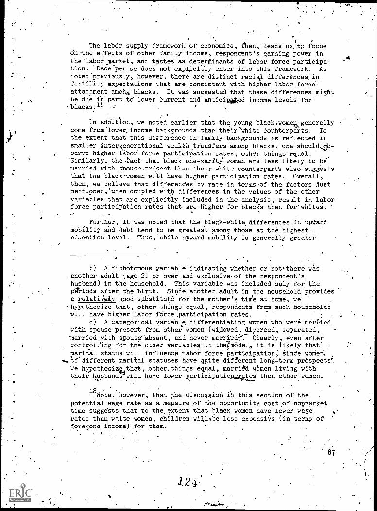
a
/
The labor supply framework of economics, Aen,'leads us.to fo cusOn:the effects of other family income, respondent's earning power ipthe °labor _market, and tastes as detertinants of labor force,participa-tion. Race per se does not explicitly enter into this framework. Asnoted' previously, however, there are distinct racial differences. infertility expectations that are consistent with higher,labor force'attachment among blackt. It was suggested that theSe differences mightbe due in part to lower Current and anticiped income'levels_for
. blacks .18 -2
In addition, we noted earlier that the young black.womellgenerallycome fromlowerincome backgrounds thar their^White -Counterparts. To
the extent that this diffeience in family backgrounds is reflected insmaller intergenerationa/ wealth transfers among blacks, one should\ja-serve higher labor force participation rates, other things equal.'Similarly, the .ract that black one- pariti women are less likely. to bemarried with Spouse-present than their white counterparts also suggeststhat the black-women will have highei- participation rates- Overall,then, we believe that differences by race in terms of the factors justmentioned,'when coupled with differences in the values of the othervariables that are explicitly included in the analysis, result in laborforce participation rates that are Higher for blacgS than for'whites.
Further, it was noted that the black-white, differences in upWardmobility and debt tend to be greatest among those at the highesteducation level. Thus, while upward mobility is generally greater
'c) A dichotomous variable indicating whether or not there wasanother adult (age 21 or over and exclusiveofthe respondent'shusband) in the household. This variable was included only for theiSgi-iods after the birth. Since another adult in the household provides
relatively good substitute for the mother's time at home, wehypothesize that, other things equal, respondents from such householdswill have higher labor force,participation rates.
;
c) A categorical variable differentiating women who were marriedwith spouse present from other women (widowed, diyorced, separated,-married with spouse 'absent, and never marree:- Clearly, even aftercontrolling forthe other variables in thefrodel, it is likely that'marital status will influence iabor force participation; since
..c different marital statuses have quite different long-term prbspect.We hy.pothesizethat,,.cther.things equal, married women living withtheir husbands will have lower participation,4gates than other women.
18 ,-
Note; however, that ;thediscussion ih this section of the .
potential wage rate as A mepsure of the opportunity cost of nolparkettime sugge'sts that to the extent that black women have lower wage %'
rates than white women, children willtbe less expensive (in terms offoregone income) for them. .
. .
124-'.
87
A

c
f
for blacks than,for whites, the interracial differencein mobility isgreatdst among-,tlie most highly educated. We hypothesize,, therefore,
that black's who are relatively-well off (college educated,, relativelyhigh income level) are most likely to be striving to move up the
, socioeconomic ladder. In sualr g Si uation, fertility lititationwould be a-Tlausible means of raisi the household's level ofmaterial well -be ng, and female r-force particeipationin affectedhouseholds shOuld-be high. Empiri lly, then, this mobility hypothesistranslatesinto'expectations of high levels of female labor forceparticipation among blacks with More education and with relativelyhigh "other" family income, everything, else being eqUal.
These hypoth6ses *ill be tested by means of multipleclassification analysis (MCA), a version of multiple regressionanalysis with the explanatory variables expressed in categoricalThe MCA technique permits one to calculate the Mean value of thedependent variable for each category of a particular explanatoryvariable, "adjusted" for the effects of all other variables in themodel. .Differences in-these adjusted values among the sveral.categorie's of a. given variable may be interpreted as indicating the
effect of that variable upon the dependent measure. To provide_a sPecifi''L example, the MCA technique calculates for each education
category of women what proportion of the category would be in the laborforce if those women were "average" in tews,of all the'other variablesentering into the analysis. In the analysis,below, we will examineour hypotheses by focusing on- these "adjusted" proportions.
Some Multivariate Results
1
We focus -here on the major hypotheses. set forth in 1:4p. preceding
section. The key variables_are other family income, respondent'spotential wage rate, and the proxy, measures for tastes -- educational
,attainment and glans for age 35. Results of the. MCA estimates foreach of the five intervals surrounding the first birth'. are presented
in Appendix Tables 3A.1 to 3A.5.__ .
.
:...-.
. .
The dependent variable in:these estimates_is labor forte
1 participation in the following periods-before and -after -the first.
birth:4
. ,(1) -"Labor force Participation 13 to 18 months before thew .
'birth (1 = in labor -force, 0 = not in labor force),
(2) Labor force participation 6 to 12 months before the ,
birth,,
(3) Labor force par4cipation Ato 5 months befOre the,birth, .
.
, .
(4) Labor force parficiiation 1 to 5 months after the-birth,
,
and (5) _Labor force participation 6 toe12 months after thebirth.
"ia 1i4
88
.125
tv
a
OW.
. .
-51.

\AI
uiw .
,Other family income was hypothesized eallier to be inversely...related to the likelihood that ayoung white woman would be in thelaber'force at any point in ttme,. It-is apparent from Figure 3.6A thatthe data do provide 'some suppdrt for this hypothesis. gore Pre-Cisely, .
while there are no, consistent differentes in participation levelsbetween the low- and middle-income groups, the high-income Foupdoes have consistently idWer participation, other= -things equal.- Thedifference.in (adjusted) participation levels narrows as the birth isapproached and then widens following the birth; as participationamong "low- and middle-income families begins to. increase whileparticipation in high-income honeholds remains quite low. It thusappears that-among whites, high-income households do "buy" more timefor work in the holhe than do less affluent households, particularlyin the early stages.of pregnancy and after the birth. -Among blaCks,there is no evidence of an inverse relationship between participation
and other'7,,Samily,income--:in fact, more than five months after the birththe highest (adjusted) labor force rates sie those of the high-incomegroUp (Figure 3:6B). In comparing white and black rates by incomegroup, it 'is apparent that after the birth blacks have generally higherparticipation rates. The differential by race is 'widest among thehigh-income group. These results are consistent with the mobilityhypothesis proposed above.
ti
The respondent's potential wage rate was hypothesized to bepositively related to her labor force participation. The data provideconsiderable'support for this hypothesis: the'potential wage rate ishighly significant in almost allthe intervals for whites, and the .
pattern is generally in the expected direction for blacks as, although- ,
the variable is not so highly signifiOant as for whites. Figures3.7A and-3,7B show the adjusted labor force rates by potential wagerate. Among whites, moving from the low7wage group up to the high-wagegroup is associated with increased labor force participation in each
.of the five intervals. It appears that the high-wage group4sAlmhmore likely to remain in.the labor force until jast before thebirth, and this group is also more likely to return to the labor forceafter tin- birth.19 Among blacks, the pattern of higher participationassociated with a higher potential,wage is generally present. Thus,even though we are considering an impdrtant transitional period. in thelives of these young women, it appears thatheir,labor force.behavior both before and after the first birth is,quite_resporisive tovariation's in the opportunity cost of nonmarket time.
Educational attainment was hypothesiied to be po;itively relatedto labor force participation prior to the birth, as a reflection ofstronger tastes for market work. We had no strong hypothesis
.
19.It should be noted that there are some women who do not drop out
of the labor force exceptefdP'very brief periods.
89
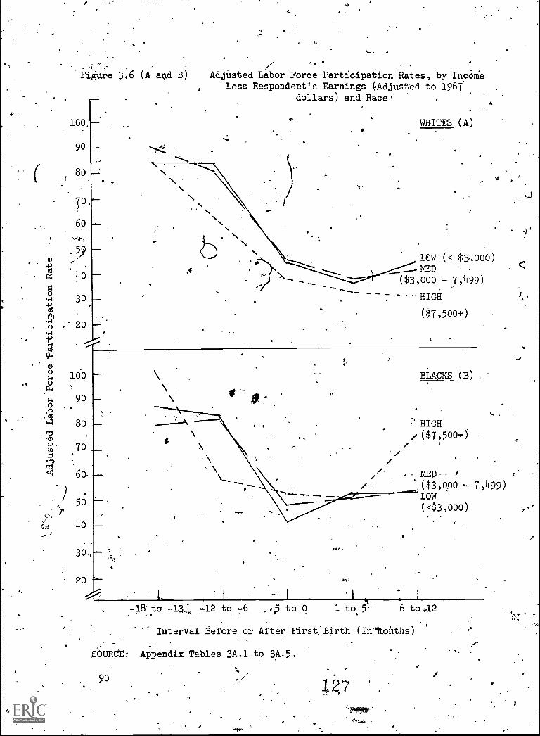
Figure 3:6 (A and B)
100.
90
8o
TO,
6o
5a)
4.)
40
030
Cd
0 .' 20
4)
01 100
0
c.)
.d80
rcsqi)4.) 70
Q 6o
90,
a
50
4o
30.,
Adjusted Labor Force Partiolpaiion Rates, by IncOnieLess Respondent's Earnings ,Adjusted to 1967
dollars) and Race,e.
WHITES (A)
LOW (< $3,000)MED -
($3,000 - 7,1499)
-HIGH
($7,500+)
01
20 --
/47 L I, I I
s,
I I
718 to -13. -12 to -6 .15 to 9 1 to.
5 6 to ,12
Interval Before or After:First Birth (Inittoilths)
BLACKS (B) .
, HIGH/($7,5004-)
./_\
\/, -- MED-- I
/. ($3,00o 7,499)
LOW(43,000)
SOURCE: Appendix Tables 3A.1 to 3A.5.
90
44*
fl
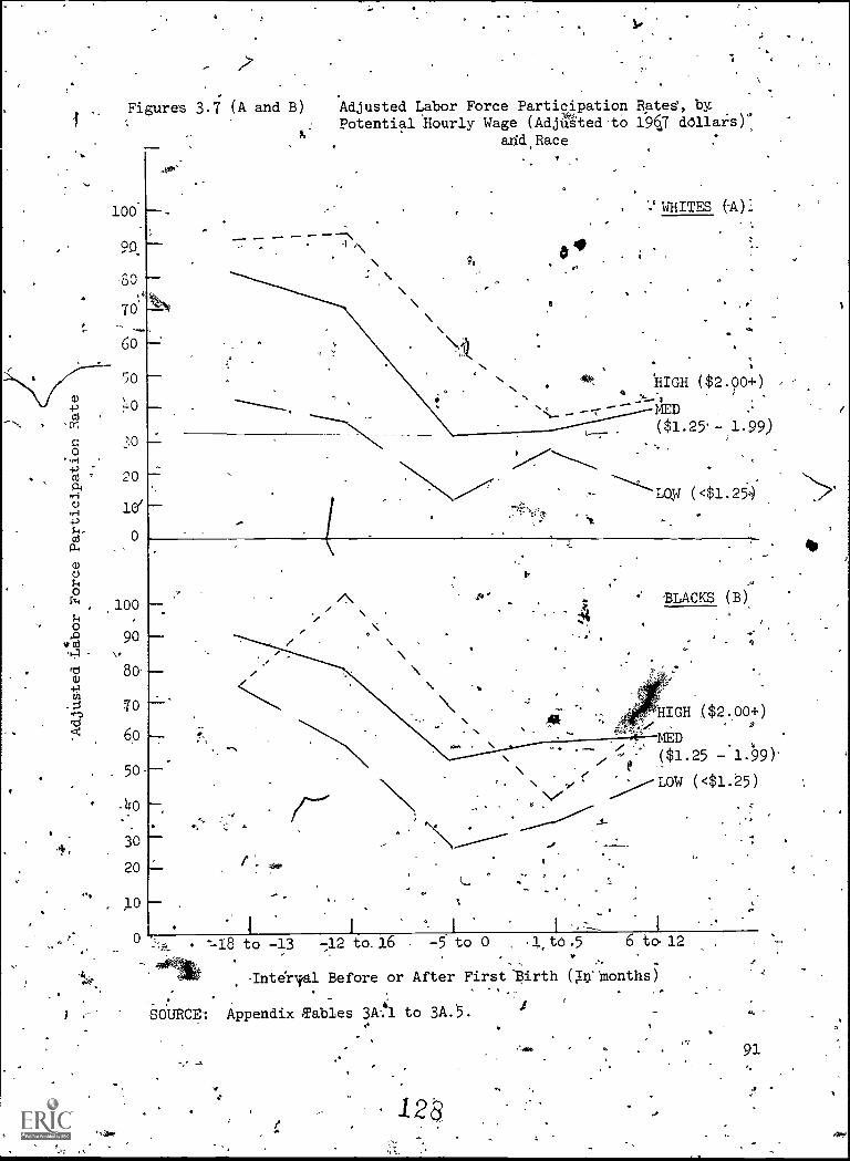
Figures 3.7 (A and B)
100
90
-80
TO
6o
5o
4.3 40
02,0
rri le4-)
00f-4
0
f-4
0
0
.100
v a)90
r 8o,
070
'd<4 6,0
50
t.30
20
100
01,
Adjusted Labor Force Participation Rates, byPotential hourly Wage (Adjated to 197 dollaisr
arid,Race
04.
WHITES (A)3
HIGH ($2.90+)
MED($1.25'- 1.99)
Loy (<$1.24
,
BLACKS (B)
L
\ (,
I
HIGH ($2.00+)
MED
e ($1.25 - 1.99)'
/' LOW (<$1.25)
.
SOURCE:
--LB to -13 -12 to, .6 -5 to 0 , .1,,, t6.5
i
6 to 12
-Inte'rval Before or After First .Birth (Xn-months)
Appendix 'Tables 3A-1 to 3A.5.
128
91

r
44*
few
; 'conce r'ningi
'cning the independeht effect of education-on particiPationfollowing the b
Lth. The mobility hypothesis suggests a stronger
'positi've relati ship among blacks. The'unadjusted'relationship.
between education and participation is quite strong: in _everyinterval, for both white's and blacks, greater education is associated
.) with higher participation. As suggested above, however; much Off this association may reflect the positive correlatiOnbetween
. .
education and 'the potential wage.. Indeed, after controlling for theeffects.gLthe potential wage (and other factors in the model), the
..- :)yoverwhelASgly positive relationship between educational attainment. , And labor force participation is.no longer present. The adjusted
labor force .rates by educational lattainment for'whites And blacks areshown in Figures 3.8A and 3.8B,respectively.
. :s. ...Among whites, there is some support PO/. the hypothesis that
education and participation will be positively related prior to thebirth: the low-education group has distinctly lower (adjusted) parti-cipation during pregnancy particularly sd-in the,- interval imtediately,precedingathe birth.' In the interval immediately following the birth,however, participation rates (b4th adjusted and unadjusted) arenearly identical for all three educational Attainment groups. .
Comparison of these two intervals` thus indicates that, other thingsequal, the presende of an infant hasa greater depressing effect onthe labor force participation / /of 'the better-educated Young whited_mothers. . a
I... ..1 ,
- Contrary to the attern among whites, sChoolingis notconsistently relatpd t 'participation of,V.acks prior to the birth,but there is a'generall positive relationship between schooling and(adjusted) participalto after the birth amonetlacks. In compal-ingwhites and blacks at comparable schooling. levels, it is apparent thatblacks, have higher Tabor force rates. In'addition, the racialdifference is widest among the col rslegeducated. This result isquite consistent With our earlier'discussion focusing on the highupward mobility. and debt accumulation, among blacks with college -
,,,..educatiOn. -. .:.1.., .
b 4 . `v
'Preferences 'for workinen-the labor market at,age 35 wereincluded in-the analysis as an additional taste factor. .Prior to thebirth,there was little variation in labor farce participation byplans to work at age 35;,either for whites or fox blacks.- ..Afterfthe
. birth, future plans do appearAd-Be somewhat related to participation,.
but only for tlitinterval ithmediately following the birth.. It isinterestinetp note that support for our hypothesis that future plans,41.s an indicator of tastes for market work, would be independentlyrelated to labor force participation is present only for the 'intervalin which the mothers time input into-child care isPresumabiy mostintensive.
...... - ."'
To summarize, then, we_began.this section by.dzaiiing upon theanalytical
4framework of economics.and hypothesizing that, other things
0
92.
et
-
1!,

Figures 3.8 .(A 'and B)
c7-- 100
90
8o
70
6o
50
40
P. 300
20
00
"45
1000ga
.90 90
O 80
_
70
6o
50
4o.
30,
20.
Adjusted Labor Force Participation Rates, byEducational Attainment and Race 5
WHITES (A)
HIGH (13+ yrs.):-...=-7NED (12 yrs.)
LOW (<12 yrs.
aI
BLACKS (B)
--,HIGH (13+ yrs.)*
.
MED (12 yrs.)
LOW (<12 yrs.)
ft: _i__ I 1 I - I
-18 to -13' -12 to -6 -5 to 0' '1 to 5 ' 6 to 12.
Interval Before oplAftec First Birth (In months)
:SOURCD: Appendix Tables 3A.1 to 3A.5.
93

V
equal, labor force participation Would be4nversely related to other, i
family income and positively related to `the respondent's earning power.in the labor market and (to some extent) to her educational attainment.We also focused on,racial differences in family background and in,SomeofitpeAKariables included directly in the analysis. TM frameworkhelps Mplain,why blacks have Onerall\hiper participation ratesthan whites; and it led las to hypothesize that the relatively greater e
upward mobility of well-educated, higher - income blacks would strengthenthe expectation of a pOsitive relationship between educationandparticipation and weaken the expected inverse relationship betweenother family'income and participation.
In general, the data provided support for most of these'hypotheses. More precisely, black participation rates, e generallygreater than those of whites, with the differences Brea est following,the birth of the first child. For both blacks and whites, the singlemost powerful variable influencing labor force participation bothbefore and'after the birth is the potential wage rate. Other family
"income is somewhat_ inversely related to participation among whites,both during pregnancy and after the birth; among blacks there is noclear relationship prIbr to the birth and more than five months afterthe birth the highest (adjusted) participatiOn is by the high-incomegroup. .There is some evidence of a positive relationship between'
- educational attainment.and prebirth participation, other things equal,for whites, but not for blacks; however, after the birth there is astrongpositiv% relationship among blacks but no,pronounced patterzT-forMtes. Thus, while the data do' provide support for the
implications of conventional labor supply analysis, we also notethe presence of interracial differences In the effects of schoolingand other' family income (partiAllarly after the'birth) that are quiteconsistent with pur discussion of-mobility effectd.
THE EFFECT OF EMPLOYMENT DISCONTINUITY ON WAGES AND OCCUPATIONAL STATUS
The discussion in this chapter has focused primarily on thedifferential propensities of women to maintain an.attachmentAo-thelabor force in the periods-before and after the birth of theiY firstchild. We have found distinct differences in participation levels byrace, by earning power in the labOr,market,'and, to a lesser degree,by educational attainment -end household income level. We haveinterpreted the racial differentials as being at least in part:due todifferences in levels-o otherfamily income, marital status, andsavings and debt accumulation, reflecting at least in part racialdifferentials in intergenyational mobility patterns.
Whereas the earlier sections cpntrast those women who are in .;thelabor f9rce with those who are not,' this analysis will focul'only on.,women who return to the labor force after the birth.. More specifically,'some women are better able to. regain or imprbve on the wage and -:.occupational status level of their prebirth jobthan others; in this
911
131
J.
f
0
section we briefly examine the factors that appear to be related tochange in wages and occupational status among these "earlireturnees."
Overall, both black and whitwomen who returned to the workforce were surprisingly successful in recouping and improving on-theirprebirth Wage and.occupational'status. White women on average attainedan.hourly *age On their first postbirth job lf percent above thatof their last prebirth 'job; black women did even better averaging' a 17percent increase (all wage are adjusted to 1967 dollars), Also,white women increased their occupational status level (as measured bythe Bose Index) by 6 perceneand black women moved up by 11 percent.'Part of these significant'increases undoubtedly reflected A "selectingout" process occurring whereby those women %.4ho were able to find a jobwhich provided above average wage or status were more likely to return
iWork.20 The somewhat better ability of blacks-to mproveon theirlorebirtiOrage level should be tempered by the knowledge, that theiraverage prebirth wage was well below that of their white counterparts;as they earned on average $1.34 an hour compared with $1.78-fOr thewhite respondents.
.In order to examine more carefully the variations among differentsubgroups in the ability to'retain orimprove on prebirth,wages andstatus, multiple classification analyses regreSsing wage change andoccupational status change on a numberof personal and prebitth job-related characteristics we're performed (Tables 3.8 and:3.9). Aftercontrolling for prebirth wage levels, it is evident that better-educatedwomen are best able timprdve on both their prebirth wages and ,occupational status. Whereas black and-white high school dropoutson average exactly attained their, prebirth wage level, white,women withat least a high school'diploma imprOved'their wages by over 10 percentand then black counterparts showed a 25 percent increase, Similarpatte4aswere evidenced with respect to.occupatiOnal status. Thesubstantial improveirftt for better-educated black women is consistentwith our earlier discussions which highlighted the fact that thesewomen were more likely to return to the labor' force than any otherrace-education group. The more successful that women in a particular,group expect to be in their labor market search, in terms df maintainingor impr oving on an earlier job position, the more likely theywill be'to. seek employment.,-. w*
C
4,
In addition, women whose absence from employment (associated with _
childbearing) was relatively brief tended to4be more. successful_ at
improving on earlier wage.levels, as shown by the fact that a lesser
200ne should keep in mind, however, that we are in no sense
focusing here on a rare event. As alteady.demonstrated in_thiS' chapter,-substantial proportions of women; particularly blacks, return to work_soon after' the birth of their first"` child.
\.132
O
95

Table 3.8s
Unadjusted and Adjusted Ratiosa of Hourly Rate of'Pay at First Pastbirth ,7810to Hourly Rate of Pay at Last Prebirth Jobby Race: .Multiple Classification
Analysis
O
4.
. ..
Characteristics
.
..
..Number ofrespondents
Unadjnstedratio *
Adjusted. ratio,
_F-ratio
.
--WHITES.
,
.
Same employer ;
Yes
No . .
Sourly rate of pay' at last pre-birth job(adjusted to 1967 dollars)40.- 1.49 .
$1°.50 - 1.99
$26,00 or more -..
, . . .
Highest grade of schooling completed .
0-1112 .
13)'
. .
Occupation on last prebirth jobProfessional/manageriAl IClerical/sales .'
ServiceOther .
class of worker at' last prebirth jobPriyate .
, Public. .
Enrollment status. 4e .
Enrolled..i.;Not -enrolled,:
.
Number of months between,prplrth arid :. a.postbirt*Jobs-
...
0 -6 I's
7-1215-2 v
25; or more.
e .
Grand mean .
R2 (adjusted).
..
6.
.
.1
142221
103121
139
59207
97.
.
59.
177
6661
,
. 308
55
.
. 49
314
184'
64
74
'41
,A63
'
A
.
.
'
107114
132105102
\111
.
113107
.
110105 s
125113
111111
,
'126
199 .
-V.
111 ,*
'115
109,111 '
'
ill
'f-
.108114
,
- 1340798'
99114
112
,
120, 106
, 117 ...44.
110
111
-.115
' ' 40110
,
118110
102100,
111-,.
.
-2.29..
-
27.951!**
.
...,
3.30*;
.
2.71**
....
,
0.53,T.
3.45*.-
1
4.21***
.
4.98***.a-
.1S1 t
(TaLua cox trued on next page.)
96
a9
'a-
9..
i 3 3

4
.10
Table 3.8 Continued
.
¢.
,.
Characteristics
."
Number ofKespondnts
.
Unadjusted-. ratio
AdSustedratio
F-ratio
. . BLACKS.
Sam employerYes
No or not ascertainable.
Hourlgrate of pay at last prebirth job(adjusted to 1967 dollars)$0 - 1,49$1.50 -, 1.99.
$2.00 or more. , .
Highest grade of schooling completed0-11 ,
12
. - 13-18
bccupationsIn last prebirth jobProlssiohal/managerialClerical/salesService
r,-.Other .
Class of worker at_last prebirth job.Private .
Public-. .
Enrollment statusEnrolled
.Not enrolled
Number of months"between prebirth andpostbirth jobs 'mta.,. - ,
0-67-12
13-2425 or more ,
.:'.-
Grand mean..
. R2 (adjusted)'f
. _
.
.
.
:
64
146
11750
43
7710528
13
8052
65
16050
72
138
,
8352
58
17
210
Si
,
.
-..:-
4
A
'
'.
I
*
104122
134.
102 ,
88
116119110
93116124
117
.
119108,
137106.
_
- ft
107125
123123_
117
122114*
.
-135102
85..
101- 128
'123
. .
115
122'113
115--
119109-
137
106
112126
118107
-117
.... .
--
1
,
'
0.53
9.28***
'3.68"
0.20
,
0.79
_
9.77***
l'
,
0.53
2.21***
.07
.
a -RatioesAre multiplied by. 100.b Universe consists of womerfempld-Yed before and after the birth of, their first 'child.**g Significant at the 3,0 percent level.-** Significant at the 5 percent level.*** SignifiCani at he 1 percent leVel.
e
134
+-
4
41P..1

Table 3.9
.I
Unadjusted and Adjusted Ratiosa of Occupational Status (Bose,Index) at FirstPostbirth Job to Occupational Status at Last Prebirth Job, by Rice: Multiple
Classification Analysisb
,
Characteristic: Number of-respondents
Unadjustedratio-
Adjustedratio
F-ratio
IL.
WHITES
Same .employer -
Yes' .
...
No or not ascertainable
Boss index score of last prebirth job0-29
30-39 .
4o-4950-59 .
60 or more
Highest grade of schooling completed0-11 .
.1.-.
12
13-18
Class of worker at last prebirth jobPrivatePublic
,
Enrbllment statusEnrolled . ,
Not enrolled
Number of months between prebirth andpostbirth job 4
o=6
7-12'13-24 :
25 or more.
Grand mean .
.
R2 (adjusted) r
,
-.
.
.
,
-
'
157293
72
85
.65
191
37
. I
107'229 .
114
3777'3
76374.
.
205
e7710365
450
.
N
.
.
c
'
.
,99110 :
147
11210294
85
\'112106,101
109
91
128101
loo105
107124 ,
106
,'
.
'
,
,
,
105107
148
111
10194
82
97106114
07102
118
103
.
,
107103
103110
106
0.21
37.01***
.
-6.15***
1.14
12.30***
.
0.77
13.90***
26
(Table continued onitext,page.)
98
135-
tk
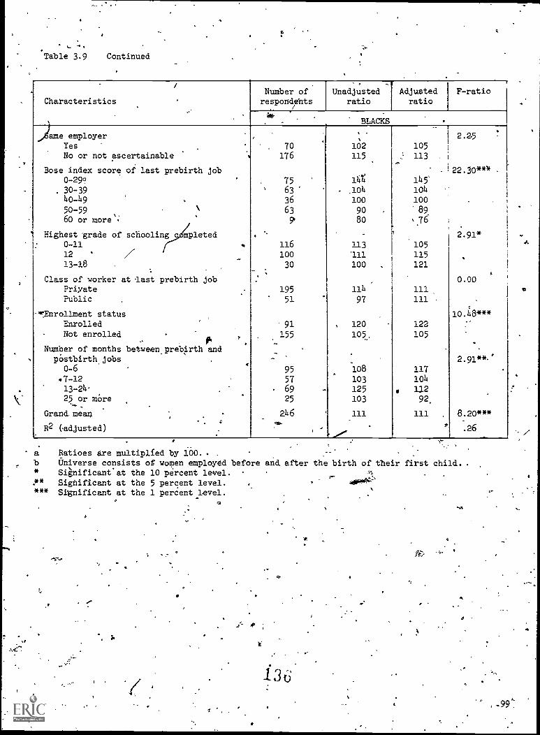
Table 3.9 Continued
Characteristics
.
. .,
.
Number ofrespondfnts
Unadjustedratio
Adjusted 1
ratioF-ratio
BLACKS
dime employerYes
.
No or not ascertainable
Bose index score of last prebirth job
0 -29?
. 30-3940-49 ,
50-59 . \
60 or more
Highest grade of schooling mpleted. 0-11
12 ' /13-18
,
Class of worker at last prebirth jobPriyatePublic
-10Enrollment status.
Enrolled.
Not enrolledIF .
Number of months betweenhrebirth andpOstbirthjobs
0-6
7-1213-24 .
25 or more..... .
Grand-mea4
R2 (adjusted)- .
.
.
.
-
,.
'
. '
_ .
-
70
176
756336
63
9'
116
100
30
195
51
' 91
155
.
95
576925
246
,
'
,
102115
.
147;
.104
100
90
80
113111100 ,
114
97
120 .
105..
108
103125103
111
105
S 113,
145'
104
100
89.
s 76
105
115121
.
111111
122105
117104
, 11292.
111
1
i
i22.50*"
.
'
2.25
-
2.91*
s
.
0.00
10.48***
2.91**-'
8.20***
.26
a Ratioes are multiplied by 100. . --.
b Universe consists of women employed before and after the birth of their first child. .
* Significant'at the 10 percent level.%
,.** Sighificant at the 5 percent level.4.
*** Significant at the 1 percent level.a
130
a
a.

-.
4
,
number of months between 'last" and "first" jobs is generallyassociated with better wage retention. This is consistent with thenotion hat a shorter period of absence is assn 4,
I not only with asm ler depreciation of specific and general skills acquired onear r jobs, but in addition, probably reflects closer continuing
-, ties wi h the job.market.21 A woman who is absent from work for only'.a relatively brief time probably, on average, still'has better bersonaljob contacts andao. greater.aware4ess'of available employment
/Opportunities.
Class of worker at last prebirth job was included in the analysisbecause we hypothesized thb.t civil service provisions and (perhaps)more liberal maternity leave policies in the public sector wouldresult ingovernntent workers being better able to retain their prebirthwage and ovupational stabs levels. There istlittle ev4ence tosupport this hypothesis, however.
CONCLUSION
The results of this chapter are suggestive of continuing dramaticincreases in labor force partisioation levels at that life cycle pointwhere women, for the most part,- have traditionally withdrawn frommarket work activities. Young women now clearly stay in the laborforce until they are withip g fevz months of the birth of theinfirstchild, and Treouently return,to the labo force shortly after thebirth. This is ParticularlSr 'true for blac women. _
o
$
Reflecting-both a relatively short interval'away from work as'wellas the likelihood that women with better job options appear to be the_first ones to return, mbst'of the women who do return within a brieftime span are relatively successful in at least regaining their pre-birth occupational status and wages; and in many ipstances they returnat levels substantially above those of their plebirth jobs.
From a policy perspective, all o f the above suggesta- that both in-
; b and out-af-school guidance; training and.4ducation should be aimed at. assisting young women in Plinning for work carearethat will problblybe substantially continuous, ratherhan following the tradWonaimodal pattern of Postschoo/ work,t,extensive interruption for child-bearing and child rearing and, perhaps, a return to work when the
: children reach sbhool,age.- The average young woman in high. school.(or college) may not be cognizant of contemporary realities; thus,guidance programs should emphasize the likely short-term work,interruption'that young women now ehcounter,:and education and training
21 A.,71FoF evidence on this point, 'see Sandell and Shapiro (in press,
100
J l o
it, 137.,, ....
a ...
1
111 .?"

programs should befgeared toward patterns of continuing rather thanwidely intermittent lifetime -employment.
L
The results of this chapter presenta mixed Picture concerning theability of women at this life cycle stage to he successfulin the labormarket. We have demohstrated that the unemploy;aent rate for white
women reaches 20 percent andforblack women exceeds 30 percent in-themonths following the first birth, even though virtually all of thesewomen have had recent labor market experience. On the other hand, wehavealso shown! that those who do find jobs often are quite successful.o
Generally speaking, the employment related experiences of thesewomen parallel the experiences of the adult population at largeOgthatis,-those with.less education and skills have disproportionatedifficulty 'finding employment and attaining satisfactory wages andOccupational status. The most satisfactory adjustMents are made bythose with the most edUcations This is particuldrly true for blackwomen.
It appears that better institutional means are necessary forhelping many of' these young women--particularly those with lesseducation and work-related skills--wih their reentry problems,as wellas ensuring maximum complIance with maternity-related employment
visions. Where these provisions are inadequate, perhaps stronger'employment providions are needed for ensuring more equitable wages,hours and working conditions for tU,is increasingly important segmeht of,the American labor force. ,
From 's. research *perspective, it is apparent that the lifetime workorientation of women is gradually approaching the more continuous'pattern follOwe4.by.m.n. As such, theoretical economic,modeling.offemale labor force participationbothshort and long term--may in the37ears ahead be more closely approximated by the standard theoretiCal,perspectives,previously appropriate only for.diagnosing male workactivity.
40k-
a
a
13.8
8
101

fiEFEBEN-CES,
-
Becker, Gary. The Economics of Discrimination, Second Ed tion.Chicago: University of, Chicago Press, 1971.
itBose, Christine E. Jobs and Gender: Sex and Occupational Prestige.
Baltimore, Maryland: Johns Hopkilps Press,1973.. .
.
Bpweri, William G., and Finegan, T. Aldiich. The Economj.'',''S. of Labor
Force Participation.. Princeton, N.J.: Princeton UniversityPress, 1969.
"Goldberg, David. "The Fertility of Two Generation Urbanites."Population Studies (March 1959):"214-22.
Goldstein, Sidney, and Goldscheider, Calvin. JewishAmericans.. --Englewood Cliffs, N.J.: Prentice -Hall Inc., 1968.
ti
Hayghe, Howard. "Marital- and Family Characteristics of the LaborForce in March 1973." Monthly Labor Review 97 .(April
21-27..
. "Marital and Family Characteristics of the Labor Force,'March 1975.'" Monthly Labor Review.98 (November 1975: 52-55.
" HiL1,+C.Itreell, and Stafford, Frank P. "Allocation Of Time toPiresohool Children arid Educational Opportunity." Journal, of
Human Resources 9. (Summary 1974): 323-41.. -
Leibowitz, Arleen. "Education an4 Home Production." American Economic
Review' 64 (May-1974): 243-50.
Merton, Robert K. Social Theory and Social Structure. NAw York:The Free Press, 1968.
Sandell, Steven H. and ShapirO, David. "The Theory of Human Capital
and the Earnings of-Women: A Re-examination of the Evidence."Jour.rial of Human Resources (inn press):
U.S. Bureau of the Census, Census' of Population: 1970. .Subject
Reports. Final Report PC(2)-6A Employment Status and WorkExperience. , K
102,
3.!
an,
. 1 3 9
J.

t
4
A P P E N D I X
Glossary Of Variable and Universe Descriptions
I
Universe Descriptions
In thelanalysis of labor force participation raes:before thefirst birth, a respondent is not seleCted for any cross- sectional
4,universe unless her first child was born between ,the 1968 and 1973'Anterview dates- Each model requires. a scan of all survey dat6s
(1968 to 1973) in order to select women 'in the appropriate timeinterval relative to the child's birth. As a result ofthis procedure,any one respondent-may be represented in more than one model.Information for the explanatory variables is drawn from the surveyat which the respondent reaches the required time period for eachmodel. As an additional universe restriction,, no respondent can be
.00.
enrolled in school at the survey date referenced.
Respondents selected for the change in wage and occupationalstatus models :dust have been employed 'before and after the 'birth oftheir first child. The reference point for each explanStory variableis either implicit in the variable title or explained in the variable'definition. -
Depende nt Variables
In theanalysi- s of labor Throe participation rates surroundirig.the first birth there area total of Live dependent variables,eaChassociated, itti one of five cross-sectional models. An individual whois in the4labor force during the indicated time interval rebeties 40a value of one on the dependent varial:Ae, otherwise-she receives avalue of zero. The five selected time intervals are divided asfollows: (1) eighteep to thirteen months prior to the bitth of thefirst child,; (2) twelve to six months before; (3) five zero monthstiorei.. (4) one. to five months after. tie birth; and a(5) 'six to twelvemonths after.
For the analysis of changes in wage before Andafter the firstbirth; th 'dependent measure is created by'dividing the hourly rate ofpay. on th first postbirth job by the hourly rate, of pay on the lastprebirth job and multiplying the resulting quantity 'by 100. To con-
,struct the .dependent variable for-change in occupational status,..thesame technique is performed using the Bose Index score.
Explanatoiy Variables
Bose %ndex score of last prebirth job.- The Bose Index isan ordinal measure of occupational prestige. For further
.
it
. 140
103

- .
'detail; 'see Bose (1973): Variable is categorized as, follows:
(1) 0 to 29.(2) 30 to 39(3) 40 to 49(4) 50 to 52(5) 60 or.more
Class of worker at last prebirth job. Variable is-categorized as, follolis:
W. Private sector,. (2) Public sector
dr.Does health limit the amount.or kind of work'respondelatcan dp?, Variable is categorized as follows:
(1) Yes
-(.2) No
Does respondent desire to work at age 35? Variable ise categorized as follows:
'(1) Yes
(2). No or Ddn't know 00"
Enrollment status. For'the change in age andloccupzItionalstatus models,.this variable is.measur s aS of the survey' year:
o in,which the last-prebirth job ended,` If a woman never stbppedher prebirth job, then the reference point is-the survey yearn which her childN1.ras born. Variable -is categorized as .
golloWs:
(1) Enrolled...(2) Not-enrolled
'Highest grade of schooling completed.' For the phange.in wage,-and occupational status models',-,tiiis variable is measured as_ofthe survey year in yhict"the first postbirth job be n-.I. "If a
woman-never stopped her, fast prebirtri ..fob., then-th ref6rehcepoint is, the survey year in which her child,was b n. Variable
. is categorized as folldtrs:a 1 - i. * sI (1) o to 11 , ..,
, (2). 12.
. (3) 13 to'18..
.
'4.,. . ,
/Hou y rate d pay at laSt prebirth job. Wages are adjusted to19. dollars,- Variables is:categorised as dbllowS: .
(.l) $0 to` 1.149
,(2) 41.50 to 1.99
(3) $2.00 oK more
141

b
4
Is the employere.on last prebirth job the same as the employer on'first postbirth job? Variable 1s categorized as folloys:
(1) Yes(2) No or Not- ascertainable
. Marital status.. Variable is categorized as follows:°(1) Married, spouse present
(2) Other, which 'includes: marri d, spouse absent;widowed; divorced; separated; eyk. married
4 .0Number of months b6tVeen last prebirth ,jbb and fartt postbirthjob. Variable is categorized as fbllows:
,;
,(1) 0,:to
(2) 7 tip 12 -
(3) 13 tO '4111(4) 25 or more
OccUpation (1-digit) on last prebirth job. Variable iscategorized-as follows: ?
(1) Professional, Technical and rindred.Workers, Managers,Officials, and Proprietors
(2) Clerical and Kindred Workers', Sales-Workers(3) Service Workers, excitiot private household..(4) Craftsmen, Foremen, 'and Kindred Workers; Operatives
and Kindred Workers; Private househRld.workers;Farmers and Farm Managers; Farm Laborers and Foremen;
,..Laborers, except Farm and+Mine
otria ad s age 21 or older other than respondent or respondent'shusband,esent in household. Variable is categorized as follows:
0
(1) Yes(2) No
Potential wage. Separate wage equations were eimated forwhile and black working women. Wage's were expressedin..1967
-dollars..
4
For whites the wage eqgation is as follows (with t statistics-inpartntheses):
°
4WAGE= 143.38 - 20.802x(EDUCATION) + 1.6313x(EDUCATION2)(2.99.). (-2:80) . "(5.64). '
. ,
+ 20.57x(WORK EXPERIENCE).- .97405x(W6RK EXPERIENCE2).0.25) ' (-4.47)
I
+ 24,07:25x(SMSA) = 6:4141x(SOUTH)
(5%pI) - (-1.25)
No. of observations-= 1,482 R2 .(adjusted) = .26'
' f
1 42
-.4
, 1'05
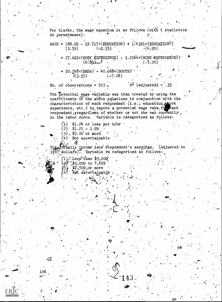
*MD
e
s
For blacks, the wage equation is as follows (with t statisticsin parentheses):
WAGE = 186.22 - 19.717x(EDUCATION) + 1:4391X(EDUCATION2,)
(3.59) ('-2.331 -(4.05)
$
+ 17.022)0079tpRIENCE) - 1.2564x(WORK0EXPERIENCE2)'. (6:8 , -
,
(-5.20).
+ 20.7,48x(S,MSA)- 4o.c168x(souni)- t ,_
4. ( 3.35) A-7.28) y
f.'- .
No. of observations = 523,, 13? (adjusted). = .331 ,.
le.The potential wage var,iable, was then created by using thecoeffiicents Ot the abdve equations in conjunction with thecharacteristics of each respondent (i.e.',. education ork
ctexperience, etc.) to,impute a potentiai wage ratef ach
respondent,tregardlets of whether or not she was currently,.in the labor force. Variable is categorized as follows:
(1) $1.24 or less per hdur
(2) $1.25 7.1.99.
II, (3) $2.00" or more: '
:-, (4) Not ascertainable .
. 4, To aily ipcome'less iespondent's earniligs. (Adjusted to
.
' 19 dollOs): Variable is categorized as follows:,
' (1)) IesS-6-lan $3,0001:.
( °,$3,000 to 7,499-$/,50pydr more
106g
Neat ascertainable , ... '. 4,-;,
I...o. g i*D
:...11 ".
.414. 'p As.., 4
°
1I'
. . , .
I
M.
6
1'
Wit
a V
..A
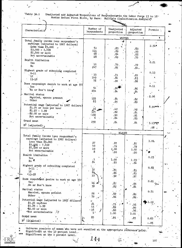
'Table 3A.1 Unadjusted and Adj'usted'Propol.tionsof Respondents*in the Labor Force 13 to 18-
Months Before First Birth, by Race: Multiple
. -
Characteristi
-' -
Number of'respondents
Unadjustedproportion
Adjusted.proportion
F-ratio
WHITESTotal,family income less respondent'searnings (adjusted to 1967 dollarS),Lee s than $3,000
, .
$3,000 - 7,499$7,500 or more -3
Not ascertainable
Health limitation .
Yes
No
Highest grade of schooling completed- 0-11
...12 . .
13-18.
.1.
.
Does respondent desire to work at age 35?Yes ,
No or Don't know'
Marital status
Married, spouse presentr Other 4°
.
Potential wage (adjusted to 1967 dollars)$1.24 or less per hour$1.25 - 1.99
-$2.00 or more ' .
Not ascertainable
Grand mean.
R2 (adjusted):,4.
511116828
11247
'33149
76
54204
.
.
1T.5
83
.
161.04
132. 6
258
.
.
_
.
.
.
.83
.89
.84
.69
.70,
.85
.71
.84
.90
.84
.84
.84
.85.
.42
.82
.90
.84
.84
!
..
:
.
,
,
0'43
.90
.8
.70
.79
.84.
.85
.83
.86
.86
.84
.82
.89
.42
.81
.91
.83
.84
,
2.54*
....
.
0.21
0.13
0.11
.
.2.06
8.90 **4
3:13,1*
.08 ,.
. - . .
Total family income less respondent'searnings (adjusted to 1967 dollars)Less than $3,000
$3,Q,00 - 7,499 .
$7,5.00 or more
Not ascertainable.
Health limitation.
Yes .
No
Highest grade of schooling completed0-11 :
_ . -
12.
-13 -18
Does respohOnt desire to York at age 35?Yes.
.
,NO or Don't know
Marital status .
Married, spouse presentOther .
.
,;-
Potential imge (adjusted to 1967 dollars)$1.24 or?less$1225 - 1.99 -
42.00 or more'Not ascertainable
.
Grand mean- .
R2 (adjusted),
. BLACKS
27
40
10
.1
84
...
32
10
46
39
26
59
-
2145
' 15
4'
85
-
,,,
j
.
'
.87
.791.00
x.90.90
....
7..00
.85
,-
:81
.86
.92
.87
.82
.82
.86
.75
.89
.80
1.00
.85
6
.
.87
.79
1.02.90
1.03. .814
.83
.83
.97
.85
.84
.80
.86.
' .76-
.90
.76.
'1:01
.85
-
.
1.01
r
0.25'
o.68
0.01ebt,
0.51
4.1.1971*
.
0.65
-.0$
Universe_ consists of women'yho were not enrolled at the appropriate /4ference"polnt.Significallt at the.10 percent level.Significant at the 1percent level.
144 107

Tab1e,3A.2 Unadjusted and Adjusted Proportions of Respondents ih the Labor Force 6 to 12Montht Before First Birth, by Race: Multiple ClassificatiSn AilT5sisa
Number ofCharacteristic -retpondints.A4.
. ,..
Unadjus.ted
pr;portionAdjustedproportion
F-ra*.tio
WHITES
Total family income less respondent'searnings (adjusted to 1967 dollars). Less than $3,000 /
$3,000 - 7,499$7,500 or moreNot ascertainable
Health limitationYesNo ,
Highest grade of schooling completed.0-11/12 .
-13-4 18
'Does respondent'desire to work at age 35?-YesNo or Don't,know
Marital status .
Married, spouse present .
- Other0 ..,
Potential wage (adjusted to 1967 doll'ars)$1.24 or less per hour'
$1.25 - 1.99$2.00 or moreNot ascertainable'
.'Grand mean .
R2 (adjusted).
.
.
..
82
201
9749
28
401
77253
99
115
314
.
319
'110
48-
19817310
429
-
'' .
^
.81
:79.68 .
;O.
.57
.77
.53
.78
.134
.77
.75
1.,
.74
.80
.36
.13
:$8
.73
.75
.83
.80-4.w
:63 .
.684
.66
.76
.70
.78
73
.77
.75
.71
.88
.35
.70
.92
.67
.75
I
5.61***
.
1.55
1.29
0.40
16.92***
"27:051***
.,
8.75***
-.17
. s
Total family income less respondentsearnings (adjusted to-1967 dollars)
Less than $3,000$3,000 - 7,499$7,500 or.more ,
Not ascertainable
Health limitationYes .
No_
Higtiest grade of schooling completedA 0-11 >Ile. .
12 .
13-18 .. . . f-..- /
Does faspondentfdepire to woricat age,35?Yes
. No or DOn!t know. ,
Marital status .
..
Married; tpouse present-Other .
.
.
Potential wage (Adjusted to 1967 dollars)$1.24.or lesi per hour$1.25 - 1.99$2.00 or more
ZNot ascertainable ..
. ,. Grand mean
112 (,adjusted) A/
BLACKS
.N
.
'
s
55
5017
15
11
116
.
7067
5483
29
°80
.. 22
6
137
.
.
4,
.
.79-1.84
.71
.95
i,
.25
.85
.71
.85
.89
.76
.86
.77
.85%
.62
.80
1.00.88
...... . _
.
.8S' '
.84
.83
.58
- .95
.
'.30-
.85
- .
.66
.81
.76
,82..82
i
, .
,-.76'
.85
.57
.80
1.03.83
.82
.
-
. :,3:16" '
.
20.12***.
. -
0.45
0.00c
2.10
8.36***.
,
40-43***
'.21.
.
a .Universe consists Ot women who were** Significant at the 5 percent level..***''Significant.ab the 1 percent level.
los
not enrolled, at the Appropriate re?arenct point.
145
I',
a
0

Table 3k.3 Unadjusted and Adjusted Proportions of Respondents in the Labor Force t) to 5Mohths Before First Birth, by Race: Multiple Classification Analysisa
i
Characteristic
L.
Number ofrespondents
41Unadjustedproportion
Adjustedproportion
F-ratio
.
"1
.
WHITES, .
Total family income less respondent's.7 earnings (adjusted to 1963, dollars)
j
Less than $3,000$3,000 - 7,499' .
$7,500 or moreNot ascertainable
Health limitation ,
Yes ,-
'"' No -
Highest grade of schooling Completed0-11
12 .
13-18 .
Does respondent desire to work At age 35?',Yes
. No or Don't know ,..
Marital status. .
Married ,' spouse present .
Other
Potential wage (adjusted to 1967 dollars)$1.24 or -less per hour
_ $1.25 - 1.99$2.00 or moreNot ascertainable
Grand mean
(adjusted)
.
o
f
.
81200
9946
.
, 21405
88
230108
.
130
296
' ,364
62
50
180x.80-
16
426
.
'
.
-.42
.44 .
.44
.38
.51
.42
.15
.47
. .57
.50
.40
a
.43
.40
%05-.32
.61
.48
.43
.
-
-
.44
.45-
.38
.4;4i
.
.58
.42
.28
.47
.46
.46 ,
'.41
.41
:54
.13
.3
.60
.47
.43
-
,
0.58
r
2.68:
5.92 * **
.
-
0.98,
4.32#*
*-------
19.19 * **
.
. .
8.12***
.16 °
I/ .
Total family income less respo dent'searnings (adjusted td11967 dol Ts) .
Less than $3,000$3,000 - 7,499
$7,500-or more.
Not ascertainable --
.L
Health limitationYes .
No ..
.
Highest grade of chooling completed0-11 .
. -12.
13-18. ,
%.Does respondent desire to work at age 35?
Yes
No or,Don't know ..
--.
Marital Status .
Married, spouse present.
Other _
Potential gage (adjusted to 1967 dollars)-$1.24 qr_less per hour$1:25 - 1.99
. //,'$2.00 or more ..-`
.
Not......agdertainable .
Grand mean ..
'. ' ..
1,R2 (adjusted) : . '
r BLACKS
51
- -7216
,,31
-
a
16. 154
-
%
73
7819
' 10169
74
96
*
51
84
30
5
170..p.
'
.
8
,
.43
.t5
Or;61
. .55 ."-
..
.57
.47-.
.35
'-.56
.64
.48
.149,
.48
.49
.
.
.73
.20
.48
.
.
.41
.t8
.52
. .57
,
.60;
,47
, .41
-.52
.57 r^
- .50
-.47
-.43
.53
.28
.52. .69
.21
- .48'
.
.
,
0.83
1.40
.1.36
.
0.17
1.92
,
5,37***,.
2.5211t*
,09
t
a Universe consists of women Who were not enrolled.at the appropriate reference point.** Significant at thil5 peTceht level."41 Significant at the,IpercAt level. .
4,4.4
1-4
.8*

Table 3A4 Unadjusted,and Adjusted Proportions of Respondents in the Labor Force 1 to 5Months After First Birth, by. Race: Multiple Classification'Analysis&
I
Characteristic .
Number ofrespondents
OnadjUStedproportion
Adjustedproportion
F-ratio
. ,
WHITES
Total family ineome'less respondentlsearnings (adjusted to 1967 dollars)
.- Less than $3,000$3,000 - 7,499$7,500 or moreNotascertaiable -
Health limitationYes .
No i
Highest grade of schooling completed_0-11 AOT,
1213-18
Does respondent desire to work at age 35?Yes .
No or Don't know'
Marital status iMarried,.spouse presentOther
Potential wage (adjusted to 1967 dollars)$1.24'or,less per hour'$1.25 - 1.99 .
.
$2:60 or-more ,
'.. Not ascertainable
Other adult age 21 or older present in,household 4
Yes.
.
No \
Grand mean.
R2 (adjusted)
,
.
.
..
72211107
52 ,
18424
95
246
101
164
278
39745
57,
183
18022
74
368
.4142
.
.
9
-
_
.,
.
-
.31
.37
.35
.30
.35
.35
.33
*.35
.37
.45
.28
,34
.45
,
.30
.34
-.38
.31
.14
.33
.35
.
-
.35
.37
.32t .31
,,
.37
.35
.36
, 35.34
. ( .
.45
.28.
o
.34
.40
.29
. :.33
o' .39.26 .
...
.44
.33
.35
.
f
0.42
.
.
0.05
.
0.05
13,26*** ;
. .
0.63
.
1.07
3.22*.
1.70*
.02'")
...
.'
Total family income lest, respondent's
earnings (adjusted to 1967 dollars) -%'l -.Leas than $3,000
$3,000 - '7,499 '-'°'' ,
$7,500 or moreNot
.Health limitation
Yes.. '.
No. .
.
Highest grade of schooling completed,0-1112 . -
A
/
13,18 . - °,
Does respondent desire to work at age 35-7faYes 4
. No or'Don't know
Marital status - .
Married, spouse presentOther
Potential wage (adjusted to 1967 dollars)$1.24 or less per hour
.
$1.25 - 1.99 '
$2.00 Or moreW Not ascertainable - .
Other adult age 21 or older presenn'household .
, -.
.,.r-,.r- Yes
c
.11o.
Grand mean
R2 (adjustedZ._ .
.
:BLACKS
'
.
54 4
. 7323
21
.
169
-70
86
15
/
'109p.
90
, 81
39
- 103'
_ 20
s.-.- 9
86...
11171
.
.
.
..,
-
-
*
c
.
.
.
52.
.48
.53
.56
.41
.51
.41
_54
.72
:
.57:.40
,
.50
.53
.28
..59.
.49
......
.
--.53
.49
.51
(
-
,,
.,
-
.
.53
.-49
.49
''.53
.50
, %51
.42
.52
.78
.55
.43
.49 :. .53
.-35
ii'.51
p .54
.48
.51 ,
----
'
.-
Nk
0.07.4.- -
0.(Q0:,
.
3.51**
.
.
2 58 4'.
,
, d
0.29
*
2.41*.
%r:"--
0.69
'1.55*
.04
--- , N. -
. .
Uhivers'e consists of women who were not enollvd at the appropriate reference point.Sgnificant at the 10 percent level. .,)
gnificant at the 5 percent level.*** s gnificant'at the 1 percent level.
Vs.110 ,
. 1 4 7
,

gl.
0°Table 3A.5 Unadjusted and Adjusted PrOportionslif Respondents in the Labor Force 6 to 12
Months After First Di ,by Race: Multiple Olassifpotion'Analysisa
Characteristics- [ Number of
r -respondents
Unadjustedpropottion
Adjusted : j
proportion'
'F -ratio
T WHITES
't"
.
Total family income less respondent'searnings (adjusted te1967 dollars)Less than $3,000 80
1j 264$3,000 - 7,499.$7,500 or more 153
Not ascertainable 51
Health limitationYes . 29
No 519
Highest grade of schooling completed0-11 127
12 293
13-18 128
Does respo ent deisre to work at age 35?, Yes 240
NO or Don' know 308
Marital statusMarried, spouse present 495 .
Other . 53
POlential wage (adjusted to 1967,dollars) ,..,.,,,,,,,
$1.24 or less per hour 7S$1.25 - 1.99 , 228
i $2.00 or more 215
Not ascertainable 32
Other adult tige -21 or older present in 4
householdYes , 70
478
Grad mean - 548
R2 (adjusted)
.44
41.33
.39
' .32
.39
.32
.40
.43
.39
.39
.3T
.53
.17
.42
" .42;46
,44
.38-
'`.39
2.70**
.45.42
.30
.39
! 0.34
.34
.39IS .
0.35 i/36
.39,
,41 1 lc as
0.06
38- .39.
3.58*.38
51
6.50***.15.40
.44
.46
1.52
.38
P.39 2.53e**1
03 '
Total family income lessearnings (adjusted,to,Less than $3,000
$3,000 -.7,499 1
$7,500 or more jNot ascertainable
;Health limitation :j
YesNo
-...'
1
Highest grade of schooling0-11,12
13-18 1
Does' vespond'ent desire
Yes - r ' 1
No orDon't know'44 1'
,
Marit'al status;
a spouse piesentOther -
potential wage,(AdjUsted$1-.-24-or less terhour
$1.25 - 1.99 , I
' $2.00 ort,iore
1Not ascertainablei
,Other adult age, 21 or
-., householdYes . , .
No '
y
4' Grand mean
R2 (adjusted).'
BLACKS
respondent's1967 dollars)
r .*7
lir4. 38
i
21
1 16.
237
completed
9628
29
to -work at age 35?. 136
, -..117%
1
133
120
to 1967 dollars.),
73
125
39 ,.,16'
't 7
older present ill
.
,,-... 437, j 116
' 253
.
.52
.51 fit:80
.60
'.64
.56
1(----Hai
. p60
',52 i\
:54
.59
44.62
71, .
-.37
,
.56
.57
''.56
/
.52.
.51
.75
,61
62.56
.53
.55
.59
.53
N49..64'
.
49 ..61.67,
-36'
1
.54
-59-r ,
.56;
0.24
2.25
0.81
5,82**
2.60*
0.70
2.33***
06
. 1 i.'. , '
1
J
Universe censists,9q7 women who were not edrolled'at the appropria referenc.point.
pipitreant at the%10'percent level. . .
Significant at the 15 percen't level.'SignificanAat the 4 percent level ,',
)
1 1
I
111 .
s
f.
1
1
Ot,
CHAPTER 4
OCCUPATIONAL EXPECTATIONS FOR AGE 35
Patricia K. Brito and Carol L. Jusenius
INTRODUCTION
Over the past several years there has,been'a growing interest inoccupational patterns of female employtent. Evidence of this is theexp'ding literature on the extent to which women are concentrated in,a re atiyely number of occupationTand on the-extent-to whichrome are moving out, of these "stereotypically female" occupations andinto one which have beencharacterized.as "stereotypically male."1Concurrently, there has been much concern about the effects onyomenof chgnging demands for'workers in specific occupations. For example,tshe projected oversupply of individuals .training to become teachershavignificant ramifications for college-educated women.2
This chapteAsxploresboth.these areas. Focusing on, the young.;women who in 1973 indicated they expected to be working outside thehome at age 35, in thekfiegt major section we analyze the characteris-
'tics of those whostated a desire tolbe in occupations typicallyheldby men. In the second major section, we examine the extent to.which these women's aspirations regarding'employment.in specific'occupations have changed between 1968 and'1973 and the relationshipbetween the, shifts and proected demand.
OCCUPATIONAL PREFERENCE: TYPICAL VS. ATYPICAL OCCUPATIONS
.Odeupational segregation of women'in the American labor market
has been a persistent phenomenOn. According to the 1940 decennialcensus; 63 percent of all women.ln the labor force werg.in occupationalcategories in whiCh 50 iiercenor more of the'incumbents were.femele;by 1970, the comparable percentage was about 65 percent.3
.
'r Tor example, see Oppenheimer (1197.3); Jusenius and Shortlidge-1
(1975);exic1111clis(1.975). '
.
P.
2Fo example; see The'Ca negie Comtiasion on Higher Education
(1973) ; :
3The 1970.estihate is based..ola figures for the experienced
divilian labor 466 from U:S.! Department .of Commerce, Occupational`Characteristics: I.The 1970 occupational cat6gorpas were'coddd into the
-1960 classificAtiOn schete,WhSch is ore :nearly comparable 'to that
used in 1940. SeWriebe, Heinkelana Greene, (19T21.
4.7
1
1.
;
ti
..,
.
113.
1

,
t .
//The' Importance of DccuPation Segregation t
Research has found that occupational segregation has had a-profound effect on wages. yorkerbf both sexes who are in pre-dominantly female occupations earn -= substantially lesssthan similarlyeducated persons in characteristically male Occupations)
Given that workers in typically female occupations are at aneconomic disadvantage relative totheir counterparts in typically maleoccupations, it is not clear why women enter these Occupations.
Proponents of affirmative action rogi-ams have argued that demand-sidefactors, i.e., the preference of:employers'for men or women incertain occupations, are to a large extent-responsible for'the extant
. occupational segregation. However, when young women who expect to be_working at age 35 are asked in what Occupation they would like to be,the vast majority mention occupations typically held by women (Table4.1). Hence, it seems probable that the predominance of women incertain occupations reflects, in part, theLr,own treferenCes. ;Statedanother way, it appears that supply-side factors are also responsiblefor.ocCutational segregation.
To the extent that women prefer a typically female occupation,affirmative action programs directed solely at employers will notsubstantially reduce occupgtiOnal segregation. HeAce, in.addition topursuing a vigorouS affirmative action program, public policy.
4
undoubtedly should be concerned with counseling and educational,programs if young women are to be informed about the flillrange ofavailable occupations.
If the observed preferences of women fol. is. relatively smallnumber of occupations dO reflect -their tastes for 'Articular kindsof work, this suggests that,.stereotypicaly female occupationS may havechgracteiistics wkch correspond especially well to women's s"
requiremep. For'example,job opportunities inipese occupations may.permit geographic mobility, hours of work may be_flexible, or:theremay be little financial penalty associated with leaving and subse-
'quently reen ering'the labor force. .
AO."An alternative, but not mutually exclusive, explanation is that:
the choice of a typically female occupation is the product f theqbcia/iiation process within the fami1y'and society or of hepolicies.of,educational institutions. To some extent,the perSonalattributes of a young woman shbuld reflect her pastsocial oreducational experiences. To the degree that these determine thestrength of her labor market commitment and her views on which
, occupations are suitable for Women, one would expect the probability
Treiman and Terrell (197.5) See also Jusenius (1976).,S
150s
s
i '
r
I

1
Table 4.1 Sex - typing of Occupation Desired for Age 35, byEducational Expectations and Race, 1968 and 1973a
(Percentage distributions)
..
Sex-type of ocaupation,prefer/ rib
1968
.
... ,
. .
1973 k
Whites Blacks' Whites Blacks
Noncollegec.
Number.of respondenti 443 358 , 507 302. 4
Total percent . 100 100 . 100 100 .AtYpical- . , 14 10 19 13Typicql 86 90 81 1. -87
aCollek-46
Number of respondents 448 279 877 339
Total percent . 100 100 100 100Atypical .23 15 25 22'Typical 77 85 75 78
a Sample size in 1968 differs from that in 1973 because eachconstitutes an independent cross- section of,therespondents. ,
f Occupations-are defined as "atypical"ior "t ca for femalesbyby a.comparison of the percentage of the 190 labor force ',..
which was fema;e-with the percentage of an cupation'sincumbents 'who were female. See p. 118 forl
i
more complete.5,
texplanation.
.c "Noncollege"'refers to thbse respondents whO have completed .
less than 13 years of sdhool and say that-th y do not expectto go to college. "College" refers to tho4 respondents whohave at least fine-year of Co4ege, are attep ng college, or
1indicate theyexpect to go to college.
J.
..151
}
.r !
1,..400tr,
A .11 I

of choosing a stereotypically masculine career to vary by personalcharacteristics of the respondent.
In this chapter, we'attempt to identify the periOnal
characteristics of women -Oiat'are correlated with the choice of atypically male occupation. By limiting our analysis in this fashion,we do not deal-with the characteristics of the occupations themselyesthat might make them especially attractive or convenient forwomen. .
Nevertheless, identification of those attributes of young women whichinfluence their preferences for typically male or female occupationsis important: it provides information necessary for the formulationof public policy aimed at reducing.Supply -side barriers to entry intotypically male occupations.
Clearly there are a myriad of factors associated with both theindividual and specific-types of wort which influence a woman'schoice of occupation. .In selecting among thexh, we have chosen tofocus on those` suggested by previous research in the area of women'soccupational preTerences.
previous
k'
Previous Research .
Pre :ous.research on this subject can be roughly characterizedas Tflecting two schools of thought. One group of studies, found-chiefly in thevocational and psychological counseling literature,_has suggested the -concentration of women in a relatively smallnumber of occupations reflects the differentiated sex roles foundwithin the family and society. ,For instance, a mother's role'as"homemaker" anda father's role 'as "income-earner" may act assignaling devices to the daughter regarding her expected role aseanadult. Familial roles that proyide a woman with a broader view of'her "proper'! sphere wili alsotend to7increEise the probability of her,entering a less traditional occupation.5 A second argument has beenthat family size and the sex distribution of the.children,arefactors which influence a young,woman!s occupationa1.choice.' Foragiven level of income, theicomaller the ukEMber,of children, the greater-the amount of resources which can be devoted to each child.LFurthermore, if a: young woman is an only child_or-if there are nosons inthe household, all the-parents' ambitions will-be centered on.the deughter(s).' Thusin small families, there is a higherprobability that daughters will receive the financial aid and `
encouragement necessary for thOse atypical, professional occupationswhich require extensive training.6 .
5For example's, see AlMquist and Angrist (1971); Klemmak andEdwards (1973); Nagely (1971).
,
-; 116 ,
i ;
6Roe (1953) ;1 Klemmack, ando Edwa.rdS1(1973).
*
....
4
O
Another group of researchers, notably human capital theorists,have suggested that women's concentration in a select number ofoccupations may arise from b. rational economic motive. Theseeconomists argue that when earnings'over the life cycle are considered,
, .incumbents of typically female occupations may not be at an economicdisadvantage relative '-to their counterparts in typically m§leccupations.7 That is, if typically female occupationp arecharacterized by a relatively high initial wage and a,relatively flat,life-time-earnings-profile,, it may-be economically ratiOnal_gorwoman to enter these occupations if they, expect a short workingcareer. In contrast, men, who typically foresee a long,workingcareer, tend to z.nest in themselves by entering occupations' which mayhave a'lower initial wagp buI higher future earnings. Women who alsoexpect a sufficiently long warking career would behave in a mannersimilar to their male counterparts: they would be willing to sacrificepresent wages to maximize wages over the.long run. Hence, thesewomen would be. interested in the tame types of occupations as men andwould be likely to choose an occupation in which men predominate.
The Empirical Model_
The model of occupational choice rre'Sented in°this chapterrefines boththe human capital and the vocational counselingperpectives of occupational preference.' First, it includes in oneempirical model both those variables describing aspbcts-of tifechildhood' familial environment suggested bit the literature invocational counseling'and those measures o, career commitmentsuggested by the human capital school. SedOnd; it is assumed in thismodel that while the roles played.:4F one'siparents are importantdeterminantS of occUp*ional choice, their effect may be modified by
.1
later schooling and work experience. Hence, it includes variablesmeasuring certain aspects of previous educational and labor marketexperiences.
Finally, the iodel advances the human'capital perspective bydi:ferentiating between women who expect to attend college and thosewho .o -lit.' At-the coileg<level,, a higher'proportiOn of-stereo- .
typi,: .y male professions (e.g., lawyer, physician) require graduateschOO1 a tendance and imply. a greater investmeptin human capitalthrOugh o the-job training than i_the case among Stereotypicallyfemale prfessions. Such inyestmens are typicpy associated
'with a sting ,commitment to,the labor force:. Thus,in line with humancapital r asoning, for:college women we hypothesize.that'gh,,expectati of-beinein a isle occupation would be significantlyassociated with those variables which meas4e the probable cadent of .
future labor market participation. In contrast to standard'hUMan'o
1
. i
I. Zellner (1975); Chiswick 'eta.1, (191()., .
I ,
11....; i, ; .
.
If 1, i
,-i, - ,1.53 1 '
i'1
i I ,-, .g. i
1
I . 117

capitd1 reasoning, we suggest that male occufVrions accessibleto noncollege women,(e.g., bartender) may not necessarily requiremore investment through formal education or on-Ithe-job training thanwould ,a female occupation (e.g., secretary). To the extent that thetwo types of occupations do tit differ in the amount of requiredinvestment in human capital, the choice of one or the other is ,
unlikely to be associated with measures O f career commitment.
,Specifically, temodel explores the correlates of the expectationof being in a typically male occupation at age 35 as reported by youxrgwomen Who anticipate being in the labor'force at that age. Thus, wedeal with plans, outlined in 1973, for a,time which is from six tdsixteen years ih the future.$ -
The techniqud employed irPthis investigation is MultipleClassification Analysis (MCA). With MCA we can determine for eachcategory of every independent variable what proportion of womenanticipated a male occupation at age 35, assuming that members of thecategory are "average" in terms of all other variables included.Differences in these proportions among the-several categories' of avariable ate interpreted as indicating the "pure" association of thatvariable with the probability of a young woman's choosing an atypicaloccupation.
;
I -
-The-dependent'variable_is-dichotomotia with the value' of r if-theWoman aspired to a typically male occupation and 0 if her choice wasaAtYpiCally female occupation. (For Simplicity, those occupationswhich -are stereotypically male will be referred to as "atypical. ". thosewhich'are stereotypically female, as 7typical.") Typical occupationsare defined empirically as those in which the percentage of incumbentswho are women exceeds the percentage of women represented in the totalexperienced civilian labor force. Since women.were-'38.1 percent ofthe experienced civiliah labor force in 1970, typical occupations thusare those in which 38.2,percent or more of.theincumbents,in 1970were women.' ,In an analOgOus fashion, atypical occupations are'thosein which 38.1 percent or lesa of the workers we're women in 1970.this definition, about 75 percent oaf the women in the experienced.
'8We believe that by studying expectations, we, have a "purer"imeasutefof occupational choice than is found in studies that examine
. a woman's presence in a particular occupation since presence in anOccupation is clearly;determihed by both,demand Conditions andpersonal preferences. .bf course, the respondent may prefe? an,occupation simply because she feels job prospects, are good in that'field; but it is felt that the piestion pf.what she:would like to be.I' , . ,
doing at age 35, by virtue of its being less related to present. liabor. market conditions', is a.hetter measure of preference.
,11
I i
,
rr
41,
civilian labor force at the time of the 1970 census would have beenclassified as being in a typical occupation?
The sample consists of young women who in 1973 stated t theyexpected to be.in the labor force'at age 35 This6un erse is-stratified into four groups: for both black and white omen (1) thosewho have attended c011ege or expect to attend college and (2) those
,with no college who do not expect to attend college.10 As alreadynoted, the stratification by education waslconsidered necessary. since
the implications for occupational choice of varying degrees of labormarket commitment are different for college educated and high schooleducated women. The stratification by race Was deemed necessary .
because of the probability that black and white women live in different'social contexts which influence the formation of occupational
'expectations.1111
NC.
Empirical Results 44>
-,F.'or ease -of exposition, the total set of independent variableshas been divided into three major headingS: Familial Environment;Educational and Labor Market Experience, and Potential Labor MarketInvolvement. The results are reported in Tables 4.2 to 4.)4. Thethree-separate tables,represent one MCA for each race and educationgroup.
,
.., . _a - .. o. .. ..
In the followibg sections, empirical results for each of thesecategories of women Is deFribed in detail12 It should be noted
. 4
4
9To define typical 'and atyplcal occupations, 1970 classifications
were converted into their 1960 'equivalents, using Priebe, Heinkel,ndGreene, 1970 Occupational and Industry Classification, since accupa-Lions in the NLS data aA,reportedin their- 1960 codes. Otherdefinitioh;, 5 and 10 percentage points above or beloy the 38.1 percentreference point, were tested in preliminary analysis. Since the re-sults aid not differ significantly among the three definition's, only,the results of the one model are presented here.,
1,110The results for black noncollege women are .not discussed in the;
text but are reported in Appendix 'able kA.1. Two7thirds'of those inthis group whowxpected to be in an atypical occupatioh had been coded
t' specifically as "operative, n.e.c." Hence our model seemed to betesting the probability of expecting{ to be an unskilled or semiskilledblUe collar .worker as much as expectations regarding;,;an atypicaloccupation.
liSiatisticalandlysis 'verifiadithe need for stratification byrace and education
,
412It will be apparent to the eaderAatr.-the empirical models
reported here differ forirade and ed4eational categories. Thel'
1
5I6119

i
at the outset.thatWhite college'women had the highest proportionexpecting to be in atypical, occupations at age 35--25 percent'. Theywele followed"by black college women and'white noncollege women, with22 and 19 percent, respectively.
Familial Environment
Thie set liCvariables corresponds most closely to those which,have been .studied as determinants of ocCupationai.choic6-inthevocational counseling and psychology literature. Here, we hypothesizedfirst that those women whose motherswere highly educated dr hadworked outside! the hom,e, would have- an above- average probability of'choosing an atypical occupation.
The empirical results indicate that the relationship betweenthe mother's experiences and the data', occupationalexpectationsdiffers by race gind educational ,level. A, variable representing the'
mother's education'and type of occulltion had a significant influence,,only on white women who expected to attend college (Table 4.2).13Even here, however, the hypothesis that the mother acted as a rolemodel was not substantiated. Of the women who had lived with theirmothers, only two groups had an abcorez-average.probability ofpreferring an atypical occupation: those whose mothers had a highschool education only and had worked in d4typical occupation and thoee-whose mothers had at leest some' college, but were not working whenthe daughter As 14 years of age.
This finding does not necessarily,imply that the mother had noinfluence on the young womanis 'Occupational choice. As indicated ,
in Table 4.2, whitecollege women who lived in households headed bytheir mothers had a higher than average likelihood of-expecting to bein an atypical occupation. This was not true' for their black
4 44counterparts.14 -
_. .43i ,,
model for college,...
whitee was also run fqr college blacks sand noncol3egewhites. The results, are shown in Appendix'Tables 4A.2 ane4A.3. Where .1
a comparison of identical. models is useful, the resulte are mentionedin-fbotnotes to the text.-
13 )
....
The finding that mother's influence is not significant for non-'
. college whites or for college blacks is consistent Ath the fihdi,ngSin Dilly,- Stephan, andTbainCe (1976). 'While it cOnflietswithexpectations basedion the vocational education, literature, the differ-ent results are explainable: the groUps whicffthad been tested in this .:. .
..1.,
literature were cofiege woM4, ince not knob. , _ , (1
{t -
11
' k
'.). i i i 4 i 1
120
;
Seg dIvo Appendix Table
6 t
it
S.
\

... A. ,
.
-Table4.2 'Unadjusted and Adjusteda Percentagei of Young Women Choosing an Atypical Occupation,_
by Selected Characteristics of'Familial Environment, Race, and. Educational-,
'Expectations: Maitiple Classification Analysisb. ,
.
.Selected characteristics '
.
_.
.. 1
Number of'respbudents
..s...
Unadjustedt perdent
,
Adjusted F-ratio.Rercenta
. .,
White collegec,.
Mother's education and type of occupationd,
0 to 12years school and .
-' Worked at atypical dccupationWorked etttypical occupECtion ,
Did not work ,
13 to 18 years school, anti: (vWorked at atypical occupationWorked at typical occupationDid .:,not work .
Bid not live with motherNot ascertainable or occupation not reported
Occupation of mal.e head of, householdd'
Professional,.technical or managerial.
Lived with mother onlyNot ascertainable or occupation'not reported.* -
Number of siblings'None
i
.
.
1-or more. .
Not ascertainable,
,iI
1.
Birthplace,of parents '' ,... .r ,. One or both parents born in Latin America,
Central, Southern, br Eastern Europe.
Neither parent born in Latin America,,
Central, Southern, or Eastern EuropeDid not live with either tarentft '.
t, .Not ascertainable-' :,.1,
i' -
.v ,
Grand mean,-
f
.
R2 (adjusted) , -'i-
A.4..
.
v
.
.
.'
44
193'. 147
19 :83
13122
38
,
352431 -,
.63
31
`"......, ,Ifts6
805,6
,
.
47
81811
l'
877
'. 4
.,
,
.
.
'
1
.I-
. .-
.
11.7'
28.5
20.9.
'e /26.828,4,.
e.
45.2
26,122.0
'37.628
..5
1.
31.924.1
e.
-
18.1,
27.7'e
e
24.9
,P' .
°
11.4,28.7 .
.21.1
,
e4
20.926.3'
e.
41.2.
25.622.439.8
j 2 3.7)
31.124.1
e
33.0'
24.9e -\,
e
24.9
.
2.61".
.
...
3.39**
4.32**. ,
--,.
3.19**
. .
1
4.
3:5.38***
.109
,
-,
(Table continued on next page.) --
4
10.
.7
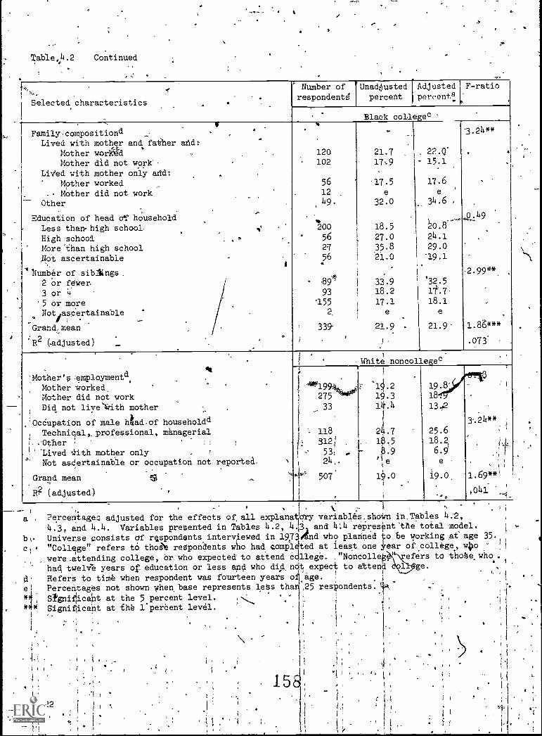
..Table,14.2 Continued
.
Selected characteristics .
.
Number ofrespondents
Unadjustedpercent
Adjusted! F-ratiopercent! I'
Black colleges, I
Familycompositiond ,...-
..
Lived with mother and faiher and:....$. .
Mother work'ed .
Mother did not work'LiVed with mother only arid:
Mother workedMother did not work
.
Other.
Education of head at' householdLess than high schoolHigh school ,>
More than high schoolNot ascertainable -
1 Number of sibAkngs2 or fewer3 or li.
'5 or moreNot,ascertainable
.
,. IGrand, mean
R2 adjusted)
.
.
.
,
4°
-
.
.
120102
56
1249
,
'6200
56
27
56.
3f- 89
93'155
2
339
I
..
21.717-.9
-17.5e
32.0
18.5
27.0
35.8'21.0
.
33.918.2
17.1e
.
21.9 .
I
22.Q'
15.1
17.6e
34.6 ,
0.8'
24.129.0
'19.1.
'32.5
1t.7-
18.1e
21.9-
--3.24**
.
,
.
0149
2.99**
.
1.86***
.073* .
. .
:Mother's :enploymentd.
Mother -worked.
Mother did not workDid not liyeith mother
.
'Occupation of male htadof householddTechniial, professional, managerial
i. Uther , ' 1 1
'Lived lath mother only .,
Not asdertainable or occupation not reported-
Grand mean 111 -
R? (adjusted) ,
.
,,
1 ..
White noncollegec
.
19
275
33
118is 312;
'''531
24,.
4- 507
1
19.219.3
14%4
I
24.74.5§:9
'le
19.01 .i-..
19.8'
18.
18.p
25.6
18.26.9e ,
19.0
,
324**i
.
. .
1.69**1
.041-1.
a,
b t.
c
e1
**
, I
Percentages adjusted for the effects or all explanatory variabLes..sbc4n in.Tabies 4:2,
4.3, and 4.4. Variables presented in Tables 4.2, 413 and 4:4 representthe total model.
Universe consists of respondents interviewed in 1967"College" refers to those respondents who had complwere.attending college, Or. who expected' to attend college. ,"Noncolleg.had .weiVe years or education or less and who did not expect to attend
Refers to time when respondent was fourteen years ofage.Percentages not shown When base represents leSs than 25 respondents.A
SlEglifiice-intattile,percerrtlev, '' ,
.
Significant at the l'perCent level. I '
:- -;
nd who planned to be working at age 35ted at least one rear of college, wlio
efers tO tho§e who .. ,
; I i
'
N
e

,
I
elt
^4.-
r
AIN
.FOr white women with no plans to atten 611 e, the fatherproved to be a much greater influence th J the mother in the daughter''expectation of an atypical occupation. Having had.a father (or other.?'male head of hOusehbld) in a professional,technical or managerialoccupation was positively 'associated with the choice of a typically .-
male occupation. While this result could be interpreted-as the effectof "father, as role model," it .is also possible that the result reflects
theeffect of family income on the daughter's occupational choice.Young women-from'families with relative;v..,high ifie-bmes probably hive
be/ter market information andexposure to a broader range of exl=irces than those from poorer backgrounds.' SUch.anenvironment may well
be conduciVe.tothe choice of ad-occupation atypical ?or women.
Finally, our hypothesisthat the eXpectation of an atypical. .
occupation would be associated with small family size is supported bythe data for college women. Specifically, among white college women,those withoUt siblings had a higher than average probabllity'ofaspiring to an atypicaroccupation. Among blacks,those with one ortwo siblings in the fami4y, as well as:those with none, showed a higherthan av4rage ypically male occupation.
Educational.and Labor Market Experience
Clearly,.the influence of a family on a young woman's careeraspirlions may be modified by her educational and labor market.experience. For college students, the sex composition of the studentbody where a Woman attends college mi6bt,be expectedoto affect heroccupational aspiimtionis. One argument advanced in favor oftferrialecolleges has been that women in such an environment are lessirifluenced.by a stereotyping of sex roles which would discourage them
,from majoring in traditionally maledominated fields (e.:g., the purpsciences.TRT Mathematics) or from assuming leadership positions.
1
HoweVer, offsetting this is the p'rgbability that predominantly male.or *iXed colleges..aremore likely t16,offer the curriculum necessaryito enter anatypical occupation. Given these two opposing effects,_one cannot hypothesize With certainty the. direction of the relationphip
between the sex-compositiOn of the .College attended and the sex-labelof the expected occupation.
.
. .. . ,.
The empirical results indicate that sex composition of the college.attended was related to the choice f an atypical occupation for both
t1
whites and black's (Tabld 4.3)'. However, only among white women was!,.attendance at either a predominantly men's or women's collegeassociated with an above average probability of aspiiing to anatypical occupation-. For blacks., attendinta.female college wasscor4elated with a lower pr babilit3r1of choosing an atypical occupation.
i.:
,
iOf course, the direr of eaUsation cannot be infei-red withcertiainty. Young women who attend male collegeS may, even before 1
entdring!, be relatively unconstrain4d by sex stereotypes and s '
),i, I..
1,
1
/1.
1

0 .4
Table 4.3. Unadjusted and Adjusteda Percentages of Young Women-Choosing an Atypical Occupation,by.Selected Measures of Experience, Race, and Educational Expectations: Multiple 01
Classification Analyslsb
0.
0
, . ...
Selected characttristics.
, , ....
Number ofrespondents
Upadjustedpercent
4
Adjustedpercenta
F-ratio
.v
White college.c
-
.°.
. .
Educational level and ljx composition of collegestudent .body '' . .,
Not yei. in college in 1972_
In college by 1972,and:-. Females less than 31 percent of student body
Females 31 to 60 percent of student bOdYFemales more than 60 percentwof student body .
, Nursing AChoolsNot ascertainable
'Number and'types of occupations, 1968 to 193
No work experience. l'or 2 different. occupations and:
Worked in atypical qccupationOther , - ,
3 or 4differentooccupations and: 0
i. Worked in atypical occupation
Other5 or 6 different occupations and: .
.°Worked in atypical occupation ,
, Other ,
7 or more different occupations., , _
Not ascertainable .i
Age in 1973 '" .
19'to 22 ' -ia23 to ,25 .
, l
26 to 29i, 1
Grand.
mean I..
B2
(adjusted) ° .1-.,
,
/
. .
21&
664 457
6
299 4'4"
38-
. ,, 28
'28
208
10319.6,
.103
82
'79,
50
337281
X259
877
.19.2
°33.0'7.8
° 33.5,2.5
16.6
.3.8
' 32.613.4
31.4
22.9
32.630.1
36.034:1
. t
25.i.21.0 ,
28.8
° ''19
.
.
20.5
a3'..-14
'26.0
33.0
11.721.5
..
13.1
34.214.5
0
30.421.7
30.3
31.434.9 r
. 34.4.,
22.7'21.4
31.7
24.9 ,,3.3e1.***1
.
2.54** ' jr
e 1
3.97***.
1
,
5.11***
f
v
.109
(Table continued on'neXt page.)
124
.°
0
o o or
1_60 ,
O
1

fr.
Tablei4.3 Continued
Selected- characteristics
Number orrespondents
Unadjustedpercent
o
4Adjusted T-ratiopercents .
Black colle4ec
Educationa11evel and sex composition of collegestudent bodyNot yet in college in 1972In college by 1972Fdmales less than 61 percent of student bo4kFemales more than 60 percent of studentNot ascertainable or nursing schools
Number of occupations held; 1968 to. 1973. 'Never worked - -
1 or 2 different Occupaikons3 different occupations4 different occupations
3different occupations6 or more different occupationsNot-ascertainable
Age in 1973. 19 to 22
. 23 to 2526 to 29
.Grand (mean'
R2 (adjusted)
144
139
18
15.0
28.320.8
;
e
10- e81 14.6
63 9 29.468 16.758 31.945' 22.614
174 26.1
78 ,22.2a4.3
539 1* 21.9
16.3 '
28.2
e
e
15.126.0,
16.535.223.2 '
25.919.316.6
21.9
2.70 **
1..88
1.864**
W3'0
Highest grade of schooling completed0 to 910 to 11
'Number and typed of occupations, L968 to 197'3-, 0
No work.experience.1 to 3 different occupations and:
7" Worked in atypical occupation:
4 to 5 different occupations and:Worked in atypical occupation, kOther ,-
6 or more different oceltloations and!:
Worild in atypical occupationOther
Not ascertainable
Grand mean
R2 (adjusted).
es
White noncollegec
41105
361
33
514
7-245,
.64
20
J620 ,
507
a
b
8.1
22.4
19.2.
"t",..10.0
18.8.
16.5
* 26.3
20.3
34.2e"e
_19.0
. 4,224.019 . 3
10.10
.19.616,8
26.0
19.7
32.1` e
e
19.0
.03**
1.86*
.d41
.3
Percentageiadjusted for.qp effects of all explanatory variables shown i.n Tables 4.2, 4.3, "and4.4. VarAablestpresented ,Tables 14.2, 4.3, and 4.4 represent thq total model.Universd.11,consists of respondents'intei:vieWed in 1973 and who planned to .be working at age 35. ''
"College" refers to those respondents Who had completed at least one year oft college, who wereattending college, or, who expectedo attend coLLege. "Noncollege" refers to those,who hadtwelve years of edlleation or less and who did not, xpect to 'attend college.To be classified as "Worked in atypical occupation" a respondent must have worked in anatypical 'occupation different'frotAhe occupation to which she.-aSpires. Therefore,"Other"2ategoriep include those who have never worked in an atypical occupation and those whbse
.
experienc in dn,atypical Orcupatiop is in -Ohe*Occivation deSired4for age 35. See footnote 17,page 126.1 . .
.
Percentages not ;shown' where base 4resents lesetban 25 respondents.$igniffcaht at the 10 percentil4g1.Significant at:Me 5i.percent navel.)
*g* SignificantlatJthe.lq&ercent1 ,
7 *
r

1
i 1.i .
1t- 1 .
i
1
cOmfortable in social or work situations where men; are a'majority.1
Furthermore, thel, choice of a predominantly male or .mixed college . $
imay have been the result of ..a previous occupational decision whicti,
reqUired a curribulum not available at a female college. In a .vi.
similar vein, young women who attend female colleges may, prior toentrance, be/ieve that attendance at such a college is important
`..f1;kbecause of the "Constraining" influence introducedfby the presence1
of men in more mixed institutions.C
.i
As noted.ealier, for noncollege women it was hypothesized that '.
no monotonic ilationship.woUld exist between year4'of schooling andchoice of an atypical Occ4ation.15 Those male and female .
1.
s occupations open to individuals at the high school level differ morein the type than in the amount of training required-for entrance.The empirical results confirm this hypothesis: only those womeit with.10 to 11 years of education completed had a higher than averageprobability of anticipating a typically male occupation for thefuture.
In addition to educational experiences, the number and types ofoccupations.a young4woman has held may serve to broaden the range ofoccupat-which she considers potentially desirable to enter. Pre-vious research has indicated that thAreater the number of diWerentoccupations a young woman has held, the highe'r the likelihood that she
will be interested in entering an atypical occupation in the future.l6In this model we haVe included a variable which represents previousexperience not only in a variety of occupations but also previousexperience in atypical occupations specifically.17
15A hypothesis regarding the relationship between schooling and
Athe typicality of the expected occupatIon could be tested only for thenoncollege women. Given the age'of oui sample in 1973 (19 to 29),-, many '
respondents may still be attending college and highest grade completed.does not necessarily represent the level:of schooling the respondents
4pwill ultimately attain. However,.the noncollege w ite goupseems to'have completed their schooling; in 1973, only two re ondepts in thissample were still enrolled in school. A further argument against the',use of, highest4gre:de Complete; for the college universe is the fact.that attendance in graduate school is probably the result rather.thanthe cause of chobsing an atypical career.
16See Harmon .(1970); Almidist and AngriSt (1971); and Almquist
(1974).
1 7
7For th'e respondent to'be. coded as having held an atypical Job,she must have been7in an atypical occupation which is different fromthat anticipated for age35 This procedure was followed so that wewould avoid using the result of an earlier decision to work in atypically male occupation as the predictor of a choice for the future..
.
126
164:
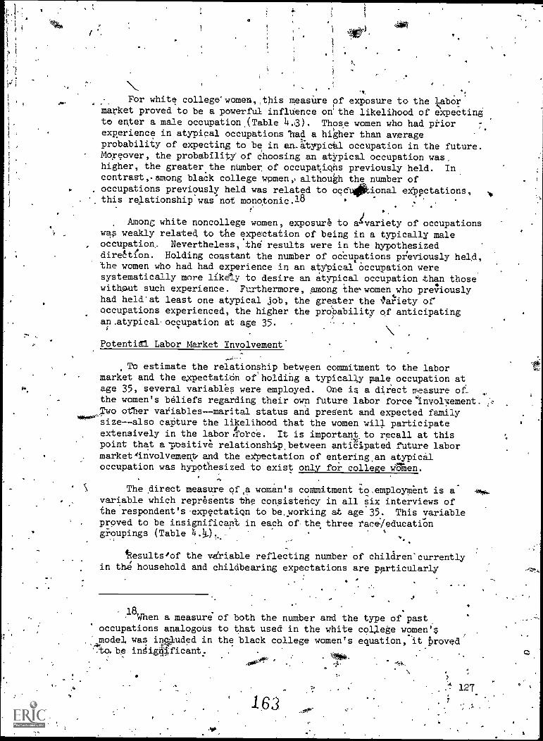
1
?s,
For white college'women,,this measure of exposure to the Labormarket proved to be a powerful inflUence on the likelihood of expectingto enter a male occupation.(Table 4.3). Those women who had priorexperience in atypical occupations "had a higher than averageprobability of expecting to be in an_gtypical occupation in the future.Moreover, the probability of choosing an atYpical occupation was,higher, the greater the number, of occupations previously held. Incontrast,- among black college women,: although the number of
. occupations previously held was related to occtional expectations,. this relationship was not monotonic.18
*
Among white noncollege women, exposure to a' variety of occupationswas weakly related to the expectation of being in a typically male
, occupation, Nevertheless, the results were in the hypothesizeddirettion. Holding constant the number of occupations previously held,the women who had had experience in an atypical occupation weresystematically more likely to desire an atypical occupation than thosewitnout such experience. Furthermore, among the,womenwho previouslyhad held'at least one atypical job, the greater the 4ariety ofoccupations experienced, the higher the probability of anticipatingan.atypical occupation at age 35.
\ .
Potential Labor Market Involvement'
To estimate the relationship between commitment to the labormarket and the expectatiOn ofholding a typically pale occupation atage 35, several variables were employed. One is a direct measure of_the women's beliefs regarding their own future labor force'Involyement.Two other variables--marital status and present and expected familysize--also capture the likelihood that the women will participateextensively in the labortfoi.ce. It is important, to recall at thispoint that a Ttrsitive relationshibp.between anticipated future labor
market4involvemente and the eXpectation of entering.an atypicaloccupation was hypothesized to exist only for college women.
The direct measure of ,a woman's commitment to .employment is a
variable which represents the consistency in all six interviews ofthe respondent's-expectation to be, working at age 35. This variableproved to be insignificant in each of-the three ?ace/educationgi-oupings (Table
tesults4Of the vdriable reflecting number of children'currentlyin the household and childbearing expectations are particularly
..
11,
18When a measure of both the number and the type of past.
occupations analogous to that used in the white coljege women'smodel, was included in the black college women's equatibn, it broved
.F.1.r
'to, be indignificant10,
163127
7
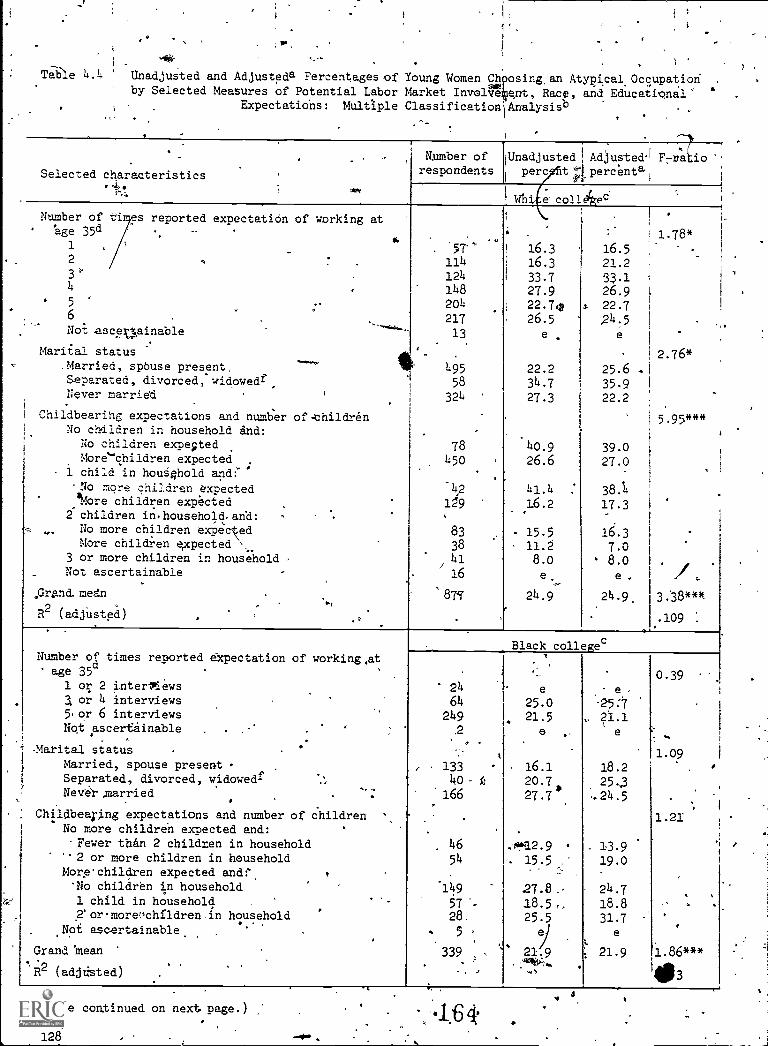
Tale 4.4 '
;v.
by Selected Measures of Potential Labor Market Involve et, Race, and Educational'Unadjusted and Adjusteda Percentages of Young Women Atypical Occupation
nBxpectations: Multiple Classification Analysisb
Selected characteristics.4,.
N.umber of
respondentslUnadjustedlioidnjusted1 F7ra io
perc t percental
Number ofage 35d
1
2
3
4
5
6
ti reported expectation of working at
O
Noi escekainable
Marital status,Married, spbuse present,Separated, divorced, widowedfNever married
-
Childbearing expectations and number of- childrenNo children in household and:
No children expe;tedMore`children expected
1 child in houS4hold and(No more children expected'ore children expected
2 children in.householdarid:No more children expectedMore children expected
3 or more children in householdNot ascertainable
.,
Grand. mean
R2 (adjusted)
v
124224148204
21713
49558
324
78450
42
19
83
3841
16
e condkec
L
16.3 16.516.3 21.2
33.7 33.127.9 26.922.74? 1 22.726.5 24.5
e
22.234.7
27.3
40.9
26.6
41.4
16.2
15.511.28.oe
24.9
25.6
35.922.2
39.0
27.0
38.1:
17.3
16.3
7.08.oe
24.9_
1
1.78*
2.76*
5.95***
Number of times renorted expectation of working,atage 35a1 or 2 interviewsa or 4 interviews5, or 6 interviews
Not ascertainable
-Marital status
Married, spouse presentSeparated, divorced, widowedfNev* ,married
Childbearing expectations and number of childrenNo more children expected and:-Fewer than 2 children in household-2 or more children in householdMorgchildren expected and:"
No children in household1 child in household2'or.more-chrldren,in household
Not ascertainable.
Grand 'mean
2R (adjtited)
24
64
249.2
,
1334o k
166
Black collegec
25.021.5
. 16.120.7
27.7*
46 -'022.954 15.5
-249 27.857 . 28.5 .28, 25.55 .
//,,339 22.9
-25:7
21.1e
18.225..3
,24.5
13.919.0
24.7
18.831.7
e
21.9
0.39
1.09
1.21
- t
(Table continued on next page.) .
128. -*a
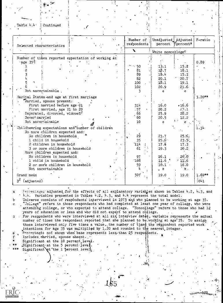
1. ,
I
Table 4.4 I Continued ..r
1
1
i ,
k '
[ Selected characteristics 1
.r.
i
1 Number of times reported expectation of working ati
.
. .
age 35? !I
11 '
2
3
4 !
5 *-
6I
Not ascertainable
Marital hatts.and age at first marriage. Married, spouse present: '
First married before age-21First married, age 21 to 29
Separated, divorced, widowedfNever\marriedNot ascertainable
Childbearing expectations and"humber of childrenNo more children expected and:
No childreh in household1 child in household2 children in household3 or more children in household
More children.expected and:No children in household1 child in houSehold2 or more children in householdNot ascertainable
Grand mean2
(adjusted)
1
Number of 1
respondents
1
Unadjustedl Adjusted F-ratiopercent "Irpercenta
N,1 White noncoilegec
I,1 0.89
-. 50 13..1 15.281 , 16.7 18.189 18.4 15.382 20.1 20.7100 18:1 19.1102 20.9 21.6
3 e e
3.20 **
314 16.0 .16.6.57 20.2 2"i.1
66 25.9 28.260 20.5 12.210 e
:e .
1.34
29 23.7 25.'6:
35 '25.6' 23.5'.
"114 17.6 17.361 19.3 20.2
97 26.1'108 11.6 ,° 11'.6
59 16.1 16.0e
507 19.0 19.0 1.69**
.041
.
a Fel-:!enta,,7e-adjusted,for the effects of all explanatory ariabj.es shown in Tables 4.2, 4,3, and4.4. Variables presented in Tables 4.2, L.3, and 4:4 represent the total model.
b Universe consists of respOndenti interviewed it 1973 814 who planned to be working at age 35c "College" refers to those respondents who had completed at least one year of college, who were
attending college, or who expected to attend college. "Nonc4lege" refers to those who had 12years of education or less and who- did not. expect to attend college. . . 4
d . For respcndents who were interviewed at all sib interview da*, variable represents the actualnumber of times the respondent reported that she planned to be,worYcing at age.35 To assignthose interviewed only five times a value,the number of iimeA therd,spondent reported work_ .--
.
intettions for age 35 was multiplied by 1:20 and rounded to t e neares%integer. .
4 7PPTcevItages not shown when' base represents lessethan 2,5 respo ents.
* Significant at the 10 percent_leve .
. I
.f Includes,married, spouse absent. .-
** .Sfgnificant-at the 5 percentjeve .
*** Significant t'the 1 'percent level .
. .

t-
intersting, As expected, Illite'college women who had eith c nochildren or only one child and who expected no additional childrenhad a higher than average probability of choosing an atypical 4*occupation for age 35., Furthermore, regardless of the currentfamily size, those who anticipated no additional. children were more
. , .
likely also to expect to be. in a'male occupation than those women who
i anticipated having additional children.'
,However, Among black college women family size did not appear to !
influence occupational choice. This suggests that, unlike theirwhite%coAnterparts, black women do not perceive a traderoff betweentime commitments to a family and!time commitments to the labor force.
Marital status had little or no relationship to occupational. -
! aspirationsamong either racial group of college wdmen. Thus it:
, appears that it is the presence of kildren (and there only amongwhite women) and not marriage per se which has a negative effect onthe probability of selecting a typically male occupation.
In contrast, marital status was a significant factor influencingthe probability of noncollege white women entering a typically male'occupation. While the direction-of causationought not to beinferred, it is ,intriguing to find that,the women.who,had marriedrelatively late or. who were divorced, widowed or separated-at the
interview date 1.18:a a higher than,iverage probability of expecting tobe in a' typically male occupation.
Comparison of Race/Education Groups
The empiricalModels presented 'in the previpus section indicatethat the determinants of expectations regarding employment in a
) typically male, or'a typically female, occupation vary across race_,
and educational groupings. No one factor, or set of factors, appeared', to be systematically related to the occupational aspirations of allwomen., Hence, one implication of these results is that demographicchanges--such as'higher divorce rates or :smaller family sizes--will notbe similarly associated with occupational ch6ice for different raceand educational grolips. A second implication ot,ourjndinis at\thatif occupational integration is a social goal, then policies' formffatedto affect supply-side factors must take into consideration differencesamong women in racial chAracteristics and in educational levels.
The racial variations in factors influencing occupationalexpectations are not surprising. The two racial groups experienceddifferent social and familial environments when they were young.It is also likely that some ofthe Variations are attributable tohistorical patterns of occupational' segregation by race. The nutber .
and types of occupations / historically open to black college-edrateawomen may differ from those historically open to their whitecounterparts. Hence, while the 'dependent variable' may have
categorized accurately occupation's which are typical and atypical
-
130
166,
4

f
1.
for white women; it may be a less accurate Measure of occupations thatare typical Or atypical for black women.19
1,Likewise, the variations found betweenlwhite. collegeand.
nonc011ege women are noj surprising: It was, noted at the outsetthatmany ofythe atypical occupations open to college women require-postbacculaureate training and therefore would be attractive only to ,Athose women who anticipate extended workingicareers. In contrast,atypical occupations available to noncollege'vothen do'not necessarilyinvolve greater investment in human capital'and therefore morextensive participation'in the labor fOrce than typical occupations.s a result, it was expected that,-forthis,group,factors reflectinghe possibility of a strong commitment to the labor market (such ashe expectation of a small faMily size) would not be relatedpirically to the choice of an atypical occupation. The results,ich confirm our expectations, illustrate the need for further
research on the process by whi'ch occupational choices are made bynoncollege women. By implication, the results also suggest thepotential for programs aimed at reduding occupational segregation by°reorienting women's training and +education at the high school level.
ilk Finally, the results indicate that a young woman's familybackground, is, at best, only weaklyassociated with occupational .
choice. Although the data available give a very incompletelindicationIDf the childhood environment of the women, the findings suggest thatone need not-be "deterministic" about the possibilities fdr increasingoccupational integration. A young woman's choice between a typical oran atypical occupation is not determined solely by her childhood
, environment; educational and labor market experiences later in lifealso have an important impact.20
OCCUPATIONAL,PREFERMICES D OCCIPATIONAL OUTLOOK
In assessing the proltable success of young women in finding Workin their. Treferred fields, it is useful to examine the.growth'prospects
A 19Black women are underrepresented in some typically female
'occupations and overrepresented, in others. For.example, while black..,1 women were 12 .percent of .the femalelabor force in the 1970 census,
they comprised only 3 Percent of the female secretaries and 8 percentof the female ,nurses (U.S. Department of COmmerce, 1973)
t
go
experiences are associated with factors in the childhood environmentwhich we do not measure. For example, certak women may be pre-disposed because of attitudes learned in Childhood to acquire
.experience in atypical occupations or'to work, at a greater number ofOCcupations.
20'Of course, we canrApt discard the possibility that these later
167 //131

a
of the occupations which were frequently mentioned as desiredoccupations for age 35. i Clearly, young women who are planning" careersin fields which are growing slowly and where competitiOn is keen maybe frustrated in achieving their career goals,1eVen with therequisite education and training. Among such women who drop out ofthe labor force, subseqUent reentry may require retraining oreducation for another career.
Table IL5 shows the occupations mentioned in1968 and 1973 byyoung Women who expect tb be workingt age 35.21 The results suggestthat if young women are able to realize their occupational ambitionsfor age 35, they will still be concentrated in a relatively smallnumber of occupations. ong white women who have attended or planto attend college, 60 pe, ent want employment in only three generalareas: teaching, health ervices, and clerical work. Among -womenwith no college ambition , one in three expects to.be a clericalworker.
Occupational projectiods'suggeSt that many of the fields in, which women have traditionally been a majority will have a high or
moderate growth"rate. As Table 4.6 indicates, most occupations in'the health field are expected to have excellent growth prospects. 1
Likewise, rapiegrowth for workers in clerical.occupations wasforecast in, 1973, and secretaries, in particular, were projected tohave excellent chances for employment throughout the 1970'-i and early.1980's. HairdresSers are expected to benefit both from generdllyincreased,incomesand the rising labor force participation of womenand, hence, to maintain:a growth rate well above avervge. These threefields, by themselves, account for about tWS-thirds of the responsesof the young women in the noncollege sample.
For young4women expecting to go to college,the future employmentpicture is mixed. Particularly important fot college women is theexpected decrease in the number of openings for teachers. In 11968,
1973, and 1974, the Department of Labor consistently.projected that'teaching, at*both primary and secondary levels, would attest be a .
very, slow growth occupation. Table 4.5doesindicate a concurrentdecline ip the percentage of our sample who expect to be teachers. In1968, 471percent pf the whites who pitined to go to college andexpected to be employed at age 35 planned a teaching career; in 1973this percentage had dropped by 16 points. However, even.withsuch adecline in the percentage of women, planning teaching careers, 31percent of the whites and 23 percbnt,of the blacks were still planning
421"Related .occupations are grouped together. For example, the.
category "teachers" includes the following: elementary andsecondary-school teachers, sports instructors and officials, musicians and musicteachers,dancess Ind dancing teachers,, and artists and art teachers.
v

11
1
1
Table 4.5
et
I 1
Occupational Expectations for Age 35, AS Reported in1968 and 19.73, by Educational Expectationsa and Race
(Percentage distributions)
Occupational expectation- 1968 1973
Wfii-ees 1 Blacks 'Whites IBlacMS
.
Number of respondents-.Total percent
Teachers.
Health workers
Registered nurses, techniciansPractical nurses, attendants
Clericalecretari.ri:es .
z...., .
Hairdressers,. All others _
. ,
.
.
Number of respondents.
Total... ,
percentTeachers n
Health workers '
Registered nurses, techniciansPractical nurses, attendantsPhysicians, pharmacists -
Clerical .
SecretariesSocial workersPsychologistsLawyers
tHairdressersAccountants .
&lagers.Ail others
_
Noncollegeb
.443
1003
13
76
35-14
18
31
'
358 ,
1003
26
11
15
3511
4
32
5O100-4
12
5
7
3818
12
15
302
100 .
5:
28'
'16
12
--3210
2':
33
, Collegeb/ .
448'
10047
3,4
1p
1 -
8
6 -
3 ..
. 1
2 ,1 h'1
222
40',
27
100
3522
12
4
7-
25
18
r.,
'' 1
. 0
1
0
1
9
.
,4.,
877
100
31
1915
2
.1
13,,6*
5;2
. 1
1 .),
2
3
24,
339
.01:?.,
23
.. 22
16
5-
4 2 .
15
8
"511
3.-1
. 3
25
a Sample ize,in 1968 differs from that in 1973 becauSe each consti-tutes an independent- cross- section of the respondents. The universefor each ear'cong.ists of black and wilite,women who answered in thatyear that they planned to be Working at age 35 and named theoccupatiOn at which they_expected tb work.
b "Noncollege" refers to those responden4Twho have:completed 12years ofschool or less and say that they do not expect togo tocollege. ''C011egen.refers to those respondeptent have at leastone year of college,'whoare.attending college or who indicate thatthey expect-4).g° to College.
_/< , 1 69,

'
Table 4.6 : Occupational Projections for, Occupations Expected at Age-35, by Yearin1Which Projection was Made "
es.
1968-19qt '1972-1973a
HighjLrowthb
1974a.
Health professions .
Registbrdd nurses.Health technologists
and techniciansPractical nursesHealth aide's, expect.
nurses (nurses, aides-orderlies)
*Physicians*Veterinarians
*PsychologfsteS8 a1 workers.Lngineering and science.
technicians.*College and university
teacherse*AccountantsStenographers
Hairdressers
Health professions:Registered nurses:
'"" Health technologistsan technicians
Practical nurseH&alth aides, excepttnurses (nurses aidesordeflies)
*Physicians*Veterinarians*Psychologistse
*Social workers*Engineering and-science'technicians
*AccouhtantsHairdressersSecretariesClerical workers (all)
So
Health professions:,Registered nursesHealth technologists7.rid-technicians
'PraJtioal nursesHealth aides, except
nurses (nurses aides,orderlies)
*Phyeici-o,ns
*Veterinariewed*Psychologistse*LawyersSocial workers4*Engineering and scienceteelTriFTlans
*Police and detectives*Professional andtechnical workers(n.e.c.)
'SecretariesClerical workers
. Moderate ,rowthc,t
*Lawyers*Pharmacists*Managerial occupations*Polite and detectives*Designers_*Peal es 'agents and
brokers'.
-*Writing professionsClerical workers ('all)
-*Lawyers
'*Pharmaciste*Managerial occupations*Police an.dderaives
. *Designers s-
*Real estate agents and,brokers
*Writing pf6Tesifons*college,universityteacherse
*Accountants
*Mans ial occupations
*Designers*Real estate agents and
bf-Okers--
-*WfttiA professionsHairdresEAS
-Slow growthd
. ,
Prekindergarten teachersElementary schoolteachers
- High school teachers-*Farmers, and farm
managers"Operatives
Prekindergarten teachersElementary school
teachersHigh school teachers.*Farmers and farm'Managers
,*Operatives (all)
.
Prekindergarten teachers.Elementary school
teachei.'s
High school teachers*Farmers and farm 4
tanagers*Operatives, (all)
*College andipniversity1teacherse/
4 1.
Sources: U.S. Department of Ilbor, iurgeu of Labor Statistics, Occupational OutlSok Handbooks,
.
-%-1968 -69; 1972-73; and',1974-75. Matt L. Carey,, "Revised' Occupational Projections
to 1985" Monthly Labor Review (November 1976): 10-22.
/.
a Projections for 1968-1969 usually concern the period until the mid-1970's. 'Tbe
projections for- 1972 -1973 extend,to the end of the decade; those for 1974 are for 1974 !.
to 1985. 0 , .
includes occupations in which employment is expected.to increase by 30.0 percent or i
. 'rEi-e with jobopportunitfes t'"excellent" or "very good." ' - 1
includes occupations,in which employment i. s expected to increase bet Teen 15,0 and 29.9
... ... percent with job opportunities "good or favorable.'" ,
1includes oc ipations inwhichemployment 3s expected to increase not more tlip 14.9
percent (tile' also experience decline) with -job opportunities "Competitive."
.e With Ph.D.
' Atypicaltoa
ply:ccupation for women. j 7
170
1
0
.
AO,
,,to teach ir1/1973. Clearly, there are:lags in to adjustment to thei
poor occupational outlook for teachers, and the oversupply of4%teachers will4robably continue..,
.
'".
Those occupations for college graduates that,are expected to haveexcellent employment opportunities, forthe most part, were'notmentioned significantly, more often by the 1973 ample than in the.1968sample. For example, the Percentage expecting to be employed as socialworkers, psychologists,' or*.ccountaRts was not 4ignificantly higher in,1973:than in 1968. The one possible exception is aslight increase inthe Prcentageof white college women who foresaw working in the healthfield. This increase is largely the result of the more frequent choiceOf work as a registered nurse:
Table 4:7;shows the distributions among specific atypicalotcupakions of, respondents who expected to be in stereotypically
male occupations at age 35 These data show rather dramatieallythatthe range of occupational choice is very narrow even among those'youngwomen who plan.to.enter an,.atypical Occupation. Of the mc-xe thau 200
stereotypically male occupations, only ,28 were mentioned by a noncol-lege respondent in 1973 and only 7 were chosgn by ,5 or more
; --respondents., .
In particupir, women evAced almostno interest in highly skilledblue collar jobs. Only two respondents mentioned employment it one ofthe skilled crafts; only fOur aspired to potitions as foremen. In
contrast, operative positions were a significant portion oi'the.
atypical occupations mentioned for both rakes. Approximately two-thirds of the blacks and one-fiftnof the. whits in the noncollegesample, who wanted an atypical,occupation are recorded as expecting to
work as OperatiVee, n.e.c. . -..
Moreover.thQse atypical occUpations.menii.oned py noncollege young
omen are no more likely to experience rapid groWth than are theypiCal occupations: Of the stereotypically male occupations
mentioned by noncollege women, only accounting and work as aprofessional or technical warker, n.e.c., were projected to be highgrowth occupations in either 1973 or 197.4. Furthermore, operative . ,
. positions were expected -to have a slow growth ate: This fa,: could
have a particularly heavy impacton black women. : .
Among the college women, the range of atypical 'occupations
. mentioned by five or more women was broader. 4evelipheless, in 1973 ,,,only three respondents expected to be engileers,,otfe expected to be .
'Tp±lot,rand only four expected to be architects. HoWever, in 1973
interest was, evinced in several occupations which had not been listed
. by five or more women inr1968. For example, in 1973, of the blackcollege women who expecte& to beworking in an atypical.oacupationat/age 35, 6 percent indicated they expected to be'members of the'.
it, police force, and.-.5 percent indicate& they expected to be accountants...
.171. 135
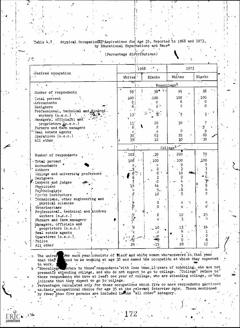
,
'Table 4.7 Atypical Occupationl'Aspirations foil Age 35, Reported an 1968 and 1973,.
, .
by Educational Expectations and Racea .,
1°(Percentage distritions)
I: ]
,
Desired occupation, ,,
,
)
1968 ' , 1973_
Whiteq, Blacks.
Whites Blacks
. .
Number of respondents
Total percent ,
AdcountantsDesignersProfessional, technical andWdred,workers (n.e.c.) % e.
Mane:kers; Official's; and -.
proprietors4in.e.c.)Farmers and 'farm managers
"Real estate agents,
Operatives (n.e.c.)All other
.
Number.of respondents,
Total percentAccountants ° 14
' AuthorsCollege and university profeS'sori
DesignersF-Lawyersand judges -41,,,
f s
PhysiciansPsychologistsFportt instructors
,
Technicians, other engineeringphySical sciences
VeterinarianserinariansProfessional, technical and
workers (n.e.c.)farmers and farm managers,'Managers, offieials and
proprietors (n.e.c.)Real estate agentsOperatives (n.e.c.),
PoliceAll other
00-,
Y,00.' .
',. -
:
. -
,.
,
l
andJ
.
kindred1,
1
.
-
.
i , Noncollegeb,,
591
100i
ei)
6;.f
13 k
'
11!
. Ce,
30
351
I
:
384
,100,100
c
2 ,''
t',
162
c
63
12
95
loo6
0
.
5
30
0
22i0
.
38
1000
0
3
7- -4.
0
60
'30
.
.
,e--
,-e"Collegeb
1
10.
1004
c,
4 .9 "-`
-. i 6
7
'14
14
6 ,
3
Itf
..t'7*
.
)3
.,c, 4,,-.c
24
0.
_
%
!
.39..
100c
, 2
0 -3
244 ,
5..
12
. ,
2,
6
c
.
10
, c
,c . .
A P,.c
-15
1:
. . 220
- 100
. 9, 3
10
24
5
85
c
c
12
3
13h
to
1
'2
20
*is*
,
1
,
-
'
72
,100
5
3
5
"' 6,
'8'
8
6
2
c
-6
23..., -
0
'14
1
2
6
17
.
.
^ 0 P
a The unive f'dt each year consists of Mack' and white women who answered in.that year
that they ned to be wolking at age 35 and named the occupatiOn at which they expected
to work.b ."Noncolleg efers to those*respondents.with less than,13years of schcibling, who are not
presently at.tending college, and who do not expect to go to college. !'College" refers to
'.those respondents who have at leagt one year of college, who are attending college, or'who
indicate that they expect to go'tocollege. .
6. .
.Percentages ,calculated only for those occupations which five or more respondents )*ItiOnedas,theiroccupational choice for age 35 at the relevant interview date. Those mentioned
by fewer than five persons are included inOkhe 'all other" Oategory.
411, a ,116. 172 ,
a

For' -
the col ege women, several of the atypical professions-9intioned--e.g., accountants, physicians, and veterinarians- -were pro-jecteAin 1973 to be rapidly expanding. However -, the 'proportion ofyoung women expedting to work ap physiiians or veterinarians declinedbetWeen l968 and 1973, while a.larger percentage indicated a desireto be in some fields, such as iVanagemerit' or-college teaching, which 'should have only moderate or slow increaseft22
I
In general, in spite of theodo,broad range of atypical pccupations.
which Could have been mentioned%'the oCcupational expectations of ..
young women who anticipated being in a 'stereotypically maleoccupation were limited. ,Unfortunately, too, the demand for eeceral,of theoccupations mentioned 5.6, expeCted to be below average.o. .SUMMARY AND CONCLUSIONS
This chapter has analyzed the factors associated with a youngwoman's expectation of being in, an occupation at age 3; that isatypical for women. It has beenfound that the factors afectingexpectations vary between the races and between women who arecollege or expect to attend college and those with no college plans.For example,- the presence or expectation of children degatiyelyaffdcted the likelihood that white college warned wduld expect tobe in a male occupation, but'it had-no'significant effect on eitherblack college women or white nOncoilege. women.
The chapter has also shown that the numbel and types of
occupations--regardless of their sex-typing--to which the womenaspire is 411te4. Moreover, even though extensive publicity hasbeen accorded women who have become kfor example) truck drivers and.
. telephone line repair workers, and even tndUgh there is a broadrange of-Stereotypically male occupations from which young women mi-
.
choose, they actually tend to mention relatively few occupations.,...,
.
Thus.dt is'clear that if young women are to move into all types-of typically male, occupations, affirmative action programs are notsufficient: It is necessary alsO to bilOaden young women's exPOPureto the full nang40.oftheir emplpyment-Opportunitiu. . ,
it,
.. .. .
....
4
4'
viOW
4
.4Some of the decrease in women,expectineto be physicians .or
veterinarians is probably the result of a readjustment ,of expectations,which were initially unrealistic;
1 73.
137
7,1

r
4.
REF RENCES
Almquist, Elizabeth M. "Sex. Case.of College Women."
(August 1974)i°13-21-
Almquist, Elizabeth'M., and Angrist, $hirley, S. "Role ModelInfluenCes on College Wo en's Career. Aspirations." Merrill-
, Palmer Quarterly 17 (Jul 1971): 263=79.°
tereotypesiii Occupational. Choice: TheJournal of Vocational Behavior 5
Carey, Max L. "Revised OccupaticSnal Pi.ojectionS to 1985." Monthly
Labor Review 99.(Novemb Ir. 1976): 10-22.
.Carnegie Commission on Highei. Education. College Graduates' and Jobs.r - New York: McGraw-Hill o., 1973. ,---'--
' 1 * .0. ''''
sChiswiCk, Barry; Fachler, Jalhe, O'Neill, June; and PolachIlk, Solomon.- PThe Effect of Occupation on Rage and Sex Pifferences:in Hc0:1-:::Earnings." PubiltDateAse 3 (April 1975): 2-9.
.
FuchS, Victor. "A Note on Spx Segregation in Professional,-
Occupations. ", Explorations in Economic Research 2 (Winter 1975):-1.1.10 % ( ,
14""Nvw '..Harmon, Lenore W. "Aligromy of Career Commitment in Women." Journal
of Counseling Psychology 17 (1970): 77=-80.
Jusenius, Carol L. "The Influence of Work Experience and Typicality ofOccupational Assignment on Women's Earnings." In Herbert S.'Parges Dual Careers: A Lpngitudinal Analysis of the -
Libor Market'Experience of Women,'Vol. IV. Manpower ResearchMonograph no. 21. U.S. Department of Labor._ Washington,0%C.:U.S. Government Printing Office, 1976, pp. 97-118.
sicJusenius, Carol L., and Shortlidge, Richgrd L., Jr. Dual_Careers: A
Longitudinal'StUdy of the Labor MariKgt Experiene of Women, Vol.* III. Manpower Reielr,ch Monograph no. 21._ U.S. Department of ...
Labor, Waphingtoo, D2C.: U.S. GoVernment Printing Office,:N;r*.
KlemmgCk, David L., and.,Edwards, John,N. "Women's AcquisitiOn ofStergOtyped Occupational Aspirations." Sociology and Social
Research 57 (July. 1973): 510-25.,.
.
Nagely, Donna L. "Traditional and Pioneer Working MothersX Journal.of Vocatidhal 13ehavior '1'(Qctober 1971): 331-41.
_4,4.. .
4.1,A ,
.f ;:, A
Oppenheimer, Valarie Kincaid. "The Sex -Label of Jobs." Industrial
. .
Relations (may.1973): 219-34.
136
174_
4
,

Priebe, John A.;'Heinkel, Joan; and'breene, Stanley. 1970 Occupationand Industry Classification Systems inTerms of Their 1960Occupation and IndifStrA'Elements. U.S. Bureau of. the Census\Technical Paper no. .26.; Washington, D.C.: ,U.S. GovernmentPrintingdOffice, 1972.
Rbe, Anne. The .Making of a Sciertist. New York: Dodd, Mead, 1953J1
1Treiman, Donald J., and Terrell, Kermit.' "Women, Work, and Wages,-
Trends in the Female Occupation Structure." Social IndicatorModels. Edited by Kenneth C. Land and Seymour Spilerman.4 NewYork:- Russell Sage Foundation, 1975, pp. 157-99
Tully, Judy border;-Stephan, Cookie; and'Chance, Barbara J._ "TheStatus and Sex -Typed Dimensions of Occupational Aspirationsin Young Adolescent's." Social Science Quarterly 56 (1976):639-49.
U.S. Department of Commerce, Bureail of the.CensuS, Census of thePopulation 1970. Subject Reports (PC (2)-7A), Occupational,Characteristics. Washington, D.C.: U.S. Government PrintingOffice, 1973.
U.S. Department of Labor, Bureau.of Labor Statistics. OccupationalOutlook Handbook,i1968. Hu1letin 1550. Washington, D.C.:U.S. Government Printing Office,1904.
#4
. Occupational Outlook Handbook. ,1972-73 Bulletiq 1700.Washington, D.0 a: 'U.S. Government Printing Office, 1972.
e
. Occupational Outlook Handbook, 1,974-75-. Bulletin 1785.Washington, D.C.: U.S. Government Printing Office, 1974
'
..,
. .
Zenner, larriet:':"The Deteiminantsof Occupational ..!Segregation.'! 4
Sex, Discrimination, and the Division of Labor. Edited by. . Cynthia L1oy . New York: Cdlumbia University Press, 975,
PP. 125-3. .,
° 4
. e
4
4o
44,
4 -
, --r-._

AGE IN
sr
ATYPICAL
4trx
. GL0SSA2Ri
spondent's age at'her last birthday before January 1, 1973.
Term used to describe those occupation's in which 38.1 'Percent or.fewer of the incumbents in 1970 were female. (See SEX-TYPE OFdCCUPATION)
CHILDBEARINGTXPECTATIONS
A dichotomous variable indicating whether in 1973 the respondentexpects to bear more children. from items 100b, 101c,and 102c, 1073 questionnaire)
.
COLLEGE
. A term used to describe those respondents who, at the applicableinterview date, are enrolled in college, have ,completed at'leadtone 'yed.r ofcollege, br report that they expect to attend college. _
in the future.
EDUCATIONAL EXPECTATIONS .
-A dichotomous variable which indicates whether the respondenNhas attended or expects to 'attend college. (See COLLEGE and )-NONCOLLEGt) .
HIGHEST GRADE COMPLETE9
The highest year of "regular" school completed by the resppndent--from 0 to 18--ad of the survey week in 1973. "Regular" schoolsinclude, graded public, private, and parochfal%elementary andsecondary schools colleges; universities; and professionalschools.
.
- , NONC046 '''
. A'term used tp describe those respondents who, at the applicableinterview date, have no more than 12 years of pchoolirig completed,.... -
are not (enrolled in, college, and report that they do not expectto attend college; ,..
.
'.'NUMBER OF.CHILDREN :..;,---- .
,
-Numbef respondent'S sons and daughters Underthe age d 18
,living in the household. ..4 6
.
.
1
NUMBER OF OCCUPATIONS . a -,;. . #.. . -,
44, co.
.
The number different7three-digit CensUS...pccUpational categoriesin Which
.theretpOndent reported working between 1968 and 1973.
: p
. 4,.
1

. - ,f
I
AkNUMBER, OF-SIBLINGS
The pumber of brothers and,sisters of the respondent, as reported.11P
by the respondent in items 107a anSP113 of.the 1968 questionnaire.
NUMBER OF TIMES REPORTED EXPECTATION OF WORKING AT AGE35
A continuous variablt indicating the number oft.times in the yearly'interviews the respondent indicated she expected to be workingoutside-the home at age 35., In all interviews, respondents wereasked what they.planned to be doing at age 35. (See item 72a for1968 and ;tem 69 for 1973.) For respondents interviewed in allyears, the variable represents the'timple number of times out ofthe possible six that the respondent reported expectations ofwork outside the'home for age 35. To assign respondents inter-s.viewed only five times -a comparable value, the number,V timesthe respondent report4d.work intentions for age 35 wasby 1.20 and rounded to the nearest integer.,
SEX- COMPOSITION OF COLLEGE STUDENT BODY
A categorical variable indicating, for those respondents whoentered college before the 1972 interview, the percentage of.'
' t women represented in the student body Of the -rst college therespondent-attended.
SEX-TYPE OF OCCUPATION
A dichotomous variable derived from the 1970 Census of"Population data which compares the degree of representation of"women in a three-digit,occupation with their repreAentatiAn inthe experienced civilian labor force. Those occupations in whichwomen. are overrepresented are termed :typical"; those in whichfemale representation is _less,than :their,representation in the ,
entire labor force are termed "atypical."
TYPE OF OCCUPATION
(See SEX7TYPE'OF OCCUPATION)
_. ,.-
TYPICAL -
DTerm used4to denote those occupationsjn,whi-ch more than:38.1
,
percent'of-the incumbent's in 1970 were femalg. (See SEX-TYPE OF ''OCCUPATION), °
1 77%
a
,
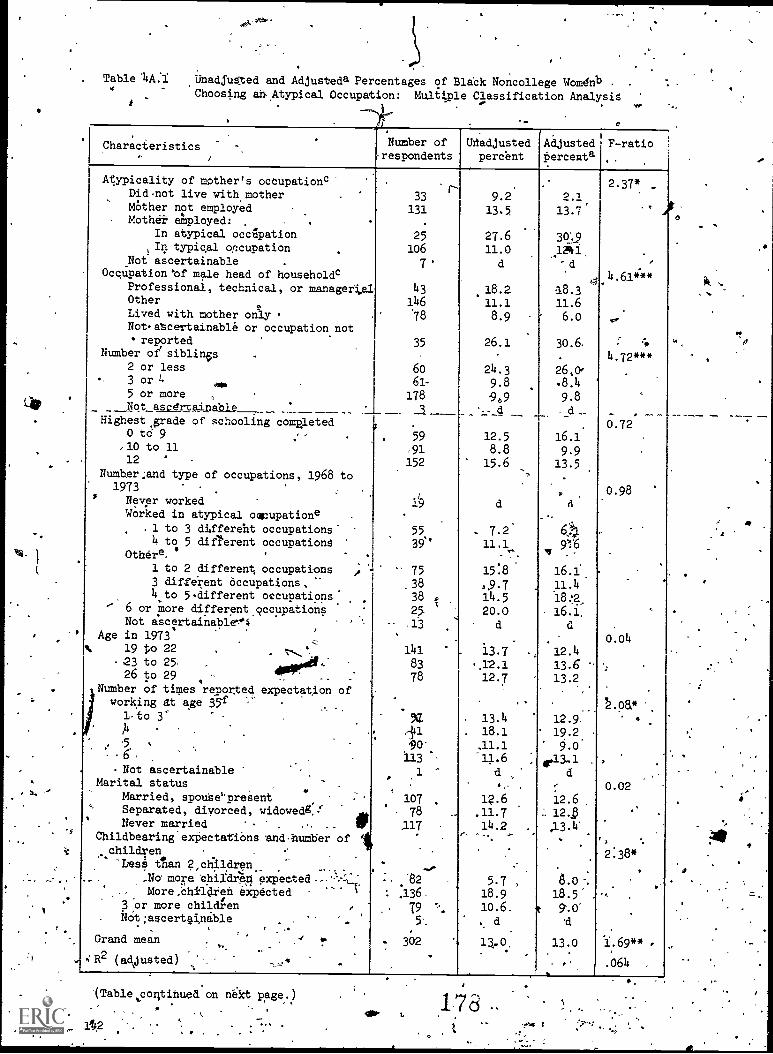
Table '4A:1 Unadjusted and Adjusteda Percentages of Black Noncollege Womdnb .
tChoosing air Atypical Occupation: Mulif,ple Classification Analysis
..
Characteristicseristics.
/
,
Number of-respondents
UiadJustedpercent
Adjusted'Percenta
F-ratio,.
Alypicality of mother's occupationcDidnot live with mother .
MOther not employedMothe employed: . .
In atypical occupationIn typigal ooccupation
_Not ascertainable .
Occpationf male head of householdcu 'o
Professional, technical, or managerialOther
sLived with mother onlyNotatcertainable or occupation not
reportedNumber ofl siblings ,
2 or less3 or 4
420. .
5 or more ,
Not_ascerainahle
33131
25
106
7 '
43
146
'78
35
60
61-
178
9.2
13.5
27.611.0
d
.18.211.18.9
26.1
24.3
9.8909
12.58.8
15.6
d
_ 7.211.1,
15.8
.9.714.5
20.0d
.
. 13.7
.12.112.7
. 13.4. 18.1
,1141
11.6d
12.6.11.714.2
5.718.9
10.6..
d.
13,0,
,
.
.,
.
"
:
.
=
,
.'
2.113.7
30i9
.12h 1
'd4,4.6114*
18.311.6
' 6.0
30.6
26,0-
.8.4 '
9.8
16.1
9.913.5
-
.
d...
6.49'16
16.1.
11.41842
......
16.1.
a
.
12.4
13.6 -13.2
. .
12.9,
19.2
e
d
..
9.00.13.1
12.6L 12..D
A3.4'
..
6.o .
18.5'
t 9.0.
t
13.0
e-
2.37* .
..
.
'
,..
.i.
4.72***
.
,
0.72
0.98
-
.
0.04
',
.08.41
*
.
0.02
'
.
2:38*
.
',. .
.
1.69**
.064 ,
JO
.
.
Highest grade of schooling comRleted0 to 9 .
-10 to 1112
Number:and type of occupations, 1968 to1973
' Never worked .
, .
Worked in atypical oapupationa.
.1 to 3 differeht occupations'4 to 5 different occupations
Othera. '
1 to 2 different, occupations
3 different Occupations,4..to 5different occupations:more- 6 or different occupations
Not a.scertafnable.45.
Age in 1973% 19 to 22
. .23 to 25 .
Number of times reported expectation ofworking dt age 35f
26 to 29 4,4e1"'
1:to 3'
, .. 5 `
6 ,
Not ascertainable.
.Marital status
Married, spouSepreSent.
Separated, divorced, widowedg,. ., Am' lieVer married . ,. ._ 111,
ChildbearingexPectatiOns and.huMber of 1
.-.children -
,
`LesS Aan 2,caldren .
_No more thlidAp expected - --...1_,
More.childien expected 1
3 or more chilc4en,
. kOt;ascertoi,nable .
Grand mean
4112 (adjusted) ,,' .
'.
.
.
.
.
59,91
152
./..
ly
55
39'
75.38
38 *%
25
.13,
1418378
51,141
-
90'
113
1
107
78.3.17
,....
82
,136-
79 '..
5'.
'
302
.
..
0 '(Table ,continued on nekt page.)
l2178
0
4-

V
Table 14-1 Continued
a 'Fercentaes adjusted for the effects of all ,explariatory variables,b Sample consists of black respondents interviewed in 1973 who plannedto be workiri
ift age 35, who had completed no more than 12 years of schooling and who dicl notexpect to attend College.
,c Refers to time when respondent -,4
was 14... ,
d Percentsoes not shown when base represents less than 25 respondents.e To be included in!the category "Worked in atypical` occupation" the respondent
must have worked in an occupation which was atypical and different from Aideoiredoccupation, Thus, the category "Other" includes both tho'Se who have never workedin an atypical occupation and those whOse only experience in an atypical occup ionis in the occupation chosen for, age'35. See footnote 21,
-page 132.
f For 'respondents interviewed in all six years, the categqies represent the actualnumber of times the respondent reported_, she expected to be working -at age 35. Toassign a value to those interviewed only five times, the number of times the 7respondent reported work intentions for age 35 was multi flied by 1.20 and roundedto the-nearest integer.
:g Includes married, spouse absent. 1.
* Significant at the 10 percent level.4* c' Significant at the 5 percent lelzel.*** Significant at the 1 perdent level.
-....\\. ..
o'

Table 4A.2
. .
.411O
Unadjusted an Adjusteda Percentages of Inack College Wbmen'1.,
Choo.T.ing azi
Atypi Occupation: Multiple ClassificatiOn Analysisc
1
. :
Characteristics0 .
.
.Number ofrespondents
Unadjustedpercent
Adjustedpercenta
1
F-ratio'
.,
.
Mother's education and type of occupationd0 to 12 years of school and:Worked at atypical occupation _Worked at typical occupationDid not work /
.
13 to 18 years of school . ',
Did not live with motherNot ascertainable or occupation not reported
OcZupatien of male lead of.
householddProfessional; technic or managerialOther .
Lived with mother. only
' Not ascertainable or occupation not reported ,Number of siblings
2 or fewer . .,-..
3 or 4 ./ ,.-
5 or moreNot s.certai.nabae %.
.
Educational level and sex composition of college-student body . .. .-
Not yet in college in 1972 ,
' In coli.ege in 1972 .and:
Females less than 61 percent ,of student--tody-,
Females more than 60 percept of student body' ..N4ct-'aieei:tainable dr nAsing schools :
Number,and typer of accupAtions, 1968 to 1973No workexperience . )
- 1 to 3 differe*t occupatio and: .
Worked in,atypical occupationOther .
. .
4 different occupations and '
a Worked in atypical occupationOther , Ili
5 or more different occupations and: ':
:Worked in atypical occupationOther
3
[ Not ascertainable .
Age in 173 .
'19 to 22to23 25
.
26' to 29
Number of:times reported.exlration'of working,... at'age-35g , - j::
1 or 2 interviews .,
... .
:" 3 or 4 interviews , - ,. ,)
'5 Orr-6 interviews s., ' !.
,Not ascertainable I 1
.Marital statue
)
Married; spouse Present--r
. :-
Separated, divorced widdwedh
' Never Married' ,1,'
Childbearing.expectations and n ber of children') No 'More children expected an : *'=', i
Fewer tan 2 phildren in ousehold. 4.
2' or mare children in SehOld )
More children.expectea-and: ' --, *)
No children in househ&ld '
1 child in househ'old ': 1
2 or more children in ,bduseholdNot ascertainable 1.-
'Grand mean,
$2, (adjusted, .
,
'
25
125
10730.-31
21
. 40°'21068
21
89
93.
155,2
.
144
139 .
38
18
.
10 .
33
28. 4o
57 4...
-46
14
174,_78'
'87_-
.
.
24
64'
249'
2-.
133 ',y4.0, ,
Q.66
46 ,
-54'
.
, '149
57
8,5 .
_,e339
k
' 1.
9.021.3
19.442.7
28.3e
22.3
21.8 :
21.3
e
,-,
33.918.2
4417.1e
, '
15:0
28.31°20.8,e
,
e. .
16.022.8 :
,..
15.8
17.8'
31.32.9
e
26.1,22.2 --57'
.14.3.
-,:-,'
.
.-e
25:.0
21.
e.,
16:120.727.7 .
A ,
12.9
.- i5'.5
, 27.818.5
25.5e
...
21.9 ,,,
.
.
11.422.5,18.7
. 34.129 .:a
.e
24.7
-,20.524.1
-. e
31.519.5
17.7e
15.7
28.616:6
e
e
' 18.820.5
19.1,16.0.
33.421.7,
e
6.720.1
. 14.7
e
26.221.4
'e.
-
18.4-
. 28.123.7
ft
10;7
':ii.tt--1,
c221519.0
33.1'
.i
21.9-
1.4
.
_
.
0.22
.,_
2:48*
.
2.82 **
.
'1.06..
o
2:78
:) .
0.56
.. .
. .
1.14 .
.
.
"0.82
. ..
*
41
,
.
1.37*
,0351-
: (Table coritinued:on next-page.)
144. -
--44fibt

1 .
ry
o
e
Table 4A.2 Continued ' Asrf .,
4 Tercentaes adjusted for the effects of tll explanatory variables.b Sample consists of black respondents interviewed in 19fr73 who, planned to be working at age
35,1(who had completed 'at least one year of college, wbq were ,attending college or who, .
:,'dndicated that they expect to go to college. .
c -This.is the same model as that for whitecollege women (with the exception. of a variablerepresenting birthplace-of parents) shown in the text (Tables 4,2 tQ tr.4). Due to sample
size probgeems, categories may differ from those shown in the model for white college women.
d Refers to time when respondent was 14. .
e .Percentages shown when base represents less than 25 respondents. N...
f TO be included in the category; "Worked in atypical Occupation" the respondent must have
- worked in an,occupation' which was. atypical and different from her desired occupation.Thus, the categor0;e0ther" includes both those who have never worked in'an atypical 4
occupation and those whose only experkencwin an atypical occupation is in the occupation
-cilpsen for:age 35. See footnote 17,-Page 126. , .
g For respondent; interviewed ilall six years, the categories.represent the actual number,of times the respondent repqrfed she expeoted to be working at age 35 To assign a value
to those interviewe'only five times, the number of times the respondent reported workintentions for age 35.wts multiplied by 1.20 and rounded to the nearest integer.
Includes married, spouse absent.SignifiCant at the 10 percentSignificant at the 5 percent level.
I
**
A.. .
411
a
,
t
.4
.
t.
A
I
.t..)
.75
fi
'O
5
145,

Table 4A.3
. ,
r
Unadjusted and Adjusteda Percentages of White Noncollege Womenb Choosing .an"Atypical Occupation: Multiple Classification Analysisc
i
le,Characteristics
.
N ber ofresp ndents
.
Unadjusted.percent,
Adjustedpercenta
.
F-ratio
.
1
Mother's education andtype of occupationd. 0 to 12 years of school and.:
Worked. at atypical occupationWorked at typical occupati&
. Did not, work
13 to 18 years of school ..
Dfd not live' with mother ,./ .
Not ascertainable or occupati9n not reportedOccupation of male head'of householdd . .
Professional', techn.lcal or nanai4erial
Other ,
,
Lived with mother only'.
Not ascertainable or occupation not reportedN umber of siblings
7None ' . Via.
146r2 .
3 or-4 .
, 5 or moteNot ascertainable
. rBirthplace of parents - s
One or both paKents born in Latin America,-Central; Southern, or Eastern Europe
Neither parent born in Latin American,Central, Southern, or Eastern EurOrit
, Did not live with either parent -
Highest grade of schooling' completed .
0 to 9 ,.
10 -or lIt''la , . 1.
Number'and typj of ocCupa Dnsil.1968 to 1973No 'work experience ,
1 to 3-different occupations"and:- Worked in ical occupation
Otheritapir
4 to 5 differ t-occupations arid:
Worked in a ical occupation't, Other. ,
: 6 or more different occupations and:Worked in atypical occupatipn."
Other.- 4VI'' ,
Not asCelisinableAge-
. .
n 1973i - . . '.
19 to 22 . .
.
23 to 25 , .
26 to 29 . -
. Number bf titestreported.expectation of working0 at age.35g ,,
. , ; -,.-
1 .
.,
2 -. . ,:::-
3 ":
4 . . .
5 -f,,.. ,
6..0 --_ .
s'Not ascrtaffiable' 4 , .
"Marital stiktus
Marrfed, spouse present..
Separated,i-divorced, widoWedb
. Never married _ .
,'
.
,
.
.
45'
126.,'264- 21
27. 24
118
312
.53 '
. 24. .
.
34
\ 11' 170
.125
3.,
.
17
4
46921 '
,
41
-105561
.
33 -
54 :
. : 245 '
. 49,.::-
64
, .'..
26 ,.,,,
1620
'14:7
152,208'
' , .-, .
50
. 81;
89,
82 '
,. 100.' 102 '4
. i 11,33-,,,
381 i
. '66
.
- 60 ,,,
18.4
-1.9.7
20.2e
'' 16.3e .
24.7
18.58.9
e
20.117.318.920.6
e
1
e,
19.0e",
- 8.1
22...4.,
19.2
10..
*- 18.8
16.15
.
26.320.3
34.2
e
e
21.7
14.8',19.9
'13.1
18.420.1-18.1-20.9
,.
17.4
. 25.9.20.5"
'
.
°
4
.
,
,k
.
. 18.721.1
. 20.0e
10.8e
,
24v718.29.6
e
\21.2
. 17.718.420.5
e
,
:
el.
. 18.8e
"3.724.119.3 ,
8.2
.
20.6
416.P
25;920.2
'33:2
e
e
19.0. .15.621.4
44014
3,4.01
16.2
'39.918.422.3 .
e
,
.18.6-28.310.14
,
0.85
.
,
N....
2.03
. .
, 0.33,.
4.
.
0.44
4.
.. .
42 .02**
1
.
0 96,
,
.
0.97
,-
i.,.
3.47**
.
.
-
,
. .(Table continued on next page.) .
1.82
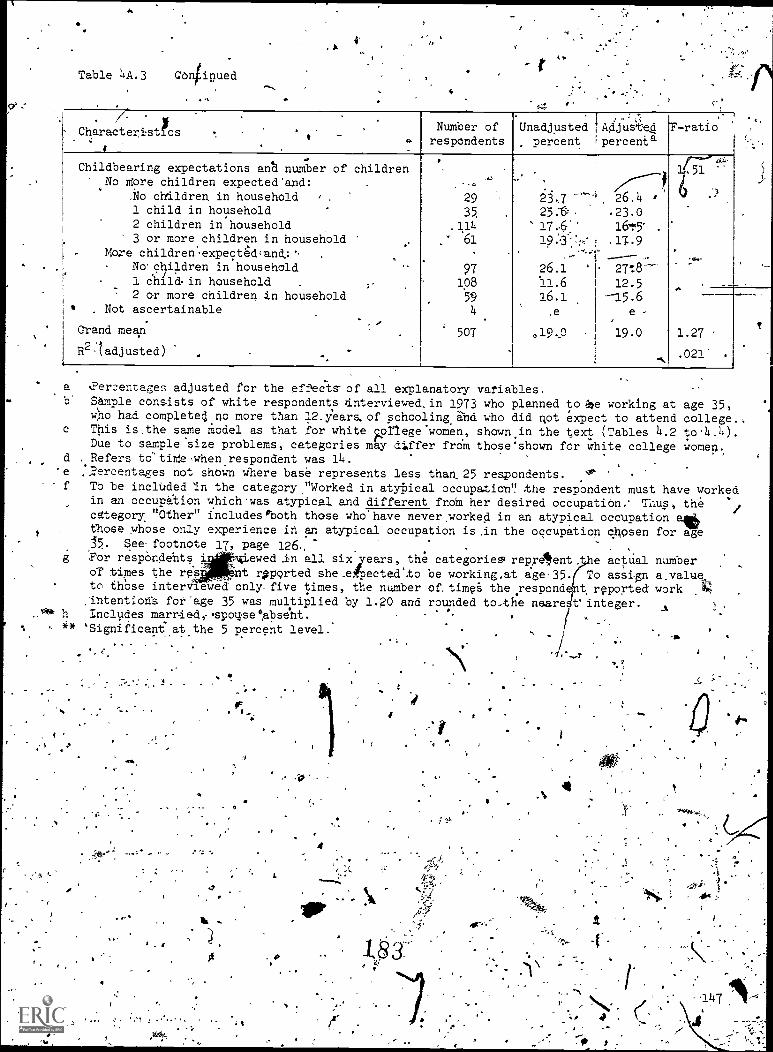
Table 4A.3 Continuedt
sCharacteristfcs
4I
Number ofrespondents
,-;CkUnadjusted 1
Adjuste.4.
percent percenta-ratio
Childbearing expectations an number of childrenNo More children expected'and:
chdldren in household 29 26.4 '1 child in household 35. 25:' .23.02 children in household 114 17,6." 1615 .
3 or more children in household 61 19.3: .17.9More children-expect&liand;'. .
No children in household 97 26.1 271:81 childin household 108 11.6 12.52 or more children in household 59 16.1 --15.6
. Not ascertainable 4 ,e e
Grand mean 507 o19.0 19.0 1.27
R2Stadjusted) .021 .
a 'Percentages adjusted for the effects- of all explanatory vatiables.
Sample consists of white respondents dntervieued,in 1973 who planned to ape working atwho had complete4no more than 12.years. of schooling and who did riot expect to attend
c This is,the same model as that for white prlegewomen, shown in the text (Tables 4.2Due to sample'size problems, categories may differ froM those'shown for white college
d . Refers to'tiMewhenrespondent was 14..
'e ,percentages not shown Where base represents less than, 25 respondents. :16'
f TO be inclUded 'in the category."Worked in atypical occupation" the respondent must have workedin an occupation which'was atypical and different frdm her desired occupation; Thus, the
/category "Other" includes both those who'have never worked in an atypical occupation aft
t those whose only experience in an atypical occupation is.in the occupation chosen for age15. See- 17, page 126, .
g For respondents i ;.1.iiewed,in all six,years, the categories reprdient, e actual numberOf times the is ,,nt zworted she_efoecteeto be working.at age,35 To assign a value
-,,,
to those interviewed' only-five times, the number of. times the respond t reported work:intention's for 35 was multiplied by 1.20 and rounded to_.te neare t'integer. Ai h Includes marniedfspogse%bse'llt.
/ .** sSignificantat_the 5 percent level.
-4...., .
age 35,college.,to.4.4).womeh.,
' $
4
0
1.
183
-. -147 -11--

A
v
t
&u/CHAPTER FIVE
'INVESTMENTS.IN HUMAN CAPITAL AND THE EARNINGSOF YOUN!'WOMEN
David Shapiro and Ti,moth? J. ,Carr*
. , ,-, . .
This chapter examines the determinants of Average hourly earningS.
of young women, The primary objective,4 the Chapter is to analyze theimpactOf iriVestmentsjn human capital.oh hourly earnings, with :.
particular f-c-rcus on postsChoolThvestments-in-htman Capital. In . zaddition,.a,Comparabli analysis,will, be made for young men, in orderto examine diffeeences in the wage structures by sex and the .lederlyindsources of the wage gap between young me-and young women.1',
POSTaCHOOL INVESTMENTS 'IN HUMAN CAPITAL4z
-According to the;
humah .capital Model.Of theearnings,2 investments ih human 'clapital ,(such asitreAning) enhance a worker 's productiv,ity,--and hence,,earninp.
Considerable empirical eviden6e has c..4istently documented thetheoretically'expected association between.yages a* aO'Climulatedhuman capital. Recentlyi the process of-invest*mtpiOhuman capitalby women ovel.:the life cydlp has been subjected:to considerabletheoretical and e m c 'analysis:3- In considering:Avestment s inhuman capital `over the life cycle, a'yeri important diffeience
.
betw eep-women and merPemerges: mien often drop out of the labor force forextended periods of time,-while-the labor force participation of-men'
;? ._...
(particularly married menj.is Ansistently very hi The-intei-mi*ent
distribution ofschooling and on- the -job
4
*The authors
assistance:-
1,
7 . -.3 - ,,... ..
wish to thank Le la 'V.; .
for her reSearchs'
,
., ,- . ....
IThe.initial.,analYs s'usei7data from survey f youngomen._'Howeer, since the 1973 survey of young was telephone....-
si
.4".
vey (aneconsequently subject t6-conSiderible mea urement error on:ral key variables); the comparati--Ve analysts betweep women and mep
makes use of the 1971 0 young men and the 1972_survey of thoung,women (these two,suryestoole place closeSurveys of young hen a d womeqf
2 .
For discASsidn(1WO, 1714):
Fox..exa 161
7-7*.papp7611976).t
' i '7"/4
_this mode', see Beker(
in timetthan did the 1971- e
. -- -*--
.
and Polachek (1*4 .and' SAE-delland
9614- 4,67) apd Mince
.184.
)I
"k, z1/44.1'
-vb
wyr;

4
2
r O
labor force' participation of women is closely associated_with thebearing and raising of children.4
The pattern of labor'force participation of women (particularlymarried women) has two important implications for their hullan capitalinvestment behavior. First, -nce women will spend less time over thelife cycle engagedin work the labor market, they will have lesstime to acquire on-the-job raining than men of com9erable age andschooling, and employers ma alsobe more reluctantrtoprovicle -such,training. Stc'ond, returns (in the form of higher *age rates) to
,investments in human.capital can only be received while-the individualis at wor4,;'hence, prospective discontinuity.in lifeiMe,aabOr fOrce"experience will hav the effect ()lowering the returnt from (andconsequently,lowering the incentive for) investments in on- the -jobt/aining.5 ;
A.
The preceding paragraph focuses on implications of the life-cyclehuman caithl model with regard to sex differences in on-the-job
.training.- HoweVer, the ;lode] also has implications re
'differences in investment behavior among women, for to the extent thatthere are substantial differences.in lifetime Libor force attachmentamong women, the human capital model,implies that women with stronger
..).abor force attachment will engage in postschool human capital invest;.--mentS more heavily than women with weaker, labor ford'e attachment. Afurther implication is that the taming of investments will also differ:'investment profiles for women' with greater commitment to.tiork should be
more-similar to ,the monotonically declining investment profiles of menthah those for, women with weaker commitment to work,.
..,
Thus, in 'examining wage raf6's and humah capitalinVestmepts'ofyoung women and men, we may distinguish three groups: :1) ;women whose
ti
,..,;For; ,evidence to this effect (based on data from'the-1967.NL8Of Mature women ), ee Appendix A ,of Sandell -and'Shapiro (1976) In ",
view of the secular crease in female labor force participation, thereduction of fertility rates in recent years,'and the evidence,presentedin Chapter 1 of thiS volume, it seems most likely that 'me spent athome,folloMig the birth of the first child will be Much porter for
- the young women under, co - iderationI ,
ti
3' . . :t,
, ..
. qt3
'
has also' be arguedZat pros 'pective Ascontinuity of laborots.
-fo.
rce P kpeft.
ence af eats the 'she of the' postScHoul investment profileof women -- via.,, w le the investment p;ofile for men is monOtOnIcalirdepli 'ngAphe:p sfile 'or Married women with children,is'not'; xi..4hei=
ittends to.be laii)ler,in:the postAterndl Mitul4n111prmaternal:Irriod(4ncer snrPolachek, 074): However, as noted by Sandell 'and Shapiro0.976r,: this hypothesit ia6 noVtestqd'ilroperWby Mincer end Po74.chek,
.
i : . / t .'..&
1.
f5o .tt
a

9-
r
*
9
4!
.
expected attachment to the laborforbe over the-life.cyclel
is" wea2) women whose expected attachment is- (relatively) strong; and 3),.men, whose expected'attachffi
cent is strongest. According to human apitaltheory, - investment in on---the-job tmining6 should be increasinglyimportant as one moves across these groups. Differences in postschoo]investment ehavior between the first two _groups and ditferendes ininvestme etweeb the second and third groups will fie examined'separate.
WAGE EQUATIONS FOR YOUNG WOMEN
below.
-
)In this 'ection, wage st'uctures of "weakly commit5ed"-and "strongfy
committed" young women are es imated. The'primary focus here is onwhether or-not these empirical estimates are consistent with our .
hypothesis that in'restments in on- the -job training are greater forwomen with strong attachment to the labor force-.
Specification.
.
The basic &ciliation to e estimated is:
LNWAGE a- 4- -a.
therOILNWAGErate; SCHOOLtmeasures thCmarket since'number of,:t:
represents k-
::i
measui;ing.:05j4ty-k1wages. are' S'etiby d70:1tie- South 04 *10;"health probreinda"V.'
.-' 1,:,:.:4.! j;-, 9, tx .'=.-
is 4e nmeasurerespondeshe laSt
tears that the.
setof.control variables: a continuous variable, and separate dummy variables for workers whosectfvebargakning, and for those who reside inICSMEA,.woiqc. in t e public sector, and have
6Choi, + a2EXPER +,a,TEN URE + ,a .Z..
' 3 41.i = 1. .
ithm of the respondenti6 hourlk,wage.<years of school completed; EXPFR
rs of experieve in the labor1 full time; TENURE meisures.the
spondent hasheld.her current jeb; and Zi
-. Alitc'6,The
term'"on4e,job**line is her 'used in the broadest Senae..ezIt. refers to anyfOtlal-or inlormal,proccs.s of'learning skills.whichip-1."hances productivity Viand her116e wages) white e is employed,on a g4venjob. Fora furtheiSPUssi:15,h, see page,6,below.
, ; 1..- :-!-, .- . . .
. 'a fr. , ,je7. -I, -i.;
Alternative tpecaficatkonsOf the wage equation were,also estima-- '' ted. First, we explicitly pincluCied avariableidentifying,those'
individuals who hOLiompletedtor-oh,the-job training reivant totheir ;duirent johSTIlis varialpie waSnot statistically significant-and, :
, it isno'Lincludtd'iri'the.regrefsion reported below. Seccipd, tile re-.
_ gresDons.were-eAi. Ofusing fladrat4c specifications off' the.itorkexperience variables, 'The quadratic specifications generally yielded, abettef fit, and are r po e4 below. HoWever, for illuArative purposes
,the digcussiOn hOe fl9du gsonsthe simple linear specification presented. 2above.
.
0018v. 151
J
(

.8
0
The semilogarithmic specification of the wage equation guaranteesthat the predicted hourly rate of pay generated by the model will always _
take on a positive,value. .It'also 'means that. the coefficients may beinterpreted as the percentage effects on the wage rate of unit ofchanges in the independent wariables--i.e.,, bompleting an additionalyea r of schoolinglceteris paribus,.wili result in an'increase in, the
ae.hourly wage rate of,i00'. al percent-.'1'"" 4
The, first -three independent variables in the egtion- ,- shoolirig,
total..work experience, and current job tenure--are human capitalvarlables, and 'their oefficients are expected to be positive. Total.experience and job tenurerepresent'periods during which postschttahuman capital investments will be made., Holding tenure on current jobconstant,. Epe coefficient of total experience measures the return togeneral training; while the coefficient of tenure in this specificdtionmeasures the return to firm - speci'fi'c
The life-offcgman capital model is implicitly concerned withinvestmentiniodlneral training, Hence,n`thecontext of the wageequations-to 1e estimated tire-, the hypothesis that postiChoolinyestments will be eieatet among women with stronger expected lifetirnelabor force attachment may be seen.as implying the coefficient (ca)of total.`experience will be greater among such won n than among womenwith weaker labor force dttac ent. -
.
Beliaviorally,.postschool inyestments in general human cap±tal willbe.manifestld largely through, occupational choice.' ,Occupatibns differin.the amouAt of on-the-job training re4pkred in order,to reaChfulleffectiveness. Human capital theprY suggests tTia--m-illgh-training"occupations will be cAaracterized by low wages in the initial phase of
- experience (.4.Thile the wbrker is acquiring the'necessary skills throughon-tlip-,f ob training),"and increasing wages'aff experience (and the
410
8Tias interpretation of the total'experience and tenure coeffi-
cient$ is identical to that in*SandeIl and-Shapiro'(1976). FOr a morerigorous theoretical! ijustification of this interpretation,..seeShapiro0.976). The concepts of_Oneral training and firm-s9Rcific trainingwere first 'ven-4roMinent fOcus,)py Becker,;(1961). Most simply,
"periectl'-gene " training ietrainin!W.ch raises a worker'sproducti ity eqyally at many firms; comp etely specific training raisesa worker's productivity onlywilth a single firm. Most types of real-
. .
world training invoive,both general and specific cOmponents;.however,the mix Of these -components varies.,-.For exAmple,iililiary training-inelecti.oni,csand a,skilled-tradesapprenticeship are two forms of.(predominantly) ;gerra3~ training; while learningthe rules and. '.-
'regulati.ensjn,a,paricular firm and training as-an astronaut constituteprimarily specific training. .Foit a more- thorough discussion of the Se '
two types of/training'ind the fina'ncing of training, see Secker.(1964).
152
1 8 7
s.
f

- ,
individual's caAabilities to perform the job) increases: Consequently,experience-wage prof4les')-/ill be steep for/high-training" occupations,and relatively flat for "low-training" occupations., .Presumably, women .
Stith strongeg4xpected,li etime labor force attachment will have greaterincentive ;..t4) Westin t /iIr, general tizman capital by choosing "high-training" occupations. This greater investment, kn turn, should be
.
reflected insteeper experience=wage profiles- -i.e., a,Zargercoefficient of total experiende, and..a. lower intercept term (a0)..
. .
/.
. . ..,
Apart from'the influence of schooling, total work experience, andtenure, several control variable', represegting additional determinants'.Of wage.rates, are included in.th sage equations. Ability, measuredhere by an intelligence quotient (IQ) score, has beed shogri to be an, .
important independent f'actor influencing wages.9* Since our empiricalfocus is on the experience-earnings profiles implied 1y the experience °
o coefficients in the wage equations, conLrolling for,ability isimpirative to'insure thatotte propleS.are not-simply.reflectingability differenceSbetween the ttronglyattaChedland'weakl!T attached
/. young women. . .
i ., . . .
Considerable empirical el/II:le/ice has been4presented in the
literature indicating that, other things being equal, wage rates are. !
higher for workers.whosewagis are set by'col_lectlip bargaining, whowork in the public sectoriand'who,reside in large uriln areas.Similarly, wages tend tO'be lower, ceteris'Taribus, for workers Who havehealth probie&s.and who reside ifs the South.lP Since the distributions
/.) differ, it is desirable to control explicitly for the effects of theseof'estrontly and weakTY attached. women cross these characteristics may
factors. In-brief, then, the control variables are introduced Into the ,r
wage equations in order to prevent 13ias_in the testing of- our .hypothesized relationships.
,,,The array of variables just described exemp/ihei the advahtages '
of.using the National LongitudinalSurveys relative toother mfcrodata.souries for the eppArieal analysis 'of wage determinatiori. A compari;onwith the work of Mincer (1974), 'S,:typical example of the' use o.f 17:8,:
Census (1 /1000 sample) data, fol. this'purpos2,is most instructive.First, Mincer wes forced by data liMithtionso-a"use an-annual-earAinksmeasure asadependent variable;, such.a variable is_ l'an, Igam_of
- labor-supply responses and human capital formAtion."11 In, his study
et .. ,1 v 4.04 -arge number o'f studies.provide evidence ,df wage differentials
associated with one or.more of these fiv,l'agtors; the interested teAdrmay wish tp conspltDaxaca (1973) for a single study that-considers all
..of\these"factorst(as well as several oplers)oimdltaneouSly. \
11Blinder*-
,.. ( 976) , p . 17:- ' g, .
es
1
l
_153.

a.
, ,.-
we use-a "purer" measure: an hourly, rate of loa.3,.. -.Second, Mlincer'uded
.a measure of "'potential" experience obtained by the.formula. -.
' t-41
experience = ag - highestkOade; completed:- 5.. .
. .. .,
This proxy is clearly untenable for samples (such as.
young women)characterized by less -than- continuous labor firCe.participation.a2Again, the NLS permit us tg aVicertain the actual labor market experienceof our sample'with tolerable accurad.13'Finally,-we avail ourselvesof information'on "ability" (tC1),*llective bargainIng cC'erage, tenureOn current Jot, and health. status 4-hich is'not generally available intie /100.0 Census'sawle.4or'fther'microdata Sets.
',.4
atStratificion -r
.
.
Thus far;tthe discus; ion has focused on the distinction betweenwomen whose expected attachment-to the labor force over the life'cycleis weak and women who a expected attachlTent is strong,. This distinctions,will,,be. used to str ity the sample fo.r-purposes of estimatpg wageequations.' The c fical operational qtlestion, then, is by what
criterion will women be judged to be weakly or strongly committed to' , ,-
the la\or force?' .,0-0 .. ;
' 0 00 : e
7 l'.
There-We a number Of criteria which might be lased in this.regard..°16
.
We have made use of a woman's future,plans as an 'indicator of the,..strength of her attachment ,to the labor force.14. Eespondents Were askedin 1968 what they would like to beg*.who stated that they would_like to b
- those with-a igeater attaChthbnpAnned_tobe housewive/mothhave weak attac ent to
-the.
Table 5.1the sample ofand by race.
ows mean va;,g woman,an
is apparepi,
t.'_
at age 35., Prqumably, those .- ,
4 -
workint in the labOr market aree labor force; ?bile thoSeirho' .,.
rs and those who responded."dori't know". ,
:ork force -
-
.
,a 'di .
,,, 17.
es for selectee. variables'
..
oeinterest for .
alyzed beloJ, separately by plansoforage 35.from the 'table thati.thee qre no large- :
12Ibiddrpp. 13-1U. .
/Ia.,. . .
. nA potential experience . measure will be used in the case of young
men, examined elow. P J i 0'.7 .
, r. ':04'....,.. 1 r s
e.
. Other criteria trhich we/7 tested included expected number of..
children and SpecificVocational.Preparation (S1/1").sdore of first. .
postschool jobjsp score measures the time required to, reach profir..,.. i
ciency in aparticular'vocation). Insufffoient vatidtion in the - formerand reduced Sampleisizes using the latter-resultedq9 re,j-ecttion'..of
these criteria as stratification variables... . .
.7
? ro-
'
Or
14
154 0.0
me

w
Table 5.1
t
Selected Variable Means for.Young,Women, by Race'Plans to Work at Age 35a'
and
I'
r
,Variableb
.8
WHITES BLCKS
Plan to ;No workwork plans
Plan towork.
No workplans .
Highest grade completed
Total.work experience (years)
'Poteritial vor.k experience(Years) . \!5.79
Tenure on current job (years)
inlielligence quotient1'
rAeExtected-nuMber of
children
Number of respondentsc
13.18 .,13.11
4.46 4.31
5.22
2.17\ 2.10
106.46 107:50
24.61 23.83
I
2.06 2.25
264 706(205) (.463)
12.58
4.26'
5.46
2.26
89.51
24.33
2.31
. 127. _
(114)
1276.
4.54
5.77
2.06
90.05
24.52
2.18
138(x.18)
a The sample consists of women who,were employed as wage and salaryworkers and were not enrolled in school full time as of the 1973survey;' and for whom the reauired.data'are ascertainable.(
in 2.n. . .b All variableA.are defined n ue Glossary.c Numbb;s in paxentheses refer'to sizes of:the samples used to .
calculate.mean expected numbe-24of children (i.e., excluaingthoserespoftdents for which such information was not ascertainable)..
.11 '//
..
e
r
IP
,
4
.
t
4.
A
differences in" variable 'means accor
future plansorariable appears to befactots;_that is, it ins not serving
(obvious) variable.,
.- ' .
I
I 4
'Empirical Estimates
'lig to future plaq.. Thus; the-reasonably independent of thesesimply as a proxy for some other
.
Inthis section, we focus on wage equations estimated for out -of-...school women whoyere employed as wage and salary workers in 197J.: Thehypothesis of interest here is that women who desire to"work at age 35will invest more heavily in on-the-job training,-an6 consequently havesteeper experience wage profiles. In the context of the wage equationpresented above,, our hypothesis indicates` that women who plan to Voilk
should have a larger coefficient for total work experience and asmaller intercept (constant) term. .
.-
I14 _The procedure used; to test this' hypothesis is as 4o.l.,lows:
*for :
. . .
...' black and white women 4parately, we have estimated wage equations- inwhich interaction terms (for total work experience, tenure, and theconstant) are included to differentiate those who plan to irk at age35 Within each equation, then,,:the interaction terms allow fdr. .
differences between those who plan. to work and those'who '0i.0 not plan in
terms ofethe coefficients off' total work experience, tenure and the
constant.15 .
%.
'.. .
The empirical restlts pertinent to our pringipal hypothesis -are. , presented in Table 5.2.16 As noted above, we e4itated the wage.
equations using quadratic -soecificatiOns for both total experience and
tenure.17 These quadratic specifications make comparison,of the "plans". .
15The interaction terms for tenure are included to.seeif invest-
ment in specific training is gi.eater for women with strOwer labOtforce attachment. An,implicitsassumption here is that teCoefficientsof pie other variables in the wage equation dO not differ by plans to
work. A formal test'indicated that this assumption is consistent withthe data-=i.e.., when interaction terms were introduced,for allvariables in the wage equation, there was no pattern ...of signific
differences by plans to irk in the coefficients ofscho4ing oof the control variables. ,7 4
any
,.' -.16The coefficients for the,"no work plans" groups are takendirect-
ly from the corresponding wage, equations (see Appendix Table 5A.1),while the:coefficients for the "plan ..to work" groupsPare obtained foreach variable-by summing the'"no work plans"'coefTnient and thecorresponding interaction term coefficient. For a further discussion .
of this and similar econometric procedareS, see, 4ohnston-(1§72), pp.
176-186. .
70 e exception is in the specificatibn of tenure in the equation
fot blacks. With the quadratic specification, both Coefficients were
0/P .
156..191 II
t. "

M
le
*
1.
i, 00
a The sample consists o women who were emp1010 as wage a salary'workers and wire notenroll in,school f 11 time as.of,the 1973 survey, and for whom the required 4ta areascertainable.
.
-,i .
,
c,1b 411 variables, are d fined.in the:GlosSary. ,
:,,,
c Significance teyel efers to whether or not, the coefficients of a /particular varittlIediffersigriifidantl according to plans,to 1../(4k: "
,d not included in th s equation.* Signiticant,at'th 10 percentlevel. t
,,
' '.
Table 5.2 Regression COei ficients Relating Ln. WaF:e to Selected Variables, by Race'
and Plans'to Work at Age 35P-,/
d
'. .. , .
Variableb .
.
.
..
1
, WHITES'
.
BLACH6'
, Plantojwork
No work'plans
Zignficance,evelc.,
Plan,
to workIgo work
plansSignificance
levelc / ,
Total work experience'(years):
d'etal work experience-Squared.
Tenure on mirrehe job.....(y'ars)
.
Tehure on 'current job(' squ4redConstanf;',.,-
4 'Number of respondents
I
.07,62
1... 0041
i
i
' 1 .0652
,
--,.:0041
I .3.56611
I . 264
.0335..
-7.001A
'831'
I .
=.0064,
3.6720
106
/
. /
.,
.0543
-.0052
..
.04.70
.
d
3.6583
127
:0424..
.
:-.'0039;
-
.0303
d v
3.73400.'
'138'
.,
.t .
'
/t
.
"
4
..
'
. .
,
,f
, A
°
+1,

,Y.
4
and "no plans' groups'e bit,more complex than in the cage of a,linearNspecification, since there are two coefficients fof each of the two , P ..liprk`eXperience measures. With a qui:dratic specification 4 the coeffi=-----cient of the linear term measures the ini:tialsteepness,of therelationship in question, while the coefficient of the scplared'terMreflects the rate at which the steepness changes as the independentvariable increases.
The'coefficients in Table 5:2 reGeale'that for both white's and. ,
'blacks, the relationship between hourly wages and total,work experience.isinitially&steeper (significantly so for, whites) for'those who plantp work at age 35, A's hypothesized. In addition, withtp each racegroup the'ihtercept'term is -lower for At .'plan to work" group-..(Uainf the difference is.'significant fof whites): This evidence thuspirViaes.tentative support 'for.the human capital hypothesis that womenwith stronger expected attachment to the labor force will invest moreheavily in general on-the-job training.-\A-C the -same time, however, thecoefficients of the experience-squ red terms indicatethat the
steeper experience-wage rofiles for those:who plan to worka6)
'intfall
at e.&,e flatten out more rapidlyithan thePI-ofiles_for those withno work,i.pIans (81.111,though the latter.effectia not statistically ,
,
significant).-4 s 'a
Figure 5.1 shows that this flattening out is not verz consequential.for the range of total work xperience relevant, to our inquiry. Thatis,Figure 5.1 sh ws experience-wage profiles for young white womenaccording jo whe er or not they plan to be in the labor market at age*35 'The, profile are drawn assuming 12-years of schooling, IQ of 100,/zero tenure, res dence in non -South SMSA; Wages not set by collectivbargaining, empl yed in the private sector, sand Ao healtfi'problems.18As impliedby h n theOry, the profile for those women Withstronger expect d attachment to the Yabor force-begins atalower point and then rises more rapidly than the profile for weakly %.
attached women, reflecting investment in trainingvia reduced wages,initiallY-and returng to___Ipvestment in the form of more rapid groWth in
knsignific,ant (and positive), ixesuatably reflecting multicollfnearity.'Consequently, N linear specification of tenure was used for blacks.In any case, f r both blacks and whites, thp empiri4a1 ifferences byplans to work oullbe quite similar if we had'reported estimates ofthe wage equat ons using linear. specifications of,Potal work experience'ana tenure.
18'Profil
ships' between
. rate. For pu.drawn the fi
158
s generated from he wage equation-depict the relation-.4xperience and th patural logarithm of 'the hourly 'Illpposes of Figure 5.1, we have taken antilogarithms an .:
re with. "wage" insteWo"61n wage" On the.vertical'axis.)1
-
194t
'4

V.
41
4 .
/ r
Figune 5.1
Experience -Wage Profiles for Young Whj...te WoMen by Plan s to Work at Ate 35(assuminglj.years of school', an IQ-of ;00, 'zero tenure, no' healthTrolilems; residence j.n anon -South SMSA, and employment in a privatesecitorjob-noticovered by a collective bargaining-agreement)
HourlyRate ofPay (_961 ,
Dollars!)
200 --
1 .90
VI-
o
,- Plan to wor
*Do, not plan
to work,, .
1;60 --
1.59
a.:14o
0
I
I
8
1 2
.,.%otp,a. work
'5
Expeilience:(ears)
-159
"y. 195't .
a
O
. e
1410 /2'
k
4.1

\
WWI
o
.01
-I' .
wage rakes subsequently. Whi4.e.the 4 lan to work" group's profile doesflatten,put somewhat more rapidly remains steeper than-the profile. --
for the "no work plans=' 6.04 throughout the range of experience,depicted in the figure,
/1...,'
,.
.
`,Table 5.2 also reports differences by plans to workgin the7.'Cdefficients for tenure. Our principal hypothesis is concerned with,
, ',inies#ment in general-training; however, interaction terms with tenure.
were included in order to"see whether or not plansooto work affectinvestment In specific training. In general,,the evidence does not ,'support the contention that women:with stropger labor force attachmentwill'invest lore heavily in Specific training: withinracsgroups,there are no significant differencei between the "plans". and "poplans" groups in the estimated tenPre coefficients.19'
. .. ..,
In considering differences by race in the wage equationg; it is-,apparent fromTable 5.2 that the plans/no plans distinction is. more,relevant follwhites than for blacks. That is, the-differences among%.blacks in the intercept and initial slope of the exPerience-wage.profiles,;4iie inthe expected direction, are not significant andare sMlilleriin magnitude than thOse for whites. Two possible reasonsfor 'such a phenomenon have been, propoStd.20 First, 'eater labor.'markettdiscrimination agaipst black women than white women may preventstrongly attached black women from acquiring 'as much on7the-,,lob,trainiag as thOrvould like. In additiOn; Miniium wage laws (which.
.
have aigreater impa;ct on blacks than whites) may have aSimilar effect.However, thorough examination of these and.other hypotheses- is beyopdthe scope oc-khis chapter. t '
Comparison by race of the remaining coefficients in the wage'equations reporteddin Table 5A.1, indicates that, with one except n,
'the coefficients are broadlyasimilar. Theexception is the coefficient. for - residence in the South. Among Whites, a Yopng women who resides _
in the South is paid approkimately 5 percent less, on average, than hernon-South counterpart, other thrhgs equal; among blacks, the South/non74South differential exceed$:18 percent. It seems likely that this 7 ' .
. .. . -Iv
difference by race in the magnitude of the South /non -South wage. t
,-.
1-,differential is a refleCtion of greater labor Market discA4linatioh..:st", . -
against blacks in the South.21 ... , ------ ,
alt
,
iYr
19Among whites, the Inure -wage relationship is initi somewhat
steeper for those women with no work plans,; but flattens out e ra-pidly for these women as tenure increases. Among blacL,aTaiDle 5.2indi-Cates that the tenure coeffiCient is greater fOrrthe women:AWhd"planto work at age 35;:.boyever, this:difference is not significarit'i,
02 -See Rosen (1972)v
21 .
For a discussion of. regional differences-in ractal_disctimina-, ition, see BeCls,er (1971),, ch. !8: .
- rf
160
awl
ti
.1

... ,"40*. .
(.../ . ,
. , .Tc,tummarize:then, we find empirical 'support here for,thehypothes4s},that expected future labor force attachment will be'an..importankdeterminant of accumulation of general human capitalthrough invAtmeht in.bn-the-job training. It has been,sugges.ted-.elsewhere that'young women tend 'to underestimate the likelihood oftheir being in th'iabor forceafter completing child-raising. 22Our res tS are consistentswith the hypothesis-4at young'women whodO not esireffutiire!labor force attachient will. not acquire ituch.gen.. er training in job skills in the initial stages of their working
. lived. ,Consequently,it seem& likely that mink young Women will be ata serious.disadvantagebf they attempt to reenter the labor.fopte-'
. aftei. raising aPamilSr. This suggests' that 'young women shoulde,more) accurately apprised of the.likelihzgathat'they will be in the'lapr
ToTee-following-child-raiging, anetheldesirabil?ity of> being.ade6ately..(prepared for this-labor market experience.' Counseling and vocational
° * guidoce at both the secondary school and college levels could beutilized in this regard. .
/-
.
..,..
.
WAGE DIFFERENCES-BY SEX AND THE EFFECTS OF POSTSCHOOL INVESTMENTSIN TRAINING - ...;,..,. . . 4'
* A , ,- . 1 , d .° Ilk ,
Inthe previou'section, we found empil.ical evidence whichill:Torts the human ,capital hypothesis that PobtSohool investmentsin (general) training are greater for your women-with ,strongere)tpected attachment to the labor -force over the'life cycle. Afurthers' implication of human capital theory is that investments,in training. should be greater fOT youneMen than for young women,since women (but not men) face prospective discontinuity in lifetimelabor force Aperience. This implication is considered in the presection, which examines differences in postschool investment-behavibr'betwedn'the stiongIy attached Nung women and young men:In, addition, we, examine differences (among whites) in the wage
- structures'by sex more generally, in order to inquire into the* 'underlying sources of the wage:gap between young ten and young women.0 . . .0,
* , ,.
t, e
...1
:22 .
Jusenius and Sandell (1974) report that, in 1968, approximately29 percent of _the young' white women'iLthe NLS sample planned-to work.at age IS', while the corresponding figure fo;.joung black women was59 percent. Actual labbr force participation rates in 1967 for the 1
older NLS.woman (33 to'37 "ears.of age) were 47 percent for whites and'67'percent for lAtzq. :
i, , _,- ) .
. .23Thd overwhelming majority (over 85 percent) of strongly attache
young women expect to bear 'children,. Hence, on average, young menshould have granter expected lifetime attachment to the labor force(and greater incentive tbinvest in on-the-job training) than thestrongly attached yourig.women.
.
\ -.. . '
_197
66,

k
.
-(
, As notkd previously (footnote17,*the comparati4'an lysis of the
.wagerates of young women and yOung men is based on the 197 survey of
rYO,ungwomen 1(con§ucted betwden January and April of 1972)tand the 197
, survey of,young men (conducted between October 1971 and Februarl- 19,72. .
fWage' equatibnS, were estimated for both groups. The samples are compa-a!
rdbleto those used .in the analysis in't.he previous section, in that
t they consist of persons who were not full time'students anewho'Were' t
empoyedas, wage and-salary workers at, f,the time o the survey. The'
-......-,samples were turthet restricted to respondent's who ranged in age frOm
19-to 28.24\-Summary statistics foe'Oertain'variables of interest are.r .1
shown for ,each group in Table-$.3; more_complete,infOrmation, includ'ng-
4.occupational distributions, is given in Appendix Tables 5A.2 and 5A
. .... I,*.'
.
EmpiriCal tstiAtes .
A'_
1`
,,
.
# ,
t.. ,The wageequatlons%for young women who plan tt work at age 35 :,
r.p ' and for young men are-repOrted in full in Appendix'nible 5A.)4. The
.specifications used generally.followed thos4'used'i::1 the previous
,..... "section.25 To illustrate the differing postschooljgeneral) invest-'
.jment behavior .of ioungmen end,strony attached young Women, weconsider a ("typical") young man and young women, each of Whom is a
high'sohool graduate who lives in a non-Sout. SMSA,.has an IQ of,100,
is employed in an establishmenein,t4e private pectorand not coveredLy a collectiv argaining agreement, and' is -new to the job ( .e., hat
,p.
.
I
no tenure). respective experience-wage profiles for two stitch. .
..-hypothetical persons that are implied bythe wage equations in
,
. . 4ppendiX Table 5A.4 are depicted -in Figure 5.2...:
.,
. . 4 k-*
.The profiles depicted in Figure 5.2 do. not Offer very much
support for the thesiS that the male profile should start at a lower
. ,level and exlitanbe more rapidly than the profile for the young women.
t For 'one thing, the :nun's profile lies uniformly above the womdts..profile, despite theact thatit should be depressed at low : . .
levels of Work experience. This consistent with human
theory only ff the male-fe 4.0 gap al zero :experience '(which amounts
to $.66 in Figure 5,24, d have been even larger in the absence of
.1,4
24 . t '
_ ,
If they had: been, so reStrttteq; the women Would. have ranged. i /I
,in age from 18 to 28 and the men from 719 to 29., .
1.
1 . -
.
_
.25InforMation,on hea th limitations was not available' on- 19.72, ._
Survey Of yoAg women; the variabIe:repr4enting healthilimitations wasaccOrdingly dropped from/the men's equation, in order., tOSncrease 'that ,,
.
equation's compardlidlitY- to-the young women's equation. Since
information on ,actUal work experience could'not be ascertained for -
yEungMenin,the same Way as for "y'CaingWorret94, potential work'lperience
(time out of schoo as used as a.
. .
e
162
4:
:000, I;a 4
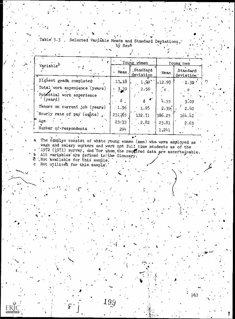
I '1
\"Selected Variable Meads and Standard Deyiation4,''
by Sex&
.
Variable' i.4
t-
r.
Young women Young men1
.
, Mean
i
Standard-
deviationMean ,Standard 1
deviation' !..
Highest gradt, completed-_
,Total:work-expenience(years)
Po'tietial work experience((year)
Tenp.re on current job (years)
HourlY rate of pay (40ts) ,.
Age- :. ,
*
Number oi respondents
-
.13.18
: 5ile
.
d
. 1:96
231:65.
23:33
294
.s
. . 1...5,0'c-12.98
2.56'.
,
d r
1.95
132.71
, .2.82
.
,c .
)4.55
2.39'
386.25
23.81
1;241
2.39'
c'
5.09
2.40r
164.42
2:63
..-
4 1
1
i
. .
a The samples consist of white young women (men) who werewage and salary wqrkers and wei.t riot full time students'1972 (1971) survey, and .for whom, the reqered data are
b All variAblesdre defined in:the Glossary.Iwc Not 'available for thii sample.c Not utilized for this, sample'.'
6
A. I
6
4-
r
. r
t
,
19.9
ti
employed as '
as of. the
ascertainable.
-' 4' J
4
s,
4
16,3
A
.

, -
Figure 5.2'
. ,
Experience.TWagefrofiles for White "Strongly Attached",Ibung Women and YoungMen (assuming 12 years, or schooling, an IQ of 100-zero tenure, residence ina non -South smat, and employment in a private sector job not covered by 'a
collective bargaining iireemelft)
Hourly .
Rate of .
,Pay (1967
Dollars)
260,
2.40
. 2.2Q
Vi
2.00
1.80
O
`N.
fr
c
Young men
.
. Young women
1.60.1
4444,4O,
.1\
1.40
'1
164
I.
2 3
Experience (Years)
.
.
0
. e
1
-7
II
*d.

,Vf
,
N,
/-
,
'I
t.ilhe investment which (presumably) leads to a steeper men!s profile.,The investigation of the sources of the gap between the two.profiles(such as disormination), apart from differential'investment behaVior,is an important topic which lies%beybnd the 'scope of this inquiry.Another problem is that the two profilesare nearly parallelAivergingsignificantly only at high (efght years -or more) leVels of experience.Phs, too, is a question which',deserves,furtherlattention:...
Wage-Gap Analysis4) ' ti
The technique of "wage-gap analyst s" has been used by some,revarchers26 to decompose the difference in average wages bet.ieentwo grbups (e.g., finales' and females; blacks and whites) into that,'portion which is accounted for by differential "endowments",of those .-Tharacteristics which, are presumed to.determine wages and that portion,which is accounted forby differences in the wage "struc-eUre," asrepresented 'by the regression coefficients df estimated wageequations for the two groups\in,q4estion:That is, it is possiblethat a member of one group receives a tower returnto a.given endowmentof a certain characteristic than a member of the other, group.
f .bIn applying this technique to our samples of young woMenand young .
men, we first note that the geometric mean Wage27 for the female, sample.is $2.06, whereas thqj for the male sample is $2.93 If toe young,womenhad the average characteristics of the -young 'Men (rather.thantieir own charaCteristics), but.were still subject to the feMale wage .structure, the resulting (geometric) ;;lean wage would be $2.15 Ifente,using the female wage structuriej the sex differenge .in:endowment's ofthose characteristics ID-resumed to influence wages accounts r only$0.09 of, the $0..87 'difference in mean wageb. :Conversely,-iftheyoudgmen had the average characteiistics of'the young women, but were.Stillsubject to the male wage structure, the resulting Xgeometric)-mean. p 4--wage would'be $2.76. Using the tale wage structure, then, the 5ex 4
difference in endowment5,aecounts fOr $0:17 of the actual Wage gap:28 W'k1 .
o
4 .
It
,,
(
.
.----
5e /.'
For instanqp,_see Blinder (4973) 1 Kohen -and Roderick (1975), andbaxaca-:(1973) '
. ..at,
26
27 i -,' ' 0
. .. ' k, '.4Due to the semilogarithmic specification of the wale/equations,
t ' "'the use of'the geometric mean hourly /:ate of pAy (he antilogarithm ofthe mean of the natural logarithm of the wage) is more appropriate thanthe arithmettic mean.
,'
. .-
astie methodology used.here involves the.familiar 3.Qdex umber '
probleMT4'n6nceloAe get two estimates (establishi.ng a yangeof. passibleValues) of'the importance of sexidifi'erences in endowments of,,those.characteristicspresumed
4*/
/
2
A
16?,
4
0

O .t
5 o:
CllarTyT+4.1.1E event endowments of,these characteriggcsay onlyEC,minor.rdie,in de ermi tion of the' wage gap among young workers: on
'averageithe differ' endowments of young men- and women can account- for o0.y A.j-ittle more than 15'ercentof the wage gap. The renlinder
of the ,Irage,gap-2thaeportion attributable to differences' in the wagestructure--may be viewed as an upper limit estimate of the im act Of.diserimination.29 4, 4
.., .
', ..PUMMARY AND CONCLUSIONS. .."
..- . . .. .11e,began ty'con5idering the role.,of e"1-ectations of, future labor,force attachment In inftuencingpostschool human capital investmentbehavior. Tree groups were diistingliished: 1) women,whose expected .
attachment t the,labo;:jorce ever the life cycle is weak'; 2)°womenwhose expecte attachmenti's (relatively)'strong; and 3) men, whose.expectedattac ent is strongest. We hypothesiied that 1.1vestment.in
,on-the-jobtraining should increase as one moves across these 'groups. ,
..Differences in Rostschool investment >behavior betWan the weakly
crr.,and-strongly attacheh.women were considered first. Human capitaltheory suggests!thkeexperierice-wage profiles for workers who investrelat44ely heavily in on-the-job -raining will (start at a lower 'point.-and bd steeper In slope -than those for workers with low levels ofinvestment. Etimation of experience-wage profiles for the two'grodpsof women provided tentative support for our'hypothesis: he profilesfor the strongly attached womeo,began at a lower point and were moresteeply sloped than those for -6..heweakly attached women, suggestingthat women 4:11 the foLer_group do indeed invest more-heavily.in:
-Ton-the-job training than women in the latter grOup..,,--Thede differences, in profiles were More pronounced among 1:Fhites than among blacks.
We next examined.;differences (among whites/it postsch(11investment behavior between the strongly attached young women andyoung men.' Estimation of experience7Wage.profiles tor these two
did not provide support for our hypothesis: we expected the -
profile for,men to start at klower point and. be more)steegly sloped;.however, the estimated profiles fdr_these two'groupi were. essentially
. 'parallel, with the profile for women beihg considerably belowthat formen. In addition, a wage -gap analysis of the rdiqeremes in wage ratesbetween the young ;Women and the young,te.n revealed that sex differences .
in endowments of thoSecharadteristics presumed to determine wagescould account for only-a smallportioliof the average difference ift
.1.,rae;s!'rates. The remainder of the wage gap (that piotion attributableto,differencto es in tile wage structure) may he viewed as an upper limitestimate of the impact of discrimination.
42-
29 ,
, . This analysis. does notexplore the question-of whether the"differences in endowments themselves are a result of discrimination;cf., 'Blinder.(1973). A i' A
166
: 1202
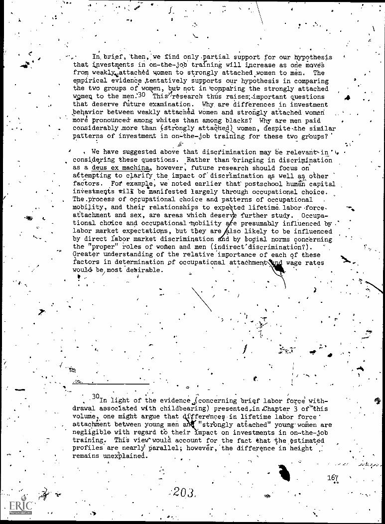
. .
-40 4,
. ®ff
f.
0
4 4
In. brief, then,:we find only partial support for our hypothesisthat investments in on-the-job training will increase as one Movefrom weaklyvattached &omen to strongly attached women to men. The
empirical evidence ;tentatively supports our hypothesis in comparingthe two groups of warn, but not in 'comparing the strongly attachedwgpmen to the men:30 Thisresearch tilts raises:mportant questionsthat deserve future examination. Why, are differences in investmentbehavior between weakly attached women and strongly attached women
,
more pronounce& among whites than among blacks? Why are men paidcon.siderably. more than (Strongly attaChed}women, despite-the similarpatterns of investment in onthe-job training for these two grbups?'
4 t We have suggested above that disctimination may be relevant-in't.considering these questions. Rather thantringing in discriminationas a deus ex machinao however, future research should focus onattempting to clarify the impact of'discilmination as well ae otherfactors. For' examplie, we noted earlier that postschool human capitalinvestments will be manifested largely through occupational choice.The,process of occupational choice and patterns of occupational .
mobility, and their relationships to exile ted lifetime.labor.force,attachment and sex, are areas which deser further study. Occupa-tional choice and occupational-Mobility e presumably influenced bylabor market expectations, but they are so likely to be influencedby direct labor market discrimination d by §oCial norms concerningthe "proper" roles of woten and men (indirect"discrimination?).Greater understanding of the relative importance of each of thesefactors in determination pf occupational attadhme wage rateswould. be most deSirable.
-
A
/S.
f
(
30In light of the evidence (concerning brief labor force with-
drawal associated with childbearing) presented4n.Chapter 3 of'thisvolume, one might argue thatattachment between young men
ferences in lifetime labor force'"strongly attached" young.woien are
negligible with regard -Co their impact on investments in on-the-jobtraining. ThiS view would account for the fact that the estimatedprofiles are nearly parallel; however,.the difference in heightremains unexplained.
. .
203.
0,
16.1
o 1

1
.41
R.E E R.SNd/ .
Becker, Gary S. The Economics of Discrimination,, Second Iklition%
Chicago: _University of Chicago Press, 1971:.
A. Human Capital:. A Theoretical Empirical An alysis, with
Special Reference to Education. National Bureau of EconomicEesearch.' New York: Columbia University Ptess, 1964.
k
Humay. Capital and the Z'ersonal Distribution of Income: An. Analytic Approach:. Woyt:inskytecture No. 1, Ann Arbor:University of Michfgan; 1967.
' .
Blinder, Alan S. "On Dogmatism -in Human Capital Theory.". Journal of,Human Resources (Winter 1976): 8-22, . s.
"Wage DisCrithination: Reduced Form and Structural. Estimates."' Journal of Human Resources, (Fall 1973) :' 436155.
Hause, John C., "Earnings Profile: Ability and Schooling..." 'Journal of
Political Economy Oay/June 1972, Part 2): 5108-5138.0
.Johnston, J. Econometric Methods, Second edition. New-York:
4 ,McGraw-Hill, 1972.
jusenius, Carol and Sandell, Steven H. "Barriers to Entry. and Re-entryinto the Labor Force." 'Columbus, Ohio: Center for Human ResourceResearch,'The Ohio State University, June 1971.
A Kohen, Andrew agd Roderick, Roger. ""The EffectS of Race tnd SexDiscrimination on Early-CareerEarnings." Columbus; Ohio:Center for Human Resource Research, The Ohio State- University, <,
%. June 1975.
Mincer, Jacob., TIThe Distribution'of LabOr Incomes: A Survey withSpecial Reference to the Hutan Capital Approach." Journal ofEconomic Literature (March 1970) : 1-26.
. Schooling, Experience, and Earnings. New York: 'Columbia
University Press,.1974:
k
Mincer, Jacob and Polachek, Solomon. t'Fdmily Investment.On HumanCapital: Earnings of Women," Journal of Political'- Economy
,.(March /April 1974,.Part.II):
r
Oaxaca, Ronald.Markets."
Rosen, Sherwin.Journal of
"MAle-Feffiald-Wage Differentials in Urban 'LaborInternational Economic Review (October 1973)
168
"Learning and Experience iii.the'Labor'Market."Human Resources,(Summer 1972)': 326-342.
204
o
93-709.
4.

I
yC
Sandell, Steven H. and Shapiro,and the Earnings of WomenRevised (September_ 1976)%
David: "The,Theory of Human Capital: :A' Re- examination of the Evidence."Journal of Human Resources (forth-
-
comn0. .
Shapiro, David. "Specificlhiman Capital, JobTenure, i.nd the EarningsbfWomen."- Unpublished mimeo, The.Ohio'State University, 1976.
I)
1
a
(..
44,
t
1692 05

. .
.
4'4
o
AGE
L OS $A R Y
Age of the,respondent as of January 1, of the wiry y.in-'clOetion (1972 0/':1973) in the case of the young w men#,and as of April 1s.1971'in the case of the'young
.., -
I
.
COLLECT VE 'GAINING' COVERAGE,.
-. . Takes a-yalue of one if the respondent's wages e set 15y a0 coIleCtive bargaining agreement, and zero otherwisd. ,
ft'. DESIRE TO,WORK AT A..4 35
Takes a value of'one if the respondent indicatied.at the timor the 1968 survey that sheAesired to be empltoyed at age
ti
eeSPN.1
35, and Zero otherwise-.
DESIRE-TENURE INTERACTION 'i -
Equals tenure on current job if the respondent desires towprk at age 35 and zero otherwise.
... DESIRE-TENURE SQUARED INTERACTION,
'Equals the square of tenbre on cut/lent job if he respondentdesires to work-at age 35 and zeib otherwise.
_.
.
DESIRE-WORK EITERIENCE'INTERACTION
's
Equals total.wor.keqgrience if the respondent desires to ;.'workat age 35 and tet-O otherwise.i 4 ..
4..4,-it DESIRE-WORK EXPERIENCE $QUARED'INTERACTION - .
-.
Equals tfiesquare, of total work experience if'the respondentdesires to work at age 35 and tero-otherwiie.
.
.
EXPECTED gUMtER OF CHILDREN
Equals the total.number ofchildi4en the respondent_to' bear durintlier lifetime as reported in the c1973 su ey.
P, i\\
ti
Takes a value' of one i he respondent has a's f-defink,work-limiting health-pr blem and zero otherwise
0
ects
- .
HEALTH LIMITATIONS
).,..
HIGHEST GRADE COMPLETED..:,
.,
. , Highest'grap ofrespondent-as of
..,.
' HOURLY LATE OP PAY.
170
. .
"regular" schobl completed by thethe Survey in question.'
Usual gross rate' of, compensatiOn-per hoUr.onthe lob in'question:,.
_ ,
3.
I
.....vs

fl t
IliTELfiGENCE QUOTIENT =(IQ)N
'...
:lest. score obtained from/the 190 school survey.= ..., ii/ 1
.c1: POTENTIAL WORK" EXPERIENCE
, . t..\ .-4..
'Number'of months elapSed since the respondent left :schoolrf/,:. (diVided'by 12 sothat it is expressed in yearsY. ,
e.
AP
:' POTENTIP4 WORK EXPERIENCE SQUARED, , . .7 ,. , -
Equals the square of potential .work experience.
% * -I ..-
44
,A. PUBLIC SECTOR EMPLOYMENT0 ,
' :Takes )a value of .one if the respondelit is employed in thepublic sector and zero otherwise.-.'
RESIDENCE it SMSA... .
,
. .
g ,,
.. .
Takes:a Value of one if the respondent resides iri a StandardMetropblitan S atistical Area and zero otherwise.'
','.. .
RESIDENCE IN :80 7 ae I
"Of
Takes a valueoof onp"3.%the respondent resides in the South
iand zard'otherwise.0..
TENURE ON CURRENT JOB
Number of.montlils that a'regPonden't has worked ,for her/his-
current employer (diviaed by 12 so that it is expressed inyears).
.
E ON CURRENT JOB SQUARED
'Equals the square Of-tenure on current job..
TOTAL WORK EXPERIENCE/
4
..,.A ,4). .
Number of years the. respondent has worked six months ormore since She waslast eniolltd full timp-in (re "gillar) school.
& .
,TOTAL WORK EXPERIENCE SQUARED- .
Equals the square of dotal work. eXperienc.
sat O
of
3
171
I
,
2
4. I_ (7-7

f"
7.
f
, 4Table 5A.1 1973 Wage Equations for Young Women, by Race: Regression
Resultsa,b
Independent variable-
,/
' WHITES
-AD
BLACKS
Coefficient ft-value ) Coefficient,
(t-value r
Highest grade completedTotal work experience
,(years) j .,0335
Total work,experience fi
.... squared, / !, -..0014
Tenure on current job , ,
(years). .
. .0831. .
Tenure on current job.
.
,,,squared . ,
, -..0064
Collective bargaining ..
coverage ,.1672Public ,sector employment .0433'
,..., 0Health prob.lemd.!: .-.0561
lividence in, SMSA .1506-.0451,Residence in South-, 2,
intelligence quotient , .0029'
Desire to work at age :35 -.A.057
Desire-work experience ,,,, . .
..
Intekotion.
.0426
Desire -work' experience , f
spared.interebtion 7-V7.Desire-tenure interaction -.0179
pesire-tenui:e squaredRI
interaction ' '1 .00
Constant . !PET. . A %
.0790 (lo73)***
(.4.91)**
.(-o,86). .
( 4.64)***
(- 2.89) * **
.41594-)*-
( 6.36)***
(-1.8o)**( 3.06.) * **
(-1.43)x
( 1.3o)*
(-0.94),
(-.0.57)
( 0:64)
.61)***
,.0833
.0424
=.0039
. 0303
d
116t9.0136
:0848.702
- .1811,
0032
:0119
-e0013'
:0168
3.7340
( 7.17) ***
1.40)*,
(-1.45)*
2.21)***
7, d
( 4.54)***( 0.34)
( 0.99)( 3.78)***(_5.18i***
( 2.49)***
(70.90)0 4
( 0.29)
(-0.36)
( 0.84)1
d.
(20.65)***
2 'R. (adjusted) ".
F-rati
Numb r of resElondents
.1492-
'9.24***265
a The sample oonsists of,women-who'were employed as wage and salaryworkers and were not enrolled in school fUll time as of the 1973survey, and for whom the requiled data. are ascertainable.'
b The dependent variable is the naturalologarithm of the hourly rate 6fpay on the job held at the time of he 1973 survey .(in 1967 dollars).
c. All variablese.re'defined in the Glossary,'d : Not included this equation.-* Significant ait7the 10 percent level.
** Significant A the 5 percent level.-***N OigniiIcant- ait the 1 percent leVel.
172
208
I
f
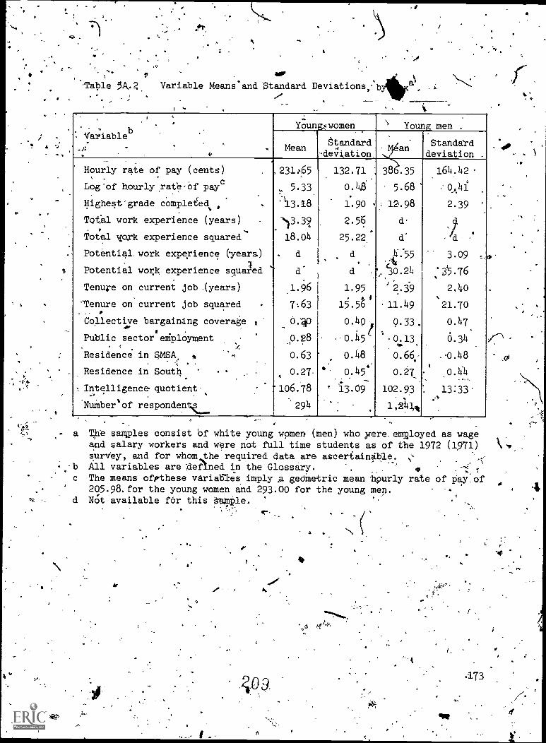
I
a°
'Table 1A- Variable Meansand Standard Deviations,' by a\
,
. ,
bVariable
..,g
.
.
. 4-
,
Younp women.
Young men
MeanStandard
.,
-deviationfan
Standarddeviation
Hourly rate of pay (cents)
Log 'of hourly ate'Of payc
Highest' grade completed .
TQta1 work experience (years). . ,Total Tiork experience squared
Potential. work experience years)
Potential work experience squar1 ed
Tenure on current job .(years)
'Tenure on current job squared.- .
Collective bargaining coverage a4w
Public sector eiployment. ,.
Residence in SMSA I.
Residence in South.
: Intelligence quotient-..: . ,
'Nuinber'of respondenti..._
,
,231:65
5.33
'113.18
-3.39
18.04
. d
d,
1.96
7163
6.00.28
0.63
0.27-
106.78
'294
'
132.71 ;
0.4
1.90
2.5
25.22.
d.
d,
.'
1.95
1.56
0.4Q-
-0.45
0.48
0.45'
13.09
38 .35
5.68
12.98
d'
d'
144:55
',30.24
-
'2.39
11.49
0.33,
.0.13
0.66;
0.27
102.93
1,241%
'
.
164.42
20.41
2.39 .,
)cli-
3.09
'315.76
2.4o
21.70
0.47.
6.34
.,0.48
0.4-4
13:33'
a The samoles consist of white young women (men) who were -employed as wageand salary workers and were pot full time students as of the 1972 (1971)survey, and for whom,the required data are ascertainable.
,-b Ali variables are defined in the Glossary. o ,c The means ofrthese variaBles imply A geometric mean hpurly rate of riay.of
205.98. for the young women and 293.00 for the young men. .
d Not available for this Allaple.,
Sr
CI
10
.173
4
o
. 9
-0
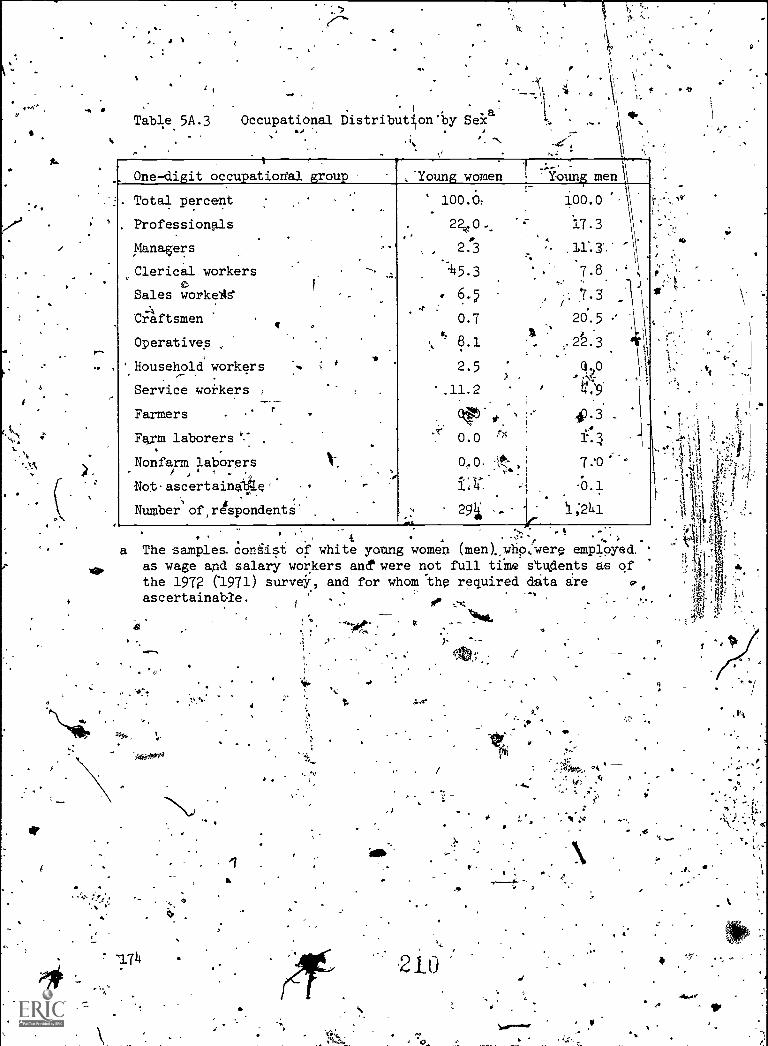
:
at
740
't
Table 5A.3
41.
Occupational Distribu-4on)y SekaA /
T
One-digit occupational group
.,*Young women -Young men
. Total percent :
. Professionals.
.
Managers
Clerical workerse)
Sales worke/le
tAftsmenq
Operatives ...
Household workers H.
Service workers ,
.Farmers
'Farm laborers'," .
Nonfarm laborers. / y 4 r
Not.ascertain4e' ..
iNumber
,
of,respondentS.
0
-
.
..
e
V.
.
.
-.
,
,'
.
.
:,
.
.11.2
100.0:
2240-,
23
4t5.3
. 6..
0.7ft.
8.1
2.5
0.0
0..0
5:1t.
291
.
)
'''s
,...-s*-
,.
*c
.
.,
_.
100.0'
17.3
- .11. 3::i-.
.
. 7.8
7.3
20.5 .'
t ' /.... 22.3
q. o....44.9'
4P30.1.5
7:'
-0.1
1,241
.
"\'
a The samples.coniisi of white young women (men).,who,wer emplOyed.
as wage and salary workers and' were not full time students as ofthe 1972 (1971) survey, and for whom 'thp required data are ob
Tit
ascertainable.
o.
1
4
EA
210,
t By
1'

I
1
0 e.416;'- ..
. V A da,b
Able 5A.4 : 'Wage EquaLonsbySex: RegressionAlesults.o.,.. , . , '
.
.c
Independent Variableij
....67611,4...fi,er ' Younellen.
Coefficient_."
t-value ,
.
u,..
\oe/fficient t-value
. ,
,Highest grade completedTOtal-work
sdxp6ience
(years)-
Total work experience ,
squaredPete4ial 'work experience
' (yearp) , .
Potential work .experience,
. ' squaredTenure on urrent' job
-cj
(years
Tenure oi current ,job. .
squared ,
'.Collective bargainingcoverage
Public sector employmentResidence in SMSA
' ResideVce in mouth',IntelligenceuOtient
* ...
Constant , -' ,
. .
.0474
fo740 *
-'-'.W32%
±'o d -
.
..p3
-.003
.3068
4.1 .1127 .
s.W6. ,
,.0394
.0056 .
3.:6608 "(1488)**i
('2.9*i
( 2.5O)***.
(-1.07)
PO ,d %
. ..
/rd. .
.( 7.16)
(-0:77), 1 '
i .1.1.914***.
( 1.86)**(. 2.-95)***
1,..0 .72)
( .78)***2
.0168
..%
d.
d
,
.0510
-.0020
e 0795.
-.0553
.2162
.-.0623
.1555 ,(
-.0524 '(-2:26)**.0036
- 4.2565
(.9.13)***
d
d
( 4.19)***
'(-2.03)**
7.79) ***
.
(-4.81)***,
( 9.65) * **
(-2.02Wf.27)***
( 443)**(39.88)***'
.
2.
R (adjusted)6-
F-ratio : --
Number of respondents
,
.09 ,
1:92***
294 1"`''- ..,
.282
t 49.77***
'1 :'':''''
/1
1247:
-A('
a The sampled eonsist of whiteyOung women (men)'' who ,were employed asywage
and salary workers a0d were not full time'stadents as of the 1972 '(1971)survey,' and,for whom the zequirea data are ascertainable;
't The dependent variable i; the natural Aogalithm of the hourly rate of_pay on the jobheldat' the time of,the survey (.in 1967 dollipsY,
c All variablet are defined in the:A6sSary.-** Significant at the 5 percent*. Significant at the 1 percent level,, ',
211
i75,
9
O
I
ft
a
/ it
.
. .. \,
- r .
N,
. ,\. .
..
.... %
IAPTNK
THE GEOGRAPHIC MOBILITY OF YOUNG WOMEN AND THEIR FAMILIES
''Steven H. Sandell and Peter J. Koe
fNTRODIAION
%...
,
In $4s chapter, the determiriants of migration and' the effect.ofgeographid anobaityNF:In the labor market,parningsof married rim 9,51.,women and single women are antlYzechZ °This Rtudy'has reievanee-to
policy bondiderations in at least two respect.i. First, to,Zhe degree.'that Married women have ,their careers disrupted by .the migration of
'-their husbands or are. inhibited from migrating to further their own'careers, the effect of these factors must be taken 'into account whei).interpreting differehces in wages between equally circumstanced men
146' and women.- Second, knowledge pf the effect of unemployment on 1.
migration i' a prefequisite to effective policies for dealing with.thbgeogr)phic diMension ofiagt'ructural unemiloymerit:2
. THE THEORY OF FAMItY MIGRATION7
.The Model:
1.../
...__..--\
, , - , p,A , I
In our development of a liUbl -location, work-leisure 'choice model,n9npecuniarY benefits fru), working or living in eitheraocation areignoied.3 The family is assumed to attempt to maximize its utiIity,.,which is posited to depend on 'total family ingomal the wife's leiure,and the hnhand's.leibure. Total; family incomeri a,function of thewage irateS of husband and wife and the amount of labor *hat eachLofferb. The'present model is an extension f the standard laborsupply- model -in'that'the family is allowed to migrate, "thereby'.
- changing the husband's and wife's wage...rates. If the familymigrate, moving costs are slItracted from total family income'(
440;
0
1,, .1The tra*WorkNsed is Itoto that used one of the',.
. , .
authors in a Prevloba study of the migration of mature women (Sandell,"1975)
,
11.
,
.. ..,..,
auth.tr. c
-.4.i.,.. `While thocs acknowledge the many np edam mid aspects ofmigration., thU paper iSie,doncernad primarill, w h the economic aspects.
4to_
o
) t e'to 3We make the simplifying assumption,tAat family income consists
of only the labor market earnings of the husband and wif4. 'Inclusionof nonlabor, incOmeOr labor market .earnings of other family memberswOuldnot change the conclusions. , .. ', .-%
.
b, -1 ;,,-
. 21 ,
.4 .
S
e
'41!
/

IF.
tiC
-0. . t% - I.
The choice of,resideoce depends not only on theliWage rates
obtainable by the husband and wife but als2,204eir dispositionsto enter or remain in the laborrmarket. A. potentially high wake .
for theWf in' e; nett location would not provide an incentive forthe family tOmigrate if the wife-woularnot choose.to work', at -that
wage. Hence, f4100families, where ,the wife would not work at any .°conceivable wage, the Ocision to migrate begipee a fUnCtion of thehusband's labor market- opportunities only. the wife iewilling. .
to work at.certain wage rates, then her labor, market opportudities%
.' become a consideration in the family's loca;tion,Choice: ..
,
.. )
y .1In Families mheie the husband,and wife both,Nork we would expect't ' .
l.ess migration than Among other families. ThatAp., the potentialreduCtion in the wife's earoinga isicoosiAred* the h4band to bea cost'ofIra geographic:Sob change on his part7and will constrain
/ both hia SCINearch behavior and family migration: Likewise, itoften does not pay forAha wife to'aearCh for ajob in a distantarea until her husiiand:has obtained satisfactory'.employment there,since, his poteOtial reduction in'eaFnings is oth'ertrise auitelarge. '
r,
,'. .
The greater Utility,achieved in the new location for the migrant.
family can be associatedwith a change in'lts labor supply' Thus, thenew set of wage rates available ti the'migrant' family can lead toincreased income with the same or an increased amount of,leisure,ipcieased leisure 'at the same level of income, .increased leisure whiehmbre than compensates for reduced family income, or increased faMilyincomq} which'more than compensates for reduced leisure.,,It is alsopossible for tlibo total family labor supply to remain unchanged Whilethe wife and husband.change their individual. hours of Work in responseto' the new market wages. ' . .-
!,
/
As a consequence of migration, the 'family fades a hdif set oftemporary and permanent market prices which it bases i2ta behavior.Since there are costa to job switching and sthbe job 'search often'requires fleXible hours, recent ftmale migrants might.refuse.low-payintjob's (or jobs with 14tle chance of career advancement) that would-beimmediately available in order first to make an' extensive search of
the neon labor market. In addition, the high-va3ue the family places s'
-on the wife's time in selting'up the new household might initiallyNat
keep her out.of.the labor fore?: 'Hence;,holding skill and.edUcation;constant, we:would expect'to observe higher ilgempioyment'iatea andlover labor force particip4ion'rates among married women Who_arerecent migrants than among other married women:
, g.
aFertilitY--plans, by affecting the costs aakciated, with moving;
can affect migratory behavior. .If a' working wifehwere planning ,to'Ar9p.out of the labor forCe, irrespective of the decision to move,the cost to the family of setting up a liousehold Orneig location
would be reduced; thus the would be a greaterlikelihood'af.'-' migration. On the othorhand, the presence or prospectof a child
,0, I.
1 -
178
213
re'
./
4
11
.
. . .4. 111,%. d
*C ,
.. , . .
4,
-could maiOthe husand more cautious AboU,..9Uitting his job, thereby.inhibiting-migration. --Conversely, migration. may affect fertilityplans. .Th wife may decide t, work fewer liours. (or not at all) and;revise her fertility'plans if Is a result ormigration htr wage rats
..,is &creased or her husband's Wage .rate is increased..
. ':.- .4
Unemployment, Unemployment Compensation, and the, propensity to Migrate-,,
,.
4 -. In a two-worker family, the', unemployment. statp of each brlad-winner,is'important, An unemployed person will migrate if job,:
`'--- prospects appear better elsOhere. DaVanzo (1976), prevents some ."- -. .,.. .1
empitidal,eviden'ae.thowing that 'unemployed persons are more ii , A -. '1 .to migrate-thanalse-persowwho are working. %-4 4
.
Thexeceipt of unemplOyment!compensation is expected td-2,,te ',.0._
,.. . ..,.- ,f
negativelyssociated with migration. First, the receipt-of:: °.Icompensation, could 'redudecihe pressure on- the family to migrate. .
Second, to the 'extent that unemployment compensation IsubsOlizes job.,., ,
.search only in the person's ori4.nal.area of residqnde (because ofignorance or the pOsibility. Apkeceiving compensation in' anotherlocation), persons who receive'Ainelplbyment compensation are lesslikely "to migrate than are otfiersunemployed persons) .-Ndition,-since jobquitteiS; are usually pot:eligible for unemployment'coMpen-
, sation and'are more likely to migrate, personswho 4,not receivebenefits re mote-likely to kigratethan other ugeftlyed persons.
The theoretical effect of'n4ional eonomic conditiohs on familymigratiOn is ambiguous.. The greater number of empIoyinent opportunitiesduring an economic upswing should induce"more migration during-pros-perous than depressed economic periods. It is well%ocumented that ,job'Thits are lower\when economic conditions are poo.r'(Parsons, 1973).
.
- ' Risk averseoindividuals will be less likely to make Voluntary-(geo-tgraphic) Al changes in pralor compared to prosperous times. On the'otherlland, since unemployed persons are more likely to migrate than - .4 4 - N4employed persons, the migrationirate could be.greater during poor
,
ecenoMic'conditions when there are more unemployea..5,6
*.
1
An,unemployed migrant can continue to collect unemploymentinsurance benefits from his original area of residence See U.S.
,Department of Labor (1973).
5This assumes that some of thd employed believe employment.
'prospects arebetter.elsewhere.'
.
.
*,
6,The literature on the effect of the business cycle oh"migration".
is sparse: Eldridge (1964) found that U.S, migration fell precipitoUbl.ly during the Great Depre&sion years. Shicter (1950) noted the -
,..,
Z4
21,4,

1
The College Experience and the Propensity to Migrate' ..
. .I. ;
Aside from the effect of college On labol market earnings,sother:;aspeAs of the college experience might, contribute to later migratory, -
':,behavior. In particular, living in a different city than that of the
- parental:family while attending coliege might be related to subsequentmigration, experience in the following Manner:
. . . ...
'.-..:-.' ,. .
.1. The.decision to' attend- schOol out of 'town might'reflect a
_Inete for migration." 7-Persons who live away'frOt their parentswhile 'in .coll4dpi4probably oriinally had looser.Xes to their parents'
-. -resdence than arsons whoattend college locally: If this is thecase, these persou would. be less likely to live in the locality in'Which they atterided. high school after they graduate froltncollege.
.,r,.'' ' % 4'.'.. 2. ,Evemif those who attend. college locallyand those who go
411,flay-,4p. co lege begin.college withsimilar,;:tastes for migration,"
the differentcollege experiences might lead to different postcollege'migratory behavior/ To the extent that - hometown ties are loos'ened.
.wring the college years for those who are may from home, these
... -students are morelikely to move to a new locale after-graduation, than are;: who attended_c011ege in proximity to their high ,' -
', scllool'residtnce. Furthermore, local college attendees are more likelyto find'emplOyment otrto:Marry persons who have.foundepployment in : 1
.the local area.
'Family Income and the Migration Declon .'..,
, . ,
s . , ..
..6 ^' tPt. . 1. ,
4 .
In thigsection, a Model arthe_migration decision. is presented',.based,an the assumption that the family's objective isto maximize the,present value of its t6tal expected future income` stream. Let thevalue of the expected.iuture'family stream di% earnings be, equal to thesum of the present vaIge'pf the, labor market earnings of the husband-
.'
.
plus the present value-af:the labor market earnings of the wife',1.,
,.
. .
If a fami4acts rationally,(from an economic perspective) anddecidds to mOvAi it'expects the -present value of the returns to °.t.;-*
migration to-:'exceed the cost of tigr3tion. That-is, the expected '. -
earnings stream after migration must.be greater than the expectedearnings without ration by' at least the cost of the move. Forthe household.with two perSons willing to -wollk; i t is not possible -.".'
4 .,-- . - .
to say anything about the income stream of either spouse separatelywithout additional information. -Maximization df,fatily earnings
TA implies.. that the sum bf_the two personal income streams must increaseas a result of migration. This-cam happen if,bbth increase br i,f,the
-.increase in the income stream of one spouse is'gi. t. ..-eater than-the.
1:A,
variations in labor mobility relatedto the business cycles of thethiities and forties. Internafional migration is also influenced bythe business cycle (Jerome, 126).
18Q'
1
-00044.1.4.
reduction of theincome stream of the other (plus the cost of moving),'The motivation for a family's migration could be due solely toiun;Lriavement of the husband's earnings if the negative effect on theearnings of the wife is offset by the husband's improvement.
The model immediately yields a testable hypotheAs: migrantfamilies expect their total earnings stream after migration to begreyter than.it would have been without migration. Assuming thatexpectatiOns are fulfilled.(in the aggregate) and using earnings ina single year as a proxy for the earnings stream, the hypothesis canbe tested-with the NLS data. Whenprelevant.personal and labor marketcharacteristics are controlled, it. is hypothesnedhat the increasein labor market earnings of migrant families (between the year beforeand the year after migration) should be greater than the increase for
-nonmigrant famiiies.7 For married women, threlevant earningsfigure is the zum ofetheirown plus their husbands' labor market`earnings. For single women, only their own earnings are relevant.
EMPIRICAL TESTS'
In this section, hypotheses de1reloped from the model of faddymigration are tested empirically. These involve two aspects ofmigration: the detertinants-ofmigration.and the effect of thegeographic movement on family and individual earnings. Because ofthe limited number of observations for blacks, the empirical tests,often focus exclusively on whites.
'The Likelihood of Migration,
The dependent' variable to be,usedin the regression analyses-isa dungy xariable with the value "1" 1f'the family is migratory and thevalue'"0'LotherwiseJ3, A family is considered to have Migrated if it
a
-7Assuminea given migration is final, the dd.ff ce in current,
incomes (before emd 'ter migration) is a valid proxy for the presentvalue of returns4to migration, since the,two are highly correlated(Schwartz, 1968). thA1/4
8BeQausetpof the econometric problems associated with estimation'
when thedependent variable can only take the values "0" or "1"'(Theil.[1971Y, pp. 632-33), _lpgit analysis was used. The 'dependent variableis converted to the natural'logof the relative, probability of
migrating (i.e., ln1-p
-
,
I
216
O
181

Oa,
reports that its county or SMSA or residence'is different,* at ,leastone survey year (1969 to 1973) than it was in 1968.9'
The probability, of a family's moving 'depends on labwr-market-,
related personal.characteristics of eaih labor force participant.If migi-atioh is looked a-Vas an'investment, the incentive to move oo
should decrease with, age, since the length of time over which tht'person, 6an reap benefits from moving decreases and the psychic costs,of moving probably increase. Sincetile geographicecope .of the labormarket is likely to be larger for the highly educated than for the
educated, migration is expected to be positively related to,education.10
For our purposes, however, these variables are control variables.,Our chief interest is the effect on the migration decision of thewife's labor force commitment.' Since it hasibeen shown that a familyis probably less likely to' improve its economic-position by migrationif two persons rather than one are working, the-propensity of the
. family to move is expected to be inversely related to the labor forcecommitment of the wife. Thus, coefficients of thevariables for thewife's survey week employment status, job tenure, and weeks worte5oFthe preYious year are crucial. These three variables will be in -
dudad into three separate versions of the 1968 to 1973'family migrationmodel. ,
To examine the effect of unemployment and unemploymentcompensation on migration, dumAy variables are included in the regres-sion analysis. These assume the value "1" if the young womari'wasunemployed at the initial survey date, if she received any unemploymentcompensation during the previous year, or if the husband received .
. _
, pdr
, 1
9Apprbximately 34 percent (269) of the families of Zhite married
women (same spouse present'all survey years) are Migrants under this-. definition. Between 1968 and 1973 61 percent of the migrants moved
more than 100 miles and'65 percem,-moved more than 50 miles.' We shouldcaution the reader that in all four NLS cohorts errorsin some of thevariables revesenting'comparisons of areas of residence have beendiscovered. These errors are being corrected' by having the Census
, Bureau check the addresses recorded on the interview schedules.
10BowleS (1970) and Schwartz (1968) explain the positive
correlation between migration rates and educational level by hypothe-sizing that these with more education have.better access to labormarket information for distant regions. Further, those wirth more'
. \human capital'are.more productive in seeking investment alternatives,according to human capital theory. So,, considering.migration as aninvestment, the more educated should be more responsive to interareawage differentials. , .
182'
t

4
Oo
' unemployment compensation dying the, previous year, and zero otherwise.Since the interview schedules contain no direct question about thehusband's,unemploymeni experience, husband's weeks worked over theprevious year is used as a proxy for his unemployment experience.
Attending college away from home is expected to be associated- with greater postc3llege migration. Thus, a dummy variable equal to"l" if the Wife" attended a nonlocal college, zero ,otherwise, is%ntered into the regressions. Finally; identical regressions are runfor the 1968 to 197Q and 1971 to 1973 time spans, in addition to the1968 to 1973 time span; t9 ascertain-if the. propensity to migrate isinfluenced by the business cycle. For the six-year period 1968 to1973, the annual unemplOyment rates were 3.6, 3.5, 4.9, 5.9, 5.6 and4.9 percent, respectively.n. '
' Table 6.1 summarizes the results of the determinants' of migration.The coefficients indicate the number of percentage points of the changein the probability of migration per -unit change in the independentvariables' (for an individual originally with the ample, mean'
probability of_migration).12As predicted, employment of the wife, asmeasured by survey week'(1968) employment status, weeks worked in 1967,or 1968 jOb tenire, was negatively related to the likelihood of
4.
1-mployment and Training Report of the President 1976, a89.
Since the NLS interviews were conducted betw'een January. and April of
.each year, the 1968 to 1970 time span covers early 1968 to early 1970.The 1971 to 1973 time span covers early 1971 to early 1973.
-7L2-14oreforinallyithecoeffica1(13.) (P) (1-P) where-t4e
B.'s,are the logit coefficientsiound in Appendix Tables'6A.1.and 6A.2
and "P". is the sample mean probability of migration. The logitcoefficients found in the appendix_ tables indicate the percentage,change in the odds in favor of migration per unit, change in the
. independent variables. Between the husbdhd's educatiOn and age.control varib]es, only the husband's age was nonsignificant and -
often of the theoretically wrong sign. It,was hypothesized that thecoefficient'for'husband's age would be negative since the length oftime fora persori-to reap benefits froM movTng decreases with age.-However, Becker's (1964) illustrative calculations indjbate thatreturns reoeived 20 years after ahcinvestment are so heavily
'.-discounted that they do not substantially influence the rate ofreturn on the investment. Thus; for our very ybung sample (averageage of the nllsbandi was 25) it is not surprising that the differencesin propensities tolnigrate fOr different aged of thehusband.should be unsubstantial. .. Ca
,
218-7183
a

4,
`
Table 6.1 Net Effects (s)1 Selected Variables on the Probabileilty of Family Migriltionbetween 1968 and 1973, 1968 and 1970, and 1971 and 1973: Logit Resultga
4
Selected 1968 -1973 migrationb
(1) (2) (3)
* (
..
1968-1970
migratione1971-1973migrationd
Employede .
Tenuree (in months),
Weeks'worked over the pastyear
Unemployede
Received unemploymentcompensation in past 12months
. Attended nonlocal college
Attended local college
Husband's weeks worked overpast year
.Husband received
- unemployment cOmpensatpnin-past 12 months
Husband's education
Husband's age
Local area unemployment rate
7 0,:080 **
-
d.013
.
= 0.200*.
0.123**
= 0.040
.
- 4.003*
'0
0.024
0.043*
0.004--.
'=.0.0004
.
-0.605***
.. .
f ,
f
f
f
f
%
f
f
f ,
.
-0.00
f
i
f
f
.
f
.
_
f
f
f
f
4r
**
,r
6.005' *
.
,
0.067
- 1.199
ii113***
=17003
- 0.003**4
- 0.058
0.6001
Q.002
-0.0004
"0.008
0.137**
- 4
-6.168*
0:072
-0.043
-0.004***
-0.108*
p.o18*A
-0.003
0.001
`-a Al]. logit equations ate based on unweiglited data. The -coekficients indicate the
percentage point change in the probability of. migration per unit change in the4))independent variables. That is, the c efficients, equal (Bi)(P) (1-P) where the. "Bits"
are logit coefficients and "Ie"is th sample mean probability of migration. Completeresults of the original logic equations and summary statistics are presented: inAppendix Tables 6A.1 to 6A.3 and all variables are defined in the GloSsaryl
b Pniverse consists of 528 white married respondents age 17 to 24 in 1968 For allIsurvey years (1968 to 1973), the fotlowing restrictions Also apply: same spouses,
is present for each respondent; neither respondent nor. husband are enrolled in school;:4 ,
.husband of respondent is'not',.in the military. The dependent variable is a dummyvariable equal to "1" if respondent reports her SMSA or county of residence in 1969,1970, 1971, 1972, or 1973 differs from her 1968 residence.' .
c. Universe Consists-of 650 white married respondents age 17 to 24 in 1968. For all,Survey years (1968 to 1970) the following restrictions also apply: same spouse ispresent for each-respondent; :neither respondent nor husband are enrolled in sphool; .
husband of respondent is.not :in the military.' The dependent variable isa dummyvariable equalto,"1" if the respondent reports her 1968 SMSA or county of'regidencedfffers from her 1969 or 1970-residence.-- , . ,,
d Universe consists of 534' white married respondents age 1 7 to 24 in 1971. For all .
survey years (1971 to 1973) the following restrictions' also apply;. same spouse ispresent for each, respondenti neither respondent nor husband are enrolled in school;husband of respondent is not in the military.' The dependent variable is a dummyvariable equal to "1" if the respondent reports her 1971 SMSA or county of residencediffers froM,her 1972 or .19737 residence.
e At the 1968 (1971) interview-date for the 1968 to1970 and 1968 to 1973 equations .
(1971 to 1973 equations).f Included in equation as a control variable.* Logit coefficient significant pt the 10 percent level. '
t,
** Logit coefficient significaneat the 5 percent level. r. ,
*** Logit coefficient signific!ant at the 1 percent level.-3
184.
.
.r .
. 214

c *. . .
,.migration between 1968 and 1973.13,14 Also, a married woman's
.i.
A ,
nonlocal college attendancehad a statistically significant positiveeffect on mi ration in all,three'saMples in Table 6.1, whi1e,hp11_10oa,k
r co7Ifleg '..a endanCehad an insignificant effect. 15,16
,e The unemployment variables in Table 6.1 have the expectedXi-____ teffects on migration. Since the' Wife'S unemployment and fewer weekstawworked by the' husband are associated with-greater probability of -
migration, ityseems that the labor market welfare of both marriage. f
13For the separate 1968 to.1970.and 1971 to 1973 migration
equations, tne coefficients'of the respondent's labor fotce commitmentvariables were nonsignificant and positive. This apparent, differencebewteen the results of the two-year time span equations and the 1968,to 1973 equations might occur because the husbands:on average, are.. 1older over the 1968 to.1973'regression sample period than over the.two-year regression sample periods. That is, in the 1968 to 1979,;
to 1973, 1968 to 1973 equations, the respondent is tetween417' and 2 t the beginning of each of the respective.periods: Thus, theaverage age pf the husbands at the end of the period examined in the'1968 to 1973 regressions is 33, while it is only,29 at the eadof,the periods 1968 to 1970 and 1971 to a973: Using Census data, Mincer(1976) and Long (1974) found that the,sii0le-correlation between thewife's labor'force.'cCbtitment and migration was'negative only I./hen
the husband,was over 30. tong (1974) hypothesized that only afterthe husband had become established inhis career did the wife'semployment'reduce his willingness to migrate. 7.
14, 'Variables reflecting work expectations ("Does respondent plan to
tie worapg at age 35?") and-the fertility planS of- working wives in1968 were also examined: They were not.'significant determinantsofmigration. .
15 .-
_.
The coefficients of the wife'snonloc ,collegedummy variableswere statistically different`from the aoe icienis of the local , ,r
co3rlege-dummy variables at the, 10 percent'aeltel.. ,
. . . .,
, .*., .16
Further analysis showed (Appendix Table 611.4),that asubStantial* higher percentage of nonlocal (compared to local) college.attendees do not live in their high_school artaof residence sittercollege. Of course, tursl 'high school students aremorecfikely to
it
a end nonlocal Colleges and to leave their high school area ofr silence after-College. .And, this `could explain the positiVe associ7ion between nonlocal college attendance and a postcollege residenaifferent fromoone's high school residence. _However; this positivessociation remained when 'the sample was restricted to thqse residing
, n a cit di .over 25,000 at age 14 (Appendix Table 6A.4). ''
loA , r.
220:
185
L.
c
or '
._
.I 4 )
partners ig'-a.onsidered in tile,family decigion to migrate. However, the.effect of wife's unemployment on migration is statistically signifi,sant-only between' 1971 and,1973. Nationallyi'unemployment'rates were '''::
higher durini g this - -period than in he 1968,tcz 1970 period.
3
The.st4tisticially signifi retarding effect.of both the Wife'sand the husband's receipt of une loyment compensation in the 1968 toly7Q and 1971` to 1973 equations "of. Table 6.1 is.subjectto two
.....-
interpretatlions.17' In the first place, since persons who voluntarilyII -
quit their...previous jobs are usually. ineligible for unemployment :
compensatidn, it seems that persons who lost their jobs because of alayoff"or discharge are less likely to move than persons who becameunemployed"as a result of their own volition. Second, it relight :-,.:...,,,.,,,
indicate that persons who receiverCuiemPloyment compensation are potfamiliar -yrith the interstateildgration provisions of the ,unemployment
_ compensation system. That is, some personswho receive compensationwould not want to risk losing their payments because of an'interstatemove.18 ' \
. , .
Tables 6.2 to 6.4. simply transform Appendix Tables 6A.1 and 6A.2to a more readable form. All the above results. are illustrated. Forinstance, coltimn one, Table 6.2, suggests that the likelihood of-migration. is negatively related to the length of the Wife's tenure
,at ,Ir current job.fr.
-
_ .
The likelihood, of migration between 1968 and 1970 andibetween 1971and 1973 wag 16.5 percent and 17 percent, respectively.. Apparently the...me
.
17The coefficients were statistically significant rdnly at the 10
percent level: The preferred klaribies waild have been whether-therespondent or her husband received unemployment compensation imMedi-ately prior to the relevant migration period, instead of sometime
/6 during the year previousto:the migrationperiod. Thus ourunemployment compsnsation variables are bia'sed toward zero,kwhichcould account for the low levelof'significance.
;..;
. 18"push o-
'''''44The "push" effect of the local unemployment rate n out- .
4,
migration was never signiticant.* Using aggregate interarea migrationdata, Lansing and Mueller *(19,67), Wadycki (1974); and Lowry (1966) , -
among others, reported similar findings. Many of these studies used .
the end-of-period local unemployment rate to analyze migration overthe period:: But'migration will influence the end-of-period unemploy-ment rate. This'simultaneous equation bias, could have accounted forthefailurd of unemployment to influence migration in the singleequation m6dels of., a studies: We avoid this difficulty by using
1microdata to examine the effect of beginning-of-period uneiplOienton migration over the period. :44 .
186
22i
4

.ti
JTable 6.2 'Percentage of White Respondents' Families Who Migrated between 1968 and' . 1973, by Respondent's Employment Status,-Job Tenure, and College Locationa
mploymert 'status-and job tenure
.
Did not attend'college
i
Attended college
Localcollege
Nonlocalcollege
Out of labor force
Employed
26,7,
30.3,
40.8
i
1 year 21.4 24.5
2 yearS r 16.9 . 19.5 7.8
a Calculated on the basis of the logit coefficients in Equation (3), Appendix 'fable 6A.1,for a family with the sample means for ,all characteristics other than wife's 1968 survkyweek joh tenure and college location.
Table 6.3 Percentage of White Respondents' Families Who Migrated between 1968)and1970, by Employment Status .of.Respondent and Husbands
.,.
' Respondent's.employment
I status 1
I.
.
Number of weeks worked, by husband, 1967
.
Husband received
unemploymente ,
compensation.
-
52 40 30 L.
1
-t Unemployed
Without-Unemploymentcompensation
With compensation
All others1
,
22.5
-6:4 .
14.7
26.7
7.9
17.7
_
.
...,
31.0
9.5
21.0
,
19.6
5.4
12.6
'
,
.
a Calculated on the basis of the logit coefficients in Equation (1),Appendix Table'6A.2, for a family with the sample means for all dharacteristics other than wife's__and husband's receipt of unemployment compensation over the past.year and husband's III
1967 weeksggorked.
Table6.14, Pgrcentage of.White Respondents' Families Who Migrated between 1971 and1973, by Employment Status of Respondent acid Husbands
.
Respondents
employmentstatus
.
Numberby
of weeks Workedhusband, 1970
40
./-
30
Husband receivedunepploymentcompensation .52
.
UnemployedWi out unemployment
compensation 1
tt.. '
With compenSation
All others ''
.
.
-
30:44'
11.8
13:8
36.14
14.9
17.4
43.3
18.9
21.9
.
22.2
8.0
; 9.5
a Calculated on the basia',of the logit c efficients in Equation (26AP2, for a family with the sample mea s for all characteristics
and husband's receipt pf unemployment compensation over the past1970 weeks worked. .
222
), Appendix Tableother than'..wife's
year Tnd husband's
187
A
migration-inducing effect of a cyclical downturn ( 'e greater migrationpropensity, of the unemployed compared to the employed is almost
exactly offset by the migration-retarding effect of ,thereduction in-voluntary quests,. This result may well-be due to the mildness of the
cyclical downturn. .
.However'-the underlying determinants of migration listed in iable
6.1 appear to change over the busin ss ,cycle. The variable reflecting!
"taste for migration" (wife' attende a non -local collegd) is ,4,3. .. .
_significant positiVe determinant of gratIonduring all phases of thebusiness cycle.19 Yet, several Var pled' influencing the monetary.
,s. gains from migration (respondent's unemployment,. husband's educatiori,and husband's receipt of unemployment compensation) are significantonly during the business downturn. Also, the.signs of the variablesreflecting'husband'
.age and local areaunemployment rate are
consistent with_ecoii
c theory only during. the cyclical downturn.
Apparently, variabl- influen g the financial remuneration 'of -
migration are move important du ng times of econorgic stagnation'than
prosperity .20,21 Indeed, 47 pe cent ofthe migranis during the 1971
to 1973 period reported movin for "economic" reasons (unemploytent,.,steadier work, better job, and so on) as compared with only 38_perdent in the 1968 to 1970 period.
,. ,
The 1968 to .1973 regressionp in Table 6.1'were also run for asample of 118 blacks. The coeffiAentsof wife's tenure and employmentstatus and husband's education (all hypothesized to be correlated with,'the expected income return A-Om migraticm) were nonsignificant.Apparently blaftrespond less than whites to the expected' income
. gain from migrItlthrs tolLes6(1970) findings were similar. ..'He offeredas an explanat'on'evidele -Olt blacks are more risk-averse and _
r-,discount the.fAture more than, whites.
4 ,...
.
19The difference between the coefficients for the dummy variables
represeriting local and nonlocal college attended represents the efk'ectofnonlocal,college attendance on. migration. .
coefficient20The only variable whose is different
between the two time periods was husbands education (at the 5,percentlevel).
21A Chow test rejected at the 1 percent level the null hypothesis'
that the underlying determinants.of migration,between'1968 and'1970were the same as the determinants between 1971 and 1973.,. The Chowtest was performed on the OLS equivalents to the 068.to,A.970 and
1971 o 1973 equations in ilable*C.1. The OLS said logit. equations
were very, similar. ,e-
-
188 2234
,.
I

The Effect of Mtg'ration on Earnings
,
The 'coefficientof the dummy variable - representing- migrationstatus in asregressian equat4on where the dependent variable ischange in labor market earnings represents the chalgednearningsa s lated wR.h migration. By controlling for personalcharacteristics
ffect of migration.on earnixgs.22 gable 6.5, umj the regressionee., age and education) and base year,earnin we isolate the net
results when change in the husband's; respondent's, family's and .single woman's eaiminge- and respOndent's weeks worked are thedependent variables.2-1 4
. . .2 .
Thecantrol variables'in the regression equations summarized in.'Table 6.5 are worthy of some dismvsion.24- A negative coefficient fic4-
age and a positive coefficient for the variable reflecting the numberof years of education,arepredi*d by the theory of human capital.Since the dependent variable is the change in earnings, we are actuallyexaminingthe experience/earnings profile. Theory suggests thatinvestment in on-the-job training is positively associated witheducAtion and negatively associated with age; therefore, it is expectedthat younger and more educated individUals,will-e ibit, ceterisparibus-, faster ear ings growth than their olderand r less :
educated,counterpar s. Since the propensItytoimigrate is positively.:associated with ed ation, omission Of 'education from the change in-earnings equation w uld lead to overstateMent.of the returns tomigration.25
,
.
22Lack of.data on a migrant's jbb situation immediately prior to'
migration (i.e., whether she had been or was likely to be fired or laidoff) forced us to assume that the premigration earnings:A eam wouldhave persisted in elabsende of migration. If this pr trationearnings stream would not have persisted (e.gli themi. Ant; ad been ,fired or-laid off), then we understate returns
.tormigration.
4,...
4,23SeeAppendix Tables 6A.5 to 611:!8'for complete regression
results and sumnrystatisticS,2./
24-,
SeeAppendix Tables 6A-.5 6A.8 for the coefficients of thecontrol vitriables. 4
The signs of same, of the age' and education coefficients in ,!
Appendix Tables 6A.5 to 6A.7 are ostensibly inconsistent with,excectation. However, the only one of these that is statistically
Wwe
IilfiCant Is the negative coeffidient -of wife't educAtion4whench ge in thewiFe's earnings is the dependent varial?le. And eventhis, pn further reflection, is not riecessarily;iriconsastent with
.
human capitaltheory. Fleisher (1977) foulid that. schooling increases.
C

Table 6.5 Differences in Growth of Migranta.Annual'Earnings Cin 1968 dollars) and inWeeks Worked per Year between 1969 and1967, by Marital Status: Regression
Resultsb ,
.\
/Migrant characteriatice
..
.
'''''.,:.Married womend
Siff le
womenchange inearnings
Change inhusband'searnings
Chan einrespondent'searnings
,
Change in,respondent'a,
'weeks
worked.
°.
Change in familye nin s
Husband'svariables
pRespondent'svariables
Year of migration ,o.L.:._
. ,Between 19640end 1972':*survey dates
.. 'Between 1969 and 1971survey dates.
Reason for migrationEconomic
Nonecphomic
':-:
324
.
710*
1064**
-355 ',
.
°
,
.;
.
t-51544".
_
-405:
4. '-367:
-552**
-
-6: 6***. ,
e-'.L'-'"
-5 .t*
,..
-4.1
-6.4**
'
.
J-L 106 .
gi3
1-971*
-,1008**.
66
629
1409i
-1049**,
1218**
--
l'Al.,
-..,.""
a RefeAW e group is nonmigraPtS. ... . . , ,....:_ b 1969 (1 73) earnings are defined as earnings over the twelve month period preceding the
1969 (1973) survey date. See Appendix Tables tier5 to 6A.8 for-complete regression results. . and Appendix Table 6A.9 for summary Statistics.
.
c If the dependent variable is change in /armband's earnings, the control variables arehusband's age, education, ,and 196, earnings. If change in wife's or Angle female'searnings is the'dependent variable, the control variables correspond to her age,ecAlcation, and" 1969 earnings; / , ,
d'-',.
'Id 'Universe consists of 357 white married respondents. FOr all survey Years (1968 to 1973), .
the following,mestrictions app7S: samp'spokse present for each resporident; neitherrespondent not hustand enrolled in %Acta; husband is not, in-military. Husband's-Over 25
years of age were not ask a in the surveys.if they were currently enrolled in school. Thus,
there may be a few husban over age 25 enrolled in school in the sample: Responde tincluded in the semplp mus have lived. at their. f969'SMSA or county of residence at.
.two years and'their husb4nd must have yorked fuIltime,in 1969 and 1973 '
e Universe consists of 107 wh e respondents, never married and not enrolled in school in.: 9.1 survey years.: Respondents must have lived.in1969 SMSA or county of residence at
. least two years to be included in saipl. ' .0 ,*
Significant at the 10 percent lvel./
** Significant at the 5 percent level: f---, .:'
,,
*** Significant at.-tile.1 percent-level,. _ .,
;
190
0
9P
4 v.. ??--
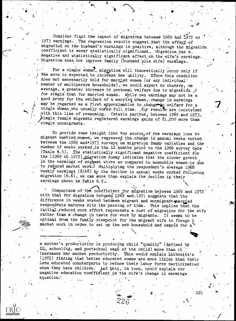
Consider first the impact of migratim between 1969 and15/72 on1973 earnings. The regression results suggest_that theeffe911.-ofmigration on the husband's earnings is positive, although the migrationcoefficient is never qtatistically significant. Migration has aonegative and statistically significant effect,on the wifes earnings.Migration does,not improve family. (hisband"plus wife) earnings.
For a single woman, migration will theoretically occur only ifthe move is, expected, to increase her utility. Si!nce this conditiondoes not necessarily hold for married women (or any individual'member of multiperson households), we would expect to observe, onaverage, a greater increase in personal-welfare due to migraiidn ,)for singlethan for married women. While own earnings may not be agood proxy for the welfare of a marriei wdman,change in earnings'may be regarded as a first approximation to chang* welfare for asingle 1;Oman.who usually woiks. fuil time. .Our results are consistentwith this line of reasoning. Ceteris paribus,' between 1969 and 1973/,ingle. female migrants registered earnings gains of $1,200 more than
single nonmigrants.
To provide- some insight into the source of the earnings loss tomigrant married;women, we, regressed the_change in annual weeks workedbetween the 1969 and01973 surveys on migration dumMy variables and the
0 number Of weeksworkedin the 12 months prior to the 1969 survey date(Table 6.5). The statistically significant negative coefficient forthe (1969 tb 1972) ration dummy indicates that the slower growthin the earnings of mig ant wives as compared to nonmobile womends dueto reduced market work; Multiplying the respondent's average 1968Weekly earnings ($148) by the decline in annual weeks worked' followingmigration (6.6), we can more than explain the.decline in theirearnings shown in Table C-,
.
' Comparison of the coefficient for migration between 1969 and 1972with that for Migration betwel 1969 an(1,1971 suggests that thedifference in weeks worked bet een migrant and nonmigrantimarried-retpondents narrows With.the passing of tithe. This implies that_theinitial .reduced work effort represents a cost of migration for the wiferather than a'change in taste, for Work by migrants. It seems to beoptimal from the family viewpoint for the migrant wife to foregomarket work in order,to set up the nevi household and search for
.
a mother's productivity in producing child "quality" (defined byIQ, schooling, and postschool wage-of the child) more than it'-increases her market productivity. This would explain Leibowitz!s
/(1972)'finding that better educated women-are more Ilkley than theirless,educated counterparts to reduce their labor force participationwhen they have children. d this, in turn, could explain ournegative education -coeffi lent in the wife's change in earningsequation -.' .
'4%
*
191
7
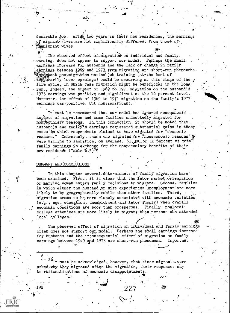
a
./
desirable job. Aftttwo years in their new residences, the earningsf migrantives.are riot significantly different from those of
igrant wives.
The observed effect of..nagrati on individual and family.earnings does not appear to support our model. Perhaps the smallearnings increase for husbands and the lack of change in family
.45Rings between 1969 and 1973, from migration are short-run phenomena.'aTCant postmigistion n-the Ljob training (ate-the Cost of
_,temppiarily lower earnings) could be occurring at this'stagg of the jlife cycle, in which case migration might be beneficial in the long,run., Indeed, the effect of 1969 to 1971 migration on the husband'S.1973 earnings was positive and.significantat the 10 percent level..Moreover, the effedt of 1969 to 1971 migration on the family's 1973earnings was-positive, but nonsignificant.
It must be remembered that our model has ipred noneconomicasp cts of migration and "some families undoubtedly migrated fornon cuniary reasons. In.this connection, it should be noted thathusbands and fami4;4s earnings registered substantial gains in thosecases'in which respondents claimed to have migrated for "economicreasons." Conversely, those who migrated for ."noneconomic reasons"S,were willing to sacrifice, on average, $1,p0(1.or 12 percent of totalfamily earnings in exchange for the nonpecuniary benefits of theirnew resideadt (Table .6,5)26
-1
SUMMARY AND: CONCLUSIONSa
In this chapter several - determinants of family-nigration havebeen examined. Fii.st, it is clear that the labor marketorier4a44onof married women enters family decisions to migTte. Second, familiesin which either the lrusband_or wife experiences unemployment-are morelikely to be geographically mobile than other families. Third,
migration seems to be more closely associated with economic variables,(e:g.z age, educalion, unemployment'and labor supply) when overalleconomic conditions are poor than prosperous. Finally, nonlocacollege attendees are more likely to migrate than.persons who attendedlocal colleges.
The observed effect of migration on i ividual and family earningsoften does not support our, model. Perhaps the small earnings increasefor husbands and the inconsequential effect of migration on familyearnings between-1969 and 1973 are short-run phenomena, Important
Oa
26It must be acknowledged, however, that since migrants..-were
asked -.why they migrated after-the migratiOn,their responses may
r.
be rationalizations of economic disappointments.
4-41227

in
4
s.
.4 on-the-job training takes place ati,this stage of the . life cycle, whichmay make migi.ation beneficial in the long run even when no short-runbenefits are evident. The earnings loss to migrant wives diminishesover time as their labor supply increases.
We observe significant differences in the effectof migration onthe earnings of single compared to married women. This chapter, webelieve, is the first doeUmentation of the earnings gain to unmarriedwomen who'riigrate: They gain $1,200 per year, more tAn nonmigrants,while migrant wives earn $500 per Yearless:thantheir nonmobilecounterparts;
1
tO
3.'93
O

4
a
REFERENCES,
'7 -4
B cker,,Gary. Human Capital; A Theoretical and EmpiricalAnalysral_','With Special Refere'nce to Education. 'NFtional Buieau_of Economic
Research. New York: Columbia UniversityPresi, 1964.-
Bowles, Samuel. "Migration as Inireatment: Empirical TessOf the ,
Human Investment Approach to Geographical Mobility." The Reviewof Economics and Statistics 52 (November 1970): 356-62.
P. 'DaVanzo, Julie. Why Families Move. U.S. Government Printing Office,1977.
Eldridge, Hope T. "A Cohort Approach to the Analysig of MigrationDifferentiELls." Demography 1 (1964): 212-19.- 1*
Flei er,* Belton M. "Mother's Biome Time and the Production of Childality." Demography 14 (May 1,977): 197-212.
Jerome, Harry. Migration and Business,Bureau. of Economid Research; 192
cles. New York: National -
-.0
Lansing, John.B. and Muellei% Evr: The Geographic Mobility of Labor.Ann Aibor: Institute for Social Research, 1967. 0
Leibowitz, Arleen S. Women%s,Allocetiou of Time'to Market*:andNonmarket Activities: lifferencep.by Education. Ph.D.dissertation, Columbia dpiiiersity, 1972.
, )
.'. .
......) .,LongLarry,H* "Women's Labor Force Participation and the Resideatial
,
it: . MobilitY/of Families:" Soqtal Forces 52 (March 1974): 34-2-45.
4,-.
I
Lowry, fi$i"1-
.Modei.kMigration and Metropolitan Growth: Two Anal"San Francisco: Chandler Publishing Company; 1966,
A. Mincer, Jacob. ly Migration Decision." -,linp'ublished mimeo,January 19 v
$'
Parsons, Donald O. "Quit Rates Ovei- Time: A Search and informationApproach." American Economic Review (June .1973): 390-401.
Sandell, Steven H. "The Economics, of'Family -Migration." In Dual'Careers, Vol,..TV. Columbuss. The Ohio StateUtEiNersity, Center
'' for Human Resource, Researchi.Decembere.1075-. ,
Schwartz, Aba, "Migration and Life Span.Earnings-in t-:U.S." Ph.D.dissertation, University of Chicgo;'',1968.,
.
.- ..e,. t, - .
A
'Shist.L.m. Joseph. -"Labor Mobility: Some' Institutional- Aspects." --,
Industrial'Relations Research Association Proceedings of Third. Annual Meeting (1950): 42-59..
1.914
229
,
Wii00.--
0

,
Theil, Henri. Principles of Econometrics. New York: John i4iley andSons, Inc.,1971. -
U.S.. Department of Labor, Manpower AaministratiOric UnemploymentLnsurance SerVice, Comparison of-State Unemployment InsuranceLaws, U.S. Government Printing Office,.1973.
, Employment and Training Administration.Employment and Training Report. of the President. Washington:U.S.. Government Printing OffiCe, 197E.
Wadycki, W.J. "Alternative Opportunities-and Interst.ute Migration:Some Additional Rasults." Review of Economics. and Statistics'56 (May 1974): 254-57.
7
4
195
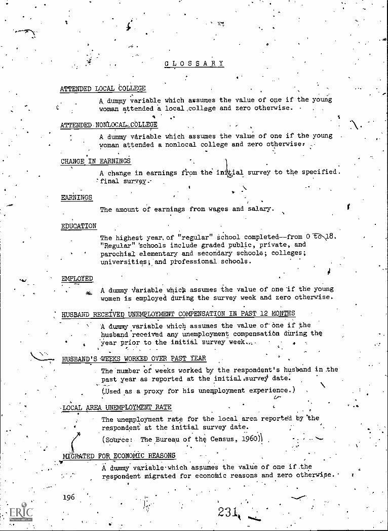
r GLOSSARY
ATTENDED LOCAL COLLEGE
dumpy variable which assumes the value of one if the youngwoman attended a local,college and zero otherwise.
ATTENDED-NONLOCAL,COLLEGE
A dummy variable which assumes the value of one if the youngwoman attended a nonlocal college and zero otherwise:
CHANGE IN EARNINGS
A change in earnings from the in'final surVe.-
EARNINGS
EDUCATION
EMPLOYED
al survey to the specified.
The amount of earnings from wages and salary.
The highest yearsof "regular" school completed- -from 0'51..q.8."Regular" 'schools include graded public, private, andparochial elementary and secondary schools; colleges;universities;and professional schools.
A dummy liariable.whicla assumes the value of oneif the youngwomen is employed during the survey week and zero otherwise.
HUSBAND RECE2VED UNEMPLOYMENT COMPENSATION IN PAST 12 MONTHS
A dummy variable which assumes the value of'ane if thehusband'received any unemployment compensation during theyear prior to the initial survey week..:.
HUSBAND'S MEEKS WORKED OVER PAST YEAR
The number of weeks worked by the respondent's husband in .the
past year as reported at the initialisurve3f date.
(Used as a proxy for his unemployment experience.)lr
LOCAL AREA UNEMPLOYMENT RATE
\
The unemployment rate for the local area reported by 'the
respondent at the initial survey date.4
.
(SOUrce! The Bureau of the Census, 1960)\
MIGRATED FOR ECONOMIC REASONS ...
A dummy variablewhich assumes the value of one if.therespondent migrated for economic reasons and zero otherwise. r
196
231

4
MIGRATED FOR NONECONOMIC REASONS
A dummy, variable which assumes'the value of one if therespondent migrate4fOr noneconomic reasons and zerootherwise.
MfGRATION
Dummy variablesIwhich assume the value'of one if thetherespondent migrated between,the ndicated surveys.,a6 zero
otherwise.
MULTIPLE MIGRANTS,1 0
A d fitt variable which assumes the value of one:if the---: re .ondent migrated more than once between'the indicate&
urveys and zero otherwise.
1RECEIVED UNEMPLOYMENT COMPENSATION IN PAST 12 MONTHS
A dummy variable which assumes the valge of one if theyoung woman received any unemployment compensation during-the year prior to the initial survey date and zero otherwise.
TENURE
A measure (in months) of the young woman's length of servfCeon thejob reported during the survey week.
UNEMPLOYED - 41.
A dummy variable which assumeg*the value Oeone-if the Qe
young woman was unemployed at the initial survey date.andzero otherwise.-
1PEEKS WORKED -OVER THE PAST YEAR
The number of weeks worked by the young woman in the pastyear as reported at the initial survey date.
O
232197-
k
.41

O
Table 64.1 The Likelihood 'of Family Migration between 1968 and 197: LogitResultsa,b°
. .
.
Independent variablesc. ,i-,-,
Equation (1)
_
Equ'atid t..) Equation (3)
Coeff. 4(t-value) Coeff. (t.:V.41' Coeff: (t- value)
,Employed, 1968 sUrvey.date
,1967,weeks worked
Tenure, 1968 (in6*months).
Unemployed, 1968
Received unemploymentcompensation in past12 months °
Attended norh:ocalcollege 4
Attended local college
Husband receivedunemployment .
compensation in past, 12 months
Vusband's 1967 weeksworked
,-,i,
, Husband's education-
Husband's age '
Local area -'
unemployment'rate
Constant '
.
.
',....0.4N
0.069
-1.059
;0.651
0.210.
.
0.129
.
-9.of8
i0.070
0.024
-0.003
-1.431
(-1.90)**
( 0.15),
( 1.4o)*
( 1.89)**
( 0.42)
( 0.26)
4
(-1.58)*
.( 1.55)*..
( 0.81)
( '-0.39)
-1.41}*
-
-0.013
0.095
-
-0.982
0.7'20:T.2.07)**
0.263'
. .
0.090
-6.018
0.074
0.025
-
-0.904
-1.36
(-2.50)***
,
( 0.21)
( -1.28)
i.-
. ,
( 0.53)-
.
.
( 0.18)
'41/4;1.62)* '
.( i.62)*
( 0.86)
(-0.60)
(=-1.33)*
t
,
-0.024
0.044
-0.965
0.637
0.177.
.
0.238
-0.015
0.075,
0.034
-0.003
-1.860
s
,
(--3.09)****
( 0.10)
.
(-1.25)
Alk( 1.82)4*.
( 0.35)
( o.48)-
(-1..34)*
( 1.63)%.
.
( 1,16) .
.
(-0.41)
(-1.80)4*
Pseudo R2d
Chi-square °
Number' of respondents
. . 4'0.052 .
.19.00***
; 528
0.060
21.88***
528 *
0.076.
, 27.77***
528
-
Universe: White married respondents, .same spouse present, neither respondentnor tiubband.in school, between 1968 and 1973. Husbands not in the military'
,.' , ' service. Husbands over age 25 were not askedlin the surveys if they were
. enrolled in school., Thus, there may be some husbands over age 25 enrolled inschool in the sample. . .
. Dependent variable: a dummy variable'With the value "1" if the respondent'reported that her SMSA or county oVresidence in 1968 differs from her.residencein 1969, -1970, 1971, 1972 or 1973,."0" otherwise. ,
b- All logit equations baseAn unweighted data.c All variables are defined in the Glossary. See Appendii Table 6A.3 ?or summary
statistics. f
°d PseUdo R2.F [1 - exp (Z(Lw . Lr)/T))/41 - exp (Z(Lw Lmax)/111 where Lw is. the .
. , maximum,of the log of the.likelihood function using a constant, Lr is the maxitum
.
_using all variables and Lmax is themaxlmum possible.
Significant at the 10 Rercent4141, Siglificant at the 5 percentlevel.
. ***' Signiffbant at the 1perCent
19ft
7,
2 33,
4

t
TOole 6A.2 - The d of Family Migration between 1968 and1970 and between1971 and 1973: togit Resultsa,b
_
.
Inde ndent vhriablesc1968-1970
.
1971-1973
,
,
(t-value) Coefficient (t-value
Wife employe'dd
Unempi'.byedd . .
Received unemploymentcoMpensation_in past,
I, 12,monthge '
Attended nonlocal college,
Attended local college,,-
Husband's weeks workedoverpast year
'''
ridiusband received
unemployment compensationin past 12 monthse
Husband's education
Husband's age
Local area unemploymentr
Constant'
0.032
0.487
.
-1.449
0.820
-0.021
-0.021
-0.422
0.001
0.011
-0.003
-D.914
, ( 0.14)
( 1.12)
.
(-1.40)*
(- 2.39)***
(-0.04)
(-1.92)**
.
(-0.75)
(.0.02)
( 0.40)
(-0.38)
(=0.91) '
.
'-0.766
-
0.058
0.968
-1.19
0.511
-0:306
-0.029
0.126 -
-0.0.24
0.006
-1.614
.
( 0.23)
( 2.1T)**
(-1.51)*
( 1.24)
(-0.62):
(-2078)***
(-1.594*
( 2.036**
(-0.56)
.( 0.92)
(=1.16)
.
Pseudo R2f
Chi-square ,
Number of respondents
. 0.042
16.30*** .
65
.1.
.
0.087
28.52***
534
a ;Universe: The universe for the 1968 to 1970 sample consists of young wives (age 17 to24) w ose spouses were present and of in the military service in all survey years (1968to 704. Husbands over age 25 -re not asked in the surveys if they,were enrolled-insch ol. Thus, there may be soil husbands over age 25 enrolled in school in the sample.In addition, both htisband wife may not be enrolled in school at any survey date (1968to 1970). Th4 1971 to 1973 universe is similarly defined for the 1971 to 1973-period.Dependent variables: For the 1968 to 1970 sample", the dependegt variable equals "1" ifthe reLpondent reports that her 1966 SMSA or county of residence lifters, from her 1969or 1970 residence. The dependent variable for the 1971-1973 period is similarly defined.
b All logit_equations,based on unweighted data.,c All vafiables are defined in.tht Glossary. See Appendix Table 6A.3 for summary
statistics.d The variables refer.to the 1968 (1971) survey date for the 196873!1970 (1971 to
1973) sample.e Over the 12 month period priorcto the 1968 (1971) survey Ltd for the 19681-1970 .
(1971-1973) tilde 'span.
f Pseitdo R2 = [1 -AZ10 {Z(Lw Li.)/T}] /E1 = exp {Z(Lw '\EMax)/T)] where Lw is the maximum v.
of the log-of the likelihood function using a cOnstanr is the Maximuh using all
variables and-Latucis the maximum possible.
Significant at the 10 percent level.Significant at the 5 percent level.Significant at the 1 percent level:
J.-
*
* * *
;
234. 149

°Table 6A.3 Summary Statistics for Determinants of Family Migration Equations(Appendix Tables 6A.1 and 6A.2)
-
-
Valiablesa-
1968-19'3 sample'
1968-1970sample
(
1971-10-frS...,,
`sample- Nonmigrants Migrants
MeanStandard
deviatiOn Mean
.
, Standarddeviation Mean
Standard,deviation Mean
Standarddeviation
Employed
Weeks workedb
Tenure (in months). ,Ithemihoyed
Received.unemploymentcompensationb
Attended nonlocalcollege
Attended localcollege
)Respondent's incomeb
Husbandusband receivedunemploymentcpmpensationb
Husband's weeks.workedb. '' . .
401a.Husband's education
.
Husband's age
/ Husband's incOM
Local area 1
unemployment rate
Migration rate,
(dependent variable)
rNumber of respondents,
:,424
21.6
10.8
:06--
.04
.09
.04
1590
,
.04',-i.
49.3
11.7
25.1
5606
3.8
.
386
'
.49 -
21.8
20.0
.23
.20
.28 .
.21
2213
.21
7.8
24
3.6
478
,.15
,
.38
18.7
6.6
.06'
.03
.17
.0c,
1282
_04
47.9
12.3
25.4
)5572
.
3.9
142
%
°
,.49
20.0
15.5'
.24 -
.18
.37
.22 .
2Q47
:21 .
9.5
3.1
.83183
.15
.41
20:8
9.4
.o6
.04
do
.05
.05
48.4
11.6
25.1
.9
.16
1`650
.49
21.4
18.9
-.23'
.18
.29
.22
.2a
8.8
2.6
3-.9
.16
.37
.41
21.3
10.4
.0.6
.05
.09
.07
--wre-0
46.9
12.0
24.3
6.3
.17
534
f
.
.-49
21.9
53.3
.24 -
.22
.28
.26
.29
10.3'
2.3
3.0
..19 ,
-.38 ,I,
a' The variables refer to the 1968(1971) survey date forhe1968-1973 agd 1968 -1970 (1971-
1973) samples.,] All variables are defined in the Glossary.b Over the twelv,smonth period prior to the 1968 (1971) survey, date for the 1968-197Q and
1968 -1973 -(1971 -1973) time spans.
200
"la
yr-
Ilk
4

4
.
'Table 6A4 Pet.centage Whose Postcollege.ReSidence Is Different from High School Residence,by Residence at Age 14',.College-Location and Marital Statusa
,
Ire
Residence at age14 and collegelocationb
.
-
'
.
Number of'respondents
-
Percentage with different high school, ..
and-postcollege residences.
'%
.,
2 years after° college
.
In 1968d.
,
,
.
.-
Married
./Never
married
.-. .
MariedNevermarried
r'All areas,. '
LocalNonlocal uii
Rural, town, city .
under 25,000LocalNOnlocal
City over 25,000Local
Nonlocal.
.
w,
223414
.
-76
-250
:
147
164
.
.
19
37
14
' 36 ;6
,.
21
39 v
922 '
.
6'
.
30 ..y.1(2
16 .
. 11,
.
29
68
39,
791
4:
23 .
619
1644'
3345 i
. ,
943
- ,,
4-
- .
,a Universe consists ofwhite respondents who. attended oollege. Based on unweighted data.-b Relative to parentst,resj.dence-,c7.,Refersto women,who last'attended college bktween 1968-and 1971.'d Refers-to women wild last-a.ftefided 662:lege:before 1968.4
ti
36
I
10,10.
,
23'?
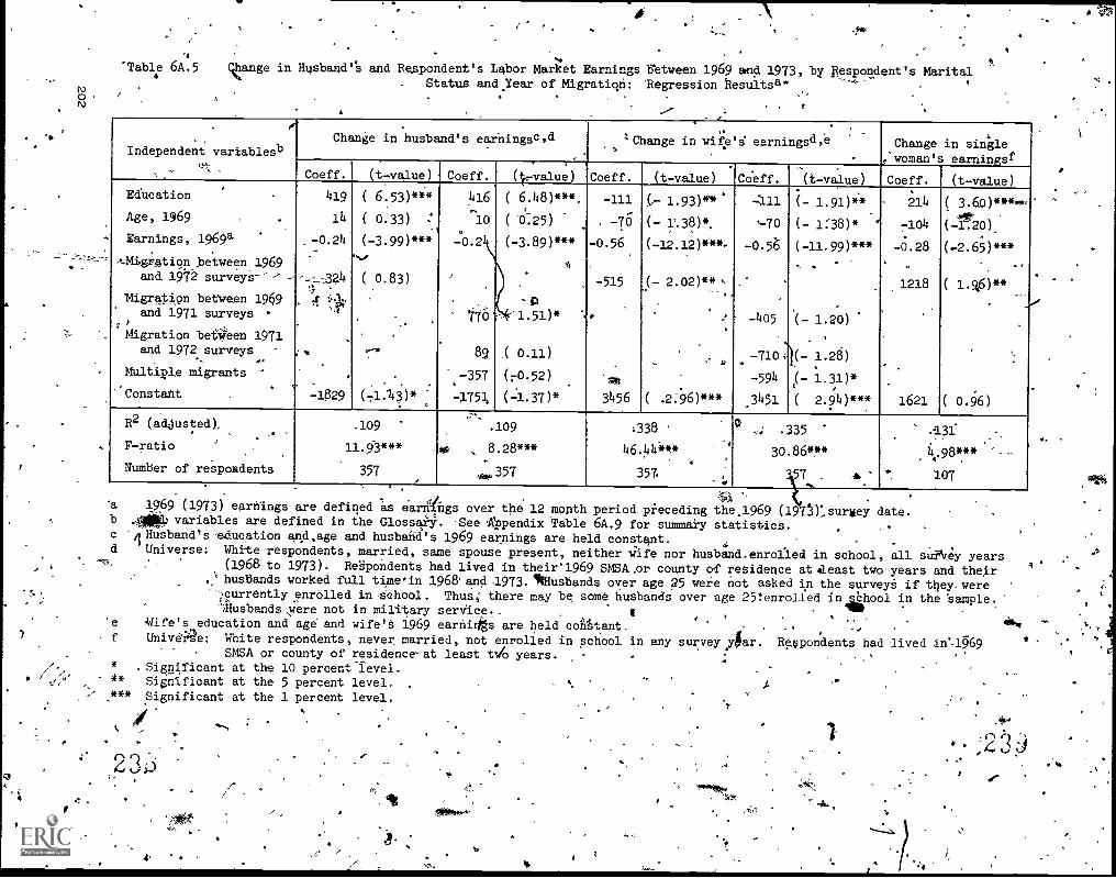
Lzy
4
V I1
-,
t'Table 6A.5 Change in Husband's and Respondent's Labor Market Earnings between 1969 and 1973, by Respondent's Marital- Status and Year of Migratiqn: 'Regression h aesults"
4r
N .".Cr ' ' ,eJIndependent variablesb
,.!:,
Change in husband's earningsc.d 'Change in wife's' earnings,,A ,e0 Change
, woman's
0in singleearningsf
(t-value)Coeff.
.
(t-value) Coeff..
(trvalue) Coeff. (t-value) Coeff. (t-value) Coeff.Education
Age, 1969 - -
Earnings, 1969a
.ALMIgratign between 1969
and 1972 survey-a-'-' -----.:_,324
Migration between 1969and 1971 surveys ,
'
Migration befWeen 1971and 1972 surveys
od.
Multiple migrants
"Constaht
419
14
.-0.24
..).
4 .::*
iv
,
-1829
( 6.53) * **
( 0.33) :1
(-3.99)***',..,
( 0.83)
-
.
e,71,
(71:43)*
416
10
-0.2
_
176",
89
-357
-1.75?
( 6.48)***.
( 0.25)
(-3.89)***
A
-0'1.51)* %
1 0.11)
(70.52)
(-1-37)*
-111
. -76
-0.56
-515
.
.
sit
3456
(- 1.93)0*'
(- 1%.383*
(-12.12)***-
(- 2.02)**
.
.
( .2:96)***
7.11
'-70
-0.56
-405
-7104)(-
-594
3451
(- 1.91)**
(- 1:38)* '
(-11.99)***
..
(- 1.20)
1.28)
(- 1.31)*,
( 2.91) ***
214
7104
-0.28
1218
.
1621
( 3.60)*****'
(-120):
(-2.65) ***
( 1.96) **__
.
,
( 0.96)
R2 (adjusted),,
)F-ratio .
Number of respondents
.109
11.9-3***
357
.109
8.28***.
357
:338f
46.44***.
357
0 4 .335
30.86***
357 4. 2
A3f
4.98 * ** .
' 107
'a 1969 (1973) earnings are defined as earn ngs over the 12 month period .preceding the.1969 (1 sMsuriley date.,51 '
b .401* variables are defined in the Glossary. See Appendix Table 6A.9 for summary statistics.0 ,.
c A Husband's -education and.age and husband's 1969 earnings are held constant..,:
.
d Universe: White respondents, married, same spouse present, neither wife nor husband.enrolled in school, all survey years(1968 to 1973). Rebpondents had lived in their'1969 SMSA,or county of residence ataeast two years and their
..' husbands worked full time'in 1968'and -1973.14Husbands over age 25 were not asked in the survey6 if they. were"',currently enrolled in school. Thus; there may be some husbands over age 25:enrolled in chool in the 'sample.":Husbands ,were not in military service..
. 477, .'e afe's education and age and wife's 1969 earnirgs are held constant.
.-., .., ,
f Universe: White respondents, never married, not enrolled in school in any survey,y0ar. Respondents had lived in%1969SMSA or county of residence=at least t/o years.
_...
* . Significant at the 10 percent level.4* Significant at the 5 percent level. % 1*** Significant at the 1 percent level.
k
23.)
ti
'

Table 6A.6 Change in Family Earnings 1969 to 1973, by Year of Migration on Husband's and Wife's,`Variables: Regresion Resultsa,b' e
.\
i
..c.Independent variables:
.
Husbands variables .
1 .
Wife's variables
Coeff. (t-valub) Coeff,.' (t-value) Coeff. (3- value) Coeff. (t-value)
Education
Age, 1969
Earnings, 1969a
Migration between,I969and 1972 surveys
Migrationipetween 1969and 19.71 surveys .,
Migration between 1971and 1972 surveys
Multiple Migrants
Constant
342
.78
-0.41
-106
.
-915
( 4.71),**
(' 1.71)
(-7.53)***
(-0.5)
(-0.64)
335
73?
.
.-0.41
.
413
-308
.-935
-812
r..
,.V6
10.35***
( 4.61)***
( 1.61)
(-7.30***
( 0.72).
-0.33)
(-1.23)
(-0.57)
357
.
,
-24
"118
-0.37
'66
.4.
.
-808 4(-0.40)
'4.101...,
...11.03***
( 2.40***
'( 1.35)
(-6.63)***
.
( 0.15)
..
,
'. .
57
237
113
'-0.36
...
629
.
-125
-870
-lido
, .103
' 7.80***-
357
( 2.34)***
( 1.29)
(-6.42)***
.
( 1.09)
. ,
(-0.13)
(-1.12)
(-0.35)
R2 (Cadjusted)
F-ratio
Number of reartndents... ,
.136
14.97***
351---.
. =
.,.
.
. a' 1969 (1973) earrings are 4efift'd as earnings over the 12-month period preceding the 1969 (1971) survedate.
. ..
'. ,
. .1) Universe: White respondents, Married, same spouse present, neither wife nor husband enrolled in school,all survey years (1968 to '1973). Redpondents had lived in their 1969 Sg64 or county 9f.',". ","
., residence least two years and theirhusbands worked( fulltimel.n1968 to 1913 Husbands ..over age 25 were not asked in the surveys iethey were currently enrolled in school. Thus,there may be some husbands ove'age 25 enrolled in school in the sample. Husbands were not inmilitary service.
c All variables are defined in the Glossary. See Appendix Table 6A.9 for summary statistics.*** Significant at the 1 percent level.
240IN)0w
rfaa''
Or
r IV
2414

O Tab1efl6A.7 Change in Husband's, Wife's and Family's Earnings, by Reason for Migration: Regression
Resultsa,b -
Independent variablesc
Change inhusband s earnings
t '-,,
Change inwife's earnings
,
Change in family earnings, ' -
Coeff. (t-value) Coeff. (t-value). Coeff.d (t-value Coeff.e (t-value)
Education..
Age, 1969 :,
Earnings, 1969a .
Migrated for economic.. reasons
,
Migrated for
. noneconomic reasons
Constant.
407..,
, 19
-0.24
1064
-35--1836
(-6.33)***
( 0.46)
(-3.94)***
( 1.85)**
-
(-0.77). .
(-1.4)*
-115
-66
-0.55
-367,
-552
3424
= 1.99)4**
(- 1.30)
(-12.00)***
4(- 0.96)
(-1.80)**
( 2.92)***
323
84
-0:40
971 .(_
-1008-
916
( 4.44)***
( 1:1301*
(-7-.35)4**:
1.51)*-
(-1.97)**
( -0.65)
214
158
-0,36
-
1409
-1049:
-1377
( 2.13)**
( 1.79)".
( 6.54)**
( 2.17)**
(-2.o1)**
00.69)
R2 (adjusted)
F-ratio -
Number if respondents
.115 ft-
10.23***
? 357
-
..337 ....
f .37.18***
357 .
.147 '4,
13.28***.
' 357
419
.10.61*!*
. .
357 :'
a
4earnings are,defined as earnings over the 12 month period preceding the 1969 (1973)1969 (1973)
Survey dateb Universe:
c
d
e**** * *
'--- :.
- ... ;. ._;.:...--.
White respondents, married, same spouse. present; neither wife nor husband enrolled in
school,all survey yiars (1968 to 197). Respondents had li
county of residence at least, two years and their hu;bands wo
1973. Husbands over Age 26 were not asked in the surveys ifin school: Thus, there may be-some husbands over age 25 enro
"6k sample. Husbands were not in the military.All variables are defined in the GloSsark.; See Appendix Table 6A.9 forIndependent variables refer to husband's education, age, -and earnings.Itdependent variables refer to wife's education, age, and earnings;Signifita4/at the 10 percent level- ' qt ',...r4
ed in thei:r 1969 SMSA' or,
ed_full time in l98 andey were currently enrolled-
-
ed in'school in the
Significarit at the 5 percent level.SignifIcant/at the 1 percent ,level.
a
summary statislics.1
24.E
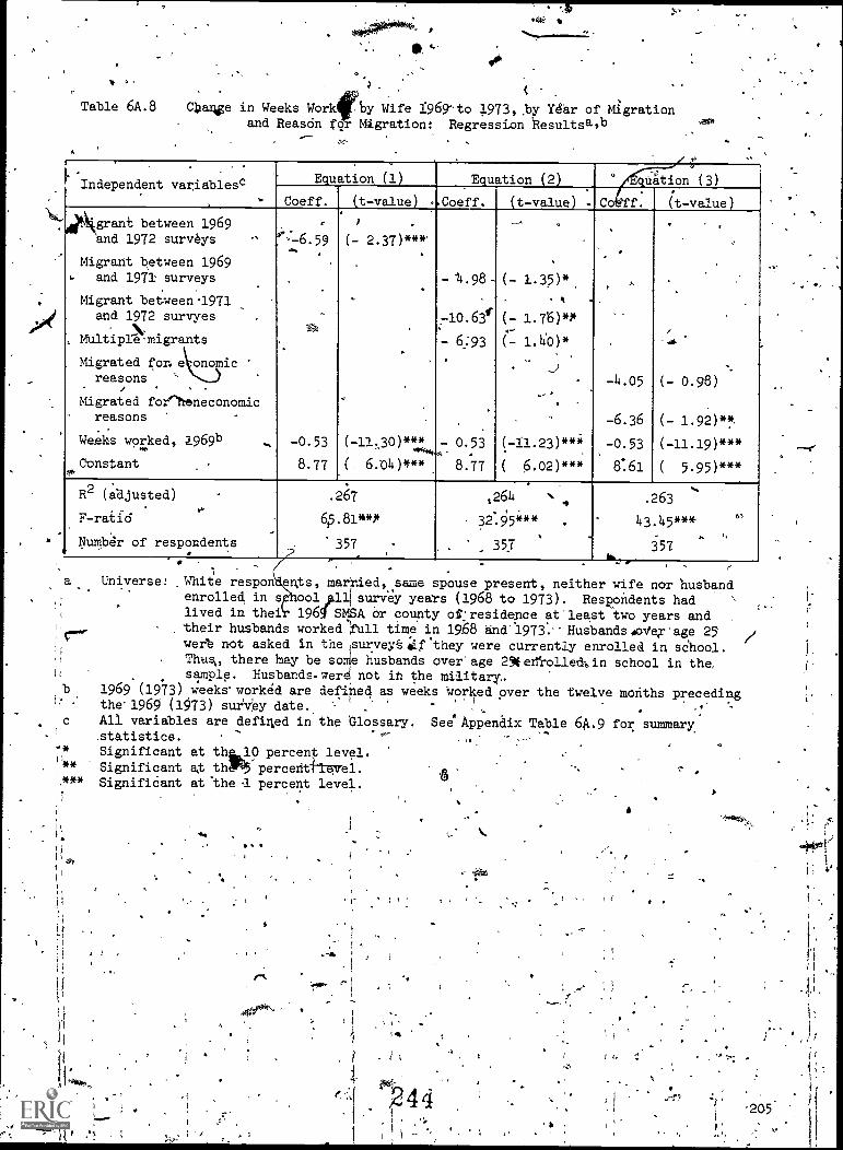
00
W
Table 6A.8 4anee in Weeks Work by Wife i969-to 1973, by Ydar of Migrationand Reason for Migration: Regression liesultsa,b
Independent varisblesc
-
Equation (1) Equation (2) ° qUation
.
(3)
Coeff. (t-value) ..Coeff. (t-value) - Co'ff. (t-value)
dOgkgrant between 1969and 1972 surveys -
Migrant between 19691.. and 1971 surveys
Migrant between 1971.and 1972 survyes
MUltiple'k. migrants
Mig rated for. e ono is
reasons .
Migrated foe^heneconomicreasons. -
Weeks worked, 19169b ,-.0
Constant.
.
1*-
-,
-;--6.59
,
.
.
-0.53
8.77
P .
(- 2.37)**4'
.
.
-
(-11.,30)***4,4,4.
(, 6:010***
- '14.98-
-10.63(
- 6.93
- 0.53
8.77
.- .
.
(- 1.32)*
. i ..
(- 1.76)*P
(- 1.4'0)*.-
...)
-
. -
(-11.23)**4
( 6.02)***
.
, ,-
.
-4.05
-6.36
-0.53
8:61
.
.
.
.
-s
.. .
(- 0.98)
.
(- 1.92)*!.
(-11.19)***
( 5.95)***
R2 (adjusted)
F-ratio4,-
Number of respondents
.26T
6,5.81**0
357 .
7
,264
32.05*** .
35
.263
43.45***bt
357J.-
rs
'.
.
Universe: White respon eats, married, same spouse present, neither wife nor husbandenrolled in s oolp, survey years (1968 to 1973). Respondents hadlived in thei 1961 SMSA Or county of'residence at'least two years andtheir husbands workeefull time in 19.68 and-1973. Husbands4oVerage 25were not asked in thelsurveyS44f'they were currently enrolled in school.Thus there May be sole husbands over age 251leel-olledi,in school in the,sample. Husbands-were not in the military.
1969 (1973) weeks'worked are defined as weeks worked over the twelve months preceding. - ; .the'1969 (1973) survey date. -- . . 4
..
All variables are defined in the Glossary. See Appendix Table 6A.9 for summary-.statistics.
.*Significant at th 10 percent level.
'** Significant at thgN5 percent-flvel.*** SignifiCant at'thel percent level.
1 1 '
244 -205'
4*
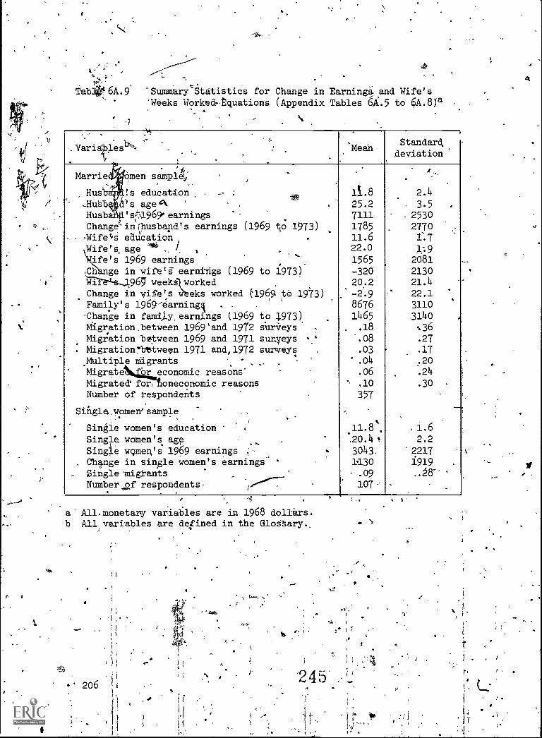
-..
o 4
Tab44 6A.9 'Summary` Statistics for Change in Earnin0and Wife's'Weeks WorkedEquations (Appendix Tables 6A.5 to 6A.8)a
\,..-:
4 1,
1-- ''
.Vari 1 s'-`. -
.
.
.
.
Meah.
Standard
deviation,
.' t .Marrialumen sampl6; .
..
Husb.li:s education...HuSb. a's ageA . .
Husb-4 iy s,19690 earnings
Changeinchusband's earnings (1969 tp 1973)- Wifet,s eaucation,
Wife's. age ."* , I. .
fife's 1969 earningsI
Ch ge in wife's' earnings (1969 to 1973)171-11-e-s-4969' weekitworked
Change in wife's Weeks worked (1969 to 1973)Family's 1969 9-arningi . . .
Change in family, earnings (1969 to 1973)Migration.between 1969'and 19/2 siiiieys. .
Migration between 1969 and 1971 sumyeys ,_4
. Migration'tttween 1971 and,1972 surveys ,
_Multiple migrants , .
-.
' MigrateS4g4economic reasons. .
Migrate& for, toneconomic reasonsNumber of respondents
Siiigle women'sample .,. - ., .
Single women's education .
Single women's age .,Single womeg's 1969 earnings .;-,
'. ChElmge in single women's earnings
- Single 'migrantsNumber of respondents-
1
11.8
25.27111178511.622.0
1565-32020.2
.- -2.9
86761465
, .18
.08.03
.014
.06
-. .10
357
.
A
.11.8,20.4 t
3043,1130.09
107
.
.
A
2.4
3.5- 2530
27701-.7
1.92081
213021.4
-' 22.1
3110
3140%36
.27
.17
.20.24
.30
,
.
.1.62.2
'22171919..M-
..
.
.
. .
a Allmonetary variables are in 1968 dollars.b All variables are defined in the Glossary..
i
f
'h I..
' 206 ii) A
r, .,
ui r;
)
1
J'1tiI . 1 ,...,
2 4
I-
tis
'INTRODUCTION.
CHAPTER 7
MARITAL DISRUPTION: CAUSES AND CONSEQUENCES-,,.I.-
Frank L. Mott and SylviaT. Moore*.
'4e
....
.-.In this volume, we have already highlighted'a number of phenomenawhich reflect in major ways thp`changing status of women in Americansociety. We have repeatedly demonstrated the increasing °work
-commitment of women. It is clear that, for the young.adultwomen,work is and will continue to be not an alternative to family and child,raising but a complementary and(essential component of contemporaryfamily life styles.
Paralleling many fundamental changes in our Society, theincreasing work activity of women in some instances has perhaps beenboth a determinant,and consequence of other,social,pbenomena. The6process of marital disruption is a case inpoint. The ability tofind remunerativeremployment can certainly facilitate and perhapsincrease the likelihood of a marital breakdown flr some women. Thiswork, or the potential of finding work, may play the dual role of Iaffecting the probability of marital breakdown and of ameolioratingthe economic traumas assdciat
rd with the breakdown a%pr it occurs. -
The major objective of:this chapter isto,examine the association:between work and this marit4..clisruption process. Of course, thislassociation cannot be analy4eCin a vacuum. Thus; in examining thdeterminants of the marital disruption process,a wide 'range ofOther factors 1411 be considered; when the. consequences of a marit
.
brealtdown are analyzed, labor( market activity will bejuxtaposedagainst the needs of different subsets of *omen. Obviously, workis only one way of compensating for. th 'loss of the husband's earningsand'needs to be considered in conWpakT66Willt"71.ccesg to other inc e. .
sources.#'....r-
.
.
Recent years have witnessed a spirallingorthe inci eve of' .
marital' breakdown from what had been, historically, rathe loi and-stable levels. During the periOtbetween 1900 and 190,,t e divOrde-.-
rate.,..)rose froth 0.7 to .25 peii. 1,000 population.1 However, duringi 1 k I t 1 - t
... - -,
*1. 1 44-* '''
- -
'- The aut rs wish to thank Dennis Grey p:a. hts .outstanding,f ...
retear6b assist ce in proiucing this chapter.i
').,'
i )
lateriS 41973).1
.
;
. #
\ .
1
; ...- . I,
.
246
I
,.,it
1 7
,
I
I
.the following ten -year ,period the rate, virtuallY doubled froq 2.5 to
4.9 per thousand Population.2
-Perhaps the most'dramatic changes inmarital'disruption patterns
4 - are 'occurring at the present time. There has" been a dramatic increase
in the priportion of marriages estimated to end in divorce among
successive generations of-contemporary women. The Census Bureau'
estimates that about one-third of the marriages of youngwomen now
between.the ages of'25 and-34 Will ultimately end in divorCe as
compared with about, 20 percent four those who are presently in their
fifties.3 Indeed, during the short five-year period between 1968 and
1973, fully 14 percent of the ;tarried young women (12 percent of -die
white and 30 percent of the black women) in our nationally representa-
tive-gLS sample had their marriages end eit permanently through a
divorce or at least temporaril- through a sep at n. To the extent
. that these new higher levels of marital disrup ion ay at least
partially represent a break with traditional.disruption patterns,
this study may provide .useful baseline data for interpreting several
socioeconomic dimensions of contemporary earital trends. -
It evident that marital disruption is no longer a relatively
rare phenomenon but, in reality, either affects or Will affect a
considerable proportion of women whoare currently young adults. AS /
such, there is a need for a clear definition ofpublic policies with
respect to income maintenance and employient .asSistance for this L '
substantial group -of women. However, the effedtive'determinatidoon hand
implement ifionof.any social policy requires inTbrtation input,
includin analytical evidence concerning the.SOciodeMographic makeup
of the p ogram group as Well as quantitative indications of its :
economic status. A principal objective of this chapter, is to prove
some of his essential input.,ASome Data and Andireical Constraints
Our sample of maritally disrupting women includes all, women who
separat6 or divorce for the-first time between 1968 and 1973 4
2U.S. bepartment of Health,-Education end Welfare <19775.
3U.S. Bureau of theCensus (1976):
5
r-
4There are 520. women whq can be identified as having had a first,
marital disrUption at some time during the five-year'perioax All of :f
these women were either already married in 1968 or marregeat:sometime 1'
!after that point bitbefore the 1973 interview/(see Appendix A foi
details concerning the "eligible for disruption" population).' Of:these ;
520, 38 are excluded from:the analysislaecause:they moved' from a1
"never married" status intone survey'to a "disrupted" status in theI
I . 1,
208

Since the precise date of separation cannot be determined for mostwomen, the "before".and "after" Status will refer to the nearestinterview date before and after the Marital disruption. Throughoutthis Atudy "T" will reference the last interview before the disruption,"T +1," the first interview afterthe event; and "T - 1" and "T + 2, ".the immediately earlier and later interview dates.
In order to compare the 'characteristiCs of individuals in oursample whose marriages diArupted with a comparable group whosemarriages -mai intact, a "reference group" representing "nohdisrup-ting counterparts" to those whose m rriages broke down) wasconstructed. In the most general terms, a woman was included in thereference group if she was in her first marriage. at some point between1968 and.1973 and the marriage'did not break up during that period.5
In order to maximize our sample size we are examining thedeterminants and conse uenes of marital rather than the
!le
\next, and no information exists with respect to the characteristicsof their husbands. An additional 38 cases are excluded because therespondents were enrolled in-.school at the last survey date prior totheir maritaledisruption, which makes.infomation bn their, predisrup-"tion labor mket activity and earnings less meaningful. Thus, thesample of disrUptee'S.used in the analysiS 'limbers 449 (264 whites and185 blacks).
It sh5uld be noted that women whOse marital status was "separated"or "divorced" at the time off the first interview are excluded from theanalysis,. Since we cannot specify when the disruption occurred or. the.characteristics of the women and her family in the4pileditruption
`period.
There are two type.l.pf cases that, prevent the criteria forinclusion in our sampleof disruptees from being applied with cOmplite
.precision. First, w en ,who separate and return to the same husbandbetween two,survey ates cannot be identified.' Second, if a woman ex-.-petienced a mari 'disruption prior to the 1968 interview but was once'again.in a "married-husband-present" status As of 1968, she would notbe identifiable as a disruptee, To the extent that-either of thesecases exist_, the women in question are classified among thenondisruptdes.
5Since4any, women were eligible to be ,in the reference group at'more than.one survey date, the eligible respondents were randomly dis-tributeCracross survey years:in the same proportions as the disruptees .
were distributed. Further adinAtments were made in the reference grclupconsistent with the adjustmint:made in the diSruptee populationwhichexcluded women who were never married at T but disrupted).2y T.W 1. SOAppendix A for details.
4i-2 43
209
c

4separate divorce or separatiori components. We feel that this isjustified in most instances, as the short -term social and economicconsequences of both events-are similar, since in both cases the
husband is absent fromeand no longer a.member of the household. In
the short run the determinants of marital breakdown should also besimilar,,regardless.of whether the, process result's in aAquick-divorceor a More lingering separation process.
Given the nature of our sample, the perspective of this paperwill he from the female side. That is, we will focus on why a-woman ,separates from or is divorced from her husband and what the post-.
disruption consequences are Xbr heT and those living with her.Clearly,,the husband's perspective might be quite different both interms of the determinants and consequences of the marital disruption.While to some extent certain mirror images are implied, symMetry inall instances 1.s hot suggested.
`Finally, the nature of the data limit's and perhaps biases'thefocus,of our research,-particularly Iiith regard to the interpretatibn
of the-determinant kand consequences of the marital disruption. We .
are essentially measuring in a discreCe,way a process that is, in
reality continuous. Thus, kor example,.the factors that we find tobe significant "deteAlinants" of.marital disruption may well reflectprecipitating events it disrUptIon proceet ratger.thencauses of disruption.. As such, we are recording overt manifestations
of a much more subtle procss._1
THE WITAL DISRUPTION PRObESS
As- a mechanism for unjIerstanding better the. socioeconomic position
! of women from broken marriages, trhis,section will examine some of thef
suggested moti-17es.for marital disruption. _Subject to the constraints1
and limitations-of our data set, we will test some of the traditionalas well. as more recent theoretical statements found in both the econom-ic and-sociological literasbure concerning the likelihood of marital-disruption aMOng.women, Aour sample reiesents a cross-section ofyoung adult Women, our,reallts may be more broadly applicable andgeneralizable than those of other .studies based on more liMited samples.
A. . , -t. ':-..
The literature which focuses in the determihants of marital
li disruption has expanded greatly-in recent years and has become ,
increasingly', interdisciplzfrary-in nature,. From the sociological per-spective, they effects of baclgEround factors such as the socioeconomic
,..,-7.
.status, education, afrid. marital stability of parents in .the promotion'of
' marital stabilfty'of their; children have been explored in some' depth.6-
4 ,
1,.
I t' ,
6See, f r example, Carter and" Glick (.19y0), Bumpass a2a Sweet1
1975), and Utright (1971$ for discUSsions
1
concerning the separate and1
1,
interacting ,ffectsof social status and education, and"Pope'and
; 216'1
i
c '
.c., '249. l'i:1-
1) i 1

-in general; studies have found inverse associations between theprobability of marital disruption and background socioeconomic statusvariables and educational attainment. There is also some suggestionof aitransmission of intergenerational marital stability, as somestudies indicate that children of broken marriages are more likely tohave their own marriages dissolve.
Demographers have noted that,,in general,, marriages undertaken atyouthful ages,'particularlY those burdened bypremaritally conceived
o children, tend to have less chance of success.7 On the other hand,.economists or those working'primarily. with economic variables have mostrecently been focusing on the various economic motivations for maritalbreakdown. These include such factbrs as the absolute level of thefamily's inCcimerior to the marital disruption, the relative positionof the family is compared with peers and the level of the woman'searnings preceding the disruption event.8
It is apparent that many of the factors which traditionally havebeen' considered by researchers from different disciplines in realityoverlap'in the sense of being interdependent in origin and interactivein their effects on marital breakdown and its consequences. Indeed, aprincipal objective of the multivariate perspective of this researchis to suggest which of a myriad of baagro fac-Obrs may be the trulysignificant determinant's of the disruption up cess. ot.
Because the major purposeof this' stUdy. is to examine therelevance ofwork activity and concomitant economic factors in thedisruption process,.we will concentrate more extensively on thebackground.factot explOred in the economics, literature. We will*ttempt to distinguish those economic factors with are felt tocontripte'to marital disintegration from those economic factors .
hypothesized to "cement" 4 marriage' Ross and Sawhill term these.,forces "indePendence" and "income" effects.9 From an economicperspettive; factors which would promotea feeling,of economicindependence ih a woman; such as high wage employment Or access .fo
'unearned income independent of her husband, might, everything elsebeing equal, provide.encouragement fora woman to leave a marriage
lom-,
In contrast, factors which encourage A wife's dependence on herhusband, such as his high earnings or substantial personal unearned llit
income; are "income effects" which would normally beassoc ted withberow average probabilities of,marital breakdoWn.
,
v
Mueller} (1975) for b.. review of the literature on intergeNrationalinstability.
1
)
7See, for example, 'Wickland Norton ',(1971) and FurStenberg kl976).41-
8See, for example, ',Outright .(1971); Becker ,et al. (1976), pp. 31-; and. Ross and Sawhill (1975).
, X('9Ross and Sawhill (1975): i

.
In addition to.these absolute income and earnings conce\rts,
relative concepts also appear in the economics literature, suchthe relationship of the wife's actual or expected,prnings14 tohangesin the husband's Wirings over timell andthe ratio o usband's
actual to his expected earnings.12 Relatively high husband's earningsin comparison With (1) past periods, (2.) his "expected" earnings and(3) his wife's'ealthings would be expected' o be associated with a below .
average likelihood of marital disruption.
An examination of Table 7.1 suggests that there are indeedmajor socioeconomic' differencei between maritally disrupting andnondisrupting ( "reference "') families. Women in stable (nondisrupting) T-,families had higher family income, were less likely to be receivingpublic assistance,, and were better educated. 'From a relative _.,4 -
perspective, their famfiieS were more likely, to have improved thei4p 1...5,;
1. .-
financial situation during the preceding year (between T - 1 and T).
Aside from the direct economic factors, from stable backgrounds(living with both parents at age .14), ,livin in smaller families (with
fewer children of their own) also had lower disruption probabilities.Similar patterns are evidenced fOr both black and. white women.$o never, blacks, regardless of whether they disrupted or remainedmarried, had lower levels of economic well-being than whites.,
..,-- ..,... ..,
Some Multivariate Results ',"
Inorder to estimate'the independent influence of the varioussocioeconomic and demographic factors on the probability of marital
--... disruption, a multivariate model incorporating a variety Of relevantvariablFs was constructed. Theliultivariate technique employed ismultiple, classification analysis (MCA), ai form of regression analysis
using dUmmy variables. With MCA we'can determine Cor.relevantcategories of a certain {independent yariable what proportion of youngwomen sAbsequently expFrience4 marital d*rUption, assuming thatmembers!Of that category have'an "averagOalue" on all other variablesincluded in the analysis. Differences in4 the proportions disruptedamong the2rariable'scategories'are,anterPreted as the "pure" ...,
N.association of that variable with the probability of undergoingmarital disruption. i
The dependent variable is dichotomo4, with a value of "1" giVrito tilos0 respoN ndents whose marriages first disrupted between 1968 and
. .
4 1 i;
10fPerlin (1976):1
111Ross and SaWhiii'(1975).
12Ibid.
.212
9
O

4
A
Table 7.1 Characteristics of Marital.,,Disruptiono and Reference Groups. at TimeT, by Race
- .
.
Characterksteics'
'")
Reference group. AP-
Marital diaruptees,_
Whites Blacks
a.
Whites Blacks, 0
),wiL OWork-related
Labor force participation rateUnemployment rateMedian.Dundan.Index of,ourrent
. or last jobPercept taking training in .
-. ,past year
Percent (of employed) employed- full time .
e
Husband's weeks worked' in pastyear (parcent with less than26 weeks)
Mean hourly wage of current oror last job
income -asset _. . i. . ...
Median family income 4'
Median respondent's earnings, .
Mean family'incomeMean respondent's earningsPercent with liabilities'(excl. 30-day charge)
.
.
.Percent owning own home .
Percent with improving finances.
between T - 1 and T.i
?ercent with family member.,
, receiving public asst.
Family-elated . .-
Nan family: size .f
,
Percent with own children ,
'Dura..tion of marriage (percentmarried lesS than 3.5, years)
v . .
Personal t-..,
Percent'IAth less than 12.years. .of school . ,
i I /
Percent who lived with both'4,-parentat age 14.- .
Median age-
,
411t ,
a.
.
56.0. 10.8
44.2
'.
1
69.3,..
9.5
4.03
, .,.
7,797'1,1698,232
1,982
*4.
43.026.9
.
57.8- 1
2.5
2.9748.6
69.5.
.
--
.-17.8'e
.
85.1'22.3
.
58.517-9
22.4.
17:4,orce
75.0-,
4:8
1.71,
' 6,296
8446,890
, 1,608
49-.-3'
. .
17.6.
,
54:3
r, 1 -,-
7.a
te.'
.
.
4.1468.3
1- 73.7
.
,
35.3
to.
, 61.422.1
54:912.5
.
37.9
v.. ,.
16:3'
, 75.5
8.5'.
.
1.79
. .
:7,095833
7,5221;708,
,
59.0
32.6
48.8
...
! 5.11.
..
3.2561.4
53.1.
, ..
N.
t.:
e'.8-.
.754
F=. 21.7
.' '56.4
29.4
19.1
13.8.
*.B8.7
9.1,
1.64
.
5,70098
6,251 ,
1,594
46.9
19174.1 . .
32.4
17.3
.
4.54.
83.4 c
55.1
.
56.4
-51i3
21:8
,
252
.,
ir ,
-213
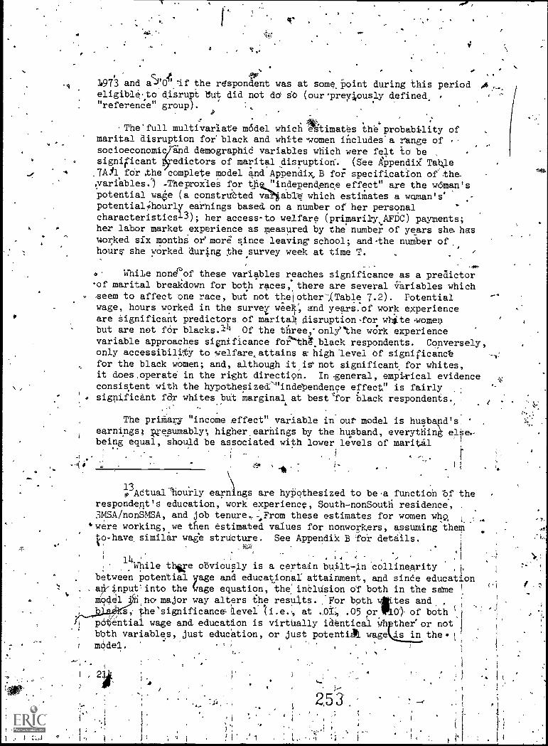
a
,we,
.'
- ,
? 41/10,
,.
1973 and 8..0'0' 'if the rdspondent was at somepoint during this period .6eligibleto disrupt llut did not dd so (our'preyi,ously defined,
, '
"referene" group).P
, ,.
.The'full multivariate model which estimates the probability of ,
marital disruption for black and white-women iricludes'a range of -'
socioeconomic and demographid variables which were felt to be -
IF--
significant edictors of marital disruption`. (See APpendii Table,7AY1 fdr the complete model and Appendix, B foi: specification of the,;variables.) .TheproxieS for tht2independence effect" are the woman'spotential wale (a constructed vallable: which estimates a woman's*potentiall;hourly earnings based on a number of her personalcharacteristics13); her access-to welfare (primarily,,AFDC) payments;her labor market experience as measured by the number of years she. hasworked sfx months or more since leaving` school; andthe number of.,hours- she worked during the survey week at time T.
, _..4.' While noneof these variables reaches significance as a predictorof marital breakdown for both races:there are several variables which-seem to affect One race, but not the other'(Table 7.2). Potentialwage, hours worked in the survey wee , and years.of work experienceare Significant predictors of marita. disruption-for w1 to womenbut are not for blacks.14 Of the three,- only"the work experiencevariable approaches significance foP'thtblack resoondents. Conversely;only accessibility to welfare,, attains a high 'level of significance
for the black women; and, although it is' not significant for whites,it does.operate in the right direction. In -general, empirical evidenceconsistent with the hypothesizee"independence effect" is fairlysignificant far whitesbut marginal at best'for black respondents.
. e 7
The prithary "income effect" variable in out model is husbapd's,.
earnings; wesumably,, higher_ earnings by the husband, everything elSe-being equal, should be associated with lower levels of marital
13AdtualIjourly earn ngs are hypothesized to be a function of the
respondent's education, work experience, South-nonSouth residence,SMSA/nonSMSA, and job tenure, :From these estimates for women whc;),
"were working, we then estimated values for nonworkers, assuming themtoo -hava similar wage structure. See Appendik B 'for details.
4
While thsre obviously is a certain built-,in collinearity,
between potential yage and educational attainment, and since education. ap/input'into the wage equation, the inalUsion Of both in the samemodel ,no.major way alters the results. For both viltites and ,
s,. the'significancelevel at .01, .05 or a')- of both
pa'ntial wage and education is virtually identical wh ther'or notbbth variables, just education, or just potentAt wage is in themodel. .
is O
t..
,t ,
t,!i'
j
t
2,53.
-4
*i

I
-Table "7.2 Unadjusted and Adjusted Proportions of Respondents Experiencing a MaritalDisruption between 1968 and 1973; by Race and Selected Economic Characteristics:
Multiple Classification Analysisa
Selected .
economic .
.
Number,
respondents
.
Unadjusted t
proportion, I
.
Adjustedproportion
Significancelevel
characteristics-
WHITES
:
Accessibility of welfare .
in state ,Loiiaccess - low benefitsRigii access- high benefitsOther , *
Debt accumulationNo'debt,
.
Somedebt..
Not a vertainable.
Work experience:
.0-2 years
more years
otential wage
IQ-50 or less$1.51 - 1.99$2.00 or more
Change in financial position. T - 1 to T-
Better
SameWorsFNot ascertainable
.
weekHours yord during survey weekiffonc, ;retorted ;
1.
'1c-34 1
. ;
1
oe more.
Grand mean )
.
/
.
0
-
°°
551812667
.
577604849
.
.
1 i202
828
1
658643729
.
992
61ZZ
182' 250
1,076283671
2,030
.
.
.14
.12
..041
.09
.15
.13.
42.13
1,R, .18
.11
.10
,
.11
.15
.14
.14
13 -f-
:t14
.13
.13
..
.
-
f.w..35
.11.
.14
.12
.11
.15
.11
.15
.16
.11
.11
.11
.14
. 14
.13 '
.10
.13
.16
%13
.
,
.
..
,
.
*
***
**
***
.
.
:
-
.
.
(Tattle cdntinUed on nett pai3e.)
!
V ,1
,
\,
. .
e.
254
215
'A
4
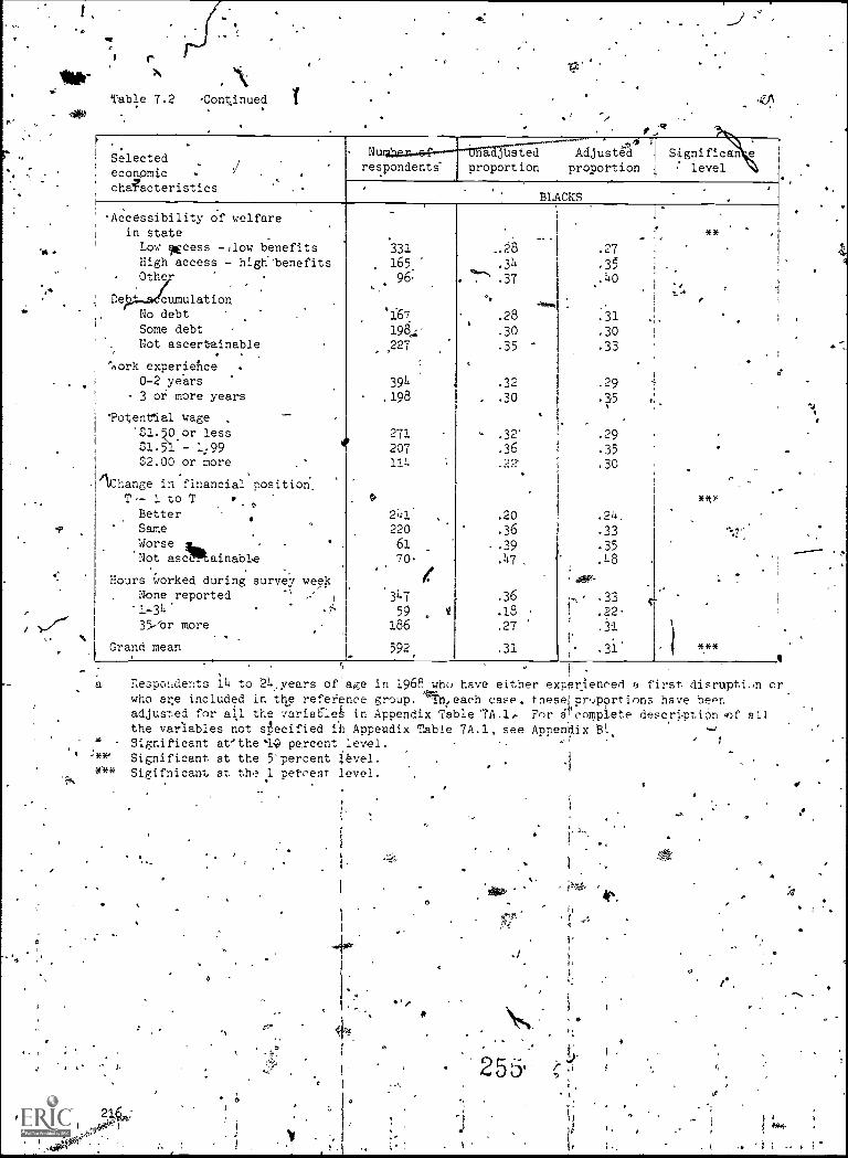
Ig
1'
t,sit
Table 7.2 -Continued
a J
, ..
Selected .
economic / ,
chActeristics .
respondents'
N PS- a.jilsted
proportion proportion
,*Adjusted 1 Significan e
f level
.. . .
BLACKS. .
-Accessibility of welfare1 in state1 Low wcess -/low benefits
High access - high'benetitsOthe
Oe
, ,
cumulation
-
331165_'
96-,
.1'67
198,'
227"394
,198
271
207114
0
241220
61
70. .
31.7
59
186
592
,
4
il
_28.34
v).. -.,-.37
-.
.28
.30
.35
.32
, .30
- .32'
.36
.22
.20
.36
.39
.47
.36
.18
.27
.31
.
.
.
.
1
.27
.35
.40
..
.31
.30
.33
.29
P.29
.35
.30
.24.
.33
.35
.48
.33
.22'
.31
.31'
.
-,
.
r.
I-
r
!
,
.,
.
.
'
ieit
***
.
.
e
e
No debt.
Some debtNot ascertainable
. .
'Nork experierice .
0-2 ye'ars
- 3 or more years
otential wage .-
..$1.0or less$1.51 - 1:99 #
$2.00 or more
'\change in financial positionT-- 1 to T .
Better ,.
SameWorseNot asc ainable
Hours Worked during survey we, None reported ,
)
-1-34' -7'
35-'or more -
. ,.
Grand mean
a
4 ,
-)**,
0*
5
nespondents 14 to 24years of'age in 1968 who have either experienced n first disruption orwho are included in the reference group. n.b,each case, theseipr,Jportions have beenadjus't'ed for all the variab'le in Appendix Table '7A.1. For Coompiete descr:lptiOn 0)1' nlithe variabies not specified ih Appendix Table 7A.1, see Appendix "Bt.Significant at'the'14) percent level. 1
Significant at the 5-percent lievel.Sigifnicant at the 1 percent level.
O3410- "
255' r ,N
I.
I ''4*
. '1 -
0
disruption. In addition, lower family debt leyels would also beexpected to'be,associated with more stable marriages. Final
relative context,one wouldxpect greater Marital stability in.thosemarviages where the family financial status has been stable orimproving. ...
.There was no substantial association between husband's'earningsand mal45.tal stability for either blacks or'whites (Table 7A.1). For
-whites, howeyer, having no accumulated debts-was associated-withlower levels of marital disruption. Finally, recent-improvementsin financial position (between T%- 1 and T) were associated withlower probabilities of marital,disruption for both.races. However,
.the association was significant. only for blacks.. This suggests' that(to the extent that economic factors are re/Srant, concepts whichmeasure changes in a,fam ly's economic status relative to long-term'norms appear to be of gre ter importance than status variablesreferencing one, point in time.'
-In contrast to the 'only moderate significance of.theeco,nomicvariables, demographic and social variables associated with the woman'sbackground are impo;-tart predictors of marital breakdown. For)both
J
black and white women, the negative association between education andmarital disruption probabilities is- highly-Significant (Table 4,4).The fact that this inverse relationship persists even after controllingfor the economic correlates of eduCational attainment indicates that k
higher levels'of schooling bear an independent relationship to apropensity'fOr Marital stability. - .
1
,
.. .--,onsistent with the literature, being raised i1 n a broken home isfoundto beeposit'vely associated with marital'disruption even withall the other so conomic 'controlS in the model. 1Thus, there-maybe certain soci ychological syndromes among 1;lo h blacks and whitescertain
to'pass on a "propensity to disrupt "from one generationto the:next. . i .
s.. . ,
,.
Itisalso of some interest to note that for both black andwhite women there remains a strong inverse association between afireand marital disruption, even after controlling:for all the otherfactors which ar,e.-nowia tb!-_,be associated:with aging,. per.se, Indeed,
the data suggest that any institutional means which canabe used tb4...
raisesitnificantly the age of marriage could well lead to majordeclines in mazital disruption rates, even if no other ch4racteristicsrelating to th. youth we're altered. The adjusted disruption'rates' .--
for white women tinder the age of, 20 are 19 percent compared with-14 .
' percent for thosecaged 20 to ai, 12 percent for 22 to 23 year oldsanl 91percent for thoge womeii *IYgp.ra of'age'and Older. Parallel
declines are evidenced for black, women.. ,
..
i
. . i.
? ,I .
In addition, after removing' the effect of the other,socioecOnomic.and demographic factors, the highest marital disruption probabilities
,
.
=
'217
.r"
./
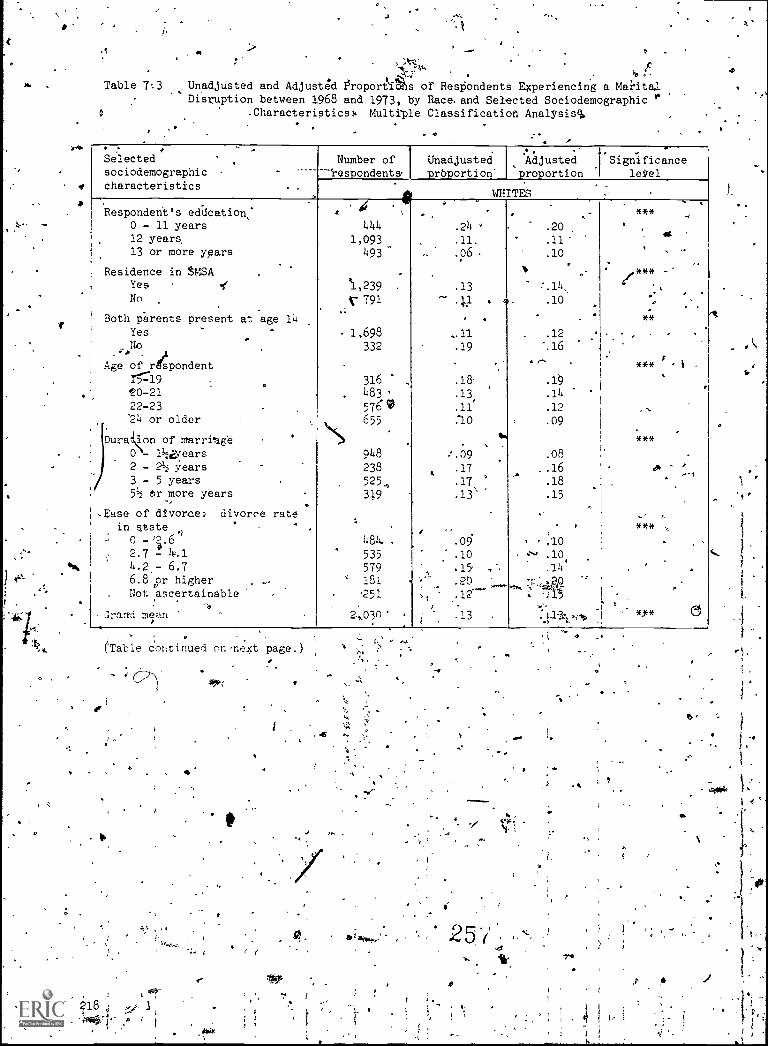
16
r-
I
ks
O .-., 't7, r
Table 7:3 Unadjusted and Adjusted Propor&-BIts of Respondents Experiencing a Mai'ita.1.
Disruption between 1968 and 1973, by Race.and Selected Sociodemographic "4 Characteristics. Multiple Classificatioh Analysisql,
. . .'
Selectedsociodemographiccharacteristics ,
Number of--respondent&
UnadjustedprOportion.
Adjustedproportion
SignificanceI let7e1
WWHITES
Respondent's education:0 - 11 years12 years13 or more years
..
Residence in SMSA .
Yes . l'
No.
Both parents present at age 14.
Yes .
I io .
Age
)
of respondentr5f19 .
.
'20 -21
22-23 ,
24 or older
.
Duration of marriage0 - 11/2eyears
2 - 21/2 years ..
3 5 years51/2 br more years
,--Ease of divorce divorce rate
in state .
0 -,2.62.7 ! 4.14.2- 6.76.8pr higher
. Not ascertainable
.Gralld mean
_
.
e
.
e444
1,093
493
'1,239
V 791.:
- 1,698
332
316483
576'0
655
948238
525,319
484..
535
579' 181
251
2.,03O'
,
..
..
,
5,
.24
.11.
.06
.13
^ 41-
.
,.11
.19
.18,
.13
.11'
:10
09
.17
.17 °
.13"
.09'
.io
.15
.20
.12
.13
.
.
.
....,
.20
.11-
.10
'
:.14.10
. .
.12
-.16
.1.
.14
.12
.09
.08
..16.18
.15.
/
'
, ,lo
.--, .io
.14,
.20
{,55
. 1-3y, y
'
,
.
!
J 0
***
,***
I '...-
**
,
***
,,
***
-***
.
.
*3"
4
at
.
$i
. .
,
,
.
.
.
.
0
(Table continued on 'next page.)
1.6
.
/-

o
1
.1;1i
Table7".3:. Continued
Selected.,..
' Aociodemographic.
characteristics
! Number of.- respondents
Unadjusted. proportion
.
Adjustedproportion
t.
Significancelevel
.
BLACKS-
1
Respondent's education0-11 years12 years'13 or more years
Residence in SMSA %.1YesN
No
both parents prese at age 14. Yes -
No.
Age of respondent15-1920-2122 -23,
: 24 or older -.
Duration of marriage0 -1 1'1 years
2 - 21/2 years .
'3 - 5 years51/2 or more years
Ease of divorce: divorce ratein state0 - 2.6
.
2.7 - '4.1.
4.2 - 6.7 -
,
6.8 or higherNot ascertainable
..
Grand mean
.,,i
.
.
.
'
.
.
254
26474
391201
;42
250
124°
143
158167
305
73,13678,,, ,
84
'22817765
38'
'592
4
-,
'
.
.
.
.
/-
4..3.
.26
*.19
.31
.32
.21
.37-
.37
.30
.27
.32
.21
.38-
.47
.31
.37
.33
.28
.29
.29
.31
.
,-.
.38
..26
.28
.
-.32
.29
.
,.29.34
. .
.42
.31
.28
.27
.22
.35
.47
.34OP
.
.32
.36
.28.
°.27.30 -
.
,31,.
.
,
.
:**:
,
4.
1* *
.
***
1
it**
...
.
(
.
N.
. YA. 'Respondents 14 to 24 years of'aie in'1968 who have either experienced a first 'disruption
or who are included in the reference group. In each case,'Ulese Proportions have. bee'n,adjusted for all of the variables in Appendix Table 7A.1. Fbr a complete description ofall the variables not specified in APpendix,Table 7A.1, see Appendix.B. ,.
** Significant at the 5 percent level.4** Significant at the 1 percent level.
. 's<'-..
cs
cf.
258
219
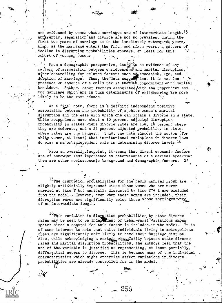
a
ar evidenced by women whose marriages are of intermed iate length.15 ,
Apparently., separation and divorce are not so prevalent duringihefirpt two years of marriage as in the immediately subsequent years.'Aisp, as the marriage enters the fifth and sixth years, a pattern ofdeg/line in disruption probabilities appears, at least for thiscohort, of younger women: ,
.4 .) From a demographic perspective, the '`3s no evidence of any
pattern of.assopiation between childbeamilt and marital diSruption,,a er controlling for related factors such aieducation, age, anddu tion of marriage. Thus, the'data suggeWthat,ii is not, the 2*
fprresence or absence of a child per se thatt,concomitant.witli maritalbreakdown. Rather, other factors asso4iated2With the respondent andthe marriage which'are in turn determinants of childbearihg are more
4 .
- " likely to be the root causes.
As a fllpal note, there is a definjte independent positive' association between the probability of a white woman's marital
disruption and the ease with which one can obtain a divoi-ce in a state.1/Kite respondents have about a 10 percent adjusted disruptionprobability in states where divorce rates are low, 14 percent wherethey are Moderate, and a 21 percent adjusted probability-in stateswhere rates are thd highest. Thus, the data sappOrt the notion (forwhit women, at least) that institutional variations in divorce lawsdo play a major,ipdependent role in determining diVorce levels.16
From an overall4viewpoint, itseems that direct economic factorsare of somewhat less importance as determinantS of a marital breakdownthen are other socioeconomic background and demographic,factors. Of
tThe disruption probabilities for the'newly'married group are
slightly, artificially depressed since those women who are nevermarried at time V but maritally disrupted by time 1'4 1 are excludedfrom the model. However, even when these women are included, theirdisruption rares are significantly below those whose marriagesof an intermediate length.
l6Thisvariation in disuatiOn probabilities, by state divorce
rates may be seen to be indePrent of urbanrural'lariations amongstates since a coptrol for this factor is included-in the model. It is
of some interest to note that white individuals living in metropolitandreas.are significantly more likely to have their-Marriagedisrupt.Also, while acknowledging a certalgs,,ciAgaity between state divorcerates and marital disruption probaBiliLes, the author feel that theuse of the variable is justified as representing,-at least partially,differential access to divorce. This is because many of the individualcharacteristics which might otherwise affect variations in, divorceprobabilities are already controlled for in the model.,
114C
-221
259.4
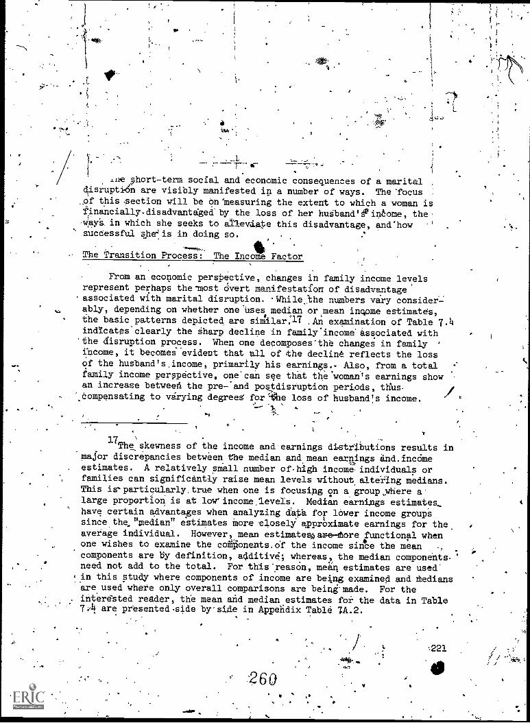
<,
1,
r
,
.
J.Lre,short-term social and economic consequences of a maritaldisrupt& are visibly manifested in a number of ways. The 'focusof this .section will be On'measuring the extent to which a woman istinancially,disadvantagedby the loss of her hudband'Ilin6ome, the-way's, in which she seeks to alleviate this disadvantage, and'howsuccessful she-'is in doing so.
111The Transition Process: The Income Factor
-4 ,..;
From an economic perspective, changes in family income levelsrepresent perhaps the -most Overt manifestation of disadvantage
.associated with marital disruption. Whilethe numbers vary consider-ably, depending on whether oneIses median or mean income estimates,the basic patterns depicted are similar.17 .An examination of Table 7.4indlcates'clearly the sharp decline in family'income'associated with'the disruption process. When one decomposes'the changes in familyincome, it becomes evident that all of the decline reflects the lossof the husband's, income, primarily his earnings.. Also, from a totalfamiy income perspective, one'can see that the'woman's earnings showan increase betwee6 the pre-'and pos>tdisruption periods, thus.
.compensating to varying degrees for `'e loss of husband's income.
1
0
17The skewness of the income and earnings di,strUutions results in
major discrepancies between the median and mean earnings and.incOme. estimates. A relatively small number ofhigh income-individuals or
families can significantly raise mean levels without, altering medians.This is'particularly.true when one is focusing on a groupyhere a-large proportion is at low'incomeleveis. Median earnings estimates,have certain advantages when analyzing data for lower income group'ssincethe."mediat" estimates more closely approximate earnings for the.average individual. However, mean estimateshare-tore functional whenone wishes to examine the cogitionents.of the income since the mean
components are 15y definition, additiv; whereas, the median components.'need not add to the total. For this'reasOn, mean estimates are used-
.in this study where components of income are being examined and tediansare used where only overall comparisons are beiij made. For theinterested reader, the mean and median estimates for the data in Table7.4! are presented -side byside in Appendix Table 7A.2.
.260,
z 22l

Table 7.4 Mean Income,;Characteritics of Respondents ExperiencinMarltal Disruption at. Time T, T + 1 and T + 2,,by Race
Meanincome
%WHITES
_ _
BLACKS ,
characteristics.
°T.
T+ 1 T 4-2 T . [ T + l' + 2 .1
. Mean faMily income 7,552 5,197 5,983 6,251 3,967 3,794
.Mean family income lessrespondent's earnings 5,845 2,709 2,855 4,658, 2,344 1,,756
Mean respondent's earnings 1,708 2,489 3,128 1,594 1,622 2,037
Mean-per capita income perfamily member . ,
w
2,688 2,124 2,656 1,721 1;176 1,024
Mean family size 41 2.8 2.4 2.3 3.6. 3.4 3:7
Numberof respondents 229 2,32 126 166 173 106.
,
a Data for T + 1 Snci T + 2 are limited to.those marital disruptees whohave not remarried or reconciled with their husbands as of thosepoints in time.
0
.b All income and earnings estimates are in 1967 dollars:
222..
\ /
,
2 61
S

N.
.
r.
. t.
,Overall, for whites between time T and T + 2 therelis a decline\of .
$2,990 (in 1967 dollars) in total income lets' respOndept'*s earnings.This decline is partially compensated for by, an increase of. $1,420 inthe respondent's earnings. Thus, the white women has compensated for47 percent of the income loss through increases in her work activity;For blacks,.the analogous numbers are -$2,02 and +$443, so the 1
average black woman replaces only 15 percent of the income loss.
While the rather sharp contrast betw4n whites and'bIACks'suggested-by the above numbers accurately depicts the relative,Rositions of white and black women, from the perspective of individualswithin the family, it is perhaps more meaningful to, analyze the for-:going income changes in per capita ,teams. If one adjusteor changesin family size between the twq points in.time (T to'Ti+ 2), per- capitainconi for blacks declines from.$1,721 to $1,024, while there is nosignificant change in per capittb income in the-White families. Froma per capita perspectiye, the white woman, by,inbreasing both her
' own earnings and her access to other sources of unearned income,largely replaces the loss of her husband's earnings.18' Of course,'while her family per capita earnings may be up to their.previouslevel, .
. the larger average child-care and dthersa§sociated costs (reflectingin part the need for many of the women to enter the labor force) maywell leave her in worse, financial condition than she had been prior 1
'to the_disruptionJ9 It is also of someimportance to note that part_of this white woman's ability 'to maintain her family's per capita. 4
income reflects the sharp decline in the mean white family size(reflecting the loss of the husband). The black woman is morelikelytobe joined by or to form into a family network after thedisruption.This extended family certainly alleviates many of the sqpial.traumasassociated with the marital di§rulAion but apparently is unable'toaugment the family income to any significant extent.
Changes in Labor Force Participation Levels 2
The above data suggest that.eniployment is one major means bywhich woven whose marriages disintegrate compenpate for the loss-of
4 -
18A cautionary note regarding these racial differences in income
is in order. To the extent that welfare payments and'or income fromj'other" family members may representmore important income sources.inmaritally disrupted black households, differences between black andwhite'incomes may be overstated due to the possible understatement of
It ese two income sources."
19Th the extent that white women are more likely to utilized morefamily child care sources and thus have on average higher child'care,costs than black women, the above statistics may overistate somewhatthp per capita income differences between black and white familiep.
' See Shortlidge and Brito (1976).
6:2

husbands' arnings.,. Figure 7.2, indicates the trend of participation
levels het een time T Iand T +.2 fo:black and white maritallydisrupted omen both with and'without %hildren. For both black and,
white womei without children, labor fore participation levels rapidlyapproach 4iind for white, women, sdrpas0 labor force participatipnlevels of never-married women-at approXimately the same ages. The ;
partiCipat4on'levels for women.yith Children sliOW large increases, butthese leveis predicta y-remain well below those of their childless;counterparts.
At time.T about percent of white and 29 percent of black' 1 s!,
disruptees in the labor force were unable to find jobs '(Table 7.1).' AS
may be noted from Table 7.5, whites, regardless of their work statusprior to the marital disruption, were more likely to be employed at i:-,.
T + 1 than were blacks. In particular, blacks in the labor force'dtT apparently had much greater difficulty in maintaining that labor.force attachment than comparable white workers.
In order to examine more carefully whether or not the trospective, 1
marital diSruption event, is associated with labor force participationlevels prior to the disruption, inddpendent of all other factorsx a
lk. multivariate analysis was performed using labor force participationat time T as the dependent ,variable. This labor supply model inclUded
.
the Standard explanatory variables and, in addition, ariable indica-4r.N.
ting whether or not the women would disrupt duAng the following year.(See Appendix Table 7A.3 for the complete model.) White women whose
marriagesmere to break up.during the following year wore indeedsignificantly more likely to be in the labor force. During the 'survey
week before the disruption. their ddjusted labor force participationrate was 62 percent compared with 55, percent for their nondisrupttng
icounterparts. There. ere no significant differences, however, betweenthe:two black groups. 'Thus, for white women at least, there is some
evidence hat anti'tfp tory lthor force behavior may be occurring; that.1
is,, some omen, in an icipation of a forthcoming marital breakup,,may;
be enteri g the.labor)force. The,above results are also consistent.withour 6arlier hypothesiZed independence effect,.wherebg- women iwithTia closer attachment to the labbr force. would be expected, to. have higher
maAtal d sruption prdbabilWed. . i1
i ,
it
,
A co parison'of the labor force transition between T and T + 1) . ! 1.
for the r ference group and the disruptees pinpoints a major behavioralvariation between these two grouiS, as seen'in Table 7.5.' ,There are
.:- some. differences in behavior at-T, 4'1 between those in thereferende± \ 1 ,.
groUp andithose marital disruptees who were in the labor force at timeT (primarily a somewhat greater movement out of the labor force bywhites in',the reference group). However, the major variations are
m --wir between marital disruptees and those in the reference group who werenot in the labor force at T. About 56 percent ,of the white disruptdes
,ffi,..,
who were not in the, labor Force, at T,wer either employed or unemployed.. at T + 1, compared with 23 percent for t the comparable reference group,.The corresponding percentages-for the blaakv Were 48 and30: 4r.224 .
1 0,263
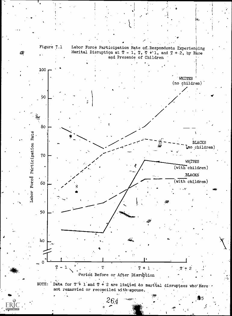
Figure 7.1
4
Labor Force Participation Rate Of,Respondents ExperiencingMarital Disruption at T - 1, T, T +'1, and T +.2, by Race
and Presence of Children 1.
WHITES(no children)
9
T - 1N
Period Before or After Disrthition
T
BLACKSIno .children)
WHITES
(with children)
BLACKS
(with children)
NOTE: Data for Ti l' and T + 2 are limited to maritalnot remarried or reconciled with-spouse.
264
. T.+ 2 .
disruptees who"have

a ,
Table 7.5, iLabor Force Status for Marital, Disruption and Reference1 Groups at T + 1, by Race andiLabor Force Status at T
VLabor forcestatus at T i --re-spent:lents
%'..-,..-/'
Niimber of
Labor force status at ,T + 1
Labor forceparticipation
Unemploymentrate
Percentemployed
Marital disrupteesIn labor forceNot in labor farce
Reference groupIn labor forceNot", in labor force
rgs
, A...
Marit eld*srUiatees
In labor forceNot. in labor force
Reference group;'
In labor fbrceNot in labor force
7WHITES
145
119
1,043
819
. .
'
84.5
55.7
.
74.6'
23.4
6.324%G.
6.3
18.9
79.242.2
69.918.9
.
BLACKS.
10283
257
V-6
'
76.8.
,47.6
.'
75.130.0
.
17.223.3
10.525.3
,. ,
63..3.
36.1
67.4.22.5
t'
226\
.6:4.0 u
41

0'
Overall, about 81 percent of those.marital.disruptees employed at.T -- 1 were working full time--at leist 35 ,hours per week. Thisfigure compares with orily_68 percent for those in the reference group'who were ,employed at the see point. Thus,, the greater need for income
iby the average disruptee is translated not only intO'higher levels oflabor force part±ciption,12Ut into a lengthier Work weeleas veil.This result is particuArly interesting, given the fact that theaverage maritally disrupted woman is more likely to_have children thanthe comparable women still in'an intact marriage. Indeed, 83 percent,of the bIa6k disruptees and 61 percent of the white had at least onechild in their household at T compelled with 68 percent for thet blackand:49 percent for the white reference grOup. Aor
' When this higher labor f'orCe participation patters is combined '
with the'khowledge.that almost half of the disrupted women had noother adult living in their household potentially available for, child'care and clearly had very limited funds for outside child careassistance, the ability of thete women to maintain employmentcontinuity is quite remarkable. In any event, the employment needsof these women combined with their limited, access to free childcareservices and limited funds suggest that this group should receive thehighest priority for child care and other forms of 'economic ,uassistance. -
.4.
Wort, and Training,
Data from the National L 'tudinal Surveys indicate that rathersubstantial numbert of women -ire enrolled in training programs of.someind'in the-periods immediately preceding and following the disruption ,
eveht.20 ,In'eddition, the ,proportion- of white wome# enrolled intraining during the,prededing jekrjncresses rather sharply betweenT and T'+ 1, from 16 to 26 percent.- There is no corresponding increasefor black women, althoughthey exhibit an reate in trainingparticipation rates from 11 to 20 pe ent etween T + l'and.T + 2.Thus, whateverthe reason for this dif er ce, whites are'better ableto gain access to training programs when they need them. On the otherhand, increased black 'participation in training associated:with maritaldisruption is somewhat delayed, perhaps -i-eflecting a lesser awareness
program aysilaility and,partly reflecting a,greater need to seekitmediate gainfulfeiploYment.'
Supplementary'mUltiveriate analysis of the determinants of,training at time T + 1 for'blaCk and white marital disruptees indickes
.ft
20The followin
school: "Since thitcourses or educationelsewhere?"
tae ion was asked-'of women not enrolled in
time last-iVear-he-Ite4eua-eny trainingprograms of any, kind-either On the job pr
266.
0
p
227

a'
O
%
. one other major -variation between the two race.groups. White trainees
are clearly selected out from the most educated of the eligibles, I
I
i whereas blacks with the least education were more ...ikely to be...
involVed
' in..:k-
.
training programs: Thhs, while maritally mdisrupted blacks may bless likely to move iqo' training prograMs at that point in the lqicycle, from a positive erspective, 'those who do enroll are most in
need of vocational. assistance.' , i ., ,
:1L.,
Since there are obvious associations between training'andwork ata:given point in time, it is useful to inquire whether receipt Oftftining between T - 1 and T is related to employment status at .T + ql
for those not in the labor forceat It. As may be notedin Table 71 ,
training is associated frith a higher, probability of being employed)at T + 1; with a lower employment rate, and with higher earnings.
These patterns are in evidence for both black and white women but i
shohld.be interpreted cautiously because of the small sample size forthe group which hat had training. .
.,)
`Work and Welfare % L.
4
While t*.,NLS income data are inadequate for measuring the extentto which,yelfare.payRents supplement the family income of maritallyAsrupted fp:mines, they are of considerable value tor interpretingsome of.the associations Sbtween the Tropensity to have welfareassistance, employment status,.and -family income levels.
Table 7.7 shows that regardless:of income level, families whicheither are or will btcome disrupted,are more likely to be'receving ,
some form of welfare transfer payment than similar "reference"
families.21 Also, in all instanCes,:black families dre more likely
than white families,to be receiving some.form of public assistance..-Regardless of race or income Level, the propo tion-Ofainaritallydisrupted famllies'receiving'some forl, of iStance increases
'sharply.as one' moves from point T 1 T °4-2. The increasingproportions receiving some form of welfare are generally consistentwithhe earlier documented sharp declines -in the family's earnedincome following the disruption event.. Also, the racial variations canbe at least partly explained by differences in earnings and number of
own children present- between white.arid black women in the yearfOl,lowing the disruption.
Some Multivariate Results
Predisruption labor force behavior Ove41, wpercent of'the.
white women who' subsequently experienced a marital disruption were
The'survey questions askedwith regard to receipt' of publicassistance do nit discriminate as'to the type of transfer paymentreceived ortas to which member of the family is receiving the
22S
'6T
t
6

A
Table 7.6 Labor Force11/41.
tatus,and Employment Characteristics at Tby Training in Year Preceding T4
.
.
Training betweenT - 1 and T
,,
.Number ofrespondents
Labor -force status at T + 1
.
Percentemployed
Unemploymentrite'
,
Percent*.
employed± 11 time
Percent earningless than
$2.00 perthour'.
Training
lfi training.
.21
';AX77:4
76.1
-.37.5
5.6'"
,26.4,
82.2
80.3
. 72. 3L
81.7
a Universe consists of marital disruptees not in the labor:force at T.
2684
r r
rd.
'
.;
.61
269

Table 7.7 Percentages of Marital Disruption and Reference Groups_Receiving Welfare, by Race and Selected, Income Characteristics
at 1, T + 1,'And T + 2
. .
Selected 'WHITES . BLACKSBL
income v. .
... Marital deference Marital Reference..characteristics f..
disruptees group disruptees group.
All respondents, .2,
T 5.4 25 17.3 . 7.7:T + 1 23.3 2.9 44.0 5.5T 4 2 26.9 '2.9 52.4 7.9
.Family income under $4000...--.-----
T 19.1. x.9.7 40.2 13.5T + 1 38.6 '4' /14.8 63.5. 16.1
-.0T + 2 . 4148.2 16.3 69.1 26.4
All respondents with_
noearnings .
.. .
f.T- 9.2 11,9 '30.1-' .'12.2
.
T + 1 48.3 5.1 ' "'77.5 10.5T + 2' 69.3. 4.6 94,:2 13.'3
.All respondents with .14"*°4f.10,*
earnings ..
T - *.f 3.7. . 1.5 ",12.9 r
.6.6'. T + 1 17.0 °. 1.6 30.7 .3.2
'T + 2 18.5 1.5 40.7 5.6
a Data at T + 1 and T + 241imited to marital 4pruptees who have not
remarried or reconciled with thiir husbands-as Of those points 4A-1 time.b ."Rdceiving welfare" reflects a positive response to the question, "Did
anyonein is amily receive any welfare or public assistance in thepast 12 mo d.f
447
ry
it,230 r
1
,
I-
,
0 ( U
7 /
. 10
-... .
working at time T, as compared with 56 percent of white women whosemarriages did not disrupt. The comparable-estimate,for the blackprospective disruptees and reference group were 56 and 5tpercent,
.1* respectively.. HoWevei-,lat,noted earlier, in labOnsupply models whichincluded bothiprospective disruptees and the.reference group at timeT,'racial'variations did appear. After controlling for socioeconomicand, other factors, white prospective-dipruptees were significantly % '
more likely to be working,or seeking work at time T than theirsnondisruptee-counterpart's', whereas no significant differences werefound between the two black grodiS: .
. ''
In the controlled'multiple classification, analysis at time,T(Appendix Tables 7A.4 and 7A.5)here are certain dramatic differencesbetween the reference group and. marital disruptees in the way
..
particular variables affect labor force-behavior. For. both_black.andwhite prospeCtive marital disruptees, there are pronOunced patterns of
4,..r,
higher labor force'participation for those women whoge'families have \
accumulated debts. Also, labor force rates are lower among:thoseprospective disruptees living in high welfare access areas. None of 4.
the above significant relationships exist in any major way for eitherthe black or white reference groups. Variations in laborforcebehavior between prOspective disruptees and "reference" respondents .
along these dimensions may well'represent divergent responses toinherently stressful situations. ,eAs,such, they are consistent withthe knowledge that one group of women did indeed have their marriagesbreak up and the other group had their marriages remain, intact.
46. -7
While
,A .. - **;*#.., .'4.
. Postdisruption labor -force behavior While the paitere ofadjusted participation rates are spmewhat-erratic, there ire nonethe- .
less certain trends and patterns worth-noting (Appendix Tables 7A.6.and4-(A.7). First, after mariital dIsruption occurs, mean labor forceparticipation rates are significantly higher for whites than forblacks, whereas before the
o-
rital breakup there were no differencesbbtWeen the twraci,al.group : Of course, for both blacks and whiteg,the labor foi.ceparticipatio rages rise precipitously after, thedisruption eve t.- The adjusted white labor force particpation ratesafter disrupt on are systematically higher for virtually:very. .
separate cat gory Of every socioeconomic and demographic characteristic.Within the parate race Models, the results conform moderately wellwith theoretical expectation's. For both.black and white women, labor,force partici appears positively associated' with.more'workexperience, higher potential earnings, better health and less access
.to welfare. ' ., / ,-,.., .
-,,,,,
....,o,-. ,
SUMMARY AND CONCLUSIONSb
Whereas economic motites'may be of,onlY Moderate importance asprecipitating factors.in'amarital breakdown,leconomic bogie uencesare very pronounced in,the',postdisrliption life cycle phase. rital.disruption is accompanied by sharp declines in family'inceie, ncreaved,
.
_fO .
d
' 231
/-

rj
O
receipt of welfare, increased desire for job - rebated training, andhigher labor force participation rites. Increased usage of incomemaintenance programs occurs do the part of large proportions ofwomticularly black women with-children, low education, few Joskied outside financial resources.
The large *proportion of all young'adul couples who experiencemarital disruption and he substantial e-conolnic impact that thig
experience has .onyoung women suggests that some thought should be.gIv.en to developing a program of transition assistance for maritallydisrupted women and their children. Such'a program might include jobguidance, training, day care for children, andttemporary incomemaintenance.
4
, 252
a
'
.4
A
: .

0
r
/AR E FE R E N C1E S
0'
Becker, Gary 8.; Landes, Elisabeft M.; and Michael, Robert T.. "Economics of Marital Instability:" Stanford: National
Bureau of Economid,Research, 1976
.0W
Bumpass, Larry L., and Sweet, James A. -"Background and Early Marital-Factors in Marital Disruption." CDE Working Paper 75-31.Madison: :Center for Demography and Ecology, University of'Wisconsin, 1975:
'1
Carter, Hugh, and Glick, Paul C. Marriage and-Divorce: A Socialand Economic Study. Cambridge: Harvard University Pre4s, 1970
Cherlin, Andrew. i*onomics,. Social Roles, and Marital Separations:"(Preliminary draft) Baltimore:- 'Johns Hopkii University, 1976
Clitright, Phillips. "Income and Family Events: Marital Stability"!..Journal of Marriage and the Family - (March 1971): 30T-17,
( Furstenberg, Jr.; Frank F. "Premarital Pregnancy and MaritalInstability." Journal of Social issues 32 (Winter,1976): 67-86
Glick, Paul C., and Norton,.Arthur J. "Frequency, Duration and. Probability of Marriage and Divorce.", Journal of Marriage and
the Family (May 1971): 307-17.
National Center for Health statistics: Monthly Vital Statistics'-ieport. Vol. 26, No. 2 - SuppleMent 2. Washington: ,PublicHealth Service, U.S.-Department of Health, Education andWelfare;-May 19, 1977 r
Plateris, Alexander A. "100 Years of Marriage and Divorce- Statistics."Vital and Health 8tatistics,Spries 21, No. 24., Washington:Division of Vital StatiNtice,-National Center for-Health.Statistics, 1973. *.
Pope,'Hallowell, and MUeller, Charles W. "The IntefgenerItiOnalTiiansmission of Marital Instability.-" Journal-8t'Social Issues_.32 (1976).: 49-66. ,
Rods, Heather, and,Sawhill, Isabel. Time of Transition., Washingtoq.i.The Urban Institute, 1975.
Shortlidge, Richard, and Brito,-Patricia., "How-Women Arrange for theCare of Their phildren WEileThey Work: A Study of ,Child,pare .
---Airangements,'Cdatand Preferences In 1971'." Columbus, Ohio:,.1Center for Human fiesddrce Research;" The Ohio State University,
1977,
233

I
,
U.S. Bureau of the CenSus ,",liumber, Timing, and DurationeoNarriage:June,' 1975." Current Population Repqrts 23 (12). Washington:
' U.S. Government Printing Office, June, 1975.
4
4514
Q
27 4,01.
0
s_

a
r.
APPENDIX A
41.
CONSTRUCTION QF THE MARITAL DISRUPTION AND REFERENCE GROUP SAITLES
The MaritalDisruption Sample
All young women-who divorce or separate for the First timeduring the 1968 to 1973 period are defined as the marital disruptionsample. A "disrupted" woman will only be counted once--the year within
' 1968 to 1973 peridd when, see first appears as disrupted (separdor divorced) . That if a woman, were-married with her spouse'presentin 1968, separated in 1969, and divorced in 197q, she would.appear ine numerator of the marital disruption variable in 1969 but not again
i 1970. ,
c'
V. ,
The ,follolking slippage exists in Bing able to identify properlyall disrupting women:
1P' _ - A- `:,.
(1) °women who were divorced or separated at some point beforethe first survey in 1968 cannot be identified. it
o(2) Women who. ar married, husband preeenti. in successive years
with the same husband. and who had a separation in iha intervening.interval cannotbe identified.
In,general, all other mien who!either separate or divorcebetween 1968 and 1973 cambeidentified unless, of eourse, they leavethe saMp),e before the disruption event.
The ReferencvGroupe
-
.*Whereas a first marital,disruPt_ion represents a unique event,
appearingin the (maritally Stable).reference group.it not, since '
Many women obviously are "eligible to disrupt" in more than one 1-.
survey, year.. Thus, to -count a woman in the - reference group every. .
year she is eligible to disrupt' Would result in mdssivetdouble counting.For this-reason, we have.used the foXlowing.procedure for defining that,.group: 411 .- .
..,,
(1) EVery woman who d4)"eligible" at ome point betiieen 1968
S., \
. . .
and 1973 is included in the ' reference, group but only one time.. ".
,(2)' After exclOding those women who areknown to experience amarital disruption between'1968 and 1973, 'the remainder are randomiy , .
distributea across the survey yearsiroughlyiin proportion to thedistribution of marital disruption Over, the five-year period. Whatis, if x/perceht Of.all the first maritairdisrUptions occurred-between1968'andf1969, then_x pereent of the eligible reference group wasrandomly assigned tO that interval. -Thus, once an individual is./
.
4.
-
F.
,
selected for the reference group in a given'year, she is-no longer) -eligible for Oclusion.in any other year. a,
<a
".
The above should meet the basic. objectives of; a properly defined.reference group. That is, it (1) defines women who were eligible todisrupt but did not do so duritg the appropriate time periods"and (2)assure that the reference group is demographically and temporally,appropriate.
...
yyari1bles for this reference grip are generally measured inthe year that the particular individual is selected to appear. Forte
example, ifwe-select a woman:for our reference group in 1970, hersociggconomic characteristics (as 'entered in our,model) 'will bemeasured as of the 1970.chterview., The only exception is the caseof those who were never ildrried in the year 4n which they wereselected to appear! jhe.socioeconomic characteristicsof these womenwill bp measured as of the next interview, when they.are ta;ried.
, \
4
236'
/
,1 ,. ,eN
A. c .1fS-.
J
V76
I
A
..
;$
- i
1. I
.
I
, ,

atr
4
.
40. CHILD
APPENDIX.B
Dictionary' of Variable Definitions and Categories
4
.- ACCESSIBILITY OF WELFARE IN STATE 4
A
4 ^To measure the easeof obtaining benefits, we use theproportion of potentially eligible-households. (according toCensus definition) actaully receiving AFDC assistance by . -
state. The actual benefit level received is>proxied by '4
Social Security qatistics giving average payment per recip1:-.ent by state. We can then construct a variable of the
1:..
'follolpg form:*. .
., '0.) High accessibility - high benefits-.(2) High accessibility - low benefits.(3)' tow accessibility - ,high benefits(4) Low cessibility - /ow benefits
fHigh aicessib ity means that the state has above the mean,
. 1
propoliaon of potentially eligible households actually.0receiving AFDC. Aigh benefit levels mean teat the,stat
"-..,,;. has above the mean average pament per recipient.
iN .i ' -,
._4
AGE OF RESPONDENT
. edtegoris are as follows:
(1) 15-19. years
(2') 20-21 yeas(3) 22-23 yeys
, (4) 24 or older'
. \
-11 set of varfables using the age of the youngest\chi14 alsowild prOxy fOr the presence of_chi4dren:
Years. 7
0,,,:
(2) Child 2 or more years -,
-1 (5),ANo childrenr,
''': , '. 1. .
1
BOTH PARENTS PRESENT AT AGE 14 I- >
. '1
./ .
: c!' 'Arvaldable indicating whether Or not the respondent waSi
; living' witch both naturAl pare4s at-the age of 14, . 3
); - -2
..
GE IN FINANCIALPOS/TION T - 1 TO T*r 4.
%the variable-isloased on tie question asked oil each -
1 respondentlatt as to whether(s4e f.eels.he 'ly's, . .
10.. .I 1
41 It"T'" fere e las interview before the disruirtion; ° I,"t e'''first..ntery ew aftenthe event; and"1T -1" and "T i 2," they' ..'
= eiliately earlier and later 4tervie dates., ..,
......._s. o. .p. ,_.!
t
, I,. 4. i or .
.
. ) .' 237.. 4 ' .
( , ,
A ..7 7:
. 2.
.1

s
position is better, about 't4J;same,. or worse than 'at ,
the previous interview dat
DEBT ACCUMULATION
e
11:A set of.categories.giving the unt 6f:debtliability'(excluding 30-day charge accounts) incurred by the ..
. respondent's family at time T. Categories include: ',-,
4.) No debts(2) Positive debtse3) Debts unknown
DISRUPTION 'VARIABLE
(1) Referenbe group° (2) Marital disruptee
J
For details of reference group specification, seeAppendix A.
rTOES HEALTH LIMIT WORK?
Categories are as folloWs:)
1
(1) Health status affects Work or schooling,'(2) Health status does not affect work or schooli
(3) Health.status not known
DURATION OF-MARRIAGE44.Duratton of marriage is measured in six month units because,the exact date of ,marriage is, not known and the efore,
duration mutt be measured reltive:to the'surve dates.
r 401) 0-11/2 years
(2) 2-211 years(3) 3-5 years,
,
(4) 51/2 or .more years.
/EASE OF DIVORCE:E: DIVORCE RATE IN STAE .
The divorce rate by-state of residence is used tq..prOxfor the ease or obtaining a divorce in a given state.,.
(1) 0 - 2.6 divol-ce rate per f,poo population
(2) 2.7 .- 4.1 divorberate '44.6.
(31 4;2,- 6.7 divorce rate(10 or higher.divdrce rate .
.(5) State of residence' unknown
kif.MAN4COS EARNINGS: .PAST YEAR
.3
II*)Taken from the question. regarding.earni gs of thehusband
in the year prior/topthe,p6int t:...
.
.(1) Earnings unknown(2) 9 - 3,90, ,, a
- 4
2384, b - 278,.
Q
if.4"
e
40,
44 .

ti
AD%
4 .
'(3)
(4),
(5)
$4,000 - $5,999$6,000 - $7j99$8,000 or more ,
.
POTENTIAL WAGE.,
Actual hourly earnings are hypothesized to be a functionof the respondent's 'educatiOn, work experience, South-non-South residence, SMSA/nonSMSA,_and job tenure. From these'estimates, assuming, women with like characteristics will' 1..
have-similar labor supply behavior, a potential wagestandardized in 1967.dollars, whether or not the woman ispresently in-the labor market, is estimated.
For whites, the wage. equatiOn is as follows ,(witht-statistics in parentheses):
WAGE'= 140..54 - 20.873x(EDUCATION) + 15.566x(WORK EXPERIENCE)(2.95) (-2.83) (6.52),
+ I4:703x(JOBIUEENURE)'- 1.2874x(JOB TENURE2)(-4.1/2) (;-2.90)
:69706x(WORK EXPERIENCE2) 25'.870x(SMSA)(-3.04)- - (5.28)
0- 4.9768x(iOUTH)'+ 1.6068x(EDUCATIDN2)
.: Z (-0 .4)3) , (5 .59)
'For blacks, thl wageequation is as follows with.
t-e tsatistics in )parentheses:.'
. 4 193.79 - 20.904x(EttCATION) 14. 0 (WORK EXPERIENCE)(3.77) (-2.49). -
f.
(5,25) . .
+ 8.8415x(JOB TENURE) - .35360.?c(JOB TENURE2') ,
(,2.10) : (Z0.58)
- 1.14 9 (WORI( EXPERIENCE2)'1:. 20.261x(S'MSig(-4.54) '1- . (3.312
39.1 2x(SOUTII) + 1...4.5lVDTTION2). (-7.17,?
.'piate4ories are as folldws:
,.(1) $1.50 or less
() $1,51 -(3) $2.0 or more
L
,RESPOniNT'S'EDUCATION A'
Renee:Ake highest,ztade con 1eted bSrthe rolppondent,Categories are' as follows:
1
.41
L
K239 -
4S It',
4. .- ,
41-

SMSA RESIDENCE
(1) -11 years,(2) 12 years(3) )13+ years
Variable -is categorized as follows:,(1) Nori SMSA: .
(2) In SMSA, .
"TOTAL FAMILY INCOME LESS RESPONDENt'S EARNINGS PAST YEAR (Adjusted to1967 dollars)* T + 1, T
-_.
At -0.4es T + 1 'and T + 2, the yariable, is based on totalfEuiii.ly income minus the respondet's earningsr) It iscategorized as follows:
(1 ) $0 499 e.(2) $500 or more
WORK EXPERIENCE.
I .Work experience ip measured by thenumber of years sinceleaving school: -t9pe that the ,resPondentworked 6mohthtr or-more. Categories are as follows:
a) In the deteArmindrits dttifi;up-acin section:(1.1,-0-2 years ,
3 or, more years ' . S._b) In the cons.equences of- disruption" section:.
(1I 0 years(2) 1-41years(3)- 3 more years..
.. e -, ,...,YEAR OF EVENT .. _ -
... A.
A variable indicating the eleant survey. year ,fronl which.the data for, each Jresponde t as _takpn'. ,
, .
fs_
.4
C."
-
A.
4

4'
N
Table 7A.1°
Unadjusted andAQusted Proportions of Respondents ,
Experiencing a Marital Disruption between 1968 and1973; by Race:' Multiple Classification* Anaiysisa
.
Characteristicsb'Number ofrespondents
.
Unadjustedproportion
1 /Aditisted
proportionF-ratio
, ( -WHITES '
Age of, youngest child,
0-1 years2 or more years3No children
Accessibility of welfarestateow access --low "
benefits r .
Hi access- high, _rbenefits * '
Other. ..,
Respondent's education--. 0-11 yearl
12 years -13'.or more years :
..
.,D bt-aqcumulationNod debtSome. debtNot .ascertainables
,
work experience-0-2 'years
.3 or more years:
wage . ...:DPotential, Wage$1.50 or less .
'$.1.51 ..:- 1.99$2..00 or ore
Resia4ace in SMS :Yes .
NO, .....'Husband's ea:rnings
past year°S0 3,999 - .
,.$4,000- 5 29$6.,000 ,, ,999,
. P;000 moreNot ascekainab1e-',
.4
.
.
,,
L./Y
.
.
650382998,
, _-----.,
*551
812 ,667
-444
1,093493
577604
849
,1,202
05,28,
658643729
,
1,239791
...
'.64G '.
4484113;10
' 161'
,-..
...
,
;
..
,
,..,.
,
.
,
, ' .
.14
.16'.10
.14
1
.12
.12
.
.
,h
11
,(12.
.
.20 ''
.11
.10
- .11
..:111:126
.15.. . ..4.5**
.11111 .
.
.14.N--- .1Q
\.1'2.13 .
:252:.-v-
' -Al-. ' 1 . . 1 '.4. .e'
.10' )-'I
0.40 '0014N,'
.
1.77
.
13.62***
-:.
;1 .
2.9P*- -I
: 9.'...5:14,:*-.:s:
-.J.4.
8.96***. ..-
2 li*. ..,
.,oc"'
O.''
1 1
:12:12
..214
.1I.:,;,,.,
.06
.09
.15
.1.5'
,
.12
.13
-
. 8*
.1140
.13->n.
.12:14.,
:. .11.
.11e.,:1217A---.:....-.
i(Talt.e c'ontinued,-bn, ntxt )3age.)
.
.
241
O'
4.{

r
/0.
Tablet,,7A.1 'Continued
- , )
Charact .isticsbt
-Number of
respondentsUnadjustedproportion
. .,
.
Adjustedproportion
F -ratio
WHITES A
Both ipe:fent s present tit a
age 14 , )YesNo .
. . .
Age of respondent15-1920 -21'
.. 22 -2324 or older
- Duratioz4af marriage-0 - 1.1/2 years. --.
- 2 - 21/2 years . :
3 - 5 year§ 4'.---1.
51/4 or ore gears -_--,)- ---Ease of divorie: .
ltivoree rata inb --- .6---
- 2.:t' 7. 4.14.2 ,. 6-476 . S .7cer higherNot ii-s-cer-ca. able
_,,,.:-
.,--) Change.:irOi.n80.ii . -posi a `:toiftl-A-.1 t T.
, r.; 4t:.- 13ettgr-ea..?;;-e-
-Sallie- 4 Ar=-',;..,v t- ..,, °,:--f`.14.
:(-Worse . ;Ity.-.4kNot asceralticble ."-
-- ....Hatits.:worked dixrpig , .
survey Ifreei..;...! ''
...
None repoileCT - ,.-:::-
1-34 ;-fi :I."'351% or more _1!
e-Grand mean . .
, ,.
R2 ,(adjusted1-L
.
,
-
:
.".,y.,
.
'
1,698332
316. 483
576655
-948238.'525
' 3'19
484359
181251
!...--, j992
-, 6o6182
. 2,50.
,
1,076,283
.671.*,030!,,,.
''''
..,
.
''-
*
"
.
°
'
.
.
.11
.19
.18"'
.10.3
-.-11.. o
7:09'I: .174,- .17,
.13
,
, .09.10.15.20.12
.
...11,- .15
.14.14
:i.i.
V
-13:.
_
,
.
,
.
:'!
-.
)
.
.
,
.12 '
.16)
.19
.14 7
.12
.09' '
' 4.60 **
, .
64***ft.
15 83***_..
/ ,.
,
,
.-4.b6**4 '
.
2i
' - " o. 0
1.03-
,:
:
71! 8,4 91*.**
-
512***.406
\ .08` .16
.18V ,
.15 '.
..,-,
, '; .10I ),' 40.., ,.it
0,20, .25
--.3
.
.11i .3.4_
.Iii.--- .13
, ,,
.10.,, .13
.1,6 1
; .13
:..)2
-(Tabie- contkeei-om next . tpage,)
242
", -
,
t.

a.
Table 7A.1 Continued
. '
,bCharacteristics -
,.
Number
.Nofrespondents
.
Unadjustedproport4on
. .,
AdSusted r=ratioproportion
. G.
.. -.4.0 J. . .
BLACKS.
.
.Age ot youngest child.-0-1 years
....
2 or_toi,,e years °
No children.
,
Accessibility of welfarein.state '.
Ldta4cess- low'k benefits1* Uigh access - high
benekdts` ot/ Nh'e
289, 135
168
, Hell't
," 331;
.
16596
i.35
.36
.20
.28
.34
e
%
.
.
,..
'
..81
.32
.28
..
.27.4.
.35
..40
.38
.'%26
.28
.31. ''
-..-"30
.33
.29'
.35
. ,
.29
..35
.30
.
.32
-.29
'.30.
.31
.24
:28-
.45
.
0.49-
,
.
4.54**
i.37,
:141
.26\
.1
..28
.30:,
.35 ,
`------,:-2--
,.32
7
.30
,,
.32' .
:36
.22
,.
.31 .
.32
.
.31
.30'
.,.231.22
.49.
Respo'ndent's ed*u tionk.'0-11 years,2 years
A. 13 or more years,
Debt accumtlation '
,'No debtSomp debt
Not ascertainable
irk 'experience0-2iyears
.
3 _rliore.years?
Poten4a1 wage , ,
$1.50\or less .
. $1.51 - 1.99' -
.$2.00 or more,
Residence n SMSAYesNo
. .
nusband'&'ear4ings inpagt, Year ,'
. $0 - 3,999k$4,000 - 5,999,$6,000 - 7,999,
.$8',006 or more y
Not'ascertar t
able.
254264
74
167...
. 198
227
394'198
.
.271% 207 .
114
- ;.
391.201
,; o.lkAA
tblopp.
248
' 155
75 .
35
79. ,,
4.T53**
r"7- :-
0.35,
.
2.P18.
,
1.20.
C,
.0.79
2.54**
(Table continued onnext0ge0
.,/
O
Atiow,
243

a
)
I
Table 7A.1 Continued
0
)'N
.
Characteris ics, .
,
!Number of,,,,
..-i-espdndents
Unadjustedproportion ..proportion
Adjusted F-rdtio
1
. _
BLACKS .-
Both parents present atage 14 , .
tesNo.
Age . of' respondent
.15 -19 '
20-21 '.
.
22-2324 or older' ,
Duration Of Arriage'111 0 - 11/2 years-
2 - 21/2 years .
3 - 5 years51/2 or more years ..;_.
Ease of divorce " .
divorce rate jk,state'0 - 2.6 ' '
.2.1'--4-*
.1 ,
:. 4.2 - 6.7 .
. '6.8-or'higher :Not ascertainable
Ch-elge in financialposition T - 1- to'T Ai
Better .
'Same . )
Worse .
leNot ascertaicabA-
.
Hours Worked during.-survey week -,
None reported3.734 i
4. 55 or more ,
Grand mean
.R2. ( EkdUt ed) .
.
ef
1
.
.
..,
32290
------124
-143
',158
10
305
? 73
78
.
84
228 .
17765.
- ' 38
. 241. 2?0-
4:70
347
59' 186
592.
,
.
.
,
.
-
r
'
'
...
.,
4
---
7
-
_
. .
."
.
.
.
27':37
.:
.
7,37 .
-.30 .
..27
.321
.21
.38
.47 .
.3l
-4
-.37...33
211,
.29
, 29.
.
.
.20
t 36 -:'
.39,
-.47_
36!
.18
.27 ,
.31,
,
..
:
.29
-tilf ...34
-). , - .
):,
'=._.142
. ,28
.27 .
.22
..35
- .47
,. '.34
.\
.32 .
-;--.36--
'.28
.27
.(80-
.
.
._21
.33
. .35.48
.
N °'
-, 33J
.22
...+
)3 1 '.A s
2.05
3.-15***
,
1.1.28***
-1.00
-
_
. ,
,
., - 1
.1.60, .
A
,'
**-3467''. *
I
. .
.a, Respondents 14 to 24 yeari of age in 1968---who have either\experienceda first disruption or who are includedin the reference group.-,,For a complete deseriptionof all variables, see Apipendix B.Significant at the 10 prcent-Significant at the 5 percept level. '
Significant at the 1 ptrcentlevel.
. 244284,'
v.

a
at,
iS
4
, . r ...
. .'Pane 7A.2 Mean and Mediap Income and Earnings Estimates (DiMarital Disruption Group..at T, 11 + 1, and T.+q,
° 'by Racea *. ,
. ''!Y ..-'.,Time
;references
_
Wumberof
respondentsi1 ,
Total 'family.income 1.:,
(dollars). ...
. ..,
Regp6ndents''earnings',(dollars)
...- Inc dme less
redpondents Iearnings
(dollars). . Mean, Median ' Meari Median Mean
.I Median.
T.
T+ 1T + 2
..."..
-
--rT + 1
1\11 +
.. '®_ - I -
_ .WHITES ...
. .
+4,#
.
v ..,-P229
I
. 232
x.26
7,552
5,197
5,983
'7,095
..14,25,3
4,641
1,-708
2%489'
3,128
833
1,658
3,293
x5,845
2,709
2,855
5,812'
466'
-392
..44 I-.7'
, -. BLACKS .I.'166173
106
6,251 "`
3,967
3,794--1,153
5,700
-3,061
1,594
1,622:
2;67
982
878
.,%i:;641
'4,6582,,3141,
1,756
4,577,
. 850 'f '
:' j.96
, ?, t, . -, ..., n . . -a Data for T + 1 and T + 2 are Amited to marital disrupteeshd havenot remarried or returned to 'their husbands3 -. , %' .
s
.,.g , ._ ..
J
42?
al
245 ;

Table 7A.3
, ,
. I !
1
linadjUsted and Adjuste'cl Propdrtion's of'Population Eligible for Marital D'i'sruptionin Labor Forceyst Time idy Race: Multiple Classification Analksisa
-,
.Characteristicsb
.
respondentsNumb6r of Unadjusted
proportion,
4Adjusted
proportion
,
F-ratio
' -WHITES '
.
.
_
.
.
Age'of 'ypungest chld*0-1 years t
A.
2 or more yep.rs %
No children'
Accessibility of welfareLow access - low benefitsHigh access - highbenefits
. Other-
'Respondent's education. 0-11 years
.
12 years .
13 or mord years-
ilebt accumulation..
No debt A.
Some 'debt .
Not ascertainable._ '
Work experience .
0 '
1-2 years
3 or more years
wage ,,ev
$fr50 or less .
.$1.51 - 1.99.$2.00 or amore
Residence id SMSA ,
,.Yes.'
No
Husband's'earnings in pastyear
.--
$0 = 3,999 "'$4,000,- 5,9990.
$6,000.- 7,999$8,000 ortmorelbt ascertainable , .
Does health limAt'work?Yes
.
1
No l .
Not ascertainable.
Year of event ., .
198.8. .
,
1969 ,- , :
1970 1.
19711972 , /
,, .
Disruption variable -
'Mdrital disruptee, .
Reference group
Grand mean. '.
R2 (adjusted)
.
,
.
.4
.
.
.
4
,
.
.
'
,
-s-
.
.
646,. 383.:
9,93.93 .':,
545
812665
.
?,
. 431i
1,09349
578-
602842
508-688
826
65Q,4
845727
1,236
786
1
632448412
' 30161.
91
1,830 ,
101
w .
245.
350'474 .
419
534
.
241
a,781 -.
e2-,022
'o.
.
*
v
.
'
4
,.
I
.32
.43 .
.76
.55
55.57'
=- ,
.36
.56
..71
.62
-,57
.51
. *
.29. .59 .
.70
.
,27
.53,.82
,
.56
..55
.
.62
.60
.58
.41
.53
.42
.56 /
-.59 /
.43 I..
. .5o
.52
. 5
,.7.
55
.56 ,:
.56 '.
,
7
I
.
.
,
1
,
-.
,
.
.40'
.49 ,','
.69
.57
- .551.56
.'52
.55
.55
.53
.61
.53
:25
.51
'..,86
....51
. :61i.
..
.59
.62
.57.44 .'
/ .0f .
..52
.56
.611
.55
. :51
.52 '
.57
.62
'062:
.55
.58'
/
.
,
,
.
N-
_
106.210***.
,
0.18'
.
24..12***
..
.
5.89***
. ... _._ ,.. ----- _
10.00***
.
Potential 394.04***
(-. .
..1
44.77***
_
13.22***r _
1 ,'
1.34.
-- 6.184*t
.
1'4,
, _.,:0. .
.23**
43.'93***
(Table continued on next sage.),
246 ,
1.86
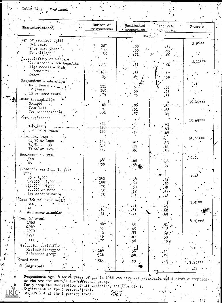
Table 7A.3 Continued
t
GfiaracteristicsbiNumber ofrespondents
i
'Unadjusted I 'Adjustedproportion 'proportion
F -ratio
BLACKSAge of youngest gild
0-1 years'
-'2'or more 'rearsNo children
Accessibility of welfare'Law access -*low bellefis
I High access -.high.benefits
Other .,
Respondent's education',0-11 years .
12 years
13, or more years
,.Debt accumulatibn
. Some''''debt
Not ascertaina ble
Work experience0 0
ears3 more years
Potential %.:age
Si .50 or less.
- 1.9'9
$2.0Vor more .
Res.'ien, in SMSA,Yes
No
fl
.
s,
husband's earnings in 'astydar
$0 - 3,999'$1;000,- 5,999.'0'
- 7,99988,000 or more
- Not ascertainable
Does health limit work?Yes..
NO-
Not ascertainable'
Year of event.
1968
4a969. 1970'
19711972
pisi-uption
Marital' disr4p,tee. Reference group
Grand mean
R27(adjusted)
287
132166
'325 '
164
96
251- 460.
.7k
164 -
197221,
211
196
1 268
263114
386
'199
4'242' 155'
'75
35
:78
35
518
32
68A
99119.
129
170
.50
.60
73:
.57
.5g.-.65 ;
.5i=
.59
.75
.56
.61
%
.34
.79
.142
.59
.88
.60
54.Aky.
, .58
60
.6o
45
6 .41
.6o _
.6o
.55
.61'
.56
.5
459 :.
.58
I
.62.68
.47
43
'.63
2 V
.59
.65-, .48
T4 5 -
1 1/4
.691k.'
.501
49ri
,771.777
2.12
-
'1.42***
19.65***
\35.22***
0.08
1.148
3.91**
....,
; 169. .59 ...
*1+16 .58
. .1
/4-. J
.,
.
e .- a RespOndents age 14-to',2L-years of &i.ge in 19.68 who have' either7experienced d firit disruption.or 11Tho are inoltided'6in thelrOferencagronp.,
b- For v. complete description of'all varia.bles; see Appendix B. I
4
4* .Significant at tile 5 percent:level. -I ,
"
*.**' Significant at the.,1 perce4 level._ 2.,4 7 ..
.11 ,
", 7:294t**
.21

,... , . . Z ..
Table 7A.4 Unaddjustedand ANusted Proportions of Reference Group in Labor Forceto at Time T, by Race:, Multiple ClassificatiorilAnalysis
,/ ,', .
Cliaracteristics
Number ofrespondents' ,'
-
;,Unadjustedproportion, latportion
AdjUSt4d- F-ratio
// WHITES
Age of youngest child0-1 years , .
2 or more yearsNo children
Accessibility of welfafelaw access ..., low benefits
High access- high benefitOther. .
Respondent's education- 0-11 years
12 years .
13 or more hears
Debt accumulationNo debt
/c..
Some debtNot ascertain bli %
Work experience .
.
0
.. 1-2 years .
s. 3 or more years
Potential wage$1.50 or less , 4i$1.51 - 1.99$2.00 or more .
Residence in SMSAYes
.
No... _
Husband's earnings in past iear
$0 - 3,999 ,
$4,000 - 5,999.16,1360 - 7,999
$8,060 or more.
Not ascertainable....
Does health limit work?Yes .
No .
Not ascertainable
Year of event
- 1968 ..'
-.4969
1976,',1
V4'..-
- */ , k.
Grand mean-/'
.!F (adjusted).
.
,
,
558
323.
900
.
.483
711587.
344
975462
527
510744
.
437615729
545
575'.. 661'
1',074
. 707
,j 55938'
c 36
-3 0
/ 1 7
/
76.1 619.
86.
210305422
,3-60
484.
.1(781
\
,
.
-
-
.
.
.
.
,.
,
..
31.42
.77
.55
.56
.57 -
.34
56.71
.
.63
.57
.51
30-- .59
.69
.27
. :52
.82
.57*-
.55
.63
, .-6f
. .57.41
.53
.43
.56
.62
.44
.49
.52
.52
.71
.56
.39
.49
.69.
4'57 .
.56
55
63.58
.47.
'
- .53.-
55.59
.52)
.61
.54
, ,
.27
.5o.8.3
.52. .63
.6o
.63
.57
.44
49
55.56
.64
.
.561'
.52-.53
.5
'.6
. 6
.
-.
.
.
105.09***
1.
. ,
0.26
'`.
.
16.83***
2.82*
f
8 42***...
300.36***
, ..
129',94***
12.9*A*
..
2.06
.
4.17***
.
40.55**40 ,
.34,
A 248
e .
(Table continued on next page.) '
.
9
28
qr
r.

0
Tble 'Continued.
" e
Characteristic0 '' 04-
.1 ,..7, Number ofrespondents
,-
Unadjustedproportion
. ,.......
/Adjusted4roportion
,
F-ratio. . ,
.
BLAdkSAge of youngest 'chin0-1 years " -
2 or more years, No children
..-., .
Accessibil welfareLow..,,,, ,,ce's`i - T ow benefits
,
geraccess. -: high benefits'''. Other
P4spondent's educations','0-11 years1,2 years e- '.
Voe13 or more ears
Debt accumulationNo debt: .,' )Sote debt .
Not' ascertainable
Work experience.
4.1-2 years
3 or more years -.%ksPbteritial wage.
$1.50 or less .
$1.51 - 1.99. .$2.00 or more
.
Residence in SHSAYes '
No.
t Husband's earnings iii past year$0 3,999 ,
4,000 7 5,999$6,000 - 7,999
._$8,000 or moreNot asctrtainah26
Does health'limit work?Ye
'''N't:A...
Not ascertainable.
Year off' event
1968, '
1969p
1970 i1971
.
1972. .
Grand mean. a
R? (adjusted).,_/
.
..1:
.
,
/
.
,
.
,.
'
'
.
4
A
,
,
194
85137
.
244
113
59
154
1.9g
64
;.16
145
155
.
10)- 129
138
18713
9
t277
139
,
172
11-8
58
'2741
25.
371:20-
3873
76
99':130
416%,.59. ,
,
,
(
'
.
,
'0
.
.
-
-
.
.
.
"..
,
...
.
-
.
.
,,
..
.52
.56:72
.57
. .59'
.66
.
;49
:6Q
.82
,:
.57,
.61.,
.5/
:v
.34 .
.62 ..
.81.
/
.42
.60
.87
.60.
.57
- -.
..60
.58
.64.-
74
.38
,,-.
.45
.62
.5
t
.5T '.:
:62
-59:,62:56
,..
.
e
'
. .
.
''.
.,
.
.:..., .
.55*
.58
.66
,. .63
,52
.57
-.58 ,.
.57
,68. -
. .62
.64 's
.53
'.40
.63!
.:744
'4.147
\ .63
. .75
.58-
.62 ''.,
.
.63 ..
.57 ', 4
.63 ..
.63.
.-4Q
-
,
.,
.49 ,
. .61
q '.39
. ' .
. -
57e.68
. `' .66-...53.:55
, ".
.59"
r k....
'
-.
2.514'
2.56*
%
1.43
.
9.46*"'
.
24%1&***..- ,
). ,
%
13.'64***,
.
"0.74,
2:50**
,
.
, ..
.4. 6G **%
.
*2.22*'.4,
.:,,..,\.
..
-
£T 5*,*
'?
.
,
.
.
,,,,
\
, ,a -For a complete detcPiptdon "6441 ,variables, see
.
Appendix B. 7
Sigdificant at the ao.percentlevel,, ,
(,.. ** Significant- at the 5 perceritlevel. 4 ' .,*** Significant at the 1 percent level..
f,
ay
I 4,
e.
r
249 ."

.y.
4
Table 7A.5., . .
.
Unadjusted and Adjusted Proportions of Marital' DisrAption Group in Labor
force at Time T, by Rade. Multiple Clasificatiol Analysis
'
.:Characteristics ---- ,
Number ofrespondents
'Unadjustedproportion'. proportion
Adjusted F-ratio
. WHITES
- ...
.. ,Age of youngest child.0-1 years . ,
2 or more yearsNo'children
Accessibility,of'welfar eLow access - low,benefiiis '
High acces - high betlefits NOther ,
". ...
Respondent'snt's education0-11.years ,
12 years13 or more years .
Debt accumulationNo debt "
'Some debt
Not4aseertainable ._.
Wokk.. experience - .
0
1-2 years -
3 or more years7
Potential .Wage:
$1.50 or les's
$1.51 - 1.99$2.00 or more .
.
' Residence in SMSAYestio ..,
t
Husband's earnings in past year
$0 - 3,999 .61.,.$4,000 - 5,999
$6-,1 - 7,999.$8,o o or moxe' -
Not ascertainable
Does health limit workfYes/
No, , .
..
No ascertainable
Yea pf eventi 68 ,
.
a 69 -
970 .
971 t ,.
972. .
, G nd mean ° .
' R (adjusted)
..
88
-60
.. 93
62'in
.
.. '78
-
41'1i8,"
'39
. -
0 51,
92
98
- . .
-71,i:
73
97..
' 1057066
.
0
\ , 162
79 '
173
`.44
.39
------24
15
211'
'15
./,
3545
52
59 :50
. 241
i
,
.
.
.
.
.
°
.
.
4.39.50
.73
:56
:48
.63
.40
.62
734
.54
.58
.53-
t.24
.56
:75
.28
.62
.89
.53
.59
.55
.55
.64
44.53
.33
.58
.36
.38
.54
.0
.68
.57
.55
'
-
.
.
..
-
,
0
-
.
9
'
(
.
.
...,
-, .47
.50
4 :66
.
( 52.49
, ,65._ ,
,.58
.59
.31
-
.35
.5a
.70
'.63
.61
.45
,,15
.65
1.05
.46
.75
56.56:61'
.47
.50 ..
42. .57
0 -.42
, .4'b
.42
:3$
.73:69.
.55 4.
.
.
.6.17***
3.67**"
6
15.45***,..
5.84***./-...-w
112:92'***.
,,-
.,
.4'
. 29..21***
,
0.81. '
,
,,
2.03
'
8.62***
%
7.69***,
, .39.
250 1,
(iCable,dontinued on next page.)
2; o
0
I
.

L
-#
O
dale 7A.:5 Continued
. ,
Characteristicsa %,
.- 0/ .
.
* Number of %
respondents.Unadjustedproportion
Adjustedproportion
,
F--"rato
). BLACKS. 7-.Age of youngest.aild
0-1 years .--,- ''. .
f- : 2 brY'MoreyearsNo chiWren -7... 4,'
Abcessiblity of welfare,L.o4 access - ,lbw benefits
.
High access - high benefitsOther A
.-, - .
Respondent's education~0-11 years12 years ,
13 or More years . .
Debt accumulatInn .
No debt,-,
. Some' deb;, ,
Not ascertainable. .
Work experience .
0 ,
.
, ,
.1- years1 -2
3 or more years'.
Potehtial I./die..p
.$1.50..or less' $1.51- 1.99 7 .
$2.00 or more
Residence ,in SMSA -
..Yes-
::,1N
'. ..
, 4*,
Hil3I-a_3's earnings, in pest year °.: S:C.- 3,999: .':' - ,
$4,3o0:- 5,999$6,000 - 7,999 _...,
.1:8,00 or more
Not ascertainable
i ,oes 'health limit work? '
.qys' ,,,..:
No ,' . ,
'Not ascertainable -.
..
Year of evert968
.A.
, . ,
c,
' .1970* . ...
1971'''tAt,.
:1972 ..,
1
Grand mean
R'0'(adjusted)
r
.
..
,
'..
.
.
,'
%
,
'-'..
4,
- ,
.
r
,
.
.
. .
,
93 ,
47 .
9
81,'
51
at. -
97.
62
.10
I,
48
52"-- ,
.09
6?
-9--q'7,,
.
8.1
no
-73
,,
10,-) ,.°
60,
37R
.,
. a.7.,,,.
.10
-1'.7
. .:,-,'
. .
30
)6. .
43
30ov
40
169..
'
-
.
.
2
.
4
,
.
,
.
,
.
,.,.
,
47 1
.67
.69
,..
.57
-.49
:.62
..
.
.54
.59
.50
,
32:.63 c
.52
"3''. 6'4
.72
.
..141
.58
.93
.60,
-4
.52
.52.:63
.49
b
.
.2a ,
.58
.49 . ,
,
64
-.55.1,9 -
:59
.54, .
.56 _ '
.
,
.
,
'
..
. ..
.
:
49.66,
.63
. .
.69
.-,0.jo
.53
.67
.47- .
.15
..
..39
.62
.60'
. .
.,.
.;-,5,
.60
.38
61
.930,
.
.61.
.14). /-
.55
.53
.65 ,
.36
bv
.
.41
.57
.49
.p59.2+8
.53,
.59-
.61
.56
.-,_
2.69*
.
7:304 **
.
9.88*4*
3. /4-3*,*r
.
.:
.
15.33**.w
5.19**.
.".
1.52.
.
'
'-..
0.69
0
.
0.53
..
.
a
. 2.79***
.:20
.
,
,.
a - For a.complete*des,crij.?ti= of all
.
ab les, see Appendixppendix B. -
b Pr4pOrtion riot reported wherelcategory cottaipsless than°10 respondents.! \ SigSificant at "*10 rercent1eve**", :Significant at .5 percent level. .
**.! Significant at the 1 percent level
Z 0 I 1 . 1!91-
°
''251,,

. . ..i
:, ,.
,.
) 6 ' '' ..,, ..pI , ,
Table 7A.6 Onadjusted and AdjuOtedProportions of Marital*Disruption Group in the Labor Force'at Time)1-F 1,,by Race: Multiple Classifination Analysis
0
I
..-1.
Characteristicsa. . . .
'.
'Number ofrespondenti
. l' Unadju-sted
prop6rtionI Adjusted.proportion
F-ratio
-WilTES.
Age of youngest child.
0-1 years2 or more years
4 No children. .
Accessibility of welfare) '
Low access - low benefitsHigh access - high benefitsOther' ,
-. Respondent's education '
- 0-11 years'' 12 years ..., .
13 or more years
Lett acclulation . .
No debt.
Some debtNot ascertainable .
.
Workexperie nce0
14 yeari --...0
3 -or more years9
Potential wage-$1,50 or less$1.51 - 1.99
..
42,.00 or moreResidence'in SMSA p
Yes' ,
'''' tkNo
. .
Does'talth-limit work?.
No - '
Not' ascertainable
_ Year of event' 196S
19691970 :
.1971
.1972 .
,
'Total fIaMily income less respondent'searnings in past.yeiar
.-$0 :- 499 , .
$500,or moreNot ascertainable ..
-Greinci. mean -.
'R2; (adjusted)
/
.
,
.
,
r .
5786
84
53
'96
78
89
109.29,
82
6778
-
.
49
64
114
85
63
79
15374
22
185 .
20
30
44
46
5750
.
105
'91r
28
227
.
,
.
4
,
.
'
.
'.
'
.
...75
4
.
,
.
.,53
.80..:
.r9
.67
.70
,.63'
.78
.83,
.68 .
.73 .
:78
'',3ES
.85.0
153. 74
)70
..79
.
.
. 54
.76 '
.64
.81.
.79
*65.73.69
.75
..72
.69
.73
.
.
.6O ..*
.82
.73 ,
loloo.
.86
.65
.74
.
.
.75
.72 ;
.69
- .81
.82.
.56,
..59..85 '.72 .
,
.50. 72
.97r.
:-- .68., .84
.67,..-
.73.
.78
, .- ..99-
.99 .
.61
.- .62
.58 .
.74 .
:.74
,65
0.73
..
.
5:87***
.
5.26***
0.36
.
.
10.96***
4
,
6.16***
.
.
31.69***.
.
8.67*** '
0.41
.
,
,12.98***
---
.
0.59.
k.99***
"s" .27._
,
.
.
(Tablt continued on next page.).
252'
_
292 .
it

.
.
.
,
.
.
.
..
.
.
.
,
c.
a a -4._ . 1
..o, . . . ! ..ITable TA.6 i, ,Continu
-. _ ,
, . .. . ,
6
...°
,
.
a.
_-
...
.'
vs'
.
,
,
.
..
.
Characteristicsa
..
.
Number ofre4ponderas
UriadjUs;ted 4
iroportion
. .
Adjus.1..e-d---, f .F-ratio
proportion , : . .
. .
' BLACKS . .
Age: of youngest child ... ,
,, Cll. years ...
' 2 or more yearsNo childran .
Accessibility of welfare'Low access - 1pw benefits
-.
Hi.gh access - high benefits .
Other k
Respondent's education .0-11 years1 years . . .
13 'z'rr more yearsi
.
Debt accuAulataopllo. debt .
Some debt .
. Not ascertainable
Work experience \ ,
0 ,
1-2 years.
.
3 or more years.
Potental.wage.. -
$1. 50 75"?...1ess-
$1.51:- i.99 ..
$2.00 or more .
Residence in SMSAt -
Yes .
'.',7,-.. <. ,
Does ;ilea th 'limit work? \F. e:,
.
No.......
,Tiot ascertainable....
. .Year of event .
19819 a a19101971 .
1972 1 -
Total family income less respondent'searnings in past year
A
o $.0 -'499'$500 or more
,
Not'ascertainable
Grand mean ,
-
R2 (adjusted) 0
. . °
65
72
26
.
68 .
:. 5243.
93-60
. 10
°
6P. 43
56 t
48, 48
. ,67.
,
4
7269 .
22
- .
'..,11.
'50
,14
139, 10
.
..
30
25
.3929
40'
65, -83
1.
. 163f
...4,--
.
,...58 -
. .64
. .77
.727 -.63'.
.3,
.52 -
- '..73-
.95
? .
.,,
.59
TO -
- , .64
. .46
, .61 . -
.78
'.49.64
r -' 1.00
.66
.59
.
.21
.70 , .
.59
.78
.48_
.79 \-.58
.52
.69
.61
.49.
.64 .
.
.61
.60 :
.81.
- .77
.59...
1
.51 4
r---,-
.63. .64
.
.65. .
.61
";1
.61
, .
.58 .
.65 .
,67
-
c .41.74
.86
.62
-.68
.21
.70 .
.55-.
.
.72
.53
.77
.54
.58.
. *
,:6.67.54
g
.64
2%85 4- :
' 5.74***.
0.61.
,
0.91
.
'0.63.
s.
A
..
15.21Je*
$ .
0.51
,*
.
.
.
2.41*
°,
}
0.61
3.690T'
.26',....
.
a
.
.
.
,
.
.
., 6 ' .
a For a complete description of all variables, see Appendix B. .
* Significant at the 10 percent. level... .
***_. Significant at the 1 pyrcent level..
.
:A.
.
.
..
.
..
,.-
-
.
4 / 293..
,
. .
. - . o, .1., . :.253
''. ' .; . . .
-.... . .
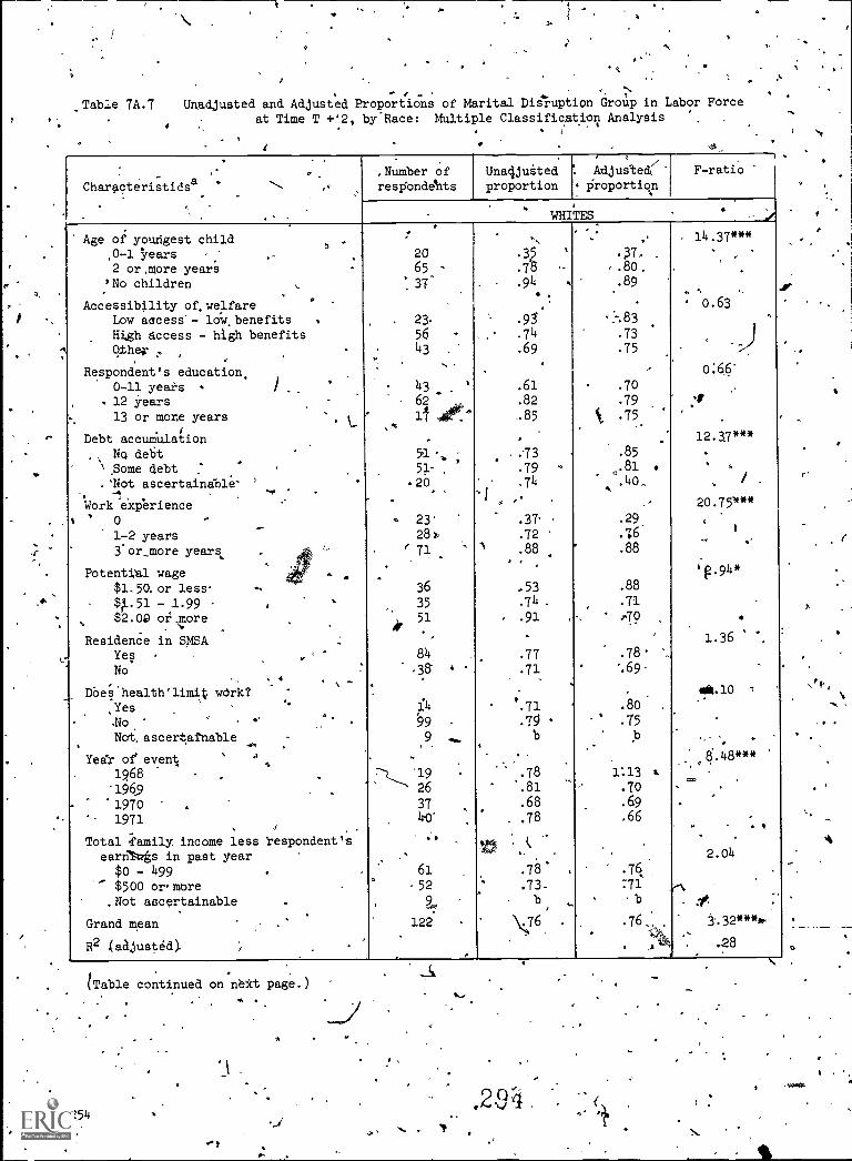
1.3*
.
Table 7A.7 Unadjusted and Adjusted Proportions of Marital Disruption Group in Labor Forceat Time T +'2, by-Race: Multiple Classification Analysis
.
°, ,Number of Unadjusted : Adjustea,
F-ratio
Characteristidsa '.-- respbndehts proportion . proportion. . .
.
.
.. .. WHITES .
.. ,Age of youhgest child . .14.37***.
0-1 Years -: - 20 35 ' .37,. ,
2 or ,more years - 65 - .78 - .- .8o, .
,
'No children . ' 37° . .94 A .89
. .
Accessibility of, welfare '
..
0.63
Low aacess'- lo'wbenefits . . 23. 95 '-_-.83
,. .Other 43 . .69 .75 :,
High Access - high benefits 56 ' .74 .73.
),
.Respondent's education, o'66'.
0-11 yeafs ' 43 ' .61 .70
, 12 years , 62 . .82 .79 413 or more years
f
k._ 11 Air. -85 k .75-
Debt accumulation
.
12.a7***
..
, \ Ng debt.
51 -o.81 ...
. ;73 . .85
Some debt : ,' 51- .79 *.
/ ..'Not ascertainable' ' ' .20 .74 .40,,
-, , ,. . , ,1 A
Work experience.
20.751***
t ' 0 ..
- . 23*.
.37. .29
1-2 years 28k' .72 .76 -
3.0r_more years = ' 71 1 .88 ' .88
Potential wage 'F.94*
$1.5 or less- . 36 .53 .88
$.51 - 1.99 , 35 .74 . .71 .
$2.04p or ,more 51 .91 ,-. ..70 .
.
.
Residence in SMSA _ ' 1.36
Yes 84 .77 .78.
No .-aa .71 -.69.
, . .
DOes'health'limit work? . . 41.10 1
,Yes..
Z4 .71 .80
.No ' ' 99 .79 .75
Nat ascertainable9 A.-
b b.
... . .
-- . -
Year of event,.
.- '
A ,-, , .
6.48***
1968 - . . 7--) '19 .78 1:13_ I.,. ---...,
'196,9 26 '.81 .7o -
. 1970 . 37 .68 .69 .
,
- 1971 lco' ,78 .66
Total .family, income less respondent's
earn'
.
, keargs in past year . '- 2.04
$0 - 499 .
.
61 .78 .76; .
$500 or' more .52 ' .73- :71.
.Not ascertainable/ 2.!
b4
, b 4ot .
_
.
Grand mean . 122 - \76 . .76 ,- 3'.32 * **
. .-
R2 :(adjusted). , . . .28
tTable continued on neit page.)
2514
ti
.2.94
0
.

1'
`c.
Table 7 .7.
Continuq0.
e
*Chara4eri ticsaNumber ofrespodents
Unadjustedproportion.
Age of youngest child0-1 yeaf2 more,,years
No.children . .
Acc essibility. f welfareLow access -'low benefitsHigh ftces - high benefiOther
,.Respondent's edu
0 -11 years ,\12 year13 or more .years
ation
Debt accnmulatio4,No debtSome debtNot tbcertaina
Work experience
01-2 years ,
or more years
Potential wage$1.50 or leSs$1.51 -1.99
..$2.op or more
Residenoe'in SMSAYes
)
Do- nealth.limit work
No
Not ascertainable
Year of event..1968
196919'TO ...
1971 1. -. .
44tal family income less respondent'searnings in past year
$0 - 499$500 br moreNot ascertainable
Grand mean
R2 (adjusted)
a ,ir a completet Proportion not* -Sigqificant at** Significant at*** Significant at
, ;1.
mormommilme
.
26
65
12
44:3326
61 '35
. 7
Ad-juste-1
'prpportir.
BLACKS
.
.60
.65
.64
. 61-
.63,
.73
.61
.59
"75
.6o
.66b
.56
38 .74
23 , .60
2130 /52
39
21
.26
. 68
;.78
49.65. 8 3
.64
. 59
: 69
.65
56.b
. 56
.65
.73
.3873
.69
F-ratio
0.07
0.39
..
1.21
. 56
.6
.83
77 .60. 26 .68 .7
5
8711
2222
36'
23,"
.
40-'
6
103
b
.69
.49
.59
. 57
. 72
.66
70.57,
bo,
. 6h
.1
e
.42 1,
-648
.64
0
:63
b
.64
3.1,!,**
0.14
'1.85**A
description of all Variables, see Appendix B.Ireported where category 'contains less than 1,0 respondents.the 10 percent level.the 5 pLercent level.
the ,1 percent level.'
'255

4
r
256
4
9Tdble 7A:8 Number of Respondentsa Experiencing a Marital Disruption by,
Year of Disruption and Ritce
.
Year of disruption. .
Race total-
.
Whites_
Blacks
Total- ,
1968-1969 -
1969-1970
3.47019 i11
071-1972
1,972-1973 '''
449.
,
.68
-. '8o
102
96.
103.
*,
'.,
.
264
35
52 a
59
-64
5
'.
'
:
185.
3
29
43
.32.
48
a Frequencies are unweighted data. ,
7
Table 7A.9
al/
Number of Respondentsa Experiphcing a Marital Disruption,lyType of Disruption, Yeg14f Disruption, and Race-'47
1.
Year ofdisrupt,ioon
Race total Whites Blacks -
Sepciration'Divorce Separation Divorce *Separatio7tivorcd
Total
1968-1969_
1969-1970.
1970=1971
1971-1972
1972-1973..
306
48
, 57
68
64 ..
. 69.
251
A .
P53
59
82
;144'
19
31
30
. 35-
29
'.
.
.
,192..
16
24
43
43
66
162 .
29-
26. .
38
28 .
4o
...
59
4
13
10.
O. .
16
a Frequencies areunweighted data.
Table 7A.10 Number' of.Respondents4 for Reference Group by Yearof5Action and Race.- -
Year ofspletion ! . Raee tote'14 Whites Blacks. .. .
Total,
1968.
196.
1970 -0
1971
. ..3.972,,
-
.
t2,305
285
371
527
514
68o
0 ,,re
.
1,862 -
2301
301
k444
398
48e
443 1
46
JO
83
116
128
. __
a Frequbncies ere unweighted data.
2 °b0
6
t
.4

. .
.'
APPENDIX A..
SAMPLING, INTERVIWING AND,EUIMATING-PROCEDUiES
I
-
2 9 -
o t
if b,
a
O
,-4
A tt,
4
;
id).<
..
,.4..

-
I .
APPENDIX A
SAMPLING,,.INTEIRVIEWING AND ESTIMATING PROCEDURES4
. .
.The Survey of Work Experience of Young Women is-on? of thefourlongitugnal surveys s3ongOred by the Emplbyment and TrainingAdminisfiTation of the U.S.' Department of Labor. Taken together,these four surveys constitute the NatiOnalIongitudinal alTveys:(NLS). Each of tie four NLS samples was, designed bx the' Bureau of'the Census to represent the'civilian noninatsttutibpal population ofthe United States* approximately the time of the initial survey. -
Because of attrition from. the sAmples.oyer'the yearsqthe'surveys,they Cannot be construed to be precisely representative of the.civilian noninstnntionalpopulation iA any year after the first.
tSample Design
The cohort is represented-by a multistagesprobabililr samplelocated in 235 sampleareas'comprising 485 counties and,independent
T-cities representing every state and he District of Columbia: The235 sample areas were selected by grouping all of the nation's countiesand independent,Aities_into about 1,900 primary sampling units (PSU's),and further forming 235.strata of one.or more'PSU's'thatare relatimelyhomogeneous'accordingto SOcioeconomic characteristics_:Nithiri each ofthe strata a single PSU was'telected to represent the stratum. Withineach PSU a probability Sample of h9using units was selected to represent
',the civilian noninst4utional.'populatioh:,'5
Since one of.the survey requirements was to provide separatereliable statistics, for blacks, households in pYedominantly blackenumeration' districts (ED's)' yere-selected at aAftlte approximately'three times that-for houteholds in predoMinantly white ID's'. Thesample was des4:zned-to provide approximately 5,000 respOndentsahout4190blacks and 3;500 whites.
- ,
An initial sample'of about 42,,000 housing' units was Selected;and a screening'interview took place,in 1 4rch and April
this number, aboUt'7,500 units were found tOLbet,vacant, occupied by-persons whose usual residence was elsewhere, changed:1'1-am "'residentialuse, or-demOlished. On the ether hand, aboUt 900 additional units wereibuddlithich had been'Oreatsd within existing living space or had. beenchanged from what was previously nonreside5tial space. Thus, 35,360,housing unit] were available for interview , of which usable informationwas cbllected for 34:622 households,a completion rate of 98.0 percent.'
Following the initial. intericiew and screeningoperation, thesample was rescreened in :the fall of immediately prior to the .
first Survey of Work Experience ofMales 14 to 24.. For the rescreening.cf, operation, the sample was stratified by the presence or absence of
, .. .
. p-. -...'
29a
4
259_

5'
14- to 24-year-old woman in the household. The rescreened sample.was used to designates ,533 young women age. ,?.4 to 24 as of-Januar1, 1268, tobe ineivieWed for-the Survey 0 Work Experience. These
were .sampled differentially, within four strata: whited'in white ,
ED's ED's which contained predominantlywhite households);nonwhites in white. ED's",-,yhies.in nonwhite It's% and nonwhites innonwhite ED's. : '
. 0-
I
;
.
'I
S
..
#
.. , ..,**
The Field Work . , /,o .
.
. .,
-il
Over 300 interviewers were.assigned to eatlis:Ot the surveys. '
. s..
Preference in t selection.election. of interviewers was..given to those who-
had had, experience on one of the other /longitudinal. surveys. ,Since
many of the procedures and the labor` forte and 'socioeconomic concepts'used in this survey were similar to those used in the Current
.
Population Survey (CPS), whenever possfble,;the BAreau of' the Censusused:intergiewers with CPS experience, . ''
0 .7Training for the interviewers consisted of a home study package
which included a refererice manual explaining'the purpose, procedures,and concepts used in the survey and the home study exercises and_a setof questions'basedon points explained do the manual. In addition tothe home study package, in tEe earlY survey years theu. Were one-dayclassroom training sessions whith all interviewers were required to'. .
attend. All training materials were prepared by the Census Bureagotaff.
reviewedand reviewed 'by the Employment and Training Administratioreandthe .,
Cenier fOr'Haman Resource Research of The Ohio State Oniver ity. .'
Professional.membets ofthc/participati.ng organiiations obse d both-
the training sesiOkS and the actual ifterViewing.
13 addition to training, i,field,edit wad instituted to insure
adequate quality- This consisted of a full edit "ofthecoipletedquestionnairesby Data .Collection Center staffs. 'The edit consistedof reviewing each -q-ftestionhaire from tegimiing to end; to leterminewhether the entries were complete and consistent and whether theskip instructions were being followed-. If -there were minor problems,
the interviewer was cosiyacted by phone, told 'of hererror,.and asked
to coAtact.the.respondent for further clarification. For More serious ;
problems, the interviewer was retrained, either totally or.in part,
and,the questionnaire was returned to her for completion.
Estimating Methods06
The estimating procedure used in the NLS involved multistage ratio- , -
,estimates.0
Basic weight' The first ,step was the assignment' .to eakt,sample
case.of a basic weight consisting of the reciprocal of the finaprobability of seleqtion. The probability reflects. the differential
sampling which was employejd by race_within'each stratum.
./
260/
:. 299
1.
4-0;11'0

V
INoninterview,adjustment, IcA41e-initial survey the weights for.)-
.tall those interviewed were adjusted to the extent needed to account'forpersOns for whdm no information was obtained'becauSe of absence,refusal, or unavailability torsother reasons: ThiSadATtment was madeseparately for the following groupings:- Census gegion,4Place of.residence, and:race. ,
.
Ratio estimates The distribution of the'population selected forthe"sample may differ somewhat'by chgnce, frop that of the nation as'4 whole with respect to residence," age, race, and sex. ,Since thesepopulation characteristics, are closely cOrrelated with the 'principalmeasurements madefrom the, sample, the. measurements can -be substantially,'improved6hen weighted appropriately to conforlOo the known distribu-tion of rese population oharacteristics-.1 'This was accomplished-V
.-the initial survey through two stages of ratio estimation'. '
`The-first stage of ratio eStimation'takes into account differencesat the time of-the 19k Censusin the disti-ibution by race and. .
residence.of the-population as estimated from-the sample PSU's and,
that,of the total population in each of the four major regions of thecountry.- Using 1960 Census data, estimated population totals by raceand residence for each region were computed byapprippriat'ely weightingthe Census counts for PSUls in the sample. Ratios were, then computed'between these estimates (based on sample P§T.P.$) and-the actual'powlat'on t o tats for t e region as shown by the 1960 tensils.
/ In the second sage,independent` current. estima
population by-age and race
he sample Proportions wereadjusted to ,
es of the cilfilian honinsti'tutiongilized -,T4ese estimate's were prepared ItrNawrying
.
, forward the most recent Census -data (1960) to take account or subsequentiging of the population, mortality, and Migration betweeh th=e UnitedStates and other countries.? The adjustment vat Imde,by race within,
. four age groupings.. °
-._
, Weights for subsequent years As a result of the above steps,=..
each sample person'has a weight which remains unchanged'throughout thelife of study. The universe,of study was thus .xiipa at the timeof interview for the first survey. Since no reweighting of the sample
. was made after subsequent surveys, the group of Interviewed persons-5,8--. -...\ .
,
.1See.Bureau of the Census
Population Survey- -A Report qnexplanation Of the preparation
Technical Paper no. 7,. The dutrenidethodology,.1963, for a more detailedof the estimates. a
..
.
.2See Bureau of the Census, CurrettPopulation Reports; Series M-254.
,.
A
.no. 352,.NoNfember 18, 1966', for a dIsaceription of:the.methods lised'in, .
preparing ,these independent 4opulation estimate4._
t s
300
.261
I ,

*
an unbiased sample of the population group in existence at-the time ofthe first survey only. The number 6f young womenwith whom inertialinterviews were cdnducted was 5,159:
Coding and Editing
Most of the.Uata on the'interview schedules required np,-coding,since a majority ,of the answers were numerical entries or in thie fOrmof precoded categories. HoWever, clerical coding was necessary forthe occupational and industrial classification of the speral jobsrbferred to in the interview. The 'Census Bureau's staBlard occupationand industry-codas'used for the CPS were emplbyed for this purpbse.Codes for other open-ended questions were assigned by the,Cehsus.Bureau, ini,some'eases on the basis of guidelines developed by theCenter for Human Resource Pesearch from tallies of subsamples of thereturns.
The consistency edits fothe interview schedules were completedon the computer by the Census BurarK. For the parts of the question-naire which were similar to the CPS, a modified CPS edit was used. Forall other sections, separate-consistency checks were performed. Noneof the edits inhluded location rilutine which was dependent onaverages or random i ormatiOn from outside sources, since s alloca-ted' data could not.,,he expected to be consistent with data fro previous
.. e, or, subsequent surveys.° However, where the answertb,a questio wasobvious frop others in the questionnaire, the missinganswer was enteredOn the tape. To take an example from the 1970SurVey, if item 62a ("Isit necessary for you to makelany regular arrangements for the careyour'child(ren) while yOu.are working ? ") was blank, but legitiM
.
entries. appeared in item 62b -and 62c ("What arrangements have you made ?"
and "What is the cost of these childcare arrangements?"), a "Yes" wasinserted in 62s! since 62b antcccould have been filled orily if theanswdr to°62a was 1!Yes." Therefore, the assumption was made that eiththe key punch operator had failed to punch the item or the interfiewehad failed to record it.
/V
A 4
o
\ .
$
301t". 262
. /
3*

a
.
P..;
°
. .
APPENDI X BA
INTERVIEW SCHEDULES
1
4
30:2.
r rc
7
-
r r

Budget Bureau No. 41- 112423. Approval 'Expip's December 31, 1973O'oRrA 4T-401 , : .-
u s, DEPARTMENT OF COMMERCE .
BUREAU OF THE CENSUS
. .
.NATIONAL-LONGITUDINAL SURVEYS
. .
lURVEY OF,WORK EXPERIENCE .
OF FEMALES 14-24--,,.
.,
.
. ,1968
.
.
.1;NOTICE 7 Your report to the CensuS Bureau is 'confidential' by law (Title,1,3, U.S. Code). It may he seen only by sworniC'en sus employees and maybrused only for statistical purposes.I. Control No.
. ..
2. Line number.s ,
pf respondek. .
-
--,3. Warne' '
A.
.
.'4. Address a ,...,
.
.. ,
5. Interviewed by , I Code ,
1 ,A
.- t-_. iI t
RECORD pf CALLS AND METHODS OF LOCATING' RESPONDENT.Date Time Comment
F NeW occupants 4,NeighborsApartment house mgr.Post office ,.
ti I. School .
r Other Specify .
uccessful Unsuccessful
a.m.p.m,
i.
2.a.m.P.m.
..
. , .
3.
/a.m.p:m. ,,
' -. . ...t1 . ., .,
GI:
4.a.m.p.m..
.
..
7t.'RECOR OF INTERVIEW
Intervie time,
Date completed' Comments,.
.
-
J. .
4
4 .
1
.
Began Erided
a.m. a:m.fin.
_.
.1.It ,4 :
- r. a NONINTERVIEW REASON r . "4
1 'Temporarily losent - 3 i Refused . -.
2 --- Unable to locate respOncient Specify A n-- Other Specify_1 ,
,, \ -. .
. .-- ..,. TRANSCRIPTION FROM HOUSEHOLD RECORD CARD ' -
.
.
2eIdentification dItm - coe ' '4' . Itgin 15 2 Age `1
er. . .
o, .r ...;.'; ,
Item 22 -.Tenu/ er- ,I Fl Owned pr);Ieing bought .
2 El Rented'3 F i No cash sent
rItems 23 --,25 'Land usagei F.; A 4,(7 0
. 2 Er; a t t El E.,e(EiC ,
.
11~ Item,13 Maritql status Item 16 Race
1 ;=-1., Married spouse present . 1'7' White.
2 Eli Married spouse abseht 2 1 -, Negro 3.,":,,.
3 7. WtdOwed 3 T ,- Other ., ' .._4 E , !Ivortea i 4
s ' S'ep'arated .6 f" Never married . .
- -, . . ,- r ,-- ,r " '. ',. c::"'"'"'"IF RESPCINDEtft iidg MOVED, ENTER NEW_ADDRESS ._ ..
rNuryther and street..
-..
City
.
.
'ZIP code
(-
-Coigity .
4
State
.303 265

1
\ ' AND TRAININGi. Are yob att nding or enrolled in regular'scholo.lE,DUCATION
.- ..
. :, -
.
1. 1 0 Yes ASK 2
2 E] No 7 ....When were you last enrolled? 1 SKIP,
, Month-Year to 4
2at-Whatgrade a e, you attending?, , t ,
.."
. . .
.13,:Are you enroll d as a.full-time or-part-time student?
2a. 1 Ele I 2 3 4 5 6 7 8 - SKIP to
2 High _ 1 2 3 4Check Item C,'pose 7
3 College I . 2. 3 4 5 6+_
b. i E2 Full time '
2 E Part time . 1
0 El Resporident3. Since you. turn
for.an entire y
is, IA - SKIP to Check Item c, page 7d 14, were you ever out of schoolar?
,,3. 1471 Yes - SKIP to 8
2 r: No - SKIP to Check Item A
4.'orha't is the higyotihave comp
. -,
estyear of regular Schooleted? .
-.
4. ' x' 0 - SKIP to 34, page) 00 None
i Elem ,I 2 3 4 5 6 7 8
2 High . 1 2 3 4.3 College. I ,2 3 4 5 6+
5. How raid were ou when you last attended ----4.
regulCr school.. ,5 , x
Age - . _
'6. Why would you say you decided to end yourseducation at that time':
- .
. l. u
.
N ' - ,..
. .
6..
0 ET Completed 4 or more years of collegei Had to,A4ctr4s .
2 [7: Couldn't afford college'__-3 I j Lack of ability ,
....
'4-[J'4-[J Disliked schoolu
1 5 Li Marriage k., 6 E: Pregnancy '
7 F.: other Specify
7. Between:the timein 5), Were youyear or more'
you turned 14 and (Age mentioned' 7. 1 [],Yes - ASK 8 I2 r] No - SKIP to Check Item A
- , .
"
ever out of school for an entire school
--,8. How old were you? (If more than once, ask ,
about most,recent time.) ,I'
8: x IAge
.,J9. Why were you out, of school at that time>
.
9 , .
e
10: Vhy did you return to school? .] ','
- ,,
- .
CHECK
ITEM+,
.. _1 El Respondent is a college grad te,- SKIP to I la '3 Flespondent is enrolled -1/i hoof - SKIP t o, page 4
3 -'"1 All others - ASK I I a: i 0 ,*.,
11a. Do--ycLu feel that not havinl more education .
has hurt you in any way? ,
. , ..-b. Why do you feelthis way?
, .
ll .a. . \ x
, i(-] des 2 [-] No
,
,. .
- ,'",
12a. if you could, would you like toget.mbre .
education or training,b. Whavkind of courses or training lould you
like to take?.
,
, ,
-c. Do yaii-expeCrilitou-ectbelly-All get this . ..Y,%ikeducation or training? .
.. .
,
120.1 ED Yes,- ASK b 2 [] No'- SKIP to 13a
b. 1 [T Techhical (vocational), traiping - Specify type,['Complete2 ['Complete high school
,3 El Go to dolle _...
4 E--, Other - Spe- . x
----c.-11-1Yes When)______ __________ ,-
- 2 E.; No Why not? 04- -
. .
3 F Don't know .. \
i66 3'04

, I. EDUCATION AND TRAINING Continued,13a. Aside from' regular schoOl, did you ever
,take a full-time program lasting twomeeks.or more at.a training course, sponsored,by an employer? ;-
b. 'Wha.t type of training-did ,you take? b. .
13°' 1 E] Yes ASK b.,
2 [D No SKIPsto 14a
c. How long did this training last?
d: Howmany'liburs per week did You spendg/t12i,sitkising?
. d,,e. Did you finish or complete thiscourse?
1
'Why didn't you complete the program?
g. Do you use-this tretining on, yourpresent (last) jobL
e. Months
'd. 1 ni 4 3'n10 14 5 L:J 20 or more
2n5 7 9 N' [7_115 19
oe C.: Yes ..-SKIP to g2 MN° ASK f
.
3 El Still going on SKIP tcl 14a
'f
1 (]Yes2 F3 No \3 r] Never worked
14a. Aside from regular school, did you ever take .
au, commercial, vocational, or skill training,such as typing practical nursing, coSmetalogy,or anything else, not -counting on-the-jobtraining given informalJy7
b. Whig did you decide to f Qiore training?
c. What type of training di you take?
'd. How long did this training l'ast?
e. How many' hours Per week did you spend"''on this training?
f. Did you finish or complete the program?
g. Why didn't you 'omplete the program?.
, h. Do you bse.thts traming'on yourpresent (last) job?
14a. it] Yes ASK b .
.2 El No SKIP to 15a
b.
c.
d. Months
*.IF11-4 - 3 Et0-14 5 Fin or more2 In 5 9 4E115
f. ,C] Yes SKIP to h2 Ti No -;ASK g
.3 El Still going on,, SKIP to 15a
9:-
1 E] Yes.. 2 nNO 3 Lij Never worked15a. Since you'stopped going to school full time,
have you taken any additional generalcburses in a regular school such asEnglish, math, science, or art?
b. Why did you decide to get more education?
c. What type of course did you take?
d.1-1'"Ow long didihis course last?
e.' How many hours per week did you spendon this course?.
f. Did you finish or complete thii course?,
g. Why dtdn't you complete thiS course?1 7Z 7 rrr- rz 77
h. Do you use this educkion on yourpresent (last) jot)?
.77 1'F .1 1
15a.
1 ri Yes ASK b
."\
' 2 ENo.- SKIP to 16a:
c.
d. Months
e 4,
2 17] 5 9
3 Ell° 14".4,] 15 19
ED 20 or more
f. 1 Yes' SKIP to ty2TD-INIO ASK g3 FT] Still going onSK1,P to 16a,
-91-"
h. 1 ri Yes2 (-1 NO
- 3 TI Never worked
.267.

4
I. EDUCATION AND TRAINING - Cantinueci.
16a. Hiveyou ever obtained a-certificaterequired for practicing any professionor trade, such a s teacher, registered .1 . ,
nurse; practical nurse, or, beautician?
b. What type of certificate was \it- - 0
.. .
1-..
?
. - .
c. is this certificate currently valid? .
16a. 1 CD Yes - ASK .I6b ,,i e -,*
2 ON° -;SKIP to 17a, .- ,.
b..
- . '`
'e -i.
.
c. 1 _ED `Al :-. 2 111 No.
:
...-,. II. HIGH SCHOOL EXPERIENCE -
X 1-] Never attended'Iiigh school - SKIP to 34, page 10lia. What is the name of the high school you
., ,attend (Last attended)? ...1-( .
.
b. What is this trigh school's address? .
1 9
.
a s
*,
.
. 4..
.
Co' Is this school public'or private?t
d. in what years have you been (were you).
enrdlled there?. ,P
e. What kind of curriculum are (were) youenrolled in (during your last year inhigh chool) - is (was) it"vocationa, .cornme ial;college preparatory
4
i or genera.
..
. "'17a.K -
.
., .
b. Street..* '
-. .'City
.County P
.
State.. Pi.
ZIP code.
P.' ' '
c. I Ca] Public- ' 2bPrivate =
d. .. -
.
,
From ToMOnthYear - MonthYear
Vocational Whartre4. 1 [] Voti specializing..
(did you specialize) in?.
2 C2 Commercial .d
3 ED College Preparatory , .,"2*5 0 .7+.4 E] General 1,
.
18a. Are you. king (did you take) anycourses in typing or shorthand in .
high school?b. What courses are yoLi taking ('did you take)?
° 4 ,
.
..
c. How,many years have you taken (typing, shorthand)?, , ^
180. I EaXes - ASK 181i-: c rt 2 ED No - SKIP to Check Item B
b.,,r L-] Ty,pirig -2 ED Shorthand -'3 ED Both
e . - , -. c. Typing .
r -. Shorthand .
CHECK
ITEMS
\ C-1 Respondent has completed one or more years of college(Q2 or 4) - SKIP to 24a, page 6 . .
2 CD Respondent -has completed less ;Ilan one year of high'school - SKIP to Check Item C, page 7
3 []AU others - ASK I 9a .
ir. 4 'a .. ,. . , I
19a. What high schdor subject' do (did) you enjoy .the most? ....,
.
, °-....1+- . .
b. What is-'ihe main reason you enjoy (enjoyed) ....?.
.
..
-..- ,..--
. . -
i.
. ..
19 a. .. -
o [] Norie.- SKIP to 20a
b. -1 ,ED Interested " . . ..-
2 ED Find it easy * .
3 ED. Do well in it I,-
4CD Prepares for future job or career -
5 ED Prepares for homemaking.___
- slorp Other - ',Specify,
20a. What high school subject do (did) you dislike,the most? .!
. ,
, -h. -What is-the main reason you dislike (disliked) ...?
; .
:k,'!
20a...
.-.... 4. 0.
0 [-21one - SKIP to 21a ..
b. 1 fl Diffitult; hard work . .
I El Felt.it.a waste of-time,-, .
.3 r-] Do pooily 'in iti ri Boring ..
.ri. Other - Specify, .
268 V

II. HIGH SCHOOL EXPERIENCE Continued21o.. IN YOUR LAST FULL YEAR IN HIGH SCHOOL, -
how.many Hours per.week,,onthe Overage;did you spend doing your homework, athonie or.anyWhere else?
_ .
- 'b. Where chtly6p normally do most of
your hienework?
c. Were there any cortditions at this place-which made it hard for-you to study?, I, .
d. What wete these conditions?
e. IN YOUR LAST FULL YEAR OF,1-11H SCHOOL.did you take,part th any extracurricularactivities at school, such as sports,
_Aromatics, publications, music, or clubs'
5
f. HOw many hours per week, on the average,did you spend-on these activities?
4. What-was yor.r 'avorite extracurritularactivity?
.;
1.1
21.a.o []None
4') `4z. 4
2 E 5 7 9"0.3r71 JO 4
4r:}15 19 .
more
ti
11
, 1 E School library, study hall on home om
i home
At friend's hOme..7
..tn Other ,Specrfy
AS d
l'i. ___] Nose (distractions)1, 24-71 Licks necesiary faelities
(desk, room, etc.) #- \\.>3 El/Other" Specify '
e: .
2 F-7 No SKIP to e
Yes --=ASK f
241 No SKIP to 22
9
f. t -4.2 [7:] 5 t93111 3 Id--144 E7.; 15 7 195 F,-1 20'cii more.
`'
g. 1;1 r_71 Spdrfs
- 2.n PubliCattons
3 [] Dramatics.e 't ,
4 ETTjtsluSicge
5,["1-0theo-clubs-
,6.,fl 0 Specify
f,,A22. When you were not involved in high schoolactivities or stud g, what activity took
'up-most of:your- tra time during your lastfull high school ear?
22. EiNon-school,elateit sports
-2 ET Hbbby
3 [] Reading,
4 LT Ww.k.for pay_
5 r-3 Helping at home
6 Other Specify23. How do (did) you feel t bout-your high
school experience? 23: Do (dJ, yoU
1 E3 like ie,rry- much?
2 [].hike well?
3 F.--J dislike 'it:somewhat?aer4 I-7 .dislik it very much.?
,
3 ' q69

,r
III\COLLEGE EXPERIENCE . ,
x 0 Respondent has never attended college° (Q. 2 or 4) - SKIP to Check Item C, page 7
24a. What are the names of -all the colleges youhave attended? .
ASK FAR EACH SC OL ATTENDED
IL When were yquenrolled there?,i
'..
C. Where is thisschool located?
-./ -Name of Gollete #
From.-Month/Year
To.?-. %
Month/Year City.
State
, \4
s
,
.. - .,'
le.
. ....-
3...."-- .
,..,
. . ..
4. ,
.
. .. .
d. What degree did you receive? (If more ' ,
than one, record the most recent) - , N,.
, ..,
_. .
e. Iii what.field did jrou receive your degree?
f. Why did you detide,to major in ...(field of study mentioned, in 24,e)?/
).
...
.
.
,`ii,
g. What is (was)-the full-time tuition per year ,-at (most resent s'chool given in 24a)? .......-\
h. Do (did) yo4have a scholarship,,flewship, assistantship, or other .`ty' of financial aid while enrolled ..at (most recent s2tliool given in 24a)? .
.!
. _
re"zp
. (
-.'i. pHow much is (was) Tt? .
j. Why did you decide to continue youreducation beyond high school?
_
.. - ,
-'
-.
.x = Respondent has not completed One year of -
college (Q. 2 or 4) -Skip to 30, page 8.
25o. What field of study in college,do (did) you4-., .-ip -'
.enjby the most? -./.-., 0.. 4, es
-. .-- -
b. What is the main'reason you enjoy (enjoyed). . a... - - , ' '
....
,,
<.
'-.
. , -7,
.
,
s
d. . ., . .
-.. . .. f
.. a [] Did not receive degree - SKIP to g
,, ... li.,
e. .
f..-
Interested in it . . 0 .
3 [] Advised to do so
I possibilities5= Prepare for homeMaking ,
' 5 = Other - Specify . .
..
$ ff; 1 = Yes .
. 2 [1 Scholarship or fel lenhip )i3 D Assistantship (teaching, research, etc.)i = Loan : : ,
. ,,
- 11 , .
. 5 E: Other Specify.
6 -, Sir
No.- SKIP' to j ,. ,
v. P
i. ty -/-, .
.. 1 Col= lege degree necessary for her work .
i . 2 =College degtee necessary 4r(succeis .
3/C] Wantecreore educatioh .
4 E] Qther -Specify -. .
. ..
. , . .
250. . -
-
i[] None - SKIP t 26a.,
. , P
b. 1 [] Interested in it-2.[] Do well in it
, 3 Ej Find it easy , . . 7
,4 n Prepares for future jp or careerV 3 El. Pfepaces for homemaling, ,,-
17, - -
. II .%, r"'6 El, Other' Specify ... -
, :. i4.
270 e

0.
' t M. COLLEGE Ei(FERIENCE Continued .16o. What field of study in 'colleg9rdo (did) you dislike' * ,,
the most? ,: , e
& ,______ .
- N', . .' . .
b. What is the main reason you dislike (disliked).. a
,. ,
..
' _ '
26a. .- . . . .
. ..
/ '. o E.: None SKIP to'27
b. 1 n Diffttult * . .. .f2 n Felt'it a waste of time
3 [J Does poorly in it 4 , _-4 E' Boring , .5 n Other Specify ' e
.I'27. How.do (did) you feet about your
college experience? , .
. .
. ',. 1
1 '
27,. Do (did) yo --,
.1.Erlike it very much?'2 El 'dislike it very much? .3[_] like it fairly well?4, El disii}2 it somewhat? i
;), FiResponCtent is-attendmg college(Q. 2) SKIP to 30
nr,
28. Would you like to receive,umore education?. ,
.. .
, .,.. 1i . ..- '-
28. t ri Yes SKI? to 30.
2 Ej No SKIPto.34. page 10
.HIV. EDUCATIONAL GOALS OF THOSE ENROLLED IN SCHOOL . .
4CHECK
ITEM C.l'HIliespon ent is enrolled in school-(Q.I) - ASK 29a .
. .
2 [J dther SKIP to 34, page 9 , //.
.
29a. How'much More education would you like to get?% .
(If ':None:' mark 'current grade and fdllOw appropriate,skip pattern). ..
.High School College < ..I .
o [?Less than 1 ri I year i 5 7 2 years (complete junior college-or equivalenthigh school .(ASK. b)- 2 7 2 years, ASK b 6 7 4 years,(graduate from 4-year college)
.
3 years '' SKIP to d- 7 [-r- 6 years (obtain Master's,degree or equiyale r
41 El 4 years SKIP to c 8 (-- 7 + years (obtain Ph. D. or professional del ree),
.--: (M.D., Law, etrok / . ....,
,, !
b. Why don't you vyantito complete high school? ..-.
-,. .
c. What do you expect to do When you.leave school?,, - ,'
-i. ., -,-
_
d. What college would you like to attend? ---.. -.) t '8S
. .
.
e: What field of study would' you like ,r,,
I; to take in college?
).
.
f.- WhY, would iou like to go into this ifield of stuffy? 1'
4, , , ,
f;,,: .--,.
e. . t *fr.
/ .... .b. / .
C. f El.Go to wo,rk I SKIP to'Check
2 _1 te,t,marriea ( Box3 r Other Specify / 'after 33c
d. Name. 1r . Y
VPLocation (City and S ate)
..
.. 9 Ti Undecided ,. ."'..
e,.
.
99 El Don't know SKIP to 31
f, 1 ED I'm interested in it, I enioy.ite. . )
2 [ ] It prepares for vocation SKIPthat pAys'well, is secure \ to,
r -31
i Ci Other Specify -
4-
9

,
.
'IVEDUCATIONAL GOALS_OFrTHOSE ENROLLED IN SCHOOL - Continued .
-,- 7 ...:- -0, 30. 'How much "niore college would you like to gel?.
..: , k6 ,
..-- ..
- . , ' /,
,
,..
.
30. 5 1 1 2 years (bmplete junior college or equiv?tlent)V, t ... p",6. 6 I 14 years (zr,:advate frc-n-four-year college)
7 ( 16 years (obtain Master's degree or equivalent) ,t
- IOU 74 years (obtain Ph.D. or professional degree)r (M.D., Law, etc.) ,;
... .. .
31. As things now stand, how muchmore education do you think You' will actually get? ,..
. .
College: .
.,High school olI
4.:,. :.t - r ., .
.!, r .1 1 year . .. , .. ..
- 5 1 1 2 years (complete Junior CalJege or equivalent) -,
. ,2 r i 2YeaPs ' . 4 I. I 4 yea; (graduate from 4-year college). \ ,
. 1 ''a I. r3 years 7 I '' I 64 yea,Ps (obtain Mastet.'s degree or equivaleat) , '
-.1..-t- ..
1- 1 4 years . .. , ---.'8 I- f 7 i years (obtaici Ph.D. or prOfes-sional degree) .
- (M.D. Law. etc.). . ;
, .
-
Nip
...
..
.
-
CHECK
ITEM D
Amount recorded in .31. is: : , .
..-. . . le: ..i t I Same or . greater than amount/k\ n in 29a or 30 - ASK 32o
2 1.1 Less thqnamount iven in 29a or 30 - ASK 32b.
'-Is
32a. How will you pay for this additionaleducation?
.
.- . ' . ..
. -
- i' .. ,
.. .
. . ..
b.:Why do you think you will actqally get .
.: less education -than you Wouldlike? - .-
a. .
- .
- ..,..
..
':',."t
32a. t I. I Scholarship
42 I
,2 I Loan
- 3' r I Parents ,,
_4,1 .1 Wolk...,; . - t--it, I Don't know, not s,'.4 e
.-t;'.6 I J Other - Skecity**, :
..,.'
SKIP P to 33O.
b. t I I Too expensive: lack of sufficient funds2) I Difficulty, in getting into college
I I Family obligations',
4 I I Have to go to work. .
5 I ' I Other - Speci.fy.______=_,___.._:._ .... T
.
4.
.
33a, What do you expect to do when.youcomplete our editcation?
.
.
. ..
. ab.ub you exPect:to work when you are .
first married? ? ... -
.... /
. I1 ,,
c. What kind of work would you like to do? .
o''.
33a. -i I j Ob to work- ASK c .
.
'' 2 I .1 Gat married -- ASK b .
: _ 3 I A Other - Specify -.
.GO to Check Box after 33c
...
'
4,---.
b. 1
o
1 Yes - ASK 't .
2, I i No - GO to Check Box after 33c. ., I 'Don't know t -
_
.
v,4, ,;-.;-'
C. .
.
While answering-Section IV was another person present? -, 5\ .
.t L--I Yes, ' 2 1-1 No - Go to 34 . .
. 4 ..
. -' .
Would you say this person influenced they respondent's answers?. .
..
i. 1- -1 Yes 2 I -No ,-., -
.
3

I/
NOTES
Irt
F.
4
S.
,
..1..1
r
p
eT
1
3
O
I
,,3:11
e
2.7-3
0
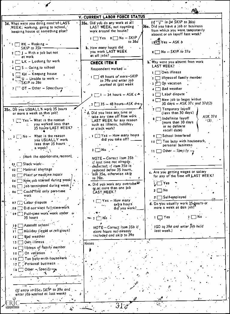
V. CURRENT LABOR FORCE STATUS
What were you doing mosi'cif-LASTWEEK; working, going to school,'keeping house or something plse?
WK Waking -SKIP to 35b
2 E j With a job butnotat work
3 E., LK - Looking for work
E; S Goingto school
5 ] Kki - Keeping house6 72 U Unable to work -
-*-n5KIP. to 38a
7 FT- OT - Other - Specify.-7
35c. D'O you USUALLY work 35 hoursor more a week at this job?.
zs
What is the reasonyou worked less than35 hours LAST WEEK?
2 E No - What is the reasonyOu USUALLY workless than 35 hoursa week?
(Mark the apprOpriate Jeason).
kfOSlack-wark--02 Li Material shortage
03 Plain' or macrkine kepair
04 ri New, job started during week,/ ,c
05 Job terminated during week;
. 06 ri Could firid only part-timework
. 7 :2-Labor dispute,08-[] Did novviant full7timeolvicrk
09 [],Full-timwork'Week under35 hours
10 E Attend§ school'
I i HOliday(legai or_retigiousY
12 [ i Bad weather13
14 El Illness of iarni1)% member
'15 C.] On va'cation
4 16 CO Too bySy with house'werk
17 E -:Personal business -
1'8 E Other -,Specify-
1 []Yes -
35a. Did yob do any work at allLAST WEEK-, not countingwork around the house?
Yes x No - SKIPto 36a
b. How many hours didyou work LAST WEEKat all jobs?
CHECK ITEM E
Respondent worked
2 [] I - 34 hours - ASK c
3 n 35 - 48 hours-ASK d-e7.. . i
t.
. d. Did you lose any time or' take any time off from wdrk
'LAST WEEK for any reason-. such as illness, holiday,
or slaCk work).
1 O 49 hours or-more-SKIPto39a and enter job.worked at Last week
2 7 4
(if entry iri.35c. SKIP to 39a and .enter job worked at last week)
I O Yes - How many hoursdid you take off'
2 D
NOTE -Correct item 35bif lost time not already.
-deducted; if item 35b isreduced below 35 hours,4aek 35e, otherwise skipto 39a.
e. Did you work any overtiineia9,/,at more than one jobEAST,WEEK ?
17 Yes - How many3.., exa hours
did you Ivork?
2 [2 NO -A
- NOT-Correct item 35b ifektra hours not-already-included and skip to 39a
(If "J" in34 SKIP to 36b)36a. Did you have a job or business
from which you were, temporarilyabsent or on layoff fast week?
Yes - ASK b
x O No - SKIP: to 37a
b: Why were you absent from workLAST WEEK?
f, El Own. illness.2 [] Illness of family Member3 It Op vacation4 Bad weather
5 Q Labol. dispute6 [] New job tobegin within
30 days - ASK 37c and 37d(2)
7 Ej Temporary layoff(less than 30 days)
Indefinite layoff(more than 30 daysor no definiterecall date)
9 ED School Interfered
10 n Too busy with housev)ork,personal business
ASK 37d' (3) _
it O Other - Specify
c. Are yo-u getting wages or salaryfor any orthe time off LAST WEEK?
I .0 Yes `-
2 O No
3 El Self-employed
d. Do you usually work 5 41 ou r s ormore a week at this job?
Yes O No .
(GO tq 39d and enter rob he Idlast week.) -
Notes
I
*
4

f'
4
V. CURRENT LABOR FORCE STATUS - Continued
(If "L_K" iritem 34, SKIP to 37b)37a. Have you been looking for work during the past 4 weeks?
x [-.1 Yes - ASK b 41 LT] No - SKIP to 38a" 4b. What have-you been doing in the last 4 weeks to
find work?(Mark alhnethods used; dolma' readhst)X Nothing-- SKIP to 38a0 [7. Checked with school ernOoyment
service (or counselor),
Checked with State employment agency.2 i Checked with private employment agency3 Checkeii direCtly with eMplorer4 Placed,or answered newspaper adss Checked with friegds or relatives6 f Other - Specify - Forexample, MDTA,
Union, or professional register, etc._
c. Why did'you start looking for work? Was it becauseyou lost or quit a lob, at that time or was theresome other reason?
Lost yob2 _Quit yob3 Left school4 i, Wanted temporarr work
5 i tier - Specify,
d. I. How many weeks have you been looking for work?2. How many weeks- ago did you start looking for a yob?3. How many weeks ago were you laid off' -
Number of \iveeks
e. Have you been looking for full-or partjtime work?
'`2 Part-time
f. Is there any reason why you cdold not take a yob.LAST WEEK' ,
4s Mark reason-;4 Needed at home
2 Temporary iltness3 7 School4 Already has yob
5 r,. Other - SpeCify
Nofr
9. When did you last work at a regular full-or part-time lob' or business lasting, two consecutive. 'weeks or more? -
r 1963 or laNk
Month. Year.
2 C- Before 1963 - SKIP to 39a andenter Ibst job-
3 Never worked 2 weeks 44'atore
4 [-.; Never worked at all
SKIP to390 andenterlast job
SKIP to44a. page 14
38a. When did you last -work at a reg u lar full- or part:time yob or:business lai.ti.ng two consecutiveweeks orMofe?
1 [ -] 1963 or later
-Month Y.efir, *
,) 2 [T1 Before 1963
3 LI Never worked 2 weeks or more4 Li Never worked at all
j SK44a. pages14
b. On this yob, did you usually work`35 hours ormore per week?.
c-135 of more2 Less than 35
c. Why.diNdlou leave that yob?r 1 To get married.
2 r Husband wanted her to quit[. Husband 'transferred; moved
4 Own healdr5 Pregnancy6,i 71-idalth of family member7 ri Devote more time to family8 School9 L Seasonal yob completed
10 Slack work or business conditionsI I: Temporary nonseasonal yob completed
.1 2 f- ' Unsatisfactory work arrangenierit (hours, pay, etc.13 Other - Specify
t
39a. For whom did you work? (Name of company,orgtnization, or other employer)
b. Where located?
CityState
C. What kind of work were you doing?(Far example- teaching, waitress, salesclerk, typist, etc.)
d. What kind of business or industry is this'(For example: TV and radio manufacturer,retail shoe store, State Labot Department, etc.)
;1.
e..Were you - .
t [` P - an employee of PRIVATE company,
W business, or individuol for I. .
wages, salary, or commission?. . 2 [..-, G - a GOVERNMENT employee
(Federal, State, County, or lacol)?3 L 0 - SELF-EMPLOYED in OWN
' bus.iness, professionalplractice,-or farm?
"ll's. this business incorporated?
1.r Yes- 2 E 142
4 L WP-Working WITHOUT PAY in4.family business or farm?
ASK 4e3
SKIP to40b
- N.
313 275
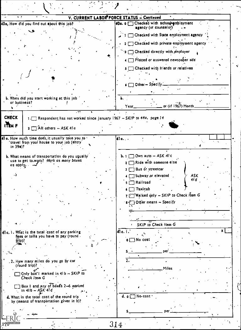
\'
V. CURRENT LABORIFORCE'STATUS Ceetinued
40a, How did you find out about this job?
40:
fit
b. When did you start wo rking at this jobor business?
40a. o ED Checked with Schoo,lirnifloymentagency (or counselor) ...
1 ED Checked with State employment agency
2 ED Checked with pri.vateemployment agency
3 ED Checked directly with employer
4 E] Placed or answered newspaper ads
5 ED Checked with friends or relatives
6 0 Other Specify
Year or (if 1967) Month.
CHECK
111164 F
1.0 Respondent has not worked since January 1967 SKIP to 44a, page 14
2 n All others ASK 4Ia
41o. How much time doe's, it usually take you to'travel from you house' to your job (ebtryin 39a)?
b. What means of transportation do you quallruse to get tojrk? 'Mark as many boxesas apply....
41c. 1. Wliat is the total 'cost of any parkingfees or tolls you have to pay (roundtrip)?
;40* '
.2. How many miles do you go by car(round trip)?
cP0 Only box'l marked in 41 b SKIP to
Check Item G
ED Box I and any of bOxes 2-6 markedin 41 b A'SK*41d
.ikt=
d. What is the total cost of the round tripby (means of transportation given in b)?
,21.6
1'
41a.. .
b. t ED Own auto ASK .4Ic
2 ED Ride with someone else
3 ED Bus Or streetcar
4 EDSubway.or elevated ASK
5 ED Railroad4td
6 [] Taxicab7 []'Walked Only SKIP to Check hem G
I-0 Other means Specify.4
SKIP to Check- Item G
41c. I
o ED No cost
$ per
2.
Miles
d. 0 E] No-cost
per
314
I/

CHECK
ITEM C'
N. CURRENT LABOR FORCE STATUS Continued
1 E"P" or iteni 39e ASK 42a
24::]"*".'.or "WP" in item 39e SKIP to Check Item H
42a. How much do (did) yoii'464n at ytiur(present, last) job?
b. How many hours ,a week do (did) .youusually work at this job?
c. Do (did)'you receive extra pay wAn youwork(ed) over a certain number of hoursa week?
d. After how many hours doldid) )ou'receive extra-pay? ,
e. For all hours worked over (entry in 42d) pprweek, are (were) iyou paltd straight time, timeand one-half, double time, or is there someother arrangement?. Mark as many as applyand explain.
CHECK
42a:per
b..Hours
c.1 [1] Yes -,)ASK 42d
2 [J No
. 3 L - compensatory time only
4 E] Never work overtime
SICIP toCheckItem H
d.CD Hours per day 2 n I-fours per week
e. 1 [] Straight time
2 E Time and one-half
3= Double time
4 Compensating time off,......--
: I : 5 [7 Other SPecify: ' ,
. .. -. .
l'Ej Respondent is in Labor Force Group A (WK in34, or "Yes" ,'in 35a or 36a) and entry in 40b is before Januar' 1967 %ASK 43aA,
2 EIRespondent is in Labor Force Zroup A and entry in 4013 is January 1967or later SKIP to 43c ---; ..
a Eji All others SKIP to 44a ..43a. Have you ever done aQy'other kind of
work for (nameofemployer. in 39a)?b. What kind of work,were you, doing a year
ago at this time?
c. Were you working a year ago at this time?
ci. For whom did you work 'then?
e. What kind of business was this?,
f. What kind of Work were you doing?
g. bees the work you do now require, morethan the work you were doing a year ago?
h. 'Do you have more responsibility in the workyou are doing now than in th'e work you weredoing a year ago?
43a..Yes 7 ASK b 2 [7jNo --SKIP toll
b. Ith 1
1 Ej Same as current job 7 SKIP to 4 3 g
c. 1 E Yes ASK d 2 El No SKIP to 44a
d.
0.
More2 ED Less
The same amount.
Notes
h. 1,CDMore2 C:I.Less.3 The same amount
315 277
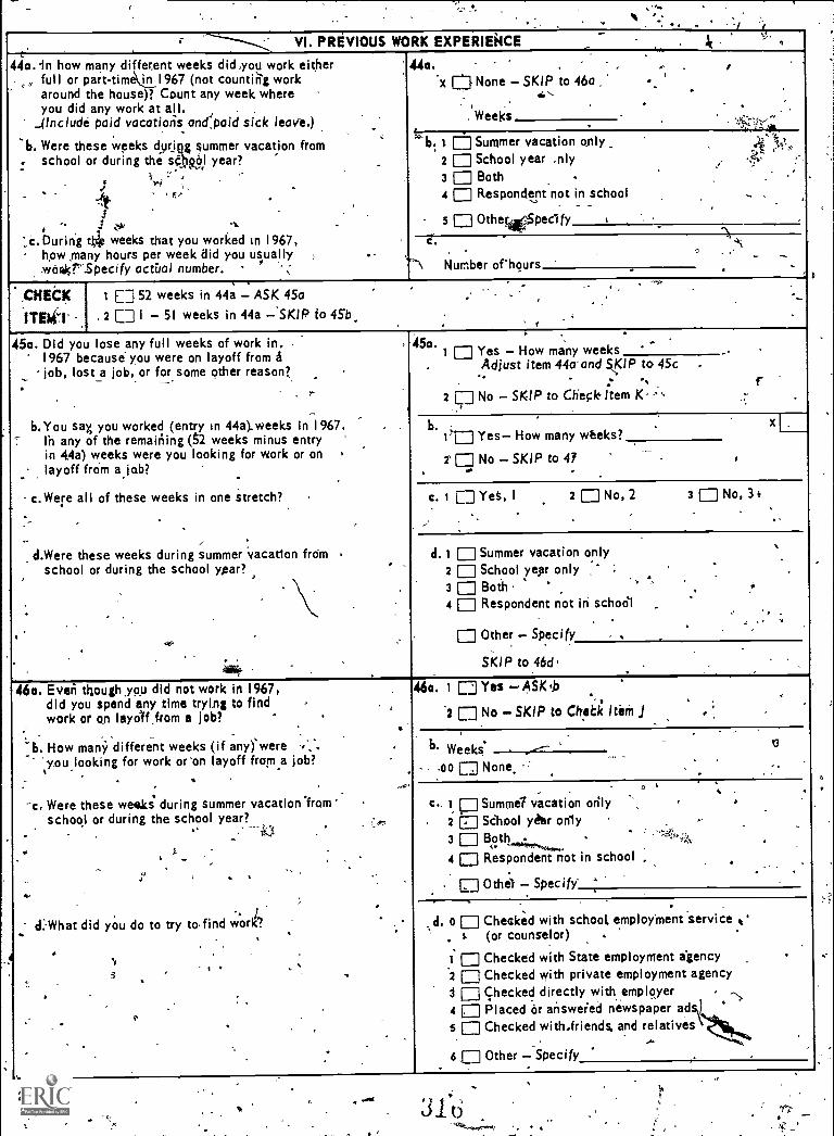
- VI. PREVIOUS WORK EXPERIENCE-
.%,-. .
44a. in how many different weeks did you work either,, full or parttimk11967 (not counting work
around the house)? Count any week whereyou did any work at all. . .
_(!nclude paid vacations ancli,paid sick leave.)
b. Were these weeks dying summer vacation fromschool or during the sit
,&b+1 year?
. . . d _
3.. .. _1 .A.lc. During tt* weeks that you worked in 1967,
how many hours per week did you usually.weekr-Specify actual number.
'440.'x Cp None SKIP to 46o .' ..
.14- -
. ., Weeks .
-,..
. - A--
'-b. 1 Summer vacation only, .
2 111 School year .nly3 Both . .
4 Respondent not in school -
5 1111 OtheWepecIfy t .
c
Number ofhours,.
.CHECK
iiEhil'1 E3 52 weeks in 44a ASK 45o
, 2 ED I 51 weeks in 44a SKIP to 45b
. , --
.
. r
......
.
45a. Did you lose any full weeks of work in.1967 because you were on layoff from ajob, lost a job, or for some other reason?
...
b. You sax you worked (entry in 44a).weeks in 1967.-:' in any of the remaining (S2 weeks minus entry '
in 44a) weeks were you looking for work or on '
..- layoff from a jab?
c.Were all of these weeks in one stretch?
-.. .-
., , .
d.Were these weeks during summer vacation fromschool or during the school year?
.
. ..
. .
,
.
-
..
.
.
,
.-
,
45a. . -I Yes How many weeks .
. Adjust item 44a'and SKIP to 45c .
'''' - :2 [::] No SKIP to Check ltem K. . ,
.,.
. .
b. x I .
1 Li Yes How many weeks?
7 No SKIP to 47.
c. 1 t] Yet, I 2 No, 2 3 No, 3+.
.
d. 1 Summer vacation only2 School yeer only :
.
, ",3 Both4 Respondent not in school
, ., ..
Other Specifys
.
.
-
.
SKIP to 46d, .
46a. Everi though,you did not work in 1967,did you spend any time trying to find ..
work or on layolf,from a job? ,. .
.
-b. How many different weeks (if any)'were -; ".-. youlooking for work oron layoff from a job?
.:c, Were these weeks during summer vacation 'from
school or during the school year?.
.
' -.. .
. J I . '
,,
/d:-What did you do to try to findwork?
. .
. _
.-,
.. . .
0 .
,
. . .
.
.
.
. :,,,ft,
..
,
.
,
'
...,
,
.
.
46a. 1 Ej Yes ASKb -, ,
2 0 No SKIP to Chick lath, J,
. .
b. Weeks...00 None -r
__ _
- E2 ,.
p.. - 4. .
c.. 1 Sumtnel vacation orily.
2 ,0 School yder only ....
3 Both '',-*,..
4 111 Respondent not in school .
ED Othel Specify :,
,
. d. 0 Checked with school, employment service. ls (or counselor)
Checked with State employment agency.2 El Checked with private employment agencyJ al Checked directly with,employer4 1111 Placed or answeiecl newspaper ads5 II Checked with-friends. and relatives'
.6,L] Other Specify
. .
a78 Jib

-
VI. PREVIOUS WORK EXPERIENCE - Continued ,-.
CHECK
1 TEM .1
i'.[] All weevIcS=ofil 967 are accounted for - SKIP to Check Item K
2 E Other - Ask 47.., ... - , ..
47. Now let me see4 During 1967. there were about ". .
(52 weweeks minus entries-in 44a, 45a, 45b or 46b)weeks that-you were not'working or looking
.for work. What would you say was the main r
reason that'jiou were not looking for work aduring these weeks?
., .. . .
,
47.: 1.E Didn't want to work,, .2 CD III or disabled and unable to work
rth of child3 Birth..
4 0 In school -
5 0 Too busy keeping hoUsdg.
6 [] Other,,- Specify
.. x L.
. ....--
CHECK
ITEM K
.
,. i ELI Respondent has not worked at a job since January 1967 - SKIP to Check Item LRespo-ndent has worked at a job since January 1967--- .
.7 [] "0" in 39e'- ASK4 8 .- .
3 L., juP," in -G," or "WP" in 39e - SKiP to 49.u _
48. Did yd4 work for anyone (else) for wagesor salary in 1967?
I - ' -
ii& 1 E I Yes - ASK 40
2 El No - SKIP to Check Item L49. In 1961, for how many different , .
V,
employers,did you work, ..
49. ,Number of employers ,.
o [ -I Did not work in '1967.
xr Respondent never attended a full year of'high school - SKIP to Check Item L ,
^ a50a. During your last full year in high SChool,
aid you hold a regular job that lasted twoweeks pr more (not ummer job)?5,4...
b: For whom did you Wog,.
c ..What kind of work did you dog Specify ..
kind of. work . .
I/.,.
d. What kind of business or industry -is that' .. .
..e. Whereis (Was) this job located?
5. How did you find this job?' ;
. ,
. ... -'
. .. '.z........--
.
-. . . .
. .. ,
' ..
50a. Vi C : Yes -7, ASK b .
---e2 [ ;No,No.,- SKIP to Check Item L'
b..
'
,,c.
,..
x [,.. J Same as current (last) job - SKIP to-
. . Check Item Lt:1:--
. 1 1 1
e. City.
State ', -
f. 04, }Checked with schobl employment service.,.I. (or counselor)
.ke1 [] Checd with State employment agency
2El Checked with private employment agency3 [] Checked directly with empl er ,
4 LT Placed or answered newspaper ads' .
5 E Checked with relatives or friends6 E.; Other - Specify
.
L ,
.
.,
CHECK
`IT-EM' ITEM 1..
iir'..
Respondent is enrolled in school this yearepa -, -ti..
.1 LT] In,Labor Force Group A, usually works 35 hours or more a Week -- ASK 5Ia ...2 [-_1-:1 All others in Labor Force Group A - SKIP to 69. page 203 CT, In Labor Force Group a - SKIP to 610, page 19 . )fr
.4 E All other; - SKIP to 66p, page 20,-5 C: Respondent. is not enrolled, in school - ASK SI a
.
51a. Now I'd dike to know about the first job at which, yoU worked'at least one month after you stopped
going to school full time. For whom did you Work?. ,
, ..air
b. What kind of business or industry was that? *40....tt,.it
41a., *: . ..
.x_L°7 Same as current (last) job - _-
SKIP to Check Item M, pose 17
.....
,
b..
'.,
279

et
VI. PREVIOUS WORK EXPERIENCE Continued '
51c. Were you.'
1. Arl employee of PRIVATE company, -business; orindividu I for wages, salary or commission?
2. A GOVER ENT employee (Federal, State, -
, county, dr:I al)? ,...: -
3. Self-employed OWN business, professionalpractice, or farm. >
4. Working WITHOUT -AY in family business or farm..;d. Where was thit job locat.
.
o. How did you find this, job? .
.-..... , .
, _
.
. - \\\ \. ,
f. Did you usually work 36hours or morea week?
g. When did you START working at thatjob?
h. When did you STOP working at that job?.
i. Then you worked there for ("h" minus "g"). )ears, this correct?years,
. .
. -
.
$
.
,
5Tc. i ED P Private
2 GED Government
3 0 0. Self-employed. .
4 [] WP : Without pay .
. -.
.
.
,
.-
, ct City, or county i1
State
o. 1 Et Chedite with school employmentservice (o selor)
2 E-3 Checked State employment aggncy3 E] Checked with private employment agency4 [] Checked directly with employer '5 E] Placed or answered newspaper ads6 0 Checked with relatives arid friends r7
,,
[] Oilier Specify , .
f. i- E] 35 hours or more ,
2 E] Less than 35 hours
g. Month Year
h. onth . - Year .
i. 1 E Yes , .., .
,2 E Noy. ,Correct dates in."g" and .h" as necessary,-.is
- , .,j. Whattind of work were you doing WHEN YOU .-
STARTED TO WORK THERE? }
- ,
.
k. Whil kind of work were you doing JUSTBE,FORE YOU LEFT THIS JOB?
,,
I. How 4i1f1 you happen td lege this job?
j. . . ,,
. -,
.
I
k,
.
1
I.
Notes. , :
, .
'
'S
ti
.
.
% . . ..
.
. .i
, ', .
.
.,
- . ,t .
.
- ..,
...
, .
'-.
,,, ;'i , ,.
' / `.
s tr, .
.
'-__....--,. -., ,
'.-
- \,
. .
, . ,, ..
,. . ..
. ,.,
...
.....
.
.
.
..
.
r .
.
260318
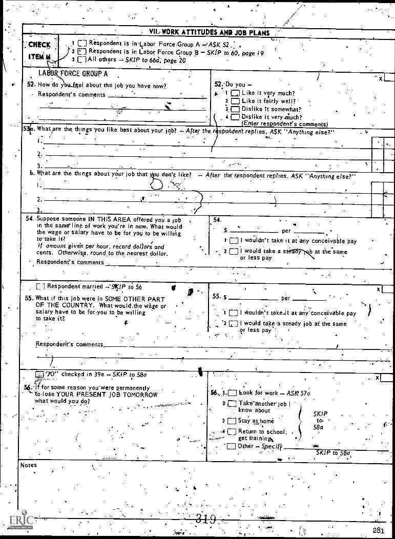
.VII.. WORK ATTITUDES A a JOB PLANS .-
. .
CHECK
ITEM
,i E] Respondent is inLabor ForceGroup A 'ASK 52,, .t' 2 E] Respondent is in Labor Force Group B - SKIP to 60, page 19
3 DAD others -4 SKIP to 66a; page 20. .
.LA : FORCE
52. How do
Respondent's
GROUP A.
..
pu...f.gel about the job you have now?
comments , `
52.'Do youX
.
'
L,
-
i 1 111$ Like it very much? .
t7
,2 IIII Like it fairly well? ..3 IIII Dislike It somewhat? ., .4 MI Dislike it very.ncuch? .
(Enter respondent's comments)53.Whatiare the, things you like best about your job? After the r spoen repies. "Anything else ?". _ o lik bst b b? A th nd't replies, ASK "Ah l ". .. ' -
_ ..
,..
..-
2 ...
3 :N
, _b. What are the things about your job that u don't like? After the' respondent replies, ASK "Anything else?"
,tx,--'. ,. <. . , ' .
2. ,t,
.3. . ,.
t54. Supposein thethe wageto-takeIf amount
cents.
Respondent's
someone IN THIS AREA offered you a lob .same' ling of work you're in now. What would
or salary have to be for you to be willihgit? ,
,given per hour, record dollars and .
Otherwisp rouncl_to the nearest dollar. -
Comments ..
54. .-
..$ per '
.
...,
, .i E I wouldn't take it at any conceivable pay
, 2 E I would take a stel-dri at the same- or less pay
,- ., .
Li Respondent
55. What ifOF THEsalaryto take
Responderh's
married 'SIP to 56 $.
this job were in SOME OTHER PARTCOUNTRY. What wouldthe Wage or .
have to be for-you to be willing.it_ . _ _
.
comments
- ,..55. $ per
..
..
,
. .. .
1 C] I vItouldn't take.it at any'conceivable pay.,
'2 Ei I would take'a steady job at the same' in. less pay
t.- ,)
,.
E110" checked in 39e SKIP to 58a......... .
56..1 for some reason you-were permanently'Thlose YOUR PRESENT JOB TOMORROW
what would you do?N
.'-_..._ .- .-. . -.-444...'s
-,..,
..
.
41
-.
,. ,
'
i- . -
...
. ..,-56,.,),CD Gook for work ASK' 57a
2' E Takeinotheriob I, know about
.SKIP ., .
3 E Stay at home to, _.-__'4
-4 Ci Return to school;58a
get training%- `C] Other Speciff, ,ifik
.
_
-
xl
.
("'
SKIP to 580... ' . . . .
_.
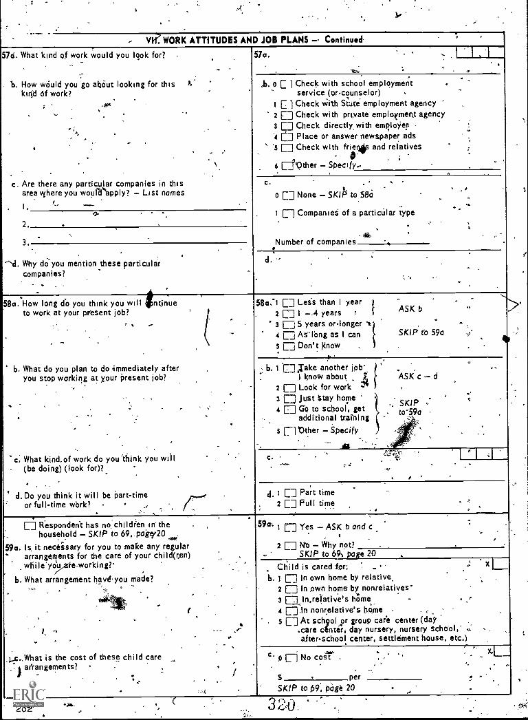
- ye WORK ATTITUDES AND JOB PLANS Continued-
57d. What kind of work would you look for?
b. How would you go about looking for this P.
kind of work?
c. Are there any particular companies in thisarea vyhere you wourat'apply? List names
2
3.
'd. Why do you mention these particulircompanies?
,
513a. How long do you think you willto work at your present job?
itntinue
57a.
o C 1 Check with school employmentservice (orcounselor)
E I Check with State employment agency2 E] Check with private emplaymeht agency3 [] Check directly,with employer4 n Place or answer newspaper ads
[] Check with fries* and relativesIt. . ;
6 LIDther Specify.,
c.6
0 C-..] None SKIP to 586
CompanieS of a particular type
-4*Number of companies
d.
b. What do you plan to do immediately afteryou stop working at your present job?
c: What kind. of work do you think you will(be doing) (look for)?,
d. Do you think it will be part -timeor full-time work? .
580.-1 El Leis than I year
2 Er] I 4 years3 C35 years orlonger4 C-] AiTong as I can5 [] Don't know
ASK b
SKIP Co 59a
b. t []biake another jobI know about
2 E: Look for work ;43 C:14 Just Stay home4 E] Go to school, get
additional veining5 El ether Specify
c.
ASK. c d
SKIPtol9a
d, i E: Part time2 [] Full time
E] Respondent has no. children in thehousehold SKIP to 69, paker20
59a. Is. it necessary for you to make any regulararrangernts for the care of your children)whileyoi,,,ate-working?
b. What arrangement havd you made?
1.c,,What is the cost of these child carearrangements?
.282'
f
59 I Er] Yes ASK b and c
2 [] Why not?SKIP to 69, page 20
Child is cared for:b. i El In own home by relative,
2 E: In own home by nonrelatives3 Ealitreiative's hiime4 [].In nonrelative's homes [-] At sch9olor group care center (daq
.care center, day nursery, nursery school,after - school center, settlement house, etc.)
xL
C.o ri No cost
1per
SKIP to 49. page 20
' -

* \9'LABOR FORCE GROUP B
60. What kind 4f, work are yOU looking for?
VII. WORK ATTITUDES AND JOB PLANS ''Continued
.60.
61. How, much would the job have t .pay foi-.you tp be willing to take it?
461.g per
9 EJ Don't know
62. How many hours per week do you want to work?. 62. Hours °
63a. Are there any restrictions, such ashours or location of job that wouldbe a factor in 'your taking a job?
0630.1 El Yes ASK-h
2 EINo. SKIP to 64a
O
b. Wh,at'are these restrictions?
Respondent has no children in the househOld.SKIP to 650
64a: Will it be necegslary for you to make any '
special arrangements for the care of your. child(ren), if you find a job?
b. What arrangements will (you make?
_
.4
64a. 1 E] Yes, A.5K b.
2 rj No Why not?SKIP to 65a
b. Child will be cared for:
1 [] In own home by relative
2 Ej In own home by nonslitative
In'relative's honie
4 E. In .nonrelairve's home ".
5 El At school or group' care center (day.cafe center, nursery school,"`after-schoolCenter, seitIpment house, etc.)
6 [] Don't knows
s,
Respondent is attending school 5kIP to 6965a. What do you expect to be doing five years
from now working or something eke?
What kind of work'do you thinkyou willbe doing?
ti
c. Do you think it will be pail time orfull time?
6541-.1 Working ASK b2 nStaying.home3 Ell Go to school, get
additional training. .4 Fi Other Spttcify
i. .
SKIP'to 69,page 20
Q.
5 7 Don't 'know SKIP to 69, palge 20
b.
c. 1 Li Fe tineSKIP to,,,69,.page 20,
2 Part time-
Notes
v.
.
.
CI
' ---
1
283-

1
$
LABOR-FORCE GROUP C
VII. WORK ATTITUDES AND JOB PLANS Coatibid;
66a. If yOu were offered a job by same employer...IN THIS AREA, do you think you would
take it?, .
b. What kind of work would it haveec? be?
c. What would the wage or salary have to be?If amount given per hour, record dollars and cents.Otherwise, round to the nearest dollar..
d. Are there any restrictions, such as hoursor location of job that would be a factorin your taking the job?
e. What are these restrictions?
66m. t []Yes ASK b2 ED It depends: SpeOfy "on what"
and ASK 66b g3 E] No SKIP to 67
e.
per
d.i EDYes ASK e
2 ED No SK/P to f
a1
f. Why would you say you are not lookingfor such a job now?
g. Do you expect to look for work within thenext six months?
Q, ED Yis2 []No
x ED Respondent has no children in thehousehold SKIP to 68a
67. Would it be' necessary for you to make anyspecial arrangements for the care of yOurdhild(ren), if you were to take a fob?
,67:1 E3 Yes ,2 ED No. Why not?
3 E3 Don't know.
x ED Respondent is attending school SKIP to 69
68a. What do you expect to be doing five yearsfrom now working or something else?
b. What kind of work do you think you willbe doing?
c. Do you think it will be parttime orfull-tiMe work?
69. What would you say is more.important to you indeciding what kind of work you, want to go into,good wages or liking the work?
.68a. t ED Working ASK b c2 [] Staying home3 ED,Gccto school, get
....-additional training4 El Other. Specify
5 ED Don't know ,
SKIPto 69
b. I I
c
e. t El Full time2 ED Part time
69. I. E icing the work
rED Good wages
. .
Wh)e answering Section VII was another perion present?
t [] Yes
Would you say this person influenced the respondent's answers?
ED Yes 2 No
2 EJ No Gp to 70
Notes
/
284
22
40

VIII. HEALTH
70o. Does your health or physical condition limit your 170a. 1 [] Yes ASK 70b d 2 [] No SKIP to 71 .. activities or the.kind of work you can dO? '
.b. What physical or health problem do, yob have?ii
c In what Nay are your activities .limited?. 9- .., .
'd. Hdw long rove you been limitedthis way? 41Months Years .
x[] Respiihdent not married SKIP to 72a . ,
71a. Does your husband's health,orphysical conditionrlinit his activities Or the kind of work he can do?
. . . .
71a. 1 [] Yes ASK b d.,
2 E] No SKIP to 72a
b. What physical or health problem does he have? r. , - -. if (
. .
c. In what way are his activities limited,...
-. .
datow locig has he been limited this way' I d. Months` . Years,,, IX. FUTURE PLANS , - .
72a. Now I would like tglk to you about yourfuture plans. What ould you like toto be doing when you re 35 years old/).,,
.
' ..
r.
.
1 .,
.b. Sometimes women decide, to work afteir they '' 4have been married for a while. If you were towork, what kind of work would you prefer' .
-.
72a. 1 [7] Working What kind ot ygork?
, . -.
(SKIP to 73)2 L---_,- Same as present (last ) job 4411. to Check3 E il Don't know' 0:16x after 754 Dl Mfiried, keeping house,
raising family ASK b- ....
5 [ 7, Other SpecifySKIP to Check Box after 75 .
b. 1 Ej Same as present (last) job SKIP to Checki2 El DOn't know ._ Box after 75 .
.....
*E-_,J. Don't plan to work ., e4 Eti Different from present job ,
Specify73ASK .
.
73, Why,do you think you would like this typeof work. . ......- :
,
73. 1 Erro,inerested in it; I enjoy it ,,
2 LI ft paii7tvell; is secure3 TT; Other Specify
74. What do you think your chances are ofactually gettin into this type-of work,
.
.
74. Are they' .
._ i LT] Excellent
SKIP to Check Box after 75,44'7 Ell Good./3 El Fair4 {-7 Poor ASK 75
. , .
.
75. Why doyou think the chances are not good? I( ,
...
.
75. 1 El Poor grades2 f-] Lack of education , .. .
3 El Lack of experieite ' - ''-.. -4 ,E: May change her mind (noc rsure)
,
s ,[] -Other Specify .
_ .- While answering Section IX, was another person,oresent? . .
i []Yes 444 2 Ei, No Go to 76 -/ , . . .
Would you say this person influenced the resporidentftswers? .1 r_:.,Yes ' -,..-. 1- No. 2 I
323 285
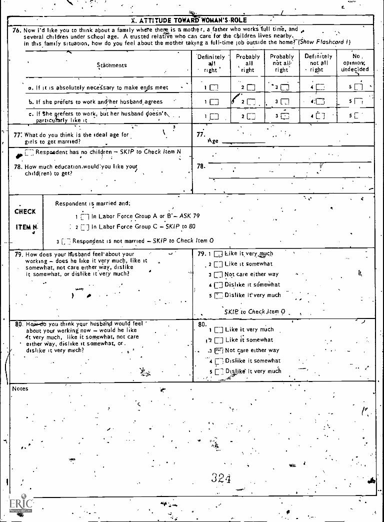
C.
X. ATTITUDE TOWARD'WOMAN'SROLE76. Now I'd like you to think about a family where there is a mother, a,father who works full time, and
several children under school age. A trusted relative who can care for the children lives nearby. .
In this family situation, how do you feel about the mother taking a full-time lob Outside the homer(Show Floshcord I)
Statements
DefinitelyAll
right
Probablyall
right
Probablynot ailright
Definitelynot all
- right
No .opinion;
Undecided-..t
4
a. If it is absolutely necessary to make ends meet -
.
1 ET] 24 - 4.-3 LJ 4 ci - -..5 [-j
b. If she prefers to work andTher husband/agrees 1 [] ( 2 3 E 4'20 5 r;c. If She 9refers to work, Init her husband sioes'n't\
particuharly like it 1 [] 2 Ei 3 Ej 4 C -] 5 r_ '
.
77: What do you think is the ideal age forgirls to get married?
77. ,
Age.
[-- ' Respondent has no Children SKIP to Check Item N. !
.:
78. How much education.woulcryou like yourichild(ren) to get? ,
.
78. . ,s
.,
CHECK
ITEM H.4
Respondent is married and: . , a '
.. -
1 El In Labor Force Group A or 8. ASK 79 .
. 2 r -. In Labor Force Group C SKIP to 80. '
3 [7 Respondent is not married SKIP to Check Item 0
79. How does your tfLsband feel-about yourworking does he like it very much, like it
. somewhat, not care eitherway, dislike..
it somewhat, or dislike it very much?.. .
.,...t.
)
79. 1 Ei Like it, very much
2 [] Like it somewhat
3 [] Not care either way 11,
. -
4 [] Dislike it somewhat,
5 Dislike it very much.
ISKIP to Check,tem 0
80. HO.ii+-60 you think yqur husband would feelabout your working now would he likeft very much, like it somewhat, not careeither way, dislike it somewhat, or.dislike it very mach? . t °
. nir--,k
80.1 E.] Like it very much ,
-1`2 Li Like it somewhat - ,
3 Ei Not care either way
4 [] Dislike it somewhat
5 El DiOslike it very much ., "
r
NotesI
. ..
. , _. . ,
. ... .
..,,. - .
.
, -.. . 9.
10
.
.-
: , , 4
, \
. .4,.S 4
n4 .
. . .
. --
286'4*

;,
. XI. ASSETS" AND INCOME" .
.c - ,tHECK
ITEM !?
.*..
1 El Respondent or husband, is NOT head of household SKIP to 83o ,. .
42 [7 Respondept or husband is head of household ASK 8I `a 0- ., .
A
-
8Ia. In 1967,fiqpnciallilatiNies?For) -; ry.
b. From
did you (or your husband), receiveassistance from any of your-
;., -
whom? :"^--'
. 81a. 1 fri Yes. ASK b c
° 2 EINO . SKIP to 820..
._
... .
.... .. -
., -
c. How much did Vou receive? _. 'c.,$.
..
-.,82a. Is this house (apartment) 'owned or being*,,bought by you (or your husband)) .,
.. ,b. About how much do you think this
property would sell for on today's market' ., ,.. .
C. Ab,outihow much do you (or your husband),
owe on this property for mortgages, .back taxes, home improvement loans, etc.' .
,82a. 1 En, Yes
2 r J No SKIP to 83a-
.
.
-b.
.
$
.
-i.if'-
-. .,
$_
o [ i None
83a. Do you {or your husband) haste any moneyin savings or checking accounts, savings .and loan companies, or credit unions?- . I. b. Do you (or your husband) have any , . ..,. .
- ` I 'I . U.S. Savings Bonds? r- ,
s'
.2. Stocks, bonds, dr mutual funds? .,,,
,.
83a.1 r` Yes How much altogether?
$ .ii
...,-,
...
------at---7
,N2 r o
b. 1 I, ' Yes What is' their .
% face, i2 ri- No GO to (2)1 r Yes About how much is ,
their market value' $t [ No _ t
.
. -84a. Do you (or your, husband) rent, own, orhave an investment in a farm, business, ; vor any 8th.dr real estate? ps 4.4
b. one 7
',
',` -
.
.. . 4`...,
.
---
- c. KbdUt how much do yo.thrikihit .{bus' mess, farms .much 1, .I,or -other real estate) would seqrPOron today'smarket' ,
a 'd'. What is the total amount of.debt.and other
.liabilitieS on this (-business, farm, or other zeal estate)?. . 161V*
.
.
84a. 1 r_ , Yes ASK b cl.. ,
2 r-:, Nos SKIP to 85a .
.
je?'b. 1 [7. Farm .
1
- 2 r_ TBusiness.
3 ri, Real estate
- ,
... a...ow
..,,
..
$ ,
.
'.
.
ct.-$- °
.
-?..
0=3 4\
..4o r_.-] None
vti 785a. Do yott,(or your husband) owri an automobile' .... *,
. . . , .. 1
i b. What 45 the make and 'model year'If rpdre than one, ask about newest. 4 .
. 1..,
, ,. a,
. c . When was it purchased? '0.
d'. Do;you owe, any money on this automobile?, . .
.a ,,,
-,.
'
,
88e. 4.1:- Yes Aie b c
,,,, 2 Ell No ----- SKIP to 86 ...-.
.. b. Model year,...
.
...
4 : ''' .....S 1\
;" Make t' ...... -,..- d 9 . ,
'C Year ",d. i'fl.Yes, How muchaltogether?'
$ 0,2 [ I No, ,
0. ;' 86. Do yod(or your hiz, band),owe, any (o4her)
Money to stores", banks, doctor,, or --4, .anyone else, excludiog 30-day-charge
.r.- at" .accounts? 4
.: .
86. 1 r,,-1 Yes How ,much'altogether?,
$ . .
. ,
. ..
:,. ,2 r No .
,..4
e'325
1 ,
287

k A- 6
-,.. --4-....... X1. ASSETS AND INCOME - Continued
NOW Iabout your
87a How muchfrom wages,
,, , ail;iobs,thing else?
b. Did you,from working
mess or
c. Did youunemployment
4
cl.. Did youincome,idends,t I I n.es5,,
would like to ask-a fey questions e ..income in 1967.did y.ou (or your hdsband) receve
salary, commissions, or,tips frombefore deductions for taxes or any,.
our husband) recepie any income(or y e'on your own or in your own bus-
.farm? $ less =
-' Respondent .1 Husband-..x FiNot married
87a.
..$ $ .
o CiiNane 1 0 in None
b...1 C-1 Ye; - How much? t 7 YeS - How much?
$ , $2 L.] No -14` 2 [7 No
..
42, (Gross income) (Expenses)
(or your huSband) receive any. .
compensation' .
. . ,
.
-.
-. .
(or your husland) receive any othersuch as rental income, interest of div-income as a result of disability, oretc.?
. .1 [-] Yes 1 T] Yes
c. (I) How many weeks? (I) How many weeks',
. (2) HoW much? (2) 1-1,ow much''
$ $
2 E7No - t 2 [] No'
. d. i [7.4Yes - How much' 1,, i 7 Yes - pow much
$ . $
2 L=1N No I 2 El No
.
. 2i;
CHECK
(TEM p
.
,I El Respondent (and husband) lives alone - SKIP to 88b -.
.r-li All others.- ASK 88p (If two or more RELATED respondents in household.
ASK 88a - b only once, and transcribe answers from the first to theother questionnaires). .
88a In 1967,. ALL fanlyttember,s.
(Show
-
. ,
..
.
b. Did anyonewelfare,.
what was the total incorilca..2:.living here? ,
Flaghcard 2).
_ ,
., . .
, ,I.
.-
Vet,.?A''... ... .
in this family receive any.
i.,;,
or ,publtd.assrkance in 1967?
88a. i ETI Under $1 ,0002 []-$ 1 ,000 $ 1,999
3 El 2,000 - 2,999.
. -4.L.4 El 3,000 - 3,9995 Ell, 4,000 - 4,999
-- 6 E 5,000 - 5,9991[ 6,000 - 7,4998 E 7,500 - 9,999 -9 ri .1o,000 -, itiit,2,99- .
a o {--:: i5,000, 24,999 , . L
i i El /5,000 and over ; . .
[] Don't know ..
.
' .f :is. 1 LTY.es - How,rnuth altogether? $
2 El. No .
.
CHECK,-.----IT& At.
a , f .° 1 EtRispondent lives with parents - SKIP to Check Box after 896 _
.
.....
2 El Re;pandent does not live with paren.t.- ASK -89a.
_ ."
.
..., . .
89 How persons, not counting yourself or(yOur,husband) are dependent upon. yoti for art'
eat one-half of their support?-
b. Do any of these dependents ;live somewhere . . ,other than here at home with",ou? i-,
a . a
,890-. .
,
Number _,-.
.----0 ,0,17 ; None - SKIP to Check Sax after itikib -,,
b. ) i ,t.-.Yes - Who..are thty?. . '- .
.
. .
4.12 L NO , ,. . ,
-..
While answerineSection Xlwas another perso'n present?' ... .
- t-E].., Yes . . 2r_ Nor GO-40 90 -. - .
`kould-you saythi4erson'influencea the respondent's answers? ''''''.
.
1 [=,..,Yes. , , 2 F. No,
. .. '
Notes,'e - .
. 8 . .
.wea`.' .A.... .
3 2 6
8 I
;
.
'288,

XIL'FAMILY BACKGROUNDNow I have some quettions on your family background.
90. Wherewne you born?411,
U.S:City
County.
7State
2 ,C71 Outside U.S.Specify country--
91. For how long have you been living in this area(city or county of CURRENT residence)?'
91.i L than I year
2, L I yearor more Specify
3 c All my lif& SKIP to 94
92. Where didyou live before moving to (name of cityor county of CURRENT residence)?
92. 1 E:, U.S.City
County
State2 OUt9tde-U.S.
Specify country
93. Where did you live when you were 18?
S.
93. o j Rprrerin t is 18 or lessT 1.7
et
County
State2 Outside U.S.
Specify tountr
94:-01-- Respondent not married SKIP''to 95*441-i'ow old were you at the time ()flour first marciage?
Now I'd Like ask about your p'arenks.
95. Are your mother and father living?
94.
Age
0TH parents alive.
MOTHER alive, Father dead
'FATHER alive, Mother dead
NEITHER,parent alive
.0 rX-7 Respondent as not,married SKIP to 92
96. What abort "your hbsband's parent's?Ar° his- mother and fatlaer living? -
.96. 1 1 BOTH' parents alive
2 r :MOTHEIt alive, Father dead
3 FATHER alive, Mother dead
4 NEITHER parent alive
97Ahere were your parfrits born in the O.S.,orsome other Country?
.
4 2 rs: Other Specify
b. MOTHER'
t u.s.. .
2 f I'Othe Specify
If either Parent tiorn outSiclq,U.S,: SKIP to 99.
t41
327'
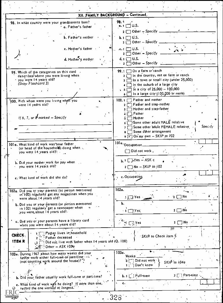
XII. FAMILY BACKGROUND - Continued.. . . ' .
98. In what country were your grandparents born?a. Father's father
..
_, b. Father's mother
.
c. Mother's father
)7' d. Mother's mother ,
98-; i ,a. 1 E U.S. .
2 n Other - Specify .,
b. 1 E U.S. -
2 E Other - Sp,:cify ,..
NI.c. I ED U.S..
1.2 E Other - .5,pecify :
d. i E U.S..
2 ED-Other - Specify
99. Which of tie categories on this card .
describes. where you were living wheni you were 14 years old?
,
(Show Floshcord 3)
.-'
99.1 ED On a farm or -ranch .. -
2 E In the country, not on farm or ranch3 ED In a town or small city (under 25,060)4 El In the suburb of a large city ,
t. 5 E In a city of 25,600 - 100,0006 ED In a large cityll 00,900 or more)
IN. With whom were you living wh n youwere 14 years old?
* ,
If 6, 7, or dmarked - Specify -
100.1 El Father and mother2 []Father and step-mothe,r3 E Mother and step-father `
.t [],Father .a
-i ci Mother,
6.[]°Some other adult MALE relative7 [] Some other adult FEMALE relative. li Specify
8 Ei Some other arrangement I
9 Fj On'my own - SKIP to r02 ..
J,
la
101o. What kind of work was'your father .
(or head of the 'householf) doing when ,. -,6,.
you were 14 years old? -
b. Did your mother work for pay whenyou were 14 years old?
, .
. .'c. What kind of Work did she do?
- .
1
101a. 'Occupation
ED Did not work _ -
b.1 []:Yes-
es - ASK c
2 ED No - SKIP to l, .
1. c. Occupat,- .
102a. Did you or your parents- (or person mentionedin"( ob) regularly get any magazines when yOu
.
were about 14 years old?
b. Did you or your clarents (or person mentionedin I 00) regular.htget a newspaper when 0you were,about 14 years old?.
.c. Did ydu or your parents have a library card
when you were about 14 years Old?
102a. .
1 .0, Y-es :fit. '2 El No
b. . ,
1 El-Y q 2 El NO ,
. ,
c. .
'',:i E-aYes 2 No -:
CHECK ,.
ITEM R
. ' P-7.4 ' '1 ,
1 rl Pather lives in,household- - *2 E .1, Father deceased . 0 c SKIP to Check Item .S ,
0 [--,, Did not live with father when 14 years old Q. 100).:;;:477 1, Other - ASK ION
. .
.
103a. During.1967 About now_many weeks did your .
- - father work either full-time:oti-Part-time----- .f*
(not countin% wiork around the house)?'V.
- 4.:
b. Did your father usually work full.time or part-time?, .
c. What kind-of work w,(he doing? ,lf more than one,recbrd the one worked at longest."
103d. . - .Weeks
..
SKI/3 'to 1,04a'0 ci Did not work }1 [--; Don't know .
'.
b. 1 r 1 Full-time 2 4 :-.. 1 Part-time %
c. .
N
.
.328

XII. FAMILY BACKGROUND - Continued104a. What was the highest grade (or year) of regular
school your father ever attended?.
,.
. ..
4 o.4 '
. . --...
b. Did he finish this grade,Jor year)? , . .-
104a.2 4 ___,I. Elementary [3 -0 E E Ei Li_
. 42.High school kt._-] 0 E]3. College, C] 0 0 Li E E
.
b. 1 E Yes .$ .
2 E-7 No
CHECK'
ITEM S .
*i [ ] Mother lives. in househbhl - r '",.. i SKIP to 107b2 I:J.Mother deceased*
3 E-1 Did not live with mother when 14 years old (Q. 1001., )-FlOther - ASK I05a _
.
,. :,.
105a. During 1967 about how manyweeks did your , .mother work either full-time or part-time .
(not counting work around the hove)?i,,.
.,, t
6. Did your mother usually work full-time"or part-time? .
c. What kind of work'was she dome If more than-record the one-worked,at longest. -
45a.Weeks0
.. 1 rir.
Did not work }Don't know
...
SKIP to 1060 .
,
..,-..-
b. 1 ttll-time.
21E1 Part-time
,c.,
. ,
106a. What was the highest grade (or year) of regularschool your mother ever attended,
I A . 4
..f* '
,b. Did shefinish this grade (oryear)? .
.
106 °.1 2 3, 4 4 6. 7. 8
'I. Elementary E EL E ED, CT E-T L ' El.
2,,FligN*Ehool n r E--, .[]..1. , 2 ,3. 4 . -4 6+
-3.Coilege El El E Cr-ib. I E Yes 2 ElNo
107a. Do you have any brothels or sisiers .107awho live somewhere else? - .
- . .6. How many,
-
.c. How old is the oldest (living) one?._ .
1 E-1 Yes . 2 El NO - SKIP to 109
b. .
...
c; Ageit
v ..
108a. What was the highest grade (or year) of regular,school he (she)'ever attended?
.,> ., . . .
.. , - .-
..
... fb. p,d he (she)finiih this grade (or year)?
.
108a. 1 2 3 4 5 6 7 ..; 1 Elementary E ED E ,ED E 7 i
1 1 -2 3 4
'2 High school. [] L-.] E3 [] '- 1 2 3 2 ' 5 6+
, 3'College . E7 ED E E ED El
.
1b. 1 [] Yes.2 ED No -
. ,109. What.issyOur Soeiaj,Security number? 7 Does not have oneNotes t r_ ... . ic",,
.<, . ..1 - .,,
,.. .
, _
, . ... , .._.
.. .
. , . ... .
. -
.
,,,,.,1,,,i1,7.7--.
___ .
.
.
.
,
''_ '.., :. -.. . ....
.
. . .,
v.;
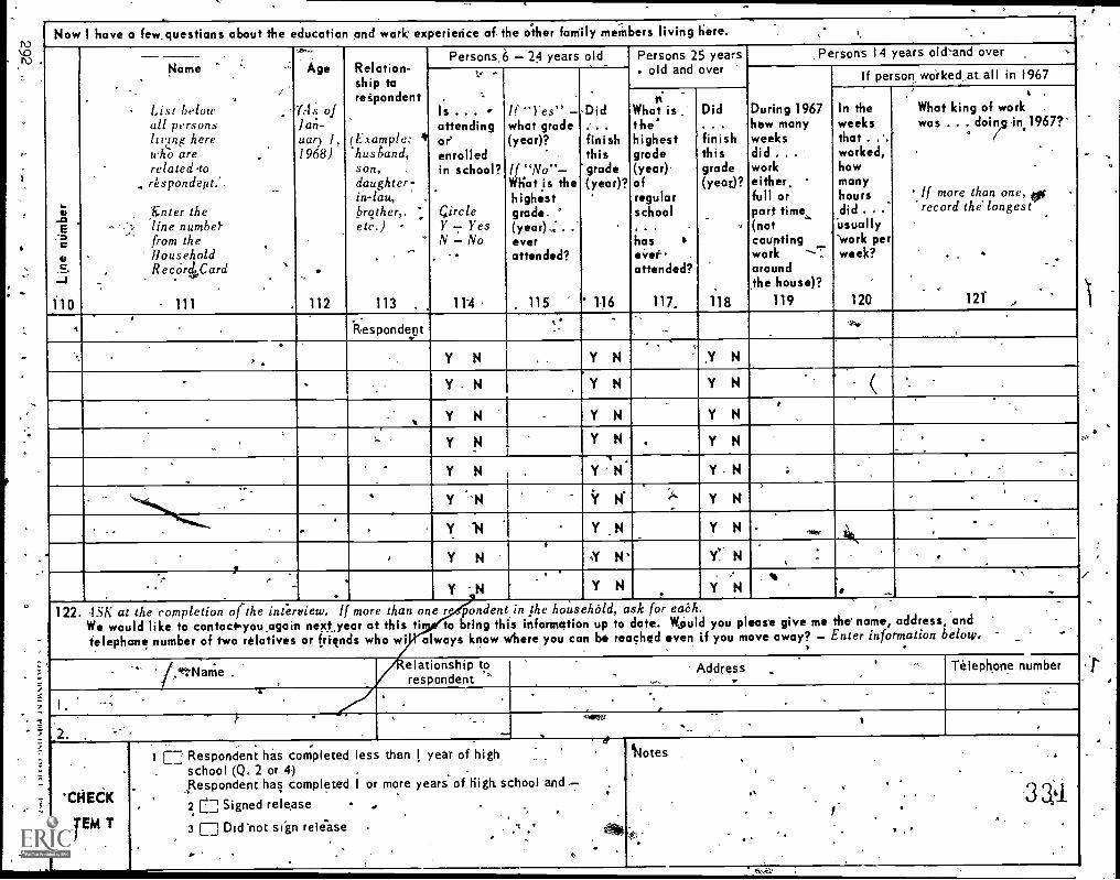
3
Now 1 have a few. questions about the education and work experience of. the other family members living here.
110
Name
List belowall personsItteig herewho arerelated .torespondent.'.
,Enter theline numbel-from theHouseholdRectirdCard
111
Age
(As ofJan-uar) 1,1968)
112
Relation-ship torespondent
(E.tample:husband,son,daughter-in-law,brother. 'etc.)
113
Persons_6 24 years old
Is ...attendingor'enrolledin school?
CircleY Y esN No
.
lt4
If Y es"what grade(year)?
If "No"natis thehighestgrade. '(year).:..everattended?
115
Did
finishthisgrade(year)?
116
Persons 25 years. old and over
Persons 14 years old'and over
nWhat is .
the'highestgrade(year)ofregularschool
haseverattended?
117.
Did
finishthisgrade(year)?
118
During 1967hew manyweeksdid . . .
work
full or°tipart me,
(notcountingworkaroundthe house)?
119
If person worked_at.all in 1967
In theweeksthat ..worked,howmanyhoursdid ..usuallyWork perweek?
120
What king of work .
was ... do,,g in. 1967?-
.lf more than one, fiftrecord the' longest
121*
Respondept
Y N Y N ,Y N
Y . N Y N Y N
Y N Y N Y N
Y N Y N
Y N Y N Y N
Y -N Y Y N
Y N Y N Y N
Y N Y N r. N
Y 'N Y N Y N
122. 5K at the completion of the interview. If more than one r pondentin the household, ask for each.We would like to contac*you.again nextyear at this ti to bring this information up to date. Keuld you please give me the' name, address, and
telephone number of two relatives or friends who we always know where you can be reached even if you move away? Enter information below,
Nanieelationship torespondent
Address Telephone number
'CHECK
ffEM T
. .
ED Respondent has completed less than 1 year of highschool (Q. 2 or 4)Respondent has completed I or more years of high. school and
2 Signed release
3 fl Did 'not sign release
°Notes
I' 3a4

t
4OM 4, No.414;2423: Approval Expires December 31. 1973
NOTICE'. Your report to the Census Bureau is confidential by law (Title 13.US. Code). It may be seen only by sworn Census employees and may be used.only for tvitical purposes. aili .
79T240.:71;GT.451 . . -
. 4
...
a# US DEPARTMENT OF COMMERCE
SOCIAL. AND iCtittO4MC STATISTICS ADMINISTRATION. BUREAU OF THE CENSUS
..
.
.
0NATIONAL LONGITUDINAL SURVEYS,
SURVEY OF WORK EXPERIENCE.
OF YOUNG WOMEN, -
t1973 .
. '
.
.
.
',.,
A.
- ..
-
_
.
t.
...
1r a. .
e ..
.
0 I "L:-:1 Respondent ailficininterview in 1972 Go to Page 30
.
METHODS OF LOCATING RESPONDENT WHO HAS MOVED_
. .
RECORD OF CALLSSuccessful Unsuccessf01.
CI E 271 New occupants
...,
CI 1 7.71 2 71 Neighbors./i0 i El 2 7. Apartment house manager
0101S 7 2 T I Post office .../. 4 .
CD E 2 7 School
I -, 2 71 . Persons listed on inforfnattok sheet0r
,0 1 2 0 Other Specify,I.'Da Timeime C omments '
.
II
, , P.m. q
'. a.m.
a.m.
.
o
"-
.
0.,;.
P.m. ...,..
.
. p.m.'
.
. .
.' RECORD OF INTERVIEW . ,Date completed
.....Month/Day/Year .
0 t
Interview time Interviewed by . ..
.4..",.
... .,. ....,
'
.
.
..
Began
,
p.m.
Ended
11.
Pao.
Length of interview (minutes)
ap
NONINTEP.VIEW REASON'.
ap Unable to contact respondent Specifyf
6 0 Temporarily absent Give return date .
a 0,1rtstitutsonalized Specify type4
9 0 Refused,. . .
,.
o ri Deceased .
.
A '' Other Specify "
' t .,
.
.
"
.,
,
TRANSCRIPTION FROM HOUSEHOLD RECORD CARD 1 4J+.Item 13 Marital status of respondent - 't-
,. s 7 Separated .(ID i.0 Married, spouse present. 3 Widowed_..w
rs
- 2 0 Marrred, spouse absent , a Di vorad. ,., 6 0 Never married. '
CID
If responttent has moved, enter new address ..'I. Number and street
.. .
t .. ` .
1
.
.....
(
al
®
2. City, .
.r
3. County 4. State.
.
.
I
5. ZIP code
. ...."
332'0

I
I
I. STATUS,
1. Are you attending or enrolled in regulai school?
, .
.s. .
:6 - ...
.
0 yes -ASK 20 . .
2 0 No-,r
. When were list *walled? -. .
.
Year - SKIP to Check Item 8CID Month,---
-26. %at grade are you attending? 2a.
b. Are ran walled as 0 full time or Port-time student? b.
. '
li ' Elementary 1 2 3 1 5 6 7
2 High school I 2 3 4
. College 1 2, 3 4 5 6+
8
.0 i Full:time ...
20 Part-time
CHECK .
ITEM A
.Refer to item I I I R on Information Sheet..
' ...
..
Respondent not in school in 1972 - ASK 3a
bRespondent in school in 1972 - SKIP to Check Item C 41., . ..
,....
CHECKITEM B
.Refer to item IIIR on.infOrmation Sheet.-, ,
Respondent insehookin 1972 - SKIP to Cheek Item F I
[73 All others - SKIP to 22a on Page 5 .t
3a. At this time lost year, you were not enrolled in school. 3a.How long had you been out of school before returning? ,
4
b. Why did you return? b.
r
C. In what curriculum on you enrolled? c.
1,
"''
. -..
I.
020 Years
CED u\
CID I 1 I
.,. ..
.. . SKIP to 9.i . .. ,
CH EC KlITEM C
_ .
Refer to Items 2a and I I IR on Information She& , .' .. . .Respondent in high' school in 1972, college now - SKIP to S. , ., s
s Other.- ASK 4 °
4. Are you attending the some school as you were at 4. lap 1 0 Yes - SKIP to 10 -timelast year?c I " 2 0 No' - ASKS
,,
5. What ithe narn of the school you now attend? 5.
,,. . , ° 4 .
6. Whiiiris this school located? 6..,
). , . . 4 .
'
cED i [ - 1
.
. . .
. -,
,. copniy
, P..i .
State. . .
Tr; Is this school public Of private? 71- ,. 3 i 0-Public ---.. ,, .- t i 2 El Private. ' . ,
8. When. did you inter this school?, ,
*. .
..
.
- .... , ,P
DA
Month Year 4.
, ..
CHECK'ITEM 1:1
.
_Refer 'to item a hr item IIIR-Jiri Information Sheet.
Ilespo dent in college rnow - SKIP, to I4a
Res ndent in high school low 1SKIPOJ
1,...
22a pn page , .
- ,
.
Respondent' ribt-m school in 1972...
, Other ASK 9 ,
9 Why did you change schools? -.. - 9: r(E) , ",,
..: t t
_
10. Would you say you now like school mom about the-. : 10. 1 i ci Moresamtt, or less than you' did lost year?
s 2 0 Less I
4 3 About the same
.
291!'Page 2
411"333
I
c
,
a
6

CE
,
7-
I. EDUCATIONAL STATUS - Continued , ,
11. Are you enrolled in the same curriculum now os you -II.were last year?
- or'
0 1 Yes1 1 college - SNIP2 7 High school3 : 1 Elementary
4 j No - ASK IN
to 14n
SKIP to 22a on Poe: r,.
.. .12. In what curriculum are you enrolled now? 1'2.
..CD I 11 -
. .
13. How did you happen to change your curriculum? 13.. 3 ( 1
. .c
7 Respondent not now in college - SKIP tcrCheck `Item E .
14o. How Much is the fulitime tuition this yeor at the I4a.- college you attend? I
:b. Do you have,a scholarship, fellowship, asses/Offs-4k b.
or other type of financial old this year?
c. at kind?.
'
. <,.. c'....
....,-
.
. c
. .
dAtiew much is, it per year? d.
.
Ait., e'' .
.
WV
3 i T- Yes ASK. op
2'''' No - S P to Check Iternt'
..
3 '-' Scholarship0
2.7 Fellowship-
3 7,Assistantship
' 4 7 Loa; .
5 ": Other - Specify
..0 S 00
CHECK'ITEM E
Refer .,t6 !tern I I IR on informationoiheet. ";
-it.3 Respondent in collegb 3-6 4n 1972 - ASK 1.5a .
Other - SKIP to 22a on page'S
15o. Have youleceived a degree since",last year at this time? 15a
,.
b. What degree was it? 6i\i-0
. , .
N i.5 ii
k..
c. in what-field did you receive your degree? c.
- - .
d. Why did you decide to continue your education d.after receiving this degree? c -.
laD i D Yes - ASK,b2' I No - SKIP to 22a on page S
-.-, .
3 : Bachelor's (B.N.. B.S., A.B./ ..
2 :12 Master's (M.S.. M.A., M.B.Ail .
3,'J Doctor's (Ph.D.) a..
4 72, Other - Specify
..
.
'Ci '1 I 1 ..
1
.
, Li. .
.
SKIP to 22a on-page 5
CHECKITEM F.
rs
Refer t6 item I I I R on Information Sheet. .. - ,ifj Respondent in high schao1,I-3fast year - ASK 16o . . .[ThRespondent in higlisdool 4 last year - SK,IP to I74 , .
.` aRespondent in college 1-3 last year - SKIP (419a . ,0 Respondent-in college 4t la.st year - SKIP to 20o Millgi..z ,Respondent -in .
ipespondept in elementary school last year -5K I 6a . ' ..
16o,-At this timegast-yiar, you wereattending 16ayour year of high school: Did you complete that year?
0 i '' Yes ,. .
.2 "-- .I-No ."?;. ,wwor.. .
b. Illy didyou 'drop ou; of high school? b.. . .
-.. ... ,
t: Do you'expeet to return?
1- 4 ... .' s ,
IC . .
d. When do, you expect to return?
..,
:d.
4
ILO
, , .
. . t,.... . ,
,.
.
.
.3 i ---1 Yes - ASK d
2 No -SKIP to 24a On Page 6. "` ,
f ).EI Within a year .
. 2 0 Within two years
.3 Don't know.CI
14 rl Other .-C
.
SKI/1 to 22iiOn page 5
, .
#
.4....
,'
-
1.41.451 1112072I
CS.
.7 03 ziPage 3
9

C
' ' I. EDUCATIONAL STATUS - Continued
17a. Did you gradate horn high school? 17a.\ -
, 4
b. Why notfl b..
, 3cp. 1 q Yes - SKIP to Check Item G .
z0 No .- ASK b. ...,.
11 . ., s..
, .
o
CHECK
ITEM G
,.. Refer to item I I3R on,Information Sheet.
D Respondent had planned to enter college when
0 Respondent had not planned to enter colte
r
last interewed - ASK 180 .
e when last interviewed - SKIP to 2.20
- i-',SKIP to 22o .4 .
1' 0 Respondent not asked, educational goal
18a. When we last interviewed you, you sold you planned 18a. 4to go ha college. Have yourpJans chaiged? ,
b. What caused your plans to change? b.
e
c.c. -
. .." ,
, .
4
. f 0
I . -
a. Why are youlesently not enrolled indtalloge? : c.
-1111,it
- -':-
) ; _9r .Ai
...4.....014V 41.4 4, . . ' {. G:t 4_, '
° si° ;-d. When do you pliirkto enroll ip co) ? ,..- 11.
/kV . V9 ° '',- 0
,. r , s.ez--'44 d d ,
i ce.3 yes - ASK b.
2 D No - SKIP t9 c
o(a i 0 Pdor gradeslackedability, wasn't accepted'.-- , because of low grades, etc i
2 0 Economic reasons (couldn't affoi.eliad to worki instead,. unable to obtain financial assistance)
, 3 Disliked school, lost.interest, had enough school
4 0 Marriage; pregnancy or children
s 0 Personal health reasons. - °..
6 0 Other - Specify-
a
SKIPto d
..i0 i 0 Economic reasons (couldn't afford, have to work. -
, -unable to Obtairt financial assistance, etc.)
' 2 O Was rejected or turned down1 .
3 0 Waiting to be accepted by a school
' 4 0 Marriage, pregnancy or children
s 0 Personal health reasoni-0 .
i.`c 0 Other - Specify"
p-
-
Month Yeas - SKIP, id 22a011,
),X lion plan o SKIP to 24eon.page 6-.-
if19a. Last year at this t you re in college. . f Li t: r . '
' s ..!ti'Why didyou decid drop out? ' , ah'-"- ' Lt e
. 04 : if ,' .4.1 - V.
, 0 Received degree - SKIP to 2Ia
I . ,b. Do you expeatto-return? . gel Yes =ASK c &etr 1. .
r.
2 if a0.:- SKIP to 24a on p'age 6,. ., c
c...When do you think you will return? c. cm Wittrin a,,Vear.;0 Within.two,yearsc.
. ,° 3 0 Don't ktiSv
-..
4 0 Other
, . . . .
SKIP to 22o
. et'.
20o. Lasf year at this time yob were in college. 20a. * I
Did you receive a degree?. 3 p Yes - SiCIP- ta 2Ia : , 3
4%
et 0 No -r ASK b
fb..Why did you decide to drop me 4 b. ' -.
"a .' .
. _
, ., ..% , I_ - .
. .e. Do you expect to repro?
, - c.Yes - ASK d
SKIP to 24a .1
._. ,
d. When? '" d.- ith/a year
, Within two years' .
a Don't know :'.
.. . 4 0 other.Ap ...... . ,
b
SKI o-220 . , .
.
0ORM 1.07-411 11.2 72Y
296 *
Page 4'
.335

,
I. EDUCATIONAL STATUS 4,..aniknued' . ..
21a. What dearee did you receive? 21a.e .
..
.
b. In what field of study did.you receive your degree? b.
-, -. :
Ale, . - , Aitza L....1 Associate (2
27 Bachelor's3 T] Master's (M.S.,
a 7,!Doctor's1Ph.D.)
's 71 Other - Specify
year coiese) r
(litAtts13.S., A.B.) ..airiirk,,
M.A-,., M:1:0.) .
...,
:
v-0 III,
...
22a. How much education would you like to get? 22a..
If "Other," Specify --,If .
....VW High school
,
College
.:...
Other,
1 7 I yr. 2 TI 2 yrs, 3:j 3 yrs. a'
sr-1 2.yrs. (complete rumor college)
. 6 F-3 4 yrs. (graduate from 4-year college)
2- 1 6 yrs. (master's degree or equivalent)
e TI 7 i yrs. (Ph.D. or professional degree)
9 ',7:1 Don't know..other,responses
I'irs:-
41,. .
a
.1): As things stand now how much education do you ' b.think you will actually get?
If "Other." Specify .
i
0 High school
College
Other ' ,:
i Ti I yr. 2 n ] 2 yrs. 3 761 3yrs. 4:..,
5'2 yrs..(complete mior college)7)
6 n1 4 yrs. (graduate from 4-year college)',
7' 16 ytt;(master's degree or equivalent)
e -; 7 yrs, (Ph.D. or professional degree)
9 j Don't know, other responses "
1 4 yrs.
°. % t
CHECK
ITEM H
Refer to item '22a and item I I3R on Inform° on Sheet,Ti Educational goal differellrfrom whet; ast interviewed - ASK 23e
Ti Educaitonal -goal same as wherrl Interviewed t . ,
T] 4Respondent not asked about educational goal -. .
ts-
23. When we last interviltwed you you said you would 23.like to get (amount of education'indicated in I OR)
.Why have youl-changed your plans?
ap i I .
,
Notes ..
.
.
. . .,. -
.,..-
." .
.,
...
.
. .
. .- ...
..,
V
a r ., ... ....-N I .
...Iv ..
..
.. .
.
' ' .
. .
. .6 .a
-
t- --,
. .I.
. .
. ....
.,
r `-t, 1Of
.
.... t .
..
.
..
..
. .
.
- .)
.
--6
.. .
t
a
. ,
, r.
. .
.
.
a
.
.
oe
It
.
CM
CID
T
a
9
9
...
,
,....
i.
,.
.01.11.4 1.014111 16x0.79
_ 3aU 297
v

-
V
I. EDUCATIONAL STATUS - Continued
- 0 Respondent now attends schagl - SKIP to 24,L24a. Since this time lost year hove you taken any training
. courses or educational programs of any kind, eitheron the job or elsewhere?
b. Whot kind of framing or education previtTn did you take(' -b.(Specifybelow, then mark one box) . ee
24a.
c. Where did you take this training course?-(Specify below, then mark one box)
d. How long did you attend this course or program?
e. Amy 1:As hove you been attending?i
f H w many hours per week did you spend on thisainingi
CI--Did you complete thisprogram?
ier
h. Why didn't you complete this program?
AV'
i.. Why did you. decide tit-get this training?
.4
Do pit,use this tioining on your present rob?
It. Did you receive o certificate for this training?
f difI. Sinc4 February 1.972,-havi you obtained
certificate for priOcing o prolession or.trade?, '
m. What type of certificate is (was) it.?
o
n. Is this certificate currently valid?
,
a
0 t Oyes - ASK b,'2 0 No SKIP to 24L
0 Professional technical
2 Managerial
3 Clerical.4 Skilled manual
s ri Other
c. 0 1 Business college, technical institute2 El Company training school
3 E.,/ Correspondence course1 40 High school 7, -
s Area vocational schocil
6 L] Community or juniOletllege0 Other
d.
g.
4
h
k.
0 Months - SKIP to fx, Still attending - ADZ e
Months
rj 1-420S-930 10-144 El I S-I9
s 20 or more
Yes -When?
Month Year - SKIP to
2 n No. dropped out - When?
1
- Month Year - ASK hx NO, still enrolled - SKIPoto i .
In Found a lob
2 0 Interfered with school
3 0 Too mucti`time involved
4 fj Lost interest
5 ri -1-0-0 difficult
6 0 Other. 'Specify 4
t fl To.obtain work
2. TO improve current lob situation
t11 To get better lob than present ,one
,4 0 Wanted to continue education '3 Need it; worthwhile -
6 I:3 Other Specify
ElsYes
2-0 No
3 0 WOCOMPiOye'd
00,
0 i El Yes(=1 No
m.
n.
C I 0 Yes - ASK m2 0 No - SKIP to 2Sa
0 'LJ
Ii Yei
21Z)No
IN
ORM LGT-W1 111.20-731
,?98its " 0 3
a
4
a

a
o
.-.-
?
0'
a
S
1. EDUCATIONAL STATUS - Continued'25a. Db you expect to take any additional courses
or educational programs of any kindin the near future?
b. What kind of training to you expecrto take?:(Specify below and mark one box)
25a4
b.
c. Where do you expect to take .This training? c.
IS
d. When do you expect to start this training?
e. On what would it depend?
.
f. Why do you think you will not take additionaltraining?,,
e.
0 i F.:I.- Yes - ASK b
2 Maybe - SKIP to e
3 No- SKIPtof
0 11-1 Professional, technical2 ,..] Manager ia I
3 L.] demo.'4, a Skilled manualr Pr*
5 Other
0 i D Business college, technical institute
2 C Company training school
3 L.] Correspondence course
High school
s Area vocational school
6 ET] Community or Junior colle e
7 El Other - Specify
Month Year - SKIP to 26
- ,KIP to 26
0 1 F.1 Not interested in train'Ing
2 CD F amilyresponsibi !ales
3 Training not available
4 Too expensive5 Would tnterfere.with work
6 E] Don't know
Other - Specify
Notes
FORM L4141111 111420124
, d
Pats 7
a
4;
4
.4.
.40
C
I
299
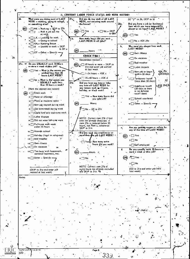
3
. '
. H. CORRENT LABOR FORCE STATUS AND WORK HISTORY .,26. What were you doing most,of LAST 27041 Did you do ony Work of all LAST. (I f "J" in.26,.SKIP to b) -
WEEK - working, spking to, schttol, t, ,,.. WEEK, not counting work around .---or something *Ise? th house? - ' 280. Did you have a job (or business)
* . -,._ ' from which you were tmitporcirifY )) , WK - Working - St to 2h) ,, absent or on layoff LAky, WEEK?
2 J With a rob but not \ 0.1 0 Yes , 2 Np.,- SKIPat work 4 / to -28a . ...work Yes
3 LK - Looklei for work b. How many hours did you work.' 4 S . Going to school , LAST.WEEK at all jpbs? 2 E] No.- ASK 29a
5 KH.- Keeping house ,-,
6 u - Unable to .e.ork - SKIP b., Why were you absent from work -
to WEEK?to 30,,, .Hours '7 0 OT - Other - Specify ,ap , 0 Own illhess
.. .
CkECKTIVA I - . .. -2 0
Respondent worked -.On vacation
22o. ,1*$ Do you USUALLY work 35 INturs 0 1 49 hours or more - SKIP toaE] Bad weather .
or more a week ofitjsi.s job? * 3Ia anc1 enter job worked 40 Labor dispute...
0 i El Yes - What is the reason you at last week
worked leas than 35 2 0 1-34 hours - ASK cS New lob to begin} ,K/9c
Tthin-31:1 days 004298(2)?hours LAST'. WEEK? er
2 N,o -What is the e- r reason you3 01 35-48 hours - ASK d ...' c El Temporary layoff
USUALLY work less 27d. Did you lase ony time or take)less than 30 days) .'-:
. than 35 hours o week? ony time off LAST WEEK for ASK 29d(3)7 0 Indefinite layoff 4,411 any mason such oli illness, .(Mark the oppropriatereason) (30 days or more
holiday, or slack work? or no definite0 1 El Slack work `
,,,,,,.recall date)
2 Material shortage ; r3 Yes - How many hours didyou yoke off? a School interfered
3 Plant or machine repair ' , -'4 0 New lab started during week 0 Hours _ 9 Other - Specify
s 0 Job terminated during week ff.: No - GO to 27e .
6 Could fond'only part-time work, . .
7 Labor dispute . -NOTE: Correct item 27b if lost _
a 0 bid not want full-time work time not'already deducted. if-
Item 27b is reduced below 359 0 Full-time wok weekunder 35 hours hours, ask hem c; otherwise
,-.,SKIP to 310. c r.A you getting wages or salary for
to p Attends school ony of the time off LAST WEEK?- _ -
Dtd)au wa oily overtime or at si 1 Holiday (legal or religious) . mar than jab LAST -WEEK? t CI) i Yes
12 al Bad weather ',e- .., 2 No-ci Yes How many extra .130 Own illness , hours did you work? 3 0 Sel (-employed.,_,..-=-\\ is 0 On vacation 50: ...
7 d. Do you usually work 35 hours or. is 0 Too busy with housework, Hours ../, - more a vittic at this,job? -
personal business, etc.
16 Other - Specify -- o No CO 1° Yes ,-
. 2 0 No I, .. .
NOTE' Cdrrect item 27b if(SKIP to 3Ia and enter lob extra hours not already included (GO to 31a and enter job held
worked at last week) -"arid SKIP to 31a. °41 last week) ..
Notes .. /. i. . .I , ,*41.g0,
:-. .i
. , .
. .
. .
... .. -. '
, 4,1, -. . r, _. .-. ,, . *4 -r-Nt`..-::',. V
VI..
. --. *
-..
.vv-. v.
. , .-.it-
-*. ' ,.
0 .
..... ....., it1 ' ' _ . .
* -
..... ..
Ga.
.

H. CURRENT LABOR FORCE STATUS AND WORK HIOTORY," 7. Continued
29a.
((f "I2K" in 26, ASK b)
Hove you been looking for work during thepost 4 weeks?
- ,0 I Ej Yes 2 rn No -: SKIP to 30
b. What :har* you been doing in the lost 4 weeks, to find vtork? .
(Mark all methods used;.do not read list)
0.0 0 Nothing SKIP to 30 `-
{.1 fl State employment agency
2 :7 Private eMploy"inent agency
3 ED Employer directly
4 Friends or relatives
Checked with
.5 0 Placed or answered ads
6 School employment service1A1,
7 Li Other Specify e.g., MDTA, union orProfessioncif register. etc.
30. When did you lost work of o regular Oh or business,. lasting two ansecutive weeks or more, 'either
full-tinie or parttimejEl Date of last interview or later (iiem I IOR on
Information Sheei) Specify?t - ,
SKIP to 416' on page 13
-.,Unable" now and ' Unable" in item' I:14R anthe Information Sheet SKIP to 820 on page-24,
3f---1 All others SKIP to 42a on page. 13
Month ) Day I Year
Why did you start looking for work? Wos it becousyoy lost or quit a job at thot time (pause) or wos
. there some other reason')
t t'lLost lob2 0 Quit job
3 0 Wanted temporary work
4 Children aria older
0,,Entoy working6 E) Help with family expenses
0 Other -Specify
314: 0 1 I DESCRIPTION OF JOB OR BUSINESS(1) For wham did you work? (Name of company, business,
. organization or other employer) ,
(2) . Is this the full'ond complete some of fite compony7Yes
ri No = What is the full and complete noine
Do. you ever refer to the company by any &the, nom,/.7 Yes Whcit is that names
.l.__: N9 e s . '' '''' ., ' .
(4) To the best of your knowledge, hos,the name of the..1,t;company chongeA in the post year?
Yes What wos the name?
No
In whof city and State is located?
City State
1 1 1 JWhot kind of business or industrfaksohis?(For ixomple TV and radio manufacturer, retail shoe store,State Labor Department, form)
d. (I) Ho'w`many weeks have you been looking for work
(2) How many weeks ago did you start looking for rrk?
(3) How many weeks ago were you loidoff? -.
Weeks
Hove you been looking for full -time or part-time wo'flr?
;;
0 Full-time
2E3 Part-time
lere youto P An employee of o PRIVATE sprn?any, business,
or individuorfor wages, salary, or`commissions?20 Cr; G. A GOVERNMENT employee (Flekrol,Stote,
couil(y, of local)? %30 0 0 Self.iernployed in your OWN business,
professional practice, Of farm?-(If not a farm)
- Is this business incorporated?'21 0 Yes,, 32 77 No
40 7 WP WITHOUT PAY in familybusiness or form?
Is there any reason why you could not take a jobLAST WEEK?
10 Needed at home
20 Temporary illness
En*Going to ;chool.
tiYes
1 4 o Child care not available
soothel, Specify
60 No,
I
I' I IWhat kind of work were you doing? (For example:registered nurse, high school English teacher, waitress)
f ,What w,ere.yo'ur most important activities or duties?(For example,: selling clothing, typing4eeping accountbooks, filing)
I_ lire_lire ,-g. What was your job title?'
When did yowlost work at a regular job'or busineslasting two consecutive we' s or more, eitherfolk*e or pOrt.timi?
,
ID Date of last, interview or later(item I IOR on Information Sheet).Specify ,
Month .1 Day -1Year-
s
1
SKIP to 41a on page 13\ ,
20 A) I:others SKIP. to .42a on page 13
toS T11111 1040.721
I
I
h. When did yoOstorf working for (ENTRY IN 310)?Month ; Day ; Year 1
How did you findout obou that.job?t 0 State employment age9cy2 0 Pitvale employmentagency3 0 Einployer 'directly4 0 Ftiends, relatives 1
,s 0 Placed or answered ads0 School employment service , ,
7 0 Other SPe'iify fe.girMDTA, Union,,etc.)
301,

6,
IL CURRENT LABOR FORCE STATUSyAND WORK HISTORY -; Continued
CHECK
ITEM J'013' or "O" in item 3Id - ASK 32o
CrO" "WP" in item 3.,d -=SIP to 33e,
32a. Altogitthe., how much do.you usrally Tarn at thisjob before deductions? ,
. A '
b. How many hours per week do you usually workof this job?
Do you receive extra pay when you work ever acertain number of hours? , -4(*
a
d. Afier ho; mony hourr,do you receive extra poy?
e. For oil hours worked over (entry in d) are you paid .itraightoime, time ond oneJhalf, double time or %Olaf'?
sr
f, Are your wages ;(salary) on tlyi job siit by a .dollectivy bargairing.agriemen't between youremployer and a union or employe) associatioo3
Ig. What is the,name of the union or employe. association?
'
32a.
d
per(Dollars) (Cents)
Hour
OR
s.(Dol tors only)
L--:1 Day
3 C:J. Week
Biweekly
s Mbnth
6 71 Year
7 Ei Other - Specify
00
r
per
I
Hours
I Yes - ASK d
No .
3 No, bit receive compensating'time off
4 "7; Never work overtime
SKIP to
_Hours per day0.
HOWS per week
Compens'iting time off
277 Straight time-
3 ' Time and one-half
Double time
sn Otaer`- Specify
"1_ Yes - ASK g
2 71 h10 SKIP to 330
<,
- C1CP
h. Are you a member of that union or employee association?;0 h.1
etm
336. Do you generally work the some dayextach week andthe tarn. hours each day, for example, 11-6 Monday.*rough Friday?1
b. WI. at.hours do youtusually wdtk?
4 r
, -,c.Somo people waiil tike to work more honed we if ,
they were "said forlit..0thers would preferfa. workfimer hours a' will*, even if they itarnoOisss. WotIde,-yu Pieter more horsaricl marine pay, fewtihours and ,,
or aboutI,the same number of hours at thes pay? re .f ,
d. bout how manyiliours would you like ta-Wark?1 1
I 1
e. ow many hours pill. week db you usually worka this,joh? I
*
33d.
d.
e.
1,0)7*. t-214111 19.20.711'
1 tIP2
a 11
.
Page 10.
151 Yes
213
Yes - ASK b
zit7, No SKIP to c
Regular day shift
Regulat eve'ntneshift
3 q.Regular night shift
410Sptlt ihiftN
0) More hours and more payASK d
Few'er hoifts and less par
Sorge hours at the same piy SKIP to 34o,
Hours - SKIP to 340:.
, 1
Hours per week
V

.
U. CURRENT LABOR FORCE StATUS AND WORK HISTORY - Continued;34a. Is your work done inside your home or outside 34a
your home?...,
b. How !Ong does it u-suolly take you to get b.to work/
rc. Whot meons of transportation do-you -.. , c
usually use to get to work? .Nark os many boxes as apply)
tf ,...
,
.J '14..`4MOP Ps the total rognif trip cost of ony <I,working fees or tollsyou hove to pay when
yosi drive your own ouzo? .
.
4ii
. ..
e. How mony miles do yo%, go round trip eoch doy?
,
7, Only box I marked in 34c - SKIP to'-- Check Item K5
-- Any of boxes 2-4 marked in 34c - ASK f.f Whot is the totol cost of the round trip
by (means of transportation in c otherthan own auto)
I Inside - SKIP to Check Item K
2 : OJISip, ,...! ,,.li
6 Minutes .
(ED t ;OwnOwn auto - Ask d .
2' Ride with someone else3 Public transportation (bug,
SKIP toetevatesi, railroad, subway, etc.)4 Tax icab s
s : Walk only l6 :' Other - Specify SKIP to Check Item K
eb , s per(Dollars) (Cents)
OD t -, Day2 : Week3 -'' Month J
. .- No,costo
.
--(ED Miles
iTh $ per..
(Dollars) (Cents) .
1 Day 1 ?2 Week l
.
. 6s Month -o;_iNgocost.
CHECKITEM K
El, Entry in 28b - SKIP t6 35dr
item 28b is blank, and - ' - -4 .-ili Entry in 3Id is "R or "G" - ASK 35o
- . '17 Entry in 31d is "0" or "WP" - ASK 35c
35a. Did you work for more thon one employer lost week? 35a.
. ,
b. In addition to working for woges or solary die you boperate your own form, business: or professionlost week?
c..1'addition to this work, did you do ony work for wages .c.or salary lost week') .
.
d. Did you have any other job of which you did not work d.at all last we k?
V
QD t Yes - SKIP to,36a
No - ASK b2
1r0t Yes r SKIP to 360
.''
, 2 -, i No -'SKIP to d
CD t:1 Yes -SKIP to 36a )
2 ij.No - ASK d
t L...,., Yes - ASK 36a , ,.
# 2 '---.. No - SKIP to 38o .
36a. For whom di4I you work in addition to (entry in 31c1? 36aNome of compay, business orianvation or other
,employer)
,:t -8, Whot kind of bainess oeindustAy is this? 'el
(For example: TV and radio manufacturer, retailshoe store, State Labor Deportment, farm)
c. W.riyau - 'I . I ..,..
....,,, ' ,.
. .# .-
. , i.,.! i
- -,d. What kind of work were you doing? (For example: d.1442)
,registerednurse. high school EnglishCecicher, waitress)
i/' .i , I
, ,
.,What ware:your most important activities or duties? I . e.,(For example: selling clothing, typing, filing) . e
:',..
t", C,Wkirt was your job title? "
1 : i ` .i
, .
CD U, .
,, .
III .-. . ,
,
1
(a) t , 7] P An emproyei of a PRIVATi comp (ny, businessor individual for wages, salary, or commission?
2-Q a,- A GOVERNMENT employee (Fechnol, State,county or to'cal)? ; .
. ,3 0 :) Self - employed in your OWN businss, professional-practice or form?
i4 El WP WOlichig WITHOUT PAY in fornilY businesi Or farm?
I 1 i 8,./7-
-
r 1.''
.
. .
CHIRCX4ITEM I.
1
....itle .ff "P" or "G" in item 36c - ASK 37o
Erg "0" or "WP" in item 36c -; SKIP to 37b ,
OPIM (.0,T-411 00-7tli .
1 ;;
Pspi ,I
. 3 2/ 303.

"" -. II. CURRENT LABOR FORCE STATUS AND WORK HISTORY - Contin'ued
37a.,Alto.gther how much do you usually eam at this job 37a.before deductions? s 4 - iti) s -4Pletkr(
- (0011ors) (Cents) . ..___.,-
- , et) I 0 Hour .
"-OR ...
1-4Th s . . r00.
; / . (Dollars only).
.
0 g 0.Dayce . . 5- . 3 E Vieek'
/.F. . .
! o 0 . t.1 4 0 Biweekly - 4 .I
. 6 0 Month
''..., r 6 El Year ' .
.... ..
7 rj Other - Specify
b. How many hours per week do you usually work . b.at this job? .,
" .) (ED 1-burs per week
° _c. When did you start working as a (entry in 36d) 'F.
-r
for (entry-in,30o) 7 6Month : Day ; Year
1 i
i .o ...
38a Before you-began to work.as a (entry in 31e) for -..._38a
."' (entry in 31a) did you do any other kind of work for,(entry in 3101?
b. Excluding paid vacations and paid sick leave, during b.' the time you have worked at this lob, were there any
full week, in which you didn't work (since dote oflost interview)'
es-- .. ' ..
c. Why were you not working daring these weeks? c.
Yes - SKIP to 390
2 n No ..
0 Yes '- How many weeks?
(11D Weeks'
o '-'1 No - SKIP to Check Item M .
LE] Ill or disabled, unable to work
20 In school'0 . .
7 El Person. family reasonsa "_-] Child-73re problems
57 Pregnancy1
6 , Layoff ;
I
7 [-1 Labor dispute
a Did not want to work.
s ri Othei - Specify
-.
_ . ......
'. es
.
CHECK
'TEM M
-Refer; to items 31h and I FOR - .
..t f. '
0 Curient lob started before.date of last interview - SKIP to Check Item T on page 15 ,
1 .!. i .0 Curient lob started date of last interview or later - SKIP to 40 S
39a. When did you start working as a (entry in 31e) for 39a.(entry in 310)7 e
Lb. Excluding paid vacations and paid sick leave, dusiin the b.
time you have worked as a (entry in 31e),,for (entry in 310), .Were *ON any, full weeks in which you didn't work (since
' 'date of last interview)!
_5., 1
'e. Why were you not working during these woolcS? ' C.
. Month :Day - Year ,..... .,
- rp Yes - Howmany weeks?-0 -Weeks .
. 0 0 No - SKIP to CheokItem N
,
1 .. , , .
.
, . ,
le
' I*.
.. ..,
.
. 1,. , :, "
-.
'
--
I 0 OViti illness20 Schilol
- 3 0 Personal, family reasons
a 00Child-care problems .
. s -7'; Pregnancy, \6 D Layoff 1 . 4itileweei -.
. 7 r_fl2abor dispute .
a 0 Did not want to work .
ig Other
..
.
cHECR"
1
ITEM H.
Refer to items 39a iii'dt1 IOR -' 0 Item139a`is lartier than date of las'y interview - SKIP to theC-k Item Ti on page 15 i (
f=j Itemi39a is dot; Of last interview or later - ASK40 i 'I,
4d. Just before you started, on Ail job, was, there a period 40',' in 1 0 Yes - Ski/3 to.53 on page 14 ;i of a week or more in which you were not Iworking!
.. i I6 No - SKIP to 43 an page 14'
1
L G T4I 1040.7il Page 12

5'
(
a
I.
.II. CURRENT LABOR FORCE STATUS AND WORK HISTORY -'Continued .
410. You said you lost worked at.° regular job on (entry 4la. .in 29g or 30). (Interviewer: Use calendar to'determine ,..
`.the numberof weeks since resbondent lost worked.). , .' (C)That would be about weeks since you last worked. (I) Weeks since last worked,
,..In 'how many of these weeks Were you looking for work oron loyoff from a job?
". (2) ' 43:0 f 'Weeks rooking or on layoff .
CHECK 71 4:a(1) is equal to 41a(2) - SKIP to 43a - .IT EM 0
r]41a(1) is greater than 41a(2) - ASK b -
41b. That letiiit's weeks that you were not working or . 41b.looking for works What would you say was the main reason aro Weeksyou were not looking for work during that period? .--
CD1 7., Ill or disabled, unable to work
2 ,:', In' school.
3 I Personal, family reasons
- 4 , -; Child-care problems SKIP
- s 7 Pregnancy .. .to 43
ais
6 ,74t#CoUldrtt fandwork . .
-7 71 Vacation
' i e n-Did not want to work'.. .
,. 9 7 Other - Specify .A420. Since (date of last interview) in how many different -- 42a
.., ..weeks dtd you do any work at all?QD Weeks i
40c-, lie
N r' ' eV
b. Since (dote of lost interview) hove you spent any weeks . b.,..?(ED '\,-- How 'many weekslooking for work or on layoff from a job? 7, Y
.: Weeks-
. o 7 No .
1 -
Refer to 42a and b andilOR - . (I) (e) Weeks since date of last interviewInterviewer: Use coleridorto determine the 'CHECK number of weeks since dote of lost injerview (2) (ED Weeks working on layoff or looking
ITEM P ., foil/Pork (items 42a + q2b) .
(1) is"tequal to (2) - SKIP to Check Item T ..z-. 1,
.
.1 ', (I) is greater than (2)- ASK c- .. .
42c. What would'you say was the main reason you were not j 42c. op ., .Ilr of unable to workworking 0# looking for work during (the resrof) that..
i ' 2 In In school
3 :--, Per 'opal, family reasons,i4 I Chil care problems
k SKIP' IS '1 Pregnancy
e 1
to Check1 '4 6 -7 Couldn't find work
...,
111. Item Ti .
,7 r-1 Vacation,. . 4
a 71Did riot want to work, .......,
, 9 '-0ther - SpecifyNotes
i . 4:11).' 0.
, .
1.
'e,. I 1 i
..
. ....
..
. z.: (.. . .10 .
t #.
1
. .1.
....i fl .
) .., 4/ .,
r1
. .- , t.
j; . .* .,FORM 1.0101 10.26 72)
305 ,

ON0a .. II. CURRENT LABOR FORCE STATUS AND WORK HISTORY - Continued
43. w let'sNjwtillk about -
a. For whom (tidbusiness, organization
b. In what city and
c. What kind of( E . g . - TV and
-. store, Store Lolyor
d. Class of worker
e.ilhat kind offrorkclerk, high school
a
f. What were your(E.g. - sellingteaching tnothernotecs,
g, was your
The job you worked at before you )
started to work as a (ENTRY IN 31eor 41e) for (ENTRY IN 310 or 43oil
The, last job you worked at, thatis, the one which ended on(ENTRY IN 299 OR 30)
you work" (Name of company,or other empfoyell
State is ... located?
business or industry is this?radio monu(octyrer, retool shoe
Deportment, form)
_
were you doing? (E.g.,- sates .English teacher, waitress)
.
most important activities or duties'clothing, keeping occaunr books,
typing) -2
job title' - .
43a.
c.
d.
e.
_.
t.
.t.
CD
(1) #
,, a
Same as 31a - SKIP /0 43er-
(D)
(2) ;
IS
(3)
,
ri Never worked before -
.
El Same as
SKIP roCheck her; 7
SKIP to 43e
. .Never worked before -
D Same as -
SKIP toCheck Item T
.SKIP to 43e
0 P 1CED
'City. State City. State City. State
(ED I 1 I 1 0 I I I 1 9-.ask
a
CD l EIP 2111G 3 0 a 7:wP 0 Zirl: G 3 40
.
(12) 2 r-- G . 3 0 4 r-1 WP0 1 Z1, I I @ I 1 I. 6 I
-
1
k; I
.' ,.
m.
..-
Aft..
--What
44a. Altogether, how much did you usually earn atthis job before 'all deductions'
b. How many 'hours per week did you usually workat this job?, 1,
44a
b.,
63)
41) :-_S per . .
Other .
$ per S_______--.-,0 I '- Fir 3 j Wk.
.Per
1 Hr. 3\.- Yr It, 5 -: Mo.lek;i4
Other -pecily
45..' Mo. ": Other
OD Hours per week
.
204 ao.esoee week
44144#4. -
30 Hours per week i1
45a. When did you start working es a (ENTRY IN 43e),,for (ENTRY IN 43o)?
---
b. Whei did you stop workingtas a (ENTRY IN 43e)for (ENTRY IN 43o)'
+5a.1
b.
t
Month Day 1Year
t )00Month t Day :Year
aps
Montfit:40ay Year
.
.
....
'; Still workingthere - SKIP
to 47
01
e j
Month i Day
. .,, .....Month !Day
7. :
Year
Year
s..
r
e.
a
El Still workingthere -, SKIP
to 47
t
i
Month Day : ear
0 ---1 Still workingx"2" there - SKIP
f6 47
46a. Why did you happen to leave this job,(change.thekind of work you Imre doing)? -
.
b. Did you have a new job lined up before youoleft-this one? ,
ii,..
46
4
b40:1)
ICD I I - .. 0 0
I I
.... 4
A
,IL Yes
,,2 7 No
0 1 El-] Yes2 0 No
.
(ID t. :I Yes,
z 71 No
47. Excluding paid vacations and plidisi.. ck leave,during the time you worked at this Job were there
' any full weeks in which you Aidn'tiwork on thisjob (since dor of lost interview!' .
47. ,
00
Yes - How mOny'weks?...
Weeks -.ASK 480 00
Yes -.How mony weeks?
Weeks - Al 48of .i
00
ó
rn Yes - How mony
Weeks ..
weeks?
ASK '48o ..
Check 'Item Q .en iIdffe SKIP to Check Item fl No - SKIP to Che k Iteril EINO .- SKIP to.
4b. Why were you not working during these ...Weeks at this job?
-
,
48a, IC 1i ..- 2
3
it
'0 Ovin illness 5 00 In 'school 6 01..a)off
Prelltippey
La
Di
Ot
'of disputeaenot want to work
er
031. 3 0 own illness' Sr-1 Fretnancy 1
2 0 In school' 6 0 Layoff3 0 Petsonal family i r-vi al, dOf dispute
reasonsg Did not Want to worka 0 Child care -.
problems 1,2 Other ,
0 Vir-iOwn illness so Pretnanc*2 0 In school 6 0 Layoff
...... 371 personal faAily ..-17.f,_ Labor disputereasons -
8 0 Did not want to work4 CPBaldproblems 0 Other .
ElPsq2nal family 7 IIIreasons
1300 Child care,problems 9
343 I .#

b. Were working 'for someone else during 5.1 0 Yes - GO to next column, enter
- this per od(s)? doto obout this gob o.. . 2Callo
(ED I ED YeS -"GO to next column:enterdote obout this 013
.2ONo
ED 1 r1 Yes - GO to next column, enterdoto obout this gob.
2 0 No $ 'CHECK
ITEM 4
Item 45a is.: , I. 0 - ASK 49 .I. Date of last,interview or later t - ,2. Before date of last interview 2. 0 - SKIP to 50
ED -.'ASK '49
CD - SKIP to , .
EaSKIP
,*- .
VI. Did you do any other kind of work for (ENTRY 49. 1 0 Yes - GO to next column, enterIN 43°) between (DATE IN 45o) and (DATE . doto obout this job ,,
OF LAST INTERVIEW)' ,, . 2 0 No - SKIP to 51 .
,
- ...___0 1 Yes 0 to ext column, entern
-, dot° @bout this gob
ZEDN0 - SKIP to 51 .-
0 1 0 Yes - GO to next column, esteri dote obout this lob .
2 O'No.,- SKIP to Si.,50. Have you worked for anyone else since (dote of 50. ai 1 0 Yes - 60 to next colunfi,lost interv4v.), enter information.
2 jallo - SKIP to Cheek Item T 1
al) 1 1 Yes - GO to next column,.enter inkirmotion *
2 No - SKIP to 'Chick Item T
ED 1 Yes - GO to next column,enter onformotion
*20 No - SKIP to cpeck Item T
51. While you were working for(EN-roi' IN 430), were si. t 0 Yes .- GO to next column, enteryou also working for someone else? doto °bout simUltoneous lob
. .
o :- ASK 52
(ED 1 Yes - GO to next column, enterdoto obout simultoneous gob
2 0 No - ASK 521
0 1 0 Yes - GO to next column, enterdoto obout simultuneous gob .
2 n No - ASK 52 -5Z. Just before you started working as a (ENV& 52. 1 E Yes - ASK 53..IN 43e) for (ENTRY IN 43o) was there a. period
of a week or more in which you were not working? 2 C] No - GO to next column' enter doto, obout previous rob
OD 10 Yes - ASK 53,
.
:,2 r: No - GO to next co/umn , enter dote
. °bout previous gob
flp i 0 Yes - ASK 53 o2 E-3 lb - GO to next column, enter doto '
obout previous /0b53. 'When did this period in which you were not -
working start?
cs-
Month I Day I YearI
*
I tX Nevet worked
before EED
Month 1 Day :YearI
II t I' :1 Never worked
before
Month :Pay Year
X Ellieverworkedbefore.
54a. Interviewer. Determine number gf weeks not 54a.working. If item 53 is before date of fast interviewcount only weeks since that tulle.
b. That would be about ... weeks that you were b.not working. How many of those weeks were youlooking for worlcor on layoff from a job?
'co Week not working
.0 Weeks not working0
EZD Weeks not workinge t
maWeeks looking or on layoffEID co Weeks tooling or on layoff
.
az ; Weeks looking or on layoff
CHECK'
ITEM R
I. 54a ts equet-to 54b I. -1 - SKIP to Check Item S.2. 54a is greateelhan 54b 2. 71 - ASK 55o
::, - SKIP to Check Item S
.g FT -.ASK 55o
' _j - SKIP 70. Check Nein S
f" ! ASK 55o '
15a. That eairest.. weeks that yotrwere'not SSa. CDworking or looking for wdrk., What would you saywas the main reason thavou were not looking -for work during that period ?
,'3 I ., , .
I1 .
se
,f.,_. ,I _i III,or disabled. * 6 0 couldn t f ind-
unable to work work
2 In school 7 0 Vacation3 t Personal f a.mtly 8 D Did not want
reasons tbworls
4 "Child care__.....1 9 El qthelo problems.. .
5 ri Pregnant h or acqtytedchildren - K,I3
.
SKIPto
CheckItem
S
CED0 ' '. -
110 III disabled,. 6 Ti Couldn't findunable to, work work
2 0 In school 7 0 Vacation :
on30 Personal family 8 n Did pot wantreasons to work
4 rJ Child care . 9 n Other- problems
50 Pregnancy,"bit h or acquiredchildren - AS)( b
SKIPto
CheckItem
,S
.
CD
,
.T 1,: ; 'Ill or disabled,
unable to
2 _-.; In scho.ol./.;
3 T] Personal f,. reasons*
4 --' Child care:.' Prot:he.ms
5" Pregriaticy,!tinthchildren -
6 L Couldn't fogdcork work
7 r1 Vacation 'milt 8 f:1 Did not want
to work
. 9 I. '.0.ther '
or acquiredASK b ' '
_.
SKIPto
Chec kItem
S
..
b. When,was your baby born (did you asSume charge b.of this child)?
'
_____,Month Year
iI
1'
fIx Not botn yet
Month :Year
' I
1
Xf1 Not bom yet. CD
Month Year
' _, -I Not born yet . .
-..= - 7- -.
c. Wereyou employed within rifle yeal, before.(this c.1 (Ilt i fjYes - ASK d , i .
pregnancy, birth of child, c ild came, to live 1
.,
with you)? -20 No - SKIP to Check Ittin S
I [2-Yó - ASK d i,
421:3 No - SKIP to Check Item S
el) t :1 Yes - ASK ci
. 2 _--1, No - SKIP, ti, chcck.item S1
i
d. Did'you receive maternity leave ar some assurance d. , 0 'Yesthat your job 'would be held for you?
' 2 No "er "
g , t] Yes t
we20 NoI 7.1 Yes
2 f 7 No
.CHECKITEM'S
.1 - 0 - GO tents, column, enter
1. Item 53 is date o last mterview or Later 1.; doto obout previous jbb '-,
.2. Item13 is beforeidate of last interview 2. C]- SKIP to Check Item.T11 $ ;
0 - GO to next column, enterdoto obout previous job0 SKIP to ChecklItem T
- in - GO to near, column, enterdoto *bout previous rob
- SKIP to Check Item T S
3 '
16
3 4 (3
9t
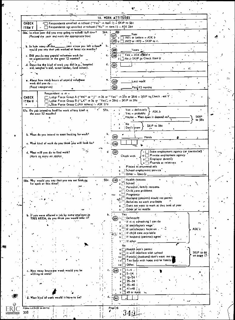
Ilk. WORK ATTITUDES .
- <,
CHECKITEM T
rEj Respondents enrolled in school ("Yes" in item I) - SKIP to 56c- E) Respondents npt enrolled in-school ("No" in item I) - ASK 56a
56ri. In .what(Recorgl
-
b. In howwould
c. Did youon organization. " .
,d. Describeaid, teacher's
. Aboutwork(Read
year did you stop going to-scholll full timr? 56a.the year and mark the appropriate-box)
1'.
many Oia year since you left schools b.
Year - .
,
.i 0 1971 or before - ASK b .
co 2 [11972' or 1973 - SKIP to C.,
YearsQyou say that yob worked at least six months?, _
do any unpaicrvolunter work for c.in the rst 12 months?
the kind of work you did (e.g., hospitol d.aid, scout leader, fund raiser).
..
4 ..
how mans, hours of unpaid voluriteerdid you do . .
categories) .
0 I; ; Yes - ASK etiiid e .
2 []'No :-SKIP,to Check Item. U
cED I I . .
-r---.
7a. .--=-_
.
'
6 Last week '_Pas 12 months
CHECKITEM U .,
Respondent is in - .0 Labs( Force Group A ("WK" or "J" in 26 or -Yes" in 27a or 28a) - SKIP ta,Check 'aril' y : -p Labor Force Group B ("LK" in 26 or "Yes'..; in 295) - SKIP to 590 ..-7 Labor Force Group C.(All others) *- ASK SIci
570. Do yaii intend to loolefor work of bny kind in y 57a.the next 12 months?
a'
.
b. When do you intend to start looking for - world b.
....
c. Who's kind of work do you think will look for/ : c . ,i
. ___--s
d. What will you do to find work? d
(Mark as many as ,apply).
1
.... N
' . Yes - definitely} .ASK.b .
I , 2 ; Yes - probably' -,I Maybe - What does it depend on/ SKIP
1 to 58a
' c 3 'No4 ] Don't now' SKIP to 58a
.0.
0tMonth `
.x
as) I I I I ,.
,, ir.
, CED, [j State employment agency (or counselor%
Check with 2 0 Private employment agency. 3 E.] Employer directly
'4 El Friends or relatives
, . ,s Placed or, answered ads6 ,_,21 School employment service'7 1 Other'- Specify . '
58a. Why would you say that you are not Idoking , 1 58a
for v4ork at this time?. , .t:siw .,
..
1 '..
--.
. -. .
.xx4,
b. if yOu were offered a job by somemployerjo b.
THIS AREA, do you think you would take it?.,
.,
, ,
,
' 1
.
te. How many hoursper week would you be , c.
willing to work? ; j
1.17
i .
.
j 1.
Ad. What lcincraf work would it have to be?
. .
..1 Health reasons -2 r school , :
. .. -"\., , ,, , , ,: 3 i-:1 rersonai. tamiiy reasons.
4 [-1 Child, are prOblemsit.'' s :::,) Pregn'ancy' . . -
.
. ,,,,,f. El Husband ,(patents) Would not permit1 7 71 Believes no work available ' -
8 ,--1 Does hot want to work at this time of year ...
, 9 ; j Other no ....
Yes -,. , -i L.1. Definitel% '
i2 ' If it is something 1 can do3,1 ,:, It satisfactory wage',4 r-I, If satisfactory location . - --:
.. 5 t _I If child care available6 T:I If husband (parents) agree - .
... x7 r r."1 If othrr,
ASK 'c
t
SKIP to 66on page 17-
.No ,
e",_, .. , i
8 Li.neatitn won't permit9 ED It will interfere with school
to C:1-Parerti(busband) don't want me' 110 To busy, with home and/or family
i 2 n other, ,
0 i 0 1-4 , 12 0 5-145 I '
1 3 El 1$ =24 l I
.
,4 L 25-34 1 .5 0 35-40 1
; 0 41-48 f 0
7 O' 49 or more
1111` .....e
, , , )
rams Lotdt le-2072i
308 -:
.Page'115
11 ,2.

*ir
c
I I
%
..o
Ill. WORK ATTITUDES - Continued
58e. What would the wage or salary have to be . 58e.,
.
- . .. . .
. .. -
. .. .
--.. . 0. .
, ' ,/
"`
-'..I .
.
o
S.ea . per
SKIPto 66
.
.
. (Dollars) (Cents) 'ilD i , -1 Hour
' .
OR f -
40- S e 00(Dollars only)
2,11 Day3 11 Week - .
4 7-] Biweekly .5 , iMonth .
6 -,--"'Year
i 7 Other - Specify
59a. What typtr
"b. What
-to be
.
IA
c. Are thereof job
d. What ate
e. How manyto work?
of work are you looking far? 59a..
.
./would the wage or salary have to be for you / b.willing4to take it?
-
.
..
: .any restrictions, such as hours or locotion c.
that Tvould be a factor in your taking a job? .. - .these restrictions?
Atd.
0 .*
e
.(2) 'ICU.
i
. S per: -,
t:.
.
". (Dollars) (Cents) I
CD Hour
OR.00
CD s' per:(Dollars only)
0 2-7 Day SIP
: 4 3 :1 ile k; 4 -1 Biweekly
s' 7 Month
6 -1 Year
7 !Other SPeCify
,(ED ,,,, Yes - ASK 0
No -SKIP to e '
GI1 F.
hours per week would you like e.sr:
Hours - SKIP to 66
CHECK
ITEM V
., ) .Resptindent - i --, Ej Was in Lab'or Force Group C last year (Item I I4R on Ipformallbri Sheet) - ASK 60
.. .El All others --SKIP to 61a - V
1
60. At .ihis.timi last year, you were not looking for work. 60 at) Recovert.d from illness' 4What made\you decide to take a job' 2 .- Bored
r
3 Completed education .
4 .-., Needed moneys -; Home responsibilities hi) longer prevent
, 1
me from working ... 6 :---' Qher - Speedy ./.
61a. HoW do rid feel about the job you have now? Do 81.a. '
you like it very much, like it fairly well, dislike it i
somewhat, dislike,,it very much?. I \ ,
- .'-i
....
ID. What are the' things you like best about your job?' b.
I . 1 t ' ) (I)
-71 i2) '
'\I
I 7
(3) 1.,
-:
What are the things about, your job` that you don't liftej c.
(1)
(2),
..., .....
. , (3), ..
6 i ::,3 Like it very.mUch2 -.:1_!ke it fairly well3 -; Dislike it Somewhat 3
-Dislike it very much.
j.
I I I
0 1 { I , . .,.
i .
C) L I', I
cr) 1i1 .,,
I 1 1 .
:.
.
.
(42072)
1 .1 r 1
r
t

,
j.
er-- J
I r - Ill. WORK ATTITUDES , Continuod ,62o. Sutirpos somon N THIS o red you a 62a.
a job in, the MR* line of work fou'r in now. Howmuch would the new job have to pay for you toll.
. 4111ing to take it?(If amount given per hour. record dollars and cents. .Otherwise, round to the nearest-dollar.)
-.
-.
.i?"
' .
i .
,- . .
-
'.
b. If someone IN THIS AR EA offered you a job of your b.prestalt raft of pay in a different line of work forwhich you or., ouolified, do you think you would toke it?
'*o--
e. What kind of work would you accept? c.lio
.
0 .5 per
r
,...-
.
.:.
,
it ....;
.
'
,,,
(Dollars) (Cents)0 i Hour
OR
vilir'CI s00 per-
(Dollars only0 20 Day
.
. 3 0 Week
... a Ei Biweekly.
sEl Month ,
.6 ED Year
, ri Other Specify ,.
a 0 I wouldn't take it at any concelJable pay '.9 0 I would take a steady same or less pay ,,-..
io 0 Would accept job: don't know specific amount
1 I 7 Don't know ,.
"1"2-1&1 Other
0 1 71 Yes ASK ce
2 ; i No SKIP to Check Item W .
1 1 1 I
.
CHECKITEM W
Refer to item 13 on the cover page and to item I . -
Respondent not married and not enrolled in school ASK 63 .
0 All other-- SKIfseter-C4ieck Item X '
63. What i this job was in the sane line.of work you are 63.in now but was IN SOME -OTHER PART OF THECOUNTRY how muclologid it have to pay in ordefor you to be willing-to RE. it? ;(I( amount given per hour: record)dollars and cents.Otherwise, round to the nearest dollar.) 1/.
t 1.
_.
,..
' . .
....J.7 i
..1
. ir,-.
.,
s
. s %
. f. .. ..,..
@ S per
.
.
.
(Dollars) (Cents)7
0 CE HourOR latr.
CD Soo per 7_.
. (Dollars only)
CD 2'71 Day
3 El Week
4 0 Biweekly
s 0 Mjnith.
61 ';year. .
7 Ei Other Specify
je a 0 I wouldn't take ot at any conceivable pay)
, 9 j:-.) I would takea steady job at same or less(pay
to Would accept job; don't know specific amount' .--- -
1 1 Obepends on location, cost of living
12 0 Don't know,
ow
13 0,(3ther .
'''''
o
- 7
CHECK
ITEM X
i Refer to item 114R od--the Infariltation Sheet. 4' . 1,,. '
ED Respondentn1LaborForce Group A, in 1972 --ASK 64 ..!.. ,
0 All other SKIP to 66 / . 4 .
64. Would you -say you lilte your pfeint job more, loss, 64.or about +groom. os,Ithesjob roir held) last' fear?
. 1 , . -',
"4)
. s '',, ,
e 1 ,More ..:,fs::
, ASK 65 ,
El LessI ' /
'
o
3 In Same SKIP to 66 ; A
65. )that would you say i); thin,' afnireasin that you like '1 , .65.your preartOt job (more, Wont 'i ,t.,-
i --
a 4 ) ' s )z . ltrY, 1 - I
; (0) I ' 1 '1 i
:
". .
iL 1
66..Whai would you say is A. molio/iMpOrtdnt thing 66?1about any job good wages or liking thiojtind -of work you are doing? .,, .
i
11/
CD o [.Good Wages. /..1
'2 0 Liking the work

s
I
set
ft
... , . III.. WORIC ATTITUDES - ContinuedVG. Would you say that
beim any change' job outside the home4.
--6. In what way has
--ol
c. Why' wouldayou say
0 .
during the past yew there hcis 67a.Yes - ASK b arid 4.in your feeling about having a
.for pay?z ;So
". y SKIP to 683 Don't know
..s
your feeling changed? b l) I
. . _.
.
.
1
.,your thinking has changed' c c)
, ..
. .4. . .
L_1..-
, .
fit 0
...-- . .. ,
68. We wdultliko to find out whether pestple's outlook on life hos any effect on the kind of robs they have,*the'waythey look'
for work, how much they work, and matters of that kind. On each of these cards is a pairpf statements, numbered I. gaj.For each pair, ele-a-Se select ONE stotement which is closer to yoUjr opinion lit addition, tell me whether the statement
. yOu select is MUCH CLOSER to your opinion or SLIGHTLY CLOSER:AG,."., PA. . . . -
...
In come cases you may field that you believe bo h itateTents, in other cases you may bellevemeither one. Even when you. o . .feel this way about a pair of statements, selec e one stotement which is more nearly true in your opinion
0''. a
trx to consder each pair of statements separately;when making your choices, do not be Influenced by your previoul choices.. ,
. . %
a 4ID 'Many of the unhappy things ,n people's2 People's misfortune . t from 'thelives 4e,partly due to bad luck
mistakes they makeIP° . , . ,
1.--I.
o
Is this stotement much closer or ;"..,,slightlyticlosdr so your opinscin." . .,, -. . .
e "-,....' 9 Slightly:''''l '''''YI . ..
1
In the,CD.
they deserve:
' i
I. ot
long rein, people get the respect.
.,2 Unfortunately, an sndividuari worthin this world. ,
, r Often Dassesionrecbgn 1 zed nr), mattert 4
.., how hard he tries.
.." - ,
Is this 'Statement much daterter or .
slightly closer to. ypur opinion'.. '
a 1 Sltihtly g i )*..- a Mucrs. i
o o . :- ,i. cp , _. Withodt
be an.
.. 1
,1.'the right breaks, one cannot , 2 Capable people o fail to.effective leadir. ,, leaders have not taken advanI
3then opportunitiesi-.
Is this stotement much closeroor a ' s
. s 0, sllhtly closer to your opinion? ,
. .6a Mucq a° 9 , Slightly
.
comege of
2
d.. im , :;_-_, B corning- hard
to do
''''''`t%
I
a success is a.rriMter of ;,.. ,
prk: luck has little or nothingith it. I ° r ,
* '
1 , . ''oo Is tills statement much"
1 slightly closet to yofft'opinton?.. ,
Much 9, .iSIghtlyi I.
_
Getting aegood lobtdepends-1.....Pn_hetng-in the-night-place at-
,. right time, A.
`..fcloser or' .
..c
.
.
filly 0
he ---"
.
i
.
i...., _. ,,.. ; What h
,.
.4, -'..-°--i
ppens to me is mty own doing.; I,..i7 ,
, lIs this statementrnuch- slightly closer Jo your°opinionl
*
1 : 8: ;Hach 9 ,:li.Sliihtlyi
l l_ r I i ''
,2 Somettmes I teel thatl-don't
p. enough control ovef the directI life is- taking. :
I .'closer 'or
.1I '
,
l ' t i
al,eon my
1
.1. :
'ORM LC 0.202)j :4441
11
S.
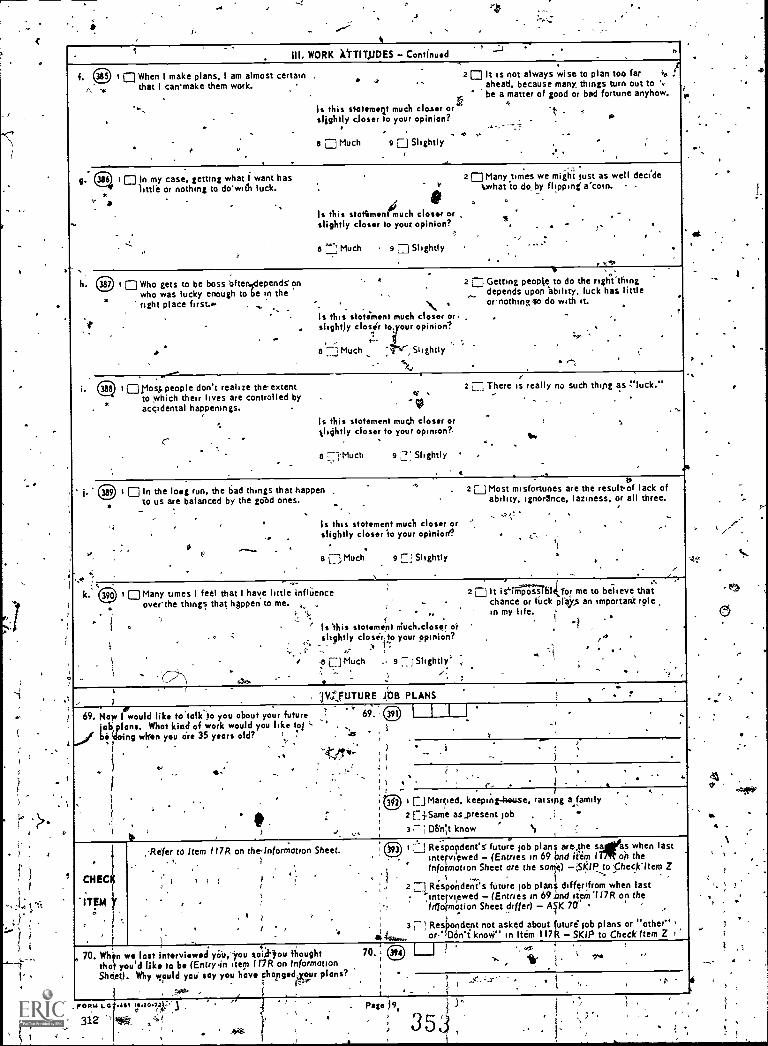
r1
5 '
T Ill. WORK VTTITJDES - Continued ' E.
f.A -
iIt is not always wise to plan too far2 0 kia ahead, because many, things turn out 0 ..
be a matter of good or bad fortune anyhow.,
much closer or -tTo your opinion? 10
. . .. R ...
9 EJ Slightly -r '
lill When I make plans, I am almost certain .
that I can.make them work.,
.... Is this statement, slightly closer
.
, a 0 Much
g. 386 i 0 In my case, getting what I want has z 0 Many times we might lust as well decidelittle or nothing to do*witli luck. .
- t.what to do by flippinf a'coin. -
r , p ..I s this steSsment
amuch closet or , ', * 'slightly closer to your opinion? '
.
; ,
8 t] Much , 9 Ei Slightly .
- r ,11's ,
i 0 Who gets to be boss Often.idepends on ,, a 2 Getting people to do the right-thingwho was lucky enough to be in the depends upon ability, luck has, little,-.right place first.. \ ornothing 40 do with it.
- . .Is this stotement much closer or . , -
. slightly closer to. our opinion?.
.. . . ,
1 8 .-H Much
,.'IN Slightlyhtla r
' '7':."..-.
. .
i. 0 10 floss, people don't realize the extent 2 Ej There is really no such thing as 'luck."ei .to which their lives are controlled by - . .
. accidental happenings. 0 _
-,,
Is this statement mut.h closer or , I' %lightly closer to your opinion ? - .
C" - lo". ,
8 7 i' 9 :...7 : Slightly .__.
_ . 0t - ...is
I p In the loag run, the bad things that happen , 2 L__) Most misfortunes are the result-of lack ofto us are balanced by the gold ones. ability, ignorance, laziness, or all three.
.. Is this stotement much closer or
slightly closer to your opiniore? . ''0" .
9a M 7; Slightlyit]uch...,
1
.-
. CD I 0 Many times I feel that I have little influence 2 It is`impo s bI,for me to believe thatover'the things that happen to me. - chance or Iiick plays an important rple
; .f., ., " in my life..1,
°1 ,' . Is' ht this stotement mucn.cioser or
* slightly closer,to your opinion? /54
. i a II Much ., 9 7t.i- Slightly' ,
';
t__. /,. - 1_ -1
.
, . iie,PUTURE .1013 PLANS .;
69. Nowlab
.../be.
.I would like to talk'to you about your future 69..01
plans. What kind of, work would you like tot 'doing Oren you are 35 years old? `
. . ,
.. '''t,p,Pit..
o,-
,
.
.) 4
I I I c..
.
i .
.
i)-.. 1
)
.4 ' i 5
CD i []Married, keeping-house, raising aofamily2 F-1-Same as,present lob ,
'3 7. ; Dtin',t know %
,
CHECK
ITEM y
:Refer to Item I I7R on rheInformation Sheet.
, , f ;/"
I .
I r ..1
444,
i :_-_.] Respondent's' future lob plans are,the slras when lastinterviewed - (Entries in 69 },nd item I oh thefnfoimorion Sheet ore the sat) -;,SKIP to -Checkitem Z
.. .,.. ---.
2 0 Respondent's future lob plant differlfrom when last'interviewed - (Entries in 69 kind item I I7R on theIrfformarfon Sheet differ) - All( 70
tondent not asked about future' lob plans or "other"3 7 I Respondent
'or-' DOn't knovr" in Item II7R - SKIP to Check Item Z
70. WinthaSheet).
s,we last interviewed yiiia, you saiktou thought 70.
you'd like to be (Entry-in 'tern II7R on InformationWhy would you soy you have Fhanged,pour plans?
1-
r, 0 LI ' ,'... r '
' it I
, .,r
1
.
FORM 1.0
312
.4511,11.20.741
4'°Pale )9.
54,
et
/ -
c5
'
.8
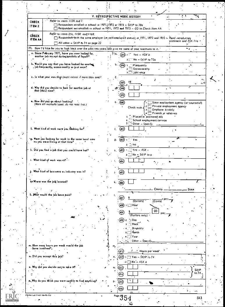
.' V. RETROSPECTI-VE WORK HISTORY . ., I,
CHECK
ITEM Z
Refer to Items 112R and l ,
IE Respondent enrolled in school in 1.171,1172 or 1973 - SKIP to 78a .0 Respondent not enrolled in school in 1971, 1972 and f973 - GO to Check Item AA
diECKITEM AA
,Refer to items .3,1a, 115R cnc1;116R I
El Responcielit-Cylth the same employer (oriselferoployed status) in 1971, 1972 and 1971 .-- Read introductory- statement and ASK 71acp All other - SKIP to 74 on page 22 i i ,-
71. Now I d like, for you to look back over the past two yearsarId give me some of your reactions to It. "o. Since February 1971, have you ever looked for, , 7ia
another job except duringverrods of layoff' i 1
b. Would you soy that you have looked for onoth%i
, job frequently, occasionally or just once?
c. In what year was tha4 t (moSt recent if more than one) 7
,
_.d. Why did you decide to look for another job of
that (this) time? " , -
tr. How 'did yaii go about looking?(Mark all methods Used; do not read list.)
.. -. .
.
f. What kind of work were ifs', tacking for' f.
...
>43. Were You looking for wink in the some local area g.as you were living at that time'
- h. Did you find o job that you could have had'1
i. What kind of work was -it? - . . i.
°j. What kind of business or, industry was it? 1 I.g1111' '';
ke Where was fie lab; located? k.
. 'I..)1iliat would the jol have paid?
,I.
.7
. a-. '1
*-,
C.1" 1
. 'I
_ l'i- - ii
1 ..
m. How many hours per week would the job .s, re?
' have involved), -. 9.
n. Did you accept this job? - i n... 4'7. 1
o. Why did you decide not to take it? . 0 0.0.... ..,
,-..-
.
p. Why do you think you were unoble to find, anything? * p,
.
. ,
CD .1 Yes - ASK' b-
2 T No --SKIP to 72a
(11) j, :-Feouently .
2 ::,-] Occasronally3 71: J u's t ? n c g _ ...
,
. .l0 19 ., ,-.,-:a
0 I, I I
0 1 I I
_
-i ::: State employthent agency (orcounselof)z tl2 Private employment agencyCheck with3 El Employer direttly4 0 Friends or relatives
41
5 Placed, or answered ads.-6 Li; School employment-service3' -' Other - Specify
0 1 I I I
0 1 -: 'Yes-. ...
2 : No
(1) 1 2 Yes - ASK t.2 72 No7..- SKIP to p
ICD I I1=1 I 4.
4
It '
CI L j .
.' County State,
,r-_-.. .
411.9 a' per:..,t
(Dollars) (Cents) f0 1 Ej ao u r
. -
® $ 00 peras
pe,*(Dollars only) .
Ci 2 ":1 Day-, -
3 ) Week ..
t
. 4 Blw,eekly ;s Ei Month6 i _;Year -
-; Other - Specify
0 - Hours per 'week'.. '
..(E) , r--] Yes - SKIP to 74 tw
-2 [J No'- ASK c ,
I I I.
r . SKIP
el) I 1 I.. , to 74 ,
I-
ra, i--.1 1 it. ,
0 I 1 I.4,0
FORM 4.0T:451 19.20.72)

4
1
V. RETROSPECTIVE
0
WORK HISTORt---Continued- 'I
72o. Sine February 101, has any otheremployer made youla definite offer of afull)time jab that you did not accept?
In vihoeyeL was dot (most recent'lf more than one)?
c. WO' did you happen to -get the offer')
d. Wj1j kind of work was it?
e. Whir kind of ,businss or indust6, was..it7
I
f Was this jab located in the same local area asyou were !wing at that time?
g. Whcit would the rar, have
I
h. Hire many baurs per week wourfl This felthave involved?
I .
..0
i. Why; did you decide net to take )t7
as
72a.
e.
f
Yest Haw many times?
ASK b
o 12; SKIP tc.73o
1
Job' offered by a friend, relativei2 L.: Jgbioffered by a business acquaintance
Jobioffered by a former employer
4 j Other Specify
I 11 I
p 1 1
Yes
4 2 No
goofs7
(Dollars) (Cents)
Hour
S
(Dollars only)
2 Day INITA cs
3 Week, '
Biweekly
5 Month
L) Year,
7 -" Other .Specify
00 cker:
Hours per week
I 1 1
( 1 1
t0SKIP
"1 1 If item 71 a is '.'Yes" SKIP to 74
,730. Ouririg this period havrtyou ev:irr seriously"thought of Jookirti for another ftsb?
)
b. Why would you say you've thadght of looking," i
c. Why didn't you actually look fot a jab'
d." Why not?
00 3.9,451 1920721
314 -'
,
73a.
d.
Yes iSK,b
21 No ASK,d-
.7)
**Pate 21, 1 ,

. I
, e' V. RETROSPECTIVE WORK HISTORYs
- Continued.
' 7,1 .E;pployers -.
) .8,..
.
.
.
77'
.
SKIPtoCheckItem88 .
74. In the past f ive years, since February 1968,for how many different employer; hoveyou worked'
-","74. ,*k
;(1);
sASKI --
vorkettlinee Fe6roary 19Elei - "KII"'
75a.:All in all, so for as yo'ur work ,s concernedwould yea say you've progressed duringthe pis* two years, moved backward, or justabout held your awn'
., .
,12t,411,it what way(s) would you soy you have progressed? V,*
...
°.
5.0
. ..
.
c. In what way(s) would you'soy you have moved.ipekward?. , .
'
75a.
J
-
,
Progressed - ASK a i. ,
2 'Movea backward - SKIP to ,. ;s
3. Held own .
SKIP to Check Ifern 884 ":"_ Not worked} .
b. IC)
?
1 440.1
, 0,1
OID
vI
.
...
1
,
,
,-
....
c. ari
, 14
I ' I 1
,,-
. ,EF
.
,
CHECK .ITEtA BB
Refer to I I2R.
Respondent enrolled ,n scno..... ol'
1
I or more years'since I068 - SKIP to 78ooil .E.-- All others - ASK 76 .
....'76. Eicluding paid vacation and p laid sick lea.ve, since
February 1968 - about how-many different weeks'were you NOT Working/
-
76. 1.
(0)o
,V
-Weeks . ASK 77a.
. ..
- / .
None - SKIP to 78a .
77a. How many of these (entry in 761 weeks were you ,
looking forwarVor an layoff Tram o jab?
.1 . .,
b, That means there were about j,enrry ,n 76 fess e-try- ; in 77a) weeks since February 1968 you were not
working or looking for work. Is that corrects1
77a.
- 446
,o
.
Weeks
I ..
None . ..
b. . - ,
Yes - GO to 78a ,- _
No - Deteirrine whethet 76 or 77a is incorrect*rake necessary correction
''Notes ..,
1 ' -. .,
, . .
.
- *1
...
1 .,
.t .
1 -, ,
.
.
...
.4.
"'
'r/ ,
-2,
.
.
..
a..._
.
.
,
.
.1
..
1 1
...
.
'
-
'
.
e
- .. ..
0
..
. . I.. . .,
. , * .. .
.
.
F .. ,
4 .R.
.,
... c, . ,
,.: ,
..
.
a
.
P
...
, .., . . .
,
..
.
FORM LGT.451 A1.0.721 Pale 22 '
./1

,)
4
VI. HEALTH
78a. Do you have ony health problem or physicol .
condition thot limits in onywoy the °mountor kind of werk,you can do? C.
.
b. Who is the rfoturs of thot heolth problem? ,
. .,
c. flow long hove you !igen limited in this woy?(Specify number of m. bnths if less than a year)
. .
d: Da" you have ony health problems that in onywoylimit your other activities?
A
ea What activities ore limited?(Mark as many as apply)
rs.
. .
. * I I
78a . I,
,
b.'
'c.
d.
e"
(D) I E - ASK b
o - SKIP to d
.4.
(1).
I
-:-r_._.
f:ED _____ Year(s)-
Months
OR.
(If less than I year)
ri
i Yes - ASK e
a 0,No - SKIP to 79 .
CD , E Housework
CD 2 C SchoolcED a 7 Child-careCD RecreationE4
45S s E Other .
.
79. During the post three years, hos your health becomebetter, remoined the some, or become worse', .
7. .
79.
-
0 I 1_171:letter2 [7, tame
3 E Worse.
E Respondent not married spouie present - SKIP to 8Ia
80o. Does your husband's health or physicol condition limitIn onywoy tfie amount or kind of work he con do',
b. In what woy is his worklimited? 4- e Ct
c. Now long has he been limited in this woy?(Specify number of months if less than a year)
;.
80a.
b.
c.
--CD , 7 Yes - ASK b and c
2 C Nb - SKIP to 8Ia
.
165 .
.,
..
ISd Year(s). ,
(If less than J year)
.
.Months
0 Respondent (and husband) lives alone - SKIP to 82a
M o. Is there any one (else) in this fomily living here, who Is not working or not going to school becouse of
poor heciIth?(Mark as many as apply) .
i.
kr..DOes the health condition of this person in anywoyaffect the kind or omount of. work yottcan do or where- ,you work?
,.. ,
.
Ella.)0s
.
b.
E Yes - Who is it?r, Son
' .2 0 Daughter
. 3 0 Parent (1n-law)'
4 ClOther SPeelf);
.
. .
s E--; No - SKIP to 82a- *
t -CI Yes *.- How?'- .., - .-
...":411-. .
.
a Q No .
Notes.
. '- ,.
. ,...
. - .
.
. .. .
.
.
. . . ". ... . . ,
.- .
. .. , ,
e
_
.
;..
CD.
,0
.
...
. ..
.
r.
/.
..
..
.
': /
.
,
.
. V--.,
. . ,
.
,
. '
/.
.
:v*..,
.
.
/04445L01111 040417
316
-
I..

t, .
't VIE. ASSETS AND INCOME
82a. So far os Your overall fin ncial positionj is concerned, . 82a.would you ;say you are b r off, about fhtfsam., orworse off now than you were at this time last year?
I 'b. In what woysige you (better, worse) off' b.
1
l
0 , D Same,- SKIP to Check Item CC2 El getter off 1 ii.
5 Worse off ASK b .71.
(D:jf
. ,
CHECK-ITEM CC
iCaRespondent (or buiband)l is NOT head of household - SKIP'to 85o+r] Respondent (or husband)is head of household - ASK 83a
83o. In. thelast 12 months did 'you (or your husband) receive 83a.financial assistance from any of your relatives'
i 1
,
b. From whom? b.
c. How much did you receiver c.
--_. ;
t El Yes - ASK b and C -
21 ; No --, SKIP to 840
CI I I .
49.5) $00
84a. Is this house (apartment) owned or being bought by 84a.you (or your husbdnd)?
b. About how-much do you think this property would sell b.foi on today's market?' 4
.
c. About how much do you (or your husband) owe on,this c.s' property for mortgages, back taxes, home improvement
loans, etc.?
al :1 Yes - ASK b ond'c
z '`, No -SKIP to 85a . .
.
000:9
is S ob
, figne
SSG. Do you (or your husband) have any money 41 savings 85e.or checking accounts, savings and loan companies ar - ...
credit unions"
b. Do pits (or your husband) have any - --ww , b.'
(1) U.S. Savings Bonds? , (1)
v..(2) Stocks, bonds, or mutual funds? (2)
/-
r ' Yes - How much altogethei?
0 s .' 00No
' Yes - What is their face value? , .
, 00(2) s' No
-: Yes- About how much is their market value?
ODNo
,86a. Do yOulor your husband) lent, own, or have an 86a.investment in a farm, business,' or any other real estate?
.b. Which one? b,
. . . , .
t. AVoutilow much do you think this (business, farm, or a.other real estate) would sell for on today's market?
d. What is the total amount of debt and other liabilitieson this (business, farm, 'or other real estate)?
CD i 7: Yes:- ASK b-d t .
2 7- No - SKIP to 87a
:1 1 -, Farm '2:: Business
Real estate
.
; .
CD S r , 00
,
CD * $00
, Li None '87a. Do you (or your husbandrown,an automobile(:)' 87a
. ..
b. What is (are) the make and model year? 1 b .
' -
c. Do you owe any money on this (ths) automobile(s)' c.- - .
, ,
.1.
,. . .
d. How-much would this (these) car(s) sell for on d.today's market?
.,.
..
, (ED , ,- Yes -,ASK b-.4 ,
2 [j No - SKIP to 88
lO
.
' Modelyear Mc;Model year Make
Model year Make
Yes - How much? .
r+
00 .S.
.0 s oo i ?c No 2
.
0 00.
. - . 00
. 00 .
8%. Do you (or your husband) ow any (other) money toStores; bankscfoctotsor anyone else, excluding ' -
I' 30.day charge,accounts?
. .
..,- Hew muc
iC.) 5- g00
n Naroam La ,,401 10.20.72)
_Pate 24317 '

t I
. i 1
- 911., ASSETS AND INCOME - Continuied * . ,
Now I would like to ask a few questions obout yourincome in the last 12 nianthi.
B90. How much did youlor your husband) receive frau;wages, salary, commissions, or tips from all jabs,before deductions for taxes or anything else?
.
b. Did you (or your husband) receive any income from1
working our own.or in your own butiness or fain?
S less S . _S '
89a
b.
°
c.
(I)
(2)
d.
,RESPONDENT
HUSBAND 10 Not married
r r. t r
0 $ P° 0 S CO
' None FA None.
; Yes - How much?40 S' i OP-5-1
I-1 Yes -'How much?eS .
1 (00(Gross income) 4Exoenses) (Net income)
. --
' c. Diclyou (or yoerts1/4Isfland) receive oilyunemployment compenirion?
- . -
d. Did you (or your husband) receive ooylther income,such as rental income, interest or dividends, incomeos a result of disability or illness, etc.?
. 1:. ! No . f:I No .
[ 1 Yes'
How,r7 ny weeks?
0
{:j Yes
How many weeks'
-,.0. How much?
i
3
.
[mildHow much?
S
.00
I No-- [j 1 No,.
Yes How much? ', I Yes - How much'
$ °15i .00@ $
No No
CHECK
ITEM DO
Refer to,Household Record Card'
ik-
-
0 I RespokfntTand husband) live alone - SKIP to 90b '.
2 All others - ASK 90a (I f two of more RELATED respon?dents in household, lsk 90aLb only once. and transcribeanswers from the first to the other ouistoonnaoreC.)
900.1n the past 12 months, what was thootal incomeof ALL family members living here? .
(Show lashcard) .
,.
,
. -.
4-
b. Did anyone in'this''farnily receive ony welfare tr.public assistance in the last 1.2 months?
.b.
gr
i
Under SI .000 N.
2 SI ,000 $1,499 t *3 2.000 - 2,999 , .
I* a 3.000 - 3.919- ,
5 ° 4,000 - 4,999 .I
e I 5,000 - .5,999
i 6.000 - 7,499
9119 . , .--
9 10.000 - 14,9999
9
10 15,000 - 24,999 a'-25.000 and over -,
I
;4-,-;\ y Yes .I V-4.1',t 2 No ..
Notes .,
4111 -
.
5,,,,..
.
,.!.-
al . .
.
.
;
, .
.0 ,
,
. . lit .,
.,.< -,. - ,
.
, . .,,-_ , . .
.
. ..
r' r .
.I #
.
,
.:..,
. .
. 1.;.
. .
.
FORM L,GY-451 O140.721
318,
Page ZS
35.'-u 4
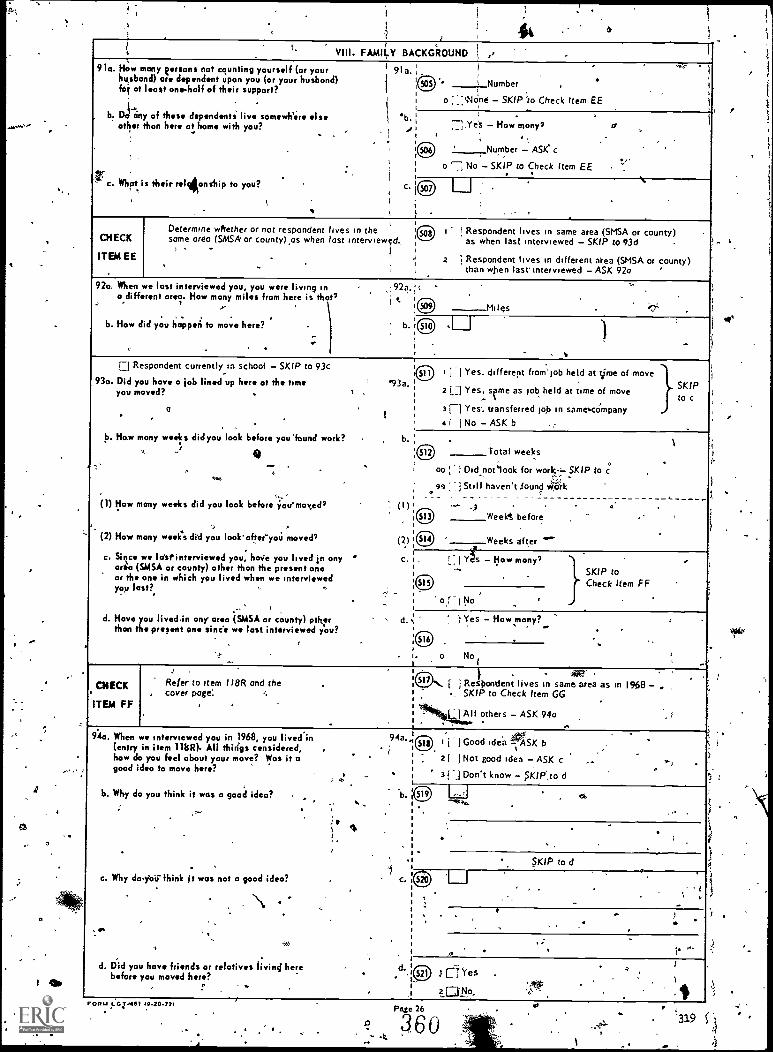
0
44fi
VIII. FAMILY BACKGROUND
91o. How many persons not counting yourself (or your 1 91a.ihusband) are dependent upon you (or your husband)
Hi at least one-holt of their support? I
b Do any of these dependenti live somewhere else b.roller than here at home with you? .. .
,
.
e. Whatt is their rellkonsitip to you? c.
t I
y
Number .!
EEi
o 'None - SKIP 'to Check item
7 ,Ye - How many/,
Number -- ASK" c
a
EE /..o 7 No - SKIP to Check Item
0 I I
. ,
CHECK
ITEM EE
Determine whether or not respondent lives in thesame area (SMSA or county) as when last interviewed,
.1
' -
Spa i ! Respondent lives in same area (SMSA or county)as when last interviewed - SKIP to 93d
2 i Respondent lives in different area (SMSA or county)than when last' interviewed - ASK 92a
92a. When we last interviewed you, you were living in ,; 92a.a different area. How many miles from here is that/ i t
...-
. , . .
b. How did you happen to move here?.
' b.
. . . .
.. ' .
Miles
al I
-%,
0 Respondent currently in school - SKIP to 93c
93a. Did you hove a job lined up here at the time ' '93a.you moved? ,
al.
b. Haw many weeks didyou look before you'found work? b,I
lif.-.. .
0as.
(1) How many weeks did you look before Yramoved7 (i)
(2) How many week's did you lookatteeyaa moved/(2)
c. Since we Ids? intorvieweel you, hove you lived in any ''aria (SMSA or county) other than the present oneor the one in which you lived when we interviewedyou last?. -
d. Hove you livedin any area (SMSA or county) outer s d.than the present one sine'e we lost interviewed you?
0 i ,. -1 Yes, different from'lob held at time of moveSKIP2 Lj Yes: re as lob held at time of moveto c
3 El Yes, transferred lob in same.company41 i No - ASK b
6 Total weeks1
to c.
._
oo 1 1 Did,not`look for work i- SKIP
99 _ ) Still haven't found w's;lk
'
Weekt before
0 Weeks after """
[7.1
_,Yes - How many/
CID.
..
SKIP toCheck Item FF
0,i- I No '
: } Yes - How many?
ap .,.
Not
CHECK
ITEM FF
: -
Refer to item I 18R and the .cover page. ,,
6 [ i Relbontleni lives in same area as in I9iS8 - .. SKIP to Check Item GG .
All others - ASK 94a.5
94a. When we Interviewed you in 1968, you lived in 94a-(entry in item 11BR). All things considered, ,how do you feel about your move? Was it a ,
good idea to move here? .. .
b. Why do you think it was a good idea? b.. ,
j P. 1
.
' 1c. Why dolair think it was not a good idea?
.
. . `
d. Did you have friends or relatives livini here - .d.before you moved here?
aD , ['J Good idea --, ASK b..
2 1 I Not good idea - ASK c ,.,' 3 { j Don't know - SKIP', to d
.L0 Li
4 .t,,,,,,
'`
SKIP to d
.1 I
. 1,. -
. . .
1
. ., .. ,
- . v',,
.I
'(ED ) nYes
. .
FORM t.G0 -0101 40.20.121Pose 26
e 3601
'319
10

/ VIII. FAMILY BACKGROUND - Continued.
ownITEM GO
i 0019' ., Refer to Household Record Card. ,
If fathei not listed, ask if.4ethar is Irving)
1
.
6 , [71 Father lives in household SKIP toCheck Item HH
21 1 Fthei,cleteased
a I Other - ASK 9So .
95o. Mang the post 12 months, about how many w...k 95a.
Ad your father work either full-time or part-timenot counting work around the haus.?
%.
4." 1 11\z-,
b. Did your father usually work ful time or port time? b
1 1
i
c. What kind of work was he doing? . c,
(If more than on4 record the one' worked at longest)
e Weeks
oo [ 1 Did not work I SKIP to Check Item NH9917bon't know
co -1 Full-time
2 [ 1 Part-time
.` ..
CHICK
ittil NH
.
Refer to Household Record Gard. 432) 1 ;Mother lives in househOldSKIP to 97
If mother not listed, ask if 2 j !Mother deceasedmother is living'.
1
31 1 Other - ASK 96'o
96a. During the past 12 montlis, 'obourhow many weeks 96a.did your mother work either full -time or porttimnot counting work around the house;
'.. ,
b. O-id your mother usually work full -time or port -time; ,
:or
c. What kind of work was she doing? c.
(If more than on, record the one worked or longest).
...
'6 Weeks,
oo ' !Did not vicirk I SKIP to 97 '99 ; Don't know
0 Full-time
2 r 1 Part-time
s29 I I. I I - ..,
..
97. What language other than English was spoken 97.in your home %Orlin you were o child;
i
,
COI No other language
98. In February -1968 were you - -
a. Working at o job or business r 98a.
(full- or pars - time)? -itb. Attending collage?
r
.
tap i ( 1Yes - SKIP to 99 .
4ez' ; No I ASK b
.
sID i 1 YeSKIP to Check Item II
1- Z1 l'N 0
,
99. t.rit's talk about your chief activity orbusiness in February 1968.
a.4What kind of blisineis or industrywa.this? 1
b. What kind of,,i4rli work you doing? bCDIIII' 4,110e-
-c, Were you -,- '''(Read categories)j . '.
,. .
,
) .6 Lti,i ,
..4 .
-,
#
.
D 1 LI An employee of a privatecompanyor government agency r
42 F1 Self-employed or an unpaid family worker
CHICK
ITEM II
. ". .
ET.R7spondent, rued or never married with own children in household - SKIP to 102 .
_AD Respondent widowed, divorced or, separated - SKIP to 101 ,
Gj All "oth rs - ASK 100.
100. Since hivattitu and plans of youncwomen, like yourself,ore amength most important factors in estimatingfu re popul tion growth in the United Stites, I wouldIi o to ask ou 'about your views toward family size. -
a. Wh you think is the ideal number' 100a..
of children for a family? '4 -
b.How man; Aildren do you .ever expect,to \rvit? b.
,r-i.-
'
-
Children
.-
.
Children - SKIP to Check Item J_J
, ..
n1111.41-0 T-4111111410421
,320Page 27
361rt.
..
-

1
1 VIII. FAMILY BACKGROUND - Continued'
101. Now f'd like to ask about your viikwi toward family six.which is so important in studying paiulatiarr grovithin the United S1atts.
,
a. Whtit'do,,you think is the ideal number of childrin 10Ia.faro family? 1
1%b. Now many chi min have you liver had, b,
k,'' not counting stillbirths? ,. 'c. How many (mare) children do you ever expect to have? C.
i =
il
k?1.9Children
(. 1
ic) Children '
1 ,,----
5101 Children - SKIP to Check Item J J,.---
102. NOW., I'd like tii ask you about your views toward familySiS0 which is so important in studying population grogthin the United States.
.,. I
a. What do you thihk is the ideal number of children 102.a. 'for 0 family? i ., .
4.
t. b. Now many children have you ever 641, b .1
not counting stillbirths?
c. Altogether, how many (dune) children do you cactually expectto have?. 1 '
e -..
t .d. NO; many children do you expect td have d.
within the nextifive years?
t
e. When do you expect to hove your next child? 44 e.
,
.
.
Children, °'-..
41D . Children ,
til, Children40°' .
item j1.
o -:;;None - SKIP to Check
4ID Children \
Item LI0 ::_j None - SKIP to Check
(ID i Within the next 12 months
2 n 13-24 months-from now'
3 ---1 More than 24 months but less than 5 years from now .
CHECK
ITEM :JJ
Refer to I I9R .. .
.. > . .
E n A Social Securey Number is entered in item f 19R - SKIP to 104. -
No Social Security Number is entered in item 119R - ASK 101
103., Whal is your SocialSecurity Number'write.
.i---r-ri-T7
..
.
V .
,/
.4 1 -1 I I
c2Notes;
- .... _
.e..
. ..
. , .,.
. .
. .. r.
- ,
.
5 a. A. . , ....
.
. .
..:4
. .
4 4 a
.
A .
Total family-members-.
/
. .
.A.. .
.
-.
..
0
.
.
. ..
.0
,
/
..4.:
40a
-.
.
....
*
A
Trtal,household membersi
CID,
'.
.
r
/,.^. .4
I
'
'4.....
.s
I.
. . ,
., -
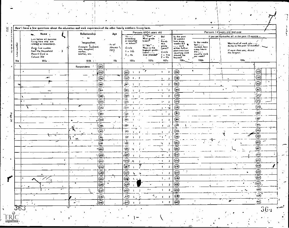
Novel have a few questions about the education and work experienc'e.of the other family members living here. .. .
-1
104
Name ,e.i..LP
L,st below all personsluvinz here who aretelited to respontden,t.
Enter /one numberCfrom the Household
Record Cord inColumn 104
105o .
.3
Relationship Age.
'respondent,a A s of
Examp/e husband. J9oi-olY I,son, doughtei, , 1973mother.brother, etc.
'
1056 I : 106
6.24 years old Persons 14 ears old and over
attendingor enrolled,n school'
CircleI - Ye's2 - No
107a
If "Yee' -What grade(year)/
If "No'. -Who, is thehighest geode(yor)ever attended?
1076
OiPersons
finishthisgrad,(yorPCire/e1 ... Yes2 No
107c
the past12 monthshow manyweeks did... work *either full.orporttimst (not
acereuunradtint g hework
house)?108o
If person1#..lorketlat all . n the past i2 months -
In the weeksthat ...worked. howmony hours
LpT°wIelY;k7rk
1086
.
1
-
7 /What kind of work was ..,.doing in the post 12 months?
I f more than one, record .
the longest.
.
.
108e
Respondent 0 . 1) I #
OD (3) 1 2 1 2 S51 .
557 I , 21 2 e . ap
5.00 '561 I 2, 6
q).1. (5115, ' 1 2 - I 2 C) 07
'(i n. 5S 1 SG 9 : I 2 I 2 ez r
, s7, . (573 i._.
___.... l 2 CD.
.
CD ----
. i 576) (577 I,....._
1 ' -2),
.,___ ________
CD
5C301 1581 I I 2 5)3 0..!----)3.1
4 584 .
-,585 i_
(51P I
'2 I 2 Se.
1
-
.
(5871i
.- q8)
'-'"
.
2
2
2
1
1
I
.2
2
2
2
TO
5941
t
,-,
1
_____,__
'.
,-; 591)---
592
q)61
593 I .
591 1
N
.
.,
595
-
....# -- 5981
606
a.....
c,c..0 .. . ,6°I. 1-...
,605' 1.._-)
`1 _TE,
60704___.
I 608 .
47-1-", t"-"")
J 609 1
/1519
4775 I
2
Nr----'2
1-
I
,
2
2 ,
(TD
di,OD
-....
kt 19
615
OD i fJ. . (11)
. ..---.7--- el ,, .
.. _ _
,
,
I 1 9aPp . .
..
9827
0 ® 629 i.
1 2 ar) i 631 r
...- @) Q533 ) 2
l 11 2 ap . . 6)5)
___-___,.
,639)636)( ,637I 2' 1 2
..__
638
rO> 610 641 I 2 1 2 CD ?
, -
.643'--)
a! 4
36g
o
1
"..r
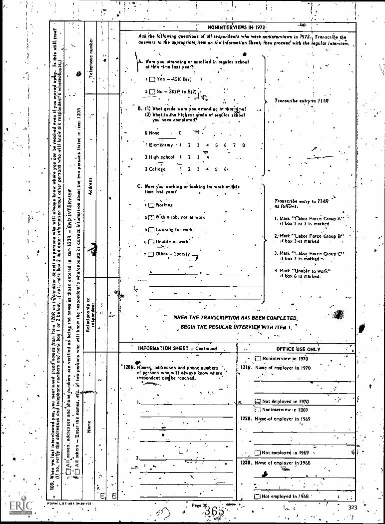
a
4..
3-
T
4 ..,Z.' el,'
1. 11
re;>.01
..e.
,...1...Tx,e 2: s'-
5-a..c30Lai.
1-
g c,4.1. f0- 672. C
PA
X't '.c ,., ..go i.-..c o
41 ...,. O,
23 °7a 8
ti..I; E
.2.t c....c 2o e.,,,,
O. I,O. c.. oor,... 041.) .0
...01 re 0o Eo0
t,L.t....,..
Co o.. ;.,'8 I04r4,E 0?,-e 0e-0
...4g,*I 00 EEcl'a
'10
2 2,160,5*
: C0 0= .e 2
t-:73a...e,. cS>,H 0
1 nI -'
LIt -aIt '34,c ......2.z:-1-.4 jg
:....-.3. :...0;Ca
.
ccto.-.
--e.
.0.-c-la
us
co
o2llE
W 0s
.... xi>g
1.ti. -z ;3.-
z c-
14; 7.. u
cc ,-)so 35:4, u
41.) vi2. s,,-0 aL .2,,,,, el.. .0c 3: s ,.,
.071 10 a.*E i'-'in ." .G,fi ..-5 3
2c -le
aZ.0 :-;... 5
0TI Ce 3c.
VI'v k-120R.10 .. 04-
.E 1-,.c. ,u,e0row.
..2 i
.12' E7 ea
13 2,,,,
: I ...
:4 2-0LLI,' I.,
a) r,g fc A os '' .---7C , .<1
ri .1.. '
.ca;,
c..,.o
aI-
v
,.
.
t * -; NONINT.ERVIEWS 114 1972
'
Ask the following questions of all respondent'sanswers to the appropriate:item on the' Information
'A. Were you attending or enrolled in regular school
at this time lost year?' . ...
i ED Yes -ASK B(I) r '
. ,2p No - SKIP to 8(2) ,- .."1t,
-''.
B. (1) What grade were you attending at thattime?(2) What.is.the highest glade of regiilar school
yeti have completed?
. /0 None 0 ""1 _. .
who were norrinterviewsSheet; ikon
2
.
,
8
. .
,
e
v
in 1972.1 Transcribe theproceed with the regular interview.
i
. .
..
,
.
Transcribe entry-to 111R
.
.
.t
c
,..." i
-......
... . ,
.....Transcribe entry to I14Ras lolro.ws: ..
. °I. biark "Dabor Force Group A"
if box'l or 2 is markedr
.
2.-Mark -"Labor Force Group B" 'if box 3es marked
3. Mark "Labor Force Group C"if box 7 is marked
.4
4. Mark "Unable to work"If tiax 6 is marked.
.
, 1 ",...
I/. .
. .
ITEM 1. .
. ,
.
I)'0-
<
.
.
1 Elementary 1 2 3 4 5 6 7
. VO, . .. 2 High school I 2 3 4
---:-- .--3 College 1 2 3 4 5 64
.'
C. Were fou working or looking hir work at=thistime last year?
....
._
- 1 0 Working
_.
2 l:fl With a job, not at work ,..
3 El Looking for work.
6 111 Unable to work"-_,-...'t t,
.7 0 Othes - SpecifyI P
.., . ' .
..
0.C'. C:2411/1 ...a z
a.11. :-ru .-cc
t , j
..
k:. %
... . t.
._
., 7 WHEN THE TRANSCRIPTION HAS BEEN-COMPLETED,
. BEGIN THE REGULAR INTERVIEW *WITH,;.
. ,
., . .
INFORMATION SHEET - Continued ., OFFICE USE ONLY
.
E
Z'
.
.
--
a
o
. 10,Nae, addresses and phone numbers '.of persons who will always know where 7
respondent c be reached.,.,,,, ..
. ..
I. _
,, ,0 Noninterview in 1970., ..
121R. Name of employer in 1970. -
.
_
f; ) Not Employed in 1970 - %'nNoninterview in 12-69
122R. N'neof employer in 1969 -
. ...,' .
. ... _
. .
-'
._ .....
20 Not employed in 1969 -
123R., Name of employer in:1968./40., ..,i
° 6.. . .. '
.
- ...,-
. .° . '
4. ..a.0 Not employed in ,I46868 t ;
fOR.41-0 T.451 1 20.72)
4
0
323

1108
113R
114R
115R
116
axe
118
/ INFORMATION SHEETDATA FROM 19712 INTERVIEWS
Date of 1-at inter;lw rinnth, .1,1,, ,.. , ,:I irr,r7nr;"79;---Fii:,., . 1
-- 1 :, '44) i I 3 li I I t I .
; ;
(6.-4 -II
J I.1
60
43...
Schsiol enr6lIment
EnrollgdNot enr
Cirade.resphighest year
' "None
I Elem.
.t ° High
College;
statu, .r I';
Iled
ndero vas attndir, 0of,rXular school c ,,,;pre,e 1
0 ,
1 2; 3 4 i 5 0, ' ti
I 2,4 3 4,1 2 3 4 5 r,
4.
School enrollmentEnrolled
..E?) , 1968
lip I 1969
(ID 1 19701
6501 ,1971
al $1 1972
statusNot enrolred
2 1968
2 1969
2 1970
2 1971 .2 1972
1
f,Respondenri's educational goal whenlast interviewed
0 Not asked educational goal
2- lgh 1 2 3 4
College 2 4 6 7..
. i
at,Respdndent's labor force status in 1972
; Labor Force Group A
Labor Flo'ke Group B' Labor Force Group C
, Unable ,to work
.40°
Noninterview in-,1971
Name of employer in 1971
...
.... .Not employed in 1971 ° - iiii-
.
1
1Nontnterview in 1972
Name of employer in 1972
'-'
,
1
1
't
.
1 ;Not emPloygd in 1972L
1 Plants for a;e 35 when last littet.,wed
r-- 1 Working $p city k nd...,
(-,--
,
,Mairiedikeeping house, raisiliga famil)/ 4
4:10ther or don't know-
, . iiResidepce in 1968
. 7
lCity*14'41`.
;
i
4C.,\
':State
' Social securlit, hunter
III111 .CID 1- 1 H 1
1
32k
*
t
f'
.2
4
Si
4