POTENTIAL SOURCE ROCKS IN THE WESTERN KANSAS ...

POTENTIAL SOURCE ROCKS IN THE WESTERN KANSAS PETROLEUM PROVINCE

by

TYLER J. HILL

B.S., Kansas State University, 2009

A THESIS

submitted in partial fulfillment of the requirements for the degree

MASTER OF SCIENCE

Department of Geology

College of Arts and Sciences

KANSAS STATE UNIVERSITY

Manhattan, Kansas

2011

Approved by:

Major Professor

Dr. Matthew Totten

Copyright

TYLER J. HILL

2011

Abstract

The source of the hydrocarbons in western Kansas has been an ongoing debate for many

years. The highly organic-rich Anadarko basin, directly south of western Kansas, has been a

very prolific producer for many years. This basin is the most widely accepted source of the oil in

Kansas, as it is very deep and thermally mature. The main source rock in this area is the

Woodford Shale, a very thick, very organic-rich unit which has been proven to produce many

hydrocarbons. Several studies have been done on the oils that are presently in Kansas,

suggesting that they can be traced back to the source of the Woodford Shale. The hydrocarbons

in the Anadarko basin would have traveled several hundred miles, which would require that the

migration mechanism be unusually efficient. An alternate explanation could be that one of the

many organic black shales in western Kansas may have sourced this oil.

This study examines formations of Cambrian to Permian ages which include organic

shales interbedded with several known producing formations. Shales of these ages in other areas

have produced thermally mature hydrocarbons, which indicate relatively high temperatures and

pressures. Several models suggest that thermal maturity may be reached even with lower

temperatures if burial times are longer. The shales in western Kansas were deposited in marine

seas, and upon TOC testing, proved to be very organic-rich. Two sets of data were analyzed in

this study, with the first from northwestern Kansas, and the second from southwestern Kansas.

These two sets were analyzed for TOC, whole-rock analysis, and vitrinite reflectance. The

shales analyzed from the first set proved to be thermally immature. Had they been subjected to

higher temperatures, then they would have made excellent source rocks. The second set of

shales analyzed also proved to be thermally immature with the exception of a few deeper shales,

which are closer to being mature source rocks. These shales may have contributed to some of

the hydrocarbons currently within Kansas.

v

Table of Contents

List of Figures ................................................................................................................................ vi

List of Tables ................................................................................................................................ viii

Acknowledgements ........................................................................................................................ ix

CHAPTER 1 - INTRODUCTION .................................................................................................. 1

1.1 Significance ........................................................................................................................... 4

1.2 Literature Review .................................................................................................................. 4

1.3 Geologic Setting .................................................................................................................... 5

1.4 Study Area ............................................................................................................................. 7

1.5 Stratigraphy of Study Area .................................................................................................... 8

1.6 Geochemistry ...................................................................................................................... 17

1.6.1 Discussion of TOC ....................................................................................................... 17

1.6.2 Discussion of Pyrolysis ................................................................................................ 18

1.6.3 Discussion of Vitrinite Reflectance .............................................................................. 21

1.8 Thermal Maturation and Burial History .............................................................................. 23

CHAPTER 2 - MATERIALS AND METHODS ......................................................................... 26

2.1 Sedimentology..................................................................................................................... 26

2.2 Geochemical Analytical Tests............................................................................................. 27

CHAPTER 3 - RESULTS ............................................................................................................. 39

CHAPTER 4 – DISCUSSION ...................................................................................................... 48

4.1 Kansas Shale Properties ...................................................................................................... 48

4.1.1 Stevens Unit ‘SMU’ ..................................................................................................... 62

4.1.2 Discussion of Bostick’s Figure. ................................................................................... 63

CHAPTER 5 – SUMMARY AND CONCLUSIONS .................................................................. 65

References Cited ........................................................................................................................... 68

Appendix A - FID Responses........................................................................................................ 70

vi

List of Figures

Figure. 1 Map showing Kansas oil and gas fields. .......................................................................... 1

Figure 2. Map showing potential oil migration from the Anadarko basin. ..................................... 3

Figure 3. Study area in western Kansas, denoted by yellow stars. ................................................. 7

Figure 4. Stratigraphic column of the Lansing Group. ................................................................... 9

Figure 5. Stratigraphic column of the Kansas City Group. ........................................................... 10

Figure 6. Stratigraphic column of the Marmaton Group. .............................................................. 11

Figure 7. Stratigraphic column of the Cherokee Group. ............................................................... 13

Figure 8. Stratigraphic column of the Morrowan Stage. ............................................................... 14

Figure 9. Stratigraphic column of the Arbuckle Group. ............................................................... 16

Figure 10. TOC evaluation. ........................................................................................................... 18

Figure 11. Kerogen quality............................................................................................................ 20

Figure 12. Vitrinite reflectance qualities. ...................................................................................... 22

Figure 13. Correlation table of common organic maturation parameters with coal rank and

hydrocarbon generation. ........................................................................................................ 23

Figure 14. Approximate vitrinite reflectance based on time and temperature relationship.

(Modified from Bostick, 1979). ............................................................................................ 25

Figure 15. Geologist's Report for well 15-051-25825 within the LKC formation........................ 29

Figure 16. Geologist’s Report for well 15-033-21470 within the LKC formation. ...................... 30

Figure 17. Geologist's Report for well 15-033-21470 within the Stark shale formation. ............. 30

Figure 18. Geologist's Report for well 15-033-21470 within the Cherokee shale formation. ...... 30

Figure 19. Porosity log for well 15-051-25316 within the LKC shale formation. ........................ 31

Figure 20. Porosity log for well 15-051-25316 within the Arbuckle shale formation. ................. 31

Figure 21. Resistivity log for well 15-051-25233 within the LKC shale formation. .................... 32

Figure 22. Porosity log for well 15-119-21194 within the Swope shale formation. ..................... 32

Figure 23. Porosity log for well 15-119-21194 within the Fort Scott and Cherokee shale

formations. ............................................................................................................................. 33

Figure 24. Porosity log for well 15-119-21194 within the Cherokee shale formation. ................ 34

Figure 25. Porosity log for well 15-119-21194 within the Morrow Shale formation. .................. 34

vii


Figure 27. Geologist's Report for well 15-135-24186 within the Labette shale sample. .............. 35

Figure 28. Geologist's Report for well 15-135-24253 within the LKC shale formation. ............. 36

Figure 29. Geologist's Report for well 15-135-24253 within the Labette shale formation. ......... 36

Figure 30. Geologist's Report for well 15-135-24254 within the LKC shale formation. ............. 37

Figure 31. Geologist's Report for well 15-135-24254 within the Labette shale formation. ......... 37

Figure 32. Porosity log for well 15-135-24314 within the LKC shale formation. ........................ 37


Figure 34. Vitrinite reflectance histogram for 4212-4218 ft. interval in well 15-135-24186. ...... 42





Figure 39. Vitrinite reflectance histogram for 5309-5313 ft. interval well 15-119-21194. .......... 46



Figure 42. Geochemical Log of TOC, remaining potential (S2), kerogen type (HI), normalized

oil content, and calculated vitrinite reflectance. Analyses from Ness and Ellis counties. ... 50

Figure 43. Geochemical Log of TOC, remaining potential (S2), kerogen type (HI), normalized

oil content, and calculated vitrinite reflectance. Analyses from Meade and Comanche

counties. ................................................................................................................................. 51

Figure 44. Kerogen type and maturity. Analyses from Ness and Ellis counties. ......................... 53

Figure 45. Kerogen type and maturity. Analyses from Meade and Comanche counties. ............ 54

Figure 46. Kerogen conversion and maturity. Analyses from Ness and Ellis counties. .............. 55

Figure 47. Kerogen conversion and maturity. Analyses from Ness and Ellis counties. .............. 56

Figure 48. Kerogen type. Analyses from Ness and Ellis counties. .............................................. 58

Figure 49. Kerogen type. Analyses from Meade and Comanche counties. ................................. 59

Figure 50. Kerogen quality. Analyses from Ness and Ellis counties. .......................................... 60

Figure 51. Kerogen quality. Analyses from Meade and Comanche counties. ............................. 61

viii

List of Tables

Table 1. General well data............................................................................................................. 28

Table 2. First set of samples analyzed........................................................................................... 40

Table 3. Summary of data obtained by TOC and Rock-Eval analyses of the selected samples, for

the first set of analyses. ......................................................................................................... 41

Table 4. Second set of data analyzed. ........................................................................................... 43

Table 5. Summary of data obtained by TOC and Rock-Eval analyses of the selected samples, for

the second set of analyses. ..................................................................................................... 44

ix

Acknowledgements

This project could not have been completed without the help of many people. First and

foremost I would like to thank Dr. Matt Totten for taking me on as a graduate student. Matt is a

good friend, and an even better advisor, I will always be indebted to him. I would also like to

thank Dr. Iris Totten, for bringing me on as a research assistant. I would also like to thank my

committee members, Dr. George Clark, and Dr. Sam Chaudhuri. George, thank you for your

patience in critiquing my writing skills, with your help this paper reads much more smoothly.

Sam thank you for your suggestions in my research, with your advice, I was able to narrow down

my focus. I would also like to thank Dr. Michael Lambert. I would not have been able to

complete this project without your extensive knowledge on this subject.

I would also like to thank all of the graduate students for their help and support.

Whenever I needed a distraction, or a beer someone was always there to join in. It has been a lot

of fun working with all of you, and I wish you all luck in your future endeavors. Lori, you

brighten up the office, and I can not imagine this department without you. You sure have a

knack for putting up with geologists! It has also been a joy to work with you.

I would like to thank Weatherford Laboratories, in particular Kristie Doyle, for running

the analysis on my samples. Funding for this project came from several different societies, and

corporations: Kansas Geological Foundation, AAPG Grants-in-aid, Lario Oil and Gas,

Mewbourne Oil and Gas, Kansas Geophysical Society, and GK-12 EiDrop. I thank you for your

all of your help, without it, the last two years would have gone a lot differently.

x

I would also like to thank my parents for their continued support of my education. You

have always pushed me to work hard and strive for better. Last but not least, I would like to

thank my wife, you were always there for me when I needed you.

1

CHAPTER 1 - I#TRODUCTIO#

The western Kansas petroleum province has been a prolific producer for almost a

century. Overall Kansas ranks eighth in the nation for oil producing states. Records have been

kept since 1930, and in that time Kansas has produced 4.3 trillion barrels of oil. This is a

significant amount of oil. There are multiple producing formations, from Cambro-Ordovician

rocks through the Permian. The Hugoton field of southwest Kansas is one of the largest gas-

producing regions from relatively shallow Permian-aged Chase Group rocks. Kansas has also

produced a large amount of gas, since 1930 it has produced 31,468,596,708 mcf. A map of all of

the oil and gas fields in Kansas can be seen in Figure 1. The red areas indicate gas fields, green

areas indicate oil fields, and orange indicates oil and gas fields.

Figure. 1 Map showing Kansas oil and gas fields.

(Modified from KGS, 2009)

There are two hypotheses regarding the generation of the petroleum deposits in western

Kansas. The first hypothesis suggests that the petroleum was generated in the deeper portions of

2

the Anadarko basin in Oklahoma, and migrated northward into Kansas reservoirs. The second

hypothesis suggests that the petroleum was generated from nearby source rocks with limited

migration into local reservoirs. Both of these hypotheses have distinct advantages and

disadvantages in explaining the distribution of Kansas petroleum deposits.

In the first hypothesis the deeper Anadarko basin has abundant organic-rich

source rocks that have undergone considerable thermal maturation, in some cases through the gas

window. These source rocks are proven petroleum generators, as evidenced by the considerable

reserves within the Oklahoma portions of the Anadarko basin. Migration over considerable

distance (greater than 300 miles) is required for these sources to charge Kansas reservoirs.

Potential oil migration pathways can be seen in Figure 2. In addition, multiple sources are

required to explain the vastly different character of petroleum reserves from different aged

reservoirs. It is not easy to explain why this long-distance migration results in the observed

distribution of oils in specific aged reservoirs, regardless of reservoir depth.

3

Figure 2. Map showing potential oil migration from the Anadarko basin.

(Modified from Gerhard, 2004.)

In the second hypothesis there are potential source rocks within the Kansas region

which might have generated the petroleum, but they are not adequately studied. Long-distance

migration is not necessary in this model, and variation between the different-aged deposits may

be explained by different source rocks. The shallower depths in Kansas, however, limit the

thermal maturation potential. Additional catalysts to petroleum generation are probably required

in this model.

4

1.1 Significance

The significance of this study has a considerable impact on western Kansas. Kansas is a

major petroleum producer with oil being produced from several different rock formations. The

oil is currently thought to have been generated in the Anadarko basin, with long distance

migration into the current reservoirs; or was generated from nearby source rocks with limited

migration into nearby reservoirs. Knowing which hypothesis better explains where the oil was

sourced will contribute to a better understanding of where to look for additional deposits. This

study may be applicable to other areas where the geology is similar to western Kansas.

1.2 Literature Review

The formation of petroleum has several aspects that have to occur in specific order for oil

or gas deposits to form. This includes time, temperature, carbohydrates from once living things,

and the correct geologic setting. Petroleum generation is based on the accumulation of organic

matter from living material, and on the generation of hydrocarbons by the action of heat on

accumulated organic matter (Hunt, 1979).

Oil has formed in many different types of sedimentary rocks all over the world. This has

resulted from thermal generation of hydrocarbons from the organic matter within the

sedimentary rocks. Migration processes have not significantly altered this distribution since

more than 80 percent of the hydrocarbons in most fine-grained sediments are autochthonous

(Hunt, 1979).

Temperature is the most studied aspect in the formation of petroleum. It plays the key

role in the transformation of organic matter to hydrocarbon. Generally in sedimentary basins, oil

formation is at relatively low temperatures of between 150 degrees F and to 300 degrees F (Hunt,

5

1979). These temperatures are not thought to have been reached for the oil province in western

Kansas, due to the shallower burial depths.

Time is also a major factor in the generation of oil. The range of in this study is the

Paleozoic Era, which is the age of the oil-bearing rocks in western Kansas. This range is 570 up

to 240 million years ago. Western Kansas is an old basin compared to many oil producing

basins, such as the Gulf of Mexico. Most formations are thought to have been at current burial

depths since early in the Mesozoic, which is several hundred million years ago (Merriam, 1963).

A key paradigm to my research is that the correct time and temperature combination can

prove to be very effective in the formation of oil. High temperatures over a short time have been

proven to produce oil, however an equivalent degree of oil generation should be realized at lower

temperatures over a longer period of time. The latter conditions could have been realized

western Kansas. According to Sweeney and Burnham (1990) 100 degrees C for 100 million

years can reach a vitrinite reflectance of 0.7, which is adequate to begin oil generation. Vitrinite

reflectance has been successfully demonstrated as a reliable indicator of organic maturation in

sedimentary rocks and is widely used in the oil industry for the evaluation of kerogens according

to Senftle and Landis (1991).

1.3 Geologic Setting

The study area is located in midwest, and southwest Kansas. Part of the samples

analyzed are on the Central Kansas Uplift, with the rest of the samples situated in the Hugoton

embayment (Figure 3).

The Central Kansas Uplift is a large structural feature (5,700 square miles) that runs

through the center of the state. The uplift is northwest-trending, and separates the Hugoton

embayment to the west, and the Salina basin to the east. The sedimentary rocks that lie on top of

6

the structure are less than 5,000 feet thick in places (Merriam, 1963). The outline of the uplift is

surrounded by the Mississippian beds which have been eroded away on the uplift.

The surface of the Central Kansas Uplift is covered by Cretaceous, Tertiary, and

Quaternary age formations. The uplift occurred during the end of the Mesozoic. Within the

uplift, there is a large unconformity, and the Precambrian rocks are overlain by Pennsylvanian

sediments.

The Hugoton embayment is a major structural unit, occupying one-third of Kansas. It

covers almost 28,600 square miles, and is situated in far western Kansas. The eastern boundary

of the embayment is stopped by the Cambridge arch, the Central Kansas Uplift, and the Pratt

Anticline. The western edge extends into eastern Colorado, and stops at the Las Animas Arch.

The southern extent thickens to the south and feeds into the Anadarko basin.

The Hugoton embayment is a large shelflike extension into western Kansas from

Oklahoma’s Anadarko basin (Merriam, 1963). The south plunging structure, which is full of

sediments, thickens toward the south and the center of the embayment stretching into the much

larger Anadarko basin. This is the deepest structural basin in Kansas, exceeding 9,500 feet thick.

This thick sediment overlies Precambrian rocks.

The embayment was formed before the Mesozoic Era. The Paleozoic beds are covered

by Cretaceous, Tertiary, and Pleistocene age rocks (Merriam, 1963). The large thick structure

includes rocks from the Cambrian-Ordovician, Mississippian, Pennsylvanian-Permian, Triassic,

Jurassic, Cretaceous, Tertiary, and Pleistocene age.

7

1.4 Study Area

This study area looks at several organic-rich black shales in four different counties (Ness,

Ellis, Comanche, and Meade) in western Kansas which might have served as source rocks for

petroleum generation (Figure 3). There are many wells that have been drilled in this area

beginning in the 1930’s to the present day. The basis for choosing the wells to analyze relied on

several different parameters. Each well had a suite of well logs (resistivity, neutron density, and

geologists reports), and each well had to have rock cuttings that were available.

Figure 3. Study area in western Kansas, denoted by yellow stars.

(Modified from Gerhard, 2004)

Many cores have been taken and studied in western Kansas. Unfortunately the cores that

were taken have not been through the rock formations that were potential source beds. As a

result geophysical logs and well cuttings were employed for this study, both of which are open to

the public and easily accessible. A total of nine wells were sampled for geochemical analyses

(Table 1).

8

1.5 Stratigraphy of Study Area

Stratigraphy can be described as the study of rock layers with emphasis on their origin,

formation, and depositional environments. Throughout this study many different shales from

many different ages, within western Kansas, have been analyzed. The ages range from late

Pennsylvanian to early Ordovician. Shales from within the formations that have been sampled

include the Lansing-Kansas City (LKC), Stark, Swope, Labette, Ft. Scott, Cherokee, Morrow,

and Arbuckle.

The Lansing-Kansas City group is part of the Missourian Stage of the upper

Pennsylvanian series. The Lansing-Kansas City Groups in Kansas are composed of interbedded

carbonates and shales with occasional minor coals and sandstones (Watney, 1980). Within this

group there is a variety of depositional environments. They range from phylloid algal-bearing,

lime-mud banks to oolite shoals (Watney, 1980). The total thickness of the LKC can range from

370 to 600 feet thick (Merriam, 1963). The LKC has a wide range in western Kansas, extending

from southwest Nebraska down to the Anadarko basin in Oklahoma. In general the LKC

thickens towards the south. The shales that are interbedded within the limestones range in color

from gray, to black with the black shales being the most organic-rich.

The LKC is a large producing formation in Kansas, producing from as many as seven or

eight different limestone members. The Stark and Swope black organic shales are also part of

the LKC Group. The Stark shale member is part of the Dennis Limestone Formation (Figure 4).

It is described as relatively thin (five to fifteen feet thick), fissile, black, and organic-rich. The

Swope shale is part of the Swope Limestone Formation (Figure 5). It is also described as

relatively thin (five to fifteen feet thick), fissile, black, and organic-rich. While both of these

shales can be described the same, they vary in organic richness from area to area.

9

Figure 4. Stratigraphic column of the Lansing Group.

(Zeller, 1968)

10

Figure 5. Stratigraphic column of the Kansas City Group.

(Zeller, 1968)

The Labette Shale Formation is part of the Marmaton Group (Figure 6). It is Middle

Pennsylvanian in age. The Marmaton Group underlies the Pleasonton Group unconformably.

The Marmaton Group is interbedded with carbonates and shales. It has four limestone

formations that are separated by four shale formations. The whole group is approximately 250

11

feet thick (Merriam, 1963). On radioactive logs the Labette shale has a high gamma ray value

making it a good marker for wellsite geologists. It is approximately ten to twenty five feet thick,

and is described as gray to black, fissile, and carbonate in part.

Figure 6. Stratigraphic column of the Marmaton Group.

(Zeller, 1968)

The Fort Scott Limestone Formation lies directly below the Labette Shale, as part of the

Marmaton Group (Figure 6). It has two limestone members that are separated by a shale

member. The Fort Scott Formation ranges in thickness from 13 feet to 145 feet (Merriam, 1963).

The Little Osage Shale Member ranges in thickness from 4 feet to 12 feet, with the uppermost

part being gray, and turning to a black fissile shale towards the bottom.

The Cherokee Group is Middle Pennsylvanian in age. It conformably lies below the

Marmaton Group, and lies unconformably on the Mississippian Lime. There is very little

limestone present, being made primarily of sand, shale and a few coal beds. It ranges in

12

thickness from 450 to 500 feet thick (Merriam, 1963). There are a total of seventeen formations

present within the Cherokee Group (Figure 7).

The sand and shale of the Cherokee Group were deposited as the Pennsylvanian sea

advanced from the south. They were laid onto the eroded surface of the Mississippian rocks,

making the unconformity between the two members. This area was at or near sea level as

evidenced by the coal and other swamp deposits that are present in the coal, shale and sandstone

formations (Merriam, 1963).

13

Figure 7. Stratigraphic column of the Cherokee Group.

(Zeller, 1968)

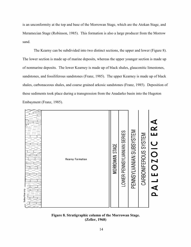
The Morrowan Stage is lower Pennsylvanian in age. The Kearney Formation is the only

formation present. Most of the available data from this formation is from wells that have been

drilled through the formation. This formation is confined mainly to basinal areas like the

Hugoton Embayment. The thickness ranges from 0 to about 600 feet thick (Franz, 1985). There

14

is an unconformity at the top and base of the Morrowan Stage, which are the Atokan Stage, and

Meramecian Stage (Robinson, 1985). This formation is also a large producer from the Morrow

sand.

The Kearny can be subdivided into two distinct sections, the upper and lower (Figure 8).

The lower section is made up of marine deposits, whereas the upper younger section is made up

of nonmarine deposits. The lower Kearney is made up of black shales, glauconitic limestones,

sandstones, and fossiliferous sandstones (Franz, 1985). The upper Kearney is made up of black

shales, carbonaceous shales, and coarse grained arkosic sandstones (Franz, 1985). Deposition of

these sediments took place during a transgression from the Anadarko basin into the Hugoton

Embayment (Franz, 1985).

Figure 8. Stratigraphic column of the Morrowan Stage.

(Zeller, 1968)

15

The Arbuckle Group is lower Ordovician, and upper Cambrian in age. The Arbuckle is a

big producer in western Kansas. There are five members in this group which consist mainly of

dolomite (Figure 9). The Arbuckle Group is bounded on the top and bottom by major

interregional unconformities, depending on whether or not the Reagan sandstone has been

eroded away.

The group as a whole consists of mainly dolomite with some interbedded sands and

shales. The dolomite is white, buff, light gray, cream and brown (Merriam, 1963). There are

large amounts of various types of chert present within the dolomite. The sands and shales where

present are sparse, and not continuous. The shales appear as gray to black.

16

Figure 9. Stratigraphic column of the Arbuckle Group.

(Zeller, 1968)

17

1.6 Geochemistry

Peters et al (2006) describes petroleum source rocks as fine-grained organic-rich rocks

that could generate (potential source rock) or have already generated (effective or active source

rock) significant amounts of petroleum. In western Kansas there are a plethora of fine-grained

organic-rich rocks that could possibly generate oil, and be a potential source rock.

According to Oko (2006) hydrocarbon potential is dependent on four factors: 1) the

quantity and quality of insitu organic matter in the rock, 2) the origins of the various types of

constituent organic matter and their capacity for hydrocarbon generation, 3) the degree of

conversion of the organic matter to hydrocarbons, and 4) the adsorption capacity of the rock.

Factors 1 and 2 are mostly dependent on the prevailing conditions at the place of deposition.

Factor 3 is related to maximum burial depth and maturation. The fourth factor is vital for any

shale to be producible. Each of these factors will be discussed in this chapter.

1.6.1 Discussion of TOC

Total organic carbon (TOC) is the measure of the quantity, or organic richness of organic

carbon within a rock sample. Peters et al (2006) pointed out that it is a measure of the quantity

and not the quality. This measurement is the first step toward assessing the potential of a

sediment to generate hydrocarbons.

The organic matter is derived from a variety of biological origins which has been

deposited and buried through geologic time (Tissot and Welte, 1984). The bulk of petroleum is

formed from the thermal decomposition of organic matter through time (Jarvie 1991). TOC

measures how much organic matter is present within the rocks that were deposited originally.

The organic carbon is different from the inorganic carbon, and can be distinguished by its

18

derivation. Organic carbon comes from biogenic matter, and the inorganic matter comes from

mineral matter, such as carbonates.

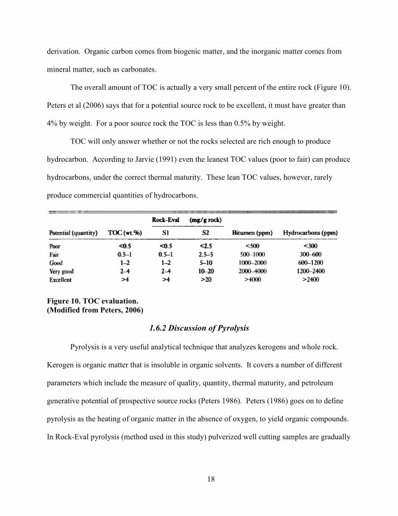
The overall amount of TOC is actually a very small percent of the entire rock (Figure 10).

Peters et al (2006) says that for a potential source rock to be excellent, it must have greater than

4% by weight. For a poor source rock the TOC is less than 0.5% by weight.

TOC will only answer whether or not the rocks selected are rich enough to produce

hydrocarbon. According to Jarvie (1991) even the leanest TOC values (poor to fair) can produce

hydrocarbons, under the correct thermal maturity. These lean TOC values, however, rarely

produce commercial quantities of hydrocarbons.

Figure 10. TOC evaluation.

(Modified from Peters, 2006)

1.6.2 Discussion of Pyrolysis

Pyrolysis is a very useful analytical technique that analyzes kerogens and whole rock.

Kerogen is organic matter that is insoluble in organic solvents. It covers a number of different

parameters which include the measure of quality, quantity, thermal maturity, and petroleum

generative potential of prospective source rocks (Peters 1986). Peters (1986) goes on to define

pyrolysis as the heating of organic matter in the absence of oxygen, to yield organic compounds.

In Rock-Eval pyrolysis (method used in this study) pulverized well cutting samples are gradually

19

heated under an inert atmosphere. The heating distills the free organic compounds (bitumen),

then cracks pyrolytic products from the insoluble organic matter (kerogen).

There are several different parameters that are measured in this analysis. During

pyrolysis there is a flame ionization detector (FID) that senses any organic compounds that were

generated throughout the process (see appendix). There are also several different peaks that are

measured: S1, S2, and S3. S1 according to Peters (1986) represents milligrams of hydrocarbons

that can be thermally distilled from one gram of rock. This is basically the amount of

hydrocarbons that have already been generated from the source rock before it was analyzed.

This is a very useful measurement, because it gives a good indication on whether or not the

potential source rock has already produced hydrocarbons. S2 according to Peters (1986)

represents milligrams of hydrocarbons generated by pyrolytic degradation of the kerogen in one

gram of rock. This measures the amount of hydrocarbons that are left within the source rock that

have not yet been generated. This is also a very useful measurement when comparing S1 to S2,

because it gives the ratio of hydrocarbons that have already been generated, to hydrocarbons that

have yet to be generated. S3 according to Peters (1986) represents milligrams of carbon dioxide

generated from a gram of rock during temperature programming. There is also one more

measurement that is taken during pyrolysis, in which the temperature is measured. The

temperature at which the maximum amount of S2 hydrocarbons is generated is called Tmax

(Peters 1986).

This information is then plotted into pyrograms or modified van Krevelen diagrams

(Figure 11). The Hydrogen Index is plotted on the vertical axis, and the Oxygen Index is plotted

on the horizontal axis. The hydrogen index (HI) corresponds to the quantity of pyrolyzable

organic compounds or hydrocarbons (HC) from S2 relative to the total organic compound

20

(TOC). The oxygen index (OI) corresponds to the quantity of carbon dioxide from S3 relative to

the TOC (Peters 1986).

Figure 11. Kerogen quality.

(Modified from Peters, 2006).

The van Krevelen diagrams can be used to classify different types of organic matter. The

different types of kerogens are plotted into four different types. Type I is very oil prone, type II is

oil prone, type III is gas prone, and type IV is inert. Type IV kerogens contain very little

hydrogen and plot near the bottom of the graph. These different types are classified by using the

hydrogen index versus the oxygen index.

One of the many benefits of pyrolysis is the ability to characterize what type of

depositional environment the shales were deposited in. Tissot and Welte (1984) describe how

the chemical structure of a shallow immature kerogen varies with the original mixture of

organisms and with the physical, chemical, and biochemical conditions of deposition. These

kerogens are broken into four different types that explain the different depositional

environments.

Type I organic matter contains material with an identifiable algal and bacterial structure.

It is highly anoxic lacustrine and marine, with minor terrestrial component.

Type II organic matter, as described by Tissot and Welte (1984), appears visually in

several different forms. This material appears as allochthonous material, principally as exinites

21

consisting of spores, pollen grains, and phytoplankton cysts, and as cuticles from plant leaves

and stems. Alternatively, this material may be autochthonous and derived principally from

bacterially reworked phyto- and zooplankton. This bacterially reworked material will also

appear largely as finely disseminated amorphous organic matter. It is anoxic-oxic marine or

lacustrine. It is also mixed marine terrestrial.

Type III organic matter, as described by Tissot and Welte (1984), often appears as

vitrinite. It may also appear as finely disseminated amorphous material. This material forms

through the degradation and or oxidation of the other maceral types. It is anoxic-oxic marine or

lacustrine. It can also range to mildly oxic, and coal swamp deposition. Its organic matter is

terrestrial, mostly vitrinite, and partially degraded algal.

Type IV organic matter is highly oxidized. Its depositional environment is highly oxic,

and its organic matter is highly oxidized marine and terrestrial. This type of organic matter

generally forms coal.

The classification of the different kerogens can be plotted in a different type of graph

where S2 is plotted against TOC. This works better in evaluating the kerogens because it

indicates the petroleum potential and the type of kerogen present (Langford and Blanc-Valleron

1990). This plot forms a linear regression with a high degree of correlation which indicates a

very coherent group, whereas in the standard van Krevelen diagram the plot forms a broad group

in the center, with some points scattered more widely (Langford and Blanc-Valleron 1990).

1.6.3 Discussion of Vitrinite Reflectance

Bostick (1979) showed that the optical properties of vitrinite from finely dispersed

organic matter in sedimentary rocks could be used to assess thermal maturity. According to

Peters et al (2006) vitrinites are a maceral group derived from terrigenous higher plants.

22

Vitrinite Reflectance (Ro) is a key measure of the thermal maturity. Vitrinites were well

developed by Devonian time, so anything of Devonian age or younger can usually be tested for

its thermal maturity. Vitrinite reflectance offers a means to evaluate organic maturity over

temperatures ranging from early diagenesis through catagenesis to metamorphism (Senftle and

Landis, 1991). The oil maturation window (Figure 13) ranges from 0.7% to 1.2% according to

Senftle and Landis (1991). This makes it a useful tool, being able to differentiate between

mature and immature source rocks.

Figure 12. Vitrinite reflectance qualities.

(Modified from Peters, 2006).

23

Figure 13. Correlation table of common organic maturation parameters with coal rank and

hydrocarbon generation.

(Modified from Senftle and Landis, 1991).

1.8 Thermal Maturation and Burial History

In most cases the maturity of any source rock is directly related to thermal heating due to

burial. There can be some localized heat sources such as thrust faults and deep-seated basement

features. Within the study area the question arose on whether or not the thermal heating due to

burial had reached temperatures high enough to begin hydrocarbon generation. This is mainly

24

due to the shallow depths at which the potential source rocks are buried. In Figure (14) Bostick

(1979) and several other authors proposed that low to medium temperatures at long periods of

time were enough to reach the onset of oil generation. Vitrinite reflectance at 0.7% should be

enough to produce hydrocarbon generation within source rocks. According to the figure, 5 ma at

120 degrees C should be enough to reach 0.7% reflectance. However, a lower temperature for a

longer period of time (70 ma at 80 degrees C) 0.7% reflectance should be achieved, and also be

enough to reach the oil maturation window.

25

Figure 14. Approximate vitrinite reflectance based on time and temperature relationship.

(Modified from Bostick, 1979).

26

CHAPTER 2 - MATERIALS A#D METHODS

Analysis of source rocks are most easily studied through several different

interdisciplinary techniques. In this study integration of stratigraphy, and geochemical data was

employed. Drill cuttings, well-logs, and geochemical data sets were utilized to characterize and

assess the source potential of several different black shales in the western Kansas Petroleum

province. The shales analyzed in this study were easiest to work with based on previously

drilled wells within the study area of western Kansas. Surface exposures are limited within the

study area. Thus, subsurface data based on well-logs became the easiest method to characterize

the different potential source rocks. Cores would have been the best method to study and

sample. However, they are very rarely taken in the black shales, with the bulk of them being in

zones of oil and gas production. The next best thing to studying cores, were well-cuttings which

are collected for almost every well drilled in Kansas. For detailed geochemical work, twenty-

four bulk shale samples were collected in five to ten foot intervals from nine different wells

spread throughout western Kansas (Table 1).

2.1 Sedimentology

The sedimentology of the organic black shales analyzed in this thesis discuss the

relationships with other similar age rocks, and the depositional environments. Stratigraphic and

sedimentologic characterization of these shales were achieved through subsurface techniques.

These techniques include geophysical well logs which include: gamma ray, neutron porosity,

bulk density, and density porosity.

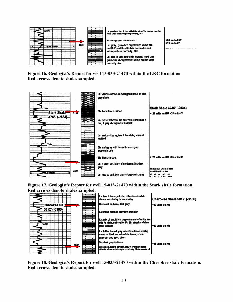
Geologist’s reports were also used to pick pertinent black shales (Figure 15). On the

figure the organic black shales are marked by a red arrow. These reports made choosing the

27

shales to analyze much easier. They would point out the obvious organic black shales, which

could then be double checked on the gamma ray (geophysical well logs) to see if there was an

increase. On the gamma ray logs, there is an increase, or spike where they are highly radioactive

due to the high organic material. Organic material is concentrated in uranium, so when the

gamma ray logging tool is run over an area that is high in organic matter, then there is an

increase in the gamma ray log response.

The organic shales within the study area are usually not more than twenty feet thick

(averaging four to ten feet). These shales were then picked out of the well cuttings that were

available from the Well Sample Library in Wichita, Kansas.

2.2 Geochemical Analytical Tests

Twenty-four samples from nine different wells (Table 1) were collected from rock

cuttings and sent to Weatherford Laboratories in Houston, Texas. The average sample weighed

about one gram (the size of a pencil eraser). The shale samples were picked based off of the

available well logs. The shale samples were collected out of the well cuttings, by looking

through a microscope. All twenty-four samples were analyzed to assess organic richness,

kerogen type, and thermal maturity. The samples were then analyzed for total organic content

(TOC) and kerogen type using Rock-Eval pyrolysis. Whole rock analysis, for vitrinite

reflectance, was also performed on eight of these samples by the same laboratory.

28

Sample County API Location Well Formation Depths

1 Comanche 15-033-21470 T32S, R20W, Sec. 18 Gal 1-18 LKC 4595-4599

2 Comanche 15-033-21470 T32S, R20W, Sec. 18 Gal 1-18 Stark 4745-4755

3 Comanche 15-033-21470 T32S, R20W, Sec. 18 Gal 1-18 Stark 4786-4792

4 Comanche 15-033-21470 T32S, R20W, Sec. 18 Gal 1-18 Cherokee 5012-5016

5 Comanche 15-033-21470 T32S, R20W, Sec. 18 Gal 1-18 Cherokee 5046-5050

6 Ellis 15-051-25825 T11S, R18W, Sec. 36 Marshall A 29 LKC 3546-3549

7 Ellis 15-051-25825 T11S, R18W, Sec. 36 Marshall A 29 LKC 3576-3580

8 Ellis 15-051-25316 T12S, R17W, Sec. 6 Shutts 2-6 LKC 3440-3450

9 Ellis 15-051-25316 T12S, R17W, Sec. 6 Shutts 2-6 Arbuckle 3660-3672

10 Ellis 15-051-25316 T12S, R17W, Sec. 6 Shutts 2-6 Arbuckle 3725

11 Ellis 15-051-25233 T11S, R18W, Sec. 15 Mcgehee Davis 1-15 LKC 3216-3220

12 Meade 15-119-21194 T33S, R30W, Sec. 3 Stevens Unit 'SMU' 316 Swope 5080-5084

13 Meade 15-119-21194 T33S, R30W, Sec. 3 Stevens Unit 'SMU' 316 Fort Scott 5309-5313

14 Meade 15-119-21194 T33S, R30W, Sec. 3 Stevens Unit 'SMU' 316 Cherokee 5346-5350

15 Meade 15-119-21194 T33S, R30W, Sec. 3 Stevens Unit 'SMU' 316 Cherokee 5414-5418

16 Meade 15-119-21194 T33S, R30W, Sec. 3 Stevens Unit 'SMU' 316 Morrow 5668-5671

17 Ness 15-135-23895 T18S, R24W, Sec. 23 Ummel 4 Cherokee 4235-4240

18 Ness 15-135-24186 T18S, R24W, Sec. 9 Wells 1-9 Labette 4212-4218

19 Ness 15-135-24253 T18S, R24W, Sec. 11 Hopper 1 LKC 4020-4024

20 Ness 15-135-24253 T18S, R24W, Sec. 11 Hopper 1 Labette 4275-4280

21 Ness 15-135-24254 T18S, R24W, Sec. 10 Lawrence Shuler 2 LKC 3925-3930

22 Ness 15-135-24254 T18S, R24W, Sec. 10 Lawrence Shuler 2 Labette 4226-4232

23 Ness 15-135-24314 T19S, R24W, Sec. 7 Stum 1 LKC 3855-3860

24 Ness 15-135-24314 T19S, R24W, Sec. 7 Stum 1 Cherokee 4232-4237

Table 1. General well data.

29

Figure 15. Geologist's Report for well 15-051-25825 within the LKC formation.

Red arrows denote shales sampled.

30

Figure 16. Geologist’s Report for well 15-033-21470 within the LKC formation.


Figure 17. Geologist's Report for well 15-033-21470 within the Stark shale formation.


Figure 18. Geologist's Report for well 15-033-21470 within the Cherokee shale formation.


31

Figure 19. Porosity log for well 15-051-25316 within the LKC shale formation.


Figure 20. Porosity log for well 15-051-25316 within the Arbuckle shale formation.


32

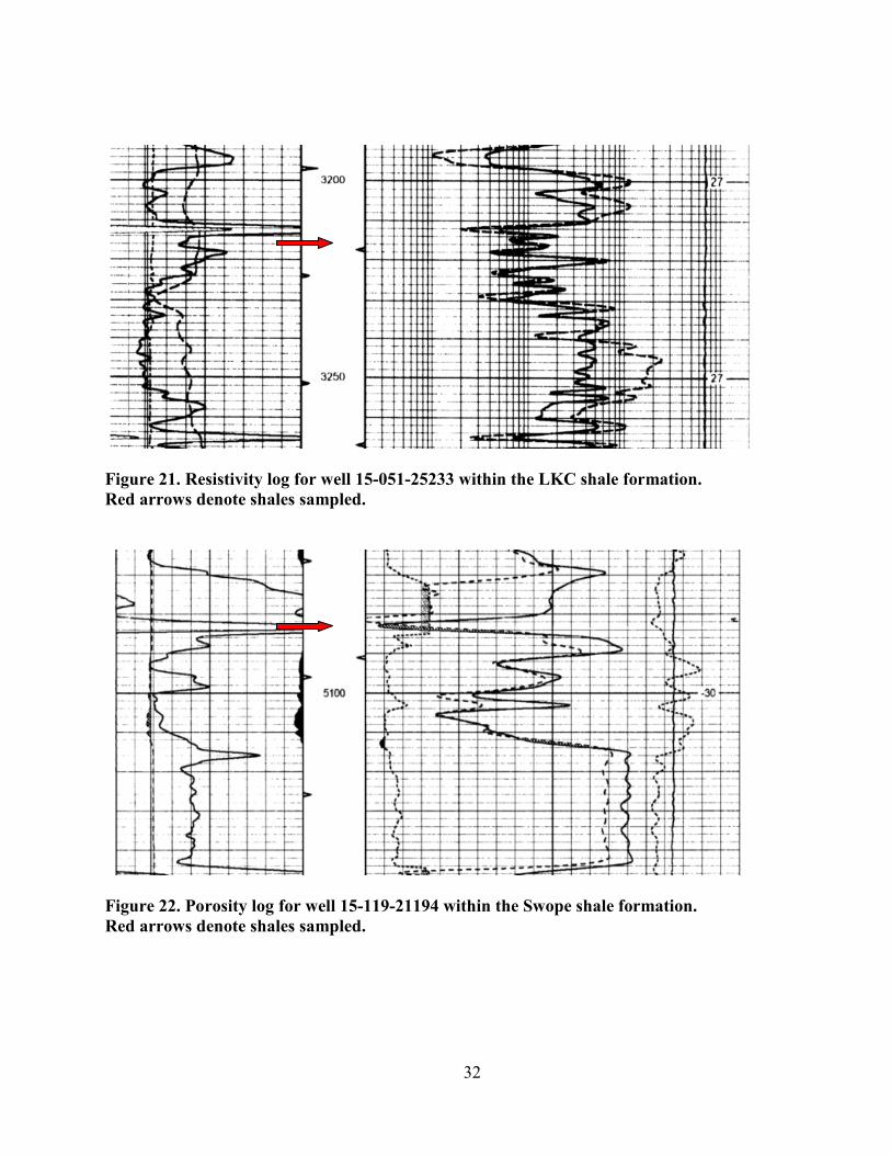
Figure 21. Resistivity log for well 15-051-25233 within the LKC shale formation.


Figure 22. Porosity log for well 15-119-21194 within the Swope shale formation.


33

Figure 23. Porosity log for well 15-119-21194 within the Fort Scott and Cherokee shale

formations.


34

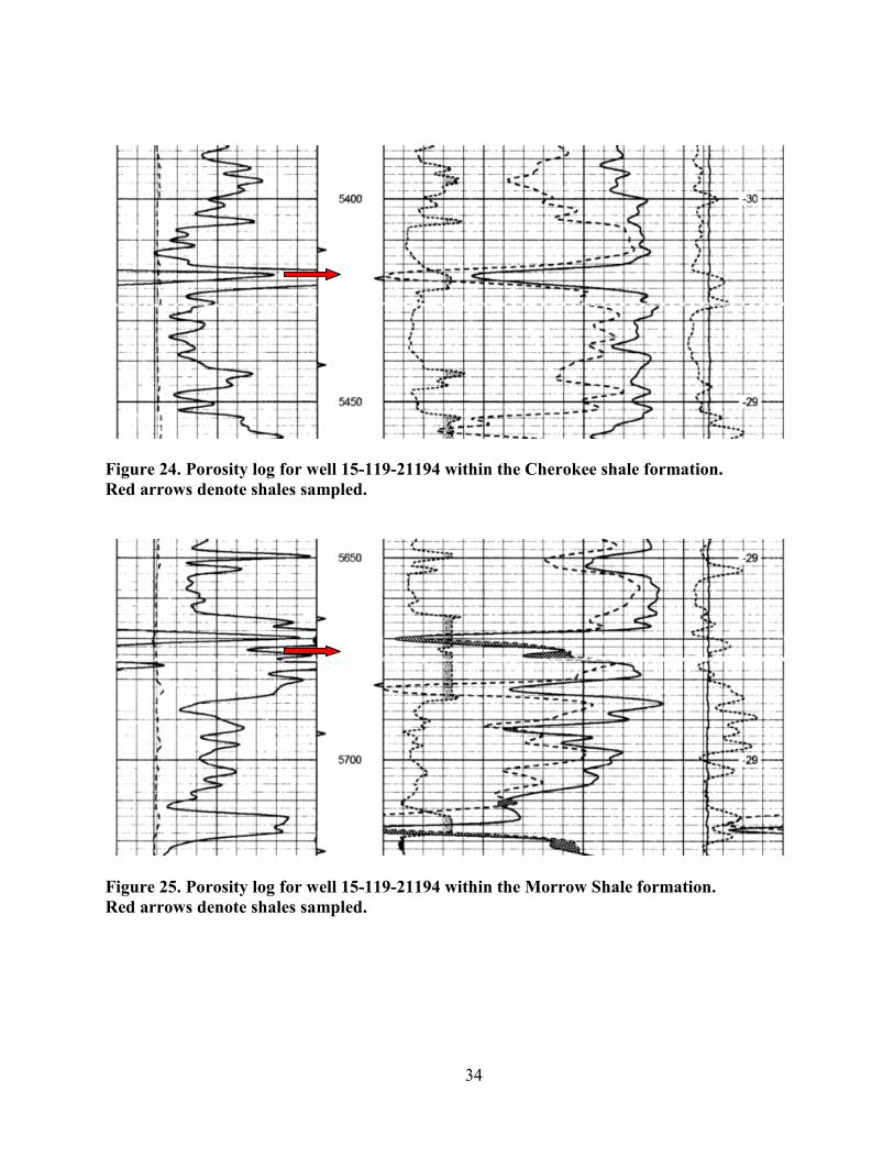
Figure 24. Porosity log for well 15-119-21194 within the Cherokee shale formation.


Figure 25. Porosity log for well 15-119-21194 within the Morrow Shale formation.


35



Figure 27. Geologist's Report for well 15-135-24186 within the Labette shale sample.


36

Figure 28. Geologist's Report for well 15-135-24253 within the LKC shale formation.


Figure 29. Geologist's Report for well 15-135-24253 within the Labette shale formation.


37

Figure 30. Geologist's Report for well 15-135-24254 within the LKC shale formation.


Figure 31. Geologist's Report for well 15-135-24254 within the Labette shale formation.


Figure 32. Porosity log for well 15-135-24314 within the LKC shale formation.


38



39

CHAPTER 3 - RESULTS

Twenty-four samples, based off of well cuttings were analyzed by Weatherford

Laboratories in Houston, Texas. The data is split into two different groups, with the first group

of data is located in Northwestern Kansas in Ellis, and Ness counties (Table 2). The second

group of data is located in Southwestern Kansas, in Comanche and Meade counties (Table 4).

The data sets were analyzed in this way, so that half the shales were taken further away

from the Anadarko basin, and the second half of the shales were collected from deeper wells

much closer to the Anadarko basin. This aided in helping us see if burial depths of the shales

would make any difference in their potential to produce hydrocarbons.

All twenty-four samples were analyzed to assess organic richness, kerogen type, and

thermal maturity. Whole rock analysis was done on eight of these samples in order to confirm

maturity measurements by vitrinite reflectance of well cuttings samples. Results of TOC, Rock-

Eval, and Vitrinite Reflectance (Table 3 and 5) are split into the first and second sets of data

analyses, respectively. The first set of vitrinite reflectance values (Figures 34-36) were

performed on three different shale formations, and their TOC and Rock-Eval can be seen in

Table 3. The second set of vitrinite reflectance values (Figures 37-41) were performed on five

different shale formations, and their TOC and Rock-Eval can be seen in Table 4. Vitrinite

reflectance was not tested on every shale chosen. This analysis is much more expensive, and

time consuming than regular Rock-Eval. Shales analyzed for vitrinite reflectance were chosen

based upon their stratigraphic location. Each reflectance analyses was taken within a different

formation. The main purpose for this was to test more formations for their thermal maturity.

40

Sample County API Formation Depths Sample Type Analysis Run

1 Ellis 15-051-25825 LKC 3546-3549 Cuttings RE/TOC/Ro

2 Ellis 15-051-25825 LKC 3576-3580 Cuttings RE/TOC


4 Ellis 15-051-25316 Arbuckle 3660-3672 Cuttings RE/TOC/Ro

5 Ellis 15-051-25316 Arbuckle 3725 Cuttings RE/TOC


7 Ness 15-135-23895 Cherokee 4235-4240 Cuttings RE/TOC

8 Ness 15-135-24186 Labette 4212-4218 Cuttings RE/TOC/Ro

9 Ness 15-135-24253 LKC 4020-4024 Cuttings RE/TOC

10 Ness 15-135-24253 Labette 4275-4280 Cuttings RE/TOC


12 Ness 15-135-24254 Labette 4226-4232 Cuttings RE/TOC


14 Ness 15-135-24314 Cherokee 4232-4237 Cuttings RE/TOC

Table 2. First set of samples analyzed.

41

Table 3. Summary of data obtained by TOC and Rock-Eval

analyses of the selected samples, for the first set of analyses.

42

Figure 34. Vitrinite reflectance histogram for 4212-4218 ft. interval in well 15-135-24186.


43


Sample County API Formation Depths Sample Type Analysis Run

1 Comanche15-033-21470 LKC 4595-4599 Cuttings RE/TOC

2 Comanche15-033-21470 Stark 4745-4755 Cuttings RE/TOC/Ro

3 Comanche15-033-21470 Stark 4786-4792 Cuttings RE/TOC

4 Comanche15-033-21470 Cherokee 5012-5016 Cuttings RE/TOC

5 Comanche15-033-21470 Cherokee 5046-5050 Cuttings RE/TOC

6 Meade 15-119-21194 Swope 5080-5084 Cuttings RE/TOC/Ro

7 Meade 15-119-21194 Fort Scott 5309-5313 Cuttings RE/TOC/Ro

8 Meade 15-119-21194 Cherokee 5346-5350 Cuttings RE/TOC/Ro

9 Meade 15-119-21194 Cherokee 5414-5418 Cuttings RE/TOC

10 Meade 15-119-21194 Morrow 5668-5671 Cuttings RE/TOC/Ro

Table 4. Second set of data analyzed.

44

Table 5. Summary of data obtained by TOC and Rock-Eval

analyses of the selected samples, for the second set of analyses.

45

0123456789

1011121314

Number of measurements

Vitrinite reflectance (%) @ 546nm

Sample: 3401928638Stark Shale #2 Depth 4745


0

1

2

3

4

5

6



Sample: 3401928626Swope Shale #1 Depth 5080


46

0

1

2

3

4

5

6

7

8

9

10



Sample: 3401928628Fr. Scott Shale #2 Depth 5309

0123456789

101112131415161718



Sample: 3401928630Cherokee Shale #3 Depth 5346

Figure 39. Vitrinite reflectance histogram for 5309-5313 ft. interval well 15-119-21194.


47

0123456789

101112131415



Sample: 3401928634Morrow Shale #5 Depth 5668


48

CHAPTER 4 – DISCUSSIO#

4.1 Kansas Shale Properties

The following sections outline in detail the geochemical characteristics of the shales that

were analyzed in this study. Studying the organic shales in depth will provide evidence that will

show whether or not they have the potential for being a source rock. The organic richness,

hydrocarbon potential, thermal maturity, and burial history are the analyses that were employed

in this study that should give a good indication for the possibility of producing oil in this area.

The TOC values that were analyzed in this study proved to be sufficient enough for

hydrocarbon generation potential. The leanest 1.26% by weight (Table 3) still falls within the

category of “Good” according to Peters et al (2006). The values ranged overall “Good to

Excellent” with the highest being 13.33% by weight (Table 3). The bulk of the values fell within

the category of “Very Good to Excellent”. A significant amount of values fell within the

“Excellent” range. The high TOC values were not from a single formation, but rather were

spread throughout all of the different formations. Out of the eight formations that were analyzed

only two of the samples fell below the range of “Excellent”, with the formations being the Ft.

Scott and Morrow Shales. There was an abundance of TOC within this study for hydrocarbon

generation. The next step was to look at kerogens, and thermal maturity.

The results for pyrolysis can be seen in Tables (3 and 5). Peak S1 plotted very low on a

majority of the formations sampled, indicating that there has been little to no hydrocarbons

produced. Peak S2 plotted very high indicating that there is still a lot of hydrocarbon left to be

produced. When comparing S1/S2 from this study, all of the analyses fell within the category of

“Poor to Excellent” (Figure 11). Most of the samples that did fall into the “Excellent” range

49

were however not mature enough to have produced hydrocarbons. There are two samples that

did however fall within this range of “Excellent”, and coupled with the other results may have

produced some hydrocarbons.

The shales that have been analyzed can be put into several different graphs that aid in

their interpretation. The Geochemical Logs (Figures 42 and 43) show a variety of different

characteristics of each shale. This shows several different values, with each one plotted against

depth. The first log is TOC, showing the range from good to excellent based on a percent. The

next log is hydrocarbon potential (S2), which plots the remaining hydrocarbons within the shale.

The next log is organic matter type (I, II, III, IV), which plot at type II and III. The last log that

is plotted shows normalized oil content, which all plot as low maturity source rock.

50

Figure 42. Geochemical Log of TOC, remaining potential (S2), kerogen type (HI),

normalized oil content, and calculated vitrinite reflectance. Analyses from #ess and

Ellis counties.

51

Figure 43. Geochemical Log of TOC, remaining potential (S2), kerogen type (HI),

normalized oil content, and calculated vitrinite reflectance. Analyses from Meade

and Comanche counties.

52

Tmax can also be plotted in several different ways that show maturity of the sample

versus the type of kerogens (Figures 44-47). This is another useful plot for determining whether

or not the kerogens are mature enough to have produced hydrocarbons. These graphs are plotted

in two different ways. The first is HI versus Tmax (Figures 44 and 45). This graph shows what

type of kerogens that are present (Type II and III in this study), plotted against Tmax, to show

whether or not they were mature or not. In the case of this study, they were not mature enough

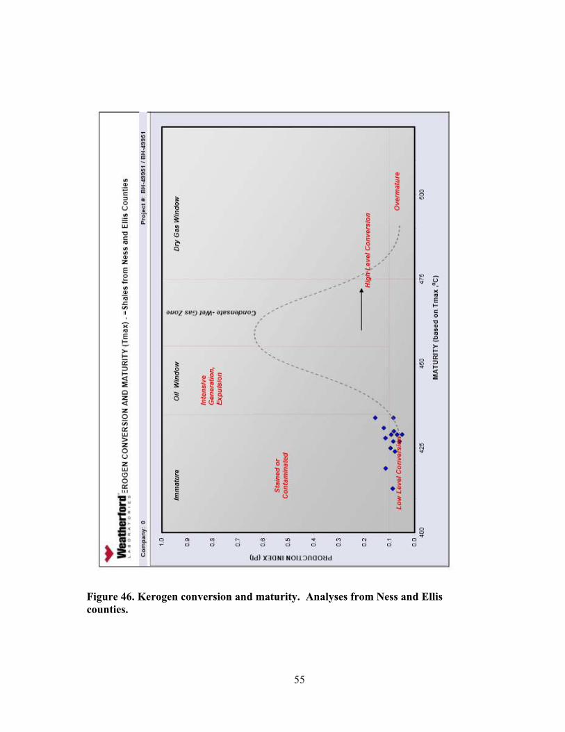
in most cases. The second plot (Figure 46 and 47) is Production Index (PI) which is S1/(S1+S2),

versus Tmax. This indicates the average oil produced, with remaining potential left, plotted

against Tmax to show its maturity. These all plot within the immature range, with one

exception. The majority of the Tmax values fall into the “Immature” category (Figure 12). This

indicates that the formations sampled are not mature enough to have produced hydrocarbons.

53

Figure 44. Kerogen type and maturity. Analyses from #ess and Ellis counties.

54

Figure 45. Kerogen type and maturity. Analyses from Meade and Comanche counties.

55

Figure 46. Kerogen conversion and maturity. Analyses from #ess and Ellis

counties.

56

Figure 47. Kerogen conversion and maturity. Analyses from #ess and Ellis

counties.

57

On the van Krevelen diagram, the kerogens plot in Type II and III (Figures 48 and 49).

These types are oil prone, and gas prone. On the S2 versus TOC diagram (Figures 50 and 51)

the kerogens plot in Types II and III, which also indicates that they are oil prone, and gas prone.

The S2 versus TOC diagram is a better way to look at the depositional environment so that the

points are not scattered as much, like they are in the standard van Krevelen plots. This puts all of

the samples within the depositional range of anoxic-oxic marine or laucustrine to, mildly oxic

and coal swamp deposition. They are also mixed marine, and terrestrial.

58

Figure 48. Kerogen type. Analyses from #ess and Ellis counties.

59

Figure 49. Kerogen type. Analyses from Meade and Comanche counties.

60

Figure 50. Kerogen quality. Analyses from #ess and Ellis counties.

61

Figure 51. Kerogen quality. Analyses from Meade and Comanche counties.

62

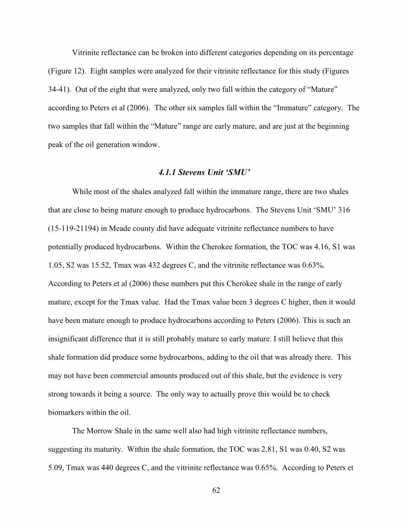
Vitrinite reflectance can be broken into different categories depending on its percentage

(Figure 12). Eight samples were analyzed for their vitrinite reflectance for this study (Figures

34-41). Out of the eight that were analyzed, only two fall within the category of “Mature”

according to Peters et al (2006). The other six samples fall within the “Immature” category. The

two samples that fall within the “Mature” range are early mature, and are just at the beginning

peak of the oil generation window.

4.1.1 Stevens Unit ‘SMU’

While most of the shales analyzed fall within the immature range, there are two shales

that are close to being mature enough to produce hydrocarbons. The Stevens Unit ‘SMU’ 316

(15-119-21194) in Meade county did have adequate vitrinite reflectance numbers to have

potentially produced hydrocarbons. Within the Cherokee formation, the TOC was 4.16, S1 was

1.05, S2 was 15.52, Tmax was 432 degrees C, and the vitrinite reflectance was 0.63%.

According to Peters et al (2006) these numbers put this Cherokee shale in the range of early

mature, except for the Tmax value. Had the Tmax value been 3 degrees C higher, then it would

have been mature enough to produce hydrocarbons according to Peters (2006). This is such an

insignificant difference that it is still probably mature to early mature. I still believe that this

shale formation did produce some hydrocarbons, adding to the oil that was already there. This

may not have been commercial amounts produced out of this shale, but the evidence is very

strong towards it being a source. The only way to actually prove this would be to check

biomarkers within the oil.

The Morrow Shale in the same well also had high vitrinite reflectance numbers,

suggesting its maturity. Within the shale formation, the TOC was 2.81, S1 was 0.40, S2 was

5.09, Tmax was 440 degrees C, and the vitrinite reflectance was 0.65%. According to Peters et

63

al (2006) these numbers put this shale in the range of early mature to peak mature. The only

value that sets this shale back, is the S1 with a “Poor” value. The rest of the values do however

suggest that this was a mature source rock, and that it did produce some oil. This is along the

same lines as the Cherokee shale though, where it probably did not produce commercial amounts

of hydrocarbons, and probably just added to what was already there. Again the only way to

check for sure would to analyze the biomarkers.

Even with the hydrocarbons that were generated from the Stevens Unit ‘SMU’, the

second hypothesis of oil migration from the Anadarko basin in Oklahoma proved to be correct.

There are a significant amount of commercial hydrocarbons in Kansas, and they did not come

from the source rocks that are currently there. The migration northward from Oklahoma is

credible, considering the amount of time that the hydrocarbons had to travel, which is at least

several hundred million years.

4.1.2 Discussion of Bostick’s Figure.

According to Bostick’s (1979) figure from Chapter 1 (Figure 14), the source rocks within

the study area could have potentially reached thermal maturity. The source rocks are shallow,

however they are old enough, and could have potentially reached high enough maturity to

produce hydrocarbons. The source rocks range in age from 440 ma to 290 ma. Early Permian

source rocks could have been subjected to much lower temperatures for a significant amount of

time, and still have produced hydrocarbons.

This figure was part of the basis for which we came up with the hypothesis for potential

source rocks within western Kansas. Geologically the study area fit into the model perfectly.

There was more than enough time for the organic shales to be subjected to enough heat to make

them thermally mature.

64

Vitrinite reflectance values did not reach 0.7% in this study. They were within the early

mature range for hydrocarbon generation. There were several that were close to Bostick’s

(1979) range for hydrocarbon generation window, but did not quite reach high enough

temperatures.

The results of the study do not support Bostick’s model for maturity to be reached at

lower temperatures if enough time is available. Because vitrinite reflectance mirrors

hydrocarbon generation, time must not be an important factor. Temperature remains the key

factor in hydrocarbon generation. According to the results from vitrinite reflectance, most of the

shales were right on the verge of being thermally mature. Had the temperatures been higher,

then there is a good possibility that the Kansas organic shales could have sourced significant

hydrocarbons.

65

CHAPTER 5 – SUMMARY A#D CO#CLUSIO#S

This study shows one of the many benefits of combining geochemistry and subsurface

mapping in basin evaluation. The shales analyzed in this study are dark-gray to black, organic-

rich, and were deposited in anoxic-oxic water conditions. They range in age from Cambrian-

Ordovician through the Permian. Their depositional environments are similar, in that they are

marine and deposited several hundred feet deep. Their current stratigraphic depths range from

3,500-4,500 ft. deep in Ellis and Ness Counties. In Meade and Comanche Counties, their depths

range from 4,500-5,600 ft. deep. The average shale is five to twenty feet thick.

The shales in Ellis and Ness proved to be extremely organic-rich, however they were

thermally immature. TOC values ranged from 1.26% up to 13.33%, which is very high for the

average source rock. Tmax values ranged from 413 degrees C to 434 degrees C, making them

immature. Vitrinite Reflectance values were 0.56%, 0.59%, and 0.59%, confirming that they

were thermally immature. All of these values combined can make a definite answer that the oil

in the reservoirs did migrate northward from the Anadarko basin of Oklahoma.

The shales in Meade and Comanche proved to be extremely organic-rich, the maturity of

some of the source rocks is on the verge of potentially producing some hydrocarbons. TOC

values ranged from 2.41% up to 12.85%, which is also very high for the average source rock.

Tmax values ranged from 422 degrees C to 440 degrees C, making the majority of them

immature, however some of them did reach temperatures high enough to make them mature.

Vitrinite Reflectance values were (0.44%, 0.58%, 0.59%, 0.63%, and 0.65%). The first three

values are thermally immature, but the last two values are early mature to peak mature,

respectively. The last two values are of great interest in this study. It is probably safe to say that

these two shales (Cherokee and Morrow) did produce some hydrocarbons. When looking at the

66

kerogens from these two shales, they fall into type II and III, making the hydrocarbon generation

gas-oil. The next step to analyzing their oil and gas generation potentials would be to check for

biomarkers within the oil.

There is an obvious, and much expected general increase in thermal maturity of the

shales from the north to the south in western Kansas. This can be expected because of the

deepening of the shales towards the south, and the Anadarko basin. In the northern counties

within this study (Ness and Ellis), the rocks are on average about a thousand feet shallower

compared to the southern counties (Meade and Comanche). The shales in the southern counties

did exhibit higher Tmax values, as well as higher vitrinite reflectance values. These counties are

very close to the Anadarko basin, and may have been subjected to higher temperatures coming

out of the basin.

This study proves that the hypothesis concerning the migration of oil from the Anadarko

basin in Oklahoma is correct. The shales in Ness and Ellis are not thermally mature enough to

produce hydrocarbons. Most of the shales in Meade and Comanche are also thermally immature.

This study also proves that the hypothesis concerning hydrocarbon generation from shales

currently present within western Kansas is also correct. There was probably not a commercial

amount of hydrocarbons that were produced, but the amount of evidence from analyses shows

that there was some generation of hydrocarbons.

This study is important to other petroleum geologist’s investigating similar basins to

western Kansas. If there are no other deep, organic, hydrocarbon rich basins surrounding the

basin being evaluated, then there would probably not be any need to explore in that area. The

bulk of the oil in Kansas did migrate north, and it has been enough to make Kansas a valuable

67

economic region. Even though western Kansas did produce hydrocarbons, they were minimal

and could not prove to be economical.

68

References Cited

Bostick, N. H. (1979). Microscopic measurement of the level of catagenesis of solid organic

matter in sedimentary rocks to aid exploration for petroleum and to determine former

burial temperatures a review. Special Publication - Society of Economic Paleontologists

and Mineralogists, (26), 17-43.

Franz, R. (1985). Distribution of Petrophysical Properties in a Lower Morrow Sandstone

(Keyes), Southwest Kansas. Subsurface Geology Series, 6, 48.

Gerhard, L. C. (2004) A New Look at an Old Petroleum Province. Current Research in Earth

Sciences, Bulletin 250, part 1, p. 1-27.

Hunt, J., 1979, Petroleum Geochemistry and Geology: New York, W. H. Freeman, p. 69-73,

195-204.

Jarvie, D. M., 1991, Total organic carbon (TOC) Analysis; in, Source Migration Processes and

Evaluation Techniques, R. K. Merrill, ed.: American Association of Petroleum

Geologists, Treatise of Petroleum Geology Handbook of Petroleum Geology, p. 113-118.

Kansas Geological Survey, 2009. Oil and Gas Fields of Kansas. Special Map 6. Lawrence, KS:

University of Kansas Publications.

Lambert, M. W., 1992, Internal Stratigraphy and Organic Facies of the Devonian-Mississippian

Chattanooga (Woodford) Shale in Oklahoma and Kansas. The Oklahoma Geological

Survey, Source Rocks Symposium, 1990. Circular 93, p. 163-176.

Langford, F. F., Blanc-Valleron, B. B., "Interpreting Rock-Eval Pyrolysis Data Using Graphs of

Pyrolizable Hydrocarbons vs. Total Organic Carbon." AAPG Bulletin 74.6 (1990): 799-

804.

Merriam, D. F., 1963, "The Geologic History of Kansas." Bulletin 162. Lawrence, KS:

University of Kansas Publications, p. 117-149.

69

Oko, A. (2006). Hydrocarbon Potential of the Floyd Shale in the Black Warrior basin,

northwestern Alabama, p. 47-48.

Peters, K. E., 1986, Guidelines for Evaluating Petroleum Source Rock Using Programmed

Pyrolysis. The American Association of Petroleum Geologists Bulletin, V. 70, No. 3.

March 1986, p. 318-329.

Peters, K. E., Walters, C. C., Moldowan, J. M., 2006, The Biomarker Guide: New York,

Cambridge University Press, p. 72-118.

Robinson, R., Chaudhuri, S., Jones, L. M., (1985). Diagenesis of the Pennsylvanian Morrowan

Sandstone, Clark County, Kansas. Subsurface Geology Series, 6, p. 56-60.

Senftle, J. T., and Landis, C. R., 1991, Vitrinite Reflectance as a Tool To Assess Thermal

Maturity; in, Source Migration Processes and Evaluation Techniques, R. K. Merrill, ed.:

American Association of Petroleum Geologists, Treatise of Petroleum Geology

Handbook of Petroleum Geology, p. 119-125.

Sweeney, J. J., and Burnham, A. K., 1990, Evaluation of a Simple Model of Vitrinite Reflectance

Based on Chemical Kinetics. The American Association of Petroleum Geologists

Bulletin V. 74 No. 10. p. 1559-1570.

Tissot, B. P., Welte, D. H., 1984, Petroleum Formation and Occurrence. Second Edition.

Springer-Verlag Berlin Heidelberg, Germany, p. 151-159, 181-183.

Watney, W. L., 1980, "Cyclic Sedimentation of the Lansing-Kansas City Groups in

Northwestern Kansas and Southwestern Nebraska." Bulletin 220. Lawrence, KS:

University of Kansas Publications, p. 1-8.

Zeller, D., 1968, "Stratigraphic Succession in Kansas." Bulletin 189. Lawrence, KS: University

of Kansas Publications.

70

Appendix A - FID Responses

POTENTIAL SOURCE ROCKS IN THE WESTERN KANSAS ...

Documents

Transcript of POTENTIAL SOURCE ROCKS IN THE WESTERN KANSAS ...