sensors

Article

Position Estimation of Vehicle Based on Magnetic Marker:Time-Division Position Correction

Yeun Sub Byun * and Rag Gyo Jeong

�����������������

Citation: Byun, Y.S.; Jeong, R.G.

Position Estimation of Vehicle Based

on Magnetic Marker: Time-Division

Position Correction. Sensors 2021, 21,

8274. https://doi.org/10.3390/

s21248274

Academic Editor: Zhanye Chen

Received: 10 November 2021

Accepted: 9 December 2021

Published: 10 December 2021

Publisher’s Note: MDPI stays neutral

with regard to jurisdictional claims in

published maps and institutional affil-

iations.

Copyright: © 2021 by the authors.

Licensee MDPI, Basel, Switzerland.

This article is an open access article

distributed under the terms and

conditions of the Creative Commons

Attribution (CC BY) license (https://

creativecommons.org/licenses/by/

4.0/).

Korea Railroad Research Institute, 176, Cheoldobangmulgwan-ro, Uiwang 16105, Gyeonggi-do, Korea;rgjeong@krri.re.kr* Correspondence: ysbyun@krri.re.kr; Tel.: +82-31-460-5437

Abstract: During the automatic driving of a vehicle, the vehicle’s positional information is importantfor vehicle driving control. If fixed-point land markers such as magnetic markers are used, thevehicle’s current position error can be calculated only when a marker is detected while driving,and this error can be used to correct the estimation position. Therefore, correction information isused irregularly and intermittently according to the installation intervals of the magnetic markersand the driving speed. If the detected errors are corrected all at once using the position correctionmethod, discontinuity of the position information can occur. This problem causes instability in thevehicle’s route guidance control because the position error fluctuates as the vehicle’s speed increases.We devised a time-division position correction method that calculates the error using the absoluteposition of the magnetic marker, which is estimated when the magnetic marker is detected, alongwith the absolute position information from the magnetic marker database. Instead of correctingthe error at once when the position and heading errors are corrected, the correction is performedby dividing the errors multiple times until the next magnetic marker is detected. This preventssudden discontinuity of the vehicle position information, and the calculated correction amount isused without loss to obtain stable and continuous position information. We conducted driving teststo compare the performances of the proposed algorithm and conventional methods. We comparedthe continuity of the position information and the mean error and confirmed the superiority of theproposed method in terms of these aspects.

Keywords: automatic driving; error estimation; position detection; guidance control; magneticmarker; magnetic sensing ruler; peak detection; autonomous vehicle; heading angle

1. Introduction

This study proposes a time-division (space-division) position correction method foruse in automatic driving vehicles to minimize the position information discontinuity andthe correction information loss that can occur in the classic position estimation methodusing magnetic markers as land marker methods.

Position estimation technology for automatic driving has been used in a variety ofways, not only for autonomous vehicles but also for automatic logistics transportationsystems in places such as factories and ports. Using this technique, various devices andtechnologies are combined, such as global positioning system (GPS) technologies [1–7],camera-based image processing technologies [8–10], and laser-scanner-related technolo-gies [11–14]. Among these various systems, land marker methods of positioning technologyare used mainly in areas with limited operating range, such as factories and ports. Positiondetection systems based on a transponder method and a magnetic marker sensing method,one of the more popular land-marker-based positioning methods, have relatively lowinstallation and maintenance costs and are less affected than other methods by changesin indoor and outdoor environments [15–22]. Furthermore, 2getthere [23] is a companythat has applied this method to small passenger transport vehicles in a pilot operation inMasdar City, Abu Dhabi, United Arab Emirates.

Sensors 2021, 21, 8274. https://doi.org/10.3390/s21248274 https://www.mdpi.com/journal/sensors

Sensors 2021, 21, 8274 2 of 16

Previous researchers [24] proposed a position estimation method using magneticmarker sensing and GPS. When such magnetic markers are used, the vehicle uses a methodfor estimating the absolute position of the vehicle while driving, whereby the magneticdetection sensor mounted on the vehicle detects magnetic markers buried in roads [16–18].In this method, the position error can be measured at each magnetic marker position basedon which error of the calculated position is corrected. Here, a Kalman filter and varioussensors, including the vehicle’s speed sensor and rotational angular velocity, are combinedto calculate the real-time position at each control cycle [16]. When the magnetic signalis collected just once in each control cycle and applied to the position estimation in theconventional magnetic detection signal processing method, there are limitations to themaximum driving speed of the vehicle because of the sampling time problem related to themagnetic signals. In other words, if the vehicle speed is too high compared to the signalcollection cycle, the sampling of the signals may be insufficient to find the peak of themagnetic signals when passing over the magnetic marker. In this method, the positionerror is calculated whenever a magnetic marker is detected, meaning that when correctingthe errors all at once in the corresponding cycle, if the correction error is large the correctedposition information in the pertinent cycle may be discontinuous from the previous position.If a value smaller than the measured correction value is applied, the discontinuity can bemitigated, although this causes a loss of correction information. In conventional methods, ifthe discontinuity is mitigated by adjusting the setting of the Kalman filter coefficient value,a position delay occurs, causing a larger rotational radius compared to the actual drivingposition when driving on a curve. This error correction problem has a significant impacton the safety of the rotational driving control of the moving object. In other words, thelongitudinal and lateral position estimation errors increase, reducing the driving precisionand stability in the route guidance control using this method.

In this study, we propose methods to solve the two major problems presented:

• First, to improve the vehicle-speed-related magnetic signal processing problem, asignal processor is implemented to process magnetic signal detection at a fast cycle(1 ms), separate from the low vehicle control cycle (50 ms);

• A position correction method is proposed to reduce the loss of correction values andimprove the position discontinuity that results from correcting errors. A time-divisionerror correction method based on the moving distance is proposed for the errorsmeasured when the magnetic markers are detected.

Based on this, we increased the speed band for position estimation by increasing themagnetic signal sampling cycle. The signal detection range of the magnetic marker by themagnetic sensor confirmed through the test is about 30 cm. This range is sufficient to detectthe center of the magnetic signal if at least eight samples are obtained at 3 cm intervals ofthe signal, including the magnetic field center. Therefore, considering the travel distanceof 3 cm in 1 ms (the magnetic signal sampling time), the theoretical maximum utilizationspeed of the developed MSR is 100 km/h. Furthermore, we used the measured correctionamount while mitigating the conversion impact caused by sudden position corrections.Thus, the driving stability and ride comfort can be improved based on driving controlusing smooth and continuous position information when driving the vehicle.

The remainder of this paper is organized as follows. Section 2 describes the structuresof the magnet-marker-based driving control system and the developed magnetic sensingruler (MSR). Next, Section 3 suggests a method for estimating the magnet marker peaksthrough the detection of their magnetic signals, as measured while driving. Section 4describes the absolute position estimation method of a vehicle, which combines the vehicle’ssensor information and the magnet marker position information measured using theMSR. Section 5 presents comparative test results with conventional methods to verifythe proposed position correction method’s effectiveness and validity. Section 6 providesthe conclusion.

Sensors 2021, 21, 8274 3 of 16

2. Magnetic-Marker-Based Guidance System

To measure the vehicle’s position while driving in the vehicle’s automatic drivingcontrol system, an MSR was installed and cylindrical magnet markers (15 mm in diameterand 30 mm in length) were buried along the driving track. The MSR was installed parallelto the axle at the bottom of the vehicle at a height of approximately 12 cm. The vehicle’s hostcomputer combines the information obtained from the gyroscope, steering angle sensor,and MSR installed on the vehicle to calculate the vehicle’s moving distance, direction, andposition in the unit sample. Based on this information, a variety of control informationrequired for the vehicle’s automatic driving was calculated. The developed vehicle wasoperated and controlled by a distant control center, as shown in Figure 1.

Sensors 2021, 21, x FOR PEER REVIEW 3 of 17

the MSR. Section 5 presents comparative test results with conventional methods to verify the proposed position correction method’s effectiveness and validity. Section 6 provides the conclusion.

2. Magnetic-Marker-Based Guidance System To measure the vehicle’s position while driving in the vehicle’s automatic driving

control system, an MSR was installed and cylindrical magnet markers (15 mm in diameter and 30 mm in length) were buried along the driving track. The MSR was installed parallel to the axle at the bottom of the vehicle at a height of approximately 12 cm. The vehicle’s host computer combines the information obtained from the gyroscope, steering angle sensor, and MSR installed on the vehicle to calculate the vehicle’s moving distance, direction, and position in the unit sample. Based on this information, a variety of control information required for the vehicle’s automatic driving was calculated. The developed vehicle was operated and controlled by a distant control center, as shown in Figure 1.

The magnetic signals of the magnet marker have a Gaussian function shape centered on the magnet marker. As the center of the buried magnet marker is approached, the strength of the magnet signals increases, and the highest strength of the magnetic signals is found at the center of the magnet marker. To measure the absolute position of the vehicle in real-time while driving, the relative longitudinal and lateral distances from the magnetic marker’s center to the MSR are calculated by analyzing the magnetic signals of the magnetic marker buried in the road. This information is used to calculate the absolute position of the vehicle based on the absolute position database information of the detected magnet marker. A variety of signal and control information for the vehicle is collected and determined in 50 ms cycles.

Heading angle estimationPosition estimation (x,y,Ө)

Designed Multi route

data

＋－

Anglesensor

Speedsensor

Magneticsensor

Gyroscope

Magneticmarker

Designed route

Magnetic ruler

Steering controlSpeed control

Contactless Power Supply

System

Control center

Lidar sensor

• Call sign• Route selection• Speed Limit• Time interval control• Emergency control Vehicle Automatic Control

• Localization (initial & driving position)• Guidance control• Distance control• Speed control• Docking control• Faults diagnosis• Object recognition

Figure 1. Schematic of the automatic guidance system based on magnetic markers.

Figure 1. Schematic of the automatic guidance system based on magnetic markers.

The magnetic signals of the magnet marker have a Gaussian function shape centeredon the magnet marker. As the center of the buried magnet marker is approached, thestrength of the magnet signals increases, and the highest strength of the magnetic signalsis found at the center of the magnet marker. To measure the absolute position of thevehicle in real-time while driving, the relative longitudinal and lateral distances from themagnetic marker’s center to the MSR are calculated by analyzing the magnetic signals ofthe magnetic marker buried in the road. This information is used to calculate the absoluteposition of the vehicle based on the absolute position database information of the detectedmagnet marker. A variety of signal and control information for the vehicle is collected anddetermined in 50 ms cycles.

Magnet Measurement SystemConfiguration of the Magnetic Sensing Rules

The MSR is mounted at the bottom of the vehicle, as shown in Figure 2. It consistsof 60 magnetic sensors arranged in 2 cm intervals in a line with an effective sensor mea-surement length of 120 cm, as shown in Figure 3. The magnetic sensors in the MSR collectmagnetic information in 1 ms intervals and send the collected data to the signal analysisprocess every 50 ms via Ethernet. The MSR receives the reference synchronization number

Sensors 2021, 21, 8274 4 of 16

from the vehicle’s signal processing device every 50 ms and uses it as the reference detec-tion time index of the collected magnetic signal. The signal processing device synchronizesthe in-vehicle processing information using the time index included in the magnetic signaltransmitted by the MSR and the current time index of the vehicle signal processing device.

Sensors 2021, 21, x FOR PEER REVIEW 4 of 17

Magnet Measurement System Configuration of the Magnetic Sensing Rules

The MSR is mounted at the bottom of the vehicle, as shown in Figure 2. It consists of 60 magnetic sensors arranged in 2 cm intervals in a line with an effective sensor measurement length of 120 cm, as shown in Figure 3. The magnetic sensors in the MSR collect magnetic information in 1 ms intervals and send the collected data to the signal analysis process every 50 ms via Ethernet. The MSR receives the reference synchronization number from the vehicle’s signal processing device every 50 ms and uses it as the reference detection time index of the collected magnetic signal. The signal processing device synchronizes the in-vehicle processing information using the time index included in the magnetic signal transmitted by the MSR and the current time index of the vehicle signal processing device.

Figure 2. Installation of the magnetic sensing ruler (MSR).

Figure 3. Magnetic sensing ruler (MSR).

3. Magnetic Marker Detection and Signal Processing 3.1. Magnetic Marker Position Detection

As shown in Figure 4, Hall effect sensors were arranged in certain intervals on the MSR installed at the bottom of the vehicle to measure magnetic signals at each sampling time. Because magnetic signals are collected as one-dimensional (1D) data according to the sampling cycle in a time sequence, the longitudinal center position of a magnet marker in the proceeding direction can always be checked after the MSR has passed the marker. Therefore, time and spatial delays inevitably occur in the recognition time-point of the center of the magnet marker because the collected 1D data must be arranged to construct and analyze 2D spatial data. The following procedure is performed on the collected time-series magnetic signal array data to check the sensing position of the magnet marker on the spatial coordinate system.

Figure 2. Installation of the magnetic sensing ruler (MSR).

Sensors 2021, 21, x FOR PEER REVIEW 4 of 17

Magnet Measurement System Configuration of the Magnetic Sensing Rules

The MSR is mounted at the bottom of the vehicle, as shown in Figure 2. It consists of 60 magnetic sensors arranged in 2 cm intervals in a line with an effective sensor measurement length of 120 cm, as shown in Figure 3. The magnetic sensors in the MSR collect magnetic information in 1 ms intervals and send the collected data to the signal analysis process every 50 ms via Ethernet. The MSR receives the reference synchronization number from the vehicle’s signal processing device every 50 ms and uses it as the reference detection time index of the collected magnetic signal. The signal processing device synchronizes the in-vehicle processing information using the time index included in the magnetic signal transmitted by the MSR and the current time index of the vehicle signal processing device.

Figure 2. Installation of the magnetic sensing ruler (MSR).

Figure 3. Magnetic sensing ruler (MSR).

3. Magnetic Marker Detection and Signal Processing 3.1. Magnetic Marker Position Detection

As shown in Figure 4, Hall effect sensors were arranged in certain intervals on the MSR installed at the bottom of the vehicle to measure magnetic signals at each sampling time. Because magnetic signals are collected as one-dimensional (1D) data according to the sampling cycle in a time sequence, the longitudinal center position of a magnet marker in the proceeding direction can always be checked after the MSR has passed the marker. Therefore, time and spatial delays inevitably occur in the recognition time-point of the center of the magnet marker because the collected 1D data must be arranged to construct and analyze 2D spatial data. The following procedure is performed on the collected time-series magnetic signal array data to check the sensing position of the magnet marker on the spatial coordinate system.

Figure 3. Magnetic sensing ruler (MSR).

3. Magnetic Marker Detection and Signal Processing3.1. Magnetic Marker Position Detection

As shown in Figure 4, Hall effect sensors were arranged in certain intervals on theMSR installed at the bottom of the vehicle to measure magnetic signals at each samplingtime. Because magnetic signals are collected as one-dimensional (1D) data according to thesampling cycle in a time sequence, the longitudinal center position of a magnet markerin the proceeding direction can always be checked after the MSR has passed the marker.Therefore, time and spatial delays inevitably occur in the recognition time-point of thecenter of the magnet marker because the collected 1D data must be arranged to constructand analyze 2D spatial data. The following procedure is performed on the collected time-series magnetic signal array data to check the sensing position of the magnet marker onthe spatial coordinate system.

3.1.1. Resampling

The values that must be checked from the collected magnetic signals are the relativelongitudinal and lateral distances from the magnetic sensor axis to the center of the magnetmarker at the reference time (50 ms). However, the data sent by the MSR are arrayinformation of the time-series magnetic signal data collected every 50 ms, measured in 1 mscycles. The obtained signals have a normalized magnetic signal shape that does not changein the lateral direction (i.e., along the MSR’s length), although the magnetic signal shape onthe time axis changes according to the vehicle speed in the longitudinal (i.e., proceeding)direction, which can cause difficulties in the process of finding the peak of the magneticsignals. Therefore, we performed a process of resampling the collected time-series data

Sensors 2021, 21, 8274 5 of 16

of the magnetic signals into spatial coordinate data. By doing so, we obtained spatiallyconsistent magnetic signal distribution data regardless of the vehicle’s speed and effectivelyfound the peak (the magnet marker’s center) position of magnetic signals on the magneticsensor axis at the reference time from the data distribution.

Sensors 2021, 21, x FOR PEER REVIEW 5 of 17

y

x

z

Figure 4. Magnetic marker and magnetic sensing ruler.

3.1.1. Resampling The values that must be checked from the collected magnetic signals are the relative

longitudinal and lateral distances from the magnetic sensor axis to the center of the magnet marker at the reference time (50 ms). However, the data sent by the MSR are array information of the time-series magnetic signal data collected every 50 ms, measured in 1 ms cycles. The obtained signals have a normalized magnetic signal shape that does not change in the lateral direction (i.e., along the MSR’s length), although the magnetic signal shape on the time axis changes according to the vehicle speed in the longitudinal (i.e., proceeding) direction, which can cause difficulties in the process of finding the peak of the magnetic signals. Therefore, we performed a process of resampling the collected time-series data of the magnetic signals into spatial coordinate data. By doing so, we obtained spatially consistent magnetic signal distribution data regardless of the vehicle’s speed and effectively found the peak (the magnet marker’s center) position of magnetic signals on the magnetic sensor axis at the reference time from the data distribution.

If there is no data resampling process, the size of the data collected on the time axis will increase when the vehicle passes the magnet marker at a low speed compared to when it passes at a high speed. Furthermore, if the MSR is above the magnet marker when the vehicle stops, the amount of data to be analyzed will increase dramatically, and a significant amount of computational time will be required to process the data. Therefore, the data collected on the time axis are resampled in 1 cm intervals in the proceeding direction to apply a consistent function model in the spatial domain. Based on the installed MSR and a buried magnet marker, the effective measurement distance of magnetic signals was found to be within 30 cm, implying that data collection in 1 cm intervals results in a sufficient resolution for signal analysis. When represented on a 3D coordinate system, the data collected by the MSR have a Gaussian distribution, as shown in Figure 5.

Figure 4. Magnetic marker and magnetic sensing ruler.

If there is no data resampling process, the size of the data collected on the time axiswill increase when the vehicle passes the magnet marker at a low speed compared to whenit passes at a high speed. Furthermore, if the MSR is above the magnet marker when thevehicle stops, the amount of data to be analyzed will increase dramatically, and a significantamount of computational time will be required to process the data. Therefore, the datacollected on the time axis are resampled in 1 cm intervals in the proceeding direction toapply a consistent function model in the spatial domain. Based on the installed MSR and aburied magnet marker, the effective measurement distance of magnetic signals was foundto be within 30 cm, implying that data collection in 1 cm intervals results in a sufficientresolution for signal analysis. When represented on a 3D coordinate system, the datacollected by the MSR have a Gaussian distribution, as shown in Figure 5.

3.1.2. Estimation of the Center Point of the Magnetic Field Signal in the Collected 2D Data Space

If the acquired magnetic signals include a peak above the threshold size (the magneticsignal distribution is acquired until the magnetic marker is passed), the position of the peakis estimated on the 2D plane. The magnetic signals have a Gaussian distribution centeringon the magnetic marker, and the peak position of the Gaussian distribution is the positionof the center of the magnetic marker. The y-axis of the collected data represents the data forthe discrete space measured with the magnetic sensors placed at certain intervals, whereasthe x-axis represents the data measured at the sampling time and may span between twocontrol cycles (based on a reference control cycle of 50 ms). Because it includes noise signalsthat distort the signals, the following process is performed to find the peak of the magneticsignal in the discrete space including noise:

1. The position of the maximum [x_max, y_max] is found in the collected 2D data;2. The top, bottom, left, and right data spaces of a certain size around the position of the

maximum are extracted;3. The sum of each row and the sum of each column in the extracted sample space

are calculated;4. Because only the peak of the signal needs to be determined, the signal is assumed to

have a parabolic shape with the maximum point to simplify and reduce the computa-tional process. Then, it is modeled using a quadratic function and the least square

Sensors 2021, 21, 8274 6 of 16

method is applied to find the coefficient of the quadratic function. As can be seenin Figure 5, while the overall shape of the acquired magnetic signal has a Gaussianform, it has a quadratic form near the peak. In order to minimize the amount ofsignal processing data, only a part including the maximum point of the signal isextracted and processed. In addition, since only the x-axis position information withthe maximum point of the signal needs to be obtained, the calculation process issimplified by a quadratic function. The validity of this method is confirmed throughan actual driving test;

5. To find the maximum point, the position value of a point with a slope of 0 is found byapplying the differential of the quadratic function.

Sensors 2021, 21, x FOR PEER REVIEW 6 of 17

Figure 5. Magnetic field signal collected by the magnetic sensing ruler.

3.1.2. Estimation of the Center Point of the Magnetic Field Signal in the Collected 2D Data Space

If the acquired magnetic signals include a peak above the threshold size (the magnetic signal distribution is acquired until the magnetic marker is passed), the position of the peak is estimated on the 2D plane. The magnetic signals have a Gaussian distribution centering on the magnetic marker, and the peak position of the Gaussian distribution is the position of the center of the magnetic marker. The y-axis of the collected data represents the data for the discrete space measured with the magnetic sensors placed at certain intervals, whereas the x-axis represents the data measured at the sampling time and may span between two control cycles (based on a reference control cycle of 50 ms). Because it includes noise signals that distort the signals, the following process is performed to find the peak of the magnetic signal in the discrete space including noise: 1. The position of the maximum [x_max, y_max] is found in the collected 2D data; 2. The top, bottom, left, and right data spaces of a certain size around the position of

the maximum are extracted; 3. The sum of each row and the sum of each column in the extracted sample space are

calculated; 4. Because only the peak of the signal needs to be determined, the signal is assumed to

have a parabolic shape with the maximum point to simplify and reduce the computational process. Then, it is modeled using a quadratic function and the least square method is applied to find the coefficient of the quadratic function. As can be seen in Figures 5, while the overall shape of the acquired magnetic signal has a Gaussian form, it has a quadratic form near the peak. In order to minimize the amount of signal processing data, only a part including the maximum point of the signal is extracted and processed. In addition, since only the x-axis position information with the maximum point of the signal needs to be obtained, the calculation process is simplified by a quadratic function. The validity of this method is confirmed through an actual driving test;

Verti

cal m

agne

tic fi

eld

Figure 5. Magnetic field signal collected by the magnetic sensing ruler.

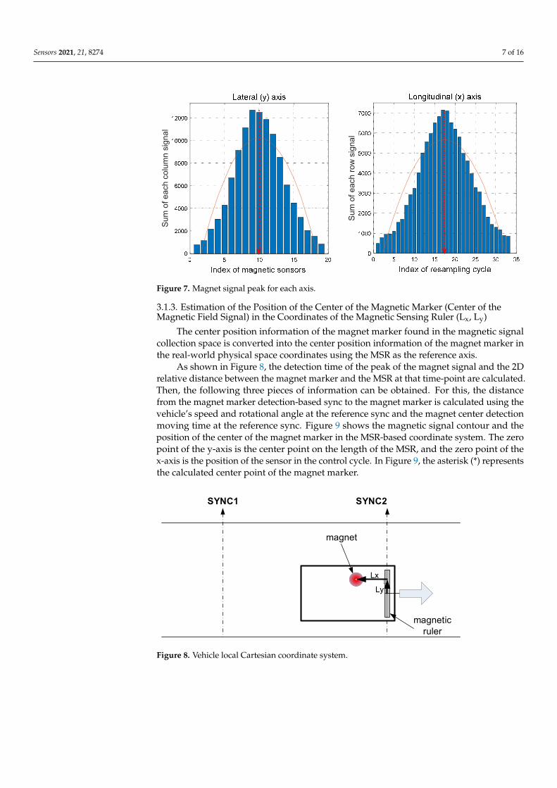
As shown in Figure 6, the peak of the signal is created for the x- and the y-axes ineach data space, and the same process is performed to check the positions. The results areshown in Figure 7. Due to the limitation of the straight section of the test route, the vehiclewas driven with a maximum speed of 25 km/h, and partial signal processing results of themagnetic signal were acquired for driving with a speed of about 15 km/h.

Sensors 2021, 21, x FOR PEER REVIEW 7 of 17

5. To find the maximum point, the position value of a point with a slope of 0 is found by applying the differential of the quadratic function. As shown in Figure 6, the peak of the signal is created for the x- and the y-axes in

each data space, and the same process is performed to check the positions. The results are shown in Figure 7. Due to the limitation of the straight section of the test route, the vehicle was driven with a maximum speed of 25 km/h, and partial signal processing results of the magnetic signal were acquired for driving with a speed of about 15 km/h.

Lateral (y) axis

Long

itudi

nal (

x) a

xis

Figure 6. Peak of magnetic field signal in the 2D data space.

Figure 7. Magnet signal peak for each axis.

3.1.3. Estimation of the Position of the Center of the Magnetic Marker (Center of the Magnetic Field Signal) in the Coordinates of the Magnetic Sensing Ruler (Lx, Ly)

The center position information of the magnet marker found in the magnetic signal collection space is converted into the center position information of the magnet marker in the real-world physical space coordinates using the MSR as the reference axis.

As shown in Figure 8, the detection time of the peak of the magnet signal and the 2D relative distance between the magnet marker and the MSR at that time-point are calculated. Then, the following three pieces of information can be obtained. For this, the distance from the magnet marker detection-based sync to the magnet marker is calculated using the vehicle’s speed and rotational angle at the reference sync and the magnet center detection moving time at the reference sync. Figure 9 shows the magnetic signal contour and the position of the center of the magnet marker in the MSR-based coordinate system. The zero point of the y-axis is the center point on the length of the MSR, and the zero point

Sum

of e

ach

colu

mn

sign

al

Sum

of e

ach

row

sig

nal

Figure 6. Peak of magnetic field signal in the 2D data space.

Sensors 2021, 21, 8274 7 of 16

Sensors 2021, 21, x FOR PEER REVIEW 7 of 17

5. To find the maximum point, the position value of a point with a slope of 0 is found by applying the differential of the quadratic function. As shown in Figure 6, the peak of the signal is created for the x- and the y-axes in

each data space, and the same process is performed to check the positions. The results are shown in Figure 7. Due to the limitation of the straight section of the test route, the vehicle was driven with a maximum speed of 25 km/h, and partial signal processing results of the magnetic signal were acquired for driving with a speed of about 15 km/h.

Lateral (y) axis

Long

itudi

nal (

x) a

xis

Figure 6. Peak of magnetic field signal in the 2D data space.

Figure 7. Magnet signal peak for each axis.

3.1.3. Estimation of the Position of the Center of the Magnetic Marker (Center of the Magnetic Field Signal) in the Coordinates of the Magnetic Sensing Ruler (Lx, Ly)

The center position information of the magnet marker found in the magnetic signal collection space is converted into the center position information of the magnet marker in the real-world physical space coordinates using the MSR as the reference axis.

As shown in Figure 8, the detection time of the peak of the magnet signal and the 2D relative distance between the magnet marker and the MSR at that time-point are calculated. Then, the following three pieces of information can be obtained. For this, the distance from the magnet marker detection-based sync to the magnet marker is calculated using the vehicle’s speed and rotational angle at the reference sync and the magnet center detection moving time at the reference sync. Figure 9 shows the magnetic signal contour and the position of the center of the magnet marker in the MSR-based coordinate system. The zero point of the y-axis is the center point on the length of the MSR, and the zero point

Sum

of e

ach

colu

mn

sign

al

Sum

of e

ach

row

sig

nal

Figure 7. Magnet signal peak for each axis.

3.1.3. Estimation of the Position of the Center of the Magnetic Marker (Center of theMagnetic Field Signal) in the Coordinates of the Magnetic Sensing Ruler (Lx, Ly)

The center position information of the magnet marker found in the magnetic signalcollection space is converted into the center position information of the magnet marker inthe real-world physical space coordinates using the MSR as the reference axis.

As shown in Figure 8, the detection time of the peak of the magnet signal and the 2Drelative distance between the magnet marker and the MSR at that time-point are calculated.Then, the following three pieces of information can be obtained. For this, the distancefrom the magnet marker detection-based sync to the magnet marker is calculated using thevehicle’s speed and rotational angle at the reference sync and the magnet center detectionmoving time at the reference sync. Figure 9 shows the magnetic signal contour and theposition of the center of the magnet marker in the MSR-based coordinate system. The zeropoint of the y-axis is the center point on the length of the MSR, and the zero point of thex-axis is the position of the sensor in the control cycle. In Figure 9, the asterisk (*) representsthe calculated center point of the magnet marker.

Sensors 2021, 21, x FOR PEER REVIEW 8 of 17

of the x-axis is the position of the sensor in the control cycle. In Figure 9, the asterisk (*) represents the calculated center point of the magnet marker.

SYNC1 SYNC2

magnet

magnetic ruler

Lx

Ly

Figure 8. Vehicle local Cartesian coordinate system.

Figure 9. Magnetic marker center position in the sensor coordinate system.

4. Localization Based on Magnetic Marker 4.1. Position Error Based on the Detected Magnetic Marker

If the relative distance (Lx, Ly) of the magnet marker detected based on the MSR coordinate system is determined, the following process is performed to find the absolute position of the vehicle using this information. A bicycle model is applied to simplify the movement of the vehicle, as shown in Figure 10, to calculate the real-time position of the vehicle on the absolute coordinate system. The vehicle’s position is calculated every cycle based on the vehicle’s center axis (C).

-0.5 0 0.5Magnetic sensing ruler (y): [m]

-0.6

-0.4

-0.2

0

0.2

0.4

Figure 8. Vehicle local Cartesian coordinate system.

Sensors 2021, 21, 8274 8 of 16

Sensors 2021, 21, x FOR PEER REVIEW 8 of 17

of the x-axis is the position of the sensor in the control cycle. In Figure 9, the asterisk (*) represents the calculated center point of the magnet marker.

SYNC1 SYNC2

magnet

magnetic ruler

Lx

Ly

Figure 8. Vehicle local Cartesian coordinate system.

Figure 9. Magnetic marker center position in the sensor coordinate system.

4. Localization Based on Magnetic Marker 4.1. Position Error Based on the Detected Magnetic Marker

If the relative distance (Lx, Ly) of the magnet marker detected based on the MSR coordinate system is determined, the following process is performed to find the absolute position of the vehicle using this information. A bicycle model is applied to simplify the movement of the vehicle, as shown in Figure 10, to calculate the real-time position of the vehicle on the absolute coordinate system. The vehicle’s position is calculated every cycle based on the vehicle’s center axis (C).

-0.5 0 0.5Magnetic sensing ruler (y): [m]

-0.6

-0.4

-0.2

0

0.2

0.4

Figure 9. Magnetic marker center position in the sensor coordinate system.

4. Localization Based on Magnetic Marker4.1. Position Error Based on the Detected Magnetic Marker

If the relative distance (Lx, Ly) of the magnet marker detected based on the MSRcoordinate system is determined, the following process is performed to find the absoluteposition of the vehicle using this information. A bicycle model is applied to simplify themovement of the vehicle, as shown in Figure 10, to calculate the real-time position of thevehicle on the absolute coordinate system. The vehicle’s position is calculated every cyclebased on the vehicle’s center axis (C).

Sensors 2021, 21, x FOR PEER REVIEW 9 of 17

fδβ

θC

X

YO

f

rrv

cvfv

rlfl

( , )c cx y

Figure 10. Kinematic model of the vehicle.

Figure 10 depicts the case in which the central axis of the vehicle moves around the center of rotation (o), defining the kinematic motion of the vehicle and associated parameters. In the above figure, β is the side slip angle, δf is the front wheel steering angle, lf is the distance from the front axle to the vehicle central axis, lr is the distance from the rear axle to the central axis, νc is the speed at the central axis, and νf and νr are the speeds of the front and rear wheels, respectively:

( 1) ( ) cos( )( 1) ( ) sin( )

cos tan( 1) ( )

c c c

c c c

fc

f r

x k x k dt vy k y k dt v

k k dt vl l

θ βθ β

β δθ θ

+ = + ⋅ ⋅ ++ = + ⋅ ⋅ +

⋅+ = + ⋅ ⋅

+

(1)

where 1 tantan r f

f r

ll l

δβ − ⋅

= + and

cos2 cos

f f rc

v vv

δβ

⋅ +=

⋅, and dt is the discrete sample time.

To set the vehicle’s initial information, we roughly match the known magnetic marker points on the driving path with the front end of the vehicle. At this time, the vehicle’s initial orientation is set, assuming that the vehicle’s orientation is close to the orientation of magnets by aligning the vehicle as parallel as possible with a straight line between magnets. In addition, the initial approximate vehicle center position (xc, yc) is calculated using the vehicle dimension information and orientation. Once the initial position is set, the position and orientation of the vehicle are calculated for each control cycle using vehicle sensor information (odometers, steering angle sensor, and gyroscope) and vehicle model (Equation (1)) until the magnetic marker is detected. When a magnetic field signal is detected, the position of the vehicle is corrected through the process in Equations (3) to (12). In order to identify the detected magnetic marker from the magnetic marker database, when a magnetic signal of a certain strength or more is measured, the position of the magnetic marker is estimated using Equation (3), and the nearest magnetic marker is obtained from this position as in Equation (4). Moreover, since the position detection error of the magnetic marker is detected within 20 cm throughout the driving test, it is judged that the magnetic object with a position error of 30 cm or more is not a magnetic marker. Even if some magnetic markers could not be detected due to a missing signal or a loss of signal during driving, the position error did not exceed 30 cm even after moving 50 m from the last detected magnetic marker. Therefore, even when magnetic markers are not detected due to some factor, distances greater than 50 m can be easily estimated. For safety reasons, however, the vehicle controller stops the vehicle when there

Figure 10. Kinematic model of the vehicle.

Figure 10 depicts the case in which the central axis of the vehicle moves aroundthe center of rotation (o), defining the kinematic motion of the vehicle and associatedparameters. In the above figure, β is the side slip angle, δf is the front wheel steering angle,lf is the distance from the front axle to the vehicle central axis, lr is the distance from the

Sensors 2021, 21, 8274 9 of 16

rear axle to the central axis, νc is the speed at the central axis, and νf and νr are the speedsof the front and rear wheels, respectively:

xc(k + 1) = xc(k) + dt · vc · cos(θ + β)yc(k + 1) = yc(k) + dt · vc · sin(θ + β)

θ(k + 1) = θ(k) + dt · vc ·cos β·tan δ f

l f +lr

(1)

where β = tan−1( lr ·tan δ f

l f +lr

)and vc =

v f ·cos δ f +vr2·cos β , and dt is the discrete sample time.

To set the vehicle’s initial information, we roughly match the known magnetic markerpoints on the driving path with the front end of the vehicle. At this time, the vehicle’sinitial orientation is set, assuming that the vehicle’s orientation is close to the orientationof magnets by aligning the vehicle as parallel as possible with a straight line betweenmagnets. In addition, the initial approximate vehicle center position (xc, yc) is calculatedusing the vehicle dimension information and orientation. Once the initial position isset, the position and orientation of the vehicle are calculated for each control cycle usingvehicle sensor information (odometers, steering angle sensor, and gyroscope) and vehiclemodel (Equation (1)) until the magnetic marker is detected. When a magnetic field signal isdetected, the position of the vehicle is corrected through the process in Equations (3) to (12).In order to identify the detected magnetic marker from the magnetic marker database,when a magnetic signal of a certain strength or more is measured, the position of themagnetic marker is estimated using Equation (3), and the nearest magnetic marker isobtained from this position as in Equation (4). Moreover, since the position detection errorof the magnetic marker is detected within 20 cm throughout the driving test, it is judgedthat the magnetic object with a position error of 30 cm or more is not a magnetic marker.Even if some magnetic markers could not be detected due to a missing signal or a lossof signal during driving, the position error did not exceed 30 cm even after moving 50 mfrom the last detected magnetic marker. Therefore, even when magnetic markers are notdetected due to some factor, distances greater than 50 m can be easily estimated. For safetyreasons, however, the vehicle controller stops the vehicle when there is no magnetic markerdetection while moving 15 m after last magnetic marker detection (corresponding to fivemissing markers in a row) [21].

Figure 11 shows the relationship between the MSR mounted on the vehicle and thedetected magnet marker. The MSR’s position (xs, ys) is calculated based on the vehicle’scenter coordinate (xc, yc), as shown in Equation (2):[

xsys

]=

[xcyc

]+ Ls

[cos θsin θ

](2)

where Ls is the distance from the center of the vehicle coordinates to the center of the MSRand θ is the vehicle’s heading angle.

Then, the absolute position (xm, ym) of the detected magnet marker can be calculated,as shown in Equation (3), using the relative distance information (Lx, Ly) measured fromthe MSR’s position (xs, ys) to the detected magnet marker (m).[

xmym

]=

[xsys

]+ Lx

[cos θsin θ

]+ Ly

[− sin θcos θ

](3)

Based on the index of the closest magnet marker from the estimated position of themagnet marker in the magnet marker database, the magnet marker with the minimumEuclidean distance is found, as shown in Equation (4):

(imin, dmin) = min(√

(XDB − xm)2 + (YDB − ym)

2)

(4)

Sensors 2021, 21, 8274 10 of 16

where imin is the index of the magnet marker that has the minimum distance, dmin isthe minimum distance, and XDB, YDB is the position coordinate array in the magnetmarker database.

Therefore, the error of the magnet marker position detected at the estimated magnetmarker position becomes the absolute position calculation error of the system, as shown inEquation (5): [

dxedye

]=

[XDB(imin)YDB(imin)

]−[

xmym

](5)

Furthermore, the error can be calculated and converted into the vehicle coordinatesystem, as shown in Equation (6):[

dxvdyv

]= dxe

[cos θsin θ

]+ dye

[− sin θcos θ

](6)

where dxv is the estimated error in the proceeding direction of the vehicle (mainly due tothe vehicle’s wheel radius and slip) and dyv is the estimated error in the lateral direction ofthe vehicle (mainly due to the vehicle’s heading error).

Sensors 2021, 21, x FOR PEER REVIEW 11 of 17

[ ]Te e edP dx dy dθ= (9)

Y

X

Magneticsensing ruler

θ

magnet

( , )c cC x ysL

( , )s sS x yxL

yL( , )m mm x y

( , )r rr x y

Figure 11. Measurement model with MSR.

4.2. Time-Division Position Correction The vehicle’s position error is calculated only when a magnet marker is detected, and

it is used to correct the vehicle’s position. Once the position error of the vehicle is determined, it is corrected by dividing it within the maximum installation interval (3 m) until the next magnet marker is detected. If the position error is large and corrected when a magnet is detected, a discontinuity of the position information may occur, causing control shock in the steering control that uses this error, which may consequently strain the steering system or reduce the ride comfort of the passengers. Therefore, a time-division correction method is proposed to prevent this.

4.2.1. Determination of the Number of Divisions The absolute position error calculated by detecting a magnet marker is a constant

until the next magnet marker is detected. Therefore, the number of divisions for this value is determined according to the vehicle’s speed, as shown in Equation (10), to determine the method of dividing and correcting the error in every control cycle until the next magnet marker is detected. In other words, the lower the speed, the higher the number of divisions. This method was determined to complete the determined correction between the magnet markers:

( )( )mkc

DisCountv k dt eps

=⋅ +

(10)

where Dis is the maximum interval (3 m) of magnet markers, vc(k) is the vehicle speed, dt is the discrete sample time of control cycles, and eps is a small value utilized to prevent the denominator from becoming zero when the speed is 0.

Equation (11) shows the condition equation for division correction:

Figure 11. Measurement model with MSR.

The vehicle’s heading error can be calculated using Equation (7).If the lateral direction error information of the currently detected magnet and the

previously detected magnet is used, the vehicle’s heading error can be determined, asshown in Equation (7). The detected magnet marker number is recorded whenever detected,and up to the three of the latest numbers are recorded:

dθe = sign(dyv) · sin−1(dyv/dm) (7)

where dm is the Euclidean distance between the two detected magnets.

dm =

√(XDB(imin(n))− XDB(imin(n− 1))2 + (YDB(imin(n))−YDB(imin(n− 1)))2 (8)

To define the sequence number of the detected magnetic marker, imin(n) refers to thecurrent detection and imin(n − 1) refers to the previous detection.

Finally, the absolute position error of the vehicle is determined, as shown in Equation (9):

dP =[

dxe dye dθe]T (9)

Sensors 2021, 21, 8274 11 of 16

4.2. Time-Division Position Correction

The vehicle’s position error is calculated only when a magnet marker is detected,and it is used to correct the vehicle’s position. Once the position error of the vehicle isdetermined, it is corrected by dividing it within the maximum installation interval (3 m)until the next magnet marker is detected. If the position error is large and corrected when amagnet is detected, a discontinuity of the position information may occur, causing controlshock in the steering control that uses this error, which may consequently strain the steeringsystem or reduce the ride comfort of the passengers. Therefore, a time-division correctionmethod is proposed to prevent this.

4.2.1. Determination of the Number of Divisions

The absolute position error calculated by detecting a magnet marker is a constantuntil the next magnet marker is detected. Therefore, the number of divisions for this valueis determined according to the vehicle’s speed, as shown in Equation (10), to determinethe method of dividing and correcting the error in every control cycle until the nextmagnet marker is detected. In other words, the lower the speed, the higher the number ofdivisions. This method was determined to complete the determined correction betweenthe magnet markers:

Countmk =Dis

(|vc(k)| · dt + eps)(10)

where Dis is the maximum interval (3 m) of magnet markers, vc(k) is the vehicle speed, dt isthe discrete sample time of control cycles, and eps is a small value utilized to prevent thedenominator from becoming zero when the speed is 0.

Equation (11) shows the condition equation for division correction:

if Countup < Countmkdp1 = dP/Countmk;

elsedp1 = [0 0 0]′;

end

if sum(abs(dP) < dP1_sum) ∪ (abs(vc(k)) < 0.01)dp1 = [0 0 0]′;

elseCountup = Countup + 1;dP1_sum = dP1_sum + abs(dp1);

end

if Countup > CountmkCountup = Countmk;

end

(11)

4.2.2. Position Correction

When the correction amount is determined, as shown in Equation (9), after the magnetmarker is detected, the division is determined according to Equations (10) and (11). Then,Equation (12) is additionally applied to the position calculated at each cycle by Equation (1)to correct the vehicle’s absolute position: xc

ycθ

=

xcycθ

+ dp1 (12)

where dp1 is the position correction amount determined after detecting the magnet marker.

Sensors 2021, 21, 8274 12 of 16

5. Results and Discussion

We conducted a driving test to demonstrate the performance of the position correctionalgorithm proposed in this study. The position estimation and the driving path guidancecontrol were performed based on magnet marker detections, and as shown in Figure 12,112 magnet markers were buried in the driving track. The vehicle was driven in a loop witha length of approximately 238 m. In Figure 12, the light blue dots represent the referencepath and the dark blue dots represent the calculated vehicle trajectory. Furthermore, theasterisk (*) indicates the positions of the magnet markers buried in the road and the unfilledblue circle (“o”) indicates the magnet marker positions detected while driving.

Sensors 2021, 21, x FOR PEER REVIEW 13 of 17

Figure 12. Magnetic-marker-based position estimation and guidance control test results.

The position estimation errors while driving are based on the magnet markers. Figure 13 shows the error in the Euclidean distance between the magnet marker position in the database and the magnet marker position estimated when the magnet marker is detected. Starting with the initial position error based on the approximate initial vehicle position information, the error decreases to below 10 cm as the magnet marker detection is repeated. The mean position detection error of the 91 detected magnet markers was 2.86 cm.

Figure 13. Absolute position error based on the magnetic marker.

Because it was difficult to verify the continuity between the data points from the diagram of the estimated position information, we assessed the continuity between the points using the slopes and the estimated position points to verify the effectiveness and validity of the proposed position correction method. If the calculated current position

180 190 200 210 220 230 240 250 260 270 280X [m]

40

50

60

70

80

90

100

Start

Reference pathMagnetic markerEstimated vehicle trajectoryDetected magnetic marker

Abso

lute

pos

ition

erro

r [m

]

Figure 12. Magnetic-marker-based position estimation and guidance control test results.

The position estimation errors while driving are based on the magnet markers.Figure 13 shows the error in the Euclidean distance between the magnet marker posi-tion in the database and the magnet marker position estimated when the magnet markeris detected. Starting with the initial position error based on the approximate initial vehicleposition information, the error decreases to below 10 cm as the magnet marker detection isrepeated. The mean position detection error of the 91 detected magnet markers was 2.86 cm.

Sensors 2021, 21, x FOR PEER REVIEW 13 of 17

Figure 12. Magnetic-marker-based position estimation and guidance control test results.

The position estimation errors while driving are based on the magnet markers. Figure 13 shows the error in the Euclidean distance between the magnet marker position in the database and the magnet marker position estimated when the magnet marker is detected. Starting with the initial position error based on the approximate initial vehicle position information, the error decreases to below 10 cm as the magnet marker detection is repeated. The mean position detection error of the 91 detected magnet markers was 2.86 cm.

Figure 13. Absolute position error based on the magnetic marker.

Because it was difficult to verify the continuity between the data points from the diagram of the estimated position information, we assessed the continuity between the points using the slopes and the estimated position points to verify the effectiveness and validity of the proposed position correction method. If the calculated current position

180 190 200 210 220 230 240 250 260 270 280X [m]

40

50

60

70

80

90

100

Start

Reference pathMagnetic markerEstimated vehicle trajectoryDetected magnetic marker

Abso

lute

pos

ition

erro

r [m

]

Figure 13. Absolute position error based on the magnetic marker.

Sensors 2021, 21, 8274 13 of 16

Because it was difficult to verify the continuity between the data points from thediagram of the estimated position information, we assessed the continuity between thepoints using the slopes and the estimated position points to verify the effectiveness andvalidity of the proposed position correction method. If the calculated current positioncoordinate (xk,yk) and the previous position coordinate (xk−1,yk−1) are available, the slopebetween position points (tan(yk−1 − yk/xk−1 − xk)) can be applied. Figure 14a shows theslopes calculated between the position coordinates as estimated by the proposed method,while Figure 14b shows the slopes calculated between the position coordinates by applyingthe conventional method, with irregular pulse values in many sections of the graph. Inthese sections, the discontinuity of the slopes between the position points is shown becausethe position error is reflected directly whenever a magnet marker is detected. Alternatively,for the results of the proposed method, there is a clearly improved continuity of the slopes,as shown in Figure 14a.

Sensors 2021, 21, x FOR PEER REVIEW 14 of 17

coordinate (xk,yk) and the previous position coordinate (xk−1,yk−1) are available, the slope between position points (tan(yk−1 − yk/xk−1 − xk)) can be applied. Figure 14a shows the slopes calculated between the position coordinates as estimated by the proposed method, while Figure 14b shows the slopes calculated between the position coordinates by applying the conventional method, with irregular pulse values in many sections of the graph. In these sections, the discontinuity of the slopes between the position points is shown because the position error is reflected directly whenever a magnet marker is detected. Alternatively, for the results of the proposed method, there is a clearly improved continuity of the slopes, as shown in Figure 14a.

Figure 14. Comparison of continuity [tan(dy/dx)] between estimated position points.

Figure 15 shows the steering angle command results when the same position control was performed, based on the position coordinates calculated derived from the conventional position correction method and the proposed position correction method. As shown in Figure 15, the discontinuity of the position information affected the steering angle calculation, causing discontinuous command values of the steering angle in the conventional method. In contrast, smoothly connected steering angle commands were generated by the proposed method. This can have significant effects on the vehicle’s driving stability and the passengers’ ride comfort with respect to controlling the vehicle. As an additional example, if a common method such as a Kalman filter is used and the filter coefficient is adjusted significantly to mitigate the discontinuity of the position information, the continuity of the position information will improve, although a delay will occur in the position information. In this case, the estimated driving trajectory will be larger compared to the actual driving position at a curve in the road. Furthermore, the error may increase as the vehicle speed increases.

Thet

a of

pos

ition

[rad

]Th

eta

of p

ositi

on [r

ad]

Figure 14. Comparison of continuity [tan(dy/dx)] between estimated position points.

Figure 15 shows the steering angle command results when the same position controlwas performed, based on the position coordinates calculated derived from the conventionalposition correction method and the proposed position correction method. As shown inFigure 15, the discontinuity of the position information affected the steering angle calcu-lation, causing discontinuous command values of the steering angle in the conventionalmethod. In contrast, smoothly connected steering angle commands were generated bythe proposed method. This can have significant effects on the vehicle’s driving stabilityand the passengers’ ride comfort with respect to controlling the vehicle. As an additionalexample, if a common method such as a Kalman filter is used and the filter coefficient isadjusted significantly to mitigate the discontinuity of the position information, the continu-ity of the position information will improve, although a delay will occur in the positioninformation. In this case, the estimated driving trajectory will be larger compared to theactual driving position at a curve in the road. Furthermore, the error may increase as thevehicle speed increases.

Sensors 2021, 21, 8274 14 of 16Sensors 2021, 21, x FOR PEER REVIEW 15 of 17

Figure 15. Comparison of steering angle command of path-following controller.

6. Conclusions In this study, we estimated vehicle positions in real-time by detecting magnet

markers and proposed novel position estimation and error correction methods. Solutions to two main problems in magnetic marker positioning system performance

were proposed as follows: • The speed of sensor utilization was improved through separate processing of the

vehicle control cycle and magnet signal detection cycle; • The continuity of position information was improved using the time-division

position correction method. In automatic driving control systems, the precision and continuity of the real-time

position of the vehicle are important elements with respect to the vehicle position control and designed driving path. In particular, we examined the discontinuity of position information, which may occur in land marker methods, such as with the use of magnet markers, and verified its effects. Accordingly, position estimation and error correction methods were then proposed to prevent such discontinuity.

A discontinuity of the position information will occur when magnet markers are detected while driving if the position is only corrected at each detected time-point. Therefore, the calculated position error value is corrected by dividing it while driving according to the proposed procedure. If the error correction is performed by dividing the moving space until the next magnet is detected, the correction value can be used without loss while ensuring there is no sharp discontinuity when the position is corrected.

To verify the validity of the proposed method, we demonstrated the problems that occur in the conventional method of estimating and correcting positions using the test data and compared the performance to that of the proposed method. Based on this comparison, the superiority of the proposed method was confirmed.

Author Contributions: Conceptualization, Y.S.B.; methodology, Y.S.B.; software, Y.S.B.; validation, Y.S.B.; formal analysis, Y.S.B.; writing—original draft preparation, Y.S.B.; writing—review and editing, Y.S.B. and R.G.J.; visualization, Y.S.B.; supervision, R.G.J.; project administration, R.G.J. All authors have read and agreed to the published version of the manuscript.

Funding: This research was supported by a grant from the R&D Program of the Korea Railroad Research Institute (KRRI) of the Republic of Korea.

Institutional Review Board Statement: Not applicable.

Stee

ring

angl

e (

f) [de

g]St

eerin

g an

gle

(f) [

deg]

Figure 15. Comparison of steering angle command of path-following controller.

6. Conclusions

In this study, we estimated vehicle positions in real-time by detecting magnet markersand proposed novel position estimation and error correction methods.

Solutions to two main problems in magnetic marker positioning system performancewere proposed as follows:

• The speed of sensor utilization was improved through separate processing of thevehicle control cycle and magnet signal detection cycle;

• The continuity of position information was improved using the time-division positioncorrection method.

In automatic driving control systems, the precision and continuity of the real-timeposition of the vehicle are important elements with respect to the vehicle position controland designed driving path. In particular, we examined the discontinuity of positioninformation, which may occur in land marker methods, such as with the use of magnetmarkers, and verified its effects. Accordingly, position estimation and error correctionmethods were then proposed to prevent such discontinuity.

A discontinuity of the position information will occur when magnet markers are de-tected while driving if the position is only corrected at each detected time-point. Therefore,the calculated position error value is corrected by dividing it while driving according tothe proposed procedure. If the error correction is performed by dividing the moving spaceuntil the next magnet is detected, the correction value can be used without loss whileensuring there is no sharp discontinuity when the position is corrected.

To verify the validity of the proposed method, we demonstrated the problems thatoccur in the conventional method of estimating and correcting positions using the test dataand compared the performance to that of the proposed method. Based on this comparison,the superiority of the proposed method was confirmed.

Author Contributions: Conceptualization, Y.S.B.; methodology, Y.S.B.; software, Y.S.B.; validation,Y.S.B.; formal analysis, Y.S.B.; writing—original draft preparation, Y.S.B.; writing—review and editing,Y.S.B. and R.G.J.; visualization, Y.S.B.; supervision, R.G.J.; project administration, R.G.J. All authorshave read and agreed to the published version of the manuscript.

Sensors 2021, 21, 8274 15 of 16

Funding: This research was supported by a grant from the R&D Program of the Korea RailroadResearch Institute (KRRI) of the Republic of Korea.

Institutional Review Board Statement: Not applicable.

Informed Consent Statement: Not applicable.

Data Availability Statement: The data presented in this study are available on request from thecorresponding author.

Conflicts of Interest: The authors declare no conflict of interest.

References1. Rogers, R. Land vehicle navigation filtering for GPS/dead-reckoning system. In Proceedings of the Institute of Navigation

National Technical Meeting, Santa Monica, CA, USA, 14–16 January 1997; pp. 703–708.2. Farrell, J.; Barth, M.; Galijan, R.; Sinko, J. GPS/INS based lateral and longitudinal control demonstration: Final report. In California

PATH Research Report; UC Berkeley: Berkeley, CA, USA, 1998.3. Bonnifait, P.; Bouron, P.; Crubille, P.; Meizel, D. Data fusion of four ABS sensors and GPS for an enhanced localization of car-like

vehicles. In Proceedings of the IEEE International Conference on Robotics and Automation, Seoul, Korea, 21–26 May 2001;pp. 1597–1602.

4. Farrell, J.; Tan, H.-S.; Yang, Y. Carrier phase GPS-aided INS based vehicle lateral control. ASME J. Dyn. Syst. Meas. Control. 2003,25, 339–353. [CrossRef]

5. Jo, K.; Chu, K.; Sunwoo, M. Interacting multiple model filter-based sensor fusion of GPS with in-vehicle sensors for real-timevehicle positioning. IEEE Trans. Intell. Trans. Syst. 2012, 13, 329–343. [CrossRef]

6. Lee, B.-H.; Song, J.-H.; Im, J.-H.; Im, S.-H.; Heo, M.-B.; Jee, G.-I. GPS/DR error estimation for autonomous vehicle localization.Sensors 2015, 15, 20779–20798. [CrossRef] [PubMed]

7. Abbott, E.; Powell, D. Land-vehicle navigation using GPS. Proc. IEEE 1999, 87, 145–162. [CrossRef]8. Broggi, A.; Bertozzi, M.; Fascioli, A.; Bianco, C.; Piazzi, A. The ARGO autonomous vehicle’s vision and control systems. Int. J.

Intell. Control Syst. 1999, 3, 409–441.9. Se, S.; Lowe, D.; Little, J. Vision-based mobile robot localization and mapping using scale-invariant features. In Proceedings of

the IEEE International Conference on Robotics and Automation (ICRA), Seoul, Korea, 9 July 2001; pp. 2051–2058.10. Alonso, I.P.; Llorca, D.; Gavilan, M.; Pardo, S.; Garcia-Garrido, M.; Vlacic, L.; Sotelo, M. Accurate global localization using visual

odometry and digital maps on urban environments. IEEE Trans. Intell. Trans. Syst. 2012, 13, 1535–1545. [CrossRef]11. Droeschel, D.; Behnke, S. Efficient Continuous-Time SLAM for 3D Lidar-Based Online Mapping. In Proceedings of the IEEE

International Conference on Robotics and Automation, Brisbane, Australia, 21–25 May 2018; pp. 5000–5007.12. Behley, J.; Stachniss, C. Efficient surfel-based SLAM using 3D laser range data in urban environments. In Robotics; Science and

Systems: Pittsburgh, PA, USA, 2018.13. Shan, T.; Englot, B. LeGO-LOAM: Lightweight and ground-optimized LiDAR odometry and mapping on variable terrain. In

Proceedings of the IEEE/RSJ International Conference on Intelligent Robots and Systems, Madrid, Spain, 1–5 October 2018;pp. 4758–4765.

14. Lu, W.; Zhou, Y.; Wan, G.; Hou, S.; Song, S. L3-net: Towards Learning Based LiDAR Localization for Autonomous Driving. InProceedings of the IEEE/CVF Conference on Computer Vision and Pattern Recognition (CVPR), Long Beach, CA, USA, 15–20June 2019; pp. 6382–6391.

15. Bento, L.; Nunes, U. Autonomous navigation control with magnetic markers guidance of a cybernetic car using fuzzy logic. Mach.Intell. Robot. Control. 2003, 4, 3–12.

16. Barata, M.; Nunes, U.; Bento, L.C.; Mendes, A. Data fusion of wheel encoders and magnetic sensors for autonomous vehiclesnavigation. In Proceedings of the 6th Portuguese Conference on Automatic Control (CONTROLO 2004), Faro, Portugal, 7–9 June2004; pp. 31–37.

17. Surrécio, A.; Nunes, U.; Araújo, R. Fusion of odometry with magnetic sensors using Kalman filters and augmented systemmodels for mobile robot navigation. In Proceedings of the IEEE International Symposium on Industrial Electronics (ISIE2005),Dubrovnik, Croatia, 20–23 June 2005.

18. Xu, H.G.; Wang, C.X.; Yang, R.Q.; Yang, M. Extended Kalman filter based magnetic guidance for intelligent vehicles. InProceedings of the Intelligent Vehicles Symposium, Tokyo, Japan, 11 September 2006; pp. 169–175.

19. Lopes, A.C.; Moita, F.; Nunes, U.; Solea, R. An outdoor guidepath navigation system for AMRs based on robust detection ofmagnetic markers. In Proceedings of the 12th IEEE Conference on Emerging Technologies and Factory Automation (ETFA2007),Patras, Greece, 25–28 September 2007.

20. Bourny, V.; Capitaine, T.; Barrandon, L.; Gard, C.; Lorthois, A. A localization system based on buried magnets and dead reckoningfor mobile robots. In Proceedings of the 2010 IEEE International Symposium on Industrial Electronics, Bari, Italy, 4–7 July 2010;pp. 373–378.

21. Byun, Y.S.; Jeong, R.G.; Kang, S.W. Vehicle position estimation based on magnetic markers: Enhanced accuracy by compensationof time delays. Sensors 2015, 15, 28807–28825. [CrossRef] [PubMed]

Sensors 2021, 21, 8274 16 of 16

22. Byun, Y.S.; Kim, Y.C. Heading angle estimation based on magnetic markers for intelligent vehicles. ASME J. Dyn. Syst. Meas.Control. 2016, 138, 71009. [CrossRef]

23. MASDAR PRT. Available online: http://www.2getthere.eu/projects/masdar-prt (accessed on 4 October 2016).24. Farrell, J.; Barth, M. Integration of GPS/INS and magnetic markers for advanced vehicle Control. In California PATH Research

Report; UC Berkeley: Berkeley, CA, USA, 2001.