Fuzzy Sets and Systems 115 (2000) 83–92www.elsevier.com/locate/fss

Portfolio selection under independent possibilistic information(

Masahiro Inuiguchi ∗, Tetsuzo TaninoDepartment of Electronics and Information Systems, Graduate School of Engineering, Osaka University, 2-1 Yamadaoka, Suita,

Osaka 565-0871, Japan

Received November 1998

Abstract

This paper deals with a portfolio selection problem with independently estimated possibilistic return rates. Under such acircumstance, a distributive investment has been regarded as a good solution in the traditional portfolio theory. However,the conventional possibilistic approach yields a concentrated investment solution. Considering the reason why a distributiveinvestment is advocated, a new approach to the possibilistic portfolio selection is proposed. c© 2000 Elsevier Science B.V.All rights reserved.

Keywords: Possibilistic programming; Portfolio selection; Minimax regret; Linear programming; Necessity measure

1. Introduction

The Markowitz model [7] is famous for portfolioselection. In this model, an expected return rate of abond is treated as a random variable. Stochastic pro-gramming is applied so that the solution is obtainedby minimizing the variance of the total expected re-turn rate under the constraint that the mean of thetotal expected return rate is equal to a predeterminedvalue. This model yields a distributive investment so-lution unless the expected return rates are completelypositively dependent on each other. In the traditionalportfolio theory, a distributive investment has been re-garded as a good policy to reduce the risk.

( This research was partly supported by the Ministry of Educa-tion, Science, Sports and Culture, Grant-in-Aid Scienti�c Researchfor Encouragement of Young Scientists, No. 08780426.

∗ Corresponding author. Tel.: + 81-6-6879-7787; fax: + 81-6-6879-7939.E-mail address: inuiguti@pwr.eng.osaka-u.ac.jp (M. Inuiguchi).

Possibilistic programming is a known similarapproach to stochastic programming. Therefore, anapplication of possibilistic programming to portfolioselection can be expected. In possibilistic program-ming approaches, the expected return rates are nottreated as random variables but as possibilistic vari-ables. Applying possibilistic programming may havea two-fold advantage [2]: (1) the knowledge of theexpert can be easily introduced to the estimation ofthe return rates and (2) the reduced problem is moretractable than that of the stochastic programming ap-proach. However, most of the previously proposedpossibilistic programming approaches treat indepen-dent possibilistic variables and thus the applicationto the portfolio selection do not yield a distribu-tive investment. This contradicts with the traditionalportfolio theory.In this paper, considering how a model yields a

distributive investment solution, a new possibilisticprogramming approach to the portfolio selection isproposed. This approach is based on a regret which the

0165-0114/00/$ - see front matter c© 2000 Elsevier Science B.V. All rights reserved.PII: S 0165 -0114(00)00026 -3

84 M. Inuiguchi, T. Tanino / Fuzzy Sets and Systems 115 (2000) 83–92

decision maker may undertake. First, the previous pos-sibilistic programming approaches are reviewed andtheir solutions to the portfolio selection problems arediscussed. It is shown that concentrated investment so-lutions are obtained by those approaches. A minimaxregret approach to the possibilistic portfolio selectionis proposed. It is shown that a distributive investmentsolution is obtained by this approach, following theproblem reduction. Some examples are given in orderto compare the solutions obtained by the previous andproposed approaches.

2. Possibilistic portfolio selection problem

When return rates of all bonds are known ex-actly, a portfolio selection problem can be formulatedas

maximize cTx;

subject to eTx=1; x¿0;(1)

where c=(c1; c2; : : : ; cn)T, x=(x1; x2; : : : ; xn)T ande=(1; 1; : : : ; 1)T. The component ci represents thereturn rate for the ith bond and xi shows the in-vestment rate to the ith bond. Thus the problem ismaximizing the total return rate. An optimal solutioncan be obtained easily as shown in the followingtheorem.

Theorem 1. An optimal solution to Problem (1)is a concentrated investment on a bond whichhas the maximum return rate. Namely; a solutionxi∗ =1; xi=0; ∀i 6= i∗ where ci∗¿ci; i=1; 2; : : : ; nis an optimal solution to Problem (1).

Proof. Trivial.

However, in the real setting, one can seldom ob-tain the return rate without any uncertainty. Thus, thedecision makers should make their decisions underuncertainty. Such an uncertainty has been treated asa random variable so far. The problem has beenformulated as the following stochastic programmingproblem:

maximize CTx;

subject to eTx=1; x¿0;(2)

where C=(C1;C2; : : : ;Cn)T is a random variablevector obeying a multivariate probability distributionwhich has a mean vector m and a covariance matrixV . To such a problem, Markowitz [7] proposed thefollowing model to determine the investment rates x:

minimize xTVx;

subject to mTx¿z0;

eTx=1; x¿0;

(3)

where z0 is a predetermined desirable expected returnrate. In the original Markowitz model, the �rst inequal-ity constraint mTx¿z0 is replaced with an equalityconstraint mTx= z0. This change enables the modelto generate a suitable solution for an underestimatedexpected return rate z0.To formulate Problem (3), we need to estimate the

probability distribution, strictly speaking, a mean vec-tor m and a covariance matrix V . This is not an easytask when the number of bonds is big. Therefore, sev-eral simpli�ed methods, sacri�cing generality, havebeen proposed. Moreover, it is di�cult to re ect theunquanti�able factors such as the knowledge of ex-perts, the trend of public opinion, and so on. Further-more, even though the probability distribution can beestimated, there is no guarantee that the return ratestruly obey it.A possibility distribution is known as an alterna-

tive to a probability distribution, where though theuncertain values are estimated substantially, the un-quanti�able factors such as the knowledge of expertscan be re ected easily. Thus, it may be worthwhile tointroduce the possibility distribution to the portfolioselection problem. In this paper, we discuss about thepossibilistic portfolio selection.Treating each return rate as a possibilistic variable

i restricted by a possibility distribution �Ci , we havethe following possibilistic portfolio selection problem:

maximize Tx;

subject to eTx=1; x¿0;(4)

where =( 1; 2; : : : ; n)T is a possibilistic variablevector restricted by a multivariate possibility distri-bution �C . Since most approaches assume the inde-pendence among possibilistic variables in thepossibilistic programming, we also assume the inde-pendence in order to show the incompatibility with

M. Inuiguchi, T. Tanino / Fuzzy Sets and Systems 115 (2000) 83–92 85

the traditional discussion in the portfolio theory.However, the proposed approach can be useful withsome changes even when this assumption is removed.Under this assumption the multivariate possibilitydistribution �C can be expressed as

�C(c)= mini=1;2;:::; n

�Ci(ci): (5)

For the sake of simplicity, we assume that �C is uppersemi-continuous, in other words, each �Ci is uppersemi-continuous. Moreover, we assume

limci →−∞ �Ci(ci)= lim

ci →+∞ �Ci(ci)= 0;

i=1; 2; : : : ; n: (6)

3. Solutions by the conventional possibilisticprogramming approaches

Various approaches have been proposed to a pos-sibilistic programming problem. In this section, weapply major possibilistic programming approaches[3, 4] to the possibilistic portfolio selection problem(4). We assume that the decision maker’s attitude isuncertainty (risk) averse. From this point of view, aproper model is introduced in each approach.

3.1. Fractile approach

Given appropriate level h0 ∈ (0; 1], Problem (4) isformulated so as to maximize the fractile z under aconstraint that a necessity measure of the event thatthe objective function value is not less than z is greaterthan or equal to h0:

maximize z;

subject to NC({c | cTx¿z})¿h0;eTx=1; x¿0;

(7)

where NC is a necessity measure under a possibilitydistribution �C and de�ned as follows for a set D:

NC(D)=

infc =∈D

1− �C(c)

if D is not a universal set;

1 if D is a universal set:

(8)

Thus, NC({c | cTx¿z}) shows a necessity degree towhat extent the objective function value is not lessthan z and represented as

NC({c | cTx¿z})= infc

cTx¡z

1− �C(c): (9)

Under the possibilistic independence (5), Problem(7) is reduced to the following linear programmingproblem [4]:

maximize cL(1− h0)Tx;subject to eTx=1; x¿0;

(10)

where cL(·)= (cL1 (·); cL2 (·); : : : cLn (·))T andcLi (h)= inf{q | �Ci(q)¿ h}: (11)

3.2. Modality optimization approach

Given a target value z0, Problem (4) is formulatedso as to maximize a necessity measure of the eventthat the objective function value is not less than z0:

maximize NC({c | cTx¿z0});subject to eTx=1; x¿0:

(12)

This problem is reduced to the following nonlinearprogramming problem [4]:

maximize h;

subject to cL(1− h)Tx¿z0;eTx=1; x¿0:

(13)

3.3. Spread minimization approach

De�ne a representative vector c of the possibilitydistribution �C . Given h0 ∈ (0; 1] and z0, the widthof the h0-level set [CTx]h0 = {y | �C Tx(y)¿h0} of thepossibility distribution �C Tx on the objective functionvalue can be minimized under the constraint cTx¿z0,where �CTx is calculated by the extension principle[1], i.e.,

�CTx(y)= supc

cTx=y

�C(c): (14)

86 M. Inuiguchi, T. Tanino / Fuzzy Sets and Systems 115 (2000) 83–92

Problem (4) is formulated as

minimize w;

subject to maxyR ; yL∈[CTx]h0

(yR − yL)6w;

cTx¿z0;

eTx=1; x¿0;

(15)

and reduced to the following linear programmingproblem [4]:

minimize (cR(h0)T − cL(h0)T)x;

subject to cTx¿z0;

eTx=1; x¿0;

(16)

where cL(·)= (c1L(·); c2L(·); : : : ; cnL(·))T, cR(·)=(c1R(·); c2R(·); : : : ; cnR(·))T and

ciL(h)= inf{q | �Ci(q)¿h};ciR(h)= sup{q | �Ci(q)¿h}:

(17)

Since the variance of a probability distribution cor-responds to the spread of a possibility distribution, thismodel is a counterpart of the Markowitz model.We have the following theorem.

Theorem 2. A concentrated investment solutionsuch that xi=1 for some i∈{1; 2; : : : ; n} is an opti-mal solution to Problem (10). The same assertionis valid for Problem (13). A semi-concentrated in-vestment solution such that xi + xj =1 for somei; j∈{1; 2; : : : ; n} is an optimal solution to Problem(16).

Proof. The �rst and third assertions of this theoremare obvious when taking into account the number ofconstraints excluding non-negativity constraints of theproblem. Indeed, Problem (10) is a linear program-ming problem with one constraint and Problem (16)is a linear programming problem with two constraints.Since a linear programming problem can be solvedby the simplex method, Problems (10) and (16) haveone and two basic variables, respectively. Hence con-centrated and semi-concentrated investment solutionsare optimal to Problems (10) and (16), respectively.Now, we prove the second assertion. Let (x; h) be an

optimal solution to Problem (13). Consider an optimalsolution x∗ to a linear programming problem,

maximize cL(1− h)Tx;subject to eTx=1; x¿0:

(18)

The solution (x∗; h) is also an optimal solution toProblem (13). By the same way of the proof of the �rstand second assertions, an optimal solution to Problem(18) is a concentrated investment solution.

Theorem 2 shows that if each of Problems (10),(13) and (16) has a unique solution, no distributive in-vestment solution is obtained. Moreover, when thoseproblems are solved by the simplex method, the con-ventional possibilistic programming approaches to theportfolio selection do not yield a solution compatiblewith the traditional portfolio theory.

4. A new possibilistic programming approach

Let us discuss why a distributive investment solu-tion under independent return rate assumption is pre-ferred by a decision maker who has an uncertainty(risk) averse attitude. We can observe at least the fol-lowing two reasons:(a) Property of a measure. Consider the event that

the total return rate is not less than a certain value.When the measure of the event under a distribu-tive investment solution is greater than that undera concentrated investment solution, the distribu-tive investment solution should be preferable. Inother words, the uncertainty is decreased by dis-tribution to many bonds.

(b) The worst regret criterion. Suppose that the de-cision maker has invested his money in a bondaccording to a concentrated investment solution.If the return rate of another bond becomes bet-ter than that of the invested bond as a result, thedecision maker may feel a regret. At the deci-sion making stage, we cannot know the return ratedetermined in the future. Thus, any concentratedinvestment solution may bring a regret to the de-cision maker. In this sense, if the decision makeris interested in minimizing the worst regret whichmay be undertaken, a distributive investment so-lution must be preferable.

M. Inuiguchi, T. Tanino / Fuzzy Sets and Systems 115 (2000) 83–92 87

Markowitz model [7] and the other stochastic pro-gramming approaches yield a distributive investmentsolution because of (a). Indeed, we have

Prob(�X1 + (1− �)X2¿k)¿ Prob(Xi¿k);

∀�∈ (0; 1); i=1; 2; (19)

when independent random variables X1 and X2 obeythe same marginal normal (probability) distribution.Moreover, we have

Var(�X1 + (1− �)X2)¡ Var(Xi);

∀�∈ (0; 1); i=1; 2; (20)

where Var(X ) is the variance, i.e., an uncertainty cri-terion, of a random variable X .In possibilistic programming approaches, we could

not obtain a distributive investment solution since pos-sibility and necessity measures do not have the prop-erty mentioned in (a). For possibility and necessitymeasures, we have

Pos(�X1 + (1− �)X2¿k)=Pos(Xi¿k);∀�∈ [0; 1]; i=1; 2;

Nes(�X1 + (1− �)X2¿k)=Nes(Xi¿k);∀�∈ [0; 1]; i=1; 2;

(21)

where X1 and X2 are mutually independent possibilis-tic variables restricted by the same marginal possibil-ity distribution. Moreover we have

Spd(�X1 + (1− �)X2)=Spd(Xi);∀�∈ [0; 1]; i=1; 2; (22)

where Spd(X ) is the spread of the possibility distri-bution �X restricts a possibilistic variable X , i.e.,

Spd(X )= sup{r | �X (r)¿ 0} − inf{r | �X (r)¿ 0}:(23)

Hence, the conventional possibilistic programmingapproaches fail to yield a distributive investment so-lution without introducing the concept of the regret.In what follows, a regret is introduced into the possi-bilistic portfolio selection problem (4).Suppose that a decision maker is informed about

the determined return rates c after he=she has invested

his=her money in bonds according to a feasible solu-tion x to (4), he=she will have a regret r(x; c) whichcan be quanti�ed as

r(x; c)= maxy

eTy=1; y¿0

F(cTy; cTx); (24)

where F :D1×D2→R (D1; D2⊆R) is a continuousfunction such that F(·; r) is strictly increasing andF(r; ·) is strictly decreasing. Those properties of thefunction F re ect the fact that the right-hand side ofEq. (24) evaluates the regret r(x; c). Since F is con-tinuous, so r(· : ·) is.At the decision making stage, the decision maker

cannot know the return rate c determined in the futurebut a possibility distribution �C(c). By the extensionprinciple [1], a possibility distribution �R(x) on regretscan be de�ned as

�R(x)(r)= supc

r=r(x;c)

�C(c): (25)

We regard the possibilistic portfolio selection prob-lem (1) as a problem of minimizing a regret R(x) witha possibility distribution �R(x), i.e.,

minimize R(x);

subject to eTx=1; x¿0:(26)

Since R(x) is a possibilistic variable restricted by apossibility distribution �R(x), (26) is also a possibilisticprogramming problem. We apply the fractile modelto Problem (26) so that, given h0, Problem (26) isformulated as

minimize z;subject to NR(x)({r | r6z})¿h0;

eTx=1; x¿0:

(27)

Now we are in position to transform Problem (27)to a linear programming problem. From Eqs. (8) and(25), we have

NR(x)({r | r6z}) = infr¿z(1− �R(x)(r))

= infr¿z

1− sup

cr=r(x;c)

�C(c)

= infc

r(x;c)¿z

(1− �C(c)): (28)

88 M. Inuiguchi, T. Tanino / Fuzzy Sets and Systems 115 (2000) 83–92

Thus, NR(x)({r | r6z})¿h0 is equivalent to�C(c)¿ 1− h0 implies r(x; c)6z: (29)

By the continuity of r(x; c) with respect to c, Eq. (29)becomes equivalent to

supc∈(C)1−h0

r(x; c)6z; (30)

where (C)1−h0 is a (1− h0)-level set, i.e.,(C)1−h0 = {c | �C(c)¿ 1− h0}: (31)

A closure of the (1− h0)-level set, cl(C)1−h0 , can beexpressed as

cl(C)1−h0 = { c=(c1; c2; : : : ; cn) | cLi (1− h0)6ci6cRi (1− h0); i=1; 2; : : : ; n};

(32)

where cLi (·) is a function de�ned by Eq. (11) and cRi (·)is de�ned by

cRi (h)= sup{q | �Ci(q)¿ h}: (33)

By the continuity of r(x; c) with respect to c, thesupremum, ‘sup’, and the (1− h0)-level set, (C)1−h0 ,can be replaced with the maximum, ‘max’, and theclosure, cl(C)1−h0 in Eq. (30), respectively. Hence,we have

NR(x)({r | r6z})¿h0 ⇔ maxc∈cl(C)1−h0

r(x; c)6z:

(34)

Introducing Eqs. (34) and (24) into Eq. (27), wehave

minimize z;

subject to maxc;y

c∈cl(C)1−h0

eTy= 1; y¿0

F(cTy; cTx)6z;

eTx=1; x¿0:

(35)

Since cl(C)1−h0 = [cLi (1 − h0); cRi (1 − h0)], Problem(35) is a minimax problem with linear constraints.From the assumption of F and Theorem 1, we have

maxc;y

c∈cl(C)1−h0

eTy= 1; y¿0

F(cTy; cTx)

= maxc∈cl(C)1−h0

F(

maxeTy= 1; y¿0

cTy; cTx)

= maxi=1;2;:::; n

maxc∈cl(C)1−h0

F(ci; cTx); (36)

where ei is a unit vector whose ith component is one.Hence, Problem (35) is reduced to

minimize z;

subject to maxc∈cl(C)1−h0

F(ci; cTx)6z; i=1; 2; : : : ; n;

eTx=1; x¿0: (37)

Problem (37) can be solved by a relaxation proce-dure and nonlinear programming techniques. More-over, we consider the case when F can be expressedas

F(r1; r2)=’(f(r1)r2 + g(r1)); (38)

where ’ :R→R is strictly increasing, f :D1→R andg :D2→R satis�es(a) f(r)¡ 0; ∀r ∈ [L; R];(b) f′(r1)r2 + g′(r1)¿ 0; ∀(r1; r2)∈ [L; R]× [L; R];(c) for all i∈{1; 2; : : : ; n},

infc;x

c∈(C)0eTx= 1; x¿0

(f′(ci)cTx+ g′(ci) + f(ci)xi)¿0:

L and R are de�ned by

L= mini=1;2;:::; n

cLi (0); R= maxi=1;2;:::; n

cRi (0): (39)

When F is represented by Eq. (38), Problem (37)can be written as

minimize q;

subject to maxc∈cl(C)1−h0

f(ci)cTx+ g(ci)6q;

i=1; 2; : : : ; n;

eTx=1; x¿0:

(40)

Let Q= {’(r) | r ∈R}⊆R and ’−1 :Q→R be theinverse function of ’. We have

@’−1(F(ci; cTx))@cj

={f(ci)xj60 if i 6= j;f′(ci)cTx+ g′(ci) + f(ci)xi¿0 if i= j:

(41)

M. Inuiguchi, T. Tanino / Fuzzy Sets and Systems 115 (2000) 83–92 89

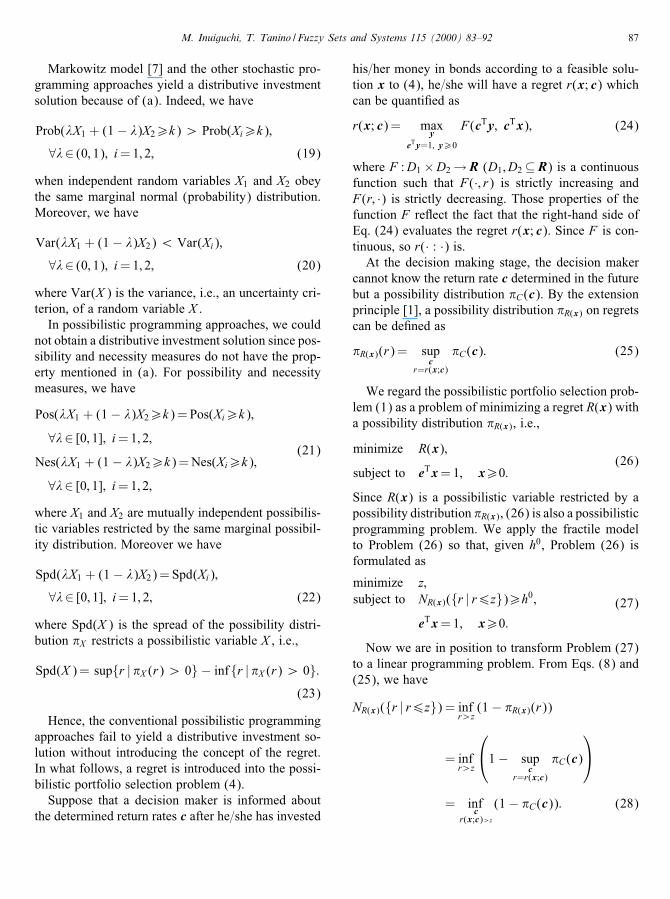
Table 1Examples of f, g and ’

No. Name f(r) g(r) ’(r)

1 Usual minimax regret −1 r r

2 Minimax regret rate − 11 + r

r1 + r

r

3 Linear combination of1 and 2 (�1; �2¿0) − �1(1 + r) + �2

1 + r�1r2 + (�1 + �2)r

1 + rr

Hence, Problem (40) can be reduced to the followinglinear programming problem:

minimize q;

subject to

f(cRi (1− h0))

n∑j=1j 6=i

cLj (1− h0)xj + cRi (1− h0)xi

6q− g(cRi (1− h0)); i=1; 2; : : : ; n;

eTx=1; x¿0: (42)

Problem (42) has (n + 1) constraints excluding non-negativity constraints. Therefore, even if a simplexmethod is applied, (n+1) variables can take positivevalues. This means that Problem (42) can yield a dis-tributive investment solution.Before describing numerical examples, we show

some meaningful combinations of f, g and h inTable 1. The �rst one is the usual minimax regretmodel [5] where the worst regret of x under a returnrate vector c is de�ned by the di�erence between theoptimal total return rate with respect to c and the ob-tained total return rate cTx. The second one is a regretrate model which is equivalent with the achievementrate model [6]. In the regret rate model, the worstregret of x under a return rate vector c is de�nedby the ratio of the di�erence between the optimaltotal return rate with respect to c and the obtainedtotal return rate cTx to the optimal total income rate.Note that, because of the negativity of f(r), for allr ∈ [L; R], we cannot consider the ratio to the optimaltotal return rate. The third one is the non-negativelinear combination of the �rst and second ones.

5. Numerical examples

In order to see what solution is obtained from Prob-lem (42), 3 numerical examples are given in what fol-lows. For comparison, not only the proposed approachbut also a stochastic and the previous possibilistic pro-gramming approaches are applied to each example. Inthose examples, we have 5 bonds whose return ratesare restricted by the following type of possibility dis-tributions with a center cci and a spread wi:

�Ci(q)= exp(− (q− cci )2

wi

): (43)

As the corresponding probability distribution pCi ,we consider the following normal distributionN(cci ;

√wi=2):

pCi(q)=1√�wi

exp(− (q− cci )2

wi

): (44)

We assume the independence among return rates. Thejoint possibility distribution is given as in Eq. (5) andthe joint probability distribution is given as

pC(c)=n∏1=1

pCi(ci): (45)

Since pCi is a normal distribution, pC becomes amultivariate normal distribution with a mean vectorm=(cc1; c

c2; : : : ; c

cn) and a covariance matrix

V =

w1=2 0 0 · · · 0

0 w2=2 0 · · · 0

0 0. . .

. . ....

......

. . .. . . 0

0 0 0 · · · wn=2

: (46)

90 M. Inuiguchi, T. Tanino / Fuzzy Sets and Systems 115 (2000) 83–92

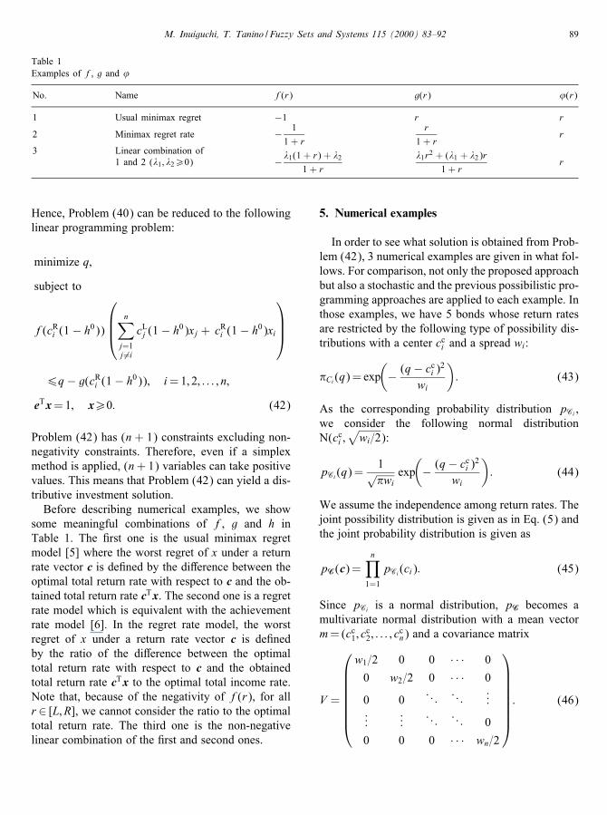
Table 2Solutions for Example 1

Approach x1 x2 x3 x4 x5

Markowitz 0.061225 0.081633 0.122449 0.244898 0.489796Fractile 0 0 0 0 1Modality 0 0 0 0 1Spread 0 0 0 0 1Regret 0.25 0.211325 0.146446 0 0.392229

Fig. 1. Five bonds for Example 1.

In the following examples, we assume that functionsf; g and’ are de�ned by those in the �rst combinationin Table 1, i.e., the usual minimax regret model.

Example 1. Let us consider �ve bonds whose returnrates are depicted as possibility distributions in Fig. 1.All cci ’s are equal to 0.2 but wi decreases as i increases:

w1 = 0:04; w2 = 0:03; w3 = 0:02;

w4 = 0:01 and w5 = 0:005:

The optimal solutions to Problems (3), (10), (13),(16) and (42) are obtained as shown in Table 2 withsetting z0 = 0:18 and h0 = 0:9. Whereas the previouspossibilistic programming approaches, i.e., the fractileapproach, the modality optimization approach and thespread minimization approach, yield a concentratedinvestment on the 5th bond, the proposed possibilis-tic programming approach yields a distributive invest-ment on the 1st, 2nd, 3rd and 5th bonds. However,the solution is rather di�erent from the distributive in-vestment solution of the Markowitz (stochastic pro-gramming) model (3). The reason is that a bond witha small variance gathers the investment rate aroundit since minimization of the variance which is not re-lated to the original objective, maximization of thetotal return rate, is adopted by the Markowitz model.

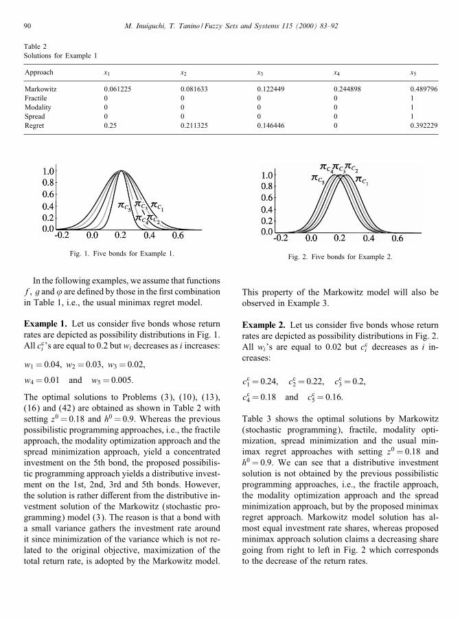
Fig. 2. Five bonds for Example 2.

This property of the Markowitz model will also beobserved in Example 3.

Example 2. Let us consider �ve bonds whose returnrates are depicted as possibility distributions in Fig. 2.All wi’s are equal to 0.02 but cci decreases as i in-creases:

cc1 = 0:24; cc2 = 0:22; cc3 = 0:2;

cc4 = 0:18 and cc5 = 0:16:

Table 3 shows the optimal solutions by Markowitz(stochastic programming), fractile, modality opti-mization, spread minimization and the usual min-imax regret approaches with setting z0 = 0:18 andh0 = 0:9. We can see that a distributive investmentsolution is not obtained by the previous possibilisticprogramming approaches, i.e., the fractile approach,the modality optimization approach and the spreadminimization approach, but by the proposed minimaxregret approach. Markowitz model solution has al-most equal investment rate shares, whereas proposedminimax approach solution claims a decreasing sharegoing from right to left in Fig. 2 which correspondsto the decrease of the return rates.

M. Inuiguchi, T. Tanino / Fuzzy Sets and Systems 115 (2000) 83–92 91

Table 3Solutions for Example 2

Approach x1 x2 x3 x4 x5

Markowitz 0.200003 0.200002 0.200002 0.199997 0.199996Fractile 1 0 0 0 0Modality 1 0 0 0 0Spread 1 0 0 0 0Regret 0.293198 0.246599 0.2 0.153401 0.106802

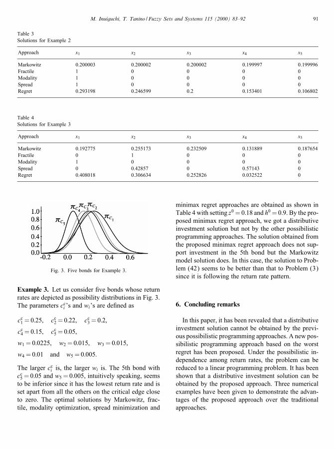
Table 4Solutions for Example 3

Approach x1 x2 x3 x4 x5

Markowitz 0.192775 0.255173 0.232509 0.131889 0.187654Fractile 0 1 0 0 0Modality 1 0 0 0 0Spread 0 0.42857 0 0.57143 0Regret 0.408018 0.306634 0.252826 0.032522 0

Fig. 3. Five bonds for Example 3.

Example 3. Let us consider �ve bonds whose returnrates are depicted as possibility distributions in Fig. 3.The parameters cci ’s and wi’s are de�ned as

cc1 = 0:25; cc2 = 0:22; cc3 = 0:2;

cc4 = 0:15; cc5 = 0:05;

w1 = 0:0225; w2 = 0:015; w3 = 0:015;

w4 = 0:01 and w5 = 0:005:

The larger cci is, the larger wi is. The 5th bond withcc5 = 0:05 and w5 = 0:005, intuitively speaking, seemsto be inferior since it has the lowest return rate and isset apart from all the others on the critical edge closeto zero. The optimal solutions by Markowitz, frac-tile, modality optimization, spread minimization and

minimax regret approaches are obtained as shown inTable 4 with setting z0 = 0:18 and h0 = 0:9. By the pro-posed minimax regret approach, we got a distributiveinvestment solution but not by the other possibilisticprogramming approaches. The solution obtained fromthe proposed minimax regret approach does not sup-port investment in the 5th bond but the Markowitzmodel solution does. In this case, the solution to Prob-lem (42) seems to be better than that to Problem (3)since it is following the return rate pattern.

6. Concluding remarks

In this paper, it has been revealed that a distributiveinvestment solution cannot be obtained by the previ-ous possibilistic programming approaches. A new pos-sibilistic programming approach based on the worstregret has been proposed. Under the possibilistic in-dependence among return rates, the problem can bereduced to a linear programming problem. It has beenshown that a distributive investment solution can beobtained by the proposed approach. Three numericalexamples have been given to demonstrate the advan-tages of the proposed approach over the traditionalapproaches.

92 M. Inuiguchi, T. Tanino / Fuzzy Sets and Systems 115 (2000) 83–92

References

[1] D. Dubois, H. Prade, Fuzzy Sets and Systems: Theory andApplications, Academic Press, New York, 1980.

[2] M. Inuiguchi, Stochastic programming problems versus fuzzymathematical programming problems, Jpn. J. Fuzzy TheorySystems 4 (1992) 97–109.

[3] M. Inuiguchi, H. Ichihashi, Y. Kume, Relationships betweenmodality constrained programming problems and various fuzzymathematical programming problems, Fuzzy Sets and Systems49 (1992) 243–259.

[4] M. Inuiguchi, H. Ichihashi, Y. Kume, Modality constrained

programming problems: A uni�ed approach to fuzzymathematical programming problems in the setting ofpossibility theory, Inform. Sci. 67 (1993) 93–126.

[5] M. Inuiguchi, M. Sakawa, Minimax regret solution to linearprogramming problems with an interval objective function,Eur. J. Oper. Res. 86 (1995) 526–536.

[6] M. Inuiguchi, M. Sakawa, An achievement rate approachto linear programming problems with an interval objectivefunction, J. Oper. Res. Soc. 48 (1997) 25–33.

[7] H. Markowitz, Portfolio Selection: E�cient Diversi�cation ofInvestments, Wiley, New York, 1959.