Political connections in china: determinants and effects on ...
374
POLITICAL CONNECTIONS IN CHINA: DETERMINANTS AND EFFECTS ON FIRMS’ EXPORTING BEHAVIOUR AND FINANCIAL HEALTH by JING DU A thesis submitted to the University of Birmingham for the degree of DOCTOR OF PHILOSOPHY Department of Economics Birmingham Business School College of Social Sciences The University of Birmingham December 2015
-
Upload
khangminh22 -
Category
Documents
-
view
3 -
download
0
Transcript of Political connections in china: determinants and effects on ...
POLITICAL CONNECTIONS IN CHINA:
DETERMINANTS AND EFFECTS ON
FIRMS’ EXPORTING BEHAVIOUR AND
FINANCIAL HEALTH
by
JING DU
A thesis submitted to the University of Birmingham for
the degree of
DOCTOR OF PHILOSOPHY
Department of Economics
Birmingham Business School
College of Social Sciences
The University of Birmingham
December 2015

University of Birmingham Research Archive
e-theses repository This unpublished thesis/dissertation is copyright of the author and/or third parties. The intellectual property rights of the author or third parties in respect of this work are as defined by The Copyright Designs and Patents Act 1988 or as modified by any successor legislation. Any use made of information contained in this thesis/dissertation must be in accordance with that legislation and must be properly acknowledged. Further distribution or reproduction in any format is prohibited without the permission of the copyright holder.
i
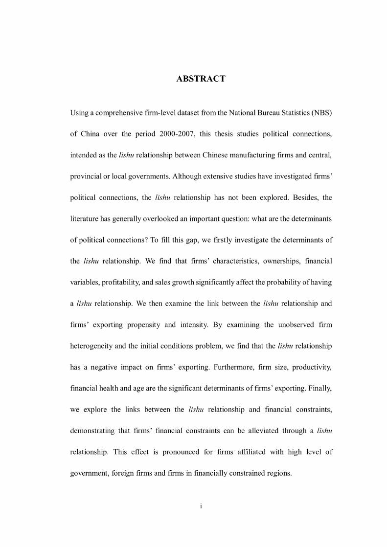
ABSTRACT
Using a comprehensive firm-level dataset from the National Bureau Statistics (NBS)
of China over the period 2000-2007, this thesis studies political connections,
intended as the lishu relationship between Chinese manufacturing firms and central,
provincial or local governments. Although extensive studies have investigated firms’
political connections, the lishu relationship has not been explored. Besides, the
literature has generally overlooked an important question: what are the determinants
of political connections? To fill this gap, we firstly investigate the determinants of
the lishu relationship. We find that firms’ characteristics, ownerships, financial
variables, profitability, and sales growth significantly affect the probability of having
a lishu relationship. We then examine the link between the lishu relationship and
firms’ exporting propensity and intensity. By examining the unobserved firm
heterogeneity and the initial conditions problem, we find that the lishu relationship
has a negative impact on firms’ exporting. Furthermore, firm size, productivity,
financial health and age are the significant determinants of firms’ exporting. Finally,
we explore the links between the lishu relationship and financial constraints,
demonstrating that firms’ financial constraints can be alleviated through a lishu
relationship. This effect is pronounced for firms affiliated with high level of
government, foreign firms and firms in financially constrained regions.

ii
To my beloved parents (Hengbin DU & Jianfeng HAO) and my dearest husband
(Dr Qiang REN)

iii
ACKNOWLEDGEMENTS
Taking this opportunity, it is my great pleasure to express my heartfelt gratitude to
the kind and wonderful people around me, who support and help me, during the
completion of this doctoral thesis.
First and foremost, I would like to express my sincere and deepest thanks and
appreciation to my supervisor, Professor Alessandra Guariglia, for her
encouragement and support during my PhD research. Since I was a master student at
Durham University, I have known Alex, who taught me the modules of Banking and
Finance and Research Methods, and supervised my MSc dissertation in 2010.
Transferring to the University of Birmingham with her after I have started my PhD
study at Durham University is the most important decision in my whole academic
life. I sincerely appreciate all her consideration on not only my academic research,
but also on all the other aspects of my staying in the UK.
A very special acknowledgement goes to my beloved parents, Hengbin Du and
Jianfeng Hao, and my dearest husband, Dr Qiang Ren, without whose love and
support this work would not have been completed. Thank you for your understanding
and patience when I was depressed, for your motivation and encouragement when I
was frustrated, and for your help and support when I went through tough times. Most
importantly, thank you, Dr Qiang Ren, for accompanying me during my long journey
of running and re-running regressions, and writing and re-writing this thesis. Words

iv
cannot express how much you all mean to me and I will forever be grateful that it is
you who are my family. I love you all dearly.
I would also like to express my deepest thanks to the examiners of this thesis,
Professor Nancy Huyghebaert and Mr Nicholas Horsewood, for their time and efforts.
Especially, I sincerely appreciate their constructive comments and suggestions which
help me improve the quality of the thesis.
Huge thanks also go to my friends and fellow doctoral candidates. Especially, I
would like to thank Dr Liyun Zhang, Dr Yan Cen, Dr Peiling Liao, Bing Liu, Rong
Huang, Marco Giansoldati, Enrico Vanino, Dr Pei Liu, Dr Xiaofei Xing, and a lot of
significant others, who accompanied and helped me over the past few years. I
gratefully acknowledge the supportive staffs in the Department.
Finally, to everyone else who is not mentioned here but contributes to my PhD
journey, I thank you all. Wish you every success in the future.
v
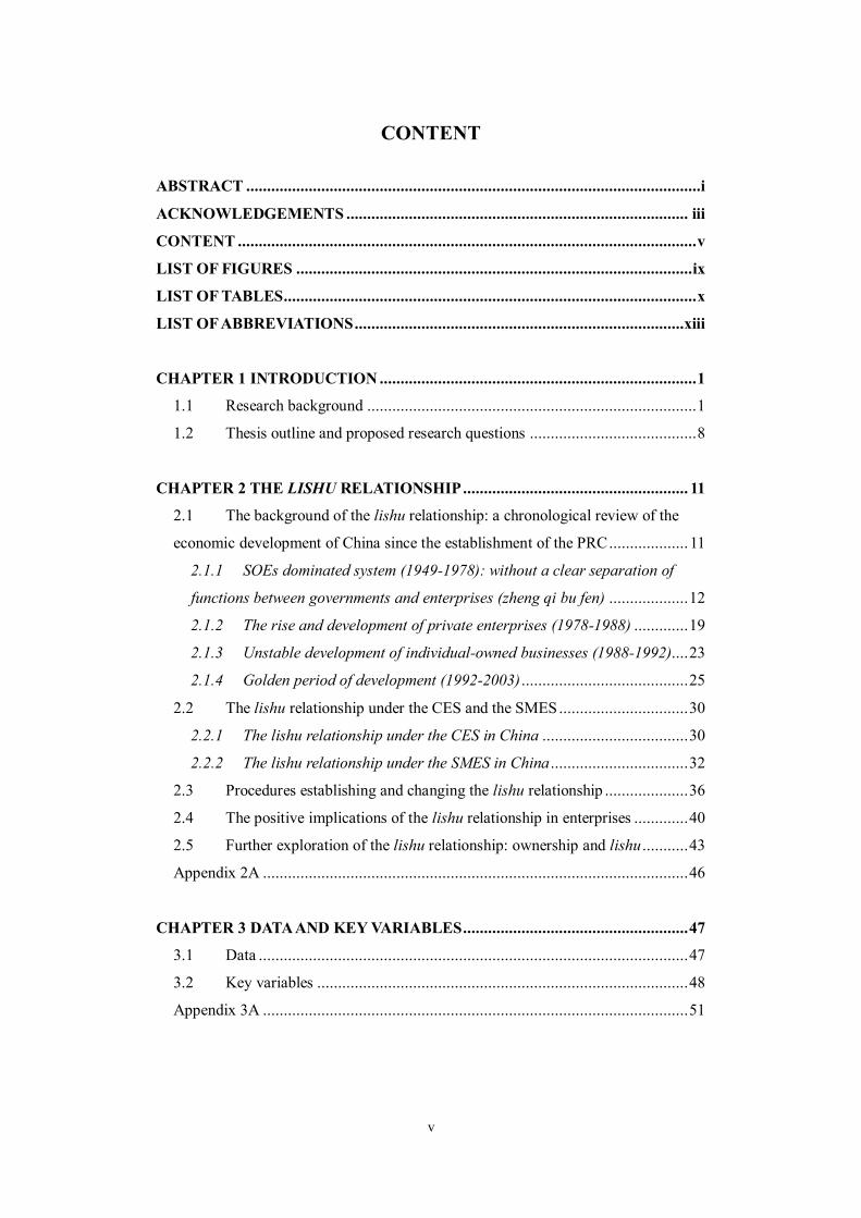
CONTENT ABSTRACT .............................................................................................................i
ACKNOWLEDGEMENTS .................................................................................. iii
CONTENT .............................................................................................................. v
LIST OF FIGURES ............................................................................................... ix
LIST OF TABLES ................................................................................................... x
LIST OF ABBREVIATIONS ...............................................................................xiii
CHAPTER 1 INTRODUCTION ............................................................................ 1
1.1 Research background ............................................................................... 1
1.2 Thesis outline and proposed research questions ........................................ 8
CHAPTER 2 THE LISHU RELATIONSHIP ...................................................... 11
2.1 The background of the lishu relationship: a chronological review of the
economic development of China since the establishment of the PRC ................... 11
2.1.1 SOEs dominated system (1949-1978): without a clear separation of
functions between governments and enterprises (zheng qi bu fen) ................... 12
2.1.2 The rise and development of private enterprises (1978-1988) ............. 19
2.1.3 Unstable development of individual-owned businesses (1988-1992).... 23
2.1.4 Golden period of development (1992-2003) ........................................ 25
2.2 The lishu relationship under the CES and the SMES ............................... 30
2.2.1 The lishu relationship under the CES in China ................................... 30
2.2.2 The lishu relationship under the SMES in China ................................. 32
2.3 Procedures establishing and changing the lishu relationship .................... 36
2.4 The positive implications of the lishu relationship in enterprises ............. 40
2.5 Further exploration of the lishu relationship: ownership and lishu ........... 43
Appendix 2A ...................................................................................................... 46
CHAPTER 3 DATA AND KEY VARIABLES ...................................................... 47
3.1 Data ....................................................................................................... 47
3.2 Key variables ......................................................................................... 48
Appendix 3A ...................................................................................................... 51

vi
CHAPTER 4 DETERMINANTS OF POLITICAL CONNECTIONS ................ 52
4.1 Introduction............................................................................................ 52
4.2 Literature review .................................................................................... 56
4.2.1 Measuring political connections ......................................................... 56
4.2.2 Determinants of political connections ................................................. 60
4.3 Conceptual framework and hypotheses ................................................... 74
4.3.1 Conceptual framework in the existing literature.................................. 74
4.3.2 Hypotheses ......................................................................................... 77
4.4 Specification and estimation methodology .............................................. 88
4.5 Data and summary statistics.................................................................... 90
4.5.1 Data ................................................................................................... 90
4.5.2 Summary statistics.............................................................................. 97
4.6 Empirical findings ................................................................................ 105
4.6.1 Estimations with pooled Probit and random-effects Probit models .... 105
4.6.2 Estimation with ordered Probit model ............................................... 109
4.7 Further tests ......................................................................................... 114
4.7.1 Determinants of the lishu relationship by ownership ......................... 114
4.7.2 Determinants of the lishu relationship by region ............................... 117
4.8 Conclusion ........................................................................................... 120
Appendix 4A .................................................................................................... 124
CHAPTER 5 POLITICAL CONNECTIONS AND EXPORTING ................... 129
5.1 Introduction.......................................................................................... 129
5.2 Background .......................................................................................... 136
5.2.1 Chinese institutional environment ..................................................... 136
5.2.2 The economic and exporting development in China .......................... 139
5.3 Literature review .................................................................................. 150
5.3.1 Determinants of firms’ exporting behaviour ...................................... 150
5.3.2 Political connections and firm performance ..................................... 173
5.3.3 Political connections and exports ..................................................... 180
5.4 Hypotheses ........................................................................................... 184
5.5 Specification and estimation methodology ............................................ 185
5.5.1 Baseline specification ....................................................................... 185
5.5.2 Unobserved firm heterogeneity ......................................................... 189
5.5.3 The initial conditions problem .......................................................... 192

vii
5.6 Data and summary statistics.................................................................. 195
5.6.1 Data ................................................................................................. 195
5.6.2 Descriptive statistics ........................................................................ 201
5.7 Empirical results .................................................................................. 208
5.7.1 The lishu relationship and the propensity of exporting ...................... 208
5.7.2 The lishu relationship and the intensity of exporting ......................... 215
5.8 Further tests ......................................................................................... 219
5.8.1 Different levels of the lishu relationship and exporting behaviour ..... 219
5.8.2 The propensity and intensity of exporting by ownership .................... 224
5.8.3 The propensity and intensity of exporting by region .......................... 227
5.9 Conclusion ........................................................................................... 230
Appendix 5A .................................................................................................... 233
CHAPTER 6 POLITICAL CONNECTIONS AND FINANCIAL
CONSTRAINTS.................................................................................................. 241
6.1 Introduction.......................................................................................... 241
6.2 Literature review and hypotheses .......................................................... 249
6.2.1 The background of financial constraints ........................................... 249
6.2.2 Controversy on measures of financial constraints ............................. 253
6.2.3 Financial constraints in China ......................................................... 264
6.2.4 Political connections and financial constraints ................................. 274
6.2.5 Hypotheses ....................................................................................... 284
6.3 Specifications and estimation methodology .......................................... 284
6.3.1 Baseline specification ....................................................................... 284
6.3.2 Estimation methodology ................................................................... 288
6.4 Data and summary statistics.................................................................. 290
6.4.1 Data ................................................................................................. 290
6.4.2 Summary statistics............................................................................ 291
6.5 Empirical results .................................................................................. 299
6.5.1 Financial constraints in China ......................................................... 299
6.5.2 The lishu relationship and financial constraints in China.................. 303
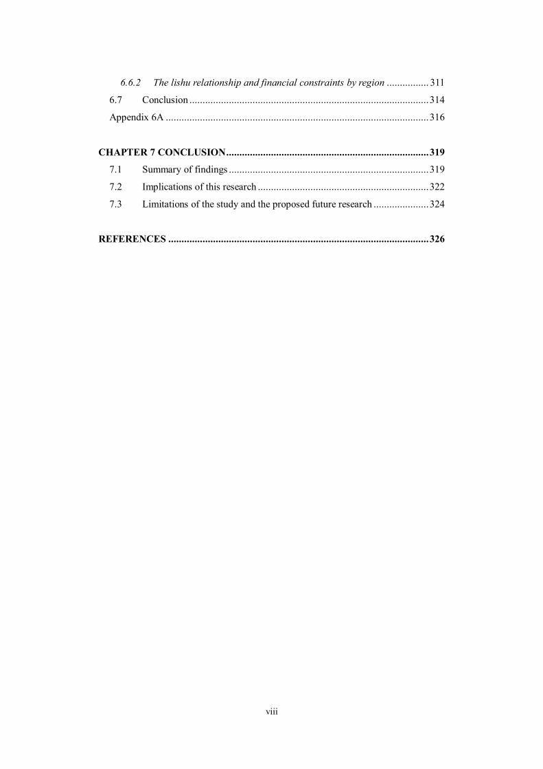
6.5.3 Different levels of the lishu relationship and financial constraints in
China 306
6.6 Further tests ......................................................................................... 308
6.6.1 The lishu relationship and financial constraints by firm ownership ... 308
viii
6.6.2 The lishu relationship and financial constraints by region ................ 311
6.7 Conclusion ........................................................................................... 314
Appendix 6A .................................................................................................... 316
CHAPTER 7 CONCLUSION ............................................................................. 319
7.1 Summary of findings ............................................................................ 319
7.2 Implications of this research ................................................................. 322
7.3 Limitations of the study and the proposed future research ..................... 324
REFERENCES ................................................................................................... 326
ix
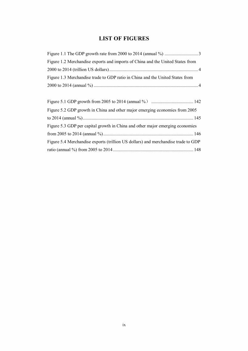
LIST OF FIGURES
Figure 1.1 The GDP growth rate from 2000 to 2014 (annual %) ............................ 3
Figure 1.2 Merchandise exports and imports of China and the United States from
2000 to 2014 (trillion US dollars) .......................................................................... 4
Figure 1.3 Merchandise trade to GDP ratio in China and the United States from
2000 to 2014 (annual %) ....................................................................................... 4
Figure 5.1 GDP growth from 2005 to 2014 (annual %) ................................... 142
Figure 5.2 GDP growth in China and other major emerging economies from 2005
to 2014 (annual %) ............................................................................................ 145
Figure 5.3 GDP per capital growth in China and other major emerging economies
from 2005 to 2014 (annual %) ........................................................................... 146
Figure 5.4 Merchandise exports (trillion US dollars) and merchandise trade to GDP
ratio (annual %) from 2005 to 2014 ................................................................... 148
x
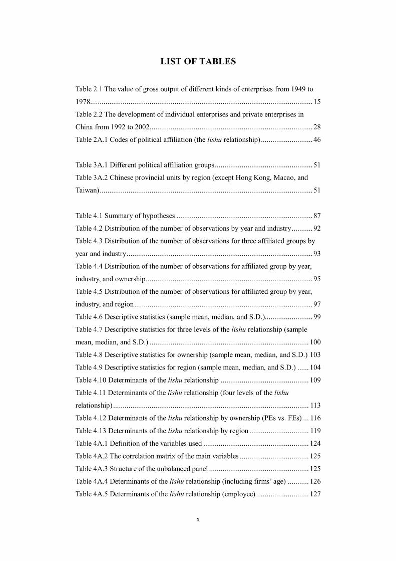
LIST OF TABLES
Table 2.1 The value of gross output of different kinds of enterprises from 1949 to
1978.................................................................................................................... 15
Table 2.2 The development of individual enterprises and private enterprises in
China from 1992 to 2002 ..................................................................................... 28
Table 2A.1 Codes of political affiliation (the lishu relationship) ........................... 46
Table 3A.1 Different political affiliation groups ................................................... 51
Table 3A.2 Chinese provincial units by region (except Hong Kong, Macao, and
Taiwan) ............................................................................................................... 51
Table 4.1 Summary of hypotheses ....................................................................... 87
Table 4.2 Distribution of the number of observations by year and industry ........... 92
Table 4.3 Distribution of the number of observations for three affiliated groups by
year and industry ................................................................................................. 93
Table 4.4 Distribution of the number of observations for affiliated group by year,
industry, and ownership ....................................................................................... 95
Table 4.5 Distribution of the number of observations for affiliated group by year,
industry, and region ............................................................................................. 97
Table 4.6 Descriptive statistics (sample mean, median, and S.D.)......................... 99
Table 4.7 Descriptive statistics for three levels of the lishu relationship (sample
mean, median, and S.D.) ................................................................................... 100
Table 4.8 Descriptive statistics for ownership (sample mean, median, and S.D.) 103
Table 4.9 Descriptive statistics for region (sample mean, median, and S.D.) ...... 104
Table 4.10 Determinants of the lishu relationship .............................................. 109
Table 4.11 Determinants of the lishu relationship (four levels of the lishu
relationship) ...................................................................................................... 113
Table 4.12 Determinants of the lishu relationship by ownership (PEs vs. FEs) ... 116
Table 4.13 Determinants of the lishu relationship by region ............................... 119
Table 4A.1 Definition of the variables used ....................................................... 124
Table 4A.2 The correlation matrix of the main variables .................................... 125
Table 4A.3 Structure of the unbalanced panel .................................................... 125
Table 4A.4 Determinants of the lishu relationship (including firms’ age) ........... 126
Table 4A.5 Determinants of the lishu relationship (employee) ........................... 127

xi
Table 4A.6 Determinants of the lishu relationship (liquidity) ............................. 129
Table 5.1 Top 11 Gross Domestic Product ranking from 2010 to 2014 ............... 141
Table 5.2 Top 11 Gross Domestic Product based on PPP valuation ranking from
2010 to 2014 ..................................................................................................... 141
Table 5.3 Comparison of China and other major emerging economies from 2010 to
2014.................................................................................................................. 144
Table 5.4 Comparison of China and other major emerging economies based on PPP
valuation from 2010 to 2014.............................................................................. 144
Table 5.5 Export and export to GDP ratio in China from 1970 to 2014 ............... 149
Table 5.6 Distribution of the number of observations by year and industry ......... 197
Table 5.7 Distribution of the number of observations for firms with the lishu
relationship ....................................................................................................... 198
Table 5.8 Distribution of the number of observations for exporters by year,
industry, and ownership ..................................................................................... 199
Table 5.9 Distribution of the number of observations for exporters by year,
industry, and region ........................................................................................... 200
Table 5.10 Descriptive statistics (sample mean, median, and S.D.) ..................... 202
Table 5.11 Descriptive statistics for ownership (sample mean, median, and
S.D.) ................................................................................................................. 205
Table 5.12 Descriptive statistics for region (sample mean, median, and S.D.)..... 207
Table 5.13 The propensity of exporting.............................................................. 214
Table 5.14 The intensity of exporting ................................................................ 218
Table 5.15 The propensity of exporting (different levels of the lishu
relationship) ...................................................................................................... 222
Table 5.16 The intensity of exporting (different levels of the lishu relationship) . 223
Table 5.17 The propensity of exporting by ownership (Private firms vs. Foreign
firms): marginal effects ..................................................................................... 225
Table 5.18 The intensity of exporting by ownership (Private firms vs. Foreign
firms): marginal effects ..................................................................................... 226
Table 5.19 The propensity of exporting by region: marginal effects ................... 228
Table 5.20 The intensity of exporting by region: marginal effects ...................... 229
Table 5A.1 Definition of the variables used ....................................................... 233
Table 5A.2 The correlation matrix of the main variables .................................... 234
Table 5A.3 Structure of the unbalanced panel .................................................... 234
xii
Table 5A.4 The propensity of exporting by ownership (Private firms vs. Foreign
firms): coefficients ............................................................................................ 235
Table 5A.5 The intensity of exporting by ownership (Private firms vs. Foreign
firms): coefficients ............................................................................................ 236
Table 5A.6 The propensity of exporting by region: coefficients ......................... 237
Table 5A.7 The intensity of exporting by region: coefficients ............................ 238
Table 5A.8 The propensity of exporting (random-effects Probit model) ............. 239
Table 5A.9 The intensity of exporting (random-effects Tobit model) .................. 240
Table 6.1 Descriptive statistics (sample mean, median, and S.D.)....................... 292
Table 6.2 Descriptive statistics for three levels of the lishu relationship (sample
mean, median, and S.D.) ................................................................................... 294
Table 6.3 Descriptive statistics for ownership (sample mean, median, and S.D.) 296
Table 6.4 Descriptive statistics for region (sample mean, median, and S.D.) ...... 298
Table 6.5 Financial constraints in China ............................................................ 302
Table 6.6 The lishu relationship and financial constraints in China..................... 305
Table 6.7 Different levels of the lishu relationship and financial constraints ....... 307
Table 6.8 The lishu relationship and financial constraints in China by
ownership ......................................................................................................... 310
Table 6.9 The lishu relationship and financial constraints in China by region
(augmented equation) ........................................................................................ 313
Table 6A.1 Definition of the variables used ....................................................... 316
Table 6A.2 The correlation matrix of the main variables .................................... 317
Table 6A.3 Structure of the unbalanced panel .................................................... 317
Table 6A.4 The lishu relationship and financial constraints by region (reduced
equation) ........................................................................................................... 318

xiii
LIST OF ABBREVIATIONS
CES Centralised Economic System
COEs Collectively-owned enterprises
CPC Communist Party of China
CPPCC Chinese People’s Political Consultative Conference
FDI Foreign Direct Investment
FE Fixed effects
FEs Foreign enterprises
GDP Gross Domestic Product
GMM Generalised Method of Moments
ME Marginal effects
MNCs Multinational corporations
NBS National Bureau of Statistics of China
OLS The Ordinary Least Squares
PA Political affiliation (the lishu relationship)
PAC Political Action Committee
PC Chinese People’s Congress
PEs Private enterprises
PPCEs Public-private cooperative enterprises
R&D Research and development
RE Random effects
ROA Return on assets
ROS Return on sales
SC State Council
SMES Socialised Market Economy System
SOEs State-owned enterprises
TFP Total factor productivity
TVEs Township and Village Enterprises
UCEs Urban Collective Enterprises
1
CHAPTER 1 INTRODUCTION
This Chapter provides an overview of this research. Section 1.1 introduces the general
background and the motivations of this research. The research questions and outlines
of this thesis are proposed Section 1.2.
1.1 Research background
Thanks to its reforming and opening-up policy since the 1970s, China has achieved
remarkable economic success over the last several decades. The growth rate of its
Gross Domestic Product (GDP) has increased dramatically during our sample period,
from 8.43% in 2000 to 14.19% in 2007. Such a growth has exceeded the GDP growth
rate of the United States (US), the United Kingdom (UK), and the global average rate
(see Figure 1.1). During 2008 and 2009, the world GDP growth experienced a
significant decline due to the global financial crisis. Both the US and the UK have
confronted negative growth, while China conserved a considerable growth above 9.00%
in both years. In 2014, China’s GDP grew approximately 3 times faster than the US
and the UK (The World Bank) (see Figure 1.1).
In addition to its GDP growth, China’s international trade witnessed a remarkable
increase. Figure 1.2 plots the value of merchandise exports and imports of China and
the US from 2000 to 2014. We observe that the US merchandise trade maintained a
deficit over the period, while China showed a surplus. Specifically, China became the
largest merchandise exporting country in 2009 with a total value of around 1.20
2
trillion US dollars, compared with 1.05 trillion US dollars in the US (the World Trade
Organization; the World Bank) (see Figure 1.2). Figure 1.2 also shows that both China
and the US suffered from a shrink in merchandise exports in 2009 because of the
economic crisis, but the growth recovered faster and rebounded more sharply in China
than that in the US after the crisis. Moreover, total merchandise trade value accounted
for 43.63% of the total GDP in China, while the figure was 18.46% in the US in 2009
(the World Trade Organization; the World Bank) (see Figure 1.3). Figure 1.3
demonstrates that the contribution of total value of merchandise exports to the GDP
remained above 38% in China over the period 2000-2014. The ratio reached 64.49%
in 2006, indicating that exporting in China has contributed to its economic
development significantly.

3
Figure 1.1 The GDP growth rate from 2000 to 2014 (annual %)
Source: World Development Indicators, The World Bank. Notes: “Annual percentage growth rate of GDP at market prices based on constant local currency. Aggregates are based on constant 2005 U.S. dollars. GDP is the sum of gross value added by all resident producers in the economy plus any product taxes and minus any subsidies not included in the value of the products. It is calculated without making deductions for depreciation of fabricated assets or for depletion and degradation of natural resources.” (The World Bank, available at http://data.worldbank.org/indicator)
-5.00
0.00
5.00
10.00
15.00
2000 2001 2002 2003 2004 2005 2006 2007 2008 2009 2010 2011 2012 2013 2014
China
United Kingdom
United States
World
(Year)
(%)

4
Figure 1.2 Merchandise exports and imports of China and the United States from 2000 to 2014 (trillion US dollars)
Source: World Development Indicators, the World Bank. International Trade Statistics 2001-2014, the World Trade Organization. Notes: “Merchandise exports show the f.o.b. (free on board) value of goods provided to the rest of the world valued in current U.S. dollars.” (The World Bank, available at http://data.worldbank.org/indicator)
Figure 1.3 Merchandise trade to GDP ratio in China and the United States from 2000 to 2014 (annual %)
Source: World Development Indicators, the World Bank. International Trade Statistics 2001-2014, the World Trade Organization. Notes: “Merchandise trade as a share of GDP is the sum of merchandise exports and imports divided by the value of GDP, all in current U.S. dollars.” (The World Bank, available at http://data.worldbank.org/indicator)
0.00
0.50
1.00
1.50
2.00
2.50
2000 2001 2002 2003 2004 2005 2006 2007 2008 2009 2010 2011 2012 2013 2014
China Merchandise Exports United States Merchandise Exports
China Merchandise Imports United States Merchandise Imports
0.00
10.00
20.00
30.00
40.00
50.00
60.00
70.00
2000 2001 2002 2003 2004 2005 2006 2007 2008 2009 2010 2011 2012 2013 2014
United States Merchandise Trade/GDP China Merchandise Trade/GDP
(Year)
(trillion US dollars)
(%)
(Year)

5
Yet, such remarkable performance in China has been achieved in recent years, despite
the underdeveloped financial and legal systems, which are not favourable to efficient
economic activities. The Chinese phenomenal economic and exporting development
has therefore been considered as a miracle, and scholars have been trying to
comprehend how this miracle was made possible.
Some scholars provide an institutional explanation for China’s development,
suggesting that the relationship among the governments, market, and firms constitutes
the main driving force through the interaction of the “visible hands” and “invisible
hands” (Walder, 1995; Qian and Weingast, 1997; Jin and Qian, 1998). They state that
during China’s economic transition, the government’s interventions help to maintain
regional stability, which in turn support the firms’ development. Additionally, the
government controls key products resources and grants favourable assistance to the
politically connected firms, which accelerates the development of these firms and in
turn enhances the economic growth. The positive relationship between political
connections and firm performance has been demonstrated in several empirical studies,
which define the political connections from the perspectives of state ownership,
politically related entrepreneurs or large shareholders, and campaign contribution
(Faccio, 2007, 2010; Chen et al., 2010; Goldman et al., 2009; Claessens et al., 2008;
Zhang and Huang, 2009).
However, China has a unique type of political connections called the lishu relationship.
With the deepening of the economic transition, the “visible hands” meet the “invisible
hands”, in which process a unique institutional variation, the lishu relationship, has
6
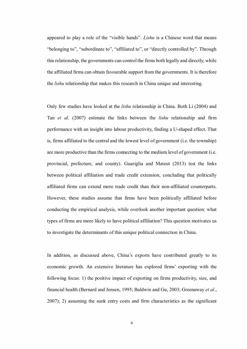
appeared to play a role of the “visible hands”. Lishu is a Chinese word that means
“belonging to”, “subordinate to”, “affiliated to”, or “directly controlled by”. Through
this relationship, the governments can control the firms both legally and directly, while
the affiliated firms can obtain favourable support from the governments. It is therefore
the lishu relationship that makes this research in China unique and interesting.
Only few studies have looked at the lishu relationship in China. Both Li (2004) and
Tan et al. (2007) estimate the links between the lishu relationship and firm
performance with an insight into labour productivity, finding a U-shaped effect. That
is, firms affiliated to the central and the lowest level of government (i.e. the township)
are more productive than the firms connecting to the medium level of government (i.e.
provincial, prefecture, and county). Guariglia and Mateut (2013) test the links
between political affiliation and trade credit extension, concluding that politically
affiliated firms can extend more trade credit than their non-affiliated counterparts.
However, these studies assume that firms have been politically affiliated before
conducting the empirical analysis, while overlook another important question: what
types of firms are more likely to have political affiliation? This question motivates us
to investigate the determinants of this unique political connection in China.
In addition, as discussed above, China’s exports have contributed greatly to its
economic growth. An extensive literature has explored firms’ exporting with the
following focus: 1) the positive impact of exporting on firms productivity, size, and
financial health (Bernard and Jensen, 1995; Baldwin and Gu, 2003; Greenaway et al.,
2007); 2) assuming the sunk entry costs and firm characteristics as the significant
7
determinants of firms’ exporting behaviour (Roberts and Tybout, 1997; Bernard and
Jensen, 1999; Liu and Shu, 2003; Das et al., 2007; Greenaway and Kneller, 2008;
Manez et al., 2008; Manova, 2013). Although few studies have concentrated on the
links between ownership and exporting (Lee, 2009; Yi and Wang, 2012; Yi, 2014;
Dixon et al., 2015), the impact of political connections on firms’ exporting decisions
and exporting intensity has not been explored yet, which motivates us to estimate the
extent to which the lishu relationship affects exporting in the context of Chinese
manufacturing firms.
According to Modigliani and Miller (1958), a firm’s financing decisions should not
affect its investment behaviour in a perfect capital market. Nevertheless, capital
markets are not perfect due to information asymmetries and agency problems. A
pioneering study by Fazzari et al. (1988) estimates financial constraints by looking at
the sensitivity of investment to cash flow. The study reveals that cash flow tends to
influence corporate investment significantly. Subsequently, a branch of literature has
supported Fazzari et al.’s main conclusion not only from the perspective of fixed
capital investment activities (Gilchrist and Himmelberg, 1995; Carpenter and
Guariglia, 2008), but also from the perspectives of inventory investment (Kashyap et
al., 1994; Carpenter et al., 1998; Guariglia, 2000), innovation investment
(Himmelberg and Petersen, 1994; Bond et al., 2005), employment (Sharp, 1994;
Nickell and Nicolitsas, 1999), and firms’ growth (Carpenter and Petersen, 2002).
Although some studies have looked at the cash flow-investment sensitivity and
political connections in terms of ownership in China, they either employ a relatively
small sample that is likely to suffer from the sample selection problem, or only look

8
at the listed firms that may not be a good representative of the whole population of
Chinese firms. Therefore, we are motivated to investigate how the lishu relationship
affects the sensitivity of investment to cash flow for the unlisted firms in China.1
1.2 Thesis outline and proposed research questions
The rest of this thesis is organised as follows. Chapter 2 introduces the development
of private enterprises in China and summaries the relationship between the Chinese
governments and enterprises in the development, providing background to understand
the lishu relationship. For the first time in literature, I explore the different meanings
of the lishu relationship under the different economic development stages in China.
Moreover, I introduce the procedures of establishing, changing, and terminating the
lishu relationship. I also elaborate the difference between the lishu relationship and
ownership structure in this chapter for the first time in literature. Chapter 3 describes
data and the key variables used for the empirical studies in this thesis.
By examining the significance of firm heterogeneity in having the lishu relationship,
Chapter 4 tests our first research question: what determines the likelihood of having a
lishu relationship for Chinese unlisted firms? I test four sets of hypotheses, including
hypotheses on firm heterogeneity, ownership status, financial factors, and profitability
and growth opportunities, by using a pooled Probit model with clustering the
observations by firms’ ID, a random-effects Probit model, and an ordered Probit
model. We conclude that the probability of a firm being politically affiliated can be
1 The “financial health” in this thesis is defined as “financial un-constraints”. Financially healthy firms refer to unconstrained firms that do not have difficulties in accessing to finance.
9
explained by the firm’s size, age, the region where it operates, ownership structure,
financial health, profitability, and growth opportunities. We also find that firms are
more prone to have the lishu relationship with the medium level of governments as
they can access the important resources owned by the governments and enjoy certain
autonomy to develop themselves.
In Chapter 5, we discuss the second research question: to what extent does the lishu
relationship affect firms’ exporting activities. Controlling for several firm
characteristics within dynamic export models, we focus on the links between the lishu
relationship and the propensity and intensity of exporting. The unobserved firm
heterogeneity and initial conditions problem are also taken into account in our
regressions. We find that sunk entry costs exist in the export markets and the lishu
relationship has a significant negative influence on both the probability and the
intensity of firms’ exporting. Other firm characteristics, such as firm size, total
productivity, financial factors, types of ownership, and location are the significant
determinants for firms’ exporting activities.
Our third research question, to what extent does the lishu relationship affect firms’
financial health, is tested in Chapter 6. We first analyse financial constraints in China
and conclude that the investment of Chinese firms is sensitive to the availability of
internal funds. Then we focus on the links between the lishu relationship and the
sensitivity of investment to cash flow in Chinese unlisted manufacturing firms by
employing the first-difference Generalised Method of Moments (GMM) procedure.
We find that the lishu relationship can mitigate the effects of financial constraints for

10
Chinese firms. This effect is more significant for the firms affiliated with a higher
level of government. We also find that compared with private firms, foreign firms are
more likely to encounter financial constraints; therefore, the lishu relationship can
reduce their financial constraints significantly. Furthermore, firms locating in the
western region have the least sensitivity of investment to the availability of internal
financing due to the regional preferential policies. However, the lishu relationship can
help firms in the central and coastal regions alleviate their financial constraints.
Finally, Chapter 7 concludes this thesis with a summary of the findings from the
empirical studies; with a discussion of its implications; and with an elaboration of the
limitations and the proposed future research.
11
CHAPTER 2 THE LISHU RELATIONSHIP
This chapter introduces the development of private enterprises in China and
summaries the relationship between the Chinese governments and enterprises in the
development, providing background to understand the lishu relationship in section 2.1.
Section 2.2 explores the different meanings of the lishu relationship under the different
economic development stages in China for the first time in literature. The procedures
of establishing, changing, and terminating the lishu relationship are presented in
section 2.3. Section 2.4 illustrates the positive implications of the lishu relationship in
enterprises. The difference between the lishu relationship and ownership structure is
explored in section 2.5.
2.1 The background of the lishu relationship: a chronological review of the
economic development of China since the establishment of the PRC
China has a unique type of political connections called the lishu relationship that
means “belonging to”, “subordinate to”, “affiliated to”, or “directly controlled by”.
Through this relationship, the government can control the firms both legally and
directly, while the affiliated firms can obtain favourable support from the government.
It is therefore the lishu relationship that makes this research in China unique and
stimulating.
The Chinese character “隶属”, or lishu, has to be comprehended with the background
of the economic development in China. The lishu relationship has different content in

12
the Centralised Economic System1 (CES) and in the Socialised Market Economy
System (SMES), even across the different development stages of the SMES. The
understanding of the history of the economic development and the main stages of the
development in China after 1949, when the PRC was established, therefore constitutes
a prerequisite to comprehend the lishu relationship of enterprises in China.
Since the foundation of the People’s Republic of China in 1949,2 the development of
enterprises and their political participation in China has experienced a long history,
which can be divided into the following four stages.
2.1.1 SOEs dominated system (1949-1978): without a clear separation of
functions between governments and enterprises (zheng qi bu fen)
The first phase during this period starts from 1949 to 1952, which is the recovery
period of the national economy. The traditional malpractice of the old Chinese
economic system had a significantly negative influence on the national economy at
the early stages of the establishment of the new China. In order to solve problems,
such as the imbalance between demand and supply and the strained relationship
between state-owned enterprises and individual-owned enterprises, the Central
Financial and Economic Committee started to reform industry and commerce. The
main content of this reform was to acknowledge the property rights and obligations
of individual-owned companies and to stimulate the development of private
1 It is also known as Planned Economic System, in which the ownership, the operation, and the management of enterprises were mixed and the state’s control is the centre of the economy (Hu, 1998; Cheng, 1986). 2 The Old China refers to the China in the period between 1840 and 1st October 1949. On 1st October 1949, the government of the People’s Republic of China was established. Since then, China was called the New China.

13
businesses.
During this recovery period, the relationship between the governments and private
firms has been defined through the slogan: “Utilisation, restriction, and transformation”
(li yong, xian zhi, gai zao)1 (Ji, 2003, p.253). The central government utilises private
enterprises by administrative management, economic lever, industry self-discipline
management, and mass movement (xing zheng guan li shou duan, jing ji gang gan
shou duan, hang ye zu zhi zi lv shou duan, qun zhong yun dong shou duan)2 (Huang,
2005).
The guiding principal of the Chinese government is to ensure the leading status of the
state-operated economy and to protect all capitalist industry and commerce, which
were beneficial to the national economy and to people’s well-being. Therefore, the
private businesses do not need to establish political connections actively but all of
1 Utilising the private economy refers to the government stimulating the enthusiasm of private enterprises, by allowing them to obtain the normal profits which can support their production and expend reproduction, and by encouraging the material exchange between city and country and among different districts, in order to develop the national economy and mitigate the conflicts between demand and supply caused by material shortages. Restricting the private economy means that along with policies aimed at regulating capital, controlling trade, and strengthening planning, the government restricts those aspects of private economy which are detrimental to the nation’s economy and the people’s well-being from various perspectives (e.g. the range of the economic activities, tax policy, market prices, and labour conditions). Transforming private enterprises refers to the government adjusting industry and commerce, promoting rural-urban trade, and motivating market circulation based on the socialist principle. 2 Administrative management includes the adjustment of the relationship between public economy and private economy, the improvement of the business environment for individual and private enterprises, and the enlargement of the amount of processing orders and government procurement from the private industries. Economic lever refers to easier money policy, demand promotion, tax adjustment, and tax items simplification. Industry self-discipline management involves formulating measures for industry so that the private firms in industry have to follow when they perform economic activities. For example, the government adjusts the relationship between labours and the companies by introducing consultative approach to deal with the conflicts in labour relations. Besides, the government requires the private enterprises to publish the production and marketing information in order to guide the entrepreneurs’ production and operation. Mass movement refers to two important political campaigns, named as Against Three Evils happened at the end of 1951 and Against Five Evils happened in the beginning of 1952. Against Three Evils refers to conduct the anti-corruption, anti-waste, and anti-bureaucratic in the national authorities and businesses. While Against Five Evils means to conduct anti-bribe, anti-tax evasion, anti-jerry work, anti-theft of the state property, and anti-theft of national economic intelligence. Through these two mass movements, the leading status of working-class and socialism state operated economy has been consolidated, the management system of workers and clerks monitoring production and participation in operation has been established, and the favourable conditions to conduct the socialism transformation of private industry and commerce have been created.

14
them are controlled and supervised by the government. Between 1949 and 1952,
although the state-operated economy was the leading part of the Chinese economy, it
did not have an overwhelming dominance over the private economy. On the contrary,
the output value of private businesses took up approximately 50% of the total output
value (see Table 2.1).

15
Table 2.1 The value of gross output of different kinds of enterprises from 1949 to 1978
Data Source: National Bureau of Statistics of China. (1985). Chinese Statistics Summary 1985. Beijing: China Statistics Press.
Year Whole people ownership Collective ownership Joint public-private ownership
Private ownership Individual ownership Total
Absolute Value (100 million RMB)
1949 36.80 0.70 2.20 68.30 32.30 140.30 1952 142.60 11.20 13.70 105.20 70.60 343.30 1957 421.50 149.20 206.30 0.40 6.50 783.90 1965 1255.50 138.40 0.00 0.00 0.00 1393.90 1978 3416.40 814.40 0.00 0.00 0.00 4230.80
Proportion(%) 1949 26.20 0.50 1.60 48.70 23.00 100.00 1952 41.50 3.30 4.00 30.60 20.60 100.00 1957 53.80 19.00 26.30 0.10 0.80 100.00 1965 90.10 9.90 0.00 0.00 0.00 100.00 1978 80.80 19.20 0.00 0.00 0.00 100.00
16
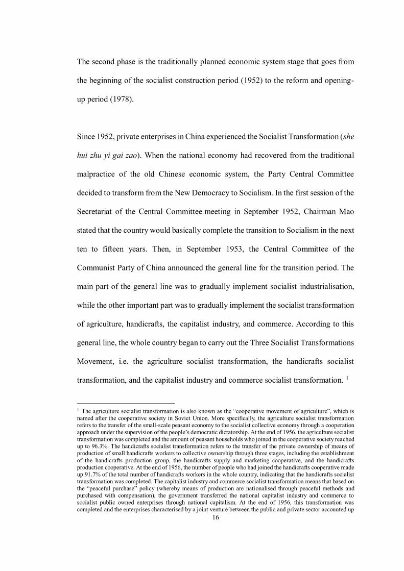
The second phase is the traditionally planned economic system stage that goes from
the beginning of the socialist construction period (1952) to the reform and opening-
up period (1978).
Since 1952, private enterprises in China experienced the Socialist Transformation (she
hui zhu yi gai zao). When the national economy had recovered from the traditional
malpractice of the old Chinese economic system, the Party Central Committee
decided to transform from the New Democracy to Socialism. In the first session of the
Secretariat of the Central Committee meeting in September 1952, Chairman Mao
stated that the country would basically complete the transition to Socialism in the next
ten to fifteen years. Then, in September 1953, the Central Committee of the
Communist Party of China announced the general line for the transition period. The
main part of the general line was to gradually implement socialist industrialisation,
while the other important part was to gradually implement the socialist transformation
of agriculture, handicrafts, the capitalist industry, and commerce. According to this
general line, the whole country began to carry out the Three Socialist Transformations
Movement, i.e. the agriculture socialist transformation, the handicrafts socialist
transformation, and the capitalist industry and commerce socialist transformation. 1
1 The agriculture socialist transformation is also known as the “cooperative movement of agriculture”, which is named after the cooperative society in Soviet Union. More specifically, the agriculture socialist transformation refers to the transfer of the small-scale peasant economy to the socialist collective economy through a cooperation approach under the supervision of the people’s democratic dictatorship. At the end of 1956, the agriculture socialist transformation was completed and the amount of peasant households who joined in the cooperative society reached up to 96.3%. The handicrafts socialist transformation refers to the transfer of the private ownership of means of production of small handicrafts workers to collective ownership through three stages, including the establishment of the handicrafts production group, the handicrafts supply and marketing cooperative, and the handicrafts production cooperative. At the end of 1956, the number of people who had joined the handicrafts cooperative made up 91.7% of the total number of handicrafts workers in the whole country, indicating that the handicrafts socialist transformation was completed. The capitalist industry and commerce socialist transformation means that based on the “peaceful purchase” policy (whereby means of production are nationalised through peaceful methods and purchased with compensation), the government transferred the national capitalist industry and commerce to socialist public owned enterprises through national capitalism. At the end of 1956, this transformation was completed and the enterprises characterised by a joint venture between the public and private sector accounted up
17
The Three Socialist Transformations Movement was completed in only four years,
from 1952 to 1956. Through this transformation, the nature of production goods was
changed from private ownership to socialist public ownership. China became a
socialist society and initially established a basic system of Socialism.
In the following 20 years, private enterprises disappeared because of the completed
socialist transformation. Especially during the Culture Revolution period, every single
private business was considered as a “remnant of capitalism”, which had to be got rid
of. Private businesses experienced a miserable and difficult period. Until 1978, all
private businesses were abandoned. The total number of individual workers in China
in 1978 was only 140,000, which only made up 0.015% of the total population
(962,590,000). There was no record of private businesses and private enterprises
during this period (see Table 2.1).
During this traditional planned economic period, the economic system was
characterised as highly centralised planned economy. As the country stood at an
economically backward starting point, the State-owned enterprises (SOEs) system
was carried out so that China could meet the needs of an increasing development rate.
With the absence of private firms, the SOEs system was compatible with the economic
system in that particular period, suggesting that the SOEs were the major income
source and major expenditure channels of the national finance. At that time, the
resource allocation system was highly centralised and enterprises did not have
autonomous rights in operation, which was controlled by the government. Therefore,
to 99% of the total original capitalist industry households and workers.
18
China established a complete industrial system which covered extensive industrial
categories only with the development of SOEs (Liu, 2009).
Under a such highly centralised planned economic system, private enterprises were
no longer an independent economic entity because of a lack of autonomy and
independence. That is, there were no private firms, but only the SOEs and politically
affiliated firms. Each enterprise was controlled by a corresponding administrative
department. Governments supervised and commanded companies’ activities directly
by administrative measures. The management rights were controlled by governments
at different levels, indicating that managers in enterprises were only executors of the
governments to carry out the governments’ operating decisions. All appointments and
dismissals of enterprises’ leaders and recruitments of employees were controlled by
governments.
At that time, the affiliated enterprises became the production department of
governments. All enterprise activities were based on governments’ administrative
goals. For example, the operating activities of enterprises only took national planned
aims into consideration, and the operating goal of enterprises was to accomplish
governments’ planned targets. Without considering sales and customers’ demands,
enterprises only cared about production quantity, instead of quality. The relationship
between private firms and the governments was quite affinitive and there was no clear
separation between the functions of governments and enterprises.
However, this situation led to several problems, such as unscientific performance

19
evaluation mechanisms and incentive system, a lack of enthusiasm of employees, and
serious bureaucracy problems (Bai and Ren, 2007).
2.1.2 The rise and development of private enterprises (1978-1988)
In the 1980s, the Chinese market started to open to individual-owned businesses. In
1978, the reform and opening-up policy was carried out in order to break the planned
economic system and to improve the enterprises system reform by introducing market
mechanisms. With the gradual establishment of a modern enterprise system, the seeds
of private enterprises were sown.
In 1979, the government allowed for the first time urban and rural individual workers
who had a valid residence registration to engage in the repair, service, and
manufacturing industry, as a subsidiary and complement to socialist public ownership.
However, they were not allowed to recruit labour. Therefore, the private firms during
that time period were quite small and their development was stagnant. Before 1980,
the policy of the Party and the government was not to encourage or to prohibit the
private businesses, indicating that the private businesses did not have a legal status at
that time.
In August 1980, the central government held a National Employment Conference and
decided to encourage and support the development of private enterprises in towns and
cities. The new “3 in 1 combination” employment policy was presented at the
conference, pointing out that employment could be improved by combining
20
employment by assignment through the Government Labour Department, voluntarily-
organised employment, and self-employment. More specifically, in the Several
Political Provisions of the State Council on Urban Non-agricultural Individual
Economy (guo wu yuan guan yu cheng zhen fei nong ge ti jing ji ruo gan zheng ce
xing gui ding) published by the State Council in July 1981, individual businesses were
allowed to employ others, but were limited to up to two assistants, and no more than
five apprentices.
These regulations ensured that the state would protect the legal rights and interests of
private operators, but also imposed certain limits on their size and fields of operation.
Only unemployed youths, the official urban residence, or retirees with certain skills
to pass on were allowed to engage in individual businesses. Additionally, individuals
could only engage in all kinds of small-scale handicrafts, retail commerce, catering,
services, repairs, non-mechanised transport, and building repairs, which were
beneficial to the national economy and did not involve the exploitation of others. The
limits imposed were for political purposes and kept the private economy under the
control of the socialist state and unlikely to develop any capitalist tendency.
A new Constitution was passed on 4th December 1982, at the fifth session of the Fifth
National People’s Congress (NPC). For the first time, the Constitution admitted the
legal status of individual-owned businesses. After his first South Tour in January 1984,
Deng Xiaoping decided to open up 14 coastal cities, which stimulated the prosperous
development of private businesses, and this phenomenon was called as “xia hai”1 in
1 The orginal meaning of “xia hai” is going to the sea. At the beginning of opening-up period, “xia hai” refers to people, especially those worked in government institutions, regisn from their old jobs and start doing business.
21
Chinese. At the end of 1986, the amount of township and village enterprises rose to
15.15 million and the population of the labour force of these enterprises was almost
80 million. The taxes they paid were 17 billion Yuan and the total value of output
amounted to 330 billion, which accounted for 20% of the whole national total value
of output (Wu, 2009).
In order to supervise and protect the legal rights of individual businesses, the
Provisional Administrative Regulation on Urban and Rural Individual Industrial and
Commercial Households (cheng xiang ge ti gong shang hu guan li zan xing tiao li)
was issued in September 1987. Then in October 1987, the Thirteenth National Party
Congress pointed out that the socialist economic mechanism was a planned
commodity economy on the basis of public ownership. A socialist planned commodity
economy mechanism should be a unitary economic system of planned economy and
market economy, indicating the markets were regulated and controlled by the state. In
this congress, the legal existence and development of the private economy were
admitted publicly for the first time. It was also stated that the State’s basic policy on
the private economy was to encourage, protect, guide, supervise and manage the
development of the private economy. Under this circumstance, private enterprises saw
their first development boom.
In April 1988, the first session of the Seventh National People’s Congress adopted an
“Amendment to the Constitution of People’s Republic of China.”1 (zhong hua ren min
1 The first article of the “Amendment to the Constitution of People’s Republic of China” states that Article 11 of the Constitution should include a new paragraph which specifies that: “The state permits the private sector of the economy to exist and develop within the restrictions prescribed by law. The private sector of the economy is complement to the socialist public economy. The state protects the legal rights and interests of the private sector
22
gong he guo xian fa xiu zheng an), suggesting the acknowledgement of the legal status
of private enterprises was been written in the Constitution of China. In June 1988, the
Provisional Regulations of the People’s Republic of China on Private Enterprises
(zhong hua ren min gong he guo si ying qi ye zan xing tiao li) was issued. It stated that
assets of private enterprises belonged to individuals and admitted the legal rights for
private businesses to employ more than eight employees. After this point, the Party
Central Committee and the State Council have acknowledged private enterprises
officially and the private economy finally had legal status.
In these early years of market economy transition, the facilities and support to obtain
the resources and access the market were quite deficient, which hindered the
commercial environment. As a response, private enterprises in China attempted to
establish political connections through “wearing a red hat” (dai hong mao zi) whereby
they disguised their private ownership and registered as a public owned organisation
by affiliating themselves to government agents. Many scholars (for example, Li, 2005;
Luo et al., 1998; Putterman, 1995) have noticed the red hat phenomenon and
developed various terms to describe it, such as disguised private enterprises, de facto
privatisation, pseudo-collectives, or pseudo-SOEs.
According to Pan (2006), the phenomenon of wearing a red hat was most popular in
the 1980s, taking up 46.30% of the total number of private enterprises. Such prevalent
activities could benefit both enterprises and public owned agents. At that time, the
private entrepreneurs were worried that the Party and state policy might change
of the economy, exercises guidance and supervision, and controls over the private sector of the economy.”
23
against them and were afraid that a socialist transformation might happen again. By
wearing a red hat, not only their rights could be secured, but also they could utilise
the prestige, customer network, and interpersonal relationships of public owned
agents to obtain greater profits. On the other hand, in order to put on a red hat, private
entrepreneurs needed good connections with government officials and had to pay a
management fee to the affiliated government agency or public-owned firm.1 In this
case, such management fee became one of the important income sources for public
owned sectors.
2.1.3 Unstable development of individual-owned businesses (1988-1992)
In the middle of the 1980s, economic reforms swept over the country. Some new
phenomena, such as the introduction of a contract system,2 appeared with the rapid
development of social productivity. However, the level of people’s awareness still
stayed at the traditional planned economy stage and did not catch up with the
development of social productivity. In this case, these new phenomena were not
understood and were considered as capitalism and some people claimed that they
should be prevented.
The most well-known event was called the “Guan Guangmei phenomenon”. Guan
1 Chan (1992, p. 251-252) quotes a classic example on such affiliation activity. An official who had worked for 10 years in a regional office of the Foreign Economic Relations and Trade Corporation decided to quit and run his own business, making use of the extensive network built up in his previous job. Instead of setting up a private firm, he made an arrangement with the local authority whereby the firm would be officially owned by the authority and subcontracted to it. According to the contract, the local authority would not invest any money but would be entitled to 30 percent of the firm’s profit. In return, the local authority would provide assistance to the firm in acquiring premises, licences, electricity and telephone lines, and in dealing with the Tax Bureau on the firm’s behalf. 2 Contract System is a labour employment system, which did not exist before. Because of the highly centralised planned economy, the labour’s recruitment, wage, and distribution are all arranged by the state. The workers recruited are the permanent workers, who will never lose his/her job.
24
Guangmei was a worker in a vegetable company in Benxi, Liaoning Province. Since
1985, she leased eight grocery stores consecutively. The profit she made during two
years was one million RMB, which was 20 times of the average income of the whole
population during that period. In this case, some people considered her as a capitalist,
who did not follow socialism. Later that year, there was a heated debate on whether
the private economy, contract, and lease operation method were characteristics of
socialism or capitalism (xing zi hai shi xing she). Since the second half of 1988, the
government started to manage the economic environment and rectify the economic
order to control the chaos in economic life. Under these circumstances, the economic
environment became strict for private entrepreneurs. In addition, a trend of bourgeois
liberalisation started in 1989. Some people propagandised bourgeois freedom and
democracy and took activities against the Party and socialism. After this political
disturbance, the whole society started to criticise bourgeois liberalisation,
westernisation and privatisation. Some people stated that the private economy posed
a threat to the status of public ownership, and thus had a negative impact on national
stability. Due to these unfavourable political and policy environments, although the
private economy had already received legal status, the development of private
enterprises was made very difficult, which weakened the development of the private
economy.
Under such an unfavourable environment during the early 1990s, many private
enterprises tried to wear a “red hat” in order to secure political protection and obtain
important resources such as energy and finance from the government (Naughton, 1994;
Che and Qian, 1998). But it was difficult for them to obtain such political connections
because they were considered to be against socialism.
25
2.1.4 Golden period of development (1992-2003)
This represents the golden period of the development of the Chinese private economy.
In order to find out whether the individual economy could be characterised as
socialism or capitalism, between January and February 1992, Deng Xiaoping
inspected the south of China and gave a speech, which scientifically explained the
essence of socialism and the relationship between the planned and market economy,
solved the ideological problem constantly obsessing the Chinese people, and defined
directions of transition from a planned economy to a market economy.
Deng Xiaoping stated that in the past the policy had focused on how to develop
productivity, while it overlooked the importance of reform. Reform referred to a
change in economic mechanisms, which fundamentally restricted the development of
productivity, established the socialist economic system with vigour and vitality, and
improved the development of productivity. In this case, reform also meant
emancipation of the productive forces. He pointed out that thanks to the reform and
opening-up activities, the development of the economy and the people’s living
standards had improved.
He also clarified that the criteria for judging the characteristics of the individual
economy should be whether it promotes the growth of productive forces in a socialist
society, whether it promotes the overall powers of the socialist country, and whether
it improves people’s living standards. He suggested people should be bolder than
before in conducting reform and opening to the outside world, by emancipating their

26
minds and attempting more experiments with courage.
This speech generated reform and an opening-up policy, encouraged people to
emancipate their minds, and woke up people’s awareness of doing business.
Thereafter, the development of private businesses started to face a favourable political
environment and private enterprises began to develop speedily.
In October 1992, the 14th National Conference of the Communist Party of China (CPC)
took a significant step of the reform and set an objective to establish a socialist market
economy system. In 1997, the 15th National Conference of the CPC enhanced the
status of private enterprises. It stated clearly that the non-public sector of the economy
was an important component of China’s socialist market economy. It also confirmed
that the basic economic system at the primary stage of socialism was keeping public
ownership in a dominant position and developing multiple forms of ownership side
by side. It indicates that the nature of the non-public sector of the economy had
become an important component of the socialist economy, instead of a necessary
supplement to the socialist economy. Afterwards, an increasing number of enterprises
began to drop their “red hats” as the economic environment became more favourable
for private firms.
The second session of the Ninth NPC in 1999 passed a new “Amendment to the
Constitution of People’s Republic of China” (zhong hua ren min gong he guo xian fa
xiu zheng an), which acknowledged, for the first time, that individually-owned
businesses, the private economy, and other non-public-owned economies were

27
important parts of the socialist market economy that could be written into the
Constitution, legally protecting the development of the private economy.
In his speech on the 80th anniversary of the Communist Party in July 2001, the
Secretary-General of China, Jiang Zemin defined private entrepreneurs for the first
time as constructors of the development of socialism with Chinese characteristics, and
stated that constructors of the socialist cause, including private entrepreneurs, should
be treated equally from a political perspective. In November 2002, the 16th National
Conference of the CPC amended the Party Constitution, allowing private
entrepreneurs to become Party members, which provided a favourable platform for
private entrepreneurs to seek political status.
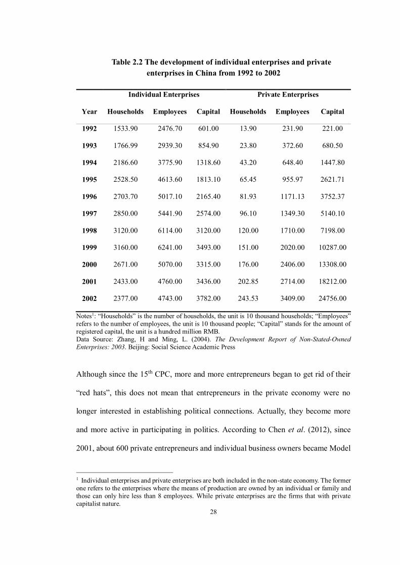
During this decade from 1992 to 2002, the non-state economy witnessed a rapid
development. For example, its output value increased from 20.5 billion up to 392.3
billion RMB. The number of households, the number of employees and the amount
of registered capital have seen a substantial increase (see Table 2.2).
28
Table 2.2 The development of individual enterprises and private enterprises in China from 1992 to 2002
Individual Enterprises Private Enterprises
Year Households Employees Capital Households Employees Capital
1992 1533.90 2476.70 601.00 13.90 231.90 221.00
1993 1766.99 2939.30 854.90 23.80 372.60 680.50
1994 2186.60 3775.90 1318.60 43.20 648.40 1447.80
1995 2528.50 4613.60 1813.10 65.45 955.97 2621.71
1996 2703.70 5017.10 2165.40 81.93 1171.13 3752.37
1997 2850.00 5441.90 2574.00 96.10 1349.30 5140.10
1998 3120.00 6114.00 3120.00 120.00 1710.00 7198.00
1999 3160.00 6241.00 3493.00 151.00 2020.00 10287.00
2000 2671.00 5070.00 3315.00 176.00 2406.00 13308.00
2001 2433.00 4760.00 3436.00 202.85 2714.00 18212.00
2002 2377.00 4743.00 3782.00 243.53 3409.00 24756.00
Notes1: “Households” is the number of households, the unit is 10 thousand households; “Employees” refers to the number of employees, the unit is 10 thousand people; “Capital” stands for the amount of registered capital, the unit is a hundred million RMB. Data Source: Zhang, H and Ming, L. (2004). The Development Report of Non-Stated-Owned Enterprises: 2003. Beijing: Social Science Academic Press
Although since the 15th CPC, more and more entrepreneurs began to get rid of their
“red hats”, this does not mean that entrepreneurs in the private economy were no
longer interested in establishing political connections. Actually, they become more
and more active in participating in politics. According to Chen et al. (2012), since
2001, about 600 private entrepreneurs and individual business owners became Model
1 Individual enterprises and private enterprises are both included in the non-state economy. The former one refers to the enterprises where the means of production are owned by an individual or family and those can only hire less than 8 employees. While private enterprises are the firms that with private capitalist nature.
29
Workers (the best worker), while some of them were elected as chairmen of the
Federation of Industry and Commerce at the province level, and some of them became
members of the Party Congress at the city or province levels. More and more private
entrepreneurs started to enter politics by obtaining membership to the People’s
Congress (PC) or the Chinese People’s Political Consultative Conference (CPPCC).
At that time, a great amount of people from the private sector started to actively
participate in politics in the two months after the 16th Party Congress in November
2002, and some of them obtained very high positions. The number of them was
unprecedentedly high since the establishment of the People’s Republic of China.
In 2003, the China Business Times (zhong hua gong shang shi bao) reported the
beginning of political activity of private entrepreneurs as one of the top 10 news of
the Chinese private economy. It was also reported that in the 10th National Committee
of the CPPCC, more than 65 members, accounting for 2.9% of the whole committee,
were from the private economic sectors. According to the Wenzhou Federation of
Industry and Commerce in 2006, 596 people, coming from private enterprises, were
members of the PC or the CPPCC at the county level or above in this industrial city.
Compared with the previous record, there was an increase of 414 people. Although
the private economy developed in an unfavourable environment in China for a long
time, private enterprises’ political participation has always been important during the
development of private firms’ history in order to deal with incomplete market and
allow firms to gain favourable support from governments.

30
2.2 The lishu relationship under the CES and the SMES
The lishu relationship under the different economic development stages in China has
different content because the roles of the government in the economic activities
change (Zhou, 2006). Under the CES, all the enterprises in China had the
lishu relationship and the relationship in certain enterprises even maintains and
continues in the contemporary economy of China (Cheng, 1986). The governmental
intervention in these enterprises and the political connections were therefore high.
However, the lishu relationship under the SMES should be read differently in different
forms of enterprises in China, which will be explored in this section.
2.2.1 The lishu relationship under the CES in China
Under the CES in the 1950s, all the enterprises should be affiliated to a government
or a governmental organ of China, in which the lishu relationship connected all the
macroeconomic and microeconomic activities closely to the government(s) (Cheng,
1986).
Before 1978, all the enterprises in China are state-owned-enterprises (SOEs) or
public-private cooperative enterprises (PPCEs) in which the governments held shares
in every enterprise (Cao, 1981; Gao, 1999; Fan, 1990). The governments acted on
behalf of the “Chinese people” to hold shares of the enterprises. The lishu relationship
therefore commonly existed in enterprises between 1950 and 1978.
The lishu relationship and the political connections in the SOEs were generated since
31
the day an enterprise was established because it was the governments or governmental
organs that directly set up (a new) or took over (an existing) enterprise. The lishu
relationship did not maintain when the enterprise did not exist any longer. As well, the
lishu relationship changed when the enterprise was affiliated to another government
or governmental organ. For example, a Chinese private investor Jiaxi Ni purchased
Yili (a foreign firm making transnational goods transactions) in 1946 from Nick, who
was a Jew operating Yili Commercial Firm before the establishment of the PRC. In
order to recover the economy of Beijing after the domestic war between 1945 and
1949, the Beijing government established a PPCEs with Jiaxi Ni, creating an
enterprise named as Beijing Yili Food Company in the 1950s. The lishu relationship
was therefore generated between the Beijing government and Yili (Jiang, 2012). As is
mentioned above, all the enterprises established in China were either SOEs or PPCEs1
before 1978, the lishu relationship was thus a characteristic commonly existed in the
enterprises.
Managing the economic activities through the lishu relationship, the governments
played the roles mixed with the administrative and economic tasks including planning
production, allocating resources, arranging salaries, purchasing products, deploying
labour force, collecting income and budgeting expenses directly (Zeng, 1999).
Through the direct management of the enterprises, the governments determined the
economic and personnel issues of the enterprises by the means of issuing
1 It is noteworthy that another important form of enterprise: collective-owned enterprises (COEs) also exist, especially in the rural areas of China. But the COEs in either the cities/towns or the villages are controlled and operated by the “working people” collectively, rather than the “government” or “organ”. Therefore, this section does not explore the lishu relationship in COEs. See Regulation on the Collective-Owned-Enterprises in Cities and Towns of the PRC, released on 9th September 1991, entered into force on 1st January 1992, amended on 8th January 2011; Regulation on the Collective-Owned-Enterprises in Villages of the PRC, released on 3rd June 1990, entered into force on 1st July 1990.
32
administrative orders.
2.2.2 The lishu relationship under the SMES in China
Since 1978, private enterprises (PEs) and foreign enterprises (FEs) began to emerge
in China. In other words, governments and governmental organs are no longer the
only participants in the economic system who can establish enterprises. Private
natural/legal person, foreign natural/legal person, government/organs, etc. are all able
to take part in the SMES but the lishu relationship does not exist in all enterprises
anymore. During this period, the Chinese character “隶属” (lishu) actually has two
different meanings.
The first meaning of lishu relationship narrowly refers to the connection between an
enterprise and the branches/offices affiliated to the enterprise. In this context, the
branches or offices are considered as the affiliations of the enterprise under the lishu
relationship. For instance, the international law firm, Linklaters, has set up three
affiliations in China until March 2015. In pursuant to the Enforcement Rules of the
PRC on Administration and Registration on Enterprise Legal Person (zhong hua ren
min gong he guo qi ye fa ren deng ji guan li shi xing xi ze), 1 such affiliations should
provide the information regarding the enterprises to which they are affiliated (lishu)
to the administrative registration office. Furthermore, the Rules of the PRC on
Administration and Registration on Individual Proprietorship Enterprise (ge ren du zi
1 Enforcement Rules of the PRC on Administration and Registration on Enterprise Legal Person, released on 20th February 2014, entered into force on 1st March 2014, Articles 21&22.
33
qi ye deng ji guan li ban fa) 1 require the enterprise’s branches to provide the
information of the affiliation body (the individual proprietorship enterprise) to the
administrative office.
However, such a lishu relationship does not refer to the theme of this thesis because it
lacks the political connections. But it is noteworthy that such a lishu relationship has
been stipulated explicitly in Chinese laws above and it is only one aspect of the
meaning of the lishu relationship.
The lishu relationship in this thesis is defined as the enterprises “belonging to”, or
“subordinate to”, or “affiliated to”, or “directly controlled by” the governments or
governmental organs. The lishu relationship establishes political connections through
linking an enterprise to a specific level of governments/organs. Unlike the lishu
relationship which was applied to all the enterprises under the CES above, the lishu
relationship under the SMES is only established through contributions to the shares
of an enterprise.
In the state-owned enterprises (SOEs) where the governments or governmental organs
control 51% shares of the enterprises or more, the share contributions (may exist in
the forms of capital, land, properties and intellectual property) make the enterprises
be affiliated to the governments or organs. For instance, the State-owned Assets
Supervision and Administration Commission of the State Council (SASAC)2 was set
1 Rules of the PRC on Administration of Registration on Individual Proprietorship Enterprise, released and entered into force on 13th January 2000, Articles 39. 2 It is a commission of the State Council (SC) of the PRC being responsible for managing the SOEs, appointing top executives and approving mergers and acquisitions. Indeed, SASAC is among the many governmental organs

34
up in 2003, representing the state and the people to hold shares only in certain
enterprises (Shi and Zhao, 2003; Wu, 2003; Zhao, 2004). The State Development &
Investment Corporation (SDIC) is a pure SOE wholly owned by the SASAC. SDIC
invested 100% shares of China International Investment and Trade Company (CIITC),
Guangzhou Textile Resources Company (GTR) and Tianjin Tianyuan Trade Company
(TTT). Moreover, in Beijing Textile Resources Limited (BTR) and Shenzhen Sanhuan
Industrial Corporation (SSI), SDIC is also holding the majority shares (Yan, 2006;
Luo, 2007; Guo, 2013). Because the shares of CIITC, GTR, TTT, BTR and SSI are
fully or majorly held by the SASAC, they are affiliated to the SASAC, which is a
governmental organ at the central level. As the SASAC is a component of the State
Council (SC) system of China, the enterprises listed above are therefore having the
lishu relationship with a central governmental organ in China and such a relationship
is established on the basis of the shares of the SASAC in the enterprises.
The lishu relationship and the political connections also exist in the private enterprises
(PEs), in which the private holds the 51% shares of the enterprises or more. In this
circumstance, the lishu relationship exists because of the existence of the shares of the
governments or governmental organs. Such PEs differ from the SOEs although they
have governmental shares because these PEs do not have compulsory public functions
for the society, which should be undertaken as the main duty of the SOEs (Qiao and
Liu, 2010; Hao and Shao, 2006). The governmental shares do not constitute the
majority shares of certain enterprises because some SOEs are in the process of
privatisation (transferring to PEs) in which the state’s shares are decreasing but have
that are still imposing political connections on the economy and the lishu relationship is hence established in the circumstances where the governmental organs (or governments) are involved.

35
not been removed completely (Hu, 2004; Xu, 2002). In other PEs where the
governmental shares are the minority, the governmental participation aims to improve
the capacity and profitability of the governmental capital, instead of controlling the
enterprises or the sectors (Lin, 2008; Xu, 2015). For instance, China Mengniu Dairy
Company (Mengniu) is a manufacture producing and distributing dairy products,
which was established by a Chinese citizen Gensheng Niu in 1999 as a PE. In 2009,
China National Oils, Foodstuffs and Cereals Corporation (COFCO) purchased 20%
stake of Mengniu (Ye and Qiu, 2008). Because the COFCO is a SOE wholly owned
and directly administrated by the SC (Gao et al., 2012), the lishu relationship was
created between Mengniu and the central level of government in China.
From the perspective of shares contributions of the government/organ, foreign
enterprises (FEs) can also have the lishu relationship. According to Chinese laws,
foreign investors/capitals can enter into China only in the forms of Sino-Foreign Joint
Venture, China-Foreign Cooperative Enterprise or Foreign-Capital Enterprise.1 In the
first two forms of FEs, the capitals or non-capital properties from the governments or
governmental organs may exist, which generate the lishu relationship. For instance,
Beijing Youshi Contact Lens Co. Ltd. (Beijing Youshi) is a Sino-Foreign Joint Venture
established in Beijing, in which Beijing Yishang Group (former: Beijing First
Commercial Bureau) holds 40% shares (Meng, 2009). Because Beijing Yishang
Group is wholly owned and directly operated by the Beijing government, Beijing
Youshi therefore has the lishu relationship with this government.
1 See Law of the People's Republic of China on Foreign-Capital Enterprises, Law of the People's Republic of China on Chinese-foreign Equity Joint Ventures, and the Law of the People's Republic of China on Chinese-foreign Co-operative Enterprise.
36
Because the governments or governmental organs hold certain shares in PEs or FEs,
they are able to elect the governmental representatives as the directors, supervisors,
or managers. Because the governments or governmental organs also work to maintain
and increase the value of their shares in the PEs, they tend to utilise the lishu
relationship to achieve the targets.
In spite of the difference of the lishu relationship in the CES and the SMES, the
enterprises having the lishu relationship are commonly affiliated to a government or
governmental organ. The possible affiliated governments are broadly expanded to: (1)
all the administrative levels of governments in China including the central government
(State Council (SC)), province-level governments (the number of provincial
governments in China is 34, sic passim), city-level governments (333), county-level
governments (2,856), and town-level governments (40,906); (2) governmental organs
including the ministries, committees, commissions, bureaus and offices of the SC, and
bureaus, committees departments and offices of the other levels of governments.
2.3 Procedures establishing and changing the lishu relationship
In SOEs, PEs, COEs and FEs, the lishu relationship is established once the
government(s) or governmental organ(s) contribute to the shares of the enterprises. In
a PE, a government or governmental organ can input capitals, land or production
equipment to the enterprise. Also, the PE can seek the governmental participation in
its shares. Either by accepting the governmental input or seeking the governmental
contribution, the PE can obtain the lishu relationship accordingly. For instance, since
37
all the economic activities were controlled by different levels of governments in China
before 1978, a natural person had to obtain the lishu relationship with a government
or governmental organ before she/he can establish an enterprise. The Public-Private
Joint Operation Enterprise at the time was created to spread the lishu relationship to
all the enterprises across the country (He, 2003; Zhang, 2007; Yang and Yan, 2010).
Apart from obtaining the lishu relationship through the means above, the enterprises
shall complete the legal procedure to record the relationship in written, as is discussed
below.
Under the CES, the lishu relationship was required to be recorded in the memorandum
of the enterprises to demonstrate the governments or governmental organs affiliated.1
The lishu relationship shall be illustrated explicitly in the registration of enterprises
under the SMES. As a procedural requirement, the Enforcement Rules of the PRC on
Administration and Registration on Enterprise Legal Person stipulates that the
enterprises having the lishu relationship shall provide the information of the lishu
relationship as part of the business registration. 2 Accordingly, the administrative
offices will handle the registration issues within 15 days from accepting the
application and will record the lishu relationship on the registration certificate of
enterprises.
The lishu relationship of an enterprise may change either because the shares
contribution from the governments/organs is changed or because the
1 Provisional Regulation on the Public-Private Joint Operation Enterprise, released and entered into force on 2nd September 1954, Articles 19&22. 2 Enforcement Rules of the PRC on Administration and Registration on Enterprise Legal Person, released on 20 th February 2014, entered into force on 1st March 2014, Article 19.
38
governments/organs themselves have changed. According to the Examining and
Endorsing Regulation (the Regulation) on the Change of the lishu Relationship,1 the
enterprises should reach agreement with the old and new governments/organs before
they change the lishu relationship. It is further stipulated explicitly that the lishu
relationship cannot be changed by any governmental or administrative organ without
a pre-consent among the enterprise, the current government/organ and the new
government/organ.
The Regulation also requires the current government with which an enterprise is
having the lishu relationship to submit a formal application in written to the State
Economic and Trade Committee (SETC)2 in order to complete the procedure of
changing the lishu relationship. As a necessary part of the application, the (1) written
consent of the government/organ; (2) the agreement of changing the lishu relationship
among the enterprise, the current government/organ and the new government/organ;
and (3) statement letters regarding the operation, property, credit and debit of the
enterprise, shall be submitted so that the SETC can make the decisions accordingly.3
In the situation where the lishu relationship is changed only through the agreement
among the enterprise, the current government/organ and the new government/organ,
but without fulfilling the registration procedure, such change will not be recognised
1 Examining and Endorsing Regulation on the Change of the lishu Relationship (1994 amendment), released and entered into force on 19th November 1994, Article 2.3. 2 Note: the application should be submitted to the National Commission for Restructuring the Economic System. See Examining and Endorsing Regulation on the Change of the lishu Relationship (1990 version), released and entered into force on 20th July 1990, Article 3.1. 3 Examining and Endorsing Regulation on the Change of the lishu Relationship (1994 amendment), released and entered into force on 19th November 1994, Article 3.4.
39
by law and the agreement is considered null in law.1 It is thus clear that the change of
the lishu relationship shall be requested by the current government or governmental
organ to which an enterprise is affiliated. However, the request has to be made in the
form of a formal application, which has to be approved by the administrative
registration offices so that the application to change the lishu relationship is valid in
law.
The termination of the lishu relationship of an enterprise can be attributed to the shares
withdrawal of the government or governmental organ from the enterprise, or to the
fact that the affiliated government or governmental organ no longer exists (Li, 2014;
Han, 1989; Zou, 2001). Because the information regarding the lishu relationship is
recorded in the registration certificate of the enterprise, the termination of the
relationship shall be considered as a modification of the certificate. For instance, the
Reply of the State Administrative Bureau of Industry and Commerce on the
Termination of the lishu Relationship requires that the enterprise in question shall
submit: (1) the application to terminate the lishu relationship; and (2) the statement
letter regarding the reasons causing the termination of the lishu relationship, to the
administrative registration office. For example, Goubuli Food Company was founded
in 1858 (Goubuli Bun Shop) and transferred as a SOE in 1956 by the Tianjin
government. By making and selling buns, the Goubuli has become one of China’s
longest established food brands having the lishu relationship with the Tianjin
government (Liu, 2007). In 2005, the Goubuli Food Company was purchased by a PE
in Tianjin (Tianjin Tong Ren Tang Company) from the Tianjin government. The
1 The Reply of the State Administrative Bureau of Industry and Commerce on the Termination of the lishu Relationship, issued on 30th March 1991, Article 2.
40
governmental share in Goubuli was withdrawn and the lishu relationship was
terminated thereof.
Although both the change and the termination of the lishu relationship should
experience the reviewing procedure through the SETC or the Administrative
Registration Office for Industry and Commerce, the bodies that initiate the application
are different. The change of the lishu relationship shall be applied by the current
government or governmental organ affiliated by an enterprise, rather than by the
enterprise. Such a requirement indicates that the viewpoints of the government or
governmental organ shall be respected to emphasise the influence of the political
connections (Zhao and Zhang, 2015). But when it comes to the termination of the
lishu relationship, the enterprise in question initiates the application largely because
the lishu relationship, the government, and the governmental organ does not exist any
longer and it is more convenient and feasible for the enterprise (rather than any other
body) to provide the information.
2.4 The positive implications of the lishu relationship in enterprises
Under the CES before 1978, enterprises had “no choice” not to establish the lishu
relationship because the state in the CES had a desire to control every aspect of the
economy (Liu et al., 1985). Because the state owned all the social resources during
1950 and 1978, the lishu relationship helped the enterprises obtain the resources.
Although the enterprises lost the initiative and autonomy because of the close
connections with the government (Cheng, 1986), the lishu relationship did play a
crucial role of “concentrating national resources to get big tasks done” (Liu et al.,

41
1985, p.67). For example, the construction of Daqing oil exploration field, the
successful research and development of nuclear power, the establishment of the first
vehicle manufacturing factory (Hongqi Vehicle Manufacturing Factory), and the
production of the seamless iron and steel pipe were all achieved under the CES (Su
and Yang, 2000).
After 1978, the influence of the lishu relationship on enterprises differs in SOEs, PEs
and FEs. The lishu relationship of the SOEs mainly achieves the governmental
functions to control the life-line of national economy, to maintain the national
economic order, and to instruct the direction of the national economy (He, 1998; Bai
and Yan, 2004). Through the close connections between the enterprises and the
government by the lishu relationship, the enterprises can be allocated the national
resources to achieve these goals.
In practice, PEs with the lishu relationship tend to obtain governmental support
directly or indirectly including equipment, machinery, labour resources and capital,
which are beneficial to the operation of the enterprises. For instance, the PEs having
the lishu relationship with the Ministry of Commerce and the SETC in the sector of
international trade tend to obtain more trade opportunities globally because these
governmental organs put such PEs in a preferential place in the allocation of resources
and information (Wu, 2011).
Apart from the benefits the PEs can obtain through the lishu relationship, the lishu
relationship in the FEs contributes to the FEs in a unique way of opening a door to
42
foreign capitals to Chinese market (Xu, 1996; Xu, 2003; Cui and Zhang, 2013). Such
a role of the lishu relationship results from the restrictions on the entry of foreign
investments/investors in China. According to the Negative List for Foreign
Investment in the Free Trade Zone of the PRC, and the Directory Category of
Industries for Foreign Investments in the PRC,1 foreign capitals are restricted to enter
into certain sectors in China. And the only way to establish an enterprise in China for
these investors is to create a Sino-Foreign Joint Venture or China-Foreign Cooperative
Enterprise. Such FEs thus shall not be wholly owned by the foreign investor(s) and
some shares must be obtained by either Chinese private investor(s) or Chinese
government or governmental organ. For instance, the FEs exploring and developing
oil and natural gas shall be in the form of either Sino-Foreign Joint Venture or China-
Foreign Cooperative Enterprise. 2 It is the Chinese participation (private or
governmental) in the FEs that makes such economic activities possible and feasible
in the territory of China. And the lishu relationship contained in the governmental
participation is therefore an element assisting the establishment of the FEs in China.
1 Limitations on foreign investments are stipulated in the Industry Category Guide for Foreign Investment (applied across China except for the free trade zones (FTZs)) and the National Negative List for Foreign Investment (applied in the free trade zones). Negative list is formally named in governmental documents as Special Regulatory Measures on the Entry of Foreign Investment in Certain Free Trade Zone. For instance, the Negative Lists for foreign investment in Shanghai FTZ have undergone the 2013 version and 2014 version. The 2015 version has been issued by the State Council of the PRC, applying in all the FTZs in China. A 2018 version has been planned at the 16th Meeting of China Leading Group for Comprehensively Deepen Reforms on 21st September 2015. The latest version of the Industry Category Guide for Foreign Investment is the Industry Category Guide for Foreign Investment 2015, which was released on 10th March 2015 and entered into force on 10th April 2015 (the 2015 Investment Guide replaces the 2011 Revision of Industry Category Guide for Foreign Investment). 2 Special Management Measures on the Entry of Foreign Investment in the Free Trade Zone of the PRC (Negative List), released on 8th April 2015, entered into force on 7th May 2015, Article 2.4.
43
2.5 Further exploration of the lishu relationship: ownership and lishu
A lishu relationship, which refers to the political affiliation and the link between
government and firm, differs from ownership in the following perspectives:
Firstly, ownership refers to property rights and is established and protected by the
basic law, namely the Constitutional Law of the People’s Republic of China (PRC).
Specifically, the state-owned enterprises (SOEs) are owned by the state, private
enterprises (PEs) are owned by the legal entities and individual investors, foreign
enterprises (FEs) are owned by investors from abroad, and collectively-owned
enterprises (COEs) are owned by all the workers working in the collective. However,
the lishu relationship refers to a political connection though the governmental
jurisdictions. China has 34 provinces and municipalities, 333 prefectures (di qu),
2,856 counties and 40,906 towns (xiang and zhen) (The National Bureau of Statistics).
Correspondingly, all firms with a lishu relationship are controlled by the hierarchically
structured governments, from low to high levels, including the township governments,
county governments, prefecture governments, provincial or municipal governments,
and the central government (Li, 2004; Tan et al., 2007; Guariglia and Mateut, 2013).
According to the state statistical survey regulation, an enterprise can establish an
affiliation only with one of these five levels of governments. On the basis of the
features of a firm, its operation, location, and size can determine the affiliated
government. Generally, SOEs are more likely to affiliate with higher levels of
governments, while PEs tend to be affiliated with lower governments.
Secondly, in the four types of ownerships, only SOEs and COEs have political

44
connections with the Chinese government. However, a firm can establish political
affiliation through the lishu relationship regardless of its ownership structure. Put
another way, political connections intended as ownership can only exist in SOEs and
COEs, while political connections intended as the lishu relationship can stand in any
type of ownership structure.
Thirdly, at the time of establishing the firm, ownership is decided. That is, firms are
born with an ownership. For SOEs and COEs, they are born with a close “political
blood relation”. However, firms can decide whether or not to have the lishu
relationship after they have been established. That is, the lishu relationship is acquired
rather than inherent.
Lishu represents an administrative power through which the government controls over
every aspect of the affiliated enterprises. According to the CNPC (1993, 1994), the
administrative controls through the lishu relationship include naming the firms;
regulating firms’ structure through appointing the directors, chairmen of the board,
and general manager; reviewing firms’ feasibility reports and business plans;
approving licences and major projects; deciding business domain and the amount of
taxes and fees; determining the major decisions such as profit distribution and
investments; issuing bank loans; and monitoring bank transactions.
The National Bureau of Statistics (NBS) provides detailed codes for the lishu
relationship. Specifically, enterprises affiliating with the central authorities are coded
as 10, enterprises affiliating with the provincial governments are coded as 20,

45
enterprises affiliating with the city and prefecture (di qu) governments are coded as
40, enterprises affiliating with the county (xian) governments are coded as 50,
enterprises affiliating with the sub-district, town, or village governments are coded as
60, enterprises affiliating with the residents’ and villagers’ committee governments
are coded as 70, and firms with no affiliation are coded as 90.1
1 See Appendix for more details about political affiliation.

46
Appendix 2A
Table 2A.1 Codes of political affiliation (the lishu relationship)
Code Affiliated level Detail
10 Central authorities
including Standing Committee of the National People’s Congress, Chinese Communist Party Central Committee, ministries and commission under the State Council and affiliated organisations, offices and organisations directly under the State Council and affiliated organisations
20 Provincial including autonomous regions and municipalities directly under the Central Government
40 City and prefecture
(di qu)
including autonomous prefecture, league (meng), provincially administered municipality, the popedom of municipality directly under the Central Government (county) (xian)
50 County (xian)
including municipality directly under the prefecture (sub-prefecture, league), the popedom of municipality directly under province, autonomous county (Banner) (qi), banner (qi), county-level city
60 Sub-district, town,
village
61 Sub-district
62 Town
63 Village
70 Residents’ and
villagers’ committee
71 Residents’ committee
72 Villagers’ committee
90 No affiliation
47
CHAPTER 3 DATA AND KEY VARIABLES
This chapter describes data and the key variables used for the empirical studies in this
research. The dataset is described in section 3.1. And section 3.2 introduces the key
variables used for the empirical studies in this thesis.
3.1 Data
We use firm-level dataset for this study as it can avoid aggregation problems in
estimation, and make it possible to take firm heterogeneity into account (Bond and
Van Reenen, 2007). The firm-level data are taken from the National Bureau of
Statistics of China (NBS) over the period 2000-2007 and include all types of firms in
China, including both state-owned and non-state-owned firms with annual sales of
more than five million RMB Yuan.1
This dataset comes from the annual accounting reports, maintained and complied by
the NBS, and provides comprehensive economic information of each firm covered,
including both basic information such as the firm’s registration code, the year founded,
location, employment, and financial variables such as current and fixed assets,
liabilities, annual sales, and total wage bill. These firms come from 31 provinces or
province-equivalent municipal cities (except Hong Kong, Macao and Taiwan) all over
China and operate in a wide range of industrial sectors, within the mining and
1 The official RMB yuan exchange rate per US dollar during the sample period was 8.2785 in 2000, 8.2771 in 2001, 8.2770 in 2002 and 2003, 8.2768 in 2004, 8.1943 in 2005, 7.9734 in 2006, and 7.6075 in 2007 (World Development Indicators, World Bank). Therefore, the threshold for including in the dataset is equivalent to between USD 604,098 and USD 657,246 over the sample period.
48
manufacturing sectors.
The dataset includes a majority of firms which are not traded on the stock market.
Compared to listed firms, which are typically large, financially healthy, long-
established, and with good credit rating, unlisted firms are more likely to be
characterised by a short track record, poor solvency, and a low level of real assets. It
is therefore more interesting to look at the political connections, intended as the lishu
relationship, in those unlisted firms.
3.2 Key variables
Key variables used in this thesis are firm characteristic variables and financial
variables. Firm characteristic variables mainly include firm size, political affiliation
intended as the lishu relationship, ownership types, and location. Financial variables
mainly include cash flow-to-capital ratio and leverage ratio. Firm ownership, political
affiliation, and location construction are introduced as follows.
Although the NBS includes the registration codes of firms, we use the fraction of paid-
in-capital by the various groups in every year to define ownership categories.1 In total,
there are six types of investors: the state; foreign investors (excluding those from
1 We prefer to use the fraction of capital paid-in to define ownership for three reasons. Firstly, there are considerable delays in updating firms’ registration codes, which in turn cause these codes to be unreliable (Dollar and Wei, 2007). Another reason is that in order to take advantage of the benefits (for example, the tax benefits) assigned to certain types of firms, they might falsely register as these types of firms. Finally, we exclude the firms with mixed ownership by using this way to categorise firms into different ownership classes. Mixed ownership firms refer to the firms with no group has a majority share. For example, a firm is characterised by a 35% state ownership, a 35% private ownership, and a 30% foreign ownership. In the sample, there are around 1.5% of firms with this type of ownership and these firms are excluded.
49
Hong Kong, Macao, and Taiwan); investors from Hong Kong, Macao, and Taiwan;
legal entities; individuals; and collective investors. As investments from Hong Kong,
Macao, and Taiwan are characterised as the “Round-Tripping” Foreign Direct
Investment (FDI),1 we separate them from other foreign investors. State legal persons
and private legal persons are included in the legal entity, which is a form of corporate
ownership.2 As for collective firms, they are managed by local governments and
typically owned collectively by communities in urban areas (known as Urban
Collective Enterprises or UCEs) or rural areas (known as Township and Village
Enterprises or TVEs). Based on the majority average shares of paid-in-capital
contributed each year by the four types of investors over the sample period,3 we group
all the firms in four categories: state-owned; privately-owned (which includes all
firms owned by legal entities and individual investors); 4 foreign owned (which
includes investors from Hong Kong, Macao, Taiwan, and other parts of the world);
and collectively-owned.
1 “Round-Tripping” FDI means that the return of Chinese capital includes part of FDI to China. That is, domestic firms go abroad first and reinvest back later. These domestic capital registers as foreign invested capital from nearby regions in the form of FDI in order to take advantage of benefits (such as tax preferential policy, property rights protection, loose exchange controls, and competitive financial services) that granted to foreign invested firms (Huang, 2003; Xiao, 2004). 2 Legal persons include a mix of different domestic institutions, such as industrial enterprises, construction and real estate development enterprises, transportation and power enterprises, securities enterprises, trust and investment enterprises, foundations and funds, banks, technology and research institutions and so on. 3 For example, if the average share of its capital owned by the state is at least 50%, we then classified this firm as state-owned firm. Similar approach is applied for the private firms, foreign firms, and collective firms (Dollar and Wei, 2007; Ayyagari et al., 2010; Guariglia et al., 2011). 4 Firms owned by individuals make up about 60% of the total private firms group. There are two reasons to include the firms owned by state legal persons into this privately-owned category. Firstly, it is caused by the limitation of our dataset, which does not allow us to separate state legal persons from non-state legal persons. Therefore, we cannot exclude the state legal persons from our privately-owned firms category. Secondly, according to Wei et al. (2005), although the state’s principal interest is mainly political, i.e. maintaining employment levels or control for the strategic industries, all legal entities are profit-oriented, which could justify their inclusion in this category.
50
Political affiliation is defined as the lishu relationship in this thesis. All firms with a
lishu relationship are controlled by hierarchically structured governments, from low
to high levels, including the township governments, county governments, prefecture
governments, provincial or municipal governments, and the central government (Tan
et al., 2007; Guariglia and Mateut, 2013; Li, 2004). According to the state statistical
survey regulation, an enterprise can establish an affiliation only with one of these five
levels of government. Furthermore, we differentiate firms into four groups according
to their degree of political affiliation provided by the NBS, namely firms without a
lishu relationship, firms affiliated with the high level of government (including the
firms affiliated with the central and provincial governments), firms affiliated with the
medium level of government (including the firms affiliated with the city and
prefecture, and county governments), and firms affiliated with the low level of
government (including the firms affiliated with the rest levels of governments).1
The 31 provincial units fall into three categories: 22 provinces (sheng); 5 autonomous
regions (zi zhi qu) (Inner Mongolia, Xinjiang, Tibet, Ningxia, and Guangxi); and 4
municipal cities (zhi xia shi) under direct supervision of the central power (Shanghai,
Tianjin, Beijing, and, since 1997, Chongqing). Due to the differences in economic
development, education level, and infrastructure, we group each firm into one of the
three regions: coastal, central, and western, according to its location and following the
study by Qin and Song in 2009.2 Detailed definition of the variables used in each
empirical study is presented in the Appendix of each subsequent chapters.
1 See Appendix for more details about different groups. 2 Also see Appendix for Chinese provincial units by region.
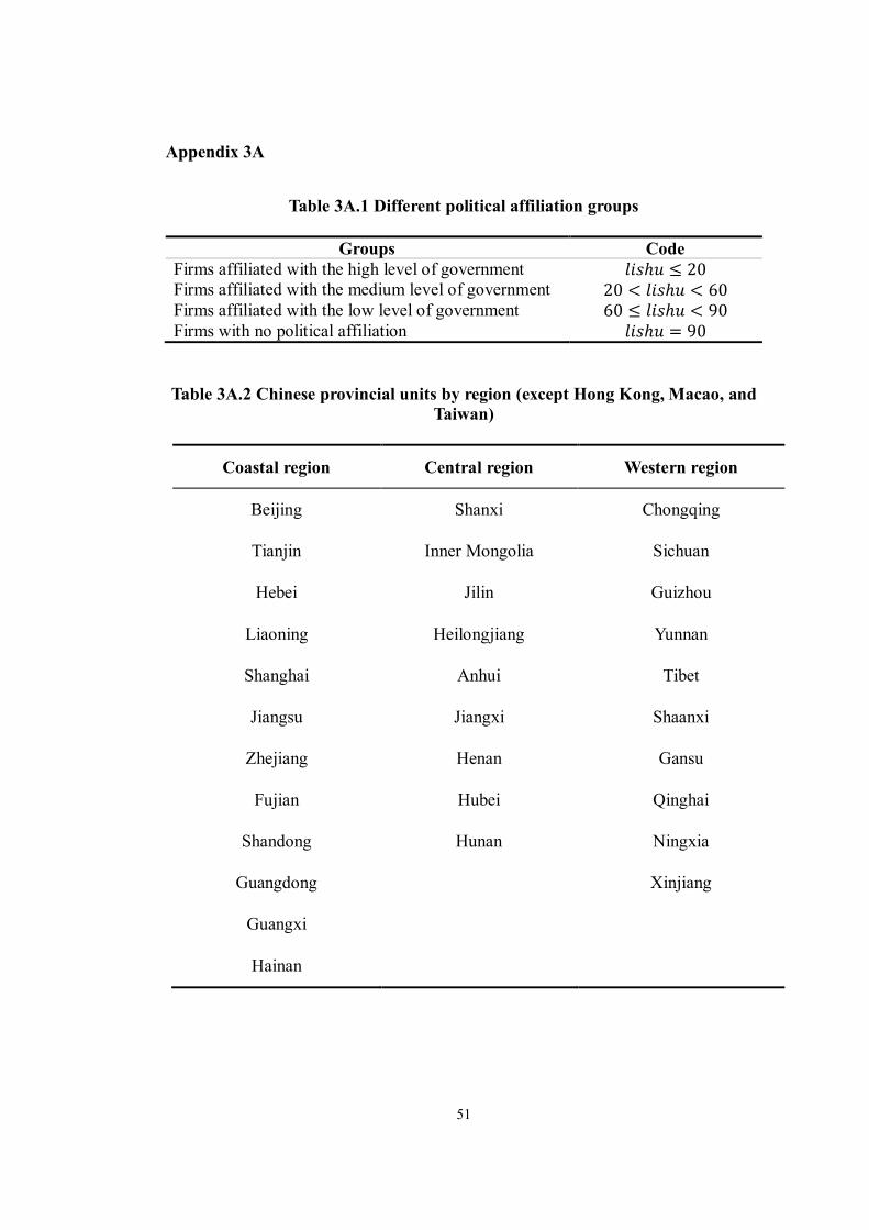
51
Appendix 3A
Table 3A.1 Different political affiliation groups
Groups Code Firms affiliated with the high level of government 𝑙𝑖𝑠ℎ𝑢 ≤ 20 Firms affiliated with the medium level of government 20 < 𝑙𝑖𝑠ℎ𝑢 < 60 Firms affiliated with the low level of government 60 ≤ 𝑙𝑖𝑠ℎ𝑢 < 90 Firms with no political affiliation 𝑙𝑖𝑠ℎ𝑢 = 90
Table 3A.2 Chinese provincial units by region (except Hong Kong, Macao, and Taiwan)
Coastal region Central region Western region
Beijing Shanxi Chongqing
Tianjin Inner Mongolia Sichuan
Hebei Jilin Guizhou
Liaoning Heilongjiang Yunnan
Shanghai Anhui Tibet
Jiangsu Jiangxi Shaanxi
Zhejiang Henan Gansu
Fujian Hubei Qinghai
Shandong Hunan Ningxia
Guangdong Xinjiang
Guangxi
Hainan
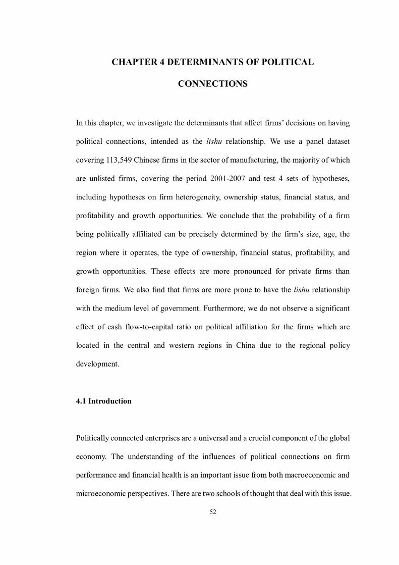
52
CHAPTER 4 DETERMINANTS OF POLITICAL
CONNECTIONS
In this chapter, we investigate the determinants that affect firms’ decisions on having
political connections, intended as the lishu relationship. We use a panel dataset
covering 113,549 Chinese firms in the sector of manufacturing, the majority of which
are unlisted firms, covering the period 2001-2007 and test 4 sets of hypotheses,
including hypotheses on firm heterogeneity, ownership status, financial status, and
profitability and growth opportunities. We conclude that the probability of a firm
being politically affiliated can be precisely determined by the firm’s size, age, the
region where it operates, the type of ownership, financial status, profitability, and
growth opportunities. These effects are more pronounced for private firms than
foreign firms. We also find that firms are more prone to have the lishu relationship
with the medium level of government. Furthermore, we do not observe a significant
effect of cash flow-to-capital ratio on political affiliation for the firms which are
located in the central and western regions in China due to the regional policy
development.
4.1 Introduction
Politically connected enterprises are a universal and a crucial component of the global
economy. The understanding of the influences of political connections on firm
performance and financial health is an important issue from both macroeconomic and
microeconomic perspectives. There are two schools of thought that deal with this issue.
53
The first one emphasises that politically connected firms can obtain several kinds of
favours, such as the favourable treatment to obtain bank loans (Brandt and Li, 2003;
Khwaja and Mian, 2005; Faccio, 2006; Fraser et al., 2006; Claessens et al., 2008),
favourable tax treatment (Adhikari et al., 2006; Faccio, 2010), profitable government
contracts and crucial licences (Leuz and Oberholzer-Gee, 2006; Goldman et al., 2010),
as well as higher market share (Faccio, 2007; Faccio, 2010).
The alternative argument is that politically associated firms underperform when
compared with the non-associated firms. This idea is supported by many studies,
including Fan et al. (2007), Faccio (2010), and Peng et al. (2011), who argue that
politically connected firms have poorer accounting performance than firms without
such connections. One of the reasons is that firms with politically connected CEOs
are more likely to appoint current or previous government officials to the board. These
officials tend to be less professional and lack experience in running a business.
Moreover, Leuz and Oberholzer-Gee (2006) point out that the investments in political
relationships could lose their value overnight because of regime changes. Therefore,
investing in political relationships could be extremely risky, and managers may have
to spend lots of time and resources to re-establish the relationships with the new
government. In this case, political connections may not always be beneficial to
enterprises’ long-term development.
Moreover, although political connections have attracted worldwide academic interest,
the definition of political connections and their influences on enterprises are different
between China and the western world as they have different political regimes. A large
54
amount of existing literature has studied private enterprises with political connections
in countries such as the United States, Malaysia and Thailand (for instance, Roberts,
1990; Agrawal and Knoeber, 2001; Johnson and Mitton, 2003; Adhikari et al., 2006;
Charumlind et al., 2006; Fraser et al., 2006; Gul, 2006; Claessens et al., 2008;
Goldman et al., 2009, 2010; Cooper et al., 2010). A few studies focus on China (see,
for example, Chow et al., 2010; Li et al., 2008; Chen et al., 2011a; Fan et al., 2008;
Tan et al., 2007).
There is a vast quantity of evidence on the correlation between political connections
and economic benefits. Most literature assumes that enterprises are politically
connected before conducting any empirical analysis. Only few researchers (for
example, Li et al., 2006; Boubakri et al., 2008; Masters and Keim, 1985; Chen et al.,
2012) have looked at another important question: what are the factors that determine
political connections. In other words, what types of enterprises are more likely to have
political connections?
In order to fill this literature gap, this chapter aims at investigating the determinants
of political connections, intended as the lishu relationship for Chinese manufacturing
firms. Specifically, this research contributes to the literature in the following ways.
Firstly, the lishu relationship is a unique type of political connections that only exists
in China. Firms can establish connections with the governments by affiliating with
different levels of government. There is hardly any research on the relationship of firm
performance, financial health and political connections intended as the lishu
relationship. As an institutional variation during the economic transition in China, it
55
is worth exploring the lishu relationship. For the first time, we estimate the
determinants of political connections from the aspect of the lishu relationship.
Secondly, a large dataset is adopted, which is provided by the National Bureau of
Statistics of China (NBS) between 2000 and 2007. This dataset contains
comprehensive economic information of firms coming from 31 provinces or province-
equivalent municipal cities (except for Hong Kong, Macao and Taiwan) across China.
Moreover, as the existing studies focus on listed firms, which do not represent the
population of Chinese firms, research on unlisted firms is very limited. This dataset
comprises a large proportion of small and young unlisted firms, representing the
population of Chinese firms better than listed firms. To the best of our knowledge, the
hypothesis on the determinants of political connections has never been explored using
such a comprehensive dataset mainly covering unlisted firms.
Thirdly, having experienced extraordinary economic growth in the past thirty years,
never in the past has China become more important world-widely than now. Given a
relatively undeveloped legal and financial system caused by significant intervention
of the government, the miracle growth speed of the Chinese economy is often
considered as a puzzle. It is the first time to explore what factors determine the lishu
relationship of firms in the context of China. Finally, we take into account various
perspectives of firm heterogeneity.
To summarise our main results, we find that older and larger firms, as well as the
financially healthy firms, are more likely to have a lishu relationship, as they are more

56
capable of affording the costs of having political relationships. Firms with foreign
ownership that are located in the east of China are less likely to affiliate with the
governments. However, firms with high profitability and sales growth do not prefer
to put their economic advantages into the risk of having political affiliation as such
relationship could lose its value overnight due to regime changes.
The remainder of this chapter is organised as follows. Section 4.2 endeavours to
review the relevant literature on the determinants of political connections. The
conceptual framework and hypotheses are provided in section 4.3. Section 4.4
introduces the specification and estimation methodology. Data sample and summary
statistics are introduced in section 4.5. Section 4.6 is devoted to presenting the
empirical analysis of the determinants of political connections. Additional tests are
presented in section 4.7. Finally, section 4.8 concludes this chapter.
4.2 Literature review
In this section, we summarise the literature on the different measurements of political
connections between China and the rest of the world, and on the determinants of
political connections.
4.2.1 Measuring political connections
Politically connected firms in the literature which looks at countries other than China
are typically defined in five ways. Firstly, at least one of the large shareholders, who

57
control 10% or more of the company’s voting rights directly or indirectly, is a
politician (e.g. a national congress member, a government minister, or a head of state)
(Faccio, 2002, 2006, 2007, 2010). Secondly, at least one of the company’s top officers
(e.g. the CEO, president or chairman) is a politician (Faccio et al., 2006; Chen et al.,
2010). A company, which is closely related to a top politician or a political party leader
through friendship, family members, and relationships with foreign politicians falls
into the third type (Faccio, 2002; Gul, 2006; Faccio et al., 2006; Leuz and Oberholzer-
Gee, 2006). The fourth group includes firms with state ownership (Boardman and
Vining, 1989; Belka et al., 1995; Dewenter and Malatesta, 2001). The final type of
connection is established by campaign contribution, which refers to a relationship
between a firm and an election candidate. That is, a firm, having supported an election
candidate in the campaign, will in return gain favours from the politician (Claessens
et al., 2008; Goldman et al., 2009; Cooper et al., 2010).
The Chinese socialist political system has attracted growing interests among scholars
studying political connections. After almost four decades of economic reform since
1978, various economic institutions in China have obtained increasing authority to
operate on market principles. However, according to Guthrie (2000), firms are still
involved in relationships with different levels of government and such relationships
can influence both firms’ strategy and performance. In addition, the Chinese
government continues to play an important role in the allocation of critical resources,
and state-owned enterprises enjoy preferential treatment in receiving bank funding
and other important resources (Chow et al., 2010; Li et al., 2008; Poncet et al., 2010).
Along with this line of research, the existing literature analyses political connections
58
in China from three different perspectives: political connections based on ownership,
political connections intended as in the other countries, and the lishu relationship.
The first form of political connections in China is established and protected by the
basic law, namely China’s Constitutional Law. Based on the ownership structure,
firms in China can be distinguished into stated-owned enterprises (SOEs),
collectively-owned enterprises (COEs), private enterprises (PEs) or foreign
enterprises (FEs). According to China’s Constitutional Law, SOEs and COEs play a
dominant role in the socialist market economy. That is, SOEs and COEs are born with
a close “state blood relation” (Liang, 2010). In this circumstance, political connections
established through ownership can be considered as a father-son blood relationship,
which is strong and long-lasting.
This type of political connection is innate rather than acquired. Unlike political
connections in western countries, SOEs and COEs are conferred with a political
relationship the moment they are established, indicating that these enterprises need no
more effort to seek political ties. In addition, such political connections are established
by the government, mainly for the purpose of controlling the life-lines of the national
economy. Chen et al. (2011a) show that the Chinese government makes use of SOEs
and COEs to achieve social and political goals. In fact, core sectors (such as natural
resources, civil aviation, real estate, and finance) are only open to SOEs and COEs in
China and the government can determine the direction of the macro economy by
directly controlling these enterprises.

59
The second form of political connections in China is similar to those in other countries.
Private firms in China seek to establish ties with politicians and governments to
survive in an environment characterised by discrimination (Liang, 2010). Most private
firms try to establish political ties by hiring current or former government officers as
their chairman or CEO (Chen et al., 2011a; Xu et al., 2011), acting as government
advisers in certain government bodies and government-affiliated organisations (Chen
et al, 2011b; Zhang and Zhang, 2005), campaigning for membership of the Chinese
People’s Political Consultative Committee (CPPCC), the National People's Congress
(NPC) or the Chinese Communist Party (CCP) (Feng et al., 2011; Chen et al., 2011b),
and even offering bribes and political contributions to the politicians in charge (Bai et
al., 2005; Fan et al., 2008).
Finally, China has a specific type of political connections called the lishu relationship,
which is exclusive to China, and the most important political connections during the
economic transition. Detailed definition of the lishu relationship and the differences
between the lishu relationship and ownership have been explored in Chapter 2. Lishu
is a Chinese word which means “belonging to”, “subordinate to”, or “directly
controlled by”. Firms can be affiliated with various levels of government. Through
this relationship, the governments can maintain administrative power to control
various aspects of the firm both directly and legally (Tan et al., 2007; Li, 2004).
Specifically, a lishu relationship implies that the government controls firms’ structures,
directors and senior manager appointments, business plans, major projects, and
operational decisions (CNPC, 1993, 1994).
60
4.2.2 Determinants of political connections
The existing studies investigate the determinants of political connections from three
perspectives, namely enterprises’ characteristics, entrepreneurs’ personal
characteristics, and the institutional analysis.
The institutional analysis can be further divided into two categories based on
corporate governance mechanisms, namely internal and external institutional
mechanisms. Internal mechanisms consist of functions and procedures created to
supervise and affect the firm’s management activities. They include board
characteristics, such as the size of the board of directors, the proportion of non-
executive directors on the board, the debt financing, the executive directors’
shareholdings, the audit committee, the internal audit function, and the choice of
external auditors (Davidson et al., 2005). External mechanisms refer to the market
and institutions that support the firms’ development.
4.2.2.1 Firm-specific characteristics
Boubakri et al. (2008) use 245 privatised firms in 14 developed and 27 developing
countries during the period 1980-2002, and perform logit regressions, to identify the
determinants of political connections. They consider that a company is politically-
connected if at least one member of its board of directors or its supervisory board is
or was a politician, including a parliament member, a minister or any other top officer.
In order to define the determinants of political connections, the authors apply logit
61
regressions to test a set of firm-specific variables (i.e. size, sector, location and
leverage), as well as a set of privatisation variables (i.e. residual government
ownership, fraction held by foreigner investors, and privatisation method).
Their results suggest that privatised firms located in a major city and in a regulated
sector (utilities, telecommunication and petroleum) are more prone to be politically
connected. Firms with a higher leverage ratio are more likely to have political
connections in order to keep them from defaulting. Moreover, politically connected
firms are generally larger with thousands of employees and more reluctant to dismiss
employees. As for privatisation variables, the results show that the residual stake of
the government yields a positive and highly significant coefficient, while the
coefficient associated with the percentage held by foreign investors is significantly
negative. These results indicate that the more significant the residual stake of the
government is, the more likely the firm is politically connected. That is, if the
government remains a larger stakeholder after privatisation, it will be more able to
appoint governmental officials as directors. Furthermore, firms privatised through
private sales are less likely to be politically connected as this type of privatisation is
characterised as concentrated ownership by private investors who focus on
profitability rather than political goals.
Masters and Keim undertake a research on the determinants of participation in the
Political Action Committee (PAC) among 1981 Fortune-ranked large corporations in
the United States. Using a logit regression, they test how firm characteristics can affect
the probability of a corporation having an active PAC in the 1981-1982 election cycle.

62
Masters and Keim (1985) define that the firms are politically-connected if they have
a PAC that contributed money to federal candidates in the election cycle.
Their results suggest that larger firms with more employees have a higher likelihood
of having a PAC. The authors point out that the administrative employees are
generally considered as the main objective of abundant PAC fund-raising and the
proportional relationship between the number of employees and the number of
administrators in a corporation is positive. Therefore, larger firms with more assets
are able to hire more employees; and a larger employment base of the firm may
indicate more administrative employees. In turn, the probability of forming a PAC is
increased with firms’ assets and the number of employees. They also find that firms
in the manufacturing or mining industries, the banking or financing or real estate
industries, the wholesale or retail trade or service industries, and the construction
industries are less likely to have a PAC. On the contrary, firms in the transportation,
energy and communication industries are more likely to have an active PAC. It has
been identified that corporations in certain industries have historically been more
heavily regulated by the federal government, in the pricing and market entrance
(Pittman, 1977; Long and Link, 1983). Therefore, firms in these industries have a
greater incentive to engage in political actions.
Masters and Keim (1985) also suggest that the greater the degree of unionisation in
the firm’s industry, the higher the probability the firm will participate in political
activity. This is because unions in an industry can raise incentives for corporations to
participate in politics by increasing government involvement in setting the minimum
63
wage and labour health standards. Additionally, the number of firms in an industry
may affect the political participation of some firms because of free rider problems.
There are strong incentives to free ride in industries with a large number of firms. In
this case, the motivation of one firm to participate in political activity decreases as the
number of firms in this industry increases. However, they do not find a precisely
determined relationship between firms’ economic performance and the decision-
making on PAC participations.
Some empirical studies have been conducted in the context of China. Li et al. (2006)
examine the determinants of political participation in China by using a matched firm-
institution data set, which is from a nationwide survey of privately owned enterprises
and provincial-level institutional indices. Their sample contains 3,258 privately
owned enterprises, including large firms and individual household businesses, drawn
from 31 provinces in mainland China. The authors define private entrepreneurs’
membership in the Chinese People’s Congress (PC) or the Chinese People’s Political
Consultative Conference (CPPCC) as political participation. Their results show that
firms with a longer history or a larger size are more prone to participate in the PC or
the CPPCC.
By applying the same definition of political connections in Li et al. (2006), Chen et
al. (2008) study the determinants of political participation of private enterprises, using
survey data of enterprises and entrepreneurs from Liuzhou in the Guangxi Province
of China. The authors conclude that the entrepreneurs in the firms with greater
registered capital, longer history, and larger number of employees are more likely to
64
participate in the PC or the CPPCC. However, they do not document ownership as an
important factor for entrepreneurs entering politics.
Yeh et al. (2010) adopt a broad definition of political connections1 and test the
determinants of political connections for Chinese listed firms over the period 1998-
2006. The dataset was jointly collected from the Taiwan Economic Journal, Market
Observation Post System, and Taiwan Stock Exchange. As the ruling party changed
from Kuomingtang (KMT) to Democratic Progressive Party (DPP) in 2000, they
divide the sample period into two periods, 1998-2000 and 2001-2006. Their final
sample comprises 303 firms per year for the first period and 555 firms per year for the
second period. The authors find that politically connected firms are characterised by
higher return on assets (ROA), lower R&D intensity, and larger size than non-
connected firms in both subsample periods. Specifically, politically-connected firms
are associated with a significantly higher average ROA (5.03% in the 1998-2000
period and 5.41% in the 2001-2006 period) than the non-connected firms (3.90% in
the 1998-2000 period and 3.93% in the 2001-2006 period), indicating that firms with
political connections have more profitable assets in generating revenue.
1 They define firms as politically connected to a certain political party when at least one of the following four conditions is met: “(1) the firm was founded or run by the political party; (2) the political party is one of the firm’s large shareholders; (3) the chairman or CEO publicly supports the presidential candidate representing a certain political party, participates in or has his/her employees participate in the presidential campaign, or was referred or reported by at least one of the major newspapers as being supportive of a certain political party; (4) one of the large shareholders, director, or top officers is/was a member of parliament, a minister, or a top government official”(Yeh et al., 2010, p.16-17).
65
4.2.2.2 Entrepreneurs’ personal characteristics
Some researchers focus on the importance of corporate executives’ personal attitudes
and personal characteristics. Jacobson (1980), for example, argues that “the individual
motives and attitudes of corporate officers are crucial in determining both the degree
of political involvement and the form it takes” (p.83). Miller et al. (1981) point out
that higher levels of education, income, and occupational status may encourage
entrepreneurs to actively engage in the political area.
Li et al. (2006) test the determinants of being a member of the PC or the CPPCC in
China by looking at the entrepreneur’s age, education background, years of
management experience, whether the entrepreneur has a rural origin, whether the
entrepreneur is a party member, and whether the entrepreneur is a former public firm
manager. They find that older entrepreneurs with more management experience are
more likely to participate in politics. Their results also show that the more education
an entrepreneur receives, the more likely he/she is to have political connections.
Additionally, entrepreneurs in the rural origin have a higher likelihood of being a
member of the PC, rather than the CPPCC, indicating that the PC can represent more
evenly the majority of the population coming from rural areas. Being a party member
or having previous work experience as a public firm manager also increases the
probability of political participation.1 The authors also suggest that both the PC and
the CPPCC pay more attention to good human capital when selecting their members.
However, party members and former public firm managers are more prone to be the
1 In China, being a Party member does not necessarily lead to the membership of the PC or the CPPCC.

66
members of the PC but not of the CPPCC.
Chen et al. (2008) evaluate entrepreneurs’ characteristics, including age, political
status, gender, education, household registration and family background and test their
relationship with the participation in the PC or the CPPCC. The authors find that
younger entrepreneurs are less likely to become members of the PC or the CPPCC,
while gender, education and household registration status do not significantly affect
their decisions. In addition, their results show that entrepreneurs with membership in
the Chinese Communist Party or other democratic parties have a greater probability
of participating in politics. Compared with other democratic parties’ membership,
those entrepreneurs belonging to the Communist Party have a much higher (five times)
probability of political participation. Chen et al. (2008) also find that entrepreneurs’
family political background is an important determinant affecting the probability of
entering politics. Parent leadership identity is a dummy variable that equals to 1 if the
entrepreneurs’ parents are officials in governments above the county level or in the
army at the corresponding level; 0 otherwise. The result indicates that parent
leadership identity increases the likelihood of entering politics for entrepreneurs,
significantly from 1.25% to 10.13%. They consider entrepreneurs’ political status and
family background as a formal de jure political power, and suggest that such political
power is a personal advantage of entrepreneurs which can be used to secure more
formal political power and to participate in politics.
67
4.2.2.3 The external institutional analysis
There is a huge amount of literature examining the underdevelopment of markets and
market-supporting institutions in developing and transition countries. According to
Bartels and Brady (2003), the institutional environment in transition economies
shapes motivations, information, and opportunities in which decisions on political
connections are made.
There are four kinds of institutional difficulties faced by private enterprises in these
countries. First, according to McMillan (1997), in the early stage of the transition,
private businesses can hardly depend on the markets, as financial markets are non-
existent and product and labour markets are elementary and undeveloped. In these
countries, the allocation of resources, including credit, is in fact tightly controlled by
the government or state-owned enterprises (Nee, 1992; McMillan, 1997; Brandt and
Li, 2003). Second, the governments may intervene in the corporate world by imposing
unnecessary regulations, known as red tape (Brunetti et al., 1997; Guriev, 2004).
According to Li et al. (2008) and Guriev (2004), red tape can be defined as excessive
official routines, and unnecessary rules or procedures resulting in delays. Firms have
to spend considerable time and resources, including pecuniary and non-pecuniary
ones, in getting through the bureaucracy. In addition, heavy formal and informal tax
burdens cost private firms substantially in transitional economies. Johnson et al. (2000)
find that the effective tax rates in Russia and Ukraine are extremely high. Local
governments may also impose different kinds of fees on corporations, and in many
cases theses fees are illegal. Finally, apart from the failures of the governments and
68
market, the legal system in these countries is also very rudimentary and weak. The
legal system can only play a limited role in protecting the property rights and the
enforcement of contracts because a sound legal framework is either non-existent or
not enforced (McMillan and Woodruff, 1999; Johnson et al., 2002).
Because of the high degree of control applied by governments and the imperfections
in the market and legal systems, private firms cannot rely on markets and market-
supporting institutions to do businesses and do not have too many choices in response
to these state and market failures. They either become passive victims or have to rely
on other organisations to do business. For example, firms in Russia and Eastern
European countries tend to go underground to reduce the high tax burdens and avoid
excessive regulations (Johnson et al., 1997, 2000; Friedman et al., 2000).
Alternatively, firms may also rely on ad hoc substitutes for the incompetent formal
institutions. Particularly, firms build their own organisations in order to succeed in
such an economy, also know as self-help (McMillan and Woodruff, 2002). For
example, corporations in Vietnam rely heavily on interfirm relationships to do
business because of the lack of the contract enforcement laws (McMillan and
Woodruff, 1999). According to Hay and Shleifer (1998), the consequence of the
absence of a sound legal system in Russia is that private mechanisms, such as social
norms or arbitration, are used to resolve disputes.
Instead of being passive victims or relying on other institutions, entrepreneurs can
actively participate in politics to overcome these difficulties. Many entrepreneurs in
Russia, for example, are eager to attend the Duma, the popularly elected lower house

69
of Russia’s legislature, so that they can protect themselves from higher taxes and
excessive regulations. Similarly, a growing number of entrepreneurs are campaigning
for the membership of the National Assembly, which is the highest legislative body in
Vietnam.
Boubakri et al. (2008) perform a cross-country analysis and define a politically
connected firm as at least one politician on its board of directors or its supervisory
board. The authors test how the judicial and political variables (i.e. government tenure,
influence of political competition, and extent of judicial independence) and
environment variables (i.e. economic development, bureaucracy, and corruption)
influence the political connections.
The authors find that political and judicial variables can significantly explain the
existence of politicians on the boards of newly privatised firms. For example, there is
a negative and significant relationship between the extent of judicial independence
and the likelihood of political connections, indicating that political appointments are
more popular in lower judicial independence countries. The results also suggest that
in order to obtain voting support and minimise frictions among veto players, a
government that features a higher fractionalisation and that has been in power for only
a few years is more likely to keep politicians on the boards of firms. As for the
institutional and macroeconomic variables, the authors do not observe a significant
explanatory power. For instance, the coefficient on bureaucracy is negative but
insignificantly related to the likelihood of political connections. Additionally, there is
no relationship between corruption and getting political connections for privatised
firms.
70
Li et al. (2006) construct an institutional index, including the development of product
markets, the development of credit markets, government regulations, the informal tax
burden, and the legal system. The authors point out that the underdevelopment of the
market, especially the credit market, can raise the likelihood of political participation,
indicating that the credit market is more specific according to different provinces and
is more crucial in deciding political connections. They also illustrate that firm owners
in provinces with an overregulation burden and without a sound legal enforcement are
more prone to have political connections. The effect of the informal tax burden,
however, is less significant in these regressions. The findings suggest that one
standard deviation increase in the institutional indices can decrease the probability of
entrepreneurs entering politics by 8% to 20%, supporting the view that the
institutional environment shapes the motivation of private firms’ owners to create
political connections.
4.2.2.4 The internal institutional analysis
Instead of analysing the rationale for political connections from an external
governance perspective, some researchers explore the determinants of political
connections from the perspective of firms’ internal governance structure. According
to Yeh et al. (2010), an internal institutional analysis can be done based on the
following two reasons.
First, the external governance structure and legal protection for minority shareholders
are weak in most developing countries. For example, according to Claessens and Fan
71
(2002), in some regions in Asia characterised by weak institutions and poor property
rights, the limited protection of minority rights allows controlling shareholders to
expropriate the minority shareholders. It is therefore unrealistic to rely on an external
corporate governance mechanism.
In addition, the relations between some firms’ characteristics affected by the internal
governance structure and political connections remain ambiguous. According to
previous studies, the relations between political connections and firms’ performance
can be positive or negative. For example, according to Bunkanwanicha and
Wiwattanakantang (2009), the market-to-book value of equity of the politically
connected firms can increase astonishingly by more than 200%. However, Bertrand
et al. (2006) find that accounting and stock market performance of firms with
politically connected CEOs are lower than those of non-connected firms in France.
Therefore, it is necessary to investigate the relationship between internal governance
and the likelihood of having political participation.
Yeh et al. (2010) point out that the quality of corporate governance is related to firms’
decisions to engage in political connections and can be illustrated from both a cost-
benefit perspective and a demand-side perspective.
The costs of political connections include governmental interferences and rent
expropriated by the connected politicians (Yeh et al., 2010). According to Black et al.
(2006) and Brown and Caylor (2006), corporate governance is a crucial factor in
determining firm value and performance. Firms with a superior governance structure

72
are supposed to be associated with better performance or higher firm value. In contrast,
firms with an inferior governance structure are expected to have poorer performance
or lower firm value. For the latter firms, governmental interventions, such as bailout
when firms face financial distress, are important and therefore, the marginal benefit
of such interventions is supposed higher. Therefore, governmental interventions are
particularly helpful for firms with poor governance structure and the rent charged by
politicians is likely to be small compared with the huge benefits they can offer,
indicating that the cost of political connections for these firms is minimal.
As for the demand-side perspective, firms with poor governance would demand more
political connections in order to obtain more help and aid from such connections.
Because aid and interventions are crucial to the development of firms with poor
governance, the marginal benefit of having these connections can almost offset the
marginal cost. These firms are therefore more willing to spend money and other
resources in having political connections. At the same time, it is easier for firms with
poor governance structure to reallocate resources for political connections, because
poor governance does not require enterprises to follow accurate accounting standards
and thus the firms have more cash to use for other activities, such as political
connections.
Before analysing the relationship between quality of internal corporate governance
and political connections, Yeh et al. (2010) exclude the external governance
environment from their hypothesis development. They assume that the external
governance structure is fixed for all firms and is related to a lower marginal cost and
73
a higher marginal benefit when the external governance structure is ineffective.
According to Bøhren and Ødegaard (2003), the true relationship between firm
performance and corporate governance may not be appropriately captured if corporate
performance relates to one particular aspect of corporate governance. Inspired by this
argument, Yeh et al. (2010) emphasise the internal governance structure to develop a
single governance index, which is a scorecard that measures a firm’s corporate
governance over three dimensions: ownership structure (including four dummies:
controlling shareholders’ cash flow rights, voting rights, the voting-cash deviation,
and pledge ratio), board structure (including two dummies: board control and
supervisory control), and related party transactions (including four dummies: sale,
purchase, loan, and guarantee). This corporate governance index (CGI) is constructed
by summing these ten dummies. The value falls in the range between 0 and 10. The
average score of CGI is 4.97 in the 1998-2000 period and 5.40 in the 2001-2006 period,
indicating that the overall corporate governance structure improved marginally over
time.
The results suggest that politically connected firms have a lower corporate governance
index. Specifically, the average CGI of politically connected firms (4.38 in the 1998-
2000 period and 4.56 in the 2001-2006 period) is significantly lower than that of their
non-connected counterparts (5.40 in the 1998-2000 period and 5.52 in the 2001-2006
period), suggesting that politically connected firms have worse corporate governance
structure than the non-connected firms.
74
4.3 Conceptual framework and hypotheses
4.3.1 Conceptual framework in the existing literature
Researchers in political science and economics have given theoretical consideration
to the political participation of private enterprises. They provide three different
perspectives to explain why a firm might want to have political connections: the
political science perspective, the organisational science perspective, and the economic
cost-benefit perspective.
4.3.1.1 Political science perspective
Political scientists state that both non-pecuniary and economic motives are the
determinants for enterprise participating in politics. According to Bentley (1995),
political participation results from the demands of social interests or social welfare.
Verba (1987) points out that effective political participation has a particularly crucial
relationship with all other social and political goals. It represents a procedure by which
goals are set and means are chosen in relation to all sorts of social issues. Through
participation, the goals of the society are set in a way that is assumed to maximise the
allocation of benefits in a society to match the needs and desires of the whole
population. In this case, participation is not committed to any social goal, but is a
technique for setting goals, choosing priorities, and deciding what resources are
required to achieve goals. Entrepreneurs are therefore willing to participate in politics
so that they can communicate firms’ needs with the governmental demands. Verba

75
(1987) also points out that participation in politics brings satisfaction to entrepreneurs:
satisfaction with governments and satisfaction with their own role.
Olson (2002) points out that the willingness of an enterprise to have political
connections is due to the expectation of obtaining additional benefits from the
government. The author states that political institutions have clear organisational
structures which determine that they are more prone to provide benefits to particular
individuals and groups, instead of any collective group with common interest. The
political institution is “at best interested in patronage, and at worse on outright graft”
(Olson, 2002, p.165). Many businessmen are willing to make contributions to political
parties so that they can obtain support from the governmental officials. In other words,
this provides economic motives and incentives for entrepreneurs to join these political
organisations or to make political patronage to officials so that they can obtain benefits
that are available only to a minority group.
4.3.1.2 Organisational science perspective
Organisation theorists apply a resource dependency theory, suggesting that political
action is motivated by an institution’s dependency on governments. According to
Pfeffer and Salancik (2003), resource dependence suggests that some organisations
have more power than others because of their control of resources and their location
in the social space. For instance, the government is a crucial provider of resources to
a number of industries and firms. Under these circumstances, organisations which rely
heavily on the government have more incentives to participate in politics in order to
76
get more resources and power. Therefore, the resource dependency theory may be the
basis for the entrepreneurs to make the decision to get involved in politics.
4.3.1.3 Economic cost-benefit perspective
Economists emphasise that an economic cost-benefit analysis is key to political
participation. Pittman (1977) considers that an economic system includes two actors,
namely individual firms, which are rational actors, and governments, the other
important actors. Firms can benefit or be restrained due to various actions taken by
governments. Each firm would like to affect government activities for its own benefit,
which can be achieved by political involvement. However, such benefits only come
at a cost. Therefore, only those firms who expect the benefits of influencing policy to
outweigh the costs of political engagement will make the effort to participate in
politics.
According to Pittman (1977), the benefits which can be achieved from impacting the
government depend on the government’s role in a particular industry. For example,
the government plays a role in some industries from the perspectives such as making
health and safety regulations and laws. In these industries, the government’s role is
important enough so that the potential benefits of the influence can be considerable.
Yet for some industries, the government’s role is so small that the potential benefits
of influencing may be small, indicating it is not worth to invest in political
involvement. Pittman (1997) considers three aspects of government’s intervention in
industry, including government regulation, government purchase of output, and
77
government antitrust investigation, and suggests that any of them could substantially
augment the benefits available to a firm by affecting government policy. Although the
costs of impacting the government may be higher for some firms than others, they are
of a comparable scale for all participants and always measured in dollar terms. Pittman
(1977) presents a theory of political involvement, which suggests that a firm is willing
to be involved in politics only if the policy influence is worth the cost, which would
happen if the government plays an important role in the industry in which the firm
operates.
Data limitations hinder the full specification and testing of any framework. For
example, the non-pecuniary motivations for firms’ political participations may be
extremely difficult to capture. In addition, executives’ ideologies are also difficult to
measure. In this analysis, the expected costs-benefits framework is explored. It intends
to capture the common argument that profit motivation is behind firms’ political
investments. It is literally impossible to measure these costs and benefits on a firm-
specific basis, as data on the costs and benefits related to political participation are
unavailable. However, it is possible to identify several organisational and contextual
factors that may have influence on these expected costs and benefits. These factors
form the basis of our hypotheses described below.
4.3.2 Hypotheses
In this section, we propose four sets of hypotheses on firm heterogeneity, ownership
types, financial status, and profitability and growth opportunities.
78
4.3.2.1 Hypotheses on firm heterogeneity
This section presents the hypotheses on firm heterogeneity, including firm size and
location.1
A. The firm size
The ability of corporations to have connections with politicians depends heavily on
the size of the resource base they have. A firm’s size can be measured from two
dimensions: total number of employees and total assets.
According to Masters and Keim (1985), administrative employees are generally
considered as the prime targets of creating political connections, as corporations raise
most of their political connection money from administrative or managerial
employees compared with shareholders or non-managerial employees. In addition, an
increase in the total number of employees will lead to an increase in the number of
1 According to the previous literature, firm age, in terms of how many years ago the firm has come into existence, is a significant determinant for political connections. However, there are two different views on the interaction between firms’ age and the likelihood of political participation. One school of thought argues that firms in their early lives are more eager to create connections with governments because they are in greater need of political help when they establish themselves in the concentrated business environment (Leuz and Oberholzer-Gee, 2006). Another school of thought states that entrepreneurs from long-standing enterprises are more likely to be involved in politics. For example, in the Chinese context, Li et al. (2006) show that entrepreneurs from firms with a longer history are more prone to participate in politics suggesting that the probability of political participation rises with firms’ age. In addition, Chen et al. (2008) point out that politically connected corporations are three years older than their non-connected counterparts, and that increasing one year in enterprises history will increase the probability of political participation. It is therefore interesting to look at how the lishu relationship is affected by firm age using our large dataset in Chinese unlisted firms. As the missing value of firm age in our dataset are 246,250 firm-year observations. We only perform the test including firm age and report the results in Appendix. And our result supports the latter thought by showing that firm age a positive and precise determinant for firms’ political participation. The results for other variables are robust.
79
administrative staff in a firm. Along with this line of research, firms with a larger
employment base should have more administrative employees who are more likely to
make sufficient money for the candidates in a political campaign, as political
contributions. Therefore, the firms can obtain favourable support from such
candidates in the future. Li et al. (2006) use 3,258 privately owned enterprises and
individual household businesses in China, and indicate a positive interaction between
the number of employees and political participation, suggesting that firms with a large
scale of employment are more likely to have political connections.
In China, the current election system regarding the representatives of the People’s
Congress (PC) at various levels provides a channel for private entrepreneurs to
participate in political areas, which stimulates entrepreneurs from enterprises with a
large employment base to get involved in politics. According to Article 24 of Chapter
6 of the Electoral Law of the People's Republic of China, the electorates for the PC
committee are not exclusively divided on the basis of territory. When territory is not
applicable, the division of electoral districts depends on the voters’ residence or
industry, including the basis of production units, institutions units and work units.
In practice, especially in cities, the People’s Congress and its Standing Committee at
the relative levels accept a method that combines both industry and residence to divide
electoral districts. Dividing electoral districts by residence refers to dividing them on
the basis of people’s household registration or habitual residence, especially the
amount of population in the area with concentrated large enterprises. In this case, the
more employees the firm has, the more votes an entrepreneur can have as a candidate,

80
thus the larger probability he/she becomes a member of the PC.
Dividing electoral districts by industry suggests dividing a large firm into one or more
electoral districts if the firm has a large number of employees in different industries.
For example, election committees divide districts of the large state-owned enterprises
affiliated with local governments, according to resources, finance, trade and
transportation, in order to make these districts more representative. Under these
circumstances, a large firm with a large number of employees in various industries
has more opportunities to vote its entrepreneurs as representatives of the PC to
represent different industries. Therefore, the political participation can be enhanced
by this channel (Chen et al., 2008).
In addition to the total number of employees, the total assets a firm has should also be
positively related to the probability of having political affiliation. Masters and Keim
(1985) point out that the incremental costs of raising more contribution funds are
relatively small for larger firms as the initial fixed costs of connecting with the
politicians can be spread over a larger asset base. This should increase the chances
and the amount of money that larger firms can raise. Therefore, the larger firms have
more money to afford the expenditure on having political connections with political
candidates. Because larger firms have more assets to take the risk of connecting with
politicians and thus are able to obtain a larger share of political benefits caused by
corporate political activities, they are more likely to be politically connected than
smaller firms.

81
Yeh et al. (2010) also find that the probability for firms to engage in political activity
is positively associated with the firm’s total assets. Boubakri et al. (2008) define firm
size as the natural log of total sales when the privatisation occurred and find that firms
with political connections are larger than non-connected firms. In addition, Agrawal
and Knoeber (2001) and Faccio (2006) find that political connections are more
common in larger firms. Chen et al. (2008) illustrate that the incremental probability
of entrepreneurs’ political participation increases from 0.08% to 1.11% if the
registered capital is doubled, indicating that entrepreneurs from large firms have a
higher probability of participating in politics. In line with these studies, we therefore
expect that a firm’s size has a positive relationship with the likelihood of political
participation.
Hypothesis 1A (H1A): A firm’s size is positively related to the probability that the firm
has a lishu relationship, ceteris paribus. 1
B. Firm location
Firm location can also influence political connections. Boubakri et al. (2008) use 245
privatised firms, the headquarters of which are located in 14 developed and 27
developing countries during 1980 and 2002, pointing out that firms locating in the
major cities are more likely to have politicians on their boards, and these firms are
more likely to attract political support. In addition, Chen et al. (2005) point out that,
1 As the correlation between the number of employees and the firms’ total assets is 0.554, we use the number of employee as a substitution for the total assets and report the results in Appendix. The results are robust.
82
in China, family firms in provinces with less developed markets are prone to have
political connections. Similarly, business transactions are more likely to depend on
personal relationships in regions with less developed markets. In these regions, local
governments usually have more flexibility in setting policies and regulations. In China,
the western region is generally considered as the less developed area, while the coastal
region is considered as more developed. Roberts (1990), Fan et al. (2007), and Khwaja
and Mian (2005) support the relationship between firm location and the decision of
political participation. According to this line of research, it is expected that firms
located in the west of China are more likely to have political affiliation.
Hypothesis 1B (H1B): A firm located in the west (coastal) of China has a higher
(lower) probability of having a lishu relationship, ceteris paribus.
4.3.2.2 Hypothesis on firm’s ownership status
According to Boubakri et al. (2008), the likelihood of having political connections in
newly privatised firms is positively associated with government residual ownership
and negatively related to foreign ownership. The government has more power to
appoint the “friends” as directors if a significant governmental shareholding remained
in the firm after privatisation. For example, Bertrand et al. (2006) use all publicly-
traded firms in France over the period 1987 to 2002 and find that CEOs with political
connections are more likely to head previously state-owned enterprises. It suggests
that the higher the residual stake of the government, the higher the probability that the
privatised firm will have political connections.

83
Using a cross-country dataset, Dyck (2001) states that foreign investors are less likely
to accept the political judgment of bureaucrats, as they monitor managers’ actions
closely and pay more attention to profitability than political goals. Therefore, it is
expected that firms are less likely to have political affiliation when foreign investors
are involved in the ownership structure.
Hypothesis 2 (H2): Foreign-owned (State-owned) firms are less (more) likely to have
a lishu relationship, ceteris paribus.
4.3.2.3 Hypotheses on firm’s financial status
A large number of finance and macroeconomics literature studies the presence and
importance of financing constraints and its relationship with firms’ behaviour.
According to the Pecking Order Model and Trade-off Theory, the first choice for a
company is internal financing, followed by debt and equity (Myers, 1984). In 1958,
Modigliani and Miller (MM) demonstrated that the firm’s value is irrelevant to its
capital structure, as internal financing and external financing can substitute each other
perfectly. However, this hypothesis does not hold in the real world, because of the
asymmetric information and the agency problem in the market. Lamont et al. (2001)
define financial constraints as frictions which can deter firms from funding all their
investments. It is therefore expected that less financially constrained firms are more
able to invest in political connections. A firm’s financial status can be measured by
the external financing and the internal financing.
84
A. External financing
We use the leverage ratio as a proxy for preferential access to the credit market. The
leverage ratio is defined as a firm’s total debt to total assets ratio (Johnson and Mitton,
2003; Faccio et al., 2006; Faccio, 2007).
In the previous literature, a high leverage ratio is associated with soft budget
constraints. Therefore, the firms with high leverage ratio are more likely to have
political connections. The literature provides two possible interpretations for the high
leverage ratio observed in private firms with political affiliation (for instance, Lamont
et al., 2001; Faccio et al., 2006; Boubakri et al., 2008). First, lenders can obtain
offsetting benefits from governments for making loans to politically connected firms.
Second, highly indebted private firms’ executives are more prone to appoint
politicians to keep them from defaulting. In this case, politically connected borrowers
will be bailed out when they encounter economic distress.
Therefore, it is expected that politically affiliated firms would have a higher leverage
ratio than their non-connected peers, i.e.:
Hypothesis 3A (H3A): A firm with a higher (low) leverage ratio is more (less) likely
to have a lishu relationship, ceteris paribus.
85
B. Internal financing
Cash flow is commonly used in empirical work as a proxy of the firm’s internal funds
(for example, Schiantarelli, 1995; Hubbard, 1998; Bond and Van Reenen, 2003;
Guariglia, 2008).1 According to Schiantarelli (1995), cash flow is not only a proxy
for internal net worth, but also delivers information about what percentage of
investment spending can be financed internally. In this case, a firm with a higher level
of cash flow faces less internal financial constraints and may find it easier to fund
firms’ investment. Along with this research, it is expected that firms with higher level
of cash flow are more likely to have a lishu relationship.
Hypothesis 3B (H3B): A firm with higher (lower) cash flow is more (less) likely to
have a lishu relationship, ceteris paribus.
4.3.2.4 Hypotheses on profitability and growth opportunities
A firm’s profitability can also influence the probability to be politically affiliated.
However, there is a debate over how profitability can affect the decision making of
political participation. On the one hand, political participation can be encouraged in
firms with more profits, as they have more resources to allocate to such political
activities. Focusing on Taiwanese firms, Yeh et al. (2010) find that the average return
on assets (ROA) is significantly higher for the connected firms (5.03% in 1998-2000
1 Liquidity ratio is another common proxy for the level of internal funds available to the firm. However, as the correlation between liquidity ratio and leverage ratio is -0.650, we only report the results by using liquidity ratio in Appendix. And the results are robust.
86
period and 5.41% in 2001-2006 period) than that for the non-connected firms (3.09%
in the 1998-2000 period and 3.93% in the 2001-2006 period), indicating that firms
with higher ROA are more likely to connect with politicians. It is also argued that this
result suggests that firms with abundant resource can spend money to create political
connections.
On the other hand, lucrative firms may not want to put their economic position at risk
by involving themselves in political activities. Salamon and Siegfried (1977) analyse
the firms in the United States and argue: “Firms earning higher than average profits
may shy away from political action if they fear that such action would attract public
attention to the monopoly position that yields them such large profits” (p.1033). In
addition, according to Leuz and Oberholzer-Gee (2006), investing in political
relationship could be extremely risky in Malaysia, because political connections can
lose their value overnight. In this case, these lucrative firms might not want to put
their profits at risk, especially in developing countries.
In order to examine whether a firm’s profitability is positively related to its likelihood
of political participation or not, we employ an accounting-based measurement for firm
profitability, the return on sales (ROS) (Tallman and Li, 1996; Hitt et al., 1997). We
hypothesise that:
Hypothesis 4A (H4A): A firm’s ROS is negatively related to its likelihood of having a
lishu relationship, ceteris paribus.

87
Yeh et al. (2010) consider sales growth as one of the factors that determine the choice
of political participation. In their analysis, politically connected firms have a lower
sales growth (4.63% in the 1998-2000 period and 18.50% in the 2001-2006 period)
compared with the non-connected firms (10.01% in the first period and 31.76% in the
latter period). Firms with poor performance associated with lower sales growth may
need to seek more help from governments, suggesting that firms with a higher sales
growth are less likely to engage in political connections. In line with Yeh et al.’s (2010)
research, it is expected that sales growth is negatively related to political connections.
Hypothesis 4B (H4B): A firm with a high (low) sales growth has a lower (higher)
probability of having a lishu relationship, ceteris paribus.
The hypotheses can be summarised as shown in Table 4.1.
Table 4.1 Summary of hypotheses
Hypothesis Number Variables Expected Sign
H1A Total Assets +
H1B Western Region +
Coastal Region _
H2 State Ownership +
Foreign Ownership _
H3A Leverage Ratio + H3B Cash Flow Ratio + H4A ROS _
H4B Sales Growth _
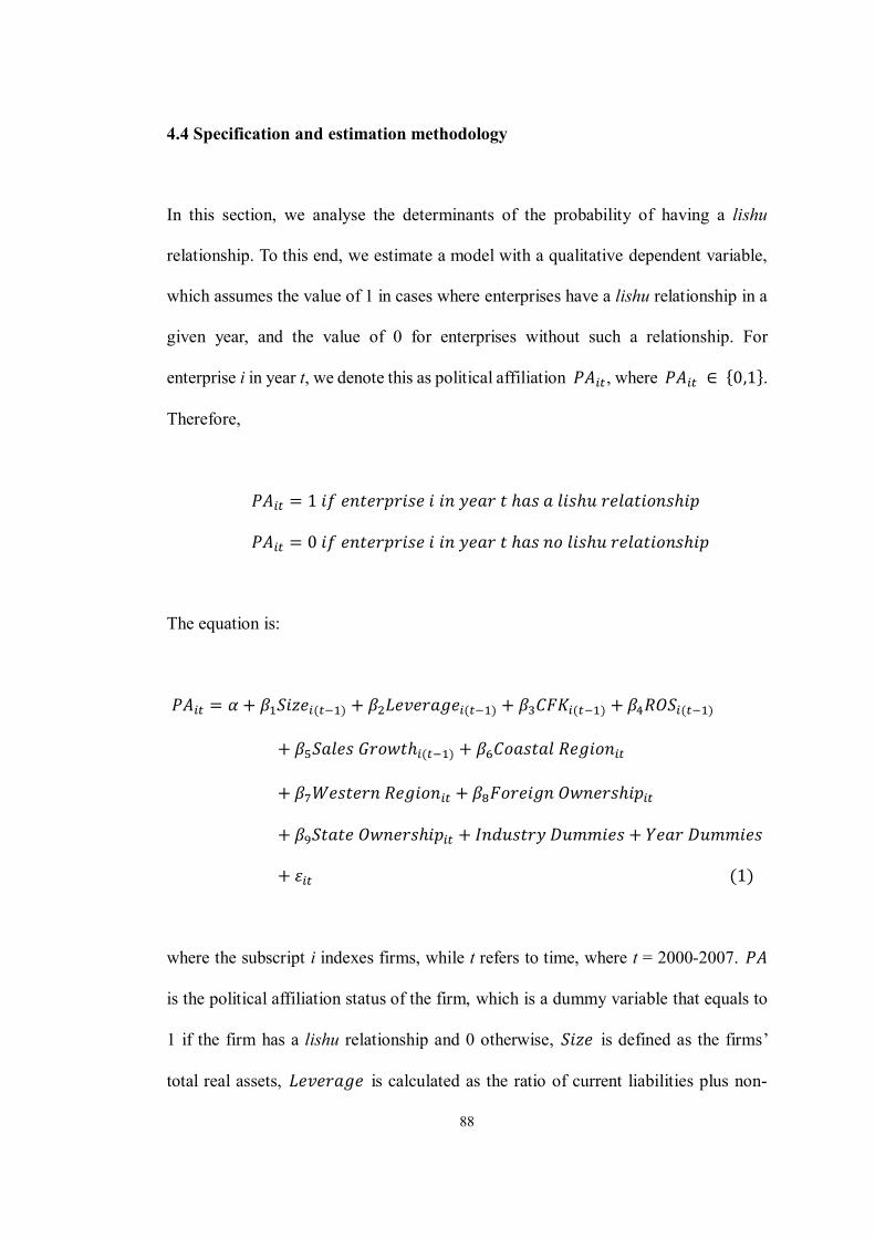
88
4.4 Specification and estimation methodology
In this section, we analyse the determinants of the probability of having a lishu
relationship. To this end, we estimate a model with a qualitative dependent variable,
which assumes the value of 1 in cases where enterprises have a lishu relationship in a
given year, and the value of 0 for enterprises without such a relationship. For
enterprise i in year t, we denote this as political affiliation 𝑃𝐴𝑖𝑡, where 𝑃𝐴𝑖𝑡 ∈ {0,1}.
Therefore,
𝑃𝐴𝑖𝑡 = 1 𝑖𝑓 𝑒𝑛𝑡𝑒𝑟𝑝𝑟𝑖𝑠𝑒 𝑖 𝑖𝑛 𝑦𝑒𝑎𝑟 𝑡 ℎ𝑎𝑠 𝑎 𝑙𝑖𝑠ℎ𝑢 𝑟𝑒𝑙𝑎𝑡𝑖𝑜𝑛𝑠ℎ𝑖𝑝
𝑃𝐴𝑖𝑡 = 0 𝑖𝑓 𝑒𝑛𝑡𝑒𝑟𝑝𝑟𝑖𝑠𝑒 𝑖 𝑖𝑛 𝑦𝑒𝑎𝑟 𝑡 ℎ𝑎𝑠 𝑛𝑜 𝑙𝑖𝑠ℎ𝑢 𝑟𝑒𝑙𝑎𝑡𝑖𝑜𝑛𝑠ℎ𝑖𝑝
The equation is:
𝑃𝐴𝑖𝑡 = 𝛼 + 𝛽1𝑆𝑖𝑧𝑒𝑖(𝑡−1) + 𝛽2𝐿𝑒𝑣𝑒𝑟𝑎𝑔𝑒𝑖(𝑡−1) + 𝛽3𝐶𝐹𝐾𝑖(𝑡−1) + 𝛽4𝑅𝑂𝑆𝑖(𝑡−1)
+ 𝛽5𝑆𝑎𝑙𝑒𝑠 𝐺𝑟𝑜𝑤𝑡ℎ𝑖(𝑡−1) + 𝛽6𝐶𝑜𝑎𝑠𝑡𝑎𝑙 𝑅𝑒𝑔𝑖𝑜𝑛𝑖𝑡
+ 𝛽7𝑊𝑒𝑠𝑡𝑒𝑟𝑛 𝑅𝑒𝑔𝑖𝑜𝑛𝑖𝑡 + 𝛽8𝐹𝑜𝑟𝑒𝑖𝑔𝑛 𝑂𝑤𝑛𝑒𝑟𝑠ℎ𝑖𝑝𝑖𝑡
+ 𝛽9𝑆𝑡𝑎𝑡𝑒 𝑂𝑤𝑛𝑒𝑟𝑠ℎ𝑖𝑝𝑖𝑡 + 𝐼𝑛𝑑𝑢𝑠𝑡𝑟𝑦 𝐷𝑢𝑚𝑚𝑖𝑒𝑠 + 𝑌𝑒𝑎𝑟 𝐷𝑢𝑚𝑚𝑖𝑒𝑠
+ 휀𝑖𝑡 (1)
where the subscript i indexes firms, while t refers to time, where t = 2000-2007. 𝑃𝐴
is the political affiliation status of the firm, which is a dummy variable that equals to
1 if the firm has a lishu relationship and 0 otherwise, 𝑆𝑖𝑧𝑒 is defined as the firms’
total real assets, 𝐿𝑒𝑣𝑒𝑟𝑎𝑔𝑒 is calculated as the ratio of current liabilities plus non-
89
current liabilities to total assets of the firm, 𝐶𝐹𝐾 is defined as the ratio of cash flow
over the tangible fixed assets, and 𝑅𝑂𝑆 is the return on sales, a measure of the firm’s
profitability. Regional dummies include: Western Region = 1 if the firm is located in
the western region, and 0 otherwise; Coastal Region = 1 if the firm is located in the
coastal region, and 0 otherwise. Ownership dummies include: Foreign Ownership =
1 if the firm is owned by foreign investors (including investors from Hong Kong,
Macao, and Taiwan), and 0 otherwise; State Ownership = 1 if the firm is owned by
the state, and 0 otherwise.
Industry dummies define firms to be located in one of the following ten industrial
sectors: metal and metal products; non-metal products and petroleum processing;
chemicals and plastic; machinery and equipment; electrical equipment; transport
equipment; food and tobacco; textile; leather, timber and furniture; and mining and
logging. Year dummies are also included to account for business cycle effects and
firm-invariant market factors such as changes in government policy.
According to our Hypothesis 1A, we expect the β1 to show a positive sign. Firms
with higher leverage ratio and cash flow-to-capital ratio are expected to be positively
related to the probability of having a lishu relationship. We also expect that less
profitable firms with lower growth opportunities are more prone to have a lishu
relationship. Firms locate in the west of China are more likely to be politically
affiliated, while firms locate in the east are less likely to have a lishu relationship.
Compared with SOEs, foreign firms are more reluctant to affiliate with the
governments.
90
In order to mitigate problems stemming from reverse causality (for example, the
causality is from having a lishu relationship to larger size), all the variables, except
for dummies, are once-lagged, following the research of Cull et al. (2009).
As the dependent variable is dichotomous, linear multiple regression is not
appropriate for estimating the model. We therefore use a Probit model instead to
estimate the effect of how the independent variables affect the probability of a firm
having a lishu relationship. We firstly employ a pooled Probit and then a random-
effects Probit models to control for the unobserved firm heterogeneity.
4.5 Data and summary statistics
This section describes the dataset used in this chapter, and presents summary statistics.
4.5.1 Data
The firm-level data used in this study are taken from the National Bureau of Statistics
of China (NBS). In order to strengthen the reliability of our analysis, we first drop
observations which make little sense, such as those with negative real assets, negative
age, and negative leverage ratio. Second, we eliminate firms without completed
records on our main regression variables. Finally, in order to control the potential
effect of extreme values, we drop the outliers, which are the observations beyond the
91
1st and the 99th percent tails for each continuous main regression variables.1 After
these adjustments, our final panel dataset includes 469,938 firm-level observations,
covering 113,549 mainly unlisted firms over the period 2001-2007.2 The sample has
an unbalanced structure,3 with a number of observations ranging from a minimum of
33,855 in 2001 to a maximum of 86,577 in 2005.
Table 4.2 presents the distribution of the full sample, affiliated group, and non-
affiliated group by year and industry. On average, around 46.13% of our firm-year
observations have a lishu relationship. This can be explained that the political and
market environment has become more supportive for the private firms in China
because of the economic reforms since the 1990s. Therefore, these firms can develop
in a relatively stable environment. However, governments still play a crucial role in
China. Focusing on the industry groups, we find that the number of observations for
affiliated firms only beats that for non-affiliated firms in food and tobacco (50.16%
vs. 49.84%) and mining and logging industry (54.54% vs. 45.46%), while firms in
other industries are less likely to have a lishu relationship. Since 1981, the State
Council of China has established the State Tobacco Monopoly Administration, which
fully controls the tobacco industry all over China. Besides, the food industry is crucial
to people’s livelihood. Therefore, the political affiliation is prevalent in these
1 It is quite common in the literature (see Greenaway et al., 2007; Guariglia, 2008; Carpenter and
Guariglia, 2008; Yan, 2012) to eliminate extreme values in this way. 2 It should be noted that our dataset include a very small proportion of listed firms for two reasons. First of all, according to Liu and Xiao (2004), when firms become listed, their legal identification numbers are changed; it is therefore hard to track these firms. The second reason is that there is no separate identification of Chinese publicly listed firms in the NBS dataset. However, they only comprise a very small portion of the whole sample. Over the whole considered period, only approximately 1,000 listed firms in the manufacturing and mining sectors, accounting for less than 0.3% of the total number of firms in the sample. 3 See Appendix for details about the structure of the panel.
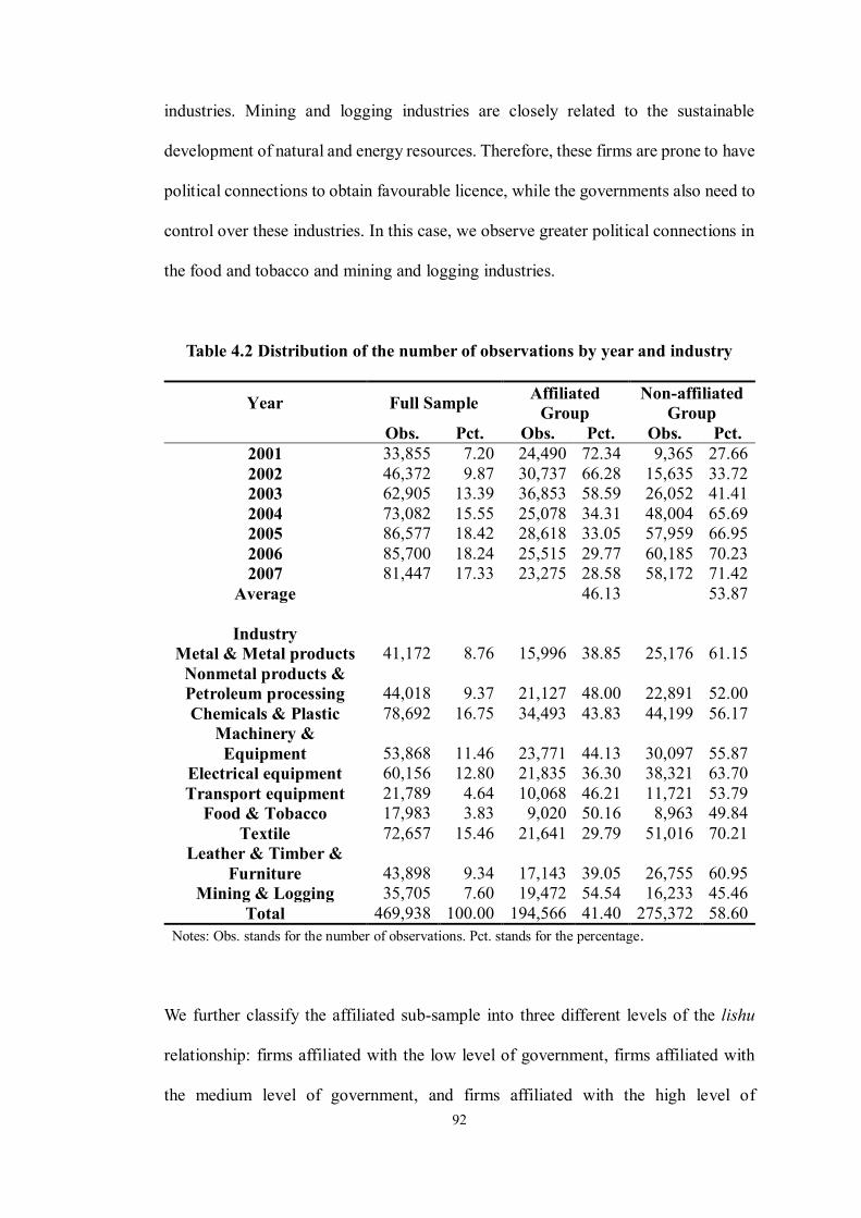
92
industries. Mining and logging industries are closely related to the sustainable
development of natural and energy resources. Therefore, these firms are prone to have
political connections to obtain favourable licence, while the governments also need to
control over these industries. In this case, we observe greater political connections in
the food and tobacco and mining and logging industries.
Table 4.2 Distribution of the number of observations by year and industry
Year Full Sample Affiliated Group
Non-affiliated Group
Obs. Pct. Obs. Pct. Obs. Pct. 2001 33,855 7.20 24,490 72.34 9,365 27.66 2002 46,372 9.87 30,737 66.28 15,635 33.72 2003 62,905 13.39 36,853 58.59 26,052 41.41 2004 73,082 15.55 25,078 34.31 48,004 65.69 2005 86,577 18.42 28,618 33.05 57,959 66.95 2006 85,700 18.24 25,515 29.77 60,185 70.23 2007 81,447 17.33 23,275 28.58 58,172 71.42
Average 46.13 53.87
Industry Metal & Metal products 41,172 8.76 15,996 38.85 25,176 61.15
Nonmetal products & Petroleum processing 44,018 9.37 21,127 48.00 22,891 52.00 Chemicals & Plastic 78,692 16.75 34,493 43.83 44,199 56.17
Machinery & Equipment 53,868 11.46 23,771 44.13 30,097 55.87
Electrical equipment 60,156 12.80 21,835 36.30 38,321 63.70 Transport equipment 21,789 4.64 10,068 46.21 11,721 53.79
Food & Tobacco 17,983 3.83 9,020 50.16 8,963 49.84 Textile 72,657 15.46 21,641 29.79 51,016 70.21
Leather & Timber & Furniture 43,898 9.34 17,143 39.05 26,755 60.95
Mining & Logging 35,705 7.60 19,472 54.54 16,233 45.46 Total 469,938 100.00 194,566 41.40 275,372 58.60
Notes: Obs. stands for the number of observations. Pct. stands for the percentage.
We further classify the affiliated sub-sample into three different levels of the lishu
relationship: firms affiliated with the low level of government, firms affiliated with
the medium level of government, and firms affiliated with the high level of

93
government. Table 4.3 reports the distribution of the number of observations by year
and industry for these three different groups. We observe that for the firms with the
lishu relationship, most of them are affiliated with the medium level of government
(20.29%), followed by firms affiliated with the low level of government (19.96%),
while only 5.88% of our firm-year observations have a high level of lishu relationship.
A similar pattern is observed in the industry distribution. Most of the industries are
affiliated with the medium level of government. This might be attributed to the fact
that the government at this level can access important resources, as well as enjoy some
authorities to support the firms’ development.
Table 4.3 Distribution of the number of observations for three affiliated groups by year and industry
Year Low Medium High Obs. Pct. Obs. Pct. Obs. Pct.
2001 10,906 32.21 10,510 31.04 3,074 9.08 2002 14,391 31.03 12,678 27.34 3,668 7.91 2003 17,963 28.56 14,930 23.73 3,960 6.30 2004 9,056 12.39 12,131 16.60 3,891 5.32 2005 11,318 13.07 13,484 15.57 3,816 4.41 2006 9,814 11.45 12,108 14.13 3,593 4.19 2007 8,960 11.00 11,110 13.64 3,205 3.94
Average 19.96 20.29 5.88
Industry Metal & Metal products 8,427 20.47 5,706 13.86 1,863 4.52
Nonmetal products & Petroleum processing 9,664 21.95 9,467 21.51 1,996 4.53 Chemicals & Plastic 14,137 17.96 16,152 20.53 4,204 5.34
Machinery & Equipment 9,806 18.20 9,746 18.09 4,219 7.83 Electrical equipment 8,567 14.24 9,694 16.11 3,574 5.94 Transport equipment 3,279 15.05 4,075 18.70 2,714 12.46
Food & Tobacco 2,091 11.63 5,736 31.90 1,193 6.63 Textile 11,750 16.17 8,417 11.58 1,474 2.03
Leather & Timber & Furniture 7,939 18.09 6,840 15.58 2,364 5.39
Mining & Logging 6,748 18.90 11,118 31.14 1,606 4.50 Total 82,408 17.54 86,951 18.50 25,207 5.36
Notes: Obs. stands for the number of observations. Pct. stands for the percentage.

94
Focusing on the distribution of the affiliated firms by four ownership types in Table
4.4, I find that on average, above 94% of SOEs have a lishu relationship, followed by
COEs (83.25%) and PEs (39.88%), while only 28.06% of FEs are politically affiliated.
This can be explained that foreign firms generally operate in an established
distribution network and can gain support from their home country or parent company.
Therefore, they have less motivation to affiliate with the government.
As for the industry distribution, I find that SOEs in mining and logging industries are
most politically affiliated, while PEs and COEs in chemicals and plastic industries are
more likely to have a lishu relationship. As these industries are generally involved
with crucial resources and licence, firms in these industries have higher motivation to
have a lishu relationship. Foreign firms in the textile industry are more likely to have
a lishu relationship with the government. This may associate to the fact that textile
industry is generally characterised by abundant labourers and lower labour costs.
Therefore, foreign firms in this industry need to be connected with the government
somehow to get financial and non-financial support.

95
Table 4.4 Distribution of the number of observations for affiliated group by year, industry, and ownership
Year SOEs PEs FEs COEs Obs. Pct. Obs. Pct. Obs. Pct. Obs. Pct.
2001 4,162 97.93 11,554 70.73 3,140 44.60 3,798 91.36 2002 4,752 97.62 14,553 60.65 4,342 45.71 4,817 90.32 2003 5,041 96.52 18,632 50.83 5,071 43.28 5,666 89.67 2004 4,746 93.54 11,551 25.57 1,964 14.81 5,078 78.39 2005 4,346 93.83 14,541 25.42 2,817 18.42 5,116 80.06 2006 3,737 91.35 13,370 23.27 2,229 14.59 4,612 77.63 2007 3,022 89.86 12,561 22.67 2,175 15.00 4,083 75.32
Average 94.38 39.88 28.06 83.25
Industry Metal & Metal products 1,497 5.02 8,212 8.49 1,597 7.35 3,606 10.87
Nonmetal products & Petroleum processing 3,455 11.59 10,547 10.90 1,228 5.65 4,449 13.41 Chemicals & Plastic 4,190 14.06 18,656 19.28 3,739 17.20 5,513 16.62
Machinery & Equipment 4,149 13.92 12,762 13.19 1,737 7.99 3,816 11.50 Electrical equipment 2,411 8.09 11,045 11.41 3,852 17.72 3,010 9.07 Transport equipment 2,102 7.05 4,809 4.97 812 3.74 1,580 4.76
Food & Tobacco 1,950 6.54 4,305 4.45 1,238 5.70 833 2.51 Textile 1,417 4.75 11,130 11.50 4,257 19.58 3,213 9.69
Leather & Timber & Furniture 3,079 10.33 7,425 7.67 2,359 10.85 3,198 9.64 Mining & Logging 5,556 18.64 7,871 8.13 919 4.23 3,952 11.91
Total 29,806 100.00 96,762 100.00 21,738 100.00 33,170 100.00 Notes: Obs. stands for the number of observations. Pct. stands for the percentage. The ownership classification is based on the majority average ownership shares (at least 50%). SOEs, PEs, FEs, and COEs refer to state-owned enterprises, private enterprises, foreign enterprises, and collectively-owned enterprises.
96
Table 4.5 presents the distribution of the affiliated firms by three different regions, i.e.
the coastal region, the central region, and the western region. Not surprisingly, we find
that the coastal region exhibits the least propensity of having a lishu relationship
(40.91%), while the firms located in the central and western regions are more likely
to have political affiliation (61.43% and 63.42%, respectively). Firms in mining and
logging industries still exhibit a high percentage of having a lishu relationship in the
central region, while firms in chemicals and plastic industries in the coastal and
western regions are the most politically affiliated. The results may be attributed to the
fact that the mining and logging resources are rich in the central region but the
governments control these resources strictly. In order to obtain the mining and logging
permit from the governments, firms may tend to have a lishu relationship with the
governments in the central region. The chemicals and plastic industries usually
generate contaminations to the environment. Firms in these sectors may seek the lishu
relationship with the aim to receive the relaxed environmental measures.
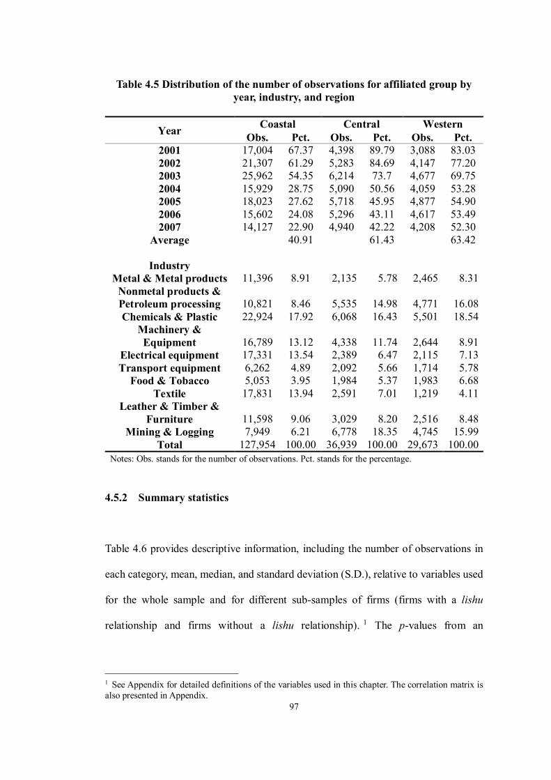
97
Table 4.5 Distribution of the number of observations for affiliated group by year, industry, and region
Year Coastal Central Western Obs. Pct. Obs. Pct. Obs. Pct.
2001 17,004 67.37 4,398 89.79 3,088 83.03 2002 21,307 61.29 5,283 84.69 4,147 77.20 2003 25,962 54.35 6,214 73.7 4,677 69.75 2004 15,929 28.75 5,090 50.56 4,059 53.28 2005 18,023 27.62 5,718 45.95 4,877 54.90 2006 15,602 24.08 5,296 43.11 4,617 53.49 2007 14,127 22.90 4,940 42.22 4,208 52.30
Average 40.91 61.43 63.42
Industry Metal & Metal products 11,396 8.91 2,135 5.78 2,465 8.31
Nonmetal products & Petroleum processing 10,821 8.46 5,535 14.98 4,771 16.08 Chemicals & Plastic 22,924 17.92 6,068 16.43 5,501 18.54
Machinery & Equipment 16,789 13.12 4,338 11.74 2,644 8.91
Electrical equipment 17,331 13.54 2,389 6.47 2,115 7.13 Transport equipment 6,262 4.89 2,092 5.66 1,714 5.78
Food & Tobacco 5,053 3.95 1,984 5.37 1,983 6.68 Textile 17,831 13.94 2,591 7.01 1,219 4.11
Leather & Timber & Furniture 11,598 9.06 3,029 8.20 2,516 8.48
Mining & Logging 7,949 6.21 6,778 18.35 4,745 15.99 Total 127,954 100.00 36,939 100.00 29,673 100.00
Notes: Obs. stands for the number of observations. Pct. stands for the percentage.
4.5.2 Summary statistics
Table 4.6 provides descriptive information, including the number of observations in
each category, mean, median, and standard deviation (S.D.), relative to variables used
for the whole sample and for different sub-samples of firms (firms with a lishu
relationship and firms without a lishu relationship). 1 The p-values from an
1 See Appendix for detailed definitions of the variables used in this chapter. The correlation matrix is also presented in Appendix.
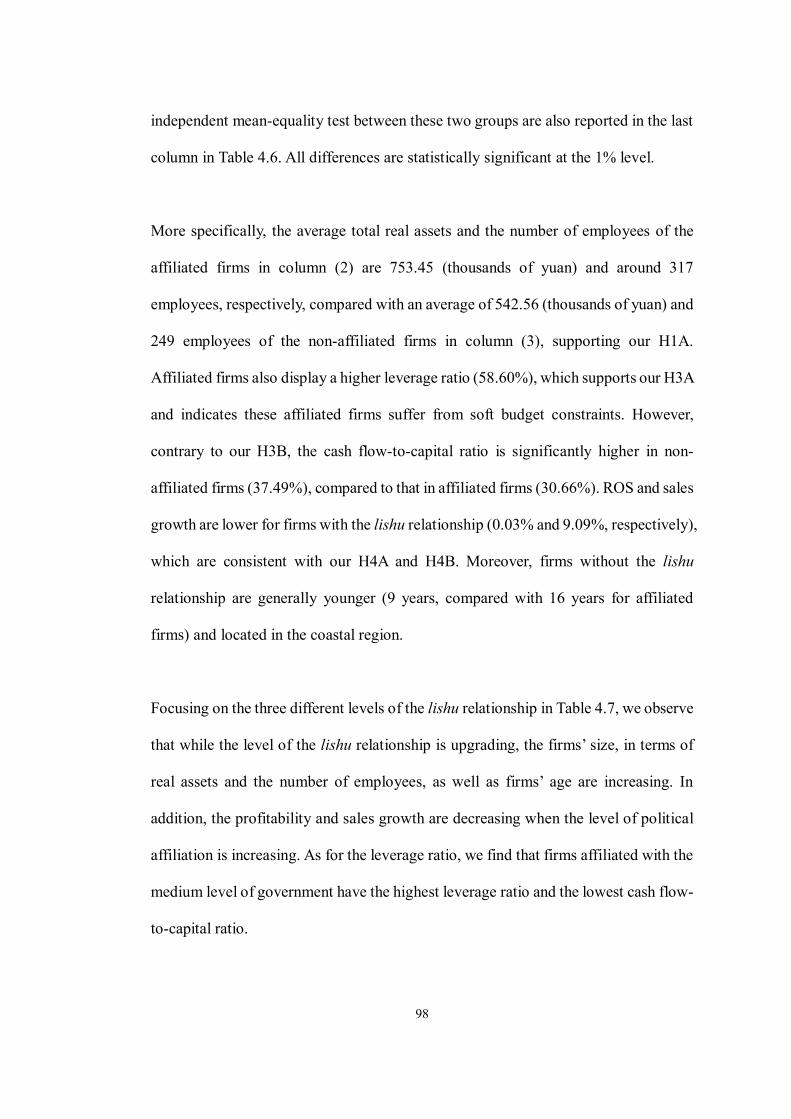
98
independent mean-equality test between these two groups are also reported in the last
column in Table 4.6. All differences are statistically significant at the 1% level.
More specifically, the average total real assets and the number of employees of the
affiliated firms in column (2) are 753.45 (thousands of yuan) and around 317
employees, respectively, compared with an average of 542.56 (thousands of yuan) and
249 employees of the non-affiliated firms in column (3), supporting our H1A.
Affiliated firms also display a higher leverage ratio (58.60%), which supports our H3A
and indicates these affiliated firms suffer from soft budget constraints. However,
contrary to our H3B, the cash flow-to-capital ratio is significantly higher in non-
affiliated firms (37.49%), compared to that in affiliated firms (30.66%). ROS and sales
growth are lower for firms with the lishu relationship (0.03% and 9.09%, respectively),
which are consistent with our H4A and H4B. Moreover, firms without the lishu
relationship are generally younger (9 years, compared with 16 years for affiliated
firms) and located in the coastal region.
Focusing on the three different levels of the lishu relationship in Table 4.7, we observe
that while the level of the lishu relationship is upgrading, the firms’ size, in terms of
real assets and the number of employees, as well as firms’ age are increasing. In
addition, the profitability and sales growth are decreasing when the level of political
affiliation is increasing. As for the leverage ratio, we find that firms affiliated with the
medium level of government have the highest leverage ratio and the lowest cash flow-
to-capital ratio.

99
Table 4.6 Descriptive statistics (sample mean, median, and S.D.)
Variables Full sample
(1) Firms with a lishu relationship
(2) Firms without a lishu relationship
(3) Diff Mean Median S.D. Mean Median S.D. Mean Median S.D.
lishu 3.165 1.000 2.935 6.229 7.000 2.187 1.000 1.000 0.000 0.000*** Real Assets 629.874 221.407 1,262.470 753.450 257.594 1,451.825 542.561 200.047 1,101.035 0.000*** Employee 277.178 154.000 344.056 317.031 177.000 383.059 249.020 143.000 310.519 0.000***
Age 11.985 9.000 10.048 16.021 11.000 12.949 9.308 8.000 6.224 0.000*** Leverage 56.610 58.275 24.693 58.595 60.054 24.756 55.207 56.960 24.551 0.000***
CFK 34.661 20.768 45.044 30.664 17.282 43.514 37.486 23.124 45.887 0.000*** ROS 0.035 0.025 0.079 0.030 0.020 0.089 0.040 0.028 0.070 0.000***
Sales Growth 10.804 10.190 34.451 9.089 8.623 33.700 12.016 11.357 34.922 0.000*** Region 1.349 1.000 0.660 1.495 1.000 0.745 1.246 1.000 0.571 0.000***
Observations 469,938 194,566 275,372 Notes: Real Assets are expressed in thousands of yuan. Leverage, CFK, ROS, and Sales growth are expressed in percentage terms. S.D. stands for standard deviations. The last column (Diff) presents p-values from an independent samples mean-equality test between firms with a lishu relationship and firms without a lishu relationship. *, **, *** indicates significance at the 10%, 5%, and1% level, respectively. See Appendix for complete definitions of all variables.

100
Table 4.7 Descriptive statistics for three levels of the lishu relationship (sample mean, median, and S.D.)
Variables Low Medium High Diff1 Diff2 Diff3 Mean Median S.D. Mean Median S.D. Mean Median S.D. lishu 4.051 5.000 1.387 7.410 7.000 0.492 9.276 9.000 0.447 0.000*** 0.000*** 0.000***
Real Assets 420.170 174.168 862.491 837.390 319.726 1,486.636 1,553.474 659.132 2,277.423 0.000*** 0.000*** 0.000*** Employee 236.368 141.000 287.259 352.887 202.000 407.644 457.050 264.000 494.288 0.000*** 0.000*** 0.000***
Age 12.108 10.000 7.654 17.980 11.000 14.698 20.483 13.000 15.468 0.000*** 0.001*** 0.000*** Leverage 56.155 57.815 24.474 61.501 63.104 24.541 56.552 57.102 25.336 0.000*** 0.025** 0.000***
CFK 40.151 24.165 48.478 23.138 12.674 36.959 25.620 13.574 41.296 0.000*** 0.000*** 0.000*** ROS 0.042 0.029 0.071 0.021 0.013 0.096 0.019 0.015 0.111 0.000*** 0.000*** 0.002***
Sales Growth 11.175 10.797 34.012 7.655 6.995 34.110 7.216 7.301 30.762 0.000*** 0.000*** 0.066* Region 1.274 1.000 0.566 1.675 1.000 0.812 1.594 1.000 0.828 0.000*** 0.000*** 0.000***
Obs. 82,408 86,951 25,207 Notes: Real Assets are expressed in thousands of yuan. Leverage, CFK, ROS, and Sales growth are expressed in percentage terms. S.D. stands for standard deviations. The last three columns present p-values from an independent samples mean-equality test between the low level of lishu group and the medium level of lishu group (Diff1), between the low level of lishu group and the high level of lishu group (Diff2), and between the medium level of lishu group and the high level of lishu group (Diff3). *, **, *** indicates significance at the 10%, 5%, and1% level, respectively. See Appendix for complete definitions of all variables.

101
Table 4.8 provides a comparison of the main variables across firms’ ownership types.
SOEs and FEs are generally large in real assets and the number of employees,
compared with PEs and COEs. SOEs have the oldest firms age (27 years) and highest
political affiliation level, followed by COEs with 17 years and the second highest
political affiliation level. While the FEs are the youngest as most of the foreign firms
entered into China after the 1990s. SOEs also suffer from soft budget constraints
indicated by their highest leverage ratio, while COEs enjoy the highest cash flow-to-
capital ratio. Table 4.8 also illustrates that the ROS and sales growth are higher for
private firms and foreign firms than that for SOEs and COEs. Finally, we observe that
the FEs prefer to locate their firms in the coastal region, while SOEs are more likely
to locate their firms in the inner region of China.
Table 4.9 provides descriptive statistics for three different regions of China. We
observe that firms located in the central and western regions exhibit higher political
affiliation levels. In addition, firms in the west of China have the largest size, in terms
of real assets (709.83 thousands of yuan) and the number of employees (319 people);
and they are older (15.48 years) than the firms in the eastern and central China.
Interestingly, firms locate in the central region have the highest ROS and sales growth.
This may be attributed to their location advantage, which is close to the heart of China,
Beijing, with enormous markets. The firms in the western region also show the highest
leverage ratio and lowest cash flow-to-capital ratio. The lowest leverage ratio for firms
operated in the coastal region may suggest that these firms depend more on their
internal funds and foreign financing, instead of debt.

102
In summary, politically affiliated firms display a larger size measured in the forms of
total assets and the number of employees, a higher leverage ratio and are older, while
unaffiliated firms have more cash flow, higher profitability and sales growth. These
rough statistics provide a primary description of our sample, and support most of our
hypotheses preliminarily. Therefore, a more thorough test of the hypotheses is
necessary, within a regression analysis framework.
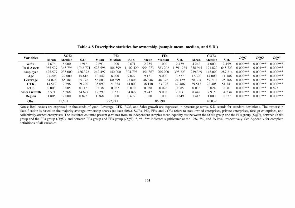
103
Table 4.8 Descriptive statistics for ownership (sample mean, median, and S.D.)
Variables SOEs PEs FEs COEs Diff1 Diff2 Diff3 Mean Median S.D. Mean Median S.D. Mean Median S.D. Mean Median S.D. lishu 7.676 8.000 1.916 2.693 1.000 2.671 2.255 1.000 2.479 4.242 4.000 2.459 0.000*** 0.000*** 0.000***
Real Assets 985.579 345.796 1,748.771 523.598 186.599 1,107.429 954.273 383.202 1,591.924 358.945 171.822 645.723 0.000*** 0.004*** 0.000*** Employee 425.579 235.000 486.372 242.497 140.000 304.793 351.867 205.000 398.223 239.369 145.000 287.214 0.000*** 0.000*** 0.000***
Age 27.206 29.000 15.616 10.542 8.000 9.027 9.181 9.000 3.577 17.390 14.000 11.186 0.000*** 0.000*** 0.000*** Leverage 64.026 65.381 25.776 58.603 60.699 23.803 46.346 46.376 24.129 58.304 59.710 25.366 0.000*** 0.000*** 0.000***
CFK 14.512 7.296 29.290 35.097 21.354 44.000 38.110 23.798 47.486 39.513 22.405 51.341 0.000*** 0.000*** 0.000*** ROS 0.003 0.005 0.115 0.038 0.027 0.070 0.038 0.026 0.085 0.036 0.024 0.081 0.000*** 0.000*** 0.823
Sales Growth 5.571 5.268 34.627 12.297 11.531 34.827 9.247 9.008 33.031 8.442 7.915 34.234 0.000*** 0.000*** 0.000*** Region 1.805 2.000 0.823 1.368 1.000 0.672 1.080 1.000 0.349 1.415 1.000 0.677 0.000*** 0.000*** 0.000***
Obs. 31,501 292,241 86,590 40,039 Notes: Real Assets are expressed in thousands of yuan. Leverage, CFK, ROS, and Sales growth are expressed in percentage terms. S.D. stands for standard deviations. The ownership classification is based on the majority average ownership shares (at least 50%). SOEs, PEs, FEs, and COEs refers to state-owned enterprises, private enterprises, foreign enterprises, and collectively-owned enterprises. The last three columns present p-values from an independent samples mean-equality test between the SOEs group and the PEs group (Diff1), between SOEs group and the FEs group (Diff2), and between PEs group and FEs group (Diff3). *, **, *** indicates significance at the 10%, 5%, and1% level, respectively. See Appendix for complete definitions of all variables.
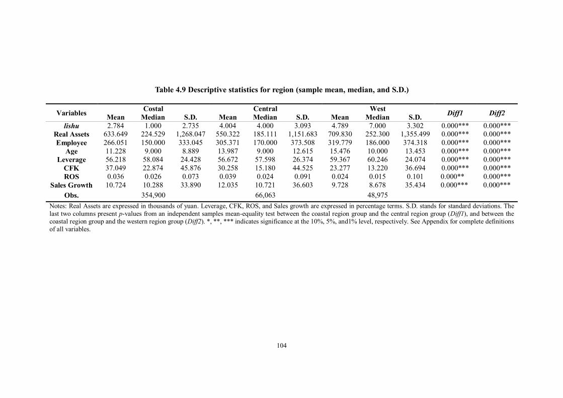
104
Table 4.9 Descriptive statistics for region (sample mean, median, and S.D.)
Variables Costal Central West Diff1 Diff2 Mean Median S.D. Mean Median S.D. Mean Median S.D. lishu 2.784 1.000 2.735 4.004 4.000 3.093 4.789 7.000 3.302 0.000*** 0.000***
Real Assets 633.649 224.529 1,268.047 550.322 185.111 1,151.683 709.830 252.300 1,355.499 0.000*** 0.000*** Employee 266.051 150.000 333.045 305.371 170.000 373.508 319.779 186.000 374.318 0.000*** 0.000***
Age 11.228 9.000 8.889 13.987 9.000 12.615 15.476 10.000 13.453 0.000*** 0.000*** Leverage 56.218 58.084 24.428 56.672 57.598 26.374 59.367 60.246 24.074 0.000*** 0.000***
CFK 37.049 22.874 45.876 30.258 15.180 44.525 23.277 13.220 36.694 0.000*** 0.000*** ROS 0.036 0.026 0.073 0.039 0.024 0.091 0.024 0.015 0.101 0.000** 0.000***
Sales Growth 10.724 10.288 33.890 12.035 10.721 36.603 9.728 8.678 35.434 0.000*** 0.000*** Obs. 354,900 66,063 48,975
Notes: Real Assets are expressed in thousands of yuan. Leverage, CFK, ROS, and Sales growth are expressed in percentage terms. S.D. stands for standard deviations. The last two columns present p-values from an independent samples mean-equality test between the coastal region group and the central region group (Diff1), and between the coastal region group and the western region group (Diff2). *, **, *** indicates significance at the 10%, 5%, and1% level, respectively. See Appendix for complete definitions of all variables.
105
4.6 Empirical findings
4.6.1 Estimations with pooled Probit and random-effects Probit models
Table 4.10 reports the regression results by employing the pooled Probit model
clustering by firms ID (column (1)) and the random-effects Probit model (column (2))
for the entire sample. Because of the non-linear model, the coefficient estimates are
not informative about the magnitude of the effects of the outcome variables. Therefore,
we also report the estimates of marginal effects (ME) in Table 4.10. The coefficients
of all variables are statistically significant at 1% level, except for the coefficient on
western region variable in the pooled Probit model.
Focusing on column (1) in Table 4.10, the coefficient on the firms’ size, in terms of
the total assets, is positively related to the probability of the firm having a lishu
relationship. This result is consistent with our first hypothesis (H1A) and with the
literature, which suggests that firms with larger size are more prone to have political
affiliation (for example, Li et al., 2006; Guariglia and Mateut, 2013; Masters and
Keim, 1985). According to the marginal effects (0.048 for the total assets), an increase
in a firm’s total assets by 0.1, or 10 percentage points, is associated with an increase
in the probability of having a lishu relationship by 0.0048 (i.e. 0.48 percentage points).
The marginal effects are tested larger by using the random-effects Probit, i.e. a 10%
increase in a firm’s asset is associated with an increase in the probability of having a
lishu relationship by 0.0107 (which is 1.07 percentage points).
106
Focusing on regional dummies, we find that the coefficients on the coastal region
dummy are negative and statistically significant at 1% level in both estimations, while
the coefficients on the western region dummy are positive in both estimations (but
insignificant using the pooled Probit). These results suggest that regional factors can
also affect the likelihood of having a lishu relationship. In China, the coastal area
generally provides a better and a more open environment for firms to develop, while
enterprises in the West, which are usually associated with fewer investment
opportunities, higher transaction costs and more informative asymmetries, could be in
greater need of political help. Our results indicate that firms locate in the west of China
are more likely to affiliate with politicians, while being a coastal firm decreases the
probability of having political affiliation. More specifically, the marginal effects imply
that a firm locating in the west of China has a 0.06% and 0.47% higher probability of
having a lishu relationship in the pooled Probit model and the random-effects Probit
model, respectively, while a firm locating in the coastal of China has a 1.21% and
3.24% lower likelihood of political participation, respectively. These results are
consistent with our Hypothesis 1B, suggesting that firms located in the western region
have higher motivation to connect with the governments.
From both columns in Table 4.10, we can also find that the ownership types precisely
determine the firms’ decision on political affiliation. The coefficient on the foreign
ownership dummy is negative and significant, while that on the state ownership is
positive and significant. These results indicate that foreign firms are less likely to have
political affiliation, while state-owned firms are more likely to be politically affiliated.
This is consistent with our Hypothesis 2 and with findings in Boubakri et al. (2008),

107
Bertrand et al. (2006), and Dyck (2001). More specifically, the marginal effects
suggest that being a foreign (state-owned) firm has a 1.65% and 4.04% (5.13% and
14.67%) lower (higher) probability of having a lishu relationship in the pooled Probit
model and the random-effects Probit model, respectively.
The coefficients on the leverage ratio and cash flow-to-capital ratio are positive and
significant, indicating that the relationship between leverage ratio (cash flow-to-
capital ratio) and the probability of having political affiliation is positive, which is
consistent with our Hypothesis 3A and 3B. According to the marginal effects (0.017
for leverage and 0.038 for cash flow-to-capital ratio) in the pooled Probit model, an
increase in a firm’s leverage (cash flow-to-capital ratio) by 0.1, or 10 percentage
points, is associated with an increase in the probability of having a lishu relationship
by 0.17 percentage points (0.38 percentage point). The marginal effects are tested
similarly by using the random-effects Probit. This finding is supported by some
existing studies.
According to Johnson and Mitton (2003) and Khwaja and Mian (2005), a higher
leverage ratio indicates that firms can benefit from soft budget terms, suggesting that
firms with a higher leverage ratio are more likely to obtain external financing. In this
case, these firms are more able to have political affiliation. Contrary to the descriptive
statistics, the cash flow has a positive and significant influence on the probability of
firms having the lishu relationship. This can be explained considering that it is widely
acknowledged that investment spending of firms should depend on their internal funds
as the first choice, which can be measured by liquidity and cash flow. Firms with
108
greater liquidity or cash flow will have more investment opportunities. In this case,
these firms may be prone to have connections with the governments to obtain
favourable support, such as crucial licences, profitable investment projects and
advantageous help in dealing with investment disputes (Leuz and Oberholzer-Gee,
2006).
From Table 4.10, we observe that ROS exhibits negative and significant coefficients
in both estimations, indicating that the relationship between profitability and the
likelihood of having political affiliation is negative. These results are consistent with
Hypothesis 4A. According to Salamon and Siegfried (1977), in order to avoid
unexpected economic losses, firms with higher profitability are less likely to get
involved in political activities. Specifically, a 10% decrease in ROS is related to an
increase in the probability of having political affiliation by 1.82 percentage points in
column (1) and 1.68 percentage points in column (2). In addition, the significant and
negative coefficients on the sales growth in both estimations support our Hypothesis
4B, suggesting that firm’s growth opportunities may also affect the political
connections decisions. In summary, firms with lower sales growth, large size, soft
budget constraints, and high cash flow ratio may need more help from governments
to obtain favourable projects and expand their investment opportunities.
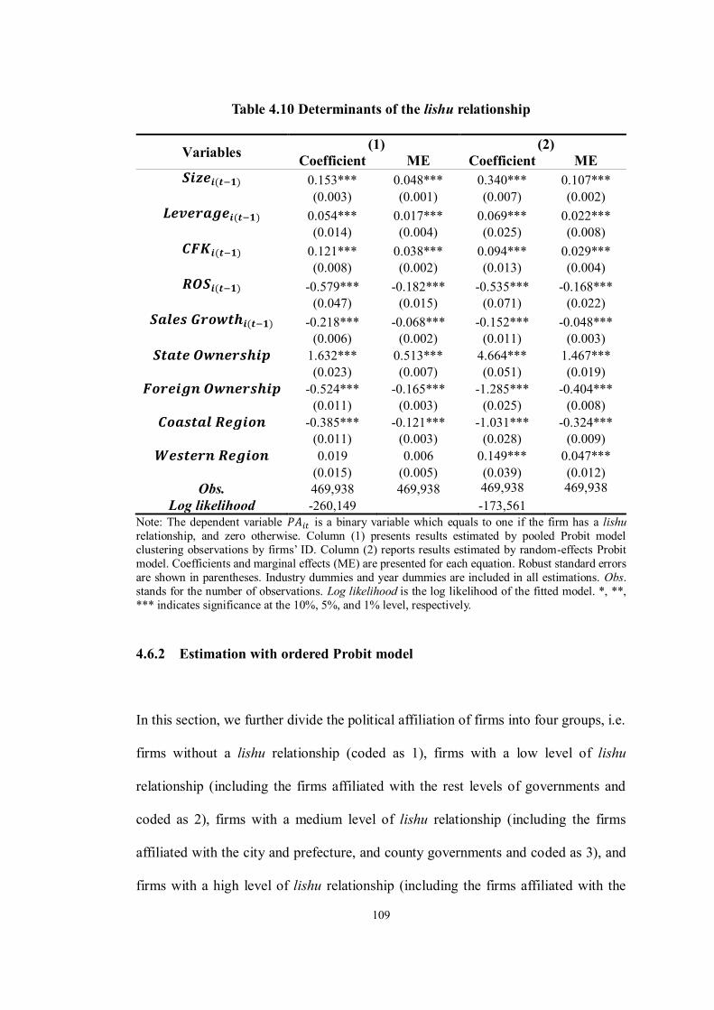
109
Table 4.10 Determinants of the lishu relationship
Variables (1) (2) Coefficient ME Coefficient ME
𝑺𝒊𝒛𝒆𝒊(𝒕−𝟏) 0.153*** 0.048*** 0.340*** 0.107*** (0.003) (0.001) (0.007) (0.002)
𝑳𝒆𝒗𝒆𝒓𝒂𝒈𝒆𝒊(𝒕−𝟏) 0.054*** 0.017*** 0.069*** 0.022*** (0.014) (0.004) (0.025) (0.008)
𝑪𝑭𝑲𝒊(𝒕−𝟏) 0.121*** 0.038*** 0.094*** 0.029*** (0.008) (0.002) (0.013) (0.004)
𝑹𝑶𝑺𝒊(𝒕−𝟏) -0.579*** -0.182*** -0.535*** -0.168*** (0.047) (0.015) (0.071) (0.022)
𝑺𝒂𝒍𝒆𝒔 𝑮𝒓𝒐𝒘𝒕𝒉𝒊(𝒕−𝟏) -0.218*** -0.068*** -0.152*** -0.048*** (0.006) (0.002) (0.011) (0.003)
𝑺𝒕𝒂𝒕𝒆 𝑶𝒘𝒏𝒆𝒓𝒔𝒉𝒊𝒑 1.632*** 0.513*** 4.664*** 1.467*** (0.023) (0.007) (0.051) (0.019) 𝑭𝒐𝒓𝒆𝒊𝒈𝒏 𝑶𝒘𝒏𝒆𝒓𝒔𝒉𝒊𝒑 -0.524*** -0.165*** -1.285*** -0.404*** (0.011) (0.003) (0.025) (0.008)
𝑪𝒐𝒂𝒔𝒕𝒂𝒍 𝑹𝒆𝒈𝒊𝒐𝒏 -0.385*** -0.121*** -1.031*** -0.324*** (0.011) (0.003) (0.028) (0.009)
𝑾𝒆𝒔𝒕𝒆𝒓𝒏 𝑹𝒆𝒈𝒊𝒐𝒏 0.019 0.006 0.149*** 0.047*** (0.015) (0.005) (0.039) (0.012)
Obs. 469,938 469,938 469,938 469,938 Log likelihood -260,149 -173,561
Note: The dependent variable 𝑃𝐴𝑖𝑡 is a binary variable which equals to one if the firm has a lishu relationship, and zero otherwise. Column (1) presents results estimated by pooled Probit model clustering observations by firms’ ID. Column (2) reports results estimated by random-effects Probit model. Coefficients and marginal effects (ME) are presented for each equation. Robust standard errors are shown in parentheses. Industry dummies and year dummies are included in all estimations. Obs. stands for the number of observations. Log likelihood is the log likelihood of the fitted model. *, **, *** indicates significance at the 10%, 5%, and 1% level, respectively.
4.6.2 Estimation with ordered Probit model
In this section, we further divide the political affiliation of firms into four groups, i.e.
firms without a lishu relationship (coded as 1), firms with a low level of lishu
relationship (including the firms affiliated with the rest levels of governments and
coded as 2), firms with a medium level of lishu relationship (including the firms
affiliated with the city and prefecture, and county governments and coded as 3), and
firms with a high level of lishu relationship (including the firms affiliated with the
110
central and provincial governments, and coded as 4). As our dependent variable is an
ordinal polychotomous variable, we perform the ordered Probit estimation for the full
sample and report the results in Table 4.11.
We start with focusing on the coefficients column. 1 The positive and significant
coefficient on firms’ real assets indicates that an increase in firms’ real assets would
yield a decrease in the probability of having no lishu relationship, and an increase in
the probability of having a lishu relationship with the high level of government.
Looking at the marginal effects for the first group (firms without a lishu relationship),
we find that the probability of having no political affiliation decrease by 0.81
percentage points as firms size increases by 10%. We also find that for the other three
groups where firms have political affiliation, an increase in firms’ real assets by 0.1,
or 10 percentage points, is associated with an increase in the probability of having a
low/medium/high level of lishu relationship by 0.23/0.48/0.11 percentage points,
respectively. These findings support our H1A.
Focusing on the regional factors in Table 4.11, we notice a negative coefficient on the
coastal region variable, suggesting that being a coastal firm necessarily is associated
with a higher probability of having no political affiliation and a lower probability of
having high political affiliation. However, the positive and significant coefficient on
1 According to Cameron and Trivedi (2010), the sign of the coefficients can be immediately interpreted as determining whether the dependent variable increases with the regressor. If coefficient 𝛽𝑗 is positive, then an increase in 𝑥𝑖𝑗 decreases the probability of being in the lowest category (𝑦𝑖 = 1) and increases the probability of being in the highest category. The marginal effects are expected to have the opposite signs to coefficients for the first outcome (𝑦𝑖 = 1) and have the same signs with coefficients for the rest outcomes. In our case, the first, second, third, and fourth outcomes refer to firms without a lishu relationship (the lowest category), firms with a low level of lishu relationship, firms with a medium level of lishu relationship, and firms with a high level of lishu relationship (the highest category), respectively.
111
western region variable suggests that being a western firm would be related to a lower
probability of having no lishu relationship and a higher probability of affiliating with
the high level of government. These findings are consistent with our H1B. Specifically,
being a coastal/western firm is associated with a 1.27%/0.62% higher/lower
likelihood of being a non-affiliated firm. Moreover, being a firm located in the east
(west) of China is related to a 0.35%/0.75%/0.17% (0.17%/0.36%/0.08%) lower
(higher) probability of having a low/medium/high level of lishu relationship,
respectively.
Similar results can also be found by looking at the ownership variables. That is, being
a foreign (state-owned) firm is related to a higher (lower) in the likelihood of having
no lishu relationship and a lower (higher) in the probability of having a high level of
lishu relationship. Focusing on the marginal effects for non-affiliated firms, we find
that being a foreign (state-owned) firm is associated with a 1.80% (5.54%) higher
(lower) likelihood of being a non-affiliated firm. For the other three groups, being a
foreign (state-owned) firm is associated with a 0.50%/1.06%/0.24%
(1.53%/3.26%/0.75%) lower (higher) probability of having low/medium/high level of
political affiliation, respectively. These results support our Hypothesis 2.
As for the financial status variables, the positive and significant coefficients on
leverage ratio and cash flow ratio indicate that an increase in leverage ratio/cash flow
ratio would yield a decrease in the propensity of being non-affiliated firms and an
increase in the propensity of being highly affiliated firms. These findings are
consistent with our H3A and H3B.
112
The negative and significant coefficients on ROS and sales growth in Table 4.11
support the Hypothesis 4A and 4B, suggesting that an increase in ROS/sales growth
is associated with a rise in the likelihood of having no lishu relationship and a drop in
that of having a high level of lishu relationship. Specifically, a 10% increase in
ROS/sales growth relates to an increase in the likelihood of being a non-affiliated firm
by 2.57/0.75 percentage points. Furthermore, an increase in ROS (sales growth) by
0.1, or 10 percentage points, would yield a decrease in the probability of having a
low/medium/high level of lishu relationship by 0.71/1.51/0.35 (0.21/0.44/0.10)
percentage points, respectively.
Furthermore, changes in variables would be associated with changes in the probability
of having the lishu relationship by a larger percentage point for firms affiliated with
medium level of government than those affiliated with low/high level of government.
This might relate to the fact that the government at this level can access important
resources, as well as enjoy authority to support the firms’ development. Therefore,
firms are more willing to have the lishu relationship with the governments at the
medium level.
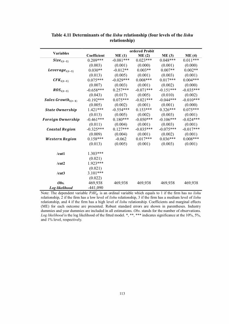
113
Table 4.11 Determinants of the lishu relationship (four levels of the lishu relationship)
Variables ordered Probit
Coefficient ME (1) ME (2) ME (3) ME (4) 𝑺𝒊𝒛𝒆𝒊(𝒕−𝟏) 0.209*** -0.081*** 0.023*** 0.048*** 0.011***
(0.003) (0.001) (0.000) (0.001) (0.000) 𝑳𝒆𝒗𝒆𝒓𝒂𝒈𝒆𝒊(𝒕−𝟏) 0.030** -0.012** 0.003** 0.007** 0.002**
(0.013) (0.005) (0.001) (0.003) (0.001) 𝑪𝑭𝑲𝒊(𝒕−𝟏) 0.075*** -0.029*** 0.008*** 0.017*** 0.004***
(0.007) (0.003) (0.001) (0.002) (0.000) 𝑹𝑶𝑺𝒊(𝒕−𝟏) -0.658*** 0.257*** -0.071*** -0.151*** -0.035***
(0.043) (0.017) (0.005) (0.010) (0.002) 𝑺𝒂𝒍𝒆𝒔 𝑮𝒓𝒐𝒘𝒕𝒉𝒊(𝒕−𝟏) -0.192*** 0.075*** -0.021*** -0.044*** -0.010***
(0.005) (0.002) (0.001) (0.001) (0.000) 𝑺𝒕𝒂𝒕𝒆 𝑶𝒘𝒏𝒆𝒓𝒔𝒉𝒊𝒑 1.421*** -0.554*** 0.153*** 0.326*** 0.075***
(0.013) (0.005) (0.002) (0.003) (0.001) 𝑭𝒐𝒓𝒆𝒊𝒈𝒏 𝑶𝒘𝒏𝒆𝒓𝒔𝒉𝒊𝒑 -0.461*** 0.180*** -0.050*** -0.106*** -0.024***
(0.011) (0.004) (0.001) (0.003) (0.001) 𝑪𝒐𝒂𝒔𝒕𝒂𝒍 𝑹𝒆𝒈𝒊𝒐𝒏 -0.325*** 0.127*** -0.035*** -0.075*** -0.017***
(0.009) (0.004) (0.001) (0.002) (0.001) 𝑾𝒆𝒔𝒕𝒆𝒓𝒏 𝑹𝒆𝒈𝒊𝒐𝒏 0.158*** -0.062 0.017*** 0.036*** 0.008***
(0.013) (0.005) (0.001) (0.003) (0.001)
/cut1 1.303*** (0.021)
/cut2 1.923*** (0.021)
/cut3 3.101*** (0.022)
Obs. 469,938 469,938 469,938 469,938 469,938 Log likelihood -441,090
Note: The dependent variable 𝑃𝐴𝑉𝑖𝑡 is an ordinal variable which equals to 1 if the firm has no lishu relationship, 2 if the firm has a low level of lishu relationship, 3 if the firm has a medium level of lishu relationship, and 4 if the firm has a high level of lishu relationship. Coefficients and marginal effects (ME) for each outcome are presented. Robust standard errors are shown in parentheses. Industry dummies and year dummies are included in all estimations. Obs. stands for the number of observations. Log likelihood is the log likelihood of the fitted model. *, **, *** indicates significance at the 10%, 5%, and 1% level, respectively.

114
4.7 Further tests
4.7.1 Determinants of the lishu relationship by ownership
We firstly estimate the determinants of the lishu relationship by ownership types.1
Table 4.12 presents the coefficients and marginal effects estimated by the pooled
Probit and random-effects Probit models. As we find that around 94% of state-owned
firms and 84% of collectively-owned firms are politically affiliated, we only report
the results for private firms (in column (1)), which accounts for more than 60% of our
full sample, and foreign firms (in column (2)), which are generally the youngest and
vigorous firms in China.
The coefficient on firm’ size is positive and significant for both types of firms in both
estimations, suggesting that having the lishu relationship increases as firms’ size
increase. The magnitude of marginal effects is larger for private firms (a 10% increase
in firms’ size is associated with a 0.64 percentage points using the pooled Probit model
1 I have estimated the regressions for firms getting the lishu relationship (from having no lishu relationship to having a lishu relationship at any level) and for firms ending the lishu relationship (from having a lishu relationship at any level to having no lishu relationship). The results are robust and available on request. In addition, I have estimated the regression by considering the initial conditions and for firms improving and decreasing their lishu level. And the results are robust and available on request. I also have estimated the regressions for ten different industries available in our dataset, i.e. Metal and metal products industry, Non-metal products and petroleum processing industry, Chemicals and plastic industry, Machinery and Equipment industry, Electrical equipment industry, Transport equipment industry, Food and Tobacco industry, Textile industry, Leather, Timber and Furniture industry, and Mining and Logging industry. And the results are robust overall. However, three industries out of ten have some different situations. Firstly, the coefficients and marginal effects of ROS for the Mining and logging industry are positive and significant. This might due to the fact that minerals and forest resource are owned by the public in China. Therefore, the firms with high profitability in this industry are more prone to have political connections to access resource and licences (Zhang, 2006; Jiang, 2000; Sun, 2004). Secondly, the transport equipment industry and textile industry show negative and significant coefficients and marginal effects on “Western Region” variable. This might be because of the fact that during our sample period, there were many local policies that provide many favourable treatments, such as land lease, taxes, and subsidies, which were only available to the transport equipment industry and textile industry in the western region (Wei, 2007; Su, 1999; Hui, 2008; Sun and Jiang, 2015; Luo and Cao, 2005). For example, according to Yang (2004), Xinjiang Province has set up 20 billion RMB subsidies and provided free land to facilitate the development of textile enterprises. Shaanxi Province has provided tax deduction and extra finance and subsidies to the transport industry. In this case, these two industries locating in the western region are less likely to have political connections during our sample period. The results are available on request.
115
and 0.69 percentage points using the random-effects Probit model), compared with
that for foreign firms (a 10% increase in firms’ size is associated with a 0.24
percentage points using pooled Probit model and 0.10 percentage points using
random-effects Probit model).
As for the regional variables, we find similar results to our previous estimations for
both private firms and foreign firms. As for private firms, being a coastal (western)
firm is associated with a 1.49% and 1.94% (0.17%) lower (higher) probability of
having a lishu relationship by using the pooled Probit model and random-effects
Probit model, respectively. Looking at the foreign firms in column (2), we find that
being a coastal (western) firm is related to a 0.70% (0.88%) and 0.35% (0.47%) lower
(higher) probability of having a lishu relationship by using the pooled Probit model
and the random-effects Probit model, respectively.
Looking at the leverage ratio and cash flow ratio, we observe a positive and significant
relationship for both types of firms, expect for the leverage ratio in the foreign firms,
which have insignificant effects. Overall, these results suggest that the higher level of
leverage ratio and cash flow ratio are associated with higher probability of having a
lishu relationship. Focusing on the profitability and sales growth, we find that the
coefficients of ROS become insignificant for foreign firms. But the results are still
robust for the private firms and for sales growth of foreign firms. ROS and sales
growth significantly and negatively affect firms’ political participation, and this effect
is larger for private firms than foreign firms.1
1 The coefficients of ROS for foreign firms are positive and insignificant, which indicates ROS is a poor determinant for foreign firms political participation. These positive sign might be related to the fact that some foreign firms with high profitability need to transfer more return to their home countries. This behaviour is associated with the law and regulation. In this case, profitable foreign firms might use political connections as one method to facilitate the transfer (Zhang, 2011; Zhu and Song, 2002; Fang, 2002; Qi, 2008).

116
Table 4.12 Determinants of the lishu relationship by ownership (PEs vs. FEs)
Variables (1) (2)
pooled Probit RE Probit pooled Probit RE Probit Coeff. ME Coeff. ME Coeff. ME Coeff. ME
𝑺𝒊𝒛𝒆𝒊(𝒕−𝟏) 0.207*** 0.064*** 0.435*** 0.069*** 0.083*** 0.024*** 0.185*** 0.010*** (0.004) (0.001) (0.008) (0.002) (0.007) (0.002) (0.015) (0.001)
𝑳𝒆𝒗𝒆𝒓𝒂𝒈𝒆𝒊(𝒕−𝟏) 0.084*** 0.026*** 0.098*** 0.016*** 0.013 0.004 0.011 0.001 (0.018) (0.006) (0.030) (0.005) (0.034) (0.010) (0.059) (0.003)
𝑪𝑭𝑲𝒊(𝒕−𝟏) 0.086*** 0.027*** 0.078*** 0.012*** 0.091*** 0.026*** 0.080*** 0.004*** (0.010) (0.003) (0.016) (0.003) (0.017) (0.005) (0.029) (0.002)
𝑹𝑶𝑺𝒊(𝒕−𝟏) -0.910*** -0.282*** -0.859*** -0.137*** 0.130 0.037 0.095 0.005 (0.064) (0.020) (0.094) (0.015) (0.090) (0.026) (0.142) (0.008)
𝑺𝒂𝒍𝒆𝒔 𝑮𝒓𝒐𝒘𝒕𝒉𝒊(𝒕−𝟏) -0.212*** -0.066*** -0.164*** -0.026*** -0.112*** -0.032*** -0.041 -0.002 (0.007) (0.002) (0.013) (0.002) (0.015) (0.004) (0.027) (0.001)
𝑪𝒐𝒂𝒔𝒕𝒂𝒍 𝑹𝒆𝒈𝒊𝒐𝒏 -0.481*** -0.149*** -1.215*** -0.194*** -0.244*** -0.070*** -0.668*** -0.035*** (0.012) (0.004) (0.031) (0.006) (0.045) (0.013) (0.113) (0.006)
𝑾𝒆𝒔𝒕𝒆𝒓𝒏 𝑹𝒆𝒈𝒊𝒐𝒏 0.001 0.001 0.109** 0.017** 0.307*** 0.088*** 0.888*** 0.047*** (0.017) (0.005) (0.042) (0.007) (0.069) (0.020) (0.171) (0.009)
Obs. 292,241 292,241 292,241 292,241 86,590 86,590 86,590 86,590 Log likelihood -160,109 -109,896 -43,984 -30,011
Note: The dependent variable 𝑃𝐴𝑖𝑡 is a binary variable which equals to one if the firm has a lishu relationship, and zero otherwise. Columns (1) and (2) present results for PEs and FEs, respectively. The regressions are estimated by pooled Probit model clustering observations by firms’ ID and random-effects Probit model. Coefficients (Coeff.) and marginal effects (ME) are presented for each regression. Robust standard errors are shown in parentheses. Industry dummies and year dummies are included in all estimations. Obs. stands for the number of observations. Log likelihood is the log likelihood of the fitted model. *, **, *** indicates significance at the 10%, 5%, and 1% level, respectively.

117
4.7.2 Determinants of the lishu relationship by region
Table 4.13 presents the results estimated by the pooled Probit and random-effects
Probit models for three regions, i.e. the coastal (column (1)), central (column (2)), and
western (column (3)) region.
In terms of firms’ size, we find that no matter which region the firm is located in, an
increase in firms’ size is generally associated with an increase in the probability of
having a lishu relationship. Similar results are found with firms ownership types.
Being a SOEs is generally related to an increase in the likelihood of having political
affiliation, while firms with foreign ownership are less likely to be politically affiliated.
The coefficient on leverage ratio is positive and significant at the 1% level for firms
locating in the central and western regions, suggesting that these firms with soft
budget constraints are more prone to have the lishu relationship. However, we find
that the cash flow-to-capital ratio is a significant determinant only for firms in the east
of China. This may be due to the Chinese regional development policies. Although
the open-door policy and the coastal development strategy before the 1990s promoted
the development of the east of China considerably, they also brought seriously
regional unbalance and inequality. In order to reduce these disparities, China has
changed its focus from the east to the inner regions. The central government carried
out a series policies to support the development of the inner regions, i.e.
“Development of the Western Region in China” (xi bu da kai fa) in the late 1990s,
“Revitalizing the Northeast Old Industries Strategy”(zheng xing dong bei lao gong ye

118
ji di) in 2003, and the “Rise of Central China Strategy” (zhong bu jue qi zhan lve) in
2004. With these favourable policies, a great amount of funding has been injected in
these areas. Therefore, firms locating in the central and western regions may have less
dependence on the availability of their internal funds to invest, including having
political affiliation.
Looking at the ROS and sales growth, our previous results are still robust across the
three regions. That is, an increase in ROS or sales growth relates to a decrease in the
probability of firms’ political participation.
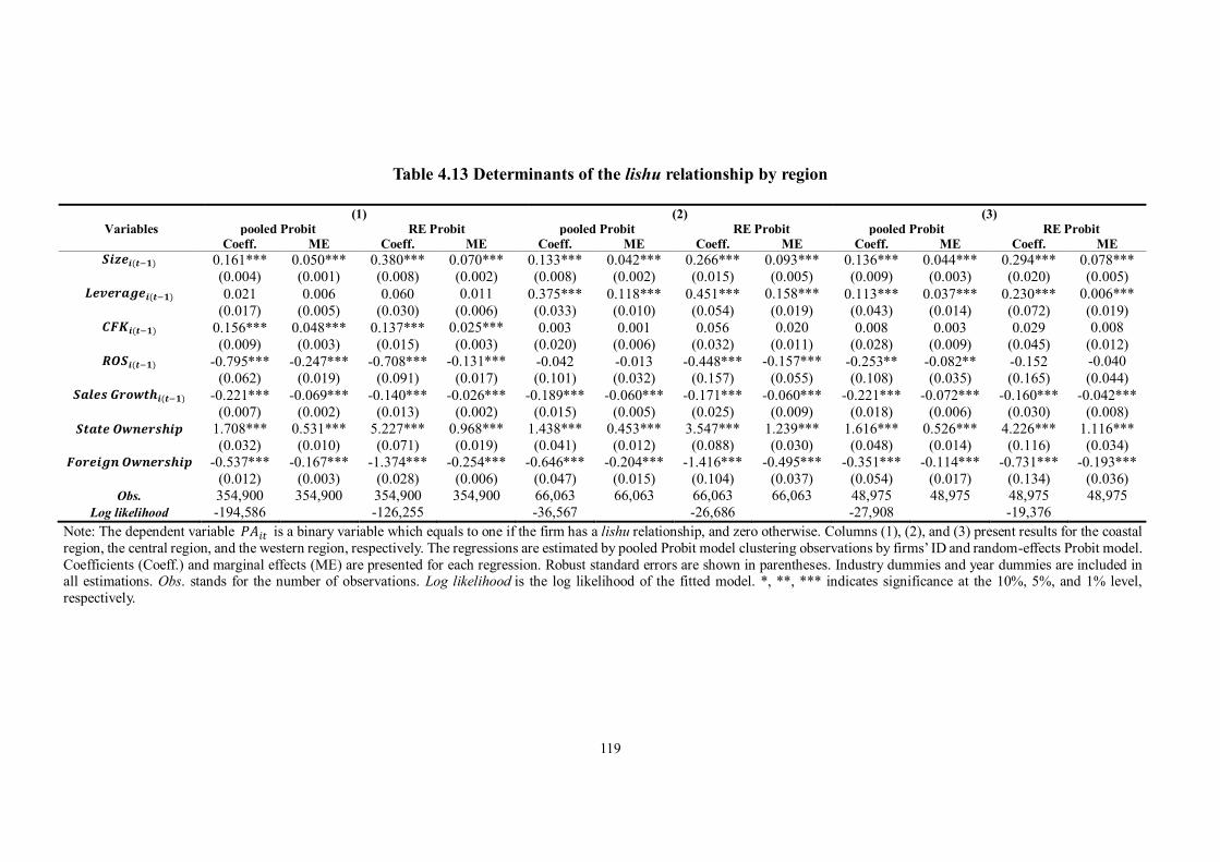
119
Table 4.13 Determinants of the lishu relationship by region
Variables
(1) (2) (3) pooled Probit RE Probit pooled Probit RE Probit pooled Probit RE Probit
Coeff. ME Coeff. ME Coeff. ME Coeff. ME Coeff. ME Coeff. ME 𝑺𝒊𝒛𝒆𝒊(𝒕−𝟏) 0.161*** 0.050*** 0.380*** 0.070*** 0.133*** 0.042*** 0.266*** 0.093*** 0.136*** 0.044*** 0.294*** 0.078***
(0.004) (0.001) (0.008) (0.002) (0.008) (0.002) (0.015) (0.005) (0.009) (0.003) (0.020) (0.005) 𝑳𝒆𝒗𝒆𝒓𝒂𝒈𝒆𝒊(𝒕−𝟏) 0.021 0.006 0.060 0.011 0.375*** 0.118*** 0.451*** 0.158*** 0.113*** 0.037*** 0.230*** 0.006***
(0.017) (0.005) (0.030) (0.006) (0.033) (0.010) (0.054) (0.019) (0.043) (0.014) (0.072) (0.019) 𝑪𝑭𝑲𝒊(𝒕−𝟏) 0.156*** 0.048*** 0.137*** 0.025*** 0.003 0.001 0.056 0.020 0.008 0.003 0.029 0.008
(0.009) (0.003) (0.015) (0.003) (0.020) (0.006) (0.032) (0.011) (0.028) (0.009) (0.045) (0.012) 𝑹𝑶𝑺𝒊(𝒕−𝟏) -0.795*** -0.247*** -0.708*** -0.131*** -0.042 -0.013 -0.448*** -0.157*** -0.253** -0.082** -0.152 -0.040
(0.062) (0.019) (0.091) (0.017) (0.101) (0.032) (0.157) (0.055) (0.108) (0.035) (0.165) (0.044) 𝑺𝒂𝒍𝒆𝒔 𝑮𝒓𝒐𝒘𝒕𝒉𝒊(𝒕−𝟏) -0.221*** -0.069*** -0.140*** -0.026*** -0.189*** -0.060*** -0.171*** -0.060*** -0.221*** -0.072*** -0.160*** -0.042***
(0.007) (0.002) (0.013) (0.002) (0.015) (0.005) (0.025) (0.009) (0.018) (0.006) (0.030) (0.008) 𝑺𝒕𝒂𝒕𝒆 𝑶𝒘𝒏𝒆𝒓𝒔𝒉𝒊𝒑 1.708*** 0.531*** 5.227*** 0.968*** 1.438*** 0.453*** 3.547*** 1.239*** 1.616*** 0.526*** 4.226*** 1.116***
(0.032) (0.010) (0.071) (0.019) (0.041) (0.012) (0.088) (0.030) (0.048) (0.014) (0.116) (0.034) 𝑭𝒐𝒓𝒆𝒊𝒈𝒏 𝑶𝒘𝒏𝒆𝒓𝒔𝒉𝒊𝒑 -0.537*** -0.167*** -1.374*** -0.254*** -0.646*** -0.204*** -1.416*** -0.495*** -0.351*** -0.114*** -0.731*** -0.193***
(0.012) (0.003) (0.028) (0.006) (0.047) (0.015) (0.104) (0.037) (0.054) (0.017) (0.134) (0.036) Obs. 354,900 354,900 354,900 354,900 66,063 66,063 66,063 66,063 48,975 48,975 48,975 48,975
Log likelihood -194,586 -126,255 -36,567 -26,686 -27,908 -19,376 Note: The dependent variable 𝑃𝐴𝑖𝑡 is a binary variable which equals to one if the firm has a lishu relationship, and zero otherwise. Columns (1), (2), and (3) present results for the coastal region, the central region, and the western region, respectively. The regressions are estimated by pooled Probit model clustering observations by firms’ ID and random-effects Probit model. Coefficients (Coeff.) and marginal effects (ME) are presented for each regression. Robust standard errors are shown in parentheses. Industry dummies and year dummies are included in all estimations. Obs. stands for the number of observations. Log likelihood is the log likelihood of the fitted model. *, **, *** indicates significance at the 10%, 5%, and 1% level, respectively.
120
4.8 Conclusion
Although political connections have attracted worldwide academic interests, most of
the studies focus on the benefits provided by political connections to the connected
firms. An important question, what types of firms are more likely to have political
connections, has been neglected.
After almost four decades of economic reform since 1978, various economic
institutions in China have gained increasing authority to operate on market principles.
However, the government continues to play an important role in the allocation of
critical resources and policy making. And the firms remain involved in the
relationship with different levels of government. As a unique institutional variation,
the lishu relationship has received the least attention in previous research. Little is
known about this particular relationship through which the Chinese government can
maintain its administrative control over the affiliated firms. To the best of our
knowledge, this study represents the first effort to empirically estimate the
determinants of political connections, intended as the lishu relationship in China.
In this chapter, we use a sample of 113,549 mainly unlisted firms in China over the
period 2001 to 2007, to test four sets of hypotheses regarding the determinants of the
probability of having political connections, measured as the lishu relationship. Our
empirical work shows that the likelihood of a firm being politically affiliated can be
explained by the firms’ characteristics, ownership types, financial factors, profitability,
and sales growth.

121
We find that firm size is a positive and precise determinant in explaining firm’s
political affiliation. Firms locating in the coastal region are less likely to have a lishu
relationship than those in the west of China. In addition, state-owned firms are more
prone to have a lishu relationship, compared with foreign firms. Moreover, the
relationship between leverage ratio/cash flow-to-capital ratio and the probability of
having a lishu relationship is positive and significant, indicating that non-financially
constrained firms are more likely to invest in political relationships. However, firms
with higher profitability and sales growth do not prefer to be politically affiliated.
Then we divide the full sample into four different levels of the lishu relationship, i.e.
firms without a lishu relationship, firms affiliated with the low level of government,
firms affiliated with the medium level of government, and firms with the high level of
government. Our findings suggest the similar patterns for firms’ size, regional factors,
ownership types, financial status, profitability, and sales growth. Furthermore, we also
find that changes in these variables would be associated with changes in the
probability of having a lishu relationship by a larger number for firms affiliated with
the medium level of governments than those affiliated with the low/high level of
government. We attribute this finding to the fact that firms affiliated with medium
level of governments can obtain important resources and retain flexibility to operate.
Looking at the ownership types, i.e. private firms and foreign firms, we find the
similar results to our previous analysis. And the magnitude of marginal effects is larger
for private firms than that for foreign firms. As for the estimations based on three
regions, i.e. the coastal, central, and western regions, similar results are found.
122
However, we do not find that cash flow is a significant determinant for firms in the
central and western areas due to the regional development policies. These favourable
policies include the “Development of the Western Region in China” (xi bu da kai fa),
“Revitalising the Northeast Old Industries Strategy” (zheng xing dong bei lao gong ye
ji di), and the “Rise of Central China Strategy” (zhong bu jue qi zhan lve). With these
favourable policies, a great amount of funding has been injected in these areas.
Therefore, firms locating in the inner regions may have less dependence on the
availability of their internal funds to develop and invest in political affiliation.
Following the economic and political reforms in China, the non-state economy
continues to play a more important role in every aspect of the country’s development.
Given a relatively underdeveloped legal and market environment, having the lishu
relationship may be an effective and active way for entrepreneurs to operate their
business in the transitional economy. Therefore, exploring the factors that affect
political participation helps understand the economic and political development in
China. Our findings have some implications for firms and policy-makers. First, not
all of the firms are good candidates to have the lishu relationship. As China is
geographically large and has different levels of governments, for firms without a lishu
relationship, they should be prepared to deal with not only one government, but at
least five layers of governments in the vertical hierarchy. Especially for the foreign
firms that are new to China. Second, China has a system of economic decentralisation
and political centralisation, in which local governments have the authority to make
economic policies. As many firms are more willing to be affiliated with these medium
level of governments, the policy makers should establish relevant policies to support
123
the firms’ development. At the same time, they should be cautious not to induce
further regional imbalance and inequity.
Further research can be undertaken from the following direction. As we use the pooled
Probit and random-effects Probit models for estimations, it would be interesting to
test whether the results are robust by using other estimations, such as the special
regressor estimator proposed by Lewbel (2000). Compared with the IV Probit or Tobit
model, the special regressor allows us to include the categorical variables as regressors.

124
Appendix 4A
Table 4A.1 Definition of the variables used
Variable Definition
PA a dummy variable that equals to 1 if firm has a lishu relationship and 0 otherwise
PAV
an ordinal dummy variable that equals to 1 if firm has no lishu relationship, 2 if firm has lishu relationship with the low level of government, 3 if firm affiliated with the medium level of government, 4 if firm has lishu relationship with the high level of government
Total Assets
sum of the firm’s fixed and current assets, where fixed assets include tangible fixed assets, intangible fixed assets, and other fixed assets; and current assets include inventories, accounts receivable, and other current assets
Size natural logarithm of total real assets (the number of employees in the Appendix Table 3A.8)
Leverage ratio ratio of total debt to total assets CFK ratio of cash flow to tangible fixed assets
ROS return on sales, ratio of profit before tax and interest to total sales, a measure of profitability
Sales growth growth of total real sales State ownership a dummy variable that equals to 1 if firm is state-owned and 0 otherwise
Foreign ownership
a dummy variable that equals to 1 if firm is owned by foreign investors (including investors from Hong Kong, Macao, and Taiwan) and 0 otherwise
Coastal region a dummy variable that equals to 1 if firm is located in the coastal region in China and 0 otherwise
Central region a dummy variable that equals to 1 if firm is located in the central region in China and 0 otherwise
Western region a dummy variable that equals to 1 if firm is located in the western region in China and 0 otherwise
Age a firm’s age is calculated since the year the firm was established
Liquidity ratio a ratio of the difference between current assets and current liabilities to total assets
Employee total number of people employed by the firm
Deflators
all variables (except tangible fixed assets) are deflated using provincial ex-factory producer price indices (pdsales) taken from various issues of the china statistical yearbook. tangible fixed assets are deflated using a deflator for fixed capital formation (pdgoods)
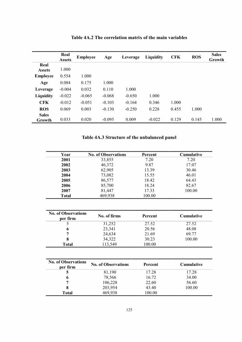
125
Table 4A.2 The correlation matrix of the main variables
Table 4A.3 Structure of the unbalanced panel
Year No. of Observations Percent Cumulative 2001 33,855 7.20 7.20 2002 46,372 9.87 17.07 2003 62,905 13.39 30.46 2004 73,082 15.55 46.01 2005 86,577 18.42 64.43 2006 85,700 18.24 82.67 2007 81,447 17.33 100.00 Total 469,938 100.00
No. of Observations per firm No. of firms Percent Cumulative
5 31,252 27.52 27.52 6 23,341 20.56 48.08 7 24,634 21.69 69.77 8 34,322 30.23 100.00
Total 113,549 100.00
No. of Observations per firm No. of Observations Percent Cumulative
5 81,190 17.28 17.28 6 78,566 16.72 34.00 7 106,228 22.60 56.60 8 203,954 43.40 100.00
Total 469,938 100.00
Real Assets Employee Age Leverage Liquidity CFK ROS Sales
Growth Real
Assets 1.000 Employee 0.554 1.000
Age 0.084 0.175 1.000 Leverage -0.004 0.032 0.110 1.000 Liquidity -0.022 -0.065 -0.068 -0.650 1.000
CFK -0.012 -0.051 -0.103 -0.164 0.346 1.000 ROS 0.069 0.003 -0.130 -0.250 0.228 0.455 1.000 Sales
Growth 0.033 0.020 -0.095 0.009 -0.022 0.129 0.145 1.000
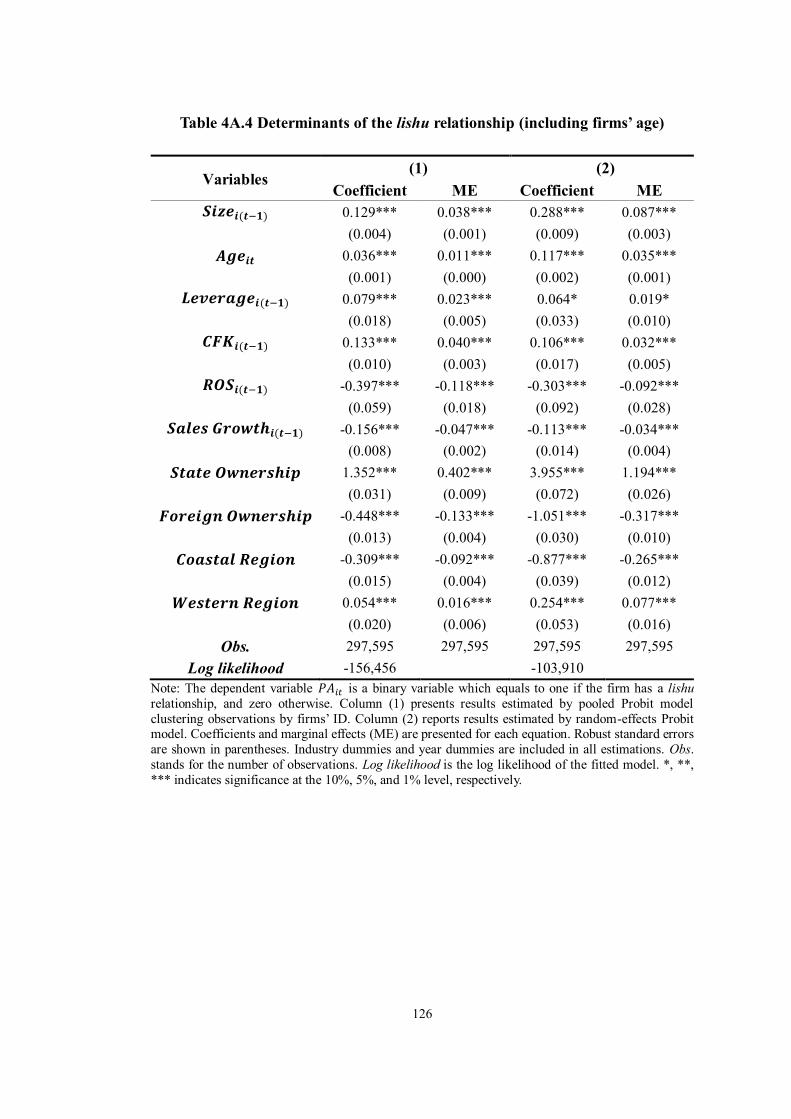
126
Table 4A.4 Determinants of the lishu relationship (including firms’ age)
Variables (1) (2)
Coefficient ME Coefficient ME 𝑺𝒊𝒛𝒆𝒊(𝒕−𝟏) 0.129*** 0.038*** 0.288*** 0.087***
(0.004) (0.001) (0.009) (0.003) 𝑨𝒈𝒆𝒊𝒕 0.036*** 0.011*** 0.117*** 0.035***
(0.001) (0.000) (0.002) (0.001) 𝑳𝒆𝒗𝒆𝒓𝒂𝒈𝒆𝒊(𝒕−𝟏) 0.079*** 0.023*** 0.064* 0.019*
(0.018) (0.005) (0.033) (0.010) 𝑪𝑭𝑲𝒊(𝒕−𝟏) 0.133*** 0.040*** 0.106*** 0.032***
(0.010) (0.003) (0.017) (0.005) 𝑹𝑶𝑺𝒊(𝒕−𝟏) -0.397*** -0.118*** -0.303*** -0.092***
(0.059) (0.018) (0.092) (0.028) 𝑺𝒂𝒍𝒆𝒔 𝑮𝒓𝒐𝒘𝒕𝒉𝒊(𝒕−𝟏) -0.156*** -0.047*** -0.113*** -0.034***
(0.008) (0.002) (0.014) (0.004) 𝑺𝒕𝒂𝒕𝒆 𝑶𝒘𝒏𝒆𝒓𝒔𝒉𝒊𝒑 1.352*** 0.402*** 3.955*** 1.194***
(0.031) (0.009) (0.072) (0.026) 𝑭𝒐𝒓𝒆𝒊𝒈𝒏 𝑶𝒘𝒏𝒆𝒓𝒔𝒉𝒊𝒑 -0.448*** -0.133*** -1.051*** -0.317*** (0.013) (0.004) (0.030) (0.010)
𝑪𝒐𝒂𝒔𝒕𝒂𝒍 𝑹𝒆𝒈𝒊𝒐𝒏 -0.309*** -0.092*** -0.877*** -0.265*** (0.015) (0.004) (0.039) (0.012)
𝑾𝒆𝒔𝒕𝒆𝒓𝒏 𝑹𝒆𝒈𝒊𝒐𝒏 0.054*** 0.016*** 0.254*** 0.077*** (0.020) (0.006) (0.053) (0.016)
Obs. 297,595 297,595 297,595 297,595 Log likelihood -156,456 -103,910
Note: The dependent variable 𝑃𝐴𝑖𝑡 is a binary variable which equals to one if the firm has a lishu relationship, and zero otherwise. Column (1) presents results estimated by pooled Probit model clustering observations by firms’ ID. Column (2) reports results estimated by random-effects Probit model. Coefficients and marginal effects (ME) are presented for each equation. Robust standard errors are shown in parentheses. Industry dummies and year dummies are included in all estimations. Obs. stands for the number of observations. Log likelihood is the log likelihood of the fitted model. *, **, *** indicates significance at the 10%, 5%, and 1% level, respectively.

127
Table 4A.5 Determinants of the lishu relationship (employee)
Variables (1) (2)
Coefficient ME Coefficient ME 𝑬𝒎𝒑𝒍𝒐𝒚𝒆𝒆𝒊(𝒕−𝟏) 0.142*** 0.045*** 0.278*** 0.086***
(0.004) (0.001) (0.008) (0.003) 𝑳𝒆𝒗𝒆𝒓𝒂𝒈𝒆𝒊(𝒕−𝟏) 0.067*** 0.021*** 0.113*** 0.035***
(0.014) (0.004) (0.025) (0.008) 𝑪𝑭𝑲𝒊(𝒕−𝟏) 0.079*** 0.025*** 0.046*** 0.014***
(0.008) (0.002) (0.013) (0.004) 𝑹𝑶𝑺𝒊(𝒕−𝟏) -0.349*** -0.110*** -0.299*** -0.093***
(0.046) (0.014) (0.071) (0.022) 𝑺𝒂𝒍𝒆𝒔 𝑮𝒓𝒐𝒘𝒕𝒉𝒊(𝒕−𝟏) -0.210*** -0.066*** -0.143*** -0.045***
(0.006) (0.002) (0.011) (0.003) 𝑺𝒕𝒂𝒕𝒆 𝑶𝒘𝒏𝒆𝒓𝒔𝒉𝒊𝒑 1.658*** 0.525*** 4.765*** 1.484***
(0.022) (0.007) (0.052) (0.019) 𝑭𝒐𝒓𝒆𝒊𝒈𝒏 𝑶𝒘𝒏𝒆𝒓𝒔𝒉𝒊𝒑 -0.453*** -0.143*** -1.129*** -0.351***
(0.011) (0.003) (0.025) (0.008) 𝑪𝒐𝒂𝒔𝒕𝒂𝒍 𝑹𝒆𝒈𝒊𝒐𝒏 -0.333*** -0.105*** -0.941*** -0.293***
(0.010) (0.003) (0.029) (0.009) 𝑾𝒆𝒔𝒕𝒆𝒓𝒏 𝑹𝒆𝒈𝒊𝒐𝒏 0.052*** 0.016*** 0.226*** 0.070***
(0.015) (0.005) (0.040) (0.012) Obs. 469,938 469,938 469,938 469,938
Log likelihood -262,029 -174,185 Note: The dependent variable 𝑃𝐴𝑖𝑡 is a binary variable which equals to one if the firm has a lishu relationship, and zero otherwise. Column (1) presents results estimated by pooled Probit model clustering observations by firms’ ID. Column (2) reports results estimated by random-effects Probit model. Coefficients and marginal effects (ME) are presented for each equation. Robust standard errors are shown in parentheses. Industry dummies and year dummies are included in all estimations. Obs. stands for the number of observations. Log likelihood is the log likelihood of the fitted model. *, **, *** indicates significance at the 10%, 5%, and 1% level, respectively.
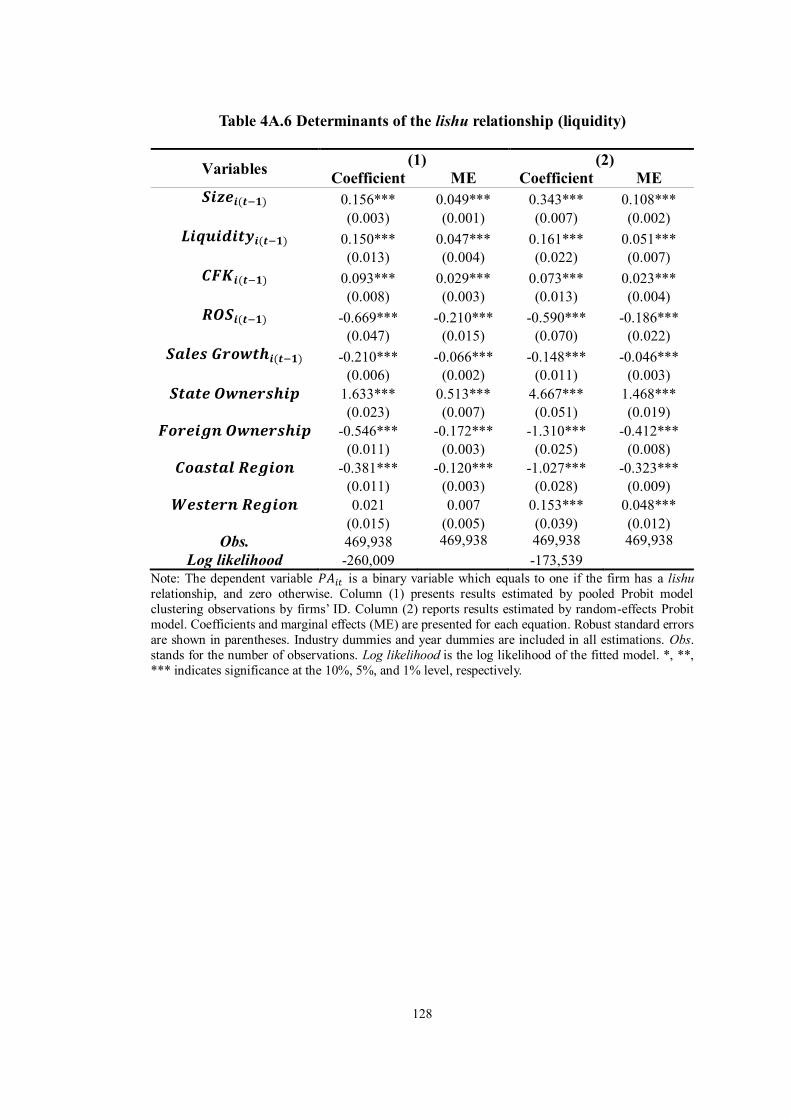
128
Table 4A.6 Determinants of the lishu relationship (liquidity)
Variables (1) (2) Coefficient ME Coefficient ME
𝑺𝒊𝒛𝒆𝒊(𝒕−𝟏) 0.156*** 0.049*** 0.343*** 0.108*** (0.003) (0.001) (0.007) (0.002)
𝑳𝒊𝒒𝒖𝒊𝒅𝒊𝒕𝒚𝒊(𝒕−𝟏) 0.150*** 0.047*** 0.161*** 0.051*** (0.013) (0.004) (0.022) (0.007)
𝑪𝑭𝑲𝒊(𝒕−𝟏) 0.093*** 0.029*** 0.073*** 0.023*** (0.008) (0.003) (0.013) (0.004)
𝑹𝑶𝑺𝒊(𝒕−𝟏) -0.669*** -0.210*** -0.590*** -0.186*** (0.047) (0.015) (0.070) (0.022)
𝑺𝒂𝒍𝒆𝒔 𝑮𝒓𝒐𝒘𝒕𝒉𝒊(𝒕−𝟏) -0.210*** -0.066*** -0.148*** -0.046*** (0.006) (0.002) (0.011) (0.003)
𝑺𝒕𝒂𝒕𝒆 𝑶𝒘𝒏𝒆𝒓𝒔𝒉𝒊𝒑 1.633*** 0.513*** 4.667*** 1.468*** (0.023) (0.007) (0.051) (0.019)
𝑭𝒐𝒓𝒆𝒊𝒈𝒏 𝑶𝒘𝒏𝒆𝒓𝒔𝒉𝒊𝒑 -0.546*** -0.172*** -1.310*** -0.412*** (0.011) (0.003) (0.025) (0.008)
𝑪𝒐𝒂𝒔𝒕𝒂𝒍 𝑹𝒆𝒈𝒊𝒐𝒏 -0.381*** -0.120*** -1.027*** -0.323*** (0.011) (0.003) (0.028) (0.009)
𝑾𝒆𝒔𝒕𝒆𝒓𝒏 𝑹𝒆𝒈𝒊𝒐𝒏 0.021 0.007 0.153*** 0.048*** (0.015) (0.005) (0.039) (0.012)
Obs. 469,938 469,938 469,938 469,938 Log likelihood -260,009 -173,539
Note: The dependent variable 𝑃𝐴𝑖𝑡 is a binary variable which equals to one if the firm has a lishu relationship, and zero otherwise. Column (1) presents results estimated by pooled Probit model clustering observations by firms’ ID. Column (2) reports results estimated by random-effects Probit model. Coefficients and marginal effects (ME) are presented for each equation. Robust standard errors are shown in parentheses. Industry dummies and year dummies are included in all estimations. Obs. stands for the number of observations. Log likelihood is the log likelihood of the fitted model. *, **, *** indicates significance at the 10%, 5%, and 1% level, respectively.
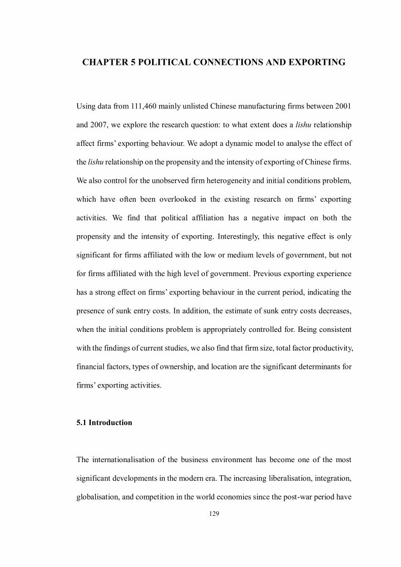
129
CHAPTER 5 POLITICAL CONNECTIONS AND EXPORTING
Using data from 111,460 mainly unlisted Chinese manufacturing firms between 2001
and 2007, we explore the research question: to what extent does a lishu relationship
affect firms’ exporting behaviour. We adopt a dynamic model to analyse the effect of
the lishu relationship on the propensity and the intensity of exporting of Chinese firms.
We also control for the unobserved firm heterogeneity and initial conditions problem,
which have often been overlooked in the existing research on firms’ exporting
activities. We find that political affiliation has a negative impact on both the
propensity and the intensity of exporting. Interestingly, this negative effect is only
significant for firms affiliated with the low or medium levels of government, but not
for firms affiliated with the high level of government. Previous exporting experience
has a strong effect on firms’ exporting behaviour in the current period, indicating the
presence of sunk entry costs. In addition, the estimate of sunk entry costs decreases,
when the initial conditions problem is appropriately controlled for. Being consistent
with the findings of current studies, we also find that firm size, total factor productivity,
financial factors, types of ownership, and location are the significant determinants for
firms’ exporting activities.
5.1 Introduction
The internationalisation of the business environment has become one of the most
significant developments in the modern era. The increasing liberalisation, integration,
globalisation, and competition in the world economies since the post-war period have
130
triggered a growing engagement of firms in exporting activities.
The study of firms’ exporting behaviour goes back to the 1960s. According to Lopez
(1967, p.126), long distance trade “became the driving force of economic progress,
and in the end affected every aspect of human activity almost as decisively as the
Industrial Revolution changed the modern world.”
The existing literature provides a comprehensive study on exporting from the
perspectives of public policy makers, managers, and researchers. According to
Czinkota (1994), in the view of public policy makers, exporting is an important way
to accumulate foreign exchange reserves, to increase employment levels, to improve
productivity, and to enhance social prosperity. As for business managers, exporting
can boost the growth of enterprises, improve financial performance, strengthen
competitive ability, and make sure companies survive in a highly internationalised
market (Samiee and Waiters, 1990; Kumcu, 1995).
The academic research on firms’ exporting can be divided into two groups:
international business studies and economics studies. Several researchers have
explored firms’ exporting behaviour from the perspectives of international business
and international management (for example, Albaum and Peterson, 1984; Yeoh and
Jeong, 1995; Zou and Stan, 1998; Robertson and Chetty, 2000; Leonidou et al., 2002;
Moen, 1999; Peng et al., 2008; Liu, 2010; Wei et al., 2014). They consider exporting
as a challenging but promising area for firms’ development and an important strategy
for firms to internationalise. The internationalised market environment provides many
131
crucial opportunities for economic development, states independence, profitability
growth, and business firms’ survival. Firms are therefore likely to enter international
markets to take advantage of these opportunities.
Economics researchers focus on the role of external institutions and infrastructure
investment on international trade (for example, Kandori, 1992; Greif, 1993, 1994;
Anderson and Marcouiller, 2002; Dixit, 2003; Li, 2003; Costinot, 2004; Anderson and
Young, 2006; Ranjan and Lee, 2007; Nunn, 2007; Méon and Sekkat, 2008; Albarran
et al., 2013). These scholars argue that trade expansion requires well-developed
support from the institutions, such as property rights institutions, contracting
institutions and financing institutions, and undeveloped economic institutions, which
sit in an imperfect contract enforcement system and causes insecurity of property
rights protection, corruption, and transport costs. These imperfections in turn, can
dramatically reduce international trade.
Another group of economics researchers attempts to analyse the relationship between
firm heterogeneity and exporting behaviour (for instance, Hirsch and Adar, 1974;
Aitken et al., 1997; Melitz, 2003; Greenaway et al., 2007; Lu, 2011; Chaney, 2013;
Lawless, 2009; Van Biesebroeck, 2005; Das et al., 2007; Greenaway and Kneller,
2008; Sinani and Hobdari, 2010; Alessandria and Choi, 2007; Bernard and Jensen,
2004; Roberts and Tybout, 1997; Bernard and Wagner, 2001; Manez et al., 2008;
Manova, 2013). They point out that the firm size, productivity, capital intensity, and
financial considerations can also affect the enterprises’ entry into export markets.
Particularly, they also point out that the existence of sunk costs is another crucial
132
determinant of firms’ exporting behaviour. As new exporters always have to deal with
huge start-up costs, they need to collect information on foreign markets, explore
marketing resources, changing and adjusting the products to cater to the needs of
international customers, and deal with the new governmental procedures.
However, one feature of the existing studies is that the majority have ignored the
effects of firms’ political connections on exporting activities. As an important
development strategy, having political connections is crucial to firms, especially in
developing countries. Several researchers point out that political connections can
provide better protection and more prerogatives to the politically connected firms (see,
for example, Brandt and Li, 2003; Khwaja and Mian, 2005; Faccio, 2006; Leuz and
Oberholzer-Gee, 2006; Goldman et al., 2010; Faccio, 2010).
These favourable treatments include better reputation and prestige, more opportunities
to access critical and diversified resources which are larger in quantity and higher in
quality, preferential policies, assistance in land purchase, favourable access to
government contracts and bank loans, reduction in the tax burden, more opportunities
in undertaking mergers and acquisitions (M&As) in heavily regulated industries (such
as finance, media, aerospace, and natural resources mining) which are not open to the
private sector. These favourable assistances all lead to improvements in operating
performance. Moreover, politically connected firms may face lower sunk costs
because these firms suffer from soft budget constraints. Given the fact that political
connections improve firm performance and facilitate sunk costs, ignoring the effects
of political connections will bias the estimation of firms exporting behaviour.
133
Therefore, this study attempts to contribute to the literature in the following four
important ways. First, we use a very large dataset, provided by the National Bureau
of Statistics of China (NBS) over the period 2000 and 2007. This dataset is made up
of comprehensive economic information of firms coming from 31 provinces or
province-equivalent municipal cities (except Hong Kong, Macao and Taiwan) all over
China. This dataset includes a large proportion of small and young firms, which can
represent the population of Chinese firms better than listed firms. It provides us with
a unique opportunity to carry out much sharper tests for the exporting activities
hypotheses than those typically performed in the literature, which is mostly based on
listed firms. Moreover, this dataset not only contains detailed information regarding
firms’ exporting activities, but also the information about their political connection,
so that we are able to examine the relationship between firms’ exporting behaviour
and political connections. Our final panel covers 111,460 mainly unlisted firms, which
corresponds to 502,196 firm-year observations. To the best of our knowledge, the
relationship between political connections and exporting activities hypotheses has
never been tested for unlisted firms using such a comprehensive dataset. Furthermore,
we not only focus on the probability of exporting, but also on the intensity of exporting.
Second, since the opening-up of China in the 1980s, China has swiftly risen as a global
trading power and its status as one of the most important countries in the world has
been greeted with a curious mixture of both admiration and fear. In particular, in 2009,
China has become the largest merchandise exporting country with a total value of
around 1.20 trillion US dollars (accounting for 43.63% of its total GDP), compared
with the 1.05 trillion US dollars in the US (accounting for 18.46% of its total GDP)

134
(the World Trade Organization; the World Bank). Some research studies the exporting
behaviour of Chinese firms (for example, Du and Girma, 2007; Lu and Tao, 2007;
Yang and Malick, 2010; Lu et al., 2010; Xu et al., 2011; Sun and Hong, 2011; Yi and
Wang, 2012; Dai and Yu, 2013). However, these studies mainly focus on exporting
behaviour without exploring the effects of political connections. At the same time,
political connections are always considered as an important instrument for private
enterprises, especially unlisted firms, to develop themselves in the market
environment with Chinese characteristics (Child, 1994; Peng et al., 2004; Li, 2004;
Tan et al., 2007; Chen et al., 2011a, 2011b; Feng et al., 2011). In China, the art of
using connections (guan xi) to subvert or take the advantages of the formal system
exists commonly in the Chinese administration. Therefore, China is a comprehensive
laboratory to study as to how political connections affect firms’ exporting activities.
Third, political connections have attracted worldwide academic interest. The existing
literature on political connections has been conducted in other countries, such as the
United States, Malaysia and Thailand (for example, Roberts, 1990; Johnson and
Mitton, 2003; Goldman et al., 2009). However, the definition of political connections
and their influences on enterprises are different between China and the other countries
around the world due to the different political regimes. China has a unique type of
political connections, named the lishu relationship. Lishu is a Chinese word which
means “belonging to”, “subordinate to”, or “directly controlled by”. Through this
relationship, the governments can maintain administrative power to control various
aspects of the firm both directly and legally (Tan et al., 2007; Li, 2004). Specifically,
a lishu relationship implies that the government controls firm structures, directors and
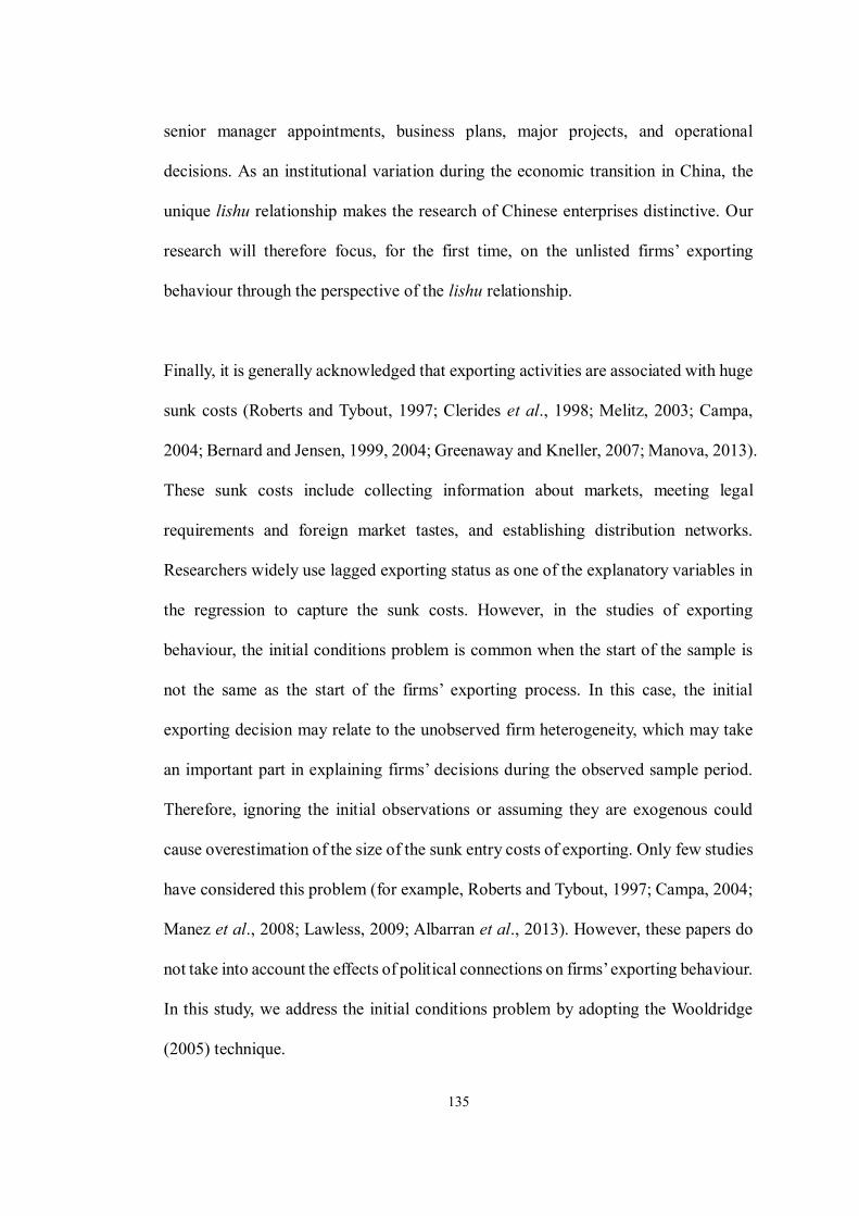
135
senior manager appointments, business plans, major projects, and operational
decisions. As an institutional variation during the economic transition in China, the
unique lishu relationship makes the research of Chinese enterprises distinctive. Our
research will therefore focus, for the first time, on the unlisted firms’ exporting
behaviour through the perspective of the lishu relationship.
Finally, it is generally acknowledged that exporting activities are associated with huge
sunk costs (Roberts and Tybout, 1997; Clerides et al., 1998; Melitz, 2003; Campa,
2004; Bernard and Jensen, 1999, 2004; Greenaway and Kneller, 2007; Manova, 2013).
These sunk costs include collecting information about markets, meeting legal
requirements and foreign market tastes, and establishing distribution networks.
Researchers widely use lagged exporting status as one of the explanatory variables in
the regression to capture the sunk costs. However, in the studies of exporting
behaviour, the initial conditions problem is common when the start of the sample is
not the same as the start of the firms’ exporting process. In this case, the initial
exporting decision may relate to the unobserved firm heterogeneity, which may take
an important part in explaining firms’ decisions during the observed sample period.
Therefore, ignoring the initial observations or assuming they are exogenous could
cause overestimation of the size of the sunk entry costs of exporting. Only few studies
have considered this problem (for example, Roberts and Tybout, 1997; Campa, 2004;
Manez et al., 2008; Lawless, 2009; Albarran et al., 2013). However, these papers do
not take into account the effects of political connections on firms’ exporting behaviour.
In this study, we address the initial conditions problem by adopting the Wooldridge
(2005) technique.

136
Our main finding in this chapter is that firms with political affiliation are less likely
to export and export less. Being consistent with the existing studies, we also find that
sunk entry costs exist in Chinese firms. By controlling for the initial conditions
properly, the overestimation of sunk entry costs can be mitigated. We also find that
firm size, total factor productivity, financial factors, types of ownership, and location
are significant determinants to firms’ exporting activities.
The rest of this chapter is organised as follows. Section 5.2 introduces the background
of Chinese exporting. Section 5.3 endeavours to provide a comprehensive review of
the existing literature on firms’ exporting behaviour and political connections. Our
hypotheses are demonstrated in section 5.4. Specification and estimation methodology
are presented in section 5.5. Data sample and summary statistics are described in
section 5.6. In section 5.7, the empirical results are presented. Section 5.8 shows
further tests. Section 5.9 concludes this chapter.
5.2 Background
5.2.1 Chinese institutional environment
It is generally acknowledged that better legal protection and better institutions lead to
better outcomes of the financial system, and in turn, lead to rapid and constant
development in exporting. For example, an entrepreneur, who aims to expand his/her
business in an unfamiliar global market, needs to consider how to prevent his/her legal
properties from being expropriated by local governments, how to make sure the

137
contracts can be well implemented by his/her distant clients, and how to obtain
sufficient funds from banks in the global financial market to support the expansion.
Therefore, well-developed legal and financial systems can encourage the entrepreneur
to participate in the international market by providing support for the development of
exporting.
Meantime, since its transformation from a centrally planned economic system to a
socialist market economic system, the Chinese economy is characterised by a unique
market environment where the private sector and public sector coexist. Despite
economic reforms provide favourable support for private investment and grant private
business preferential access to capital, technology, and markets, SOEs are still
powerful and dominate the major industries and resources in China.
Allen et al. (2005) examine the financial system in China at the aggregate level,
including both the financial markets and the banking system. They compare China’s
financial system with that in 49 countries. They show that the overhead cost of the
banking system in China is much higher, while its profitability is the lowest, indicating
that it is not an efficient system. Moreover, according to Morck et al. (2000) and Allen
et al. (2005), stock prices are more synchronous in China, indicating that the stock
markets are inefficient. They attribute this phenomenon to the weak protection for the
investors. For example, because of poor and uncertain protection of private property
rights, political events and rumours may have a significant influence on the market-
wide stock prices. In addition, problems such as intercorporate income shifting would
reduce firm-specific stock price variation, increasing stock return synchronicity. To
138
summarise, the financial system in China is influenced significantly by this powerful
but insufficient banking system, in which the state-owned banks play the dominating
role.1
As to the Chinese legal system, it is still evolving and characterised by a fragmentation
of regulatory authorities. For example, as the Chinese commercial law system is an
instrument to enforce the economic policy of the Chinese Communist Party (CCP),
the central government chooses pilot areas (shi dian) and implements special rules
within those areas to test the effects of a law or regulation before introducing the rules
national widely. In this case, the central government may delegate authority and
flexibility to local officials so that they can exercise these laws and regulations in
accordance with the local circumstances, which in turn may make laws uncertain (Ho,
1994). Moreover, the legal system in China is also characterised by ambiguity in legal
drafting. For instance, according to Law and Chen (2004), Chinese economic laws
often draw a broad picture, without specifying the concrete and detailed rules. This
situation can be attributed to the fact that the Chinese government may not have
enough time to consider every aspect of the legislation due to the rapid development
of the legal and economic environment; but at the same time, there may be urgent
need for some regulations to be carried out in the market. The government therefore
has to enact some laws or regulations hastily without containing enough details.
Allen et al. (2005) compare the legal system in China to those of other emerging
countries, including India, Pakistan, South Africa, Argentina, Brazil, and Mexico.
1 They are Bank of China (BOC), Industrial and Commercial Bank of China (ICBC), China
Construction Bank (CCB), and Agricultural Bank of China (ABC).
139
They show that the corruption index in China is the worst among the seven developing
countries, while its creditor and shareholder protection are only better than that of
India and Mexico. This indicates that the development of China’s legal system is
behind that of the other major emerging countries. Furthermore, one of the most
important and necessary factors to have an effective law enforcement system is that a
country must have an independent and efficient judicial system with a sufficient
supply of qualified legal professionals. However, according to Allen et al. (2005),
only 20% of all lawyers in China have law degrees, and even a lower percentage of
judges have formally received legal education at universities or colleges. Moreover,
only four percent of the five million business enterprises in China currently have
regular legal advisers. In a word, the law and legal institutions in China, as well as the
investor protection systems, are significantly underdeveloped.
Given such underdeveloped external institutional environment, the extraordinary
development of exporting in China is always considered as a miracle.
5.2.2 The economic and exporting development in China
The opening-up of China in the 1980s has brought momentous change to the life of
its people. The sustained rapid rate of economic growth compares favourably with the
experience of other transitional economies. China’s sudden rise as a global trading
power and its status as one of the most important countries in the world have been
greeted with a curious mixture of both admiration and fear. At the end of July 2014,
the population of China was approximately 1.36 billion people, ranking it the largest

140
country in the world (The World Factbook). In current US dollars (billion), the GDP
in China has occupied the second place in the world since 2010 (See Table 5.1). If
PPP is used to adjust GDPs,1 China’s economy is still the second largest following
the United States, and became the largest in 2014 (See Table 5.2). Moreover, the GDP
annual growth rate for the United States in 2012 was 2.30%, while the Chinese
economic growth rate was 7.80% (The World Bank) (See Figure 5.1). Assuming that
both countries continue to grow at the same rate separately, it will take only around
13 years before China overtakes the US to become the largest economy in the world.
1 Using PPP-adjusted figures to measure GDP is more appropriate. For example, the exchange rate between the RMB yuan and the U.S. dollar changed from 1 U.S. dollar = 4.25 RMB yuan to 1 U.S. dollar = 8.28 RMB yuan in 1992, which introduced a significant downward bias for China’s GDP figure in 1992.
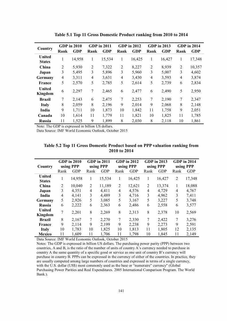
141
Table 5.1 Top 11 Gross Domestic Product ranking from 2010 to 2014
Country GDP in 2010 GDP in 2011 GDP in 2012 GDP in 2013 GDP in 2014 Rank GDP Rank GDP Rank GDP Rank GDP Rank GDP
United States 1 14,958 1 15,534 1 16,425 1 16,427 1 17,348
China 2 5,930 2 7,322 2 8,227 2 8,939 2 10,357 Japan 3 5,495 3 5,896 3 5,960 3 5,007 3 4,602
Germany 4 3,311 4 3,631 4 3,430 4 3,593 4 3,874 France 5 2,570 5 2,785 5 2,614 5 2,739 6 2,834 United
Kingdom 6 2,297 7 2,465 6 2,477 6 2,490 5 2,950
Brazil 7 2,143 6 2,475 7 2,253 7 2,190 7 2,347 Italy 8 2,059 8 2,196 9 2,014 9 2,068 8 2,148 India 9 1,711 10 1,873 10 1,842 11 1,758 9 2,051
Canada 10 1,614 11 1,779 11 1,821 10 1,825 11 1,785 Russia 11 1,525 9 1,899 8 2,030 8 2,118 10 1,861
Note: The GDP is expressed in billion US dollars. Data Source: IMF World Economic Outlook, October 2015
Table 5.2 Top 11 Gross Domestic Product based on PPP valuation ranking from 2010 to 2014
Country GDP in 2010
using PPP GDP in 2011
using PPP GDP in 2012
using PPP GDP in 2013
using PPP GDP in 2014
using PPP Rank GDP Rank GDP Rank GDP Rank GDP Rank GDP
United States 1 14,958 1 15,534 1 16,425 1 16,427 2 17,348
China 2 10,040 2 11,189 2 12,621 2 13,374 1 18,088 Japan 3 4,351 4 4,411 4 4,576 4 4,729 4 4,767 India 4 4,141 3 4,489 3 4,716 3 4,962 3 7,411
Germany 5 2,926 5 3,085 5 3,167 5 3,227 5 3,748 Russia 6 2,222 6 2,363 6 2,486 6 2,558 6 3,577 United
Kingdom 7 2,201 8 2,269 8 2,313 8 2,378 10 2,569
Brazil 8 2,167 7 2,270 7 2,330 7 2,422 7 3,276 France 9 2,114 9 2,199 9 2,238 9 2,273 9 2,591 Italy 10 1,783 10 1,825 10 1,813 11 1,805 12 2,135
Mexico 11 1,609 11 1,706 11 1,798 10 1,845 11 2,149 Data Source: IMF World Economic Outlook, October 2015 Notes: The GDP is expressed in billion US dollars. The purchasing power parity (PPP) between two countries, A and B, is the ratio of the number of units of country A’s currency needed to purchase in country A the same quantity of a specific good or service as one unit of country B’s currency will purchase in country B. PPPs can be expressed in the currency of either of the countries. In practice, they are usually computed among large numbers of countries and expressed in terms of a single currency, with the U.S. dollar (US$) most commonly used as the base or “numeraire” currency" (Global Purchasing Power Parities and Real Expenditures. 2005 International Comparison Program. The World Bank.).
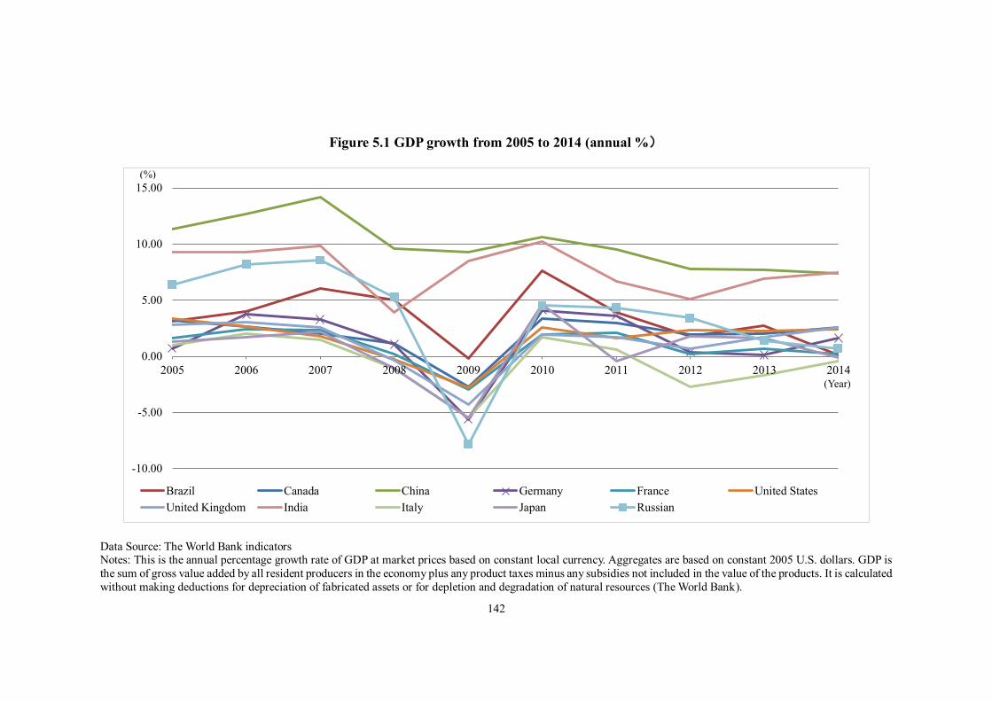
142
Figure 5.1 GDP growth from 2005 to 2014 (annual %)
Data Source: The World Bank indicators Notes: This is the annual percentage growth rate of GDP at market prices based on constant local currency. Aggregates are based on constant 2005 U.S. dollars. GDP is the sum of gross value added by all resident producers in the economy plus any product taxes minus any subsidies not included in the value of the products. It is calculated without making deductions for depreciation of fabricated assets or for depletion and degradation of natural resources (The World Bank).
-10.00
-5.00
0.00
5.00
10.00
15.00
2005 2006 2007 2008 2009 2010 2011 2012 2013 2014
Brazil Canada China Germany France United StatesUnited Kingdom India Italy Japan Russian
(%)
(Year)

143
It may be more useful to compare China’s GDP and economic growth with that of
the other major emerging economies rather than the most developed countries, since
China’s rapid economic growth only started in 1979.1 Table 5.3 compares China
with the ten largest emerging economies in the world. In 2014, China’s GDP was
more than four times the size of Brazil’s, which is the second largest developing
economy in the world (see Table 5.3). In terms of PPP-adjusted GDP figures in
2014 (See Table 5.4), China is more than twice the size of India, the second largest
emerging economy in the world. As to the annual growth rate of GDP in 2012,
China has been growing faster (7.8%) than Thailand (6.5%), which has the second
highest growth rate in this group (The World Bank) (See Figure 5.2). Moreover,
China has the largest annual GDP per capita growth rate among the group of the
emerging economies over the period of 2005 and 2014 (See Figure 5.3). With its
rapid development, China is positioned to play an increasingly significant role in
the world economy.
1 Measured in current US dollars, China’s GDP in 1978 was 148.18 billion US dollars, while in 1979 it reached 176.63 billion US dollars.
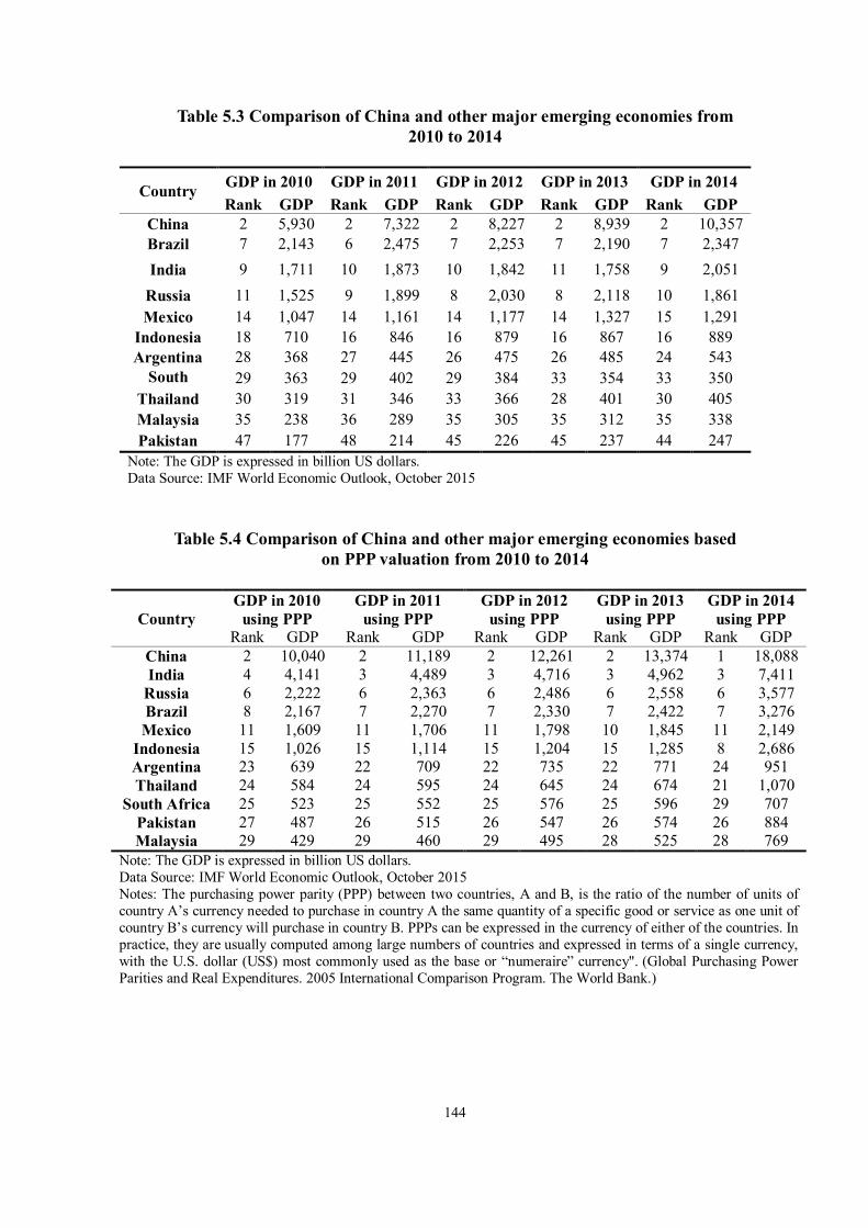
144
Table 5.3 Comparison of China and other major emerging economies from 2010 to 2014
Country GDP in 2010 GDP in 2011 GDP in 2012 GDP in 2013 GDP in 2014 Rank GDP Rank GDP Rank GDP Rank GDP Rank GDP
China 2 5,930 2 7,322 2 8,227 2 8,939 2 10,357 Brazil 7 2,143 6 2,475 7 2,253 7 2,190 7 2,347 India 9 1,711 10 1,873 10 1,842 11 1,758 9 2,051
Russia 11 1,525 9 1,899 8 2,030 8 2,118 10 1,861 Mexico 14 1,047 14 1,161 14 1,177 14 1,327 15 1,291
Indonesia 18 710 16 846 16 879 16 867 16 889 Argentina 28 368 27 445 26 475 26 485 24 543
South Africa
29 363 29 402 29 384 33 354 33 350 Thailand 30 319 31 346 33 366 28 401 30 405 Malaysia 35 238 36 289 35 305 35 312 35 338 Pakistan 47 177 48 214 45 226 45 237 44 247
Note: The GDP is expressed in billion US dollars. Data Source: IMF World Economic Outlook, October 2015
Table 5.4 Comparison of China and other major emerging economies based on PPP valuation from 2010 to 2014
Country GDP in 2010
using PPP GDP in 2011
using PPP GDP in 2012
using PPP GDP in 2013
using PPP GDP in 2014
using PPP Rank GDP Rank GDP Rank GDP Rank GDP Rank GDP
China 2 10,040 2 11,189 2 12,261 2 13,374 1 18,088 India 4 4,141 3 4,489 3 4,716 3 4,962 3 7,411
Russia 6 2,222 6 2,363 6 2,486 6 2,558 6 3,577 Brazil 8 2,167 7 2,270 7 2,330 7 2,422 7 3,276 Mexico 11 1,609 11 1,706 11 1,798 10 1,845 11 2,149
Indonesia 15 1,026 15 1,114 15 1,204 15 1,285 8 2,686 Argentina 23 639 22 709 22 735 22 771 24 951 Thailand 24 584 24 595 24 645 24 674 21 1,070
South Africa 25 523 25 552 25 576 25 596 29 707 Pakistan 27 487 26 515 26 547 26 574 26 884 Malaysia 29 429 29 460 29 495 28 525 28 769
Note: The GDP is expressed in billion US dollars. Data Source: IMF World Economic Outlook, October 2015 Notes: The purchasing power parity (PPP) between two countries, A and B, is the ratio of the number of units of country A’s currency needed to purchase in country A the same quantity of a specific good or service as one unit of country B’s currency will purchase in country B. PPPs can be expressed in the currency of either of the countries. In practice, they are usually computed among large numbers of countries and expressed in terms of a single currency, with the U.S. dollar (US$) most commonly used as the base or “numeraire” currency". (Global Purchasing Power Parities and Real Expenditures. 2005 International Comparison Program. The World Bank.)
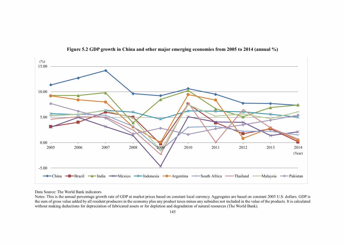
145
Figure 5.2 GDP growth in China and other major emerging economies from 2005 to 2014 (annual %)
Data Source: The World Bank indicators Notes: This is the annual percentage growth rate of GDP at market prices based on constant local currency. Aggregates are based on constant 2005 U.S. dollars. GDP is the sum of gross value added by all resident producers in the economy plus any product taxes minus any subsidies not included in the value of the products. It is calculated without making deductions for depreciation of fabricated assets or for depletion and degradation of natural resources (The World Bank).
-5.00
0.00
5.00
10.00
15.00
2005 2006 2007 2008 2009 2010 2011 2012 2013 2014
China Brazil India Mexico Indonesia Argentina South Africa Thailand Malaysia Pakistan
(%)
(Year)
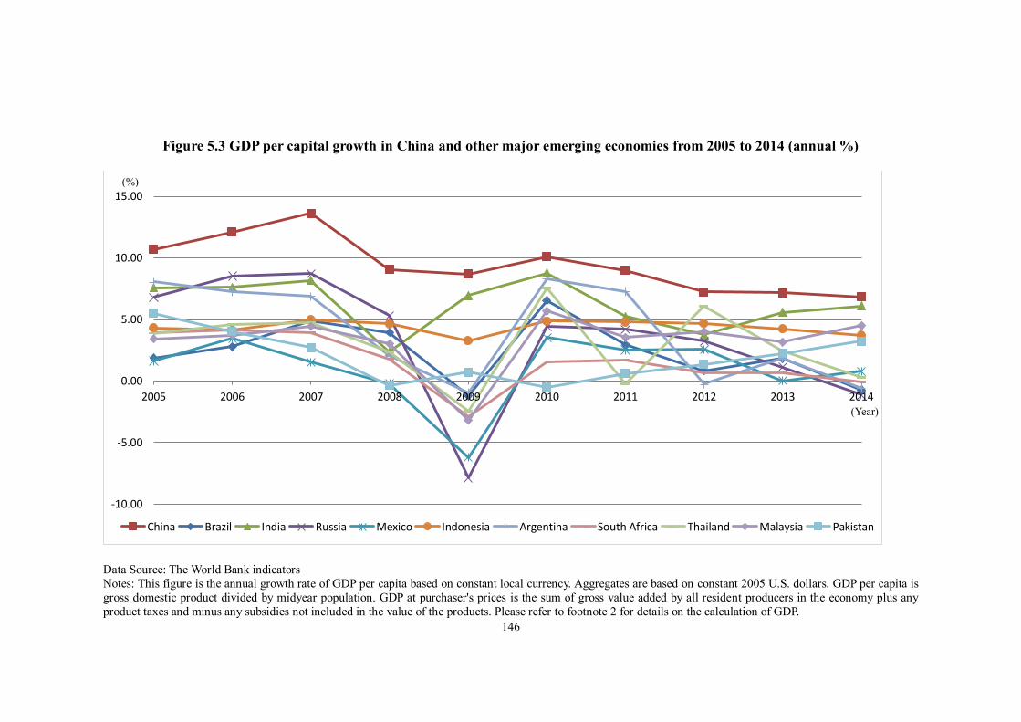
146
Figure 5.3 GDP per capital growth in China and other major emerging economies from 2005 to 2014 (annual %)
Data Source: The World Bank indicators Notes: This figure is the annual growth rate of GDP per capita based on constant local currency. Aggregates are based on constant 2005 U.S. dollars. GDP per capita is gross domestic product divided by midyear population. GDP at purchaser's prices is the sum of gross value added by all resident producers in the economy plus any product taxes and minus any subsidies not included in the value of the products. Please refer to footnote 2 for details on the calculation of GDP.
-10.00
-5.00
0.00
5.00
10.00
15.00
2005 2006 2007 2008 2009 2010 2011 2012 2013 2014
China Brazil India Russia Mexico Indonesia Argentina South Africa Thailand Malaysia Pakistan
(%)
(Year)

147
In light of the miraculous development of the Chinese economy in the past decades,
understanding the exporting behaviour of Chinese firms is important. Since the
economic reform initiated in the 1970s, China has not only experienced a dramatic
economic growth, but also actively engaged in international markets and encouraged
exports by establishing the Special Economic Zones1 and the duty drawback system.2
During the earlier years of the establishment of the new China since 1949, the export
value was only around 0.55 billion US dollars (WTO databases). Through the
development in the next two decades, the export value amounted to 2.31 billion US
dollars in 1970, but only taking up 2.61% of the total GDP (See Table 5.5). Along
with the deepening of China’s economic reform and the opening-up policy in the next
thirty years, the total value of exports experienced a steady and rapid growth reaching
266.10 billion US dollars in 2001, and the ratio of export to GDP increased to 22.60%.
1 As a part of the economic reform, the Special Economic Zones were considered as bridges linking home and abroad. On the one hand, these regions enjoy considerable autonomy, preferential tax treatment, and high levels of resources. They are the front line of the opening-up policy and closely connected with the international markets, having easier access to market information, foreign capital, modern technology, and management experience. These zones can absorb and utilise foreign capital and introduce developed technology and management experience for the construction of the socialist modernisation. On the other hand, through these zones, firms in the inland areas have more opportunities to develop economical and technological cooperation with the outside world. Currently, China has six Special Economic Zones, including Shenzhen in Guangdong Province (authorised in May 1980), Zhuhai in Guangdong Province (authorised in August 1980), Xiamen in Fujian Province (authorised in October 1980), Shantou in Guangdong Province (authorised in November 1984), Hainan (authorised in April 1988), and Kashi in Xinjiang Province (authorised in May 2010). 2 Duty drawback schemes, which typically involve a combination of import duty drawbacks and value-added tax (VAT) rebates and exemptions on imports that are used for the production of exports in China. For imported inputs, the VAT levy is in addition to the import duty. Finished final goods are also subject to VAT. However, previously paid VAT on its inputs is deducted from the VAT payment on its final goods. When the final goods are exported, the previously paid VAT on imported inputs is rebated to the export processor (see China’s Ministry of Finance: www.mof.gov.cn and Ministry of Commerce: www.mofcom.gov.cn). Therefore, duty drawbacks and VAT rebates respectively reduce the tariffs and domestic taxes on imported inputs for export processing. For example, a 17% tariff was imposed on the imports of electronic equipment and an additional 17% domestic tax was levied on its value-added in production in 1998. Both taxes are rebated when the electronic equipment is used for export processing. Moreover, the rebate rates were increased and many products enjoyed zero value-added tax rates in 1999 (see China’s Ministry of Finance: www.mof.gov.cn). These policies provide great incentives for firms to sell products abroad as they discriminate against imported inputs used in goods sold in domestic markets.
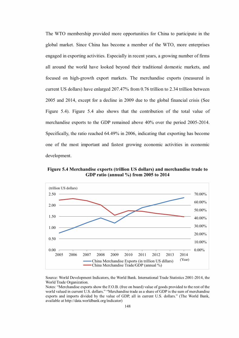
148
The WTO membership provided more opportunities for China to participate in the
global market. Since China has become a member of the WTO, more enterprises
engaged in exporting activities. Especially in recent years, a growing number of firms
all around the world have looked beyond their traditional domestic markets, and
focused on high-growth export markets. The merchandise exports (measured in
current US dollars) have enlarged 207.47% from 0.76 trillion to 2.34 trillion between
2005 and 2014, except for a decline in 2009 due to the global financial crisis (See
Figure 5.4). Figure 5.4 also shows that the contribution of the total value of
merchandise exports to the GDP remained above 40% over the period 2005-2014.
Specifically, the ratio reached 64.49% in 2006, indicating that exporting has become
one of the most important and fastest growing economic activities in economic
development.
Figure 5.4 Merchandise exports (trillion US dollars) and merchandise trade to GDP ratio (annual %) from 2005 to 2014
Source: World Development Indicators, the World Bank. International Trade Statistics 2001-2014, the World Trade Organization. Notes: “Merchandise exports show the F.O.B. (free on board) value of goods provided to the rest of the world valued in current U.S. dollars.” “Merchandise trade as a share of GDP is the sum of merchandise exports and imports divided by the value of GDP, all in current U.S. dollars.” (The World Bank, available at http://data.worldbank.org/indicator)
0.00%
10.00%
20.00%
30.00%
40.00%
50.00%
60.00%
70.00%
0.00
0.50
1.00
1.50
2.00
2.50
2005 2006 2007 2008 2009 2010 2011 2012 2013 2014China Merchandise Exports (in trillion US dillars)China Merchandise Trade/GDP (annual %)
(Year)
(Year)
(Year)
(trillion US dollars)

149
Table 5.5 Export and export to GDP ratio in China from 1970 to 2014
Year Value (Billion US dollars)
Export to GDP (Percentage)
1970 2.31 2.61 1975 7.69 4.59 1980 18.10 10.65 1985 27.35 9.21 1990 62.09 16.07 1991 71.91 17.37 1992 84.94 18.65 1993 91.74 19.65 1994 121.01 21.27 1995 148.78 20.23 1996 151.05 20.05 1997 182.79 21.75 1998 183.71 20.35 1999 194.93 20.17 2000 249.20 23.33 2001 266.10 22.60 2002 325.60 25.13 2003 438.23 29.56 2004 593.33 33.95 2005 761.95 37.08 2006 968.98 39.13 2007 1,220.46 38.41 2008 1,430.69 34.98 2009 1,201.61 26.71 2010 1,577.75 29.40 2011 1,898.38 28.54 2012 2,048.71 27.33 2013 2,213.30 23.32 2014 2,342.54 22.61
Data Source: The WTO databases and the World Factbook
(Year) (Year)

150
5.3 Literature review
We hereby survey the literature on the determinants of firms’ exporting decisions, the
relationship between firm performance and political connections, and the relationship
between political connections and firms’ exports.
5.3.1 Determinants of firms’ exporting behaviour
There are a growing number of empirical studies on the determinants of firms’
exporting decisions. The existing literature focuses on the four aspects including the
sunk entry costs, the relationship between firms’ characteristics and exporting
behaviour, the connection between financial factors and exporting behaviour, and the
impact of innovation on firms’ exporting activities.
5.3.1.1 The sunk entry costs
Before starting exporting, new potential exporters must gather information from
foreign markets, decide whether or not exporting is feasible and potentially profitable,
and identify the target market(s). Once exporting decisions are made, a firm has to
learn the foreign regulations and new bureaucratic procedures, adapt their products
and packages to foreign market standards and tastes, develop new distribution
channels and export department, comply with all the shipping regulations specified
by the foreign customs agency, and face transportation and insurance costs and tariffs.
Das et al. (2007) calculate the sunk costs participating in foreign markets in currency
151
units for Colombian manufacturing firms and find that in 1999 US dollars, the sunk
costs of entering exporting market range from $730,000 to $1.6 million based on firm
size. Kasahara and Lapham (2013) estimate the magnitude of the sunk costs of
exporting for Chilean manufacturing firms and find that the sunk costs of exporting
are $363,000 1990 on average for wood products to $998,000 1990 for food products.
A growing literature studies the hysteresis in the exporting market due to the sunk
entry costs. Roberts and Tybout (1997) test a sample of 650 Columbian firms and find
that among firms that did not export in year t, more than 85 percent of them did not
export in year t+1. Similarly, for firms that initially export, the proportion of
manufacturing firms that remain in the export market from one year to the next is
between 83% and 91% from 1983 to 1989. This indicates that there is substantial
persistence in firm-level patterns of entry into the export market. More specifically,
participation in the previous year can increase the probability of exporting in the
current years by as much as 0.63 percent, suggesting that export history affects firms’
exporting decision-making due to the existence of sunk costs. Furthermore, the
authors demonstrate that the re-entry costs for firms that have departed from the
foreign market for two years are not significantly different from the costs for new
exporters, suggesting that the start-up costs cannot be avoided.
Similar findings have been found in other countries. Bernard and Wagner (2001) find
substantial sunk costs of 6,400 Germany firms. Bugamelli and Infante (2003) show
that being a current exporter increases the probability of exporting in the next year by
70% larger than that of non-exporters in Italy. Significant sunk entry costs have also
been observed in the United States by Bernard and Jensen (2004), in the United
152
Kingdom by Greenaway and Kneller (2004), in Ireland by Lawless (2009), and in
Spain by Campa (2004).
5.3.1.2 Firm characteristics and exporting behaviour
It appears that good firms become exporters. However, some researchers may argue
that firms become good because they are exporters and the substantial differences
between exporters and non-exporters do not indicate any direction of causality. In this
case, the direction of causality between firm characteristics and export behaviour is
vague, i.e. it is not clear whether good firms become exporters or exporters become
good firms. In this case, apart from the sunk entry costs, a number of empirical works
have estimated the relationship between firms’ characteristics and exporting activities
from the perspective of firm size, productivity, foreign ownership, age, location, and
labour costs and industries.
A. Firm size
A large numbers of international business studies examine the relationship between
firm size and export performance from a theoretical perspective. It is pointed out that
the size of the firm can be used as a substitute indicator of resource availability (Calof,
1994; Katsikeas et al., 1996; Prasad et al., 2001). These resources can influence the
firm’s decision on marketing strategy and performance (Dhanaraj and Beamish, 2003).
Katsikeas et al. (1996, p.56) maintain that “there is a consensus in the international
business literature that larger companies possess more financial and human resources
as well as production capacity, attain higher levels of economies of scale, and tend to
153
perceive lower levels of risk about overseas markets and operations”. Bonaccorsi
(1992) states that these size-related properties can facilitate the exporting activity.
Some studies look at the relationship between firms’ size and exporting by employing
the empirical analysis. By using firm-level data from the Census Bureau’s Annual
Survey of Manufactures (ASM) over the period 1976-1987, Bernard and Jensen (1995)
show that compared with non-exporters, exporters in the US manufacturing industry
perform better. The authors find that the difference in size between exporters and non-
exporters is remarkable. Exporters are substantially larger than non-exporters. On
average, exporters are more than four times larger than non-exporters regarding the
total employment and more than six times larger in term of the value of shipments.
Similar results have been found by other scholars. Roberts and Tybout (1997) use
annual firm-level data of Colombian manufacturing plants from 1981 to 1989 and
show that the increase in firm size, measured by the firm’s capital stock, improves the
propensity of exporting. Aitken et al. (1997) use annual data on 2,104 Mexican
manufacturing firms over the period 1986-1990 and find that firms’ size is positively
associated with the probability of exporting. In a given industry, larger firms generally
produce more compared with smaller firms. Therefore, the fixed entry costs for
entering international markets can be spread over more production for larger firms. In
this case, the costs of foreign distribution per unit decline with the increase of the
firm’s size.
Bernard and Jensen (1999) use the US firms’ data from the Longitudinal Research
Database (LRD) of the Bureau of the Census, including all the manufacturing firms
154
in both the Census of Manufactures (CM) from 1987 to 1992 and the ASM for inter-
census years from 1984 to 1992. They test the relationship between the export status
of the firm today and the subsequent performance, finding that from 1984 to 1987,
firm size grew substantially faster for firms that became exporters in 1988 when
compared with the non-exporters. It is thus suggested that being a good firm increases
the probability of exporting.
Some studies of the determinants of exporting behaviour have been made in China.
For instance, using data from The Data of the Third National Industrial Census of the
People’s Republic of China (DTNICPRC) conducted by the China State Statistic
Bureau (SSB) (now called National Bureau of Statistics of China (NBS)) in 1995, Liu
and Shu (2003) explore the relationship between firm size and exporting behaviour
from the perspective of sunk costs and find that larger firms are more capable of
bearing sunk costs, and are therefore more likely to export. Similar results have been
found by Lu et al. (2008), who use a sample of 779 manufacturing firms listed on
Chinese stock markets between 2002 and 2005, and Xu et al. (2011), who use a larger
dataset drawn from the China Industrial Firms Database from 2001 to 2007.
These studies find that compared with domestic sales, exporting involves extra costs,
such as collecting market information, establishing overseas sales promotion
campaigns, adapting products to foreign markets, transporting, and communicating.
Moreover, due to the uncertainties in international markets and the different economic
environments in trading partner countries, exporting firms face more risks than in the
domestic market. Such costs and problems can be extremely severe for small firms.
By contrast, larger firms are more capable of expanding abroad because they have
155
more resources to enter the foreign market.
To summarise the existing literature, the fact that small and medium-sized firms
export less than large firms can be attributed to three factors. Firstly, large firms have
the cost advantage in export activities, in terms of the start-up costs and trading costs
(Wagner, 1995, 2001). Only large firms can afford the sunk entry costs. In addition,
because of the scale economy, large firms can reduce trading costs through bulk
shipping and extensive overseas network. Secondly, large firms export more than
small and medium-sized firms through the effect of productivity. Large firms are
considered as firms with higher productivity, which is one of the driving forces of
exporting (Roberts and Tybout, 1997; Bernard and Jensen, 1995; Bernard et al., 2007;
Baldwin and Gu, 2003; Bernard et al., 2003; Melitz, 2003; Greenaway and Kneller,
2007). Finally, large firms face less financial constraints in financing exporting
activities because the information asymmetry between lenders and borrowers of these
firms is less severe (Amiti and Weinstein, 2011; Manova, 2013).
However, some scholars find there is no significant relationship between firm size and
export performance (Contractor et al., 2005; Moen, 1999; Wolff and Pett, 2000).
Therefore, the relationship between firm size and export performance is still
controversial (Brouthers and Nakos, 2005; Kaynak and Kuan, 1993). These mixed
results may be explained by the fact that various studies have used different samples,
including firms from many different industrial sectors, or by the fact that they used
different measures to evaluate firm size. Additionally, small, medium and large firms
are defined differently from one country to another, indicating that the connections
between firm size and export performance may be different depending on the criterion
156
and measurement scales used (Contractor et al., 2005; Baldauf et al., 2000; Hoang,
1998).
B. Productivity
Good firms can be interpreted as firms with a high level of productivity. Exporters
have been found to be more capital intensive, more innovative, and more productive
than non-exporters (Tybout, 2001; Baldwin and Hanel, 2003). Bernard and Jensen
(1995) document that labour productivity, whether measured by shipments or value-
added per employee, is around a third greater for exporters than non-exporters in both
large and small firms.
On the other hand, participation in export markets may improve production efficiency.
The current literature provides two mechanisms to explain the positive correlation
between exporting and productivity.
The first mechanism argues that exporting improves productivity. That is, the
improvement in productivity can be attributed to the fact that exporters have to
increase their efficiency because they are forced by more competitive markets. Some
scholars argue that exporters gain access to new knowledge, technical expertise from
their international contracts or global buyers in the exporting market, and hence learn
both new product designs and production methods, to which their domestic
counterparts do not have access. This “learning and developing by exporting” effect
may be particularly relevant to the developing countries in East Asia (for example,
Evenson and Westphal, 1995; Grossman and Helpman, 1991; Rhee et al., 1984; World
157
Bank, 1993).
The second mechanism states a reverse causality. That is, the productivity difference
between exporters and non-exporters may reflect the self-selection hypothesis. That
is, only the more productive firms can self-select and survive in the highly competitive
international markets. Considering that the sunk costs are higher in the foreign
markets than in the domestic markets, only firms with high efficiency will find it
profitable to enter the export market. Furthermore, exporters who experience a
reduced productivity will be forced to exit from the international market. According
to Melitz (2003), the “New-New Trade Theory” states that the firms’ characteristics
such as the productivity, determine the exporting participation in the international
market. Beyond a certain amount of productivity, firms can profitably export as the
value of their sales on the foreign markets exceeds the level of fixed costs.
These two mechanisms have been tested in different countries. For instance, Clerides
et al. (1998) make use of microdata of manufacturing firms in Columbia, Mexico, and
Morocco; Bernard and Jensen (1995, 2004) and Bernard et al. (2007) look at the US
data; Baldwin and Gu (2003) examine data for Canadian manufacturing firms;
Delgado et al. (2002) explore the data of Spanish firms; Bernard and Wagner (2001)
look at the German firms; Mayer and Ottaviano (2007) estimate several European
countries, including Belgium, France, Germany, Hungary, Italy, Norway, and the UK;
Hallward-Driemeier et al.(2002) focus on the East Asia countries, including Indonesia,
Korea, Malaysia, Philippine, and Thailand; Aw et al. (2000) use manufacturing data
from the Republic of Korea and Taiwan (China); and Xu et al. (2011) focus on the
Chinese firms. All of these authors find that self-selection in export markets is
158
important. They document that an increase in labour productivity will improve the
percentage of firms’ exporting dramatically, confirming that more productive firms
are more likely to enter foreign markets. Moreover, this effect is much stronger for
foreign-owned firms (including foreign firms with funds from Hong Kong, Macao
and Taiwan) than for domestically-controlled firms, and more sizeable for younger
enterprises than for older ones. However, the productivity growth is slower for
exporters than non-exporters, indicating that, although exporting provides expanded
market opportunities and more potential jobs, it does not show evidence of boosting
firm productivity (Bernard and Jensen, 2004).
C. Foreign ownership
A few studies have estimated the relationship between foreign ownership and the
probability of exporting. For example, Aitken et al. (1997) find that firms with foreign
ownership are more likely to export than domestic firms do in Mexico. They suggest
that foreign firms have the natural advantages in gathering information regarding the
foreign markets and technology. These firms can also improve the export prospects
for domestic local firms through directly or indirectly sharing information and
providing distribution services for domestic firms to distribute their products. Bernard
and Jensen (2004) use all firms in the ASM from 1984 to 1992 and find that the
ownership of a US multinational firm increases the probability of exporting.
Xu et al. (2011) also find similar results in Chinese firms. They divide firms by
ownership into three categories, including domestic firms, foreign-owned firms, and
firms with funds from Hong Kong, Macao and Taiwan. Foreign-funded firms and
159
firms with funds from Hong Kong, Macao and Taiwan are more likely to export than
domestic firms. More specifically, in both the foreign-funded firms and firms with
funds from Hong Kong, Macao and Taiwan, the percentage of exporting firms is about
70%, while in domestic firms, the number stays around 25%.
Raff and Wagner (2014) examined around 7,000 manufacturing firms in German in
2009 and find that foreign firms export more goods to more countries. Based on
14,585 firms from 30 countries and 14 industries collected by the World Bank between
2002 and 2006, Boddin et al. (2015) show a statistically significant and positive
relationship between foreign ownership and the propensity of exporting. Specifically,
they find that foreign-owned firms are 17.60% more likely to engage in exporting.
This effect is more obvious for low-income countries: foreign ownership increases the
propensity of exporting by 25%. The authors point out that firms in less developed
countries face more severe constraints, such as the technology, marketing know-how,
and financing opportunities, which can be alleviated through foreign ownership.
Raff and Wagner (2014) also document several reasons for such effect. Firstly,
foreign-owned firms can benefit from the established international networks to
connect customers in more countries and with more goods. These firms enjoy an
integrated international supply chain and support from a multinational group, which
in turn can lower transaction costs. Secondly, foreign-owned firms can obtain
financial support from their parent companies to reduce credit constraints. Thirdly,
firms with foreign ownership are prone to invest more in R&D and therefore are more
innovative. The decision on the participation in the export market positively relates to
both innovative products and improved production processes.

160
D. Firm age
Several researchers have looked at the linkage between firm age and exporting
decisions from an empirical perspective. Roberts and Tybout (1997) find that older
firms are more likely to export because of the cost differences among producers. The
older the firms are, the more efficient and competitive they are in world markets
because of cost advantages that cannot be copied by their competitors. By contrast,
young firms would observe smaller returns to enter the export market because they
are less likely to survive. Becchetti and Rossi (2000) use data on Italian firms and
conclude that firm age, which is defined as the firm’s foundation year, has a positive
relationship with export intensity and export participation. This finding is consistent
with the studies by Roberts and Tybout (1997). Moreover, using data from the
Encuesta Sobre Estrategias Empresariales (ESEE) of the Spanish Ministry of Industry
and Energy (MINER) and the Fundacion Empresa Publica (FUNEP, Madrid) over the
period 1990-1998, Barrios et al. (2003) also find that older firms are more likely to be
efficient and to have higher exporting activity than other firms.
E. Location
The location is also a determinant of exporting behaviour. According to Roberts and
Tybout (1997), firms located in less mountainous areas and closer to the coast are
more likely to export. A similar result has been found by Xu et al. (2011) in China.
That is, firms in the eastern region of China are more likely to export and to export
more than firms in central or western regions. More specifically, in the eastern
provinces, more than 50% of firms in Guangdong Province choose to export, while

161
the largest proportion of firms that export in the central region is around 24% (in
Henan Province) and that proportion in the western region is about 19% (in Guangxi
Province).
F. Labour costs and industries
Aitken et al. (1997) point out that export production is relatively skill-intensive and
high wages can reflect high levels of individual-specific human capital. They find that
increases in the average wage in a given region are related to a higher probability of
exporting. Similarly, Bernard and Jensen (2004) consider high average wages and the
white collar employment share as indicators of labour quality and find that average
wages and white collar employment shares are positively related to the probability of
exporting.
However, Liu and Shu (2003) point out that a negative relationship exists between
labour costs and exports in China. Labour costs can be defined as the ratio of total
wages to the total number of employees. According to the traditional factor
endowment theory, an industry should import goods which are produced using
relatively scarce resources of the home country, while export goods are using the
relatively abundant resources of the country. China is well known to have wage rates
which are relatively low compared with other countries. Therefore, its manufacturing
industries have an international competitiveness in labour costs. In this case, the lower
the labour costs are, the more a country exports. According to the The Data of the
Third National Industrial Census of the People’s Republic of China (DTNICPRC),
conducted by the SSB in 1995, the leading exporting industries are cotton textiles,

162
clothing manufacturing, leather products, daily electronic apparatus and electronic
components, which all produce labour intensive products. The authors further
demonstrate that a 1% decrease in labour costs would increase exports by 1.88% in a
sector. Xu et al. (2011) also indicate that Chinese firms operating in labour-intensive
sectors and high-tech sectors are more likely to export.
5.3.1.3 Financial factors and exporting behaviour
According to Modigliani and Miller (1958), with perfect capital and credit markets,
the financing decisions of a firm are irrelevant to its investment behaviour. Therefore,
if the Modigliani-Miller assumption is satisfied, firms’ investment decisions are
motivated by the maximisation of shareholders’ benefits, but are independent of the
financial factors, such as internal liquidity, leverage, or dividend payments. However,
in the real world, which is characterised by imperfect markets, financing constraints
will affect firms’ investment decisions. Substantial research has estimated the
relationship between financial constraints and firm investment, employment, and
R&D decisions. A high sensitivity of investment (or other firm activities) to cash flow
is considered as an indicator of financial constraints. In this case, financially
constrained firms only invest when they have sufficient internal funds, and will invest
more when they have higher cash flow (for example, Degryse and Jong, 2006;
Carpenter and Petersen, 2002; Hubbard et al., 1993; Fazzari et al., 1988; Whited,
1992).
A number of researchers have examined the models of fixed investment, inventory,
and R&D investment as the functions of financial factors in countries across the world,

163
such as the United Kingdom (Blundell et al., 1992; Bond and Meghir, 1994; Guariglia,
1999, 2000; Bond et al., 2003; Benito, 2005) and some developing countries (for
instance, Jaramillo et al., 1996; Harrison and McMillan, 2003).
By looking at manufacturing firms in the US over the period 1969-1984, Fazzari et al.
(1988) point out that because of asymmetric information and capital market
imperfections, a firm’s opportunity cost of external finance is substantially higher than
its costs of internal funds. Therefore, when compared with the non-financially
constrained firms, the investment of constrained firms is more sensitive to fluctuations
in their cash flow. In addition, liquidity has a greater effect on investment among the
constrained firms than the non-constrained firms.
Additionally, Whited (1992) focuses on US manufacturing firms from 1972 to 1986
and concludes that asymmetric information in debt markets can affect financially
constrained firms’ ability to obtain outside finance, and therefore, the opportunity cost
of investment is higher. According to Kashyap et al. (1994) and Carpenter et al. (1994,
1998), financial factors have influence on inventory movements. More specifically,
the inventory investment of firms without access to public debt markets is
significantly liquidity-constrained.
Recently, several scholars have considered exporting as a type of investment.
According to Melitz (2003), there is a large pool of prospective entrants into the export
markets. Before entering into the foreign market, all firms are identical. Compared
with the economic activities in the domestic market, entering into the exporting
markets involves huge sunk costs, which can be considered as a form of investment.
164
That is, in order to enter into the global markets, firms must firstly make an initial
investment. Furthermore, most entry costs must be paid up in advance, thus only firms
with abundant liquidity are able to afford the costs. These features make the financial
markets crucial to the firms’ exporting activities.
A. Does financial health improve exporting?
This is a common argument that exporting relates to the additional upfront
expenditures that make production for foreign markets more costly than
manufacturing in the home country. Sunk and fixed costs of international trade include
understanding the potential profitability in the global exporting market, making
market-specific investments in capacity, product customisation and regulatory
compliance, and establishing and maintaining foreign distribution networks. Variable
trade costs involve shipping, duties, and freight insurance. Compared with domestic
operations, most of these expenses have to be paid off before export revenues are
realised. Moreover, international shipping and delivery usually take one to three
months to complete, when compared with domestic orders (Djankov et al., 2010). In
these circumstances, the liquidity needs relating to set-up costs are especially large for
exporting.
Kletzer and Bardhan (1987) extend the Heckscher-Ohlin trade model by introducing
a financial sector and forecast that the export of goods, that depend more on external
financing, will have a comparative advantage in a country with a well-developed
financial sector. Chaney (2013) builds a model of international trade with liquidity
constraints and shows that only those firms that have sufficient liquidity are able to

165
export, because firms must pay entry costs in order to access foreign markets. Firms
with liquidity constraints tend to be non-exporters. In addition, a set of firms which
can profitably export may be prevented from doing so if they lack sufficient liquidity
to finance these entry costs. Moreover, whether a firm is financially constrained or not
can impact on the firm’s decision to sell abroad and the volume of its foreign sales. In
line with these studies, firms’ export decisions are likely to be affected by financial
variables.
Berman and Héricourt (2010) analyse a sample of 5,000 firms in 9 developing and
emerging economies and state that the correlation between the productivity and the
selection of firms in the export market is imperfect because of the existence of
financial constraints. As standard international trade models assume that the financial
markets are perfect, if the firm does not have enough liquidity ex-ante, the firm can
always borrow enough funds to pay the fixed costs and enter the export market if it is
profitable for them to do so. However, under the imperfect financial markets, only
firms that have sufficient liquidity or access to external finance will be able to enter
the exporting market. Their results suggest that better financial health promotes the
entry into the export market, but has no impact on the volume of foreign sales. More
specifically, a 10% increase in the ratio of total debt over total assets and the ratio of
cash flow over total assets can increase the probability of exporting respectively
between 0.5% and 1%. Similar results are found by Muûls (2008), who argue that
Belgian firms with more credit constraints are less likely to export, and if they do
export, they sell fewer types of products to fewer destinations overseas.
Manova (2013) focuses on 107 countries across 27 industrial sectors over the period
166
1985-1995, and estimates the relationship between financial market imperfections and
firms’ international trade. Her results suggest that companies that face binding
constraints in the financing of their fixed export costs may not be able to serve a
foreign market. Similarly, binding constraints in the financing of their variable export
costs may affect the size of foreign shipments. In this case, strong financial institutions
lead to firms’ exporting in more destinations, to an increase in the variety of the export
products, and to a rise in aggregate trade volumes. Between 1985 and 1995, financial
development alone explains 22% of the observed growth in trade. Moreover, as
exporters rely more on external financing than domestic producers to mitigate the
additional costs to trade, greater transaction risks, and the higher working capital
requirements because of the longer shipping times, the financial frictions reduce
foreign exports disproportionately.
By analysing a dataset which matches exporting firms with the main banks that
provide them trade finance in Japan over the period 1990-2010, Amiti and Weinstein
(2011) show that exports declined much faster than domestic sales during financial
crises. They attribute this phenomenon to the fact that the health of financial
institutions is a crucial determinant to firm-level exports during financial crises.
Specifically, a decline in bank health destroys firms’ exports 7 times more than their
domestic sales. In particular, the greater the credit default risks are and the longer time
lags the international trade has, the more dependence on financing are required by the
exporters. The authors also demonstrate that the drops in exports due to financial
factors made up at least 20% of the total drop in exports in financial crises. As the
evidence suggests that exporters in many countries highly depend on trade finance,
these results indicate that financial shocks are more likely to play important roles on

167
the decrease of export in other countries.
Focusing on 170,000 firm-year observations from an unbalanced panel of over 25,000
French manufacturing enterprises over the period 1993-2005, Bellone et al. (2010)
use the liquidity ratio and the leverage ratio to measure financial constraints and
analyse the link between financial factors and firm exporting behaviour. They point
out that while liquidity is generally regarded as a sign of financial health, firms may
be forced to withhold cash because they are unable to access external funds. The
authors find strong evidence that firms with less credit-constraints are more likely to
self-select in the exporting markets. Similar results are reported by Minetti and Zhu
(2011), who use survey data on firms’ credit rationing in Italy at the beginning of 2001
and conclude that firms with a higher liquidity ratio are more likely to export, as a
high liquidity ratio can be interpreted as a sign of good financial health.
Some studies have been conducted in the context of China. Using detailed customs
data on China international trade transactions in 2005 from the Chinese Customs
Office, Manova et al. (2011) demonstrate that credit frictions hinder firms’ trade flows
and also affect the number of export destinations. Furthermore, they point out that
foreign firms can overcome such frictions by obtaining additional funding from their
parent companies. Using data from the Annual Report of Industrial Enterprise
Statistics compiled by the SSB from 1999 to 2002, Du and Girma (2007) indicate that
access to formal financial channels (i.e. bank loans) increases the export intensity of
private firms in China. Li and Yu (2009) use firm-level data made up of more than
160,000 manufacturing firms per year for the period 2000-2007. They measure credit
constraints using a firm’s interest expenditure (cost of servicing debt), which is a

168
proxy for the firm’s capability to obtain external financing. Therefore, firms with
larger interest expenditures are assumed to have less severe credit constraints. Their
result indicates that a positive linkage exists between interest expenditure and firm’s
export. In other words, firms with easier access to external finance or the alternative
sources of funds face less severe credit constraints, and consequently, such firms are
more likely to export and are able to export more.
B. Does exporting enhance financial health?
Some studies indicate that the direction of causality goes from exporting to better
financial health, i.e. exporting exerts a positive effect on firms’ financial health.
Campa and Shaver (2002) study the Spanish manufacturing sector from 1990 to 1998.
They find that firms are more financially constrained when they do not participate in
the global market. Therefore, they conclude that exporting can help firms reduce their
financial constraints.
Greenaway et al. (2007) use a panel dataset of 9,292 UK manufacturing firms
collected by the Bureau Van Dijk in the Financial Analysis Made Easy (FAME)
database from 1993 to 2003 and explore the relationship between firms’ financial
health and their export market engagement decisions. Their results suggest that
exporters enjoy better financial health than non-exporters. However, this result seems
to be mainly attributed to the fact that financial health is improved by participating in
exporting activities, indicating that financial health is not a determinant to the entry
into the exporting markets, but rather an outcome of entry. In other words, the authors
find no evidence that less constrained firms are more likely to initiate export activities,
169
but they find strong evidence that the participation in export markets improves firms’
financial health. In particular, they find little difference in leverage ratios and liquidity
ratios between the new exporters and non-exporters, suggesting that firms that just
started to export are not considerably different from non-exporters in terms of
financial health. On the other hand, when comparing the continuous exporters and the
new exporters, they find that the former enjoy a better average financial health over
the sample period.
Bridges and Guariglia (2008) focus on 61,496 UK firms over the period 1997 to 2002,
and study the impact of financial factors on firm survival, differentiating firms into
globally engaged firms and purely domestic firms. More specifically, they estimate a
model of the likelihood of firm failure with financial variables, which are interacted
with dummies indicating whether firms are globally engaged or purely domestic. They
consider two dimensions of global engagement: exporting and being foreign-owned.
Their results show that higher leverage and lower collateral cause higher failure
probabilities only among the purely domestic firms. Therefore, they conclude that
international activities affect firms’ survival probabilities by shielding firms from
financial constraints.
5.3.1.4 Innovation, technology spillovers and exporting behaviour
The current literature recognises the importance of innovation on the probability of
exporting, especially in developing countries. According to Lall (1992) and Westphal
(2002), innovation at the firm-level in developing countries is considered as the
acquisition, application, modification, improvement, and creation of technology.
170
More specifically, innovation refers to the acquisition of technological capabilities.
That is, the skills and information needed to use the imported technologies efficiently.
However, firms in developing countries lack domestic capabilities and depend on a
series of mechanisms to import technology from foreign investors. For example,
multinational corporations (MNCs) can transfer technology to firms in developing
countries by setting up industries which can provide advanced technology and
educated and trained labour. Foreign buyers can also transfer the product technology
in the form of market feedback regarding the product blueprints, models, patterns,
design, styling, and packaging.
A few studies have tested the relationship between innovation, learning, and exporting
in developing countries, suggesting that the technology factor is a crucial determinant
for manufacturing exports in less developed countries. For example, Bhaduri and Ray
(2004) use 1994-1995 cross-sectional data for two R&D intensive industries in India,
i.e. pharmaceutical industry and electronics/electrical industry. They categorise
technological capability into know-how- and know-why-oriented. The former group
focuses on production engineering and the reduction of the marginal costs by
improving production efficiency, while the latter group aims at improving new
processes and designs. The authors find that the know-how-oriented capabilities
enhance exports of both sectors, while the know-why-oriented capabilities are
particularly important for pharmaceutical exports only.
Similar results have been found in electronic exports in Malaysia and Thailand by
Rasiah (2003), in garment exports in Mauritius by Wignaraja (2002), and in clothing
firms in Sri Lanka by Wignaraja (2008a, 2008b). These studies reveal that technology
171
capabilities and skills drive exports because the improvement of technological
capabilities demands experience, skills development and information collecting.
The relationship between innovation and exporting has also been analysed in the
developed countries, such as the UK. Roper and Love (2002) use firm-level data of
around 1,700 UK manufacturing firms and 1,300 German firms over the period 1991-
1994, finding that product innovation has a strong effect on the probability (i.e. the
likelihood of becoming an exporter) and intensity (i.e. the proportion of a firm’s sales,
which are exported) of exporting in both countries. Wakelin (1998) examines a
microeconomic dataset of 320 UK firms’ propensity to export over the period 1988-
1992, which covers half of the total UK manufacturing output over the five years. She
examines the role of innovation in determining exporting activities in both innovating
and non-innovating firms. Her results show sizeable differences in the innovating and
non-innovating firms both in terms of the probability of exporting and the level of
exports, indicating that the capacity to innovate fundamentally changes the exporting
behaviours of firms.
Some scholars focus on the Chinese exporting market, and find a similar positive link
between technology and exporting performance. Guan and Ma (2003) analyse survey
data from 213 industrial firms in China and explore the relationship between
innovation capability and export performance by adopting a resource-based
perspective at the firm-level. They propose seven innovation capability dimensions,
namely learning, research and development (R&D), manufacturing, marketing,
organisational, resource allocating, and strategy planning. Furthermore, they divide
these seven dimensions into two groups, namely the core innovation assets and the

172
supplementary innovation assets. The core innovation assets are defined as the ability
of a firm to translate innovation concepts through R&D, manufacturing and marketing
processes, while the supplementary innovation assets are defined as the ability of a
firm to support and harmonise core innovation capability to play the role effectively.
This includes the other four dimensions (i.e. learning, organisational, resource, and
strategic). Their results show that, except for manufacturing capability, export growth
is significantly and positively related to the other six innovation capability dimensions.
More specifically, their findings suggest that the core innovation assets alone cannot
lead to significant export growth. On the other hand, the supplementary innovation
assets not only provide a possibility for core innovation assets to form and operate
effectively, but also become dominant in determining the export performance of
Chinese firms by enabling these firms to obtain sustainable international
competitiveness.
Using a dataset of Chinese firms drawn from the World Bank’s Investment Climate
Survey (now called Enterprise Surveys) undertaken in 2003, Wignaraja (2012)
analyses China’s extraordinary success in the export of automobiles and electronics
since starting an open-door to foreign direct investment (FDI) policy in 1978. The
author attributes such success to the technology transfer from multinationals to local
firms in the automobile and electronics industries. The technology spillovers have
been well documented. Previous studies (for example, Javorcik, 2004; Blalock and
Gertler, 2004) suggest that multinationals can benefit local firms by increasing the
demand for components made by local firms. In particular, in order to improve the
quality of the required components, multinationals provide employee training and
technical support. For example, Tianjin FAW Toyota Motor Co., Ltd received more
173
than 150 engineers from its international partners in order to introduce the Toyota
production system. In addition, the capability of technology is a crucial source of
competitive advantage in the exporting market. Benefitting from enormous
technology transfer and significant access to market networks of MNCs, China’s share
of world automobile exports increased from 0.6% to 2.8% between 2001 and 2009,
while its share of world electronics increased from 5.8% to 9.7% (Wignaraja, 2012).
5.3.2 Political connections and firm performance
Although exporting behaviour is one of the most important parts of firm performance,
the existing literature focuses on the relationship between political connections and
firm performance, for example, the ability to obtain profitable government contracts,
equity value, stock returns, and market share, instead of exporting. The current studies
can be categorised into four groups: research in the United States, cross-country
analysis, developing countries other than China, and in the context of China.
5.3.2.1 Research in the United States
According to Roberts (1990), the accidental death of a senator decreases the stock
prices of enterprises connected with this senator, while the prices of enterprises related
to the senator’s successor experience an increase, suggesting that the existing political
connections impose a positive influence on stock prices and enterprise value.
Goldman et al. (2009) analyse S&P 500 companies from 1996 to 2000 and conclude
that companies with politically connected board members enjoy a positive abnormal
stock return after the nomination announcement of an individual. Specifically,

174
companies connected to the Republican Party saw a growth in stock price and
enterprise value in 2000 when the Republicans won the presidential election, whilst
companies connected to the Democratic Party experienced a decline in stock price and
enterprise value. By using data from the S&P 500 companies between 1990 and 2004,
especially during the years of the 1994 midterm election and the 2000 presidential
election, Goldman et al. (2010) find that the firms connecting to the winning (losing)
party are more likely to experience an increase (decrease) in procurement contracts.
5.3.2.2 Cross-country analysis
Focusing on 541 companies with political connections in 47 countries in 1997, Faccio
(2007, 2010) finds that firms with political connections enjoy a considerably higher
market share than firms without such connections (18.04% versus 9.48% separately),
especially when the connection is established through a stronger political connection.
The author points out that political connection is stronger when companies are
connected through owners rather than directors, or when such a connection is linked
with a minister rather than with a member of the parliament, or when the connection
occurs in countries with high levels of corruption. In addition, connected firms have
a lower tax rate (29.67%) than their non-connected peers (32.70%).
5.3.2.3 Research in developing countries other than China
Politically connected firms tend, in fact to receive preferential treatment from
governments. Johnson and Mitton (2003) point out that one of the forms of political
favouritism in Malaysia is the official status awarded to firms run by ethnic Malays

175
(known as Bumiputeras). Bumiputeras have the priority for government contracts,
opportunities to buy privatised assets, increased access to other subsidies from the
government. In Indonesia, the family of B.J. Habibie, the third President, controlled
several crucial industries, such as chemicals, construction, real estate, transport, and
communications. Thanks to such connections, many of these businesses had made
considerable profits from government contracts and state-granted monopolies (Leuz
and Oberholzer-Gee, 2006). Moreover, political ties can lead to easier approval of
crucial licences for the politically connected enterprises. According to Leuz and
Oberholzer-Gee (2006), with a very close association with President Suharto, the
Salim Group in Indonesia obtained franchises in industries where huge profits could
be produced, such as banking, flour milling, and telecommunications.
Some scholars point out that the enterprises with political connections pay lower taxes.
Using the listed firms’ annual reports in the Kuala Lumpur Stock Exchange (KLSE)
over the period 1990 and 1999, Adhikari et al. (2006) show that politically connected
firms pay tax at significantly lower effective rates than other firms in Malaysia. This
result suggests that the relationship with governments can influence the effective tax
rates in a relationship-based economy.
The equity value of firms can also be significantly affected by political activities.
Fisman (2001) examines the role of the announcement about the health condition of
the former President Suharto on stock prices in Indonesia, and finds that share prices
of companies with close ties to the Suharto family experienced an abnormal decrease
after the news regarding the president’s deteriorating health was announced.
176
However, investments in political relationships could lose their value overnight
because of regime changes (Leuz and Oberholzer-Gee, 2006). Therefore, investing in
political relationships could be extremely risky, and political connections may
therefore not always be valuable for enterprises’ long-term development. According
to Bernheim and Whinston (1986), there is a way to lower the negative effects of
government change. The authors believe that politicians are prone to provide support
for firms which have the strongest willingness to pay for political patronage. In this
case, well-connected managers can easily re-establish the relationships with the new
government once a political regime has changed; therefore, government changes only
have little influence on long-term firm performance.
5.3.2.4 Research in China
Several studies have examined the performance of firms with political connections in
the context of China. From the angle of ownership, SOEs are congenital with a variety
of state’s valuable resources and are able to receive more favourable support than
other groups in China (Child, 1994; Steinfeld, 1998). Peng et al. (2004) point out that
unlike PEs, SOEs receive more opportunities to access critical resources which are
larger in quantity and higher in quality. Zhang and Huang (2009) conduct a research
on listed SOEs and PEs in China and find that SOEs have easier access to more
diversified and crucial resources.
Chen et al. (2011a) indicate that private firms are more likely to hire executives with
political connections to change their weaker positions or enhance their competitive
positions. By using a survey data from 150 small- and medium-sized Chinese

177
enterprises, Chen et al. (2011b) find that firms with political connections receive
favourable treatment from government authorities, in terms of the preferential policies,
the assistance in land purchase, and the easier access to governmental contracts,
especially when the entrepreneurs are governmental advisers or members in high level
legislative organisations.
Looking at privately controlled listed firms on the Shanghai and Shenzhen Stock
Exchange between 1993 and 2009, Feng et al. (2011) shed light on the benefits of
political connections for private enterprises in China from a relatively comprehensive
perspective. They find that the firms controlled by private entrepreneurs who begin to
participate in politics enjoy an increase in cumulative abnormal market-adjusted stock
returns (7.5% over 12 months and 18.9% over 24 months), indicating that political
relationships can benefit the connected firm over a long period of time. In addition,
they document a significantly positive improvement in operating performance (assets,
sales, earnings, return on sales, return on assets, and return on earnings) for firms
controlled by private entrepreneurs who begin to participate in politics. They also find
that political participation benefits the firms through reducing their tax burden. The
authors also point out that compared with the firms without political participation,
firms with such connections are more likely to obtain beneficial corporate deals
through mergers and acquisitions (M&As) in heavily regulated industries which are
not open to the private sector, including finance, media, aerospace, and natural
resources mining (14% and 24% separately).
By analysing manufacturing firms from the China Database of Industrial Firms
developed by the National Bureau of Statistics of China (NBS) from 1994 to 1996,
178
Tan et al. (2007) evaluate the relationship between the lishu at different governmental
levels and firms’ performance. The authors state that firms with a lishu relationship
have many advantages, including the enhanced legitimacy, better reputation and
prestige, greater access to superior resources, and governmental supports and
subsidies. The higher level governments possess more monopolised resources and
have greater capacity and authority to provide privileges to firms they control. In turn,
firms affiliated with higher levels of government have more resource, which can
improve their performance. Similarly, using the dataset including approximately
900,000 observations between 1994 and 1996 drawn from China’s Database of
Industrial Firms (DIF), Li (2004) illustrates that the relationship between the lishu and
firm performance, in terms of labour productivity, is U-shaped and that firms linked
to the central government and the lowest level of government outperform firms
affiliated with intermediate governments.
Lu (2011) employs survey data of Chinese private firms in 2004 and studies the impact
of political connections on trade expansion among different regions in China. Political
connections are defined as an entrepreneur being a member of the Chinese People’s
Congress (PC), which is divided into four administrative levels, namely the town-
level, the county-level, the prefecture-level and the region-level or above. Their
results show that political connections have a positive influence on the firms’ degrees
of trade expansion. Being a member of the PC significantly reduces the firm’s sales
within the local county, but has a statistically significant and positive effect on trade
expansion in other counties and other regions. The author finds that the trade
expansion into other administrative areas requires the firm to have a high hierarchical
level of political connections, i.e. the entrepreneur should be a member of the PC at
179
the corresponding administrative level or above. For example, sales within the county
can only be affected by the political connection at the county-level or above; the
expansion into other areas in the same region can only be affected by political
connection at the prefectural-level or above; and the expansion into other regions can
only be affected by the political connection at the region-level or above.
However, politically connected firms do not always benefit from their connections
with the governments. Fan et al. (2007) provide a different view of political
connections’ effects on firm performance by analysing CEO and board data from the
IPO prospectuses of newly listed A-share enterprises on the Shanghai and Shenzhen
Stock Exchange during the period 1993-2001. Their evidence shows that, based on
three-year post-IPO stock returns, firms run by politically connected CEOs have an
18% poorer performance compared with the non-connected counterparts. They also
have lower three-year post-IPO earning growth, sales growth, and change in returns
on sales. Such negative effects appear shortly after the initial trading day. One of the
reasons for these findings is that firms with politically connected CEOs are more
likely to appoint other current or previous government officials to the board. These
officials tend to be less professional and lack of experience in running a business. Xia
et al. (2009) collect a sample of COEs in Chinese manufacturing industries from the
National Industrial Census (NIC) and track changes of ownership between 2000 and
2005. They find that transformed (privatised and corporatised) COEs achieved better
performance in productivity, sales growth, and profitability than the untransformed
COEs.
180
By analysing non-financial A-share firms in China from 2001 to 2006, Chen et al.
(2011a) show that the sensitivity of investment expenditure to growth opportunities
for SOEs is 62.5% lower than that for non-SOEs, suggesting that SOEs are less
efficient than non-SOEs. Furthermore, they point out that political connections have
a significant negative influence on investment efficiency in SOEs, while no such
evidence is found in the non-SOEs. They attribute such poor performance of SOEs to
distortions in firms’ investment behaviour caused by governmental intervention.
Moreover, Liu et al. (2010) point out that SOEs and COEs tend to employ too many
people and are therefore characterised by lower employee efficiency.
In summary, political connections are linked to firm performance. As firms with better
performance are usually considered as the potential exporting candidates, it is now
interesting to investigate the relationship between political connections and exporting
behaviour of firms.
5.3.3 Political connections and exports
Although there is a growing literature investigating the determinants of firms’ export
decisions and the value of political connections, studies on the relationship between
political connections and the probability of exporting are much scarcer. A few studies
focus on the political connections only in terms of state-ownership.
Because of the connections with government, SOEs also enjoy several political and
financial advantages, such as soft budget constraints, more secure property rights,
181
better public provision, greater access to monopoly industries and industries subsidise
by the government, and less competition than non-SOEs (Sun and Tong, 2003; Yi and
Wang, 2012; Connelly et al., 2010). However, the negative relation between state
ownership and firm performance has been documented worldwide.
For example, Dewenter and Malatesta (2001) use a 1,369 firm-year sample reported
in Fortune magazine around the world, and find that the profits of government-owned
firms are significantly less than that of private firms. Meggionson et al. (1994) point
out that privatised state-owned firms have improvement in real sales, profits, capital
investment spending, operating efficiency, and work forces by exploring 61
enterprises from 18 countries and 32 industries.
According to Dixon et al. (2015), Yi (2014), Yi and Wang (2012), Connelly et al.
(2010), Sun and Tong (2003), Wei et al. (2005), and Bai and Xu (2005), there are
several reasons explaining such an inverse relationship: lack of motivation for top
management team, redundant employees and excessive wages, appointing politically
connected people as top managers without considering their experience and expertise,
burdening with political and social goals, suffering from higher transaction costs and
serve agency problem, poor innovation and financial performance, low productivity,
and increased corruption. These problems are particularly predominant in China.
In line with these studies, a few scholars find a negative relationship between
exporting and state ownership in China. Yi and Wang (2012) and Yi (2014) analyse
30,333 firms in Zhejiang Province across mining, manufacturing, electricity, gas, and
182
water industries from 2001 to 2003, demonstrating that state ownership is negatively
associated with the exporting participation. They further point out that firms with state
ownership are lack of capabilities to internationalise, and that these disadvantages of
SOEs make them less competitive in the global market.
Using a dataset covering 1,240 listed companies drawn from the China Stock Market
Accounting Database (CSMAR) and Sino-fin over the period 2004-2010, Dixon et al.
(2015) find state ownership negatively relates to the export intensity, while they do
not document such relationship between export probability and state ownership. Todo
et al. (2014) focus on the privatisation of Chinese SOEs and estimate whether the
privatisation improves the probability of exporting in China by using 13,991 firm-
year observations from 2000 to 2007. The results suggest that Chinese firms are more
likely to export after privatisation.
Lee (2009) provides an alternative explanation for this negative link between state
ownership and exporting participation from the perspective of the industry. The author
points out that the state controls for strategic and energy industries, such as petroleum,
nuclear fuel, raw chemical material, mining, supply of electric and heat power, gas,
and water, which are less export-oriented industries in China.
There is another study estimating the linkage between firms’ exporting behaviour and
political connections, in terms of political affiliation to some level of government. Du
and Girma (2007) analyse whether politically affiliated firms make less efficient use
of external finance when compared with their unconnected counterparts regarding the

183
growth of export. They use 28,400 Chinese firms over the period 1999 to 2002 and
divide the firms into two sub-samples, i.e. purely private and politically connected
firms.
The authors conclude that politically affiliated Chinese firms enjoy softer financing
constraints as the relevant state organisations are prone to provide financial assistance
(bailout) to the connected firms when they default on their loans. In general, more
finance support more exports. As for private firms, they were only allowed to export
through state-owned trading companies and did not have the right to reserve foreign
exchange earnings obtained from their exports before the 1990s. Although such
discrimination no longer exists, private firms still suffer from financial suppression,
especially those without political connections. However, the authors find that private
firms with no political affiliation utilise bank loans more efficiently in promoting the
export growth. Moreover, firms with political affiliation in capital-intensive industries
do not exhibit a significant export-promoting effect of bank loans. The authors
attribute this phenomenon to the resource misallocation by the banking sector caused
by political bias. Compared with their study, which mainly focus on the export
intensity using private firms over four years sample periods, our study explores a more
comprehensive dataset with state ownership, private ownership, foreign ownership,
and collective ownership and estimate both export probability and intensity.

184
5.4 Hypotheses
Although the effects of political connections on firms’ behaviour on the one hand, and
the determinants of firms’ export decisions on the other hand have been studied
separately in the existing literature, to the best of our knowledge, there are only a few
papers examining the link between political connections in terms of state ownership
and export. Furthermore, only one paper estimates how the political connections in
the form of political affiliation with certain levels of government affect the export
intensity.
According to Chen et al. (2012), Jiang (2007) and Wei et al. (2004), firms without the
political connections in China may choose to export in order to obtain benefits from
the global market. Yet, in this case, they have to take risks associated with venturing
overseas. In contrast, firms with a lishu relationship are able to obtain the benefits
such as financing, markets and resources without exporting, thanks to their political
connections. Firms with a lishu relationship may therefore not need to venture
overseas, as they can benefit from financing, resources and so on domestically.
Following this line of research, we estimate the relation between political connections,
defined as the lishu relationship, and the propensity of entering into foreign markets.
It is expected that a firm’s lishu relationship has a negative impact on the likelihood
of becoming an exporter, and that the lishu relationship can reduce the export intensity.
We therefore posit the following two hypotheses:
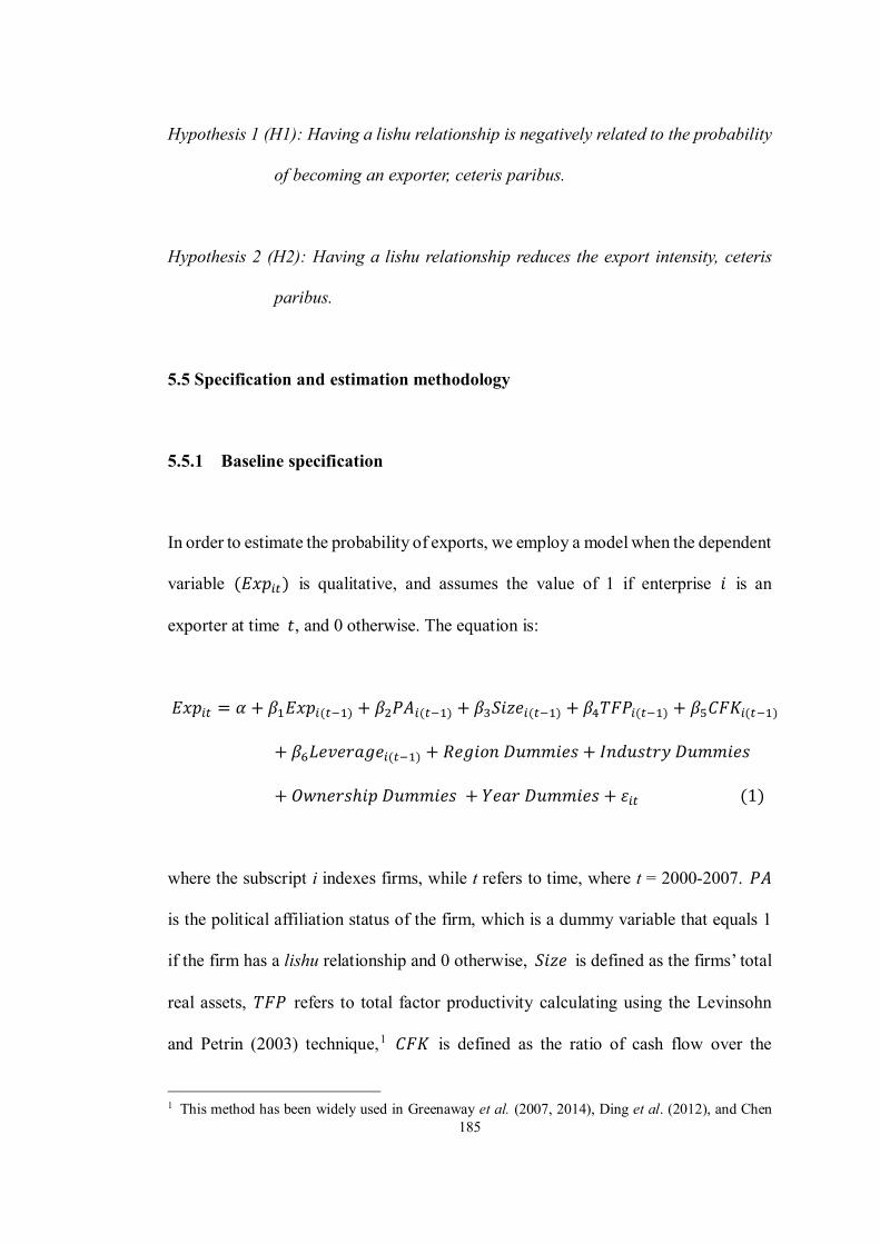
185
Hypothesis 1 (H1): Having a lishu relationship is negatively related to the probability
of becoming an exporter, ceteris paribus.
Hypothesis 2 (H2): Having a lishu relationship reduces the export intensity, ceteris
paribus.
5.5 Specification and estimation methodology
5.5.1 Baseline specification
In order to estimate the probability of exports, we employ a model when the dependent
variable (𝐸𝑥𝑝𝑖𝑡) is qualitative, and assumes the value of 1 if enterprise 𝑖 is an
exporter at time 𝑡, and 0 otherwise. The equation is:
𝐸𝑥𝑝𝑖𝑡 = 𝛼 + 𝛽1𝐸𝑥𝑝𝑖(𝑡−1) + 𝛽2𝑃𝐴𝑖(𝑡−1) + 𝛽3𝑆𝑖𝑧𝑒𝑖(𝑡−1) + 𝛽4𝑇𝐹𝑃𝑖(𝑡−1) + 𝛽5𝐶𝐹𝐾𝑖(𝑡−1)
+ 𝛽6𝐿𝑒𝑣𝑒𝑟𝑎𝑔𝑒𝑖(𝑡−1) + 𝑅𝑒𝑔𝑖𝑜𝑛 𝐷𝑢𝑚𝑚𝑖𝑒𝑠 + 𝐼𝑛𝑑𝑢𝑠𝑡𝑟𝑦 𝐷𝑢𝑚𝑚𝑖𝑒𝑠
+ 𝑂𝑤𝑛𝑒𝑟𝑠ℎ𝑖𝑝 𝐷𝑢𝑚𝑚𝑖𝑒𝑠 + 𝑌𝑒𝑎𝑟 𝐷𝑢𝑚𝑚𝑖𝑒𝑠 + 휀𝑖𝑡 (1)
where the subscript i indexes firms, while t refers to time, where t = 2000-2007. 𝑃𝐴
is the political affiliation status of the firm, which is a dummy variable that equals 1
if the firm has a lishu relationship and 0 otherwise, 𝑆𝑖𝑧𝑒 is defined as the firms’ total
real assets, 𝑇𝐹𝑃 refers to total factor productivity calculating using the Levinsohn
and Petrin (2003) technique,1 𝐶𝐹𝐾 is defined as the ratio of cash flow over the
1 This method has been widely used in Greenaway et al. (2007, 2014), Ding et al. (2012), and Chen
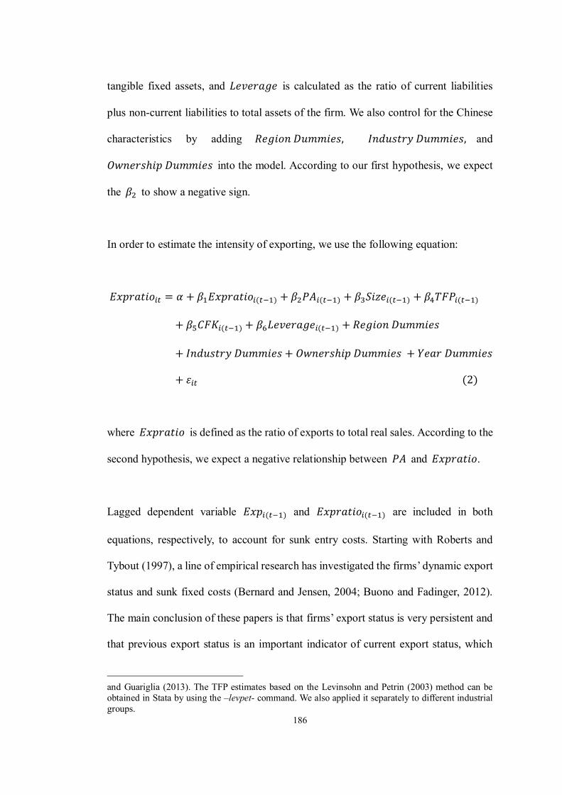
186
tangible fixed assets, and 𝐿𝑒𝑣𝑒𝑟𝑎𝑔𝑒 is calculated as the ratio of current liabilities
plus non-current liabilities to total assets of the firm. We also control for the Chinese
characteristics by adding 𝑅𝑒𝑔𝑖𝑜𝑛 𝐷𝑢𝑚𝑚𝑖𝑒𝑠, 𝐼𝑛𝑑𝑢𝑠𝑡𝑟𝑦 𝐷𝑢𝑚𝑚𝑖𝑒𝑠, and
𝑂𝑤𝑛𝑒𝑟𝑠ℎ𝑖𝑝 𝐷𝑢𝑚𝑚𝑖𝑒𝑠 into the model. According to our first hypothesis, we expect
the 𝛽2 to show a negative sign.
In order to estimate the intensity of exporting, we use the following equation:
𝐸𝑥𝑝𝑟𝑎𝑡𝑖𝑜𝑖𝑡 = 𝛼 + 𝛽1𝐸𝑥𝑝𝑟𝑎𝑡𝑖𝑜𝑖(𝑡−1) + 𝛽2𝑃𝐴𝑖(𝑡−1) + 𝛽3𝑆𝑖𝑧𝑒𝑖(𝑡−1) + 𝛽4𝑇𝐹𝑃𝑖(𝑡−1)
+ 𝛽5𝐶𝐹𝐾𝑖(𝑡−1) + 𝛽6𝐿𝑒𝑣𝑒𝑟𝑎𝑔𝑒𝑖(𝑡−1) + 𝑅𝑒𝑔𝑖𝑜𝑛 𝐷𝑢𝑚𝑚𝑖𝑒𝑠
+ 𝐼𝑛𝑑𝑢𝑠𝑡𝑟𝑦 𝐷𝑢𝑚𝑚𝑖𝑒𝑠 + 𝑂𝑤𝑛𝑒𝑟𝑠ℎ𝑖𝑝 𝐷𝑢𝑚𝑚𝑖𝑒𝑠 + 𝑌𝑒𝑎𝑟 𝐷𝑢𝑚𝑚𝑖𝑒𝑠
+ 휀𝑖𝑡 (2)
where 𝐸𝑥𝑝𝑟𝑎𝑡𝑖𝑜 is defined as the ratio of exports to total real sales. According to the
second hypothesis, we expect a negative relationship between 𝑃𝐴 and 𝐸𝑥𝑝𝑟𝑎𝑡𝑖𝑜.
Lagged dependent variable 𝐸𝑥𝑝𝑖(𝑡−1) and 𝐸𝑥𝑝𝑟𝑎𝑡𝑖𝑜𝑖(𝑡−1) are included in both
equations, respectively, to account for sunk entry costs. Starting with Roberts and
Tybout (1997), a line of empirical research has investigated the firms’ dynamic export
status and sunk fixed costs (Bernard and Jensen, 2004; Buono and Fadinger, 2012).
The main conclusion of these papers is that firms’ export status is very persistent and
that previous export status is an important indicator of current export status, which
and Guariglia (2013). The TFP estimates based on the Levinsohn and Petrin (2003) method can be obtained in Stata by using the –levpet- command. We also applied it separately to different industrial groups.
187
provides evidence of the sunk-cost model. That is, the coefficient on the lagged export
status can be regarded as a measure of the extent of these costs if sunk costs are
significant. Alternatively, if current exporting does not rely on previous exporting
experience, then there are no sunk costs.
We also control for the firms’ characteristics in both equations. Moreover, in order to
mitigate problems stemming from reverse causality (for example, the causality is from
exporting to changes in firms’ characteristics, such as size and productivity), I follow
the previous studies (Roberts and Tybout, 1997; Bernard and Jensen, 2004;
Greenaway et al., 2007; Yi and Wang, 2012) and make all time-varying variables pre-
determined and lagged by one period.
In order to control for time-invariant factors common to firms across regions and
industries, we also include region and industry dummies in both equations. Region
dummies are dummy variables for firm location: Coastal = 1 if the firm is located in
the coastal region, and 0 otherwise; Central = 1 if the firm is located in the central
region, and 0 otherwise; Western = 1 if the firm is located in the western region, and
0 otherwise. 1 Industry dummies define firms to be located in one of the following ten
industrial sectors: metal and metal products; non-metal products and petroleum
processing; chemicals and plastic; machinery and equipment; electrical equipment;
transport equipment; food and tobacco; textile; leather, timber and furniture; and
mining and logging. Year dummies are also included to account for business cycle
1 In order to avoid the dummy variable trap and multicollinearity problem, we only include the Coastal dummy and Western dummy in doing the regression analysis. And we expect that firms located in the coastal region are more likely to export, while firms located in the western region are less likely to export.

188
effects and firm-invariant market factors, such as changes in exchange rates or
government policy.
We expect that firm’s previous export experience, size, TFP, and financial health can
improve the export participation and intensity for Chinese unlisted firms. Due to the
sunk entry costs happened in exporting, previous exporters are more likely to export
in the current period as they do not have to pay for the sunk entry costs again. Larger
and more productive firms are more prone to be involved in exporting activities as
they are able to afford the huge sunk costs. In terms of ownership, we expect that
foreign ownership helps firms’ exporting as they can obtain well-established
distribution network, foreign market information, and financing assistance from their
parent companies. As for the state-ownership, we expect a negative relationship.
As the dependent variable in Eq. (1) is dichotomous, linear multiple regression is not
appropriate for estimating the model. We therefore use a pooled Probit estimator
instead. As for the estimation of Eq. (2), there are many observations that have zero
values in their export intensity (i.e. a firm either exports with 𝐸𝑥𝑝𝑟𝑎𝑡𝑖𝑜𝑖𝑡 > 0 or it
does not with 𝐸𝑥𝑝𝑟𝑎𝑡𝑖𝑜𝑖𝑡 = 0 ). Therefore, OLS estimation may not be an
appropriate method as it can deliver inconsistent parameter estimates due to the fact
that the sample is not representative of the whole population. We therefore start with
the pooled Tobit model (Tobin, 1958), which is estimated by a maximum likelihood
method and yields consistent estimates of the model parameters.1
1 It is important to note that we cluster observations by firms’ ID in our pooled Tobit and pooled Probit regressions. This means that we relax the usual requirement that the observations be independent, and allow observations to be independent across groups (clusters) but not necessarily with in groups (clusters).Clustering correct heteroskedastic standard errors but not affecting the coefficients estimates.

189
5.5.2 Unobserved firm heterogeneity
In Eq. (1) and Eq. (2), we control for a set of observed firm characteristics that may
affect firms’ export participation and intensity. However, it is likely to have some
unobserved firms’ characteristics that are not included in the regression, but are able
to influence the firms’ exporting (Roberts and Tybout, 1997; Bernard and Jensen, 2004;
Greenaway et al., 2007; Yi and Wang, 2012). Such unobserved firm heterogeneity
includes managerial ability, product characteristics, technology, and foreign
experience and networks. As these unobserved characteristics are potentially serial
correlated and permanent over time, they will cause persistence in exporting
behaviour. In this case, ignoring them will give rise to an overestimation of the effects
of sunk entry costs and the previous export experience because the lagged export
variable could act as the only determinant of the current exporting. For instance, for a
firm with a management strategy of internationalisation, the exporting decision of this
firm in an initial period and in the future may be made out of this unobserved
heterogeneity. Therefore, it is inappropriate to assume that exporting experience in the
past gives rise to the current exporting decision by applying the standard econometric
techniques. Heckman (1981) terms the conditional relationship between previous and
future experience caused by improper treatment of unobserved firm characteristics as
spurious state dependence. Himmelberg et al. (1999) find a spurious relation between
ownership and performance, which caused by unobserved heterogeneity.
Following Bernard and Jensen (2004) and Yi and Wang (2012), we assume the error
term 휀𝑖𝑡 in both equations consists of two components: the permanent unobserved

190
firm-specific time-invariant component, 𝑘𝑖 , and an exogenous random disturbance
component, 𝜇𝑖𝑡 . That is:
휀𝑖𝑡 = 𝑘𝑖 + 𝜇𝑖𝑡 (3)
where 𝑘𝑖 is independently and identically distributed normal, and 𝜇𝑖𝑡 is
independently and identically distributed normal for each firm and year.
There are several proposed estimation techniques that can be used to account for
unobserved heterogeneity, including a Probit model with random effects (RE) or fixed
effects (FE), conditional Logit, and linear probability models with random or fixed
effects. The disadvantages of the conditional Logit model are that this estimation
drops all the time-invariant variables and all the firms with a dependent variable which
equals either always 0 or 1, and reduces the accuracy of those variables with negligible
variance across time (Greenaway et al., 2007). However, as for the linear probability
models, Yi and Wang (2012) and Greenaway et al. (2007) point out that the
probabilities indicated by estimated coefficients could lie outside the unit interval [0,
1] and that the assumption of constant variance in the OLS estimation could be
violated by the heterogeneous error term. Therefore, the Probit model with FE or RE
can model the unobserved heterogeneity of the firm better. The FE framework treats
the unobserved effect 𝑘𝑖 as a parameter to be estimated, while the RE framework
treats it as a random variable. Most fixed-effects model leads to biased and
inconsistent parameter estimates, especially of the coefficient of the lagged dependent
variables (Wooldridge, 2010).
191
The random-effects Probit model requires the firm-specific unobserved effects to be
uncorrelated with the regressors, which could cause bias (Bernard and Jensen, 2004;
Greenaway et al., 2007). Especially if the heterogeneity of the unobserved firm-
specific effects is large, the RE Probit estimate of the coefficient on the lagged
dependent variable could be overestimated (Heckman, 1981). However, as our
objective with dynamic specifications is not to obtain a precise estimate of the lagged
dependent variable coefficient, this problem is unlikely to affect out main conclusions.
Additionally, according to Wooldridge (2010, p.286), “With a large number of random
draws…, it almost always makes sense to treat the unobserved effects…as random
draws... This approach is certainly appropriate from an omitted variables or neglected
heterogeneity perspective”. Therefore, I follow Heckman (1981) and Roberts and
Tybout (1997) and employ a random-effects Probit model for the estimation of Eq.
(1). And a random-effects Tobit model is applied to estimate the Eq. (2).1
As discussed above, the RE Probit model has a strong assumption that the unobserved
heterogeneity is uncorrelated with all the other explanatory variables, which is hard
to hold in reality. Therefore, I follow Mundlak (1978) and Chamberlain (1984) and
allow for possible correlation between the unobserved firm heterogeneity and the
regressors by:
1 Our results are robust to using pooled Probit and Tobit estimators. Therefore, we prefer the pooled Probit and Tobit models with cluster-robust standard errors to the random-effects estimators due to their computational advantages. For a large sample, computational time is in fact an issue for random-effects Probit and Tobit models, because they use “full ‘random effects’ with lots of covariates” Wooldridge (2009, p.18). Therefore, we only report the results by using pooled Probit and Tobit models in the empirical analysis. The results for the two main hypotheses obtained from random-effects Probit and Tobit models are presented in Appendix.
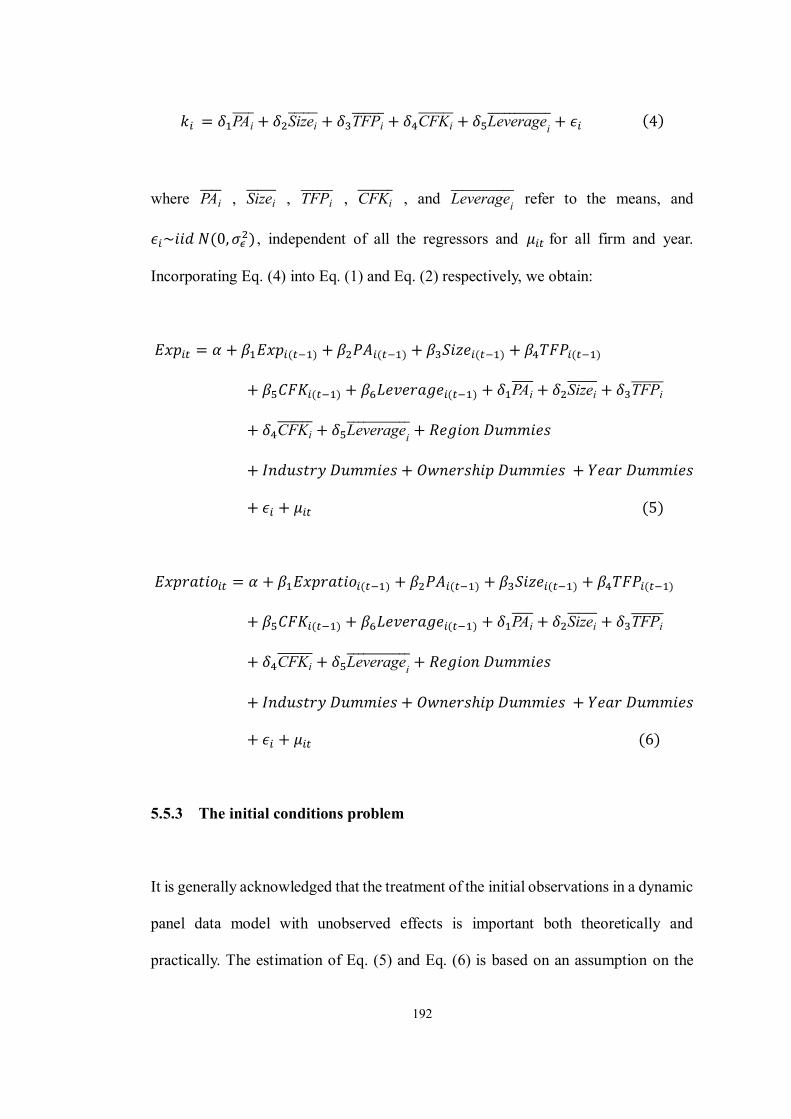
192
𝑘𝑖 = 𝛿1PAi̅̅ ̅̅ + 𝛿2Sizei̅̅ ̅̅ ̅̅ + 𝛿3TFPi̅̅ ̅̅ ̅̅ + 𝛿4CFKi̅̅ ̅̅ ̅̅ ̅ + 𝛿5Leveragei̅̅ ̅̅ ̅̅ ̅̅ ̅̅ ̅̅ + 𝜖𝑖 (4)
where PAi̅̅ ̅̅ , Sizei̅̅ ̅̅ ̅̅ , TFPi̅̅ ̅̅ ̅̅ , CFKi̅̅ ̅̅ ̅̅ ̅ , and Leveragei̅̅ ̅̅ ̅̅ ̅̅ ̅̅ ̅̅ refer to the means, and
𝜖𝑖~𝑖𝑖𝑑 𝑁(0, 𝜎𝜖2) , independent of all the regressors and 𝜇𝑖𝑡 for all firm and year.
Incorporating Eq. (4) into Eq. (1) and Eq. (2) respectively, we obtain:
𝐸𝑥𝑝𝑖𝑡 = 𝛼 + 𝛽1𝐸𝑥𝑝𝑖(𝑡−1) + 𝛽2𝑃𝐴𝑖(𝑡−1) + 𝛽3𝑆𝑖𝑧𝑒𝑖(𝑡−1) + 𝛽4𝑇𝐹𝑃𝑖(𝑡−1)
+ 𝛽5𝐶𝐹𝐾𝑖(𝑡−1) + 𝛽6𝐿𝑒𝑣𝑒𝑟𝑎𝑔𝑒𝑖(𝑡−1) + 𝛿1PAi̅̅ ̅̅ + 𝛿2Sizei̅̅ ̅̅ ̅̅ + 𝛿3TFPi̅̅ ̅̅ ̅̅
+ 𝛿4CFKi̅̅ ̅̅ ̅̅ ̅ + 𝛿5Leveragei̅̅ ̅̅ ̅̅ ̅̅ ̅̅ ̅̅ + 𝑅𝑒𝑔𝑖𝑜𝑛 𝐷𝑢𝑚𝑚𝑖𝑒𝑠
+ 𝐼𝑛𝑑𝑢𝑠𝑡𝑟𝑦 𝐷𝑢𝑚𝑚𝑖𝑒𝑠 + 𝑂𝑤𝑛𝑒𝑟𝑠ℎ𝑖𝑝 𝐷𝑢𝑚𝑚𝑖𝑒𝑠 + 𝑌𝑒𝑎𝑟 𝐷𝑢𝑚𝑚𝑖𝑒𝑠
+ 𝜖𝑖 + 𝜇𝑖𝑡 (5)
𝐸𝑥𝑝𝑟𝑎𝑡𝑖𝑜𝑖𝑡 = 𝛼 + 𝛽1𝐸𝑥𝑝𝑟𝑎𝑡𝑖𝑜𝑖(𝑡−1) + 𝛽2𝑃𝐴𝑖(𝑡−1) + 𝛽3𝑆𝑖𝑧𝑒𝑖(𝑡−1) + 𝛽4𝑇𝐹𝑃𝑖(𝑡−1)
+ 𝛽5𝐶𝐹𝐾𝑖(𝑡−1) + 𝛽6𝐿𝑒𝑣𝑒𝑟𝑎𝑔𝑒𝑖(𝑡−1) + 𝛿1PAi̅̅ ̅̅ + 𝛿2Sizei̅̅ ̅̅ ̅̅ + 𝛿3TFPi̅̅ ̅̅ ̅̅
+ 𝛿4CFKi̅̅ ̅̅ ̅̅ ̅ + 𝛿5Leveragei̅̅ ̅̅ ̅̅ ̅̅ ̅̅ ̅̅ + 𝑅𝑒𝑔𝑖𝑜𝑛 𝐷𝑢𝑚𝑚𝑖𝑒𝑠
+ 𝐼𝑛𝑑𝑢𝑠𝑡𝑟𝑦 𝐷𝑢𝑚𝑚𝑖𝑒𝑠 + 𝑂𝑤𝑛𝑒𝑟𝑠ℎ𝑖𝑝 𝐷𝑢𝑚𝑚𝑖𝑒𝑠 + 𝑌𝑒𝑎𝑟 𝐷𝑢𝑚𝑚𝑖𝑒𝑠
+ 𝜖𝑖 + 𝜇𝑖𝑡 (6)
5.5.3 The initial conditions problem
It is generally acknowledged that the treatment of the initial observations in a dynamic
panel data model with unobserved effects is important both theoretically and
practically. The estimation of Eq. (5) and Eq. (6) is based on an assumption on the
193
relationship between the initial export participation, 𝐸𝑥𝑝𝑖1 / 𝐸𝑥𝑝𝑟𝑎𝑡𝑖𝑜𝑖1 and the
error term 𝜖𝑖. In the existing studies of a dynamic binary discrete-choice model, the
initial conditions are assumed to be pre-determined or exogenous using a standard
random-effects Probit model (Hackman, 1981b; Bernard and Jensen, 2004). That is,
the initial observation values are independent of the unobserved firm-specific effects.
If the observation period for each firm initiates from the very beginning of the
exporting, the initial conditions should be exogenous. However, most micro-
econometric studies with panel datasets, including ours, the start of the sample is not
the same as the start of the exporting behaviour. In this case, the unobserved time-
invariant firm heterogeneity that can influence current exporting activities can also
affect the exporting activities in the initial period. Therefore, it is improper to assume
that the initial conditions are exogenous. Overlooking the endogeneity of the initial
conditions will therefore cause an upward biased estimation of the lagged dependent
variable. That is, the impact of previous exporting experience of the current export
activities would indicate that the sunk entry costs are overestimated.
Wooldridge (2005) suggests a conditional maximum likelihood estimator, which is
simpler and more practical in empirical research than the solution proposed by
Heckman (1981b). This estimator suggests a model that the distribution of the
unobserved heterogeneity effect is conditional on the initial value and other
exogenous explanatory variables. The model is shown as:
𝜖𝑖 = 𝜌0 + 𝜌1𝑌𝑖1 + 𝛿�̅�𝑖′ + 𝜔𝑖 (7)
where 𝜔 is uncorrelated with the initial observation 𝑌1. Incorporating Eq. (7) into Eq.
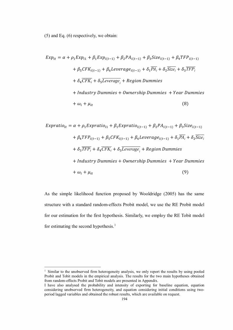
194
(5) and Eq. (6) respectively, we obtain:
𝐸𝑥𝑝𝑖𝑡 = 𝛼 + 𝜌1𝐸𝑥𝑝𝑖1 + 𝛽1𝐸𝑥𝑝𝑖(𝑡−1) + 𝛽2𝑃𝐴𝑖(𝑡−1) + 𝛽3𝑆𝑖𝑧𝑒𝑖(𝑡−1) + 𝛽4𝑇𝐹𝑃𝑖(𝑡−1)
+ 𝛽5𝐶𝐹𝐾𝑖(𝑡−1) + 𝛽6𝐿𝑒𝑣𝑒𝑟𝑎𝑔𝑒𝑖(𝑡−1) + 𝛿1PAi̅̅ ̅̅ + 𝛿2Sizei̅̅ ̅̅ ̅̅ + 𝛿3TFPi̅̅ ̅̅ ̅̅
+ 𝛿4CFKi̅̅ ̅̅ ̅̅ ̅ + 𝛿5Leveragei̅̅ ̅̅ ̅̅ ̅̅ ̅̅ ̅̅ + 𝑅𝑒𝑔𝑖𝑜𝑛 𝐷𝑢𝑚𝑚𝑖𝑒𝑠
+ 𝐼𝑛𝑑𝑢𝑠𝑡𝑟𝑦 𝐷𝑢𝑚𝑚𝑖𝑒𝑠 + 𝑂𝑤𝑛𝑒𝑟𝑠ℎ𝑖𝑝 𝐷𝑢𝑚𝑚𝑖𝑒𝑠 + 𝑌𝑒𝑎𝑟 𝐷𝑢𝑚𝑚𝑖𝑒𝑠
+ 𝜔𝑖 + 𝜇𝑖𝑡 (8)
𝐸𝑥𝑝𝑟𝑎𝑡𝑖𝑜𝑖𝑡 = 𝛼 + 𝜌1𝐸𝑥𝑝𝑟𝑎𝑡𝑖𝑜𝑖1 + 𝛽1𝐸𝑥𝑝𝑟𝑎𝑡𝑖𝑜𝑖(𝑡−1) + 𝛽2𝑃𝐴𝑖(𝑡−1) + 𝛽3𝑆𝑖𝑧𝑒𝑖(𝑡−1)
+ 𝛽4𝑇𝐹𝑃𝑖(𝑡−1) + 𝛽5𝐶𝐹𝐾𝑖(𝑡−1) + 𝛽6𝐿𝑒𝑣𝑒𝑟𝑎𝑔𝑒𝑖(𝑡−1) + 𝛿1PAi̅̅ ̅̅ + 𝛿2Sizei̅̅ ̅̅ ̅̅
+ 𝛿3TFPi̅̅ ̅̅ ̅̅ + 𝛿4CFKi̅̅ ̅̅ ̅̅ ̅ + 𝛿5Leveragei̅̅ ̅̅ ̅̅ ̅̅ ̅̅ ̅̅ + 𝑅𝑒𝑔𝑖𝑜𝑛 𝐷𝑢𝑚𝑚𝑖𝑒𝑠
+ 𝐼𝑛𝑑𝑢𝑠𝑡𝑟𝑦 𝐷𝑢𝑚𝑚𝑖𝑒𝑠 + 𝑂𝑤𝑛𝑒𝑟𝑠ℎ𝑖𝑝 𝐷𝑢𝑚𝑚𝑖𝑒𝑠 + 𝑌𝑒𝑎𝑟 𝐷𝑢𝑚𝑚𝑖𝑒𝑠
+ 𝜔𝑖 + 𝜇𝑖𝑡 (9)
As the simple likelihood function proposed by Wooldridge (2005) has the same
structure with a standard random-effects Probit model, we use the RE Probit model
for our estimation for the first hypothesis. Similarly, we employ the RE Tobit model
for estimating the second hypothesis.1
1 Similar to the unobserved firm heterogeneity analysis, we only report the results by using pooled Probit and Tobit models in the empirical analysis. The results for the two main hypotheses obtained from random-effects Probit and Tobit models are presented in Appendix. I have also analysed the probability and intensity of exporting for baseline equation, equation considering unobserved firm heterogeneity, and equation considering initial conditions using two-period lagged variables and obtained the robust results, which are available on request.
195
5.6 Data and summary statistics
5.6.1 Data
In this chapter, we use a firm-level dataset which includes both state-owned and non-
state-owned firms from 31 provinces or province-equivalent municipal cities (except
Hong Kong, Macao and Taiwan) all over China. This dataset is from the annual
accounting reports, maintained and complied by the NBS. In order to strengthen the
reliability of our analysis, we first drop observations which make little sense, such as
those with negative real assets, negative export, negative age, and negative leverage
ratio. Second, we eliminate firms without complete records on our main regression
variables. Finally, in order to control for the potential effect of extreme values, we
drop outliers, which are the observations beyond the 1st and the 99th percent tails for
each continuous main regression variables.1 After the above adjustments, our final
panel dataset includes 502,196 firm-level observations, covering 111,460 mainly
unlisted firms over the period 2001-2007.2 The sample has an unbalanced structure,3
with the number of observations ranging from a minimum of 43,187 in 2001 to a
maximum of 85,698 in 2004.
We classify firms into exporters and non-exporters and present the distribution of the
1 It is quite common in the literature (see Greenaway et al., 2007; Guariglia, 2008; Carpenter and Guariglia, 2008; Yan, 2012) to eliminate extreme values in this way.
2 It should be noted that our dataset include a very small proportion of listed firms for two reasons. Frist of all, according to Liu and Xiao (2004), when firms become listed, their legal identification numbers are changed; it is therefore hard to track these firms. The second reason is that there is no separate identification of Chinese publicly listed firms in the NBS dataset. However, they only comprise a very small portion of the whole sample. Over the whole considered period, only approximately 1000 listed firms in the manufacturing and mining sectors, accounting for less than 0.3% of the total number of firms in the sample. 3 See Appendix for details about the structure of the panel.
196
full sample, exporters, and non-exporters by year and industry in Table 5.6. We
observe that on average, only around 31.04% of our firm-year observations are
involved in exporting activities. This can be explained by the fact that exporting
activities always involve huge sunk entry costs, such as collecting information,
establishing distribution network, and adjusting the products and packages for foreign
markets. Focusing on the industry groups, we find that the number of observations for
exporters only exceeds that for non-exporters in the textile industry (51.32% vs.
48.68%), while firms in other industries are less likely to export. This can be attributed
to the fact that Chinese textile industry is characterised by huge comparative
advantages, such as abundant raw material and low human labour costs. Therefore,
the textile industry has been playing an important part in the foreign trade ever since
the opening-up policy was adopted in China. This is also consistent with the existing
literature that firms in labour intensive industries are more likely to export in China
(Liu and Shu, 2003).
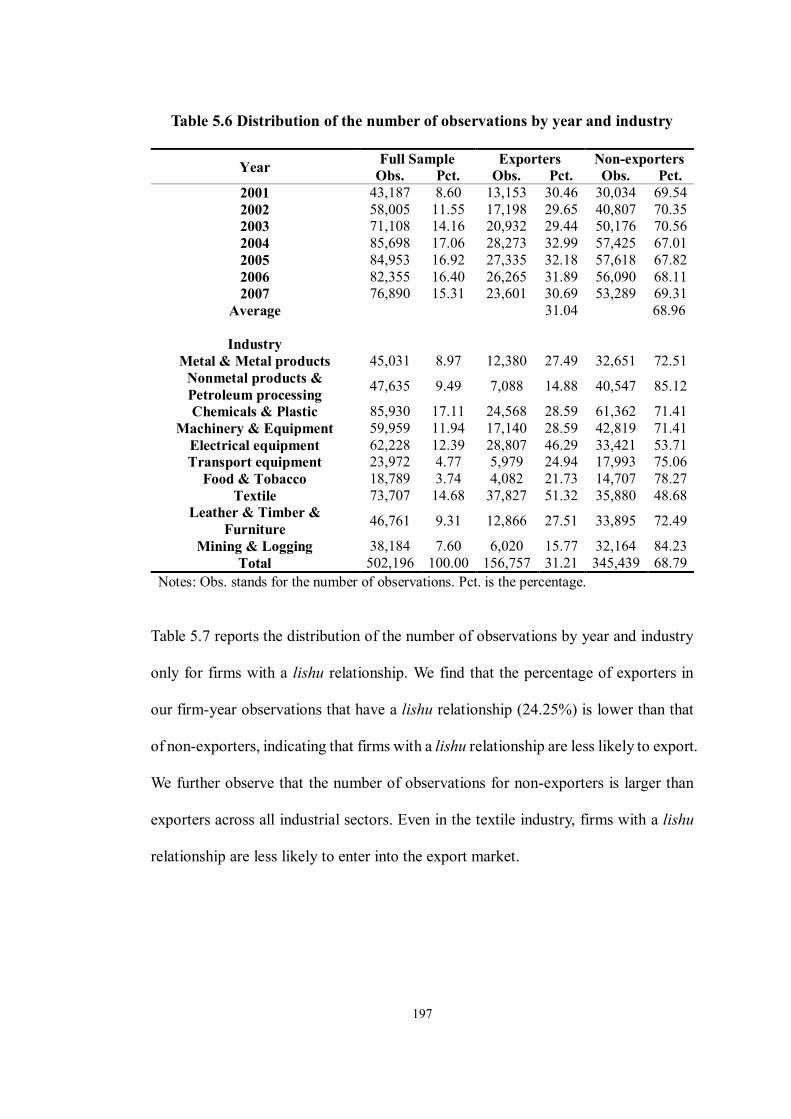
197
Table 5.6 Distribution of the number of observations by year and industry
Year Full Sample Exporters Non-exporters Obs. Pct. Obs. Pct. Obs. Pct.
2001 43,187 8.60 13,153 30.46 30,034 69.54 2002 58,005 11.55 17,198 29.65 40,807 70.35 2003 71,108 14.16 20,932 29.44 50,176 70.56 2004 85,698 17.06 28,273 32.99 57,425 67.01 2005 84,953 16.92 27,335 32.18 57,618 67.82 2006 82,355 16.40 26,265 31.89 56,090 68.11 2007 76,890 15.31 23,601 30.69 53,289 69.31
Average 31.04 68.96
Industry Metal & Metal products 45,031 8.97 12,380 27.49 32,651 72.51
Nonmetal products & Petroleum processing 47,635 9.49 7,088 14.88 40,547 85.12
Chemicals & Plastic 85,930 17.11 24,568 28.59 61,362 71.41 Machinery & Equipment 59,959 11.94 17,140 28.59 42,819 71.41
Electrical equipment 62,228 12.39 28,807 46.29 33,421 53.71 Transport equipment 23,972 4.77 5,979 24.94 17,993 75.06
Food & Tobacco 18,789 3.74 4,082 21.73 14,707 78.27 Textile 73,707 14.68 37,827 51.32 35,880 48.68
Leather & Timber & Furniture 46,761 9.31 12,866 27.51 33,895 72.49
Mining & Logging 38,184 7.60 6,020 15.77 32,164 84.23 Total 502,196 100.00 156,757 31.21 345,439 68.79
Notes: Obs. stands for the number of observations. Pct. is the percentage.
Table 5.7 reports the distribution of the number of observations by year and industry
only for firms with a lishu relationship. We find that the percentage of exporters in
our firm-year observations that have a lishu relationship (24.25%) is lower than that
of non-exporters, indicating that firms with a lishu relationship are less likely to export.
We further observe that the number of observations for non-exporters is larger than
exporters across all industrial sectors. Even in the textile industry, firms with a lishu
relationship are less likely to enter into the export market.
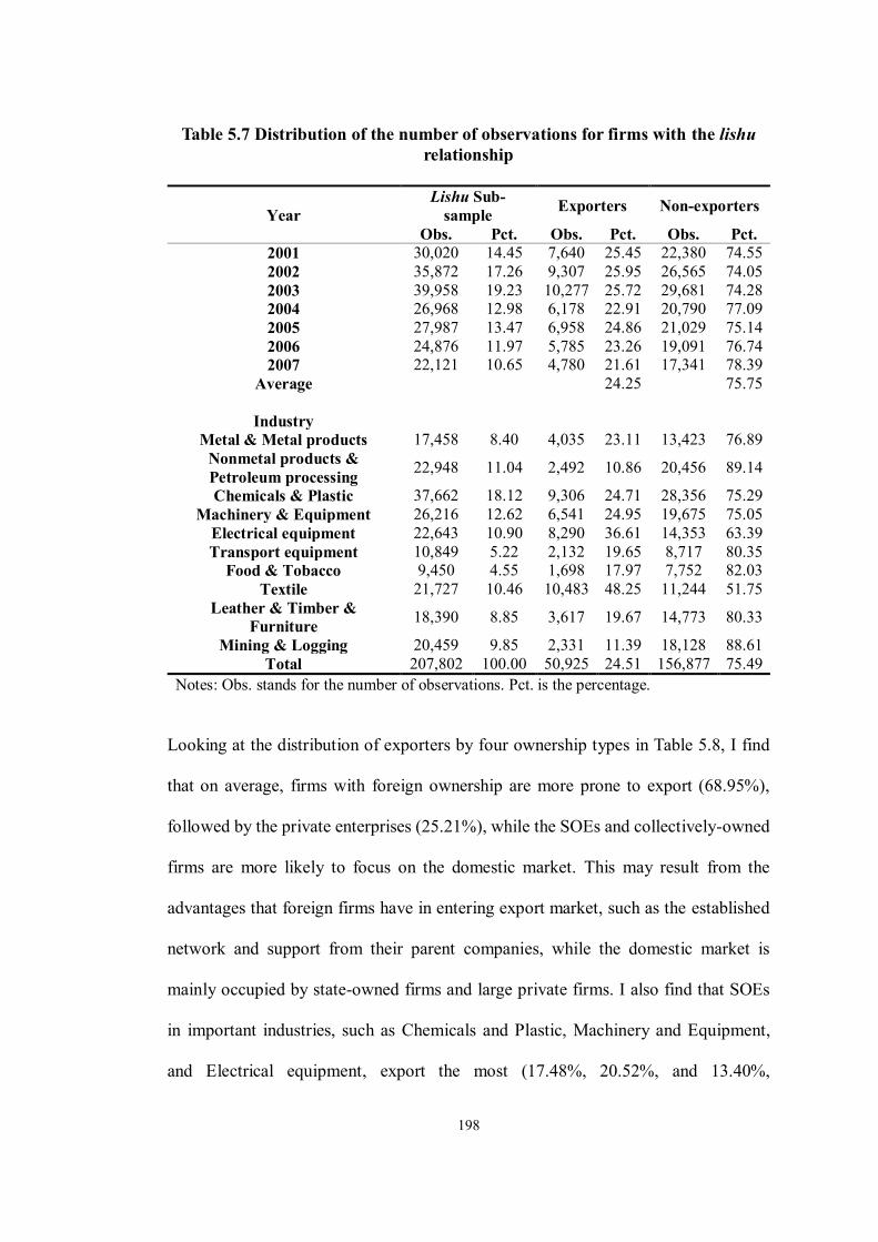
198
Table 5.7 Distribution of the number of observations for firms with the lishu relationship
Year Lishu Sub-
sample Exporters Non-exporters
Obs. Pct. Obs. Pct. Obs. Pct. 2001 30,020 14.45 7,640 25.45 22,380 74.55 2002 35,872 17.26 9,307 25.95 26,565 74.05 2003 39,958 19.23 10,277 25.72 29,681 74.28 2004 26,968 12.98 6,178 22.91 20,790 77.09 2005 27,987 13.47 6,958 24.86 21,029 75.14 2006 24,876 11.97 5,785 23.26 19,091 76.74 2007 22,121 10.65 4,780 21.61 17,341 78.39
Average 24.25 75.75
Industry Metal & Metal products 17,458 8.40 4,035 23.11 13,423 76.89
Nonmetal products & Petroleum processing 22,948 11.04 2,492 10.86 20,456 89.14
Chemicals & Plastic 37,662 18.12 9,306 24.71 28,356 75.29 Machinery & Equipment 26,216 12.62 6,541 24.95 19,675 75.05
Electrical equipment 22,643 10.90 8,290 36.61 14,353 63.39 Transport equipment 10,849 5.22 2,132 19.65 8,717 80.35
Food & Tobacco 9,450 4.55 1,698 17.97 7,752 82.03 Textile 21,727 10.46 10,483 48.25 11,244 51.75
Leather & Timber & Furniture 18,390 8.85 3,617 19.67 14,773 80.33
Mining & Logging 20,459 9.85 2,331 11.39 18,128 88.61 Total 207,802 100.00 50,925 24.51 156,877 75.49
Notes: Obs. stands for the number of observations. Pct. is the percentage.
Looking at the distribution of exporters by four ownership types in Table 5.8, I find
that on average, firms with foreign ownership are more prone to export (68.95%),
followed by the private enterprises (25.21%), while the SOEs and collectively-owned
firms are more likely to focus on the domestic market. This may result from the
advantages that foreign firms have in entering export market, such as the established
network and support from their parent companies, while the domestic market is
mainly occupied by state-owned firms and large private firms. I also find that SOEs
in important industries, such as Chemicals and Plastic, Machinery and Equipment,
and Electrical equipment, export the most (17.48%, 20.52%, and 13.40%,
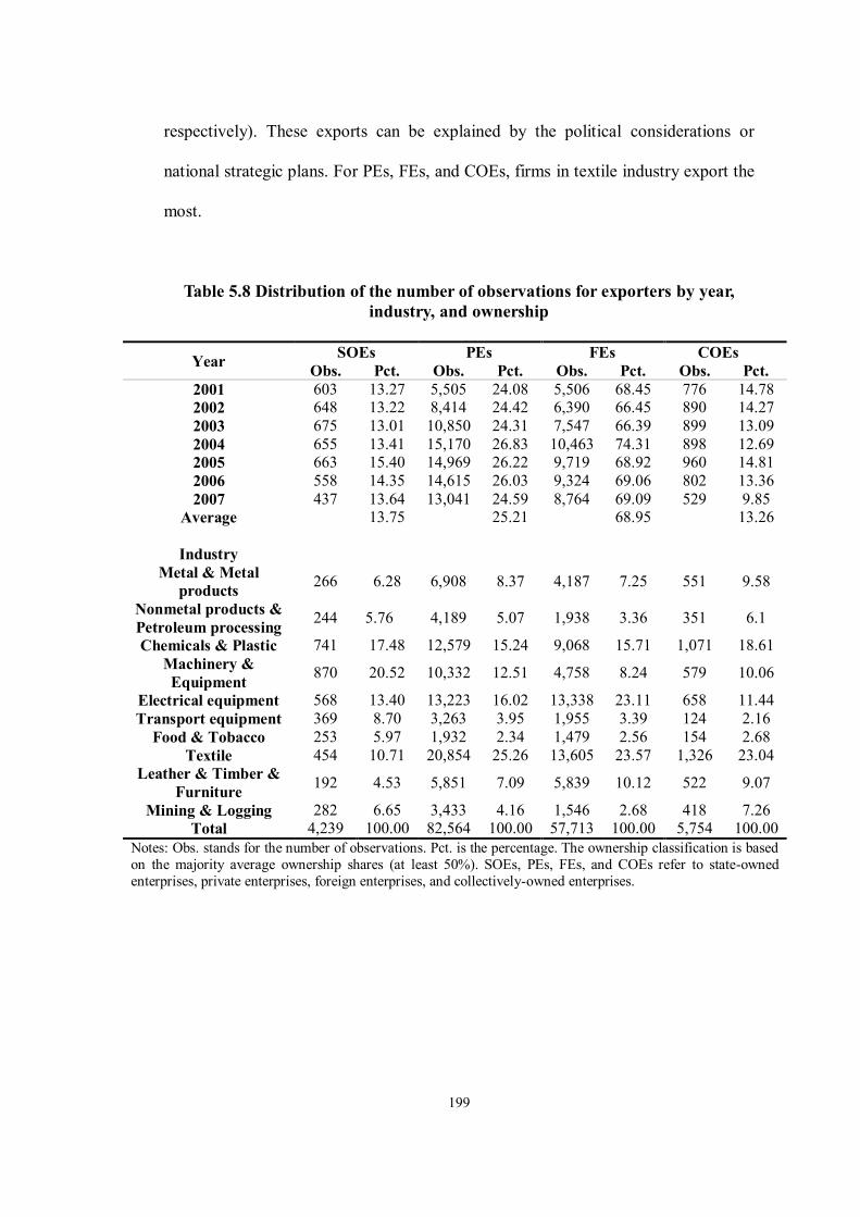
199
respectively). These exports can be explained by the political considerations or
national strategic plans. For PEs, FEs, and COEs, firms in textile industry export the
most.
Table 5.8 Distribution of the number of observations for exporters by year, industry, and ownership
Year SOEs PEs FEs COEs Obs. Pct. Obs. Pct. Obs. Pct. Obs. Pct.
2001 603 13.27 5,505 24.08 5,506 68.45 776 14.78 2002 648 13.22 8,414 24.42 6,390 66.45 890 14.27 2003 675 13.01 10,850 24.31 7,547 66.39 899 13.09 2004 655 13.41 15,170 26.83 10,463 74.31 898 12.69 2005 663 15.40 14,969 26.22 9,719 68.92 960 14.81 2006 558 14.35 14,615 26.03 9,324 69.06 802 13.36 2007 437 13.64 13,041 24.59 8,764 69.09 529 9.85
Average 13.75 25.21 68.95 13.26
Industry Metal & Metal
products 266 6.28 6,908 8.37 4,187 7.25 551 9.58
Nonmetal products & Petroleum processing 244 5.76 4,189 5.07 1,938 3.36 351 6.1
Chemicals & Plastic 741 17.48 12,579 15.24 9,068 15.71 1,071 18.61 Machinery & Equipment 870 20.52 10,332 12.51 4,758 8.24 579 10.06
Electrical equipment 568 13.40 13,223 16.02 13,338 23.11 658 11.44 Transport equipment 369 8.70 3,263 3.95 1,955 3.39 124 2.16
Food & Tobacco 253 5.97 1,932 2.34 1,479 2.56 154 2.68 Textile 454 10.71 20,854 25.26 13,605 23.57 1,326 23.04
Leather & Timber & Furniture 192 4.53 5,851 7.09 5,839 10.12 522 9.07
Mining & Logging 282 6.65 3,433 4.16 1,546 2.68 418 7.26 Total 4,239 100.00 82,564 100.00 57,713 100.00 5,754 100.00
Notes: Obs. stands for the number of observations. Pct. is the percentage. The ownership classification is based on the majority average ownership shares (at least 50%). SOEs, PEs, FEs, and COEs refer to state-owned enterprises, private enterprises, foreign enterprises, and collectively-owned enterprises.
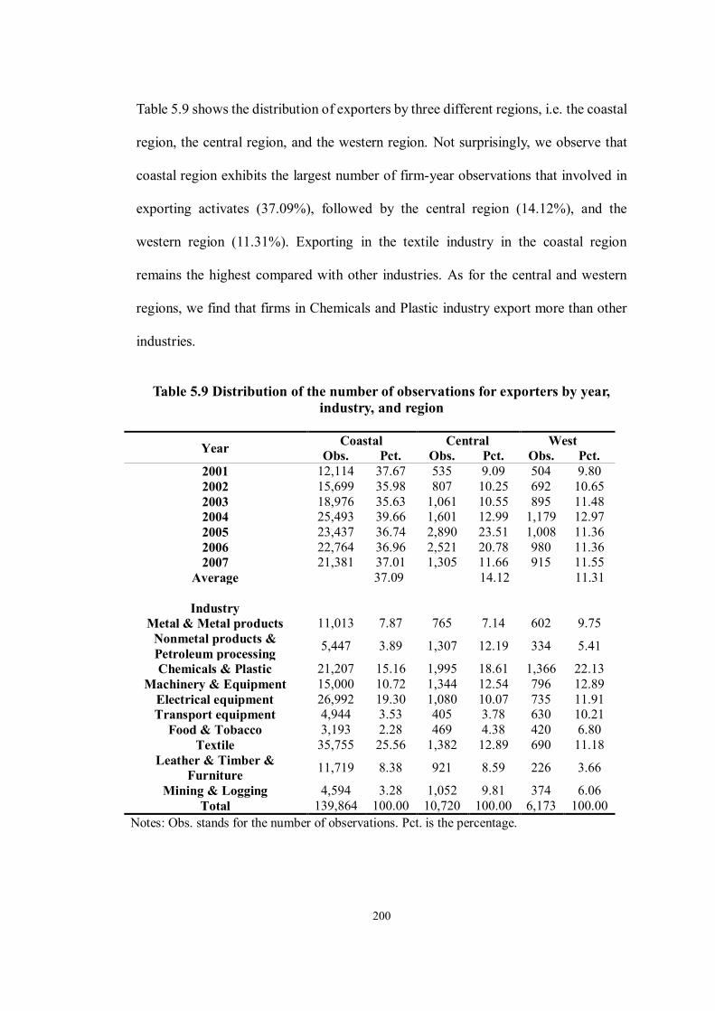
200
Table 5.9 shows the distribution of exporters by three different regions, i.e. the coastal
region, the central region, and the western region. Not surprisingly, we observe that
coastal region exhibits the largest number of firm-year observations that involved in
exporting activates (37.09%), followed by the central region (14.12%), and the
western region (11.31%). Exporting in the textile industry in the coastal region
remains the highest compared with other industries. As for the central and western
regions, we find that firms in Chemicals and Plastic industry export more than other
industries.
Table 5.9 Distribution of the number of observations for exporters by year,
industry, and region
Year Coastal Central West Obs. Pct. Obs. Pct. Obs. Pct.
2001 12,114 37.67 535 9.09 504 9.80 2002 15,699 35.98 807 10.25 692 10.65 2003 18,976 35.63 1,061 10.55 895 11.48 2004 25,493 39.66 1,601 12.99 1,179 12.97 2005 23,437 36.74 2,890 23.51 1,008 11.36 2006 22,764 36.96 2,521 20.78 980 11.36 2007 21,381 37.01 1,305 11.66 915 11.55
Average 37.09 14.12 11.31
Industry Metal & Metal products 11,013 7.87 765 7.14 602 9.75
Nonmetal products & Petroleum processing 5,447 3.89 1,307 12.19 334 5.41
Chemicals & Plastic 21,207 15.16 1,995 18.61 1,366 22.13 Machinery & Equipment 15,000 10.72 1,344 12.54 796 12.89
Electrical equipment 26,992 19.30 1,080 10.07 735 11.91 Transport equipment 4,944 3.53 405 3.78 630 10.21
Food & Tobacco 3,193 2.28 469 4.38 420 6.80 Textile 35,755 25.56 1,382 12.89 690 11.18
Leather & Timber & Furniture 11,719 8.38 921 8.59 226 3.66
Mining & Logging 4,594 3.28 1,052 9.81 374 6.06 Total 139,864 100.00 10,720 100.00 6,173 100.00
Notes: Obs. stands for the number of observations. Pct. is the percentage.
201
5.6.2 Descriptive statistics
We start with looking at some summary statistics (sample mean, medians, and
standard deviations). 1 Table 5.10 presents these descriptive statistics for the full
sample, exporters, and non-exporters. We find in the full sample, that most of our
firms are less likely to export, and the average export/total sales ratio is only 17.20%.
Exporters are larger than non-exporters, in terms of the real assets (661.48 thousands
of yuan vs. 415.67 thousand of yuan), and the number of employees (325 people vs.
205 people). Besides, exporters are less likely to have political affiliations than non-
exporters. Table 5.10 also shows that exporters generally locate in the east of China
and more productive than their counterpart, and cash flow/capital ratio is slight but
significantly larger in exporters than that in non-exporters, suggesting that financial
health improves the participation of exporting.
However, we find that the leverage ratio is slight but significantly lower in exporters:
54.76% compared to 57.78% for non-exporters, and exporters are younger than non-
exporters (10.45 years vs. 11.89 years). As we expect that the older firms with high
leverage ratio are more likely to export, this finding goes against our expectation, but
in line with the stylised facts documented in the existing literature: Chinese exporters
appear to be younger and less leveraged than non-exporters. According to the last
column in Table 5.10, all these variables are significantly different across the exporters
group and non-exporters group.
1 See Appendix for detailed definitions of the variables used in this chapter. The correlation matrix is also presented in Appendix.
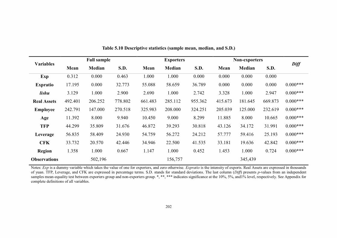
202
Table 5.10 Descriptive statistics (sample mean, median, and S.D.)
Variables Full sample Exporters Non-exporters
Diff Mean Median S.D. Mean Median S.D. Mean Median S.D.
Exp 0.312 0.000 0.463 1.000 1.000 0.000 0.000 0.000 0.000
Expratio 17.195 0.000 32.773 55.088 58.659 36.789 0.000 0.000 0.000 0.000***
lishu 3.129 1.000 2.900 2.690 1.000 2.742 3.328 1.000 2.947 0.000***
Real Assets 492.401 206.252 778.802 661.483 285.112 955.362 415.673 181.645 669.873 0.000***
Employee 242.791 147.000 270.518 325.983 208.000 324.251 205.039 125.000 232.619 0.000***
Age 11.392 8.000 9.940 10.450 9.000 8.299 11.885 8.000 10.665 0.000***
TFP 44.299 35.809 31.676 46.872 39.293 30.818 43.126 34.172 31.991 0.000***
Leverage 56.835 58.409 24.930 54.759 56.272 24.212 57.777 59.416 25.193 0.000***
CFK 33.732 20.570 42.446 34.946 22.500 41.535 33.181 19.636 42.842 0.000***
Region 1.358 1.000 0.667 1.147 1.000 0.452 1.453 1.000 0.724 0.000***
Observations 502,196 156,757 345,439
Notes: Exp is a dummy variable which takes the value of one for exporters, and zero otherwise. Expratio is the intensity of exports. Real Assets are expressed in thousands of yuan. TFP, Leverage, and CFK are expressed in percentage terms. S.D. stands for standard deviations. The last column (Diff) presents p-values from an independent samples mean-equality test between exporters group and non-exporters group. *, **, *** indicates significance at the 10%, 5%, and1% level, respectively. See Appendix for complete definitions of all variables.
203
Table 5.11 provides a comparison of the main variables across firm-ownership types.
Foreign firms normally exhibit the highest probability of exporting (0.692 vs. 0.254
in PEs, 0.137 in SOEs, and 0.133 in COEs) and intensity of exporting (45.56% vs.
12.74% in PEs, 3.88% in SOEs, and 5.84% in COEs). As for the political affiliation,
foreign firms have the lowest level of lishu relationship (2.28), followed by the PEs
(2.67) and COEs (4.22), while the SOEs have the highest level of lishu relationship
(7.66). SOEs and foreign firms enjoy the largest asset base (723.41 thousands of yuan
and 741.90 thousand of yuan, respectively). SOEs and FEs hire more employees (369
people in SOEs and 301 people in FEs) than PEs and COEs (216 people and 222
people, respectively).
Table 5.11 also shows that SOEs and COEs are much older than PEs, while the FEs
are the youngest one as most of the foreign firms entered China after the 1990s. This
finding is consistent with the fact that younger firms may be established as global
firms; therefore, they are more likely to participate in exporting from China. Foreign
firms also enjoy the highest productivity (50.78%), followed by PEs (43.85%), COEs
(42.57%), and SOEs (32.47%), suggesting that FEs are the most efficient firms in
China but SOEs perform non-efficiently. This may be associated with the reason that
FEs have advanced management experience and technology, while SOEs take too
much the political and social responsibilities. As for financial variables, SOEs show
the highest leverage ratio (64.33%), while that for the foreign firms is the lowest
(46.15%), suggesting that SOEs suffer from the soft budget constraints due to the
favourable support from the state banks. Interestingly, we observe that the cash
flow/capital ratio is larger for FEs and COEs than PEs and SOEs. Finally, we find that

204
FEs prefer to set up their firms in the coastal region, while SOEs are more likely to
locate their businesses in the central region, where is closer to China’s capital, Beijing,
the heart of political and economic development.

205
Table 5.11 Descriptive statistics for ownership (sample mean, median, and S.D.)
Variables SOEs PEs FEs COEs
Diff1 Diff2 Diff3 Mean Median S.D. Mean Median S.D. Mean Median S.D. Mean Median S.D.
Exp 0.137 0.000 0.344 0.254 0.000 0.435 0.692 1.000 0.462 0.133 0.000 0.339 0.000*** 0.000*** 0.000***
Expratio 3.877 0.000 14.699 12.742 0.000 28.513 45.558 39.916 42.071 5.836 0.000 19.675 0.000*** 0.000*** 0.000***
lishu 7.658 8.000 1.960 2.671 1.000 2.639 2.280 1.000 2.488 4.221 4.000 2.444 0.000*** 0.000*** 0.000***
Real
Assets 723.410 332.687 979.872 421.170 176.599 696.037 741.901 358.335 991.308 327.558 167.538 500.722 0.000*** 0.005*** 0.000***
Employee 369.093 230.000 370.529 216.735 131.000 242.984 301.263 187.000 313.468 222.875 140.000 241.354 0.000*** 0.000*** 0.000***
Age 26.495 28.000 15.802 9.948 7.000 8.884 8.810 9.000 3.706 16.887 14.000 11.064 0.000*** 0.000*** 0.000***
TFP 32.471 24.365 27.441 43.853 35.608 30.815 50.779 42.086 34.146 42.569 33.640 32.017 0.000*** 0.000*** 0.000***
Leverage 64.329 65.463 26.296 58.661 60.651 24.122 46.145 45.949 24.253 58.413 59.770 25.451 0.000*** 0.000*** 0.000***
CFK 15.247 7.794 29.520 33.608 20.833 40.968 38.255 24.272 46.010 38.642 22.438 48.506 0.000*** 0.000*** 0.000***
Region 1.811 2.000 0.825 1.375 1.000 0.678 1.085 1.000 0.359 1.417 1.000 0.678 0.000*** 0.000*** 0.000***
Obs. 30,912 324,757 83,394 43,291 Notes: Exp is a dummy variable which takes the value of one for exporters, and zero otherwise. Expratio is the intensity of exports. Real Assets are expressed in thousands of yuan. TFP, Leverage, and CFK are expressed in percentage terms. S.D. stands for standard deviations. The ownership classification is based on the majority average ownership shares (at least 50%). SOEs, PEs, FEs, and COEs refer to state-owned enterprises, private enterprises, foreign enterprises, and collectively-owned enterprises. The last three columns present p-values from an independent samples mean-equality test between the SOEs group and the PEs group (Diff1), between SOEs group and the FEs group (Diff2), and between PEs group and FEs group (Diff3). *, **, *** indicates significance at the 10%, 5%, and1% level, respectively. See Appendix for complete definitions of all variables.
206
Focusing on the different regions of China shown in Table 5.12, we observe that firms
in the east of China have higher probability and intensity of exporting (0.37 and
21.46%), followed by firms in the central (0.15 and 4.99%) and west of China (0.11
and 3.66%). Firms located in the western and central regions exhibit the higher
political affiliation levels (4.64 and 3.94, respectively) than that of coastal firms (2.76).
In addition, firms in the west of China have the largest size, in terms of real assets
(549.92 thousands of yuan) and the number of employees (286 employees), and are
older (14.55 years) than firms in the centre (436.14 thousands of yuan, 268 employees,
and 13.07 years old) and east of China (494.88 thousands of yuan, 231 employees,
and 10.71 years old).
As for the productivity and financial variables, firms in the East enjoy the highest TFP
(45.82%) and cash flow-to-capital ratio (36.09%), indicating they are more effective
compared with firms in the central region (with 41.57% TFP and 28.91% cash flow
ratio) and those in the West (37.24% TFP and 23.70% cash flow ratio). Furthermore,
we observe that firms in the western region enjoy the highest leverage ratio (59.43%),
followed by firms in the central area (56.59%) and those in the coastal area (56.51%).
The lowest leverage ratio for coastal firms may suggest that coastal firms depend more
on their internal funds and foreign financing, instead of debt.
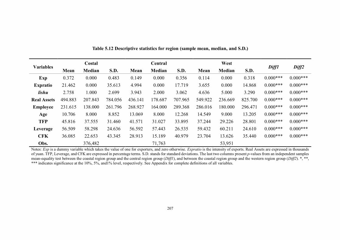
207
Table 5.12 Descriptive statistics for region (sample mean, median, and S.D.)
Variables Costal Central West
Diff1 Diff2 Mean Median S.D. Mean Median S.D. Mean Median S.D.
Exp 0.372 0.000 0.483 0.149 0.000 0.356 0.114 0.000 0.318 0.000*** 0.000*** Expratio 21.462 0.000 35.613 4.994 0.000 17.719 3.655 0.000 14.868 0.000*** 0.000***
lishu 2.758 1.000 2.699 3.943 2.000 3.062 4.636 5.000 3.290 0.000*** 0.000*** Real Assets 494.883 207.843 784.056 436.141 178.687 707.965 549.922 236.669 825.700 0.000*** 0.000*** Employee 231.615 138.000 261.796 268.927 164.000 289.368 286.016 180.000 296.471 0.000*** 0.000***
Age 10.706 8.000 8.852 13.069 8.000 12.268 14.549 9.000 13.205 0.000*** 0.000*** TFP 45.816 37.555 31.460 41.571 31.027 33.895 37.244 29.226 28.801 0.000*** 0.000***
Leverage 56.509 58.298 24.636 56.592 57.443 26.535 59.432 60.211 24.610 0.000*** 0.000*** CFK 36.085 22.653 43.345 28.913 15.189 40.979 23.704 13.626 35.440 0.000*** 0.000*** Obs. 376,482 71,763 53,951
Notes: Exp is a dummy variable which takes the value of one for exporters, and zero otherwise. Expratio is the intensity of exports. Real Assets are expressed in thousands of yuan. TFP, Leverage, and CFK are expressed in percentage terms. S.D. stands for standard deviations. The last two columns present p-values from an independent samples mean-equality test between the coastal region group and the central region group (Diff1), and between the coastal region group and the western region group (Diff2). *, **, *** indicates significance at the 10%, 5%, and1% level, respectively. See Appendix for complete definitions of all variables.

208
5.7 Empirical results
5.7.1 The lishu relationship and the propensity of exporting
Table 5.13 provides the regression results of applying pooled Probit 1 clustering
observations by firms ID in Eqs. (1), (5), and (8). Both coefficients and marginal
effects are presented in Table 5.13.2 Column (1) presents results for the baseline
equation (Eq. (1)). Column (2) reports results by considering unobserved firm
heterogeneity (Eq. (5)). Results that take account of initial conditions problem (Eq.
(8)) are reported in column (3).
Focusing on column (1) in Table 5.13, we find that the lagged export experience is
positive and significant at 1% level. Besides, the marginal effects suggest that being
an exporter in the previous period is 3.50% more likely to export in the current period
than those that did not. Being consistent with the existing literature, we find that sunk
entry costs of exporting exist in Chinese manufacturing firms.
Looking at the lishu variable in column (1), we find a significant negative relationship
between political affiliation and the probability of exporting. Specifically, being a
politically affiliated firm is associated with a 0.13% lower probability of exporting.
This finding supports our first hypothesis, which suggests that firms with a lishu
relationship are less likely to export.
1 Out results are robust by using the random-effects Probit model. The results obtained from random-effects Probit model are presented in Appendix. 2 Because of the non-linear model, the coefficient estimates are not informative about the magnitude of the effects of the outcome variables.
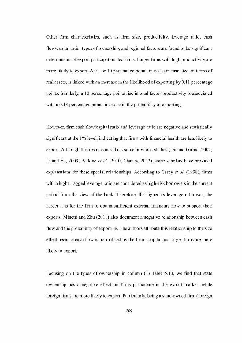
209
Other firm characteristics, such as firm size, productivity, leverage ratio, cash
flow/capital ratio, types of ownership, and regional factors are found to be significant
determinants of export participation decisions. Larger firms with high productivity are
more likely to export. A 0.1 or 10 percentage points increase in firm size, in terms of
real assets, is linked with an increase in the likelihood of exporting by 0.11 percentage
points. Similarly, a 10 percentage points rise in total factor productivity is associated
with a 0.13 percentage points increase in the probability of exporting.
However, firm cash flow/capital ratio and leverage ratio are negative and statistically
significant at the 1% level, indicating that firms with financial health are less likely to
export. Although this result contradicts some previous studies (Du and Girma, 2007;
Li and Yu, 2009; Bellone et al., 2010; Chaney, 2013), some scholars have provided
explanations for these special relationships. According to Carey et al. (1998), firms
with a higher lagged leverage ratio are considered as high-risk borrowers in the current
period from the view of the bank. Therefore, the higher its leverage ratio was, the
harder it is for the firm to obtain sufficient external financing now to support their
exports. Minetti and Zhu (2011) also document a negative relationship between cash
flow and the probability of exporting. The authors attribute this relationship to the size
effect because cash flow is normalised by the firm’s capital and larger firms are more
likely to export.
Focusing on the types of ownership in column (1) Table 5.13, we find that state
ownership has a negative effect on firms participate in the export market, while
foreign firms are more likely to export. Particularly, being a state-owned firm (foreign
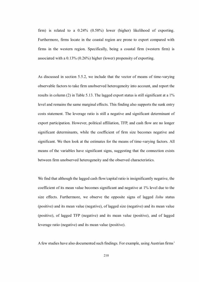
210
firm) is related to a 0.24% (0.58%) lower (higher) likelihood of exporting.
Furthermore, firms locate in the coastal region are prone to export compared with
firms in the western region. Specifically, being a coastal firm (western firm) is
associated with a 0.13% (0.26%) higher (lower) propensity of exporting.
As discussed in section 5.5.2, we include that the vector of means of time-varying
observable factors to take firm unobserved heterogeneity into account, and report the
results in column (2) in Table 5.13. The lagged export status is still significant at a 1%
level and remains the same marginal effects. This finding also supports the sunk entry
costs statement. The leverage ratio is still a negative and significant determinant of
export participation. However, political affiliation, TFP, and cash flow are no longer
significant determinants, while the coefficient of firm size becomes negative and
significant. We then look at the estimates for the means of time-varying factors. All
means of the variables have significant signs, suggesting that the connection exists
between firm unobserved heterogeneity and the observed characteristics.
We find that although the lagged cash flow/capital ratio is insignificantly negative, the
coefficient of its mean value becomes significant and negative at 1% level due to the
size effects. Furthermore, we observe the opposite signs of lagged lishu status
(positive) and its mean value (negative), of lagged size (negative) and its mean value
(positive), of lagged TFP (negative) and its mean value (positive), and of lagged
leverage ratio (negative) and its mean value (positive).
A few studies have also documented such findings. For example, using Austrian firms’
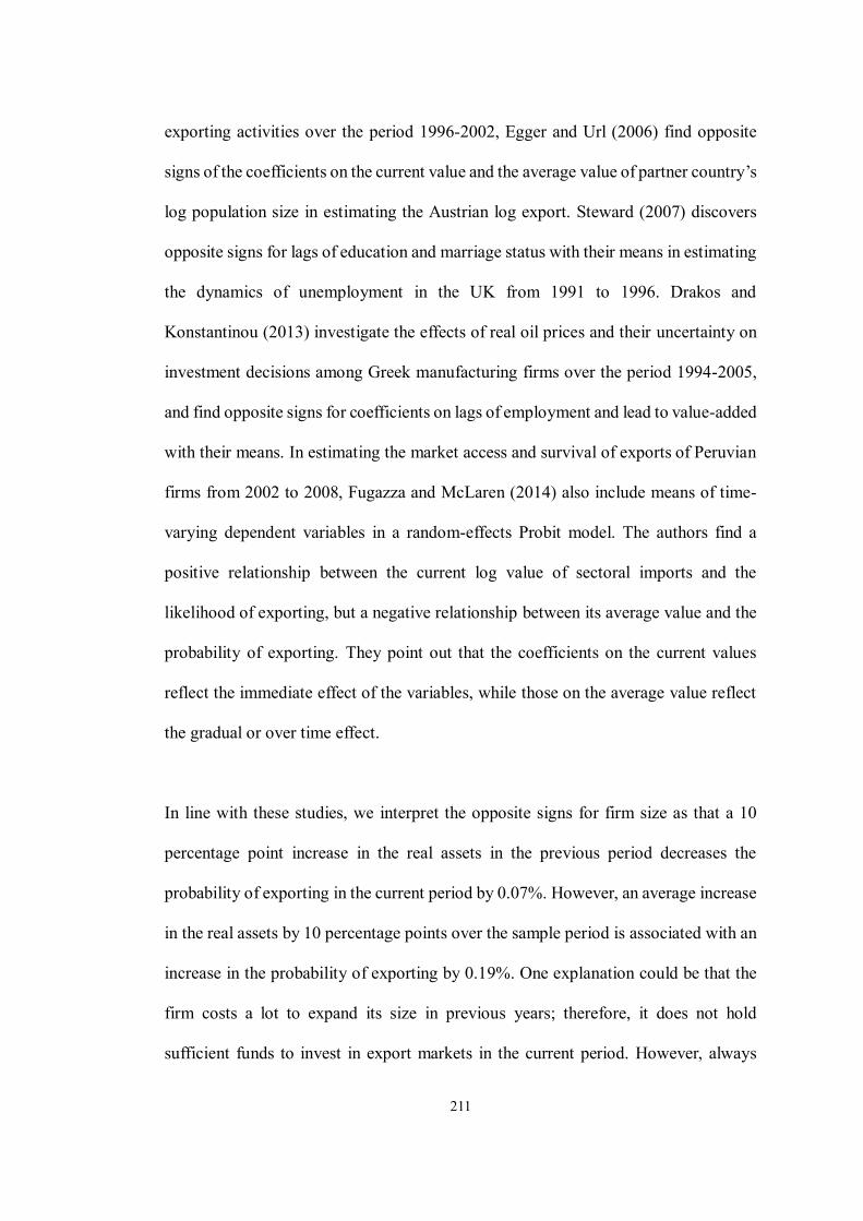
211
exporting activities over the period 1996-2002, Egger and Url (2006) find opposite
signs of the coefficients on the current value and the average value of partner country’s
log population size in estimating the Austrian log export. Steward (2007) discovers
opposite signs for lags of education and marriage status with their means in estimating
the dynamics of unemployment in the UK from 1991 to 1996. Drakos and
Konstantinou (2013) investigate the effects of real oil prices and their uncertainty on
investment decisions among Greek manufacturing firms over the period 1994-2005,
and find opposite signs for coefficients on lags of employment and lead to value-added
with their means. In estimating the market access and survival of exports of Peruvian
firms from 2002 to 2008, Fugazza and McLaren (2014) also include means of time-
varying dependent variables in a random-effects Probit model. The authors find a
positive relationship between the current log value of sectoral imports and the
likelihood of exporting, but a negative relationship between its average value and the
probability of exporting. They point out that the coefficients on the current values
reflect the immediate effect of the variables, while those on the average value reflect
the gradual or over time effect.
In line with these studies, we interpret the opposite signs for firm size as that a 10
percentage point increase in the real assets in the previous period decreases the
probability of exporting in the current period by 0.07%. However, an average increase
in the real assets by 10 percentage points over the sample period is associated with an
increase in the probability of exporting by 0.19%. One explanation could be that the
firm costs a lot to expand its size in previous years; therefore, it does not hold
sufficient funds to invest in export markets in the current period. However, always
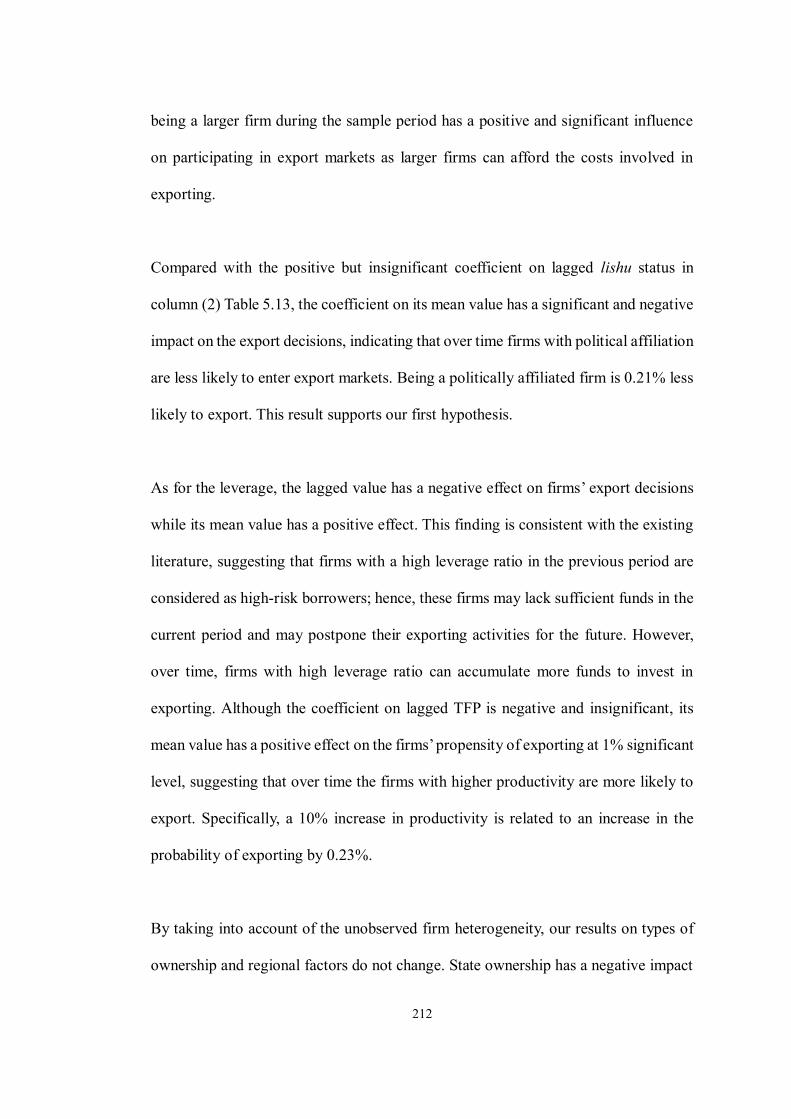
212
being a larger firm during the sample period has a positive and significant influence
on participating in export markets as larger firms can afford the costs involved in
exporting.
Compared with the positive but insignificant coefficient on lagged lishu status in
column (2) Table 5.13, the coefficient on its mean value has a significant and negative
impact on the export decisions, indicating that over time firms with political affiliation
are less likely to enter export markets. Being a politically affiliated firm is 0.21% less
likely to export. This result supports our first hypothesis.
As for the leverage, the lagged value has a negative effect on firms’ export decisions
while its mean value has a positive effect. This finding is consistent with the existing
literature, suggesting that firms with a high leverage ratio in the previous period are
considered as high-risk borrowers; hence, these firms may lack sufficient funds in the
current period and may postpone their exporting activities for the future. However,
over time, firms with high leverage ratio can accumulate more funds to invest in
exporting. Although the coefficient on lagged TFP is negative and insignificant, its
mean value has a positive effect on the firms’ propensity of exporting at 1% significant
level, suggesting that over time the firms with higher productivity are more likely to
export. Specifically, a 10% increase in productivity is related to an increase in the
probability of exporting by 0.23%.
By taking into account of the unobserved firm heterogeneity, our results on types of
ownership and regional factors do not change. State ownership has a negative impact
213
on the propensity of exporting, while foreign ownership has a positive effect.
Compared with firms located in the coastal region, these located in the west of China
are less likely to export.
In column (3), I address the initial conditions problem by Wooldridge’s (2005) method
and include the initial values of export status in the regressions. Similar results with
slight changes in the magnitudes of marginal effects are obtained. Over time, smaller
firms with a lishu relationship are less likely to export. Firms with high productivity
and leverage ratio are more likely to export. The negative coefficient on cash flow is
still affected by size effects. State ownership (foreign ownership) is negatively
(positively) related to the probability of exporting. Furthermore, firms in the coastal
area are more likely to export. As for the exporting status in the initial period, 𝐸𝑥𝑝𝑖1,
it is positive and significant at a 1% level. Firms that exported in the first period of
the sample are 0.95% more likely to export in the current period. As for the previous
exporting experience, we find a decrease from 3.50% to 2.81%, confirming that
without proper control of the initial conditions, the size of sunk entry costs of
exporting is overestimated.
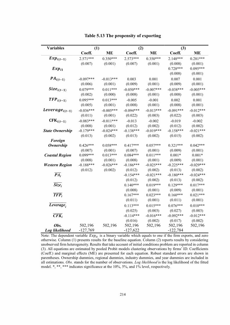
214
Table 5.13 The propensity of exporting Variables (1) (2) (3) Coeff. ME Coeff. ME Coeff. ME
𝑬𝒙𝒑𝒊(𝒕−𝟏) 2.571*** 0.350*** 2.573*** 0.350*** 2.148*** 0.281*** (0.007) (0.001) (0.007) (0.001) (0.008) (0.001)
𝑬𝒙𝒑𝒊𝟏 0.728*** 0.095*** (0.008) (0.001)
𝑷𝑨𝒊(𝒕−𝟏) -0.097*** -0.013*** 0.003 0.001 0.007 0.001 (0.006) (0.001) (0.009) (0.001) (0.009) (0.001)
𝑺𝒊𝒛𝒆𝒊(𝒕−𝟏) 0.079*** 0.011*** -0.050*** -0.007*** -0.038*** -0.005*** (0.002) (0.000) (0.008) (0.001) (0.008) (0.001)
𝑻𝑭𝑷𝒊(𝒕−𝟏) 0.095*** 0.013*** -0.005 -0.001 0.002 0.001 (0.005) (0.001) (0.008) (0.001) (0.008) (0.001)
𝑳𝒆𝒗𝒆𝒓𝒂𝒈𝒆𝒊(𝒕−𝟏) -0.036*** -0.005*** -0.094*** -0.013*** -0.091*** -0.012*** (0.011) (0.001) (0.022) (0.003) (0.022) (0.003)
𝐂𝐅𝐊𝒊(𝒕−𝟏) -0.083*** -0.011*** -0.013 -0.002 -0.019 -0.002 (0.008) (0.001) (0.012) (0.002) (0.012) (0.002)
State Ownership -0.179*** -0.024*** -0.138*** -0.019*** -0.158*** -0.021*** (0.013) (0.002) (0.013) (0.002) (0.015) (0.002)
Foreign Ownership 0.426*** 0.058*** 0.417*** 0.057*** 0.321*** 0.042***
(0.007) (0.001) (0.007) (0.001) (0.009) (0.001) Coastal Region 0.099*** 0.013*** 0.084*** 0.011*** 0.001* 0.001*
(0.008) (0.001) (0.008) (0.001) (0.009) (0.001) Western Region -0.188*** -0.026*** -0.186*** -0.025*** -0.225*** -0.029***
(0.012) (0.002) (0.012) (0.002) (0.013) (0.002) PAi̅̅ ̅̅ ̅ -0.154*** -0.021*** -0.180*** -0.024***
(0.012) (0.002) (0.013) (0.002) Sizei̅̅ ̅̅ ̅̅ 0.140*** 0.019*** 0.129*** 0.017***
(0.008) (0.001) (0.009) (0.001) TFPi̅̅ ̅̅ ̅̅ ̅ 0.167*** 0.023*** 0.160*** 0.021***
(0.011) (0.001) (0.011) (0.001) Leveragei̅̅ ̅̅ ̅̅ ̅̅ ̅̅ ̅̅ 0.113*** 0.015*** 0.076*** 0.010***
(0.025) (0.003) (0.027) (0.003) CFKi̅̅ ̅̅ ̅̅ ̅ -0.114*** -0.016*** -0.092*** -0.012***
(0.016) (0.002) (0.017) (0.002) Obs. 502,196 502,196 502,196 502,196 502,196 502,196
Log likelihood -127,769 -127,622 -122,784 Note: The dependent variable 𝐸𝑥𝑝𝑖𝑡 is a binary variable which equals to one if the firm exports, and zero otherwise. Column (1) presents results for the baseline equation. Column (2) reports results by considering unobserved firm heterogeneity. Results that take account of initial conditions problem are reported in column (3). All equations are estimated by pooled Probit models clustering observations by firms’ ID. Coefficients (Coeff.) and marginal effects (ME) are presented for each equation. Robust standard errors are shown in parentheses. Ownership dummies, regional dummies, industry dummies, and year dummies are included in all estimations. Obs. stands for the number of observations. Log likelihood is the log likelihood of the fitted model. *, **, *** indicates significance at the 10%, 5%, and 1% level, respectively.

215
5.7.2 The lishu relationship and the intensity of exporting
The regression results obtained by the pooled Tobit model 1 with clustering
observations by firms ID in Eqs. (2), (6), and (9) are presented in Table 5.14. Both
coefficients and marginal effects are presented in Table 5.14. Column (1) presents
results for the baseline equation (Eq. (2)). Column (2) reports results by considering
unobserved firm heterogeneity (Eq. (6)). Results that take account of initial conditions
problem (Eq. (9)) are reported in column (3). Only 156,757 observations are
uncensored, indicating a relatively low level of exporting of Chinese manufacturing
firms. A total of 345,439 observations are left-censored, which suggests that these
firms do not export during our sample period.
Focusing on column (1), we find that lagged export ratio is positive and significant
related to the current export ratio. The marginal effects suggest that a 10% increase in
the previous export ratio is associated with an increase in the export intensity by 4.05
percentage points in the current period. Firms with political affiliations export less
than their counterparts, indicating that having a lishu relationship reduces the export
intensity. Being a politically affiliated firm is associated with a 7.94% less exporting.
This finding is consistent with existing studies and our Hypothesis 2.
From column (1) Table 5.14, we also find that larger firms with higher productivity
export more than smaller firms with lower productivity. Specifically, a 10% increase
in the firms’ size (TFP) would yield an increase of 11.69 (10.46) percentage points in
1 Out results are robust by using the random-effects Tobit model. The results obtained from random-effects Tobit model are presented in Appendix. Using the GMM technique, we find that the main result that political connections have a negative impact on exporting intensity is still holding.
216
export ratio. These results suggest that once firms become exporters, the magnitudes
of firm size and productivity are significant in improving the export intensity. As for
the financial variables, we observe negative relationships between leverage ratio and
export intensity, and between cash flow/capital ratio and export ratio. A 10% decrease
in the leverage ratio (cash flow/capital ratio) increases the export intensity by 0.10
(7.07) percentage points. Similar to our results in section 5.7.1, the negative
coefficient on cash flow-to-capital ratio could be related to the size effects. And the
negative leverage ratio can be explained by the fact that exporters can obtain global
financing from their exporting activities, which provides a motivation for firms with
low leverage ratio in the previous period to export more in the global market in the
current period.
As for the ownership and regional factors, we find that firms with state (foreign)
ownership export less (more). Specifically, being a state-owned (foreign) firm is
associated with a 17.67% (32.60%) lower (higher) export ratio. Firms located in the
coastal region export more, while the firms in the west of China export less. Being a
coastal (western) firm is associated with a 17.59% (19.97%) more (less) exporting.
This can be attributed to the fact that firms locate in the east of China have geographic
advantages in terms of accessing to foreign markets and reducing transportation costs.
Unobserved firm heterogeneity is considered by adding a vector of means of time-
varying observable factors in the regressions. Results are reported in column (2) Table
5.14. The lagged export ratio maintain a positive and significant impact on the current
export ratio, indicating that a 0.1 increase in the previous export ratio is related to an
increase in the export intensity by 4.05 percentage points in the current period.
217
Similar to our results in section 5.7.1, we also observe opposite signs between lagged
lishu status and its mean value, and between lagged leverage ratio and its mean value.
These results suggest that over time, political affiliated firms export less (i.e. being a
political affiliated firm is associated with a 12.37% less exporting.) and firms with
high leverage ratio export more (i.e. a 10% increase in leverage ratio is related to an
increases in the export intensity by 13.04 percentage points). This result indicates that
over time, a firm with good financial status can improve its export intensity.
By considering the unobserved firm characteristics, the results on types of ownership
and regional factors only change slightly in terms of the magnetite of marginal effects.
Being a state-owned (foreign) firm is related to a 14.26% (32.00%) less (more)
exporting. Moreover, being a coastal (western) firm is associated with a 16.35%
(19.75%) more (less) exporting.
Column (3) in Table 5.14 presents the regression results that address the initial
conditions problem. We obtain similar results with slight changes in the magnitude of
marginal effects. The reduced marginal effects on the lagged export ratio indicate that
a 10% increase in export ratio in the previous period improves the export intensity in
the current period by 3.39 percentage points. As for the export intensity in the initial
period, 𝐸𝑥𝑝𝑟𝑎𝑡𝑖𝑜𝑖1, the positive and significant effect suggests that having positive a
export ratio in the first period of the sample increases the export ratio in current period
by 0.84 percentage points. Over time, larger firms with high productivity and leverage
ratio export more. Firms with the lishu relationship and locating in the west of China
export less. The negative coefficient on cash flow is still affected by size effects. State
ownership (foreign ownership) is negatively (positively) related to the intensity of
exporting.
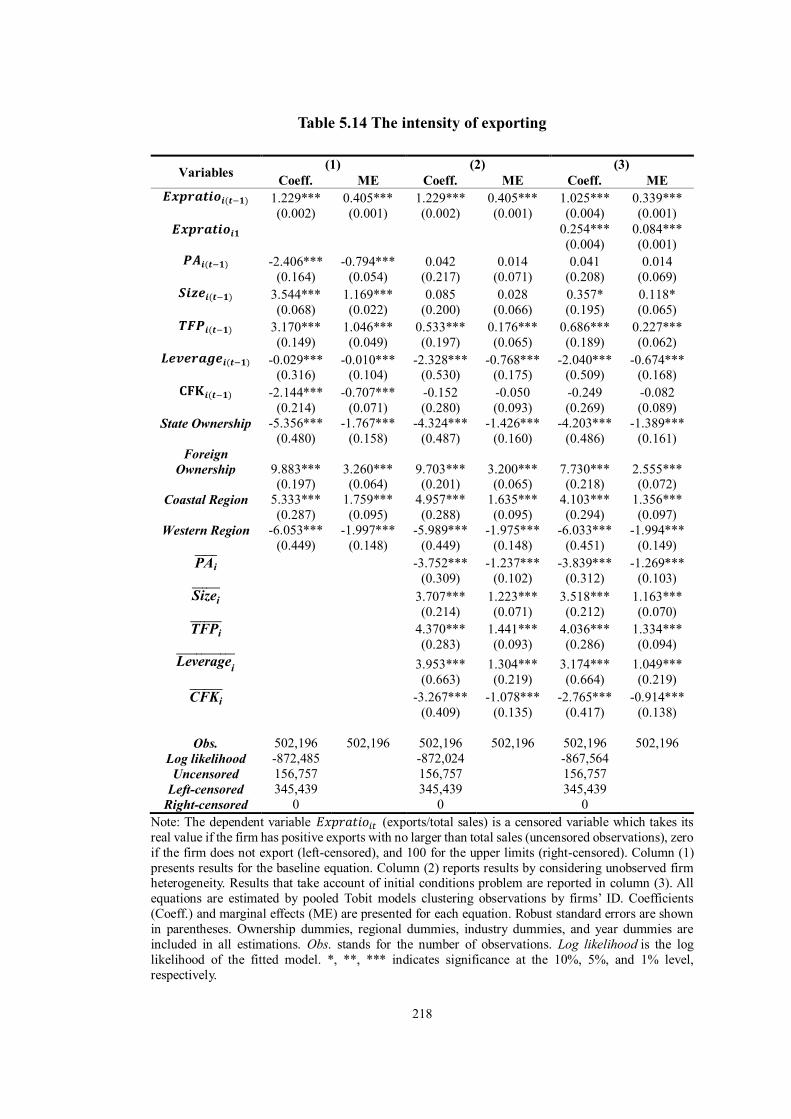
218
Table 5.14 The intensity of exporting
Variables (1) (2) (3) Coeff. ME Coeff. ME Coeff. ME
𝑬𝒙𝒑𝒓𝒂𝒕𝒊𝒐𝒊(𝒕−𝟏) 1.229*** 0.405*** 1.229*** 0.405*** 1.025*** 0.339*** (0.002) (0.001) (0.002) (0.001) (0.004) (0.001)
𝑬𝒙𝒑𝒓𝒂𝒕𝒊𝒐𝒊𝟏 0.254*** 0.084*** (0.004) (0.001)
𝑷𝑨𝒊(𝒕−𝟏) -2.406*** -0.794*** 0.042 0.014 0.041 0.014 (0.164) (0.054) (0.217) (0.071) (0.208) (0.069)
𝑺𝒊𝒛𝒆𝒊(𝒕−𝟏) 3.544*** 1.169*** 0.085 0.028 0.357* 0.118* (0.068) (0.022) (0.200) (0.066) (0.195) (0.065)
𝑻𝑭𝑷𝒊(𝒕−𝟏) 3.170*** 1.046*** 0.533*** 0.176*** 0.686*** 0.227*** (0.149) (0.049) (0.197) (0.065) (0.189) (0.062)
𝑳𝒆𝒗𝒆𝒓𝒂𝒈𝒆𝒊(𝒕−𝟏) -0.029*** -0.010*** -2.328*** -0.768*** -2.040*** -0.674*** (0.316) (0.104) (0.530) (0.175) (0.509) (0.168)
𝐂𝐅𝐊𝒊(𝒕−𝟏) -2.144*** -0.707*** -0.152 -0.050 -0.249 -0.082 (0.214) (0.071) (0.280) (0.093) (0.269) (0.089)
State Ownership -5.356*** -1.767*** -4.324*** -1.426*** -4.203*** -1.389*** (0.480) (0.158) (0.487) (0.160) (0.486) (0.161)
Foreign Ownership 9.883*** 3.260*** 9.703*** 3.200*** 7.730*** 2.555***
(0.197) (0.064) (0.201) (0.065) (0.218) (0.072) Coastal Region 5.333*** 1.759*** 4.957*** 1.635*** 4.103*** 1.356***
(0.287) (0.095) (0.288) (0.095) (0.294) (0.097) Western Region -6.053*** -1.997*** -5.989*** -1.975*** -6.033*** -1.994***
(0.449) (0.148) (0.449) (0.148) (0.451) (0.149) PAi̅̅ ̅̅ ̅ -3.752*** -1.237*** -3.839*** -1.269***
(0.309) (0.102) (0.312) (0.103) Sizei̅̅ ̅̅ ̅̅ 3.707*** 1.223*** 3.518*** 1.163***
(0.214) (0.071) (0.212) (0.070) TFPi̅̅ ̅̅ ̅̅ ̅ 4.370*** 1.441*** 4.036*** 1.334***
(0.283) (0.093) (0.286) (0.094) Leveragei̅̅ ̅̅ ̅̅ ̅̅ ̅̅ ̅̅ 3.953*** 1.304*** 3.174*** 1.049***
(0.663) (0.219) (0.664) (0.219) CFKi̅̅ ̅̅ ̅̅ ̅ -3.267*** -1.078*** -2.765*** -0.914***
(0.409) (0.135) (0.417) (0.138)
Obs. 502,196 502,196 502,196 502,196 502,196 502,196 Log likelihood -872,485 -872,024 -867,564
Uncensored 156,757 156,757 156,757 Left-censored 345,439 345,439 345,439
Right-censored 0 0 0 Note: The dependent variable 𝐸𝑥𝑝𝑟𝑎𝑡𝑖𝑜𝑖𝑡 (exports/total sales) is a censored variable which takes its real value if the firm has positive exports with no larger than total sales (uncensored observations), zero if the firm does not export (left-censored), and 100 for the upper limits (right-censored). Column (1) presents results for the baseline equation. Column (2) reports results by considering unobserved firm heterogeneity. Results that take account of initial conditions problem are reported in column (3). All equations are estimated by pooled Tobit models clustering observations by firms’ ID. Coefficients (Coeff.) and marginal effects (ME) are presented for each equation. Robust standard errors are shown in parentheses. Ownership dummies, regional dummies, industry dummies, and year dummies are included in all estimations. Obs. stands for the number of observations. Log likelihood is the log likelihood of the fitted model. *, **, *** indicates significance at the 10%, 5%, and 1% level, respectively.
219
5.8 Further tests
5.8.1 Different levels of the lishu relationship and exporting behaviour
In this section, we aim to test whether the different levels of lishu relationship have
the same effect on firms’ exporting behaviour. To this end, we further divide the
political affiliation of firms into four groups, i.e. firms with a low level of lishu
relationship (including the firms affiliated with the rest levels of governments), firms
with a medium level of lishu relationship (including the firms affiliated with the city
and prefecture, and county governments), and firms with a high level of lishu
relationship (including the firms affiliated with the central and provincial
governments).
We start with the first column in Table 5.15. We find that the lagged export status
remains positive and significant with the same magnitude of marginal effects as that
in Table 5.13, suggesting that firms export in the previous period are more likely to
remain their export status in the current period. The coefficients on three levels of
lishu relationship are all negative and significant at a 1% level. Being a firm affiliated
with the low/medium/high level of government is associated with a 0.12/0.14/0.13
lower probability of exporting. As for the other factors that can affect the firms’
exporting decisions, we find the similar results as in section 5.7.1 with slight change
in the magnitude of marginal effects.
Column (2) in Table 5.15 takes into account the unobserved firm heterogeneity.
Looking at the three levels of lishu relationship, we find, over time, firms with a lishu
220
relationship, no matter which level it is, are less likely to export. Interestingly, this
negative effect is significant for firms affiliated with a low or medium level of
government, but insignificant for the firms with a high level of lishu relationship. In
China, the major participants in the governmental external communications (with
foreign countries and cities) are dominated by the central and the provincial
governments. Economic communication and transnational trade are the two
predominant types of governmental external communications (Yang, 2015). These
governments prefer to grant their affiliated firms with exporting opportunities through
sharing information and bridging the cooperation. In this case, the negative effects of
the lishu relationship on firms’ exporting can be mitigate somehow. Additionally, all
the other results are similar to our previous findings.
Column (3) in Table 5.15 addresses the initial conditions problem. Focusing on our
three main coefficients on different levels of lishu relationship, we find similar results.
The low or medium level of political affiliation have a significant and negative
influence on firms’ exporting propensity, while this negative effect becomes only
significant at a 10% level for firms with a high level of lishu relationship due to the
scarce exporting opportunities the high level government can obtain through their
external communication with other foreign countries. The results for other variables
remain robust.
Table 5.16 estimates the effects of different levels of the lishu relationship on export
intensity. Similar results have been found. That is, without controlling for the
unobserved firm heterogeneity and initial conditions problem, affiliation with all the

221
three levels of government have a negative and significant relationship with firms’
export intensity. Focusing on columns (2) and (3), we find that over time, this negative
effect becomes insignificant for firms affiliated with high levels of government, but
remains significant for firms affiliated with low/medium level of government. As for
other variables, the results are robust. By controlling the initial conditions problem
appropriately, the overestimation of sunk costs can be reduced.

222
Table 5.15 The propensity of exporting (different levels of the lishu relationship)
Variables (1) (2) (3) Coeff. ME Coeff. ME Coeff. ME
𝑬𝒙𝒑𝒊(𝒕−𝟏) 2.571*** 0.350*** 2.573*** 0.350*** 2.148*** 0.281*** (0.007) (0.001) (0.007) (0.001) (0.008) (0.001)
𝑬𝒙𝒑𝒊𝟏 0.727*** 0.095*** (0.008) (0.001)
𝑷𝑨𝒍𝒐𝒘𝒊(𝒕−𝟏) -0.091*** -0.012*** -0.013 -0.002 -0.015 -0.002 (0.007) (0.001) (0.011) (0.002) (0.011) (0.002)
𝑷𝑨𝒎𝒆𝒅𝒊𝒖𝒎𝒊(𝒕−𝟏) -0.106*** -0.014*** -0.005 -0.001 0.001 0.001 (0.008) (0.001) (0.014) (0.002) (0.014) (0.002)
𝑷𝑨𝒉𝒊𝒈𝒉𝒊(𝒕−𝟏) -0.097*** -0.013*** -0.075** -0.010** -0.072** -0.009** (0.014) (0.002) (0.034) (0.005) (0.035) (0.005)
𝑺𝒊𝒛𝒆𝒊(𝒕−𝟏) 0.080*** 0.011*** -0.049*** -0.007*** -0.037*** -0.005*** (0.002) (0.000) (0.008) (0.001) (0.008) (0.001)
𝑻𝑭𝑷𝒊(𝒕−𝟏) 0.094*** 0.013*** -0.005 -0.001 0.002 0.001 (0.005) (0.001) (0.008) (0.001) (0.008) (0.001)
𝑳𝒆𝒗𝒆𝒓𝒂𝒈𝒆𝒊(𝒕−𝟏) -0.035*** -0.005*** -0.093*** -0.013*** -0.091*** -0.012*** (0.011) (0.001) (0.022) (0.003) (0.022) (0.003)
𝐂𝐅𝐊𝒊(𝒕−𝟏) -0.083*** -0.011*** -0.013 -0.002 -0.019 -0.002 (0.008) (0.001) (0.012) (0.002) (0.012) (0.002)
State Ownership -0.175*** -0.024*** -0.146*** -0.020*** -0.158*** -0.021*** (0.014) (0.002) (0.014) (0.002) (0.016) (0.002)
Foreign Ownership 0.426*** 0.058*** 0.417*** 0.057*** 0.322*** 0.042***
(0.007) (0.001) (0.007) (0.001) (0.009) (0.001) Coastal Region 0.097*** 0.013*** 0.084*** 0.011*** 0.003* 0.001*
(0.008) (0.001) (0.008) (0.001) (0.009) (0.001) Western Region -0.187*** -0.025*** -0.187*** -0.025*** -0.224*** -0.029***
(0.012) (0.002) (0.012) (0.002) (0.013) (0.002) PAlowi̅̅ ̅̅ ̅̅ ̅̅ ̅ -0.168*** -0.023*** -0.181*** -0.024***
(0.014) (0.002) (0.015) (0.002) PAmediumi̅̅ ̅̅ ̅̅ ̅̅ ̅̅ ̅̅ ̅̅ ̅ -0.148*** -0.020*** -0.188*** -0.025***
(0.017) (0.002) (0.018) (0.002) PAhighi̅̅ ̅̅ ̅̅ ̅̅ ̅̅ -0.049 -0.007 -0.083* -0.011*
(0.037) (0.005) (0.038) (0.005) Sizei̅̅ ̅̅ ̅̅ 0.139*** 0.019*** 0.129*** 0.017***
(0.008) (0.001) (0.009) (0.001) TFPi̅̅ ̅̅ ̅̅ ̅ 0.167*** 0.023*** 0.158*** 0.021***
(0.011) (0.001) (0.011) (0.001) Leveragei̅̅ ̅̅ ̅̅ ̅̅ ̅̅ ̅̅ 0.114*** 0.016*** 0.077*** 0.010***
(0.025) (0.003) (0.027) (0.003) CFKi̅̅ ̅̅ ̅̅ ̅ -0.114*** -0.015*** -0.093*** -0.012***
(0.016) (0.002) (0.017) (0.002) Obs. 502,196 502,196 502,196 502,196 502,196 502,196
Log likelihood -127,997 -127,617 -122,924 Note: The dependent variable 𝐸𝑥𝑝𝑖𝑡 is a binary variable which equals to one if the firm exports, and zero otherwise. Column (1) presents results for the baseline equation. Column (2) reports results by considering unobserved firm heterogeneity. Results that take account of initial conditions problem are reported in column (3). All equations are estimated by pooled Probit models clustering observations by firms’ ID. Coefficients (Coeff.) and marginal effects (ME) are presented for each equation. Robust standard errors are shown in parentheses. Ownership dummies, regional dummies, industry dummies, and year dummies are included in all estimations. Obs. stands for the number of observations. Log likelihood is the log likelihood of the fitted model. *, **, *** indicates significance at the 10%, 5%, and 1% level, respectively.
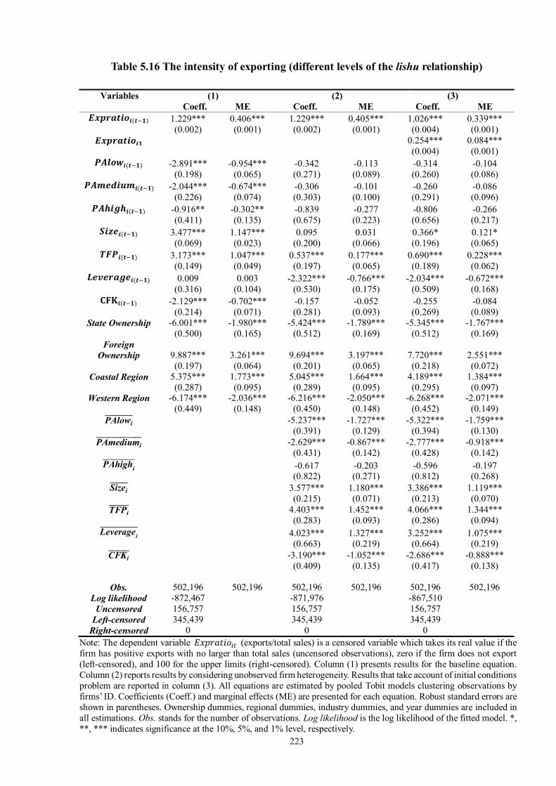
223
Table 5.16 The intensity of exporting (different levels of the lishu relationship)
Variables (1) (2) (3) Coeff. ME Coeff. ME Coeff. ME
𝑬𝒙𝒑𝒓𝒂𝒕𝒊𝒐𝒊(𝒕−𝟏) 1.229*** 0.406*** 1.229*** 0.405*** 1.026*** 0.339*** (0.002) (0.001) (0.002) (0.001) (0.004) (0.001)
𝑬𝒙𝒑𝒓𝒂𝒕𝒊𝒐𝒊𝟏 0.254*** 0.084*** (0.004) (0.001)
𝑷𝑨𝒍𝒐𝒘𝒊(𝒕−𝟏) -2.891*** -0.954*** -0.342 -0.113 -0.314 -0.104 (0.198) (0.065) (0.271) (0.089) (0.260) (0.086)
𝑷𝑨𝒎𝒆𝒅𝒊𝒖𝒎𝒊(𝒕−𝟏) -2.044*** -0.674*** -0.306 -0.101 -0.260 -0.086 (0.226) (0.074) (0.303) (0.100) (0.291) (0.096)
𝑷𝑨𝒉𝒊𝒈𝒉𝒊(𝒕−𝟏) -0.916** -0.302** -0.839 -0.277 -0.806 -0.266 (0.411) (0.135) (0.675) (0.223) (0.656) (0.217)
𝑺𝒊𝒛𝒆𝒊(𝒕−𝟏) 3.477*** 1.147*** 0.095 0.031 0.366* 0.121* (0.069) (0.023) (0.200) (0.066) (0.196) (0.065)
𝑻𝑭𝑷𝒊(𝒕−𝟏) 3.173*** 1.047*** 0.537*** 0.177*** 0.690*** 0.228*** (0.149) (0.049) (0.197) (0.065) (0.189) (0.062)
𝑳𝒆𝒗𝒆𝒓𝒂𝒈𝒆𝒊(𝒕−𝟏) 0.009 0.003 -2.322*** -0.766*** -2.034*** -0.672*** (0.316) (0.104) (0.530) (0.175) (0.509) (0.168)
𝐂𝐅𝐊𝒊(𝒕−𝟏) -2.129*** -0.702*** -0.157 -0.052 -0.255 -0.084 (0.214) (0.071) (0.281) (0.093) (0.269) (0.089)
State Ownership -6.001*** -1.980*** -5.424*** -1.789*** -5.345*** -1.767*** (0.500) (0.165) (0.512) (0.169) (0.512) (0.169)
Foreign Ownership 9.887*** 3.261*** 9.694*** 3.197*** 7.720*** 2.551***
(0.197) (0.064) (0.201) (0.065) (0.218) (0.072) Coastal Region 5.375*** 1.773*** 5.045*** 1.664*** 4.189*** 1.384***
(0.287) (0.095) (0.289) (0.095) (0.295) (0.097) Western Region -6.174*** -2.036*** -6.216*** -2.050*** -6.268*** -2.071***
(0.449) (0.148) (0.450) (0.148) (0.452) (0.149) PAlowi̅̅ ̅̅ ̅̅ ̅̅ ̅ -5.237*** -1.727*** -5.322*** -1.759***
(0.391) (0.129) (0.394) (0.130) PAmediumi̅̅ ̅̅ ̅̅ ̅̅ ̅̅ ̅̅ ̅̅ ̅ -2.629*** -0.867*** -2.777*** -0.918***
(0.431) (0.142) (0.428) (0.142) PAhighi̅̅ ̅̅ ̅̅ ̅̅ ̅̅ -0.617 -0.203 -0.596 -0.197
(0.822) (0.271) (0.812) (0.268) Sizei̅̅ ̅̅ ̅̅ 3.577*** 1.180*** 3.386*** 1.119***
(0.215) (0.071) (0.213) (0.070) TFPi̅̅ ̅̅ ̅̅ ̅ 4.403*** 1.452*** 4.066*** 1.344***
(0.283) (0.093) (0.286) (0.094) Leveragei̅̅ ̅̅ ̅̅ ̅̅ ̅̅ ̅̅ 4.023*** 1.327*** 3.252*** 1.075***
(0.663) (0.219) (0.664) (0.219) CFKi̅̅ ̅̅ ̅̅ ̅ -3.190*** -1.052*** -2.686*** -0.888***
(0.409) (0.135) (0.417) (0.138)
Obs. 502,196 502,196 502,196 502,196 502,196 502,196 Log likelihood -872,467 -871,976 -867,510
Uncensored 156,757 156,757 156,757 Left-censored 345,439 345,439 345,439
Right-censored 0 0 0 Note: The dependent variable 𝐸𝑥𝑝𝑟𝑎𝑡𝑖𝑜𝑖𝑡 (exports/total sales) is a censored variable which takes its real value if the firm has positive exports with no larger than total sales (uncensored observations), zero if the firm does not export (left-censored), and 100 for the upper limits (right-censored). Column (1) presents results for the baseline equation. Column (2) reports results by considering unobserved firm heterogeneity. Results that take account of initial conditions problem are reported in column (3). All equations are estimated by pooled Tobit models clustering observations by firms’ ID. Coefficients (Coeff.) and marginal effects (ME) are presented for each equation. Robust standard errors are shown in parentheses. Ownership dummies, regional dummies, industry dummies, and year dummies are included in all estimations. Obs. stands for the number of observations. Log likelihood is the log likelihood of the fitted model. *, **, *** indicates significance at the 10%, 5%, and 1% level, respectively.

224
5.8.2 The propensity and intensity of exporting by ownership
We then estimate the decision to export and export intensity by ownership types.1 We
report the marginal effects of the regression results for the probability of exporting in
Table 5.17 and for export intensity in Table 5.18. The coefficient estimates are
provided in Table 5A.4 and Table 5A.5 in the Appendix. As we find that around 94%
of state-owned firms and 84% of collectively-owned firms are politically affiliated,
we only report the results for private firms (in column (1)), which accounts for more
than 60% of our full sample, and foreign firms (in column (2)), which are most
effective and active sector in China.
Focusing on the main regressor, lishu status variable, we find that the lishu
relationship negatively affects the propensity of exporting. Once these firms export,
their export intensity is less for politically affiliated firms. Such negative relationship
is more significant in foreign firms than that in private firms. All the other estimation
results are robust as found in the previous sections.
1 I also have estimated the regressions for ten different industries available in our dataset, i.e. Metal and metal products industry, Non-metal products and petroleum processing industry, Chemicals and plastic industry, Machinery and Equipment industry, Electrical equipment industry, Transport equipment industry, Food and Tobacco industry, Textile industry, Leather, Timber and Furniture industry, and Mining and Logging industry. And the main results are robust, indicating that during our sample period, political connections have a negative impact on export probability and intensity in these sub-samples. Results are available on request.
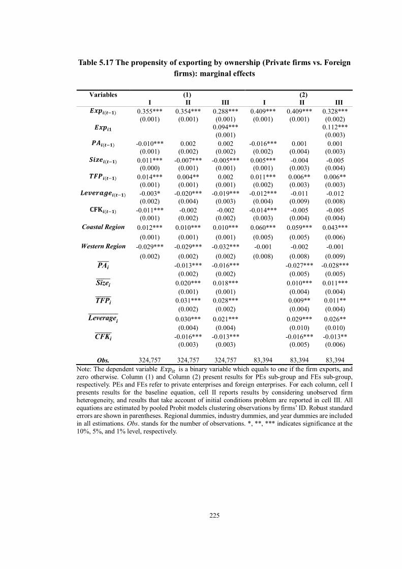
225
Table 5.17 The propensity of exporting by ownership (Private firms vs. Foreign firms): marginal effects
Variables (1) (2)
I II III I II III 𝑬𝒙𝒑𝒊(𝒕−𝟏) 0.355*** 0.354*** 0.288*** 0.409*** 0.409*** 0.328***
(0.001) (0.001) (0.001) (0.001) (0.001) (0.002) 𝑬𝒙𝒑𝒊𝟏 0.094*** 0.112***
(0.001) (0.003) 𝑷𝑨𝒊(𝒕−𝟏) -0.010*** 0.002 0.002 -0.016*** 0.001 0.001
(0.001) (0.002) (0.002) (0.002) (0.004) (0.003) 𝑺𝒊𝒛𝒆𝒊(𝒕−𝟏) 0.011*** -0.007*** -0.005*** 0.005*** -0.004 -0.005
(0.000) (0.001) (0.001) (0.001) (0.003) (0.004) 𝑻𝑭𝑷𝒊(𝒕−𝟏) 0.014*** 0.004** 0.002 0.011*** 0.006** 0.006**
(0.001) (0.001) (0.001) (0.002) (0.003) (0.003) 𝑳𝒆𝒗𝒆𝒓𝒂𝒈𝒆𝒊(𝒕−𝟏) -0.003* -0.020*** -0.019*** -0.012*** -0.011 -0.012
(0.002) (0.004) (0.003) (0.004) (0.009) (0.008) 𝐂𝐅𝐊𝒊(𝒕−𝟏) -0.011*** -0.002 -0.002 -0.014*** -0.005 -0.005
(0.001) (0.002) (0.002) (0.003) (0.004) (0.004) Coastal Region 0.012*** 0.010*** 0.010*** 0.060*** 0.059*** 0.043***
(0.001) (0.001) (0.001) (0.005) (0.005) (0.006) Western Region -0.029*** -0.029*** -0.032*** -0.001 -0.002 -0.001
(0.002) (0.002) (0.002) (0.008) (0.008) (0.009) PAi̅̅ ̅̅ ̅ -0.013*** -0.016*** -0.027*** -0.028***
(0.002) (0.002) (0.005) (0.005) Sizei̅̅ ̅̅ ̅̅ 0.020*** 0.018*** 0.010*** 0.011***
(0.001) (0.001) (0.004) (0.004) TFPi̅̅ ̅̅ ̅̅ ̅ 0.031*** 0.028*** 0.009** 0.011**
(0.002) (0.002) (0.004) (0.004) Leveragei̅̅ ̅̅ ̅̅ ̅̅ ̅̅ ̅̅ 0.030*** 0.021*** 0.029*** 0.026**
(0.004) (0.004) (0.010) (0.010) CFKi̅̅ ̅̅ ̅̅ ̅ -0.016*** -0.013*** -0.016*** -0.013**
(0.003) (0.003) (0.005) (0.006)
Obs. 324,757 324,757 324,757 83,394 83,394 83,394 Note: The dependent variable 𝐸𝑥𝑝𝑖𝑡 is a binary variable which equals to one if the firm exports, and zero otherwise. Column (1) and Column (2) present results for PEs sub-group and FEs sub-group, respectively. PEs and FEs refer to private enterprises and foreign enterprises. For each column, cell I presents results for the baseline equation, cell II reports results by considering unobserved firm heterogeneity, and results that take account of initial conditions problem are reported in cell III. All equations are estimated by pooled Probit models clustering observations by firms’ ID. Robust standard errors are shown in parentheses. Regional dummies, industry dummies, and year dummies are included in all estimations. Obs. stands for the number of observations. *, **, *** indicates significance at the 10%, 5%, and 1% level, respectively.
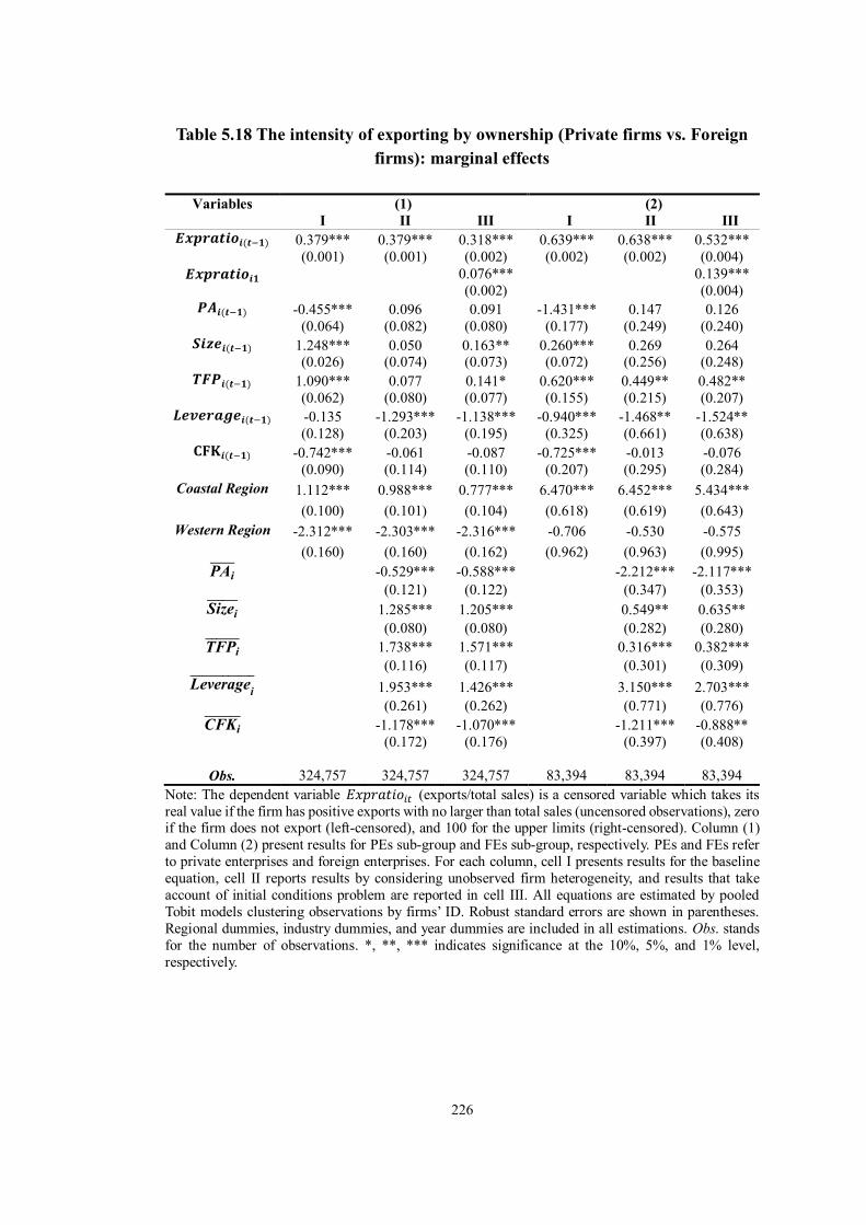
226
Table 5.18 The intensity of exporting by ownership (Private firms vs. Foreign firms): marginal effects
Variables (1) (2)
I II III I II III 𝑬𝒙𝒑𝒓𝒂𝒕𝒊𝒐𝒊(𝒕−𝟏) 0.379*** 0.379*** 0.318*** 0.639*** 0.638*** 0.532***
(0.001) (0.001) (0.002) (0.002) (0.002) (0.004) 𝑬𝒙𝒑𝒓𝒂𝒕𝒊𝒐𝒊𝟏 0.076*** 0.139***
(0.002) (0.004) 𝑷𝑨𝒊(𝒕−𝟏) -0.455*** 0.096 0.091 -1.431*** 0.147 0.126
(0.064) (0.082) (0.080) (0.177) (0.249) (0.240) 𝑺𝒊𝒛𝒆𝒊(𝒕−𝟏) 1.248*** 0.050 0.163** 0.260*** 0.269 0.264
(0.026) (0.074) (0.073) (0.072) (0.256) (0.248) 𝑻𝑭𝑷𝒊(𝒕−𝟏) 1.090*** 0.077 0.141* 0.620*** 0.449** 0.482**
(0.062) (0.080) (0.077) (0.155) (0.215) (0.207) 𝑳𝒆𝒗𝒆𝒓𝒂𝒈𝒆𝒊(𝒕−𝟏) -0.135 -1.293*** -1.138*** -0.940*** -1.468** -1.524**
(0.128) (0.203) (0.195) (0.325) (0.661) (0.638) 𝐂𝐅𝐊𝒊(𝒕−𝟏) -0.742*** -0.061 -0.087 -0.725*** -0.013 -0.076
(0.090) (0.114) (0.110) (0.207) (0.295) (0.284) Coastal Region 1.112*** 0.988*** 0.777*** 6.470*** 6.452*** 5.434***
(0.100) (0.101) (0.104) (0.618) (0.619) (0.643) Western Region -2.312*** -2.303*** -2.316*** -0.706 -0.530 -0.575
(0.160) (0.160) (0.162) (0.962) (0.963) (0.995) PAi̅̅ ̅̅ ̅ -0.529*** -0.588*** -2.212*** -2.117***
(0.121) (0.122) (0.347) (0.353) Sizei̅̅ ̅̅ ̅̅ 1.285*** 1.205*** 0.549** 0.635**
(0.080) (0.080) (0.282) (0.280) TFPi̅̅ ̅̅ ̅̅ ̅ 1.738*** 1.571*** 0.316*** 0.382***
(0.116) (0.117) (0.301) (0.309) Leveragei̅̅ ̅̅ ̅̅ ̅̅ ̅̅ ̅̅ 1.953*** 1.426*** 3.150*** 2.703***
(0.261) (0.262) (0.771) (0.776) CFKi̅̅ ̅̅ ̅̅ ̅ -1.178*** -1.070*** -1.211*** -0.888**
(0.172) (0.176) (0.397) (0.408)
Obs. 324,757 324,757 324,757 83,394 83,394 83,394 Note: The dependent variable 𝐸𝑥𝑝𝑟𝑎𝑡𝑖𝑜𝑖𝑡 (exports/total sales) is a censored variable which takes its real value if the firm has positive exports with no larger than total sales (uncensored observations), zero if the firm does not export (left-censored), and 100 for the upper limits (right-censored). Column (1) and Column (2) present results for PEs sub-group and FEs sub-group, respectively. PEs and FEs refer to private enterprises and foreign enterprises. For each column, cell I presents results for the baseline equation, cell II reports results by considering unobserved firm heterogeneity, and results that take account of initial conditions problem are reported in cell III. All equations are estimated by pooled Tobit models clustering observations by firms’ ID. Robust standard errors are shown in parentheses. Regional dummies, industry dummies, and year dummies are included in all estimations. Obs. stands for the number of observations. *, **, *** indicates significance at the 10%, 5%, and 1% level, respectively.
227
5.8.3 The propensity and intensity of exporting by region
In this section, we estimate the decision to export and export intensity by regions. We
report the marginal effects of the regression results for the probability of exporting by
regions in Table 5.19 and for export intensity in Table 5.20. The coefficients estimates
are provided in Table 5A.6 and Table 5A.7 in the Appendix. In each table, column (1)
reports the results for firms located in coastal region, column (2) presents the results
for firms in the central region, and column (3) shows the results for firms in the
western region.
In all three regressions, for the firms in the east of China, the lishu relationship has a
significant negative effect on the propensity and intensity of exporting. As for other
factors, we find the similar results with the analysis in the previous sections.
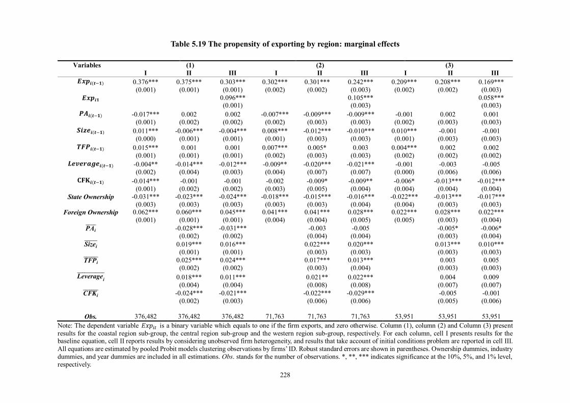
228
Table 5.19 The propensity of exporting by region: marginal effects
Variables (1) (2) (3) I II III I II III I II III
𝑬𝒙𝒑𝒊(𝒕−𝟏) 0.376*** 0.375*** 0.303*** 0.302*** 0.301*** 0.242*** 0.209*** 0.208*** 0.169*** (0.001) (0.001) (0.001) (0.002) (0.002) (0.003) (0.002) (0.002) (0.003)
𝑬𝒙𝒑𝒊𝟏 0.096*** 0.105*** 0.058*** (0.001) (0.003) (0.003)
𝑷𝑨𝒊(𝒕−𝟏) -0.017*** 0.002 0.002 -0.007*** -0.009*** -0.009*** -0.001 0.002 0.001 (0.001) (0.002) (0.002) (0.002) (0.003) (0.003) (0.002) (0.003) (0.003)
𝑺𝒊𝒛𝒆𝒊(𝒕−𝟏) 0.011*** -0.006*** -0.004*** 0.008*** -0.012*** -0.010*** 0.010*** -0.001 -0.001 (0.000) (0.001) (0.001) (0.001) (0.003) (0.003) (0.001) (0.003) (0.003)
𝑻𝑭𝑷𝒊(𝒕−𝟏) 0.015*** 0.001 0.001 0.007*** 0.005* 0.003 0.004*** 0.002 0.002 (0.001) (0.001) (0.001) (0.002) (0.003) (0.003) (0.002) (0.002) (0.002)
𝑳𝒆𝒗𝒆𝒓𝒂𝒈𝒆𝒊(𝒕−𝟏) -0.004** -0.014*** -0.012*** -0.009** -0.020*** -0.021*** -0.001 -0.003 -0.005 (0.002) (0.004) (0.003) (0.004) (0.007) (0.007) (0.000) (0.006) (0.006)
𝐂𝐅𝐊𝒊(𝒕−𝟏) -0.014*** -0.001 -0.001 -0.002 -0.009* -0.009** -0.006* -0.013*** -0.012*** (0.001) (0.002) (0.002) (0.003) (0.005) (0.004) (0.004) (0.004) (0.004)
State Ownership -0.031*** -0.023*** -0.024*** -0.018*** -0.015*** -0.016*** -0.022*** -0.013*** -0.017*** (0.003) (0.003) (0.003) (0.003) (0.003) (0.004) (0.004) (0.003) (0.003)
Foreign Ownership 0.062*** 0.060*** 0.045*** 0.041*** 0.041*** 0.028*** 0.022*** 0.028*** 0.022*** (0.001) (0.001) (0.001) (0.004) (0.004) (0.005) (0.005) (0.003) (0.004)
PAi̅̅ ̅̅̅ -0.028*** -0.031*** -0.003 -0.005 -0.005* -0.006* (0.002) (0.002) (0.004) (0.004) (0.003) (0.004)
Sizei̅̅ ̅̅ ̅̅ 0.019*** 0.016*** 0.022*** 0.020*** 0.013*** 0.010*** (0.001) (0.001) (0.003) (0.003) (0.003) (0.003)
TFPi̅̅ ̅̅ ̅̅ ̅ 0.025*** 0.024*** 0.017*** 0.013*** 0.003 0.005 (0.002) (0.002) (0.003) (0.004) (0.003) (0.003)
Leveragei̅̅ ̅̅ ̅̅ ̅̅ ̅̅ ̅̅ 0.018*** 0.011*** 0.021** 0.022*** 0.004 0.009
(0.004) (0.004) (0.008) (0.008) (0.007) (0.007) CFKi̅̅ ̅̅ ̅̅ ̅ -0.024*** -0.021*** -0.022*** -0.029*** -0.005 -0.001
(0.002) (0.003) (0.006) (0.006) (0.005) (0.006)
Obs. 376,482 376,482 376,482 71,763 71,763 71,763 53,951 53,951 53,951 Note: The dependent variable 𝐸𝑥𝑝𝑖𝑡 is a binary variable which equals to one if the firm exports, and zero otherwise. Column (1), column (2) and Column (3) present results for the coastal region sub-group, the central region sub-group and the western region sub-group, respectively. For each column, cell I presents results for the baseline equation, cell II reports results by considering unobserved firm heterogeneity, and results that take account of initial conditions problem are reported in cell III. All equations are estimated by pooled Probit models clustering observations by firms’ ID. Robust standard errors are shown in parentheses. Ownership dummies, industry dummies, and year dummies are included in all estimations. Obs. stands for the number of observations. *, **, *** indicates significance at the 10%, 5%, and 1% level, respectively.
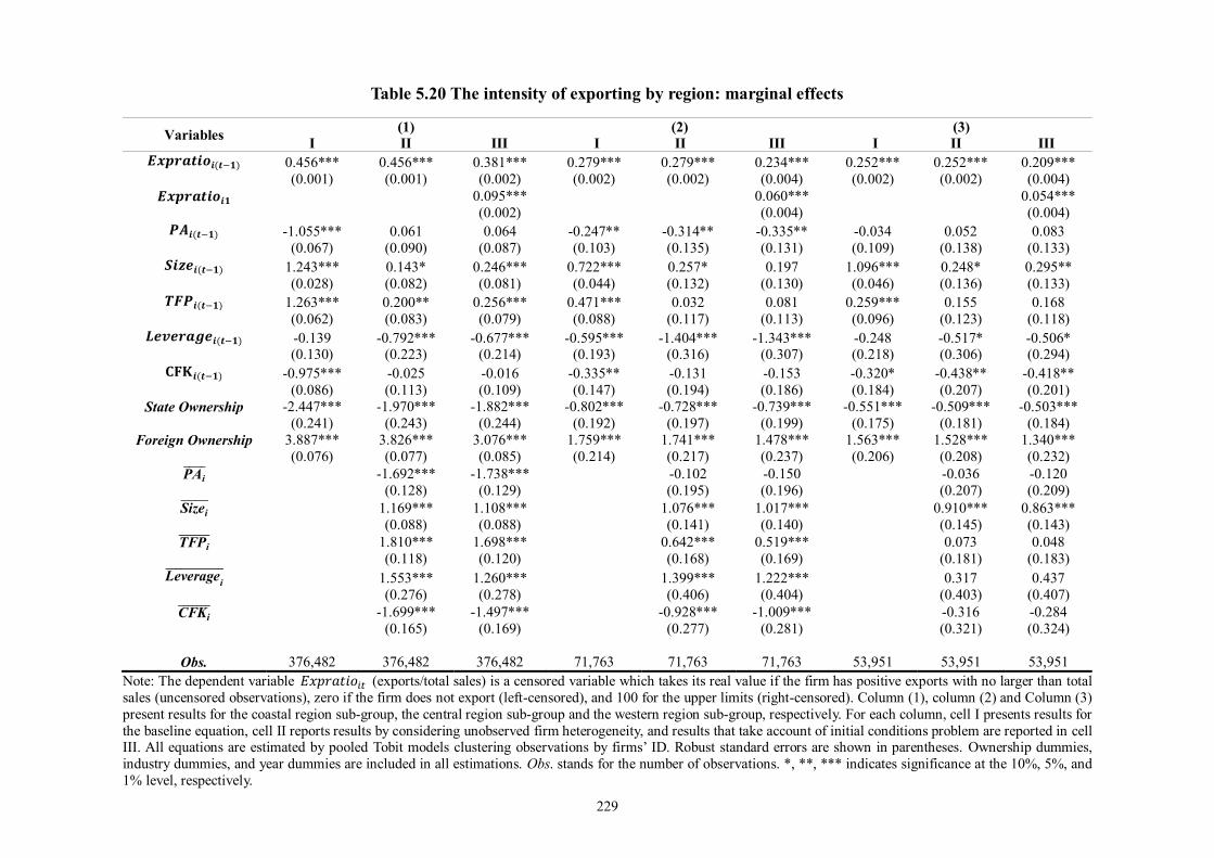
229
Table 5.20 The intensity of exporting by region: marginal effects
Variables (1) (2) (3) I II III I II III I II III
𝑬𝒙𝒑𝒓𝒂𝒕𝒊𝒐𝒊(𝒕−𝟏) 0.456*** 0.456*** 0.381*** 0.279*** 0.279*** 0.234*** 0.252*** 0.252*** 0.209*** (0.001) (0.001) (0.002) (0.002) (0.002) (0.004) (0.002) (0.002) (0.004)
𝑬𝒙𝒑𝒓𝒂𝒕𝒊𝒐𝒊𝟏 0.095*** 0.060*** 0.054*** (0.002) (0.004) (0.004)
𝑷𝑨𝒊(𝒕−𝟏) -1.055*** 0.061 0.064 -0.247** -0.314** -0.335** -0.034 0.052 0.083 (0.067) (0.090) (0.087) (0.103) (0.135) (0.131) (0.109) (0.138) (0.133)
𝑺𝒊𝒛𝒆𝒊(𝒕−𝟏) 1.243*** 0.143* 0.246*** 0.722*** 0.257* 0.197 1.096*** 0.248* 0.295** (0.028) (0.082) (0.081) (0.044) (0.132) (0.130) (0.046) (0.136) (0.133)
𝑻𝑭𝑷𝒊(𝒕−𝟏) 1.263*** 0.200** 0.256*** 0.471*** 0.032 0.081 0.259*** 0.155 0.168 (0.062) (0.083) (0.079) (0.088) (0.117) (0.113) (0.096) (0.123) (0.118)
𝑳𝒆𝒗𝒆𝒓𝒂𝒈𝒆𝒊(𝒕−𝟏) -0.139 -0.792*** -0.677*** -0.595*** -1.404*** -1.343*** -0.248 -0.517* -0.506* (0.130) (0.223) (0.214) (0.193) (0.316) (0.307) (0.218) (0.306) (0.294)
𝐂𝐅𝐊𝒊(𝒕−𝟏) -0.975*** -0.025 -0.016 -0.335** -0.131 -0.153 -0.320* -0.438** -0.418** (0.086) (0.113) (0.109) (0.147) (0.194) (0.186) (0.184) (0.207) (0.201)
State Ownership -2.447*** -1.970*** -1.882*** -0.802*** -0.728*** -0.739*** -0.551*** -0.509*** -0.503*** (0.241) (0.243) (0.244) (0.192) (0.197) (0.199) (0.175) (0.181) (0.184)
Foreign Ownership 3.887*** 3.826*** 3.076*** 1.759*** 1.741*** 1.478*** 1.563*** 1.528*** 1.340*** (0.076) (0.077) (0.085) (0.214) (0.217) (0.237) (0.206) (0.208) (0.232)
PAi̅̅ ̅̅̅ -1.692*** -1.738*** -0.102 -0.150 -0.036 -0.120 (0.128) (0.129) (0.195) (0.196) (0.207) (0.209)
Sizei̅̅ ̅̅ ̅̅ 1.169*** 1.108*** 1.076*** 1.017*** 0.910*** 0.863*** (0.088) (0.088) (0.141) (0.140) (0.145) (0.143)
TFPi̅̅ ̅̅ ̅̅ ̅ 1.810*** 1.698*** 0.642*** 0.519*** 0.073 0.048 (0.118) (0.120) (0.168) (0.169) (0.181) (0.183)
Leveragei̅̅ ̅̅ ̅̅ ̅̅ ̅̅ ̅̅ 1.553*** 1.260*** 1.399*** 1.222*** 0.317 0.437
(0.276) (0.278) (0.406) (0.404) (0.403) (0.407) CFKi̅̅ ̅̅ ̅̅ ̅ -1.699*** -1.497*** -0.928*** -1.009*** -0.316 -0.284
(0.165) (0.169) (0.277) (0.281) (0.321) (0.324)
Obs. 376,482 376,482 376,482 71,763 71,763 71,763 53,951 53,951 53,951 Note: The dependent variable 𝐸𝑥𝑝𝑟𝑎𝑡𝑖𝑜𝑖𝑡 (exports/total sales) is a censored variable which takes its real value if the firm has positive exports with no larger than total sales (uncensored observations), zero if the firm does not export (left-censored), and 100 for the upper limits (right-censored). Column (1), column (2) and Column (3) present results for the coastal region sub-group, the central region sub-group and the western region sub-group, respectively. For each column, cell I presents results for the baseline equation, cell II reports results by considering unobserved firm heterogeneity, and results that take account of initial conditions problem are reported in cell III. All equations are estimated by pooled Tobit models clustering observations by firms’ ID. Robust standard errors are shown in parentheses. Ownership dummies, industry dummies, and year dummies are included in all estimations. Obs. stands for the number of observations. *, **, *** indicates significance at the 10%, 5%, and 1% level, respectively.

230
5.9 Conclusion
On the one hand, extensive studies have been done to estimate firms’ exporting
activities; on the other hand, political connections and the benefits they can provide
have attracted worldwide academic attentions. However, only few studies have looked
at firms’ exporting activities and political connections from the perspective of state
ownership. Having experienced almost four decades of economic reform since 1978,
China has risen as a leading power in the global exporting market. Meanwhile,
government interventions still play an important part in firms’ development. Therefore,
it is interesting to look at the links between political connections and firms’ exporting
activities in the context of China.
I investigate the probability of exporting and the intensity of exporting by examining
how sunk costs, the lishu relationship, firm observed and unobserved heterogeneity,
and the initial conditions affect the exporting behaviour of Chinese firms. An
important feature of this chapter is that I take into account firms’ political affiliation,
in terms of the lishu relationship. Using a large dataset of Chinese manufacturing firms
between 2001 and 2007, I find that the sunk entry costs exist in exporting, and that
previous export status and export ratio play an important role in the current export
participation and intensity. We also find that firms with a lishu relationship in the
previous year and over the period have a negative impact on both the propensity and
intensity of exporting in the current period. Such negative effects are more significant
for foreign firms compared with private firms, and for firms located in the coastal
region. Interestingly, when we further divide the firms’ lishu relationship into four
231
different levels, we find that this negative effect is only significant for firms affiliated
with low or medium levels of government, but insignificant for firms affiliated with
high level government. We attribute this finding to the fact that high level government
can obtain scarce exporting opportunities through their external relations with foreign
governments and prefer to transfer these opportunities to the affiliated firms to
mitigate the negative influence of the lishu relationship.
We also find that firms with larger size and higher productivity are more likely to
participate in export markets and export more. As for the financial variables, we find
that although the lagged leverage ratio is negatively related to the propensity and
intensity of exporting, over time such negative relationship diminishes and a higher
leverage ratio is associated with high probability and intensity of exporting. The
negative coefficients on cash flow/capital ratio may attribute to the size-effects
(Minetti and Zhu, 2011). Moreover, the size of sunk entry costs of exporting is
overestimated without proper controlling for the initial conditions problem. We
correct the unobserved firm heterogeneity and the initial conditions problem by
adding a vector of means of observed firm characteristics and the initial values.
Our results have some implications for the development of Chinese manufacturing
firms and policy makers. Firstly, not all firms have the appropriate characteristics to
become exporters. Participating in foreign markets is always involved in huge sunk
costs. Therefore, policies aiming to help firms overcome the obstacles of exporting
should be more effective and helpful in promoting more exporting entrant. The
governments are advised to provide information about the potential foreign markets
232
to reduce parts of the sunk costs for the potential exporters. Secondly, we find that
state ownership has a negative and significant impact on firms’ exporting activities. It
may be considered as a result of the SOEs lacking the capabilities to internationalise.
Therefore, firms with an exporting plan should avoid collaborating with SOEs or
holding large state stakes in the firms. Last but not least, we find that affiliation with
low or medium level of government is negatively associated with firms’ exporting
activities, while this negative effect diminishes for firms affiliated with high level of
government. Therefore, firms with an international agenda should try to affiliate with
high level government, while avoiding the affiliation with low or medium level of
government. Further research can be done by adopting other estimations such as the
special regressor estimator proposed by Lewbel (2000).
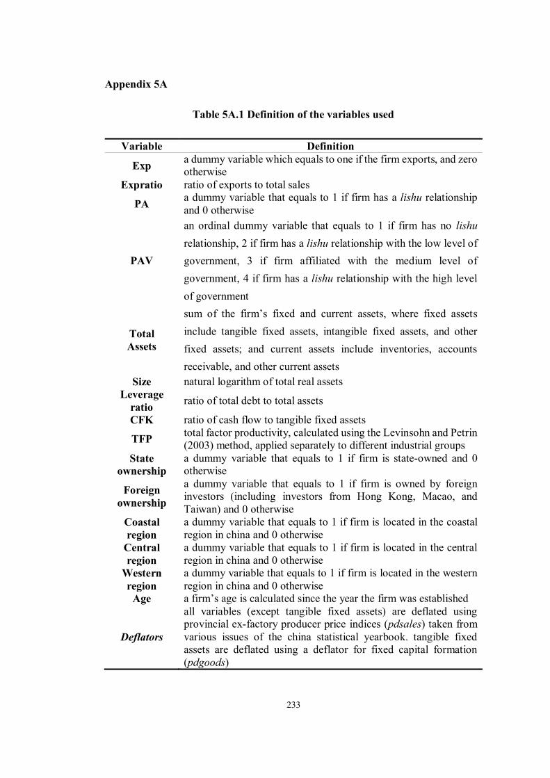
233
Appendix 5A
Table 5A.1 Definition of the variables used
Variable Definition
Exp a dummy variable which equals to one if the firm exports, and zero otherwise
Expratio ratio of exports to total sales
PA a dummy variable that equals to 1 if firm has a lishu relationship and 0 otherwise
PAV
an ordinal dummy variable that equals to 1 if firm has no lishu relationship, 2 if firm has a lishu relationship with the low level of government, 3 if firm affiliated with the medium level of government, 4 if firm has a lishu relationship with the high level of government
Total Assets
sum of the firm’s fixed and current assets, where fixed assets include tangible fixed assets, intangible fixed assets, and other fixed assets; and current assets include inventories, accounts receivable, and other current assets
Size natural logarithm of total real assets Leverage
ratio ratio of total debt to total assets
CFK ratio of cash flow to tangible fixed assets
TFP total factor productivity, calculated using the Levinsohn and Petrin (2003) method, applied separately to different industrial groups
State ownership
a dummy variable that equals to 1 if firm is state-owned and 0 otherwise
Foreign ownership
a dummy variable that equals to 1 if firm is owned by foreign investors (including investors from Hong Kong, Macao, and Taiwan) and 0 otherwise
Coastal region
a dummy variable that equals to 1 if firm is located in the coastal region in china and 0 otherwise
Central region
a dummy variable that equals to 1 if firm is located in the central region in china and 0 otherwise
Western region
a dummy variable that equals to 1 if firm is located in the western region in china and 0 otherwise
Age a firm’s age is calculated since the year the firm was established
Deflators
all variables (except tangible fixed assets) are deflated using provincial ex-factory producer price indices (pdsales) taken from various issues of the china statistical yearbook. tangible fixed assets are deflated using a deflator for fixed capital formation (pdgoods)
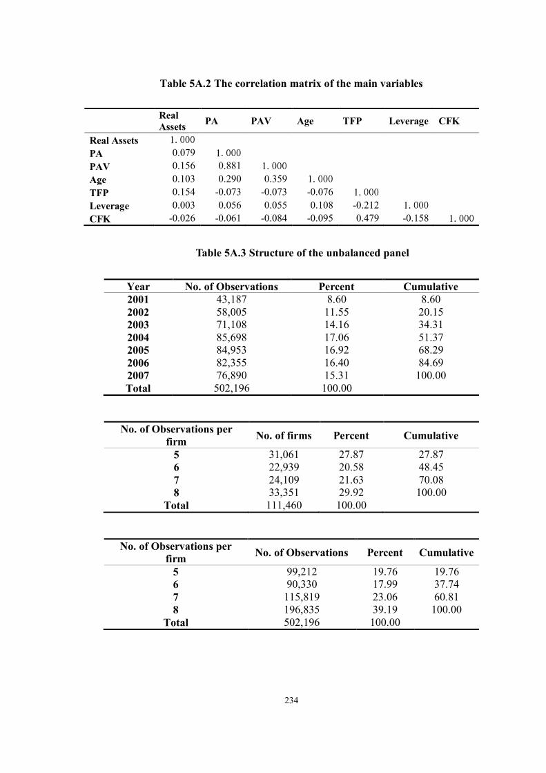
234
Table 5A.2 The correlation matrix of the main variables
Real Assets PA PAV Age TFP Leverage CFK
Real Assets 1.000 PA 0.079 1.000 PAV 0.156 0.881 1.000 Age 0.103 0.290 0.359 1.000 TFP 0.154 -0.073 -0.073 -0.076 1.000 Leverage 0.003 0.056 0.055 0.108 -0.212 1.000 CFK -0.026 -0.061 -0.084 -0.095 0.479 -0.158 1.000
Table 5A.3 Structure of the unbalanced panel
Year No. of Observations Percent Cumulative 2001 43,187 8.60 8.60 2002 58,005 11.55 20.15 2003 71,108 14.16 34.31 2004 85,698 17.06 51.37 2005 84,953 16.92 68.29 2006 82,355 16.40 84.69 2007 76,890 15.31 100.00 Total 502,196 100.00
No. of Observations per firm No. of firms Percent Cumulative
5 31,061 27.87 27.87 6 22,939 20.58 48.45 7 24,109 21.63 70.08 8 33,351 29.92 100.00
Total 111,460 100.00
No. of Observations per firm No. of Observations Percent Cumulative
5 99,212 19.76 19.76 6 90,330 17.99 37.74 7 115,819 23.06 60.81 8 196,835 39.19 100.00
Total 502,196 100.00

235
Table 5A.4 The propensity of exporting by ownership (Private firms vs. Foreign firms): coefficients
Variables (1) (2) I II III I II III
𝑬𝒙𝒑𝒊(𝒕−𝟏) 2.596*** 2.597*** 2.189*** 2.361*** 2.361*** 1.964*** (0.009) (0.009) (0.010) (0.016) (0.016) (0.018)
𝑬𝒙𝒑𝒊𝟏 0.717*** 0.669*** (0.010) (0.017)
𝑷𝑨𝒊(𝒕−𝟏) -0.072*** 0.012 0.011 -0.094*** 0.008 0.007 (0.007) (0.007) (0.005) (0.014) (0.004) (0.003)
𝑺𝒊𝒛𝒆𝒊(𝒕−𝟏) 0.083*** -0.053*** -0.037*** 0.030*** -0.023 -0.033 (0.003) (0.009) (0.010) (0.006) (0.020) (0.021)
𝑻𝑭𝑷𝒊(𝒕−𝟏) 0.104*** 0.026** 0.015 0.065*** 0.036** 0.037** (0.007) (0.010) (0.011) (0.012) (0.017) (0.017)
𝑳𝒆𝒗𝒆𝒓𝒂𝒈𝒆𝒊(𝒕−𝟏) -0.025* -0.146*** -0.141*** -0.069*** -0.066 -0.073 (0.014) (0.026) (0.026) (0.025) (0.050) (0.051)
𝐂𝐅𝐊𝒊(𝒕−𝟏) -0.081*** -0.013 -0.018 -0.084*** -0.029 -0.033 (0.011) (0.015) (0.015) (0.016) (0.023) (0.024)
Coastal Region 0.091*** 0.073*** 0.004*** 0.344*** 0.341*** 0.258*** (0.009) (0.009) (0.010) (0.030) (0.030) (0.034)
Western Region -0.214*** -0.212*** -0.242*** -0.003 -0.012 -0.003 (0.014) (0.014) (0.016) (0.047) (0.047) (0.053)
PAi̅̅ ̅̅̅ -0.093*** -0.119*** -0.156*** -0.167*** (0.014) (0.016) (0.027) (0.029)
Sizei̅̅ ̅̅ ̅̅ 0.148*** 0.135*** 0.055*** 0.066*** (0.010) (0.011) (0.021) (0.022)
TFPi̅̅ ̅̅ ̅̅ ̅ 0.226*** 0.212*** 0.055** 0.064** (0.013) (0.014) (0.023) (0.025)
Leveragei̅̅ ̅̅ ̅̅ ̅̅ ̅̅ ̅̅ 0.220*** 0.158*** 0.169*** 0.156**
(0.031) (0.033) (0.058) (0.062) CFKi̅̅ ̅̅ ̅̅ ̅ -0.117*** -0.098*** -0.095*** -0.080**
(0.020) (0.022) (0.031) (0.034)
Obs. 324,757 324,757 324,757 83,394 83,394 83,394 Log likelihood -83,154 -82,860 -80,009 -26,544 -26,515 -25,555
Note: The dependent variable 𝐸𝑥𝑝𝑖𝑡 is a binary variable which equals to one if the firm exports, and zero otherwise. Column (1) and Column (2) present results for PEs sub-group and FEs sub-group, respectively. PEs and FEs refer to private enterprises and foreign enterprises. For each column, cell I presents results for the baseline equation, cell II reports results by considering unobserved firm heterogeneity, and results that take account of initial conditions problem are reported in cell III. All equations are estimated by pooled Probit models clustering observations by firms’ ID. Robust standard errors are shown in parentheses. Regional dummies, industry dummies, and year dummies are included in all estimations. Obs. stands for the number of observations. Log likelihood is the log likelihood of the fitted model. *, **, *** indicates significance at the 10%, 5%, and 1% level, respectively.
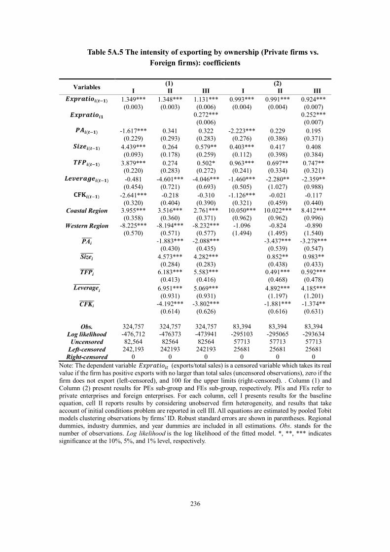
236
Table 5A.5 The intensity of exporting by ownership (Private firms vs. Foreign firms): coefficients
Variables (1) (2) I II III I II III
𝑬𝒙𝒑𝒓𝒂𝒕𝒊𝒐𝒊(𝒕−𝟏) 1.349*** 1.348*** 1.131*** 0.993*** 0.991*** 0.924*** (0.003) (0.003) (0.006) (0.004) (0.004) (0.007)
𝑬𝒙𝒑𝒓𝒂𝒕𝒊𝒐𝒊𝟏 0.272*** 0.252*** (0.006) (0.007)
𝑷𝑨𝒊(𝒕−𝟏) -1.617*** 0.341 0.322 -2.223*** 0.229 0.195 (0.229) (0.293) (0.283) (0.276) (0.386) (0.371)
𝑺𝒊𝒛𝒆𝒊(𝒕−𝟏) 4.439*** 0.264 0.579** 0.403*** 0.417 0.408 (0.093) (0.178) (0.259) (0.112) (0.398) (0.384)
𝑻𝑭𝑷𝒊(𝒕−𝟏) 3.879*** 0.274 0.502* 0.963*** 0.697** 0.747** (0.220) (0.283) (0.272) (0.241) (0.334) (0.321) 𝑳𝒆𝒗𝒆𝒓𝒂𝒈𝒆𝒊(𝒕−𝟏) -0.481 -4.601*** -4.046*** -1.460*** -2.280** -2.359**
(0.454) (0.721) (0.693) (0.505) (1.027) (0.988) 𝐂𝐅𝐊𝒊(𝒕−𝟏) -2.641*** -0.218 -0.310 -1.126*** -0.021 -0.117
(0.320) (0.404) (0.390) (0.321) (0.459) (0.440) Coastal Region 3.955*** 3.516*** 2.761*** 10.050*** 10.022*** 8.412***
(0.358) (0.360) (0.371) (0.962) (0.962) (0.996) Western Region -8.225*** -8.194*** -8.232*** -1.096 -0.824 -0.890
(0.570) (0.571) (0.577) (1.494) (1.495) (1.540) PAi̅̅ ̅̅̅ -1.883*** -2.088*** -3.437*** -3.278***
(0.430) (0.435) (0.539) (0.547) Sizei̅̅ ̅̅ ̅̅ 4.573*** 4.282*** 0.852** 0.983**
(0.284) (0.283) (0.438) (0.433) TFPi̅̅ ̅̅ ̅̅ ̅ 6.183*** 5.583*** 0.491*** 0.592***
(0.413) (0.416) (0.468) (0.478) Leveragei̅̅ ̅̅ ̅̅ ̅̅ ̅̅ ̅̅ 6.951*** 5.069*** 4.892*** 4.185***
(0.931) (0.931) (1.197) (1.201) CFKi̅̅ ̅̅ ̅̅ ̅ -4.192*** -3.802*** -1.881*** -1.374**
(0.614) (0.626) (0.616) (0.631)
Obs. 324,757 324,757 324,757 83,394 83,394 83,394 Log likelihood -476,712 -476373 -473941 -295103 -295065 -293634
Uncensored 82,564 82564 82564 57713 57713 57713 Left-censored 242,193 242193 242193 25681 25681 25681
Right-censored 0 0 0 0 0 0 Note: The dependent variable 𝐸𝑥𝑝𝑟𝑎𝑡𝑖𝑜𝑖𝑡 (exports/total sales) is a censored variable which takes its real value if the firm has positive exports with no larger than total sales (uncensored observations), zero if the firm does not export (left-censored), and 100 for the upper limits (right-censored). . Column (1) and Column (2) present results for PEs sub-group and FEs sub-group, respectively. PEs and FEs refer to private enterprises and foreign enterprises. For each column, cell I presents results for the baseline equation, cell II reports results by considering unobserved firm heterogeneity, and results that take account of initial conditions problem are reported in cell III. All equations are estimated by pooled Tobit models clustering observations by firms’ ID. Robust standard errors are shown in parentheses. Regional dummies, industry dummies, and year dummies are included in all estimations. Obs. stands for the number of observations. Log likelihood is the log likelihood of the fitted model. *, **, *** indicates significance at the 10%, 5%, and 1% level, respectively.

237
Table 5A.6 The propensity of exporting by region: coefficients
Variables (1) (2) (3) I II III I II III I II III
𝑬𝒙𝒑𝒊(𝒕−𝟏) 2.616*** 2.615*** 2.191*** 2.374*** 2.371*** 1.988*** 2.789*** 2.783*** 2.343*** (0.008) (0.008) (0.009) (0.023) (0.023) (0.024) (0.031) (0.031) (0.037)
𝑬𝒙𝒑𝒊𝟏 0.698*** 0.863*** 0.798*** (0.009) (0.028) (0.038)
𝑷𝑨𝒊(𝒕−𝟏) -0.115*** 0.012 0.018 -0.056*** -0.068*** -0.075*** -0.003 0.021 0.020 (0.007) (0.011) (0.011) (0.016) (0.024) (0.025) (0.023) (0.037) (0.037)
𝑺𝒊𝒛𝒆𝒊(𝒕−𝟏) 0.078*** -0.042*** -0.028*** 0.064*** -0.095*** -0.086*** 0.138*** -0.019 -0.009 (0.003) (0.009) (0.009) (0.006) (0.022) (0.023) (0.009) (0.033) (0.035)
𝑻𝑭𝑷𝒊(𝒕−𝟏) 0.106*** 0.003 0.008 0.053*** 0.036* 0.024 0.059*** 0.024 0.032 (0.006) (0.009) (0.010) (0.014) (0.021) (0.021) (0.021) (0.032) (0.032)
𝑳𝒆𝒗𝒆𝒓𝒂𝒈𝒆𝒊(𝒕−𝟏) -0.029** -0.096*** -0.090*** -0.073** -0.154*** -0.176*** -0.001 -0.034 -0.066 (0.013) (0.025) (0.025) (0.029) (0.055) (0.056) (0.000) (0.081) (0.083)
𝐂𝐅𝐊𝒊(𝒕−𝟏) -0.096*** -0.004 -0.002 -0.018 -0.070* -0.073** -0.003* -0.172*** -0.167*** (0.009) (0.013) (0.013) (0.025) (0.036) (0.036) (0.001) (0.059) (0.060)
State Ownership -0.214*** -0.162*** -0.176*** -0.138*** -0.121*** -0.130*** -0.291*** -0.171*** -0.238*** (0.018) (0.018) (0.021) (0.026) (0.027) (0.030) (0.054) (0.034) (0.041)
Foreign Ownership 0.428*** 0.420*** 0.327*** 0.324*** 0.320*** 0.227*** 0.296*** 0.376*** 0.311*** (0.008) (0.008) (0.009) (0.033) (0.034) (0.040) (0.060) (0.042) (0.051)
PAi̅̅ ̅̅̅ -0.193*** -0.227*** -0.022 -0.038 -0.062* -0.082* (0.013) (0.014) (0.031) (0.033) (0.046) (0.050)
Sizei̅̅ ̅̅ ̅̅ 0.130*** 0.119*** 0.177*** 0.161*** 0.175*** 0.138*** (0.009) (0.010) (0.023) (0.024) (0.035) (0.037)
TFPi̅̅ ̅̅ ̅̅ ̅ 0.177*** 0.172*** 0.132*** 0.106*** 0.044 0.063 (0.012) (0.013) (0.027) (0.029) (0.041) (0.044)
Leveragei̅̅ ̅̅ ̅̅ ̅̅ ̅̅ ̅̅ 0.122*** 0.079*** 0.164** 0.178*** 0.052 0.126
(0.029) (0.030) (0.065) (0.068) (0.096) (0.102) CFKi̅̅ ̅̅ ̅̅ ̅ -0.170*** -0.152*** -0.173*** -0.235*** -0.063 -0.012
(0.017) (0.018) (0.046) (0.048) (0.073) (0.081)
Obs. 376,482 376,482 376,482 71,763 71,763 71,763 53,951 53,951 53,951 Log likelihood -101,028 -100,696 -97,112 -17,010 -16,942 -16,319 -7,815 -7,816 -7,525
Note: The dependent variable 𝐸𝑥𝑝𝑖𝑡 is a binary variable which equals to one if the firm exports, and zero otherwise. Column (1), column (2) and Column (3) present results for the coastal region sub-group, the central region sub-group and the western region sub-group, respectively. For each column, cell I presents results for the baseline equation, cell II reports results by considering unobserved firm heterogeneity, and results that take account of initial conditions problem are reported in cell III. All equations are estimated by pooled Probit models clustering observations by firms’ ID. Robust standard errors are shown in parentheses. Ownership dummies, industry dummies, and year dummies are included in all estimations. Obs. stands for the number of observations. Log likelihood is the log likelihood of the fitted model. *, **, *** indicates significance at the 10%, 5%, and 1% level, respectively.

238
Table 5A.7 The intensity of exporting by region: coefficients
Variables (1) (2) (3) I II III I II III I II III
𝑬𝒙𝒑𝒓𝒂𝒕𝒊𝒐𝒊(𝒕−𝟏) 1.212*** 1.212*** 1.010*** 1.395*** 1.399*** 1.172*** 1.444*** 1.445*** 1.199*** (0.002) (0.002) (0.004) (0.009) (0.009) (0.018) (0.014) (0.014) (0.023)
𝑬𝒙𝒑𝒓𝒂𝒕𝒊𝒐𝒊𝟏 0.251*** 0.302*** 0.309*** (0.004) (0.019) (0.025)
𝑷𝑨𝒊(𝒕−𝟏) -2.806*** 0.163 0.170 -1.239** -1.573** -1.679** -0.194 0.297 0.477 (0.180) (0.240) (0.231) (0.518) (0.678) (0.657) (0.624) (0.793) (0.762)
𝑺𝒊𝒛𝒆𝒊(𝒕−𝟏) 3.304*** 0.379* 0.652*** 3.617*** 1.287* 0.987 6.281*** 1.423* 1.693** (0.074) (0.219) (0.214) (0.220) (0.664) (0.653) (0.275) (0.781) (0.765)
𝑻𝑭𝑷𝒊(𝒕−𝟏) 3.359*** 0.531** 0.680*** 2.357*** 0.161 0.406 1.483*** 0.889 0.966 (0.166) (0.220) (0.211) (0.441) (0.587) (0.568) (0.552) (0.705) (0.677)
𝑳𝒆𝒗𝒆𝒓𝒂𝒈𝒆𝒊(𝒕−𝟏) -0.370 -2.107*** -1.797*** -2.982*** -7.043*** -6.733*** -1.424 -2.965* -2.905* (0.346) (0.594) (0.569) (0.966) (1.586) (1.540) (1.252) (1.754) (1.687)
𝐂𝐅𝐊𝒊(𝒕−𝟏) -2.592*** -0.067 -0.041 -1.678** -0.657 -0.769 -1.836* -2.511** -2.400** (0.229) (0.301) (0.289) (0.737) (0.971) (0.933) (1.053) (1.190) (1.155)
State Ownership -6.507*** -5.239*** -4.993*** -4.016*** -3.652*** -3.706*** -3.156*** -2.917*** -2.888*** (0.641) (0.647) (0.648) (0.965) (0.991) (0.996) (1.007) (1.039) (1.057)
Foreign Ownership 10.336*** 10.174*** 8.160*** 8.813*** 8.733*** 7.409*** 8.963*** 8.766*** 7.691*** (0.205) (0.209) (0.226) (1.076) (1.090) (1.189) (1.188) (1.197) (1.334)
PAi̅̅ ̅̅ ̅ -4.498*** -4.611*** -0.510 -0.750 -0.209 -0.690 (0.340) (0.343) (0.980) (0.984) (1.185) (1.202)
Sizei̅̅ ̅̅ ̅̅ 3.108*** 2.938*** 5.396*** 5.100*** 5.221*** 4.954***
(0.234) (0.232) (0.709) (0.702) (0.836) (0.825) TFPi̅̅ ̅̅ ̅̅ ̅ 4.813*** 4.504*** 3.220*** 2.600*** 0.418 0.277
(0.315) (0.318) (0.842) (0.847) (1.036) (1.051) Leveragei̅̅ ̅̅ ̅̅ ̅̅ ̅̅ ̅̅ 4.130*** 3.341*** 7.014*** 6.128*** 1.821 2.507
(0.735) (0.737) (2.040) (2.025) (2.314) (2.338) CFKi̅̅ ̅̅ ̅̅ ̅ -4.517*** -3.972*** -4.654*** -5.060*** -1.814 -1.629
(0.439) (0.448) (1.392) (1.410) (1.844) (1.858)
Obs. 376,482 376,482 376,482 71,763 71,763 71,763 53,951 53,951 53,951 Log likelihood -768,016 -767,615 -763,624 -65,806 -65,736 -65,429 -36,477 -36,452 -36,211
Uncensored 139,864 139,864 139,864 10,720 10,720 10,720 6,173 6,173 6,173 Left-censored 236,618 236,618 236,618 61,043 61,043 61,043 47,778 47,778 47,778
Right-censored 0 0 0 0 0 0 0 0 0 Note: The dependent variable 𝐸𝑥𝑝𝑟𝑎𝑡𝑖𝑜𝑖𝑡 (exports/total sales) is a censored variable which takes its real value if the firm has positive exports with no larger than total sales (uncensored observations), zero if the firm does not export (left-censored), and 100 for the upper limits (right-censored). Column (1), column (2) and Column (3) present results for the coastal region sub-group, the central region sub-group and the western region sub-group, respectively. For each column, cell I presents results for the baseline equation, cell II reports results by considering unobserved firm heterogeneity, and results that take account of initial conditions problem are reported in cell III. All equations are estimated by pooled Tobit models clustering observations by firms’ ID. Robust standard errors are shown in parentheses. Ownership dummies, industry dummies, and year dummies are included in all estimations. Obs. stands for the number of observations. Log likelihood is the log likelihood of the fitted model. *, **, *** indicates significance at the 10%, 5%, and 1% level, respectively.
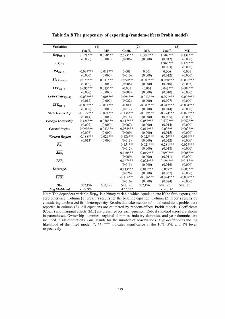
239
Table 5A.8 The propensity of exporting (random-effects Probit model)
Variables (1) (2) (3) Coeff. ME Coeff. ME Coeff. ME
𝑬𝒙𝒑𝒊(𝒕−𝟏) 2.571*** 0.350*** 2.573*** 0.350*** 1.507*** 0.138*** (0.006) (0.000) (0.006) (0.000) (0.012) (0.000)
𝑬𝒙𝒑𝒊𝟏 1.965*** 0.179*** (0.023) (0.000)
𝑷𝑨𝒊(𝒕−𝟏) -0.097*** -0.013*** 0.003 0.001 0.006 0.001 (0.006) (0.000) (0.010) (0.000) (0.012) (0.000)
𝑺𝒊𝒛𝒆𝒊(𝒕−𝟏) 0.079*** 0.011*** -0.050*** -0.007*** -0.060*** -0.006*** (0.002) (0.000) (0.008) (0.000) (0.010) (0.003)
𝑻𝑭𝑷𝒊(𝒕−𝟏) 0.095*** 0.013*** -0.005 -0.001 0.042*** 0.004*** (0.006) (0.000) (0.008) (0.000) (0.010) (0.000)
𝑳𝒆𝒗𝒆𝒓𝒂𝒈𝒆𝒊(𝒕−𝟏) -0.036*** -0.005*** -0.094*** -0.013*** -0.091*** -0.008*** (0.012) (0.000) (0.022) (0.000) (0.027) (0.000)
𝐂𝐅𝐊𝒊(𝒕−𝟏) -0.083*** -0.011*** -0.013 -0.002*** -0.047*** -0.004*** (0.008) (0.000) (0.012) (0.000) (0.014) (0.000)
State Ownership -0.179*** -0.024*** -0.138*** -0.019*** -0.274*** -0.025*** (0.014) (0.000) (0.014) (0.000) (0.025) (0.000)
Foreign Ownership 0.426*** 0.058*** 0.417*** 0.057*** 0.572*** 0.052*** (0.007) (0.000) (0.007) (0.000) (0.014) (0.000)
Coastal Region 0.099*** 0.013*** 0.084*** 0.011*** 0.036** 0.003*** (0.008) (0.000) (0.009) (0.000) (0.015) (0.000)
Western Region -0.188*** -0.026*** -0.186*** -0.025*** -0.429*** -0.039*** (0.013) (0.000) (0.013) (0.000) (0.022) (0.000)
PAi̅̅ ̅̅ ̅ -0.154*** -0.021*** -0.281*** -0.026*** (0.012) (0.000) (0.018) (0.000)
Sizei̅̅ ̅̅ ̅̅ 0.140*** 0.019*** 0.090*** 0.008***
(0.009) (0.000) (0.011) (0.000) TFPi̅̅ ̅̅ ̅̅ ̅ 0.167*** 0.023*** 0.194*** 0.018***
(0.011) (0.000) (0.016) (0.000) Leveragei̅̅ ̅̅ ̅̅ ̅̅ ̅̅ ̅̅ 0.113*** 0.015*** 0.077** 0.007***
(0.026) (0.000) (0.037) (0.000) CFKi̅̅ ̅̅ ̅̅ ̅ -0.114*** -0.016*** -0.094*** -0.009***
(0.016) (0.000) (0.024) (0.000) Obs. 502,196 502,196 502,196 502,196 502,196 502,196
Log likelihood -127,999 -127,622 -120,143 Note: The dependent variable 𝐸𝑥𝑝𝑖𝑡 is a binary variable which equals to one if the firm exports, and zero otherwise. Column (1) presents results for the baseline equation. Column (2) reports results by considering unobserved firm heterogeneity. Results that take account of initial conditions problem are reported in column (3). All equations are estimated by random-effects Probit models. Coefficients (Coeff.) and marginal effects (ME) are presented for each equation. Robust standard errors are shown in parentheses. Ownership dummies, regional dummies, industry dummies, and year dummies are included in all estimations. Obs. stands for the number of observations. Log likelihood is the log likelihood of the fitted model. *, **, *** indicates significance at the 10%, 5%, and 1% level, respectively.
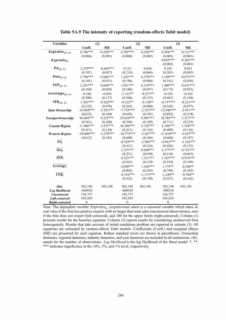
240
Table 5A.9 The intensity of exporting (random-effects Tobit model)
Variables (1) (2) (3) Coeff. ME Coeff. ME Coeff. ME
𝑬𝒙𝒑𝒓𝒂𝒕𝒊𝒐𝒊(𝒕−𝟏) 0.786*** 0.238*** 0.785*** 0.238*** 0.394*** 0.121*** (0.004) (0.001) (0.004) (0.002) (0.003) (0.001)
𝑬𝒙𝒑𝒓𝒂𝒕𝒊𝒐𝒊𝟏 0.855*** 0.263*** (0.005) (0.001)
𝑷𝑨𝒊(𝒕−𝟏) -2.259*** -0.684*** 0.112 0.034 0.102 0.031 (0.187) (0.057) (0.218) (0.066) (0.201) (0.062)
𝑺𝒊𝒛𝒆𝒊(𝒕−𝟏) 2.794*** 0.846*** 1.233*** 0.374*** 2.189*** 0.673*** (0.101) (0.031) (0.196) (0.060) (0.181) (0.056)
𝑻𝑭𝑷𝒊(𝒕−𝟏) 2.291*** 0.694*** 1.051*** 0.319*** 1.409*** 0.433*** (0.164) (0.050) (0.188) (0.057) (0.173) (0.053)
𝑳𝒆𝒗𝒆𝒓𝒂𝒈𝒆𝒊(𝒕−𝟏) -0.186 -0.056 -1.112** -0.337** -0.334 -0.103 (0.388) (0.117) (0.506) (0.153) (0.467) (0.144)
𝐂𝐅𝐊𝒊(𝒕−𝟏) -1.855*** -0.562*** -0.522** -0.158** -0.757*** -0.233*** (0.232) (0.070) (0.263) (0.080) (0.242) (0.075)
State Ownership -10.868*** -3.291*** -7.755*** -2.351*** -12.846*** -3.951*** (0.623) (0.189) (0.642) (0.195) (0.892) (0.274)
Foreign Ownership 30.464*** 9.225*** 29.654*** 8.991*** 10.785*** 3.317*** (0.361) (0.106) (0.369) (0.109) (0.711) (0.219)
Coastal Region 11.468*** 3.473*** 10.394*** 3.152*** 4.350*** 1.338*** (0.411) (0.124) (0.411) (0.124) (0.409) (0.126)
Western Region -10.800*** -3.270*** -10.774*** -3.267*** -11.810*** -3.633*** (0.612) (0.185) (0.609) (0.184) (0.608) (0.187)
PAi̅̅ ̅̅ ̅ -8.528*** -2.586*** -4.962*** -1.526*** (0.411) (0.124) (0.426) (0.131)
Sizei̅̅ ̅̅ ̅̅ 2.275*** 0.690*** 2.377*** 0.731***
(0.231) (0.070) (0.218) (0.067) TFPi̅̅ ̅̅ ̅̅ ̅ 4.323*** 1.311*** 3.167*** 0.974***
(0.361) (0.110) (0.354) (0.109) Leveragei̅̅ ̅̅ ̅̅ ̅̅ ̅̅ ̅̅ 4.650*** 1.410*** 1.775** 0.546**
(0.802) (0.243) (0.789) (0.243) CFKi̅̅ ̅̅ ̅̅ ̅ -4.336*** -1.315*** -1.249** -0.384**
(0.522) (0.158) (0.527) (0.162)
Obs. 502,196 502,196 502,196 502,196 502,196 502,196 Log likelihood -860926 -860543 -840536 Uncensored 156,757 156,757 156,757
Left-censored 345,439 345,439 345,439 Right-censored 0 0 0
Note: The dependent variable 𝐸𝑥𝑝𝑟𝑎𝑡𝑖𝑜𝑖𝑡 (exports/total sales) is a censored variable which takes its real value if the firm has positive exports with no larger than total sales (uncensored observations), zero if the firm does not export (left-censored), and 100 for the upper limits (right-censored). Column (1) presents results for the baseline equation. Column (2) reports results by considering unobserved firm heterogeneity. Results that take account of initial conditions problem are reported in column (3). All equations are estimated by random-effects Tobit models. Coefficients (Coeff.) and marginal effects (ME) are presented for each equation. Robust standard errors are shown in parentheses. Ownership dummies, regional dummies, industry dummies, and year dummies are included in all estimations. Obs. stands for the number of observations. Log likelihood is the log likelihood of the fitted model. *, **, *** indicates significance at the 10%, 5%, and 1% level, respectively.
241
CHAPTER 6 POLITICAL CONNECTIONS AND FINANCIAL
CONSTRAINTS
In this chapter, we examine the extent to which political connections, intended as the
lishu relationship, affect the financial constraints using 105,487 unlisted Chinese
manufacturing firms over the period 2002-2007. We document that Chinese firms face
financial constraints, which is indicated by the high sensitivity of investment to the
availability of internal financing. We also find that compared with private firms,
foreign firms are more likely to encounter financial constraints; therefore, the lishu
relationship can reduce their financial constraints significantly. Furthermore, firms
locating in the western region have the least significant sensitivity of investment to
the availability of internal financing due to the implement of the regional development
policies. However, the lishu relationship can help firms in the central and coastal
regions alleviate their financial constraints.
6.1 Introduction
For private firms, the possession of resource and sufficient financing represents a
crucial competitive edge. According to Modigliani and Miller (1958), a firm’s
investment decisions are not affected by their financing decisions on perfect capital
markets. Capital markets, however, are not perfect and the imperfections create a
wedge between the costs of internal funds and external funds. Due to asymmetric
information and agency problems, firms face higher costs of external financing.
Therefore, firms are considered financially constrained when their investments are

242
sensitive to internal funds. Put another way, firms facing higher imperfections
experience a wider difference between internal and external financing, and therefore
are more financially constrained.
There is considerable evidence that financial constraints are an impediment to the
efficient allocation of credit for corporate investments and therefore to the growth of
firms, and hence the economy (Stein, 2003; Hubbard, 1998; King and Levin, 1993).
Some studies focus on a) the relationship between financial constraints and firms’
characteristics, such as size, age, and business group affiliation, b) the links between
financial constraints and firms’ activities, such as acquisitions, and c) the connection
between financial constraints and institutional environment, such as the legal and
financial systems that affect their financial constraints (for example, Hadlock and
Pierce, 2010; Lensinka et al., 2003; Erel et al., 2015; Demirgüç-Kunt and Maksimovic,
1998). Few studies examine the relationship between firms’ political connections and
financial constraints.
The impact of political connections on firm financial constraints can be categorised
into two groups. The first group focuses on the “direct effect”, which indicates that
governments provide more preferential treatment and assistance, such as the extended
welfare terms to the connected firms directly. Faccio (2010) states that politically
connected firms find it easier to access governmental support when the International
Monetary Fund or the World Bank provides financial assistance to domestic firms.
Bartels and Brady (2003) find that private enterprises that have political connections
with local government are able to receive more financial subsidies.

243
The second group focuses on the “indirect effect”, which considers political
connections as a middle power between firms and financing institutions, like banks.
Through the indirect effect, political connections can bring favourable loan terms to
the connected firms. According to Faccio (2006), enterprises with political
connections can access more bank loans and more preferential interest and tax rates
than those without political connections.1 Boubakri et al. (2008) also show that the
costs of equity financing for firms with political connections are lower than that for
the firms without such ties. Similar results have been found in developing countries,
such as Malaysia and Pakistan. Johnson and Mittion (2003) and Khwaja and Mian
(2005) assert that politically connected firms can receive more loans than unconnected
firms.
Whilst most of the literature that looked at the links between political connections and
financial constraints focused on developed countries, some literature focused on
developing countries. However, the definitions of political connections and the
impacts on enterprises are different between China and other countries due to the
different political regime. In addition, among the developing countries, financial
market imperfections are considered to be very pronounced in China for the following
three reasons.
1 Faccio (2006) looked at 47 countries covered by the Worldscope database, which provides full coverage of developed markets. These 47 countries are Argentina, Australia, Austria, Belgium, Brazil, Canada, Chile, Colombia, Czech Rep., Denmark, Finland, France, Germany, Greece, Hong Kong, Hungary, India, Indonesia, Ireland, Israel, Italy, Japan, Luxembourg, Malaysia, Mexico, Netherlands, New Zealand, Norway, Peru, Philippines, Poland, Portugal, Russia, Singapore, South Africa, South Korea, Spain, Sri Lanka, Sweden, Switzerland, Taiwan, Thailand, Turkey, the US, the UK, Venezuela, and Zimbabwe.

244
First, the development of market-supporting institutions does not match the rapid
growth of the economy. Private entrepreneurs face many barriers in running their
businesses because the weak state, financial markets, and legal system cannot
appropriately secure property rights and enforce contracts (Hay and Shleifer, 1998;
McMillan and Woodruff, 1999; Frye and Zhuravskaia, 2000). Second, although
private firms are growing fast and the private sector has stimulated most of China’s
economic growth since the 1980s (Allen et al., 2005), the state sector is favoured by
the government in China. Crucial industries, including national security, civil aviation,
finance, natural resources, and real estate, are still dominated by state-owned firms
(SOEs).1 Third, by law, the state banks, which were the largest Chinese banks, were
instructed not to lend to private enterprises until 1997, suggesting that private
enterprises did not have high rank in terms of political status at that time. Due to the
lingering legacy of the centrally-planned economy, capital allocation in China has
been characterised by government intervention. The state controls the primary
resources and the financial system, and a bias exists in favour of the state-owned firms
(Brandt and Li, 2003; Bai et al., 2006; Li et al., 2008; Cull et al., 2009, 2014; Gordon
and Li, 2011). Huang (2003) considers this lending bias as a “political pecking order”
in the Chinese capital market.
Moreover, insufficient financing support may set up obstacles to the development of
firms that lack political connections. According to Johnson et al. (2000), McMillan
1 In the fourth Plenary Session of the 15th Central Committee in September 1999, it was proposed by The Decisions of Chinese Communist Party Central Committee Regarding the Reform and Development of State-owned Enterprises and other Important Issues (zhong gong zhong yang guan yu guo you qi ye gai ge he fa zhan ruo gan zhong da wen ti de jue ding). This phenomenon is called as Guo Jin Min Tui in Chinese since 2002, which means that the state advances and the private sector recedes.
245
and Woodruff (2002), and Guriev (2004), private firms are often rejected access to
bank loans, which are largely reserved for the state-owned firms, or suffer from heavy
governmental regulations (red tape) and extra legal fees. Farrell and Lund (2006)
report that the private sector had produced more than half of China’s GDP by 2006
but the loans they received only account for 27% of total loans. Dollar and Wei (2007)
also point out that the distorted credit allocation has led to the continued uneven
distribution in the return to capital on the grounds of firm ownership, regions, and
industrial sectors.
Although the “political pecking order” in the allocation of resource where private
firms were discriminated has been alleviated since 1997, credit constraints on private
firms still exist and may hinder the growth of the Chinese economy. Therefore, this
research contributes to the literature in the following ways.
Firstly, the Chinese economy is a particularly interesting setting due to its
heterogeneity. Firms in developing countries are more likely to face severer financial
constraints than those in developed countries, and firm owners typically consider
financial constraints as one of their key obstacles to invest and develop (Dethier et al.,
2011). Given the noticeable imperfections in the Chinese capital market, China is an
ideal pilot region to test the financial constraints hypothesis and the extent to which
political connections can alleviate these constraints.
Secondly, the existing studies examining the financial constraints hypothesis for
Chinese firms are based on the datasets containing relatively small numbers of firms,
246
which do not represent the whole population of Chinese firms, and are likely to suffer
from sample selection bias. For example, Chow and Fung (1998, 2000) use a dataset
from the Shanghai Economic Commission that includes 5,325 manufacturing firms in
32 manufacturing industries of Shanghai from 1989 to 1992. Héricourt and Poncet
(2009) use a dataset of 1,300 companies over the period 2000-2002, taken from the
World Bank’s 2003 Investment Climate Survey. Poncet et al. (2010) use firm-level
data originating from the Oriana dataset, which contains 14,967 firms over the period
1998-2005. Cull et al. (2014) use a dataset from the World Bank 120 city survey
covering 12,400 firms in 2005. By contrast, our paper uses a very large dataset,
compiled by the Chinese National Bureau of Statistics from 2002 to 2007, which
includes 105,487 unlisted manufacturing firms, summing up to 356,053 observations.
This dataset contains a large proportion of small and young firms that are more prone
to suffer from liquidity constraints. It therefore provides a unique opportunity to carry
out sharper tests of the financial constraints than those typically performed in the
literature.
Although a series of studies conducted by Guariglia apply the same dataset, they do
not test the relationship between political connections and financial constraints. For
example, Chen and Guariglia (2013) look at the link between internal financial
constraints and firm-level productivity, Ding et al. (2013) analyse the relation between
investment in fixed and working capital and financial constraints, Guariglia et al.
(2008, 2011) investigate the extent to which the internal financial constraints affect
firms’ asset growth, Guariglia and Liu (2014) examine the relationship between
financial constraints and firms’ innovation activities, and Guariglia and Mateut (2013)
247
explore the linkage between political affiliation and trade credit extension by Chinese
firms. To the best of our knowledge, the hypothesis of the linkage between political
connections and financial constraints, measured by investment-cash flow sensitivity,
has never been tested using such a comprehensive dataset.
Thirdly, the existing studies are almost based on the data from firms quoted on the
stock market. However, financial constraints on these listed firms tend to be weaker
as they are typically large, financially healthy, and long-established enterprises with
good credit ratings, compared with the unlisted firms. A sharper test of financial
constraints should be done from unquoted firms, which are generally considered as a
short track record, poor solvency, and low real assets compared with their counterparts.
Although few studies have examined the financial constraints hypotheses in unlisted
firms (for instance, Chen and Guariglia, 2013; Ding et al., 2013; Guariglia et al., 2008,
2011; Guariglia and Liu, 2014; Guariglia and Mateut, 2013), again, these studies do
not focus on the extent to which political connections can affect financial constraints.
Therefore, this paper attempts to shed light on the tests of the hypothesis of political
connections and financial constraints by using unlisted firms in China.
Finally, although political connections have attracted worldwide academic interest,
China is characterised by a type of political connection which does not exist in other
parts of the world.1 This unique political connection is called the lishu relationship,
1 In other parts of the world, politically connected firms are typically defined in five ways. Firstly, at least one of the large shareholders who controlling 10% or more of the company’s voting rights directly or indirectly is a politician (e.g. a national congress member, a government minister, or a head of state) (Faccio, 2002, 2006, 2007 and 2010). Secondly, at least one of the company’s top officers (e.g. the CEO, president or chairman) is a politician (Faccio et al., 2006; Chen et al., 2010). A company, which is closely related to a top politician or a political party leader through friendship, family members, and

248
which is an institutional variation during the economic transition in China. Lishu is a
Chinese word which means “belonging to”, “subordinate to”, or “directly controlled
by”. Through this relationship, the governments can maintain administrative power to
control various aspects of the firm both directly and legally (Tan et al., 2007; Li, 2004).
In addition to the control perspectives, the firms with the lishu relationship can get
governmental support and subsidies (Tan et al., 2007). As the non-state ownership is
growing in China, having the lishu relationship is an important route through which
the firm can be connected with the government. There is hardly any research on the
relationship between financial health and political connections intended as the lishu
relationship. Our research will therefore focus, for the first time, on financial
constraints for unlisted firms through the perspective of the lishu relationship.
In this chapter, we document that the investments for unlisted firms are constrained
by the accessibility of the firms’ internal funds. Firms that locate in the coastal region
are more financially constrained. However, through the lishu relationship with the
government, these financial constraints can be reduced for affiliated firms. Such a
mitigating effect is more significant for firms affiliated with a high level of
government.
The rest of this chapter is organised as follows. Section 6.2 endeavours to provide a
relationships with foreign politicians falls into the third type (Faccio, 2002; Gul, 2006; Faccio et al., 2006; Leuz and Oberholzer-Gee, 2006). The fourth group includes firms with state ownership (Boardman and Vining, 1989; Belka et al., 1995; Dewenter and Malatesta, 2001). The final kind of connection is established by campaign contribution, which refers to a relationship between a firm and an election candidate. That is, a firm, having supported an election candidate in the campaign, will in return gain favours from the politician (Claessens et al., 2008; Goldman et al., 2009; Cooper et al., 2010).
249
comprehensive review of the related existing literature on financial constraints and
political connections and propose our hypotheses. Baseline specification and
methodology are described in section 6.3. Section 6.4 describes the data sample and
summary statistics. In section 6.5, our empirical results are presented. Section 6.6
presents further tests. Section 6.7 concludes this chapter.
6.2 Literature review and hypotheses
This chapter analyses the following four streams of literature: the background of
financial constraints, the debate on indicators of financial constraints, financial
constraints in China, and the impact of political connections on firms’ financial
constraints.
6.2.1 The background of financial constraints
Financial constraints have received intensive academic interest. In the perfect world
with frictionless capital markets proposed by Modigliani and Miller (1958), a firm’s
value is irrelevant to its capital structure, which is the way that a firm is financed,
because the internal financing and external financing can substitute each other
perfectly. That is, a firm’s investment only relies on the profitability of this investment
project and a firm can make the investment decisions independently. Although this
theory has been the foundation of corporate investment analysis, it does not exist in
the real world. Researchers and scholars have theoretically and empirically identified
a variety of frictions and distortions that prevent firms from making investment
250
decisions optimally and independently.
Information asymmetries and agency problems are two major types of frictions. They
will arise when managers are better informed than outside investors or when managers
have inside information about the firm but not about the market or the economy
(Myers and Majluf, 1984). Information asymmetries are a fact of life and difficult to
diminish due to the following three perspectives.
First of all, it is hard for a firm to only disclose proprietary information to investors
and financiers without revealing it to competitors (Myers and Majluf, 1984). In order
to illustrate the true value of a project, the firm has to provide sufficient verifiable
details to the lenders, rather than only saying, for example, “we have a fantastic
investment plan, but we cannot tell you the details for confidential reasons”. However,
making a public investment project will in most cases let the firm’s competitors gain
the confidential information which they have not known. The leakage of confidential
information to the public or to the competitors can be catastrophic and disastrous as
the competitors may act as a free rider to take unfair advantage of others’ hard work.
The proposed investment can also be jeopardised by competitors as they may steal the
idea.
Secondly, it is costly to convey all the information to the market (Myers and Majluf,
1984; Campbell, 1979). The investors’ and lenders’ information disadvantages are
reflected not only through the fact that investors obtain fewer facts than the managers,
but also through how to process and understand this information. As outsiders of a
251
firm, investors and lenders always do not have a better understanding on what the
information means for the firm and what should (not) be done, when compared with
the managers, who are the insiders of a firm. Therefore, the costs of providing and
verifying the information are very high because educating investors and lenders
always involved substantial time and labour capital inputs.
Finally, under most situations, there is no need to convey proprietary information to
investors as it is difficult to require an outside investor to have the equal understanding
and intelligence as managers do. Therefore, Myers and Majluf (1984) argue that the
asymmetric information is created naturally because of the separation of professionals
(managers) from others (investors, lenders, or public).
Ross (1973, p.134) points out that the agency relationship is “one of the oldest and
common codified modes of social interaction”. He defines the agency relationship as
an interaction between two or more parties, with one assigned as agent or as
representative, acting on behalf of another or the other part(ies), which is (are) the
principal. Furthermore, Gjesdal (1982, p.373) shows that “the principal-agent
relationship is arisen when corporate decisions are made by managers or individuals
(agents) on behalf of the firm’s capital suppliers (principals) in firms, without
considering how principals can be affected by these decisions”. For example, when
the top managers aim at obtaining greater wages and bonuses, they may tend to make
decisions which can improve the company’s performance in the short term, but can
cause some problems in the long term. Obviously, these decisions will not be approved
by shareholders. In this situation, agency costs appear as the corporate decisions are

252
made by agents on behalf of the shareholders.
Moral hazard and adverse selection are the two forms of information asymmetries and
agency problems. Adverse selection arises at the earliest stage of financing. As it is
difficult to observe the risk of a project for the lenders in front of a group of firms that
need external finance, they cannot distinguish a good borrower from a bad one and
price correctly according to good and bad borrowers respectively (Hyytinen and
Väänänen, 2006; Stiglitz and Weiss, 1981). The lenders therefore can only grant
financing at a higher rate that compensates them for losses if the firm turns out to be
bad. When the interest rate increases, some good borrowers may withdraw from the
market, increasing the probability of default of loans-making. As a consequence, the
expected benefits of lenders will decrease. Moral hazard occurs after the lender
provides a firm with external financing. The firm may take activities that jeopardise
the repayment or use this financing for other purposes instead of the indicated purpose.
From the viewpoint of the lenders, the owner of the firm may be prone to accept more
risky investments or work less hard (Jensen and Meckling, 1976).
Due to the friction, financial constraints and preference for financing exist in the
reality. According to the Pecking Order Model and the Trade-off Theory, the first
choice of a company is internal financing, followed by issuing debt and equity (Myers,
1984). Financial constraints refer to the friction that makes firms unable to finance all
investment they want to, including assets illiquidity, heavy dependence on bank loans,
and difficulty in borrowing (Lamont et al., 2001). These capital market imperfections
may have a significant influence on firms’ behaviour and their growth.

253
6.2.2 Controversy on measures of financial constraints
A long debate on whether the sensitivity of firm’s investment to their cash flow should
be considered as an indicator of financial constraints has initiated since Fazzari,
Hubbard, and Petersen (FHP hereafter) published their ground-breaking work in 1988.
6.2.2.1 Evidence of financial constraints
FHP (1988) use annual data on 421 manufacturing firms over the period 1970-1984
constructed from the Value Line database and examine the importance of a financing
hierarchy caused by capital market imperfections, i.e. asymmetric information. The
authors test whether the determinants of investments are the same for firms with
similar costs between internal financing and external financing and firms with a
remarkable financing hierarchy by modifying a model of firm financial and
investment decisions taken from the public finance literature.
FHP point out that the different tax treatments to capital gains and dividends generate
the differences in the costs of internal and external financing. That is, external funds
are more expensive than internal funds because dividends are taxed higher than capital
gains. Hence, the authors use firms’ average retention ratios to identify firms that
faced financial constraints. This logic can be explained as follows. Suppose that the
cost disadvantage of external finance is small (e.g. only issue costs), the retention
behaviour should contain little or no information about firm’s investment behaviour
or its q value. Therefore, firms would just choose the external finance to support their
254
investment when internal finance fluctuates. On the other hand, if a prominent
financing hierarchy exists, then the costs of external funding are higher than that of
internal funding because of the information costs, tax treatment, or transaction. In this
case, choosing external finance by paying considerable dividends would not be a
valuable decision to fund investment opportunities. Therefore, if financial constraints
exist, the constrained firms will have a different investment to cash flow sensitivity
compared with non-constrained firms. That is, the investment of firms that reserve all
or almost all of their earnings will prone to be more sensitive to cash flow than that of
the high dividend payout ratio firms.
Specifically, they classify firms into four categories according to the payout ratios
from Class 1 to Class 4 in decreasing the likelihood of facing financial constraints.
They regard Class 1 firms as those facing binding financial constraints, which retained
95% of their income and paid an average dividend of 35%. In this group, they find
that most firms do not pay any dividend for the first 7-10 years and a small dividend
in the rest of the sample period. In particular, around 41% of total firms in Class 1
never pay a dividend over the entire sample period even though these firms are
profitable. The average retention ratio (percentage of years with positive dividend) for
Class 2, Class 3, and Class 4 are 85%, 68%, and 34% (83%, 98%, and 99%),
respectively.
In their empirical tests, FHP estimate a model with both Q and cash flow included
under the framework of the q-theory of investment as below:

255
(𝐼
𝐾)𝑖𝑡 = 𝛼 + 𝛽1𝑄𝑖𝑡 + 𝛽2(
𝐶𝐹
𝐾)𝑖𝑡 + 𝛽3(
𝐶𝐹
𝐾)𝑖𝑡−1 + 𝜇𝑖𝑡
where I is the investment, K represents the replacement value of the capital stock at
the beginning of the sample period, CF is firms’ available cash flow, 𝛼 is the normal
value of (𝐼
𝐾)𝑖, and 𝜇𝑖𝑡 is a white noise error term . Q is Tobin’s Q at the beginning of
the period after being adjusted for personal and corporate tax. The authors find that
investment is approximately three times more sensitive to cash flow in Class 1 (firms
with low-dividend payout ratio) compared with Class 3 and 4, suggesting that cash
flow tends to affect the investment significantly in financially constrained firms.
A number of papers followed FHP’s research, supporting their main conclusion not
only from the perspectives of investment behaviour, 1 but also from inventory
investment,2 R&D investment,3 employment decisions, and growth.4
6.2.2.2 Conflicting views
An important challenge to FHP’s (1988) work came from Kaplan and Zingales (1997)
(hereafter KZ (1997)). They focus on the 49 low-dividend paying firms (i.e. Class 1)
1 For example, Gilchrist and Himmelberg (1995) and Carpenter and Guariglia (2008) point out that firms’ investment-cash flow sensitivity is significant for financially constrained firms. 2 For firms without access to external finance markets, their inventory investment is significantly constrained by their internal funding because of the low adjustment costs of inventory investment. That is, those firms have to reduce their inventory investment if they do not have enough cash reserves (Kashyap et al., 1994; Carpenter et al., 1994, 1998; Guariglia, 2000; Benito, 2005). 3 Bond et al. (2005), Himmelberg and Petersen (1994), and Bloch (2005) find that internal finance is the principal determinants of R&D investment. 4 For example, Cantor (1990), Sharp (1994), and Nickell and Nicolitsas (1999) show that the sensitivity of employment demand to fluctuations in internal financing is more significant in highly leveraged firms. While Carpenter and Petersen (2002) state that financially constrained firms with small size present roughly a dollar-for-dollar linkage between the growth of the assets and internal funding.
256
used in FHP (1988) for the same fifteen years, 1970 to 1984, and reclassify firms in
this sample into five groups according to their degree of financial constraints based
on information contained in the firms’ annual reports and management’s statements
on liquidity.
The first group in their classification contains firms without financial constraints,
named as not financially constrained (NFC). This group includes the definitely
financial healthy firms with low debt and high cash in the predictable future. The
second group contains the firms that are likely not to be financially constrained
(LNFC). Firms in this group are financially healthy and do not indicate any sign of
being liquidity constrained. The third group includes firms that are possibly
financially constrained (PFC). These firms cannot be classified either as financially
constrained or as unconstrained because they do not show any clear indication of
financial constraints, but they do not seem to hold sufficient liquidity and cash
reserves either. The fourth group embraces the firms that have difficulties to gain
funding. These firms are classified as likely to be financially constrained (LFC). The
last group includes financially constrained firms (FC). These firms are either in
shortage of debt or expressly state that they have to reduce investments due to liquidity
problems.
The authors find that sensitivities of investments to cash flow are higher, rather than
lower in FHP (1988), for those firms classified as less financially constrained firms.
Therefore, they conclude that higher sensitivities of investment to cash flow cannot
be interpreted as a proper indicator showing that firms are more financially
constrained.
257
Following the approach of KZ (1997), Cleary (1999) examines 1,317 US firms
between 1987 and 1994 from the SEC Worldscope Disclosure database, and finds that
although investment decisions of all firms are very sensitive to liquidity, the sensitivity
is greater for more creditworthy firms than for less creditworthy firms. This result
supports the conclusion of KZ (1997).
Another series of studies focus on the conventional Q model of investment and
challenge the findings in FHP (1988). The definition of average q is the ratio of the
value of the firm to the replacement cost of its installed capital. However, share prices
may indicate a noisy measure of the firm’s true value, which may lead to a serious
measurement error problem. Therefore, some scholars argue that the traditional Q
model of investment has weakness as it uses share prices to measure average q.
Cummins et al. (2006) believe that market-based average q has measurement error
because of the substantial and persistent error during the process when the stock
market is measuring the firm’s intrinsic value. The authors study 11,431 observations
over the period 1982-1999 from the Compustat and I/B/E/S data set, and find a strong
relationship between investment spending and an alternative measure of average q
obtained by earnings forecasts from securities analysts. They also find that when
controlling for the expected future profitability by analysts’ earnings forecasts,
internal funds are insignificant in explaining investment decisions, even for firms who
do not pay dividends and firms without bond ratings (which were considered as
financially constrained firms in previous studies). They conclude that there is no
correlation between internal finance and investment. Furthermore, Erickson and
258
Whited (2000) obtain similar results to the series of studies that used earnings
forecasts, suggesting that cash flow is uncorrelated with investment outlays in both
liquidity-constrained firms and unconstrained firms by using 737 manufacturing firms
from the Compustat dataset over 1992-1995.
Similar results have been found by Bond and Cummins (2001), who use 1,066 firms
from 1982 to 1999 taken from the Compustat and I/B/E/S database, and Bond et al.
(2004), who use 703 UK quoted firms from 1987 to 2000. Their results show that
there is a positive relationship between investment spending and cash flow when
applying the conventional measure of average q (based on stock market valuations).
However, such a relationship vanishes when using the alternative measure of average
q (based on analysts’ earnings forecasts), even for the financially constrained firms.
This suggests that in the former studies, it is simply because cash flow picks up
investment opportunities, which is not appropriately accounted for by average q, cash
flow becomes a significant determinant of investment.
Another branch of the literature relative to this debate demonstrates theoretically that
empirical findings on the investment-cash flow sensitivity cannot be interpreted as
evidence for the existence of financial constraints. For example, according to Alti
(2003), the sensitivity of investment to cash flow exists even in the benchmark case
with no financial constraints, and such sensitivity is higher for younger, smaller, and
low dividend payout firms that are growing fast. The author argues that the
investment-cash flow sensitivity should be attributed to the fact that cash flow
contains information about investment opportunities that is not captured by Tobin’s q,
259
rather than to capital market imperfections. Under this circumstance, the sensitivity
for younger firms is higher because these firms face uncertainties of their projects’
quality and therefore respond more aggressively to the information reflected in cash
flow. Gomes (2001), Abel and Eberly (2003), and Cooper and Ejarque (2001, 2003)
also provide theoretical challenges to the hypothesis that a significant relationship
between cash flow and investment can be regarded as a predictor of the presence of
financial constraints, suggesting that the sensitivity is probably due to a combination
of measurement error in q and identification problems.
However, Carpenter and Guariglia (2007) point out that the I/B/E/S analysts are more
likely to follow larger and profitable firms that face less financial constraints, which
may explain why authors that considered securities analysts’ earnings forecasts from
I/B/E/S database did not find significant effects of cash flow on investment.
6.2.2.3 The rationale of the debate
According to Cleary (1999) and Guariglia (2008), the different conclusions of the
validity of investment–cash flow sensitivities as measures of financial constraints
obtained by these different groups of researchers can be attributed to the fact that they
use different ways to measure financial constraints.
Studies that support the results of FHP (1988) generally classify firms, according to
their characteristics such as dividend payout ratio, firms’ age and size, the access to
commercial paper, and information on whether they have a bond rating. These
260
variables can be seen as proxies of the capital market imperfections and information
asymmetries faced by these firms, which in turn make financial constraints appear.
Information asymmetries considerably affect smaller and younger firms, as they can
only access little public information and it is more difficult for financial institutions
to gather this information. Hence, external finance is particularly expensive for these
firms (Bernanke et al., 1996). In an imperfect market with asymmetric information,
dividends can be used for firms to transmit information to shareholders and the outside
world. Firms with a high dividend payout ratio indicate that they have good long-term
prospects (John and Williams, 1985; Miller and Rock, 1985). By contrast, getting
external funds will be more complicated for firms with low-dividend payout ratios as
they are more likely to suffer from moral hazard and adverse selection problems.
Finally, in order to make bond rating feasible (issue bond) and access the commercial
paper market, Calomiris et al. (1995) point out that firms must achieve a minimum
requirement on size, age, and collateral level to ensure that the additional risk related
to information asymmetries is low enough for them.
As for the study that has found results in line with KZ (1997), they categorise firms
based on the level of available internal financing, which can be considered as a proxy
for the degree of internal financial constraints that firms face. For example, KZ (1997)
separate their sample according to firms’ liquidity related variables, which are
significantly correlated with the level of available internal funds to firms. Cleary
(1999) constructs an index of firms’ financial strength based on variables such as the
current ratio, debt ratio, and the coverage ratio etc., which are strongly associated with
firms’ internal financing.
261
In addition, Allayannis and Mozumdar (2004) point out that the findings in KZ and
Cleary are mainly due to the inclusion of negative cash flow observations, which can
be considered as a proxy for identifying firms that are in financially distressed
situations. They argue that when firms are in a considerably worse situation and cash
shortage is severe, firms’ investments may have been reduced to their lowest possible
levels and only extremely essential and necessary investments can be undertaken. In
this case, even if cash flow declines, investments cannot be reduced any further. This
situation is quite predominant among the most constrained firms. Hence, the
sensitivity of investment-cash flows is low in these firms.
6.2.2.4 The reconciliation of the debate
Some studies provide evidence to reconcile the existing conflicting debate. Moyen
(2004) uses a simulated sample of 2,000 firms between 1987 and 2001 from annual
Compustat data and provide evidence that reconciles the conflicting empirical studies
by identifying firms with financial constraints via various criteria.1 She finds that
using the constrained model or Cleary’s index to identify firms with financial
constraints leads to KZ’s result, which is that constrained firms have a lower
sensitivity of investment to cash flow than unconstrained firm’ investment. She points
out that in the presence of favourable opportunities, both constrained and
1 The author builds an unconstrained model, in which firms have no financial constraints and can access to external financing markets. These firms maximize their equity value by choosing its policies of investment, dividend, and debt. Another model is called the constrained model, in which firms cannot obtain external funds. These firms can only choose its dividend and investment policies to maximise their equity value. Combining with these two models, the author defines financially constrained firms as those with low dividends, low cash flow, described in constrained model, especially those that invest less due to insufficient internal funds and no access of external funds, and low Cleary index values.

262
unconstrained firms invest more. For unconstrained firms, they can issue debt to
finance their additional investment opportunities. As this debt financing effect is not
considered in her regression specification, it amplifies the cash flow sensitivity for
unconstrained firms. While for constrained firms, they must choose either to allocate
their cash flow to more investment or more dividends. This weakens the sensitivity
between constrained firms’ cash flow and their investment. Additionally, the result
shows that firms with low index value (financially constrained firms) have a lower
investment-cash flow sensitivity than those with high index value (0.292 vs. 1.007).
She also confirms FHP’s result under the conditions that financially constrained firms
are identified by low cash flow, by low dividends, or by both the constrained model
and an investment policy that their internal financing has been used up. The author
states that if the constrained firms run out of their internal funds, their investment
depends on cash flow and asset sales. In this case, the sensitivity between investment
and cash flow for these firms is very significant.
Another study supporting the findings of both FHP and KZ/Cleary is Cleary et al.
(2007). The authors use 88,599 observations from the annual S&P Compustat
financial statement data between 1980 and 1999 and argue that existing models that
present a monotonic relationship between internal financing and investment depends
either on excessively restrictive assumptions on a firm’s investment or funding
opportunities, or on particular assumptions on the external funding costs. Therefore,
they provide three more plausible assumptions1 and find that the linkage between
1 Firstly, internal financing is cheaper than external financing. Secondly, the cost of external financing is determined endogenously, and hence depends on the firm’s financial situation and the investment it

263
internal finance and investment is U-shaped. That is, investment increases
monotonically with internal financing if the firm has a high level of internal funds,
but decreases for firms with low level of internal financing. Their results indicate that
firms with high level of internal financing only need to borrow a small amount of
money in order to meet the almost-best investment scale. In this case, they only need
to take the responsibility of a small repayment and face a small expected liquidation
loss. If these firms’ internal funds decrease, they can reduce a small scale of
investment without losing too much revenue to avoid borrowing more money.
Therefore, an increase in internal funds will cause an increase in investment, and vice
versa. The story is quite different among the firms with low level of internal financing.
These firms generally invest less, but require more loans and suffer higher default and
liquidation risks. At the same time, through enlarging investment scale, these firms
can obtain more revenue, which would in turn increase the firm’s ability to make
repayments and reduce the risk of default. Due to this revenue effect, firms with low
level of internal funds will eventually invest more when a decrease happened in its
internal funds.
Furthermore, Guariglia (2008) also provides reconciliation for the conflicting findings
in FHP and KZ by using 24,184 mainly unquoted UK companies1 over the period
1993-2003. By dividing the sample based on the level of accessible internal funds to
the firms, she finds a U-shaped relationship between investment and cash flow. That
is, given the cash flow-to-capital ratio with an around 0 value, the investment-to-
plans to make. Finally, investment is scalable, which means that firms can choose between larger and smaller investments. 1 Guariglia (2008) estimates 7,534 firms in the manufacturing sector and 24,184 firms in a broader range of industries.
264
capital ratio is at its minimum level, and then the investment to capital ratio increases
in both situations when the cash flow becomes negative and positive. The results also
suggest that the sensitivity of investment to cash flow is likely to increase
monotonically with the degree of external financial constraints that firms face, and the
sensitivity is the highest for firms with external financial constraints and without
internal financial constraints.
6.2.3 Financial constraints in China
6.2.3.1 Institutional environment in China
According to Beck et al. (2006), firms in countries with higher levels of institutional
development face significantly lower financial constraints than firms in countries with
less developed institutions. When compared with the governments in developed
countries, those in developing countries play a more crucial role in allocating financial
resources. In addition, they tend to support state-owned firms and firms that have
stronger ties with the government in allocating the capital (Ayyagari et al., 2012). As
the largest developing countries in the world, capital market imperfections and the
underdeveloped legal/institutional support are considered to be very noticeable in
China.
Since its transformation from a centrally planned economic system to a market
economic system with socialist characteristics, the Chinese economy is characterised
as a unique market environment where the private sector and public sector exist
265
simultaneously. Although a series of economic reforms since 1978 have been carried
out and provided favourable support to private investments, such as granting private
businesses preferential access to capital, technology, and markets, stated-owned
enterprises are still powerful and dominate the major industries and resources. In
practice, the state banks, which were the largest Chinese banks, were not allowed to
lend loans to private firms until 1997. Not having loans from state banks indicated
that private firms were excluded from the external financing as the credit market was
dominated by state banks at that time. Although the situation has become better since
1997, the financial market in China is still controlled by the state and private firms are
still treated unfavourably. As a result, in order to start and expand firms, most private
entrepreneurs had to depend on self-financing (Li et al., 2008).
The Chinese financial system is generally regarded as inefficiency and fragmented.
Allen et al. (2005) explore the financial system, including both the financial markets
and the banking system, in China at the aggregate level. They compare China’s
financial system with that in 49 countries. Their results show that the banking system
is not an efficient system due to its higher overhead cost and the lowest profitability.
In addition, according to Morck et al. (2000) and Allen et al. (2005), poor minority
investor protection and imperfect regulation of market give rise to a phenomenon that
stock prices are more synchronous in China than in other countries, suggesting that
the stock markets are inefficient. For example, due to poor and uncertain protection
of private property rights, political events and rumours may significantly affect the
market-wide stock prices, which should be associated with economic fundamentals,
266
and may cause stock prices to diverge considerably from fundamental values. In
addition, the relative amounts of capitalised firm-level and market-level information
into stock prices determine the extent to which stocks move together. Among
developing countries, less protection for public investors’ property rights against
corporate insiders is associated with less firms-specific information being capitalised
into stock prices. This effect would reduce firm-specific stock price variation,
increasing stock return synchronicity.
The four stated-owned banks constitute the largest financial institutions in China and
have been dominating the financial market with low efficiency. 1 However, it is
noteworthy that the Chinese financial system has experienced important structural
reforms over the past decade.
In order to mitigate the Asian financial crisis at the end of the 1990s, the State Council
released the Notice Concerning Deepening Financial Reform, Rectifying Financial
Order and Preventing Financial Risk (zhong gong zhong yang guan yu shen hua jin
rong gai ge, zheng dun jin rong zhi xu, fang fan jin rong feng xian de tong zhi), which
outlined the risks that were faced by the financial system and proposed a reform plan
(Chinese Communist Party News and Documents, 1997). In a speech at 2002 National
Financial Work Conference, Premier Zhu Rongji pointed out that overheating in the
real estate market, unnecessary government investment projects, redundant
government interference in bank lending decisions, misappropriation of bank funds,
and heavily indebted SOEs led to the problems in the financial system (Zhu, 2013).
1 They are Bank of China (BOC), Industrial and Commercial Bank of China (ICBC), China Construction Bank (CCB), and Agricultural Bank of China (ABC).
267
The Premier outlined an aspiring restructuring reform of the financial system, which
spanned around ten years and included three phases (Borst and Lardy, 2015).
The first stage of the reform aimed to improve the banks’ balance sheet and efficiency
by dismissing redundant employees and closing excessive branches, increasing the
banks’ capital base, and establishing four asset management companies1 to deal with
the nonperforming loans and bad assets. The second stage of the reform focused on
adjustments of the structure of financial regulatory institutions, including establishing
the China Banking Regulatory Commission (CBRC) to regulate the banking sector
independently, and creating Central Huijin Investment Company Ltd. to implement
the shareholders’ rights and obligations in the large state-owned commercial banks on
behalf of the government. The final phase of the reform aimed to corporatise and list
the major national banks on the stock market by introducing foreign strategic
investments in Chinese banks, and increasing disclosure and transparency of the banks.
Later, during the Third Plenary Session of the 18th Central Committee of the Chinese
Communist Party in November 2013, A Decision on Major Issues Concerning
Comprehensive and Far-Reaching Reform (zhong gong zhong yang guan yu quan
mian shen hua gai ge ruo gan zhong da wen ti de jue ding) has been issued (Xinhua
News, 2013). This document states a clear outline of the far-reaching financial reform,
including establishing private financial institutions, developing the capital markets,
accelerating liberalisation of interest rate, moving to a market-based exchange rate,
1 They are China Orient Asset Management Corporation, China Great Wall Asset Management Corporation, China Cinda Asset Management Corporation, and China Huarong Asset Management Corporation.

268
promoting capital account convertibility, establishing a deposit insurance scheme,
creating a market-based exit mechanism, and experimenting with mixed ownership
reform.
These new developments have improved the financial system in China, but at the same
time they have also brought new risks. For example, the amount of nonperforming
loans has increased significantly. At the same time, a shadow banking system has
played a crucial role in credit allocation with insufficient regulations, which might
cause moral hazard and some other risks. In this case, the financial system in China is
underdeveloped and financial constraints still exist.
According to Beck et al. (2008), better protection of property rights can increase
external financing, especially for small firms. However, the Chinese legal system is
still evolving and is too weak to protect property rights and enforce contracts (Hay
and Shleifer, 1998; McMillan and Woodruff, 1999; Frye and Zhuravskaia, 2000). The
Chinese legal system is characterised by a fragmentation of regulatory authorities. For
example, as the Chinese commercial law system is an instrument aimed at enforcing
the economic policy of the Chinese Communist Party (CCP), the central government
chooses model areas (shi dian) and implements special regulations within those areas
to test the effects of these rules in one area before introducing them to the whole nation.
In this case, the central government may delegate authority and flexibility to local
officials so that they can exercise the authority in accordance with the local
circumstances. In this case, laws may become uncertain (Ho, 1994). Moreover, the
legal system in China is also characterised by ambiguity in legal drafting. For example,

269
according to Law and Chen (2004), Chinese economic laws often draw a broad picture,
without specifying the concrete and detailed rules. This situation can be explained by
the fact that the Chinese government may not have enough time to consider every
aspect of the legislation because of the rapid development of the legal and economic
environment; but at the same time, some regulations may be in urgent need to be
carried out in the market economy. The government therefore often enacts some laws
or regulations hurriedly without containing sufficient details.
Allen et al. (2005) compare the legal system in China to those of other emerging
countries, including India, Pakistan, South Africa, Argentina, Brazil, and Mexico.
They show that the corruption index in China is the worst among the seven developing
countries, while its protection for creditors and shareholders are only better than that
of India and Mexico. This indicates that the development of China’s legal system is
behind that of the other major emerging countries. Furthermore, one of the most
important factors necessary to have an effective law enforcement system is that a
country must have an independent and efficient judicial system with a sufficient
supply of qualified legal professionals. However, according to Allen et al. (2005),
only 20% of all lawyers in China have law degrees, and even a lower percentage of
judges have formally studied law at universities or colleges. Moreover, only 4% of the
five million business firms in China have regular legal advisers. Allen et al. (2005)
also argue that the most important problem with China’s accounting system is the lack
of independence, and the situation of professional auditors is similar to that for legal
professionals.
270
In a word, the financial, legal, and accounting institutions in China, including investor
protection systems, accounting standards, and quality of government are significantly
underdeveloped. Additionally, governments also place heavy regulations (red tape) or
extra-legal fees on private firms (Brunetti et al., 1997; Johnson et al., 2000, 2002;
Hellman et al., 2003; Guriev, 2004). Under this circumstance, the banking lending
decisions could be biased by the weak institutional supports and financial constraints
would be pronounced in China.
6.2.3.2 Empirical evidence on financial constraints in China
Using 5,325 companies in Shanghai from 1989 to 1992 supplied by the Shanghai
Economic Commission, Chow and Fung (1998) show that the investment of
manufacturing firms in Shanghai is sensitive to cash flow. Cash flow plays an
important role in determining investment behaviour, indicating the existence of
financial constraints in China. The authors also find that non-state firms are more
liquidity-constrained than state-owned firms in terms of the availability of cash flow.
This can be attributed to the lending bias of favourable treatments obtained by state-
owned firms. Because of this bias, non-state firms find it hard to obtain bank loans,
which are the major source of external funding in a transition economy, and in turn,
the progress of economic reforms will be impeded. The difference between the cash
flow estimates of non-state firms and SOEs supports their overinvestment hypothesis:
private firms with more efficient and good investment opportunities have to depend
more on internal financing, while state-owned firms with less efficient and poor
investment opportunities do not. Chen (2008) analyses 815 Chinese listed firms over
271
the period 1998-2004 obtained from the 2005 China Stock Market Financial Database
(Annual Report). Similar to the results obtained by Chow and Fung (1998), Chen
(2008) shows that non-state firms exhibit a larger dependency of investment on cash
flow, indicating that they are more significant constrained than SOEs.
According to Héricourt and Poncet (2009), state-owned firms are insensitive to the
debt-to-asset ratio and the interest coverage ratio, which are proxies for financial
distress. By contrast, domestic private firms show credit constraints. Similar results
have been reached by Poncet et al. (2010), who uses 14,967 Chinese firms from 1998
to 2005, originating from the Oriana data set. The authors find that Chinese private
firms are significantly financial-constrained, while state-owned firms and foreign-
owned firms are not. Guariglia et al. (2011) estimate the relationship between liquidity
constraints and asset growth using 79,841 mainly unlisted Chinese firms from the
Chinese National Bureau of Statistics between 2000 and 2007, and confirm that
private and foreign firms are affected significantly by the available amount of cash
flow, while SOEs are not. This result suggests that SOEs do not suffer from financial
constraints, while private firms suffer a lot, especially those private firms that are
located in coastal regions and with negligible foreign ownership.
Furthermore, both Héricourt and Poncet (2009) and Poncet et al. (2010) point out that
although domestic private firms in China face financial distortion and discriminations,
which can be alleviated by FDI. One reason is that foreign investment inflows can
bring abundant capital and inject equity for domestically owned firms to reduce their
credit constraints (Harrison et al., 2004). Moreover, Chinese governments grant

272
foreign-financed firms elite status legally and politically compared with other private
firms. Under this circumstance, having foreign investments can help private domestic
firms get around legal obstacles as well.
Ding et al. (2013) provide another insight for financially constrained Chinese firms to
reduce their constraints and keep a high investment rate. Using a panel of 758,849
firm-year observations covering 116,724 mainly unlisted firms, Ding et al. (2013)
analyse the reasons why Chinese firms facing significant financial constraints are
characterised as very high investment rates. Specifically, they focus on the role of
working capital management. The author considers the working capital as a measure
of liquidity and defines it as the difference between current assets and current
liabilities. Their results firstly confirm that SOEs in China are not financially
constrained, while private, foreign, and collective firms show a high sensitivity of
fixed investment to cash flow. Moreover, the authors point out that the latter three
types of firms also have a high sensitivity of working capital investment to cash flow,
indicating that firms can adjust both the fixed and working capital investment to ease
the cash flow shocks. Especially, those firms with a high working capital to fixed
capital ratio are prone to adjust their working capital investment in the presence of
fluctuations in cash flow. Furthermore, except for foreign firms, all other firms with
high working capital exhibit a low sensitivity of fixed capital investment to cash flow,
which suggests that these firms can mitigate the impact of cash flow fluctuations on
their fixed capital investment by using their working capital. To summarise, firms can
alleviate their financial constraints by adjusting their working capital management:
adjusting both fixed and working capital investment for firms with internal finance
273
constraints, while adjusting working capital investment more than fixed capital for
firms with external credit constraints.
Lin and Bo (2012) find an interesting result using 1,325 non-financial listed firms on
either the Shanghai Stock Exchange or the Shenzhen Stock Exchange over the period
of 1999 and 2008. The authors confirm that the listed firms experience financial
constraints in China by estimating two proxies for financial constraints: the
investment-cash flow sensitivity and the KZ index.
From the above analysis of Chinese institutional environment and empirical evidence
in the existing literature, we can conclude that given such an under-developed
financial and legal system, the government has severely got involved in resource
allocation, in which the SOEs are provided with preferential treatment. Firms that lack
government connections confront difficulties in development and investment, as they
have insufficient financial support (Cull et al., 2014; Dollar and Wei, 2007; Farrell
and Lund, 2006). In other words, these obstacles are more significant in China because
of the hostility of the political environment to private firms, which do not rank high
in terms of political status. Having political connections is therefore important for
Chinese firms. The art of using connections (guan xi) to subvert or take advantages of
the formal system, also known as “using the back door” (zou hou men), exists
everywhere in the Chinese administration. Political connections are always
considered as an important instrument for private enterprises, especially unlisted firms,
to overcome these market and state failures and to develop themselves in the market
environment with Chinese characteristics.

274
6.2.4 Political connections and financial constraints
The ownership of capital can determine the enterprises’ ability to receive external
funding. In practice, private firms are always considered to be more risky than their
state-owned counterparts in the eyes of banks in China. Financial resources, therefore,
are more likely to be allocated to SOEs (Havrylchyk and Poncet, 2007). In other words,
PEs are discriminated against on credit market. Under the circumstance where they
lack market supporting institutions, private firms either become passive victims or
have to depend on other institutions to do business (Li et al., 2006; Johnson et al.,
1997; Friedman et al., 2000; McMillan and Woodruff, 1999). Such phenomenon is
particularly pronounced in developing countries, especially in China. Political
connections are found to be prevalent among firms and are considered as crucial
resources for the connected firms.
Specifically, political connections can in fact provide favourable financing for well-
connected firms both directly (providing favourable finance support to the connected
firms) and indirectly (acting as a bridge between connected firms and the financing
providers). The financial benefits provided by political connections have been
documented in previous studies on different countries. Specifically, political
connections can bring easier access to funding and more loans, lower-cost financing,
and a preferential bailout for the connected enterprises. In turn, these benefits can
mitigate financial constraints on the connected firms.

275
6.2.4.1 Access to funding
Faccio (2002) focuses on firms in 42 countries and defines higher leverage as a proxy
for easier access to financing. Her results illustrate that firms with political
connections, and especially firms with stronger and closer connections, have a
statistically significant higher leverage ratio than non-connected firms. She also
provides some anecdotal examples to support the idea that connected firms can obtain
easy funding from government-controlled banks, even though they are not qualified
to get this bank credit. For example, Tommy, former President Soeharto’s son, was
declined twice by the central bank and Sultan of Brunei in searching credit to finance
his corporations. Finally, he asked his father to intervene and the central bank lent him
$600 million under the president’s pressure.
A few studies have demonstrated that political connections can grant easier access to
financing and more funding in developing countries, such as Thailand, Malaysia,
Pakistan, and Brazil. The scholars find that banks in Asia tend to allocate credit to
friends and relatives on soft terms, instead of focusing on hard market criteria. Using
a sample of non-financial listed companies in Stock Exchange of Thailand in 1996,
Charumilind et al. (2006) conclude that compared to firms without connections to
politicians, firms with such ties have easier access to long-term debt with much less
collateral needed.
According to Johnson and Mittion (2003), political connections can increase the debt-
to-asset ratio for the connected firms by 50% to 60%. The debt-to-asset ratio of the
276
unconnected firms is much smaller than the figure of the connected firms in Malaysia.
Similarly, analysing loan-level data of 90,000 firms in Pakistan from 1996 to 2002,
Khwaja and Mian (2005) show that compared to non-affiliated firms, politically
associated enterprises receive 45% more loans from banks controlled by the
government.
Using a novel dataset of firm-level and candidate-level contributions during the 1998
and 2002 elections in Brazil, Claessens et al. (2008) look at the relationship between
political connections and preferential access to finance from the perspective of
campaign contributions. They find that political connections affect contributing firms
positively in terms of growth in bank financing following an election. The empirical
evidence shows that a one-standard-deviation increase in contributions to deputies
leads to a 9.4% increase in bank financing. Furthermore, the authors point out that
firms making contributions to winning deputies benefit more in terms of greater
access to funding. Their regression results suggest that a one standard deviation
increase in contributions to the elected government leads to a 12.1% growth in bank
credit, indicating that these firms obtain more loans from banks.
In China, the ownership of capital can determine the enterprises’ ability to receive
external funding. In practice, private firms are always considered to be more risky
than their state-owned counterparts in the eyes of banks. Financial resources, therefore,
are more likely to be allocated to SOEs (Havrylchyk and Poncet, 2007). In other words,
Private Enterprises (PEs) are discriminated in the credit market, while SOEs have the
privilege to obtain as many bank loans as they need (Ge and Qiu, 2007; Lin, 2011;
277
Dong et al., 2012). Collectively-owned enterprises (COEs) are the firms owned by all
of the citizens of a township or village, but controlled by the local government (Park
and Shen, 2003). These firms can benefit from preferential access to the newly
emerged product and input markets and massive loans from state banks on rather soft
terms (Che and Qian, 1998; Kung and Lin, 2007; Park and Shen, 2003; Chang and
Wang, 1994; Brandt et al., 2005).
Gordon and Li (2003) theoretically point out that SOEs can access a better financing
platform because the Chinese government restricts the access to bank loans for non-
state owned firms to increase its market control power. Guariglia et al. (2011) point
out that SOEs can absorb surplus labour and help governments to maintain social
stability; therefore, they can access unlimited loans from the state banks.
Dong et al. (2012) study 779,157 firm-year observations and 182,973 unique
manufacturing firms in the non-listed sector over the period 1998-2007. Their data are
taken from the National Basic Unit Census (which is developed and maintained by
the National Bureau of Statistics of China (NBS)), and find that there is a significant
difference between firms with and without state ownership in terms of financing debts.
That is, the long-term debt ratio for state-owned firms is 3.55% higher than that for
firms without such ownership. This effect is much stronger in the regions with less
developed institutions, such as the less developed financial and legal systems.
According to the descriptive statistics over the sample period, the ratio of long-term
liabilities to total assets for both firms with and without state ownership show a
decrease from 1999 to 2007. The decreasing pattern, however, is more significant in
278
firms without state ownership (from 7.60% to 4.03%) compared with firms with state
ownership (from 13.59% to 11.08%). This finding indicates that firms with state
ownership can benefit from bank loans on rather soft terms.
However, Lin and Bo (2010) do not illustrate that state ownership can alleviate firms’
financial constraints through bringing in more bank loans for the firms in the state-
controlled banking sector. They argue that SOEs do suffer from the soft budget
constraints; however, when these firms go through the corporatisation movement,
these benefits have been eliminated. In this case, although these firms still have
connections with the state, they can be considered as modern enterprises operating in
a market environment.
Private entrepreneurs can establish political connections through actively
participating in the political organisations. According to Li et al. (2006), Chinese
private entrepreneurs with the membership of the People’s Congress (PC) or the
Chinese People’s Political Consultative Conference (CPCC) can gain scarce resources
that are not accessible from the markets, favourable tax treatment, and better access
to credit and other resources.
Using a national wide survey of 3,258 Chinese private firms in 2002, Li et al. (2008)
find that Chinese Communist Party members assist connected private firms to obtain
more loans from state banks and other state institutions, and Party membership is
particularly crucial for enterprises in areas with weaker legislation. Fan et al. (2008)
collect 23 high-level government bureaucrats (including provincial level government
279
and central level government) corruption cases that happened during the period 1995
to 2003, and point out that private firms with connections to politicians have
advantages in receiving more loans for a longer term and better growth opportunities.
Moreover, Feng et al. (2011) find that the leverage ratio and long-term debt are
significantly related to political participation in a positive way, suggesting that firms
controlled by entrepreneurs who participate in politics have better access to debt
financing, especially long-term debt.
Chan et al. (2012a) analyse Chinese listed firms on the Shanghai and Shenzhen Stock
Exchange markets from 2005 to 2007 and conclude that political connections can
reduce financial constraints for the connected firms. The investment sensitivity to cash
holdings is positive and statistically significant for firms without political ties (0.065),
while the sensitivity is much smaller and not statistically significant for politically
connected firms (0.010). This evidence suggests that non-connected firms experience
huge financial constraints, whereas connected firms seem to be free from such
constraints. In addition, firms without connections controlled by families face greater
constraints than non-connected firms with state ownership. The authors attribute such
benefits of connected firms to easier access to external credit, preferential policy
treatment, and implicit government guarantee. Our work is different from this study
by using a comprehensive dataset covering unlisted firms. In addition, the authors
define political connections as the firm’s chairman or CEO is a current or previous
governmental official, while ours depends on the lishu relationship, which has
received the least academic attention.
280
There is only one study looking at the relationship between political affiliation and
trade credit in China conducted by Guariglia and Mateut (2013). Using a sample of
over 72,000 firms in the manufacturing and mining industrial sectors from the
National Bureau of Statistics of China (NBS) between 2000 and 2007, Guariglia and
Mateut (2013) document evidence that political affiliation (lishu) has a significant
impact on the trade credit extension. They point out that politically affiliated firms can
access short-run external financing more easily in China. As a result, these firms, and
especially firms with more financial constraints, can extend more trade credit than
their non-affiliated counterparts. Their findings suggest that bank financing can be
redistributed by trade credit and therefore, political connections can increase the
efficiency in the allocation of resources.
6.2.4.2 Cost of financing
Politically connected firms can receive loans at a relatively cheap price. Using data
for firms in 47 countries, Faccio (2007) shows that companies connected with a
minister enjoy an average decrease of 1.14% in the interest rate on debt. Similarly,
Leuz and Oberholzer-Gee (2006) point out that establishing political connections is a
way to obtain low-cost financing.
By analysing 2,537 firms from 25 countries between 1997 and 2001, Boubakri et al.
(2008) show that the cost of equity financing for firms with political connections is
lower than that for firms without such ties. More specifically, connected firms in 16
out of 25 countries face a lower cost of equity capital than that for the non-connected
281
firms from the same countries. In other words, connected firms have an approximately
50 basis-point lower equity financing cost, especially when political ties are strong.
Chaney et al. (2011) support the idea above by conducting an analysis of accounting
data for more than 4,500 corporations in 19 countries, suggesting that firms without
connections are more likely to pay more when issuing debt.
Similar results are observed in China. Li et al. (2011) consider all listed private
enterprises on the Shanghai and Shenzhen Stock Exchange market from 2005 to 2009
and conclude that political connections can reduce the cost of financing among private
firms in China, as political officials contribute to allocate financial resources to target
enterprises through rent-seeking.
Xu et al. (2013) use the 489 listed family firms in Shanghai and Shenzhen A-share
stock markets in China between 2000 and 2007, corresponding to 2,094 observations,
and estimate whether the political connections of family firms can help these firms to
ease the financial constraints. The authors demonstrate that family firms with political
connections can overcome the underinvestment problem by reducing information
asymmetry, and by reducing the investment sensitivity to their internal funds. The
authors point out that through the good relationship with the government that controls
privileged resources, the costs of external financing can be reduced for the connected
firms. They also prove that this effect is more remarkable for firms with significant
financial constraints.

282
6.2.4.3 Bailout benefits
Some research illustrates that politically connected firms tend to get government aid
in economic distress. By analysing 450 politically connected firms in 35 countries
over the period 1997-2002, Faccio et al. (2006) document that 11.3% of firms with
political connections receive financial assistance from the governments, while only
4.4% of their non-connected peers receive such a package, indicating that connected
firms are particularly more likely to be bailed out than other firms. They also find that
51 firms (out of 71 firms), which received a bailout more than once during the sample
period were politically connected. Additionally, they find that in countries that receive
financial assistance from the International Monetary Fund or the World Bank,
politically associated firms are disproportionately more likely to receive a financial
aid package than non-connected firms (21.1% and 7.4% respectively).
Blau et al. (2013) use data on lobbying expenditures for 237 US financial firms that
received the 2008 Troubled Asset Relief Program (TARP)1 support from the Centre
for Responsive Politics (CRP), and confirm that political engagement significantly
affects the distribution, timing, and magnitude of the TARP bailout, and firms that
obtained bailout dollars spent four times or more on lobbying than firms that did not
obtain bailout dollars. The authors measure political engagement from two proxies,
1 The TARP program is proposed by Hank Paulson, the U.S. Treasury Secretary, on 19th September 2008 to address the mortgage crisis. “The TARP bill was passed by Congress on October 3rd. It authorized the Treasury department to purchase up to $700 billion worth of troubled assets (especially mortgage-backed securities) from financial institutions to stabilize financial markets and prevent the crisis from escalating further. On October 14th, 2008, secretary Paulson and President Bush announced revisions to the program, which authorized the Treasury department to use up to $250 billion of the available $700 billion to purchase preferred stock from US financial institutions under the Capital Purchase Program (CPP).”(Blau et al., 2013, p.3009).

283
i.e. lobbying expenditures and political connections.1
The authors also find that firms with political engagement during the 5 years prior to
TARP had a better chance (37%-51% for the firms that lobbied and 23.5%-39.3% for
the firms with political connections) to receive such bailout supports. The timing of
bailout decisions is also related to political engagement of firms. 62% of firms that
lobbied and 70% of politically connected firms during the 5 years prior to TARP
obtained the TARP funds in the first two payouts, while 95% of firms that lobbied and
100% of firms with political connections received funding during the first nine
payouts. Specifically, all eight firms that received bailouts on the first payout date
(28th October 2008) had both lobbied and connected with politicians during the 5 years
before the TARP. 15 firms received support on the second payout date (17th November
2008), of which five had lobbied and four firms had political connections.
The authors also find that firms that lobbied/firms that had political connections
obtained bailouts 21.34%/35.37% sooner than firms that did not lobby/firms that were
not politically connected. Furthermore, their results show that politically engaged
firms obtained more support than other firms. Specifically, firms that did not lobby
accepted between $2.02 billion and $5.14 billion less than firms that had lobbied,
while unconnected firms received between $3.08 billion and $6.47 billion less than
connected firms.
1 Blau et al. (2013) consider a firm to be politically connected if at least one of the following three conditions holds: 1) the firm previously employed a current federal government officer; 2) the firm currently employs a previous federal government officer; 3) the firm currently employs a current federal government officer.
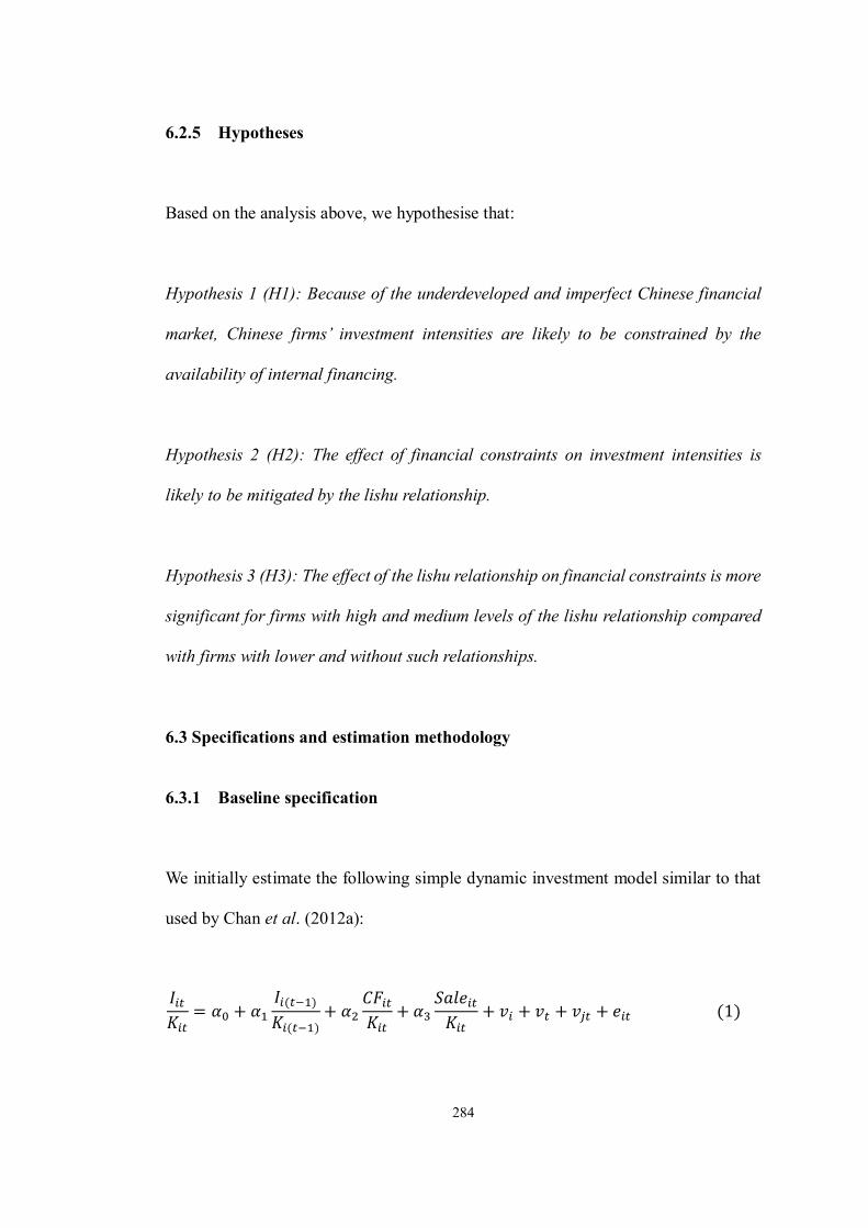
284
6.2.5 Hypotheses
Based on the analysis above, we hypothesise that:
Hypothesis 1 (H1): Because of the underdeveloped and imperfect Chinese financial
market, Chinese firms’ investment intensities are likely to be constrained by the
availability of internal financing.
Hypothesis 2 (H2): The effect of financial constraints on investment intensities is
likely to be mitigated by the lishu relationship.
Hypothesis 3 (H3): The effect of the lishu relationship on financial constraints is more
significant for firms with high and medium levels of the lishu relationship compared
with firms with lower and without such relationships.
6.3 Specifications and estimation methodology
6.3.1 Baseline specification
We initially estimate the following simple dynamic investment model similar to that
used by Chan et al. (2012a):
𝐼𝑖𝑡
𝐾𝑖𝑡= 𝛼0 + 𝛼1
𝐼𝑖(𝑡−1)
𝐾𝑖(𝑡−1)+ 𝛼2
𝐶𝐹𝑖𝑡
𝐾𝑖𝑡+ 𝛼3
𝑆𝑎𝑙𝑒𝑖𝑡
𝐾𝑖𝑡+ 𝑣𝑖 + 𝑣𝑡 + 𝑣𝑗𝑡 + 𝑒𝑖𝑡 (1)
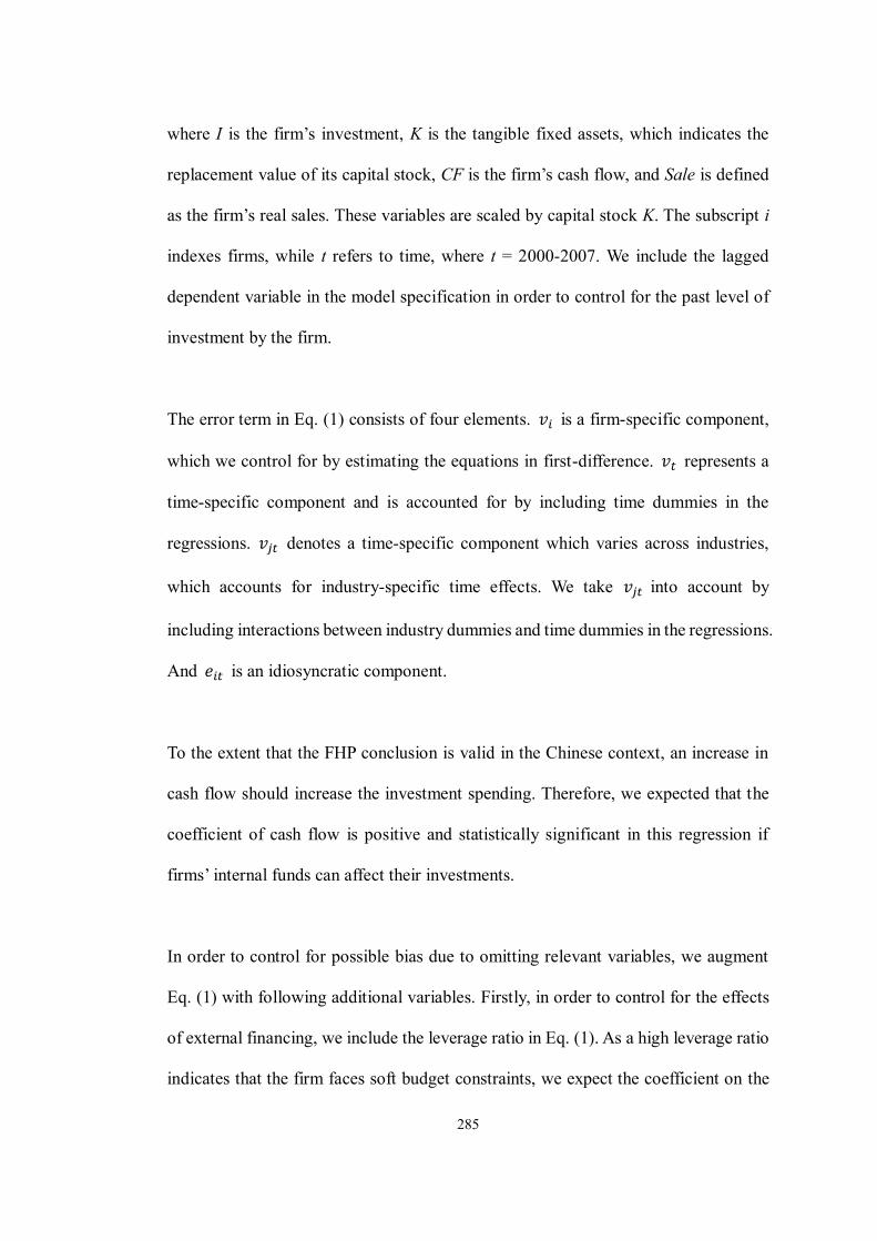
285
where I is the firm’s investment, K is the tangible fixed assets, which indicates the
replacement value of its capital stock, CF is the firm’s cash flow, and Sale is defined
as the firm’s real sales. These variables are scaled by capital stock K. The subscript i
indexes firms, while t refers to time, where t = 2000-2007. We include the lagged
dependent variable in the model specification in order to control for the past level of
investment by the firm.
The error term in Eq. (1) consists of four elements. 𝑣𝑖 is a firm-specific component,
which we control for by estimating the equations in first-difference. 𝑣𝑡 represents a
time-specific component and is accounted for by including time dummies in the
regressions. 𝑣𝑗𝑡 denotes a time-specific component which varies across industries,
which accounts for industry-specific time effects. We take 𝑣𝑗𝑡 into account by
including interactions between industry dummies and time dummies in the regressions.
And 𝑒𝑖𝑡 is an idiosyncratic component.
To the extent that the FHP conclusion is valid in the Chinese context, an increase in
cash flow should increase the investment spending. Therefore, we expected that the
coefficient of cash flow is positive and statistically significant in this regression if
firms’ internal funds can affect their investments.
In order to control for possible bias due to omitting relevant variables, we augment
Eq. (1) with following additional variables. Firstly, in order to control for the effects
of external financing, we include the leverage ratio in Eq. (1). As a high leverage ratio
indicates that the firm faces soft budget constraints, we expect the coefficient on the

286
leverage ratio to be positive. Moreover, if expected future profit is high, then firms
may hold more cash because they anticipate greater capital investment. In this case,
the coefficient of cash flow may not reflect financial constraints. We therefore
incorporate an accelerator term, defined as sales growth (𝑆𝑎𝑙𝑒𝑠 𝐺𝑟𝑜𝑤𝑡ℎ) into Eq. (1)
to account for the effects of future opportunities of investment (Chan et al., 2012b;
Cull et al., 2014).
𝐼𝑖𝑡
𝐾𝑖𝑡= 𝛼0 + 𝛼1
𝐼𝑖(𝑡−1)
𝐾𝑖(𝑡−1)+ 𝛼2
𝐶𝐹𝑖𝑡
𝐾𝑖𝑡+ 𝛼3
𝑆𝑎𝑙𝑒𝑖𝑡
𝐾𝑖𝑡+ 𝛼4𝐿𝑒𝑣𝑒𝑟𝑎𝑔𝑒𝑖𝑡 + 𝛼5𝑆𝑎𝑙𝑒𝑠 𝐺𝑟𝑜𝑤𝑡ℎ𝑖𝑡
+ 𝑣𝑖 + 𝑣𝑡 + 𝑣𝑗𝑡 + 𝑒𝑖𝑡 (2)
In order to test the influences of the lishu relationship on the sensitivity of cash flow
to investments for Chinese firms, rather than estimating all the equations on separate
sub-samples of firms as in Cull et al. (2014), Chen et al. (2011), and Chan et al.
(2012a), we estimate a single equation and interact the cash flow variables with
political affiliation variable, which is a dummy variable that equals to 1 if the firm has
a lishu relationship and 0 otherwise following Chen et al. (2011) and Mclean et al.
(2012). Specifically, we estimate the following reduced and augmented equations:
𝐼𝑖𝑡
𝐾𝑖𝑡= 𝛼0 + 𝛼1
𝐼𝑖(𝑡−1)
𝐾𝑖(𝑡−1)+ 𝛼21
𝐶𝐹𝑖𝑡
𝐾𝑖𝑡+ 𝛼22
𝐶𝐹𝑖𝑡
𝐾𝑖𝑡× 𝑃𝐴𝑖𝑡 + 𝛼3
𝑆𝑎𝑙𝑒𝑖𝑡
𝐾𝑖𝑡+ 𝑣𝑖 + 𝑣𝑡 + 𝑣𝑗𝑡
+ 𝑒𝑖𝑡 (3)

287
𝐼𝑖𝑡
𝐾𝑖𝑡= 𝛼0 + 𝛼1
𝐼𝑖(𝑡−1)
𝐾𝑖(𝑡−1)+ 𝛼21
𝐶𝐹𝑖𝑡
𝐾𝑖𝑡+ 𝛼22
𝐶𝐹𝑖𝑡
𝐾𝑖𝑡× 𝑃𝐴𝑖𝑡 + 𝛼3
𝑆𝑎𝑙𝑒𝑖𝑡
𝐾𝑖𝑡+ 𝛼4𝐿𝑒𝑣𝑒𝑟𝑎𝑔𝑒𝑖𝑡
+ 𝛼5𝑆𝑎𝑙𝑒𝑠 𝐺𝑟𝑜𝑤𝑡ℎ𝑖𝑡 + 𝑣𝑖 + 𝑣𝑡 + 𝑣𝑗𝑡 + 𝑒𝑖𝑡 (4)
Using interactions rather than separate regressions for each group allows us to avoid
the endogenous sample selection problems, obtain degrees of freedom, and take
account of the fact that firms can transit between groups (Guariglia, 2008). For all the
sample firms, we expect that the coefficient on the interaction term to be significantly
less than zero.
We further divide the lishu relationship into four degrees by generating an ordinal
dummy variable, named PAV, which takes the value of 1 if firms have no lishu
relationship, takes the value of 2 for firms affiliated with the low level of government,
takes the value of 3 for firms affiliated with the medium level of government, and
takes the value of 4 for firms affiliated with the high level of government.1 We interact
cash flow with this dummy indicating various degrees of political connections held
by firms and expect that the firms affiliated with higher level of governments in China
face less financial constraints. Specifically, we estimate the following reduced and
augmented equations:
𝐼𝑖𝑡
𝐾𝑖𝑡= 𝛼0 + 𝛼1
𝐼𝑖(𝑡−1)
𝐾𝑖(𝑡−1)+ 𝛼21
𝐶𝐹𝑖𝑡
𝐾𝑖𝑡+ 𝛼22
𝐶𝐹𝑖𝑡
𝐾𝑖𝑡× 𝑃𝐴𝑉𝑖𝑡 + 𝛼3
𝑆𝑎𝑙𝑒𝑖𝑡
𝐾𝑖𝑡+ 𝑣𝑖 + 𝑣𝑡 + 𝑣𝑗𝑡
+ 𝑒𝑖𝑡 (5)
1 See Appendix for detailed definitions.
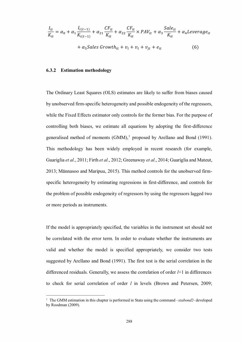
288
𝐼𝑖𝑡
𝐾𝑖𝑡= 𝛼0 + 𝛼1
𝐼𝑖(𝑡−1)
𝐾𝑖(𝑡−1)+ 𝛼21
𝐶𝐹𝑖𝑡
𝐾𝑖𝑡+ 𝛼22
𝐶𝐹𝑖𝑡
𝐾𝑖𝑡× 𝑃𝐴𝑉𝑖𝑡 + 𝛼3
𝑆𝑎𝑙𝑒𝑖𝑡
𝐾𝑖𝑡+ 𝛼4𝐿𝑒𝑣𝑒𝑟𝑎𝑔𝑒𝑖𝑡
+ 𝛼5𝑆𝑎𝑙𝑒𝑠 𝐺𝑟𝑜𝑤𝑡ℎ𝑖𝑡 + 𝑣𝑖 + 𝑣𝑡 + 𝑣𝑗𝑡 + 𝑒𝑖𝑡 (6)
6.3.2 Estimation methodology
The Ordinary Least Squares (OLS) estimates are likely to suffer from biases caused
by unobserved firm-specific heterogeneity and possible endogeneity of the regressors,
while the Fixed Effects estimator only controls for the former bias. For the purpose of
controlling both biases, we estimate all equations by adopting the first-difference
generalised method of moments (GMM),1 proposed by Arellano and Bond (1991).
This methodology has been widely employed in recent research (for example,
Guariglia et al., 2011; Firth et al., 2012; Greenaway et al., 2014; Guariglia and Mateut,
2013; Männasoo and Maripuu, 2015). This method controls for the unobserved firm-
specific heterogeneity by estimating regressions in first-difference, and controls for
the problem of possible endogeneity of regressors by using the regressors lagged two
or more periods as instruments.
If the model is appropriately specified, the variables in the instrument set should not
be correlated with the error term. In order to evaluate whether the instruments are
valid and whether the model is specified appropriately, we consider two tests
suggested by Arellano and Bond (1991). The first test is the serial correlation in the
differenced residuals. Generally, we assess the correlation of order l+1 in differences
to check for serial correlation of order l in levels (Brown and Petersen, 2009;
1 The GMM estimation in this chapter is performed in Stata using the command –xtabond2- developed by Roodman (2009).
289
Roodman, 2009). The instrument set needs to be restricted to lag 3 and deeper if the
serial correlation of order 2 in the differenced residuals exists. Therefore, we use the
m(l) test to evaluate the presence of lth-order serial correlation in the differenced
residuals. This test is under the null of no lth-order serial correlation of the differenced
residuals and asymptotically distributed as a standard normal.
The second test is the Sargan test (also known as J-test). This test is used for assessing
over-identifying restrictions. The null hypothesis being evaluated by the Sargan test
is the instrument validity. That is, the instrumental variables are uncorrelated with the
set of residuals, and therefore, they are acceptable, healthy, and valid instruments. It
is asymptotically distributed as a chi-square variable with (n-k) degrees of freedom,
where n is the number of instruments and k is the number of parameters. However,
according to Blundell and Bond (1998) and Benito (2005), when the estimation is
used for samples with a very large cross-sectional dimension, it is likely to over-reject
the null hypothesis of valid instrument. Therefore, given the size of our panel, we tend
to pay little attention to the J-test.
We select our instruments starting with lagged twice regressors. If m2 test is rejected,
we delete the regressors lagged twice from the instrument set and use regressors
lagged three times as instruments.1 We only include the deeper lags if they can
improve the specification estimations.
1 The m1 test for first-order serial correlation of the differenced residuals is reported in all the tables. As our regressions are tested in first-differences, we observe negative first-order autocorrelation in the differenced residuals. If the regressions use instruments both lagged twice (t-2) and three times (t-3), both the m2 and the m3 tests for second- and third- autocorrelation in the differenced residuals are reported in the tables. If the most recent instruments are lagged twice (t-2) or three times (t-3), only the m2 or m3 test will be reported in the tables. Note that the differences between bad instruments and model specification cannot be diagnosed neither by the Sargan test nor by the lth-order serial correlation in the differenced residuals.
290
6.4 Data and summary statistics
6.4.1 Data
We use firm-level dataset for this study as it can avoid aggregation problems in
estimation, and make it possible to take firm heterogeneity into account (Bond and
Van Reenen, 2007). This dataset is from the annual accounting reports, maintained
and complied by the National Bureau of Statistics of China (NBS), and provides
comprehensive economic information of all types of firms in China with annual sales
of more than five million Yuan.1
In order to improve the reliability of our analysis, we first drop observations which
make little sense, such as those with negative sales, negative age, and negative
leverage ratio. Second, we eliminate firms without complete records on our main
regression variables. Finally, in order to control for the potential effect of extreme
values, we drop outliers, which are the observations beyond the 1st and 99th percent
tails for each continuous main regression variables.2 After the above adjustments, our
final panel dataset includes 356,053 firm-level observations, covering 105,487 mainly
unlisted firms over the period 2002-2007.3 The sample has an unbalanced structure,4
with the number of observations ranging from a minimum of 32,358 in 2002 to a
1 The official RMB exchange rate per US dollar during the sample period was 8.2785 in 2000, 8.2771 in 2001, 8.2770 in 2002 and 2003, 8.2768 in 2004, 8.1943 in 2005, 7.9734 in 2006, and 7.6075 in 2007 (World Development Indicators, World Bank). Therefore, the threshold for including in the dataset is equivalent to between USD 604,098 and USD 657,246 over the sample period. 2 It is quite common in the literature (see Greenaway et al., 2007; Guariglia, 2008; Carpenter and Guariglia, 2008; Yan, 2012) to eliminate extreme values in this way.
3 It should be noted that our dataset include a very small proportion of listed firms for two reasons. Frist of all, according to Liu and Xiao (2004), when firms become listed, their legal identification numbers are changed; it is therefore hard to track these firms. The second reason is that there is no separate identification of Chinese publicly listed firms in the NBS dataset. However, they only comprise a very small portion of the whole sample. Over the whole considered period, only approximately 1000 listed firms in the manufacturing and mining sectors, accounting for less than 0.3% of the total number of firms in the sample. 4 See Appendix for details about the structure of the panel.
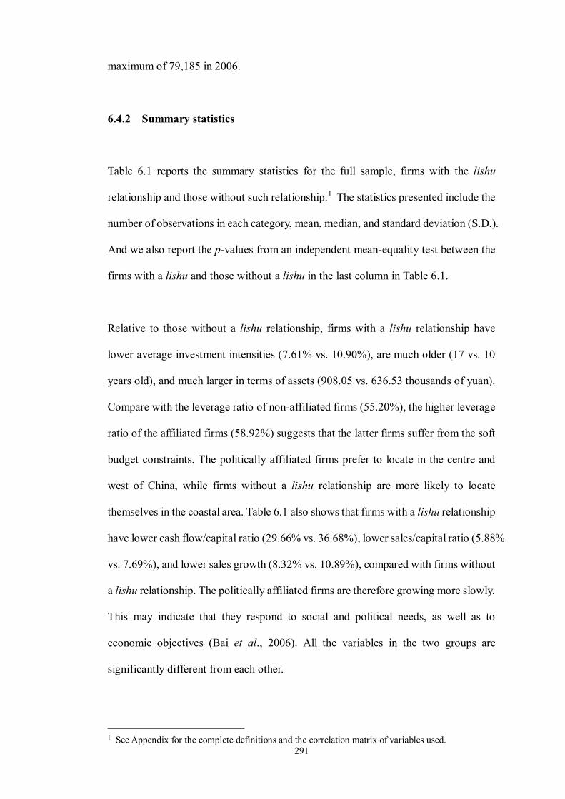
291
maximum of 79,185 in 2006.
6.4.2 Summary statistics
Table 6.1 reports the summary statistics for the full sample, firms with the lishu
relationship and those without such relationship.1 The statistics presented include the
number of observations in each category, mean, median, and standard deviation (S.D.).
And we also report the p-values from an independent mean-equality test between the
firms with a lishu and those without a lishu in the last column in Table 6.1.
Relative to those without a lishu relationship, firms with a lishu relationship have
lower average investment intensities (7.61% vs. 10.90%), are much older (17 vs. 10
years old), and much larger in terms of assets (908.05 vs. 636.53 thousands of yuan).
Compare with the leverage ratio of non-affiliated firms (55.20%), the higher leverage
ratio of the affiliated firms (58.92%) suggests that the latter firms suffer from the soft
budget constraints. The politically affiliated firms prefer to locate in the centre and
west of China, while firms without a lishu relationship are more likely to locate
themselves in the coastal area. Table 6.1 also shows that firms with a lishu relationship
have lower cash flow/capital ratio (29.66% vs. 36.68%), lower sales/capital ratio (5.88%
vs. 7.69%), and lower sales growth (8.32% vs. 10.89%), compared with firms without
a lishu relationship. The politically affiliated firms are therefore growing more slowly.
This may indicate that they respond to social and political needs, as well as to
economic objectives (Bai et al., 2006). All the variables in the two groups are
significantly different from each other.
1 See Appendix for the complete definitions and the correlation matrix of variables used.
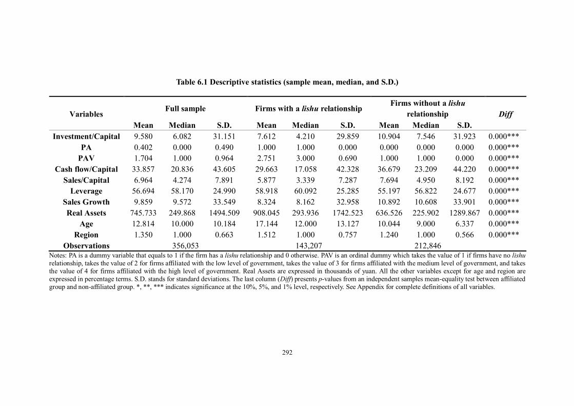
292
Table 6.1 Descriptive statistics (sample mean, median, and S.D.)
Variables Full sample Firms with a lishu relationship Firms without a lishu
relationship Diff Mean Median S.D. Mean Median S.D. Mean Median S.D.
Investment/Capital 9.580 6.082 31.151 7.612 4.210 29.859 10.904 7.546 31.923 0.000*** PA 0.402 0.000 0.490 1.000 1.000 0.000 0.000 0.000 0.000 0.000***
PAV 1.704 1.000 0.964 2.751 3.000 0.690 1.000 1.000 0.000 0.000*** Cash flow/Capital 33.857 20.836 43.605 29.663 17.058 42.328 36.679 23.209 44.220 0.000***
Sales/Capital 6.964 4.274 7.891 5.877 3.339 7.287 7.694 4.950 8.192 0.000*** Leverage 56.694 58.170 24.990 58.918 60.092 25.285 55.197 56.822 24.677 0.000***
Sales Growth 9.859 9.572 33.549 8.324 8.162 32.958 10.892 10.608 33.901 0.000*** Real Assets 745.733 249.868 1494.509 908.045 293.936 1742.523 636.526 225.902 1289.867 0.000***
Age 12.814 10.000 10.184 17.144 12.000 13.127 10.044 9.000 6.337 0.000*** Region 1.350 1.000 0.663 1.512 1.000 0.757 1.240 1.000 0.566 0.000***
Observations 356,053 143,207 212,846 Notes: PA is a dummy variable that equals to 1 if the firm has a lishu relationship and 0 otherwise. PAV is an ordinal dummy which takes the value of 1 if firms have no lishu relationship, takes the value of 2 for firms affiliated with the low level of government, takes the value of 3 for firms affiliated with the medium level of government, and takes the value of 4 for firms affiliated with the high level of government. Real Assets are expressed in thousands of yuan. All the other variables except for age and region are expressed in percentage terms. S.D. stands for standard deviations. The last column (Diff) presents p-values from an independent samples mean-equality test between affiliated group and non-affiliated group. *, **, *** indicates significance at the 10%, 5%, and 1% level, respectively. See Appendix for complete definitions of all variables.
293
Focusing on the three different levels of lishu relationship in Table 6.2, we observe
that while the level of lishu relationship is upgrading, the investment/capital ratio is
decreasing (from 9.62% to 6.46% and 5.81% for firms affiliated with the
low/medium/high level of government, respectively), while the firm size (measured
by the real assets), as well as firm age are increasing. In addition, the sales-to-capital
ratio and sales growth are decreasing when the level of political affiliation is
increasing. As for the financial factors, we find that firms affiliated with the medium
level of government have the highest leverage ratio (62.02%) and the lowest cash flow
to capital ratio (22.79%). Furthermore, we observe that the firms affiliated with
medium level of government are more likely to locate themselves in the inner regions.
294
Table 6.2 Descriptive statistics for three levels of the lishu relationship (sample mean, median, and S.D.)
Variables LOW MEDIUM HIGH
Diff1 Diff2 Diff3 Mean Median S.D. Mean Median S.D. Mean Median S.D.
Investment/Capital 9.624 6.249 31.311 6.462 3.074 29.417 5.811 3.161 26.746 0.000*** 0.000*** 0.005*** PA 1.000 1.000 0.000 1.000 1.000 0.000 1.000 1.000 0.000 0.000*** 0.000*** 0.000***
PAV 2.000 2.000 0.000 3.000 3.000 0.000 4.000 4.000 0.000 0.000*** 0.000*** 0.000*** Cash flow/Capital 39.656 24.408 47.341 22.786 12.815 36.345 24.432 13.319 40.267 0.000*** 0.000*** 0.000***
Sales/Capital 7.870 5.007 8.408 4.697 2.621 6.236 4.226 2.273 5.719 0.000*** 0.000*** 0.000*** Leverage 55.893 57.338 24.662 62.024 63.277 25.201 57.244 57.578 26.057 0.000*** 0.000*** 0.000***
Sales Growth 10.619 10.517 33.420 6.890 6.641 33.275 6.661 7.180 30.213 0.000*** 0.000*** 0.378 Real Assets 489.051 194.224 1034.712 976.108 351.838 1752.263 1828.692 741.653 2631.622 0.000*** 0.000*** 0.000***
Age 12.907 11.000 7.597 18.996 12.000 14.693 21.476 14.000 15.469 0.000*** 0.000*** 0.000*** Region 1.273 1.000 0.569 1.681 1.000 0.815 1.623 1.000 0.837 0.000*** 0.000*** 0.000***
Observations 56,354 66,092 20,761 Notes: PA is a dummy variable that equals to 1 if the firm has a lishu relationship and 0 otherwise. PAV is an ordinal dummy which takes the value of 1 if firms have no lishu relationship, takes the value of 2 for firms affiliated with the low level of government, takes the value of 3 for firms affiliated with the medium level of government, and takes the value of 4 for firms affiliated with the high level of government. Real Assets are expressed in thousands of yuan. All the other variables except for age and region are expressed in percentage terms. S.D. stands for standard deviations. The last three columns present p-values from an independent samples mean-equality test between the low level of lishu group and the medium level of lishu group (Diff1), between the low level of lishu group and the high level of lishu group (Diff2), and between the medium level of lishu group and the high level of lishu group (Diff3). *, **, *** indicates significance at the 10%, 5%, and1% level, respectively. See Appendix for complete definitions of all variables.
295
Table 6.3 presents a comparison of the main variables by the types of firms’ ownership.
In terms of investment-to-capital ratio, PEs and FEs invest more (10.88% and 9.28%,
respectively), followed by COEs (7.72%), while SOEs have the lowest ratio (3.15%).
SOEs and FEs are generally large in real assets (1220.30 thousands of yuan and
1118.85 thousands of yuan, respectively), compared with PEs and COEs (608.10
thousands of yuan and 407.01 thousands of yuan, respectively). SOEs have the highest
political affiliation level (level 3) and are the longest-established firms in terms of
firms age (28 years), followed by COEs with 18 years old and the second highest
political affiliation level (level 2), while the FEs are the youngest one (10 years old).
This is due to the fact that most foreign firms entered China after the 1990s. SOEs also
suffer from soft budget constraints indicated by their highest leverage ratio (65.35%),
while FEs enjoy the highest cash flow-to-capital ratio (37.88%). Table 6.3 also shows
that sales/capital ratio is the highest for COEs (7.48%) and the sales growth is the
highest for private firms (11.29%). Finally, we observe that the FEs prefer to locate
their firms in the coastal region, while SOEs are more likely to locate their firms in
the inner area of China.
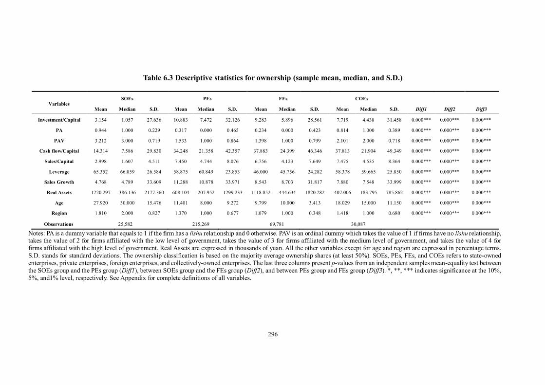
296
Table 6.3 Descriptive statistics for ownership (sample mean, median, and S.D.)
Variables SOEs PEs FEs COEs
Diff2 Diff3 Mean Median S.D. Mean Median S.D. Mean Median S.D. Mean Median S.D. Diff1
Investment/Capital 3.154 1.057 27.636 10.883 7.472 32.126 9.283 5.896 28.561 7.719 4.438 31.458 0.000*** 0.000*** 0.000***
PA 0.944 1.000 0.229 0.317 0.000 0.465 0.234 0.000 0.423 0.814 1.000 0.389 0.000*** 0.000*** 0.000***
PAV 3.212 3.000 0.719 1.533 1.000 0.864 1.398 1.000 0.799 2.101 2.000 0.718 0.000*** 0.000*** 0.000***
Cash flow/Capital 14.314 7.586 29.830 34.248 21.358 42.357 37.883 24.399 46.346 37.813 21.904 49.349 0.000*** 0.000*** 0.000***
Sales/Capital 2.998 1.607 4.511 7.450 4.744 8.076 6.756 4.123 7.649 7.475 4.535 8.364 0.000*** 0.000*** 0.000***
Leverage 65.352 66.059 26.584 58.875 60.849 23.853 46.000 45.756 24.282 58.378 59.665 25.850 0.000*** 0.000*** 0.000***
Sales Growth 4.768 4.789 33.609 11.288 10.878 33.971 8.543 8.703 31.817 7.880 7.548 33.999 0.000*** 0.000*** 0.000***
Real Assets 1220.297 386.136 2177.360 608.104 207.952 1299.233 1118.852 444.634 1820.282 407.006 183.795 785.862 0.000*** 0.000*** 0.000***
Age 27.920 30.000 15.476 11.401 8.000 9.272 9.799 10.000 3.413 18.029 15.000 11.150 0.000*** 0.000*** 0.000***
Region 1.810 2.000 0.827 1.370 1.000 0.677 1.079 1.000 0.348 1.418 1.000 0.680 0.000*** 0.000*** 0.000***
Observations 25,582 215,269 69,781 30,087
Notes: PA is a dummy variable that equals to 1 if the firm has a lishu relationship and 0 otherwise. PAV is an ordinal dummy which takes the value of 1 if firms have no lishu relationship, takes the value of 2 for firms affiliated with the low level of government, takes the value of 3 for firms affiliated with the medium level of government, and takes the value of 4 for firms affiliated with the high level of government. Real Assets are expressed in thousands of yuan. All the other variables except for age and region are expressed in percentage terms. S.D. stands for standard deviations. The ownership classification is based on the majority average ownership shares (at least 50%). SOEs, PEs, FEs, and COEs refers to state-owned enterprises, private enterprises, foreign enterprises, and collectively-owned enterprises. The last three columns present p-values from an independent samples mean-equality test between the SOEs group and the PEs group (Diff1), between SOEs group and the FEs group (Diff2), and between PEs group and FEs group (Diff3). *, **, *** indicates significance at the 10%, 5%, and1% level, respectively. See Appendix for complete definitions of all variables.

297
The descriptive statistics for three different regions of China are provided in Table 6.4.
We observe that firms located in the central region have the highest investment to
capital ratio (10.01%), followed by firms in the central area (9.21%), and firms in the
west of China have the lowest investment/capital ratio (7.03%) and the highest political
affiliation level. In addition, firms in the west of China are generally larger, in terms of
real assets (835.87 thousands of yuan) and older (around 17 years) than firms in the east
and central of China. Interestingly, firms located in the coastal region have the highest
sales/capital ratio and cash flow/capital ratio (7.55% and 36.12%, respectively), while
those located in the west of China enjoy the highest leverage ratio (60.01%). However,
firms in the central area have the largest sales growth (11.06%). This may be attributed
to their location advantage, which is close to the heart of China, Beijing, which is one
of the biggest cities with rapid growth rate, providing extensive markets to the firms.

298
Table 6.4 Descriptive statistics for region (sample mean, median, and S.D.)
Variables Costal Central Western
Diff1 Diff2 Mean Median S.D. Mean Median S.D. Mean Median S.D.
Investment/Capital 10.006 6.617 30.936 9.205 5.326 33.253 7.030 3.301 29.710 0.000*** 0.000*** PA 0.345 0.000 0.475 0.554 1.000 0.497 0.612 1.000 0.487 0.000*** 0.000***
PAV 1.572 1.000 0.890 2.004 2.000 1.015 2.259 3.000 1.106 0.000*** 0.000*** Cash flow/Capital 36.122 22.938 44.173 29.887 15.078 44.272 22.852 13.286 35.950 0.000*** 0.000***
Sales/Capital 7.550 4.778 8.187 5.494 3.144 6.749 4.680 2.532 6.288 0.000*** 0.000*** Leverage 56.098 57.814 24.672 57.412 58.095 26.632 60.014 60.505 24.765 0.000*** 0.000***
Sales Growth 9.781 9.666 32.999 11.059 10.156 35.522 8.869 8.289 34.749 0.000*** 0.000*** Real Assets 742.927 253.649 1475.306 691.417 210.000 1487.587 835.868 277.434 1629.327 0.000*** 0.000***
Age 11.971 10.000 8.953 15.079 10.000 12.859 16.680 11.000 13.695 0.000*** 0.000*** Region 1.000 1.000 0.000 2.000 2.000 0.000 3.000 3.000 0.000 0.000*** 0.000***
Observations 269,414 48,828 37,811 Notes: PA is a dummy variable that equals to 1 if the firm has a lishu relationship and 0 otherwise. PAV is an ordinal dummy which takes the value of 1 if firms have no lishu relationship, takes the value of 2 for firms affiliated with the low level of government, takes the value of 3 for firms affiliated with the medium level of government, and takes the value of 4 for firms affiliated with the high level of government. Real Assets are expressed in thousands of yuan. All the other variables except for age and region are expressed in percentage terms. S.D. stands for standard deviations. The last two columns present p-values from an independent samples mean-equality test between the coastal region group and the central region group (Diff1), and between the coastal region group and the western region group (Diff2). *, **, *** indicates significance at the 10%, 5%, and1% level, respectively. See Appendix for complete definitions of all variables.
299
6.5 Empirical results
6.5.1 Financial constraints in China
Table 6.5 presents the estimation of Eq. (1) and Eq. (2) for the full sample of firms.
Column (1) reports the estimation for Eq. (1), while column (2) reports the estimation
for Eq. (2). Both equations are estimated by the first-difference GMM technique.
Focusing on the coefficient of cash flow variable in column (1). Under the assumption
of perfect capital markets without financial constraints, we should find a negative and
insignificant relationship between investment and the availability of cash flow.
However, if the cash flow is positively and significantly associated with the investment,
this suggests that the firm’s investment activities are subject to credit constraints. Our
result shows a positive and precisely determined coefficient on cash flow in Eq. (1),
which is consistent with our first hypothesis that Chinese firms’ investments have a
significant sensitivity to its internal funds. The coefficient of cash flow in first column
estimator is 0.202 and the standard deviation for cash flow in Table 6.1 is 43.605.
Therefore, a one-standard-deviation increase in cash flows yields an 8.808 increase in
investment. The mean value of the investment is 9.580, hence a one-standard-deviation
increase in cash flows creates a 91.94% increase of investment. This result indicates
that the effect of cash flow on investment is economically significant.
Column (2) in Table 6.5 presents the results by controlling for the sales growth and
leverage ratio. We find that the coefficient on cash flows decreases to 0.141, but remain

300
significant at a 5% level, indicating that the investment is sensitive to the availability
of internal funds in China. Specifically, one-standard-deviation increase in cash flows
yields a 6.148 increase in investment. Evaluated at the sample mean for investment, a
one-standard-deviation increase in cash flow creates a 64.18% increase in investment.
This result also consistent with most of the existing studies (FHP, 1988; Chow and
Fung, 1998; Cull et al., 2014; Chen et al., 2011; Hubbard, 1998; Stein, 2003; Dethier
et al., 2011).
When focusing on the coefficients of the other regressors, we find a positive and
significant relationship between sales-to-capital ratio and investment in both columns.
More specifically, in the reduced equation, a 10% increase in sales-to-capital ratio
causes a 3.427 increase in investment. Considering the mean value for investment, a
10% increase in sales-to-capital ratio enhances the investment by 35.75%. As for the
augment equation, a 10% increase in sales-to-capital ratio causes a 3.299 increase in
investment. Evaluated at the mean value of investment, a 10% increase in sales to
capital ratio enhances the investment by 34.44%.
The insignificant but positive coefficient on the leverage ratio indicates that debt may
not be the first preference for Chinese firms to finance their investment activities. This
can be explained by the fact that private firms, which takes up almost 60% of our
sample, are not favoured in the capital market, which is dominated by the government.
Therefore, it might be difficult for them to obtain sufficient external financing when
there is an investment opportunity. We also find a negative and significant (at 1% level)
relationship between sales growth and investment intensity. One possible explanation
301
for the negative relationship between sales growth and investment/capital ratio is that
firms with less expected future profits generally invest less, but require more loans and
face higher default risks. Meanwhile, via expanding investments, these firms can gain
more revenue, which in turn can reduce the risk of default and increase these firms’
liquidity. According to Cleary et al. (2007), these firms will ultimately invest more.
Although the Sargan test indicates some problems with the specification of the model
and/or the validity of the instruments, the m3 test in both columns shows that the null
of no 3rd-order autocorrelation of the differenced residuals cannot be rejected. As we
have discussed in section 6.3.2, the J-test tends to over-reject given the large size of
our panel, we incline not to consider too much about this statistic. We therefore
conclude that the instruments and specifications are generally acceptable.
To summarise, the results suggest that Chinese firms suffer from financial constraints
as their investment intensity is sensitive to the access to cash flow.
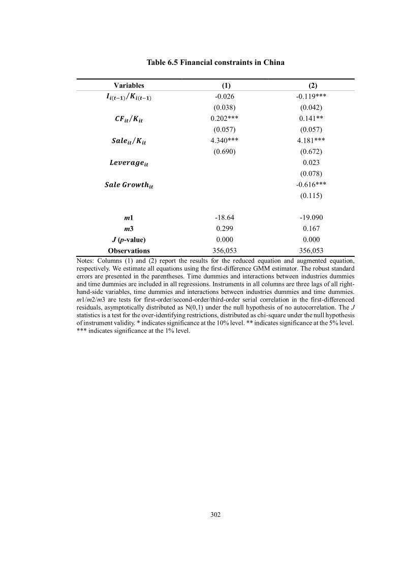
302
Table 6.5 Financial constraints in China
Variables (1) (2) 𝑰𝒊(𝒕−𝟏) 𝑲𝒊(𝒕−𝟏)⁄ -0.026 -0.119***
(0.038) (0.042) 𝑪𝑭𝒊𝒕 𝑲𝒊𝒕⁄ 0.202*** 0.141**
(0.057) (0.057) 𝑺𝒂𝒍𝒆𝒊𝒕 𝑲𝒊𝒕⁄ 4.340*** 4.181***
(0.690) (0.672) 𝑳𝒆𝒗𝒆𝒓𝒂𝒈𝒆𝒊𝒕 0.023
(0.078) 𝑺𝒂𝒍𝒆 𝑮𝒓𝒐𝒘𝒕𝒉𝒊𝒕 -0.616***
(0.115)
m1 -18.64 -19.090 m3 0.299 0.167
J (p-value) 0.000 0.000 Observations 356,053 356,053
Notes: Columns (1) and (2) report the results for the reduced equation and augmented equation, respectively. We estimate all equations using the first-difference GMM estimator. The robust standard errors are presented in the parentheses. Time dummies and interactions between industries dummies and time dummies are included in all regressions. Instruments in all columns are three lags of all right-hand-side variables, time dummies and interactions between industries dummies and time dummies. m1/m2/m3 are tests for first-order/second-order/third-order serial correlation in the first-differenced residuals, asymptotically distributed as N(0,1) under the null hypothesis of no autocorrelation. The J statistics is a test for the over-identifying restrictions, distributed as chi-square under the null hypothesis of instrument validity. * indicates significance at the 10% level. ** indicates significance at the 5% level. *** indicates significance at the 1% level.

303
6.5.2 The lishu relationship and financial constraints in China
Test results of estimating the second hypothesis, which predicts that firms with a lishu
relationship face less financial constraints than their counterpart, are reported in Table
6.6. Column (1) reports the results for Eq. (3), while column (2) presents the results
for Eq. (4). The interaction terms are based on the cash flow-to-capital ratio and the
lishu dummy variable.
The negative coefficient of the interaction term between cash flow and lishu
relationship in column (1) indicates investment/capital ratio is less sensitive to the level
of cash flow for the firms with a lishu relationship. This insignificant level is due to
omitting the relevant control variables. Focusing on the results in column (2), we find
that the coefficient of the interaction term is significantly negative, suggesting that the
lishu relationship reduces the sensitivity of investment to cash flow.
In the regressions including interactions, the overall cash flow coefficient equals the
cash flow coefficient plus the interaction coefficient multiplied by the mean value of
the interactive variable (Mclean et al., 2012). In this case, in column (1) the total cash
flow coefficient is the sum of the cash flow coefficient plus the cash flow-PA
interaction coefficient multiplied by the mean value of PA. The cash flow coefficient
in this regression is 0.215, whereas the interaction term is -0.055, the mean value of
PA for firms with a lishu relationship is 1.00 and for those without a lishu relationship
is 0.00. Therefore, the overall cash flow ratio for firms with a lishu relationship is 0.16
and for non-affiliated firms is 0.215, which is more than one time larger than that for
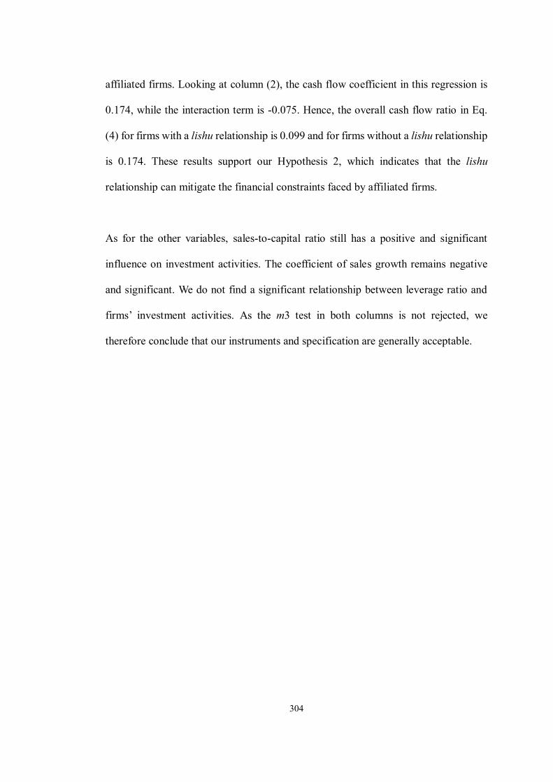
304
affiliated firms. Looking at column (2), the cash flow coefficient in this regression is
0.174, while the interaction term is -0.075. Hence, the overall cash flow ratio in Eq.
(4) for firms with a lishu relationship is 0.099 and for firms without a lishu relationship
is 0.174. These results support our Hypothesis 2, which indicates that the lishu
relationship can mitigate the financial constraints faced by affiliated firms.
As for the other variables, sales-to-capital ratio still has a positive and significant
influence on investment activities. The coefficient of sales growth remains negative
and significant. We do not find a significant relationship between leverage ratio and
firms’ investment activities. As the m3 test in both columns is not rejected, we
therefore conclude that our instruments and specification are generally acceptable.
305
Table 6.6 The lishu relationship and financial constraints in China
Variables (1) (2)
𝑰𝒊(𝒕−𝟏) 𝑲𝒊(𝒕−𝟏)⁄ -0.012 -0.077*
(0.038) (0.040)
𝑪𝑭𝒊𝒕 𝑲𝒊𝒕⁄ 0.215*** 0.174***
(0.067) (0.065)
𝑪𝑭𝒊𝒕 𝑲𝒊𝒕⁄ × 𝑷𝑨 -0.055 -0.075* (0.045) (0.043)
𝑺𝒂𝒍𝒆𝒊𝒕 𝑲𝒊𝒕⁄ 4.344*** 4.263*** (0.692) (0.667)
𝑳𝒆𝒗𝒆𝒓𝒂𝒈𝒆𝒊𝒕 0.002 (0.076)
𝑺𝒂𝒍𝒆 𝑮𝒓𝒐𝒘𝒕𝒉𝒊𝒕 -0.447*** (0.105)
m1 -18.990
-18.73
m3 0.194
-0.103
J (p-value) 0.000 0.000
Observations 356,053 356,053 Notes: Columns (1) and (2) report the results for the reduced equation and augmented euqtion, respectively. We estimate all equations using the first-difference GMM estimator. The robust standard errors are presented in the parentheses. Time dummies and interactions between industries dummies and time dummies are included in all regressions. Instruments in all columns are three lags of all right-hand-side variables, time dummies and interactions between industries dummies and time dummies. m1/m2/m3 are tests for first-order/second-order/third-order serial correlation in the first-differenced residuals, asymptotically distributed as N(0,1) under the null hypothesis of no autocorrelation. The J statistics is a test for the over-identifying restrictions, distributed as chi-square under the null hypothesis of instrument validity. * indicates significance at the 10% level. ** indicates significance at the 5% level. *** indicates significance at the 1% level.
306
6.5.3 Different levels of the lishu relationship and financial constraints in China
Table 6.7 presents the test results for our third hypothesis, which expects that the higher
level of government the firms affiliated with, the lower cash flow-investment
sensitivity they face. To this end, we estimate the Eqs. (5) and (6) and report the results
in columns (1) and (2), respectively.
Looking at the results in column (1), the negative coefficient of the interaction term
indicates that firms with a high level of lishu relationship face less investment-cash
flow sensitivity. By controlling for relevant variables, this effect becomes significant.
Specifically, the cash flow coefficient in column (1) is 0.248, while the interaction term
is -0.033. The mean value of PAV for firms without a lishu relationship, and firms
affiliated with a low/medium/high level of government are 1.00/2.00/3.00/4.00,
respectively. Therefore, the overall cash flow coefficient of the firms without a lishu
relationship is 0.215, the figure is 0.182 for the firms with a low level of lishu
relationship, it is 0.149 for the firms with a medium level of lishu relationship, and for
the firms with a high level of lishu relationship the number is 0.116. Focusing on the
results of the augmented equation, we calculate the overall cash flow coefficient for
non-affiliated firms is 0.187, while that for firms affiliated with a low/medium/high
level of government is 0.125/0.063/0.001, respectively. In line with our Hypothesis 3,
these results suggest that the sensitivity of investment to cash flow decreases when the
level of the affiliated government increases. This may be attributed to the higher level
of governmental control of the abundant resources, which is likely to support their
affiliated firms. In this regard, the dependence of investment on cash flow can be
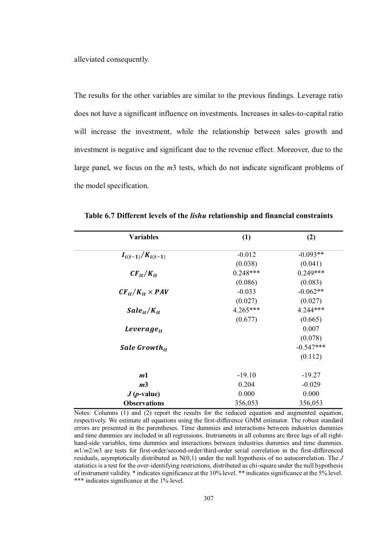
307
alleviated consequently.
The results for the other variables are similar to the previous findings. Leverage ratio
does not have a significant influence on investments. Increases in sales-to-capital ratio
will increase the investment, while the relationship between sales growth and
investment is negative and significant due to the revenue effect. Moreover, due to the
large panel, we focus on the m3 tests, which do not indicate significant problems of
the model specification.
Table 6.7 Different levels of the lishu relationship and financial constraints
Variables (1) (2)
𝑰𝒊(𝒕−𝟏) 𝑲𝒊(𝒕−𝟏)⁄ -0.012 -0.093** (0.038) (0.041)
𝑪𝑭𝒊𝒕 𝑲𝒊𝒕⁄ 0.248*** 0.249*** (0.086) (0.083)
𝑪𝑭𝒊𝒕 𝑲𝒊𝒕⁄ × 𝑷𝑨𝑽 -0.033 -0.062** (0.027) (0.027)
𝑺𝒂𝒍𝒆𝒊𝒕 𝑲𝒊𝒕⁄ 4.265*** 4.244*** (0.677) (0.665)
𝑳𝒆𝒗𝒆𝒓𝒂𝒈𝒆𝒊𝒕 0.007 (0.078)
𝑺𝒂𝒍𝒆 𝑮𝒓𝒐𝒘𝒕𝒉𝒊𝒕 -0.547*** (0.112)
m1 -19.10
-19.27
0 m3 0.204
-0.029
J (p-value) 0.000 0.000
Observations 356,053 356,053 Notes: Columns (1) and (2) report the results for the reduced equation and augmented equation, respectively. We estimate all equations using the first-difference GMM estimator. The robust standard errors are presented in the parentheses. Time dummies and interactions between industries dummies and time dummies are included in all regressions. Instruments in all columns are three lags of all right-hand-side variables, time dummies and interactions between industries dummies and time dummies. m1/m2/m3 are tests for first-order/second-order/third-order serial correlation in the first-differenced residuals, asymptotically distributed as N(0,1) under the null hypothesis of no autocorrelation. The J statistics is a test for the over-identifying restrictions, distributed as chi-square under the null hypothesis of instrument validity. * indicates significance at the 10% level. ** indicates significance at the 5% level. *** indicates significance at the 1% level.
308
6.6 Further tests
6.6.1 The lishu relationship and financial constraints by firm ownership
We firstly estimate the financial constraints and the extent to which a lishu relationship
affects financial constraints by different types of firms’ ownership. As we find that
around 94% of state-owned firms and 84% of collectively-owned firms are politically
affiliated, in Table 6.8, we only report the results for private firms (in column (1)),
which account for more than 60% of our full sample, and foreign firms (in column (2)),
which are generally the youngest and active firms in China.
Focusing on sub-columns (a) and (b) of private firms, and (I) and (II) of foreign firms,
we find that the coefficients on cash flow in all regressions are significant and positive,
indicating that financial constraints exist in private and foreign firms in China.
Interestingly, we observe that financial constraints are more severe in foreign firms
than in private firms. Looking at the augmented equation results for both firms (sub-
columns (b) and (II), respectively), we find that the coefficient on cash flow is
significant at the 10% level for private firms, while it is at the 1% level for foreign
firms. In particular, a one-standard-deviation increase in cash flow leads to a 7.918
increase in investment of foreign firms and a 6.404 increase in private firms. Evaluated
at the mean value of investment in each group, a one-standard-deviation increase in
cash flow creates an 85.29% increase for foreign firms and a 58.85% increase in
private firms.
309
Sub-columns (c) and (d) in column (1), and (III) and (IV) in column (2) report the
linkage between the lishu relationship and financial constraints of private and foreign
firms, respectively. Focusing on the coefficient on the interaction term between cash
flow and the lishu relationship, we find that it is negatively related to the
investment/capital ratio in all four regressions, suggesting that the lishu relationship
can alleviate financial constraints for both private and foreign firms. Especially, such
effect is more pronounced for foreign firms (significant at the 1% level) when
compared with private firms (significant at the 10% level). Particularly in the
augmented regressions for foreign firms, the overall cash flow coefficient for affiliated
firms is 0.159, while it is 0.281 for non-affiliated firms. Similar results are found for
other independent variables.

310
Table 6.8 The lishu relationship and financial constraints in China by ownership
Variables Private Firms
(1) Foreign Firms
(2) (a) (b) (c) (d) (I) (II) (III) (IV)
𝑰𝒊(𝒕−𝟏) 𝑲𝒊(𝒕−𝟏)⁄ -0.085*** -0.191*** -0.085*** -0.114** -0.032 -0.069 -0.022 -0.042 (0.005) (0.060) (0.005) (0.054) (0.062) (0.063) (0.064) (0.064)
𝑪𝑭𝒊𝒕 𝑲𝒊𝒕⁄ 0.286*** 0.187* 0.290*** 0.123* 0.238*** 0.209*** 0.298*** 0.281*** (0.045) (0.096) (0.050) (0.095) (0.078) (0.078) (0.086) (0.085)
𝑪𝑭𝒊𝒕 𝑲𝒊𝒕⁄ × 𝑷𝑨 -0.031 -0.024* -0.125** -0.122*** (0.041) (0.061) (0.049) (0.046)
𝑺𝒂𝒍𝒆𝒊𝒕 𝑲𝒊𝒕⁄ 4.727*** 4.590*** 4.759*** 4.133*** 2.016 1.686 2.158 1.769 (0.407) (0.754) (0.410) (0.694) (1.805) (1.320) (1.849) (1.357)
𝑳𝒆𝒗𝒆𝒓𝒂𝒈𝒆𝒊𝒕 0.063 0.042 0.120 0.120 (0.118) (0.106) (0.119) (0.122)
𝑺𝒂𝒍𝒆 𝑮𝒓𝒐𝒘𝒕𝒉𝒊𝒕 -0.882*** -0.632*** -0.205 -0.130 (0.171) (0.146) (0.135) (0.125)
m1 -68.16
-15.10
-67.36
-15.64
-10.56
-9.706
-10.57
-9.602
m2 1.539 1.550
m3 -0.022
-0.032
-0.011
0.285
-0.087
0.0460 J (p-value) 0.0000 0.417
0.000 0.000
0.000 0.000 0.000 0.000
Observations 215,269 215,269 215,269 215,269 69,781 69,781 69,781 69,781 Notes: Columns (1) and (2) report the results for private firms and foreign firms, respectively. Sub-columns (a) and (I) present the results for estimating Eq. (1) in each group. Sub-columns (b) and (II) report the results for estimating Eq. (2) in each group. Sub-columns (c) and (III) present the results for estimating Eq. (3) in each group. Sub-columns (d) and (IV) report the results for estimating Eq. (4) in each group. We estimate all equations using the first-difference GMM estimator. The robust standard errors are presented in the parentheses. Time dummies and interactions between industries dummies and time dummies are included in all regressions. Instruments in all columns are two and deeper lags of all right-hand-side variables, time dummies and interactions between industries dummies and time dummies. m1/m2/m3 are tests for first-order/second-order/third-order serial correlation in the first-differenced residuals, asymptotically distributed as N(0,1) under the null hypothesis of no autocorrelation. The J statistics is a test for the over-identifying restrictions, distributed as chi-square under the null hypothesis of instrument validity. * indicates significance at the 10% level. ** indicates significance at the 5% level. *** indicates significance at the 1% level.
311
6.6.2 The lishu relationship and financial constraints by region
Given China’s huge size and various geographic distributions, the regions have played
a vital role in the development and growth of the Chinese economy. In fact, most
regional development policies in China are based on three zones, i.e. the east, the
central, and the west.
Because of the reform and opening-up policy, firms locating in the east of China have
experienced fast development since the 1970s, which causes development divergences
between the coastal and inner regions. In order to reduce the regional inequalities and
balance the development across different regions, the Chinese government has
changed its development policies with a focus on the central and western regions. The
government implemented the “Development of the Western Region in China” (xi bu
da kai fa) in the late 1990s, and the “Rise of Central China Strategy” (zhong bu jue qi
zhan lve) in 2004. Supported by these national strategies, substantial financing has
been invested in environment, infrastructure, and energy and resource extraction in
those regions.
As the coastal region in China is the most developed and competitive market for firms,
they have to get involved in the severe competition for financial resources and other
benefits. In this case, firms in the eastern provinces are more prone to rely on their own
internal financing than firms in the central and western provinces. Therefore, firms in
the eastern region are more likely to be financially constrained (Chen, 2008; Guariglia
et al., 2011).

312
We test the Hypotheses 1 and 2 in the three regional groups and report our results in
Table 6.9.1 Column (1) presents the results of the coastal region, column (2) reports
the results of the central region, and the results of the western region are presented in
column (3). We find that the sensitivity of investment to the internal funds is significant
for firms in the eastern and central regions than those in the western region. This can
be attributed to the fact that the central development policy has been carried out by the
Chinese government only since 2004. Given our sample period, which is from 2002 to
2007, it may not have enough time for us to observe the significant effect of this policy.
Furthermore, focusing on the interaction term, we find that, for those firms with
financial constraints in the coastal and central regions, the lishu relationship can reduce
the cash flow-investment sensitivity.
1 We only report the results by estimating the augmented equations, and present the results by estimating the reduced equations in the Appendix.
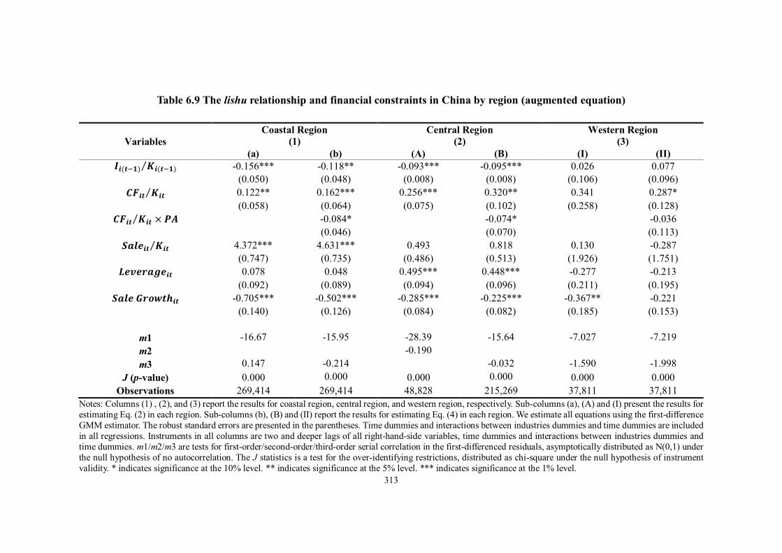
313
Table 6.9 The lishu relationship and financial constraints in China by region (augmented equation)
Variables Coastal Region
(1) Central Region
(2) Western Region
(3) (a) (b) (A) (B) (I) (II)
𝑰𝒊(𝒕−𝟏) 𝑲𝒊(𝒕−𝟏)⁄ -0.156*** -0.118** -0.093*** -0.095*** 0.026 0.077 (0.050) (0.048) (0.008) (0.008) (0.106) (0.096)
𝑪𝑭𝒊𝒕 𝑲𝒊𝒕⁄ 0.122** 0.162*** 0.256*** 0.320** 0.341 0.287* (0.058) (0.064) (0.075) (0.102) (0.258) (0.128)
𝑪𝑭𝒊𝒕 𝑲𝒊𝒕⁄ × 𝑷𝑨 -0.084* -0.074* -0.036 (0.046) (0.070) (0.113)
𝑺𝒂𝒍𝒆𝒊𝒕 𝑲𝒊𝒕⁄ 4.372*** 4.631*** 0.493 0.818 0.130 -0.287 (0.747) (0.735) (0.486) (0.513) (1.926) (1.751)
𝑳𝒆𝒗𝒆𝒓𝒂𝒈𝒆𝒊𝒕 0.078 0.048 0.495*** 0.448*** -0.277 -0.213 (0.092) (0.089) (0.094) (0.096) (0.211) (0.195)
𝑺𝒂𝒍𝒆 𝑮𝒓𝒐𝒘𝒕𝒉𝒊𝒕 -0.705*** -0.502*** -0.285*** -0.225*** -0.367** -0.221 (0.140) (0.126) (0.084) (0.082) (0.185) (0.153)
m1 -16.67
-15.95
-28.39
-15.64
-7.027
-7.219 m2 -0.190
m3 0.147
-0.214
-0.032
-1.590
-1.998 J (p-value) 0.000 0.000
0.000 0.000
0.000 0.000
Observations 269,414 269,414 48,828 215,269 37,811 37,811 Notes: Columns (1) , (2), and (3) report the results for coastal region, central region, and western region, respectively. Sub-columns (a), (A) and (I) present the results for estimating Eq. (2) in each region. Sub-columns (b), (B) and (II) report the results for estimating Eq. (4) in each region. We estimate all equations using the first-difference GMM estimator. The robust standard errors are presented in the parentheses. Time dummies and interactions between industries dummies and time dummies are included in all regressions. Instruments in all columns are two and deeper lags of all right-hand-side variables, time dummies and interactions between industries dummies and time dummies. m1/m2/m3 are tests for first-order/second-order/third-order serial correlation in the first-differenced residuals, asymptotically distributed as N(0,1) under the null hypothesis of no autocorrelation. The J statistics is a test for the over-identifying restrictions, distributed as chi-square under the null hypothesis of instrument validity. * indicates significance at the 10% level. ** indicates significance at the 5% level. *** indicates significance at the 1% level.
314
6.7 Conclusion
The impacts of financial constraints on firms’ investment activities have been
substantially explored since FHP (1988), which for the first time that it was pointed
out that the sensitivity of investment to cash flow can be regarded as an indicator of
financial constraints. The existing studies on financial constraints have been extended
to inventory investment, R&D investment, employment demand, and the growth of
firms. Most literature estimating the links between political connections and financial
constraints focuses on the developed countries. Some literature explores the
developing countries, but with a focus on Thailand, Pakistan, and Malaysia. However,
these studies define political connections either as state ownership or the linkage
established by entrepreneurs’ political participation. Our study fills the gap in the
literature testing the effects of political connections, in the context of the lishu
relationship, on the cash flow-investment sensitivity for Chinese unlisted firms.
We use a comprehensive firm-level dataset from 2002 to 2007 provided by the NBS,
which includes 105,487 mainly unlisted firms from 31 provinces or province-
equivalent municipal cities all across China. We demonstrate that Chinese firms
confront financial constraints and can mitigate their cash flow-investment sensitivity
through the lishu relationship. Moreover, this effect is more significant to the firms
affiliated with a high level of government. We also find that compared with private
firms, foreign firms are more likely to encounter financial constraints; therefore, the
lishu relationship can reduce their financial constraints significantly. Furthermore,
firms locating in the western region have the least sensitivity of investment to the
315
availability of internal financing due to the implement of the regional development
policies. However, the lishu relationship can help firms in the central and coastal
regions alleviate financial constraints.
Our findings confirm the “lending bias” and “political pecking order” existing in the
Chinese capital market. One of the implications for Chinese firms is that they can
diminish financial constraints by the lishu relationship with the governments. In
addition, the higher level of government they can affiliate with, the more investment-
cash flow sensitivity they can reduce. In addition, the Chinese governments should
also develop policies to mitigate financing obstacles for the financially constrained
firms and the firms with a lower level of political affiliation. Non-banking financial
institutions, such as trust, security, insurance, financial leasing, rural credit
cooperatives, and financial companies, should be established to improve the financial
system and reduce financial constraints for Chinese unlisted firms.
Further research can be undertaken from the following directions. Firstly, it would be
interesting to test other models, such as the error-correction model and Euler equation
model. Secondly, it would be interesting to investigate the links between the lishu
relationship and other types of investment activities. Thirdly, it also would be worthy
of incorporating investments in net working capital (NWC), particularly in the context
of China.
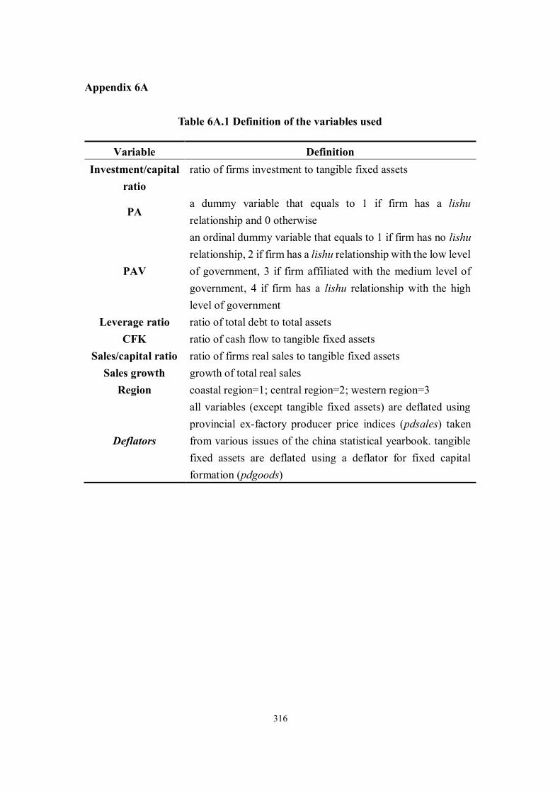
316
Appendix 6A
Table 6A.1 Definition of the variables used
Variable Definition Investment/capital
ratio ratio of firms investment to tangible fixed assets
PA a dummy variable that equals to 1 if firm has a lishu relationship and 0 otherwise
PAV
an ordinal dummy variable that equals to 1 if firm has no lishu relationship, 2 if firm has a lishu relationship with the low level of government, 3 if firm affiliated with the medium level of government, 4 if firm has a lishu relationship with the high level of government
Leverage ratio ratio of total debt to total assets CFK ratio of cash flow to tangible fixed assets
Sales/capital ratio ratio of firms real sales to tangible fixed assets Sales growth growth of total real sales
Region coastal region=1; central region=2; western region=3
Deflators
all variables (except tangible fixed assets) are deflated using provincial ex-factory producer price indices (pdsales) taken from various issues of the china statistical yearbook. tangible fixed assets are deflated using a deflator for fixed capital formation (pdgoods)
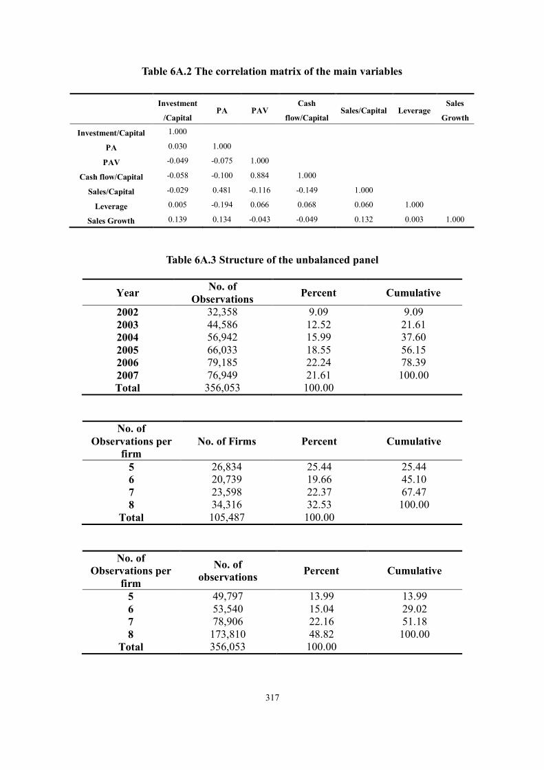
317
Table 6A.2 The correlation matrix of the main variables
Table 6A.3 Structure of the unbalanced panel
Year No. of Observations Percent Cumulative
2002 32,358 9.09 9.09 2003 44,586 12.52 21.61 2004 56,942 15.99 37.60 2005 66,033 18.55 56.15 2006 79,185 22.24 78.39 2007 76,949 21.61 100.00 Total 356,053 100.00
No. of Observations per
firm No. of Firms Percent Cumulative
5 26,834 25.44 25.44 6 20,739 19.66 45.10 7 23,598 22.37 67.47 8 34,316 32.53 100.00
Total 105,487 100.00
No. of Observations per
firm
No. of observations Percent Cumulative
5 49,797 13.99 13.99 6 53,540 15.04 29.02 7 78,906 22.16 51.18 8 173,810 48.82 100.00
Total 356,053 100.00
Investment
/Capital PA PAV
Cash
flow/Capital Sales/Capital Leverage
Sales
Growth
Investment/Capital 1.000
PA 0.030 1.000
PAV -0.049 -0.075 1.000
Cash flow/Capital -0.058 -0.100 0.884 1.000
Sales/Capital -0.029 0.481 -0.116 -0.149 1.000
Leverage 0.005 -0.194 0.066 0.068 0.060 1.000
Sales Growth 0.139 0.134 -0.043 -0.049 0.132 0.003 1.000
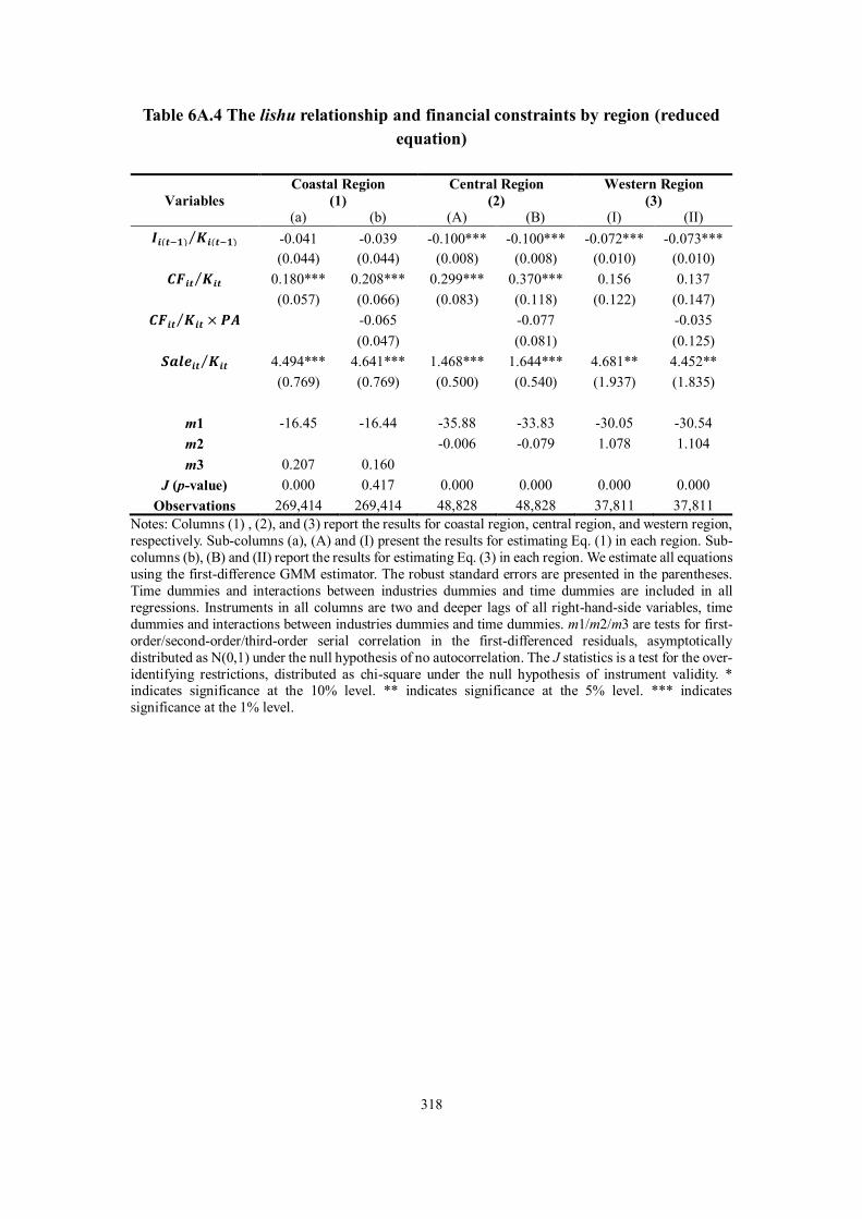
318
Table 6A.4 The lishu relationship and financial constraints by region (reduced equation)
Variables Coastal Region
(1) Central Region
(2) Western Region
(3) (a) (b) (A) (B) (I) (II)
𝑰𝒊(𝒕−𝟏) 𝑲𝒊(𝒕−𝟏)⁄ -0.041 -0.039 -0.100*** -0.100*** -0.072*** -0.073*** (0.044) (0.044) (0.008) (0.008) (0.010) (0.010)
𝑪𝑭𝒊𝒕 𝑲𝒊𝒕⁄ 0.180*** 0.208*** 0.299*** 0.370*** 0.156 0.137 (0.057) (0.066) (0.083) (0.118) (0.122) (0.147)
𝑪𝑭𝒊𝒕 𝑲𝒊𝒕⁄ × 𝑷𝑨 -0.065 -0.077 -0.035 (0.047) (0.081) (0.125)
𝑺𝒂𝒍𝒆𝒊𝒕 𝑲𝒊𝒕⁄ 4.494*** 4.641*** 1.468*** 1.644*** 4.681** 4.452** (0.769) (0.769) (0.500) (0.540) (1.937) (1.835)
m1 -16.45
-16.44
-35.88
-33.83
-30.05 -30.54 m2 -0.006
-0.079
1.078 1.104
m3 0.207
0.160
J (p-value) 0.000 0.417
0.000 0.000
0.000 0.000
Observations 269,414 269,414 48,828 48,828 37,811 37,811 Notes: Columns (1) , (2), and (3) report the results for coastal region, central region, and western region, respectively. Sub-columns (a), (A) and (I) present the results for estimating Eq. (1) in each region. Sub-columns (b), (B) and (II) report the results for estimating Eq. (3) in each region. We estimate all equations using the first-difference GMM estimator. The robust standard errors are presented in the parentheses. Time dummies and interactions between industries dummies and time dummies are included in all regressions. Instruments in all columns are two and deeper lags of all right-hand-side variables, time dummies and interactions between industries dummies and time dummies. m1/m2/m3 are tests for first-order/second-order/third-order serial correlation in the first-differenced residuals, asymptotically distributed as N(0,1) under the null hypothesis of no autocorrelation. The J statistics is a test for the over-identifying restrictions, distributed as chi-square under the null hypothesis of instrument validity. * indicates significance at the 10% level. ** indicates significance at the 5% level. *** indicates significance at the 1% level.

319
CHAPTER 7 CONCLUSION
This chapter concludes the thesis. A summary of the findings is presented in section
7.1. Section 7.2 raises the implications of this research. Limitations of this study and
recommendations for future research are discussed in section 7.3.
7.1 Summary of findings
The lishu relationship is a unique kind of political connections, which only exists in
China. Through this relationship, the government can control the firms legally and
directly, while the affiliated firms can obtain favourable support from the government
and develop smoothly under the market economy with Chinese characteristics.
However, as a unique institutional variation of importance, the lishu relationship has
received the least attention in previous research. For the first time in literature, Chapter
2 provides the political and economic background of this relationship, explores its
different meanings under the different economic development stages in China,
introduces the procedures of establishing, changing, and terminating this relationship,
and explores the difference between the lishu relationship and ownership structure.
The dataset we use in this thesis is presented in Chapter 3. The dataset is drawn from
the NBS (National Bureau of Statistics of China) from 2000 to 2007, which covers
more than 100,000 mainly unlisted manufacturing firms from 31 provinces or
province-equivalent municipal cities. This thesis investigates the determinants and
effects of the lishu relationship between Chinese manufacturing enterprises and

320
central, provincial, or local governments. This thesis comprises three main empirical
studies. In particular, we examine the determinants of the lishu relationship, the links
between the lishu relationship and firms’ exporting, and the effects of the lishu
relationship on firms’ financial constraints.
Chapter 4, being the first empirical part, explores what types of firms are more likely
to have political affiliation. This is an important question, but has been overlooked in
the existing literature. We find that the older and larger firms are prone to have a lishu
relationship, while the firms with foreign ownership and locating in the east of China
are less likely to affiliate with the governments. Financially healthy firms are more
likely to have the lishu relationship. However, firms with high profitability and sales
growth do not show such preference. Furthermore, we find that firms are more
inclined to have connections with the medium level of governments. We attribute this
finding to the fact that the governments can provide the affiliated firms with the
important resources and high flexibilities at the same time. Similar results are found
by looking at the types of ownership and the locations of firms. Particularly, the
magnitude of marginal effects is larger for private firms than that for foreign firms.
Moreover, we do not find that cash flow is a precise determinant to the firms in the
central and western regions. This can be explained by the fact that firms in these
regions have received preferential financial supports due to the Chinese regional
development policies. Therefore, these firms have less dependence on their internal
funding.
In Chapter 5, we estimate dynamic models for both the propensity and intensity of

321
exports of Chinese manufacturing firms. We employ the pooled Probit and Tobit
models, clustering observations by firms ID, as well as random-effects Probit and
Tobit models, respectively. Furthermore, we take into account of the sunk entry costs,
unobserved firm heterogeneity, and the initial conditions problem. It is supposed to be
the first study that estimates both firms’ exporting probability and intensity for the
unlisted Chinese firms from the perspective of the lishu relationship. We reveal that
sunk entry costs exist in firms’ exporting behaviour. Moreover, the overestimation of
the size of the sunk entry costs can be alleviated by controlling the initial conditions
problem appropriately. In addition, we find that the politically affiliated firms are less
likely to participate in the export markets and export less once they enter these markets.
This can be attributed to the political and social goals the affiliated firms have
responsibilities to achieve, which in turn restricts the firms’ capability to
internationalise. Interestingly, this negative effect is only significant to the firms
affiliated with low or medium level of governments. We also find that firm size, total
factor productivity, financial factors, ownership structure, and location are the
significant determinants of firms’ exporting activities.
Chapter 6 focuses on the relations between the lishu relationship and firms’ financial
constraints, proxied by the sensitivity of investment to internal funds. We document
that the investments of Chinese firms significantly depend on the availability of cash
flow, suggesting that financial constraints exist in the context of China. We further
find that by the lishu relationship, firms can alleviate such constraints. This effect is
more significant for the firms affiliated with a higher level of government. We also
find that, when compared with the private firms, the lishu relationship can reduce the
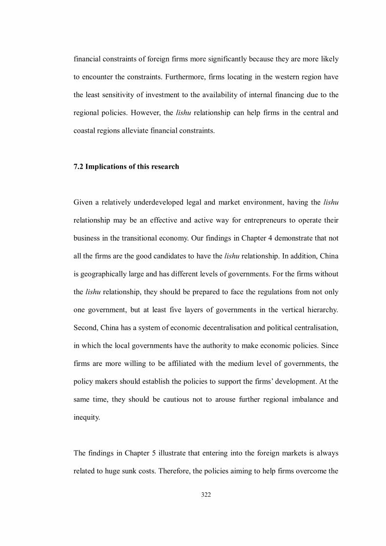
322
financial constraints of foreign firms more significantly because they are more likely
to encounter the constraints. Furthermore, firms locating in the western region have
the least sensitivity of investment to the availability of internal financing due to the
regional policies. However, the lishu relationship can help firms in the central and
coastal regions alleviate financial constraints.
7.2 Implications of this research
Given a relatively underdeveloped legal and market environment, having the lishu
relationship may be an effective and active way for entrepreneurs to operate their
business in the transitional economy. Our findings in Chapter 4 demonstrate that not
all the firms are the good candidates to have the lishu relationship. In addition, China
is geographically large and has different levels of governments. For the firms without
the lishu relationship, they should be prepared to face the regulations from not only
one government, but at least five layers of governments in the vertical hierarchy.
Second, China has a system of economic decentralisation and political centralisation,
in which the local governments have the authority to make economic policies. Since
firms are more willing to be affiliated with the medium level of governments, the
policy makers should establish the policies to support the firms’ development. At the
same time, they should be cautious not to arouse further regional imbalance and
inequity.
The findings in Chapter 5 illustrate that entering into the foreign markets is always
related to huge sunk costs. Therefore, the policies aiming to help firms overcome the
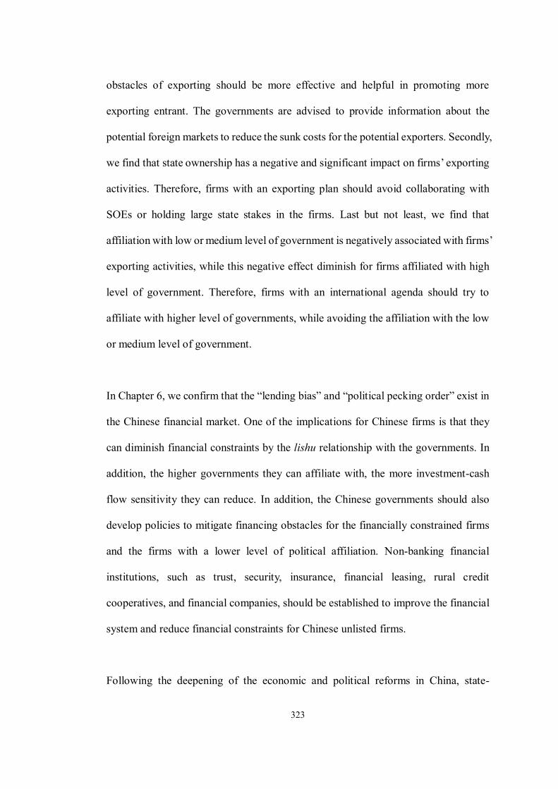
323
obstacles of exporting should be more effective and helpful in promoting more
exporting entrant. The governments are advised to provide information about the
potential foreign markets to reduce the sunk costs for the potential exporters. Secondly,
we find that state ownership has a negative and significant impact on firms’ exporting
activities. Therefore, firms with an exporting plan should avoid collaborating with
SOEs or holding large state stakes in the firms. Last but not least, we find that
affiliation with low or medium level of government is negatively associated with firms’
exporting activities, while this negative effect diminish for firms affiliated with high
level of government. Therefore, firms with an international agenda should try to
affiliate with higher level of governments, while avoiding the affiliation with the low
or medium level of government.
In Chapter 6, we confirm that the “lending bias” and “political pecking order” exist in
the Chinese financial market. One of the implications for Chinese firms is that they
can diminish financial constraints by the lishu relationship with the governments. In
addition, the higher governments they can affiliate with, the more investment-cash
flow sensitivity they can reduce. In addition, the Chinese governments should also
develop policies to mitigate financing obstacles for the financially constrained firms
and the firms with a lower level of political affiliation. Non-banking financial
institutions, such as trust, security, insurance, financial leasing, rural credit
cooperatives, and financial companies, should be established to improve the financial
system and reduce financial constraints for Chinese unlisted firms.
Following the deepening of the economic and political reforms in China, state-
324
ownership has witnessed a decrease in recent years. Private enterprises are expected
to play a more important and active role in every aspect of the country’s development.
Under the current socialism political regime with the Chinese characteristics, the
economic system in China is neither centrally planned nor market-based. According
to the main findings in our three empirical chapters, as a part of an administrative
strategy, the lishu relationship should be assessed carefully before deciding how to
establish an efficient lishu relationship. To achieve the harmonious development
national widely, the Chinese governments should establish new policies and
regulations to alleviate the financial constraints, reduce large sunk entry costs for
exporters, and balance the development across different political affiliation groups,
ownership types, and regions.
7.3 Limitations of the study and the proposed future research
One of the limitations of this study results from the period covered in this dataset.
Although the original panel data covers a relatively long period from 2000 to 2007, it
does not include the data since 2008. As the global financial crisis swept all over the
world during 2008 and 2009, Chinese firms have also experienced a decline in firm
performance and exporting. Therefore, it would be of interest to examine whether the
politically affiliated firms performed differently compared with the unaffiliated
counterparts during the crisis.
Secondly, we do not employ the IV Probit or Tobit estimator in Chapters 4 and 5,
because it requires that the endogenous regressors are continuous and cannot be
325
applied when the categorical variables are included as regressors. Therefore, it would
be prudent to test whether these results are robust by using other methods, for example,
the special regressor estimator proposed by Lewbel (2000). Compared with the IV
Porbit or Tobit model, the special regressor allows discrete or limited endogenous
regressor. Baum (2012) develops the –sspecialreg- command in Stata. In this case,
future research can be done by employing new estimation methods.
Thirdly, in Chapter 6, it would be interesting to test whether the results remain robust
if other models are applied, such as the error-correction model and Euler equation
model (Bond et al., 2003; Guariglia, 2008). It also would be worthy of incorporating
investments in net working capital (NWC), particularly in the context of China.
326
REFERENCES Abel, A. B. and Eberly, J. (2003). Q theory Without Adjustment Costs & Cash Flow Effects Without Financing Constraints. 2004 Meeting Papers No. 205, Society for Economic Dynamics. Adhikari, A., Derashid, C. and Zhang, H. (2006). Public Policy, Political Connections, and Effective Tax Rates: Longitudinal Evidence from Malaysia. Journal of Accounting and Public Policy, 25(2006), 574-595. Agrawal, A. and Knoeber, C. R. (2001). Do Some Outside Directors Play a Political Role? Journal of Law and Economics, 44(1), 179-198. Aitken, B., Hanson, G. H., Harrison, A. E. (1997). Spillovers, Foreign Investment, and Export Behavior. Journal of International Economics, 43 (1-2), 103-132. Albarran, P., R. Carrasco, and A. Holl (2013). Domestic transport infrastructure and Firms’ Export Market Participation. Small Business Economics, 40(4), 879-898. Albaum, G. and Peterson, R. A. (1984). Empirical Research in International Marketing: 1976-1982. Journal of International Business Studies, 15 (1), 161-173.
Alessandria, G. and Choi, H. (2007). Do Sunk Costs of Exporting Matter for Net Export Dynamics?. The Quarterly Journal of Economics, 122 (1), 289-336. Allayannis, G. and Mozumdar, A. (2004). The Impact of Negative Cash Flow and Influential Observations on Investment-cash Flow Sensitivity Estimates. Journal of Banking and Finance, 28, 901-930. Allen, F., Qian, J. and Qian, M. (2005). Law, Finance, and Economic Growth in China. Journal of Financial Economics, 77 (2005), 57-116. Alti, A., (2003). How Sensitive is Investment to Cash Flow When Financing is Frictionless?. The Journal of Finance. 58 (2), 707-722. Amiti, M. and Weinstein, D. E. (2011). Exports and Financial Shocks. Quarterly Journal of Economics, 126 (4), 1841-1877.
327
Anderson, J. E. and Marcouiller D. (2002). Insecurity and the Pattern of Trade: an Empirical Investigation. Review of Economics and Statistics, 84 (2), 342-352. Anderson, J. E. and Young, L. (2006). Trade and Contract Enforcement. Contributions to Economic Analysis and Policy, 5 (1), 1-33. Arellano, M. and Bond, S. (1991). Some Tests of Specification for Panel Data: Monte Carlo Evidence and an Application to Employment Equations. Review of Economic Studies, 58 (2), 277-297. Aw, B.Y., Chung, S. and Roberts, M.J. (2000). Productivity and Turnover in the Export Market: Micro Evidence from the Republic of Korea and Taiwan (China). World Bank Economic Review, 14, 65-90. Ayyagari, M., Demirgüç-Kunt, A., Maksimovic, V. (2010). Formal Versus Informal Finance: Evidence from China. Review of Financial Studies, 23, 3048-3097. Ayyagari, M., Demirguc-Kunt, A. and Maksimovic, V. (2012). Financing of Firms in Developing Countries: Lessons from Research. The World Bank Policy Research Working Paper Series 6036. Bai, C., Lu, J. and Tao, Z. (2005). An Empirical Study on the Access to Bank Loans by Private Enterprises in China. China Economic Quarterly, 4(3), 605-622. Bai, C.E., and L. C. Xu. (2005). Incentives for CEOs with Multitasks: Evidence from Chinese State-Owned Enterprises. Journal of Comparative Economics, 33 (3), 517-539. Bai, C.E., Lu, J. and Tao, Z. (2006). The Multitask Theory of State Enterprise Reform: Empirical Evidence from China. The American Economic Review, 96 (2), 353-357. Bai, Y and Ren, B. (2007). The Economy Theory and Practice in Chinese Market. Beijing: Higher Education Press. Baldauf, A., Cravens, D. W. and Wagner, U. (2000). Examining Determinants of Export Performance in Small Open Economies. Journal of World Business, 35 (1), 61-79. Baldwin, J. R. and Gu, W. (2003). Export-Market Participation and Productivity Performance in Canadian Manufacturing. Canadian Journal of Economic, 36(3), 634-657.

328
Baldwin, J.R. and Hanel, P. (2003). Innovation and Knowledge Creation in an Open Economy: Canadian Industry and International Implications. Cambridge: Cambridge University Press. Barrios, S., Gorg, H. and Strobl, E. (2003). Explaining Firms’ Export Behaviour: R&D, Spillovers and the Destination Market. Oxford Bulletin of Economic and Statistics, 65 (4), 475-496. Bartels, L. and Brady, H. (2003). Economic Behaviour in Political Context. The American Economic Review, 93, 156-161. Baum, C. F. (2012) SSPECIALREG: Stata Module to Estimate Binary Choice Model with Discrete Endogenous Regressor via Special Regressor Method. Available at: https://ideas.repec.org/c/boc/bocode/s457546.html Becchetti, L. and Rossi, S. P. S. (2000). The Positive Effect of Industrial District on the Export Performance of Italian Firms. Review of Industrial Organization, 16, 53-68. Beck, T., Demirgüç-Kunt, A. and Maksimovic, V. (2008). Financing Patterns Around the World: Are Small Firms Different?. Journal of Financial Economics, 89(3), 467-487. Beck, T., Demirgüç-Kunt, A., Laeven, L. and Maksimovic, V. (2006). The Determinants of Financing Obstacles. Journal of International Money and Finance, 25(6), 932-952. Belka, M. and Estrin, S., Schaffer, M. E. and Singh, I. J. (1995). Enterprise Adjustment in Poland: Evidence from a Survey of 200 Private, Privatised, and State-Owned Firms. Centre for Economic Performance Discussion Paper. No. 233. Bellone, F., Musso, P., Nesta, L. and Schiavo, S. (2010). Financial Constraints and Firm Export Behaviour. The World Economy, 33 (3), 347-373. Benito, A. (2005). Financial Pressure, Monetary Policy Effects and Inventories: Firm-Level Evidence from a Market-based and a Bank-based Financial System. Economica, 72, 201-224. Bentley, A. F. (1995). The Process of Government: A Study of Social Pressures. Chicago:
329
University of Chicago Press. Berman, N. and Héricourt, J. (2010). Financial Factors and the Margins of Trade: Evidence from Cross-country Firm-level Data. Journal of Development Economics, 93 (2), 206-217. Bernanke, B., Gertler, M. and Gilchrist, S. (1996). The Financial Accelerator and then Flight to Quality. The Review of Economics and Statistics, 78, 1-15. Bernard, A.B., Jensen, J.B. (1995). Exporters, Jobs, and Wages in U.S. Manufacturing, 1976–1987. Bookings Papers on Economic Activity, Microeconomics. Bernard, A. B. and Jensen, J. B. (1999). Exceptional Exporter Performance: Cause, Effect or Both? Journal of International Economics, 47(1), 1-25. Bernard, A. B. and Jensen, J. B. (2004). Why Some Firms Export?. The Review of Economics and Statistics, 86(2), 561-569. Bernard, A. B. and Wagner, J. (2001). Export Entry and Exit by German Firms. Review of World Economics, 137 (1), 105-123. Bernard, A. B., J. B. Jensen, S. J. Redding, and P. K. Schott (2007). Firms in International Trade. Journal of Economic Perspectives 21(3), 105-130. Bernheim, B. and Whinston, M. (1986). Menu Auctions, Resource Allocation, and Economic Influence. The Quarterly Journal of Economics, 101 (1), 1-31. Bertrand, M., Kramaraz, F., Schoar, A. and Thesmar, D. (2006). Politicians, Firms and the Political Business Cycle: Evidence from France. University of Chicago Working Paper. Bhaduri, S., and Ray, A. (2004). Exporting Through Technological Capability: Econometric Evidence from India’s Pharmaceutical and Electrical/Electronics Firms. Oxford Development Studies, 32(1), 87-100. Black, B. S., Jang, H. and Kim, W. (2006). Predicting Firms' Corporate Governance Choices: Evidence from Korea. Journal of Corporate Finance, 12 (3), 660-691.

330
Blalock, G. and Gertler, P.J. (2004). Learning from Exporting Revisited in a Less Developed Setting. Journal of Development Economics, 75, 397-416. Blau, B. M., Brough, T. J. and Thomas, D. W. (2013). Corporate Lobbying, Political Connections, and the Bailout of Banks. Journal of Banking and Finance, 37(8), 3007-3017. Bloch, C. (2005). R&D Investment and Internal Finance: the Cash Flow Effect. Economics of Innovation and New Technology, 14 (3), 213-223. Blundell, R. and Bond, S. (1998). Initial Conditions and Moment Restrictions in Dynamic Panel Data Models. Journal of Econometrics, 87(1), 115-143. Blundell, R., Bond, S., Devereux, M. and Schiantarelli, F. (1992). Investment and Tobin's Q: Evidence from Company Panel Data. Journal of Econometrics, 51, 233-257. Boardman, A. E. and Vining, A. R. (1989). Ownership and Performance in Competitive Environments: A Comparison of the Performance of Private, Mixed, and State-Owned Enterprises. Journal of Law and Economics, 32(32), 1-33. Boddin, D., Raff, H. and Trofimenko, N. (2015). Foreign Ownership and the Export and Import Propensities of Developing-country Firms. Kiel Working Paper No. 1995. Bøhren, O. and Ødegaard, B., (2003). Governance and performance revisited. European Corporate Governance Institute Working Paper No. 28/2003. Bonaccorsi, A. (1992). On the Relationship between Firm Size and Export Intensity. Journal of International Business Studies, 23(4), 605-636. Bond, S. and Van Reenen, J. (2007). Microeconometric Models of Investment and Employment. Handbook of Econometrics, 6, 4417-4498. Bond, S. and Cummins, J. (2001). Noisy Share Prices and the Q Model of Investment. Institute for Fiscal Studies Discussion Paper No. 22. Bond, S. and Meghir, C. (1994). Dynamic Investment Models and the Firm's Financial Policy. Review of Economic Studies, 61, 197-222.
331
Bond, S., Elston, J., Mairesse, J. and Mulkay, B. (2003). Financial Factors and Investment in Belgium, France, Germany, and the United Kingdom: a Comparison Using Company Panel Data. Review of Economics and Statistics, 85, 153-165. Bond, S., Harhof, D. and Van R. J. (2005). Investment, R&D and financial constraints in Britain and Germany. Annales d'Economie et de Statistique, 79/80, 433-460. Bond, S., Klemm, A., Newton-Smith, R., Syed, M. and Vlieghe, G. (2004). The Roles of Expected Profitability, Tobin’s Q and Cash Flow in Econometric Models of Company Investment. Bank in England Working Paper No. 222. Borst, N., and Lardy, N. (2015). Maintaining Financial Stability in the People's Republic of China during Financial Liberalization. Peterson Institute for International Economics Working Paper, 15-4. Boubakri, N., Cosset, J. C. and Saffar, W. (2008) Political Connections of Newly Privatized Firms. Journal of Corporate Finance, 14(5), 654-673. Brandt, L. and Li, H. (2003). Bank Discrimination in Transition Economies: Ideology, Information, or Incentives? Journal of Comparative Economics. 31(3), 387-413. Brandt, L., Li, H. and Roberts, J. (2005). Banks and Enterprise Privatization in China. Journal of Law, Economics, and Organization, 21(2), 524-546. Bridges, S. and Guariglia, A. (2008). Financial Constraints, Global Engagement, and Firm Survival in the United Kingdom: Evidence from Micro Data. Scottish Journal of Political Economy, 55 (4), 444-464. Brouthers, L. E. and Nakos, G. (2005). The Role of Systematic International Market Selection on Small Firms’ Export Performance. Journal of Small Business Management, 43 (4), 363-381. Brown, J. R. and Petersen, B. C. (2009). Why has the Investment-cash Flow Sensitivity Declined So Sharply? Rising R&D and Equity Market Developments. Journal of Banking and Finance, 33(5), 971-984. Brown, L. D. and Caylor, M. L. (2006). Corporate Governance and Firm Valuation. Journal of Accounting and Public Policy, 25 (4), 409-434.

332
Brunetti, A., Kisunko, G. and Weder, B. (1997). Institutional Obstacles to Doing Business: Region-by-Region Results from a Worldwide Survey of the Private Sector. World Bank PRD Working, 1759. Bugamelli, M. and L. Infante (2003). Sunk Costs to Exports: A Role for Industrial Districts? Local Economies and Internationalization in Italy Conference, 343-372. Bunkanwanicha, P. and Wiwattanakantang, Y. (2009). Big Business Owners in Politics. Review of Financial Studies, 22 (6), 2133-2168. Buono, I. and Fadinger, H. (2012). The Micro Dynamics of Exporting: Evidence from French Firms. Bank of Italy Temi di Discussione (Working Paper) No,880. Calof, J. L. (1994). The Relationship between Firm Size and Export Behaviour Revisited. Journal of International Business Studies, 25 (2), 367-387. Calomiris, C., Hubbard, G. and Watchel, P. (1995). Commercial Paper, Corporate Finance, and the Business Cycle: a Microeconomic Perspective. Carnegie-Rochester Conference Series on Public Policy, 42, 203-250. Cameron, A. C. and Trivedi, P. K. (2010). Microeconometrics Using Stata. Texas: Stata Press. Campa, J. M., (2004). Exchange Rates and Trade: How Important is Hysteresis in Trade? European Economic Review, 48, 527-548. Campa, J. M. and Shaver, J. M. (2002). Exporting and Capital Investment: on the Strategic Behavior of Exporters. IESE Business School, University of Navarra, Discussion Paper, (469). Campbell, T. S. (1979). Optimal Investment Financing Decisions and the Value of Confidentiality, Journal of Financial and Quantitative Analysis, 14, 913-924. Cantor, R. (1990). Effects of leverage on Corporate Investment and Hiring Decisions. FRBNY Quarterly Review, (1990), 31-41. Carey, M., Post, M. and Sharpe, S. A. (1998). Does Corporate Lending by Banks and Finance Companies Differ? Evidence on Specialization in Private Debt Contracting.

333
The Journal of Finance, 53 (3), 845-878. Carpenter, R. and Guariglia, A. (2007). Investment Behaviour, Observable Expectations, and Internal Funds: a Comment on Cummins, Hassett, and Oliner. Economics Bulletin, 5 (12), 1-12. Carpenter, R. E. and Guariglia, A. (2008). Cash Flow, Investment, and Investment Opportunities: New Tests using UK Panel Data. Journal of Banking and Finance, 32 (2008), 1894-1906. Carpenter, R. E. and Petersen, B. C. (2002). Is the Growth of Small Firms Constrained by Internal Finance?. The Review of Economics and Statistics, 84(2), 298-309. Carpenter, R., Fazzari, S. and Petersen, B. (1994). Inventory (Dis)investment, Internal Finance Fluctuations, and the Business Cycle. Brookings Papers in Economic Activity, 2, 75-122. Carpenter, R., Fazzari, S. and Petersen, B. (1998). Financing Constraints and Inventory Investment: a Comparative Study with High-frequency Panel Data. Review of Economics and Statistics, 80, 513-519. Chamberlain, G. (1984). ‘Panel Data’. in Griliches Z. and Intrilligator M. (eds), Handbook of Econometrics (1st edn), Volume 2, Amsterdam: North-Holland Elsevier, 1247-318. Chan, H.L. (1992). Private entrepreneurs in the People’s Republic of China. Proceedings of the ENDEC World Conference on Entrepreneurship, 248-253. Chan, K. S., Dang, V. Q. and Yan, I. K. (2012a). Chinese Firms’ Political Connection, Ownership, and Financing Constraints. Economics Letters, 115(2), 164-167. Chan, K. S., Dang, V. Q. and Yan, I. K. (2012b). Financial Reform and Financing Constraints: Some Evidence from Listed Chinese Firms. China Economic Review, 23(2), 482-497. Chaney, P. K., Faccio, M. and Parsley, D. (2011). The Quality of Accounting Information in Politically Connected Firms. Journal of Accounting and Economics, 51(1), 58-76.
334
Chaney, T. (2013). Liquidity Constrained Exporters. NBER Working Paper No. 19170. Chang, C. and Wang, Y. (1994). The Nature of the Township-village Enterprise. Journal of Comparative Economics, 19(3), 434-452. Charumilind, C., Kali, R. and Wiwattanakantang, Y. (2006). Connected Lending: Thailand before the Financial Crisis. The Journal of Business, 79(1), 181-218. Che, J. and Qian, Y. (1998). Institutional Environment, Community Government, and Corporate Governance: Understanding China’s Township-village Enterprises. Journal of Law, Economics, and Organization, 14(1), 1–23. Chen, C. J. P., Ding, Y. and Kim, C. (2010). High-Level Politically Connected Firms, Corruption, and Analyst Forecast Accuracy around the World. Journal of International Business Studies, 41(9), 1505-1524. Chen, C., Li, Z. and Su, X. (2005). Rent Seeking Incentives, Political Connections and Organizational Structure: Empirical Evidence from Listed Family Firms in China. City University of Hong Kong Working Paper. Chen, M. (2008). Financial Constraints to the Investment of Chinese Listed Firms across Firm Characteristics. Tthe University of Nottingham Discussion Paper. Chen, M. and Guariglia, A. (2013). Internal Financial Constraints and Firm Productivity in China: Do Liquidity and Export Behaviour Make a Difference? Journal of Comparative Economics, 41(4), 1123-1140. Chen, S., Sun, Z., Tang, S. and Wu, D. (2011a). Government Intervention and Investment Efficiency: Evidence from China. Journal of Corporate Finance, 17(2), 259-271. Chen, Y., Li, Y. and Zhou, S. (2012). Determinants and Duration of Exporting of Chinese Enterprises. Economic Research Journal. 7, 48-61. Chen, Z., Lu, M. and He, J. (2008). Power and Political Participation of Entrepreneurs: Evidence from Liuzhou, Guangxi, China. Journal of the Asia Pacific Economy, 13(3), 298-312.

335
Chen, Z., Sun, Y. Z., Newman, A. and Xu, W. (2011b). Entrepreneurs, Organizational Members, Political Participation and Preferential Treatment: Evidence from China. International Small Business Journal. 1-17. Child, J. (1994). Management in China during the Age of Reform. Cambridge: Cambridge University Press. China’s Ministry of Finance, available at www.mof.gov.cn Chinese Communist Party News and Documents. (1997). Notice Concerning Deepening Financial Reform, Rectifying Financial Order and Preventing Financial Risk (December 6). Available at http://cpc.people.com.cn/GB/64184/64186/66688/4494459.html. Chow, C. K. W. and Fung, M. K. Y. (1998). Ownership Structure, Lending Bias, and Liquidity Constraints: Evidence from Shanghai's Manufacturing Sector. Journal of Comparative Economics, 26 (2), 301-316. Chow, C. K. W. and Fung, M. K. Y. (2000). Small Businesses and Liquidity Constraints in Financing Business Investment: Evidence from Shanghai's Manufacturing Sector. Journal of Business Venturing, 15 (4), 363-383. Chow, C.K.W., Song, F.M. and Wong, K.P. (2010). Investment and the Soft Budget Constraint in China. International Review of Economics and Finance, 19(2010), 219-227. Claessens, S. and Fan, J. P. H. (2002). Corporate Governance in Asia: A Survey. International Review of Finance, 3(2), 71-103. Claessens, S., Feijen, E., and Laeven, L. (2008). Political Connections and Preferential Access to Finance: The Role of Campaign Contributions. Journal of Financial Economics, 88(3), 554-580. Cleary, S. (1999). The Relationship between Firm Investment and Financial Status. The Journal of Finance, 54 (2), 673-692. Cleary, S., Povel, P. and Raith, M. (2007). The U-Shaped Investment Curve: Theory and Evidence. Journal of Financial and Quantitative Analysis. 42 (01), 1-39.

336
Clerides, S., Lach, S., Tybout, J., 1998. Is learning by exporting important? Micro-dynamic evidence from Colombia, Mexico, and Morocco. Quarterly Journal of Economics, 113, 903 – 947. CNPC (China’s National People’s Congress). (1993). Zhong hua ren min gong he guo gong si fa (Company law of the PRC). Beijing: Zhong guo Fa zhi Chu ban she, 1997 CNPC (China’s National People’s Congress). (1994). Zhong hua ren min gong he guo gong si deng ji guan li tiao li (Company registration regulations of the PRC). Beijing: Zhong guo Fa zhi Chu ban she, 1997 Connelly, B. L., Hoskisson, R. E., Tihanyi, L., and Certo, S. T. (2010). Ownership as a Form of Corporate Governance. Journal of Management Studies, 47(8), 1561-1589. Contractor, F. J., Hsu, C. and Kundu, S. K. (2005). Explaining Export Performance: A Comparative Study of International New Ventures in Indian and Taiwanese Software Industry. Management International Review, 45 (3), 83-110. Cooper, M. J., Gulen, H. and Ovtchinnikov, A. V. (2010). Corporate Political Contributions and Stock Returns. Journal of Finance, 65(2), 687-724. Cooper, R. and Ejarque, J. (2001). Exhuming Q: Market Power vs. Capital Market Imperfections. National Bureau of Economic Research Working Paper No. 8182. Cooper, R. and Ejarque, J. (2003). Financial Frictions and Investment: Requiem in Q. Review of Economic Dynamics, 6, 710-728. Costinot, A. (2004). Imperfect Contract Enforcement, Firm Size, and the Pattern of Trade. Department of Economics, Mimeo: Princeton University. Cull, R., Li, W., Sun, B. and Xu, L. C. (2014). Government Connections and Financial Constraints: Evidence from a Large Representative Sample of Chinese Firms. Journal of Corporate Finance, 32, 271-294. Cull, R., Xu, L. C. and Zhu, T. (2009). Formal Finance and Trade Credit during China's Transition. Journal of Financial Intermediation, 18 (2), 173-192. Cummins, J. G., Hasset, K. A. and Oliner, S. D. (2006). Investment Behaviour,

337
Observable Expectations, and Internal Funds. American Economic Review, 96, 796-810. Czinkota, M.R. (1994). A National Export Assistance Policy for New and Growing Businesses. Journal of International Marketing, 2 (1), 91-101.
Dai, M. and M. Yu (2013). Firm R&D, Absorptive Capacity and Learning by Exporting: Firm-level Evidence from China. The World Economy, 26(9), 1131-1145. Das, S., M. J. Roberts, and J. R. Tybout (2007). Market Entry Costs, Producer Heterogeneity, and Exporting Dynamics. Econometrica, 75(3), 837-873. Davidson, R., Goodwin-Stewart, J. and Kent, P. (2005). Internal Governance Structures and Earnings Management. Accounting and Finance, 45(2), 241-267. Degryse, H. and Jong, A. D. (2006). Investment and Internal Finance: Asymmetric Information or Managerial Discretion?. International Journal of Industrial Organization, 24 (1), 125-147.
Delgado, M.A., Fariñas, J.C. and Ruano, S. (2002). Firm Productivity and Export Market: a Non-parametric Approach. Journal of International Economics, 57, 397-422. Demirgüç-Kunt, A. and Maksimovic, V. (1998). Law, Finance, and Firm Growth. The Journal of Finance, 53 (6), 2107-2137. Dethier, J. J., Hirn, M. and Straub, S. (2011). Explaining Enterprise Performance in Developing Countries with Business Climate Survey Data. World Bank Research Observer lkq007. Dewenter, K. L. and Malatesta, P. H. (2001). State-Owned and Privately Owned Firms: An Empirical Analysis of Profitability, Leverage, and Labor Intensity. The American Economic Review, 91(1), 320-334. Dhanaraj, C. and Beamish, P. W. (2003). A Resource-Based Approach to the Study of Export Performance. Journal of Small Business Management, 41 (3), 242-261. Ding, S., Guariglia, A. and Knight, J. (2012). Negative Investment in China: Financing Constraints and Restructuring versus Growth. Leverhulme Centre for Research on Globalization and Economic Policy, Research Paper, 12/01.
338
Ding, S., Guariglia, A. and Knight, J. (2013). Investment and Financing Constraints in China: Does Working Capital Management Make a Difference?. Journal of Banking and Finance, 37(5), 1490-1507. Dixit, A. (2003). Trade Expansion and Contract Enforcement. Journal of Political Economy, 111 (6), 1293-1317. Dixon, R., Guariglia, A., and Vijayakumaran, R. (2015). Managerial Ownership, Corporate Governance and Firms’ Exporting Decisions: Evidence from Chinese Listed Companies. The European Journal of Finance, 1-39.
Djankov, S., Freund, C. and Pham, C. S. (2010). Trading on Time. The Review of Economics and Statistics, 92, 166-173. Dollar, D. and Wei, S. J. (2007). Das (Wasted) Capital: Firm Ownership and Investment Efficiency in China. International Monetary Fund Working Paper 07/09. Dong Y., Liu Z., Shen Z. and Sun Q. (2012). State Ownership, the Institutional Environment and Corporate Financing: Evidence from Chinese Industrial Firms. Mimeograph: South-Western University of Finance and Economics. Drakos, K. and P. T. Konstantinou (2013). Investment Decisions in Manufacturing: Assessing the Effects of Real Oil Prices and their Uncertainty. Journal of Applied Econometrics, 28(1), 151-165. Du, J. and Girma, S. (2007). Finance and Firm Export in China. KYKLOS, 60 (1), 37-54. Dyck, A. (2001). Privatization and Corporate Governance: Principles, Evidence, and Future Challenges. The World Bank Research Observer, 16 (1), 59-84. Egger, P. and T. Url (2006). Public Export Credit Guarantees and Foreign Trade Structure: Evidence from Austria. World Economy, 29 (4), 399-418. Erel, I., Jang, Y. and Weisbach, M. S. (2015). Do acquisitions relieve target firms' financial constraints?. The Journal of Finance, 70 (1), 289-328. Erickson, T. and Whited, T. (2000). Measurement Error and the Relationship between
339
Investment and Q. Journal of Political Economy, 108, 1027-1057. Evenson, R. E. and Westphal, L. E. (1995). Technological Change and Technology Strategy. Economic Growth Center Discussion Paper No. 709. Faccio, M. (2002). Politically–Connected Firms: Can They Squeeze the State? AFA 2003 Washington DC Meetings. Faccio, M. (2006). Politically Connected Firms. The American Economic Review, 96(1), 369-386. Faccio, M. (2007). The Characteristics of Politically Connected Firms. Purdue CIBER Working Papers. Paper 51. 2007-006 Faccio, M. (2010). Differences between Politically Connected and Nonconnected Firms: A Cross-Country Analysis. Financial Management, 39(3), 905-928. Faccio, M., Masulis, R.W. and McConnell, J.J. (2006). Political Connections and Corporate Bailouts. Journal of Finance, 61(6), 2597-2635. Fan, J. P. H., Rui, O. M. and Zhao M. (2008). Public Governance and Corporate Finance: Evidence from Corruption Cases. Journal of Comparative Economics, 36(3), 343-364. Fan, J. P. H., Wong, T. J. and Zhang, T. (2007). Politically Connected CEOs, Corporate Governance, and Post-IPO Performance of China's Newly Partially Privatized Firms. Journal of Financial Economics, 84(2), 330-357. Fang, Z. (2002). The Determinants of Return Transfer of the Foreign Enterprises in China. Foreign Exchange. 2, 16-17. Farrell, D. and Lund, S. (2006). Putting China's Capital to Work. Far Eastern Economic Review, 169, 5-10. Fazzari, S., Hubbard, R. G. and Petersen, B. C. (1988). Financing Constraints and Corporate Investment. NBER Working Paper, No. 2387. Feng, X. N., Johansson, A. C. and Zhang, T. Y. (2011). Political Participation and Firm Behavior: Evidence from China. Proceedings of Macao International Symposium on
340
Accounting and Finance. Firth, M., Malatesta, P. H., Xin, Q. and Xu, L. (2012). Corporate Investment, Government Control, and Financing Channels: Evidence from China's Listed Companies. Journal of Corporate Finance, 18(3), 433-450. Fisman, R. (2001). Estimating the Value of Political Connections. The American Economic Review, 91(4), 1095-1102. Fraser, D. R., Zhang, H., and Derashid, C. (2006). Capital Structure and Political Patronage: The Case of Malaysia. Journal of Banking and Finance, 30(2006), 1291-1308. Friedman, E., Johnson, S., Kaufmann, D. and Zoido-Lobaton, P. (2000). Dodging the Grabbing Hand: The Determinants of Unofficial Activity in 69 Countries. Journal of Public Economics, 76(3), 459-493. Frye, T. and Zhuravskaia, E. (2000). Rackets, Regulations and the Rule of Law. Journal of Law, Economics, and Organization, 16, 478-502. Fugazza, M. and A. McLaren (2014). Market Access, Export Performance and Survival: Evidence from Peruvian Firms. Review of International Economics, 22(3), 599-624. Ge, Y. and Qiu, J. (2007). Financial Development, Bank Discrimination and Trade Credit. Journal of Banking and Finance, 31 (2007), 513-530. Gilchrist, S. and Himmelberg, C. P. (1995) Evidence on the Role of Cash Flow for Investment. Journal of Monetary Economics, 36(3), 541-572. Gjesdal, F. (1982). Information and Incentives: the Agency Information Problem. The Review of Economic Studies, 49 (3), 373-390. Goldman, E., Rocholl, J. and So, J. (2009). Do Politically Connected Boards Affect Firm Value?. Review of Financial Studies, 22 (6), 2331-2360. Goldman, E., Rocholl, J. and So, J. (2010). Political Connections and the Allocation of Procurement Contracts. Indiana University Working Paper.
341
Gomes, J. (2001). Financing Investment. American Economic Review, 91, 1263-1285. Gordon, R. H. and Li, W. (2003). Government as a discriminating monopolist in the financial market: the case of China. Journal of Public Economics, 87 (2), 283-312. Gordon, R. H. and Li, W. (2011). ‘Provincial and Local Governments in China: Fiscal Institutions and Government Behaviour’ in Fan, J and Morck, R. (eds) National Bureau of Economic Research Book Capitalizing China. Chicago: University of Chicago Press. 337-369. Greenaway, D., Guariglia, A. and Yu, Z. (2014). The More the Better? Foreign Ownership and Corporate Performance in China. The European Journal of Finance, 20(7-9), 681-702. Greenaway, D. and R. Kneller (2004). Exporting and Productivity in the United Kingdom. Oxford Review of Economic Policy, 20(3), 325-371. Greenaway, D. and R. Kneller (2008). Exporting, Productivity and Agglomeration. European Economic Review, 52(5), 919-939. Greenaway, D., Guariglia, A. and Kneller, R. (2007) Financial Factors and Exporting Decisions. Journal of International Economics, 73(2007), 377-395. Greif, A. (1993). Contract Enforceability and Economic Institutions in Early Trade: The Maghribi Traders’ Coalition. American Economic Review, 83 (3), 525-548. Greif, A. (1994). Cultural Beliefs and the Organization of Society: A Historical and Theoretical Reflection on Collectivist and Individualist Societies. Journal of Political Economy, 102 (5), 912-950. Grossman, G. and Helpman, E. (1991). Innovation and Growth in the World Economy. Cambridge: the MIT Press. Guan, J. and Ma, N. (2003). Innovative Capability and Export Performance of Chinese Firms. Technovation, 23(9), 737-747. Guariglia, A. (1999). The Effects of Financial Constraints on Inventory Investment: Evidence from a Panel of UK Firms. Economica, 66, 43-62.
342
Guariglia, A. (2000). Inventory Investment and Capital Market Imperfections: a Generalization ofthe Linear Quadratic Inventory Model. Oxford Bulletin of Economics and Statistics, 62(2), 223-242.
Guariglia, A. (2008). Internal Financial Constraints, External Financial Constraints, and Investment Choice: Evidence from a Panel of UK Firms. Journal of Banking and Finance, 32 (2008), 1795-1809. Guariglia, A. and Mateut, S. (2013). External Finance and Trade Credit Extension in China: Does Political Affiliation Make a Difference?. The European Journal of Finance, 1-26. Guariglia, A., and Liu, P. (2014). To What Extent do Financing Constraints Affect Chinese Firms' Innovation Activities?. International Review of Financial Analysis, 36, 223-240. Guariglia, A., Liu, X. X. and Song, L. (2008). Is the Growth Of Chinese Firms Constrained by Internal Finance? Available on: http://www.nottingham.ac.uk/cpi/documents/events/2008/ifccs/alessandra-guariglia.pdf Guariglia, A., Liu, X. X. and Song, L. (2011). Internal Finance and Growth: Microeconometric Evidence on Chinese Firms. Journal of Development Economics, 96 (2011), 79-94. Gul, F. A. (2006). Auditors' Response to Political Connections and Cronyism in Malaysia. Journal of Accounting Research, 44(5), 931-963. Guriev, S. (2004). Red Tape and Corruption. Journal of Development Economics, 73(2), 489-504. Guthrie, D. (2000). Understanding China's Transition to Capitalism: The Contributions of Victor Nee and Andrew Walder. Sociological Forum, 15(4), 727-749. Hadlock, C. J. and Pierce, J. R. (2010). New evidence on Measuring Financial Constraints: Moving beyond the KZ index. The Review of Financial Studies, 23 (5), 1909-1940.

343
Hallward-Driemeier, M., Iarossi, G. and Sokoloff, K. L. (2002). Exports and Manufacturing Productivity in East Asia: A comparative Analysis with firm-level Data. National Bureau of Economic Research No. w8894. Harrison, A. and McMillan, M. (2003). Does Direct Foreign Investment Affect Domestic Credit Constraints?. Journal of International Economics, 61, 73–100. Harrison, A. E., Love, I. and McMillan, M. S. (2004). Global Capital Flows and Financing Constraints. Journal of Development Economics, 75(1), 269-301. Havrylchyk, O. and Poncet, S. (2007). Foreign Direct Investment in China Reward or Remedy?. The World Economy, 30 (11), 1662-1681. Hay, J. R. and Shleifer, A. (1998). Private Enforcement of Public Laws: A Theory of Legal Reform. The American Economic Review, 88(2), 398-403. Heckman, J. J. (1981). ‘Heterogeneity and State Dependence’. in Rosen S. (eds) Studies in Labour Markets, Chicago: University of Chicago Press, 91–139. Heckman, J. J. (1981b). ‘The Incidental Parameters Problem and the Problem of Initial Conditions in Estimating a Discrete Time-Discrete Data Stochastic Process’ in Manski C. and McFadden D. (eds) Structural Analysis of Discrete Data with Econometric Applications,. Cambridge, MA.: MIT Press, 179-195. Hellman, J. S., Jones, G. and Kaufmann, D. (2003). Seize the State, Seize the Day: State Capture, Corruption, and Influence in Transition. Journal of Comparative Economics, 31, 751-773. Héricourt, J. and Poncet, S. (2009). FDI and Credit Constraints: Firm Level Evidence in China. Economic Systems, 33, 1-21. Himmelberg, C. and Petersen, B. (1994). R&D and Internal Finance: a Panel Study of Small Firms in High-tech Industries. The Review of Economics and Statistics, 76(1), 38-51. Himmelberg, C. P., Hubbard, R. G., & Palia, D. (1999). Understanding the determinants of managerial ownership and the link between ownership and performance. Journal of financial economics, 53(3), 353-384.
344
Hirsch, S. and Adar, Z. (1974). Firm Size and Export Performance. World Development, 2 (7), 41-46. Hitt, M. A., Hoskisson, R. E. and Kim, H. (1997). International Diversification: Effects on Innovation and Firm Performance in Product-Diversified Firms. Academy of Management Journal, 767-798. Ho, D. (1994). Conveyancing in China: A Special Report. Hong Kong: Asia Law and Practice Ltd. Hoang, B. P. (1998). A Causal Study of Relationships Between Firm Characteristics, International Marketing Strategies, and Export Performance. Management International Review, 38 (Special Issue 1), 73-94. Huang, M. (2005). The Development Report of Private Enterprises in China 2004. Beijing: Social Science Academic Press. Huang, Y. (2003). Selling China: Foreign Direct Investment during the Reform Era. Cambridge University Press. Hubbard, R. G. (1998). Capital market imperfections and investment. Journal of Economic Literature, 36 (1), 193-225. Hubbard, R. G., Kashyap, A. K. and Whited, T. M. (1993). Internal Finance and Firm Investment. NBER Working Paper No. 4392. Hui, P. (2008). Entering into the West: China’s Textile Industry. Economy. 3, 34-35. Hyytinen, A. and Väänänen, L. (2006). Where Do Financial Constraints Originate from? An Empirical Analysis of Adverse Selection and Moral Hazard in Capital Markets. Small Business Economics, 27(4-5), 323-348. International Trade Statistics, The World Trade Organization, available at https://www.wto.org/english/res_e/statis_e/its_e.htm Jacobson, G. L. (1980). Money in Congressional Elections. New Haven, CT: Yale University Press.
345
Jaramillo, F., Schiantarelli, F. and Weiss, A. (1996). Capital Market Imperfections Before and After Financial Liberalization: an Euler Equation Approach to Panel Data for Ecuadorian firms. Journal of Development Economics, 51, 367-386. Javorcik, B.S. (2004). Does Foreign Direct Investment Increase the Productivity of Domestic Firms? In Search of Spillovers through Backward Linkages. American Economic Review, 94, 605-627. Jefferson, G. H., and Singh, I. (1998). Enterprise Reform in China: Ownership, Transition, and Performance. Oxford University Press. Jensen, M. C. and Meckling, W. H. (1976). Theory of the Firm: Managerial Behaviour, Agency Costs and Ownership Structure. Journal of Financial Economics, 3(4), 305-360. Ji, Z. (2003). A History of Modern Shanghai Banking: The Rise and Decline of China's Finance Capitalism. USA: ME Sharpe. Jiang, X. (2007). Determinants and Trends of China’s Export Goods Structure Upgrading. Economic Research Journal. 5, 4-15. Jiang, Z. (2000). Chinese Modern Logging Industry. Chinese Forestry Publishing. 2000, 76-78. Jin, H. and Qian, Y. (1998). Public Versus Private Ownership of Firms: Evidence from Rural China. Quarterly Journal of Economics, 773-808. John, K. and Williams, J. (1985). Dividends, Dilution, and Taxes: a Signalling Equilibrium. Journal of Finance, 40, 1053-1070. Johnson, S. and Mitton, T. (2003). Cronyism and Capital Controls: Evidence from Malaysia. Journal of Financial Economics, 67(2), 351-82. Johnson, S., Kaufmann, D., McMillan, J. and Woodruff, C. (2000). Why Do Firms Hide? Bribes and Unofficial Activity after Communism. Journal of Public Economics, 76(3), 495-520. Johnson, S., Kaufmann, D., Shleifer, A., Goldman, M. I. and Weitzman, M. L. (1997). The Unofficial Economy in Transition. Brookings Papers on Economic Activity,

346
1997(2), 159-239. Johnson, S., McMillan, J. and Woodruff, C. (2002). Property Rights and Finance. National Bureau of Economic Research Working Paper Series No. 8852. Kandori, M. (1992). Social Norms and Community Enforcement. Review of Economic Studies, 59 (1), 63-80. Kaplan, S. N. and Zingales, L. (1997). Do Investment-Cash Flow Sensitivities Provide Useful Measures of Financing Constraints?. The Quarterly Journal of Economics, 112 (1), 169-215. Kasahara, H. and B. Lapham (2013). Productivity and the Decision to Import and Export: Theory and Evidence. Journal of International Economics, 89(2), 297-316. Kashyap, A., Lamont, O. and Stein, J. (1994). Credit Conditions and the Cyclical Behavior of Inventories. Quarterly Journal of Economics, 109, 565-592. Katsikeas, C.S., Piercy, N.F. and Ioannidis, C. (1996). Determinants of Export Performance in a European Context. European Journal of Marketing, 30 (6), 6-35. Kaynak, E. and Kuan, W.K. (1993). Environment, Strategy, Structure, and Performance in the Context of Export Activity: an Empirical Study of Taiwanese Manufacturing Firms. Journal of Business Research, 27, 33-49. Khwaja, A. I. and Mian, A. (2005). Do Lenders Favor Politically Connected Firms? Rent Provision in an Emerging Financial Market. The Quarterly Journal of Economics, 120(4), 1371-1411. King, R. G. and Levin, R. (1993) Finance and Growth: Schumpeter Might Be Right. The Quarterly Journal of Economics, 108 (3), 717-737. Kletzer, K. and Bardhan, P. (1987). Credit Markets and Patterns of International Trade. Journal of Development Economics, 27 (1-2), 57-70. Kumcu, E. (1995). Managerial Perceptions of the Adequacy of Export Incentive Programs: Implications for Export-Led Economic Development Policy. Journal of Business Research, 32 (2), 163-174.
347
Kung, J. K. and Lin, Y. (2007). The Decline of Township-and-village Enterprises in China’s Economic Transition. World Development, 35 (4), 569-584. Lall, S. (1992). Technological Capabilities and Industrialization. World Development, 20 (2), 165-186. Lamont, O., Polk, C. and Saá-Requejo, J. (2001). Financial Constraints and Stock Returns. Review of Financial Studies, 14 (2), 529-554. Law, Y. T. and Chen, Z. (2004). The Development of the Construction Legal System in China. Construction Management and Economics, 22 (4), 347-356. Lawless, M. (2009). Firm Export Participation: Entry, Spillovers and Tradability. Applied Economics, 41(5), 665–675. Lee, J. (2009). State owned enterprises in China: Reviewing the evidence. OECD Occasional Paper. Leonidou, L. C., Katsikeas, C. S. and Samiee, S. (2002). Marketing Strategy Determinants of Export Performance: A Meta-Analysis. Journal of Business Research, 55 (1), 51-67. Leuz, C. and Oberholzer-Gee, F. (2006). Political Relationships, Global Financing, and Corporate Transparency: Evidence from Indonesia. Journal of Financial Economics, 81(2), 411-439. Levinsohn, J. and Petrin, A. (2003). Estimating Production Functions Using Inputs to Control for Unobservables. The Review of Economic Studies, 70(2), 317-341. Lewbel, A. (2000). Semiparametric Qualitative Response Model Estimation with Unknown Heteroskedasticity or Instrumental Variables. Journal of Econometrics, 97, 145-177. Li, H., Meng, L. and Zhang, J. (2006). Why Do Entrepreneurs Enter Politics? Evidence from China. Economic Inquiry, 44(3), 559-578. Li, H., Meng, L., Wang, Q. and Zhou, L.-A. (2008). Political Connections, Financing and Firm Performance: Evidence from Chinese Private Firms. Journal of Development
348
Economics, 87(2), 283-299. Li, L., Xue, D. H. and Zhang, D. X. (2011). Political Connections, Rent-Seeking Environment and Financing Constraints of Private Enterprise in China. Proceeding Paper of the 6th Annual Chinese Meeting on Management. Li, P. (2005). The puzzle of China’s Township-Village Enterprises: the Paradox of Local Corporatism in a Dual-track Economic Transition. Management and Organization Review, 1(2), 197-224. Li, S. (2003). Relation-based versus Rule-based Governance: an Explanation of the East Asian Miracle and Asian Crisis. Review of International Economics, 11 (4), 651-673. Li, S. (2004). The Puzzle of Firm Performance in China: An Institutional Explanation. Economics of Planning, 37(1), 47-68. Li, Z. and Yu, M. (2009). Exports, Productivity, and Credit Constraints: A Firm-Level Empirical Investigation of China. Global COE Hi-Stat Hitotsubashi University Institute of Economic Research Discussion Paper Series gd09-098. Liang, Y. (2010). Political Connections, Government Subsidies and Enterprise Performance: the Evidence from the Privately Listed Enterprises. Master Thesis of Beijng University of Industry and Commerce. Lin, X. (2010). State versus Private MNCs from China: Initial Conceptualizations. International Marketing Review, 27, 366-380. Lin, H. (2011). Foreign Bank Entry and Firms’ Access to Bank Credit: Evidence from China. Journal of Banking and Finance, 35 (2011), 1000-1010. Lin, H. C. M. and Bo, H. (2012). State-ownership and Financial Constraints on Investment of Chinese-listed Firms: New Evidence. The European Journal of Finance, 18(6), 497-513. Liu, H., Zhang, M., Wang, Y. and Wu, L. (2010). Political Connections, Compensation Incentive, and Employee Allocation Efficiency. Economic Research Journal, 9, 109-136.

349
Liu, Q., Xiao, G., 2004. Look Who are Disguising Profits: An Application to Chinese Industrial Firms. Mimeograph: University of Hong Kong. Liu, S. (2009). The Relationship between Chinese Governments and Enterprises and its History. Social Science Review, 24 (11), 29-31. Liu, X. and Shu, C. (2003). Determinants of Export Performance: Evidence from Chinese Industries. Economics of Planning, 36, 45-67. Long, James E., and Albert N. Link (1983). The Impact of Market Structure on Wages, Fringe Benefits, and Turnover. Industrial and Labour Relations Review, 36, 239-250. Lopez, R. S. (1967). The Birth of Europe. New York: M. Evans and Co Inc. Lu, J. and Tao, Z. (2007). Firm Heterogeneity and Exporting Behavior: Evidence from China’s Manufacturing Firms. HIEBS Working Paper. Lu, J., Xu, B. and Liu, X. (2008). The Effects of Corporate Governance and Institutional Environments on Export Behaviour: Evidence from Chinese Listed Firms. MPRA Paper No. 6600. Lu, J., Y. Lu, and Z. Tao (2010). Exporting Behavior of Foreign Affiliates: Theory and Evidence. Journal of International Economics, 81(2), 197-205. Lu, Y. (2011). Political Connections and Trade Expansion. Economics of Transition, 19 (2), 231-254. Luo, Y. and Cao, L. (2005). The Change of Vehicle Industry Cluster in China: Trend and Empirical Research. Economic Research. 8, 106-117. Luo, Y., Tan, J. and Shenkar, O. (1998). Strategic Responses to Competitive Pressure: the Case of Township and Village Enterprises in China. Asia Pacific Journal of Management, 15(1), 33-50. Manez, J. A., M. E. Rochina-Barrachina, and J. A. Sanchis (2008). Sunk Costs Hysteresis in Spanish Manufacturing Exports. Review of World Economics, 144(2), 272-294.
350
Männasoo, K. and Maripuu, P. (2015). Company Performance, Investment Decision, and Cyclical Sensitivity: A Dynamic Estimation on Company Microdata. Eastern European Economics, 53(1), 25-38. Manova, K. (2013). Credit Constraints, Heterogeneous Firms, and International Trade. Review of Economic Studies, 80, 711-744. Manova, K., Wei, S.J. and Zhang, Z. (2011). Firm Exports and Multinational Activity under Credit Constraints. NBER Working Paper No. 16905. Masters, M. F. and Keim, G. D. (1985). Determinants of Pac Participation among Large Corporations. The Journal of Politics, 47(04), 1158-1173. Mayer, Thierry and Ottaviano, Gianmarco I.P. (2007). The Happy Few: The Internationalisation of European firms. New Facts Based on Firm-level Evidence. Bruegel Blueprint Series, Volume 3. McLean, R. D., Zhang, T., & Zhao, M. (2012). Why does the Law Matter? Investor Protection and Its Effects on Investment, Finance, and Growth. The Journal of Finance, 67(1), 313-350. McMillan, J. (1997). ‘Markets in Transition’, in Kreps D. M. and Wallis K. F. (eds) Advances in Economics and Econometrics. 6th edn. Cambridge: Cambridge University Press. 210-239. McMillan, J. and Woodruff, C. (1999). Interfirm Relationships and Informal Credit in Vietnam. The Quarterly Journal of Economics, 114(4), 1285-1320. McMillan, J. and Woodruff, C. (2002). The Central Role of Entrepreneurs in Transition Economies. The Journal of Economic Perspectives. 16 (3), 153-170 Megginson, W., Nash R. and van Randenborgh M. (1994). The Financial and Operating Performance of Newly Privatized Firms: An International Empirical Analysis. Journal of Finance, 49(2), 403-452. Melitz, M. J. (2003). The Impact of Trade on Intra-Industry Reallocations and Aggregate Industry Productivity. Econometrica, 71 (6), 1695-1725.
351
Méon, P. and Sekkat K. (2008). Institutional Quality and Trade: Which Institutions? Which Trade?. Economic Inquiry, 46 (2), 227-240. Miller, A. H., Gurin, P., Gurin, G. and Malanchuk, O. (1981). Group Consciousness and Political Participation. American Journal of Political Science, 25 (3), 494-511. Miller, M. and Rock, K. (1985). Dividend Policy under Asymmetric Information. Journal of Finance, 40, 1031-1052. Minetti, R. and Zhu, S. C. (2011). Credit Constraints and Firm Export: Microeconomic Evidence from Italy. Journal of International Economic, 83(2011), 109-125. Ministry of Commerce, available at www.mofcom.gov.cn Modigliani, F. and Miller, M. H. (1958). The Cost of Capital, Corporation Finance and the Theory of Investment. American Economic Review, 48(3), 261–297. Moen, Ø. (1999). The Relationship Between Firm Size, Competitive Advantages Export Performance Revisited. International Small Business Journal, 18 (1), 53-72. Morck, R., Yeung, B. and Yu, W. (2000). The Information Content of Stock Markets: Why Do Emerging Markets Have Synchronous Stock Price Movement. Journal of Financial Economics, 58, 215-260. Moyen, N. (2004). Investment–cash Flow Sensitivities: Constrained versus Unconstrained Firms. The Journal of Finance, 59(5), 2061-2092. Mundlak, Y. (1978). On the Pooling of Time Series and Cross Section Data. Econometrica, 46(1), 69-85. Muûls, M. (2008). Exporters and Credit Constraints: A Firm-Level Approach. National Bank of Belgium Research Series 200809-22. Myers, S. C. (1984). The Capital Structure Puzzle. The Journal of Finance, 39(3), 574-592.
Myers, S. C. and Majluf, N. S. (1984). Corporate Financing and Investment Decisions When Firms Have Information that Investors Do Not Have. Journal of Financial
352
Economics, 13(2), 187-221. National Bureau of Statistics of China. (1985). Chinese Statistics Summary 1985. Beijing: China Statistics Press. Naughton, B. (1994). Chinese Institutional Innovation and Privatization from Below. American Economic Review, 84(2), 266–270. NBS (National Bureau of Statistics). Available at: http://www.stats.gov.cn/ Nee, V. (1992). Organizational Dynamics of Market Transition: Hybrid Forms, Property Rights, and Mixed Economy in China. Administrative Science Quarterly, 37(1), 1-27. Nickell, S. and Nicolitsas, D. (1999). How does financial pressure affect firms?. European Economic Review, 43: 1435-1456 Nunn, N. (2007). Relationship-Specificity, Incomplete Contracts and the Pattern of Trade. Quarterly Journal of Economics, 122 (2), 569-600. Olson, M. (2002). The Logic of Collective Action: Public Goods and the Theory of Groups. London: Harvard University Press. Pan, S. (2006). Chinese Private Capital Accumulation. Beijing: The Qinghua Univeristy Press. Park, A. and Shen, M. (2003). Joint Liability Lending and the Rise and Fall of China’s Township and Village Enterprises. Journal of Development Economics, 71 (2), 497-531. Peng, M. W., Wang, D. Y. L., & Yi, J. (2008). An Institution-based View of International Business Strategy: A Focus on Emerging Economies. Journal of International Business Studies, 39, 920-936. Peng, M., Tan, J. and Tong, T. (2004). Ownership Types and Strategic Groups in an Emerging Economy. Journal of Management Studies, 41 (7), 1105-1129. Peng, W. Q., Wei, K. C. J. and Yang, Z. S. (2011). Tunneling or Propping: Evidence from Connected Transactions in China. Journal of Corporate Finance, 17(2), 306-325.
353
Pfeffer, J. and Salancik, G. (2003). The External Control of Organizations. Stanstard: Stanstard Universiry Press. Pittman, R. (1977). Market Structure and Campaign Contributions. Public Choice, 31(1), 37-52. Poncet, S., Steingress, W. and Vandenbussche, H. (2010). Financial Constraints in China: Firm-Level Evidence. China Economic Review, 21(2010), 411-422. Prasad, V K., Ramamurthy, K. and Naidu, G. M. (2001). The Influence of Internet-Marketing Integration on Marketing Competencies and Export Performance. Journal of International Marketing, 9 (4), 82-110. Putterman, L. (1995). The role of Ownership and Property Rights in China’s Economic Transition. China Quarterly, 144, 1047-1064. Qi, J. (2008). Return Transfer of Foreign Direct Investment, Exports and Balance of International Payment in China. Journal of the University of Foreign Economy and Trade. 6, 61-67. Qian, Y. and Weingast, B.R. (1997). Federalism as a Commitment to Preserving Market Incentives. Journal of Economic Perspectives, 11(4), 83-92. Qin, D. and Song, H. (2009). Sources of Investment Inefficiency: The Case of Fixed-Asset Investment in China. Journal of Development Economics, 90 (1), 94-105. Raff, H. and Wagner, J. (2014). Foreign Ownership and the Extensive Margins of Exports: Evidence for Manufacturing Enterprises in Germany. The World Economy, 37(5), 579-591. Ranjan, P. and Lee, J. Y. (2007). Contract Enforcement and International Trade. Economics and Politics, 19 (2), 191-218. Rasiah, R. (2003). Foreign Ownership, Technology and Electronics Exports from Malaysia and Thailand. Journal of Asian Economics, 14, 785-811. Rhee, Y. W., Ross-Larson, B. and Pursell G. (1984). Korea’s Competitive Edge: Managing the Entry into World Markets. Baltimore. Maryland: Johns Hopkins
354
University Press. Roberts, B. E. (1990). A Dead Senator Tells No Lies: Seniority and the Distribution of Federal Benefits. American Journal of Political Science, 34(1), 31-58. Roberts, M. and Tybout, J. (1997). The Decision to Export in Columbia: An Empirical Model of Entry with Sunk Costs. American Economic Review, 87(4), 545-564. Robertson, C. and Chetty, S. K. (2000). A Contingency-Based Approach to Understanding Export Performance. International Business Review, 9 (2), 211-235.
Roodman, D. (2009). How to Do Xtabond2: An Introduction to Difference and System GMM in Stata. Stata Journal, 9(1), 86. Roper, S. and Love, J. H. (2002). Innovation and Export Performance: Evidence from the UK and German Manufacturing Plants. Research Policy, 31 (2002), 1087-1102. Ross, S. A. (1973). The Economic Theory of Agency: The Principal's Problem. The American Economic Review, 63 (2), 134-139. Salamon, L. M. and Siegfried, J. J. (1977). Economic Power and Political Influence: The Impact of Industry Structure on Public Policy. The American Political Science Review, 71 (3), 1026-1043. Samiee, S. and Walters, P. G. P. (1990). Influence of Firm Size on Export Planning and Performance. Journal of Business Research, 20 (3), 235-248.
Schiantarelli, F. (1995). Financial Constraints and Investment: Methodological Issues and International Evidence. Oxford Review of Economic Policy, 12, 70-89. Sharpe, S. A. (1994). Financial Market Imperfections, Firm Leverage, and the Cyclicality of Employment. The American Economic Review, 84(4), 1060-1074. Sinani, E. and B. Hobdari (2010). Export Market Participation with Sunk Costs and Firm Heterogeneity. Applied Economics, 42(25), 3195-3207. Stein, J. (2003). ‘Agency, Information and Corporate Investment’ in Constantinides G., Harris, M. and Stulz, R. (eds) Handbook of the Economics of Finance. Volume 1.
355
Amsterdam: North Holland. 111-165. Steinfeld, E. (1998). Forging Reform in China: The Fate of State-Owned Industry. Cambridge: Cambridge University Press. Stewart, M. B. (2007). Inter-related Dynamics of Unemployment and Low-wage Employment. Journal of Applied Econometrics, 22(3), 511-531. Stiglitz, J. E. and Weiss, A. (1981). Credit Rationing in Markets with Imperfect Information. The American Economic Review, 393-410. Su, H. (1999). Getting into the West of China’s Textile Industry: Means to Narrow the Gap between the West and the East of China. Development Research. 3, 21-23. Sun, J. (2004). A Macro Analysis of the Logging Industry Development in China. China Forestry Industry. 1, 18-20. Sun, Q., and W. H. S. Tong. (2003). China Share Issue Privatization: The Extent of Its Success. Journal of Financial Economics, 70 (2), 183-222.
Sun, W. and Jiang, Z. (2015). Strategy of the “Entering into the West” Policy of China’s Vehicle Industry. Economic Review. 2, 21-25.
Sun, X. and J. Hong (2011). Exports, Ownership and Firm Productivity: Evidence from China. The World Economy, 34 (7), 1199-1215. Tallman, S. and Li, J. (1996). Effects of International Diversity and Product Diversity on the Performance of Multinational Firms. The Academy of Management Journal, 39 (1), 179-196. Tan, J., Li, S. and Xia, J. (2007). When Iron Fist, Visible Hand, and Invisible Hand Meet: Firm-Level Effects of Varying Institutional Environments in China. Journal of Business Research, 60(2007), 786-794. The World Bank database, The World Bank, available at http://data.worldbank.org/ The World Factbook, available at: https://www.cia.gov/library/publications/the-world-factbook/
356
Todo, Y., Inui, T. and Yuan, Y. (2014). Effects of Privatization on Exporting Decisions: Firm-level Evidence from Chinese State-owned Enterprises.Comparative Economic Studies, 56(4), 536-555. Tybout, J.R. (2001). Plant- and Firm-level Evidence on “New” Trade Theory. NBER Working Paper No. 8418. Van Biesebroeck, J. (2005). Exporting Raises Productivity in Sub-Saharan Manufacturing Plants. Journal of International Economics, 67( 2), 373-391. Verba, S. (1987). Participation in American: Political Democracy and Social Equality. London: the University of Chicago Press. Wagner, J. (1995). Exports, Firm Size, and Firm Dynamics. Small Business Economics, 7, 29-39. Wagner, J. (2001). A Note on the Firm Size–Export Relationship. Small Business Economics, 17, 229-237.
Wakelin, K. (1998). Innovation and Export Behaviour at the Firm Level. Research Policy, 26 (7-8), 829-841. Walder, A.G. (1995). Local Governments as Industrial Firms: An Organizational Analysis of China’s Transition Economy. American Journal of Sociology, 101(2), 263-301. Wei, H. (2007). Entering into the West: Trend of Chinese Coastal Enterprises. Foreign Exchange. 9, 52-53. Wei, W., Tian, Z. and Liu, J. (2004). Political Connections in the Operation of Chinese Enterprises. China Industry Economy. 4, 67-75. Wei, Y., Zheng, N., Liu, X., and Lu, J. (2014). Expanding to Outward Foreign Direct Investment or Not? A Multi-dimensional Analysis of Entry Mode Transformation of Chinese Private Exporting Firms. International Business Review, 23(2), 356-370. Wei, Z., Xie, F. And Zhang, S. (2005). Ownership Structure and Firm Value in China’s Privatized Firms. Journal of Financial and Quantitative Analysis, 40, 87-108.
357
Westphal, L. E. (2002). Technology Strategies for Economic Development in a Fast Changing Global Economy. Economics of Innovation and New Technology, 11 (4-5), 275-320. Whited, T. M. (1992). Debt, Liquidity Constraints, and Corporate Investment: Evidence from Panel Data. The Journal of Finance, 47 (4), 1425-1460. Wignaraja, G. (2002). Firm Size, Technological Capabilities and Market-Oriented Policies in Mauritius. Oxford Development Studies, 30(1), 87-104. Wignaraja, G. (2008a). Foreign Ownership, Technological Capabilities and Clothing Exports in Sri Lanka. Journal of Asian Economics, 19, 29-39. Wignaraja, G. (2008b). Ownership, Technology and Buyers: Explaining Exporting in China and Sri Lanka. Transnational Corporations, 17 (2), 1-15. Wignaraja, G. (2012). Innovation, Learning, and Exporting in China: Does R&D or a Technology Index Matter? Journal of Asian Economics, 23 (2012), 224-233. Wolff, J. A. and Pett, T. L. (2000). Internationalization of Small Firms: An Examination of Export Competitive Patterns, Firm Size, and Export Performance. Journal of Small Business Management, 38 (2), 34-47. Wooldridge, J. M. (2005). Simple Solutions to the Initial Conditions Problem in Dynamic, Nonlinear Panel Data Models with Unobserved Heterogeneity. Journal of Applied Econometrics, 20(1), 39-54. Wooldridge, J. M. (2010). Econometric Analysis of Cross Section and Panel Data (2nd edn). World Bank. (1993). The East Asian Miracle: Economic Growth and Public Policy. New York: Oxford University Press for the World Bank. World Development Indicators, available at: http://data.worldbank.org/data-catalog/world-development-indicators
Wu, X. (2009). Collected Works of Wu Xiaobo. Shanghai: The Oriental Press.
358
Xia, J., Li, S., and Long, C. (2009). The Transformation of Collectively Owned Enterprises and Its Outcomes in China, 2001-05. World Development, 37 (10), 1651-1662. Xiao, G. (2004). People’s Republic of China’s Round-tripping FDI: Scale, Causes and Implications. Asia Development Bank Institute Discussion Paper. Xinhua News, ‘Authorized Release: A Decision on Major Issues Concerning Comprehensive and Far-Reaching Reform’. November 15, 2013, http://news.xinhuanet.com/politics/2013-11/15/c_118164235.htm. Xu, K., Qiu, B., Gao, B. and Sun, S. (2011). Determinants of Exporting Behaviour of Chinese Industrial Firms: An Empirical Test on Heterogeneous Theory. Aviliable at: http://www.economics.hawaii.edu/apts/papers2011/bin.pdf. Xu, N. H., Xu, X. Z. and Yuan, Q. B. (2013). Political connections, financing friction, and corporate investment: evidence from Chinese listed family firms. European Financial Management, 19(4), 675-702. Yan, Z. Q. (2012). The Impact of Political Connections Measured by Government Subsidies on Firm Performance in Private Companies Working Paper. Yang, X. (2004). Rethinking on the Development of Transport Industry in Shaanxi. China Automotive Manufacturing. 2, 23-29. Yang, Y. (2015). Promoting External Communication with Foreign Governments through Friends Cities. China Government Cadre Forum, 2015 (10), 88-90. Yang, Y. and S. Mallick (2010). Export Premium, Self-selection and Learning-by-Exporting: Evidence from Chinese Matched Firms. The World Economy, 33(10), 1218–1240. Yeh, Y., Shu, P. and Su, Y. (2010). Political Connection, Corporate Governance and Preferential Bank Loan. Fu Jen Catholic University, European Financial Management Association Annual Meeting Working Paper. Yeoh, P.-L. and Jeong, I. (1995). Contingency Relationships between Entrepreneurship, Export Channel Structure and Environment: A Proposed Conceptual Model of Export

359
Performance. European Journal of Marketing, 29 (8), 95-115. Yi, J. (2014). Firm Heterogeneity, Sunk Costs, Spatial Characteristics and Export Market Participation: Evidence from China. Journal of International Trade and Economic Development, 23(3), 361-386.
Yi, J. and Wang C. (2012). The Decision to Export: Firm heterogeneity, Sunk Costs, and Spatial Concentration. International Business Review, 21(3), 766-781. Zhang, H and Ming, L. (2004). The Development Report of Non-Stated-Owned Enterprises: 2003. Beijing: Social Science Academic Press. Zhang, M. (2011). Analysis of Return Transfer of Foreign Enterprises in China. Foreign Exchange. 15, 70-71. Zhang, J. J. and Zhang, Z. X. (2005). The Political Strategy of Entrepreneurs in Chinese Private Firms. Management World, 7, 94-105. Zhang, M. and Huang, J. (2009). Political Connections, Diversified Management and Risks in Enterprises: Evidence from Securities Market in China. Management World, 7, 156-164. Zhang, W. (2006). The Entry into Mining Industry and the Tenement in China. Natural Resource Economics of China. 10, 4-8. Zhu, R. (2013). Zhu Rongji on the Record—The Road to Reform: 1998-2003. Washington: Brookings Institution Press. Zhu, T. and Song, W. (2002). Research on the Behaviour of Transferring Returns among the Foreign Enterprises in China. Foreign Economics and Management. 6, 12-17. Zou, S. and Stan, S. (1998). The Determinants of Export Performance: A Review of the Empirical Literature between 1987 and 1997. International Marketing Review. 15 (5), 333-356.