Plot-scale modelling to detect size, extent, and correlates of changes in tree defoliation in French...

Forest Ecology and Management xxx (2013) xxx–xxx

Contents lists available at SciVerse ScienceDirect

Forest Ecology and Management

journal homepage: www.elsevier .com/locate / foreco

Plot-scale modelling to detect size, extent, and correlates of changesin tree defoliation in French high forests

0378-1127/$ - see front matter � 2013 Elsevier B.V. All rights reserved.http://dx.doi.org/10.1016/j.foreco.2013.05.009

⇑ Corresponding author. Tel./fax: +39 0566 916681.E-mail address: [email protected] (M. Ferretti).

Please cite this article in press as: Ferretti, M., et al. Plot-scale modelling to detect size, extent, and correlates of changes in tree defoliation in Frenforests. Forest Ecol. Manage. (2013), http://dx.doi.org/10.1016/j.foreco.2013.05.009

Marco Ferretti a,⇑, Manuel Nicolas b, Giovanni Bacaro a,c, Giorgio Brunialti a, Marco Calderisi a, Luc Croisé b,Luisa Frati a, Marc Lanier b, Simona Maccherini a,c, Elisa Santi a, Erwin Ulrich b

a TerraData Environmetrics, Spin Off Company of the University of Siena, Via L. Bardelloni 19, 58025 Monterotondo M.mo, Grosseto, Italyb Office National des Forêts, Département Recherche et Développement, Direction Technique et Commerciale Bois, Boulevard de Constance, 77300 Fontainebleau, Francec BIOCONNET, Biodiversity and Conservation Network, Department of Environmental Science ‘‘G. Sarfatti’’, University of Siena, Via P. A. Mattioli 4, 53100 Siena, Italy

a r t i c l e i n f o a b s t r a c t

Article history:Available online xxxx

Keywords:Forest conditionMonitoringPartial Least Square regressionMeta-analysisRENECOFOR

Tree crown defoliation data collected on 102 managed forest plots of the RENECOFOR programme inFrance were investigated to identify (i) short-term (annual) changes and medium term (1994–2009)trends, and (ii) possible correlates of such changes and trends. Methodological aspects (trees assessed,changes in methods and reporting units, observers, assessment dates) were considered. To account forthe specificity of individual plots in terms of tree provenance, age, site condition and managementregime, an individual plot approach was adopted. Results showed highly frequent, statistically significantand methodologically meaningful (>5% of the expected measurement error) annual defoliation changes,with pulses of increasing defoliation occurring in 1994–1997 (with a possible methodological bias), in2002–2004 and 2008–2009. A meta-analysis of individual plot results revealed a significant overallincrease, in defoliation over the examination period; when the potentially biased 1994–1996 data wereexcluded from the analysis, the increase in defoliation was also significant. Within this overall increasingtrend, cases of stability (11–24% of the plots) or even decreasing defoliation (11–18%) were frequent. Weused a Partial Least Square (PLS) regression to model defoliation on 87 plots where sufficient data wasavailable for a standard set of predictors, including meteorology, nutrition, phenology, reported healthproblems, management regime and assessment methodology. The most frequent correlates of defoliationwere precipitation-related variables (of the current and previous years), tree density and frequency oftrees with reported health problems. Foliar nutrients, air temperature, assessment method and observerswere never found to be important predictors. Within this general pattern, interactions among predictorsvaried on a plot basis, leading to divergent estimated effects for the same predictor. The adopted plot-based approach avoids the bias that affects traditional cross-sectional, correlative studies and makes itpossible to estimate correlates of change at the scale of individual plots; it is therefore a powerful toolto identify response patterns that can be of value when considering (or re-considering) managementoptions.

� 2013 Elsevier B.V. All rights reserved.

1. Introduction

Detecting and understanding changes in forest condition isimportant in terms of sustainability and adaptation of forestsand forest management to environmental changes (Bolte et al.,2009; Wulff et al., 2012; Niinemets, 2010), with climate changebeing of particular concern (Allen et al., 2010; Carnicer et al.,2011). In Europe, anticipated climate change scenarios (e.g. IPCC,2007; Meehl and Tebaldi, 2004) include increased frequency ofheat waves, droughts, storms and related pathogen attacks thatmay all result in a loss of forest health and productivity and a

reduction in the efficiency of terrestrial carbon sinks (e.g. Ciaiset al., 2005). Concretely, forests ‘‘are exposed to a myriad of stressfactors with varying strength and duration throughout their life-time’’ (Niinemets, 2010). These multiple factors cause broad fluc-tuations in forest condition, and make it difficult to properlyidentify meaningful changes and trends and of the main factorsassociated to such changes, and to generalize the results obtained.While experiments with mature forests are subject to many con-straints (e.g. Köhl et al., 1994), long-term large-scale forest mon-itoring provides consistent data series and is a powerful tool toinvestigate the role of biotic and abiotic factors on the develop-ment of forest conditions over time (e.g. Innes, 1995; Lindenma-yer and Likens, 2009; Ferretti and Fischer, 2013); monitoring istherefore crucial to inform any adaptive management process

ch high

http://dx.doi.org/10.1016/j.foreco.2013.05.009

mailto:[email protected]


http://www.sciencedirect.com/science/journal/03781127

http://www.elsevier.com/locate/foreco


https://www.researchgate.net/publication/222962712_Responses_of_forest_trees_to_single_and_multiple_environmental_stresses_from_seedlings_to_mature_plants_Past_stress_history_stress_interactions_tolerance_and_acclimation?el=1_x_8&enrichId=rgreq-b0a24b50-ef6b-4d9b-91ba-4f7da22fdc76&enrichSource=Y292ZXJQYWdlOzIzNjYyMzExNztBUzoxMDI2OTUyNjQzMjU2MzZAMTQwMTQ5NTg2NzIwOQ==

2 M. Ferretti et al. / Forest Ecology and Management xxx (2013) xxx–xxx

(Elzinga et al., 2001). During the 1990s, internationally co-ordi-nated intensive forest monitoring programmes (known as ‘‘LevelII’’ monitoring, Lorenz and Fischer, 2013) were launched in mostEuropean countries under the auspices of the United Nations Eco-nomic Commission for Europe (UNECE) and with the support ofthe European Commission (EC). Intensive forest monitoring net-works are series of permanent plots purposely selected to mea-sure – at the same sites – forest response variables and a suiteof possible driving factors (e.g. Ferretti, 2013). The potential of amonitoring network to provide the desired information rests onoverall monitoring design, on the ability of the measured re-sponse variables to capture the phenomenon of concern, and onproper data evaluation (e.g. Innes, 1998; Percy and Ferretti,2004; Wulff et al., 2012). In Europe, forest monitoring networksand response variables were established in the 1990s (Ferrettiand Fischer, 2013). Regrettably, however, the question of dataevaluation was almost completely disregarded at the time theintensive monitoring networks were being designed (Lindenma-yer and Likens, 2009; Ferretti and Chiarucci, 2003). With theexception of Seidling (2007), evaluation approaches adopted forLevel II data were based on spatial, cross-sectional (sensu Sei-dling, 2007) data aggregation (e.g. Zierl, 2002; Innes and Boswell,1991; Innes and Whittaker, 1993; Klap et al., 2000; Ferretti et al.,2003, 2007; see also the review by Seidling, 2000). With this ap-proach, data from different plots over a given region were aver-aged over a defined time frame and plots were used as cases invarious statistical models to determine significant predictors ofselected response variables at the biological and chemical level(e.g. tree defoliation, growth, nutrition). Unfortunately, this ap-proach failed to consider that each Level II monitoring plot is aunique combination of various elements (trees, site, stand, past-and present disturbances, management, stressors, measurementerrors) and that these factors need to be explicitly incorporatedinto the analysis. A few examples will suffice. Firstly, the develop-ment of the forest plot is punctuated by a number of planned (e.g.thinning) and random (e.g. storms and pest epidemics) distur-bances, and the time passed after the disturbance is of greatimportance in determining forest condition and performance(e.g. Magnani et al., 2007). Past management operations werenever taken into account in previous studies based on Level IIplots, simply because the relevant information had not beenincorporated into the database. Secondly, the suite of stressorsthat affect the condition of a given plot varies from plot to plotin terms of type, timing, strength, combination and duration(Niinemets, 2010) and the response pattern to such disturbancesvery much depends on specific plot characteristics (e.g. tree age,density and provenance). Thirdly, monitoring design at the plotlevel and reference standards may change from country to coun-try (e.g. Ferretti et al., 2009), and within a country, observers anderrors may vary from plot to plot and year to year. Finally, the co-occurrence of chance events and financial constraints preventingdata collection may lead to unpredictable disturbances in the dataseries that often remain unreported (and are therefore not con-sidered in the data analysis). In the end, a statistical analysisbased on a cross-sectional approach carries an inherent risk ofmixing different response patterns, different adaptation mecha-nisms and of incorporating noise from different sources of error.All together, this may lead to a substantial interpretation biasand threaten the ability of the monitoring programmes to re-spond to the questions they were designed for.

In our study, we acknowledged the specific nature of individualplots, and adopted an individual plot approach. For each individualplot, we considered a time series for one selected response variable(tree crown defoliation – see below and Section 2.3) and for a set ofpredictors (site, stand, nutrition, meteorology, phenology, method-ology – see Section 2.4), and applied a set of statistical techniques

Please cite this article in press as: Ferretti, M., et al. Plot-scale modelling to detforests. Forest Ecol. Manage. (2013), http://dx.doi.org/10.1016/j.foreco.2013.05

to produce plot-wise results. We then combined the individual plotresults to generalize the results while including the specificity ofthe response at the level of the individual plots.

Defoliation is a raw visual indicator of the relative amount of fo-liage on the tree crown compared with a reference standard. InFrance, an actual apparently non-defoliated living tree on the sameor a nearby plot (same site and stand conditions) is taken as a ref-erence (see Ulrich et al., 1994b and subsequent editions). Usingdefoliation as an indicator has been widely criticized in the pastbecause of the inherent subjectivity of the assessment (e.g. Ferretti,1998) and because of its unclear relationship with other, moreobjective indicators of tree condition such as tree growth (e.g. In-nes, 1993). Subjectivity can, however, be controlled by adequatetraining and field checks (e.g. Ferretti et al., 1999) and a significantrelationship between defoliation and growth has been demon-strated (e.g. Solberg, 1999; Solberg and Tveite, 2000; Ferrettiet al., 2013a). Despite its inherent limitations, defoliation (and/ora similar proxy indicator such as crown density or transparency)is used to estimate tree condition in Europe and elsewhere (Ferrettiand Fischer, 2013) and represents one of the indicator adopted toevaluate and report the sustainability of forest management (e.g.FOREST EUROPE, UNECE and FAO, 2011). The defoliation data inour study were collected by the French RENECOFOR intensivemonitoring programme during the period 1994–2009. Two spe-cific, explicit questions were of concern for this paper:

(i) Was there any statistically significant and meaningfulchange (between subsequent years) or trend (over 15 years)in defoliation during the period 1994–2009 at the RENECO-FOR plots?

(ii) What is the relationship between biotic and abiotic stressorsand defoliation across the same spatial (102 plots) and tem-poral (1994–2009) range?

Since the RENECOFOR plots are located in managed forest thatundergo regular prescribed management operations, both ques-tions are clearly of relevance in management terms and can pro-vide insight into the response of managed forests to changingenvironmental factors. We therefore considered not only the setof variables customarily measured on the plots, but also the occur-rence and extent of thinnings (in terms of tree density and basalarea), the methodology and timing for tree condition assessmentand the turnover of field observers.

Given the coverage of Level II monitoring programmes in Eur-ope (ca. 35 countries), the substantial financial investments in-volved, and the importance of monitoring in providing data toassess the sustainability of forest management, we believe thatour methodological approach and results can be of general interestthroughout Europe, and perhaps even beyond.

2. Materials and methods

2.1. The RENECOFOR monitoring plots

The RENECOFOR was launched in 1992 and is based on a seriesof 102 specially selected permanent monitoring plots. The plotswere selected in 1991 by taking into account the region, its maintree species, plot homogeneity in terms of site conditions, overalltree health status (only sites with a majority of trees in relativelygood health were selected), management regime (only high for-ests), and stand age in relation to the management cycle (Ulrichet al., 1994a). All RENECOFOR plots are subject to managementoperations and planned thinnings have been carried out on mostof the plots. The plots are located throughout France, cover a rangeof environmental conditions and include the main tree species

ect size, extent, and correlates of changes in tree defoliation in French high.009


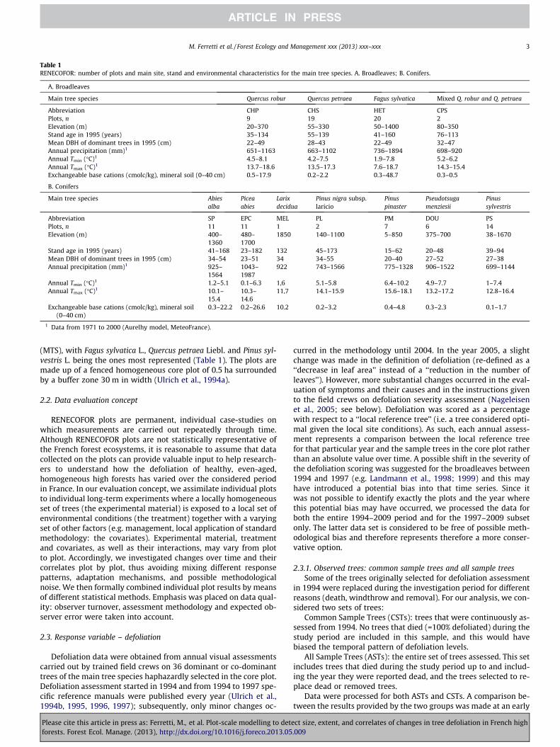
https://www.researchgate.net/publication/226417108_Implementation_of_Quality_Assurance_Procedures_in_the_Italian_Programs_of_Forest_Condition_Monitoring?el=1_x_8&enrichId=rgreq-b0a24b50-ef6b-4d9b-91ba-4f7da22fdc76&enrichSource=Y292ZXJQYWdlOzIzNjYyMzExNztBUzoxMDI2OTUyNjQzMjU2MzZAMTQwMTQ5NTg2NzIwOQ==

Table 1RENECOFOR: number of plots and main site, stand and environmental characteristics for the main tree species. A. Broadleaves; B. Conifers.

A. Broadleaves

Main tree species Quercus robur Quercus petraea Fagus sylvatica Mixed Q. robur and Q. petraea

Abbreviation CHP CHS HET CPSPlots, n 9 19 20 2Elevation (m) 20–370 55–330 50–1400 80–350Stand age in 1995 (years) 35–134 55–139 41–160 76–113Mean DBH of dominant trees in 1995 (cm) 22–49 28–43 22–49 32–47Annual precipitation (mm)1 651–1163 663–1102 736–1894 698–920Annual Tmin (�C)1 4.5–8.1 4.2–7.5 1.9–7.8 5.2–6.2Annual Tmax (�C)1 13.7–18.6 13.5–17.3 7.6–18.7 14.3–15.4Exchangeable base cations (cmolc/kg), mineral soil (0–40 cm) 0.5–17.9 0.2–2.2 0.3–48.7 0.3–0.5

B. Conifers

Main tree species Abiesalba

Piceaabies

Larixdecidua

Pinus nigra subsp.laricio

Pinuspinaster

Pseudotsugamenziesii

Pinussylvestris

Abbreviation SP EPC MEL PL PM DOU PSPlots, n 11 11 1 2 7 6 14Elevation (m) 400–

1360480–1700

1850 140–1100 5–850 375–700 38–1670

Stand age in 1995 (years) 41–168 23–182 132 45–173 15–62 20–48 39–94Mean DBH of dominant trees in 1995 (cm) 34–54 23–51 34 34–55 20–40 27–52 27–38Annual precipitation (mm)1 925–

15641043–1987

922 743–1566 775–1328 906–1522 699–1144

Annual Tmin (�C)1 1.2–5.1 0.1–6.3 1,6 5.1–5.8 6.4–10.2 4.9–7.7 1–7.4Annual Tmax (�C)1 10.1–

15.410.3–14.6

11,7 14.1–15.9 15.6–18.1 13.2–17.2 12.8–16.4

Exchangeable base cations (cmolc/kg), mineral soil(0–40 cm)

0.3–22.2 0.2–26.6 10.2 0.2–3.2 0.4–4.8 0.3–2.3 0.1–1.7

1 Data from 1971 to 2000 (Aurelhy model, MeteoFrance).

M. Ferretti et al. / Forest Ecology and Management xxx (2013) xxx–xxx 3

(MTS), with Fagus sylvatica L., Quercus petraea Liebl. and Pinus syl-vestris L. being the ones most represented (Table 1). The plots aremade up of a fenced homogeneous core plot of 0.5 ha surroundedby a buffer zone 30 m in width (Ulrich et al., 1994a).

2.2. Data evaluation concept

RENECOFOR plots are permanent, individual case-studies onwhich measurements are carried out repeatedly through time.Although RENECOFOR plots are not statistically representative ofthe French forest ecosystems, it is reasonable to assume that datacollected on the plots can provide valuable input to help research-ers to understand how the defoliation of healthy, even-aged,homogeneous high forests has varied over the considered periodin France. In our evaluation concept, we assimilate individual plotsto individual long-term experiments where a locally homogeneousset of trees (the experimental material) is exposed to a local set ofenvironmental conditions (the treatment) together with a varyingset of other factors (e.g. management, local application of standardmethodology: the covariates). Experimental material, treatmentand covariates, as well as their interactions, may vary from plotto plot. Accordingly, we investigated changes over time and theircorrelates plot by plot, thus avoiding mixing different responsepatterns, adaptation mechanisms, and possible methodologicalnoise. We then formally combined individual plot results by meansof different statistical methods. Emphasis was placed on data qual-ity: observer turnover, assessment methodology and expected ob-server error were taken into account.

2.3. Response variable – defoliation

Defoliation data were obtained from annual visual assessmentscarried out by trained field crews on 36 dominant or co-dominanttrees of the main tree species haphazardly selected in the core plot.Defoliation assessment started in 1994 and from 1994 to 1997 spe-cific reference manuals were published every year (Ulrich et al.,1994b, 1995, 1996, 1997); subsequently, only minor changes oc-


curred in the methodology until 2004. In the year 2005, a slightchange was made in the definition of defoliation (re-defined as a‘‘decrease in leaf area’’ instead of a ‘‘reduction in the number ofleaves’’). However, more substantial changes occurred in the eval-uation of symptoms and their causes and in the instructions givento the field crews on defoliation severity assessment (Nageleisenet al., 2005; see below). Defoliation was scored as a percentagewith respect to a ‘‘local reference tree’’ (i.e. a tree considered opti-mal given the local site conditions). As such, each annual assess-ment represents a comparison between the local reference treefor that particular year and the sample trees in the core plot ratherthan an absolute value over time. A possible shift in the severity ofthe defoliation scoring was suggested for the broadleaves between1994 and 1997 (e.g. Landmann et al., 1998; 1999) and this mayhave introduced a potential bias into that time series. Since itwas not possible to identify exactly the plots and the year wherethis potential bias may have occurred, we processed the data forboth the entire 1994–2009 period and for the 1997–2009 subsetonly. The latter data set is considered to be free of possible meth-odological bias and therefore represents therefore a more conser-vative option.

2.3.1. Observed trees: common sample trees and all sample treesSome of the trees originally selected for defoliation assessment

in 1994 were replaced during the investigation period for differentreasons (death, windthrow and removal). For our analysis, we con-sidered two sets of trees:

Common Sample Trees (CSTs): trees that were continuously as-sessed from 1994. No trees that died (=100% defoliated) during thestudy period are included in this sample, and this would havebiased the temporal pattern of defoliation levels.

All Sample Trees (ASTs): the entire set of trees assessed. This setincludes trees that died during the study period up to and includ-ing the year they were reported dead, and the trees selected to re-place dead or removed trees.

Data were processed for both ASTs and CSTs. A comparison be-tween the results provided by the two groups was made at an early




stage in the study on the basis of (i) the frequency of significant an-nual changes and (ii) the slope of the individual plot linear regres-sion models (Ferretti et al., 2012a,b). Since there was almost nodifference, the results reported in this paper refer to the AST setonly.

2.3.2. Data qualityData quality was evaluated in terms of completeness and con-

sistency. Data completeness for tree condition was high (>98%),with the exception of the year 2003 when no assessment was car-ried out. Data consistency was assessed by comparing data col-lected during training and field checks. Data from field checkscarried out between 2001–2005 and 2008–2009 on 16 plots and697 trees revealed that 76% of the defoliation scores attributedwere within ±5% difference between field crew and control team,and 92% within ±10%. These values fit data quality requirementsoften used in tree condition surveys (e.g. Tallent-Halsell, 1994; Fer-retti et al., 1999; Bussotti et al., 2009) and are much higher thanthose recommended by the ICP Forests (Ferretti et al., 2013b).Deviations from plot median defoliation values were always<10%, and were <5% in 12 plots out of 16. Nonetheless, hidden devi-ations may have occurred due to observer changes. To account for

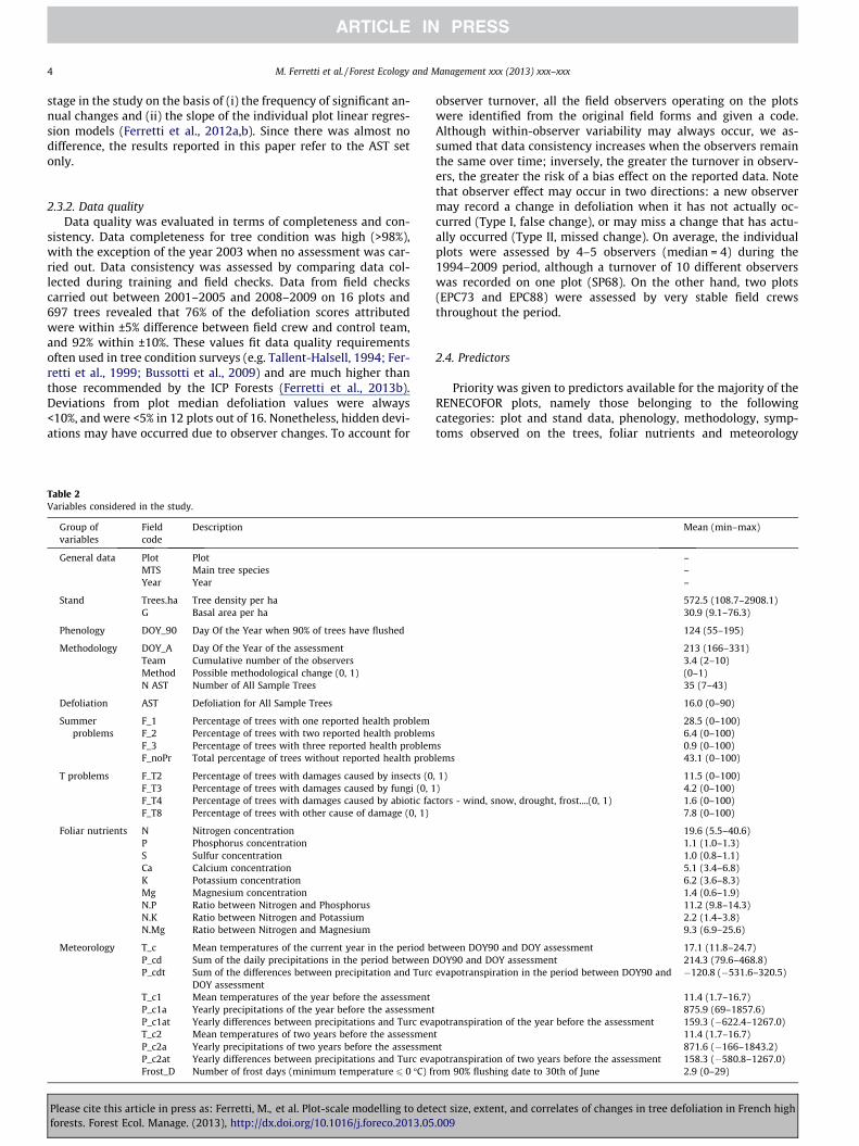
Table 2Variables considered in the study.

Group ofvariables

Fieldcode

Description

General data Plot PlotMTS Main tree speciesYear Year

Stand Trees.ha Tree density per haG Basal area per ha

Phenology DOY_90 Day Of the Year when 90% of trees have flushed

Methodology DOY_A Day Of the Year of the assessmentTeam Cumulative number of the observersMethod Possible methodological change (0, 1)N AST Number of All Sample Trees

Defoliation AST Defoliation for All Sample Trees

Summerproblems

F_1 Percentage of trees with one reported health problemF_2 Percentage of trees with two reported health problemsF_3 Percentage of trees with three reported health problemF_noPr Total percentage of trees without reported health prob

T problems F_T2 Percentage of trees with damages caused by insects (0F_T3 Percentage of trees with damages caused by fungi (0, 1F_T4 Percentage of trees with damages caused by abiotic facF_T8 Percentage of trees with other cause of damage (0, 1)

Foliar nutrients N Nitrogen concentrationP Phosphorus concentrationS Sulfur concentrationCa Calcium concentrationK Potassium concentrationMg Magnesium concentrationN.P Ratio between Nitrogen and PhosphorusN.K Ratio between Nitrogen and PotassiumN.Mg Ratio between Nitrogen and Magnesium

Meteorology T_c Mean temperatures of the current year in the period bP_cd Sum of the daily precipitations in the period betweenP_cdt Sum of the differences between precipitation and Turc

DOY assessmentT_c1 Mean temperatures of the year before the assessmentP_c1a Yearly precipitations of the year before the assessmentP_c1at Yearly differences between precipitations and Turc evaT_c2 Mean temperatures of two years before the assessmenP_c2a Yearly precipitations of two years before the assessmeP_c2at Yearly differences between precipitations and Turc evaFrost_D Number of frost days (minimum temperature 6 0 �C) f


observer turnover, all the field observers operating on the plotswere identified from the original field forms and given a code.Although within-observer variability may always occur, we as-sumed that data consistency increases when the observers remainthe same over time; inversely, the greater the turnover in observ-ers, the greater the risk of a bias effect on the reported data. Notethat observer effect may occur in two directions: a new observermay record a change in defoliation when it has not actually oc-curred (Type I, false change), or may miss a change that has actu-ally occurred (Type II, missed change). On average, the individualplots were assessed by 4–5 observers (median = 4) during the1994–2009 period, although a turnover of 10 different observerswas recorded on one plot (SP68). On the other hand, two plots(EPC73 and EPC88) were assessed by very stable field crewsthroughout the period.

2.4. Predictors

Priority was given to predictors available for the majority of theRENECOFOR plots, namely those belonging to the followingcategories: plot and stand data, phenology, methodology, symp-toms observed on the trees, foliar nutrients and meteorology

Mean (min–max)

–––

572.5 (108.7–2908.1)30.9 (9.1–76.3)

124 (55–195)

213 (166–331)3.4 (2–10)(0–1)35 (7–43)

16.0 (0–90)

28.5 (0–100)6.4 (0–100)

s 0.9 (0–100)lems 43.1 (0–100)

, 1) 11.5 (0–100)) 4.2 (0–100)tors - wind, snow, drought, frost....(0, 1) 1.6 (0–100)

7.8 (0–100)

19.6 (5.5–40.6)1.1 (1.0–1.3)1.0 (0.8–1.1)5.1 (3.4–6.8)6.2 (3.6–8.3)1.4 (0.6–1.9)11.2 (9.8–14.3)2.2 (1.4–3.8)9.3 (6.9–25.6)

etween DOY90 and DOY assessment 17.1 (11.8–24.7)DOY90 and DOY assessment 214.3 (79.6–468.8)evapotranspiration in the period between DOY90 and �120.8 (�531.6–320.5)

11.4 (1.7–16.7)875.9 (69–1857.6)

potranspiration of the year before the assessment 159.3 (�622.4–1267.0)t 11.4 (1.7–16.7)nt 871.6 (�166–1843.2)potranspiration of two years before the assessment 158.3 (�580.8–1267.0)

rom 90% flushing date to 30th of June 2.9 (0–29)



https://www.researchgate.net/publication/236147090_Concepts_and_Design_Principles_Adopted_in_the_International_Cooperative_Program_on_the_Assessment_and_Monitoring_of_Air_Pollution_Effects_on_Forests_ICP_Forests?el=1_x_8&enrichId=rgreq-b0a24b50-ef6b-4d9b-91ba-4f7da22fdc76&enrichSource=Y292ZXJQYWdlOzIzNjYyMzExNztBUzoxMDI2OTUyNjQzMjU2MzZAMTQwMTQ5NTg2NzIwOQ==


(Table 2). We assumed that soil chemistry did not change over the1994–2009 period and, since our evaluation was plot-wise, we didnot consider predictors related to soil chemistry in our analysis.However, the effect of possible nutritional changes was evaluatedby means of foliar chemistry data. Other predictors such as atmo-spheric deposition chemistry and tropospheric ozone concentra-tions were not considered because such data were available onlyfor a limited subset of plots. No reliable modelled annual data sui-ted for site specific estimates were available (large-scale modelsare not suited to plot-scale estimates, e.g. Gottardini et al., 2010).Although effects on defoliation from atmospheric deposition andozone cannot be excluded, it is worth noting that (i) deposition willin turn affect tree nutrition and should – at least to some extent,and especially for nitrogen – be reflected by foliar chemistry; and(ii) published studies on an ozone effect on defoliation have pro-vided controversial results, and, even when significant, ozone ex-plained only a very small portion of the variance (e.g. Ferrettiet al., 2007; Bussotti and Ferretti, 2009).

Plot, stand, phenology and foliar nutrient data are self-explana-tory (Table 2). Changes in tree density due to thinning were ob-tained from stand inventories carried out before and afterthinning (Diameter at Breast Height-DBH-threshold = 8 cm).

Data related to methodological aspects were of a different nat-ure (Table 2). In particular, ‘‘Methods’’ refers to the possible meth-odological adjustments in defoliation assessment (e.g. Landmannet al., 1998, 1999) that may have occurred between 1994and1996 and subsequent years, and which are not explicit in thefield manuals. We incorporated this variation as a categorical var-iable (0 = method used from 1994–1996; 1 = method used from1997–2009) in the regression model for the 1994–2009 dataset. Fi-nally, ‘‘N AST’’ is the total number of trees assessed each year.

Data about tree condition refer to defoliation (see Section 2.3)and to a set of variables that include frequency of trees with re-ported symptoms either in terms of presence of different, unspec-ified ‘‘problems’’ or in terms of insects, fungi, abiotic and otherdamage (Table 2). Given that changes in the scoring system forthese symptoms occurred during the study period, we back-calcu-lated the related data to obtain a consistent dataset for the15 years. For example, the estimation of the extent of a given prob-lem changed from a purely qualitative scale to different semi-quantitative scales. Moreover, before 2005, it is unclear if this esti-mation refers to the whole tree or to a specific part of the tree. Fur-thermore, the list of problems to consider was updated severaltimes, with some additions but also some removals. Back calcula-tion was therefore only possible by aggregating the records interms of number of reported health problems for each individualtree and category of problems (e.g., insects, fungi, etc.) and summa-rizing data for each plot (e.g. total number of trees with one, two,three reported problems or number of trees for any given categoryof problems).

Meteorological data for the 1992–2009 period were obtainedfrom the most relevant meteorological station of Météo-Francefor each plot, i.e. the closest station within a maximum range of50 km and with complete raw data (more than 99% completenessfor daily temperature and precipitation and more than 85% com-pleteness for 10-day global radiation) (Table 2). In addition, localRENECOFOR weather stations installed in 1995 provided tempera-ture and precipitation data for 24 plots and global radiation datafor seven of those plots. Precipitation surplus indicates the differ-ence between precipitation and potential evapotranspiration (cal-culated from global radiation and temperature data according tothe Turc formula for temperate countries with a humidity rate ofover 50% – Turc, 1955;Turc 1961).

All measurements and assessment were carried out accordingto the Standard Operating Procedures (SOPs) adopted by the RENE-COFOR programme.


2.5. Missing data and imputation

Missing values were detected for almost every variable, partlyas a result of random events, partly because some investigationsstarted at a later date (e.g. phenology measurements began in1997), and partly because some investigations were designed withlower data collection frequency (e.g. foliar chemistry, carried outevery 2 years from 1999 on). Different imputation techniques wereused to obtain a consistent and fully balanced dataset (see Ferrettiet al., 2012b for a full account). Missing DOY90 annual values wereestimated by interpolating the DOY90 values reported for theavailable years in relation to main tree species (MTS) and plot alti-tude. Principal Component Analysis (PCA) was used for plot-wiseimputation of foliar chemistry data and tested against 20 randomlyselected plots for which annual data series were available. Gaps indaily temperature and precipitation were filled with station-spe-cific monthly means. When necessary, gaps in local RENECOFORdata were filled by means of the closest Météo-France stationand vice versa.

2.6. Statistical methods

2.6.1. Changes over time and trendsChange and trend analysis was carried out on 102 plots by

means of a Spearman analysis of correlation and a Simple LinearRegression (SLR) with the associate t-test (Elzinga et al., 2001). AWilcoxon rank-sum test was used to test variations between adja-cent years, e.g. 1997–1998, 1998–1999 and so on. On the basis ofthe results obtained from the control assessment, we set a mini-mum 5% defoliation change threshold in addition to statistical sig-nificance, to evaluate meaningful annual changes.

Spearman rho values for the individual plots were used as effectsize in the meta-analysis. Meta-analysis makes it possible to com-bine and compare results from ecological experiments and studieswhose small sample sizes yield low statistical power (Harrison,2011; Stewart, 2010; Hillebrand, 2008). The basic models are thefixed- and random/mixed-effects models (Berkey et al., 1995; vanHouwelingen et al., 2002). Let i = 1,. . ., k independent effect sizeestimates, each estimating a corresponding (true) effect size. Weassume that:

yi ¼ hi þ ei ð1Þ

where yi denotes the observed effect in the ith study, hi the corre-sponding (unknown) true effect, ei is the sampling error, andei � N(0, vi). Therefore, the yi’s are assumed to be unbiased and nor-mally distributed estimates of their corresponding true effects. Thesampling variances (i.e., vi values) are assumed to be known.Depending on the outcome measure used (effect size), a bias correc-tion, normalising, and/or variance stabilising transformation may benecessary to ensure that these assumptions are (approximately)true.

The weight adopted in the meta-analysis was the number oftrees per plot, and the degrees of freedom (df) were obtained bythe available data per year. When a dataset is composed of studieswhich differ in their methods and/or the characteristics of the in-cluded samples (the individual plots in our case), such a differencemay introduce variability (‘‘heterogeneity’’) among the true effects.We modelled heterogeneity in three different ways. Firstly, wetreated it as purely random. This led to the following random- ef-fects model:

hi ¼ lþ ui ð2Þ

where ui � N (0, s2). In this case, the true effects are assumed to benormally distributed with mean l and variance s2. The goal is thento estimate l, the average true effect and s2, the (total) amount of



https://www.researchgate.net/publication/236133999_Variability_of_ozone_concentration_in_a_montane_environment_northern_Italy?el=1_x_8&enrichId=rgreq-b0a24b50-ef6b-4d9b-91ba-4f7da22fdc76&enrichSource=Y292ZXJQYWdlOzIzNjYyMzExNztBUzoxMDI2OTUyNjQzMjU2MzZAMTQwMTQ5NTg2NzIwOQ==

https://www.researchgate.net/publication/233801204_Monitoring_plant_and_animal_populations?el=1_x_8&enrichId=rgreq-b0a24b50-ef6b-4d9b-91ba-4f7da22fdc76&enrichSource=Y292ZXJQYWdlOzIzNjYyMzExNztBUzoxMDI2OTUyNjQzMjU2MzZAMTQwMTQ5NTg2NzIwOQ==


heterogeneity among the true effects. If s2 = 0, then this implieshomogeneity among the true effects (i.e., h1 =. . . = hk � h), so thatl = h then denotes the true effect.

Secondly, we included ‘‘moderators’’ (i.e., study-level covari-ates) in the model to account for at least part of the heterogeneityin the true effects. This led to the following mixed-effects model:

hi ¼ b0 þ b1xi1 þ . . .þ bp0xip0 þ ui ð3Þ

where xij denotes the value of the jth moderator variable for the ithstudy; again we assume that ui � N (0, s2). Here, s2 denotes theamount of residual heterogeneity among the true effects, that is,the variability among the true effects that is not accounted for bythe moderators included in the model. The goal of the analysis isthen to examine to what extent the moderators included in themodel influence the size of the average true effect.

When moderators were used, an omnibus test of all the modelcoefficients was conducted. The test excludes the intercept b0 (thefirst coefficient) if it is included in the model (i.e., a test of H0: b1 -= . . . = bp0 = 0). If no intercept is included in the model, then theomnibus test includes all of the coefficients in the model includingthe first one.

Both continuous and categorical variables were used as moder-ators. To observe and analyze existing spatial patterns, we used amixed-effect model for continuous variables with geographicallycontinuous quantitative variables (elevation and latitude/longi-tude) and plot age as moderators. Categorical moderator variablescan be included in the model as coded categorical independentvariables (dummies). A mixed-effects model using dominant treespecies as a categorical qualitative moderator was used to assessthe relative influence of different species on the observed defolia-tion trend.

The various meta-analytical models are merely special cases ofthe general linear (mixed-effects) model with heteroscedastic sam-pling variances that are assumed to be known. Random/mixed-ef-fects models can therefore be fitted using a two-step approach(Raudenbush, 2009). First, the amount of (residual) heterogeneity(i.e., s2) was estimated by the restricted maximum-likelihood esti-mator (Viechtbauer, 2005; Raudenbush, 2009). Secondly, l orb0,. . ., bp0 were estimated via weighted least squares with weightsequal to:

wi ¼ 1=ðmi þ s2Þ ð4Þ

where s22 denotes the estimate of s2.Once parameter estimates have been obtained, Wald-type tests

and confidence intervals (CIs) are then easy to apply for l or b0,. . .,bp0 under the assumption of normality. For models involving mod-erators, subsets of the parameters can also be tested in the samemanner. The null hypothesis H0: s2 = 0 in random- and mixed-ef-fects models can be tested with Cochran’s Q-test (Hedges and Olk-in, 1985). A confidence interval for s2 can then be obtained withthe method described in Viechtbauer (2007).

2.6.2. Individual plot modellingBecause of limited available data (missing meteorological and

foliar data) and low amenability for analyses (no variability inthe response variable), a correlative study at the level of individualplots was carried out on 87-90 out of the 102 plots. A Partial LeastSquare (PLS) regression (Martens and Naes, 1989) was used. A PLSregression generalises and combines features from principal com-ponent analyses and multiple regressions. PLS defines orthogonallatent variables (LVs) to compress the information and disregardirrelevant variables. A PLS regression is not sensitive to multi-collinearity and, at the same time, it is not particularly affectedby unfavourable case/variable ratios. A PLS regression explicitlyaims at constructing LVs in such a way as to capture as much as


possible of the variance in X and Y, and to maximise the correlationbetween these matrices. The number of LVs needed to obtain thebest generalisation for the prediction of new observations is, ingeneral, achieved with cross-validation techniques such asbootstrapping. We based our variable selection and model evalua-tion on VIP (Variable Importance in the Projections) coefficients(Wold et al., 1993). Since the average of the squared VIP scoresequals 1, variables with scores > 1 are considered to be the mostimportant.

In cross-validation, n different models are created, each timeomitting one or more samples from the training data. The RootMean Square Error (RMSE) and the RMSE in the cross validation(RMSE_CV) were calculated.

3. Results

3.1. Defoliation changes over time and trends

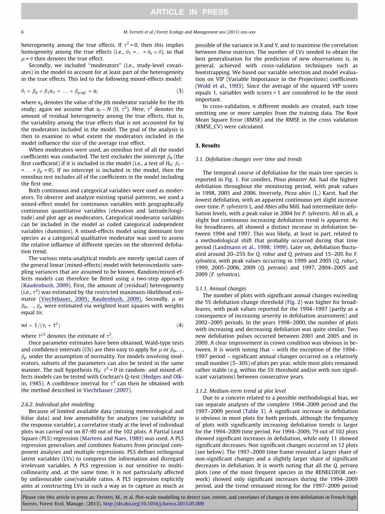
The temporal course of defoliation for the main tree species isreported in Fig. 1. For conifers, Pinus pinaster Ait. had the highestdefoliation throughout the monitoring period, with peak valuesin 1998, 2005 and 2006. Inversely, Picea abies (L.) Karst. had thelowest defoliation, with an apparent continuous yet slight increaseover time. P. sylvestris L. and Abies alba Mill. had intermediate defo-liation levels, with a peak value in 2004 for P. sylvestris. All in all, aslight but continuous increasing defoliation trend is apparent. Asfor broadleaves, all showed a distinct increase in defoliation be-tween 1994 and 1997. This was likely, at least in part, related toa methodological shift that probably occurred during that timeperiod (Landmann et al., 1998; 1999). Later on, defoliation fluctu-ated around 20–25% for Q. robur and Q. petraea and 15–20% for F.sylvatica, with peak values occurring in 1999 and 2005 (Q. robur),1999, 2005–2006, 2009 (Q. petraea) and 1997, 2004–2005 and2009 (F. sylvatica).

3.1.1. Annual changesThe number of plots with significant annual changes exceeding

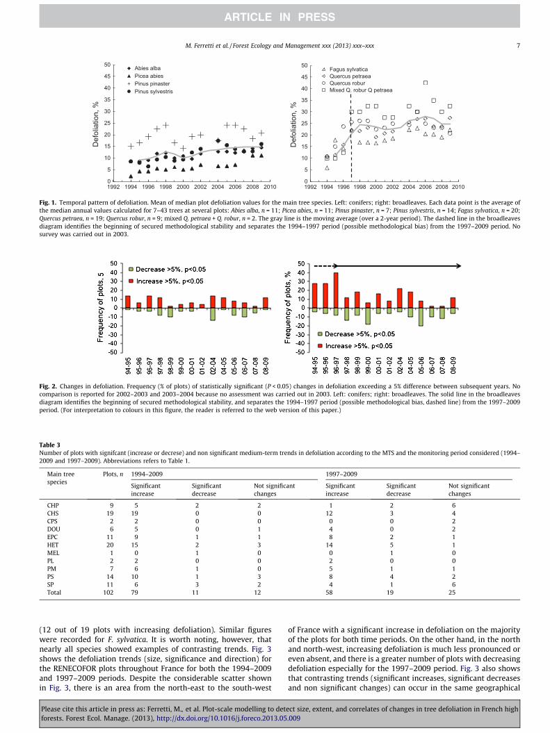
the 5% defoliation change threshold (Fig. 2) was higher for broad-leaves, with peak values reported for the 1994–1997 (partly as aconsequence of increasing severity in defoliation assessment) and2002–2005 periods. In the years 1998–2000, the number of plotswith increasing and decreasing defoliation was quite similar. Twonew defoliation pulses occurred between 2001 and 2005 and in2009. A clear improvement in crown condition was obvious in be-tween. It is worth noting that – with the exception of the 1994–1997 period – significant annual changes occurred on a relativelysmall number (5–30%) of plots per year, while most plots remainedrather stable (e.g. within the 5% threshold and/or with non signif-icant variations) between consecutive years.

3.1.2. Medium-term trend at plot levelDue to a concern related to a possible methodological bias, we

ran separate analyses of the complete 1994–2009 period and the1997–2009 period (Table 3). A significant increase in defoliationis obvious in most plots for both periods, although the frequencyof plots with significantly increasing defoliation trends is largerfor the 1994–2009 time period. For 1994–2009, 79 out of 102 plotsshowed significant increases in defoliation, while only 11 showedsignificant decreases. Non significant changes occurred on 12 plots(see below). The 1997–2009 time frame revealed a larger share ofnon-significant changes and a slightly larger share of significantdecreases in defoliation. It is worth noting that all the Q. petraeaplots (one of the most frequent species in the RENECOFOR net-work) showed only significant increases during the 1994–2009period, and the trend remained strong for the 1997–2009 period



https://www.researchgate.net/publication/240802126_Bias_and_Efficiency_of_Meta-Analytic_Variance_Estimators_in_the_Random-Effects_Model?el=1_x_8&enrichId=rgreq-b0a24b50-ef6b-4d9b-91ba-4f7da22fdc76&enrichSource=Y292ZXJQYWdlOzIzNjYyMzExNztBUzoxMDI2OTUyNjQzMjU2MzZAMTQwMTQ5NTg2NzIwOQ==

0

5

10

15

20

25

30

35

40

45

50

Def

olia

tion,

%

Abies alba Picea abies Pinus pinaster Pinus sylvestris

0

5

10

15

20

25

30

35

40

45

50

1992 1994 1996 1998 2000 2002 2004 2006 2008 2010 1992 1994 1996 1998 2000 2002 2004 2006 2008 2010

Def

olia

tion,

%

Fagus sylvatica Quercus petraea Quercus robur Mixed Q. robur Q petraea

Fig. 1. Temporal pattern of defoliation. Mean of median plot defoliation values for the main tree species. Left: conifers; right: broadleaves. Each data point is the average ofthe median annual values calculated for 7–43 trees at several plots: Abies alba, n = 11; Picea abies, n = 11; Pinus pinaster, n = 7; Pinus sylvestris, n = 14; Fagus sylvatica, n = 20;Quercus petraea, n = 19; Quercus robur, n = 9; mixed Q. petraea + Q. robur, n = 2. The gray line is the moving average (over a 2-year period). The dashed line in the broadleavesdiagram identifies the beginning of secured methodological stability and separates the 1994–1997 period (possible methodological bias) from the 1997–2009 period. Nosurvey was carried out in 2003.

Fig. 2. Changes in defoliation. Frequency (% of plots) of statistically significant (P < 0.05) changes in defoliation exceeding a 5% difference between subsequent years. Nocomparison is reported for 2002–2003 and 2003–2004 because no assessment was carried out in 2003. Left: conifers; right: broadleaves. The solid line in the broadleavesdiagram identifies the beginning of secured methodological stability, and separates the 1994–1997 period (possible methodological bias, dashed line) from the 1997–2009period. (For interpretation to colours in this figure, the reader is referred to the web version of this paper.)

Table 3Number of plots with signifcant (increase or decrese) and non significant medium-term trends in defoliation according to the MTS and the monitoring period considered (1994–2009 and 1997–2009). Abbreviations refers to Table 1.

Main treespecies

Plots, n 1994–2009 1997–2009

Significantincrease

Significantdecrease

Not significantchanges

Significantincrease

Significantdecrease

Not significantchanges

CHP 9 5 2 2 1 2 6CHS 19 19 0 0 12 3 4CPS 2 2 0 0 0 0 2DOU 6 5 0 1 4 0 2EPC 11 9 1 1 8 2 1HET 20 15 2 3 14 5 1MEL 1 0 1 0 0 1 0PL 2 2 0 0 2 0 0PM 7 6 1 0 5 1 1PS 14 10 1 3 8 4 2SP 11 6 3 2 4 1 6Total 102 79 11 12 58 19 25


(12 out of 19 plots with increasing defoliation). Similar figureswere recorded for F. sylvatica. It is worth noting, however, thatnearly all species showed examples of contrasting trends. Fig. 3shows the defoliation trends (size, significance and direction) forthe RENECOFOR plots throughout France for both the 1994–2009and 1997–2009 periods. Despite the considerable scatter shownin Fig. 3, there is an area from the north-east to the south-west


of France with a significant increase in defoliation on the majorityof the plots for both time periods. On the other hand, in the northand north-west, increasing defoliation is much less pronounced oreven absent, and there is a greater number of plots with decreasingdefoliation especially for the 1997–2009 period. Fig. 3 also showsthat contrasting trends (significant increases, significant decreasesand non significant changes) can occur in the same geographical



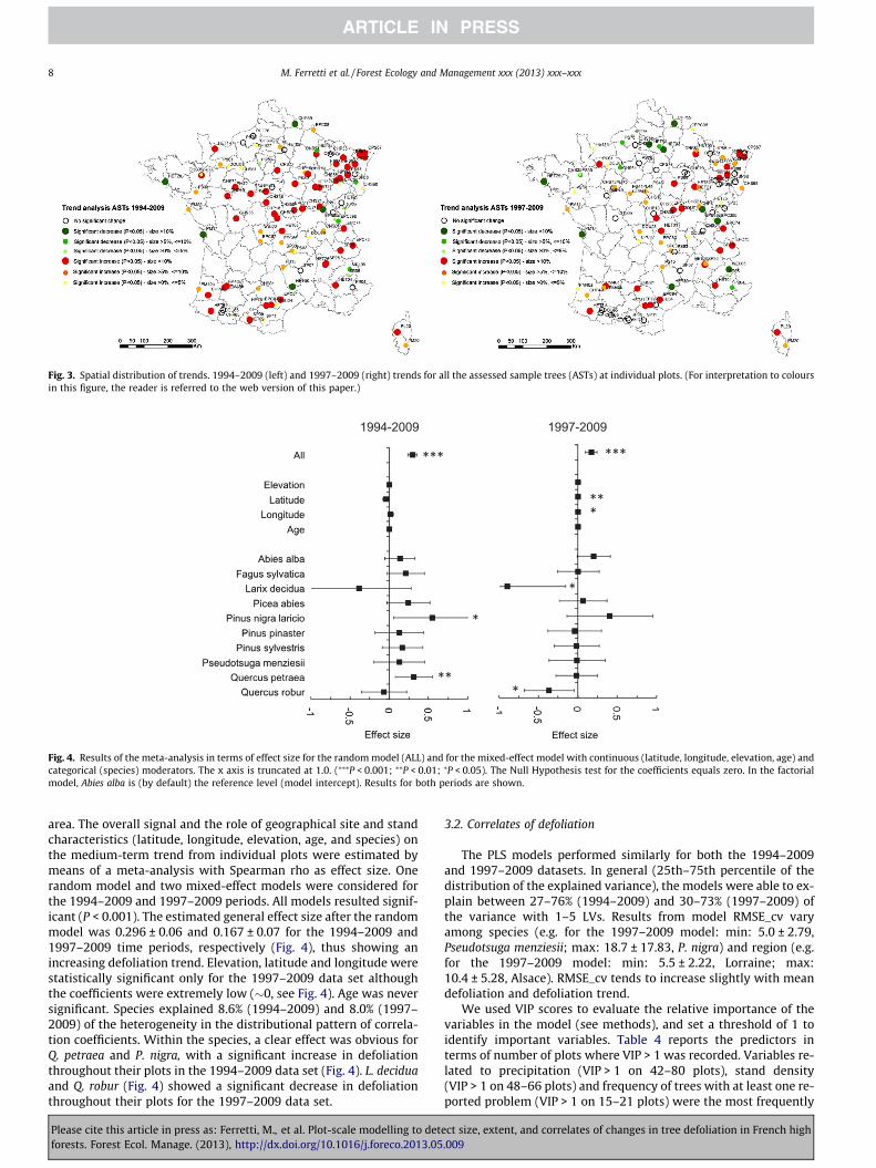
Fig. 3. Spatial distribution of trends. 1994–2009 (left) and 1997–2009 (right) trends for all the assessed sample trees (ASTs) at individual plots. (For interpretation to coloursin this figure, the reader is referred to the web version of this paper.)

***

*

*

** *

***

*

**

1994-2009 1997-2009

Fig. 4. Results of the meta-analysis in terms of effect size for the random model (ALL) and for the mixed-effect model with continuous (latitude, longitude, elevation, age) andcategorical (species) moderators. The x axis is truncated at 1.0. (⁄⁄⁄P < 0.001; ⁄⁄P < 0.01; ⁄P < 0.05). The Null Hypothesis test for the coefficients equals zero. In the factorialmodel, Abies alba is (by default) the reference level (model intercept). Results for both periods are shown.


area. The overall signal and the role of geographical site and standcharacteristics (latitude, longitude, elevation, age, and species) onthe medium-term trend from individual plots were estimated bymeans of a meta-analysis with Spearman rho as effect size. Onerandom model and two mixed-effect models were considered forthe 1994–2009 and 1997–2009 periods. All models resulted signif-icant (P < 0.001). The estimated general effect size after the randommodel was 0.296 ± 0.06 and 0.167 ± 0.07 for the 1994–2009 and1997–2009 time periods, respectively (Fig. 4), thus showing anincreasing defoliation trend. Elevation, latitude and longitude werestatistically significant only for the 1997–2009 data set althoughthe coefficients were extremely low (�0, see Fig. 4). Age was neversignificant. Species explained 8.6% (1994–2009) and 8.0% (1997–2009) of the heterogeneity in the distributional pattern of correla-tion coefficients. Within the species, a clear effect was obvious forQ. petraea and P. nigra, with a significant increase in defoliationthroughout their plots in the 1994–2009 data set (Fig. 4). L. deciduaand Q. robur (Fig. 4) showed a significant decrease in defoliationthroughout their plots for the 1997–2009 data set.


3.2. Correlates of defoliation

The PLS models performed similarly for both the 1994–2009and 1997–2009 datasets. In general (25th–75th percentile of thedistribution of the explained variance), the models were able to ex-plain between 27–76% (1994–2009) and 30–73% (1997–2009) ofthe variance with 1–5 LVs. Results from model RMSE_cv varyamong species (e.g. for the 1997–2009 model: min: 5.0 ± 2.79,Pseudotsuga menziesii; max: 18.7 ± 17.83, P. nigra) and region (e.g.for the 1997–2009 model: min: 5.5 ± 2.22, Lorraine; max:10.4 ± 5.28, Alsace). RMSE_cv tends to increase slightly with meandefoliation and defoliation trend.

We used VIP scores to evaluate the relative importance of thevariables in the model (see methods), and set a threshold of 1 toidentify important variables. Table 4 reports the predictors interms of number of plots where VIP > 1 was recorded. Variables re-lated to precipitation (VIP > 1 on 42–80 plots), stand density(VIP > 1 on 48–66 plots) and frequency of trees with at least one re-ported problem (VIP > 1 on 15–21 plots) were the most frequently



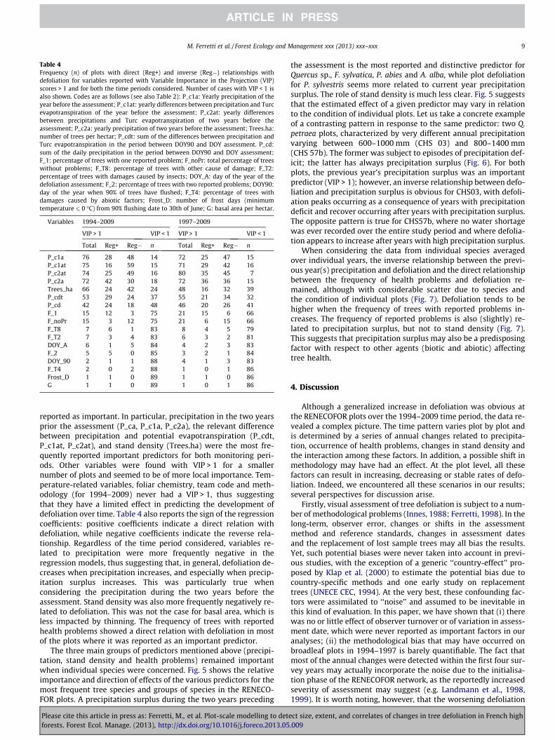
Table 4Frequency (n) of plots with direct (Reg+) and inverse (Reg�) relationships withdefoliation for variables reported with Variable Importance in the Projection (VIP)scores > 1 and for both the time periods considered. Number of cases with VIP < 1 isalso shown. Codes are as follows (see also Table 2): P_c1a: Yearly precipitation of theyear before the assessment; P_c1at: yearly differences between precipitation and Turcevapotranspiration of the year before the assessment; P_c2at: yearly differencesbetween precipitations and Turc evapotranspiration of two years before theassessment; P_c2a: yearly precipitation of two years before the assessment; Trees.ha:number of trees per hectar; P_cdt: sum of the differences between precipitation andTurc evapotranspiration in the period between DOY90 and DOY assessment. P_cd:sum of the daily precipitation in the period between DOY90 and DOY assessment;F_1: percentage of trees with one reported problem; F_noPr: total percentage of treeswithout problems; F_T8: percentage of trees with other cause of damage; F_T2:percentage of trees with damages caused by insects; DOY_A: day of the year of thedefoliation assessment; F_2: percentage of trees with two reported problems; DOY90:day of the year when 90% of trees have flushed; F_T4: percentage of trees withdamages caused by abiotic factors; Frost_D: number of frost days (minimumtemperature 6 0 �C) from 90% flushing date to 30th of June; G: basal area per hectar.

Variables 1994–2009 1997–2009

VIP > 1 VIP < 1 VIP > 1 VIP < 1

Total Reg+ Reg� n Total Reg+ Reg� n

P_c1a 76 28 48 14 72 25 47 15P_c1at 75 16 59 15 71 29 42 16P_c2at 74 25 49 16 80 35 45 7P_c2a 72 42 30 18 72 36 36 15Trees_ha 66 24 42 24 48 16 32 39P_cdt 53 29 24 37 55 21 34 32P_cd 42 24 18 48 46 20 26 41F_1 15 12 3 75 21 15 6 66F_noPr 15 3 12 75 21 6 15 66F_T8 7 6 1 83 8 4 5 79F_T2 7 3 4 83 6 3 2 81DOY_A 6 1 5 84 4 2 3 83F_2 5 5 0 85 3 2 1 84DOY_90 2 1 1 88 4 1 3 83F_T4 2 0 2 88 1 0 1 86Frost_D 1 1 0 89 1 1 0 86G 1 1 0 89 1 0 1 86


reported as important. In particular, precipitation in the two yearsprior the assessment (P_ca, P_c1a, P_c2a), the relevant differencebetween precipitation and potential evapotranspiration (P_cdt,P_c1at, P_c2at), and stand density (Trees.ha) were the most fre-quently reported important predictors for both monitoring peri-ods. Other variables were found with VIP > 1 for a smallernumber of plots and seemed to be of more local importance. Tem-perature-related variables, foliar chemistry, team code and meth-odology (for 1994–2009) never had a VIP > 1, thus suggestingthat they have a limited effect in predicting the development ofdefoliation over time. Table 4 also reports the sign of the regressioncoefficients: positive coefficients indicate a direct relation withdefoliation, while negative coefficients indicate the reverse rela-tionship. Regardless of the time period considered, variables re-lated to precipitation were more frequently negative in theregression models, thus suggesting that, in general, defoliation de-creases when precipitation increases, and especially when precip-itation surplus increases. This was particularly true whenconsidering the precipitation during the two years before theassessment. Stand density was also more frequently negatively re-lated to defoliation. This was not the case for basal area, which isless impacted by thinning. The frequency of trees with reportedhealth problems showed a direct relation with defoliation in mostof the plots where it was reported as an important predictor.

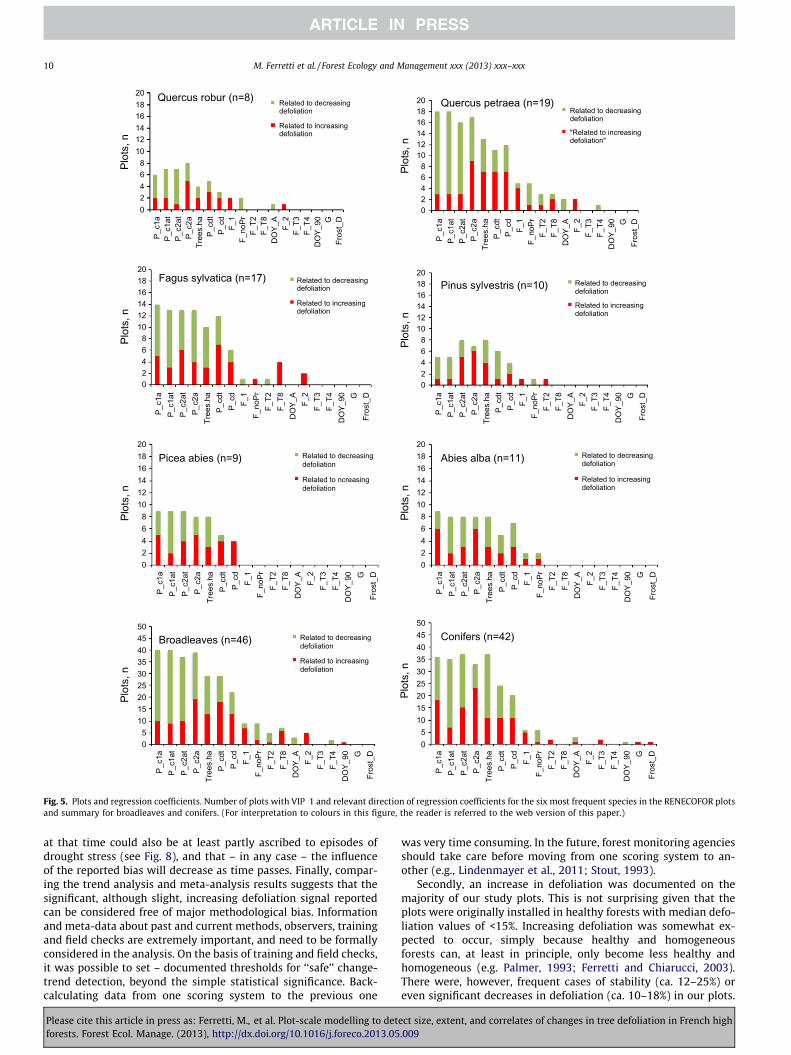
The three main groups of predictors mentioned above (precipi-tation, stand density and health problems) remained importantwhen individual species were concerned. Fig. 5 shows the relativeimportance and direction of effects of the various predictors for themost frequent tree species and groups of species in the RENECO-FOR plots. A precipitation surplus during the two years preceding


the assessment is the most reported and distinctive predictor forQuercus sp., F. sylvatica, P. abies and A. alba, while plot defoliationfor P. sylvestris seems more related to current year precipitationsurplus. The role of stand density is much less clear. Fig. 5 suggeststhat the estimated effect of a given predictor may vary in relationto the condition of individual plots. Let us take a concrete exampleof a contrasting pattern in response to the same predictor: two Q.petraea plots, characterized by very different annual precipitationvarying between 600–1000 mm (CHS 03) and 800–1400 mm(CHS 57b). The former was subject to episodes of precipitation def-icit; the latter has always precipitation surplus (Fig. 6). For bothplots, the previous year’s precipitation surplus was an importantpredictor (VIP > 1); however, an inverse relationship between defo-liation and precipitation surplus is obvious for CHS03, with defoli-ation peaks occurring as a consequence of years with precipitationdeficit and recover occurring after years with precipitation surplus.The opposite pattern is true for CHS57b, where no water shortagewas ever recorded over the entire study period and where defolia-tion appears to increase after years with high precipitation surplus.

When considering the data from individual species averagedover individual years, the inverse relationship between the previ-ous year(s) precipitation and defoliation and the direct relationshipbetween the frequency of health problems and defoliation re-mained, although with considerable scatter due to species andthe condition of individual plots (Fig. 7). Defoliation tends to behigher when the frequency of trees with reported problems in-creases. The frequency of reported problems is also (slightly) re-lated to precipitation surplus, but not to stand density (Fig. 7).This suggests that precipitation surplus may also be a predisposingfactor with respect to other agents (biotic and abiotic) affectingtree health.

4. Discussion

Although a generalized increase in defoliation was obvious atthe RENECOFOR plots over the 1994–2009 time period, the data re-vealed a complex picture. The time pattern varies plot by plot andis determined by a series of annual changes related to precipita-tion, occurrence of health problems, changes in stand density andthe interaction among these factors. In addition, a possible shift inmethodology may have had an effect. At the plot level, all thesefactors can result in increasing, decreasing or stable rates of defo-liation. Indeed, we encountered all these scenarios in our results;several perspectives for discussion arise.

Firstly, visual assessment of tree defoliation is subject to a num-ber of methodological problems (Innes, 1988; Ferretti, 1998). In thelong-term, observer error, changes or shifts in the assessmentmethod and reference standards, changes in assessment datesand the replacement of lost sample trees may all bias the results.Yet, such potential biases were never taken into account in previ-ous studies, with the exception of a generic ‘‘country-effect’’ pro-posed by Klap et al. (2000) to estimate the potential bias due tocountry-specific methods and one early study on replacementtrees (UNECE CEC, 1994). At the very best, these confounding fac-tors were assimilated to ‘‘noise’’ and assumed to be inevitable inthis kind of evaluation. In this paper, we have shown that (i) therewas no or little effect of observer turnover or of variation in assess-ment date, which were never reported as important factors in ouranalyses; (ii) the methodological bias that may have occurred onbroadleaf plots in 1994–1997 is barely quantifiable. The fact thatmost of the annual changes were detected within the first four sur-vey years may actually incorporate the noise due to the initialisa-tion phase of the RENECOFOR network, as the reportedly increasedseverity of assessment may suggest (e.g. Landmann et al., 1998,1999). It is worth noting, however, that the worsening defoliation



02468

101214161820

P_c

1a P

_c1a

t P

_c2a

tP_

c2a

Tre

es.h

aP_

cdt

P_cd F_1

F_n

oPr

F_T

2F_

T8D

OY_

AF_

2F_

T3 F

_T4

DO

Y_90 G

Fros

t_D

Plot

s, n

Related to decreasingdefoliation

Related to increasingdefoliation

Quercus robur (n=8)

0 2 4 6 8

10 12 14 16 18 20

P_c

1a

P_c

1at

P_c

2at

P_c2

a T

rees

.ha

P_cd

t P_

cd

F_1

F_n

oPr

F_T

2 F_

T8

DO

Y_A

F_2

F_T3

F

_T4

DO

Y_90

G

Fr

ost_

D

Related to decreasing defoliation

"Related to increasing defoliation"

Quercus petraea (n=19)

0 2 4 6 8

10 12 14 16 18 20

P_c

1a

P_c

1at

P_c

2at

P_c2

a T

rees

.ha

P_cd

t P_

cd

F_1

F_n

oPr

F_T

2 F_

T8

DO

Y_A

F_2

F_T3

F

_T4

DO

Y_90

G

Fr

ost_

D

Plot

s, n


Related to increasing defoliation

Fagus sylvatica (n=17)

0 2 4 6 8

10 12 14 16 18 20

P_c

1a

P_c

1at

P_c

2at

P_c2

a T

rees

.ha

P_cd

t P_

cd

F_1

F_n

oPr

F_T

2 F_

T8

DO

Y_A

F_2

F_T3

F

_T4

DO

Y_90

G

Fr

ost_

D



Pinus sylvestris (n=10)

0 2 4 6 8

10 12 14 16 18 20

P_c

1a

P_c

1at

P_c

2at

P_c2

a T

rees

.ha

P_cd

t P_

cd

F_1

F_n

oPr

F_T

2 F_

T8

DO

Y_A

F_2

F_T3

F

_T4

DO

Y_90

G

Fr

ost_

D

Plot

s, n


Related to ncreasing defoliation

Picea abies (n=9)

0 2 4 6 8

10 12 14 16 18 20

P_c

1a

P_c

1at

P_c

2at

P_c2

a T

rees

.ha

P_cd

t P_

cd

F_1

F_n

oPr

F_T

2 F_

T8

DO

Y_A

F_2

F_T3

F

_T4

DO

Y_90

G

Fr

ost_

D



Abies alba (n=11)

0 5

10 15 20 25 30 35 40 45 50

P_c

1a

P_c

1at

P_c

2at

P_c2

a Tr

ees.

ha

P_cd

t P_

cd

F_1

F_n

oPr

F_T

2 F_

T8

DO

Y_A

F_2

F_T3

F

_T4

DO

Y_90

G

Fr

ost_

D

Plot

s, n

Plot

s, n

Plot

s, n

Pl

ots,

n

Plot

s, n



Broadleaves (n=46)

0 5

10 15 20 25 30 35 40 45 50

P_c

1a

P_c

1at

P_c

2at

P_c2

a Tr

ees.

ha

P_cd

t P_

cd

F_1

F_n

oPr

F_T

2 F_

T8

DO

Y_A

F_2

F_T3

F

_T4

DO

Y_90

G

Fr

ost_

D

Conifers (n=42)

Fig. 5. Plots and regression coefficients. Number of plots with VIP 1 and relevant direction of regression coefficients for the six most frequent species in the RENECOFOR plotsand summary for broadleaves and conifers. (For interpretation to colours in this figure, the reader is referred to the web version of this paper.)


at that time could also be at least partly ascribed to episodes ofdrought stress (see Fig. 8), and that – in any case – the influenceof the reported bias will decrease as time passes. Finally, compar-ing the trend analysis and meta-analysis results suggests that thesignificant, although slight, increasing defoliation signal reportedcan be considered free of major methodological bias. Informationand meta-data about past and current methods, observers, trainingand field checks are extremely important, and need to be formallyconsidered in the analysis. On the basis of training and field checks,it was possible to set – documented thresholds for ‘‘safe’’ change-trend detection, beyond the simple statistical significance. Back-calculating data from one scoring system to the previous one


was very time consuming. In the future, forest monitoring agenciesshould take care before moving from one scoring system to an-other (e.g., Lindenmayer et al., 2011; Stout, 1993).

Secondly, an increase in defoliation was documented on themajority of our study plots. This is not surprising given that theplots were originally installed in healthy forests with median defo-liation values of <15%. Increasing defoliation was somewhat ex-pected to occur, simply because healthy and homogeneousforests can, at least in principle, only become less healthy andhomogeneous (e.g. Palmer, 1993; Ferretti and Chiarucci, 2003).There were, however, frequent cases of stability (ca. 12–25%) oreven significant decreases in defoliation (ca. 10–18%) in our plots.



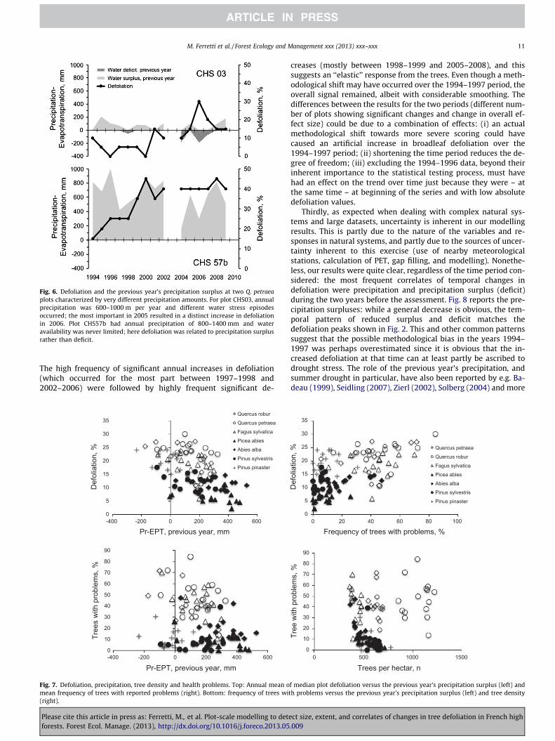
Fig. 6. Defoliation and the previous year’s precipitation surplus at two Q. petraeaplots characterized by very different precipitation amounts. For plot CHS03, annualprecipitation was 600–1000 m per year and different water stress episodesoccurred; the most important in 2005 resulted in a distinct increase in defoliationin 2006. Plot CHS57b had annual precipitation of 800–1400 mm and wateravailability was never limited; here defoliation was related to precipitation surplusrather than deficit.


The high frequency of significant annual increases in defoliation(which occurred for the most part between 1997–1998 and2002–2006) were followed by highly frequent significant de-

0

5

10

15

20

25

30

35

-400 -200

Def

olia

tion,

%

Pr-EPT, previous year, mm

Quercus robur

Quercus petraea

Fagus sylvatica

Picea abies

Abies alba

Pinus sylvestris

Pinus pinaster

0

10

20

30

40

50

60

70

80

90

-400 -200

Tree

s w

ith p

robl

ems,

%

Pr-EPT, previous year, mm

0 200 400 600

0 200 400 600

Fig. 7. Defoliation, precipitation, tree density and health problems. Top: Annual mean omean frequency of trees with reported problems (right). Bottom: frequency of trees wi(right).


creases (mostly between 1998–1999 and 2005–2008), and thissuggests an ‘‘elastic’’ response from the trees. Even though a meth-odological shift may have occurred over the 1994–1997 period, theoverall signal remained, albeit with considerable smoothing. Thedifferences between the results for the two periods (different num-ber of plots showing significant changes and change in overall ef-fect size) could be due to a combination of effects: (i) an actualmethodological shift towards more severe scoring could havecaused an artificial increase in broadleaf defoliation over the1994–1997 period; (ii) shortening the time period reduces the de-gree of freedom; (iii) excluding the 1994–1996 data, beyond theirinherent importance to the statistical testing process, must havehad an effect on the trend over time just because they were – atthe same time – at beginning of the series and with low absolutedefoliation values.

Thirdly, as expected when dealing with complex natural sys-tems and large datasets, uncertainty is inherent in our modellingresults. This is partly due to the nature of the variables and re-sponses in natural systems, and partly due to the sources of uncer-tainty inherent to this exercise (use of nearby meteorologicalstations, calculation of PET, gap filling, and modelling). Nonethe-less, our results were quite clear, regardless of the time period con-sidered: the most frequent correlates of temporal changes indefoliation were precipitation and precipitation surplus (deficit)during the two years before the assessment. Fig. 8 reports the pre-cipitation surpluses: while a general decrease is obvious, the tem-poral pattern of reduced surplus and deficit matches thedefoliation peaks shown in Fig. 2. This and other common patternssuggest that the possible methodological bias in the years 1994–1997 was perhaps overestimated since it is obvious that the in-creased defoliation at that time can at least partly be ascribed todrought stress. The role of the previous year’s precipitation, andsummer drought in particular, have also been reported by e.g. Ba-deau (1999), Seidling (2007), Zierl (2002), Solberg (2004) and more

0

5

10

15

20

25

30

35

Def

olia

tion,

%

Frequency of trees with problems, %

Quercus petraea

Quercus robur

Fagus sylvatica

Picea abies

Abies alba

Pinus sylvestris

Pinus pinaster

0

10

20

30

40

50

60

70

80

90

0

0 20 40 60 80 100

500 1000 1500

Tree

with

pro

blem

s, %

Trees per hectar, n

f median plot defoliation versus the previous year’s precipitation surplus (left) andth problems versus the previous year’s precipitation surplus (left) and tree density



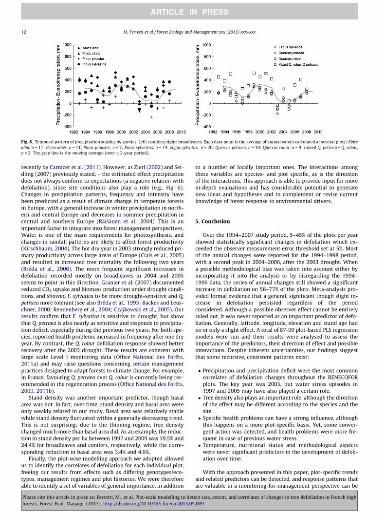
Fig. 8. Temporal pattern of precipitation surplus by species. Left: conifers; right: broadleaves. Each data point is the average of annual values calculated at several plots: Abiesalba, n = 11; Picea abies, n = 11; Pinus pinaster, n = 7; Pinus sylvestris, n = 14; Fagus sylvatica, n = 20; Quercus petraea, n = 19; Quercus robur, n = 9; mixed Q. petraea + Q. robur,n = 2. The gray line is the moving average (over a 2-year period).


recently by Carnicer et al. (2011). However, as Zierl (2002) and Sei-dling (2007) previously stated, – the estimated effect precipitationdoes not always conform to expectations (a negative relation withdefoliation), since site conditions also play a role (e.g., Fig. 6).Changes in precipitation patterns, frequency and intensity havebeen predicted as a result of climate change in temperate forestsin Europe, with a general increase in winter precipitation in north-ern and central Europe and decreases in summer precipitation incentral and southern Europe (Räisänen et al., 2004). This is animportant factor to integrate into forest management perspectives.Water is one of the main requirements for photosynthesis, andchanges in rainfall patterns are likely to affect forest productivity(Kirschbaum, 2004). The hot dry year in 2003 strongly reduced pri-mary productivity across large areas of Europe (Ciais et al., 2005)and resulted in increased tree mortality the following two years(Bréda et al., 2006). The more frequent significant increases indefoliation recorded mostly on broadleaves in 2004 and 2005seems to point in this direction. Granier et al. (2007) documentedreduced CO2 uptake and biomass production under drought condi-tions, and showed F. sylvatica to be more drought-sensitive and Q.petraea more tolerant (see also Bréda et al., 1993; Backes and Leus-chner, 2000; Rennenberg et al., 2004; Czajkowski et al., 2005). Ourresults confirm that F. sylvatica is sensitive to drought, but showthat Q. petraea is also nearly as sensitive and responds to precipita-tion deficit, especially during the previous two years. For both spe-cies, reported health problems increased in frequency after one dryyear. By contrast, the Q. robur defoliation response showed betterrecovery after the 2003 drought. These results are coherent withlarge scale Level I monitoring data (Office National des Forêts,2011a) and may raise questions concerning certain managementpractices designed to adapt forests to climate change. For example,in France, favouring Q. petraea over Q. robur is currently being rec-ommended in the regeneration process (Office National des Forêts,2009, 2011b).

Stand density was another important predictor, though basalarea was not. In fact, over time, stand density and basal area wereonly weakly related in our study. Basal area was relatively stablewhile stand density fluctuated within a generally decreasing trend.This is not surprising; due to the thinning regime, tree densitychanged much more than basal area did. As an example, the reduc-tion in stand density per ha between 1997 and 2009 was 19.5% and24.4% for broadleaves and conifers, respectively, while the corre-sponding reduction in basal area was 3.4% and 4.6%.

Finally, the plot-wise modelling approach we adopted allowedus to identify the correlates of defoliation for each individual plot,freeing our results from effects such as differing genotypes/eco-types, management regimes and plot histories. We were thereforeable to identify a set of variables of general importance, in addition


to a number of locally important ones. The interactions amongthese variables are species- and plot specific, as is the directionof the interactions. This approach is able to provide input for morein-depth evaluations and has considerable potential to generatenew ideas and hypotheses and to complement or revise currentknowledge of forest response to environmental drivers.

5. Conclusion

Over the 1994–2007 study period, 5–45% of the plots per yearshowed statistically significant changes in defoliation which ex-ceeded the observer measurement error threshold set at 5%. Mostof the annual changes were reported for the 1994–1998 period,with a second peak in 2004–2006, after the 2003 drought. Whena possible methodological bias was taken into account either byincorporating it into the analysis or by disregarding the 1994–1996 data, the series of annual changes still showed a significantincrease in defoliation on 56–77% of the plots. Meta-analysis pro-vided formal evidence that a general, significant though slight in-crease in defoliation persisted regardless of the periodconsidered. Although a possible observer effect cannot be entirelyruled out, it was never reported as an important predictor of defo-liation. Generally, latitude, longitude, elevation and stand age hadno or only a slight effect. A total of 87-90 plot-based PLS regressionmodels were run and their results were analysed to assess theimportance of the predictors, their direction of effect and possibleinteractions. Despite inherent uncertainties, our findings suggestthat some recursive, consistent patterns exist:

� Precipitation and precipitation deficit were the most commoncorrelates of defoliation changes throughout the RENECOFORplots. The key year was 2003, but water stress episodes in1997 and 2005 may have also played a certain role.� Tree density also plays an important role, although the direction

of the effect may be different according to the species and thesite.� Specific health problems can have a strong influence, although

this happens on a more plot-specific basis. Yet, some conver-gent action was detected, and health problems were more fre-quent in case of previous water stress.� Temperature, nutritional status and methodological aspects

were never significant predictors in the development of defoli-ation over time.

With the approach presented in this paper, plot-specific trendsand related predictors can be detected, and response patterns thatare valuable in a monitoring-for-management perspective can be




revealed. For example, the blanket practice of favouring Q. petraeaover Q. robur to adapt French forests to climate change may needreconsideration in light of the results from our dataset showingthat Q. petraea did not react better to drought. In a similar way,other species-specific responses can be identified in relation tospecific stressors, and this information is useful for local managersto help determine whether management options were, are and willbe capable of sustaining the health and productivity of theirforests.

Acknowledgements

We are grateful to Jean-Luc Flot, Louis-Michel Nageleisen, Fabi-en Caroulle and Morgane Goudet (DSF) for their assistance in thepreparation of the dataset and for stimulating discussions. Weacknowledge Vincent Badeau (INRA) for his input and commentsduring the early phases of this work.

References

Allen, C.D., Macalady, A.K., Chenchouni, H., Bachelet, D., McDowell, N., Vennetier,M., Kitzberger, T., Rigling, A., Breshears, D.D., Hogg, E.H., Gonzalez, P., Fensham,R., Zhang, Z., Castro, J., Demidova, N., Lim, J.H., Allard, G., Running, S.W., Semerci,A., Cobb, N., 2010. A global overview of drought and heat-induced tree mortalityreveals emerging climate change risks for forests. For. Ecol. Manage. 259, 660–684.

Backes, K., Leuschner, C., 2000. Leaf water relations of competitive Fagus sylvaticaand Quercus petraea trees during 4 years differing in soil drought. Can. J. For.Res. 30, 335–346.

Badeau, V., 1999. Etude des relations entre l’état sanitaire des peuplementsforestiers et les conditions de l’environnement. Premiers résultats de l’analysespatio-temporelle de la partie française du réseau européen de suivi desdommages forestiers. Rapport final à la CE et à la DERF, INRA Nancy, 172p.+annexes.

Berkey, C.S., Hoaglin, D.C., Mosteller, F., Colditz, G.A., 1995. A random-effectsregression model for meta-analysis. Stat. Med. 14, 395–411.

Bolte, A., Ammer, C., Löf, M., Madsen, P., Nabuurs, G., Schall, P., Spathelf, P., Rock, J.,2009. Adaptive forest management in central Europe: Climate change impacts,strategies and integrative concept. Scand. J. For. Res. 24, 471–480.

Bréda, N., Cochard, H., Dreyer, E., Granier, A., 1993. Water transfer in a mature oakstand (Quercus petraea): seasonal evolution and effects of a severe drought. Can.J. For. Res. 23, 1136–1143.

Bréda, N., Huc, R., Granier, A., Dreyer, E., 2006. Temperate forest trees and standsunder severe drought: a review of ecophysiological responses, adaptationprocesses and long-term consequences. Ann. For. Sci. 63, 625–644.

Bussotti, F., Cozzi, A., Cenni, E., Bettini, D., Sarti, C., Ferretti, M., 2009. Measurementerrors in monitoring tree crown conditions: entity, control, evolution andimplications for results. J. Environ. Monit. 11, 769–773.

Bussotti, F., Ferretti, M., 2009. Visible injury, crown condition, and growth responsesof selected Italian forests in relation to ozone exposure. Environ.l Pollut. 15,1427–1437.

Carnicer, J., Coll, M., Ninyerola, M., Pons, X., Sánchez, G., Peñuelas, J., 2011.Widespread crown condition decline, food web disruption, and amplified treemortality with increased climate change-type drought. Proc. Natl. Acad. Sci.USA 108, 1474–1478.

Ciais, P., Reichstein, M., Viovy, N., Granier, A., Ogee, J., Allard, V., Aubinet, M.,Buchmann, N., Bernhofer, C., Carrara, A., Chevallier, F., De Noblet, N., Friend,A.D., Friedlingstein, P., Grunwald, T., Heinesch, B., Keronen, P., Knohl, A., Krinner,G., Loustau, D., Manca, G., Matteucci, G.M., F., Ourcival, J.M., Papale, D.,Pilegaard, K., Rambal, S., Seufert, G., Soussana, J.F., Sanz, M.J., Schulze, E.D.,Vesala, T., Valentini, R., 2005. Europe-wide reduction in primary productivitycaused by the heat and drought in 2003. vol. 437, pp. 529–533.

Czajkowski, T., Kühling, M., Bolte, A., 2005. Impact of the 2003 summer drought ongrowth of beech sapling natural regeneration (Fagus sylvatica L.) in north-eastern Central Europe. Allgemeine Forst- und Jagd-Zeitung 176, 133–143.

Elzinga, C.L., Salzer, D.W., Willoughby, J.W., Gibbs, J.P., 2001. Monitoring Plant andAnimal Populations. Blackwell Science, Malden, Massachusetts, 360 ps.

Ferretti, M., 1998. Potential and limitation of visual indices of tree condition.Chemosphere 36, 1031–1036.

Ferretti, M., 2013. Concepts and design principles adopted in the internationalcooperative program on the assessment and monitoring of air pollution effectson forests (ICP Forests). In: Ferretti, M., Fischer, R. (Eds.), Forest Monitoring.Elsevier, London, pp. 91–104.

Ferretti, M., Chiarucci, A., 2003. Design concepts adopted in long-term forestmonitoring programs in Europe – problems for the future? Sci. Tot. Environ.310, 171–178.

Ferretti, M., Fischer, R., 2013. Forest Monitoring. Elsevier, London, 507 ps.Ferretti, M., Bussotti, F., Cenni, E., Cozzi, A., 1999. Implementation of quality

assurance procedures in the Italian Programs of Forest Condition Monitoring.Water Air Soil Pollut. 116, 371–376.


Ferretti, M., Gerosa, G., Bussotti, F., Fabbio, G., 2003. Ozone exposure, crowntransparency and basal area increment at the Permanent Monitoring Plots ofthe CONECOFOR programme in Italy. Annali Istituto Sperimentale per laSelvicoltura 30, 107–120.

Ferretti, M., Calderisi, M., Bussotti, F., 2007. Ozone exposure, defoliation of beech(Fagus sylvatica L.) and visible foliar symptoms on native plants in selected plotsof South-Western Europe. Environ. Pollut. 145, 644–651.

Ferretti, M., König, N., Rautio, P., Sase, H., 2009. Quality assurance in internationalforest monitoring programmes: activity, problems and perspectives from EastAsia and Europe. Ann. For. Sci. 66, 403–415.

Ferretti M., Bacaro G., Brunialti G., Calderisi M., Frati L., Leone L., Marignani M., SantiE., 2012a. Analysis of Forest Health data from the RENECOFOR plots. Part 2.Change and Trend Analysis. Report TDe 47–2010/9 v1 r1, MonterotondoMarittimo (GR): 78 ps.

Ferretti M., Bacaro G., Brunialti G., Calderisi M., Frati L., Leone L., Santi E., 2012b.Analysis of Forest Health data from the RENECOFOR plots. Part 3+. Relationshipwith environmental factors, 1997–2009. Report TDe 53–2011/2 v1 r1,Monterotondo Marittimo (GR): 120 ps.

Ferretti M., Bacaro G., Brunialti G., Calderisi M., Frati L., Pollastrini M., 2013a.Relationship between forest health and growth at the RENECOFOR plots. Part 2.Final Report. Report TDe 66–2013/1 v1 r1, Monterotondo Marittimo: 64 ps.

Ferretti, M., Beuker, E., Calatayud, V., Canullo, R., Dobbertin, M., Eichhorn, J.,Neumann, M., Roskams, P., Schaub, M., 2013b. Data quality in field surveys:methods and results for tree condition, phenology, growth, plant diversity andfoliar injury due to ozone. In: Ferretti, M., Fischer, R. (Eds.), Forest Monitoring.Elsevier, London, pp. 397–414.

FOREST EUROPE, UNECE and FAO, 2011. State of Europe’s Forests 2011. Status andTrends in Sustainable Forest Management in Europe.

Gottardini, E., Cristofori, A., Cristofolini, F., Ferretti, M., 2010. Variability of ozoneconcentration in a montane environment, northern Italy. Atmos. Environ. 44(2010), 147–152.

Granier, A., Reichstein, M., Bréda, N., Janssens, I.A., Falge, E., Ciais, P., Grünwald, T.,Aubinet, M., Berbigier, P., Bernhofer, C., Buchmann, N., Facini, O., Grassi, G.,Heinesch, B., Ilvesniemi, H., Keronen, P., Knohl, A., Köstner, B., Lagergren, F.,Lindroth, A., Longdoz, B., Loustau, D., Mateus, J., Montagnani, L., Nys, C., Moors,E., Papale, D., Peiffer, M., Pilegaard, K., Pita, G., Pumpanen, J., Rambal, S.,Rebmann, C., Rodrigues, A., Seufert, G., Tenhunen, J., Vesala, T., Wang, Q., 2007.Evidence for soil water control on carbon and water dynamics in Europeanforests during the extremely dry year: 2003. Agric. Forest Meteorol. 143, 123–145.

Harrison, F., 2011. Getting started with meta-analysis. Methods Ecol. Evol. 2, 1–10.Hedges, L.V., Olkin, I., 1985. Statistical Methods for Meta-Analysis. Academic Press,

San Diego, CA.Hillebrand, H., 2008. Meta-analysis in ecology. Encyclopedia of Life Sciences (ELS).

John Wiley & Sons, Ltd., Chichester.Innes, J.L., 1988. Forest health surveys: problems in assessing observer objectivity.

Can. J. For. Res. 18, 560–565.Innes, J.L., 1993. Forest Health: Its Assessment and Status. CAB International,

Wallingford,Oxon, UK.Innes, J.L., 1995. Theoretical and practical criteria for the selection of ecosystem

monitoring plots in Swiss forests. Environ. Monit. Assess. 36, 271–294.Innes, J.L., 1998. Measuring environmental change. In: Peterson, D.L., Parker, V.T.

(Eds.), Ecological Scale—Theory and Applications. Columbia University Press,New York, pp. 429–457.

Innes, J.L., Boswell, R.C., 1991. Monitoring of forest condition in Great Britain 1990.Forestry Commission. Bullettin 98, HMSO London.

Innes, J.L., Whittaker, R.J., 1993. Relationships between the crown condition of Sitkaand Norway spruce and the environment in Great Britain: an exploratoryanalysis. J. Appl. Ecol. 30, 341–360.

IPCC, 2007. Climate change 2007: impacts, adaptation and vulnerability.Contribution of Working Group II to the Fourth Assessment. Report of theIntergovernmental Panel on Climate Change. Cambridge University Press,Cambridge, UK.

Kirschbaum, M.U.F., 2004. Assessing long-term trend in forest productivity underchanging climatic conditions. In: IUFRO 4.01.09 Process Based Models for ForestManagement – Internationa Conference on Modeling Forest Production,University of Natural Resources and Applied Life Science, Department ofEcology, Vienna, Austria.

Klap, J.M., Oude Voshaar, J.H., De Vries, W., Erisman, J.W., 2000. Effects ofenvironmental stress on forest crown condition in Europe. Part IV: statisticalanalysis of relationships. Water Air Soil Pollut. 119, 387–420.

Köhl, L.M., Scott, C.T., Zingg, A.,1994. Permanent Monitoring Plots: Potential andLimitations. In: Innes, J.L. (Ed.), Assessment of increment in permanent sampleplots established to determine the effects of air pollution on forests, Proceed. ofthe Sopron workshop, August 28 September 1, 1993, Sopron, Hungary, WSL/FNP, pp. 17–24.

Landmann, G., Nageleisen, L.-M., Ulrich, E., 1998. De nouveaux éléments en faveurd’un glissement récent d’origine méthodologique dans l’appréciation visuelledes cimes des feuillus. Les Cahiers de DSF 1, 74–76.

Landmann, G., Pierrat, J.-C., Nageleisen, L.-M., 1999. 1995–97: période deréajustement à la hausse de la notation de l’état des cimes des arbresforestiers en France. Les Cahiers de DSF 1, 63–66.

Lindenmayer, D.B., Likens, G.E., 2009. Adaptive monitoring: a new paradigm forlong-term research and monitoring. Trends Ecol. Evol. 24, 482–486.

Lindenmayer, D.B., Likens, G.E., Haywood, A., Miezis, L., 2011. Adaptive monitoringin the real world: proof of concept. Trends Ecol. Evol. 26, 641–646.


http://refhub.elsevier.com/S0378-1127(13)00299-5/h0005





































































































Lorenz, M., Fischer, R., 2013. Pan-European forest monitoring: and overview. In:Ferretti, M., Fischer, R. (Eds.), Forest Monitoring. Elsevier, London.

Magnani, F., Mencuccini, M., Borghetti, M., Berbigier, P., Berninger, F., Delzon, S.,Grelle, A., Hari, P., Jarvis, P.G., Kolari, P., Kowalski, A.S., Lankreijer, H., Law, B.E.,Lindroth, A., Loustau, D., Manca, G., Moncrieff, J.B., Rayment, M., Tedeschi, V.,Valentini, R., Grace, J., 2007. The human footprint in the carbon cycle oftemperate and boreal forests. Nature 447, 848–850.

Martens, H., Næs, T., 1989. Multivariate Calibration. Wiley, Chichester.Meehl, G.A., Tebaldi, C., 2004. More intense, more frequent, and longer lasting heat

waves in the 21st century. Science 305, 994–997.Nageleisen, L.-M., Depierre, A., Letz, J.-M., 2005. Réseaux européens de suivi des

dommages forestiers, Niveau 1 (réseau systématique 16 km � 16 km) et Niveau2 (RENECOFOR). Manuel Notation des dommages forestiers (Symptômes,causes, état des cimes). Avril 2005. 87p.

Niinemets, U., 2010. Responses of forest trees to single and multiple environmentalstresses from seedlings to mature plants: past stress history, stress interactions,tolerance and acclimation. For. Ecol. Manage. 260, 1623–1639.

Office National des Forêts, 2009. Directive régionale d’aménagement du bassinligérien. Avril 2009. Office National des Forêts, 137 p.

Office National des Forêts, 2011a. Bilan patrimonial des forêts domaniales horsDOM. ONF, Paris: 180 ps. ISBN 978-2-84207-354-1.

Office National des Forêts, 2011b. Directive régionale d’aménagement deBourgogne. Mars 2011. Office National des Forêts, 224 p.

Palmer, M.W., 1993. Potential biases in sites and species selection for ecologicalmonitoring. Environ. Monit. Assess. 26, 277–282.

Percy, K.E., Ferretti, M., 2004. Air pollution and forest health: toward newmonitoring concepts. Environ. Pollut. 130, 113–126.

Räisänen, J., Hansson, U., Ullerstig, A., Döscher, R., Graham, L.P., Jones, C., Meier,H.E.M., Samuelsson, P., Willén, U., 2004. European climate in the late twenty-first century: regional simulations with two driving global models and twoforcing scenarios. Clim. Dyn. 22, 13–31.

Raudenbush, S.W., 2009. Analyzing effect sizes: random effects models. In: Cooper,H., Hedges, L.V., Valentine, J.C. (Eds.), The Handbook of Research Synthesis andMeta-Analysis, 2nd ed. Russell Sage Foundation, New York, pp. 295–315.

Rennenberg, H., Seiler, W., Matyssek, R., Gessler, A., Kreuzwieser, J., 2004. Europeanbeech (Fagus sylvatica L.) – a forest tree without future in the south of CentralEurope? Allgemeine Forst Und Jagdzeitung 175, 210–224.

Seidling, W., 2000. Multivariate statistics within integrated studies in tree crowncondition in europe – an overview, United Nations Economic Commission forEurope, European Commission, Geneva, Brussels, 56 p. + Annexes.

Seidling, W., 2007. Signals of summer drought in crown condition data from theGerman Level I network. Eur. J. For. Res. 126, 529–544.

Solberg, S., 1999. Crown condition and growth relationships within stands of Piceaabies. Scand. J. For. Res. 14 (4), 320–327.

Solberg, S., 2004. Summer drought: a driver for crown condition and mortality ofNorway spruce in Norway. For. Pathol. 34, 93–107.


Solberg, S., Tveite, B., 2000. Crown density and growth relationships between standsof Picea abies in Norway. Scand. J. For. Res. 15 (1), 87–96.

Stewart, G., 2010. Meta-analysis in applied ecology. Biol. Lett. 6, 78–81.Stout, B., 1993. The good, the bad and the ugly of monitoring programs: defining

questions and establishing objectives. Environ. Monit. Assess. 26 (2–3), 91–98.Tallent-Halsell, N.G., 1994. Forest health monitoring 1994. Field Methods Guide,

EPA/620/R-94/027. US Environmental Protection Agency, Washington, DC, USA.Turc, L., 1955. Le bilan d’eau des sols. Relation entre les precipitations, l’évaporation

et l’écoulement. Ann. Agron. 5, 501–596.Turc, L., 1961. Evaluation des besoins en eau d’irrigation, évapo-transpiration

potentielle. Ann. Agron. 12, 13–49.Ulrich, E., Vannière, B., Duplat, P., Demolis, C., Guyon, J.-P., 1994a. RENECOFOR –

Manuel de référence n�1 pour la sélection et l’implantation des placettespermanentes, éditeur: Office National des Forêts, Département des RecherchesTechniques, 34 p.

Ulrich, E., Barthod, C., Bouhot, L., 1994b. Manuel de référence no. 7 pour lesobservations de l’état des cimes et des symptômes pathologiques etentomologiques. Placettes de niveau 1 (Level II plots within the EuropeanUnion). Première version, Juin 1994, 41 p.

Ulrich, E., Barthod, C., Bouhot, L., 1995. Manuel de référence no. 7 pour lesobservations de l’état des cimes et des symptômes pathologiques etentomologiques. Placettes de niveau 1 (Level II plots within the EuropeanUnion). Deuxième version, Mai 1995, 51p.

Ulrich, E., Barthod, C., Bouhot, L., 1996. Manuel de référence no. 7 pour lesobservations de l’état des cimes et des symptômes pathologiques etentomologiques. Placettes de niveau 1 (Level II plots within the EuropeanUnion). Troisième version, Juin 1996, 51p.

Ulrich, E., Barthod, C., Bouhot, L., 1997. Manuel de référence no. 7 pour lesobservations de l’état des cimes et des symptômes pathologiques etentomologiques. Placettes de niveau 1 (Level II plots within the EuropeanUnion). Quatrième version, Juin 1997, 51p.

UN/ECE, CEC, 1994. Forest Condition in Europe. Report on the 1993 Survey. Geneva,Brussels: UN/ECE, CEC, 173p.

van Houwelingen, H.C., Arends, L.R., Stijnen, T., 2002. Advanced methods in meta-analysis: multivariate approach and meta-regression. Stat. Med. 21, 589–624.

Viechtbauer, W., 2005. Bias and efficiency of meta-analytic variance estimators inthe random-effects model. J. Educ. Behav. Stat. 30, 261–293.

Viechtbauer, W., 2007. Confidence intervals for the amount of heterogeneity inmeta-analysis. Stat. Med. 26, 37–52.

Wold, S., Johansson, E., Cocchi, M., 1993. 3D QSAR in drug design: theory, methods,and applications, ESCOM, Leiden, Holland, pp. 523–550.

Wulff, S., Lindelöw, Å., Lundin, L., Hansson, P., Axelsson, A.L., Barklund, P., Wijk, S.,Ståhl, G., 2012. Adapting forest health assessments to changing perspectives onthreats – a case example from Sweden. Environ. Monit. Assess. 184, 2453–2464.

Zierl, B., 2002. Relations between crown condition and ozone and its dependence onenvironmental factors. Environ. Pollut. 119, 55–68.
























































Plot-scale modelling to detect size, extent, and correlates of changes in tree defoliation in French...

Documents

Transcript of Plot-scale modelling to detect size, extent, and correlates of changes in tree defoliation in French...