Planning of the Agrifood supply chain: a case study for the FVG region
13
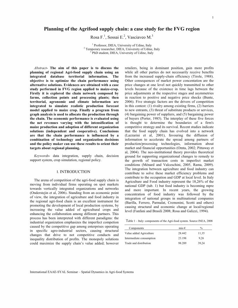
1 International EAAE-SYAL Seminar – Spatial Dynamics in Agri-food Systems Planning of the Agrifood supply chain: a case study for the FVG region Rosa F. 1 , Sossai E. 2 , Vasciaveo M. 3 1 Professor, DIEA, University of Udine, Italy 2 Temporary researcher, DIEA, University of Udine, Italy 3 PhD student, DIEA, University of Udine, Italy Abstract- The aim of this paper is to discuss the planning of regional Agri-food supply chain using an integrated database territorial information. The objective is to optimize the chain performance using alternative solutions. Evidences are obtained with a case study performed in FVG region applied to maize-crop. Firstly it is explored the chain network composed by farms, collection points and processing plants; then territorial, agronomic and climate information are integrated to simulate realistic production forecast model applied to maize crop. Finally a program from graph analysis is used to allocate the production through the chain. The economic performance is evaluated using the net revenues varying with the intensification of maize production and adoption of different organization solutions (independent and cooperative). Conclusions are that the chain performance is influenced by a combination of technology and organization decisions and the policy maker can use these results to orient their targets about regional planning. Keywords- data integration, supply chain, decision support system, crop simulation, regional policy. I. INTRODUCTION The arena of competition of the agri-food supply chain is moving from individual firms operating on spot markets towards vertically integrated organizations and networks (Onderstejin et al, 2006). Standing from an economic point of view, the integration of agriculture and food industry in the regional agri-food chain is an excellent instrument for promoting the development of local production systems, by increasing the value added of agricultural crops and enhancing the collaboration among different partners. This process has been interpreted with different paradigms: the industrial organization emphasizes the imperfect competion caused by the competitive gap among enterprises operating in specific agro-industrial sectors, causing structural changes that drive to not competitive conducts and inequality distribution of profits. The monopoly solutions could maximize the supply chain’s value added; however retailers, being in dominant position, gain more profits while all other parties do not necessarily receive benefits from the increased supply-chain efficiency (Tirole, 1988). Other consequences of market power concentation are the price changes at one level not quickly transmitted to other levels because of the existence in time lags between the price adjustments at the respective stages and asymmetries in reaction to positive and negative price shocks (Bunte, 2006). Five strategic factors are the drivers of competition in this contest: (1) rivalry among existing firms, (2) barriers to new entrants, (3) threat of substitute products or services, (4) bargaining power of suppliers, and (5) bargaining power of buyers (Porter, 1985). The interplay of these five forces is thought to determine the boundaries of a firm's competitive strategy and its survival. Recent studies indicate that the food supply chain has evolved into a network (Lazzarini et al, 2001), favouring the diffusion of information to accelerate the spread among partners of production/processing technologies, information about market and financial opportunities (Omta, 2002; Pittaway et al, 2004). The neo-institutional theory provides theoretical ground for supporting organizational changes to remedy to the growth of transaction costs in imperfect market conditions (Ménard and Valceschini, 2005, Rama, 2009). The integration between agriculture and food industry can contribute to solve these market efficiency problems and contribute to the occupation and GDP at local level. In Italy Agriculture and Food industry represent the 18,26% of the national GDP (tab. 1) but food industry is becoming mpre and more important. In recent years, the growing concentration of food industry was followed by the integration of national groups in multinational companies (Barilla, Ferrero, Parmalat, Cremonini, Scotti and others) causing structural and economic change at local/regional level (Fanfani and Brasili 2008; Rosa and Galizzi, 1994). Table 1 – Italy: components of the Agri-food system. Source INEA, 2008 Components mio € % Value added Agriculture 28.442 11,35 Intermediate consumption 23.198 9,26 Trade and distribution 98.289 39,24
Transcript of Planning of the Agrifood supply chain: a case study for the FVG region
1
International EAAE-SYAL Seminar – Spatial Dynamics in Agri-food Systems
Planning of the Agrifood supply chain: a case study for the FVG region
Rosa F.1, Sossai E.
2, Vasciaveo M.
3
1 Professor, DIEA, University of Udine, Italy 2 Temporary researcher, DIEA, University of Udine, Italy
3 PhD student, DIEA, University of Udine, Italy
Abstract- The aim of this paper is to discuss the
planning of regional Agri-food supply chain using an
integrated database territorial information. The
objective is to optimize the chain performance using
alternative solutions. Evidences are obtained with a case
study performed in FVG region applied to maize-crop.
Firstly it is explored the chain network composed by
farms, collection points and processing plants; then
territorial, agronomic and climate information are
integrated to simulate realistic production forecast
model applied to maize crop. Finally a program from
graph analysis is used to allocate the production through
the chain. The economic performance is evaluated using
the net revenues varying with the intensification of
maize production and adoption of different organization
solutions (independent and cooperative). Conclusions
are that the chain performance is influenced by a
combination of technology and organization decisions
and the policy maker can use these results to orient their
targets about regional planning.
Keywords- data integration, supply chain, decision
support system, crop simulation, regional policy.
I. INTRODUCTION
The arena of competition of the agri-food supply chain is
moving from individual firms operating on spot markets
towards vertically integrated organizations and networks
(Onderstejin et al, 2006). Standing from an economic point
of view, the integration of agriculture and food industry in
the regional agri-food chain is an excellent instrument for
promoting the development of local production systems, by
increasing the value added of agricultural crops and
enhancing the collaboration among different partners. This
process has been interpreted with different paradigms: the
industrial organization emphasizes the imperfect competion
caused by the competitive gap among enterprises operating
in specific agro-industrial sectors, causing structural
changes that drive to not competitive conducts and
inequality distribution of profits. The monopoly solutions
could maximize the supply chain’s value added; however
retailers, being in dominant position, gain more profits
while all other parties do not necessarily receive benefits
from the increased supply-chain efficiency (Tirole, 1988).
Other consequences of market power concentation are the
price changes at one level not quickly transmitted to other
levels because of the existence in time lags between the
price adjustments at the respective stages and asymmetries
in reaction to positive and negative price shocks (Bunte,
2006). Five strategic factors are the drivers of competition
in this contest: (1) rivalry among existing firms, (2) barriers
to new entrants, (3) threat of substitute products or services,
(4) bargaining power of suppliers, and (5) bargaining power
of buyers (Porter, 1985). The interplay of these five forces
is thought to determine the boundaries of a firm's
competitive strategy and its survival. Recent studies indicate
that the food supply chain has evolved into a network
(Lazzarini et al, 2001), favouring the diffusion of
information to accelerate the spread among partners of
production/processing technologies, information about
market and financial opportunities (Omta, 2002; Pittaway et
al, 2004). The neo-institutional theory provides theoretical
ground for supporting organizational changes to remedy to
the growth of transaction costs in imperfect market
conditions (Ménard and Valceschini, 2005, Rama, 2009).
The integration between agriculture and food industry can
contribute to solve these market efficiency problems and
contribute to the occupation and GDP at local level. In Italy
Agriculture and Food industry represent the 18,26% of the
national GDP (tab. 1) but food industry is becoming mpre
and more important. In recent years, the growing
concentration of food industry was followed by the
integration of national groups in multinational companies
(Barilla, Ferrero, Parmalat, Cremonini, Scotti and others)
causing structural and economic change at local/regional
level (Fanfani and Brasili 2008; Rosa and Galizzi, 1994).
Table 1 – Italy: components of the Agri-food system. Source INEA, 2008
Components mio € %
Value added Agriculture 28.442 11,35
Intermediate consumption 23.198 9,26
Trade and distribution 98.289 39,24
2
International EAAE-SYAL Seminar – Spatial Dynamics in Agri-food Systems
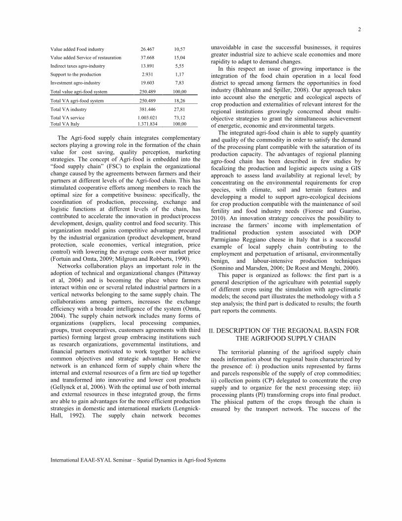
Value added Food industry 26.467 10,57
Value added Service of restauration 37.668 15,04
Indirect taxes agro-industry 13.891 5,55
Support to the production 2.931 1,17
Investment agro-industry 19.603 7,83
Total value agri-food system 250.489 100,00
Total VA agri-food system 250.489 18,26
Total VA industry 381.446 27,81
Total VA service 1.003.021 73,12
Total VA Italy 1.371.834 100,00
The Agri-food supply chain integrates complementary
sectors playing a growing role in the formation of the chain
value for cost saving, quality perception, marketing
strategies. The concept of Agri-food is embedded into the
“food supply chain” (FSC) to explain the organizational
change caused by the agreements between farmers and their
partners at different levels of the Agri-food chain. This has
stimulated cooperative efforts among members to reach the
optimal size for a competitive business: specifically, the
coordination of production, processing, exchange and
logistic functions at different levels of the chain, has
contributed to accelerate the innovation in product/process
development, design, quality control and food security. This
organization model gains competitive advantage procured
by the industrial organization (product development, brand
protection, scale economies, vertical integration, price
control) with lowering the average costs over market price
(Fortuin and Omta, 2009; Milgrom and Robberts, 1990).
Networks collaboration plays an important role in the
adoption of technical and organizational changes (Pittaway
et al, 2004) and is becoming the place where farmers
interact within one or several related industrial partners in a
vertical networks belonging to the same supply chain. The
collaborations among partners, increases the exchange
efficiency with a broader intelligence of the system (Omta,
2004). The supply chain network includes many forms of
organizations (suppliers, local processing companies,
groups, trust cooperatives, customers agreements with third
parties) forming largest group embracing institutions such
as research organizations, governmental institutions, and
financial partners motivated to work together to achieve
common objectives and strategic advantage. Hence the
network is an enhanced form of supply chain where the
internal and external resources of a firm are tied up together
and transformed into innovative and lower cost products
(Gellynck et al, 2006). With the optimal use of both internal
and external resources in these integrated group, the firms
are able to gain advantages for the more efficient production
strategies in domestic and international markets (Lengnick-
Hall, 1992). The supply chain network becomes
unavoidable in case the successful businesses, it requires
greater industrial size to achieve scale economies and more
rapidity to adapt to demand changes.
In this respect an issue of growing importance is the
integration of the food chain operation in a local food
district to spread among farmers the opportunities in food
industry (Bahlmann and Spiller, 2008). Our approach takes
into account also the energetic and ecological aspects of
crop production and externalities of relevant interest for the
regional institutions growingly concerned about multi-
objective strategies to grant the simultaneous achievement
of energetic, economic and environmental targets.
The integrated agri-food chain is able to supply quantity
and quality of the commodity in order to satisfy the demand
of the processing plant compatible with the saturation of its
production capacity. The advantages of regional planning
agro-food chain has been described in few studies by
focalizing the production and logistic aspects using a GIS
approach to assess land availability at regional level; by
concentrating on the environmental requirements for crop
species, with climate, soil and terrain features and
developping a model to support agro-ecological decisions
for crop production compatible with the maintenance of soil
fertility and food industry needs (Fiorese and Guariso,
2010). An innovation strategy conceives the possibility to
increase the farmers’ income with implementation of
traditional production system associated with DOP
Parmigiano Reggiano cheese in Italy that is a successful
example of local supply chain contributing to the
employment and perpetuation of artisanal, environmentally
benign, and labour-intensive production techniques
(Sonnino and Marsden, 2006; De Roest and Menghi, 2000).
This paper is organized as follows: the first part is a
general description of the agriculture with potential supply
of different crops using the simulation with agro-climatic
models; the second part illustrates the methodology with a 5
step analysis; the third part is dedicated to results; the fourth
part reports the comments.
II. DESCRIPTION OF THE REGIONAL BASIN FOR
THE AGRIFOOD SUPPLY CHAIN
The territorial planning of the agrifood supply chain
needs information about the regional basin characterized by
the presence of: i) production units represented by farms
and parcels responsible of the supply of crop commodities;
ii) collection points (CP) delegated to concentrate the crop
supply and to organize for the next processing step; iii)
processing plants (Pl) transforming crops into final product.
The phisical pattern of the crops through the chain is
ensured by the transport network. The success of the
3
International EAAE-SYAL Seminar – Spatial Dynamics in Agri-food Systems
regional planning depends on the configuration and
flexibility of the resource basin and is supported by
agronomic and climatic conditions, technology innovation,
and policies. Such policies support financially and with
suitable regulations the needed organizational adjustments.
In table 2 the structure of Agriculture in FVG region is
reported; composed by 24 thousand farms managing 225
thousand ha with an average surface of 9,43 ha per farm;
most of the agriculture is concentrated in larger farms: the
56,3% of the cultivated land is owned by 2.349 farms that
represent only the 10% of the total.
Table 1 – Farms and surface classified by size in FVG region. Source
ISTAT
variable < 1 1-2 2-5 5-10 10-20 20-50 > 50 Total
farm (n) 2.817 4.151 7.829 4.002 2.671 1.732 617 23.819
% 11,83 17,43 32,87 16,80 11,21 7,27 2,59 100,00
land (ha) 1.696 5.845 25.111 28.125 37.365 50.973 75.406 224.521
% 0,76 2,60 11,18 12,53 16,64 22,70 33,59 100,00
land/farm 0,60 1,41 3,21 7,03 13,99 29,43 122,21 9,43
Frequently the regional planning uses geografic
information techniques (GIS), soil representationa combined
with more traditional statistical sources (ISTAT, INEA,
ISMEA) giving an accurate representation of local
conditions affecting the crop supply.
Modern farm technologies improve consistently the crop
yield by combining agronomic and climatic condition at
local level in order to simulate models able to predict the
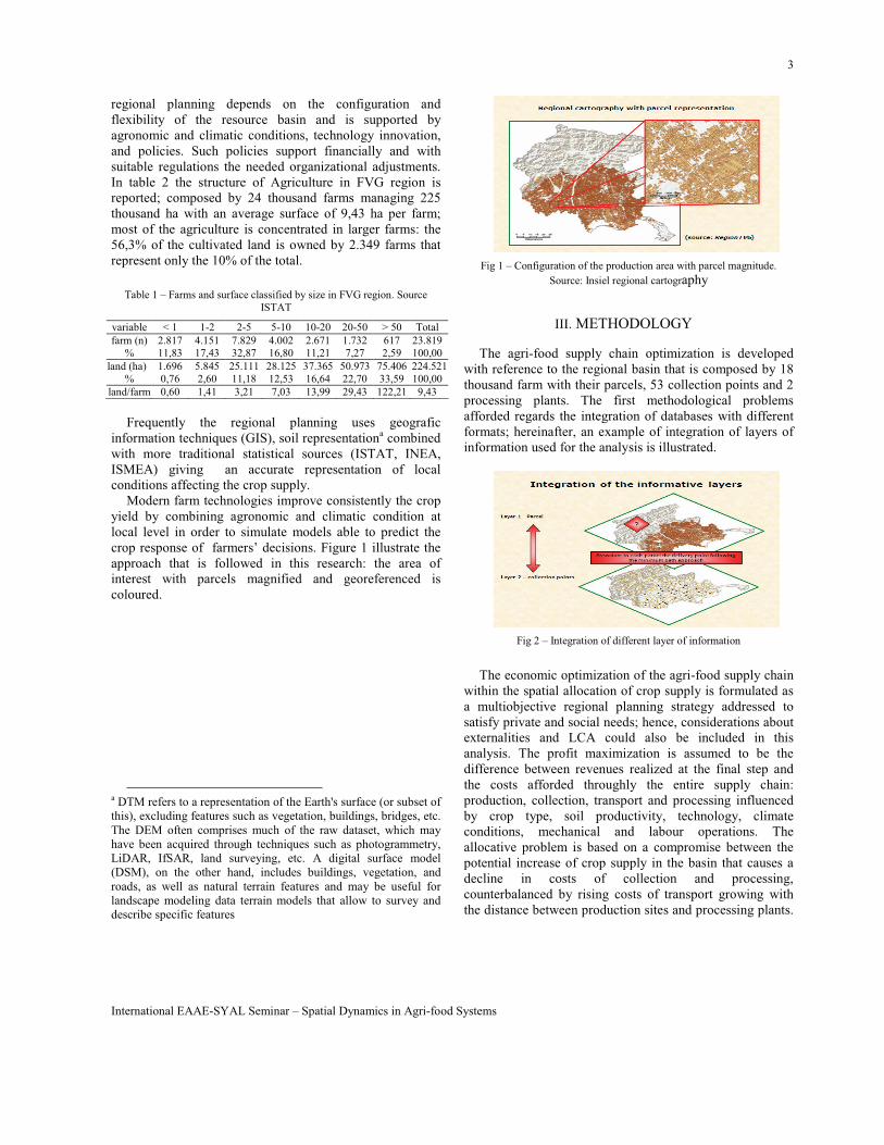
crop response of farmers’ decisions. Figure 1 illustrate the
approach that is followed in this research: the area of
interest with parcels magnified and georeferenced is
coloured.
a DTM refers to a representation of the Earth's surface (or subset of
this), excluding features such as vegetation, buildings, bridges, etc.
The DEM often comprises much of the raw dataset, which may
have been acquired through techniques such as photogrammetry,
LiDAR, IfSAR, land surveying, etc. A digital surface model
(DSM), on the other hand, includes buildings, vegetation, and
roads, as well as natural terrain features and may be useful for
landscape modeling data terrain models that allow to survey and
describe specific features
Fig 1 – Configuration of the production area with parcel magnitude.
Source: Insiel regional cartography
III. METHODOLOGY
The agri-food supply chain optimization is developed
with reference to the regional basin that is composed by 18
thousand farm with their parcels, 53 collection points and 2
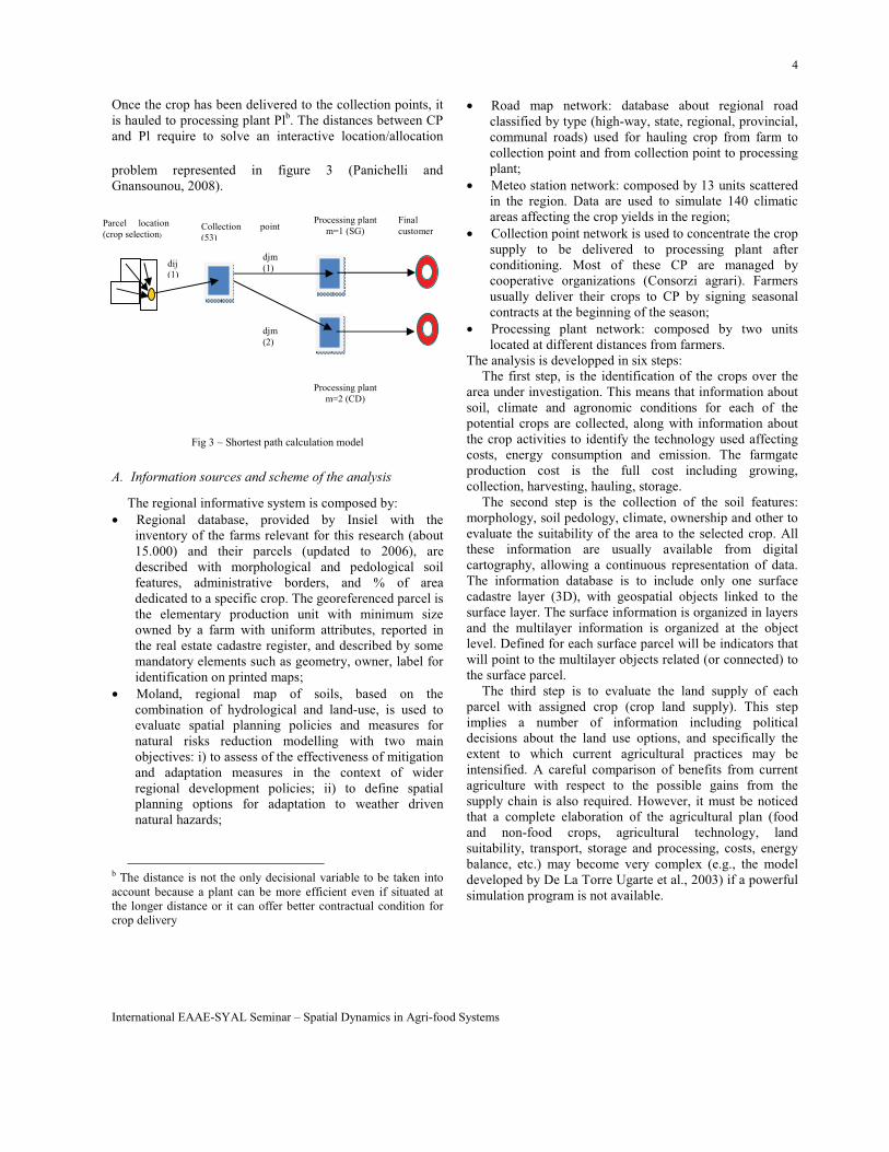
processing plants. The first methodological problems
afforded regards the integration of databases with different
formats; hereinafter, an example of integration of layers of
information used for the analysis is illustrated.
Fig 2 – Integration of different layer of information
The economic optimization of the agri-food supply chain
within the spatial allocation of crop supply is formulated as
a multiobjective regional planning strategy addressed to
satisfy private and social needs; hence, considerations about
externalities and LCA could also be included in this
analysis. The profit maximization is assumed to be the
difference between revenues realized at the final step and
the costs afforded throughly the entire supply chain:
production, collection, transport and processing influenced
by crop type, soil productivity, technology, climate
conditions, mechanical and labour operations. The
allocative problem is based on a compromise between the
potential increase of crop supply in the basin that causes a
decline in costs of collection and processing,
counterbalanced by rising costs of transport growing with
the distance between production sites and processing plants.
4
International EAAE-SYAL Seminar – Spatial Dynamics in Agri-food Systems
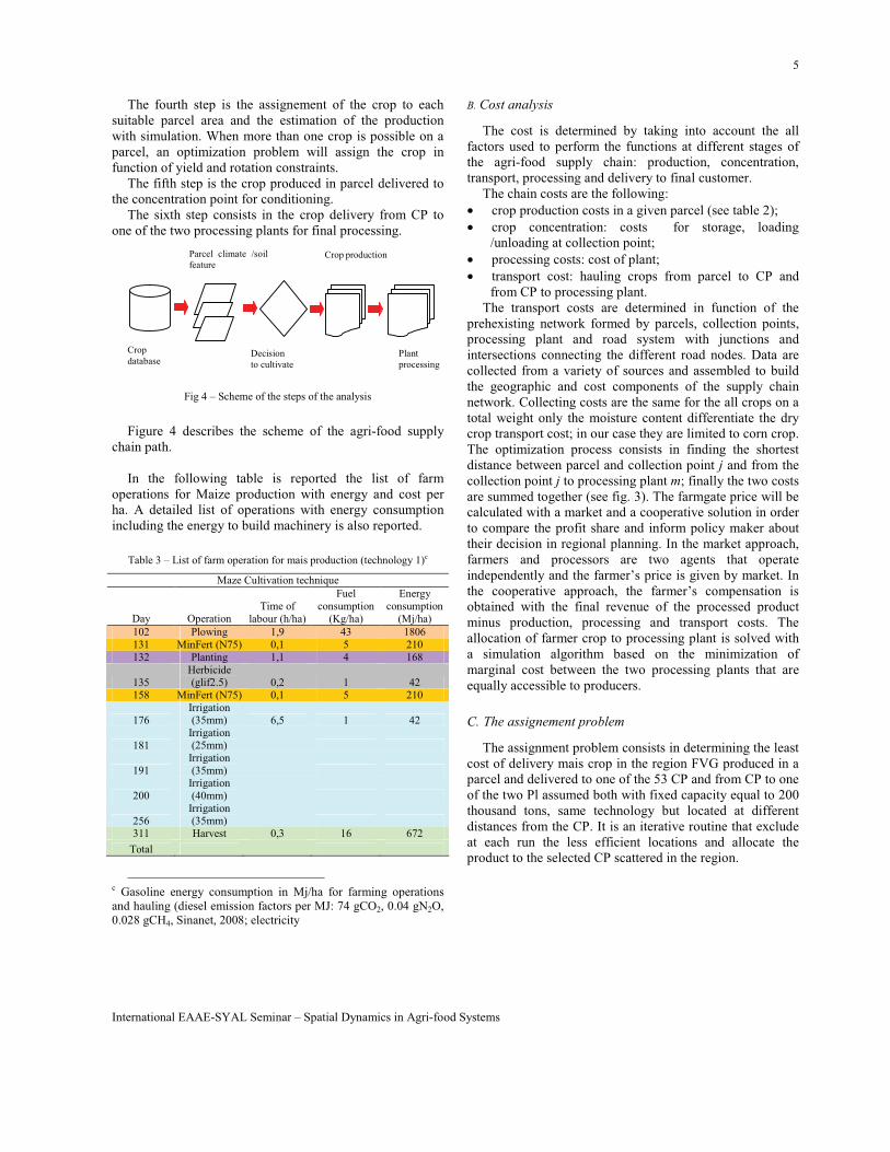
Once the crop has been delivered to the collection points, it
is hauled to processing plant Plb. The distances between CP
and Pl require to solve an interactive location/allocation
problem represented in figure 3 (Panichelli and
Gnansounou, 2008).
Fig 3 – Shortest path calculation model
A. Information sources and scheme of the analysis
The regional informative system is composed by:
• Regional database, provided by Insiel with the
inventory of the farms relevant for this research (about
15.000) and their parcels (updated to 2006), are
described with morphological and pedological soil
features, administrative borders, and % of area
dedicated to a specific crop. The georeferenced parcel is
the elementary production unit with minimum size
owned by a farm with uniform attributes, reported in
the real estate cadastre register, and described by some
mandatory elements such as geometry, owner, label for
identification on printed maps;
• Moland, regional map of soils, based on the
combination of hydrological and land-use, is used to
evaluate spatial planning policies and measures for
natural risks reduction modelling with two main
objectives: i) to assess of the effectiveness of mitigation
and adaptation measures in the context of wider
regional development policies; ii) to define spatial
planning options for adaptation to weather driven
natural hazards;
b The distance is not the only decisional variable to be taken into
account because a plant can be more efficient even if situated at
the longer distance or it can offer better contractual condition for
crop delivery
• Road map network: database about regional road
classified by type (high-way, state, regional, provincial,
communal roads) used for hauling crop from farm to
collection point and from collection point to processing
plant;
• Meteo station network: composed by 13 units scattered
in the region. Data are used to simulate 140 climatic
areas affecting the crop yields in the region;
• Collection point network is used to concentrate the crop
supply to be delivered to processing plant after
conditioning. Most of these CP are managed by
cooperative organizations (Consorzi agrari). Farmers
usually deliver their crops to CP by signing seasonal
contracts at the beginning of the season;
• Processing plant network: composed by two units
located at different distances from farmers.
The analysis is developped in six steps:
The first step, is the identification of the crops over the
area under investigation. This means that information about
soil, climate and agronomic conditions for each of the
potential crops are collected, along with information about
the crop activities to identify the technology used affecting
costs, energy consumption and emission. The farmgate
production cost is the full cost including growing,
collection, harvesting, hauling, storage.
The second step is the collection of the soil features:
morphology, soil pedology, climate, ownership and other to
evaluate the suitability of the area to the selected crop. All
these information are usually available from digital
cartography, allowing a continuous representation of data.
The information database is to include only one surface
cadastre layer (3D), with geospatial objects linked to the
surface layer. The surface information is organized in layers
and the multilayer information is organized at the object
level. Defined for each surface parcel will be indicators that
will point to the multilayer objects related (or connected) to
the surface parcel.
The third step is to evaluate the land supply of each
parcel with assigned crop (crop land supply). This step
implies a number of information including political
decisions about the land use options, and specifically the
extent to which current agricultural practices may be
intensified. A careful comparison of benefits from current
agriculture with respect to the possible gains from the
supply chain is also required. However, it must be noticed
that a complete elaboration of the agricultural plan (food
and non-food crops, agricultural technology, land
suitability, transport, storage and processing, costs, energy
balance, etc.) may become very complex (e.g., the model
developed by De La Torre Ugarte et al., 2003) if a powerful
simulation program is not available.
dij
(1)
djm
(1)
Processing plant
m=1 (SG)
Processing plant
m=2 (CD)
Final
customerParcel location
(crop selection) Collection point
(53)
djm
(2)
5
International EAAE-SYAL Seminar – Spatial Dynamics in Agri-food Systems
The fourth step is the assignement of the crop to each
suitable parcel area and the estimation of the production
with simulation. When more than one crop is possible on a
parcel, an optimization problem will assign the crop in
function of yield and rotation constraints.
The fifth step is the crop produced in parcel delivered to
the concentration point for conditioning.
The sixth step consists in the crop delivery from CP to
one of the two processing plants for final processing.
Fig 4 – Scheme of the steps of the analysis
Figure 4 describes the scheme of the agri-food supply
chain path.
In the following table is reported the list of farm
operations for Maize production with energy and cost per
ha. A detailed list of operations with energy consumption
including the energy to build machinery is also reported.
Table 3 – List of farm operation for mais production (technology 1)c
Maze Cultivation technique
Day Operation Time of
labour (h/ha)
Fuel
consumption
(Kg/ha)
Energy
consumption
(Mj/ha)
102 Plowing 1,9 43 1806
131 MinFert (N75) 0,1 5 210
132 Planting 1,1 4 168
135
Herbicide (glif2.5) 0,2 1 42
158 MinFert (N75) 0,1 5 210
176
Irrigation (35mm) 6,5 1 42
181
Irrigation (25mm)
191
Irrigation
(35mm)
200
Irrigation
(40mm)
256
Irrigation (35mm)
311 Harvest 0,3 16 672
Total
c Gasoline energy consumption in Mj/ha for farming operations
and hauling (diesel emission factors per MJ: 74 gCO2, 0.04 gN2O,
0.028 gCH4, Sinanet, 2008; electricity
B. Cost analysis
The cost is determined by taking into account the all
factors used to perform the functions at different stages of
the agri-food supply chain: production, concentration,
transport, processing and delivery to final customer.
The chain costs are the following:
• crop production costs in a given parcel (see table 2);
• crop concentration: costs for storage, loading
/unloading at collection point;
• processing costs: cost of plant;
• transport cost: hauling crops from parcel to CP and
from CP to processing plant.
The transport costs are determined in function of the
prehexisting network formed by parcels, collection points,
processing plant and road system with junctions and
intersections connecting the different road nodes. Data are
collected from a variety of sources and assembled to build
the geographic and cost components of the supply chain
network. Collecting costs are the same for the all crops on a
total weight only the moisture content differentiate the dry
crop transport cost; in our case they are limited to corn crop.
The optimization process consists in finding the shortest
distance between parcel and collection point j and from the
collection point j to processing plant m; finally the two costs
are summed together (see fig. 3). The farmgate price will be
calculated with a market and a cooperative solution in order
to compare the profit share and inform policy maker about
their decision in regional planning. In the market approach,
farmers and processors are two agents that operate
independently and the farmer’s price is given by market. In
the cooperative approach, the farmer’s compensation is
obtained with the final revenue of the processed product
minus production, processing and transport costs. The
allocation of farmer crop to processing plant is solved with
a simulation algorithm based on the minimization of
marginal cost between the two processing plants that are
equally accessible to producers.
C. The assignement problem
The assignment problem consists in determining the least
cost of delivery mais crop in the region FVG produced in a
parcel and delivered to one of the 53 CP and from CP to one
of the two Pl assumed both with fixed capacity equal to 200
thousand tons, same technology but located at different
distances from the CP. It is an iterative routine that exclude
at each run the less efficient locations and allocate the
product to the selected CP scattered in the region.
Decision
to cultivate
Crop
database
Parcel climate /soil
feature
Plant
processing
Crop production
6
International EAAE-SYAL Seminar – Spatial Dynamics in Agri-food Systems
Definition:
• CC = {pre-defined network of 53 collection points in
Friuli Venezia Giulia region};
• CD = {collection points deliverying to the processing
plant 2 (CD-Cereal Docks)};
• SG = {collection points deliverying to the processing
plant 1 (SG-San Giorgio)}.
Hypothesis: CCSGCD =∪ .
Assumption:
qi = quantity of feedstock available at the ith collection point
∈
=otherwise0
ifDocsCereaplant processing thefrompoint collection- theof distance CDiithd
CDi
∈
=otherwise0
ifGiorgioSan plant processing thefrompoint collection- theof distance SGiithd
SGi
the total delivery distance of the 53 CP from processing
points is:
∑∑==
+=
53
1
53
1 i
SGi
i
CDiTOT ddd (total delivery distance)
D. Description of the allocative algorithm
1- Assume CD = CC (inizialize the procedure by
asssuming that the all CP deliver to processing plant 2
(Cereal Docks) and compute dTOT;
2- For each CP deliverying to processing plant 2 it is
associated the value dTOTi = dTOT – dCDi + dSGi (actually it is
assumed that the ith collection point delivers to the plant 1
and it is computed the inherent variation dTOT);
3- The collection point corresponding to the minimum
dTOTi is asociated to the PP1 (SG);
4- If the sum of the feedstock quantities delivered by
each of the collection points that deliver to PP1 is greater
than the processing capacity of the plant 1, the last CP will
be associated to the PP2 , otherwise we return to step 2 and
impose dTOT = dTOTi minimum.
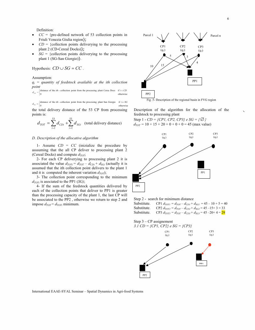
Fig .5- Description of the regional basin in FVG region
Description of the algorithm for the allocation of the
feedstock to processing plant
Step 1 - CD = {CP1, CP2, CP3} e SG = {∅ }
dTOT = 10 + 15 + 20 + 0 + 0 + 0 = 45 (max value)
Step 2 - search for minimum distance
Substitute. CP1 dTOT1 = dTOT – dCD1 + dSG1 = 45 – 10 + 5 = 40
Substitute. CP2 dTOT2 = dTOT – dCD2 + dSG2 = 45 –15+ 3 = 33
Substitute. CP3 dTOT3 = dTOT – dCD3 + dSG3 = 45 –20+ 4 = 29
Step 3 – CP assignement
3.1 CD = {CP1, CP2} e SG = {CP3}
1510
3 5
CP3
(q3)
PP2
4
CP2 (q2)
PP1
CP1 (q1)
Parcel 1 Parcel n
CP3
(q3)
PP2
CP2
(q2)
PP1
CP1
(q1)
CP3
(q3)
PP2
CP2
(q2)
PP1
CP1
(q1)
7
International EAAE-SYAL Seminar – Spatial Dynamics in Agri-food Systems
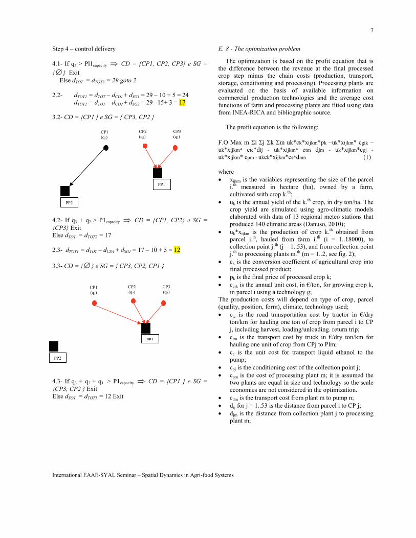
Step 4 – control delivery
4.1- If q3 > Pl1capacity ⇒ CD = {CP1, CP2, CP3} e SG =
{∅ } Exit
Else dTOT = dTOT3 = 29 goto 2
2.2- dTOT1 = dTOT – dCD1 + dSG1 = 29 – 10 + 5 = 24
dTOT2 = dTOT – dCD2 + dSG2 = 29 –15+ 3 = 17
3.2- CD = {CP1 } e SG = { CP3, CP2 }
4.2- If q3 + q2 > P1capacity ⇒ CD = {CP1, CP2} e SG =
{CP3} Exit
Else dTOT = dTOT2 = 17
2.3- dTOT1 = dTOT – dCD1 + dSG1 = 17 – 10 + 5 = 12
3.3- CD = {∅ } e SG = { CP3, CP2, CP1 }
4.3- If q3 + q2 + q1 > P1capacity ⇒ CD = {CP1 } e SG =
{CP3, CP2 } Exit
Else dTOT = dTOT1 = 12 Exit
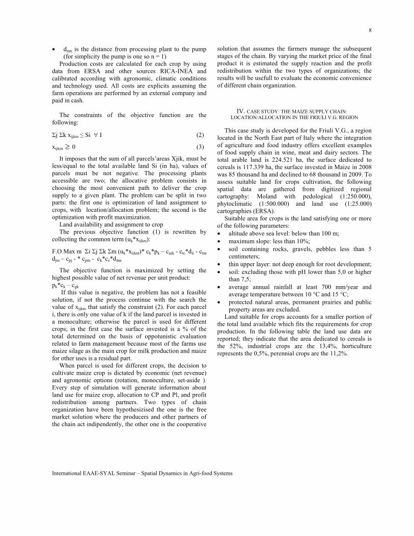
E. 8 - The optimization problem
The optimization is based on the profit equation that is
the difference between the revenue at the final processed
crop step minus the chain costs (production, transport,
storage, conditioning and processing). Processing plants are
evaluated on the basis of available information on
commercial production technologies and the average cost
functions of farm and processing plants are fitted using data
from INEA-RICA and bibliographic source.
The profit equation is the following:
F.O Max m Σi Σj Σk Σm uk*ck*xijkm*pk –uk*xijkm* cgik –
uk*xijkm* ctc*dij - uk*xijkm* ctm djm - uk*xijkm*cpj -
uk*xijkm* cpm - ukck*xijkm*ce*dmn (1)
where
• xijkm is the variables representing the size of the parcel
i.th
measured in hectare (ha), owned by a farm,
cultivated with crop k.th
;
• uk is the annual yield of the k.th
crop, in dry ton/ha. The
crop yield are simulated using agro-climatic models
elaborated with data of 13 regional meteo stations that
produced 140 climatic areas (Danuso, 2010);
• uk*xijkm is the production of crop k.th
obtained from
parcel i.th
, hauled from farm i.th
(i = 1..18000), to
collection point j.th
(j = 1..53), and from collection point
j.th
to processing plants m.th
(m = 1..2, see fig. 2);
• ck is the conversion coefficient of agricultural crop into
final processed product;
• pk is the final price of processed crop k;
• cgik is the annual unit cost, in €/ton, for growing crop k,
in parcel i using a technology g;
The production costs will depend on type of crop, parcel
(quality, position, form), climate, technology used;
• ctc is the road transportation cost by tractor in €/dry
ton/km for hauling one ton of crop from parcel i to CP
j, including harvest, loading/unloading. return trip;
• ctm is the transport cost by truck in €/dry ton/km for
hauling one unit of crop from CPj to Plm;
• ce is the unit cost for transport liquid ethanol to the
pump;
• cpj is the conditioning cost of the collection point j;
• cpm is the cost of processing plant m; it is assumed the
two plants are equal in size and technology so the scale
economies are not considered in the optimization.
• cdm is the transport cost from plant m to pump n;
• dij for j = 1..53 is the distance from parcel i to CP j;
• djm is the distance from collection plant j to processing
plant m;
CP3
(q3)
PP2
CP2
(q2)
PP1
CP1
(q1)
CP1
(q1)
CP3
(q3)
CP2
(q2)
PP2
PP1
8
International EAAE-SYAL Seminar – Spatial Dynamics in Agri-food Systems
• dmn is the distance from processing plant to the pump
(for simplicity the pump is one so n = 1)
Production costs are calculated for each crop by using
data from ERSA and other sources RICA-INEA and
calibrated according with agronomic, climatic conditions
and technology used. All costs are explicits assuming the
farm operations are performed by an external company and
paid in cash.
The constraints of the objective function are the
following:
Σj Σk xijkm ≤ Si ∀ I (2)
xijkm ≥ 0 (3)
It imposes that the sum of all parcels’areas Xjik, must be
less/equal to the total available land Si (in ha), values of
parcels must be not negative. The processing plants
accessible are two; the allocative problem consists in
choosing the most convenient path to deliver the crop
supply to a given plant. The problem can be split in two
parts: the first one is optimization of land assignment to
crops, with location/allocation problem; the second is the
optimization with profit maximization.
Land availability and assignment to crop
The previous objective function (1) is rewritten by
collecting the common term (uk*xijkm):
F.O Max m Σi Σj Σk Σm (uk*xijkm)* ck*pk – cgik - ctc*dij - ctm
djm – cpj - * cpm - ck*ce*dmn
The objective function is maximized by setting the
highest possible value of net revenue per unit product:
pk*ck – cgk
If this value is negative, the problem has not a feasible
solution, if not the process continue with the search the
value of xijkm that satisfy the constraint (2). For each parcel
i, there is only one value of k if the land parcel is invested in
a monoculture; otherwise the parcel is used for different
crops; in the first case the surface invested is a % of the
total determined on the basis of oppotunistic evaluation
related to farm management because most of the farms use
maize silage as the main crop for milk production and maize
for other uses is a residual part.
When parcel is used for different crops, the decision to
cultivate maize crop is dictated by economic (net revenue)
and agronomic options (rotation, monoculture, set-aside ).
Every step of simulation will generate information about
land use for maize crop, allocation to CP and Pl, and profit
redistribution among partners. Two types of chain
organization have been hypothesizised the one is the free
market solution where the producers and other partners of
the chain act indipendently, the other one is the cooperative
solution that assumes the farmers manage the subsequent
stages of the chain. By varying the market price of the final
product it is estimated the supply reaction and the profit
redistribution within the two types of organizations; the
results will be usefull to evaluate the economic convenience
of different chain organization.
IV. CASE STUDY: THE MAIZE SUPPLY CHAIN:
LOCATION/ALLOCATION IN THE FRIULI V.G. REGION
This case study is developed for the Friuli V.G., a region
located in the North East part of Italy where the integration
of agriculture and food industry offers excellent examples
of food supply chain in wine, meat and dairy sectors. The
total arable land is 224.521 ha, the surface dedicated to
cereals is 117.339 ha, the surface invested in Maize in 2008
was 85 thousand ha and declined to 68 thousand in 2009. To
assess suitable land for crops cultivation, the following
spatial data are gathered from digitized regional
cartography: Moland with pedological (1:250.000),
phytoclimatic (1:500.000) and land use (1:25.000)
cartographies (ERSA).
Suitable area for crops is the land satisfying one or more
of the following parameters:
• altitude above sea level: below than 100 m;
• maximum slope: less than 10%;
• soil containing rocks, gravels, pebbles less than 5
centimeters;
• thin upper layer: not deep enough for root development;
• soil: excluding those with pH lower than 5,0 or higher
than 7,5;
• average annual rainfall at least 700 mm/year and
average temperature between 10 °C and 15 °C;
• protected natural areas, permanent prairies and public
property areas are excluded.
Land suitable for crops accounts for a smaller portion of
the total land available which fits the requirements for crop
production. In the following table the land use data are
reported; they indicate that the area dedicated to cereals is
the 52%, industrial crops are the 13,4%, horticulture
represents the 0,5%, perennial crops are the 11,2%.
9
International EAAE-SYAL Seminar – Spatial Dynamics in Agri-food Systems
Tab 4 - The agricultural land in FVG region. Source: Rica-Inea (2008)
Product Surface (ha) %
Annual crops: 172.396,58 76,80 Cereals 117.339,30 52,30
Industrial crops 30.162,36 13,40
Horticulture and potatoes 1.182,19 0,50 Forage crop 14.214,07 6,30
Other crops 79,16 0,00
Set aside 9.419,51 4,20 Of which Public property 204,57 0,10
Perennial crops: 25.243,41 11,20
Viticulture 19.333,48 8,60 Olives 238,49 0,10
Orchards 2.904,08 1,30
Other 2.766,33 1,20 Of which Public property 28,78 0,00
Permanent prairies and pasture 26.881,00 12,00
Of which Public property 6.341,69 2,80
Total (Excluding Public property) 217.944,92 97,10 Public property 6.576,08 2,90
Total 224.521,00 100,00
For the purpose of this study the crop selected is Maize
used to produce ethanol because of a political interest in this
product related to a regional planning; however, this
approach can be extended to any other crop for which
information is available. The data base provided by Insiel
indicate that the land dedicated to the agrifood chain, is less
than the cultivated land in the region because a consistent
quota doesn’t accomplish with the parameters above and the
use of maize in dairy farms. The available surface for maize
is approximately 118 thousand ha.
The first part of the analysis is the allocation problem to
find the shortest distance from parcel to the corresponding
CP and from CP to Pl. The crop delivery from CP to one of
the processing plants is a decision to be evaluated by
considering the different competitive conditions of the two
plants situated at different average distance from CP.
The transportation distances to processing plant 1 or 2
are consistently different; if the two plants would have the
same size and use the same processing technology the
solution based on transport cost minimization will privilege
the plant situated at minimum distance from the CP; in this
case the collection points have a cost advantage to haul their
product to plant 1; instead the optimization is based on the
difference of the distance of a CP from the two procesing
plants that allow the cohexistence of these two processing
plants with the crop supply.
However the computation will show that the transport
cost are only a smal quota of the total costs and the
difference between Pl1 and Pl2, very limited can be
compensated by the processing plant with higher transport
cost because the economic advantage of exploiting the plant
capacity compensate the cost difference paid to farmers.
V. RESULTS
The allocation is solved first by dividing the region in
two basins one having the processing plant CD and the
other SG, then assigning the parcels to one of the 53
collection points and connectiong the CP to the Pl. The
quantity delivered is almost equivalent for the two basins,
the difference is due to the fact that the CP can deliver to
only one of the two Pl. The average distances between
parcel and CP of the two basins are not greatly different, but
the transport costs from CP to Pl are different and this will
affect the farmers’ decisions.
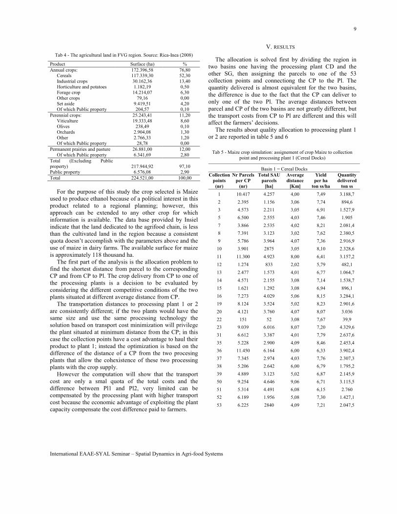
The results about quality allocation to processing plant 1
or 2 are reported in table 5 and 6
Tab 5 - Maize crop simulation: assignement of crop Maize to collection
point and processing plant 1 (Cereal Docks)
Basin 1 = Cereal Docks
Collection
points
(nr)
Nr Parcels
per CP
(nr)
Total SAU
parcels
[ha]
Average
distance
[Km]
Yield
per ha
ton ss/ha
Quantity
delivered
ton ss
1 10.417 4.257 4,00 7,49 3.188,7
2 2.395 1.156 3,06 7,74 894,6
3 4.573 2.211 3,05 6,91 1.527,9
5 6.500 2.555 4,03 7,46 1.905
7 3.866 2.535 4,02 8,21 2.081,4
8 7.391 3.123 3,02 7,62 2.380,5
9 5.786 3.964 4,07 7,36 2.916,9
10 3.901 2875 3,05 8,10 2.328,6
11 11.300 4.923 8,00 6,41 3.157,2
12 1.274 833 2,02 5,79 482,1
13 2.477 1.573 4,01 6,77 1.064,7
14 4.571 2.155 3,08 7,14 1.538,7
15 1.621 1.292 3,08 6,94 896,1
16 7.273 4.029 5,06 8,15 3.284,1
19 8.124 3.524 5,02 8,23 2.901,6
20 4.121 3.760 4,07 8,07 3.036
22 151 52 3,08 7,67 39,9
23 9.039 6.016 8,07 7,20 4.329,6
31 6.612 3.387 4,01 7,79 2.637,6
35 5.228 2.900 4,09 8,46 2.453,4
36 11.450 6.164 6,00 6,33 3.902,4
37 7.345 2.974 4,03 7,76 2.307,3
38 5.206 2.642 6,00 6,79 1.795,2
39 4.889 3.123 5,02 6,87 2.145,9
50 9.254 4.646 9,06 6,71 3.115,5
51 5.314 4.491 6,08 6,15 2.760
52 6.189 1.956 5,08 7,30 1.427,1
53 6.225 2840 4,09 7,21 2.047,5
10
International EAAE-SYAL Seminar – Spatial Dynamics in Agri-food Systems
Total 85956 4,34 7.23 62.545,5
Tab 6 - Maize crop simulation: assignement of crop Maize to collection point and processing plant 1 (San Giorgio)
Basin 2 = San Giorgio
Collection
points
(nr)
Nr Parcels
per CP
(nr)
Total SAU
parcels
[ha]
Average
distance
[Km]
Yield
per ha
ton ss/ha
Quantity
delivered
ton ss
4 4.095 1.548 3,07 7,88 1.219,8
6 1.910 1.195 3,01 8,19 978,6
17 2.680 2.135 4,01 7,66 1.635,3
18 6.840 2.621 3,07 7,94 2.081,4
21 4.655 2.187 3,04 7,72 1.687,8
24 5.494 2.553 4,02 8,23 2.102,1
25 4.061 6.396 5,02 7,37 4.713,6
26 3.470 3.353 5,01 7,99 2.680,2
27 3.734 2.571 5,01 7,47 1.919,4
28 19.751 8.110 10,00 7,84 6.356,1
29 7.213 3.088 3,05 8,25 2.547,3
30 10.971 5.600 6,01 7,38 4.132,5
32 6.527 2.570 3,05 8,54 2.194,8
33 6.066 5.614 4,03 6,98 3.919,5
34 3.217 4.338 6,05 7,17 3.109,5
40 7.912 3.619 4,02 8,02 2901
41 4.938 3.308 4,02 8,17 2.702,1
42 3.717 2.166 4,05 8,17 1.769,4
43 1.573 1.665 3,04 7,75 1.290,3
44 813 699 1,06 7,88 550,5
45 5.100 2.418 3,05 7,99 1.931,7
46 8.248 3.854 5,04 8,26 3.182,4
47 3.634 1.416 3,05 8,06 1.140,6
48 3.609 1.630 4,07 7,87 1.282,8
49 2.459 678 7,03 7,85 532,5
Total 75.332 4,15 7,86 58,561,2
The optimal allocation is complicated by the
configuration of the road network requiring to solve
decisional problems as: search the minimum distance
compatible with traffic intensity, urban areas, intersections;
bridges and other obstacles; hence distances are calibrated
with the time requested to complete the pattern.
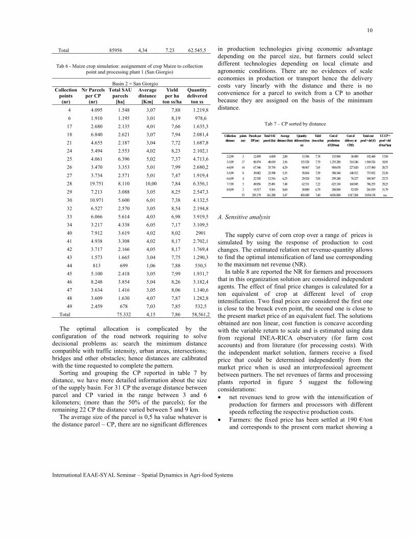
Sorting and grouping the CP reported in table 7 by
distance, we have more detailed information about the size
of the supply basin. For 31 CP the average distance between
parcel and CP varied in the range between 3 and 6
kilometers; (more than the 50% of the parcels); for the
remaining 22 CP the distance varied between 5 and 9 km.
The average size of the parcel is 0,5 ha value whatever is
the distance parcel – CP, there are no significant differences
in production technologies giving economic advantage
depending on the parcel size, but farmers could select
different technologies depending on local climate and
agronomic conditions. There are no evidences of scale
economies in production or transport hence the delivery
costs vary linearly with the distance and there is no
convenience for a parcel to switch from a CP to another
because they are assigned on the basis of the minimum
distance.
Tab 7 – CP sorted by distance
A. Sensitive analysis
The supply curve of corn crop over a range of prices is
simulated by using the response of production to cost
changes. The estimated relation net revenue-quantity allows
to find the optimal intensification of land use corresponding
to the maximum net revenue (NR).
In table 8 are reported the NR for farmers and processors
that in this organization solution are considered independent
agents. The effect of final price changes is calculated for a
ton equivalent of crop at different level of crop
intensification. Two final prices are considered the first one
is close to the breack even point, the second one is close to
the present market price of an equivalent fuel. The solutions
obtained are non linear, cost function is concave according
with the variable return to scale and is estimated using data
from regional INEA-RICA observatory (for farm cost
accounts) and from literature (for processing costs). With
the independent market solution, farmers receive a fixed
price that could be determined independently from the
market price when is used an interprofessioal agreement
between partners. The net revenues of farms and processing
plants reported in figure 5 suggest the following
considerations:
• net revenues tend to grow with the intensification of
production for farmers and processors with different
speeds reflecting the respective production costs.
• Farmers: the fixed price has been settled at 190 €/ton
and corresponds to the present corn market showing a
Collection
distance
points
(nr)
Parcels per
DP (nr)
Total SAU
parcel (ha)
Average
distance (Km)
Quantity
delivered (ton
ss)
Yield
(ton ss/ha)
Cost of
production
(€120/ton)
Cost of
delivery at
CP(€)
Total cost
prod + del (€)
UC-CP +
prod + del
(€/ton*km)
2-2,99 3 12.859 6.009 2,80 15.396 7,74 153.960 38.489 192.449 17,00
3-3,99 17 88.974 48.659 3,56 125.528 7,79 1.255.280 314.246 1.569.526 18,91
4-4,99 14 67.346 35.754 4,29 90.967 7,65 909.670 227.820 1.137.490 20,73
5-5,99 8 39.082 23.598 5,35 58.854 7,59 588.540 148.512 737.052 23,50
6-6,99 4 22.545 12.516 6,25 29.524 7,03 295.240 74.327 369.567 25,73
7-7,99 5 49.856 25.491 7,48 62.531 7,22 625.310 160.945 786.255 29,25
8-8,99 2 14.517 9.261 8,60 20.889 6,79 208.890 52.929 261.819 31,79
53 295.179 161.288 5,47 403.689 7,40 4.036.890 1.017.268 5.054.158 n.a
11
International EAAE-SYAL Seminar – Spatial Dynamics in Agri-food Systems
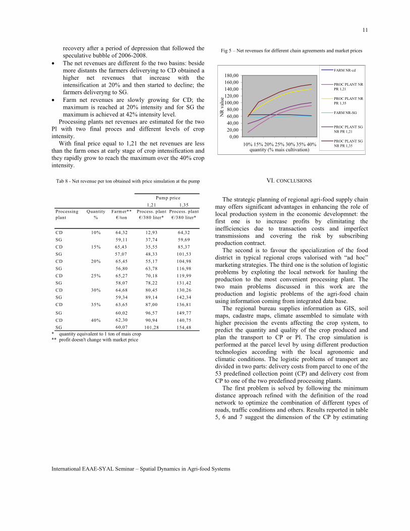
recovery after a period of depression that followed the
speculative bubble of 2006-2008.
• The net revenues are different fo the two basins: beside
more distants the farmers deliverying to CD obtained a
higher net revenues that increase with the
intensification at 20% and then started to decline; the
farmers deliveryng to SG.
• Farm net revenues are slowly growing for CD; the
maximum is reached at 20% intensity and for SG the
maximum is achieved at 42% intensity level.
Processing plants net revenues are estimated for the two
Pl with two final proces and different levels of crop
intensity.
With final price equal to 1,21 the net revenues are less
than the farm ones at early stage of crop intensification and
they rapidly grow to reach the maximum over the 40% crop
intensity.
Tab 8 - Net revenue per ton obtained with price simulation at the pump
* quantity equivalent to 1 ton of mais crop ** profit doesn't change with market price
Fig 5 – Net revenues for different chain agreements and market prices
0,00
20,00
40,00
60,00
80,00
100,00
120,00
140,00
160,00
180,00
10% 15% 20% 25% 30% 35% 40%quantity (% mais cultivation)
NR
val
ue
FARM NR-cd
PROC PLANT NR
PR 1,21
PROC PLANT NR
PR 1,35
FARM NR-SG
PROC PLANT SG
NR PR 1,21
PROC PLANT SG
NR PR 1,35
VI. CONCLUSIONS
The strategic planning of regional agri-food supply chain
may offers significant advantages in enhancing the role of
local production system in the economic developmnet: the
first one is to increase profits by elimitating the
inefficiencies due to transaction costs and imperfect
transmissions and covering the risk by subscribing
production contract.
The second is to favour the specialization of the food
district in typical regional crops valorised with “ad hoc”
marketing strategies. The third one is the solution of logistic
problems by exploting the local network for hauling the
production to the most convenient processing plant. The
two main problems discussed in this work are the
production and logistic problems of the agri-food chain
using information coming from integrated data base.
The regional bureau supplies information as GIS, soil
maps, cadastre maps, climate assembled to simulate with
higher precision the events affecting the crop system, to
predict the quantity and quality of the crop produced and
plan the transport to CP or Pl. The crop simulation is
performed at the parcel level by using different production
technologies according with the local agronomic and
climatic conditions. The logistic problems of transport are
divided in two parts: delivery costs from parcel to one of the
53 predefined collection point (CP) and delivery cost from
CP to one of the two predefined processing plants.
The first problem is solved by following the minimum
distance approach refined with the definition of the road
network to optimize the combination of different types of
roads, traffic conditions and others. Results reported in table
5, 6 and 7 suggest the dimension of the CP by estimating
Pump price
1,21 1,35
Processing
plant
Quantity
%
Farmer**
€/ton
Process. plant
€/380 liter*
Process. plant
€/380 liter*
CD 10% 64,32 12,93 64,32
SG 59,11 37,74 59,69
CD 15% 65,43 35,55 85,37
SG 57,07 48,33 101,53
CD 20% 65,45 55,17 104,98
SG 56,80 63,78 116,98
CD 25% 65,27 70,18 119,99
SG 58,07 78,22 131,42
CD 30% 64,68 80,45 130,26
SG 59,34 89,14 142,34
CD 35% 63,65 87,00 136,81
SG 60,02 96,57 149,77
CD 40% 62,30 90,94 140,75
SG 60,07 101,28 154,48
12
International EAAE-SYAL Seminar – Spatial Dynamics in Agri-food Systems
the following parameters: average distance between parcel
and CP, number of parcels, quantity of product delivered;
the most important result was the predominant size of the
CP mesured with the average distance varying in the range
between 3 and 5 km.
The selection of the most convenient processing plant is
based on the assumption that the crop supply is enough to
feed both processing plants then the strategy consists in
saturating the first plant capacity with the crop supply
delivered by the most efficient CP evaluated in terms of cost
distance and the residual crop is allocated to the second
processing plant. With this solution it is possible to evalute
the delivery costs and the efficiency in terms of saving
delivery cost by comparing plant 1 and 2.
Three are the possible solution to absorb this cost:
1. the cost difference is beared by a public organization
which interest is to create the best condition of
functioning for the supply chain and the presence of
local processing facililities will increase the demand for
agricultural crops.
2. the cooperative opportunity: farmers involved in the
processing operations, will receive an amount
corresponding to the loss in delivery cost but the
margin is variable because depends on the balance
results.
3. the last solution is to increase the unexploited capacity
of the more distant processing plant for decreasing the
average cost to compensate the transport cost. In this
case it is important for the plant 2 to be able to attract
more crop to be competitive with the firt one.
This work has demonstrated the possibility to use a
complex informative system to afford the problem of
regional planning the agrofood supply chain by
simultaneously considering production and processing
operations. Some problems remain still open to further
investigation: 1) the economy of the agri-food chain can be
afforded with different organization models such as free
market, coopearative or hybrid with public intervention, not
discussed in this paper; 2) the LCA and particularly the
energy consumption must be considered because it is
another method to afford the efficiency of the regional
production basin measured with the distance ; 3) the crop
planning must be afforded by allowing different crops to be
cultivated on the same parcel, constrained with the rotation
or set aside.
REFERENCES
1. Bahlmann J., Spiller A., (2008), “The relationship between supply
chain coordination and quality assurance system: a case study
approach on German meat sector”, in Proceeding of the second International European Forum on System innovation in food network,
edts: Fritz, U. Rickert, G. Schiefer, Universitaet Bonn.
2. Bunte F., (2006), “Pricing and performance in agri-food supply chains” in Ondersteijn, C.J.M.and others edts., “Quantifying the Agri-
Food Supply Chain” Springer 2006
3. Claasen G.D.H., Hendriks T.H.S., Hendrix E.M.T., (2007), “Decision Science: theory and application“, Mansholt Publication Series vol. 2,
Wageningen Academic Publisher,
4. De La Torre Ugarte, D.G., Walsh, M.E., Shapouri, H,, Slinsky, S.P., (2003), “The Economic Impacts of Bioenergy Crop Production on
U.S. Agriculture”, U.S. Department of Agriculture, Office of the
Chief Economist, Office of Energy Policy and New Uses [online] URL: Agricultural Economie Report No. 816
http://beag.ag.utk.edu/default.html.
5. De La Rosa D., Mayol F., Diaz-Pereira E., Fernandez, M., (2004), A land evaluation decision support system (MicroLEIS DSS) for
agricultural soil protection: With special reference to the
Mediterranean region. Environmental Modelling and Software 19 (10), 929-942.
6. De Roest K., Menghi A., (2000), “Reconsidering ‘Traditional’ Food:
The Case of Parmigiano Reggiano Cheese”, Sociologia Ruralis 40, pp 439–451.
7. Drezner, Z., Hamacher, H.W. (Eds.), 2001. Facility Location:
Applications and Theory. Springer Verlag, Berlin. EEA, 2007. Annual European Community greenhouse gas inventory 1990-2005
and inventory report 2007. Technical report No 7/2007. [online]
URL: http://reports. eea.europa.eu/technicaLreport_2007_7/en. 8. Fanfani R., Brasili C., (2008), “A mosaic type of development: Food
district and SME in the italian experience”, in “System Dynamics and
Food Network”, edts: Fritz, U. Rickert, G. Schiefer, Universitaet Bonn, pp 95-108.
9. Fiorese G., Guariso G., (2010), “A GIS-based approach to evaluate
biomass potential from energy crops at regional scale” Environmental Modelling & Software, 25, pp 702-711.
10. Floyd, Robert W. (1962). "Algorithm 97: Shortest Path".
Communications of the ACM 5 (6), pp 345-350. 11. Fortuin T.J.M., Omta S.W.G., (2009), “Drivers and Barrier to
Innovation in the Food Processing Industry: a comparison between
the Netherlands and Shangai Region in China” in “System Dynamics and Food Network”, edts: Fritz, U. Rickert, G. Schiefer, Universitaet
Bonn.
12. Gellinck X., B. Kuhne, (2008), “Innovation in traditional food network”, in Proceeding of the second International European Forum
on System innovation in food network, edts: Fritz, U. Rickert, G.
Schiefer, Universitaet Bonn. 13. Galluzzo N., 2008, ”Cambiamenti strutturali dell’agro-alimentare
italiano”, Rivista Agraria N° 54, pp 2-4. 14. Lazzarini, S. G., F. R. Chaddad and M. L. Cook. (2001). Integrating
supply chain and network analyses: The study of netchains. Chain and
network science, 1(1), p 7-22. 15. Karantininis K., J.T. Graversen, H.J. Nymann Rasmussen, (2008),
“Relational contracting and allocation of decision rights in the
agrifood industry: producer contracts and food safety.”, in “System Dynamics and Food Network”, edts: Fritz, U. Rickert, G. Schiefer,
Universitaet Bonn
16. Lengnick-Hall, C. A. (1992). Innovation and Competitive Advantage: What we know and what we need to learn. Journal of Management,
18(2), p 399-429.
13
International EAAE-SYAL Seminar – Spatial Dynamics in Agri-food Systems
17. Menard C., Valceschini E., (2005), “New Institutions for governing
the Agri-food industry “, European Review of Agricultural
Economics 32 (3), pp. 421-440 18. Milgrom P., Robberts, J. (1990). The Economics of Modern
Manufacturing: Technology, Strategy, and Organization. American
Economie Review, 80 (3), 511-528. 19. Omta, O. (2004). Management of Innovation in Chains and Networks.
IN: The Emerging World of Chains and Networks. Eds: T. Camps, P.
Diederen, G. J. Hofstede and B. Vos. 's-Gra-venhage: Elsevier Juridisch (Reed Business Information ).
20. Ondersteijn, C.J.M., Wijnands J.H.M., Huirne R.B.M., van Kooten
O., (2006), “Quantifying the Agri-Food Supply Chain” Springer 2006
21. Panichelli L., E. Gnansounou, (2008), “GIS-based approach for
defining the bioenergy facilities location: a case study in Northern Spain based on marginal delivery cost and resource competition
between facilities”, Biomass and Bioenergy, 32, pp. 289-300.
22. Parker N., P. Tittmann, Q.Hartc, R. Nelsond, K. Skog, A. Schmidt, E. Gray,B.Jenkins, (2010), ”Development of a biorefinery optimized
biofuel supply curve for the Western United States”, Biomass &
Bioenergy, XXX, pp. 1-11 23. Pittaway, L., M. Robertson, K. Munir, D. Denyer and A. Neely.
(2004), Networking and innovation: a systematic review of the
evidence. International Journal of Management Reviews, 5-6(3-4), p 137-168.
24. Porter M.E., (1985). Technology and Competitive Advantage. In: M.
E. Porter (Ed.), Competitive Advantege: Creating and Sustaining
Superior Performance. The Free Press, New York, 164-200. 25. Rama D., (2009), “Ruolo ed evoluzione delle istituzioni di marketing
(hybrids) nei nuovi scenari competitivi del sistema agro-alimentare”
in S. Boccaletti a cura di, “Cambiamenti nel sistema agroalimentare: nuovi problemi, strategie, politiche”, XLVI Convegno SIDEA
26. Rosa F., (2008), “L’organizzazione economica dell’azienda agro-
energetica”, Economia e Diritto Agroalimentare, XIII, pp. 123-157 27. Rosa F., Galizzi G., (1994), “The Agrifood System in Italy: structural
Adjustments to Face the Internationalization of the Food Industry”
Journal of International Food & Agribusiness Marketing, 5, pages 55 – 81.
28. Sonnino R., Marsden T., (2006), “Beyond the divide: rethinking
relationships between alternative and conventional food networks in Europe”, Journal of Economic Geography 6 pp. 181–199
29. Tirole J., (1988) The Theory of Industrial Organization. The MIT
Press, Cambridge, MA, 1988
Request of information can be addressed to [email protected]
)