Physics of pore closure in polar firn, and its implications for the ...
280
HAL Id: tel-02338731 https://tel.archives-ouvertes.fr/tel-02338731 Submitted on 30 Oct 2019 HAL is a multi-disciplinary open access archive for the deposit and dissemination of sci- entific research documents, whether they are pub- lished or not. The documents may come from teaching and research institutions in France or abroad, or from public or private research centers. L’archive ouverte pluridisciplinaire HAL, est destinée au dépôt et à la diffusion de documents scientifiques de niveau recherche, publiés ou non, émanant des établissements d’enseignement et de recherche français ou étrangers, des laboratoires publics ou privés. Physics of pore closure in polar firn, and its implications for the understanding of past feedbacks between climate and carbon cycle Kevin Fourteau To cite this version: Kevin Fourteau. Physics of pore closure in polar firn, and its implications for the understanding of past feedbacks between climate and carbon cycle. Climatology. Université Grenoble Alpes, 2019. English. NNT : 2019GREAU018. tel-02338731
-
Upload
khangminh22 -
Category
Documents
-
view
4 -
download
0
Transcript of Physics of pore closure in polar firn, and its implications for the ...
HAL Id: tel-02338731https://tel.archives-ouvertes.fr/tel-02338731
Submitted on 30 Oct 2019
HAL is a multi-disciplinary open accessarchive for the deposit and dissemination of sci-entific research documents, whether they are pub-lished or not. The documents may come fromteaching and research institutions in France orabroad, or from public or private research centers.
L’archive ouverte pluridisciplinaire HAL, estdestinée au dépôt et à la diffusion de documentsscientifiques de niveau recherche, publiés ou non,émanant des établissements d’enseignement et derecherche français ou étrangers, des laboratoirespublics ou privés.
Physics of pore closure in polar firn, and its implicationsfor the understanding of past feedbacks between climate
and carbon cycleKevin Fourteau
To cite this version:Kevin Fourteau. Physics of pore closure in polar firn, and its implications for the understanding ofpast feedbacks between climate and carbon cycle. Climatology. Université Grenoble Alpes, 2019.English. �NNT : 2019GREAU018�. �tel-02338731�

THÈSEPour obtenir le grade de
DOCTEUR DE LA COMMUNAUTÉ UNIVERSITÉ GRENOBLE ALPES
Spécialité : Sciences de la Terre et de l'Univers et de l'Environnement (CESTUE)
Arrêté ministériel : 25 mai 2016
Présentée par
Kévin FOURTEAU
Thèse dirigée par Patricia MARTINERIE, Chargée de recherche , Communauté Université Grenoble Alpeset codirigée par Xavier FAIN, Chargé de recherche, Communauté Université Grenoble Alpes
préparée au sein du Laboratoire Institut des Géosciences de l'Environnementdans l'École Doctorale Terre, Univers, Environnement
Physique de la fermeture des pores dans le névé polaire, implications pour la compréhension des rétrocations passées entre cycle du carbone et climat
Physics of pore closure in polar firn, and its implications for the understanding of past feedbacks between climate and carbon cycle
Thèse soutenue publiquement le 6 septembre 2019,devant le jury composé de :
Madame PATRICIA MARTINERIECHARGE DE RECHERCHE, CNRS DELEGATION ALPES, Directeur de thèse
Monsieur MASSIMO FREZZOTTIPROFESSEUR, UNIVERSITE DE ROME III - ITALIE, Rapporteur
Madame RACHAEL RHODESMAITRE DE CONFERENCES, UNIVERSITE DE CAMBRIDGE - ROYAUME-UNI, Rapporteur
Monsieur LAURENT OXARANGOPROFESSEUR, UNIVERSITE GRENOBLE ALPES, Président
Monsieur OLIVIER CASTELNAUDIRECTEUR DE RECHERCHE, CNRS DELEGATION ILE-DE-FRANCE MEUDON, Examinateur


i
...
...

ii
Abstract
As they contain air from past atmospheres, ice cores are unparalleled climate paleo-archives. The
study of the gases enclosed in ice cores from the arid region of East Antarctica allows to infer the
past compositions of the atmosphere back to 800,000 years ago. Gases are trapped during the com-
paction of the snow deposited on top of the ice sheet. In the near-surface snow, also referred to as
firn, the interstitial porous network shrinks until it eventually pinches and traps gases in the ice.
However, the very process of gas trapping has impacts on the gas signals recorded in ice cores. The
interpretation of gas records requires to characterize how ice core and atmospheric signals differ. The
aim of this PhD is to study two effects altering ice core gas records, namely gas layered trapping that
creates stratigraphic irregularities and firn smoothing that removes fast variability from the record.
A specific focus is put on low-accumulation East Antarctic ice cores.
This inquiry starts with the multi-tracer study of a firn core drilled at the Lock-In site, East Antarc-
tica. The results show that the bottom of the firn can be seen as a stack of heterogeneous strata that
densify following the same porous network evolution with density. In this vision, the stratification
simply reflects the fact that some strata are in advance (or late) in their densification, but that pore
closure happens in a similar fashion in all strata. This notably means that all strata contain nearly
similar amounts of gases, as supported by direct measurements. High-resolution chemistry data in-
dicate that denser strata are characterized by a high liquid conductivity, suggesting that deep firn
stratification is due the impurity-induced preferential densification.
This knowledge is then used to explain abrupt spikes observed in ice core methane records. For this
PhD we rely on 6 new high-resolution methane records, measured in several East Antarctic ice cores
at IGE. We show that the abrupt variations are layering artifacts due to stratigraphic irregularities
caused by dense firn strata closing in advance. A simple model is developed to simulate the irregular
occurrence of layering artifacts.
A novel technique is proposed to estimate the age distributions of gases in ice cores, that are responsi-
ble for the smoothing of fast atmospheric variations. It can notably be applied to glacial records, and
for the first time provides quantitative insights on the smoothing of very low-accumulation records.
Our results show that in East Antarctica, the firn smoothing is weakly sensitive to the accumulation
rate, meaning that more information than previously thought is preserved.
Finally, we present the development of a new type of micro-mechanical firn model. Its ambition is to
simulate the evolution of the porous network of a firn stratum. Such a model could be used to better
constrain the enclosure of gases in polar ice under glacial conditions.
Keywords: ice cores, gas trapping, firn smoothing, layering, methane Continuous Flow Analysis,
paleoclimate

iii
Résumé
Les carottes de glace sont des archives climatiques sans équivalents : les gaz contenus dans la glace de
la région aride de l’Antarctique de l’Est permettent de reconstruire les compositions atmosphériques
au cours des derniers 800000 ans. Les gaz sont piégés pendant la compaction de la neige tombée
sur l’inlandsis. Dans la neige en surface, aussi appelée névé, le réseau poreux interstitiel diminue
jusqu’au pincement des pores qui piègent définitivement les gaz dans la glace. Cependant, le pro-
cessus même de piégeage des gaz impacte l’enregistrement des signaux mesurés dans les carottes.
L’interprétation de ces signaux demande de caractériser en quoi ils diffèrent de l’atmosphère passée.
Le but de cette thèse est d’étudier deux effets altérant les enregistrements gaz des carottes, le piégeage
par couches qui crée des irrégularités stratigraphiques et le lissage qui retire la variabilité rapide de
l’enregistrement. Une attention particulière est portée sur les glaces de l’Antarctique de l’Est.
Ce travail démarre avec l’étude multi-traceurs d’une carotte de névé forée au site de Lock-In en
Antarctique de l’Est. Les résultats montrent que le bas du névé est un empilement hétérogène de
strates se densifiant suivant une même évolution de leur réseau poreux. La stratification reflète
simplement que certaines strates sont en avance (ou retard) dans leur densification, mais la fer-
meture des pores est similaire dans toutes les strates. Notamment, les strates contiennent toutes
des quantités similaires de gaz, comme le montrent des mesures directes. Des mesures de chimie à
haute-résolutionmontrent que les strates denses ont une haute conductivité liquide, suggérant que la
stratification profonde du névé est due à une densification préférentielle induite par des impuretés.
Ces connaissances sont appliquées pour étudier des variations centimétriques mesurées dans les sig-
naux méthane des carottes de glace. Pour cette thèse, nous utilisons 6 nouveaux signaux méthane à
haute résolution, mesurés dans des carottes d’Antarctique de l’Est à l’IGE. Nous montrons que ces
variations sont des artefacts dus aux irrégularités stratigraphiques causées par des strates denses se
fermant en avance. Un modèle est proposé pour simuler la présence irrégulière de ces artefacts.
Une nouvelle méthode est proposée pour estimer la distribution en âge des gaz dans les carottes,
qui est à l’origine du lissage des variations atmosphériques rapides. Elle peut être appliquée aux
carottes de la dernière période glaciaire, et donne pour la première fois des indications quantitatives
sur le lissage des signaux dans les carottes à très faible accumulation. Nos résultats montrent qu’en
Antarctique de l’Est, le lissage est peu sensible au taux d’accumulation, et que plus d’information
que prévu est préservée lors du piégeage.
Enfin, nous présentons le développement d’un nouveau type de modèle micro-mécanique du névé.
Son but est de simuler l’évolution des pores dans une strate de névé. Un tel modèle pourrait être
utilisé pour contraindre le piégeage des gaz dans la glace, dans des conditions de période glaciaire.
Mots Clés : carottes de glace, piégeage des gaz, lissage du névé, stratification, mesure en continu du
méthane, paléoclimat
iv
Merci
Je tiens évidemment à remercier en premier lieu Patricia et Xavier pour ces années, non seulement de
thèse, mais aussi de Master passées ensemble. On m’a souvent dit que la thèse serait un moment dif-
ficile (surtout la deuxième année), mais cela a toujours été un plaisir pour moi de venir travailler sur
ce sujet. Vous avez su me laisser travailler en autonomie et poursuivre mes idées, tout en m’épaulant
sur mes points faibles (l’ortaugraphe entre autre).
Je remercie chaleureusement Massimo Frezzotti et Rachael Rhodes pour le temps passé à lire et com-
menter mon manuscrit, et également Olivier Castelnau et Laurent Oxarango pour avoir fait partie
de mon jury de thèse.
Durant cette thèse, j’ai également bénéficié de l’aide indispensable d’un certain nombre de membres
de l’IGE: Grégory qui m’a dépanné (plus d’une fois) pour des découpes de carottes et du bougeage
de caisses, Laurent pour ses connaissances encyclopédiques sur la pycno et les mesures vieilles de 25
ans, Fabien et Olivier pour m’avoir initié au développement d’usine à gaz avec Elmer/Ice, et Maurine
pour m’avoir expliqué encore et encore comment fonctionnent les dislocations. Je tiens aussi à re-
mercier le reste des personnes m’ayant fait avancer dans cette thèse (scientifiquement ou non) qu’ils
soient de l’IGE ou non: Sophie, Johannes, Amélie, Jérôme, Rob, Anaïs, Amaëlle, Martin, Volodya,
Olivier M., Henning, Becky, ...
C’est bien connu, un des gros avantage de la thèse c’est de pouvoir partager ses galères avec les autres
thésards du laboratoire: Marion, Lucas, Maria, Fanny, Cédric, Jai, Étienne, Olivier, Jihnwa, Claudio,
Julien B. et Julien B., Ugo, Jordi, Romain, Ilann, Albane, Hans, Gabi, Jospeh, Alexis, et David. Si ces
années ont été si agréables, c’est aussi grâce à vous. Cette thèse étant officiellement la fin de mon
parcours universitaire, j’aimerais aussi y glisser le nom de Pierre B., que je remercie pour les bons
moments passés ensemble depuis la prépa.
Et finalement, je remercie mes parents qui m’ont toujours soutenu et m’ont permis de me lancer dans
mes études sans que j’ai à me soucier du reste. Nul doute que l’intérêt que j’ai pour la science et la
nature du monde qui nous entoure leur est dû.
Et bien sûr, une pensée pour Léa et Molly (qui n’a sans doute pas lu cette thèse) pour les randonnées,
le bon temps ensemble, et tout le reste.
Contents
1 Introduction 1
2 Ice Cores and their Gas Records 5
2.1 Climatic cycles of the Quaternary Era . . . . . . . . . . . . . . . . . . . . . . . . . . . . . 7
2.1.1 Glacial-Interglacial cycles . . . . . . . . . . . . . . . . . . . . . . . . . . . . . . . 7
2.1.2 Millennial variability . . . . . . . . . . . . . . . . . . . . . . . . . . . . . . . . . . 9
2.1.3 Records of climatic variability in ice cores . . . . . . . . . . . . . . . . . . . . . . 10
2.2 From snow to firn and ice . . . . . . . . . . . . . . . . . . . . . . . . . . . . . . . . . . . . 14
2.2.1 Description of the firn column . . . . . . . . . . . . . . . . . . . . . . . . . . . . . 14
2.2.2 Stratification of the firn . . . . . . . . . . . . . . . . . . . . . . . . . . . . . . . . . 17
2.2.3 Deformation of the ice matrix . . . . . . . . . . . . . . . . . . . . . . . . . . . . . 21
2.3 The porous network and the gases inside . . . . . . . . . . . . . . . . . . . . . . . . . . . 25
2.3.1 Firn from the standpoint of gases . . . . . . . . . . . . . . . . . . . . . . . . . . . 25
2.3.2 Air content of polar ice . . . . . . . . . . . . . . . . . . . . . . . . . . . . . . . . . 27
2.4 Modeling the firn and gas trapping . . . . . . . . . . . . . . . . . . . . . . . . . . . . . . 29
2.4.1 Firn densification models . . . . . . . . . . . . . . . . . . . . . . . . . . . . . . . 29
2.4.2 Gas trapping models . . . . . . . . . . . . . . . . . . . . . . . . . . . . . . . . . . 32
2.5 Alterations of the gas record . . . . . . . . . . . . . . . . . . . . . . . . . . . . . . . . . . 37
2.5.1 The smoothing effect . . . . . . . . . . . . . . . . . . . . . . . . . . . . . . . . . . 38
2.5.2 Layered gas trapping . . . . . . . . . . . . . . . . . . . . . . . . . . . . . . . . . . 40
2.6 Objectives of the PhD . . . . . . . . . . . . . . . . . . . . . . . . . . . . . . . . . . . . . . 41
3 Methods 43
3.1 Continuous Flow Analysis of methane concentrations . . . . . . . . . . . . . . . . . . . 45
3.1.1 Description of the CFA apparatus . . . . . . . . . . . . . . . . . . . . . . . . . . . 46
3.1.2 Preparation of the ice . . . . . . . . . . . . . . . . . . . . . . . . . . . . . . . . . . 48
v
vi
3.1.3 Processing of the raw data . . . . . . . . . . . . . . . . . . . . . . . . . . . . . . . 49
3.1.4 Correcting for methane dissolution . . . . . . . . . . . . . . . . . . . . . . . . . . 50
3.1.5 Internal smoothing of the CFA system . . . . . . . . . . . . . . . . . . . . . . . . 56
3.2 Pycnometry . . . . . . . . . . . . . . . . . . . . . . . . . . . . . . . . . . . . . . . . . . . 61
3.2.1 Physical basis . . . . . . . . . . . . . . . . . . . . . . . . . . . . . . . . . . . . . . 61
3.2.2 Experimental protocol . . . . . . . . . . . . . . . . . . . . . . . . . . . . . . . . . 66
3.2.3 Calibration of the chamber volumes . . . . . . . . . . . . . . . . . . . . . . . . . 67
3.2.4 Experimental uncertainties . . . . . . . . . . . . . . . . . . . . . . . . . . . . . . 69
3.3 Other measurements performed during the thesis . . . . . . . . . . . . . . . . . . . . . . 71
3.3.1 Density measurements by Xray absorption . . . . . . . . . . . . . . . . . . . . . . 72
3.3.2 Tomography . . . . . . . . . . . . . . . . . . . . . . . . . . . . . . . . . . . . . . . 75
3.3.3 Air content . . . . . . . . . . . . . . . . . . . . . . . . . . . . . . . . . . . . . . . . 76
3.3.4 Chemistry measurements . . . . . . . . . . . . . . . . . . . . . . . . . . . . . . . 77
3.3.5 Thin sections and crystalline texture . . . . . . . . . . . . . . . . . . . . . . . . . 78
3.4 Conclusion of the chapter . . . . . . . . . . . . . . . . . . . . . . . . . . . . . . . . . . . 79
4 Study of pore closure in an East Antarctic firn core 81
4.1 Presentation of the chapter . . . . . . . . . . . . . . . . . . . . . . . . . . . . . . . . . . . 83
4.2 Multi-tracer study of gas trapping in an East Antarctic ice core . . . . . . . . . . . . . . 84
4.2.1 Introduction . . . . . . . . . . . . . . . . . . . . . . . . . . . . . . . . . . . . . . . 85
4.2.2 Methods . . . . . . . . . . . . . . . . . . . . . . . . . . . . . . . . . . . . . . . . . 87
4.2.3 Results and discussion . . . . . . . . . . . . . . . . . . . . . . . . . . . . . . . . . 93
4.2.4 Conclusions . . . . . . . . . . . . . . . . . . . . . . . . . . . . . . . . . . . . . . . 113
4.2.5 Supplementary Material . . . . . . . . . . . . . . . . . . . . . . . . . . . . . . . . 115
4.3 To go further . . . . . . . . . . . . . . . . . . . . . . . . . . . . . . . . . . . . . . . . . . . 121
4.3.1 Structural anisotropy of firn . . . . . . . . . . . . . . . . . . . . . . . . . . . . . . 121
4.3.2 Analysis of thin sections . . . . . . . . . . . . . . . . . . . . . . . . . . . . . . . . 123
4.4 Conclusion of the chapter . . . . . . . . . . . . . . . . . . . . . . . . . . . . . . . . . . . 126
5 Alterations of methane records in East Antarctic ice cores 129
5.1 Presentation of the chapter . . . . . . . . . . . . . . . . . . . . . . . . . . . . . . . . . . . 131
5.2 Analytical constraints on layered gas trapping and smoothing of atmospheric variabil-
ity in ice under low-accumulation conditions . . . . . . . . . . . . . . . . . . . . . . . . 132
5.2.1 Introduction . . . . . . . . . . . . . . . . . . . . . . . . . . . . . . . . . . . . . . . 133
5.2.2 Ice core samples and analytical methods . . . . . . . . . . . . . . . . . . . . . . . 135
5.2.3 Experimental results . . . . . . . . . . . . . . . . . . . . . . . . . . . . . . . . . . 137
5.2.4 Layered bubble trapping . . . . . . . . . . . . . . . . . . . . . . . . . . . . . . . . 141
Contents vii
5.2.5 Smoothing and age distribution in the Vostok 4G-2 ice core . . . . . . . . . . . . 148
5.2.6 Discussion . . . . . . . . . . . . . . . . . . . . . . . . . . . . . . . . . . . . . . . . 151
5.2.7 Conclusions . . . . . . . . . . . . . . . . . . . . . . . . . . . . . . . . . . . . . . . 155
5.2.8 Supplementary Material . . . . . . . . . . . . . . . . . . . . . . . . . . . . . . . . 156
5.3 Estimation of gas record alteration in very low accumulation ice cores . . . . . . . . . . 164
5.3.1 Introduction . . . . . . . . . . . . . . . . . . . . . . . . . . . . . . . . . . . . . . . 165
5.3.2 Methods . . . . . . . . . . . . . . . . . . . . . . . . . . . . . . . . . . . . . . . . . 167
5.3.3 Results and Discussion . . . . . . . . . . . . . . . . . . . . . . . . . . . . . . . . . 169
5.3.4 Loss of climatic information in a deep and thinned ice core from East Antarctica 182
5.3.5 Conclusions . . . . . . . . . . . . . . . . . . . . . . . . . . . . . . . . . . . . . . . 187
5.3.6 Supplementary Material . . . . . . . . . . . . . . . . . . . . . . . . . . . . . . . . 188
5.4 Conclusion of the chapter . . . . . . . . . . . . . . . . . . . . . . . . . . . . . . . . . . . 193
6 Modeling the compression of firn layers 195
6.1 Presentation of the chapter . . . . . . . . . . . . . . . . . . . . . . . . . . . . . . . . . . . 197
6.2 Description of the model . . . . . . . . . . . . . . . . . . . . . . . . . . . . . . . . . . . . 198
6.2.1 General principles . . . . . . . . . . . . . . . . . . . . . . . . . . . . . . . . . . . 199
6.2.2 Numerical implementation . . . . . . . . . . . . . . . . . . . . . . . . . . . . . . 200
6.3 Numerical experiments . . . . . . . . . . . . . . . . . . . . . . . . . . . . . . . . . . . . . 208
6.3.1 Mass conservation . . . . . . . . . . . . . . . . . . . . . . . . . . . . . . . . . . . . 208
6.3.2 Effect of internal pressure on pore compression . . . . . . . . . . . . . . . . . . . 210
6.3.3 Evolution of a firn layer . . . . . . . . . . . . . . . . . . . . . . . . . . . . . . . . 212
6.4 Discussion . . . . . . . . . . . . . . . . . . . . . . . . . . . . . . . . . . . . . . . . . . . . 215
6.5 Conclusion of the chapter . . . . . . . . . . . . . . . . . . . . . . . . . . . . . . . . . . . 217
7 Conclusion and Outlooks 219
7.1 General conclusion . . . . . . . . . . . . . . . . . . . . . . . . . . . . . . . . . . . . . . . 221
7.2 Perspectives . . . . . . . . . . . . . . . . . . . . . . . . . . . . . . . . . . . . . . . . . . . 223
7.3 A few personal words . . . . . . . . . . . . . . . . . . . . . . . . . . . . . . . . . . . . . . 225
A Historical closed porosity data in polar firn 229
A.1 Introduction . . . . . . . . . . . . . . . . . . . . . . . . . . . . . . . . . . . . . . . . . . . 230
A.2 The pycnometry method . . . . . . . . . . . . . . . . . . . . . . . . . . . . . . . . . . . . 231
A.3 Processing of the data . . . . . . . . . . . . . . . . . . . . . . . . . . . . . . . . . . . . . . 232
A.3.1 Original data processing . . . . . . . . . . . . . . . . . . . . . . . . . . . . . . . . 233
A.3.2 A new data processing . . . . . . . . . . . . . . . . . . . . . . . . . . . . . . . . . 234
A.4 The Barnola parametrization for closed porosity . . . . . . . . . . . . . . . . . . . . . . . 236
viii
A.5 Conclusion . . . . . . . . . . . . . . . . . . . . . . . . . . . . . . . . . . . . . . . . . . . . 237
B Firn air pumping campaigns at EastGRIP 239
B.1 General principle of firn air pumping . . . . . . . . . . . . . . . . . . . . . . . . . . . . . 239
B.2 Preparing the firn air pumping system . . . . . . . . . . . . . . . . . . . . . . . . . . . . 240
B.2.1 Preparing the bladder . . . . . . . . . . . . . . . . . . . . . . . . . . . . . . . . . 240
B.2.2 Preparing the pumping and tubing system . . . . . . . . . . . . . . . . . . . . . . 242
B.3 Field work . . . . . . . . . . . . . . . . . . . . . . . . . . . . . . . . . . . . . . . . . . . . 243
B.3.1 Protocol of firn air pumping . . . . . . . . . . . . . . . . . . . . . . . . . . . . . . 243
B.4 Tips and tricks . . . . . . . . . . . . . . . . . . . . . . . . . . . . . . . . . . . . . . . . . . 244
Bibliography 245

Chapter 1
Introduction
The Earth’s climate and its archives
In the last decades, the Earth’s climate and its evolutions became one of the major topics of
our time. This broad interest is the consequence of the current climate change, driven by
the emission and accumulation of greenhouse gases (GHG) in the atmosphere (IPCC, 2014).
If the anthropogenic nature of this change is well established, it remains necessary to accu-
rately characterize the response of the Earth’s climate to the increase of GHG concentrations,
and this in order to properly predict its evolution by the end of the century and beyond.
Several types of natural archives are used by climatologists to study the previous states of
the Earth’s climate, to reconstruct its history, and to characterize the mechanisms at play
during periods of climate change. Among others, one can cite marine sediment cores that
notably enclose information on the past conditions of ocean temperature and salinity (Roth-
well and Rack, 2006). Another example are speleothems retrieved in caves, whose isotopic
composition is used to deduce temperature variations and biosphere activity (Hendy and
Wilson, 1968; McDermott, 2004). Each type of archive is characterized by the time period
it covers and by its time resolution. For instance, marine sediment cores cover time periods
reaching millions of years, but have a resolution of the order of the century (Shackleton and
Opdyke, 1976; Lisiecki and Raymo, 2005). On the contrary, the study of speleothems only
covers periods of a few hundred thousand of years, but does so with a resolution of the order
1
2
of the year (Lauritzen, 1995). Naturally, the longer is the time coverage of a climatic archive
and the shorter is its time resolution, the better is the archive. However, long time coverage
usually comes at the expense of a precise time resolution.
Among all the available archives for the study of climate, this thesis deals with a particular
type: the polar ice cores.
Polar ice cores
Ice cores have the particularity to enclose bubbles composed of air directly originating from
past atmospheres (Stauffer et al., 1985). Thanks to these air bubbles, ice cores are the ideal
archive to study the past evolutions of the Earth’s atmospheric composition, and notably its
concentration of greenhouse gases (Barnola et al., 1987; Loulergue et al., 2008; Lüthi et al.,
2008; Mitchell et al., 2013; Marcott et al., 2014). In addition to the bubbles, the ice mate-
rial of ice cores is used to derive other information about the past conditions of the climate.
Notably, the isotopic composition of the ice allows scientists to reconstruct the evolution of
past temperatures (Dansgaard et al., 1993; Jouzel et al., 2007). The joint study of the gases
trapped in the Vostok ice core (Antarctica) and of its isotopic composition highlighted the
close relationship between the concentration in carbon dioxide and the Earth temperature
(Barnola et al., 1987; Genthon et al., 1987).
The time coverage of ice cores depends on the local temperature and precipitation condi-
tions under which they were formed. Currently, the oldest ice core has been dated back
to 800,000 years in the past, encompassing the last eight glacial cycles (EPICA community
members et al., 2004). Yet, the International Partnership in Ice Cores Science (IPICS) set the
goal to obtain an ice core old of a million-and-a-half years old (Fischer et al., 2013). The
search for this ice core is already carried out on the East Antarctic plateau, and a new deep
drilling is planed to start during the 2020/2021 austral summer. The time resolution of the
measurements performed in the ice material varies between one month to several hundreds
of year, depending on the drilling site conditions and on the history of deformation of the
ice. The resolution of the greenhouse gases measurements varies from several decades to
several hundreds of years, a point detailed in this thesis. Ice cores can enclose information
about abrupt climate evolutions, evolutions under which the climate conditions change in
less than a hundred years (Dansgaard et al., 1993; Chappellaz et al., 2013). These abrupt
past variations offer crucial insights on the Earth’s climate dynamics.

Chapter 1. Introduction 3
Objectives and organization of the thesis
This thesis deals with the process of gas trapping in polar ice. In other words: how are
the bubbles in polar ice formed? Besides the purely theoretical interest, this work aims to
help the interpretation of the gas concentrations measured in polar ice cores. Indeed, the
concentrations recorded in polar ice are the picture of the past atmospheric concentrations,
but also of the processes involved during gas trapping (Spahni et al., 2003; Rhodes et al.,
2016). Moreover, the recent development of high-resolution gas measurement techniques
(Stowasser et al., 2012; Chappellaz et al., 2013; Rhodes et al., 2013) now gives access to cen-
timeter scale concentration variability in ice cores. In order to provide climatologists with
the best possible interpretation of the gas records in ice cores, it is thus necessary to distin-
guish between what can be attributed to atmospheric variability (climatically relevant) and
what originates from the very process of gas trapping. A special emphasis will be put on the
gas trapped in the ice of the low-accumulation East Antarctic plateau. This region, which is
the most affected by gas trapping effects, encloses the oldest climatically exploitable ice and
is where the future oldest-ice core is currently searched (Van Liefferinge et al., 2018; Sutter
et al., 2019).
Chapter 2 presents a review of the scientific literature in ice cores science, with a particular
focus on gas trapping. This section also introduces the specific questions that this PhD aims
to answer. Chapter 3 presents the experimental methods utilized for this work. Chapter 4
is based on the study of a shallow core from East Antarctica, specifically dedicated to a
multi-tracer characterization of gas trapping. This chapter aims to improve the description
of the processes responsible for the trapping of gases in polar ice. Chapter 5 focuses on
the impacts of gas trapping on the recorded gas signals in ice cores. A special emphasis is
placed on ice cores from the East Antarctic plateau that were formed during the last glacial
period. Chapter 6 describes the development of a numerical model aiming to simulate
the compression of a layer of deep firn. Finally, Chapter 7 concludes this manuscript and
proposes outlooks to keep improving our understanding of gas trapping in polar ice. Two
annexes are also included at the end of themanuscript. The first one covers the processing of
historical firn data that were measured in the 1990’s at IGE, but haven’t been published yet.
The second one presents my involvement in the firn air pumping campaigns at EastGRIP,

4
Greenland.

Chapter 2
Ice Cores and their Gas Records
Contents
2.1 Climatic cycles of the Quaternary Era . . . . . . . . . . . . . . . . . . . . . . 7
2.1.1 Glacial-Interglacial cycles . . . . . . . . . . . . . . . . . . . . . . . . . 7
2.1.2 Millennial variability . . . . . . . . . . . . . . . . . . . . . . . . . . . . 9
2.1.3 Records of climatic variability in ice cores . . . . . . . . . . . . . . . . 10
2.2 From snow to firn and ice . . . . . . . . . . . . . . . . . . . . . . . . . . . . . 14
2.2.1 Description of the firn column . . . . . . . . . . . . . . . . . . . . . . . 14
2.2.2 Stratification of the firn . . . . . . . . . . . . . . . . . . . . . . . . . . . 17
2.2.3 Deformation of the ice matrix . . . . . . . . . . . . . . . . . . . . . . . 21
2.3 The porous network and the gases inside . . . . . . . . . . . . . . . . . . . . 25
2.3.1 Firn from the standpoint of gases . . . . . . . . . . . . . . . . . . . . . 25
2.3.2 Air content of polar ice . . . . . . . . . . . . . . . . . . . . . . . . . . . 27
2.4 Modeling the firn and gas trapping . . . . . . . . . . . . . . . . . . . . . . . 29
2.4.1 Firn densification models . . . . . . . . . . . . . . . . . . . . . . . . . 29
2.4.2 Gas trapping models . . . . . . . . . . . . . . . . . . . . . . . . . . . . 32
2.5 Alterations of the gas record . . . . . . . . . . . . . . . . . . . . . . . . . . . 37
2.5.1 The smoothing effect . . . . . . . . . . . . . . . . . . . . . . . . . . . . 38
2.5.2 Layered gas trapping . . . . . . . . . . . . . . . . . . . . . . . . . . . . 40
2.6 Objectives of the PhD . . . . . . . . . . . . . . . . . . . . . . . . . . . . . . . 41

6

Chapter 2. Ice Cores and their Gas Records 7
2.1 Climatic cycles of the Quaternary Era
During the Quaternary period, starting 2.58 million years ago and still ongoing today, the
Earth’s climate has been characterized by regular temperature variations. These variations
took place across various time scales ranging from a hundred years to tens of thousands of
years.
2.1.1 Glacial-Interglacial cycles
One of the characteristic variations of the Earth’s climate, is the alternation between cold
glacial periods, notably characterized by a large extension of ice sheets in the Northern
hemisphere (Svendsen et al., 2004; Abe-Ouchi et al., 2013), and warm interglacial peri-
ods. This alternation between glacial and inter-glacial periods forms the so-called glacial-
interglacial cycles.
Figure 2.1 – Relationship between Antarctic temperature and CO2 over the last eight glacial cycles. Fig-ure from Lüthi et al. (2008)
During the last 800,000 years, glacial periods have lasted several ten thousand years. On
the other hand, the warmer interglacial periods have been shorter with durations of only
ten thousand years. Consequently, over the last million years, the glacial cycle is charac-
terized by asymmetric oscillations of the temperature, with a period of repetition around
100,000 years (Muller and MacDonald, 1997; Lisiecki and Raymo, 2005; Kawamura et al.,
2007; Lüthi et al., 2008). Such 100,000 years oscillations are notably visible in ice cores, as
seen in Figure 2.1, and in marine sediment cores, as seen in the left side of Figure 2.2. It
8
is understood that the transitions from glacial to interglacial periods (known as deglacia-
tions or terminations) or the transitions from interglacial to glacial (known as glaciations)
are initiated by changes in the distribution of solar irradiance on the Earth surface (Berger,
1988; Daruka and Ditlevsen, 2016). In turn, these variations in solar irradiance are due to
changes in the orbital parameters of the Earth’s course around the Sun, and are described
by the Milankovitch cycles (Milankovitch, 1920; Muller and MacDonald, 1997). However,
the change in solar irradiance alone does not suffice to fully explain the observed variations
in the Earth’s climate. A correct description of glaciations and deglaciations requires to take
into account feedbacks in the Earth’s climate, notably involving the amount of greenhouse
gases (GHG) in the atmosphere (Genthon et al., 1987; Köhler et al., 2010).
Thanks to their particularity of containing both information about past temperatures and
GHG concentrations, polar ice cores have been widely used to study glacial-interglacial cy-
cles in the past (Genthon et al., 1987; Barnola et al., 1987; Petit et al., 1999; Delmotte et al.,
2004). In particular, climatologists have used ice cores from the arid East Antarctic plateau,
as this region contains very old and stratigraphically undisturbed ice (Fischer et al., 2013;
Passalacqua et al., 2018). The oldest dated ice retrieved to this day, from the EPICA Dome
C ice core (EDC), reaches back 800,000 years in the past and provides a precise description
of the temperature and GHG evolution over the last eight glacial cycles (Lüthi et al., 2008;
Loulergue et al., 2008). It provides a clear evidence of the link between the temperature and
the atmospheric concentrations in GHG (notably CO2), as illustrated in Figure 2.1
However, marine sediment cores indicate that the typical duration of 100,000 years for the
glacial cycles no longer holds true when reaching 1 million years in the past (Shackleton
and Opdyke, 1976; Lisiecki and Raymo, 2005). Further back in time, the glacial-interglacial
cycles are characterized by a 41,000 years period, much shorter than the 100,000 years of
the late Quaternary. This transition from a 41,000 to a 100,000 years climate is known as
the Mid-Pleistocene Transition (MPT), and is visible in benthic records as shown in Fig-
ure 2.2. However, the precise mechanisms at the origin of the MPT are not yet clear (Clark
et al., 2006). The solution to this problem might lie in the feedbacks between GHG and the
global temperatures, as a decline in CO2 concentrations appears in numerical models as a
necessary conditions to reproduce the MPT (Willeit et al., 2019). However, marine sediment
cores do not provide sufficient information on the past atmospheric compositions. Thanks

Chapter 2. Ice Cores and their Gas Records 9
to the bubbles they enclose, ice cores could provide a clear picture of the GHG concentra-
tions during the MPT, and help clarify their role this climatic transition. That is notably
why the International Partnership in Ice Core Sciences (IPICS) is currently searching for an
ice core as old as one-and-a-half million years and covering the MPT (Van Liefferinge et al.,
2018; Sutter et al., 2019).
Figure 2.2 – Transition from a 100,000 year climate to a 41,000 year climate. Benthic δ18O data fromLisiecki and Raymo (2005).
2.1.2 Millennial variability
The late Quaternary Earth’s climate is not only characterized by 100,000 years long cycles.
The study of ice cores drilled in the Greenland ice sheet have revealed the presence of fast
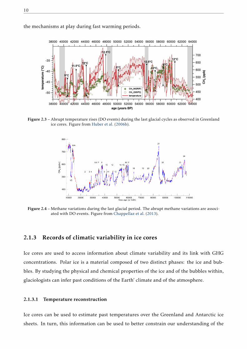
warming events during the last glacial period (Dansgaard et al., 1993). They are referred
to as Dansgaard-Oeschger (DO) events, and are associated with Greenland temperature in-
creases between 8 and 15◦C in a few decades, as seen in Figure 2.3 (Huber et al., 2006b).
Similar DO events have since then been observed during the other glacial periods of the
last eight glacial-interglacial cycles (Loulergue et al., 2008). As seen in Figure 2.4, these
abrupt warming events are associated with strong increases in methane concentration, that
can reach up to 300ppbv with rates up to 3ppbv per year (Chappellaz et al., 2013). The
global increases of atmospheric methane during the DO events are due to the activation of
methane sources (such as wetlands) in response to the warming and changes in precipitation
of the Northern hemisphere (Hopcroft et al., 2011). The proper mechanisms at the origin
of the DO events are not yet perfectly understood (Landais et al., 2015), even though they
likely involve interactions between the ocean circulation and sea ice (Boers et al., 2018).
These abrupt DO events provide valuable insights about the Earth climate dynamics and
10
the mechanisms at play during fast warming periods.
Figure 2.3 – Abrupt temperature rises (DO events) during the last glacial cycles as observed in Greenlandice cores. Figure from Huber et al. (2006b).
Figure 2.4 – Methane variations during the last glacial period. The abrupt methane variations are associ-ated with DO events. Figure from Chappellaz et al. (2013).
2.1.3 Records of climatic variability in ice cores
Ice cores are used to access information about climate variability and its link with GHG
concentrations. Polar ice is a material composed of two distinct phases: the ice and bub-
bles. By studying the physical and chemical properties of the ice and of the bubbles within,
glaciologists can infer past conditions of the Earth’ climate and of the atmosphere.
2.1.3.1 Temperature reconstruction
Ice cores can be used to estimate past temperatures over the Greenland and Antarctic ice
sheets. In turn, this information can be used to better constrain our understanding of the
Chapter 2. Ice Cores and their Gas Records 11
evolution of global temperatures in the past. The past temperatures can notably be esti-
mated from ice cores thanks to the isotopic composition of the ice matrix (Dansgaard et al.,
1993; Jouzel et al., 2007).
Water on Earth is present under different isotopic forms. The most common one is com-
posed of two 1H (simply referred to as H after) and one 16O (referred to as O). Yet, other
stable water isotopes are naturally encountered on Earth, notably under the form substitut-
ing one H atom for one 2H (denoted D, for deuterium) or substituting the O for one 18O
atom. These two stables isotopes, HDO and H218O are heavier than the more abundant
H2O, and therefore present slightly different physical properties.
Within the hydrological cycle, water evaporates from the oceans and does it with a certain
isotopic composition. It contains less heavy isotopes compared to the ocean, usually referred
to as the Standard Mean Ocean Water composition (or SMOW). Indeed, the evaporation of
heavier isotopes is harder than the one of lighter isotopes. During their journey to the ice
sheets, the air masses condensate and produce precipitations. As HDO and H218O are heav-
ier than H2O, they precipitate more easily. This preferential precipitation of heavy isotopes
acts as a distilling mechanism that impoverishes the air masses in heavy isotopes. The re-
sult of these combined mechanisms is that the air masses reaching the inland of ice sheets,
where ice cores are drilled, are depleted in heavy isotopes compared to the original SMOW.
However, the degree of depletion is dependent on the temperatures of the air masses (Dans-
gaard, 1953). During cold periods, the precipitations over the ice sheets are further depleted
than during warmer periods. Climatologists and glaciologists therefore rely on the degree
of depletion in heavy isotopes to infer past temperatures.
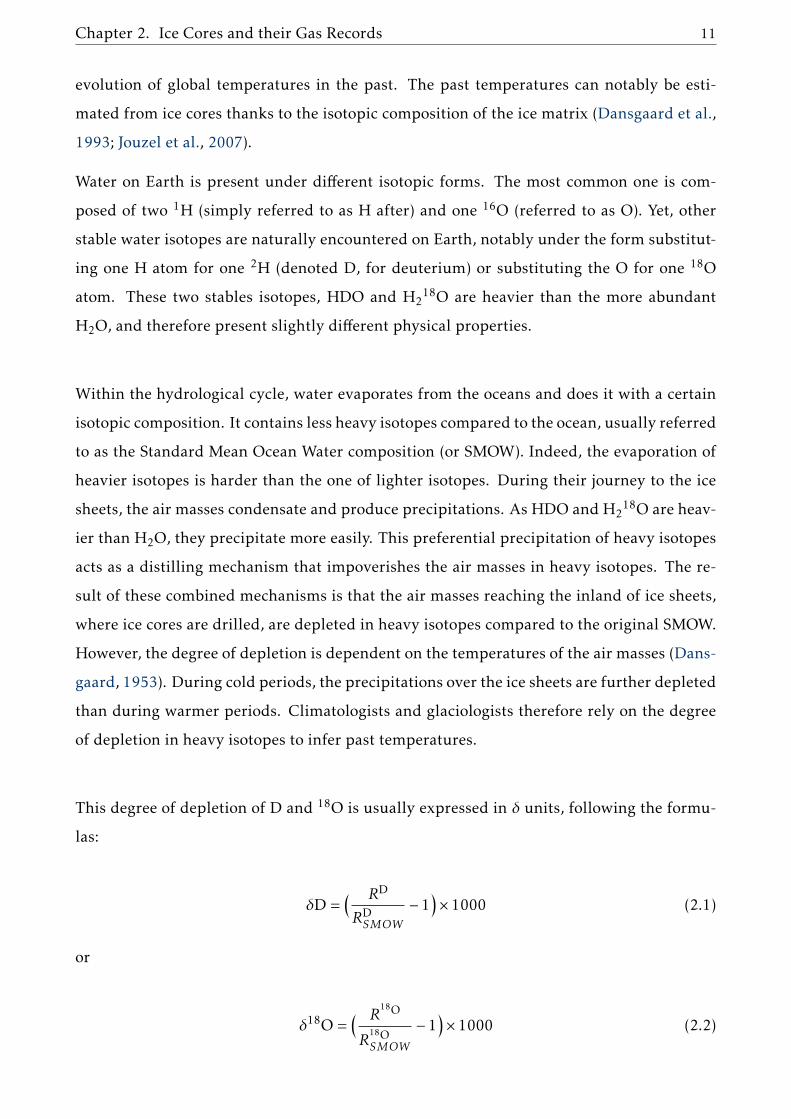
This degree of depletion of D and 18O is usually expressed in δ units, following the formu-
las:
δD =( RD
RDSMOW
− 1)× 1000 (2.1)
or
δ18O =( R
18O
R18OSMOW
− 1)× 1000 (2.2)
12
where RX and RXSMOW are the concentration ratios between the rare isotopesX and the abun-
dant H2O, respectively in the sample of interest and in the SMOW.
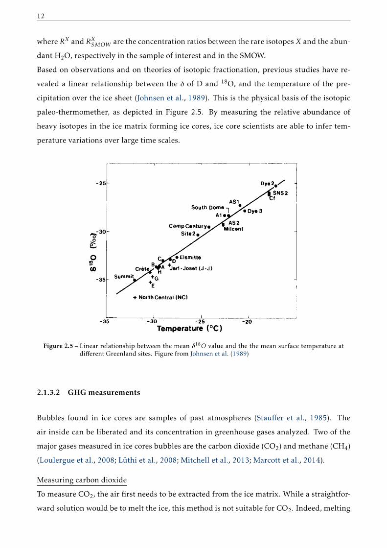
Based on observations and on theories of isotopic fractionation, previous studies have re-
vealed a linear relationship between the δ of D and 18O, and the temperature of the pre-
cipitation over the ice sheet (Johnsen et al., 1989). This is the physical basis of the isotopic
paleo-thermomether, as depicted in Figure 2.5. By measuring the relative abundance of
heavy isotopes in the ice matrix forming ice cores, ice core scientists are able to infer tem-
perature variations over large time scales.
Figure 2.5 – Linear relationship between the mean δ18O value and the the mean surface temperature atdifferent Greenland sites. Figure from Johnsen et al. (1989)
2.1.3.2 GHGmeasurements
Bubbles found in ice cores are samples of past atmospheres (Stauffer et al., 1985). The
air inside can be liberated and its concentration in greenhouse gases analyzed. Two of the
major gases measured in ice cores bubbles are the carbon dioxide (CO2) and methane (CH4)
(Loulergue et al., 2008; Lüthi et al., 2008; Mitchell et al., 2013; Marcott et al., 2014).
Measuring carbon dioxide
To measure CO2, the air first needs to be extracted from the ice matrix. While a straightfor-
ward solution would be to melt the ice, this method is not suitable for CO2. Indeed, melting
Chapter 2. Ice Cores and their Gas Records 13
the ice induces a chemical reaction between (hydrogen)carbonates and the ice acidity, that
results in CO2 as a product (Raynaud et al., 1982). This artificial production of CO2 con-
taminates the air released from the bubbles, and thus carbon dioxide measurements must
be performed without melt. This is achieved by crushing or sublimating the ice (Delmas
et al., 1980; Wilson and Long, 1997; Schmitt et al., 2011). Once liberated the gas can be
collected and sent to a CO2 concentration analyzer, such as a gas chromatographic column
coupled with an ion detector or a laser spectrometer.
Analyzing carbon dioxide is a labor intensive task. Even when fully operational, carbon
dioxide analysis systems can rarely measure more than ten samples per day. Thus, CO2 mea-
surement campaigns span several months to several years, with spatial resolutions ranging
from a fewmeters to a few ten of centimeters (Barnola et al., 1987; Lüthi et al., 2008; Marcott
et al., 2014). To overcome these limitations, there is an ongoing effort to develop techniques
able to continuously measured CO2 in ice cores.
Measuring methane
Contrary to CO2, methane can be extracted by melting the ice. A discrete sampling tech-
nique similar to CO2 analysis has been developed, but where the ice is melted to liberate the
gases (Chappellaz et al., 1990; Mitchell et al., 2013). In some systems, the water is slowly
refrozen from the bottom after melting, in order to release the dissolved gases from the liq-
uid phase (Chappellaz et al., 1990; Loulergue et al., 2008). The released methane can then
be sent to either chromatographic column or a laser spectrometer for analysis. Like CO2,
this type of discrete measurements suffers from being labor intensive, as no more than 20
samples are usually measured per day.
To overcome these limits, a method based on the continuous melt, extraction, and concen-
tration analysis has been developed in the last decade (Chappellaz et al., 2013; Rhodes et al.,
2013). This technique is referred to as Continuous Flow Analysis (CFA). It enables to mea-
sure a large quantity of ice, with a spatial resolution around the centimeter, in a few days or
weeks. This technique of measurement will be addressed in details in Section 3.1.
The parallel analysis of the ice isotopic composition and of the GHG concentrations of the
bubbles trapped within, have highlighted the strong link between the Earth temperature

14
and the CO2 and CH4 concentrations (e.g., Lüthi et al., 2008; Shakun et al., 2012). The
demonstration of this link is one the great successes of ice core sciences. However, the
precise interpretation of ice core gas records in terms of past atmospheric concentrations
requires a good understanding of the mechanisms of gas trapping in ice cores. In order not
to over-interpret the gas records of ice cores, it is important to properly characterize how
gases get embedded in the ice and how this process affects the variability recorded in the
ice.
2.2 From snow to firn and ice
The polar bubbly ice, in which ice cores are drilled, is formed due to the accumulation of
snow at the surface of ice sheets. In these regions, snow does not melt during the summer
season and accumulates over time. The fallen snow first transforms into firn, a name for
compressed and dense snow, and eventually into airtight ice in which air bubbles are en-
capsulated (Stauffer et al., 1985). Our description of gas trapping thus naturally starts with
the transformation of snow into ice, and the description of the firn structure.
2.2.1 Description of the firn column
Surface snow
Snow that falls on top of ice sheets is characterized by its low density, around 350kg.m−3
(Herron and Langway, 1980; Hörhold et al., 2011). In this condition, snow is a highly porous
material and most of its volume is occupied by the interstitial pores rather than the ice ma-
trix. The upper surface snow (typically above 2m depth) is subject to surface metamorphism
due to the effects of temperature gradients and wind (Hutterli et al., 2009; Calonne et al.,
2017). This type of metamorphism is controlled by water vapor fluxes due to gradients of
concentrations resulting from the variations in curvature of the snow material surface and
of the temperature gradients in the snowpack.
The processes involved are complex and not easily taken into account for the study of firn
densification and gas trapping. Nonetheless, a link between the surface insolation and the
quantity of gas trapped in the ice has been observed in deep ice cores (Raynaud et al., 2007;
Chapter 2. Ice Cores and their Gas Records 15
Lipenkov et al., 2011). The same observation was made between the surface insolation and
the ratio of O2 to N2 in bubbles (Bender, 2002; Lipenkov et al., 2011). This indicates that
the metamorphism happening at the surface might ultimately influence the process of gas
trapping, deeper in the firn.
This surface snow then gets buried under newly precipitated snow, starting its transforma-
tion first into firn and eventually into ice. The weight of the newly added precipitations put
compressive stresses on the buried snow. In response to the mechanical stress, the ice phase
of the snow get deformed and compressed (Maeno and Ebinuma, 1983; Herron and Lang-
way, 1980). This compression is associated with an increase in density and consequently
a reduction in the porous phase volume. The densification of snow into ice is usually di-
vided into three zones or stages, depending on the mechanism driving the densification of
the medium (Maeno and Ebinuma, 1983; Alley, 1987; Arnaud et al., 2000; Salamatin et al.,
2009).
First stage of densification
For densities below 550kg.m−3, the deformation experienced by the snow-firn material is
reported to be mainly due to geometrical rearrangement driven by the mechanism of ag-
gregates sliding (Anderson and Benson, 1963; Alley, 1987; Arnaud et al., 2000). In this
framework, an aggregate is viewed as an ice particle that moves relative to other aggregates,
but does so without large deformations. The term of grain sliding is usually used in the
literature to refer to aggregates sliding. The sliding of ice aggregates results in a tighter
arrangement, and thus an increase in density. However, this denser arrangement also tends
to limit the possibility of movement of the ice aggregates (Alley, 1987). Thus, the mecha-
nism of aggregates sliding gradually slows down and eventually stops being the dominant
mechanism of densification.
While the mechanism of aggregates sliding is reported to dominate the first stage of densi-
fication, there is little observations to support it. This vision mainly originates from the fact
that there is a change in densification speed for densities around 550km.m−3, the density of
a close packing of spheres (Anderson and Benson, 1963). This suggest that the mechanism
of densification at low density is hindered due to geometrical effects.
Second stage of densification
16
For densities above 550kg.m−3, the main mechanism responsible for the compression of firn
is the creep of the ice matrix due to the presence of dislocations in the ice crystals (Wilkin-
son and Ashby, 1975; Arzt et al., 1983; Maeno and Ebinuma, 1983). Under the creep defor-
mation of the ice phase, the firn keeps increasing in density and consequently keeps loosing
porous volume. This second stage of firn densification encompasses most of the firn column.
With the increase in density, the pores of the firn eventually pinch and become bubbles that
encapsulate the air (Stauffer et al., 1985; Shieh and Evans, 1991; Schaller et al., 2017). This
marks the transition between the porous firn and the airtight ice. The firn-ice transition,
marking the end of the firn column, is located between about 50 to 120m below the ice
sheet surface, depending on the local temperature and accumulation conditions (Witrant
et al., 2012). Moreover, this transition from firn to ice does not happen instantaneously but
rather spans a depth range of about 10m between the formation of the first and last bubbles
(Schwander and Stauffer, 1984; Schwander et al., 1993). This firn-ice transition zone will be
referred to as the pore closure zone for the rest of the manuscript.
Third stage of densification
Finally, below the pore closure zone, the densification of bubbly ice is still controlled by the
ice matrix creep, but it is necessary to take into account the pressure increase in bubbles and
its effect on the mechanical deformation (Wilkinson and Ashby, 1975; Maeno and Ebinuma,
1983). The effect of bubble pressure is taken into account by considering the pressure drop
between the overburden pressure of the ice column and the building pressure in the bub-
bles (Wilkinson and Ashby, 1975; Lipenkov et al., 1997; Lipenkov, 2000). During the third
stage of densification, the air remains entrapped in the ice and its composition no longer
changes (apart from possible radioactive decays and in situ production). Since this third
stage of densification does not impact the gas concentrations recorded in polar ice, it will
not be discussed in this thesis.
The pore closure zone is of particular interest for the study of gas trapping as this is the
zone where most the air gets embedded in the ice. Lipenkov (2000) and Ueltzhöffer et al.
(2010) report the presence of microbubbles already sealed in shallower parts of the firn.
However, as pointed out by Lipenkov (2000), these microbubbles only account for 0.3% of
the air entrapped in deep ice. We can therefore neglect them for our study of gas trapping,
as they do not impact the recorded concentrations in the ice.

Chapter 2. Ice Cores and their Gas Records 17
The transition from firn to airtight ice is not only characterized by the increase in the
medium density, but also by the transformation of open pores (connecting to the atmo-
sphere) into sealed bubbles, also referred to as a closed pores. This transformation from
open to closed pores can be quantified using the open and closed porosity volumes. Indeed,
fully open firn is characterized by a zero closed porosity volume. On the other hand, airtight
ice is characterized by a zero open porosity volume. Naturally, partially open firn is charac-
terized by a spectrum of non zero open and closed porosity volumes. The degree of closure
of a firn stratum can easily be characterized by comparing the open and closed volumes.
Measurements of the open and closed porosity volumes have been performed, and are no-
tably reported by Schwander et al. (1993) and Trudinger et al. (1997) for the sites of Summit
in Greenland and DE08 in Antarctica. In both cases, at low density the firn is characterized
by a zero closed porosity volume, indicating a fully open porous network. Then, for densi-
ties around 800kg.m−3 the closed porosity volume starts to increase with density, indicating
the gradual transformation of open pores into bubbles. Then, for densities above 850kg.m−3
the closed porosity volume decreases, due to the compression of the bubbles with the den-
sification of the medium.
Figure 2.6 – Closed porosity volumes measured in the Summit and DE08 firns. Summit figure fromSchwander et al. (1993) and DE08 figure from Trudinger et al. (1997).
2.2.2 Stratification of the firn
Up to now, the laid out vision of the firn has been the one of a medium with a continuous
increase of density with depth. While this vision is adequate when considering the firn at a
scale of the order of the meter, it no longer accurately describes the state of the firn at the
centimeter scale. Indeed, as notably reported by Fujita et al. (2009) or Hörhold et al. (2011),
polar firns are characterized by a strong stratification, particularly apparent in terms of den-
sity.

18
The different snow events at the surface of the ice sheet, coupled with the metamorphism
induced by the different atmospheric and surface conditions, tend to create an heteroge-
neous layering near the surface of the firn column (Calonne et al., 2017). Fujita et al. (2009)
and Hörhold et al. (2011) report density variations of the order of 35kg.m−3 at the surface of
firns from Greenland and Antarctica. This corresponds to a 10% variability when compared
to the typically observed density of 350kg.m−3. As seen in Figure 2.7, the upper part of
the firn is characterized by a decrease in the density variability with depth, indicating that
initially low density firn (ILDF) densify faster than initially high density firn (IHDF). Then,
for densities around 650kg.m−3 the density variability starts to increase with depth. This
indicates that different firn layers densify at different speeds despite having similar densi-
ties.
Figure 2.7 – Density variability observed in several firn cores fromGreenland and Antarctica. The densityvariability decreases with increasing density until mean densities of about 650kg.m−3 arereached. Then, the density variability increases towards a second maximum. Figure fromHörhold et al. (2011).
Two mechanisms have been advanced to explain this observation. Fujita et al. (2009) ar-
gue that this difference is due to a difference in the ice matrix structure of the firn. They
propose that IHDF is due to surface metamorphism, inducing bond like structures between

Chapter 2. Ice Cores and their Gas Records 19
the ice aggregates of the firn. Because of these bonds, an IHDF stratum densify slower than
its ILDF counterpart. IHDF and ILDF reach a similar density around the 650kg.m−3 value,
corresponding to the minimum of density variability. After that, the ILDF keeps densifying
faster and the density variability thus increases with depth. This mechanism of different
densification rate for the IHDF and ILDF is justified by the observations of the anisotropy
of the firn structure. As displayed in Figure 2.8, at the surface of the firn dense layers are
characterized by a strong structural anisotropy. With the increase in density, the anisotropic
layers become less dense than the less anisotropic ones. This suggests that the IHDF strata
become the less dense strata.
Figure 2.8 – Variations of the firn anisotropy (represented by the variable ∆ǫ) with the increase in density.The transformation of the anisotropic IHDF strata into the less dense strata is illustrated bythe counter clockwise rotation of the ∆ǫ-ρ relationship in the curves a-j. Figure from Fujitaet al. (2009).
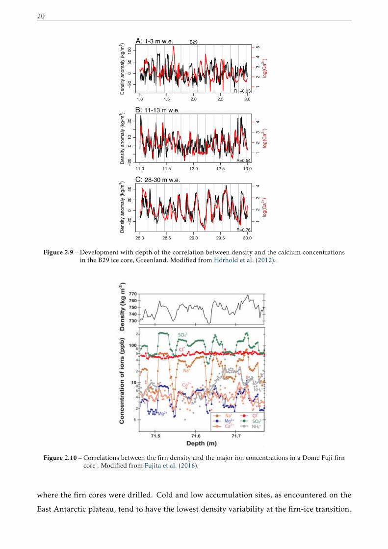
The second proposed mechanism is based on the observation of a building correlation with
depth between density and chemical content by Hörhold et al. (2012), as illustrated in Fig-
ure 2.9. In this idea, firn strata with a high ionic content densify faster than the rest of the
firn. The preferential deformation of ion-rich strata creates the firn stratification observed
for density higher than 650kg.m−3. Finally, the link between chemistry and density in strata
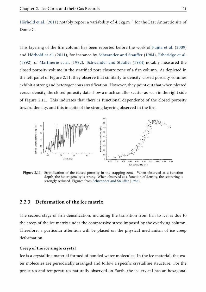
was confirmed by Fujita et al. (2016) based on three firn cores from Dome Fuji, Antarctica.
This link is illustrated in a Dome Fuji firn core in Figure 2.10. They however, argue that the
firn stratification is the combined result of both the effect of the ice matrix structure (due to
surface metamorphism) and the effect of chemical impurities.
The firn-ice transition inherits the stratified characteristics of the firn column. Hörhold et al.
(2011) compiled density variabilities observed at the bottom of firns from Greenland and
Antarctica. They report variabilities between 4.5 and 14.5kg.m−3 depending on the sites
20
Figure 2.9 – Development with depth of the correlation between density and the calcium concentrationsin the B29 ice core, Greenland. Modified from Hörhold et al. (2012).
Figure 2.10 – Correlations between the firn density and the major ion concentrations in a Dome Fuji firncore . Modified from Fujita et al. (2016).
where the firn cores were drilled. Cold and low accumulation sites, as encountered on the
East Antarctic plateau, tend to have the lowest density variability at the firn-ice transition.
Chapter 2. Ice Cores and their Gas Records 21
Hörhold et al. (2011) notably report a variability of 4.5kg.m−3 for the East Antarctic site of
Dome C.
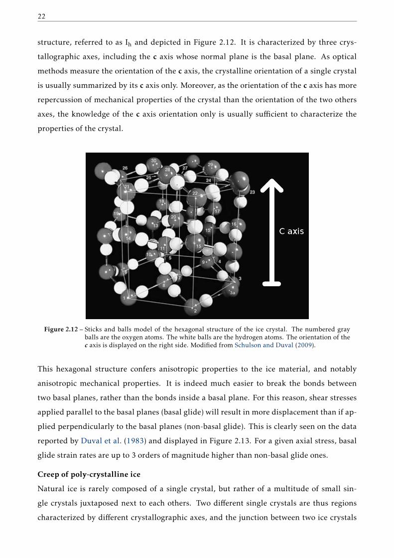
This layering of the firn column has been reported before the work of Fujita et al. (2009)
and Hörhold et al. (2011), for instance by Schwander and Stauffer (1984), Etheridge et al.
(1992), or Martinerie et al. (1992). Schwander and Stauffer (1984) notably measured the
closed porosity volume in the stratified pore closure zone of a firn column. As depicted in
the left panel of Figure 2.11, they observe that similarly to density, closed porosity volumes
exhibit a strong and heterogeneous stratification. However, they point out that when plotted
versus density, the closed porosity data show a much smaller scatter as seen in the right side
of Figure 2.11. This indicates that there is functional dependence of the closed porosity
toward density, and this in spite of the strong layering observed in the firn.
Figure 2.11 – Stratification of the closed porosity in the trapping zone. When observed as a functiondepth, the heterogeneity is strong. When observed as a function of density, the scattering isstrongly reduced. Figures from Schwander and Stauffer (1984).
2.2.3 Deformation of the ice matrix
The second stage of firn densification, including the transition from firn to ice, is due to
the creep of the ice matrix under the compressive stress imposed by the overlying column.
Therefore, a particular attention will be placed on the physical mechanism of ice creep
deformation.
Creep of the ice single crystal
Ice is a crystalline material formed of bonded water molecules. In the ice material, the wa-
ter molecules are periodically arranged and follow a specific crystalline structure. For the
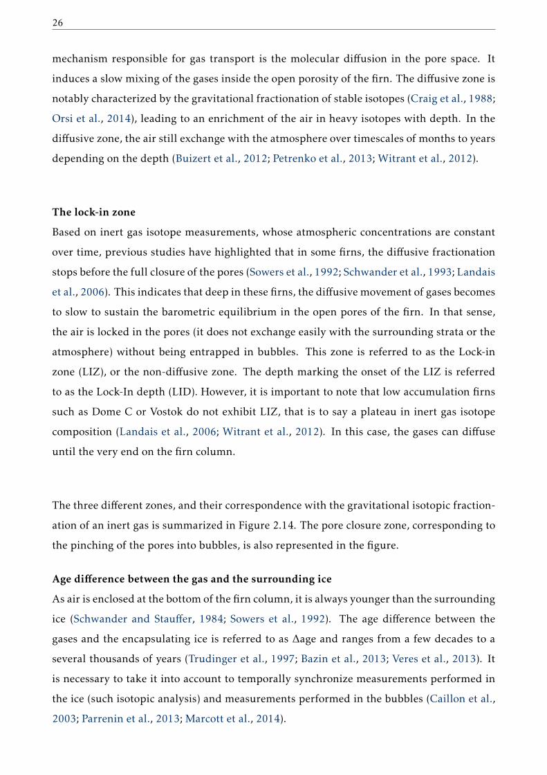
pressures and temperatures naturally observed on Earth, the ice crystal has an hexagonal
22
structure, referred to as Ih and depicted in Figure 2.12. It is characterized by three crys-
tallographic axes, including the c axis whose normal plane is the basal plane. As optical
methods measure the orientation of the c axis, the crystalline orientation of a single crystal
is usually summarized by its c axis only. Moreover, as the orientation of the c axis has more
repercussion of mechanical properties of the crystal than the orientation of the two others
axes, the knowledge of the c axis orientation only is usually sufficient to characterize the
properties of the crystal.
Figure 2.12 – Sticks and balls model of the hexagonal structure of the ice crystal. The numbered grayballs are the oxygen atoms. The white balls are the hydrogen atoms. The orientation of thec axis is displayed on the right side. Modified from Schulson and Duval (2009).
This hexagonal structure confers anisotropic properties to the ice material, and notably
anisotropic mechanical properties. It is indeed much easier to break the bonds between
two basal planes, rather than the bonds inside a basal plane. For this reason, shear stresses
applied parallel to the basal planes (basal glide) will result in more displacement than if ap-
plied perpendicularly to the basal planes (non-basal glide). This is clearly seen on the data
reported by Duval et al. (1983) and displayed in Figure 2.13. For a given axial stress, basal
glide strain rates are up to 3 orders of magnitude higher than non-basal glide ones.
Creep of poly-crystalline ice
Natural ice is rarely composed of a single crystal, but rather of a multitude of small sin-
gle crystals juxtaposed next to each others. Two different single crystals are thus regions
characterized by different crystallographic axes, and the junction between two ice crystals

Chapter 2. Ice Cores and their Gas Records 23
Figure 2.13 – Relationship between strain rate and stress for an axial deformation of ice. The data in-clude basal glide of mono-crystalline ice (upper line), non-basal glide of mono-crystallineice (lower line), and isotropic poly-crystalline ice (middle line). Figure from Duval et al.(1983).
is referred to as a grain boundary.
The mechanical behavior of poly-crystalline ice is therefore the result of the collective be-
havior of its multiple constitutive single crystals. In the case where the orientations of the
single crystals are uniformly distributed in space, the poly-crystal behaves as an isotropic
material. On the other hand, if the single crystal population has a preferential orientation
the anisotropy of the single crystal is transferred to the poly-crystalline material, that now
exhibits a mechanical anisotropic behavior.

24
Duval et al. (1983) compiled creep deformation data obtained for isotropic poly-crystalline
ice. As seen in Figure 2.13, poly-crystalline ice is less easily deformed than a single crystal
under basal gliding, but more easily than a single crystal under non-basal gliding.
Under the stress and temperature conditions encountered in polar firns, it is commonly
assumed that the ice material deforms according to a stationary creep (also referred to as
secondary creep, Duval et al., 1983; Schulson and Duval, 2009). In this case, the strain rates
are linked to the stresses by Glen’s law (sometimes referred to as Norton’s law):
ǫij = Aτn−1σ ′ij (2.3)
where ǫij are the strain rate tensor components, σ ′ij = σij − 1/3T r(σ)δij are the deviatoric
stress tensor components (σ being the stress tensor and δij the Kronecker delta), and τ =12∑
ij(σ′ij )
2.
The physical parameter n is the stress exponent, which represents the non-linear behav-
ior of the ice material. Values near 3 are reported for this parameter, when estimated in
laboratory conditions (Duval et al., 1983; Lipenkov et al., 1997). It can be visualized in Fig-
ure 2.13, where the strain rates relationship with stress has a slope of about 3 for isotropic
poly-crystalline ice. However, values around 2 are estimated for deviatoric stresses inferior
to 0.2MPa (Pimienta and Duval, 1987; Schulson and Duval, 2009).
The parameters A represents the fluidity of the ice material. It is the inverse of its viscosity.
This parameter is dependent on the temperature, following an Arrhenius type law with an
activation energy around 60 to 80kJ.mol−1 (Duval et al., 1983; Lipenkov et al., 1997; Schul-
son and Duval, 2009). This temperature dependence implies that the firn of East Antarc-
tica should deform and densify slower during glacial periods than during interglacial ones.
However, based on modeling and estimation of past firn heights, Bréant et al. (2017) ar-
gue that this reduction of densification in glacial firns is not supported by observations.
Yet, the physical basis of this sustained deformation of firn at very-low temperature is still
unclear.

Chapter 2. Ice Cores and their Gas Records 25
Effect of impurities
Mechanical experiments on ice doped with impurities have been performed in late 1960’s.
Jones (1967) and Jones and Glen (1969) focused on the effect of hydrofluoric (HF) doping.
They observed that doping with HF has a softening effect on the ice, meaning that the de-
formation of the ice material is facilitated and greater strain rates are observed. Similarly,
Nakamura and Jones (1970) studied the influence of hydrochloric doping on the ice creep
properties. They found a softening effect and facilitated deformation, similar to the one
observed for HF. The softening effects observed in these studies are consistent with the hy-
pothesis proposed by Hörhold et al. (2012) or Fujita et al. (2016) for the chemically induced
stratification of polar firn.
2.3 The porous network and the gases inside
2.3.1 Firn from the standpoint of gases
From the point of view of the air filling the pores of the firn, the column is generally divided
in three main zones: the convective, diffusive and lock-in zones.
The convective zone
The convective zone is the upper part of the firn column. It is the zone in which the air in-
side the pores exchange rapidly with the atmosphere above the surface. This fast exchange
is due to the mechanism of wind pumping (Colbeck, 1989). In the convective zone, the air
composition inside a pore is thus similar to the one of the atmosphere. Measurements per-
formed at the Vostok Antarctic site indicates a convective zone spanning 13m (Bender et al.,
1994), while measurements performed at at South Pole suggest an almost inexistent convec-
tive zone (Battle et al., 1996). Other values of convective zone thicknesses are reported by
Severinghaus et al. (2010). It is not clear however, how the thickness of this zone changes
with climatic conditions (Dreyfus et al., 2010; Capron et al., 2013).
The diffusive zone
The end of the convective zone marks the start of the diffusive zone, in which the air is no
longer rapidly mixed with the atmosphere by the surface wind. In that zone, the primary
26
mechanism responsible for gas transport is the molecular diffusion in the pore space. It
induces a slow mixing of the gases inside the open porosity of the firn. The diffusive zone is
notably characterized by the gravitational fractionation of stable isotopes (Craig et al., 1988;
Orsi et al., 2014), leading to an enrichment of the air in heavy isotopes with depth. In the
diffusive zone, the air still exchange with the atmosphere over timescales of months to years
depending on the depth (Buizert et al., 2012; Petrenko et al., 2013; Witrant et al., 2012).
The lock-in zone
Based on inert gas isotope measurements, whose atmospheric concentrations are constant
over time, previous studies have highlighted that in some firns, the diffusive fractionation
stops before the full closure of the pores (Sowers et al., 1992; Schwander et al., 1993; Landais
et al., 2006). This indicates that deep in these firns, the diffusive movement of gases becomes
to slow to sustain the barometric equilibrium in the open pores of the firn. In that sense,
the air is locked in the pores (it does not exchange easily with the surrounding strata or the
atmosphere) without being entrapped in bubbles. This zone is referred to as the Lock-in
zone (LIZ), or the non-diffusive zone. The depth marking the onset of the LIZ is referred
to as the Lock-In depth (LID). However, it is important to note that low accumulation firns
such as Dome C or Vostok do not exhibit LIZ, that is to say a plateau in inert gas isotope
composition (Landais et al., 2006; Witrant et al., 2012). In this case, the gases can diffuse
until the very end on the firn column.
The three different zones, and their correspondence with the gravitational isotopic fraction-
ation of an inert gas is summarized in Figure 2.14. The pore closure zone, corresponding to
the pinching of the pores into bubbles, is also represented in the figure.
Age difference between the gas and the surrounding ice
As air is enclosed at the bottom of the firn column, it is always younger than the surrounding
ice (Schwander and Stauffer, 1984; Sowers et al., 1992). The age difference between the
gases and the encapsulating ice is referred to as ∆age and ranges from a few decades to a
several thousands of years (Trudinger et al., 1997; Bazin et al., 2013; Veres et al., 2013). It
is necessary to take it into account to temporally synchronize measurements performed in
the ice (such isotopic analysis) and measurements performed in the bubbles (Caillon et al.,
2003; Parrenin et al., 2013; Marcott et al., 2014).
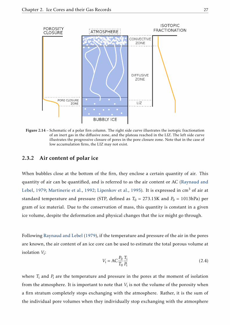
Chapter 2. Ice Cores and their Gas Records 27
Figure 2.14 – Schematic of a polar firn column. The right side curve illustrates the isotopic fractionationof an inert gas in the diffusive zone, and the plateau reached in the LIZ. The left side curveillustrates the progressive closure of pores in the pore closure zone. Note that in the case oflow accumulation firns, the LIZ may not exist.
2.3.2 Air content of polar ice
When bubbles close at the bottom of the firn, they enclose a certain quantity of air. This
quantity of air can be quantified, and is referred to as the air content or AC (Raynaud and
Lebel, 1979; Martinerie et al., 1992; Lipenkov et al., 1995). It is expressed in cm3 of air at
standard temperature and pressure (STP, defined as T0 = 273.15K and P0 = 1013hPa) per
gram of ice material. Due to the conservation of mass, this quantity is constant in a given
ice volume, despite the deformation and physical changes that the ice might go through.
Following Raynaud and Lebel (1979), if the temperature and pressure of the air in the pores
are known, the air content of an ice core can be used to estimate the total porous volume at
isolation Vi:
Vi = ACP0T0
TiPi
(2.4)
where Ti and Pi are the temperature and pressure in the pores at the moment of isolation
from the atmosphere. It is important to note that Vi is not the volume of the porosity when
a firn stratum completely stops exchanging with the atmosphere. Rather, it is the sum of
the individual pore volumes when they individually stop exchanging with the atmosphere
28
(Martinerie et al., 1992). Due the compression of pores in the trapping zone, the total porous
volume at isolation Vi is always larger than the porous volume at complete closure. Still, Vi
can be used to estimate ρc, the typical density of the firn during closure (Raynaud and Lebel,
1979; Martinerie et al., 1992).
ρc =ρice
1+Viρice(2.5)
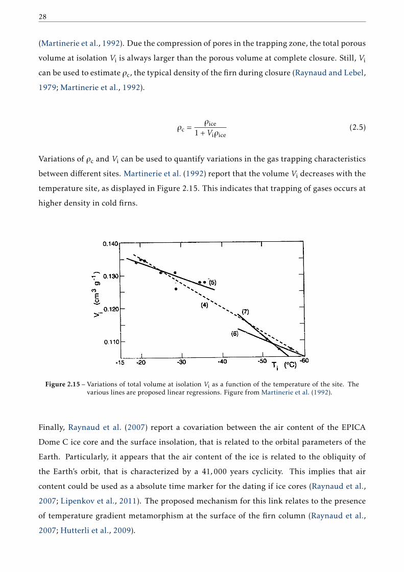
Variations of ρc and Vi can be used to quantify variations in the gas trapping characteristics
between different sites. Martinerie et al. (1992) report that the volume Vi decreases with the
temperature site, as displayed in Figure 2.15. This indicates that trapping of gases occurs at
higher density in cold firns.
Figure 2.15 – Variations of total volume at isolation Vi as a function of the temperature of the site. Thevarious lines are proposed linear regressions. Figure from Martinerie et al. (1992).
Finally, Raynaud et al. (2007) report a covariation between the air content of the EPICA
Dome C ice core and the surface insolation, that is related to the orbital parameters of the
Earth. Particularly, it appears that the air content of the ice is related to the obliquity of
the Earth’s orbit, that is characterized by a 41,000 years cyclicity. This implies that air
content could be used as a absolute time marker for the dating if ice cores (Raynaud et al.,
2007; Lipenkov et al., 2011). The proposed mechanism for this link relates to the presence
of temperature gradient metamorphism at the surface of the firn column (Raynaud et al.,
2007; Hutterli et al., 2009).

Chapter 2. Ice Cores and their Gas Records 29
2.4 Modeling the firn and gas trapping
Gas trapping models have been developed in order to predict the age of the gases trapped
in polar ice. The modeling of gas trapping can be divided in two main steps. First, the den-
sity profile of the firn has to be known. This can either be achieved by models or by direct
field observations and measurements. Once the firn density is characterized, the proper gas
transport and trapping can be modeled. Some models are thus specialized in firn densifi-
cation (Herron and Langway, 1980; Arnaud et al., 2000; Lundin et al., 2017), some others
solely address gas transport and trapping (Rommelaere et al., 1997; Buizert et al., 2012;
Witrant et al., 2012), while some attempt to describe both firn densification and elements of
gas trapping (Goujon et al., 2003).
2.4.1 Firn densification models
The primary characteristics of firn is its density, as it naturally describes the transformation
of surface snow into airtight ice, as well as the constriction of the porous network. Moreover,
the density of a firn column is a quantity that can directly be measured, and can therefore
be used to access the model predicting capabilities. For these reasons, density is the primary
quantity addressed by firn models (Lundin et al., 2017).
One of the pioneer firn densification model is the one proposed by Herron and Langway
(1980). It is based on the observations of density-depth profiles in Greenland and Antarctic
firn cores. In this framework, the firn column is divided in two zones, above and below a
density of 550kg.m−3. The rate of change of a firn stratum density ρ in each zone is given
by:
dρ
dt= k0A
a(ρice − ρ) for ρ < 550kg.m−3 (2.6)
and
dρ
dt= k1A
b(ρice − ρ) for ρ > 550kg.m−3 (2.7)
30
where ρice is the density of pure ice, A is the accumulation rate, and k0, k1, a and b are phys-
ical parameters that have been experimentally tuned. Herron and Langway (1980) assume
that the parameters k0 and k1 obey an Arrhenius type dependence to temperature.
While this model is not based on physics first principles, the distinction between the two
zones is interpreted as the transition from one dominant mechanism of densification to
another. This is consistent with the distinction between the first and second stage of densifi-
cation presented in Section 2.2.1 (Anderson and Benson, 1963; Maeno and Ebinuma, 1983;
Alley, 1987).
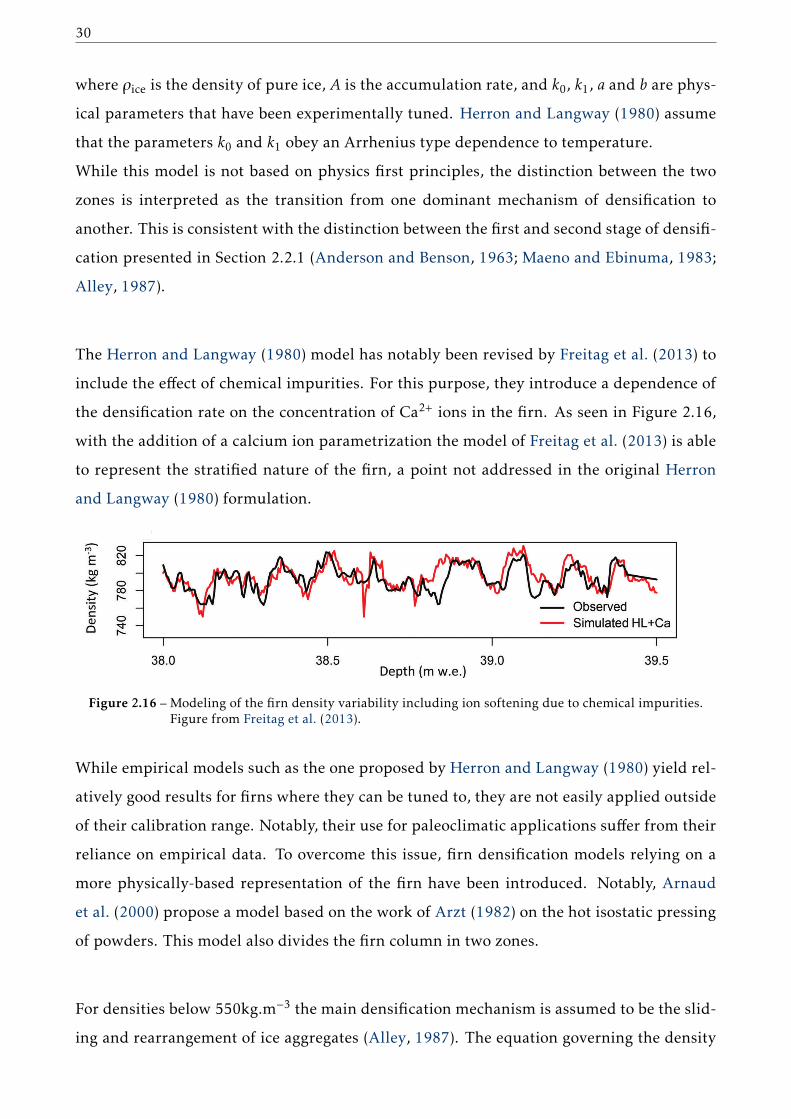
The Herron and Langway (1980) model has notably been revised by Freitag et al. (2013) to
include the effect of chemical impurities. For this purpose, they introduce a dependence of
the densification rate on the concentration of Ca2+ ions in the firn. As seen in Figure 2.16,
with the addition of a calcium ion parametrization the model of Freitag et al. (2013) is able
to represent the stratified nature of the firn, a point not addressed in the original Herron
and Langway (1980) formulation.
Figure 2.16 – Modeling of the firn density variability including ion softening due to chemical impurities.Figure from Freitag et al. (2013).
While empirical models such as the one proposed by Herron and Langway (1980) yield rel-
atively good results for firns where they can be tuned to, they are not easily applied outside
of their calibration range. Notably, their use for paleoclimatic applications suffer from their
reliance on empirical data. To overcome this issue, firn densification models relying on a
more physically-based representation of the firn have been introduced. Notably, Arnaud
et al. (2000) propose a model based on the work of Arzt (1982) on the hot isostatic pressing
of powders. This model also divides the firn column in two zones.
For densities below 550kg.m−3 the main densification mechanism is assumed to be the slid-
ing and rearrangement of ice aggregates (Alley, 1987). The equation governing the density

Chapter 2. Ice Cores and their Gas Records 31
change is:
dD
dt= γ
(P
D2
)(1−
(53
)D)
(2.8)
where D = ρ/ρice is the relative density of ice, γ is a physical parameters depending on the
ice viscosity and on the ice clusters geometry, and P is the overburden pressure on the firn.
Note that the original derivation of Alley (1987) assumes an idealized spherical geometry
for the ice aggregates.
For density above 550kg.m−3, the main driving mechanism for densification in the Arnaud
et al. (2000) model is assumed to be the sintering and creep of the ice clusters. Following
the derivation of Arzt (1982), that assumes spherical ice aggregates at the beginning of this
densification stage, the governing equation of this stage is:
dD
dt= 5.3A(D2D0)
1/3(a
π
)1/2(P∗3
)n(2.9)
where
P∗ = 4πPaZD
(2.10)
with P is the pressure of the above firn column, Z is the coordination number, a is the av-
erage contact area expressed in units of R2 (R being the radius of the ice aggregates before
compression), A is a physical parameter with an Arrhenius dependence on temperature, and
D0 is the relative density at the beginning of the second stage.
The Arnaud et al. (2000) model is therefore derived from a physical representation, despite
its reliance on strong simplifying assumptions concerning the geometry of the ice aggregates
constituting the firn material. The diffusion of heat has been implemented in the Arnaud
et al. (2000) model by Goujon et al. (2003), notably to be used in paleoclimatic studies.
Yet, the Arnaud et al. (2000) model do not manage to adequately represent the past varia-
tions of firn heights on the East Antarctic plateau, as estimated from ice core data (Capron
et al., 2013). Specifically, the firn model overestimate the height of the firn column for the
very cold sites of East Antarctica during glacial conditions. Bréant et al. (2017) propose

32
two revisions to the model to improve the agreement with data. First, they introduce a
parametrization for the enhancement of ice creep due to the presence of impurities, sim-
ilarly to Freitag et al. (2013). Secondly, they argue that at temperatures below −60°C a
physical mechanism becomes dominant for the creep of ice, and balance the reduction of
the mechanism responsible for creep at higher temperatures. Consequently, in the case of
very cold firn, the creep of ice is not as slow as one would expect in the case of a single
mechanism and the firn densify faster. Yet, this mechanical behavior of ice is not supported
by laboratory experiments.
2.4.2 Gas trapping models
The sole knowledge of firn density is not enough to characterize the enclosure of gases in
polar ice. Indeed, to fully describe the trapping of gases it is necessary to take into account
the progressive closure of the porosity, as well as the diffusive mixing of gases in the firn
open porosity.
Closure of the porosity
As displayed in Figure 2.6, the open pores progressively transform into closed bubbles for
densities around 850kg.m−3. The amount and the age of the trapped gases depend on how
this progressive closure takes place, and it therefore has to be included in gas trapping mod-
els. For sites where firn core are available, the amount of closed pores can bemeasured using
gas pycnometry (Stauffer et al., 1985) or tomographic imagery (Gregory et al., 2014; Schaller
et al., 2017; Burr et al., 2018). Yet, during the excavation of the firn samples some closed
pores are open (Martinerie et al., 1990). This leads to an underestimations of the measured
closed porosity, that should ideally be corrected for (Schaller et al., 2017).
In cases where the closed porosity volumes cannot be directly measured, for instance for
glacial firns that no longer exist, the closed porosity has to be estimated with the aid of pore
closure models or of empirical laws.
Using closed porosity data, JM Barnola derived a relationship between the density and the
amount of closed pore in a firn stratum. This empirical law was first introduced in the arti-
cle of Goujon et al. (2003) and writes:
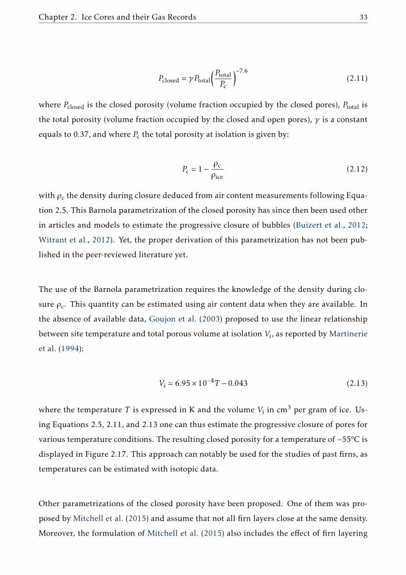
Chapter 2. Ice Cores and their Gas Records 33
Pclosed = γPtotal
(PtotalPc
)−7.6(2.11)
where Pclosed is the closed porosity (volume fraction occupied by the closed pores), Ptotal is
the total porosity (volume fraction occupied by the closed and open pores), γ is a constant
equals to 0.37, and where Pc the total porosity at isolation is given by:
Pc = 1− ρcρice
(2.12)
with ρc the density during closure deduced from air content measurements following Equa-
tion 2.5. This Barnola parametrization of the closed porosity has since then been used other
in articles and models to estimate the progressive closure of bubbles (Buizert et al., 2012;
Witrant et al., 2012). Yet, the proper derivation of this parametrization has not been pub-
lished in the peer-reviewed literature yet.
The use of the Barnola parametrization requires the knowledge of the density during clo-
sure ρc. This quantity can be estimated using air content data when they are available. In
the absence of available data, Goujon et al. (2003) proposed to use the linear relationship
between site temperature and total porous volume at isolation Vi, as reported by Martinerie
et al. (1994):
Vi = 6.95× 10⁻⁴T − 0.043 (2.13)
where the temperature T is expressed in K and the volume Vi in cm3 per gram of ice. Us-
ing Equations 2.5, 2.11, and 2.13 one can thus estimate the progressive closure of pores for
various temperature conditions. The resulting closed porosity for a temperature of −55°C is
displayed in Figure 2.17. This approach can notably be used for the studies of past firns, as
temperatures can be estimated with isotopic data.
Other parametrizations of the closed porosity have been proposed. One of them was pro-
posed by Mitchell et al. (2015) and assume that not all firn layers close at the same density.
Moreover, the formulation of Mitchell et al. (2015) also includes the effect of firn layering

34
on the amount of closed bubbles. In this framework, the bulk closed porosity relates to the
bulk total porosity with:
< Pclosed >=< Ptotal >(1−φ(u,0, v) + exp
[−u +
v2
2+ ln(φ(u,v2, v))
])(2.14)
with
φ(x,µ,Σ) =12+12erf(
x −µ√2Σ
)
u = λ(ρc − ρ)
v = λ√σ2c +σ2
layer
(2.15)
where erf is the error function, λ = 75/ρc, and σc and σlayer respectively represent the vari-
ability in density of closure and the variability in density due to firn layering. The operator
<.> stands for the operation of spatial averaging, that is to say looking at variables on a bulk
scale rather than at the individual stratum scale. Equation 2.14 can be modified to rather
express the relation between closed and total porosity at the local stratum scale. In this case,
the variable v of Equation 2.15 simply is λσc. Mitchell et al. (2015) proposed a different for-
mulation than Equation 2.13 to infer the density during closure ρc:
ρc =1
1− 1/75( 1ρice
+7.02× 10⁻⁴T − 4.5× 10⁻²)−1
(2.16)
where the temperature T is expressed in Kelvin. The resulting closed porosity for a temper-
ature of −55°C, using the value σc = 7 × 10⁻³g.cm−3 (Mitchell et al., 2015), and neglecting
firn layering, is displayed in Figure 2.17.
Finally, based on 3D models of firn samples obtained with tomographic scanning, Schaller
et al. (2017) have proposed three new closed porosity parametrizations for three different
polar sites. The main particularity of their result, is that they observed a constant porosity
at full closure for all the three sites. They propose that the closed and total porosities are

Chapter 2. Ice Cores and their Gas Records 35
related with:
Pclosed = Pcrit(be−λ1(Ptotal−Pcrit) + (1− b)e−λ2(Ptotal−Pcrit)) (2.17)
where Pcrit = 0.10 is the total porosity at full closure and is independent of the studied site,
and where b, λ1, and λ2 are three parameters that depend on the site of study. The closed
porosity parametrization proposed for the site of B53 in Antarctica, is displayed in Fig-
ure 2.17.
The idea of the density of full closure Pcrit being independent of the site of study is incon-
sistent with the parametrization proposed in Goujon et al. (2003) and Mitchell et al. (2015).
Schaller et al. (2017) explains this difference by percolation and finite size effects. They
argue that the small sample sizes used to measure the closed porosity in previous studies
yield non-representative data, due to the opening of closed pores at the surface of the sam-
ples (Martinerie et al., 1990). Therefore, the parametrizations based on these data suffer
from this problem. On the other hand the large samples used in the study of Schaller et al.
(2017) should be less sensitive to this opening of bubbles at the firn surface. The closed
porosity parametrization proposed by Schaller et al. (2017) suggest that gas trapping occurs
at a lower density than in the case of the Goujon et al. (2003) and Mitchell et al. (2015)
parametrizations.
Gas transport and mixing
In order to properly model the age of the gas trapped in the ice, it is necessary to estimated
the age of the gases in the open porosity of the firn column. As discussed in Section 2.3.1,
the age of the air in the open pores is mainly controlled by the molecular diffusion of gases
in the pores. The molecular diffusion in the open porosity is characterized by an effective
diffusivity coefficient, that encapsulates the limitation of diffusion in firn, due to the in-
creasing tortuosity and constriction of the porous network with depth.
Due to the finite size of the samples excavated, it is not possible to measure this effective dif-
fusion coefficient directly using firn cores (Fabre et al., 2000). Instead, the standard method
is to determine the diffusivity profile of the firn based on firn air pumping data. Briefly, air

36
Figure 2.17 – Closed porosity parametrization proposed in the literature. The Goujon et al. (2003) andMitchell et al. (2015) parametrizations are estimated using a temperature of −55°C. TheSchaller et al. (2017) parametrization corresponds to the site of B53 that has a local temper-ature of −55°C.
is fisrt sampled from the open porosity at various depths during the drilling of a firn core.
Then, air samples are analyzed for chemical components whose atmospheric concentrations
are known over the past century. Finally, the effective diffusivity of the model is adjusted so
it can best reproduce the concentrations measured in the open porosity (Severinghaus and
Battle, 2006; Buizert et al., 2012; Witrant et al., 2012; Petrenko et al., 2013). This methodol-
ogy is summarized in Figure 2.18.
Once the effective diffusivity profile is known, the ages of the air inside the porosity can be
deduced. In particular, the ages are known in the open porosity of the pore closure zone.
In order to be able to predict the ages and concentrations in the closed porosity, one has
to know at which rates the open and closed porosity get compressed in the trapping zone.
All models make the assumption that the closed and open porosities compress at the same
rate (Rommelaere et al., 1997; Severinghaus and Battle, 2006; Buizert et al., 2012). This is
justified by the relative low pressure difference in closed and open pores compared to the
pressure in the surrounding ice (Martinerie et al., 1992). In this case, Rommelaere et al.
(1997) state that the concentration qbX of the chemical component X obeys:
∂qbX∂t
+∂(vqbX)∂z
+ vqXǫ
f
∂
∂z
(fǫ
)+λXq
bX = 0 (2.18)
where qbX is the concentration of X in the bubbles (expressed in moles per m3 of bubble
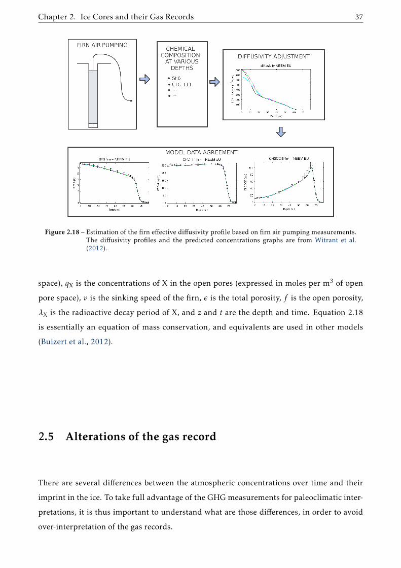
Chapter 2. Ice Cores and their Gas Records 37
Figure 2.18 – Estimation of the firn effective diffusivity profile based on firn air pumping measurements.The diffusivity profiles and the predicted concentrations graphs are from Witrant et al.(2012).
space), qX is the concentrations of X in the open pores (expressed in moles per m3 of open
pore space), v is the sinking speed of the firn, ǫ is the total porosity, f is the open porosity,
λX is the radioactive decay period of X, and z and t are the depth and time. Equation 2.18
is essentially an equation of mass conservation, and equivalents are used in other models
(Buizert et al., 2012).
2.5 Alterations of the gas record
There are several differences between the atmospheric concentrations over time and their
imprint in the ice. To take full advantage of the GHGmeasurements for paleoclimatic inter-
pretations, it is thus important to understand what are those differences, in order to avoid
over-interpretation of the gas records.

38
2.5.1 The smoothing effect
Spahni et al. (2003) compared the methane records in a Dome C ice core (Antarctica) and
the GRIP ice core (Greenland). Looking at the two records in Figure 2.19, one can see that
the Dome C record displays less variability than the GRIP one. As methane is a well mixed
GHG, Antarctic andGreenland atmospheric concentrations should be similar (apart from an
inter-hemispheric gradient, Dällenbach et al., 2000). The difference between the two records
cannot therefore be explained by a smaller methane variability over Antarctica. Rather, this
highlights that the imprints of the same atmospheric variation are different in the Dome C
and GRIP ice cores. One can then wonder, which of the two records presented in Figure 2.19
is the closest to the actual atmospheric variability. This also raises the question of how to
best reconstruct the true past state of the atmosphere based on ice core gas records.
Figure 2.19 – Comparison of the imprints of the same atmospheric event in the Dome C and GRIP icecores. Modified from Spahni et al. (2003).
The difference between the Dome C and GRIP records presented in Figure 2.19, is due to
the smoothing effect (Spahni et al., 2003; Joos and Spahni, 2008; Köhler et al., 2011; Ahn
et al., 2014). The origin of this smoothing effect is twofold. First, due to the molecular
diffusion in the firn column, gases are mixed in the open porosity of the firn (Schwander
et al., 1993; Trudinger et al., 1997; Petrenko et al., 2013). Thus, the air in the open porosity
of a given firn stratum is not composed of atmospheric molecules originating from a single
date. Rather, the air is composed of molecules that were taken from the atmosphere at
different periods (Buizert et al., 2012; Witrant et al., 2012). Therefore, the age of the gases
in the firn is described by an age distribution. As seen in Figure 2.20, the age distribution
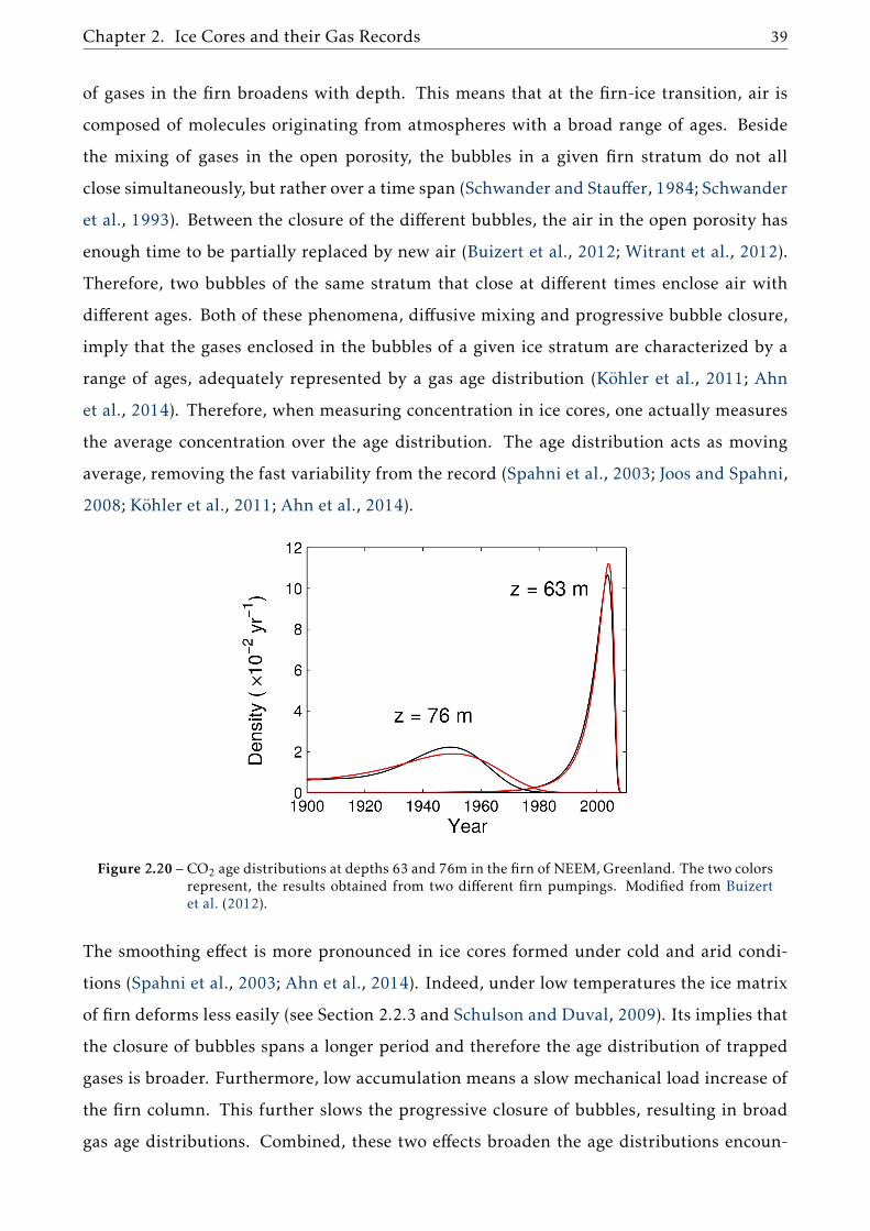
Chapter 2. Ice Cores and their Gas Records 39
of gases in the firn broadens with depth. This means that at the firn-ice transition, air is
composed of molecules originating from atmospheres with a broad range of ages. Beside
the mixing of gases in the open porosity, the bubbles in a given firn stratum do not all
close simultaneously, but rather over a time span (Schwander and Stauffer, 1984; Schwander
et al., 1993). Between the closure of the different bubbles, the air in the open porosity has
enough time to be partially replaced by new air (Buizert et al., 2012; Witrant et al., 2012).
Therefore, two bubbles of the same stratum that close at different times enclose air with
different ages. Both of these phenomena, diffusive mixing and progressive bubble closure,
imply that the gases enclosed in the bubbles of a given ice stratum are characterized by a
range of ages, adequately represented by a gas age distribution (Köhler et al., 2011; Ahn
et al., 2014). Therefore, when measuring concentration in ice cores, one actually measures
the average concentration over the age distribution. The age distribution acts as moving
average, removing the fast variability from the record (Spahni et al., 2003; Joos and Spahni,
2008; Köhler et al., 2011; Ahn et al., 2014).
Figure 2.20 – CO2 age distributions at depths 63 and 76m in the firn of NEEM, Greenland. The two colorsrepresent, the results obtained from two different firn pumpings. Modified from Buizertet al. (2012).
The smoothing effect is more pronounced in ice cores formed under cold and arid condi-
tions (Spahni et al., 2003; Ahn et al., 2014). Indeed, under low temperatures the ice matrix
of firn deforms less easily (see Section 2.2.3 and Schulson and Duval, 2009). Its implies that
the closure of bubbles spans a longer period and therefore the age distribution of trapped
gases is broader. Furthermore, low accumulation means a slow mechanical load increase of
the firn column. This further slows the progressive closure of bubbles, resulting in broad
gas age distributions. Combined, these two effects broaden the age distributions encoun-
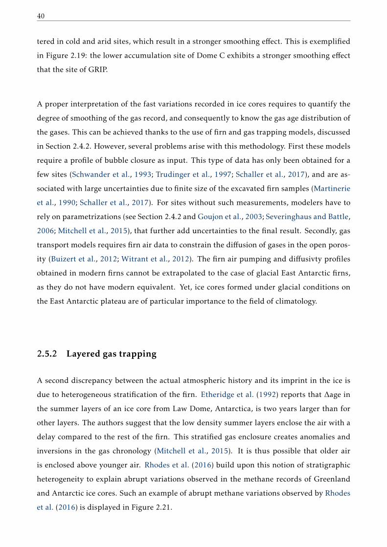
40
tered in cold and arid sites, which result in a stronger smoothing effect. This is exemplified
in Figure 2.19: the lower accumulation site of Dome C exhibits a stronger smoothing effect
that the site of GRIP.
A proper interpretation of the fast variations recorded in ice cores requires to quantify the
degree of smoothing of the gas record, and consequently to know the gas age distribution of
the gases. This can be achieved thanks to the use of firn and gas trapping models, discussed
in Section 2.4.2. However, several problems arise with this methodology. First these models
require a profile of bubble closure as input. This type of data has only been obtained for a
few sites (Schwander et al., 1993; Trudinger et al., 1997; Schaller et al., 2017), and are as-
sociated with large uncertainties due to finite size of the excavated firn samples (Martinerie
et al., 1990; Schaller et al., 2017). For sites without such measurements, modelers have to
rely on parametrizations (see Section 2.4.2 and Goujon et al., 2003; Severinghaus and Battle,
2006; Mitchell et al., 2015), that further add uncertainties to the final result. Secondly, gas
transport models requires firn air data to constrain the diffusion of gases in the open poros-
ity (Buizert et al., 2012; Witrant et al., 2012). The firn air pumping and diffusivty profiles
obtained in modern firns cannot be extrapolated to the case of glacial East Antarctic firns,
as they do not have modern equivalent. Yet, ice cores formed under glacial conditions on
the East Antarctic plateau are of particular importance to the field of climatology.
2.5.2 Layered gas trapping
A second discrepancy between the actual atmospheric history and its imprint in the ice is
due to heterogeneous stratification of the firn. Etheridge et al. (1992) reports that ∆age in
the summer layers of an ice core from Law Dome, Antarctica, is two years larger than for
other layers. The authors suggest that the low density summer layers enclose the air with a
delay compared to the rest of the firn. This stratified gas enclosure creates anomalies and
inversions in the gas chronology (Mitchell et al., 2015). It is thus possible that older air
is enclosed above younger air. Rhodes et al. (2016) build upon this notion of stratigraphic
heterogeneity to explain abrupt variations observed in the methane records of Greenland
and Antarctic ice cores. Such an example of abrupt methane variations observed by Rhodes
et al. (2016) is displayed in Figure 2.21.
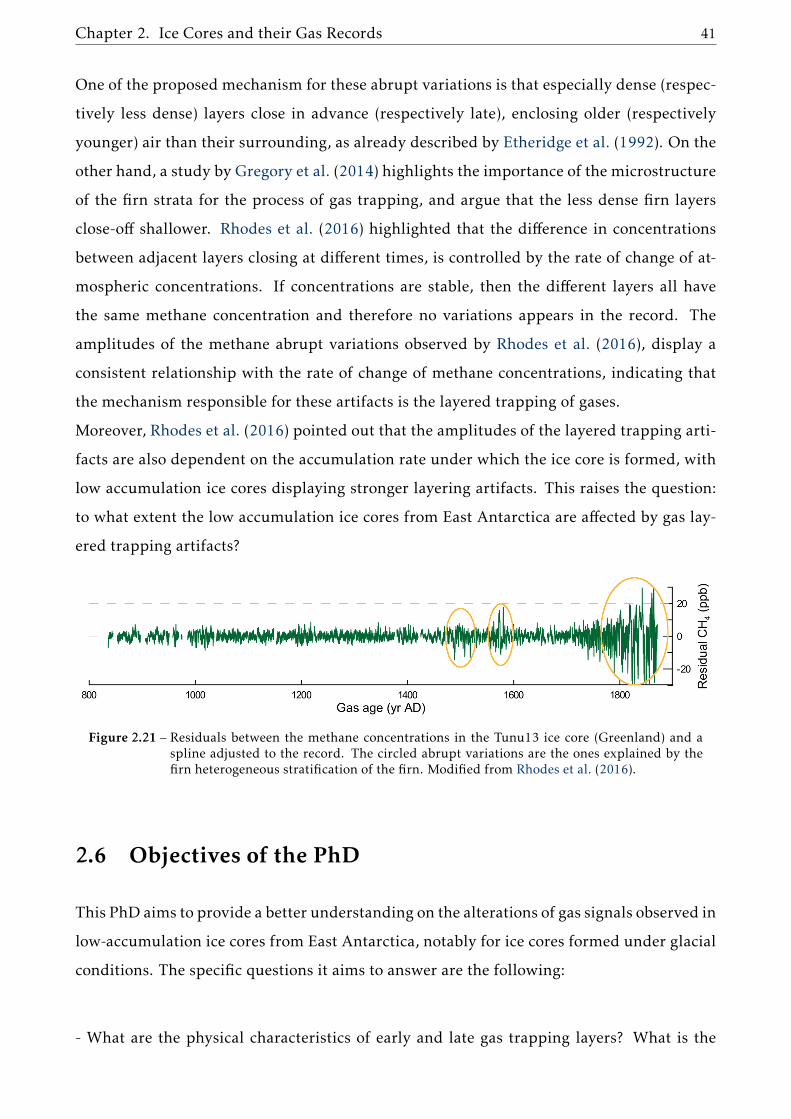
Chapter 2. Ice Cores and their Gas Records 41
One of the proposed mechanism for these abrupt variations is that especially dense (respec-
tively less dense) layers close in advance (respectively late), enclosing older (respectively
younger) air than their surrounding, as already described by Etheridge et al. (1992). On the
other hand, a study by Gregory et al. (2014) highlights the importance of the microstructure
of the firn strata for the process of gas trapping, and argue that the less dense firn layers
close-off shallower. Rhodes et al. (2016) highlighted that the difference in concentrations
between adjacent layers closing at different times, is controlled by the rate of change of at-
mospheric concentrations. If concentrations are stable, then the different layers all have
the same methane concentration and therefore no variations appears in the record. The
amplitudes of the methane abrupt variations observed by Rhodes et al. (2016), display a
consistent relationship with the rate of change of methane concentrations, indicating that
the mechanism responsible for these artifacts is the layered trapping of gases.
Moreover, Rhodes et al. (2016) pointed out that the amplitudes of the layered trapping arti-
facts are also dependent on the accumulation rate under which the ice core is formed, with
low accumulation ice cores displaying stronger layering artifacts. This raises the question:
to what extent the low accumulation ice cores from East Antarctica are affected by gas lay-
ered trapping artifacts?
Figure 2.21 – Residuals between the methane concentrations in the Tunu13 ice core (Greenland) and aspline adjusted to the record. The circled abrupt variations are the ones explained by thefirn heterogeneous stratification of the firn. Modified from Rhodes et al. (2016).
2.6 Objectives of the PhD
This PhD aims to provide a better understanding on the alterations of gas signals observed in
low-accumulation ice cores from East Antarctica, notably for ice cores formed under glacial
conditions. The specific questions it aims to answer are the following:
- What are the physical characteristics of early and late gas trapping layers? What is the

42
origin of their presence in the firn?
- What is the influence of accumulation on the progressive closure of pores in firn of the East
Antarctic plateau? What can be known about the closing of pore at very-low accumulation?
- What is the degree of smoothing encountered in glacial and interglacial period ice core
samples from East Antarctica? What is the relationship of smoothing with accumulation?
- What is the loss of atmospheric information that one can expect, in the case of low-
accumulation and highly thinned deep ice cores drilled on the East Antarctic plateau?
Chapter 3
Methods
Contents
3.1 Continuous Flow Analysis of methane concentrations . . . . . . . . . . . . 45
3.1.1 Description of the CFA apparatus . . . . . . . . . . . . . . . . . . . . . 46
3.1.2 Preparation of the ice . . . . . . . . . . . . . . . . . . . . . . . . . . . . 48
3.1.3 Processing of the raw data . . . . . . . . . . . . . . . . . . . . . . . . . 49
3.1.4 Correcting for methane dissolution . . . . . . . . . . . . . . . . . . . . 50
3.1.5 Internal smoothing of the CFA system . . . . . . . . . . . . . . . . . . 56
3.2 Pycnometry . . . . . . . . . . . . . . . . . . . . . . . . . . . . . . . . . . . . . 61
3.2.1 Physical basis . . . . . . . . . . . . . . . . . . . . . . . . . . . . . . . . 61
3.2.2 Experimental protocol . . . . . . . . . . . . . . . . . . . . . . . . . . . 66
3.2.3 Calibration of the chamber volumes . . . . . . . . . . . . . . . . . . . 67
3.2.4 Experimental uncertainties . . . . . . . . . . . . . . . . . . . . . . . . 69
3.3 Other measurements performed during the thesis . . . . . . . . . . . . . . . 71
3.3.1 Density measurements by Xray absorption . . . . . . . . . . . . . . . . 72
3.3.2 Tomography . . . . . . . . . . . . . . . . . . . . . . . . . . . . . . . . . 75
3.3.3 Air content . . . . . . . . . . . . . . . . . . . . . . . . . . . . . . . . . . 76
3.3.4 Chemistry measurements . . . . . . . . . . . . . . . . . . . . . . . . . 77
3.3.5 Thin sections and crystalline texture . . . . . . . . . . . . . . . . . . . 78
3.4 Conclusion of the chapter . . . . . . . . . . . . . . . . . . . . . . . . . . . . . 79

44
Chapter 3. Methods 45
This chapter describes the different experimental methods used during this PhD. Even
though these methods are recapitulated in the method sections of the articles composing
Chapters 4 and 5, more details will be given here. In particular, an in depth discussion of
the Continuous Flow Analysis of methane and the gas pycnometry measurements of firn
porosity is provided.
3.1 Continuous FlowAnalysis ofmethane concentrations
A large part of this PhD work relies on the study of methane concentrations measured in
polar ice cores. Methane sources (such as mid-latitude wetlands) have a short enough re-
sponse time to produce abrupt increases of methane atmospheric concentrations when acti-
vated (Brook et al., 2000). Moreover, methane has a residence time in the atmosphere long
enough to be well mixed at the global scale, but short enough to display abrupt decrease
when sources are shut down (Mayer et al., 1982). Atmospheric methane thus exhibits a fast
atmospheric variability with some variations occurring in a few decades only, and is there-
fore an ideal tracer to study the impact of layered gas trapping and firn smoothing on the
gaseous signals recorded in the ice. Furthermore, methane is a major greenhouse gas and
measuring its concentration in polar ice cores is of particular importance for the study of
climate (Gedney et al., 2004; Shindell et al., 2004).
Methane was also chosen for this thesis as it is relatively easy to measure with a high resolu-
tion. The availability of high resolution datasets is necessary to fully resolve the variability
recorded in the ice, in order to study how it is affected by gas trapping. Contrary to CO2,
melting the ice containing the bubbles does not contaminate the freed air. Accordingly, a
measurement system of methane based on the continuousmelting and analysis of the ice has
been developed at IGE, notably by J. Chappellaz and X. Faïn, with the help of R. Dallmayr
and O. Pascual. This system is referred to as a Continuous Flow Analysis (CFA) system. It is
able to resolve methane concentration variations in ice cores at the centimeter scale. More-
over, it is possible to analyze up to 15m of ice per day, which in turns enables to analyze a
100m ice core in about two weeks. The methane CFA data of this thesis have been obtained
with X. Faïn and with the occasional help of G. Teste.
The CFAmethod is partially described in the article reported in Chapter 5. However, a more
detailed description will be given here.

46
3.1.1 Description of the CFA apparatus
The CFA apparatus of IGE used during this thesis is based on the same principles that the
system presented by Stowasser et al. (2012), Chappellaz et al. (2013), and Rhodes et al.
(2013). To be measured, the ice core is first cut into 34mm×34mm sticks. Such a stick is
shown in Figure 3.1. The ice is then melted on a square melt head (Bigler et al., 2011) at
an average rate of 3.6cm.min−1. The melting of a CFA stick and the met head are shown in
Figure 3.2. This melting rate is continuously monitored and recorded.
Figure 3.1 – Example of a CFA stick ready to be melted and analyzed. Picture by X. Faïn.
The meltwater and the gases it contains are retrieved and pumped outside of the cold room
for analysis. In order to avoid contaminations, only the meltwater originating from the cen-
ter of the sticks is retrieved, while the rest of the water is discarded (Bigler et al., 2011). This
water/bubbles mixture is sent to a glass, home made, T-shaped debubbler through pumps
and ETFE tubing. This debubbler routes a part of the melt water, now free of bubbles,
toward sensors monitoring dust particle concentration (Abakus®) and liquid conductivity
(Dionex™). As it is important for these sensors to receive a perfectly bubble free water, a
second open split is added on this line to ensure that absolutely no bubble remains in the
water. The T-shaped debubbler was designed to minimize the dead volume added in the
system. It is important to limit the presence of dead volumes to avoid internal mixing of the

Chapter 3. Methods 47
Figure 3.2 – Left: Picture of a CFA sticks being melt, by X. Fain. Right: Picture of the melt head, fromBigler et al. (2011).
sample stream and ensure a good spatial resolution during measurements.
The water/bubbles mixture is then transported to a thermally regulated box, maintained at
30◦C. This box encloses an IDEX© Transfer Line degasser 1. It separates the bubbles from
the meltwater by applying a ∼ 450mbar depression through a porous membrane. The ex-
tracted gas is then dried by an ultra-pure nitrogen counter flux (ALPHAGAZ™2, 99.9999%
purity) inside Nafion tubing. The gas, now free of water vapor, can be sent to an opti-
cal spectrometer for methane concentration analysis. The spectrometer used at IGE is a
SARA spectrometer developed at the Laboratoire Interdisciplinaire de Physique (LiPhy) in
Grenoble. This spectrometer is based on optical feedback cavity enhanced absorption spec-
troscopy (OF-CEAS; Morville et al., 2005; Chappellaz et al., 2013; Rhodes et al., 2013), and
has a precision of 1ppbv (one standard deviation) when measuring methane in a standard
gas. The OF-CEAS technique makes possible the use of a low volume laser cavity of only
12cm3. Furthermore, the pressure inside the cavity is maintained at 20mbar, meaning that
the spectrometer only requires 0.22cm3 of gas at standard pressure and temperature (STP,
1013mbar and 0◦C). The renewal time of gases in the cavity is about 10s for a typical CFA
gas flow of 1.5mL.min−1. Minimizing dead volumes in the tubing results in a spatial reso-
lution of about a centimeter for the CFA system.
Finally, the IGE CFA system also includes a set up able to produce a synthetic water/bubbles
mixture, notably for calibration purposes. This section is referred to as the Full Loop and
will be further discussed in Section 3.1.4.3. The Full Loop can also be used to estimate the
analytical noise of the CFA system. Using it to measure a synthetic mixture of water and
1https://www.idex-hs.com/store/fluidics/degassers/debubblers/transfer-line-degasser.html

48
standard gas, the analytical noise of the CFA system was determined to be around 10ppbv
peak-to-peak (X Faïn, personal communication). The different elements of the CFA system
are summarized in Figure 3.3.
Figure 3.3 – Schematic of the IGE CFA system, courtesy of S Darfeuil.
3.1.2 Preparation of the ice
To be analyzed for methane concentration by the CFA system, the ice cores measured for
this PhD have to prepared into 34 × 34cm section sticks. These sticks are cut directly in
the center of the ice cores, in the IGE cold rooms. A picture of an ice core where a CFA
stick is to be cut is given in Figure 3.4. The preparation of the CFA sticks for this PhD
have been done with the help of X. Faïn, P. Martinerie, G. Teste and G. Aufresne. The
presence of cracks in the CFA sticks might let ambient air enter the analysis system during
measurements. This ambient air will contaminate the ice core gases and lead to abnormally
high measured methane concentrations. In order to prevent such contaminations, the sticks
are preferentially cut in crack free zones of the core.
Ice sticks are melted continuously and sequentially on top of each other. Similarly to cracks,
ambient lab air may enter the sample line when the transition between two consecutive
sticks reaches the melter. We refer to these spaces between consecutive sticks as breaks.
Moreover, as seen Figure 3.1, we systematically checked for the end of the sticks to be as flat
as possible, to ensure an optimal contact between the consecutive sticks in order to limit air
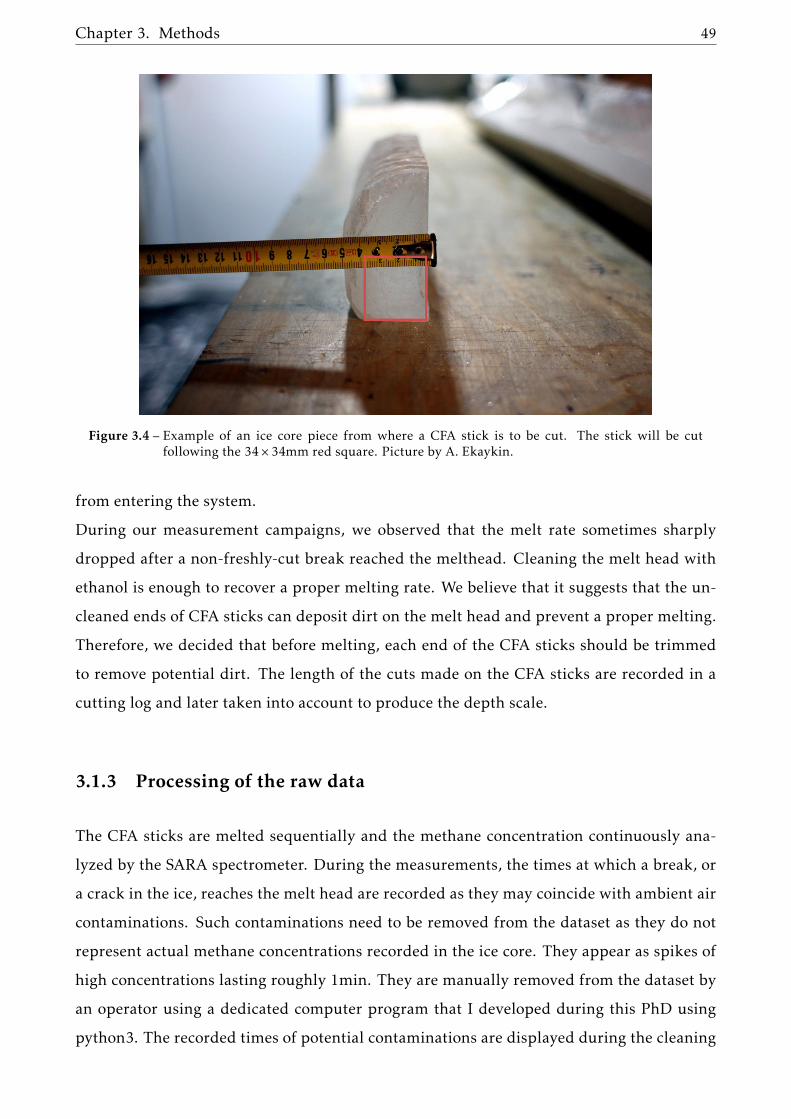
Chapter 3. Methods 49
Figure 3.4 – Example of an ice core piece from where a CFA stick is to be cut. The stick will be cutfollowing the 34× 34mm red square. Picture by A. Ekaykin.
from entering the system.
During our measurement campaigns, we observed that the melt rate sometimes sharply
dropped after a non-freshly-cut break reached the melthead. Cleaning the melt head with
ethanol is enough to recover a proper melting rate. We believe that it suggests that the un-
cleaned ends of CFA sticks can deposit dirt on the melt head and prevent a proper melting.
Therefore, we decided that before melting, each end of the CFA sticks should be trimmed
to remove potential dirt. The length of the cuts made on the CFA sticks are recorded in a
cutting log and later taken into account to produce the depth scale.
3.1.3 Processing of the raw data
The CFA sticks are melted sequentially and the methane concentration continuously ana-
lyzed by the SARA spectrometer. During the measurements, the times at which a break, or
a crack in the ice, reaches the melt head are recorded as they may coincide with ambient air
contaminations. Such contaminations need to be removed from the dataset as they do not
represent actual methane concentrations recorded in the ice core. They appear as spikes of
high concentrations lasting roughly 1min. They are manually removed from the dataset by
an operator using a dedicated computer program that I developed during this PhD using
python3. The recorded times of potential contaminations are displayed during the cleaning

50
to ensure that they are all removed.
The records provided by the spectrometer are originally expressed as a function of the mea-
surement time. To be interpreted in terms of ice core concentrations, they need to be ex-
pressed on the core depth scale. The conversion from a time to a depth scale relies on the
fact that the top and bottom ends of each CFA stick have a depth that is known from the
drilling and cutting logs. The depth scale between two breaks is reconstructed taking into
account the melt rate, as illustrated in Figure 3.5. To produce the depth scale of a CFA cam-
paign, I developed a dedicated program (python3).
Figure 3.5 – Conversion of the time based data from the SARA spectrometer are converted to depth baseddata. The bottom and top depths of the sticks are known.
3.1.4 Correcting for methane dissolution
The CFA data need to be corrected for the preferential dissolution of methane in the melt-
water (Rhodes et al., 2013; Chappellaz et al., 2013). Indeed, methane has a higher solubility
than oxygen and nitrogen in water. As a consequence, the methane mixing ratio in the bub-
bles carried by the meltwater is biased towards lower values, and need to be raised to its
absolute level by the application a correcting factor f .

Chapter 3. Methods 51
3.1.4.1 Dissolution correction using other measurements
One way to estimate this correcting factor is to compare the CFA concentrations with data
already on an absolute scale. During this thesis, I notably used methane data obtained
using discrete measurement methods (Loulergue et al., 2008; Mitchell et al., 2013). For
discrete measurements, the effect of methane dissolution can either be mitigated using a
melt-refreeze technique (Raynaud et al., 1988; Chappellaz et al., 1990) or empirically es-
timated (Mitchell et al., 2011; Mitchell et al., 2013). The overall agreement between the
melt-refreeze and empirically corrected discrete measurements suggests that the two meth-
ods are properly corrected for the preferential dissolution of methane. I also used CFA data
provided by other laboratories, and already corrected for methane dissolution (Rhodes et al.,
2015). Using such comparisons, I found that the correcting factor f for the IGE system is
close to 1.13 for East Antarctic ice cores.
Yet, this method requires the availability of methane records not affected or corrected for
dissolution. This type of data is however not always available. That is why there is an ongo-
ing effort to estimate this factor independently of other data, to which I contributed during
my PhD.
3.1.4.2 Theoretical dissolution correction
One possible way is to theoretically estimate the dissolution of methane in the meltwater.
For this purpose, I derived a simple analytical model of dissolution that assumes: i) the wa-
ter/bubbles mixture is characterized by a unique temperature T , ii) gaseous molecules are
in equilibrium between the water and gas phases, iii) the two phases are homogeneous and
iv) surface tension effects at the boundaries of bubbles are negligible.
Let us consider a volume V 0 of ice core containing N0X molecules of the gas species X. Melt-
ing the ice core will result in two distinct phases of water and air, with volumes Vw and
V g. These two phases respectively contain NwX and N
gX molecule of X. Following Henry’s
law and considering the gas in the bubbles to be an ideal gas, the condition of chemical
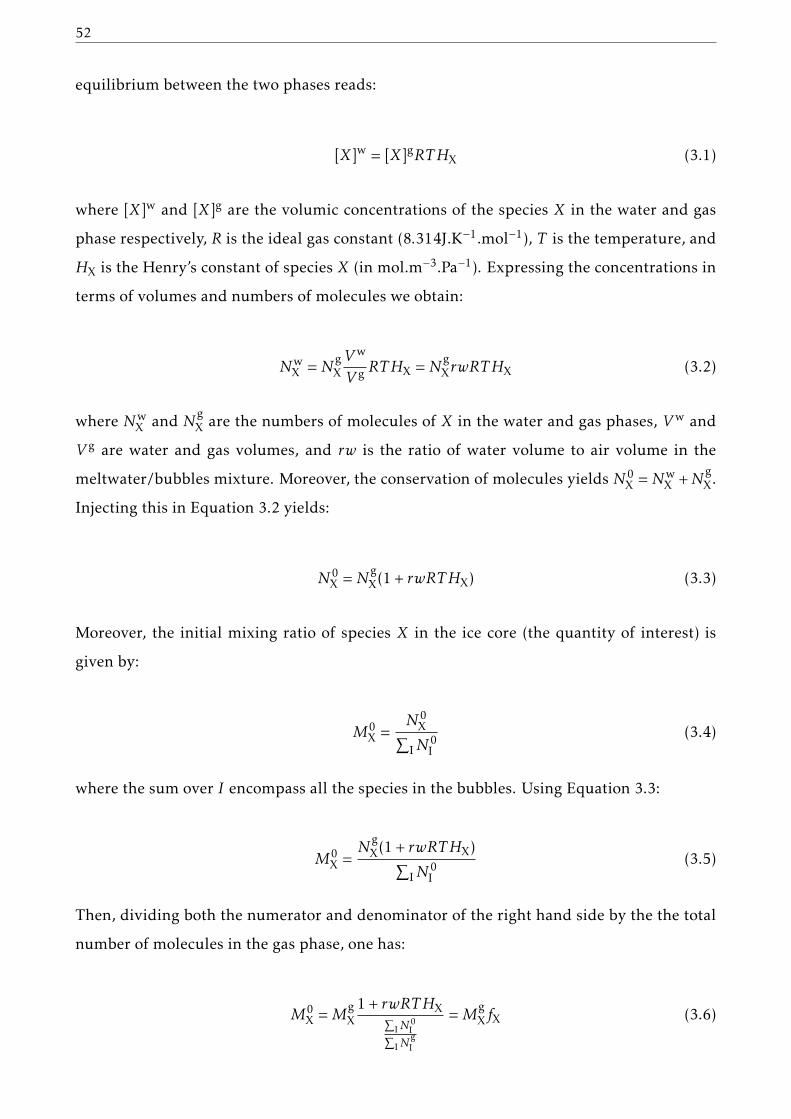
52
equilibrium between the two phases reads:
[X]w = [X]gRTHX (3.1)
where [X]w and [X]g are the volumic concentrations of the species X in the water and gas
phase respectively, R is the ideal gas constant (8.314J.K−1.mol−1), T is the temperature, and
HX is the Henry’s constant of species X (in mol.m−3.Pa−1). Expressing the concentrations in
terms of volumes and numbers of molecules we obtain:
NwX =N
gXVw
V g RTHX =NgXrwRTHX (3.2)
where NwX and N
gX are the numbers of molecules of X in the water and gas phases, Vw and
V g are water and gas volumes, and rw is the ratio of water volume to air volume in the
meltwater/bubbles mixture. Moreover, the conservation of molecules yields N0X =Nw
X +NgX.
Injecting this in Equation 3.2 yields:
N0X =N
gX(1 + rwRTHX) (3.3)
Moreover, the initial mixing ratio of species X in the ice core (the quantity of interest) is
given by:
M0X =
N0X∑
IN0I
(3.4)
where the sum over I encompass all the species in the bubbles. Using Equation 3.3:
M0X =
NgX(1 + rwRTHX)∑
IN0I
(3.5)
Then, dividing both the numerator and denominator of the right hand side by the the total
number of molecules in the gas phase, one has:
M0X =M
gX1+ rwRTHX
∑IN
0I∑
INgI
=MgXfX (3.6)

Chapter 3. Methods 53
where MgX is the mixing ratio in the gas phase (the one measured by the spectrometer) and
fX is the correcting factor to be applied. One can further simplify the computation by using
the fact trace gas concentrations are negligible in front of O2 and N2. Then, the sums over
all species are reduced to the sums over O2 and N2 only. The denominator of Equation 3.6
then becomes:
∑IN
0I∑
INgI
=N0
02+N0
N2
Ng02+N
gN2
=N0
02
Ng02+N
gN2
+N0
N2
Ng02+N
gN2
(3.7)
Using Equation 3.3 for O2 and N2, one can rearrange Equation 3.7 to:
∑IN
0I∑
INgI
=1+ rwRTHO2
1+N0N2
N0O2
1+rwRTHN21+rwRTHO2
+1+ rwRTHN2
1+N0O2
N0N2
1+rwRTHO21+rwRTHN2
(3.8)
Therefore, one finally has:
fX =1+ rwRTHX
1+rwRTHO2
1+N0N2
N0O2
1+rwRTHN21+rwRTHO2
+1+rwRTHN2
1+N0O2
N0N2
1+rwRTHO21+rwRTHN2
(3.9)
The ratio of N2 to O2 in the ice core bubbles is considered to be 80:20. Note that in the
special case were all species have the same solubility, that is to say that all Henry’s constants
are equal, the correcting factor fX is valued at one. This is consistent with the consideration
that in this special case, the mixing ratios of species is not affected by the dissolution.
To be applicable to the case of methane dissolution in meltwater, Equation 3.9 requires
the knowledge of Henry’s constants of O2, N2 and CH4. These physical parameters are
published in the NIST Chemistry WebBook2, as well as their dependence on temperature.
The water to air ratio rw is not directly measured in the CFA system. A closed equation can
however be inferred using the air content of the ice:
rw =1
ACρw
T0T
10.2
1+rwRTHO2+ 0.8
1+rwRTHN2
(3.10)
2https://webbook.nist.gov/chemistry/
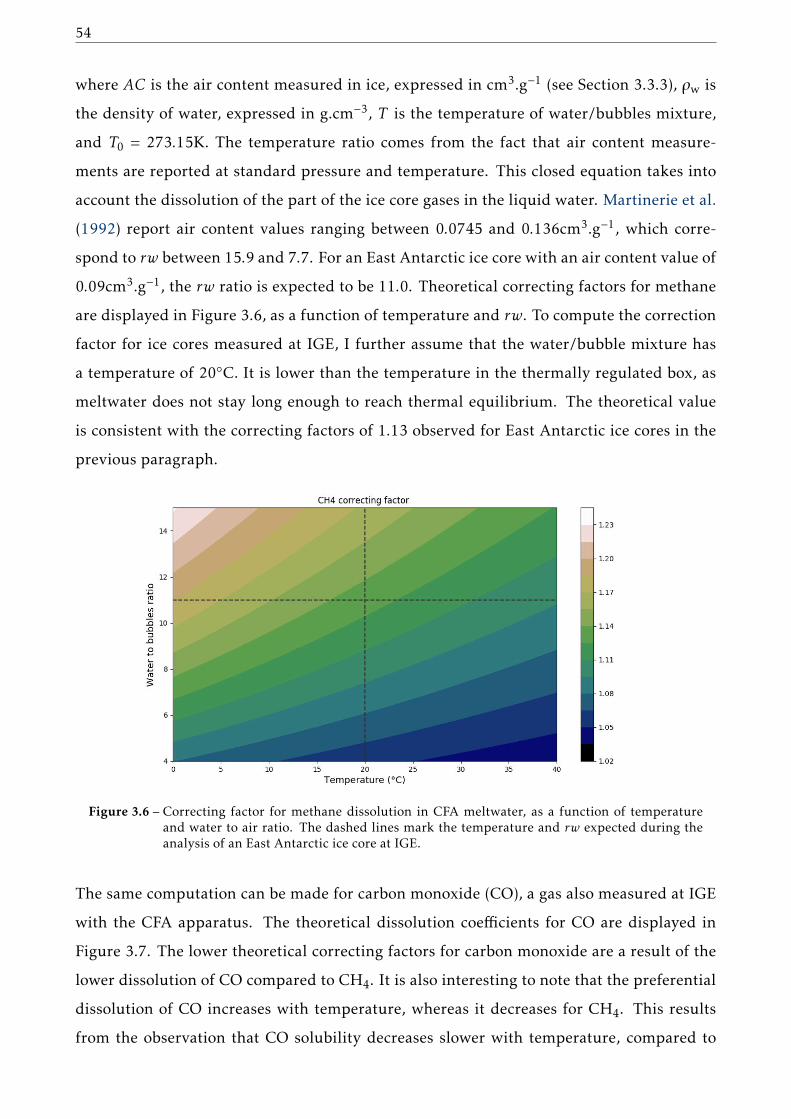
54
where AC is the air content measured in ice, expressed in cm3.g−1 (see Section 3.3.3), ρw is
the density of water, expressed in g.cm−3, T is the temperature of water/bubbles mixture,
and T0 = 273.15K. The temperature ratio comes from the fact that air content measure-
ments are reported at standard pressure and temperature. This closed equation takes into
account the dissolution of the part of the ice core gases in the liquid water. Martinerie et al.
(1992) report air content values ranging between 0.0745 and 0.136cm3.g−1, which corre-
spond to rw between 15.9 and 7.7. For an East Antarctic ice core with an air content value of
0.09cm3.g−1, the rw ratio is expected to be 11.0. Theoretical correcting factors for methane
are displayed in Figure 3.6, as a function of temperature and rw. To compute the correction
factor for ice cores measured at IGE, I further assume that the water/bubble mixture has
a temperature of 20◦C. It is lower than the temperature in the thermally regulated box, as
meltwater does not stay long enough to reach thermal equilibrium. The theoretical value
is consistent with the correcting factors of 1.13 observed for East Antarctic ice cores in the
previous paragraph.
Figure 3.6 – Correcting factor for methane dissolution in CFA meltwater, as a function of temperatureand water to air ratio. The dashed lines mark the temperature and rw expected during theanalysis of an East Antarctic ice core at IGE.
The same computation can be made for carbon monoxide (CO), a gas also measured at IGE
with the CFA apparatus. The theoretical dissolution coefficients for CO are displayed in
Figure 3.7. The lower theoretical correcting factors for carbon monoxide are a result of the
lower dissolution of CO compared to CH4. It is also interesting to note that the preferential
dissolution of CO increases with temperature, whereas it decreases for CH4. This results
from the observation that CO solubility decreases slower with temperature, compared to

Chapter 3. Methods 55
other gases.
As there currently is no apparatus for the discrete measurement of CO, we cannot compare
this result with independent data corrected for CO dissolution.
Figure 3.7 – Correcting factor for carbonmonoxide dissolution in CFAmeltwater, as a function of temper-ature and water to air ratio. The dashed lines mark the temperature and rw expected duringthe analysis of an East Antarctic ice core at IGE.
3.1.4.3 Dissolution correction using the Full Loop
Another strategy to estimate this correction factor is to emulate the dissolution of methane
using standard gases of known concentrations. This is done on the CFA system of IGE using
the so called Full Loop (FL), which is displayed in Figure 3.3. The idea behind it is to inject
standard gases in de-ionized (DI) and degassed water with a specific water to air ratio. This
synthetic mixture of water and bubbles is then transported to the spectrometer like ice core
meltwater would be. Then, by measuring the methane concentration in the spectrometer
one is able to estimate the degree of dissolution and the correcting factor required.
Experiments using the FL have shown that the methane concentration is not at equilibrium
in the IGE CFA line. An increase in the length of the tubing results in a higher dissolution
(personal communication from X. Faïn). It is thus not clear how to set up the FL to faithfully
reproduce the dissolution of methane in ice core meltwater. Moreover in the case of CO, FL
experiments performed at IGE contradict the theoretical model with correcting factor closer
to 1.10. One possible way to use the FL for CO would be to tune it to recreate the estimated
dissolution for CH4 (using discrete measurements), and to directly measure the correcting
factor needed for CO. Yet, this methodology assumes a direct relation between the dissolu-
56
tion of methane and carbon monoxide. It is however possible that in a dynamical system
such as the CFA, different tunings of the FL (playing on the length of the tubes or the water
to air ratio for instance) can reproduce similar CH4 dissolution but several degrees of CO
dissolution.
In conclusion, there is currently no clear strategy to be implemented to correct for the dis-
solution of methane using only CFA-based data. Theoretical derivation is limited by simpli-
fying assumptions (such as thermodynamical equilibrium) that are not necessarily met in
the case of ice core measurements. This strongly limits the confidence in these theoretical
results. On the other hand, it seems reasonable that the FL can be tuned to faithfully repro-
duce the dissolution of methane and of other gases such as carbon monoxide. Yet, there are
several adjustable parameters to determine in order to reproduce the gas dissolution, and is
still an ongoing development at IGE.
Finally, a potential way of escaping the dissolution problem would be the development of
an extraction system able to fully extract dissolved gases. Such a system would also make
possible the measurement of highly soluble gases such as N2O.
3.1.5 Internal smoothing of the CFA system
Due to the mixing of gases in the tubing, the data provided by the CFA system are a
smoothed version of the record in the ice core. This limits the spatial resolution of the
data, as variability faster than the smoothing limit of the CFA are removed from the data.
Even though the CFA system has been designed to minimize this smoothing, it is however
important to properly characterize it to interpret the final data. In particular, I needed the
precise degree of smoothing of the CFA system in order to study the fast, centimeter-scale,
methane variabilities observed in ice cores (Rhodes et al., 2016). The smoothing of the CFA
is fully characterized through a single function G, such as:
Ss = S ∗G (3.11)
where, Ss and S are respectively the smoothed and un-smoothed ice core records, and ∗ isthe operator standing for the convolution product of two real-valued functions. The aim of
my work in this section is thus to determine the function G and to study its characteristics.
Chapter 3. Methods 57
For normalization reasons the integral of G over the whole time domain is equals to one.
Following Stowasser et al. (2012), G can be determined thanks to a step experiment. This
experiment consists of abruptly changing the concentration of the methane sent in the CFA
line from one value C1 to another value C2. Due to the smoothing, the measured concentra-
tions appears as a smeared step. The analytical expression of the concentrations is:
Ss(t) = [C1 + (C2 −C1)H(t)] ∗G(t)
=
+∞∫
−∞
[C1 + (C2 −C1)H(τ)]×G(t − τ)dτ(3.12)
where H(t) is the Heaviside function (also called step function). Time derivation of the
measured concentrations is given by:
dSs(t)dt
=d
dt[C1 + (C2 −C1)H(t)] ∗G(t)
= (C1 −C2)dH
dt∗G(t)
= (C1 −C2)δ ∗G(t)
= (C1 −C2)G(t)
(3.13)
where δ is the Dirac distribution. Integrating Equation 3.13, one has:
Ss(t)− Ss(0) = Ss(t)−C1
= (C1 −C2)
t∫
0
G(t)(3.14)
Therefore, the smeared step measured by the CFA system is simply the integral of the
smoothing function G. To determine this function, the protocol is thus to perform a step
experiment to find the integral form of G, and finally derive the function G itself.

58
Similarly to Stowasser et al. (2012), I search the function G under the form of a log-normal
law. This allows me to express G as a smooth analytical function, that nonetheless matches
the data. Therefore, once the step experiment is performed, the results are fitted, using a
dedicated python program, with the cumulative function of a log-normal law as displayed
in Figure 3.8. This yields the set of parameters best representing the smoothing function.
The smoothing function of the IGE CFA system is displayed in Figure 3.9.
Figure 3.8 – Methane concentrations during a step experiment. Measured data are the blue dots, andthe orange curve is the cumulative log-normal fit to these data. As a reference, the step inconcentrations imposed at the start of the CFA system is shown in black.
Figure 3.9 – Lognormal smoothing function of the IGE CFA system deduced from the step experiment.
The smoothing function deduced from the step experiment has a width of around 50s. Com-
bined with the typical 3.6cm.min−1 meltrate, the gases are mixed in the CFA system on a
depth range of about 3.5cm. In order to better quantify the mixing and smoothing of ice
core signals, one can use a frequency response diagram. This type of diagrams links the
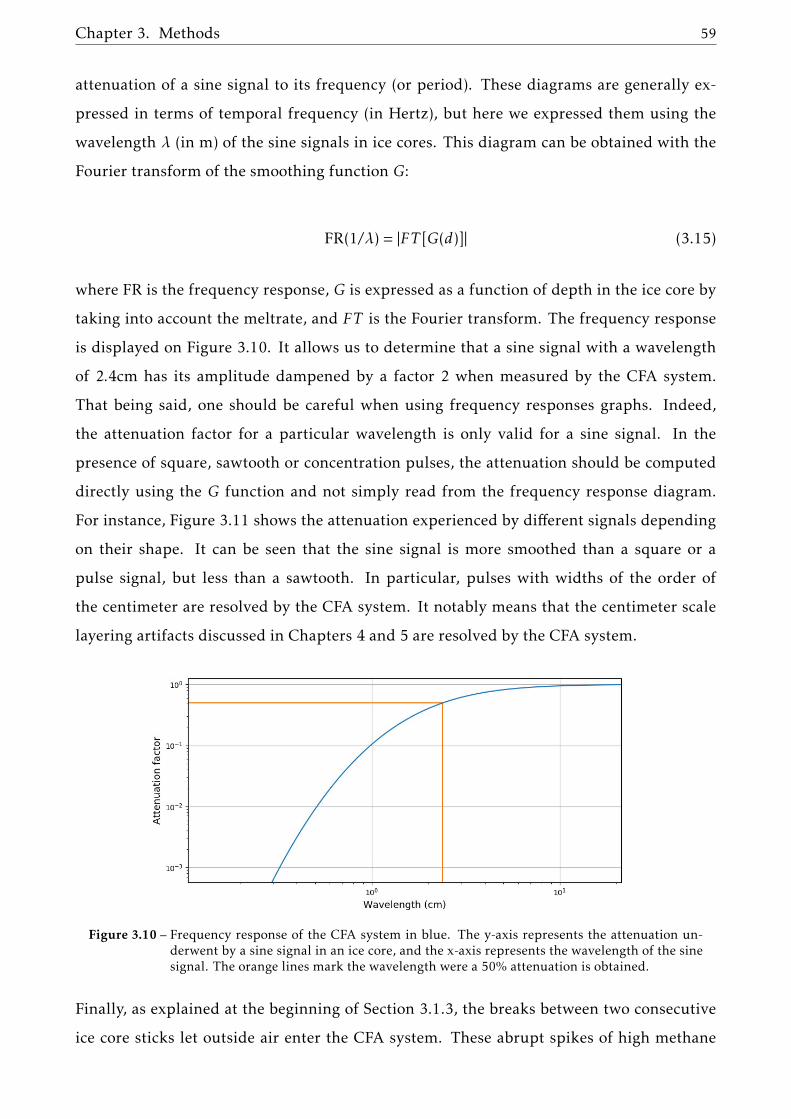
Chapter 3. Methods 59
attenuation of a sine signal to its frequency (or period). These diagrams are generally ex-
pressed in terms of temporal frequency (in Hertz), but here we expressed them using the
wavelength λ (in m) of the sine signals in ice cores. This diagram can be obtained with the
Fourier transform of the smoothing function G:
FR(1/λ) = |FT [G(d)]| (3.15)
where FR is the frequency response, G is expressed as a function of depth in the ice core by
taking into account the meltrate, and FT is the Fourier transform. The frequency response
is displayed on Figure 3.10. It allows us to determine that a sine signal with a wavelength
of 2.4cm has its amplitude dampened by a factor 2 when measured by the CFA system.
That being said, one should be careful when using frequency responses graphs. Indeed,
the attenuation factor for a particular wavelength is only valid for a sine signal. In the
presence of square, sawtooth or concentration pulses, the attenuation should be computed
directly using the G function and not simply read from the frequency response diagram.
For instance, Figure 3.11 shows the attenuation experienced by different signals depending
on their shape. It can be seen that the sine signal is more smoothed than a square or a
pulse signal, but less than a sawtooth. In particular, pulses with widths of the order of
the centimeter are resolved by the CFA system. It notably means that the centimeter scale
layering artifacts discussed in Chapters 4 and 5 are resolved by the CFA system.
Figure 3.10 – Frequency response of the CFA system in blue. The y-axis represents the attenuation un-derwent by a sine signal in an ice core, and the x-axis represents the wavelength of the sinesignal. The orange lines mark the wavelength were a 50% attenuation is obtained.
Finally, as explained at the beginning of Section 3.1.3, the breaks between two consecutive
ice core sticks let outside air enter the CFA system. These abrupt spikes of high methane

60
Figure 3.11 – Attenuation experienced by signals depending on their shape. The unaltered signals are inblue, and their corresponding smoothed version in orange. The sine, square, and sawtoothsignals have a wavelength of 2.4cm, and the pulse signal has a width of 1.2cm. The dashedlines mark the 50% amplitude attenuation level.
concentration can be seen as impulse inputs to the system. Theoretically, the response of the
CFA system to such an impulse is directly the smoothing function G, simply scaled accord-
ing to amount of air entering the system. Figure 3.12 shows next to each other, the response
of the CFA to a contamination due to a break, and the smoothing function calculated with
the step experiment. As seen, they are in good agreement, indicating the validity of the
step-experiment method.
Figure 3.12 – In blue: smoothing function G derived from the step experiment. In orange: CFA systemresponse to air contamination due to a break.
Chapter 3. Methods 61
3.2 Pycnometry
Gas pycnometry is a method which allows us to measure the closed and open porosity vol-
umes in firn samples, based on a gas dilation experiment (Stauffer et al., 1985). In this
context, a pore is considered open if it reaches an edge of the firn sample. The IGE pycnom-
etry systemwas first developed by J.M. Barnola during the 1990’s. It was then restored by O.
Magand and L. Arnaud a couple of years prior to this PhD. The pycnometry measurements
made for this thesis were obtained with the help of X. Faïn and S. Pion.
3.2.1 Physical basis
The determination of the closed and open porosity volumes is based on the measurement of
Vs, the volume inaccessible to outside gases in a firn sample. This volume Vs is composed of
the ice phase and of the closed porosity. Therefore the closed and open porosity volumes Vc
and Vo are given by:
Vc = Vs −Vice
Vo = Vcyl −Vs
Vice =M/ρice
(3.16)
where Vice is the volume of the ice phase calculated from the sample weight and Vcyl is the
volume of the firn sample measured geometrically. M and ρice are respectively the mass of
the firn sample and the density of pure ice.
The measurement of Vs is based on the dilation of an ideal gas between two chambers of
known volumes V1 and V2, depicted in Figure 3.13. The volume of the tubing between
the two chambers is included in the value of V1. The firn sample to be analyzed is placed
in chamber V1, while the chamber V2 is isolated by a valve and then vacuum-pumped. A
pressure gauge is attached to chamber V1 in order to monitor its internal pressure. Then,
the valve isolating the two chambers is opened, resulting in the dilation of the gas originally
contained in V1, in a larger volume V1 + V2. The dilation creates a pressure drop that is
recorded with the pressure gauge. Application of the ideal gas law before and after the

62
dilation yields:
P(V1 −Vs) =NRT
P ′(V1 +V2 −Vs) = (N +∆Nw)RT(3.17)
where P and P ′ are the pressures monitored respectively before and after the dilation, R is
the ideal gas constant, T is the temperature, N is the number of gas moles present before
the dilation, Vs is the volume rendered inaccessible to gases by the firn sample, and ∆Nw is
the additional water vapor molecules that have sublimated from the firn surface to establish
the thermodynamical equilibrium between vapor pressure and ice in the expanded V1 +V2
volume.
To calculate Vs, one has to determine the number of moles of water molecules ∆Nw that have
been sublimated from the firn sample. This number depends on whether the establishment
of the equilibrium in the expanded volume is fast or slow, compared to the duration of the
experiment.
Figure 3.13 – Left: Schematics of the pycno apparatus including the two chambers of known volume V1and V2, and three valves in orange. Right: Picture of the pycnometry system.
Fast equilibrium case:
Assuming that the establishment of the equilibrium vapor pressure is fast compared to the
time of the experiment (which is of the order of the minute), one can assume that the vapor
pressure equals its equilibrium value Pw. The amount of added water vapor molecules ∆Nw
is then simply linked to Pw by:
∆NwRT = PwV2 (3.18)
This fast equilibrium hypothesis is notably assumed by Stauffer et al. (1985) while perform-
Chapter 3. Methods 63
ing pycnometry experiments. Re-arranging Equations 3.17 and 3.18, the inaccessible vol-
ume Vs can be determined by the pressures recorded during the experiment.
Vs = V1 −R
1−RV2 +PwV2
P −P ′ (3.19)
where R equals P/P ′. The last term of the right-hand side of Equation 3.19 is a correction
term taking into account the effect of equilibrium vapor pressure over ice. For a typical
temperature of −8°C during the measurements performed in this thesis, the equilibrium
vapor pressure of ice is equals to 310Pa (Lide, 2005). Using pressures recorded during ex-
periments, the correcting factor has been estimated to be about 0.2cm3. This is about 10%
of the closed or open porosity volumes.
Slow equilibrium case:
In the case where the time to establish the vapor pressure equilibrium is much larger than
the time of the experiments, one can neglect the release of water molecules from the firn
sample. Then, ∆Nw is close to zero and the correction term of 3.19 vanishes. The equation
then writes:
Vs = V1 −R
1−RV2 (3.20)
The problem is now to estimate if the pycnometry experiments performed during this PhD
correspond to a fast or slow equilibrium case, that is to say if Equation 3.19 or 3.20 should
be used. To answer this question, I used pycnometry experiments performed on cylinders
of pure ice. As the pycnometry method yields the inaccessible volume to gases, it should
directly yield the volume of the cylinder in the case of pure ice. Moreover, the volume of an
ice cylinder can be determined with a good accuracy by measuring its mass and knowing
the density of pure ice (Bader, 1964; Goujon et al., 2003).
One way to determine if Equation 3.19 or 3.20 should be used, is thus to examine which one
yields the best results with pure ice samples. Figure 3.14 shows the difference between the
volumes determined by pycnometry and the weighting methods. It indicates that the fast
equilibrium hypothesis results in a systematic overestimation of the sample volume. On the
other hand, the slow equilibrium hypothesis yield more consistent results. For this reason, I
consider the slow equilibrium hypothesis to hold true and use Equation 3.20 for the rest of
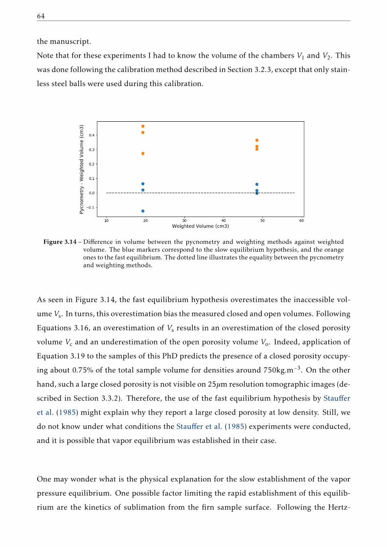
64
the manuscript.
Note that for these experiments I had to know the volume of the chambers V1 and V2. This
was done following the calibrationmethod described in Section 3.2.3, except that only stain-
less steel balls were used during this calibration.
Figure 3.14 – Difference in volume between the pycnometry and weighting methods against weightedvolume. The blue markers correspond to the slow equilibrium hypothesis, and the orangeones to the fast equilibrium. The dotted line illustrates the equality between the pycnometryand weighting methods.
As seen in Figure 3.14, the fast equilibrium hypothesis overestimates the inaccessible vol-
umeVs. In turns, this overestimation bias themeasured closed and open volumes. Following
Equations 3.16, an overestimation of Vs results in an overestimation of the closed porosity
volume Vc and an underestimation of the open porosity volume Vo. Indeed, application of
Equation 3.19 to the samples of this PhD predicts the presence of a closed porosity occupy-
ing about 0.75% of the total sample volume for densities around 750kg.m−3. On the other
hand, such a large closed porosity is not visible on 25µm resolution tomographic images (de-
scribed in Section 3.3.2). Therefore, the use of the fast equilibrium hypothesis by Stauffer
et al. (1985) might explain why they report a large closed porosity at low density. Still, we
do not know under what conditions the Stauffer et al. (1985) experiments were conducted,
and it is possible that vapor equilibrium was established in their case.
One may wonder what is the physical explanation for the slow establishment of the vapor
pressure equilibrium. One possible factor limiting the rapid establishment of this equilib-
rium are the kinetics of sublimation from the firn sample surface. Following the Hertz-

Chapter 3. Methods 65
Knudsen equation, one has:
dN
dt= A
αe(Pw −P)√2πmkT
(3.21)
where dNdt is the number of water molecules leaving the ice through sublimation, A is the
area of sublimation, m is the mass of a water molecule, k is the Boltzmann constant, and
αe is the evaporation coefficient. Hobbs (1974) report values of αe close to 0.67. Consider-
ing the vapor to be rapidly mixed in the total accessible volume V of the experiment, the
rearrangement of Equation 3.21 yields:
dP
dt+P
τ=Pwτ
(3.22)
with
τ =V√2πm
Aαe
√kT
(3.23)
The solution to Equation 3.22 is a rising exponential with an e-folding time equals to τ.
Numerical application in the case of the pycnometry case (V = 150cm3 and A = 70cm2)
yields an e-folding time of 0.2ms. This indicates that the establishment of vapor equilibrium
is not limited by the kinetics of sublimation at the surface of the sample.
A second factor limiting the establishment of vapor equilibrium is the time required for the
homogenization of the gases in the pycnometry apparatus. Lide (2005) reports a diffusion
coefficient Dw of 0.219cm2.s−1 at 0°C. To diffuse over a typical length scale of l of 10cm
(the size of the pycnometry apparatus), water vapor requires a time t = l2/D equals to about
450s, that is to say 7min30s. Note that the diffusion coefficient at 0°C is an overestimation of
the diffusion coefficient at −8°C, and therefore leads to an underestimation of the diffusion
time. Therefore, vapor equilibrium cannot be achieved over the course of one experiment by
the process of diffusion alone. My understanding is thus that the apparition of equilibrium
is limited, not by the kinetics of surface evaporation, but rather by the homogenization time
of the gases within the pycnometry apparatus.

66
3.2.2 Experimental protocol
Firn samples first need to be carved into cylinders directly from the firn core, following the
cutting procedure of Figure 3.15. For that, we use the half of the core that was not dedicated
to gas and chemistry measurements. Sections of about 30cm long are carved into cylinders
using a lathe at IGE. This step is crucial as it influences the quality of the sample’s shape
and the precision with which its volume can later be determined. Extra care must be taken
to ensure that the indentations made at the top and bottom of the core, which are used to
maintain the core in the lathe, are well aligned. If not, the core will have a wobbly motion
on the lathe that will result in a poor geometry. Moreover, the core must be carved slowly
to avoid any shock that could deteriorate the indentations or the surface of the sample. The
30cm section is lathed until all initial faces are removed, which usually yields a cylinder
with a 4cm diameter. Once carved, the 30cm long cylinder is cut into approximately 5cm
long pieces using a vertical wheel saw. These 5cm pieces are the ones measured in the pyc-
nometry apparatus. The samples are cleaned with a brush to remove potential inclusions of
snow dust in the open porosity, and they are let one day in the cold room to reach thermal
equilibrium. To avoid sublimation, the samples are sealed in plastic wrap and stored in
packing plastic.
The protocol for the pycnometry measurements is as follows:
- The sample is weighted using a high precision scale.
- The radius and height are measured with a digital caliper.
- Chamber V1 is open. Valve 1 is closed, while valves 2 and 3 are open.
- Chamber V2 is vacuum-pumped (pressure inferior to 10−3mbar).
- Valve 2 and 3 are closed, and valve 1 is opened. Chamber V2 is thus isolated and outside
air enters the tubing connecting the chambers.
- The firn sample is placed in chamber V1 and the chamber is closed.
- The system is let 1min to reach pressure equilibrium, and the internal pressure P is
recorded using a LabView virtual instrument.
- Valve 2 is slowly opened, and the gas expands in the volume V1 +V2.
- The system is let 1min to reach pressure equilibrium, the internal pressure P ′ is recorded.
The firn sample can then be removed from chamber V1, and the experiment started over

Chapter 3. Methods 67
for a new sample. It is important during the experiment to ensure that the first chamber
is properly sealed and airtight. The internal pressure of the chamber should increase while
tightening the sealing bolt and not rapidly drop after sealing. If a leak is detected, chamber
V1 should be opened to re-position the seal. To ensure that volume V1 is consistent between
experiments, the sealing bolt needs to be tightened in the same fashion in all experiments.
It is important that all manipulations on the sample and on the pycnometry apparatus are
made with thick and insulating gloves, to ensure that the whole system is at equilibrium
temperature. Moreover, the movable parts of the system should not touch any heated el-
ement, including the wood box containing the pumps and other heated elements, still in
order to maintain the system at a unique temperature. Drifts in the cold room tempera-
ture over time scales of ten minutes have been observed. By monitoring the variations in
internal pressure and in the cold room temperature, we observed that the internal pres-
sure varies greatly with the external temperature. Therefore, after dilation the pycnometry
system should not be allowed more than a couple of minutes to reach the pressure equilib-
rium. Finally, valves need to be opened slowly not to overwhelm the pressure monitor and
the pump with abrupt pressure variations.
Figure 3.15 – Cutting procedure for the pycnometry samples. The red cross marks the position of the topindentations maintaining the sample to the lathe.
3.2.3 Calibration of the chamber volumes
To be applicable, Equation 3.20 requires to know the volumes V1 and V2 of the chambers.
For this PhD, I developed a calibration procedure based on the fact that these volumes can
be determined using the pycnometry apparatus itself. For this purpose, we execute gas
dilation as one would do with firn samples, but instead with non porous object of known

68
volumes. Since these objects do not have pores, the volume Vs they render inaccessible to
gases is simply their full volume. Performing N experiments we thus have the system of
equations:
V 1s = V1 − R1
1−R1V2
V 2s = V1 − R2
1−R2V2
...
VNs = V1 − RN
1−RNV2
(3.24)
where V is and Ri are the volume of the object and the recorded pressure ratio during the ith
experiment. This linear system can be expressed in matrix form:
Xβ = y (3.25)
where X is a N×2 matrix with Xi1 = 1 and Xi2 = Ri/(1−Ri), y = [V 1s ...V
Ns ]⊺ is the vector of the
known volumes, and β = [V1,V2]⊺ is the vector of the unknown parameters. This problem is
overdetermined, and can be solved by minimizing the sum of the squared residuals between
the known volumes and their estimations. The optimal β vector is given by:
β = (X⊺X)−1X⊺y (3.26)
Moreover, the variance of the vector of unknowns β is given by:
σβ = σ(X⊺X)−1 (3.27)
where σ is the variance of the residuals between y (vector of known volumes) and y = Xβ
(estimation of the known volumes).
To calibrate the pycnometry apparatus for this PhD, we used two types of non porous ob-
jects. We first used commercial stainless balls of known volumes and bought from the
Marteau & Lemarié company. These balls respect the ANSI 440C norm and have volumes of
22.3, 33.5 and 46.0 cm3. Similar stainless steel balls were used by J.M. Barnola, L. Arnaud
and O. Magand when using and restoring the pycnometry apparatus. However, the firn
samples measured during this thesis have volumes of about 60cm3, outside of the volume
range of the stainless steel balls. One might then wonder about the validity of the calibra-

Chapter 3. Methods 69
tion for firn samples that lay outside the calibration range. This problem can be corrected by
using larger non-porous objects. However, it is not possible to use larger stainless steel balls,
as they do not fit in chamber V1 for volumes over than 46.0cm3. As a solution, I proposed
to use cylinders of pure ice grown at IGE. Their volumes were determined by a weighting
method, knowing that Vs = M/ρice. As explained in the next section, this method is much
more precise than measuring volumes with calipers. With this method, we created four new
calibration samples with volumes of 19.3, 48.5, 81.7, and 104.4cm3. Each stainless steel ball
and ice cylinder was measured three times. We also performed three experiments without
any object in the chamber, corresponding to the case Vs = 0, for a total of 24 calibration
experiments.
The volumes V1 and V2 have been determined to be 138.97 ± 0.05 and 6.875 ± 0.003 cm3.
The good agreement between the estimated and known volumes Vs, with residuals around
0.07cm3, is highlighted in Figure 3.16.
Figure 3.16 – Estimation of Vs against known values of Vs after calibration. The dashed line representsthe Measured Volume = Known Volume curve.
3.2.4 Experimental uncertainties
For a firn sample, the volume of the ice phase Vice is derived using the weight of the sample
and the density of pure ice. For this purpose a high precision weighting scale is used, that
yields results with a precision of 0.01g. The density of pure ice is determined using the tem-
perature parametrization proposed by Goujon et al. (2003) and based on data from Bader
(1964):
ρice = 0.9165(1− 1.53× 10⁻⁴T ) (3.28)

70
where the temperature T is expressed in ◦C, and ρice is expressed in g.cm−3. The temper-
ature during the measurements was regulated to be at −8◦C. The discontinuities of cool-
ing cycles lead to variations of ±2◦C in the cold room. The density of pure ice is thus
0.9176 ± 0.0003 g.cm−3, that is to say an uncertainty lower than 0.05%. The firn sam-
ples measured during this PhD have a mean mass of 50g, with extremal values of 39 and
71g. This corresponds to a mean ice volume of 51.46 ± 0.019cm3, with extremal values of
40.14 ± 0.016cm3 and 73.08 ± 0.025cm3. The ice phase volume is thus determined with a
precision better than 0.04%. Note that the same method was used to determine the volumes
of the calibration cylinders made of pure ice and used in Section 3.2.3, with the same degree
of precision.
The volumes of the samples Vcyl are determined by geometrical measurements using a digi-
tal caliper. As the samples are carved into cylinders, their volumes are determined by mea-
suring the diameter and the height of each sample. The digital caliper used has a precision
of 0.02mm. However, due to irregularities and defaults in the shapes of the samples it does
not follow that the diameters and heights are determined with a 0.02mm accuracy. By per-
forming multiple diameter and height measurements on the same samples, we concluded
that these quantities are rather known with a precision closer to 0.05mm. For a typical di-
ameter of 4cm and height of 5cm, firn samples have a volume of 63 ± 3cm3. The sample
volumes are thus determined with a precision of about 5%, and are consequently the main
source of uncertainty of the method.
I combined the impacts of the different sources of uncertainties using the propagation for-
mula: (∆X
)2=∑
i
(∂X
∂xi∆xi
)2(3.29)
where X is the quantity the uncertainty is computed for, xi are the independent sources
of uncertainties, and ∆A is the standard deviation of a variable A. The uncertainty for
the closed porosity ratio (ratio of closed pores to open pores) and the density have been
computed for the samples of the measurement campaign of this PhD. They are displayed in
Figure 3.17 as a function of the firn sample density.
The uncertainty on the density of the samples is relatively constant with a value of of 0.0082
g.cm−3, that is to say an uncertainty of 0.009 in density relative to pure ice. On the other

Chapter 3. Methods 71
Figure 3.17 – Closed porosity against relative density in firn samples. The left panel highlights the uncer-tainties on the closed porosity ratio, and the right panel highlight the uncertainties on therelative density of the samples.
hand, the uncertainty on the closed porosity ratio increases with higher density. For low
density the uncertainty is close to 0.02, and reaches up to 0.2 for high density firn. Equa-
tion 3.29 enables to differentiate the contribution of each uncertainty source to the total
uncertainty. The individual contributions for two firn samples are displayed in Figure 3.18.
It appears that the uncertainties on the open and closed volumes do not significantly change
between low and high density firn. The determination of the open volumes is strongly af-
fected by the uncertainty associated with the radius estimation, with a contribution close to
1.5cm3. On the other hand, determination of the closed pores volume is independent of the
volume of the firn sample, and is therefore not affected by the radius uncertainty. In that
case the largest contributions are due to determination of the pressure values in chamber
V1. Concerning the closed porosity ratio, the contributions of the error sources depend on
density. At low density, the contributions are similar to the ones affecting the closed volume
with no influence of the sample volume determination. At high density, the closed poros-
ity ratio is greatly affected by the determination of the sample radius similarly to the open
volume. We can therefore conclude that the increase of the closed porosity ratio uncertainty
with density is due to increasing effect of the radius determination. Future work to improve
the pycnometry precision should focus on improving the radius and volume determination
of the sample.
3.3 Other measurements performed during the thesis
For the work of this PhD, other measurements have been performed to characterize the
physical and chemical properties of firn and ice cores. These methods are well established
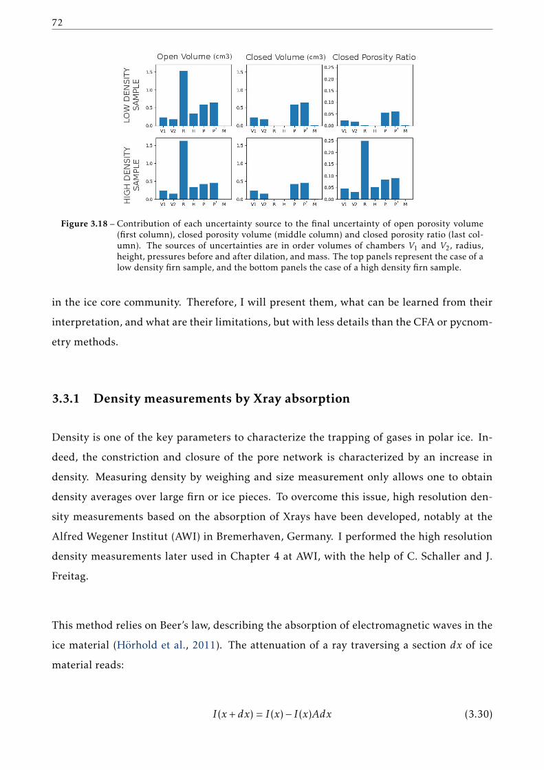
72
Figure 3.18 – Contribution of each uncertainty source to the final uncertainty of open porosity volume(first column), closed porosity volume (middle column) and closed porosity ratio (last col-umn). The sources of uncertainties are in order volumes of chambers V1 and V2, radius,height, pressures before and after dilation, and mass. The top panels represent the case of alow density firn sample, and the bottom panels the case of a high density firn sample.
in the ice core community. Therefore, I will present them, what can be learned from their
interpretation, and what are their limitations, but with less details than the CFA or pycnom-
etry methods.
3.3.1 Density measurements by Xray absorption
Density is one of the key parameters to characterize the trapping of gases in polar ice. In-
deed, the constriction and closure of the pore network is characterized by an increase in
density. Measuring density by weighing and size measurement only allows one to obtain
density averages over large firn or ice pieces. To overcome this issue, high resolution den-
sity measurements based on the absorption of Xrays have been developed, notably at the
Alfred Wegener Institut (AWI) in Bremerhaven, Germany. I performed the high resolution
density measurements later used in Chapter 4 at AWI, with the help of C. Schaller and J.
Freitag.
This method relies on Beer’s law, describing the absorption of electromagnetic waves in the
ice material (Hörhold et al., 2011). The attenuation of a ray traversing a section dx of ice
material reads:
I(x + dx) = I(x)− I(x)Adx (3.30)
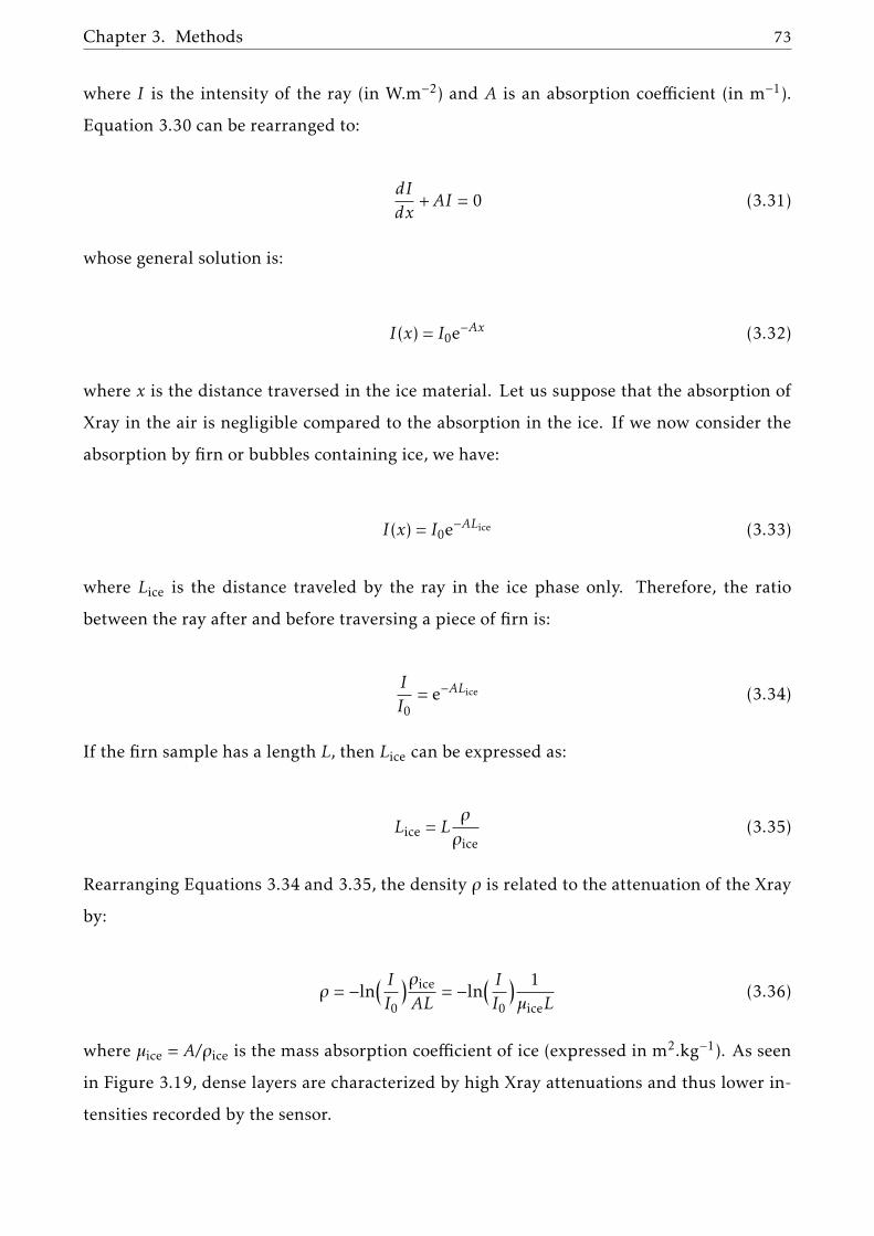
Chapter 3. Methods 73
where I is the intensity of the ray (in W.m−2) and A is an absorption coefficient (in m−1).
Equation 3.30 can be rearranged to:
dI
dx+AI = 0 (3.31)
whose general solution is:
I(x) = I0e−Ax (3.32)
where x is the distance traversed in the ice material. Let us suppose that the absorption of
Xray in the air is negligible compared to the absorption in the ice. If we now consider the
absorption by firn or bubbles containing ice, we have:
I(x) = I0e−ALice (3.33)
where Lice is the distance traveled by the ray in the ice phase only. Therefore, the ratio
between the ray after and before traversing a piece of firn is:
I
I0= e−ALice (3.34)
If the firn sample has a length L, then Lice can be expressed as:
Lice = Lρ
ρice(3.35)
Rearranging Equations 3.34 and 3.35, the density ρ is related to the attenuation of the Xray
by:
ρ = −ln( II0
)ρiceAL
= −ln( II0
) 1µiceL
(3.36)
where µice = A/ρice is the mass absorption coefficient of ice (expressed in m2.kg−1). As seen
in Figure 3.19, dense layers are characterized by high Xray attenuations and thus lower in-
tensities recorded by the sensor.
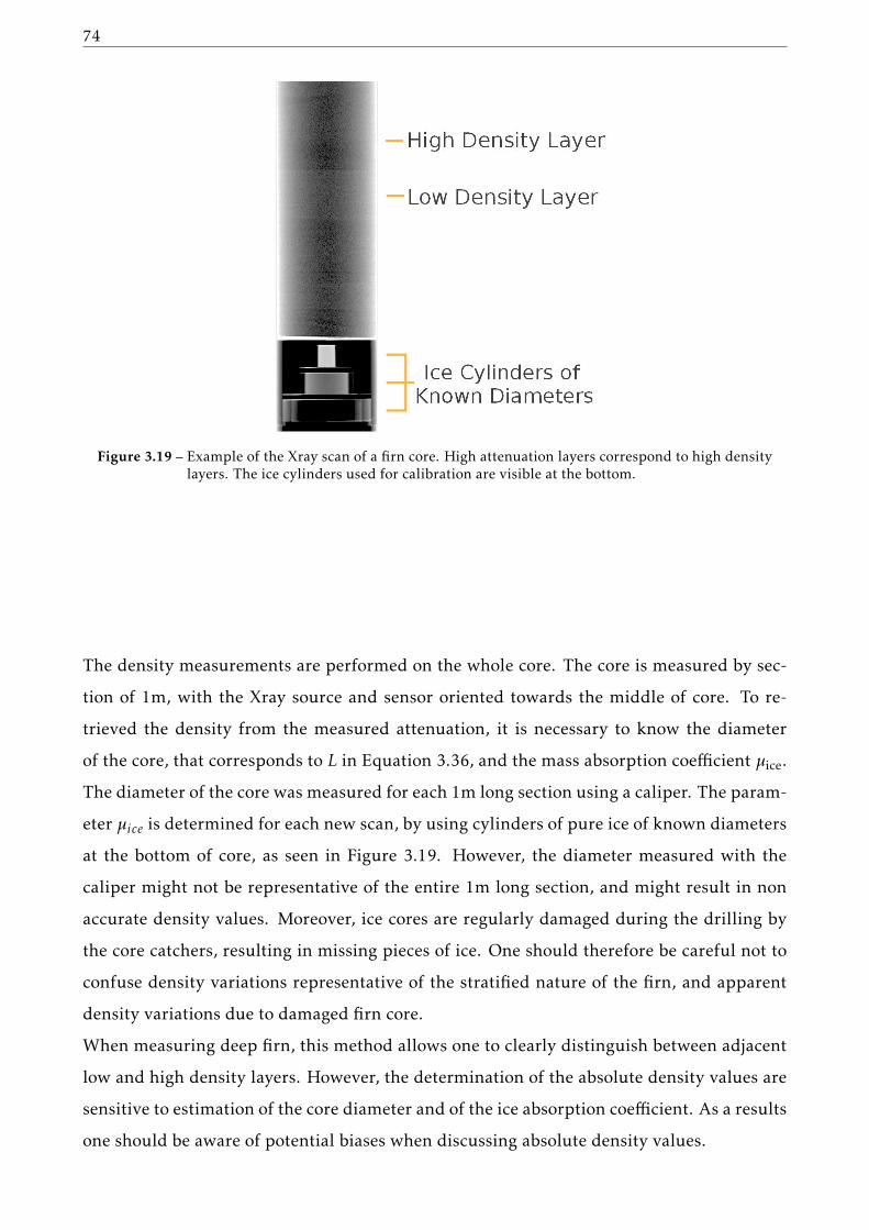
74
Figure 3.19 – Example of the Xray scan of a firn core. High attenuation layers correspond to high densitylayers. The ice cylinders used for calibration are visible at the bottom.
The density measurements are performed on the whole core. The core is measured by sec-
tion of 1m, with the Xray source and sensor oriented towards the middle of core. To re-
trieved the density from the measured attenuation, it is necessary to know the diameter
of the core, that corresponds to L in Equation 3.36, and the mass absorption coefficient µice.
The diameter of the core was measured for each 1m long section using a caliper. The param-
eter µice is determined for each new scan, by using cylinders of pure ice of known diameters
at the bottom of core, as seen in Figure 3.19. However, the diameter measured with the
caliper might not be representative of the entire 1m long section, and might result in non
accurate density values. Moreover, ice cores are regularly damaged during the drilling by
the core catchers, resulting in missing pieces of ice. One should therefore be careful not to
confuse density variations representative of the stratified nature of the firn, and apparent
density variations due to damaged firn core.
When measuring deep firn, this method allows one to clearly distinguish between adjacent
low and high density layers. However, the determination of the absolute density values are
sensitive to estimation of the core diameter and of the ice absorption coefficient. As a results
one should be aware of potential biases when discussing absolute density values.

Chapter 3. Methods 75
3.3.2 Tomography
Tomography is a technique used to reconstruct 3D models of objects. In this thesis, I use it
to produce voxelized models of firn samples, with voxels either being part of the ice or pore
phase. Similarly to the density measurements, Xray scans of the firn samples are performed.
However for tomography, the same firn sample is scanned from different angles. These scans
are used as a set of different projections of the same firn sample. Then, a tomography al-
gorithm is used to reconstruct the structure of the firn sample from its projections and to
create a voxelized model of the sample (Ritman, 2004). The 3D models are segmented to
produce the final binary models (Hagenmuller et al., 2013). Tomographic scanning is a well
established technique with a wide range of application fields, frommedical to earth sciences
(Mees et al., 2003; Bouxsein et al., 2010). Therefore, commercial apparatuses are available,
and can be used for the study of firn samples.
I selected and lathed 10 firn samples to be analyzed with tomography for my PhD. The to-
mographic scans of the selected samples were performed by M. Schneebeli, H. Löwe and A.
Marshal at the Institut für Schnee und Lawinenforschung (SLF) in Davos, Switzerland. The
samples scanned have the same geometry as the pycnometry samples, that is to say cylin-
ders of radius and height of 4 and 5cm. Examples of the obtained 3D representation of the
firn are displayed in Figure 3.20.
The tomography models of the thesis are composed of 25µm cubes. Burr et al. (2018) report
that the size of voxels influence the determination of closed and open porosity in firn sam-
ples. However, Burr et al. (2018) also report that changing from 12 to 30µm voxels, only
modify the total amount of closed pores by a few percent, and that this effect decreases with
firn density.
During my PhD, I analyzed these tomographic images to characterize the changes of the
porous network with the increase in density, with a specific focus put on the study of cen-
timeter scale stratification. This analysis wasmadewith python, ImageJ, andMATLAB®scripts
that I coded during this PhD. I am grateful to A. Burr for introducing me to the scripting
language of ImageJ. Moreover, a comparison of the closed porosity volumes obtained with
the pycnometry and tomogaphy methods is reported in Chapter 4.

76
Figure 3.20 – Porous networks as obtained from two tomography images.
3.3.3 Air content
Air content is a direct measurement of the amount of air trapped in polar ice. It is expressed
in cm3 of trapped air at STP per gram of ice. The measurements used in thesis were per-
formed by V. Lipenkov at IGE, following the method detailed in Lipenkov et al. (1995).
Briefly, an ice sample of mass M is placed in a cell of known volume Vcell. The cell is then
vacuum-pumped to remove all air, except the one enclosed in the ice sample. The ice sample
is melted to liberate the gas inside. The meltwater is then slowly refrozen from the bottom
to extract all gases from the ice phase. The cell is thermalized at a temperature T , and the
pressure Pmeas in the cell is measured. The air content is:
AC =VairPT0MTP0
(3.37)
where AC is the air content expressed in cm3 at STP per gram of ice, Vair = Vcell −M/ρice is
the volume occupied by the air in the cell, P = Pmeas −Pw is the pressure of gas corrected for
the pressure of water vapor Pw, and T0 and P0 are the standard pressure and temperature.
Lipenkov et al. (1995) report an uncertainty of about 1% on the determination of AC.
Typical samples have a volume of less than 30cm3. Therefore, a significant portions of
bubbles that are closed at the scale of the firn column might be re-opened when cutting the
sample. Such cut bubbles release the gas they contain before the measurements, resulting
in underestimated values of air content. It is therefore necessary to correct for the presence
of these cut bubbles at the surface of the sample (Martinerie et al., 1990). This correction

Chapter 3. Methods 77
was taken into account by V. Lipenkov using the surface to volume ratio of the ice samples
and bubble size measurements.
3.3.4 Chemistry measurements
Chemical ions and impurities are present within the ice phase of polar firn. Previous stud-
ies, such as Hörhold et al. (2012) or Fujita et al. (2016), have highlighted the role of chemical
impurities on the densification of firn. To study the potential effect of chemical species on
polar firn, I participated to high resolution chemistry measurements during this PhD. They
were realized at the British Antarctic Survey (BAS) in Cambridge, UK, with the help of R.
Tuckwell, R. Mulvaney, E. Ludlow, S. Jackson, and S. Miller. The measurements were done
using a Continuous Flow Analysis system, similarly to the methane measurements.
Sticks of 34mm×34mm section are cut in the firn core, similarly to the methane CFA sticks.
Prior to melting, the chemistry CFA sticks are flattened at the end to avoid outside air en-
trance in the system, and cleaned to avoid contamination. They are continuously melted
and the meltwater retrieved through a pumping system. The meltwater is then debubbled
and sent to an array of analyzers. They notably include the continuous analysis of Ca2+,
Na+, and NH+4 using colorimetry, the continuous measurement of liquid conductivity, the
continuous measurement of dust concentration and a Fast Ion Chromatography (FIC). The
FIC consists of two ion chromatographs working in parallel. While one chromatograph is
collecting meltwater, the other one is performing the chromatographic separation of anions
and their concentration analysis. The chromatographs are designed so they can analyze an-
ion concentrations (notably F−, Cl−, and SO2−4 ) in less than a minute, meaning that a data
point is obtained roughly every 4cm. Finally, a part of the meltwater is collected in clean
vials for later ion chromatography (IC) measurements. Besides anions, the IC is used to ob-
tain the concentrations of cations that cannot be determined with the FIC, including Mg2+,
Na+, and Ca2+. Moreover, the IC data have a resolution of about 2.5cm, better than the FIC.
However, the IC is more labor intensive to operate and therefore only 4m of firn core have
been analyzed with it during this PhD. The IC measurements were performed by S. Jackson
in the weeks following my visit to BAS.
Only the liquid conductivity measurements and concentrations from IC will be discussed

78
in this thesis (in Chapter 4). Indeed, the continuous colorimetry was not to able to resolve
the low ion concentrations present in firn cores from the East Antarctic plateau. Moreover,
the spatial resolution of the FIC data is too coarse to properly identify centimeter scale
variations of anions. Nonetheless, I ensured that the concentrations measured by the IC are
consistent with the FIC, indicating that the collecting vials were not contaminated.
3.3.5 Thin sections and crystalline texture
As discussed in Section 2.2.3, the hexagonal crystalline structure of an ice single crystal is
characterized by its c axis, specifying the orientation of the hexagonal structure (see Fig-
ures 2.12 and 3.21). The orientation of this vector is defined by an azimuth angle θ and a
colatitude angle φ, as defined in Figure 3.21.
The ice in firn and polar ice sheets is poly-crystalline, composed of multiple single ice crys-
tals, each with its own c-axis. The size and orientation distribution of the crystals (also
called its texture) influence the behavior of ice at the macroscopic scale. This ice texture can
be determined with the aid of thin sections.
Figure 3.21 – Left: Hexagonal structure of an ice single crystal with the c-axis represented as a verticalline. Right: Definition of the azimuth angle θ and the colatitude angle φ, specifying theorientation of the blue vector.
The thin sections of ice and firn are prepared by trimming rectangular samples to a thick-
ness of about 0.3mmwith a dedicatedmicrotome. To determine the orientation of the c-axis,
the thin sections are then observed between two light polarizers. Indeed, ice is a birefringent
medium meaning that its refraction index depends on the light direction of polarization.
When a linearly polarized wave propagates within a birefringent medium, the polarization
rotates around the propagation direction. The degree of rotation of the polarization can
Chapter 3. Methods 79
be estimated by studying the light intensity transmitted though the second polarizer as a
function of its orientation. In the case of ice, the rotation of the light polarization in the
medium depends on the orientation of the c-axis. Automated analyzers exploits the bire-
fringent properties of ice to construct a map of the crystalline orientations of a thin section
(Peternell et al., 2010).
Thin sections and texture maps were made for this PhD. They were performed by M. Mon-
tagnat and C. Argenville at IGE using the Automatic Ice Texture Analyzer (AITA). An ex-
ample of a analyzed thin sections in displayed Figure 3.22.
Figure 3.22 – Example of the crystalline texture of a thin section. Each color represents a c-axis orienta-tion.
3.4 Conclusion of the chapter
This chapter presents the experimental methods used during this thesis and my implication
in the measurement campaigns. A specific focus is put on the Continuous Flow Analysis of
methane and on the gas pycnometry method, as I contributed to their ongoing development
at IGE.
In the case of the CFA, I performed the measurements and developed the programs cur-
rently used to process the raw CFA data and to express them on a proper depth scale. To
help with the estimation of methane solubility correction, I proposed a theoretical model
with an analytical solution. I also characterized the smoothing function of the IGE CFA sys-
tem, that is notably used in Chapter 5 and Fourteau et al. (2017) to estimate the impact of
CFA smoothing on centimeter scale variations and on very-thinned ice cores. In total, 250m
of ice were analyzed with X. Faïn during this PhD, representing a total of about 115 hours
of melting.
80
For the pycnometry method, I set up the processing chain used to analyze the dilation ex-
periments. I notably revised the calibration procedure using pure ice cylinders, in order to
provide a calibration range consistent with the size of the measured samples. I also per-
formed an uncertainty analysis in order to identify the sources of error in the method. For
this PhD, 80 firn samples have been characterized to study the closure of pores at the bot-
tom of the Lock-In site firn column.
I also participated in other measurement campaigns at AWI (high resolution density) and
BAS (high resolution chemistry). In the case of the tomography imagery at SLF, I prepared
the samples but only assisted for the measurements of the first two firn samples. The rest
of the measurements were performed after my visit. I performed the post-processing and
analysis of all the experimental data, with the help of my co-authors and PhD supervisors.
Thanks to the acquisition of a broad type of high resolution data on the same firn core, I
was able to perform a multi-tracer study of the pore closure in a firn of East Antarctica,
as described in Chapter 4. Moreover, the high-resolution datasets of methane mixing ratio
measured in deep ice allowed me to characterize the impact of gas trapping processes on
the gas records in ice cores of the East Antarctic plateau, as discussed in Chapter 5. The
tomographic images acquired at SLF were also used to study the compression of a firn layer
in the model presented in Chapter 6.
Chapter 4
Study of pore closure in an East Antarctic
firn core
Contents
4.1 Presentation of the chapter . . . . . . . . . . . . . . . . . . . . . . . . . . . . 83
4.2 Multi-tracer study of gas trapping in an East Antarctic ice core . . . . . . . 84
4.2.1 Introduction . . . . . . . . . . . . . . . . . . . . . . . . . . . . . . . . . 85
4.2.2 Methods . . . . . . . . . . . . . . . . . . . . . . . . . . . . . . . . . . . 87
4.2.3 Results and discussion . . . . . . . . . . . . . . . . . . . . . . . . . . . 93
4.2.4 Conclusions . . . . . . . . . . . . . . . . . . . . . . . . . . . . . . . . . 113
4.2.5 Supplementary Material . . . . . . . . . . . . . . . . . . . . . . . . . . 115
4.3 To go further . . . . . . . . . . . . . . . . . . . . . . . . . . . . . . . . . . . . . 121
4.3.1 Structural anisotropy of firn . . . . . . . . . . . . . . . . . . . . . . . . 121
4.3.2 Analysis of thin sections . . . . . . . . . . . . . . . . . . . . . . . . . . 123
4.4 Conclusion of the chapter . . . . . . . . . . . . . . . . . . . . . . . . . . . . . 126

82

Chapter 4. Study of pore closure in an East Antarctic firn core 83
4.1 Presentation of the chapter
This chapter is based on an article submitted to the journal The Cryosphere. It deals with
the study of a new firn core drilled in East Antarctica, at the Lock-In site 136km away
from Dome C. It was chosen as it exhibits a surface temperature similar to Dome C (around
−53°C) but a higher accumulation rate. One of the original goals motivating this new
drilling was to estimate the effect of accumulation, independently of temperature, on the
trapping of gases in polar ice.
The study of this new firn core, and the ability to use the whole core without saving an
archive, motivated to restart the IGE pycnometry system and top optimize its operating
procedures. Moreover, thanks to the high resolution of the data collected from this firn
core, a specific focus could be placed on stratification, on the presence of early closure firn
strata and their physical origins. Using the new collected data, the ability of a standard gas
trapping model to predict the quantity of trapped air is also assessed.
As the pycnometry method is detailed in Section 3.2, the original Supplementary Informa-
tion of the article has been revised to remove repetitions. The references in the text of the
article have been modified accordingly.
Additional investigations of the firn structural anisotropy and crystalline texture (not pre-
sented in the submitted article or in its supplement) are presented at the end of the chapter,
in Section 4.3.
84
4.2 Multi-tracer study of gas trapping in an East Antarctic
ice core
Kévin Fourteau1, Patricia Martinerie1, Xavier Faïn1, Christoph F. Schaller2, Rebecca J. Tuckwell3,
Henning Löwe4, Laurent Arnaud1, OlivierMagand1, Elizabeth R. Thomas3, Johannes Freitag2, Robert
Mulvaney3, Martin Schneebeli4, and Vladimir Ya. Lipenkov5
[1] Univ. Grenoble Alpes, CNRS, IRD, Grenoble INP, IGE, 38000 Grenoble, France
[2] Alfred Wegener Institute, Helmholtz Centre for Polar and Marine Research, 27568 Bremerhaven, Germany
[3] British Antarctic Survey, Natural Environment Research Council, Cambridge, UK
[4] WSL Institute for Snow and Avalanche Research (SLF), CH-7260 Davos Dorf, Switzerland
[5] Climate and Environmental Research Laboratory, Arctic and Antarctic Research Institute, St. Petersburg,
199397, Russia
AbstractWe study a firn and ice core drilled at the new Lock-In site in East Antarctica, located 136km
away from Concordia station towards Durmont d’Urville. High resolution chemical and
physical measurements were performed on the core, with a particular focus on the trapping
zone of the firn where air bubbles are formed. We measured the air content in the ice, closed
and open porous volumes in the firn, firn density, firn liquid conductivity and major ion
concentrations, as well as methane concentrations in the ice. The closed and open porosity
volumes of firn samples were obtained by the two independent methods of pycnometry
and tomography, that yield similar results. The measured increase of the closed porosity
with density is used to estimate the air content trapped in the ice with the aid of a simple
gas trapping model. Results show a discrepancy, with the model trapping too much air.
Experimental errors have been considered but do not explain the discrepancy between the
model and the observations. The model and data can be reconciled with the introduction
of a reduced compression of the closed porosity compared to the open porosity. Yet, it is
not clear if this limited compression of pores is the actual mechanism responsible for the
low amount of air in the ice. High resolution density measurements reveal the presence of a
strong layering, manifesting itself as centimeter scale variations. Despite this heterogeneous
stratification, all layers, including the ones that are especially dense or less dense compared
to their surroundings, displays similar pore morphology and closed porosity as function
of density. This implies that all layers close in a similar way, even though some close in
advance or later than the surrounding normal layers. Investigation of the chemistry data
suggests that in the trapping zone, the observed stratification is mainly due to the effect of
Chapter 4. Study of pore closure in an East Antarctic firn core 85
chemical impurities.
4.2.1 Introduction
Deep ice cores drilled in polar ice sheets are climatic archives of first importance in the field
of paleoclimatology (e.g. Masson-Delmotte et al., 2013). Indeed, ice cores have the unparal-
leled characteristic of containing various past climatic information in the ice matrix and the
bubbles within (e.g. Petit et al., 1999; Jouzel et al., 2007; Brook and Buizert, 2018). In partic-
ular, the bubbles enclosed in polar ice contain air from past atmospheres, and their analysis
can be used to reconstruct the atmospheric composition history of the last 800kyr (Stauffer
et al., 1985; Loulergue et al., 2008; Lüthi et al., 2008). The bubbles get progressively en-
closed in the ice at depths approximately ranging from 50 to 120m below the surface of the
ice sheet, depending on the local temperature and accumulation conditions. These depths
correspond to the transformation of the firn, a name for dense and compacted snow, into
airtight ice encapsulating bubbles.
The firn column is characterized by the increase of its density with depth, as the material
gets compressed by the load pressure of the newly accumulated snow (e.g. Arnaud et al.,
2000; Salamatin et al., 2009). As the firn density increases, the interstitial pore network
is reduced. Eventually, some sections become small enough to prevent gas movement and
pinch, enclosing part of the interstitial air (Schwander et al., 1993). This marks the begin-
ning of the trapping zone where bubbles are closing and encapsulate atmospheric air. The
trapping zone usually spans over about 10m (Witrant et al., 2012).
The process of gas trapping has impacts for the interpretation of ice core gas records. First,
since bubbles are trapped deep in the firn, the enclosed air is always younger than the sur-
rounding ice (e.g. Schwander and Stauffer, 1984). This age difference between the ice and
the air is known as ∆age in the ice core community, and needs to be taken into account to
synchronize the measurements performed in the bubbles, such as greenhouse gas concen-
trations, and the ones performed in the ice, such as temperature reconstruction (Shakun
et al., 2012; Parrenin et al., 2013). Secondly, due to the progressive closure of bubbles, an ice
layer does not contain air corresponding to a single date, but rather from a wide distribution
of ages (e.g. Buizert et al., 2012; Witrant et al., 2012). These distributions act as a moving
86
average on the recorded gas signal, and attenuate the variability in the record compared to
the true variability in the atmosphere (Spahni et al., 2003; Joos and Spahni, 2008; Köhler
et al., 2011; Fourteau et al., 2017). Finally, due to the heterogeneous stratification of the firn
at the centimeter scale, some layers might close in advance or late compared to their sur-
roundings (Etheridge et al., 1992; Mitchell et al., 2015). The gases enclosed in these layers
are thus older or younger than the gases in adjacent layers and appear as anomalous values
in the record (Rhodes et al., 2016; Fourteau et al., 2017). Several studies have investigated
the closing of porosity and increase of density in firns from both Greenland and Antarctica
(Martinerie et al., 1992; Schwander et al., 1993; Trudinger et al., 1997; Fujita et al., 2014;
Gregory et al., 2014), and linked it with the trapping of gas in polar ice (Rommelaere et al.,
1997; Goujon et al., 2003; Schaller et al., 2017). One of the major results is the observa-
tion of a strong and heterogeneous stratification in polar firn and its correlation with ionic
and impurity content (Hörhold et al., 2012; Freitag et al., 2013; Fujita et al., 2016). Moreover
some studies have highlighted the direct relationship between the density of a firn layer and
the amount of closed pores (Schwander and Stauffer, 1984; Martinerie et al., 1992; Mitchell
et al., 2015).
Among the polar regions, East Antarctica is of particular interest for ice core drilling as this
is where the oldest ice is retrieved. While several studies focus on the cold and arid sites of
this region, none of them to our knowledge attempts to encompass a detailed description of
stratification, closed porosity and gas trapping within the same firn. As particular examples,
the study of Fujita et al. (2016) describes the link between density variability and ionic
content in three firns core near Dome Fuji without addressing pore closure, while the studies
of Schaller et al. (2017) and Burr et al. (2018) propose detailed descriptions of the of the pore
network closure but without discussing stratification.
Our study thus aims to provide a detailed description of chemical and physical properties
along the trapping zone of an Antarctic firn core. This core was drilled at the site of Lock-In
in East Antarctica. It was chosen as its temperature is similar to the cold sites of Dome C
and Vostok where deep ice cores have been drilled. Nonetheless, Lock-In displays a higher
annual precipitation rate than Dome C and Vostok. When possible, the measurements were
performed with a resolution allowing us to observe stratification and variabilities at the
centimeter scale in the firn. Using high-resolution data sets, we intend to investigate the
impact of firn stratification on gas trapping.

Chapter 4. Study of pore closure in an East Antarctic firn core 87
4.2.2 Methods
4.2.2.1 Lock-In study site
The ice core studied in this article was drilled in January 2016 at a site called Lock-In, lo-
cated on the East Antarctic plateau, 136km away from Dome C along the traverse road join-
ing Concordia and Dumont d’Urville stations (coordinates 74°08.310’ S, 126°09.510’ E). As
an East Antarctic plateau site, Lock-In exhibits a fairly low temperature of −53.15°C (mea-
sured at 20m depth in the borehole), slightly higher than at the deep drilling sites of Dome C
and Vostok. The site has an elevation of 3209m above sea level, and the surface atmospheric
pressure was estimated to be 645mbar using the value at Dome C of 643mbar (data from
the Automatic Weather Station Project) and a pressure elevation gradient of 0.084mbar.m−1
(evaluated using pressure differences between D80 and Dome C). Lock-In is also charac-
terized by a relatively low accumulation rate of 3.6cm.we.yr−1. The accumulation rate was
evaluated by locating volcanic events with solid conductivity measurements. Hence, Lock-
In has a similar temperature but a higher accumulation rate than Vostok and Dome C.
The drilling operation retrieved ice down to 200m below the surface. The amount of ma-
terial was sufficient in the 10cm diameter core to perform several parallel measurements,
which are described below. During the drilling procedure, air was sampled from the firn
open porosity along the firn column. The last pumping was performed at 108m depth, in-
dicating the depth where the firn reaches full closure and transforms into airtight ice.
4.2.2.2 High resolution density profile
Density is a parameter of particular interest when studying the enclosure of gas in polar
ice. Indeed, the densification speed measures the amount of compaction of the firn and the
reduction in pore volume. Hence, the density was continuously measured in the Lock-In
firn and ice core. The measurements were performed on the whole 10cm diameter core
from 6m down to 131m below the surface, at the Alfred Wegener Institute, Bremerhaven,
Germany. The measurement technique is based on the absorption of gamma rays by the ice
phase while traversing the core. The density is then derived from the ray attenuation using
Beer’s law. The method of measurement is described in details in Hörhold et al. (2011).

88
To be applicable, Beer’s law requires the estimation of the core diameter d and the ice spe-
cific absorption coefficient µice. The diameter of the core was measured using a caliper for
one meter long sections. However, due irregularities this value might not be representative
of the entire section. Therefore, ice core parts where ice was missing (for instance parts bro-
ken during drilling) were removed from the final dataset. Finally, the value of the specific
absorption coefficient µice was calibrated for each new scan using cylinders of pure ice with
known diameters. One should note that the results are quite sensitive to the determination
of d and µice. Thus, the high-resolution density data will not be discussed in terms of abso-
lute values but rather in terms of centimeter scale variations, which are better constrained.
This measurement method allows one to retrieve density variations at the sub-centimeter
scale.
4.2.2.3 Pycnometry measurements
Pycnometry is an experimental method for the measurement of closed and open porosity
volumes in a firn sample (Stauffer et al., 1985; Schwander et al., 1993). In this context, a
pore is determined as open if it reaches the edge of the sample.
The pycnometry experimental set-up is composed of two sealed chambers of known vol-
umes V1 and V2, with a pressure gauge connected to the first chamber and a valve allowing
the operator to isolate V2 from V1. The sample is placed in chamber V1, while chamber V2 is
isolated and vacuum pumped. Then, the two chambers are connected, resulting in a homo-
geneous pressure in both chambers lower than the initial pressure in V1. This pressure drop
is linked to Vs, the volume rendered inaccessible to gases by the sample in the first chamber,
by the relation:
Vs = V1 −R
1−RV2 (4.1)
where R = P ′/P with P ′ and P being the pressure value in chamber V1 respectively after and
before the dilation. The application of the equation requires the knowledge of the volumes
V1 and V2. The two volumes V1 and V2 were calibrated using stainless steel balls and bubble
free ice pieces of known volumes. The derivation of Equation 4.1 and the description of the
calibration procedure are provided in the Section 3.2.

Chapter 4. Study of pore closure in an East Antarctic firn core 89
Then the closed and open porosity volumes are computed given that:
Vc = Vs −Vice
Vo = Vcyl −Vs
Vice =M/ρice
(4.2)
where Vc is the closed pore volume, Vo is the open pore volume, Vice is the volume occupied
by the ice phase, Vcyl is the volume of the sample, M is the mass of the sample, and ρice is
the density of pure ice. The density of pure ice was taken as 0.918g.cm−3, for a recorded
temperature of −8°C during the measurements (Bader, 1964; Goujon et al., 2003).
A total of 80 samples were taken within the Lock-In core, with depths ranging from 76m
to 130m. The measured samples were cylinders with typical diameters and heights of 4cm,
obtained with a vertical lathe at the Institut des Géosciences de l’Environnement (IGE),
Grenoble, France. The radius and height were measured for each sample using a digital
caliper in order to estimate the volume of the firn sample Vcyl. To estimate the ice volumes
Vice, the samples were weighted. Finally, the densities ρ of the samples were computed as
ρ =M/Vcyl.
The treatment of uncertainties is reported in the Section 3.2.4. One of the main results of
this uncertainty analysis is the large uncertainties associated with the sample volumes Vcyl
due to their sensitivity to the radii measurements. The large uncertainty on Vcyl affects the
determination of the density ρ with a typical uncertainty of 0.01g.cm−3.
Following the definition of an open pore from a pycnometry point of view, some pores that
are closed in the firn (they no longer connect to the atmosphere) might appear open in small
samples. For instance, the blue pore in Figure 4.1 is closed when taken in the whole firn
column, but open when observed in a small cylindrical sample. This opening of closed
pores when sampling firn is known as the cut-bubble effect, and will be discussed in sec-
tion 4.2.3.1.

90
Figure 4.1 – Depiction of a cylindrical firn sample, numerical slices in tomographic images, and pores.The yellow and orange slices, represent two overlapping slices. The blue pore illustrates thecut-bubble effect: a pore initially closed in the firn column appears open in the cylindricalsample. The green pore is fully enclosed in the cylindrical sample, and is thus consideredclosed in the slices even if it intersects with their boundaries.
4.2.2.4 Tomography measurements
Computed X-ray tomography is a technique gaining traction for the study of firn densifica-
tion and pore closure (Barnola et al., 2004; Freitag et al., 2004; Gregory et al., 2014; Schaller
et al., 2017; Burr et al., 2018). Briefly, several 2D X-ray scans of the samples are performed
under different angles. Then, based on the contrast of X-ray absorption between the ice
and pore phases, tomography techniques are able to reconstruct a voxelized 3D model of
the scanned samples. Ten samples from the Lock-In firn core were measured at the Institut
für Schnee und Lawinenforschung (SLF), Davos, Switzerland, using a commercial tomogra-
phy apparatus. The tomography samples have the same geometry as the pycnometry ones,
and were also prepared at IGE using a lathe. Four of the samples measured using tomog-
raphy were also measured by pycnometry. The obtained 3D models are gray scale images,
composed of square voxels of 25µm in length. The gray scale images were automatically seg-
mented by fitting the gray value histogram to three Gaussian curves (based on Hagenmuller
et al., 2013), producing binary images of pore and ice voxels.
Using the 3D images, one can then compute the relative density to pure ice ρR = ρ/ρice of
the samples as the ratio of ice voxels to the total number of voxels. The relative density rep-
resents the volume fraction occupied by the ice phase in the firn sample. Throughout the
article, we use relative densities instead of densities (mass to volume ratio). This was chosen
as relative densities are not sensitive to temperature, and thus allow an easier comparison
between sites.
Chapter 4. Study of pore closure in an East Antarctic firn core 91
Tomographic images give access to the pore network, and can thus be used to determine
the volume of closed and open porosity. As with the pycnometry measurements, a pore is
considered open if it reaches the boundary of the sample. Using the software ImageJ and
the plug-in Analysis_3D (Boulos et al., 2012), we differentiated the open and closed pores
in the 3D images. The volume of the open and closed porosity is then simply computed by
summing the volume of the voxels belonging to an open or closed pore.
4.2.2.5 Air content
Air content, denoted AC in this article, is a measure of the quantity of air enclosed in polar
ice. It is expressed in cm3 of trapped air at standard temperature and pressure (STP) per
gram of ice. Air content is directly related to the volume of pores during closure, and can
thus be used to estimate the density at which a particular firn layer closed.
Air content was measured in the Lock-In firn core using the method described in Lipenkov
et al. (1995). In order to correct the AC values for the cut-bubble effect, an estimation of
the re-opened volume has been performed (based on bubble size measurements, Martinerie
et al., 1990). In total 10 samples were measured, including 4 replicates. Six of these samples
were taken around 122m depth, with a specific focus on stratification, and the four others
were taken deeper at 145m.
4.2.2.6 Chemistry along the trapping zone
Several studies highlight the link between density heterogeneities and ionic content in firn
layers (Hörhold et al., 2012; Freitag et al., 2013; Fujita et al., 2016). To study the presence
of this link in the trapping zone of the Lock-In firn, chemical analyses were performed on
this part of the core. The measurements were performed at the British Antarctic Survey,
Cambridge, United-Kingdom, using a continuous flow analysis (CFA) system. Sticks were
cut from the center of the core (34 × 34mm), covering depths from 90 to 115m. The sticks
were then continuously melted, and the meltwater analyzed for conductivity. Additional
meltwater was collected in vials, using a fraction collector, for later analysis with ion chro-
matography (IC). Four one meter sections were analyzed at 2.5cm resolution using a dionex
reagent-free ion chromatography system in a class-100 cleanroom. The measured species,
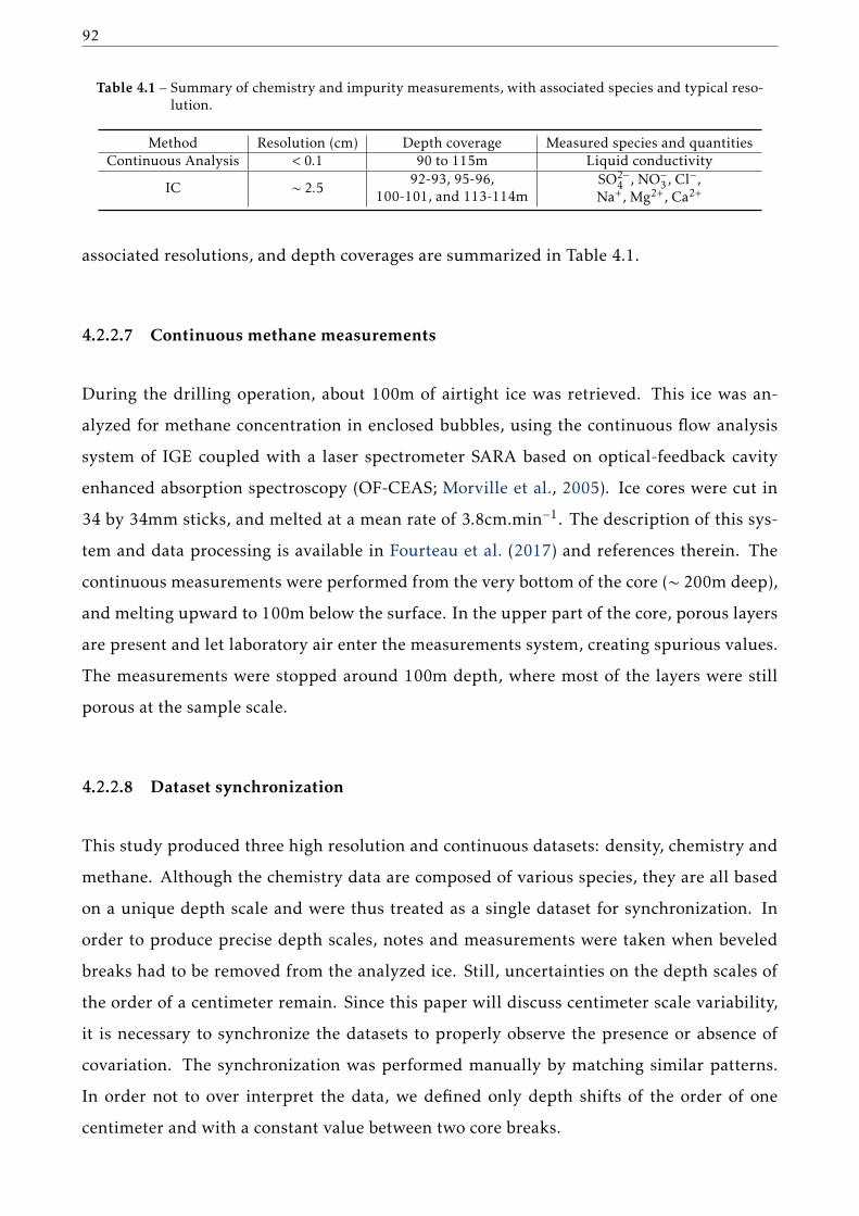
92
Table 4.1 – Summary of chemistry and impurity measurements, with associated species and typical reso-lution.
Method Resolution (cm) Depth coverage Measured species and quantitiesContinuous Analysis < 0.1 90 to 115m Liquid conductivity
IC ∼ 2.592-93, 95-96,
100-101, and 113-114mSO2−
4 , NO−3 , Cl−,
Na+, Mg2+, Ca2+
associated resolutions, and depth coverages are summarized in Table 4.1.
4.2.2.7 Continuous methane measurements
During the drilling operation, about 100m of airtight ice was retrieved. This ice was an-
alyzed for methane concentration in enclosed bubbles, using the continuous flow analysis
system of IGE coupled with a laser spectrometer SARA based on optical-feedback cavity
enhanced absorption spectroscopy (OF-CEAS; Morville et al., 2005). Ice cores were cut in
34 by 34mm sticks, and melted at a mean rate of 3.8cm.min−1. The description of this sys-
tem and data processing is available in Fourteau et al. (2017) and references therein. The
continuous measurements were performed from the very bottom of the core (∼ 200m deep),
and melting upward to 100m below the surface. In the upper part of the core, porous layers
are present and let laboratory air enter the measurements system, creating spurious values.
The measurements were stopped around 100m depth, where most of the layers were still
porous at the sample scale.
4.2.2.8 Dataset synchronization
This study produced three high resolution and continuous datasets: density, chemistry and
methane. Although the chemistry data are composed of various species, they are all based
on a unique depth scale and were thus treated as a single dataset for synchronization. In
order to produce precise depth scales, notes and measurements were taken when beveled
breaks had to be removed from the analyzed ice. Still, uncertainties on the depth scales of
the order of a centimeter remain. Since this paper will discuss centimeter scale variability,
it is necessary to synchronize the datasets to properly observe the presence or absence of
covariation. The synchronization was performed manually by matching similar patterns.
In order not to over interpret the data, we defined only depth shifts of the order of one
centimeter and with a constant value between two core breaks.

Chapter 4. Study of pore closure in an East Antarctic firn core 93
4.2.3 Results and discussion
4.2.3.1 Closed porosity ratios
Deep firn densification is characterized by the transformation of the open pore network into
bubbles encapsulating the air. Notably, pore closure is quantified through the evolution of
the closed porosity ratio CP, defined as the ratio between the closed pores volume and the
total pore volume (Mitchell et al., 2015; Burr et al., 2018). This closed porosity ratio falls
to zero when the porosity is fully open and reaches 1 when the firn sample porosity is fully
closed, making it a simple indicator of pore closure.
For the pycnometry measurements, CP was simply computed for each cylindrical sample
from the measured open and closed volumes. On the other hand, thanks to the explicit rep-
resentation of the pore network, tomography data can be used to access variations at scales
finer than the sample size. Hence, the tomography images were numerically divided into
1cm thick slices, as depicted in Figure 4.1. The spacing between two slices was set as 0.5cm,
meaning that slices are overlapping. The closed porosity ratio, as well as density, were then
determined for each slice. To minimize the impact of the cut-bubble effect, the distinction
between closed and open pores was performed on the full cylindrical images as displayed in
Figure 4.1. Moreover, the top and bottom slices of each sample were discarded since, as in
described Section 4.2.5.1 of the Supplement, they are the most affected by cut bubbles. The
values of closed porosity obtained using both pycnometry and tomography are displayed
Figure 4.2-a against relative density.
Burr et al. (2018) proposed to use the connectivity index as an indicator of pore closure.
This index is defined as the ratio between the volume of the largest pore and the volume of
all pores in a given sample, and is less sensitive to the cut-bubble effect (Burr et al., 2018).
However, this index cannot be used in models of gas transport and trapping as it does not
explicitly represent the amount of closed pores. Therefore, we will use the closed porosity
ratio, rather than the connectivity index as an indicator of closure.
Consistency between pycnometry and tomography
The first closed porosity datasets have been obtained using pycnometry or similar methods

94
Figure 4.2 – Closed porosity ratio against relative density. a) Raw closed porosity ratios obtained from py-cnometry and tomography. b) Pycnometry results corrected for volume overestimation, andunaltered tomography data. c) Pycnometry and tomography data corrected for cut-bubbleeffect. Colors stand for the depth of the sample. Note that the color scale has been limited tothe range 95 to 110m to emphasize the middle of the trapping zone.
(Schwander et al., 1993; Trudinger et al., 1997; Goujon et al., 2003; Mitchell et al., 2015).
However, the last decade has seen the development of tomography for the study of firn, and
estimations of porosity closure based on tomographic images (Barnola et al., 2004; Gregory
et al., 2014; Schaller et al., 2017; Burr et al., 2018). It is thus important to evaluate the con-
sistency between the two types of methods.
A comparison of the results obtained for Lock-In in Figure 4.2-a indicates an inconsistency
between the two datasets, with the tomography data closing at higher densities. To investi-
gate this difference, we focused our attention on four specific cylindrical samples that have
been measured both with the pycnometry and tomography methods. Comparison of the
densities of these samples confirm a disagreement between the two methods, with system-
atically higher density values obtained with tomography. While the differences fall within
the uncertainty range of the pycnometry measurements, a stochastic error cannot explain
the observed systematic discrepancy. To estimate a possible bias of the tomography based
density, four gray scale images were manually re-segmented. Relative deviations in den-
sity values were of the order of 9.10−4, that is to say 0.1%. These deviations are similar to
the uncertainties reported by Burr et al. (2018). Moreover, Burr et al. (2018) estimated the
influence of voxel size on the determination of density values. They found that reducing
voxel size from 30 to 12µm does not change the density by more than 0.1% for relative den-
sities in the range considered here. Therefore, it appears that the densities obtained with
tomographic scanning are fairly robust. On the other hand, the densities obtained by size
measurements and weighting are sensitive to the volume estimation, particularly through

Chapter 4. Study of pore closure in an East Antarctic firn core 95
the radius measurement. A close look at the cylindrical samples, notably using the tomog-
raphy 3D models, revealed rough surfaces and some broken edges. An overestimation of
the measured radius by 0.05mm is enough to explain the density discrepancy between the
four samples measured with both pycnometry and tomography. Our understanding is that
while measuring with a caliper, the operator tends to overestimate the actual radius of the
sample because of the irregular geometry, leading to a density underestimation. We thus
corrected the whole pycnometry dataset by considering a systematic overestimation of the
radius by 0.05mm. This is consistent with the observation of sample surfaces using tomog-
raphy models, reduces the overall discrepancy between the two methods and is within the
uncertainty range for radius measurements. This radius correction has an influence on the
density values but also on the open pore volumes (Equation 4.2). The corrected pycnometry
results are displayed Figure 4.2-b, along with the unaltered tomography results. This cor-
rection is sufficient to explain the discrepancy in density between the two methods, while
also improving the agreement on measured closed porosity ratios. Thus, after correction,
pycnometric and tomographic methods produce consistent results of closed porosity.
Cut-bubble effect
As mentioned in Sections 4.2.2.3 and 4.2.2.4, during pycnometry or tomography measure-
ments, a pore is considered open if it reaches the edge of the sample. However, some pores
that are closed in the firn (that is to say not reaching the atmosphere), are considered as
open if the edges of the sample intersect with them. This leads to the cut-bubble effect,
where a fraction of the closed bubbles are considered as open pores (Martinerie et al., 1990;
Lipenkov et al., 1997; Schaller et al., 2017). The impact of the cut-bubble effect is clearly
visible Figure 4.2-a and b: while closed porosity ratio should reach 100% for high densities
(corresponding to a fully closed material), an upper limit of CP = 90% appears in the data.
This is due to the presence of cut bubbles at the surface of the cylindrical samples, even in
fully closed ice. This cut-bubble effect can be partially mitigated by the use of large samples.
To correct for this effect, one has to estimate the fraction f of bubble volume opened during
sampling. Then, the true close porosity ratio CPtrue is given by:
CPtrue =CP
1− f (4.3)

96
Martinerie et al. (1990) reports a fraction of cut bubbles up to 10% for deep ice samples
nearly the same size as the sample used in this paper. However, this value should not be
used to correct for cut-bubble effect in the trapping zone. Indeed, this 10% value was ob-
tained in deep ice where bubbles tend to have cylindrical or spherical shapes. As pointed-
out by Schaller et al. (2017), closed pores tend to have elongated and tortuous geometries
in the trapping zone. The opening of a single pore reaching far into the sample can re-open
a significant portion of the closed porosity. They estimated the impact of cut-bubble effect
for cylindrical samples of 5cm in diameter and height, taken from the East Antarctic firn of
the site B53 (−55°C temperature and 3.0cm.we.yr−1 accumulation rate). Using tomography,
they scanned large firn samples of 10cm in diameter and 5cm in height. They then extracted
5cm diameter cylinders from the large samples. By comparing the state of pores before and
after the extraction, they were able to determine which bubbles have been opened. Their
findings indicate that up to 60% of the closed porosity gets re-opened near the density of
full closure. Moreover, they find that still 30% of bubbles are re-opened when measuring
deep ice samples with relative density close to 0.94 (Figure 4 in Schaller et al., 2017).
However, when applied to the Lock-In closed porosity ratio, the correction proposed by
Schaller et al. (2017) leads to unphysical results. For high relative densities, direct appli-
cation of their correction yields a closed porosity ratio well over 100%. This indicates an
overestimation of the fraction of re-open bubbles for the Lock-In firn.
Two methods were used to estimate the fraction of cut bubbles specifically for the Lock-In
samples. First, for depths well below the firn-ice transition, one knows that the samples
are fully closed. Using pycnometry, we thus measured closed and open pore volumes in
deep samples, and attributed all the open volumes to the cut-bubble effect. However, this
only allows us to access the correction for fully closed firn. The second method was used
to estimate the correction in partially closed samples. Similarly to Schaller et al. (2017), a
tomography image was numerically re-shaped into a smaller sub-sample. The distinction
between closed and open pores in the sub-sample was then performed following the method
of section 4.2.2.4. Then, by comparing with the full sample image, one is able to measure
the fraction of closed pores that have been opened. To produce the sub-samples we trimmed
the original cylinder to remove 1cm in height and 0.5cm in diameter. The goal is to remove
most of the immediate boundary effect described Section 4.2.5.1 of the Supplement, while

Chapter 4. Study of pore closure in an East Antarctic firn core 97
conserving a size and a geometry close to the full-sample. The method would yield more
robust results if, similarly to Schaller et al. (2017), larger volumes would be reduced to 4cm
diameter cylinders. However, large volume tomography was not available for the Lock-In
firn core. The deduced fraction of re-opened bubbles is displayed in Figure 4.3 as a function
of relative density. Our findings suggests that up to 25% of the bubble volume is re-opened
in our samples for relative densities closed to 0.90. This value drops to around 7.5% for high
densities.
In order to correct the CP values obtained by both pycnometry and tomography, we derived
a linear piecewise relationship relating the relative density of a sample and the cut bubbles
fraction f , displayed in black in Figure 4.3. This linear law was derived to match the esti-
mated re-open fraction, while still resulting in physically sound closed porosity ratios, i.e. a
monotonous increase without ratios well above 100%. We then applied the correction from
Equation 4.3 to the pycnometry and tomography datasets. The cut-bubble corrected values
are displayed Figure 4.2-c.
Unfortunately, there is a lack of available data for relative densities ranging from 0.86 to
0.89, as no tomography sample falls in this range. To test the possible sensitivity to a bad
estimation of the re-open fraction at these densities, we derived a second correction lawwith
a re-open fraction set at about 25% for all the relative densities below 0.91. This correction
and the corrected data are displayed in the Supplement Section 4.2.5.1. Application of this
correction does not significantly change the final closed porosity data, as low closed porosity
values are obtained for relative densities below 0.91.
4.2.3.2 Reconciling air content and closed porosity
The air content measurements in the Lock-In core indicate a value of 0.0915 ± 0.0017cm3
of air at standard temperature and pressure per gram of ice based on four samples at 145m
depth, and of 0.0874±0.0013cm3.g−1 based on six samples at 122m. These values of air con-
tent have been corrected for the effect of cut bubbles, with correction factors of 9.2% and
5.8% for the samples from 122 and 145m respectively. The difference in air content between
the two depth ranges cannot be solely attributed to the effect of cut bubbles. Similar low
values of air content have been reported in the upper part of a Vostok ice core (Lipenkov

98
Figure 4.3 – Fraction of re-opened bubbles as a function of relative density. Values obtained from tomog-raphy samples are represented as blue dots, and values obtained from pycnometry measure-ments as orange dots. The piecewise linear model used to correct for cut-bubble effect isdisplayed as a solid black line. The correction necessary to reproduce the closed porositiesobserved by Schaller et al. (2017) is displayed as a dashed blue line.
et al., 1997), but not observed in Dome C ice cores (Raynaud et al., 2007). This suggests a po-
tential change of local conditions of the Lock-In and Vostok sites during the late Holocene,
that did not occur at Dome C.
Lipenkov et al. (1997) report an air content value of 0.0862cm3.g−1 for the Holocene part of
Vostok, while Martinerie et al. (1992) report air content values of 0.0865 and 0.0925cm3.g−1
for the sites of Dome C (1970’s drilling site) and South Pole. These three sites have respec-
tive elevations of 3471, 3240 and 2835m above sea level. With an elevation of 3209m and
air content values of 0.0874 and 0.0915cm3.g−1, Lock-In is consistent with these reported
values.
The air content value can be used to estimate the density of the firn during closure. For this
purpose, following Raynaud and Lebel (1979) and Martinerie et al. (1990) we use:
Vi = AC TiPi
P0T0
1ρc
= Vi +1
ρice
(4.4)
where Vi is the total porous volume at air isolation (expressed in cm3 per gram of ice), Ti
and Pi the temperature and pressure of pores at isolation, T0 = 273.15K and P0 = 1013mbar
are the standard temperature and pressure, and ρc the estimation of the density during clo-
Chapter 4. Study of pore closure in an East Antarctic firn core 99
sure. Note that Vi is not the porous volume when the firn reaches full closure. Indeed, the
volumes of the closed pores evolve in the trapping zone due to compression. Therefore, Vi
is the sum of the individual pores volume when they close, and is larger than the porous
volume at complete closure. This means that ρc is smaller than the density at which full
closure is reached, and should rather be seen as the typical density at which bubbles are
formed when the air pressure starts to deviate from the atmospheric value. Finally, ρc can
be expressed as a relative density ρRc by assuming a density of pure ice at −53.15°C equal to
0.924g.cm−3 (Bader, 1964; Goujon et al., 2003).
The air content values determined at depths 122 and 145m, combined with the local tem-
perature and the pressure at the bottom of the firn column, yield ρRc values of 0.909 and
0.905, respectively. As shown by the dashed lines in Figure 4.4, these densities roughly cor-
respond to the middle of the trapping zone. To further analyze the consistency between the
air content values and the closed porosity data, we use a gas trapping model to estimate the
air content value.
For this purpose we use the gas trapping model of Rommelaere et al. (1997) (Equations 19a
and 21a of their article). This model takes as inputs the surface pressure and temperature
of the site, as well as density versus depth and closed porosity data. Using the hypothesis
of similar compression between closed and open pores, the model is able to compute qbair,
the quantity of air in bubbles expressed in moles of air per cm3 of ice. This quantity can
directly be converted to air content knowing that AC = qbairRT0P0ρ
, where R is the ideal gas con-
stant. To apply the model to the Lock-In core, the measured closed porosity ratios have been
fitted by a spline to obtain a smooth porosity curve (in blue in Figure 4.4). Moreover, the
high resolution density data were fitted by a polynomial function of degree 5 to produce a
smooth density curve. Using these smooth closed porosity and density curves in the model,
leads to an estimated air content value of 0.102cm3.g−1. This is about 10% higher than the
measured values, and well outside the uncertainty range of the measurements.
To explain the discrepancy between data and model, we first investigate the impact of the
input uncertainties on the modeled air content value. A first source of discrepancy between
the modeled and observed air content values could be an underestimation of the densities
in the closed porosity-density relationship. Indeed, if densities are underestimated, then
the model would trap air at too low densities, resulting in a too large bubble volume and
100
too much air. To test this hypothesis, we shifted the smooth closed porosity ratio curve to-
wards higher densities in order to obtain the measured air content values. To achieve this
result, the relative densities have to be shifted by an amount of 9 .10−3. The resulting closed
porosity curve is displayed in orange in Figure 4.4. However, such a large shift cannot be
reconciled with the pycnometry and tomographymeasurements. Indeed, the absolute errors
on relative densities from the tomography apparatus, estimated as 9 .10−4 in Section 4.2.3.1,
are much smaller than 9 .10−3.
A second explanation could be a bad estimation of the cut-bubble correction. Indeed, if we
overestimated the cut-bubble effect in the middle of the trapping zone, the model would
also trap too much air at low densities and thus overestimate the air content. To test this
hypothesis, we used the extremal case of a cut-bubble correction corresponding to only 7.5%
of opened bubbles throughout the trapping zone. The modeled air content then decreases
to 0.096cm3.g−1, still much higher than the measured values of 0.0874 and 0.0915cm3.g−1.
A bad estimation of the cut-bubble correction thus cannot explain themodel overestimation.
Finally, the discrepancy could be due to a poor estimation of the surface atmospheric pres-
sure and of the temperature at the Lock-In site. Using a surface pressure of 643mbar, sim-
ilar to Dome C, and a temperature of −50°C, the modeled air content only decreases to
0.0994cm3.g−1. Therefore it appears that the discrepancy between the modeled and mea-
sured air content is not due to errors in the input data of the model.
The discrepancy should thus originate from an incomplete representation of the physical
process of gas trapping in the model itself. Schaller et al. (2017) hypothesized a possible
impact of stratification on the amount of air trapped. As previous studies (Stauffer et al.,
1985; Martinerie et al., 1992) they argue that the presence of impermeable layers above an
open firn layer could retain air in the open porosity. However, this mechanism yields an in-
crease in the amount of air trapped, and can therefore not explain the low value measured
in Lock-In ice.
Another explanation could be the wrong representation of closed pores compression in the
trapping zone. Originally, the model is based on the iso-compression of bubbles with the
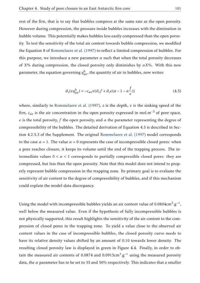
Chapter 4. Study of pore closure in an East Antarctic firn core 101
rest of the firn, that is to say that bubbles compress at the same rate as the open porosity.
However during compression, the pressure inside bubbles increases with the diminution in
bubble volume. This potentially makes bubbles less easily compressed than the open poros-
ity. To test the sensitivity of the total air content towards bubble compression, we modified
the Equation 8 of Rommelaere et al. (1997) to reflect a limited compression of bubbles. For
this purpose, we introduce a new parameter α such that when the total porosity decreases
of X% during compression, the closed porosity only diminishes by αX%. With this new
parameter, the equation governing qbair, the quantity of air in bubbles, now writes:
∂z(vqbair) = −cairv(∂zf +∂zǫ(α − 1−α
f
ǫ)) (4.5)
where, similarly to Rommelaere et al. (1997), z is the depth, v is the sinking speed of the
firn, cair is the air concentration in the open porosity expressed in mol.m−3 of pore space,
ǫ is the total porosity, f the open porosity, and α the parameter representing the degree of
compressibility of the bubbles. The detailed derivation of Equation 4.5 is described in Sec-
tion 4.2.5.3 of the Supplement. The original Rommelaere et al. (1997) model corresponds
to the case α = 1. The value α = 0 represents the case of incompressible closed pores: when
a pore reaches closure, it keeps its volume until the end of the trapping process. The in-
termediate values 0 < α < 1 corresponds to partially compressible closed pores: they are
compressed, but less than the open porosity. Note that this model does not intend to prop-
erly represent bubble compression in the trapping zone. Its primary goal is to evaluate the
sensitivity of air content to the degree of compressibility of bubbles, and if this mechanism
could explain the model-data discrepancy.
Using the model with incompressible bubbles yields an air content value of 0.0804cm3.g−1,
well below the measured value. Even if the hypothesis of fully incompressible bubbles is
not physically supported, this result highlights the sensitivity of the air content to the com-
pression of closed pores in the trapping zone. To yield a value close to the observed air
content values in the case of incompressible bubbles, the closed porosity curve needs to
have its relative density values shifted by an amount of 0.10 towards lower density. The
resulting closed porosity law is displayed in green in Figure 4.4. Finally, in order to ob-
tain the measured air contents of 0.0874 and 0.0915cm3.g−1 using the measured porosity
data, the α parameter has to be set to 35 and 50% respectively. This indicates that a smaller
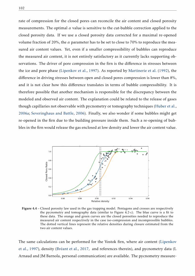
102
rate of compression for the closed pores can reconcile the air content and closed porosity
measurements. The optimal α value is sensitive to the cut-bubble correction applied to the
closed porosity data. If we use a closed porosity data corrected for a maximal re-opened
volume fraction of 20%, the α parameter has to be set to close to 70% to reproduce the mea-
sured air content values. Yet, even if a smaller compressibility of bubbles can reproduce
the measured air content, it is not entirely satisfactory as it currently lacks supporting ob-
servations. The driver of pore compression in the firn is the difference in stresses between
the ice and pore phase (Lipenkov et al., 1997). As reported by Martinerie et al. (1992), the
difference in driving stresses between open and closed pores compression is lower than 8%,
and it is not clear how this difference translates in terms of bubble compressibility. It is
therefore possible that another mechanism is responsible for the discrepancy between the
modeled and observed air content. The explanation could be related to the release of gases
though capillaries not observable with pycnometry or tomography techniques (Huber et al.,
2006a; Severinghaus and Battle, 2006). Finally, we also wonder if some bubbles might get
re-opened in the firn due to the building pressure inside them. Such a re-opening of bub-
bles in the firn would release the gas enclosed at low density and lower the air content value.
Figure 4.4 – Closed porosity law used in the gas trapping model. Pentagons and crosses are respectivelythe pycnometry and tomography data (similar to Figure 4.2-c). The blue curve is a fit tothese data. The orange and green curves are the closed porosities needed to reproduce themeasured air content respectively in the case iso-compression and incompressible bubbles.The dotted vertical lines represent the relative densities during closure estimated from thetwo air content values.
The same calculations can be performed for the Vostok firn, where air content (Lipenkov
et al., 1997), density (Bréant et al., 2017, and references therein), and pycnometry data (L
Arnaud and JM Barnola, personal communication) are available. The pycnometry measure-
Chapter 4. Study of pore closure in an East Antarctic firn core 103
ments also need to be corrected for the cut-bubble effect. However, contrary to Lock-In we
do not have tomographic images of the Vostok trapping zone that could be used to quantify
the re-opened volumes. Thus, we apply the correction previously derived for Lock-In in
Section 4.2.3.1 to the raw Vostok pycnometry data. The application of this correction yields
physically sound closed porosity values, with continuously increasing closed porosity ratios
up to 1. The uncorrected Vostok data are displayed in the Supplement Figure 4.14. Fi-
nally, the Vostok corrected closed porosity data have been fitted to obtain a smoothed closed
porosity curve to be used in the gas trapping model.
Similarly to Lock-In, a direct application of the original Rommelaere et al. (1997) gas trap-
ping model with iso-compression of bubbles yields a predicted air content of 0.0960cm3.g−1
much higher than the measured value of 0.0862cm3.g−1. This provides further insights that
the gas trapping process might not be well represented in the Rommelaere et al. (1997)
model. Again, the introduction of a limited compressibility of the bubbles with a coefficient
α = 50% is able to reconcile the modeled and observed air content values.
4.2.3.3 Comparison with other sites and porosity laws
The comparison in Figure 4.5 of the measured closed porosity data for Lock-In with the
proposed parametrization for the B53 site by Schaller et al. (2017) reveals a discrepancy be-
tween the two East Antarctic sites. While the B53 closed porosity curve reaches full closure
for relative densities of 0.90, the data we obtained for Lock-In reach closure for relative den-
sities closer to 0.92. Therefore, we were not able to reproduce one of their main findings,
namely that firn should close at a common critical relative density of 0.90, independently of
the studied sites. This discrepancy could be due to an underestimation of the cut-bubble ef-
fect for the Lock-In data set. To test this hypothesis, we derived a new cut-bubble correction
that reproduces the closed porosity parametrization proposed by Schaller et al. (2017). As
seen in Figure 4.3, this new correction assumes a very large re-open fraction around relative
densities of 0.90. This is consistent with the results of Schaller et al. (2017), but inconsistent
with the re-opened fraction of 24% deduced from the tomography image at a relative den-
sity of 0.9025. It is therefore possible that the true Lock-In closed porosities are similar to
the ones observed by Schaller et al. (2017) at B53, but a better estimation of the cut-bubble
effect is required to answer this question. However, a closed porosity curve similar to the one
104
observed in B53 would trap a higher quantity of air, and further increases the discrepancy
between the modeled and measured air content described in Section 4.2.3.2. Even in the ex-
treme case of incompressible bubbles (α = 0), the gas trapping used Section 4.2.3.2 predicts
an air content value of 0.0974cm3.g−1, larger than the values of 0.0874 and 0.0915cm3.g−1
measured in Lock-In.
Based on previous pycnometry measurements, JM Barnola proposed an analytical formu-
lation to represent the closed porosity of firn. This parametrization is fully characterized
by the total porous volume Vi (or equivalently the density during closure ρc) as a single pa-
rameter. The derivation of this parametrization is not published in the scientific literature,
but Goujon et al. (2003) included this Barnola parametrization in their model (Equation
9 of Goujon et al., 2003) and used the linear relationship between site temperature and
Vi by Martinerie et al. (1994) to model closed porosity data using temperature as the only
parameter. Application of the Goujon et al. (2003) parametrization using the Lock-In site
temperature yields a predicted total porous volume Vi of 0.110cm3.g−1 and the closed poros-
ity curve displayed in orange in Figure 4.5. The resulting closed porosity curve for Lock-In
clearly underestimates the closed porosity ratios. In the case of Lock-In, the two air contents
values can be used to estimate the total porous volume Vi at 0.109 and 0.114cm3.g−1, indi-
cating a possible underestimation of Vi by the temperature relationship. Using the Vi value
of 0.114cm3.g−1 in the Barnola parametrization results in the closed porosities displayed in
black in Figure 4.5. This curve is more consistent with the pycnometry and tomography
data, but still displays a clear underestimation of the closed porosity ratio. Two problems
thus arise when using the Goujon et al. (2003) parametrization to predict the Lock-In closed
porosities. First, the estimation of the total porous volume Vi using the temperature rela-
tionship might be underestimated, which in turns tends to predict pore closure at too high
densities. Then, even with a better constrained Vi, the Barnola curve appears to underesti-
mate the closed porosity ratios in the Lock-In firn.
Finally, the closed porosity data measured in a Vostok firn core (JM Barnola and L Arnaud,
personal communication) are displayed in blue in Figure 4.5 alongside the Lock-In data in
black. As explained Section 4.2.3.2, these data were corrected for cut bubbles using the
Lock-In correction derived Section 4.2.3.1. In the case of Vostok, the Goujon et al. (2003)
parametrization predicts closed porosity ratios (in red in Figure 4.5) that are more in line
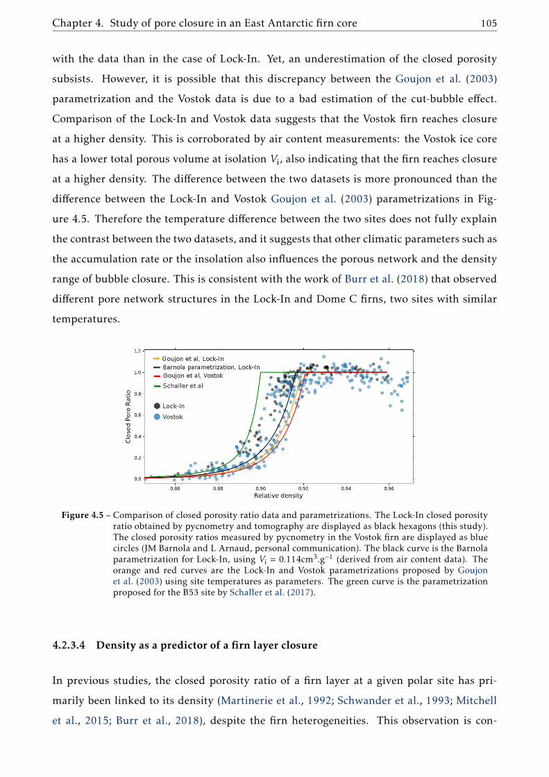
Chapter 4. Study of pore closure in an East Antarctic firn core 105
with the data than in the case of Lock-In. Yet, an underestimation of the closed porosity
subsists. However, it is possible that this discrepancy between the Goujon et al. (2003)
parametrization and the Vostok data is due to a bad estimation of the cut-bubble effect.
Comparison of the Lock-In and Vostok data suggests that the Vostok firn reaches closure
at a higher density. This is corroborated by air content measurements: the Vostok ice core
has a lower total porous volume at isolation Vi, also indicating that the firn reaches closure
at a higher density. The difference between the two datasets is more pronounced than the
difference between the Lock-In and Vostok Goujon et al. (2003) parametrizations in Fig-
ure 4.5. Therefore the temperature difference between the two sites does not fully explain
the contrast between the two datasets, and it suggests that other climatic parameters such as
the accumulation rate or the insolation also influences the porous network and the density
range of bubble closure. This is consistent with the work of Burr et al. (2018) that observed
different pore network structures in the Lock-In and Dome C firns, two sites with similar
temperatures.
Figure 4.5 – Comparison of closed porosity ratio data and parametrizations. The Lock-In closed porosityratio obtained by pycnometry and tomography are displayed as black hexagons (this study).The closed porosity ratios measured by pycnometry in the Vostok firn are displayed as bluecircles (JM Barnola and L Arnaud, personal communication). The black curve is the Barnolaparametrization for Lock-In, using Vi = 0.114cm3.g−1 (derived from air content data). Theorange and red curves are the Lock-In and Vostok parametrizations proposed by Goujonet al. (2003) using site temperatures as parameters. The green curve is the parametrizationproposed for the B53 site by Schaller et al. (2017).
4.2.3.4 Density as a predictor of a firn layer closure
In previous studies, the closed porosity ratio of a firn layer at a given polar site has pri-
marily been linked to its density (Martinerie et al., 1992; Schwander et al., 1993; Mitchell
et al., 2015; Burr et al., 2018), despite the firn heterogeneities. This observation is con-

106
firmed by our work in the Lock-In firn, where both pycnometry and tomography indicate
that the closed porosity ratio of a sample is primarily determined by its density. As depicted
Figure S4.15 of the supplement, a larger dispersion is obtained when plotting the closed
porosity ratios as a function of depth. In other words, two firn layers with same density,
no matter how far apart they are in the firn column, have nearly the same closed porosity
ratio. For example, a particular pycnometry sample taken at depth 97.40m has a relative
density of 0.90 and a closed porosity ratio close to 60%. Such values are usually expected
for samples around 102m depth.
However, the fact that different firn layers exhibit a functional relationship between their
density and closed porosity ratio, does not imply that they are equivalent in terms of pore
structure. One can then wonder if especially high or low density layers display similar pore
structure as the rest of the firn, or if they have a significantly different porous networks.
To answer this question we used the tomography 3D images, which explicitly represent the
porous network. Three different pore structure indicators were computed on each of the
1cm thick slices.
The first indicator is the Structure Model Index or SMI. This index was developed by Hilde-
brand and Rüegsegger (1997) to analyze the structure of bones. It is traditionally used to
quantify the degree of rodness, plateness, and spheriness in 3D images. In this study the
SMI will be used as a simple indicator of pore shape, considering that different pore mor-
phologies should result in different SMI. As pointed out by Salmon et al. (2015) this index
only provides sensible results when used on convex structures. For the Lock-In firn, the
SMI was computed in each slice using the BoneJ plug-in within ImageJ (Doube et al., 2010).
Results from the plug-in indicated that the porous structure is more than 90% convex, jus-
tifying the use of SMI for firn studies (Gregory et al., 2014; Burr et al., 2018). Nonetheless,
the obtained SMI values were sensitive to the resolution of the mesh used to compute the
index.
The second indicator is the ratio of pore surface to pore volume, denoted S/V here. This sur-
face to volume ratio was determined using the method presented in Krol and Löwe (2016),
and is based on the determination of the two-point correlation function. The S/V ratio is
notably dependent on the size of the pore, as smaller objects tend to have higher surface to
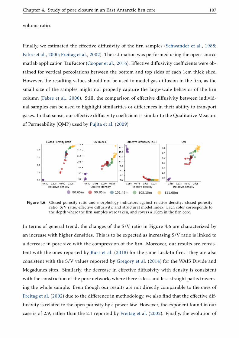
Chapter 4. Study of pore closure in an East Antarctic firn core 107
volume ratio.
Finally, we estimated the effective diffusivity of the firn samples (Schwander et al., 1988;
Fabre et al., 2000; Freitag et al., 2002). The estimation was performed using the open-source
matlab application TauFactor (Cooper et al., 2016). Effective diffusivity coefficients were ob-
tained for vertical percolations between the bottom and top sides of each 1cm thick slice.
However, the resulting values should not be used to model gas diffusion in the firn, as the
small size of the samples might not properly capture the large-scale behavior of the firn
column (Fabre et al., 2000). Still, the comparison of effective diffusivity between individ-
ual samples can be used to highlight similarities or differences in their ability to transport
gases. In that sense, our effective diffusivity coefficient is similar to the Qualitative Measure
of Permeability (QMP) used by Fujita et al. (2009).
Figure 4.6 – Closed porosity ratio and morphology indicators against relative density: closed porosityratio, S/V ratio, effective diffusivity, and structural model index. Each color corresponds tothe depth where the firn samples were taken, and covers a 10cm in the firn core.
In terms of general trend, the changes of the S/V ratio in Figure 4.6 are characterized by
an increase with higher densities. This is to be expected as increasing S/V ratio is linked to
a decrease in pore size with the compression of the firn. Moreover, our results are consis-
tent with the ones reported by Burr et al. (2018) for the same Lock-In firn. They are also
consistent with the S/V values reported by Gregory et al. (2014) for the WAIS Divide and
Megadunes sites. Similarly, the decrease in effective diffusivity with density is consistent
with the constriction of the pore network, where there is less and less straight paths travers-
ing the whole sample. Even though our results are not directly comparable to the ones of
Freitag et al. (2002) due to the difference in methodology, we also find that the effective dif-
fusivity is related to the open porosity by a power law. However, the exponent found in our
case is of 2.9, rather than the 2.1 reported by Freitag et al. (2002). Finally, the evolution of
108
SMI is characterized by an increase in values with density, indicating a transformation of the
pore shapes with increasing density. The values displayed Figure 4.6 are consistent with the
ones reported by Burr et al. (2018) for the Lock-In firn. Similarly to Burr et al. (2018), our
SMI values are higher than the ones reported by Gregory et al. (2014) for the WAIS Divide
and Megadunes firns. This can be explained by the fact that the SkyScan software used by
Gregory et al. (2014) yield lower SMI values (Salmon et al., 2015; Burr et al., 2018).
The tomography data of closed porosity ratio for the firn slices are also reported in Fig-
ure 4.6. Note that the closed porosity values displayed in Figure 4.6 have not been corrected
for cut-bubbles. It is particularly apparent for the slices taken at the depth 99.85m (in red
Figure 4.6) that the firn stratification can lead to a wide range of closed porosity ratios within
a 10cm section. Nonetheless, these layers with especially closed or open porosity do not ap-
pear as outliers in terms of pore morphology. Their morphological indicators are overall
consistent with the other firn samples. Hence, this indicates that all layers tend to follow a
similar evolution with density not only in terms of closed porosity ratio, but also in terms
of pore morphology and gas transport properties.
4.2.3.5 Origin of the density variability
We have seen in the previous sections that the degree of closure of a firn layer is primarily
a function of its density. However, an important variability of the density is observed at the
centimeter scale. One may then wonder about the origin of this density variability in the
trapping zone. Previous studies have advanced two mechanisms for the appearance of firn
stratification in upper parts of the firn.
The first one is the softening of firn layers due to chemical impurities in the ice phase. Layers
with a high concentration of specific ions densify faster, thus creating the density layering.
Hörhold et al. (2012) observed a positive correlation between Ca2+ and density anomalies
in Greenland and Antarctic firn cores. They however do not argue that calcium is the ion
specifically responsible for ice softening. Similarly, based on observation in three Dome Fuji
firn cores (East Antarctic plateau) Fujita et al. (2016) advanced that the presence of F− and
Cl− ions facilitates the densification of a firn layer. They also proposed a hardening effect of
NH+4 , preventing the deformation and compaction of firn. The second stratification mecha-

Chapter 4. Study of pore closure in an East Antarctic firn core 109
Figure 4.7 – Density (blue curve) and liquid conductivity (orange curve) variations in five one-meter longcore sections. The green and blue portions respectively highlight some sections were densityand liquid conductivity show simultaneous increase or decrease. The pink portion highlightsa section where the decrease in density is not matched by a decrease in liquid conductivity.
nism is detailed in Fujita et al. (2009), and takes into account the ice phase structure of firn
layers. Briefly, due to surface metamorphism, some layers develop bonds between the ice
clusters giving them more resistance to deformation. These layers, that are initially denser
at the surface, thus densify slower and are associated with negative density anomalies in
deep firn.
Concerning the Lock-In firn core, the comparison of the high resolution density and liquid
conductivity datasets indicates a covariation between the two signals, with denser layers
110
having higher conductivities. Density and liquid conductivity variations for five one-meter
long sections are displayed in Figure 4.7, with green and blue portions highlighting some of
the observed covariations. The covariation is present throughout the whole trapping zone,
and is consistent with the preferential deformation of firn with high ionic contents. Even
though liquid conductivity cannot distinguish between ions with and without ice-softening
effects, an increase in liquid conductivity indicates a greater ionic content, and therefore
potentially more ice-softening ions in the ice matrix. Thus, we conclude that the centimeter
scale stratification observed in the trapping zone of Lock-In is largely related to the presence
of chemical impurities. Yet, liquid conductivity does not account for all the observed den-
sity variability. An illustration can be seen at the depth 90.30m (pink section Figure 4.7),
where a lower density layer does not show low values of liquid conductivity. This means one
of two things. Either this less dense layer is due the absence of ice softening impurities but
still contains enough conductive species for the liquid conductivity no to drop. In this case
the density variability is still due to chemical impurities, but is simply not reflected in the
liquid conductivity. Or this less dense layer is not due to a chemistry based effect but rather
to another mechanism, potentially related to the ice structure as described by Fujita et al.
(2009). Moreover, due to its inability to distinguish between specific ions, the measurement
of liquid conductivity can only provide a quantitative relationship between chemistry and
density.
To better understand the effect of specific ions on the firn density, four one meter long
sections been measured using ion chromatography with a resolution of 2.5cm. The concen-
tration of H+ was obtained by closing the ionic balance following Equation 3 of Legrand
and Mayewski (1997). Since H+ ions have a high mobility, H+ concentration estimates could
therefore help to explain the centimeter scale variations of liquid conductivity. The ion con-
centrations measured on the 113 to 114m section are displayed in lower panels of Figure 4.8,
with density and liquid conductivity variations above. On this section, the data highlight
that in one occasion, the sulfate and conductivity undergo strong increases, uncorrelated
with other species (green section in Figure 4.8). We interpret this spike as a volcanic event,
depositing sulfuric acid. This volcanic event is not associated with any particular effect on
the firn density, and we therefore conclude that sulfate has no impact on the layering in
the trapping zone. Unfortunately for other species, we were not able to decipher the effect
of particular ions on densification due to the frequent correlations between the different

Chapter 4. Study of pore closure in an East Antarctic firn core 111
Figure 4.8 – Upper panel: Methane concentration measured by CFA between 113 and 114m depth, witha reversed axis. Upper middle panel: Density (blue) and liquid conductivity (orange) varia-tions. Lower middle panel: Cation concentrations obtained with ion chromatography. Lowerpanel: Anion concentrations obtained with ion chromatography. The ion concentrations areexpressed in arbitrary units to highlight their variability. The green portion highlights thepresence of a volcanic event. The blue portion highlights a partially open layer.
species and the limited spatial resolution. Moreover, the diffusion of ions in the firn tends
to smooth out the ion variations (Barnes et al., 2003; Fujita et al., 2016). The same inconclu-
sive observations were made on the three other sections (displayed in Figures 4.16 to 4.18
of the Supplement), where density variations could not be attributed to a particular species
measured by ion chromatography. Measurements with a better spatial resolution could po-
tentially help to decipher the impact of specific ion species, similarly to the work of Fujita
et al. (2016).
4.2.3.6 Examples of stratified gas trapping
Thanks to the continuous methane record, we were able to identify layers which were not
entirely closed below the bulk firn-ice transition. In the upper part of the methane record,
these layers appear as spikes of high concentrations. This is due to the presence of modern
air that entered the center CFA stick through the open porosity. An example of a partially
open layer is displayed in the blue portion of Figure 4.8. This still open layer is associated
with low density and low liquid conductivity values. Please note that the methane axis
is reversed in this figure, and in the following ones. The same observation was made on
the ice core section displayed in Figure 4.9. Two late closure layers, depicted by the blue
sections, are associated with lower density values and lower liquid conductivities than in

112
the surrounding layers. All these examples are consistent with the previous observation that
layers with low ionic content are less dense and thus reach closure deeper in the firn.
Figure 4.9 – Examples of late closure layers highlighted by the blue shadings. The positive spikes inmethane around 110.69 and 110.82m reveal the presence of open pores reaching the middleof the sample (reversed axis). These open layers are associated with low density and liquidconductivity values.
Similarly, an early closure layer was found in the bubbly-ice portion of the core (Figure 4.10).
Following Rhodes et al. (2016) and Fourteau et al. (2017), this layer was detected as a neg-
ative methane anomaly during a period of methane rise. This section corresponds to a part
of the core with a poor geometry due to a broken edge, and we were not able properly de-
termine the absolute density values. Still, using the X-ray scan of the non broken part of the
core we could identify the density variability. However, as we do not know the actual thick-
ness of the core that was crossed by the ray, the resulting density variability is expressed in
arbitrary units and rather than in g.cm−3. The comparison between density and the methane
records in Figure 4.10, indicates that the early closure layer corresponds to a denser layer.
Air content measurements were performed on this section of the core. Results indicates that
the early closure layer does not undergo outlier values of air content. This implies that the
early closure layer trapped gases at similar densities as the rest of the firn. It is in line with
the description of stratified gas trapping supported in this article, where dense layers close
in advance but with the same critical density as others. Unfortunately, no chemical analysis
could be performed on this section.

Chapter 4. Study of pore closure in an East Antarctic firn core 113
Figure 4.10 – Example of an early closure layer highlighted by the orange shade. The reduced methaneconcentration around 112.40m is indicative of early gas trapping in the ice (reversed axis).This early closure layer is associated with high density values, but air content values similarwith the adjacent layer.
4.2.4 Conclusions
We studied the enclosure of gases at the East Antarctic site of Lock-In, characterized by a
temperature of −53.15°C and an accumulation rate of 3.6cm.we.yr−1. The closed porosity
ratio profile in the trapping zone was measured using two independent methods: pycnom-
etry and tomography. Our findings suggest that the two methods yield consistent results
when measuring similar samples, and can thus be interpreted in similar ways. However,
pycnometry measurements are very sensitive to the determination of sample volumes. On
the other hand, tomography appears to provide more robust results and can be used to
access more complex characterization of the firn, including pore size and shapes. One im-
portant remaining problem in the study of pore closure is the estimation of the cut-bubble
effect in the trapping zone as it can drastically change the shape of the closed porosity curve
and the estimation of the full closure density. Thus, we encourage the usage of large volume
tomography for future studies of gas trapping and firn densification. Notably, large volume
tomographies of firn where pycnometry data are available could help understand the dis-

114
crepancy between our results and the results of Schaller et al. (2017).
Using a gas trapping model, we found that under the assumption of iso-compression of
open and closed pores, the measured air content and closed porosity ratios are inconsistent,
with the model predicting to much enclosed air. The same overestimation of air content
by the gas trapping model have been found in the Vostok ice core. We have shown that
this discrepancy cannot be explained by a poor estimation of the closed porosity data or of
the cut-bubble effect. On the other hand, the introduction of a reduced compressibility for
closed pores in the gas trapping model is able to resolve this discrepancy. Yet, this mecha-
nism is not fully satisfactory as it requires a very limited compression of bubbles that has
no direct supporting observations. The mechanism responsible for these low quantities of
air trapped in ice cores is thus not clear.
Consistently with previous studies conducted at other sites, we observed a strong layering in
the Lock-In firn, manifesting itself as centimeter scale density and firn structure variations
(Hörhold et al., 2011; Fujita et al., 2016). Despite this heterogeneity, it appears that all firn
layers roughly follow the same behavior relating their closed porosity ratio and pore struc-
ture to their density. Layers associated with positive density anomalies close in advance, but
at the same critical density as others. This vision simplifies the modeling of stratified gas
trapping, as it reduces the firn to a stack of equivalent layers.
Finally, using liquid conductivity as a proxy for ionic content, our results suggest that when
focusing on the trapping zone, chemical impurities play a major role in establishing the firn
stratification. This does not mean that effects due to the ice phase structure, as described
by Fujita et al. (2009), does not strongly influence firn stratification in upper parts. But,
as a first approximation, the effect chemical impurities appears as the main mechanism for
stratified gas trapping. However, we were not able to determine which chemical species are
responsible for the preferential densification of firn. Continuous impurity measurements
along the trapping zone with a resolution higher than a centimeter could help decipher the
species responsible for the presence of firn heterogeneities.
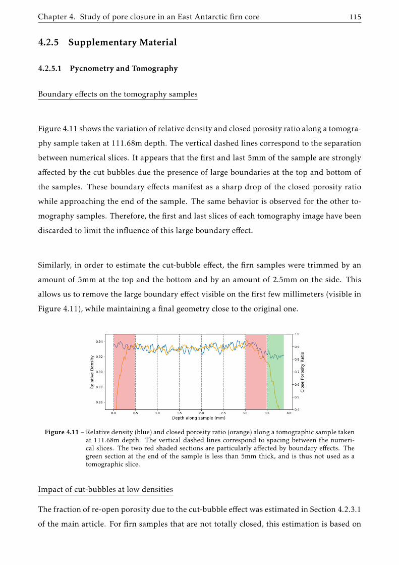
Chapter 4. Study of pore closure in an East Antarctic firn core 115
4.2.5 Supplementary Material
4.2.5.1 Pycnometry and Tomography
Boundary effects on the tomography samples
Figure 4.11 shows the variation of relative density and closed porosity ratio along a tomogra-
phy sample taken at 111.68m depth. The vertical dashed lines correspond to the separation
between numerical slices. It appears that the first and last 5mm of the sample are strongly
affected by the cut bubbles due the presence of large boundaries at the top and bottom of
the samples. These boundary effects manifest as a sharp drop of the closed porosity ratio
while approaching the end of the sample. The same behavior is observed for the other to-
mography samples. Therefore, the first and last slices of each tomography image have been
discarded to limit the influence of this large boundary effect.
Similarly, in order to estimate the cut-bubble effect, the firn samples were trimmed by an
amount of 5mm at the top and the bottom and by an amount of 2.5mm on the side. This
allows us to remove the large boundary effect visible on the first few millimeters (visible in
Figure 4.11), while maintaining a final geometry close to the original one.
Figure 4.11 – Relative density (blue) and closed porosity ratio (orange) along a tomographic sample takenat 111.68m depth. The vertical dashed lines correspond to spacing between the numeri-cal slices. The two red shaded sections are particularly affected by boundary effects. Thegreen section at the end of the sample is less than 5mm thick, and is thus not used as atomographic slice.
Impact of cut-bubbles at low densities
The fraction of re-open porosity due to the cut-bubble effect was estimated in Section 4.2.3.1
of the main article. For firn samples that are not totally closed, this estimation is based on
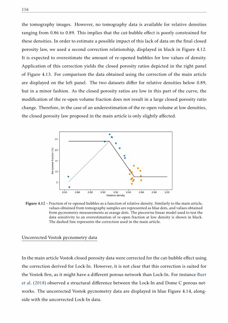
116
the tomography images. However, no tomography data is available for relative densities
ranging from 0.86 to 0.89. This implies that the cut-bubble effect is poorly constrained for
these densities. In order to estimate a possible impact of this lack of data on the final closed
porosity law, we used a second correction relationship, displayed in black in Figure 4.12.
It is expected to overestimate the amount of re-opened bubbles for low values of density.
Application of this correction yields the closed porosity ratios depicted in the right panel
of Figure 4.13. For comparison the data obtained using the correction of the main article
are displayed on the left panel. The two datasets differ for relative densities below 0.89,
but in a minor fashion. As the closed porosity ratios are low in this part of the curve, the
modification of the re-open volume fraction does not result in a large closed porosity ratio
change. Therefore, in the case of an underestimation of the re-open volume at low densities,
the closed porosity law proposed in the main article is only slightly affected.
Figure 4.12 – Fraction of re-opened bubbles as a function of relative density. Similarly to the main article,values obtained from tomography samples are represented as blue dots, and values obtainedfrom pycnometry measurements as orange dots. The piecewise linear model used to test thedata sensitivity to an overestimation of re-open fraction at low density is shown in black.The dashed line represents the correction used in the main article.
Uncorrected Vostok pycnometry data
In the main article Vostok closed porosity data were corrected for the cut-bubble effect using
the correction derived for Lock-In. However, it is not clear that this correction is suited for
the Vostok firn, as it might have a different porous network than Lock-In. For instance Burr
et al. (2018) observed a structural difference between the Lock-In and Dome C porous net-
works. The uncorrected Vostok pycnometry data are displayed in blue Figure 4.14, along-
side with the uncorrected Lock-In data.

Chapter 4. Study of pore closure in an East Antarctic firn core 117
Figure 4.13 – Closed porosity ratios with two different cut-bubble corrections. Left: Using the correctionproposed in the main article. Right: Sensitivity test to a large re-open volume fraction atlow densities.
Figure 4.14 – Closed porosity data for Lock-In and Vostok without correction for the cut-bubble effect.
Closed porosity versus depth
The figures provided in the article are plotted using relative density as the abscissa. Here,
we display in Figure 4.15 the closed porosity data as a function of the sample depth. This
highlights the firn layering, as samples taken at similar depths display a large variability of
closed porosity and density values.
4.2.5.2 Ion Chromatography
In total four one-meter long sections were analyzed using ion chromatography. One of the
sections is displayed in Figure 8 of the main article. The three remaining sections are dis-
played in Figure 4.16 to 4.18 with density, liquid conductivity and major ion concentrations
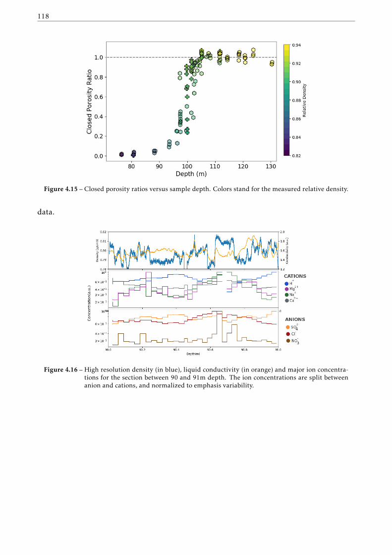
118
Figure 4.15 – Closed porosity ratios versus sample depth. Colors stand for the measured relative density.
data.
Figure 4.16 – High resolution density (in blue), liquid conductivity (in orange) and major ion concentra-tions for the section between 90 and 91m depth. The ion concentrations are split betweenanion and cations, and normalized to emphasis variability.

Chapter 4. Study of pore closure in an East Antarctic firn core 119
Figure 4.17 – Same as Figure 4.16 for the section between 92 and 93m depth.
Figure 4.18 – Same as Figure 4.16 for the section between 100 and 101m depth.
4.2.5.3 Gas trapping model
To model the air content in ice, we used a modified version of the Rommelaere et al. (1997)
gas trapping model, introducing a limited compressibility for the closed pores. Here, we
describe how the new equation representing air trapping is obtained. The derivation is
similar to the one of Rommelaere et al. (1997), and we only detail the differences with the
original calculation. The symbols used and the quantities they represent are the same as in
Rommelaere et al. (1997).
Our new model is based on the replacement of Equation 8 of Rommelaere et al. (1997)
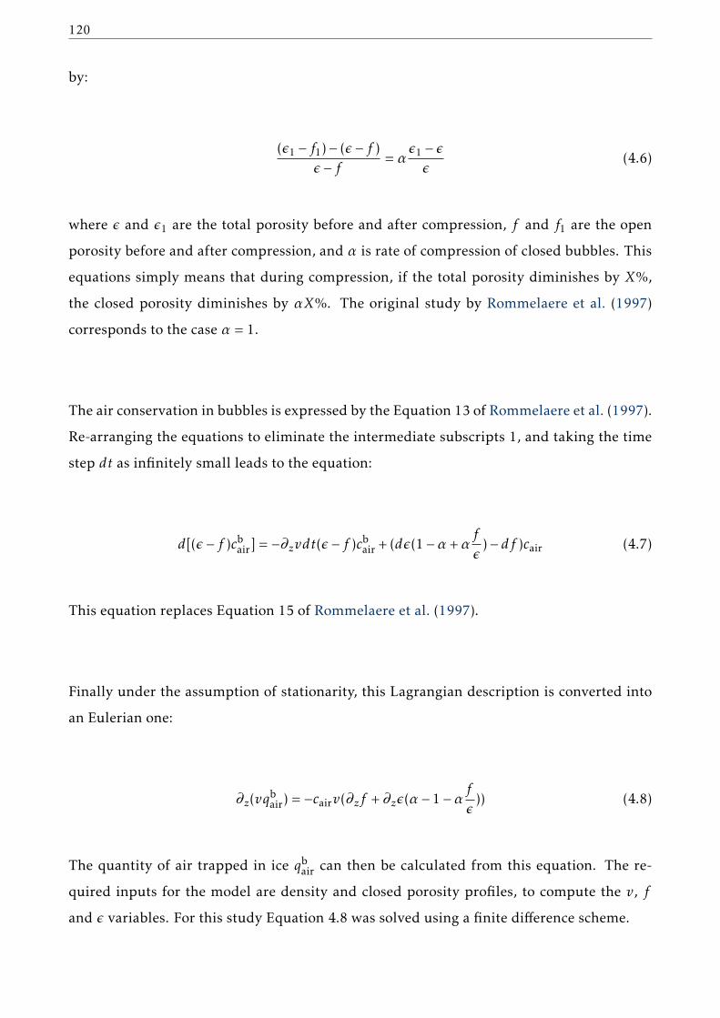
120
by:
(ǫ1 − f1)− (ǫ − f )ǫ − f = α
ǫ1 − ǫǫ
(4.6)
where ǫ and ǫ1 are the total porosity before and after compression, f and f1 are the open
porosity before and after compression, and α is rate of compression of closed bubbles. This
equations simply means that during compression, if the total porosity diminishes by X%,
the closed porosity diminishes by αX%. The original study by Rommelaere et al. (1997)
corresponds to the case α = 1.
The air conservation in bubbles is expressed by the Equation 13 of Rommelaere et al. (1997).
Re-arranging the equations to eliminate the intermediate subscripts 1, and taking the time
step dt as infinitely small leads to the equation:
d[(ǫ − f )cbair] = −∂zvdt(ǫ − f )cbair + (dǫ(1−α +αf
ǫ)− df )cair (4.7)
This equation replaces Equation 15 of Rommelaere et al. (1997).
Finally under the assumption of stationarity, this Lagrangian description is converted into
an Eulerian one:
∂z(vqbair) = −cairv(∂zf +∂zǫ(α − 1−α
f
ǫ)) (4.8)
The quantity of air trapped in ice qbair can then be calculated from this equation. The re-
quired inputs for the model are density and closed porosity profiles, to compute the v, f
and ǫ variables. For this study Equation 4.8 was solved using a finite difference scheme.
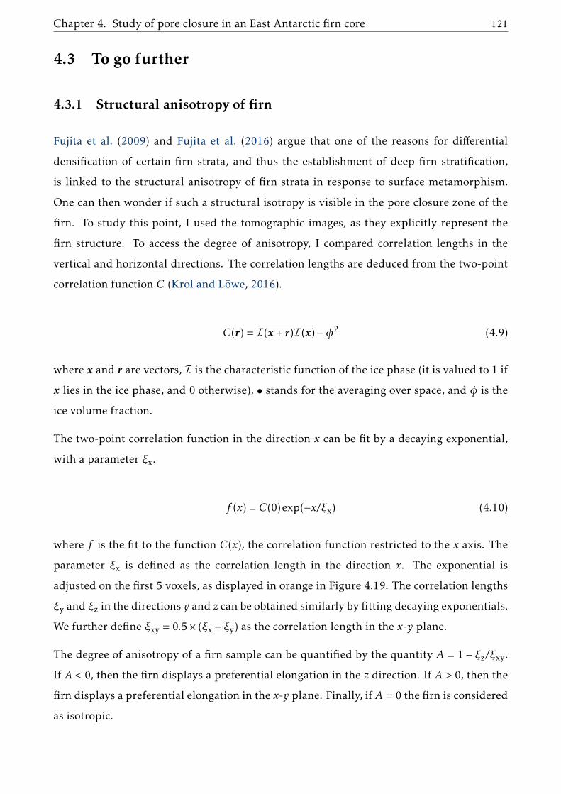
Chapter 4. Study of pore closure in an East Antarctic firn core 121
4.3 To go further
4.3.1 Structural anisotropy of firn
Fujita et al. (2009) and Fujita et al. (2016) argue that one of the reasons for differential
densification of certain firn strata, and thus the establishment of deep firn stratification,
is linked to the structural anisotropy of firn strata in response to surface metamorphism.
One can then wonder if such a structural isotropy is visible in the pore closure zone of the
firn. To study this point, I used the tomographic images, as they explicitly represent the
firn structure. To access the degree of anisotropy, I compared correlation lengths in the
vertical and horizontal directions. The correlation lengths are deduced from the two-point
correlation function C (Krol and Löwe, 2016).
C(r) = I (x + r)I (x)−φ2 (4.9)
where x and r are vectors, I is the characteristic function of the ice phase (it is valued to 1 if
x lies in the ice phase, and 0 otherwise), • stands for the averaging over space, and φ is the
ice volume fraction.
The two-point correlation function in the direction x can be fit by a decaying exponential,
with a parameter ξx.
f (x) = C(0)exp(−x/ξx) (4.10)
where f is the fit to the function C(x), the correlation function restricted to the x axis. The
parameter ξx is defined as the correlation length in the direction x. The exponential is
adjusted on the first 5 voxels, as displayed in orange in Figure 4.19. The correlation lengths
ξy and ξz in the directions y and z can be obtained similarly by fitting decaying exponentials.
We further define ξxy = 0.5× (ξx + ξy) as the correlation length in the x-y plane.
The degree of anisotropy of a firn sample can be quantified by the quantity A = 1 − ξz/ξxy.If A < 0, then the firn displays a preferential elongation in the z direction. If A > 0, then the
firn displays a preferential elongation in the x-y plane. Finally, if A = 0 the firn is considered
as isotropic.

122
Figure 4.19 – In blue: Correlation function as determined using Fourier transform. In orange: Exponen-tial fit to determine the correlation length.
To compute the two-point correlation function, we rely on Fourier transform, following
Newman and Barkema (1999).
C(k) =1N||I ′(k)||2 (4.11)
where I ′ = I − I , and • stand for the Fourier transform. The correlation function C is then
obtained with a inverse Fourier transform.
I computed the degree of anisotropy A for each tomographic slice, using Equations 4.9, 4.10,
and 4.11. The Fourier transforms are estimated with the use of Fast Fourier Transforms.
The resulting anisotropies A are displayed in Figure 4.20 as a function of local density.
They indicate that the deep part of the firn does not display a strong anisotropic structure.
There appears to be a small vertical elongation for the shallowest samples (in purple in
Figure 4.20). However, this preferential elongation do not exceed a couple of percents. In
deeper firn, this potential preferential elongation disappears, in favor of a general isotropy
of the firn structure. A closer look at the centimeter scale indicates that firn strata that
are especially dense compared to their surroundings do not exhibit a particular degree of
anisotropy. Therefore, we cannot confirm the hypothesis of Fujita et al. (2009) that less dense
layers are associated with a higher anisotropy in the deeper parts of firn. That being said,
Fujita et al. (2009) report the gradual disappearance of anisotropy with depth. Therefore,
our observations do not invalidate their hypothesis.

Chapter 4. Study of pore closure in an East Antarctic firn core 123
Figure 4.20 – Anisotropy of firn slices as a function of relative density. Same color code as Figure 4.6,where each color represent the depth were the firn sample is taken.
4.3.2 Analysis of thin sections
Thin sections of the Lock-In firn core have been performed and analyzed for crystalline
texture using an the Automatic Ice Texture Analyzer (AITA; Peternell et al., 2010). The
principal products of the AITA are maps of the azimuth and colatitude angles of the crys-
tals inside the thin sections. These maps can be used to differentiate single crystals from
each others, and thus to infer the typical size of the crystals.
The thin sections in the Lock-In firn core were prepared to investigate whether or not den-
sity variability can be associated with variability in the crystalline texture. However as seen
in Fiture 4.21, because of noise in the obtained images it is not possible for a simple algo-
rithm to directly count the number of crystals and to estimate their size.
A first solution to this problem is to manually redraw each crystal boundary, for the com-
puter to have a clean image to work with. However, this method is rather cumbersome and
not suited to treat a large number of single crystals.
A second method is to draw a network of lines crossing the thin section, as displayed in
Figure 4.22, and to manually count the number of intersections between a line and crystal
boundaries. This number of intersections is related to the size of the crystals, as zones char-
acterized by small crystals exhibit higher numbers of intersections. The results obtained
for two 10cm long thin sections of the Lock-In core are displayed in Figure 4.23, alongside
with density. No clear link between density and crystal size is apparent using this method-
ology.
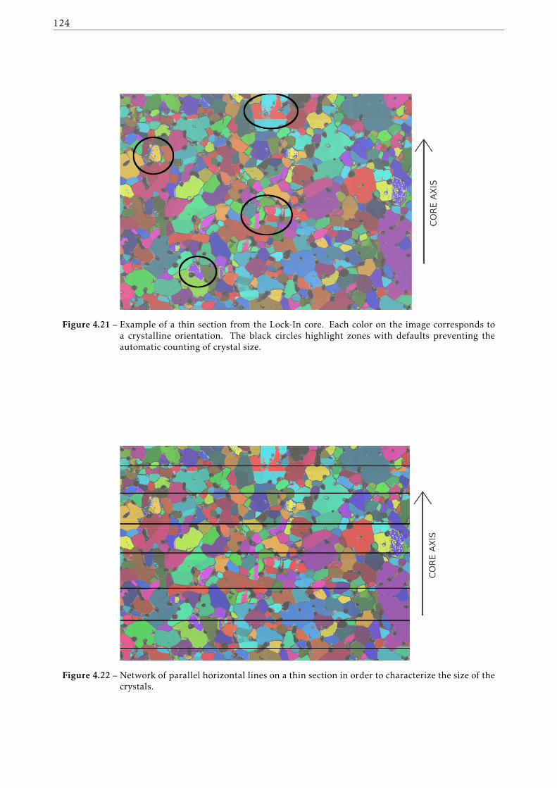
124
Figure 4.21 – Example of a thin section from the Lock-In core. Each color on the image corresponds toa crystalline orientation. The black circles highlight zones with defaults preventing theautomatic counting of crystal size.
Figure 4.22 – Network of parallel horizontal lines on a thin section in order to characterize the size of thecrystals.

Chapter 4. Study of pore closure in an East Antarctic firn core 125
Figure 4.23 – Density (in blue) and number of line intersections (in orange) over a 20cm section. Thenumber of line intersections is related to the size of the crystals.

126
4.4 Conclusion of the chapter
This chapter reports a multi-tracer analysis of gas trapping in an East Antarctic firn. For
this purpose, I exploit datasets obtained with the different methods described in Chapter 3.
A first issue discussed in the chapter is the acquisition of reliable closed porosity data. The
data obtained by pycnometry and tomography, two independent methods, are compared.
The initial discrepancy between the two types of data can be resolved if one considers
the geometrical radius measurement of firn samples to be systematically overestimated by
0.05mm. To support this hypothesis, I use the tomographic images to estimate the rough-
ness of the sample surfaces. I finally propose a method, similar to Schaller et al. (2017), to
correct for the effect of cut-bubbles in firn samples.
Using the air content data measured by V. Lipenkov and the closed porosity data, I assess
the ability of the Rommelaere et al. (1997) gas trapping model to predict the right amount
of trapped air. It appears that there is a large disagreement between the modeled and mea-
sured air content. I first ensure that this discrepancy was not due experimental errors on
the air content or the closed porosity data. As the mismatch does not seem to originate from
experimental issues, I conclude that it must be related to the mechanism of gas trapping
implemented in the model. As it can easily be added to the model, I test the influence a
limited compressibility of bubbles on the discrepancy. To reconcile the data and model,
the compressibility of bubbles must be heavily reduced. It it thus probable than an other
mechanism, not yet identified, is responsible for the low amount of air measured in the ice.
Potential mechanisms could be the transport of gases outside the bubbles thought capillaries
not detectable with the tomography and pycnometry methods, or the re-opening of closed
bubbles in the firn due to the building pressure inside them. Finally, the same observations
of model-data mismatch are made in the case of the Vostok ice core where pycnometry and
air content data are available, indicating that the model-data discrepancy is not limited to
the sole case of Lock-In.
The rest of the article is centered around the study of firn stratification and its impact on
gas trapping. Using the pycnometry and tomography data, I reproduce the observation of
Schwander and Stauffer (1984) and Martinerie et al. (1992) that there is a direct relationship

Chapter 4. Study of pore closure in an East Antarctic firn core 127
between the density of a firn stratum and its amount of closed pores. I then check if the same
observation could be made for other parameters characterizing the porous network. It ap-
pears that indexes characterizing the morphology and size of the porous network are closely
linked to density. In particular, strata that are especially dense compared to their surround-
ings still obey the same relationship between pore morphology and density. It implies that
all layers close at nearly the same density, and present similar transport properties. In par-
ticular, layers that are especially dense close at shallower depths but at the same density as
the rest of the firn. This idea will used in Chapter 5 to model layered gas trapping.
The origin of especially dense layers is then studied thanks to the high resolution density
and chemistry measurements. Using liquid conductivity, I observe a clear link between
the density of firn strata and their ionic contents. This observation supports the idea that
chemical softening of ice might enhance the densification of some strata, and thus create a
stratification deep in the firn (Hörhold et al., 2012; Fujita et al., 2016). However, I am not
able to distinguish the particular ion(s) responsible for this preferential densification. In
the additional content of the chapter, I investigate the potential link of densification with
the structural anisotropy of the firn or with the size of ice crystals. Fujita et al. (2009) and
Fujita et al. (2016) report that dense layers at the bottom of firns are associated with weaker
structural anisotropy. However, using the tomography images I do not find any clear link
supporting the Fujita et al. (2009) and Fujita et al. (2016) hypothesis. It is possible that
differences in anisotropy between dense and less dense layers have attenuated with densifi-
cation, and that their are no longer easily observed in our deep samples.
Finally, a few examples of layered gas trapping of methane are provided. They are consistent
with the vision laid out in this chapter, namely that firn strata with a high (respectively low)
ionic content are denser (respectively less dense) at the bottom of the firn and thus close in
advance (respectively late). Air content data support the idea of firn strata all closing at the
a similar density.

128

Chapter 5
Alterations of methane records in East
Antarctic ice cores
Contents
5.1 Presentation of the chapter . . . . . . . . . . . . . . . . . . . . . . . . . . . . 131
5.2 Analytical constraints on layered gas trapping and smoothing of atmo-
spheric variability in ice under low-accumulation conditions . . . . . . . . 132
5.2.1 Introduction . . . . . . . . . . . . . . . . . . . . . . . . . . . . . . . . . 133
5.2.2 Ice core samples and analytical methods . . . . . . . . . . . . . . . . . 135
5.2.3 Experimental results . . . . . . . . . . . . . . . . . . . . . . . . . . . . 137
5.2.4 Layered bubble trapping . . . . . . . . . . . . . . . . . . . . . . . . . . 141
5.2.5 Smoothing and age distribution in the Vostok 4G-2 ice core . . . . . . 148
5.2.6 Discussion . . . . . . . . . . . . . . . . . . . . . . . . . . . . . . . . . . 151
5.2.7 Conclusions . . . . . . . . . . . . . . . . . . . . . . . . . . . . . . . . . 155
5.2.8 Supplementary Material . . . . . . . . . . . . . . . . . . . . . . . . . . 156
5.3 Estimation of gas record alteration in very low accumulation ice cores . . . 164
5.3.1 Introduction . . . . . . . . . . . . . . . . . . . . . . . . . . . . . . . . . 165
5.3.2 Methods . . . . . . . . . . . . . . . . . . . . . . . . . . . . . . . . . . . 167
5.3.3 Results and Discussion . . . . . . . . . . . . . . . . . . . . . . . . . . . 169
5.3.4 Loss of climatic information in a deep and thinned ice core from East
Antarctica . . . . . . . . . . . . . . . . . . . . . . . . . . . . . . . . . . 182
5.3.5 Conclusions . . . . . . . . . . . . . . . . . . . . . . . . . . . . . . . . . 187
129

5.3.6 Supplementary Material . . . . . . . . . . . . . . . . . . . . . . . . . . 188
5.4 Conclusion of the chapter . . . . . . . . . . . . . . . . . . . . . . . . . . . . . 193
Chapter 5. Alterations of methane records in East Antarctic ice cores 131
5.1 Presentation of the chapter
This chapter presents two articles, one published in the journal Climate of the Past (https:
//www.clim-past.net/13/1815/2017/) and the other one to be submitted to the same jour-
nal. It deals with the discrepancies that exist between the atmospheric history and its mea-
surement in ice core records, due to the effect of gas layered trapping and firn smoothing.
The first article is based on a high-resolution methane record measured in a glacial section
of the Vostok ice core from East Antarctica. These data were obtained at IGE with X. Faïn
during my Master’s degree internship, a few months prior to my PhD in the spring of 2016.
Using these data I aim to quantify the alterations due to effects of layered gas trapping and
smoothing. Moreover, I propose a model to simulate the effect of layered gas trapping and
present a novel methodology able to estimate the gas age distribution of a low-accumulation
record, applicable to climatic conditions without present-day equivalent. These two meth-
ods can easily be extended to other ice cores from East Antarctica.
The second article builds on the ideas introduced in the first one. Five new high-resolution
methane records have been measured at IGE and exploited to estimate the impact of gas
layered trapping and smoothing. I notably investigate the impact of impurities in the ice
phase on layered gas trapping artifacts. The high-resolution methane records are used to
estimate new gas age distributions for a range of accumulation conditions typical of the East
Antarctic plateau for both glacial and interglacial periods. I finally apply the knowledge
gained on layered gas trapping and smoothing to the case of a low-accumulation and very-
thinned ice core from East Antarctica. The goal is to estimate the degree of alteration of
methane and carbon dioxide signals that can be expected in the future ice core of the Oldest-
Ice project.

132
5.2 Analytical constraints on layered gas trapping and smooth-
ing of atmospheric variability in ice under low-accumulation
conditions
Kévin Fourteau1, Xavier Faïn1, Patricia Martinerie1, Amaëlle Landais2, Alexey A. Ekaykin3, Vladimir
Ya. Lipenkov3, and Jérôme Chappellaz1
[1] Univ. Grenoble Alpes, CNRS, IRD, Grenoble INP, IGE, 38000 Grenoble, France
[2] Laboratoire des Sciences du Climat et de l’Environnement, UMR8212, CEA-CNRS-UVSQ-UPS/IPSL, Gif-
sur-Yvette, France
[3] Climate and Environmental Research Laboratory, Arctic and Antarctic Research Institute, St. Petersburg,
199397, Russia
AbstractWe investigate for the first time the loss and alteration of past atmospheric information
from air trapping mechanisms under low-accumulation conditions, through continuous
CH4 (and CO) measurements. Methane concentration changes were measured over the
Dansgaard-Oeschger event 17 (DO-17, ∼ 60,000yrBP) in the Antarctic Vostok 4G-2 ice core.
Measurements were performed using continuous-flow analysis combined with laser spec-
troscopy. The results highlight many anomalous layers at the centimeter scale that are un-
evenly distributed along the ice core. The anomalous methane mixing ratios differ from
those in the immediate surrounding layers by up to 50ppbv. This phenomenon can be the-
oretically reproduced by a simple layered trapping model, creating very localized gas age
scale inversions. We propose amethod for cleaning the record of anomalous values that aims
at minimizing the bias in the overall signal. Once the layered-trapping-induced anomalies
are removed from the record, DO-17 appears to be smoother than its equivalent record from
the high-accumulation WAIS Divide ice core. This is expected due to the slower sinking and
densification speeds of firn layers at lower accumulation. However, the degree of smoothing
appears surprisingly similar between modern and DO-17 conditions at Vostok. This sug-
gests that glacial records of trace gases from low-accumulation sites in the East Antarctic
plateau can provide a better time resolution of past atmospheric composition changes than
previously expected. We also developed a numerical method to extract the gas age distribu-
tions in ice layers after the removal of the anomalous layers based on the comparison with a
weakly smoothed record. It is particularly adapted for the conditions of the East Antarctic
plateau, as it helps to characterize smoothing for a large range of very low-temperature and
Chapter 5. Alterations of methane records in East Antarctic ice cores 133
low-accumulation conditions.
5.2.1 Introduction
In a context of climate change, the study of paleoclimate is an important tool for under-
standing the interactions between climate and atmospheric conditions (Masson-Delmotte
et al., 2013). Ice cores have been used to retrieve climatic and atmospheric conditions back
to 800,000 years before present (BP) (Jouzel et al., 2007; Loulergue et al., 2008; Lüthi et al.,
2008). Notably, ancient atmospheric gases get enclosed within bubbles in the ice and allow
us to reconstruct the past history of atmospheric composition (Stauffer et al., 1985). The
trapping of air in ice is due to the transformation of firn (porous compacted snow) into
airtight ice at depths ranging from ∼ 50 to ∼ 120m depending on temperature and accu-
mulation conditions. It is characterized by an increase in bulk density and a decrease in
porosity with depth along the firn column. It is only at the bottom of the firn column that
the porosity of the medium gets closed and traps the interstitial air. From a gas point of
view the firn is traditionally divided in three main parts from the surface to the bottom: the
convective zone, the diffusive zone and the trapping zone (e.g., Schwander, 1989; Buizert
et al., 2012). The convective zone is characterized by the mixing of air in the snow with at-
mospheric air through wind action (Colbeck, 1989). In the diffusive zone the dominant gas
transport processes are molecular diffusion and gravitational settling. Finally, the trapping
zone corresponds to the enclosure of air into bubbles through the closure of the porosity.
The process of densification and pore closure can last for thousands of years at the most
arid sites in Antarctica.
Air trapping affects the recording of atmospheric variability in ice cores. One known ef-
fect of the gas enclosure mechanism is the damping of fast variations in the atmosphere,
also called smoothing (Spahni et al., 2003; Joos and Spahni, 2008; Köhler et al., 2011; Ahn
et al., 2014). This smoothing arises for two reasons: (i) the gas diffusion in the firn mixes
air from different dates, and thus a bubble does not enclose gases with a single age but
rather an age range (Schwander et al., 1993; Rommelaere et al., 1997; Trudinger et al., 1997;
Witrant et al., 2012); (ii) in a given horizontal layer, bubble enclosure takes place over a
range of time rather than instantaneously. These two phenomena combined mean that at a
given depth, the air enclosed is represented by a gas age distribution and not by a single age
134
(Schwander et al., 1993; Rommelaere et al., 1997). Gas enclosure mechanisms thus act as a
low-pass filter, attenuating signals whose periods are too short compared to the span of the
distribution. Spahni et al. (2003) reported the only existing observations of the smoothing
effect under low-accumulation conditions. They concluded that the abrupt methane varia-
tion during the cold event of 8.2kyrBP recorded in the EPICA Dome C ice core, compared
with its counterpart from the Greenland GRIP ice core had experienced an attenuation of
34% to 59%. Sites with low accumulation tend to have broader age distributions leading to
a stronger damping effect (Spahni et al., 2003; Joos and Spahni, 2008; Köhler et al., 2011;
Ahn et al., 2014). A heuristic explanation is that the span of the age distribution is directly
related to the densification speed of a firn layer, which is slow at the low-temperature and
arid sites of the Antarctic plateau. For the most arid sites the impact of diffusive mixing is
negligible compared to progressive trapping, and the smoothing is hence mainly driven by
the speed of porosity closure.
Even if the bulk behavior in firn is the increase in density and decrease in open porosity
with depth, local physical heterogeneities affect firn densification and gas trapping (Stauffer
et al., 1985; Martinerie et al., 1992; Hörhold et al., 2011; Fujita et al., 2016). Working on ice
cores and firn from high-accumulation site,s Etheridge et al. (1992), Mitchell et al. (2015),
and Rhodes et al. (2016) have discussed the influence of centimeter-scale physical variabil-
ity in firn on recorded gas concentrations. They argue that physical heterogeneities can lead
to variations in closure depth for juxtaposed ice layers. For instance, a given layer could
reach bubble enclosure at a shallower depth and earlier (respectively deeper and later) than
the surrounding layers in the firn, thus trapping relatively older gases (respectively younger
gases). In periods of atmospheric variations in trace gas composition occurring on a similar
timescale as the trapping process, this mechanism can lead to gas concentration anomalies
along depth in an ice core and has been called layered bubble trapping. Based on obser-
vations in high-accumulation Greenland ice cores, and modeling for the WAIS Divide ice
core, Rhodes et al. (2016) report that such artifacts can reach 40ppbv in the methane (CH4)
record during the industrial time. In addition, the amplitude of the artifacts increases with
lower accumulation rates.
Here we investigate for the first time the existence and impacts of heterogeneous trap-
ping and smoothing in very low-accumulation conditions using continuous measurements
Chapter 5. Alterations of methane records in East Antarctic ice cores 135
of trace gases. High-resolution methane concentration (combined with carbon monoxide)
measurements were performed along a section of the Vostok 4G-2 ice core drilled in the
Antarctic plateau. The section studied corresponds to the Dansgaard-Oeschger event num-
ber 17 (DO-17, ∼ 60,000yrBP, a climatic event associated with particularly fast and large
atmospheric methane variations (Brook et al., 1996; Chappellaz et al., 2013; Rhodes et al.,
2015). This makes this event especially adapted for the quantification of both gas record
smoothing and layered trapping. To interpret our data we compare them with the much
less smoothed methane record measured in the WAIS Divide ice core (WDC, Rhodes et al.,
2015), where the accumulation rate is an order of magnitude larger than at Vostok.
5.2.2 Ice core samples and analytical methods
5.2.2.1 Vostok ice samples
The ice core analyzed in this study is the 4G-2 core drilled at Vostok, East Antarctica in
the 1980s (Vasiliev et al., 2007). Measured depths range from 895 to 931m, with a cumu-
lative length of 27.5m due to several missing portions in the archived ice at Vostok station.
The ice core sections analyzed have been stored at Vostok Station since the drilling, and
were transported to the Institut des Geosiences de l’Environnement (IGE, Grenoble, France;
formerly LGGE) 3 months before analyses. Although stored at Vostok at temperatures of
∼ −50°C, the samples showed clathrate relaxation cavities. The gas age over this depth in-
terval spans over a 3,000-year interval centered on 59,400 ± 1,700yrBP (Bazin et al., 2013;
Veres et al., 2013). The estimated snow accumulation rate at the Vostok core site for this
period is 1.3 ±0.1cm.ice.yr−1 (Bazin et al., 2013; Veres et al., 2013). Even though DO events
are associated with large warmings in the Northern Hemisphere, isotopic records indicate
that DO-17 temperatures on the Antarctic plateau remain at least 5°C below modern tem-
peratures (Fig. 2 in Jouzel et al., 2007).
5.2.2.2 Continuous methane measurements
The Vostok 4G-2 ice core sections were analyzed at high resolution for methane concentra-
tion (and carbon monoxide as a by-product) at IGE over a 5-day period and using a contin-
uous ice core melting system with online gas measurements (CFA, continuous flow analy-
sis). Detailed descriptions of this method have been reported before (Stowasser et al., 2012;

136
Chappellaz et al., 2013; Rhodes et al., 2013). Ice core sticks of 34 by 34mm were melted at
IGE at a mean rate of 3.8cm.min−1 using a melt head as described by Bigler et al. (2011),
and the water and gas bubble mixture was pumped toward a low-volume T-shaped glass
debubbler. All the gas bubbles and approximately 15% of the water flow were transferred
from the debubbler to a gas extraction unit maintained at 30°C. The gas was extracted by
applying a pressure gradient across a gas-permeable membrane (optimized IDEX in-line de-
gasser, internal volume 1mL). The gas pressure recorded downstream of the IDEX degasser
was typically 500− 600mbar and was sufficiently low to extract all visible air bubbles from
the sample mixture. A homemade Nafion dryer with a 30mL.min−1 purge flow of ultrapure
nitrogen (Air Liquide 99.9995% purity) dried the humid gas sample before entry into the
laser spectrometer. Online gas measurements of methane were conducted with a SARA laser
spectrometer developed at Laboratoire Interdisciplinaire de Physique (Grenoble, France)
based on Optical Feedback-Cavity Enhanced Absorption Spectroscopy (OF-CEAS, Morville
et al., 2005; Romanini et al., 2006). Such a laser spectrometer has been used before for con-
tinuous flow gas analyses (e.g., Chappellaz et al., 2013; Rhodes et al., 2013, 2015, 2016; Faïn
et al., 2014); however, the IGE CFA system was specifically optimized to reduce experimen-
tal smoothing by limiting all possible dead and mixing volumes along the sample line. For
this study the rate of OF-CEAS spectrum acquisition was 6Hz. The 12cm3 optical cavity of
the spectrometer was maintained at 30mbar of internal pressure, which corresponds to an
equivalent cavity volume of only 0.36cm3 at STP and allows for a fast transit time of the
gaseous sample in the cavity. Consequently, the SARA instrument introduces a significantly
lower smoothing than the CFA setup. The SARA spectrometer was carefully calibrated onto
the NOAA2004 scale (Dlugokencky et al., 2005) before the CFA analyses using three syn-
thetic air standards with known methane concentrations (Scott Marrin Inc.; Table 5.3, Sup-
plementary Information (SI)). CH4 concentrations measured during the calibration agreed
with NOAA measurements within 0.1% over a 360-1790ppbv range. A linear calibration
law was derived and applied to all CH4 data (Fig. S1, SI).
Allan variance tests (Allan, 1966; Rhodes et al., 2013) were conducted using mixtures of
degassed deionized water and synthetic air standard to evaluate both the stability and the
precision of the measurements. The best Allan variance was obtained with an integration
time larger than 1000s, illustrating the very good stability of the CFA system. However, in
order to optimize the depth resolution of our measurements, we used an integration time
of 1s for which a precision of 2.4ppbv (1σ) was observed. This corresponds to a peak-to-
peak CH4 variability of ∼ 10ppbv. Hereafter, this variability will be referred to as analytical
Chapter 5. Alterations of methane records in East Antarctic ice cores 137
noise.
The mixing of gases and meltwater during the sample transfer from the melt head to the
laser spectrometer induces a CFA experimental smoothing of the signal. The extent of the
CFA-based damping was determined by performing a step test (Figure 3.8), i.e., a switch
between two synthetic mixtures of degassed DI water and synthetic air standards of dif-
ferent methane concentrations, following the method of Stowasser et al. (2012). It shows
that the CFA system can resolve signals down to the centimeter scale. We were also able to
extract the impulse response of the system, that will be used in Section 5.2.4.3 to emulate
CFA smoothing. A more detailed discussion of the frequency response of the system can
be found in Section 3.1.5. Breaks along the core regularly let ambient air enter the system,
resulting in strong positive spikes in methane concentration. In order to remove these con-
tamination artifacts, exact times corresponding to a break running through the melt head
were recorded during the measurements and later used to identify and clean the data from
contamination.
5.2.2.3 Nitrogen isotopes
The ratio of stable nitrogen isotopes, 15N/14N, was measured at the Laboratoire des Sciences
du Climat et de l’Environnement (LSCE), France. Briefly, a melting technique followed by
gas condensation in successive cold traps was used to extract the air from the ice, and the
air samples were then transferred to a dual-inlet mass spectrometer (Delta V Plus, Thermo
Scientific). The analytical method and corrections applied to the results are described in
Landais et al. (2004), and the references therein.
The results are expressed as deviations from the nitrogen isotopic ratio in dry atmospheric
air (δ15N). Discrete samples every 50 cm and duplicates were analyzed when possible. A to-
tal of 96 data points, including 39 duplicates were obtained. The pooled standard deviation
over duplicate samples is 0.011‰.
5.2.3 Experimental results
5.2.3.1 Methane record
The methane record spanning the DO-17 event extracted from the Vostok 4G-2 ice core is
presented in blue in Fig. 5.1. Two corrections were applied to these data: (i) data screening

138
and removal of kerosene contamination, and (ii) full dataset calibration to account for the
preferential dissolution of methane during the melting process.
Kerosene, used as drilling fluid for the Vostok 4G-2 ice core extraction, was detected in
some of the meltwater from our continuous flow analysis. This contamination induces sur-
face iridescent colors and a strong characteristic smell; it and was detected not only in the
meltwater from the outer part of our ice sticks but also in some of the meltwater from the
center of the ice samples. However, the continuous flow of the meltwater does not allow
us to clearly identify the contaminated ice core sections. Carbon monoxide (CO) was mea-
sured simultaneously with methane by using our laser spectrometer (Faïn et al., 2014). We
attributed simultaneous anomalies in CH4 (increase of about 20ppbv or more) and CO (in-
crease of about 100ppbv or more) mixing ratios to kerosene contamination, and suppressed
the corresponding data by visual inspection of the dataset. An example of such a kerosene
contamination is visible in Fig. 5.10 (SI). Chappellaz et al. (1990) indicate that methane
contamination lower than 40ppbv was observed by discrete measurements in the brittle
zone of the Vostok 3G core, which is consistent with our observation in 4G-2. The impact
of kerosene contamination on CO in ice cores has not been quantified so far. Adding the
length of all kerosene-affected ice core sections, a total of 2.1 of data was removed. The
calibration of the methane mixing ratio for preferential solubility (Rhodes et al., 2013) was
achieved by matching our continuous methane measurements with the already calibrated
WDC methane dataset (Rhodes et al., 2015), as described in Section 5.2.8.1 of Supplemen-
tary Information. The resulting methane record has a high resolution, but presents numer-
ous discontinuities due to missing ice, ambient air infiltration, and kerosene contamination.
The signal displays two distinct scales of variability.
Atmospheric-history-relevant variability. The general shape of the signal can be divided in
two parts, a stable zone extending from 931 to 915m of depth and two consecutive methane
variations of approximately 100ppbv each, extending respectively from 915 to 907m and
from 907 to 895m. They respectively correspond to the plateau preceding the DO-17 event
and the DO-17 event itself.
Centimeter-scale variability. The signal also displays centimeter-scale methane variations.
A portion of these variations is explained by the 10ppbv analytical noise of the CFA sys-
tem. However, in the upper part of the core (above 915m) the signal also exhibits abrupt

Chapter 5. Alterations of methane records in East Antarctic ice cores 139
variations with amplitudes reaching up to 50ppbv and widths of about 2cm. Most of those
spikes is negatively orientated and therefore laboratory air or kerosene contamination can
be ruled out. It should be noted that the width of the spikes are in the attenuation range of
the CFA system, meaning that the true signal in the core has a somewhat larger amplitude
than the measured signal. Moreover, the spikes exhibit a specific distribution with depth.
For instance no spike is observed in the lower part of the ice core where the methane concen-
tration is essentially flat, and only negative spikes appear between 900 and 905m of depth
as seen in the zoomed part of Fig. 5.1.
Figure 5.1 – Top: Methane concentration along the Vostok 4G-2 ice core. In blue: data cleaned fromambient air and kerosene contamination, and calibrated. In black: data cleaned from layeredtrapping. Top right corner: zoom of the section from 902.0 to 902.7m.Bottom: δ15N of N2 as a function of depth in the Vostok 4G-2 ice core. Orange dots: isotopicmeasurements. The vertical error bars correspond to the pooled standard deviation. In blue:linear regression.
5.2.3.2 Revised age scale using Nitrogen isotopes
The current reference chronology for the Vostok ice core is the Antarctic Ice Core Chronol-
ogy 2012 (AICC2012; Bazin et al., 2013; Veres et al., 2013). However, only two gas strati-
graphic links between Vostok and other cores are available for the DO-17 period in AICC2012,
leading to relatively large uncertainties in the Vostok gas age scale over this period. The
δ15N of N2 profile over the DO-17 event in the Vostok core is shown Fig. 5.1. We fitted the
experimental values with a linear regression (slope of 9.63 × 10⁻⁴‰m−1 and intercept of
−0.417‰). Considering the diffusive zone of the firn to be stratified according to a baro-
metric equilibrium (Craig et al., 1988; Orsi et al., 2014), its height can be expressed as
H = (RT /g∆M) ln(1 + δ15N), where R is the ideal gas constant, T the temperature, g the

140
gravitational acceleration, and ∆M the difference in molar mass between 14N and 15N. With
a firn temperature of 217K (Petit et al., 1999), the mean δ15N value of 0.46‰translates into
a diffusive column height of 85m, and an LIDIE (lock-in depth in ice equivalent) of 59m
(using a mean firn relative density of D = 0.7). This value lies in the lower range of the
AICC2012 LIDIE estimations for this depth range in the Vostok ice core: 58 to 70m (Bazin
et al., 2013; Veres et al., 2013).
The age difference between the ice and the enclosed gases (∆Age) can be estimated using
the height of the firn with ∆Age=(H +Hconv)D/accu, where H and Hconv are the heights of
the diffusive and convective zones, respectively, D is the average density of the firn column
and accu the accumulation rate. Present-day observations report a convective zone span-
ning down to 13m at Vostok (Bender et al., 1994). We used this value as an estimate for the
convective zone depth during DO-17. In Fig. 5.2, the ∆Age values inferred from our δ15N
record using D = 0.7 and an accumulation rate of 1.3cm.ice.yr−1 are compared with the
values from AICC2012 (Bazin et al., 2013; Veres et al., 2013). The AICC2012 ∆Age values
display a variability of several centuries as shown by the dashed black line in Fig. 5.2. These
variations are sufficient to induce significant distortions in the duration of methane events.
These distortions affect the comparison between our measurements and the WDC record
from Rhodes et al. (2015), as seen in Fig. 5.18 of the supplement. Furthermore, the ampli-
tude of the ∆Age variations is similar to the uncertainty in gas age (1479 to 1841 years). The
studied period is fairly stable in terms of temperature and accumulation at Vostok (Petit
et al., 1999; Bazin et al., 2013; Veres et al., 2013); thus the ∆Age changes in the AICC2012
chronology are likely to result from artifacts of the optimization method rather than to cor-
respond with actual variations. We hence revised the AICC2012 gas age scale by deriving
a new smooth gas age using the AICC2012 ice age scale and our ∆Age values inferred from
the linear interpolation of δ15N data (Fig. 5.2). This new smooth chronology enables us to
visually identify the different subparts of the DO-17 event between the Vostok and WDC
methane records. It is important to note that this gas age chronology will again be improved
by matching the Vostok andWDCmethane records (see Section 5.2.5.2). The corresponding
∆Age of this final chronology is displayed as the green line in Fig. 5.2.

Chapter 5. Alterations of methane records in East Antarctic ice cores 141
Figure 5.2 – ∆Age along the Vostok record. Orange dots: ∆Age directly estimated from δ15N measure-ments. In blue: ∆Age derived from the linear regression on isotopic measurements. Blackdashed line: ∆Age as given by AICC2012. In green: ∆Age after matching with the WDC CH4record. Black dots: tie points (minima, maxima, and mid-slope points) used to match theWDC record (see 5.2.5.2).
5.2.4 Layered bubble trapping
5.2.4.1 Conceptual considerations of the layered trapping mechanism
Due to heterogeneities in firn density and porosity, an ice layer may undergo early gas trap-
ping (Etheridge et al., 1992; Rhodes et al., 2013; Mitchell et al., 2015; Rhodes et al., 2016).
Thus during gas trapping, the corresponding layer is at a more advanced state of closure
than the surrounding bulk layers. Similarly, some layers may undergo a late closure. If
gases can circulate through the open porosity surrounding the anomalous layers, the early
closed layers will contain abnormally ancient gas with respect to the surrounding layers.
On the other hand, layers closed late will contain abnormally recent gas. This leads to very
local inversions of the gas age scale along depth. As explained in Rhodes et al. (2016), such
a mechanism affects trace gas records only during periods of variations in the concentration
of atmospheric gases. Then, abnormal layers contain air significantly different in composi-
tion from surrounding layers and appear as spikes in the record. On the other hand, during
periods without atmospheric variations, the abnormal layers do not contain air significantly
different in composition from their surroundings, and the gas record is not affected.
The orientation of layered trapping spikes depends on the type of atmospheric variations, as
illustrated in Fig. 5.3. For instance, in a period of local maximum inmethane concentrations,
both early and late closures tend to enclose air with lower mixing ratios, as displayed in case
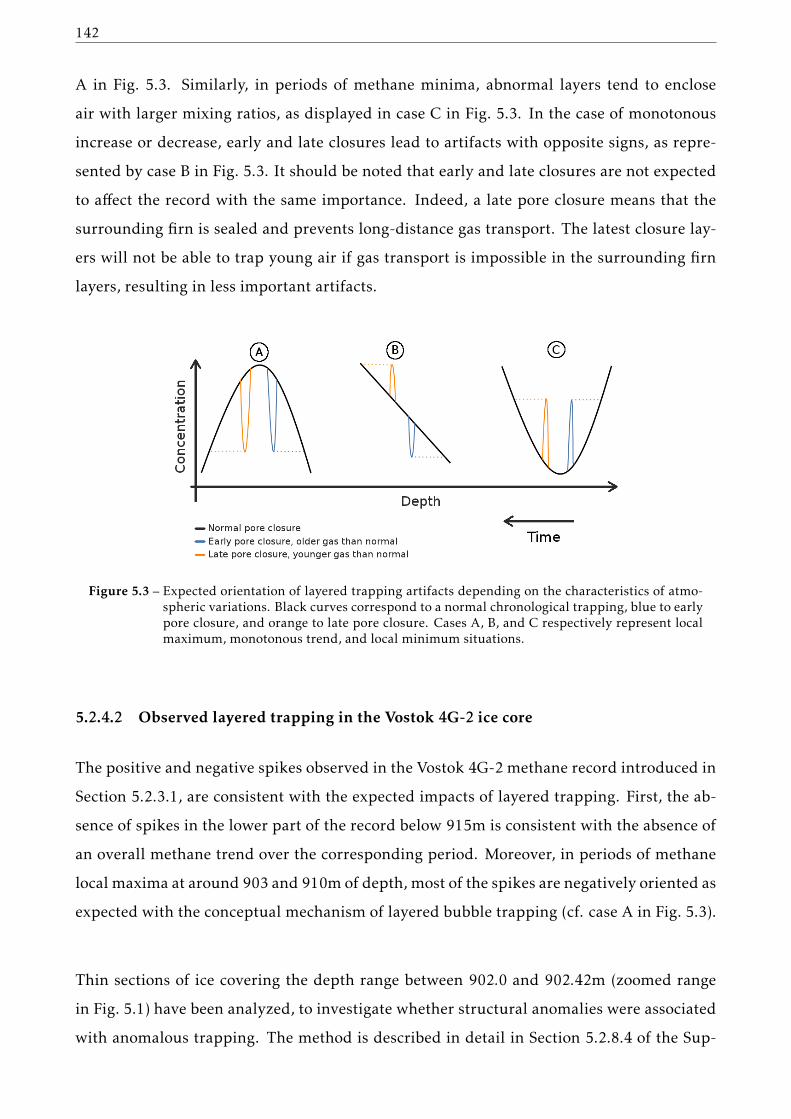
142
A in Fig. 5.3. Similarly, in periods of methane minima, abnormal layers tend to enclose
air with larger mixing ratios, as displayed in case C in Fig. 5.3. In the case of monotonous
increase or decrease, early and late closures lead to artifacts with opposite signs, as repre-
sented by case B in Fig. 5.3. It should be noted that early and late closures are not expected
to affect the record with the same importance. Indeed, a late pore closure means that the
surrounding firn is sealed and prevents long-distance gas transport. The latest closure lay-
ers will not be able to trap young air if gas transport is impossible in the surrounding firn
layers, resulting in less important artifacts.
Figure 5.3 – Expected orientation of layered trapping artifacts depending on the characteristics of atmo-spheric variations. Black curves correspond to a normal chronological trapping, blue to earlypore closure, and orange to late pore closure. Cases A, B, and C respectively represent localmaximum, monotonous trend, and local minimum situations.
5.2.4.2 Observed layered trapping in the Vostok 4G-2 ice core
The positive and negative spikes observed in the Vostok 4G-2 methane record introduced in
Section 5.2.3.1, are consistent with the expected impacts of layered trapping. First, the ab-
sence of spikes in the lower part of the record below 915m is consistent with the absence of
an overall methane trend over the corresponding period. Moreover, in periods of methane
local maxima at around 903 and 910m of depth, most of the spikes are negatively oriented as
expected with the conceptual mechanism of layered bubble trapping (cf. case A in Fig. 5.3).
Thin sections of ice covering the depth range between 902.0 and 902.42m (zoomed range
in Fig. 5.1) have been analyzed, to investigate whether structural anomalies were associated
with anomalous trapping. The method is described in detail in Section 5.2.8.4 of the Sup-

Chapter 5. Alterations of methane records in East Antarctic ice cores 143
plement. We were not able to observe any link between the grain sizes and abnormal layers
in the methane record. Nonetheless, structural anomalies may have existed at the time of
pore closure before disappearing with ∼ 60,000 years of grain evolution. Explanations for
the methane anomalies other than layered trapping were considered as well. Looking for a
correlation between ice quality and methane anomalies was also a motivation for the above
thin section analysis. Although the samples showed small clathrate relaxation cavities, the
CFA sticks did not reveal visual signs of stratification possibly associated with abnormal
layers. Examples of a CFA stick picture and thin section results are provided in the Sup-
plement. The ice samples were not large enough to allow for CFA duplicate analysis, but
the sticks were not melted in a regular depth order so that instabilities in the measurement
system could be more easily detected. As contamination cannot explain negative methane
concentration anomalies, we could not find a convincing alternate explanation for layered
bubble trapping in our results.
5.2.4.3 Simple model of layered trapping
A major difficulty for understanding the gas trapping in ice is to relate the structural prop-
erties measured in small samples to the three-dimensional behavior of the whole firn. For
example, pore closure anomalies have been associated with tortuosity anomalies, with more
tortuous layers closing earlier (Gregory et al., 2014), or to density anomalies, with denser
layers closing earlier (Etheridge et al., 1992; Mitchell et al., 2015; Rhodes et al., 2016). In
this section we used the latter hypothesis supported by observed relationships between local
density and closed porosity (e.g., Stauffer et al., 1985; Mitchell et al., 2015), to test whether
density-driven anomalies could result in artifacts as observed in the Vostok methane record.
In our simple model, the ice core is discretized in layers of 2cm width. Abnormal layers
are stochastically distributed along the ice core. Based on the characteristics of our Vos-
tok methane signal, we use a density of 10 abnormal layers per meter. They are given
a random density anomaly (∆ρ, normally distributed) representing the density variabil-
ity at the bottom of the firn. Based on various sites, Hörhold et al. (2011) propose lin-
ear regressions in which the close-off density variability declines for declining accumula-
tion and temperature. Their lowest-accumulation site is Dome C, with an accumulation
of 2.5cm.ice.yr−1 and a density variability (∆ρ) of 4.6kg.m−3. Applied to Vostok DO-17

144
conditions, the accumulation-based extrapolation leads to a variability of 7kg.m−3 and the
temperature-based extrapolation leads to a variability of 2.7kg.m−3. This defines our ex-
treme values (7 and 3kg.m−3), and we chose the middle number of 5kg.m−3 as the best-guess
value. Hence, in the model, the abnormal layers are given a firn density anomaly distributed
according to a zero-centered Gaussian distribution of standard deviation of 5kg.m−3. In or-
der to convert density anomalies into a closure depth anomaly (the difference in pore clo-
sure depth between an abnormal layer and an adjacent layer following the bulk behavior),
we assume that all layers have similar densification rates (dρ/dz). Using the data-based den-
sity profiles at Dome C, Vostok, and Dome A in Bréant et al. (2017), dρ/dz in deep firn is
estimated to be in the range 1.7 to 2.5kg.m−4. Thus, the gradient is set to be 2kg.m−4. Specif-
ically, a layer closing in advance (or late) closes higher (or lower) in the firn. Dividing the
above typical density anomaly (∆ρ) by the depth gradient (dρ/dz), the characteristic depth
anomaly in deep firn of anomalous layers is about 2.5 meters. Using the estimated accumu-
lation rate of 1.3cm.ice.yr−1 for this period, it translates into an age anomaly (the gas age
difference between an abnormal layer and an adjacent layer following the bulk behavior) of
about 207 years. As explained in Section 5.2.4.1, late pore closure tends to produce weaker
age anomalies than early closure due to the sealing of the surrounding firn. To take into
account the lack of explicit gas transport in the model, we reduce the standard deviation of
late closure age anomalies to 52yr, i.e., 25% of the value used for early closure artifacts. The
value of 25% has been chosen to limit late trapping artifacts in a visually consistent man-
ner with the observations. The methane mixing ratio at a given depth is computed using
an atmospheric trend history and a gas age distribution (GAD) of trapped gases (Romme-
laere et al., 1997). The atmospheric methane scenario used is the high-resolution methane
record from the WAIS Divide ice core (Rhodes et al., 2015). The WDC gas age chronology
(WD2014) was scaled to the GICC05 chronology (with present defined as 1950) dividing by
a factor of 1.0063 as in Buizert et al. (2015). For the rest of the paper we use this scaled
WD2014 chronology to express WDC gas ages. All layers are assumed to have the same
GAD, simply centered on different ages. The GAD used here is the one derived in Sec-
tion 5.2.5.2 specifically for the Vostok ice core during the DO-17 event. A sensitivity test
using a very different GAD is described in the next paragraph. Finally, in order to reproduce
the gas mixing in the CFA system discussed in Section 5.2.2.2, the modeled concentrations
have been smoothed by convolving the signal with an estimated impulse response of the
CFA system (Fig. S2, SI). The smoothing characteristics of our measurement system were
determined experimentally as in Stowasser et al. (2012). The CFA smoothing induces a
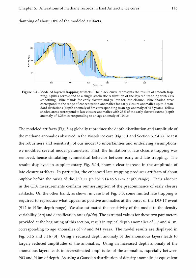
Chapter 5. Alterations of methane records in East Antarctic ice cores 145
damping of about 18% of the modeled artifacts.
Figure 5.4 – Modeled layered trapping artifacts. The black curve represents the results of smooth trap-ping. Spikes correspond to a single stochastic realization of the layered trapping with CFAsmoothing. Blue stands for early closure and yellow for late closure. Blue shaded areascorrespond to the range of concentration anomalies for early closure anomalies up to 2 stan-dard deviations (depth anomaly of 5m corresponding to an age anomaly of 415 years). Yellowshaded areas correspond to late closure anomalies with 25% of the early closure extent (depthanomaly of 1.25m corresponding to an age anomaly of 104yr.
The modeled artifacts (Fig. 5.4) globally reproduce the depth distribution and amplitude of
the methane anomalies observed in the Vostok ice core (Fig. 5.1 and Section 5.2.4.2). To test
the robustness and sensitivity of our model to uncertainties and underlying assumptions,
we modified several model parameters. First, the limitation of late closure trapping was
removed, hence simulating symmetrical behavior between early and late trapping. The
results displayed in supplementary Fig. 5.14, show a clear increase in the amplitude of
late closure artifacts. In particular, the enhanced late trapping produces artifacts of about
50pbbv before the onset of the DO-17 (in the 914 to 917m depth range). Their absence
in the CFA measurements confirms our assumption of the predominance of early closure
artifacts. On the other hand, as shown in case B of Fig. 5.3, some limited late trapping is
required to reproduce what appear as positive anomalies at the onset of the DO-17 event
(912 to 913m depth range). We also estimated the sensitivity of the model to the density
variability (∆ρ) and densification rate (dρ/dz). The extremal values for these two parameters
provided at the beginning of this section, result in typical depth anomalies of 1.2 and 4.1m,
corresponding to age anomalies of 99 and 341 years. The model results are displayed in
Fig. 5.15 and 5.16 (SI). Using a reduced depth anomaly of the anomalous layers leads to
largely reduced amplitudes of the anomalies. Using an increased depth anomaly of the
anomalous layers leads to overestimated amplitudes of the anomalies, especially between
903 and 910m of depth. As using a Gaussian distribution of density anomalies is equivalent
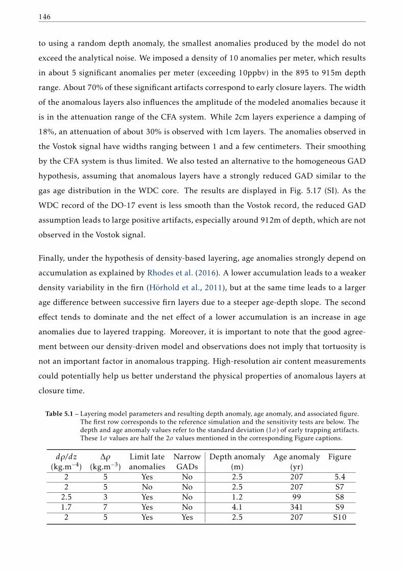
146
to using a random depth anomaly, the smallest anomalies produced by the model do not
exceed the analytical noise. We imposed a density of 10 anomalies per meter, which results
in about 5 significant anomalies per meter (exceeding 10ppbv) in the 895 to 915m depth
range. About 70% of these significant artifacts correspond to early closure layers. The width
of the anomalous layers also influences the amplitude of the modeled anomalies because it
is in the attenuation range of the CFA system. While 2cm layers experience a damping of
18%, an attenuation of about 30% is observed with 1cm layers. The anomalies observed in
the Vostok signal have widths ranging between 1 and a few centimeters. Their smoothing
by the CFA system is thus limited. We also tested an alternative to the homogeneous GAD
hypothesis, assuming that anomalous layers have a strongly reduced GAD similar to the
gas age distribution in the WDC core. The results are displayed in Fig. 5.17 (SI). As the
WDC record of the DO-17 event is less smooth than the Vostok record, the reduced GAD
assumption leads to large positive artifacts, especially around 912m of depth, which are not
observed in the Vostok signal.
Finally, under the hypothesis of density-based layering, age anomalies strongly depend on
accumulation as explained by Rhodes et al. (2016). A lower accumulation leads to a weaker
density variability in the firn (Hörhold et al., 2011), but at the same time leads to a larger
age difference between successive firn layers due to a steeper age-depth slope. The second
effect tends to dominate and the net effect of a lower accumulation is an increase in age
anomalies due to layered trapping. Moreover, it is important to note that the good agree-
ment between our density-driven model and observations does not imply that tortuosity is
not an important factor in anomalous trapping. High-resolution air content measurements
could potentially help us better understand the physical properties of anomalous layers at
closure time.
Table 5.1 – Layering model parameters and resulting depth anomaly, age anomaly, and associated figure.The first row corresponds to the reference simulation and the sensitivity tests are below. Thedepth and age anomaly values refer to the standard deviation (1σ) of early trapping artifacts.These 1σ values are half the 2σ values mentioned in the corresponding Figure captions.
dρ/dz ∆ρ Limit late Narrow Depth anomaly Age anomaly Figure(kg.m−4) (kg.m−3) anomalies GADs (m) (yr)
2 5 Yes No 2.5 207 5.42 5 No No 2.5 207 S72.5 3 Yes No 1.2 99 S81.7 7 Yes No 4.1 341 S92 5 Yes Yes 2.5 207 S10
Chapter 5. Alterations of methane records in East Antarctic ice cores 147
5.2.4.4 Removing layering artifacts in the methane record
To extract an undisturbed (chronologically monotonous and representative of atmospheric
variability only) methane signal from the Vostok 4G-2 core, layered trapping artifacts need
to be removed from the high-resolution CFA record. Some sections of the core exhibit
mainly positive or negative artifacts. Hence removing them using a running average would
bias the signal. To account for this specificity, a cleaning algorithm has been developed. The
underlying assumptions are that the chronological signal is a slowly varying signal with su-
perimposed noise composed of the analytical noise and the layered trapping artifacts. Using
a looping procedure, the artifacts are progressively trimmed until the resulting noise is free
of spikes. The detailed algorithm is described in the following.
- Using the CFA signal (with or without already partially removed layering artifacts during
the cleaning process) a running median is computed with a window of 15cm. Then a binned
mean is computed with bins of 50cm. The goal of this step is to remove noise, without in-
troducing a bias due to layering artifacts.
- A spline of degree 3 is used to interpolate between the binned points on the original CFA
depth scale. This interpolating spline does not further smooth the signal, and is used as an
approximation of the chronologically monotonous signal, free of layering artifacts.
- By removing the spline from the CFA signal we obtain the detrended noise of the signal
composed of the analytical noise and the remaining artifacts.
- We then compute the Normalized Median Absolute Deviation (NMAD) of the detrended
noise. The expression of the NMAD is 1.4826×med(|xi −med(xi)|), where xi represents the
noise values and med the median. This is a robust estimator of variability, weakly sensitive
to outliers (Höhle and Höhle, 2009; Rousseeuw and Hubert, 2011). It enables the estimation
the variability of the noise without the artifacts, i.e. the analytical noise.
- The detrended noise is cut off with a threshold of 2.5 times the NMAD.
- We then check whether the noise is free of spikes. For this we compare the NMAD (estima-
tion of the variability without spikes) and the Standard Deviation (estimation of variability
with spikes) of the detrended noise. If these two quantities are similar, the noise is free
of anomalous layers. Once the Standard Deviation is lower than 1.5 times the NMAD, the
procedure is finished. Otherwise, the algorithm is looped.
This algorithm does not require an estimation of the analytical noise beforehand, since this
value is dynamically computed. However, it is sensitive to the value of 1.5 used to compare
the NMAD and standard deviation to test the presence of artifacts. The remaining signal

148
after cutting off the layered trapping anomalies has a noise amplitude of ±16ppbv, and is
represented in black in Fig. 5.1. With our method 15% of the methane data points have
been removed. As expected, the signal is almost unmodified below 915m, with a portion
of removed points of only 1.3%. On the other hand, the variability above 915m is greatly
reduced and about 26% of the methane data points have been removed.
5.2.5 Smoothing and age distribution in the Vostok 4G-2 ice core
5.2.5.1 The smoothing of the methane record
Once the methane signal is cleaned from layered trapping artifacts, we consider the data
to be a chronologically ordered and unbiased signal recorded in the core. It is smoothed
(high frequencies are damped) with respect to the true atmospheric signal and can be used
to infer the degree of smoothing in the Vostok ice core. The damping can be visualized in
Fig. 5.5 by comparing the Vostok record with theWDC record. High-frequency atmospheric
variability is much better preserved in the WAIS Divide ice core because the accumulation
rate is more than an order of magnitude higher (in the range from 18 to 22cm.ice.yr−1 for
the studied period, Buizert et al., 2015) and thus the firn densification and gas trapping
are faster. For instance, the methane variation spanning between 59,000 and 58,800yrBP
is damped by ∼ 50% in the Vostok record compared to WDC. Moreover, a 20ppbv sub-
centennial variation is present in the WDC record between 58,700 and 58,600yrBP. In the
Vostok record, however, this short-scale variability event has been smoothed out. On the
other hand the multi-centennial variability visible between 58,700 and 58,400yrBP is well
preserved with only a slight damping. From the comparison between WDC and Vostok, we
can infer that the smoothing in Vostok 4G-2 prevents us from retrieving information below
the centennial scale during the DO-17 period.
5.2.5.2 Estimate of the gas age distribution
The smoothing of gas concentrations in ice core records is the direct consequence of the
broad gas age distributions in the ice (Spahni et al., 2003; Joos and Spahni, 2008; Köhler
et al., 2011; Ahn et al., 2014). We call absolute GAD the age distribution expressed on an
absolute timescale, in years before present. The relative GAD is the distribution expressed
relatively to its mean age. For a given layer, absolute and relative GAD thus only differ by a

Chapter 5. Alterations of methane records in East Antarctic ice cores 149
Figure 5.5 – WDCCH4 signal convolvedwith different GADs: the DomeCGAD estimated for the Bølling-Allerød by Köhler et al. (2015) in red, the Dome C GAD estimated for the Last Glacial Max-imum by Köhler et al. (2011) in green, a lognormal fit to the modern Vostok GAD fromWitrant et al. (2012) in yellow, and the Vostok DO-17 GAD estimated in Section 5.2.5.2 inblack (uncertainty envelope shown in light blue). The WDC record (Rhodes et al., 2015) isdisplayed in dashed green, and the CFA Vostok measurements in blue. Yellow dots show thetie points used to match the WDC and Vostok records.
translation in age. Here we assume that all layers densified under the same physical condi-
tions, hence share the same relative GAD. Since computing concentrations along an ice core
using GADs is equivalent to a convolution product (Rommelaere et al., 1997), the resulting
concentrations will be called convolved signals.
The climatic conditions of the glacial period on the Antarctic plateau have no modern ana-
logue, and thus relevant GADs cannot be inferred from modern firn observations. High-
resolution CFA based gas records offer a new opportunity to estimate GADs without mod-
ern analogue. We thus developed such a method, which requires a reference atmospheric
scenario with much higher frequencies resolved. The method can be extended to gases other
than methane or to low-accumulation records other than the Vostok 4G-2 core. The princi-
ple of the method is to determine a GAD able to convolve the high-accumulation record (in
our case, WAIS Divide) into a smoothed signal that minimizes the differences with the ob-
served low-accumulation record (in our case, Vostok). It can be seen as an inverse problem.
Two assumptions are made to reduce the number of adjusted parameters and thus ensure
that the problem is well defined in a mathematical sense. First, all ice layers have the same
relative GAD over the considered period. Second, following Köhler et al. (2011), this rela-
tive GAD is assumed to be a lognormal distribution that is fully characterized by two free
parameters (for instance, its mean and standard deviation). Due to the asymmetry of the
150
GAD, the resulting convolved signal displays age shifts when compared with the original
atmospheric scenario. Hence for a valid comparison between the record and convolved sig-
nals, it is necessary to modify the age scale and to optimize the GAD in an iterative process.
Using an initial age scale, the steps are as follows.
-1: First, a new gas age scale is derived. Tie points are manually selected between the low-
accumulation record and the convolved high-accumulation record. The tie points we se-
lected correspond to minima, maxima, and mid-slopes points of the methane record. For
the initialization, since no GAD has been optimized yet, we use the atmospheric scenario
instead of the convolved signal. The new gas chronology is then generated by interpolation
and extrapolation between tie points.
-2: A new lognormal GAD is optimized by modifying its two parameters in order to mini-
mize differences between the simulated and observed smoothed signals. We performed this
optimization with a differential evolution algorithm (Storn and Price, 1997).
-3: If the definition of a new chronology and a new GAD does not improve the RMSD (root
mean square deviation) between the convolved signal and the measurements five times in a
row, then the algorithm is stopped.
The above methodology can be applied to different ice drilling sites. Here we describe the
specific aspects to match the Vostok record with WDC. Rhodes et al. (2015) state the follow-
ing: ”Only at gas ages > 60ka BP is there a possibility that the continuous measurement sys-
tem caused dampening of the CH4 signal greater than that already imparted by firn-based
smoothing processes”. Moreover, Fig. S1 of the supplement to Rhodes et al. (2015) predicts
a GAD width of about 40yr for the DO-17 event, which is much smaller than the width
of the Vostok GAD. This ensures that the WDC signal resolves enough high frequencies to
be used as the weakly smoothed atmospheric scenario compared to the Vostok record, and
that the convolving function given by the algorithm is close to the actual Vostok GAD. As
explained in Section 5.2.4.2, the WD2014 gas chronology is converted to the GICC05 scale
(Buizert et al., 2015) and not further modified. The algorithm only adjusts the Vostok gas
ages, which remain well within AICC2012 uncertainties. The initial gas ages used are the
ones derived from nitrogen isotope measurements in Section 5.2.3.2, and the optimization
has been performed on data ranging from 900 to 915m of depth. This depth interval has
been chosen since it corresponds to a significantly dampened event in the Vostok record,
which is sensitive to the choice of the GAD. The optimized gas age distribution is displayed

Chapter 5. Alterations of methane records in East Antarctic ice cores 151
in Fig. 5.6 in black, with uncertainty intervals shown as light blue shaded area. The un-
certainty envelope encloses all the distributions resulting in simulated Vostok signals with
a RMSD from the measurements lower than 150% of the optimal an RMSD. The optimal
lognormal parameters are given in Table 5.2. The chosen tie points are displayed in Fig. 5.5,
and the optimized ∆Age values along the Vostok core are depicted in green in Fig. 5.2. The
optimal convolution of the WDC methane record from Rhodes et al. (2015) into a Vostok
signal can be seen in black in Fig. 5.5, with the impact of the uncertainty on the GAD dis-
played as the light blue envelope. The convolution fits the methane measurements within
the analytical noise. The overall consistency between the measured and simulated Vostok
signals confirms that the Vostok record is a smoothed version of the WDC record, and that
the choice of a single GAD for the whole DO-17 record is a credible hypothesis. This last
point is consistent with the fairly stable climatic conditions on the Antarctic plateau over
this time period (Petit et al., 1999; Bazin et al., 2013; Veres et al., 2013).
Figure 5.6 – Gas age distributions. In black: the Vostok GAD during the DO-17 estimated with our opti-mization scheme, the uncertainty envelope is shown in light blue. In yellow: a lognormal fitto the modern-condition Vostok GAD fromWitrant et al. (2012). In red: the estimated DomeC GAD during B/A from Köhler et al. (2015). In green: the estimated Dome C GAD duringLGM from Köhler et al. (2011).
5.2.6 Discussion
5.2.6.1 Understanding the smoothing of ice core signals under low-accumulation con-
ditions
In Fig. 5.6, our GAD adjusted to produce the expected smoothing rate for the DO-17 event
in the Vostok ice core (in black) is compared to other available gas age distributions for
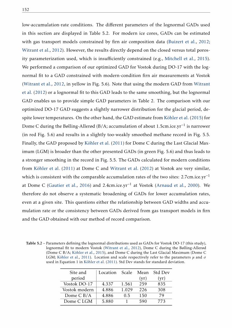
152
low-accumulation-rate conditions. The different parameters of the lognormal GADs used
in this section are displayed in Table 5.2. For modern ice cores, GADs can be estimated
with gas transport models constrained by firn air composition data (Buizert et al., 2012;
Witrant et al., 2012). However, the results directly depend on the closed versus total poros-
ity parameterization used, which is insufficiently constrained (e.g., Mitchell et al., 2015).
We performed a comparison of our optimized GAD for Vostok during DO-17 with the log-
normal fit to a GAD constrained with modern-condition firn air measurements at Vostok
(Witrant et al., 2012, in yellow in Fig. 5.6). Note that using the modern GAD from Witrant
et al. (2012) or a lognormal fit to this GAD leads to the same smoothing, but the lognormal
GAD enables us to provide simple GAD parameters in Table 2. The comparison with our
optimized DO-17 GAD suggests a slightly narrower distribution for the glacial period, de-
spite lower temperatures. On the other hand, the GAD estimate from Köhler et al. (2015) for
Dome C during the Bølling-Allerød (B/A; accumulation of about 1.5cm.ice.yr−1 is narrower
(in red Fig. 5.6) and results in a slightly too-weakly smoothed methane record in Fig. 5.5.
Finally, the GAD proposed by Köhler et al. (2011) for Dome C during the Last Glacial Max-
imum (LGM) is broader than the other presented GADs (in green Fig. 5.6) and thus leads to
a stronger smoothing in the record in Fig. 5.5. The GADs calculated for modern conditions
from Köhler et al. (2011) at Dome C and Witrant et al. (2012) at Vostok are very similar,
which is consistent with the comparable accumulation rates of the two sites: 2.7cm.ice.yr−1
at Dome C (Gautier et al., 2016) and 2.4cm.ice.yr−1 at Vostok (Arnaud et al., 2000). We
therefore do not observe a systematic broadening of GADs for lower accumulation rates,
even at a given site. This questions either the relationship between GAD widths and accu-
mulation rate or the consistency between GADs derived from gas transport models in firn
and the GAD obtained with our method of record comparison.
Table 5.2 – Parameters defining the lognormal distributions used as GADs for Vostok DO-17 (this study),lognormal fit to modern Vostok (Witrant et al., 2012), Dome C during the Bølling-Allerød(Dome C B/A; Köhler et al., 2015), and Dome C during the Last Glacial Maximum (Dome CLGM; Köhler et al., 2011). Location and scale respectively refer to the parameters µ and σused in Equation 1 in Köhler et al. (2011). Std Dev stands for standard deviation.
Site and Location Scale Mean Std Devperiod (yr) (yr)
Vostok DO-17 4.337 1.561 259 835Vostok modern 4.886 1.029 226 308Dome C B/A 4.886 0.5 150 79Dome C LGM 5.880 1 590 773

Chapter 5. Alterations of methane records in East Antarctic ice cores 153
The most likely reason for an inconsistency between GADs inferred from firn models and
from CFA data is the large uncertainty in the representation of gas trapping in firn mod-
els. As mentioned above, the closed versus total porosity ratio is very uncertain, as it was
measured only at a few sites and in small size samples. Better constraints on the physics of
gas trapping would thus be helpful. However, there is no modern analogue of the central
Antarctic plateau sites (such as Vostok or Dome C) under glacial conditions. Thus, using
CFA high-resolution gas measurements at different sites to constrain Holocene GADs at
low-accumulation sites would be the only way to check the consistency of the two meth-
ods. Previous comparisons between sites indicate that the smoothing is larger for low-
accumulation conditions (Spahni et al., 2003; Joos and Spahni, 2008; Köhler et al., 2011;
Ahn et al., 2014). Indeed, a simple argument is that the lower the accumulation and the
temperature, the slower a firn layer will densify, and thus the broader the GAD. The com-
parison of the DO-17 records betweenWDC and Vostok 4G-2 corroborates this relationship:
the higher-accumulation WDC signal is less smooth than the Vostok signal (Fig. 5.5). The
weaker-than-expected smoothing during DO-17 at Vostok could be due to the presence of a
strong layering preventing air renewal and mixing, as suggested in Mitchell et al. (2015).
From a paleoclimatic point of view, an important conclusion of this work is that the smooth-
ing of atmospheric trace gases recorded in ice cores from the central Antarctic plateau could
be less than expected under glacial conditions, resulting in more retrievable information
about past atmospheric conditions. Ice cores with the oldest enclosed gases, such as in the
Oldest Ice project (Fischer et al., 2013), will be retrieved from very low-accumulation sites.
They could thus potentially provide meaningful information down to the multi-centennial
scale.
5.2.6.2 Layered trapping and atmospheric trend reconstructions
The anomalous layers in the Vostok methane record discussed in Section 5.2.4.2 are 1 to a
few centimeters thick, and discrete samples used for methane measurements in ice cores
are typically also a few centimeters thick. In our study, the use of high-resolution con-
tinuous analysis made it possible to identify abnormal methane values that appeared as
spikes in the record. However, in the case of discrete measurements, the absence of con-
tinuous information makes it hard to discriminate between normal and abnormal layers.
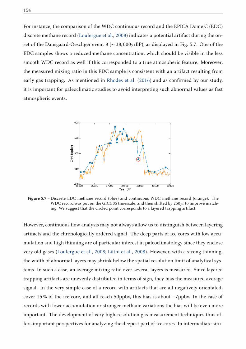
154
For instance, the comparison of the WDC continuous record and the EPICA Dome C (EDC)
discrete methane record (Loulergue et al., 2008) indicates a potential artifact during the on-
set of the Dansgaard-Oeschger event 8 (∼ 38,000yrBP), as displayed in Fig. 5.7. One of the
EDC samples shows a reduced methane concentration, which should be visible in the less
smooth WDC record as well if this corresponded to a true atmospheric feature. Moreover,
the measured mixing ratio in this EDC sample is consistent with an artifact resulting from
early gas trapping. As mentioned in Rhodes et al. (2016) and as confirmed by our study,
it is important for paleoclimatic studies to avoid interpreting such abnormal values as fast
atmospheric events.
Figure 5.7 – Discrete EDC methane record (blue) and continuous WDC methane record (orange). TheWDC record was put on the GICC05 timescale, and then shifted by 250yr to improve match-ing. We suggest that the circled point corresponds to a layered trapping artifact.
However, continuous flow analysis may not always allow us to distinguish between layering
artifacts and the chronologically ordered signal. The deep parts of ice cores with low accu-
mulation and high thinning are of particular interest in paleoclimatology since they enclose
very old gases (Loulergue et al., 2008; Lüthi et al., 2008). However, with a strong thinning,
the width of abnormal layers may shrink below the spatial resolution limit of analytical sys-
tems. In such a case, an average mixing ratio over several layers is measured. Since layered
trapping artifacts are unevenly distributed in terms of sign, they bias the measured average
signal. In the very simple case of a record with artifacts that are all negatively orientated,
cover 15% of the ice core, and all reach 50ppbv, this bias is about −7ppbv. In the case of
records with lower accumulation or stronger methane variations the bias will be even more
important. The development of very high-resolution gas measurement techniques thus of-
fers important perspectives for analyzing the deepest part of ice cores. In intermediate situ-
Chapter 5. Alterations of methane records in East Antarctic ice cores 155
ations in which anomalous layers could be distinguished but a high-accumulation record is
not available (before the last glacial-interglacial cycle), the effect of smoothing is more diffi-
cult to constrain, but the presence of layered trapping artifacts is in itself an indication that
some smoothing may occur because layered trapping occurs only under fast atmospheric
change conditions.
5.2.7 Conclusions
Wepresented the first very high-resolution record ofmethane in an ice core sequence formed
under very low-accumulation-rate conditions. It covers the gas record of Dansgaard-Oeschger
event 17, chosen for its abrupt atmospheric methane changes on a similar timescale as gas
trapping.
The continuous flow analysis system, optimized to reduce gas mixing, allowed us to reveal
numerous centimeter-scale methane concentration anomalies. Positive anomalies affecting
both the methane and carbon monoxide records were attributed to kerosene contamination
and discarded. The remaining anomalies are unevenly distributed, a few centimeters wide
and mostly negatively oriented with dips as low as −50ppbv. The anomalies occur only dur-
ing time periods of fast atmospheric methane variability. The main characteristics of the
size and distribution of the anomalies could be reproduced with a simple model based on
relating realistic firn density anomalies to early or (to a lesser extent) late trapping. Such
layered trapping anomalies may be confused with the climatic signal in discrete climate
records or bias the signal if too narrow to be detected by a CFA system (e.g., under the high-
thinning conditions of the deep part of ice cores). It is important for future paleoclimatic
studies not to interpret those abrupt variations as fast chronologically ordered atmospheric
variations. Further use of high-resolution continuous analysis will allow us to discriminate
layered trapping artifacts and to better identify their statistical characteristics. Moreover,
the sign of the trapping artifacts is not random: some sections of the record display only
positive or negative artifacts. Thus, simple averaging would result in a systematic bias of
the signal. Hence, we developed a cleaning algorithm aiming at minimizing this bias.
After removing the centimeter-scale anomalies, the remaining Vostok methane signal is dis-
tinctly smoother than the WDC record (Rhodes et al., 2015). The snow accumulation rate

156
being more than 1 order of magnitude higher at WDC than at Vostok, the WDC signal con-
tains higher-frequency features. The comparison of the two signals opens the possibility to
estimate gas age distributions for conditions of the East Antarctic plateau during the last
glacial period, which have no modern analogue. For the DO-17 event at Vostok, the result-
ing gas age distribution is narrower than expected from a comparison with modern firns
(Köhler et al., 2011; Witrant et al., 2012). It may be due to an incorrect prediction of gas
trapping by firn models and/or an incorrect extrapolation of the firn behavior to very low-
temperature and low-accumulation conditions. The apparently similar smoothing at Vostok
under DO-17 and present conditions contradicts the expected primary effect of tempera-
ture and accumulation rate: lower temperature and accumulation rates induce a longer gas
trapping duration and thus a stronger smoothing. On the other hand, Mitchell et al. (2015)
point out the lack of firn layering representation in most firn models and conclude that firn
layering narrows gas age distribution in ice. From a paleoclimatic point of view, ice cores
with the lowest accumulations contain very old gases. The smoothing under glacial condi-
tions being less important than expected implies that atmospheric information on a shorter
timescale than previously expected might be retrieved. However, similar measurements
need to be performed on other low-accumulation records, to confirm our results for differ-
ent sites and/or periods. For the DO-17 event at Vostok, multi-centennial atmospheric vari-
ations are still accessible in the record. Further comparisons of high- and low-accumulation
records of the last glacial cycle will allow us to better constrain the relationship between ice
cores and atmospheric gas signals, even with no modern analogue conditions.
5.2.8 Supplementary Material
5.2.8.1 Calibration of methane measurements
Calibration of SARA on NOAA2004 scale
The laser spectrometer used for the continuous methane measurements (SARA) was cali-
brated against the NOAA2004 scale (Dlugokencky et al., 2005) before starting the ice core
analyzes. Three calibrated standard gases of known methane mixing ratios, listed Table
5.3, were measured with the SARA instrument. We derived a linear relationship between
measured and calibrated mixing ratios over the range of 361 to 1790ppbv, with a coefficient
of determination R = 0.9999993. The data and regression line are displayed Fig. 5.8. This
correction was applied to the SARA Vostok 4G-2 measurements.

Chapter 5. Alterations of methane records in East Antarctic ice cores 157
Table 5.3 – Calibrated and measured methane mixing ratios of Scott Marrin Inc. standard gases.
Gas Reference Calibrated value (pbbv) Measured value (pbbv)CB09722 703.90 695.5CB09752 1789.42 1775.9CB09754 360.09 355.3
Correction for methane solubility
In the measurement line, once the ice core is melted, the liberated gases dissolve in the melt
water. However, methane has a higher solubility than oxygen or nitrogen, and it follows that
CH4 dissolves preferentially, leading to reduced methane mixing ratios in the extracted air
reaching the SARA spectrometer. The solubility correction was evaluated by comparing the
Vostok signal with WAIS Divide ice core (WDC) data: a CFA record already corrected for
solubility effects (Rhodes et al., 2015). The solubility factor was estimated by comparing the
mean concentration over the plateau preceding the DO-17 event, unaffected by smoothing.
This corresponds to a depth interval from 920 to 931m in the Vostok ice core. The resulting
solubility correction coefficient of 1.125, consistent with the previous estimate for our CFA
system, was applied to the whole Vostok dataset.
5.2.8.2 Quantification of the smoothing by the CFA system
Due to mixing and dead volumes, the CFA system introduces a smoothing of the gas signals.
Using the method described in Stowasser et al. (2012), we measured the switch between two
mixes of deionized water and standard gas (Fig. S2, left panel). It allowed us to determine
the step response of the CFA system, which is not instantaneous but spreads over time. The
observed step response was fitted using the cumulative density function of a log-normal
distribution. This log-normal distribution (Fig. S2, middle panel) can be further used as a
Green’s function, or impulse response of the CFA system, to estimate the smoothing of other
signals such as the simulated density-related concentration anomalies in Section 5.2.4.3 of
the article. Finally, the Green’s function can be used to derive the frequency response of the
system using Fourier transform, that is to say the attenuation factor (also referred to as a
gain) experienced by a sine signal depending on its frequency/period/wavelength.
A cut-off wavelength can be defined as the wavelength of a sine signal experiencing a 50%
attenuation in amplitude. For our CFA system with a melting rate of 3.8cm.min−1, the cut-
158
off wavelength is about 2.4cm. It is important to note that this cut-off is defined for sine
signals, and therefore cannot be directly applied to other types of signals. For instance, a
square spike with a width of 2.4cm will not be attenuated by 50%. Indeed, it has a low-
frequency rich harmonic content and thus undergoes a weaker attenuation. This explains
why layered trapping artifacts with widths slightly below the cut-off wavelength used in
Section 5.2.4.3 of the article are weakly damped in the CFA signal.
5.2.8.3 Kerosene contamination
As explained in Section 5.2.3.1 of the article, traces of kerosene producing iridescent colors
and a strong smell were occasionally detected in the meltwater. Concomitant increases in
CH4 and CO were assumed to result from kerosene contaminations. An example of such
typical simultaneous increases is displayed on Fig. 5.10. Even though the origin of these
kerosene contaminations is not clear, they might come from cracks observed in the CFA
sticks as seen in Fig. 5.11.
5.2.8.4 Thin sections of the Vostok 4G-2 core
Four thin sections were prepared over a region of the Vostok 4G-2 ice core which shows
layered trapping artifacts. The crystallographic orientations of grains were measured using
an Automatic Texture Analyzer (Wilson et al., 2003; Peternell et al., 2010). The images were
then segmented to visualize grain boundaries, using a high-pass filter and a threshold tech-
nique. Grain boundaries were enhanced with cycles of dilate/erode. The segmented thin
sections are displayed on Fig. 5.12. The numbers of intersections between grain boundaries
and constant depth lines were computed as a metric for local grain size. However, the thin
sections displayed various degrees of noise, impacting the number of intersection counted.
To reduce the influence of noise, we normalized the numbers of intersections of each section
by dividing them by the mean number of intersections of the whole thin section. This did
not affect the interpretation of our results, as we were searching for local variations of grain
size rather than absolute size values. Figure 5.13 shows the methane record together with
the normalized number of intersections around 902m depth. The methane record presents
two clear layered trapping artifacts, marked by red dots on Fig. 5.13. However, the grain
size metric does not show a correlation with the two anomalous layers.
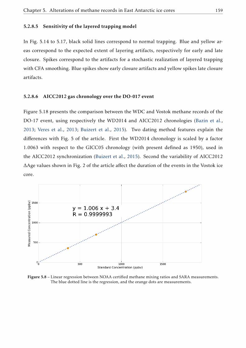
Chapter 5. Alterations of methane records in East Antarctic ice cores 159
5.2.8.5 Sensitivity of the layered trapping model
In Fig. 5.14 to 5.17, black solid lines correspond to normal trapping. Blue and yellow ar-
eas correspond to the expected extent of layering artifacts, respectively for early and late
closure. Spikes correspond to the artifacts for a stochastic realization of layered trapping
with CFA smoothing. Blue spikes show early closure artifacts and yellow spikes late closure
artifacts.
5.2.8.6 AICC2012 gas chronology over the DO-017 event
Figure 5.18 presents the comparison between the WDC and Vostok methane records of the
DO-17 event, using respectively the WD2014 and AICC2012 chronologies (Bazin et al.,
2013; Veres et al., 2013; Buizert et al., 2015). Two dating method features explain the
differences with Fig. 5 of the article. First the WD2014 chronology is scaled by a factor
1.0063 with respect to the GICC05 chronology (with present defined as 1950), used in
the AICC2012 synchronization (Buizert et al., 2015). Second the variability of AICC2012
∆Age values shown in Fig. 2 of the article affect the duration of the events in the Vostok ice
core.
Figure 5.8 – Linear regression between NOAA certified methane mixing ratios and SARA measurements.The blue dotted line is the regression, and the orange dots are measurements.

160
Figure 5.9 – Left panel: step response of the CFA system. Orange dots: measurement points. In blue:fit by the cumulative density function of a log-normal law. Middle panel: Green’s Functionof the CFA system approximated by a log normal law. Right panel: Gain of the CFA systemagainst the wavelength of sine signals. Gray lines correspond to the cut-off wavelength and a50% attenuation.
Figure 5.10 – Example of concomitant increases in CH4 and CO attributed to kerosene contamination.Methane (in blue) and carbon monoxide (in yellow) records display simultaneous fast vari-ability. The x-scale represents the measurement time. The length of ice melted in the datashown is about 25cm.
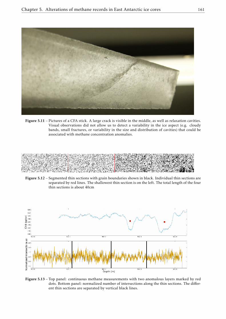
Chapter 5. Alterations of methane records in East Antarctic ice cores 161
Figure 5.11 – Pictures of a CFA stick. A large crack is visible in the middle, as well as relaxation cavities.Visual observations did not allow us to detect a variability in the ice aspect (e.g. cloudybands, small fractures, or variability in the size and distribution of cavities) that could beassociated with methane concentration anomalies.
Figure 5.12 – Segmented thin sections with grain boundaries shown in black. Individual thin sections areseparated by red lines. The shallowest thin section is on the left. The total length of the fourthin sections is about 40cm
Figure 5.13 – Top panel: continuous methane measurements with two anomalous layers marked by reddots. Bottom panel: normalized number of intersections along the thin sections. The differ-ent thin sections are separated by vertical black lines.

162
Figure 5.14 – Layered trapping model without limitation for late closure age anomalies. Both shaded ar-eas correspond to the range of concentration anomalies for early and late closure anomaliesup to two standard deviations (depth anomaly of 5m corresponding to an age anomaly of415yr.
Figure 5.15 – Layered trapping model with density anomalies standard deviation set to 3kg.m−3 anddρ/dz set to 2.5kg.m−4. Blue shaded areas correspond to the range of concentration anoma-lies for early closure anomalies up to two standard deviations (depth anomaly of 2.4m cor-responding to an age anomaly of 200yr). Yellow shaded areas correspond to late closureanomalies with 25% of the early closure extent (depth anomaly of 0.6m corresponding toan age anomaly of 50yr).
Figure 5.16 – Layered trapping model with density anomalies standard deviation set to 7kg.m−3 anddρ/dz set to 1.7kg.m−4. Blue shaded areas correspond to the range of concentration anoma-lies for early closure anomalies up to two standard deviations (depth anomaly of 8.2m cor-responding to an age anomaly of 684yr). Yellow shaded areas correspond to late closureanomalies with 25% of the early closure extent (depth anomaly of 2.1m corresponding toan age anomaly of 171yr).

Chapter 5. Alterations of methane records in East Antarctic ice cores 163
Figure 5.17 – Layered trapping model with anomalous layers undergoing the WDC gas age distribution.The dashed black line corresponds to the WDC signal on the Vostok depth scale. Blueshaded areas correspond to the range of concentration anomalies for early closure anomaliesup to two standard deviations (depth anomaly of 5m corresponding to an age anomaly of415yr. Yellow shaded areas correspond to late closure anomalies with 25% of the earlyclosure extent (depth anomaly of 1.25m corresponding to an age anomaly of 104yr).
Figure 5.18 – In green: WDC methane record with the WDC2014 gas chronology from Buizert et al.(2015). In blue: Vostok methane record with the AICC2012 gas chronology (Bazin et al.,2013; Veres et al., 2013).

164
5.3 Estimation of gas record alteration in very low accumu-
lation ice cores
Kévin Fourteau1, Patricia Martinerie1, Xavier Faïn1, Alexey A. Ekaykin2, and Jérôme Chappellaz1,
Vladimir Ya. Lipenkov2
[1] Univ. Grenoble Alpes, CNRS, IRD, Grenoble INP, IGE, 38000 Grenoble, France
[2] Climate and Environmental Research Laboratory, Arctic and Antarctic Research Institute, St. Petersburg,
199397, Russia
Abstract
We measured the methane mixing ratios of enclosed air in five ice core sections drilled on
the East Antarctic plateau. Our work aims to study two effects that affect the recorded gas
concentrations in ice cores: layered gas trapping artifacts and firn smoothing. Layered gas
trapping artifacts are due to the heterogeneous nature of polar firn, where some strata might
close early and trap abnormally old gases that appear as spurious values during measure-
ments. The smoothing is due to the combined effects of diffusive mixing in the firn and the
progressive closure of bubbles at the bottom of the firn. Consequently, the gases trapped
in a given ice layer span a distribution of ages that acts similarly to a moving average, re-
moving the fast variability from the record. We focus on the study of East Antarctic plateau
ice cores, as these low accumulation ice cores are particularly affected by both layering and
smoothing. Our results suggest that presence of layering artifacts in deep ice cores is linked
with the chemical content of the ice. We use high resolution methane data to parametrize
a simple model reproducing the layered gas trapping artifacts for different accumulation
conditions typical of the East Antarctic plateau. We also use the high resolution methane
measurements to estimate the gas age distributions of the enclosed air in the five newlymea-
sured ice core sections. It appears that for accumulations below 2cm ie yr−1 (ice equivalent)
the gas records experience nearly the same degree of smoothing. We therefore propose to
use a single gas age distribution to represent the firn smoothing observed in the glacial ice
cores of the East Antarctic plateau. Finally, we used the layered gas trapping model and the
estimation of glacial firn smoothing to estimate their potential impacts on a million-and-
a-half years old ice core from the East Antarctic plateau. Our results indicate that layering
artifacts are no longer individually resolved in the case of very thinned ice near the bedrock.
They nonetheless contribute to slight biases of the measured signal (less than 10ppbv and

Chapter 5. Alterations of methane records in East Antarctic ice cores 165
0.5ppmv in the case of methane and carbon dioxide). However, these biases are small com-
pared to the dampening experienced by the record due to firn smoothing.
5.3.1 Introduction
The East Antarctic plateau is characterized by low temperatures and low accumulation rates.
The low precipitations create the conditions for the presence of very old ice near the domes
of the region (Raymond, 1983; Martín and Gudmundsson, 2012). Thanks to this particu-
larity, the ice core retrieved at Dome C, within the EPICA project, has been dated back to
800,000yr in the past (Bazin et al., 2013; Veres et al., 2013). The analysis of the ice, and
of the bubbles within, has made possible the reconstruction of the Earth past temperatures
and atmospheric concentrations in major greenhouse gases over the last eight glacial cycles
(Lüthi et al., 2008; Loulergue et al., 2008). In turn, this knowledge helps us to better un-
derstand the Earth climate system and its past and future evolutions (Shakun et al., 2012).
Furthermore, there is currently an active search for ice older than one-and-a-half million
years with the International Partnership in Ice Core Sciences oldest ice core project. Most of
the potential drilling sites for such old ice are located on the East Antarctic plateau (Fischer
et al., 2013; Van Liefferinge and Pattyn, 2013; Passalacqua et al., 2018). Within the next
decade, we might therefore expect the retrieval of new deep ice cores at low accumulation
drilling sites of East Antarctica, with ages reaching back to one-and-a-half million years or
more.
However, the gas records in low accumulation ice cores should not be directly interpreted
as images of the atmospheric history. Indeed, due to the very process of gas trapping in the
ice, two distinct effects might create discrepancies between the actual atmosphere’s history
and its imprint the ice. The first one is due to the heterogeneous structure of the firn when
transforming into airtight ice. The overall structure of the firn column is characterized by a
progressive increase in density with depth, associated with the constriction of the intersti-
tial pore network (Stauffer et al., 1985; Arnaud et al., 2000; Salamatin et al., 2009). At high
enough densities, pores in the firn pinch and isolate the interstitial air from the atmosphere
(Stauffer et al., 1985). However, firn is a highly stratified medium (Freitag et al., 2004; Fujita
et al., 2009; Hörhold et al., 2012; Gregory et al., 2014) and some of the strata might experi-
ence early (respectively late) pore closure when compared to the rest of the firn (Etheridge

166
et al., 1992; Martinerie et al., 1992). Consequently, abnormal strata might enclose older
(respectively younger) air than their immediate surroundings, creating age irregularities in
the gas record (Mitchell et al., 2015; Rhodes et al., 2016). In turn, the irregularities appear
as spurious values in the measured gas record (Rhodes et al., 2016; Fourteau et al., 2017).
These anomalies have been referred to as layered gas trapping artifacts and do not reflect
actual atmospheric variations. The second effect that creates differences between the atmo-
sphere and its imprint in the ice, is due to the combination of diffusive air mixing in the
firn (Schwander, 1989) and the progressive closure of pores in a firn stratum (Schwander
et al., 1993; Mitchell et al., 2015). Consequently, the air enclosed in a given ice layer does
not originate from a single point in time, but is rather characterized by a continuous age
distribution covering tens to hundreds of years (Schwander et al., 1988; Schwander et al.,
1993; Rommelaere et al., 1997). Therefore, the concentration measured in an ice stratum is
an average of atmospheric concentrations over a period of time. This effect acts as a mov-
ing average, removing the variability from the record, and has therefore been referred to as
the smoothing effect (Spahni et al., 2003; Joos and Spahni, 2008; Köhler et al., 2011; Ahn
et al., 2014; Fourteau et al., 2017). The degree of alteration between the atmosphere and its
recording is strongly dependent on the local precipitation rate, with low accumulation ice
cores being particularly affected both in terms of gas layered artifacts (Rhodes et al., 2016;
Fourteau et al., 2017) and in terms of smoothing (Spahni et al., 2003; Joos and Spahni, 2008;
Köhler et al., 2011; Ahn et al., 2014; Fourteau et al., 2017).
In order to properly evaluate the composition of past atmospheres based on the gas records
in polar ice cores, it is thus necessary to characterize the specificities of those two effects. For
the smoothing, the gas age distributions can be calculated, in the case of modern ice cores,
using gas trapping models parameterized by firn pumping and pore closure data (Buizert
et al., 2012; Witrant et al., 2012). However, to estimate the gas age distribution in bubbles
it is necessary to use a closed porosity profile in firn. Such closed porosity profiles are as-
sociated with large uncertainties (Schaller et al., 2017). Moreover, a specific problem arises
in the case of glacial ice cores from East Antarctica. They were formed under very low pre-
cipitation rates, below 2cm.ie.yr−1 (ice equivalent, Veres et al., 2013; Bazin et al., 2013), and
temperatures that have no known equivalent nowadays. Thus, gas trapping models can-
not be constrained and used to estimate the gas age distributions responsible for smoothing
during glacial periods. Concerning layered gas trapping, it originates from firn hetero-

Chapter 5. Alterations of methane records in East Antarctic ice cores 167
geneities and is therefore a stochastic process. Moreover, current gas trapping models do
not fully represent the centimeter scale variability of the firn. The proper modelling of lay-
ered gas trapping is thus limited by the lack of knowledge of glacial firn heterogeneities and
the difficulty to model gas trapping in a layered medium. Fourteau et al. (2017) proposed
an empirical model to reproduce the artifacts observed in the Vostok ice core during the
Dansgaard-Oeschger event 17. However, this model has only been applied to this particular
event and might not be directly applicable for different periods and conditions.
For this work, we analyzed methane concentrations in five ice core sections from the East
Antarctic plateau. These sections cover accumulation and temperature conditions represen-
tative of East Antarctica for both the glacial and inter-glacial periods. The new data are used
to parameterize a revised version of the gas layered trapping model proposed by Fourteau
et al. (2017). Our goal is to render this model applicable to a range of accumulation rates
characteristic of glacial and inter-glacial conditions on the East Antarctic plateau. Then,
the gas age distributions for each of the five records are estimated by comparing the low
accumulation records with much higher accumulation records (Fourteau et al., 2017). Fi-
nally, we simulate gas trapping in a hypothetical million-and-a-half years old and thinned
ice core, including gas layering artifacts. We then simulate the process of methane measure-
ments using a continuous flow analysis system, and of carbon dioxide measurements using
a discrete method. The synthetic signals are finally compared to the original atmospheric
reference to quantify the deterioration of atmospheric information.
5.3.2 Methods
5.3.2.1 Choice and description of the studied ice cores
The newly measured ice core sections originate from the East Antarctic sites of Vostok,
Dome C, and Lock-In. The three sites are displayed on a map in Figure 5.19. The five mea-
sured sections correspond to time periods where high resolution methane measurements
from high-accumulation ice cores are also available.
Modern Lock-In ice core:
The first studied ice core section is the upper part of the Lock-In ice core. The site of Lock-In
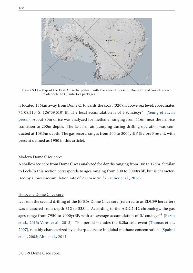
168
Figure 5.19 – Map of the East Antarctic plateau with the sites of Lock-In, Dome C, and Vostok shown(made with the Quantartica package).
is located 136km away from Dome C, towards the coast (3209m above sea level, coordinates
74°08.310′ S, 126°09.510′ E). The local accumulation is of 3.9cm.ie.yr−1 (Yeung et al., in
press.). About 80m of ice was analyzed for methane, ranging from 116m near the firn-ice
transition to 200m depth. The last firn air pumping during drilling operation was con-
ducted at 108.3m depth. The gas record ranges from 500 to 3000yrBP (Before Present, with
present defined as 1950 in this article).
Modern Dome C ice core:
A shallow ice core fromDome Cwas analyzed for depths ranging from 108 to 178m. Similar
to Lock-In this section corresponds to ages ranging from 500 to 3000yrBP, but is character-
ized by a lower accumulation rate of 2.7cm.ie.yr−1 (Gautier et al., 2016).
Holocene Dome C ice core:
Ice from the second drilling of the EPICA Dome C ice core (referred to as EDC99 hereafter)
was measured from depth 312 to 338m. According to the AICC2012 chronology, the gas
ages range from 7950 to 9000yrBP, with an average accumulation of 3.1cm.ie.yr−1 (Bazin
et al., 2013; Veres et al., 2013). This period includes the 8.2ka cold event (Thomas et al.,
2007), notably characterized by a sharp decrease in global methane concentrations (Spahni
et al., 2003; Ahn et al., 2014).
DO6-9 Dome C ice core:
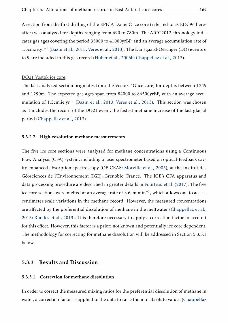
Chapter 5. Alterations of methane records in East Antarctic ice cores 169
A section from the first drilling of the EPICA Dome C ice core (referred to as EDC96 here-
after) was analyzed for depths ranging from 690 to 780m. The AICC2012 chronology indi-
cates gas ages covering the period 33000 to 41000yrBP, and an average accumulation rate of
1.5cm.ie.yr−1 (Bazin et al., 2013; Veres et al., 2013). The Dansgaard-Oeschger (DO) events 6
to 9 are included in this gas record (Huber et al., 2006b; Chappellaz et al., 2013).
DO21 Vostok ice core:
The last analyzed section originates from the Vostok 4G ice core, for depths between 1249
and 1290m. The expected gas ages span from 84000 to 86500yrBP, with an average accu-
mulation of 1.5cm.ie.yr−1 (Bazin et al., 2013; Veres et al., 2013). This section was chosen
as it includes the record of the DO21 event, the fastest methane increase of the last glacial
period (Chappellaz et al., 2013).
5.3.2.2 High-resolution methane measurements
The five ice core sections were analyzed for methane concentrations using a Continuous
Flow Analysis (CFA) system, including a laser spectrometer based on optical-feedback cav-
ity enhanced absorption spectroscopy (OF-CEAS; Morville et al., 2005), at the Institut des
Géosciences de l’Environnement (IGE), Grenoble, France. The IGE’s CFA apparatus and
data processing procedure are described in greater details in Fourteau et al. (2017). The five
ice core sections were melted at an average rate of 3.6cm.min−1, which allows one to access
centimeter scale variations in the methane record. However, the measured concentrations
are affected by the preferential dissolution of methane in the meltwater (Chappellaz et al.,
2013; Rhodes et al., 2013). It is therefore necessary to apply a correction factor to account
for this effect. However, this factor is a priori not known and potentially ice core dependent.
The methodology for correcting for methane dissolution will be addressed in Section 5.3.3.1
below.
5.3.3 Results and Discussion
5.3.3.1 Correction for methane dissolution
In order to correct the measured mixing ratios for the preferential dissolution of methane in
water, a correction factor is applied to the data to raise them to absolute values (Chappellaz
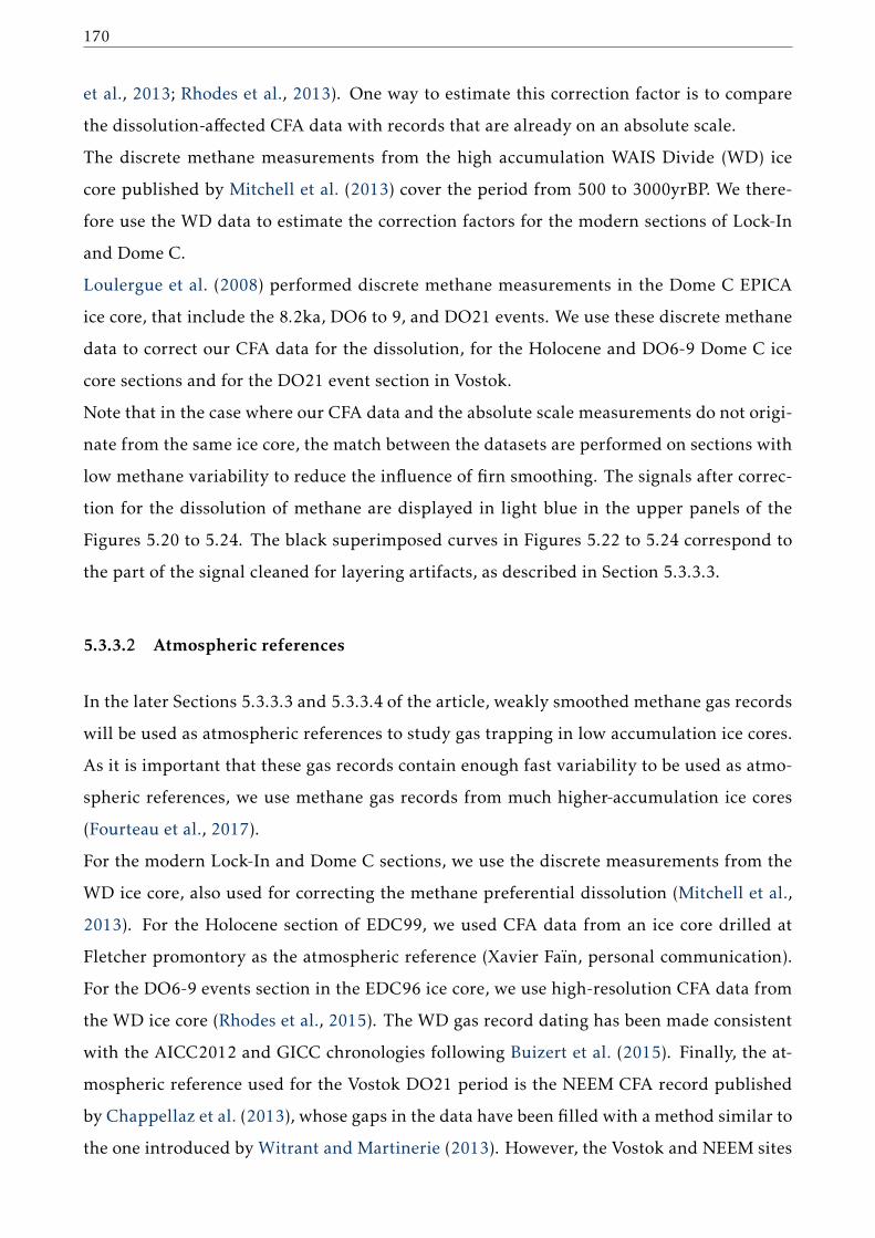
170
et al., 2013; Rhodes et al., 2013). One way to estimate this correction factor is to compare
the dissolution-affected CFA data with records that are already on an absolute scale.
The discrete methane measurements from the high accumulation WAIS Divide (WD) ice
core published by Mitchell et al. (2013) cover the period from 500 to 3000yrBP. We there-
fore use the WD data to estimate the correction factors for the modern sections of Lock-In
and Dome C.
Loulergue et al. (2008) performed discrete methane measurements in the Dome C EPICA
ice core, that include the 8.2ka, DO6 to 9, and DO21 events. We use these discrete methane
data to correct our CFA data for the dissolution, for the Holocene and DO6-9 Dome C ice
core sections and for the DO21 event section in Vostok.
Note that in the case where our CFA data and the absolute scale measurements do not origi-
nate from the same ice core, the match between the datasets are performed on sections with
low methane variability to reduce the influence of firn smoothing. The signals after correc-
tion for the dissolution of methane are displayed in light blue in the upper panels of the
Figures 5.20 to 5.24. The black superimposed curves in Figures 5.22 to 5.24 correspond to
the part of the signal cleaned for layering artifacts, as described in Section 5.3.3.3.
5.3.3.2 Atmospheric references
In the later Sections 5.3.3.3 and 5.3.3.4 of the article, weakly smoothed methane gas records
will be used as atmospheric references to study gas trapping in low accumulation ice cores.
As it is important that these gas records contain enough fast variability to be used as atmo-
spheric references, we use methane gas records from much higher-accumulation ice cores
(Fourteau et al., 2017).
For the modern Lock-In and Dome C sections, we use the discrete measurements from the
WD ice core, also used for correcting the methane preferential dissolution (Mitchell et al.,
2013). For the Holocene section of EDC99, we used CFA data from an ice core drilled at
Fletcher promontory as the atmospheric reference (Xavier Faïn, personal communication).
For the DO6-9 events section in the EDC96 ice core, we use high-resolution CFA data from
the WD ice core (Rhodes et al., 2015). The WD gas record dating has been made consistent
with the AICC2012 and GICC chronologies following Buizert et al. (2015). Finally, the at-
mospheric reference used for the Vostok DO21 period is the NEEM CFA record published
by Chappellaz et al. (2013), whose gaps in the data have been filled with a method similar to
the one introduced by Witrant and Martinerie (2013). However, the Vostok and NEEM sites

Chapter 5. Alterations of methane records in East Antarctic ice cores 171
are in different hemispheres and it is necessary to take into account the inter-hemispheric
methane gradient between the two sites. We evaluated this inter-hemispheric gradient to
be at 30ppbv for the DO21 period. This value is in line with the work of Dällenbach et al.
(2000). Yet, it remains possible that the inter-hemispheric gradient is not constant dur-
ing this period of global methane rise. The use of a high resolution and weakly smoothed
Antarctic record as the atmospheric reference would resolve this problem, but such a record
is not available. The atmospheric references are displayed as orange dashed lines in the
lower panels of Figure 5.20 to 5.24.
Figure 5.20 – Measured and modeled modern Lock-In methane profile. Upper panel: High resolutionmethane measurements in light blue. Lower panel: Modeled layering artifacts. The blackcurve is the expected signal without artifacts. The blue and yellow spikes respectively arerandomly distributed early and late closure artifacts. The blue and yellow shaded areasrespectively correspond to the range of early and late artifacts with density anomalies upto two standard deviations. The dashed orange curve is the record used as the atmosphericreference.
Figure 5.21 – Same as Figure 5.20 for the modern Dome C section.
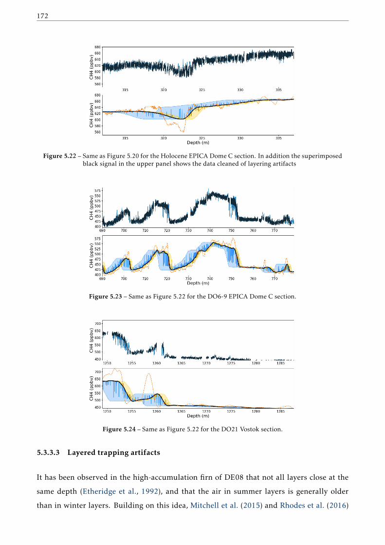
172
Figure 5.22 – Same as Figure 5.20 for the Holocene EPICA Dome C section. In addition the superimposedblack signal in the upper panel shows the data cleaned of layering artifacts
Figure 5.23 – Same as Figure 5.22 for the DO6-9 EPICA Dome C section.
Figure 5.24 – Same as Figure 5.22 for the DO21 Vostok section.
5.3.3.3 Layered trapping artifacts
It has been observed in the high-accumulation firn of DE08 that not all layers close at the
same depth (Etheridge et al., 1992), and that the air in summer layers is generally older
than in winter layers. Building on this idea, Mitchell et al. (2015) and Rhodes et al. (2016)

Chapter 5. Alterations of methane records in East Antarctic ice cores 173
proposed that the layering observed at the firn-ice transition induces gas stratigraphic ir-
regularities and age inversions in the record. Rhodes et al. (2016) and Fourteau et al. (2017)
used such stratigraphic heterogeneities to explain the observation of sudden variations in
high resolution methane records. These abrupt methane variations do not correspond to ac-
tual atmospheric variations and have been called layered trapping artifacts, or more simply
layering artifacts. The mechanism producing them is that layers closing especially early (or
late) contain air older (or younger) than their immediate surroundings. During periods of
variations of atmospheric composition, the methane mixing ratios in these layers are thus
different than in their surroundings and appear as anomalous values (Rhodes et al., 2016).
In accordance with Rhodes et al. (2016) and Fourteau et al. (2017), we observe abrupt varia-
tions in the methane records, larger than the analytical noise of ∼ 10ppbv, during periods of
variations in atmospheric concentrations. These layering artifacts are notably well marked
during the onset of DO events 8 and 21, corresponding to 750 and 1252m depth in the
EDC96 and Vostok ice cores, respectively in Figure 5.23 and 5.24. They appear as reduced
methane concentration layers near the onset of the DO events, and cannot therefore be ex-
plained by contamination issues. The layered trapping artifacts tend to disappear in the
absence of marked atmospheric variations. This explains the absence of important layering
artifacts in the Lock-In and Dome C modern records (Figures 5.20 and 5.21).
Important late closure artifacts are unusual in methane gas records. These new measure-
ments confirm this observation. Late closure artifacts, that should appear as positivemethane
anomalies at the onset of the DO events, are almost absent in our measurements. This can
be explained by the fact that the surrounding firn layers are already sealed and prevent long
distance gas transport, which in turn prevents the late closure layers to enclose young air
(Fourteau et al., 2017).
Impact of chemistry on layered gas trapping
The EDC96 methane data suggest a lack of layering artifacts affecting the DO6 event
(around the depth 700m in Figure 5.23). We counted only 14 layering artifacts that clearly
stand out of the analytical noise on the 20m long section between 695 and 715m. For a
comparison, we counted 15 artifacts on the 4m long section from 718 to 722m (DO7 event).
These sections are not directly comparable as they are not characterized by the same atmo-
spheric methane variations, but it nonetheless suggests that the upper section of the DO6-9
record shows a lower number of layering artifacts per meter. Previous studies have high-

174
lighted the role of chemical impurities for the presence of dense strata in polar firn. Hörhold
et al. (2012) and Fujita et al. (2016) argue that the presence of ions can soften the firn and
facilitate the densification of some strata.
To evaluate the potential impact of ions on layered gas trapping artifacts in the EDC96
methane record, we compared the high resolution methane data with total calcium data
measured in the ice phase (Lambert et al., 2012). We chose to focus on calcium since high
resolution data are readily available and Hörhold et al. (2012) observed a correlation be-
tween calcium content and the density of firn layers. However, as pointed out by Hörhold
et al. (2012) and Fujita et al. (2016), calcium should not be seen as the ion responsible for
the preferential densification of firn, but rather as a proxy for the general ionic content. A
comparison of the two datasets is shown in Figure 5.25. The depth difference between the
EDC96 ice core, in which the methane measurements were performed, and the EDC99 ice
core, in which the calcium measurements were performed, was taken into account using
volcanic markers (Parrenin et al., 2012). The calcium data clearly show a transition between
two parts: ice below the depth 718m is characterized by relatively high calcium values and
a high variability, while ice above 718m is characterized by low calcium values and a low
variability. The transition between these two parts corresponds to the high methane plateau
of the DO7 event. It also matches with the transition described above between the two re-
gions of large and small numbers of layering artifacts. It therefore appears that the number
of significant artifacts (standing out of the analytical noise) is correlated to the variability
of calcium concentrations. It is consistent with the mechanisms proposed in the literature:
calcium variability is associated with a general ionic concentration variability that creates
particularly dense strata in the firn (Hörhold et al., 2012; Freitag et al., 2013; Fujita et al.,
2016). These strata then close in advance and trap young air that appears as layering arti-
facts (Rhodes et al., 2016; Fourteau et al., 2017). As the methane and calcium records were
measured in two different ice cores, we are not able to quantify the direct link between the
presence of layering artifacts and the local calcium concentration.
We then evaluated the calcium levels for the other studied ice sore sections. Using the data
of Lambert et al. (2012), it appears that the 8.2ka and modern periods of Dome C are char-
acterized by low calcium levels and variability. Similar low calcium levels and variability
at Lock-In have been observed by chemistry measurements (Fourteau et al, 2019, submitted
to The Cryosphere and presented in Chapter 4). Unfortunately, high resolution chemistry
data are not available for Vostok. Assuming that the calcium variability is similar at Dome
C and Vostok, the data from Lambert et al. (2012) indicate that the DO21 period displays

Chapter 5. Alterations of methane records in East Antarctic ice cores 175
low calcium level and variability, while the DO17 period studied by Fourteau et al. (2017)
shows high calcium level and variability, similar to the DO7 to 9 period.
Figure 5.25 – Upper panel: Calcium concentrations measured in the EPICA Dome C ice core section cov-ering the DOs 6 to 9 (Lambert et al., 2012). Lower panel: Methane mixing ratios measuredin this study.
Modeling layered trapping artifacts
The ability to model layered gas trapping helps quantifying and predicting its impact on
gas records. For this purpose, we revised the simple layered gas trapping model proposed
by Fourteau et al. (2017) for the Vostok DO17 section. Our aim is to parametrize the model
in order to reproduce the layering artifacts observed in the new five measured sections, as
well as in the previously published DO17 section of the Vostok core. This layered trapping
model is based on the physical assumption that the density anomaly of a layer (its density
difference with the bulk behavior) can directly be converted into a trapping depth anomaly
(the difference in closing depth with the bulk behavior). The computation of depth anoma-
lies is given by:
∆z =∆ρ
∂zρ(5.1)
where ∆z is the depth anomaly of a layer, ∆ρ the density anomaly, and ∂zρ the derivative of
the bulk firn density with depth in the trapping zone. For the rest of the article ∂zρ will be
referred to as the densification rate. The concentration enclosed in an early trapping layer is
then simply the concentration trapped by the bulk firn at a depth ∆z below. Fourteau et al.
(2017) original model is based on the computation of the age anomalies of abnormal layers
(the time difference between the closure of the layers and the bulk behavior). However, this
age-based formulation is sensitive to the dating of the ice core, and can lead to abnormally
strong artifacts where the chronology is poorly constrained. On the other hand, the depth-
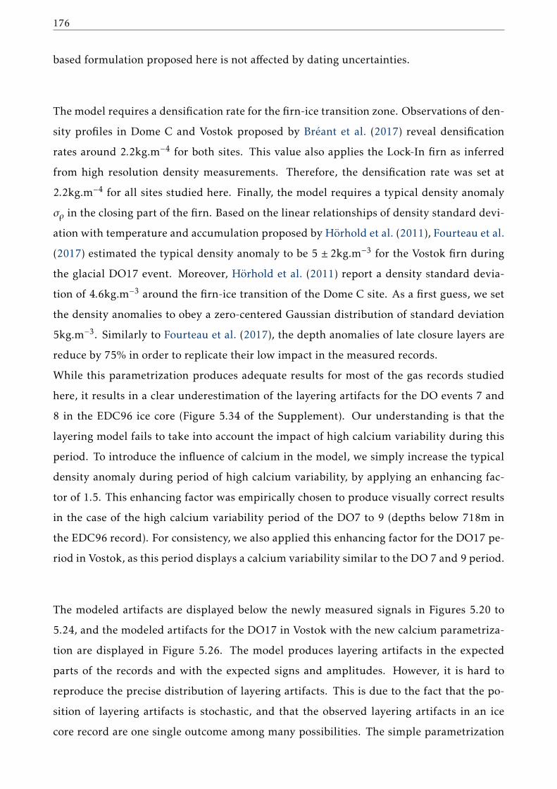
176
based formulation proposed here is not affected by dating uncertainties.
The model requires a densification rate for the firn-ice transition zone. Observations of den-
sity profiles in Dome C and Vostok proposed by Bréant et al. (2017) reveal densification
rates around 2.2kg.m−4 for both sites. This value also applies the Lock-In firn as inferred
from high resolution density measurements. Therefore, the densification rate was set at
2.2kg.m−4 for all sites studied here. Finally, the model requires a typical density anomaly
σρ in the closing part of the firn. Based on the linear relationships of density standard devi-
ation with temperature and accumulation proposed by Hörhold et al. (2011), Fourteau et al.
(2017) estimated the typical density anomaly to be 5 ± 2kg.m−3 for the Vostok firn during
the glacial DO17 event. Moreover, Hörhold et al. (2011) report a density standard devia-
tion of 4.6kg.m−3 around the firn-ice transition of the Dome C site. As a first guess, we set
the density anomalies to obey a zero-centered Gaussian distribution of standard deviation
5kg.m−3. Similarly to Fourteau et al. (2017), the depth anomalies of late closure layers are
reduce by 75% in order to replicate their low impact in the measured records.
While this parametrization produces adequate results for most of the gas records studied
here, it results in a clear underestimation of the layering artifacts for the DO events 7 and
8 in the EDC96 ice core (Figure 5.34 of the Supplement). Our understanding is that the
layering model fails to take into account the impact of high calcium variability during this
period. To introduce the influence of calcium in the model, we simply increase the typical
density anomaly during period of high calcium variability, by applying an enhancing fac-
tor of 1.5. This enhancing factor was empirically chosen to produce visually correct results
in the case of the high calcium variability period of the DO7 to 9 (depths below 718m in
the EDC96 record). For consistency, we also applied this enhancing factor for the DO17 pe-
riod in Vostok, as this period displays a calcium variability similar to the DO 7 and 9 period.
The modeled artifacts are displayed below the newly measured signals in Figures 5.20 to
5.24, and the modeled artifacts for the DO17 in Vostok with the new calcium parametriza-
tion are displayed in Figure 5.26. The model produces layering artifacts in the expected
parts of the records and with the expected signs and amplitudes. However, it is hard to
reproduce the precise distribution of layering artifacts. This is due to the fact that the po-
sition of layering artifacts is stochastic, and that the observed layering artifacts in an ice
core record are one single outcome among many possibilities. The simple parametrization

Chapter 5. Alterations of methane records in East Antarctic ice cores 177
we derived thus appears to provide reasonable results for accumulation conditions ranging
from 3.9 to 1.3cm.ie.yr−1, encompassingmost of the climatic conditions of the East Antarctic
plateau for both the glacial and interglacial periods.
Figure 5.26 – Same as Figure 5.20 for the DO17 Vostok section. The methane data of the upper panel arefrom Fourteau et al. (2017) and the atmospheric reference of the lower panel is from Rhodeset al. (2015).
Removing layered trapping artifacts
Since layered gas trapping artifacts are not due to chronologically ordered atmospheric vari-
ations, a proper interpretation of gas records requires them to be cleaned from the datasets.
As pointed out by Fourteau et al. (2017), in some sections of the records these artifacts only
exhibit negative or positive methane anomalies. They cannot therefore be removed by ap-
plying a running average without introducing bias in the signal.
To clean the new three methane signals presenting layering artifacts (EDC96, EDC99 and
Vostok) we use the cleaning procedure described by Fourteau et al. (2017). Briefly, this
cleaning algorithm starts by estimating a smooth signal that should represent the measured
signal free of layering artifacts and analytical noise. For this purpose, a running median
is first computed to remove the layering artifacts while minimizing bias. Then, the signal
is smoothed with a binned average, and interpolated back to high resolution using an in-
terpolating spline. Then, the analytical noise is estimated and the data clipped to remove
artifacts larger than the analytical noise.
This procedure was successfully applied to the Holocene section of EDC99, that only ex-
hibits a few artifacts. The resulting cleaned signal is displayed in the upper panel of Fig-
ure 5.22 as a black curve. However, direct application of this algorithm to the EDC96 DO6-9
and Vostok DO21 records leads to an ineffective removal of layering artifacts in periods of

178
fast methane rise. After investigation, it appears that the main issue the algorithm is facing
is the determination of an artifacts free signal by the rolling median. In some section of
the ice cores, the signal displays high concentrations of artifacts with methane anomalies of
50ppbv or more, as seen for instance in the onset of the DO8 in Figure 5.23. In these con-
ditions, the rolling median is influenced by the presence of the artifacts and yields a biased
signal. To circumvent this problem, we manually provided a set of values that correspond to
the artifact free part of the signal. As it is easy to distinguish the layering artifacts from the
rest of the signal, the manual selection of these points is fairly unambiguous and straight-
forward. The rest of algorithm then proceeds as normal. The cleaned EDC99 Holocene,
EDC96 DO6-9 and Vostok DO-21 signals are displayed in the upper panels of Figures 5.23
and 5.24 in black.
5.3.3.4 Smoothing in East Antarctic ice cores
The five ice core sections measured in this article all originate from the East Antarctic
plateau. The low temperatures and aridity of this region result in a slow densification of
the firn, and a slow bubble closure. Therefore, the gas enclosed in a given ice layer tends
to have a broad age distribution. This leads to the important smoothing of atmospheric fast
variability observed in East Antarctic ice cores (Spahni et al., 2003; Joos and Spahni, 2008;
Köhler et al., 2011; Ahn et al., 2014; Fourteau et al., 2017).
Estimating gas age distributions
Since smoothing in an ice core record is a direct consequence of the gas age distribution
(GAD), the knowledge of GADs for various temperature and accumulation conditions is
necessary to predict the impact of smoothing on gas signals. We thus apply the GAD ex-
traction method proposed by Fourteau et al. (2017) to the five new high resolution records.
This method, designed to estimate the GAD of low accumulation records, is based on the
comparison with a weakly smoothed record from a high accumulation ice core, used as an
atmospheric reference (see Section 5.3.3.2). An optimal log-normal age distribution is de-
rived to best match the measured signal with the smoothing of the atmospheric reference by
the GAD. Using a log-normal law allows one to have a well-defined problem in the mathe-
matical sense. A log-normal distribution is fully defined by two independents parameters.
The GAD extraction problem is thus reduced to the recovery of a pair of optimal parameters.
Nonetheless, log-normal laws exhibit a large range of shapes that can adequately represent
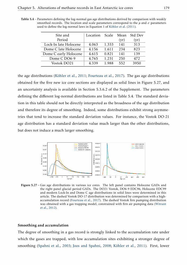
Chapter 5. Alterations of methane records in East Antarctic ice cores 179
Table 5.4 – Parameters defining the log-normal gas age distributions derived by comparison with weaklysmoothed records. The location and scale parameters correspond to the µ and σ parametersused to define the log-normal laws in Equation 1 of Köhler et al. (2011).
Site and Location Scale Mean Std DevPeriod (yr) (yr)
Lock-In late Holocene 4.063 1.333 141 313Dome C late Holocene 4.156 1.611 234 823Dome C early Holocene 4.615 0.821 141 139
Dome C DO6-9 4.765 1.231 250 472Vostok DO21 4.339 1.988 552 3950
the age distributions (Köhler et al., 2011; Fourteau et al., 2017). The gas age distributions
obtained for the five new ice core sections are displayed as solid lines in Figure 5.27, and
an uncertainty analysis is available in Section 5.3.6.2 of the Supplement. The parameters
defining the different log-normal distributions are listed in Table 5.4. The standard devia-
tion in this table should not be directly interpreted as the broadness of the age distribution
and therefore its degree of smoothing. Indeed, some distributions exhibit strong asymme-
tries that tend to increase the standard deviation values. For instance, the Vostok DO-21
age distribution has a standard deviation value much larger than the other distributions,
but does not induce a much larger smoothing.
Figure 5.27 – Gas age distributions in various ice cores. The left panel contains Holocene GADs andthe right panel glacial period GADs. The DO21 Vostok, DO6-9 EDC96, Holocene EDC99and modern Lock-In and Dome C age distributions in solid lines were determined in thisarticle. The dashed Vostok DO-17 distribution was determined by comparison with a high-accumulation record (Fourteau et al., 2017). The dashed Vostok firn pumping distributionwas obtained with a gas trapping model, constrained with firn air pumping data (Witrantet al., 2012).
Smoothing and accumulation
The degree of smoothing in a gas record is strongly linked to the accumulation rate under
which the gases are trapped, with low accumulation sites exhibiting a stronger degree of
smoothing (Spahni et al., 2003; Joos and Spahni, 2008; Köhler et al., 2011). First, lower

180
accumulation is generally associated with low temperatures. Low-temperature ice deforms
less easily and the densification process is therefore slower and bubble closure spans a larger
time period. Moreover, low accumulation is also associated with a slow mechanical load in-
crease of the ice material, also resulting in a slower densification and a longer bubble closure
period.
Two new glacial period gas age distributions were derived in this work (EDC96 DO6-9 and
Vostok DO21). This is to be added to the previously published GAD obtained for the Vostok
site during the DO17 event (1.3cm.ie.yr−1 accumulation rate; Fourteau et al., 2017). These
three age distributions of East Antarctic sites under glacial conditions are displayed in the
right panel of Figure 5.27. The smoothing they induce is represented for the DO6 to 9 and
DO21 events in Figure 5.28. It appears that the two Vostok distributions lead to similar
smoothing. On the other hand the GAD obtained for EDC96 for the DO6-9 events is signif-
icantly broader than the Vostok ones and results in a stronger smoothing, especially visible
on the onset of the DO21 event. This is surprising as the Vostok DO21 and Dome C DO6-9
records have the same accumulation rate, and should therefore present similar age distri-
butions. However, the distributions obtained for glacial Vostok (DO17 and 21 events) also
appear to be suited for the smoothing of DO6 to 9 events in EDC96, as seen in the lower
panel of Figure 5.28. Moreover, the uncertainty analysis reveals that the distribution ex-
tracted from the EDC96 record is poorly constrained, with a large range of GADs resulting
in adequate smoothing (Figure S8 in Section S2 of the supplement). It appears that the
three glacial records exhibits similar degree of smoothing, and therefore enclose gases with
the same gas age distribution. We propose to use a common gas age distribution to rep-
resent the smoothing in ice cores with accumulations below 2cm.ie.yr−1. The distribution
proposed by Fourteau et al. (2017) is a good candidate for this common distribution, as it
reproduces well the smoothing in the EDC96 DO6-9 record and the Vostok DO17 and 20
records. Moreover, its shape is a compromise between the two other glacial GADs proposed
in this article (right panel of Figure 5.27). Finally, the similarity of the smoothing encoun-
tered during the DO17 (high calcium variability) and DO21 (low calcium variability) events
suggests the absence of significant impurity effect on the GADs.
Comparing the common GAD of the glacial period with the ones obtained for the Holocene
and modern periods indicates that the later lead to a slightly smaller degree of smoothing.
This illustrated with the smoothing of the 8.2ka event displayed in Figure 5.29. It is con-

Chapter 5. Alterations of methane records in East Antarctic ice cores 181
Figure 5.28 – Comparison of smoothing for the three different glacial age distributions, and the modernVostok GAD constrained with firn air pumping data. Atmospheric references (dashed lines)have been smoothed by the four different GADs and are displayed overlying the measure-ments (light blue). The upper panel shows the DO21 event as measured in Vostok, and thelower panel shows the DO-6 to 9 as measured in EDC96.
sistent with the expectation that the smoothing during the low-accumulation glacial period
should be more important than during the higher-accumulation Holocene period. However,
the doubling of accumulation between the DO17 event at Vostok and the 8.2ka event in
EDC99 does not result in a drastic diminution of smoothing. It is also noteworthy that for
the Dome C site, the transition from 8.2ka conditions (3.1cm.ie.yr−1 accumulation rate) to
modern conditions (2.7cm.ie.yr−1 accumulation rate) does not significantly change the de-
gree of smoothing. It thus appears that for accumulations below 3.9cm.ie.yr−1 the degree of
smoothing only slowly increases with the diminution of the precipitation rate.
Finally, the expected smoothing using the firn pumping GAD estimation for modern Vostok
is also displayed in Figure 5.28 in black (Witrant et al., 2012). The smoothing estimated for
modern Vostok is stronger than the one measured in the glacial Vostok ice core. This can be
seen on the onset of the DO21, where the smoothing induced by the Vostok firn pumping
distribution results in a signal with less variability than the CFA measurements. This con-
firms the observation of Fourteau et al. (2017) that the firn pumping GAD of modern Vostok
leads to a stronger smoothing than the one observed during the DO17 event. This stronger
smoothing in a modern ice core is in contradiction with the Holocene and modern GADs
reported in this article for Dome C and Lock-In. This discrepancy could result from the

182
Figure 5.29 – Comparison of the smoothing induced by three different Holocene and a modern age distri-butions. The atmospheric reference for the 8.2ka event (dashed line) has been smoothed bythe four different GADs and displayed over the EDC99 measurements (light blue).
large uncertainties associated with the firn-model-based GAD, which notably arise from the
poor constraints on the closed porosity profiles used (Schaller et al., 2017). Unfortunately,
high-resolution methane measurements of the late Holocene period in the Vostok ice core
are not available to apply the GAD extraction method.
Effect of smoothing on the synchronization of records
Compared to the GADs of the Holocene and modern periods, the GADs of the glacial period
exhibits a stronger degree of skewness (see Figure 5.27). This asymmetry of the distributions
means that the smoothing not only removes variability, but also induces phase shifts during
fast variations (Fourteau et al., 2017). This is especially visible on the variation recorded
at depth 1260m in the Vostok DO21 ice core section, displayed in the upper panel of Fig-
ure 5.28. The peak of the event is recorded a couple of meters before its position in the
absence of smoothing. Studies relying on the synchronization of atmospheric variability be-
tween ice cores should be aware of this potential bias (Bazin et al., 2013; Veres et al., 2013).
The best synchronization should either be done on signals with similar degree of smoothing,
or the phase shifts should be taken into account in the age uncertainty estimates.
5.3.4 Loss of climatic information in a deep and thinned ice core from
East Antarctica
East Antarctica is a region of particular interest for the drilling of deep ice cores. Indeed,
thanks to low accumulation rates, it likely contains the oldest stratigraphically-undisturbed

Chapter 5. Alterations of methane records in East Antarctic ice cores 183
ice on earth. There is currently a search for very old ice, with ages potentially dating back
one-and-a-half million years (Fischer et al., 2013; Passalacqua et al., 2018). When retrieved,
such an ice core will be characterized by the gas trapping of low-accumulation East Antarc-
tic plateau ice cores. Moreover, the old ice will be located close to the bedrock and therefore
will be thinned by shear strains.
In this section, we estimate the potential alterations that smoothing and layering would in-
duce between the atmosphere and its measurements in a theoretical one-and-a-half million
years old ice core, for methane and carbon dioxide. For this purpose, we consider that the
gas trapping occur under an accumulation rate of 2cm.ie.yr−1. We suppose that the enclosed
gases follow the age distribution obtained for Vostok during the DO17 period, established
to be representative of East Antarctic glacial smoothing in Section 5.3.3.4. The presence of
layered trapping artifacts is simulated using the model parametrized Section 5.3.3.3, with
the assumption of high calcium variability. Finally, we assume that the thinning of the ice
results in a resolution of 10,000yr.m−1 (Passalacqua et al., 2018). This implies that a given
ice layer at the bottom of the core is 200 times thinner than at the firn-ice transition. This
has to be taken into account as analytical techniques have limited spatial resolutions below
which variations are no longer resolved. In particular, layering artifacts will no longer be
visible as singular events in the record. Note that we do not consider the loss of climatic
information due to diffusive mixing of trace gases within the ice matrix itself (Bereiter et al.,
2014). This effect would further degrade the recorded trace gas signal.
5.3.4.1 Methane alterations
As a first case, we study the alterations of a methane record measured using a CFA system
analogous to the one currently used at IGE. For the sake of simplicity, we assume that the
atmospheric history recorded in this theoretical one-and-a-half million year-old ice core is
similar to the DO17 event of the last glacial period. Hence, we simply use the WD CFA
methane measurements as the atmospheric reference (Rhodes et al., 2015). We first deter-
mine the initially enclosed signal using the layering artifacts and smoothing models, and
apply a 200 times thinning factor. The resulting signal is displayed in blue in the upper
panel of Figure 5.30. Then, we simulate the process of CH4 measurements by applying
the smoothing induced by the CFA system. For this, we use the CFA impulse response de-
rived by Fourteau et al. (2017). The end result is displayed in blue in the lower panel of
Figure 5.30. The layering artifacts are no longer visible as they have been smoothed out

184
by the CFA measurement. However, they affect the measured signal due to their asymme-
try. This is illustrated by the difference between the blue and green curves in the lower
panel of Figure 5.30, that respectively represent the CFA measurements with and without
the presence of layering artifacts. However, even during periods of strong methane varia-
tions, the bias specifically due to layering artifacts does not exceed 10ppbv. This is of the
order of the analytical noise usually observed with the CFA system (Fourteau et al., 2017).
It therefore appears that layering artifacts only negligibly affect the measured signal in the
case of thinned ice cores. However, the potential impact of layering artifacts is sensitive to
the parameters of the layering model. Notably, increasing the number of anomalous layers
increases the amplitude of the biases.
Figure 5.30 – Impacts of layered trapping and smoothing on a synthetic million-and-a-half years oldmethane record. Upper panel: signal recorded in the ice taking into account smoothing(in black) and layered trapping artifacts (in blue). The atmospheric reference is displayedin orange. The depth scale takes into account the thinning of the ice. Lower panel: CFAmeasurements with (in blue) and without layering artifacts (in green). The atmospheric ref-erence is displayed orange and the initial recorded signal without layering artifacts is alsodisplayed in black.
The internal smoothing of the CFA system also tends to deteriorate information recorded
in the ice core by attenuating fast variability. It is therefore important to determine to what
extent CFA smoothing adds to the already present firn smoothing. To study this point, we
compare the frequency responses of the CFA system and firn smoothing. These frequency
responses represent the attenuation experienced by a sine signal, as a function of the sine pe-
riod. To achieve this, we first expressed the CFA impulse response (its smoothing function)
on a gas age scale, taking into account the thinning of the ice. Then, the frequency responses
were deduced using fast Fourier transforms. The gas age distribution and the CFA impulse
response are displayed in the left panel of Figure 5.31 with the frequency responses in the
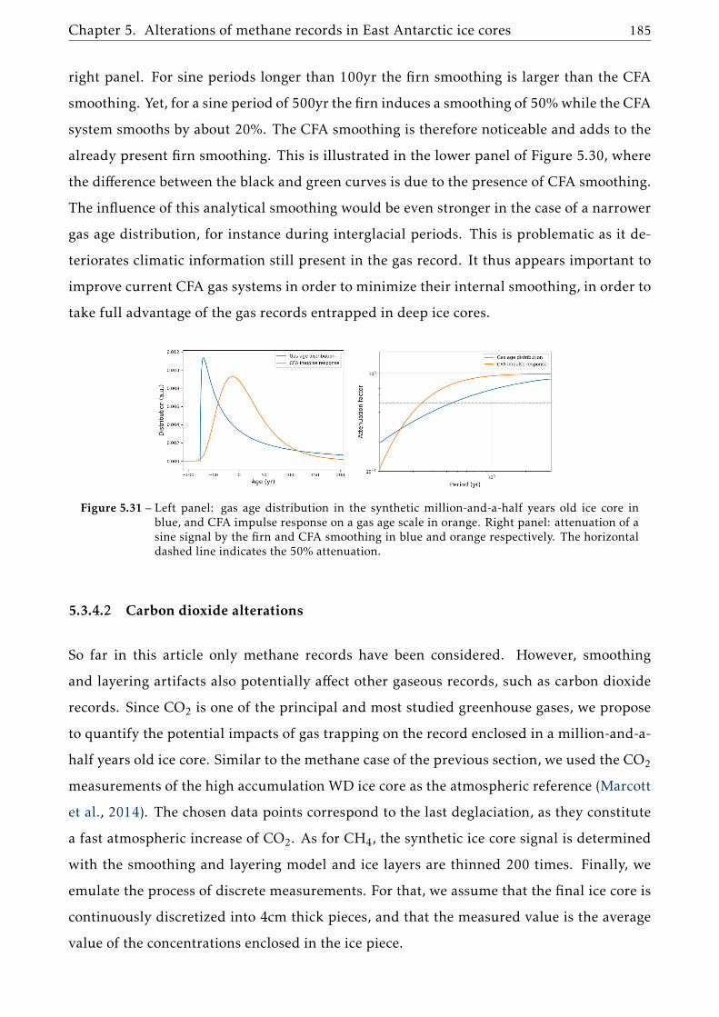
Chapter 5. Alterations of methane records in East Antarctic ice cores 185
right panel. For sine periods longer than 100yr the firn smoothing is larger than the CFA
smoothing. Yet, for a sine period of 500yr the firn induces a smoothing of 50%while the CFA
system smooths by about 20%. The CFA smoothing is therefore noticeable and adds to the
already present firn smoothing. This is illustrated in the lower panel of Figure 5.30, where
the difference between the black and green curves is due to the presence of CFA smoothing.
The influence of this analytical smoothing would be even stronger in the case of a narrower
gas age distribution, for instance during interglacial periods. This is problematic as it de-
teriorates climatic information still present in the gas record. It thus appears important to
improve current CFA gas systems in order to minimize their internal smoothing, in order to
take full advantage of the gas records entrapped in deep ice cores.
Figure 5.31 – Left panel: gas age distribution in the synthetic million-and-a-half years old ice core inblue, and CFA impulse response on a gas age scale in orange. Right panel: attenuation of asine signal by the firn and CFA smoothing in blue and orange respectively. The horizontaldashed line indicates the 50% attenuation.
5.3.4.2 Carbon dioxide alterations
So far in this article only methane records have been considered. However, smoothing
and layering artifacts also potentially affect other gaseous records, such as carbon dioxide
records. Since CO2 is one of the principal and most studied greenhouse gases, we propose
to quantify the potential impacts of gas trapping on the record enclosed in a million-and-a-
half years old ice core. Similar to the methane case of the previous section, we used the CO2
measurements of the high accumulation WD ice core as the atmospheric reference (Marcott
et al., 2014). The chosen data points correspond to the last deglaciation, as they constitute
a fast atmospheric increase of CO2. As for CH4, the synthetic ice core signal is determined
with the smoothing and layering model and ice layers are thinned 200 times. Finally, we
emulate the process of discrete measurements. For that, we assume that the final ice core is
continuously discretized into 4cm thick pieces, and that the measured value is the average
value of the concentrations enclosed in the ice piece.
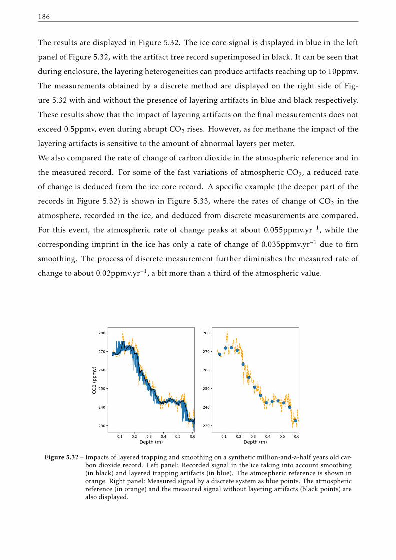
186
The results are displayed in Figure 5.32. The ice core signal is displayed in blue in the left
panel of Figure 5.32, with the artifact free record superimposed in black. It can be seen that
during enclosure, the layering heterogeneities can produce artifacts reaching up to 10ppmv.
The measurements obtained by a discrete method are displayed on the right side of Fig-
ure 5.32 with and without the presence of layering artifacts in blue and black respectively.
These results show that the impact of layering artifacts on the final measurements does not
exceed 0.5ppmv, even during abrupt CO2 rises. However, as for methane the impact of the
layering artifacts is sensitive to the amount of abnormal layers per meter.
We also compared the rate of change of carbon dioxide in the atmospheric reference and in
the measured record. For some of the fast variations of atmospheric CO2, a reduced rate
of change is deduced from the ice core record. A specific example (the deeper part of the
records in Figure 5.32) is shown in Figure 5.33, where the rates of change of CO2 in the
atmosphere, recorded in the ice, and deduced from discrete measurements are compared.
For this event, the atmospheric rate of change peaks at about 0.055ppmv.yr−1, while the
corresponding imprint in the ice has only a rate of change of 0.035ppmv.yr−1 due to firn
smoothing. The process of discrete measurement further diminishes the measured rate of
change to about 0.02ppmv.yr−1, a bit more than a third of the atmospheric value.
Figure 5.32 – Impacts of layered trapping and smoothing on a synthetic million-and-a-half years old car-bon dioxide record. Left panel: Recorded signal in the ice taking into account smoothing(in black) and layered trapping artifacts (in blue). The atmospheric reference is shown inorange. Right panel: Measured signal by a discrete system as blue points. The atmosphericreference (in orange) and the measured signal without layering artifacts (black points) arealso displayed.

Chapter 5. Alterations of methane records in East Antarctic ice cores 187
Figure 5.33 – Impact of gas trapping processes and measurements on the CO2 rate of change. The rate ofchange of the atmosphere is displayed in orange, while the rate change recorded in the iceis in black, and the measured one is in blue.
5.3.5 Conclusions
This work evaluated two gas trapping effects that affect the recorded atmospheric trace gas
history in polar ice cores. The first one is the layered gas trapping, that produces strati-
graphic heterogeneities appearing as spurious values in the measured record (Rhodes et al.,
2016). The second one is the smoothing effect that removes a part of the variability in the
gas records (Spahni et al., 2003; Joos and Spahni, 2008; Köhler et al., 2011). Our work fo-
cuses on the arid region of East Antarctica, as this is where the oldest ice cores are retrieved.
Five new sections from East Antarctic ice cores have been analyzed at high resolution for
methane concentration.
The observation of layering artifacts in these newmeasurements is consistent with the phys-
ical mechanisms already proposed for their existence (Etheridge et al., 1992; Rhodes et al.,
2016). In accordance with previous studies (Hörhold et al., 2012; Fujita et al., 2016), the
data suggest that chemistry could promote the presence of especially dense layers closing in
advance and creating the layering artifacts. We parameterized a simple model to reproduce
the observed distribution and characteristics of layering artifacts, and were able to find a
common set of parameters to reproduce the measured artifacts in all studied East Antarctic
ice cores.
In order to study the smoothing effect, we estimated the enclosed gas age distributions in
each of the five ice core sections. For this purpose, we use the method proposed by Fourteau
et al. (2017) based on the comparison with higher accumulation methane records. It appears
that during the last glacial period, the different methane records in ice cores formed under
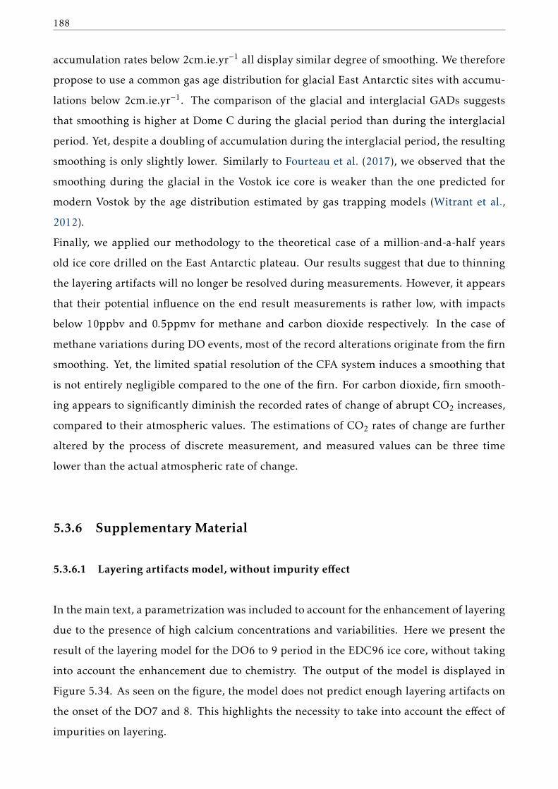
188
accumulation rates below 2cm.ie.yr−1 all display similar degree of smoothing. We therefore
propose to use a common gas age distribution for glacial East Antarctic sites with accumu-
lations below 2cm.ie.yr−1. The comparison of the glacial and interglacial GADs suggests
that smoothing is higher at Dome C during the glacial period than during the interglacial
period. Yet, despite a doubling of accumulation during the interglacial period, the resulting
smoothing is only slightly lower. Similarly to Fourteau et al. (2017), we observed that the
smoothing during the glacial in the Vostok ice core is weaker than the one predicted for
modern Vostok by the age distribution estimated by gas trapping models (Witrant et al.,
2012).
Finally, we applied our methodology to the theoretical case of a million-and-a-half years
old ice core drilled on the East Antarctic plateau. Our results suggest that due to thinning
the layering artifacts will no longer be resolved during measurements. However, it appears
that their potential influence on the end result measurements is rather low, with impacts
below 10ppbv and 0.5ppmv for methane and carbon dioxide respectively. In the case of
methane variations during DO events, most of the record alterations originate from the firn
smoothing. Yet, the limited spatial resolution of the CFA system induces a smoothing that
is not entirely negligible compared to the one of the firn. For carbon dioxide, firn smooth-
ing appears to significantly diminish the recorded rates of change of abrupt CO2 increases,
compared to their atmospheric values. The estimations of CO2 rates of change are further
altered by the process of discrete measurement, and measured values can be three time
lower than the actual atmospheric rate of change.
5.3.6 Supplementary Material
5.3.6.1 Layering artifacts model, without impurity effect
In the main text, a parametrization was included to account for the enhancement of layering
due to the presence of high calcium concentrations and variabilities. Here we present the
result of the layering model for the DO6 to 9 period in the EDC96 ice core, without taking
into account the enhancement due to chemistry. The output of the model is displayed in
Figure 5.34. As seen on the figure, the model does not predict enough layering artifacts on
the onset of the DO7 and 8. This highlights the necessity to take into account the effect of
impurities on layering.

Chapter 5. Alterations of methane records in East Antarctic ice cores 189
5.3.6.2 Uncertainty on Gas Age Distributions
The extraction method yields an optimal GAD that minimizes the RMSD between the CFA
measurements and the smoothed atmospheric reference. To quantify the uncertainties as-
sociated with the calculated GADs, we performed a dedicated analysis. For each of the five
ice core sections, we studied the impact of choosing slightly modified location and scale pa-
rameters.
Practically, we modify the scale and location parameters until the resulting RMSD is 15%
larger than its optimal value. The location and scales were modified following straight lines
in the {location, scale} space, starting from the optimal values (Figure 5.35). We then ob-
tained a set of 10 GADs meant to represent the limit of acceptable distributions. These
GADs and their corresponding smoothed methane records in the ice are displayed in Fig-
ures 5.36 to 5.40. In the right panel of these figures, we also represented the set of location
and scale values that increase the RMSD by 15%. The regions enclosed by the those values
can be viewed as the uncertainty ranges of the location and scale parameters.
To better appreciate the uncertainty associates with the EDC96 and Vostok glacial GADs,
we plotted their uncertainty ranges on the common Figure 5.41. It confirms that the EDC96
age distribution is less well constrained than Vostok GAD.
Figure 5.34 – Results of the layering model. This figure is similar to Figure 5 of the main article, but doesnot include the effect of impurity driven enhancement of layering.

190
Figure 5.35 – Method used to modify the location and scale parameters for the uncertainty assessment.Starting from the optimal values (blue square), the location and scale parameters are movedaway following straight lines (dashed lines). If the new RMSD differs by less than 15% withthe optimal value (green dots) the location and scale are further modified, until the 15%are reached (red dots). Then the parameters are modified following a new line. In total 10different lines are tested.
Figure 5.36 – GAD for the DO21 event in Vostok. Left panel: Optimal gas age distribution as a bold solidline. Age distributions resulting in 15% RMSD increases are shown as dashed lines. Middlepanel: Methane smoothed record using the optimal GAD as a bold solid line, and methanesmoothed records using the 15% higher RMSD distributions are displayed as dashed lines.CFAmeasurements are displayed in gray. Right panel: Location and scale parameters defin-ing the gas age distributions. The blue square marks the optimal parameters and the reddots represent age distributions resulting in a 15% increase of RMSD.
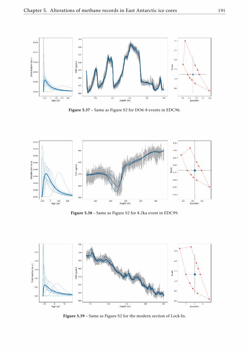
Chapter 5. Alterations of methane records in East Antarctic ice cores 191
Figure 5.37 – Same as Figure S2 for DO6-8 events in EDC96.
Figure 5.38 – Same as Figure S2 for 8.2ka event in EDC99.
Figure 5.39 – Same as Figure S2 for the modern section of Lock-In.

192
Figure 5.40 – Same as Figure S2 for the modern section of Dome C.
Figure 5.41 – Uncertainty range of the location and scale parameters for the EDC96 DO6-8 and VostokDO21 GADs. The EDC96 uncertainty range is represented as red dots, and the optimalEDC96 parameters is marked as a blue square. The Vostok DO21 uncertainty range is rep-resented as orange dots, and the optimal Vostok DO21 parameters is marked as a blacksquare.
Chapter 5. Alterations of methane records in East Antarctic ice cores 193
5.4 Conclusion of the chapter
This chapter presents new insights concerning the impact of layered gas trapping and firn
smoothing on gas signals recorded in low-accumulation ice cores. This study was made pos-
sible thanks to the acquisition of high-resolution methane data using the CFA system of IGE
during my PhD.
In both articles, I first analyze the impact of layered gas trapping. In accordance with
Rhodes et al. (2016), layered gas trapping artifacts appear as centimeter scale methane vari-
ations during periods of atmospheric methane variations. In the case of low-accumulation
ice cores these artifacts’ anomalies can reach of up to 100pbbv, equivalent to the methane in-
creases observed during DO events. Moreover, the numbers of artifacts in the EPICA Dome
C ice core appears to be linked with the level and variability of calcium in the ice. This is
consistent with the description of stratified gas trapping presented in Chapter 4.
I propose a simple model to predict the presence and amplitudes of the layering artifacts in
gas signals. This model converts the density anomaly of a firn stratum into a closure depth
anomaly, representing the advance or delay of closure of the stratum. The greenhouse gas
concentrations of the air enclosed in the stratum is computed according to its time of clo-
sure. The model was originally developed for the record of the DO17 event in the Vostok
ice core. It was then extended to the all the methane records obtained during this PhD, and
was revised to include the influence of ionic content of the ice. After model parameters ad-
justment, the model can simulate the presence of layering artifacts observed in six ice cores
from East Antarctica, for accumulation rates ranging from 3.9 to 1.3cm.ie.yr−1.
I introduce a novel technique to estimate the gas age distribution of gases enclosed in low-
accumulation ice cores. It is based on the comparison of the low-accumulation record with
a higher-accumulation one. In particular, this method can be applied to the case of glacial
ice cores from East Antarctica and climatic conditions with no present-day equivalent. Ap-
plying this methodology to six different East Antarctic methane records, I am able to obtain
estimations of gas age distributions for accumulation rates between 3.9 to 1.3cm.ie.yr−1. In
particular, I estimate three age distributions for glacial conditions over the East Antarctic
plateau, for accumulation rates of 1.5 and 1.3cm.ie.yr−1. All the three glacial period records

194
display a similar degree of smoothing. I thus propose to use a common gas age distribution
to represent the smoothing of gas signals recorded in glacial ice cores of the East Antarctic
plateau. Moreover, comparing the smoothing observed in glacial and interglacial condi-
tions, it appears that smoothing is only slightly more important during the glacial period.
This suggests that the degree of smoothing slowly increases with the decrease of accumula-
tion in the case of ice cores from the East Antarctica plateau.
Finally, I apply the layering model and smoothing methodology to the theoretical case of
a million-a-and-half years old and very thinned ice core from East Antarctica. The goal is
to estimate the alterations to be expected for the gas signals recorded in the future core of
the Oldest-Ice project. For the case of methane measured with a CFA system, the signal will
be principally altered by firn smoothing, with also a non-negligible contribution of CFA
smoothing, if current setups are applied without further improvements. The layered gas
trapping artifacts will no longer be resolved, but only account for a slight bias (< 10ppbv) of
the measurements. In the case of discrete measurements of carbon dioxide, firn smoothing
leads to an underestimation of the rate of change recorded in the ice during fast variations.
Moreover, the process of discrete measurement also strongly affects the rate of change, and
results in a further underestimation of the rates of change in CO2 concentrations.
Chapter 6
Modeling the compression of firn layers
Contents
6.1 Presentation of the chapter . . . . . . . . . . . . . . . . . . . . . . . . . . . . 197
6.2 Description of the model . . . . . . . . . . . . . . . . . . . . . . . . . . . . . 198
6.2.1 General principles . . . . . . . . . . . . . . . . . . . . . . . . . . . . . 199
6.2.2 Numerical implementation . . . . . . . . . . . . . . . . . . . . . . . . 200
6.3 Numerical experiments . . . . . . . . . . . . . . . . . . . . . . . . . . . . . . 208
6.3.1 Mass conservation . . . . . . . . . . . . . . . . . . . . . . . . . . . . . . 208
6.3.2 Effect of internal pressure on pore compression . . . . . . . . . . . . . 210
6.3.3 Evolution of a firn layer . . . . . . . . . . . . . . . . . . . . . . . . . . 212
6.4 Discussion . . . . . . . . . . . . . . . . . . . . . . . . . . . . . . . . . . . . . . 215
6.5 Conclusion of the chapter . . . . . . . . . . . . . . . . . . . . . . . . . . . . . 217

196
Chapter 6. Modeling the compression of firn layers 197
6.1 Presentation of the chapter
One question at the beginning of my PhD was if closed porosity profiles could be estimated
for the case of past glacial firns from East Antarctica. Indeed, the amount of smoothing in
gas records is directly linked to the progressive closure of bubbles, and knowing the rela-
tion between density and closed porosity for past firns would help to better constrain the
age distribution of entrapped gases.
Direct observations of past glacial firns of the East Antarctic plateau or of modern equiv-
alents are not possible. A possibility to overcome this issue would be the development of
numerical models explicitly able to represent the porous network and its evolution during
densification. Such models could be forced with accumulations and temperatures that have
no known modern equivalents on the Antarctic continent. Moreover, such a general model
could also be used to study the impact of the firn microstructure on the evolution of the
density and of the porous network. After discussions with C. Martin from the SIMAP lab-
oratory, Grenoble, I was introduced to the Level-Set method and its application to metallic
powder sintering, notably by Bruchon et al. (2012).
I consequently worked on the implementation of a similar method to the case of firn com-
pression, as described in this chapter. For this work, F. Gillet-Chaulet helped me with the
Finite Element Method and the Elmer software. The chapter begins with the presentation
of the algorithm and the specificities of firn compression. In its current form, the model is
not fully operational to estimate closed porosity profiles. Nonetheless, it can simulate the
mechanical response of a 3D porous network due compression forces, and its evolution over
time. In this chapter, the model is used to study the influence of internal pressure of bubbles
on their compression in deep firn. Furthermore, an illustration of firn evolution with the
processes of curvature-driven diffusion and ice creep is provided at the end of the chapter.
Moreover, while this study is focused on the deep pore-closure zone, the model developed
here could be applied to shallower and less dense firn samples.
I intend to publish my work on this firn compression model in the special issue of the
Frontiers in Earth Science journal: About the Relevance of Snow Microstructure Study in
Cryospheric Sciences. This article will be presented as a proof-of-concept of using the Level-
Set method to study the evolution of the microstructure of snow, firn, or other bi-phasic
media under compression forces.

198
6.2 Description of the model
Firn layers are composed of two phases, namely the ice matrix and the pores inside. Under
the compression forces due to the overlying column, firn layers get compressed over time,
and the porous network evolves as a response to this compression (Arzt et al., 1983; Maeno
and Ebinuma, 1983). In addition to compression, curvature differences at the surface of
the ice material induce molecular diffusion of the water molecules and further modify the
porous network (Burr et al., 2019). The overall evolution of the porous network is charac-
terized by a reduction in size, equivalent to an increase in firn density, as well as topological
changes such as pore splitting or coalescence (Burr et al., 2019). A numerical model explic-
itly representing the porous network and its evolution should therefore be able to handle
these topological changes. The bi-phasic nature of the firn is replaced by a mono-phasic
medium with the addition of a characteristic function retaining the position of the ice-pore
interface, the so called Level-Set (LS) function φ (Osher and Sethian, 1988; Gibou et al.,
2018). A typical choice for the LS function is the signed distance to the interface.
Let’s consider a domain D of firn, which for the rest of the chapter will be a rectangular
cuboid. The Level-Set function φ is given by:
φ(x) =
+dist(x,Σ) if x ∈ ice
−dist(x,Σ) if x ∈ pore
0 if x ∈ Σ
(6.1)
where x is a point of D, Σ is the interface between the ice and pore phases, and dist(x,Σ) is
the distance of point x to the interface. The position of the interface is thus captured by the
zero-level of the LS function. In other words, one can retrieve the position of the interface
with Σ = {x | φ(x) = 0}. The evolution of the porous network is therefore represented
through the evolution of the zero-level of the LS function. This framework naturally handles
topological changes (Osher and Sethian, 1988). Furthermore, due to the complex geometries
present in firn, the model relies on the Finite Element Method (FEM) to solve the equations
involved.

Chapter 6. Modeling the compression of firn layers 199
6.2.1 General principles
Assuming that a LS function φ is already defined on a tetrahedral meshMD covering the
whole domain D, the model simulates the evolution of the porous network by looping over
three main stages, summarized in Figure 6.1. During a complete cycle, the time of simula-
tion advances by a time-step ∆t.
Figure 6.1 – The three stages composing a time-step loop in the firn compression model.
6.2.1.1 Mesh adaptation
Themethod involves amesh adaptation step at the beginning of every time-step. It first aims
at improving the computational efficiency of the model by keeping a refined mesh near the
ice-pore interface and a coarser resolution far from it, where a high density of elements is
not needed. The second goal is to produce two sub-meshes. One is meant to cover the ice
phase only, while the second one covers the pore phase only. The sub-meshes are referred
to asMi andMp, respectively for the ice and pore phases.
6.2.1.2 Computation of the interface velocity
Once the meshes for a given time-step are ready, they are used to compute the ice-pore inter-
face velocity. This is done by solving the equations governing the mechanisms responsible
for the motion of the interface using the FEM. This step encapsulates all the physics of the
model. Here, I take into account the motion of the interface due to ice dislocation creep
(Arzt et al., 1983; Maeno and Ebinuma, 1983) and curvature driven diffusion (Burr et al.,
2019). Thanks to the modular nature of this model, other mechanisms can be added in the
future, if necessary.
6.2.1.3 Advection of the interface
Once the total velocity of the ice-pore interface vtot is calculated, it is used to advect the
Level-Set function. This is done by solving the transport equation over a time-step ∆t (Ols-

200
son and Kreiss, 2005; Bernacki et al., 2008):
∂φ
∂t+ vtot · ∇φ = 0 (6.2)
6.2.2 Numerical implementation
This section describes the specific implementation of the general principles introduced in
the previous section. The main FEM framework used in this study is the open-source soft-
ware Elmer1, that has been completed with equation solvers specifically developed for this
firn layer model.
6.2.2.1 Mesh adaptation
Assuming that at the end of the nth time-step the Level-Set function is defined on a tetra-
hedral meshMnD , the mesh adaptation procedure produces three meshesMn+1
D ,Mn+1i , and
Mn+1p that respectively cover the whole domain, the ice phase and the pore phase. The ice
and pore meshes are sub-meshes ofMn+1D , meaning that the ice mesh is composed of the ele-
ments ofMn+1D that lie in the ice phase region, and similarly for the pore mesh. The vertices
ofMn+1i andMn+1
p are thus also vertices ofMn+1D .
Figure 6.2 – Mesh adaptation of the domain following the LevelSet function. The submeshes of the iceand pore phasesMi , andMp are also produced during mesh adaptation.
1https://www.csc.fi/web/elmer/elmer

Chapter 6. Modeling the compression of firn layers 201
To remesh the domain according to the LS function, I use the remeshing library MMG2
(based on Dapogny et al., 2014), that we have interfaced with Elmer. The library yields a
tetrahedral mesh that is refined around the pore-ice interface, with tetrahedral elements
either in the ice or the pore phase and tagged accordingly. The boundaries between the ele-
ments of the ice and pore regions thus lie on the interface defined by the Level-Set function.
The MMG library includes parameters to adjust the mesh refinement. The main ones are
the hgrad and hausd parameters, that respectively set the gradation of element sizes and the
maximal distance between the ideal interface defined by the Level-Set function and the in-
terface captured by the tetrahedral mesh.
The mesh obtained with MMG is then converted into the three meshes Mn+1D , Mn+1
i , and
Mn+1p . Note that forMn+1
D , the elements are no longer tagged according their original phase
as the LS framework relies on a mono-phasic medium. The different variables defined at the
nodes ofMnD are finally interpolated on the new nodes ofMn+1
D . This includes the Level-Set
function.
In order to facilitate the transfer of variables between theMn+1D ,Mn+1
i , andMn+1p meshes,
permutations tables that link a vertex inMn+1D to its equivalent inMn+1
i and/orMn+1p are
saved under the form of two arrays of integers. For a given node of index i in the domain
mesh, the ith value of the permutation table is the index of the corresponding node in the ice
mesh (respectively pore mesh) or 0 if the node does not lie in the ice phase (respectively pore
phase). This allows one to transfer variables from one mesh to another without interpola-
tion, and with a good numerical efficiency. The complete mesh adaptation step procedure
is summarized in Figure 6.2.
6.2.2.2 Ice creep
The first physical mechanism responsible for the deformation of the porous network and
therefore the motion of the ice-pore interface is the dislocation creep of the ice phase due
to the compression forces of the firn column above (Maeno and Ebinuma, 1983; Arzt et al.,
1983). The creep motion of ice is represented thanks a to viscoplastic motion with a low
Reynolds number. The Equation governing the ice motion is the Stokes equation:
∇. ¯σ + ρg = 0 (6.3)
2https://www.mmgtools.org
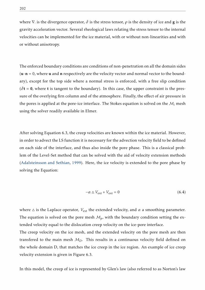
202
where ∇. is the divergence operator, ¯σ is the stress tensor, ρ is the density of ice and g is the
gravity acceleration vector. Several rheological laws relating the stress tensor to the internal
velocities can be implemented for the ice material, with or without non-linearities and with
or without anisotropy.
The enforced boundary conditions are conditions of non-penetration on all the domain sides
(u ·n = 0, where u and n respectively are the velocity vector and normal vector to the bound-
ary), except for the top side where a normal stress is enforced, with a free slip condition
( ¯σt = 0, where t is tangent to the boundary). In this case, the upper constraint is the pres-
sure of the overlying firn column and of the atmosphere. Finally, the effect of air pressure in
the pores is applied at the pore-ice interface. The Stokes equation is solved on theMi mesh
using the solver readily available in Elmer.
After solving Equation 6.3, the creep velocities are known within the ice material. However,
in order to advect the LS function it is necessary for the advection velocity field to be defined
on each side of the interface, and thus also inside the pore phase. This is a classical prob-
lem of the Level-Set method that can be solved with the aid of velocity extension methods
(Adalsteinsson and Sethian, 1999). Here, the ice velocity is extended to the pore phase by
solving the Equation:
−α △Vext +Vext = 0 (6.4)
where △ is the Laplace operator, Vext the extended velocity, and α a smoothing parameter.
The equation is solved on the pore meshMp, with the boundary condition setting the ex-
tended velocity equal to the dislocation creep velocity on the ice-pore interface.
The creep velocity on the ice mesh, and the extended velocity on the pore mesh are then
transfered to the main mesh MD . This results in a continuous velocity field defined on
the whole domain D, that matches the ice creep in the ice region. An example of ice creep
velocity extension is given in Figure 6.3.
In this model, the creep of ice is represented by Glen’s law (also referred to as Norton’s law
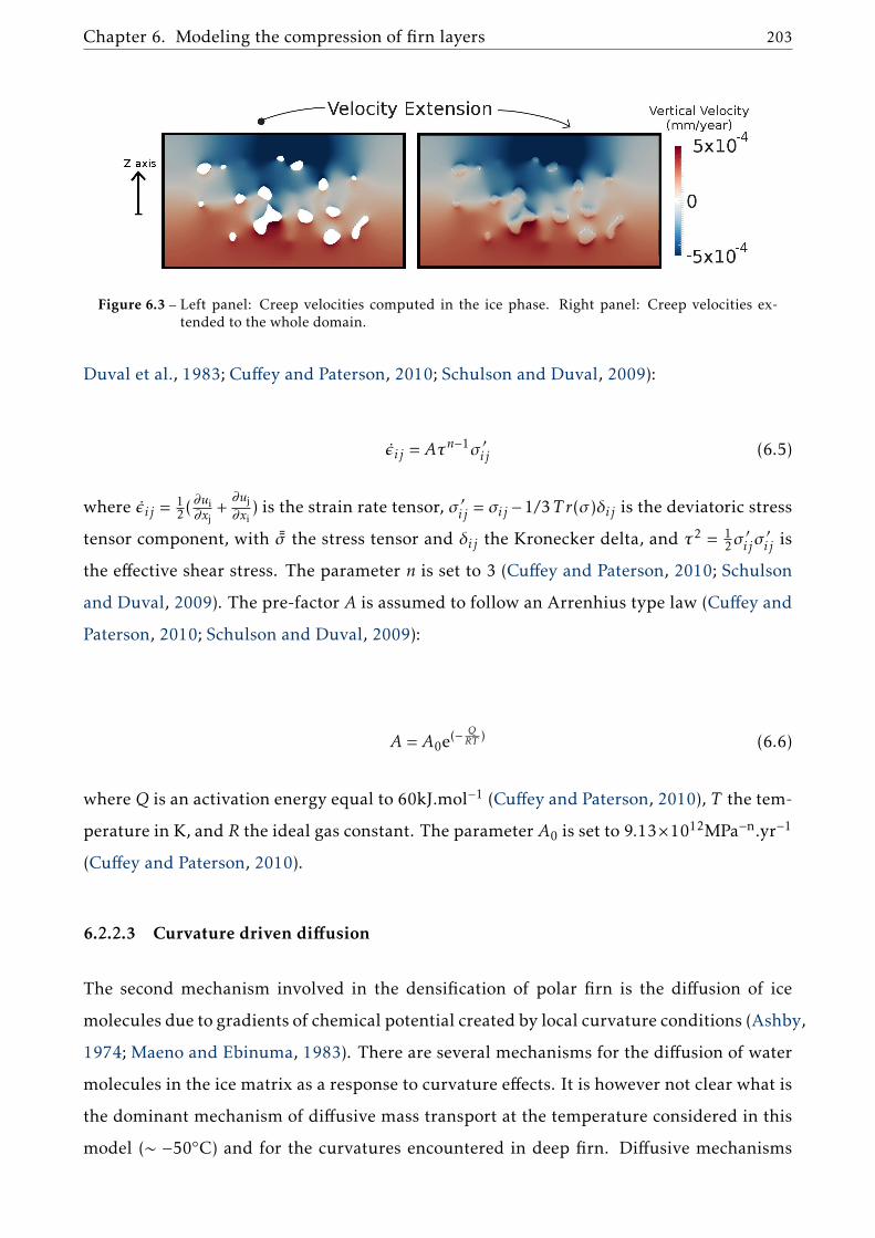
Chapter 6. Modeling the compression of firn layers 203
Figure 6.3 – Left panel: Creep velocities computed in the ice phase. Right panel: Creep velocities ex-tended to the whole domain.
Duval et al., 1983; Cuffey and Paterson, 2010; Schulson and Duval, 2009):
ǫij = Aτn−1σ ′ij (6.5)
where ǫij =12(
∂ui∂xj
+∂uj∂xi
) is the strain rate tensor, σ ′ij = σij −1/3T r(σ)δij is the deviatoric stresstensor component, with ¯σ the stress tensor and δij the Kronecker delta, and τ2 = 1
2σ′ijσ′ij is
the effective shear stress. The parameter n is set to 3 (Cuffey and Paterson, 2010; Schulson
and Duval, 2009). The pre-factor A is assumed to follow an Arrenhius type law (Cuffey and
Paterson, 2010; Schulson and Duval, 2009):
A = A0e(− Q
RT ) (6.6)
whereQ is an activation energy equal to 60kJ.mol−1 (Cuffey and Paterson, 2010), T the tem-
perature in K, and R the ideal gas constant. The parameter A0 is set to 9.13×10¹²MPa−n.yr−1
(Cuffey and Paterson, 2010).
6.2.2.3 Curvature driven diffusion
The second mechanism involved in the densification of polar firn is the diffusion of ice
molecules due to gradients of chemical potential created by local curvature conditions (Ashby,
1974; Maeno and Ebinuma, 1983). There are several mechanisms for the diffusion of water
molecules in the ice matrix as a response to curvature effects. It is however not clear what is
the dominant mechanism of diffusive mass transport at the temperature considered in this
model (∼ −50◦C) and for the curvatures encountered in deep firn. Diffusive mechanisms
204
however tend to reduce the overall curvatures of the ice/pore interface. To achieve this, we
implemented the specific mechanism of surface diffusion (Bruchon et al., 2010, 2012). The
equation governing the motion of the interface is:
vd = −C0(△sK)n (6.7)
with C0 being a parameter representing the effectiveness of the diffusive mechanism, K
the curvature of the interface, n the normal vector to the interface and pointing in the ice
phase, and △s is the "surface Laplacian" (the Laplace-Beltrami operator). To compute vd, this
equation requires the curvature K and the normal vector n. They are calculated using:
n =∇φ∥∥∥∇φ
∥∥∥(6.8)
and
K = −∇.n (6.9)
Equations6.7 and 6.9 requires second-order derivatives. To reduce numerical noise, they are
stabilized with the introduction of diffusion parameters Ak and Av:
K +Ak △K = −∇.nvd +Av △ vd = C0(△sK)
(6.10)
In Equation 6.10, vd is the norm of vd. All equations are defined over the all domain, and
are thus solved on the meshMD using specifically developed Elmer solvers. This yields a
velocity field defined over the whole domain, that matches the diffusion velocity at the ice/-
pore interface.
We set the physical parameter C0 of Equation 6.7 so that it would ideally represent the
contribution of the different diffusive mechanisms to the overall curvature decrease (Ashby,
1974; Maeno and Ebinuma, 1983). We evaluated that the mechanism of diffusion results
in interface velocities similar to ice creep for C0 ≃ 10−6 mm4.yr−1. Therefore, in the rest of
the study the parameter C0 will be set to the values 10−6 or 10−7 mm4.yr−1 to respectively
Chapter 6. Modeling the compression of firn layers 205
represent the presence of a strong or mild influence of the diffusion process, relatively to ice
creep.
6.2.2.4 Advection of the Level-Set function
Once the total velocity of the interface is computed, it is used to modify the porous structure
of the firn material by advecting the Level-Set function. However, the sole advection of the
Level-Set using the velocity field is not sufficient to ensure a good representation of the evo-
lution of the interface. Indeed, the property of the Level-Set function to be a signed distance
function is lost during the advection step, although it is fundamental for the computation
of normal vectors and curvatures. That is why the Level-Set is regularly renormalized to
remain a signed distance (Osher and Fedkiw, 2001). However, the renormalization of the
Level-Set introduces errors and numerical diffusion in the model, that result in unphysical
gain or loss of volume (Olsson and Kreiss, 2005). To overcome this issue, Zhao et al. (2014a)
introduced the Improved Conservative Level-Set (ICLS) method following the work of Ols-
son et al. (2007) on the Conservative Level-Set method. To ensure volume conservation, I
have implemented a version of the ICLS method for the advection stage.
The ICLS method introduces a new scalar field H , similar to the Level-Set function φ, de-
fined as:
H =12(1+ tanh(
φ
2ǫ)) (6.11)
This new function is a Heaviside function, smeared on a width of the order of ǫ. Similarly
to the LS function,H captures the position of the ice-pore interface, that lies whereH = 1/2.
Moreover, H can also be used to compute the normal vector to the interface using Equa-
tion 6.8.
The implementation of the ICLS method works as follows. The LS and H functions are both
advected on the mesh MD using the total interface velocity. The advection is performed
using the Advect software 3. Then, the LS function is renormalized to remain a signed dis-
3https://github.com/ISCDtoolbox/Advection

206
tance function, using the mshdist software 4 (based on Dapogny and Frey, 2012).
Then, the normal vectors to the new interface are computed. Near the interface the normal
vector n is computed using the H function, and far from it is computed using the renormal-
ized LS function. This is done because using the H function to compute the normal vectors
yields spurious oscillations far from the interface, a problem that does not arise with the LS
function (Zhao et al., 2014a,b,c). A point of the domain is considered to be in the vicinity of
the interface if its distance to the interface is smaller than ǫ. Then the shape and the width
of the H function are maintained thanks to a re-initialization step (Olsson et al., 2007; Zhao
et al., 2014a,b,c). It consists in solving the equation:
∂H
∂τ+∇.[H(1−H)n] = ∇.[ǫ(∇H.n)n] (6.12)
In this equation, τ is a fictional time, distinct from the actual time, that is solely used to relax
the equation to equilibrium. The equation should be solved until a steady-state is reached. I
solve it for 15 time-steps, which is enough to reach a steady state (Olsson et al., 2007). Once
the H function has been re-initialized, the Level-Set function φ is updated in the vicinity of
the interface using:
φ = 2ǫ tanh−1(2H − 1) (6.13)
Then, the advection step is over and the Level-Set function now defines the new interface.
6.2.2.5 Initialization
The model needs to be initialized with an initial LS function, representing either a real firn
porous structure or an idealized geometry. The initial porous structure can be derived from
3D voxel models obtained with Xray tomography of firn samples (Barnola et al., 2004; Gre-
gory et al., 2014; Burr et al., 2018). To simplify the boundary conditions, the tomography
models are padded with ice material on all sides, meaning that the pore-ice interface lies
away from the boundaries of the domain D.
Starting from a 3D voxel model, the signed distance is computed on a Cartesian grid using
4https://github.com/ISCDtoolbox/Mshdist

Chapter 6. Modeling the compression of firn layers 207
the Fast Marching Method (FMM). It was performed using the scikit-fmm 5 python package.
The signed distance is then smoothed using a gaussian filter to remove the jags of the in-
terface. The resulting signed distance defines the initial LS function, and is interpolated on
the initial meshM0D . Since, one does not know in advance where the pore-ice interface lies
in the domain,M0D is finely resolved over the whole domain to properly capture the initial
position of the interface.
Then, the H function is determined using Equation 6.11. In order to further smooth the
interface and remove remaining jags, I perform a re-initialization step of H solving Equa-
tion 6.12 to equilibrium. Then, the Level-Set function is updated using Equation 6.13. The
simulation can then start with a mesh adaptation step.
The overall algorithm, including the initialization, mesh adaptation, computation of veloc-
ities, and advection steps, is summarized in Figure 6.4.
Figure 6.4 – Scheme of the model algorithm. Each blue box represents a stage of the simulation.
5https://pypi.org/project/scikit-fmm/
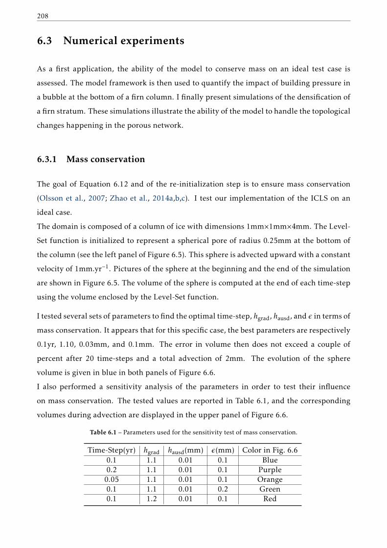
208
6.3 Numerical experiments
As a first application, the ability of the model to conserve mass on an ideal test case is
assessed. The model framework is then used to quantify the impact of building pressure in
a bubble at the bottom of a firn column. I finally present simulations of the densification of
a firn stratum. These simulations illustrate the ability of the model to handle the topological
changes happening in the porous network.
6.3.1 Mass conservation
The goal of Equation 6.12 and of the re-initialization step is to ensure mass conservation
(Olsson et al., 2007; Zhao et al., 2014a,b,c). I test our implementation of the ICLS on an
ideal case.
The domain is composed of a column of ice with dimensions 1mm×1mm×4mm. The Level-
Set function is initialized to represent a spherical pore of radius 0.25mm at the bottom of
the column (see the left panel of Figure 6.5). This sphere is advected upward with a constant
velocity of 1mm.yr−1. Pictures of the sphere at the beginning and the end of the simulation
are shown in Figure 6.5. The volume of the sphere is computed at the end of each time-step
using the volume enclosed by the Level-Set function.
I tested several sets of parameters to find the optimal time-step, hgrad, hausd, and ǫ in terms of
mass conservation. It appears that for this specific case, the best parameters are respectively
0.1yr, 1.10, 0.03mm, and 0.1mm. The error in volume then does not exceed a couple of
percent after 20 time-steps and a total advection of 2mm. The evolution of the sphere
volume is given in blue in both panels of Figure 6.6.
I also performed a sensitivity analysis of the parameters in order to test their influence
on mass conservation. The tested values are reported in Table 6.1, and the corresponding
volumes during advection are displayed in the upper panel of Figure 6.6.
Table 6.1 – Parameters used for the sensitivity test of mass conservation.
Time-Step(yr) hgrad hausd(mm) ǫ(mm) Color in Fig. 6.60.1 1.1 0.01 0.1 Blue0.2 1.1 0.01 0.1 Purple0.05 1.1 0.01 0.1 Orange0.1 1.1 0.01 0.2 Green0.1 1.2 0.01 0.1 Red

Chapter 6. Modeling the compression of firn layers 209
Figure 6.5 – Advection of a sphere using the LevelSet framework. The left and right panels respectivelycorrespond to the start and end the simulation. In each panel: the left part is the side view ofthe structure with the surface of the sphere in gray and the mesh of the exterior ice in white.The right part is a cross section of the column showing the Level-Set function. Red colorsrepresent the ice phase and blue colors the pore phase.
Figure 6.6 – Volume error of the advected sphere, expressed in percent of its initial volume. The blue dotscorrespond to the optimal parametrization for mass conservation. The specifics parametersof the other simulations are given in Table 6.1. The lower panel is a zoom of the results of theoptimal simulation.
The results of the sensitivity analysis show that smaller time-steps do not necessarily imply a
better mass conservation. Indeed, comparing the blue (∆t = 0.1yr) and orange (∆t = 0.05yr)
curves in Figure 6.6 indicates a larger error at the end of the total advection in the case of

210
the smallest time-step. My understanding is that each time-step introduces volume errors
during the advection step, and that multiplying time-steps accumulates the errors. Increas-
ing the time-step from 0.1 to 0.2yr (in purple in Figure 6.6) does not increase or reduce the
volume error at the end of the total advection.
Moreover, it appears that a poor choice of parameters can lead to a drastic accumulation of
errors over time, as seen in green and red in Figure 6.6. The main problem is that it is not
straightforward to estimate the ideal parameters for a given simulation, as it depends on the
specific geometry and velocity field of the problem. To limit problems of mass conservation,
the rest of the simulations of this chapter will not be run for more than 10 time-steps. Fol-
lowing Figure 6.6, this should result in total errors of 5% maximum.
Zhao et al. (2014b) report a similar mass conservation experiment for a 2D case using an
advected circle. They manage to maintain a relative error below 2%, for a total advection
of about 250 diameters of the circle. Even though the 3D and 2D cases cannot be directly
compared, it suggests that the model could be improved in order to ensure a better mass
conservation. A better choice of the mesh characteristics (element size and gradation) near
the interface could likely improve the mass conservation properties of the method.
6.3.2 Effect of internal pressure on pore compression
Current gas trapping models assume that in deep firn, open and already closed pores com-
press in a similar fashion (Rommelaere et al., 1997; Buizert et al., 2012; Witrant et al., 2012),
despite the increased pressure in the already closed bubbles that might slow their compres-
sion. However, a lower compression speed in the closed bubbles could explain the discrep-
ancy between measured open to closed porosity ratios in firn and the total amount of air
measured in ice in Chapter 4. In this section, we thus propose to test the influence of the
internal pressure of bubbles on their compression speed at the bottom of a firn column. For
this test, we rely on a firn tomography image obtained in the Lock-In firn core, drilled on the
East Antarctic plateau. This site is characterized by an accumulation rate of 3.9cm.yr−1 (ice
equivalent), a surface temperature of −53◦C, and a surface pressure evaluated at 0.0645MPa
(645mbar). The chosen sample is 2.5mm×2.5mm×2.5mm wide, and originates from 80m
depth, near the start of the pore closure zone.
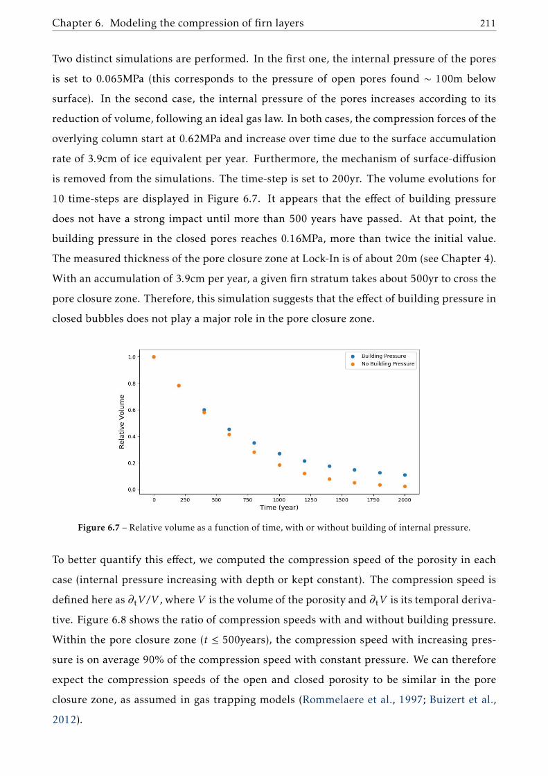
Chapter 6. Modeling the compression of firn layers 211
Two distinct simulations are performed. In the first one, the internal pressure of the pores
is set to 0.065MPa (this corresponds to the pressure of open pores found ∼ 100m below
surface). In the second case, the internal pressure of the pores increases according to its
reduction of volume, following an ideal gas law. In both cases, the compression forces of the
overlying column start at 0.62MPa and increase over time due to the surface accumulation
rate of 3.9cm of ice equivalent per year. Furthermore, the mechanism of surface-diffusion
is removed from the simulations. The time-step is set to 200yr. The volume evolutions for
10 time-steps are displayed in Figure 6.7. It appears that the effect of building pressure
does not have a strong impact until more than 500 years have passed. At that point, the
building pressure in the closed pores reaches 0.16MPa, more than twice the initial value.
The measured thickness of the pore closure zone at Lock-In is of about 20m (see Chapter 4).
With an accumulation of 3.9cm per year, a given firn stratum takes about 500yr to cross the
pore closure zone. Therefore, this simulation suggests that the effect of building pressure in
closed bubbles does not play a major role in the pore closure zone.
Figure 6.7 – Relative volume as a function of time, with or without building of internal pressure.
To better quantify this effect, we computed the compression speed of the porosity in each
case (internal pressure increasing with depth or kept constant). The compression speed is
defined here as ∂tV /V , where V is the volume of the porosity and ∂tV is its temporal deriva-
tive. Figure 6.8 shows the ratio of compression speeds with and without building pressure.
Within the pore closure zone (t ≤ 500years), the compression speed with increasing pres-
sure is on average 90% of the compression speed with constant pressure. We can therefore
expect the compression speeds of the open and closed porosity to be similar in the pore
closure zone, as assumed in gas trapping models (Rommelaere et al., 1997; Buizert et al.,
2012).

212
Figure 6.8 – Ratio of compression speeds: with building pressure in the porosity over without buildingpressure.
6.3.3 Evolution of a firn layer
This section presents the evolution of the porous network of a firn layer, as simulated by
the model. Four different experiments are reported to present the contribution of ice creep
and curvature-driven diffusion to the morphological changes of the porous network. The
simulation are all initialized with the same porous network, extracted from the tomography
image of a real firn sample. The firn sample was excavated around the 100m depth in the
Lock-In firn core, described in the previous section. A 5.35mm×5.35mm×3.75mm rectangu-
lar cuboid was extracted from a tomography image and used for initialization. The external
compression starts at 0.66MPa and increases over time according to the 3.9cm of ice per year
accumulation rate. The internal pressure of the pores is maintained at 0.065MPa, as we have
seen that the building pressure in closed pores is small in the pore closure zone. All simu-
lations are performed with a 100 years time-step, for a maximum of 10 time-steps.
6.3.3.1 Diffusion process only
In the first simulation, the process of ice creep is removed and only the curvature-driven
diffusion is taken into account. The parameter C0 is set to 10−6mm4.yr−1. A slice of the firn
medium is shown in Figure 6.9, and illustrates the evolution of the micro-structure over
700 years. As seen in the figure, the mechanism of surface diffusion leads to a rounding
of pores over time. This is consistent with a mass transport occurring from regions of high
Chapter 6. Modeling the compression of firn layers 213
curvature towards regions of low curvature, as exemplified in Figure 6.10. While Burr et al.
(2019) reports that letting firn samples at rest in a relatively high-temperature environment
(−2◦C) leads to pore splitting, we did not observe such phenomenon in our simulation. To
the contrary, our simulation exhibits pore coalescence, where several small pores merge into
a larger one.
As the Level-Set function gives the position of the ice/pore interface, it is possible to con-
vert the output of the simulation into binary images, similar to tomographic images. We
performed this conversion for the time-steps t = 0 and t = 700 years. The binary images
can then be analyzed as tomographic images, and the number of individual pores in the
medium can be counted (using the ImageJ plug-in Analysis_3D here; Boulos et al., 2012).
It reveals that the simulation starts with 39 individual pores in the volume and drops to
only 9 individual pores after 700 years. This highlights that pore coalescence happened
multiple times during the simulation. Thanks to the Level-Set function, the density of the
medium during the simulation can be quantified. The initial relative density to pure ice is
0.902, and drops to 0.884 after 700 years, that is to say a decrease of about 2%. However, the
mechanism of surface diffusion should theoretically not modify the density of the medium
(Bruchon et al., 2010). The density variation is of the order of the volume error reported in
Section 6.3.1. Furthermore, a closer look at the surface diffusion velocity field in Figure 6.10,
indicates that despite the stabilization of the equations (introduced in Equations 6.10) the
velocity field exhibits a lot of variability that is likely related to numerical noise, rather than
physically-relevant variability. We might therefore expect our representation of surface dif-
fusion to introduce some numerical noise in the results, which could also contribute to the
decrease in density.
6.3.3.2 Ice creep only
The second simulation is performed with solely the mechanism of ice creep. A slice of
the firn medium after compression is displayed in Figure 6.9. As seen in the figure, this
simulation leads to a densification of the medium, with a smaller porous network. This
observation is confirmed by the analysis of the density, that increased from 0.902 to 0.960
after 700 years. Moreover, the simulation visually exhibits pore splitting. This is again
confirmed by counting the number of individual pores before and after the compression.
This number increased from 39 to 57 pores, showing the ability of the ice creep mechanism
to split and isolate pores from the atmosphere.

214
Figure 6.9 – 2D cut-views of the firn material during the simulations. The gray medium is the ice matrix,and the white spaces are the pores. The slice on the left shows the initial porous structureused in all the simulations, and the four slices on the right show the results of the fourdifferent simulations after 700 years.
Figure 6.10 – 2D cut-view of the firn material showing the surface-diffusion velocity field in the horizon-tal direction. Blue colors stand for negative values and red colors for positive values. Theinterface of a pore is highlighted in white in the middle of the section. The green and or-ange circles respectively show the regions where the interface is receding in the ice phaseand growing in the pore phase. This leads to the rounding of the pore.

Chapter 6. Modeling the compression of firn layers 215
6.3.3.3 Ice creep and surface diffusion
The third and fourth simulations take into account the combined effects of curvature-driven
diffusion and ice creep. The parameterC0 is set to values of 10−6mm4.yr−1 and 10−7mm4.yr−1,
to represent different levels of curvature-driven diffusion, respectively referred to as the low
and high-diffusion case for the rest of the section.
2D cut-views of both simulations after 700 years are displayed in Figure 6.9. The results
show an increase in relative density from 0.902 to 0.959 for the low-diffusion case, and to
0.953 for the high-diffusion case. Increasing the role of diffusion in the simulation leads to
a slightly smaller density. This is consistent with the 0.960 value reported in the absence
of surface diffusion. Observation of the Lock-In firn core shows that densities of 0.95 are
found around the 130m depth. This is consistent with the 700 years sinking time of the
simulation, which corresponds to about 30m of depth increase.
Analysis of the results also shows an increase in the number of individual pores from 39 to
61 and 50 for the low and high-diffusion respectively. It appears that in the high-diffusion
case, the mechanism of surface diffusion slows down the splitting of pores. The diffusive
mechanism leads to a rounding of the pores, preventing the development of small necks
that would eventually lead to pore splitting. Surprisingly, the low-diffusion case displays
a little more pore splitting than the case without any surface diffusion, that resulted in
57 individual pores after 700 years. It is not clear if this is related to a specific inter-play
between the diffusion and creep mechanisms that would accelerate the splitting of pores, or
simply numerical noise.
6.4 Discussion
Combining the Finite Element and Level-Set methods is a promising modeling approach to
simulate the topological evolution of firn under compression. Notably, the use of a separate
mesh for the ice phase enables to easily compute deformation velocities as response to me-
chanical compression. This velocity field can then be used to simulate the evolution of the
ice/pore interface using the Level-Set function.
Yet, several optimizations of the model are still required before its operational application
to study the closure of pores in polar firn. First, the model is currently fully sequential. Run-
216
ning a ten steps simulation in a 5.35mm×5.35mm×3.75mm firn sample requires roughly a
day of computation. The parallelization of the model would curb down this time, to use the
model on larger domains. This will allow one to perform simulations of several-centimeter
large domains, which have been shown to be more representative of real firn (Schaller et al.,
2017). Moreover, as shown in Section 6.3.3.1, the current implementation of the surface
diffusion mechanism leads to a noisy velocity field that might deteriorate the robustness of
the results. The use of a very fine mesh near the interface could help resolve this problem,
but would lead to a sharp increase in the computation time. On the other hand, the use of
more sophisticated stabilization techniques (such as in Bruchon et al., 2010) could resolve
this issue without an additional computational cost. Another solution could be the use of
second-order elements for the computation of the second-derivatives required for the diffu-
sive mechanism. As diffusion appears to play a significant role in the morphology of pores
(Burr et al., 2019), it seems important to implement a fast and robust representation of dif-
fusive mechanisms in the model. This would help to decipher the relative contributions of
ice creep and diffusion to the evolution of the porous network, and provide insights on the
evolution of pores at very-low temperature.

Chapter 6. Modeling the compression of firn layers 217
6.5 Conclusion of the chapter
This chapter presents the development, and first few applications of a new model simulat-
ing the micro-mechanics of firn. In this model, the ice-pore interface is explicitly taken into
account, and its movement is deduced from physical laws. To handle the complex geome-
tries and the topological changes that occur in firn, the model relies on the Level-Set and
Finite Element methods.
To capture the evolution of the interface, the model is decomposed in three independent
steps, namely the mesh adaptation, computation of velocities and the advection steps. This
formulation gives modularity to the model, as physical mechanisms can be added or re-
moved from the computation of the interface’s velocity. Moreover, thanks to this modular
formulation, the mesh adaptation and advection steps could be modified (for instance to
improve mass conservation) without complicating their integration to the rest of the model.
In this chapter, I use the model to first quantify the effect of the building pressure in bub-
bles in the pore closure zone. Results indicate that the building of pressure does not have a
strong impact on the compressibility of bubbles in the pore closure zone, and can therefore
be safely neglected in gas trapping models. I also use the model to estimate the impacts
of curvature-driven surface diffusion and ice creep on the evolution of the pores in a firn
sample. The mechanism of ice creep leads to a densification of the medium, as well as pores
splitting. On the other hand, it appears that the mechanism of surface diffusion is responsi-
ble for pore coalescence rather than splitting. Moreover, these two examples should be seen
as showcases, to demonstrate the ability of the model to compute and capture the movement
of the ice-pore interface in response to physical drivers.
Two major issues remain to be improved before an operational use of the model is made
possible. First, as shown in the chapter, the Level-Set method does not naturally conserve
mass during the simulation. The implementation of the ICLS method greatly improve the
mass conservation performance of the model, but improvements remains possible. Notably,
more control could be put of the size of the mesh elements near the interface, as Zhao et al.
(2014a) showed that its is an important factor for a proper mass conservation. Secondly,
the simulations sometimes produce small degenerate elements during the mesh adaptation
step. Because of these degenerate elements, the simulations crash before the last time-step.

218
Again, a better focus should be put on the mesh adaptation step in order to better control
the size of the elements near the interface.
Unfortunately, this model cannot represent the crystalline texture of the ice material. Future
work should be dedicated to quantify the impact of not explicitly representing the crystal
orientations at the pore scale. Such a crystalline texture could be implemented using more
than one Level-Set function, each representing a specific crystalline orientation (Bernacki
et al., 2008), but is beyond the scope of this study.
Nonetheless, this work exemplifies the possibility to use Level-Set methods to characterize
the evolution of porous network in firn. A potential application could be to estimate the
impact of different thermodynamical mechanisms on the movement of the interface and
the closure of pores (Ashby, 1974; Shieh and Evans, 1991). A second potential application
in the future would be to apply it to a large domain (of the order a few centimeters), in
order to estimate the progressive closure of the firn porosity. Finally, this type of model
could be used to study the development or disappearance of structural anisotropy under
metamorphism and compression, and to quantify its impact of the mechanical behavior of
the firn material.
Chapter 7
Conclusion and Outlooks
Contents
7.1 General conclusion . . . . . . . . . . . . . . . . . . . . . . . . . . . . . . . . . 221
7.2 Perspectives . . . . . . . . . . . . . . . . . . . . . . . . . . . . . . . . . . . . . 223
7.3 A few personal words . . . . . . . . . . . . . . . . . . . . . . . . . . . . . . . 225

220

Chapter 7. Conclusion and Outlooks 221
7.1 General conclusion
The goal of this work was to provide a better understanding of the process of gas trapping
in polar ice, and notably for the very low accumulation rates typical of the glacial periods
on the East Antarctic plateau. By studying the enclosure of gases, we aim to enable a more
precise interpretation of the gas signals in ice cores, in order to take full advantage of ice
core gas records.
The new insights obtained on the questions introduced in Chapter 2, and that guided my
work during these three years of PhD, are summarized below.
What are the physical characteristics of early and late gas trapping layers ? What is the
origin of their presence in the firn?
The study of the Lock-In firn core in Chapter 4 confirmed that the firn is a medium with a
strong and heterogeneous stratification. This heterogeneous stratification is responsible for
the staggered trapping of gases, creating age inversions in the gas records (Mitchell et al.,
2015; Rhodes et al., 2016). Using closed porosity data obtained with gas pycnometry, we
observed that all firn strata of a given firn have the same relationship between their density
and their amount of closed pores. In particular, strata that are especially dense compared to
their surroundings contain a higher quantity of closed bubbles than neighboring strata. A
similar observation was made concerning the centimeter scale variations of the porous net-
work morphology. Two layers with the same density appears to have porous network with
similar shapes, sizes, and gas transport properties, no matter how apart they might be in
the firn column. Therefore, early closure layers simply correspond to the dense layers of the
firn, and trap gases in a similar fashion as the rest of the firn, simply at shallower depths.
A direct link between the liquid conductivity of firn strata and their density was observed in
the pore closure zone. This supports the vision of a deep firn stratification due to the chem-
ical softening of certain firn layers (Hörhold et al., 2012; Fujita et al., 2016). Some layers
contain abnormally high amount of ions in their ice phase, leading to a faster densification
and a shallower closure in the firn column. This impurity-driven layered gas trappingmech-
anism is also supported by observations made in deep ice cores. Indeed, we observed that
periods with high numbers of important layering artifacts correspond to periods of high
levels and variabilities of calcium concentrations in the ice phase.
222
What is the influence of accumulation on the progressive closure of pores in firn of the
East Antarctic plateau? What can be known about the closing of pores under very-low
accumulation rate conditions?
Comparing closed porosity data obtained in the Lock-In and Vostok firn cores, we observed
that an increase in accumulation rate at constant temperature results in a firn closing at a
lower density. This is corroborated by air content data showing that the total porous volume
during closure Vi is higher at the higher-accumulation site of Lock-In. This difference in
closure density is certainly linked to a difference in the morphology of the two sites’ porous
networks (e.g. Burr et al., 2018).
The next questions are thus in what sense are the porous networks different, and why would
that cause them to seal-off at different densities? The ongoing acquisition of tomography
images from different firns of both Greenland and Antarctica (Gregory et al., 2014; Schaller
et al., 2017; Burr et al., 2018) could help decipher what are the important characteristics
governing the density of closure of firn strata. The compression model that I started to
develop during this PhD aims at using tomographic images to simulate the evolution of the
firn micro-structure over time, and notably help predicting the characteristics of the porous
networks present in past glacial firns of East Antarctica.
What is the degree of smoothing encountered in glacial and interglacial period ice cores
from East Antarctica ? What is the relationship of smoothing with accumulation?
The gas age distributions of the gases enclosed in ice cores from East Antarctica have been
estimated, thanks to a novel technique presented in this work. We are then able to com-
pare the degree of smoothing of gas records for different low-accumulation conditions. The
smoothing of gas records in ice cores from East Antarctica dampens out the atmospheric
variability that takes place over time scales shorter than a couple of centuries. This notably
means that sub-millennial variability can be inferred from the gas records of very low accu-
mulation ice cores, unlike previously thought
We observed that the degree of smoothing increases with the reduction of accumulation
from interglacial to glacial conditions. Yet, it is not as drastic as expected. Moreover, the
different gas records obtained for the glacial period all appear to have the same degree of
smoothing. Thus, smoothing is weakly sensitive to the variations of accumulation for the
conditions encountered on the East Antarctic plateau. Therefore, future studies could rely
on the usage of a unique age distribution for the study of glacial gas records from East
Antarctica.

Chapter 7. Conclusion and Outlooks 223
What is the loss of atmospheric information that one can expect, in the case of low-
accumulation and highly thinned deep ice cores drilled on the East Antarctic plateau?
The total loss of information between the atmospheric history and its estimation in ice core
gas records, is due to the combined effect of firn smoothing, layering artifacts, and analytical
limitations. As discussed above, firn smoothing in ice cores from East Antarctica removes
variations that take place over time scales of a couple of hundreds of years and shorter. For
layered gas trapping, the thinning of the ice at the bottom of ice sheets implies that the ar-
tifacts will no longer be individually resolved. Due to their non-symmetrical distribution,
they will add to the total alteration of the gas signal. Yet, results of the layering model, com-
bined with analytical smoothing, indicate that the overall impact will be limited to 10ppbv
and 0.5ppmv for the case of methane and carbon dioxide respectively. The influence of
analytical resolution cannot be neglected. In the case of methane, even with current CFA
systems specifically designed to ensure a good spatial resolution, the act of measurement
will remove a part of the record variability and add up to the firn smoothing. For carbon
dioxide, estimations of rates of change in the gas records can be significantly underesti-
mated due to the effect of firn smoothing. This underestimation is further aggravated due
to the limited spatial resolution of discrete measurements.
7.2 Perspectives
Amissing mechanism for gas trapping?
The data obtained for the Lock-in firn and ice core have shown that there is a large discrep-
ancy between the modeled and measured air content values. As explained, this mismatch
does not appear to originate from measurement errors, which indicate that the problem lie
in the model itself. The inability of models to estimate the right amount of air highlights
a potentially missing mechanism in our comprehension of gas trapping in polar ice. To
improve our understanding of gas trapping, and to be able to properly model it, this dis-
crepancy needs to be resolved.
In Chapter 4 we proposed a few potential mechanisms to reconcile the data and model. The
mechanism of limited compression in the closed bubbles seems unlikely to be the expla-
nation at this stage. Other explanations could be the re-opening of closed bubbles in the
firn due to excessive pressure building, or the releasing of air through capillaries not visible

224
with our experimental methodology. Future work should focus on solving this discrepancy.
It will improve the capabilities of models not only to estimate the amount of air in polar
ice, but also its composition. Finally, the study of the potential release of gases through cap-
illaries in the pore closure zone could work in synergy with the study of the fractionation
of O2 and N2 during the trapping process (Huber et al., 2006a; Severinghaus and Battle,
2006).
Parametrizations of pore closure
Another point to improve the ability of gas trapping models to accurately represent the en-
closure of gases in polar ice, is the availability of reliable closed porosity profiles. Two major
problems hindered this point. First, the measurements of closed porosity data are affected
by finite size effects, under the form of cut-bubbles. The acquisition of large firn samples
can mitigate this point, but do not totally resolve it. The adaptation of the percolation the-
ory (Enting, 1993) and of finite size analysis (Baglietto and Albano, 2008) from the field of
statistical physics could be a way to determine the firn macroscopic properties from smaller
scale samples. Moreover, the tools of statistical physics could also help to determine the
diffusive properties of firn from centimetric samples.
Then, from the knowledge gained studying various polar sites, new closed porosity parametriza-
tions should be derived. Indeed, such parametrizations are required for firns without direct
measurements, such as past firns. Currently, the development of robust closed porosity
parametrizations is limited by the inerrant uncertainties due to finite size effects and by the
low number of studied sites. It is particularly important to obtain data from sites with sim-
ilar temperatures but different accumulations (and vice-versa), to independently study the
impact of temperature and accumulation on the closure of pores.
Influence of surface metamorphism
A point introduced in Chapter 2, but not further developed in this thesis, is the impact of
surface metamorphism. A better comprehension of surface metamorphism and its impact
on gas trapping would be of great interest for the dating of ice cores based on air content or
O2/N2 records (Bender, 2002; Raynaud et al., 2007; Lipenkov et al., 2011). The recent study
of Calonne et al. (2017) on the upper surface layering observed at Point Barnola in East
Antarctica reports the development of a preferential texture of the ice crystals due to meta-
morphism. They notably observe, similarly to alpine snow, that dense layers at the surface
are characterized by smaller rounded grains and a lesser degree of structural anisotropy.
Chapter 7. Conclusion and Outlooks 225
This appears as inconsistent with the observation of Fujita et al. (2009), that report a pos-
itive correlation between density and structural anisotropy. This indicates that the mech-
anisms at play in the first few meters of the firn column are not yet well understood. The
ongoing development of analytical techniques and models focused on the stratification and
on the micro-structural properties of snow should bring new insights within the coming
years.
Retrieving methane sub-millennial variability
This work provides the gas age distributions of the gas enclosed in East Antarctica ice cores.
With this new knowledge, deconvolution techniques could now be used to retrieve as much
information as possible from ice core methane records (Shumway and Der, 1985; Witrant
and Martinerie, 2013). Deconvolution methods applied to CFA data from the penultimate
glacial period and beyond, would yield new insights on the atmospheric methane variations
at the sub-millennial scale.
Such deconvolution could also be applied to the future Oldest-Ice core. In this case, the
convolution function to be used in the method should reflect the combined smoothing of
the firn and of the analytical system.
7.3 A few personal words
The combination of experimental methods, code development, and general problem solv-
ing has been greatly intellectually stimulating during these past few years. This thesis has
convinced me of the importance of the interaction between experimental methods and nu-
merical modeling. In my near (and perhaps long) future I intend to continue in the field of
scientific research, with a combined approach of experimental and modeling works.
My stay at IGE also introduced me to teaching and science communication. During this
three years of PhD I have been teaching at Université Grenoble Alpes, for both undergradu-
ate and graduate students and in the fields of physics, mathematics, computer sciences, and
remote sensing. These 192 hours of teaching have been valorized by a Label Recherche et
Enseignement Supérieur (Research and Higher Education). Concerning science communi-
cation, I have been involved in outreach events outside the institute (Tribulations Savantes,
Rencontres Montagnes et Sciences, Pint of Science) and within the institute walls (Cordées

226
de la réussite and tours of the lab for visitors). I notably keep a particularly good memory of
my involvement in the 100 Parrains 100 Classes program, in which I mentored a high school
class on the subject of climate change and Antarctic glaciology. These outreach events were
the occasion to inform a general audience about the physical mechanisms behind natural
phenomena such as glacier flow or the greenhouse effect. I hope that by having a better in-
sight on the underlying material processes, people got a deeper and lasting understanding
of the natural phenomena around them.

Appendices
227


Appendix A
Historical closed porosity data in polar
firn
This appendix deals with pycnometry measurements performed by Jean Marc Barnola at
IGE in the 1990’s. The data have been used to derive a parametrization of the closure of
firn porosity, notably used in Goujon et al. (2003), Buizert et al. (2012), or Witrant et al.
(2012). Yet, despite their significance for the ice core community, these data have not been
published to this day.
To be able to compare the pycnometry data of Lock-In (measured during my PhD) with the
ones from Vostok, Antarctica, (measured by JM Barnola), I had to re-process the experimen-
tal data of JM Barnola. I reconstructed, with the aid of L Arnaud, X Faïn, and P Martinerie,
the processing chain of JM Barnola and was able to apply it to the data obtained for the three
polar sites measured in the 1990’s: Vostok, Summit (Greenland), and DE08 (Antarctica).
We now intend to publish these data, alongside with the explanation of the processing chain.
The goal is to provide the ice core community with these datasets of closed porosity data,
to clarify how the parametrization first proposed in Goujon et al. (2003) was derived, and
to discuss their limitations. This appendix is thus written as an article draft for a data jour-
nal.
229

230
Article Draft
Kévin Fourteau1, Laurent Arnaud1, Xavier Faïn1, Patricia Martinerie1, Jean-Marc Barnola1,†
[1] Univ. Grenoble Alpes, CNRS, IRD, Grenoble INP, IGE, 38000 Grenoble, France
A.1 Introduction
The enclosing of atmospheric air in the ice of polar regions is of great importance for the
study of past climates. Indeed, ice cores drilled in the polar regions have the unique char-
acteristics of containing bubbles of air from past atmospheres. These enclosed bubbles have
been used to reconstruct the atmosphere history in major greenhouse gas concentrations
for the last 800,000 years (Lüthi et al., 2008; Loulergue et al., 2008). However, in order
to properly interpret the gas records from ice cores, it is necessary to understand how they
are trapped in the ice (Stauffer et al., 1985; Schwander et al., 1993; Rommelaere et al., 1997).
The snow at the surface of polar ice sheets is a porous material, and its interstitial air can
freely exchange with the atmosphere (Stauffer et al., 1985). Snow strata are progressively
buried under new precipitations and are compressed due to the weight of the younger snow
above. This buried and compacted snow is referred to as firn. With time the firn strata
are further buried and their interstitial porous networks shrink. Depending on the local
temperature and accumulation conditions, some of the pores start to pinch and encapsulate
the interstitial air at depths between 50 and 100m below the surface (Witrant et al., 2012).
The porous network then continues to pinch until all the interstitial space is isolated from
the atmosphere. The firn then becomes airtight ice with enclosed bubbles of atmospheric air.
One way to characterize the closing of the porous network and the trapping of gases is to
rely on the closed and the open pore volumes. Closed pores are pores that no longer reach
to the atmosphere, and are therefore airtight. On the other hand, open pores reach the at-
mosphere and the air inside is thus free to escape. Moreover, data of closed and open pore
volumes are required for the usage of densification and gas trapping models (Rommelaere
et al., 1997; Goujon et al., 2003; Buizert et al., 2012; Witrant et al., 2012). That is why these
closed and open volumes have been measured along various firn columns from Greenland

Appendix A. Historical closed porosity data in polar firn 231
and Antarctica (Schwander et al., 1993; Schaller et al., 2017).
Such measurements were notably performed in the 1990’s by JM Barnola on firn cores
drilled at the three polar sites of Vostok (Antarctica), Summit (Greenland) andDE08 (Antarc-
tica), using the technique of gas pycnometry on cylindrical samples of approximately 4cm
in diameter and height. These data have been used to parametrized closed porosity curves
used in gas trapping models (Goujon et al., 2003; Buizert et al., 2012; Witrant et al., 2012).
Unfortunately, JM Barnola passed away before publishing the data in the peer-reviewed lit-
erature. In an effort of transparency, we propose to make them available. Our goal is to
provide an understanding of how the closed porosity parametrization proposed in Goujon
et al. (2003) was derived. Moreover, measuring closed porosity is labor intensive and re-
quires large amount of firn material. As a result, this type of data is rather scarce. We hope
that making these data available will help the ice core community to better understand the
trapping of gases in polar ice.
A.2 The pycnometry method
The technique used by JM Barnola to measure the closed and open porosity volumes in firn
samples is the gas pycnometry method (Stauffer et al., 1985). The pycnometry apparatus is
composed of two airtight chambers of known volumes V1 and V2 with a valve between them
allowing one to either connect or isolate the chambers. A pressure gauge is joined to the
chamber V1 to monitor its internal pressure. For the measurements, a firn sample is placed
in the first chamber V1, while the second one is isolated and vacuum-pumped. Placing a
firn sample in the chamber V1 renders a volume Vs inaccessible to the gases. The pressure P
in V1 is recorded. Then the two chambers are connected, and the gas in chamber V1 expand
in a larger volume. The pressure after dilation P ′ is then recorded. The volume Vs can be
related to the recorded pressure by:
Vs = V1 −R
1−RV2 (A.1)
where R = P ′/P.
The specific protocol followed by JM Barnola was to first execute a dilation without any sam-
232
ple in the first chamber, then a second dilation with the sample in. In this case, Equation A.1
can be rearranged as:
Vs = V2
( R0
1−R0− R1
1−R1
)(A.2)
where R0 and R1 are respectively the pressure ratio in the cases without and with the firn
sample in V1.
The volume inaccessible to gases in composed of the ice phase and of the closed pores phase.
Therefore, one can deduced the closed and open porosity volume:
Vcl = Vs −Vice
Vo = Vcyl −Vs
(A.3)
where Vcl and Vo are the closed and open porosity volumes, Vice the volume of the ice phase
and Vcyl the volume of the firn sample. The volume of the ice phase is deduced from the
mass M of the sample knowing that Vice =M/ρice, where ρice is the density of pure ice. The
density of pure ice is estimated using the temperature relationship ρice = 0.9165(1− 1.53 ×10⁻⁴T ), where T is the temperature (Bader, 1964; Goujon et al., 2003). The volume of the
firn sample Vcyl is measured geometrically.
Note that the pycnometry method assumes that all the pores reaching the edge of the sample
are considered as open. This means that some pores that are closed in the firn column (they
do not reach the atmosphere) will be considered open during the pycnometry measurement.
This is known as the cut-bubble effect and leads to an underestimation of the closed porosity
(Martinerie et al., 1990; Schaller et al., 2017).
A.3 Processing of the data
For each of the three sites we retrieved a computer file containing the dilation ratios R0 and
R1, the mass of the firn samples, their volumes, and the temperature during the experiment.
We also retrieve the source codes of JM Barnola used to process the data. Finally, we also
have the experiment notebooks of JM Barnola.

Appendix A. Historical closed porosity data in polar firn 233
A.3.1 Original data processing
In this section, we aim to reproduce the data processing performed by JM Barnola. This is
done for two reasons. First, the data have been used to derived a parametrization of the
closed porosity in polar firn (Goujon et al., 2003), and it is therefore important to under-
stand how they were processed. Secondly, the original processing includes corrections for
experimental biases that were observed by JM Barnola and that have to be taken into ac-
count.
A look at the original source codes indicates that the processing included a correction for
a pycnometry system drift and a cut bubbles correction. This correction is based on the
idea that the pycnometry method should ideally indicate fully open samples at low density
(ρ < 0.72g.cm−3) and fully closed ones at high density (ρ > 0.86g.cm−3). Based on this, a
correcting factor α to be applied to the inaccessible volume Vs is computed. In the case of
low density firn, α is compoutd as 1 − Vb/Vice and in the case of high density firn one has
α = Vcyl /Vs. JM Barnola observed that this α factor is linearly related to the empty dilation
ratio R0 (Figure A.1). We interpret that this relation is indicative of a drift in the pycnometry
apparatus. However, as seen in figure A.1, this linear relationship is not the same for high
density and low density firn samples. JM Barnola derived intermediate linear relationships,
in black Figure A.1. Using this linear relationship, the correcting factor α can be determined
even in the case of not fully closed or open samples. Thus, all the Vs measured in a firn core
are corrected by estimating an α factor based on the R0 of the preceding empty dilation.
Finally, in all of the three measurement campaigns the volume V2 has been estimated to be
of 7.2cm3 (value found directly in JM Barnola’s processing codes).
Vostok measurement campaign:
In the case of the Vostok campaign, JM Barnola observed a bias due to the measurements of
sample volumes with a caliper, depending of the pressure applied by the caliper. He there-
fore proposed to apply a volume correction of 0.9% to the firn samples that were measured
by applying a too weak pressure with the caliper. JM Barnola also applied a 4°C correction to
the recorded temperatures, in order to account for the heat dissipation of heated elements
towards the temperature sensor. For the Vostok campaign measurements α is computed

234
following α = −40.2145R0 + 39.22304, in black in the left panel of Figure A.1. These three
corrections were found hard coded in the Vostok processing source code, and have been cor-
roborated by the notebooks.
Summit measurement campaign:
In the case of the Summit campaign the same volume correction of 0.9% was applied to all
the samples. Moreover, a weighting bias has been found by JM Barnola and is taken into ac-
count by applying a 0.9983 correction factor to the measured mass. Finally, the α correction
is given by α = −45.045045R0 + 43.820459, in black in the middle panel of Figure A.1. It is
interesting to note that in the case the correction chosen by JM Barnola seems to be based
on the low density α only.
DE08 measurement campaign:
For DE08, no volume or mass correction is reported in the original processing code. The α
correction is given by α = −37.2577R0 + 36.4204, in black in the right panel of Figure A.1.
Again, the correction chosen by JM Barnola appears to be based on the low density α.
Using all these data we can deduce the closed and open porosity volumes. Figure A.2 dis-
plays closed porosity and closed porosity ratio values against total porosity. Closed porosity
is defined as the volume fraction occupied by the closed pores in the firn sample, total poros-
ity is defined as the volume fraction of all pores and the closed porosity ratio is the ratio of
the closed pores volume over the total porous volume. We chose to use volume fractions
instead of porous volumes per gram of firn, as the former are not sensitive to temperature
and therefore makes the comparison between sites easier. Yet, the volume fraction data can
easily be converted to porous volumes per gram of firn using the density of ice.
A.3.2 A new data processing
We identify one major issue in the processing elaborated by JM Barnola. In the case of high
density firn samples, the correcting factor α both encapsulates the effect of a system drift

Appendix A. Historical closed porosity data in polar firn 235
Figure A.1 – In each panel: The blue dots are the correcting factors α computed for low density firn asa function of the preceding R0. The orange dots are the correcting factors α computed forhigh density firn as a function of R0. The black line is the linear relation originally derivedby JM Barnola. The blue line is the linear regression based solely on the low density α
Figure A.2 – Closed porosity data using JM Barnola processing chain. Left panel: Closed porosity againsttotal porosity. The dashed line represents the Closed porosity = Total porosity line. Rightpanel: Closed porosity ratio against total porosity. The dashed line marks where the closedporosity ratio equals one.
and of cut-bubbles. Indeed, the assumption under which this factor is computed is that
the pycnometry experiment should measure a fully closed sample at high density, de facto
including a cut-bubble correction. However, the correction to be applied for cut-bubbles
is not the same at all densities (Schaller et al., 2017). It thus explains why the high and
low density α relationship with R0 might differ. On the other hand, the low density α does
not include any cut-bubble correction, and therefore only accounts for system drifts. We
therefore propose to correct the data using only the relationship between low density α and
R0. These corrections are displayed as blue lines in Figure A.1. As shown in the figure, the
new correction mainly differ in the Vostok case. The closed porosity and closed porosity
ratio after applying this new correction are displayed in Figure A.3.
It is important to note that these data are not corrected for cut bubbles, and therefore do
not directly represent the amount of closed pores in the firn column. We decided not to
correct the data for cut bubbles in this article. Indeed, the appropriate corrections are hard

236
Figure A.3 – Same as Fgire A.2 with the new α correction.
to estimate and potentially site dependent (Schaller et al., 2017). Further research is needed
to fully solve this problem.
A.4 The Barnola parametrization for closed porosity
The firn densification and gas trappingmodel of Goujon et al. (2003) used a parametrization
of closed porosity proposed by JM Barnola (Equation 9 of Goujon et al., 2003). This Barnola
parametrization relates the closed porosity to the total porosity with:
Pclosed = γPtotal( PtotalPclose−off
)−7.6(A.4)
where Pclosed is the closed porosity, Ptotal the total porosity, Pclose−off the close-off porosity that
can be estimated using air content measurements or a temperature regression (Martinerie
et al., 1994), and γ a factor valued at 0.37.
We are confident to state that the Barnola closed porosity parametrization was deduced
from the pycnometry data described in Section A.3.1, with the original processing chain.
Indeed, there is a clear linear relationship between the logarithm of the closed porosity
ratio and the logarithm of the total porosity normalized by the porosity close-off deduced
from air content data. This is relation is displayed in Figure A.4, and matches with the
Barnola parametrization. The comparison between the experimental closed porosities and
the Barnola parametrization is also displayed in Figure A.5. It is therefore important to
acknowledge that the Barnola parametrization is based on data that are not fully corrected
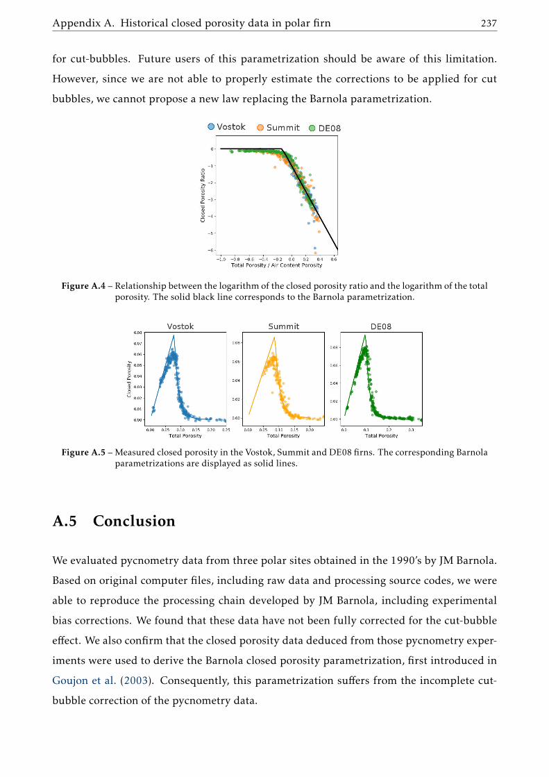
Appendix A. Historical closed porosity data in polar firn 237
for cut-bubbles. Future users of this parametrization should be aware of this limitation.
However, since we are not able to properly estimate the corrections to be applied for cut
bubbles, we cannot propose a new law replacing the Barnola parametrization.
Figure A.4 – Relationship between the logarithm of the closed porosity ratio and the logarithm of the totalporosity. The solid black line corresponds to the Barnola parametrization.
Figure A.5 – Measured closed porosity in the Vostok, Summit and DE08 firns. The corresponding Barnolaparametrizations are displayed as solid lines.
A.5 Conclusion
We evaluated pycnometry data from three polar sites obtained in the 1990’s by JM Barnola.
Based on original computer files, including raw data and processing source codes, we were
able to reproduce the processing chain developed by JM Barnola, including experimental
bias corrections. We found that these data have not been fully corrected for the cut-bubble
effect. We also confirm that the closed porosity data deduced from those pycnometry exper-
iments were used to derive the Barnola closed porosity parametrization, first introduced in
Goujon et al. (2003). Consequently, this parametrization suffers from the incomplete cut-
bubble correction of the pycnometry data.

238
Finally, we intend to make these data publicly available. The three sites studied in this
article are characterized by a wide range of accumulation rates and temperatures. These
data could be useful for future studies focusing on the effect of the climatic conditions on
pore closure and gas trapping.

Appendix B
Firn air pumping campaigns at EastGRIP
During my PhD, I participated to two firn air pumping campaigns at the Greenland site of
EastGRIP (EGRIP) 1. EGRIP is located in North-East Greenland, at the surface of the North
East Greenland Ice Stream (NEGIS). NEGIS is a large ice steam draining 12% of the Green-
land coastal mass flux. A deep drilling campaign is currently taking place, with the main
objective of better understanding of the evolution of NEGIS in the past.
Taking advantage of the camp and facilities deployed to host the deep drilling, other scien-
tific projects are conducted at the EGRIP site. Notably, a project of firn air pumping was
decided. The main objective of this project is to retrieve a firn core, as well as firn air data
from the open porosity of the firn column. This campaign serve three scientific objectives: i)
reconstructing past atmospheric concentrations using the air hold in the firn, ii) providing
insights on the firn smoothing and layered trapping at a site with no studied equivalent in
terms of temperature and accumulation, iii) helping understand the O2/N2 signals in ice
cores.
My role during this project was to restore and prepare the IGE firn air pumping system, and
to participate on its deployment at the EGRIP site.
B.1 General principle of firn air pumping
The method to sample air from the open porosity of the firn is fairly straightforward:
- Drill to the depth of interest.
1https://eastgrip.org/
239

240
- Seal the borehole to isolate the bottom of the hole from the upper atmosphere.
- Pump at the bottom of the borehole.
Figure B.1 – Firm pumping methodology. The borehole is drilled until the depth of interest. Then theborehole is sealed (in gray in the Figure) and the air is pumped from the bottom of the firn.
This methodology is summarized in Figure B.1. The borehole is sealed with an inflated
rubber bladder, that acts as a plug. The sampled air is then stored either in canisters or in
glass bottles.
B.2 Preparing the firn air pumping system
IGE has a firn air pumping system composed of:
- A rubber bladder
- A tripod with a winch fit to lower the bladder into the borehole
- A system of dedicated pumps, tubing, and valves to route the pumped air to containers
This system was restored and assembled at IGE with the help of A. Orsi and X. Faïn. The
goal was to ensure that the firn air pumping gear could be deployed in working conditions
at the EGRIP site.
B.2.1 Preparing the bladder
A rubber bladder is used to seal the borehole. It ensures that the pumped air originates
from the open porosity of the firn, and not from the overlying atmosphere (see Figure B.1).
The bladder is composed of a rubber tube, sealed by two aluminum pieces (as shown in

Appendix B. Firn air pumping campaigns at EastGRIP 241
Figures B.2 and B.3). Three separate pieces of dekabon tubing are also connected to the
bladder: two that are traversing it (referred to as the Sample and Purge tubings), and one
that stops inside the bladder (referred to as the Bladder tubing). The bladder tubing is used
to inflate the bladder, and the sample and purge tubings are used to pump firn air.
Figure B.2 – Schematics of the bladder with the sealing aluminum pieces. The sample (S), purge (P), andbladder (B) tubings are also displayed.
Figure B.3 – Aluminum piece sealing the rubber tube. The piece is pierced for tubing connections. Threemounted airtight tube fittings are visible.
It is crucial that the bladder does not leak air when inflated in the borehole. Indeed, in
the case of a leak two problems arise. First, the bladder might lose its sealing effect and let
atmospheric air reach the bottom of the borehole. This would contaminate the sampled firn
air. Secondly, the air leaking from the bladder might be released at the bottom of the firn.
This would also lead to a contamination of the sample.
The bladder was thus assembled in Grenoble, and checked for potential leaks. To test for
leaks, the bladder was inflated with Helium and connected to a pressure gauge. A leak can

242
be visualized through a decrease in the internal pressure of the bladder. The use of Helium
to fill the bladder also allows one to use an Helium detector to spot the precise connection
responsible for the leak. The bladder was also tested for leaks in cold rooms, to estimate its
airtightness at low temperatures.
From these tests, we decided to use Viton© o-rings and PTFE ferrules. Specific care is needed
when tightening the PTFE ferrules, as they deform easily and can become leaky. Moreover,
with used tube fittings on both sides of the aluminum pieces (therefore inside and outside
of the rubber bladder) to increase the airtightness of the system.
B.2.2 Preparing the pumping and tubing system
The pumping system used to collect firn air data can be decomposed in three parts, corre-
sponding to each of the tubings.
Sample tubing
The goal of the sample tubing is to collect firn air from the open porosity and transfer it to
the containers at the surface. The air is pumped from the open porosity thanks to a clean
pump (Metal Bellows MN151), suitable for carbon monoxide sampling. This air is then
dried with a water trap, and routed either to a pre-vacuumed canister or a to glass bottle.
Purge tubing
The goal of the purge tubing is to catch potential leaks before they reach the sample tubing.
Indeed, the purge tubing is located above the sample tubing and will thus pump air arriving
from the above atmosphere or bladder. The air from the purge tubing is discarded through
a vent or used to inflate the bladder.
Bladder tubing
The bladder tubing is simply designed to inflate the bladder in the borehole. It is connected
to a pressure gauge to monitor the internal pressure of the bladder. The air sent down the
bladder tubing is the air originating from the purge line. This way, it is possible to fill the
bladder with firn air and limit the impact of potential bladder leaks.
A specific table was build by X. Faïn and A. Orsi to mount all the necessary valves and

Appendix B. Firn air pumping campaigns at EastGRIP 243
connections. The overall pumping system is summarized in Figure B.4. The table includes
a branch to connect spectrometers in order to monitor the sample concentration (e.g. CO2,
CH4, or CO) in real-time. A pressure regulator is mounted on this branch. A valve used to
shunt the table in also included (number 2 in Figure B.4), so other pumping systems can be
plugged to the sample line. Before deploying the firn air gear, it is necessary to ensure that
the 300m+ of dekabon tubing used to pump gases are not damaged.
Figure B.4 – Connections table of the IGE system.
B.3 Field work
B.3.1 Protocol of firn air pumping
A specific protocol was written with the help of A. Orsi to sample firn air with the IGE
pumping system. It is shown in Figures B.5 and B.6. The number of the valves are the one
written on the table in Figure B.4. The valves 9 and 10, which are not directly mounted in
the table, are also shown in the figure.

244
B.4 Tips and tricks
Here are a few feedbacks on my experience doing firn air pumping at EasGRIP.
- Extreme care must be taken to ensure that the bladder fits in the borehole. The first firn air
pumping campaign was not successful as the bladder got stuck in the borehole. Moreover,
analysis of the collected air samples indicates that the bladder was higher than the bottom
of the borehole during the different sample collections. A way to avoid this problem is to
ensure that no part of the bladder sticks outside of the rubber tube. In particular, the clamps
used to fix the aluminum pieces to the rubber tube might be poorly orientated. Secondly,
the borehole should be drilled as straight as possible.
- When the pre-vacuumed canister is abruptly open, a pressure drop will propagates along
the sample line. After investigation we discovered that the pressure regulator used to con-
nect measuring instruments to the sample line lets ambient air enter the system, if its input
pressure drops below the atmospheric level. To avoid this issue, future users of the IGE
system should slowly connect pre-vacuumed canisters to ensure that the pressure at the
pressure regulator remains above atmospheric levels at all times.

Appendix B. Firn air pumping campaigns at EastGRIP 245
Figure B.5 – Firn air pumping protocol, Part 1.
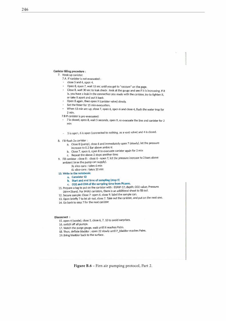
246
Figure B.6 – Firn air pumping protocol, Part 2.

Bibliography
Abe-Ouchi, A., Saito, F., Kawamura, K., Raymo, M. E., Okuno, J., Takahashi, K., and Blat-
ter, H.: Insolation-driven 100,000-year glacial cycles and hysteresis of ice-sheet volume,
Nature, 500, 190, doi:10.1038/nature12374, 2013.
Adalsteinsson, D. and Sethian, J.: The Fast Construction of Extension Velocities in Level Set
Methods, J. Comput. Phys., 148, 2 – 22, doi:10.1006/jcph.1998.6090, 1999.
Ahn, J., Brook, E. J., and Buizert, C.: Response of atmospheric CO2 to the abrupt cooling
event 8200 years ago, Geophys. Res. Lett., 41, 604–609, doi:10.1002/2013gl058177, 2014.
Allan, D. W.: Statistics of atomic frequency standards, Proc. IEEE, 54, 221–230,
doi:10.1109/proc.1966.4634, 1966.
Alley, R. B.: Firn densification by grain-boundary sliding: a first model, J. Phys. Colloques,
48, C1–249, doi:10.1051/jphyscol:1987135, 1987.
Anderson, D. L. and Benson, C. S.: The densification and diagenesis of snow, in: Ice and
Snow: Properties, Processes, and Applications, edited by Kingery, W. D., pp. 391–411,
MIT Press, Camb., Mass., 1963.
Arnaud, L., Barnola, J.-M., and Duval, P.: Physical modeling of the densification of snow/-
firn and ice in the upper part of polar ice sheets, Phys. Ice Core Rec., pp. 285–305, URL
http://hdl.handle.net/2115/32472, 2000.
Arzt, E.: The influence of an increasing particle coordination on the densification of spheri-
cal powders, Acta Metall., 30, 1883–1890, doi:10.1016/0001-6160(82)90028-1, 1982.
Arzt, E., Ashby, M. F., and Easterling, K. E.: Practical applications of hotisostatic press-
ing diagrams: four case studies, Metall. Trans. A, 14, 211–221, doi:10.1007/BF02651618,
1983.
247

248
Ashby, M.: A first report on sintering diagrams, Acta Metall., 22, 275 – 289,
doi:10.1016/0001-6160(74)90167-9, 1974.
Bader, H.: Density of ice as a function of temperature and stress, Cold Regions Research and
Engineering Laboratory, US Army Material Command, 1964.
Baglietto, G. and Albano, E. V.: Finite-size scaling analysis and dynamic study of the critical
behavior of a model for the collective displacement of self-driven individuals, Phys. Rev.
E, 78, 021 125, doi:10.1103/PhysRevE.78.021125, 2008.
Barnes, P. R. F., Wolff, E. W., Mader, H. M., Udisti, R., Castellano, E., and Röthlisberger, R.:
Evolution of chemical peak shapes in the Dome C, Antarctica, ice core, J. Geophys. Res.
Atmos., 108, doi:10.1029/2002JD002538, 2003.
Barnola, J.-M., Raynaud, D., Korotkevich, Y. S., and Lorius, C.: Vostok ice core provides
160,000-year record of atmospheric CO2, Nature, 329, 408, doi:10.1038/329408a0, 1987.
Barnola, J. M., Pierritz, R., Goujon, C., Duval, P., and Boller, E.: 3D reconstruction of the
Vostok firn structure by X-ray tomography, in: Data Glaciol. Stud, vol. 97, pp. 80–84,
2004.
Battle, M., Bender, M., Sowers, T., Tans, P., Butler, J., Elkins, J., Ellis, J., Conway, T., Zhang,
N., Lang, P., et al.: Atmospheric gas concentrations over the past century measured in air
from firn at the South Pole, Nature, 383, 231, doi:10.1038/383231a0, 1996.
Bazin, L., Landais, A., Lemieux-Dudon, B., Toyé Mahamadou Kele, H., Veres, D., Parrenin,
F., Martinerie, P., Ritz, C., Capron, E., Lipenkov, V. Y., Loutre, M.-F., Raynaud, D., Vinther,
B., Svensson, A., Rasmussen, S. O., Severi, M., Blunier, T., Leuenberger, M., Fischer, H.,
Masson-Delmotte, V., Chappellaz, J., and Wolff, E. W.: An optimized multi-proxy, multi-
site Antarctic ice and gas orbital chronology (AICC2012): 120-800 ka, Clim. Past, 9, 1715–
1731, doi:10.5194/cp-9-1715-2013, 2013.
Bender, M. L.: Orbital tuning chronology for the Vostok climate record supported by
trapped gas composition, Earth Planet. Sci. Lett., 204, 275 – 289, doi:10.1016/S0012-
821X(02)00980-9, 2002.
Bender, M. L., Sowers, T., Barnola, J.-M., and Chappellaz, J.: Changes in the O2/N2 ratio
of the atmosphere during recent decades reflected in the composition of air in the firn
at Vostok Station, Antarctica, Geophys. Res. Lett., 21, 189–192, doi:10.1029/93gl03548,
1994.

Bibliography 249
Bereiter, B., Fischer, H., Schwander, J., and Stocker, T. F.: Diffusive equilibration of N2,
O2 and CO2 mixing ratios in a 1.5-million-years-old ice core, Cryosphere, 8, 245–256,
doi:10.5194/tc-8-245-2014, 2014.
Berger, A.: Milankovitch theory and climate, Rev. Geophys., 26, 624–657,
doi:10.1029/RG026i004p00624, 1988.
Bernacki, M., Chastel, Y., Coupez, T., and Logé, R.: Level set framework for the numerical
modelling of primary recrystallization in polycrystalline materials, Scr. Mater., 58, 1129
– 1132, doi:10.1016/j.scriptamat.2008.02.016, 2008.
Bigler, M., Svensson, A., Kettner, E., Vallelonga, P., Nielsen, M. E., and Steffensen, J. P.:
Optimization of high-resolution continuous flow analysis for transient climate signals in
ice cores, Envir. Sci. Tech., 45, 4483–4489, doi:10.1021/es200118j, 2011.
Boers, N., Ghil, M., and Rousseau, D.-D.: Ocean circulation, ice shelf, and sea ice inter-
actions explain Dansgaard–Oeschger cycles, Proc. Natl. Acad. Sci. USA, 115, E11 005–
E11 014, doi:10.1073/pnas.1802573115, 2018.
Boulos, V., Fristot, V., Houzet, D., Salvo, L., and Lhuissier, P.: Investigating performance
variations of an optimized GPU-ported granulometry algorithm, in: Proceedings of the
2012 Conference on Design and Architectures for Signal and Image Processing, pp. 1–6,
URL https://hal.archives-ouvertes.fr/hal-00787861, 2012.
Bouxsein, M. L., Boyd, S. K., Christiansen, B. A., Guldberg, R. E., Jepsen, K. J., and Müller,
R.: Guidelines for assessment of bone microstructure in rodents using micro–computed
tomography, J. Bone Miner. Res., 25, 1468–1486, doi:10.1002/jbmr.141, 2010.
Bréant, C., Martinerie, P., Orsi, A., Arnaud, L., and Landais, A.: Modelling firn thickness
evolution during the last deglaciation: constraints on sensitivity to temperature and im-
purities, Clim. Past, 13, 833–853, doi:10.5194/cp-13-833-2017, 2017.
Brook, E. J. and Buizert, C.: Antarctic and global climate history viewed from ice cores,
Nature, 558, 200, doi:10.1038/s41586-018-0172-5, 2018.
Brook, E. J., Sowers, T., and Orchardo, J.: Rapid variations in atmospheric
methane concentration during the past 110,000 years, Science, 273, 1087–1091,
doi:10.1126/science.273.5278.1087, 1996.
Brook, E. J., Harder, S., Severinghaus, J., Steig, E. J., and Sucher, C. M.: On the origin and

250
timing of rapid changes in atmospheric methane during the Last Glacial Period, Global
Biogeochemical Cycles, 14, 559–572, doi:10.1029/1999GB001182, 2000.
Bruchon, J., Drapier, S., and Valdivieso, F.: 3D finite element simulation of the matter flow
by surface diffusion using a level set method, Int. J. Numer. Methods Eng., 86, 845–861,
doi:10.1002/nme.3079, 2010.
Bruchon, J., Pino-Muñoz, D., Valdivieso, F., and Drapier, S.: Finite element simulation of
mass transport during sintering of a granular packing. Part I. Surface and lattice diffu-
sions, J. Am. Ceram. Soc., 95, 2398–2405, doi:10.1111/j.1551-2916.2012.05073.x, 2012.
Buizert, C., Martinerie, P., Petrenko, V. V., Severinghaus, J. P., Trudinger, C. M., Witrant,
E., Rosen, J. L., Orsi, A. J., Rubino, M., Etheridge, D. M., Steele, L. P., Hogan, C., Laube,
J. C., Sturges, W. T., Levchenko, V. A., Smith, A. M., Levin, I., Conway, T. J., Dlugokencky,
E. J., Lang, P. M., Kawamura, K., Jenk, T. M., White, J. W. C., Sowers, T., Schwander,
J., and Blunier, T.: Gas transport in firn: multiple-tracer characterisation and model
intercomparison for NEEM, Northern Greenland, Atmos. Chem. Phys., 12, 4259–4277,
doi:10.5194/acp-12-4259-2012, 2012.
Buizert, C., Cuffey, K. M., Severinghaus, J. P., Baggenstos, D., Fudge, T. J., Steig, E. J., Markle,
B. R., Winstrup, M., Rhodes, R. H., Brook, E. J., Sowers, T. A., Clow, G. D., Cheng, H.,
Edwards, R. L., Sigl, M., McConnell, J. R., and Taylor, K. C.: The WAIS Divide deep ice
core WD2014 chronology-Part 1: methane synchronization (68-31 ka BP) and the gas age-
ice age difference, Clim. Past, 11, 153–173, doi:10.5194/cp-11-153-2015, 2015.
Burr, A., Ballot, C., Lhuissier, P., Martinerie, P., Martin, C. L., and Philip, A.: Pore morphol-
ogy of polar firn around closure revealed by X-ray tomography, Cryosphere, 12, 2481–
2500, doi:10.5194/tc-12-2481-2018, 2018.
Burr, A., Lhuissier, P., Martin, C. L., and Philip, A.: In situ X-ray tomography densifica-
tion of firn: The role of mechanics and diffusion processes, Acta Mater., 167, 210 – 220,
doi:10.1016/j.actamat.2019.01.053, 2019.
Caillon, N., Severinghaus, J. P., Jouzel, J., Barnola, J.-M., Kang, J., and Lipenkov, V. Y.: Tim-
ing of Atmospheric CO2 and Antarctic Temperature Changes Across Termination III, Sci-
ence, 299, 1728–1731, doi:10.1126/science.1078758, 2003.
Calonne, N., Montagnat, M., Matzl, M., and Schneebeli, M.: The layered evolution of fabric

Bibliography 251
and microstructure of snow at Point Barnola, Central East Antarctica, Earth Planet. Sci.
Lett., 460, 293 – 301, doi:10.1016/j.epsl.2016.11.041, 2017.
Capron, E., Landais, A., Buiron, D., Cauquoin, A., Chappellaz, J., Debret, M., Jouzel, J.,
Leuenberger, M., Martinerie, P., Masson-Delmotte, V., Mulvaney, R., Parrenin, F., and
Prié, F.: Glacial-interglacial dynamics of Antarctic firn columns: comparison between
simulations and ice core air-δ15N measurements, Clim Past, 9, 983–999, doi:10.5194/cp-
9-983-2013, 2013.
Chappellaz, J., Barnola, J.-M., Raynaud, D., Korotkevich, Y. S., and Lorius, C.: Ice-core
record of atmospheric methane over the past 160,000 years, Nature, 345, 127–131,
doi:10.1038/345127a0, 1990.
Chappellaz, J., Stowasser, C., Blunier, T., Baslev-Clausen, D., Brook, E. J., Dallmayr, R.,
Faïn, X., Lee, J. E., Mitchell, L. E., Pascual, O., Romanini, D., Rosen, J., and Schüpbach,
S.: High-resolution glacial and deglacial record of atmospheric methane by continuous-
flow and laser spectrometer analysis along the NEEM ice core, Clim. Past, 9, 2579–2593,
doi:10.5194/cp-9-2579-2013, 2013.
Clark, P. U., Archer, D., Pollard, D., Blum, J. D., Rial, J. A., Brovkin, V., Mix, A. C., Pisias,
N. G., and Roy, M.: The middle Pleistocene transition: characteristics, mechanisms, and
implications for long-term changes in atmospheric pCO2, Quat. Sci. Rev., 25, 3150–3184,
doi:10.1016/j.quascirev.2006.07.008, 2006.
Colbeck, S. C.: Air movement in snow due to windpumping, J. Glaciol., 35, 209–213,
doi:10.1017/S0022143000004524, 1989.
Cooper, S. J., Bertei, A., Shearing, P. R., Kilner, J. A., and Brandon, N. P.: TauFactor: An open-
source application for calculating tortuosity factors from tomographic data, SoftwareX, 5,
203–210, doi:10.1016/j.softx.2016.09.002, 2016.
Craig, H., Horibe, Y., and Sowers, T.: Gravitational separation of gases and isotopes in polar
ice caps, Science, 242, 1675–1678, doi:10.1126/science.242.4886.1675, 1988.
Cuffey, K. and Paterson, W. S. B.: The Physics of Glaciers, 4th Edition, Academic Press, 2010.
Dansgaard, W.: The Abundance of O18 in Atmospheric Water and Water Vapour, Tellus A,
Dyn. Meteorol. Oceanogr., 5, 461–469, doi:10.1111/j.2153-3490.1953.tb01076.x, 1953.
Dansgaard, W., Johnsen, S. J., Clausen, H. B., Dahl-Jensen, D., Gundestrup, N. S., Hammer,

252
C. U., Hvidberg, C. S., Steffensen, J. P., Sveinbjornsdottir, A. E., and Jouzel, J.: Evidence for
general instability of past climate from a 250-kyr ice-core record, nature, 364, 218–220,
doi:10.1038/364218a0, 1993.
Dapogny, C. and Frey, P.: Computation of the signed distance function to a discrete contour
on adapted triangulation, Calcolo, 49, 193–219, doi:10.1007/s10092-011-0051-z, 2012.
Dapogny, C., Dobrzynski, C., and Frey, P.: Three-dimensional adaptive domain remeshing,
implicit domain meshing, and applications to free and moving boundary problems, J.
Comput. Phys., 262, 358–378, doi:10.1016/j.jcp.2014.01.005, 2014.
Daruka, I. and Ditlevsen, P. D.: A conceptual model for glacial cycles and the middle Pleis-
tocene transition, Clim. Dyn., 46, 29–40, doi:10.1007/s00382-015-2564-7, 2016.
Delmas, R. J., Ascencio, J.-M., and Legrand, M.: Polar ice evidence that atmospheric CO2
20,000 yr BP was 50% of present, Nature, 284, 155, doi:10.1038/284155a0, 1980.
Delmotte, M., Chappellaz, J., Brook, E., Yiou, P., Barnola, J., Goujon, C., Raynaud, D.,
and Lipenkov, V.: Atmospheric methane during the last four glacial-interglacial cycles:
Rapid changes and their link with Antarctic temperature, J. Geophys. Res. Atmos., 109,
doi:10.1029/2003JD004417, 2004.
Dlugokencky, E. J., Myers, R. C., Lang, P. M., Masarie, K. A., Crotwell, A. M., Thoning, K. W.,
Hall, B. D., Elkins, J. W., and Steele, L. P.: Conversion of NOAA atmospheric dry air CH4
mole fractions to a gravimetrically prepared standard scale, J. Geophys. Res. Atmos., 110,
doi:doi.org/10.1029/2005jd006035, 2005.
Doube, M., Kłosowski, M. M., Arganda-Carreras, I., Cordelières, F. P., Dougherty, R. P., Jack-
son, J. S., Schmid, B., Hutchinson, J. R., and Shefelbine, S. J.: BoneJ: free and extensi-
ble bone image analysis in ImageJ, Bone, 47, 1076–1079, doi:10.1016/j.bone.2010.08.023,
2010.
Dreyfus, G. B., Jouzel, J., Bender, M. L., Landais, A., Masson-Delmotte, V., and Leuenberger,
M.: Firn processes and δ15N: potential for a gas-phase climate proxy, Quat. Sci. Rev., 29,
28 – 42, doi:10.1016/j.quascirev.2009.10.012, 2010.
Duval, P., Ashby, M. F., and Anderman, I.: Rate-controlling processes in the creep of poly-
crystalline ice, J. Phys. Chem., 87, 4066–4074, doi:10.1021/j100244a014, 1983.
Dällenbach, A., Blunier, T., Flückiger, J., Stauffer, B., Chappellaz, J., and Raynaud, D.:

Bibliography 253
Changes in the atmospheric CH4 gradient between Greenland and Antarctica during
the Last Glacial and the transition to the Holocene, Geophys. Res. Lett., 27, 1005–1008,
doi:10.1029/1999GL010873, 2000.
Enting, I. G.: Statistics of firn closure: a simulation study, Journal of Glaciology, 39, 133–142,
doi:10.3189/S0022143000015781, 1993.
EPICA community members, Augustin, L., Barbante, C., Barnes, P. R., Barnola, J. M., Bigler,
M., Castellano, E., Cattani, O., Chappellaz, J., Dahl-Jensen, D., Delmonte, B., et al.: Eight
glacial cycles from an Antarctic ice core, Nature, 429, 623–628, doi:10.1038/nature02599,
2004.
Etheridge, D. M., Pearman, G. I., and Fraser, P. J.: Changes in tropospheric methane between
1841 and 1978 from a high accumulation-rate Antarctic ice core, Tellus B Chem. Phys.
Meteorol., 44, 282–294, doi:10.3402/tellusb.v44i4.15456, 1992.
Fabre, A., Barnola, J.-M., Arnaud, L., and Chappellaz, J.: Determination of gas diffusivity
in polar firn: comparison between experimental measurements and inverse modeling,
Geophys. Res. Lett., 27, 557–560, doi:10.1029/1999GL010780, 2000.
Faïn, X., Chappellaz, J., Rhodes, R. H., Stowasser, C., Blunier, T., McConnell, J. R., Brook,
E. J., Preunkert, S., Legrand, M., Debois, T., and Romanini, D.: High resolution measure-
ments of carbon monoxide along a late Holocene Greenland ice core: evidence for in situ
production, Clim. Past, 10, 987–1000, doi:10.5194/cp-10-987-2014, 2014.
Fischer, H., Severinghaus, J., Brook, E., Wolff, E. W., Albert, M., Alemany, O., Arthern, R.,
Bentley, C., Blankenship, D., Chappellaz, J., Creyts, T., Dahl-Jensen, D., Dinn, M., Frez-
zotti, M., Fujita, S., Gallee, H., Hindmarsh, R., Hudspeth, D., Jugie, G., Kawamura, K.,
Lipenkov, V. Y., Miller, H., Mulvaney, R., Parrenin, F., Pattyn, F., Ritz, C., Schwander, J.,
Steinhage, D., van Ommen, T., and Wilhelms, F.: Where to find 1.5 million yr old ice for
the IPICS "Oldest-Ice" ice core, Clim. Past, 9, 2489–2505, doi:10.5194/cp-9-2489-2013,
2013.
Fourteau, K., Faïn, X., Martinerie, P., Landais, A., Ekaykin, A. A., Lipenkov, V. Y., and
Chappellaz, J.: Analytical constraints on layered gas trapping and smoothing of atmo-
spheric variability in ice under low-accumulation conditions, Clim. Past, 13, 1815–1830,
doi:10.5194/cp-13-1815-2017, 2017.
Freitag, J., Dobrindt, U., and Kipfstuhl, J.: A newmethod for predicting transport properties
254
of polar firn with respect to gases on the pore-space scale, Ann. Glaciol., 35, 538–544,
doi:10.3189/172756402781816582, 2002.
Freitag, J., Wilhelms, F., and Kipfstuhl, S.: Microstructure-dependent densifica-
tion of polar firn derived from X-ray microtomography, J. Glaciol., 50, 243–250,
doi:10.3189/172756504781830123, 2004.
Freitag, J., Kipfstuhl, S., Laepple, T., and Wilhelms, F.: Impurity-controlled den-
sification: a new model for stratified polar firn, J. Glaciol., 59, 1163–1169,
doi:10.3189/2013JoG13J042, 2013.
Fujita, S., Okuyama, J., Hori, A., and Hondoh, T.: Metamorphism of stratified firn at
Dome Fuji, Antarctica: A mechanism for local insolation modulation of gas trans-
port conditions during bubble close off, J. Geophys. Res. Earth Surf., 114, F03023,
doi:10.1029/2008JF001143, 2009.
Fujita, S., Hirabayashi, M., Goto-Azuma, K., Dallmayr, R., Satow, K., Zheng, J., and Dahl-
Jensen, D.: Densification of layered firn of the ice sheet at NEEM, Greenland, J. Glaciol.,
60, 905–921, doi:10.3189/2014JoG14J006, 2014.
Fujita, S., Goto-Azuma, K., Hirabayashi, M., Hori, A., Iizuka, Y., Motizuki, Y., Motoyama, H.,
and Takahashi, K.: Densification of layered firn in the ice sheet at Dome Fuji, Antarctica,
J. Glaciol., 62, 103–123, doi:10.1017/jog.2016.16, 2016.
Gautier, E., Savarino, J., Erbland, J., Lanciki, A., and Possenti, P.: Variability of sulfate signal
in ice core records based on five replicate cores, Clim. Past, 12, 103–113, doi:10.5194/cp-
12-103-2016, 2016.
Gedney, N., Cox, P., and Huntingford, C.: Climate feedback from wetland methane emis-
sions, Geophys. Res. Lett., 31, doi:10.1029/2004GL020919, 2004.
Genthon, G., Barnola, J., Raynaud, D., Lorius, C., Jouzel, J., Barkov, N., Korotkevich, Y., and
Kotlyakov, V.: Vostok ice core: climatic response to CO2 and orbital forcing changes over
the last climatic cycle, Nature, 329, 414, doi:10.1038/329414a0, 1987.
Gibou, F., Fedkiw, R., and Osher, S.: A review of level-set methods and some recent applica-
tions, J. Comput. Phys., 353, 82 – 109, doi:10.1016/j.jcp.2017.10.006, 2018.
Goujon, C., Barnola, J.-M., and Ritz, C.: Modeling the densification of polar firn in-
cluding heat diffusion: application to close-off characteristics and gas isotopic frac-

Bibliography 255
tionation for Antarctica and Greenland sites, J. Geophys. Res. Atmos., 108, 4792,
doi:10.1029/2002jd003319, 2003.
Gregory, S. A., Albert, M. R., and Baker, I.: Impact of physical properties and accumulation
rate on pore close-off in layered firn, Cryosphere, 8, 91–105, doi:10.5194/tc-8-91-2014,
2014.
Hagenmuller, P., Chambon, G., Lesaffre, B., Flin, F., Calonne, N., and Naaim, M.: Energy-
based binary segmentation of snow microtomographic images, in: 1st International
Conference on Tomography of Materials and Structures (ICTMS), URL https://hal.
archives-ouvertes.fr/hal-00863099, 2013.
Hendy, C. and Wilson, A.: Palaeoclimatic data from speleothems, Nature, 219, 48,
doi:10.1038/219048a0, 1968.
Herron, M. M. and Langway, C. C.: Firn Densification: An Empirical Model, J. Glaciol., 25,
373–385, doi:10.3189/S0022143000015239, 1980.
Hildebrand, T. and Rüegsegger, P.: Quantification of Bone Microarchitecture with
the Structure Model Index, Comput. Methods Biomech. Biomed. Eng., 1, 15–23,
doi:10.1080/01495739708936692, 1997.
Hobbs, P.: Ice Physics, Clarendron Press, Oxford, 1974.
Höhle, J. and Höhle, M.: Accuracy assessment of digital elevation models by means
of robust statistical methods, ISPRS J. Photogramm. Remote Sens., 64, 398–406,
doi:10.1016/j.isprsjprs.2009.02.003, 2009.
Hopcroft, P. O., Valdes, P. J., and Beerling, D. J.: Simulating idealized Dansgaard-Oeschger
events and their potential impacts on the global methane cycle, Quat. Sci. Rev., 30, 3258
– 3268, doi:10.1016/j.quascirev.2011.08.012, 2011.
Hörhold, M. W., Kipfstuhl, S., Wilhelms, F., Freitag, J., and Frenzel, A.: The densification of
layered polar firn, J. Geophys. Res. Earth Surf., 116, doi:10.1029/2009jf001630, 2011.
Hörhold, M. W., Laepple, T., Freitag, J., Bigler, M., Fischer, H., and Kipfstuhl, S.: On the
impact of impurities on the densification of polar firn, Earth Planet. Sci. Lett., 325, 93–99,
doi:10.1016/j.epsl.2011.12.022, 2012.
Huber, C., Beyerle, U., Leuenberger, M., Schwander, J., Kipfer, R., Spahni, R., Severinghaus,
J., and Weiler, K.: Evidence for molecular size dependent gas fractionation in firn air
256
derived from noble gases, oxygen, and nitrogen measurements, Earth Planet. Sci. Lett.,
243, 61–73, doi:10.1016/j.epsl.2005.12.036, 2006a.
Huber, C., Leuenberger, M., Spahni, R., Flückiger, J., Schwander, J., Stocker, T. F., Johnsen, S.,
Landais, A., and Jouzel, J.: Isotope calibrated Greenland temperature record over Marine
Isotope Stage 3 and its relation to CH4, Earth Planet. Sci. Lett., 243, 504–519, 2006b.
Hutterli, M. A., Schneebeli, M., Freitag, J., Kipfstuhl, J., and Röthlisberger, R.: Impact of lo-
cal insolation on snowmetamorphism and ice core records, in: Physics of Ice Core Records
II : Papers collected after the 2nd International Workshop on Physics of Ice Core Records,
vol. 68, pp. 223–232, Institute of Low Temperature Science, Hokkaido University, URL
http://hdl.handle.net/2115/45450, 2009.
IPCC: Climate Change 2014: Synthesis Report. Contribution of Working Groups I, II and III
to the Fifth Assessment Report of the Intergovernmental Panel on Climate Change, 2014.
Johnsen, S. J., Dansgaard, W., and White, J.: The origin of Arctic precipitation un-
der present and glacial conditions, Tellus B: Chem. Phys. Meteorol., 41, 452–468,
doi:10.3402/tellusb.v41i4.15100, 1989.
Jones, S. and Glen, J.: The effect of dissolved impurities on the mechanical
properties of ice crystals, Philos. Mag. J. Theor. Exp. Appl. Phys., 19, 13–24,
doi:10.1080/14786436908217758, 1969.
Jones, S. J.: Softening of ice crystals by dissolved fluoride ions, Phys. Lett., 25A, 366–367,
doi:10.1016/0375-9601(67)90702-5, 1967.
Joos, F. and Spahni, R.: Rates of change in natural and anthropogenic radiative forcing over
the past 20,000 years, Proc. Natl. Acad. Sci. USA, 105, 1425–1430, URL https://doi.
org/10.1073/pnas.0707386105, 2008.
Jouzel, J., Masson-Delmotte, V., Cattani, O., Dreyfus, G., Falourd, S., Hoffmann, G., Minster,
B., Nouet, J., Barnola, J.-M., Chappellaz, J., Fischer, H., Gallet, J. C., Johnsen, S., Leuen-
berger, M., Loulergue, L., Lüuthi, D., Oerter, H., Parrenin, F., Raisbeck, G., Raynaud,
D., Schilt, A., Schwander, J., Selmo, E., Souchez, R., Spahni, R., Stauffer, B., Steffensen,
J. P., Stenni, B., Stocker, T. F., Tison, J. L., Werner, M., and Wolff, E. W.: Orbital and mil-
lennial antarctic climate variability over the past 800,000 years, Science, 317, 793–796,
doi:10.1126/science.1141038, 2007.
Kawamura, K., Parrenin, F., Lisiecki, L., Uemura, R., Vimeux, F., Severinghaus, J. P.,
Bibliography 257
Hutterli, M. A., Nakazawa, T., Aoki, S., Jouzel, J., et al.: Northern Hemisphere forc-
ing of climatic cycles in Antarctica over the past 360,000 years, Nature, 448, 912,
doi:10.1038/nature06015, 2007.
Köhler, P., Bintanja, R., Fischer, H., Joos, F., Knutti, R., Lohmann, G., and Masson-Delmotte,
V.: What caused Earth’s temperature variations during the last 800,000 years? Data-based
evidence on radiative forcing and constraints on climate sensitivity, Quat. Sci. Rev., 29,
129 – 145, doi:10.1016/j.quascirev.2009.09.026, 2010.
Köhler, P., Knorr, G., Buiron, D., Lourantou, A., and Chappellaz, J.: Abrupt rise in atmo-
spheric CO2 at the onset of the Bølling/Allerød: in-situ ice core data versus true atmo-
spheric signal, Clim. Past, 7, 473–486, doi:10.5194/cp-7-473-2011, 2011.
Köhler, P., Völker, C., Knorr, G., and Bard, E.: High latitude impacts on deglacial CO2:
southern ocean westerly winds and northern hemisphere permafrost thawing, Nova. Act.
Lc., 121, 135–140, doi:10013/epic.45322.d002, 2015.
Krol, Q. and Löwe, H.: Relating optical and microwave grain metrics of snow: the relevance
of grain shape, Cryosphere, 10, 2847–2863, doi:10.5194/tc-10-2847-2016, 2016.
Lambert, F., Bigler, M., Steffensen, J. P., Hutterli, M., and Fischer, H.: Centennial mineral
dust variability in high-resolution ice core data from Dome C, Antarctica, Clim. Past, 8,
609–623, doi:10.5194/cp-8-609-2012, 2012.
Landais, A., Caillon, N., Severinghaus, J., Barnola, J.-M., Goujon, C., Jouzel, J., and Masson-
Delmotte, V.: Analyse isotopique de l'air piégé dans la glace pour quantifier les variations
de température, C.R. Geosci., 336, 963–970, doi:10.1016/j.crte.2004.03.013, 2004.
Landais, A., Barnola, J., Kawamura, K., Caillon, N., Delmotte, M., Ommen, T. V., Dreyfus,
G., Jouzel, J., Masson-Delmotte, V., Minster, B., Freitag, J., Leuenberger, M., Schwan-
der, J., Huber, C., Etheridge, D., and Morgan, V.: Firn-air δ15N in modern polar sites
and glacial–interglacial ice: a model-data mismatch during glacial periods in Antarctica?,
Quat. Sci. Rev., 25, 49 – 62, doi:10.1016/j.quascirev.2005.06.007, 2006.
Landais, A., Masson-Delmotte, V., Stenni, B., Selmo, E., Roche, D., Jouzel, J., Lambert,
F., Guillevic, M., Bazin, L., Arzel, O., Vinther, B., Gkinis, V., and Popp, T.: A re-
view of the bipolar see–saw from synchronized and high resolution ice core water sta-
ble isotope records from Greenland and East Antarctica, Quat. Sci. Rev., 114, 18 – 32,
doi:10.1016/j.quascirev.2015.01.031, 2015.
258
Lauritzen, S.-E.: High-Resolution Paleotemperature Proxy Record for the Last In-
terglaciation Based on Norwegian Speleothems, Quat. Res., 43, 133 – 146,
doi:10.1006/qres.1995.1015, 1995.
Legrand, M. and Mayewski, P.: Glaciochemistry of polar ice cores: A review, Rev. Geophys.,
35, 219–243, doi:10.1029/96RG03527, 1997.
Lide, D. R.: CRC Handbook of Chemistry and Physics, CRC Press, 2005.
Lipenkov, V., Candaudap, F., Ravoire, J., Dulac, E., and Raynaud, D.: A new de-
vice for the measurement of air content in polar ice, J. Glaciol., 41, 423–429,
doi:10.1017/S0022143000016294, 1995.
Lipenkov, V. Y.: Air bubbles and air-hydrate crystals in the Vostok ice core, in: Phys. Ice
Core Rec., pp. 327–358, Hokkaido University Press, 2000.
Lipenkov, V. Y., Salamatin, A. N., and Duval, P.: Bubbly-ice densification in ice sheets: II.
Applications, J. Glaciol., 43, 397–407, doi:10.1017/S0022143000034973, 1997.
Lipenkov, V. Y., Raynaud, D., Loutre, M., and Duval, P.: On the potential of coupling air
content and O2/N2 from trapped air for establishing an ice core chronology tuned on
local insolation, Quat. Sci. Rev., 30, 3280 – 3289, doi:10.1016/j.quascirev.2011.07.013,
2011.
Lisiecki, L. and Raymo, M. E.: A Pliocene-Pleistocene stack of 57 globally distributed ben-
thic δ18O records, Paleoceanograph., 20, doi:10.1029/2004PA001071, 2005.
Loulergue, L., Schilt, A., Spahni, R., Masson-Delmotte, V., Blunier, T., Lemieux, B.,
Barnola, J.-M., Raynaud, D., Stocker, T. F., and Chappellaz, J.: Orbital and millennial-
scale features of atmospheric CH4 over the past 800,000 years, Nature, 453, 383–386,
doi:10.1038/nature06950, 2008.
Lundin, J. M., Stevens, C. M., Arthern, R., Buizert, C., Orsi, A., Ligtenberg, S. R., Simonsen,
S. B., Cummings, E., Essery, R., Leahy, W., et al.: Firn Model Intercomparison Experiment
(FirnMICE), J. Glaciol., 63, 401–422, doi:10.1017/jog.2016.114, 2017.
Lüthi, D., Floch, M. L., Bereiter, B., Blunier, T., Barnola, J.-M., Siegenthaler, U., Raynaud,
D., Jouzel, J., Fischer, H., Kawamura, K., and Stocker, T. F.: High-resolution carbon diox-
ide concentration record 650,000– 800,000 years before present, Nature, 453, 379–382,
doi:10.1038/nature06949, 2008.

Bibliography 259
Maeno, N. and Ebinuma, T.: Pressure sintering of ice and its implication to the den-
sification of snow at polar glaciers and ice sheets, J. Phys. Chem., 87, 4103 – 4110,
doi:10.1021/j100244a023, 1983.
Marcott, S. A., Bauska, T. K., Buizert, C., Steig, E. J., Rosen, J. L., Cuffey, K. M., Fudge, T. J.,
Severinghaus, J. P., Ahn, J., Kalk, M. L., McConnell, J. R., Sowers, T., Taylor, K. C., White,
J. W. C., and Brook, E. J.: Centennial-scale changes in the global carbon cycle during the
last deglaciation, Nature, 514, 616–619, doi:10.1038/nature13799, 2014.
Martín, C. and Gudmundsson, G. H.: Effects of nonlinear rheology, temperature and
anisotropy on the relationship between age and depth at ice divides, Cryosphere, 6, 1221–
1229, doi:10.5194/tc-6-1221-2012, 2012.
Martinerie, P., Lipenkov, V. Y., and Raynaud, D.: Correction of air-content measurements in
polar ice for the effect of cut bubbles at the surface of the sample, J. Glaciol., 36, 299–303,
doi:10.3189/002214390793701282, 1990.
Martinerie, P., Raynaud, D., Etheridge, D. M., Barnola, J.-M., and Mazaudier, D.: Physical
and climatic parameters which influence the air content in polar ice, Earth Planet. Sc.
Lett., 112, 1–13, doi:10.1016/0012-821x(92)90002-d, 1992.
Martinerie, P., Lipenkov, V. Y., Raynaud, D., Chappellaz, J., Barkov, N., and Lorius,
C.: Air content paleo record in the Vostok ice core (Antarctica): A mixed record
of climatic and glaciological parameters, J. Geophys. Res. Atmos., 99, 10 565–10 576,
doi:10.1029/93JD03223, 1994.
Masson-Delmotte, V., M., Schulz, A., Abe-Ouchi, J., Beer, A., Ganopolski, J.,
González Rouco, E., Jansen, K., Lambeck, J., Luterbacher, T., Naish, T., Osborn, B., Otto-
Bliesner, T., Quinn, R., Ramesh, M., Rojas, X. S., and Timmermann, A.: Information from
paleoclimate archives, in: Climate change 2013: the physical science basis. Contribution
of working group I to the fifth assessment report of the Intergovernmental Panel on Cli-
mate Change, edited by Stocker, T. F., Qin, D., Plattner, G. K., Tignor, M., Allen, S. K.,
Boschung, J., Nauels, A., Xia, Y., Bex, V., and Midgley, P. M., pp. 383–464, Cambridge
University Press, Cambridge, United Kingdom and New York, NY, USA, 2013.
Mayer, E. W., Blake, D. R., Tyler, S. C., Makide, Y., Montague, D. C., and Rowland, F. S.:
Methane: Interhemispheric concentration gradient and atmospheric residence time, Proc.
Natl. Acad. Sci. USA, 79, 1366–1370, doi:10.1073/pnas.79.4.1366, 1982.
260
McDermott, F.: Palaeo-climate reconstruction from stable isotope variations in speleothems:
a review, Quat. Sci. Rev., 23, 901 – 918, doi:10.1016/j.quascirev.2003.06.021, 2004.
Mees, F., Swennen, R., Geet, M. V., and Jacobs, P.: Applications of X-ray com-
puted tomography in the geosciences, Geol. Soc. Lond. Special Publ., 215, 1–6,
doi:10.1144/GSL.SP.2003.215.01.01, 2003.
Milankovitch, M. M.: Théorie Mathématique des Phenomenes Thermiques Produits par la
Radiation Solaire, Ph.D. thesis, Académie Yougoslave des Sciences et des Arts de Zagreb,
1920.
Mitchell, L., Brook, E., Lee, J. E., Buizert, C., and Sowers, T.: Constraints on the Late
Holocene Anthropogenic Contribution to the Atmospheric Methane Budget, Science, 342,
964–966, doi:10.1126/science.1238920, 2013.
Mitchell, L. E., Brook, E. J., Sowers, T., McConnell, J. R., and Taylor, K.: Multidecadal vari-
ability of atmospheric methane, 1000–1800 C.E., J. Geophys. Res. Biogeosci., 116, 2007,
doi:10.1029/2010JG001441, 2011.
Mitchell, L. E., Buizert, C., Brook, E. J., Breton, D. J., Fegyveresi, J., Baggenstos, D.,
Orsi, A., Severinghaus, J., Alley, R. B., Albert, M., Rhodes, R. H., McConnell, J. R.,
Sigl, M., Maselli, O., Gregory, S., and Ahn, J.: Observing and modeling the influence
of layering on bubble trapping in polar firn, J. Geophys. Res. Atmos., 120, 2558–2574,
doi:10.1002/2014jd022766, 2015.
Morville, J., Kassi, S., Chenevier, M., and Romanini, D.: Fast, low-noise, mode-by-mode,
cavity-enhanced absorption spectroscopy by diode-laser self-locking, Appl. Phys. B-
Lasers O., 80, 1027–1038, doi:10.1007/s00340-005-1828-z, 2005.
Muller, R. A. and MacDonald, G. J.: Glacial cycles and astronomical forcing, Science, 277,
215–218, doi:10.1126/science.277.5323.215, 1997.
Nakamura, T. and Jones, S.: Softening effect of dissolved hydrogen chloride in ice crystals,
Scr. Metall., 4, 123–126, doi:10.1016/0036-9748(70)90176-6, 1970.
Newman, M. and Barkema, G.: Monte carlo methods in statistical physics chapter 1-4, Ox-
ford University Press: New York, USA, 1999.
Olsson, E. and Kreiss, G.: A conservative level set method for two phase flow, J. Comput.
Phys., 210, 225 – 246, doi:10.1016/j.jcp.2005.04.007, 2005.

Bibliography 261
Olsson, E., Kreiss, G., and Zahedi, S.: A conservative level set method for two phase flow II,
J. Comput. Phys., 225, 785–807, doi:10.1016/j.jcp.2005.04.007, 2007.
Orsi, A. J., Cornuelle, B. D., and Severinghaus, J. P.: Magnitude and temporal evolution
of Dansgaard–Oeschger event 8 abrupt temperature change inferred from nitrogen and
argon isotopes in GISP2 ice using a new least-squares inversion, Earth Planet. Sc. Lett.,
395, 81–90, doi:10.1016/j.epsl.2014.03.030, 2014.
Osher, S. and Fedkiw, R. P.: Level Set Methods: An Overview and Some Recent Results, J.
Comput. Phys., 169, 463 – 502, doi:10.1006/jcph.2000.6636, 2001.
Osher, S. and Sethian, J. A.: Fronts propagating with curvature-dependent speed: Al-
gorithms based on Hamilton-Jacobi formulations, J. Comput. Phys., 79, 12 – 49,
doi:10.1016/0021-9991(88)90002-2, 1988.
Parrenin, F., Petit, J.-R., Masson-Delmotte, V., Wolff, E., Basile-Doelsch, I., Jouzel, J.,
Lipenkov, V., Rasmussen, S. O., Schwander, J., Severi, M., Udisti, R., Veres, D., and
Vinther, B. M.: Volcanic synchronisation between the EPICA Dome C and Vostok ice cores
(Antarctica) 0-145 kyr BP, Clim. Past, 8, 1031–1045, doi:10.5194/cp-8-1031-2012, 2012.
Parrenin, F., Masson-Delmotte, V., Köhler, P., Raynaud, D., Paillard, D., Schwander, J., Bar-
bante, C., Landais, A., Wegner, A., and Jouzel, J.: Synchronous Change of Atmospheric
CO2 and Antarctic Temperature During the Last Deglacial Warming, Science, 339, 1060–
1063, doi:10.1126/science.1226368, 2013.
Passalacqua, O., Cavitte, M., Gagliardini, O., Gillet-Chaulet, F., Parrenin, F., Ritz, C., and
Young, D.: Brief communication: Candidate sites of 1.5Myr old ice 37 km southwest of the
Dome C summit, East Antarctica, Cryosphere, 12, 2167–2174, doi:10.5194/tc-12-2167-
2018, 2018.
Peternell, M., Russell-Head, D., and Wilson, C.: A technique for recording polycrys-
talline structure and orientation during in situ deformation cycles of rock analogues us-
ing an automated fabric analyser, J. Microsc. Oxford, 242, 181–188, doi:10.1111/j.1365-
2818.2010.03456.x, 2010.
Petit, J. R., Jouzel, J., Raynaud, D., Barkov, N. I., Barnola, J.-M., Basile, I., Bender, M. L.,
Chappellaz, J., Davis, M., Delaygue, G., Delmotte, M., Kotlyakov, V. M., Legrand, M.,
Lipenkov, V. Y., Lorius, C., Pépin, L., Ritz, C., Saltzman, E., and Stievenard, M.: Climate

262
and atmospheric history of the past 420,000 years from the Vostok ice core, Antarctica,
Nature, 399, 429–436, doi:10.1038/20859, 1999.
Petrenko, V. V., Martinerie, P., Novelli, P., Etheridge, D. M., Levin, I., Wang, Z., Blunier,
T., Chappellaz, J., Kaiser, J., Lang, P., Steele, L. P., Hammer, S., Mak, J., Langenfelds,
R. L., Schwander, J., Severinghaus, J. P., Witrant, E., Petron, G., Battle, M. O., Forster, G.,
Sturges, W. T., Lamarque, J.-F., Steffen, K., and White, J. W. C.: A 60 yr record of atmo-
spheric carbon monoxide reconstructed from Greenland firn air, Atmos. Chem. Phys., 13,
7567–7585, doi:10.5194/acp-13-7567-2013, 2013.
Pimienta, P. and Duval, P.: Rate controlling processes in the creep of polar glacier ice, J. Phys
Colloques, 48, C1–243, doi:10.1051/jphyscol:1987134, 1987.
Raymond, C. F.: Deformation in the Vicinity of Ice Divides, J. Glaciol., 29, 357–373,
doi:10.3189/S0022143000030288, 1983.
Raynaud, D. and Lebel, B.: Total gas content and surface elevation of polar ice sheets, Na-
ture, 281, 289, doi:10.1038/281289a0, 1979.
Raynaud, D., Delmas, R., Ascencio, J., and Legrand, M.: Gas Extraction From Polar Ice
Cores: A Critical Issue For Studying The Evolution of Atmospheric CO2 and Ice-Sheet
Surface Elevation, Ann. Glaciol., 3, 265–268, doi:10.3189/S0260305500002895, 1982.
Raynaud, D., Chappellaz, J., Barnola, J., Korotkevich, Y. S., and Lorius, C.: Climatic and
CH4 cycle implications of glacial–interglacial CH4 change in the Vostok ice core, Nature,
333, 655, doi:10.1038/3336, 1988.
Raynaud, D., Lipenkov, V., Lemieux-Dudon, B., Duval, P., Loutre, M.-F., and Lhomme,
N.: The local insolation signature of air content in Antarctic ice. A new step to-
ward an absolute dating of ice records, Earth Planet. Sci. Lett., 261, 337–349,
doi:10.1016/j.epsl.2007.06.025, 2007.
Rhodes, R. H., Faïn, X., Stowasser, C., Blunier, T., Chappellaz, J., McConnell, J. R., Ro-
manini, D., Mitchell, L. E., and Brook, E. J.: Continuous methane measurements from a
late Holocene Greenland ice core: atmospheric and in-situ signals, Earth Planet. Sc. Lett.,
368, 9–19, doi:10.1016/j.epsl.2013.02.034, 2013.
Rhodes, R. H., Brook, E. J., Chiang, J. C. H., Blunier, T., Maselli, O. J., McConnell,
J. R., Romanini, D., and Severinghaus, J. P.: Enhanced tropical methane produc-

Bibliography 263
tion in response to iceberg discharge in the North Atlantic, Science, 348, 1016–1019,
doi:10.1126/science.1262005, 2015.
Rhodes, R. H., Faïn, X., Brook, E. J., McConnell, J. R., Maselli, O. J., Sigl, M., Edwards, J.,
Buizert, C., Blunier, T., Chappellaz, J., and Freitag, J.: Local artifacts in ice core methane
records caused by layered bubble trapping and in situ production: a multi-site investiga-
tion, Clim. Past, 12, 1061–1077, doi:10.5194/cp-12-1061-2016, 2016.
Ritman, E. L.: Micro-Computed Tomography—Current Status and Developments, Annu.
Rev. Biomed. Eng., 6, 185–208, doi:10.1146/annurev.bioeng.6.040803.140130, 2004.
Romanini, D., Chenevier, M., Kassi, S., Schmidt, M., Valant, C., Ramonet, M., Lopez, J.,
and Jost, H.-J.: Optical-feedback cavity-enhanced absorption: a compact spectrometer for
real-time measurement of atmospheric methane, Appl. Phys. B-Lasers O., 83, 659–667,
doi:10.1007/s00340-006-2177-2, 2006.
Rommelaere, V., Arnaud, L., and Barnola, J.-M.: Reconstructing recent atmospheric trace
gas concentrations from polar firn and bubbly ice data by inverse methods, J. Geophys.
Res. Atmos., 102, 30 069–30 083, doi:10.1029/97jd02653, 1997.
Rothwell, R. G. and Rack, F. R.: New techniques in sediment core analysis: an introduction,
Geol. Soc. Lond. Special Publ., 267, 1–29, doi:10.1144/GSL.SP.2006.267.01.01, 2006.
Rousseeuw, P. J. and Hubert, M.: Robust statistics for outlier detection, Wires Data Min.
Knowl. Discov., 1, 73–79, doi:10.1002/widm.2, 2011.
Salamatin, A. N., Lipenkov, V. Y., Barnola, J. M., Hori, A., Duval, P., and Hondoh, T.: Snow/-
firn densification in polar ice sheets, Low Temperature Science, 68, 195–222, 2009.
Salmon, P. L., Ohlsson, C., Shefelbine, S. J., and Doube, M.: Structure Model Index
Does Not Measure Rods and Plates in Trabecular Bone, Front. Endocrinol., 6, 162,
doi:10.3389/fendo.2015.00162, 2015.
Schaller, C. F., Freitag, J., and Eisen, O.: Critical porosity of gas enclosure in polar firn
independent of climate, Clim. Past, 13, 1685–1693, doi:10.5194/cp-13-1685-2017, 2017.
Schmitt, J., Schneider, R., and Fischer, H.: A sublimation technique for high-precision mea-
surements of δ13CO2 and mixing ratios of CO2 and N2O from air trapped in ice cores,
Atmos. Meas. Tech., 4, 1445–1461, doi:10.5194/amt-4-1445-2011, 2011.

264
Schulson, E. M. and Duval, P.: Creep and Fracture of Ice, Cambridge University Press,
doi:10.1017/CBO9780511581397, 2009.
Schwander, J.: The transformation of snow to ice and the occlusion of gases, in: The envi-
ronmental record in glaciers and ice sheets, edited by Oeschger, H. and Langway, C. C. J.,
pp. 53–67, John Wiley, New York, 1989.
Schwander, J. and Stauffer, B.: Age difference between polar ice and the air trapped in its
bubbles, Nature, 311, 45–47, doi:10.1038/311045a0, 1984.
Schwander, J., Stauffer, B., and Sigg, A.: Air mixing in firn and the age of the air at pore
close-off, Ann. Glaciol., 10, 141–145, doi:10.1017/S0260305500004328, 1988.
Schwander, J., Barnola, J.-M., Andrié, C., Leuenberger, M., Ludin, A., Raynaud, D., and
Stauffer, B.: The age of the air in the firn and the ice at Summit, Greenland, J. Geophys.
Res. Atmos., 98, 2831–2838, doi:10.1029/92jd02383, 1993.
Severinghaus, J. P. and Battle, M. O.: Fractionation of gases in polar ice during bubble close-
off: New constraints from firn air Ne, Kr and Xe observations, Earth Planet. Sci. Lett., 244,
474–500, doi:10.1016/j.epsl.2006.01.032, 2006.
Severinghaus, J. P., Albert, M. R., Courville, Z. R., Fahnestock, M. A., Kawamura, K.,
Montzka, S. A., Mühle, J., Scambos, T. A., Shields, E., Shuman, C. A., Suwa, M., Tans,
P., and Weiss, R. F.: Deep air convection in the firn at a zero-accumulation site, central
Antarctica, Earth Planet. Sci. Lett., 293, 359 – 367, doi:10.1016/j.epsl.2010.03.003, 2010.
Shackleton, N. and Opdyke, N.: Investigation of late Quaternary paleoceanography and
paleoclimatology, vol. 145, chap. Oxygen-Isotope and Paleomagnetic Stratigraphy of
Pacific Core V28-239 Late Pliocene to Latest Pleistocene, p. 449, Geol. Soc. Am.,
doi:10.1130/MEM145-p449, 1976.
Shakun, J. D., Clark, P. U., He, F., Marcott, S. A., Mix, A. C., Liu, Z., Otto-Bliesner, B.,
Schmittner, A., and Bard, E.: Global warming preceded by increasing carbon dioxide con-
centrations during the last deglaciation, Nature, 484, 49–54, doi:10.1038/nature10915,
2012.
Shieh, S. and Evans, J. W.: The stability of cylindrical voids and of cylinders subject to
closure by viscous flow or evaporation/condensation, J. Appl. Phys., 70, 2968–2972,
doi:10.1063/1.349323, 1991.
Bibliography 265
Shindell, D. T., Walter, B. P., and Faluvegi, G.: Impacts of climate change on methane emis-
sions from wetlands, Geophys. Res. Lett., 31, doi:10.1029/2004GL021009, 2004.
Shumway, R. H. and Der, Z. A.: Deconvolution of Multiple Time Series, Technometrics, 27,
385–393, doi:10.1080/00401706.1985.10488077, 1985.
Sowers, T., Bender, M., Raynaud, D., and Korotkevich, Y. S.: δ15N of N2 in air trapped in
polar ice: A tracer of gas transport in the firn and a possible constraint on ice age-gas age
differences, J. Geophy. Res. Atmos., 97, 15 683–15 697, doi:10.1029/92JD01297, 1992.
Spahni, R., Schwander, J., Flückiger, J., Stauffer, B., Chappellaz, J., and Raynaud, D.: The
attenuation of fast atmospheric CH4 variations recorded in polar ice cores, Geophys. Res.
Lett., 30, doi:10.1029/2003gl017093, 2003.
Stauffer, B., Fischer, G., Neftel, A., and Oeschger, H.: Increase of atmo-
spheric methane recorded in antarctic ice core, Science, 229, 1386–1388,
doi:0.1126/science.229.4720.1386, 1985.
Stauffer, B., Schwander, J., and Oeschger, H.: Enclosure of air during metamorphosis of dry
firn to ice, Ann. Glaciol., 6, 108–112, doi:10.3189/1985AoG6-1-108-112, 1985.
Storn, R. and Price, K.: Differential evolution – A simple and efficient heuristic
for global optimization over continuous spaces, J. Global. Optim., 11, 341–359,
doi:10.1023/a:1008202821328, 1997.
Stowasser, C., Buizert, C., Gkinis, V., Chappellaz, J., Schüpbach, S., Bigler, M., Faïn, X.,
Sperlich, P., Baumgartner, M., Schilt, A., and Blunier, T.: Continuous measurements of
methane mixing ratios from ice cores, Atmos. Meas. Tech., 5, 999–1013, doi:10.5194/amt-
5-999-2012, 2012.
Sutter, J., Fischer, H., Grosfeld, K., Karlsson, N. B., Kleiner, T., Van Liefferinge, B., and Eisen,
O.: Modelling the Antarctic Ice Sheet across the mid-Pleistocene transition – implications
for Oldest Ice, Cryosphere, 13, 2023–2041, doi:10.5194/tc-13-2023-2019, 2019.
Svendsen, J. I., Alexanderson, H., Astakhov, V. I., Demidov, I., Dowdeswell, J. A., Fun-
der, S., Gataullin, V., Henriksen, M., Hjort, C., Houmark-Nielsen, M., Hubberten, H. W.,
Ólafur Ingólfsson, Jakobsson, M., Kjær, K. H., Larsen, E., Lokrantz, H., Lunkka, J. P.,
Lyså, A., Mangerud, J., Matiouchkov, A., Murray, A., Möller, P., Niessen, F., Nikolskaya,
O., Polyak, L., Saarnisto, M., Siegert, C., Siegert, M. J., Spielhagen, R. F., and Stein,
R.: Late Quaternary ice sheet history of northern Eurasia, Quat. Sci. Rev., 23, 1229

266
– 1271, doi:10.1016/j.quascirev.2003.12.008, quaternary Environments of the Eurasian
North (QUEEN), 2004.
Thomas, E. R., Wolff, E. W., Mulvaney, R., Steffensen, J. P., Johnsen, S. J., Arrowsmith, C.,
White, J. W., Vaughn, B., and Popp, T.: The 8.2 ka event from Greenland ice cores, Quat.
Sci. Rev., 26, 70–81, doi:10.1016/j.quascirev.2006.07.017, 2007.
Trudinger, C. M., Enting, I. G., Etheridge, D. M., Francey, R. J., Levchenko, V. A., Steele,
L. P., Raynaud, D., and Arnaud, L.: Modeling air movement and bubble trapping in firn,
J. Geophys. Res. Atmos., 102, 6747–6763, doi:10.1029/96jd03382, 1997.
Ueltzhöffer, K. J., Bendel, V., Freitag, J., Kipfstuhl, S., Wagenbach, D., Faria, S. H.,
and Garbe, C. S.: Distribution of air bubbles in the EDML and EDC (Antarctica)
ice cores, using a new method of automatic image analysis, J. Glaciol., 56, 339–348,
doi:10.3189/002214310791968511, 2010.
Van Liefferinge, B. and Pattyn, F.: Using ice-flowmodels to evaluate potential sites of million
year-old ice in Antarctica, Clim. Past, 9, 2335–2345, doi:10.5194/cp-9-2335-2013, 2013.
Van Liefferinge, B., Pattyn, F., Cavitte, M. G. P., Karlsson, N. B., Young, D. A., Sutter, J.,
and Eisen, O.: Promising Oldest Ice sites in East Antarctica based on thermodynamical
modelling, Cryosphere, 12, 2773–2787, doi:10.5194/tc-12-2773-2018, 2018.
Vasiliev, N., Talalay, P., Bobin, N., Chistyakov, V., Zubkov, V., Krasilev, A., Dmitriev, A.,
Yankilevich, S., and Lipenkov, V. Y.: Deep drilling at Vostok station, Antarctica: history
and recent events, Ann. Glaciol., 47, 10–23, URL 10.3189/172756407786857776, 2007.
Veres, D., Bazin, L., Landais, A., Toyé Mahamadou Kele, H., Lemieux-Dudon, B., Parrenin,
F., Martinerie, P., Blayo, E., Blunier, T., Capron, E., Chappellaz, J., Rasmussen, S. O., Sev-
eri, M., Svensson, A., Vinther, B., and Wolff, E. W.: The Antarctic ice core chronology
(AICC2012): an optimized multi-parameter and multi-site dating approach for the last
120 thousand years, Clim. Past, 9, 1733–1748, doi:10.5194/cp-9-1733-2013, 2013.
Wilkinson, D. and Ashby, M.: Pressure sintering by power law creep, Acta Metall., 23, 1277
– 1285, doi:10.1016/0001-6160(75)90136-4, 1975.
Willeit, M., Ganopolski, A., Calov, R., and Brovkin, V.: Mid-Pleistocene transition in
glacial cycles explained by declining CO2 and regolith removal, Sci. Adv., 5, eaav7337,
doi:10.1126/sciadv.aav7337, 2019.

Bibliography 267
Wilson, A. T. and Long, A.: New approaches to CO2 analysis in polar ice cores, J. Geophys.
Res. Oceans, 102, 26 601–26 606, doi:10.1029/97JC00159, 1997.
Wilson, C. J. L., Russell-Head, D. S., and Sim, H. M.: The application of an automated fabric
analyzer system to the textural evolution of folded ice layers in shear zones, Ann. Glaciol.,
37, 7–17, URL 10.3189/172756403781815401, 2003.
Witrant, E. and Martinerie, P.: Input Estimation from Sparse Measurements in LPV Systems
and Isotopic Ratios in Polar Firns, IFAC Proc. Vol., 46, 659 – 664, doi:10.3182/20130204-
3-FR-2033.00201, 5th IFAC Symposium on System Structure and Control, 2013.
Witrant, E., Martinerie, P., Hogan, C., Laube, J. C., Kawamura, K., Capron, E., Montzka,
S. A., Dlugokencky, E. J., Etheridge, D., Blunier, T., and Sturges, W. T.: A new multi-
gas constrained model of trace gas non-homogeneous transport in firn: evaluation and
behaviour at eleven polar sites, Atmos. Chem. Phys., 12, 11 465–11 483, doi:10.5194/acp-
12-11465-2012, 2012.
Yeung, L. Y., Murray, L. T., Martinerie, P., Witrant, E., Hu, H., Banerjee, A., Orsi, A., and
Chappellaz, J.: Isotopic constraint on the increase in tropospheric ozone in the twentieth
century, Nature, in press.
Zhao, L., Bai, X., Li, T., and Williams, J.: Improved conservative level set method, Int. J.
Numer. Methods Fluids, 75, 575–590, doi:10.1002/fld.3907, 2014a.
Zhao, L., Mao, J., Bai, X., Liu, X., Li, T., and Williams, J.: Finite element implementation of
an improved conservative level set method for two-phase flow, Comput. Fluids, 100, 138
– 154, doi:10.1016/j.compfluid.2014.04.027, 2014b.
Zhao, L.-h., Mao, J., Liu, X.-q., Bai, X., and Williams, J.: Improved conservative level set
method for free surface flow simulation, J. Hydrodyn., 26, 316–325, doi:10.1016/S1001-
6058(14)60035-4, 2014c.