Physics at the CLIC Multi-TeV Linear Collider
227
arXiv:hep-ph/0412251v1 17 Dec 2004 CERN-2004-005 10 June 2004 Physics Department hep-ph/0412251 ORGANISATION EUROP ´ EENNE POUR LA RECHERCHE NUCL ´ EAIRE CERN EUROPEAN ORGANIZATION FOR NUCLEAR RESEARCH PHYSICS AT THE CLIC MULTI-TeV LINEAR COLLIDER Report of the CLIC Physics Working Group Editors: M. Battaglia, A. De Roeck, J. Ellis, D. Schulte
-
Upload
donthaveone -
Category
Documents
-
view
1 -
download
0
Transcript of Physics at the CLIC Multi-TeV Linear Collider

arX
iv:h
ep-p
h/04
1225
1v1
17
Dec
200
4
CERN-2004-00510 June 2004Physics Departmenthep-ph/0412251
ORGANISATION EUROP EENNE POUR LA RECHERCHE NUCL EAIRE
CERN EUROPEAN ORGANIZATION FOR NUCLEAR RESEARCH
PHYSICS AT THE CLIC MULTI-TeV LINEAR COLLIDER
Report of the CLIC Physics Working Group
Editors: M. Battaglia, A. De Roeck, J. Ellis, D. Schulte

ii
GENEVA2004

CLIC Physics Working Group
E. Accomando (INFN, Torino), A. Aranda (Univ. of Colima), E.Ateser (Kafkas Univ.), C. Balazs (ANL),D. Bardin (JINR, Dubna), T. Barklow (SLAC), M. Battaglia (LBL and UC Berkeley), W. Beenakker(Univ. of Nijmegen), S. Berge (Univ. of Hamburg), G. Blair (Royal Holloway College, Univ. of Lon-don), E. Boos (INP, Moscow), F. Boudjema (LAPP, Annecy), H. Braun (CERN), P. Burikham (Univ. ofWisconsin), H. Burkhardt (CERN), M. Cacciari (Univ. Parma), O. Cakır (Univ. of Ankara), A.K. Ciftci(Univ. of Ankara), R. Ciftci (Gazi Univ., Ankara), B. Cox (Manchester Univ.), C. Da Via (Brunel),A. Datta (Univ. of Florida), S. De Curtis (INFN and Univ. of Florence), A. De Roeck (CERN), M. Diehl(DESY), A. Djouadi (Montpellier), D. Dominici (Univ. of Florence), J. Ellis (CERN), A. Ferrari (Upp-sala Univ.), J. Forshaw (Manchester Univ.), A. Frey (CERN),G. Giudice (CERN), R. Godbole (Banga-lore), M. Gruwe (CERN), G. Guignard (CERN), T. Han (Univ. of Wisconsin), S. Heinemeyer (CERN),C. Heusch (UC Santa Cruz), J. Hewett (SLAC), S. Jadach (INP, Krakow), P. Jarron (CERN), C. Kenney(MBC, USA), Z. Kırca (Osmangazi Univ.), M. Klasen (Univ. of Hamburg), K. Kong (Univ. of Florida),M. Kramer (Univ. of Edinburgh), S. Kraml (HEPHY Vienna and CERN), G. Landsberg (Brown Univ.),J. Lorenzo Diaz-Cruz (BUAP, Puebla), K. Matchev (Univ. of Florida), G. Moortgat-Pick (Univ. ofDurham), M. Muhlleitner (PSI, Villigen), O. Nachtmann (Univ. of Heidelberg), F. Nagel (Univ. ofHeidelberg), K. Olive (Univ. of Minnesota), G. Pancheri (INFN, Frascati), L. Pape (CERN), S. Parker(Univ. of Hawaii), M. Piccolo (LNF, Frascati), W. Porod (Univ. of Zurich), E. Recepoglu (Univ. ofAnkara), P. Richardson (Univ. of Durham), T. Riemann (DESY-Zeuthen), T. Rizzo (SLAC), M. Ronan(LBL, Berkeley), C. Royon (CEA, Saclay), L. Salmi (HIP, Helsinki), D. Schulte (CERN), R. Settles(MPI, Munich), T. Sjostrand (Lund Univ.), M. Spira (PSI, Villigen), S. Sultansoy (Gazi Univ., Ankaraand IP Baku), V. Telnov (Novosibirsk, IYF), D. Treille (CERN), M. Velasco (Northwestern Univ.),C. Verzegnassi (Univ. of Trieste), G. Weiglein (Univ. of Durham), J. Weng (CERN, Univ. of Karl-sruhe), T. Wengler (CERN), A. Werthenbach (CERN), G. Wilson(Univ. of Kansas), I. Wilson (CERN),F. Zimmermann (CERN)
CERN Scientific Information Service–1000–June 2004

iii
Abstract
This report summarizes a study of the physics potential of the CLICe+e− linear collider operatingat centre-of-mass energies from 1 TeV to 5 TeV with luminosity of the order of 1035 cm−2 s−1. First,the CLIC collider complex is surveyed, with emphasis on aspects related to its physics capabilities,particularly the luminosity and energy, and also possible polarization,γγ and e−e− collisions. Thenext CLIC Test facility, CTF3, and its R&D programme are alsoreviewed. We then discuss aspects ofexperimentation at CLIC, including backgrounds and experimental conditions, and present a conceptualdetector design used in the physics analyses, most of which use the nominal CLIC centre-of-mass energyof 3 TeV. CLIC contributions to Higgs physics could include completing the profile of a light Higgs bosonby measuring rare decays and reconstructing the Higgs potential, or discovering one or more heavy Higgsbosons, or probing CP violation in the Higgs sector. Turningto physics beyond the Standard Model,CLIC might be able to complete the supersymmetric spectrum and make more precise measurementsof sparticles detected previously at the LHC or a lower-energy lineare+e− collider: γγ collisions andpolarization would be particularly useful for these tasks.CLIC would also have unique capabilities forprobing other possible extensions of the Standard Model, such as theories with extra dimensions or newvector resonances, new contact interactions and models with strongWW scattering at high energies.In all the scenarios we have studied, CLIC would provide significant fundamental physics informationbeyond that available from the LHC and a lower-energy lineare+e− collider, as a result of its uniquecombination of high energy and experimental precision.


Contents
1 INTRODUCTION 1
2 ACCELERATOR ISSUES AND PARAMETERS 5
1. Overview of the CLIC Complex . . . . . . . . . . . . . . . . . . . . . . . . .. . . . . 5
2. CLIC Energy and RF Technology Choice . . . . . . . . . . . . . . . . . .. . . . . . . 6
3. CLIC Luminosity . . . . . . . . . . . . . . . . . . . . . . . . . . . . . . . . . . .. . . 9
3.1. Horizontal Beam Size and Bunch Charge . . . . . . . . . . . . . . .. . . . . . 10
3.2. Vertical Beam Size . . . . . . . . . . . . . . . . . . . . . . . . . . . . . . .. . 10
3.2.1. Damping ring emittance . . . . . . . . . . . . . . . . . . . . . . . . .11
3.2.2. Bunch compressor emittance growth . . . . . . . . . . . . . . .. . . 12
3.2.3. Main linac emittance growth . . . . . . . . . . . . . . . . . . . . .. 12
3.2.4. Beam delivery system emittance growth . . . . . . . . . . . .. . . . 12
3.2.5. Dynamic imperfections . . . . . . . . . . . . . . . . . . . . . . . . .13
3.3. Efficiency and Luminosity . . . . . . . . . . . . . . . . . . . . . . . . .. . . . 14
4. The CLIC Energy Range . . . . . . . . . . . . . . . . . . . . . . . . . . . . . . .. . . 15
5. Polarization Issues . . . . . . . . . . . . . . . . . . . . . . . . . . . . . . .. . . . . . 16
6. γγ Collisions at CLIC . . . . . . . . . . . . . . . . . . . . . . . . . . . . . . . . . . .18
7. e−e− Collisions at CLIC . . . . . . . . . . . . . . . . . . . . . . . . . . . . . . . . . . 19
8. The CLIC Test Facility and Future R&D . . . . . . . . . . . . . . . . . .. . . . . . . . 20
9. Summary . . . . . . . . . . . . . . . . . . . . . . . . . . . . . . . . . . . . . . . . . .23
3 EXPERIMENTATION AT CLIC 29
1. CLIC Luminosity . . . . . . . . . . . . . . . . . . . . . . . . . . . . . . . . . . .. . . 29
1.1. Beam–Beam Interaction . . . . . . . . . . . . . . . . . . . . . . . . . . .. . . 29
1.2. Luminosity Spectrum . . . . . . . . . . . . . . . . . . . . . . . . . . . . .. . . 32
2. Accelerator-Induced Backgounds and Experimental Conditions . . . . . . . . . . . . . . 33
2.1. Beam Delivery System . . . . . . . . . . . . . . . . . . . . . . . . . . . . .. . 33
2.2. Muon Background . . . . . . . . . . . . . . . . . . . . . . . . . . . . . . . . .35
2.3. Neutron Background . . . . . . . . . . . . . . . . . . . . . . . . . . . . . .. . 38
3. Beam–Beam Backgrounds and their Impact . . . . . . . . . . . . . . .. . . . . . . . . 38
3.1. Coherent Pairs . . . . . . . . . . . . . . . . . . . . . . . . . . . . . . . . . .. 38
3.2. Spent Beam . . . . . . . . . . . . . . . . . . . . . . . . . . . . . . . . . . . . . 39
3.3. Incoherent Pairs . . . . . . . . . . . . . . . . . . . . . . . . . . . . . . . .. . 39
v

vi CONTENTS
3.4. Hadronic Background and Resulting Neutrons . . . . . . . . .. . . . . . . . . 39
3.5. Crossing Angle . . . . . . . . . . . . . . . . . . . . . . . . . . . . . . . . . .. 40
3.5.1. Lower limit of the crossing angle . . . . . . . . . . . . . . . . .. . . 41
3.5.2. Beam coupling to the detector field . . . . . . . . . . . . . . . .. . . 41
3.6. Impact on the Vertex Detector Design . . . . . . . . . . . . . . . .. . . . . . . 41
3.7. Mask Design . . . . . . . . . . . . . . . . . . . . . . . . . . . . . . . . . . . . 41
4. The Detector: Concept and Techniques . . . . . . . . . . . . . . . . .. . . . . . . . . . 43
4.1. Vertex Tracker . . . . . . . . . . . . . . . . . . . . . . . . . . . . . . . . . .. 44
4.2. Trends in Si Sensor Developments and Future R&D . . . . . . .. . . . . . . . 44
4.2.1. 3D sensors . . . . . . . . . . . . . . . . . . . . . . . . . . . . . . . . 46
4.2.2. Monolithic Si sensors: MAPS . . . . . . . . . . . . . . . . . . . . .. 48
4.2.3. Hydrogenated amorphous Si on ASIC Technology . . . . . .. . . . . 49
4.2.4. Readout electronics, microelectronics and design effort . . . . . . . . 50
4.2.5. R&D directions for Si sensors and associated electronics . . . . . . . 50
4.3. b-Tagging . . . . . . . . . . . . . . . . . . . . . . . . . . . . . . . . . . . . . . 51
4.4. Main Tracker . . . . . . . . . . . . . . . . . . . . . . . . . . . . . . . . . . . .53
4.5. Calorimetry . . . . . . . . . . . . . . . . . . . . . . . . . . . . . . . . . . . .. 54
4.6. Forward Region . . . . . . . . . . . . . . . . . . . . . . . . . . . . . . . . . .. 55
4.7. Summary of Detector Performance . . . . . . . . . . . . . . . . . . .. . . . . 57
4.8. Luminosity Measurement and Energy Calibration . . . . . .. . . . . . . . . . . 57
4.8.1. Luminosity determination with Bhabha scattering . .. . . . . . . . . 58
4.8.2. Bhabha scattering and√s′ . . . . . . . . . . . . . . . . . . . . . . . 59
5. Simulation Tools . . . . . . . . . . . . . . . . . . . . . . . . . . . . . . . . . .. . . . 61
5.1. BDSIM . . . . . . . . . . . . . . . . . . . . . . . . . . . . . . . . . . . . . . . 61
5.2. GUINEAPIG . . . . . . . . . . . . . . . . . . . . . . . . . . . . . . . . . . . . 61
5.3. CALYPSO . . . . . . . . . . . . . . . . . . . . . . . . . . . . . . . . . . . . . 62
5.4. HADES . . . . . . . . . . . . . . . . . . . . . . . . . . . . . . . . . . . . . . . 62
5.5. GEANT Simulation . . . . . . . . . . . . . . . . . . . . . . . . . . . . . . . .62
5.6. Parametric Detector Simulation . . . . . . . . . . . . . . . . . . .. . . . . . . 62
6. Generators and Physics Code . . . . . . . . . . . . . . . . . . . . . . . . .. . . . . . . 63
6.1. Monte Carlo Event Generators for CLIC . . . . . . . . . . . . . . .. . . . . . . 63
6.1.1. General-purpose event generators . . . . . . . . . . . . . . .. . . . . 64
6.1.2. Parton level programs . . . . . . . . . . . . . . . . . . . . . . . . . .64
6.1.3. Automatic matrix element calculations . . . . . . . . . . .. . . . . . 64
6.2. Programs for Spectra, Decay and Production . . . . . . . . . .. . . . . . . . . 65
6.2.1. Programs for the MSSM spectrum . . . . . . . . . . . . . . . . . . .65
6.2.2. Decay and production . . . . . . . . . . . . . . . . . . . . . . . . . . 67
7. Standard Model Cross Sections . . . . . . . . . . . . . . . . . . . . . . .. . . . . . . . 67
7.1. Electroweak Sudakov Logarithms . . . . . . . . . . . . . . . . . . .. . . . . . 68
7.2. e+e− → t t Cross Sections . . . . . . . . . . . . . . . . . . . . . . . . . . . . 71

CONTENTS vii
4 HIGGS PHYSICS 85
1. Completing the Light Higgs Boson Profile . . . . . . . . . . . . . . .. . . . . . . . . . 85
1.1. H → µ+µ− . . . . . . . . . . . . . . . . . . . . . . . . . . . . . . . . . . . 86
1.2. H → bb for an Intermediate-Mass Higgs Boson . . . . . . . . . . . . . . . . . 87
1.3. Triple Higgs Coupling and Reconstruction of the Higgs Potential . . . . . . . . 87
1.4. Heavy Higgs Boson . . . . . . . . . . . . . . . . . . . . . . . . . . . . . . . .92
2. Testing New Physics in the Higgs Sector . . . . . . . . . . . . . . . .. . . . . . . . . . 92
2.1. Heavy MSSM Higgs Bosons . . . . . . . . . . . . . . . . . . . . . . . . . . .. 92
2.1.1. e+e− → H+H− . . . . . . . . . . . . . . . . . . . . . . . . . . . 93
2.1.2. e+e− → H0A0 . . . . . . . . . . . . . . . . . . . . . . . . . . . . 94
2.1.3. γγ → H,A . . . . . . . . . . . . . . . . . . . . . . . . . . . . . . 95
2.2. CP Violation in the Supersymmetric Higgs Sector . . . . . .. . . . . . . . . . . 98
3. Summary . . . . . . . . . . . . . . . . . . . . . . . . . . . . . . . . . . . . . . . . . .103
5 SUPERSYMMETRY 109
1. Post-LEP Benchmarks and the CLIC Reach . . . . . . . . . . . . . . . .. . . . . . . . 110
1.1. Benchmark Points . . . . . . . . . . . . . . . . . . . . . . . . . . . . . . . .. 111
1.2. Detection at the LHC . . . . . . . . . . . . . . . . . . . . . . . . . . . . . .. . 112
1.3. Detection at Linear Colliders . . . . . . . . . . . . . . . . . . . . .. . . . . . . 112
1.4. Perspectives . . . . . . . . . . . . . . . . . . . . . . . . . . . . . . . . . . .. . 113
1.5. Generalized Supersymmetric Models . . . . . . . . . . . . . . . .. . . . . . . 115
1.6. Alternative Benchmark Scenarios . . . . . . . . . . . . . . . . . .. . . . . . . 117
2. Slepton and Squark Mass Determination . . . . . . . . . . . . . . . .. . . . . . . . . . 117
2.1. Smuon Mass Determination . . . . . . . . . . . . . . . . . . . . . . . . .. . . 117
2.1.1. The energy distribution method for mass determination . . . . . . . . 117
2.1.2. The threshold scan method for mass determination . . .. . . . . . . . 119
2.2. Analysis of Stop Squarks . . . . . . . . . . . . . . . . . . . . . . . . . .. . . . 119
3. Neutralino Mass Determination . . . . . . . . . . . . . . . . . . . . . .. . . . . . . . . 120
4. Gluino Sensitivity inγγ Collisions . . . . . . . . . . . . . . . . . . . . . . . . . . . . . 122
5. Reconstructing High-Scale SUSY Parameters . . . . . . . . . . .. . . . . . . . . . . . 126
6. The Role of Beam Polarization . . . . . . . . . . . . . . . . . . . . . . . .. . . . . . . 129
6.1. Slepton Quantum Numbers . . . . . . . . . . . . . . . . . . . . . . . . . .. . . 130
6.2. Gaugino Couplings . . . . . . . . . . . . . . . . . . . . . . . . . . . . . . .. . 130
6.3. Distinction between the MSSM and (M+1)SSM . . . . . . . . . . .. . . . . . . 131
6.4. Determination oftan β and Trilinear Couplings . . . . . . . . . . . . . . . . . . 132
7. Measuring Neutrino Mixing Angles at CLIC . . . . . . . . . . . . . .. . . . . . . . . . 133
8. Summary . . . . . . . . . . . . . . . . . . . . . . . . . . . . . . . . . . . . . . . . . .135
6 PROBING NEW THEORIES 141
1. Extra Dimensions . . . . . . . . . . . . . . . . . . . . . . . . . . . . . . . . . .. . . . 141
1.1. ADD Type of Extra Dimensions . . . . . . . . . . . . . . . . . . . . . . .. . . 142
1.2. Graviton Production at CLIC: Randall–Sundrum Model . .. . . . . . . . . . . 144

viii CONTENTS
1.3. Transplanckian Scattering . . . . . . . . . . . . . . . . . . . . . . .. . . . . . 146
1.4. Kaluza–Klein Excitations in Theories with Extra Dimensions . . . . . . . . . . 150
1.4.1. Kaluza–Klein excitations in two-fermion processes. . . . . . . . . . 150
1.4.2. Hidden Higgs boson in TeV−1 type of extra dimensions . . . . . . . . 152
1.5. Universal Extra Dimensions . . . . . . . . . . . . . . . . . . . . . . .. . . . . 154
2. New Vector Resonances . . . . . . . . . . . . . . . . . . . . . . . . . . . . . .. . . . . 156
2.1. Extra-Z′ Boson Studies . . . . . . . . . . . . . . . . . . . . . . . . . . . . . . 157
2.2. Heavy Majorana Neutrinos inZ′ Decays . . . . . . . . . . . . . . . . . . . . . 159
3. Indirect Sensitivity to New Physics . . . . . . . . . . . . . . . . . .. . . . . . . . . . . 160
3.1. Triple-Gauge-Boson Couplings . . . . . . . . . . . . . . . . . . . .. . . . . . 166
4. EWSB Without the Higgs Boson . . . . . . . . . . . . . . . . . . . . . . . . .. . . . . 169
4.1. WLWL Scattering . . . . . . . . . . . . . . . . . . . . . . . . . . . . . . . . . 169
4.2. Degenerate BESS Model . . . . . . . . . . . . . . . . . . . . . . . . . . . .. . 171
5. Further Alternative Theories . . . . . . . . . . . . . . . . . . . . . . .. . . . . . . . . 174
5.1. Heavy Gauge Bosons in Little Higgs Models . . . . . . . . . . . .. . . . . . . 174
5.2. Fourth Family . . . . . . . . . . . . . . . . . . . . . . . . . . . . . . . . . . .. 176
5.3. Leptoquarks . . . . . . . . . . . . . . . . . . . . . . . . . . . . . . . . . . . .. 179
5.4. Lepton-Size Measurements . . . . . . . . . . . . . . . . . . . . . . . .. . . . . 185
5.5. Excited Electrons . . . . . . . . . . . . . . . . . . . . . . . . . . . . . . .. . . 185
5.6. Non-Commutative Theories . . . . . . . . . . . . . . . . . . . . . . . .. . . . 188
6. Summary . . . . . . . . . . . . . . . . . . . . . . . . . . . . . . . . . . . . . . . . . .190
7 QCD 201
1. Introduction . . . . . . . . . . . . . . . . . . . . . . . . . . . . . . . . . . . . .. . . . 201
2. Total Cross Section . . . . . . . . . . . . . . . . . . . . . . . . . . . . . . . .. . . . . 202
3. Photon Structure . . . . . . . . . . . . . . . . . . . . . . . . . . . . . . . . . .. . . . 204
4. Tests of BFKL Dynamics . . . . . . . . . . . . . . . . . . . . . . . . . . . . . .. . . . 207
8 SUMMARY 217

Chapter 1
INTRODUCTION
The energy range up to 100 GeV has been explored by the hadron–hadron colliders at CERN and Fermi-lab, by the LEPe+e− collider and the SLC, and by theep collider HERA. The next energy frontier is therange up to 1 TeV, which will first be explored by the LHC. Just ase+e− colliders provided an essentialcomplement to hadron–hadron colliders in the 100 GeV energyrange, establishing beyond doubt thevalidity of the Standard Model, so we expect that higher-energy e+e− colliders will be needed to helpunravel the TeV physics, to be unveiled by the LHC. They provide very clean experimental environmentsand democratic production of all particles within the accessible energy range, including those with onlyelectroweak interactions. These considerations motivateseveral projects fore+e− colliders in the TeVenergy range, such as TESLA, the NLC and JLC. We assume that atleast one of these projects will startup during the operation of the LHC. However, we do not expect that the full scope of TeV-scale physicswill then be exhausted, and we therefore believe that a higher-energye+e− collider will be needed.
The best candidate for new physics at the TeV scale is that associated with generating massesfor elementary particles. This is expected to involve a Higgs boson, or something to replace it. Theprecision electroweak data from LEP and elsewhere rule out many alternatives to the single elementaryHiggs boson predicted by the Standard Model, and suggest that it should weigh<∼ 200 GeV. A singleelementary Higgs boson is not thought to be sufficient by itself to explain the variety of the different massscales in physics. Many theories beyond the Standard Model,such as those postulating supersymmetry,extra dimensions or new strong interactions, predict the appearance of non-trivial new dynamics at theTeV scale.
For example, supersymmetry predicts that every particle inthe Standard Model should be ac-companied by a supersymmetric partner weighing<∼ 1 TeV. Alternatively, theories with extra spatialdimensions predict the appearance of new particle excitations or other structural phenomena at the TeVscale. Finally, alternatives to an elementary Higgs boson,such as new strong interactions, also predictmany composite resonances and other effects observable at the TeV energy scale.
Whilst there is no direct evidence, there are various indirect experimental hints that there is indeednew dynamics at the TeV scale. One is the above-mentioned agreement of precision electroweak datawith the Standard Model,if there is a relatively light Higgs boson. Another is the agreement of thegauge couplings measured at LEP and elsewhere with the predictions of simple grand unified theories,if there is a threshold for new physics at the TeV scale, such as supersymmetry. Another hint may beprovided by the apparent dominance of dark matter in the Universe, which may well consist of massive,weakly-interacting particles,in which casethey should weigh<∼ 1 TeV. Finally, we note that theremaybe a discrepancy between the measurement of the anomalous magnetic moment of the muon and theprediction of the Standard Model, which could only be explained by new dynamics at the TeV scale.
We expect that the clean experimental conditions at a TeV-scale lineare+e− collider will enablemany detailed measurements of this new dynamics to be made. However, we also expect some aspects
1

2 CHAPTER 1. INTRODUCTION
0
10
20
30
40
G B L C J I M E H A F K D0
10
20
30
40
G B L C J I M E H A F K D
0
10
20
30
40
G B L C J I M E H A F K D0
10
20
30
40
G B L C J I M E H A F K D
0
10
20
30
40
G B L C J I M E H A F K D
Nb.
of O
bser
vabl
e P
artic
les
0
10
20
30
40
G B L C J I M E H A F K D
Fig. 1.1: Bar charts of the numbers of different sparticle species observable in a number of benchmark supersymmetric scenarios
at different colliders, including the LHC and lineare+e− colliders with various centre-of-mass energies. The benchmark
scenarios are ordered by their consistency with the most recent BNL measurement ofgµ − 2 and are compatible with the
WMAP data on cold dark matter density. We see that there are some scenarios where the LHC discovers only the lightest
neutral supersymmetric Higgs boson. Lower-energy lineare+e− colliders largely complement the LHC by discovering or
measuring better the lighter electroweakly-interacting sparticles. Detailed measurements of the squarks would, in many cases,
be possible only at CLIC.
of TeV-scale physics to require further study using a higher-energye+e− collider. For example, if thereis a light Higgs boson, its properties will have been studiedat the LHC and the firste+e− collider, butone would wish to verify the mechanism of electroweak symmetry breaking by measuring the Higgsself-coupling associated with its effective potential, which would be done better at a higher-energye+e−
collider. On the other hand, if the Higgs boson is relativelyheavy, measurements of its properties at theLHC or a lower-energye+e− collider will quite possibly have been incomplete. As another example, ifNature has chosen supersymmetry, it is quite likely that theLHC and the TeV-scalee+e− collider willnot have observed the complete sparticle spectrum, as seen in Fig. 1.1.

3
Fig. 1.2: An example of the dilepton spectrum that might be observed at the LHC in some scenario for extra dimensions,
including Kaluza–Klein excitations of the photon andZ and their interferences.
Moreover, in many cases detailed measurements at a higher-energye+e− collider would be neededto complement previous exploratory observations, e.g. of squark masses and mixing, or of heaviercharginos and neutralinos. Analogous examples of the possible incompleteness of measurements at theLHC and the TeV-scalee+e− collider can be given in other scenarios for new physics, such as extra di-mensions, as discussed in later chapters of this report. Certainly a multi-TeV lineare+e− collider wouldbe able to distinguish smaller extra dimensions than a sub-TeV machine. Even if prior machines do un-cover extra dimensions, it would, for example, be fascinating to study in detail at CLIC a Kaluza–Kleinexcitation of theZ boson that might have been discovered at the LHC, as seen in Fig. 1.2.
For all the above reasons, we think that further progress in particle physics will necessitate cleanexperiments at multi-TeV energies, such as would be possible at a higher-energye+e− collider likeCLIC. This would, in particular, be the logical next step in CERN’s vocation to study physics at thehigh-energy frontier. CERN and collaborating institutes have already made significant progress towardsdemonstrating the feasibility of this accelerator concept, whilst other projects for reaching multi-TeVenergies, such as aµ+µ− collider or a very large hadron collider, seem to be more distant prospects.
Some exploratory studies of CLIC physics have already been made, but the close integration ofexperiments at lineare+e− colliders with the accelerator, particularly in the final-focus region, nowmandate a more detailed study, as described in this report.
Chapter 2 summarizes the design of the CLIC accelerator, including the overall design concept, itsgeneral parameters such as energy and luminosity, the collision energy spread, the prospects for obtaining

4 CHAPTER 1. INTRODUCTION
polarized beams, and the option for aγγ collider. A crucial step has recently been demonstrated at thesecond CLIC test facility, namely the attainment of an accelerating gradient in excess of 150 MeV/m.Chapter 3 discusses experimental aspects, such as the levels of experimental backgrounds expected, thespecification of a baseline detector, the luminosity measurement, and the simulation tools available forexperimental studies.
Chapter 4 is devoted to Higgs physics, including the prospects for measuring the triple-Higgscoupling for a relatively light Higgs boson, heavy-Higgs studies, the possibility of observing CP violationin the heavy-Higgs sector of the minimal supersymmetric extension of the Standard Model (MSSM), andpossible Higgs studies with aγγ collider.
Chapter 5 reviews possible studies of supersymmetry at CLIC, with particular attention to certainbenchmark MSSM scenarios where we demonstrate their complementarity with studies at the LHC anda lower-energye+e− collider. We discuss in particular possible precision measurements of sleptons,squarks, heavier charginos and neutralinos, and the possibility of gluino production inγγ collisions.
Other scenarios for new physics are presented in Chapter 6, including direct and indirect observa-tions of extra dimensions, black-hole production, non-commutative theories, etc. Chapter 7 summarizesQCD studies that would be possible at CLIC, in bothe+e− andγγ collisions.
Finally, Chapter 8 summarizes the conclusions of this studyof the physics accessible with CLIC.

Chapter 2
ACCELERATOR ISSUES ANDPARAMETERS
1. Overview of the CLIC Complex
The CLIC (Compact Linear Collider) study aims at a multi-TeV, high-luminositye+e− linear collider.In order to reach high energies with a linear collider, a cost-effective technology is of prime importance.In conventional linear accelerators, the RF power used to accelerate the main beam is generated byklystrons. To achieve multi-TeV energies, high accelerating gradients are necessary to limit the lengthsof the two main linacs and hence the cost. Such high gradientsare easier to achieve at higher RFfrequencies since, for a given gradient, the peak power in the accelerating structure is smaller than atlow frequencies. For this reason, a frequency of 30 GHz has been chosen for CLIC to attain a gradientof 150 MV/m. However, the production of highly efficient klystrons is very difficult at high frequency.Even in the X-band at 11.5 GHz, a very ambitious programme hasbeen necessary at SLAC and KEKto develop prototypes that come close to the required performance. At even higher frequencies, thedifficulties of building efficient high-power klystrons aresignificantly larger. Instead, the CLIC studyis based on the two-beam accelerator scheme. The RF power is extracted from a low-energy, high-current drive beam, which is decelerated in power extraction and transfer structures of low impedance.This power is then directly transferred into the high-impedance structures of the main linac and used toaccelerate the high-energy, low-current main beam, which is later brought into collision. The two-beamapproach offers a solution that avoids the use of a large number of active RF elements, e.g. klystrons ormodulators, in the main linac. This potentially eliminatesthe need for a second tunnel.
In the CLIC scheme, the drive beam is created and acceleratedat low frequency (0.937 GHz)where efficient klystrons can be realized more easily. The frequency and intensity of the beam is thenincreased in the chain of a delay loop and two combiner rings.This drive-beam generation system canbe installed at a central site, thus allowing easy access andreplacement of the active RF elements.
The CLIC design parameters have been optimized for a nominalcentre-of-mass energy√s = 3 TeV with a luminosity of about 1035 cm−2s−1 [1], but the CLIC concept allows its construction
to be staged without major modifications (see Fig. 2.1). The possible implementation of a lower-energyphase for physics would depend on the physics requirements at the time of construction. In principle, afirst CLIC stage could cover centre-of-mass energies between ∼ 0.1 and 0.5 TeV with a luminosity ofL = 1033–1034 cm−2s−1, providing an interesting physics overlap with the LHC. This stage could thenbe extended first to 1 TeV, withL above 1034 cm−2s−1, and then to multi-TeV operation, withe+e−
collisions at 3 TeV, which should break new physics ground. Afinal stage might reach a collision energyof 5 TeV or more.
The sketch of Fig. 2.1 gives an overall layout of the complex with the linear decelerator unitsrunning parallel to the main beam [2]. Each unit is 625 m long and decelerates a low-energy, high-
5

6 CHAPTER 2. ACCELERATOR ISSUES AND PARAMETERS
DETECTORS
624 m DRIVE BEAM
DECELERATOR
e-
e -
FINALFOCUS
e - e+
γ γe -
e+
e + MAIN LINAC
LASER
FINALFOCUS
e - MAIN LINAC
LASER
DRIVE BEAM
GENERATION
COMPLEX
~ 460 MW/m
30 GHz RF POWER
MAIN BEAM
GENERATION
COMPLEX
Fig. 2.1: The schematics of the overall layout of the CLIC complex
intensitye− beam, the drive-beam, which provides the RF power for each corresponding unit of the mainlinac through energy-extracting RF structures. Hence, there are no active elements in the main tunnel.With a gradient of 150 MV/m, the main beam is accelerated by∼ 70 GeV in each unit. Consequently, thenatural lowest value and step size of the colliding beam energy in the centre of mass (
√s) is∼ 140 GeV,
though both can be tuned by adjusting the drive-beam and decelerator. The nominal energy of 3 TeVrequires 2× 22 units, for a total two-linac length of∼ 28 km. Each unit contains 500 power-extractiontransfer structures (PETSs) feeding 1000 accelerating structures.
The two-beam acceleration method of CLIC ensures that the design remains essentially indepen-dent of the final energy for all the major subsystems, such as the main beam injectors, the damping rings,the drive-beam generators, the RF power source, the main-linac and drive-beam decelerator units, as wellas the beam delivery systems (BDSs). The CLIC modularity is made easier by the fact that the complexesfor the generation of all the beams and the interaction point(IP) are located at a central position, whereall power sources are also concentrated. The main tunnel houses both linacs, the various beam transferlines and, in its centre, the BDSs.
This chapter summarizes the CLIC two-beam study and discusses the interplay between theachievable energy and luminosity and the design of the various accelerator system components, withemphasis on the features most relevant to the CLIC physics performance. These systems are the focusof a continuing research and development programme, in particular for the high-gradient structures, thedamping rings, the vibration stabilization systems, and the beam delivery section. The main-beam andthe drive-beam parameters are summarized in Table 2.1, for the nominal energy of 3 TeV as well as for500 GeV, as an example for lower energies.
2. CLIC Energy and RF Technology Choice
Linear, single-pass colliders are currently the most advanced concepts for particle accelerators capableof reaching multi-TeV energies in lepton collisions. At these energies, the choice of technology may benarrowed down to high-frequency, normal-conducting cavities for the reasons discussed above. Super-conducting linac technology, such as that proposed for the lower-energy TESLA collider, is limited toaccelerating gradients of about 50 MV/m. At this value, the critical magnetic field strength for super-conductivity is reached on the cavity walls. This limit is fundamental and cannot be overcome, at least

2.. CLIC ENERGY AND RF TECHNOLOGY CHOICE 7
Table 2.1: Main CLIC machine parameters
Collision energy√s (TeV) 0.5 3.0
Design luminosityL (1035 cm−2s−1) 0.2 0.8
Linac repetition frequency (Hz) 200 100
No. of ptcs./bunchN (1010) 0.4 0.4
No. of bunches/pulsenb 154 154
Bunch separation (ns) 0.67 0.67
Bunch length (µm) 35 35
Normalized emittanceγǫ∗x/γǫ∗y (m·rad× 10−6) 2.0/0.01 0.68/0.01
Beam size at collisionσ∗x/σ∗y /σ∗z (nm/nm/µm)) 202/12/35 60/0.7/35
Energy spread∆E/E (%) 0.25 0.35
Crossing angle (mrad) 20 20
BeamstrahlungδB (%) 4.4 21
Beam power/beam (MW) 4.9 14.8
Gradient unloaded/loaded (MV/m) 150 150
Two-linac length (km) 5.0 28.0
Beam delivery length (km) 5.2 5.2
Final focus length (km) 1.1 1.1
Total site length (km) 10.2 33.2
Total AC power (MW) 175 410
in the present theoretical understanding of superconductivity. Using normal conducting linear acceler-ator technology, as employed for the SLC and now proposed forthe NLC/JLC projects, the achievableaccelerating gradients are considerably higher, in principle. Gradients of 65 MV/m are now routinelyachieved with NLC/JLC test structures in the X band at 11.5 GHz over long running periods.
In principle, higher RF frequencies facilitate higher fieldstrength. Furthermore in the high beam-strahlung regime the luminosity increases with the RF frequency and is independent of the gradient.Recent results at dedicated test facilities have shown, however, that above≃ 10 GHz the cavity ge-ometry, material and surface preparation become the predominant factors, determining the achievableaccelerating fields [3]. The choice of frequency for normal conducting linacs is therefore based on anoptimization of other aspects, such as beam dynamics, technical feasibility, power consumption, andinvestment costs.
The energy needed to establish a given accelerating fieldE over a given length scales withν2,which can readily be understood from the scaling of cavity dimensions with the frequencyν. The timescale for the dissipation of this energy by resistive losseson the cavity walls in conjunction with theskin effect scales likeν−3/2. Hence, the instantaneous power per unit length to maintaina certain fieldstrength scales asν−1/2, favouring higher frequencies. However, the small cavity dimensions at highfrequency lead to strong beam-induced transverse wakefields, generating transverse instabilities. These

8 CHAPTER 2. ACCELERATOR ISSUES AND PARAMETERS
Fig. 2.2: Macro-photographs of the input coupler of a 30 GHz RF copper structure, showing the erosion damage subsequent to
breakdown in RF tests
limit the number of particles that can be stored in a single bunch and hence the luminosity. This effectcan be offset by choosing a shorter bunch lengthσz at higher frequency, which increases the luminosityfor multi-TeV collisions. To take advantage of from this effect, the horizontal beam size at the interactionpoint has to be decreased with increasing frequency. This beam size has, however, a lower limit due tothe performance of damping rings and beam-delivery systems[4].
Considering these aspects together, it turns out that for anaccelerating field of 150 MV/m theoverall cost as a function of frequency has a rather flat minimum between 20 GHz and 30 GHz. Forlower frequencies the costs to supply the pulsed RF energy become prohibitive and for higher frequenciesthe reduced bunch charge precludes sufficient luminosity with present damping ring and beam-deliverysystems [5].
The RF power needed to establish an accelerating field of 150 MV/m is about 100–200 MW/m at30 GHz, with the precise value depending on the details of thecavity geometry. While such power canonly by supplied over short pulses, it would be more favourable from the RF power-source point of viewto supply a given amount of pulse energy in a longer pulse of lower power. To reconcile these conflictingrequirements, different RF pulse compression schemes havebeen developed. In the case of NLC/JLC,the compression is performed by intermediate storage of long RF pulses in low loss waveguides. In theCLIC design, the compression is achieved by accelerating a long drive beam pulse in a low frequency(937 MHz) accelerator. This long pulse is wound up in a combiner ring using a sophisticated injectionscheme based on RF dipoles. This scheme achieves multiplication of the bunch repetition frequency andpulse compression simultaneously.
The limiting factors to the achievable accelerating gradient are the RF breakdown in the cavitiesand the related erosion of the cavity surfaces. Erosion effects due to breakdown were observed in earlytests of a CLIC prototype structure, whose damaged iris is shown in Fig. 2.2. The physics of these break-downs is currently not precisely known. It is generally believed that field emission from the cavity wallstriggering a runaway plasma formation is the process responsible for it. Recent experiments in the CLICTest Facility 2 (CTF2) indicate that these effects can be overcome, in normal operating conditions, byreplacing the copper with either molybdenum or tungsten as material for the structure irises. Figure 2.3summarizes the results obtained with test structures adopting this new configuration. The feasibility ofachieving gradients up to 193 MV/m has thus been demonstrated [6] in CTF2 for short RF pulses. Testswith pulses of nominal length will become possible in the CLIC Test Facility 3 (CTF 3).
Pulsed surface heating represents another potentially severe limitation. Although the present CLICRF structure design attempts to minimize this effect, a temperature rise still beyond that sustained inpresent linacs is expected. A full understanding of its impact on the operation of the cavities will become

3.. CLIC LUMINOSITY 9
Fig. 2.3: Accelerating gradients obtained with 30 GHz structures of different designs. The gradient measured in the first cell of
the structure is shown as a function of the number of applied RF pulses.
possible once CTF3 provides 30 GHz RF pulses of the designed length and amplitude.
3. CLIC Luminosity
The luminosityL in a linear collider can be expressed as a function of the effective transverse beamsizes1 σx,y at the interaction point (IP), the bunch populationN , the number of bunchesnb per beampulse and the number of pulses per secondfr:
L = HDN2
4πσxσynbfr . (2.1)
Here, the luminosity enhancement factorHD, which is usually in the range of 1–2, is due to the beam–beam interaction, which focuses thee+e− beams during collision. The equation can be expressed as afunction of the power consumptionP of the collider and of the total power to beam power efficiencyη, obtaining:
L ∝ HDN
σx
1
σyηP . (2.2)
The different parameters are not independent and the dependences can be quite complex. However,three main fundamental limitations arise from the factorsN/σx, σy andη, if the other parameters arekept fixed.
• The optimum ratioN/σx is determined by the beam–beam interaction2. At largeN/σx the totalluminosity is highest, but the colliding particles strongly emit beamstrahlung during the collision.Hence the luminosity spectrum will be degraded and the backgrounds higher.
1In CLIC the colliding bunches will have significant transverse tails and a much better focused core. To simplify thefollowing discussion, effective beam sizes are used. They give the sigmas of the Gaussian distributions that would leadto thesame luminosity and beam–beam interaction at the collisionpoint as the actual distributions [4].
2The relevant parameter is more preciselyN/(σx+σy), but, in order to maximize luminosity and simultaneously minimizebeam–beam effects, one normally has parameters withσx ≫ σy . In this case the important term isN/σx.

10 CHAPTER 2. ACCELERATOR ISSUES AND PARAMETERS
• The value ofσy is, in the case of CLIC, mainly limited by the difficulty of creating such a smallbeam size and by the difficulty of keeping two small beams in collision. The achievableσy dependson the bunch chargeN .
• The efficiency of the beam accelerationη mainly depends on the RF technology chosen for themain linac and on the beam current, e.g. largerN leads to better efficiency.
The above parameters are strongly coupled. An important example for a coupling parameter is the bunchlengthσz. In a given main linac the bunch length is a function of the bunch charge, largerN requiringlargerσz. In turn, the optimum ratioN/σx is a function ofσz. The achievableσy also depends onN ,since largerN and largerσz lead to largerσy.
An additional limitation arises from the damping ring and the beam delivery system.
• For the nominal CLIC parameters, a lower limitσx ≥ 60 nm is currently found. The damping ringand the beam delivery system contribute equally to this limit. It remains to be investigated if thislimit is fundamental.
In the following the limitations for the three main factors that determine the luminosity are pre-sented. The trade-off between luminosity and beamstrahlung at the interaction point is discussed first.Then the issues related to achieving the small neededσy are detailed, with emphasis on the resultingluminosity.
3.1. Horizontal Beam Size and Bunch Charge
A fundamental lower limit to the ratio of bunch charge and horizontal beam size at the IP arises fromthe strong beam–beam interaction. Because of this effect, the beams are focused during the collision.While increasing the luminosityL, this gives rise to the emission of beamstrahlung, with eachbeamparticle typically emittingO(1) photon. The beamstrahlung alters the beam particles’ energies, so thatparticles can collide at energies different from nominal and a wide luminosity spectrum is delivered. Inmost physics investigations, only some fraction of the luminosityL1 close to the nominal centre-of-massenergy is of interest3.
If one keeps the other parameters constant, the beamstrahlung depends almost completely on theratioN/σx. Decreasingσx or increasingN increases the total luminosity, but also increases the beam-strahlung. Consequently the fraction of luminosity close to the nominal energyL1/L decreases. Forotherwise fixed parameters an optimumσx exists, which maximizesL1, see Fig. 2.4. However, the op-timum σx and the maximum luminosityL1 depend on these other parameters. As can be seen in thefigure, the use of a shorter bunch allows one to use a smaller horizontal beam size and yields a higherluminosity even for the same transverse size.
However, it is not only the wish to maximizeL1 that can lead to a lower limit onσx. One may alsorequire a certain quality of the luminosity spectrum (e.g. for threshold studies) or certain backgroundconditions: at smallerσx the background levels will be higher.
With the current damping ring and BDS designs it is found thatone cannot achieve horizontalbeam sizes below aboutσx ≥ 60 nm. If this limit is fundamental, it will make it impossible to achievethe optimumN/σx for small bunch charges, with the consequences discussed inSection 3.3.
3.2. Vertical Beam Size
In order to achieve a small vertical beam size at the IP, the vertical phase space occupied by the beam—the vertical emittanceǫy—must be small. The total effective beam size at the IP can be expressed in
3The definition of which part of the luminosity belongs toL1 depends on the experiment. For simplicity one can assumeL1 =
∫ Ec.m.,0
(1−x)Ec.m.,0L(Ec.m.)dEc.m., wherex ≪ 1. The precise value ofx turns out not to be very important and we shall
use 0.01.

3.. CLIC LUMINOSITY 11
2.5
3
3.5
4
4.5
5
5.5
10 20 30 40 50 60 70 80 90
L 1 [1
034cm
-2s-1
]
σx [nm]
σz=40µmσz=20µm
Fig. 2.4: The high-energy luminosityL1 as a function of the horizontal beam size for two different bunch lengths and nominal
bunch charge. In both cases there exists a clear optimum. Forthe shorter bunch length the total peak luminosity is highersince
the beamstrahlung is more suppressed.
a simplified way as a function of the total emittance and the focal strength of the final-focus system(described byβy):
σy,eff ∝√βy (ǫy,DR + ǫy,BC + ǫy,linac + ǫy,BDS + ǫy,jitter) . (2.3)
Consequently a number of challenges have to be met to achievea small vertical beam size.
• First, a beam with a small emittanceǫy,DR must be created in the damping ring. The target forCLIC is ǫy,DR ≤ 3 nm.
• This beam needs to be longitudinally compressed and transported to the main linac with a smallemittance growthǫy,BC. The target isǫy,BC ≤ 2 nm.
• The emittance growth during the acceleration in the main linac ǫlinac has to be kept small. Thetarget isǫy,linac ≤ 10 nm.
• In the BDS the beam tails are scraped off and the beam is focused to a very small spot size.This system must also lead to a small emittance growthǫBDS and at the same time achieve strongfocusing, i.e. a small vertical beta-functionβy. The target isǫy,BDS ≤ 10 nm for the nominalβy = 70µm.
• The beams need to collide. Dynamic effects in the whole accelerator lead to a continuous motionof the beam trajectory, and this motion can be described by a growth of the multi-pulse emittanceǫy,jitter. This growth should be much smaller than the other contributions.
It is obvious that all the emittance contributions must be minimized to achieve a small spot size and thatfurther optimization of one value becomes useless if the sumis dominated by some other contribution.The different contributions are not independent, but for the sake of simplicity, they are discussed sep-arately in the following. For each subsystem a design must first be developed, which in principle canachieve the required performance; then the consequences ofimperfect realizations of this design must beconsidered and finally the effects of dynamic imperfections.
3.2.1. Damping ring emittance
The vertical emittance of the beam is large at production. Hence, it needs to be reduced in a dampingring. The design value for the vertical emittance after the damping ring isǫy,DR = 3 nm. The possibilityto achieve this is currently under investigation. Simulations of different possible layouts of the ring have

12 CHAPTER 2. ACCELERATOR ISSUES AND PARAMETERS
so far not reached values better thanǫy,DR = 9 nm [7]. In addition, not all effects in the ring have beenstudied yet, in particular the imperfections. However, it is hoped that the design can be improved by afurther optimization that takes into account all the limiting physics effects at the design stage.
3.2.2. Bunch compressor emittance growth
A design for the bunch compressor exists, but its performance has not been completely evaluated [8]. Inparticular, the simulation of the emittance growth due to coherent synchrotron radiation and imperfec-tions remains to be done. However, preliminary studies of the coherent synchrotron radiation indicatethat they remain acceptable [9].
3.2.3. Main linac emittance growth
The preservation of the emittance in the main linac is one of the major challenges in a linear colliderdesign. This is due to a large extent to the so-called wakefields that the beam experiences when passingthe accelerating structures. The size of these wakefields isstrongly dependent on the chosen acceleratingtechnology and frequency. The design of the main linac has now reached a relatively mature state andsome significant work has already been done to estimate and minimize the effect of imperfections, whichis the main issue.
Structure offsets from the nominal beam line induce a transverse electric field, the wakefield,which induces a transverse kick on the beam. This effect can be large, especially in a high-frequencylinac. The emittance growth due to imperfections can be tackled with different countermeasures.
• First, the main linac lattice is designed to reduce the sensitivity to such imperfections.
• Second, a sophisticated prealignment system using wires, lasers and hydrostatic levelling devicesis foreseen to position the elements in CLIC with small errors to reduce the imperfections.
• Third, beam-based alignment will be used. Small remaining imperfections are detected using thebeam itself, and their effect on the beam is corrected. Simulations predict that, after applicationof these procedures, most of the remaining emittance growthis due to the wakefields in the RFstructures of the main linac [10].
• The accelerating structures are mounted on movable girdersand each of them incorporates a beamposition monitor. This allows one to correct their positionwith respect to the beam by directobservation and minimization of the beam offset.
• Finally, so-called emittance tuning bumps are used. A few structures are moved in order to mini-mize the emittance at the end of the linac. This globally compensates the mean beam offset, whichremains because of imperfect measurement of the beam position in each structure.
The final emittance growth after these steps is about 1.5 nm and thus significantly smaller than the target.
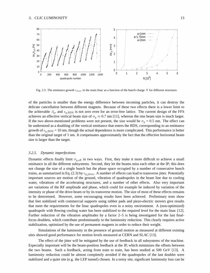
The dependence of the emittance growth on the bunch charge and structure can be seen in Fig. 2.54.The structure with an iris radiusa = 2 mm corresponds to the reference design of the accelerating struc-ture. As can be seen, the structures with larger values ofa (the radius of the iris) allow larger bunchcharges. However, it is more difficult to achieve the required gradient in them.
3.2.4. Beam delivery system emittance growth
In the final focus system (FFS) the beam is strongly focused, and consequently the system has a tendencyto be very chromatic. Since the beam has an energy spread, oneneeds to reduce the chromaticity by adelicate system of cancelling magnets; but some residual effect remains. Another problem arises fromthe emission of synchrotron radiation in the magnets. Whilethe resulting stochastic energy change
4The beam that enters the linac has an energy spread that leadsto some emittance growth during acceleration; this effect isneglected in the figure.
3.. CLIC LUMINOSITY 13
0
10
20
30
40
50
60
70
80
0 200 400 600 800 1000 1200 1400
∆εy/
ε y,0
[%
]
quadrupole number
0
1
2
3
4
5
0 1 2 3 4 5 6
∆ε y
[nm
]
N [109]
a=1mma=1.75mm
a=2mm
Fig. 2.5: The emittance growthǫlinac in the main linac as a function of the bunch chargeN for different structures
of the particles is smaller than the energy difference between incoming particles, it can destroy thedelicate cancellation between different magnets. Becauseof these two effects there is a lower limit tothe achievableβy, andǫy,BDS is not zero even for an error-free lattice. The current design of the FFSachieves an effective vertical beam size ofσy ≈ 0.7 nm [11], whereas the rms beam size is much larger.If the two above-mentioned problems were not present, the size would beσy = 0.5 nm. The effect canbe understood as a doubling of the vertical emittance that enters the BDS, corresponding to an emittancegrowth ofǫy,BDS = 10 nm, though the actual dependence is more complicated. This performance is betterthan the original target of 1 nm. It compensates approximately the fact that the effective horizontal beamsize is larger than the target.
3.2.5. Dynamic imperfections
Dynamic effects finally limitσy,eff in two ways. First, they make it more difficult to achieve a smallemittance in all the different subsystems. Second, they letthe beams miss each other at the IP; this doesnot change the size of a single bunch but the phase space occupied by a number of consecutive bunchtrains, as summarized in Eq. (2.3) byǫy,jitter. A number of effects can lead to transverse jitter. Potentiallyimportant sources are motion of the ground, vibration of quadrupoles in the beam line due to coolingwater, vibrations of the accelerating structures, and a number of other effects. Also very importantare variations of the RF amplitude and phase, which could forexample be induced by variation of theintensity or phase of the drive-beam or by its transverse motion. The size of most of these effects remainsto be determined. However, some encouraging results have been achieved. Preliminary tests showthat feet stabilized with commercial supports using rubberpads and piezo-electric movers give resultsthat meet the requirements for the linac quadrupoles even ina noisy environment. A (non-optimized)quadrupole with flowing cooling water has been stabilized tothe required level for the main linac [12].Further reduction of the vibration amplitudes by a factor 2–5 is being investigated for the last final-focus doublets, which contribute predominantly to the luminosity reduction. This clearly requires activestabilization, optimized by the use of permanent magnets inorder to reduce their weight.
Simulations of the luminosity in the presence of ground motion as measured at different existingsites showed good performance for motion levels measured atCERN and SLAC [13].
The effect of the jitter will be mitigated by the use of feedback in all subsystems of the machine.Especially important will be the beam-position feedback atthe IP, which minimizes the offsets betweenthe two beams. Such a feedback, acting from train to train, has been studied at 500 GeV [13]. Aluminosity reduction could be almost completely avoided ifthe quadrupoles of the last doublet werestabilized and a quiet site (e.g. the LEP tunnel) chosen. In anoisy site, significant luminosity loss can be

14 CHAPTER 2. ACCELERATOR ISSUES AND PARAMETERS
1
10
100
2 2.5 3 3.5 4 4.5 5 5.5 6
L 1 [1
034cm
-2s-1
]
N [109]
case 1case 2case 3
Fig. 2.6: The luminosityL1 as a function of the bunch charge, under different assumptions, at√s =3 TeV. In case 1 it is
assumed that the only source of vertical emittance is the main linac and that the horizontal beam size can be optimized for
maximum luminosity. In case 2, the other sources of verticalemittance growth are taken into account. In case 3, the lowerlimit
of the horizontal beam size as given by the current referencedesign of damping ring and BDS is taken into account.
experienced. The possibility of an intra-pulse feedback, which has to respond extremely fast since thepulse duration is short, has also been investigated [14] anda substantial reduction of the luminosity losshas been reached.
Further studies to determine the size of different dynamic effects, their impact on the luminosity,and the possible counter measures remain to be done. This wasidentified as an important R&D issue forall future linear colliders [15].
3.3. Efficiency and Luminosity
The efficiency of a future linear collider is affected by technical limitations. The transformation of wall-plug power into RF power in the klystrons is affected by losses. Such inefficiencies can be improvedrelatively independently of the main parameter choices. However, most RF devices have reached a highlevel of maturity and large improvements are not to be expected.
Some efficiency limitations are, however, more complex, andarise from the interplay of differentcollider parameters. An example is that, for an otherwise unchanged design, a higher beam currentwill lead to higher efficiency. A higher current can be achieved by increasing the bunch chargeN ,which requires a longer bunch and leads to an increase of the wakefield effects in the main linac andconsequently of the vertical emittanceǫy,linac. In addition, the beamstrahlung will be more severe. Takinginto account the different limitations, one can thus determine an optimum choice ofN giving the bestcompromise between efficiency and vertical beam size and leading to maximum luminosity. Figure 2.6illustrates this for the reference design. If the only source of emittance growth were the linac, small bunchcharges would be favoured because the loss in efficiency is more than compensated by the reduction ofthe emittance growth. Taking into account the other sourcesof emittance growth, however, one finds analmost flat dependence with an optimum aroundN = 4 × 10⁹, the current reference bunch charge. Forsmaller bunch charges, the loss in efficiency is slightly larger than the luminosity increase owing to theshorter bunch and smaller linac emittance growth. At largerbunch charges the larger emittance growthstarts to dominate over the increased efficiency. If one assumes, however, that a lower limit exists for thehorizontal beam size at the value of the current reference design, the luminosity reduction at lower bunch
4.. THE CLIC ENERGY RANGE 15
0
1
2
3
4
5
6
0 1 2 3 4 5 6
L 1 [1
034cm
-2s-1
]
N [109]
a=1mmσx>60nm
a=1.75mmσx>60nm
a=2mmσx>60nm
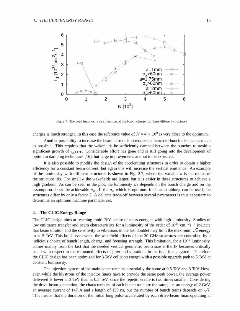
Fig. 2.7: The peak luminosity as a function of the bunch charge, for three different structures
charges is much stronger. In this case the reference value ofN = 4× 10⁹ is very close to the optimum.
Another possibility to increase the beam current is to reduce the bunch-to-bunch distance as muchas possible. This requires that the wakefields be sufficiently damped between the bunches to avoid asignificant growth ofǫy,LET. Considerable effort has gone and is still going into the development ofoptimum damping techniques [16], but large improvements are not to be expected.
It is also possible to modify the design of the accelerating structures in order to obtain a higherefficiency for a constant beam current, but again this will increase the vertical emittance. An exampleof the luminosity with different structures is shown in Fig.2.7, where the variablea is the radius ofthe structure iris. For smalla the wakefields are larger, but it is easier in these structures to achieve ahigh gradient. As can be seen in the plot, the luminosityL1 depends on the bunch charge and on theassumption about the achievableσx. If the σx which is optimum for beamstrahlung can be used, thestructures differ by only a factor 2. A delicate trade-off between several parameters is thus necessary todetermine an optimum machine parameter set.
4. The CLIC Energy Range
The CLIC design aims at reaching multi-TeV centre-of-mass energies with high luminosity. Studies oflow emittance transfer and beam characteristics for a luminosity of the order of 1035 cm−2s−1 indicatethat beam dilution and the sensitivity to vibrations in the last doublet may limit the maximum
√s energy
to ∼ 5 TeV. This holds even when the wakefield effects of the 30 GHz structures are controlled by ajudicious choice of bunch length, charge, and focusing strength. This limitation, for a 1035 luminosity,comes mainly from the fact that the needed vertical geometric beam size at the IP becomes criticallysmall with respect to the estimated effects of jitter and vibrations in the final-focus system. Thereforethe CLIC design has been optimized for 3 TeV collision energywith a possible upgrade path to 5 TeV, atconstant luminosity.
The injection system of the main beam remains essentially the same at 0.5 TeV and 3 TeV. How-ever, while the klystrons of the injector linacs have to provide the same peak power, the average powerdelivered is lower at 3 TeV than at 0.5 TeV, since the repetition rate is two times smaller. Consideringthe drive-beam generation, the characteristics of each bunch train are the same, i.e. an energy of 2 GeV,an average current of 147 A and a length of 130 ns, but the number of bunch trains depends on
√s.
This means that the duration of the initial long pulse accelerated by each drive-beam linac operating at

16 CHAPTER 2. ACCELERATOR ISSUES AND PARAMETERS
937 MHz differs and is proportional to the energy. The directconsequence is an increase of the pulselength of the drive-beam klystrons by a factor of 6. However,since the repetition rate is correspond-ingly reduced from 200 to 100 Hz, the average power to be provided by these klystrons increases onlyby a factor of 3 when going from 0.5 TeV to 3 TeV and the same klystrons can be used at both ener-gies. The power consumption for accelerating the drive-beams increases from∼ 106 MW at 0.5 TeV to∼ 319 MW at 3 TeV.
The combiner rings remain unchanged while the repetition rate of the RF deflectors is halved andtheir pulse is 6 times longer. Each decelerator unit also remains the same, so that all the technical prob-lems related to the drive-beam control, RF power extractionand transfer to the accelerating structuresare identical, irrespective of the collision energy.
At 3 TeV, each linac contains 22 RF power source units, that is22000 accelerating structuresrepresenting an active length of 11 km. With a global cavity-filling factor of ∼ 78%, the total lengthof each linac is∼ 14 km. To keep the filling factor about constant along the linac, the target values ofthe FODO focal length and quadrupole spacing are scaled withE1/2. For practical reasons, however,the beam line consists of 12 sectors (5 at 500 GeV), each with constant lattice cells and with matchinginsertions between sectors. The total number of quadrupoles is 1324 per linac and their length rangesfrom 0.5 m to 2.0 m from the start to the last sector. The rms energy spread along the linac is about0.55% average for BNS damping and decreases to∼ 0.36% at the linac end (1% full width).
The beam delivery system has to be adjusted to the collision energy. In particular, the designscaling and the bending angles are different at 3 TeV and 0.5 TeV. The design has been optimized at3 TeV, where it is most critical, and changing the energy by a large factor currently assumes some changesin the magnet positions, and in the bend and quadrupole strengths. However, the 5.1 km total length ofthe proposed system remains unchanged, as well as the 20 mradcrossing angle. Calculations indicate anacceptable emittance growth in the presence of sextupole aberrations and Oide effects, provided that thelast focusing quadrupole is properly stabilized. The collimation efficiency remains to be checked throughnumerical simulations. The optics, the collimator survival and the control of wakefield effects are stillbeing studied and improved. In any case, the static luminosity optimization procedure needs furtherstudies together with the time-dependent effects and theircontrol via feedbacks including a luminosity-related feedback.
The CLIC design allows one to increase the collider energy with the number of two-beam unitsinstalled in each linac and the length of the pulse required in each drive-beam accelerator. As an illus-tration, these correspond to 4 units with 17µs, 22 units with 100µs and 37 units with 154µs, for
√s =
500 GeV, 3 TeV and 5 TeV, respectively. These numbers correspond to a two-linac length of 5 km, 28 kmand 46.5 km with total collider lengths of about 10 km, 33 km and 51.5 km. A length of up to 40 km totalis available at a site near CERN, extending parallel to the Jura mountain range, in a molasse comparableto that housing the SPS and LHC tunnels. To get beyond this length would require diging the tunnelin the limestone on one end or crossing a 2 km-wide underground fault on the other end. In spite ofthe anticipated technical difficulties, this second solution appears preferable as the additional cost wouldbe limited and this would open the possibility of extending the tunnel to a total length of 52 km. Thelimitation is then set by the presence of a major fault. With this extension, the tunnel length would besufficient for a collider capable of achieving 5 TeV with the proposed parameters.
5. Polarization Issues
The linear collider physics potential is greatly enhanced if the beams are polarized. The requirements forCLIC are relaxed with respect to the NLC-II, JLC, or TESLA parameters, since at CLIC both the chargeper bunch, and the average beam current are lower than in the lower-frequency, lower-energy machines.Table 2.2 compares the relevant CLIC parameters with those of the SLC and with a 1996 parameter setfor NLC-II [17].

5.. POLARIZATION ISSUES 17
Table 2.2: Comparison of electron source parameters achieved at the SLC with those required for NLC-II [17] and CLIC
Parameter SLC NLC-II CLIC
Bunch ch. (1010 e−) 7 2.8 0.4
Total ch. (1010 e−) 14 252 62
Av. pulse current (A) 0.4 3.2 1.0
Pulse length (ns) 62 126 103
Beam polarization ∼ 80% ∼ 80% ∼ 80%
A polarized electron beam with about 80% polarization can beproduced by an SLC-type photoin-jector [18]. Though producing an intense polarized positron beam is more difficult, Compton scatteringoff a high-power laser beam may provide a source of positronswith 60%–80% polarization [19,20]. Ex-perimental R&D and prototyping of a polarized positron source based on Compton scattering is ongoingat KEK for the JLC project [21]. This scheme is taking advantage of rapid advancements in laser tech-nology.
The geometry of the CLIC transfer lines and the damping-ringenergy are chosen so that the beampolarization is preserved, as was the case at the SLC. No significant depolarization is expected to occuron the way to the collision point. We have demonstrated this explicitly by spin tracking through twoversions of the CLIC beam delivery system at the 3 TeV centre-of-mass energy [22]. However, thebending magnets of the beam delivery system rotate the polarization vector by aboutπ/2 (see Fig. 2.8)and the rotation angle changes with the beam energy. Complete control over the IP spin orientation needsto be provided by an orthogonal set of spin rotators, which can be installed between the damping ringand the main linac.
Fig. 2.8: Rotation of the polarization vector in thex–z plane in the nominal (‘short’) and an alternative (‘base’) CLIC final-
focus system at 3 TeV centre-of-mass energy. The initial (Px = 0,Pz = 1, i.e. purely longitudinal) and final polarization values
are indicated by underlaid boxes.

18 CHAPTER 2. ACCELERATOR ISSUES AND PARAMETERS
During the beam–beam collision itself, because of beamstrahlung and the strong fields at 3 TeV,about 7% of effective polarization will be lost. About half of this loss is due to spin precession, the otherhalf to spin-flip radiation. The latter is accompanied by a large energy change and thus does not affectthe luminosity-weighted polarization at the nominal energy.
In view of the fairly large depolarization in collision, thepolarization should be measured bothfor the incoming and for the spent beam. Therefore, we anticipate the installation of two Comptonpolarimeters on either side of the detector. A measurement resolution of 0.5% for the incoming beamwould be comparable to that achieved at the SLC and expected for the other linear-collider designs.Reaching a similar resolution for the highly disrupted spent beam appears very challenging.
More details on polarization issues for CLIC at 3 TeV centre-of-mass energy can be foundin Ref. [22].
6. γγ Collisions at CLIC
Gamma collider options have been considered in all linear collider studies. The energy region of 0.5–1 TeV is particularly well suited forγγ collisions from a technical point of view: the wavelength ofthelaser should be about 1µm, i.e. in the region of the most powerful solid-state lasersand collision effectsdo not restrict theγγ luminosity [23,24].
In the multi-TeV energy region the situation is more difficult: collision effects with coherente+e− pair creation inγγ collisions will be hard to avoid and may restrict the luminosity. The optimumlaser wavelength increases proportionally with the energy. In addition, the required laser flash energyincreases because of non-linear Compton scattering. Options for a 3-TeV photon collider based on 4–6 µm wavelength have been studied recently [25]. We summarize here the main results and give atentative list of parameters and luminosity spectra.
Parameters of a possible photon collider at CLIC with2E0 = 3000 GeV are listed in Table 2.3.
Table 2.3: Possible parameters of the photon collider at CLIC. Parameters of electron beams are the same as fore+e− collisions.
2E0 3000 GeV
λL [µm]/x 4.4 / 6.5
tL [λscat] 1
N / 1010 0.4
σz [mm] 0.03
frep × nb [kHz] 15.4
γǫx/y/10−6 [m·rad] 0.68 / 0.02
βx/y [mm] at IP 8 / 0.15
σx/y [nm] 43 / 1
b [mm] 3
Lee(geom) [1034] cm−2s−1 4.5
Lγγ (z > 0.8zm,γγ) [1034] 0.45
Lγe (z > 0.8zm,γe) [1034] 0.9
Lee (z > 0.65) [1034] 0.6

7.. E−E− COLLISIONS AT CLIC 19
1.2
1
0.8
0.6
0.4
0.2
00 0.2 0.4 0.6 0.8 1 0 0.2 0.4 0.6 0.8 1
dLγedz
1Lgeom
dLγγdz
1Lgeom
R = |ω1 - ω2| / ωav R = |ω1 - ω2| / |ωav-Rpeak|
CLIC (3000)
no cut no cut
R < 0.5 R < 0.5
z = Wγγ / 2 E0 z = Wγe / 2 E0
L0L2
L0L2
3.
2.5
2.
1.5
1.0
0.5
0
Fig. 2.9: γγ (left) andγe (right) luminosity spectra at CLIC(3000).L0, L2 are the luminosities with the total helicity of
two colliding photons in the case ofγγ collisions (or the total helicity of the colliding photon and electron in the case ofγe
collisions) equal to 0 and 2, respectively.
The electron beam parameters shown in the table are the same as for e+e− collisions. As discussedin Ref. [25], this is somewhat conservative, and there may beways of decreasing electron beam sizes incollisions and potentially increase theγγ luminosity by a factor of about 3. The laser parameterx = 6.5approximately corresponds to the threshold fore+e− creation for the non-linear parameterξ2 ≈ 0.3.The corresponding wavelength is 4.4µm. It is not clear at present which kind of laser would be bestsuited for a photon collider at this wavelength. Candidatesare a gas CO laser, a free-electron laser,some solid-state laser or a parametric solid-state laser (the ‘short’ wavelength laser pulse is split in anon-linear laser medium into two beams with longer wavelength). The luminosity spectra obtained by afull simulation [26] based on the parameters quoted here arepresented in Fig. 2.9.
7. e−e− Collisions at CLIC
While e−e− collisions are considered an interesting option, not much effort was made to study it indetail. Most subsystems used to provide a positron beam can also be used for an electron beam, withminor modifications. The subsystems, which need larger changes, e.g. the injector that produces thebeam, are usually simpler for electrons. The main concern isthus the beam–beam collision. In electron–positron collisions the two beams focus each other while they will deflect each other in electron–electroncollisions. A preliminary study of the collision has been performed [27].
The simulations show that the total luminosity is reduced bya factor of roughly 4, but that therelative quality of the luminosity spectrum is better in thee−e− collisions. For the part of the luminosityspectrum close to the nominal centre-of-mass energy, the reduction ine−e− mode is thus only a factorof about 2.5 compared withe+e−. More remarkably, the background spectra of thee−e− mode havea minuscule lower-energy tail, as is clearly shown in Fig. 2.10. Figure 2.11 shows the spent-beam andcoherent pair production angular distributions, of major importance mainly for detector configurationstudies. The number of beamstrahlung photons and coherent pairs is slightly reduced. The incoherentpair and hadronic background are reduced by a factor of 3 to 4.The angular distribution of the spentbeam seems not to be worse than the one frome+e− collisions. A detector designed for the latter shouldbe perfectly capable of handling thee−e− collisions as well.

20 CHAPTER 2. ACCELERATOR ISSUES AND PARAMETERS
Fig. 2.10: Absolute luminosity spectrum for thee+e− ande−e− cases. The bins have a width of 0.5% of the center-of-mass
energy.
Fig. 2.11: Angular distribution of the spent beam and the coherent pairs produced in the 3TeV collision
8. The CLIC Test Facility and Future R&D
The goals of the CLIC scheme are ambitious, and require further R&D to demonstrate that they are in-deed technically feasible. The basic principle of two-beamacceleration with 30 GHz accelerating struc-tures has already been demonstrated in CLIC Test Facilities1 and 2 (CTF1 and CTF2). The technicalstatus of CLIC was recently evaluated by the International Linear Collider Technical Review Commit-tee (ILC-TRC), which was nominated by the International Committee on Future Accelerators (ICFA) inFebruary 2001 to assess the current technical status of the four electron–positron linear-collider designsin the various regions of the world. The report [28] identified two groups of key issues for CLIC: (i) thosethat were related specifically to CLIC technology, and (ii) those which were common to all linear col-lider studies (such as the damping rings, the transport of low-emittance beams, the relative phase jitter ofthe beams, etc.). The CLIC study is for the moment focusing its activities on the following five CLIC-technology-related issues, which were given either an R1 (R&D needed for feasibility demonstration oran R2 (R&D needed to finalize design choices) rating by the ILC-TRC.

8.. THE CLIC TEST FACILITY AND FUTURE R&D 21
Fig. 2.12: Schematic layout of CTF3
1. Test of damped accelerating structures at design gradient and pulse length (R1)
2. Validation of drive-beam generation scheme with a fully-loaded linac (R1)
3. Design and test of damped ON/OFF power extraction structure (R1)
4. Validation of beam stability and losses in the drive-beamdecelerator, and design ofmachine protection system (R2)
5. Test of relevant two-beam linac subunit (R2).
Answers to these key R1 and R2 issues will be provided by the new CLIC Test Facility (CTF3),which is being built to demonstrate the technical feasibility of the key concepts of the novel CLIC RFpower generation scheme, albeit on a smaller scale and re-using existing equipment, buildings and tech-nical infrastructure that have become available followingthe closure of LEP. A schematic layout ofCTF3 is given in Fig. 2.12. CTF3 is being constructed in collaboration with INFN, LAL, NorthwesternUniversity (Illinois), RAL, SLAC, and Uppsala University.
The principal aim is to demonstrate the efficient CLIC-type production of short-pulse RF powerat 30 GHz from 3-GHz long-pulse RF power. This involves manipulations on intense electron beams incombiner rings using transverse RF deflectors as required inthe CLIC scheme [29].
The following are some significant details of the scheme. A 140-ns-long train of high-intensityelectron bunches with a bunch spacing of 2 cm is created from a1.4-µs continuous train of bunchesspaced by 20 cm. The 2-cm spacing is required for an efficient generation of 30-GHz RF power. This isdone by interleaving trains of bunches and is done in two stages. The first combination takes place in thedelay loop, where every other 140-ns slice of the 1.4-µs continuous train is sent round the 42-m (140-ns)circumference of the loop before being interleaved with thefollowing 140-ns slice. This results in areduction in the bunch spacing of a factor of 2 and an increasein the train intensity by a factor of 2. Thesecond stage of combination — this time by a factor 5 — takes place in the combiner ring. After passingthrough the delay loop, the 1.4-µs train from the linac is made up of five 140-ns pulses with bunchesspaced by 10 cm, and five interspaced 140-ns gaps. The combiner ring combines these five pulses into asingle 140-ns pulse using a novel system of beam interleaving.

22 CHAPTER 2. ACCELERATOR ISSUES AND PARAMETERS
Fig. 2.13: Low-charge demonstration of electron pulse combination and bunch frequency multiplication by a factor 5 in CTF3
Progress CTF3 to date is as follows. Preliminary tests of bunch interleaving with five trains usinga new gun and a modified version of the old LEP injector complex(LPI linac and EPA ring) at verylow beam current were successfully completed in November 2002, and the results are summarized inFig. 2.13. This result confirms the basic feasibility of the scheme. In December 2002 the old LPI linacwas dismantled and in June 2003 the new CTF3 injector was installed. A bunched beam of the nominalcurrent, pulse length and energy was obtained from the injector for the first time in August 2003.
Good progress has also been made with CLIC machine studies. The following steps have beenachieved within the 30-GHz CLIC RF structure programme.
(i) Peak accelerating gradients of almost 200 MV/m have beenobtained with short (16-ns) RF pulseswith a 30-GHz molybdenum-iris accelerating structure — a comparative conditioning curve forthree different materials is given in Fig. 2.3.
(ii) A new fully-optimized design of the 30-GHz damped accelerating structure has been made, withsignificantly lower long-range transverse wakefields, which allow shorter bunch spacings andhence shorter pulse lengths.
(iii) A new RF design of the 30-GHz power-generating structure has been proposed, with the ability toturn the power ON and OFF.
(iv) The CLIC Stabilization Study Group has stabilized a prototype CLIC quadrupole to the level of0.5 nm using commercially available equipment. Beam dynamics simulations of the main beamsin the different parts of the machine have been integrated togive results with fully-consistentconditions.

9.. SUMMARY 23
9. Summary
We have summarized in this chapter the aims and status of the CLIC study, with emphasis on featuresrelated to its physics performance. The objective of a compact high-energy complex dictates the choiceof a high accelerating gradient, requiring a high-frequency accelerating structure based on a two-beamapproach. Accelerating structures capable of over 150 MV/mat 30 GHz have been operated successfullywith short RF pulses in CTF2. Though optimized for a nominal centre-of-mass energy of 3 TeV witha design luminosity of 1035 cm−2s−1, CLIC parameters for other energies between 0.5 and 5 TeV havealso been proposed.
We have also discussed the principal machine characteristics that control the achievable lumi-nosity, including the horizontal beam size, the bunch charge and the vertical beam size. The latter isconstrained by the emittance produced in the damping ring, and its subsequent growth in the bunch com-pressor, the main linac and the beam delivery system. Further studies of the damping ring are needed,as are further studies of the effects of dynamical imperfections. In view of the small beam size, goodalignment and stability of the CLIC components are crucial,and seem possible in a quiet site such as atunnel through the molasse rock in the neighbourhood of CERN.
The scaling of CLIC parameters with the centre-of-mass energy has been discussed, and there aregood prospects for polarized beams,γγ ande−e− collisions. Principal R&D issues have been identifiedby the CLIC team and the Loew Panel. The CLIC Test Facility 3 (CTF3) now under construction atCERN will address the most critical R1 issues, and should enable the technical feasibility of CLIC to beestablished within a few years.

24 CHAPTER 2. ACCELERATOR ISSUES AND PARAMETERS

Bibliography
[1] The CLIC Study Team, ed. G. Guignard,‘A 3 TeVe+e− linear collider based on CLIC technology’,CERN 2000-008 (2000).
[2] H.H. Braunet al., ‘The CLIC RF power source – A novel scheme of two-beam acceleration forelectron–positron linear colliders’, CERN 99-06 (1999).
[3] S. Dobert,‘Status of very high-gradient cavity tests’, in Proc. 21st International Linac Conference(LINAC 2002), Gyeongju, Korea, 19–23 Aug 2002, p. 276, CERN-CLIC-Note-533 (2002).
[4] D. Schulte,‘Luminosity limitations at the multi-TeV linear collider frontier’, in Proc. 8th EuropeanParticle Accelerator Conference, 3–7 June 2002, Paris, France, CLIC-Note 527.
[5] H. Braun and D. Schulte,‘Optimum coice of RF frequency for two beam linear colliders’ , in Proc.Particle Accelerator Conference (PAC 03), Portland, Oregon, USA, 12–16 May 2003, CERN-CLIC-Note-563 (2003).
[6] W. Wuenschet al., ‘A demonstration of high-gradient acceleration’, in Proc. Particle AcceleratorConference (PAC 03), Portland, Oregon, USA, 12–16 May 2003,CERN-CLIC-Note-569 (2003).
[7] M. Korostelev and F. Zimmermann,‘Optimization of CLIC damping ring design parameters’, inProc. 8th European Particle Accelerator Conference, 3–7 June 2002, Paris, France.
[8] T.E. D’Amico, G. Guignard and T. Raubenheimer,‘The CLIC main linac bunch compressor’, inProc. 6th European Particle Accelerator Conference (EPAC 98), Stockholm, Sweden, 22–26 Jun1998, CERN-CLIC-Note-372 (1998).
[9] T.E. D’Amico. Private communication.
[10] D. Schulte,‘Emittance preservation in the main linac of CLIC’, in Proc. 6th European ParticleAccelerator Conference (EPAC 98), Stockholm, Sweden, 22–26 Jun 1998, CERN-CLIC-Note-320(1998).
[11] M. Aleksaet al., ‘Design status of the CLIC beam delivery system’, in Proc. 8th European ParticleAccelerator Conference, 3–7 June 2002, Paris, France, CLIC-Note-521.
[12] S. Redaelliet al., ‘The effect of cooling water on magnet vibration’, in Proc. 8th European ParticleAccelerator Conference, 3–7 June 2002, Paris, France, CERN-CLIC-Note-531 (2002).
[13] D. Schulte,‘An update on the banana effect’, in Proc. 26th Advanced ICFA Beam Dynamics Work-shop on Nanometer Size Colliding Beams, Lausanne, Switzerland, 2–6 Sep 2002, CLIC-Note-560(2003).
[14] D. Schulte,‘Simulation of an intra-pulse interaction point feedback for future linear colliders’, inProc. 20th International Linear Accelerator Conference, Monterey, CA, USA, 21–25 Aug 2000,CLIC-Note-454.
25

26 BIBLIOGRAPHY
[15] International Linear Collider Review Committee, Second Report 2003, SLAC-R-606.
[16] J.-Y. Raguin, I. Wilson and W. Wuensch,‘Progress in the design of a damped and tapered accel-erating structure for CLIC’, in Proc. Particle Accelerator Conference (PAC 03), Portland, Oregon,USA, 12–16 May 2003, CERN-CLIC-Note-567 (2003).
[17] ‘Zeroth order design report for the next linear collider’, SLAC-Report-474 (1996).
[18] H. Tanget al., ‘The SLAC polarized electron source’, Talk at the 5th International Workshop onPolarized Beams and Polarized Gas Targets, Cologne, Germany, 6–9 Jun 1995, SLAC-PUB-6918(1995).
[19] T. Omori,‘A polarized positron beam for linear coliders’, 1st ACFA Workshop on Physics Detectorat the Linear Collider, Beijing, China, 26–28 Nov 1998, KEK-Preprint-98-237 (1999).
[20] T. Omori, ‘A concept of a polarized positron source for a linear collider’, International Conferenceon Lasers’99, Quebec, Canada, Dec 13–17, 1999, KEK-Preprint-99-188 (2000).
[21] T. Hiroseet al., Nucl. Instrum. Meth.A455 (2000) 15.
[22] R. Assmann and F. Zimmermann, CERN-SL-2001-064 AP, CERN-CLIC-NOTE-501 (2001).
[23] V. Telnov,Nucl. Instrum. Meth.A472 (2001) 43, hep-ex/0010033.
[24] B. Badeleket al., ‘TESLA technical design report’, Part VI, DESY 2001-011, hep-ex/0108012.
[25] V. Telnov and H. Burkhardt, CERN-SL-2002-013 AP, CLIC-Note-508 (2002).
[26] V. Telnov,Nucl. Instrum. Meth.A355 (1995) 3.
[27] D. Schulte,Int. J. Mod. Phys.A18 (2003) 2851, CLIC-Note-512 (2002).
[28] LC technology evaluation report 2001.
[29] CERN/PS2002-008-RF,http://doc.cern.ch/archive/electronic/cern/preprints/ps/ps-2002-008.pdf.


28 BIBLIOGRAPHY

Chapter 3
EXPERIMENTATION AT CLIC
The definition of the CLIC programme in the multi-TeV range still requires essential data; these willbecome available only after the first years of LHC operation and, possibly, also the results frome+e−
collisions at lower energy. At present we have to envisage several possible scenarios for the fundamentalquestions to be addressed by accelerator particle experiments after the LHC.
It is therefore interesting to consider benchmark physics signatures for assessing the impact of theaccelerator characteristics on experimentation and for defining the needs on the detector response. Eachphysics signature may signal the manifestation of different physics scenarios, possibly beyond those weenvisage today. Nevertheless, the results of these studiesshould be generally applicable also to thoseother processes, having similar characteristics.
While considering experimentation at a multi-TeV collider, it is also interesting to verify to whichextent extrapolations from experimental techniques successfully developed at LEP, and subsequently ex-tended in the studies for a TeV-class linear collider, are still applicable. This has important consequenceson the requirements for the experimental conditions at the CLIC interaction region and for the definitionof the CLIC physics potential.
Four main classes of physics signatures have been identified. These are:resonance scans, electro-weak fits, multijet final statesandmissing energy and forward processes. Their sensitivities to the char-acteristics of the luminosity spectrum and the underlying accelerator-induced backgrounds differ sig-nificantly. Results of detailed simulations of several physics processes representative of each of theseclasses of physics signatures are discussed in the subsequent chapters. A physics matrix summarizingthe various processes studied in detail for CLIC, with theirinterdependence on these classes of physicssignatures and the aspects of the machine parameters, is given in Tables 3.1 and 3.2.
This chapter discusses the issues related to the experimental conditions at CLIC, the conceptualdesign for the detector and the software tools developed andused for simulation.
1. CLIC Luminosity
In order to obtain the required high luminosity the beams need to have very small transverse dimensionsat the collision point of a linear collider. This leads to strong beam–beam effects and subsequently to asmearing of the luminosity spectrum and an increase of the background. The main beam parameters andbackground numbers are summarized in Table 3.3.
1.1. Beam–Beam Interaction
During collision in an electron–positron collider, the electromagnetic fields of each beam acceleratethe particles of the oncoming beam toward its centre. In CLICthis effect is so strong that the particletrajectories are significantly changed during the collision, leading to reduction of the transverse beam
29

30 CHAPTER 3. EXPERIMENTATION AT CLIC
Table 3.1: Physics signatures and CLIC physics programme: matrix of the simulated processes
Physics Higgs SUSY SSB New gauge Extrasignatures sector bosons dimensions
Resonance scan µ D-BESS Z ′ KKthresholds resonances
EW fits σff , AffFB, σff , A
ffFB,
Multijets H+H−
H0A0
H0H0νν
Emiss, Fwd H0e+e− ℓ WW
χ02 scattering
Table 3.2: Physics signatures and CLIC accelerator parameters
Physics Beam- Beam e+ Pairs γγ bkgdsignatures strahlung E spread polarization
Resonance scan Stat. shape syst. Shape syst. CouplingsΓbb,cc ,tt Γbb,cc ,tt
EW fits Unfold boost Polarization bb, cc cos θmin
measurement tags bkgd flavour
Multijets 5-C fit Tags for Fake jetsjet pairing
Emiss, Fwd θmiss Fwd tracking Ehem, ET
sizes, the so-called pinch effect. This enhances the luminosity but since it bends the particle trajectoriesit also leads to the emission of beamstrahlung, which is comparable to synchrotron radiation and reducesthe particle energy. The average number of photons emitted is of the order of 1, so the impact on thecentre-of-mass energy of colliding particles is somewhat comparable to initial-state radiation.
The produced beamstrahlung photons also contribute to the production of background. In the caseof CLIC at high energies, the largest number of particles is expected from the so-called coherent pair cre-ation. In this process a real photon is converted into an electron–positron pair in the presence of a strong

1.. CLIC LUMINOSITY 31
Table 3.3: The parameters of CLIC atEc.m. = 500 GeV andEc.m. = 3 TeV. For the latter energy two parameter sets are
given: the first one is used to evaluate the background. The second set has been used for the ILC-TRC; it takes into account
some recent findings of the structure research and beam-delivery system. The first set is used for background evaluation,as the
second set is going to evolve soon, and because it yields higher background levels, so that it presents a more conservative view
of the conditions. It should be noted that the beam sizesσx andσy are determined by fitting the results of full tracking with
normal distributions. For background and luminosity the full tracking is used, including non-linear effects.Ec.m.: centre-of-
mass energy,L: actual luminosity,L0.99: luminosity withEc.m. > 0.99Ec.m.,0, frep: repetition frequency,Nb: number of
bunches per train,∆b: distance between bunches,N : number of particles per bunch,σ: bunch dimensions at IP,ǫ: normalized
emittances,δ: average energy loss,nγ : number of photons per beam particle,N⊥: number of particles from incoherent pair
production, produced withp⊥ > 20 MeV andθ > 0.15,Nhadr: number of hadronic events,NMJ: number of minijet pairs at
p⊥ > 3.2 GeV/c; for Ec.m. = 3 TeV this has a significant theoretical uncertainty.
Ec.m. (TeV) 0.5 3 3
L (1034cm−2s−1) 2.1 10.0 8.0
L0.99 (1034cm−2s−1) 1.5 3.0 3.1
frep (Hz) 200 100 100
Nb 154 154 154
∆b (ns) 0.67 0.67 0.67
N (1010) 0.4 0.4 0.4
σz (µm) 35 30 35
ǫx (µm) 2 0.68 0.68
ǫy (µm) 0.01 0.02 0.01
σ∗x (nm) 202 43 ≈ 60
σ∗y (nm) ≈ 1.2 1 ≈ 0.7
δ (%) 4.4 31 21
nγ 0.7 2.3 1.5
N⊥ 7.2 60 43
Nhadr 0.07 4.05 2.3
NMJ 0.003 3.40 1.5
electromagnetic field. The cross section for this process depends exponentially on the field strength andthe photon energy. It is therefore very small atEc.m. = 500 GeV but very important atEc.m. = 3 TeV.
Programs have been developed to simulate the pinch effect aswell as the production of beam-strahlung and the different sources of background. For our estimates we use GUINEAPIG [1].
For the old reference parameters, each particle emits on average 2.3 photons per bunch crossing,see Table 3.3. This corresponds to an average energy loss of about 30%. With the new parameters this isreduced to 1.5 photons per particle and a loss of about 20%. The number of coherent pairs is less than anorder of magnitude smaller than the number of beam particles. They will thus give rise to some notableelectron–electron and positron–positron luminosity.

32 CHAPTER 3. EXPERIMENTATION AT CLIC
1.2. Luminosity Spectrum
Not all the electron–positron collisions will take place atthe nominal centre-of-mass energy. Severalsources for an energy reduction of the initial-state particles exist. Each bunch has an initial energyspread of aboutσE/E ≈ 3 × 10⁻³, the bunch-to-bunch as well as pulse-to-pulse energies vary andthe beamstrahlung leads to energy loss during the collision. The bunch-to-bunch as well as pulse-to-pulse energy variations should be small, better than 0.1% peak to peak. While the feasibility of such atight tolerance has been studied for the static bunch-to-bunch variation [2], further studies remain to beperformed. The main sources of energy spread will, however,remain the single-bunch energy spread andthe beamstrahlung. Most of the single-bunch energy spread is due to the single-bunch beam loading inthe main linac, i.e. the fact that a particle in the head of a bunch extracts energy from the accelerating RFstructure, so a particle in the tail sees a reduced gradient.In addition, because of the bunch length, notall particles are accelerated at the same RF phase, which changes the gradient they experience.
In principle the energy spread in the main linac could be reduced somewhat below the currentreference value. This however would compromise the beam stability and would thus probably imply areduction in bunch charge and consequently in luminosity.
In the collision, beam particles lose energy because of beamstrahlung. This limits the maximumluminosity that can be achieved close to the nominal centre-of-mass energy. The lower-energy collisionscan also compromise the performance of experiments as they add to the background and make crosssection scans more difficult. For otherwise fixed parameters, the beamstrahlung is a function of thehorizontal beam size. A larger horizontal beam size leads tothe emission of fewer beamstrahlung photonsand consequently to a better luminosity spectrum. However,the total luminosity is reduced. Figure 3.1shows the luminosity for the nominal CLIC parameters as a function of the horizontal beam size. On theright-hand side the total luminosity above
√s ≥ 0.99Ec.m.,0 is shown.
1
10
100
20 30 40 50 60 70 80 90 100 110
L [10
34cm
-2s-1
]
σx [nm]
L0.99Ltot
5
10
15
20
25
30
35
40
45
50
55
20 30 40 50 60 70 80 90 100 110
L0
.99/L
tot [
%]
σx [nm]
Fig. 3.1: Left: Total luminosity and the luminosity withEc.m. ≥ 0.99Ec.m.,0 as a function of the horizontal beam size. Right:
The fraction of the luminosity withEc.m. ≥ 0.99Ec.m.,0.
It should be noted that also the coherent pairs contribute toluminosity. While they increase thee+e− luminosity by some percent (mainly at low centre-of-mass energies), they createe−e− (ande+e+)collisions, where an electron, from a coherent pair produced in the positron beam, collides with theelectron beam (and vice versa). Also there will occur a smallnumber ofe−e+ collisions, where theinitial-state particles come from the wrong direction.
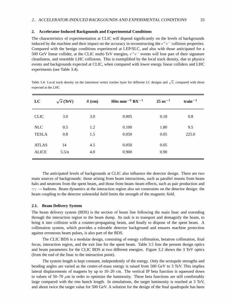
2.. ACCELERATOR-INDUCED BACKGOUNDS AND EXPERIMENTAL CONDITIONS 33
2. Accelerator-Induced Backgounds and Experimental Conditions
The characteristics of experimentation at CLIC will dependsignificantly on the levels of backgroundsinduced by the machine and their impact on the accuracy in reconstructing thee+e− collision properties.Compared with the benign conditions experienced at LEP/SLC, and also with those anticipated for a500 GeV linear collider, at the CLIC multi-TeV energies,e+e− events will lose part of their signaturecleanliness, and resemble LHC collisions. This is exemplified by the local track density, due to physicsevents and backgrounds expected at CLIC, when compared withlower energy linear colliders and LHCexperiments (see Table 3.4).
Table 3.4: Local track density on the innermost vertex tracker layer for different LC designs and√s, compared with those
expected at the LHC
LC√s (TeV) R (cm) Hits mm−2 BX−1 25 ns−1 train −1
CLIC 3.0 3.0 0.005 0.18 0.8
NLC 0.5 1.2 0.100 1.80 9.5
TESLA 0.8 1.5 0.050 0.05 225.0
ATLAS 14 4.5 0.050 0.05
ALICE 5.5/n 4.0 0.900 0.90
The anticipated levels of backgrounds at CLIC also influencethe detector design. There are twomain sources of backgrounds: those arising from beam interactions, such as parallel muons from beamhalo and neutrons from the spent beam, and those from beam–beam effects, such as pair production andγγ → hadrons. Beam dynamics at the interaction region also set constraints on the detector design: thebeam coupling to the detector solenoidal field limits the strength of the magnetic field.
2.1. Beam Delivery System
The beam delivery system (BDS) is the section of beam line following the main linac and extendingthrough the interaction region to the beam dump. Its task is to transport and demagnify the beam, tobring it into collision with a counter-propagating beam, and finally to dispose of the spent beam. Acollimation system, which provides a tolerable detector background and ensures machine protectionagainst erroneous beam pulses, is also part of the BDS.
The CLIC BDS is a modular design, consisting of energy collimation, betatron collimation, finalfocus, interaction region, and the exit line for the spent beam. Table 3.5 lists the present design opticsand beam parameters for the CLIC BDS at two different energies. Figure 3.2 shows the 3 TeV optics(from the end of the linac to the interaction point).
The system length is kept constant, independently of the energy. Only the sextupole strengths andbending angles are varied as the centre-of-mass energy is raised from 500 GeV to 3 TeV. This implieslateral displacements of magnets by up to 10–20 cm. The vertical IP beta function is squeezed downto values of 50–70µm in order to optimize the luminosity. These beta functions are still comfortablylarge compared with the rms bunch length. In simulations, the target luminosity is reached at 3 TeV,and about twice the target value for 500 GeV. A solution for the design of the final quadrupole has been

34 CHAPTER 3. EXPERIMENTATION AT CLIC
Table 3.5: Final-focus (FF), collimation system (CS), and beam parameters at 3 TeV and 500 GeV cm energy. Emittance
numbers refer to the entrance of the BDS. The quoted spot sizes refer to the rms values obtained by particle tracking and are
larger than the ‘effective’ beam sizes, which determine theluminosity.
Parameter (unit) Symbol 3 TeV 500 GeV
FF length (km) 0.5 0.5
CS length (km) 2.0 2.0
BDS length (km) 2.5 2.5
Hor. emittance (µm) γǫx 0.68 2.0
Vert. emittance (nm) γǫy 10 10
Hor. beta function (mm) β∗x 6.0 10.0
Vert. beta function (mm) β∗y 0.07 0.05
Effective spot size (nm) σ∗x,y 65, 0.7 202, 1.2
Bunch length (µm) σ∗z 35 35
IP free length l∗ 4.3 4.3
Crossing angle (mrad) θc 20 20
Repetition rate (Hz) frep 100 200
Luminosity (1034 cm−2s−1) L0 8 2
Fig. 3.2: Optics of the 3-TeV CLIC beam delivery system. The collision point is on the right, at 2.6 km.

2.. ACCELERATOR-INDUCED BACKGOUNDS AND EXPERIMENTAL CONDITIONS 35
Fig. 3.3: Synchrotron radiation fans at 3 TeV with beam envelopes of 14σx and 83σy (Courtesy O. Napoly [8]).
demonstrated, based on permanent-magnet material [3]. Typical synchrotron radiation fans inside thetwo final quadrupoles are depicted in Fig. 3.3, for an envelope covering 14σx and 83σy. The require-ment that synchrotron-radiation photons do no hit the quadrupoles on the incoming side determines thecollimation depth.
Collimation efficiency, energy deposition by lost particles and photons along the beam line, andmuon background have been studied by various authors [4–6],and were found to be acceptable. Colli-mator wakefields and collimator survival have been taken into account in the design optimization [7].
A recent extended review of the present BDS designs for centre-of-mass energies of 3 TeV and500 GeV can be found in Ref. [7]. The final focus has also been discussed in Refs. [8, 9], and thecollimation system in Refs. [9,10].
2.2. Muon Background
The rate of muons, produced as secondary particles in the collimation of high-energy (1.5 TeV) elec-trons’, can be substantial and requires a reliable simulation.
First estimates for CLIC have been obtained, based on the MUBKG code developed forTESLA [11] interfaced to GEANT3 for the simulation of the energy loss of the muons.
Figure 3.4 shows some simulated tracks of muons, produced atthe first, horizontal spoiler (SPX1)and reaching the detector, which is located at about 3 km. Thefigure also shows the position of threeoptional, magnetized (2 T) iron ‘tunnel fillers’, each 10 or 30 m thick. They should be considered as afirst attempt at implementing a dedicated muon protection system, as their properties and locations havenot yet been optimized.
Tracks that reached the detector region were input to a GEANT3-based detector simulation. Fig-ure 3.5 shows the muon background overlayed on a physics event in the CLIC detector.
The simulation allows the prediction of the ratioreµ of beam particles removed by the collimationsystem to the number of muons reaching the detector. For an estimate of the muon flux in the detector,assumptions have to be made about the fraction of halo electrons in the beam that will hit the collima-tors. The amount of beam particles in the tails is difficult topredict, but it is generally expected to besmall. Here, the fraction hitting the first spoiler was assumed to beftail = 10−3. With the parameters inTable 3.6, and for the two (e+ and e−) beams in CLIC, we estimate that 2NeNb ftail cµ/reµ ≈ 2.7× 10⁴

36 CHAPTER 3. EXPERIMENTATION AT CLIC
500 1000 1500 2000 2500 3000
z [m]
y [m
]
6
42
0
-2-4
-6
µ's from first spoiler, SPX1 ( 1X0 carbon )
Detector
CLIC tunnel, Ø = 3.8 m, 30 cm concrete walls
x [m
]
6
42
0
-2-4
-6
inside tunnel: magnetsTUF1,2,3
Fig. 3.4: Tracking of muons, produced at the first spoiler, through the beam delivery system up to the detector region. Topis
the horizontal and bottom the vertical plane.
2 m
eter
Fig. 3.5: Physics event (e+e− → µµ → χ01µχ
01µ) and muon background (in this case 1650µ tracks) as seen in the detector
simulation

2.. ACCELERATOR-INDUCED BACKGOUNDS AND EXPERIMENTAL CONDITIONS 37
Table 3.6: Parameters chosen to estimate the muon flux at the detector
Parameter Symbol Value
Beam energy E 1.5 TeV
Number ofe+, e− per bunch Ne 4× 10⁹
Bunches per train Nb 154
Fraction of tail particles ftail 10−3
Secondaries and other processes cµ 2
e/µ ratio without TUF reµ 9.2× 10⁴
e/µ ratio with TUF reµ 6.2× 10⁵
muons per bunch train crossing would reach the detector. With a muon protection system of three tunnelfillers, their number could be reduced to 4000 muons per train, or 26 per bunch crossing.
The factor ofcµ = 2 is based on more complete simulations for TESLA at 250 GeV;it accountsfor muon production processes that were not included in the GEANT3 simulation used here, such asmuon production from secondary photons in the cascade,e+e− annihilation and hadronic muon produc-tion [11].
While the rate is modest and will not deteriorate the trackerwhen based on, say, silicon, theeffect could be substantial for calorimetric measurementsdue to catastrophic radiation events. GEANT4was used to estimate the amount of high energy showers that could be produced by the high energymuons. The expected muon background spectrum at the surfaceof the detector, shown in Fig. 3.6 (left),from Ref. [12], was used to shoot muons into a block of iron of 8interaction lengths. This corresponds toa typical endcap of a calorimeter. Using approximately 106 muons, the resulting spectrum of the energyreleased in the block is shown in Fig. 3.6 (right), for energyreleases larger than 100 GeV. About 0.15%of the muons of this spectrum may leave a large energy shower in the calorimeter. Future studies willneed to develop tools to recognize these showers, includingthe investigation of calorimeter techniques.
Muon Energy / GeV0 200 400 600 800 1000
Muon Energy / GeV0 200 400 600 800 1000
#
0
200
400
600
800
1000
1200
1400
1600
1800
2000
2200
24002x10
Input Energy Spectrum
Energy / GeV0 200 400 600 800 1000
Energy / GeV0 200 400 600 800 1000
#
0
20
40
60
80
100
120
140
160
180
200
Muon with over 100GeV Energy Loss
Fig. 3.6: Left: The energy spectrum of the background muons that hit the detector surface; Right: The energy deposited ina
block of iron of 8 interaction lengths

38 CHAPTER 3. EXPERIMENTATION AT CLIC
More recently, a fully integrated approach using GEANT4 hasbeen implemented. This includesthe conversion of photons into a pair of muons in the presenceof the fields of the nucleus and theannihilation of high energy positrons with atomic electrons [13, 14]. The GEANT4 program has alsobeen extended to perform the tracking through the machine lattice and materials in a combined, flexiblemanner. The simulation can then be built from an existing machine description, allowing for backgroundoptimization during the machine design phase [5].
2.3. Neutron Background
No detailed study of the neutron flux expected from the spent beam has been performed. Some estimateof the flux induced by the hadrons produced in the beam–beam interaction is given in the next section.Regarding the spent beam, a simple estimate of the neutron flux can be based on the giant resonanceproduction of neutrons. The low energy neutrons from this process tend to fly in all spatial directionswith an almost equal probability. The high energy neutrons from other processes tend to move more inthe direction of the incoming particle beam and will thus fly away from the detector.
The total number of neutrons produced depends on the material of the beam dump. With water,about one neutron is produced per 32 GeV of incoming photon orelectron energy. Neglecting backscat-tering and shielding, the flux at the interaction point wouldthen be 4.6× 1013 cm−2 per year (107 s) ofoperation, for a dump to IP distance of 100 m. While a good fraction of the neutrons can be shielded,this shielding needs to have a hole to let the spent beam pass.While the electron and positron beamscan in principle be bent in such a way that there remains no direct line of sight between beam dumpand detector, this is not possible for the photon beam. The best (and probably only) place where thevertex detector can be shielded from the photon dump is inside the detector. Such a mask can reducethe flux by about three orders of magnitude [15]. In the present case this would yield a flux of about4.6× 1010 cm−2 per year. Increasing the distance between dump and interaction point would reduce thisvalue further. However, a careful, detailed study of this problem, including backscattering of neutrons,remains to be done.
3. Beam–Beam Backgrounds and their Impact
During the collision a number of particles are produced as background. Beamstrahlung photons and co-herent pairs have already been mentioned. Their number is comparable to the number of beam particles,so they strongly constrain the detector design. Further electron–positron pairs are created by incoher-ent two-photon production. Hadrons are produced in a similar fashion. The number of these particlesis small enough not to modify the beam–beam interaction any further, but they still have a significantimpact on the detector design.
3.1. Coherent Pairs
The number of coherent pairs is quite large: at√s = 3 TeV about 7× 10⁸ pairs are produced per bunch
crossing. The spectrum of the particles is shown in Fig. 3.7;it peaks at about 100 GeV and has a long tailtoward high energies, almost reaching the full beam energy.At low energies (≈ 10 GeV) the productionis strongly suppressed.
The particles initially have small angles with respect to the beam axis. While a newly createdelectron that flies in the direction of the electron beam is focused by the positron beam, a positron goingin the same direction is deflected away from the axis. Since the energy of a typical coherent pair particleis lower than that of a beam particle, the angle after the collision is significantly larger. The coherent pairproduction thus significantly affects the aperture requirement for the spent beamline. Since the numberof coherent pairs is very large, one has to avoid losing even asmall fraction of them in the detectorregion. In order to achieve a reasonable statistics, a largenumber of particles thus has to be simulated,requiring a significant amount of computing time.

3.. BEAM–BEAM BACKGROUNDS AND THEIR IMPACT 39
0
0.5
1
1.5
2
2.5
3
3.5
0 200 400 600 800 1000 1200 1400 1600
dNco
h/dE
[106 G
eV-1
]
E [GeV]
Fig. 3.7: The energy spectrum of the coherent pairs producedduring the collision
3.2. Spent Beam
The spent beam consists mainly of the beam particles, the secondary beamstrahlung photons and thecoherent pairs. While the former two components are confinedto relatively small angles (of the order of1 mrad), the latter can reach larger angles. In order to avoidmore losses in the detector region, an exitaperture must be provided for these particles. Simulationswith GUINEAPIG showed that an apertureof about 10 mrad around the axis of the spent beam is sufficient[16]. Since space is needed aroundthe axis of the incoming beam for the final-focus quadrupole,a total crossing angle of about 20 mradappears reasonable.
3.3. Incoherent Pairs
The production ofe+e− pairs through two-photon processes can lead to significant background at allenergies. The main contributions arise fromee → eee+e−, eγ → ee+e−, andγγ → e+e−, where thephotons are from beamstrahlung. In the beam–beam simulations, the processes that include one or twobeam particles are calculated by replacing the particle with the equivalent photon spectra. This allowsthe effect of the beam size and the strong beam fields onto the cross sections to be taken into account.
It is important to track the produced particles through the fields of the beams, since they can bestrongly deflected. Figure 3.8 shows particles after the collision. For the bulk of these, a clear correlationis visible between the maximum particle angle and the transverse momentum. These particles wereproduced at small angles and obtained most of their transverse momentum from the deflection by thebeams. A few particles above this edge were produced with large angles and transverse momenta. Theycan produce significant background in the vertex detector.
3.4. Hadronic Background and Resulting Neutrons
Two-photon collisions can also lead to the production of hadrons. The cross section for this process isnot very well established at higher centre-of-mass energies, and measuring it will be an interesting exper-iment at a future linear collider. In order to estimate the number of these events, a simple parametrizationof the cross section [17] is done with GUINEAPIG. For the old reference parameters, this simulationyields about 4 events with a centre-of-mass energy above 5 GeV per bunch crossing (Fig. 3.9). For thenew beam parameters this number is reduced to 2.3 events per bunch crossing. The final states of thehadronic background were simulated using PYTHIA. The average visible energy in the detector is about90 GeV per bunch crossing. The hadronic background also causes charged hits in the vertex detector.

40 CHAPTER 3. EXPERIMENTATION AT CLIC
Fig. 3.8: Angle and transverse momentum of the incoherent pairs after the collision. Only particles with an energy larger than
5 MeV were tracked
0.0001
0.001
0.01
0.1
1
10
0 50 100 150 200 250 300 350 400 450 500
even
ts p
er b
unch
cro
ssin
g
Evis [GeV]
θ>=0.0θ>0.1θ>0.2
0.0001
0.001
0.01
0.1
1
10
0 20 40 60 80 100
even
ts p
er b
unch
cro
ssin
g
Pt,vis [GeV]
θge0.0θ>0.1θ>0.2
Fig. 3.9: Left: The average number of hadronic events per bunch crossing as a function of the visible energy above a given cut
angleθ. Right: The number of events as a function of the transverse energy.
The highest density of these hits is 0.25 hits mm−2. While this is still lower than the≃ 1 hit mm−2 dueto incoherent pairs, it is still a sizeable contribution. A database containing the hadronic background ofabout 2000 bunch crossings has been made available [18] and can be accessed using the HADES library(see Section 5.4.) [19].
The secondary neutron flux from these hadronic events has also been simulated, yielding a maxi-mum flux of 3× 10⁹ n cm−2 per year (= 107 s) of operation [20]. The flux is highest around the masksand smaller around the IP.
3.5. Crossing Angle
In CLIC the beams will collide with a full crossing of 20 mrad.Lower limits of this crossing anglearise from the so-called multibunch kink instability and the necessity to extract the spent beam from thedetector with minimal losses. An upper limit is imposed by the detector solenoidal field, which, in thepresence of a crossing angle, affects the beams, leading to the emission of synchrotron radiation and thesubsequent increase of the beam spot size.
To avoid the luminosity reduction normally associated withcollisions at a crossing angle, the so-called crab-crossing cavities should be used. These cavities add a small horizontal kick to the beamparticles, depending on their longitudinal position in thebunch. This scheme allows the bunches tocollide head-on.

3.. BEAM–BEAM BACKGROUNDS AND THEIR IMPACT 41
3.5.1. Lower limit of the crossing angle
During the beam collision a large number of electron–positron pairs is created. These particles carryabout1% of the total beam energy and are deflected by the strong electromagnetic fields of the beams.Consequently they can lead to large losses in the line for thespent beam. While the detector is shieldedagainst the resulting secondaries by a tungsten mask, some of these are still of concern, in particularneutrons. In addition, the sheer energy deposition may leadto problems. In particular, the tolerance forthe position stability of the final quadrupoles, which are inside the detector and must not move by morethan≈ 0.2 nm, may be hard to meet. However, providing an exit hole lets all the particles through withan angle of less than 10 mrad and solves the problem [16]. Thiscan be achieved with a crossing angleof at least 10 mrad. Since additional space is required for the quadrupole around the incoming beam areasonable lower limit isθc ≥ 20 mrad.
Another issue is the kick that the outgoing beam applies on the incoming one during the parasiticcrossing inside the detector. This effect can be reduced by shielding the incoming beam line from theoutgoing one, but to achieve this some material must be placed close to the IP. Another possibility isto increase the crossing angle in order to reduce the parasitic kicks. A sufficient suppression can beachieved with a crossing angle ofθc = 20 mrad.
3.5.2. Beam coupling to the detector field
If the beams have an angle with respect to the detector solenoidal field, they will travel on a helix towardthe collision point. By choosing an appropriate optics for the incoming beam, the associated effects canbe compensated. However, in the solenoidal field the particles will emit synchrotron radiation, whichmodifies their energy and thus their trajectory slightly. Asa consequence the beam-spot size will increasein the vertical direction. This effect can be reduced by decreasing either the detector solenoidal field orthe crossing angle. A preliminary study indicates that forBz = 4 T a crossing angle ofθc = 20 mrad isstill acceptable [21]. However, the results depend significantly on the detector end fields, for which onlya simple model was used in the study. Therefore it will be necessary to perform more precise simulationswhen a design for the detector solenoid becomes available.
3.6. Impact on the Vertex Detector Design
A crucial constraint on the detector design arises from the hits of incoherent pairs in the innermostvertex detector layer. An acceptable density of hits from background on the innermost layer is ofO(1) hits mm−2 per readout cycle. Beyond this level the pattern recognition will be affected by theassociation of spurious hits to particle tracks and by the creation of ghost tracks. To allow some safetymargin a target of not more than 1 hit mm−2 has been adopted. The number of hits in the vertex detectorhas been obtained using a full GEANT simulation. Figure 3.10shows the expected hit density per beampulse at different values of the radiusr of the innermost vertex detector layer as a function of the longi-tudinal positionz. At r = 30 mm the hit density reaches the limit of about 1 mm−2, and this radius hastherefore been adopted in the detector design. A higher detector solenoidal field could be used to furtherreducer.
3.7. Mask Design
Another potentially important source of hits in the vertex detector is that of low-energy electrons andpositrons from coherent pair creation; these are backscattered in the final quadrupoles and are then guidedby the main solenoidal field back into the vertex detector [15]. The total number of hits from this sourcecan be an order of magnitude larger than the direct hits. Thiseffect can be suppressed by using a maskthat covers the side of the quadrupole facing the detector. If the mask is covered with a low-Z material,backscattering can be almost completely suppressed; graphite is currently considered. Figure 3.11 shows

42 CHAPTER 3. EXPERIMENTATION AT CLIC
0.1
1
10
100
1000
0 1 2 3 4 5
hits
per
mm
−2 p
er tr
ain
z/r
r=35mmr=30mmr=25mmr=20mmr=15mm
Fig. 3.10: Number of hits per train as function of the ratio ofthe longitudinal position along the beam axis to the detector radius,
for different values of the radius
θ i
θm
2m
4cm
quadrupole
vertex detector instr. tungsten
interaction point
graphite
tungsten
Fig. 3.11: Sketch of the mask layout
the full masking system, of which the part discussed here consists of the graphite and instrumentedtungsten layers.
Originally the mask has been developed for a machine withouta crossing angle [15] and it wasfound that it worked excellently as soon as the inner opening, through which the beam passes, is smallerthan the vertex detector. In the presence of a crossing anglethe situation is more complicated, as partof the vertex detector cannot be protected by the mask. One therefore has to provide further maskingdownstream, to prevent backscattering through the hole of the mask.
The inner mask also serves as a shield against neutrons, which are produced by the spent beamand backscattered into the detector. It has been shown that such a shield can reduce the neutron flux inthe vertex detector by three orders of magnitude [15]. For this purpose, the opening in the mask needs tobe smaller than the vertex detector; the crossing angle doesnot matter as the neutrons will mainly comeantiparallel to the spent beam. The further the mask is from the IP the larger the opening must be toallow the passage of the spent beam. At the chosen distance of2 m between mask and IP, the openinghas a radius of 2 cm and satisfies both conditions.
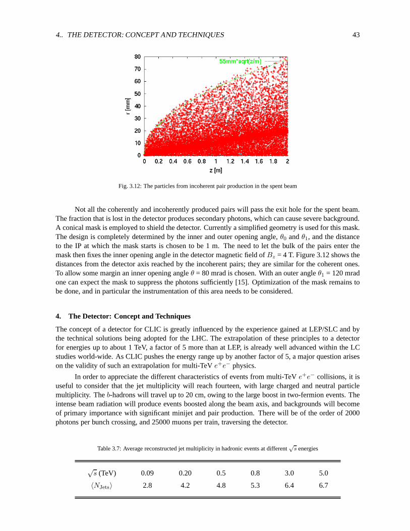
4.. THE DETECTOR: CONCEPT AND TECHNIQUES 43
Fig. 3.12: The particles from incoherent pair production inthe spent beam
Not all the coherently and incoherently produced pairs willpass the exit hole for the spent beam.The fraction that is lost in the detector produces secondaryphotons, which can cause severe background.A conical mask is employed to shield the detector. Currentlya simplified geometry is used for this mask.The design is completely determined by the inner and outer opening angle,θ0 andθ1, and the distanceto the IP at which the mask starts is chosen to be 1 m. The need tolet the bulk of the pairs enter themask then fixes the inner opening angle in the detector magnetic field ofBz = 4 T. Figure 3.12 shows thedistances from the detector axis reached by the incoherent pairs; they are similar for the coherent ones.To allow some margin an inner opening angleθ = 80 mrad is chosen. With an outer angleθ1 = 120 mradone can expect the mask to suppress the photons sufficiently [15]. Optimization of the mask remains tobe done, and in particular the instrumentation of this area needs to be considered.
4. The Detector: Concept and Techniques
The concept of a detector for CLIC is greatly influenced by theexperience gained at LEP/SLC and bythe technical solutions being adopted for the LHC. The extrapolation of these principles to a detectorfor energies up to about 1 TeV, a factor of 5 more than at LEP, isalready well advanced within the LCstudies world-wide. As CLIC pushes the energy range up by another factor of 5, a major question ariseson the validity of such an extrapolation for multi-TeVe+e− physics.
In order to appreciate the different characteristics of events from multi-TeVe+e− collisions, it isuseful to consider that the jet multiplicity will reach fourteen, with large charged and neutral particlemultiplicity. Theb-hadrons will travel up to 20 cm, owing to the large boost in two-fermion events. Theintense beam radiation will produce events boosted along the beam axis, and backgrounds will becomeof primary importance with significant minijet and pair production. There will be of the order of 2000photons per bunch crossing, and 25000 muons per train, traversing the detector.
Table 3.7: Average reconstructed jet multiplicity in hadronic events at different√s energies
√s (TeV) 0.09 0.20 0.5 0.8 3.0 5.0
〈NJets〉 2.8 4.2 4.8 5.3 6.4 6.7

44 CHAPTER 3. EXPERIMENTATION AT CLIC
Studies of the detector concept for a 500 GeV LC have considered both a small and a large detector.The first consists of a compact Si tracker with high magnetic field (B = 5–6 T). The large detector relieson a continuous time projection chamber (TPC) main tracker,has a lower magnetic field (B = 3–4 T)and moves the calorimeter further away from the interactionregion, which is advantageous for energyflow reconstruction based on a fine granularity.
At CLIC, the beam delivery system will constrain the solenoidal magnetic field of the detectorto below about 6 T. We consider here a model for a large detector, which inherits much of the solu-tions adopted in the ECFA/DESY study for a 500–800 GeV LC, adapted to the experimental conditionsexpected at CLIC.
4.1. Vertex Tracker
A CLIC vertex tracker design may consist of a multilayered detector with very high 3-D space resolutionand stand-alone tracking capabilities. At CLIC, the anticipated background frome+e− pairs producedin the interaction of the colliding beams will limit the approach to the interaction region to about 3.0 cm,compared with≃ 1.5 cm foreseen for the lower energy projects. This is partlycompensated by theincrease of the short-lived hadron decay length due to the larger boost. At
√s = 3 TeV, the average
decay distance of aB hadron is 9.0 cm, in the two-jet processe+e− → bb, and 2.5 cm in multipartone+e− → H+H− → tbtb → W+bbW−bb decays. Because of the large boost and large hadronicmultiplicity, the local detector occupancy ine+e− → bb events is expected to increase, by a factor ofalmost 10, to> 1 particle mm−1 from
√s = 0.5 TeV to
√s = 3.0 TeV. This indicates the need to design
a large vertex tracker based on small-area pixel sensors, able to accurately reconstruct the trajectories ofsecondary particles originating few tens of centimetres away from the beam IP and contained in highlycollimated hadronic jets. There are other background issues relevant to the conceptual design of a vertextracker for CLIC. These are the rate ofγγ → hadrons events, estimated at 4.0 BX−1, and the neutronflux, possibly of the order of 1010 1-MeV-equivalent n cm−2 year−1. The need to reduce the number ofγγ events overlapped to ane+e− interaction requires fast time stamping capabilities, while the neutron-induced bulk damage has to be considered in terms of sensor efficiency reduction. Significant R&D isunder way for meeting the requirements of a TeV-classe+e− linear collider; further developments areexpected when the issues related to the SLHC will be addressed.
Emerging silicon sensor technologies and possible paths for the upcoming R&D are discussed inthe next section.
A detector consisting of seven concentric Si layers locatedfrom 3.0 cm to 30 cm from the beam IPand based on pixel sensors, with 20 ns time stamping and radiation hardness capabilities, demonstratedfor their LHC applications can be considered as a baseline design for the vertex tracker. The layer spacinghas been chosen to optimally sample the heavy hadron decay length, resulting in a closer spacing for theinnermost layers (see Fig. 3.13).
4.2. Trends in Si Sensor Developments and Future R&D
Silicon sensors have been very successfully employed in collider experiments for many years. They arebased on well established technologies and their prices have dropped quite significantly over the years,making large-area trackers both feasible and affordable. Obvious advantages of Si pixel detectors aretheir accurate point resolution, of the order of 10µm, true 3D reconstruction of the point of passage of theparticle, and fast charge collection. The main drawback is certainly related to the relatively high materialburden represented by the present sensors and related read-out electronics. R&D studies performed forthe SLHC experiments to improve the radiation hardness of silicon devices have shown that fluences ofseveral 1014 1-MeV equivalent neutrons cm−2 can be coped with, which is orders of magnitude higherthan those expected at CLIC.
Tracking systems for future collider experiments will needvery large area detectors with a macro-

4.. THE DETECTOR: CONCEPT AND TECHNIQUES 45
Radius (cm)
Mul
tiplic
ity in
AoI
0
1
2
3
4
5
6
7
8
9
0 5 10 15 20 25 30 35
Fig. 3.13: Display of ae+e− → bb event at√s = 3 TeV (left) with the detected hit multiplicity steps from the cascade decay
of a long-flyingB hadron (right)
pad geometry (0.5 mm to 1 mm pixels). A large pixel granularity, with < 50 × 50 µm2 pixels, arerequired for vertex detectors. The time structure of the colliding beams at CLIC and SLHC, high-multiplicity events, and the precise tracking requirements will need time-stamping capabilities ofO(1–10 ns). These challenging requirements call both for innovative detector technologies and readout elec-tronics that profit from future nanoscale microelectronicstechnologies.
Based on the experience from the LEP silicon trackers and thepast R&D work and productionof prototype tracker systems, strip and pixel, for the LHC experiments, some preliminary guidelinescan be drawn to direct the needed R&D on Si detectors for future tracking systems. Identified issuesin designing and constructing large-area Si tracking systems (with detector areas of tens to hundreds ofsquare metres) can be categorized as follows:
• Cost: present Si detector technology, based on crystal Si wafers, has reached an industrial maturityand the current production cost of about 10 CHF/cm2 cannot realistically be expected to decreasesignificantly.
• Spatial resolution: LHC hybrid pixel detectors currently have a minimum pixel dimension of50 µm, corresponding to the minimum pitch realistically feasible for the current bump bondingtechnology. The wafer thickness of 300µm can be thinned down to 200µm.
• Charge collection speed: the nominal charge collection time of a standard silicon detector is in therange of 10 ns to 20 ns.
• Radiation hardness: the R&D work on radiation hardness of crystal Si detectors done for the LHCexperiments has shown that standardn-doped high-resistivity substrates reach the doping inversionat about 2× 10¹³ n/cm2 and sustain a displacement damage at a fluence of few 1014 n/cm2. Abovethis limit, standard crystal Si detectors cannot be used.
• Interconnections: bonding between silicon detectors and readout ASICs, wirebonding for stripsand bump bonding for pixel detectors, represents a substantial effort and expansive step in theconstruction of silicon strip and silicon pixel detector modules.
• Cooling: Si strip and pixel detectors in central LHC trackers operate at−15 C to control theleakage current and reverse annealing after radiation damage. This poses strong constraints on thedesign of cooling systems, substantially increasing the material budget.
Considering all these issues, it turns out that scaling up dimensions, improving spatial precision,radiation hardness, charge collection speed of future silicon trackers is a very challenging task, without atechnological breakthrough based on emerging solid-statedetector technologies, the cost issue not beingthe least obstacle. Thinner standard crystal Si (of order 100 µm) could in principle improve the detector

46 CHAPTER 3. EXPERIMENTATION AT CLIC
speed and minimize voxel thickness for a better geometry. However, large-area thin-crystal detectorsare impractical for outer-tracker systems and delicate formicrovertex systems; furthermore, they do notsolve the other issues mentioned above.
There are three novel solid-state detector technologies that are likely to have a significant impacton their design at future collider experiments. A comparison of the different pixel sensor technologies isgiven in Table 3.8.
4.2.1. 3D sensors
3D detectors are a new generation of silicon sensors, which combine fast readout signals, low depletionvoltage and full sensitivity, independently of the substrate thickness. This detector design was originallyproposed by S. Parker and C. Kenney [22, 23], and is schematically represented in Fig. 3.14 (left). Theprocess involved in the fabrication of 3D devices is a combination of traditional VLSI (Very LargeSystem Integration) and Deep Reactive Ion Etching (DRIE), which was developed for micromechanicalsystems. DRIE allows microholes to be etched in silicon witha thickness-to-diameter ratio as large as20 : 1. In the 3D detectors currently processed at Stanford, USA, by a collaboration involving scientistsfrom Brunel (UK), Hawaii, The Molecular Biology Consortium(MBC), CERN, Stanford, ESRF andothers, this technique is used to etch holes as deep as several hundred microns, at distances as short as50 microns from one another. These holes are filled with polycrystalline silicon doped with either Boronor Phosphorus, which is then diffused into the surrounding single-crystal silicon to make the detectorelectrodes. The silicon substrate used for this process canbe either p-type or n-type, and the crystalorientation is< 100>, where 1,0,0 represent the crystal plane coordinates. Silicon atoms line up incertain directions in the crystal.< 100> corresponds to having a particular crystal plane at the surface,and is preferred for a better surface quality. Once the electrodes are filled, the polycrystalline silicon isremoved from the surfaces, and the dopant is diffused. The same process is then used to fabricate ‘activeedges’, or all around trench electrodes doped with either phosphorus or boron to properly complete theelectric field lines. The presence of active edges reduces the dead volume around the detector to< 10µm,as can be seen from theX-ray beam scan in Fig. 3.14 (right). From this figure, obtained using the 2µm,12-keV beam line at the Advanced Light Source, Berkeley, it is possible to see the rapid turn on responseof the detector at the edge and the partial response of the centre of the electrodes. Similar tests have been
Fig. 3.14: Left: Sketch of a 3D detector where the p+ and n+ electrodes are processed inside the silicon bulk. The edges are
trench electrodes (active edges) and surround the sides of the 3D device making the active volume sensitive to a few microns
from the physical edge. Right: Scan of part of a 3D detector performed with a 12 keVX–ray beam. The edge signal turn-on is
visible on the left. The vertical scale represents the current pulse height in arbitrary units (also colour coded), and the distance
between electrodes is 100 microns.

4..T
HE
DE
TE
CT
OR
:CO
NC
EP
TA
ND
TE
CH
NIQ
UE
S47
Table 3.8: Comparison of the different pixel sensor technologies
Properties Standard planar crystal 3-D silicon Monolithic CMOS pixel a-Si:H pixel detector
silicon detector
Collection speed 10 ns Short drift Thermal drift Short drift, high field
Electron transient t 20 ns <1 ns 100 ns 2 ns
Holes transient t 1 ns 200 ns 150 ns
Thickness 300µm 100–200µm 2–8µm 30–50µm
MIP charge signal 24 000e− 10 000–20 000e− 100–500e− 1000–2000e−
Radiation hardness 3× 10¹⁴ At least 1015 at + 20C < 1013, > 5 × 10¹⁵, limit not known,
strong surface effects self-annealing by mobile H
Fluence (n/cm2) at – 20C
Operating temperature – 20C, cryogenic Room Room Room to 60C
Manufacturing cost High High Low Low
Field of applications Microvertex detector Small detectorarea, Microvertex detector, Large–area detector,
tracker fast timing, high low radiation level, macropad andmicrovertex,
radiation level slow readout high radiation environment

48 CHAPTER 3. EXPERIMENTATION AT CLIC
Fig. 3.15: Left: 3D detector with microstrip readout configuration. The electrodes and the aluminium strips, which tie the rows
of p+ andn+ electrodes, are clearly visible. Thep+ strips end at the bonding pads (top). Right: Oscilloscope traces of mips of
3D detectors at room temperature. The rise time is 3.5 ns and is dominated by the readout electronics. The electrode spacing is
100 microns.
performed with particle beams [24]. The new etching machines and the new etching techniques that arebecoming available should allow one to reduce the electrodecentral part as much as possible. Whenthe etching process is completed, aluminium can be deposited in a pattern that will depend on how theindividual electrodes are to be read out.
A 3D detector, where all the electrodes have been connected together by an aluminium microstrip,is shown in Fig. 3.15 (left). The oscilloscope trace of its response to a minimum ionising particle isshown in Fig. 3.15 (right) [25]. The fast radiation-hard electronics used for this test, designed by theCERN microelectronics group dominates the rise time of the pulse, which was measured to be 3.5 ns anddid not degrade after 1× 10¹⁵ protons/cm2 . The same device was tested at 130 K. At this temperaturethe pulse rise timed improved to 1.5 ns while the full pulse width was measured to be less than 5 ns.The inter electrode spacing of these detectors was 100 mm. Devices with shorter spacing have beenprocessed and should have an intrinsic charge collection time of< 1 ns [22]. Tests with such devicesand 0.13 microns electronics readout are in preparation.
4.2.2. Monolithic Si sensors: MAPS
The integration of detector and electronics is particularly crucial in high-resolution silicon pixel detec-tors for microvertex applications, where a very high density of pixel elements has to be achieved. Themonolithic approach [26,27] is based on Active Pixel Sensor(APS) technology and utilizes the epitaxiallayer of the CMOS wafer as detector substrate. The Monolithic Active Pixel Sensors (MAPS) detectorspotentially provide unambiguous two-dimensional tracking, where the detecting element is inseparablefrom the readout electronics. In this approach, both the detector and the front-end readout electronics areintegrated on the same silicon wafer, using standard CMOS fabrication processes. The development ofMAPS detectors started with their use as photon detectors, in the visible band, where they are becomingincreasingly popular at the expence of Charge Coupled Devices (CCDs). MAPS devices are detectors

4.. THE DETECTOR: CONCEPT AND TECHNIQUES 49
Fig. 3.16: Amorphous silicon detector. Left: a schematic ofa hydrogenated amorphous Si detector on ASIC. Right: The time
behaviour of the signal for different polarization voltages showing the intrinsically fast charge-collection properties.
with a small-area readout section, yielding good noise performance. However, the charge collected orig-inates from a thin active volume. In this approach, a thin, moderately doped, undepleted Si layer is usedas radiation-sensitive volume, while the readout electronics is implemented on top of it. This particularstructure makes the entire sensor surface sensitive (100% fill factor), as required for particle tracking.The sensitive volume is usually an epitaxial layer, which isavailable in modern CMOS processes, whereit is grown on a highly, usuallyp++-type, doped substrate. The pixel readout electronics is placed inthep-well. Because of the difference in doping levels (about 103), the epitaxial layer junctions with thep-well and the substrate acts as reflective barriers, confining the charge carriers.
The electron-hole collection is performed by thermal diffusion betweenn-well electrodes. Thecharge-collection is then spread over severaln-well collecting electrodes. But MAPS devices have a lowtolerance to radiation effects. Ionizing radiation induces surface effects that deteriorate charge collection,and displacement damage decreases the minority carrier lifetime, thus rapidly deteriorating the chargecollection efficiency. Only NMOS transistors can be used in pixel circuits, which represents an importantlimitation for the circuit design of the pixel cell.
4.2.3. Hydrogenated amorphous Si on ASIC Technology
A seed R&D on the technology of deposition of hydrogenated amorphous silicon n.i.p layer on ASIC [28,29] has shown that this detector technology has a great potential to solve present limitations of standardSi crystal detector technology.
One of the main advantages of such techniques is the potential cost reduction and the sensor inte-gration with the readout electronics, as in pixel monolithic detectors. Compared with standard Si hybridpixels, the deposition of a-Si:H on ASIC greatly simplifies the pixel detector fabrication (see Fig. 3.16).The problem of interconnections to the electronics is also solved. Another advantage is that a-Si:H semi-conductor is extremely radiation-hard, thanks to a self-annealing process operated by mobile hydrogen(15%) within the amorphous tissue, and defects are continuously passivated. The intrinsic limit of radi-ation hardness is expected to be above 1015 ptcs cm−2. An a-Si:H detector can also operate in a widetemperature range, from room temperature to up to≃ 60 C, without affecting the charge collectionefficiency. This feature represents a great simplification for the cooling systems, which are at present abottleneck in the system design of the LHC trackers.
Preliminary results have demonstrated that charge collection is quite fast: 3 ns to 5 ns for electroncarriers (see Fig. 3.16). High-energy electrons of63Ni and90Sr have been measured with a short peakingtime of 15 ns. However, a substantial R&D effort is essentialto master the deposition technology of a-
50 CHAPTER 3. EXPERIMENTATION AT CLIC
Si:H on ASIC. Several technological issues have to be mastered, in order to obtain an excellent a-Si:H, inparticular a low dangling bond defect density, with a high deposition rate of 1 to 2 nm s−1. The need fora low defect density is essential to deplete a thick intrinsic layer, 50µm with reasonable bias voltages.
4.2.4. Readout electronics, microelectronics and design effort
The development of microelectronics will continue its pacetowards nanoscaled transistor feature size.The particle physics community should monitor and understand how to profit from these technologi-cal advances, which have been a crucial basis for developingnovel solid-state detector and radiation-hardened electronics for LHC applications. Low-power pixel readout architecture should be furtherdeveloped in adapting circuit design techniques to very lowsupply voltages and nanoscale MOSgate length.
4.2.5. R&D directions for Si sensors and associated electronics
Emerging solid-state detector technologies need to be supported by an adequate R&D effort. There arelargely complementary: 3-D detectors offer the fastest possible pixel response, pad, or strip detector withan excellent radiation hardness, the a-Si:H detector can beused to build large-area detector at low cost,and monolithic MAPS sensors offer a low material budget option for vertex trackers.
The 3-D detector technology is already developed at Stanford as a small sensor, but a future fabri-cation of large area should be demonstrated, and transferred to industry. A study of its radiation hardnessshould be made to determine its maximum tolerance. However,for detectors such as this one a hybridiza-tion technique like bump bonding should still be used to forman hybrid detector module.
Fast readout techniques should be adapted to monolithic pixel MAPS, and MAPS operation shouldbe demonstrated at wafer scales with a readout scheme compatible with the vertex tracker requirementsof future collider experiments. Limitations in radiation hardness should be clearly assessed. The devel-opment design effort should be concentrated on three main axes. At the system level, possible imple-mentation of on-chip, real-time hit-reconstruction readout architectures and data-transfer strategies areinvestigated. At the pixel level, the development should address the design of pixel readout circuitryallowing on-pixel integration of an amplifier and circuitryallowing double sampling operation leading tothe effective zero suppression. Another issue is the optimization of the charge-sensitive element orientedon the specific requirements and conditions met for a given tracking application, e.g. vertex detectors.This includes recently emerged designs with auto-reverse polarization of a charge-collecting diode and anew solution for charge-sensitive elements, featuring built-in signal amplification. A conceptual designof this new element, realizing charge-to-current conversion, called PhotoFET, is a charge-sensing ele-ment, in which ionization-generated charge carriers collected from the epitaxial layer directly modulatethe channel current of a PMOS transistor implemented on top of an n-well.
Sensors of the a-Si:H type have a significant potential, in particular for low-cost large-area detec-tors. However, the technology of amorphous silicon, thoughextremely well developed for photovoltaicsolar panels and TFT screens, is still at an early stage in particle physics applications and needs a vigorousR&D effort. In particular, the know-how to grow high-quality thick films of hydrogenated amorphousSi at high deposition rate needs to be acquired. This comes from the need of depositing a thick intrinsica-Si:H layer, which is not usual for mainstream industrial applications. Also a good film quality, ensuringa maximum depletion layer thickness for good sensor sensitivity, crucially depends of the deposition ofa film with a low defect density, a requirement that is not so stringent for other applications. Depositionof a-Si:H film on ASIC demands also the development of adaptedlithography and planarization process.To demonstrate the full potential of the a-Si:H TFA technology it is mandatory to prove that good sensorscan be manufactured on 8- or 12-inch wafers. This will require a substantial effort in circuit design andan improvement in the a-Si:H film deposition technology.

4.. THE DETECTOR: CONCEPT AND TECHNIQUES 51
4.3. b-Tagging
The physics studies at the multi-TeV frontier are expected to still largely rely on the detector ability toidentify the flavour of final-state fermions with high efficiency and purity.
A high resolution vertex tracker, located immediately outside the beam pipe, should provide thetrack position and extrapolation accuracy needed to distinguish particles originated from secondary de-cays of short-lived hadrons, from those produced indirectly at the position of the colliding beams.
At CLIC we envisage to propose a multilayered vertex trackerbased on pixel Si sensors. Thedensity of hits from the machine-induced backgrounds will limit the approach to the interaction region toa radius of about 3 cm. Assuming a rather modest single-pointresolution of 5µm, the achievable resolu-tion on the point of closest approach to the colliding beam spot (impact parameter) is shown in Fig. 3.17.Since the boost of the short-lived particles is large, this performance appears to be sufficient for effec-tively discriminating the secondary from the primary particles. Also, multiple-scattering effects are lesssevere here than at lower-energy colliders, since typically only 10% or less of theb andc decay productshave momenta below 3 GeV.
0
2.5
5
7.5
10
12.5
15
17.5
20
22.5
25
0 5 10 15 20 25 30 35 40
p sin3/2θ (GeV/c)
σIPR
-Phi (
µm)
p sin5/2θ (GeV/c)
σIPz
(µm
)
0
2.5
5
7.5
10
12.5
15
17.5
20
22.5
25
0 5 10 15 20 25 30 35 40
Fig. 3.17: Track extrapolation resolution at CLIC. Left: Impact parameter accuracy as function ofpt for theR–φ (upper plot)
andR–z (lower plot) projections. Right: Display of a multijet event simulated with GEANT3 showing secondary decays
in b jets.
Pixel sensors of different technologies can be considered,from CCDs to the monolithic pixelsensors of new design currently under development. Potentially interesting technologies and an outlineof the needed R&D are discussed later in this section.
Jet-flavour tagging, based on the combination of particle topology and kinematics, has succesfullybeen applied to experiments at LEP and the SLC. The kinematics in multi-TeVe+e− collisions suggeststhat the extensions of the reconstruction and tagging algorithms, pioneered at LEP and the SLC andfurther developed for application at a lower-energy LC, mayneed to be reconsidered. The high jetcollimation and largeb decay distance pose significant challenges to the track pattern recognition andreconstruction that may affect the accuracy ofb andc identification, relying only on secondary vertexand impact parameter tagging. It is thus interesting to consider new quark tagging techniques, whichprofit from the kinematics of multi-TeVe+e− collisions. A b-tagging algorithm based on the tag ofthe steps in particle multiplicity originating from the heavy hadron decay along its flight path echoes atechnique developed for charm photoproduction experiments [30]. At CLIC, the signal of the productionand decay of ab or c hadron can be obtained from an analysis of the number of hits recorded within acone centred on the jet direction as a function of the radial position of the detector layer. In the tested

52 CHAPTER 3. EXPERIMENTATION AT CLIC
implementation of the algorithm, a cone of half-aperture angleψ = 40 mrad, optimized to maximize thesensitivity in the presence of background and fragmentation particles, defines the area of interest (AoI)on each detector layer. The decay of a highly boosted short-lived hadron is characterized by a step in thenumber of hits recorded in each AoI, corresponding to the additional charged multiplicity generated bythe decay products.
Since the average charged decay multiplicity of a beauty hadron is about 5.2 and that of a charmhadron 2.3, theB-decay signature can consist of either one or two steps, depending on whether the charmdecay length exceeds the vertex tracker layer spacing.
The number of background hits in the AoI is estimated to be 0.7, constant with the radius, theincrease of the AoI surface being compensated by the background track density reduction due to thedetector solenoidal field. This background density can be monitored, by sampling the region outside theAoI, and subtracted. The effect of significant fluctuations of the number of these background hits andof low-momentum curling tracks in the innermost layers can also be removed. The typical multiplicitypattern of a taggedB decay is shown in Fig. 3.13.
Jets with an upward multiplicity step at least larger than 1 and a total multiplicity increase largerthan 2 have been considered. According to the simulation, 69%, 29% and 3% of these jets are due tob,c and light quarks respectively. Theb jets can be further discriminated using ab-likelihood based on thesize, radial position and number of multiplicity steps, thefraction of the jet energy and the invariant massof the tracks originating at the detected multiplicity steps. The resulting likelihood forb and lighter jetsand theb efficiency and purity resulting from a cut on this discriminating variable are shown in Fig. 3.18.
b Prob
0
1000
2000
3000
4000
5000
0 0.1 0.2 0.3 0.4 0.5 0.6 0.7 0.8 0.9 1
b Jet Purity
b Je
t Effic
iency
0
0.1
0.2
0.3
0.4
0.5
0.6
0.7
0.6 0.65 0.7 0.75 0.8 0.85 0.9 0.95 1
Fig. 3.18: Theb likelihood for jets ine+e− → qq events at√s = 3 TeV (left) with a multiplicity tag. The response forb (c
and lighter) jets is shown in light (dark) grey. Theb-jet efficiency is given as a function of the purity corresponding to different
likelihood cut values (right).
Table 3.9: Average decay distance in space forB hadrons at different√s
√s (TeV) 0.09 0.2 0.35 0.5 3.0
Process Z0 HZ HZ HZ H+H− | bb
dspace (cm) 0.3 0.3 0.7 0.85 2.5| 9.0

4.. THE DETECTOR: CONCEPT AND TECHNIQUES 53
10-5
10-4
10-3
10-2
10-1
1
10
0 20 40 60 80 100 120R (cm)
hits
in c
one
Cone radius
100 µm 1 mm 5 mm 1 cm
10-5
10-4
10-3
10-2
10-1
1
10
0 20 40 60 80 100 120R (cm)
hits
in c
one
Cone radius
100 µm 1 mm 5 mm 1 cm
Fig. 3.19: Average number of additional hits within a cone ofa given radius, as a function of the radius of the tracking layer.
Left:√s = 500 GeV,B = 4 T; Right:
√s = 3 TeV,B = 6 T.
4.4. Main Tracker
Possible concepts for the central tracking device are similar to those studied for the 500 GeV LC, a smallsilicon tracker surrounded by a large TPC, and for CMS at the LHC, a compact full Si tracker in anintense magnetic field. A TPC would offer some advantages by providing continuous hit informationalong the charged-particle trajectory, a large lever arm with a minimum material burden, anddE/dxspecific ionization information, useful for particle identification. However, local occupancies and two-track separation may represent serious limitations. The total occupancy of a TPC with a inner radiusof 50 cm, which integrates a full train due to its maximum drift time of ≃ 50 µs is estimated to be afew per cent. However, the local track density in hadronic jets is extremely high due to the large boost.Figure 3.19 shows the result of a GEANT3 simulation ofe+e− → bb events at
√s = 0.5 TeV and 3 TeV
with a solenoidal filed of 4 T and 6 T, respectively.
The average number of additional hits contained within a cone of given radius around a track hitis plotted as a function of the radial position from the beam line. In the case of 0.5 TeV centre-of-massenergy, the probability to find additional hits within 1 cm distance at a radius of 40 cm is below 10%.However, in the case of multi-TeV collisions, the jet collimation becomes so pronounced that for 1 cmdistance a 10% probability for an additional hit is only reached at radii exceeding 1 m. Hence, a solid-state tracker with its intrinsic two-track resolution of 100 µm seems to be an advantageous option forquality tracking at CLIC. The CMS experiment at the LHC will deploy an all-Si tracker with an activesurface of 230 m2. While the physics at the LHC and at a 500 GeV LC impose clear requirements onmomentum resolution, from processes such asH → ZZ → 4µ andHZ → Xµ+µ−, at multi-TeVenergies there are no obvious benchmark reaction striving for ultimate momentum resolution. A studyof the processe+e− → µµ→ µ+µ−χ0χ0, where theµ smuon mass is determined from the edges of themuon momentum spectrum, has shown that a momentum resolution comparable to that aimed at for the500 GeV LC, i.e.δpT/p
2T ≤ 5 × 10⁻⁵ GeV−1, seems adequate.
We consider here a central Si tracker consisting of eight concentric layers located between 18 cmand 110 cm from the interaction point. A model of this trackerhas been implemented in GEANT3,assuming 0.65% of a radiation length per layer, and is shown in Fig. 3.20. Its performance has beenstudied withbb andWW events. The targetedδpT/p
2T ≤ 5 × 10⁻⁵ GeV−1 can be achieved as shown
in Fig. 3.20.

54 CHAPTER 3. EXPERIMENTATION AT CLIC
0
20
40
60
80
100
-0.5 -0.4 -0.3 -0.2 -0.1 0 0.1 0.2 0.3 0.4 0.5x 10
-3
MeanRMS
-.1883E-05 .4185E-04
28.09 / 23Constant 89.48Mean -.2124E-05Sigma .3323E-04
∆pT/pT2 (GeV-1)
pT > 100 GeV
Fig. 3.20: The proposed Si tracker for the CLIC detector. Left: R–z view of detector layout with a simulated evente+e− →W+W− at
√s = 3 TeV. Right: Momentum resolution for tracks withpT > 100 GeV obtained using the full GEANT3
simulation.
4.5. Calorimetry
The quality of the reconstruction of jets at CLIC should be guiding the calorimetry concept. The reasonsto achieve the best energy resolution for jets are multiple.A classical example is the need to distinguishhadronic decays of theZ0 from those of theW±, so as to separate the two pair production fusionreactionse+e− → Z0Z0νν and e+e− → W+W−νν in the search for possible strong interactionsamong intermediate vector bosons. The ability to use these hadronic final states besides their leptonic ormixed counterparts would be a key asset in such studies.
Many search channels also claim for a good two-jet mass resolution. The possibility to identify aZ0 or a Higgs boson in the final states of supersymmetry is an important tool in deciphering the natureof cascades. Having access to the hadronic modes, such ash0 → bb, is required to ensure a sizeableevent yield.
Another example is the radion search, an object similar to the Higgs bosons whose main decaychannel is a pair of gluons. The little Higgs scenario, to be identified, would require a precise measure-ment of itsW 3
H boson modes intoℓℓ, qq andZh.
A first requirement from the calorimetry would be to avoid theusual weak points (of most systemsconceived up to now), namely a break between the electromagnetic sector and the hadronic part, eitherdue to the coil or to some other uninstrumented gap. Since anyelectromagnetic system has about oneinteraction length, a large fraction of hadrons interact inits depth and the first interaction is poorlysampled.
It is likely that the way to approach the required performances at CLIC is to achieve the best possi-ble energy-flow reconstruction. The energy-flow technique was developed at LEP and has been adoptedfor the current LC detector studies. This technique combines tracking and calorimetric information in anoptimal way to obtain the best possible resolution on the energy of the produced partons. This requiresan optimal distinction between hadrons, neutral and charged, electrons, photons and muons with a min-imal double-counting. At CLIC the boost is large enough to make intra-jet particle separation difficult,as exemplified by the energy-flow plot of Fig. 3.21.
Conventional wisdom and present experience then call, beside other requirements, for high gran-ularity, both transverse and longitudinal, to disentangleneutral energy deposits from those produced by

4.. THE DETECTOR: CONCEPT AND TECHNIQUES 55
Phi (rad)
z (cm)
E (
GeV
)
00.2
0.40.6
0.81
1.21.4
1.6
010
2030
4050
6070
8090
100
0
50
100
150
200
250
300
350
Fig. 3.21: Ae+e− → W+W− event at√s = 3 TeV (left) and the energy flowing at the entrance of the e.m.calorimeter
located at a radius of 170 cm, assuming a solenoidal field of 6 Tand 5× 5 cm2 cell size (right)
charged particles, which are already accounted for by the more accurate tracker measurements. Thisrequires on the one hand a dense radiator material, with minimal Moliere radius, and a finely segmentedreadout. On the other hand a sufficiently large radius, with excellent matching between charged particletracks, as seen in the main tracker and the calorimeter information is needed. Beside having a minimalamount of material along the tracker, this implies that the transition zone, involving the outermost endof the tracker and the front part of the calorimeter should beparticularly well studied, with minimalthickness of the inert and minimal albedo effects. The problem may be particularly acute in the forwardregion, because of the rates and of the effect of interactions in the mask.
Given the time scale and the rapid evolution of techniques, we are still far from having a workedout scenario. On the other hand we advise to define and set up, or join, a strong program of R&D alongthe lines defined in [31–33] aiming at a very finely pixellatedcalorimeter, made of a dense tungstenradiator and a very compact detecting medium, such as silicon. In its main lines this activity shouldaddress the modelling of the transition from the main tracker to the calorimeter, understand the merits ofa digital approach for the hadronic part with respect to a more classical sampling approach, and whethercompensation should be used.
4.6. Forward Region
The small-angle environment at CLIC is very demanding for low-angle calorimetry: the region below50 mrad, in particular, will be difficult to instrument, bothbecause of the high level of radiation andparticle density. At larger polar angles the situation improves and we are led to believe that varioustypes of detectors are suited for operating at polar angles above 100 mrad. Simulation results show,however, that there still is a sizeable amount of energy deposited byγγ background, between 100 mradand 400 mrad.
The evaluation of theγγ → hadrons background was performed using the output of the GUI-NEAPIG simulation. Backgrounds have then been tracked through the detector using the GEANT3simulation up to scoring planes located at±150 cm downstream from the interaction region.

56 CHAPTER 3. EXPERIMENTATION AT CLIC
Fig. 3.22: The average deposited energy forγγ event at angles larger than 280 mrad
The results of the simulation show that the situation is manageable down to 300 mrad for generalhadronic events and down to about 100 mrad for identifying and measuring energetic electrons fromBhabha events and from fusion processes such ase+e− → ZZe+e−. Assuming that the forward calori-metric coverage is located at 200 cm from the interaction point, theγγ energy would spread over an areaof 20 cm radius. Using a small Moliere radius material for thee.m. calorimeter, one should be able toconfine showers from high energy electrons to a transverse area about one order of magnitude smallerthan the figure reported above. Taking into account that the average energy per particle inγγ events is≃ 2.5 GeV, this contribution does not spoil the energy measurement of a 250 GeV electron.
Even requiring a minimum angle close to 300 mrad, for total energy measurement purposes itis not feasible to integrate a full train. The average deposited energy perγγ event at 280 mrad isshown in Fig. 3.22.
Timing capability should be implemented up to polar angles of about 400 mrad. Two strategies areavailable: either to incorporate time-stamping capabilities in the whole forward calorimeter or to breakthe end-cap calorimeter in two sections. One with nsec-typetime resolution and the other extending thesame technology as the main calorimeter. A specialized calorimeter at small angle is better optimizedand represents the option discussed here.
Small-angle calorimetry for luminosity measurement and beam condition monitoring covers theangular region below 100 mrad. These devices must have good properties for radiation hardness andtime resolution. Out of the various options for the active part of this type of calorimeters, one might usediamond, quartz fibers, parallel-plate chambers, liquid scintillators; we focus here on quartz fibers. Suchdetectors have been widely used in various applications. R&D has been carried out to address the mainrequirements. Energy resolutions better than 40%/
√E have been routinely obtained. The output light is
mostly due to Cherenkov effect by high energy particles in the shower. As for the timing characteristics,the Cherenkov light is intrinsically fast and allows resolutions of the order of 1 nsec to be achieved. Asnoted before, a requirement is for the low-angle calorimeter to have a very small Moliere radius. Thechoice of lead as radiator imposes small gaps for the quartz fibres, and using these as active mediumimproves on the already small Moliere radius achieved with lead. In fact the fibres are sensitive tothose high-energy particles in the shower which travel close to the original primary trajectory. Such aphenomenon is extremely important for hadronic showers. The shower radius has been found to shrink

4.. THE DETECTOR: CONCEPT AND TECHNIQUES 57
by a factor of 3 for the same radiator material. The effect is instead a factor of about 2 for e.m. showers.The discrimination of high-energy electrons benefits from this feature. Given the smaller radius, all edgeeffects will also be of lesser importance. Using a volume ratio of 10:1 gives an equivalent Moliere radiuswell below 1 cm. This can be further reduced by adopting tungsten as the passive radiator.
4.7. Summary of Detector Performance
The parameters and response of the different detector components are summarized in Table 3.10. Thetracking performance has been validated using the full GEANT simulation in terms of both momen-tum resolution and track extrapolation accuracy. The calorimetric performances are derived from thoseassumed in the TESLA study, as they should not be significantly affected by the larger energy. Thecoverage is limited in the forward region by the beam delivery system and forward background.
Table 3.10: Summary of detector performances
Detector CLIC studies
Vertexing δ(IPrφ) = 15 µm ⊕ 35 µm GeV/c
p sin3/2 θ
δ(IPz) = 15 µm ⊕ 35 µmGeV/c
p sin5/2 θ
Solenoidal field B = 4.0 T
Tracking δptpt2
= 5.0× 10⁻⁵(
GeVc
)−1
E.m. calorimeter δEE (GeV) = 0.10 1√
E⊕ 0.01
Hadron calorimeter δEE (GeV) = 0.50 1√
E⊕ 0.04
µ detector Instrumented Fe yokeδpp ≃ 30% at 100 GeV/c
Energy flow δEE (GeV) ≃ 0.3 1√
E
Coverage |cos θ| < 0.98
4.8. Luminosity Measurement and Energy Calibration
The intense beamstrahlung that smears significantly the luminosity spectrum will have to be accuratelymeasured and unfolded from the observed data, to relate themto theoretical predictions. Accurate deter-minations of both the absolute luminosity and the luminosity spectrum are therefore crucial to preservethe CLIC physics potential. Bhabha scatteringe+e− → e+e− represents a favourable reaction, with across section still sizeable beyond 1 TeV (9.4 pb at
√s = 3 TeV) and a simple, accurately measurable
final state.

58 CHAPTER 3. EXPERIMENTATION AT CLIC
4.8.1. Luminosity determination with Bhabha scattering
At LEP-1 a final luminosity precision of 0.07% was achieved, by using double-tags for the Bhabha pro-cess. The theoretical QED prediction for the Bhabha processat LEP was obtained using the BHLUMIMonte Carlo program [34]. The theoretical uncertaintyσth of the BHLUMI prediction was estimatedoriginally to be 0.1% [35], and later reduced to the level of 0.07% [36–38]. The main contributions tothe theoretical uncertainties at LEP-1 were (a) the photonic second-order subleading correctionO(α2Le)
whereLe = ln |t|m2e; (b) the hadronic vacuum polarization; and (c) theO(α2) light fermion-pair produc-
tion. Thes-channelZ contribution being only∼ 1%, its contribution was well under control. At LEP-1,the measured Bhabha rate had to be substantially larger thanthat of thes-channelZ at the resonancepeak. Hence, the polar-angle acceptance was pushed down to 25–50 mrad range, corresponding to
√|t|
of 1–2 GeV.
At CLIC, the angular range of Bhabha luminometer will need tobe shifted to∼ 50–100 mrad dueto background conditions. At 3 TeV, thet-channel transfer becomes 75–150 GeV and thet-channelZtexchange can in principle be as important as that of thet-channel photon exchangeγt. The contributionfrom hadronic vacuum polarization increases at higher transfers too. It is thus important to estimatethe magnitude of these theoretical uncertainties in the low-angle Bhabha (LABH) process at multi-TeVenergies.
The contributions from photonic corrections will scale linearly withLe, if some part ofO(α2Le)will still be missing from the Monte Carlo generators (whichis however unlikely by a realistic time forCLIC operation). We therefore estimate the photonic uncertainty to increase, at most, by≃ 30% w.r.t.its LEP-1 value. TheZt contribution was estimated by completely removing theZ contribution. Thischanges the cross section by a few 0.1% at 0.8 TeV and by 2–6% at3 TeV.
The theoretical uncertainty of theO(α) electroweak corrections in the LABH process at CLIChave been estimated with the help of the DIZET EW library of ZFITTER [39, 40]. This was obtainedby manipulating the non-leadingO(α2) EW corrections ofO(G2
FM2tM
2Z) of Degrassi et al., keeping
O(G2FM
4t ) as accounted for. This is shown in Fig. 3.23, where the effectof change ofMH from 120 GeV
to 500 GeV is also given. We estimate them to be 0.025% at 0.8 TeV and 0.10% at 3 TeV. ChangingMt from 165 GeV to 185 GeV has led to even smaller effect. In summary, σth ≃ 0.10% of the LABHluminometer at CLIC because of EW corrections emerges as a conservative estimate.
0.040 0.060 0.080 0.100
−0.0010
−0.0005
0.0000
0.0005
0.0010
0.0015
0.0020
⋆⋆⋆⋆⋆⋆⋆⋆
⋆⋆⋆⋆⋆⋆
⋆⋆⋆⋆⋆⋆
⋆⋆⋆⋆⋆⋆
⋆⋆⋆⋆⋆⋆
⋆⋆⋆⋆⋆⋆
⋆⋆
√s =3000GeV
ϑ1 [rad]
2-loop EWRC
0.040 0.060 0.080 0.100
−0.0010
−0.0005
0.0000
0.0005
0.0010
0.0015
0.0020
⋄⋄⋄⋄⋄⋄⋄⋄⋄⋄⋄⋄⋄⋄⋄⋄⋄⋄⋄⋄⋄⋄⋄⋄
⋄⋄⋄⋄⋄⋄⋄⋄⋄⋄⋄⋄⋄⋄⋄⋄
√s =3000GeV
ϑ1 [rad]
MH=120, 500GeV
Fig. 3.23: Change of Bhabha differential cross section due to uncontrolled 2-loop corrections and due to Higgs mass error.
Results were obtained using the DIZET library of ZFITTER [39,40].

4.. THE DETECTOR: CONCEPT AND TECHNIQUES 59
The theoretical uncertainties of LABH due to hadronic vacuum polarization (HVP), taking 1995estimates of HVP of Refs. [41,42], was estimated as 0.03% at LEP-2. Using the same calculation of HVPwe get 0.12% at 3 TeV, i.e. larger by a factor of 4. This means that HVP would become the dominantcomponent of theory systematics on the absolute luminosityat CLIC. However, the recent improvementsof HVP [43, 44] modifies the situation substantially: according to preliminary estimates we get a factor2 reduction in the error due to HVP. By the time of CLIC operation, we hope for another factor 2 ofimprovement.
Summarizing, we think that a theoretical uncertaintyσth ≃ 0.1% for the low-angle Bhabha processat energies up to 3 TeV is realistic.
Since the LABH cross section depends as 1/s on the total CMS energy, in order to preserve the0.1% precision of LABH, a knowledge of the absolute beam energy calibration to∼ 0.05% accuracyis needed. The energy spectrum of the luminosity also needs to be determined, which can be obtainedaccurately using the acolinearity of Bhabha scattering as discussed in the next section.
4.8.2. Bhabha scattering and√s′
The reconstruction of the effectivee+e− energy√s′ from the acolinearity in large-angle Bhabha events
has been proposed for a lower energy linear collider [45], extending the experience with the√s′ deter-
mination at LEP-2 [46].
In the approximation where the energy lost before thee+e− interaction is radiated in a singledirection, the effective collision energy
√s can be related to the final statee+e− acolinearity by
√s′ =
√s
√1 − 2
sin(θ1 + θ2)
sin(θ1 + θ2) − sin θ1 − sin θ2,
whereθ1 andθ2 are the angles of the final electron and the positron w.r.t. the photon direction. Therefore,with this assumption, the
√s′ distribution can be measured by a determination of thee+ ande− direc-
tions. At CLIC, there are two main processes leading to electron and positron energy loss, beamstrahlung(BS) and initial-state radiation (ISR). In order to infer the
√s′ spectrum due to BS, it is important that
ISR can be reliably computed and unfolded from the measured distribution.
A preliminary study has been performed by generating Bhabhaevents with the BHLUMI 4.04generator [34]. The CLIC electron and positron energy spectra have been obtained from the result ofthe beam simulation for the CLIC parameters at 1.5 TeV beam energy and the effect of the beam energyspread in the Linac has been included in the form of a Gaussiansmearing with a r.m.s. of 6 GeV.The determination of
√s′ has been based only on the electron and positron direction determination,
assuming a tracking coverage down to7 in polar angle. While the calorimetric information may providefurther important constraints, it needs to be validated by afull simulation, accounting for the backgroundconditions at small angles. Therefore, no attempt to reconstruct ISR photons has been made in thisstudy. It is also important to measure the final-state-particle energy so as to be able to disentangle theeffect of the correlations in the energies of the colliding particles, which are not taken into account in theapproximation introduced.
The beamstrahlung spectrum has been parametrized using twomodels: 1) the modified Yokoya–Chen approximation [47]:e−Nγ
(δ(x − 1) + e−k(1−x)/x
x(1−x) h(x)), h = f(Υ) whereNγ andΥ are treated
as free parameters, and 2) the CIRCE polynomial form:a0δ(1 − x) + a1xa2(1 − x)a3 were the free
parameters area0, a2, a3, respectively. The fractionF of events outside the 0.5% of the nominal√s
energy has also been left free and extracted from the reconstructed data.
The accuracy on the parameters has been obtained by performing a likelihood fit to the recon-structed
√s′ spectrum and the uncertainty on the mean
√s′/
√s has been extracted accounting for cor-
relations. The results are given in Table 3.11 for an equivalent luminosity∫L = 15 fb−1, corresponding

60 CHAPTER 3. EXPERIMENTATION AT CLIC
√sprime (GeV)
N(e
+e- →
e+e- )
/ 6.5
GeV
10 3
10 4
2500 2600 2700 2800 2900 3000
Fig. 3.24: The reconstructed luminosity spectrum for CLIC at 3 TeV (points with error bars). The continuous lines represent
the fit obtained using the first of the parametrizations discussed in the text, for the fitted value and by varying the parameters
within the± 2 σ range.
to≃ 3 days at the nominal luminosity of1035 cm−2s−1. The study has been performed for two differentassumptions on the CLIC parameters, denoted here as CLIC.01and CLIC.02, corresponding to differentbeamstrahlung spectra.
The sensitivity to details of the beamstrahlung spectrum obtained in this analysis needs to befurther validated once the detector resolution effects have been taken into account. However it has beenshown that the detector resolution can be made small with respect to the intrinsic beam energy spread.
Table 3.11: The relative accuracy for the parameters in the Yokoya–Chen and CIRCE parametrization
Parameter CLIC.01 CLIC.02
δNγ/Nγ ± 0.044 ± 0.084
δΥ/Υ ± 0.019 ± 0.018
δ√s′/
√s ± 7.8× 10⁻⁵ ± 5.3× 10⁻⁵
δa0/a0 ± 0.044 ± 0.049
δa2/a2 ± 0.089 ± 0.058
δa3/a3 ± 0.018 ± 0.021
δ√s′/
√s ± 9.8× 10⁻⁵ ± 7.2× 10⁻⁵
5.. SIMULATION TOOLS 61
5. Simulation Tools
The influence of backgrounds on the extraction of physics signals cannot be forgotten. Tools have thusbeen developed to account for these effects by overlaying background particles to physics events andby simulating the
√s energy smearing effects due to the beamstrahlung. These tools are interfaced to
the simulation programs used in the physics analyses discussed in the second part of this report. Thedetector response has been incorporated both through full GEANT3 simulation and through a parametricsmearing program. Both are based on the software developed in the framework of the ECFA/DESYWorkshops on Physics and Detectors at ae+e− Linear Collider, but have been customized to describethe CLIC specific geometry and detector concept.
5.1. BDSIM
A detailed simulation program BDSIM [5] has been developed,based on GEANT4 [48], to model thebeam delivery system (BDS). BDSIM builds the BDS GEANT4 geometry directly from an acceler-ator (MAD) optics file, which allows a rapid turn-around as the BDS designs get updated. BDSIMincorporates efficient accelerator-style tracking based on transfer matrix techniques, together with thestandard shower generation and physics processes of GEANT4. The program has been used to studyelectron/positron tracking, collimation, muon production [49, 50], and the backgrounds associated withsecondaries from showers produced when primary beam or haloparticles strike apertures along the BDS.BDSIM also allows for specialized processes such as the tracking of Compton-scattered electrons andphotons from a laser-wire [51], including the effects of backgrounds and limitations of beam line aper-tures. Such a study was first performed for the nominal long CLIC 1.5 TeV BDS [7]. BDSIM continuesto be upgraded and now also incorporates hadronic processes, including neutron production and track-ing. GEANT4 is set up to allow for efficient weighting and biasing of events and tracks, and BDSIMwill incorporate these techniques to provide high-statistics background estimates for physics and detec-tor studies as well as for BDS optimization. It is also planned to interface BDSIM directly to the nextgeneration of detector simulation codes as they are developed.
5.2. GUINEAPIG
The GUINEAPIG code simulates the beam–beam interaction in alinear collider. It was originally devel-oped for TESLA [15] and later extended to be able to simulate CLIC at high energies [16]. The programuses a clouds-in-cells method to calculate the effect of thefields of one beam on the incoming beam. Abeam is typically represented by about 105 macroparticles. The emission of beamstrahlung is simulatedby approximating the particle trajectory locally with a circular motion and using the Sokolov–Ternovspectrum [52] for the radiation. The produced photons are also tracked on the grid. The productionof coherent pairs from the beamstrahlung photons is implemented similarly to the beamstrahlung. It isalso possible to load an arbitrary distribution of particlefrom an input file, so as to be able to take fulladvantage of the simulation of other components of the accelerator.
The production of incoherent pairs, bremsstrahlung and hadronic background, is achieved usingthe Weizacker–Williams approach. Each beam particle is replaced by a number of virtual photons. In thecollision these photons are treated as real and the cross sections forγγ → e+e− andγγ → hadrons areused. Secondary electrons and positrons are tracked through the field of the beams. Beam-size effectsand those due to the strong field on the virtual photon spectrum can also be taken into account [15].
The produced particles and the beams can be saved after the simulation and so used for furtherstudies. Also the collision energies of electrons, positrons and photons can be stored allowing the re-construction of the luminosity spectra, including all correlations. The CALYPSO and HADES programlibraries provide useful tools for interfacing with event generation and detector simulation programs,using the GUINEAPIG outputs.

62 CHAPTER 3. EXPERIMENTATION AT CLIC
5.3. CALYPSO
CALYPSO [53] is a small Fortran library that gives access to the luminosity output files from theGUINEAPIG simulation. An initialization routine allows the file name to be specified and the typeof particles to be considered for each beam. Subsequent calls of the main subroutine return the energiesof colliding particles. The use of the luminosity file allowsthe inclusion of the full correlations betweenthe colliding beams. Luminosity data files exist for different energies and can be found in Ref. [53].
There also exists a simple Fortran package that uses parametrizations to generate the energies ofcolliding particles at3 TeV. While the correlation is only partially included and some simplificationsare made for the energy spread of the colliding beams, the program reproduces the luminosity spectraquite accurately. This library needs no data files but must belinked to the CERN library CERNLIB.
5.4. HADES
HADES consists of two parts. The first is a simple Fortan library that can write and retrieve backgroundevents to and from a file. Originally designed for hadronic background, the library allows the generationof background events with any generator and their storage ina file. With other routines, it is easy torandomly choose a number of events from such a file and add to them an event generated with PYTHIA.HADES has been used in these studies also to load and overlay the muon background. The secondpart is a small program that uses PYTHIA to generate the hadronic background events from the initialphotons provided by GUINEAPIG. Hadronic background files exist for CLIC atEc.m. = 3 TeV andEc.m. = 5 TeV [18].
5.5. GEANT Simulation
A full simulation of the CLIC tracking system has been developed, based on GEANT3 and on theBRAHMS program set up for the TESLA study. In the CLIC version, the beam-pipe configurationand the tungsten-mask geometry have been modified accordingly and a multilayered tracker based on Sisensors has been implemented according to the conceptual design discussed above. The GEANT pro-gram has been interfaced with CALYPSO and HADES to include the beamstrahlung effects and overlaybackgrounds. The pair,γγ → hadrons and parallel muon backgrounds have been implemented andused in the studies. The GEANT program has been used both to provide parametrizations of the trackingperformances used in the fast simulation and to carry out analyses based on the tracker only such asthe development of theb-tagging algorithm discussed above and the smuon pair production. For thisthe track-reconstructed parameters have been passed to theanalysis code via the VECP commons in theVECSUB package, so that the same code could be used on the fulland fast simulations.
5.6. Parametric Detector Simulation
The program SIMDET simulates the reconstruction ofe+e− collision events, based on a parametrizeddetector response. This response was originally tuned on that expected for the TESLA detector, accord-ing to its full GEANT3 simulation. For its application to theCLIC studies, several extensions have beenimplemented1. The response has been modified to reflect that expected for a detector suitable for use atCLIC. The track momentum resolution and extrapolation accuracy have been parametrized according tothe results of the full GEANT3 simulation of a discrete multilayered Si tracker. Also the angular coveragehas been modified, while the calorimeter performances have been kept as for the TESLA detector.
SIMDET provides a fast treatment of detector simulation andevent reconstruction, while ensuringrather realistic performances. The basic detector components implemented are:
1We thank the Europeane+e− Study Group for TESLA, who allowed us to use and develop this program for CLIC.

6.. GENERATORS AND PHYSICS CODE 63
• Vertex tracker,
• Main tracker and Forward tracker,
• Electromagnetic calorimeter,
• Hadronic calorimeter
• Low-angle tagger and low-angle luminosity calorimeter.
The program applies Gaussian smearing to charged-particlemomenta and impact parameters withresolutions obtained from full simulation. The calorimetric response is also treated parametrically. Pat-tern recognition is emulated by means of cross-reference tables between generated particles and detectorresponse. An energy-flow algorithm defines the output of the program. The track covariance matrix anddE/dx information is also available.
SIMDET processes events generated in line with PYTHIA, and also events stored in HepEvt for-mat. As part of the CLIC extensions, an interface with partons generated with the CompHep program hasbeen set up. It is thus possible to read CompHep event files andperform hadronization and short-livedparticle decays in line. Also, the CALYPSO and HADES interfaces have been added to read the lumi-nosity spectrum and overlay backgrounds, respectively. Inthe CLIC physics studies, the GUINEAPIGluminosity files have been used to describe the shape of the luminosity spectrum and to overlay theγγ → hadrons and the parallel muon backgrounds.
After simulation, particles are classified, for the purposeof physics analysis, as electrons, photons,muons, charged hadrons (taken as pions), neutral hadrons (taken as long-lived kaons) and clusters ofunresolved particles. Detector coverage, tracking efficiencies, charge mismeasurement and thresholdenergies for detector response are taken into account with user-adjustable values. These have been tunedaccording to the CLIC detector concept discussed earlier on.
Best estimates for energy-flow objects have been stored using the VECSUB conventions and usedfor the physics analyses.
6. Generators and Physics Code
6.1. Monte Carlo Event Generators for CLIC
Monte Carlo (MC) event generators are an essential tool in all experimental analyses. In this section wewill briefly recall the key features of these programs and describe those simulations which are availablefor CLIC physics. Here we limit ourselves to the discussion of the physics event generators. Theseprograms must be interfaced to both detector simulations and beam energy spectra in order to give acomplete simulation. In general the MC event generation process can be divided into three main phases2:(1) The hard process where the particles in the hard collision and their momenta are generated, usuallyaccording to the leading-order matrix element. (2) The parton-shower phase where the coloured particlesin the event are perturbatively evolved from the hard scale of the collision to the infrared cut-off. Theemission of electromagnetic radiation from charged-particles can be handled in the same way. (3) Ahadronization phase in which the partons left after the perturbative evolution are formed into the observedhadrons.
Most generators fall into one of two classes: general-purpose event generators aim to perform thefull simulation of the event starting with the hard process and finishing with the final-state hadrons; thesecond class of programs perform only the hard scattering part of the simulation and rely on one of thegeneral-purpose generators for the rest of the simulation.
During the LEP era the most common practice was to rely on the general-purpose Monte Carloprograms for the description of hadronic final states supplemented with more accurate parton-level gen-
2Those particles which decay before hadronization, for example, the top quark, are decayed before the hadronization phaseand treated as a secondary hard process.

64 CHAPTER 3. EXPERIMENTATION AT CLIC
erators interfaced to general-purpose event generators for specific processes, for example four-fermionproduction. At future linear colliders, and particularly CLIC, this is even more important as we wishto study final states with higher multiplicities, for example six or even eight fermions, which cannot bedescribed by the general-purpose generators.
We will first discuss the general-purpose event generators.This is followed by a discussion of theparton-level programs that are available to calculate particular final states and the automatic programsthat are available to calculate any final state.
6.1.1. General-purpose event generators
Historically the main general-purpose generators have been HERWIG [54], ISAJET [55], andPYTHIA [56]. While the general philosophy of these programsis similar, the models used and ap-proximations made are different. In general, at least fore+e− collisions, the range of hard productionprocesses available in the different generators is very similar. All the generators have a wide range ofSM processes predicted by the MSSM, and some processes for other models.
The differences in the parton shower phase of the process aremore pronounced. While ISAJETstill uses the original parton-shower algorithm which onlyresums collinear logarithms, both HERWIGand PYTHIA include the effects of soft logarithms via an angular-ordered parton shower in the case ofHERWIG and by applying a veto to enforce angular ordering on avirtuality-ordered shower in the caseof PYTHIA. There is also a separate program, ARIADNE [57], which implements the dipole cascadeand is interacted to PYTHIA for hadronization. Like the parton-shower phase the models used for thehadronization phase are very different in the different programs. ISAJET uses the Feynman-Field in-dependent fragmentation model while PYTHIA uses the LUND string model and HERWIG the clusterhadronization model.
While these programs will continue to be used in the near future, a major programme is underway to produce a new generation of general-purpose event generators in C++. The main aim of thisprogramme is to provide the tools needed for the LHC. However, these tools will be used for the nextgeneration of linear colliders. The only generator currently available in C++ that can generate physicsresults is APACIC++ [58]; work is under way to rewrite both PYTHIA [59] and HERWIG [60] in C++.These programs should be available in the next few years and we expect them to be the major tools forevent generation at CLIC.
6.1.2. Parton level programs
Many programs are available to calculate an individual hardprocess, or some set of hard processes,and are interfaced to one of the general-purpose generators, most often PYTHIA, to perform the partonshower and hadronization. In this brief review it is impossible to list all these programs and discuss them.
As many of these programs were used by the LEP collaborations, a detailed discussion of bothtwo- [61] and four- [62] fermion generators can be found in the report of the LEP-II Monte Carlo work-shop [63]. In addition there is also one program, LUSIFER [64], for six-fermion processes. In practicethe computation of processes with six or more final-state particles is complex and it seems likely thatthese calculations will be performed by the automatic programs discussed in the next section.
6.1.3. Automatic matrix element calculations
There are an increasingly large number of programs available that are capable of calculating and inte-grating the matrix elements for large numbers of final-stateparticles automatically.
In general there are two important components of any such program. The first step is the calcu-lation of the matrix element for a given momentum configuration. There are three different techniquesin use to perform this step of the calculation: (1) The matrixelement squared can be evaluated symboli-

6.. GENERATORS AND PHYSICS CODE 65
cally using traditional trace techniques. (2) A number of programs use helicity amplitude techniques toevaluate them. (3) There are techniques [65] which can be used to evaluate the matrix element withoutusing Feynman diagrams.
The second step of the process is to integrate the matrix element. There are two main techniquesin use: One approach is to use adaptive integration programssuch as VEGAS [66] to perform the in-tegration. A second approach is to use the knowledge of the matrix element to perform multi-channelphase-space integration based on its peak structure.
In practice some programs combine these two approaches. In general, adaptive programs such asVEGAS [66] are ill-suited to the integration of functions which have complex peaked structures, suchas multiparticle matrix elements, and therefore for most practical applications multichannel integrationtechniques converge much faster.
There are a number of programs available which combine a variety of these techniques:
— AMEGIC++ [67] makes use of helicity amplitude techniques to evaluatethe matrix element to-gether with efficient multichannel phase-space integration to calculate the cross section.
— CompHep[68] is an automatic program for calculation of the cross section for processes with upto eight external particles.3 It uses the traditional trace techniques to evaluate the matrix elementtogether with a modified adaptive integrator to compute the cross section.
— GRACE [69] combines the calculation of matrix element via helicity amplitude techniques andadaptive integration to calculate cross sections. Recently it has been used to calculate the one-loopcorrections to Higgs production inWW fusion [70].
— HELAC/PHEGASuses the approach of Ref. [71] which is based on the Dyson–Schwinger equa-tion together with multichannel integration [72] to calculate the cross section.
— MADGRAPH/MADEVENT [73] uses helicity amplitude techniques for the matrix element to-gether with an efficient multichannel phase-space integrator to compute the cross section.
— WHIZARD is a multichannel integration package which can use either CompHep, MADGRAPHor OMEGA4 [74] to calculate the matrix elements.
— There are tools which are used to calculate loop processes [75]: FeynArts automatically gener-ates the Feynman diagrams for the considered process, whileFeynCalc evaluates analytically therelevant amplitudes. Another package FormCalc can also be used for the calculation of the loopamplitudes with the numerical evaluation performed by the program LoopTools. All these pro-grams have been also used recently to evaluate the radiativecorrections toe+e− → Hνeνe inthe SM [76].
All of these programs apart from HELAC/PHEGAS are publicly available. At present only Com-pHep and GRACE include supersymmetric processes, althoughthe both MADGRAPH and AMEGIC++can be extended to add the additional interactions which areneeded. In order to simulate events theseprograms needed to be interfaced to the general-purpose event generators. Most of these programs areinterfaced to one of the major general-purpose event generators although the details vary from pro-gram to program.
6.2. Programs for Spectra, Decay and Production
6.2.1. Programs for the MSSM spectrum
It is well known that in the unconstrained MSSM, it is a rathertedious task to deal with the basic param-eters of the Lagrangian and to derive in an exhaustive mannertheir relationship with the particle massesand couplings. This is mainly due to the fact that in the MSSM,despite its minimality, there are morethan one hundred new parameters. Even if one constrains the model to have a viable phenomenology,
3CompHep can have up to six final-state particles for scattering processes and seven for decays.4OMEGA uses the approach of Ref. [65] to evaluate the matrix element but does not include any QCD processes.

66 CHAPTER 3. EXPERIMENTATION AT CLIC
there are still more than 20 free parameters left. This largeamount of input enters in the evaluation ofthe masses ofO(30) SUSY particles and Higgs bosons as well as their complicated couplings, which in-volve several non-trivial aspects. The situation becomes particularly difficult if one aims at rather precisecalculations and hence attempts to include some refinementssuch as higher-order corrections, which forthe calculation of a single parameter need the knowledge of alarge part of the spectrum.
However, there are well-motivated theoretical models where the soft SUSY-breaking parametersobey a number of universal boundary conditions at the high (GUT) scale, leading to only a handful of ba-sic parameters. This is the case for instance of the minimal Supergravity model (mSUGRA) and anomaly(AMSB) or gauge mediated (GMSB) SUSY-breaking models. However, this introduces another com-plication since the low-energy parameters are to be obtained through renormalization group equations(RGE) and the models should necessarily give radiative electroweak symmetry-breaking (EWSB). Theimplementation of these two ingredients poses numerous non-trivial technical problems when done in anaccurate way; this complication has to be added to the one from the calculation of the particle massesand couplings with radiative corrections (RC) which is still present.
To deal with the supersymmetric spectrum in all possible cases, one needs very sophisticatedprograms to encode all the information and, eventually, to pass it to other programs or Monte Carlogenerators to simulate the physical properties of the new particles, decay branching ratios, productioncross sections at various colliders, etc. These programs should have a high degree of flexibility in thechoice of the model and/or the input parameters and an adequate level of approximation at differentstages, for instance in the incorporation of the RGEs, the handling of the EWSB and the inclusion ofradiative corrections to (super)particle masses, which inmany cases can be very important. They shouldalso be reliable, quite fast to allow for rapid comprehensive scans of the parameter space, and simpleenough to be linked with other programs.
There are four main public codes (there are also some privatecodes which will not be discussedhere; see later) which make rather detailed calculations ofthe Supersymmetric particle spectrum in theMSSM or in constrained scenarios (mSUGRA, etc.):
— ISASUSY [55], which is available since the early 90s and is implemented in the Monte Carlogenerator ISAJET; it is the most widely used for simulationsin the MSSM.
— SuSpect[77], a new version has been released very recently but a preliminary version of theprogram has existed 1998 and was described in Ref. [78].
— SOFTSUSY[79], a code written in object–oriented C++ but which has a Fortran interface forcalculations in mSUGRA; it was released two years ago.
— SPHENO[80], which was released this year and also calculates the decay branching ratios and theproduction rates ine+e− collisions of SUSY particles.The codes have different features in general, but they all incorporate the four main ingredients or
requirements for any complete calculation of the SUSY spectrum: i) the RG evolution, ii) the implemen-tation of radiative EWSB, iii) the calculation of the massesof the Higgs and SUSY particles, includingthe radiative corrections, and iv) the possibility of performing some checks of important theoretical fea-tures and some experimental constraints.
The radiative corrections are particularly important, as is well known, in the Higgs sector. Codessuch as ISASUSY and SuSpect have their own approximate calculations, but they are also linked withroutines which do a more sophisticated job. The main available routines for the Higgs sector are: Subh-pole (SUBH) [81] which calculates the leading radiative corrections in the effective potential approachwith a two-loop RG improvement; HMSUSY (HHH) [82] which calculates the one-loop corrections inthe effective potential approach and includes the leading two-loop standard QCD and EW corrections;FeynHiggsFast [83], which calculates the corrections in the Feynman diagrammatic approach with theone and two-loop QCD corrections at zero momentum transfer (the version FeynHiggs [84] has the fullone-loop corrections and is slower); and BDSZ [85] gives theleading one-loop corrections from the third-generation (s)fermion sector as well as the fullαsλ
2t , λ
4t andαsλ2
b , λtλb corrections at zero-momentum

7.. STANDARD MODEL CROSS SECTIONS 67
transfer and also has the corrections to the effective potential. The radiative corrections to the SUSYspectrum are in general performed following Pierce, Bagger, Matchev and Zhang [86].
Detailed comparisons of these codes have been performed. The main conclusion is that despitethe different ways in which the various items discussed above are implemented, they in general agreeat the per cent level in large parts of the MSSM parameter space. Several more important differencesoccur, however, in some areas of the parameter space, in particular in the hightan β and/or focus pointregions with largem0 values, where the Yukawa couplings of top and bottom quarks play an importantrole; see Ref. [87] for details.
6.2.2. Decay and production
For the production of SUSY and Higgs particles, the matrix elements of most important processes arealready included in the MC generators. However, in some cases, specific-purpose programs which in-clude some higher-order effects such as radiative corrections, spin correlations, width effects, etc. arevery useful. A non-exhaustive list of available public codes for Higgs and sparticle production ine+e−
collisions including higher-order effects is:
— SUSYGEN[88] for Higgs and sparticle production, also a MC generator(see above).
— HZHA [89]: the most used Monte Carlo generator for Higgs production at LEP2.
— HPROD[90]: a code which calculates the cross sections for SM and MSSM Higgs production ine+e− collisions in the main production channels.
— SPHENO[80]: discussed earlier and which also calculates the crosssections for SUSY particleproduction ate+e− colliders.
— Many four- or six- fermion production processes ate+e− colliders as discussed earlier; some ofthem have been discussed for the LEP–II MC Workshop [63].
The decays of SUSY and Higgs particles can be rather complicated and it is important to determinethem with good accuracy. There can be a large number of decay modes for some particles: simple two-body decays in which it is important sometimes to include higher-order corrections (as is the case forHiggs bosons and strongly interacting sparticles), and rather complicated many-body decay modes suchas the three- or four- body decays of charginos, neutralinosand top squarks or important loop-induceddecay modes. There are several available codes doing this job with a different level of sophistication:
— ISASUSY[55]: only tree-level two-body Higgs and SUSY decays (three-body for gauginos).
— HDECAY [91]: SM and MSSM Higgs decays with higher-order effects.
— SDECAY [92]: sparticle decays including higher-order effects (RCand multi-body).
— SPHENO[80]: discussed above and has two- and three-body SUSY particle decays.
Some decay routines are also included in the Monte Carlo event generators SUSYGEN [88], HZHA [89],PYTHIA [56] and HERWIG [54] with possible links to the programs mentioned above. The treatmentof SUSY production and decay in the various programs is very different. Both ISAJET and PYTHIAassume that the production and decay of the SUSY particles takes place independently, while HERWIGand SUSYGEN [88] include correlations between the production and decay. HERWIG includes thesecorrelations in all processes [93] while in SUSYGEN they areonly included for some processes anddecays. Some development in this subject is expected in the near future.
7. Standard Model Cross Sections
In order to maximize the sensitivity to new physics signals,it is important not only to consider radiativecorrections to the process under investigation, but also radiative corrections to so-called background pro-cesses provided by the Standard Model. At multi-TeV energies, some processes are of major interest notonly for direct searches, but also as backgrounds for new physics. This is especially true for gauge-boson

68 CHAPTER 3. EXPERIMENTATION AT CLIC
and fermion-pair production. Electroweak one-loop corrections are a central building block in any pre-cision study of fermion-pair production. The complete set of electroweak contributions, including realhard-photon corrections needs then to be calculated [64,94]. One novelty at CLIC is that electroweak ra-diative corrections become sizeable at multi-TeV energies, due to the appearance of Sudakov logarithms.In this section, we first describe the general status of theselarge corrections, and then discuss the specificreactione+e− → tt.
7.1. Electroweak Sudakov Logarithms
At the next generation of linear colliders with centre-of-mass energies in the TeV range, well above theelectroweak scale, one enters the realm of large perturbative corrections. Even the effects arising fromweak corrections are expected to be of the order of 10% or more[95–100], i.e., just as large as thewell-known electromagnetic corrections. In order not to jeopardize any of the high-precision studies atthese high-energy colliders, it is indispensable to improve the theoretical understanding of the radiativecorrections in the weak sector of SM. In particular this willinvolve a careful analysis of effects beyondfirst order in the perturbative expansion in the (electromagnetic) couplingα = e2/(4π).
The dominant source of radiative corrections at TeV-scale energies is given by logarithmicallyenhanced effects of the formαn logk(m2/s) for k ≤ 2n. These large logarithms arise when the finiteparticle massm, which is well below the collider energy
√s, acts as a natural cut-off of a singularity.
To give a numerical example, at a collider energy of 1 TeV, logarithmically enhancedW -boson correc-tions of the formα log2(M2
W/s) and α log(M2
W/s) amount to 19% and –4%, respectively. A natural
way of controlling the theoretical uncertainties therefore consists in a comprehensive study of these largelogarithms, taking into account all possible sources. One class of large logarithms is of ultraviolet ori-gin. They involve short-distance scales and are controlledby the renormalization-group equations. Theremaining large logarithms are of soft and/or collinear origin. They involve long-distance scales and,based on QCD/QED experience, they are expected to possess specific factorization properties. Here wereview our present understanding of the latter class of large-logarithmic effects.
The potentially most important electroweak corrections are the so-called Sudakov logarithms∝ αn log2n(M2/s), arising from the exchange of collinear-soft, effectivelyon-shell transverse gaugebosons [101]. It should be noted, however, that for pure fermionic final states (numerical) cancellationscan take place between leading and subleading logarithms [102]. For on-shell bosons in the final state,the Sudakov logarithms in general tend to be dominant [96,100].
Over the last few years, various QCD-motivated methods havebeen applied to predict the elec-troweak Sudakov logarithms to all orders in perturbation theory [103–105]. The methods vary in the waythat the QCD-motivated factorization and exponentiation properties are translated to the electroweak the-ory. This is caused by the fact that the electroweak theory isa spontaneously broken theory with twomass scales in the gauge-boson sector, whereas QCD is basically a single-scale theory. The main de-bate has therefore focused on the question to what extent theSM behaves like an unbroken theory athigh energies.
In Ref. [106] a first hint was given that the transition from QCD to electroweak theory does notcome without surprises. It was shown that the Bloch–Nordsieck cancellation between virtual and realcollinear-soft gauge-boson radiation [107] is violated for W bosons in the SM as soon as initial- orfinal-state particles carry an explicit weak charge (isospin) and summation over the partners within anSU(2) multiplet is not performed. In the case of final-state particles the event-selection procedure might(kinematically) favour one of the partners within theSU(2) multiplet, leading to a degree of ‘isospin-exclusiveness’. In the initial state the situation is more radical. At an electron–positron collider the weakisospin of the initial state particles is fixed by the accelerator, in contrast to QCD where confinementforces average over initial colour at hadron colliders. As aresult, the Bloch–Nordsieck theorem is ingeneral violated for left-handed initial states, even for fully inclusive cross sections. If we start off witha pure left-handed electron beam,W -boson radiation will change this before the actual (hard) scattering

7.. STANDARD MODEL CROSS SECTIONS 69
process takes place into a mixture of left-handed electronsand neutrinos, with relative weights
WeL =1
2
1 + exp[−2LW (s)]
and Wνe =
1
2
1 − exp[−2LW (s)]
, (3.1)
respectively. The Sudakov coefficientLW (s) is given by
LW (s) =α
4π sin2 θwlog2(M2
W/s) , (3.2)
with θw being the weak mixing angle. The difference in the weights originates from the fact that theisospin-singlet component of the beam receives no Sudakov corrections, whereas the isospin-triplet com-ponent is subject to the Sudakov reduction factorexp[−2LW (s)]. The exponent of this reduction factoramounts to roughly−0.13 at
√s = 1 TeV. This implies a 6% neutrino component of the beam at
that energy. Since the (hard) scattering cross section can be quite different for left-handed electrons andneutrinos, the corrections due to this electroweak phenomenon can be very large, exceeding the QCDcorrections for energies in the TeV range. They are such thatat infinite energy the weak charges willbecome unobservable as asymptotic states [106], which implies for instance anSU(2) charge averaging(‘pre-confinement’) of the initial-state beams.
With this in mind, explicit calculations of (virtual) Sudakov corrections at the two-loop level havebeen performed to resolve any ambiguity in the translation from QCD to the SM. In the first few calcu-lations, the focus was on pure fermionic processes, likee+e− → f f [108] and fermion-pair productionby an SU(2) × U(1)-singlet source [109, 110]. The survey was finally completedby an (Coulomb-gauge) analysis that covered all SM particles [111], including scalar particles as well as transverse andlongitudinal gauge bosons. By means of this explicit calculation it was established to what extent theSM behaves like an unbroken theory at high energies.
It was observed that the SM behaves dynamically like an unbroken theory in the Sudakov limit, inspite of the fact that the explicit particle masses are needed at the kinematical (phase-space) level whilecalculating the Sudakov correction factors. For instance,a special version of the Equivalence Theoremwas obtained, which states that the longitudinal degrees offreedom of the massive gauge bosons can besubstitutedby the corresponding Goldstone-boson degrees of freedom without the need for finite com-pensation factors. As a result, the Sudakov form factors forlongitudinal gauge bosons exhibit featuresthat are typical for particles in the fundamental representation ofSU(2), whereas for the transverse gaugebosons the usual adjoint features are obtained. Moreover, in the transverse neutral gauge-boson sectorthe mass eigenstates decompose into the unbrokenSU(2) field W 3 andU(1) field B, each multipliedby the corresponding Sudakov form factor. At the kinematical level, though, the large mass gap betweenthe photon and the weak gauge bosons remains.
These findings support the Ansatz made in Ref. [104], where the Sudakov form factors weredetermined by postulating a generalized IR evolution equation for the SM in the unbroken phase. Asa result, the virtual Sudakov correction for an arbitrary on-shell external particle with massm, chargeQ and hyperchargeY , amounts to multiplying the matrix element by an exponentiated external wave-function factor
Z1/2 = exp (δZ (1)/2) , (3.3)
with
δZ (1) = − α
4π
[C2(R)
sin2 θw+
(Y
2 cos θw
)2]log2
(M2
s
)
− α
4πQ 2
[log2
(λ2
s
)− log2
(λ2
m2
)− log2
(M2
s
)]. (3.4)
70 CHAPTER 3. EXPERIMENTATION AT CLIC
Hereλ is the fictitious (infinitesimally small) mass of the photon,used as infrared regulator, andM de-notes the generic mass scale of the massive gauge bosons. ThecoefficientC2(R) is theSU(2) Casimiroperator of the particle. So,C2(R) = CSU(2)
F = 3/4 for particles in the fundamental representation: theleft-handed fermions (fL/fR), the physical Higgs boson (H) and the longitudinal gauge bosons (W±LandZL) being equivalent to the Goldstone bosonsφ± andχ. For the particles in the adjoint representa-tion of SU(2), i.e. the transverseW bosons (W±T ) and theW 3 components of both the photon and thetransverseZ boson, one obtainsC2(R) = CSU(2)
A = 2. For theSU(2) singlets, i.e., the right-handedfermions (fR/fL) and theB components of both the photon and the transverseZ boson, theSU(2)Casimir operator vanishes,C2(R) = 0. Note that the terms proportional toQ 2 in Eq. (3.4) are theresult of the mass gap between the photon and the weak bosons.
These Sudakov form factors apply, in principle in a universal way, to arbitrary non-mass-suppressed electroweak processes at high energies. This universality follows from the two definingconditions for the Sudakov corrections: the lowest-order matrix element of the process should not bemass suppressed to start with, and all kinematical invariants of the process other than the masses theexternal particles should be of the order ofs. We would like to stress, though, that the universality ofthe Sudakov form factors has to be interpreted with care. Foran electroweak process likee+e− → 4fit is in general not correct to assume universality and merely calculate the Sudakov form factors forthe external particles (i.e., the six fermions). Dependingon the final state and the kinematical config-uration, the processe+e− → 4f can be dominated by different near-resonance subprocesses[62] likee+e−→W+W−→ 4f or e+e−→ ZZ → 4f . These subprocesses all have their own Sudakov correc-tion factors, which can be determined by employing the so-called pole scheme [112] in the leading-poleapproximation, which restricts the calculation to the on-shell residue belonging to the unstable particlethat is close to its mass shell. In that case, the Sudakov correction factor is given by the wave-functionfactors of the near-resonance intermediate particles rather than the four final-state fermions. The reasonfor this is that the invariant masses of those intermediate particles are close to being on-shell, and there-fore not of the same order ass. The subsequent decays of the intermediate particles into the final-statefermions do not involve a large invariant mass, and will as such not give rise to Sudakov logarithms. Inthis way the Sudakov form factors for unstable particles, like the massive gauge bosons and the Higgsboson, can participate in the high-energy behaviour of reactions with exclusively stable particles in thefinal state.
The observations for the virtual Sudakov corrections can beextended to real-emission processes ina relatively straightforward way. After all, since the Sudakov logarithms originate from the exchange ofcollinear-soft, effectively on-shell transverse gauge bosons, many of the features derived for the virtualcorrections will be intimately related to properties of thecorresponding real-emission processes. Tworemarks are in order, though. First of all, the Bloch–Nordsieck cancellation between virtual and realcollinear-soft gauge-boson radiation can be violated in the SM, as was mentioned earlier. So, unlikein QED/QCD, the Sudakov corrections can show up in inclusiveexperimental observables. Secondly,unlike in QED/QCD, the masses of the weak gauge bosons provide a physical cut-off for realZ/W -boson emission. This means that, given a sufficiently good experimental resolution, it is possible toconstruct exclusive experimental observables that do not receive contributions from realZ/W -bosonradiation. Such observables thus provide direct access to the virtual Sudakov corrections.
Next we discuss the subleading logarithms. For a complete understanding of the perturbativestructure of large logarithmic correction factors, subleading logarithms originating from soft, collinear,or ultraviolet singularities cannot be ignored [100, 102].In the case of pure fermionic final states, forinstance, the subleading effects can reach several per centin the TeV energy range, giving rise to (nu-merical) cancellations between leading and subleading contributions [102].
Over the last few years, some progress has been made in understanding and predicting the sub-leading logarithms. In Ref. [113], a first step was made on theroad towards the construction of a full setof collinear evolution equations in the electroweak theory. It was investigated how collinear logarithms

7.. STANDARD MODEL CROSS SECTIONS 71
factorize in a spontaneously broken gauge theory. As was to be expected on the basis of the aforemen-tioned violation of the Bloch–Nordsieck theorem, a factorization pattern emerges that is qualitativelydifferent from the one in QCD. In order to deal with the explicit weak charges of the initial-state beams,extra splitting functions have to be introduced. These new splitting functions are infrared-sensitive, inthe sense that they depend explicitly on the infrared cut-off provided by the symmetry-breaking scale. Itis precisely this infrared sensitivity that gives rise to the observability of Sudakov logarithms in particularinclusive experimental quantities.
In Ref. [114], finally, the (collinear-soft) angular-dependent, next-to-leading logarithms were de-termined at two-loop level. This explicit SM calculation was found to agree with the exponentiation pre-scriptions proposed in Refs. [102,105,115]. These prescriptions are based on a symmetricSU(2)×U(1)theory matched with QED at the electroweak scale and involvea product of two exponentials. The firstexponential corresponds to theSU(2) × U(1)-symmetric corrections, which are obtained by replacingthe photon mass by the weak-boson mass scaleM . The second exponential corresponds to the QEDcorrections, which are subtracted in such a way that they vanish when the photon mass becomes equaltoM . The order of the two exponentials is such that the QED factoris the last one to act on the matrixelement. In other words, the order respects the hierarchy ofthe generic scales:
√s for the hard-scattering
matrix element,M for theSU(2)×U(1)-symmetric corrections, andλ for the QED corrections. This isnot surprising, since in a gauge-invariant effective-Lagrangian formulation of collinear and soft effectsone would integrate out the momentum-scales exactly along this hierarchy.
7.2. e+e− → t t Cross Sections
Thee+e− → t t reaction is of special interest [116–118], due to its largercross section and a direct linkof the top mass with the coupling to the Higgs boson. This section discusses the processe+e− → tt asan example of the need to include electroweak radiative corrections to obtain reliable predictions.
First we discuss the virtual one-loop corrections. In lowest-order perturbation theory, the processe+e− → tt can be described by two Feynman diagrams. The radiative corrections are parametrized bymeans of form factors. Defining the following four matrix elements
Mij1 =
[v(p4) γ
µ Gi u(p1)]×[u(−p2) γµ Gj v(−p3)
], i, j = 1, 5, (3.5)
with G1 = 1 andG5 = γ5, the Born amplitude can be written in a compact form:
MB = Mγ + MZ =∑
i,j=1,5F ij,B1 Mij
1 , (3.6)
with
F 11,B1 = ve vt
e2
s−M2Z + iMZΓZ
+ QeQte2
s≡ F 11,B,Z
1 + F 11,B,γ1 , (3.7)
F 15,B1 = −ve at
e2
s−M2Z + iMZΓZ
, (3.8)
F 51,B1 = −vt ae
e2
s−M2Z + iMZΓZ
, (3.9)
F 55,B1 = ae at
e2
s−M2Z + iMZΓZ
. (3.10)
Besides (3.5), at one-loop level three further basic matrix-element structures are found (in the limit ofvanishing electron mass):
M1loop =4∑
a=1
∑i,j=1,5
F ij,1loopa Mij
a , (3.11)
72 CHAPTER 3. EXPERIMENTATION AT CLIC
with
Mij1 = γµGi ⊗ γµGj , Mij
2 = p/2 Gi ⊗ p/4 Gj , (3.12)
Mij3 = p/2 Gi ⊗ Gj , Mij
4 = γµGi ⊗ γµ p/4 Gj ,
and correspondingly there are sixteen scalar form factorsF ija in total. The interferences of these matrixelements with the Born amplitude have to be calculated. Onlysix of these interferences are independent,i.e.,Mij
1 , M311 andM3
51. In order to express the results compactly for possible later implementationinto a full Monte Carlo program, the virtual corrections areexpressed in terms of the six independent,modified, dimensionless form factorsF ij1 , F
113 , F 51
3 :
F 111 =
[F 11
1 +1
4(u− t) F 11
2 − 1
4(u+ t+ 2m2
t ) F552 +mt (F 55
4 − F 114 )], (3.13)
F 151 =
[F 15
1 − 1
4(u+ t− 2m2
t ) F512 +
1
4(u− t) F 15
2
], (3.14)
F 511 =
[F 51
1 +1
4(u− t) F 51
2 − 1
4(u+ t+ 2m2
t ) F152 +mt (F 15
4 − F 514 )], (3.15)
F 551 =
[F 55
1 − 1
4(u+ t− 2m2
t ) F112 +
1
4(u− t) F 55
2
], (3.16)
F 113 =
[F 11
3 − F 114 + F 55
4 −mt F552
], (3.17)
F 513 =
[F 51
3 + F 154 − F 51
4 −mt F152
]. (3.18)
The form factorsF 113 and F 51
3 would be modified explicitly, if the coupling of the top-quark deviatesfrom the Standard Model prediction. The proportionality ofthe form factors to the mass of the producedquark ensures a particularly sensitive probe into physics beyond the Standard Model.
The resulting cross-section formula is:
dσ
d cos θ=
πα2
2sct β 2ℜe
[(u2 + t2 + 2m2
t s)(F 11
1 F 11,B∗1 + F 51
1 F 51,B∗1
)
+ (u2 + t2 − 2m2t s)(F 15
1 F 15,B∗1 + F 55
1 F 55,B∗1
)
+ (u2 − t2)(F 55
1 F 11,B∗1 + F 15
1 F 15,B∗1 + F 51
1 F 51,B∗1 + F 11
1 F 55,B∗1
)
+ 2mt(tu−m4t )(F 11
3 F 11,B∗1 + F 51
3 F 51,B∗1
)], (3.19)
where the dimensionless form factors are
F ij,B∗1 =s
e2F ij,B∗1 , F ija =
s
e2
[1
2δa,1F
ij,B1 +
1
16π2F ij,1loopa
], (3.20)
andct = 3, α = e2/4π. TheF ija are defined so that double counting for the Born contributions F ij,B1
is avoided. The factor1/(16π2) is conventional.
Self-energy insertions, vertex and box diagrams as well as renormalization lead to virtual correc-tions. A complete list of the contributing diagrams can be found in Ref. [119]. By means of the packageDIANA [120, 121], useful graphical presentations of the diagrams and the input for subsequent FORMmanipulations are generated. With the DIANA output (FORM input), two independent calculations ofthe virtual form factors were performed, both using the ’t Hooft–Feynman gauge.

7.. STANDARD MODEL CROSS SECTIONS 73
Both the ultraviolet (UV) and the infrared (IR) divergencesare treated by dimensional regulariza-tion, working ind = 4 − 2ǫ dimensions and parametrizing the infinities as poles inǫ. For the infrareddivergences this is realized in the form ofPIR = − 1
2ǫ + γE2 − ln(2
√π). The UV divergences have
to be eliminated by renormalization on the amplitude level,while the IR ones can only be eliminatedon the cross-section level by including the emission of softphotons. For the IR divergences, alterna-tively, a finite photon mass can be introduced, yielding a logarithmic singularity in this mass. Agreementto high precision was achieved for the two approaches. Renormalization is performed closely follow-ing [64,94,122], in the on-shell mass scheme.
Next we discuss the real photonic radiative corrections. The cross section fore+(p4)e−(p1) →
t(p2)t(p3)γ(p) may be subdivided into gauge-invariant subsets of initial-state radiation, final-state radia-tion and the interference between them; the phase-space is five-dimensional. Basically, the approachproposed in Refs. [123, 124] is followed and extend to the massive fermion case. The differentialbremsstrahlung cross section takes the form
dσ =1
(2π)51
2sβ0|M|2 · π
16sdφγds′dV2dcos θ (3.21)
with β0 =√
1 − 4m2e/s, s
′ = (p2 + p3)2 andV2 = −2pp3. The first integration overφγ is performed
analytically, and the remaining integrations are tackled numerically. The program TOPFIT [125] allowsone to set cuts on the invariant mass of the top-quark pair,s′, and/or the scattering anglecos θ. The lowerhard photon energy (being also the upper soft photon energy)is ω = Emin
γ , the final result is of courseindependent ofω. 5
dσ
d cos θ(s, t,mt, ...) =
dσsoft
d cos θ(ω, s, t,mt, ...)+
dσhard
d cos θ(ω, s, t,mt, ...)+
dσvirtual
d cos θ(s, t,mt, ...) (3.22)
Soft photon terms have to be identified in order to combine them with virtual corrections for a finite netelastic cross section. The four-dimensional integration of the bremsstrahlung contributions is divergentin the soft-photon part of the phase-space and is treated ind dimensions. The photonic phase-spacepart is parametrized with Born-like kinematics for the matrix-element squared. To obtain a soft photoncontribution, the bremsstrahlung amplitude has to be takenwithout p0 ≡ Eγ ≤ ω in the numerators. Inthis limit, s′ approachess and the soft contribution to the differential cross sectiontakes the form
dσsoft
d cos θ=α
π
(Q2e δ
softini +QeQt δ
softint +Q2
t δsoftfin
) dσBornd cos θ
(3.23)
with
δsoftini (me, ω, ǫ, µ) = 2
(PIR + ln
2ω
µ
)[−1 +
s− 2m2e
sβ0ln
(1 + β0
1 − β0
)]+
1
β0ln
(1 + β0
1 − β0
)
− s− 2m2e
sβ0
[1
2ln2
(2β0
1 − β0
)+ Li2(1) + Li2
(β0 − 1
2β0
)+ Li2
(2β0
β0 + 1
)],
(3.24)
δsoftfin (mt, ω, ǫ, µ) = δsoftini (mt, ω, ǫ, µ), (3.25)
δsoftint (me,mt, ω, ǫ, µ) = 2
(PIR + ln
2ω
µ
)(T√λT
lnT +
√λT
T −√λT
− U√λU
lnU +
√λU
U −√λU
)
+1
2[T F(T ) − U F(U)] , (3.26)
5The formulas for the hard photon scattering are rather lengthy and can be found in Refs. [64,94].

74 CHAPTER 3. EXPERIMENTATION AT CLIC
and
λT = T 2 − 4m2em
2t , F(T ) = −4
s
∫ 1
0dα
1
βT (1 − β2T )
ln1 + βT1 − βT
, (3.27)
and analogous definitions forT ↔ U . The infrared-divergent parts proportional toPIR have been shownto cancel analytically against those obtained from virtualcorrections. This cancellation is indeed true forall orders in perturbation theory.
For the numerical evaluation performed by the code TOPFIT [125] the following input values6
are assumed [64,94,119,126,127]:
ΓZ = 2.49977 GeV , α = e2
4π = 1/137.03599976 , mt = 173.8 GeV , mb = 4.7 GeV ,
MW = 80.4514958 GeV , MZ = 91.1867 GeV , MH = 120 GeV .(3.28)
The package LoopTools [128] has been used for the numerical evaluation of the loop integrals. Toillustrate the increasingly sizeable effects of electroweak radiative corrections, the total cross section, thedifferential cross section and the forward–backward asymmetry are shown in Figs. 3.25 and 3.26 for twotypical CLIC centre-of-mass energies, namely
√s = 3 TeV and
√s = 5 TeV.
Fig. 3.25: Total cross-section for top-pair production as afunction ofs. Born (solid lines), electroweak (dashed lines), elec-
troweak withs′ = 0.7s-cut (dotted lines) and electroweak withs′ = 0.7s- andcos θ = 0.95-cut (dashed-dotted lines).
The total cross section of top-pair production decreases byalmost one order of magnitude overthe considered energy range. This has the effect that sizeable relative radiative corrections at higherenergies result in moderately sizedabsoluteradiative corrections. Considering the increasing luminosityat higher energies, the effect is more or less compensated and again, for reliable predictions, the crosssections have to be taken into account beyond leading order inα.
The differential cross section is, as often, an observable containing more detailed informationabout the underlying dynamics of the process. Radiative corrections in the forward and backward direc-tions have indeed very different sizes, while the total cross section is mainly sensitive to the dominatingeffects in the forward direction (see Fig. 3.26). In particular, QED radiative corrections, which dominate
6All observables exhibit very little dependence on the variation of the Higgs mass.

7.. STANDARD MODEL CROSS SECTIONS 75
Fig. 3.26: Top-pair production: Differential cross sections (left) and forward–backward asymmetries fortt pair-production in
the Born approximation (solid lines), and with full electroweak corrections (dashed lines). Cross sections with as ’= 0.7 s cut
are shown as dashed–dotted lines. Asymmetries haves′ = 0.7s- and acos θ = 0.95-cut shown as dashed–dotted lines. The pure
weak corrections (dotted lines, photonic corrections and running ofα excluded) for√s = 3 TeV and 5 TeV are also shown for
the cross sections.
the electroweak correction (dashed lines) in Fig. 3.26 are the main contributor to the overall radiative cor-rections. The clear message in the context of CLIC physics isthat, for all signal processes, a fixed-ordercalculation will be insufficient and higher-order QED effects need to be taken into account.

76 CHAPTER 3. EXPERIMENTATION AT CLIC

Bibliography
[1] D. Schulte,‘Beam–beam simulation with GUINEA-PIG’, ICAP98, Monterey, CA., USA, Septem-ber 1998, CERN-PS-99-014 (LP).
[2] D. Schulte and I. Syratchev,‘Beam loading compensation in the main linac of CLIC’, XX Inter-national Linac Conference, 21–25 August 2000, Monterey, California, USA,CERN-PS-2000-050-AE.
[3] M. Aleksa and S. Russenschuck,‘Study of some options for the CLIC final focusing quadrupole’ ,CLIC-Note-506 (2001).
[4] A. Drozhdinet al., ‘Comparison of the TESLA, NLC and CLIC beam collimation systems perfor-mance’, Study Report of TRC Collimation Task Force (2002)http://www-ap.fnal.gov/ drozhdin/prdriver/index.html.
[5] G.A Blair, ‘Simulation of the CLIC beam delivery system using using BDSIM’ ,CLIC-Note-509 (2002).
[6] G. Blair, H. Burkhardt and H.-J. Schreiber,‘Background simulation for the CLIC beam deliv-ery system with GEANT’, in Proc. 8th European Particle Accelerator Conference: a EurophysicsConference, La Villette, Paris, France, 3–7 Jun 2002, CERN-SL-2002-029.
[7] M. Aleksa et al., ‘CLIC beam delivery system’, in Proc. 26th Advanced ICFA Beam DynamicsWorkshop on Nanometer Size Colliding Beams (Nanobeam 2002), Lausanne, Switzerland, 2–6Sep 2002,http://www.cern.ch/nanobeam.
[8] F. Zimmermannet al., CERN-SL-2001-010-AP, CLIC-Note-476 (2001).
[9] M. Aleksaet al., ‘Design status of the CLIC beam delivery system’, in Proc. 8th European ParticleAccelerator Conference: a Europhysics Conference, La Villette, Paris, France, 3–7 Jun 2002,CERN-SL-2002-031 (2002).
[10] R. Assmannet al., ‘Overview of the CLIC Collimation Design’, in Proc. IEEE Particle AcceleratorConference (PAC 2001), Chicago, Illinois, 18–22 Jun 2001, CLIC-Note-493, CERN-SL-2001-036-AP (2001).
[11] M. Sachwitz and H.J. Schreiber (TESLA Collaboration),‘Muon background in a 500-GeV TESLAlinear collider’, TESLA-94-27.
[12] M. Battaglia, Contributed talk to LCWS02, Jeju, Korea.
[13] H. Burkhardt, S.R. Kelner and R.P. Kokoulin,‘Monte Carlo generator for muon pair production’,CERN-SL-2002-016 (AP), CLIC-Note-511.
[14] H. Burkhardt, S.R. Kelner and R.P. Kokoulin,‘Production of muon pairs in annihilation of high-energy positrons with resting electrons’, CERN-AB-2003-002-ABP, CLIC-Note-554.
77

78 BIBLIOGRAPHY
[15] D. Schulte,‘Study of electromagnetic and hadronic background in the interaction region of theTESLA collider’, PhD thesis, TESLA 97-08 (1996).
[16] D. Schulte,‘High energy beam–beam effects in CLIC’, in Proc. IEEE Particle Accelerator Con-ference (PAC 99), New York, 29 Mar – 2 Apr 1999, CERN-PS-99-017 (LP).
[17] G.A. Schuler and T. Sjostrand, CERN-TH/96-119 (1996).
[18] HADES can be found athttp://home.cern.ch/dschulte/physics/hades/hades.html .
[19] D. Schulte, to be published.
[20] D. Schulte, ‘Machine–detector interface at CLIC’, in Proc. 5th International Linear ColliderWorkshop (LCWS 2000), Fermilab, Batavia, Illinois, 24–28 Oct 2000, CERN-PS-2001-002-AE,CLIC-NOTE-469 (2001).
[21] D. Schulte and F. Zimmermann,‘The crossing angle in CLIC’, in Proc. IEEE Particle AcceleratorConference (PAC 2001), Chicago, Illinois, 18–22 Jun 2001, CERN-PS-2001-038-AE, CERN-SL-2001-043-AP.
[22] S. Parker, C. Kenney and J. Segal,Nucl. Instrum. Meth.A395 (1997) 328.
[23] C. Kenney, S. Parker and E. Walckiers,IEEE Trans. Nucl. Sci., 48 (2001) 2405.
[24] TOTEM TDR, CERN-LHCC-2004-002, 7 January 2004, the publication on the test beam resultsreported in the TDR is in preparation.
[25] C. Da Via’ et al., Nucl. Instrum. Meth.A509 (2003) 86.
[26] G. Deputch,‘New generation of monolithic active pixel sensors for charged particle detection’,PhD thesis, University of Strasbourg Louis Pasteur IReS, UMR7500, September 2002.
[27] W. Dulinski et al., IEEE Nucl. Science Symposium Conf. Record (2001) IEEE 0-7803-7326-X.
[28] N. Wyrschet al., to appear in the Proc of the MRS Spring Meeting, San Francisco, CA, April 2003.
[29] P. Jarron, A. Shah and N. Wyrsch, to appear in Proc. of the9th Pisa Meeting on Advanced Detec-tors, Isola d’Elba, Italy, May 2003.
[30] A. Albini et al., (NA1 Collaboration),Phys. Lett.B110(1982) 339.
[31] TESLA TDR/Part 4: Detector, T. Benhkeet al., DESY-01-011D (2001).
[32] J.C. Brient and H. Videau,‘The calorimetry at the futuree+e− linear collider’, in Proc. ofAPS/DPF/DPB Summer Study on the Future of Particle Physics (Snowmass 2001), Snowmass,Colorado, 30 Jun – 21 Jul 2001,eConfC010630(2001) E3047, hep-ex/0202004.
[33] R. Freyet al., SLAC-Pub 10171 (2002).
[34] S. Jadachet al., Comput. Phys. Commun.102 (1997) 229.
[35] S. Jadach, W. Placzek and B.F. Ward,Phys. Lett.B353(1995) 349.
[36] D. Bardin, W. Hollik and G. Passarino (eds), Report of the Working Group on Precision Calcula-tions for theZ Resonance, CERN-95-03.
[37] A. Arbuzovet al., Phys. Lett.B383(1996) 238, hep-ph/9605239.

BIBLIOGRAPHY 79
[38] B.F. Ward, S. Jadach, M. Melles and S.A. Yost,Phys. Lett.B450(1999) 262, hep-ph/9811245.
[39] D.Y. Bardinet al., Comput. Phys. Commun.59 (1990) 303.
[40] D.Y. Bardinet al., Comput. Phys. Commun.133(2001) 229, hep-ph/9908433.
[41] H. Burkhardt and B. Pietrzyk,Phys. Lett.B356(1995) 398.
[42] S. Eidelman and F. Jegerlehner,Z. Phys.C67 (1995) 585.
[43] H. Burkhardt and B. Pietrzyk,Phys. Lett.B513(2001) 46.
[44] F. Jegerlehner,‘The effective fine structure constant at TESLA energies’, hep-ph/0105283.
[45] K. Moenig, LC-PHSM-2000-060, Dec 2000.
[46] P. Abreuet al., Note DELPHI 96-124 PHYS 632 (1996).
[47] M. Peskin, Note LCC-0010 (1999).
[48] S. Agostinelliet al., (GEANT4 Collaboration),‘GEANT4 – A simulation toolkit’, SLAC-PUB-9350.
[49] G.A. Blair, H. Burkhardt and H.J. Schreiber,‘Background simulation for the CLIC beam deliv-ery system with GEANT’, in Proc. 8th European Particle Accelerator Conference: a EurophysicsConference, La Villette, Paris, France, 3–7 Jun 2002, CERN-SL-2002-029.
[50] D. Schulteet al., ‘CLIC simulations from the start of the linac to the interaction point, in Proc. ofEPAC02.
[51] G.A Blair, ‘Simulation of laser-wires at CLIC using BDSIM’, in Proc. of the Nanobeam Workshop,Lausanne, 2002.
[52] A.A. Sokolov and I.M. Ternov,‘Synchrotron radiation’, Pergamon Press, New York, (1968).
[53] CALYPSOcan be found athttp://home.cern.ch/dschulte/physics/calypso/calypso.html .
[54] HERWIG, G. Corcellaet al., JHEP01 (2001) 010, hep-ph/0011363;S. Morettiet al., JHEP04 (2002) 028, hep-ph/0204123.
[55] ISAJET, H. Baer, F.E. Paige, S.D. Protopopescu and X. Tata, hep-ph/0001086;ISAJET is available fromhttp://paige.home.cern.ch/paige/.
[56] PYTHIA, T. Sjostrand, L. Lonnblad and S. Mrenna, hep-ph/0108264;T. Sjostrandet al., Comput. Phys. Commun.135(2001) 238, hep-ph/0010017;PYTHIA is available fromhttp://www.thep.lu.se/tf2/staff/torbjorn/Pythia.html .
[57] ARIADNE, L. Lonnblad,Comput. Phys. Commun.71 (1992) 15;ARIADNE is available fromhttp://www.thep.lu.se/%7Eleif/ariadne/.
[58] APACIC++, R. Kuhnet al., Comput. Phys. Commun.134, 223 (2001), hep-ph/0004270.
[59] M. Bertini, L. Lonnblad and T. Sjostrand,Comput. Phys. Commun.134(2001) 365,hep-ph/0006152.
[60] S. Gieseke,‘Event generators: New developments’, hep-ph/0210294.
[61] M. Kobel et al., ‘Two-fermion production in electron positron collisions’, hep-ph/0007180.

80 BIBLIOGRAPHY
[62] M.W. Grunewaldet al., ‘Four-fermion production in electron positron collisions’ ,hep-ph/0005309.
[63] S. Jadachet al., (2000).
[64] LUSIFER, S. Dittmaier and M. Roth,Nucl. Phys.B642(2002) 307, hep-ph/0206070.
[65] F. Caravaglios and M. Moretti,Phys. Lett.B358(1995) 332, hep-ph/9507237.
[66] G.P. Lepage, CLNS-80/447.
[67] AMEGIC++, F. Krauss, R. Kuhn and G. Soff,JHEP02 (2002) 044, hep-ph/0109036.
[68] COMPHEP, A. Pukhovet al., ‘CompHEP: A package for evaluation of Feynman diagrams andintegration over multi-particle phase space’, hep-ph/9908288;E. Booset al. [CompHEP Collaboration], hep-ph/0403113;COMPHEPis available fromhttp://theory.sinp.msu.ru/comphep/.
[69] GRACE, T. Ishikawaet al., (MINAMI-TATEYA group) KEK-92-19;GRACE is available fromhttp://minami-home.kek.jp/.
[70] G. Belangeret al., Phys. Lett.B559(2003) 252 , hep-ph/0212261.
[71] A. Kanaki and C.G. Papadopoulos,Comput. Phys. Commun.132(2000) 306, hep-ph/0002082.
[72] C.G. Papadopoulos,Comput. Phys. Commun.137(2001) 247, hep-ph/0007335.
[73] MADGRAPH/MADEVENT, F. Maltoni and T. Stelzer,JHEP02 (2003) 027, hep-ph/0208156;T. Stelzer and W.F. Long,Comput. Phys. Commun.81 (1994) 357, hep-ph/9401258;MADGRAPH/MADEVENT is available fromhttp://madgraph.physics.uiuc.edu/.
[74] M. Moretti, T. Ohl and J. Reuter,‘O’Mega: An optimizing matrix element generator’,hep-ph/0102195.
[75] J. Kublbeck, M. Bohm and A. Denner,Comput. Phys. Commun.60 (1990) 165;T. Hahn and M. Perez-Victoria,Comput. Phys. Commun.118(1999) 153;T. Hahn,Comput. Phys. Commun.140(2001) 418;FeynArtsis available fromhttp://www.feynarts.de/.
[76] A. Denneret al., Nucl. Phys.B660(2003) 289.
[77] A. Djouadi, J.L. Kneur and G. Moultaka,‘SuSpect: A Fortran code for the supersymmetric andHiggs particle spectrum in the MSSM’, hep-ph/0211331;SuSpectis available fromhttp://www.lpm.univ-montp2.fr:6714/∼kneur/Suspect/.
[78] A. Djouadiet al., (MSSM Working Group Collaboration)‘The minimal supersymmetric standardmodel: Group summary report’, hep-ph/9901246.
[79] B.C. Allanach,Comput. Phys. Commun.143(2002) 305, hep-ph/0104145;SOFTSUSYis available fromhttp://allanach.home.cern.ch/allanach/softsusy.html.
[80] W. Porod,Comput. Phys. Commun.153(2003) 275, hep-ph/0301101;SPHENOis available fromhttp://www-theorie.physik.unizh.ch/∼porod/SPheno.html.
[81] M. Carena, J. Espinosa, M. Quiros and C. Wagner,Phys. Lett.B335(1995) 209;Subhpoleis available fromhttp://fnth37.fnal.gov/higgs/carenawagner.html.

BIBLIOGRAPHY 81
[82] H. Haber, R. Hempfling and A. Hoang,Z. Phys.C75 (1997) 539.
[83] S. Heinemeyer, W. Hollik and G. Weiglein,‘FeynHiggsFast: A program for a fast calculation ofmasses and mixing angles in the Higgs sector of the MSSM’, hep-ph/0002213;FeynHiggsFastis available fromhttp://www.feynhiggs.de/.
[84] S. Heinemeyer, W. Hollik and G. Weiglein,Comput. Phys. Commun.124(2000) 76;FeynHiggsis available fromhttp://www.feynhiggs.de/.
[85] G. Degrassi, P. Slavich and F. Zwirner,Nucl. Phys.B611(2001) 403;A. Brignoleet al., Nucl. Phys.B631(2002) 195,B643(2002) 79.
[86] D.M. Pierce, J.A. Bagger, K. Matchev and R.J. Zhang,Nucl. Phys.B491(1997) 3.
[87] B. Allanach, S. Kraml and W. Porod,‘Comparison of SUSY mass spectrum calculations’,hep-ph/0207314.
[88] N. Ghodbane,‘SUSYGEN3: An event generator for linear colliders’, hep-ph/9909499;S. Katsanevas and P. Morawitz,Comput. Phys. Commun.112(1998) 227, hep-ph/9711417;SUSYGENis available fromhttp://lyoinfo.in2p3.fr/susygen/susygen3.html.
[89] P. Janot, in the report‘Physics at LEP2’, CERN-96-01-V-1;HZHA is available fromhttp://alephwww.cern.ch/∼janot/Generators.html.
[90] A. Djouadi, available at:http://djouadi.home.cern.ch/djouadi/.
[91] HDECAY, A. Djouadi, J. Kalinowski and M. Spira,Comput. Phys. Commun.108(1998) 56;HDECAY is available fromhttp://mspira.home.cern.ch/mspira/hdecay/.
[92] A. Djouadi, Y. Mambrini and M. Muhlleitner, to appear.
[93] P. Richardson,JHEP11 (2001) 029, hep-ph/0110108.
[94] J. Fleischer, A. Leike, T. Riemann and A. Werthenbach,‘Electroweak one-loop corrections fore+e− annihilation into tt including hard bremsstrahlung’, DESY 02-204, CERN-TH-2003-023(2003), hep-ph/0302259.
[95] M. Kuroda, G. Moultaka and D. Schildknecht,Nucl. Phys.B350(1991) 25.
[96] W. Beenakkeret al., Nucl. Phys.B410(1993) 245;Phys. Lett.B317(1993) 622.
[97] P. Ciafaloni and D. Comelli,Phys. Lett.B446(1999) 278.
[98] M. Beccariaet al., Phys. Rev.D61 (2000) 073005;M. Beccaria, F.M. Renard and C. Verzegnassi,Phys. Rev.D63 (2001) 053013;Phys. Rev.D64(2001) 073008.
[99] J. Layssac and F.M. Renard,Phys. Rev.D64 (2001) 053018.
[100] A. Denner and S. Pozzorini,Eur. Phys. J.C18 (2001) 461;Eur. Phys. J.C21 (2001) 63.
[101] V.V. Sudakov,Sov. Phys. JETP3 (1956) 65;V.G. Gorshkovet a.l, Phys. Lett.22 (1966) 671.
[102] J.H. Kuhn, S. Moch, A.A. Penin and V.A. Smirnov,Nucl. Phys.B616(2001) 286.
[103] P. Ciafaloni and D. Comelli,Phys. Lett.B476(2000) 49.

82 BIBLIOGRAPHY
[104] V.S. Fadinet al., Phys. Rev.D61 (2000) 094002;M. Melles,Phys. Rep.375(2003) 219.
[105] J.H. Kuhn, A.A. Penin and V.A. Smirnov,Eur. Phys. J.C17 (2000) 97.
[106] M. Ciafaloni, P. Ciafaloni and D. Comelli,Nucl. Phys.B589(2000) 359;Phys. Lett.B501(2001) 216.
[107] F. Bloch and A. Nordsieck,Phys. Rev.52 (1937) 54.
[108] W. Beenakker and A. Werthenbach,Phys. Lett.B489(2000) 148.
[109] M. Hori, H. Kawamura and J. Kodaira,Phys. Lett.B491(2000) 275.
[110] M. Melles,Phys. Lett.B495(2000) 81.
[111] W. Beenakker and A. Werthenbach,Nucl. Phys.B630(2002) 3.
[112] R.G. Stuart,Phys. Lett.B262(1991) 113;A. Aeppli, G.J. van Oldenborgh and D. Wyler,Nucl. Phys.B428(1994) 126;W. Beenakker and A. Denner,Int. J. Mod. Phys.A9 (1994) 4837.
[113] M. Ciafaloni, P. Ciafaloni and D. Comelli,Phys. Rev. Lett.88 (2002) 102001.
[114] A. Denner, M. Melles and S. Pozzorini,Nucl. Phys.B662(2003) 299, hep-ph/0301241.
[115] M. Melles,Eur. Phys. J.C24 (2002) 193.
[116] E. Accomandoet al., Phys. Rep.299(1998) 1;
[117] J.A. Aguilar-Saavedraet. al. (ECFA/DESY LC Physics Working Group Collaboration),‘TESLATechnical Design Report Part III: Physics at ane+e− Linear Collider’, hep-ph/0106315.
[118] T. Abeet al. (American Linear Collider Working Group Collaboration),‘Linear collider physicsresource book for Snowmass 2001. 2: Higgs and supersymmetrystudies’, in Proc. of theAPS/DPF/DPB Summer Study on the Future of Particle Physics (Snowmass 2001), ed. N. Graf,hep-ex/0106056.
[119] J. Fleischer, T. Hahn, W. Hollik, T. Riemann, C. Schappacher and A. Werthenbach,‘Completeelectroweak one-loop radiative corrections to top-pair production at TESLA: A comparison’,LC-TH-2002-002, hep-ph/0202109.
[120] M. Tentyukov and J. Fleischer,Comput. Phys. Commun.132(2000) 124.
[121] M. Tentyukov and J. Fleischer,‘DIANA, a program for Feynman diagram evaluation’,hep-ph/9905560.
[122] J. Fleischer and F. Jegerlehner,Phys. Rev.D23 (1981) 2001.
[123] D. Bardin and N. Shumeiko,Nucl. Phys.B127(1977) 242.
[124] G. Passarino,Nucl. Phys.B204(1983) 237.
[125] J. Fleischer, A. Leike and T. Riemann and A. Werthenbach, Fortran programtopfit.Fv.0.91
[126] J. Fleischeret al., ‘One-loop corrections to the processe+e− → tt including hard bremsstrah-lung’, hep-ph/0203220.

BIBLIOGRAPHY 83
[127] J. Fleischer, A. Leike, T. Riemann and A. Werthenbach,‘Status of electroweak corrections to toppair production’, DESY-02-203 (2002), hep-ph/0211428.
[128] T. Hahn and M. Perez-Victoria,Comput. Phys. Commun.118(1999) 153;http://www.feyn-arts.de/looptools.


Chapter 4
HIGGS PHYSICS
Understanding the origin of electroweak symmetry breakingand mass generation will be a central themeof the research programme in particle physics over the coming decades. The Standard Model (SM),successfully tested to an unprecedented level of accuracy by the LEP, SLC and Tevatron experiments,and now also by theB factories, achieves electroweak symmetry breaking and mass generation via theHiggs mechanism [1]. The primary direct manifestation of the Higgs mechanism is the existence ofat least one Higgs boson,H0. The observation of a new spin-0 particle would represent the first signthat the Higgs mechanism of mass generation is realized in nature. Data from the direct Higgs searchat LEP indicate that it is heavier than 114.4 GeV [2], and precision electroweak data suggest that it isprobably lighter than about 212 GeV [3]. The discovery of theHiggs boson may be made at the FNALTevatron [4], or may have to wait for the LHC, the CERN hadron collider currently under construction.Experiments at the LHC will determine the mass of the Higgs boson and perform a first survey of itsbasic properties, measuring a few of its couplings [5]. A TeV-class linear collider, operating at centre-of-mass energies 350 GeV<
√s ≤ 1 TeV, will provide the accuracy needed to validate further the Higgs
mechanism and to probe the SM or the possible extended natureof the Higgs sector. It will performcrucial measurements in a model-independent way and it willalso complement the LHC in the searchfor the heavy Higgs bosons expected in extensions of the SM [6]. Their observation would provide directevidence that nature has chosen a route different from the minimal Higgs sector of the SM.
Neither the precision study of the Higgs profile nor the search for additional Higgs bosons willbe completed at energies below 1 TeV. There are measurementsthat will be limited in accuracy or maybe not feasible at all at the LHC or a TeV-class linear collider, owing to limitations in both the availablestatistics and the centre-of-mass energy. CLIC representsa unique opportunity to probe further theHiggs sector ine+e− collisions, complementing the information that the LHC anda TeV-class linearcollider will obtain. Thus, CLIC may complete our understanding of the origin of electroweak symmetrybreaking and mass generation.
1. Completing the Light Higgs Boson Profile
The TeV-class LC will perform highly accurate determinations of the Higgs profile [6]. However, even atthe high design luminosities of TESLA, the JLC and the NLC, there are properties of even a light Higgsboson that cannot be tested exhaustively.
A fundamental test of the Higgs mechanism in the Standard Model is the predicted scaling of theHiggs couplings to fermions,gHff , with their masses,Mf : gHff
gHf ′f ′∝ Mf
Mf ′. This must be checked with
good accuracy for all particle species, whatever the Higgs boson mass. A LC with√s = 350–500 GeV
will be able to test exhaustively the Higgs couplings to gauge bosons and quarks,if the Higgs boson islight. To complete this programme for Higgs couplings to leptons, to study the couplings of intermediate-mass Higgs bosons, and to study Higgs self-couplings, it is necessary to study rare processes, which need
85

86 CHAPTER 4. HIGGS PHYSICS
M H (GeV)
σ ZH+H
υυ (f
b)
10
10 2
200 300 400 500 600 700
Fig. 4.1: Inclusive Higgs production cross section as a function of the Higgs massMH for three values of thee+e− centre-of-
mass energy√s
Higgs samples in excess of 105 events. As the cross section fore+e− → H0νν production increaseswith energy aslog s
M2H
, this process dominates at CLIC energies. The resulting large Higgs production
rate at√s ≥ 3 TeV seen in Fig. 4.1 yields samples of the order of (0.5–1)× 106 decays of a Standard
Model Higgs boson in 1–2 years at the design luminosity ofL = 1035 cm−2s−1.
1.1. H → µ+µ−
Measuring the muon Yukawa coupling by the determination of theH0 → µ+µ− branching fractionwould complete the test of the scaling of the Higgs couplingsto gauge bosons, quarks and leptons sepa-rately, ensuring that the observed Higgs boson is indeed responsible for the masses of all types of elemen-tary particles. A data set of 3 ab−1 at 3 TeV corresponds to 400H → µµ decays, forMH = 120 GeV,assuming Standard Model couplings. The main background from WW → µνµν can be reduced bycuts on the dimuon recoil mass and energy. The total background has been estimated including alsotheZZνν, WWνν and the inclusiveµµνν processes, evaluated without the Higgs contribution. Theresulting dimuon invariant mass for all particle species isshown in Fig. 4.2. A signal significance ofmore than5σ is obtained up toMH ≃ 155 GeV. The number of signal events is extracted from a fit to thedimuon invariant mass, where the signal is modelled by a Gaussian distribution peaked at the nominalHiggs mass and the background by a polynomial curve fitted on the peak side bands. The accuracies inthe product of production cross section andµµ decay branching fraction, derived from the fitted numberof signal events, are summarized in Table 4.1 for different values ofMH .
Table 4.1: Statistical accuracy on thegHµµ coupling expected with an integrated luminosity of 3 ab−1 at√s = 3 TeV, for
different values of the Higgs boson mass,MH
MH 120 GeV 140 GeV 150 GeV
δgHµµ/gHµµ 0.042 0.065 0.110

1.. COMPLETING THE LIGHT HIGGS BOSON PROFILE 87
µ+µ− Mass (GeV)
Evts.
/ 5
ab-1
0
50
100
150
200
250
110 120 130 140 150 160
bb Mass (GeV)
Evts/
1 ab
-1
0
200
400
600
800
1000
1200
1400
1600
140 160 180 200 220 240 260 280 300
Fig. 4.2: Reconstructed signals forH0 → µ+µ− (left) andH0 → bb (right) forMH = 120 GeV and 200 GeV, respectively, at√s = 3 TeV
These accuracies are comparable to those achievable with a muon collider operating at the Higgsmass peak [7], and more than a factor of 2 better than those expected at a very large hadron collider(VLHC) with a centre-of-mass energy of 200 TeV [8].
1.2. H → bb for an Intermediate-Mass Higgs Boson
The scaling of the Higgs couplings to fermions also needs to be tested for Higgs bosons of intermediatemass. Beyond theH → WW threshold, the branching fractionsH → f f fall rapidly with increasingMH values. The processe+e− → ννH → bb at
√s ≥ 1 TeV still offers a favourable signal-to-
background ratio for probinggHbb for these intermediate-mass Higgs bosons. TheH0 → bb decay canbe measured for masses up to about 240 GeV, with the accuracies summarized in Table 4.2.
Table 4.2: Signal significance and relative accuracy for thedetermination of theb Yukawa coupling for different values of the
MH mass at√s = 3 TeV
MH (GeV) S/√B δ gHbb / gHbb
180 40.5 0.016
200 25.0 0.025
220 18.0 0.034
These accuracies are comparable to those expected for a light Higgs at a 300–500 GeV LC. Theywill ensure an accurate test of the Yukawa coupling to quarksfor masses up to the limit set by theelectroweak data for the Standard Model Higgs boson.
1.3. Triple Higgs Coupling and Reconstruction of the Higgs Potential
Another fundamental test of the Higgs sector with a light Higgs boson, which would benefit significantlyfrom multi-TeV data, is the study of the Higgs self-couplings and the reconstruction of the Higgs poten-

88 CHAPTER 4. HIGGS PHYSICS
tial. We recall that symmetry breaking in the Standard Modelis completely encoded in the scalar Higgspotential. With the assumption of one Higgs doubletΦ, the most general potential takes the form [9,10]:
VSSB = λ
∑
n=2
g2(n−2)
Λ2(n−2)
an(n− 1)2
[Φ†Φ − v2
2
]n, (4.1)
in order that spontaneous symmetry breaking ensues with thecorrect value of the vacuum expectationvalue that gives the gauge bosons correct masses. The leading dimension-4 operator withn = 2 abovecorresponds to the minimal Standard Model realization. In particular, this fixes the mass of the HiggsMH and its self-couplings in terms of a single parameter,λ. Higher-order operators may change therelationship between the Higgs mass and its self-couplings, as well as the couplings to the Goldstonebosons. Taking into account dimension-6 operators, and denoting the Goldstone bosons byφ3 andφ±
and the Higgs boson withH, Eq. (4.1) leads to:
VSSB =1
2M2H
H2 +
g
MWH
(Φ+Φ− +
Φ23
2
)+
g
2MWh3H
3 +
h4
(g
4MW
)2
H4 + h′3
(g
2MW
)2
H2
(Φ+Φ− +
Φ23
2
)...
(4.2)
h3 ≡ gHHH = 1 + a3M2W
Λ2= 1 + δh3 , h4 ≡ gHHHH = 1 + 6δh3 , h′3 = 1 + 3δh3 .
Probing the Higgs potential amounts to measuring the self-couplings of the Higgs, of which the mostaccessible is the trilinear coupling.
The triple-Higgs couplinggHHH can be accessed at a TeV-class LC in the double-Higgs produc-tion processe+e− → HHZ [11]. However, this measurement is made difficult by the tinyproductioncross section and by the dilution due to diagrams, leading todouble Higgs production, that are notsensitive to the triple Higgs vertex. It has been concluded that a LC operating at
√s = 500 GeV can
measure theHHZ production cross section to about 15% accuracy if the Higgs boson mass is 120 GeV,corresponding to a fractional accuracy of 23% ingHHH [12].
This accuracy can be improved by performing the analysis at multi-TeV energies, as seenin Fig. 4.3, using the processe+e− → HHνν and introducing observables sensitive to the presenceof the triple-Higgs vertex. TheH∗ → HH decay angleθ∗ in theH∗ rest frame, which is sensitive to thescalar nature of the Higgs boson, has been adopted for theHHνν process. The resulting distribution in| cos θ∗| is flat for the signal, while it is peaked forward for the otherdiagrams leading to theHHνν finalstate. Results are summarized in Table 4.3 [13]. No polarization has been included in this study. How-ever, the double Higgs production for polarized beams is four times larger, indicating a further potentialimprovement of the accuracy by a factor of 2. Assuming that only some fraction of the time favorablepolarized beams will be used, the precision is on the triple-Higgs coupling will be in the range of 0.07 to0.09.
A qualitative study of the channele+e− → Hνν was further made at the generator level, takinginto account both background and signal, for a wider range ofHiggs masses (120 to 240 GeV) and severalCMS energies (1.5 to 5 TeV). Figure 4.4 shows the cross section of the processes, the sensitivity of thecross section to the triple Higgs coupling, and and the expected precision with which the triple Higgscoupling can be determined. The calculations include the branching ratios into the relevant channels, anda reconstruction efficiency as determined for 3 TeV, using the fast simulation. The assumed integratedluminosity is 5 ab−1.
The figure shows that for all Higgs masses concerned, a 3 TeV CLIC will give a measurement ofthe triple Higgs coupling with a precision of 10–15%. If the Higgs is relatively heavy one can gain inprecision by operating CLIC at a higher (centre-of-mass system) (CMS) energy. Note that these numbers

1.. COMPLETING THE LIGHT HIGGS BOSON PROFILE 89
MH (GeV)
σ(e+ e−
HH
νν) (
fb)
10−2
10−1
1
120 140 160 180 200 220 240 260 280
−>
cos θ*
Evt
s0
20
40
60
80
100
-1 -0.8 -0.6 -0.4 -0.2 0 0.2 0.4 0.6 0.8 1
Fig. 4.3: Double Higgs production at CLIC: cross section forthee+e− → HHνν process as a function of the Higgs boson
mass for different centre-of-mass energies (left) and the| cos θ∗| distributions for different values of the triple Higgs coupling
(right). A combined fit to the cross section and the decay angle distribution is used to extract the triple Higgs coupling.
Table 4.3: Relative accuracy for the determination of the triple-Higgs couplinggHHH for different values of theMH mass at√s = 3 TeV, assuming unpolarized beams
MH (GeV) Counting Fit
120 ± 0.131 (stat) ± 0.093 (stat)
180 ± 0.191 (stat) ± 0.115 (stat)

90 CHAPTER 4. HIGGS PHYSICS
0
0.2
0.4
0.6
0.8
1
1.2
1.4
1 2 3 4 50.5
0.6
0.7
0.8
0.9
1
1.1
1.2
1.3
1.4
1.5
1 2 3 4 5
√ s (TeV)σ
(fb)
√ s (TeV)
1/σ
∆σ/∆
λ√ s (TeV)
∆ λ
/ λ /
5 ab
-1
0
0.025
0.05
0.075
0.1
0.125
0.15
0.175
0.2
0.225
0.25
1 1.5 2 2.5 3 3.5 4 4.5 5 5.5
Fig. 4.4: The cross section of the processese+e− → Hνν, the sensitivity of the cross section to the triple Higgs coupling,
and the expected precision with which the triple Higgs coupling, for the masses 120 GeV (circle), 140 GeV (box), 180 GeV
(traingle), and 240 GeV (inverse triangle), for 5 ab−1
do not include beam polarization and do not use a topologicalselection, as was done for the more detailedstudy reported above. Hence one can gain another 30-50% in precision.
On the other hand, the quartic Higgs coupling remains elusive at CLIC, due to the smallness ofthe relevant triple-Higgs production cross sections. Evena 10-TeV collider would be able to produceonly about five such events in one year (= 107s) of operation at a luminosity of 1035 cm−2s−1, whilethe dilution of the quartic coupling sensitivity is large owing to the effect of the background diagrams inHHHνν, as seen in Table 4.4.
Table 4.4: Production cross sections fore+e− → HHHνν at various centre-of-mass energies for different values ofthe
quartic Higgs coupling
√s gHHHH
gSMHHHH
= 0.9 gHHHH
gSMHHHH
= 1.0 gHHHH
gSMHHHH
= 1.1
3 TeV 0.400 0.390 0.383
5 TeV 1.385 1.357 1.321
10 TeV 4.999 4.972 4.970
A further important advantage of multi-TeVe+e− collisions is that heavier Higgses can also bescrutinized. Despite the much reduced cross section for heavier Higgs masses, any deviation in the Higgsself-couplings gets amplified as the Higgs mass gets higher,and can easily make up for the reductionin cross section that occurs for a Higgs with standard self-couplings. This is illustrated in Fig. 4.5 fore+e− → ννHH.

1.. COMPLETING THE LIGHT HIGGS BOSON PROFILE 91
Total
Background
Signal
√s¬ = 2 TeV
Fig. 4.5: Thee+e− → ννHH signal and background, together with the total cross section, as functions of the Higgs mass
for√s = 2 TeV. The second panel shows how the cross section varies asa function ofgHHH for MH = 120, 400 GeV at
√s = 3 TeV.
The signal is identified by the contribution of the diagram containing thegHHH coupling normal-ized to its Standard Model value,gHHH = 1, and the remaining contributions are identified as back-ground. The signal increases as a function of the Higgs mass up to aboutMH = 350 GeV, beforedropping. For higher centre-of-mass energies, this turnover occurs for even higher masses, and the back-ground decreases at the same time. As the Higgs mass increases, a subtle cancellation between these twocontributions takes place. This leads to a precipitous dropin the total cross section for a Standard ModelHiggs boson. This type of cancellation is reminiscent of what occurs ine+e− → W+W− between theneutrino exchange and the triple vector gauge coupling diagrams. If thegHHH strength deviates slightlyfrom unity, this cancellation may not be effective, and would increase the cross section, as shown inthe second panel of Fig. 4.5. A deviation ingHHH has a more drastic effect forMH = 400 GeV thanfor MH = 120 GeV. For example, forgHHH = 2 the cross section is larger forMH = 400 GeV thanfor MH = 120 GeV.
This behaviour can easily be explained, if we recall that in this case double Higgs production isdue to longitudinalW bosons that can be identified at these high energies with the charged Goldstonemodes. The amplitude forWLWL → HH may be approximated as
MWLWL→HH → g2
4r(3h3 − 2) + . . . , r = M2
H/M2W . (4.3)
Not only does this reveal the enhanced coupling factorr = M2H/M
2W , but it also shows that, ifh3
deviates from its standard value, the cancellation betweensignal and background is disrupted. Evenin the present absence of a full simulation for the extraction of the Higgs self-couplings for high Higgsmasses, we can attempt to derive some limit forMH = 400 GeV, since a naive 3σ limit for MH = 120 GeVreproduces quite closely the result of a more detailed analysis. ForMH = 400 GeV, both the producedH bosons will usually decay into aWW pair. We take
∫L = 5 ab−1 and assume 50% efficiency for the
reconstruction of theWWWW,WWZZ andZZZZ final states. A 3σ accuracy on the cross sectionleads to the constraint 0.88< gHHH < 1.18, i.e., a precision of about 15% on the trilinear self-couplingof the Higgs boson.

92 CHAPTER 4. HIGGS PHYSICS
1.4. Heavy Higgs Boson
The precision electroweak data indicate that the Higgs boson is probably lighter than about 212 GeV [14].However, this limit can be evaded if new physics cancels the effect of the heavy Higgs boson mass. Inthese scenarios, it is interesting to search for a heavier boson through theZZ fusion processe+e− →H0e+e− → Xe+e− at high energies. Like the associatedHZ production in the Higgs-strahlung processat lower energies, this channel allows a model-independentHiggs search, through the tagging of the twoforward electrons and the reconstruction of the mass recoiling against them [15]. This analysis needs toidentify electrons and measure their energies and directions down to≃ 100 mrad, as seen in the left panelof Fig. 4.6. This is close to the bulk of theγγ → hadrons and pair backgrounds, creating a challenge forforward tracking and for the calorimetric response of the detector. Preliminary results show that a cleanHiggs signal can be extracted at
√s = 3 TeV forMH ≤ 900 GeV, as seen in the right panel of Fig. 4.6.
Electron Polar Angle (mrad)
0
50
100
150
200
250
300
350
0 50 100 150 200 250 300 350 400 450 500
e+e- Recoil Mass (GeV/c2)
Evt
s / 4
0 G
eV/c
2 / 50
0 fb
1
0
25
50
75
100
125
150
175
200
225
200 400 600 800 1000 1200
Fig. 4.6: Left panel: The distribution of electron polar angles ine+e− → H0e+e− events at CLIC withEc.m. = 3 TeV. Right
panel: The distribution of recoil massesMX in e+e− → (H0 → X)e+e− events at CLIC withEc.m. = 3 TeV.
2. Testing New Physics in the Higgs Sector
The accurate measurement of Higgs couplings achievable at the LC may reveal discrepancies with theSM predictions. These might provide us with a first signal that nature realizes the Higgs mechanismthrough a scalar sector, which is more complex than the minimal Higgs doublet of the SM. A minimalextension of the Higgs sector contains two complex scalar doublets, in which case the Higgs sector hasfive physical Higgs bosons: two that are CP-even and neutral (h0 andH0), one CP-odd and neutral (A0)and two that are charged (H±). In addition to the Higgs masses, there are two more parameters: the ratiotanβ of the vacuum expectation values of the two fields and a mixingangleα. In the minimal supersym-metric extension of the SM (MSSM) discussed here, only two ofthese parameters are independent.
2.1. Heavy MSSM Higgs Bosons
If the heavier Higgs bosonsH0, A0 andH± of a non-minimal Higgs sector are not too heavy, theywill be pair-produced directly at a LC. At tree level, the production cross sections fore+e− → H+H−
and e+e− → H0A0 are independent oftanβ. In calculating the effective production cross section,initial-state radiation (ISR) and the beam–beam effects for the CLIC.01 parameters have been taken into

2.. TESTING NEW PHYSICS IN THE HIGGS SECTOR 93
account. As a result, for low values ofMH± the effective cross section is enhanced with respect to thetree-level cross section, while close to the kinematical threshold only a smaller fraction of the energyspectrum is available and the effective cross section is reduced, as seen in Fig. 4.7.
0
1
2
3
4
5
6
7
8
200 400 600 800 1000 1200 1400
No ISR, no beamstrahlungCLIC with ISR and beamstrahlung
m(H) in GeV
σ(e+
e- → H
+H
- ) in
fb
0
0.5
1
1.5
2
2.5
3
3.5
4
200 400 600 800 1000 1200 1400
No ISR, no beamstrahlungCLIC with ISR and beamstrahlung
m(A) in GeVσ(
e+e- →
A0 H
0 ) in
fb
Fig. 4.7: Heavy Higgs production at CLIC: thee+e− → H+H− (left) ande+e− → H0A0 (right) production cross sections
for√s = 3 TeV, as functions of the Higgs mass
The sizeable production cross sections for theH+H− andH0A0 pair production processes pro-vide sensitivity at CLIC for masses up to about 1 TeV and beyond, for all values oftanβ, thus extendingthe LHC reach. For large values ofMA, the main processes of interest aree+e− → H+H− → tbtb ande+e− → H0A0 → bbbb or tttt. These result in highly distinctive, yet challenging, multijet final stateswith multiple b-quark jets, which must be identified and reconstructed efficiently. We now discuss eachof these processes in turn.
2.1.1. e+e− → H+H−
A detailed analysis has been performed for the reconstruction of e+e− → H+H− → tbtb withMH = 880 GeV, corresponding to the constrained minimal supersymmetric standard model (CMSSM)benchmark point J of Ref. [16]. A sample Higgs analysis is illustrated in Fig. 4.8, whose left panel showsa simulation of a ‘typical’e+e− → H+H− event. Event reconstruction is based on the identificationof theWbbWbb final state, and applies a mass-constrained fit to improve themass resolution and rejectmultifermion and other combinatorial backgrounds [17], asseen in the right panel of Fig. 4.8. Eventswith no jet combination compatible with theW or t masses within the observed resolution have beendiscarded. The fit uses energy and momentum conservation, theW andt mass constraints, and imposesequal masses for theH± bosons. The cross section for the irreducible SMe+e− → tbtb background hasbeen estimated to be 1.5 fb at
√s = 3 TeV.
The superposition of accelerator-inducedγγ → hadrons events has also been included. Herespecial care has been taken to make the result robust in the presence of all high-energy beam–beameffects. The additional hadrons generated by theseγγ collisions, mostly in the forward regions, mayeither be merged into the jets coming from theH± decay or result in extra jets being reconstructed. Inorder to minimize the impact on the event reconstruction, only the four leading non-b jets have beenconsidered, together with theb-tagged jets. Besause of the significant loss of energy of thecolliding e+
ande−, energy and momentum conservation constraints cannot be applied on the reconstructed system

94 CHAPTER 4. HIGGS PHYSICS
0
10
20
30
40
700 800 900 1000 1100 1200
Before kinematical fitAfter kinematical fit
mrec(H±) in GeV
N /
25 G
eV
Fig. 4.8: Charged-Higgs analysis. Left: Display of ae+e− → H+H− → tbtb event at√s = 3 TeV. The accelerator-induced
backgrounds are not overlaid. Right:H± mass signal reconstructed before (continuous line) and after (dashed line) applying a
global mass-constrained fit.
for the nominal√s. Instead, the kinematical fit allows for an extra particle tobe radiated, but imposes
its transverse momentum to be zero. This kinematical fit improves the Higgs mass resolution by a factorof nearly 2, as seen in Fig. 4.8.
The signal event rate has been estimated including theγγ background, assuming that the detectorintegrates over 15 bunch crossings. The fitted signal width is 45 GeV after the mass-constrained fit andthere are 149e+e− → H+H− → (tb)(tb) signal events with a reconstructed mass in the signal window,corresponding to an efficiency of 0.05. Thetbtb SM background processes contribute 43 events for3 ab−1. By scaling these results, the estimated maximum mass reachfor a 5σ discovery with 3 ab−1 at3 TeV is 1.25 TeV if thetb mode saturates theH decay width, or 1.20 TeV if it accounts for only 0.85%of the decays.
By reconstructing either both theH± or only one, the analysis can be optimized in terms ofefficiency and resolution for either mass measurement or an unbiased study ofH± decays, respectively.Fractional accuracies of 0.5–1.0% on the heavy boson mass for 600< MH < 900 GeV and of 5–7% onthe product of production cross section andtb decay branching fraction are expected withL = 3 ab−1 at√s = 3 TeV. The results do not depend critically on the underlying hadronic background.
2.1.2. e+e− → H0A0
A similar study has been performed for the reconstruction ofthe e+e− → H0A0 → bbbb process, asillustrated in Fig. 4.9. The reconstruction has been based on the identification of two pairs ofb-tagged jetswith close invariant masses. Again, masses have been chosento correspond to the CMSSM benchmarkpoint J, which hasMA = 876 GeV. The reconstruction is based on the identification of two pairs ofb-tagged jets with equal dijet masses. Similarly to the study of charged Higgs bosons, a kinematical fithas been applied, imposing energy and momentum conservation and equal masses. Energy loss due toinitial-state radiation and beamstrahlung has also been accounted for, as described above. Owing to thesimpler final state considered for this analysis, the efficiency for e+e− → H0A0 → bbbb is about seventimes larger than that obtained fore+e− → H+H− → tbtb. After reduction of the SMe+e− → bbbbbackground, the discovery potential fore+e− → A0H0 in thebbbb final states extends toMA ≤ 1.3 TeV,

2.. TESTING NEW PHYSICS IN THE HIGGS SECTOR 95
for an integrated luminosity of 3 ab−1. The reconstruction yields relative accuracies of 0.004 and 0.062for the measurement of theA0 mass and of the signal event rate, respectively, for the CMSSM benchmarkpoint J which has BR(H,A→ bb) = 0.87.
For low values oftanβ, the main decay channel isA0, H0 → tt. The analysis in this channel isbased on the reconstruction of the hadronic decays of the fourW bosons and the identification of the fourb jets. Because of the complex final state, the signal efficiency reaches only 2% in this channel. Afterreduction of the SMe+e− → tttt background, the discovery potential is up to about 1.1 TeV, for 3 ab−1.
The relative accuracies achievable on the mass and production cross sections areδMA/MA = 0.012 andδσHA/σHA = 0.075, respectively, assumingmA = 576 GeV and thett chan-nel saturating the decay width. The CLIC mass reach for observing theA0 andH0 bosons as functionof tanβ is shown in Fig. 4.9.
0
10
20
30
40
50
60
600 700 800 900 1000 1100 1200 1300 1400
Before kinematical fitAfter kinematical fit
mrec(A,H) in GeV
N /
25 G
eV
800
900
1000
1100
1200
1300
1400
1500
0 2 4 6 8 10 12 14 16 18 20
combined
tttt final states
bbbb final states
tanβ
mA (
GeV
)
Fig. 4.9: Neutral Higgs analysis. Left: The signal reconstructed in thee+e− → H0A0 → bbbb for the CMSSM point J.
Right: TheH0A0 discovery reach with 3 ab−1 of CLIC data at 3 TeV as a function oftanβ obtained by summing thebbbb and
tttt channels.
2.1.3. γγ → H,A
Photons generated by Compton back-scattering of laser light off the incominge− beams can reachc.m. energies of 70–80% of the primary collider energies andhigh degrees of polarization [18]. Higgsbosons can be produced as s-channel resonances and thus the full (photon) beam energy can be used toproduce the heavy particles. In this way,γγ colliders can extend the Higgs discovery to higher massregions thane+e− colliders with the same centre-of-mass energies. With integrated annual luminositiesof 100–200 fb−1, sufficiently high signal rates are guaranteed so that photon colliders provide a usefulinstrument for the search of Higgs bosons in regions of the parameter space not accessible elsewhere [19].
The decay channelH,A → bb is particularly promising for theH andA discovery. Figure 4.10shows the branching ratios ofH,A [20, 21] for tanβ = 7 andMH,A > 200 GeV, a parameter regionnot covered by LHC discovery modes. The higgsino and gauginoMSSM parameters have been set to|µ| = M2 = 200 GeV, with a universal gaugino mass at the GUT scale. Squarks and sleptons are assumedto be so heavy that they do not affect the results significantly. Results are shown for both signs of theµparameter. Owing to the enhancement of the MSSM Higgs boson couplings tobb at largetanβ, thebbdecay is sizeable and dominates for moderate masses.

96 CHAPTER 4. HIGGS PHYSICS
Fig. 4.10: Branching ratios of the heavy Higgs bosonsH,A as a function of the corresponding Higgs mass:χ0χ0 (χ+χ−)
represents the sum of all neutralinos (charginos) except the lightest neutralino pair

2.. TESTING NEW PHYSICS IN THE HIGGS SECTOR 97
Figure 4.11 shows the result forγγ → bb and polarizede− and laser photon beams fortanβ = 7andMH,A > 200 GeV. The NLO QCD corrections to the signal [20, 22], background [23] and inter-ference term [19] have been included. Since the signals are generated for equal photon helicities, theinitial beam polarizations have been chosen such that this configuration is enhanced. Assuming that ev-idence for a Higgs boson has been found in a preliminary roughscan of theγγ energy, the maximumof the γγ luminosity spectrum, which is at 70–80% of thee±e− c.m. energy for equal photon helic-ities [18, 24], has been tuned to the massMA. The analysis can be optimized by applying final-statecuts. A cut in the production angle of the bottom quarks,| cos θ| < 0.5, strongly reduces the back-ground, whereas the signal is affected only moderately. By collecting bb final states with an expectedresolutionMA± 3 GeV [25], the sensitivity to the resonance signal above thebackground is stronglyincreased. Furthermore, in order to suppress gluon radiation, which increases the background at NLOin the same-helicity configuration, slim two-jet configurations have been selected in the final state asdefined within the Sterman–Weinberg criterion; events withradiated gluon energies above 10% of theγγ invariant energy and opening angles between the three partons exceeding 20 have been rejected.Higher-order corrections beyond NLO, which become important in the two-jet final states, have beentaken into account by (non-)Sudakov form factors [26].
As can be inferred from Fig. 4.11, the background is stronglysuppressed (even if the experimentalresolution is less favourable than assumed) and the significance of the heavy Higgs boson signals is suf-ficient for the discovery of the Higgs particles up to about 0.8–1 TeV, if about 10–20 events are neededfor the discovery. In order to reach higher masses more luminosity needs to be accumulated. The dis-covery/measurement reach increases in this channel for highertanβ values, as shown in Fig. 4.11(right).
Fig. 4.11: Left: Sum of the signal, background and interference cross sections (full, dashed lines) for the resonantH,A
production inγγ fusion as a function ofMA with final decays intobb, and the corresponding background cross section. The
SUSY parameters are chosen astanβ = 7,M2 = ±µ = 200 GeV. For comparison the cross section in the case of vanishing
supersymmetric-particle contributions is also shown. Right: The same as on the left, but fortanβ = 15.
The production of Higgs bosonsh,H,A in γγ collisions may serve a second purpose beyonddiscovery. The formation of Higgs bosons inτ+τ− collisions, with theτ ’s generated in the splittingof the two photons,γ + γ → (τ+τ−)(τ+τ−) → (τ+τ−) + h/H/A, is very sensitive totanβ forhigh values, cf. Ref. [27]. The production cross section rises quadratically withtanβ in this regime,σγγ ≈ tan2β, so that the mixing parameter can be measured very well by this method. With expectedaccuracies∆tanβ/tanβ at a level of 5 to 10%, sufficiently below the kinematical limit [specifically,∆tanβ/tanβ ≃ 5.7% [H +A] for MH,A = 500 GeV,
√sγγ = 2 TeV andL = 500 fb−1, thisγγ method
of Higgs analyses can improve significantly on complementary measurements in channels at the LHC

98 CHAPTER 4. HIGGS PHYSICS
and in thee+e− mode of a linear collider.
2.2. CP Violation in the Supersymmetric Higgs Sector
Several of the soft supersymmetry-breaking parameters of the MSSM can have a complex phase, induc-ing new sources of CP violation in addition to the phase in theCabbibo–Kobayashi–Maskawa matrix ofthe SM, even if minimal flavour violation is assumed, as here.The phenomenology of such an MSSMwith complex parameters (CMSSM) can be substantially different from the case in which all the softsupersymmetry-breaking parameters are assumed to be real (see, for example, Ref. [28] for an analysisconcerning LEP constraints on the Higgs sector in the CMSSM). The possibly complex parameters arethe trilinear Higgs–sfermion couplings,Aq, q = t, b, τ, . . ., the Higgs mixing parameterµ, and the softsupersymmetry-breaking gaugino mass parametersM1,M2,M3.
The situation becomes simpler in the constrained version ofthe MSSM with universal soft super-symmetry-breaking scalar massesm0, gaugino massesm1/2, and trilinear couplingsA0 (the CMSSM)input at some high scale. In this case there are just two new sources of CP violation. In a suitableconvention, these can be chosen as the phases of the complex parametersm1/2 andA0 relative to thatof the Higgs mixing parameterµ. The values of these phases are constrained by the upper limits onthe electric dipole moments (EDMs) of the electron, neutron[29, 30] and mercury atom [31] and othermeasurements, but large CP-violating phases inm1/2 and in the third-generation trilinear couplingsA0
cannot yet be excluded. The ongoing probes of CP violation atB factories can test the consistency ofthis and other non-minimal CP-violating supersymmetric scenarios [32,33].
At the tree level, the Higgs boson sector of the CMSSM is CP-invariant. However, taking radiativecorrections into account, all three neutral Higgs bosons,h, H, andA can mix with each other [34, 35].Thus the charged Higgs boson massMH± is the best choice as input parameter, contrary to the caseof the real MSSM, whereMA is usually chosen as input. In the approximation of vanishing externalmomentum the mixing can be written as
H1
H2
H3
= O
hHA
, O =
O11 O12 O13
O21 O22 O23
O31 O32 O33
, (4.4)
withmH1 ≤ mH2 ≤ mH3 . (4.5)
This mixing is induced by sizeable off-diagonal scalar–pseudoscalar contributionsM2SP [35–38] to
the general 3× 3 Higgs-boson mass matrix. Each of the individual CP-violating off-diagonal scalar–pseudoscalar mixing entriesM2
SP in the neutral MSSM mass-squared matrix contains terms scalingqualitatively as
M2SP ∼ m4
t
v2
Im (µAt)
32π2 M2SUSY
(1,
|At|2M2
SUSY
,|µ|2
tan βM2SUSY
,2Re (µAt)
M2SUSY
), (4.6)
at the one-loop level, which could be of orderM2Z . The gluino phase contributes at two-loop order.
In Eq. (4.6),M2SUSY denotes a common soft supersymmetry-breaking scale definedby the arithmetic
average of the squared stop masses.
Furthermore, the effective couplings of Higgs bosons to bottom and top squarks [39] can be af-fected by the additional CP violation [35, 38]. These effective couplings are induced by loops involvinggluinos and higgsinos, as well as top and bottom squarks. Although these effects enter the charged andneutral Higgs-boson masses and couplings formally at the two-loop level, they can still modify the nu-merical predictions or masses and couplings in a significantway, and therefore have to be included inthe analysis.

2.. TESTING NEW PHYSICS IN THE HIGGS SECTOR 99
Two of the main production mechanisms for producing neutralHiggs bosons ine+e− collisionsare the Higgs-strahlung process and the pair-production reaction:
e+e− → ZHi with i = 1, 2, 3 (4.7)
e+e− → HiHj with i 6= j, i, j = 1, 2, 3 . (4.8)
The effectiveHiZZ andHiHjZ couplings are given by
Lint =gw
2 cos θw
[MZ
3∑
i=1
gHiZZ HiZµZµ +
3∑
j>i=1
gHiHjZ (Hi
↔∂µ Hj)Z
µ
], (4.9)
wherecos θw ≡MW /MZ ,↔∂µ ≡
→∂µ −
←∂µ, and
gHiZZ = cos β O1i + sin β O2i ,
gHiHjZ = O3i
(cos β O2j − sin β O1j
)− O3j
(cos β O2i − sin β O1i
). (4.10)
From the above coupling structure it follows that
• the effective couplingsHiZZ andHiHjZ are related to each other through
gHkZZ = εijk gHiHjZ , and (4.11)
• unitarity leads to the coupling sum rule [40]
3∑
i=1
g2HiZZ = 1 , (4.12)
which reduces the number of independentHiZZ andHiHjZ couplings.
It is obvious from Eq. (4.6) that CP-violating effects on theneutral Higgs-boson mass matrixbecome significant when the productIm (µAt)/M
2SUSY is large. Motivated by this observation, the
following CP-violating benchmark scenario (CPX)is defined as [41]:
MQ = Mt = Mb = MSUSY , µ = 4MSUSY ,
|At| = |Ab| = 2MSUSY , arg(At) = 90 ,
|mg| = 1 TeV , arg(mg) = 90 , (4.13)
where we follow the notation of Ref. [38]. Without loss of generality, theµ parameter is considered tobe real. We note that the CP-odd phasesarg(At) andarg(mg) are chosen to take their maximal CP-violating values. In the following, we also discuss variants of the CPX scenario with other values ofarg(At) andarg(mg), keeping the other quantities fixed at the values in Eq. (4.13).
In Fig. 4.12, we display the masses of the two heaviest neutral Higgs bosons,H2 andH3, asfunctions ofarg (At), in the CPX scenario withtanβ = 5, MSUSY = 1 TeV. Going from the upper tothe lower panel in Fig. 4.12, we vary the charged Higgs-bosonpole mass:MH± = 200, 400, 600 GeV.Numerical results pertaining to the effective-potential masses are indicated by solid lines, while theresults of pole masses are given by the dashed lines.
We see that the mass difference between the two heavier neutral Higgs bosonsH2 andH3 may bevery different from its value whenarg (At) = 0, because of repulsive CP-violating mixing between thetwo states. Although in general every possible mass difference for CP-violating parameters can also bereached in the real MSSM [42], the measurement ofmH3 −mH2 can give valuable information about thecomplex phases in the CMSSM Higgs sector. Measuring these mass differences accurately will require

100 CHAPTER 4. HIGGS PHYSICS
360
380
400
420
-150 -100 -50 0 50 100 150
arg (At) = arg (Ab) [ deg ]
H2,
H
3 m
ass
es
[ Ge
V ]
CPX scenario tanβ = 5, MSUSY = 1 TeV
M∧
H+ = 200 GeV
180-180
(a)
arg (At) = arg (Ab) [ deg ]
H2,
H
3 m
ass
es
[ Ge
V ]
M∧
H+ = 400 GeV
180-180
(b)
arg (At) = arg (Ab) [ deg ]
H2,
H
3 m
ass
es
[ Ge
V ]
M∧
H+ = 600 GeV
180-180
(c)
160
180
200
220
-150 -100 -50 0 50 100 150
540
560
580
600
620
-150 -100 -50 0 50 100 150
Fig. 4.12: Numerical estimates of the two heaviestH2- andH3-boson masses versusarg (At) for different charged Higgs-
boson pole masses in a CPX scenario witharg(mg) = 90 andMSUSY = 1 TeV. Effective-potential masses are indicated by
solid lines and pole masses by dashed ones.
ane+e− linear collider, which can only be CLIC ifMH± is large. As shown in the previous section, itshould be possible to measure theH± andH2,3 masses with an accuracy∼ 1% at CLIC, smaller thanthe possible mass shifts shown in Fig. 4.12.
If the mass of the charged Higgs boson is large,MH± ≫ MZ , the lightest MSSM Higgs bosonbecomes an almost pure CP-even state, whilst the other two neutral Higgs bosons mix through a singlemixing angleθ23 between the CP eigenstatesH andA. If the mixing is substantial, which can happen incertain parts of the CMSSM parameter space [42], determining the value ofθ23 will be one of the mostimportant measurements in the Higgs sector. Sinceθ23 can be strongly influenced byarg (At) via theloop-corrected Higgs boson self-energies and the loop-induced Higgs boson mixing, one can expect anon-negligible numerical correlation between the two parameters.
In the limit whenMH± ≫ MZ , the only mode for producing the neutral heavy Higgs bosonsat CLIC is the associated production mechanisme+e− → Z∗ → H2H3. Determining the angleθ23can in principle be done in two different ways. In the first approach, the decay products of theH2
andH3 would have to be analysed. If theH2,3 → τ+τ− channels have sufficiently large branching

2.. TESTING NEW PHYSICS IN THE HIGGS SECTOR 101
ratios, theτ polarizations might be used to get a handle onθ23 [43]. However, formH2,3>∼ 2mt the
τ+τ− decay branching ratio becomes strongly suppressed, and other methods to determineθ23 becomemore interesting.
We have analysed the correlation of the branching ratios ofH2 andH3, the angleθ23 and thephasearg (At) for MH± = 300, 400 GeV. Assuming heavy charginos, the relevant decaychannels forthe heavy Higgs bosons are in this case
H2,3 → tt, bb, τ+τ−, ¯t1t1, H1H1 . (4.14)
Any of these channels is of course absent if it is kinematically forbidden. If the¯t1t1 channel is allowed, itusually dominates the other decays, and hardly any variation of the branching ratios witharg (At) can beobserved. Therefore we focus on the more favourable scenarios in whicht1 is too heavy to be producedin Higgs decays.
As representative sample parameters, we choosetanβ = 5, MSUSY = 500 GeV,|At| = Ab = Aτ = 1200 GeV,µ = 800 GeV,M2 = 400 GeV andmg = 500 GeV. We varyarg (At)in the interval[0, π/2] radians, and note that a measurement ofarg (At) thus corresponds directly toa determination ofθ23. Our evaluations have been performed withFeynHiggs2.0 [44, 45], taking intoaccount corrections up to the two-loop level in the Higgs boson masses, mixing and decays. The resultsfor MH± = 300, 400 GeV are shown in the left and right plots of Fig. 4.13, respectively. Since it willbe nearly impossible to distinguish the decay of theH2 from that of theH3, we have averaged overthe two branching ratios, i.e. what is shown in Fig. 4.13 is[BR(H2 → X) + BR(H3 → X)]/2. ForMH± = 300 GeV, the channelH2,3 → tt is absent, whilst forMH± = 400 GeV it is dominant. Thusthese two different choices ofMH± represent two distinct cases for the branching-ratio analysis.
0.0 0.2 0.4 0.6 0.8 1.0 1.2 1.4arg(At)
0.0
0.2
0.4
0.6
0.8
1.0
BR
(H2,
3 --->
X),
O2 2,
3 3
H2,3 ---> bb
H2,3 ---> h1h1
H2,3 ---> tt
H2,3 ---> τ+τ-
CP-odd part of H2
CP-odd part of H3
MH+ = 300 GeV
0.0 0.2 0.4 0.6 0.8 1.0 1.2 1.4arg(At)
0.0
0.2
0.4
0.6
0.8
1.0
BR
(H2,
3 --->
X),
O2 2,
3, 3
H2,3 ---> bb
H2,3 ---> h1h1
H2,3 ---> tt
H2,3 ---> τ+τ-
CP-odd part of H2
CP-odd part of H3
MH+ = 400 GeV
Fig. 4.13: The principal branching ratios (see text) and theCP-odd parts∼ cos2 θ23, sin2 θ23 of H2 andH3 are shown as
functions ofarg (At). In the left (right) plot the charged Higgs boson mass is set to MH± = 300 (400) GeV. The other
parameters are specified in the text.
Together with the branching ratios, we also display the CP-odd parts ofH2, scaling likecos2 θ23,and ofH3, scaling likesin2 θ23. The numerical correlations between the branching ratios,arg (At)andcos, sin2θ23 can be read off from the plots. Therefore, a precise measurement of arg (At) viathe branching ratios would allow one to retrieve information aboutθ23. However, one should keepin mind that we have varied only one parameter and kept the others fixed. This would correspond to

102 CHAPTER 4. HIGGS PHYSICS
perfect experimental knowledge of the other parameters, which is of course an unrealistic assumption.However, the potential for determiningθ23 andarg (At) in this way is nevertheless demonstrated in thisexploratory study.
Furthermore, the precision with whicharg (At) andθ23 can be determined depends strongly onthe achievable precision of the branching-ratio measurement. The cross section at CLIC for thee+e− →Z∗ → H2H3 production process is slightly larger than 1 fb [46], and is largely independent of the valueof MH± , which results in about 1000 events for each collected 1 ab−1. Unfortunately, no evaluation ofthe precision with which the branching ratios of the heavy neutral Higgs bosons could be measured atCLIC is yet available.
Finally, another possible observable in the MSSM with complex parameters is a difference in thedecay rates ofH+ andH− [47]. For thetb final state, the rate asymmetry
δCP ≡ Γ(H+ → bt) − Γ(H− → tb)
Γ(H+ → bt) + Γ(H− → tb)(4.15)
can be induced by the one-loop diagrams shown in Fig. 4.14 [47]. For the numerical analysis of thispossibility, we use
M2 = 200 GeV , µ = −350 GeV , MQ = 350 GeV ,
MU : MQ : MD = 0.85 : 1 : 1.05 , At = Ab = −500 GeV , (4.16)
assuming GUT unification between the gaugino massesM1,M2,M3, and investigate the effect of CP-violating phasesφt,b in the soft trilinear supersymmetry-breaking parametersAt,b. In Fig. 4.15(a) weshow the CP-violating asymmetryδCP as a function of the charged Higgs mass for various values ofφt,with φb = 0 andtanβ = 10. In Fig. 4.15(b) we show thetanβ dependence ofδCP formH+ = 700 GeV andφt = π/2. As can be seen,δCP could amount to≃ 15%. The leading contribution is due to the diagramof Fig. 4.14(b) witht, b andg in the loop;δCP can become large if this diagram has an absorptive part,i.e. if the decay channelH± → tb is open.
Fig. 4.14: Sources of CP violation inH+ → tb decays at the one-loop level in the MSSM with complex couplings (i, j = 1, 2;
k = 1, ..., 4;l = 1, 2, 3)
With mH+ = 700 GeV, taking the expected statistics ofe+e− → H+H− → tbtb at√s = 3 TeV
and assuming realistic charge tagging performances, a 3σ effect would be observed withL = 5 ab−1, foran asymmetry|δCP| = 0.10.

3.. SUMMARY 103
200 400 600 800 1000 12000.
0.02
0.04
0.06
0.08
0.1
0.12
0.14
0.16φt = π/2
π/4
π/8
mH+ [GeV]
−δC
P
a)
10 20 30 40-0.14
-0.12
-0.1
-0.08
-0.06
-0.04
-0.02
0.
µ = +350 GeV,φb = 0
φb = 0
φb = π2
tan β
δCP
b)
Fig. 4.15: CP violation in charged Higgs decays: (a) the asymmetry δCP as a function ofmH+ for selected values ofφt,
assumingtanβ = 10 andφb = 0, and (b)δCP as a function oftanβ for mH+ = 700 GeV andφt = π/2. The other
parameters are fixed by (4.16).
3. Summary
The CLIC multi-TeVe+e− linear collider has the potential to complete the study of the Higgs boson andto investigate an extended Higgs sector over a wide range of model parameters. Preserving the LC signa-ture properties of clean events, with well-defined kinematics, will require a substantial effort of machineparameter optimization, detector design and data analysistechniques. However, exploratory studies, ac-counting for realistic experimental conditions, confirm that CLIC will perform precision measurementsand push its sensitivity up to the kinematical limits.
While the main motivation for experimentation at a multi-TeV LC arises from the search for newphenomena beyond the Standard Model, as discussed in the following Chapters, CLIC’s role in study-ing the Higgs sector will also be crucial in completing the mapping of theH0 boson profile. Table 4.5summarizes the accuracies expected from some CLIC measurements of the properties of a Higgs bosonin the SM. Additionally, CLIC would have unique capabilities for studying heavy Higgs bosons in ex-tended scenarios. In this way, the multi-TeV CLIC project will ensure the continuation of a competitivee+e− physics programme via a second-generation project able to address deeper physics questions in theHiggs sector.

104 CHAPTER 4. HIGGS PHYSICS
Table 4.5: Summary of expected accuracies on Higgs properties at CLIC with√s = 3 TeV and 5 ab−1 of luminosity
Parameter MH (GeV) δX/X
δgHtt/gHtt 120–180 0.05–0.10
δgHbb/gHbb 180–220 0.01–0.03
δgHµµ/gHµµ 120–150 0.03–0.10
δgHHH/gHHH 120–180 0.07–0.09
gHHHH 120 6= 0 (?)

Bibliography
[1] P.W. Higgs,Phys. Rev. Lett.12 (1964) 132,Phys. Rev.145(1966) 1156;F. Englert and R. Brout,Phys. Rev. Lett.13 (1964) 321;G.S. Guralnik, C.R. Hagen and T.W. Kibble,Phys. Rev. Lett.13 (1964) 585.
[2] R. Barateet al., Phys. Lett.B565(2003) 61, hep-ex/0306033 .
[3] M.W. Grunewald,Nucl. Phys. Proc. Suppl.117(2003) 280, hep-ex/0210003.
[4] J.D. Hobbs,‘Standard Model Higgs Prospects at the Tevatron’, in Proc. APS/DPF/DPB SummerStudy on the Future of Particle Physics (Snowmass 2001), ed.N. Graf, Snowmass, Colorado, 30Jun – 21 Jul 2001,eConfC010630(2001) P103.
[5] S. Abdullin et al., CMS-Note-2003/033;D. Cavalli et al., ‘The Higgs Working Droup: Summary report’, in Proc. Workshop on Physics atTeV Colliders, Les Houches, France, 21 May – 1 Jun 2001, hep-ph/0203056.
[6] K. Desch,‘Higgs Boson Precision Studies at a Linear Collider’, in Proc. 4th ECFA/DESY Work-shop on Physics and Detectors for a 90-GeV to 800-GeV Lineare+e− Collider, Amsterdam, TheNetherlands, 1–4 Apr 2003, hep-ph/0311092.
[7] The Muon Collider Collaboration,http://www.cap.bnl.gov/mumu/.
[8] The VLHC, Snowmass report 2001.
[9] F. Boudjema and E. Chopin,Z. Phys.C73 (1996) 85.
[10] V. Barger, T. Han, P. Langacker, B. McElrath and P.M. Zerwas,Phys. Rev.D67 (2003) 115001.
[11] A. Djouadi, W. Kilian, M. Muhlleitner and P.M. Zerwas,Eur. Phys. J.C10 (1999) 27,hep-ph/9903229.
[12] C. Castanier, P. Gay, P. Lutz and J. Orloff,‘Higgs self coupling measurement ine+e− collisionsat center-of-mass energy of 500-GeV’, in ‘2nd ECFA/DESY Study 1998–2001’ pp. 1362-1372,hep-ex/0101028.
[13] M. Battaglia, E. Boos and W. M. Yao,‘Studying the Higgs potential at thee+e− linear collider’,in Proc. of the APS/DPF/DPB Summer Study on the Future of Particle Physics (Snowmass 2001),ed. N. Graf, Snowmass, Colorado, 30 Jun – 21 Jul 2001,eConfC010630(2001) E3016,hep-ph/0111276.
[14] LEP Electrowaek workking group,‘A Combination of Preliminary Electroweak Measurements andConstrains on the Standard Model’, hep-ex/0312023.
[15] M. Battaglia, ‘Physics Signatures at CLIC’, in ‘2nd ECFA/DESY Study 1998–2001’ pp. 2475-2489, CERN-CLIC-Note-474 (2001), hep-ph/0103338.
105

106 BIBLIOGRAPHY
[16] M. Battagliaet al., Eur. Phys. J.C22 (2001) 535.
[17] M. Battaglia, A. Ferrari and A. Kiiskinen, in Proc. of the APS/DPF/DPB Summer Study on theFuture of Particle Physics (Snowmass 2001), ed. N. Graf, Snowmass, Colorado, 30 Jun – 21 Jul2001,eConfC010630(2001) E3066, hep-ph/0111307.
[18] I.F. Ginzburg, G.L. Kotkin, V.G. Serbo and V.I. Telnov,JETP Lett.34 (1981) 491 [Pisma Zh. Eksp.Teor. Fiz.34 (1981) 514],Nucl. Instrum. Meth.205(1983) 47;I.F. Ginzburget al., Nucl. Instrum. Meth.A219 (1984) 5.
[19] M.M. Muhlleitner, PhD thesis, DESY-THESIS-2000-033, hep-ph/0008127;M.M. Muhlleitner, M. Kramer, M. Spira and P.M. Zerwas,Phys. Lett.B508(2001) 311.
[20] A. Djouadi, M. Spira and P.M. Zerwas,Z. Phys.C70 (1996) 427.
[21] A. Djouadi, J. Kalinowski and M. Spira,Comput. Phys. Comm.108(1998) 56.
[22] A. Djouadiet al., Phys. Lett.B257(1991) 187,Phys. Lett.B311(1993) 255;K. Melnikov and O. Yakovlev,Phys. Lett.B312(1993) 179;M. Inoueet al., Mod. Phys. Lett.A9 (1994) 1189;M. Spiraet al., Nucl. Phys.B453(1995) 17;E. Braaten and J.P. Leveille,Phys. Rev.D22 (1980) 715;N. Sakai,Phys. Rev.D22 (1980) 2220;T. Inami and T. Kubota,Nucl. Phys.B179(1981) 171;S.G. Gorishnyet al., Sov. J. Nucl. Phys40 (1984) 329;M. Drees and K. Hikasa,Phys. Rev.D41 (1990) 1547,Phys. Lett.B240(1990) 455,(Erratum)B262(1991) 497.
[23] B. Kamalet al., Phys. Rev.D51 (1995) 4808, (Erratum)D55 (1997) 3229;G. Jikia and A. Tkabladze,Phys. Rev.D54 (1996) 2030,Phys. Rev.D63 (2001) 074502.
[24] J.H. Kuhn, E. Mirkes and J. Steegborn,Z. Phys.C57 (1993) 615.
[25] H.J. Schreiber (TESLA Collaboration), private communication.
[26] V.S. Fadinet al., Phys. Rev.D56 (1997) 484;M. Melles and W.J. Stirling,Phys. Rev.D59 (1999) 094009,Eur. Phys. J.C9 (1999) 101,Nucl. Phys.B564(2000) 325.
[27] S.Y. Choi, J. Kalinowski, J.S. Lee, M.M. Muhlleitner,M. Spira and P.M. Zerwas, hep-ph/0404119.
[28] M. Carena, J.R. Ellis, S. Mrenna, A. Pilaftsis and C.E.M. Wagner,Nucl. Phys.B659 (2003) 145,hep-ph/0211467.
[29] For recent analyses of one- and two-loop EDM effects, seeT. Ibrahim and P. Nath,Phys. Rev.D58 (1998) 111301, hep-ph/9807501;Phys. Rev.D61 (2000)093004, hep-ph/9910553;M. Brhlik, G.J. Good and G.L. Kane,Phys. Rev.D59 (1999) 115004, hep-ph/9810457;S. Pokorski, J. Rosiek and C.A. Savoy,Nucl. Phys.B570(2000) 81, hep-ph/9906206;E. Accomando, R. Arnowitt and B. Dutta,Phys. Rev.D61 (2000) 115003, hep-ph/9909333;A. Bartl, T. Gajdosik, W. Porod, P. Stockinger and H. Stremnitzer,Phys. Rev.D60 (1999) 073003,hep-ph/9903402;D. Chang, W.-Y. Keung and A. Pilaftsis,Phys. Rev. Lett.82 (1999) 900, hep-ph/9811202;S.A. Abel, S. Khalil and O. Lebedev,Nucl. Phys.B606(2001) 151, hep-ph/0103320;D.A. Demir, M. Pospelov and A. Ritz,Phys. Rev.D67 (2003) 015007, hep-ph/0208257.
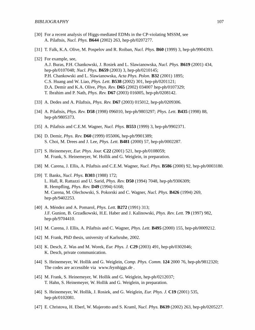
BIBLIOGRAPHY 107
[30] For a recent analysis of Higgs-mediated EDMs in the CP-violating MSSM, seeA. Pilaftsis,Nucl. Phys.B644(2002) 263, hep-ph/0207277.
[31] T. Falk, K.A. Olive, M. Pospelov and R. Roiban,Nucl. Phys.B60 (1999) 3, hep-ph/9904393.
[32] For example, see,A.J. Buras, P.H. Chankowski, J. Rosiek and L. Slawianowska,Nucl. Phys.B619(2001) 434,hep-ph/0107048;Nucl. Phys.B659(2003) 3, hep-ph/0210145;P.H. Chankowski and L. Slawianowska,Acta Phys. Polon.B32 (2001) 1895;C.S. Huang and W. Liao,Phys. Lett.B538(2002) 301, hep-ph/0201121;D.A. Demir and K.A. Olive,Phys. Rev.D65 (2002) 034007 hep-ph/0107329;T. Ibrahim and P. Nath,Phys. Rev.D67 (2003) 016005, hep-ph/0208142.
[33] A. Dedes and A. Pilaftsis,Phys. Rev.D67 (2003) 015012, hep-ph/0209306.
[34] A. Pilaftsis,Phys. Rev.D58 (1998) 096010, hep-ph/9803297;Phys. Lett.B435(1998) 88,hep-ph/9805373.
[35] A. Pilaftsis and C.E.M. Wagner,Nucl. Phys.B553(1999) 3, hep-ph/9902371.
[36] D. Demir,Phys. Rev.D60 (1999) 055006, hep-ph/9901389;S. Choi, M. Drees and J. Lee,Phys. Lett.B481(2000) 57, hep-ph/0002287.
[37] S. Heinemeyer,Eur. Phys. Jour.C22 (2001) 521, hep-ph/0108059;M. Frank, S. Heinemeyer, W. Hollik and G. Weiglein, in preparation.
[38] M. Carena, J. Ellis, A. Pilaftsis and C.E.M. Wagner,Nucl. Phys.B586(2000) 92, hep-ph/0003180.
[39] T. Banks,Nucl. Phys.B303(1988) 172;L. Hall, R. Rattazzi and U. Sarid,Phys. Rev.D50 (1994) 7048, hep-ph/9306309;R. Hempfling,Phys. Rev.D49 (1994) 6168;M. Carena, M. Olechowski, S. Pokorski and C. Wagner,Nucl. Phys.B426(1994) 269,hep-ph/9402253.
[40] A. Mendez and A. Pomarol,Phys. Lett.B272(1991) 313;J.F. Gunion, B. Grzadkowski, H.E. Haber and J. Kalinowski,Phys. Rev. Lett.79 (1997) 982,hep-ph/9704410.
[41] M. Carena, J. Ellis, A. Pilaftsis and C. Wagner,Phys. Lett.B495(2000) 155, hep-ph/0009212.
[42] M. Frank, PhD thesis, university of Karlsruhe, 2002.
[43] K. Desch, Z. Was and M. Worek,Eur. Phys. J.C29 (2003) 491, hep-ph/0302046;K. Desch, private communication.
[44] S. Heinemeyer, W. Hollik and G. Weiglein,Comp. Phys. Comm.1242000 76, hep-ph/9812320;The codes are accessible viawww.feynhiggs.de.
[45] M. Frank, S. Heinemeyer, W. Hollik and G. Weiglein, hep-ph/0212037;T. Hahn, S. Heinemeyer, W. Hollik and G. Weiglein, in preparation.
[46] S. Heinemeyer, W. Hollik, J. Rosiek, and G. Weiglein,Eur. Phys. J.C19 (2001) 535,hep-ph/0102081.
[47] E. Christova, H. Eberl, W. Majerotto and S. Kraml,Nucl. Phys.B639(2002) 263, hep-ph/0205227.

108 BIBLIOGRAPHY

Chapter 5
SUPERSYMMETRY
Supersymmetry (SUSY) is one of the best-motivated theoriesbeyond the Standard Model [1]. Not onlyis it theoretically elegant, providing a unified description of fermions and bosons, including matter par-ticles and force carriers, but it is also potentially capable of connecting gravity with the other interac-tions, and appears an essential ingredient of string theory. From the phenomenological point of view,the most compelling feature of SUSY is that it stabilizes theHiggs mass against radiative corrections,provided the supersymmetric particles have massesm ≤ O(1) TeV [2]. The minimal supersymmetricextension of the Standard Model (MSSM) also predicts a lightHiggs boson withmh <∼ 130 GeV [3],which is favoured by present precision electroweak data [4,5]. Furthermore, unification of the StandardModel gauge couplings and electroweak symmetry breaking occur naturally in the MSSM as a result ofrenormalization-group (RG) evolution [6], and the lightest supersymmetric particle (LSP) is a good colddark matter candidate, if SUSY appears within the TeV energyrange [7].
In the MSSM, as well as two scalar partners for each quark and lepton, there are four neutralinosand two charginos as superpartners for the gauge and Higgs bosons. Moreover, there are five physicalHiggs bosons,h0,H0,A0, andH±. If nature is indeed supersymmetric, it is likely that the LHC will haveobserved part of the spectrum by the time CLIC comes into operation. In addition, it is likely that a TeV-scalee+e− linear collider (LC) will have made accurate measurements of some kinematically accessiblestates, as illustrated by the sample spectra in Fig. 5.1. However, to explore the theory fully, we will needto measure accurately the complete sparticle spectrum, just as we need measurements of the top quarkand the Higgs boson to complete the Standard Model. We will need to determine all the MSSM masses,mixing angles, couplings, spins, etc., in order to
• determine all the soft SUSY-breaking parameters,
• test their unification at some high scale, which might be the GUT scale orthe SUSY-breaking scale,
• pin down the SUSY-breaking mechanism, e.g. whether it is mediated by gravity,gauge interactions or anomalies,
• test the consistency of the model.
We also emphasize that the minimality of the MSSM is an assumption, which must be tested.
The LHC has discovery potential for squarks and gluinos for masses up to about 2.5 TeV. However,its reach for neutralinos, charginos and sleptons is much lower, namely of the order of 0.5 TeV. We recallthat the questions of unification of SUSY parameters and of the nature of SUSY breaking require that themeasured parameters be extrapolated over many orders of magnitude, from 103 GeV to 1016 GeV. Veryaccurate measurements are required in order to avoid large errors at the high scale, which needs the mostprecise measurements possible at ane+e− collider, even of sparticles previously discovered at the LHC.
At CLIC, the clean experimental conditions ofe+e− annihilation at√s = 3–5 TeV will enable us
109
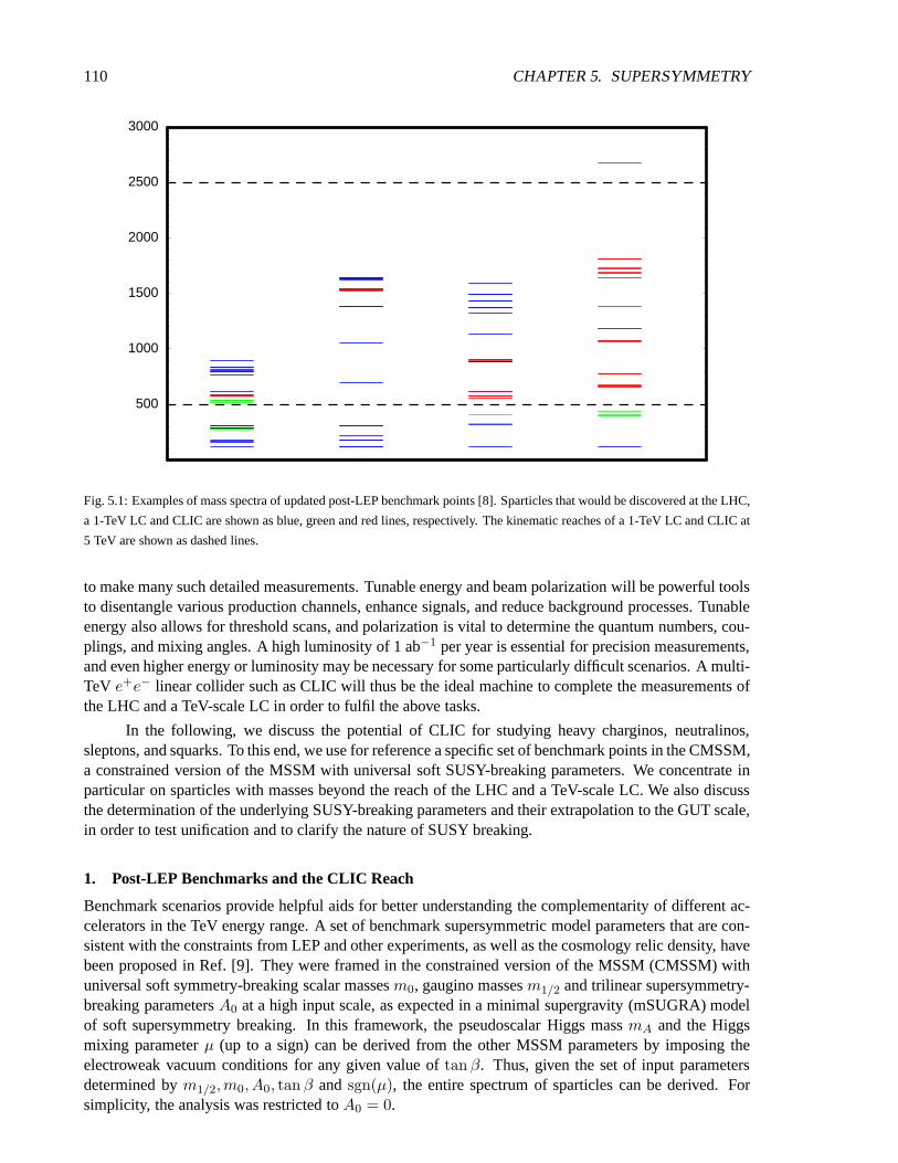
110 CHAPTER 5. SUPERSYMMETRY
500
1000
1500
2000
2500
3000
Fig. 5.1: Examples of mass spectra of updated post-LEP benchmark points [8]. Sparticles that would be discovered at the LHC,
a 1-TeV LC and CLIC are shown as blue, green and red lines, respectively. The kinematic reaches of a 1-TeV LC and CLIC at
5 TeV are shown as dashed lines.
to make many such detailed measurements. Tunable energy andbeam polarization will be powerful toolsto disentangle various production channels, enhance signals, and reduce background processes. Tunableenergy also allows for threshold scans, and polarization isvital to determine the quantum numbers, cou-plings, and mixing angles. A high luminosity of 1 ab−1 per year is essential for precision measurements,and even higher energy or luminosity may be necessary for some particularly difficult scenarios. A multi-TeV e+e− linear collider such as CLIC will thus be the ideal machine tocomplete the measurements ofthe LHC and a TeV-scale LC in order to fulfil the above tasks.
In the following, we discuss the potential of CLIC for studying heavy charginos, neutralinos,sleptons, and squarks. To this end, we use for reference a specific set of benchmark points in the CMSSM,a constrained version of the MSSM with universal soft SUSY-breaking parameters. We concentrate inparticular on sparticles with masses beyond the reach of theLHC and a TeV-scale LC. We also discussthe determination of the underlying SUSY-breaking parameters and their extrapolation to the GUT scale,in order to test unification and to clarify the nature of SUSY breaking.
1. Post-LEP Benchmarks and the CLIC Reach
Benchmark scenarios provide helpful aids for better understanding the complementarity of different ac-celerators in the TeV energy range. A set of benchmark supersymmetric model parameters that are con-sistent with the constraints from LEP and other experiments, as well as the cosmology relic density, havebeen proposed in Ref. [9]. They were framed in the constrained version of the MSSM (CMSSM) withuniversal soft symmetry-breaking scalar massesm0, gaugino massesm1/2 and trilinear supersymmetry-breaking parametersA0 at a high input scale, as expected in a minimal supergravity (mSUGRA) modelof soft supersymmetry breaking. In this framework, the pseudoscalar Higgs massmA and the Higgsmixing parameterµ (up to a sign) can be derived from the other MSSM parameters byimposing theelectroweak vacuum conditions for any given value oftan β. Thus, given the set of input parametersdetermined bym1/2,m0, A0, tan β and sgn(µ), the entire spectrum of sparticles can be derived. Forsimplicity, the analysis was restricted toA0 = 0.

1.. POST-LEP BENCHMARKS AND THE CLIC REACH 111
These post-LEP benchmark scenarios have recently been updated [8], so as to respect the improvedrestrictions on the relic density of cold dark matter particles imposed by the WMAP measurements [10].We summarize below some features of the updates mandated by WMAP. In the subsequent discussion,we use the updated post-WMAP benchmarks as far as possible, commenting on differences from theoriginal set when necessary.
1.1. Benchmark Points
Details of the experimental constraints imposed on the CMSSM, the values of the parameters chosen asbenchmark points, their justifications and the resulting sparticle spectra may be found in Refs. [8,9].
Figure 5.2 displays most of the proposed CMSSM benchmark points, superimposed on the regionsof the (m1/2,m0) plane allowed by laboratory limits, particularly that fromLEP onmh, from b → sγ,and cosmology. The original versions of the CMSSM benchmarkpoints were chosen with a relic densityin the range 0.1< Ωχh
2 < 0.3 [9], but WMAP and previous data now prefer the more limited range0.094< Ωχh
2 < 0.129, corresponding to the narrow strips shown in Fig. 5.2.For most of the benchmarkpoints, a small reduction inm0 sufficed to relocate them on the WMAP strip for the corresponding valueof tan β [8]. However, in some cases, notably benchmarks H and M, moresubstantial changes inm0
and/orm1/2 were made in order to accommodate the new WMAP constraint. Later, where relevant forspecific sparticle analyses, we comment on the implicationsof these changes.
Fig. 5.2: Overview of the updated proposed CMSSM benchmark points in the(m0,m1/2) planes, superposed on the strips
allowed by laboratory limits and the relic density constraint, for µ > 0 andtan β = 5, 10, 20, 35, 50, and forµ < 0 and
tan β = 10, 35 [8]
The lightest supersymmetric particle would be charged in the bottom right dark-shaded triangularregion, which is therefore excluded. The experimental constraints onmh andb → sγ exert pressuresfrom the left, which depend on the value oftan β and the sign ofµ. The indication of a deviation fromthe Standard Model ingµ−2 disfavoursµ < 0 at the 2σ level. Large values ofm0 andm1/2 for µ > 0 aredisfavoured at the 1σ level, as indicated by darker shading on parts of the WMAP lines. The improvedWMAP constraint on the relic density has shrunk the previous‘bulk’ region at lowm0 andm1/2, andnarrowed and shortened the coannihilation ‘tails’ extending to largem1/2, which dominate Fig. 5.2. Notshown is the ‘focus-point’ region at largem0 near the boundary of the region with proper electroweaksymmetry breaking, where two more benchmark points are located.

112 CHAPTER 5. SUPERSYMMETRY
The proposed benchmark points are not intended to sample theallowed CMSSM parameter spacein a statistically unbiased way, but rather to span the essential range of theoretical possibilities, given ourpresent knowledge. Estimates of the numbers of CMSSM particles accessible to different accelerators inthe various proposed benchmark scenarios are summarized inFig. 1.1 in the general introduction.
1.2. Detection at the LHC
In compiling Fig. 1.1, a preliminary inspection was made of the LHC potential for these benchmarkpoints, based on the simulation results summarized in the ATLAS Technical Design Report [11] and inthe CMS Note [12]. A detailed study is clearly required before a real assessment of the LHC physicspotential for these benchmarks can be made, and both ATLAS and CMS have made more detailed studiesof these and earlier benchmark scenarios. However, for thispreliminary look, simplified assumptionswere adopted to estimate the discovery potential of the LHC,assuming ATLAS and CMS combined,together with an integrated luminosity of 300 fb−1 per experiment [8, 9]. We see in Fig. 5.3(a) how thenumber of MSSM particles detectable at the LHC varies along the WMAP line fortan β = 10, includingthe points B and C as special cases. For a more complete discussion of sparticle observability alongWMAP lines, including other values oftan β, see Ref. [8]. We see that the LHC can detect gluinos andall the squarks, for any allowed value ofm1/2, but may be expected to miss many sleptons, neutralinos,charginos and Higgs bosons, except in the lower part of them1/2 range.
Thus, in the framework of the CMSSM, the open questions afterthe LHC might include complet-ing the spectrum of electroweakly-interacting sparticles, as well as detailed measurements of the gluinoand squarks, which will not be easy at the LHC.
1.3. Detection at Linear Colliders
Sparticles can generally be produced at any lineare+e− collider (LC) if its centre-of-mass energy islarger than twice the mass of the sparticles, the pair-production threshold. Exceptions include heaviercharginos and neutralinos, which can be produced in association with lighter charginos or neutralinos, re-spectively. Also, for sufficiently light neutralinos and sneutrinos, observation of the radiative productionof otherwise invisible final states may be experimentally accessible.
Typical supersymmetric signals are multilepton final states and multijet ones with large missingtransverse energy. Sneutrinos can be detected at thresholdenergies if they decay into channels includingcharged leptons with a sufficiently large branching ratio. For example, in some scenarios, theντ candecay intoτW . A counter example to this possibility is the updated benchmark point B, where allthe sneutrino decays are invisible. However, even in such a case, sneutrinos can be detected at higherenergies via the decays of charginos.
Fore+e− linear colliders, data samples of the order of 1000 fb−1 or more are expected to be col-lected over a period of several years. Apart from the threshold requirement to produce the particles, theproduct of the branching ratio times the unpolarized cross section for the detectable channels was re-quired to be larger than 0.1 fb in order to observe the sparticle, leading to at least 100 produced sparticlesin the total data sample.
We see in Fig. 5.3(b) that a 0.5-TeVe+e− linear collider would already be able to fill in manyof the gaps in the MSSM spectrum left by the LHC for smallerm1/2. The reach of a 1-TeVe+e−
linear collider would be correspondingly greater, as seen in Fig. 5.3(c). Such a machine would be largelycomplementary to the LHC, as seen in Fig. 5.3(d).

1.. POST-LEP BENCHMARKS AND THE CLIC REACH 113
LHC tan β = 10
m1/2 (GeV)
Nb.
of O
bser
vabl
e P
tcs.
gluino squarks sleptons χ H
B, C,
0
5
10
15
20
25
30
35
300 400 500 600 700 800 900 1000
LC √s = 0.5 TeV tan β = 10
m1/2 (GeV)
Nb.
of O
bser
vabl
e P
tcs.
gluino squarks sleptons χ H
B, C,
0
5
10
15
20
25
30
35
300 400 500 600 700 800 900 1000
LC √s = 1.0 TeV tan β = 10
m1/2 (GeV)
Nb.
of O
bser
vabl
e P
tcs.
gluino squarks sleptons χ H
B, C,
0
5
10
15
20
25
30
35
300 400 500 600 700 800 900 1000
LHC+LC 1 TeV tan β = 10
m1/2 (GeV)
Nb.
of O
bser
vabl
e P
tcs.
gluino squarks sleptons χ H
B, C,
0
5
10
15
20
25
30
35
300 400 500 600 700 800 900 1000
Fig. 5.3: Estimates of the numbers of MSSM particles that maybe detectable as functions ofm1/2 along the WMAP line for
µ > 0 andtan β = 10, for the LHC, a 0.5-TeVe+e− linear collider, a 1-TeVe+e− linear collider, and the latter combined with
the LHC. The complementarity of the LHC and a linear collideremerge clearly. The locations of the benchmark points B′ and
C′ along these WMAP lines are indicated, as is the nominal lowerbound onm1/2 imposed bymh (dashed lines) [8].
1.4. Perspectives
Assuming that the LHC and ane+e− linear collider in the range<∼ 1 TeV have been taking data forseveral years before the start of a 3 TeV machine like CLIC (CLIC3000), we infer that supersymmetrywill most probably already have been discovered by that time, if it exists. Hence the primary role of CLICmay be to complete the sparticle spectrum, and disentangle and measure more precisely the properties ofsparticles already observed at the LHC and/or a lower-energy e+e− linear collider. However, a machinelike CLIC would be needed even for the direct discovery of supersymmetry in the most problematiccases, such as benchmark scenarios H and particularly M, where no sparticles may be seen at either theLHC or a TeV-class LC, as seen in Fig. 1.1.

114 CHAPTER 5. SUPERSYMMETRY
A few benchmark points emerge as typical of situations that could arise in the future.
• Point C has very low masses, and is representative also of points A, B, D, G, I, L. In these cases, theLHC would have discovered theH±, as well as seen theh0, and also the gauginosχ0
1, χ02 andχ±1 ,
the charged sleptons, the squarks and the gluino. A 1-TeV linear collider would enable the detailedstudy of theh0 and of the same gauginos and sleptons, and it might discover the missing gauginosin some of the scenarios. However, one would require CLIC, perhaps running around 2 TeV, tocomplete the particle spectrum by discovering and studyingthe heavy Higgses and the missinggauginos. CLIC could also measure more precisely the squarks and in particular disentangle theleft- and right-handed states and, to some extent, the different light squark flavours.
• Point J features intermediate masses, much like point K. Here, the LHC would have discovered allthe Higgs bosons, the squarks and the gluino, but no gauginosor sleptons. The 1-TeVe+e− linearcollider would study in detail theh0 and could discover theeR, µR and τ1, but other sparticleswould remain beyond its kinematic reach. CLIC3000 could then study in detail the heavy Hig-gses, as discussed in the previous chapter. It would also discover and study the gauginos and themissing sleptons, and even observe in more detail a few of thelighter squarks that had already beendiscovered at the LHC. However, to see the remaining squarksat a linear collider would requireCLIC to reach slightly more than 3 TeV.
• Point E has quite distinctive decay characteristics, due tothe existence of heavy sleptons andsquarks. In this situation, the LHC would have discovered theh0, all squarks and the gluino. Thegauginos are in principle accessible, but their discovery may be made more difficult by their pre-dominant decays into jets, contrary to the previous benchmark points, and sleptons would remainunobserved. At a 1-TeVe+e− linear collider, the detailed study of theh0 and of the gauginoscould be undertaken. The discovery of the first slepton, actually a νe, could be made at CLIC3000,which could also study the three lightest squarks. The discovery and analysis of the heavy Higgseswould then require the CLIC energy to reach about 3.5 TeV, which would also allow the discov-ery of all sleptons and the observation of all squarks. A detailed analysis of the accuracy in thedetermination of the smuon mass at
√s = 3.8–4.2 TeV is presented later in this chapter.
• Point H has quite heavy states, as does scenario M. The LHC would only discover theh0, all otherstates being beyond its reach, so the LHC might leave the existence of supersymmetry as an openquestion! At point H, a 1-TeV linear collider would discoverthe lighterτ and the LSPχ, but noother sparticles. A 1-TeV linear collider would discover nosparticles at point M. However, CLICat 3 TeV would be able to discover most of the gauginos and sleptons. The CLIC sensitivity to thesmuon mass, using both a muon energy technique and a threshold scan, is discussed later. On theother hand, to discover all the squarks,ℓ+ℓ− collisions in excess of 5 TeV would be needed. Thereis currently noe+e− project aiming at such energies, and we recall that neutrinoradiation wouldbecome a hazard for aµ+µ− collider at such a high energy.
• Along the lines defined by the WMAP constraints, the reach in supersymmetric particles for agiven collider and the phenomenology of their decays changesignificantly. As we discuss later, theCLIC reach for the dilepton decay signature of a heavier neutralino,χ2 → ℓ+ℓ−χ is significantlygreater than that of the LHC or a 1-TeV linear collider. Additionally, we have chosen a point atm1/2 = 750 GeV andtan β = 10 to study the potential accuracy in the determination of the massof the sleptons and of theχ0
2. This point is located at the limit of the sensitivity of the LHC andof a 1-TeV linear collider for probing the heavy neutralinosand the slepton sectors, and representsthe limit of the coverage of the full supersymmetric spectrum at CLIC at 3 TeV.
• As in the case of a 1-TeVe+e− linear collider, a photon collider option for CLIC would extendthe discovery range for heavy Higgs bosons. Additionally, it would allow one to discover all fourHiggs bosons in scenarios E, H and M, for a 3-TeV collider, andalso in F, for a 5-TeV collider.The detection of heavier MSSM Higgs bosons at a CLIC-basedγγ collider is discussed in moredetail in the previous section.

1.. POST-LEP BENCHMARKS AND THE CLIC REACH 115
The corresponding estimates of the numbers of MSSM particles that can be detected are shownin Fig. 5.4. Beyond the discovery of sparticles, a crucial issue in the understanding of the nature ofany new physics observed will be the accuracy obtainable in the determination of the sparticle massesand decays, and also their quantum numbers and mixing. A strong advantage of lepton colliders is theprecisionwith which such sparticle properties can be measured. A strong advantage of lepton colliders istheprecisionwith which such sparticle properties can be measured, as discussed in the next section of thischapter. Typically, the masses of sleptons and gauginos canbe determined with a precision of a few permille, by threshold scans and by measuring end-points of two-body decay channel signatures in inclusivedistributions. This high precision, even for a limited number of sparticles, will be of cardinal importancefor the reconstruction of the underlying supersymmetric model and exploration of the supersymmetry-breaking mechanism [13].
The availability of polarized beams at CLIC would, furthermore, provide additional tools for iden-tifying supersymmetric particles and allow for additionalmeasurements of parameters of the supersym-metric model, such as the mixing angles of the sparticles, asdiscussed later in this chapter.
CLIC √s = 3.0 TeV tan β = 10
m1/2 (GeV)
Nb.
of O
bser
vabl
e P
tcs.
gluino squarks sleptons χ H
B, C,
0
5
10
15
20
25
30
35
300 400 500 600 700 800 900 1000
CLIC √s = 5.0 TeV tan β = 10
m1/2 (GeV)
Nb.
of O
bser
vabl
e P
tcs.
gluino squarks sleptons χ H
B, C,
0
5
10
15
20
25
30
35
300 400 500 600 700 800 900 1000
Fig. 5.4: Estimates of the numbers of MSSM particles that maybe detectable as functions ofm1/2 along the WMAP line for
µ > 0 andtan β = 10, for CLIC operating at 3 TeV (left panel) and 5 TeV (right panel). The locations of the benchmark points
B′ and C′ along these WMAP lines are indicated, as is the nominal lowerbound onm1/2 imposed bymh (dashed lines) [8].
1.5. Generalized Supersymmetric Models
We complete this introductory discussion by looking beyondspecific CMSSM benchmark scenarios andWMAP lines, considering the prospects for observing supersymmetric particles ate+e− colliders inmore general scenarios that conserveR parity. For this purpose, we display in Fig. 5.5 random samplesof supersymmetric models, initially disregarding the cosmological relic-density constraint (red points)and subsequently including it (blue points). The plots feature the masses of the two lightest observablesparticles, namely the next-to-lightest supersymmetric particle (NSP) and the next-to-next-to-lightestsupersymmetric particle (NNSP).
In order to make contact with the previous analysis, we first consider in panel (a) of Fig. 5.5 theCMSSM with parameters chosen to obey the standard experimental (and cosmological) constraints. Wethen consider in panel (b) models in which no universality isassumed for the squark and slepton masses,subject to the supplementary constraint that the effectivepotential remain stable when the theory is

116 CHAPTER 5. SUPERSYMMETRY
CMSSM
|A0| ≤ 1 TeV, µ > 0
NSP (GeV)
NN
SP
(GeV
)
150010005000
2500
2000
1500
1000
500
0
mE 6= mL
mQ 6= mU 6= mD
|A0| ≤ 1 TeV, µ > 0
NSP (GeV)
NN
SP
(GeV
)
150010005000
2500
2000
1500
1000
500
0
Input scale: 10 TeV
|At,b,τ | ≤ 1 TeV, µ > 0
NSP (GeV)
NN
SP
(GeV
)
150010005000
2500
2000
1500
1000
500
0
LSP gravitino, µ > 0
NSP (GeV)
NN
SP
(GeV
)
8006004002000
2000
1500
1000
500
0
Fig. 5.5: Scatter plots of the masses of the next-to-lightest supersymmetric particle (NSP) and the next-to-next-to-lightest
supersymmetric particle (NNSP) for (a) the CMSSM, (b) models without squark and slepton mass universality, (c) universality
for the squark and slepton masses separately but stability of the effective potential up to 10 TeV only, and (d) a gravitino
LSP. Each scatter plot contains 50,000 points withmQ,mD,mU ,mL,mE,m1/2,m1,m2 < 2 TeV (wherem1,2 are the soft
supersymmetry-breaking contributions to the Higgs boson masses), – 1 TeV< A0 < 1 TeV,tan β < 58 andµ > 0. We thank
Vassilis Spanos for supplying these figures
extrapolated up to the GUT scale, using the renormalization-group equations (RGEs). Panel (c) assumesuniversality for the squark and slepton masses separately,but stability is required only for RGE evolutionup to 10 TeV. Finally, panel (d) is for models in which the LSP is assumed to be a gravitino.
In each case, we have generated 50,000 points withmQ,mD,mU ,mL,mE,m1/2,m1,m2 < 2 TeV(wherem1,2 are the soft supersymmetry-breaking contributions to the Higgs boson masses), – 1 TeV< A0 < 1 TeV, tan β < 58 andµ > 0 (the plots forµ > 0 are not very different). The upper limits onthe soft supersymmetry-breaking parameters are somewhat arbitrary, and one could argue that a varyingmeasure related to the amount of hierarchical fine-tuning should be applied. However, we do notethat the range considered contains comfortably most pointsallowed by the cosmological relic-densityconstraint.
We see that CLIC withEc.m. = 3 TeV would observe both the NSP and the NNSP in most cases,and CLIC withEc.m. = 5 TeV would observe them both in all the cases considered.

2.. SLEPTON AND SQUARK MASS DETERMINATION 117
1.6. Alternative Benchmark Scenarios
Apart from the points discussed in Ref. [8] several other groups have recently proposed benchmark pointsfor SUSY studies. For example, in Ref. [14] a number of mSUGRAbenchmark points similar to the onesdiscussed in [8] are proposed. Since these points were conceived at the Snowmass workshop in 2001,these benchmark points are often referred to as the Snowmasspoints (SPS points). In addition, pointsgenerated with different SUSY-breaking mechanisms are proposed: two points from a gauge-mediatedSUSY-breaking scenario (GMSB), and from an anomaly-mediated SUSY-breaking scenario (AMSB).Both GMSB points have heavy squarks and gluinos, which are beyond the reach of a 1 TeV LC, butwithin reach of CLIC. For the second GMSB point also the heavyHiggses are beyond the reach of a 1TeV LC (and even the LHC). The AMSB point chosen has many sparticles with a mass around or above1 TeV: several gauginos, the heavy Higgses and all coloured sparticles. All these sparticles are, however,within the reach of a 3 TeV CLIC.
An alternative set of ‘string-inspired’ benchmark points,are given in Ref. [15]. These points arechosen such that there are always a few light sparticles which could possibly be detected at the Tevatron.However, each of these proposed benchmark scenarios alwayshas a large number of sparticles in the TeVmass range and can be studied by CLIC. In some cases the massesare so large that even CLIC will notbe able to see the full sparticle spectrum. In some of these scenarios only a few gauginos are accessibleat a 1-TeV LC, and the sleptons and Heavy Higgses can only be studied at CLIC.
In all, these benchmark points, in scenarios different frommSUGRA, all seem to indicate thatthere is a role for CLIC to complete the sparticle spectrum.
2. Slepton and Squark Mass Determination
2.1. Smuon Mass Determination
A study has been performed of the reactione+e− → µLµL → µ+χ01µ−χ0
1 at CLIC. The threemain sources of background, also leading to two muons plus missing energy, are i)e+e− →W+W− → µ+µ−νµνµ, ii) e+e− → W+W−νν → µ+µ−νµνµνeνe and iii) e+e− → χ0
1χ02, χ
02χ
02 →
µ+µ−ννχ01χ
01. These backgrounds can be suppressed by requiring central production and decay kine-
matics compatible with those characteristic of smuon pair production. A multidimensional discriminantbased onMµµ,Mrecoil,Emissing, µµ acolinearity,| cos θthrust|,Et andEhem has been applied. The signalefficiency is flat with the muon energy.
2.1.1. The energy distribution method for mass determination
If the centre-of-mass energy√s is significantly larger than twice the sparticle massMµ, the latter can be
determined by an analysis of the energy spectrum of the muon emitted in the two-bodyµ→ χ01µ decay,
as seen in Fig. 5.6. The two end-points,Emin andEmax, of the spectrum are related to theµ and χ01
masses and to theµ boost by:
Emax/min =Mµ
2
(1 −
M2χ0
1
M2µ
)×
1 ±
√1 −
M2µ
E2beam
(5.1)
from which either the smuon massMµ can be extracted, ifMχ01
is already known, or both masses can besimultaneously fitted.
This technique, considered for the determination of squarkmasses at a 500-GeV LC in Ref. [16],has already been applied to sleptons for the LHC [11, 17] and aTeV-class LC [18]. It is interestingto consider its implications for the required momentum resolution in the detector. Two values of thesolenoidal magnetic fieldB = 4 and 6 T have been tested, corresponding to momentum resolutionsδp/p2 of 4.5× 10⁻⁵ and 3.0× 10⁻⁵ GeV−1 respectively. No appreciable difference on the resultingmass accuracy has been found for these two momentum resolutions. This reflects the fact that, at CLIC,
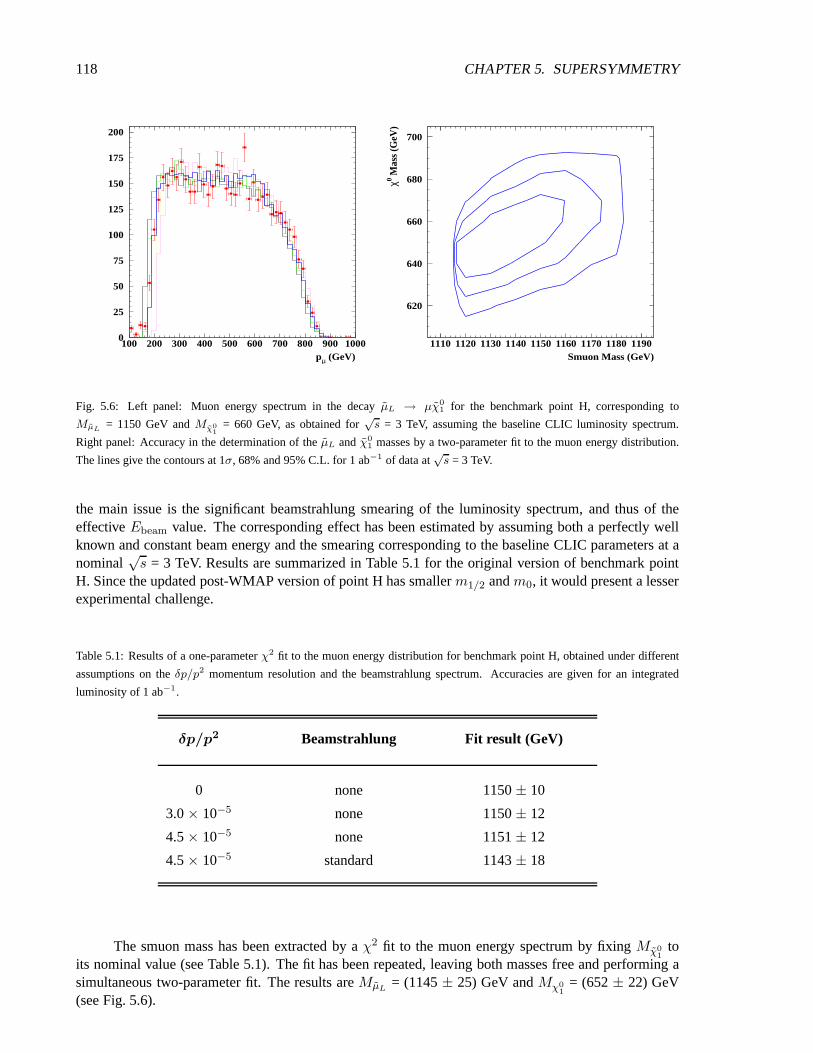
118 CHAPTER 5. SUPERSYMMETRY
pµ (GeV)
0
25
50
75
100
125
150
175
200
100 200 300 400 500 600 700 800 900 1000Smuon Mass (GeV)
χ0 Mas
s (G
eV)
620
640
660
680
700
1110 1120 1130 1140 1150 1160 1170 1180 1190
Fig. 5.6: Left panel: Muon energy spectrum in the decayµL → µχ01 for the benchmark point H, corresponding to
MµL= 1150 GeV andMχ0
1= 660 GeV, as obtained for
√s = 3 TeV, assuming the baseline CLIC luminosity spectrum.
Right panel: Accuracy in the determination of theµL andχ01 masses by a two-parameter fit to the muon energy distribution.
The lines give the contours at 1σ, 68% and 95% C.L. for 1 ab−1 of data at√s = 3 TeV.
the main issue is the significant beamstrahlung smearing of the luminosity spectrum, and thus of theeffectiveEbeam value. The corresponding effect has been estimated by assuming both a perfectly wellknown and constant beam energy and the smearing corresponding to the baseline CLIC parameters at anominal
√s = 3 TeV. Results are summarized in Table 5.1 for the original version of benchmark point
H. Since the updated post-WMAP version of point H has smallerm1/2 andm0, it would present a lesserexperimental challenge.
Table 5.1: Results of a one-parameterχ2 fit to the muon energy distribution for benchmark point H, obtained under different
assumptions on theδp/p2 momentum resolution and the beamstrahlung spectrum. Accuracies are given for an integrated
luminosity of 1 ab−1.
δp/p2 Beamstrahlung Fit result (GeV)
0 none 1150± 10
3.0× 10⁻⁵ none 1150± 12
4.5× 10⁻⁵ none 1151± 12
4.5× 10⁻⁵ standard 1143± 18
The smuon mass has been extracted by aχ2 fit to the muon energy spectrum by fixingMχ01
toits nominal value (see Table 5.1). The fit has been repeated, leaving both masses free and performing asimultaneous two-parameter fit. The results areMµL = (1145± 25) GeV andMχ0
1= (652± 22) GeV
(see Fig. 5.6).
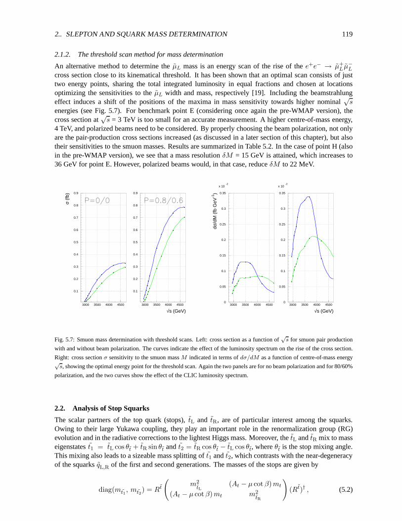
2.. SLEPTON AND SQUARK MASS DETERMINATION 119
2.1.2. The threshold scan method for mass determination
An alternative method to determine theµL mass is an energy scan of the rise of thee+e− → µ+L µ−L
cross section close to its kinematical threshold. It has been shown that an optimal scan consists of justtwo energy points, sharing the total integrated luminosityin equal fractions and chosen at locationsoptimizing the sensitivities to theµL width and mass, respectively [19]. Including the beamstrahlungeffect induces a shift of the positions of the maxima in mass sensitivity towards higher nominal
√s
energies (see Fig. 5.7). For benchmark point E (consideringonce again the pre-WMAP version), thecross section at
√s = 3 TeV is too small for an accurate measurement. A higher centre-of-mass energy,
4 TeV, and polarized beams need to be considered. By properlychoosing the beam polarization, not onlyare the pair-production cross sections increased (as discussed in a later section of this chapter), but alsotheir sensitivities to the smuon masses. Results are summarized in Table 5.2. In the case of point H (alsoin the pre-WMAP version), we see that a mass resolutionδM = 15 GeV is attained, which increases to36 GeV for point E. However, polarized beams would, in that case, reduceδM to 22 MeV.
0.1
0.2
0.3
0.4
0.5
0.6
0.7
0.8
0.9
3000 3500 4000 4500
σ (f
b)
√s (GeV)
0.1
0.2
0.3
0.4
0.5
0.6
0.7
0.8
0.9
3000 3500 4000 45000
0.05
0.1
0.15
0.2
0.25
0.3
0.35
x 10-2
3000 3500 4000 4500
dσ/d
M (
fb G
eV-1
)
√s (GeV)
0
0.05
0.1
0.15
0.2
0.25
0.3
0.35
x 10-2
3000 3500 4000 4500
Fig. 5.7: Smuon mass determination with threshold scans. Left: cross section as a function of√s for smuon pair production
with and without beam polarization. The curves indicate theeffect of the luminosity spectrum on the rise of the cross section.
Right: cross sectionσ sensitivity to the smuon massM indicated in terms ofdσ/dM as a function of centre-of-mass energy√s, showing the optimal energy point for the threshold scan. Again the two panels are for no beam polarization and for 80/60%
polarization, and the two curves show the effect of the CLIC luminosity spectrum.
2.2. Analysis of Stop Squarks
The scalar partners of the top quark (stops),tL and tR, are of particular interest among the squarks.Owing to their large Yukawa coupling, they play an importantrole in the renormalization group (RG)evolution and in the radiative corrections to the lightest Higgs mass. Moreover, thetL andtR mix to masseigenstatest1 = tL cos θt + tR sin θt andt2 = tR cos θt − tL cos θt, whereθt is the stop mixing angle.This mixing also leads to a sizeable mass splitting oft1 andt2, which contrasts with the near-degeneracyof the squarksqL,R of the first and second generations. The masses of the stops are given by
diag(mt1, mt2
) = Rt
(m2tL
(At − µ cot β)mt
(At − µ cot β)mt m2tR
)(Rt)† , (5.2)

120 CHAPTER 5. SUPERSYMMETRY
Table 5.2: Accuracies in the determinations of the smuon masses for the two benchmark scenarios considered in this study,
using threshold scans with different experimental conditions
Point Beam- Pol.√s
∫L δM
strahlung (TeV) (ab−1) (GeV)
H none 0/0 3.0–3.5 1 ± 11
H standard 0/0 3.0–3.5 1 ± 15
E none 0/0 3.8–4.2 1 ± 29
E standard 0/0 3.8–4.2 1 ± 36
E none 80/60 3.8–4.2 1 ± 17
E standard 80/60 3.8–4.2 1 ± 22
whereAt is the trilinear stop–Higgs coupling,Rt is the stop mixing matrix
Rt =
(cos θt sin θt
− sin θt cos θt
), (5.3)
andmt1< mt2
by convention. As already mentioned, stops play an important role in the RG running.For the extrapolation to the GUT scale discussed later in this chapter, it is thus essential to know theirparameters as precisely as possible. At the LHC, stop massesmay be measured with errors of a few percent, but measuringθt andAt will hardly be possible. Ine+e− collisions, however, measurements of theproducts of cross sections with branching ratios (especially with polarized beams), threshold scans andkinematical distributions may be used to determinemt1
,mt2, θt andAt quite precisely.
Figure 5.8 shows cross sections fore+e− → ti¯it (i = 1, 2) formt1
= 1 TeV,mt2= 1.3 TeV
and θt = 70 as functions of√s for unpolarized beams. Supersymmetric QCD corrections [20] and
initial-state radiation (ISR) are included. The cross sections show characteristic dependences [21] on themixing angle and on beam polarization. Measurements with different polarizations may thus be usedto determineθt. Figure 5.9 shows polarized cross sections fort1
¯t1 and t2¯t2 production normalized
to the unpolarized ones,σpol/σunpol, as functions of the electron beam polarizationPe− and the stopmixing angle. Positron polarization is assumed to be zero, but could be used to enhance further thedependence onθt.
If both stop masses and the mixing angle are measured, andtan β andµ are known from, forexample, the chargino/neutralino sector,At can be determined by
At =1
2mt
(m2t1−m2
t2
)sin 2θt +
µ
tan β. (5.4)
This can then be compared with indirect estimates ofAt from precision measurements ofmh [22]. Itis also possible to determineAt via the associated production of stops with Higgs bosons [23] (whichhas, however, a very small cross section at CLIC energies) and/or from t2 → t1 (h0,H0, A0) and biH+
decays [24], which can have large branching ratios ifAt and/orµ are large.
3. Neutralino Mass Determination
Operating at 3 to 5 TeV with large luminosity, CLIC will be able to improve significantly on the reach forheavy neutralinos, beyond the anticipated LHC sensitivity. A general study of the prospective CLIC sen-sitivity has been carried out, including a simulation of thedetector response parametrized by the SIMDET

3.. NEUTRALINO MASS DETERMINATION 121
2 3 4 5 60.
0.5
1.
1.5
2.
σ(e
+e−
→t i
¯ it)
[fb]
√s [TeV]
t1¯t1
t2¯t2
θt = 70
Fig. 5.8: Cross Sections for stop pair production formt1= 1 TeV,mt2
= 1.3 TeV,θt = 70 andmg = 750 GeV
Fig. 5.9: Polarized cross sections fort1 ¯t1 and t2 ¯t2 production normalized to the unpolarized ones,σpol/σunpol, as functions
of the electron beam polarizationPe− and the stop mixing angleθt, for mt1= 1 TeV,mt2
= 1.3 TeV and√s = 3 TeV. The
positron beam polarization has been assumed to vanish.
program. Inclusive chargino and neutralino pair production have been analysed to determine the sensitiv-ity obtainable from the dilepton invariant mass spectrum. The decay chainsχ0
j → ℓ±ℓ∓ → ℓ+ℓ−χ01 and
χ0j → χ0
iZ0 → χ0
i ℓ+ℓ− give rise to an excess of events in theℓ+ℓ− mass spectrum corresponding to the
phase space for the cascade two-body decay of the first process or to theZ0 mass peak in the second. Afull scan of the(m1/2, m0) plane has been carried out, using PYTHIA 6.21 interfaced to ISAJET 7.64.Events with at least two leptons and significant missing energy have been selected. Both SUSY back-grounds involving sleptons and SM gauge-boson pair production have been considered. Combinatorialbackgrounds have been subtracted by taking the difference of the pair e+e− + µ+µ− events and themixede±µ∓ events, and a sliding window has been used to search for an excess of 5 standard deviationsor more of events in theMℓℓ mass distribution. Results are shown in Figure 5.10 fortan β = 10, wherethe extended reach provided by CLIC is manifest. At larger values oftan β, decays intoτ become moresignificant, requiring a more detailed study, which must includeτ -lepton reconstruction.

122 CHAPTER 5. SUPERSYMMETRY
tan β = 10
LHC
CLIC 3 TeV
m1/2 (GeV)
m0
(GeV
)
100
200
300
400
500
600
700
800
900
200 300 400 500 600 700 800 900 1000Mll (GeV)
Evt
s / 1
ab-1
0
50
100
150
200
250
300
350
400
0 25 50 75 100 125 150 175 200 225
Fig. 5.10: Left panel: The sensitivity toχ02 production at CLIC for
√s = 3 TeV compared with that of the LHC. Right panel:
Dimuon spectrum measured at CLIC, assumingm0 = 150 GeV,m1/2 = 700 GeV andtan β = 10, used to derive the particle
masses as discussed in the text.
To verify the CLIC capability for measuring the masses of heavy neutralinos, a representativepoint has been chosen atm0 = 150 GeV,m1/2 = 700 GeV andtan β = 10, which is compatible withthe constraint on cold dark matter from the WMAP data and hasMχ0
2= 540 GeV,Mχ0
1= 290 GeV
andMℓL = 490 GeV.
The dilepton invariant mass distribution shows a clear upper edge at 120 GeV, due toχ02 →
µ±µ∓L → µ+µ−χ01, which can be very accurately measured, already with 1 ab−1 of data. However, in
order to extract the mass of theχ02 state, the masses of both theµL andχ0
1 need to be known. As alreadydiscussed, a two-parameter fit to the muon energy distribution yields the masses of theµL andχ0
1 withaccuracies of 3% and 2.5% respectively, using 1 ab−1 of data. An improved accuracy can be obtainedwith higher luminosity and using also a threshold energy scan. We therefore assume that these masses canbe known to 1.7% and 1.5% respectively, which gives an uncertainty of 8 GeV, or 1.6%, on theχ0
2 mass,when accounting for correlations. This uncertainty is dominated by that in theµL andχ0
1 masses. Theaccuracy in the determination of the end-point would correspond to aχ0
2 mass determination of 0.3 GeV,fixing all other masses, and is not sensitive to the details ofthe beamstrahlung and accelerator-inducedbackgrounds.
Last but not least, at CLIC with 3 TeV also the heavierχ03 andχ0
4 are accessible in this scenarioand can be detected via the decaysχ0
3 → χ01,2Z
0 andχ04 → χ0
1,2h0.
4. Gluino Sensitivity in γγ Collisions
Measurements of the mass and coupling of the gluino pose somedifficulties ine+e− collisions, since thegluino couples only to strongly-interacting particles andis thus produced only at the one-loop level or inmultiparton final states. In a recent publication, gluino pair production through triangular quark/squarkloops ine+e− annihilation with energies up to 1 TeV was investigated [25]. Owing to the large cancel-lation effects, it was found that promisingly large cross sections can only be expected for scenarios withlarge left-/right-handed up-type squark mass splittings,or with large top-squark mixing and for gluino
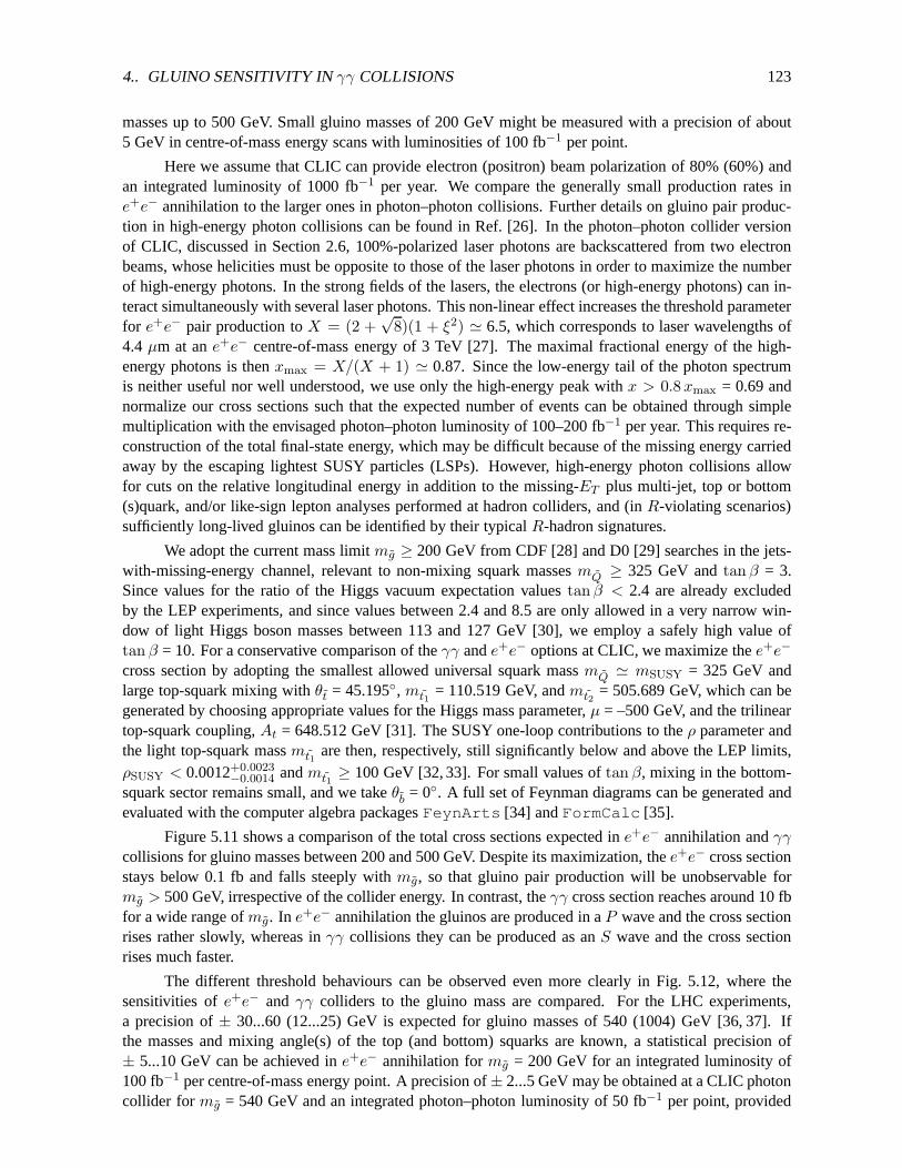
4.. GLUINO SENSITIVITY IN γγ COLLISIONS 123
masses up to 500 GeV. Small gluino masses of 200 GeV might be measured with a precision of about5 GeV in centre-of-mass energy scans with luminosities of 100 fb−1 per point.
Here we assume that CLIC can provide electron (positron) beam polarization of 80% (60%) andan integrated luminosity of 1000 fb−1 per year. We compare the generally small production rates ine+e− annihilation to the larger ones in photon–photon collisions. Further details on gluino pair produc-tion in high-energy photon collisions can be found in Ref. [26]. In the photon–photon collider versionof CLIC, discussed in Section 2.6, 100%-polarized laser photons are backscattered from two electronbeams, whose helicities must be opposite to those of the laser photons in order to maximize the numberof high-energy photons. In the strong fields of the lasers, the electrons (or high-energy photons) can in-teract simultaneously with several laser photons. This non-linear effect increases the threshold parameterfor e+e− pair production toX = (2 +
√8)(1 + ξ2) ≃ 6.5, which corresponds to laser wavelengths of
4.4 µm at ane+e− centre-of-mass energy of 3 TeV [27]. The maximal fractionalenergy of the high-energy photons is thenxmax = X/(X + 1) ≃ 0.87. Since the low-energy tail of the photon spectrumis neither useful nor well understood, we use only the high-energy peak withx > 0.8xmax = 0.69 andnormalize our cross sections such that the expected number of events can be obtained through simplemultiplication with the envisaged photon–photon luminosity of 100–200 fb−1 per year. This requires re-construction of the total final-state energy, which may be difficult because of the missing energy carriedaway by the escaping lightest SUSY particles (LSPs). However, high-energy photon collisions allowfor cuts on the relative longitudinal energy in addition to the missing-ET plus multi-jet, top or bottom(s)quark, and/or like-sign lepton analyses performed at hadron colliders, and (inR-violating scenarios)sufficiently long-lived gluinos can be identified by their typicalR-hadron signatures.
We adopt the current mass limitmg ≥ 200 GeV from CDF [28] and D0 [29] searches in the jets-with-missing-energy channel, relevant to non-mixing squark massesmQ ≥ 325 GeV andtan β = 3.Since values for the ratio of the Higgs vacuum expectation values tan β < 2.4 are already excludedby the LEP experiments, and since values between 2.4 and 8.5 are only allowed in a very narrow win-dow of light Higgs boson masses between 113 and 127 GeV [30], we employ a safely high value oftan β = 10. For a conservative comparison of theγγ ande+e− options at CLIC, we maximize thee+e−
cross section by adopting the smallest allowed universal squark massmQ ≃ mSUSY = 325 GeV andlarge top-squark mixing withθt = 45.195, mt1
= 110.519 GeV, andmt2= 505.689 GeV, which can be
generated by choosing appropriate values for the Higgs massparameter,µ = –500 GeV, and the trilineartop-squark coupling,At = 648.512 GeV [31]. The SUSY one-loop contributions to theρ parameter andthe light top-squark massmt1
are then, respectively, still significantly below and abovethe LEP limits,ρSUSY < 0.0012+0.0023
−0.0014 andmt1≥ 100 GeV [32, 33]. For small values oftan β, mixing in the bottom-
squark sector remains small, and we takeθb = 0. A full set of Feynman diagrams can be generated andevaluated with the computer algebra packagesFeynArts [34] andFormCalc [35].
Figure 5.11 shows a comparison of the total cross sections expected ine+e− annihilation andγγcollisions for gluino masses between 200 and 500 GeV. Despite its maximization, thee+e− cross sectionstays below 0.1 fb and falls steeply withmg, so that gluino pair production will be unobservable formg > 500 GeV, irrespective of the collider energy. In contrast, theγγ cross section reaches around 10 fbfor a wide range ofmg. In e+e− annihilation the gluinos are produced in aP wave and the cross sectionrises rather slowly, whereas inγγ collisions they can be produced as anS wave and the cross sectionrises much faster.
The different threshold behaviours can be observed even more clearly in Fig. 5.12, where thesensitivities ofe+e− and γγ colliders to the gluino mass are compared. For the LHC experiments,a precision of± 30...60 (12...25) GeV is expected for gluino masses of 540 (1004) GeV [36, 37]. Ifthe masses and mixing angle(s) of the top (and bottom) squarks are known, a statistical precision of± 5...10 GeV can be achieved ine+e− annihilation formg = 200 GeV for an integrated luminosity of100 fb−1 per centre-of-mass energy point. A precision of± 2...5 GeV may be obtained at a CLIC photoncollider formg = 540 GeV and an integrated photon–photon luminosity of 50 fb−1 per point, provided

124 CHAPTER 5. SUPERSYMMETRY
e−(80%−) e+(60%+) → g~ g~
10-4
10-3
10-2
10-1
0 500 1000 1500 2000 2500 3000√ s [GeV]
σ [fb
]
mSUSY = 325 GeV
mt~,1= 110 GeV
θt~ = 45.2˚
mg~ = 200 GeV
mg~ = 300 GeV
mg~ = 400 GeV
mg~ = 500 GeV
e−(80%−) e−(80%−) → e− e− g~ g~
10-1
1
10
0 500 1000 1500 2000 2500 3000√ see [GeV]
σ [fb
]
mSUSY = 325 GeVmt
~,1 = 110 GeV
θt~ = 45.2˚
X = 6.5x > 0.8 xmax
mg~ = 200 GeV
mg~ = 300 GeV
mg~ = 400 GeV
mg~ = 500 GeV
Fig. 5.11: Gluino pair-production cross sections ine+e− annihilation (left) andγγ collisions (right) as functions of thee±e−
centre-of-mass energy, for various gluino masses. The photon–photon luminosity has been normalized to unity in the high-
energy peak.
e−(80%−) e+(60%+) → g~ g~
0
0.01
0.02
0.03
0.04
0.05
0.06
0.07
0.08
0.09
0.1
400 410 420 430 440 450 460√ s [GeV]
σ [fb
]
mSUSY = 325 GeVmt
~,1 = 110 GeV
θt~ = 45.2˚
mg~ = 200 GeV
δmg~ = 5 GeV
δmg~ = 10 GeV
£ =100 fb-1/point
e−(80%−) e−(80%−) → e− e− g~ g~
0
1
2
3
4
5
6
7
1240 1260 1280 1300 1320 1340 1360 1380 1400 1420√ see [GeV]
σ [fb
]
mSUSY = 325 GeV
mt~,1 = 110 GeV
θt~ = 45.2˚
mg~ = 540 GeV
δmg~ = 2 GeV
δmg~ = 5 GeV
£γγ = 50 fb-1/
point
X = 6.5
x > 0.8 xmax
Fig. 5.12: Sensitivity of thee+e− annihilation (left) andγγ collision cross section (right) to the mass of the pair-produced
gluino. The photon–photon luminosity has been normalized to unity in the high-energy peak.

4.. GLUINO SENSITIVITY IN γγ COLLISIONS 125
e−(80%−) e−(80%−) → e− e− g~ g~
10-2
10-1
1
10
200 400 600 800 1000 1200 1400 1600mg
~ [GeV]
σ [fb
]√ see = 2mg
~ / 0.8 / 0.866
800 3000 5000√ see [GeV]
MS = 325 GeV
MS = 500 GeV
MS = 800 GeV
MS = 1500 GeV
A
B
C
D
E
GI
J
L
Eur.Phys.J.C 22, 535 (2001)
Fig. 5.13: Dependence of the gluino pair-production cross section inγγ collisions on the universal squark massmSUSY for no
squark mixing (thick curves) and maximal top-squark mixing(thin curves). The photon–photon luminosity has been normal-
ized to unity in the high-energy peak. Also shown are the cross sections for the pre-WMAP versions of the supersymmetric
benchmark points of Ref. [38].
that the total final-state energy can be sufficiently well reconstructed. Of course, uncertainties from arealistic photon spectrum and the detector simulation should be added to the statistical error.
Finally, we demonstrate in Fig. 5.13 that gluino pair production in γγ collisions depends onlyweakly on the universal squark massmSUSY, and even less on the top-squark mixing. This is in sharpcontrast to the results obtained ine+e− annihilation [25]. In this plot, thee+e− or e−e− centre-of-massenergy is chosen close to the threshold for gluino pair production and is varied simultaneously withmg.Also shown in Fig. 5.13 are several of the post-LEP supersymmetric benchmark points, considered herein their pre-WMAP versions [38]. We expect similar results for most of the post-WMAP versions, sincethey have similar values ofm1/2 [8]. Studies similar to those performed in Fig. 5.12 show that, with theexception of point E, where only about ten events per year areto be expected, the gluino mass can bedetermined with a precision of± 20 GeV (as at point J) or better.
In summary, the determination of the gluino mass and coupling will be difficult in e+e− col-lisions since the gluino couples only strongly and its pair-production cross section suffers from largecancellations in the triangular quark/squark loop diagrams. A photon collider may therefore be the onlyway to obtain precise gluino mass determinations and visible gluino pair production cross sections forgeneral squark masses, and would thus strongly complement the physics programme feasible ine+e−
annihilation.

126 CHAPTER 5. SUPERSYMMETRY
5. Reconstructing High-Scale SUSY Parameters
If LHC measurements of the MSSM spectrum are complemented byhigh-precision measurements at aprospective LC with sufficiently high energy, one can try to reconstruct the original theory at the highscale in a model-independent way, as shown in Refs. [13, 39].We first summarize the procedure used,referring to Refs. [13,39,40] for further details.
We take the masses and cross sections of a particular point inSUSY parameter space together withtheir expected experimental errors from the LHC, a
√s = 800 GeV LC of the TESLA design [41] and a
4-TeV LC of the CLIC design. We assume that electrons can be polarized to 80% and positrons to 40%at the LCs. We then fit the underlying SUSY-breaking parameters at the electroweak symmetry-breakingscale,QEWSB =
√mt1
mt2, to these observables. An initial set of parameters is obtained by inverting
tree-level formulas for masses and cross sections. This setserves as a starting point for the fit, which iscarried out with MINUIT [42] to obtain the complete correlation matrix. In the fit, the complete spectrumis calculated at the 1-loop level using the formulae given in[43]. In the cases of the neutral Higgs bosonsand theµ parameter, the 2-loop corrections given in [44] are included. In addition, the cross sections forthird-generation sfermions at a LC are calculated, including the effect of initial-state radiation [45] and,in the case of squarks, also the supersymmetric QCD corrections [45,46]). The low-scale SUSY-breakingparameters and the errors on them are then run up to the high-energy (GUT) scale. In this way one cancheck the extent to which the original theory can be reconstructed.
As an example we take the pre-WMAP version of benchmark pointE, which hasm1/2 = 300 GeV,m0 = 1.5 TeV,A0 = 0, tan β = 10 andsign(µ) = 1, to generate the SUSY spectrum – later ‘forgetting’ thisorigin of the masses and cross sections. For the experimental errors, we assume that: (i) the lightest Higgsmass can be measured with a precision of 50 MeV, (ii) the charginos and neutralinos have been measuredat a TeV-class linear collider, and we rescale the corresponding errors given in Ref. [39], (iii) the LHC hasmeasured the gluino mass with an accuracy of 3% [47]. For the heavy Higgs bosons and the sfermions,we consider three different scenarios: (a) slepton masses can be measured with an accuracy of 2% andthe remaining heavy particle masses within 7%, (b) slepton masses can be measured with an accuracyof 2% and the remaining heavy particle masses within 3%, (c) all the masses of heavy particles can bemeasured with an accuracy of 1% at CLIC. Moreover, we assume that the production cross sections forstops, sbottoms and staus, as well as their corresponding branching ratios, can be measured with errorsthat are twice the statistical errors.
In Table 5.3, the best-fit values and the corresponding errors are given for the three cases describedabove. The errors on the underlying SUSY-breaking parameters of the first-generation sfermions scaleroughly like the errors on the corresponding physical masses. The situation is different for the parametersof the third-generation and the Higgs mass parameters since(1) the precise knowledge ofmh0 restrictsin particularM2
H,2, M2U,3, M2
Q,3 andAt, and (2) there is additional information from the measurementsof cross sections and branching ratios in the cases of the sfermions. Note that most of the errors arecorrelated, because all particles appear in the higher-order corrections to the masses.
In Fig. 5.14 the evolutions of the gaugino mass parameters, the squared-mass parameters of thefirst-generation sfermions andM2
H,2 are shown for scenario (c) where 1% accuracy on all heavy masseshas been assumed. One clearly sees that the evolution is under excellent control. In the cases of the third-generation sfermion squared-mass parameters andM2
H,1, the accuracy at the GUT scale is somewhatworse, as can be seen in Fig 5.15, where the 1σ ranges for the sfermion mass parameters and the Higgsmass parameters (in TeV2) are given for the three scenarios with the different mass errors. As can beseen, there is a clear overlap between all mass parameters, as expected for universal boundary conditions.
One sees that the mean value of some parameters can be somewhat shifted with respect to the idealvalue of 2.25 TeV2. The reasons are (i) the correlations between the errors and(ii) the anomaly termS = Tr(Y M2) in the RGEs is not zero any more, because one starts from a slightly shifted minimum. Inthe case of the third generation, there is an additional shift due to the large errors onAb andAτ . The use

5.. RECONSTRUCTING HIGH-SCALE SUSY PARAMETERS 127
(a)Mi [GeV]
Q
(b) M2i [GeV2]
Q
Fig. 5.14: Running of (a) gaugino mass parameters and (b) first-generation sfermion mass parameters andM2H,2 assuming 1%
errors on sfermion masses and heavy Higgs boson masses. The width corresponds to 1σ errors.
1.8
2
2.2
2.4
2.6
2.8
3 M2E,1 M2
L,1 M2D,1 M2
Q,1 M2U,1 M2
E,3 M2L,3 M2
D,3 M2Q,3 M
2U,3 M2
H,1 M2H,2
Fig. 5.15: The 1σ bands for the sfermion and Higgs mass parameters in TeV2 atMGUT. The following cases are considered:
(dark boxes) slepton masses can be measured with an accuracyof 2% and the remaining particle masses within 7%; (light gray
boxes) slepton masses can be measured with an accuracy of 2% and the remaining particle masses within 3%; (dark gray boxes)
sfermion and heavy Higgs boson masses can be measured with anaccuracy of 1%.
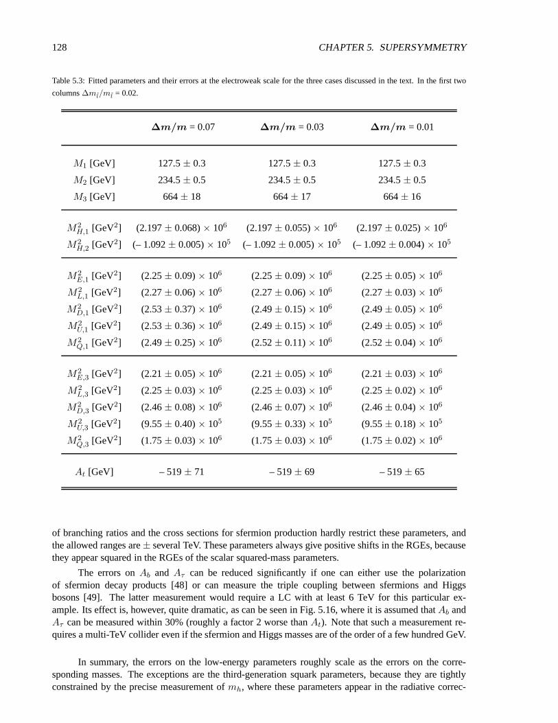
128 CHAPTER 5. SUPERSYMMETRY
Table 5.3: Fitted parameters and their errors at the electroweak scale for the three cases discussed in the text. In the first two
columns∆ml/ml = 0.02.
∆m/m = 0.07 ∆m/m = 0.03 ∆m/m = 0.01
M1 [GeV] 127.5± 0.3 127.5± 0.3 127.5± 0.3
M2 [GeV] 234.5± 0.5 234.5± 0.5 234.5± 0.5
M3 [GeV] 664± 18 664± 17 664± 16
M2H,1 [GeV2] (2.197± 0.068)× 106 (2.197± 0.055)× 106 (2.197± 0.025)× 106
M2H,2 [GeV2] (– 1.092± 0.005)× 105 (– 1.092± 0.005)× 105 (– 1.092± 0.004)× 105
M2E,1 [GeV2] (2.25± 0.09)× 106 (2.25± 0.09)× 106 (2.25± 0.05)× 106
M2L,1 [GeV2] (2.27± 0.06)× 106 (2.27± 0.06)× 106 (2.27± 0.03)× 106
M2D,1 [GeV2] (2.53± 0.37)× 106 (2.49± 0.15)× 106 (2.49± 0.05)× 106
M2U,1 [GeV2] (2.53± 0.36)× 106 (2.49± 0.15)× 106 (2.49± 0.05)× 106
M2Q,1 [GeV2] (2.49± 0.25)× 106 (2.52± 0.11)× 106 (2.52± 0.04)× 106
M2E,3 [GeV2] (2.21± 0.05)× 106 (2.21± 0.05)× 106 (2.21± 0.03)× 106
M2L,3 [GeV2] (2.25± 0.03)× 106 (2.25± 0.03)× 106 (2.25± 0.02)× 106
M2D,3 [GeV2] (2.46± 0.08)× 106 (2.46± 0.07)× 106 (2.46± 0.04)× 106
M2U,3 [GeV2] (9.55± 0.40)× 105 (9.55± 0.33)× 105 (9.55± 0.18)× 105
M2Q,3 [GeV2] (1.75± 0.03)× 106 (1.75± 0.03)× 106 (1.75± 0.02)× 106
At [GeV] – 519± 71 – 519± 69 – 519± 65
of branching ratios and the cross sections for sfermion production hardly restrict these parameters, andthe allowed ranges are± several TeV. These parameters always give positive shifts in the RGEs, becausethey appear squared in the RGEs of the scalar squared-mass parameters.
The errors onAb andAτ can be reduced significantly if one can either use the polarizationof sfermion decay products [48] or can measure the triple coupling between sfermions and Higgsbosons [49]. The latter measurement would require a LC with at least 6 TeV for this particular ex-ample. Its effect is, however, quite dramatic, as can be seenin Fig. 5.16, where it is assumed thatAb andAτ can be measured within 30% (roughly a factor 2 worse thanAt). Note that such a measurement re-quires a multi-TeV collider even if the sfermion and Higgs masses are of the order of a few hundred GeV.
In summary, the errors on the low-energy parameters roughlyscale as the errors on the corre-sponding masses. The exceptions are the third-generation squark parameters, because they are tightlyconstrained by the precise measurement ofmh, where these parameters appear in the radiative correc-

6.. THE ROLE OF BEAM POLARIZATION 129
1.8
2
2.2
2.4
2.6
2.8
3 M2E,1 M2
L,1 M2D,1 M2
Q,1 M2U,1 M2
E,3 M2L,3 M2
D,3 M2Q,3 M
2U,3 M2
H,1 M2H,2
Fig. 5.16: The 1σ bands for the sfermion and Higgs mass parameters atMGUT. The following cases are considered: (dark
boxes) slepton masses can be measured with an accuracy of 2% and the remaining particle masses within 7%; (light gray
boxes) slepton masses can be measured with an accuracy of 2% and the remaining particle masses within 3%; (dark gray
boxes) sfermion and heavy Higgs boson masses can be measuredwith an accuracy of 1%. In addition, it has been assumed that
Ab andAτ can be measured within 30%.
tions. The error in the high-scale parameters of the first generation atMGUT improves by a factor 2to 7 when the precision in the corresponding masses is improved from 7% to 1%. In the case of thethird-generation parameters, a determination ofAb andAτ is necessary for reducing the errors atMGUT.This can be done by measuring the trilinear Higgs sfermion couplings, for example from processes likee+e− → bibjA
0 or e+e− → τiτjA0. If Ab andAτ can be determined within 30% in such processes,
the errors on the high-scale parameters can be reduced by an order of magnitude. This conclusion re-mains valid for scenarios where most of the spectrum can be measured precisely at ane+e− collider inthe TeV range.
6. The Role of Beam Polarization
Polarized beams provide an important analysis tool at any LC, and in the following we summarize somehighlights [50]. In particular, for the analysis and the precise determination of the underlying structure ofNew Physics (NP), polarized cross sections and asymmetriesare superior observables. One may expectto reach an electron polarization of about 80% via a strainedphotocathode technology as used at the SLC,whereP (e−) = (77.34± 0.61)% was reached. One may also expect to reach a positron polarization ofabout 40%–60%.
For Standard Model processes, it is suitable to introduce the effective luminosity
Leff/L =1
2[1 − P (e−)P (e+)] , (5.5)
as a fraction of the total colliding-beam luminosity, and the effective polarization
Peff = [P (e−) − P (e+)]/[1 − P (e−)P (e+)] . (5.6)
Comparing these two numbers (Leff/L, Peff ) for the unpolarized case (0.5, 0), the case with only electronpolarization of aboutP (e−) = –80% (0.5, – 0.8) and the case withP (e−) = –80% andP (e+) = +60%(0.74, –0.95), we see that only the latter option can enhancethe effective luminosity.
It is well known that suitable beam polarization suppressesthe dominant SM background processWW (as well asZZ): the use of 80% electron polarization leads to a reduction by a factor 0.2 (0.76)
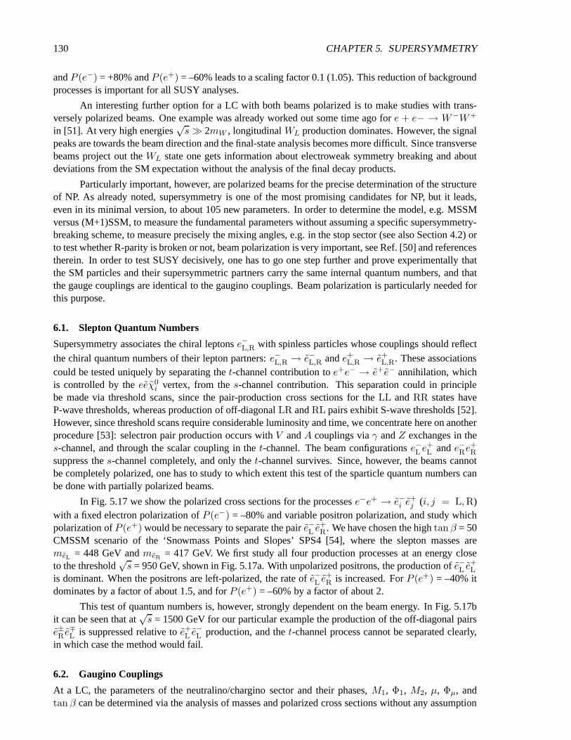
130 CHAPTER 5. SUPERSYMMETRY
andP (e−) = +80% andP (e+) = –60% leads to a scaling factor 0.1 (1.05). This reduction ofbackgroundprocesses is important for all SUSY analyses.
An interesting further option for a LC with both beams polarized is to make studies with trans-versely polarized beams. One example was already worked outsome time ago fore + e− → W−W+
in [51]. At very high energies√s≫ 2mW , longitudinalWL production dominates. However, the signal
peaks are towards the beam direction and the final-state analysis becomes more difficult. Since transversebeams project out theWL state one gets information about electroweak symmetry breaking and aboutdeviations from the SM expectation without the analysis of the final decay products.
Particularly important, however, are polarized beams for the precise determination of the structureof NP. As already noted, supersymmetry is one of the most promising candidates for NP, but it leads,even in its minimal version, to about 105 new parameters. In order to determine the model, e.g. MSSMversus (M+1)SSM, to measure the fundamental parameters without assuming a specific supersymmetry-breaking scheme, to measure precisely the mixing angles, e.g. in the stop sector (see also Section 4.2) orto test whether R-parity is broken or not, beam polarizationis very important, see Ref. [50] and referencestherein. In order to test SUSY decisively, one has to go one step further and prove experimentally thatthe SM particles and their supersymmetric partners carry the same internal quantum numbers, and thatthe gauge couplings are identical to the gaugino couplings.Beam polarization is particularly needed forthis purpose.
6.1. Slepton Quantum Numbers
Supersymmetry associates the chiral leptonse−L,R with spinless particles whose couplings should reflect
the chiral quantum numbers of their lepton partners:e−L,R → e−L,R ande+L,R → e+L,R. These associationscould be tested uniquely by separating thet-channel contribution toe+e− → e+e− annihilation, whichis controlled by theeeχ0
i vertex, from thes-channel contribution. This separation could in principlebe made via threshold scans, since the pair-production cross sections for theLL andRR states haveP-wave thresholds, whereas production of off-diagonalLR andRL pairs exhibit S-wave thresholds [52].However, since threshold scans require considerable luminosity and time, we concentrate here on anotherprocedure [53]: selectron pair production occurs withV andA couplings viaγ andZ exchanges in thes-channel, and through the scalar coupling in thet-channel. The beam configurationse−L e
+L ande−Re
+R
suppress thes-channel completely, and only thet-channel survives. Since, however, the beams cannotbe completely polarized, one has to study to which extent this test of the sparticle quantum numbers canbe done with partially polarized beams.
In Fig. 5.17 we show the polarized cross sections for the processese−e+ → e−i e+j (i, j = L,R)
with a fixed electron polarization ofP (e−) = –80% and variable positron polarization, and study whichpolarization ofP (e+) would be necessary to separate the paire−L e
+R. We have chosen the hightan β = 50
CMSSM scenario of the ‘Snowmass Points and Slopes’ SPS4 [54], where the slepton masses aremeL = 448 GeV andmeR = 417 GeV. We first study all four production processes at an energy closeto the threshold
√s = 950 GeV, shown in Fig. 5.17a. With unpolarized positrons, the production ofe−L e
+L
is dominant. When the positrons are left-polarized, the rate of e−L e+R is increased. ForP (e+) = –40% it
dominates by a factor of about 1.5, and forP (e+) = –60% by a factor of about 2.
This test of quantum numbers is, however, strongly dependent on the beam energy. In Fig. 5.17bit can be seen that at
√s = 1500 GeV for our particular example the production of the off-diagonal pairs
e±R e∓L is suppressed relative toe+L e
−L production, and thet-channel process cannot be separated clearly,
in which case the method would fail.
6.2. Gaugino Couplings
At a LC, the parameters of the neutralino/chargino sector and their phases,M1, Φ1, M2, µ, Φµ, andtan β can be determined via the analysis of masses and polarized cross sections without any assumption

6.. THE ROLE OF BEAM POLARIZATION 131
Fig. 5.17: Test of selectron quantum numbers ine+e− → e+L,Re−L,R with fixed electron polarizationP (e−) = –80% and
variable positron polarizationP (e+). The masses aremeL = 448 GeV,meR = 417 GeV and a) at√s = 950 GeV both the pairs
e−L e+L ande−L e
+R have comparable cross sections for unpolarized beams. ForP (e+) = –40% (P (e+) = –60%) thet–channel
pair e−L e+R dominates by a factor of about 1.5 (about 2). b) At
√s = 1500 GeV, the paire−L e
+L dominates kinematically and the
t-channel process can not be separated.
on the supersymmetry-breaking scheme. Even if only the lighter statesχ01,2 and χ±1 are kinematically
accessible, a precise determination of these parameters could be made [55]. Once these parametersare known, another important check of fundamental supersymmetric relations could be made with thehelp of polarized beams: the test whether the SU(2) and U(1) gauge couplingsg andg′ are identicalto the gaugino couplingsgW andgB from theℓℓW andℓℓB interactions. The comparison between thepolarized cross sectionsσL andσR for neutralino production with the theoretical predictionfor variableratiosgW /g andgB/g
′ provides a precise test of the gaugino couplings at the % level [55,56].
6.3. Distinction between the MSSM and (M+1)SSM
Supersymmetric models with additional chiral or vector superfields give rise to extensions of the gaug-ino/higgsino sector in general, and additional neutralinos occur. We consider here the (M+1)SSM withone new Higgs singlet, which leads to an extra singlino state. Since the neutralino mass spectra of thelightest four neutralinos in such extended models can be similar to those in the MSSM, a distinctionbetween the models might be difficult. However, the couplingstructure is different in the two mod-els. Therefore they could be distinguished via the polarization dependences of the cross sections. InFig. 5.18 we show the cross section fore+e− → χ0
1χ02 for one example in the MSSM and one in the
(M+1)SSM [57], where the mass spectra of the light particlesin the two models are similar.
Powerful tests for the closure of the system are evaluationsof sum rules. The four-state mixingin the MSSM induces sum rules for the couplings that follow from the unitarity of the diagonalizationmatrices. For asymptotic energies, these sum rules can be transformed directly into sum rules for theassociated cross sections [55], and are given in the MSSM by
lims→∞
s
4∑
i≤jσij =
πα2
48 c4W s4W
[64s4W − 8s2W + 5
]. (5.7)
In Fig. 5.19 the exact values for the summed cross sections are shown for one example, normalizedto the asymptotic values. The final stateχ0
1χ01 is invisible inR-invariant theories, and its detection is
difficult. Nevertheless, it can be studied directly by photon tagging in the final stateγχ01χ
01, which can
be observed at the LC. In this example the mass spectra of the light neutralinos in the two models are

132 CHAPTER 5. SUPERSYMMETRY
similar, and the asymptotic cross-section value is not affected by the additional singlet of the (M+1)SSM.However, as can be seen in Fig. 5.19, because of the incompleteness of these states below the thresholdsfor producing the heavy neutralino, the value measurable inthe (M+1)SSM differs significantly from thecorresponding sum rule of the MSSM. Therefore, even if the extended neutralino states are very heavy,the study of sum rules can shed light on the underlying structure of the supersymmetric model. In thiscontext, beam polarization is important to enhance the rates of even those pairs that have extremely smallcross sections.
Fig. 5.18: Cross sections for the processσ(e+e− → χ01χ
02) with polarized beams(Pe− = ± 80%,Pe+ = ∓ 60%) for an
example in the MSSM and the (M+1)SSM, where the mass spectra of the light neutralinos are similar [57].
6.4. Determination oftan β and Trilinear Couplings
Several studies have been made of howtan β can be measured in the Higgs sector via rates, widths andbranching ratios [58]. However, iftan β > 10, its precise determination will be difficult. It was shownin Ref. [48,59] that in this case theτ andt polarizations are suitable observables for determiningtan β.The procedure is as follows: one studies the rates for producing the lighter sparticle pairse+e− → τ1τ1or t1t1, and measures the mixing angle of the system by analysing polarized rates, as already workedout in earlier studies [60]. The masses as well as the mixing angle can be measured with precisionsat the per cent level. Ambiguities can be resolved, e.g. via measurements of the cross sections withanother configuration of the beam polarization [48, 59]. Determining the polarization of the final decayfermions, theτ or t polarization, while taking into account the complete neutralino and chargino mixing,leads to a determination oftan β with an accuracy of 10% even at hightan β. In this context, themeasurement of thet polarization fromb1 → tχ± decays could be very tricky, since the reconstructionof the system is difficult because of the missing transverse energy. However, analysing the distributionsof the quark jets in the hadronic top decayst → b+ cs could lead to a very precise measurement of thetop polarization [48,59] as seen in Fig. 5.20.
If the heavier statesτ2, b2 or t2 are also accessible, one can even go a step further, and determinethe trilinear couplingsAf . If t2 andb2 can be measured at the per cent level,At andAb may be extractedwith 30–50% precision [21, 59]. Because of the smallτ mass, one cannot expect to determine theparameterAτ with very high precision.

7.. MEASURING NEUTRINO MIXING ANGLES AT CLIC 133
500 1000 1500 2000 2500√s (GeV)
0
0.25
0.5
0.75
1
1.25
rati
o
MSSM(M+1)SSM
Fig. 5.19: The energy dependence of the sum of all the neutralino–pair-production cross sections normalized to the asymptotic
form of the summed cross section. The solid line represents the exact sum in the MSSM and the dashed line the sum of the
cross sections for the first four neutralino states for a specific parameter set of the (M+1)SSM [55].
7. Measuring Neutrino Mixing Angles at CLIC
Recent neutrino experiments [61–63] clearly show that neutrinos are massive particles and that they mix.A possible way to account for the observed neutrino data in supersymmetric theories is to break leptonnumber, either spontaneously or explicitly, and thus R-parity. The simplest realization of this idea is toadd bilinear terms to the superpotentialW :
W = WMSSM + ǫiLiHu . (5.8)
For consistency one also has to add the corresponding bilinear terms to soft SUSY-breaking, whichinduce small vacuum expectation values (vevs) for the sneutrinos. These vevs induce a mixing betweenneutrinos and neutralinos, giving mass to one neutrino. Thesecond neutrino mass is induced by loopeffects (see Ref. [64] and references therein). The same parameters that induce neutrino masses andmixings are also responsible for the decay of the lightest supersymmetric particle (LSP). This impliesthat there are correlations between neutrino physics and LSP decays [65–67].
As a specific example we present the relationship between theatmospheric neutrino mixing angleand the decays of a neutralino into semileptonic final statesliq
′q (li = e, µ, τ ). There are several moreexamples, which are discussed in Ref. [66]. In the model specified by Eq. (5.8) the atmospheric mixingangle is given by
tan θatm =Λ2
Λ3(5.9)
Λi = ǫivd + µvi , (5.10)
wherevi are the sneutrino vevs andvd is the vev ofH01 . It turns out that the dominant part of theχ0
1-W -licouplingOLi is given by
OLi = Λif(M1,M2, µ, tan β, vd, vu) , (5.11)

134 CHAPTER 5. SUPERSYMMETRY
-1 -0.5 0 0.5 10
10
20
30
40
50
,s1χθcos
event N
0.10±= -0.44 topP
=3300N
Angle correlation in the t-quark rest frame
Fig. 5.20: Angular distribution incos θ∗s , the angle between theb1 and s partons in the top rest frame oft → b cs decays
from e+Le−R → b1b1 → tχ±
1 + b1 production at√s = 1.9 TeV. The line represents a fit to a top polarization ofPt = –
0.44± 0.10 [48,59].
where the exact form off can be found in Eq. (20) of Ref. [66]. The important point is, thatf dependsonly on MSSM parameters and not on the R-parity-violating parameters. Putting everything together onefinds:
tan2 θ2atm =
∣∣∣∣Λ2
Λ3
∣∣∣∣2
≃ BR(χ01 → µ±W∓)
BR(χ01 → τ±W∓)
≃ BR(χ01 → µ±qq′)
BR(χ01 → τ±qq′)
. (5.12)
The restriction to the hadronic final states of theW is necessary for the identification of the leptonflavour. Depending on the specific parameters, one gets additional small contributions due to three-bodydecays of intermediate sleptons and squarks. Note that Eq. (5.12) is a prediction of the bilinear modelindependent of the R-parity-conserving parameters. It hasbeen shown that under favourable conditionsthe LHC can measure the ratio of branching ratios in Eq. (5.12) with an accuracy of about 3% [68].
In this note we study an example of such a correlation in a scenario where the lightest neutralinois rather heavy and where it is most likely that the LHC will have difficulties to measure the branchingratios accurately. For the numerical example, we take pointH as reference, which is characterized byM1/2 = 1.5 TeV,M0 = 419 GeV,A0 = 0, tan β = 20 and a positive sign ofµ. We vary randomly theR-parity-conserving parameters around this point so that the masses of the supersymmetric particles varywithin 10% for the particles that can be observed at a 5 TeV collider. For the remaining particles we seta lower cut of 2.5 TeV on the masses. To these sets of parameters we add the R-parity-breaking parame-ters such that the correct differences between the squared neutrino masses and the correct mixing anglesare obtained within the experimental allowed range: 1.2× 10⁻³ eV2 < ∆m2
atm < 4.8 × 10⁻³ eV2,5.1 × 10−5 eV2 < ∆m2
sol < 1.9 × 10⁻⁴ eV2, 0.29< sin2 θatm < 0.86, sin2 θ13 < 0.05. Forillustrative purpose only we allow a range forsin2 θatm wider than the experimentally allowed one:0.3 < sin2 θatm < 0.7. The main LSP decay modes are: BR(χ0
1 → h0∑
i = 1,3 νi) ≃ 50%,BR(χ0
1 → W±e∓ + W±µ∓ + W±τ∓) ≃ 30%, BR(χ01 → Z0
∑i = 1,3 νi) ≃ 20%. In addition there
are three-body decay modes mainly mediated by virtual sleptons whose sum of the branching ratiosis about 1–2%.

8.. SUMMARY 135
In Fig. 5.21 we show the correlation betweentan2 θatm andBR(χ01 → µ±qq′)/BR(χ0
1 →τ±qq′). Note that the width of the band is due to the variation of the parameters as discussed above.It becomes by a factor of 4–5 smaller if the SUSY masses can be measured with an accuracy of 2%instead of the assumed 10%. Figure 5.21 clearly shows that these decay modes can be used to relate ob-servables measured at CLIC to those measured at neutrino experiments. Moreover, they allow for a con-sistency test of the theory. Note that R-parity-violating decay modes into gauge bosons (Higgs bosons)and leptons are forbidden in R-parity-violating models where only trilinear R-parity-breaking couplingsexist. Therefore, the observation of such decays give a clear proof that bilinear R-parity-breaking isrealized in nature.
0.1 0.2 0.5 1 2 5 100.1
0.2
0.5
1
2
5
10BR(χ0
1 → µ±qq′)/BR(χ01 → τ±qq′)
tan2 θatm
Fig. 5.21: Correlation between atmospheric neutrino mixing angle and semileptonic branching ratios of the lightest neutralino.
In summary, models where R-parity is broken by bilinear terms can explain recent neutrino dataand predict at the same time certain decay properties of the lightest supersymmetric particle. CLIC isparticularly suited to explore the resulting correlationsbetween neutrino mixing angles and ratios of LSPbranching ratios in scenarios where the LSP is rather heavy.
8. Summary
The CLIC multi-TeV lineare+e− collider has important potential for supplementing the information onsupersymmetry that might be provided by previous colliderssuch as the LHC and a TeV-class linearcollider, as we have illustrated within the CMSSM. The CMSSMparameter space is restricted by ex-perimental constraints from LEP and elsewhere, and by cosmology. If sparticle masses are in the lowerpart of the range still allowed by these constraints, much ofthe supersymmetric spectrum will have beendiscovered by the LHC and/or by a TeV-class linear collider,which would also be able to make someprecision measurements. In this case, CLIC would be invaluable for extending precision measurementsto squarks and heavier neutralinos and charginos, in particular. On the other hand, if sparticle masses arein the upper part of the allowed range, CLIC might be the first accelerator to produce many of the SUSYparticles.
Using benchmark CMSSM points as examples, we have demonstrated that CLIC would be able tomake detailed measurements of sparticle masses and mixing angles. These would enable accurate testsof unification hypotheses for mechanisms of supersymmetry breaking to be made. Electron and positronbeam polarization would be a useful tool for disentangling sparticle properties, and theγγ option would

136 CHAPTER 5. SUPERSYMMETRY
be especially interesting for gluino production, in particular. Although most of this discussion referredto the CMSSM, we have also shown that CLIC has important capabilities for distinguishing this frommore complicated supersymmetric models, and for exploringscenarios in which R parity is violated.
We conclude that CLIC will be an invaluable tool for exploring supersymmetry, even if it has beendiscovered previously at the LHC and explored at a TeV-classlinear collider.

Bibliography
[1] See for instance,H.P. Nilles,Phys. Rep.110(1984) 1;H.E. Haber and G.L. Kane,Phys. Rep.117(1985) 75.
[2] L. Maiani, in Proc. of the 1979 Gif-sur-Yvette Summer School on Particle Physics, 1;G. ’t Hooft, Recent Developments in Gauge Theories, in Proc. of Advanced Study Institute,Carg ese, 1979, eds. G. ’t Hooftet al., Plenum Press, NY, 1980;E. Witten,Phys. Lett.B105, 267 (1981).
[3] H. Haber and R. Hempfling,Phys. Rev. Lett.66 (1991) 1815;M. Carena, M. Quiros and C.E.M. Wagner,Nucl. Phys.B461(1996) 407;H. Haber, R. Hempfling and A. Hoang,Z. Phys.C75 (1997) 539;S. Heinemeyer, W. Hollik and G. Weiglein,Phys. Rev.D58 (1998) 091701,Eur. Phys. J.C9(1999) 343;R.-J. Zhang,Phys. Lett.B447(1999) 89.
[4] LEP Higgs Working Group for Higgs Boson Searches Collaboration, ‘Search for the StandardModel Higgs boson at LEP’, contributed to International Europhysics Conference on High EnergyPhysics (HEP 2001), Budapest, Hungary, 12–18 Jul 2001, hep-ex/0107029.
[5] J. Erler,Phys. Rev.D63 (2001) 071301, hep-ph/0010153.
[6] J. Ellis, S. Kelley and D.V. Nanopoulos,Phys. Lett.B260(1991)131;U. Amaldi, W. de Boer and H. Furstenau,Phys. Lett.B260(1991) 447;P. Langacker and M. Luo,Phys. Rev.D44 (1991) 817;C. Giunti, C.W. Kim and U.W. Lee,Mod. Phys. Lett.A6 (1991) 1745.
[7] J.R. Elliset al., Nucl. Phys.B238(1984) 453;see also H. Goldberg,Phys. ReV. Lett.50 (1983) 1419.
[8] M. Battagliaet al., Eur. Phys. J.C33 (2004) 273, hep-ph/0306219.
[9] M. Battagliaet al., Eur. Phys. J.C22 (2001) 535.
[10] C.L. Bennettet al., Astrophys. J. Suppl.148 (2003) 1, astro-ph/0302207;H.V. Peiriset al., Astrophys. J. Suppl.148(2003) 213, astro-ph/0302225.
[11] ATLAS Collaboration, ‘ATLAS: Detector and Physics Performance Technical DesignReport’,CERN-LHCC 99-14/15 (1999).
[12] S. Abdullinet al., (CMS Collaboration),J. Phys.G28 (2002) 469, hep-ph/9806366;S. Abdullin and F. Charles,Nucl. Phys.B547(1999) 60;CMS Collaboration, Technical Proposal, CERN-LHCC 94-38 (1994).
137

138 BIBLIOGRAPHY
[13] G. Blair, W. Porod and P.M. Zerwas,Phys. Rev.D63 (2001) 017703, hep-ph/0007107.
[14] B.C. Allanachet al., Eur. Phys. J.C25 (2002) 113.
[15] G.L. Kaneet al., Phys. Rev.D67 (2003) 045008.
[16] J. Feng and D. Finnell,Phys. Rev.D49 (1994) 2369.
[17] D. Denegri, W. Majerotto and L. Rurua,Phys. Rev.D58 (1998) 095010, hep-ph/9711357.
[18] H.U. Martyn, contributed to Workshop on Physics at TeV Colliders, Les Houches, France, 7–18Jun 1999, hep-ph/0002290.
[19] G.A. Blair, ‘Sparticle masses and widths via threshold scans at the linear collider’, in Proc. of theAPS/DPF/DPB Summer Study on the Future of Particle Physics (Snowmass 2001), ed. N. Graf,Snowmass, Colorado, 30 Jun – 21 Jul 2001, eConfC010630(2001) E3019.
[20] M. Drees and K. Hikasa,Phys. Lett.B252(1990) 127.
[21] S. Kraml,‘Stop and sbottom phenomenology in the MSSM’, Ph.D. Thesis, hep-ph/9903257.
[22] S. Heinemeyer, S. Kraml, W. Porod and G. Weiglein,JHEP0309(2003) 075, hep-ph/0306181.
[23] G. Belanger, F. Boudjema, T. Kon and V. Lafage,Eur. Phys. J.C9 (1999) 511, hep-ph/9811334;A. Djouadi, J.L. Kneur and G. Moultaka,Nucl. Phys.B569(2000) 53, hep-ph/9903218.
[24] A. Bartl et al., Phys. Lett.B435(1998) 118, hep-ph/9804265.
[25] S. Berge and M. Klasen,Phys. Rev.D66 (2002) 115014.
[26] S. Berge and M. Klasen,Eur. Phys. J.C30 (2003) 123, hep-ph/0303032.
[27] H. Burkhardt and V. Telnov,‘CLIC 3-TeV photon collider option’, CERN-SL-2002-013-AP.
[28] T. Affolder et al. (CDF Collaboration),Phys. Rev. Lett.88 (2002) 041801.
[29] S. Abachiet al. (D0 Collaboration),Phys. Rev. Lett.75 (1995) 618.
[30] LEP Higgs Working Group Collaboration, Note 2001-04,‘Searches for the neutral Higgs bosonsof the MSSM: Preliminary combined results using LEP data collected at energies up to 209 GeV’,hep-ex/0107030.
[31] T. Hahn and C. Schappacher,Comput. Phys. Commun.143(2002) 54, hep-ph/0105349.
[32] K. Hagiwaraet al. (Particle Data Group Collaboration),Phys. Rev.D66 (2002) 010001.
[33] J. Abdallahet al. (LEP SUSY Working Group Collaboration),http://lepsusy.web, cern.ch/lepsusy.
[34] T. Hahn,Comput. Phys. Commun.140(2001) 418, hep-ph/0012260.
[35] T. Hahn and M. Perez-Victoria,Comput. Phys. Commun.118(1999) 153, hep-ph/9807565.
[36] A. Airapetianet al.(ATLAS Collaboration),‘ATLAS Detector and Physics Performance. Technicaldesign report’, Vol. 2, CERN-LHCC-99-15.
[37] S. Abdullinet al. (CMS Collaboration),J. Phys.G28 (2002) 469, hep-ph/9806366.
[38] M. Battagliaet al., Eur. Phys. J.C22 (2001) 535, hep-ph/0106204.

BIBLIOGRAPHY 139
[39] G. Blair, W. Porod and P.M. Zerwas,Eur. Phys. J.C27 (2003) 263, hep-ph/0210058.
[40] W. Porod,Comput. Phys. Commun.153(2003) 275, hep-ph/0301101.
[41] J. Aguilar-Saavedraet al., ‘Physics at ane+e− Linear Collider’, TESLA TDR Part 3,hep-ph/0106315.
[42] F. James and M. Roos,Comput. Phys. Commun.10 (1975) 343.
[43] D. Pierceet al., Nucl. Phys.B491(1997) 3, hep-ph/9606211.
[44] G. Degrassi, P. Slavich and F. Zwirner,Nucl. Phys.611(2001) 403, hep-ph/0105096;A. Brignoleet al., Nucl. Phys.B631(2002) 195, hep-ph/0112177;A. Dedes and P. Slavich,Nucl. Phys.B657(2003) 333, hep-ph/0212132.
[45] M. Drees and K. Hikasa,Phys. Lett.B252(1990) 127.
[46] H. Eberl, A. Bartl and W. Majerotto,Nucl. Phys.B472(1996) 481, hep-ph/9603206.
[47] A. de Roeck, private communication.
[48] E. Booset al., Eur. Phys. J.C30 (2003) 395, hep-ph/0303110.
[49] A. Bartl, K. Hidaka, T. Kernreiter and W. Porod,Phys. Rev.D66 (2002) 115009, hep-ph/0207186.
[50] G. Moortgat-Pick and H.M. Steiner,Eur. Phys. J. directC3 (2001) 6, hep-ph/0106155;see also, G. Moortgat-Pick, hep-ph/0303234, hep-ph/0106315.
[51] J. Fleischer, K. Kolodziej and F. Jegerlehner,Phys. Rev.D49 (1994) 2174;see also K. Desch, talk at International Workshop on Linear Colliders, August 26–30, 2002, JejuIsland, Korea:http://lcws2002.korea.ac.kr/.
[52] P. Chiappettaet al., Nucl. Phys.B259(1985) 365.
[53] C. Blochingeret al., Eur. Phys. J.C24 (2002) 297, hep-ph/0201282.
[54] B. C. Allanachet al., Eur. Phys. J.C25(2002) 113 [eConfC010630(2001) P125], hep-ph/0202233;N. Ghodbane and H.U. Martyn,‘Compilation of SUSY particle spectra from Snowmass 2001 bench-mark models’, in Proc. of the APS/DPF/DPB Summer Study on the Future of Particle Physics(Snowmass 2001), ed. N. Graf, Snowmass, Colorado, 30 Jun – 21Jul 2001, hep-ph/0201233.
[55] S.Y. Choi, J. Kalinowski, G. Moortgat-Pick and P.M. Zerwas,Eur. Phys. J.C22 (2001) 563,hep-ph/0108117;C23 (2002) 769, hep-ph/0202039.
[56] A. Freitaset al., hep-ph/0211108;A. Freitas and A. von Manteuffel, hep-ph/0211105.
[57] S. Hesselbach, F. Franke and H. Fraas, hep-ph/0003272;F. Franke and S. Hesselbach,Phys. Lett.B526(2002) 370, hep-ph/0111285;G. Moortgat-Pick, S. Hesselbach, F. Franke and H. Fraas, hep-ph/9909549.
[58] H. Baeret al., Phys. Rev.D59 (1999) 055014, hep-ph/9809223;V.D. Barger, T. Han and J. Jiang,Phys. Rev.D63 (2001) 075002, hep-ph/0006223;J.F. Gunionet al., eConfC010630(2001) P120, hep-ph/0112334.
[59] E. Booset al., hep-ph/0211040;

140 BIBLIOGRAPHY
[60] M.M. Nojiri, Phys. Rev.D51 (1995) 6281, hep-ph/9412374;M.M. Nojiri, K. Fujii and T. Tsukamoto,Phys. Rev.D54 (1996) 6756, hep-ph/9606370;A. Bartl et al., Z. Phys.C73 (1997) 469, hep-ph/9603410;C76 (1997) 549, hep-ph/9701336;Eur. Phys. J. directC2 (2000) 6, hep-ph/0002115.
[61] Y. Fukudaet al. (Super-Kamiokande Collaboration),Phys. Rev. Lett.81 (1998) 1562;S. Fukudaet al. (Super-Kamiokande Collaboration),Phys. Rev. Lett.86 (2001) 5651.
[62] Q.R. Ahmadet al. (SNO Collaboration),Phys. Rev. Lett.87 (2001) 071301, hep-ph/0106015.
[63] K. Eguchiet al. (KamLAND Collaboration),Phys. Rev. Lett.90 (2003) 021802, hep-ex/0212021
[64] J.C. Romaoet al., Phys. Rev.D61 (2000) 071703, hep-ph/9907499;M. Hirschet al., Phys. Rev.D62 (2000) 113008, (Erratum)D65 (2002) 119901, hep-ph/0004115;M.A. Diaz, Phys. Rev.D68 (2003) 013009, hep-ph/0302021.
[65] B. Mukhopadhyaya, S. Roy and F. Vissani,Phys. Lett.B443(1998) 191, hep-ph/9808265.
[66] W. Porod, M. Hirsch, J. Romao and J.W. Valle,Phys. Rev.D63 (2001) 115004, hep-ph/0011248.
[67] M. Hirsch, W. Porod, J. C. Romao and J.W. Valle,Phys. Rev.D66 (2002) 095006, hep-ph/0207334;M. Hirsch and W. Porod,Phys. Rev.D68 (2003) 115007, hep-ph/0307364.
[68] W. Porod and P. Skands, contributed to 3rd Les Houches Workshop: Physics at TeV Colliders, LesHouches, France, 26 May – 6 Jun 2003, hep-ph/0401077.

Chapter 6
PROBING NEW THEORIES
The LHC is expected to probe directly possible new physics (NP) beyond the Standard Model (SM) upto a scale of a few TeV. While its data should provide answers to several of the major open questions inthe present picture of elementary particle physics, it is important to start examining how this sensitivitycan be further extended at a next generation of colliders. Today we have a number of indications that NPcould be of supersymmetric nature. If this is the case, the LHC will have a variety of signals to discoverthese new particles, and a linear collider will be required to complement the probe of the supersymmetricspectrum with detailed measurements, as discussed in the previous chapter. However, beyond supersym-metry, there is a wide range of other scenarios invoking new phenomena at, and beyond, the TeV scale.They are aimed at explaining the origin of electroweak symmetry breaking, if there is no light elementaryHiggs boson, at stabilizing the SM, if supersymmetry is not realized in nature, or at embedding the SMin a theory of grand unification.
1. Extra Dimensions
In the last few years there has been considerable interest inthe possibility that new spatial dimensions canbe observed at high-energy colliders. One interesting theoretical option is that only gravity propagates inthe extra dimensions, whilst gauge and matter fields are confined on a three-dimensional brane [1,2]. Thishypothesis is motivated by the hierarchy problem and naturally realized in string theory. Two differentkinds of scenarios have been proposed: those in which the space metrics are factorizable [1] and thosein which they are non-factorizable [2]. Their relative phenomenological consequences are quite distinct.When discussing the experimental signals of these models, one should bear in mind that the theory isnon-renormalizable, with an unknown ultraviolet completion. It is then necessary to distinguish variouskinematical regimes, which can be tackled with different theoretical tools.
We first consider thecisplanckian region, in which the centre-of-mass energy of the collision ismuch smaller than the fundamental quantum-gravity scaleMD. We can then describe graviton produc-tion using an effective theory obtained by linearizing the Einstein action. In the case of factorizable extradimensions, we obtain a nearly-continuous spectrum of Kaluza–Klein (KK) graviton excitations, whichinteract very weakly and give rise to experimental missing-energy signatures.
In the case of non-factorizable metrics, the graviton KK excitations have mass gaps of the orderof the fundamental scaleMD and they have a sizeable interaction with ordinary matter, leading to char-acteristic resonant production at high-energy collisions. A study of the predictions for CLIC and thecomparison with the LHC reach is presented in Section 1.2.
The effective theory, valid at energies belowMD, also contains the most general set of gauge-invariant higher-dimensional operators. The coefficientsof these operators cannot be computed withoutknowledge of the short-distance theory. Therefore, a general experimental study of contact interactionswill be very useful to gain information about the underlyingtheory. One can perform a more restrictive
141

142 CHAPTER 6. PROBING NEW THEORIES
(but more predictive) analysis by considering only those operators generated by graviton exchange. Attree level, a single dimension-8 operator is generated. This operator contributes to a variety of processesat CLIC. The most interesting is probablye+e− → γγ, since no other local operator of lower dimensioncan generate this process. Therefore, the study of diphotonfinal states can be of particular importancein probing new gravitational effects. The exchange of gravitons at the loop level generates a singledimension-6 operator, which is the product of two flavour-universal axial currents. In this case, therelevant final state is dilepton or dijet. We do not pursue here an analysis of these processes, but we referthe reader to the later section on contact interactions.
At centre-of-mass energies of the order ofMD, we are entering thePlanckian region, where theeffective theory approach discussed above is no longer valid. This is the most interesting region from theexperimental point of view, since new phenomena related to quantum gravity and string theory will fullymanifest themselves. However, it is also the most difficult region to tackle theoretically, in the absenceof a complete description of the short-distance behaviour of gravity. It is however easy to predict that, incase of a discovery at the LHC, the role of a multi-TeV linearcollider will be crucial to disentangle thenew physics signals, leading to new understanding of the underlying theory.
In thetransplanckian region, where√s≫MD, we can give a reliable description of the scattering
process (at least under certain kinematical conditions), since semiclassical physics give the dominanteffects. At impact parameters larger than the Schwarzschild radius, gravitational elastic scattering iscomputable in the eikonal approximation. This gives a prediction for Bhabha scattering at small angleswhich can be compared with observations at CLIC. When the impact parameter is of the order of theSchwarzschild radius or smaller, strong classical-gravity effects complicate the theoretical description,but there are plausible arguments that suggest that black holes are formed. If this is the case, any purelyshort-distance interactions from quantum gravity will be masked by the black hole, as the collision energyis increased. We also briefly discuss some of the implications of transplanckian physics at CLIC.
So far we have considered the case in which gauge and matter fields are strictly four-dimensional.It is not implausible that, within the scenarios consideredabove, also SM fields have extra-dimensionalexcitations, although different in nature from those of thegravitons. We consider such possibility inSection 1.4, where we describe the present bounds on KK excitations of SM fields and future prospectsfor discovery at CLIC. To emphasize the importance of the complementarity role of a multi-TeV linearcollider with respect to the LHC, we also discuss in Section 1.4 how studies at CLIC can distinguishbetween the surprisingly similar collider signals of KK excitations of SM particles from those of a su-persymmetric model with a nearly degenerate superpartner spectrum.
1.1. ADD Type of Extra Dimensions
The first model we consider is that of Arkani-Hamed, Dimopoulos and Dvali (ADD) [1]; we limit ourdiscussion to the case of graviton tower exchange ine+e− → f f . The effect of summing the KKgravitons is to produce a set of effective dimension-8 operators of the form∼ λT µνTµν/M
4s , where
Tµν is the stress-energy tensor of the SM matter exchanging the tower [3]. This approximation onlyapplies in the limit that the centre-of-mass energy of the collision process lies sufficiently below thecut-off scaleMs, which is of the order of the size of the Planck scale in the extra-dimensional space.In the convention used by Hewett [3] and adopted here, the contribution of the spin-2 exchanges can beuniversally expressed in terms of the scaleMs and a signλ. Current experimental constraints from LEPand the Tevatron [4] tell us thatMs ≥ 1 TeV for either sign ofλ; values ofMs as large as the low 10’sof TeV may be contemplated in this scenario.
In the case ofe+e− → f f , the addition of KK tower exchange leads to significant deviationsin differential cross Sections and polarization asymmetries from their SM values, which are stronglydependent on both the sign ofλ and the ratios/M2
s . Such shifts are observable in final states of allflavours. In addition, the shape of these deviations from theSM with varying energy and scatteringangle, as shown by Hewett [3], tells us that the underlying physics arises from dimension-8 operators

1.. EXTRA DIMENSIONS 143
Fig. 6.1: Deviations in the cross section forµ pairs (left) andALR for b quarks (right) at√s = 5 TeV forMs = 15 TeV in
the ADD model for an integrated luminosity of 1ab−1. The SM is represented by the histogram while the red and green data
points show the ADD predictions withλ = ± 1. In both plotsz = cos θ.
and not, for example,Z ′ exchange. Figure 6.1 shows an example of how such deviationsfrom the SMmight appear at a 5-TeV CLIC in the case thatMs = 15 TeV for either sign ofλ. The indirect searchreach for the scaleMs can be obtained by combining the data for several of the fermion final states(µ, τ, c, b, t, etc.) in a single overall fit. The result of this analysis forCLIC is theλ-independent boundshown in Fig. 6.2 as a function of the integrated luminosity for
√s = 3 or 5 TeV. For an integrated
luminosity of 1ab−1 we see that the reach isMs ≃ 6√s, which is consistent with analyses at lower-
energy machines [3].
Fig. 6.2: (Left) Search reach for the ADD model scaleMs at CLIC as a function of the integrated luminosity from the set of
processese+e− → ff , assuming√s = 3 (bottom) or 5 (top) TeV. Heref = µ, τ, b, c, t, etc. (Right) Corresponding reach for
the compactification scale of the KK gauge bosons in the case of one extra dimension and all fermions localized at the same
orbifold fixed point.
Scenarios with large extra dimensions have been studied forTeV-class linear colliders, e.g.TESLA [5], and are searched for typically in the channele+e− → γ + G. One of the acclaimedadvantages of a LC with respect to the LHC is that, by measuring the γG cross section at differentcentre-of-mass energies, one can disentangle the Planck scale and the number of extra dimensionsδsimultaneously, as is shown for CLIC in Fig. 6.3 by the solid lines. The cross sections are calculatedfor cuts similar to those in [5]:sin θγ > 0.1, pγt > 0.06Ebeam andxγ < 0.65. The cross sections arenormalized in such a way that for each value ofδ, the scaleMD is chosen to give the same cross sectionat 500 GeV.
These predictions assume, however, that lower-dimensional physics is attached to rigid branes.Allowing for flexible branes instead [6] introduces a new dependence on a parameter∆, the softeningscale, which is related to the brane tension. The dashed lines in Fig. 6.3 show the effect of∆ for valuesof 4 TeV and 1 TeV, respectively.

144 CHAPTER 6. PROBING NEW THEORIES
Fig. 6.3: The cross section fore+e− → Gγ with cuts as described in the text, for rigid (solid lines) and soft (dashed lines)
branes. The different curves correspond, from bottom to top, to different numbers of extra dimensionsδ = 2, 3, 4, 5, 6 and 7.
Left, for ∆ = 4 TeV, right for∆ = 1 TeV.
For a brane tension of 4 TeV, the effect on the cross section israther small. A collider in the rangeof 0.5–1 TeV would not be sensitive to the effect and thusMD andδ can still be disentangled. However,at CLIC the cross sections are 30–40% lower than expected, allowing one to observe the softness ofthe brane. For a brane of 1 TeV tension the effect is more spectacular. For the example given here, alower-energy LC would get fooled when measuring cross sections only at 0.5 TeV and 1 TeV, and extractwrong values ofδ andMD. Extending the range in the multi-TeV region will again allow this effect tobe observed in its full drama. The cross section of the background channele+e− → e+e−γ with the cutsas listed above is 16 fb at 3 TeV, which sets the scale for the detectability of a signal: forδ = 2 or 3 thesignal event rate at 3 TeV gets too small for such a soft brane scenario.
1.2. Graviton Production at CLIC: Randall–Sundrum Model
In the extra-dimension scenario proposed by Randall and Sundrum (RS) [2] the hierarchy between thePlanck and the electroweak scale is generated by an exponential function called the ‘warp factor’. Thismodel predicts KK graviton resonances with weak-scale masses and strong couplings to matter. Hencethe production of TeV-scale graviton resonances is expected in two-fermion channels [7]. In its simplestversion, with two branes and one extra dimension, and where all of the SM fields remain on the brane, themodel has two fundamental parameters: the mass of the first KKstatem1, and the parameterc = k/MP l,wherek is related to the curvature of the 5D space andMPl is the 4D effective Planck scale. Theparameterc controls the effective coupling strength of the graviton and thus the width of the resonances,and should be less than 1 but yet not too far away from unity.
The resulting spectrum fore+e− → µ+µ− is shown in Fig. 6.4. The cross sections are hugeand the signal cannot be missed at a LC with sufficient centre-of-mass energy. If such resonances areobserved — perhaps first by the LHC in the range of a few TeV — it will be important to establish thenature of these newly produced particles, i.e. to measure their properties (mass, width and branching ra-tios) and quantum numbers (spin). Note that the massm1 of the first resonance determines the resonancepattern: the masses of all higher-mass resonances are then fixed.
The signal for one KK resonance (G1) is implemented in PYTHIA 6.158 [8] via process 41.For the study, PYTHIA has been extended to include two more resonances (G2, G3, corresponding toprocesses 42 and 43) to allow a check on the measurability of the graviton self-coupling. The decaybranching ratios of these resonances were modified according to [7, 9]. In particular, the gravitons candecay into two photons in about 4% of the cases, a signature that would distinguish them from, forexample, new heavyZ ′ states [10].

1.. EXTRA DIMENSIONS 145
cos(theta)
0
25
50
75
100
125
150
175
200
225
-1 -0.8 -0.6 -0.4 -0.2 0 0.2 0.4 0.6 0.8 1
Fig. 6.4: Left: KK graviton excitations in the RS model produced in the processe+e− → µ+µ−. From the most narrow to
widest resonances, the curves are for 0.01< c < 0.2. Right: Decay-angle distribution of the muons fromG3 (3200 GeV)
→ µµ.
The resonance spectrum was chosen such that the first resonanceG1 has a mass around 1.2 TeV,just outside the reach of a TeV-class LC, and consequently the mass of the third resonanceG3 will bearound 3.2 TeV, as shown in Fig. 6.4. The
√s energy for thee+e− collisions of CLIC was taken to be
3.2 TeV in this study. Mainly the muon and photon decay modes of the graviton have been studied. Theevents used to reconstruct theG3 resonance signal were selected via either two muons or twoγ’s withE > 1200 GeV and| cos θ| < 0.97. The background from overlaid two-photon events — on averagefour events per bunch crossing — is typically important onlyfor angles below 120 mrad, i.e. outside thesignal search region considered.
First we study the precision with which one can measure the shape, i.e. thec andM parameters,of the observed new resonance. A scan similar to that of theZ at LEP was made for an integratedluminosity of 1 ab−1. The precision with which the cross sections are measured allows one to determinec to 0.2% andM to better than 0.1%.
Next we determine some key properties of the new resonance: the spin and the branching ratios.The graviton is a spin-2 object, and Fig. 6.4 shows the decay angle of the fermionsG → µµ for theG3
graviton, obtained using PYTHIA/SIMDET for 1 ab−1 of data, including the CLIC machine background.The typical spin-2 structure of the decay angle of the resonance is clearly visible.
For gravitons as proposed in [7, 9] one expectsBR(G → γγ)/BR(G → µµ) = 2. With thepresent SIMDET simulation we get efficiencies in the mass peak (± 200 GeV) of 84% and 97% fordetecting the muon and photon decay modes, respectively. With cross sections of O(1 pb),σγγ andσµµcan be determined to better than a per cent. Hence the ratioBR(G → γγ)/BR(G → µµ) can bedetermined to an accuracy of 1% or better.
Finally, if the centre-of-mass energy of the collider is large enough to produce the first threeresonance states, one has the intriguing possibility to measure the graviton self-coupling via theG3 →G1G1 decay [9]. The dominant decay mode will beG1 → gg or qq giving a two-jet topology. Figure 6.5shows the resulting spectacular event signature of four jets of about 500 GeV each in the detector (nobackground is overlaid). These jets can be used to reconstruct G1. Figure 6.5 shows the reconstructedG1 invariant mass. The histogram does not include the background, while the dots include 10 bunchcrossings of background overlaid on the signal events. Hence the mass ofG1 can be well reconstructedand is not significantly distorted by theγγ background.

146 CHAPTER 6. PROBING NEW THEORIES
JJ Inv. Mass (GeV)
Evt
s/40
GeV
0
10
20
30
40
50
60
70
600 800 1000 1200 1400
Fig. 6.5: Left: Event in a CLIC central detector with the decay G3 → G1G1 → four jets. Right: Invariant jet–jet mass of
G1(1200 GeV) produced inG3 → G1G1 andG1 → two jets.
In summary, a multi-TeV collider such as CLIC will allow a precise determination of the shapeand mass of the new resonance(s), and of its spin. In particular, for the RS model it was shown thatthe key discriminating properties of these resonances can be reconstructed, and the underlying modelparameters can be determined precisely.
1.3. Transplanckian Scattering
Elastic collisions in the transplanckian region, where thecentre-of-mass energy√s is much larger than
the fundamental gravity mass scaleMD, can be described by linearized general relativity and knownquantum-mechanical effects, as long as the momentum transfer in the process is sufficiently small. There-fore, the interesting observable at CLIC is Bhabha scattering at small deflection angle. The relevant crosssection can be computed using the eikonal approximation, inthe kinematical regime in which the impactparameter is smaller than the Schwartzschild radius
RS =2√π
MD
[Γ(δ+32
)
2π2(δ + 2)
√s
MD
] 1δ+1
.
At small momentum transfert, the gravitational-scattering differential cross section is
dσ
dt= Cδ
σBHs
(s
M2D
) (δ+2)2
δ(δ+1)
, σBH = πR2S ,
whereCδ is a δ-dependent coefficient. With large gravity-induced cross sections (∼ 102–103 pb) forall MD/
√s ≪ 1, combined with relatively low background, CLIC could certainly provide very im-
portant tests of extra-dimensional theories. The maximum values ofMD that can be studied at CLICin the transplanckian gravitational scattering are uniquely determined by the condition for validity ofthe eikonal approximation (
√s ≫ MD). Therefore very high energies should be achieved to compete
with the LHC. However, the cleanere+e− environment offers several advantages for precision testsandparameter determinations.
For our study, we consider centre-of-mass energies as high as 10 TeV, but it is not difficult torescale our results to different values of
√s. In Fig. 6.6 we give one example of the signal and background

1.. EXTRA DIMENSIONS 147
Fig. 6.6: Angular distribution of thee+e− → e+e− signal forMD = 2 TeV and√s = 10 TeV. The solid line is forδ = 6,
the dotted forδ = 4 and the dashed forδ = 2. The almost-vertical dash-dotted line at the far left of the figure is the Bhabha
scattering rate expected from the Standard Model.
distributions in the scattering angleθ forMD = 2 TeV. Hereθ is the scattering angle of the electron in theBhabha process, andθ = 0 indicates the electron going down the beam pipe undeflected by the collision.Notice that the SM background is completely insignificant aslong as we exclude a small region alongthe beam direction. This allows experimental studies of thecross section in a much more forward regionthan what is possible at the LHC.
The signal angular distribution is characterized by the peak structure shown in Fig. 6.6, with thefirst peak approximately given by
θpeak ≃(aδMD√
s
) δ+2δ
,
whereaδ is a numerical coefficient with the valuesa2,3,4,5,6 = 0.9, 1.2, 1.1, 1.1, 1.0. Theδ = 6 line (solidline) in Fig. 6.6 is the most telling line, since a careful measurement of the ups and downs ofdσ/dθwould be hard to reproduce in another framework. Given the good energy and angular resolutions thatcan be achieved at a linear collider, CLIC could perform a much more precise study of the peak structurethan what is feasible at the LHC.
Another advantage of CLIC is that, unlike app collider, the scattering particles are distinguishable.This means that the calculable limit oft→ 0 (small-angle scattering) is unambiguously identifiable.Onthe other hand, in thepp collider case, the case of partons glancing off each other att → 0 is notdistinguishable from partons bouncing backwards at large momentum transfert → −s. It is plausiblethat these non-calculable large momentum transfer contributions are negligible, but CLIC can test thatassertion.
At large scattering angle, whent approachess, the eikonal description breaks down, and non-lineargravitational effects cannot be neglected. Although a complete calculation has not been performed, it isplausible to assume that black holes are formed. If the fundamental scaleMD lies in the TeV range,the cross section is expected to be very large, as in the case of the elastic scattering discussed above:σ ≃ σBH ∼ O(100) pb (TeV/MD)2. The lifetime of such a black hole is of order∼ 10−25–10−27 s,and hence the black hole will evaporate before it could possibly ‘attack’ any detector material, certainlycausing no safety concern.
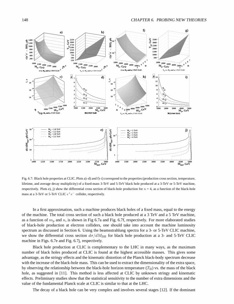
148 CHAPTER 6. PROBING NEW THEORIES
1000 1500 2000 2500 3000
34
56
200
400
600
800
1000
1200
1400
σ vs. MP and n, 3 TeV CLIC
MP, GeV n
σ(e+ e- →
BH
), p
b
a)
σ vs. MP and n, 3 TeV CLIC
1000 1500 2000 2500 3000
34
56
250500750
100012501500175020002250
TH vs. MP and n, 3 TeV CLIC
MP, GeV n
TH, G
eV
b)
1000150020002500300034 5 6
10-27
10-26
10-25
TH vs. MP and n, 3 TeV CLICM P, G
eVn
τ, s
c)
TH vs. MP and n, 3 TeV CLIC
0
1
2
3
4
5
6
7
1000 1500 2000 2500 3000
⟨N⟩, 3 TeV CLIC
MP, GeV
⟨N⟩
⟨N⟩, 3 TeV CLIC⟨N⟩, 3 TeV CLIC⟨N⟩, 3 TeV CLIC
n=2
n=3n=5
n=7
d)
1000 2000 3000 4000 50002
34
56
7
10 2
10 3
σ vs. MP and n, 5 TeV CLIC
MP, GeV n
σ(e+ e- →
BH
), p
b
f)
σ vs. MP and n, 5 TeV CLIC
1000 2000 3000 4000 50002
34
56
7500
100015002000
25003000
3500
TH vs. MP and n, 5 TeV CLIC
MP, GeV n
TH, G
eV
g)
10002000300040005000
23
45
67
10-27
10-26
10-25
TH vs. MP and n, 5 TeV CLICM P, G
eVnτ,
s
h)
0
2
4
6
8
10
12
14
1000 2000 3000 4000 5000
⟨N⟩, 5 TeV CLIC
MP, GeV
⟨N⟩
⟨N⟩, 5 TeV CLIC⟨N⟩, 5 TeV CLIC⟨N⟩, 5 TeV CLIC
n=2
n=3n=5n=7
i)
1
10
10 2
10 3
1000 1250 1500 1750 2000 2250 2500 2750 3000
e)
MBH, GeV
dσ/d
MB
H, p
b/G
eV
MP = 1.0 TeVMP = 1.5 TeVMP = 2.0 TeVMP = 2.5 TeV
1
10
10 2
1000 1500 2000 2500 3000 3500 4000 4500 5000
j)
MBH, GeV
dσ/d
MB
H, p
b/G
eV
MP = 1 TeVMP = 2 TeVMP = 3 TeVMP = 4 TeV
Fig. 6.7: Black hole properties at CLIC. Plots a)–d) and f)–i) correspond to the properties (production cross section, temperature,
lifetime, and average decay multiplicity) of a fixed-mass 3-TeV and 5-TeV black hole produced at a 3-TeV or 5-TeV machine,
respectively. Plots e), j) show the differential cross section of black-hole production forn = 4, as a function of the black-hole
mass at a 3-TeV or 5-TeV CLICe+e− collider, respectively.
In a first approximation, such a machine produces black holesof a fixed mass, equal to the energyof the machine. The total cross section of such a black hole produced at a 3 TeV and a 5 TeV machine,as a function ofmp andn, is shown in Fig 6.7a and Fig. 6.7f, respectively. For more elaborated studiesof black-hole production at electron colliders, one shouldtake into account the machine luminosityspectrum as discussed in Section 6. Using the beamsstrahlung spectra for a 3- or 5-TeV CLIC machine,we show the differential cross sectiondσ/dMBH for black hole production at a 3- and 5-TeV CLICmachine in Figs. 6.7e and Fig. 6.7j, respectively.
Black hole production at CLIC is complementary to the LHC in many ways, as the maximumnumber of black holes produced at CLIC is found at the highestaccessible masses. This gives someadvantage, as the stringy effects and the kinematic distortion of the Planck black-body spectrum decreasewith the increase of the black-hole mass. This can be used to extract the dimensionality of the extra space,by observing the relationship between the black-hole horizon temperature (TH) vs. the mass of the blackhole, as suggested in [11]. This method is less affected at CLIC by unknown stringy and kinematiceffects. Preliminary studies show that the statistical sensitivity to the number of extra dimensions and thevalue of the fundamental Planck scale at CLIC is similar to that at the LHC.
The decay of a black hole can be very complex and involves several stages [12]. If the dominant

1.. EXTRA DIMENSIONS 149
Fig. 6.8: Black hole production in a CLIC detector
mode is Hawking radiation, then all particles (quarks, gluons, gauge bosons, leptons) are expected tobe produced democratically, with, for instance, a ratio 1/5between leptonic and hadronic activity. Themultiplicity is expected to be large. The production and decay processes have been included in thePYTHIA generator [13]. Figure 6.8 shows two black-hole events produced in a detector at CLIC, leadingto spectacular multijet and lepton/photon signals. As an example, Fig. 6.9 shows the sphericity of theevents measured after detector simulation and addition of 5bunch crossings ofγγ background for blackholes and conventional annihilation events.
If this scenario is realized in nature, black holes will be produced at high rates at the LHC. CLICcan be very instrumental in providing precise measurements. For example, it may be possible to testHawking radiation or get information on the number of underlying extra dimensions.
Fig. 6.9: Black hole production in a CLIC detector: Sphericity distribution for 2- and 4-fermion events (full histogram) and
black holes (hatched histogram)

150 CHAPTER 6. PROBING NEW THEORIES
1
10
10 2
10 3
1000 1250 1500 1750 2000 2250 2500 2750 3000 3250 3500
Fig. 6.10: Left: The cross sectionσµµ for different models for TeV-scale extra dimensions. Right: The cross sectionσµµ before
(solid line) and after (dotted line) smearing by the CLIC luminosity spectrum.
1.4. Kaluza–Klein Excitations in Theories with Extra Dimensions
Another class of models that leads to a resonance structure in the energy dependence of the two-fermioncross section has a TeV-scale extra dimension [14]. In the simplest versions of these theories, only the SMgauge fields are in the bulk, whereas the fermions remain at one of the two orbifold fixed points; Higgsfields may lie at the fixed points or propagate in the bulk. In such a model, to a good approximation, themasses of the KK tower states are given byMn = nM , whereM = R−1 is the compactification scaleandR is the compactification radius.
1.4.1. Kaluza–Klein excitations in two-fermion processes
The masses and couplings of the KK excitations are compactification-scheme-dependent and lead toa rather complex KK spectrum. Examples of models with one or more extra dimensions, assumingM = 4 TeV, are shown in Fig. 6.10. The positions of the peaks and dips and their corresponding crosssections and widths can be used to identify uniquely the extra-dimensional model. As an example, one ofthese models was taken and the production cross section was folded with the CLIC luminosity spectrum.The result is shown in Fig. 6.10 for the dip position, since the peaks are likely to be beyond the reach of a3-TeV collider. The structure of the dip is largely preserved. It is smeared and somewhat systematicallyshifted, but also here the CLIC data will be sensitive to the model parameters, and will allow one todisentangle different scenarios.
Among the models with extra dimensions, we have studied a 5D extension of the SM with fermionson they = 0 brane of theS1/Z2 orbifold. This predicts KK excitations of the SM gauge bosons withfermion couplings a factor of
√2 larger than those of the SM [15]. We have considered two Higgs
bosons: one on they = 0 brane and the other propagating in the bulk. Indirect limits from electroweakmeasurements already exist and are derived by considering the modifications to the electroweak observ-ables at theZ0 peak and at low energy [16]. The masses of the lowest-lying KKstates are constrainedto be rather large, i.e. a few TeV, depending on the value ofβ, which is related to the ratio betweenthe vev’s of the two Higgs fields and consequently parametrizes the mixing between the KK excitationsand the SM gauge bosons. Bounds can be derived by consideringthe latest experimental values of theǫparameters coming from the precision measurement data [17]. The 95% C.L. lower bounds on the scale

1.. EXTRA DIMENSIONS 151
0 0.2 0.4 0.6 0.8 1
1500
2000
2500
3000
3500
4000
4500
5000
APV
M = 180 GeV
M = 98 GeV
H
H
M (
GeV
)
βsin
Fig. 6.11: 95% C.L. lower bounds on the compactification scale M , as functions ofsin β, from the high-energy precision
measurements (ǫ parameters) and from the APV data. The regions below the lines are excluded.
M at fixedsβ, coming from theǫ observables, are given by the upper curves in Figs. 6.11. Thetwocurves correspond tomt = 175.3 GeV withmH = 98 GeV and 180 GeV. The curve formH = 120 GeVis very close to the one formH = 98 GeV. Bounds can be also obtained from low-energy neutral-currentexperiments, for example, from the atomic parity-violation (APV) experiments. Nevertheless, they liesignificantly below the corresponding high-energy limits,and are shown by the lower curves in Fig. 6.12.Bounds can be derived from cross sections at LEP 2 energies. By combining with the precision data, the95% C.L. lower limit onM is around 6.8 TeV, while the expected sensitivity at the LHC for 100 fb−1 isaround 13–15 TeV, depending on the assumed systematics [18].
Fig. 6.12:µ+µ− production cross sections (left) and forward–backward asymmetry (right) in the 5D SM, including the lower
KK excitations of theZ0 andγ with MZ(1) ∼ Mγ(1) = 3 TeV. The continuous lines represent the Born-level expectations,
while the dots include the effect of the CLIC luminosity spectrum.
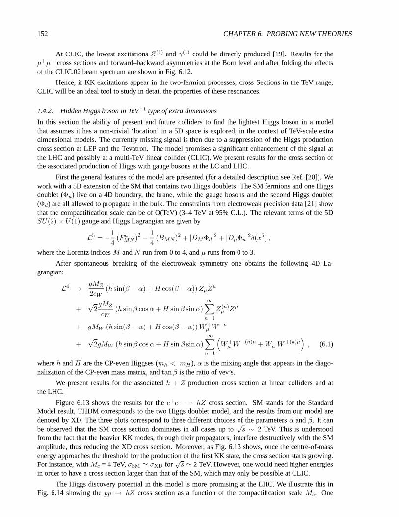
152 CHAPTER 6. PROBING NEW THEORIES
At CLIC, the lowest excitationsZ(1) andγ(1) could be directly produced [19]. Results for theµ+µ− cross sections and forward–backward asymmetries at the Born level and after folding the effectsof the CLIC.02 beam spectrum are shown in Fig. 6.12.
Hence, if KK excitations appear in the two-fermion processes, cross Sections in the TeV range,CLIC will be an ideal tool to study in detail the properties ofthese resonances.
1.4.2. Hidden Higgs boson in TeV−1 type of extra dimensions
In this section the ability of present and future colliders to find the lightest Higgs boson in a modelthat assumes it has a non-trivial ‘location’ in a 5D space is explored, in the context of TeV-scale extradimensional models. The currently missing signal is then due to a suppression of the Higgs productioncross section at LEP and the Tevatron. The model promises a significant enhancement of the signal atthe LHC and possibly at a multi-TeV linear collider (CLIC). We present results for the cross section ofthe associated production of Higgs with gauge bosons at the LC and LHC.
First the general features of the model are presented (for a detailed description see Ref. [20]). Wework with a 5D extension of the SM that contains two Higgs doublets. The SM fermions and one Higgsdoublet (Φu) live on a 4D boundary, the brane, while the gauge bosons and the second Higgs doublet(Φd) are all allowed to propagate in the bulk. The constraints from electroweak precision data [21] showthat the compactification scale can be of O(TeV) (3–4 TeV at 95% C.L.). The relevant terms of the 5DSU(2) × U(1) gauge and Higgs Lagrangian are given by
L5 = −1
4(F aMN )2 − 1
4(BMN )2 + |DMΦd|2 + |DµΦu|2δ(x5) ,
where the Lorentz indicesM andN run from 0 to 4, andµ runs from 0 to 3.
After spontaneous breaking of the electroweak symmetry oneobtains the following 4D La-grangian:
L4 ⊃ gMZ
2cW(h sin(β − α) +H cos(β − α))ZµZ
µ
+√
2gMZ
cW(h sin β cosα+H sinβ sinα)
∞∑
n=1
Z(n)µ Zµ
+ gMW (h sin(β − α) +H cos(β − α))W+µ W
−µ
+√
2gMW (h sin β cosα+H sin β sinα)
∞∑
n=1
(W+µ W
−(n)µ +W−µ W+(n)µ
), (6.1)
whereh andH are the CP-even Higgses (mh < mH ), α is the mixing angle that appears in the diago-nalization of the CP-even mass matrix, andtan β is the ratio of vev’s.
We present results for the associatedh + Z production cross section at linear colliders and atthe LHC.
Figure 6.13 shows the results for thee+e− → hZ cross section. SM stands for the StandardModel result, THDM corresponds to the two Higgs doublet model, and the results from our model aredenoted by XD. The three plots correspond to three differentchoices of the parametersα andβ. It canbe observed that the SM cross section dominates in all cases up to
√s ∼ 2 TeV. This is understood
from the fact that the heavier KK modes, through their propagators, interfere destructively with the SMamplitude, thus reducing the XD cross section. Moreover, asFig. 6.13 shows, once the centre-of-massenergy approaches the threshold for the production of the first KK state, the cross section starts growing.For instance, withMc = 4 TeV,σSM ≃ σXD for
√s ≃ 2 TeV. However, one would need higher energies
in order to have a cross section larger than that of the SM, which may only be possible at CLIC.
The Higgs discovery potential in this model is more promising at the LHC. We illustrate this inFig. 6.14 showing thepp → hZ cross section as a function of the compactification scaleMc. One

1.. EXTRA DIMENSIONS 153
Fig. 6.13: SM, THDM and XD cross Sections fore+e− → Zh. Each plot corresponds to a different set of values forα andβ,
all withmh = 120 GeV and with a compactification scaleMc = 4 TeV.
sees from the figure that depending on the particular values of α andβ the enhancement is more or lesspronounced. But independently from the values ofα, β (and the KK width), the XD production crosssection is considerably enhanced with respect to the SM forMc . 6 TeV. For certain parameter valuesthere is an enhancement even up toMc ∼ 8 TeV.
The singularity atRA(s) = 1 is regulated by the width of the KK mode, which is not includedin our calculation. Thus, the peak region in Fig. 6.14 is onlycorrect in the order of magnitude. Yet,since the width of thenth KK mode Γn ∼ 2αemmn is rather small (sinceαem is small), the largeenhancement is expected to prevail after the inclusion of the width. For particularα andβ values itmight also happen that there is a cancellation among the terms containing the KK state information(see Ref. [20]). This cancellation also depends on the centre-of-mass energys andMc and happens closeto 8.5 TeV in Fig. 6.14.
In summary, we presented a model that accounts for the missing Higgs signal. Furthermore, themodel promises an enhanced signal at the LHC or CLIC. It assumes one extra dimension and two Higgsdoublets, one fixed to a brane and the other living in the bulk.The lightest CP-even scalar may be amixing of the two and this non-trivial ‘location’ is the key ingredient in the suppression–enhancementof the discovery signal. We presented the results for the associated production cross sections at linearcolliders and the LHC.
Fig. 6.14: Higgs production cross section in association with aZ boson as a function of the compactification scale for selected
values of the mixing parameters. For reference the SM cross section is shown with a 10% uncertainty band around it.

154 CHAPTER 6. PROBING NEW THEORIES
1.5. Universal Extra Dimensions
Supersymmetry and extra dimensions offer two different paths to a theory of new physics beyond the SM.They both address the hierarchy problem, play a role in a morefundamental theory aimed at unifying theSM with gravity, and offer a candidate particle for dark matter, which is compatible with cosmologicaldata. If either supersymmetry or extra dimensions exist at the TeV scale, signals of new physics arebound to be found by the ATLAS and CMS experiments at the LHC. However, the proper interpretationof such discoveries, namely the correct identification of the nature of the new physics signals, maynot be straightforward at the LHC. It may have to be complemented by the data of a multi-TeVe+e−
colliders, such as CLIC [22].
A particularly interesting scenario is offered by Universal Extra Dimensions (UEDs), as originallyproposed in [23]. It bears interesting analogies to supersymmetry1, and has sometimes been referred toas ‘bosonic supersymmetry’ [24]. In principle, disentangling UED and supersymmetry may be highlynon-trivial at hadron colliders. For each SM particle, theyboth predict the existence of a partner (orpartners) with identical interactions. As the masses of these new particles are model-dependent, theycannot be used to discriminate between the two theories.
At the LHC, strong processes dominate the production in either case. The resulting signaturesinvolve relatively soft jets, leptons and missing transverse energy [24]. The study in [24] shows that, with100 fb−1 of integrated luminosity, the LHC experiments will be able to cover all of the cosmologicallypreferred parameter space in UED [25]. However, the discrimination between UED and supersymmetryappears very difficult at the LHC.
In fact, there are only three fundamental differences between UED and supersymmetry. In thecase of extra dimensions, there is an infinite tower of KK partners, labelled by their KK leveln, while insupersymmetry, there is just a single superpartner for eachSM particle. However, it is possible that thesecond and higher KK levels are too heavy to be observed. The second fundamental distinction betweenUED and supersymmetry is the fact that the KK partners have identical spin quantum numbers, whilethose of the superpartners differ by1/2. Unfortunately, spin determinations also appear to be difficultat the LHC. Finally, supersymmetry has an extended Higgs sector and gaugino states, which have nocounterparts in the UED model. However, it is possible that these heavier Higgs bosons and gauginosare too heavy to be observed.
In its simplest incarnation, the UED model has all the SM particles propagating in a single extradimension of sizeR, which is compactified on anS1/Z2 orbifold. A peculiar feature of UED is theconservation of the KK number at tree level, which is a simpleconsequence of momentum conserva-tion along the extra dimension. However, bulk and brane radiative effects [26–28] break the KK numberdown to a discrete conserved quantity, the so-called KK parity, (–1)n, wheren is the KK level. KK parityensures that the lightest KK partners — those at level one — are always pair-produced in collider exper-iments, similar to the case of supersymmetry models with conservedR-parity. KK-parity conservationalso implies that the contributions to various precisely measured low-energy observables [29–35] onlyarise at the one-loop level and are small. In the minimal UED model, the boundary terms are assumedto vanish at the cutoff scaleΛ, and are subsequently generated through RGE evolution to lower scales.Thus the minimal UED model has only two input parameters: thesize of the extra dimensionR andthe cutoff scaleΛ.
In order to study the discrimination of UED signals from supersymmetry at CLIC, we concen-trate on the pair production of level-1 KK muonse+e− → µ+
1 µ−1 , and compare it to the analogous
process of smuon pair production in supersymmetry:e+e− → µ+µ−. In UED there are twon = 1 KKmuon Dirac fermions: anSU(2)W doubletµD1 and anSU(2)W singletµS1 , both of which contribute.In complete analogy, in supersymmetry, there are two smuon eigenstates,µL and µR, both of which
1More precisely, the phenomenology of the first level of KK modes in UEDs is very similar to that ofN = 1 supersymmet-ric models, with a somewhat degenerate superpartner spectrum and a stable lightest supersymmetric particle (LSP). In whatfollows, we shall use the term ‘supersymmetry’ in this somewhat narrower context.

1.. EXTRA DIMENSIONS 155
contribute ine+e− → µ+µ−.
We first fix the UED parameters toR−1 = 500 GeV, RΛ = 20, corresponding to the spectrumgiven in Table 6.1.
Table 6.1: Masses of the KK excitations for the parametersR−1 = 500 GeV andΛR = 20 used in the analysis
Particle Mass
(GeV)
µD1 515.0
µS1 505.4
γ1 500.9
This analysis has backgrounds coming from SMµ+µ−νν final states, which are mostly dueto gauge-boson pair productionW+W− → µ+µ−νµνµ, Z0Z0 → µ+µ−νν and from e+e− →W+W−νeνe, e+e− → Z0Z0νeνe, followed by muonic decays. The total cross Sections are≃ 20 fb and≃ 2 fb, respectively. In addition to its competitive cross section, this background has leptons producedpreferentially at small polar angles, therefore biasing the UED/MSSM discrimination. In order to reducethe background, a suitable event selection has been appliedbased on the missing energy, the transverseenergy and the event sphericity, which provides a factor≃ 5 background suppression in the kinematicalregion of interest. It does not bias the lepton-momentum distribution. The estimated background fromγγ → hadrons appears to be negligible for muon energies above 2.5 GeV.
The angular distributions in UED and supersymmetry are sufficiently distinct to discriminate thetwo cases. However, the polar anglesθ of the original KK muons and smuons are not directly observable,and the production polar anglesθµ of the final-state muons are measured instead. As long as the massdifferencesMµ1−Mγ1 andMµ−Mχ0
1, respectively, remain small, the muon directions are well correlated
with those of their parents (see Fig. 6.15a). In Fig. 6.15b weshow the same comparison after detector
0
250
500
750
1000
1250
1500
1750
2000
-1 -0.5 0 0.5 1
Ent
ries
/ 1 a
b-1
cos θµ
0
50
100
150
200
250
300
350
-1 -0.5 0 0.5 1
Fig. 6.15: Differential cross sectiondσ/d cos θµ for UED (blue, top) and supersymmetry (red, bottom) as a function of the
muon scattering angleθµ. We have chosenR−1 = 500 GeV andΛR = 20 and then adjusted the SUSY-breaking parameters
until we get a perfect spectrum match. The figure on the left isthe ISR-corrected theoretical prediction, while the result on the
right incorporates a detector simulation.

156 CHAPTER 6. PROBING NEW THEORIES
pµ (GeV)
Ent
ries
/ 1 a
b-1
0
250
500
750
1000
1250
1500
1750
2000
0 20 40 60 80 100
Fig. 6.16: The muon energy spectrum resulting from KK muon production in UED (blue, top curve) and smuon production in
supersymmetry (red, bottom curve), for the same UED and supersymmetry parameters in Fig. 6.15. The figure on the left is the
ISR-corrected theoretical prediction, whilst the result on the right shows the distribution after detector simulation and including
the background contribution.
simulation and including the SM background. The angular distributions are still easily distinguishableafter accounting for these effects. By performing aχ2 fit to the normalized polar-angle distribution,the UED scenario considered here could be distinguished from the MSSM, solely on the basis of thedistribution shape, with 350 fb−1 of data.
Further methods to distinguish between SUSY and UED are the production cross section and athreshold scan. The cross section for the UED processes rises at thresholds∝ β, while in supersymmetrytheir threshold onset is∝ β3. Furthermore the cross section for the UED process is about 5times largercompared to the smuon production in supersymmetry, for these masses.
The muon energy spectrum is completely determined by the kinematics of the two-body decay, andis therefore equivalent for the case of UED and of supersymmetry, if the relevant MSSM particle massesare properly tuned. We show the ISR-corrected expected distributions for the muon energy spectra atgenerator level in Fig. 6.16 (left), using the same parameters as in Fig. 6.15. We observe that the shapeof theEµ distribution in the case of the UED coincides with that for MSSM.
In Fig. 6.16 (right) we show the muon energy distribution after detector simulation. The end-points can be used to extract the masses by a three-parameterfit to this distribution. A one-parameterfit, assuming the mass of theγ1 state is known, gives an uncertainty on theµ1 mass of± 0.25 GeV for1 ab−1 of statistics.
2. New Vector Resonances
Many scenarios of NP predict the existence of new particles that would manifest themselves as ratherspectacular resonances ine+e− collisions, if the achievable centre-of-mass energy is sufficient. A high-energy LC represents an ideal laboratory for studying this NP. Signals from NP that can be probed bya collider such as CLIC at 1 TeV<
√s < 5 TeV, belong to a rather large domain. The most striking
manifestation of NP in the multi-TeV region would come from asudden increase of thee+e− → f fcross section indicating thes-channel production of a new particle. The experimental study of suchresonances at a multi-TeV collider will have to accurately measure their masses, widths, production anddecay properties to determine their nature and identify which kind of NP has been manifested. Thereare several theories that predict the existence of new vector resonances. A prominent class consists ofmodels with extra gauge bosons such as a new neutralZ ′ gauge boson.

2.. NEW VECTOR RESONANCES 157
2.1. Extra-Z′ Boson Studies
One of the simplest extensions of the SM consists of an additional U(1) gauge symmetry broken ata scale close to the Fermi scale. This extra symmetry is predicted in both GUT-inspiredE6 modelsand in left–right-symmetric models. For example, inE6 scenarios we have an additionalU(1) currentJfZ′µ = Jfχµcos θ6 +Jfψµsin θ6 with different models parametrized by specific values of theangleθ6. The
valuesθ6 = 0, θ6 = π/2 andθ6 = − tan−1√
5/3 are called theχ,ψ andη models, respectively. In theLR models, the newZLR boson couples to the currentJZ′µ = αLRJ3Rµ−1/(2αLR)J(B−L)µ with αLR =√g2R/g
2L cot2 θW − 1. The vector- and axial-vector couplings of theZ ′ boson to the SM fermions,
for E6-inspired and for LR models, are given in Table 6.2, assumingJfZ′µ = f[γµv′f + γµγ5a
′f
]f
and the parametrizationθ2 = θ6 + tan−1√
5/3. Finally, a useful reference is represented by the so-called sequential standard model (SSM), which introduces an extraZ ′ boson with the same couplings asthe SMZ0 boson.
Table 6.2: Vector and axial-vector couplings for theE6-inspired and LR models, withsθ = sin θ, s2 = sin θ2, c2 = cos θ2,
c2θ = cos 2θ, with θ2 = θ6 + tan−1√
5/3 andθ ≡ θW
Extra -U(1) LR (gL = gR)
v′e = −14sθ
(c2 +
√53s2
)v′e =
(−1
4 + s2θ)/√c2θ
a′e = 14sθ
(−1
3c2 +√
53s2
)a′e = −1
4
√c2θ
v′u = 0 v′u =(
14 − 2
3s2θ
)/√c2θ
a′u = −13sθc2 a′u = 1
4
√c2θ
v′d = 14sθ
(c2 +
√53s2
)v′d =
(−1
4 + 13s
2θ
)/√c2θ
a′d = a′e a′d = a′e
There exist several constraints on the properties of new neutral vector gauge bosons. Directsearches for a newZ ′ boson set lower limits on the masses [36]. These are summarized in Table 6.3for various models. An extraZ ′ naturally mixes with the SMZ0 boson. The present precision elec-troweak data constrain the mixing angleθM within a few mrad, and the allowed masses are shownin Table 6.3 [37,38].
Table 6.3: The 95% C.L. limits onMZ′ (GeV) fromσ(pp → Z′)B(Z′ → ll) (CDF data) and from the average of the four
LEP experiments, for the mixing angleθM = 0
χ ψ η LR SSM
CDF 595 590 620 630 690
LEP 673 481 434 804 1787

158 CHAPTER 6. PROBING NEW THEORIES
A third class of constraints can be derived from the atomic-parity violation (APV) data [19, 39],since models involving extra neutral vector bosons can modify theQW value significantly. The presentvalue ofQW extracted from the caesium data differs by only≃ 0.8σ from the SM prediction. Wenote that there exist improved predictions ofQW in the SM, which account for the effect of the Breitinteraction among electrons and have a refined calculation of the radiative corrections [40].
Assuming noZ0–Z ′ mixing, we can evaluate the contribution to the weak charge due to the directexchange of theZ ′ and derive bounds onMZ′ . The 95% C.L. limit from APV onMZ′ for theχ, η, LRand SSM models are 627, 476, 665 and 1010 GeV respectively [19], while no bounds can be set on theψ model by the APV measurements. These are less stringent than, or comparable to, those from the LEPexperiments. However, as these bounds are very sensitive tothe actual value ofQW and its uncertainties,further determinations may improve the sensitivity.
The LHC will push the direct sensitivity to new vector gauge bosons past the TeV threshold. Withan integrated luminosity of 100 fb−1, ATLAS and CMS are expected to observe signals fromZ ′ bosonsfor masses up to 4–5 TeV, depending on the specific model [41].
Extra-U(1) models can be accurately tested at CLIC. With an expected effective production crosssectionσ(e+e− → Z ′SSM) of ≃ 15 pb, including the effects of ISR and luminosity spectrum,a Z ′
resonance will tower over aqq continuum background of≃ 0.13 pb. Whilst the observability of sucha signal is guaranteed, the accuracy that can be reached in the study of its properties depends on thequality of the accelerator beam-energy spectrum and on the detector response, including accelerator-induced backgrounds. One of the main characteristics of theCLIC collider is the large design luminosity,L = 1035 cm−2 s−1 at
√s = 3 TeV for its baseline parameters, obtained in a regime of strong beam-
strahlung effects. The optimization of the total luminosity and its fraction in the peak has been studiedfor the case of a resonance scan. The CLIC luminosity spectrum has been obtained with a dedicatedbeam simulation program [42], as discussed in Chapter 3, forthe nominal parameters at
√s = 3 TeV.
In order to study the systematic uncertainties in the knowledge of this spectrum, the modified Yokoya–Chen parametrization [43] has been adopted. In this formulation, the beam energy spectrum is describedin terms ofNγ , the number of photons radiated pere± in the bunch, the beam energy spread in thelinac σp and the fractionF of events outside the 0.5% of the centre-of-mass energy. Twosets of pa-rameters have been considered, obtained by modifying the beam size at the interaction point and there-fore the total luminosity and its fraction in the highest energy region of the spectrum: CLIC.01 withL = 1.05× 1035 cm−2 s−1 andNγ = 2.2 and CLIC.02 withL = 0.40× 1035 cm−2 s−1 andNγ = 1.2.TheZ ′ mass and width can be determined by performing either an energy scan, like theZ0 line-shapescan performed at LEP/SLC, or an autoscan, by tuning the collision energy just above the top of theresonance and profiting from the long tail of the luminosity spectrum to probe the resonance peak.
For the first method, both dijet and dilepton final states can be considered, while for the au-toscan onlyµ+µ− final states can provide the necessary accuracy for theZ ′ energy. We have generatede+e− → Z ′ events forMZ′ = 3 TeV, including the effects of ISR, the luminosity spectrum andγγ back-grounds, assuming SM-like couplings, corresponding to a total width ΓZ′
SSM≃ 90 GeV. The resonance
widths for extra-U(1) models as well as for other SM extensions with additional vector bosons are shownin Fig. 6.17 as a function of the relevant model parameters.
A data set of 1 ab−1 has been assumed for the CLIC.01 beam parameters and of 0.4 ab−1 forCLIC.02, corresponding to one year ( = 107 s) of operation at nominal luminosity. This has been sharedin a five-point scan, as seen in Fig. 6.17, andMZ′ , ΓZ′/ΓZ0 andσpeak have been extracted from aχ2 fitto the predicted cross section behaviour for different massand width values (see Table 6.4) [45]. The di-lution of the analysing power due to the beam energy spread isappreciable, as can be seen by comparingthe statistical accuracy from a fit to the pure Born cross section after including ISR and beamstrahlung ef-fects. Still, the relative statistical accuracies are better than 10−4 on the mass and 5× 10⁻³ on the width.In the case of wide resonances, there is an advantage in employing the broader luminosity spectrum ofCLIC.01, which offers larger luminosity. Sources of systematics from the knowledge of the shape of the

2.. NEW VECTOR RESONANCES 159
Γ (G
eV)
10−1
1
Model Parameter
10
102
0 0.2 0.4 0.6 0.8 1 1.2 1.4
E (GeV)
σ (
fb)
0
400
800
1200
1600
2900 2950 3000 3050 3100
Fig. 6.17: Left: Widths of new gauge vector bosons as functions of the relevant parameters:θ2 for Z′E6
, λ = gL/gR for
Z′LR [44], g/g′′ for D-BESS. The KKZ(1) width has a negligible dependence on the mixing anglesin β. TheZ′
E6andZ′
LR
widths are computed by assuming only decays into SM fermions. Right: TheZ′SSM → ℓ+ℓ− resonance profile obtained by
an energy scan. The Born production cross section, the crosssection with ISR included and that accounting for the CLIC
luminosity spectrum (CLIC.01) and tagging criteria are shown.
luminosity spectrum have also been estimated. In order to keepσsyst ≤ σstat it is necessary to controlNγ to better than 5% and the fractionF of collisions at
√s < 0.995
√s0 to about 1% [46].
Table 6.4: Results of fits for the cross-Section scan of aZ′SSM obtained by assuming no radiation and ISR with the effects of
two different choices of the CLIC luminosity spectrum
Observable Breit–Wigner CLIC.01 CLIC.02
MZ′ (GeV) 3000± .12 ± .15 ± .21
ΓZ′/ΓZ0 1. ± .001 ± .003 ± .004
σeffpeak (fb) 1493± 2.0 564± 1.7 669± 2.9
2.2. Heavy Majorana Neutrinos inZ′ Decays
If neutrinos are Majorana particles, then the left–right-symmetric model and the see-saw mechanism [47]may provide an explanation for the lightness of the left-handed neutrinos, by introducing heavy right-handed neutrinos,Nl. The LHC is expected to discover these new particles after three years of operationat high luminosity, mostly throughpp → WR → lNl, if m(Nl) andm(WR) are smaller than 4 and6 TeV, respectively [48]. At CLIC, the resonant production of Z ′LR → NeNe may lead to signal ratesup to about three orders of magnitude higher than forpp → Z ′LR → NeNe at LHC energies. Thisprocess has been studied using the fast detector simulation[49]. SinceNe is expected to decay promptlyinto e± and aqiqj pair, two electrons of equal charge and four quarks in the final state are the decaysignature. Theγγ background may induce a shift of theZ ′ andNe invariant mass peaks towards highermasses. In order to reduce this effect a kinematical fit can beapplied after the reconstruction procedure.It requires that the twoNe candidates have equal mass, the system consisting of the twoelectrons and the

160 CHAPTER 6. PROBING NEW THEORIES
0
2500
5000
7500
10000
12500
15000
17500
20000
22500
2500 2750 3000 3250 3500 3750
With γγ → hadrons after correctionsmrec(Z') = 2991.0 GeV/c2
before correctionsmrec(Z') = 3076.1 GeV/c2
minv(eejjjj) in GeV/c2
N /
10 G
eV.c-2
0
2500
5000
7500
10000
12500
15000
17500
20000
22500
500 750 1000 1250 1500 1750
With γγ → hadrons after correctionsmrec(Ne) = 1006.6 GeV/c2
before correctionsmrec(Ne) = 1034.0 GeV/c2
(minv(e1jajb)+minv(e2jcjd))/2 in GeV/c2
N /
10 G
eV.c-2
Fig. 6.18: Signature of Majorana neutrinos. The left plot shows the reconstructed 3 TeVZ′ boson before and after the kinemat-
ical fit, and the right plot shows the reconstructed 1 TeV Majorana neutrino before and after the kinematical fit for an integrated
luminosity of 1 ab−1.
four leading hadronic jets have a zero transverse momentum,the momentum and energy conservation at√s = 3 TeV. These corrections allow a good reconstruction ofZ ′LR andNe, as shown in Fig. 6.18.
3. Indirect Sensitivity to New Physics
The direct reach for the mass scales of new phenomena provided by CLIC are in many cases compa-rable to those provided by the LHC. However, CLIC would be able to explore more details of any newprocesses, possibly allowing one to determine better the nature of the new physics discovered. Withthe centre-of-mass energies and the luminosity envisionedfor CLIC, a new era of precision physics isapproaching. Precision electroweak measurements performed in multi-TeVe+e− collisions will pushthe indirect sensitivity to new mass scales beyond the 10 TeVfrontier.
We review here the sensitivity to new gauge bosonsZ ′, to KK excitations of the SM gauge bosonsand to contact interactions [45, 50], as examples of the anticipated potential of CLIC. These results arebased on studies of the two-fermion (µ+µ−, bb and tt) production cross sections,σff , and forward–
backward asymmetries,AffFB.
At CLIC design centre-of-mass energies, the relevante+e− → f f cross sections are significantlyreduced with respect to those at present-day energies, and the experimental conditions in the interactionregion need to be taken into account in validating the accuracies on electroweak observables. Sincetwo-fermion cross sections are of the order of only 10 fb, it is imperative to operate the collider at highluminosity. This can be achieved only in a regime where beam–beam effects are important and primarye+e− collisions are accompanied by severalγγ → hadrons interactions. Being mostly confined inthe forward regions, thisγγ background reduces the polar-angle acceptance for quark-flavour tagging,and dilutes the possible jet-charge separation. These experimental conditions require efficient and robustalgorithms to ensure sensitivity to flavour-specificf f production.
The statistical accuracies for the determination ofσff andAffFB have been studied using a realisticsimulation. For example, the identification ofbb final states was based on the sampling of the chargedmultiplicity in decays of highly-boostedb hadrons at CLIC energies [51]. Similarly to LEP analyses,the forward–backward asymmetry forbb has been extracted from a fit to the flow of the jet charge

3.. INDIRECT SENSITIVITY TO NEW PHYSICS 161
Table 6.5: Relative statistical accuracies on electroweakobservables obtainable for 1 ab−1 of CLIC data at√s = 3 TeV,
including the effect of theγγ → hadrons background
Observable Relative stat. accuracy
δO/O for 1 ab−1
σµ+µ− ± 0.010
σbb ± 0.012
σtt ± 0.014
AµµFB ± 0.018
AbbFB ± 0.055
AttFB ± 0.040
Qjet, defined asQjet =∑i qi|~pi·~T |k∑i |~pi·~T |k
, whereqi is the particle charge,~pi its momentum,~T the jet thrust
unit vector,k a positive number, and the sum is extended to all the particles in a given jet. Here thepresence of additional particles, from theγγ background, causes a broadening of theQjet distributionand thus a dilution of the quark charge separation. The trackselection and the value of the powerparameterk need to be optimized as a function of the number of overlaid bunch crossings. Results forthe e+e− → tt channel have been obtained using a dedicated top tagging algorithm [52]. This usesan explicit reconstruction of thet → bW decay and also includes the physics and machine-inducedbackgrounds. Fortt forward–backward asymmetries, the sign of the lepton from the W± → ℓ±νdecay has been used. The results are summarized in terms of the relative statistical accuraciesδO/Oin Table 6.5.
However, it is important to stress that, at the energy scalesconsidered here, electroweak virtualcorrections are strongly enhanced by Sudakov double logarithms of the typelog2(s/M2
W ). Until a com-plete two-loop result settles the problem, a theoretical error on the cross Section of the order of a percent could be considered [53]. We have not included it in the present analyses. This issue is discussed indetail in the next section.
The indirect sensitivity of a LC to theZ ′ massMZ′ can be parametrized in terms of the availableintegrated luminosityL and the centre-of-mass energy
√s. A scaling law for largeMZ′ can be obtained
by considering the effect of theZ ′–γ interference in the cross section. Fors ≪ M2Z′ and assuming that
the uncertaintiesδσ are statistically dominated, we can infer the range of mass values that would give asignificant difference from the SM prediction:
|σSM − σSM+Z′ |δσ
∝ 1
M2Z′
√sL >
√∆χ2, (6.2)
and the sensitivity to theZ ′ mass scales as:
MZ′ ∝ (sL)1/4. (6.3)
This relation points to the direct trade-off possible between√s andL. This needs to be taken into
account in the optimization of the parameters of a high-energy e+e− linear collider.
Theσff andAffFB (f = µ, b, t) values have been computed for 1 TeV<√s < 5 TeV, both in the
SM and including the corrections due to the presence of aZ ′ boson with 10 TeV< MZ′ < 40 TeV, with

162 CHAPTER 6. PROBING NEW THEORIES
E (TeV)
L (
ab−
1 ) M (TeV)20 30 40
SSM
0.5
1
1.5
2
2.5
3
3.5
4
4.5
5
1 1.5 2 2.5 3 3.5 4 4.5 5
E (TeV)
M (TeV)10 20
E6 − χ
0.5
1
1.5
2
2.5
3
3.5
4
4.5
5
1 1.5 2 2.5 3 3.5 4 4.5 5
Fig. 6.19: The 95% C.L. sensitivity contours in theL vs.√s plane for different values ofMZ′ in the SSM model (left) and in
theE6 χ model (right). The points represent the results of the analysis, while the curves show the behaviour expected from the
scaling suggested in (6.3).
couplings defined by the models discussed in Section 2. Predictions have been obtained by implementingthese models in the COMPHEPprogram [54]. Relative statistical errors on the electroweak observablesare obtained by rescaling the values of Table 6.5 for different energies and luminosities. The sensitivityhas been defined as the largestZ ′ mass, giving a deviation of the actual values of the observables fromtheir SM predictions corresponding to a SM probability of less than 5%. The SM probability has beendefined as the minimum of the global probability computed forall the observables and that for each ofthem taken independently.
This sensitivity has been determined, as a function of the√s energy and integrated luminosity
L, and compared to the scaling in (6.3). Results are summarized in Fig. 6.19. For theη model thesensitivity is lower. To reach the sensitivity ofMZ′ = 20 TeV, more than 10 ab−1 of data at
√s = 5 TeV
are necessary.
In the case of the 5D SM, we have included only the effects of the exchange of the first KKexcitationsZ(1) andγ(1), neglecting those of the remaining excitations of the towers, which give onlysmall corrections. The scaling law for the limit onM can be obtained by considering the interference ofthe two new nearly degenerate gauge bosons with the photon inthe cross section and taking thes≪M2
limit. The result is the same as (6.3). The analysis closely follows that for theZ ′ boson discussed above.In Fig. 6.20 we give the sensitivity contours as a function of
√s for different values ofM . We conclude
that the achievable sensitivity to the compactification scaleM for an integrated luminosity of 1 ab−1 ine+e− collisions at
√s = 3–5 TeV is of the order of 40–60 TeV. Results of a similar analysis, including
all electroweak observables, are discussed in Ref. [55].
An important issue concerns the ability to probe the models,if a significant discrepancy from theSM predictions were to be observed. Since the model parameters and the mass scale area priori arbitrary,an unambiguous identification of the realized scenario is difficult. However, some information can beextracted by testing the compatibility of different modelswhile varying the mass scale. Figure 6.21shows an example of such a test. TakingM = 20 TeV,L = 1 ab−1 of CLIC data at
√s = 3 TeV could
distinguish the SSM model from theE6 χ model at 86% C.L. and from the 5D SM at 99% C.L. Fora mass scale of 40 TeV,L = 3 ab−1 of CLIC data at
√s = 5 TeV, the corresponding confidence levels

3.. INDIRECT SENSITIVITY TO NEW PHYSICS 163
E2 (GeV )
M = 60 TeV
M = 40 TeV
2
∆σ/ σ
−0.25
−0.2
−0.15
−0.1
−0.05
0
0 500 1000 1500 2000 2500 3000
x 104 E (TeV)
M (TeV)40 60
5D SM
0.5
1
1.5
2
2.5
3
3.5
4
4.5
5
1 1.5 2 2.5 3 3.5 4 4.5 5
Fig. 6.20: Left: Scaling of the relative change in thee+e− → bb cross section, in the 5D SM, as a function of the square of the
centre-of-mass energy, for two values of the compactification scaleM . Right: The 95% C.L. sensitivity contours in theL vs.√s plane for different values of the compactification scaleM in the 5D SM. The points represent the results of the analysis,
while curves show the behaviour expected from the scaling suggested in (6.3).
become 91% and 99%, respectively. Further sensitivity to the nature of the gauge bosons could beobtained by studying the polarized forward–backward asymmetry Apol
FB and the left–right asymmetryALR using colliding polarized beams.
The scenarios investigated above address specific models ofnew physics beyond the SM. Fermioncompositeness or exchanges of very heavy new particles can be described in all generality by four-fermion contact interactions [56]. These parametrize the interactions beyond the SM in terms of aneffective scaleΛij:
LCI =∑
i,j=L,R
ηijg2
Λ2ij
(eiγµei)(fjγ
µfj) . (6.4)
The strength of the interaction is set by convention asg2/4π = 1, and models can be considered bychoosing either|ηij | = 1 or |ηij | = 0 as detailed in Table 6.6. The contact scaleΛ can be interpreted as aneffect of new particles at a massMX : 1/Λ2 ∝ λ2/M2
X .
Table 6.6: Definition of different models of contact interaction
Model LL RR LR RL VV AA V0 A0
ηLL ± 1 0 0 0 ± 1 ± 1 ± 1 0
ηRR 0 ± 1 0 0 ± 1 ± 1 ± 1 0
ηLR 0 0 ± 1 0 ± 1 ∓ 1 0 ± 1
ηRL 0 0 0 ± 1 ± 1 ∓ 1 0 ± 1
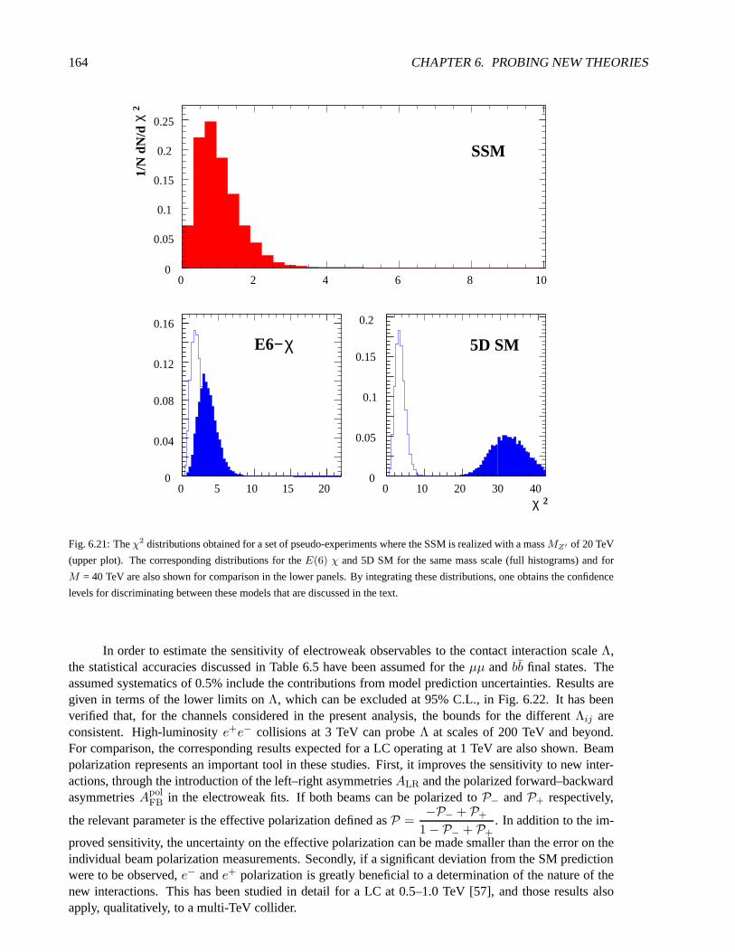
164 CHAPTER 6. PROBING NEW THEORIES
0
0.05
0.1
0.15
0.2
0.25
0 2 4 6 8 10
0
0.04
0.08
0.12
0.16
0 5 10 15 20
SSM1/
N d
N/d
χ2
E6−χ 5D SM
χ 2
0
0.05
0.1
0.15
0.2
0 10 20 30 40
Fig. 6.21: Theχ2 distributions obtained for a set of pseudo-experiments where the SSM is realized with a massMZ′ of 20 TeV
(upper plot). The corresponding distributions for theE(6) χ and 5D SM for the same mass scale (full histograms) and for
M = 40 TeV are also shown for comparison in the lower panels. By integrating these distributions, one obtains the confidence
levels for discriminating between these models that are discussed in the text.
In order to estimate the sensitivity of electroweak observables to the contact interaction scaleΛ,the statistical accuracies discussed in Table 6.5 have beenassumed for theµµ andbb final states. Theassumed systematics of 0.5% include the contributions frommodel prediction uncertainties. Results aregiven in terms of the lower limits onΛ, which can be excluded at 95% C.L., in Fig. 6.22. It has beenverified that, for the channels considered in the present analysis, the bounds for the differentΛij areconsistent. High-luminositye+e− collisions at 3 TeV can probeΛ at scales of 200 TeV and beyond.For comparison, the corresponding results expected for a LCoperating at 1 TeV are also shown. Beampolarization represents an important tool in these studies. First, it improves the sensitivity to new inter-actions, through the introduction of the left–right asymmetriesALR and the polarized forward–backwardasymmetriesApol
FB in the electroweak fits. If both beams can be polarized toP− andP+ respectively,
the relevant parameter is the effective polarization defined asP =−P− + P+
1 − P− + P+. In addition to the im-
proved sensitivity, the uncertainty on the effective polarization can be made smaller than the error on theindividual beam polarization measurements. Secondly, if asignificant deviation from the SM predictionwere to be observed,e− ande+ polarization is greatly beneficial to a determination of thenature of thenew interactions. This has been studied in detail for a LC at 0.5–1.0 TeV [57], and those results alsoapply, qualitatively, to a multi-TeV collider.

3.. INDIRECT SENSITIVITY TO NEW PHYSICS 165
0 100 200 300 [TeV]
LL
RR
RL
LR
VV
AA
V0
A0
1 ab-1, P-=0.8, e+e−→µ+µ-
CLIC(3 TeV): P+=0.6, ∆sys=0.5%, ∆L=0.5%
LC (1TeV): P+=0.6, ∆sys=0.2%, ∆L=0.5%
∆P/P=0.5%
0
10
0
20
0
30
0
40
0
[TeV]
LL
RR
RL
LR
VV
AA
V0
A0
1 ab-1, P-=0.8, e+e−→b b-
P+=0.0:
P+=0.6:
∆P/P=0.5%∆P/P=0%
∆sys=0 ∆sys=0.5%,
LC, 1 TeVP+=0.4
Fig. 6.22: Limits on the scaleΛ of contact interactions for CLIC operating at 3 TeV (dashed histogram) compared with a 1 TeV
LC (filled histogram) for different models and theµ+µ− (left) andbb (right) channels. The polarization of electronsP− is
taken to be 0.8 and that of positronsP+ = 0.6. For comparison, the upper bars in the right plot show the sensitivity achieved
without positron polarization. The influence of systematicuncertainties is also shown.
Using the scaling law, the expected gain in reach onΛ for 5 ab−1 and a 5 TeV (10 TeV)e+e−
collider would be 400–800 GeV (500–1000 GeV). This is a very exciting prospect,if for the ‘doomsday’scenario where in some years from now only a light Higgs has been discovered, and no sign of othernew physics has been revealed by the LHC or a TeV-class LC. Indeed, if the Higgs particle is light,i.e. below 150 GeV or so, then the SM cannot be stable up to the GUT or Planck scale, and a newmechanism is needed to stabilize it, as shown in Fig. 6.23 [58]: only a narrow corridor of Higgs massesaround 180 GeV allow an extrapolation of the SM up to the Planck scale without introduction of any newphysics. For example, for a Higgs with a mass in the region of 115–120 GeV, the SM will hit a regionof electroweak unstable vacuum in the range of 100–1000 TeV.Hence, if the theoretical assessment ofFig. 6.23 remains valid, and the bounds do not change significantly (which could happen following achange in the top-quark mass from, e.g. new measurements at the Tevatron)and the Higgs is as light as120 GeV, then the signature of new physics cannot escape precision measurements at CLIC.
Finally, we note that straightforward left–right asymmetry measurements in Møller scattering, asobserved ine−e− interactions, can be used as sensitive probes of new physicseffects due to, say, theexistence of higher-massZ ′ bosons, doubly-charged scalars (which might belong to an extended Higgssector), or the presence of extra dimensions [59]. The running of sin2 θW with Q2 can be measured overa large parameter range to probe for such novel effects, in a single experiment. The added energy reachof CLIC will be of major importance for the sensitivity of such studies. As an example: assuming 90%polarized beams at a CLIC energy of 3 TeV,e−e− interactions will be sensitive to interference effectsup to a compositeness scale of∼ 460 TeV, far outdistancing the Bhabha scattering sensitivity even if theelectron (but not the positron) is polarized. For the same integrated luminosity, the sensitivity toΛ isabout a factor 1.6 larger ine−e− scattering, compared withe+e− scattering.

166 CHAPTER 6. PROBING NEW THEORIES
Fig. 6.23: The range allowed for the mass of the Higgs boson ifthe SM is to remain valid up to a given scaleΛ. In the upper
part of the plane, the effective potential blows up, whereasin the lower part the present electroweak vacuum is unstable[58].
3.1. Triple-Gauge-Boson Couplings
Another example of precision measurements is the determination of triple-gauge-boson couplings(TGCs), studied, e.g. viae+e− → W+W−. An important feature of the electroweak SM is the non-Abelian nature of its gauge group, which gives rise to gauge-boson self-interactions, in particular toTGCs. A precision measurement of these interactions at highenergies will be a crucial test of the valid-ity of the SM, given that many of its extensions predict deviations, typically through the effects of newparticles and couplings in radiative corrections: see Ref.[60], for example.
An initial study using TeV-class LC results for background and detector effects suggests that thesensitivity to the anomalous∆λγ and∆κγ couplings (which are zero in the SM) for CLIC at 3 (5) TeVamounts to roughly 1.3× 10⁻⁴ (0.8× 10⁻⁴) and 0.9× 10⁻⁴ (0.5× 10⁻⁴) respectively, for 1 ab−1 ofdata [61]. A comparative study is shown in Fig. 6.24. The TGC errors are statistical only, but onlyeandµ semileptonicWW events have been included in the analysis. It has been arguedheuristically thatthe statistical error frome andµ semileptonicWW events approximates well the total statistical andsystematic error that is obtained when allWW events are analysed. This was shown to be true at LEP 2,and was also found to be true in a complete analysis of TGCs fora
√s = 500 GeV analysis. We infer
that a multi-TeV collider such as CLIC could probe these couplings a factor 2–4 times more preciselythan a TeV-class LC.
Allowing for complex couplings, in a form factor approach the most generalγWW andZWWvertex functions lead to 28 real parameters altogether [62]. All four LEP collaborations have investigatedTGCs and found agreement with the SM. The 68% C.L. errors for the combined results [63] are of order0.02 forgZ1 andλγ , and of order 0.06 forκγ . The tightest constraints for the real and imaginary parts ofC- and/orP -violating couplings [64–66] are of order 0.1 to 0.6. All these values correspond to single-parameter fits. Since only fits with up to three parameters have been performed, only a small subset ofcouplings has been considered at a time, thereby neglectingpossible correlations between most of them.Moreover, many couplings, notably the imaginary parts ofC- andP -conserving couplings, have so farbeen dropped from the experimental analyses.

3.. INDIRECT SENSITIVITY TO NEW PHYSICS 167
Fig. 6.24: Precision of triple gauge coupling (TGC) measurements at different accelerators, for one year of high-luminosity
data taking [61]
At a future lineare+e− collider one will be able to study these couplings with unprecedentedaccuracy. A process particularly suitable for this isW pair production, where both theγWW andZWW couplings can be measured at the scale given by the centre-of-mass energy
√s.
Given the intricacies of a multidimensional parameter space, the full covariance matrix for theerrors on all 28 couplings should be studied. The high statistics needed for that is available both at a first-generation LC in the 1-TeV range and at a multi-TeV machine like CLIC. With an integrated luminosityof 3 ab−1 and unpolarized beams at
√s = 3 TeV, about 1.5 millionW pairs are produced before cuts.
In experimental analyses of TGCs and various other processes, optimal observables [67] haveproved to be a useful tool to extract physics parameters fromthe event distributions. These observablesare constructed so as to have the smallest possible statistical errors. Thanks to this property, they are alsoa convenient means of determining the theoretically achievable sensitivity in a given process. In addition,they take advantage of the discrete symmetries of the cross Section. InW pair production, the covariancematrix of these observables consists of four blocks that correspond to CP-even or CP-odd TGCs and totheir real and imaginary parts. For this process it is convenient to use the following parameters:
g1L = 4 sin2 θW gγ1 + (2 − 4 sin2θW ) ξ gZ1 , (6.5)
gR1 = 4 sin2 θW gγ1 − 4 sin2θW ξ gZ1 ,
and similarly for the other couplings, whereξ = s/(s − m2Z). The linear combinations are chosen
such that the couplingshL (hR) occur in the amplitudes of left- (right-) handede− and right- (left-)handede+. With unpolarized beams one mainly measures thehL, which are strongly enhanced by theinterference with neutrino exchange in thet channel. Table 6.7 shows the achievable errors on the realparts of the couplings in the presence of all TGCs [60]. Notice the increase in sensitivity for higherenergies, especially forRe ∆κL,R, ReλL,R andRe λL,R.

168 CHAPTER 6. PROBING NEW THEORIES
Table 6.7: Errors on the real parts of CP-even (top) and -odd (bottom) couplings for different centre-of-mass energies in units of
10−3. The assumed integrated luminosities are 500 fb−1, 1 ab−1 and 3 b−1 at√s = 500 GeV, 800 GeV and 3 TeV, respectively.
Only those final states are considered where oneW decays into a quark–antiquark pair and the other intoeν or µν. These are
the errors that can be obtained in the presence of all 28 TGCs (the covariance matrices are not shown).
√s (GeV) Re∆gL
1 Re∆κL ReλL RegL5 Re∆gR
1 Re∆κR ReλR RegR5
500 2.6 0.85 0.59 2.0 10 2.4 3.6 6.7
800 1.6 0.35 0.24 1.4 6.2 0.92 1.8 4.8
3000 0.93 0.051 0.036 0.88 3.1 0.12 0.36 3.2
√s (GeV) Re∆gL
4 Re λL Re κL Re∆gR4 Re λR Re κR
500 2.5 0.60 2.7 10 3.8 11
800 1.7 0.24 1.8 6.5 1.8 6.8
3000 0.90 0.036 0.97 3.4 0.36 3.2
The sensitivity to anomalous TGCs changes considerably in the presence of initial beam polariza-tion. With longitudinally-polarized beams, the strength of the neutrino exchange can in essence be variedfreely. In Table 6.8 we give the errorsδh on the real parts of the CP-conserving couplings (in the pres-ence of all couplings) for
√s = 3 TeV and various combinations of beam polarizations. For all couplings
hL and all couplingshR we find roughly the following gain or loss in sensitivity, with luminosities givenin the caption of Table 6.7. Turning on ane− polarization of –80% we gain a factor of 1.5 forhL andlose a factor of 6 forhR. If in additionP+ = +60%, we gain a factor of 2 forhL and lose a factor of 17
Table 6.8: Errors in the real parts of CP-even couplings at√s = 3 TeV for different initial beam polarizations in units of 10−3
P− P+ Re∆gL1 Re∆κL ReλL RegL
5 Re∆gR1 Re∆κR ReλR RegR
5
– 80% + 60% 0.54 0.028 0.021 0.50 52 2.0 6.0 53
– 80% 0 0.68 0.036 0.026 0.64 19 0.71 2.2 19
0 0 0.93 0.051 0.036 0.88 3.1 0.12 0.36 3.2
+ 80% 0 2.4 0.14 0.089 2.2 1.0 0.040 0.12 1.1
+ 80% – 60% 4.4 0.28 0.17 4.2 0.56 0.022 0.060 0.59

4.. EWSB WITHOUT THE HIGGS BOSON 169
for hR compared to unpolarized beams. ForP− = + 80% we lose a factor of 2.5 forhL and gain a factorof 3 for hR. If furthermoreP+ = – 60%, we lose a factor of 5 forhL and gain a factor of 5.5 forhR
with respect to unpolarized beams. Especially for the right-handed couplings, the gain from having bothbeams polarized is thus appreciable.
To see the effects of beam polarization in the full parameterspace, it is advantageous to use aparticular basis for the couplings [60, 68]. Here one diagonalizes simultaneously the covariance matrixof the observables and transforms the part of the cross section that is quadratic in the couplings to the unitmatrix. In this way one obtains a set of coupling constants that are naturally normalized for the particularprocess and—in the limit of small anomalous couplings—can be measured without statistical correla-tions. The total cross section acquires a particularly simple form and provides additional constraints.
Using this method one finds in particular that for unpolarized beams or longitudinal polarizationthe process is—in lowest order—insensitive to the linear combinationIm(gR
1 + κR) of imaginary CP-conserving TGCs. This can be traced back to the analytic expression of the differential cross section. Weremark, however, that this parameter is measurable with transverse beam polarization, which has beenquantified in Ref. [69].
In contrast to the form-factor approach where everything apart from theγWW andZWW verticesis assumed to be SM-like, one may consider a locallySU(2)×U(1) invariant effective Lagrangian withoperators of dimension 6 built from SM boson fields, the effective Lagrangian approach (ELb approach)of [70]. After spontaneous symmetry breaking some operators lead to new three- and four-gauge-bosoninteractions, some contributing to the diagonal and off-diagonal kinetic terms of the gauge bosons and tothe mass terms of theW andZ bosons. This requires a renormalization of the gauge-bosonfields, which,in turn, modifies the charged- and neutral-current interactions, although none of the additional operatorscontain fermion fields. Bounds on the anomalous couplings from electroweak precision measurementsat LEP and SLD are correlated with the Higgs-boson massmH . Rather moderate values of anomalouscouplings allowmH up to 500 GeV [70]. The translation of the bounds on the couplings in the reactione+e− →WW at a future LC from the form-factor approach to the ELb approach is not straightforward.It is done in [70] for this process by defining neweffectiveZWW couplings.
4. EWSB Without the Higgs Boson
Present precise electroweak data are consistent with the realization of the Higgs mechanism with a lightelementary Higgs boson. But as the Higgs boson has so far eluded the direct searches, it remains impor-tant to assess the sensitivity of future colliders to strongelectroweak symmetry-breaking (SSB) scenarios.
4.1. WLWL Scattering
In the scenario where no Higgs boson with large gauge boson couplings and a mass less than about700 GeV is found, then theW±, Z bosons are expected to develop strong interactions at scales of order1–2 TeV. Generally one expects an excess of events above SM expectation, and, possibly, resonanceformation. The reactione+e− → ννW+
LW−L at 3 TeV was studied using two approaches.
The chirally-coupled vector model [71] forWLWL scattering describes the low-energy behaviourof a technicolour-type model with a techni-ρ vector resonance V (spin-1, isospin-1 vector resonance).The mass of the resonance can be chosen at will, and the casesM ∼ 1.5, 2.0 and 2.5 TeV were studied.
In a second approach, the prescription given in Refs. [72, 73] using the electroweak chiral La-grangian (EHChL) formalism is applied. The Higgs terms in the SM Langrangian are replaced by termsin the next order of the chiral expansion
L = L(2) + α4 [〈(DµU)U †(DνU)U †〉]2 + α5 [〈(DµU)U †(DµU)U †〉]2 , (6.6)
where the matricesU represent chiral boson fields, and the parametersα4 andα5 quantify our ignoranceof the new physics. Unitarity corrections are important forenergies larger than 1 TeV, and the Pade

170 CHAPTER 6. PROBING NEW THEORIES
Fig. 6.25: Mass spectrum forWW scattering andWZ andZZ scattering backgrounds forα5 = – 0.002,α4 = 0, before (left)
and after (right) detector smearing and addition ofγγ background [75]
approach has been used to estimate these. High-mass vector resonances will be produced inWW andWZ scattering for certain combinations ofα4 andα5.
The total cross section forWW → WW scattering with the valuesα4 = 0 andα5 = – 0.002,amounts to 12 fb ine+e− collisions at 3 TeV, and is measurable at a high luminosity LC. With theseparameters a broad resonance is produced at 2 TeV in theWW invariant mass, as shown in Fig. 6.25.A detector study is performed for this scenario, implemented in the PYTHIA generator [73]. Events areselected with the following cuts:pWT > 150 GeV,| cos θW | < 0.8;MW > 500 GeV;pWW
T < 300 GeV;and (200< Mrec (GeV)< 1500), withMrec the recoil mass. Cross sections including these cuts fordifferent masses and widths are calculated with the programof Ref. [71] and are given in Table 6.9 [74].
Table 6.9: Cross sections for vector resonances inWW scattering, with the cuts given in the text
√s M=1.5 TeV M=2.0 TeV M=2.5 TeV
3 TeV Γ = 35 GeV Γ = 85 GeV Γ = 250 GeV
σ (fb) 4.5 4.3 4.0
The big advantage of ane+e− collider is the clean final state, which allows the use of the hadronicdecay modes of theW bosons in selecting and reconstructing events. Four jets are produced in thedecays of the twoW bosons. However, the boost from the decay of the heavy resonance makes the twojets of eachW very collimated and appear close to each other, as shown in Fig. 6.26. With the presentassumptions on the energy flow in SIMDET, the resolution to reconstruct theW,Z mass is about 7%.
A full spectrum, which contains contributions from all the channelsZZ → ZZ,ZZ →WW,ZW → ZW,WW → ZZ andWW → WW is shown for 1.6 ab−1 in Fig. 6.25, before andafter detector smearing with parametersα5 = – 0.002,α4 = 0 [75].
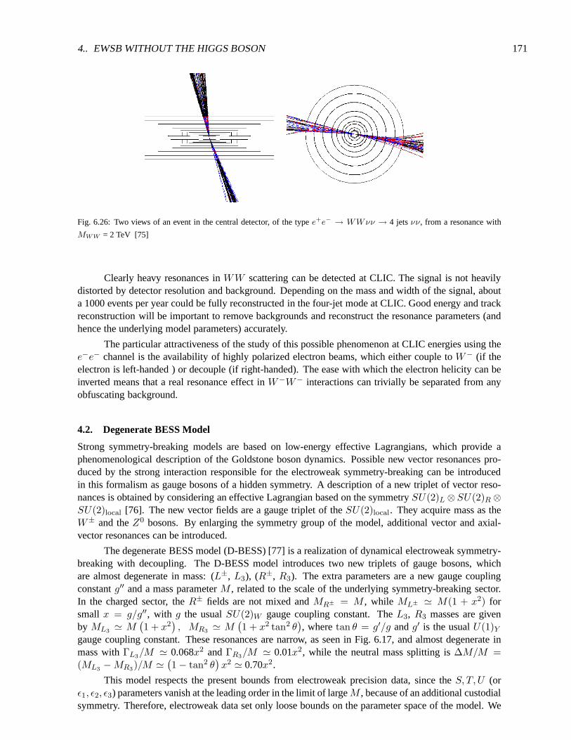
4.. EWSB WITHOUT THE HIGGS BOSON 171
Fig. 6.26: Two views of an event in the central detector, of the typee+e− → WWνν → 4 jetsνν, from a resonance with
MWW = 2 TeV [75]
Clearly heavy resonances inWW scattering can be detected at CLIC. The signal is not heavilydistorted by detector resolution and background. Depending on the mass and width of the signal, abouta 1000 events per year could be fully reconstructed in the four-jet mode at CLIC. Good energy and trackreconstruction will be important to remove backgrounds andreconstruct the resonance parameters (andhence the underlying model parameters) accurately.
The particular attractiveness of the study of this possiblephenomenon at CLIC energies using thee−e− channel is the availability of highly polarized electron beams, which either couple toW− (if theelectron is left-handed ) or decouple (if right-handed). The ease with which the electron helicity can beinverted means that a real resonance effect inW−W− interactions can trivially be separated from anyobfuscating background.
4.2. Degenerate BESS Model
Strong symmetry-breaking models are based on low-energy effective Lagrangians, which provide aphenomenological description of the Goldstone boson dynamics. Possible new vector resonances pro-duced by the strong interaction responsible for the electroweak symmetry-breaking can be introducedin this formalism as gauge bosons of a hidden symmetry. A description of a new triplet of vector reso-nances is obtained by considering an effective Lagrangian based on the symmetrySU(2)L ⊗SU(2)R ⊗SU(2)local [76]. The new vector fields are a gauge triplet of theSU(2)local. They acquire mass as theW± and theZ0 bosons. By enlarging the symmetry group of the model, additional vector and axial-vector resonances can be introduced.
The degenerate BESS model (D-BESS) [77] is a realization of dynamical electroweak symmetry-breaking with decoupling. The D-BESS model introduces two new triplets of gauge bosons, whichare almost degenerate in mass: (L±, L3), (R±, R3). The extra parameters are a new gauge couplingconstantg′′ and a mass parameterM , related to the scale of the underlying symmetry-breaking sector.In the charged sector, theR± fields are not mixed andMR± = M , while ML± ≃ M(1 + x2) forsmall x = g/g′′, with g the usualSU(2)W gauge coupling constant. TheL3, R3 masses are givenby ML3 ≃ M
(1 + x2
), MR3 ≃ M
(1 + x2 tan2 θ
), wheretan θ = g′/g andg′ is the usualU(1)Y
gauge coupling constant. These resonances are narrow, as seen in Fig. 6.17, and almost degenerate inmass withΓL3/M ≃ 0.068x2 andΓR3/M ≃ 0.01x2, while the neutral mass splitting is∆M/M =(ML3 −MR3)/M ≃
(1 − tan2 θ
)x2 ≃ 0.70x2.
This model respects the present bounds from electroweak precision data, since theS, T, U (orǫ1, ǫ2, ǫ3) parameters vanish at the leading order in the limit of largeM , because of an additional custodialsymmetry. Therefore, electroweak data set only loose bounds on the parameter space of the model. We

172 CHAPTER 6. PROBING NEW THEORIES
500 1000 1500 2000 2500 3000M(GeV)
0
0.1
0.2
0.3
0.4
0.5
g/g’’
M(GeV)
g/g’’
0
0.05
0.1
0.15
0.2
0.25
0.3
0.35
0.4
0.45
0.5
500 750 1000 1250 1500 1750 2000 2250 2500 2750
Fig. 6.27: 95% C.L. contours in the plane(M, g/g′′) from the presentǫ measurements (left) and from measurements of
σµ+µ− , σbb, AµµFB, AbbFB at e+e− linear colliders with
√s = 500 (800) GeV andL = 1 ab−1 (right). The allowed regions are
below the curves.
have studied these bounds by considering the latest experimental values of theǫ parameters coming fromthe high-energy data [17]:ǫ1 = (5.4± 1.0)× 10−3, ǫ2 = (– 9.7± 1.2)× 10−3, ǫ3 = (5.4± 0.9)× 10−3.We have included radiative corrections, taken to be the sameas in the SM, with the Higgs mass as acut-off [77]. Formt = 175.3 GeV andmH = 1000 GeV, one has [78]:ǫrad1 = 3.78× 10⁻³, ǫrad2 = –6.66× 10⁻³, ǫrad3 = 6.65× 10⁻³. The 95% C.L. bounds on the parameters of the D-BESS model areshown in Fig. 6.27. Comparable bounds come from the direct search at the Tevatron [77].
The LHC can discover these new resonances, which are produced via qq annihilations, throughtheir leptonic decayqq′ → L±,W± → (eνe)µνµ andqq → L3, R3, Z, γ → (e+e−)µ+µ−.
The relevant observables are the dilepton transverse and invariant masses. The main backgroundsleft in these channels after the lepton isolation cuts are the Drell–Yan processes with SM gauge bosonsexchange in the electron and muon channels. A study has been performed using a parametric detec-tor simulation [79]. Results are given in Table 6.10 for the combined electron and muon channels for
Table 6.10: Sensitivity to production of theL3 and R3 D-BESS resonances at the LHC forL = 100 (500) fb−1 with
M = 1.2 (3) TeV and accuracy on the mass splitting at CLIC forL = 1 ab−1.
g/g′′ M ΓL3 ΓR3 S/√S + B ∆M
(GeV) (GeV) (GeV) LHC (e+ µ) CLIC
1000 0.7 0.1 17.3
0.2 1000 2.8 0.4 44.7
0.1 2000 1.4 0.2 3.7
0.2 2000 5.6 0.8 8.8
0.1 3000 2.0 0.3 (3.4) 23.20± 0.06
0.2 3000 8.2 1.2 (6.6) 83.50± 0.02

4.. EWSB WITHOUT THE HIGGS BOSON 173
L = 100 fb−1, except forM = 3 TeV where 500 fb−1 are assumed. The discovery limit at the LHC,with L = 100 fb−1, isM ∼ 2 TeV for g/g′′ = 0.1. Beyond discovery, the possibility to disentangle thecharacteristic double-peak structure depends strongly ong/g′′ and smoothly on the mass.
The LC can also probe this multi-TeV region through virtual effects in the cross sections fore+e− → L3,R3, Z, γ → f f , at centre-of-mass energies below the resonances. Thanks to the presence ofnew spin-1 resonances, the annihilation channel inf f andW+W− has a better sensitivity than the fusionchannel. In the case of the D-BESS model, theL3 andR3 states are not strongly coupled toW pairs,making thef f final states the most favourable channel for discovery. The analysis at
√s = 500 GeV and√
s = 800 GeV is based onσµ+µ− , σbb,AµµFB andAbbFB. We assume identification efficiencies ofǫµ = 95%
andǫb = 60% and systematic uncertainties of∆ǫµ/ǫµ = 0.5%,∆ǫb/ǫb = 1%. The sensitivity contoursobtained forL = 1 ab−1 are shown in Fig. 6.27. The 3 TeV LC indirect reach is lower than that of theLHC or comparable to it. However, the QCD background rejection essential for the LHC sensitivity stillneeds to be validated using a full detector simulation and pile-up effects.
Assuming a resonant signal to be seen at the LHC or indirect evidence to be obtained at a lower-energy LC, CLIC could measure the width and mass of this stateand also probe its almost degeneratestructure [80]. This needs to be validated, taking the luminosity spectrum and accelerator-induced back-grounds into account. The ability to identify the model’s distinctive features has been studied using theproduction cross section and the flavour-dependent forward–backward asymmetries for different valuesof g/g′′. The resulting distributions are shown in Fig. 6.28 for the case of the narrower CLIC.02 beam
Fig. 6.28: Hadronic cross section (upper left) andµ+µ− (upper right),cc (lower left) andbb (lower right) forward–backward
asymmetries at energies around 3 TeV. The continuous lines represent the predictions for the D-BESS model withM = 3 TeV
andg/g′′ = 0.15, the flat lines the SM expectation, and the dots the observable D-BESS signal after accounting for the CLIC.02
luminosity spectrum.

174 CHAPTER 6. PROBING NEW THEORIES
parameters [19]. A characteristic feature of the cross-Section distributions is the presence of a narrowdip, due to the interference of theL3, R3 resonances with theγ andZ0, and to cancellations of theL3, R3
contributions. Similar considerations hold for the asymmetries. In the case shown in Fig. 6.28, the effectis still visible after accounting for the luminosity spectrum. In this analysis, the beam-energy spread setsthe main limit to the smallest mass splitting observable. With realistic assumptions and 1 ab−1 of data,CLIC will be able to resolve the two narrow resonances for values of the coupling ratiog/g′′ > 0.08,corresponding to a mass splitting∆M = 13 GeV forM = 3 TeV, and to determine∆M with a statisticalaccuracy better than 100 MeV, as seen in Table 6.10.
5. Further Alternative Theories
There exist a plethora of other new phenomena that may appearat the TeV scale. In the following, wediscuss briefly Little Higgs models, a possible fourth family of quarks and leptons, leptoquarks, excitedleptons and leptons of finite size, and finally non-commutative field theories.
5.1. Heavy Gauge Bosons in Little Higgs Models
Within Little Higgs models [81], new heavy particles can be expected in the TeV range, such as a heavytop quarkT and new gauge bosons. The LHC is sensitive to these particlesup to 2.5 TeV for theTquark [82], but CLIC will produce these copiously, via associated (W ′, T ) or single (Z ′) production,allowing for a precise study of the properties of the particles.
The existence of the heavySU(2) gauge bosonsZH andWH is one of the main predictions of theLittle Higgs models. The masses ofZH andWH should be within about a few TeV in order to solve thehierachy problem.
At ane+e− linear collider, if the centre-of-mass (c.m.) energy can beset at the mass of the vectorresonance, one is able to reach a substantial production cross section and perform precision studies of theproperties of the particle. Above the resonance threshold,the dominant production for the heavy gaugebosons is through theWWH final state. FixingMWH
= 1 TeV, we plot in Fig. 6.29 (solid curves) the totalcross section forWWH production forMWH
= 1 and 2 TeV as a function of the c.m. energy. For a fixed
Fig. 6.29: Total cross section fore+e− → WWH production versus centre-of-mass energyEc.m. for MWH= 1 and 2 TeV
(solid curves). Both charge statesW± W∓H have been included. Some relevant SM processes have also been included for
comparison (dashed curves).

5.. FURTHER ALTERNATIVE THEORIES 175
Fig. 6.30: Total cross section fore+e− → WWH production versus its massMWHat the CLIC energiesEc.m. = 3 and 5 TeV.
Both charge statesW± W∓H have been included.
value ofMWH, the cross section scales ascot2 θ, and the changes forcot θ = 1/2 and 2 are indicated
by a vertical bar. For comparison, we also include some relevant SM processes ofW+W−, WWZ,andWWH. We see that the signal cross section for theWWH final state is large and asymptoticallydecreases to the level ofW+W−.
In Fig. 6.30, we show the total cross-Section versusMWHat the CLIC energies, 3 and 5 TeV,
for cot θ = 1. The cross section grows when the mass increases because of the less and less severepropagator suppression1/(s −MZH )2, until it is cut off by the threshold kinematics.
Generically, the mass and coupling ofWH depend oncot θ, the mixing parameter between theSM and new gauge groupsSUL(2) andSUH(2). Keeping the mass fixed at 1 TeV, we can explore thetotal cross section with respect tocot θ, as shown in Fig. 6.31.
Fig. 6.31: Total cross section fore+e− → WWH production as a function of gauge coupling mixing parametercot θ for
MWH= 1 TeV

176 CHAPTER 6. PROBING NEW THEORIES
Fig. 6.32: Branching fractions forWH decay to SM particles
OnceWH is produced, it can decay to SM particles, either fermion pairs orWZ, WH. Thebranching fractions are given with respect to the mixing parametercot θ, as in Fig. 6.32. The decaychannels to fermions are dominant, asymptotically 1/4 for the three generations of leptons or one gen-eration of quarks, for most of the paramter space. For a valueof cot θ < 0.4,WH → WH,WZ decaymodes become more important, comparable to fermionic channels, as shown in Fig. 6.32. The produc-tion rate for the signal is still quite sizeable once above the kinematical threshold, and likely above theSM backgrounds.
In summary, once above the kinematical threshold, the heavygauge boson production at the CLICenergies can be substantial. The threshold behaviour can determine its mass accurately, and the crosssection rate will measure the coupling strengthcot θ.
5.2. Fourth Family
The mass and mixing patterns of the fundamental fermions areamong the most mysterious aspects ofparticle physics today. The number of fermion generations is not fixed by the SM. It is intriguing thatflavour democracy may hint at the existence of a fourth SM family (see [83,84] and references therein),and its possible existence is a fundamental question on which CLIC can cast new light. In order to avoidviolation of partial-wave unitarity, the masses of new quarks and leptons should be smaller than about1 TeV [85]. Therefore, CLIC with 1–3 TeV centre-of-mass energy will give the opportunity to measurethe fourth-SM-family fermions and quarkonia in detail.
Fourth-family quarks, if they exist, will be copiously produced at the LHC [86,87] if their massesare less than1 TeV. Therefore, any fourth-family quarks might be discovered at the LHC well beforeCLIC goes into operation. The same is true for pseudoscalar quarkonia (η4) formed by the fourth-familyquarks [88]. However, the observation of the fourth-familyleptons at the LHC is problematic becauseof the large backgrounds from realW andZ boson production, both singly and in pairs, that hide theseheavy lepton signals [89]. Lepton colliders will thereforebe advantageous for the investigation of thefourth-SM-family leptons and vector (ψ4) quarkonia. The potential of muon colliders was analysed

5.. FURTHER ALTERNATIVE THEORIES 177
in Ref. [90]. In this section we consider the production of the fourth-family fermions and quarkonia atCLIC, starting with pair production.
First we consider thee+e− option of CLIC. The annihilation ofe+e− is a classic channel toproduce and study new heavy fermions, because the cross sections are relatively large with respect tothe backgrounds [89]. The obtained cross section values forpair production of the fourth-SM-familyfermions withm4 = 320 (640) GeV and the corresponding numbers of events per working year (107 s)are given in Table 6.11 (Table 6.12). Event signatures are defined by the mass pattern of the fourthfamily and the 4× 4 Cabibbo–Kobayashi–Maskawa (CKM) matrix. According to the scenario givenin Ref. [91], the dominant decay modes areu4 → b W−, d4 → t W+, l4 → ντW
− andν4 → τ−W+.The chargedl4 lepton will have a clear signature at CLIC. For example, if the producedW± bosons decayleptonically, one has two acoplanar opposite-charge leptons and large missing energy. Pair productionof the neutralν4 leptons will lead to a more complicated event topology. In this case,τ tagging will behelpful for the identification of the events. Indeed, the producedτ leptons will decay at a distance of1–2 cm from the interaction point, which can easily be measured by a vertex detector. In addition, thepolarization of electron and positron beams should help to experimentally determine the axial and vectorneutral-current coupling constants of the fourth-family fermions.
Table 6.11: Cross sections and event numbers per year for pair production of the fourth-SM-family fermions with mass 320GeV
at CLIC (√see = 1 TeV,Lee = 2.7× 1034cm−2s−1 andLγγ = 1034cm−2s−1)
u4u4 d4d4 l4l4 ν4ν4
e+e− option σ (fb) 130 60 86 15
Nev/year 35 000 16 000 23 000 4100
γγ option σ (fb) 34 2 58 –
Nev/year 3400 200 5700 –
Table 6.12: Cross sections and event numbers per year for pair production of the fourth-SM-family fermions with mass 640GeV
at CLIC (√see = 3 TeV,Lee = 1× 1035cm−2s−1 andLγγ = 3× 1034cm−2s−1)
u4u4 d4d4 l4l4 ν4ν4
e+e− option σ (fb) 16 8 10 2
Nev/year 16 000 8000 10 000 2000
γγ option σ (fb) 27 2 46 –
Nev/year 8100 600 14 000 –
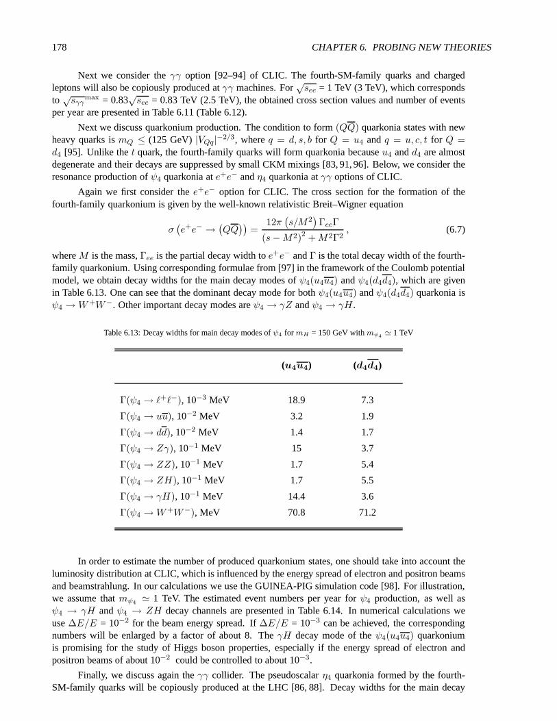
178 CHAPTER 6. PROBING NEW THEORIES
Next we consider theγγ option [92–94] of CLIC. The fourth-SM-family quarks and chargedleptons will also be copiously produced atγγ machines. For
√see = 1 TeV (3 TeV), which corresponds
to√sγγ
max = 0.83√see = 0.83 TeV (2.5 TeV), the obtained cross section values and number of events
per year are presented in Table 6.11 (Table 6.12).
Next we discuss quarkonium production. The condition to form (QQ) quarkonia states with newheavy quarks ismQ ≤ (125 GeV)|VQq|−2/3, whereq = d, s, b for Q = u4 andq = u, c, t for Q =d4 [95]. Unlike thet quark, the fourth-family quarks will form quarkonia because u4 andd4 are almostdegenerate and their decays are suppressed by small CKM mixings [83, 91, 96]. Below, we consider theresonance production ofψ4 quarkonia ate+e− andη4 quarkonia atγγ options of CLIC.
Again we first consider thee+e− option for CLIC. The cross section for the formation of thefourth-family quarkonium is given by the well-known relativistic Breit–Wigner equation
σ(e+e− →
(QQ))
=12π
(s/M2
)ΓeeΓ
(s−M2)2 +M2Γ2, (6.7)
whereM is the mass,Γee is the partial decay width toe+e− andΓ is the total decay width of the fourth-family quarkonium. Using corresponding formulae from [97]in the framework of the Coulomb potentialmodel, we obtain decay widths for the main decay modes ofψ4(u4u4) andψ4(d4d4), which are givenin Table 6.13. One can see that the dominant decay mode for both ψ4(u4u4) andψ4(d4d4) quarkonia isψ4 → W+W−. Other important decay modes areψ4 → γZ andψ4 → γH.
Table 6.13: Decay widths for main decay modes ofψ4 for mH = 150 GeV withmψ4 ≃ 1 TeV
(u4u4) (d4d4)
Γ(ψ4 → ℓ+ℓ−), 10−3 MeV 18.9 7.3
Γ(ψ4 → uu), 10−2 MeV 3.2 1.9
Γ(ψ4 → dd), 10−2 MeV 1.4 1.7
Γ(ψ4 → Zγ), 10−1 MeV 15 3.7
Γ(ψ4 → ZZ), 10−1 MeV 1.7 5.4
Γ(ψ4 → ZH), 10−1 MeV 1.7 5.5
Γ(ψ4 → γH), 10−1 MeV 14.4 3.6
Γ(ψ4 →W+W−), MeV 70.8 71.2
In order to estimate the number of produced quarkonium states, one should take into account theluminosity distribution at CLIC, which is influenced by the energy spread of electron and positron beamsand beamstrahlung. In our calculations we use the GUINEA-PIG simulation code [98]. For illustration,we assume thatmψ4 ≃ 1 TeV. The estimated event numbers per year forψ4 production, as well asψ4 → γH andψ4 → ZH decay channels are presented in Table 6.14. In numerical calculations weuse∆E/E = 10−2 for the beam energy spread. If∆E/E = 10−3 can be achieved, the correspondingnumbers will be enlarged by a factor of about 8. TheγH decay mode of theψ4(u4u4) quarkoniumis promising for the study of Higgs boson properties, especially if the energy spread of electron andpositron beams of about 10−2 could be controlled to about 10−3.
Finally, we discuss again theγγ collider. The pseudoscalarη4 quarkonia formed by the fourth-SM-family quarks will be copiously produced at the LHC [86, 88]. Decay widths for the main decay

5.. FURTHER ALTERNATIVE THEORIES 179
Table 6.14: The production event numbers per year for the fourth-SM-family ψ4 quarkonia at a CLIC 1 TeV option
with mψ4 ≃ 1 TeV
(u4u4) (d4d4)
e+e− → ψ4 26 600 10 400
e+e− → ψ4 → γH 510 50
e+e− → ψ4 → ZH 60 80
modes ofη4(u4u4) andη4(d4d4) are given in Table 6.15. From there, it is clear that the dominant decaymode isη4 → ZH. One can estimate theγγ → η4 production cross section by using the followingrelation [99]:
σ ≈ 50 fb(1 + λ1λ2)
(BRγγ
4 × 10⁻³
)(Γtot
1MeV
)(200GeV
Mη
)3
, (6.8)
whereBRγγ is the branching ratio of theη4 → γγ decay mode,Γtot is the quarkonium total decaywidth andλ1,2 are helicities of the initial photons. Assumingλ1λ2 = 1, we obtain total event numbersof η4 produced per year as follows: 900η4(u4u4) and 56η4(d4d4). The corresponding numbers forη4 → ZH events are 610 and 38 events, respectively. The advantage ofη4(u4u4) with respect toη4(d4d4) is obvious.
Table 6.15: Decay widths for main decay modes ofη4 for mH = 150 GeV withmη4 = 0.75 TeV
(u4u4) (d4d4)
Γ(η4 → γγ), 10−3 MeV 19.5 1.06
Γ(η4 → Zγ), 10−3 MeV 4.6 3.7
Γ(η4 → ZZ), 10−1 MeV 2.2 2.8
Γ(η4 → gg), MeV 5.1 5.1
Γ(η4 → ZH), MeV 47.3 47.3
Γ(η4 →W+W−), 10−2 MeV 5.7 5.7
Γ(η4 → tt), MeV 16.4 16.4
Γ(η4 → bb), 10−2 MeV 1.0 1.0
5.3. Leptoquarks
In the SM of electroweak and colour (QCD) interactions, quarks and leptons appear as formally inde-pendent components. However, the observed symmetry between the lepton and quark sectors in theSM could be interpreted as a hint for common underlying structures. If quarks and leptons are madeof constituents there should appear, at the scale of constituent binding energies, new interactions among
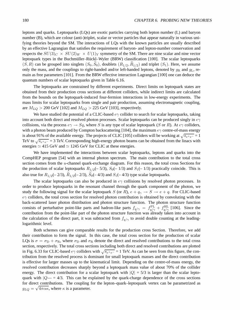
180 CHAPTER 6. PROBING NEW THEORIES
leptons and quarks. Leptoquarks (LQs) are exotic particlescarrying both lepton number (L) and baryonnumber (B), which are colour (anti-)triplet, scalar or vector particles that appear naturally in various uni-fying theories beyond the SM. The interactions of LQs with the known particles are usually describedby an effective Lagrangian that satisfies the requirement ofbaryon- and lepton-number conservation andrespects theSU(3)C × SU(2)W × U(1)Y symmetry of the SM. There are nine scalar and nine vectorleptoquark types in the Buchmuller–Ruckl–Wyler (BRW) classification [100]. The scalar leptoquarks(S,R) can be grouped into singlets(S0, S0), doublets(R1/2, R1/2) and triplet(S1). Here, we assumeonly the mass, and the couplings to right-handed and/or left-handed leptons, denoted bygR andgL, re-main as free parameters [101]. From the BRW effective interaction Lagrangian [100] one can deduce thequantum numbers of scalar leptoquarks given in Table 6.16.
The leptoquarks are constrained by different experiments.Direct limits on leptoquark states areobtained from their production cross sections at differentcolliders, while indirect limits are calculatedfrom the bounds on the leptoquark-induced four-fermion interactions in low-energy experiments. Themass limits for scalar leptoquarks from single and pair production, assuming electromagnetic coupling,areMLQ > 200 GeV [102] andMLQ > 225 GeV [103], respectively.
We have studied the potential of a CLIC-basedeγ collider to search for scalar leptoquarks, takinginto account both direct and resolved photon processes. Scalar leptoquarks can be produced singly ineγcollisions, via the processeγ → Sq, whereS is any type of scalar leptoquark (S orR). At eγ colliders,with a photon beam produced by Compton backscattering [104], the maximumeγ centre-of-mass energyis about 91% of the available energy. The projects of CLIC [105] colliders will be working at
√se+e− = 1
TeV to√se+e− = 3 TeV. Corresponding high-energy photon beams can be obtained from the linacs with
energies≃ 415 GeV and≃ 1245 GeV for CLIC at these energies.
We have implemented the interactions between scalar leptoquarks, leptons and quarks into theCompHEP program [54] with an internal photon spectrum. The main contribution to the total crosssection comes from theu-channel quark-exchange diagram. For this reason, the total cross Sections forthe production of scalar leptoquarksR1/2(– 5/3),S0(– 1/3) andS1(– 1/3) practically coincide. This is
also true forR1/2(– 2/3),R1/2(– 2/3),S0(– 4/3) andS1(– 4/3) type scalar leptoquarks.
The scalar leptoquarks can also be produced ineγ collisions by resolved photon processes. Inorder to produce leptoquarks in the resonant channel through the quark component of the photon, westudy the following signal for the scalar leptoquarkS (or R), e + qγ → S → e + q. For CLIC-basedeγ colliders, the total cross section for resolved photon contribution is obtained by convoluting with theback-scattered laser photon distribution and photon structure function. The photon structure functionconsists of perturbative point-like parts and hadron-likepartsfq/γ = fPL
q/γ + fHLq/γ [106]. Since the
contribution from the point-like part of the photon structure function was already taken into account inthe calculation of the direct part, it was subtracted fromfq/γ to avoid double counting at the leading-logarithmic level.
Both schemes can give comparable results for the productioncross Section. Therefore, we addtheir contribution to form the signal. In this case, the total cross section for the production of scalarLQs isσ = σD + σR, whereσD andσR denote the direct and resolved contributions to the total crosssection, respectively. The total cross sections includingboth direct and resolved contributions are plottedin Fig. 6.33 for CLIC-basedeγ colliders with
√se+e− = 1 TeV. As can be seen from this figure, the con-
tribution from the resolved process is dominant for small leptoquark masses and the direct contributionis effective for larger masses up to the kinematical limit. Depending on the centre-of-mass energy, theresolved contribution decreases sharply beyond a leptoquark mass value of about 70% of the colliderenergy. The direct contribution for a scalar leptoquark with |Q| = 5/3 is larger than the scalar lepto-quark with |Q— = 4/3. This can be explained by the quark-charge dependenceof the cross sectionsfor direct contributions. The coupling for the lepton–quark–leptoquark vertex can be parametrized asgLQ =
√4πακ, whereκ is a parameter.

5..F
UR
TH
ER
ALT
ER
NAT
IVE
TH
EO
RIE
S181
Table 6.16: Quantum numbers of scalar leptoquarks according to the BRW classification. The numbers in the parentheses inthe last two columns denote the values forgL = gR.
Leptoquark F I Qem Decay Coupling BR(S → lq) BR(S → νq)
eLuL g0L
S0 2 0 – 1/3 eRuR g0Rg20L+g20R2g20L+g20R
(23)
g20L2g20L+g20R
(13)
νdL −g0L
S0 2 0 – 4/3 eRdR g0R 1 0
1 2/3 νuL√
2g1L 0 1
S1 0 0 – 1/3 νdL, eLuL −g1L 1/2 1/2
– 1 – 4/3 eLdL −√
2g1L 1 0
1/2 – 2/3 νuR g1/2L
1/2 – 2/3 eRdL – g1/2R
g21/2R
g21/2R
+g21/2L
(12)
g21/2L
g21/2R
+g21/2L
(12)
R1/2 0– 1/2 – 5/3 eLuR g1/2L 1 0
– 1/2 – 5/3 eRuL g1/2R
1/2 1/3 νdR g1/2L 0 1R1/2 0
– 1/2 – 2/3 eLdR g1/2L 1 0

182C
HA
PT
ER
6.P
RO
BIN
GN
EW
TH
EO
RIE
S
Table 6.17: The number of events and signal significance for2j+ e and2j+ 6pT channels in scalar leptoquark decays. The lower and upper indices on scalar leptoquarksS orR denote
weak isospinI andI3, respectively.
√se+e− = 1 TeV Number of events S√
B(eγ → qqe) S√
B(eγ → qq′ν)
Lint = 105 pb−1 (σD + σR) × Lint
MLQ(GeV) |Q| = 5/3 |Q| = 4/3 S0 S01 R
−1/21/2 R
1/21/2 R
−1/21/2 , S0, S
−11 S0 S0
1 R1/21/2
200 452407 210085 704 556 1113 258 517 89 135 63
300 247050 94763 401 304 608 117 233 49 74 28
400 157382 53386 255 194 387 66 131 31 47 16
500 107389 32904 174 132 264 40 81 21 32 10
600 76050 21310 123 94 187 26 52 15 23 6
700 54541 14335 88 67 134 18 35 11 16 4
800 38152 9782 62 47 94 12 24 7 11 –
900 6629 1660 11 8 16 2 4 1 2 –
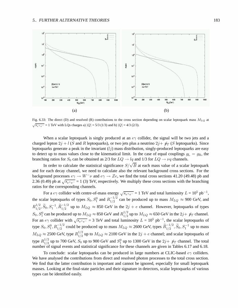
5.. FURTHER ALTERNATIVE THEORIES 183
(a) (b)
Fig. 6.33: The direct (D) and resolved (R) contributions to the cross section depending on scalar leptoquark massMLQ at√se+e− = 1 TeV with LQs charges a)|Q| = 5/3 (1/3) and b)|Q| = 4/3 (2/3).
When a scalar leptoquark is singly produced at aneγ collider, the signal will be two jets and acharged lepton2j + l (S andR leptoquarks), or two jets plus a neutrino2j+ 6pT (S leptoquarks). Sinceleptoquarks generate a peak in the invariant (lj) mass distribution, singly-produced leptoquarks are easyto detect up to mass values close to the kinematical limit. Inthe case of equal couplingsgL = gR, thebranching ratios forS0 can be obtained as 2/3 forLQ→ lq and 1/3 forLQ→ νq channels.
In order to calculate the statistical significanceS/√B at each mass value of a scalar leptoquark
and for each decay channel, we need to calculate also the relevant background cross sections. For thebackground processeseγ → W−ν andeγ → Ze, we find the total cross sections 41.20 (49.48) pb and2.36 (0.49) pb at
√se+e− = 1 (3) TeV, respectively. We multiply these cross sections with the branching
ratios for the corresponding channels.
For aeγ collider with centre-of-mass energy√se+e− = 1 TeV and total luminosityL = 105 pb−1,
the scalar leptoquarks of typesS0, S01 andR−1/2
1/2 can be produced up to massMLQ ≈ 900 GeV, and
R1/21/2, S0, S
−11 , R
−1/21/2 up toMLQ ≈ 850 GeV in the2j + e channel. However, leptoquarks of types
S0, S01 can be produced up toMLQ ≈ 850 GeV andR1/2
1/2 up toMLQ ≈ 650 GeV in the2j+ 6pT channel.
For aneγ collider with√se+e− = 3 TeV and total luminosityL = 105 pb−1, the scalar leptoquarks of
typeS0, S01 , R
−1/21/2 could be produced up to massMLQ ≈ 2600 GeV, typesR−1/2
1/2 , S0, S−11 up to mass
MLQ ≈ 2500 GeV, typeR1/21/2 up toMLQ ≈ 2100 GeV in the2j + e channel; and scalar leptoquarks of
typeR1/21/2 up to 700 GeV,S0 up to 900 GeV andS0
1 up to 1300 GeV in the2j+ 6 pT channel. The totalnumber of signal events and statistical significance for these channels are given in Tables 6.17 and 6.18.
To conclude: scalar leptoquarks can be produced in large numbers at CLIC-basedeγ colliders.We have analysed the contributions from direct and resolvedphoton processes to the total cross section.We find that the latter contribution is important and cannot be ignored, especially for small leptoquarkmasses. Looking at the final-state particles and their signature in detectors, scalar leptoquarks of varioustypes can be identified easily.

184C
HA
PT
ER
6.P
RO
BIN
GN
EW
TH
EO
RIE
S
Table 6.18: The same as Table 6.17, but for a CLIC-basedeγ collider with√se+e− = 3 TeV
√se+e− = 1 TeV Number of events S√
B(eγ → qqe) S√
B(eγ → qq′ν)
Lint = 105 pb−1 (σD + σR) × Lint
MLQ(GeV) |Q| = 5/3 |Q| = 4/3 S0 S01 R
−1/21/2 R
1/21/2 R
−1/21/2 , S0, S
−11 S0 S0
1 R1/21/2
300 181523 124657 648 491 981 337 674 33 49 34
500 73182 35515 261 198 396 99 197 13 20 10
700 43722 18168 156 118 236 49 98 8 12 5
900 30084 11135 107 81 163 30 60 5 8 3
1100 22141 7513 79 60 120 20 41 4 6 –
1300 16929 5335 60 46 92 14 29 – 5 –
1500 13251 3906 47 36 72 11 21 – 4 –
1700 10520 2922 38 28 57 8 16 – – –
1900 8406 2225 30 23 45 6 12 – – –
2100 6705 1728 24 18 36 5 9 – – –
2300 5340 1377 19 14 29 4 7 – – –
2500 3842 975 14 10 21 – 5 – – –
2700 824 206 3 2 4 – 1 – – –

5.. FURTHER ALTERNATIVE THEORIES 185
5.4. Lepton-Size Measurements
High-energye+e− scattering can also be used to study whether the leptons havea finite size. Similarstudies have been made in the past, for example at LEP [107]. Amodel inspired by string theory, whichcan lead to elastic ministrings, with finite size (dubbed Nylons), has been proposed in Ref. [108].
In the presence of structure, annihilations to fermionsf will be modified to becomedσdQ2 =
( dσdQ2 )SMF
2e (Q2)F 2
f (Q2), with F (Q2) = 1 + 16Q
2R2, whereR is an effective fermion radius. The cur-
rent best limit on the radiusRe of the electron comes from LEP, and isRe < 2.8× 10⁻¹⁷ cm (95 C.L.).For CLIC, the results foree→ ee, under the assumption that thet channel dominates, for an angular cuton the scattered electrons of| cos θ| < 0.9, and for a luminosity of 500 fb−1, are given in Table 6.19. Wesee that a 5-TeV machine will probe structures of dimensionsa factor of 10 smaller than in the presentresults from LEP [107].
Table 6.19: Bounds on the possible electron radiusRe obtainable with CLIC operating at various centre-of-mass energies
Radius (cm)√s (TeV)
3.0× 10⁻¹⁸ 1
1.2× 10⁻¹⁸ 3
0.9× 10⁻¹⁸ 5
5.5. Excited Electrons
The replication of three fermionic generations of known quarks and leptons suggest, the possibility thatthey are composite structures made up of more fundamental constituents. The existence of such quarkand lepton substructure leads one to expect a rich spectrum of new particles with unusual quantumnumbers. A possible signal of excited states of quarks and leptons [109] as predicted by composite mod-els [110] would supply convincing evidence for a new substructure of matter. All composite models offermions have an underlying substructure that may be characterized by a scaleΛ. The absence of electronand muon electric dipole moments implies that the excited leptons must have specific chiral properties.A right-handed excited lepton should couple only to the left-handed component of the correspondinglepton. Excited leptons may be classified bySU(2) × U(1) quantum numbers, and they are assumedto be both left- and right-handed weak isodoublets. In the effective Lagrangian of [109], the parame-tersf andf ′ associated with the gauge groups SU(2) and U(1) depend on compositeness dynamics anddescribe the effective changes from the SM coupling constants g andg′.
Experimental lower limits for the excited electron mass aregiven asme⋆ > 200 GeV in [111],andme⋆ > 306 GeV in [112]. The higher limits are derived from indirecteffects due toe⋆ exchangein the t channel, and depend on a transition magnetic coupling between e and e⋆. Relatively smalllimits (mµ⋆,τ⋆ > 94.2 GeV) for excited muon (µ⋆) and excited tau (τ⋆) are given by the L3 experimentat LEP [113].
In this work, resonant production of an excited electron in thes channel and its subsequent decaymodese⋆ → eγ, e⋆ → νW , e⋆ → eZ are considered. In addition, we include the contributions comingfrom the excited electron in thet channel. The production cross section and decays of excitedelectronsare calculated using the effective Lagrangian of [109], which depends on a compositeness scaleΛ andon free parametersf andf ′. We have implemented the interaction vertices into CompHEP[54] for the

186 CHAPTER 6. PROBING NEW THEORIES
excited electron interactions with leptons and gauge bosons. We choose eitherf = f ′ or f = −f ′ inour calculations in order to reduce the number of free parameters. For the casef = f ′ (f = −f ′) thecoupling of the photon to excited neutrinos (electrons) vanishes.
When produced, an excited electron decays predominantly into aW boson and a neutrino, andthe branching ratios are insensitive to the excited electron mass when it is high with respect tomW ormZ . We obtain the limiting values for the branching ratios at largeme⋆ as 0.28, 0.60 and 0.11 for thecouplingf = f ′ = 1, in the photon,W andZ channels, respectively. In the casef = −f ′ = – 1, thebranching ratio for theW channel does not change, whilst it increases to 0.39 for theZ channel. Takingf = −f ′ = 1 andΛ = 1 TeV, we find the total decay width of an excited electron to be 0.83 GeV and6.9 GeV forme⋆ = 500 GeV andme⋆ = 1000 GeV, respectively.
Excited electrons can be produced directly via the subprocesseγ → e⋆ → lV (V = γ, Z,W ) andindirectly via at-channel exchange diagram [114]. The production cross section of excited electrons inthree modes, takingf = f ′ = 1 andΛ = me⋆ , are given in Table 6.20 for CLIC-basedeγ colliders atthe centre-of-mass energy
√se+e− = 1 TeV (
√se+e− = 3 TeV). The following information can be read
off Table 6.20 the following information: theW channel gives higher cross sections than the others, butthere is an ambiguity with the neutrino in this final state. Therefore, the photon channel gives a morepromising result, because of its simple kinematics. The cross sections and the numbers of signal eventsare shown in Table 6.20. For the signal and background processes we apply a cutpe,γT > 10 GeV forexperimental identification of final-state particles. The backgrounds to theW andZ decay channels inthe hadronic final states are fairly large. The backgrounds to the photonic final states are relatively smallwith respect to theW andZ channels.
For the signal processeγ → e⋆ → eγ, the transverse momentumpT distribution of the photonor electron is peaked around the half of the mass value of the excited electron, as seen in Fig. 6.34. Forthe processeγ → e⋆ → νW (eZ), thepT distribution of theW boson (electron) shows a peak aroundme⋆/2 −m2
V /2me⋆ , wheremV denotes theW boson (orZ boson) mass.
In order to estimate the number of events for the signal and background in a chosenpT window,we integrate the transverse momentum distribution around the half the mass of each excited electron(me⋆/2 −m2
V /2me⋆ ) in an interval of the transverse momentum resolution∆pT . Here∆pT is approx-imated as≈ 10 GeV forme⋆ = 500 GeV and≈ 15 GeV forme⋆ = 750 GeV, for a generic detector.In order to calculate the significance of the signal, we use integrated luminosities for CLIC-basedeγcolliders ofL = 105 pb−1. In order to see the potential of CLIC-basedeγ colliders to search for an ex-cited electron, we define the statistical significanceS/
√B, whereS andB are the total number of events
for signal and background inside the chosenpT window, respectively. We calculate the value ofS/√B
for different couplings, assumingf = f ′ and requiring the conditionS/√B > 5 for the signal to be
observable. We find from Table 6.20 that excited electrons can be observed down to couplingsf ≃ 0.05andf ≃ 0.1 at CLIC-basedeγ colliders with
√se+e− = 1 TeV and
√se+e− = 3 TeV, respectively.
In this study, we have assumed that the excited electrons interact with the SM particles throughthe effective Lagrangian [109]. This may be a conservative assumption, because it is possible for excitedfermions to couple to ordinary quarks and leptons via contact interactions originating from the strongconstituent dynamics. In this case, the decay widths can be enhanced [115].
To conclude: we have presented results for excited electronproduction with subsequent decaysinto three channels. The excited electrons can be produced at CLIC-basedeγ colliders up to the kinemat-ical limit in each channel, due to the nearly flat photon energy spectrum. We find that an excited electronwith mass 500 (750) GeV can be probed down to the couplingf = f ′ ≃ 0.05 at
√se+e− = 1 TeV. At a
CLIC-basedeγ collider with√se+e− = 3 TeV the excited electron can be probed down with couplings
as low asf = f ′ ≃ 0.1.

5..F
UR
TH
ER
ALT
ER
NAT
IVE
TH
EO
RIE
S187
Table 6.20: The total cross sections of signal and background inside the chosen bin and the statistical significance (S/√B) values for differentf = f ′ for me⋆ = 750 GeV at
√se+e− = 1 TeV (
√se+e− = 3 TeV) withL = 105 pb−1.
eγ → eγ eγ → νW eγ → eZ
f = f ′ σtot (pb) S/√
B σtot (pb) S/√
B σtot (pb) S/√
B
1.00 24.70 (4.30) 1892.4 (963.1) 80.10 (53.40) 1869.3 (211.3) 8.90 (1.51) 1905.5 (705.4)
0.50 11.30 (1.80) 963.1 (183.8) 51.40 (50.00) 466.5 (51.9) 3.40 (0.53) 694.4 (131.2)
0.10 7.04 (1.20) 18.9 (6.1) 42.13 (48.94) 13.2 (0.7) 1.60 (0.32) 24.3 (4.1)
0.05 6.87 (1.18) 0.7 (0.8) 41.88 1.1 1.52 3.9

188 CHAPTER 6. PROBING NEW THEORIES
Fig. 6.34: Transverse momentum distribution of the photon,W boson and electron from excited electron production processes
at a CLIC-basedeγ collider with√smaxeγ = 911 GeV for different couplingsf = f ′ andme⋆ = 500 GeV
5.6. Non-Commutative Theories
Recent theoretical studies have demonstrated that non-commutative (NC) quantum field theories appearnaturally in the context of string theory in the presence of background fields [116]. In this case, the usualspace-time coordinates no longer commute, and instead obeythe relation
[xµ, xν ] = iθµν , (6.9)
where theθµν are a constant, frame-independent set of six dimensionful parameters [117]. Theθµν maybe separated into two classes: (i) space–space non-commutativity with θij = cBij/Λ
2NC, and (ii) space-
time non-commutativity withθ0i = cE0i/Λ2NC. The quantitiescE,B are two, fixed, frame-independent
unit vectors associated with the NC scaleΛNC. The NC scaleΛNC is most likely to be near the stringor Planck scale, which could be as low as a TeV; it characterizes the threshold where NC effects becomeapparent. Since the two vectorscE,B are frame-independent, they correspond to preferred directions inspace, related to the directions of the background fields. Thus, NC theories violate Lorentz invariance,and upper limits on such effects provide model-dependent constraints on the NC scale [117,118]. Sinceexperimental probes of NC theories are sensitive to the directions ofcE,B, the experiments must employastronomical coordinate systems and time-stamp their dataso that the rotation of the Earth or the Earth’smotion around the Sun, for example, does not wash out or dilute the effect through time-averaging.Note that momenta still commute in the usual way and hence energy and momentum remain conservedquantities, as does CPT.
5.. FURTHER ALTERNATIVE THEORIES 189
It is possible to construct non-commutative analogues of conventional field theories following twoapproaches: Weyl–Moyal (WM) [117] or Seiberg–Witten (SW) [116], both of which have their ownadvantages and disadvantages. In the SW approach, the field theory is expanded in a power series inθ, which then produces an infinite tower of additional operators. At any fixed order inθ the theorycan be shown to be non-renormalizable [119]. The SW construction can, however, be applied to anygauge theory with arbitrary matter representations. In theWM approach, onlyU(N) gauge theories arefound to be closed under the group algebra, and the matter content is restricted to the (anti-)fundamentaland adjoint representations. However, these theories are at least one-loop renormalizable, and appearto remain so even when spontaneously broken [120]. These distinctive properties of NC gauge theoriesrender it difficult to construct a satisfactory non-commutative version of the SM [121].
However, a NC version of QED is a well-defined theory in the WM approach, and its implicationsfor very-high-energye+e− colliders may be explored. This version of NCQED differs from ordinaryQED in several ways: (i) the ordering of products of fields must be preserved through the introductionof the star product [117], which absorbs the effect of the commutation relation via a series of Fouriertransforms; (ii) all vertices pick up a Lorentz-violating phase factor that is dependent on the momentaflowing through the vertex; (iii) NCQED takes on a non-Abelian nature in that trilinear and quarticphoton couplings are generated; and (iv) only the chargesQ = 0, ± 1 are allowed by gauge invariance.We note that propagators, however, are not modified since quadratic forms remain unchanged when oneintroduces the star product.
NCQED provides a testing ground for the basic ideas behind NCquantum field theory, and pro-duces striking signatures in QED processes at CLIC. The NC modifications to pair annihilation, Bhabha,Møller, and Compton scattering, as well asγγ → γγ, e+e− have been examined by a number of au-thors [122]. Some of these processes receive new diagrammatic contributions due to the non-Abeliancouplings, and all of them acquire a phase dependence due to the relative interference of the vertex kine-matic phases. The lowest-order NC contribution to these processes occurs via dimension-8 operatorswhose scale is set byΛNC. The most striking result is that an azimuthal-angle,φ, dependence is inducedin 2 → 2 scattering processes, since there exist the NC-preferred space-time directions, providing aunique signature of the Lorentz violation inherent in thesetheories.
Very-high-energye+e− colliders such as CLIC will allow us to probe values ofΛNC up to sev-eral TeV provided sufficient luminosity,∼ 1 ab−1, is available [123]. To demonstrate this claim, weexamine the case of pair annihilation, taking the incominge− direction to be along thez-axis. In addi-tion to the new phases that enter thet- andu-channel amplitudes, there is now an additionals-channelphoton exchange graph involving the NC-generated three-photon vertex. The resulting azimuthal depen-dence andcos θ distribution are shown in Fig. 6.35 for the illustrative case c02 = 1. Writing c01 = cosα,c02 = sinα cos β, andc03 = sinα sin β, Fig. 6.36 displays the reach forΛNC for CLIC energies forseveral values ofα.
The 95% C.L. search reaches for the NC scale in a variety of processes are summarized in Ta-ble 6.21 for both
√s = 500 GeV and CLIC energies. We see that these machines have a reasonable
sensitivity to NC effects and provide a good probe of such theories. It turns out that Møller scattering,while sensitive only to space/space non-commutativity, isa particularly promising process for experimen-tal investigation: once the non-commutative Feynman rulesare written down, we can interpret precisemeasurements of the Møller scattering cross-Section. It may be the interaction of choice for a possibleobservation of this new effect.

190 CHAPTER 6. PROBING NEW THEORIES
Fig. 6.35: Shifts in thez = cos θ andφ distributions for the processe+e− → γγ at a 3 or 5 TeV CLIC, assuming an integrated
luminosity of 1 ab−1. The dashed curves show the SM expectations while the ‘data’assumec02 = 1 andΛNC =√s. A cut of
|z| < 0.5 has been applied in theφ distribution.
Fig. 6.36: Reach forΛNC at a 3 TeV (left) or a 5 TeV (right) CLIC as a function of the integrated luminosity for the process
e+e− → γγ following the notation discussed in the text
6. Summary
A summary of the reach for exotic physics at CLIC, assuming a centre-of-mass energy of 5 TeV and anintegrated luminosity of 5 ab−1, is given in Table 6.22.
As we have shown in this chapter, the particular characteristics of CLIC, such as larger beam-strahlung andγγ backgrounds than a lower-energy LC, are not in general obstacles to full exploitationof CLIC’s higher centre-of-mass energy. If the new physics is within CLIC’s kinematic reach, CLIC willfind it.
In many cases, CLIC will be able to explore in detail and unravel hints of new physics that mightbe found at the LHC. In other cases, CLIC can reach even far beyond the LHC, thanks to its relativelyclean experimental conditions and its democratic production of new weakly-interacting particles.

6.. SUMMARY 191
Table 6.21: Summary of the 95% C.L. search limits on the NC scale ΛNC from the various processes considered above at a
500 GeVe+e− linear collider with an integrated luminosity of 500 fb−1 or at a 3 or 5 TeV CLIC with an integrated luminosity
of 1 ab−1. The sensitivities are from the first two papers in Ref. [122]. Theγγ → e+e− andγe → γe analyses of Godfrey
and Doncheski include an overall 2% systematic error not included by Hewett, Petriello and Rizzo.
Process Structure probed√s = 500 GeV
√s = 3 TeV
√s = 5 TeV
e+e− → γγ Space-time 740–840 GeV 2.5–3.5 TeV 3.8–5.0 TeV
Møller scattering Space–space 1700 GeV 5.9 TeV 8.5 TeV
Bhabha scattering Space-time 1050 GeV 4.5–5.0 TeV 6.6–7.2 TeV
γγ → γγ Space-time 700–800 GeV
Space–space 500 GeV
γγ → e+e− Space-time 220–260 GeV 1.1–1.3 TeV 1.8–2.1 TeV
γe→ γe Space-time 540–600 GeV 3.1–3.4 TeV 4.8–5.8 TeV
Space–space 700–720 GeV 4.0–4.2 TeV 6.3–6.5 TeV
Table 6.22: Summary of the physics reach of CLIC for various examples of exotic new physics, assuming√s = 5 TeV and an
integrated luminosity of 5 ab−1
Z ′ (direct) 5 TeV
Z ′ (indirect) 30 TeV
l∗, q∗ 5 TeV
TGC (95%) 0.00008
Λ compos. 400 TeV
WLWL > 5 TeV
ED (ADD) 30 TeV (e+e−)
55 TeV (γγ)
ED (RS) 18 TeV (c = 0.2)
ED (TeV−1) 80 TeV
Resonances δM/M, δΓ/Γ ∼ 10−3
Black holes 5 TeV

192 CHAPTER 6. PROBING NEW THEORIES

Bibliography
[1] N. Arkani-Hamed, S. Dimopoulos and G. Dvali,Phys. Lett.B429(1998) 263,Phys. Rev.D59 (1999) 086004;I. Antoniadis, N. Arkani-Hamed, S. Dimopoulos and G. Dvali,Phys. Lett.B436(1998) 257.
[2] L. Randall and R. Sundrum,Phys. Rev. Lett.83 (1999) 3370.
[3] For an introduction to ADD phenomenology, seeG.F. Giudice, R. Rattazzi and J.D. Wells,Nucl. Phys.B544(1999) 3;T. Han, J.D. Lykken and R. Zhang,Phys. Rev.D59 (1999) 105006;E.A. Mirabelli, M. Perelstein and M.E. Peskin,Phys. Rev. Lett.82 (1999) 2236;J.L. Hewett,Phys. Rev. Lett.82 (1999) 4765;T.G. Rizzo,Phys. Rev.D60 (1999) 115010.
[4] J. Hewett and M. Spiropulu,Ann. Rev. Nucl. Part. Sci.52 (2002) 397, hep-ph/0205106.
[5] A. Aguilar-Saavedraet al., ‘TESLA technical design report part III: Physics at ane+e− linearcollider’, hep-ph/0106315.
[6] H. Murayama and J.D. Wells,Phys. Rev.D65 (2002) 056011, hep-ph/0109004.
[7] For an overview of the Randall–Sundrum model phenomenology, seeH. Davoudiasl, J.L. Hewett and T.G. Rizzo,Phys. Rev. Lett.84 (2000) 2080;Phys. Lett.B493(2000) 135;Phys. Rev.D63 (2001) 075004.
[8] T. Sjostrand,Comput. Phys. Commun.82 (1994) 74;T. Sjostrand, L. Lonnblad and S. Mrenna,‘PYTHIA 6.2: Physics and manual’, hep-ph/0108264.
[9] H. Davousdiasl and T. Rizzo,Phys. Lett.B512(2001) 100.
[10] For a review of new gauge boson physics at colliders and details of the various models, seeJ.L. Hewett and T.G. Rizzo,Phys. Rep.183(1989) 193;A. Leike, Phys. Rep.317(1999) 143.
[11] S Dimoupoulos and G. Landsberg,Phys. Rev Lett.87 (2001) 161602.
[12] S.B. Giddings and S. Thomas,Phys. Rev.D65 (2002) 056010, hep-ph/0106219.
[13] G. Landsberg, in Proc. of the APS/DPF/DPB Summer Study on the Future of Particle Physics(Snowmass 2001), ed. N. Graf.
[14] See, for example, I. Antoniadis,Phys. Lett.B246(1990) 377;I. Antoniadis, C. Munoz and M. Quiros,Nucl. Phys.B397(1993) 515;I. Antoniadis and K. Benakli,Phys. Lett.B326(1994) 69,Int. J. Mod. Phys.A15 (2000) 4237;I. Antoniadis, K. Benakli and M. Quiros,Phys. Lett.B331(1994) 313.
193

194 BIBLIOGRAPHY
[15] A. Pomarol and M. Quiros,Phys. Lett.B438(1998) 255, hep-ph/9806263.
[16] See, for example,T.G. Rizzo and J.D. Wells,Phys. Rev.D61 (2000) 016007;P. Nath and M. Yamaguchi,Phys. Rev.D60 (1999) 116006;M. Masip and A. Pomarol,Phys. Rev.D60 (1999) 096005;L. Hall and C. Kolda,Phys. Lett.B459(1999) 213;R. Casalbuoni, S. DeCurtis, D. Dominici and R. Gatto,Phys. Lett.B462(1999) 48;A. Strumia,Phys. Lett.B466(1999) 107;F. Cornet, M. Relano and J. Rico,Phys. Rev.D61 (2000) 037701;T.G. Rizzo,Phys. Rev.D61 (2000) 055005,Phys. Rev.D64 (2001) 015003;C.D. Carone,Phys. Rev.D61 (2000) 015008.
[17] G. Altarelli, F. Caravaglios, G.F. Giudice, P. Gambinoand G. Ridolfi,JHEP0106(2001) 018.
[18] K. Cheung,‘Collider phenomenology for models of extra dimensions’, hep-ph/0305003.
[19] M. Battaglia, S. De Curtis and D. Dominici,JHEP0212(2002) 004, hep-ph/0210351.
[20] A. Aranda, J.L. Dıaz-Cruz and C. Balazs,Nucl. Phys.B670(2003) 90, hep-ph/0212133.
[21] M. Masip and A. Pomarol,Phys. Rev.D60 (1999) 096005, hep-ph/9902467.
[22] R.W. Assmann, CERN-2000-008, Jul 2000.
[23] T. Appelquist, H.-C. Cheng and B. Dobrescu,Phys. Rev.D64 (2000) 035002, hep-ph/0012100.
[24] H.-C. Cheng, K.T. Matchev and M. Schmaltz,Phys. Rev.D66 (2002) 056006.
[25] G. Servant, T.M.P. Tait,Nucl. Phys.B650(2002) 391, hep-ph/0206071.
[26] H. Georgi, A.K. Grant and G. Hailu,Phys. Lett.B506(2001) 207, hep-ph/0012379
[27] G. von Gersdorff, N. Irges and M. QuirosNucl. Phys.B635(2002) 127, hep-th/0204223.
[28] H.-C. Cheng, K.T. Matchev and M. Schmaltz,Phys. Rev.D66 (2002) 036005, hep-ph/0204342.
[29] K. Agashe, N.G. Deshpande and G.H. Wu,Phys. Lett.B511(2001) 85, hep-ph/0103235.
[30] K. Agashe, N.G. Deshpande and G.H. Wu,Phys. Lett.B514(2001) 309, hep-ph/0105084.
[31] T. Appelquist and B. A. Dobrescu,Phys. Lett.B516(2001) 85, hep-ph/0106140.
[32] F.J. Petriello,JHEP0205(2002) 003, hep-ph/0204067.
[33] T. Appelquist, H.-U. Yee,Phys. Rev.D67 (2003) 055002, hep-ph/0211023.
[34] D. Chakraverty, K. Huitu and A. Kundu,Phys. Lett.B558(2003) 173, hep-ph/0212047.
[35] A.J. Buras, M. Spranger and A. Weiler,Nucl. Phys.B660(2003) 225, hep-ph/0212143.
[36] F. Abeet al. (CDF Collaboration),Phys. Rev. Lett.79 (1997) 2192.
[37] M. Kobel, ‘Minireview on other signatures of new physics at LEP and HERA’, in Proc. 31st Inter-national Conference on High Energy Physics (ICHEP 2002), Amsterdam, The Netherlands, 24–31Jul 2002.
[38] P. Langacker, in Proc. of the APS/DPF/DPB Summer Study on the Future of Particle Physics(Snowmass 2001), ed. N. Graf, eConfC0106307 (2001) P10, hep-ph/0110129.

BIBLIOGRAPHY 195
[39] R. Casalbuoni, S. De Curtis, D. Dominici and R. Gatto,Phys. Lett.B460(1999) 135,hep-ph/9905568.
[40] See, for example: V.A. Dzuba, V.V. Flambaum and J.S.M. Ginges,Phys. Rev.D66 (2002) 076013,hep-ph/0204134 and references therein.
[41] S. Godfrey, in Proc. of the APS/DPF/DPB Summer Study on the Future of Particle Physics (Snow-mass 2001), ed. N. Graf, eConfC010630(2001) P344, hep-ph/0201093.
[42] D. Schulte, CERN-PS-2001-002-AE, prepared for 5th International Linear Collider Workshop(LCWS 2000), Fermilab, Batavia, Illinois, 24–28 Oct 2000.
[43] K. Yokoya and P. Chen, in Proc. 1989 Particle Accelerator Conference, eds. F. Bennet and L. Tay-lor, IEEE 1989 and M. Peskin, LCC-Note-0010.
[44] See, for example: G. Altarelliet al., Mod. Phys. Lett.A5 (1990) 495,Nucl. Phys.B342(1990) 15.
[45] M. Battaglia, S. De Curtis, D. Dominici, A. Ferrari and J. Heikkinen, in Prc. 5th InternationalLinear Collider Workshop (LCWS 2000), Fermilab, Batavia, Illinois, 24–28 Oct 2000,hep-ph/0101114.
[46] M. Battaglia, S. Jadach and D. Bardin, inProc. of the APS/DPF/DPB Summer Study on the Futureof Particle Physics (Snowmass 2001)ed. N. Graf, SNOWMASS-2001-E3015.
[47] R.N. Mohapatra and G. Senjanovic,Phys. Rev.D12 (1975)1502,D23 (1981) 165.
[48] A. Ferrariet al., Phys. Rev.D62 (2000) 013001.
[49] A. Ferrari,Phys. Rev.D65 (2002) 093008, LC-PHSM-2001-076-CLIC.
[50] M. Battaglia, S. De Curtis and D. Dominici,JHEP0212(2002) 004, hep-ph/0210351.
[51] M. Battaglia, in Proc. Physics and Experiments with Future Lineare+e− Colliders, (eds. A. Paraand H.E. Fisk), AIP Conference Proceedings, New York, 2001,813, hep-ex/0011099.
[52] L. Salmi, ‘tt cross section and forward–backward asymmetry at CLIC’, hep-ex/0301021.
[53] P. Ciafaloni,‘TeV scale weak interactions: Inclusive vs. exclusive observables’, talk given at 14thRencontres de Physique de la Valle d’Aoste: Results and Perspectives in Particle Physics, LaThuile, Valle d’Aoste, Italy, 27 Feb – 4 Mar 2000, hep-ph/0005277, and references therein.
[54] A. Pukhovet al., ‘CompHEP: A package for evaluation of Feynman diagrams and integrationover multi-particle phase space’, INP-MSU-98-41-542, hep-ph/9908288.
[55] T.G. Rizzo, ‘Extra dimensional signatures for CLIC’, in Proc. of the APS/DPF/DPB SummerStudy on the Future of Particle Physics (Snowmass 2001), ed.N. Graf, hep-ph/0108235.
[56] E. Eichten, K. Lane and M. Peskin,Phys. Rev. Lett.50 (1983) 811;H. Kroha,Phys. Rev.D46 (1992) 58.
[57] S. Riemann, LC Note LC-TH-2001-007 (2001).
[58] T. Hambye and K. Riesselmann,‘SM Higgs mass bounds from theory’, hep-ph/9708416.
[59] A. Czarnecki and W. Marciano,Int. J. Mod. Phys.A15 (2000) 2365, hep-ph/0003049
[60] M. Diehl, O. Nachtmann and F. Nagel,Eur. Phys. J.C27 (2003) 375, hep-ph/0209229.

196 BIBLIOGRAPHY
[61] T. Barklow, LC Orange Book, SLAC-R-570, May 2001.
[62] K. Hagiwara, R. D. Peccei, D. Zeppenfeld and K. Hikasa,Nucl. Phys.B282, 253 (1987).
[63] D. Abbaneoet al., ‘A combination of preliminary electroweak measurements and constraints onthe Standard Model’, hep-ex/0212036.
[64] M. Acciarri et al. (L3 Collaboration),Phys. Lett.B467(1999) 171, hep-ex/9910008.
[65] G. Abbiendiet al. (OPAL Collaboration),Eur. Phys. J.C19 (2001) 229, hep-ex/0009021.
[66] A. Heisteret al. (ALEPH Collaboration),Eur. Phys. J.C21 (2001) 423, hep-ex/0104034.
[67] D. Atwood and A. Soni,Phys. Rev.D45 (1992) 2405;M. Davier, L. Duflot, F. Le Diberder and A. Rouge,Phys. Lett.B306(1993) 411;M. Diehl and O. Nachtmann,Z. Phys.C62 (1994) 397.
[68] M. Diehl and O. Nachtmann,Eur. Phys. J.C1 (1998) 177, hep-ph/9702208.
[69] M. Diehl, O. Nachtmann and F. Nagel,Eur. Phys. J.C32 (2003) 17, hep-ph/0306247.
[70] O. Nachtmann, F. Nagel and M. Pospischil,‘Anomalous gauge-boson couplings and the Higgs-boson mass’, hep-ph/0404006
[71] V.D. Barger, K.M. Cheung, T. Han and R.J. Phillips,Phys. Rev.D52 (1995) 3815;V.D. Bargeret al., Phys Rev.D52 (1995) 3815,V.D. Barger, M.S. Berger, J.F. Gunion and T. Han,Phys. Rev.D55 (1997) 142.
[72] A. Dobado, M.J. Herrero, J.R. Pelaez and E. Ruiz Morales, Phys. Rev.D62 (2000) 055011.
[73] J.M. Butterworth, B.E. Cox and J.R. Forshaw,Phys. Rev.D65 (2002) 096014.
[74] T.L. Barklow and A. De Roeck,‘Physics at multi-TeV linear colliders’, in Proc. of theAPS/DPF/DPB Summer Study on the Future of Particle Physics (Snowmass 2001), ed. N. Graf,eConfC010630(2001) E3002, hep-ph/0112313.
[75] A. De Roeck, ‘Resonances ine+e− → ννWW scattering at CLIC’, in Proc. of theAPS/DPF/DPB Summer Study on the Future of Particle Physics (Snowmass 2001), ed. N. Graf,eConfC010630(2001) E3018.
[76] R. Casalbuoni, S. De Curtis, D. Dominici and R. Gatto,Phys. Lett.B155(1985) 95;Nucl. Phys.B282(1987) 235.
[77] R. Casalbuoniet al., Phys. Lett.B349(1995) 533;Phys. Rev.D53 (1996) 5201.
[78] G. Altarelli, ‘The standard electroweak theory and beyond’, hep-ph/0011078.
[79] R. Casalbuoni, S. De Curtis and M. Redi,Eur. Phys. J.C18 (2000) 65.
[80] R. Casalbuoniet al., JHEP9908(1999) 011, hep-ph/9904268.
[81] V. Bargeret al., Phys. Rev.D67 (2003) 115001, hep-ph/0301097.
[82] G. Azuelos,et al., ‘Exploring little Higgs models with ATLAS at the LHC,’hep-ph/0402037.
[83] S. Sultansoy,‘Why the four SM families’, contributed to 30th International Conference on High-Energy Physics (ICHEP 2000), Osaka, Japan, 27 Jul – 2 Aug 2000, hep-ph/0004271.

BIBLIOGRAPHY 197
[84] E. Arik and S. Sultansoy,‘Turkish comments on future perspectives in HEP’, hep-ph/0302012.
[85] M.S. Chanowitz, M. A. Furman and I. Hinchliffe,Nucl. Phys.B153(1979) 402.
[86] ATLAS Collaboration, ATLAS Technical Design Report, CERN/LHCC-95-15 (1999).
[87] E. Arik et al., Phys. Rev.D58 (1998) 117701.
[88] E. Arik et al., Phys. Rev.D66 (2002) 116006.
[89] V.D. Barger and R.J.N. Phillips,Collider Physics, Addison-Wesley, New York, (1996).
[90] A.K. Ciftci, R. Ciftci and S. Sultansoy,Phys. Rev.D65 (2002) 055001.
[91] S. Ataget al., Phys. Rev.D54 (1996) 5745.
[92] I. Ginzburget al., Nucl. Instrum. Meth.205(1983) 47.
[93] I. Ginzburget al., Nucl. Instrum. Meth.219(1984) 5.
[94] V.I. Telnov,Nucl. Instrum. Meth.A294, 72 (1990).
[95] I. Bigi et al., Phys. Lett.B181(1986) 157.
[96] A. Celikel, A.K. Ciftci and S. Sultansoy,Phys. Lett.B342(1995) 257.
[97] V. Bargeret al., Phys. Rev.D35 (1987) 3366.
[98] D. Schulte, TESLA 97-08 (1997).
[99] D.S. Gorbunov, V.A. Ilyin and V.I. Telnov,Nucl. Instrum. Meth.A472 (2001) 171,hep-ph/0211428.
[100] W. Buchmuller, R. Ruckl and D. Wyler,Phys. Lett.B191(1987) 442.
[101] O. Cakir, E. Ateser and H. Koru,Euro. Phys. J.C28 (2003) 381.
[102] C. Adloff et al. (H1 Collaboration),Euro. Phys. J.C11 (1999) 447.
[103] B. Abbotet al. (D0 Collaboration),Phys. Rev. Lett.80 (1998) 2051.
[104] I.F. Ginzburget al., Nucl. Instrum. Meth., 219(1984) 5;I.F. Ginzburg, G.L. Kotkin, V.G. Serbov and V.I. Telnov,Nucl. Instrum. Meth.47 (1983) 205.
[105] R.W. Assmannet al., (CL IC Study Team), CERN-2000-008.
[106] M. Gluck, E. Reya and A. Vogt,Phys. Rev.D46 (1992) 1973.
[107] D. Bourilkov,Phys. Rev.D62 (2000) 076005, hep-ph/0002172.
[108] J. Lykken, contributed paper to LCWS00, FNAL, 2000.
[109] F.M. Renard,Phys. Lett.B116(1982) 264;K. Hagiwara, S. Komamiya and D. Zeppenfeld,Z. Phys.C29 (1985) 115;U. Baur, M. Spira and P. M. Zerwas,Phys. Rev.D42 (1990) 815;F. Boudjema, A. Djouadi and J.L. Kneur,Z. Phys.C57 (1993) 425.
[110] H. Harari,Phys. Lett.B86 (1979) 83;H. Terazawa,Phys. Rev.D22 (1980) 184;L. Abbott and E. Farhi,Nucl. Phys.B189, 547 (1981);H. Fritzsch and G. Mandelbaum,Phys. Lett.B102(1981) 319.

198 BIBLIOGRAPHY
[111] J. Breitweget al. (ZEUS Collaboration),Z. Phys.C76 (1997) 631.
[112] G. Abbiendiet al. (OPAL Collaboration),Phys. Lett.B465(1999) 303.
[113] M. Acciarri et al. (L3 Collaboration),Phys. Lett.B353(1984) 431.
[114] Z. Kirca, O. Cakir and Z.Z. Aydin,Acta Phys. Polon.B34 (2003) 4079.
[115] O. Cakir, C. Leroy and R. Mehdiyev, ATLAS Internal Note, ATL-PHYS-2002-014, (2002).
[116] For a review of Non-commutative theories, seeN. Seiberg and E. Witten,JHEP9909(1999) 032, hep-th/9908142;see also A. Connes, M.R. Douglas and A. Schwarz,JHEP9802(1998) 003.
[117] For a recent review of non-commutative theories, seeM.R. Douglas and N.A. Nerrasov,Rev. Mod. Phys.73 (2001) 977, hep-th/0106048.
[118] S.M. Carrollet al., Phys. Rev. Lett.87 (2001) 141601, hep-th/0105082.
[119] R. Wulkenhaar,JHEP0203(2002) 024, hep-th/0112248.
[120] A. Micu, JHEP0101(2001) 025;A. Armoni, Nucl. Phys.B593(2001) 229;L. Bonara and M. Salizzoni,Phys. Lett.B504(2001) 80;B.A. Campbell and K. Kaminsky,Nucl. Phys.B581(2000) 240,B606(2001) 613;F.J. Petriello,Nucl. Phys.B601(2001) 169;Y. Liao JHEP0111(2001) 067, hep-th/0201135.
[121] M. Chaichian, P. Presnajder, M.M. Sheikh-Jabbari andA. TureanuPhys. Lett.B526 (2002) 132,hep-th/0107037;Eur. Phys. J.C29 (2003) 413, hep-th/0107055;X. Calmetet al., Eur. Phys. J.C23 (2002) 363, hep-ph/0111115;J.L. Hewett, F.J. Petriello and T.G. Rizzo,Phys. Rev.D66 (2002) 036001, hep-ph/0112003.
[122] J.L. Hewett, F.J. Petriello and T.G. Rizzo,Phys. Rev.D64 (2001) 075012, hep-ph/0010354;S. Godfrey and M. Doncheski,Phys. Rev.D65 (2002) 015005, hep-ph/0108268;H. Grosse and Y. Liao,Phys. Rev.D64, 115007 (2001);S.W. Baek, D.K. Ghosh, X.G. He and W.Y. Hwang,Phys. Rev.D64 (2001) 056001.
[123] J.L. Hewett, F.J. Petriello and T.G. Rizzo, in Proc. ofthe APS/DPF/DPB Summer Study on theFuture of Particle Physics (Snowmass 2001), ed. N. Graf, eConf C010630(2001) E3064,hep-ph/0201275.


200 BIBLIOGRAPHY

Chapter 7
QCD
1. Introduction
Strong-interaction measurements at a multi-TeVe+e− collider such as CLIC will constitute an impor-tant part of its physics programme. CLIC will provide uniquetests of QCD at high energy scales ina relatively clean experimental and theoretical environment. Examples of general QCD measurementsthat can be made include the fragmentation and hadronization of partons at high energies and a preciseextraction ofαs through multijet rates and event-shape variables, for example. For a TeV-class linearcollider, a precision inαs of the order of 1% may be achievable if the relevant perturbative QCD calcu-lations become available with sufficiently high precision [1]. Also, virtualγγ interactions can be studiedat ane+e− collider, which will help the understanding of low-x data at hadron colliders. A dedicatedγγcollider interaction region would allow further detailed measurements of the enigmatic photon structure.
In this chapter, the following items, essentially in the category of two-photon physics, have beenworked out in more detail:
• Measurement of the totalγγ cross section
• Measurement of the photon structure
• Measurement of BFKL dynamics
At lower-energye+e− colliders, two-photon interactions have traditionally been studied usingbremsstrahlung photons from the electron beams [2]. Similar processes, together with reactions inducedby beamstrahlung photons, will also occur at a future high-energy e+e− collider such as CLIC, andwill allow a rich two-photon physics programme. The energy spectra of the photons emitted in theseprocesses are, however, peaked at rather low energies.
Since the colliding beams are used only once at linear colliders, other operation modes becomepossible, such as a photon (γγ) collider (PC) [3, 4]. At a PC, the electron and positron beams of alinear collider are converted into photon beams via Comptonlaser backscattering. This option has beendiscussed for CLIC in chapter 2. The advantage of the photon spectrum from laser backscattering is that itpeaks at high energy values, typically∼ 80% of the initial electron energy, with a relatively narrowwidthof approximately 10%. Thus, a PC offers the exciting possibility of studying two-photon interactions atthe highest possible energies with high luminosity.
Finally, we note in passing that, since the overlaidγγ collisions form the most important back-ground at CLIC, a good knowledge and understanding of two-photon processes will be essential forcontrolling these background contributions to other processes.
201

202 CHAPTER 7. QCD
200
400
600
800
1000
1200
1400
1 10 102
103
BKKS x 0.85
EMM with Form factors
LEP2-L3 189 GeV and 192-202 GeV
TPCDesy 1984DESY 86LEP2-OPAL 189 GeV
Regge/Pomeron, SaS
(EMM with kt resummation) x 1.1
Fig. 7.1: The totalγγ cross section as function of the collision energy, comparedwith model calculations: a band of predictions
in the BKKS model, whose upper and lower limits correspond todifferent photon densities [5]; a proton-like model (solidline
[6–8]); an eikonal minijet model (EMM) band for the total andinelastic cross sections, with different photon densitiesand
different minimum jet transverse momenta [9]). The proton-like and BKKS models have been normalized to the data, in order
to show the energy dependence of the cross section.
2. Total Cross Section
A key example for the study of the properties of the photon is the totalγγ cross section, which is notyet understood from first principles. The nature of the photon itself is known to be rather complex. Ahigh-energy photon can fluctuate into a fermion pair or even into a hadronic bound state, i.e. a vectormeson with the same quantum numbers as the photon,JPC = 1−−. These quantum fluctuations lead tothe so-called hadronic structure of the photon.
The data from LEP [10–13] show that the totalγγ cross section rises with energy. Such a risewas observed previously inpp collisions, but, intriguingly, the rise inγγ collisions seems to be steeper.Figure 7.1 shows the data [10–13] together with predictionsof various models.
As seen in Fig. 7.1, models differ in their predictions for the totalγγ cross section at CLIC ener-gies. The wide band is obtained using the eikonal minijet model (EMM), the thinner one using a modeldue to BKKS [5], and the full curve is an early prediction by Schuler and Sjostrand [7] using a Regge–Pomeron fit. The EMM, which embeds QCD minijet cross sectionsin an eikonal formalism [14,15], candescribe the rise observed in present LEP data quite well, apart from a 10% normalization uncertainty.The predictions forγγ interactions are obtained with a parameter set extrapolated from similar fits tothe photoproduction cross section at HERA. The tuned parameters include the different parton densities,minimum minijet transverse momenta, the soft cross sectionand a model for the transverse momentumdistribution of partons in the photon. It should be noted, however, that the EMM, with a form-factormodel for the parton transverse momentum distribution and the same set of parameters, does not repro-duce at all the early rise seen in proton–proton scattering,unless higher-order effects due to soft gluonemission are included [16]. Although at present energies the EMM without soft gluons can describethe γγ data well, within the experimental errors, reliable predictions at higher energies, like those atCLIC, will require the proper inclusion of such higher-order contributions. The figure shows the effectof applying one particular realization of this idea [16] to the γγ case. Predictions for CLIC energies,based on soft gluon resummation and after fixing the normalization, are shown for a particular chosenset of parameters.

2.. TOTAL CROSS SECTION 203
Clearly, new measurements at a higher-energy linear collider will be indispensable for establishingwhether the photon cross section indeed rises faster than, for instance, thepp data. A detailed compar-ison of the predictions of the different models forγγ cross sections reveals that, in order to distinguishbetween them, the cross sections should be determined to a precision of better than about 10% [9] at afuture 0.5–1 TeVe+e− collider [1], though the differences between models get larger at larger energy.This precision will however be difficult to achieve at ane+e− collider, since the variable
√sγγ needs
to be reconstructed from the visible hadronic final state in the detector, which is a problem already atLEP. For example, the hadronic final state in the pseudorapidity η = ln tan θ/2 extends over the range– 9< η < 9 at 3 TeV, while the detector covers roughly the region – 3< η < 3.
As already mentioned, at aγγ collider the photon beam energy can be tuned with a spread ofless than 10%, so that measurements ofσtot
γγ can be made at a number of ‘fixed’ energies, e.g. in therange 0.5<
√sγγ < 2.5 TeV, as shown in Fig. 7.1. A detailed study reveals that the absolute precision
with which these cross sections can be measured in the TeV region ranges from 8% to 15%, where thelargest contributions to the errors are due to the modellingof the diffractive component of the cross sec-tion, the choice of the Monte Carlo model used to correct for the event selection cuts, the knowledge ofthe absolute luminosity and the shape of the luminosity spectrum. It will be necessary to constrain thediffractive component using high-energy two-photon data.A technique to measure diffractive contribu-tions separately, modelled on the rapidity gap methods usedat HERA, has been proposed in Ref. [17].The potential measurements that can be made at CLIC are shownin Fig. 7.1 with 15% total errors.
Finally, we can use the above model predictions to update thecalculation of the number ofhadronic events per bunch crossing, which is expected to be significant at a high-energye+e− collidersuch as CLIC. However, in this case, it is necessary to add theeffect of the beamstrahlung photons aswell. We do this for CLIC using the spectra of beamstrahlung photons provided in Ref. [18]. For thedesign parameters considered, the two-photon luminosities per bunch crossing, corresponding to one orboth photons being due to bremsstrahlung, areLγγeg = 5.3589× 1034 m−2 orLγγee = 6.4852× 1034 m−2,respectively, whereas that due to beamstrahlung photons alone isLγγgg = 4.9534× 1034 m−2. The num-bers of hadronic events expected per bunch crossing, using these effective two-photon luminosities perbunch crossing, are shown in Table 7.1, for three different values of the lower limit onsγγ , instead of thefixed value of 50 GeV2 considered earlier.
Table 7.1: Numbers ofγγ events per bunch crossing expected at CLIC
smin GeV2 Aspen [8] EMM(BN) BKKS EMM
5 4.0 5.5 5.7 6.3
25 3.4 4.7 5.0 5.5
50 3.2 4.5 4.7 5.3
The number obtained here using the Aspen model [8] is consistent with that obtained in Ref. [19]with the SAS parametrization ofσtot(γγ → hadrons). Thus, we see that, depending on which theoret-ical model gives the right high-energy description, we expect 4 to 7 hadronic events per bunch crossingat CLIC. The beamstrahlung photons completely dominate theγγ luminosity. Inclusion of the beam-strahlung contribution increases the expected number of events by a factor of about 10 with respectto that expected for just the bremsstrahlung photons. Abouthalf of these extra events come from thecontribution to theγγ luminosity from interactions between bremsstrahlung and beamstrahlung photons.

204 CHAPTER 7. QCD
3. Photon Structure
Two-photon interactions have been traditionally used to measure the structure of the photon. In contrastto the proton, the structure function of the photon is predicted to rise linearly with the logarithm of themomentum transferQ2, and to increase with increasing Bjorkenx [20]. The absolute magnitude of thephoton structure function is asymptotically determined bythe strong coupling constant [21].
The classical way to study the structure of the photon is via deep-inelastic electron–photon scat-tering (DIS), i.e. two-photon interactions with one quasi-real (virtualityQ2 ∼ 0) and one virtual (Q2 >few GeV2) photon. The unpolarized eγ DIS cross-section is
dσ(eγ → eX)
dQ2dx=
2πα2
Q4x
[1 + (1 − y)2
F γ
2 (x,Q2) − y2F γL (x,Q2)
], (7.1)
whereF γ2,L(x,Q2) denotes the structure functions of the real photon. The structure function is given by
the quark content, i.e.F γ2 = Σqe
2q(xq
γ(x,Q2) + xqγ(x,Q2)) , (7.2)
to leading order.
To measureF γ2 it is important to detect (tag) the scattered electron that has emitted the virtual pho-ton. Background studies at CLIC suggest that these electrons can be detected down to 40 mrad and 100GeV. An important limiting factor for present measurementsof F γ2 at LEP is the understanding and mod-elling of the hadronic final state, needed to reconstruct thekinematics of the events in thee+e− collidermode; this limitation will become even more severe at higherenergies, because of the increased rapidityspan of the hadronic final state. Foreγ scattering at aneγ collider, however, the energy of the probedquasi-real photon is known (within the beam spread of 10%) and the systematic error can be controlledto about 5%. Figure 7.2 shows the measurement potential for an eγ collider [22]. The measurements areshown with statistical and (5%) systematical error, for 100fb−1 of eγ collider luminosity, i.e. about ayear of data taking. Measurements can be made in the region 5.6 × 10⁻⁵ < x < 0.56, a region similarto the HERA proton structure function measurements, and in the region 100< Q2 < 8× 10⁵ GeV2.
F2 γ
x
5.6 10-5
(× 5.6)
1.8 10-4
(× 4.0)
5.6 10-4
(× 2.8)
1.8 10-3
(× 2.0)
5.6 10-3
(× 1.4)
1.8 10-2
Leγ = 100 fb-1
Q2(GeV2)
x0.8
(× 10)
0.6(× 6.4)
0.4(× 4.0)
0.25(× 2.5)
0.14(× 1.6)
0.056
Etag ≥ 0.1 TeV, θtag ≥ 40 mr, y ≥ 10-3
EB = 1.5 TeV
BLapprox
1
10
102
103
104
105
106
102
103
104
105
106
107
Fig. 7.2: The kinematic coverage of the measurement ofF γ2 for the backscatteredeγ mode at a 3-TeV linear collider such as
CLIC [22]

3.. PHOTON STRUCTURE 205
TheQ2 evolution of the structure function at largex andQ2 has often been advocated as a cleanmeasurement ofαs. It has been shown [22], however, that a 5% change onαs results in a 3% change inF γ2 only, hence such aαs determination will require very preciseF γ2 measurements.
At very high values ofQ2 ∼ 10000 GeV2, alsoZ andW exchange will become important, thelatter leading to charged-current events [23] with large missing transverse momentum due to the escapingneutrino. By measuring the electroweak neutral and charged-current structure functions, the up- anddown-type quark content of the photon can be determined separately.
A linear collider can also provide circularly-polarized photon beams, either from the polarizedbeams of thee+e− collider directly, or via polarized laser beams scattered on the polarizede+e− drivebeam. This offers a unique opportunity to study the polarized parton distributions of the photon, forwhich no experimental data are available to date.
While eγ scattering allows one to measure the quark distributions inside the photon, it constrainsonly weakly the gluon distribution via the QCD evolution of the structure functions. Direct informationon the gluon in the photon can however be obtained from measurements of jet [24], open charm [25],andJ/ψ [26] production inγγ interactions at ane+e− andγγ collider.
Dijet production inγγ interactions has been studied at CLIC energies. The two jetscan be used toestimate the fraction of the photon momentum participatingin the hard interaction, which is a sensitiveprobe of the structure of the photon. The transverse energy of the jets provides a hard scale, which allowssuch processes to be calculated in perturbative QCD. Fixed-order calculations at the next-to-leading order(NLO) in the strong coupling constantαs for dijet production are available and can be compared with thedata, providing tests of the theory. Measurements of this kind are available from TRISTAN [27,28] andLEP [29–31]. Thek⊥-clustering algorithm [32] is used to define jets because of the advantages of thisalgorithm in the comparison to theoretical calculations [33]. The study is done using PHOJET [34] andPYTHIA [35] for ane+e− centre-of-mass energy of 3 TeV with SIMDET modified for CLIC to simulatethe detector response. HADES is used to provide additionalγγ interactions.
For studies of the photon structure, a pair of variables,x+γ andx−γ , is defined [36]. They estimate
the fraction of the photon’s momentum participating in the hard scattering process:
x+γ ≡
∑
jets=1,2
(Ejet + pjetz )
∑
hfs
(E + pz)and x−γ ≡
∑
jets=1,2
(Ejet − pjetz )
∑
hfs
(E − pz), (7.3)
wherepz is the momentum component along thez axis of the detector andE is the energy of thejets or other hard objects in the hadronic final state (hfs). In leading order, for direct events, all theenergy of the event is contained in two jets, i.e.x+
γ = 1 andx−γ = 1, whereas for single-resolved ordouble-resolved events one or both values are smaller than 1. The dijet differential cross section as afunction of xγ is therefore particularly well suited to study the structure of the photon, since it sepa-rates predominantly-direct events at highxγ (xγ > 0.75) from predominantly-resolved events at lowxγ(xγ < 0.75). However, as is evident from the definition ofxγ , it is crucial to identify the two jets fromthe sameγγ interaction if one is to gain access to the structure of the photon.
Figure 7.3 shows a generator study of the distribution ofxγ , for events ine+e− collisions selectedby having two jets with transverse energies above thresholdsEjet1
T > 10 GeV andEjet2T > 8 GeV bothin the region|η| < 2.5, predicted for two different photon parametrizations.The measurements cango down toxγ ∼ 5 × 10⁻⁴. The difference between the two parton distributions givesa factor of 2difference in the dijet cross sections in this kinematic region.
This measurement will have to be made at reduced luminosities. For the nominal high-luminosityscenario, it is expected that each bunch crossing will yieldon average fourγγ interactions. In addition,several bunch crossings may be overlaid; these, being genuineγγ interactions, are they part of the signal.

206 CHAPTER 7. QCD
0
1000
2000
3000
4000
5000
6000
7000
8000
0 0.2 0.4 0.6 0.8 1xγ
dσ/d
x γ [p
b]
0
0.5
1
1.5
2
2.5
3
0 0.2 0.4 0.6 0.8 1xγ
ratio
10-1
1
10
10 2
10 3
-4 -3 -2 -1 0log10( xγ)
dσ/d
log1
0(x γ)
[p
b]
0
0.5
1
1.5
2
2.5
3
-4 -3 -2 -1 0log10( xγ)
ratio
Pho 1.12, GRVPho 1.12, SASPho 1.12, SAS
Fig. 7.3: Thexγ andlog10(xγ) cross sections for a singleγγ collision, for different photon structure functions on a linear (top)
and a logarithmic scale (bottom). The figures to the right show the ratio of the distributions of the two structure functions.
However, overlaid interactions would spoil the measurement, both by smearing the energy of thejets and by adding additional jets to the event, making it increasingly unlikely that the leading two jetsoriginate from the same hard interaction. In addition, the extra energy added outside the two leading jetsleads to a distortion of thexγ distribution towards lower values, as can be seen in Fig. 7.4.
In addition to the type of physics studies mentioned above, the presence of manyγγ collisionsin each event has potentially severe implications for many other analyses. To investigate these effects,a dedicated study was carried out using PYTHIA forZ-pair production, where bothZ bosons decayexclusively to neutrinos. This process does not deposit anysignal in the detector and enables us to studythe effect of the hadronic background as simulated by HADES.This study demonstrates that even if theinvariant mass of the hadronic system is required to be above200 GeV, between 5 and 10 GeV per unitrapidity are added to the event, per bunch crossing. Furthermore, the visible transverse momentum ofthe hadronic final state rises as a function of the number ofγγ collisions present. Figure 7.5 shows that,already for two bunch crossings, between 5 and 10 GeV of visible transverse momentum will be addedto each event.

4.. TESTS OF BFKL DYNAMICS 207
solid - sngl γγ coll., dashed - 1 BX, dotted - 2 BX overlayed
10-210-11
1010 210 310 410 5
0 0.2 0.4 0.6 0.8 1xγ
arb.
uni
ts
10-210-11
1010 210 310 410 5
-3 -2 -1 0log10(xγ)
arb.
uni
ts
10-210-11
1010 210 310 410 5
0 0.2 0.4 0.6 0.8 1xγ
arb.
uni
ts
10-210-11
1010 210 310 410 5
-3 -2 -1 0log10(xγ)
arb.
uni
ts
Fig. 7.4: Thexγ andlog10(xγ) distributions for a singleγγ collision compared with the case where one or two bunch crossings
of γγ collisions are overlaid. The upper two plots require the first and second jets in the event to be above 7 GeV and 5 GeV
transverse momentum. In the lower two plots the thresholds have been raised to 10 GeV and 8 GeV, respectively.
4. Tests of BFKL Dynamics
One of the important open questions in high-energy QCD is theexistence of BFKL effects. The BFKLequation [37,38] resums multiple gluon radiation of the gluon exchanged in thet channel, correspondingto a resummation ofαs ln 1/x terms. It predicts a power increase of the cross section. HERA, theTevatron and even LEP have been searching for BFKL effects inthe data. Currently the situation is thatin some corners of the phase space the NLO calculations undershoot the measured QCD activity, e.g. forforward jets and neutral pions at HERA, but the BFKL dynamicshas not yet been established.
The BFKL dynamics can be tested at future high-energye+e− linear colliders. In this section,the totalγ∗γ∗ cross section derived in the leading-logarithmic QCD dipole picture of BFKL dynamics iscalculated, with higher-order corrections. The advantageof γ∗γ∗ scattering is that it is a process withoutnon-perturbative couplings.
Definingy1 (y2) andQ21 (Q2
2) to be the rapidities and the squared transferred energies for the two

208 CHAPTER 7. QCD
0
5
10
15
20
25
30
35
0 200 400 600 800 1000 1200 1400 1600 1800 2000Wvis [GeV]
av. v
isib
le P
T [G
eV]
Fig. 7.5: Visible transverse momentum of the hadronic final state contributed on average by backgroundγγ collisions in one
(solid), two (dashed) and eight (dotted) bunch crossings, as a function of the invariant mass of the hadronic final state.The
vertical error bars indicate the spread.
virtual photons, one obtains [39,40]
dσe+e−(Q21, Q
22; y1, y2) =
4
9
(α2
em
16
)2
α2s π
2√π dQ21
Q21
dQ22
Q22
dy1
y1
dy2
y2
1
Q1Q2
exp(
4αsNcπ Y ln 2
)√
14αsNcπ Y ζ(3)
× exp
−
ln2 Q21
Q22
56αsNcπ Y ζ(3)
[2l1 + 9t1] [2l2 + 9t2] , (7.4)
for the leading-order BFKL cross section, wheret1 ≡ 12 (1 + (1 − y1)
2), l1 ≡ 1 − y1, t2 and l2 are
defined analogously, andY ≡ ln(sy1y2/
√Q2
1Q22
).
The two-gluon-exchange cross section has been calculated exactly in the high-energy approxima-tion, and reads
dσe+e−(Q21, Q
22; y1, y2) =
dQ21
Q21
dQ22
Q22
dy1
y1
dy2
y2
64 (α2emαs)
2
243π3
1
Q21[
t1t2 ln3 Q21
Q22
+ (7t1t2 + 3t1l2 + 3t2l1) ln2 Q21
Q22
+
((119
2− 2π2
)t1t2 + 5(t1l2 + t2l1) + 6l1l2
)lnQ2
1
Q22
+
(1063
9− 14
3π2
)t1t2 + (46 − 2π2)(t1l2 + t2l1) − 4l1l2
]. (7.5)

4.. TESTS OF BFKL DYNAMICS 209
It is shown in Ref. [40] that the two-gluon cross section almost always dominates over the DGLAP onein the double-leading-logarithmic (DLL) approximation, and that the difference between the BFKL andtwo-gluon cross-sections increases withY .
The comparison between the DGLAP-DLL and two-gluon cross sections in the leading-order(LO) approximation shows that they are similar whenQ1 andQ2 are not too different, precisely in thekinematical domain where the BFKL cross section is expectedto dominate. However, whenQ2
1/Q22 is
further away from 1, the LO two-gluon cross section is lower than the DGLAP one, especially at largeY .This suggests that the two-gluon cross section could be a good approximation to the DGLAP one if bothwere restricted to the region whereQ2
1/Q22 is close to 1. In this section we use the exact two-gluon
cross-section to evaluate the effect of the non-BFKL background, since the two-gluon term appears toconstitute the dominant part of the DGLAP cross section in the region 0.5< Q2
1/Q22 < 2.
The results given here are based on these calculations for a future Linear Collider (LC) with500 GeV in the centre of mass, and either 3 or 5 TeV for CLIC. In general,γ∗γ∗ interactions are selectedat e+e− colliders by detecting in forward calorimeters scattered electrons that leave the beam pipe. Forthe LC, it has been argued [39] that angles as low as 20 mrad should be reached. Currently, angles downto 40 mrad are foreseen to be instrumented for a generic detector at CLIC.
Details of the calculation are discussed in Refs. [40, 41]. Higher-order (HO) effects are added tothe LO BFKL calculation in a phenomenological way. The results of the BFKL and two-gluon crosssections are given in Table 7.2, assuming that tagging of scattered leptons can be done down to 40 mradand to 50 (100) GeV at LC (CLIC). The ratio between HO BFKL and two-gluon cross sections is lowerat CLIC than at LC, owing to the difference in phase space. We find that about 97 (28) events can beexpected per year at CLIC operating at 3 (5) TeV.
Table 7.2: Final cross sections (in fb), for event selections described in the text
BFKL HO two-gluon ratio
CLIC (3 TeV) 9.7E–2 3.7E–2 2.6
CLIC (5 TeV) 2.8E–2 1.1E–3 2.5
LC (500 GeV) 8.7 2.6 3.3
The HO BFKL and two-gluon cross sections for a 3 TeV CLIC are plotted in Fig. 7.6, as well astheir ratio for different values of the tagging angle. As wasalready noted in Ref. [40], it is important todecrease the tagging angle to obtain a larger ratio and largevalues of the cross sections. The conclusionsare similar for a 5 TeV machine.
The dependence on the tagging energy is studied in Fig. 7.7. The ratio between the HO BFKLand two-gluon cross sections remains almost constant, but lowering the tagging energy has an importanteffect on the cross-section value, and on the number of events expected per year. Another strategy toidentify BFKL effects in the data is to study the energy orY dependence of the cross sections. Toillustrate this, we show calculations of the HO BFKL and two-gluon cross sections, as well as their ratio,for given cuts on rapidityY in Table 7.3. We note that one could reach up to a factor 6 difference, whilekeeping a cross section measurable at CLIC, if one could tag leptons down to 25 mrad. If this is notpossible, a cut onY at 8 would probably be sufficient to see BFKL effects.
TheY dependence of the cross section remains a powerful tool to increase this ratio, and is moresensitive to BFKL effects, even in the presence of large HO corrections. The uncertainty in the BFKL

210 CHAPTER 7. QCD
θtag (mrad)
BF
KL
/ 2-g
luon
22.22.42.62.8
33.23.43.63.8
10 20 30 40 50 60 70 80
Cro
ss-s
ectio
n (p
b)
10-6
10-5
10-4
10-3
10-2
Fig. 7.6: The HO BFKL and two-gluon cross sections and their ratio as functions of the tagging angle for CLIC at 3 TeV.
Leptons are tagged beyond 100 GeV.
Etag (GeV)
BF
KL
/ 2-g
luon
22.22.42.62.8
3
100 200 300 400 500 600 700 800 900 1000
Cro
ss-s
ectio
n (p
b)
0
0.05
0.1
0.15
0.2
0.25
0.3
x 10-4
Fig. 7.7: The HO BFKL and two-gluon cross sections and their ratio as functions of the tagging energy for CLIC at 5 TeV.
Leptons are tagged beyond 40 mrad.

4.. TESTS OF BFKL DYNAMICS 211
Table 7.3: Final cross sections (in fb), for event selections described in the text, after different cuts onY
Y cut BFKL NLO Two-gluon Ratio BFKL NLO Two-gluon Ratio
3 TeV 3 TeV 3 TeV 5 TeV 5 TeV 5 TeV
No cut 9.7E–2 3.7E–2 2.6 2.8E–2 1.1E–3 2.5
Y ≥ 8. 7.8E–3 1.6E–3 4.8 2.8E–3 6.2E–4 4.5
Y ≥ 9. 1.9E–3 3.1E–4 6.2 9.3E–4 1.6E–4 5.7
Y ≥ 9. 3.3E–2 4.4E–3 7.5 1.1E–2 1.8E–3 6.2
θ ≥ 25 mrad
cross section after HO corrections is still quite large. Thus, measurements performed at a LC or CLICshould be compared with the precise calculation of the two-gluon cross section after the kinematical cutsdescribed above, and any difference would be a sign of BFKL effects. A fit of these cross sections wouldthen be made to determine the BFKL pomeron intercept after HOcorrections as done, for instance, forLEP or HERA data [42].
Closely related to theγ∗γ∗ measurement is vector-meson production, e.g.γγ → J/ψJ/ψ or (atlarget) γγ → ρρ, where the hard scale in the process is given by theJ/ψ mass or the momentum trans-fer t. TheJ/ψ particles can be detected via their decays into leptons, andseparated from the backgroundthrough their peaks in the dilepton invariant mass spectra.Approximately 100 fully reconstructed 4-muon events are expected for 200 fb−1 of luminosity for a 500 GeVe+e− collider [43]. For this channelit is crucial that the decay muons and/or electrons can be measured to angles below 10 degrees in theexperiment. Further processes, which are strongly sensitive to BFKL effects, includeeγ scattering withassociated jet production [44], ande+e− → e+e−γX andγγ → γX [45].
In summary, the study of these various processes will provide fundamental new insight into small-x QCD physics, going beyond that obtainable from present accelerators and the LC.

212 CHAPTER 7. QCD

Bibliography
[1] J.A. Aguillar-Saavedraet al., ‘TESLA technical design report part III: Physics at ane+e− linearcollider’, hep-ph/0106315.
[2] C.F. Weizsacker,Z. Phys.88 (1934) 612;E.J. Williams,Phys. Rev.45 (1934) 729.
[3] I.F. Ginzburg, G.L. Kotkin, V.G. Serbo and V.I. Telnov,Nucl. Instrum. Meth.205 (1983) 47;I.F. Ginzburget al., Nucl. Instrum. Meth.219(1984) 5.
[4] V.I. Telnov, Nucl. Instrum. Meth.A294 (1990) 72.
[5] B. Badelek, M. Krawczyk, J. Kwiecinski and A.M. Stasto,Phys. Rev.D62 (2000) 074021,hep-ph/0001161.
[6] A. Donnachie and P.V. LandshoffPhys. Lett.B296(1992) 227.
[7] G. Schuler and T. Sjostrand,Z. Phys.C68 (1995) 607.
[8] M. Block, E. Gregores, F. Halzen and G. Pancheri,Phys. Rev.D60 (1999) 54024.
[9] R.M. Godbole and G. Pancheri,Eur. Phys. J.C19 (2001) 129, hep-ph/0010104.
[10] H. Aiharaet al. (TPC/Two-Gamma Collaboration),Phys. Rev.D41 (1990) 2667.
[11] S.E. Baruet al., Z. Phys.C53 (1992) 219.
[12] M. Acciarri et al. (L3 Collaboration),Phys. Lett.B519(2001) 33, hep-ex/0102025,CERN-EP/2001-012.
[13] G. Abbiendiet al. (OPAL Collaboration),Eur. Phys. J.C14 (2000) 199.
[14] A. Corsetti, R.M. Godbole and G. Pancheri,Phys. Lett.B435(1998) 441.
[15] R.M. Godbole, A. De Roeck and G. Pancheri, LC–TH–2001–030;R.M. Godbole, A. De Roeck, A. Grau and G. Pancheri,JHEP0306(2003) 061.
[16] A. Grau, G. Pancheri and Y.N. Srivastava,Phys. Rev.D60 (1999) 114020.
[17] A. De Roeck, R. Engel and A. Rostovtsev,‘Diffraction in two-photon collisions at TESLA’,hep-ph/9710366.
[18] D. Schulte, private communication, andhttp://clicphysics.web.cern.ch/CLICphysics/.
[19] D. Schulte, DESY-TESLA-97-08, 1997.
[20] T.F. Walsh and P.M. Zerwas,Phys. Lett.B44 (1973) 196.
213

214 BIBLIOGRAPHY
[21] E. Witten,Nucl. Phys.B120(1977) 189.
[22] A. Vogt, Nucl. Phys. Proc. Suppl.82 (2000) 394;A. De Roeck, in Proc. of the International Workshop on LinearColliders (LCWS99) Sitges,May 1999; LC-TH-2001-032.
[23] A. Gehrmann-De Ridder, H. Spiesberger and P.M. Zerwas,Phys. Lett.B469(1999) 259.
[24] T. Wengler and A. De Roeck,Nucl. Instrum. Meth.A472 (2001) 217.
[25] P. Jankovski, M. Krawczyk and A. De Roeck,‘Heavy quark production at a lineare+e− andphoton collider and its sensitivity to the gluon content of the photon’, hep-ph/0002169,LC-TH-2000-034.
[26] R.M. Godbole, D. Indumathi and M. Kramer, LC-TH-2001-019.
[27] B.J. Kimet al. (AMY Collaboration),Phys. Lett.B325(1994) 248.
[28] H. Hayashiiet al.(TOPAZ Collaboration),‘Jet production in gamma gamma collisions at TRISTANwith the TOPAZ detector’, hep-ex/9506005;H. Hayashiiet al. (TOPAZ Collaboration),Phys. Lett.B314(1993) 149.
[29] K. Ackerstaffet al. (OPAL Collaboration),Z. Phys.C73 (1997) 433.
[30] G. Abbiendiet al. (OPAL Collaboration),Eur. Phys. J.C10 (1999) 547.
[31] G. Abbiendiet al. (OPAL Collaboration), CERN-EP-2002-093, submitted toEur. Phys. J.
[32] S. Catani, Yu.L. Dokshitzer, M.H. Seymour and B.R. Webber,Nucl. Phys.B406(1993) 187;D.E. Soper,Phys. Rev.D48 (1993) 3160.
[33] M. Wobisch and T. Wengler,‘Hadronization corrections to jet cross sections in deep-inelastic scat-tering’, in Proc. of Workshop on Monte Carlo Generators for HERA Physics (Plenary StartingMeeting), Hamburg, Germany, 27–30 Apr 1998, hep-ph/9907280;M.H. Seymour, hep-ph/9707349;S.D. Ellis, Z. Kunszt and D.E. Soper,Phys. Rev. Lett.69 (1992) 3615.
[34] R. Engel,Z. Phys.C66 (1995) 203;R. Engel and J. Ranft,Phys. Rev.D54 (1996) 4244.
[35] T. Sjostrand,Comput. Phys. Commun.82 (1994) 74;T. Sjostrand, LUND University Report, LU–TP–95–20 (1995).
[36] L. Lonnblad and M. Seymour (conveners),‘γγ event generators’, in ‘Physics at LEP2’,CERN–96–01, eds. G. Altarelli, T. Sjostrand and F. Zwirner, Vol. 2 (1996) 187.
[37] E.A. Kuraev, L.N. Lipatov and V.S. Fadin,Sov. Phys. JETP45 (1972) 199;Y.Y. Balitsky and L.N. Lipatov,Sov. J. Nucl. Phys.28 (1978) 822.
[38] A.H. Mueller,Nucl. Phys.B415(1994) 373;A.H. Mueller and B. Patel,Nucl. Phys.B425(1994) 471;A.H. Mueller,Nucl. Phys.B437(1995) 107.
[39] J. Bartels, A. De Roeck and H. Lotter,Phys. Lett.B389(1996) 742;J. Bartels, A. De Roeck, H. Lotter and C. Ewerz, DESY preprint97-123E ;J. Kwiecinski and L. Motyka,Phys. Lett.B462(1999) 203, and references therein.

BIBLIOGRAPHY 215
[40] M. Boonekamp, A. De Roeck, Ch. Royon and S. Wallon,Nucl. Phys.B555(1999) 540.
[41] C. Royon,‘BFKL γ∗γ∗ cross-sections at LC and CLIC’, in Proc. 5th International Linear ColliderWorkshop (LCWS 2000), Fermilab, Batavia, Illinois, 24–28 Oct 2000.
[42] J.G. Contreras, R. Peschanski and C. Royon,Phys. Rev.D62 (2000) 034006.
[43] J. Kwiencinski, L. Motyka and A. De Roeck,‘The QCD pomeron at TESLA: Motivation and exclu-sive J/psi production’, in Proc. of 5th Workshop of the 2nd ECFA–DESY Study on Physics and De-tectors for a Linear Electron–Positron Collider, Obernai,France, 16–19 Oct 1999, hep-ph/0001180,LC-TH-2000-012.
[44] G. Contreras and A. De Roeck,‘Forward jets as a BFKL signature at ane+e− or eγ linear collider’,LC-TH-2001-031.
[45] N. Evanson and J. Forshaw,‘Diffractive production of highp(t) photons at a future linear collider’,in Proc. of 5th Workshop of the 2nd ECFA–DESY Study on Physicsand Detectors for a LinearElectron–Positron Collider, Obernai, France, 16–19 Oct 1999, hep-ph/9912487,LC-TH-2000-010.

216 BIBLIOGRAPHY

Chapter 8
SUMMARY
The LHC will provide unique physics at the energy frontier inthe TeV energy range, for many yearsafter its commissioning. However, scenarios for physics inthe TeV range generally have aspects that theLHC is unable to test. Electron–positron linear colliders can complement the LHC by producing directlynew weakly-interacting particles and making possible precision studies. These are the core motivationsfor a linear collider with centre-of-mass energy in the TeV range. However, a complete understandingof physics in the TeV range may require a multi-TeV lineare+e− collider, for which the only availablecandidate is CLIC.
Research and development work on the two-beam accelerationconcept to be used in CLIC hasbeen maturing over a number of years, with the CLIC Test Facilities 1 and 2 demonstrating many key as-pects of the required technologies. There have, in particular, been significant advances in demonstratingthe feasibility of the high frequency and high acceleratinggradient central to the CLIC design, as wellas the high geometrical stability that it would require. Based on these studies, parameter sets have beenproposed for a nominal CLIC centre-of-mass energy of 3 TeV and for a possible upgrade to 5 TeV, aswell as for lower-energy linear colliders based on CLIC technologies.
The high-energy CLIC parameter sets imply a large amount of beamstrahlung, which produces im-portant photon and electron–positron pair-production backgrounds, as well as a relatively broad spectrumof beam collision energies. This study has shown that these are not insuperable barriers to experimenta-tion at CLIC. There are designs for the beam-delivery system, interaction region and detector that reducethe beam-induced backgrounds sufficiently for all the essential physics measurements to be made. Theconcepts proposed for detectors at lower-energy linear colliders may be adapted for experiments at CLIC.
Likewise, studies for lower-energy colliders have developed tools for simulating physics eventsand backgrounds that serve also for experiments at CLIC. These tools include generators for StandardModel events and code suitable for modelling new physics processes. We note in particular that the elec-troweak radiative corrections to interesting physics processes are well understood, and can be calculatedwith sufficient accuracy to enable CLIC data to be interpreted reliably.
A key topic for experiments at CLIC will be the completion of the phenomenological profile ofthe Higgs boson. Within the Standard Model, CLIC will make itpossible to determine whether a lightcandidate Higgs boson is indeed responsible for the muon mass. The higher centre-of-mass energy ofCLIC will enable the triple-Higgs coupling of a light Higgs boson to be measured much more accuratelythan at lower-energy linear colliders. If there is a heavy SMHiggs boson, CLIC will enable it to bestudied closely. If nature is described by supersymmetry, there will be more than one physical Higgsboson. CLIC will provide unparalleled reach for the heaviersupersymmetric Higgs bosons, opening newpossibilities for probing CP violation.
The relatively high centre-of-mass energy of CLIC will provide unique kinematic reach for thesupersymmetric particles themselves. The luminosity offered by CLIC will be ample to study their
217

218 CHAPTER 8. SUMMARY
masses and decays in detail. The strong beamstrahlung at CLIC will smear the centre-of-mass energyand complicate missing-energy analyses. However, studiesof the production and decay of several speciesof supersymmetric particles, including smuons, selectrons, charginos and stop squarks demonstrate thatthese complications do not impede accurate measurements ofsparticle masses and decays. In somesupersymmetric scenarios, CLIC will produce many types of sparticle that are too heavy to be producedat a lower-energy linear collider. In other supersymmetricscenarios, CLIC will make possible precisemeasurements of strongly-interacting squarks and gluinosthat cannot be performed at the LHC.
CLIC will likewise provide a unique kinematic reach for probing other theories of physics beyondthe Standard Model, such as extra dimensions. In each of the cases studied, the experimental conditionsat CLIC are no obstacle to exploiting fully the broad kinematic reach of CLIC.
There will also be unique opportunities at CLIC to study QCD.In addition to jet production andfragmentation studies in electron–positron annihilationevents, CLIC will make possible detailed probesof QCD predictions in the collisions of real and virtual photons. In particular, the high CLIC centre-of-mass energy will enable BFKL predictions for high-energy scattering to be tested.
This exploratory study has demonstrated that experiments at CLIC will be able to exploit fully itshigh centre-of-mass energy for tests of the Standard Model as well as unique probes of ideas for newphysics beyond the Standard Model. CLIC will take physics atthe energy frontier to a new scale andlevel of accuracy.