Physical Properties of Rocks HANDBOOK OF PETROLEUM EXPLORATION AND PRODUCTION
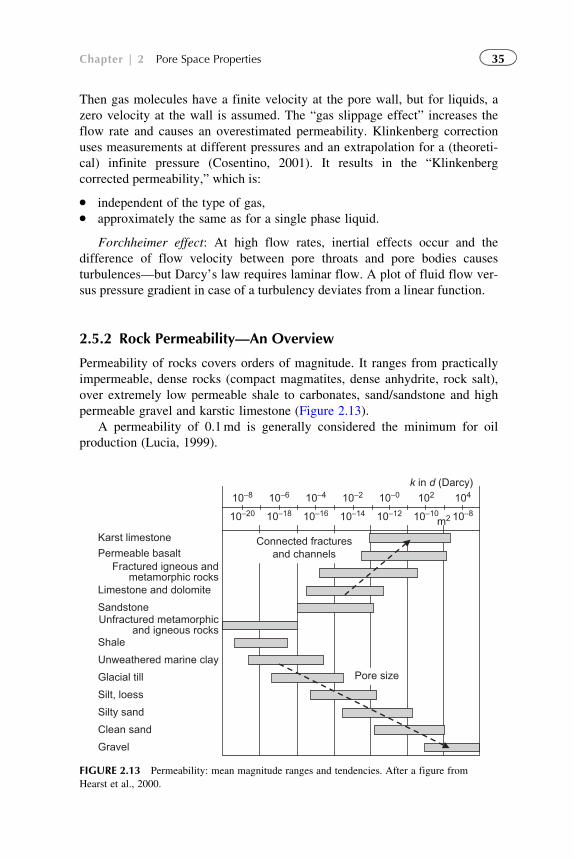
494
Transcript of Physical Properties of Rocks HANDBOOK OF PETROLEUM EXPLORATION AND PRODUCTION

Physical Properties of Rocks
HANDBOOK OF PETROLEUM EXPLORATIONAND PRODUCTION
8
Series EditorJOHN CUBITT
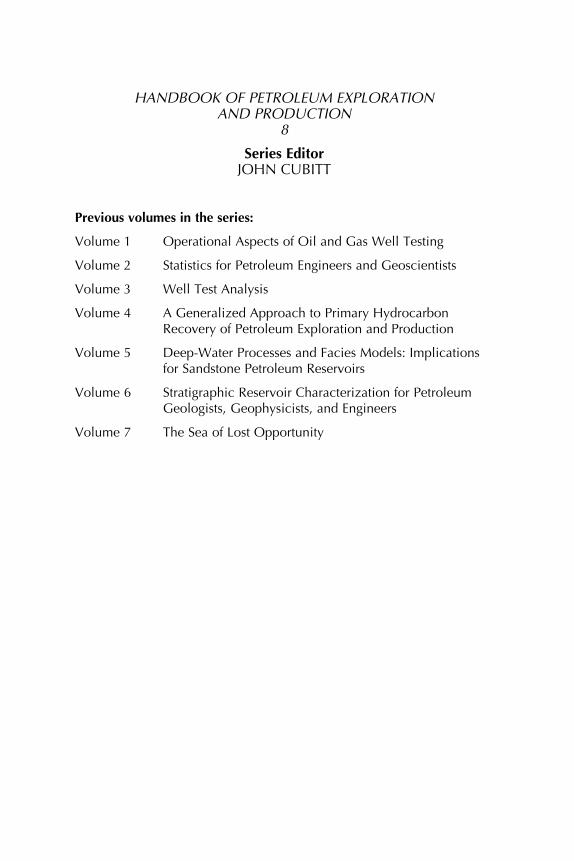
Previous volumes in the series:
Volume 1 Operational Aspects of Oil and Gas Well Testing
Volume 2 Statistics for Petroleum Engineers and Geoscientists
Volume 3 Well Test Analysis
Volume 4 A Generalized Approach to Primary HydrocarbonRecovery of Petroleum Exploration and Production
Volume 5 Deep-Water Processes and Facies Models: Implicationsfor Sandstone Petroleum Reservoirs
Volume 6 Stratigraphic Reservoir Characterization for PetroleumGeologists, Geophysicists, and Engineers
Volume 7 The Sea of Lost Opportunity
Handbook of Petroleum Exploration and Production, 8
Physical Propertiesof Rocks
A Workbook
J.H. Schon
AMSTERDAM � BOSTON � HEIDELBERG � LONDONNEW YORK � OXFORD � PARIS � SAN DIEGO
SAN FRANCISCO � SINGAPORE � SYDNEY � TOKYO
Elsevier
The Boulevard, Langford Lane, Kidlington, Oxford, OX5 1GB, UK
Radarweg 29, PO Box 211, 1000 AE Amsterdam, The Netherlands
Copyright © 2011 Elsevier B.V. All rights reserved
No part of this publication may be reproduced, stored in a retrieval system or
transmitted in any form or by any means electronic, mechanical, photocopying,
recording or otherwise without the prior written permission of the publisher
Permissions may be sought directly from Elsevier’s Science & Technology Rights
Department in Oxford, UK: phone (+44) (0) 1865 843830; fax (+44) (0) 1865 853333;
email: [email protected]. Alternatively you can submit your request online by
visiting the Elsevier website at http://elsevier.com/locate/permissions, and selecting
Obtaining permission to use Elsevier material
Notice
No responsibility is assumed by the publisher for any injury and/or damage to persons
or property as a matter of products liability, negligence or otherwise, or from any use or
operation of any methods, products, instructions or ideas contained in the material herein
British Library Cataloguing-in-Publication Data
A catalogue record for this book is available from the British Library
Library of Congress Cataloging-in-Publication Data
A catalog record for this book is available from the Library of Congress
ISBN: 978-0-444-53796-6
For information on all Elsevier publications
visit our website at elsevierdirect.com
Printed and bound in Great Britain
11 12 13 14 10 9 8 7 6 5 4 3 2 1
-------------------l( Contents )1----
Preface Acknowledgments
1. Rocks-Their Classification and General Properties 1.1 Introduction 1.2 Igneous Rocks 1.3 Metamorphic Rocks 1.4 Sedimentary Rocks 1.5 Physical Properties of Rocks-Some General
Characteristics
2. Pore Space Properties
ix xi
1
2
3
4
12
2.1 Overview-Introduction 17
2.2 Porosity 17
2.3 Specific Internal Surface 29
2.4 Fluids in the Pore Space-Saturation and Bulk Volume Fluid 30
2.5 Permeability 32
2.6 Wettability 56
2.7 Fluid Distribution-Capillary Pressure in a Reservoir 59
2.8 Example: Sandstone-Part 1 70
3. Nuclear Magnetic Resonance- Petrophysical Properties 3.1 Introduction 75
3.2 Physical Origin 76
3.3 The Principle of an NMR Measurement 77
3.4 NMR Relaxation Mechanisms of Fluids in Pores and Fluid-Surface Effects 80
3.5 Applications
4. Density 4.1 Definition and Units 4.2 Density of Rock Constituents 4.3 Density of Rocks
90
97
98
101
v
Contents
5. Nuclear/Radioactive Properties
6.
7.
8.
9.
5.1 Fundamentals 5.2 Natural Radioactivity 5.3 Interactions of Gamma Radiation
107
108
126
5.4 Interactions of Neutron Radiation 131
5.5 Application of Nuclear Measurements for a Mineral Analysis 139
5.6 Example: Sandstone-Part 2 146
Elastic Properties 6.1 Fundamentals 149
6.2 Elastic Properties of the Rock Constituents 154
6.3 Velocity of Rocks-Overview 160
6.4 Velocity of Igneous and Metamorphic Rocks 161
6.5 Velocity of Sedimentary Rocks 164
6.6 Anisotropy 181
6.7 Theories 188
6.8 Reservoir Properties from Seismic Parameters 226
6.9 Attenuation of Elastic Waves 232
6.10 Example of Elastic Properties: Sandstone (Gas Bearing) 240
Geomechanical Properties 7.1 Overview, Introduction 245
7.2 Classification Parameters 246
7.3 Fundamental Geomechanical Properties and Processes 249
7.4 Correlation Between Static and Dynamic Moduli 259
7.5 Correlation Between Seismic Velocity and Strength Properties 264
Electrical Properties 8.1 Fundamentals 273
8.2 Electrical Properties of Rock Components 275
8.3 Specific Electrical Resistivity of Rocks 278
8.4 Clean Rocks-Theories and Models 288
8.5 Shaly Rocks, Shaly Sands 296
8.6 Laminated Shaly Sands and Laminated Sands-Macroscopic Anisotropy 304
8.7 Dielectric Properties of Rocks 310
8.8 Complex Resistivity-Spectral-Induced Polarization 324
8.9 Example: Sandstone-Part 3 335
Thermal Properties 9.1 Introduction 337
9.2 Thermal Properties of Minerals and Pore Contents 339
9.3 Thermal Properties of Rocks-Experimental Data 343
9.4 Theories and Models 360
Contents
10. Magnetic Properties 10.1 Fundamentals and Units 10.2 Magnetic Properties of Rock Constituents 10.3 Magnetic Properties of Rocks
11. Relationships Between Some Petrophysical Properties 11.1 Introduction 11.2 Relationships Based on layered Models-log Interpretation
373 376 381
393
for Porosity and Mineral Composition Estimate 394 11.3 Relationships Between Thermal Conductivity and Elastic
Wave Velocities 403
Appendix A: Physical Properties of Rock-Forming Minerals 415 Appendix B: Some Conversions 423 Appendix C: Files available on the website http://www.elsevierdirect.com/
companion.jsp11SBN=9780444537966 425 References 433 Index 463
Preface
Petrophysics, beginning with Archie’s historical yet evergreen equations, has
a key function in all applications of geosciences, petroleum engineering and
related technologies. It helps us with understanding the processes and con-
trolling properties, and creates relationships between:
� parameters we can measure as output of the dramatic progress in explora-
tion techniques;� properties we need for reservoir characterization (hydrocarbons, water,
minerals, geothermal energy), but also stability of formations and
constructions.
Therefore, there is an increasing interest to understand and manage these
relationships.
Petrophysics is complex and multidisciplinary. For the high sophisticated
techniques like seismic investigations, nuclear magnetic resonance measure-
ments and spectral methods, excellent textbooks are available. Practical
applications and techniques are described in manuals and chartbooks.
Thus, in front of this highly sophisticated, specialized, and detailed world
of petrophysical books and literature, my wish is to give a comprehensive
presentation of fundamentals from my point of view. To define these topics
and contents, I had the valuable help of a long experience working at univer-
sities and teaching courses for the industry with colleagues.
As a student, I had a book about “Theoretical Physics” (by Georg Joos)
with the preface, “This book should not be a lift carrying the reader without
energy on the tops of science. It should be only a simple mountain guide,
leading on an elevation, which gives the view on the top of the mountains
and acts as a “base camp” for reaching these tops.” I have learned to under-
stand this fundamental function of a “base camp” as a location to prepare
and to train and to find motivation for the next levels from the real life
experiences of our son Peter, when he voyages high on the fascinating
summits of mountains in our world.
Over the course of my professional life, I’ve had the happiness to work
on the fascinating subject of “rocks,” and as always, as well as with this
book, I have the wish to transform and share a little bit this fascination of
ix

studying rocks, to show the pleasure we get from the investigation of the
natural rock and its beauty:
“to see a world in a grain of sand,
and a heaven in a wild flower,
held infinity in the palm of your hand
and eternity in an hour . . .”
William Blake (1757�1829)
x Preface

Acknowledgments
I wish to express my deepest gratitude to all my friends, colleagues, and stu-
dents for their indispensable help, for sharing ideas, and for giving me the
motivation to complete this work.
I would like to give special thanks to Erika Guerra for editing the manu-
script and for her time and patience spent dealing with my text, the figures,
references, and all the details. Many thanks, Erika, you have been more than
a “technical writer,” you gave me the foundation for a proper text (that is . . .I hope so).
Over the course of my professional life, I have had the honour and plea-
sure to work with and to learn from many wonderful people, and to share a
common enthusiasm. However, there are too many to name here, and with
great regret I can only share a few acknowledgments at this moment. My
colleagues and dear friends, Daniel Georgi and Allen Gilchrist, for their long
cooperation in teaching petrophysics, as well as in research, and for giving
me valuable comments and help . . . especially for the NMR and nuclear sec-
tion. But most of all, our long cooperation gave me the motivation to try this
experiment of writing the fundamentals of our discipline. Frank Borner, one
of my first students, and now my friend and colleague, contributed valuable
insight and ideas for electrical properties.
The opportunity to teach at universities, particularly Bergakademie
Freiberg/Germany, Montanuniversitat Leoben, Technical University Graz/
Austria, and at the Colorado School of Mines/Golden, laid the foundation for
a fruitful teamwork with students—their response to a book like this is of
substantial importance. Some of them have followed the “petrophysics way”
and helped me mainly with experimental data—one of the rarest components
in our science. Nina Gegenhuber made measurements of elastic and thermal
properties and I could use these, many thanks.
I could expand teaching beyond the university to training courses for
industry—a completely new and valuable experience with the important
response of the practice and the fruitful sharing of knowledge and problem
analyses. I thank Baker Atlas (Houston) and HOT-Engineering (Leoben) for
placing the fundamentals of petrophysics as an integral component of geos-
ciences in their programs and for supporting this work. I was able to acquire
much practical experience in my job with Joanneum Research (Graz/Leoben).
I would like to give thanks to various companies and organizations for giv-
ing me permission to use their valuable materials—particularly Baker Atlas/
Baker Hughes, Schlumberger, AGU, AAPG, EAGE, SEG, SPE, and SPWLA.
xi

Thanks to the staff at Elsevier, in particular Linda Versteeg, Derek
Coleman, and Mohana Natarajan, for their constructive cooperation.
Writing a book requires a creative environment and people who can moti-
vate you, focus your energy, and refresh your patience from time to time.
My wife, Monika, has done a perfect job in the background and has moti-
vated me many times. Many thanks�now we are ready. Also, our son, Peter,
was and is such an energizing factor�his energy and discipline to work for
an idea frequently gave me confirmation that we need to use the time we
have to do valuable things.
xii Acknowledgments
Chapter 1
Rocks—Their Classification andGeneral Properties
1.1 INTRODUCTION
Rocks are naturally occurring aggregates of one or more minerals. In the
case of porosity or fracturing, they also contain fluid phases.
With respect to their geological genesis and processes, rocks are divided
into three major groups:
� igneous rocks (magmatites);� metamorphic rocks (metamorphites);� sedimentary rocks (sediments).
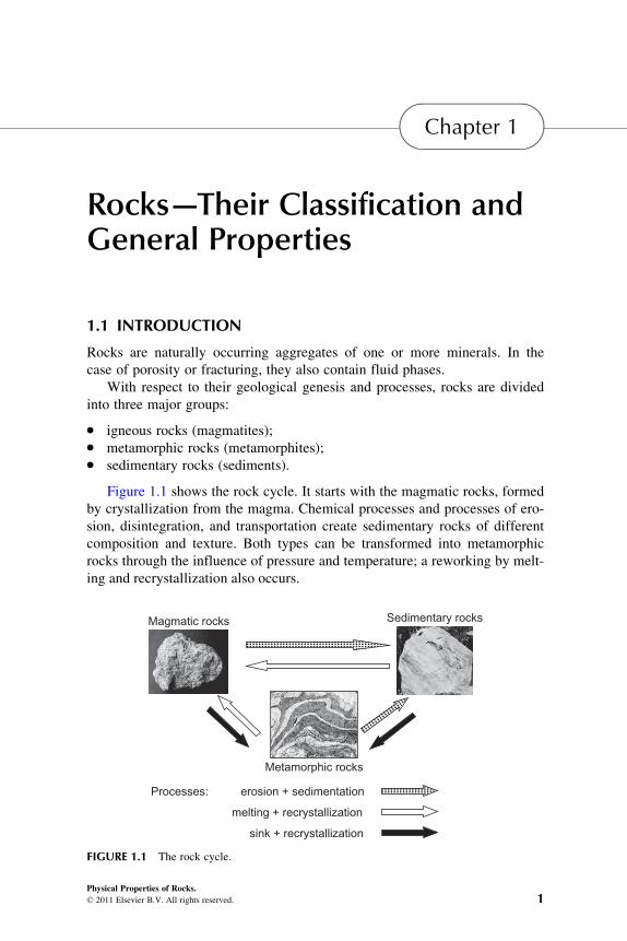
Figure 1.1 shows the rock cycle. It starts with the magmatic rocks, formed
by crystallization from the magma. Chemical processes and processes of ero-
sion, disintegration, and transportation create sedimentary rocks of different
composition and texture. Both types can be transformed into metamorphic
rocks through the influence of pressure and temperature; a reworking by melt-
ing and recrystallization also occurs.
Magmatic rocks Sedimentary rocks
Metamorphic rocks
Processes: erosion + sedimentation
melting + recrystallization
sink + recrystallization
FIGURE 1.1 The rock cycle.
1Physical Properties of Rocks.
© 2011 Elsevier B.V. All rights reserved.
The following sections briefly describe the three rock types. Sedimentary
rocks are discussed in more detail with respect to their importance to fluid
reservoir exploration (e.g., hydrocarbons, water) and their abundance on the
earth’s surface. A detailed classification of rocks and their abundances on
the earth is given by Best (1995) in A Handbook of Physical Constants/AGU
Reference Shelf 3.
1.2 IGNEOUS ROCKS
Igneous rocks are formed by crystallization from a molten magma. Three
types are characterized by their occurrence and position in the crust:
� plutonic rocks crystallized in great depth and forming large rock bodies;� volcanic rocks reaching the surface, in many cases forming layers of
rocks like a blanket;� dikes have dominant vertical extension and a horizontal extension in one
direction; also, they frequently separate geological units.
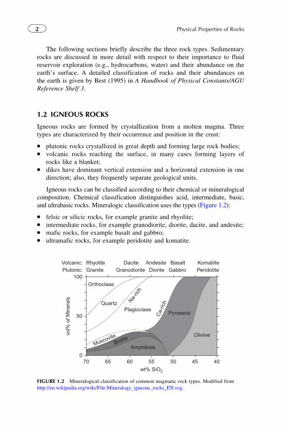
Igneous rocks can be classified according to their chemical or mineralogical
composition. Chemical classification distinguishes acid, intermediate, basic,
and ultrabasic rocks. Mineralogic classification uses the types (Figure 1.2):
� felsic or silicic rocks, for example granite and rhyolite;� intermediate rocks, for example granodiorite, diorite, dacite, and andesite;� mafic rocks, for example basalt and gabbro;� ultramafic rocks, for example peridotite and komatite.
PlagioclaseQuartz
Orthoclase
Volcanic:Plutonic:
RhyoliteGranite
Dacite Andesite BasaltGabbro
KomatiitePeridotiteDioriteGranodiorite
vol%
of M
iner
als
wt% SiO2
Amphibole
Olivine
PyroxeneCa-
richNa-
rich
BiotiteMuscovite
50
070 65 60 55 50 45 40
100
FIGURE 1.2 Mineralogical classification of common magmatic rock types. Modified from
http://en.wikipedia.org/wiki/File:Mineralogy_igneous_rocks_EN.svg.
2 Physical Properties of Rocks
Mineral composition controls physical properties (e.g., density and seis-
mic velocity increases from felsic to mafic rock types).
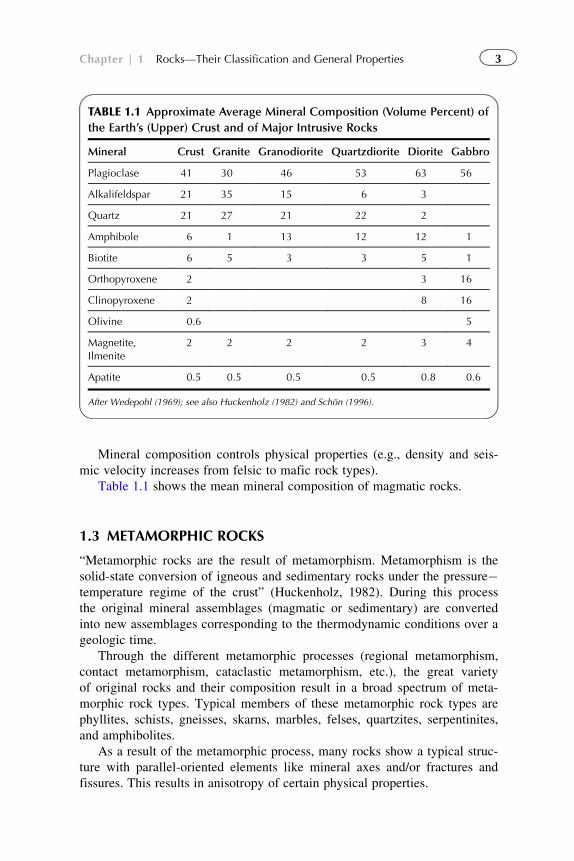
Table 1.1 shows the mean mineral composition of magmatic rocks.
1.3 METAMORPHIC ROCKS
“Metamorphic rocks are the result of metamorphism. Metamorphism is the
solid-state conversion of igneous and sedimentary rocks under the pressure�temperature regime of the crust” (Huckenholz, 1982). During this process
the original mineral assemblages (magmatic or sedimentary) are converted
into new assemblages corresponding to the thermodynamic conditions over a
geologic time.
Through the different metamorphic processes (regional metamorphism,
contact metamorphism, cataclastic metamorphism, etc.), the great variety
of original rocks and their composition result in a broad spectrum of meta-
morphic rock types. Typical members of these metamorphic rock types are
phyllites, schists, gneisses, skarns, marbles, felses, quartzites, serpentinites,
and amphibolites.
As a result of the metamorphic process, many rocks show a typical struc-
ture with parallel-oriented elements like mineral axes and/or fractures and
fissures. This results in anisotropy of certain physical properties.
TABLE 1.1 Approximate Average Mineral Composition (Volume Percent) of
the Earth’s (Upper) Crust and of Major Intrusive Rocks
Mineral Crust Granite Granodiorite Quartzdiorite Diorite Gabbro
Plagioclase 41 30 46 53 63 56
Alkalifeldspar 21 35 15 6 3
Quartz 21 27 21 22 2
Amphibole 6 1 13 12 12 1
Biotite 6 5 3 3 5 1
Orthopyroxene 2 3 16
Clinopyroxene 2 8 16
Olivine 0.6 5
Magnetite,Ilmenite
2 2 2 2 3 4
Apatite 0.5 0.5 0.5 0.5 0.8 0.6
After Wedepohl (1969); see also Huckenholz (1982) and Schon (1996).
3Chapter | 1 Rocks—Their Classification and General Properties
1.4 SEDIMENTARY ROCKS
1.4.1 Overview
Sedimentary rocks are highly important for hydrocarbon exploration; most
commercial reservoirs occur in this rock type characterized by its porosity
and permeability. Sedimentary rocks cover more than 50% of the earth’s sur-
face and are therefore also of fundamental importance in many aspects of
our lives, from agriculture to the foundation for buildings, and from ground-
water resources to the whole environment.
Sedimentary rocks are formed by a sequence of physical, chemical, and
biological processes.
Magmatic, sedimentary, and metamorphic source rocks are disaggregated
by weathering to:
� resistant residual particles (e.g., silicate minerals, lithic fragments);� secondary minerals (e.g., clays);� water soluble ions of calcium, sodium, potassium, silica, etc.
Weathered material is transported via water, ice, or wind to sites and
deposited:
� mineral grains drop to the depositional surface;� dissolved matter precipitates either inorganically, where sufficiently con-
centrated, or by organic processes;� decaying plant and animal residues may also be introduced into the depo-
sitional environment.
Lithification (consolidation) occurs when the sedimentary material becomes
compacted; aqueous pore solutions interact with the deposited particles to form
new, cementing diagenetic (authigenic) minerals (Best, 1995).
We distinguish two major rock classes of sedimentary rocks:
� clastics (siliciclastics);� carbonates and evaporites.
Siliciclastics are composed of various silicate grains; carbonates consist
mainly of only the two minerals dolomite and calcite. Clastic sediments have
been transported over long distances, whereas carbonates are formed on-site
(mostly marine). Clastic sediments are relatively chemically stable; they
form an intergranular pore space. Carbonates on the other hand are chemi-
cally instable; their pore space is very complex and controlled by a variety
of influences and pore space geometries.
In addition to the mineral composition for geological characterization of rocks
in general and for sedimentary rocks in particular, the term “lithology” is used.
The American Geological Institute Glossary of Geology defines lithology as “the
4 Physical Properties of Rocks
physical character of a rock.” This character is influenced mainly by mineral
composition (mineralogy) and texture of the solids (Jorden & Campbell, 1984).
1.4.2 Clastic Rocks
1.4.2.1 Classification
Clastic rocks are formed by:
� erosion, reworking, and transportation of rock components;� deposition and sedimentation of the material;� compaction and diagenetic processes.
Typical members of this important group of rocks are conglomerate,
sandstone, siltstone, shale, and claystone.1
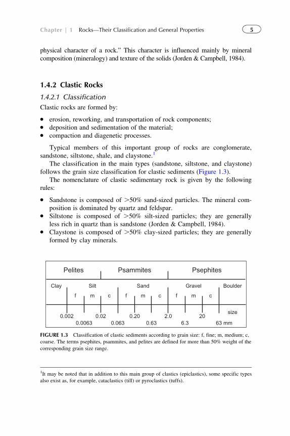
The classification in the main types (sandstone, siltstone, and claystone)
follows the grain size classification for clastic sediments (Figure 1.3).
The nomenclature of clastic sedimentary rock is given by the following
rules:
� Sandstone is composed of .50% sand-sized particles. The mineral com-
position is dominated by quartz and feldspar.� Siltstone is composed of .50% silt-sized particles; they are generally
less rich in quartz than is sandstone (Jorden & Campbell, 1984).� Claystone is composed of .50% clay-sized particles; they are generally
formed by clay minerals.
1It may be noted that in addition to this main group of clastics (epiclastics), some specific types
also exist as, for example, cataclastics (till) or pyroclastics (tuffs).
Pelites PsephitesPsammites
Clay GravelSandSilt Boulder
f cm f cm mf c
0.002 0.02 0.20 2.0 200.0063 0.063 0.63 6.3 63 mm
size
FIGURE 1.3 Classification of clastic sediments according to grain size: f, fine; m, medium; c,
coarse. The terms psephites, psammites, and pelites are defined for more than 50% weight of the
corresponding grain size range.
5Chapter | 1 Rocks—Their Classification and General Properties
The term “shale” describes a sedimentary rock type which is a mixture
of clay-sized particles (mainly clay minerals), silt-sized particles (quartz,
feldspar, calcite), and perhaps some sand-sized particles as, for example,
quartz, occasionally feldspar, calcite (Jorden & Campbell, 1984). Serra
(2007) wrote “from a compilation of 10,000 shale analyses made by
Yaalon (1962), the average composition of shale is 59% clay minerals,
predominantly illite; 20% quartz and chert; 8% feldspar; 7% carbonates;
3% iron oxides; 1% organic material; and others 2%. . . . Mudstone is a
rock having the grain size and composition of a shale but lacking its lami-
nations and/or its fissility . . ..” As an example, for Pierre shale, Borysenko
et al. (2009) gave the following mineral composition: quartz 29%; kaolin-
ite, chlorite 8%; illite, muscovite, smectite 26%; mica 24%; orthoclase,
dolomite, albite 13%.
Many properties of shale are controlled by the clay components (e.g.,
gamma radiation, electrical properties, cation exchange capacity (CEC), neu-
tron response, permeability). For understanding physical properties of sedi-
mentary rocks it is important to distinguish the different terms referred to as
shale and clay:
� clay describes a group of minerals (hydrous aluminum silicates, see
Section 1.4.2.3);� clay also defines a particle size (,0.002mm);� shale describes a rock type as defined above (“claystone” also refers to a
rock type).
The physical properties of clastic sediments are strongly controlled by:
� textural properties (particle dimensions, size, shape, spatial orientation);� mineral composition, mainly the presence and effect of clay minerals.
1.4.2.2 Textural Properties�Grain-Size Parameters
The term texture encompasses particle size and size distribution, and shape
and packing of the solid particles in clastic sediments.
Grain size is the classifying and defining parameter for clastic rocks. In
general, particles are of nonspherical shape; thus the “grain diameter”
depends on the technique of its determination:
� sieve analysis gives an estimate closed to the minimum cross-sectional
axis (corresponding to the used mesh size) or a sphere equivalent measure
following Stokes’ law (sedimentation analysis);� image or laser scanned techniques allow the application of numerical
algorithms for a representative size description.
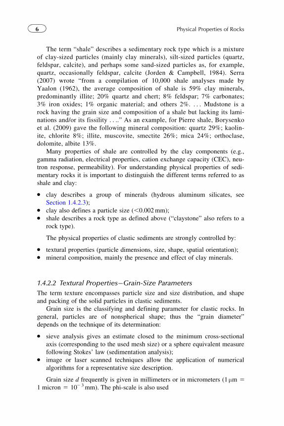
Grain size d frequently is given in millimeters or in micrometers (1 µm 51 micron 5 102 3mm). The phi-scale is also used
6 Physical Properties of Rocks
phi ¼ 2 log2ðdÞ ð1:1Þwhere d is in millimeters.
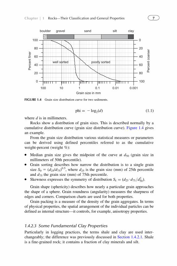
Rocks show a distribution of grain sizes. This is described normally by a
cumulative distribution curve (grain size distribution curve). Figure 1.4 gives
an example.
From the grain size distribution various statistical measures or parameters
can be derived using defined percentiles referred to as the cumulative
weight-percent (weight %):
� Median grain size gives the midpoint of the curve at d50 (grain size in
millimeters of 50th percentile).� Grain sorting describes how narrow the distribution is to a single grain
size S0 5 (d25/d75)0.5, where d25 is the grain size (mm) of 25th percentile
and d75 the grain size (mm) of 75th percentile.� Skewness expresses the symmetry of distribution Sk ¼ ðd25Ud75=d250Þ:
Grain shape (sphericity) describes how nearly a particular grain approaches
the shape of a sphere. Grain roundness (angularity) measures the sharpness of
edges and corners. Comparison charts are used for both properties.
Grain packing is a measure of the density of the grain aggregates. In terms
of physical properties, the spatial arrangement of the individual particles can be
defined as internal structure—it controls, for example, anisotropy properties.
1.4.2.3 Some Fundamental Clay Properties
Particularly in logging practices, the terms shale and clay are used inter-
changeably; the difference was previously discussed in Section 1.4.2.1. Shale
is a fine-grained rock; it contains a fraction of clay minerals and silt.
100 10 1 0.1 0.01 0.001
Grain size in mm
0
20
40
60
80
100
Per
cent
fine
r
100
80
60
40
20
0
Per
cent
coa
rser
boulder gravel sand silt clay
well sorted poorly sorted
FIGURE 1.4 Grain size distribution curve for two sediments.
7Chapter | 1 Rocks—Their Classification and General Properties
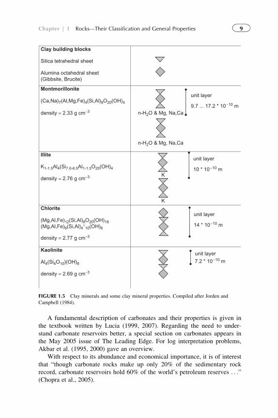
Clay minerals are aluminosilicates with a sheet structure. The principal
building elements are two types of sheets or units:
� a tetrahedral unit of a central Si atom and surrounding O atoms;� an octahedral unit of O atoms and OH groups around a central Al atom.2
Clay minerals (kaolinite, illite, montmorillonite, chlorite) are character-
ized by different stacking combinations or “architecture” of the two building
elements (Figure 1.5). Individual figures always represent one crystal.
Montmorillonite has a water layer between the two units; the amount of
water varies so that the size also ranges between 9.7 � 102 10 and
17.2 � 102 10m (9.7 and 17.2 A). Water trapped between the units or layers
influence electrical conductivity (see Section 8.5) and contributes to total
porosity (but not to effective porosity).
In the tetrahedral sheet, silica (Si1 4) is sometimes partly replaced by alu-
minum (Al1 3); in the octahedral sheet, aluminum (Al1 3) can be replaced by
magnesium (Mg1 2) or other atoms (e.g., iron). Such a replacement by atoms
of lower positive valence results in an excess of negative charge. This excess
is compensated for by adsorption of cations (Na, Ca, Mg) from the adjacent
water and an electric double layer is formed. The compensating cations on
the surface layer can be exchanged by other cations. The number of the
exchangeable cations is measured by the Cation Exchange Capacity (CEC)
Montmorillonite has a high CEC value, but kaolinite and chlorite without
interlayer cations have low CEC. Clays with high CEC play a leading role
in the electrical conduction of shales and shaly sands (see Section 8.5). The
ability of clay minerals to adsorb ions results in case of “radioactive ions” in a
contribution to natural radioactivity (see Section 5.2) (Table 1.2).
The effect of clay minerals in the rock depends on the mineral properties
and the type of clay distribution. There are three fundamental types:
1. Dispersed: clay is formed within the sediment when clay crystals precipi-
tate from pore fluids.
2. Laminated: clay is of detrital origin, that is, formed outside the sandstone
framework.
3. Structural: clay is of diagenetic origin, that is, formed within the sand-
stone framework as a deposit of clay clasts.
1.4.3 Carbonate and Evaporate Rocks
1.4.3.1 Introduction
The nonclastic carbonate and evaporate rocks are formed mainly by chemical
and biochemical precipitation in special environments (typically warm, shal-
low, clear marine water in low latitudes).
2In some cases also Mg or Fe.
8 Physical Properties of Rocks
A fundamental description of carbonates and their properties is given in
the textbook written by Lucia (1999, 2007). Regarding the need to under-
stand carbonate reservoirs better, a special section on carbonates appears in
the May 2005 issue of The Leading Edge. For log interpretation problems,
Akbar et al. (1995, 2000) gave an overview.
With respect to its abundance and economical importance, it is of interest
that “though carbonate rocks make up only 20% of the sedimentary rock
record, carbonate reservoirs hold 60% of the world’s petroleum reserves . . .”(Chopra et al., 2005).
Clay building blocks
Silica tetrahedral sheet
Alumina octahedral sheet(Gibbsite, Brucite)
Montmorillonite
(Ca,Na)7(Al,Mg,Fe)4(Si,Al)8O20(OH)4
density = 2.33 g cm−3
Illite
K1-1.5Al4(Si7.0-6.5Al1-1.5O20(OH)4
density = 2.76 g cm−3
Chlorite
(Mg,Al,Fe)12(Si,Al)8O20(OH)16(Mg,Al,Fe)6(Si,Al)4°10(OH)8
density = 2.77 g cm−3
Kaolinite
Al4(Si4O10)(OH)8
density = 2.69 g cm−3
n-H2O & Mg, Na,Ca
n-H2O & Mg, Na,Ca
unit layer
9.7 ... 17.2 * 10−10 m
K
K
unit layer
10 * 10−10 m
unit layer
14 * 10−10 m
unit layer
7.2 * 10−10 m
FIGURE 1.5 Clay minerals and some clay mineral properties. Compiled after Jorden and
Campbell (1984).
9Chapter | 1 Rocks—Their Classification and General Properties
1.4.3.2 Composition
Carbonates originated autochthonous (formed very close to the depositional
site) whereas clastics sandstone and shale are formed of transported sedimen-
tary particles mostly from sources outside the depositional site.
The most abundant carbonatic minerals are calcite (CaCO3) and dolomite
(CaMg(CO3)2). Secondary minerals are anhydrite, chert, and quartz.
Accessory minerals are phosphates, glauconite, ankerite, siderite, feldspars,
clay minerals, pyrite, etc., depending on the environment of deposition and
diagenetic history.
The two main rock types are as follows:
1. Limestone: composed of more than 50% carbonates, of which more than
half is calcite.
2. Dolomite: composed of more than 50% carbonates, of which more than
half is dolomite. Dolomite can precipitate directly from a solution con-
taining Mg, Ca, and carbonate ions or by chemical alteration of limestone
or calcareous mud (dolomitization). Dolomite frequently forms larger
crystals than the calcite it replaces (Al-Awadi, 2009) and forms good res-
ervoir properties.
Carbonates are modified by various postdepositional processes such as
dissolution, cementation, recrystallization, dolomitization, and replacement
by other minerals. Dolomitization is connected with an increase of porosity.
The interaction with meteoric pore fluids can result in a leaching of
grains and influence reservoir quality in both directions (new pore space,
cementation).
Fracturing as a result of stress and stylolithification are diagenetic processes
in carbonates; they can create high-permeability zones and permeability barriers
or baffles.
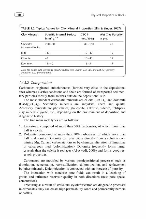
TABLE 1.2 Typical Values for Clay Mineral Properties (Ellis & Singer, 2007)
Clay Mineral Specific Internal Surface
in m2 g2 1
CEC in
meq/100 g
Wet Clay Porosity
in p.u.
Smectite/Montmorillonite
700�800 80�150 40
Illite 113 10�40 15
Chlorite 42 10�40 15
Kaolinite 15�40 3�5 5
Note the trend: with increasing specific surface (see Section 2.3) CEC and wet clay porosityincreases. p.u., porosity units.
10 Physical Properties of Rocks
Evaporate sediments are a special type of sedimentary rock that is formed
from the concentration of dissolved salts through evaporation (e.g., rock salt/
halite).
1.4.3.3 Classification
Carbonates are biologically deposited and contain fossil fragments and other
particles with complicated morphology and shape. This results in complex
pore structures in general. Dissolution, precipitation, recrystallization, dolo-
mitization, and other processes increase this complexity over scales.
Different types of porosity and complex pore size distributions also result
in wide permeability variations for the same total porosity, making it diffi-
cult to predict their producibility. Therefore, the analysis of carbonate pore
geometries is the key to characterize the reservoir properties of this group of
rocks.
For carbonates, two main types of classification have been developed:
1. Textural classification (Dunham, 1962) based on the presence or absence
of lime mud and grain support and ranges from:
a. grain-supported grainstones, mudstones, and packstones to;
b. mud-supported wackestones and mudstones;
c. crystalline or boundstones.
2. Fabric selective and nonfabric selective pore type classification (Choquette
& Pray, 1970) including:
a. fabric selective (interparticle, intraparticle, intercrystal, moldic, fenestral,
shelter, and framework);
b. nonfabric selective (vug and channel, cavern, and fracture) porosity.
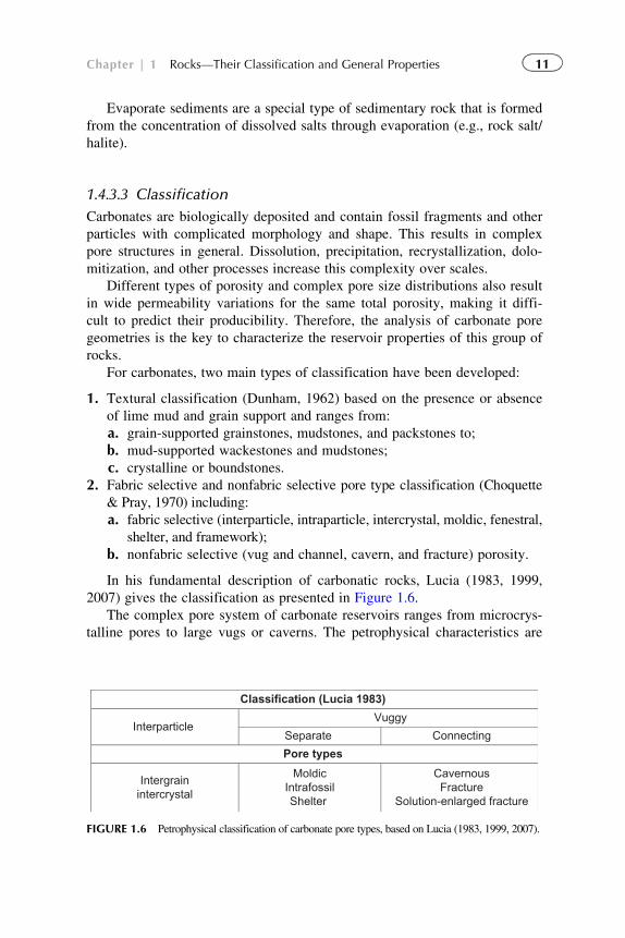
In his fundamental description of carbonatic rocks, Lucia (1983, 1999,
2007) gives the classification as presented in Figure 1.6.
The complex pore system of carbonate reservoirs ranges from microcrys-
talline pores to large vugs or caverns. The petrophysical characteristics are
Classification (Lucia 1983)
Interparticle Vuggy
Separate Connecting
Pore types
Intergrainintercrystal
MoldicIntrafossilShelter
CavernousFracture
Solution-enlarged fracture
FIGURE 1.6 Petrophysical classification of carbonate pore types, based on Lucia (1983, 1999, 2007).
11Chapter | 1 Rocks—Their Classification and General Properties
controlled by connected networks of interparticle pores (matrix), vuggy pore
space, and fractures, where:
� a matrix occupies the major portion of the reservoir, stores most of the
fluid volume but has a low permeability;� fractures (and vugs) occupy a small portion of reservoir volume but have
high permeability and control the fluid flow (Iwere et al., 2002).
A classification and description of carbonate pore geometries is also
given in Schlumberger’s “Carbonate Advisor” (www.slb.com/carbonates) as
follows:
� “Micropores, with pore-throat diameters ,0.5 µm, usually contain mostly
irreducible water and little hydrocarbon.� Mesopores, with pore-throat diameters between 0.5 and 5 µm, may con-
tain significant amounts of oil or gas in pores above the free-water level
(FWL).� Macropores, with throats measuring more than 5 µm in diameter, are
responsible for prolific production rates in many carbonate reservoirs, but
often provide pathways for early water breakthrough, leaving consider-
able gas and oil behind in the mesopores above the FWL.� Vugs are cavities, voids, or large pores in rocks. Vugular porosity is com-
mon in rocks prone to dissolution, such as carbonates.”
1.4.4 Comparison of Siliciclastic and Carbonate Sediments
In siliciclastic rocks, many physical properties (elastic wave velocity, electri-
cal resistivity, permeability) show a strong correlation to porosity. In carbon-
ate rocks, correlations are controlled or superimposed by the heterogeneous
pore distribution, pore type, pore connectivity, and grain size (Westphal
et al., 2005).
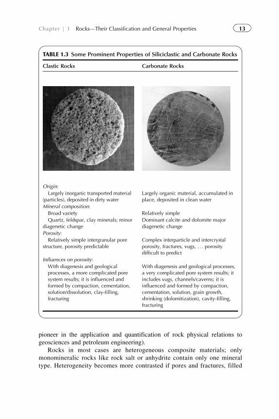
Table 1.3 compares some prominent properties of the two main groups of
reservoir rocks.
1.5 PHYSICAL PROPERTIES OF ROCKS—SOME GENERALCHARACTERISTICS
The term “petrophysics” was created for physics of reservoir rocks.
“‘Petrophysics’ is suggested as the term pertaining to the physics of particu-
lar rock types. . . . This subject is a study of the physical properties of rock
which are related to the pore and fluid distribution . . .” (Archie (1950), the
12 Physical Properties of Rocks
pioneer in the application and quantification of rock physical relations to
geosciences and petroleum engineering).
Rocks in most cases are heterogeneous composite materials; only
monomineralic rocks like rock salt or anhydrite contain only one mineral
type. Heterogeneity becomes more contrasted if pores and fractures, filled
TABLE 1.3 Some Prominent Properties of Siliciclastic and Carbonate Rocks
Clastic Rocks Carbonate Rocks
Origin:
Largely inorganic transported material(particles), deposited in dirty water
Largely organic material, accumulated inplace, deposited in clean water
Mineral composition:
Broad variety Relatively simple
Quartz, feldspar, clay minerals; minordiagenetic change
Dominant calcite and dolomite majordiagenetic change
Porosity:
Relatively simple intergranular porestructure, porosity predictable
Complex interparticle and intercrystalporosity, fractures, vugs, . . . porositydifficult to predict
Influences on porosity:
With diagenesis and geologicalprocesses, a more complicated poresystem results; it is influenced andformed by compaction, cementation,solution/dissolution, clay-filling,fracturing
With diagenesis and geological processes,a very complicated pore system results; itincludes vugs, channels/caverns; it isinfluenced and formed by compaction,cementation, solution, grain growth,shrinking (dolomitization), cavity-filling,fracturing
13Chapter | 1 Rocks—Their Classification and General Properties
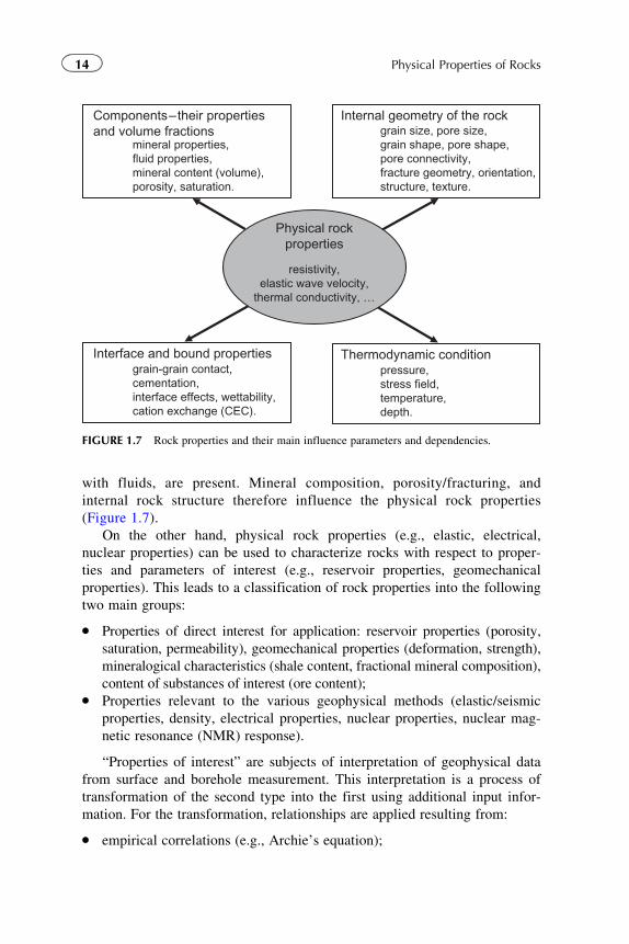
with fluids, are present. Mineral composition, porosity/fracturing, and
internal rock structure therefore influence the physical rock properties
(Figure 1.7).
On the other hand, physical rock properties (e.g., elastic, electrical,
nuclear properties) can be used to characterize rocks with respect to proper-
ties and parameters of interest (e.g., reservoir properties, geomechanical
properties). This leads to a classification of rock properties into the following
two main groups:
� Properties of direct interest for application: reservoir properties (porosity,
saturation, permeability), geomechanical properties (deformation, strength),
mineralogical characteristics (shale content, fractional mineral composition),
content of substances of interest (ore content);� Properties relevant to the various geophysical methods (elastic/seismic
properties, density, electrical properties, nuclear properties, nuclear mag-
netic resonance (NMR) response).
“Properties of interest” are subjects of interpretation of geophysical data
from surface and borehole measurement. This interpretation is a process of
transformation of the second type into the first using additional input infor-
mation. For the transformation, relationships are applied resulting from:
� empirical correlations (e.g., Archie’s equation);
Components–their propertiesand volume fractions
mineral properties,fluid properties,mineral content (volume),porosity, saturation.
Internal geometry of the rock grain size, pore size,grain shape, pore shape,pore connectivity,fracture geometry, orientation,structure, texture.
Interface and bound properties grain-grain contact,cementation,interface effects, wettability,cation exchange (CEC).
Thermodynamic condition pressure,stress field,temperature,depth.
Physical rockproperties
resistivity,elastic wave velocity,
thermal conductivity, …
FIGURE 1.7 Rock properties and their main influence parameters and dependencies.
14 Physical Properties of Rocks
� model-based theories (e.g., Gassmann’s equation for fluid substitution,
capillary pore channel models); in most cases “theoretical” equations
need an empirical modification or calibration with experimental data.
In this book, the most frequently used properties are described. For the
physics behind the individual properties, it is important to characterize them
with respect to their character as a “scalar property” (given as one value for
the property, no directional dependence of the property) or a “tensorial prop-
erty” (given as a tensor with several components with directional depen-
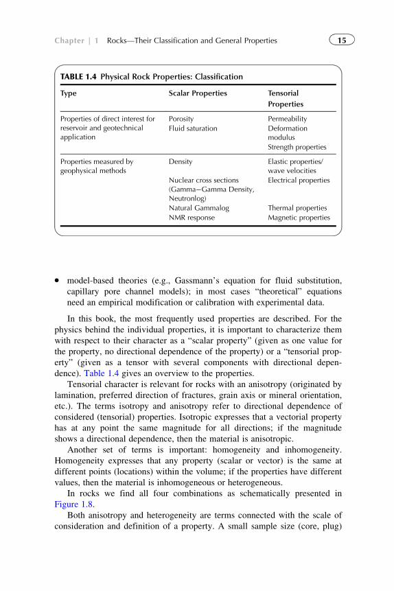
dence). Table 1.4 gives an overview to the properties.
Tensorial character is relevant for rocks with an anisotropy (originated by
lamination, preferred direction of fractures, grain axis or mineral orientation,
etc.). The terms isotropy and anisotropy refer to directional dependence of
considered (tensorial) properties. Isotropic expresses that a vectorial property
has at any point the same magnitude for all directions; if the magnitude
shows a directional dependence, then the material is anisotropic.
Another set of terms is important: homogeneity and inhomogeneity.
Homogeneity expresses that any property (scalar or vector) is the same at
different points (locations) within the volume; if the properties have different
values, then the material is inhomogeneous or heterogeneous.
In rocks we find all four combinations as schematically presented in
Figure 1.8.
Both anisotropy and heterogeneity are terms connected with the scale of
consideration and definition of a property. A small sample size (core, plug)
TABLE 1.4 Physical Rock Properties: Classification
Type Scalar Properties Tensorial
Properties
Properties of direct interest forreservoir and geotechnicalapplication
Porosity Permeability
Fluid saturation Deformationmodulus
Strength properties
Properties measured bygeophysical methods
Density Elastic properties/wave velocities
Nuclear cross sections(Gamma�Gamma Density,Neutronlog)
Electrical properties
Natural Gammalog Thermal properties
NMR response Magnetic properties
15Chapter | 1 Rocks—Their Classification and General Properties
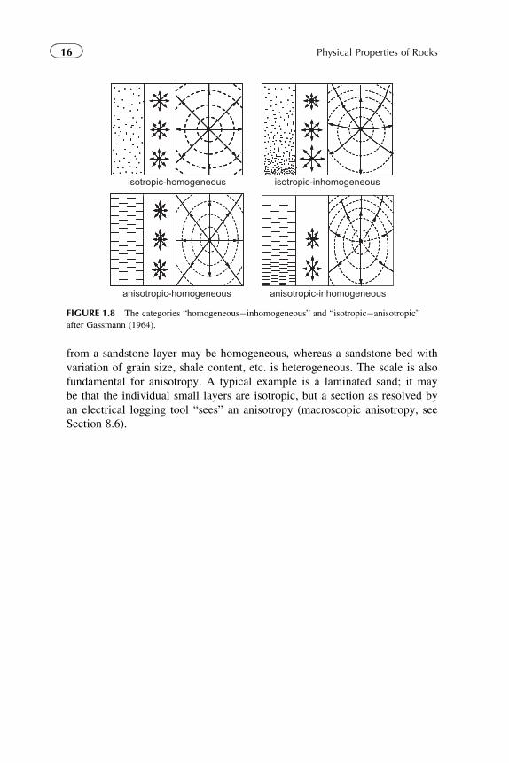
from a sandstone layer may be homogeneous, whereas a sandstone bed with
variation of grain size, shale content, etc. is heterogeneous. The scale is also
fundamental for anisotropy. A typical example is a laminated sand; it may
be that the individual small layers are isotropic, but a section as resolved by
an electrical logging tool “sees” an anisotropy (macroscopic anisotropy, see
Section 8.6).
isotropic-inhomogeneousisotropic-homogeneous
anisotropic-homogeneous anisotropic-inhomogeneous
FIGURE 1.8 The categories “homogeneous�inhomogeneous” and “isotropic�anisotropic”
after Gassmann (1964).
16 Physical Properties of Rocks
Chapter 2
Pore Space Properties
2.1 OVERVIEW—INTRODUCTION
Pore space characterization is based on defined reservoir properties (e.g.,
porosity and permeability). Pore space properties are important for the
description and characterization of pore volume and fluid flow behavior of
reservoirs. Laboratory techniques (standard and special core analysis) deliver
fundamental properties; thin sections and microscopic or scanning electron
microscopic (SEM) investigations are used for description and computer-
aided analysis. Sophisticated techniques result in “digitized core images”
(Arns et al., 2004; Kayser et al., 2006) and the development of a “virtual rock
physics laboratory” (Dvorkin et al., 2008).
The fundamental reservoir properties of the pore space describe:
� volume fractions of the fluids (porosity, saturation, bulk volume of
fluids);� properties controlling fluid distribution in the pore space (capillary pres-
sure, specific internal surface, and wettability);� properties controlling fluid flow under the influence of a pressure gradi-
ent (permeability).
There are relationships between properties: permeability, for example,
correlates with porosity.
Important pore geometrical controlling parameters are the pore body size,
which defines the average volumetric dimensions of the pores, and the pore
throat size, which is the controlling factor in transmissibility/permeability.
2.2 POROSITY
Porosity is a fundamental volumetric rock property: it describes the potential
storage volume of fluids (i.e., water, gas, oil) and influences most physical
rock properties (e.g., elastic wave velocity, electrical resistivity, and density).
17Physical Properties of Rocks.
© 2011 Elsevier B.V. All rights reserved.
Porosity can be determined directly by various laboratory techniques and
indirectly by logging methods.
2.2.1 Definitions
“Porosity is the fraction of rock bulk volume occupied by pore space”
(Jorden & Campbell, 1984).
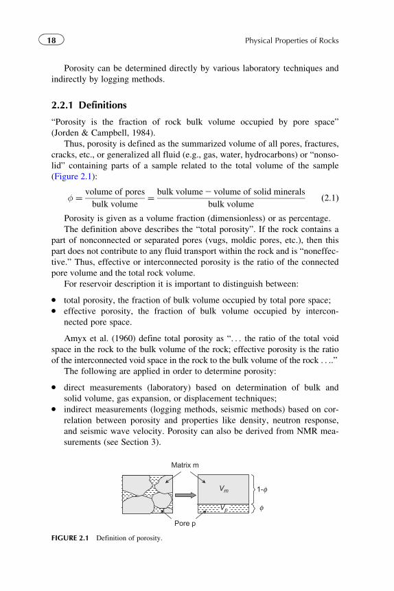
Thus, porosity is defined as the summarized volume of all pores, fractures,
cracks, etc., or generalized all fluid (e.g., gas, water, hydrocarbons) or “nonso-
lid” containing parts of a sample related to the total volume of the sample
(Figure 2.1):
φ ¼ volume of pores
bulk volume¼ bulk volume2 volume of solid minerals
bulk volumeð2:1Þ
Porosity is given as a volume fraction (dimensionless) or as percentage.
The definition above describes the “total porosity”. If the rock contains a
part of nonconnected or separated pores (vugs, moldic pores, etc.), then this
part does not contribute to any fluid transport within the rock and is “noneffec-
tive.” Thus, effective or interconnected porosity is the ratio of the connected
pore volume and the total rock volume.
For reservoir description it is important to distinguish between:
� total porosity, the fraction of bulk volume occupied by total pore space;� effective porosity, the fraction of bulk volume occupied by intercon-
nected pore space.
Amyx et al. (1960) define total porosity as “. . . the ratio of the total void
space in the rock to the bulk volume of the rock; effective porosity is the ratio
of the interconnected void space in the rock to the bulk volume of the rock . . ..”The following are applied in order to determine porosity:
� direct measurements (laboratory) based on determination of bulk and
solid volume, gas expansion, or displacement techniques;� indirect measurements (logging methods, seismic methods) based on cor-
relation between porosity and properties like density, neutron response,
and seismic wave velocity. Porosity can also be derived from NMR mea-
surements (see Section 3).
Vm
Vp
Pore p
1-
φ
φ
Matrix m
FIGURE 2.1 Definition of porosity.
18 Physical Properties of Rocks
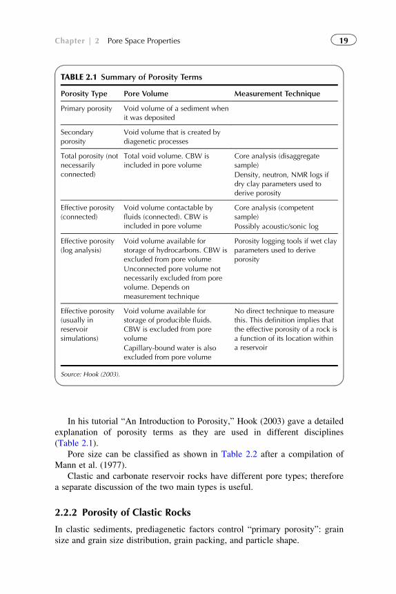
In his tutorial “An Introduction to Porosity,” Hook (2003) gave a detailed
explanation of porosity terms as they are used in different disciplines
(Table 2.1).
Pore size can be classified as shown in Table 2.2 after a compilation of
Mann et al. (1977).
Clastic and carbonate reservoir rocks have different pore types; therefore
a separate discussion of the two main types is useful.
2.2.2 Porosity of Clastic Rocks
In clastic sediments, prediagenetic factors control “primary porosity”: grain
size and grain size distribution, grain packing, and particle shape.
TABLE 2.1 Summary of Porosity Terms
Porosity Type Pore Volume Measurement Technique
Primary porosity Void volume of a sediment whenit was deposited
Secondaryporosity
Void volume that is created bydiagenetic processes
Total porosity (notnecessarilyconnected)
Total void volume. CBW isincluded in pore volume
Core analysis (disaggregatesample)
Density, neutron, NMR logs ifdry clay parameters used toderive porosity
Effective porosity(connected)
Void volume contactable byfluids (connected). CBW isincluded in pore volume
Core analysis (competentsample)
Possibly acoustic/sonic log
Effective porosity(log analysis)
Void volume available forstorage of hydrocarbons. CBW isexcluded from pore volume
Porosity logging tools if wet clayparameters used to deriveporosity
Unconnected pore volume notnecessarily excluded from porevolume. Depends onmeasurement technique
Effective porosity(usually inreservoirsimulations)
Void volume available forstorage of producible fluids.CBW is excluded from porevolume
No direct technique to measurethis. This definition implies thatthe effective porosity of a rock isa function of its location withina reservoirCapillary-bound water is also
excluded from pore volume
Source: Hook (2003).
19Chapter | 2 Pore Space Properties
“Secondary porosity” is the result of mechanical processes (compaction,
plastic and brittle deformation, fracturing) and geochemical processes (disso-
lution, precipitation, volume reductions by mineralogical changes, etc.).
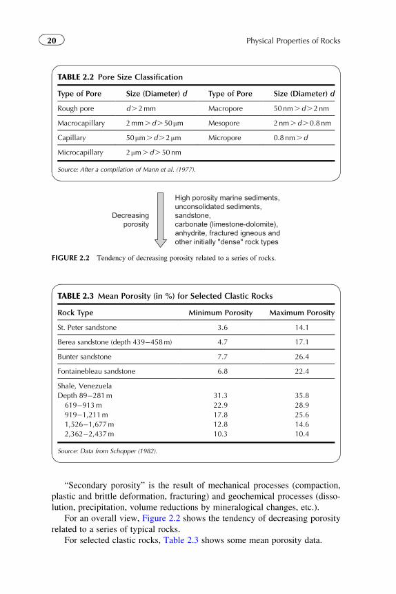
For an overall view, Figure 2.2 shows the tendency of decreasing porosity
related to a series of typical rocks.
For selected clastic rocks, Table 2.3 shows some mean porosity data.
TABLE 2.3 Mean Porosity (in %) for Selected Clastic Rocks
Rock Type Minimum Porosity Maximum Porosity
St. Peter sandstone 3.6 14.1
Berea sandstone (depth 439�458m) 4.7 17.1
Bunter sandstone 7.7 26.4
Fontainebleau sandstone 6.8 22.4
Shale, Venezuela
Depth 89�281m 31.3 35.8
619�913m 22.9 28.9
919�1,211m 17.8 25.6
1,526�1,677m 12.8 14.6
2,362�2,437m 10.3 10.4
Source: Data from Schopper (1982).
Decreasingporosity
High porosity marine sediments,unconsolidated sediments,sandstone,carbonate (limestone-dolomite),anhydrite, fractured igneous andother initially "dense" rock types
FIGURE 2.2 Tendency of decreasing porosity related to a series of rocks.
TABLE 2.2 Pore Size Classification
Type of Pore Size (Diameter) d Type of Pore Size (Diameter) d
Rough pore d.2mm Macropore 50nm.d.2nm
Macrocapillary 2mm.d.50μm Mesopore 2nm.d.0.8 nm
Capillary 50μm.d.2 μm Micropore 0.8 nm.d
Microcapillary 2μm.d.50nm
Source: After a compilation of Mann et al. (1977).
20 Physical Properties of Rocks
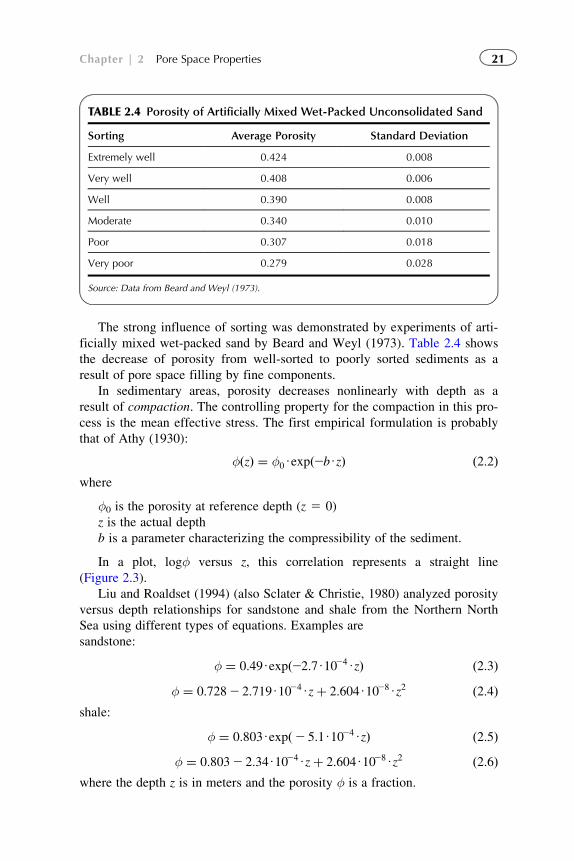
The strong influence of sorting was demonstrated by experiments of arti-
ficially mixed wet-packed sand by Beard and Weyl (1973). Table 2.4 shows
the decrease of porosity from well-sorted to poorly sorted sediments as a
result of pore space filling by fine components.
In sedimentary areas, porosity decreases nonlinearly with depth as a
result of compaction. The controlling property for the compaction in this pro-
cess is the mean effective stress. The first empirical formulation is probably
that of Athy (1930):
φðzÞ ¼ φ0Uexpð2bUzÞ ð2:2Þwhere
φ0 is the porosity at reference depth (z 5 0)
z is the actual depth
b is a parameter characterizing the compressibility of the sediment.
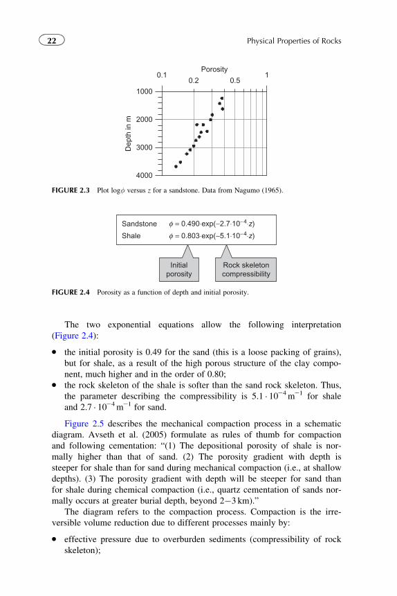
In a plot, logφ versus z, this correlation represents a straight line
(Figure 2.3).
Liu and Roaldset (1994) (also Sclater & Christie, 1980) analyzed porosity
versus depth relationships for sandstone and shale from the Northern North
Sea using different types of equations. Examples are
sandstone:
φ ¼ 0:49Uexpð22:7U1024UzÞ ð2:3Þφ ¼ 0:7282 2:719U1024Uzþ 2:604U1028Uz2 ð2:4Þ
shale:
φ ¼ 0:803Uexpð2 5:1U1024UzÞ ð2:5Þφ ¼ 0:8032 2:34U1024Uzþ 2:604U1028Uz2 ð2:6Þ
where the depth z is in meters and the porosity φ is a fraction.
TABLE 2.4 Porosity of Artificially Mixed Wet-Packed Unconsolidated Sand
Sorting Average Porosity Standard Deviation
Extremely well 0.424 0.008
Very well 0.408 0.006
Well 0.390 0.008
Moderate 0.340 0.010
Poor 0.307 0.018
Very poor 0.279 0.028
Source: Data from Beard and Weyl (1973).
21Chapter | 2 Pore Space Properties
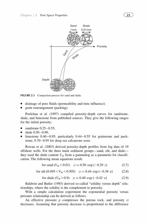
The two exponential equations allow the following interpretation
(Figure 2.4):
� the initial porosity is 0.49 for the sand (this is a loose packing of grains),
but for shale, as a result of the high porous structure of the clay compo-
nent, much higher and in the order of 0.80;� the rock skeleton of the shale is softer than the sand rock skeleton. Thus,
the parameter describing the compressibility is 5.1 � 1024m21 for shale
and 2.7 � 1024m21 for sand.
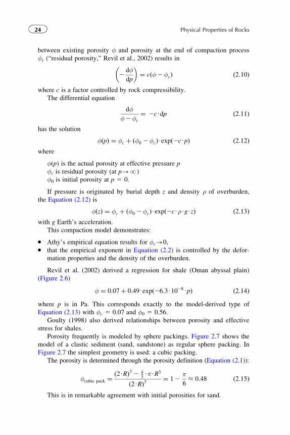
Figure 2.5 describes the mechanical compaction process in a schematic
diagram. Avseth et al. (2005) formulate as rules of thumb for compaction
and following cementation: “(1) The depositional porosity of shale is nor-
mally higher than that of sand. (2) The porosity gradient with depth is
steeper for shale than for sand during mechanical compaction (i.e., at shallow
depths). (3) The porosity gradient with depth will be steeper for sand than
for shale during chemical compaction (i.e., quartz cementation of sands nor-
mally occurs at greater burial depth, beyond 2�3 km).”
The diagram refers to the compaction process. Compaction is the irre-
versible volume reduction due to different processes mainly by:
� effective pressure due to overburden sediments (compressibility of rock
skeleton);
4000
3000
2000
1000
Dep
th in
m
0.1 10.2 0.5
Porosity
FIGURE 2.3 Plot logφ versus z for a sandstone. Data from Nagumo (1965).
Initialporosity
Rock skeletoncompressibility
Sandstone
Shale
φφ
= 0.490⋅exp(−2.7⋅10−4⋅z)
= 0.803⋅exp(−5.1⋅10−4⋅z)
FIGURE 2.4 Porosity as a function of depth and initial porosity.
22 Physical Properties of Rocks
� drainage of pore fluids (permeability and time influence);� grain rearrangement (packing).
Poelchau et al. (1997) compiled porosity-depth curves for sandstone,
shale, and limestone from published sources. They give the following ranges
for the initial porosity:
� sandstone 0.25�0.55,� shale 0.50�0.90,� limestone 0.40�0.95; particularly 0.44�0.55 for grainstone and pack-
stone, 0.70�0.95 for deep sea calcareous ooze.
Rowan et al. (2003) derived porosity-depth profiles from log data of 19
offshore wells. For the three main sediment groups—sand, silt, and shale—
they used the shale content Vsh from a gammalog as a parameter for classifi-
cation. The following mean equations result:
for sand ðVsh,0:01Þ φ ¼ 0:50Uexp ð20:29UzÞ ð2:7Þfor silt ð0:495,Vsh,0:505Þ φ ¼ 0:44Uexp ð20:38UzÞ ð2:8Þ
for shale ðVsh.0:9Þ φ ¼ 0:40Uexp ð20:42UzÞ ð2:9ÞBaldwin and Butler (1985) derived so-called “solidity versus depth” rela-
tionships, where the solidity is the complement to porosity.
With a simple calculation experiment the exponential porosity versus
pressure relationship can be derived as follows.
An effective pressure p compresses the porous rock, and porosity φdecreases. Assuming that porosity decrease is proportional to the difference
Porosity
Depth
Sand Shale1mm 0.01mm
ShaleSand
FIGURE 2.5 Compaction process for sand and shale.
23Chapter | 2 Pore Space Properties
between existing porosity φ and porosity at the end of compaction process
φc (“residual porosity,” Revil et al., 2002) results in
2dφdp
� �¼ cðφ2φcÞ ð2:10Þ
where c is a factor controlled by rock compressibility.
The differential equation
dφφ2φc
¼ 2cUdp ð2:11Þ
has the solution
φðpÞ ¼ φc þ ðφ0 2φcÞUexpð2cUpÞ ð2:12Þwhere
φ(p) is the actual porosity at effective pressure p
φc is residual porosity (at p-N)
φ0 is initial porosity at p 5 0.
If pressure is originated by burial depth z and density ρ of overburden,
the Equation (2.12) is
φðzÞ ¼ φc þ ðφ0 2φcÞUexpð2cUρUgUzÞ ð2:13Þwith g Earth’s acceleration.
This compaction model demonstrates:
� Athy’s empirical equation results for φc-0,� that the empirical exponent in Equation (2.2) is controlled by the defor-
mation properties and the density of the overburden.
Revil et al. (2002) derived a regression for shale (Oman abyssal plain)
(Figure 2.6)
φ ¼ 0:07þ 0:49Uexpð26:3U1028UpÞ ð2:14Þwhere p is in Pa. This corresponds exactly to the model-derived type of
Equation (2.13) with φc 5 0.07 and φ0 5 0.56.
Goulty (1998) also derived relationships between porosity and effective
stress for shales.
Porosity frequently is modeled by sphere packings. Figure 2.7 shows the
model of a clastic sediment (sand, sandstone) as regular sphere packing. In
Figure 2.7 the simplest geometry is used: a cubic packing.
The porosity is determined through the porosity definition (Equation (2.1)):
φcubic pack ¼ð2URÞ3 2 4
3UπUR3
ð2URÞ3 ¼ 12π6� 0:48 ð2:15Þ
This is in remarkable agreement with initial porosities for sand.
24 Physical Properties of Rocks
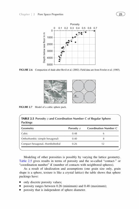
Modeling of other porosities is possibly by varying the lattice geometry.
Table 2.5 gives results in terms of porosity and the so-called “contact-” or
“coordination number” K (number of contacts with neighbored spheres).
As a result of idealization and assumptions (one grain size only, grain
shape is a sphere, texture is like a crystal lattice) the table shows that sphere
packings have:
� only discrete porosity values;� porosity ranges between 0.26 (minimum) and 0.48 (maximum);� porosity that is independent of sphere diameter.
0
1000
2000
3000
4000
5000
0 0.1 0.2 0.3 0.4 0.5 0.6 0.7Porosity
Dep
th b
elow
sea
floo
r in
m
FIGURE 2.6 Compaction of shale after Revil et al. (2002). Field data are from Fowler et al. (1985).
R
FIGURE 2.7 Model of a cubic sphere pack.
TABLE 2.5 Porosity φ and Coordination Number C of Regular Sphere
Packings
Geometry Porosity φ Coordination Number C
Cubic 0.48 6
Orthorhombic (simple hexagonal) 0.40 8
Compact hexagonal, rhombohedral 0.26 12
25Chapter | 2 Pore Space Properties
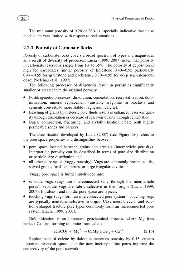
The minimum porosity of 0.26 or 26% is especially indicative that these
models are very limited with respect to real situations.
2.2.3 Porosity of Carbonate Rocks
Porosity of carbonate rocks covers a broad spectrum of types and magnitudes
as a result of diversity of processes. Lucia (1999, 2007) notes that porosity
in carbonate reservoirs ranges from 1% to 35%. The porosity at deposition is
high for carbonates (initial porosity of limestone 0.40�0.95 particularly
0.44�0.55 for grainstone and packstone, 0.70�0.95 for deep sea calcareous
ooze; Poelchau et al., 1997).
The following processes of diagenesis result in porosities significantly
smaller or greater than the original porosity.
� Postdiagenetic processes: dissolution, cementation, recrystallization, dolo-
mitization, mineral replacement (unstable aragonite in bioclasts and
cements converts to more stable magnesium calcite).� Leaching of grains by meteoric pore fluids results in enhanced reservoir qual-
ity through dissolution or decrease of reservoir quality through cementation.� Burial compaction, fracturing, and stylolithification create both highly
permeable zones and barriers.
The classification developed by Lucia (2007) (see Figure 1.6) refers to
the pore space properties and distinguishes between:
� pore space located between grains and crystals (interparticle porosity).
Interparticle porosity can be described in terms of pore-size distribution
or particle-size distribution and� all other pore space (vuggy porosity). Vugs are commonly present as dis-
solved grains, fossil chambers, or large irregular cavities.
Vuggy pore space is further subdivided into:
� separate vugs (vugs are interconnected only through the interparticle
pores). Separate vugs are fabric selective in their origin (Lucia, 1999,
2007). Intrafossil and moldic pore space are typical;� touching vugs (vugs form an interconnected pore system). Touching vugs
are typically nonfabric selective in origin. Cavernous, breccia, and solu-
tion-enlarged fracture pore types commonly form an interconnected pore
system (Lucia, 1999, 2007).
Dolomitization is an important geochemical process, where Mg ions
replace Ca ions, forming dolomite from calcite:
2CaCO3 þ Mg2þ-CaMgðCO3Þ2 þ Ca2þ ð2:16ÞReplacement of calcite by dolomite increases porosity by 0.13, creates
important reservoir space, and the new intercrystalline pores improve the
connectivity of the pore network.
26 Physical Properties of Rocks
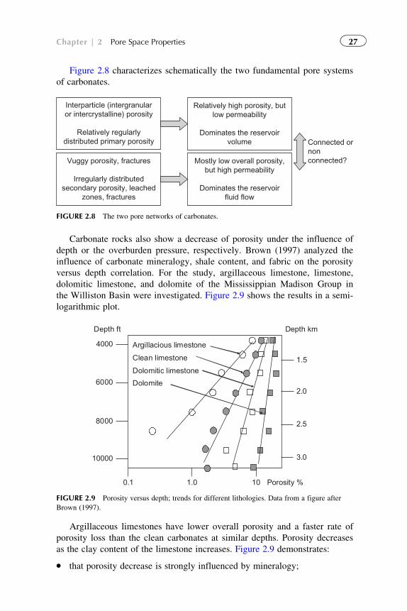
Figure 2.8 characterizes schematically the two fundamental pore systems
of carbonates.
Carbonate rocks also show a decrease of porosity under the influence of
depth or the overburden pressure, respectively. Brown (1997) analyzed the
influence of carbonate mineralogy, shale content, and fabric on the porosity
versus depth correlation. For the study, argillaceous limestone, limestone,
dolomitic limestone, and dolomite of the Mississippian Madison Group in
the Williston Basin were investigated. Figure 2.9 shows the results in a semi-
logarithmic plot.
Argillaceous limestones have lower overall porosity and a faster rate of
porosity loss than the clean carbonates at similar depths. Porosity decreases
as the clay content of the limestone increases. Figure 2.9 demonstrates:
� that porosity decrease is strongly influenced by mineralogy;
Interparticle (intergranularor intercrystalline) porosity
Relatively regularlydistributed primary porosity
Vuggy porosity, fractures
Irregularly distributedsecondary porosity, leached
zones, fractures
Relatively high porosity, butlow permeability
Dominates the reservoirvolume
Mostly low overall porosity,but high permeability
Dominates the reservoirfluid flow
Connected ornonconnected?
FIGURE 2.8 The two pore networks of carbonates.
Argillacious limestone
Clean limestone
Dolomitic limestoneDolomite
0.1 1.0 10 Porosity %
4000
6000
8000
10000
1.5
2.0
2.5
3.0
Depth kmDepth ft
FIGURE 2.9 Porosity versus depth; trends for different lithologies. Data from a figure after
Brown (1997).
27Chapter | 2 Pore Space Properties
� that clay content increases deformation sensitivity and accelerates poros-
ity loss;� that (in the example) dolomite shows a higher porosity but a smaller
porosity decrease than limestone; the dolomite is more porous but also
more rigid than the limestone;� that straight lines in the semilogarithmic plot indicate in a first approxi-
mation an exponential equation.
2.2.4 Fractures, Fractured Rocks
“Fractures are mechanical breaks in rocks; they originate from strains that
arise from stress concentrations around flaws, heterogeneities, and physical
discontinuities. . . . They occur at a variety of scales, from microscopic to
continental.” (Committee on Fracture Characterization and Fluid Flow, US
National Committee for Rock Mechanics, 1996).
The effect of fractures on physical rock properties is controlled mainly by:
� fracture geometry (size, aperture, aspect ratio);� fracture orientation (random or preferred direction);� roughness of fracture boundaries.
The Committee on Fracture Characterization and Fluid Flow noted that
“fracture is a term used for all types of generic discontinuities.” Fracture
types can be classified into two groups related to their mode of formation
(Bratton et al., 2006):
1. Shear fractures, originated from shear stress parallel to the created fracture.
On a big scale, this type corresponds to faults as a result of tectonic events.
2. Tension fractures (extension fractures) originated from tension stress per-
pendicular to the created fracture. On a big scale, this type corresponds to
joints.
Fractures are not only caused by external stress—processes like dolomiti-
zation result in volume reduction and create fractures and pore space in the
rock. Thermal effects can also create fracturing.
Fractures occur over a broad range of scales. In many cases, the fracture
patterns at one scale are similar to patterns at a different scale. This hierar-
chical similarity is the basis for an upscaling and the quantitative characteri-
zation by fractal analysis (Mandelbrot, 1983; Barton & Hsieh, 1989;
Turcotte, 1992).
In all types of rocks—igneous, metamorphic, and consolidated sedimen-
tary rocks—fractures may be present. Their origin can be natural or artificial.
Fractures have a very strong influence on many rock properties; the occur-
rence of fractures, for example:
� increases or creates a permeability for fluids;� decreases dramatically the mechanical strength properties;
28 Physical Properties of Rocks
� changes elastic wave velocity, electrical resistivity, and thermal
conductivity.
If fractures have a preferred orientation, anisotropy of tensorial rock
properties result.
Fractures are important for fluid flow in oil, gas, and water production and
geothermal processes. In such cases, the fluids are stored mainly in the matrix
porosity but produced primarily using fracture permeability (Figure 2.8).
Fractures penetrating impermeable shale layers create hydraulic conductivity
and can develop a reservoir. Artificial fracturing (hydrofrac) can create new
fractures or magnify existing fracture. On the other hand, fractures significantly
reduce mechanical rock properties.
Most magmatic (intrusive) and metamorphic rocks have almost no inter-
granular porosity. Formed by crystallization, the grains intergrow tightly,
leaving almost no void space. Typically, granite after formation has a mini-
mal porosity φ= 0.001, most of which occurs as small irregular cavities that
are remnants of the crystallization process. Tectonic and thermal stresses can
create later fractures and cracks—they represent planar discontinuities,
occupy a very small volume fraction (low porosity), but can create a con-
nected network and result in permeability.
Volcanic (extrusive) rocks are different. Rapid cooling and pressure
decrease can result in porosity. Typical volcanic rocks are porous basalts.
Characterization of fractures is difficult. A volumetric description by frac-
ture porosity in most cases cannot explain the effects. Additional parameters
describing geometry and orientation are necessary (e.g., aperture, crack den-
sity parameter). Therefore, imaging technologies (acoustic, resistivity) in log-
ging techniques are a very important component for evaluation and detection.
2.3 SPECIFIC INTERNAL SURFACE
Porosity characterizes the volumetric aspect of the pore system. Specific
internal surface characterizes the surface area of the pore space or the area
of interface solid�fluid. Thus, with the specific internal surface, a second
pore-geometrical property is defined and has particular importance for:
� the effects at this interface (e.g., CEC);� the derivation of model equations for permeability (see Section 2.5.7.2);� NMR petrophysics (see Chapter 3).
In this section, only the definition and some fundamental properties are
discussed.
Pore surface area is normalized by the total sample volume, the pore vol-
ume, or the mass and is defined as:
Stotal ¼surface area of the pores
total volumeð2:17Þ
29Chapter | 2 Pore Space Properties
Spore ¼surface area of the pores
pore volumeð2:18Þ
Smass ¼ surface area of the pores
total massð2:19Þ
with the relationships Stotal ¼ SporeUφ Smass ¼Stotal
densityð2:20Þ
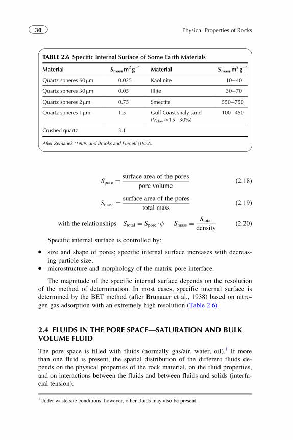
Specific internal surface is controlled by:
� size and shape of pores; specific internal surface increases with decreas-
ing particle size;� microstructure and morphology of the matrix-pore interface.
The magnitude of the specific internal surface depends on the resolution
of the method of determination. In most cases, specific internal surface is
determined by the BET method (after Brunauer et al., 1938) based on nitro-
gen gas adsorption with an extremely high resolution (Table 2.6).
2.4 FLUIDS IN THE PORE SPACE—SATURATION AND BULKVOLUME FLUID
The pore space is filled with fluids (normally gas/air, water, oil).1 If more
than one fluid is present, the spatial distribution of the different fluids de-
pends on the physical properties of the rock material, on the fluid properties,
and on interactions between the fluids and between fluids and solids (interfa-
cial tension).
TABLE 2.6 Specific Internal Surface of Some Earth Materials
Material Smassm2 g21 Material Smassm
2 g21
Quartz spheres 60 μm 0.025 Kaolinite 10�40
Quartz spheres 30 μm 0.05 Illite 30�70
Quartz spheres 2 μm 0.75 Smectite 550�750
Quartz spheres 1 μm 1.5 Gulf Coast shaly sand(Vclay�15�30%)
100�450
Crushed quartz 3.1
After Zemanek (1989) and Brooks and Purcell (1952).
1Under waste site conditions, however, other fluids may also be present.
30 Physical Properties of Rocks
In this section, only the volumetric or fractional description of different
fluids is presented. The factors that control the distribution of immiscible
fluids under static conditions are discussed in Section 2.7.
Fluid saturation can be determined as follows:
� from cores, plugs, or samples (direct determination by fluid extraction,
capillary pressure measurements);� indirectly from logs (resistivity, dielectric, neutron measurements, etc.);� by NMR measurements.
For the description of the volume fraction of a fluid i in a porous rock,
the term saturation Si is used and defined as follows:
Si ¼volume of fluid i
pore volumeð2:21Þ
Thus, saturation is the fluid volume, normalized by pore volume.
Saturation is given as a fraction or as percentage.
A reservoir with the fluids water, oil, and gas is characterized by three
saturation terms and their sum must be 1:
Swater þ Soil þ Sgas ¼ 1 ð2:22Þ
In addition to the parameter “saturation,” the parameter “bulk volume of
the fluid” is also used. Bulk volume of a fluid i refers to the volume of that
fluid to the rock bulk volume. Bulk volume water is, for example,
BVW ¼ volume of water
rock volume¼ SwUφ ð2:23Þ
In a (water wet)2 porous rock, the water, depending on its interaction
with minerals and bonding type, is present as:
� free movable water in the pore space;� capillary bound water, connected with the grain surface;� clay-bound water (CBW) with its strong clay�water effects.
The types have different physical properties and effects (e.g., with respect
to permeability, electrical resistivity). Therefore, a subdivision into these
types is necessary.
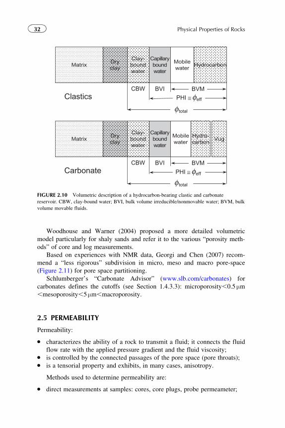
The volumetric composition for the two main reservoir rock types is pre-
sented in Figure 2.10.
2See Section 2.6.
31Chapter | 2 Pore Space Properties
Woodhouse and Warner (2004) proposed a more detailed volumetric
model particularly for shaly sands and refer it to the various “porosity meth-
ods” of core and log measurements.
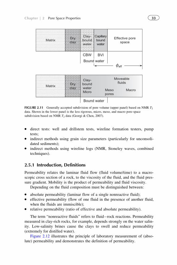
Based on experiences with NMR data, Georgi and Chen (2007) recom-
mend a “less rigorous” subdivision in micro, meso and macro pore-space
(Figure 2.11) for pore space partitioning.
Schlumberger’s “Carbonate Advisor” (www.slb.com/carbonates) for
carbonates defines the cutoffs (see Section 1.4.3.3): microporosity,0.5 μm,mesoporosity,5 μm,macroporosity.
2.5 PERMEABILITY
Permeability:
� characterizes the ability of a rock to transmit a fluid; it connects the fluid
flow rate with the applied pressure gradient and the fluid viscosity;� is controlled by the connected passages of the pore space (pore throats);� is a tensorial property and exhibits, in many cases, anisotropy.
Methods used to determine permeability are:
� direct measurements at samples: cores, core plugs, probe permeameter;
MatrixDryclay
Clay-boundwater
Mobilewater
Capillaryboundwater
Hydrocarbon
BVMBVICBWClastics
Mobilewater
Hydro-carbon
VugMatrixDryclay
Clay-boundwater
Capillaryboundwater
BVMBVI
totalφ
totalφ
PHI ≅ effφ
PHI ≅ effφCBW
Carbonate
FIGURE 2.10 Volumetric description of a hydrocarbon-bearing clastic and carbonate
reservoir. CBW, clay-bound water; BVI, bulk volume irreducible/nonmovable water; BVM, bulk
volume movable fluids.
32 Physical Properties of Rocks
� direct tests: well and drillstem tests, wireline formation testers, pump
tests;� indirect methods using grain size parameters (particularly for unconsoli-
dated sediments);� indirect methods using wireline logs (NMR, Stoneley waves, combined
techniques).
2.5.1 Introduction, Definitions
Permeability relates the laminar fluid flow (fluid volume/time) to a macro-
scopic cross section of a rock, to the viscosity of the fluid, and the fluid pres-
sure gradient. Mobility is the product of permeability and fluid viscosity.
Depending on the fluid composition must be distinguished between:
� absolute permeability (laminar flow of a single nonreactive fluid);� effective permeability (flow of one fluid in the presence of another fluid,
when the fluids are immiscible);� relative permeability (ratio of effective and absolute permeability).
The term “nonreactive fluids” refers to fluid�rock reactions. Permeability
measured in clay-rich rocks, for example, depends strongly on the water salin-
ity. Low-salinity brines cause the clays to swell and reduce permeability
(extremely for distilled water).
Figure 2.12 illustrates the principle of laboratory measurement of (abso-
lute) permeability and demonstrates the definition of permeability.
MatrixDryclay
Clay-boundwater
Capillaryboundwater
Effective porespace
BVICBW
MatrixDryclay
Clay-boundwaterMicro Meso
poresMacro
Moveablefluids
Bound water
Bound watereffφ
FIGURE 2.11 Generally accepted subdivision of pore volume (upper panel) based on NMR T2data. Shown in the lower panel is the less rigorous, micro, meso, and macro pore-space
subdivision based on NMR T2 data (Georgi & Chen, 2007).
33Chapter | 2 Pore Space Properties
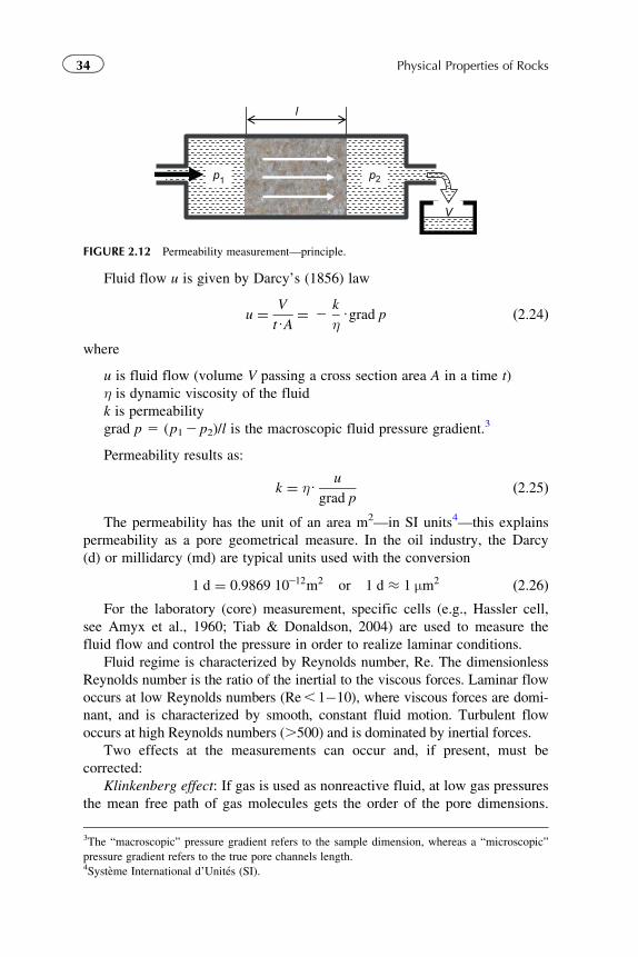
Fluid flow u is given by Darcy’s (1856) law
u ¼ V
tUA¼ 2
k
ηUgrad p ð2:24Þ
where
u is fluid flow (volume V passing a cross section area A in a time t)
η is dynamic viscosity of the fluid
k is permeability
grad p 5 (p12 p2)/l is the macroscopic fluid pressure gradient.3
Permeability results as:
k ¼ ηUu
grad pð2:25Þ
The permeability has the unit of an area m2—in SI units4—this explains
permeability as a pore geometrical measure. In the oil industry, the Darcy
(d) or millidarcy (md) are typical units used with the conversion
1 d ¼ 0:9869 10212m2 or 1 d � 1 μm2 ð2:26ÞFor the laboratory (core) measurement, specific cells (e.g., Hassler cell,
see Amyx et al., 1960; Tiab & Donaldson, 2004) are used to measure the
fluid flow and control the pressure in order to realize laminar conditions.
Fluid regime is characterized by Reynolds number, Re. The dimensionless
Reynolds number is the ratio of the inertial to the viscous forces. Laminar flow
occurs at low Reynolds numbers (Re, 1�10), where viscous forces are domi-
nant, and is characterized by smooth, constant fluid motion. Turbulent flow
occurs at high Reynolds numbers (.500) and is dominated by inertial forces.
Two effects at the measurements can occur and, if present, must be
corrected:
Klinkenberg effect: If gas is used as nonreactive fluid, at low gas pressures
the mean free path of gas molecules gets the order of the pore dimensions.
3The “macroscopic” pressure gradient refers to the sample dimension, whereas a “microscopic”
pressure gradient refers to the true pore channels length.4Systeme International d’Unites (SI).
l
p1 p2
V
FIGURE 2.12 Permeability measurement—principle.
34 Physical Properties of Rocks
Then gas molecules have a finite velocity at the pore wall, but for liquids, a
zero velocity at the wall is assumed. The “gas slippage effect” increases the
flow rate and causes an overestimated permeability. Klinkenberg correction
uses measurements at different pressures and an extrapolation for a (theoreti-
cal) infinite pressure (Cosentino, 2001). It results in the “Klinkenberg
corrected permeability,” which is:
� independent of the type of gas,� approximately the same as for a single phase liquid.
Forchheimer effect: At high flow rates, inertial effects occur and the
difference of flow velocity between pore throats and pore bodies causes
turbulences—but Darcy’s law requires laminar flow. A plot of fluid flow ver-
sus pressure gradient in case of a turbulency deviates from a linear function.
2.5.2 Rock Permeability—An Overview
Permeability of rocks covers orders of magnitude. It ranges from practically
impermeable, dense rocks (compact magmatites, dense anhydrite, rock salt),
over extremely low permeable shale to carbonates, sand/sandstone and high
permeable gravel and karstic limestone (Figure 2.13).
A permeability of 0.1md is generally considered the minimum for oil
production (Lucia, 1999).
Karst limestonePermeable basalt
Fractured igneous andmetamorphic rocks
Limestone and dolomiteSandstoneUnfractured metamorphic
and igneous rocksShaleUnweathered marine clayGlacial tillSilt, loessSilty sandClean sandGravel
k in d (Darcy)10−8 10−6 10−4 10−2 10−0 102 104
10−20 10−18 10−16 10−14 10−12 10−10 10−8m2
Pore size
Connected fracturesand channels
FIGURE 2.13 Permeability: mean magnitude ranges and tendencies. After a figure from
Hearst et al., 2000.
35Chapter | 2 Pore Space Properties
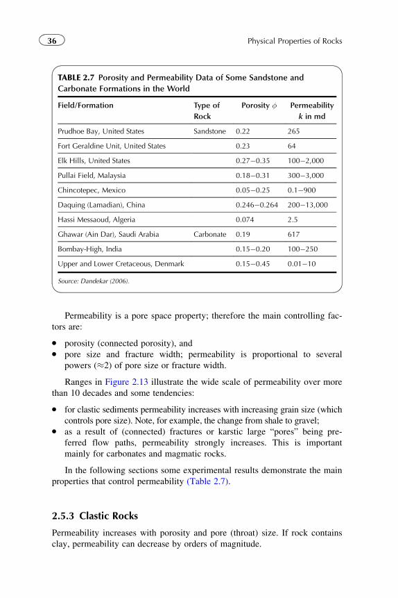
Permeability is a pore space property; therefore the main controlling fac-
tors are:
� porosity (connected porosity), and� pore size and fracture width; permeability is proportional to several
powers (�2) of pore size or fracture width.
Ranges in Figure 2.13 illustrate the wide scale of permeability over more
than 10 decades and some tendencies:
� for clastic sediments permeability increases with increasing grain size (which
controls pore size). Note, for example, the change from shale to gravel;� as a result of (connected) fractures or karstic large “pores” being pre-
ferred flow paths, permeability strongly increases. This is important
mainly for carbonates and magmatic rocks.
In the following sections some experimental results demonstrate the main
properties that control permeability (Table 2.7).
2.5.3 Clastic Rocks
Permeability increases with porosity and pore (throat) size. If rock contains
clay, permeability can decrease by orders of magnitude.
TABLE 2.7 Porosity and Permeability Data of Some Sandstone and
Carbonate Formations in the World
Field/Formation Type of
Rock
Porosity φ Permeability
k in md
Prudhoe Bay, United States Sandstone 0.22 265
Fort Geraldine Unit, United States 0.23 64
Elk Hills, United States 0.27�0.35 100�2,000
Pullai Field, Malaysia 0.18�0.31 300�3,000
Chincotepec, Mexico 0.05�0.25 0.1�900
Daquing (Lamadian), China 0.246�0.264 200�13,000
Hassi Messaoud, Algeria 0.074 2.5
Ghawar (Ain Dar), Saudi Arabia Carbonate 0.19 617
Bombay-High, India 0.15�0.20 100�250
Upper and Lower Cretaceous, Denmark 0.15�0.45 0.01�10
Source: Dandekar (2006).
36 Physical Properties of Rocks
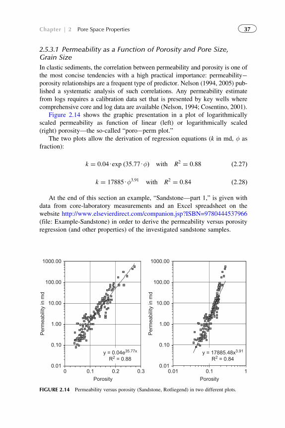
2.5.3.1 Permeability as a Function of Porosity and Pore Size,Grain Size
In clastic sediments, the correlation between permeability and porosity is one of
the most concise tendencies with a high practical importance: permeability�porosity relationships are a frequent type of predictor. Nelson (1994, 2005) pub-
lished a systematic analysis of such correlations. Any permeability estimate
from logs requires a calibration data set that is presented by key wells where
comprehensive core and log data are available (Nelson, 1994; Cosentino, 2001).
Figure 2.14 shows the graphic presentation in a plot of logarithmically
scaled permeability as function of linear (left) or logarithmically scaled
(right) porosity—the so-called “poro�perm plot.”
The two plots allow the derivation of regression equations (k in md, φ as
fraction):
k ¼ 0:04Uexp ð35:77UφÞ with R2 ¼ 0:88 ð2:27Þ
k ¼ 17885Uφ3:91 with R2 ¼ 0:84 ð2:28Þ
At the end of this section an example, “Sandstone—part 1,” is given with
data from core-laboratory measurements and an Excel spreadsheet on the
website http://www.elsevierdirect.com/companion.jsp?ISBN=9780444537966
(file: Example-Sandstone) in order to derive the permeability versus porosity
regression (and other properties) of the investigated sandstone samples.
y = 0.04e35.77x
R2 = 0.880.01
0.10
1.00
10.00
100.00
1000.00
0 0.1 0.2 0.3
Porosity
Per
mea
bilit
y in
md
0.01
0.10
1.00
10.00
100.00
1000.00
Per
mea
bilit
y in
md
0.01 0.1 1
Porosity
y = 17885.48x3.91
R2 = 0.84
FIGURE 2.14 Permeability versus porosity (Sandstone, Rotliegend) in two different plots.
37Chapter | 2 Pore Space Properties
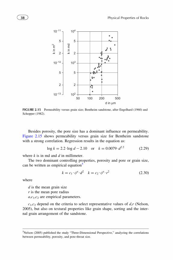
Besides porosity, the pore size has a dominant influence on permeability.
Figure 2.15 shows permeability versus grain size for Bentheim sandstone
with a strong correlation. Regression results in the equation as:
log k ¼ 2:2Ulog d2 2:10 or k ¼ 0:0079Ud2:2 ð2:29Þwhere k is in md and d in millimeter.
The two dominant controlling properties, porosity and pore or grain size,
can be written as empirical equation5
k ¼ c1UφaUd2 k ¼ c2UφaUr2 ð2:30Þwhere
d is the mean grain size
r is the mean pore radius
a,c1,c2 are empirical parameters.
c1,c2 depend on the criteria to select representative values of d,r (Nelson,
2005), but also on textural properties like grain shape, sorting and the inter-
nal grain arrangement of the sandstone.
104
5
102
2
5
2
103
50 100 200 500d in μm
k in
md
10−11
5
10−13
2
5
2
10−12
k in
m2
FIGURE 2.15 Permeability versus grain size; Bentheim sandstone, after Engelhard (1960) and
Schopper (1982).
5Nelson (2005) published the study “Three-Dimensional Perspective,” analyzing the correlations
between permeability, porosity, and pore-throat size.
38 Physical Properties of Rocks
Many empirical equations follow this general form; two examples are
presented:
Berg’s (1970) equation:
k ¼ 5:1U102 6Uφ5:1Ud2Uexpð21:385UψÞ ð2:31Þwhere
k is the permeability in Darcies (d)
φ is the porosity as percentage
d is the median grain diameter in millimeter
ψ is sorting term in phi units ψ 5 P902P10.
Nelson (1994) recommended this equation for unconsolidated sands and
relatively clean quartzose rocks.
van Baaren’s (1979) equation:
k ¼ 10Uφ3:64þmUD2dUS
23:64o ð2:32Þ
where
k is permeability in md
φ is the porosity as fraction
Dd is dominant grain diameter in micrometer
So is sorting index derived from grain size distribution
m Archie’s cementation exponent (see Section 8.3).
Both equations are very similar (Nelson, 1994). They show:
� the same exponent for correlation with grain size (2);� approximately the same exponent for correlation with porosity; for
m 5 1.8 results in van Baaren’s equation an exponent of 5.4.
A somewhat different concept of permeability prediction was developed
by Pape et al. (1999, 2000). It is based on fractal understanding of pore-
space parameters. It “yields a general and petrophysical justified relation
linking porosity to permeability.”
2.5.3.2 Permeability Description in Hydrogeology
In hydrogeologic practice, a modified version of Darcy’s law is frequently
applied. Water flow q is referenced to the hydraulic gradient
q ¼ 2kf Ugrad h ð2:33ÞThe property kf (filtration coefficient, hydraulic conductivity) has the unit
of a velocity (m s21). Between the two properties k and kf, the following con-
version can be used (the correct equation implements water density and vis-
cosity) in a good approximation
1 md � 1028m s21 or 1 m s21 � 105 d ð2:34Þ
39Chapter | 2 Pore Space Properties
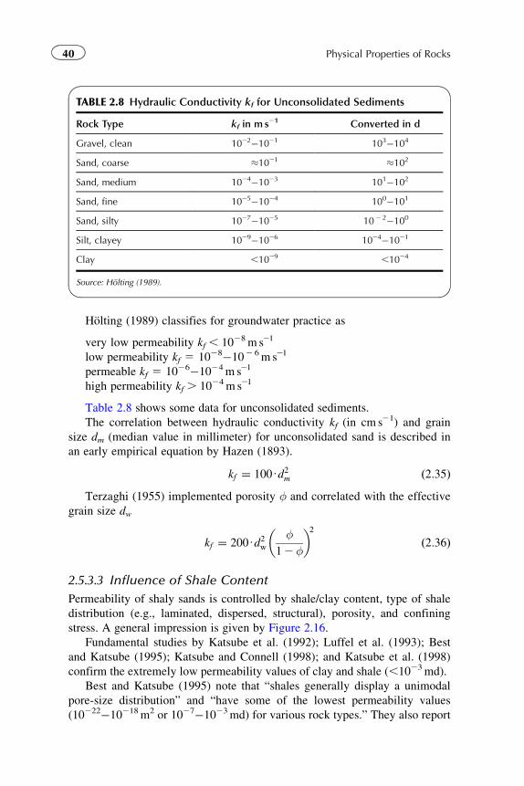
Holting (1989) classifies for groundwater practice as
very low permeability kf , 1028m s21
low permeability kf 5 1028�102 6m s21
permeable kf 5 1026�1024m s21
high permeability kf . 1024m s21
Table 2.8 shows some data for unconsolidated sediments.
The correlation between hydraulic conductivity kf (in cm s21) and grain
size dm (median value in millimeter) for unconsolidated sand is described in
an early empirical equation by Hazen (1893).
kf ¼ 100Ud2m ð2:35ÞTerzaghi (1955) implemented porosity φ and correlated with the effective
grain size dw
kf ¼ 200Ud2wφ
12φ
� �2ð2:36Þ
2.5.3.3 Influence of Shale Content
Permeability of shaly sands is controlled by shale/clay content, type of shale
distribution (e.g., laminated, dispersed, structural), porosity, and confining
stress. A general impression is given by Figure 2.16.
Fundamental studies by Katsube et al. (1992); Luffel et al. (1993); Best
and Katsube (1995); Katsube and Connell (1998); and Katsube et al. (1998)
confirm the extremely low permeability values of clay and shale (,1023md).
Best and Katsube (1995) note that “shales generally display a unimodal
pore-size distribution” and “have some of the lowest permeability values
(10222�10218m2 or 1027�1023md) for various rock types.” They also report
TABLE 2.8 Hydraulic Conductivity kf for Unconsolidated Sediments
Rock Type kf in m s21 Converted in d
Gravel, clean 1022�1021 103�104
Sand, coarse �1021 �102
Sand, medium 1024�1023 101�102
Sand, fine 1025�1024 100�101
Sand, silty 1027�1025 1022�100
Silt, clayey 1029�1026 1024�1021
Clay ,1029 ,1024
Source: Holting (1989).
40 Physical Properties of Rocks
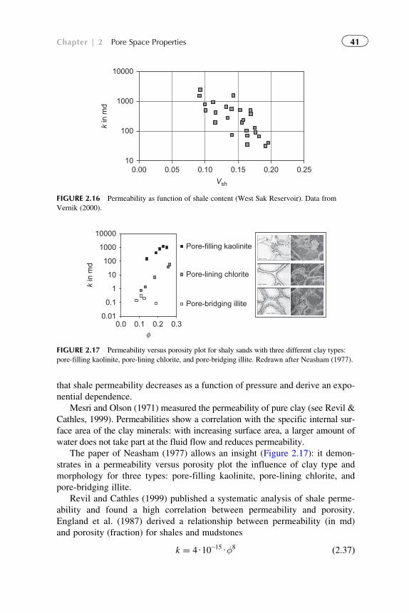
that shale permeability decreases as a function of pressure and derive an expo-
nential dependence.
Mesri and Olson (1971) measured the permeability of pure clay (see Revil &
Cathles, 1999). Permeabilities show a correlation with the specific internal sur-
face area of the clay minerals: with increasing surface area, a larger amount of
water does not take part at the fluid flow and reduces permeability.
The paper of Neasham (1977) allows an insight (Figure 2.17): it demon-
strates in a permeability versus porosity plot the influence of clay type and
morphology for three types: pore-filling kaolinite, pore-lining chlorite, and
pore-bridging illite.
Revil and Cathles (1999) published a systematic analysis of shale perme-
ability and found a high correlation between permeability and porosity.
England et al. (1987) derived a relationship between permeability (in md)
and porosity (fraction) for shales and mudstones
k ¼ 4U10215Uφ8 ð2:37Þ
0.01
0.1
1
10
100
1000
10000
0.0 0.1 0.2 0.3
k in
md
Pore-filling kaolinite
Pore-lining chlorite
Pore-bridging illite
φ
FIGURE 2.17 Permeability versus porosity plot for shaly sands with three different clay types:
pore-filling kaolinite, pore-lining chlorite, and pore-bridging illite. Redrawn after Neasham (1977).
10
100
1000
10000
0.00 0.05 0.10 0.15 0.20 0.25
Vsh
k in
md
FIGURE 2.16 Permeability as function of shale content (West Sak Reservoir). Data from
Vernik (2000).
41Chapter | 2 Pore Space Properties
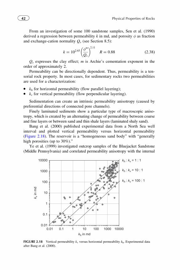
From an investigation of some 100 sandstone samples, Sen et al. (1990)
derived a regression between permeability k in md, and porosity φ as fraction
and exchange-cation normality Qv (see Section 8.5):
k ¼ 102:65φm
Qv
� �2:11R ¼ 0:88 ð2:38Þ
Qv expresses the clay effect; m is Archie’s cementation exponent in the
order of approximately 2.
Permeability can be directionally dependent. Thus, permeability is a ten-
sorial rock property. In most cases, for sedimentary rocks two permeabilities
are used for a characterization:
� kh for horizontal permeability (flow parallel layering);� kv for vertical permeability (flow perpendicular layering).
Sedimentation can create an intrinsic permeability anisotropy (caused by
preferential directions of connected pore channels).
Finely laminated sediments show a particular type of macroscopic aniso-
tropy, which is created by an alternating change of permeability between coarse
and fine layers or between sand and thin shale layers (laminated shaly sand).
Bang et al. (2000) published experimental data from a North Sea well
interval and plotted vertical permeability versus horizontal permeability
(Figure 2.18). The reservoir is a “homogeneous sand body” with “generally
high porosities (up to 30%).”
Ye et al. (1999) investigated outcrop samples of the Bluejacket Sandstone
(Middle Pennsylvania) and correlated permeability anisotropy with the internal
0.01
0.1
1
10
100
1000
10000
0.01 0.1 1 10 100 1000 10000
kh in md
k v in
md
kh : kv = 1 : 1
kh : kv = 10 : 1
kh : kv = 100 : 1
FIGURE 2.18 Vertical permeability kv versus horizontal permeability kh. Experimental data
after Bang et al. (2000).
42 Physical Properties of Rocks
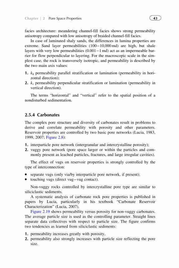
facies architecture: meandering channel-fill facies shows strong permeability
anisotropy compared with low anisotropy of braided channel-fill facies.
In case of laminated shaly sands, the differences in lamina properties are
extreme. Sand layer permeabilities (100�10,000md) are high, but shale
layers with very low permeabilities (0.001�1md) act as an impermeable bar-
rier for flow perpendicular to layering. For the macroscopic scale in the sim-
plest case, the rock is transversely isotropic, and permeability is described by
the two main axis values:
1. kh permeability parallel stratification or lamination (permeability in hori-
zontal direction);
2. kv permeability perpendicular stratification or lamination (permeability in
vertical direction).
The terms “horizontal” and “vertical” refer to the spatial position of a
nondisturbed sedimentation.
2.5.4 Carbonates
The complex pore structure and diversity of carbonates result in problems to
derive and correlate permeability with porosity and other parameters.
Reservoir properties are controlled by two basic pore networks (Lucia, 1983,
1999, 2007; Figure 2.8):
1. interparticle pore network (intergranular and intercrystalline porosity);
2. vuggy pore network (pore space larger or within the particles and com-
monly present as leached particles, fractures, and large irregular cavities).
The effect of vugs on reservoir properties is strongly controlled by the
type of interconnection:
� separate vugs (only via/by interparticle pore network, if present);� touching vugs (direct vug�vug contact).
Non-vuggy rocks controlled by intercrystalline pore type are similar to
siliciclastic sediments.
A systematic analysis of carbonate rock pore properties is published in
papers by Lucia, particularly in his textbook “Carbonate Reservoir
Characterization” (Lucia, 2007).
Figure 2.19 shows permeability versus porosity for non-vuggy carbonates.
The average particle size is used as the controlling parameter. Straight lines
separate data collectives with respect to particle size. The figure confirms
two tendencies as learned from siliciclastic sediments:
1. permeability increases greatly with porosity,
2. permeability also strongly increases with particle size reflecting the pore
size.
43Chapter | 2 Pore Space Properties
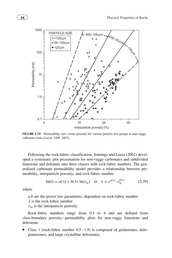
Following the rock-fabric classification, Jennings and Lucia (2001) devel-
oped a systematic plot presentation for non-vuggy carbonates and subdivided
limestone and dolomite into three classes with rock-fabric numbers. The gen-
eralized carbonate permeability model provides a relationship between per-
meability, interparticle porosity, and rock-fabric number
lnðkÞ ¼ aðλÞ þ bðλÞUlnðφipÞ or k ¼ eaðλÞUφbðλÞip ð2:39Þ
where
a,b are the power law parameters, dependent on rock-fabric number
λ is the rock-fabric number
φip is the interparticle porosity.
Rock-fabric numbers range from 0.5 to 4 and are defined from
class-boundary porosity�permeability plots for non-vuggy limestone and
dolostone:
� Class 1 (rock-fabric number 0.5�1.5) is composed of grainstones, dolo-
grainstones, and large crystalline dolostones;
1000
100
10
Per
mea
bilit
y (m
d)
1.0
0.110
Interparticle porosity (%)
PARTICLE SIZE
>100μm20–100μm
500–100μm 100–20μm<20μm
<20μm
4 20 40
FIGURE 2.19 Permeability (air) versus porosity for various particle-size groups in non-vuggy
carbonate rocks (Lucia, 1999, 2007).
44 Physical Properties of Rocks
� Class 2 (rock-fabric number 1.5�2.5) is composed of grain-dominated
packstones, fine and medium crystalline, grain-dominated dolopack-
stones, and medium crystalline, mud-dominated dolostones;� Class 3 (rock-fabric number 2.5�4.0) includes mud-dominated limestones
and fine crystalline, mud-dominated dolostones.
For the power law parameters a, b, Jennings and Lucia (2001) give the
following empirical relationships:
aðλÞ ¼ 22:562 12:08UlnðλÞ ð2:40ÞbðλÞ ¼ 8:6712 3:603UlnðλÞ ð2:41Þ
when k is in md and φip is as fraction.
The addition of separate-vug porosity to interparticle porosity:
� increases total porosity, but� does not increase permeability.
Therefore, it is important to determine interparticle porosity by subtract-
ing separate-vug porosity from total porosity and using interparticle porosity
to estimate permeability (Lucia, 1983). Figure 2.20 illustrates this effect of
separate-vug porosity Svug. Subtracting Svug shifts the dots into the grainstone
field.
2.5.5 Summary: Main Influences Controlling Permeability�Porosity Relationships
Figure 2.21 gives schematic porosity�permeability plots for clastic and car-
bonate rocks, based on figures from Nelson (1994, 2005) and Akbar et al.
(1995).
1000
100P
erm
eabi
lity
(md)
10
1
0.15
Porosity (percent)
Grainstonefield
Svugporosityaverage
20 percent
Svugporosityaverage8 percent
10 20 30 40
FIGURE 2.20 Effect of separate-vug porosity Svug on permeability (grainstones with molds)
(Lucia, 1999).
45Chapter | 2 Pore Space Properties
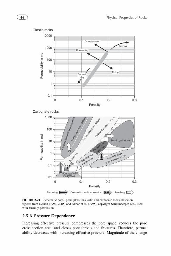
2.5.6 Pressure Dependence
Increasing effective pressure compresses the pore space, reduces the pore
cross section area, and closes pore throats and fractures. Therefore, perme-
ability decreases with increasing effective pressure. Magnitude of the change
Moldic grainstone
Clastic rocks
10000
Gravel fraction
Coarsening
Sorting
FiningCement,
clay
1000
Per
mea
bilit
y in
md
100
10
1
0.10 0.1
Porosity0.2 0.3
Carbonate rocks
1000
100
Per
mea
bilit
y in
md
10
1
0.1
0.010 0.1
Wackestones,mudstones
Fracturing Compaction and cementation Leaching
Coccolith chalk
pore diameter <1μm
Vuggy dolomite
wacke stone
Packesto
nes,
lime m
ud
Grains
tone
Parti
cle d
iam
eter
~30
0μmPar
ticle
diam
eter
~10
0μm
Parti
cle
diam
eter
~50
0μm
Leac
hed
chan
nels
in re
etal
rock
s
Porosity0.2 0.3
FIGURE 2.21 Schematic poro�perm plots for clastic and carbonate rocks, based on
figures from Nelson (1994, 2005) and Akbar et al. (1995), copyright Schlumberger Ltd., used
with friendly permission.
46 Physical Properties of Rocks
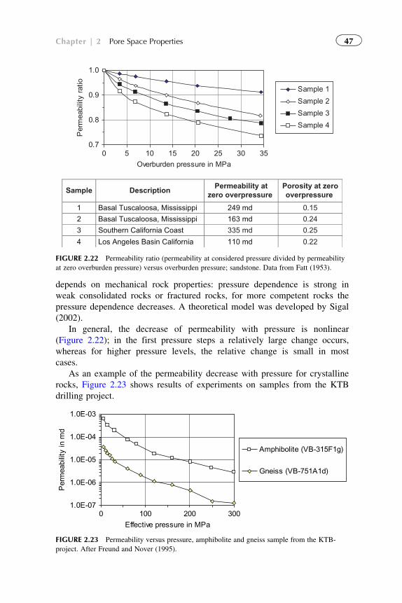
depends on mechanical rock properties: pressure dependence is strong in
weak consolidated rocks or fractured rocks, for more competent rocks the
pressure dependence decreases. A theoretical model was developed by Sigal
(2002).
In general, the decrease of permeability with pressure is nonlinear
(Figure 2.22); in the first pressure steps a relatively large change occurs,
whereas for higher pressure levels, the relative change is small in most
cases.
As an example of the permeability decrease with pressure for crystalline
rocks, Figure 2.23 shows results of experiments on samples from the KTB
drilling project.
0.7
0.8
0.9
1.0
0 5 10 15 20 25 30 35
Overburden pressure in MPa
Per
mea
bilit
y ra
tioSample 1
Sample 2
Sample 3
Sample 4
Sample DescriptionPermeability at
zero overpressure Porosity at zerooverpressure
0.15
0.24
335 md 0.25
1 Basal Tuscaloosa, Mississippi 249 md 2 Basal Tuscaloosa, Mississippi 163 md 3 Southern California Coast4 Los Angeles Basin California 110 md 0.22
FIGURE 2.22 Permeability ratio (permeability at considered pressure divided by permeability
at zero overburden pressure) versus overburden pressure; sandstone. Data from Fatt (1953).
1.0E-07
1.0E-06
1.0E-05
1.0E-04
1.0E-03
0 100 200 300
Effective pressure in MPa
Per
mea
bilit
y in
md
Amphibolite (VB-315F1g)
Gneiss (VB-751A1d)
FIGURE 2.23 Permeability versus pressure, amphibolite and gneiss sample from the KTB-
project. After Freund and Nover (1995).
47Chapter | 2 Pore Space Properties
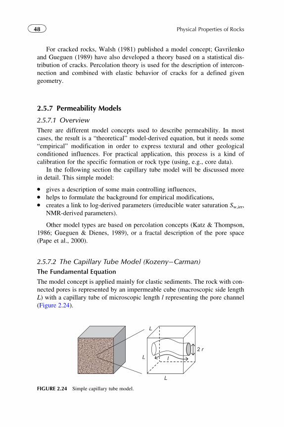
For cracked rocks, Walsh (1981) published a model concept; Gavrilenko
and Gueguen (1989) have also developed a theory based on a statistical dis-
tribution of cracks. Percolation theory is used for the description of intercon-
nection and combined with elastic behavior of cracks for a defined given
geometry.
2.5.7 Permeability Models
2.5.7.1 Overview
There are different model concepts used to describe permeability. In most
cases, the result is a “theoretical” model-derived equation, but it needs some
“empirical” modification in order to express textural and other geological
conditioned influences. For practical application, this process is a kind of
calibration for the specific formation or rock type (using, e.g., core data).
In the following section the capillary tube model will be discussed more
in detail. This simple model:
� gives a description of some main controlling influences,� helps to formulate the background for empirical modifications,� creates a link to log-derived parameters (irreducible water saturation Sw,irr,
NMR-derived parameters).
Other model types are based on percolation concepts (Katz & Thompson,
1986; Gueguen & Dienes, 1989), or a fractal description of the pore space
(Pape et al., 2000).
2.5.7.2 The Capillary Tube Model (Kozeny�Carman)
The Fundamental Equation
The model concept is applied mainly for clastic sediments. The rock with con-
nected pores is represented by an impermeable cube (macroscopic side length
L) with a capillary tube of microscopic length l representing the pore channel
(Figure 2.24).
l
L
L
L
2 r
FIGURE 2.24 Simple capillary tube model.
48 Physical Properties of Rocks
The element with the length L has the cross section A 5 L � L. The model
can be considered under two views:
In a “macroscopic view” the fluid flow can be described by Darcy’s law
u ¼ k
ηUgrad p ð2:42Þ
Thus, the flowing fluid volume per time is
q ¼ uUA ¼ k
ηAUgrad p ¼ k
ηAU
Δp
Lð2:43Þ
In a “microscopic view” pore space properties are described by capillary
length l and capillary radius r. The tortuosity of the pore channel is
τ ¼ l
Lð2:44Þ
The porosity of the model is
φ ¼ πUr2UlAL
¼ πUr2UτA
ð2:45ÞThe fluid flow in the capillary is given by Hagen�Poiseulle’s law
q ¼ π8U1
ηUr4U
Δp
lð2:46Þ
With the tortuosity the “microgradient” Δp/l can be transformed into the
“macrogradient”
Δp
lUτ ¼ Δp
L¼ grad p ð2:47Þ
Comparison of the two expressions (Equations (2.43) and (2.46)) for
volume flow results in
q ¼ k
ηAUgrad p ¼ π
8U1
ηUr4U
1
τUgrad p ð2:48Þ
Solved for permeability and implementation of porosity gives
k ¼ 1
8UφU
r2
τ2ð2:49Þ
The equation shows and explains permeability as a function of:
� porosity: the resulting linear dependence is not in agreement with the
stronger dependence derived from experiments;� pore radius: the dependence on the square of the radius fits the general
correlation found by experiments with a dependence of permeability on
the square of mean grain or pore size very well;� tortuosity: this property stands in the model for the complicated path of
the pore channel and covers a part of the textural influences; it probably
also covers a part of the porosity influence.
49Chapter | 2 Pore Space Properties
For practical derivation of permeability from other physical properties
(e.g., well logs) the crucial problem is the effect of pore size and pore chan-
nel geometry (pore throat size, tortuosity), whereas porosity in many cases
can be derived using standard methods.
Implementation of Specific Surface
The simple geometry of the model opens the way to transform the funda-
mental problem of permeability dependence on pore radius into the problem
dependence on specific internal surface. With this step, a permeability esti-
mate from logs becomes possible.
For the simple capillary model, pore radius can be expressed by specific
internal surface. The (microscopic) model results in
Spore ¼2πUrπUr2
¼ 2
ror r ¼ 2
Sporeð2:50Þ
Insertion into Equation (2.49) results in the permeability
k ¼ 1
8UφU
r2
τ2¼ 1
2UφU
1
S2poreU1
τ2ð2:51Þ
Now the controlling effect of the pore dimension is expressed by the spe-
cific internal surface of the pore space. There are two ways to implement the
effect of specific internal surface (in addition to porosity) in techniques for
permeability estimate:
Method 1 Understand irreducible water saturation Sw,irr as a measure of
Spor. In a water-wet (see Section 2.6) oil- or gas-bearing formation, irreduc-
ible water covers the grain surface with a thin water film. Thus, the water
content (determined, e.g., by a resistivity measurement) gives a measure of
the pore surface (Spor ~ Sw,irr). This is expressed by Timur’s empirical equa-
tion (Timur, 1968).
k ¼ 100Uφ2:25
Sw;irr
� �2¼ 104Uφ4:5U
1
S2w;irrð2:52Þ
Spor (Equation (2.51)) is expressed by Sw,irr. However, this technique only
works under condition of a reservoir section with Sw,irr (above transition
zone).
Method 2 Derivation of Spor from an NMR measurement. The Coates
equation (Coates et al., 1991) for NMR-derived permeability is (see
Section 3.5.2)
k ¼ φC
� �4UBVM
BVI
� �2ð2:53Þ
50 Physical Properties of Rocks
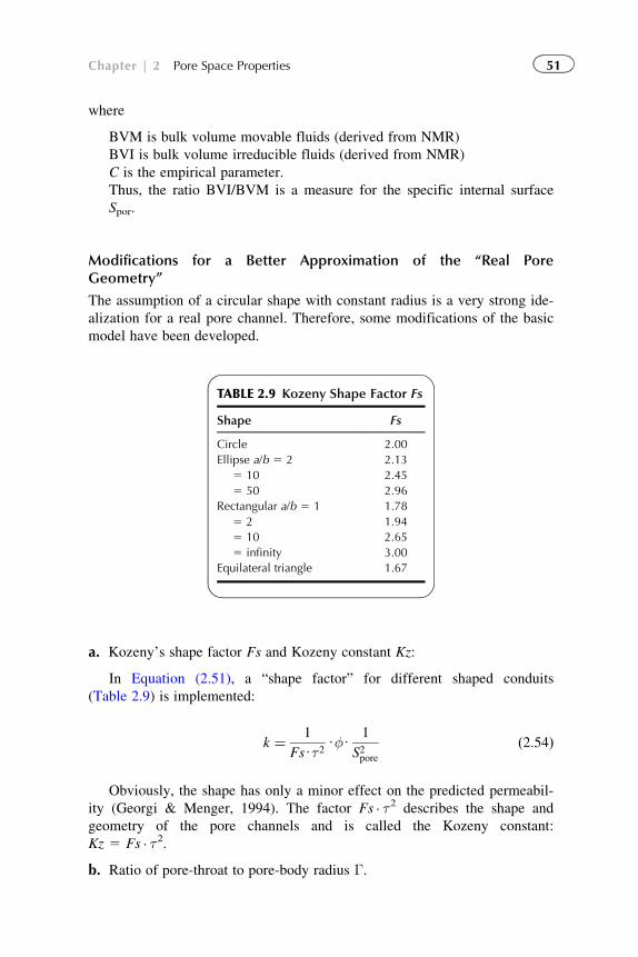
where
BVM is bulk volume movable fluids (derived from NMR)
BVI is bulk volume irreducible fluids (derived from NMR)
C is the empirical parameter.
Thus, the ratio BVI/BVM is a measure for the specific internal surface
Spor.
Modifications for a Better Approximation of the “Real PoreGeometry”
The assumption of a circular shape with constant radius is a very strong ide-
alization for a real pore channel. Therefore, some modifications of the basic
model have been developed.
a. Kozeny’s shape factor Fs and Kozeny constant Kz:
In Equation (2.51), a “shape factor” for different shaped conduits
(Table 2.9) is implemented:
k ¼ 1
FsUτ2UφU
1
S2poreð2:54Þ
Obviously, the shape has only a minor effect on the predicted permeabil-
ity (Georgi & Menger, 1994). The factor Fs � τ2 describes the shape and
geometry of the pore channels and is called the Kozeny constant:
Kz 5 Fs � τ2.b. Ratio of pore-throat to pore-body radius Γ.
TABLE 2.9 Kozeny Shape Factor Fs
Shape Fs
Circle 2.00
Ellipse a/b 5 2 2.13
5 10 2.45
5 50 2.96
Rectangular a/b 5 1 1.78
5 2 1.94
5 10 2.65
5 infinity 3.00
Equilateral triangle 1.67
51Chapter | 2 Pore Space Properties
Permeability is controlled by pore-throat radius, but Spor by pore-body
radius. Therefore, the ratio of pore-throat to pore-body radius Γ is introduced
in Equation (2.54):
k ¼ Γ 2
4UFsUφU
r2
τ2¼ Γ 2
FsUφU
1
S2poreU1
τ2ð2:55Þ
c. Definition of a “Reservoir Quality index (RQI)”
Leverett (1939, 1940) equated the termffiffiffiffiffiffiffiffik=φ
pas a rock property. From
Equation (2.55) ffiffiffik
φ
s¼ Γ
2ffiffiffiffiffiFs
p Ur
τ¼ Γffiffiffiffiffi
Fsp U
1
τU
1
Sporeð2:56Þ
The right-hand side of the equation indicates that the termffiffiffiffiffiffiffiffik=φ
pis con-
trolled by specific internal surface or pore size, tortuosity, pore shape, and
pore-throat to pore-body ratio. Thus, it covers all textural properties that con-
trol permeability except porosity. An RQI can be defined as (Altunbay et al.,
1997):
RQI ¼ 0:0314
ffiffiffik
φ
sð2:57Þ
A plot RQI versus φ can be used for a quality characterization and a clas-
sification in hydraulic units. Georgi and Menger (1994) and Altunbay et al.
(1997) have developed an “extended hydraulic unitization” and applied it for
carbonates.
2.5.7.3 Flow Through Fractures and Channels
In rocks with intergranular and fracture porosity:
� intergranular pores usually contain a significant volume of fluids, but
have a low permeability;� fractures and channels are important for fluid flow and have a relatively
high permeability.
A simple fracture model (Figure 2.25) is considered: a cube with length
L. In a single fracture the fluid flow is
q ¼ 1
12UηUhUw3
f UΔp
Lð2:58Þ
with fracture porosity
φfracture ¼wf
Lð2:59Þ
52 Physical Properties of Rocks
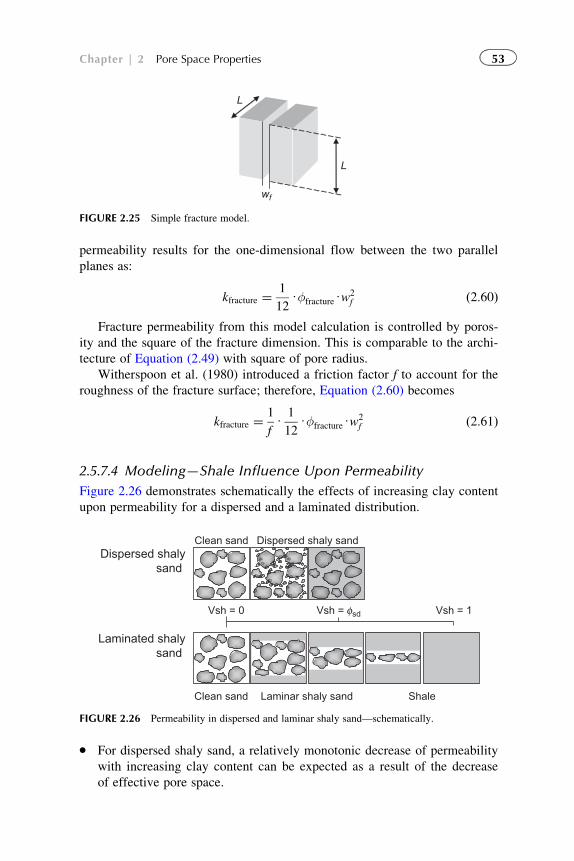
permeability results for the one-dimensional flow between the two parallel
planes as:
kfracture ¼1
12UφfractureUw
2f ð2:60Þ
Fracture permeability from this model calculation is controlled by poros-
ity and the square of the fracture dimension. This is comparable to the archi-
tecture of Equation (2.49) with square of pore radius.
Witherspoon et al. (1980) introduced a friction factor f to account for the
roughness of the fracture surface; therefore, Equation (2.60) becomes
kfracture ¼1
fU1
12UφfractureUw
2f ð2:61Þ
2.5.7.4 Modeling—Shale Influence Upon Permeability
Figure 2.26 demonstrates schematically the effects of increasing clay content
upon permeability for a dispersed and a laminated distribution.
� For dispersed shaly sand, a relatively monotonic decrease of permeability
with increasing clay content can be expected as a result of the decrease
of effective pore space.
Dispersed shalysand
Laminated shalysand
Clean sand Dispersed shaly sand
Clean sand Laminar shaly sand Shale
Vsh = 0 Vsh = sdφ Vsh = 1
FIGURE 2.26 Permeability in dispersed and laminar shaly sand—schematically.
wf
L
L
FIGURE 2.25 Simple fracture model.
53Chapter | 2 Pore Space Properties
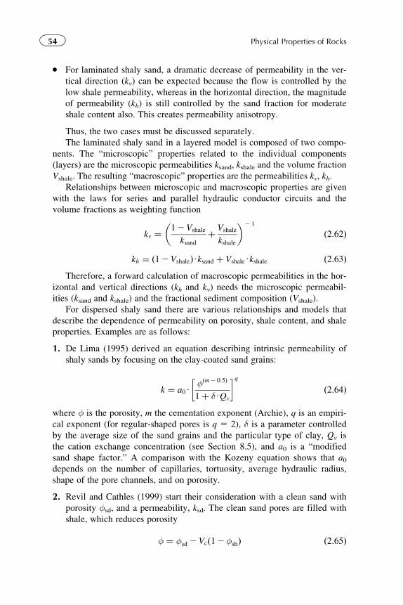
� For laminated shaly sand, a dramatic decrease of permeability in the ver-
tical direction (kv) can be expected because the flow is controlled by the
low shale permeability, whereas in the horizontal direction, the magnitude
of permeability (kh) is still controlled by the sand fraction for moderate
shale content also. This creates permeability anisotropy.
Thus, the two cases must be discussed separately.
The laminated shaly sand in a layered model is composed of two compo-
nents. The “microscopic” properties related to the individual components
(layers) are the microscopic permeabilities ksand, kshale and the volume fraction
Vshale. The resulting “macroscopic” properties are the permeabilities kv, kh.
Relationships between microscopic and macroscopic properties are given
with the laws for series and parallel hydraulic conductor circuits and the
volume fractions as weighting function
kv ¼12Vshale
ksandþ Vshale
kshale
� �2 1
ð2:62Þ
kh ¼ ð12VshaleÞUksand þ VshaleUkshale ð2:63ÞTherefore, a forward calculation of macroscopic permeabilities in the hor-
izontal and vertical directions (kh and kv) needs the microscopic permeabil-
ities (ksand and kshale) and the fractional sediment composition (Vshale).
For dispersed shaly sand there are various relationships and models that
describe the dependence of permeability on porosity, shale content, and shale
properties. Examples are as follows:
1. De Lima (1995) derived an equation describing intrinsic permeability of
shaly sands by focusing on the clay-coated sand grains:
k ¼ a0Uφðm2 0:5Þ
1þ δUQv
� �qð2:64Þ
where φ is the porosity, m the cementation exponent (Archie), q is an empiri-
cal exponent (for regular-shaped pores is q 5 2), δ is a parameter controlled
by the average size of the sand grains and the particular type of clay, Qv is
the cation exchange concentration (see Section 8.5), and a0 is a “modified
sand shape factor.” A comparison with the Kozeny equation shows that a0depends on the number of capillaries, tortuosity, average hydraulic radius,
shape of the pore channels, and on porosity.
2. Revil and Cathles (1999) start their consideration with a clean sand with
porosity φsd, and a permeability, ksd. The clean sand pores are filled with
shale, which reduces porosity
φ ¼ φsd 2Vcð12φshÞ ð2:65Þ
54 Physical Properties of Rocks
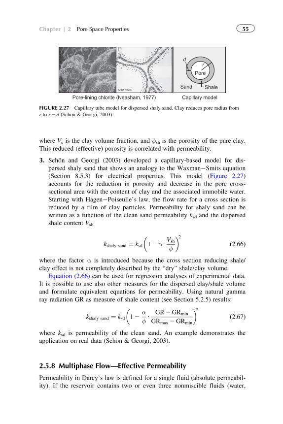
where Vc is the clay volume fraction, and φsh is the porosity of the pure clay.
This reduced (effective) porosity is correlated with permeability.
3. Schon and Georgi (2003) developed a capillary-based model for dis-
persed shaly sand that shows an analogy to the Waxman�Smits equation
(Section 8.5.3) for electrical properties. This model (Figure 2.27)
accounts for the reduction in porosity and decrease in the pore cross-
sectional area with the content of clay and the associated immobile water.
Starting with Hagen�Poiseulle’s law, the flow rate for a cross section is
reduced by a film of clay particles. Permeability for shaly sand can be
written as a function of the clean sand permeability ksd and the dispersed
shale content Vsh
kshaly sand ¼ ksd 12αUVsh
φ
� �2ð2:66Þ
where the factor α is introduced because the cross section reducing shale/
clay effect is not completely described by the “dry” shale/clay volume.
Equation (2.66) can be used for regression analyses of experimental data.
It is possible to use also other measures for the dispersed clay/shale volume
and formulate equivalent equations for permeability. Using natural gamma
ray radiation GR as measure of shale content (see Section 5.2.5) results:
kshaly sand ¼ ksd 12αφU
GR2GRmin
GRmax 2GRmin
� �2ð2:67Þ
where ksd is permeability of the clean sand. An example demonstrates the
application on real data (Schon & Georgi, 2003).
2.5.8 Multiphase Flow—Effective Permeability
Permeability in Darcy’s law is defined for a single fluid (absolute permeabil-
ity). If the reservoir contains two or even three nonmiscible fluids (water,
dr
Pore-lining chlorite (Neasham, 1977) Capillary model
Sand Shale
Pore
FIGURE 2.27 Capillary tube model for dispersed shaly sand. Clay reduces pore radius from
r to r2 d (Schon & Georgi, 2003).
55Chapter | 2 Pore Space Properties
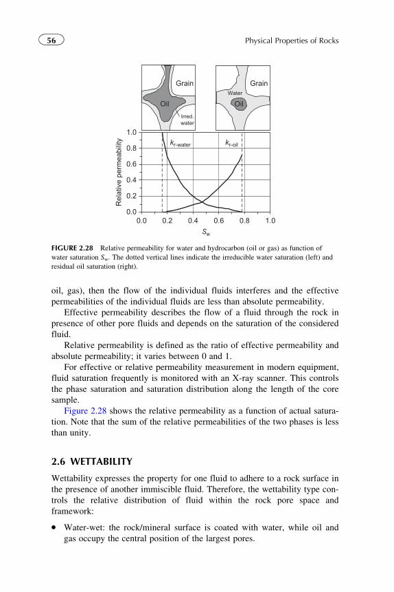
oil, gas), then the flow of the individual fluids interferes and the effective
permeabilities of the individual fluids are less than absolute permeability.
Effective permeability describes the flow of a fluid through the rock in
presence of other pore fluids and depends on the saturation of the considered
fluid.
Relative permeability is defined as the ratio of effective permeability and
absolute permeability; it varies between 0 and 1.
For effective or relative permeability measurement in modern equipment,
fluid saturation frequently is monitored with an X-ray scanner. This controls
the phase saturation and saturation distribution along the length of the core
sample.
Figure 2.28 shows the relative permeability as a function of actual satura-
tion. Note that the sum of the relative permeabilities of the two phases is less
than unity.
2.6 WETTABILITY
Wettability expresses the property for one fluid to adhere to a rock surface in
the presence of another immiscible fluid. Therefore, the wettability type con-
trols the relative distribution of fluid within the rock pore space and
framework:
� Water-wet: the rock/mineral surface is coated with water, while oil and
gas occupy the central position of the largest pores.
0.0
0.2
0.4
0.6
0.8
1.0
0.0 0.2 0.4 0.6 0.8 1.0
Sw
Rel
ativ
e pe
rmea
bilit
y kr-water kr-oil
Grain
Oil
GrainWater
Oil
Irred.water
FIGURE 2.28 Relative permeability for water and hydrocarbon (oil or gas) as function of
water saturation Sw. The dotted vertical lines indicate the irreducible water saturation (left) and
residual oil saturation (right).
56 Physical Properties of Rocks
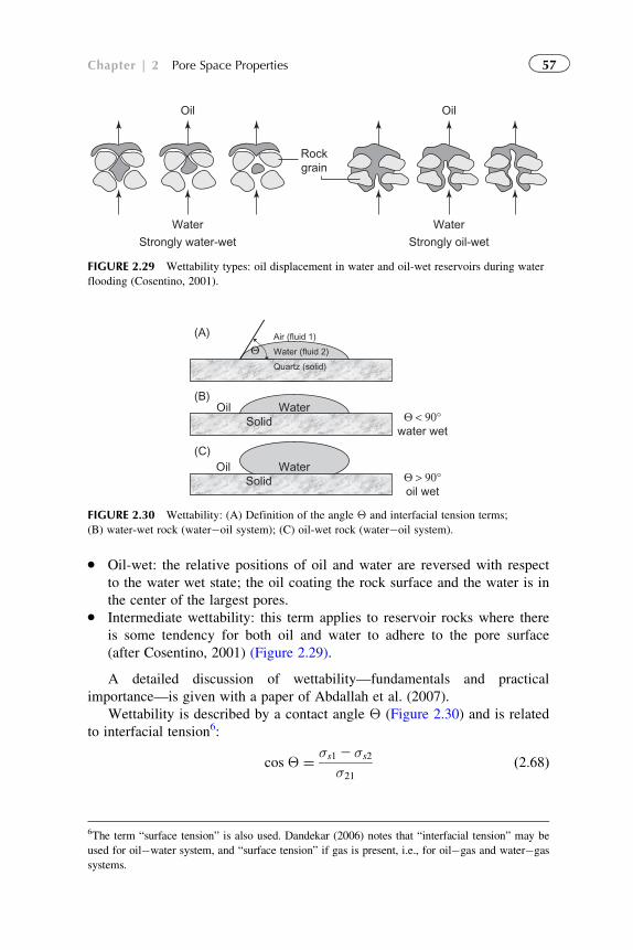
� Oil-wet: the relative positions of oil and water are reversed with respect
to the water wet state; the oil coating the rock surface and the water is in
the center of the largest pores.� Intermediate wettability: this term applies to reservoir rocks where there
is some tendency for both oil and water to adhere to the pore surface
(after Cosentino, 2001) (Figure 2.29).
A detailed discussion of wettability—fundamentals and practical
importance—is given with a paper of Abdallah et al. (2007).
Wettability is described by a contact angle Θ (Figure 2.30) and is related
to interfacial tension6:
cos Θ ¼ σs1 2σs2
σ21
ð2:68Þ
Water
Oil
Rockgrain
WaterStrongly oil-wetStrongly water-wet
Oil
FIGURE 2.29 Wettability types: oil displacement in water and oil-wet reservoirs during water
flooding (Cosentino, 2001).
ΘAir (fluid 1)
Water (fluid 2)
Quartz (solid)
Θ < 90°water wet
Θ > 90°oil wet
Oil WaterSolid
Oil WaterSolid
(A)
(B)
(C)
FIGURE 2.30 Wettability: (A) Definition of the angle Θ and interfacial tension terms;
(B) water-wet rock (water�oil system); (C) oil-wet rock (water�oil system).
6The term “surface tension” is also used. Dandekar (2006) notes that “interfacial tension” may be
used for oil�water system, and “surface tension” if gas is present, i.e., for oil�gas and water�gas
systems.
57Chapter | 2 Pore Space Properties
where
σs1 is interfacial tension between solid and fluid 1 (e.g., air)
σs2 is interfacial tension between solid and fluid 2 (e.g., water)
σ12 is interfacial tension between fluid 1 and fluid 2.
In the oilfield terminology (see also Dandekar, 2006; Tiab & Donaldson,
2004) a rock:
� is strongly water-wet if the contact angle is Θ 5 0�70�,� has intermediate wettability7 if the contact angle is Θ 5 70�110�,� is strongly oil-wet if the contact angle is Θ 5 110�180�.
Clean sandstone tends to be water-wet, but many sandstone reservoir
rocks are intermediate-wet. Carbonates tend to be more oil-wet than clastics.
In gas�liquid systems, gas is always the nonwetting phase. Frequently
water-wet, for example, are North Sea sandstone reservoirs whereas fre-
quently oil- or mixed-wet are Middle East carbonate reservoirs. Wettability
is influenced by saturation history: “Pore surfaces that had been previously
contacted by oil may be oil-wet, but those never contacted by oil may be
water wet.” (Abdallah et al., 2007).
Laboratory methods for wettability determination are (for details of labo-
ratory technique see Ahmed, 2001; Amyx et al., 1960; Tiab & Donaldson,
1996, 2004):
� Measurement of the contact angle after principle in Figure 2.30.� Amott method: determination at a core sample. Based on a combination
of spontaneous imbibition and forced displacement of the fluids (oil,
water) two “displacement ratios” (displacement by oil ratio, displacement
by water ratio) are determined.� USBM (US Bureau of Mines, Texas) wettability index: determination
at a core sample. From centrifuge capillary pressure curves (see
Section 2.7) in imbibition and drainage modus, the area under the curves
are used to calculate a wettability index IUSBM (for more details see e.g.,
Dandekar, 2006; Tiab & Donaldson, 1996).
For a wettability index determination from NMR logs (see Chapter 3)
based on the different relaxation characteristic of wetting and nonwetting
fluid, Looyestijn (2008) defined a new index as
Iw ¼ surface wetted by water2 surface wetted by oil
total surfaceð2:69Þ
This index is scaled from +1 (fully water-wet) to 21 (fully oil-wet).
7Abdallah et al. (2007) note that there is a difference between “intermediate-wetting” (lacking a
strong wetting preference) and “mixed-wetting” (variety of wetting preferences).
58 Physical Properties of Rocks
2.7 FLUID DISTRIBUTION—CAPILLARY PRESSURE IN ARESERVOIR
Capillary pressure pc is defined as the pressure difference between the non-
wetting phase and the wetting phase as a function of the wetting-phase satu-
ration. In reservoir engineering, capillary pressure is an important parameter
for the study of vertical saturation distribution.
A petroleum reservoir initially was saturated with water. Migration of oil
into the reservoir displaced a part of water. This displacement of the wetting
phase (water) by a nonwetting phase (oil) can be simulated in the laboratory
experiment of measuring the drainage capillary pressure curve. In reservoir
studies the inflow of water must also be modeled. In this case, the imbibition
capillary pressure is of interest.
Methods of capillary pressure determination in the laboratory are:
� static methods: mercury injection,� dynamic methods: centrifuge methods.
2.7.1 Fundamentals
In a reservoir under static conditions (no production and flow influence),
gravity and capillary forces are in balance. The fluid distribution in the pore
space is controlled by:
� properties of the pore space,� properties of the fluids,� interactions between fluids and pore surface and interactions between
different fluids.
Figure 2.31 illustrates the fluid distribution in a homogeneous water-wet
reservoir (e.g., a sandstone). There are three different regions with respect to
the pore fluids:
� Water zone: the rock is 100% water-saturated. Note that the 100% water
level is above the FWL (Free Water Level) as a result of the capillary
forces; this position correlates with the “displacement pressure” pd (also
called threshold or entry pressure). Displacement pressure is the capillary
pressure at the top of the water-saturated zone. It is the minimum pres-
sure required for the nonwetting fluid to displace the wetting fluid (water)
and enter the largest pores (Jorden & Campbell, 1984).� Transition zone (also funicular region): over the transition zone changes
of saturation takes place. This region reflects “the most abundant and
accessible pore-throat sizes; the steeper the capillary pressure curve in
this region, the less uniform the pore throats” (Jorden & Campbell,
1984).
59Chapter | 2 Pore Space Properties
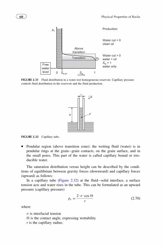
� Pendular region (above transition zone): the wetting fluid (water) is in
pendular rings at the grain�grain contacts, on the grain surface, and in
the small pores. This part of the water is called capillary bound or irre-
ducible water.
The saturation distribution versus height can be described by the condi-
tions of equilibrium between gravity forces (downward) and capillary forces
(upward) as follows:
In a capillary tube (Figure 2.32) at the fluid�solid interface, a surface
tension acts and water rises in the tube. This can be formulated as an upward
pressure (capillary pressure)
pc ¼2UσUcos Θ
rð2:70Þ
where
σ is interfacial tension
Θ is the contact angle, expressing wettability
r is the capillary radius.
ρh
r g
FIGURE 2.32 Capillary tube.
pc
Sw
pd
0 Sw,irr 1
Abovetransition
Transition
water zone
Production:
Water cut = 0clean oil
Water cut > 0water + oilSw = 1water only
Freewaterlevel
FIGURE 2.31 Fluid distribution in a water-wet homogeneous reservoir. Capillary pressure
controls fluid distribution in the reservoir and the fluid production.
60 Physical Properties of Rocks
In equilibrium the capillary pressure equals the pressure by the weight of
the rising water column (gravity):
pg ¼ gUΔρUh ð2:71Þwhere
g is Earth’s acceleration
Δρ is the density difference between wetting and nonwetting fluid
h is the height above the FWL.
This gives the height above the FWL
h ¼ pc
gUΔρ¼ 2UσUcos Θ
gUΔρUrð2:72Þ
Thus, the finer the capillary tube, the higher the water will rise.
The vertical equilibrium between capillary forces and gravitational force
determines the height of the capillary fringe in an oil reservoir (or any other
fluid reservoir).
Equation (2.72) contains two types of properties:
1. reservoir pore geometric properties (in the simple model expressed by
radius r),
2. interface properties σ � cosΘ and difference of fluid densities Δρ.
Therefore, a conversion between different fluid systems is possible by
changing the interface properties σ � cosΘ and densities. Also a conversion
from laboratory measurements to reservoir conditions is possible.
Table 2.10 gives some data for different fluid systems. A detailed study
about the oil�brine interfacial tension and influencing factors (salinity, pH,
viscosity) was published by Buckley and Fan (2007).
Figure 2.33 demonstrates the principle of a capillary pressure measure-
ment (drainage, water-wet rock). The piston pressures the nonwetting fluid
(oil) into the pores. The process starts (B) if the pressure equals the displace-
ment pressure and the largest pores are filled. The process ends (D) if all
pores are filled with oil—only the irreducible water is present.
In real rocks, pores are not tubes but have a complicated shape with throats
and bodies of different size (pore size distribution) and a curve results.
Amyx et al. (1960) give a description of the mercury injection technique:
“Mercury is normally a nonwetting fluid. The core sample is inserted in the
mercury chamber and evacuated. Mercury is forced in the core under pressure.
The volume of mercury injected at each pressure determines the nonwetting-
phase saturation. This procedure is continued until the core sample is filled
with mercury or the injection pressure reaches some predetermined value.”
The incremental mercury volume injected is plotted as function of the
injection pressure and delivers the (injection) capillary pressure curve: a mer-
cury withdrawal capillary pressure curve can be obtained by decreasing the
pressure in increments and recording the volume of mercury withdrawn.
61Chapter | 2 Pore Space Properties
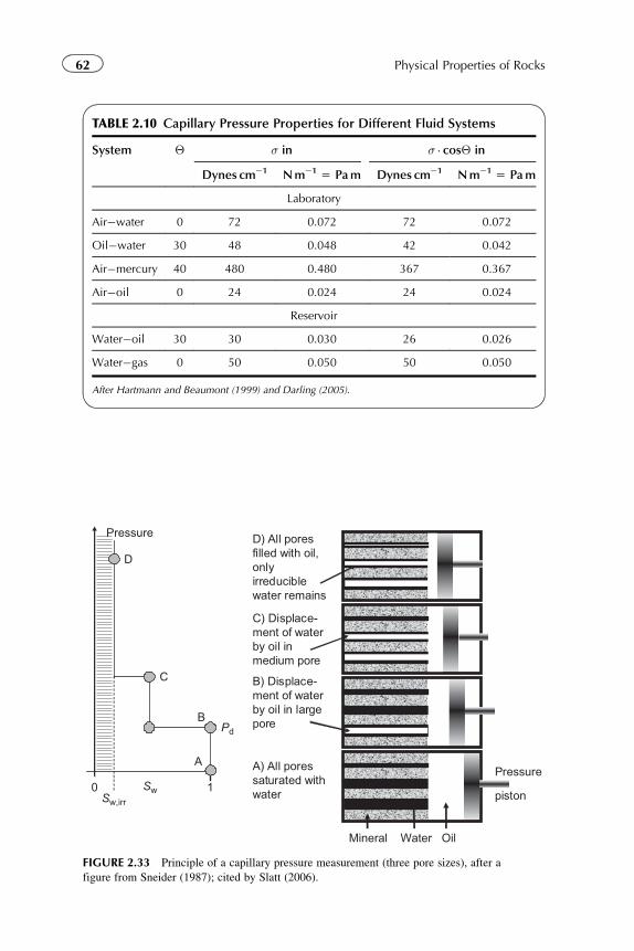
TABLE 2.10 Capillary Pressure Properties for Different Fluid Systems
System Θ σ in σ � cosΘ in
Dynes cm21 Nm21 5 Pam Dynes cm21 Nm21 5 Pam
Laboratory
Air�water 0 72 0.072 72 0.072
Oil�water 30 48 0.048 42 0.042
Air�mercury 40 480 0.480 367 0.367
Air�oil 0 24 0.024 24 0.024
Reservoir
Water�oil 30 30 0.030 26 0.026
Water�gas 0 50 0.050 50 0.050
After Hartmann and Beaumont (1999) and Darling (2005).
0 1Pressure
piston
Mineral Water Oil
Pressure
D
D) All poresfilled with oil,onlyirreduciblewater remains
C) Displace-ment of waterby oil inmedium pore
B) Displace-ment of waterby oil in largepore
A) All poressaturated withwater
C
B
A
Pd
SwSw,irr
FIGURE 2.33 Principle of a capillary pressure measurement (three pore sizes), after a
figure from Sneider (1987); cited by Slatt (2006).
62 Physical Properties of Rocks
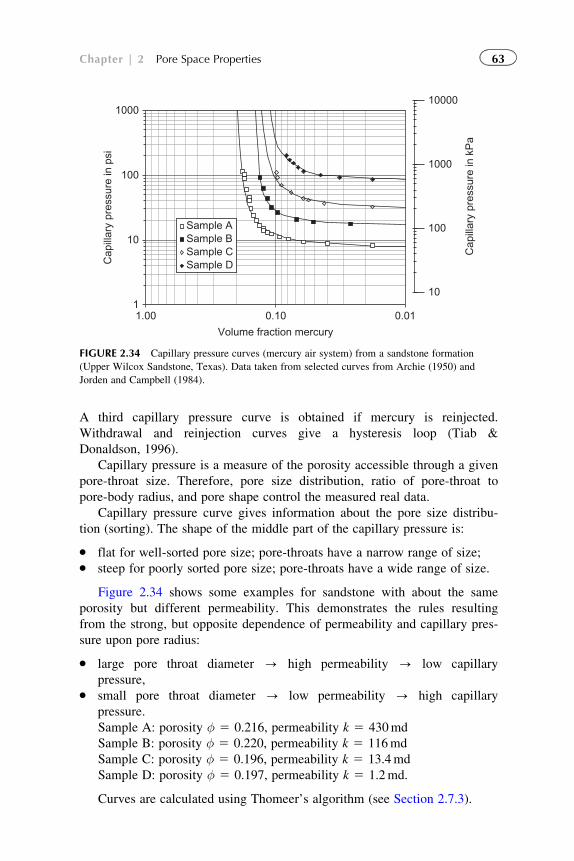
A third capillary pressure curve is obtained if mercury is reinjected.
Withdrawal and reinjection curves give a hysteresis loop (Tiab &
Donaldson, 1996).
Capillary pressure is a measure of the porosity accessible through a given
pore-throat size. Therefore, pore size distribution, ratio of pore-throat to
pore-body radius, and pore shape control the measured real data.
Capillary pressure curve gives information about the pore size distribu-
tion (sorting). The shape of the middle part of the capillary pressure is:
� flat for well-sorted pore size; pore-throats have a narrow range of size;� steep for poorly sorted pore size; pore-throats have a wide range of size.
Figure 2.34 shows some examples for sandstone with about the same
porosity but different permeability. This demonstrates the rules resulting
from the strong, but opposite dependence of permeability and capillary pres-
sure upon pore radius:
� large pore throat diameter - high permeability - low capillary
pressure,� small pore throat diameter - low permeability - high capillary
pressure.
Sample A: porosity φ 5 0.216, permeability k 5 430md
Sample B: porosity φ 5 0.220, permeability k 5 116md
Sample C: porosity φ 5 0.196, permeability k 5 13.4md
Sample D: porosity φ 5 0.197, permeability k 5 1.2md.
Curves are calculated using Thomeer’s algorithm (see Section 2.7.3).
1
10
100
1000
0.010.101.00
Volume fraction mercury
Cap
illar
y pr
essu
re in
psi
Sample ASample BSample CSample D
10
100
1000
10000
Cap
illar
y pr
essu
re in
kP
a
FIGURE 2.34 Capillary pressure curves (mercury air system) from a sandstone formation
(Upper Wilcox Sandstone, Texas). Data taken from selected curves from Archie (1950) and
Jorden and Campbell (1984).
63Chapter | 2 Pore Space Properties
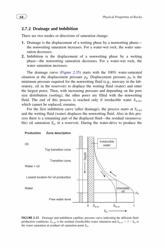
2.7.2 Drainage and Imbibition
There are two modes or directions of saturation change:
1. Drainage is the displacement of a wetting phase by a nonwetting phase—
the nonwetting saturation increases. For a water-wet rock, the water satu-
ration decreases.
2. Imbibition is the displacement of a nonwetting phase by a wetting
phase—the nonwetting saturation decreases. For a water-wet rock, the
water saturation increases.
The drainage curve (Figure 2.35) starts with the 100% water-saturated
situation at the displacement pressure pd. Displacement pressure pd is the
minimum pressure required for the nonwetting fluid (e.g., mercury in the lab-
oratory, oil in the reservoir) to displace the wetting fluid (water) and enter
the largest pores. Then, with increasing pressure and depending on the pore
size distribution (sorting), the other pores are filled with the nonwetting
fluid. The end of this process is reached only if irreducible water Sw,irr,
which cannot be replaced, remains.
For the first imbibition curve (after drainage), the process starts at Sw,irrand the wetting fluid (water) displaces the nonwetting fluid. Also in this pro-
cess there is a remaining part of the displaced fluid—the residual (nonmova-
ble) oil saturation Sro in a reservoir. During the water-drive to produce the
0 Sw,irr Sw,ro 1
Sw
Production Zone description
Oil
Top transition zone
Transition zone
Water + oil
Lowest location for oil production
Water
Free water level
Immobileoil
Irreduciblewater
Dep
th
pd
FIGURE 2.35 Drainage and imbibition capillary pressure curve indicating the different fluid
production conditions; Sw,irr is the residual (irreducible) water saturation and Sw,ro 5 12 Sro is
the water saturation at residual oil saturation point Sro.
64 Physical Properties of Rocks
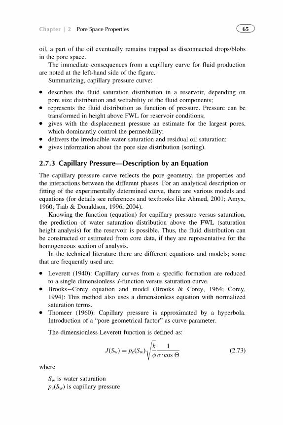
oil, a part of the oil eventually remains trapped as disconnected drops/blobs
in the pore space.
The immediate consequences from a capillary curve for fluid production
are noted at the left-hand side of the figure.
Summarizing, capillary pressure curve:
� describes the fluid saturation distribution in a reservoir, depending on
pore size distribution and wettability of the fluid components;� represents the fluid distribution as function of pressure. Pressure can be
transformed in height above FWL for reservoir conditions;� gives with the displacement pressure an estimate for the largest pores,
which dominantly control the permeability;� delivers the irreducible water saturation and residual oil saturation;� gives information about the pore size distribution (sorting).
2.7.3 Capillary Pressure—Description by an Equation
The capillary pressure curve reflects the pore geometry, the properties and
the interactions between the different phases. For an analytical description or
fitting of the experimentally determined curve, there are various models and
equations (for details see references and textbooks like Ahmed, 2001; Amyx,
1960; Tiab & Donaldson, 1996, 2004).
Knowing the function (equation) for capillary pressure versus saturation,
the prediction of water saturation distribution above the FWL (saturation
height analysis) for the reservoir is possible. Thus, the fluid distribution can
be constructed or estimated from core data, if they are representative for the
homogeneous section of analysis.
In the technical literature there are different equations and models; some
that are frequently used are:
� Leverett (1940): Capillary curves from a specific formation are reduced
to a single dimensionless J-function versus saturation curve.� Brooks�Corey equation and model (Brooks & Corey, 1964; Corey,
1994): This method also uses a dimensionless equation with normalized
saturation terms.� Thomeer (1960): Capillary pressure is approximated by a hyperbola.
Introduction of a “pore geometrical factor” as curve parameter.
The dimensionless Leverett function is defined as:
JðSwÞ ¼ pcðSwÞffiffiffik
φ
s1
σUcos Θð2:73Þ
where
Sw is water saturation
pc(Sw) is capillary pressure
65Chapter | 2 Pore Space Properties
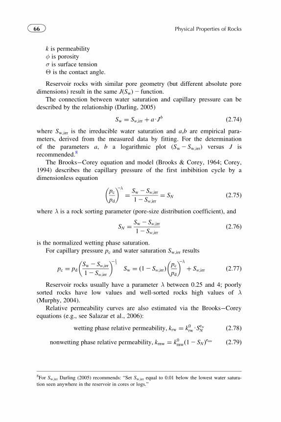
k is permeability
φ is porosity
σ is surface tension
Θ is the contact angle.
Reservoir rocks with similar pore geometry (but different absolute pore
dimensions) result in the same J(Sw)2 function.
The connection between water saturation and capillary pressure can be
described by the relationship (Darling, 2005)
Sw ¼ Sw;irr þ aUJb ð2:74Þwhere Sw,irr is the irreducible water saturation and a,b are empirical para-
meters, derived from the measured data by fitting. For the determination
of the parameters a, b a logarithmic plot (Sw2 Sw,irr) versus J is
recommended.8
The Brooks�Corey equation and model (Brooks & Corey, 1964; Corey,
1994) describes the capillary pressure of the first imbibition cycle by a
dimensionless equation
pc
pd
� �2λ¼ Sw 2 Sw;irr
12 Sw;irr¼ SN ð2:75Þ
where λ is a rock sorting parameter (pore-size distribution coefficient), and
SN ¼ Sw 2 Sw;irr
12 Sw;irrð2:76Þ
is the normalized wetting phase saturation.
For capillary pressure pc and water saturation Sw,irr results
pc ¼ pdSw 2 Sw;irr
12 Sw;irr
� �21λ
Sw ¼ ð12 Sw;irrÞpc
pd
� �2λþ Sw;irr ð2:77Þ
Reservoir rocks usually have a parameter λ between 0.25 and 4; poorly
sorted rocks have low values and well-sorted rocks high values of λ(Murphy, 2004).
Relative permeability curves are also estimated via the Brooks�Corey
equations (e.g., see Salazar et al., 2006):
wetting phase relative permeability; krw ¼ k0rwUSewN ð2:78Þ
nonwetting phase relative permeability; krnw ¼ k0rnwð12 SNÞenw ð2:79Þ
8For Sw,irr Darling (2005) recommends: “Set Sw,irr equal to 0.01 below the lowest water satura-
tion seen anywhere in the reservoir in cores or logs.”
66 Physical Properties of Rocks
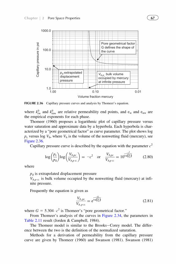
where k0rw and k0rnw are relative permeability end points, and ew and enw are
the empirical exponents for each phase.
Thomeer (1960) proposes a logarithmic plot of capillary pressure versus
water saturation and approximate data by a hyperbola. Each hyperbola is char-
acterized by a “pore geometrical factor” as curve parameter. The plot shows log
pc versus log Vb, where Vb is the volume of the nonwetting fluid (mercury), see
Figure 2.36.
Capillary pressure curve is described by the equation with the parameter c2
logpc
pd
� �log
Vb;pc
Vb;pN
� �¼ 2c2 or
Vb;pc
Vb;pN¼ 10
2c2
logpcpdð Þ ð2:80Þ
where
pd is extrapolated displacement pressure
Vb,pN is bulk volume occupied by the nonwetting fluid (mercury) at infi-
nite pressure.
Frequently the equation is given as
Vb; pc
Vb; pN¼ e
2G
logpcpdð Þ ð2:81Þ
where G 5 5.304 � c2 is Thomeer’s “pore geometrical factor.”
From Thomeer’s analysis of the curves in Figure 2.34, the parameters in
Table 2.11 result (Jorden & Campbell, 1984).
The Thomeer model is similar to the Brooks�Corey model. The differ-
ence between the two is the definition of the normalized saturation.
Methods for a derivation of permeability from the capillary pressure
curve are given by Thomeer (1960) and Swanson (1981). Swanson (1981)
1.0
10.0
100.0
1000.0
0.010.101.00
Volume fraction mercury
Cap
illar
y pr
essu
re in
psi Pore geometrical factor
G defines the shape ofthe curve
pd extrapolateddisplacementpressure
Vb,p∞ bulk volumeoccupied by mercuryat infinite pressure
FIGURE 2.36 Capillary pressure curves and analysis by Thomeer’s equation.
67Chapter | 2 Pore Space Properties
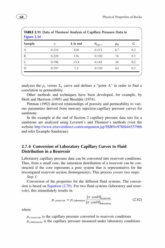
analyzes the pc versus Sw curve and defines a “point A” in order to find a
correlation to permeability.
Other methods and techniques have been developed, for example, by
Skelt and Harrison (1995) and Heseldin (1974).
Pittman (1992) derived relationships of porosity and permeability to vari-
ous parameters derived from mercury injection-capillary pressure curves for
sandstone.
In the example at the end of Section 2 capillary pressure data sets for a
sandstone are analyzed using Leverett’s and Thomeer’s methods (visit the
website http://www.elsevierdirect.com/companion.jsp?ISBN=9780444537966
and refer Example-Sandstone).
2.7.4 Conversion of Laboratory Capillary Curves to FluidDistribution in a Reservoir
Laboratory capillary pressure data can be converted into reservoir conditions.
Thus, from a small core, the saturation distribution of a reservoir can be con-
structed if the core represents a pore system that is representative for the
investigated reservoir section (homogeneity). This process covers two steps:
Step 1:
Conversion of the properties for the different fluid systems. The conver-
sion is based on Equation (2.70). For two fluid systems (laboratory and reser-
voir), this immediately results in:
pc;reservoir ¼ pc;laboratoryσUcosΘ½ �reservoirσUcosΘ½ �laboratory
ð2:82Þ
where
pc,reservoir is the capillary pressure converted to reservoir conditions
pc,laboratory is the capillary pressure measured under laboratory conditions
TABLE 2.11 Data of Thomeer Analysis of Capillary Pressure Data in
Figure 2.34
Sample φ k in md Vb,pN pd G
A 0.216 430 0.215 6.7 0.2
B 0.220 116 0.150 16 0.1
C 0.196 13.4 0.145 26 0.2
D 0.197 1.2 0.130 65 0.2
68 Physical Properties of Rocks
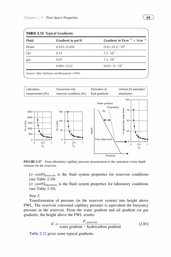
[σ � cosΘ]reservoir is the fluid system properties for reservoir conditions
(see Table 2.10)
[σ � cosΘ]laboratory is the fluid system properties for laboratory conditions
(see Table 2.10).
Step 2:
Transformation of pressure (in the reservoir system) into height above
FWL. The reservoir converted capillary pressure is equivalent the buoyancy
pressure in the reservoir. From the water gradient and oil gradient (or gas
gradient), the height above the FWL results:
h0 ¼ Pc;reservoir
water gradient2 hydrocarbon gradientð2:83Þ
Table 2.12 gives some typical gradients.
TABLE 2.12 Typical Gradients
Fluid Gradient in psi/ft Gradient in Pam21 5 Nm23
Water 0.433�0.450 (9.8�10.2) �103
Oil 0.33 7.5 �103
gas 0.07 1.5 �103
0.001�0.22 (0.02�5) � 103
Source: After Hartman and Beaumont (1999).
Pressure
Dep
th
Water gradient
Oil gradient
Pb
Free water level0
50
100
150
0 0.5 1Sw
Pc
in k
Pa
0
500
1000
1500
2000
2500
0 0.5 1Sw
Pc
in k
Pa
0
25
50
75
100
0 0.5 1Sw
m a
bove
free
wat
er le
vel
Laboratory
measurement (Pc)
Conversion into
reservoir conditions (Pc)
Derivation of
fluid gradients
Vertical (h) saturation
distribution
FIGURE 2.37 From laboratory capillary pressure measurement to the saturation versus depth
estimate for the reservoir.
69Chapter | 2 Pore Space Properties
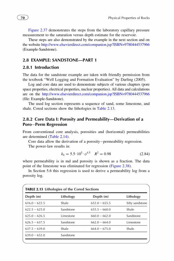
Figure 2.37 demonstrates the steps from the laboratory capillary pressure
measurement to the saturation versus depth estimate for the reservoir.
These steps are also demonstrated by the example in the next section and on
the website http://www.elsevierdirect.com/companion.jsp?ISBN=9780444537966
(Example-Sandstone).
2.8 EXAMPLE: SANDSTONE—PART 1
2.8.1 Introduction
The data for the sandstone example are taken with friendly permission from
the textbook “Well Logging and Formation Evaluation” by Darling (2005).
Log and core data are used to demonstrate subjects of various chapters (pore
space properties, electrical properties, nuclear properties). All data and calculations
are on the http://www.elsevierdirect.com/companion.jsp?ISBN=9780444537966
(file: Example-Sandstone).
The used log section represents a sequence of sand, some limestone, and
shale. Cored sections show the lithologies in Table 2.13.
2.8.2 Core Data I: Porosity and Permeability—Derivation of aPoro�Perm Regression
From conventional core analysis, porosities and (horizontal) permeabilities
are determined (Table 2.14).
Core data allow the derivation of a porosity�permeability regression.
The power-law results in:
kh ¼ 5:5U105Uφ4:5 R2 ¼ 0:98 ð2:84Þwhere permeability is in md and porosity is shown as a fraction. The data
point of the limestone was eliminated for regression (Figure 2.38).
In Section 5.6 this regression is used to derive a permeability log from a
porosity log.
TABLE 2.13 Lithologies of the Cored Sections
Depth (m) Lithology Depth (m) Lithology
616.02 622.5 Shale 652.02 655.5 Silty sandstone
622.52 625.0 Sandstone 655.52 660.0 Shale
625.02 626.5 Limestone 660.02 662.0 Sandstone
626.52 637.5 Sandstone 662.02 664.0 Limestone
637.52 639.0 Shale 664.02 675.0 Shale
639.02 652.0 Sandstone
70 Physical Properties of Rocks
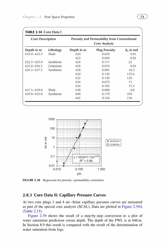
2.8.3 Core Data II: Capillary Pressure Curves
At two core plugs 1 and 4 air�brine capillary pressure curves are measured
as part of the special core analysis (SCAL). Data are plotted in Figure 2.39A
(Table 2.15).
Figure 2.39 shows the result of a step-by-step conversion to a plot of
water saturation prediction versus depth. The depth of the FWL is at 646m.
In Section 8.9 this result is compared with the result of the determination of
water saturation from logs.
TABLE 2.14 Core Data I
Core Description Porosity and Permeability from Conventional
Core Analysis
Depth in m Lithology Depth in m Plug Porosity kh in md616.0�622.5 Shale 620 0.020 0.01
622 0.020 0.02
622.5�625.0 Sandstone 624 0.111 22
625.0�626.5 Limestone 626 0.010 0.03
626.5�637.5 Sandstone 628 0.095 10.5
630 0.156 135.6
632 0.150 120
634 0.075 11
636 0.105 15.3
637.5�639.0 Shale 638 0.060 0.8
639.0�652.0 Sandstone 640 0.179 350
642 0.156 130
0.010 0.100 1.000phi
0.01
0.1
1
10
100
1000
kh in
md
SandstoneLimestone
y = 553577.73x4.50
R2 = 0.98
FIGURE 2.38 Regression for porosity�permeability correlation.
71Chapter | 2 Pore Space Properties
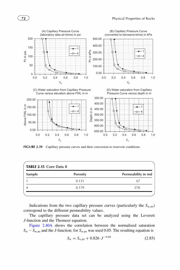
Indications from the two capillary pressure curves (particularly the Sw,irr)
correspond to the different permeability values.
The capillary pressure data set can be analyzed using the Leverett
J-function and the Thomeer equation.
Figure 2.40A shows the correlation between the normalized saturation
Sw2 Sw,irr and the J-function; for Sw,irr was used 0.05. The resulting equation is
Sw ¼ Sw;irr þ 0:826UJ20:44 ð2:85Þ
(A) Capillary Pressure Curve(laboratory data air-brine) in psi
0
50
100
150
200
0.0 0.2 0.4 0.6 0.8 1.0Sw
Pc
in p
si
14
(C) Water saturation from Capillary PressureCurve versus elevation above FWL in m
0.00
50.00
100.00
150.00
200.00
0.0 0.2 0.4 0.6 0.8 1.0Sw
Abo
ve F
WL
in m 1
4
(B) Capillary Pressure Curve(converted to kerosene-brine) in kPa
0.00
100.00
200.00
300.00
400.00
500.00
0.0 0.2 0.4 0.6 0.8 1.0Sw
Pc
in k
Pa 1
4
(D) Water saturation from CapillaryPressure Curve versus depth in m
350.00
400.00
450.00
500.00
550.00
600.00
650.000.0 0.2 0.4 0.6 0.8 1.0
Sw
Dep
th in
m
14
FIGURE 2.39 Capillary pressure curves and their conversion to reservoir conditions.
TABLE 2.15 Core Data II
Sample Porosity Permeability in md
1 0.131 67
4 0.179 278
72 Physical Properties of Rocks
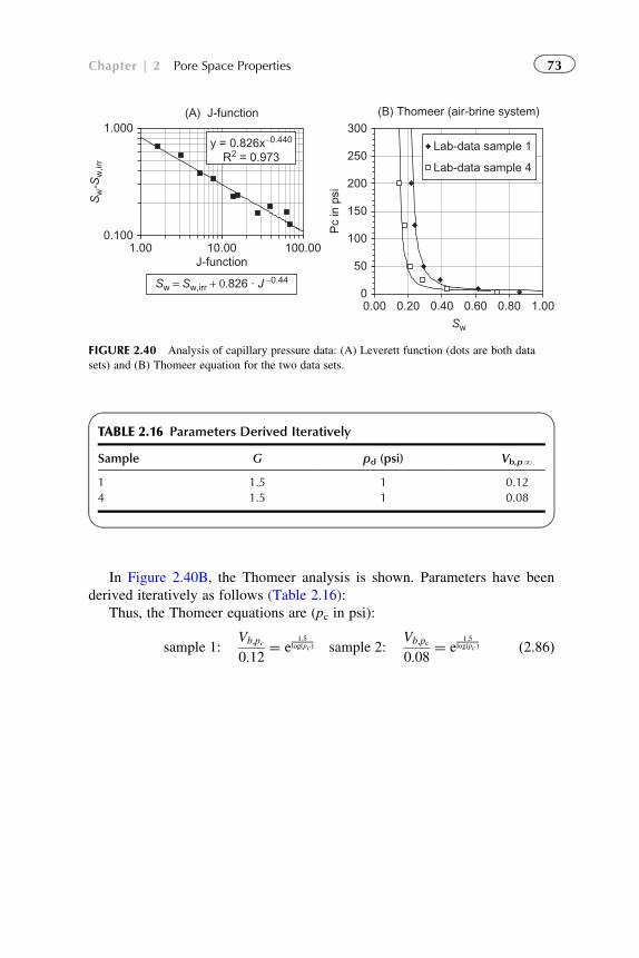
In Figure 2.40B, the Thomeer analysis is shown. Parameters have been
derived iteratively as follows (Table 2.16):
Thus, the Thomeer equations are (pc in psi):
sample 1:Vb;pc
0:12¼ e
1:5logðpcÞ sample 2:
Vb;pc
0:08¼ e
1:5logðpc Þ ð2:86Þ
(A) J-function
y = 0.826x−0.440
R2 = 0.973
0.100
1.000
1.00 10.00 100.00J-function
Sw-S
w,ir
r
Sw = Sw,irr + 0.826 · J −0.44
(B) Thomeer (air-brine system)
0
50
100
150
200
250
300
0.00 0.20 0.40 0.60 0.80 1.00
SwP
c in
psi
Lab-data sample 1
Lab-data sample 4
FIGURE 2.40 Analysis of capillary pressure data: (A) Leverett function (dots are both data
sets) and (B) Thomeer equation for the two data sets.
TABLE 2.16 Parameters Derived Iteratively
Sample G pd (psi) Vb,pN
1 1.5 1 0.12
4 1.5 1 0.08
73Chapter | 2 Pore Space Properties

Chapter 3
Nuclear Magnetic Resonance—Petrophysical Properties
NMR is not the end all to petrophysics. It is a new tool for understanding and
describing the subsurface, both reservoir and non-reservoir rocks, which expands the
petrophysical content of our logging data, providing direct estimates of irreducible
water, clay bound water, and the permeability.
Georgi and Chen (2007)
3.1 INTRODUCTION
The development and application of nuclear magnetic resonance (NMR)
techniques in formation evaluation has originated new insights into the pore
space and the pore fluids distribution and behavior. Primarily NMR measure-
ments deliver relaxation data. Figure 3.1 shows as an example the relaxation
process as decay of the measured signal calibrated in porosity units for two
sandstones with the same porosity. The different decay curves result from
different specific internal surface (high Spor for fine-grained sand, low Sporfor coarse-grained sand). Processing techniques result in a partitioning of
porosity in free movable (bulk volume movable—BVM) and capillary bound
(bulk volume irreducible—BVI) fraction. This characterizes pore sizes and
gives a link to a permeability estimate (see the following sections).
Most nuclei have a magnetic moment and an angular momentum; both
are coaxial. NMR measurements in particular use this property of hydrogen
nuclei and their ability to interact in a magnetic field like a bar magnet�gyro
combination.
Hydrogen nuclei are in fluid molecules of water and hydrocarbons.
Therefore, the response of this type of NMR measurements in geosciences
applications comes only from the hydrogen nuclei and their physical envi-
ronment in the pore space—there is no “matrix effect” as is commonly asso-
ciated with conventional nuclear porosity determinations (see Sections 5.3
and 5.4).
75Physical Properties of Rocks.
© 2011 Elsevier B.V. All rights reserved.
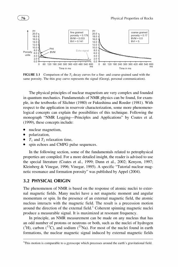
The physical principles of nuclear magnetism are very complex and founded
in quantum mechanics. Fundamentals of NMR physics can be found, for exam-
ple, in the textbooks of Slichter (1980) or Fukushima and Roeder (1981). With
respect to the application in reservoir characterization, some more phenomeno-
logical concepts can explain the possibilities of this technique. Following the
monograph “NMR Logging—Principles and Applications” by Coates et al.
(1999), these concepts include:
� nuclear magnetism,� polarization,� T1 and T2 relaxation time,� spin echoes and CMPG pulse sequences.
In the following section, some of the fundamentals related to petrophysical
properties are compiled. For a more detailed insight, the reader is advised to use
the special literature (Coates et al., 1999; Dunn et al., 2002; Kenyon, 1997;
Kleinberg & Vinegar, 1996; Vinegar, 1995). A specific “Tutorial nuclear mag-
netic resonance and formation porosity” was published by Appel (2004).
3.2 PHYSICAL ORIGIN
The phenomenon of NMR is based on the response of atomic nuclei to exter-
nal magnetic fields. Many nuclei have a net magnetic moment and angular
momentum or spin. In the presence of an external magnetic field, the atomic
nucleus interacts with the magnetic field. The result is a precession motion
around the direction of the external field.1 Coherent spinning magnetic nuclei
produce a measurable signal. It is maximized at resonant frequency.
In principle, an NMR measurement can be made on any nucleus that has
an odd number of protons or neutrons or both, such as the nuclei of hydrogen
(1H), carbon (13C), and sodium (23Na). For most of the nuclei found in earth
formations, the nuclear magnetic signal induced by external magnetic fields
1This motion is comparable to a gyroscope which precesses around the earth’s gravitational field.
Porosityunits
20.0pu
18.016.014.012.010.08.06.04.02.00.0
0 60 120 180 240
Time in ms Time in ms
300 360 420 480 540 600ms
20.0pu
18.016.014.012.010.08.06.04.02.00.0
0 60 120 180 240 300 360 420 480 540 600ms
fine grainedporosity = 0.179BVM = 0.033BVI = 0.141
coarse grainedporosity = 0.17BVM = 0.0BVI = 0.
PHIEcho signalBVM
FIGURE 3.1 Comparison of the T2 decay curves for a fine- and coarse-grained sand with the
same porosity. The thin gray curve represents the signal (Georgi, personal communication).
76 Physical Properties of Rocks
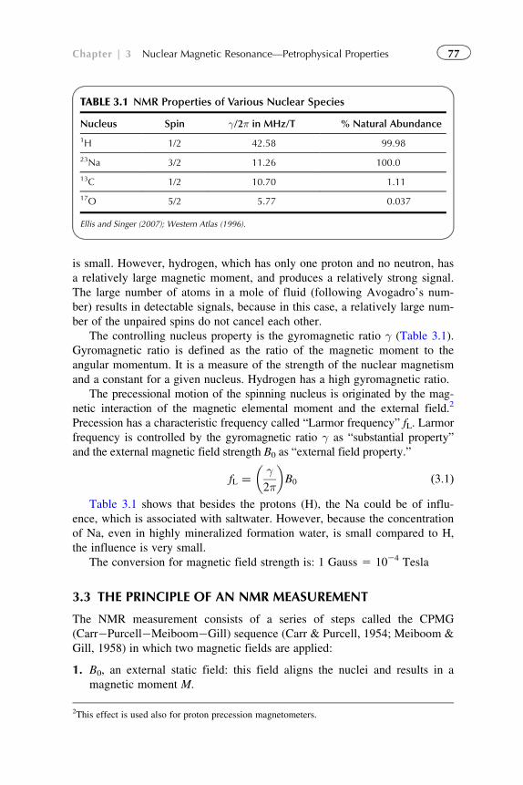
is small. However, hydrogen, which has only one proton and no neutron, has
a relatively large magnetic moment, and produces a relatively strong signal.
The large number of atoms in a mole of fluid (following Avogadro’s num-
ber) results in detectable signals, because in this case, a relatively large num-
ber of the unpaired spins do not cancel each other.
The controlling nucleus property is the gyromagnetic ratio γ (Table 3.1).
Gyromagnetic ratio is defined as the ratio of the magnetic moment to the
angular momentum. It is a measure of the strength of the nuclear magnetism
and a constant for a given nucleus. Hydrogen has a high gyromagnetic ratio.
The precessional motion of the spinning nucleus is originated by the mag-
netic interaction of the magnetic elemental moment and the external field.2
Precession has a characteristic frequency called “Larmor frequency” fL. Larmor
frequency is controlled by the gyromagnetic ratio γ as “substantial property”
and the external magnetic field strength B0 as “external field property.”
fL ¼ γ2π
� �B0 ð3:1Þ
Table 3.1 shows that besides the protons (H), the Na could be of influ-
ence, which is associated with saltwater. However, because the concentration
of Na, even in highly mineralized formation water, is small compared to H,
the influence is very small.
The conversion for magnetic field strength is: 1 Gauss 5 1024 Tesla
3.3 THE PRINCIPLE OF AN NMR MEASUREMENT
The NMR measurement consists of a series of steps called the CPMG
(Carr�Purcell�Meiboom�Gill) sequence (Carr & Purcell, 1954; Meiboom &
Gill, 1958) in which two magnetic fields are applied:
1. B0, an external static field: this field aligns the nuclei and results in a
magnetic moment M.
TABLE 3.1 NMR Properties of Various Nuclear Species
Nucleus Spin γ/2π in MHz/T % Natural Abundance
1H 1/2 42.58 99.98
23Na 3/2 11.26 100.0
13C 1/2 10.70 1.11
17O 5/2 5.77 0.037
Ellis and Singer (2007); Western Atlas (1996).
2This effect is used also for proton precession magnetometers.
77Chapter | 3 Nuclear Magnetic Resonance—Petrophysical Properties
2. B1, a “tipping” field: this is a series of electromagnetic, radio frequency
(RF) pulses (with Larmor frequency). It is applied perpendicular to the
B0 field.
The four CPMG steps are as follows.
Step 1: Hydrogen nuclei alignment.
The static field B0 aligns the elemental magnets in the direction of B0.
This polarization results in a net magnetization (vector summation of the
individual magnetic moments). Polarization does not occur immediately but
rather grows with a time constant T1 and can be described as an exponential
law. Magnetization at time t after start of the experiment is
MðtÞ ¼ M0 12 exp 2t
T1
� �� �ð3:2Þ
whereM0 is the final and maximum magnetization in a given magnetic field B0.
Step 2: Tipping the aligned protons into transverse plane.
By an oscillating magnetic field B1, perpendicular to the direction of B0,
the aligned protons are tipped from the longitudinal direction (direction of
B0) into the transverse plane. This magnetic field is provided by an RF pulse
with resonant frequency (Larmor frequency) and a given duration. The dura-
tion determines how far the protons are tipped relative to the B0 field. The
result is a precession with the Larmor frequency in the plane perpendicular
to B0. Because the protons precess about the axis of the B0 field, the proton
spin axis now describes a cone figure. The maximum NMR signal is
received when the protons are tipped by an angle of 90�.Step 3: Precessing and dephasing.
At the beginning, all the protons precess in unison with the same fre-
quency; they generate a magnetic field that is measured with an antenna.
After turning off B1, the protons begin to dephase—they lose phase coher-
ency and the resulting net magnetization decreases. This decay with the char-
acteristic relaxation time T2 has two origins:
1. Dephasing caused by diffusion in an inhomogeneous magnetic field—
reversible dephasing effect (this is sometimes referred to as T2*).
2. Dephasing caused by molecular interactions—irreversible dephasing effect.
Note that T1 recovery occurs continually and causes some protons to
realign with the B0 field. However, when subsequent π- or 180�-pulses are
applied, as described in Step 4, these protons are randomized relative to their
orientation with respect to the B0 field. This implies that T2 relaxation time
constant must be less than or equal to T1 relaxation time constant.
Step 4: Refocusing by (partial) reversible dephasing.
The application of a π- or 180�-pulse reverses the precession motion. The
idea is that the reverse process for the individual protons has the same rate and
the effect of inhomogeneities is compensated after one cycle. The rephased
78 Physical Properties of Rocks
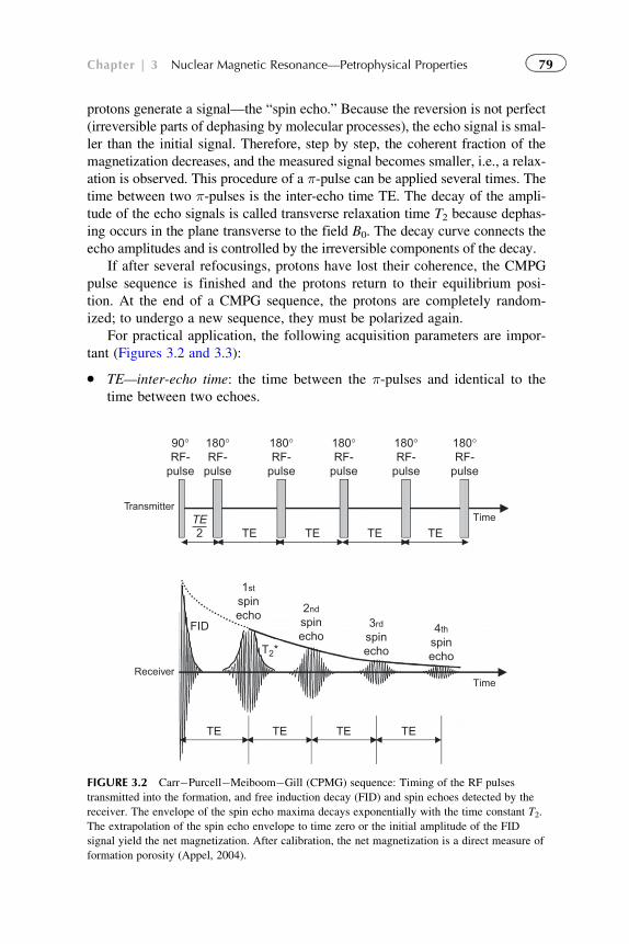
protons generate a signal—the “spin echo.” Because the reversion is not perfect
(irreversible parts of dephasing by molecular processes), the echo signal is smal-
ler than the initial signal. Therefore, step by step, the coherent fraction of the
magnetization decreases, and the measured signal becomes smaller, i.e., a relax-
ation is observed. This procedure of a π-pulse can be applied several times. The
time between two π-pulses is the inter-echo time TE. The decay of the ampli-
tude of the echo signals is called transverse relaxation time T2 because dephas-
ing occurs in the plane transverse to the field B0. The decay curve connects the
echo amplitudes and is controlled by the irreversible components of the decay.
If after several refocusings, protons have lost their coherence, the CMPG
pulse sequence is finished and the protons return to their equilibrium posi-
tion. At the end of a CMPG sequence, the protons are completely random-
ized; to undergo a new sequence, they must be polarized again.
For practical application, the following acquisition parameters are impor-
tant (Figures 3.2 and 3.3):
� TE—inter-echo time: the time between the π-pulses and identical to the
time between two echoes.
T2*
FID
1st
spinecho
90°RF-
pulse
180°RF-
pulse
180°RF-
pulse
180°RF-
pulse
180°RF-
pulse
180°RF-
pulse
2nd
spinecho
3rd
spinecho
4th
spinecho
TE TE TE
TETETETETE2
Time
Time
Receiver
Transmitter
TE
FIGURE 3.2 Carr�Purcell�Meiboom�Gill (CPMG) sequence: Timing of the RF pulses
transmitted into the formation, and free induction decay (FID) and spin echoes detected by the
receiver. The envelope of the spin echo maxima decays exponentially with the time constant T2.
The extrapolation of the spin echo envelope to time zero or the initial amplitude of the FID
signal yield the net magnetization. After calibration, the net magnetization is a direct measure of
formation porosity (Appel, 2004).
79Chapter | 3 Nuclear Magnetic Resonance—Petrophysical Properties
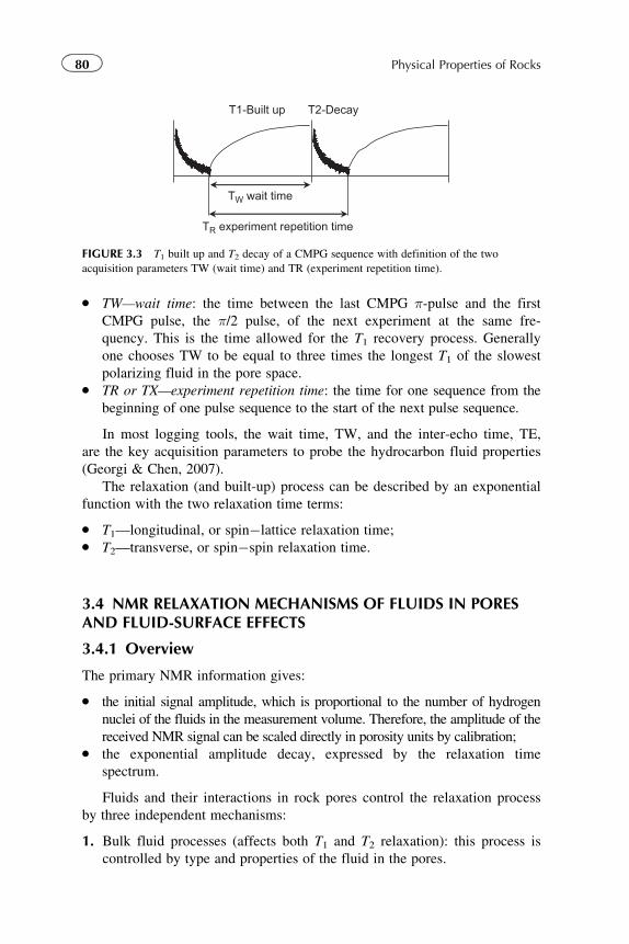
� TW—wait time: the time between the last CMPG π-pulse and the first
CMPG pulse, the π/2 pulse, of the next experiment at the same fre-
quency. This is the time allowed for the T1 recovery process. Generally
one chooses TW to be equal to three times the longest T1 of the slowest
polarizing fluid in the pore space.� TR or TX—experiment repetition time: the time for one sequence from the
beginning of one pulse sequence to the start of the next pulse sequence.
In most logging tools, the wait time, TW, and the inter-echo time, TE,
are the key acquisition parameters to probe the hydrocarbon fluid properties
(Georgi & Chen, 2007).
The relaxation (and built-up) process can be described by an exponential
function with the two relaxation time terms:
� T1—longitudinal, or spin�lattice relaxation time;� T2—transverse, or spin�spin relaxation time.
3.4 NMR RELAXATION MECHANISMS OF FLUIDS IN PORESAND FLUID-SURFACE EFFECTS
3.4.1 Overview
The primary NMR information gives:
� the initial signal amplitude, which is proportional to the number of hydrogen
nuclei of the fluids in the measurement volume. Therefore, the amplitude of the
received NMR signal can be scaled directly in porosity units by calibration;� the exponential amplitude decay, expressed by the relaxation time
spectrum.
Fluids and their interactions in rock pores control the relaxation process
by three independent mechanisms:
1. Bulk fluid processes (affects both T1 and T2 relaxation): this process is
controlled by type and properties of the fluid in the pores.
T1-Built up T2-Decay
TR experiment repetition time
TW wait time
FIGURE 3.3 T1 built up and T2 decay of a CMPG sequence with definition of the two
acquisition parameters TW (wait time) and TR (experiment repetition time).
80 Physical Properties of Rocks
2. Surface relaxation (affects both T1 and T2 relaxation): this process is con-
trolled by pore-size distribution and surface relaxivity.
3. Diffusion in the presence of magnetic field gradients (affects T2 relaxa-
tion only): this molecular diffusion process is controlled by type and
properties of the fluid in the pores.
Because the processes act in parallel, the resulting relaxation time is
given by the sum of relaxation rates. For transverse relaxation, all three
mechanisms contribute
1
T2¼ 1
T2;bulkþ 1
T2;surfaceþ 1
T2;diffusionð3:3Þ
For longitudinal relaxation only bulk and surface relaxation contribute; longi-
tudinal relaxation is unaffected by diffusion in a gradient field (Kenyon, 1997):
1
T1¼ 1
T1;bulkþ 1
T1;surfaceð3:4Þ
where
T1 is the overall longitudinal relaxation time as measured and determined
by inversion recovery or other NMR acquisition
T1,bulk is the bulk longitudinal relaxation time of the pore fluid (no con-
tainer effects, T1,surface-0)
T1,surface is the longitudinal relaxation time of the pore fluid resulting
from surface relaxation
T2 is the overall transverse relaxation time as measured by a CPMG
sequence
T2,bulk is the bulk transverse relaxation time of the pore fluid (no con-
tainer effects, T2,surface-0)
T2,surface is the transverse relaxation time of the pore fluid resulting from
surface relaxation
T2,diffusion is the transverse relaxation time of the pore fluid as induced by
diffusion in the magnetic field gradient.
T1 and T2 are controlled by molecular processes. For water-saturated
rocks, it is frequently the case that T1�T2. It varies if oil or gas are present
(Kenyon, 1997; see Section 3.4.2).
The relative contribution of the three relaxation mechanisms depends on the
type of fluid in the pores (water, oil, or gas), the sizes of the pores, the strength
of the surface relaxation, and the wettability of the rock surface. Some general
rules are formulated by Kleinberg and Vinegar (1996) as follows:
� For the water in a water-wet rock, the surface relaxation will usually
dominate. A bulk relaxation correction must be made when there are iron,
manganese, chromium, nickel, or other paramagnetic ions in the mud
filtrate.
81Chapter | 3 Nuclear Magnetic Resonance—Petrophysical Properties
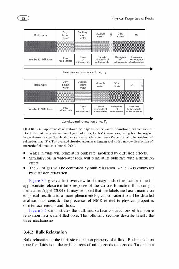
� Water in vugs will relax at its bulk rate, modified by diffusion effects.� Similarly, oil in water-wet rock will relax at its bulk rate with a diffusion
effect.� The T1 of gas will be controlled by bulk relaxation, while T2 is controlled
by diffusion relaxation.
Figure 3.4 gives a first overview to the magnitude of relaxation time for
approximate relaxation time response of the various formation fluid compo-
nents after Appel (2004). It may be noted that the labels are based mainly on
empirical results and a more phenomenological consideration. The detailed
analysis must consider the processes of NMR related to physical properties
of interface regions and fluids.
Figure 3.5 demonstrates the bulk and surface contributions of transverse
relaxation in a water-filled pore. The following sections describe briefly the
three mechanisms.
3.4.2 Bulk Relaxation
Bulk relaxation is the intrinsic relaxation property of a fluid. Bulk relaxation
time for fluids is in the order of tens of milliseconds to seconds. To obtain a
Rock matrixClay-boundwater
Capillary-boundwater
Movablewater
OBMfiltrate
Gas Oil
Transverse relaxation time, T2
Longitudinal relaxation time, T1
Hundredsto thousands
of millisecondsInvisible to NMR tools Few
milliseconds
Tensof
milliseconds
Tens tohundreds ofmilliseconds
Hundredsof
milliseconds
Rock matrixClay-boundwater
Capillary-boundwater
Movablewater
OBMfiltrate
GasOil
Hundredsto thousands
of millisecondsInvisible to NMR tools Few
milliseconds
Tensof
milliseconds
Tens tohundreds ofmilliseconds
Hundredsof
milliseconds
FIGURE 3.4 Approximate relaxation time response of the various formation fluid components.
Due to the fast Brownian motion of gas molecules, the NMR signal originating from hydrogen
in gas features a significantly shorter transverse relaxation time (T2) compared to its longitudinal
relaxation time (T1). The depicted situation assumes a logging tool with a narrow distribution of
magnetic field gradients (Appel, 2004).
82 Physical Properties of Rocks
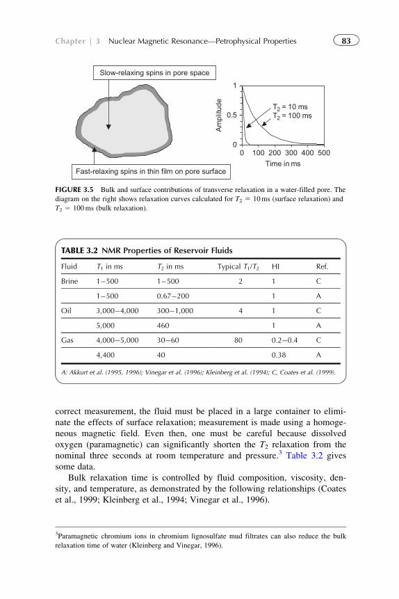
correct measurement, the fluid must be placed in a large container to elimi-
nate the effects of surface relaxation; measurement is made using a homoge-
neous magnetic field. Even then, one must be careful because dissolved
oxygen (paramagnetic) can significantly shorten the T2 relaxation from the
nominal three seconds at room temperature and pressure.3 Table 3.2 gives
some data.
Bulk relaxation time is controlled by fluid composition, viscosity, den-
sity, and temperature, as demonstrated by the following relationships (Coates
et al., 1999; Kleinberg et al., 1994; Vinegar et al., 1996).
3Paramagnetic chromium ions in chromium lignosulfate mud filtrates can also reduce the bulk
relaxation time of water (Kleinberg and Vinegar, 1996).
0
0.5
1
0 100 200 300 400 500
Time in ms
Am
plitu
de T2 = 10 msT2 = 100 ms
Slow-relaxing spins in pore space
Fast-relaxing spins in thin film on pore surface
FIGURE 3.5 Bulk and surface contributions of transverse relaxation in a water-filled pore. The
diagram on the right shows relaxation curves calculated for T2 5 10ms (surface relaxation) and
T2 5 100ms (bulk relaxation).
TABLE 3.2 NMR Properties of Reservoir Fluids
Fluid T1 in ms T2 in ms Typical T1/T2 HI Ref.
Brine 1�500 1�500 2 1 C
1�500 0.67�200 1 A
Oil 3,000�4,000 300�1,000 4 1 C
5,000 460 1 A
Gas 4,000�5,000 30�60 80 0.2�0.4 C
4,400 40 0.38 A
A: Akkurt et al. (1995, 1996); Vinegar et al. (1996); Kleinberg et al. (1994); C, Coates et al. (1999).
83Chapter | 3 Nuclear Magnetic Resonance—Petrophysical Properties
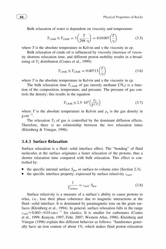
Bulk relaxation of water is dependent on viscosity and temperature:
T1;bulkDT2;bulk ¼ 3T
298Uη
� �¼ 0:01007
T
η
� �ð3:5Þ
where T is the absolute temperature in Kelvin and η the viscosity in cp.
Bulk relaxation of crude oil is influenced by viscosity (increase of viscos-
ity shortens relaxation time, and different proton mobility results in a broad-
ening of T2 distribution (Coates et al., 1999):
T1;bulkDT2;bulk ¼ 0:00713T
η
� �ð3:6Þ
where T is the absolute temperature in Kelvin and η the viscosity in cp.
The bulk relaxation time T1,bulk of gas (mostly methane CN4) is a func-
tion of the composition, temperature, and pressure. The pressure of gas con-
trols the density; this results in the equation
T1;bulkD2:5U104ρgT1:17
� �ð3:7Þ
where T is the absolute temperature in Kelvin and ρg is the gas density in
g cm23.
The relaxation T2 of gas is controlled by the dominant diffusion effects.
Therefore, there is no relationship between the two relaxation times
(Kleinberg & Vinegar, 1996).
3.4.3 Surface Relaxation
Surface relaxation is a fluid�solid interface effect. The “bonding” of fluid
molecules at the surface originates a faster relaxation of the protons, thus a
shorter relaxation time compared with bulk relaxation. This effect is con-
trolled by:
� the specific internal surface Spor or surface-to-volume ratio (Section 2.3);� the specific interface property, expressed by surface relaxivity ςsurf.
1
Tsurface¼ ςsurfUSpor ð3:8Þ
Surface relaxivity is a measure of a surface’s ability to cause protons to
relax, i.e., lose their phase coherence due to magnetic interactions at the
fluid�solid interface. It is dominated by paramagnetic ions on the grain sur-
faces (Kleinberg et al., 1994). In general, surface relaxation falls in the range
ςsurf� 0.003�0.03 cm s21 for clastics. It is smaller for carbonates (Coates
et al., 1999; Kenyon, 1997; Fehr, 2007; Western Atlas, 1996). Kleinberg and
Vinegar (1996) explain this different behavior as follows: “Sandstones gener-
ally have an iron content of about 1%, which makes fluid proton relaxation
84 Physical Properties of Rocks
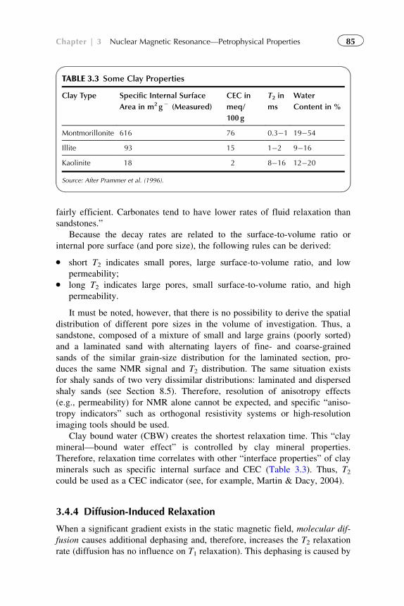
fairly efficient. Carbonates tend to have lower rates of fluid relaxation than
sandstones.”
Because the decay rates are related to the surface-to-volume ratio or
internal pore surface (and pore size), the following rules can be derived:
� short T2 indicates small pores, large surface-to-volume ratio, and low
permeability;� long T2 indicates large pores, small surface-to-volume ratio, and high
permeability.
It must be noted, however, that there is no possibility to derive the spatial
distribution of different pore sizes in the volume of investigation. Thus, a
sandstone, composed of a mixture of small and large grains (poorly sorted)
and a laminated sand with alternating layers of fine- and coarse-grained
sands of the similar grain-size distribution for the laminated section, pro-
duces the same NMR signal and T2 distribution. The same situation exists
for shaly sands of two very dissimilar distributions: laminated and dispersed
shaly sands (see Section 8.5). Therefore, resolution of anisotropy effects
(e.g., permeability) for NMR alone cannot be expected, and specific “aniso-
tropy indicators” such as orthogonal resistivity systems or high-resolution
imaging tools should be used.
Clay bound water (CBW) creates the shortest relaxation time. This “clay
mineral—bound water effect” is controlled by clay mineral properties.
Therefore, relaxation time correlates with other “interface properties” of clay
minerals such as specific internal surface and CEC (Table 3.3). Thus, T2could be used as a CEC indicator (see, for example, Martin & Dacy, 2004).
3.4.4 Diffusion-Induced Relaxation
When a significant gradient exists in the static magnetic field, molecular dif-
fusion causes additional dephasing and, therefore, increases the T2 relaxation
rate (diffusion has no influence on T1 relaxation). This dephasing is caused by
TABLE 3.3 Some Clay Properties
Clay Type Specific Internal Surface
Area in m2 g2 (Measured)
CEC in
meq/
100 g
T2 in
ms
Water
Content in %
Montmorillonite 616 76 0.3�1 19�54
Illite 93 15 1�2 9�16
Kaolinite 18 2 8�16 12�20
Source: After Prammer et al. (1996).
85Chapter | 3 Nuclear Magnetic Resonance—Petrophysical Properties
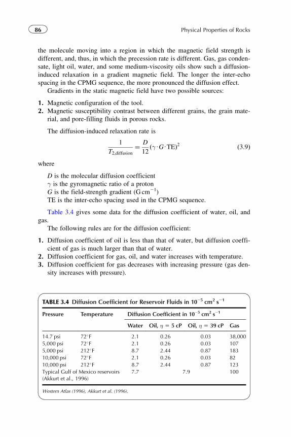
the molecule moving into a region in which the magnetic field strength is
different, and, thus, in which the precession rate is different. Gas, gas conden-
sate, light oil, water, and some medium-viscosity oils show such a diffusion-
induced relaxation in a gradient magnetic field. The longer the inter-echo
spacing in the CPMG sequence, the more pronounced the diffusion effect.
Gradients in the static magnetic field have two possible sources:
1. Magnetic configuration of the tool.
2. Magnetic susceptibility contrast between different grains, the grain mate-
rial, and pore-filling fluids in porous rocks.
The diffusion-induced relaxation rate is
1
T2;diffusion¼ D
12ðγUGUTEÞ2 ð3:9Þ
where
D is the molecular diffusion coefficient
γ is the gyromagnetic ratio of a proton
G is the field-strength gradient (G cm21)
TE is the inter-echo spacing used in the CPMG sequence.
Table 3.4 gives some data for the diffusion coefficient of water, oil, and
gas.
The following rules are for the diffusion coefficient:
1. Diffusion coefficient of oil is less than that of water, but diffusion coeffi-
cient of gas is much larger than that of water.
2. Diffusion coefficient for gas, oil, and water increases with temperature.
3. Diffusion coefficient for gas decreases with increasing pressure (gas den-
sity increases with pressure).
TABLE 3.4 Diffusion Coefficient for Reservoir Fluids in 1025 cm2 s21
Pressure Temperature Diffusion Coefficient in 1025 cm2 s21
Water Oil, η 5 5 cP Oil, η 5 39 cP Gas
14.7 psi 72�F 2.1 0.26 0.03 38,000
5,000 psi 72�F 2.1 0.26 0.03 107
5,000 psi 212�F 8.7 2.44 0.87 183
10,000 psi 72�F 2.1 0.26 0.03 82
10,000 psi 212�F 8.7 2.44 0.87 123
Typical Gulf of Mexico reservoirs(Akkurt et al., 1996)
7.7 7.9 100
Western Atlas (1996), Akkurt et al. (1996).
86 Physical Properties of Rocks
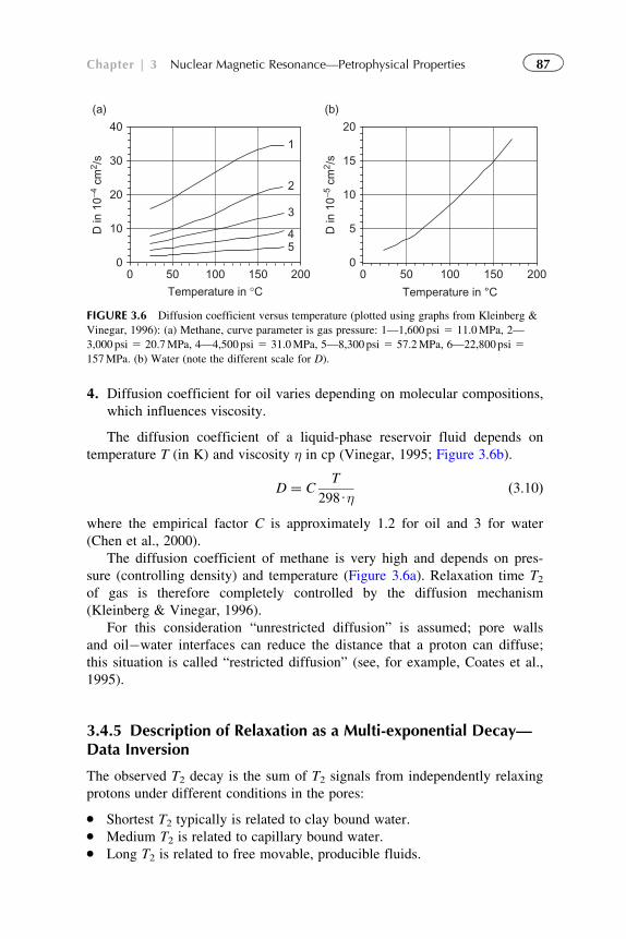
4. Diffusion coefficient for oil varies depending on molecular compositions,
which influences viscosity.
The diffusion coefficient of a liquid-phase reservoir fluid depends on
temperature T (in K) and viscosity η in cp (Vinegar, 1995; Figure 3.6b).
D ¼ CT
298Uηð3:10Þ
where the empirical factor C is approximately 1.2 for oil and 3 for water
(Chen et al., 2000).
The diffusion coefficient of methane is very high and depends on pres-
sure (controlling density) and temperature (Figure 3.6a). Relaxation time T2of gas is therefore completely controlled by the diffusion mechanism
(Kleinberg & Vinegar, 1996).
For this consideration “unrestricted diffusion” is assumed; pore walls
and oil�water interfaces can reduce the distance that a proton can diffuse;
this situation is called “restricted diffusion” (see, for example, Coates et al.,
1995).
3.4.5 Description of Relaxation as a Multi-exponential Decay—Data Inversion
The observed T2 decay is the sum of T2 signals from independently relaxing
protons under different conditions in the pores:
� Shortest T2 typically is related to clay bound water.� Medium T2 is related to capillary bound water.� Long T2 is related to free movable, producible fluids.
0
10
20
30
40
0 50 100 150 200
Temperature in °C
D in
10−4
cm
2 /s
0
5
10
15
20
D in
10−5
cm
2 /s
1
2
3
45
0 50 100 150 200
Temperature in °C
(a) (b)
FIGURE 3.6 Diffusion coefficient versus temperature (plotted using graphs from Kleinberg &
Vinegar, 1996): (a) Methane, curve parameter is gas pressure: 1—1,600psi 5 11.0MPa, 2—
3,000 psi 5 20.7MPa, 4—4,500psi 5 31.0MPa, 5—8,300psi 5 57.2MPa, 6—22,800psi 5
157MPa. (b) Water (note the different scale for D).
87Chapter | 3 Nuclear Magnetic Resonance—Petrophysical Properties
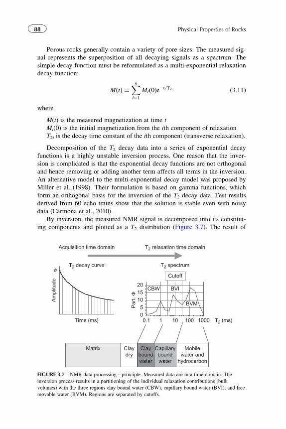
Porous rocks generally contain a variety of pore sizes. The measured sig-
nal represents the superposition of all decaying signals as a spectrum. The
simple decay function must be reformulated as a multi-exponential relaxation
decay function:
MðtÞ ¼Xni¼1
Mið0Þe2t=T2i ð3:11Þ
where
M(t) is the measured magnetization at time t
Mi(0) is the initial magnetization from the ith component of relaxation
T2i is the decay time constant of the ith component (transverse relaxation).
Decomposition of the T2 decay data into a series of exponential decay
functions is a highly unstable inversion process. One reason that the inver-
sion is complicated is that the exponential decay functions are not orthogonal
and hence removing or adding another term affects all terms in the inversion.
An alternative model to the multi-exponential decay model was proposed by
Miller et al. (1998). Their formulation is based on gamma functions, which
form an orthogonal basis for the inversion of the T2 decay data. Test results
derived from 60 echo trains show that the solution is stable even with noisy
data (Carmona et al., 2010).
By inversion, the measured NMR signal is decomposed into its constitut-
ing components and plotted as a T2 distribution (Figure 3.7). The result of
Am
plitu
de
Time (ms)
T2 decay curveφ
Acquisition time domain T2 relaxation time domain
T2 spectrum
05
101520
0.1 1 10 100 1000 T2 (ms)
Cutoff
CBW BVI
BVMPar
t. Φ
Matrix Mobilewater and
hydrocarbon
Capillaryboundwater
Clayboundwater
Claydry
FIGURE 3.7 NMR data processing—principle. Measured data are in a time domain. The
inversion process results in a partitioning of the individual relaxation contributions (bulk
volumes) with the three regions clay bound water (CBW), capillary bound water (BVI), and free
movable water (BVM). Regions are separated by cutoffs.
88 Physical Properties of Rocks
this process is a partitioning of the relaxation curve into the individual relax-
ation contributions from different fluid types and pore-size distributions. The
amplitude of the received NMR signal is scaled directly in porosity units.
The T2 spectrum is the primary result for following petrophysical inter-
pretation directed on (Westphal et al., 2005):
� Porosity: Porosity is proportional to the strength of the NMR echo train at
t 5 0. This value corresponds to the area under the T2 distribution curve.� T2 distribution: The T2 distribution is composed by the individual consti-
tuents and related to three main effects: bulk relaxation, surface relaxa-
tion, and diffusion relaxation. Inversion allows the separate interpretation
of the three effects.� BVI versus BVM: The BVI (bulk volume irreducible fluid) and BVM
(bulk volume of movable fluid) can be estimated by partitioning the T2distribution and “can also be interpreted as pore-size distribution” (Chen &
Georgi, 1997; Kenyon, 1992; Straley et al., 1995).� Permeability: Permeability is not measured directly with NMR but is esti-
mated on the basis of T1 and/or T2, porosity and pore size (BVM, BVI).
The regions between CBW, BVI, and BVM are separated by “cutoffs,”
which depend on the specific internal surface and the surface relaxation.
Recommended values are:
� Cutoff CBW/BVI: 3ms (1�5ms, depends on clay minerals).� Cutoff BVI/BVM: for faster decaying clastics about 33ms, for slower
decaying carbonates about 90ms.
These values are empirical and used to “differentiate different pore sizes
and quantify the amount of water bound by capillary pressures .50 psi in
the rock” (Western Atlas, 1996).
Carbonates in particular exhibit a broad variation of T2 cutoff values as a
result of the diversity of pore geometries. Westphal et al. (2005) investigated
a series of carbonate rock types and recommend:
� If the predominant pore types are infilled pores or isolated pores like in-
traparticle pores resulting in lower permeability, a T2 cutoff value of
T2, 45ms should be used.� If low connectivity of interparticle pores predominates, a T2 cutoff value
of 45�60ms will deliver the best results.� If connected porosity originating from interparticle pore space or postde-
positional diagenetic processes such as dolomitization or dissolution
increasing porosity and connectivity predominated, a T2 cutoff value of
60�110ms will provide the best results.� For carbonates with no visual porosity, a T2 cutoff value of 120�190ms
is suitable.� For carbonates with very large moldic and/or vuggy pores, the T2 cutoff
value should be at .200ms.
89Chapter | 3 Nuclear Magnetic Resonance—Petrophysical Properties
3.5 APPLICATIONS
The analysis of NMR measurements delivers information about porosity,
pore-filling fluids, and petrophysical properties related to the relaxation pro-
cesses. The influence of the many petrophysical properties represents both a
challenge and an opportunity for petrophysics. Some of the influences are
additive and difficult to isolate. Fortunately, however, one can control many
of the NMR data by using acquisition parameters (e.g., TE and TW), which
allow an isolation of some of petrophysical effects (Akkurt et al., 1995;
Chen et al., 2006; Vinegar et al., 1996).
3.5.1 Porosity and Pore Volume Partitioning
With the inversion, the relaxation curve is transformed into a porosity distri-
bution with respect to the individual relaxation times. Association of relaxa-
tion times with different pore sizes and water volumes allows the
determination of:
� total porosity (total area under the curve) φ 5 PHI;� volume of clay bound water (CBW);� volume of irreducible (capillary bound) water (BVI);� volume of free movable fluids (BVM).4 The movable fluid can be any
combination of water, oil, and/or gas.
The observed effects are controlled by the density of proton distribution.
Porosity calibration of most tools is based on the known volume of water.
For other fluids—particularly gas—a normalization using a “hydrogen
index,” HI, is therefore recommended. Hydrogen index is defined as (Appel
2004; Zhang et al., 1998) “the ratio between the amount of hydrogen in the
sample and the amount of hydrogen in pure water at standard conditions
(STP):
HI ¼ amount of hydrogen in sample
amount of hydrogen in pure water at STP¼ moles H cm�3
0:111¼ ρflUNH=M
0:111
ð3:12Þwhere
ρfl is the mass density of the fluid in g cm23
NH is the number of hydrogen atoms in the molecule
M is the molecular weight of the fluid.
The denominator, 0.111, represents the moles of hydrogen in one cubic
centimeter of water at standard conditions. Consequently, the numerator is
4Also referred to as free fluid index or FFI.
90 Physical Properties of Rocks
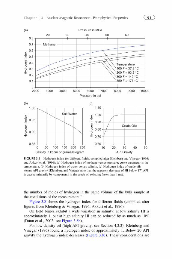
the number of moles of hydrogen in the same volume of the bulk sample at
the conditions of the measurement.”
Figure 3.8 shows the hydrogen index for different fluids (compiled after
figures from Kleinberg & Vinegar, 1996; Akkurt et al., 1996).
Oil field brines exhibit a wide variation in salinity; at low salinity HI is
approximately 1, but at high salinity HI can be reduced by as much as 10%
(Dunn et al., 2002; see Figure 3.8b).
For low-density oil (high API gravity, see Section 4.2.2), Kleinberg and
Vinegar (1996) found a hydrogen index of approximately 1. Below 20 API
gravity the hydrogen index decreases (Figure 3.8c). These considerations are
(a)
0
0.1
0.2
0.3
0.4
0.5
0.6
0.7
0.8
2000 3000 4000 5000 6000 7000 8000 9000 10000
Pressure in psi
Hyd
roge
n In
dex
Pressure in MPa
20 30 40 50 60
Temperature100 F = 37.8 °C200 F = 93.3 °C300 F = 149 °C350 F = 177 °C
Methane
(b)
0.85
0.90
0.95
1.00
0 50 100 150 200 250
Salinity in kppm or grams/kilogram
Hyd
roge
n In
dex Salt Water
c)
0.60
0.70
0.80
0.90
1.00
1.10
10 20 30 40 50API Gravity
Hyd
roge
n In
dex
Crude Oils
FIGURE 3.8 Hydrogen index for different fluids, compiled after Kleinberg and Vinegar (1996)
and Akkurt et al. (1996): (a) Hydrogen index of methane versus pressure; curve parameter is the
temperature. (b) Hydrogen index of water versus salinity. (c) Hydrogen index of crude oils
versus API gravity (Kleinberg and Vinegar note that the apparent decrease of HI below 17� APIis caused primarily by components in the crude oil relaxing faster than 1ms).
91Chapter | 3 Nuclear Magnetic Resonance—Petrophysical Properties
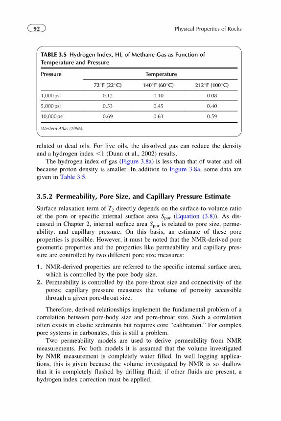
related to dead oils. For live oils, the dissolved gas can reduce the density
and a hydrogen index ,1 (Dunn et al., 2002) results.
The hydrogen index of gas (Figure 3.8a) is less than that of water and oil
because proton density is smaller. In addition to Figure 3.8a, some data are
given in Table 3.5.
3.5.2 Permeability, Pore Size, and Capillary Pressure Estimate
Surface relaxation term of T2 directly depends on the surface-to-volume ratio
of the pore or specific internal surface area Spor (Equation (3.8)). As dis-
cussed in Chapter 2, internal surface area Spor is related to pore size, perme-
ability, and capillary pressure. On this basis, an estimate of these pore
properties is possible. However, it must be noted that the NMR-derived pore
geometric properties and the properties like permeability and capillary pres-
sure are controlled by two different pore size measures:
1. NMR-derived properties are referred to the specific internal surface area,
which is controlled by the pore-body size.
2. Permeability is controlled by the pore-throat size and connectivity of the
pores; capillary pressure measures the volume of porosity accessible
through a given pore-throat size.
Therefore, derived relationships implement the fundamental problem of a
correlation between pore-body size and pore-throat size. Such a correlation
often exists in clastic sediments but requires core “calibration.” For complex
pore systems in carbonates, this is still a problem.
Two permeability models are used to derive permeability from NMR
measurements. For both models it is assumed that the volume investigated
by NMR measurement is completely water filled. In well logging applica-
tions, this is given because the volume investigated by NMR is so shallow
that it is completely flushed by drilling fluid; if other fluids are present, a
hydrogen index correction must be applied.
TABLE 3.5 Hydrogen Index, HI, of Methane Gas as Function of
Temperature and Pressure
Pressure Temperature
72�F (22�C) 140�F (60�C) 212�F (100�C)
1,000psi 0.12 0.10 0.08
5,000psi 0.53 0.45 0.40
10,000psi 0.69 0.63 0.59
Western Atlas (1996).
92 Physical Properties of Rocks
The two models are:
1. Coates model (Coates & Denoo, 1988; Coates et al., 1991):
kCoates ¼φC
� �mBVM
BVI
� �n
ð3:13Þ
where
φ is the porosity in percent
BVM is bulk volume fluid movable
BVI is bulk volume fluid nonmovable (irreducible)
the parameters m and n are empirical and approximately equal to 4 and 2,
respectively
C is also an empirical parameter generally between 6 and 15.
Again, the parameter should be calibrated by comparing core-based per-
meability. Frequently the equation is written as follows:
kCoates ¼φ10
� �4BVM
BVI
� �2ð3:14Þ
2. Schlumberger-Doll Research (SDR) model (Kenyon et al., 1986):
kSDR ¼ bUφ4UT22;gm ð3:15Þ
where T2,gm is the geometric mean of the T2 distribution and b is an empiri-
cal parameter.
Both concepts:
� have a strong dependence on porosity (permeability is proportional poros-
ity with an exponent in the order of 4; compare Section 2.5.3);� rely on empirical parameters that, ideally, are determined by calibration
with core data.
Calibration parameters in both equations are necessary mainly to account
for the relation between pore-throat radius (controlling permeability) and
pore-body radius (controlling NMR measurement) for the specific rock type.
Georgi et al. (1997) and Kasap et al. (1999) describe the calibration of
NMR-derived permeability using Coates equation: When core (conventional
or rotary sidewall) or wireline formation test data are available, the optimum
value for the parameter C can be determined by an error minimization (devi-
ation between core permeability and NMR-derived permeability). Figure 3.9
demonstrates this technique.
In carbonate formations, probably as a consequence of the complicated
pore systems with micro- and macroporosity, it has proven difficult to com-
pute accurate permeabilities.
93Chapter | 3 Nuclear Magnetic Resonance—Petrophysical Properties
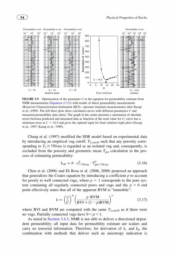
Chang et al. (1997) modified the SDR model based on experimental data
by introducing an empirical vug cutoff, T2,cutoff such that any porosity corre-
sponding to T2$ 750ms is regarded as an isolated vug and, consequently, is
excluded from the porosity and geometric mean Tgm calculation in the pro-
cess of estimating permeability:
ksdr ¼ b Uφ4,750 ms UT
2gm,750 ms ð3:16Þ
Chen et al. (2006) and Di Rosa et al. (2006, 2008) proposed an approach
that generalizes the Coates equation by introducing a coefficient p to account
for poorly to well connected vugs, where p 5 1 corresponds to the pore sys-
tem containing all regularly connected pores and vugs and the p 5 0 end
point effectively states that all of the apparent BVM is “immobile”:
k ¼ φC
� �mpUBVM
BVIþ ð12 pÞBVM
� �n
ð3:17Þ
where BVI and BVM are computed with the same T2,cutoff as if there were
no vugs. Partially connected vugs have 0, p, 1.
As noted in Section 3.4.3, NMR is not able to deliver a directional depen-
dent permeability; all input data for permeability estimate are scalars and
carry no tensorial information. Therefore, for derivation of kv and kh, the
combination with methods that deliver such an anisotropy indication is
Permeability in md
103103 101101 10−1 10−1 100 101 102 10310−110310110−1
Permeability in mdPermeability in md Permeability in md
C = 14.4solutionError minimum
0
100
200
300
400
500
600
700
800
900
0 5 10 15 20 25C
Su
mm
atio
n o
f l
erro
r I
C = 14.5
C = 10 C = 14iterative steps
C = 18
FIGURE 3.9 Optimization of the parameter C in the equation for permeability estimate from
NMR measurements (Equation (3.13)) with results of direct permeability measurements
(Reservoir Characterization Instrument (RCI)—pressure transient measurements) after Kasap
et al. (1999). The left three plots show calculated curves with different parameters C and
measured permeability data (dots). The graph in the center presents a summation of absolute
errors between predicted and measured data as function of the used value for C; curve has a
minimum error at C 5 14.5 and gives the optimal input for final solution (right plot) (Georgi
et al., 1997; Kasap et al., 1999).
94 Physical Properties of Rocks
necessary; Schon et al. (2001) recommended a combination with resistivity
measurements using orthogonal induction systems.
From measured NMR relaxation curves, pore size can be derived, which
primarily is controlled by the pore-body size.
Kenyon (1992) and Marshall et al. (1995) compared the relaxation time
distribution with thin-section images and results of mercury injection mea-
surements and discusses the differences:
� Mercury pressure is controlled by pore-throat or constriction size.� NMR relaxation is controlled by pore-body size (which controls specific
surface).� Optical microscopy cannot resolve micropores.
The petrophysical background for a relationship between capillary pres-
sure and surface relaxation time is given by three equations.
The fundamental equation for capillary pressure (Equation (2.74)) with
the pore throat rt as controlling pore geometrical parameter:
pc ¼2UσUcos Θ
rtð3:18Þ
The equation for surface relaxation (Equation (3.8)) with specific internal
surface as controlling pore geometric parameter:
1
T2¼ ζsurfUSpor ¼ ζsurf
S
Vð3:19Þ
The relationship between pore-throat radius and specific internal surface
(implementing the ratio of pore-throat radius and pore-body radius). The
basic equations for capillary channel models are valid only for a cylindrical
capillary with constant radius. If the radius is changing, the constrictivity of
the pore system must be considered.
Thus, the relationship is controlled by interface tension terms, pore geom-
etry, and surface relaxivity. Summarized, the equation can be written as
pc ¼ κ1
T2ð3:20Þ
where the parameter κ covers these influences. Volotkin et al. (2001) used
Equation (3.20) for an analysis of sandstone measurements and derived a mean
value of κ 5 3psi s, where capillary pressure was measured in a mercury-air
system (injection).
3.5.3 Fluid (Hydrocarbon) Typing
NMR-based fluid typing techniques are based on differences of T1 and T2relaxation time, diffusion coefficient (D0), and hydrogen index (HI) for dif-
ferent fluids. The relevant NMR properties of bulk fluids are compiled in
95Chapter | 3 Nuclear Magnetic Resonance—Petrophysical Properties
Tables 3.2 and 3.4. Techniques are described, for example, by Vinegar et al.
(1996), Chen et al. (2000), and by Freedman and Heaton (2004).
Two fundamental methods of hydrocarbon typing have been developed:
1. The dual-wait-time (dual-TW)
2. The dual-interecho-time (dual-TE) methods.
Experiment wait time, TW, and inter-echo time, TE, are two acquisition
parameters that can usually be controlled during data acquisition. The dual-
TW method is based on the T1 contrast between water and light hydrocar-
bons, while the dual-TE method exploits the difference in diffusion contrast
of water, oil, and gas.
The two fundamental techniques for hydrocarbon typing can be character-
ized as follows (Chen et al., 2000):
� Dual-TW technique (Akkurt et al., 1995, 1996, 1998): Dual-wait-time,
dual-TW, uses the T1 contrast between the nonwetting light hydrocarbons
and the wetting phase (water). The long wait time is chosen such that
both oil and water signals are fully polarized before the next experiment.
The short wait time is chosen such that the wetting phase (water) signal
is fully polarized but the oil signal is only partially polarized. The echo
difference signal obtained by subtracting partially polarized echo signal
from the fully polarized echo signal represents the oil signal only.� Dual-TE technique (Akkurt et al., 1998; Coates et al., 1995; Looyestijn,
1996): Dual-interecho-time, dual-TE, responds to viscosity contrast, and
therefore diffusivity, between reservoir fluids. It separates especially
based on the diffusivity difference between water and medium-viscosity
oil or between liquid and gas.
Chen et al. (2000) combined dual-TW with multiple TE approaches to
maximize the advantages of both T1 and T2 contrasts and determine the vis-
cosity of the hydrocarbon fluids.
96 Physical Properties of Rocks
Chapter 4
Density
4.1 DEFINITION AND UNITS
Density ρ is defined as the quotient of mass m and volume V of a material:
ρ ¼ m
Vð4:1Þ
The SI unit for density is kgm23. Conversions give the relationships to
other used units:
1 g cm23 ¼ 103 kg m23
1 kg m23 ¼ 62:43 1023 lb ft23 ¼ 8:345 1023 lb gal2 1 ðUSÞ
1 kg m23 ¼ 0:0361 1023 lb in23
Due to the heterogeneity of rocks, it is necessary to distinguish between
different densities that are related to different rock components:
� ρ—bulk density: the mean density of the considered rock volume (includ-
ing pores, etc.); for example, density of sandstone.� ρi—density of any individual mineral rock component i; for example,
density of quartz.� ρma—mean density of the solid matrix material (mineral or mixture of
minerals), also called grain density; for example, density of a carbonate
matrix (without pore fluid).� ρfl—mean density of the pore (or fracture) fluid; for example, density of
water ρw.
Bulk density of a composite material (rock) consisting of n components is
ρ ¼Xn
i¼1
ρiUVi ð4:2Þ
where ρi is the density and Vi is the volume fraction of component i.
97Physical Properties of Rocks.
© 2011 Elsevier B.V. All rights reserved.
For a porous rock, the volume fraction for the pore space is given by the
total porosity φ and Equation (4.2) is
ρ ¼ ð12φÞUρma þ φUρfl ð4:3ÞIf the pore fluid is composed by different fluids (water, oil, gas), satura-
tion must be implemented:
ρ ¼ ð12φÞUρma þ φUðSwaterUρwater þ SoilUρoil þ SgasUρgasÞ ð4:4Þ
4.2 DENSITY OF ROCK CONSTITUENTS
4.2.1 Density of Minerals
The density of minerals is controlled by their elemental composition and
internal bonding and structure (Table 4.1). Compilations of mineral densities
are published by Clark (1966), Dortman (1976), Olhoeft and Johnson (1989),
Rosler and Lange (1972), Serra (1984), and Wohlenberg (1982).
The density range is for:
� the most abundant rock-forming minerals between 2.2 � 103 and
3.5 � 103 kgm23
� ore minerals between 4.0 � 103 and 8.0 � 103 kgm23.
4.2.2 Density of Pore Fluids
The density of liquids and gases is controlled by:
� chemical composition (including soluble components);� temperature and pressure (density increases with increasing pressure and
decreasing temperature).
For liquid substances, Schlumberger (2000) gives the following mean
density values:
Fresh water 1.000 � 103 kgm23
Salt water (200,000 ppm) 1.146 � 103 kgm23
Oil 0.85 � 103 kgm23
Some detailed data are given in Table 4.2.
For water at 23.9�C (75�F) and atmospheric pressure, the relationship
between NaCl concentration C (weight fraction) and density can be approxi-
mated (Schlumberger, 1989a) as:
ρwater ¼ 1þ 0:73C ð4:5ÞA detailed description of the relationships of fluid density, temperature,
pressure, and NaCl concentration (weight fraction) was published by Batzle
and Wang (1992). Figure 4.1a shows a graphic presentation of selected
curves (the original paper also gives the regression equations).
98 Physical Properties of Rocks
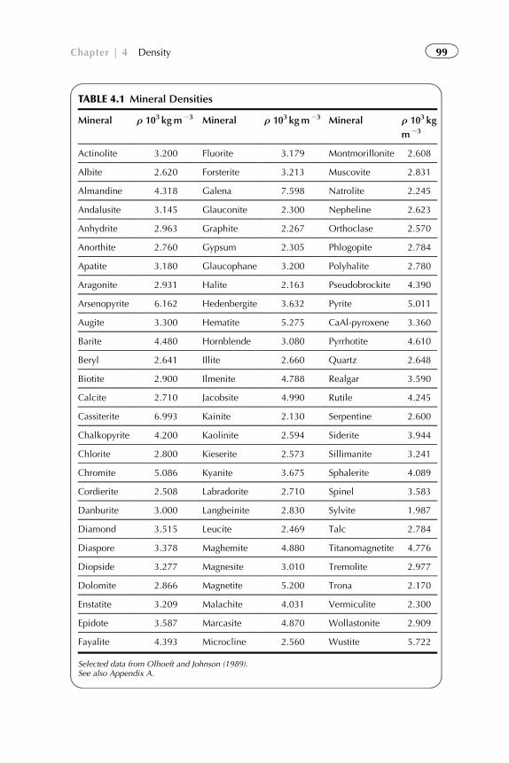
TABLE 4.1 Mineral Densities
Mineral ρ 103 kgm23 Mineral ρ 103 kgm23 Mineral ρ 103 kg
m23
Actinolite 3.200 Fluorite 3.179 Montmorillonite 2.608
Albite 2.620 Forsterite 3.213 Muscovite 2.831
Almandine 4.318 Galena 7.598 Natrolite 2.245
Andalusite 3.145 Glauconite 2.300 Nepheline 2.623
Anhydrite 2.963 Graphite 2.267 Orthoclase 2.570
Anorthite 2.760 Gypsum 2.305 Phlogopite 2.784
Apatite 3.180 Glaucophane 3.200 Polyhalite 2.780
Aragonite 2.931 Halite 2.163 Pseudobrockite 4.390
Arsenopyrite 6.162 Hedenbergite 3.632 Pyrite 5.011
Augite 3.300 Hematite 5.275 CaAl-pyroxene 3.360
Barite 4.480 Hornblende 3.080 Pyrrhotite 4.610
Beryl 2.641 Illite 2.660 Quartz 2.648
Biotite 2.900 Ilmenite 4.788 Realgar 3.590
Calcite 2.710 Jacobsite 4.990 Rutile 4.245
Cassiterite 6.993 Kainite 2.130 Serpentine 2.600
Chalkopyrite 4.200 Kaolinite 2.594 Siderite 3.944
Chlorite 2.800 Kieserite 2.573 Sillimanite 3.241
Chromite 5.086 Kyanite 3.675 Sphalerite 4.089
Cordierite 2.508 Labradorite 2.710 Spinel 3.583
Danburite 3.000 Langbeinite 2.830 Sylvite 1.987
Diamond 3.515 Leucite 2.469 Talc 2.784
Diaspore 3.378 Maghemite 4.880 Titanomagnetite 4.776
Diopside 3.277 Magnesite 3.010 Tremolite 2.977
Dolomite 2.866 Magnetite 5.200 Trona 2.170
Enstatite 3.209 Malachite 4.031 Vermiculite 2.300
Epidote 3.587 Marcasite 4.870 Wollastonite 2.909
Fayalite 4.393 Microcline 2.560 Wustite 5.722
Selected data from Olhoeft and Johnson (1989).See also Appendix A.
99Chapter | 4 Density
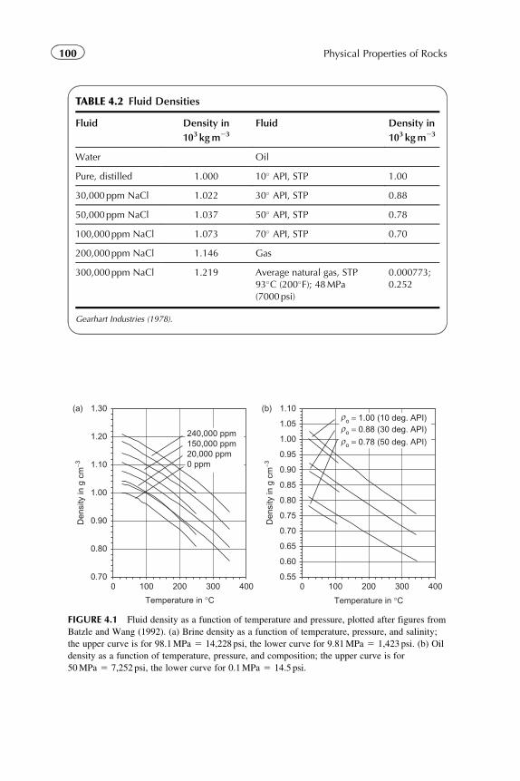
TABLE 4.2 Fluid Densities
Fluid Density in
103 kgm23
Fluid Density in
103 kgm23
Water Oil
Pure, distilled 1.000 10� API, STP 1.00
30,000ppm NaCl 1.022 30� API, STP 0.88
50,000ppm NaCl 1.037 50� API, STP 0.78
100,000ppm NaCl 1.073 70� API, STP 0.70
200,000ppm NaCl 1.146 Gas
300,000ppm NaCl 1.219 Average natural gas, STP93�C (200�F); 48MPa(7000psi)
0.000773;0.252
Gearhart Industries (1978).
(a)
0.70
0.80
0.90
1.00
1.10
1.20
1.30
0 100 200 300 400
Temperature in °C
Den
sity
in g
cm
−3
Den
sity
in g
cm
−3
240,000 ppm150,000 ppm20,000 ppm0 ppm
(b)
0.55
0.60
0.65
0.70
0.75
0.80
0.85
0.90
0.95
1.00
1.05
1.10
0 100 200 300 400
Temperature in °C
ρρρ
o = 1.00 (10 deg. API)
o = 0.88 (30 deg. API)
o = 0.78 (50 deg. API)
FIGURE 4.1 Fluid density as a function of temperature and pressure, plotted after figures from
Batzle and Wang (1992). (a) Brine density as a function of temperature, pressure, and salinity;
the upper curve is for 98.1MPa 5 14,228 psi, the lower curve for 9.81MPa 5 1,423 psi. (b) Oil
density as a function of temperature, pressure, and composition; the upper curve is for
50MPa 5 7,252 psi, the lower curve for 0.1MPa 5 14.5 psi.
100 Physical Properties of Rocks
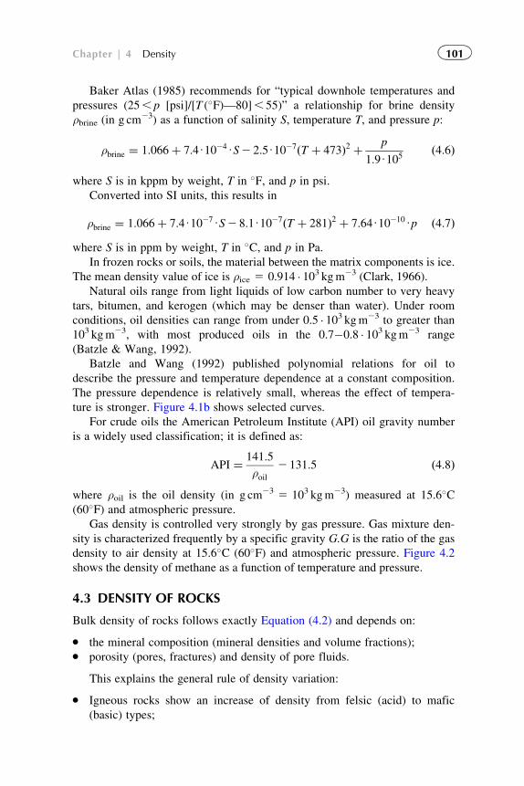
Baker Atlas (1985) recommends for “typical downhole temperatures and
pressures (25, p [psi]/[T (�F)—80], 55)” a relationship for brine density
ρbrine (in g cm23) as a function of salinity S, temperature T, and pressure p:
ρbrine ¼ 1:066þ 7:4U1024US2 2:5U1027ðT þ 473Þ2 þ p
1:9U105ð4:6Þ
where S is in kppm by weight, T in �F, and p in psi.
Converted into SI units, this results in
ρbrine ¼ 1:066þ 7:4U1027US2 8:1U1027ðT þ 281Þ2 þ 7:64U10210Up ð4:7Þwhere S is in ppm by weight, T in �C, and p in Pa.
In frozen rocks or soils, the material between the matrix components is ice.
The mean density value of ice is ρice 5 0.914 � 103 kgm23 (Clark, 1966).
Natural oils range from light liquids of low carbon number to very heavy
tars, bitumen, and kerogen (which may be denser than water). Under room
conditions, oil densities can range from under 0.5 � 103 kgm23 to greater than
103 kgm23, with most produced oils in the 0.7�0.8 � 103 kgm23 range
(Batzle & Wang, 1992).
Batzle and Wang (1992) published polynomial relations for oil to
describe the pressure and temperature dependence at a constant composition.
The pressure dependence is relatively small, whereas the effect of tempera-
ture is stronger. Figure 4.1b shows selected curves.
For crude oils the American Petroleum Institute (API) oil gravity number
is a widely used classification; it is defined as:
API ¼ 141:5
ρoil2 131:5 ð4:8Þ
where ρoil is the oil density (in g cm23 5 103 kgm23) measured at 15.6�C(60�F) and atmospheric pressure.
Gas density is controlled very strongly by gas pressure. Gas mixture den-
sity is characterized frequently by a specific gravity G.G is the ratio of the gas
density to air density at 15.6�C (60�F) and atmospheric pressure. Figure 4.2
shows the density of methane as a function of temperature and pressure.
4.3 DENSITY OF ROCKS
Bulk density of rocks follows exactly Equation (4.2) and depends on:
� the mineral composition (mineral densities and volume fractions);� porosity (pores, fractures) and density of pore fluids.
This explains the general rule of density variation:
� Igneous rocks show an increase of density from felsic (acid) to mafic
(basic) types;
101Chapter | 4 Density
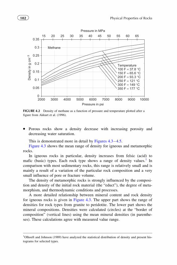
� Porous rocks show a density decrease with increasing porosity and
decreasing water saturation.
This is demonstrated more in detail by Figures 4.3�4.5.
Figure 4.3 shows the mean range of density for igneous and metamorphic
rocks.
In igneous rocks in particular, density increases from felsic (acid) to
mafic (basic) types. Each rock type shows a range of density values.1 In
comparison with most sedimentary rocks, this range is relatively small and is
mainly a result of a variation of the particular rock composition and a very
small influence of pore or fracture volume.
The density of metamorphic rocks is strongly influenced by the composi-
tion and density of the initial rock material (the “educt”), the degree of meta-
morphism, and thermodynamic conditions and processes.
A more detailed relationship between mineral content and rock density
for igneous rocks is given in Figure 4.3. The upper part shows the range of
densities for rock types from granite to peridotite. The lower part shows the
mineral compositions. Densities were calculated (circles) at the “border of
composition” (vertical lines) using the mean mineral densities (in parenthe-
ses). These calculations agree with measured value range.
1Olhoeft and Johnson (1989) have analyzed the statistical distribution of density and present his-
tograms for selected types.
0
0.05
0.1
0.15
0.2
0.25
0.3
0.35
2000 3000 4000 5000 6000 7000 8000 9000 10000
Pressure in psi
Pressure in MPa
15 20 25 30 35 40 45 50 55 60 65
Temperature100 F = 37.8 °C150 F = 65.6 °C200 F = 93.3 °C250 F = 121 °C300 F = 149 °C350 F = 177 °C
Methane
Den
sity
in g
cm
−3
FIGURE 4.2 Density of methane as a function of pressure and temperature plotted after a
figure from Akkurt et al. (1996).
102 Physical Properties of Rocks
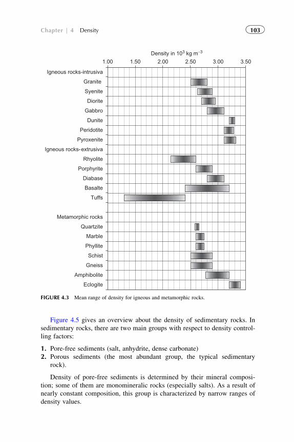
Figure 4.5 gives an overview about the density of sedimentary rocks. In
sedimentary rocks, there are two main groups with respect to density control-
ling factors:
1. Pore-free sediments (salt, anhydrite, dense carbonate)
2. Porous sediments (the most abundant group, the typical sedimentary
rock).
Density of pore-free sediments is determined by their mineral composi-
tion; some of them are monomineralic rocks (especially salts). As a result of
nearly constant composition, this group is characterized by narrow ranges of
density values.
1.00 1.50 2.00 2.50 3.00 3.50
Igneous rocks-intrusiva
Granite
Syenite
Diorite
Gabbro
Dunite
Peridotite
Pyroxenite
Igneous rocks-extrusiva
Rhyolite
Porphyrite
Diabase
Basalte
Tuffs
Metamorphic rocks
Quartzite
Marble
Phyllite
Schist
Gneiss
Amphibolite
Eclogite
Density in 103 kg m−3
FIGURE 4.3 Mean range of density for igneous and metamorphic rocks.
103Chapter | 4 Density
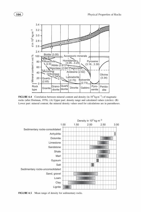
3.4
3.2
3.0
2.8
d in
103
kg·m
−3M
iner
al c
onte
nt in
vol
.%
2.6
2.4
100
80
60
40
20
0Rocktype Granite Dirorite GabbroGrano-
dioriteQuartz-diorite
Quartz-(2.65)
Microcline
Albite (2.61)Oligoclase (2.64) Plagioclase
Hornblende (3.05...3.25)
Muscovite (2.8)
Pyroxene(3.18...3.30)
Accessoric mineralsBiotite (3.05)
Andesine (2.62)
Labradorite(2.70) Bytownite
(2.73)
Olivine(3.34)
Orthoclase(2.54... 2.57)
Pyro-xenite
Perido-dite
FIGURE 4.4 Correlation between mineral content and density (in 103 kgm23) of magmatic
rocks (after Dortman, 1976). (A) Upper part: density range and calculated values (circles). (B)
Lower part: mineral content; the mineral density values used for calculations are in parentheses.
Density in 103 kg m−3
1.00 1.50 2.00 2.50 3.00
Sedimentary rocks-consolidated
Anhydrite
Dolomite
Limestone
Sandstone
Shale
Marl
Gypsum
Salt
Sedimentary rocks-unconsolidated
Sand, gravel
Loam
Clay
Lignite
FIGURE 4.5 Mean range of density for sedimentary rocks.
104 Physical Properties of Rocks
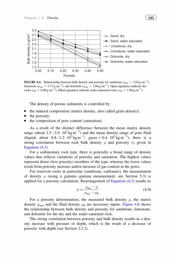
The density of porous sediments is controlled by:
� the mineral composition (matrix density, also called grain density);� the porosity;� the composition of pore content (saturation).
As a result of the distinct difference between the mean matrix density
range (about 2.5�2.9 � 103 kgm23) and the mean density range of pore fluid
(liquids about 0.8�1.2 � 103 kgm23; gases, 0.4 � 103 kgm23), there is a
strong correlation between rock bulk density ρ and porosity φ, given in
Equation (4.3).
For a sedimentary rock type, there is generally a broad range of density
values that reflects variations of porosity and saturation. The highest values
represent dense (low porosity) members of the type, whereas the lower values
result from porosity increase and/or increase of gas content in the pores.
For reservoir rocks in particular (sandstone, carbonate), the measurement
of density ρ (using a gamma�gamma measurement, see Section 5.3) is
applied for a porosity calculation. Rearrangement of Equation (4.3) results in
φ ¼ ρma 2 ρρma 2 ρfl
ð4:9Þ
For a porosity determination, the measured bulk density ρ, the matrix
density ρma, and the fluid density ρfl are necessary inputs. Figure 4.6 shows
the relationship between bulk density and porosity for sandstone, limestone,
and dolomite for the dry and the water-saturated rock.
The strong correlation between porosity and bulk density results in a den-
sity increase with pressure or depth, which is the result of a decrease of
porosity with depth (see Section 2.2.2).
1.31.51.71.92.12.32.52.72.9
0.00 0.10 0.20 0.30 0.40 0.50
Porosity
Bul
k de
nsity
in g
/cm
3 Sand, dry
Sand, water saturated
Limestone, dry
Limestone, water saturated
Dolomite, dry
Dolomite, water saturated
FIGURE 4.6 Relationship between bulk density and porosity for sandstone (ρma 5 2.65 g cm23),
limestone (ρma 5 2.71g cm23), and dolomite (ρma 5 2.86 g cm23). Open signatures indicate dry
rocks (ρfl 5 0.00 g cm23); filled signatures indicate water-saturated rocks (ρfl 5 1.00g cm23).
105Chapter | 4 Density

Chapter 5
Nuclear/Radioactive Properties
5.1 FUNDAMENTALS
Nuclear properties are related to the atomic structure of matter: an atom con-
sists of a nucleus and a number of orbiting electrons e2. Electrons occupy
shells (K, L, M, etc.). The nucleus is a combination of electrically neutral
neutrons n and positively charged protons p1. Table 5.1 gives some funda-
mental properties of these components.
The number of protons in a nucleus is the atomic number Z. An electri-
cally neutral atom with the atomic number Z also has Z orbiting electrons.
The sum of protons and neutrons in the nucleus is the mass number A.
The nomenclature for elements is Zchemical symbolA. For example,
helium is 2He4.
Each nuclide has a unique set of discrete energy levels or states. A
stable nucleus exists at the lowest energy level (ground state). In a higher
energy level it is in an excited state and unstable. It releases the excess
energy by radiation in order to reach the stable state. The time required for
this decay process can range from a fraction of a second to millions of years,
depending on the element. The decay process follows the equation:
NðtÞ ¼ N0Uexpð2CdUtÞ ¼ N0Uexp 20:693Ut
t1=2
� �ð5:1Þ
where
N0 is the number of parent nuclei at the start of counting
N(t) is the number of parent nuclei at a time t after the start of counting
Cd is the decay constant of the considered element
t1/2 is the “half-life time” of the considered element.
107Physical Properties of Rocks.
© 2011 Elsevier B.V. All rights reserved.
Nuclear processes are statistically determined and can be described by
Poisson’s distribution. For Poisson’s distribution, the standard deviation σ is
related to the number of measured counts n:
σ ¼ ffiffiffin
p ð5:2ÞFor practical measurements, this has the consequence that the uncertainty
of a measurement is controlled by the absolute number of counts; thus it
depends on the intensity of radiation and the counting time. Consequently,
there are limits or restrictions on the logging speed of nuclear tools.
5.2 NATURAL RADIOACTIVITY
There are three types of natural radioactivity:
1. Alpha radiation (positively charged particle radiation)
2. Beta radiation (negatively charged particle radiation)
3. Gamma radiation (electromagnetic radiation, photons).
The depth of penetration of the radiation is extremely small for both
alpha and beta particles. For practical applications (well logging), gamma
radiation is used.
The energy E of the gamma radiation is given in electron volts (eV) or as
frequency f in Hz:
E ¼ hUf ¼ 4:1357U10215Uf ð5:3Þwhere h is Planck’s constant: h 5 4.1357 � 10215 eV s 5 6.6261 � 10234 J s.
5.2.1 Origin of Natural Gamma Radiation in Rocks
Elements frequently have a variety of isotopic forms. If these isotopes are
unstable, then they decay to a more stable form and emit radiation. Only
three radioactive decay processes, producing measurable quantities of
gamma rays, occur in natural rocks:
1. Uranium�radium series (half-life time of 4.4 � 109 years)
TABLE 5.1 Atomic Properties
Mass Electrical Charge
Proton p1 1.67 � 10227 kg 11.602 � 10219 CNeutron n 1.67 � 10227 kg Neutral, 60
Electron e2 9.11 � 10231 kg 21.602 � 10219 C
108 Physical Properties of Rocks
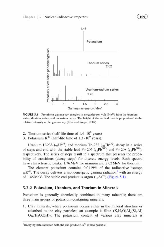
2. Thorium series (half-life time of 1.4 � 109 years)3. Potassium K40 (half-life time of 1.3 � 109 years).
Uranium U-238 (92U238) and thorium Th-232 (90Th
232) decay in a series
of steps and end with the stable lead Pb-206 (82Pb206) and Pb-208 (82Pb
208),
respectively. The series of steps result in a spectrum that presents the proba-
bility of transitions (decay steps) for discrete energy levels. Both spectra
have characteristic peaks: 1.76MeV for uranium and 2.62MeV for thorium.
The element potassium contains 0.0119% of the radioactive isotope
19K40. The decay delivers a monoenergetic gamma radiation1 with an energy
of 1.46MeV. The stable end product is argon (18Ar40) (Figure 5.1).
5.2.2 Potassium, Uranium, and Thorium in Minerals
Potassium is generally chemically combined in many minerals; there are
three main groups of potassium-containing minerals:
1. Clay minerals, where potassium occurs either in the mineral structure or
adsorbed to the clay particles; an example is illite (K,H3O)Al2(Si3Al)
O10(H2O,OH)2. The potassium content of various clay minerals is
1Decay by beta radiation with the end product Ca40 is also possible.
1.46
Potassium
Thorium series
Uranium-radium series
32.521.5Pro
babi
lity
of e
mis
sion
per
dis
inte
grat
ion
1.76
2.62
Gamma ray energy, MeV1.50
FIGURE 5.1 Prominent gamma-ray energies in megaelectron volt (MeV) from the uranium
series, thorium series, and potassium decay. The height of the vertical lines is proportional to the
relative intensity of the gamma ray (Ellis and Singer, 2007).
109Chapter | 5 Nuclear/Radioactive Properties
different: illite has a high content (3.5�8.3%), whereas kaolinite has a
low content.
2. Rock-forming minerals, where potassium is chemically combined in the
mineral structure; typical examples are the potassium feldspars (ortho-
clase KAlSi3O8, microcline KAlSi3O8), mica (biotite, muscovite); see
Table 5.2.
3. Evaporates, where potassium occurs chemically as salt (sylvite KCl,
carnallite KCl MgCl2(H2O)6).
“Potassium is considered an element that owes its origin to erosion; it is
often reworked and transported for long distances” (Baker Atlas, 1985).
Thorium is generally associated with acid (and intermediate) rocks. It is
very stable and will not dissolve in a solution. As a result of alteration, tho-
rium is deposited only with detrital sediments, never with purely chemical
sediments (carbonates, aragonite). Therefore, in carbonate reservoirs, thorium
becomes a very important clay indicator. It is found in mudstones where it is
adsorbed by clay minerals, and with heavy minerals that are often abundant
in the silty fraction. Thorium is generally considered a marine element
(Baker Atlas, 1985).
Uranium is also generally associated with acid (and intermediate)
rocks—their average concentration is about 4.65 ppm. As a result of weather-
ing and alteration it forms—unlike potassium and thorium—soluble salts,
which are transported in seawater and river water. The salts are unstable and
go into sediments. There are three ways that uranium passes into sediments
(Serra, 1984, 2004):
1. Chemical precipitation in an acid-reducing (pH 2.5�4.0) environment
2. Adsorption by organic matter or living plants and animals
3. Chemical reaction in phosphorites.
Acid-reducing conditions are found particularly in stagnant, anoxic
waters with a relatively low rate of sedimentation, which typically produce
black shales (Rider, 1986).
Controlled by transport and sedimentation processes and the chemical
environment, uranium occurs in both detrital and chemical sediments (shale,
sandstone, conglomerate, carbonate) and is also common in tuff and phos-
phates. Carbonates rich in organic matter that form under reducing condi-
tions are often very high in uranium. These “radioactive carbonates” are
often productive reservoirs. Uranium is also adsorbed by clay minerals;
excessively high uranium content in shales indicates source rock (Baker
Atlas, 1985).
Rider (1996) stated that “uranium behaves as an independent constituent:
it is not chemically combined in the principal molecules of rocks like potas-
sium, but it is loosely associated with secondary components. For this reason
it has a very heterogeneous distribution in sediments.”
110 Physical Properties of Rocks
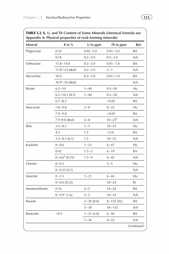
TABLE 5.2 K, U, and Th Content of Some Minerals (chemical formula see
Appendix A: Physical properties of rock-forming minerals)
Mineral K in % U in ppm Th in ppm Ref.
Plagioclase 0.54 0.02�5.0 0.01�3.0 BA
0.54 0.2�5.0 0.5�3.0 Sch
Orthoclase 11.8�14.0 0.2�3.0 0.01�7.0 BA
11.8a (14 ideal) 0.2�3.0 3�7 Sch
Microcline 10.9 0.2�3.0 0.01�7.0 BA
10.9a (16 ideal) Sch
Biotite 6.2�10 1�40 0.5�50 Hu
6.2�10.1 [8.5] 1�40 0.5�50 Sch
6.7�8.3 ,0.01 BA
Muscovite 7.8�9.8 2�8 0�25 Hu
7.9�9.8 ,0.01 BA
7.9 (9.8 ideal) 2�8 10�25b Sch
Illite 3.5�8.3 1�5 10�25 Hu
4.5 1.5 ,2.0 BA
3.5�8.3 [6.1] 1.5 10�25 Sch
Kaolinite 0�0.6 1�12 6�47 Hu
0.42 1.5�3 6�19 BA
0�0.6d [0.35] 1.5�9 6�42 Sch
Chlorite 0�0.3 3�5 Hu
0�0.35 [0.1] Sch
Smectite 0�1.5 1�21 6�44 Hu
0�0.6 [0.22] 10�24 Ri
Montmorillonite 0.16 2�5 14�24 BA
0�4.9c [1.6] 2�5 10�24 Sch
Bauxite 3�30 [8.0] 8�132 [42] BA
3�30 10�132 Sch
Bentonite ,0.5 1�21 [5.0] 6�50 BA
1�36 4�55 Sch
(Continued )
111Chapter | 5 Nuclear/Radioactive Properties
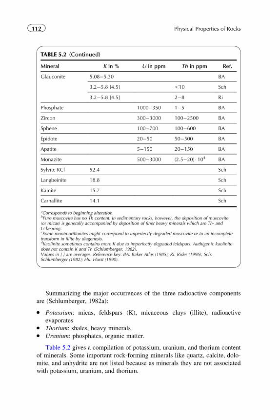
Summarizing the major occurrences of the three radioactive components
are (Schlumberger, 1982a):
� Potassium: micas, feldspars (K), micaceous clays (illite), radioactive
evaporates� Thorium: shales, heavy minerals� Uranium: phosphates, organic matter.
Table 5.2 gives a compilation of potassium, uranium, and thorium content
of minerals. Some important rock-forming minerals like quartz, calcite, dolo-
mite, and anhydrite are not listed because as minerals they are not associated
with potassium, uranium, and thorium.
TABLE 5.2 (Continued)
Mineral K in % U in ppm Th in ppm Ref.
Glauconite 5.08�5.30 BA
3.2�5.8 [4.5] ,10 Sch
3.2�5.8 [4.5] 2�8 Ri
Phosphate 1000�350 1�5 BA
Zircon 300�3000 100�2500 BA
Sphene 100�700 100�600 BA
Epidote 20�50 50�500 BA
Apatite 5�150 20�150 BA
Monazite 500�3000 (2.5�20) � 104 BA
Sylvite KCl 52.4 Sch
Langbeinite 18.8 Sch
Kainite 15.7 Sch
Carnallite 14.1 Sch
aCorresponds to beginning alteration.bPure muscovite has no Th content. In sedimentary rocks, however, the deposition of muscovite(or micas) is generally accompanied by deposition of finer heavy minerals which are Th- andU-bearing.cSome montmorillonites might correspond to imperfectly degraded muscovite or to an incompletetransform in illite by diagenesis.dKaolinite sometimes contains more K due to imperfectly degraded feldspars. Authigenic kaolinitedoes not contain K and Th (Schlumberger, 1982).Values in [ ] are averages. Reference key: BA: Baker Atlas (1985); Ri: Rider (1996); Sch:Schlumberger (1982); Hu: Hurst (1990).
112 Physical Properties of Rocks
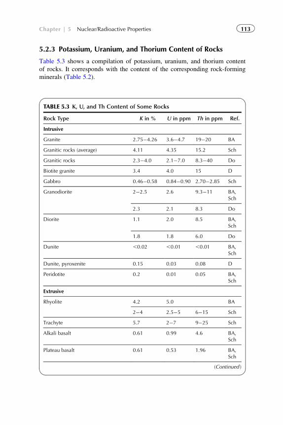
5.2.3 Potassium, Uranium, and Thorium Content of Rocks
Table 5.3 shows a compilation of potassium, uranium, and thorium content
of rocks. It corresponds with the content of the corresponding rock-forming
minerals (Table 5.2).
TABLE 5.3 K, U, and Th Content of Some Rocks
Rock Type K in % U in ppm Th in ppm Ref.
Intrusive
Granite 2.75�4.26 3.6�4.7 19�20 BA
Granitic rocks (average) 4.11 4.35 15.2 Sch
Granitic rocks 2.3�4.0 2.1�7.0 8.3�40 Do
Biotite granite 3.4 4.0 15 D
Gabbro 0.46�0.58 0.84�0.90 2.70�2.85 Sch
Granodiorite 2�2.5 2.6 9.3�11 BA,Sch
2.3 2.1 8.3 Do
Diorite 1.1 2.0 8.5 BA,Sch
1.8 1.8 6.0 Do
Dunite ,0.02 ,0.01 ,0.01 BA,Sch
Dunite, pyroxenite 0.15 0.03 0.08 D
Peridotite 0.2 0.01 0.05 BA,Sch
Extrusive
Rhyolite 4.2 5.0 BA
2�4 2.5�5 6�15 Sch
Trachyte 5.7 2�7 9�25 Sch
Alkali basalt 0.61 0.99 4.6 BA,Sch
Plateau basalt 0.61 0.53 1.96 BA,Sch
(Continued )
113Chapter | 5 Nuclear/Radioactive Properties
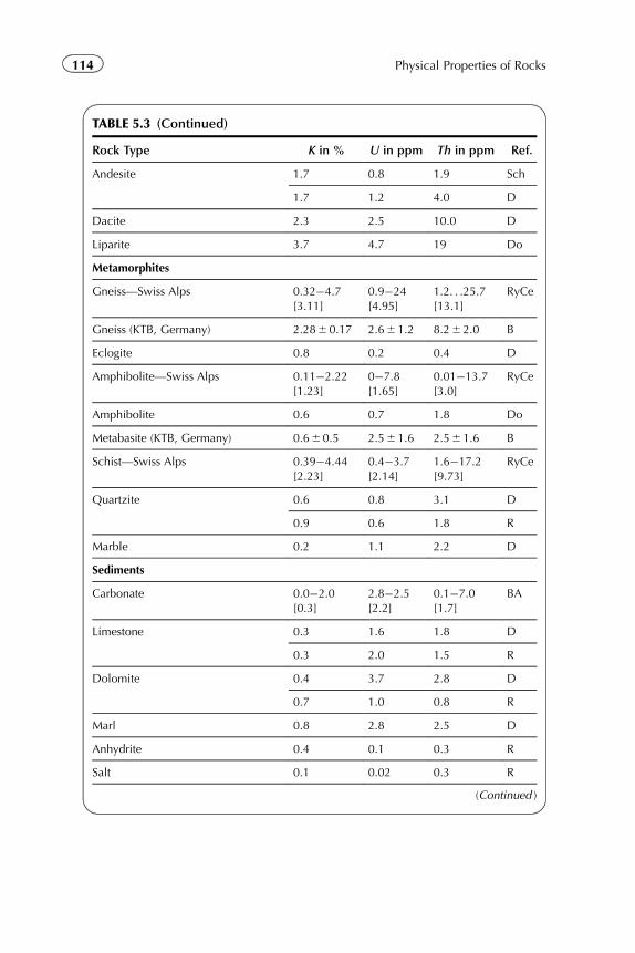
TABLE 5.3 (Continued)
Rock Type K in % U in ppm Th in ppm Ref.
Andesite 1.7 0.8 1.9 Sch
1.7 1.2 4.0 D
Dacite 2.3 2.5 10.0 D
Liparite 3.7 4.7 19 Do
Metamorphites
Gneiss—Swiss Alps 0.32�4.7[3.11]
0.9�24[4.95]
1.2. . .25.7[13.1]
RyCe
Gneiss (KTB, Germany) 2.2860.17 2.661.2 8.262.0 B
Eclogite 0.8 0.2 0.4 D
Amphibolite—Swiss Alps 0.11�2.22[1.23]
0�7.8[1.65]
0.01�13.7[3.0]
RyCe
Amphibolite 0.6 0.7 1.8 Do
Metabasite (KTB, Germany) 0.660.5 2.561.6 2.561.6 B
Schist—Swiss Alps 0.39�4.44[2.23]
0.4�3.7[2.14]
1.6�17.2[9.73]
RyCe
Quartzite 0.6 0.8 3.1 D
0.9 0.6 1.8 R
Marble 0.2 1.1 2.2 D
Sediments
Carbonate 0.0�2.0[0.3]
2.8�2.5[2.2]
0.1�7.0[1.7]
BA
Limestone 0.3 1.6 1.8 D
0.3 2.0 1.5 R
Dolomite 0.4 3.7 2.8 D
0.7 1.0 0.8 R
Marl 0.8 2.8 2.5 D
Anhydrite 0.4 0.1 0.3 R
Salt 0.1 0.02 0.3 R
(Continued )
114 Physical Properties of Rocks
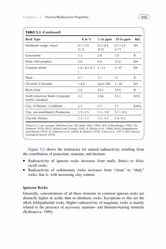
Figure 5.2 shows the tendencies for natural radioactivity resulting from
the contribution of potassium, uranium, and thorium:
� Radioactivity of igneous rocks increases from mafic (basic) to felsic
(acid) rocks.� Radioactivity of sedimentary rocks increases from “clean” to “shaly”
rocks, that is, with increasing clay content.
Igneous Rocks
Generally, concentrations of all three elements in common igneous rocks are
distinctly higher in acidic than in ultrabasic rocks. Exceptions to this are the
alkali feldspathoidal rocks. Higher radioactivity of magmatic rocks is mainly
related to the presence of accessory uranium- and thorium-bearing minerals
(Kobranova, 1989).
TABLE 5.3 (Continued)
Rock Type K in % U in ppm Th in ppm Ref.
Sandstone (range, mean) 0.7�3.8[1.1]
0.2�0.6[0.5]
0.7�2.0[1.7]
BA
Graywacke 1.3 2.0 7.0 R
Shale (200 samples) 2.0 6.0 12.0 BA
Common shales 1.6�4.2 [2.7]
2�13 3�47 BA
Shale 2.7 3.7 12 R
Oil shale (Colorado) ,4.0 up to 500 1�30 BA
Black shale 2.6 20.2 10.9 R
North American Shale Composite(NASC) standard
3.2 2.66 12.3 KGS
Clay, N-Atlantic, Caribbean 2.5 2.1 11 KaHa
Clay, unconsolidated, Pleistocene 1.9�2.5 1.1�3.8 5.7�10.2
Clay/silt, Tertiary 1.3�3.1 1.2�4.3 1.4�9.3
Values in [ ] are averages. Reference key: BA: Baker Atlas (1985); Sch: Schlumberger (1982); Do:Dortman (1976); RyCe: Rybach and Cermak (1982); B: Bucker et al. (1989); KaHa: Kappelmeyerand Haenel (1974); D: Dobrynin et al. (2004); R: Rybach (1976); Yalcin et al. (1977); KGS: KansasGeological Survey (2010).
115Chapter | 5 Nuclear/Radioactive Properties
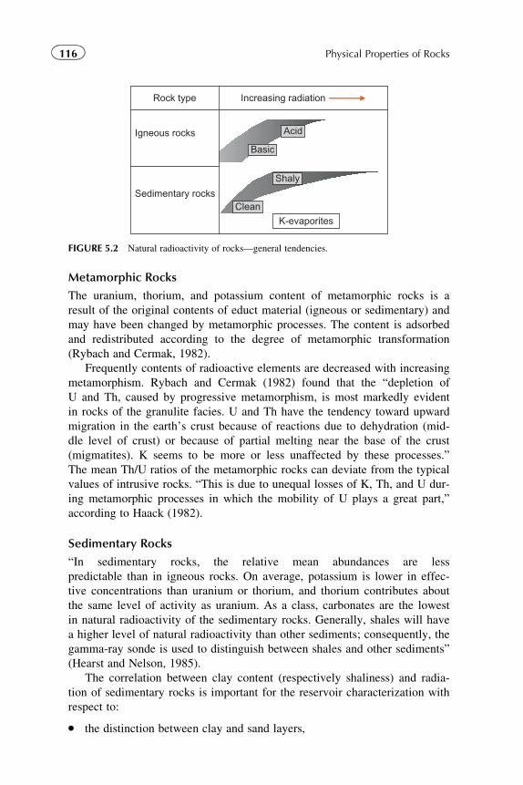
Metamorphic Rocks
The uranium, thorium, and potassium content of metamorphic rocks is a
result of the original contents of educt material (igneous or sedimentary) and
may have been changed by metamorphic processes. The content is adsorbed
and redistributed according to the degree of metamorphic transformation
(Rybach and Cermak, 1982).
Frequently contents of radioactive elements are decreased with increasing
metamorphism. Rybach and Cermak (1982) found that the “depletion of
U and Th, caused by progressive metamorphism, is most markedly evident
in rocks of the granulite facies. U and Th have the tendency toward upward
migration in the earth’s crust because of reactions due to dehydration (mid-
dle level of crust) or because of partial melting near the base of the crust
(migmatites). K seems to be more or less unaffected by these processes.”
The mean Th/U ratios of the metamorphic rocks can deviate from the typical
values of intrusive rocks. “This is due to unequal losses of K, Th, and U dur-
ing metamorphic processes in which the mobility of U plays a great part,”
according to Haack (1982).
Sedimentary Rocks
“In sedimentary rocks, the relative mean abundances are less
predictable than in igneous rocks. On average, potassium is lower in effec-
tive concentrations than uranium or thorium, and thorium contributes about
the same level of activity as uranium. As a class, carbonates are the lowest
in natural radioactivity of the sedimentary rocks. Generally, shales will have
a higher level of natural radioactivity than other sediments; consequently, the
gamma-ray sonde is used to distinguish between shales and other sediments”
(Hearst and Nelson, 1985).
The correlation between clay content (respectively shaliness) and radia-
tion of sedimentary rocks is important for the reservoir characterization with
respect to:
� the distinction between clay and sand layers,
Rock type
Igneous rocks
Sedimentary rocks
Increasing radiation
K-evaporites
Basic
Acid
Shaly
Clean
FIGURE 5.2 Natural radioactivity of rocks—general tendencies.
116 Physical Properties of Rocks
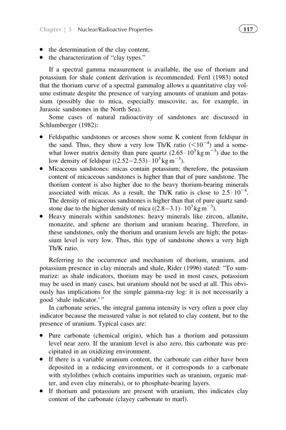
� the determination of the clay content,� the characterization of “clay types.”
If a spectral gamma measurement is available, the use of thorium and
potassium for shale content derivation is recommended. Fertl (1983) noted
that the thorium curve of a spectral gammalog allows a quantitative clay vol-
ume estimate despite the presence of varying amounts of uranium and potas-
sium (possibly due to mica, especially muscovite, as, for example, in
Jurassic sandstones in the North Sea).
Some cases of natural radioactivity of sandstones are discussed in
Schlumberger (1982):
� Feldspathic sandstones or arcoses show some K content from feldspar in
the sand. Thus, they show a very low Th/K ratio (,1024) and a some-
what lower matrix density than pure quartz (2.65 � 103 kgm23) due to the
low density of feldspar ((2.52�2.53) � 103 kgm23).� Micaceous sandstones: micas contain potassium; therefore, the potassium
content of micaceous sandstones is higher than that of pure sandstone. The
thorium content is also higher due to the heavy thorium-bearing minerals
associated with micas. As a result, the Th/K ratio is close to 2.5 � 1024.
The density of micaceous sandstones is higher than that of pure quartz sand-
stone due to the higher density of mica ((2.8�3.1) � 103 kgm23).� Heavy minerals within sandstones: heavy minerals like zircon, allanite,
monazite, and sphene are thorium and uranium bearing. Therefore, in
these sandstones, only the thorium and uranium levels are high; the potas-
sium level is very low. Thus, this type of sandstone shows a very high
Th/K ratio.
Referring to the occurrence and mechanism of thorium, uranium, and
potassium presence in clay minerals and shale, Rider (1996) stated: “To sum-
marize: as shale indicators, thorium may be used in most cases, potassium
may be used in many cases, but uranium should not be used at all. This obvi-
ously has implications for the simple gamma-ray log: it is not necessarily a
good ‘shale indicator.’ ”
In carbonate series, the integral gamma intensity is very often a poor clay
indicator because the measured value is not related to clay content, but to the
presence of uranium. Typical cases are:
� Pure carbonate (chemical origin), which has a thorium and potassium
level near zero. If the uranium level is also zero, this carbonate was pre-
cipitated in an oxidizing environment.� If there is a variable uranium content, the carbonate can either have been
deposited in a reducing environment, or it corresponds to a carbonate
with stylolithes (which contains impurities such as uranium, organic mat-
ter, and even clay minerals), or to phosphate-bearing layers.� If thorium and potassium are present with uranium, this indicates clay
content of the carbonate (clayey carbonate to marl).
117Chapter | 5 Nuclear/Radioactive Properties
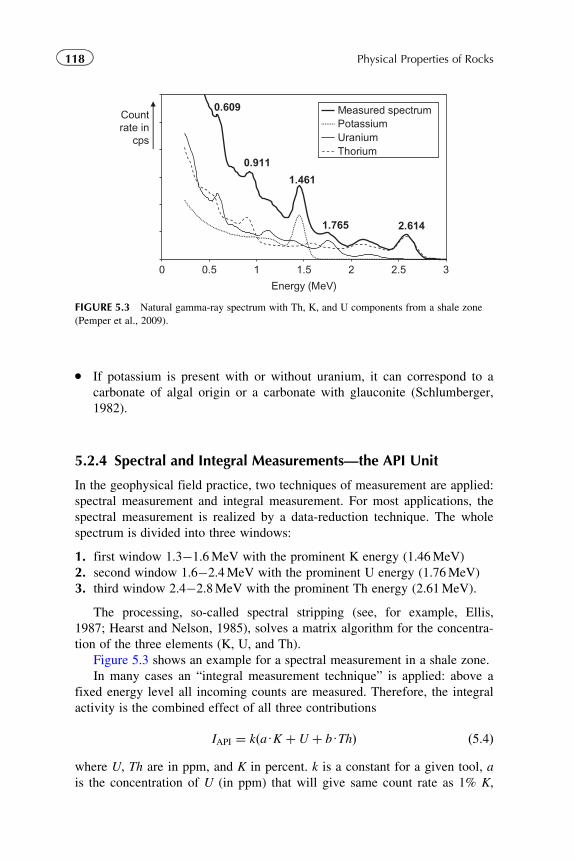
� If potassium is present with or without uranium, it can correspond to a
carbonate of algal origin or a carbonate with glauconite (Schlumberger,
1982).
5.2.4 Spectral and Integral Measurements—the API Unit
In the geophysical field practice, two techniques of measurement are applied:
spectral measurement and integral measurement. For most applications, the
spectral measurement is realized by a data-reduction technique. The whole
spectrum is divided into three windows:
1. first window 1.3�1.6MeV with the prominent K energy (1.46MeV)
2. second window 1.6�2.4MeV with the prominent U energy (1.76MeV)
3. third window 2.4�2.8MeV with the prominent Th energy (2.61MeV).
The processing, so-called spectral stripping (see, for example, Ellis,
1987; Hearst and Nelson, 1985), solves a matrix algorithm for the concentra-
tion of the three elements (K, U, and Th).
Figure 5.3 shows an example for a spectral measurement in a shale zone.
In many cases an “integral measurement technique” is applied: above a
fixed energy level all incoming counts are measured. Therefore, the integral
activity is the combined effect of all three contributions
IAPI ¼ kðaUK þ U þ bUThÞ ð5:4Þ
where U, Th are in ppm, and K in percent. k is a constant for a given tool, a
is the concentration of U (in ppm) that will give same count rate as 1% K,
0 0.5 1 1.5 2 2.5 3
Energy (MeV)
Measured spectrumPotassiumUraniumThorium
0.609
0.911
1.461
1.765 2.614
Countrate in
cps
FIGURE 5.3 Natural gamma-ray spectrum with Th, K, and U components from a shale zone
(Pemper et al., 2009).
118 Physical Properties of Rocks
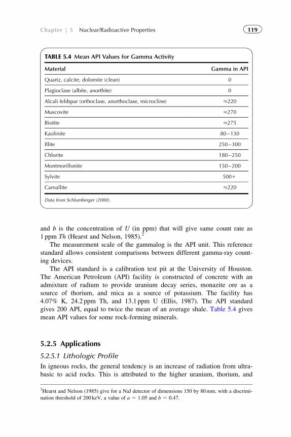
and b is the concentration of U (in ppm) that will give same count rate as
1 ppm Th (Hearst and Nelson, 1985).2
The measurement scale of the gammalog is the API unit. This reference
standard allows consistent comparisons between different gamma-ray count-
ing devices.
The API standard is a calibration test pit at the University of Houston.
The American Petroleum (API) facility is constructed of concrete with an
admixture of radium to provide uranium decay series, monazite ore as a
source of thorium, and mica as a source of potassium. The facility has
4.07% K, 24.2 ppm Th, and 13.1 ppm U (Ellis, 1987). The API standard
gives 200 API, equal to twice the mean of an average shale. Table 5.4 gives
mean API values for some rock-forming minerals.
5.2.5 Applications
5.2.5.1 Lithologic Profile
In igneous rocks, the general tendency is an increase of radiation from ultra-
basic to acid rocks. This is attributed to the higher uranium, thorium, and
2Hearst and Nelson (1985) give for a NaJ detector of dimensions 150 by 80mm, with a discrimi-
nation threshold of 200 keV, a value of a 5 1.05 and b 5 0.47.
TABLE 5.4 Mean API Values for Gamma Activity
Material Gamma in API
Quartz, calcite, dolomite (clean) 0
Plagioclase (albite, anorthite) 0
Alcali feldspar (orthoclase, anorthoclase, microcline) �220
Muscovite �270
Biotite �275
Kaolinite 80�130
Illite 250�300
Chlorite 180�250
Montmorillonite 150�200
Sylvite 5001
Carnallite �220
Data from Schlumberger (2000).
119Chapter | 5 Nuclear/Radioactive Properties
potassium content of mica and alkali feldspars. Alteration can change the
radioactivity.
In sedimentary rocks, clean carbonates and sands normally show the low-
est values. Radioactivity increases with the shale content; therefore, the gam-
malog is one of the most indicative shale indicators. The highest values are
from black marine shales.
But there are some important specific cases of high radiation (see
Section 5.2.3):
� Sandstone with high content of feldspar, mica, glauconite (“green sand”)� Carbonate in reducing environment, stylolithes, phosphates.
A gammalog allows (qualitative) lithologic profiling. Clean zones (sand,
carbonates) and shaly sections can be separated. In geological applications,
the gammalog is a tool for
� sedimentological studies by typical curve shapes for channel, coarsening
upward, fining upward, and other formations (Rider, 1996);� well-to-well correlation in sedimentary areas and trend derivation.
5.2.5.2 Shale Content Estimate
A shale content estimate can be derived from a gamma measurement based
on the correlation between shale content and radioactive isotope content,
which originates natural gamma activity. It is assumed that only shale or
clay are responsible for the radiation; no other “radioactive minerals” are
present.
For this application, in many cases an integral measurement is used; in
order to eliminate the effect of variability of the uranium content, a spectral
measurement of the potassium and thorium contribution is recommended.
The analysis consists of two steps:
1. Calculation of a “gamma-ray index” IGR: this is the actual gamma reading
normalized by the value for the clean rock (minimum gamma read-
ing) and the shale (maximum gamma reading)
IGR ¼ GR2GRcn
GRsh 2GRcn
ð5:5Þ
where
GRcn is the log response in a clean zone—no shale
GRsh is the log response in a shale zone
GR is the log response in the zone of interest.
This normalization of the logs results in IGR 5 0 for clean rocks and
IGR 5 1 for shale (100% shale).
120 Physical Properties of Rocks
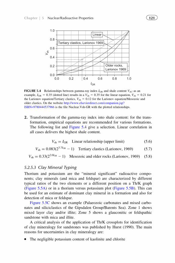
2. Transformation of the gamma-ray index into shale content: for the trans-
formation, empirical equations are recommended for various formations.
The following list and Figure 5.4 give a selection. Linear correlation in
all cases delivers the highest shale content.
Vsh ¼ IGR Linear relationship ðupper limitÞ ð5:6ÞVsh ¼ 0:083ð23:7IGR 2 1Þ Tertiary clastics ðLarionov; 1969Þ ð5:7Þ
Vsh ¼ 0:33ð22:0IGR 2 1Þ Mesozoic and older rocks ðLarionov; 1969Þ ð5:8Þ
5.2.5.3 Clay Mineral Typing
Thorium and potassium are the “mineral significant” radioactive compo-
nents; clay minerals (and mica and feldspar) are characterized by different
typical ratios of the two elements or a different position on a Th/K graph
(Figure 5.5A) or in a thorium versus potassium plot (Figure 5.5B). This can
be used for an estimate of dominant clay mineral in a formation and also for
detection of mica or feldspar.
Figure 5.5C shows an example (Palaeozoic carbonates and mixed carbo-
nates and siliciclastics of the Gipsdalen Group/Barents Sea). Zone 1 shows
mixed layer clay and/or illite; Zone 5 shows a glauconitic or feldspathic
sandstone with mica and illite.
A critical analysis of the application of Th/K crossplots for identification
of clay mineralogy for sandstones was published by Hurst (1990). The main
reasons for uncertainties in clay mineralogy are:
� The negligible potassium content of kaolinite and chlorite
0.0
0.2
0.4
0.6
0.8
1.0
0.0 0.2 0.4 0.6 0.8 1.0
IGR
Vsh
Linear
Tertiary clastics, Larionov 1969
Older rocks,Larionov 1969
FIGURE 5.4 Relationships between gamma-ray index IGR and shale content Vsh; as an
example, IGR 5 0.35 (dotted line) results in a Vsh 5 0.35 for the linear equation, Vsh 5 0.21 for
the Larionov equation/Tertiary clastics, Vsh 5 0.12 for the Larionov equation/Mesozoic and
older clastics. On the website http://www.elsevierdirect.com/companion.jsp?
ISBN=9780444537966 is the file Nuclear.Vsh-GR with the plotted relationships.
121Chapter | 5 Nuclear/Radioactive Properties
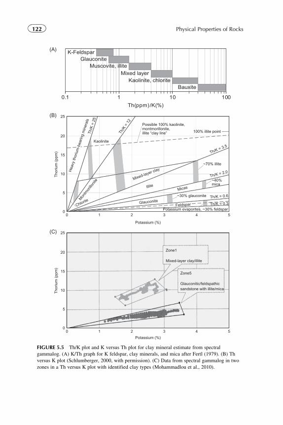
0.1 1 10 100
Th(ppm)/K(%)
K-FeldsparGlauconite
Muscovite, illiteMixed layer
Kaolinite, chloriteBauxite
(A)
(B)
(C)
Possible 100% kaolinite,montmorillonite,illite “clay line”
Kaolinite
Th/K
= 2
5
Hea
vy th
oriu
m-b
earin
g m
iner
als
Th/K
= 1
2100% illite point
Potassium evaporites, ~30% feldspar
Mon
tmor
illoni
te
Chlorite
IlliteMicas
Glauconite
Mixed-layer clay
~30% glauconite
~40%mica
~70% illite
Feldspar
Th/K = 0.6
Th/K = 2.0
Th/K = 3.5
Th/K = 0.3
0 1 2
Potassium (%)
3 4 5
25
20
15
10Tho
rium
(pp
m)
5
0
0 1 2
Potassium (%)
3 4 5
25
20
15
10Tho
rium
(pp
m)
5
0
Zone1
Mixed-layer clay/illite
Zone5
Glauconitic/feldspathicsandstone with illite/mica
FIGURE 5.5 Th/K plot and K versus Th plot for clay mineral estimate from spectral
gammalog. (A) K/Th graph for K feldspar, clay minerals, and mica after Fertl (1979). (B) Th
versus K plot (Schlumberger, 2000, with permission). (C) Data from spectral gammalog in two
zones in a Th versus K plot with identified clay types (Mohammadlou et al., 2010).
122 Physical Properties of Rocks
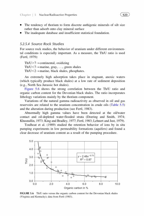
� The tendency of thorium to form discrete authigenic minerals of silt size
rather than adsorb onto clay mineral surface� The inadequate database and insufficient statistical foundation.
5.2.5.4 Source Rock Studies
For source rock studies, the behavior of uranium under different environmen-
tal conditions is especially important. As a measure, the Th/U ratio is used
(Fertl, 1979):
Th/U.7-continental, oxidizing
Th/U,7-marine, gray, . . ., green shales
Th/U,2-marine, black shales, phosphates.
An extremely high adsorption takes place in stagnant, anoxic waters
(which typically produce black shales) at a low rate of sediment deposition
(e.g., North Sea Jurassic hot shales).
Figure 5.6 shows the strong correlation between the Th/U ratio and
organic carbon content for the Devonian black shales. The ratio incorporates
lithology variations mainly by the thorium component.
Variations of the natural gamma radioactivity as observed in oil and gas
reservoirs are related to the uranium concentration in crude oils (Table 5.5)
and the alteration during production (see Fertl, 1983).
Abnormally high gamma values have been detected at the oil/water
contact and oil-depleted water-flooded strata (Doering and Smith, 1974;
Khusnullin, 1973; King and Bradley, 1977; Fertl, 1983; Lehnert and Just, 1979).
Toulhoat et al. (1989) studied the retention behavior of ions by in situ
pumping experiments in low permeability formations (aquifers) and found a
clear decrease of uranium content as a result of the pumping procedure.
y = 2.48x−0.73
R2 = 0.87
0.0
1.0
2.0
3.0
4.0
5.0
0.0 2.0 4.0 6.0 8.0 10.0
Organic carbon in %
Th/
U
FIGURE 5.6 Th/U ratio versus the organic carbon content for the Devonian black shales
(Virginia and Kentucky); data from Fertl (1983).
123Chapter | 5 Nuclear/Radioactive Properties
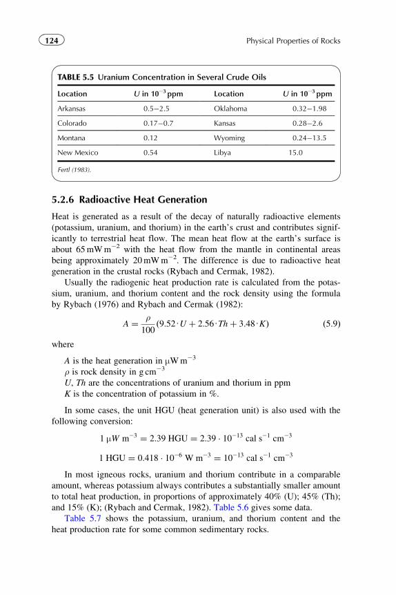
5.2.6 Radioactive Heat Generation
Heat is generated as a result of the decay of naturally radioactive elements
(potassium, uranium, and thorium) in the earth’s crust and contributes signif-
icantly to terrestrial heat flow. The mean heat flow at the earth’s surface is
about 65mWm22 with the heat flow from the mantle in continental areas
being approximately 20mWm22. The difference is due to radioactive heat
generation in the crustal rocks (Rybach and Cermak, 1982).
Usually the radiogenic heat production rate is calculated from the potas-
sium, uranium, and thorium content and the rock density using the formula
by Rybach (1976) and Rybach and Cermak (1982):
A ¼ ρ100
ð9:52UU þ 2:56UThþ 3:48UKÞ ð5:9Þ
where
A is the heat generation in μWm23
ρ is rock density in g cm23
U, Th are the concentrations of uranium and thorium in ppm
K is the concentration of potassium in %.
In some cases, the unit HGU (heat generation unit) is also used with the
following conversion:
1 μW m23 ¼ 2:39 HGU ¼ 2:39 � 10213 cal s21 cm23
1 HGU ¼ 0:418 � 1026 W m23 ¼ 10213 cal s21 cm23
In most igneous rocks, uranium and thorium contribute in a comparable
amount, whereas potassium always contributes a substantially smaller amount
to total heat production, in proportions of approximately 40% (U); 45% (Th);
and 15% (K); (Rybach and Cermak, 1982). Table 5.6 gives some data.
Table 5.7 shows the potassium, uranium, and thorium content and the
heat production rate for some common sedimentary rocks.
TABLE 5.5 Uranium Concentration in Several Crude Oils
Location U in 1023 ppm Location U in 1023 ppm
Arkansas 0.5�2.5 Oklahoma 0.32�1.98
Colorado 0.17�0.7 Kansas 0.28�2.6
Montana 0.12 Wyoming 0.24�13.5
New Mexico 0.54 Libya 15.0
Fertl (1983).
124 Physical Properties of Rocks
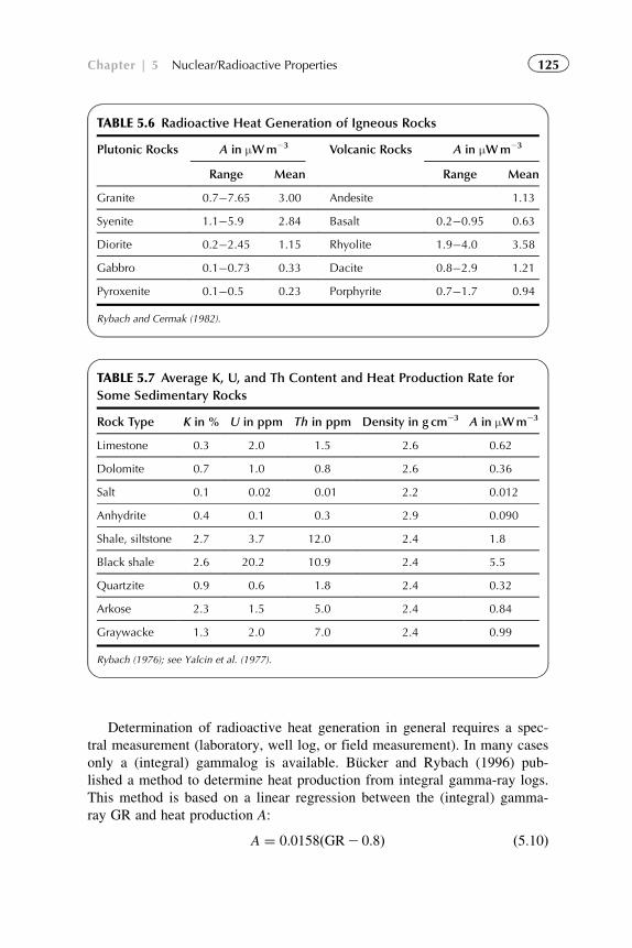
Determination of radioactive heat generation in general requires a spec-
tral measurement (laboratory, well log, or field measurement). In many cases
only a (integral) gammalog is available. Bucker and Rybach (1996) pub-
lished a method to determine heat production from integral gamma-ray logs.
This method is based on a linear regression between the (integral) gamma-
ray GR and heat production A:
A ¼ 0:0158ðGR2 0:8Þ ð5:10Þ
TABLE 5.6 Radioactive Heat Generation of Igneous Rocks
Plutonic Rocks A in μWm23 Volcanic Rocks A in μWm23
Range Mean Range Mean
Granite 0.7�7.65 3.00 Andesite 1.13
Syenite 1.1�5.9 2.84 Basalt 0.2�0.95 0.63
Diorite 0.2�2.45 1.15 Rhyolite 1.9�4.0 3.58
Gabbro 0.1�0.73 0.33 Dacite 0.8�2.9 1.21
Pyroxenite 0.1�0.5 0.23 Porphyrite 0.7�1.7 0.94
Rybach and Cermak (1982).
TABLE 5.7 Average K, U, and Th Content and Heat Production Rate for
Some Sedimentary Rocks
Rock Type K in % U in ppm Th in ppm Density in g cm23 A in μWm23
Limestone 0.3 2.0 1.5 2.6 0.62
Dolomite 0.7 1.0 0.8 2.6 0.36
Salt 0.1 0.02 0.01 2.2 0.012
Anhydrite 0.4 0.1 0.3 2.9 0.090
Shale, siltstone 2.7 3.7 12.0 2.4 1.8
Black shale 2.6 20.2 10.9 2.4 5.5
Quartzite 0.9 0.6 1.8 2.4 0.32
Arkose 2.3 1.5 5.0 2.4 0.84
Graywacke 1.3 2.0 7.0 2.4 0.99
Rybach (1976); see Yalcin et al. (1977).
125Chapter | 5 Nuclear/Radioactive Properties
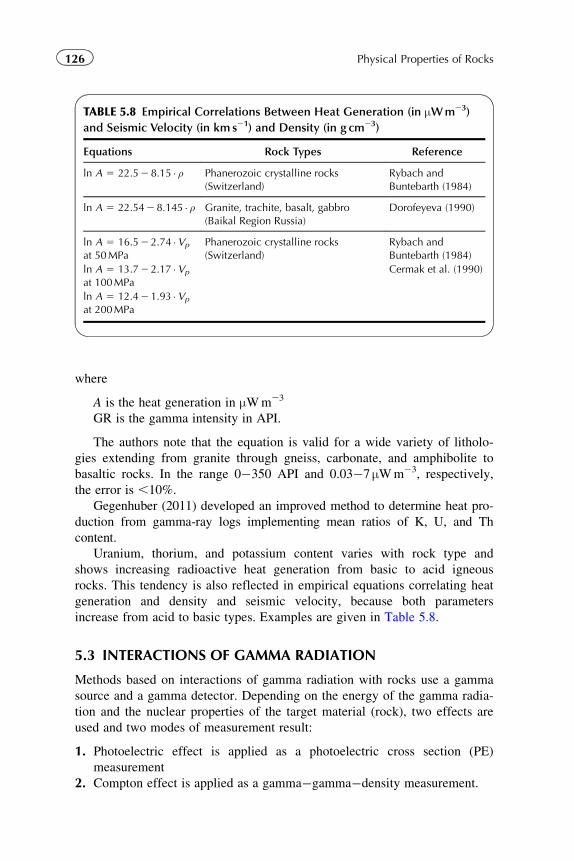
where
A is the heat generation in μWm23
GR is the gamma intensity in API.
The authors note that the equation is valid for a wide variety of litholo-
gies extending from granite through gneiss, carbonate, and amphibolite to
basaltic rocks. In the range 0�350 API and 0.03�7 μWm23, respectively,
the error is ,10%.
Gegenhuber (2011) developed an improved method to determine heat pro-
duction from gamma-ray logs implementing mean ratios of K, U, and Th
content.
Uranium, thorium, and potassium content varies with rock type and
shows increasing radioactive heat generation from basic to acid igneous
rocks. This tendency is also reflected in empirical equations correlating heat
generation and density and seismic velocity, because both parameters
increase from acid to basic types. Examples are given in Table 5.8.
5.3 INTERACTIONS OF GAMMA RADIATION
Methods based on interactions of gamma radiation with rocks use a gamma
source and a gamma detector. Depending on the energy of the gamma radia-
tion and the nuclear properties of the target material (rock), two effects are
used and two modes of measurement result:
1. Photoelectric effect is applied as a photoelectric cross section (PE)
measurement
2. Compton effect is applied as a gamma�gamma�density measurement.
TABLE 5.8 Empirical Correlations Between Heat Generation (in μWm23)
and Seismic Velocity (in km s21) and Density (in g cm23)
Equations Rock Types Reference
ln A 5 22.52 8.15 � ρ Phanerozoic crystalline rocks(Switzerland)
Rybach andBuntebarth (1984)
ln A 5 22.5428.145 � ρ Granite, trachite, basalt, gabbro(Baikal Region Russia)
Dorofeyeva (1990)
ln A 5 16.52 2.74 �Vp
at 50MPaPhanerozoic crystalline rocks(Switzerland)
Rybach andBuntebarth (1984)
ln A 5 13.72 2.17 �Vp
at 100MPaCermak et al. (1990)
ln A 5 12.42 1.93 �Vp
at 200MPa
126 Physical Properties of Rocks
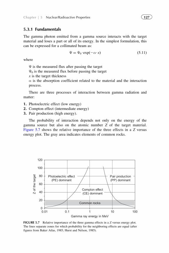
5.3.1 Fundamentals
The gamma photon emitted from a gamma source interacts with the target
material and loses a part or all of its energy. In the simplest formulation, this
can be expressed for a collimated beam as:
Ψ ¼ Ψ0Uexpð2αUxÞ ð5:11Þwhere
Ψ is the measured flux after passing the target
Ψ0 is the measured flux before passing the target
x is the target thickness
α is the absorption coefficient related to the material and the interaction
process.
There are three processes of interaction between gamma radiation and
matter:
1. Photoelectric effect (low energy)
2. Compton effect (intermediate energy)
3. Pair production (high energy).
The probability of interaction depends not only on the energy of the
gamma source but also on the atomic number Z of the target material.
Figure 5.7 shows the relative importance of the three effects in a Z versus
energy plot. The gray area indicates elements of common rocks.
0
20
40
60
80
100
120
0.01 0.1 1 10 100
Gamma ray energy in MeV
Z o
f th
e ta
rget Photoelectric effect
(PE) dominant
Compton effect(CE) dominant
Pair production(PP) dominant
Common rocks
FIGURE 5.7 Relative importance of the three gamma effects in a Z versus energy plot.
The lines separate zones for which probability for the neighboring effects are equal (after
figures from Baker Atlas, 1985; Hurst and Nelson, 1985).
127Chapter | 5 Nuclear/Radioactive Properties
Photoelectric Effect
An incident low-energy gamma photon (,0.2MeV) collides with an atom. If
the energy of the gamma photon equals or exceeds the discrete “binding
energy” of an orbital electron, then
� the gamma photon gives its energy to this orbital electron;� the electron leaves its orbit and has a kinetic energy Ekin 5 gamma-ray
energy—electron binding energy.
The probability for the photoelectric effect is controlled by the energy of
gamma radiation and the atomic number of the absorbing material Z. For
practical applications, two parameters are used:
� Photoelectric cross section index PE in b e21 (barns per electron):
PE ¼ Z
10
� �3:6ð5:12Þ
� Volumetric photoelectric cross section U in b cm23 (barns per cubic
centimeter):
U ¼ PEUρe ð5:13Þwhere ρe is the electron density (see Section 5.3.2).
U is practically independent of porosity; for a mixture of substances
U can be calculated as the weighted (by volume fraction) mean of the
components.
Compton Effect
An incident intermediate-energy gamma photon (gamma ray) collides with
an atom. It scatters at an orbiting electron and transmits only a part of its
energy. The energy of the scattered and the kinetic energy of an ejected elec-
tron (“Compton or recoil electron”) can be calculated from conservation of
energy and momentum (Hearst and Nelson, 1985). The scattering angles are
distributed and depend on energy.
Probability of the Compton effect is controlled by the number of elec-
trons in a volume unit of the target material.
Pair Production
An incident high-energy gamma photon (gamma-ray energy .1.022MeV)3
can be converted into an electron�positron pair when it is near a nucleus.
31.02MeV is exactly twice the rest mass of an electron (mc2).
128 Physical Properties of Rocks
The photoelectric and Compton effects are applied in geoscience. Both
effects result in an attenuation of the gamma radiation, which is expressed in
Equation (5.12). The absorption coefficient refers to the effect.
5.3.2 Gamma�Gamma�PE Measurement for MineralIdentification
The photoelectric index (PE) is a supplementary measurement by modern
density logging tools. It measures the absorption of low-energy gamma rays
by the formation in units of barns per electron. The gamma�gamma mea-
surement in the low energy range (,100 keV) delivers the parameter PE
(average photoelectric cross section per electron) with a strong dependence
on the (averaged) atomic number Z in the formation, and therefore a sensi-
tive indicator of mineralogy.
If the density ρe is also measured (see next section), the parameter U
(average photoelectric cross section per cm3) can be calculated. Definitions
of the two parameters are given by Equations (5.12) and (5.13).
Table 5.9 shows several important properties for individual rock-forming
minerals. The averaged charge-to-mass ratio, Z/A, the photoelectric capture
cross section, PE, and U, can be quite different for various minerals.
Particularly of interest is the difference for the main reservoir rock-
forming minerals quartz (PE 5 1.81 barns electron21; U 5 4.8 barns cm23),
calcite (PE 5 5.08 barns electron21; U 5 13.8 barns cm23), and dolomite
(PE 5 3.14 barns electron21; U 5 9.0 barns cm23). This gives a possibility of
a mineral composition estimate and is implemented in crossplot techniques
(see Section 11.2).
The extremely high value of barite (PE 5 267 barns electron21;
U 5 1066 barns cm23) influences the measurement when the mud contains
barite.
5.3.3 Gamma�Gamma�Density Measurement andPorosity Estimate
Gamma�gamma tools in the Compton energy region (0.5�5MeV) measure
a material response controlled by the number of orbiting electrons per unit
volume. Commonly used nuclear sources are cesium (0.66MeV) and cobalt
(1.17 and 1.33MeV).
The number of atoms per unit volume is
na ¼ NAUðρb=AÞ ð5:14Þwhere NA is Avogadro’s number, A the atomic mass number, and ρb the bulk
density.
129Chapter | 5 Nuclear/Radioactive Properties
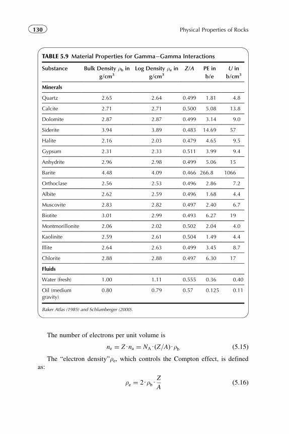
The number of electrons per unit volume is
ne ¼ ZUna ¼ NAUðZ=AÞUρb ð5:15ÞThe “electron density”ρe, which controls the Compton effect, is defined
as:
ρe ¼ 2UρbUZ
Að5:16Þ
TABLE 5.9 Material Properties for Gamma�Gamma Interactions
Substance Bulk Density ρb in
g/cm3
Log Density ρe ing/cm3
Z/A PE in
b/e
U in
b/cm3
Minerals
Quartz 2.65 2.64 0.499 1.81 4.8
Calcite 2.71 2.71 0.500 5.08 13.8
Dolomite 2.87 2.87 0.499 3.14 9.0
Siderite 3.94 3.89 0.483 14.69 57
Halite 2.16 2.03 0.479 4.65 9.5
Gypsum 2.31 2.33 0.511 3.99 9.4
Anhydrite 2.96 2.98 0.499 5.06 15
Barite 4.48 4.09 0.466 266.8 1066
Orthoclase 2.56 2.53 0.496 2.86 7.2
Albite 2.62 2.59 0.496 1.68 4.4
Muscovite 2.83 2.82 0.497 2.40 6.7
Biotite 3.01 2.99 0.493 6.27 19
Montmorillonite 2.06 2.02 0.502 2.04 4.0
Kaolinite 2.59 2.61 0.504 1.49 4.4
Illite 2.64 2.63 0.499 3.45 8.7
Chlorite 2.88 2.88 0.497 6.30 17
Fluids
Water (fresh) 1.00 1.11 0.555 0.36 0.40
Oil (mediumgravity)
0.80 0.79 0.57 0.125 0.11
Baker Atlas (1985) and Schlumberger (2000).
130 Physical Properties of Rocks
The bulk density ρb directly results in
ρb ¼ρe
2UZ=Að5:17Þ
Thus, ρb is related to the (measured) electron density ρe and the averaged
ratio Z/A of the target material (rock). For most rock-forming minerals, the
ratio Z/A is a nearly constant 0.5 (see Table 5.9):
Z=A � 0:5 ð5:18ÞUnder this condition, ρbDρe, and the tool can be calibrated directly in
bulk density units.
If the ratio deviates from the value Z/A 5 0.5, a correction must be
applied. This is also the case particularly for the presence of water with
Z/A 5 0.55. The correction results from a volumetric weighted contribution
of the two main components matrix and water:
ρb ¼ρe
1ð12φÞ þ 1:11Uφ¼ ρe
1þ 0:11Uφð5:19Þ
where φ is the porosity.
From bulk density the porosity (total porosity) can be derived:
φ ¼ ρsolid 2 ρbρsolid 2 ρfluid
ð5:20Þ
Thus, for a porosity calculation from a density measurement, the knowl-
edge of solid matrix material density ρsolid (also called “matrix density” ρma)
and fluid density ρfluid are necessary. An information about matrix mineral-
ogy can be received from geological input, crossplot techniques (see
Section 11), and PE measurement.
5.4 INTERACTIONS OF NEUTRON RADIATION
5.4.1 Fundamentals
Fundamentals of neutron logs are presented, for example, by Alger et al.
(1971) and Allen et al. (1972), and in a series of tutorials in Petrophysics
(SPWLA) by Ellis et al. (2003, 2004) and Gilchrist (2009).
Neutrons with a mass of 1.67482 � 10227 kg have no electric charge and
therefore a high penetration potential (Bassiouni, 1994). Neutrons of differ-
ent energies interact with atomic nuclei in different ways.
Neutrons are classified using their energy:
� Fast neutrons: energy. 500 keV� Intermediate neutrons: energy 1�500 keV� Slow neutrons: energy, 1 keV subdivided into:
� epithermal neutrons with energy 0.1�1 keV,� thermal neutrons with energy, 0.1 eV.
131Chapter | 5 Nuclear/Radioactive Properties
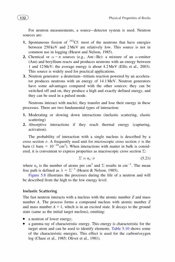
For neutron measurements, a source�detector system is used. Neutron
sources are:
1. Spontaneous fission of 252Cf: most of the neutrons that have energies
between 250 keV and 2MeV are relatively low. This source is not in
common use in logging (Hearst and Nelson, 1985).
2. Chemical or α2 n sources (e.g., Am�Be): a mixture of an α-emitter
(Am) and beryllium reacts and produces neutrons with an energy between
1 and 12MeV; the average energy is about 4.2MeV (Ellis et al., 2003).
This source is widely used for practical applications.
3. Neutron generator: a deuterium�tritium reaction powered by an accelera-
tor produces neutrons with an energy of 14.1MeV. Neutron generators
have some advantages compared with the other sources: they can be
switched off and on, they produce a high and exactly defined energy, and
they can be used in a pulsed mode.
Neutrons interact with nuclei; they transfer and lose their energy in these
processes. There are two fundamental types of interaction:
1. Moderating or slowing down interactions (inelastic scattering, elastic
scattering)
2. Absorptive interactions if they reach thermal energy (capturing,
activation).
The probability of interaction with a single nucleus is described by a
cross section σ. A frequently used unit for microscopic cross section σ is the
barn (1 barn 5 10224 cm2). When interactions with matter in bulk is consid-
ered, it is convenient to express properties as macroscopic cross section Σ:
Σ ¼ naUσ ð5:21Þwhere na is the number of atoms per cm3 and Σ results in cm21. The mean
free path is defined as λ 5 Σ21 (Hearst & Nelson, 1985).
Figure 5.8 illustrates the processes during the life of a neutron and will
be described from the high to the low energy level.
Inelastic Scattering
The fast neutron interacts with a nucleus with the atomic number Z and mass
number A. The process forms a compound nucleus with atomic number Z
and mass number A1 1, which is in an excited state. It decays to the ground
state (same as the initial target nucleus), emitting:
� a neutron of lower energy;� a gamma ray of characteristic energy. This energy is characteristic for the
target atom and can be used to identify elements. Table 5.10 shows some
of the characteristic energies. This effect is used for the carbon/oxygen
log (Chase et al., 1985; Oliver et al., 1981).
132 Physical Properties of Rocks
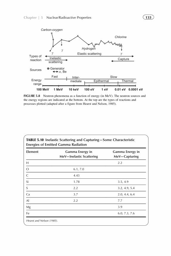
γγ
γTypes ofreaction
Sources
Energyrange
Inelasticscattering
Elastic scattering
Capture
Inter-mediate
SlowEpithermal Thermal
0.0001 eV100 MeV 1 MeV 10 keV 100 eV 1 eV 0.01 eV
Generator, Beα
Fast
Carbon-oxygen
Chlorine
Hydrogen
FIGURE 5.8 Neutron phenomena as a function of energy (in MeV). The neutron sources and
the energy regions are indicated at the bottom. At the top are the types of reactions and
processes plotted (adapted after a figure from Hearst and Nelson, 1985).
TABLE 5.10 Inelastic Scattering and Capturing—Some Characteristic
Energies of Emitted Gamma Radiation
Element Gamma Energy in
MeV—Inelastic Scattering
Gamma Energy in
MeV—Capturing
H 2.2
O 6.1, 7.0
C 4.43
Si 1.78 3.5, 4.9
S 2.2 3.2, 4.9, 5.4
Ca 3.7 2.0, 4.4, 6.4
Al 2.2 7.7
Mg 3.9
Fe 6.0, 7.3, 7.6
Hearst and Nelson (1985).
133Chapter | 5 Nuclear/Radioactive Properties
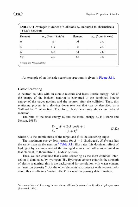
An example of an inelastic scattering spectrum is given in Figure 5.11.
Elastic Scattering
A neutron collides with an atomic nucleus and loses kinetic energy. All of
the energy of the incident neutron is converted to the combined kinetic
energy of the target nucleus and the neutron after the collision. Thus, this
scattering process is a slowing down reaction that can be described as a
“billiard ball” interaction. Therefore, elastic scattering shows no induced
radiation.
The ratio of the final energy Ef and the initial energy E0 is (Hearst and
Nelson, 1985):
Ef
E0
¼ A2 þ 2UAUcosΘþ 1
ðAþ 1Þ2 ð5:22Þ
where A is the atomic mass of the target and Θ is the scattering angle.
The maximum energy loss results for A 5 1 (hydrogen). Hydrogen has
the same mass as the neutron.4 Table 5.11 illustrates this dominant effect of
hydrogen by a comparison of the averaged number of collisions required in
that element, to thermalize a 14-MeV neutron.
Thus, we can conclude that elastic scattering as the most common inter-
action is dominated by hydrogen (H). Hydrogen content controls the strength
of elastic scattering; this is the background for correlation with water content
or “neutron porosity.” But the other elements also interact with neutron radi-
ation; this results in a “matrix effect” for neutron porosity determination.
4A neutron loses all its energy in one direct collision (head-on, Θ 5 0) with a hydrogen atom
(Bassiouni, 1994).
TABLE 5.11 Averaged Number of Collisions nco Required to Thermalize a
14-MeV Neutron
Element nco (from 14MeV) Element nco (from 14MeV)
H 19 Al 290
C 112 Si 297
O 154 Cl 343
Mg 235 Ca 380
(Hearst and Nelson (1985).
134 Physical Properties of Rocks
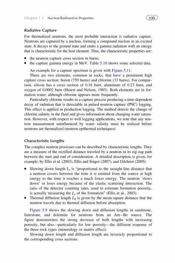
Radiative Capture
For thermalized neutrons, the most probable interaction is radiative capture.
Neutrons are captured by a nucleus, forming a compound nucleus in an excited
state. It decays to the ground state and emits a gamma radiation with an energy
that is characteristic for the host element. Thus, the characteristic properties are:
� the neutron capture cross section in barns;� the capture gamma energy in MeV. Table 5.10 shows some selected data.
An example for a capture spectrum is given with Figure 5.11.
There are two elements, common in rocks, that have a prominent high
capture cross section: boron (759 barns) and chlorine (33 barns). For compar-
ison, silicon has a cross section of 0.16 barn, aluminum of 0.23 barn, and
oxygen of 0.0002 barn (Hearst and Nelson, 1985). Both elements are in for-
mation water, although chlorine appears more frequently.
Particularly chlorine results in a capture process producing a time-dependent
decay of radiation that is detectable in pulsed neutron capture (PNC) logging.
This effect is applied in production logging. The method detects the change of
chlorine salinity in the fluid and gives information about changing water satura-
tion. However, with respect to well logging applications, we note that any neu-
tron measurement uninfluenced by water salinity must be realized before
neutrons are thermalized (neutron epithermal techniques).
Characteristic Lengths
The complex neutron processes can be described by characteristic lengths. They
are a measure of the rectified distance traveled by a neutron in its zig-zag path
between the start and end of consideration. A detailed description is given, for
example, by Ellis et al. (2003), Ellis and Singer (2007), and Gilchrist (2009):
� Slowing down length Ls is “proportional to the straight-line distance that
a neutron covers between the time it is emitted from the source at high
energy to the time it reaches a much lower energy. The neutron ‘slows
down’ or loses energy because of the elastic scattering interaction. The
ratio of the detector counting rates, used to estimate formation porosity,
is actually measuring the Ls of the formation” (Ellis et al., 2003).� Thermal diffusion length Ld is given by the mean-square distance that the
neutron travels due to thermal diffusion before absorption.
Figure 5.9 shows the slowing down and diffusion lengths in sandstone,
limestone, and dolomite for neutrons from an Am�Be source. The
figure demonstrates the strong decrease of both lengths with increasing
porosity, but also—particularly for low porosity—the different response of
the three rock types (mineralogy or matrix effect).
Slowing down length and diffusion length are inversely proportional to
the corresponding cross sections.
135Chapter | 5 Nuclear/Radioactive Properties
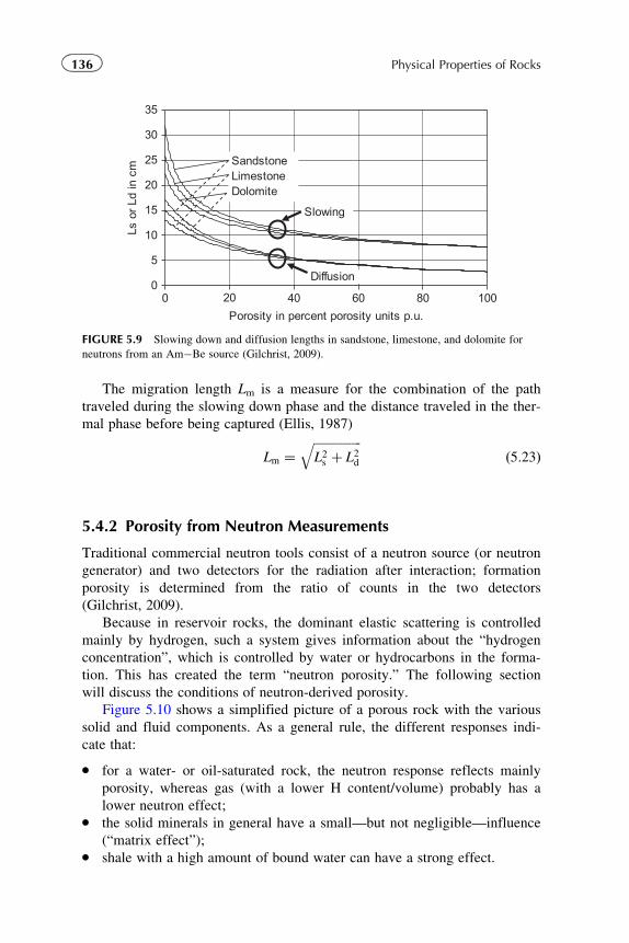
The migration length Lm is a measure for the combination of the path
traveled during the slowing down phase and the distance traveled in the ther-
mal phase before being captured (Ellis, 1987)
Lm ¼ffiffiffiffiffiffiffiffiffiffiffiffiffiffiffiffiL2s þ L2d
qð5:23Þ
5.4.2 Porosity from Neutron Measurements
Traditional commercial neutron tools consist of a neutron source (or neutron
generator) and two detectors for the radiation after interaction; formation
porosity is determined from the ratio of counts in the two detectors
(Gilchrist, 2009).
Because in reservoir rocks, the dominant elastic scattering is controlled
mainly by hydrogen, such a system gives information about the “hydrogen
concentration”, which is controlled by water or hydrocarbons in the forma-
tion. This has created the term “neutron porosity.” The following section
will discuss the conditions of neutron-derived porosity.
Figure 5.10 shows a simplified picture of a porous rock with the various
solid and fluid components. As a general rule, the different responses indi-
cate that:
� for a water- or oil-saturated rock, the neutron response reflects mainly
porosity, whereas gas (with a lower H content/volume) probably has a
lower neutron effect;� the solid minerals in general have a small—but not negligible—influence
(“matrix effect”);� shale with a high amount of bound water can have a strong effect.
0
5
10
15
20
25
30
35
0 20 40 60 80 100
Porosity in percent porosity units p.u.
Ls o
r Ld
in c
m
Diffusion
Slowing
SandstoneLimestoneDolomite
FIGURE 5.9 Slowing down and diffusion lengths in sandstone, limestone, and dolomite for
neutrons from an Am�Be source (Gilchrist, 2009).
136 Physical Properties of Rocks
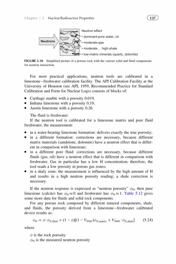
For most practical applications, neutron tools are calibrated in a
limestone�freshwater calibration facility. The API Calibration Facility at the
University of Houston (see API, 1959, Recommended Practice for Standard
Calibration and Form for Nuclear Logs) consists of blocks of:
� Carthage marble with a porosity 0.019,� Indiana limestone with a porosity 0.19,� Austin limestone with a porosity 0.26.
The fluid is freshwater.
If the neutron tool is calibrated for a limestone matrix and pore fluid
freshwater, the measurement:
� in a water-bearing limestone formation: delivers exactly the true porosity;� in a different formation: corrections are necessary, because different
matrix materials (sandstone, dolomite) have a neutron effect that is differ-
ent in comparison with limestone;� in a different pore fluid: corrections are necessary, because different
fluids (gas, oil) have a neutron effect that is different in comparison with
freshwater. Gas in particular has a low H concentration; therefore, the
tool reads a low porosity in porous gas zones;� in a shaly zone: the measurement is influenced by the high amount of H
and results in a high neutron porosity reading; a shale correction is
necessary.
If the neutron response is expressed as “neutron porosity” φN, then pure
limestone (calcite) has φN� 0 and freshwater has φN� 1. Table 5.12 gives
some more data for fluids and solid rock components.
For any porous rock composed by different mineral components, shale,
and fluids, the porosity derived from a limestone�freshwater calibrated
device results as:
φN ¼ φUφN;fluid þ ð12φÞ½ð12VshaleÞφN;matrix þ VshaleUφN;shale� ð5:24Þwhere
φ is the rock porosity
φN is the measured neutron porosity
Neutrons
Neutron effect
• dominant-pore water, oil
• moderate-gas
• moderate ... high-shale
• low-matrix minerals (quartz, dolomite)
FIGURE 5.10 Simplified picture of a porous rock with the various solid and fluid components
for neutron interaction.
137Chapter | 5 Nuclear/Radioactive Properties
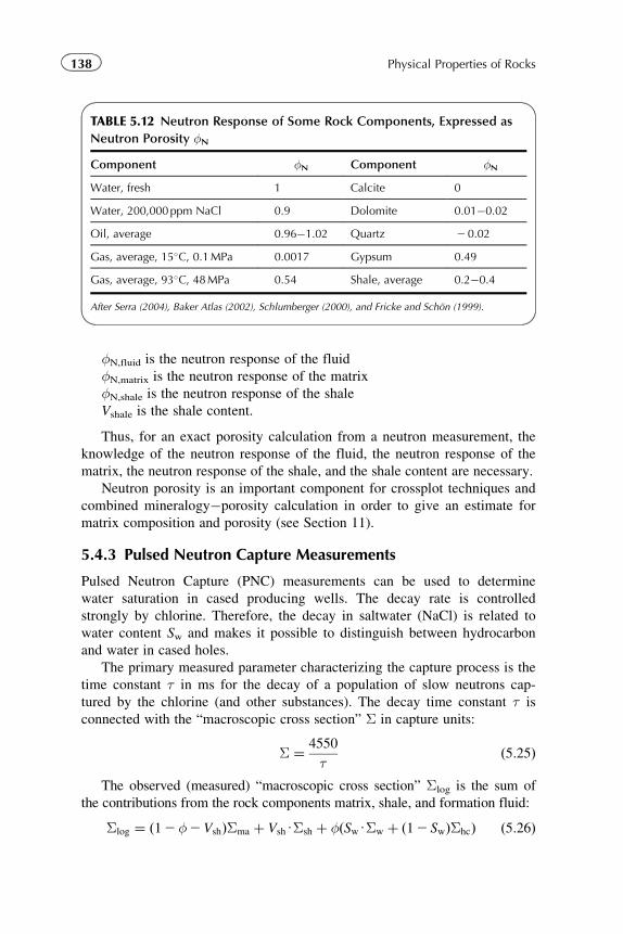
φN,fluid is the neutron response of the fluid
φN,matrix is the neutron response of the matrix
φN,shale is the neutron response of the shale
Vshale is the shale content.
Thus, for an exact porosity calculation from a neutron measurement, the
knowledge of the neutron response of the fluid, the neutron response of the
matrix, the neutron response of the shale, and the shale content are necessary.
Neutron porosity is an important component for crossplot techniques and
combined mineralogy�porosity calculation in order to give an estimate for
matrix composition and porosity (see Section 11).
5.4.3 Pulsed Neutron Capture Measurements
Pulsed Neutron Capture (PNC) measurements can be used to determine
water saturation in cased producing wells. The decay rate is controlled
strongly by chlorine. Therefore, the decay in saltwater (NaCl) is related to
water content Sw and makes it possible to distinguish between hydrocarbon
and water in cased holes.
The primary measured parameter characterizing the capture process is the
time constant τ in ms for the decay of a population of slow neutrons cap-
tured by the chlorine (and other substances). The decay time constant τ is
connected with the “macroscopic cross section” Σ in capture units:
Σ ¼ 4550
τð5:25Þ
The observed (measured) “macroscopic cross section” Σlog is the sum of
the contributions from the rock components matrix, shale, and formation fluid:
Σlog ¼ ð12φ2VshÞΣma þ VshUΣsh þ φðSwUΣw þ ð12 SwÞΣhcÞ ð5:26Þ
TABLE 5.12 Neutron Response of Some Rock Components, Expressed as
Neutron Porosity φN
Component φN Component φN
Water, fresh 1 Calcite 0
Water, 200,000ppm NaCl 0.9 Dolomite 0.01�0.02
Oil, average 0.96�1.02 Quartz 2 0.02
Gas, average, 15�C, 0.1MPa 0.0017 Gypsum 0.49
Gas, average, 93�C, 48MPa 0.54 Shale, average 0.2�0.4
After Serra (2004), Baker Atlas (2002), Schlumberger (2000), and Fricke and Schon (1999).
138 Physical Properties of Rocks
For water saturation, this results in
Sw ¼ Σlog 2Σma 2VshðΣsh 2ΣmaÞ2φðΣhc 2ΣmaÞφðΣw 2ΣhcÞ
ð5:27Þ
where
Sw is water saturation
φ is porosity
Σlog is the recorded capture cross section of the formation
Σma is the capture cross section of the rock matrix
Σsh is the capture cross section of the shale
Σw is the capture cross section of the formation water
Σhc is the capture cross section of the hydrocarbon.
In practical applications for water saturation determination, it can often
be assumed that the properties φ, Σma, Σsh, Σhc, Σw (controlled by salinity)
are constant. If this is the case, then the variation of measured Σlog directly
reflects the variation of Sw. If the properties are known (from openhole inter-
pretation), then a quantitative determination of Sw is possible.
Mean values for the magnitude of the cross section are:
� Σma� 4�10 cu (capture units)� Σsh� 10�50 cu� Σw� 70�200 cu (depends on chlorine content)� Ehc� 17�22 cu.
5.5 APPLICATION OF NUCLEAR MEASUREMENTS FOR AMINERAL ANALYSIS
5.5.1 Introduction
Determination of mineral composition (mineralogy) of a rock is of funda-
mental importance particularly in reservoir characterization. Mineral compo-
sition controls “matrix properties” and directly controls the accuracy of
derived porosity. But mineral content and composition also give information
about the rock-forming processes and resulting rock properties. In carbonatic
rocks, mineral composition is related to pore space properties and pore type.
Traditional nuclear measurements (natural gammalog, gamma�gamma
log, neutronlog) offer possibilities for an initial classification using defined
characteristic values or tendencies. Examples are:
� shale indication from gammalog and a combination gamma�gamma�density and neutronlog;
� carbonate detection (limestone, dolomite) using neutron�density cross-
plots (Chapter 11), identification of dolomite and/or limestone supported
by photoelectric cross section (PE) measurement;
139Chapter | 5 Nuclear/Radioactive Properties
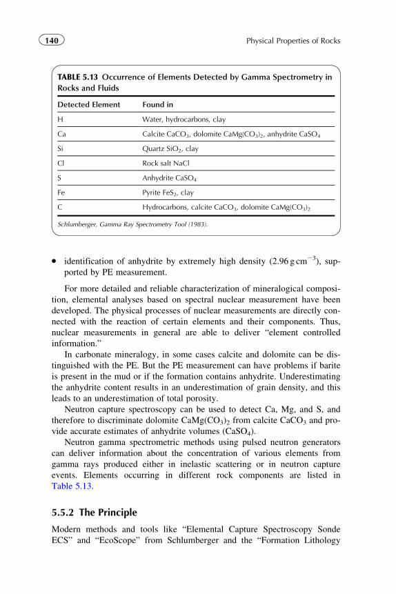
� identification of anhydrite by extremely high density (2.96 g cm23), sup-
ported by PE measurement.
For more detailed and reliable characterization of mineralogical composi-
tion, elemental analyses based on spectral nuclear measurement have been
developed. The physical processes of nuclear measurements are directly con-
nected with the reaction of certain elements and their components. Thus,
nuclear measurements in general are able to deliver “element controlled
information.”
In carbonate mineralogy, in some cases calcite and dolomite can be dis-
tinguished with the PE. But the PE measurement can have problems if barite
is present in the mud or if the formation contains anhydrite. Underestimating
the anhydrite content results in an underestimation of grain density, and this
leads to an underestimation of total porosity.
Neutron capture spectroscopy can be used to detect Ca, Mg, and S, and
therefore to discriminate dolomite CaMg(CO3)2 from calcite CaCO3 and pro-
vide accurate estimates of anhydrite volumes (CaSO4).
Neutron gamma spectrometric methods using pulsed neutron generators
can deliver information about the concentration of various elements from
gamma rays produced either in inelastic scattering or in neutron capture
events. Elements occurring in different rock components are listed in
Table 5.13.
5.5.2 The Principle
Modern methods and tools like “Elemental Capture Spectroscopy Sonde
ECS” and “EcoScope” from Schlumberger and the “Formation Lithology
TABLE 5.13 Occurrence of Elements Detected by Gamma Spectrometry in
Rocks and Fluids
Detected Element Found in
H Water, hydrocarbons, clay
Ca Calcite CaCO3, dolomite CaMg(CO3)2, anhydrite CaSO4
Si Quartz SiO2, clay
Cl Rock salt NaCl
S Anhydrite CaSO4
Fe Pyrite FeS2, clay
C Hydrocarbons, calcite CaCO3, dolomite CaMg(CO3)2
Schlumberger, Gamma Ray Spectrometry Tool (1983).
140 Physical Properties of Rocks
eXplorer (FLeX)” device in combination with the interpretation system
“RockView” from Baker Atlas determine certain elemental concentrations
and calculate—based on a model assumption—mineral composition.
Fundamental papers are written, for example, by Hertzog et al. (1987),
Gilchrist et al. (1999, 2000), Barson et al. (2005), Pemper et al. (2006), and
Han et al. (2009).
Nuclear spectroscopy methods deliver weight fractions of certain ele-
ments (see below), but of course, they cannot deliver a full mineral analysis.
Therefore, the link to the rock type requires use of a typical mineral compo-
sition (model) in terms of the detectable elements. In practice typical groups
are used, such as:
� lithologic fractions of total clay, total carbonate, and quartz, feldspar, and
mica (QFM);� lithologic categories of sand, shale, coal, carbonates, and evaporates.
The delivered concentration of certain elements includes:
� some of the most diagnostic and abundant elements in sedimentary rocks,
in particular Si, Ca, Fe, S;� some diagnostic but not frequently abundant elements like titanium (Ti)
and gadolinium (Gd);� (qualitatively) H and Cl.
In many cases, the transformation from elements to minerals requires an
accurate clay content determination followed by an analysis combining the
remaining minerals into groups and more detailed composition. The algo-
rithms use mineral standard samples.
5.5.3 Description of the Algorithm Used for the Atlas RockViewAnalysis
The interpretation is characterized by the following main steps (Pemper
et al., 2006):
Elements-general lithology-specific lithology-mineralogy
Measurement of Elemental Concentration
The nuclear logging system uses a pulsed neutron source and measures both
inelastic and capture gamma-ray energy spectra. A matrix inversion spectral
fit algorithm is used to analyze these spectra in order to separate the total
response into its individual elemental components.
The prominent measured elements associated with subsurface rock forma-
tions include calcium, silicon, magnesium, carbon, sulfur, aluminum, and
141Chapter | 5 Nuclear/Radioactive Properties
iron. Potassium, thorium, and uranium are measured separately with a natural
gamma-ray spectroscopy instrument.
As a result, the tool and data processing measures (detects and
quantifies):
� from natural gamma-ray energy spectrum: K, U, Th;� from capture spectrum: Ca, Si, S, Fe, Ti, Gd, Mn;� from inelastic spectrum: Si, Mg, Al, C.
Two notes may be added:
1. The final Si content, a very important element, is derived from both
capture and inelastic spectra.
2. Some other elements have signals in both capture and inelastic spectra,
but sometimes only one of them gives a usable signal. For example, alu-
minum is present within the capture spectrum, but its low capture cross
section makes it difficult to quantify. A similar problem exists for capture
magnesium. Both of these elements can be characterized using the inelas-
tic spectrum (Pemper et al., 2006).
Derivation of General Lithology
Lithologies are divided into general categories including sand, shale, coal,
carbonates, and evaporites. The tool response is characterized for each ele-
ment by placing it into formations of known chemical composition.
Figure 5.11 shows capture and inelastic spectra for the general basic
lithologies.
Some general observations are:
� whereas Ca and C energy peaks are prevalent in the limestone forma-
tions, Si stands out in the sandstone,� Ca, Mg, and C can be observed in the dolomite, and Ca and S can be dis-
tinguished in the anhydrite,� Al energy peaks stand out in shale formations due to the presence of clay
and feldspar.
In general, these energy spectra provide a visual display of the physical
characteristics that are exploited in the mathematical analysis of gamma-ray
spectroscopy. Thus, based upon the chemical composition of the formation,
each depth interval is classified into one of five categories: sand, shale, coal,
carbonate, evaporate.
Derivation of Specific Lithologies and Mineral Composition
The general categories (sand, shale, coal, carbonate, evaporate) are the basis
for more detailed assessment of the specific lithology. A carbonate, for
example, is concluded to be calcite or dolomite depending on the amounts of
calcium and magnesium. The purpose of the middle step is to provide the
142 Physical Properties of Rocks
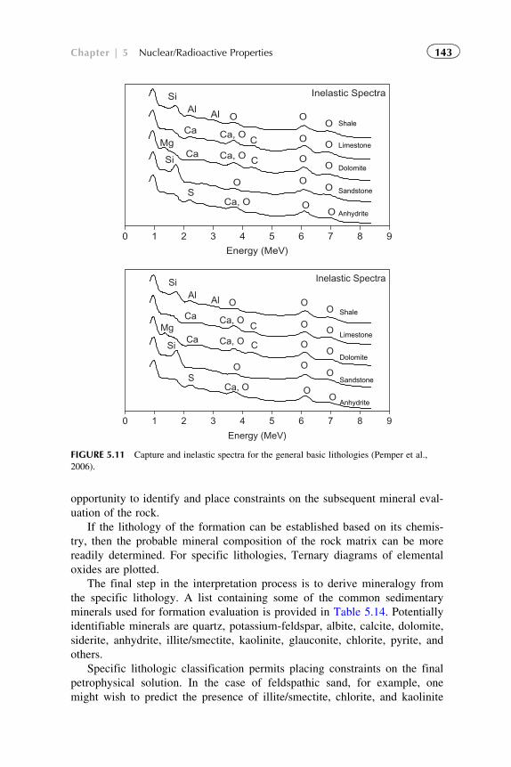
opportunity to identify and place constraints on the subsequent mineral eval-
uation of the rock.
If the lithology of the formation can be established based on its chemis-
try, then the probable mineral composition of the rock matrix can be more
readily determined. For specific lithologies, Ternary diagrams of elemental
oxides are plotted.
The final step in the interpretation process is to derive mineralogy from
the specific lithology. A list containing some of the common sedimentary
minerals used for formation evaluation is provided in Table 5.14. Potentially
identifiable minerals are quartz, potassium-feldspar, albite, calcite, dolomite,
siderite, anhydrite, illite/smectite, kaolinite, glauconite, chlorite, pyrite, and
others.
Specific lithologic classification permits placing constraints on the final
petrophysical solution. In the case of feldspathic sand, for example, one
might wish to predict the presence of illite/smectite, chlorite, and kaolinite
0 1 2 3 4 5 6 7 8 9
Energy (MeV)
Shale
Limestone
Dolomite
Sandstone
Anhydrite
SCa, O O
O
Si
O OO
OO
OO
OO
SiAl Al O
Ca Ca, OCMg
Ca, O CCa
Inelastic Spectra
0 1 2 3 4 5 6 7 8 9
Energy (MeV)
Shale
Limestone
Dolomite
Sandstone
Anhydrite
SCa, O O
O
Si
O OO
OO
OO
OO
SiAl Al O
Ca Ca, OCMg
Ca, O CCa
Inelastic Spectra
FIGURE 5.11 Capture and inelastic spectra for the general basic lithologies (Pemper et al.,
2006).
143Chapter | 5 Nuclear/Radioactive Properties
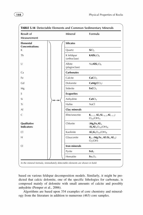
based on various feldspar decomposition models. Similarly, it might be pre-
dicted that calcic dolomite, one of the specific lithologies for carbonate, is
composed mainly of dolomite with small amounts of calcite and possibly
anhydrite (Pemper et al., 2006).
Algorithms are based upon 334 examples of core chemistry and mineral-
ogy from the literature in addition to numerous (463) core samples.
TABLE 5.14 Detectable Elements and Common Sedimentary Minerals
Result of
Measurement
Mineral Formula
ElementalConcentrations:
Silicates
K Quartz SiO2
Th K feldspar(orthoclase)
KAlSi3O8
U Albite(plagioclase)
NaAlSi3O8
Ca Carbonates
Fe Calcite CaCO3
Gd Dolomite CaMg(CO3)
Mg Siderite FeCO3
S Evaporites
Si Anhydrite CaSO4
Ti Halite NaCl
Al Clay minerals
C Illite/smectite K1-1.5 Al4(Si7-6.5,Al1-1.5)O20(OH)4
QualitativeIndicators:
Chlorite (Mg,Fe,Al)6(Si,Al)4O10(OH)8
Cl Kaolinite Al4Si4O10(OH)8
H Glauconite K0.7(Mg,Fe2,Al)(Si4,Al10)O2(OH)
O Iron minerals
Pyrite FeS2
Hematite Fe2O3
In the mineral formula, immediately detectable elements are shown in bold.
144 Physical Properties of Rocks
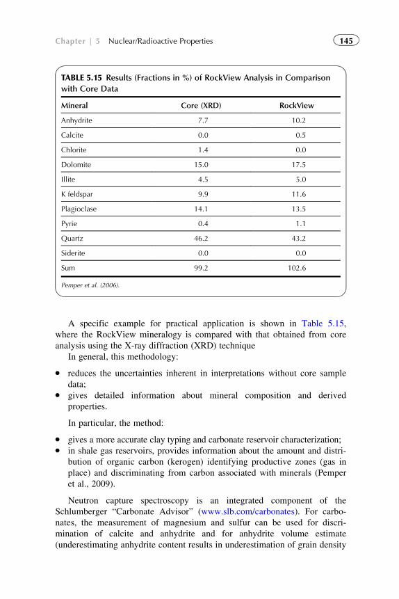
A specific example for practical application is shown in Table 5.15,
where the RockView mineralogy is compared with that obtained from core
analysis using the X-ray diffraction (XRD) technique
In general, this methodology:
� reduces the uncertainties inherent in interpretations without core sample
data;� gives detailed information about mineral composition and derived
properties.
In particular, the method:
� gives a more accurate clay typing and carbonate reservoir characterization;� in shale gas reservoirs, provides information about the amount and distri-
bution of organic carbon (kerogen) identifying productive zones (gas in
place) and discriminating from carbon associated with minerals (Pemper
et al., 2009).
Neutron capture spectroscopy is an integrated component of the
Schlumberger “Carbonate Advisor” (www.slb.com/carbonates). For carbo-
nates, the measurement of magnesium and sulfur can be used for discri-
mination of calcite and anhydrite and for anhydrite volume estimate
(underestimating anhydrite content results in underestimation of grain density
TABLE 5.15 Results (Fractions in %) of RockView Analysis in Comparison
with Core Data
Mineral Core (XRD) RockView
Anhydrite 7.7 10.2
Calcite 0.0 0.5
Chlorite 1.4 0.0
Dolomite 15.0 17.5
Illite 4.5 5.0
K feldspar 9.9 11.6
Plagioclase 14.1 13.5
Pyrie 0.4 1.1
Quartz 46.2 43.2
Siderite 0.0 0.0
Sum 99.2 102.6
Pemper et al. (2006).
145Chapter | 5 Nuclear/Radioactive Properties
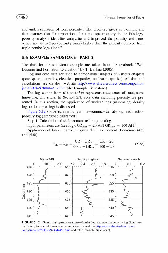
and underestimation of total porosity). The brochure gives an example and
demonstrates that “incorporation of neutron spectrometry in the lithology-
porosity analysis identifies anhydrite and improved the porosity estimates,
which are up to 2 pu (porosity units) higher than the porosity derived from
triple-combo logs alone.”
5.6 EXAMPLE: SANDSTONE—PART 2
The data for the sandstone example are taken from the textbook “Well
Logging and Formation Evaluation” by T. Darling (2005).
Log and core data are used to demonstrate subjects of various chapters
(pore space properties, electrical properties, nuclear properties). All data and
calculations are on the website http://www.elsevierdirect.com/companion.
jsp?ISBN=9780444537966 (file: Example. Sandstone).
The log section from 616 to 645m represents a sequence of sand, some
limestone, and shale. In Section 2.8, core data including porosity are pre-
sented. In this section, the application of nuclear logs (gammalog, density
log, and neutron log) is discussed.
Figure 5.12 shows gammalog, gamma�gamma�density log, and neutron
porosity log (limestone calibrated).
Step 1: Calculation of shale content using gammalog.
Input parameters are (see log): GRmin 5 20 API GRmax 5 100 API
Application of linear regression gives the shale content (Equations (4.5)
and (4.6))
Vsh ¼ IGR ¼ GR2GRcn
GRsh 2GRcn
¼ GR2 20
1002 20ð5:28Þ
615
620
625
630
635
640
645
615
620
625
630
635
640
645
615
620
625
630
635
640
645
0 100 200GR in API
Dep
th in
m
2.2 2.4 2.6 2.8Density in g/cm3
0 0.1 0.2Neutron porosity
FIGURE 5.12 Gammalog, gamma�gamma�density log, and neutron porosity log (limestone
calibrated) for a sandstone-shale section (visit the website http://www.elsevierdirect.com/
companion.jsp?ISBN=9780444537966 and refer Example. Sandstone).
146 Physical Properties of Rocks
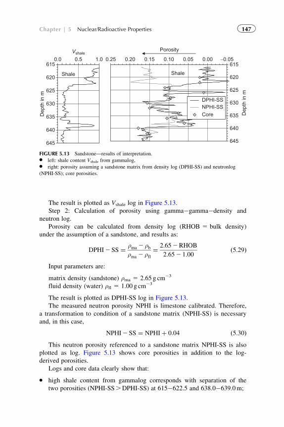
The result is plotted as Vshale log in Figure 5.13.
Step 2: Calculation of porosity using gamma�gamma�density and
neutron log.
Porosity can be calculated from density log (RHOB 5 bulk density)
under the assumption of a sandstone, and results as:
DPHI2 SS ¼ ρma 2 ρbρma 2 ρfl
¼ 2:652RHOB
2:652 1:00ð5:29Þ
Input parameters are:
matrix density (sandstone) ρma 5 2.65 g cm23
fluid density (water) ρfl 5 1.00 g cm23
The result is plotted as DPHI-SS log in Figure 5.13.
The measured neutron porosity NPHI is limestone calibrated. Therefore,
a transformation to condition of a sandstone matrix (NPHI-SS) is necessary
and, in this case,
NPHI2 SS ¼ NPHIþ 0:04 ð5:30ÞThis neutron porosity referenced to a sandstone matrix NPHI-SS is also
plotted as log. Figure 5.13 shows core porosities in addition to the log-
derived porosities.
Logs and core data clearly show that:
� high shale content from gammalog corresponds with separation of the
two porosities (NPHI-SS.DPHI-SS) at 615�622.5 and 638.0�639.0m;
615
620
625
630
635
640
645
0.0 0.5 1.0
Vshale
Dep
th in
m
Shale
615
620
625
630
635
640
645
−0.050.000.050.100.150.200.25
Dep
th in
m
DPHI-SSNPHI-SSCore
Porosity
Shale
FIGURE 5.13 Sandstone—results of interpretation.� left: shale content Vshale from gammalog,� right: porosity assuming a sandstone matrix from density log (DPHI-SS) and neutronlog
(NPHI-SS); core porosities.
147Chapter | 5 Nuclear/Radioactive Properties
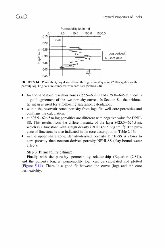
� for the sandstone reservoir zones 622.5�638.0 and 639.0�645m, there is
a good agreement of the two porosity curves. In Section 8.4 the arithme-
tic mean is used for a following saturation calculation;� within the reservoir zones porosity from logs fits well core porosities and
confirms the calculation;� at 625.5�626.5m log porosities are different with negative value for DPHI-
SS. This results from the different matrix of the layer (625.5�626.5m),
which is a limestone with a high density (RHOB� 2.72g cm23). The pres-
ence of limestone is also indicated in the core description in Table 2-13;� in the upper shale zone, density-derived porosity DPHI-SS is closer to
core porosity than neutron-derived porosity NPHI-SS (clay-bound water
effect).
Step 3: Permeability estimate.
Finally with the porosity�permeability relationship (Equation (2.84)),
and the porosity log, a “permeability log” can be calculated and plotted
(Figure 5.14). There is a good fit between the curve (log) and the core
permeability.
615
620
625
630
635
640
645
0.1 1.0 10.0 100.0 1000.0
Permeability kh in md
Dep
th in
m
Log derived
Core data
Shale
FIGURE 5.14 Permeability log derived from the regression (Equation (2.88)) applied on the
porosity log. Log data are compared with core data (Section 2.8).
148 Physical Properties of Rocks
Chapter 6
Elastic Properties
6.1 FUNDAMENTALS
6.1.1 Elastic Moduli and Elastic Wave Velocities
The theory of elasticity (see, for example, Landau and Lifshitz, 1965) gives
the basis for the description of elastic wave propagation.
Hooke’s law describes the relationship between stress and strain of an
elastic material. In a general formulation, the stress�strain relationship is a
tensorial equation:
σik ¼ Ciklmεlm ð6:1Þwhere
σik is the stress tensor
εik is the strain tensor
Ciklm is the elastic modulus (or stiffness) tensor.
If strain is expressed as a function of stress, the resulting strain�stress
relationship is
εik ¼ Diklmσlm ð6:2Þwhere Diklm is the elastic compliance tensor.
Frequently, an abbreviated notation is applied for the tensor components.
The four subscripts of the stiffness and compliance tensor are reduced to two
as follows: the pairs ij(kl) are replaced by one index m(n)
ij(kl ) 11 22 33 23, 32 13, 31 12, 21m(n) 1 2 3 4 5 6
149Physical Properties of Rocks.
© 2011 Elsevier B.V. All rights reserved.
For an isotropic material, the number of independent constants reduces to
two and the tensor of elasticity has the form
c11 c12 c12 0 0 0
c12 c11 c12 0 0 0
c12 c12 c11 0 0 0
0 0 0 c44 0 0
0 0 0 0 c44 0
0 0 0 0 0 c44
26666664
37777775
with c12 ¼ c11 2 2c44 ð6:3Þ
The relationship between the components and the Lame parameters
λ,μ are
c11 ¼ λþ 2μ c12 ¼ λ c44 ¼ μ ð6:4ÞBesides the Lame parameters λ,μ, any pair of two of the following moduli
can be used for a description of the elastic properties of an isotropic
material:
Young’s modulus E, defined as ratio of stress to strain in a uniaxial stress
state;
compressional wave modulus M, defined as ratio of stress to strain in a
uniaxial strain state;
bulk compressional modulus k, defined as ratio of hydrostatic stress to
volumetric strain1;
shear modulus μ, defined as ratio of shear stress to shear strain;
Poisson’s ratio v, defined as the (negative) ratio of lateral strain to axial
strain in a uniaxial stress state.
Note again that for a complete description, only two parameters are nec-
essary. Table 6.1 gives the conversion from one set of parameters to any
other.
Corresponding to the two moduli are two independent body waves:
Compressional, longitudinal, or P-wave with the velocity:
VP ¼ffiffiffiffiffiM
ρ
s¼
ffiffiffiffiffiffiffiffiffiffiffiffiffiffiffiffiffiffiffiffiffiffiffiffiffiffiffiffiffiffiffiffiffiffiffiE
ρ12 ν
ð1þ νÞð12 2νÞ
s¼
ffiffiffiffiffiffiffiffiffiffiffiffiffiffiλþ 2μ
ρ
s¼
ffiffiffiffiffiffiffiffiffiffiffiffiffiffiffiffiffiffiffiffiffiffik þ ð4=3Þμ
ρ
sð6:5Þ
Shear, transversal, or S-wave with the velocity:
VS ¼ffiffiffiμρ
r¼
ffiffiffiffiffiffiffiffiffiffiffiffiffiffiffiffiffiffiffiffiffiE
ρ1
2ð1þ νÞ
sð6:6Þ
where ρ is the bulk density.
1Compressibility is the inverse of compressional modulus.
150 Physical Properties of Rocks
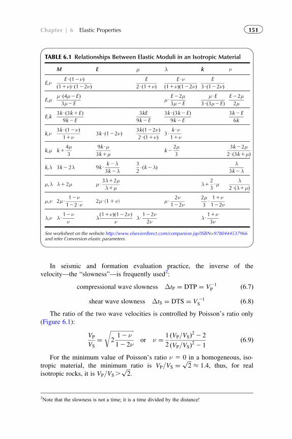
In seismic and formation evaluation practice, the inverse of the
velocity—the “slowness”—is frequently used2:
compressional wave slowness ΔtP ¼ DTP ¼ V21P ð6:7Þ
shear wave slowness ΔtS ¼ DTS ¼ V 21S ð6:8Þ
The ratio of the two wave velocities is controlled by Poisson’s ratio only
(Figure 6.1):
VP
VS
¼ffiffiffiffiffiffiffiffiffiffiffiffiffiffiffiffiffi212 ν12 2ν
ror ν ¼ 1
2
ðVP=VSÞ2 2 2
ðVP=VSÞ2 2 1ð6:9Þ
For the minimum value of Poisson’s ratio ν 5 0 in a homogeneous, iso-
tropic material, the minimum ratio is VP=VS ¼ffiffiffi2
p� 1:4; thus, for real
isotropic rocks, it is VP=VS.ffiffiffi2
p:
TABLE 6.1 Relationships Between Elastic Moduli in an Isotropic Material
M E μ λ k ν
E,νEUð12νÞ
ð11νÞUð122νÞE
2Uð11νÞEUν
ð11νÞð122νÞE
3Uð122νÞ
E,μμUð4μ2EÞ3μ2E
μUE22μ3μ2E
μUE3Uð3μ2EÞ
E22μ2μ
E,k3kUð3k1EÞ
9k2E
3kE
9k2E
3kUð3k2EÞ9k2E
3k2E
6k
k,ν3kUð12νÞ
11ν3kUð122νÞ 3kð122νÞ
2Uð11νÞ 3UkUν11ν
k,μ k14μ3
9kUμ3k1μ
k22μ3
3k22μ2Uð3k1μÞ
k,λ 3k2 2λ 9kUk2λ3k2λ
3
2Uðk2λÞ λ
3k2λ
μ,λ λ12μ μU3λ12μλ1μ
λ12
3Uμ
λ2Uðλ1μÞ
μ,ν 2μU12ν122Uν
2μU(11 ν) μU2ν
122ν2μ3U11ν122ν
λ,ν λU12νν
λð11νÞð122νÞ
νλU
122ν2ν
λU11ν3ν
See worksheet on the website http://www.elsevierdirect.com/companion.jsp?ISBN=9780444537966and refer Conversion elastic parameters.
2Note that the slowness is not a time; it is a time divided by the distance!
151Chapter | 6 Elastic Properties
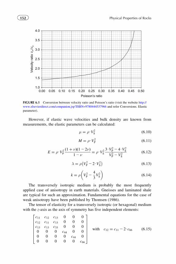
However, if elastic wave velocities and bulk density are known from
measurements, the elastic parameters can be calculated:
μ ¼ ρUV2S ð6:10Þ
M ¼ ρUV2P ð6:11Þ
E ¼ ρUV2P
ð1þ νÞð12 2νÞ12 ν
¼ ρUV2S
3UV2P 2 4UV2
S
V2P 2V2
S
ð6:12Þ
λ ¼ ρ V2P 2 2UV2
S
� � ð6:13Þ
k ¼ ρ V2P 2
4
3V2S
� �ð6:14Þ
The transversely isotropic medium is probably the most frequently
applied case of anisotropy in earth materials. Gneisses and laminated shale
are typical for such an approximation. Fundamental equations for the case of
weak anisotropy have been published by Thomsen (1986).
The tensor of elasticity for a transversely isotropic (or hexagonal) medium
with the z-axis as the axis of symmetry has five independent elements:
c11 c12 c13 0 0 0
c12 c11 c13 0 0 0
c13 c13 c33 0 0 0
0 0 0 c44 0 0
0 0 0 0 c44 0
0 0 0 0 0 c66
26666664
37777775
with c12 ¼ c11 2 2Uc66 ð6:15Þ
1.0
1.5
2.0
2.5
3.0
3.5
4.0
0.00 0.05 0.10 0.15 0.20 0.25 0.30 0.35 0.40 0.45 0.50
Poisson’s ratio
Vel
ocity
rat
io V
P/V
S
FIGURE 6.1 Conversion between velocity ratio and Poisson’s ratio (visit the website http://
www.elsevierdirect.com/companion.jsp?ISBN=9780444537966 and refer Conversions. Elastic
parameter).
152 Physical Properties of Rocks
In this material there are three modes of wave propagation, and their
velocities are dependent on the angle θ between the axis of symmetry
(z-axis) and the direction of the wave vector (Mavko et al., 1998):
quasi�longitudinal mode VP ¼ffiffiffiffiffiffiffiffiffiffiffiffiffiffiffiffiffiffiffiffiffiffiffiffiffiffiffiffiffiffiffiffiffiffiffiffiffiffiffiffiffiffiffiffiffiffiffiffiffiffiffiffiffiffiffiffiffiffiffiffiffiffiffic11Usin2θþ c33Ucos2θþ c44 þ A
2Uρ
sð6:16Þ
quasi�shear mode VSV ¼ffiffiffiffiffiffiffiffiffiffiffiffiffiffiffiffiffiffiffiffiffiffiffiffiffiffiffiffiffiffiffiffiffiffiffiffiffiffiffiffiffiffiffiffiffiffiffiffiffiffiffiffiffiffiffiffiffiffiffiffiffiffiffic11Usin2θþ c33Ucos2θþ c44 2A
2Uρ
sð6:17Þ
pure shear mode VSH ¼ffiffiffiffiffiffiffiffiffiffiffiffiffiffiffiffiffiffiffiffiffiffiffiffiffiffiffiffiffiffiffiffiffiffiffiffiffiffiffiffiffiffiffic66Usin2θþ c44Ucos2θ
ρ
sð6:18Þ
with A ¼ffiffiffiffiffiffiffiffiffiffiffiffiffiffiffiffiffiffiffiffiffiffiffiffiffiffiffiffiffiffiffiffiffiffiffiffiffiffiffiffiffiffiffiffiffiffiffiffiffiffiffiffiffiffiffiffiffiffiffiffiffiffiffiffiffiffiffiffiffiffiffiffiffiffiffiffiffiffiffiffiffiffiffiffiffiffiffiffiffiffiffiffiffiffiffiffiffiffiffiffiffiffiffiffiffiffiffiffiffiffiffiffi½ðc11 2 c44Þsin2θþ ðc33 2 c44Þcos2θ�2 þ ðc13 þ c44Þ2sin22θ
qð6:19Þ
Pure compressional and shear waves exist only for the propagation in the
main axes:
For θ 5 0�, the relationship is A 5 c332 c44 and velocities are
VP ¼ffiffiffiffiffiffic33
ρ
rVSV ¼
ffiffiffiffiffiffic44
ρ
rVSH ¼
ffiffiffiffiffiffic44
ρ
rð6:20Þ
For θ 5 90�, the relationship is A 5 c112 c44 and velocities are
VP ¼ffiffiffiffiffiffic11
ρ
rVSV ¼
ffiffiffiffiffiffic44
ρ
rVSH ¼
ffiffiffiffiffiffic66
ρ
rð6:21Þ
For the transverse isotropic material, Thomsen (1986) defined the follow-
ing parameters:
ε ¼ c11 2 c33
2Uc33ð‘‘P�wave anisotropy’’Þ ð6:22Þ
γ ¼ c66 2 c44
2Uc44ð‘‘S�wave anisotropy’’Þ ð6:23Þ
δ ¼ ðc13 þ c44Þ2 2 ðc33 2 c44Þ22Uc33ðc33 2 c44Þ
ð6:24Þ
For the determination of the five tensor elements, the following five
velocities (and the density) can be used: VP(0�), VP(90
�), Vp(45�), VSH(90
�),and VSH(0
�) 5 VSV(0�).
c11¼ρUV2Pð90�Þ c33¼ρUV2
Pð0�Þc44¼ρUV2
SHð0�Þ c12¼c1122ρUV2SHð90�Þ
c13¼ffiffiffiffiffiffiffiffiffiffiffiffiffiffiffiffiffiffiffiffiffiffiffiffiffiffiffiffiffiffiffiffiffiffiffiffiffiffiffiffiffiffiffiffiffiffiffiffiffiffiffiffiffiffiffiffiffiffiffiffiffiffiffiffiffiffiffiffiffiffiffiffiffiffiffiffiffiffiffiffiffiffiffiffiffiffiffiffiffiffiffiffiffiffiffiffiffiffiffiffiffiffiffiffiffiffiffiffiffiffiffiffiffiffiffiffiffiffiffiffiffiffiffiffiffiffi4ρ2UV4
Pð45�Þ22ρUV2Pð45�Þðc11þc33þ2c44Þþðc11þc44Þðc33þc44Þ
q22c44
ð6:25Þ
153Chapter | 6 Elastic Properties
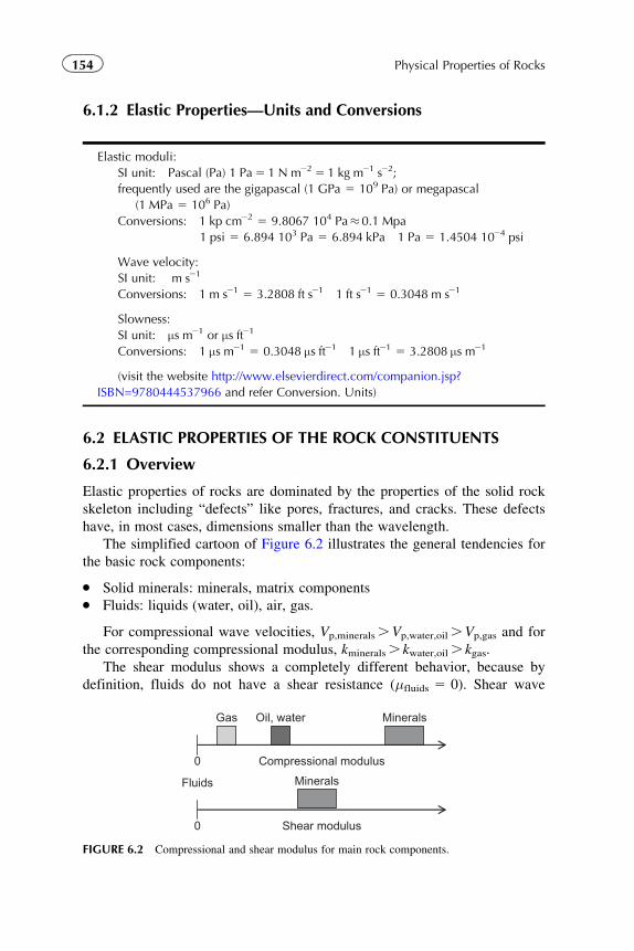
6.1.2 Elastic Properties—Units and Conversions
Elastic moduli:
SI unit: Pascal (Pa) 1 Pa5 1 N m225 1 kg m21 s22;
frequently used are the gigapascal (1 GPa 5 109 Pa) or megapascal
(1 MPa 5 106 Pa)
Conversions: 1 kp cm22 5 9.8067 104 Pa�0.1 Mpa
1 psi 5 6.894 103 Pa 5 6.894 kPa 1 Pa 5 1.4504 1024 psi
Wave velocity:
SI unit: m s21
Conversions: 1 m s21 5 3.2808 ft s21 1 ft s21 5 0.3048 m s21
Slowness:
SI unit: μs m21 or μs ft21
Conversions: 1 μs m21 5 0.3048 μs ft21 1 μs ft21 5 3.2808 μs m21
(visit the website http://www.elsevierdirect.com/companion.jsp?
ISBN=9780444537966 and refer Conversion. Units)
6.2 ELASTIC PROPERTIES OF THE ROCK CONSTITUENTS
6.2.1 Overview
Elastic properties of rocks are dominated by the properties of the solid rock
skeleton including “defects” like pores, fractures, and cracks. These defects
have, in most cases, dimensions smaller than the wavelength.
The simplified cartoon of Figure 6.2 illustrates the general tendencies for
the basic rock components:
� Solid minerals: minerals, matrix components� Fluids: liquids (water, oil), air, gas.
For compressional wave velocities, Vp,minerals.Vp,water,oil.Vp,gas and for
the corresponding compressional modulus, kminerals. kwater,oil. kgas.
The shear modulus shows a completely different behavior, because by
definition, fluids do not have a shear resistance (μfluids 5 0). Shear wave
0 Compressional modulus
Gas Oil, water Minerals
0 Shear modulus
Fluids Minerals
FIGURE 6.2 Compressional and shear modulus for main rock components.
154 Physical Properties of Rocks
velocity therefore shows only a minor dependence on pore fluids via the
density term (see Section 6.5.3).
Immediately the following tendencies result:
� increasing porosity decreases both compressional and shear wave
velocities;� compressional wave velocity is controlled also by the type of pore fluid
(gas, liquid);� shear wave velocity is not strongly controlled by type of pore fluid.
6.2.2 Solid Components, Minerals
Table 6.2 gives an orientation for the magnitude of wave velocities and para-
meters of some rock-forming minerals; the data have been taken from vari-
ous compilations.
We note with respect to:
� the composition of igneous rocks that acid or felsic components have
lower elastic moduli and velocities than basic or mafic components;� the composition of reservoir rocks that there is a significant difference
between the three basic types of matrix substances quartz, calcite, and
dolomite.
6.2.3 Fluids
6.2.3.1 Overview
Pore fluids (gas, oil, and water) usually have distinct ranges of compressional
or bulk modulus (shear modulus of fluids is zero). For orientation, the fol-
lowing ranges are given for compressional bulk modulus kfluid and density
ρfluid:
Gas: kfluid�0.01�0.4 GPa ρfluid�0.1�0.5 �103 kg m23
Oil: kfluid�0.4�3.0 GPa ρfluid�0.7�1.1 �103 kg m23
Water: kfluid�2.0�4.0 GPa ρfluid�0.9�1.2 �103 kg m23
The compressional wave velocity for some fluids is presented in
Table 6.3.
A detailed compilation of seismic properties of fluids and relevant empir-
ical equations to describe the effects of pressure and temperature have been
published by Batzle and Wang (1992) and Wang (2001). In the following
sections, only some selected results are presented; for details, the direct use
of the paper of Batzle and Wang (1992) is recommended.
155Chapter | 6 Elastic Properties
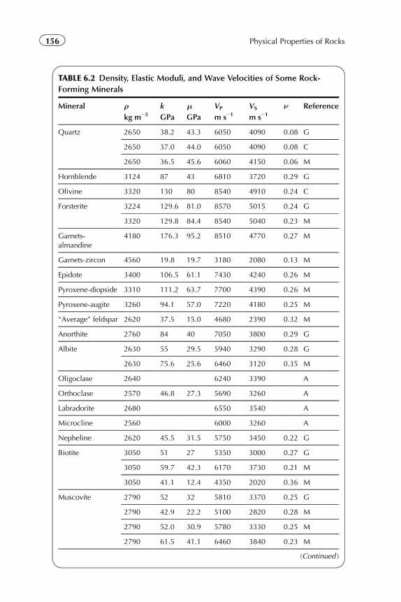
TABLE 6.2 Density, Elastic Moduli, and Wave Velocities of Some Rock-
Forming Minerals
Mineral ρkg m23
k
GPa
μGPa
VP
m s21VS
m s21ν Reference
Quartz 2650 38.2 43.3 6050 4090 0.08 G
2650 37.0 44.0 6050 4090 0.08 C
2650 36.5 45.6 6060 4150 0.06 M
Hornblende 3124 87 43 6810 3720 0.29 G
Olivine 3320 130 80 8540 4910 0.24 C
Forsterite 3224 129.6 81.0 8570 5015 0.24 G
3320 129.8 84.4 8540 5040 0.23 M
Garnets-almandine
4180 176.3 95.2 8510 4770 0.27 M
Garnets-zircon 4560 19.8 19.7 3180 2080 0.13 M
Epidote 3400 106.5 61.1 7430 4240 0.26 M
Pyroxene-diopside 3310 111.2 63.7 7700 4390 0.26 M
Pyroxene-augite 3260 94.1 57.0 7220 4180 0.25 M
“Average” feldspar 2620 37.5 15.0 4680 2390 0.32 M
Anorthite 2760 84 40 7050 3800 0.29 G
Albite 2630 55 29.5 5940 3290 0.28 G
2630 75.6 25.6 6460 3120 0.35 M
Oligoclase 2640 6240 3390 A
Orthoclase 2570 46.8 27.3 5690 3260 A
Labradorite 2680 6550 3540 A
Microcline 2560 6000 3260 A
Nepheline 2620 45.5 31.5 5750 3450 0.22 G
Biotite 3050 51 27 5350 3000 0.27 G
3050 59.7 42.3 6170 3730 0.21 M
3050 41.1 12.4 4350 2020 0.36 M
Muscovite 2790 52 32 5810 3370 0.25 G
2790 42.9 22.2 5100 2820 0.28 M
2790 52.0 30.9 5780 3330 0.25 M
2790 61.5 41.1 6460 3840 0.23 M
(Continued )
156 Physical Properties of Rocks
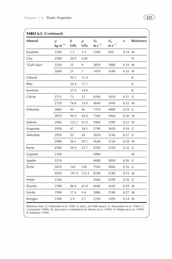
TABLE 6.2 (Continued)
Mineral ρkg m23
k
GPa
μGPa
VP
m s21VS
m s21ν Reference
Kaolinite 1580 1.5 1.4 1440 930 0.14 M
Clay 2580 20.9 6.85 H
“Gulf clays” 2550 25 9 3810 1880 0.34 M
2600 21 7 3410 1640 0.35 M
Chlorite 95.3 11.4 K
Illite 39.4 11.7 K
Kaolinite 37.9 14.8 K
Calcite 2712 73 32 6540 3430 0.31 G
2710 76.8 32.0 6640 3440 0.32 M
Dolomite 2860 94 46 7370 4000 0.29 G
2870 94.9 45.0 7340 3960 0.30 M
Siderite 3960 123.7 51.0 6960 3590 0.32 M
Aragonite 2930 47 38.5 5790 3630 0.18 G
Anhydrite 2970 55 30 5620 3140 0.27 G
2980 56.1 29.1 5640 3130 0.28 M
Barite 4500 54.9 23.7 4350 2250 0.32 G
Gypsum 2350 5800 M
Apatite 3218 6680 3830 0.26 G
Pyrite 5010 143 128 7920 5060 0.16 G
4930 147.4 132.5 8100 5180 0.15 M
Halite 2160 4560 2590 0.26 G
Fluorite 3180 86.4 41.8 6680 3620 0.29 M
Sylvite 1990 17.4 9.4 3880 2180 0.27 M
Kerogen 1300 2.9 2.7 2250 1450 0.14 M
Reference key: G, Gebrande et al. (1982) (k and μ are Hills mean); A, Alexandrov et al. (1966); C,Carmichael (1989); M, data from a compilation by Mavko et al. (1998); H, Helgerud et al. (1999);K, Katahara (1996).
157Chapter | 6 Elastic Properties
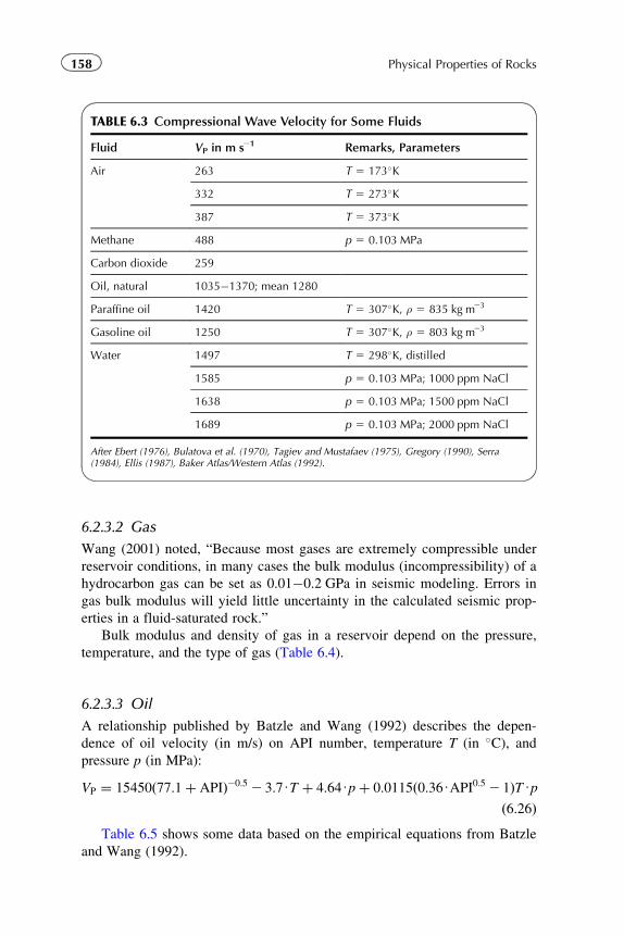
6.2.3.2 Gas
Wang (2001) noted, “Because most gases are extremely compressible under
reservoir conditions, in many cases the bulk modulus (incompressibility) of a
hydrocarbon gas can be set as 0.01�0.2 GPa in seismic modeling. Errors in
gas bulk modulus will yield little uncertainty in the calculated seismic prop-
erties in a fluid-saturated rock.”
Bulk modulus and density of gas in a reservoir depend on the pressure,
temperature, and the type of gas (Table 6.4).
6.2.3.3 Oil
A relationship published by Batzle and Wang (1992) describes the depen-
dence of oil velocity (in m/s) on API number, temperature T (in �C), andpressure p (in MPa):
VP ¼ 15450ð77:1þ APIÞ20:5 2 3:7UT þ 4:64Upþ 0:0115ð0:36UAPI0:5 2 1ÞTUpð6:26Þ
Table 6.5 shows some data based on the empirical equations from Batzle
and Wang (1992).
TABLE 6.3 Compressional Wave Velocity for Some Fluids
Fluid VP in m s21 Remarks, Parameters
Air 263 T 5 173�K
332 T 5 273�K
387 T 5 373�K
Methane 488 p 5 0.103 MPa
Carbon dioxide 259
Oil, natural 1035�1370; mean 1280
Paraffine oil 1420 T 5 307�K, ρ 5 835 kg m23
Gasoline oil 1250 T 5 307�K, ρ 5 803 kg m23
Water 1497 T 5 298�K, distilled
1585 p 5 0.103 MPa; 1000 ppm NaCl
1638 p 5 0.103 MPa; 1500 ppm NaCl
1689 p 5 0.103 MPa; 2000 ppm NaCl
After Ebert (1976), Bulatova et al. (1970), Tagiev and Mustafaev (1975), Gregory (1990), Serra(1984), Ellis (1987), Baker Atlas/Western Atlas (1992).
158 Physical Properties of Rocks
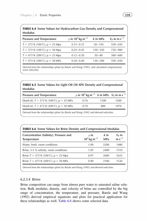
6.2.3.4 Brine
Brine composition can range from almost pure water to saturated saline solu-
tion. Bulk modulus, density, and velocity of brine are controlled by the big
range of concentration, the temperature, and pressure. Batzle and Wang
(1992) derived empirical equations and plots for practical application for
these relationships as well. Table 6.6 shows some selected data.
TABLE 6.4 Some Values for Hydrocarbon Gas Density and Compressional
Modulus
Pressure and Temperature ρ in 103 kg m23 k in MPa VP in m s21
T 5 373�K (100�C); p 5 25 Mpa 0.15�0.35 50�150 550�650
T 5 373�K (100�C); p 5 50 Mpa 0.25�0.45 150�350 750�900
T 5 473�K (200�C); p 5 25 Mpa 0.12�0.30 50�80 500�600
T 5 473�K (200�C); p 5 50 MPa 0.20�0.40 130�200 550�650
Derived from the relationships (plots) by Batzle and Wang (1992), and calculated compressionalwave velocities.
TABLE 6.5 Some Values for Light Oil (50 API) Density and Compressional
Modulus
Pressure and Temperature ρ in 103 kg m23 k in MPa VP in m s21
Dead oil, T 5 373�K (100�C); p 5 25 MPa 0.76 1100 1200
Dead oil, T 5 473�K (200�C); p 5 50 MPa 0.70 800 1070
Derived from the relationships (plots) by Batzle and Wang (1992) and derived velocities.
TABLE 6.6 Some Values for Brine Density and Compressional Modulus
Concentration (Salinity), Pressure and
Temperature
ρ in
103 kg m23
k in
MPa
VP in
m s21
Water, fresh, room conditions 1.00 2200 1480
Brine, 3.5 % salinity, room conditions 1.05 2400 1510
Brine T 5 373�K (100�C); p 5 25 Mpa 0.97 2600 1635
Brine T 5 473�K (200�C); p 5 50 MPa 0.90 2100 1530
Derived from the relationships (plots) by Batzle and Wang (1992) and derived velocities.
159Chapter | 6 Elastic Properties
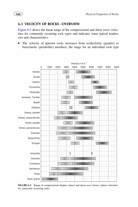
6.3 VELOCITY OF ROCKS�OVERVIEW
Figure 6.3 shows the mean range of the compressional and shear wave veloc-
ities for commonly occurring rock types and indicates some typical tenden-
cies and characteristics:
� The velocity of igneous rocks increases from acidic/felsic (granite) to
basic/mafic (peridodite) members; the range for an individual rock type
0 1000 2000 3000 4000 5000 6000 7000 8000 9000
Granite
Diorite
Gabbro
Pyroxenite
Peridodite
Andesite, Trachite
Basalt
Diabase
Gneiss, parallel
Gneiss, perpendicular
Schist, parallel
Schist, perpendicular
Quartzite
Serpentinite
Eclogite
Anhydrite
Dolomite
Limestone
Sandstone
Shale
Sand, gravel
Velocity in ms−1
FIGURE 6.3 Range of compressional (higher values) and shear wave (lower values) velocities
for commonly occurring rocks.
160 Physical Properties of Rocks
is the result of variation of rock composition (mineral content) and—if
present—fracturing.� Among the metamorphic rocks, gneiss and schist in particular show an
anisotropy with velocity parallel schistosity. velocity perpendicular
schistosity.� Sedimentary porous rocks show a broad range of velocity, where high
velocities are typical for those that are relatively dense (low porosity) and
low velocities are typical for porous (gas-bearing) members.� The lowest velocities have (dry) unconsolidated rocks as a result of the
specific grain�grain contact and high porosity.
There is a broad scatter for porous rocks (influence of porosity, pore
fluid, and mineral composition) in particular and a comparable small range
for a dense rock with well-defined composition (anhydrite).
The ratio of the two wave velocities VP/VS or the Poisson’s ratio ν is con-
trolled mainly by rock type and pore fluid. Figure 6.4 gives an overview
with some tendencies.
6.4 VELOCITY OF IGNEOUS AND METAMORPHIC ROCKS
Velocity of igneous rocks shows an increase from acid/felsic to basic/mafic
rock types. The same tendency shows the density. This gives the background
for an empirical correlation between density and velocity, first published by
Birch (1961) for magmatic rocks (North American continent and India):
VP ¼ 2:76Uρ2 0:98 ð6:27Þ
where the density ρ is in 103 kg m23 (5g cm23) and VP in km s21.
This linear correlation has been applied frequently on various types of
igneous and metamorphic rocks. Two examples may demonstrate this.
Volarovic and Bajuk (1977) derived for rocks from Kazakhstan regres-
sions, which show also the pressure influence:
VP ¼ 3:25Uρ2 3:46 R ¼ 0:85 pressure ¼ 1021 MPa ð6:28Þ
VP ¼ 2:72Uρ2 1:24 R ¼ 0:86 pressure ¼ 102 MPa ð6:29Þ
VP ¼ 2:44Uρ2 0:08 R ¼ 0:85 pressure ¼ 103 MPa ð6:30Þ
Gebrande et al. (1982) analyzed compressional and shear wave velocities
for three rock groups:
VP ¼ 4:36Uρ2 6:736 0:03 VS ¼ 1:66Uρ2 1:486 0:06 plutonic rocks
ð6:31Þ
161Chapter | 6 Elastic Properties
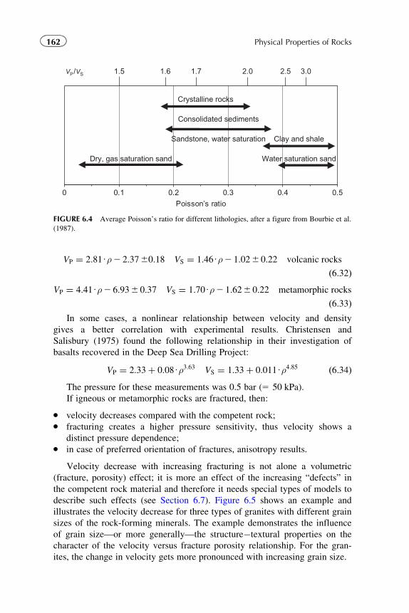
VP ¼ 2:81Uρ2 2:3760:18 VS ¼ 1:46Uρ2 1:026 0:22 volcanic rocks
ð6:32ÞVP ¼ 4:41Uρ2 6:936 0:37 VS ¼ 1:70Uρ2 1:626 0:22 metamorphic rocks
ð6:33ÞIn some cases, a nonlinear relationship between velocity and density
gives a better correlation with experimental results. Christensen and
Salisbury (1975) found the following relationship in their investigation of
basalts recovered in the Deep Sea Drilling Project:
VP ¼ 2:33þ 0:08Uρ3:63 VS ¼ 1:33þ 0:011Uρ4:85 ð6:34ÞThe pressure for these measurements was 0.5 bar (5 50 kPa).
If igneous or metamorphic rocks are fractured, then:
� velocity decreases compared with the competent rock;� fracturing creates a higher pressure sensitivity, thus velocity shows a
distinct pressure dependence;� in case of preferred orientation of fractures, anisotropy results.
Velocity decrease with increasing fracturing is not alone a volumetric
(fracture, porosity) effect; it is more an effect of the increasing “defects” in
the competent rock material and therefore it needs special types of models to
describe such effects (see Section 6.7). Figure 6.5 shows an example and
illustrates the velocity decrease for three types of granites with different grain
sizes of the rock-forming minerals. The example demonstrates the influence
of grain size—or more generally—the structure�textural properties on the
character of the velocity versus fracture porosity relationship. For the gran-
ites, the change in velocity gets more pronounced with increasing grain size.
0 0.1 0.2 0.3 0.4 0.5
Poisson’s ratio
Crystalline rocks
Consolidated sediments
Sandstone, water saturation Clay and shale
Dry, gas saturation sand Water saturation sand
VP/VS 1.5 1.6 1.7 2.0 2.5 3.0
FIGURE 6.4 Average Poisson’s ratio for different lithologies, after a figure from Bourbie et al.
(1987).
162 Physical Properties of Rocks
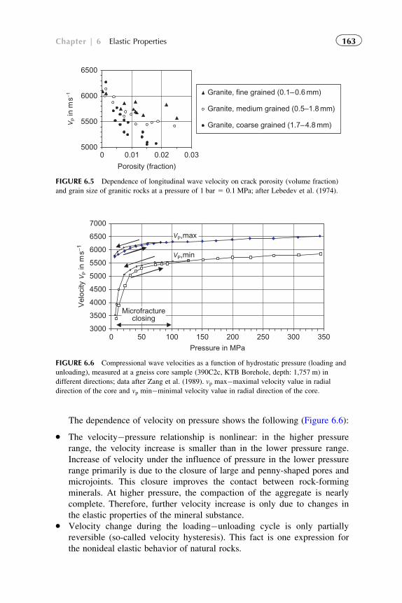
The dependence of velocity on pressure shows the following (Figure 6.6):
� The velocity�pressure relationship is nonlinear: in the higher pressure
range, the velocity increase is smaller than in the lower pressure range.
Increase of velocity under the influence of pressure in the lower pressure
range primarily is due to the closure of large and penny-shaped pores and
microjoints. This closure improves the contact between rock-forming
minerals. At higher pressure, the compaction of the aggregate is nearly
complete. Therefore, further velocity increase is only due to changes in
the elastic properties of the mineral substance.� Velocity change during the loading�unloading cycle is only partially
reversible (so-called velocity hysteresis). This fact is one expression for
the nonideal elastic behavior of natural rocks.
5000
5500
6000
6500
0 0.01 0.02 0.03
Porosity (fraction)
VP in
ms−1 Granite, fine grained (0.1–0.6 mm)
Granite, medium grained (0.5–1.8 mm)
Granite, coarse grained (1.7–4.8 mm)
FIGURE 6.5 Dependence of longitudinal wave velocity on crack porosity (volume fraction)
and grain size of granitic rocks at a pressure of 1 bar 5 0.1 MPa; after Lebedev et al. (1974).
3000
3500
4000
4500
5000
5500
6000
6500
7000
0 50 100 150 200 250 300 350
Pressure in MPa
Vel
ocity
VP in
ms−1
VP,min
Microfractureclosing
VP,max
FIGURE 6.6 Compressional wave velocities as a function of hydrostatic pressure (loading and
unloading), measured at a gneiss core sample (390C2c, KTB Borehole, depth: 1,757 m) in
different directions; data after Zang et al. (1989). vp max�maximal velocity value in radial
direction of the core and vp min�minimal velocity value in radial direction of the core.
163Chapter | 6 Elastic Properties
� Velocity anisotropy (difference of the two curves) is stronger in the low-
pressure region and becomes smaller in the high-pressure region. This is
caused by the fracture-closing process: anisotropy in the low-pressure
range is originated by fracture orientation and intrinsic mineral orienta-
tion, but anisotropy in the high-pressure range is only an intrinsic effect.
In magmatic and metamorphic rocks, increasing temperature generally
leads to decreasing velocities. The main causes of the velocity change are:
� temperature dependence of the elastic properties of the rock-forming
minerals and phase change of minerals;� temperature dependence of the elastic properties of the pore constituents
and change of pore constituents (e.g., pore water) from a liquid to a gas-
eous state;� changes in the contact conditions at grains, crack boundaries, etc., result-
ing from variations of the interface effects and/or from different thermal
expansion properties of rock-forming minerals.
For temperatures up to approximately 150�C, the change of fluid proper-
ties dominates, but at higher temperatures mineral and contact effects are
dominant.
6.5 VELOCITY OF SEDIMENTARY ROCKS
With respect to the velocity and its behavior, there are two types of sedimen-
tary rocks:
1. Dense rocks without pores (anhydrite, salt) with a well-defined velocity
that is controlled by the mineral properties and composition.
2. Porous rocks with a velocity range with strong influence of the porosity
and pore fluid, but also contact properties of solid rock components
(ranging from strong cemented rocks to unconsolidated rocks), and the
mineral composition (sandstone, dolomite, limestone, shale influence).
Of particular interest as reservoir rocks is the second group; the diversity
of influences originates the variety of relationships and correlations. The fol-
lowing sections focus on these relationships. Dominant are:
� mineralogical composition of the rock matrix;� consolidation and cementation of the rock matrix;� porosity, pore shape, and pore content;� pressure and temperature.
Additionally, fracturing can significantly influence properties of carbon-
ate rocks. Structure and texture lead to different types of anisotropy in the
elastic properties.
164 Physical Properties of Rocks
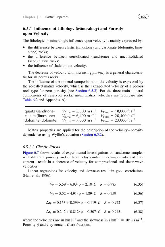
6.5.1 Influence of Lithology (Mineralogy) and Porosityupon Velocity
The lithologic or mineralogic influence upon velocity is mainly expressed by:
� the difference between clastic (sandstone) and carbonate (dolomite, lime-
stone) rocks;� the difference between consolidated (sandstone) and unconsolidated
(sand) clastic rocks;� the influence of shale on the velocity.
The decrease of velocity with increasing porosity is a general characteris-
tic for all porous rocks.
The influence of the mineral composition on the velocity is expressed by
the so-called matrix velocity, which is the extrapolated velocity of a porous
rock type for zero porosity (see Section 6.5.2). For the three main mineral
components of reservoir rocks, mean matrix velocities are (compare also
Table 6.2 and Appendix A):
quartz (sandstone) VP,ma 5 5,500 m s21 VP,ma 5 18,000 ft s21
calcite (limestone) Vp,ma 5 6,400 m s21 Vp,ma 5 20,400 ft s21
dolomite (dolomite) VP,ma 5 7,000 m s21 VP,ma 5 23,000 ft s21
Matrix properties are applied for the description of the velocity�porosity
dependence using Wyllie’s equation (Section 6.5.2).
6.5.1.1 Clastic Rocks
Figure 6.7 shows results of experimental investigations on sandstone samples
with different porosity and different clay content. Both—porosity and clay
content—result in a decrease of velocity for compressional and shear wave
velocities.
Linear regressions for velocity and slowness result in good correlations
(Han et al., 1986):
VP ¼ 5:592 6:93Uφ2 2:18UC R ¼ 0:985 ð6:35Þ
VS ¼ 3:522 4:91Uφ2 1:89UC R ¼ 0:959 ð6:36Þ
ΔtP ¼ 0:163þ 0:399Uφþ 0:119UC R ¼ 0:972 ð6:37Þ
ΔtS ¼ 0:242þ 0:812Uφþ 0:307UC R ¼ 0:945 ð6:38Þ
where the velocities are in km s21 and the slowness in s km21 5 103 μs m21.
Porosity φ and clay content C are fractions.
165Chapter | 6 Elastic Properties
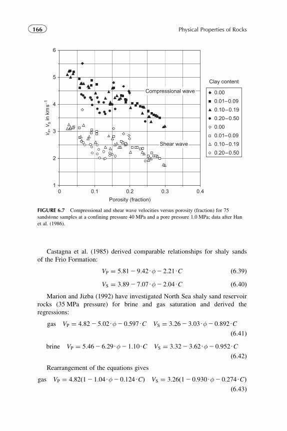
Castagna et al. (1985) derived comparable relationships for shaly sands
of the Frio Formation:
VP ¼ 5:812 9:42Uφ2 2:21UC ð6:39ÞVS ¼ 3:892 7:07Uφ2 2:04UC ð6:40Þ
Marion and Jizba (1992) have investigated North Sea shaly sand reservoir
rocks (35 MPa pressure) for brine and gas saturation and derived the
regressions:
gas VP ¼ 4:822 5:02Uφ2 0:597UC VS ¼ 3:262 3:03Uφ2 0:892UC
ð6:41Þbrine VP ¼ 5:462 6:29Uφ2 1:10UC VS ¼ 3:322 3:62Uφ2 0:952UC
ð6:42ÞRearrangement of the equations gives
gas VP ¼ 4:82ð12 1:04Uφ2 0:124UCÞ VS ¼ 3:26ð12 0:930Uφ2 0:274UCÞð6:43Þ
1
2
3
4
5
6
0 0.1 0.2 0.3 0.4
Porosity (fraction)
VP, V
S in
km
s−1
Compressional wave
Shear wave
0.00
0.01–0.09
0.10–0.19
0.20–0.50
0.00
0.01–0.09
0.10–0.19
0.20–0.50
Clay content
FIGURE 6.7 Compressional and shear wave velocities versus porosity (fraction) for 75
sandstone samples at a confining pressure 40 MPa and a pore pressure 1.0 MPa; data after Han
et al. (1986).
166 Physical Properties of Rocks
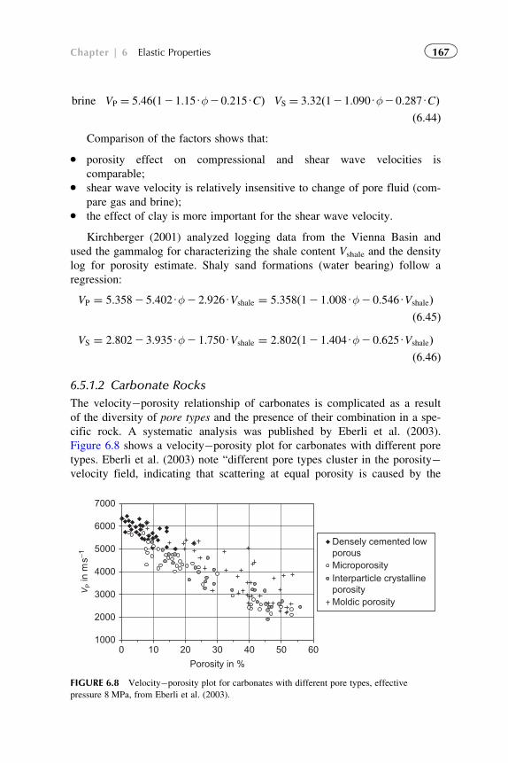
brine VP ¼ 5:46ð121:15Uφ20:215UCÞ VS ¼ 3:32ð121:090Uφ20:287UCÞð6:44Þ
Comparison of the factors shows that:
� porosity effect on compressional and shear wave velocities is
comparable;� shear wave velocity is relatively insensitive to change of pore fluid (com-
pare gas and brine);� the effect of clay is more important for the shear wave velocity.
Kirchberger (2001) analyzed logging data from the Vienna Basin and
used the gammalog for characterizing the shale content Vshale and the density
log for porosity estimate. Shaly sand formations (water bearing) follow a
regression:
VP ¼ 5:3582 5:402Uφ2 2:926UVshale ¼ 5:358ð12 1:008Uφ2 0:546UVshaleÞð6:45Þ
VS ¼ 2:8022 3:935Uφ2 1:750UVshale ¼ 2:802ð12 1:404Uφ2 0:625UVshaleÞð6:46Þ
6.5.1.2 Carbonate Rocks
The velocity�porosity relationship of carbonates is complicated as a result
of the diversity of pore types and the presence of their combination in a spe-
cific rock. A systematic analysis was published by Eberli et al. (2003).
Figure 6.8 shows a velocity�porosity plot for carbonates with different pore
types. Eberli et al. (2003) note “different pore types cluster in the porosity�velocity field, indicating that scattering at equal porosity is caused by the
1000
2000
3000
4000
5000
6000
7000
0 10 20 30 40 50 60
Porosity in %
VP in
ms−1
Densely cemented lowporousMicroporosityInterparticle crystallineporosityMoldic porosity
FIGURE 6.8 Velocity�porosity plot for carbonates with different pore types, effective
pressure 8 MPa, from Eberli et al. (2003).
167Chapter | 6 Elastic Properties
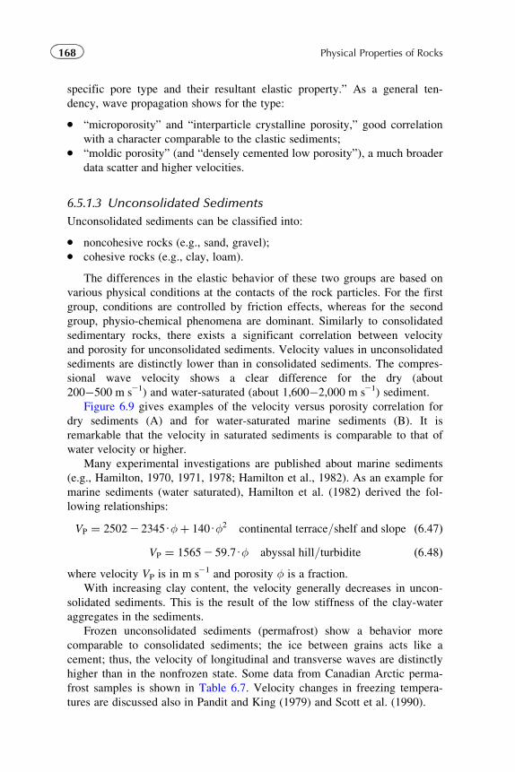
specific pore type and their resultant elastic property.” As a general ten-
dency, wave propagation shows for the type:
� “microporosity” and “interparticle crystalline porosity,” good correlation
with a character comparable to the clastic sediments;� “moldic porosity” (and “densely cemented low porosity”), a much broader
data scatter and higher velocities.
6.5.1.3 Unconsolidated Sediments
Unconsolidated sediments can be classified into:
� noncohesive rocks (e.g., sand, gravel);� cohesive rocks (e.g., clay, loam).
The differences in the elastic behavior of these two groups are based on
various physical conditions at the contacts of the rock particles. For the first
group, conditions are controlled by friction effects, whereas for the second
group, physio-chemical phenomena are dominant. Similarly to consolidated
sedimentary rocks, there exists a significant correlation between velocity
and porosity for unconsolidated sediments. Velocity values in unconsolidated
sediments are distinctly lower than in consolidated sediments. The compres-
sional wave velocity shows a clear difference for the dry (about
200�500 m s21) and water-saturated (about 1,600�2,000 m s21) sediment.
Figure 6.9 gives examples of the velocity versus porosity correlation for
dry sediments (A) and for water-saturated marine sediments (B). It is
remarkable that the velocity in saturated sediments is comparable to that of
water velocity or higher.
Many experimental investigations are published about marine sediments
(e.g., Hamilton, 1970, 1971, 1978; Hamilton et al., 1982). As an example for
marine sediments (water saturated), Hamilton et al. (1982) derived the fol-
lowing relationships:
VP ¼ 25022 2345Uφþ 140Uφ2 continental terrace=shelf and slope ð6:47ÞVP ¼ 15652 59:7Uφ abyssal hill=turbidite ð6:48Þ
where velocity VP is in m s21 and porosity φ is a fraction.
With increasing clay content, the velocity generally decreases in uncon-
solidated sediments. This is the result of the low stiffness of the clay-water
aggregates in the sediments.
Frozen unconsolidated sediments (permafrost) show a behavior more
comparable to consolidated sediments; the ice between grains acts like a
cement; thus, the velocity of longitudinal and transverse waves are distinctly
higher than in the nonfrozen state. Some data from Canadian Arctic perma-
frost samples is shown in Table 6.7. Velocity changes in freezing tempera-
tures are discussed also in Pandit and King (1979) and Scott et al. (1990).
168 Physical Properties of Rocks
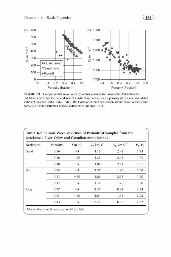
TABLE 6.7 Seismic Wave Velocities of Permafrost Samples from the
Mackenzie River Valley and Canadian Arctic Islands
Sediment Porosity T in �C VP km s21 VS km s21 VP/VS
Sand 0.36 25 4.18 2.42 1.73
0.36 215 4.21 2.43 1.73
0.40 25 3.88 2.14 1.81
Silt 0.33 25 3.57 1.90 1.88
0.33 215 3.86 2.15 1.80
0.37 25 3.38 1.78 1.90
Clay 0.37 25 2.27 0.91 2.44
0.37 215 2.64 1.31 2.02
0.43 25 2.27 0.98 2.32
Selected data from Zimmerman and King (1986).
0
100
200
300
400
500
600
700(A) (B)
0.0 0.1 0.2 0.3 0.4 0.5
Porosity (fraction)
VP in
ms−1
VP in
ms−1
Quartz sand
Sand, silty
Rockfill
1400
1500
1600
1700
1800
1900
0.4 0.5 0.6 0.7 0.8 0.9
Porosity (fraction)
FIGURE 6.9 Compressional wave velocity versus porosity for unconsolidated sediments.
(A) Mean curves for the dependence of elastic wave velocities on porosity of dry unconsolidated
sediments (Schon, 1964, 1969, 1983). (B) Correlation between compressional wave velocity and
porosity of water-saturated marine sediments (Hamilton, 1971).
169Chapter | 6 Elastic Properties
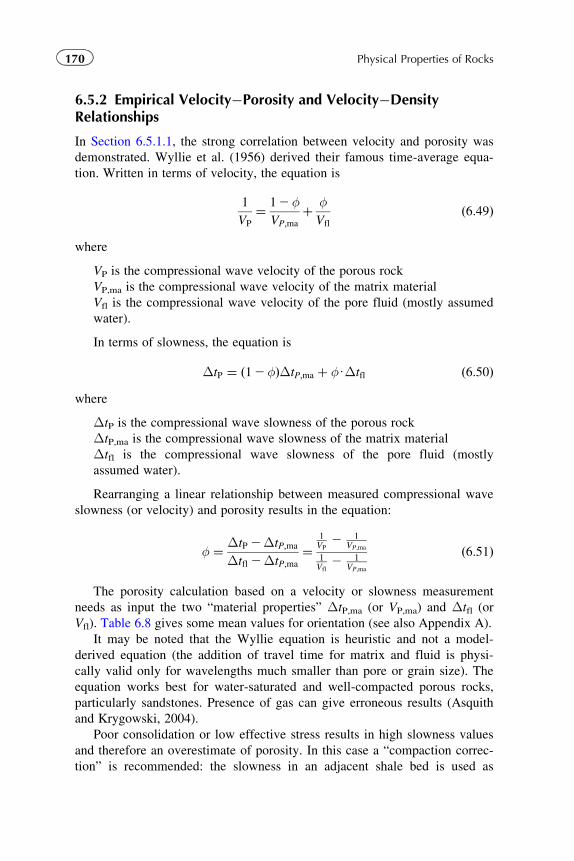
6.5.2 Empirical Velocity�Porosity and Velocity�DensityRelationships
In Section 6.5.1.1, the strong correlation between velocity and porosity was
demonstrated. Wyllie et al. (1956) derived their famous time-average equa-
tion. Written in terms of velocity, the equation is
1
VP
¼ 12φVP;ma
þ φVfl
ð6:49Þ
where
VP is the compressional wave velocity of the porous rock
VP,ma is the compressional wave velocity of the matrix material
Vfl is the compressional wave velocity of the pore fluid (mostly assumed
water).
In terms of slowness, the equation is
ΔtP ¼ ð12φÞΔtP;ma þ φUΔtfl ð6:50Þwhere
ΔtP is the compressional wave slowness of the porous rock
ΔtP,ma is the compressional wave slowness of the matrix material
Δtfl is the compressional wave slowness of the pore fluid (mostly
assumed water).
Rearranging a linear relationship between measured compressional wave
slowness (or velocity) and porosity results in the equation:
φ ¼ ΔtP 2ΔtP;ma
Δtfl 2ΔtP;ma
¼1VP
2 1VP;ma
1Vfl
2 1VP;ma
ð6:51Þ
The porosity calculation based on a velocity or slowness measurement
needs as input the two “material properties” ΔtP,ma (or VP,ma) and Δtfl (or
Vfl). Table 6.8 gives some mean values for orientation (see also Appendix A).
It may be noted that the Wyllie equation is heuristic and not a model-
derived equation (the addition of travel time for matrix and fluid is physi-
cally valid only for wavelengths much smaller than pore or grain size). The
equation works best for water-saturated and well-compacted porous rocks,
particularly sandstones. Presence of gas can give erroneous results (Asquith
and Krygowski, 2004).
Poor consolidation or low effective stress results in high slowness values
and therefore an overestimate of porosity. In this case a “compaction correc-
tion” is recommended: the slowness in an adjacent shale bed is used as
170 Physical Properties of Rocks
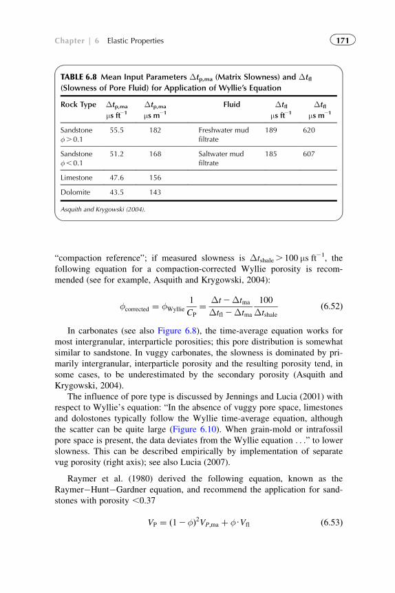
“compaction reference”; if measured slowness is Δtshale. 100 μs ft21, the
following equation for a compaction-corrected Wyllie porosity is recom-
mended (see for example, Asquith and Krygowski, 2004):
φcorrected ¼ φWyllie
1
CP
¼ Δt2Δtma
Δtfl 2Δtma
100
Δtshaleð6:52Þ
In carbonates (see also Figure 6.8), the time-average equation works for
most intergranular, interparticle porosities; this pore distribution is somewhat
similar to sandstone. In vuggy carbonates, the slowness is dominated by pri-
marily intergranular, interparticle porosity and the resulting porosity tend, in
some cases, to be underestimated by the secondary porosity (Asquith and
Krygowski, 2004).
The influence of pore type is discussed by Jennings and Lucia (2001) with
respect to Wyllie’s equation: “In the absence of vuggy pore space, limestones
and dolostones typically follow the Wyllie time-average equation, although
the scatter can be quite large (Figure 6.10). When grain-mold or intrafossil
pore space is present, the data deviates from the Wyllie equation . . .” to lower
slowness. This can be described empirically by implementation of separate
vug porosity (right axis); see also Lucia (2007).
Raymer et al. (1980) derived the following equation, known as the
Raymer�Hunt�Gardner equation, and recommend the application for sand-
stones with porosity ,0.37
VP ¼ ð12φÞ2VP;ma þ φUVfl ð6:53Þ
TABLE 6.8 Mean Input Parameters Δtp,ma (Matrix Slowness) and Δtfl(Slowness of Pore Fluid) for Application of Wyllie’s Equation
Rock Type Δtp,ma
μs ft21
Δtp,ma
μs m21
Fluid Δtflμs ft21
Δtflμs m21
Sandstoneφ.0.1
55.5 182 Freshwater mudfiltrate
189 620
Sandstoneφ,0.1
51.2 168 Saltwater mudfiltrate
185 607
Limestone 47.6 156
Dolomite 43.5 143
Asquith and Krygowski (2004).
171Chapter | 6 Elastic Properties
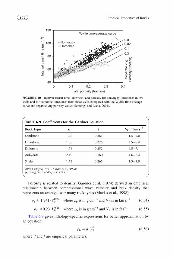
Porosity is related to density. Gardner et al. (1974) derived an empirical
relationship between compressional wave velocity and bulk density that
represents an average over many rock types (Mavko et al., 1998):
ρb � 1:741UV0:25P where ρb is in g cm23 and VP is in km s21 ð6:54Þ
ρb � 0:23UV0:25P where ρb is in g cm23 and VP is in ft s
21 ð6:55ÞTable 6.9 gives lithology-specific expressions for better approximation by
an equation:
ρb ¼ dUVfP ð6:56Þ
where d and f are empirical parameters.
Total porosity (fraction)
0
Inte
rval
tran
sit t
ime
(μs
ft−1)
120Wyllie time-average curve
NonvuggyOomoldic
100
80
60
400.1 0.2 0.3 0.4
0.00.02
0.1
0.3
Sep
arat
e vu
gP
oros
ity (
frac
tion)
FIGURE 6.10 Interval transit time (slowness) and porosity for nonvuggy limestones in two
wells and for oomoldic limestones from three wells compared with the Wyllie time-average
curve and separate vug porosity values (Jennings and Lucia, 2001).
TABLE 6.9 Coefficients for the Gardner Equation
Rock Type d f VP in km s21
Sandstone 1.66 0.261 1.5�6.0
Limestone 1.50 0.225 3.5�6.4
Dolomite 1.74 0.252 4.5�7.1
Anhydrite 2.19 0.160 4.6�7.4
Shale 1.75 0.265 1.5�5.0
After Castagna (1993), Mavko et al. (1998).ρb is in g cm23 and Vp is in km s21.
172 Physical Properties of Rocks
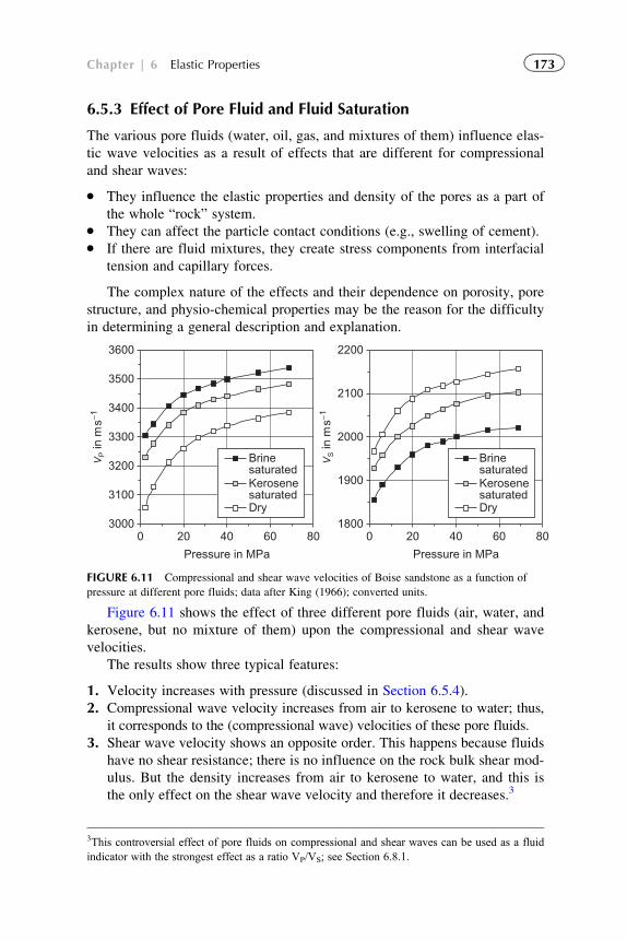
6.5.3 Effect of Pore Fluid and Fluid Saturation
The various pore fluids (water, oil, gas, and mixtures of them) influence elas-
tic wave velocities as a result of effects that are different for compressional
and shear waves:
� They influence the elastic properties and density of the pores as a part of
the whole “rock” system.� They can affect the particle contact conditions (e.g., swelling of cement).� If there are fluid mixtures, they create stress components from interfacial
tension and capillary forces.
The complex nature of the effects and their dependence on porosity, pore
structure, and physio-chemical properties may be the reason for the difficulty
in determining a general description and explanation.
Figure 6.11 shows the effect of three different pore fluids (air, water, and
kerosene, but no mixture of them) upon the compressional and shear wave
velocities.
The results show three typical features:
1. Velocity increases with pressure (discussed in Section 6.5.4).
2. Compressional wave velocity increases from air to kerosene to water; thus,
it corresponds to the (compressional wave) velocities of these pore fluids.
3. Shear wave velocity shows an opposite order. This happens because fluids
have no shear resistance; there is no influence on the rock bulk shear mod-
ulus. But the density increases from air to kerosene to water, and this is
the only effect on the shear wave velocity and therefore it decreases.3
3000
3100
3200
3300
3400
3500
3600
0 20 40 60 80
Pressure in MPa
VP in
ms−1
BrinesaturatedKerosenesaturatedDry
1800
1900
2000
2100
2200
0 20 40 60 80
Pressure in MPa
VS in
ms−1
BrinesaturatedKerosenesaturatedDry
FIGURE 6.11 Compressional and shear wave velocities of Boise sandstone as a function of
pressure at different pore fluids; data after King (1966); converted units.
3This controversial effect of pore fluids on compressional and shear waves can be used as a fluidindicator with the strongest effect as a ratio VP/VS; see Section 6.8.1.
173Chapter | 6 Elastic Properties
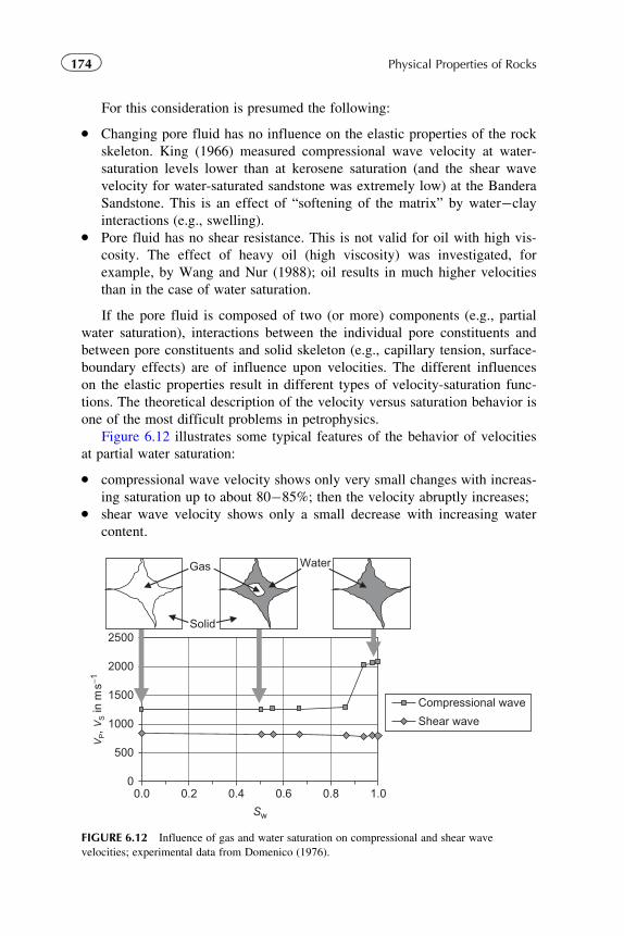
For this consideration is presumed the following:
� Changing pore fluid has no influence on the elastic properties of the rock
skeleton. King (1966) measured compressional wave velocity at water-
saturation levels lower than at kerosene saturation (and the shear wave
velocity for water-saturated sandstone was extremely low) at the Bandera
Sandstone. This is an effect of “softening of the matrix” by water�clay
interactions (e.g., swelling).� Pore fluid has no shear resistance. This is not valid for oil with high vis-
cosity. The effect of heavy oil (high viscosity) was investigated, for
example, by Wang and Nur (1988); oil results in much higher velocities
than in the case of water saturation.
If the pore fluid is composed of two (or more) components (e.g., partial
water saturation), interactions between the individual pore constituents and
between pore constituents and solid skeleton (e.g., capillary tension, surface-
boundary effects) are of influence upon velocities. The different influences
on the elastic properties result in different types of velocity-saturation func-
tions. The theoretical description of the velocity versus saturation behavior is
one of the most difficult problems in petrophysics.
Figure 6.12 illustrates some typical features of the behavior of velocities
at partial water saturation:
� compressional wave velocity shows only very small changes with increas-
ing saturation up to about 80�85%; then the velocity abruptly increases;� shear wave velocity shows only a small decrease with increasing water
content.
0
500
1000
1500
2000
2500
0.0 0.2 0.4 0.6 0.8 1.0
Sw
VP, V
S in
ms−1
Compressional wave
Shear wave
Gas
Solid
Water
FIGURE 6.12 Influence of gas and water saturation on compressional and shear wave
velocities; experimental data from Domenico (1976).
174 Physical Properties of Rocks
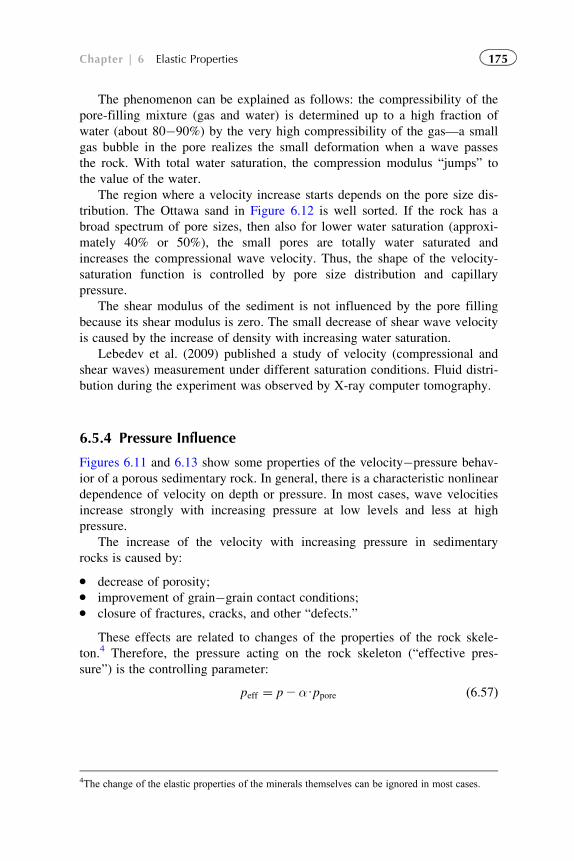
The phenomenon can be explained as follows: the compressibility of the
pore-filling mixture (gas and water) is determined up to a high fraction of
water (about 80�90%) by the very high compressibility of the gas—a small
gas bubble in the pore realizes the small deformation when a wave passes
the rock. With total water saturation, the compression modulus “jumps” to
the value of the water.
The region where a velocity increase starts depends on the pore size dis-
tribution. The Ottawa sand in Figure 6.12 is well sorted. If the rock has a
broad spectrum of pore sizes, then also for lower water saturation (approxi-
mately 40% or 50%), the small pores are totally water saturated and
increases the compressional wave velocity. Thus, the shape of the velocity-
saturation function is controlled by pore size distribution and capillary
pressure.
The shear modulus of the sediment is not influenced by the pore filling
because its shear modulus is zero. The small decrease of shear wave velocity
is caused by the increase of density with increasing water saturation.
Lebedev et al. (2009) published a study of velocity (compressional and
shear waves) measurement under different saturation conditions. Fluid distri-
bution during the experiment was observed by X-ray computer tomography.
6.5.4 Pressure Influence
Figures 6.11 and 6.13 show some properties of the velocity�pressure behav-
ior of a porous sedimentary rock. In general, there is a characteristic nonlinear
dependence of velocity on depth or pressure. In most cases, wave velocities
increase strongly with increasing pressure at low levels and less at high
pressure.
The increase of the velocity with increasing pressure in sedimentary
rocks is caused by:
� decrease of porosity;� improvement of grain�grain contact conditions;� closure of fractures, cracks, and other “defects.”
These effects are related to changes of the properties of the rock skele-
ton.4 Therefore, the pressure acting on the rock skeleton (“effective pres-
sure”) is the controlling parameter:
peff ¼ p2αUppore ð6:57Þ
4The change of the elastic properties of the minerals themselves can be ignored in most cases.
175Chapter | 6 Elastic Properties
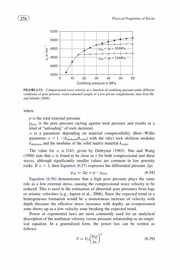
where
p is the total external pressure
ppore is the pore pressure (acting against total pressure and results in a
kind of “unloading” of rock skeleton)
α is a parameter depending on material compressibility (Biot�Willis
parameter α 5 12 (kskeleton/ksolid) with the (dry) rock skeleton modulus
kskeleton and the modulus of the solid matrix material ksolid.
The value for α is 0.83, given by Dobrynin (1963). Nur and Wang
(1988) note that α is found to be close to 1 for both compressional and shear
waves, although significantly smaller values are common in low porosity
rocks. If α 5 1, then Equation (6.57) expresses the differential pressure Δp:
peff ¼ Δp ¼ p2 ppore ð6:58ÞEquation (6.58) demonstrates that a high pore pressure plays the same
role as a low external stress, causing the compressional wave velocity to be
reduced. This is used in the estimation of abnormal pore pressures from logs
or seismic velocities (e.g., Japsen et al., 2006). Since the expected trend in a
homogeneous formation would be a monotonous increase of velocity with
depth (because the effective stress increases with depth), an overpressured
zone shows up as a low velocity zone breaking the expected trend.
Power or exponential laws are most commonly used for an analytical
description of the nonlinear velocity versus pressure relationship as an empir-
ical equation. In a generalized form, the power law can be written as
follows:
V ¼ V0
peff
p0
� �mð6:59Þ
4200
4400
4600
4800
5000
5200
0 10 20 30 40 50 60
Confining pressure in MPa
VP in
ms−1 peff = Δp = 30MPa
peff = Δp = 15MPa
FIGURE 6.13 Compressional wave velocity as a function of confining pressure under different
conditions of pore pressure, water-saturated sample of a low porous conglomerate, data from He
and Schmitt (2006).
176 Physical Properties of Rocks
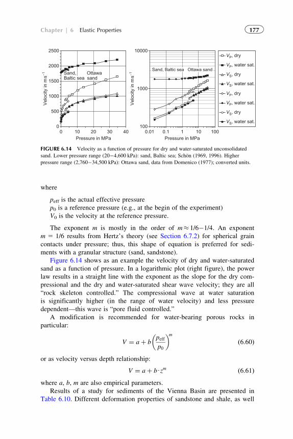
where
peff is the actual effective pressure
p0 is a reference pressure (e.g., at the begin of the experiment)
V0 is the velocity at the reference pressure.
The exponent m is mostly in the order of m� 1/6�1/4. An exponent
m 5 1/6 results from Hertz’s theory (see Section 6.7.2) for spherical grain
contacts under pressure; thus, this shape of equation is preferred for sedi-
ments with a granular structure (sand, sandstone).
Figure 6.14 shows as an example the velocity of dry and water-saturated
sand as a function of pressure. In a logarithmic plot (right figure), the power
law results in a straight line with the exponent as the slope for the dry com-
pressional and the dry and water-saturated shear wave velocity; they are all
“rock skeleton controlled.” The compressional wave at water saturation
is significantly higher (in the range of water velocity) and less pressure
dependent—this wave is “pore fluid controlled.”
A modification is recommended for water-bearing porous rocks in
particular:
V ¼ aþ bpeff
p0
� �mð6:60Þ
or as velocity versus depth relationship:
V ¼ aþ bUzm ð6:61Þwhere a, b, m are also empirical parameters.
Results of a study for sediments of the Vienna Basin are presented in
Table 6.10. Different deformation properties of sandstone and shale, as well
0
500
1000
1500
2000
2500
0 10 20 30 40Pressure in MPa
Vel
ocity
in m
s−1
100
1000
10000
0.01 0.1 1 10 100Pressure in MPa
Vel
ocity
in m
s−1
VP, dry
VP, water sat.
VS, dry
VS, water sat.
VP, dry
VP, water sat.
VS, dry
VS, water sat.
Baltic sea sandSand, Ottawa
Sand, Baltic sea Ottawa sand
FIGURE 6.14 Velocity as a function of pressure for dry and water-saturated unconsolidated
sand. Lower pressure range (20�4,600 kPa): sand, Baltic sea; Schon (1969, 1996). Higher
pressure range (2,760�34,500 kPa): Ottawa sand, data from Domenico (1977); converted units.
177Chapter | 6 Elastic Properties
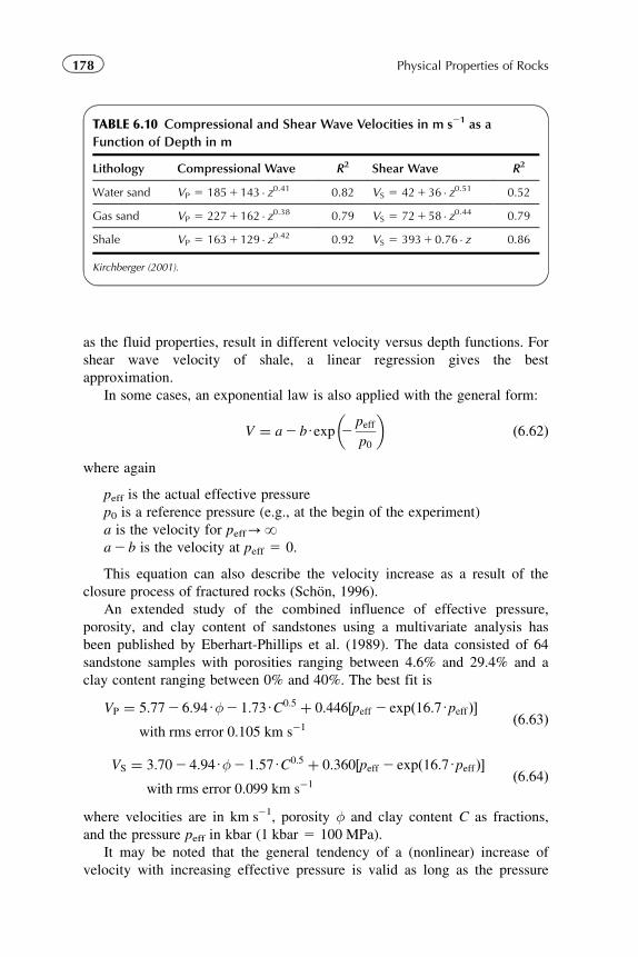
as the fluid properties, result in different velocity versus depth functions. For
shear wave velocity of shale, a linear regression gives the best
approximation.
In some cases, an exponential law is also applied with the general form:
V ¼ a2 bUexp 2peff
p0
� �ð6:62Þ
where again
peff is the actual effective pressure
p0 is a reference pressure (e.g., at the begin of the experiment)
a is the velocity for peff-Na2 b is the velocity at peff 5 0.
This equation can also describe the velocity increase as a result of the
closure process of fractured rocks (Schon, 1996).
An extended study of the combined influence of effective pressure,
porosity, and clay content of sandstones using a multivariate analysis has
been published by Eberhart-Phillips et al. (1989). The data consisted of 64
sandstone samples with porosities ranging between 4.6% and 29.4% and a
clay content ranging between 0% and 40%. The best fit is
VP ¼ 5:772 6:94Uφ2 1:73UC0:5 þ 0:446½peff 2 expð16:7UpeffÞ�with rms error 0:105 km s�1
ð6:63Þ
VS ¼ 3:702 4:94Uφ2 1:57UC0:5 þ 0:360½peff 2 expð16:7UpeffÞ�with rms error 0:099 km s�1
ð6:64Þ
where velocities are in km s21, porosity φ and clay content C as fractions,
and the pressure peff in kbar (1 kbar 5 100 MPa).
It may be noted that the general tendency of a (nonlinear) increase of
velocity with increasing effective pressure is valid as long as the pressure
TABLE 6.10 Compressional and Shear Wave Velocities in m s21 as a
Function of Depth in m
Lithology Compressional Wave R2 Shear Wave R2
Water sand VP 5 1851 143 � z0.41 0.82 VS 5 421 36 � z0.51 0.52
Gas sand VP 5 2271 162 � z0.38 0.79 VS 5 721 58 � z0.44 0.79
Shale VP 5 1631 129 � z0.42 0.92 VS 5 3931 0.76 � z 0.86
Kirchberger (2001).
178 Physical Properties of Rocks
does not break grains, particles, or sections of the particle contact. Such a
breaking can result in a structure collapse and decrease of velocity.
A detailed discussion of velocity�depth trends for sandstone and shale
from the North Sea is given by Japsen et al. (2006).
The additional influence of thermally induced microfractures in Aeolian
Rotliegend sandstone on the stress dependence of elastic properties was
investigated by MacBeth and Schuett (2007).
6.5.5 Temperature Influence
The temperature effects on the dry bulk moduli are very small. The tempera-
ture dependence of fluids is more significant and controlled by the composi-
tion (Batzle and Wang, 1992; see Section 6.2.2).
The expected trend, which is in agreement with observations, is that
velocities decrease with temperature more in saturated than in dry porous
rocks.
6.5.6 Empirical Relationships Between VP and VS—CastagnaEquation
The ratio VP/VS is an important property for seismic applications (see also
Section 6.8). In order to estimate shear wave velocities when only compres-
sional wave velocities are available, Castagna et al. (1985) derived an empir-
ical equation commonly referred to as the “mudrock line”5:
VS ¼ 0:8621UVP 2 1:1724 ð6:65Þwhere the velocities are in km s21.
Numerous researchers have published variants of the Castagna mudrock
equation. In 1993, Castagna et al. compiled an analysis of data for different
sedimentary rocks. The following consideration gives a part of the results.
Table 6.11 lists a selection of the modified equations based on a compilation
by Mavko et al. (1998) and Figure 6.15 shows some typical lines in a plot.
For carbonates, Castagna et al. (1993) gives the following regressions:
limestone ðwater saturatedÞ VS ¼2 0:055UV2P þ 1:017UVP 2 1:031 ð6:66Þ
dolomite ðwater saturatedÞ VS ¼ 0:5832UVP 2 0:07776 ð6:67ÞAll of these correlations are pure empirically and valid only for a specific
formation. They result from properties like rock composition, porosity, shale
content, etc. with an influence on both wave types in the same direction.
5Castagna et al. (1985): “We define mudrock as clastic silicate rock composed primarily of clay-or silt-sized particles” (see also Blatt et al.,1972)”.
179Chapter | 6 Elastic Properties
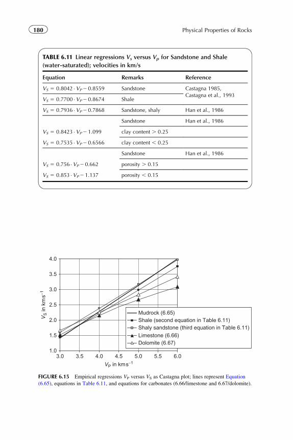
TABLE 6.11 Linear regressions Vs versus Vp for Sandstone and Shale
(water-saturated); velocities in km/s
Equation Remarks Reference
VS 5 0.8042 �VP20.8559 Sandstone Castagna 1985,Castagna et al., 1993
VS 5 0.7700 �VP20.8674 Shale
VS 5 0.7936 �VP20.7868 Sandstone, shaly Han et al., 1986
Sandstone Han et al., 1986
VS 5 0.8423 �VP21.099 clay content . 0.25
VS 5 0.7535 �VP20.6566 clay content , 0.25
Sandstone Han et al., 1986
VS 5 0.756 �VP2 0.662 porosity . 0.15
VS 5 0.853 �VP2 1.137 porosity , 0.15
1.0
1.5
2.0
2.5
3.0
3.5
4.0
3.0 3.5 4.0 4.5 5.0 5.5 6.0
VP in kms−1
VS in
km
s−1
Mudrock (6.65)Shale (second equation in Table 6.11)Shaly sandstone (third equation in Table 6.11)Limestone (6.66)Dolomite (6.67)
FIGURE 6.15 Empirical regressions VP versus VS as Castagna plot; lines represent Equation
(6.65), equations in Table 6.11, and equations for carbonates (6.66/limestone and 6.67/dolomite).
180 Physical Properties of Rocks
A general valid physically based equation is not possible, because the isotro-
pic material is also characterized by two independent elastic properties or
wave velocities.
6.6 ANISOTROPY
6.6.1 Overview
Implementation of elastic anisotropy is of increasing importance for seismic
processing and interpretation. Armstrong et al. (1994) discuss fundamental
characteristics and consequences of elastic anisotropy for seismic and acous-
tic methods. Wang (2002) gives a detailed discussion of elastic anisotropy of
sedimentary rocks. Lo et al. (1986) analyzed laboratory measurements at the
Berea sandstone, Chicopee shale, and Chelmsford granite.
Layer-induced anisotropy (transversely isotropy) and its consequences for
the interpretation of seismic data are the subjects of papers by Helbig (1958,
1992), Backus (1962), White (1983), Thomsen (1986, 1995), Schoenberg
and Muir (1989), and Schoenberg (1994).
“Shear wave splitting” is a sensitive indicator of elastic anisotropy and
therefore has a special place in rock physics (see, for example, Crampin and
Lovell, 1991).
In elastically anisotropic rocks, the velocity of wave propagation depends
on the direction of propagation. Obvious anisotropy exists:
� in metamorphic rocks with schistosity and oriented fracturing (typical
gneiss);� in sedimentary rocks with layering or bedding (e.g., laminated shaly
sand), but also if fractures are present.
The origins of anisotropy are aligned crystals in igneous rocks, aligned
grains in sediments, lamination of sediments (laminated shaly sands), aligned
fractures and cracks, and stress-induced anisotropy.
Whereas elastic properties of an isotropic medium are determined by two
independent elastic parameters, for an anisotropic material in the simplest
case (transversely isotropy), five parameters are necessary. For the transverse
isotropy, the elastic properties are equal, for example, in the x�y plane
(plane of stratification or schistosity), but vary with the angle from the verti-
cal z-axis.
Figure 6.16 demonstrates—based on Lo et al. (1986)—the petrofabric
origin of elastic rock anisotropy. The upper part shows:
� in Berea sandstone, most of the long axes of the quartz grains are parallel
to the bedding plane;� in Chicopee shale, most of the cleavage planes of mica and the long axes
of other constituent minerals are parallel to the bedding plane;
181Chapter | 6 Elastic Properties
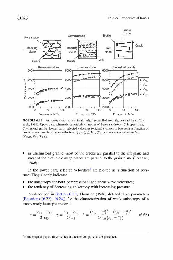
� in Chelmsford granite, most of the cracks are parallel to the rift plane and
most of the biotite cleavage planes are parallel to the grain plane (Lo et al.,
1986).
In the lower part, selected velocities6 are plotted as a function of pres-
sure. They clearly indicate:
� the anisotropy for both compressional and shear wave velocities;� the tendency of decreasing anisotropy with increasing pressure.
As described in Section 6.1.1, Thomsen (1986) defined three parameters
(Equations (6.22)�(6.24)) for the characterization of weak anisotropy of a
transversely isotropic material:
ε ¼ c11 2 c33
2Uc33γ ¼ c66 2 c44
2Uc44δ ¼ c13 þ c44
2
� �22 c33 2
c442
� �22Uc33 c33 2
c442
� � ð6:68Þ
Chikopee shaleBerea sandstone
2000
3000
4000
5000
6000
0 50 100Pressure in MPa
2000
3000
4000
5000
6000
0 50 100Pressure in MPa
2000
3000
4000
5000
6000
0 50 100Pressure in MPa
Vel
ocity
in m
s−1
Chelmsford granite
VP,h
VP,v
VS,h
VS,v
Pore space
Quartz Quartz
Grainplane
Mica
Clay minerals
Beddingplane
Riftplane
Beddingplane
Biotite
Crack
FIGUSRE 6.16 Anisotropy and its petrofabric origin (compiled from figures and data of Lo
et al., 1986). Upper part: schematic petrofabric character of Berea sandstone, Chicopee shale,
Chelmsford granite. Lower parts: selected velocities (original symbols in brackets) as function of
pressure: compressional wave velocities VP,h (Vp11), VP,v (VP33), shear wave velocities VS,h
(VS,h1), VS,v (VS,3a).
6In the original paper, all velocities and tensor components are presented.
182 Physical Properties of Rocks
where ε and γ describe the anisotropy properties of the compressional and
shear waves, respectively. Additionally, a ratio can be defined as:
λcompr ¼c11
c33¼ 2Uεþ 1 λshear ¼
c66
c44¼ 2Uγ þ 1 ð6:69Þ
If for a transversely isotropic material as the simplest type of anisotropy:
� the vertical axis (x3) is the axis of symmetry, then the material is called
TIV. This is the case, for example, for horizontally layered laminated
sediments: elastic properties are uniform horizontally, but vary vertically.� one horizontal axis (x1 or x2) is the axis of symmetry, then the material is
called TIH. In the case of vertical fractures, elastic properties are uniform
in vertical plane parallel aligned fractures, but vary in perpendicular frac-
tures/crossing fractures (see, for example, Armstrong et al., 1994).
Equations for a TIV system can be transformed into corresponding equa-
tions for a TIH system by cyclic transformation.
In the following section, two aspects of anisotropy are discussed briefly:
1. The effect of aligned fractures and cracks and the phenomenon of shear
wave splitting, anisotropy of igneous and metamorphic rocks
2. Anisotropy of laminated sediments and correlations between compres-
sional and shear wave anisotropy.
6.6.2 Anisotropy Effect of Fractures, Anisotropy of Igneous andMetamorphic Rocks
In fractured rocks with a preferred direction of fractures, anisotropy results
as an effect of the weak parts of the rock (Figure 6.17). For the main direc-
tions, four wave velocities can be observed:
� Compressional wave velocity perpendicular to the fracture plane VP> is
smaller than the compressional wave velocity parallel to this plane VP8:� low velocity VP> is controlled very strongly by the “soft” elastic ele-
ment of the fractures (a series array of elastic elements);� higher velocity VP8 is controlled by the competent part of the rock (a
parallel array of elastic elements).� Shear wave velocity must be related to the direction of polarization (par-
ticle motion) with respect to the “soft” and “competent” element. It
results in:� low velocity for the wave propagating vertically (polarization
horizontally);� low velocity for the wave propagating horizontally (polarization
vertically);� high velocity for the wave propagating horizontally (polarization
horizontally).
183Chapter | 6 Elastic Properties
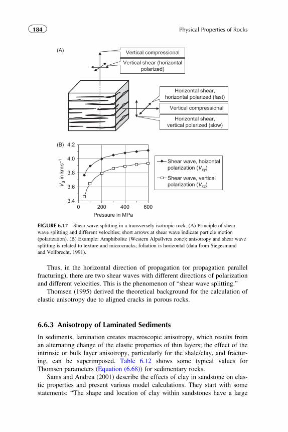
Thus, in the horizontal direction of propagation (or propagation parallel
fracturing), there are two shear waves with different directions of polarization
and different velocities. This is the phenomenon of “shear wave splitting.”
Thomsen (1995) derived the theoretical background for the calculation of
elastic anisotropy due to aligned cracks in porous rocks.
6.6.3 Anisotropy of Laminated Sediments
In sediments, lamination creates macroscopic anisotropy, which results from
an alternating change of the elastic properties of thin layers; the effect of the
intrinsic or bulk layer anisotropy, particularly for the shale/clay, and fractur-
ing, can be superimposed. Table 6.12 shows some typical values for
Thomsen parameters (Equation (6.68)) for sedimentary rocks.
Sams and Andrea (2001) describe the effects of clay in sandstone on elas-
tic properties and present various model calculations. They start with some
statements: “The shape and location of clay within sandstones have a large
Vertical compressional
Vertical shear (horizontalpolarized)
Horizontal shear,vertical polarized (slow)
Horizontal shear,horizontal polarized (fast)
Vertical compressional
3.4
3.6
3.8
4.0
4.2(B)
(A)
0 200 400 600
Pressure in MPa
VS in
km
s−1 Shear wave, hoizontalpolarization (Vxy)
Shear wave, verticalpolarization (Vxz)
FIGURE 6.17 Shear wave splitting in a transversely isotropic rock. (A) Principle of shear
wave splitting and different velocities; short arrows at shear wave indicate particle motion
(polarization). (B) Example: Amphibolite (Western Alps/Ivrea zone); anisotropy and shear wave
splitting is related to texture and microcracks; foliation is horizontal (data from Siegesmund
and Vollbrecht, 1991).
184 Physical Properties of Rocks
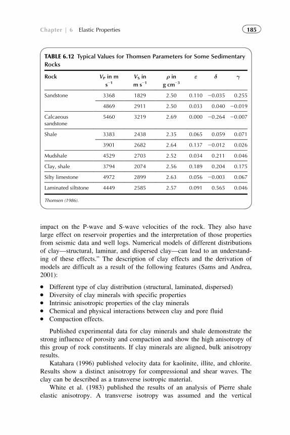
impact on the P-wave and S-wave velocities of the rock. They also have
large effect on reservoir properties and the interpretation of those properties
from seismic data and well logs. Numerical models of different distributions
of clay—structural, laminar, and dispersed clay—can lead to an understand-
ing of these effects.” The description of clay effects and the derivation of
models are difficult as a result of the following features (Sams and Andrea,
2001):
� Different type of clay distribution (structural, laminated, dispersed)� Diversity of clay minerals with specific properties� Intrinsic anisotropic properties of the clay minerals� Chemical and physical interactions between clay and pore fluid� Compaction effects.
Published experimental data for clay minerals and shale demonstrate the
strong influence of porosity and compaction and show the high anisotropy of
this group of rock constituents. If clay minerals are aligned, bulk anisotropy
results.
Katahara (1996) published velocity data for kaolinite, illite, and chlorite.
Results show a distinct anisotropy for compressional and shear waves. The
clay can be described as a transverse isotropic material.
White et al. (1983) published the results of an analysis of Pierre shale
elastic anisotropy. A transverse isotropy was assumed and the vertical
TABLE 6.12 Typical Values for Thomsen Parameters for Some Sedimentary
Rocks
Rock VP in m
s21
VS in
m s21ρ in
g cm23
ε δ γ
Sandstone 3368 1829 2.50 0.110 20.035 0.255
4869 2911 2.50 0.033 0.040 20.019
Calcaeoussandstone
5460 3219 2.69 0.000 20.264 20.007
Shale 3383 2438 2.35 0.065 0.059 0.071
3901 2682 2.64 0.137 20.012 0.026
Mudshale 4529 2703 2.52 0.034 0.211 0.046
Clay, shale 3794 2074 2.56 0.189 0.204 0.175
Silty limestone 4972 2899 2.63 0.056 20.003 0.067
Laminated siltstone 4449 2585 2.57 0.091 0.565 0.046
Thomsen (1986).
185Chapter | 6 Elastic Properties
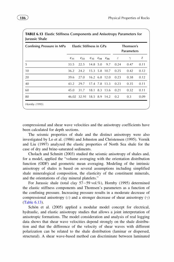
compressional and shear wave velocities and the anisotropy coefficients have
been calculated for depth sections.
The seismic properties of shale and the distinct anisotropy were also
investigated by Lo et al. (1986) and Johnston and Christensen (1995). Vernik
and Liu (1997) analyzed the elastic properties of North Sea shale for the
case of dry and brine-saturated sediments.
Cholach and Schmitt (2003) studied the seismic anisotropy of shales and,
for a model, applied the “volume averaging with the orientation distribution
function (ODF) and geometric mean averaging. Modeling of the intrinsic
anisotropy of shales is based on several assumptions including simplified
shale mineralogical composition, the elasticity of the constituent minerals,
and the orientations of clay mineral platelets.”
For Jurassic shale (total clay 57�59 vol.%), Hornby (1995) determined
the elastic stiffness components and Thomsen’s parameters as a function of
the confining pressure. Increasing pressure results in a moderate decrease of
compressional anisotropy (ε) and a stronger decrease of shear anisotropy (γ)(Table 6.13).
Schon et al. (2005) applied a modular model concept for electrical,
hydraulic, and elastic anisotropy studies that allows a joint interpretation of
anisotropic formations. The model consideration and analysis of real logging
data shows that shear wave velocities depend strongly on the shale distribu-
tion and that the difference of the velocity of shear waves with different
polarization can be related to the shale distribution (laminar or dispersed,
structural). A shear wave-based method can discriminate between laminated
TABLE 6.13 Elastic Stiffness Components and Anisotropy Parameters for
Jurassic Shale
Confining Pressure in MPa Elastic Stiffness in GPa Thomsen’s
Parameters
c11 c33 c13 c44 c66 ε γ δ
5 33.5 22.5 14.8 5.0 9.7 0.24 0.47 0.11
10 36.2 24.2 15.3 5.8 10.7 0.25 0.42 0.12
20 39.6 27.0 16.2 6.8 12.0 0.23 0.38 0.12
40 43.2 29.7 17.4 7.8 13.3 0.23 0.35 0.11
60 45.0 31.7 18.1 8.3 13.6 0.21 0.32 0.11
80 46.02 32.91 18.5 8.9 14.2 0.2 0.3 0.09
Hornby (1995).
186 Physical Properties of Rocks
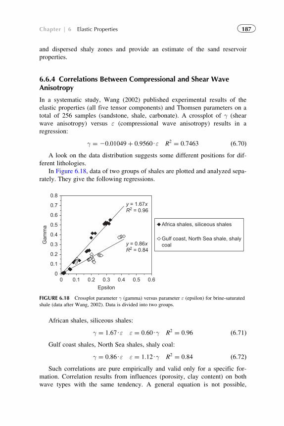
and dispersed shaly zones and provide an estimate of the sand reservoir
properties.
6.6.4 Correlations Between Compressional and Shear WaveAnisotropy
In a systematic study, Wang (2002) published experimental results of the
elastic properties (all five tensor components) and Thomsen parameters on a
total of 256 samples (sandstone, shale, carbonate). A crossplot of γ (shear
wave anisotropy) versus ε (compressional wave anisotropy) results in a
regression:
γ ¼ 20:01049þ 0:9560Uε R2 ¼ 0:7463 ð6:70ÞA look on the data distribution suggests some different positions for dif-
ferent lithologies.
In Figure 6.18, data of two groups of shales are plotted and analyzed sepa-
rately. They give the following regressions.
African shales, siliceous shales:
γ ¼ 1:67Uε ε ¼ 0:60Uγ R2 ¼ 0:96 ð6:71ÞGulf coast shales, North Sea shales, shaly coal:
γ ¼ 0:86Uε ε ¼ 1:12Uγ R2 ¼ 0:84 ð6:72ÞSuch correlations are pure empirically and valid only for a specific for-
mation. Correlation results from influences (porosity, clay content) on both
wave types with the same tendency. A general equation is not possible,
y = 1.67xR2 = 0.96
y = 0.86xR2 = 0.84
0
0.1
0.2
0.3
0.4
0.5
0.6
0.7
0.8
0 0.1 0.2 0.3 0.4 0.5 0.6
Epsilon
Gam
ma Africa shales, siliceous shales
Gulf coast, North Sea shale, shalycoal
FIGURE 6.18 Crossplot parameter γ (gamma) versus parameter ε (epsilon) for brine-saturated
shale (data after Wang, 2002). Data is divided into two groups.
187Chapter | 6 Elastic Properties
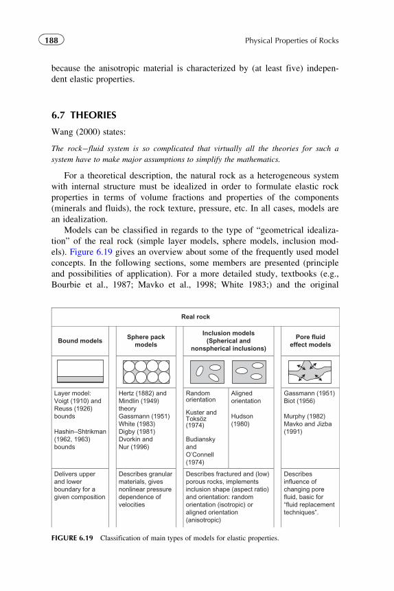
because the anisotropic material is characterized by (at least five) indepen-
dent elastic properties.
6.7 THEORIES
Wang (2000) states:
The rock�fluid system is so complicated that virtually all the theories for such a
system have to make major assumptions to simplify the mathematics.
For a theoretical description, the natural rock as a heterogeneous system
with internal structure must be idealized in order to formulate elastic rock
properties in terms of volume fractions and properties of the components
(minerals and fluids), the rock texture, pressure, etc. In all cases, models are
an idealization.
Models can be classified in regards to the type of “geometrical idealiza-
tion” of the real rock (simple layer models, sphere models, inclusion mod-
els). Figure 6.19 gives an overview about some of the frequently used model
concepts. In the following sections, some members are presented (principle
and possibilities of application). For a more detailed study, textbooks (e.g.,
Bourbie et al., 1987; Mavko et al., 1998; White 1983;) and the original
Real rock
Bound modelsSphere pack
models
Inclusion models(Spherical and
nonspherical inclusions)
Pore fluideffect models
Layer model:Voigt (1910) andReuss (1926)bounds
Hashin–Shtrikman(1962, 1963)bounds
Hertz (1882) andMindlin (1949)theoryGassmann (1951)White (1983)Digby (1981)Dvorkin andNur (1996)
Randomorientation
Kuster andToksöz(1974)
BudianskyandO’Connell(1974)
Alignedorientation
Hudson(1980)
Gassmann (1951)Biot (1956)
Murphy (1982)Mavko and Jizba(1991)
Delivers upperand lowerboundary for agiven composition
Describes granularmaterials, givesnonlinear pressuredependence ofvelocities
Describes fractured and (low)porous rocks, implementsinclusion shape (aspect ratio)and orientation: randomorientation (isotropic) oraligned orientation(anisotropic)
Describesinfluence ofchanging porefluid, basic for“fluid replacementtechniques”.
FIGURE 6.19 Classification of main types of models for elastic properties.
188 Physical Properties of Rocks
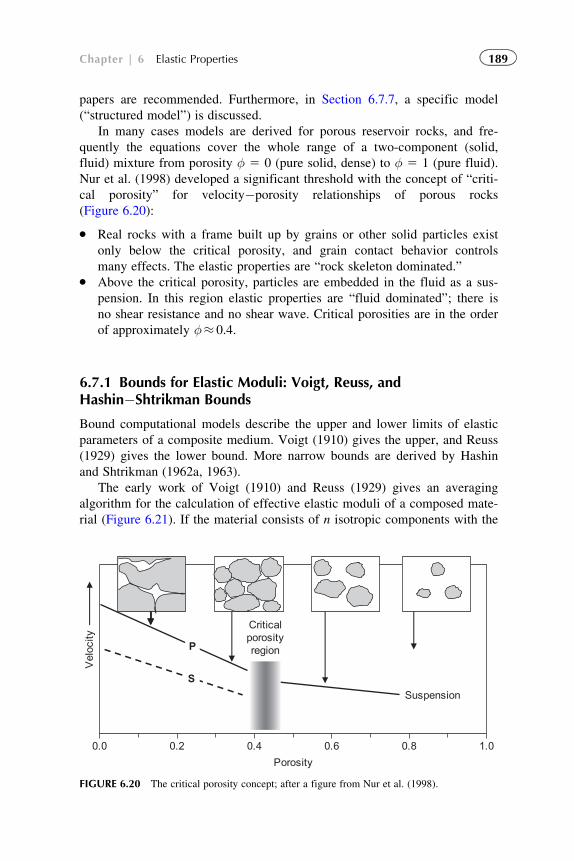
papers are recommended. Furthermore, in Section 6.7.7, a specific model
(“structured model”) is discussed.
In many cases models are derived for porous reservoir rocks, and fre-
quently the equations cover the whole range of a two-component (solid,
fluid) mixture from porosity φ 5 0 (pure solid, dense) to φ 5 1 (pure fluid).
Nur et al. (1998) developed a significant threshold with the concept of “criti-
cal porosity” for velocity�porosity relationships of porous rocks
(Figure 6.20):
� Real rocks with a frame built up by grains or other solid particles exist
only below the critical porosity, and grain contact behavior controls
many effects. The elastic properties are “rock skeleton dominated.”� Above the critical porosity, particles are embedded in the fluid as a sus-
pension. In this region elastic properties are “fluid dominated”; there is
no shear resistance and no shear wave. Critical porosities are in the order
of approximately φ� 0.4.
6.7.1 Bounds for Elastic Moduli: Voigt, Reuss, andHashin�Shtrikman Bounds
Bound computational models describe the upper and lower limits of elastic
parameters of a composite medium. Voigt (1910) gives the upper, and Reuss
(1929) gives the lower bound. More narrow bounds are derived by Hashin
and Shtrikman (1962a, 1963).
The early work of Voigt (1910) and Reuss (1929) gives an averaging
algorithm for the calculation of effective elastic moduli of a composed mate-
rial (Figure 6.21). If the material consists of n isotropic components with the
0.0 0.2 0.4 0.6 0.8 1.0
Porosity
Criticalporosityregion
Suspension
Vel
ocity
P
S
FIGURE 6.20 The critical porosity concept; after a figure from Nur et al. (1998).
189Chapter | 6 Elastic Properties
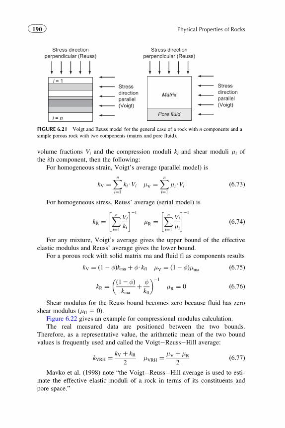
volume fractions Vi and the compression moduli ki and shear moduli μi of
the ith component, then the following:
For homogeneous strain, Voigt’s average (parallel model) is
kV ¼Xni¼1
kiUVi μV ¼Xni¼1
μiUVi ð6:73Þ
For homogeneous stress, Reuss’ average (serial model) is
kR ¼Xni¼1
Vi
ki
" #21
μR ¼Xni¼1
Vi
μi
" #21
ð6:74Þ
For any mixture, Voigt’s average gives the upper bound of the effective
elastic modulus and Reuss’ average gives the lower bound.
For a porous rock with solid matrix ma and fluid fl as components results
kV ¼ ð12φÞkma þ φUkfl μV ¼ ð12φÞμma ð6:75Þ
kR ¼ ð12φÞkma
þ φkfl
� �21
μR ¼ 0 ð6:76Þ
Shear modulus for the Reuss bound becomes zero because fluid has zero
shear modulus (μfl 5 0).
Figure 6.22 gives an example for compressional modulus calculation.
The real measured data are positioned between the two bounds.
Therefore, as a representative value, the arithmetic mean of the two bound
values is frequently used and called the Voigt�Reuss�Hill average:
kVRH ¼ kV þ kR
2μVRH ¼ μV þ μR
2ð6:77Þ
Mavko et al. (1998) note “the Voigt�Reuss�Hill average is used to esti-
mate the effective elastic moduli of a rock in terms of its constituents and
pore space.”
i = 1
i = n
Stress directionperpendicular (Reuss)
Stressdirectionparallel(Voigt)
Matrix
Pore fluid
Stress directionperpendicular (Reuss)
Stressdirectionparallel(Voigt)
FIGURE 6.21 Voigt and Reuss model for the general case of a rock with n components and a
simple porous rock with two components (matrix and pore fluid).
190 Physical Properties of Rocks
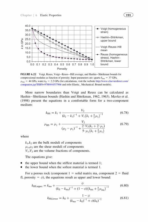
More narrow boundaries than Voigt and Reuss can be calculated as
Hashin�Shtrikman bounds (Hashin and Shtrikman, 1962, 1963). Mavko et al.
(1998) present the equations in a comfortable form for a two-component
medium:
kHS ¼ k1 þV2
ðk2 2 k1Þ21 þ V1 k1 þ 43μ1
� �21ð6:78Þ
μHS ¼ μ1 þV2
ðμ2 2μ1Þ21 þ 2UV1ðk1 þ 2Uμ1Þ5Uμ1 k1 þ 4
3μ1
� � ð6:79Þ
where
k1,k2 are the bulk moduli of components
μ1,μ2 are the shear moduli of components
V1,V2 are the volume fractions of components.
The equations give:
� the upper bound when the stiffest material is termed 1;� the lower bound when the softest material is termed 1.
For a porous rock (component 1 5 solid matrix ma, component 2 5 fluid
fl, porosity 5 φ), the equations result as upper and lower bound:
kHS;upper ¼ kma þ φ
ðkfl 2 kmaÞ21 þ ð12φÞ kma þ 43μma
� �21ð6:80Þ
kHS;lower ¼ kfl þ12φ
ðkma 2 kflÞ21 þ φðkflÞ21ð6:81Þ
0.0
5.0
10.0
15.0
20.0
25.0
30.0
35.0
40.0
0.0 0.1 0.2 0.3 0.4 0.5 0.6 0.7 0.8 0.9 1.0
Porosity
k in
GP
a
Voigt (homogeneousstrain)
Hashin–Shtrikman,upper bound
Voigt–Reuss–Hillmean
Reuss (homogeneousstress), Hashin–Shtrikman, lowerbound
FIGURE 6.22 Voigt, Reuss, Voigt�Reuss�Hill average, and Hashin�Shtrikman bounds for
compressional modulus as function of porosity. Input parameters are: quartz kma 5 37 GPa,
μma 5 44 GPa, water kfl 5 2.2 GPa (for calculations, visit the website http://www.elsevierdirect.com/
companion.jsp?ISBN=9780444537966 and refer Elastic_ Mechanical. Bound models).
191Chapter | 6 Elastic Properties
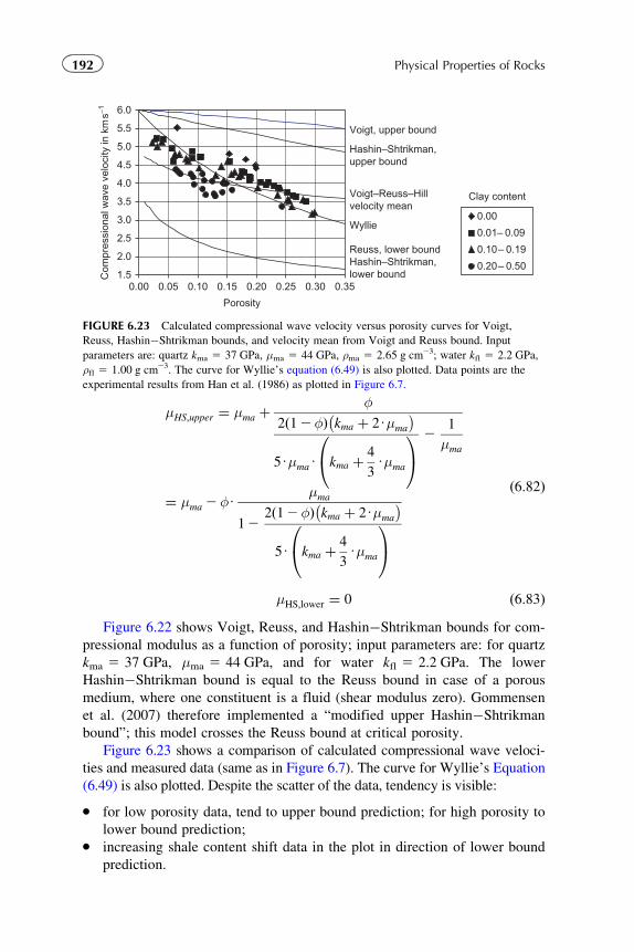
μHS;upper ¼ μma þφ
2 12φð Þ kma þ 2Uμma
� �5UμmaU kma þ
4
3Uμma
0@
1A
21
μma
¼ μma 2φUμma
122 12φð Þ kma þ 2Uμma
� �5U kma þ
4
3Uμma
0@
1A
ð6:82Þ
μHS;lower ¼ 0 ð6:83ÞFigure 6.22 shows Voigt, Reuss, and Hashin�Shtrikman bounds for com-
pressional modulus as a function of porosity; input parameters are: for quartz
kma 5 37 GPa, μma 5 44 GPa, and for water kfl 5 2.2 GPa. The lower
Hashin�Shtrikman bound is equal to the Reuss bound in case of a porous
medium, where one constituent is a fluid (shear modulus zero). Gommensen
et al. (2007) therefore implemented a “modified upper Hashin�Shtrikman
bound”; this model crosses the Reuss bound at critical porosity.
Figure 6.23 shows a comparison of calculated compressional wave veloci-
ties and measured data (same as in Figure 6.7). The curve for Wyllie’s Equation
(6.49) is also plotted. Despite the scatter of the data, tendency is visible:
� for low porosity data, tend to upper bound prediction; for high porosity to
lower bound prediction;� increasing shale content shift data in the plot in direction of lower bound
prediction.
1.5
2.0
2.5
3.0
3.5
4.0
4.5
5.0
5.5
6.0
0.00 0.05 0.10 0.15 0.20 0.25 0.30 0.35
Porosity
Com
pres
sion
al w
ave
velo
city
in k
ms−1
0.00
0.01– 0.09
0.10– 0.19
0.20– 0.50
Voigt, upper bound
Hashin–Shtrikman,upper bound
Voigt–Reuss–Hillvelocity mean
Clay content
Wyllie
Reuss, lower boundHashin–Shtrikman,lower bound
FIGURE 6.23 Calculated compressional wave velocity versus porosity curves for Voigt,
Reuss, Hashin�Shtrikman bounds, and velocity mean from Voigt and Reuss bound. Input
parameters are: quartz kma 5 37 GPa, μma 5 44 GPa, ρma 5 2.65 g cm23; water kfl 5 2.2 GPa,
ρfl 5 1.00 g cm23. The curve for Wyllie’s equation (6.49) is also plotted. Data points are the
experimental results from Han et al. (1986) as plotted in Figure 6.7.
192 Physical Properties of Rocks
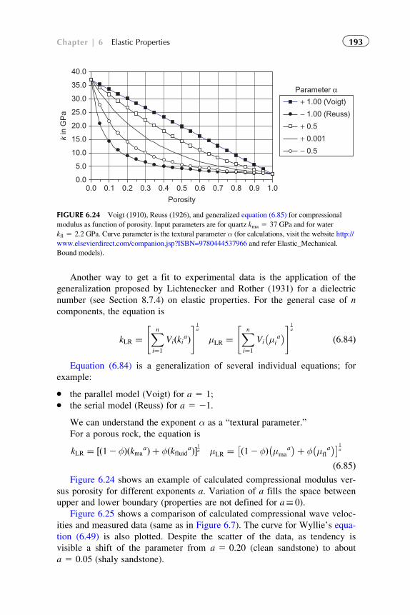
Another way to get a fit to experimental data is the application of the
generalization proposed by Lichtenecker and Rother (1931) for a dielectric
number (see Section 8.7.4) on elastic properties. For the general case of n
components, the equation is
kLR ¼Xni¼1
Vi kiað Þ
" #1a
μLR ¼Xni¼1
Vi μia
� �" #1a
ð6:84Þ
Equation (6.84) is a generalization of several individual equations; for
example:
� the parallel model (Voigt) for a 5 1;� the serial model (Reuss) for a 5 21.
We can understand the exponent α as a “textural parameter.”
For a porous rock, the equation is
kLR ¼ ð12φÞ kmaað Þ þ φ kfluid
að Þ½ �1a μLR ¼ ð12φÞ μmaa
� �þ φ μfla
� �� �1a
ð6:85ÞFigure 6.24 shows an example of calculated compressional modulus ver-
sus porosity for different exponents a. Variation of a fills the space between
upper and lower boundary (properties are not defined for a� 0).
Figure 6.25 shows a comparison of calculated compressional wave veloc-
ities and measured data (same as in Figure 6.7). The curve for Wyllie’s equa-
tion (6.49) is also plotted. Despite the scatter of the data, as tendency is
visible a shift of the parameter from a 5 0.20 (clean sandstone) to about
a 5 0.05 (shaly sandstone).
0.0
5.0
10.0
15.0
20.0
25.0
30.0
35.0
40.0
0.0 0.1 0.2 0.3 0.4 0.5 0.6 0.7 0.8 0.9 1.0
Porosity
k in
GP
a
Parameter α+ 1.00 (Voigt)
− 1.00 (Reuss)
+ 0.5
+ 0.001
− 0.5
FIGURE 6.24 Voigt (1910), Reuss (1926), and generalized equation (6.85) for compressional
modulus as function of porosity. Input parameters are for quartz kma 5 37 GPa and for water
kfl 5 2.2 GPa. Curve parameter is the textural parameter α (for calculations, visit the website http://
www.elsevierdirect.com/companion.jsp?ISBN=9780444537966 and refer Elastic_Mechanical.
Bound models).
193Chapter | 6 Elastic Properties
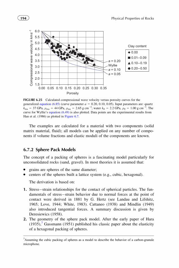
The examples are calculated for a material with two components (solid
matrix material, fluid); all models can be applied on any number of compo-
nents if volume fractions and elastic moduli of the components are known.
6.7.2 Sphere Pack Models
The concept of a packing of spheres is a fascinating model particularly for
unconsolidated rocks (sand, gravel). In most theories it is assumed that:
� grains are spheres of the same diameter;� centers of the spheres built a lattice system (e.g., cubic, hexagonal).
The derivation is based on:
1. Stress�strain relationships for the contact of spherical particles. The fun-
damentals of stress�strain behavior due to normal forces at the point of
contact were derived in 1881 by G. Hertz (see Landau and Lifshitz,
1965; Love, 1944; White, 1983). Cattaneo (1938) and Mindlin (1949)
also introduced tangential forces. A summary discussion is given by
Deresiewics (1958).
2. The geometry of the sphere pack model. After the early paper of Hara
(1935),7 Gassmann (1951) published his classic paper about the elasticity
of a hexagonal packing of spheres.
1.5
2.0
2.5
3.0
3.5
4.0
4.5
5.0
5.5
6.0
0.00 0.05 0.10 0.15 0.20 0.25 0.30 0.35
Porosity
Com
pres
sion
al w
ave
velo
city
in k
ms−1
a = 0.20
0.00
0.01–0.09
0.10–0.19
0.20–0.50
Clay content
Wylliea = 0.10a = 0.05
FIGURE 6.25 Calculated compressional wave velocity versus porosity curves for the
generalized equation (6.85) (curve parameter a 5 0.20, 0.10, 0.05). Input parameters are: quartz
kma 5 37 GPa, μma 5 44 GPa, ρma 5 2.65 g cm23; water kfl 5 2.2 GPa, ρfl 5 1.00 g cm23. The
curve for Wyllie’s equation (6.49) is also plotted. Data points are the experimental results from
Han et al. (1986) as plotted in Figure 6.7.
7Assuming the cubic packing of spheres as a model to describe the behavior of a carbon-granulemicrophone.
194 Physical Properties of Rocks
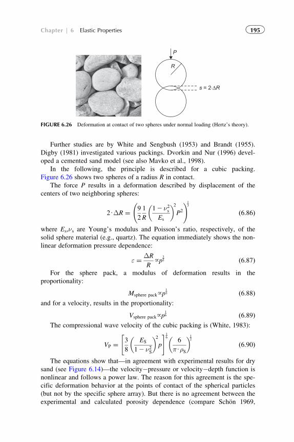
Further studies are by White and Sengbush (1953) and Brandt (1955).
Digby (1981) investigated various packings. Dvorkin and Nur (1996) devel-
oped a cemented sand model (see also Mavko et al., 1998).
In the following, the principle is described for a cubic packing.
Figure 6.26 shows two spheres of a radius R in contact.
The force P results in a deformation described by displacement of the
centers of two neighboring spheres:
2UΔR ¼ 9
2
1
R
12 ν2sEs
� �2P2
!13
ð6:86Þ
where Es,νs are Young’s modulus and Poisson’s ratio, respectively, of the
solid sphere material (e.g., quartz). The equation immediately shows the non-
linear deformation pressure dependence:
ε ¼ ΔR
R~p
23 ð6:87Þ
For the sphere pack, a modulus of deformation results in the
proportionality:
Msphere pack~p13 ð6:88Þ
and for a velocity, results in the proportionality:
Vsphere pack~p16 ð6:89Þ
The compressional wave velocity of the cubic packing is (White, 1983):
VP ¼ 3
8
ES
12 ν2S
� �2p
" #16
6
πUρS
� �12
ð6:90Þ
The equations show that—in agreement with experimental results for dry
sand (see Figure 6.14)—the velocity�pressure or velocity�depth function is
nonlinear and follows a power law. The reason for this agreement is the spe-
cific deformation behavior at the points of contact of the spherical particles
(but not by the specific sphere array). But there is no agreement between the
experimental and calculated porosity dependence (compare Schon 1969,
P
R
s = 2⋅ΔR
FIGURE 6.26 Deformation at contact of two spheres under normal loading (Hertz’s theory).
195Chapter | 6 Elastic Properties
1996). This disagreement is obviously caused by the idealized assumption of
the regular lattice array and the uniform sphere size.
For random packing of identical spheres—based on Mindlin’s (1949) the-
ory for compressional and shear behavior without a slip at the contact—
Mavko et al. (1998) give the the following:
effective bulk compressional modulus keff ¼1
18
CUμSð12φÞπð12 νSÞ
� �2
p
" #13
ð6:91Þ
effective shear modulus μeff ¼52 4UνS5ð22 νSÞ
3
2
CUμSð12φÞπð12 νsÞ
� �2
p
" #13
ð6:92Þ
where
p is the hydrostatic pressure
C is the coordination number (number of contacts to neighbors). The
coordination number correlates with the porosity (Table 2-5; Murphy,
1982; see Mavko et al., 1998).
Implementing Equations (6.91) and (6.92) into Equations (6.5) and (6.6)
results in compressional and shear wave velocities. For sphere pack models,
both wave velocities show identical dependence on porosity and pressure.
Thus, the ratio is independent of porosity and pressure and only controlled
by Poisson’s ratio of the solid material νs:
VP
VS
¼ffiffiffiffiffiffiffiffiffiffiffiffiffiffiffiffiffiffiffiffi102 7Uνs52 4Uνs
rð6:93Þ
This derivation is valid only for a dry model.
6.7.3 Inclusion Models
In inclusion models, the pores or cracks/fractures are considered as voids or
inclusions in a solid matrix—comparable to “Swiss cheese.” Such models
are preferred for hard rocks with low porosity. Pores, vugs, or cracks are
modeled as ellipsoidal inclusions in a solid host material. A variation of the
shape of inclusions (from spheres to elliptic cracks or needles) and the prop-
erties of the inclusion (empty, gaseous, liquid, solid) opens a broad spectrum
of cases.
For the calculation, it is assumed that the following:
� There is no fluid flow between the pores/fractures; this approach simu-
lates very high-frequency saturated rock behavior (Mavko et al., 1998).
Therefore Mavko et al. (1998) recommend: “it is better to find the effec-
tive moduli for dry cavities and then saturate them with the Gassmann
low-frequency relations” (see Section 6.7.5).
196 Physical Properties of Rocks
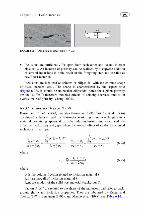
� Inclusions are sufficiently far apart from each other and do not interact
elastically. An increase of porosity can be realized by a stepwise addition
of several inclusions into the result of the foregoing step and use this as
new “host material.”
Inclusions are idealized as spheres or ellipsoids (with the extreme shape
of disks, needles, etc.). The shape is characterized by the aspect ratio
(Figure 6.27). It should be noted that ellipsoidal pores for a given porosity
are the “stiffest”; therefore modeled effects of velocity decrease tend to an
overestimate of porosity (Cheng, 2008).
6.7.3.1 Kuster and Toksoz (1974)
Kuster and Toksoz (1974; see also Berryman, 1995; Toksoz et al., 1976)
developed a theory based on first-order scattering (long wavelength) in a
material containing spherical or spheroidal inclusions and calculated the
effective moduli kKT and μKT, where the overall effect of randomly oriented
inclusions is isotropic:
kKT 2 ks
kKT þ 43μs
¼
Pni¼1
φiðki 2 ksÞPsi
ks þ 43μs
μKT 2μs
μKT þ ςs¼
Pni¼1
φiðμi 2μsÞQsi
μs þ ςsð6:94Þ
where
ςs ¼μs
6
9Uks þ 8Uμs
ks þ 2Uμs
ð6:95Þ
where
φi is the volume fraction related to inclusion material i
ki,μi are moduli of inclusion material i
ks,μs are moduli of the solid host material (background).
Factors Psi,Qsi are related to the shape of the inclusions and refer to back-
ground (host) and inclusion properties. They are tabulated by Kuster and
Toksoz (1974), Berryman (1995), and Mavko et al. (1998); see Table 6.14.
2c
2a
FIGURE 6.27 Definition of aspect ratio α 5 c/a.
197Chapter | 6 Elastic Properties
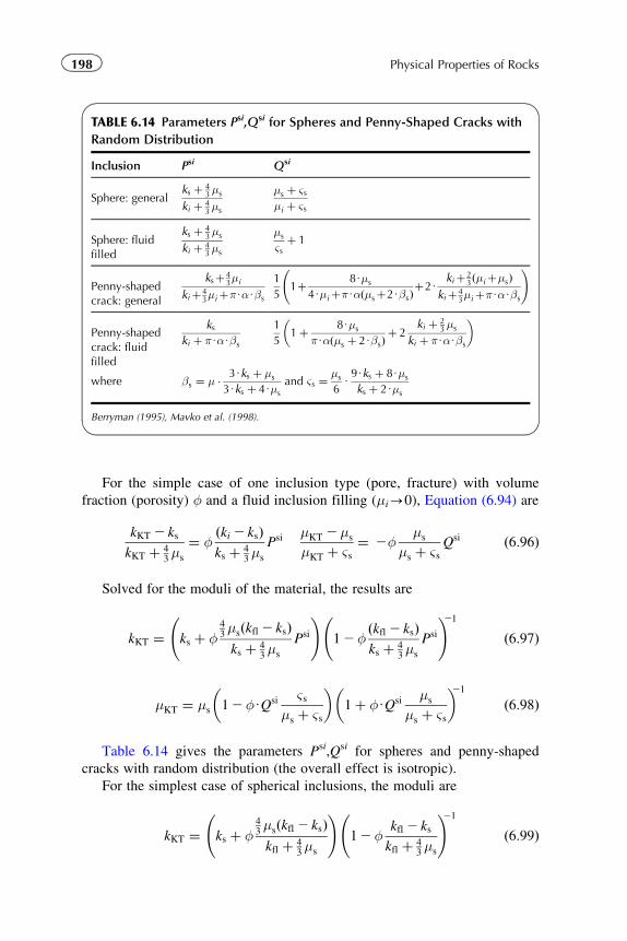
For the simple case of one inclusion type (pore, fracture) with volume
fraction (porosity) φ and a fluid inclusion filling (μi-0), Equation (6.94) are
kKT 2 ks
kKT þ 43μs
¼ φðki 2 ksÞks þ 4
3μs
Psi μKT 2μs
μKT þ ςs¼ 2φ
μs
μs þ ςsQsi ð6:96Þ
Solved for the moduli of the material, the results are
kKT ¼ ks þ φ43μsðkfl 2 ksÞks þ 4
3μs
Psi
!12φ
ðkfl 2 ksÞks þ 4
3μs
Psi
!21
ð6:97Þ
μKT ¼ μs 12φUQsi ςsμs þ ςs
� �1þ φUQsi μs
μs þ ςs
� �21
ð6:98Þ
Table 6.14 gives the parameters Psi,Qsi for spheres and penny-shaped
cracks with random distribution (the overall effect is isotropic).
For the simplest case of spherical inclusions, the moduli are
kKT ¼ ks þ φ43μsðkfl 2 ksÞkfl þ 4
3μs
!12φ
kfl 2 ks
kfl þ 43μs
!21
ð6:99Þ
TABLE 6.14 Parameters Psi,Qsi for Spheres and Penny-Shaped Cracks with
Random Distribution
Inclusion Psi Qsi
Sphere: generalks þ 4
3μs
ki þ 43μs
μs þ ςsμi þ ςs
Sphere: fluidfilled
ks þ 43μs
ki þ 43μs
μs
ςsþ 1
Penny-shapedcrack: general
ksþ43μi
kiþ43μiþπUαUβs
1
51þ 8Uμs
4UμiþπUαðμsþ2UβsÞþ2U
kiþ23ðμiþμsÞ
kiþ43μiþπUαUβs
!
Penny-shapedcrack: fluidfilled
kski þ πUαUβs
1
51þ 8Uμs
πUαðμs þ 2UβsÞþ 2
ki þ 23μs
ki þ πUαUβs
� �
where βs ¼ μ � 3Uks þ μs
3Uks þ 4Uμs
and ςs ¼μs
6U9Uks þ 8Uμs
ks þ 2Uμs
Berryman (1995), Mavko et al. (1998).
198 Physical Properties of Rocks
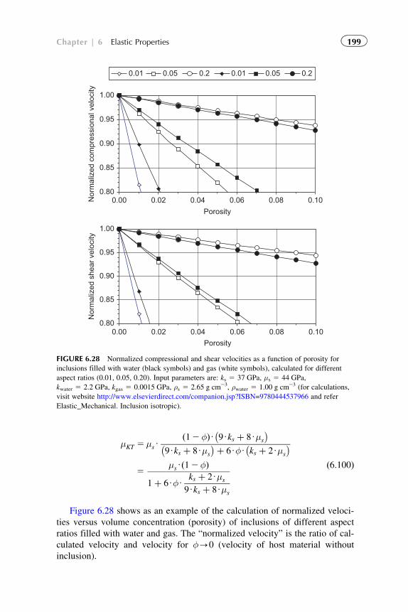
μKT 5μsU12φð ÞU 9Uks þ 8Uμs
� �9Uks þ 8Uμs
� �þ 6UφU ks þ 2Uμs
� �5
μsU 12φð Þ1þ 6UφU
ks þ 2Uμs
9Uks þ 8Uμs
ð6:100Þ
Figure 6.28 shows as an example of the calculation of normalized veloci-
ties versus volume concentration (porosity) of inclusions of different aspect
ratios filled with water and gas. The “normalized velocity” is the ratio of cal-
culated velocity and velocity for φ-0 (velocity of host material without
inclusion).
0.80
0.85
0.90
0.95
1.00
0.00 0.02 0.04 0.06 0.08 0.10Porosity
Nor
mal
ized
com
pres
sion
al v
eloc
ity
0.01 0.05 0.2 0.01 0.05 0.2
0.80
0.85
0.90
0.95
1.00
0.00 0.02 0.04 0.06 0.08 0.10Porosity
Nor
mal
ized
she
ar v
eloc
ity
FIGURE 6.28 Normalized compressional and shear velocities as a function of porosity for
inclusions filled with water (black symbols) and gas (white symbols), calculated for different
aspect ratios (0.01, 0.05, 0.20). Input parameters are: ks 5 37 GPa, μs 5 44 GPa,
kwater 5 2.2 GPa, kgas 5 0.0015 GPa, ρs 5 2.65 g cm23, ρwater 5 1.00 g cm23 (for calculations,
visit website http://www.elsevierdirect.com/companion.jsp?ISBN=9780444537966 and refer
Elastic_Mechanical. Inclusion isotropic).
199Chapter | 6 Elastic Properties
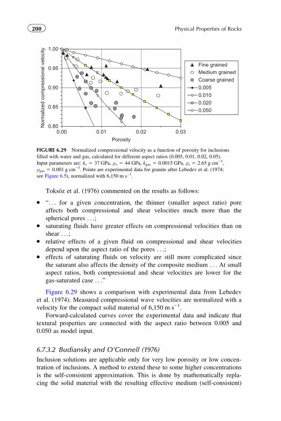
Toksoz et al. (1976) commented on the results as follows:
� “. . . for a given concentration, the thinner (smaller aspect ratio) pore
affects both compressional and shear velocities much more than the
spherical pores . . .;� saturating fluids have greater effects on compressional velocities than on
shear . . .;� relative effects of a given fluid on compressional and shear velocities
depend upon the aspect ratio of the pores . . .;� effects of saturating fluids on velocity are still more complicated since
the saturant also affects the density of the composite medium . . . At small
aspect ratios, both compressional and shear velocities are lower for the
gas-saturated case . . .”
Figure 6.29 shows a comparison with experimental data from Lebedev
et al. (1974). Measured compressional wave velocities are normalized with a
velocity for the compact solid material of 6,150 m s21.
Forward-calculated curves cover the experimental data and indicate that
textural properties are connected with the aspect ratio between 0.005 and
0.050 as model input.
6.7.3.2 Budiansky and O’Connell (1976)
Inclusion solutions are applicable only for very low porosity or low concen-
tration of inclusions. A method to extend these to some higher concentrations
is the self-consistent approximation. This is done by mathematically repla-
cing the solid material with the resulting effective medium (self-consistent)
0.80
0.85
0.90
0.95
1.00
0.00 0.01 0.02 0.03
Porosity
Nor
mal
ized
com
pres
sion
al v
eloc
ity
Fine grainedMedium grainedCoarse grained
0.0050.0100.0200.050
FIGURE 6.29 Normalized compressional velocity as a function of porosity for inclusions
filled with water and gas, calculated for different aspect ratios (0.005, 0.01, 0.02, 0.05).
Input parameters are: ks 5 37 GPa, μs 5 44 GPa, kgas 5 0.0015 GPa, ρs 5 2.65 g cm23,
ρgas 5 0.001 g cm23. Points are experimental data for granite after Lebedev et al. (1974;
see Figure 6.5), normalized with 6,150 m s21.
200 Physical Properties of Rocks
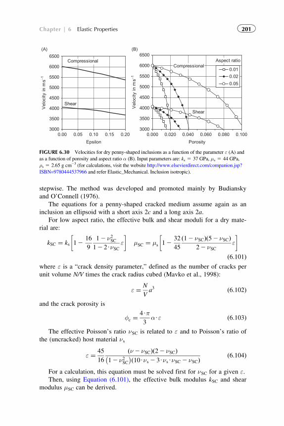
stepwise. The method was developed and promoted mainly by Budiansky
and O’Connell (1976).
The equations for a penny-shaped cracked medium assume again as an
inclusion an ellipsoid with a short axis 2c and a long axis 2a.
For low aspect ratio, the effective bulk and shear moduli for a dry mate-
rial are:
kSC ¼ ks 1216
9
12 ν2SC12 2UνSC
ε
μSC ¼ μs 1232
45
ð12 νSCÞð52 νSCÞ22 νSC
ε
ð6:101Þwhere ε is a “crack density parameter,” defined as the number of cracks per
unit volume N/V times the crack radius cubed (Mavko et al., 1998):
ε ¼ N
Va3 ð6:102Þ
and the crack porosity is
φc ¼4Uπ3
αUε ð6:103Þ
The effective Poisson’s ratio νSC is related to ε and to Poisson’s ratio of
the (uncracked) host material νs
ε ¼ 45
16
ðν2 νSCÞð22 νSCÞ12 ν2SC� �ð10Uνs 2 3UνsUνSC 2 νSCÞ
ð6:104Þ
For a calculation, this equation must be solved first for νSC for a given ε.Then, using Equation (6.101), the effective bulk modulus kSC and shear
modulus μSC can be derived.
3000
3500
4000
4500
5000
5500
6000
6500
0.00 0.05 0.10 0.15 0.20
Epsilon
Vel
ocity
in m
s−1
Shear
3000
3500
4000
4500
5000
5500
6000
6500(A) (B)
0.000 0.020 0.040 0.060 0.080 0.100
Porosity
Vel
ocity
in m
s−1
Shear
Aspect ratio
0.01
0.02
0.05
CompressionalCompressional
FIGURE 6.30 Velocities for dry penny-shaped inclusions as a function of the parameter ε (A) andas a function of porosity and aspect ratio α (B). Input parameters are: ks 5 37 GPa, μs 5 44 GPa,
ρs 5 2.65 g cm23 (for calculations, visit the website http://www.elsevierdirect.com/companion.jsp?
ISBN=9780444537966 and refer Elastic_Mechanical. Inclusion isotropic).
201Chapter | 6 Elastic Properties
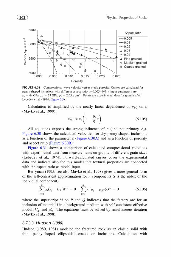
Calculation is simplified by the nearly linear dependence of νSC on ε(Mavko et al., 1999):
νSC � νs 1216
9ε
� �ð6:105Þ
All equations express the strong influence of ε (and not primary φc).Figure 6.30 shows the calculated velocities for dry penny-shaped inclusions
as a function of the parameter ε (Figure 6.30A) and as a function of porosity
and aspect ratio (Figure 6.30B).
Figure 6.31 shows a comparison of calculated compressional velocities
with experimental data from measurements on granite of different grain sizes
(Lebedev et al., 1974). Forward-calculated curves cover the experimental
data and indicate also for this model that textural properties are connected
with the aspect ratio as model input.
Berryman (1995; see also Mavko et al., 1998) gives a more general form
of the self-consistent approximation for n components (i is the index of the
individual component):Xni¼1
xiðki 2 kSCÞP�i ¼ 0Xni¼1
xiðμi 2 μSCÞQ�i ¼ 0 ð6:106Þ
where the superscript *i on P and Q indicates that the factors are for an
inclusion of material i in a background medium with self-consistent effective
moduli k�SC and μ�SC: The equations must be solved by simultaneous iteration
(Mavko et al., 1998).
6.7.3.3 Hudson (1980)
Hudson (1980, 1981) modeled the fractured rock as an elastic solid with
thin, penny-shaped ellipsoidal cracks or inclusions. Calculation with
5000
5500
6000
6500
0.000 0.005 0.010 0.015 0.020 0.025
Porosity
Vel
ocity
VP in
ms−1 0.005
0.010.020.030.04Fine grainedMedium grainedCoarse grained
Aspect ratio
FIGURE 6.31 Compressional wave velocity versus crack porosity. Curves are calculated for
penny-shaped inclusions with different aspect ratio α (0.005�0.04); input parameters are:
ks 5 44 GPa, μs 5 37 GPa, ρs 5 2.65 g cm23. Points are experimental data for granite after
Lebedev et al. (1974; Figure 6.5).
202 Physical Properties of Rocks
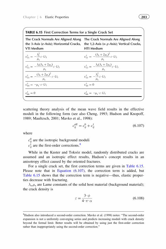
scattering theory analysis of the mean wave field results in the effective
moduli in the following form (see also Cheng, 1993; Hudson and Knopoff,
1989; Maultzsch, 2001; Mavko et al., 1998):
ceffij ¼ c0ij þ c1ij ð6:107Þwhere
c0ij are the isotropic background moduli
c1ij are the first-order corrections.8
While in the Kuster and Toksoz model, randomly distributed cracks are
assumed and an isotropic effect results, Hudson’s concept results in an
anisotropy effect caused by the oriented fractures.
For a single crack set, the first correction terms are given in Table 6.15.
Please note that in Equation (6.107), the correction term is added, but
Table 6.15 shows that the correction term is negative—thus, elastic proper-
ties decrease with fracturing.
λs,μs are Lame constants of the solid host material (background material);
the crack density is
ε ¼ 3Uφ4UπUα
ð6:108Þ
TABLE 6.15 First Correction Terms for a Single Crack Set
The Crack Normals Are Aligned Along
the 3-Axis (z-Axis); Horizontal Cracks,
VTI Medium
The Crack Normals Are Aligned Along
the 1,2-Axis (x-,y-Axis); Vertical Cracks,
HTI Medium
c111 ¼ 2λ2s
μs
εUU3 c111 ¼ 2ðλs þ 2μsÞ2
μs
εUU3
c113 ¼ 2λsðλs þ 2μsÞ
μs
εUU3 c113 ¼ 2λsðλs þ 2μsÞ
μs
εUU3
c133 ¼ 2ðλs þ 2μsÞ2
μs
εUU3 c133 ¼ 2λ2s
μs
εUU3
c144 ¼ 2μsUεUU1 c144 ¼ 0
c166 ¼ 0 c166 ¼ 2μsUεUU1
8Hudson also introduced a second-order correction. Mavko et al. (1998) notes: “The second-orderexpansion is not a uniformly converging series and predicts increasing moduli with crack densitybeyond the formal limit. Better results will be obtained by using just the first-order correctionrather than inappropriately using the second-order correction.”
203Chapter | 6 Elastic Properties
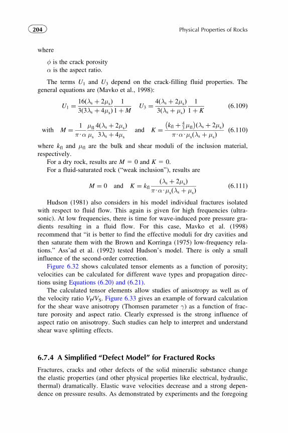
where
φ is the crack porosity
α is the aspect ratio.
The terms U1 and U3 depend on the crack-filling fluid properties. The
general equations are (Mavko et al., 1998):
U1 ¼ 16ðλs þ 2μsÞ3ð3λs þ 4μsÞ
1
1þMU3 ¼ 4ðλs þ 2μsÞ
3ðλs þ μsÞ1
1þ Kð6:109Þ
with M ¼ 1
πUαμfl
μs
4ðλs þ 2μsÞ3λs þ 4μs
and K ¼ kfl þ 43μfl
� �ðλs þ 2μsÞπUαUμsðλs þ μsÞ
ð6:110Þ
where kfl and μfl are the bulk and shear moduli of the inclusion material,
respectively.
For a dry rock, results are M 5 0 and K 5 0.
For a fluid-saturated rock (“weak inclusion”), results are
M ¼ 0 and K ¼ kflðλs þ 2μsÞ
πUαUμsðλs þ μsÞð6:111Þ
Hudson (1981) also considers in his model individual fractures isolated
with respect to fluid flow. This again is given for high frequencies (ultra-
sonic). At low frequencies, there is time for wave-induced pore pressure gra-
dients resulting in a fluid flow. For this case, Mavko et al. (1998)
recommend that “it is better to find the effective moduli for dry cavities and
then saturate them with the Brown and Korringa (1975) low-frequency rela-
tions.” Ass’ad et al. (1992) tested Hudson’s model. There is only a small
influence of the second-order correction.
Figure 6.32 shows calculated tensor elements as a function of porosity;
velocities can be calculated for different wave types and propagation direc-
tions using Equations (6.20) and (6.21).
The calculated tensor elements allow studies of anisotropy as well as of
the velocity ratio VP/VS. Figure 6.33 gives an example of forward calculation
for the shear wave anisotropy (Thomsen parameter γ) as a function of frac-
ture porosity and aspect ratio. Clearly expressed is the strong influence of
aspect ratio on anisotropy. Such studies can help to interpret and understand
shear wave splitting effects.
6.7.4 A Simplified “Defect Model” for Fractured Rocks
Fractures, cracks and other defects of the solid mineralic substance change
the elastic properties (and other physical properties like electrical, hydraulic,
thermal) dramatically. Elastic wave velocities decrease and a strong depen-
dence on pressure results. As demonstrated by experiments and the foregoing
204 Physical Properties of Rocks
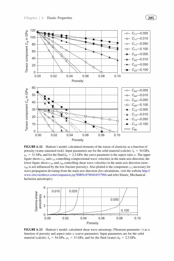
0
20
40
60
80
100
120
0.00 0.02 0.04 0.06 0.08 0.10Porosity
Tens
or c
ompo
nent
Cik in
GP
a
C11—0.005C11—0.010C11—0.050C11—0.100C33—0.005C33—0.010C33—0.050C33—0.100
0
10
20
30
40
50
60
0.00 0.02 0.04 0.06 0.08 0.10Porosity
Tens
or c
ompo
nent
Cik in
GP
a C44—0.005C44—0.010C44—0.050C44—0.100C13—0.005C13—0.010C13—0.050C13—0.100C66
FIGURE 6.32 Hudson’s model: calculated elements of the tensor of elasticity as a function of
porosity (water-saturated rock). Input parameters are for the solid material (calcite) λs 5 54 GPa,
μs 5 31 GPa, and for the fluid kfl 5 2.2 GPa: the curve parameter is the aspect ratio α. The upperfigure shows c11 and c33 controlling compressional wave velocities in the main axis direction; the
lower figure shows c44 and c66 controlling shear wave velocities in the main axis direction (note:
c66 is not influenced by the low fracture porosity). Also plotted is the component c13 necessary for
wave propagation deviating from the main axis direction (for calculations, visit the website http://
www.elsevierdirect.com/companion.jsp?ISBN=9780444537966 and refer Elastic_Mechanical.
Inclusion anisotropic).
0
2
4
6
0.00 0.02 0.04 0.06 0.08 0.10
Porosity
Gam
ma-
shea
ran
isot
ropy
0.010 0.020
0.050
0.100
FIGURE 6.33 Hudson’s model: calculated shear wave anisotropy (Thomsen parameter γ) as afunction of porosity and aspect ratio α (curve parameter). Input parameters are for the solid
material (calcite) λs 5 54 GPa, μs 5 31 GPa, and for the fluid (water) kfl 5 2.2 GPa.
205Chapter | 6 Elastic Properties
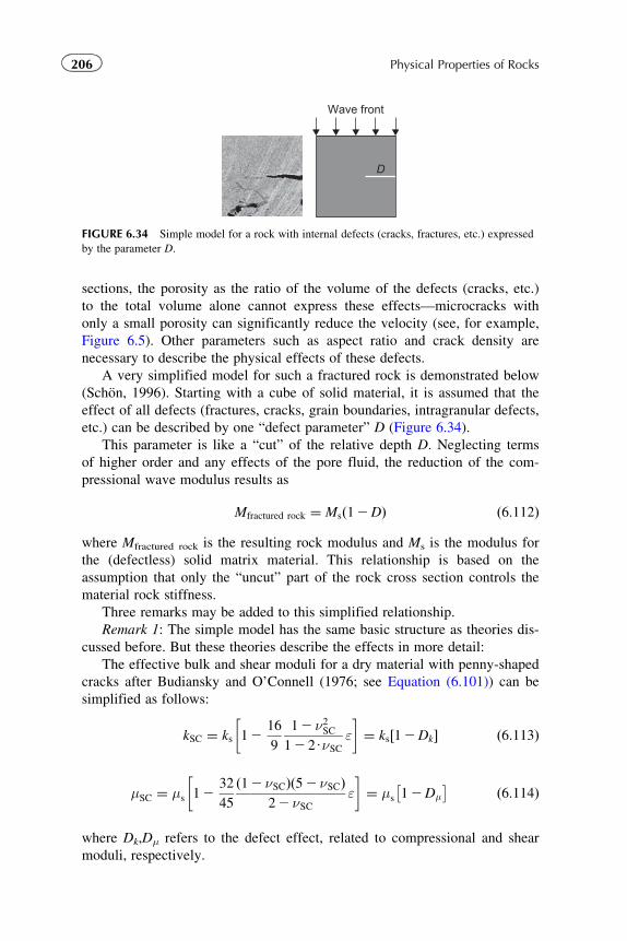
sections, the porosity as the ratio of the volume of the defects (cracks, etc.)
to the total volume alone cannot express these effects—microcracks with
only a small porosity can significantly reduce the velocity (see, for example,
Figure 6.5). Other parameters such as aspect ratio and crack density are
necessary to describe the physical effects of these defects.
A very simplified model for such a fractured rock is demonstrated below
(Schon, 1996). Starting with a cube of solid material, it is assumed that the
effect of all defects (fractures, cracks, grain boundaries, intragranular defects,
etc.) can be described by one “defect parameter” D (Figure 6.34).
This parameter is like a “cut” of the relative depth D. Neglecting terms
of higher order and any effects of the pore fluid, the reduction of the com-
pressional wave modulus results as
Mfractured rock ¼ Msð12DÞ ð6:112Þ
where Mfractured rock is the resulting rock modulus and Ms is the modulus for
the (defectless) solid matrix material. This relationship is based on the
assumption that only the “uncut” part of the rock cross section controls the
material rock stiffness.
Three remarks may be added to this simplified relationship.
Remark 1: The simple model has the same basic structure as theories dis-
cussed before. But these theories describe the effects in more detail:
The effective bulk and shear moduli for a dry material with penny-shaped
cracks after Budiansky and O’Connell (1976; see Equation (6.101)) can be
simplified as follows:
kSC ¼ ks 1216
9
12 ν2SC12 2UνSC
ε
¼ ks 12Dk½ � ð6:113Þ
μSC ¼ μs 1232
45
ð12 νSCÞð52 νSCÞ22 νSC
ε
¼ μs 12Dμ� � ð6:114Þ
where Dk,Dμ refers to the defect effect, related to compressional and shear
moduli, respectively.
Wave front
D
FIGURE 6.34 Simple model for a rock with internal defects (cracks, fractures, etc.) expressed
by the parameter D.
206 Physical Properties of Rocks
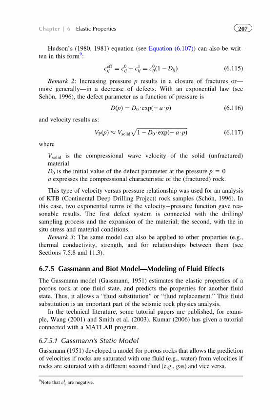
Hudson’s (1980, 1981) equation (see Equation (6.107)) can also be writ-
ten in this form9:
ceffij ¼ c0ij þ c1ij ¼ c0ijð12DijÞ ð6:115ÞRemark 2: Increasing pressure p results in a closure of fractures or—
more generally—in a decrease of defects. With an exponential law (see
Schon, 1996), the defect parameter as a function of pressure is
DðpÞ ¼ D0Uexpð2 aUpÞ ð6:116Þand velocity results as:
VPðpÞ � Vsolid
ffiffiffiffiffiffiffiffiffiffiffiffiffiffiffiffiffiffiffiffiffiffiffiffiffiffiffiffiffiffiffiffiffiffiffiffiffiffi12D0Uexpð2 aUpÞ
pð6:117Þ
where
Vsolid is the compressional wave velocity of the solid (unfractured)
material
D0 is the initial value of the defect parameter at the pressure p 5 0
a expresses the compressional characteristic of the (fractured) rock.
This type of velocity versus pressure relationship was used for an analysis
of KTB (Continental Deep Drilling Project) rock samples (Schon, 1996). In
this case, two exponential terms of the velocity�pressure function gave rea-
sonable results. The first defect system is connected with the drilling/
sampling process and the expansion of the material; the second, with the in
situ stress and material conditions.
Remark 3: The same model can also be applied to other properties (e.g.,
thermal conductivity, strength, and for relationships between them (see
Sections 7.5.8 and 11.3).
6.7.5 Gassmann and Biot Model—Modeling of Fluid Effects
The Gassmann model (Gassmann, 1951) estimates the elastic properties of a
porous rock at one fluid state, and predicts the properties for another fluid
state. Thus, it allows a “fluid substitution” or “fluid replacement.” This fluid
substitution is an important part of the seismic rock physics analysis.
In the technical literature, some tutorial papers are published, for exam-
ple, Wang (2001) and Smith et al. (2003). Kumar (2006) has given a tutorial
connected with a MATLAB program.
6.7.5.1 Gassmann’s Static Model
Gassmann (1951) developed a model for porous rocks that allows the prediction
of velocities if rocks are saturated with one fluid (e.g., water) from velocities if
rocks are saturated with a different second fluid (e.g., gas) and vice versa.
9Note that c1ij are negative.
207Chapter | 6 Elastic Properties
Gassmann’s theory assumes (Dewar and Pickford, 2001) the following:
� The rock is macroscopically homogeneous and isotropic: This assumption
ensures that wavelength. grain and pore size (this is given in most cases
of seismic field and laboratory measurements). The statistical isotropic
porous material with homogeneous mineral moduli makes no assumptions
with respect to any pore geometry.� Within the interconnected pores, there is a fluid pressure equilibrium and
no pore pressure gradient as a result of passing waves. Thus, the low fre-
quency allows an equilibration of the pore pressure within the pore space.
Therefore, Gassmann’s equation works best for seismic frequencies
(,100 Hz) and high permeability (Mavko et al., 1998).� Pores are filled with nonviscous, frictionless fluids. This also contributes
to pore pressure equilibrium and results in a fluid independent shear mod-
ulus of the porous rock.� The rock-fluid system is closed (undrained), that is, no fluid can flow in
or out of the considered volume during wave passage.� The pore fluid does not interact with the solid material or rock frame.
Gassmann’s model does not implement any change of the “rock skeleton
or frame modulus” by changing fluids (e.g., softening in case of swelling
clay cement by replacement of oil by water with reactive chemical com-
position or in general as a result of changing surface energy).� A passing wave results in the motion (displacement) of the whole rock
section, but there is no relative motion between solid rock skeleton and
fluid. This exactly is given only for zero frequency (static solution); for
high frequencies, a relative motion can result in dispersion.
Changing pore fluid influences velocity of elastic waves as a result of
changing elastic moduli and changing density. The effects can be described
as follows:
1. density follows the equation
ρ ¼ ð12φÞρs þ φUρfl ð6:118Þ2. shear modulus is independent on the fluid type
μdry ¼ μsat ¼ μ ð6:119Þ3. compressional bulk modulus is strongly dependent on fluid compressional
modulus and the key parameter in Gassmann’s model. Figure 6.35
explains the principle of the derivation for the two cases.
The left side describes the “dry case”: the pores are empty and therefore
pore fluid has zero bulk modulus and does not contribute to the compression
resistance (pore fluid also has zero shear modulus). This situation is given
approximately for air-filled rock at standard room temperature and pressure
208 Physical Properties of Rocks
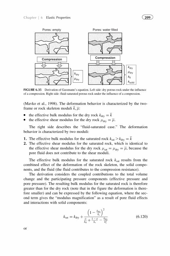
(Mavko et al., 1998). The deformation behavior is characterized by the two-
frame or rock skeleton moduli k;μ:
� the effective bulk modulus for the dry rock kdry ¼ k� the effective shear modulus for the dry rock μdry ¼ μ.
The right side describes the “fluid-saturated case.” The deformation
behavior is characterized by two moduli:
1. The effective bulk modulus for the saturated rock ksat. kdry ¼ k
2. The effective shear modulus for the saturated rock, which is identical to
the effective shear modulus for the dry rock μsat ¼ μdry ¼ μ, because the
pore fluid does not contribute to the shear moduli.
The effective bulk modulus for the saturated rock ksat results from the
combined effect of the deformation of the rock skeleton, the solid compo-
nents, and the fluid (the fluid contributes to the compression resistance).
The derivation considers the coupled contributions to the total volume
change and the participating pressure components (effective pressure and
pore pressure). The resulting bulk modulus for the saturated rock is therefore
greater than for the dry rock (note that in the figure the deformation is there-
fore smaller) and can be expressed by the following equation, where the sec-
ond term gives the “modulus magnification” as a result of pore fluid effects
and interactions with solid components:
ksat ¼ kdry þ12
kdryks
� �2φkflþ 12φ
ks2
kdryk2s
ð6:120Þ
or
Pores: empty Pores: water filled
Compression Compression
kdry
µdry
kdry
µdry
kfl
ksolid
FIGURE 6.35 Derivation of Gassmann’s equation. Left side: dry porous rock under the influence
of a compression. Right side: fluid-saturated porous rock under the influence of a compression.
209Chapter | 6 Elastic Properties
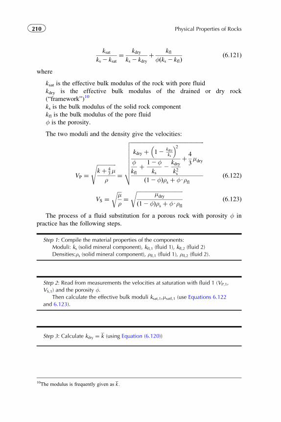
ksat
ks 2 ksat¼ kdry
ks 2 kdryþ kfl
φðks 2 kflÞð6:121Þ
where
ksat is the effective bulk modulus of the rock with pore fluid
kdry is the effective bulk modulus of the drained or dry rock
(“framework”)10
ks is the bulk modulus of the solid rock component
kfl is the bulk modulus of the pore fluid
φ is the porosity.
The two moduli and the density give the velocities:
VP ¼ffiffiffiffiffiffiffiffiffiffiffiffiffiffik þ 4
3μ
ρ
s¼
ffiffiffiffiffiffiffiffiffiffiffiffiffiffiffiffiffiffiffiffiffiffiffiffiffiffiffiffiffiffiffiffiffiffiffiffiffiffiffiffiffiffiffiffiffiffiffiffiffiffiffiffiffiffikdry þ 12
kdryks
� �2φkfl
þ 12φks
2kdry
k2s
þ 4
3μdry
ð12φÞρs þ φUρfl
vuuuuuuut ð6:122Þ
VS ¼ffiffiffiμρ
r¼
ffiffiffiffiffiffiffiffiffiffiffiffiffiffiffiffiffiffiffiffiffiffiffiffiffiffiffiffiffiffiffiffiffiffiμdry
ð12φÞρs þ φUρfl
rð6:123Þ
The process of a fluid substitution for a porous rock with porosity φ in
practice has the following steps.
Step 1: Compile the material properties of the components:
Moduli: ks (solid mineral component), kfl,1 (fluid 1), kfl,2 (fluid 2)
Densities:ρs (solid mineral component), ρfl,1 (fluid 1), ρfl,2 (fluid 2).
Step 2: Read from measurements the velocities at saturation with fluid 1 (VP,1,
VS,1) and the porosity φ.Then calculate the effective bulk moduli ksat,1,μsatl,1 (use Equations 6.122
and 6.123).
Step 3: Calculate kdry ¼ k (using Equation (6.120))
10The modulus is frequently given as k :
210 Physical Properties of Rocks
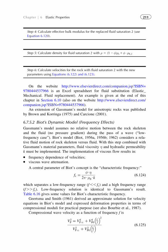
Step 4: Calculate effective bulk modulus for the replaced fluid saturation 2 (use
Equation 6.120).
Step 5: Calculate density for fluid saturation 2 with ρ 5 (12φ)ρs1φ � ρfl,2
Step 6: Calculate velocities for the rock with fluid saturation 2 with the new
parameters using Equations (6.122) and (6.123).
On the website http://www.elsevierdirect.com/companion.jsp?ISBN=
9780444537966 is an Excel spreadsheet for fluid substitution (Elastic_
Mechanical. Fluid replacement). An example is given at the end of this
chapter in Section 6.10 (also on the website http://www.elsevierdirect.com/
companion.jsp?ISBN=9780444537966).
An extension of Gassmann’s model for anisotropic rocks was published
by Brown and Korringa (1975) and Carcione (2001).
6.7.5.2 Biot’s Dynamic Model (Frequency Effects)
Gassmann’s model assumes no relative motion between the rock skeleton
and the fluid (no pressure gradient) during the pass of a wave (“low-
frequency case”). Biot’s model (Biot, 1956a, 1956b; 1962) considers a rela-
tive fluid motion of rock skeleton versus fluid. With this step combined with
Gassmann’s material parameters, fluid viscosity η and hydraulic permeability
k must be implemented. The implementation of viscous flow results in:
� frequency dependence of velocities;� viscous wave attenuation.
A central parameter of Biot’s concept is the “characteristic frequency:”
fc ¼φUη
2πUρflUkð6:124Þ
which separates a low-frequency range (f,, fc) and a high frequency range
(f.. fc). Low-frequency solution is identical to Gassmann’s result.
Table 6.16 gives some values for Biot’s characteristic frequency.
Geertsma and Smith (1961) derived an approximate solution for velocity
equations in Biot’s model and expressed deformation properties in terms of
compressional moduli for practical purpose (see also Bourbie et al., 1987).
Compressional wave velocity as a function of frequency f is
V2P ¼ V4
PN þ V4P0
fcf
� �2V2PN þ V2
P0fcf
� � ð6:125Þ
211Chapter | 6 Elastic Properties
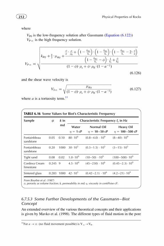
where
VP0 is the low-frequency solution after Gassmann (Equation (6.122))
VPN is the high frequency solution.
VPN ¼
ffiffiffiffiffiffiffiffiffiffiffiffiffiffiffiffiffiffiffiffiffiffiffiffiffiffiffiffiffiffiffiffiffiffiffiffiffiffiffiffiffiffiffiffiffiffiffiffiffiffiffiffiffiffiffiffiffiffiffiffiffiffiffiffiffiffiffiffiffiffiffiffiffiffiffiffiffiffiffiffiffiffiffiffiffiffiffiffiffiffiffiffiffiffiffiffiffiffiffiffiffiffiffiffiffiffiffiffiffiffiffiffiffiffiffiffiffiffiffiffiffiffiffikdry þ 4
3Uμdry þ
φaU ρρflþ 12
kdryks
� �U 12
kdryks
� �U 12
kdryks
2 2U φa
� �12
kdryks
2φ� �
U 1ksþ φ
kfl
12φð ÞUρs þ φUρflU 12 a21ð Þ
vuuuuuutð6:126Þ
and the shear wave velocity is
VSN ¼ffiffiffiffiffiffiffiffiffiffiffiffiffiffiffiffiffiffiffiffiffiffiffiffiffiffiffiffiffiffiffiffiffiffiffiffiffiffiffiffiffiffiffiffiffiffiffiffiffiffiffiffiffiffiffiffiffi
μdry
12φð ÞUρs þ φUρflU 12 a21ð Þ
rð6:127Þ
where a is a tortuosity term.11
6.7.5.3 Some Further Developments of the Gassmann�BiotConcept
An extended overview of the various theoretical concepts and their applications
is given by Mavko et al. (1998). The different types of fluid motion in the pore
TABLE 6.16 Some Values for Biot’s Characteristic Frequency
Sample φ k in
md
Characteristic Frequency fc in Hz
Water
η 5 1 cP
Normal Oil
η 5 10�50 cP
Heavy Oil
η 5 100�500 cP
Fontainbleausandstone
0.05 0.10 80 � 106 (0.8�4.0) � 109 (8�40) � 109
Fontainbleausandstone
0.20 1000 30 � 103 (0.3�1.5) � 103 (3�15) � 103
Tight sand 0.08 0.02 1.0 � 109 (10�50) � 109 (100�500) � 109
Cordova Creamlimestone
0.245 9 4.5 � 106 (45�230) � 106 (0.45�2.3) � 109
Sintered glass 0.283 1000 42 � 103 (0.42�2.1) � 106 (4.2�21) � 109
From Bourbie et al. (1987)φ, porosity as volume fraction; k, permeability in md; η, viscosity in centiPoise cP.
11For a -N (no fluid movement possible) is VN-V0.
212 Physical Properties of Rocks
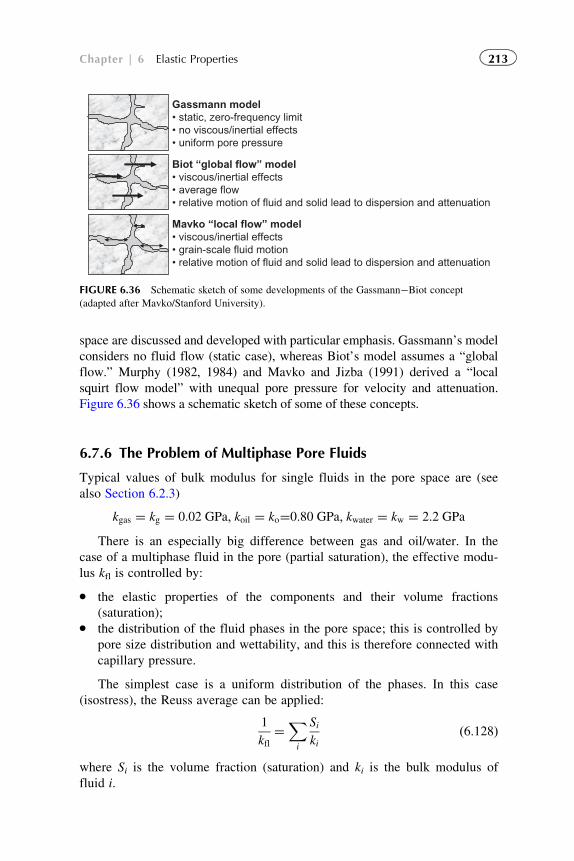
space are discussed and developed with particular emphasis. Gassmann’s model
considers no fluid flow (static case), whereas Biot’s model assumes a “global
flow.” Murphy (1982, 1984) and Mavko and Jizba (1991) derived a “local
squirt flow model” with unequal pore pressure for velocity and attenuation.
Figure 6.36 shows a schematic sketch of some of these concepts.
6.7.6 The Problem of Multiphase Pore Fluids
Typical values of bulk modulus for single fluids in the pore space are (see
also Section 6.2.3)
kgas ¼ kg ¼ 0:02 GPa; koil ¼ ko¼0:80 GPa; kwater ¼ kw ¼ 2:2 GPa
There is an especially big difference between gas and oil/water. In the
case of a multiphase fluid in the pore (partial saturation), the effective modu-
lus kfl is controlled by:
� the elastic properties of the components and their volume fractions
(saturation);� the distribution of the fluid phases in the pore space; this is controlled by
pore size distribution and wettability, and this is therefore connected with
capillary pressure.
The simplest case is a uniform distribution of the phases. In this case
(isostress), the Reuss average can be applied:
1
kfl¼Xi
Si
kið6:128Þ
where Si is the volume fraction (saturation) and ki is the bulk modulus of
fluid i.
Gassmann model• static, zero-frequency limit• no viscous/inertial effects• uniform pore pressure
Biot “global flow” model• viscous/inertial effects• average flow• relative motion of fluid and solid lead to dispersion and attenuation
Mavko “local flow” model• viscous/inertial effects• grain-scale fluid motion• relative motion of fluid and solid lead to dispersion and attenuation
FIGURE 6.36 Schematic sketch of some developments of the Gassmann�Biot concept
(adapted after Mavko/Stanford University).
213Chapter | 6 Elastic Properties
For a gas�oil�water mixture, the equation results as:
1
kfl¼ Sw
kwþ So
koþ Sg
kgð6:129Þ
With this averaging method, the modulus of the mixture is dominated by
the phase with the lowest modulus (highest compressibility). For a water�gas
or oil�gas mixture (gas and water or oil, respectively, are evenly distributed
in each pore), it results in a “jump” from the kg level to kw level immediately
at Sw-1.
A “patchy saturation” is given when fluids are not uniformly mixed.
Effective modulus values cannot be estimated from Reuss averaging (lowest
level); an upper limit is given by Voigt’s averaging:
kfl ¼Xi
SiUki ð6:130Þ
or for a gas�oil�water mixture:
kfl ¼ SwUkw þ SoUko þ SgUkg ð6:131ÞVoigt and Reuss equations in general describe the upper and lower limit
of the compressional modulus for a mixture (Section 6.7.1).
Domenico (1976) notes that Voigt’s averaging gives the best estimate
when patch sizes are large with respect to the seismic wavelength.
Endres and Knight (1989) calculated the effect of various geometrical
distributions of water and gas in the pore space upon the velocity-saturation
characteristic. Pores are assumed to be spheres and ellipsoids with four dif-
ferent saturation regimes. For calculation, the model of Kuster and Toksoz
(1974) was used. Results demonstrate the strong influence of saturation dis-
tribution related to various pores on the overall elasticity. This general model
concept was applied also by Sengupta and Mavko (2003).
Research by Brie et al. (1995) took a somewhat different approach, deriv-
ing an equation that fills the region between Reuss’s (Equation (6.129)) and
Voigt’s (Equation (6.130)) boundary by introducing an average mixing expo-
nent e:
kfluid mixture ¼ ðkw 2 kgÞSew þ kg ð6:132ÞFigure 6.37 shows a plot of fluid bulk modulus versus water saturation
with mixing coefficient e as the parameter.
6.7.7 Model with Internal Structure and Bonding Properties
6.7.7.1 The Concept of a “Structured Model”
For porous rocks—particularly sandstones—a model was developed (Schon,
1996) in order to describe various influences on physical properties and the
relationships between them. In addition to the properties of the components
214 Physical Properties of Rocks
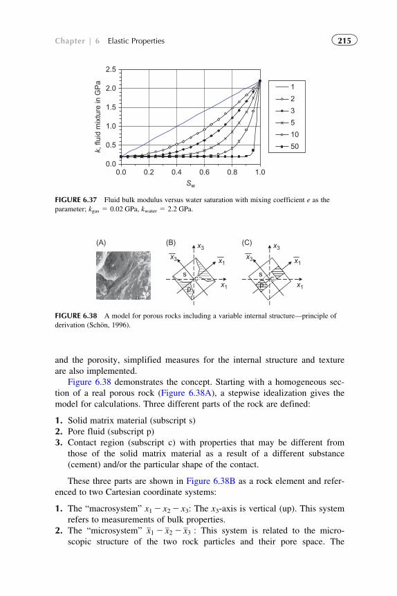
and the porosity, simplified measures for the internal structure and texture
are also implemented.
Figure 6.38 demonstrates the concept. Starting with a homogeneous sec-
tion of a real porous rock (Figure 6.38A), a stepwise idealization gives the
model for calculations. Three different parts of the rock are defined:
1. Solid matrix material (subscript s)
2. Pore fluid (subscript p)
3. Contact region (subscript c) with properties that may be different from
those of the solid matrix material as a result of a different substance
(cement) and/or the particular shape of the contact.
These three parts are shown in Figure 6.38B as a rock element and refer-
enced to two Cartesian coordinate systems:
1. The “macrosystem” x12 x22 x3: The x3-axis is vertical (up). This system
refers to measurements of bulk properties.
2. The “microsystem” x1 2 x2 2 x3 : This system is related to the micro-
scopic structure of the two rock particles and their pore space. The
x3
x1
s cp
x3 x1
x3
x1
s c
x3 x1
p
(A) (B) (C)
FIGURE 6.38 A model for porous rocks including a variable internal structure—principle of
derivation (Schon, 1996).
0.0
0.5
1.0
1.5
2.0
2.5
0.0 0.2 0.4 0.6 0.8 1.0
Sw
k, fl
uid
mix
ture
in G
Pa
1
2
3
5
10
50
FIGURE 6.37 Fluid bulk modulus versus water saturation with mixing coefficient e as the
parameter; kgas 5 0.02 GPa, kwater 5 2.2 GPa.
215Chapter | 6 Elastic Properties
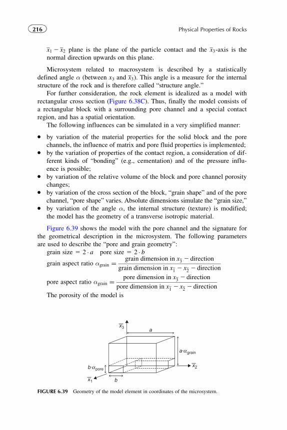
x1 2 x2 plane is the plane of the particle contact and the x3-axis is the
normal direction upwards on this plane.
Microsystem related to macrosystem is described by a statistically
defined angle α (between x3 and x3). This angle is a measure for the internal
structure of the rock and is therefore called “structure angle.”
For further consideration, the rock element is idealized as a model with
rectangular cross section (Figure 6.38C). Thus, finally the model consists of
a rectangular block with a surrounding pore channel and a special contact
region, and has a spatial orientation.
The following influences can be simulated in a very simplified manner:
� by variation of the material properties for the solid block and the pore
channels, the influence of matrix and pore fluid properties is implemented;� by the variation of properties of the contact region, a consideration of dif-
ferent kinds of “bonding” (e.g., cementation) and of the pressure influ-
ence is possible;� by variation of the relative volume of the block and pore channel porosity
changes;� by variation of the cross section of the block, “grain shape” and of the pore
channel, “pore shape” varies. Absolute dimensions simulate the “grain size,”� by variation of the angle α, the internal structure (texture) is modified;
the model has the geometry of a transverse isotropic material.
Figure 6.39 shows the model with the pore channel and the signature for
the geometrical description in the microsystem. The following parameters
are used to describe the “pore and grain geometry”:
grain size 5 2 � a pore size 5 2 � bgrain aspect ratio αgrain ¼
grain dimension in x3 2 direction
grain dimension in x1 2 x2 2 direction
pore aspect ratio αgrain ¼pore dimension in x3 2 direction
pore dimension in x1 2 x2 2 direction
The porosity of the model is
x3
x1
x2
a
b
b· poreα
a· grainα
FIGURE 6.39 Geometry of the model element in coordinates of the microsystem.
216 Physical Properties of Rocks
φ ¼ volume pore space
total model volume¼ b2Uαporeðaþ a2 bÞ
a3Uαgrain
¼ αpore
αgrain
b
a
� �222
b
a
� �ð6:133Þ
Any calculation of physical bulk properties follows two steps:
1. Calculation of properties with respect to the microsystem
2. Transformation of the properties into the macrosystem.
6.7.7.2 General Equation for Velocities
For the calculation of the elastic properties in the microsystem, the porous
rock is considered as a parallel and series arrangement of springs with the
properties of the matrix and the contact region. For simplification, it is
assumed that the solid part of the model is divided into one half of pure solid
matrix material (modulus Ms) and one half of the contact region material
(modulus Mc). All calculations are simplified for linear terms.
It is assumed that the pore space is empty (dry rock). The contribution of
the pore fluid can be implemented in a second step using the
Biot�Gassmann theory.
For the velocities (compressional and shear) results (Schon, 1996):
V ¼ Ms
ρs
2 1þMs
Mc
� �21" #
G
12φ
sikðα; f Þ½ �
( )12
¼ f1ðsÞf2Ms
Mc
; p
� �f3ðG;φÞf4ðα; f Þ
ð6:134Þ
where
Ms is the compressional wave modulus of the solid matrix material
Mc is the compressional wave modulus of the contact region
ρs is the density of the solid matrix
φ is the porosity
G is a geometric parameter that contains only geometric properties of the
grain and pore, and is related to the porosity:
G ¼ 12αpore
αgrain
b
a12 12
b
a
� �22 !" #21
ð6:135Þ
Sik (α,f) is the element of a “structure tensor.”
The elements of the tensor Sik depend only on the structure angle α and
on a bonding parameter f defined as the ratio of the compressional and
shear deformation properties of the matrix and contact region (see Equation
217Chapter | 6 Elastic Properties
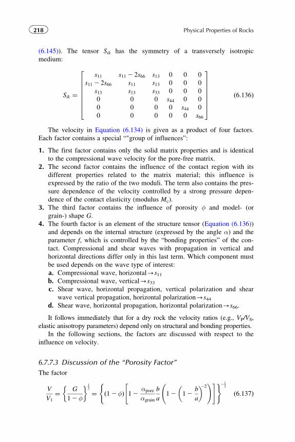
(6.145)). The tensor Sik has the symmetry of a transversely isotropic
medium:
Sik ¼
s11 s11 2 2s66 s13 0 0 0
s11 2 2s66 s11 s13 0 0 0
s13 s13 s33 0 0 0
0 0 0 s44 0 0
0 0 0 0 s44 0
0 0 0 0 0 s66
26666664
37777775
ð6:136Þ
The velocity in Equation (6.134) is given as a product of four factors.
Each factor contains a special “"group of influences”:
1. The first factor contains only the solid matrix properties and is identical
to the compressional wave velocity for the pore-free matrix.
2. The second factor contains the influence of the contact region with its
different properties related to the matrix material; this influence is
expressed by the ratio of the two moduli. The term also contains the pres-
sure dependence of the velocity controlled by a strong pressure depen-
dence of the contact elasticity (modulus Mc).
3. The third factor contains the influence of porosity φ and model- (or
grain-) shape G.
4. The fourth factor is an element of the structure tensor (Equation (6.136))
and depends on the internal structure (expressed by the angle α) and the
parameter f, which is controlled by the “bonding properties” of the con-
tact. Compressional and shear waves with propagation in vertical and
horizontal directions differ only in this last term. Which component must
be used depends on the wave type of interest:
a. Compressional wave, horizontal-s11b. Compressional wave, vertical-s33c. Shear wave, horizontal propagation, vertical polarization and shear
wave vertical propagation, horizontal polarization-s44d. Shear wave, horizontal propagation, horizontal polarization-s66.
It follows immediately that for a dry rock the velocity ratios (e.g., VP/VS,
elastic anisotropy parameters) depend only on structural and bonding properties.
In the following sections, the factors are discussed with respect to the
influence on velocity.
6.7.7.3 Discussion of the “Porosity Factor”
The factor
V
V1
¼ G
12φ
�12
¼ ð12φÞ 12αpore
αgrain
b
a12 12
b
a
� �22 !" #( )21
2
ð6:137Þ
218 Physical Properties of Rocks
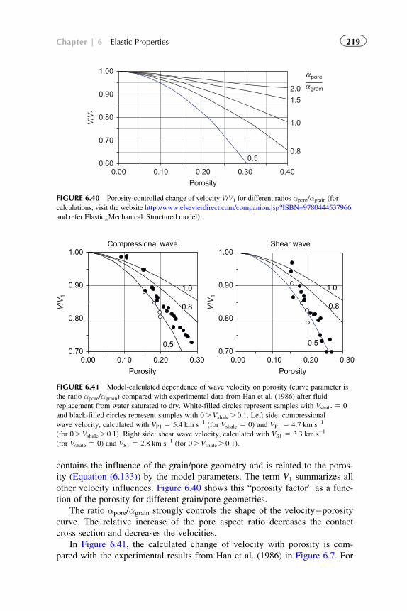
contains the influence of the grain/pore geometry and is related to the poros-
ity (Equation (6.133)) by the model parameters. The term V1 summarizes all
other velocity influences. Figure 6.40 shows this “porosity factor” as a func-
tion of the porosity for different grain/pore geometries.
The ratio αpore/αgrain strongly controls the shape of the velocity�porosity
curve. The relative increase of the pore aspect ratio decreases the contact
cross section and decreases the velocities.
In Figure 6.41, the calculated change of velocity with porosity is com-
pared with the experimental results from Han et al. (1986) in Figure 6.7. For
0.60
0.70
0.80
0.90
1.00
0.00 0.10 0.20 0.30 0.40
Porosity
V/V
12.0
1.5
1.0
0.80.5
poreα
grainα
FIGURE 6.40 Porosity-controlled change of velocity V/V1 for different ratios αpore/αgrain (for
calculations, visit the website http://www.elsevierdirect.com/companion.jsp?ISBN=9780444537966
and refer Elastic_Mechanical. Structured model).
Compressional wave
0.70
0.80
0.90
1.00
0.00 0.10 0.20 0.30Porosity
V/V
1
0.70
0.80
0.90
1.00
0.00 0.10 0.20 0.30Porosity
V/V
1
1.0
0.8
Shear wave
1.0
0.8
0.5 0.5
FIGURE 6.41 Model-calculated dependence of wave velocity on porosity (curve parameter is
the ratio αpore/αgrain) compared with experimental data from Han et al. (1986) after fluid
replacement from water saturated to dry. White-filled circles represent samples with Vshale 5 0
and black-filled circles represent samples with 0.Vshale. 0.1. Left side: compressional
wave velocity, calculated with VP1 5 5.4 km s21 (for Vshale 5 0) and VP1 5 4.7 km s21
(for 0.Vshale. 0.1). Right side: shear wave velocity, calculated with VS1 5 3.3 km s21
(for Vshale 5 0) and VS1 5 2.8 km s21 (for 0.Vshale. 0.1).
219Chapter | 6 Elastic Properties
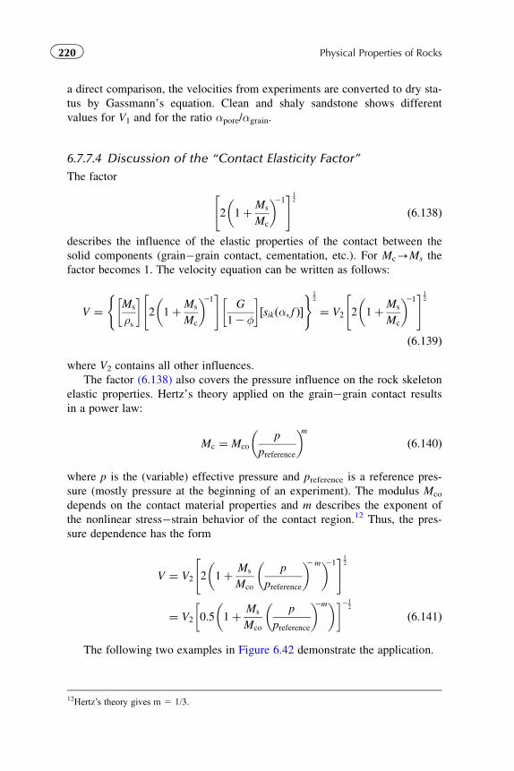
a direct comparison, the velocities from experiments are converted to dry sta-
tus by Gassmann’s equation. Clean and shaly sandstone shows different
values for V1 and for the ratio αpore/αgrain.
6.7.7.4 Discussion of the “Contact Elasticity Factor”
The factor
2 1þMs
Mc
� �21" #1
2
ð6:138Þ
describes the influence of the elastic properties of the contact between the
solid components (grain�grain contact, cementation, etc.). For Mc-Ms the
factor becomes 1. The velocity equation can be written as follows:
V ¼ Ms
ρs
2 1þMs
Mc
� �21" #G
12φ
sikðα; f Þ½ �
( )12
¼ V2 2 1þMs
Mc
� �21" #12
ð6:139Þwhere V2 contains all other influences.
The factor (6.138) also covers the pressure influence on the rock skeleton
elastic properties. Hertz’s theory applied on the grain�grain contact results
in a power law:
Mc ¼ Mco
p
preference
� �mð6:140Þ
where p is the (variable) effective pressure and preference is a reference pres-
sure (mostly pressure at the beginning of an experiment). The modulus Mco
depends on the contact material properties and m describes the exponent of
the nonlinear stress�strain behavior of the contact region.12 Thus, the pres-
sure dependence has the form
V ¼ V2 2 1þ Ms
Mco
p
preference
� �2m� �21" #1
2
¼ V2 0:5 1þ Ms
Mco
p
preference
� �2m� � 212
ð6:141Þ
The following two examples in Figure 6.42 demonstrate the application.
12Hertz’s theory gives m 5 1/3.
220 Physical Properties of Rocks
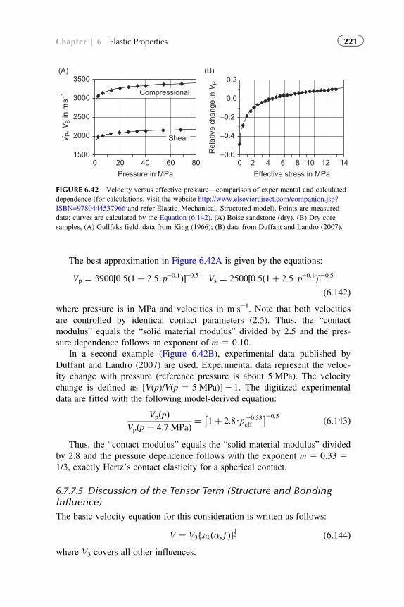
The best approximation in Figure 6.42A is given by the equations:
Vp ¼ 3900½0:5ð1þ 2:5Up20:1Þ�20:5 Vs ¼ 2500½0:5ð1þ 2:5Up20:1Þ�20:5
ð6:142Þwhere pressure is in MPa and velocities in m s21. Note that both velocities
are controlled by identical contact parameters (2.5). Thus, the “contact
modulus” equals the “solid material modulus” divided by 2.5 and the pres-
sure dependence follows an exponent of m 5 0.10.
In a second example (Figure 6.42B), experimental data published by
Duffant and Landro (2007) are used. Experimental data represent the veloc-
ity change with pressure (reference pressure is about 5 MPa). The velocity
change is defined as [V(p)/V(p 5 5 MPa)]2 1. The digitized experimental
data are fitted with the following model-derived equation:
VpðpÞVpðp ¼ 4:7 MPaÞ ¼ 1þ 2:8Up20:33
eff
� �20:5 ð6:143Þ
Thus, the “contact modulus” equals the “solid material modulus” divided
by 2.8 and the pressure dependence follows with the exponent m 5 0.33 51/3, exactly Hertz’s contact elasticity for a spherical contact.
6.7.7.5 Discussion of the Tensor Term (Structure and BondingInfluence)
The basic velocity equation for this consideration is written as follows:
V ¼ V3fsikðα; f Þg12 ð6:144Þ
where V3 covers all other influences.
−0.6
−0.4
−0.2
0.0
0.2(A) (B)
0 2 4 6 8 10 12 14Effective stress in MPa
Rel
ativ
e ch
ange
in V
P
1500
2000
2500
3000
3500
0 20 40 60 80Pressure in MPa
VP, V
S in
ms−1
Compressional
Shear
FIGURE 6.42 Velocity versus effective pressure—comparison of experimental and calculated
dependence (for calculations, visit the website http://www.elsevierdirect.com/companion.jsp?
ISBN=9780444537966 and refer Elastic_Mechanical. Structured model). Points are measured
data; curves are calculated by the Equation (6.142). (A) Boise sandstone (dry). (B) Dry core
samples, (A) Gullfaks field. data from King (1966); (B) data from Duffant and Landro (2007).
221Chapter | 6 Elastic Properties
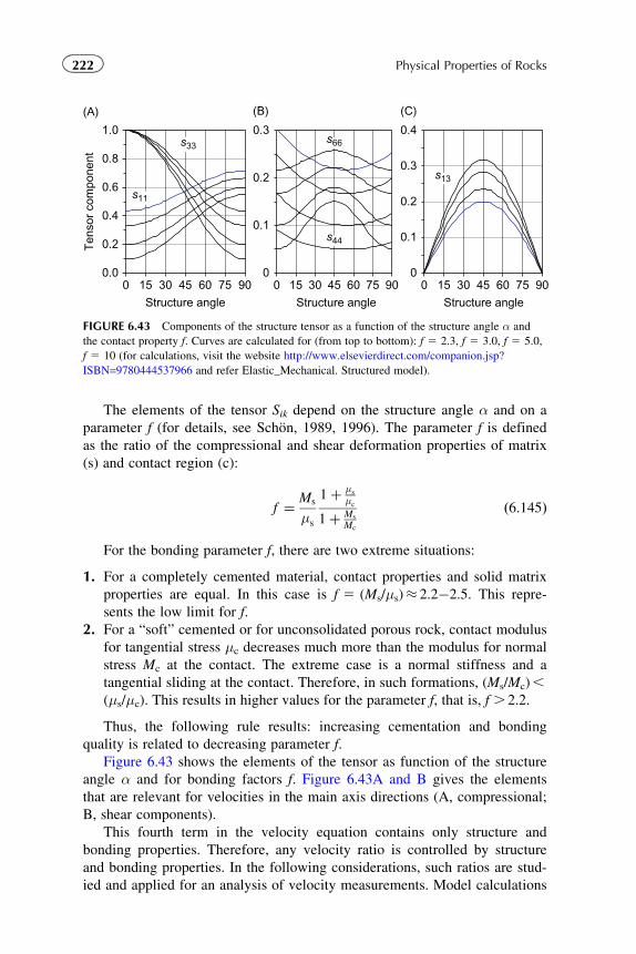
The elements of the tensor Sik depend on the structure angle α and on a
parameter f (for details, see Schon, 1989, 1996). The parameter f is defined
as the ratio of the compressional and shear deformation properties of matrix
(s) and contact region (c):
f ¼ Ms
μs
1þ μs
μc
1þ Ms
Mc
ð6:145Þ
For the bonding parameter f, there are two extreme situations:
1. For a completely cemented material, contact properties and solid matrix
properties are equal. In this case is f 5 (Ms/μs)� 2.2�2.5. This repre-
sents the low limit for f.
2. For a “soft” cemented or for unconsolidated porous rock, contact modulus
for tangential stress μc decreases much more than the modulus for normal
stress Mc at the contact. The extreme case is a normal stiffness and a
tangential sliding at the contact. Therefore, in such formations, (Ms/Mc),(μs/μc). This results in higher values for the parameter f, that is, f . 2.2.
Thus, the following rule results: increasing cementation and bonding
quality is related to decreasing parameter f.
Figure 6.43 shows the elements of the tensor as function of the structure
angle α and for bonding factors f. Figure 6.43A and B gives the elements
that are relevant for velocities in the main axis directions (A, compressional;
B, shear components).
This fourth term in the velocity equation contains only structure and
bonding properties. Therefore, any velocity ratio is controlled by structure
and bonding properties. In the following considerations, such ratios are stud-
ied and applied for an analysis of velocity measurements. Model calculations
(A)
0.0
0.2
0.4
0.6
0.8
1.0
0 15 30 45 60 75 90
Structure angle
0
0.1
0.2
0.3
0 15 30 45 60 75 90
Structure angle
0
0.1
0.2
0.4
0.3
0 15 30 45 60 75 90
Structure angle
Ten
sor
com
pone
nt
s33
s11
(B)
s66
s44
(C)
s13
FIGURE 6.43 Components of the structure tensor as a function of the structure angle α and
the contact property f. Curves are calculated for (from top to bottom): f 5 2.3, f 5 3.0, f 5 5.0,
f 5 10 (for calculations, visit the website http://www.elsevierdirect.com/companion.jsp?
ISBN=9780444537966 and refer Elastic_Mechanical. Structured model).
222 Physical Properties of Rocks
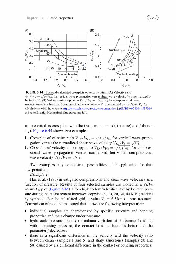
are presented as crossplots with the two parameters α (structure) and f (bond-
ing). Figure 6.44 shows two examples:
1. Crossplot of velocity ratio VP;v=VS;v ¼ffiffiffiffiffiffiffiffiffiffiffiffiffiffis33=s44
pfor vertical wave propa-
gation versus the normalized shear wave velocity VS;v=V3 ¼ ffiffiffiffiffiffis44
p:
2. Crossplot of velocity anisotropy ratio VP;v=VP;h ¼ffiffiffiffiffiffiffiffiffiffiffiffiffiffis33=s11
pfor compres-
sional wave propagation versus normalized horizontal compressional
wave velocity VP;h=V3 ¼ ffiffiffiffiffiffis11
p:
Two examples may demonstrate possibilities of an application for data
interpretation.
Example 1:
Han et al. (1986) investigated compressional and shear wave velocities as a
function of pressure. Results of four selected samples are plotted in a VP/VS
versus VS plot (Figure 6.45). From high to low velocities, the hydrostatic pres-
sure during the measurement increases stepwise (5, 10, 20, 30, 40 MPa; marked
by symbols). For the calculated grid, a value V3 5 6.5 km s21 was assumed.
Comparison of plot and measured data allows the following interpretation:
� individual samples are characterized by specific structure and bonding
properties and their change under pressure;� hydrostatic pressure creates a dominant variation of the contact bonding;
with increasing pressure, the contact bonding becomes better and the
parameter f decreases;� there is a significant difference in the velocity and the velocity ratio
between clean (samples 1 and 5) and shaly sandstones (samples 50 and
58) caused by a significant difference in the contact or bonding properties.
0.0
1.0
2.0
3.0
4.0
5.0
6.0
0.0 0.1 0.2 0.3 0.4 0.5
VS,v/V3 VP,h/V3
VP
,v/V
S,v
VP
,v/V
P,hStructure
Contact bonding
f = 20 10 104 3 2.3
4 3 2.3
= 30°α = 30°α
45°
45°60°
60°75°75°
0.0
0.5
1.0
1.5
2.0(B)(A)
0.2 0.4 0.6 0.8 1.0
Structure
6
Contact bonding
6f = 20
FIGURE 6.44 Forward-calculated crossplots of velocity ratios. (A) Velocity ratio
VP;v=VS;v ¼ffiffiffiffiffiffiffiffiffiffiffiffiffiffis33=s44
pfor vertical wave propagation versus shear wave velocity VS,V normalized by
the factor V3. (B) Velocity anisotropy ratio VP;v=VP;h ¼ffiffiffiffiffiffiffiffiffiffiffiffiffiffis33=s11
pfor compressional wave
propagation versus horizontal compressional wave velocity VP,h normalized by the factor V3 (for
calculations, visit the website http://www.elsevierdirect.com/companion.jsp?ISBN=9780444537966
and refer Elastic_Mechanical. Structured model).
223Chapter | 6 Elastic Properties
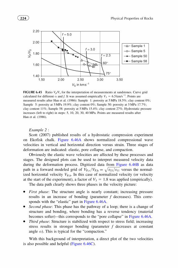
Example 2 :
Scott (2007) published results of a hydrostatic compression experiment
on Ekofisk chalk. Figure 6.46A shows normalized compressional wave
velocities in vertical and horizontal direction versus strain. Three stages of
deformation are indicated: elastic, pore collapse, and compaction.
Obviously the elastic wave velocities are affected by these processes and
stages. The designed plots can be used to interpret measured velocity data
during the deformation process. Digitized data from Figure 6.46B as data
path in a forward modeled grid of VP;v=VP;h ¼ffiffiffiffiffiffiffiffiffiffiffiffiffiffis33=s11
pversus the normal-
ized horizontal velocity VP,h. In this case of normalized velocity (or velocity
at the start of the experiment), a factor of V3 5 1.8 was applied (empirically).
The data path clearly shows three phases in the velocity picture:
� First phase: The structure angle is nearly constant; increasing pressure
results in an increase of bonding (parameter f decreases). This corre-
sponds with the “elastic” part in Figure 6.46A.� Second phase: This phase has the pathway of a loop; there is a change of
structure and bonding, where bonding has a reverse tendency (material
becomes softer)�this corresponds to the “pore collapse” in Figure 6.46A.� Third phase: Structure is stabilized with respect to stress field; increasing
stress results in stronger bonding (parameter f decreases at constant
angle α). This is typical for the “compaction.”
With this background of interpretation, a direct plot of the two velocities
is also possible and helpful (Figure 6.46C).
1.40
1.60
1.80
2.00
2.20
1.50 2.00 2.50 3.00 3.50
VS in kms−1
VP/V
S
Sample 1
Sample 5
Sample 50
Sample 58
f = 2.3
f = 3.0
60°
75°
f = 5.0
FIGURE 6.45 Ratio Vp/Vs for the interpretation of measurements at sandstones. Curve grid
calculated for different α and f. It was assumed empirically V3 5 6.5 km/s21. Points are
measured results after Han et al. (1986): Sample 1: porosity at 5MPa 18.5%; clay content 0%;
Sample 5: porosity at 5MPa 19.9%; clay content 0%; Sample 50: porosity at 5MPa 17.7%;
clay content 11%; Sample 58: porosity at 5MPa 15.4%; clay content 27%; Hydrostatic pressure
increases (left to right) in steps: 5, 10, 20, 30, 40 MPa. Points are measured results after
Han et al. (1986).
224 Physical Properties of Rocks
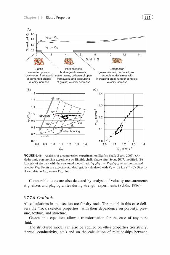
Comparable loops are also detected by analysis of velocity measurements
at gneisses and plagiogranites during strength experiments (Schon, 1996).
6.7.7.6 Outlook
All calculations in this section are for dry rock. The model in this case deli-
vers the “rock skeleton properties” with their dependence on porosity, pres-
sure, texture, and structure.
Gassmann’s equations allow a transformation for the case of any pore
fluid.
The structured model can also be applied on other properties (resistivity,
thermal conductivity, etc.) and on the calculation of relationships between
0.6
0.7
0.8
0.9
1.0
1.1
1.2
1.3
0.8 0.9 1.0 1.1 1.2 1.3 1.4
VP,h
VP
,v/V
P,h
Structure
Contact bonding60°
55°
45°
f = 50
1.0
1.1
1.2
1.3
1.4
1.0 1.1 1.2 1.3 1.4
VP,v in kms−1
VP
,h in
km
s−1
0.8
1.0
1.2
1.4
0 2 4 6 8 10 12 14
Strain in %
Nor
mal
ized
VP
VP33 = VP,v
VP11 = VP,h
Elasticcemented porous
rock—open frameworkof cemented grains;
velocity increase
Pore collapsebrekeage of cements,
some grains, collapse of openframework, and decouplingof grains; velocity decrease
(A)
(B) (C)
Compactiongrains reorient, recontact, and
recouple under stress withincreasing grain number contacts;
velocity increase
105
32.3
50°
FIGURE 6.46 Analysis of a compression experiment on Ekofisk chalk (Scott, 2007): (A)
Hydrostatic compression experiment on Ekofisk chalk, figure after Scott, 2007, modified. (B)
Analysis of the data with the structured model: ratio VP,v/VP,h 5 VP11/VP33 versus normalized
velocity VP,h. Points are experimental data; grid is calculated with V3 5 1.8 km s21. (C) Directly
plotted data as VP,h versus VP,v plot.
225Chapter | 6 Elastic Properties
them (Schon, 1996). In Section 7.5.2, the model is applied to geomechanical
strength parameters.
6.8 RESERVOIR PROPERTIES FROM SEISMIC PARAMETERS
In addition to porosity (calculated using, for example, Wyllie’s equation),
modern seismic techniques offer possibilities for:
� a lithology estimate,� fluid identification, and� reservoir fluid pressure calculation.
From the broad and permanently expanding spectrum of parameters and
attributes, only a selection can be presented in order to demonstrate some
basic idea. This demonstration began with Wyllie’s equation (6.50), which
allows the derivation of porosity from P-wave velocity or slowness.
Reflection coefficient or acoustic impedance processing gave the initial
knowledge about pore fluid (gas�water) and/or rock type (sand�shale)
effects upon these.
Implementation of shear wave parameters into seismic processing and the
philosophy of the AVO (amplitude versus offset) technique has been created
and has developed different powerful techniques. Petrophysical results are
mostly presented as crossplots to visualize both fluid and rock matrix
properties.
In the following sections, some petrophysical aspects will be discussed.
6.8.1 AVO—Basic Principle and Link to Physical Properties
AVO techniques use the partitioning of elastic wave energy at a boundary
for extraction of information about fluid and lithology. This is controlled by
the elastic properties of the two materials and the angle of the incident wave;
it results in an offset-dependent reflectivity (amplitude), observed as “AVO.”
An AVO tutorial was published by Castagna (1993).
At a boundary between two materials of different elastic properties, an
incident wave is reflected and refracted. There are two situations with respect
to the angle of incidence θ: normal incidence or non-normal incidence.
For normal incidence (θ 5 0), an incident compressional or P-wave is
reflected as P-wave.13 The reflection coefficient is defined as:
RPP ¼ VP;2Uρ2 2VP;1Uρ1VP;2Uρ2 þ VP;1Uρ1
¼ IP;2 2 IP;1
IP;2 þ IP;1ð6:146Þ
where
VP,1,VP,2 are the compressional wave velocities of the two materials
13The same relationships are valid for shear waves at normal incidence.
226 Physical Properties of Rocks
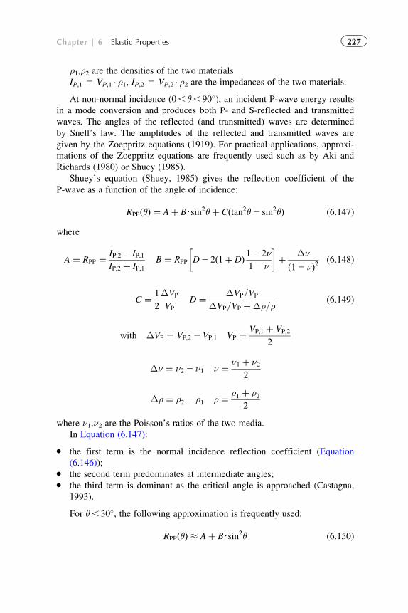
ρ1,ρ2 are the densities of the two materials
IP,1 5 VP,1 � ρ1, IP,2 5 VP,2 � ρ2 are the impedances of the two materials.
At non-normal incidence (0, θ, 90�), an incident P-wave energy results
in a mode conversion and produces both P- and S-reflected and transmitted
waves. The angles of the reflected (and transmitted) waves are determined
by Snell’s law. The amplitudes of the reflected and transmitted waves are
given by the Zoeppritz equations (1919). For practical applications, approxi-
mations of the Zoeppritz equations are frequently used such as by Aki and
Richards (1980) or Shuey (1985).
Shuey’s equation (Shuey, 1985) gives the reflection coefficient of the
P-wave as a function of the angle of incidence:
RPPðθÞ ¼ Aþ BUsin2θþ Cðtan2θ2 sin2θÞ ð6:147Þ
where
A ¼ RPP ¼ IP;2 2 IP;1
IP;2 þ IP;1B ¼ RPP D2 2ð1þ DÞ 12 2ν
12 ν
þ Δν
ð12 νÞ2 ð6:148Þ
C ¼ 1
2
ΔVP
VP
D ¼ ΔVP=VP
ΔVP=VP þΔρ=ρð6:149Þ
with ΔVP ¼ VP;2 2VP;1 VP ¼ VP;1 þ VP;2
2
Δν ¼ ν2 2 ν1 ν ¼ ν1 þ ν22
Δρ ¼ ρ2 2 ρ1 ρ ¼ ρ1 þ ρ22
where ν1,ν2 are the Poisson’s ratios of the two media.
In Equation (6.147):
� the first term is the normal incidence reflection coefficient (Equation
(6.146));� the second term predominates at intermediate angles;� the third term is dominant as the critical angle is approached (Castagna,
1993).
For θ, 30�, the following approximation is frequently used:
RPPðθÞ � Aþ BUsin2θ ð6:150Þ
227Chapter | 6 Elastic Properties
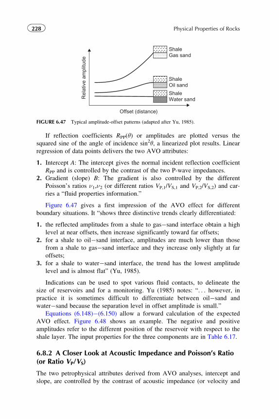
If reflection coefficients RPP(θ) or amplitudes are plotted versus the
squared sine of the angle of incidence sin2θ, a linearized plot results. Linear
regression of data points delivers the two AVO attributes:
1. Intercept A: The intercept gives the normal incident reflection coefficient
RPP and is controlled by the contrast of the two P-wave impedances.
2. Gradient (slope) B: The gradient is also controlled by the different
Poisson’s ratios ν1,ν2 (or different ratios VP,1/VS,1 and VP,2/VS,2) and car-
ries a “fluid properties information.”
Figure 6.47 gives a first impression of the AVO effect for different
boundary situations. It “shows three distinctive trends clearly differentiated:
1. the reflected amplitudes from a shale to gas�sand interface obtain a high
level at near offsets, then increase significantly toward far offsets;
2. for a shale to oil�sand interface, amplitudes are much lower than those
from a shale to gas�sand interface and they increase only slightly at far
offsets;
3. for a shale to water�sand interface, the trend has the lowest amplitude
level and is almost flat” (Yu, 1985).
Indications can be used to spot various fluid contacts, to delineate the
size of reservoirs and for a monitoring. Yu (1985) notes: “. . . however, inpractice it is sometimes difficult to differentiate between oil�sand and
water�sand because the separation level in offset amplitude is small.”
Equations (6.148)�(6.150) allow a forward calculation of the expected
AVO effect. Figure 6.48 shows an example. The negative and positive
amplitudes refer to the different position of the reservoir with respect to the
shale layer. The input properties for the three components are in Table 6.17.
6.8.2 A Closer Look at Acoustic Impedance and Poisson’s Ratio(or Ratio VP/VS)
The two petrophysical attributes derived from AVO analyses, intercept and
slope, are controlled by the contrast of acoustic impedance (or velocity and
ShaleWater sand
Shale
Offset (distance)
Rel
ativ
e am
plitu
deOil sand
ShaleGas sand
FIGURE 6.47 Typical amplitude-offset patterns (adapted after Yu, 1985).
228 Physical Properties of Rocks
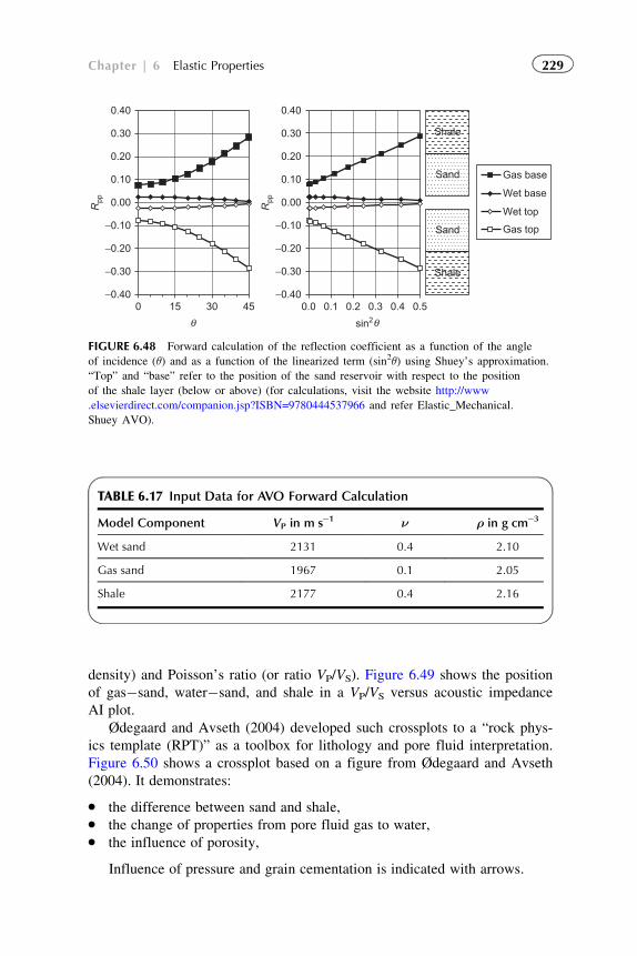
density) and Poisson’s ratio (or ratio VP/VS). Figure 6.49 shows the position
of gas�sand, water�sand, and shale in a VP/VS versus acoustic impedance
AI plot.
Ødegaard and Avseth (2004) developed such crossplots to a “rock phys-
ics template (RPT)” as a toolbox for lithology and pore fluid interpretation.
Figure 6.50 shows a crossplot based on a figure from Ødegaard and Avseth
(2004). It demonstrates:
� the difference between sand and shale,� the change of properties from pore fluid gas to water,� the influence of porosity,
Influence of pressure and grain cementation is indicated with arrows.
−0.40
−0.30
−0.20
−0.10
0.00
0.10
0.20
0.30
0.40
0 15 30 45
Rpp
−0.40
−0.30
−0.20
−0.10
0.00
0.10
0.20
0.30
0.40
Rpp
0.0 0.1 0.2 0.3 0.4 0.5
Gas base
Wet base
Wet top
Gas top
Shale
Sand
Shale
Sand
θ sin2θ
FIGURE 6.48 Forward calculation of the reflection coefficient as a function of the angle
of incidence (θ) and as a function of the linearized term (sin2θ) using Shuey’s approximation.
“Top” and “base” refer to the position of the sand reservoir with respect to the position
of the shale layer (below or above) (for calculations, visit the website http://www
.elsevierdirect.com/companion.jsp?ISBN=9780444537966 and refer Elastic_Mechanical.
Shuey AVO).
TABLE 6.17 Input Data for AVO Forward Calculation
Model Component VP in m s21 ν ρ in g cm23
Wet sand 2131 0.4 2.10
Gas sand 1967 0.1 2.05
Shale 2177 0.4 2.16
229Chapter | 6 Elastic Properties
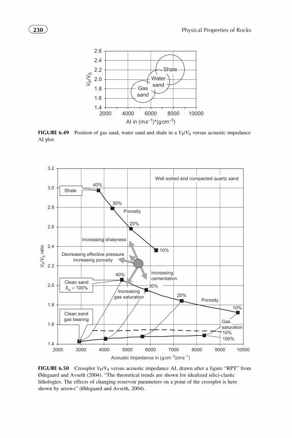
1.4
1.6
1.8
2.0
2.2
2.4
2.6
2000 4000 6000 8000 10000
AI in (ms−1)*(gcm−3)
VP/V
S
Shale
Gassand
Watersand
FIGURE 6.49 Position of gas sand, water sand and shale in a VP/VS versus acoustic impedance
AI plot.
1.4
1.6
1.8
2.0
2.2
2.4
2.6
2.8
3.0
3.2
2000 3000 4000 5000 6000 7000 8000 9000 10000
Acoustic Impedance in (gcm−3)(ms−1)
VP/V
S r
atio
40%
40%
30%
30%
20%
20%
10%
10%
Porosity
Clean sandSw = 100%
Shale
Clean sandgas bearing
10%100%
Increasing shalyness
Increasinggas saturation
Well sorted and compacted quartz sand
Increasingcementation
Decreasing effective pressureincreasing porosity
Gassaturation
Porosity
FIGURE 6.50 Crossplot VP/VS versus acoustic impedance AI, drawn after a figure “RPT” from
Ødegaard and Avseth (2004). “The theoretical trends are shown for idealized silici-clastic
lithologies. The effects of changing reservoir parameters on a point of the crossplot is here
shown by arrows” (Ødegaard and Avseth, 2004).
230 Physical Properties of Rocks
The following directions of changing reservoir parameters are remarkable
(Veeken, 2007):
� increase in gas saturation will reduce acoustic impedance AI and ratio
VP/VS,� increase in cement volume will increase acoustic impedance AI and
reduce ratio VP/VS,� increase in porosity will decrease acoustic impedance AI and increase
ratio VP/VS,� increase in shaliness will reduce acoustic impedance AI but increase ratio
VP/VS,� changing formation pressure does not have much influence, but it will
reduce acoustic impedance AI and increase the ratio VP/VS.
Veeken (2007) notes that “the RPT plot is area or basin dependent and
velocity�porosity trends are calculated for the expected lithologies and vari-
ous depth of burial (compaction). A distinction needs to be made between
silici-clastic and carbonate systems.”
Chi and Han (2009) conclude: “. . . using the crossplots of elastic proper-
ties with the RPT, we can clearly delineate the lithology and fluid content.
The prior information such as well log, core, and geological modeling can
help construct the RPT and includes the effects of pressure, temperature, and
fluid property.”
6.8.3 The Attributes Lambda Rho and Mu Rho
In addition to Shuey’s method, the “Fatti methodology” (Fatti et al., 1994;
see also Burianik, 2000) solves the problem for P and S reflectivities. The P
and S impedances of the materials (geological layers) can be calculated from
P and S reflectivities by inversion.
From P and S impedances, the attributes λ � ρ (lambda rho) and μ � ρ (mu
rho) can be derived as follows:
shear impedance is IS ¼ VSUρ ¼ffiffiffiμρ
rρ ¼ ffiffiffiffiffiffiffiffi
μUρp ð6:151Þ
parameter μUρ ð‘‘mu rho’’Þ results in μUρ ¼ I2S ð6:152Þ
Compressional impedance is IP ¼ VPUρ ¼ffiffiffiffiffiffiffiffiffiffiffiffiffiffiffiffiffiλþ 2Uμ
ρ
sρ ¼
ffiffiffiffiffiffiffiffiffiffiffiffiffiffiffiffiffiffiffiffiffiffiffiffiffiffiλUρþ 2UμUρ
pð6:153Þ
231Chapter | 6 Elastic Properties
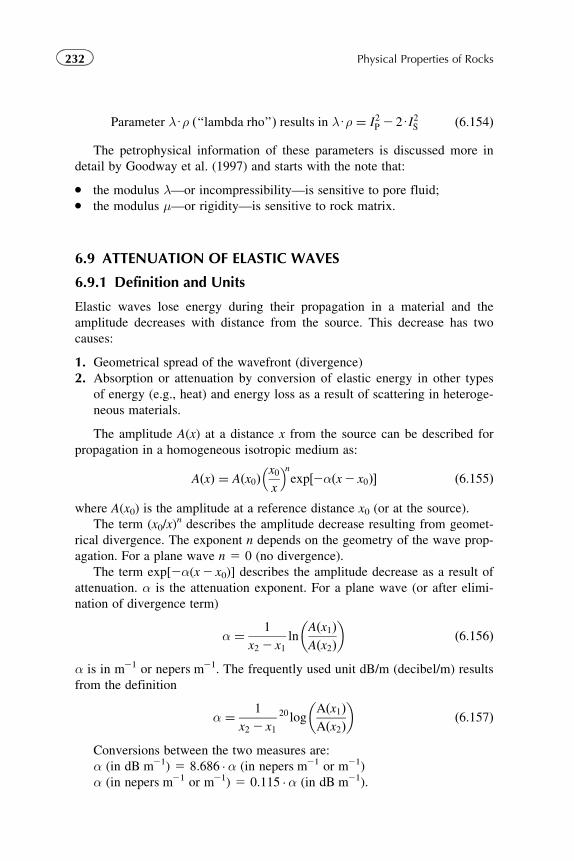
Parameter λUρ ð‘‘lambda rho’’Þ results in λUρ ¼ I2P 2 2UI2S ð6:154Þ
The petrophysical information of these parameters is discussed more in
detail by Goodway et al. (1997) and starts with the note that:
� the modulus λ—or incompressibility—is sensitive to pore fluid;� the modulus μ—or rigidity—is sensitive to rock matrix.
6.9 ATTENUATION OF ELASTIC WAVES
6.9.1 Definition and Units
Elastic waves lose energy during their propagation in a material and the
amplitude decreases with distance from the source. This decrease has two
causes:
1. Geometrical spread of the wavefront (divergence)
2. Absorption or attenuation by conversion of elastic energy in other types
of energy (e.g., heat) and energy loss as a result of scattering in heteroge-
neous materials.
The amplitude A(x) at a distance x from the source can be described for
propagation in a homogeneous isotropic medium as:
AðxÞ ¼ Aðx0Þx0
x
� �nexp2αðx2 x0Þ�½ ð6:155Þ
where A(x0) is the amplitude at a reference distance x0 (or at the source).
The term (x0/x)n describes the amplitude decrease resulting from geomet-
rical divergence. The exponent n depends on the geometry of the wave prop-
agation. For a plane wave n 5 0 (no divergence).
The term exp[2α(x2 x0)] describes the amplitude decrease as a result of
attenuation. α is the attenuation exponent. For a plane wave (or after elimi-
nation of divergence term)
α ¼ 1
x2 2 x1ln
Aðx1ÞAðx2Þ
� �ð6:156Þ
α is in m21 or nepers m21. The frequently used unit dB/m (decibel/m) results
from the definition
α ¼ 1
x2 2 x1
20 logAðx1ÞAðx2Þ
� �ð6:157Þ
Conversions between the two measures are:
α (in dB m21) 5 8.686 �α (in nepers m21 or m21)
α (in nepers m21 or m21) 5 0.115 �α (in dB m21).
232 Physical Properties of Rocks
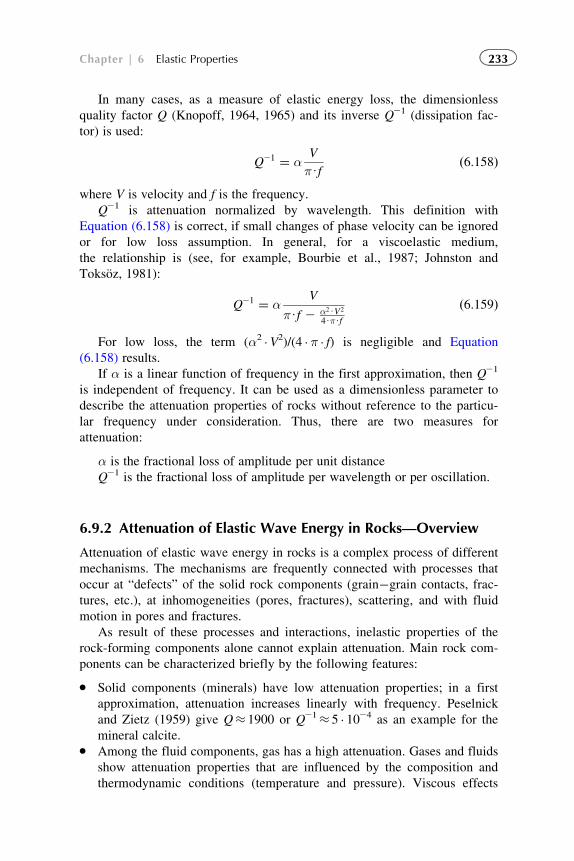
In many cases, as a measure of elastic energy loss, the dimensionless
quality factor Q (Knopoff, 1964, 1965) and its inverse Q21 (dissipation fac-
tor) is used:
Q21 ¼ αV
πUfð6:158Þ
where V is velocity and f is the frequency.
Q21 is attenuation normalized by wavelength. This definition with
Equation (6.158) is correct, if small changes of phase velocity can be ignored
or for low loss assumption. In general, for a viscoelastic medium,
the relationship is (see, for example, Bourbie et al., 1987; Johnston and
Toksoz, 1981):
Q21 ¼ αV
πUf 2 α2UV2
4UπUf
ð6:159Þ
For low loss, the term (α2 �V2)/(4 �π � f) is negligible and Equation
(6.158) results.
If α is a linear function of frequency in the first approximation, then Q21
is independent of frequency. It can be used as a dimensionless parameter to
describe the attenuation properties of rocks without reference to the particu-
lar frequency under consideration. Thus, there are two measures for
attenuation:
α is the fractional loss of amplitude per unit distance
Q21 is the fractional loss of amplitude per wavelength or per oscillation.
6.9.2 Attenuation of Elastic Wave Energy in Rocks—Overview
Attenuation of elastic wave energy in rocks is a complex process of different
mechanisms. The mechanisms are frequently connected with processes that
occur at “defects” of the solid rock components (grain�grain contacts, frac-
tures, etc.), at inhomogeneities (pores, fractures), scattering, and with fluid
motion in pores and fractures.
As result of these processes and interactions, inelastic properties of the
rock-forming components alone cannot explain attenuation. Main rock com-
ponents can be characterized briefly by the following features:
� Solid components (minerals) have low attenuation properties; in a first
approximation, attenuation increases linearly with frequency. Peselnick
and Zietz (1959) give Q� 1900 or Q21� 5 � 1024 as an example for the
mineral calcite.� Among the fluid components, gas has a high attenuation. Gases and fluids
show attenuation properties that are influenced by the composition and
thermodynamic conditions (temperature and pressure). Viscous effects
233Chapter | 6 Elastic Properties
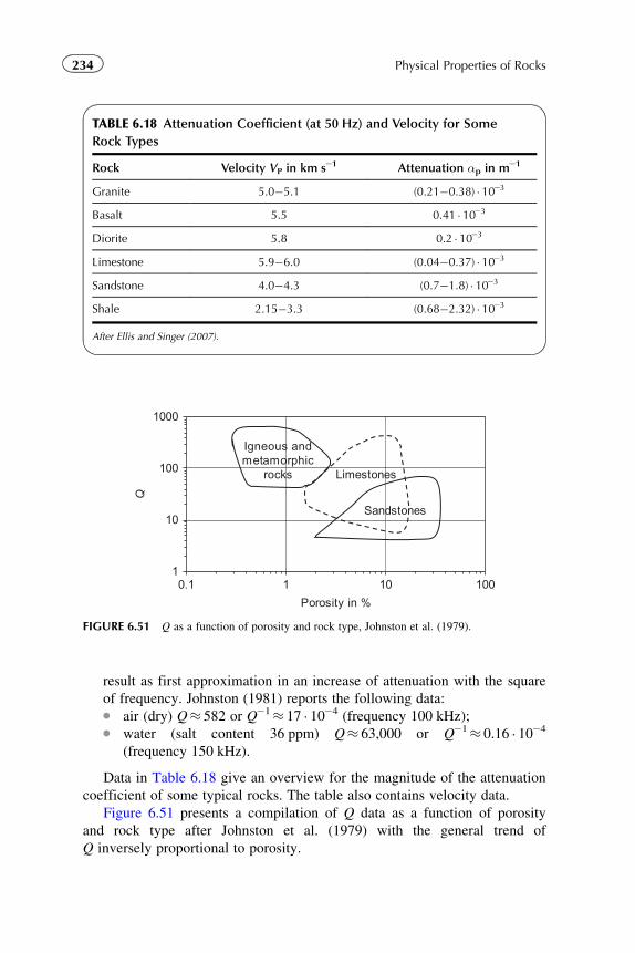
result as first approximation in an increase of attenuation with the square
of frequency. Johnston (1981) reports the following data:� air (dry) Q� 582 or Q21� 17 � 1024 (frequency 100 kHz);� water (salt content 36 ppm) Q� 63,000 or Q21� 0.16 � 1024
(frequency 150 kHz).
Data in Table 6.18 give an overview for the magnitude of the attenuation
coefficient of some typical rocks. The table also contains velocity data.
Figure 6.51 presents a compilation of Q data as a function of porosity
and rock type after Johnston et al. (1979) with the general trend of
Q inversely proportional to porosity.
TABLE 6.18 Attenuation Coefficient (at 50 Hz) and Velocity for Some
Rock Types
Rock Velocity VP in km s21 Attenuation αp in m21
Granite 5.0�5.1 (0.21�0.38) � 1023
Basalt 5.5 0.41 � 1023
Diorite 5.8 0.2 � 1023
Limestone 5.9�6.0 (0.04�0.37) � 1023
Sandstone 4.0�4.3 (0.7�1.8) � 1023
Shale 2.15�3.3 (0.68�2.32) � 1023
After Ellis and Singer (2007).
1
10
100
1000
0.1 1 10 100
Porosity in %
Q
Igneous andmetamorphic
rocks Limestones
Sandstones
FIGURE 6.51 Q as a function of porosity and rock type, Johnston et al. (1979).
234 Physical Properties of Rocks
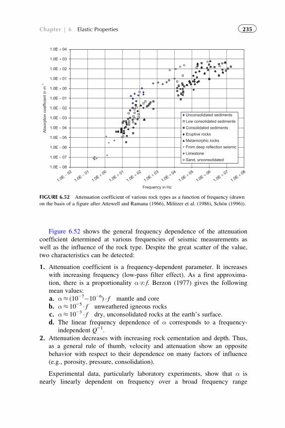
Figure 6.52 shows the general frequency dependence of the attenuation
coefficient determined at various frequencies of seismic measurements as
well as the influence of the rock type. Despite the great scatter of the value,
two characteristics can be detected:
1. Attenuation coefficient is a frequency-dependent parameter. It increases
with increasing frequency (low-pass filter effect). As a first approxima-
tion, there is a proportionality αNf. Berzon (1977) gives the following
mean values:
a. α� (1027�1026) � f mantle and core
b. α� 1025 � f unweathered igneous rocks
c. α� 1023 � f dry, unconsolidated rocks at the earth’s surface.
d. The linear frequency dependence of α corresponds to a frequency-
independent Q21.
2. Attenuation decreases with increasing rock cementation and depth. Thus,
as a general rule of thumb, velocity and attenuation show an opposite
behavior with respect to their dependence on many factors of influence
(e.g., porosity, pressure, consolidation).
Experimental data, particularly laboratory experiments, show that α is
nearly linearly dependent on frequency over a broad frequency range
1.0E − 08
1.0E − 07
1.0E − 06
1.0E − 05
1.0E − 04
1.0E − 03
1.0E − 02
1.0E − 01
1.0E + 00
1.0E + 01
1.0E + 02
1.0E + 03
1.0E + 04
1.0E − 02
1.0E − 01
1.0E + 00
1.0E + 01
1.0E + 02
1.0E + 03
1.0E + 04
1.0E + 05
1.0E + 06
1.0E + 07
1.0E + 08
Frequency in Hz
Abs
orpt
ion
coef
ficie
nt in
m−1
Unconsolidated sediments
Low consolidated sediments
Consolidated sediments
Eruptive rocks
Metamorphic rocks
From deep reflection seismic
Limestone
Sand, unconsolidated
FIGURE 6.52 Attenuation coefficient of various rock types as a function of frequency (drawn
on the basis of a figure after Attewell and Ramana (1966), Militzer et al. (1986), Schon (1996)).
235Chapter | 6 Elastic Properties
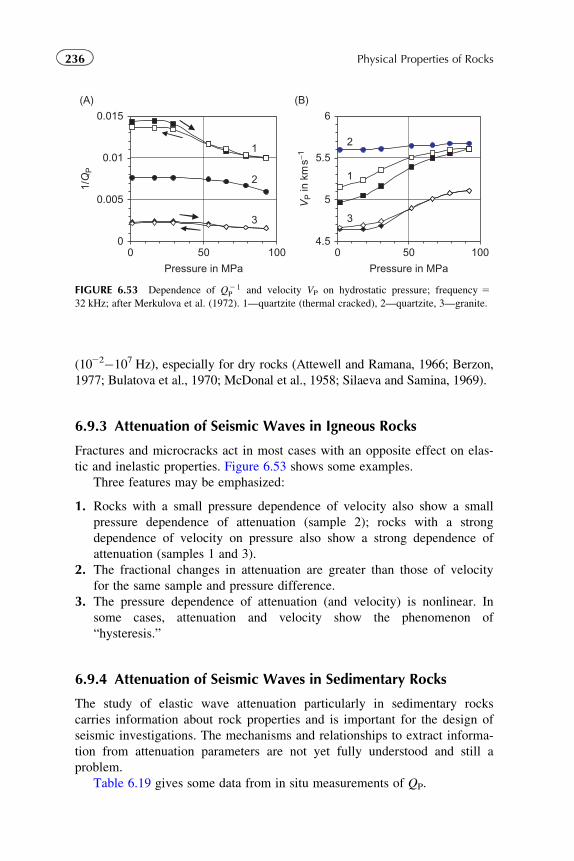
(1022�107 Hz), especially for dry rocks (Attewell and Ramana, 1966; Berzon,
1977; Bulatova et al., 1970; McDonal et al., 1958; Silaeva and Samina, 1969).
6.9.3 Attenuation of Seismic Waves in Igneous Rocks
Fractures and microcracks act in most cases with an opposite effect on elas-
tic and inelastic properties. Figure 6.53 shows some examples.
Three features may be emphasized:
1. Rocks with a small pressure dependence of velocity also show a small
pressure dependence of attenuation (sample 2); rocks with a strong
dependence of velocity on pressure also show a strong dependence of
attenuation (samples 1 and 3).
2. The fractional changes in attenuation are greater than those of velocity
for the same sample and pressure difference.
3. The pressure dependence of attenuation (and velocity) is nonlinear. In
some cases, attenuation and velocity show the phenomenon of
“hysteresis.”
6.9.4 Attenuation of Seismic Waves in Sedimentary Rocks
The study of elastic wave attenuation particularly in sedimentary rocks
carries information about rock properties and is important for the design of
seismic investigations. The mechanisms and relationships to extract informa-
tion from attenuation parameters are not yet fully understood and still a
problem.
Table 6.19 gives some data from in situ measurements of QP.
4.5
5
5.5
6
0 50 100
Pressure in MPa
VP in
km
s−1
2
1
3
0
0.005
0.01
0.015
0 50 100
Pressure in MPa
1/Q
P
1
2
3
(A) (B)
FIGURE 6.53 Dependence of Q2 1P and velocity VP on hydrostatic pressure; frequency 5
32 kHz; after Merkulova et al. (1972). 1—quartzite (thermal cracked), 2—quartzite, 3—granite.
236 Physical Properties of Rocks
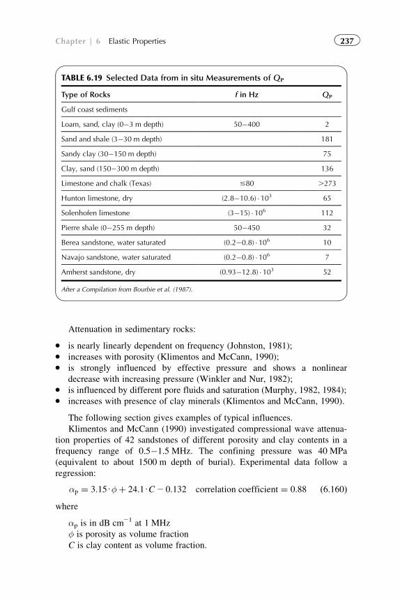
Attenuation in sedimentary rocks:
� is nearly linearly dependent on frequency (Johnston, 1981);� increases with porosity (Klimentos and McCann, 1990);� is strongly influenced by effective pressure and shows a nonlinear
decrease with increasing pressure (Winkler and Nur, 1982);� is influenced by different pore fluids and saturation (Murphy, 1982, 1984);� increases with presence of clay minerals (Klimentos and McCann, 1990).
The following section gives examples of typical influences.
Klimentos and McCann (1990) investigated compressional wave attenua-
tion properties of 42 sandstones of different porosity and clay contents in a
frequency range of 0.5�1.5 MHz. The confining pressure was 40 MPa
(equivalent to about 1500 m depth of burial). Experimental data follow a
regression:
αp ¼ 3:15Uφþ 24:1UC2 0:132 correlation coefficient ¼ 0:88 ð6:160Þwhere
αp is in dB cm21 at 1 MHz
φ is porosity as volume fraction
C is clay content as volume fraction.
TABLE 6.19 Selected Data from in situ Measurements of QP
Type of Rocks f in Hz QP
Gulf coast sediments
Loam, sand, clay (0�3 m depth) 50�400 2
Sand and shale (3�30 m depth) 181
Sandy clay (30�150 m depth) 75
Clay, sand (150�300 m depth) 136
Limestone and chalk (Texas) #80 .273
Hunton limestone, dry (2.8�10.6) � 103 65
Solenhofen limestone (3�15) � 106 112
Pierre shale (0�255 m depth) 50�450 32
Berea sandstone, water saturated (0.2�0.8) �106 10
Navajo sandstone, water saturated (0.2�0.8) �106 7
Amherst sandstone, dry (0.93�12.8) � 103 52
After a Compilation from Bourbie et al. (1987).
237Chapter | 6 Elastic Properties
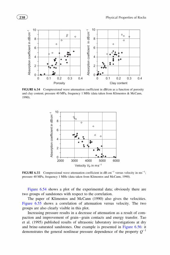
Figure 6.54 shows a plot of the experimental data; obviously there are
two groups of sandstones with respect to the correlation.
The paper of Klimentos and McCann (1990) also gives the velocities.
Figure 6.55 shows a correlation of attenuation versus velocity. The two
groups are also clearly visible in this plot.
Increasing pressure results in a decrease of attenuation as a result of com-
paction and improvement of grain�grain contacts and energy transfer. Tao
et al. (1995) published results of ultrasonic laboratory investigations at dry
and brine-saturated sandstones. One example is presented in Figure 6.56: it
demonstrates the general nonlinear pressure dependence of the property Q21
0
2
4
6
8
10
0 0.1 0.2 0.3 0.4
Porosity
Abs
orpt
ion
coef
ficie
nt in
dB
cm−1
0
2
4
6
8
10
0 0.1 0.2 0.3 0.4
Clay content
Abs
orpt
ion
coef
ficie
nt i
n dB
cm−1
FIGURE 6.54 Compressional wave attenuation coefficient in dB/cm as a function of porosity
and clay content; pressure 40 MPa, frequency 1 MHz (data taken from Klimentos & McCann,
1990).
0
2
4
6
8
10
2000 3000 4000 5000 6000
Velocity VP in ms−1
Abs
orpt
ion
coef
ficie
nt in
dB
cm−1
FIGURE 6.55 Compressional wave attenuation coefficient in dB cm21 versus velocity in ms21;
pressure 40 MPa, frequency 1 MHz (data taken from Klimentos and McCann, 1990).
238 Physical Properties of Rocks
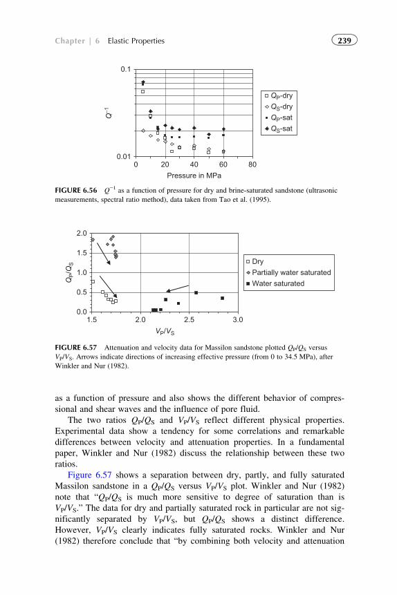
as a function of pressure and also shows the different behavior of compres-
sional and shear waves and the influence of pore fluid.
The two ratios QP/QS and VP/VS reflect different physical properties.
Experimental data show a tendency for some correlations and remarkable
differences between velocity and attenuation properties. In a fundamental
paper, Winkler and Nur (1982) discuss the relationship between these two
ratios.
Figure 6.57 shows a separation between dry, partly, and fully saturated
Massilon sandstone in a QP/QS versus VP/VS plot. Winkler and Nur (1982)
note that “QP/QS is much more sensitive to degree of saturation than is
VP/VS.” The data for dry and partially saturated rock in particular are not sig-
nificantly separated by VP/VS, but QP/QS shows a distinct difference.
However, VP/VS clearly indicates fully saturated rocks. Winkler and Nur
(1982) therefore conclude that “by combining both velocity and attenuation
0.01
0.1
0 20 40 60 80
Pressure in MPa
Q−1
QP-dry
QS-dry
QP-sat
QS-sat
FIGURE 6.56 Q21 as a function of pressure for dry and brine-saturated sandstone (ultrasonic
measurements, spectral ratio method), data taken from Tao et al. (1995).
0.0
0.5
1.0
1.5
2.0
1.5 2.0 2.5 3.0
VP/VS
QP/Q
S Dry
Partially water saturated
Water saturated
FIGURE 6.57 Attenuation and velocity data for Massilon sandstone plotted QP/QS versus
VP/VS. Arrows indicate directions of increasing effective pressure (from 0 to 34.5 MPa), after
Winkler and Nur (1982).
239Chapter | 6 Elastic Properties
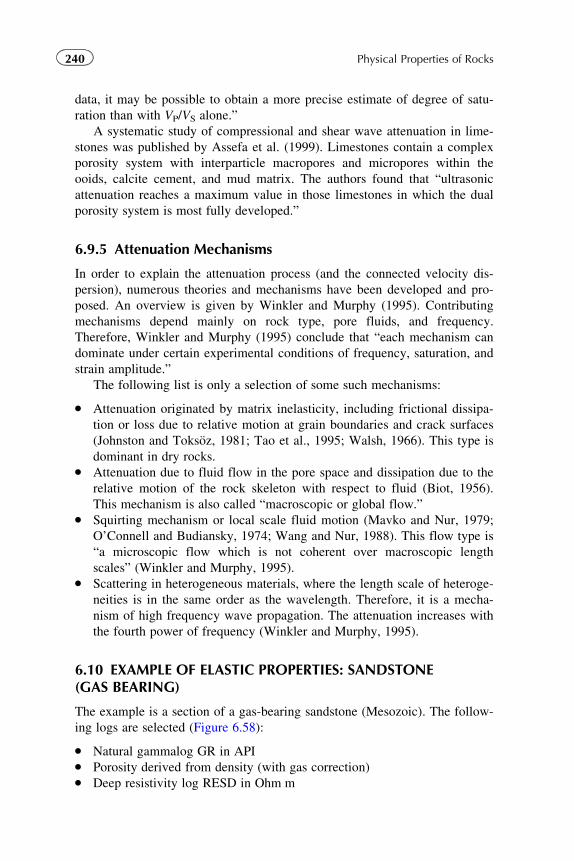
data, it may be possible to obtain a more precise estimate of degree of satu-
ration than with VP/VS alone.”
A systematic study of compressional and shear wave attenuation in lime-
stones was published by Assefa et al. (1999). Limestones contain a complex
porosity system with interparticle macropores and micropores within the
ooids, calcite cement, and mud matrix. The authors found that “ultrasonic
attenuation reaches a maximum value in those limestones in which the dual
porosity system is most fully developed.”
6.9.5 Attenuation Mechanisms
In order to explain the attenuation process (and the connected velocity dis-
persion), numerous theories and mechanisms have been developed and pro-
posed. An overview is given by Winkler and Murphy (1995). Contributing
mechanisms depend mainly on rock type, pore fluids, and frequency.
Therefore, Winkler and Murphy (1995) conclude that “each mechanism can
dominate under certain experimental conditions of frequency, saturation, and
strain amplitude.”
The following list is only a selection of some such mechanisms:
� Attenuation originated by matrix inelasticity, including frictional dissipa-
tion or loss due to relative motion at grain boundaries and crack surfaces
(Johnston and Toksoz, 1981; Tao et al., 1995; Walsh, 1966). This type is
dominant in dry rocks.� Attenuation due to fluid flow in the pore space and dissipation due to the
relative motion of the rock skeleton with respect to fluid (Biot, 1956).
This mechanism is also called “macroscopic or global flow.”� Squirting mechanism or local scale fluid motion (Mavko and Nur, 1979;
O’Connell and Budiansky, 1974; Wang and Nur, 1988). This flow type is
“a microscopic flow which is not coherent over macroscopic length
scales” (Winkler and Murphy, 1995).� Scattering in heterogeneous materials, where the length scale of heteroge-
neities is in the same order as the wavelength. Therefore, it is a mecha-
nism of high frequency wave propagation. The attenuation increases with
the fourth power of frequency (Winkler and Murphy, 1995).
6.10 EXAMPLE OF ELASTIC PROPERTIES: SANDSTONE(GAS BEARING)
The example is a section of a gas-bearing sandstone (Mesozoic). The follow-
ing logs are selected (Figure 6.58):
� Natural gammalog GR in API� Porosity derived from density (with gas correction)� Deep resistivity log RESD in Ohm m
240 Physical Properties of Rocks
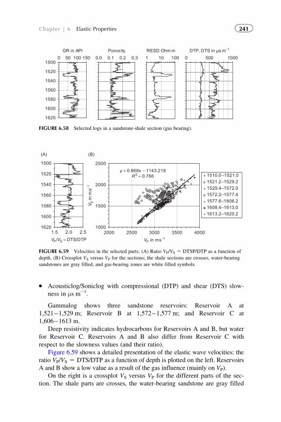
� Acousticlog/Soniclog with compressional (DTP) and shear (DTS) slow-
ness in μs m21.
Gammalog shows three sandstone reservoirs: Reservoir A at
1,521�1,529 m; Reservoir B at 1,572�1,577 m; and Reservoir C at
1,606�1613 m.
Deep resistivity indicates hydrocarbons for Reservoirs A and B, but water
for Reservoir C. Reservoirs A and B also differ from Reservoir C with
respect to the slowness values (and their ratio).
Figure 6.59 shows a detailed presentation of the elastic wave velocities: the
ratio VP/VS 5 DTS/DTP as a function of depth is plotted on the left. Reservoirs
A and B show a low value as a result of the gas influence (mainly on VP).
On the right is a crossplot VS versus VP for the different parts of the sec-
tion. The shale parts are crosses, the water-bearing sandstone are gray filled
1500
(A) (B)
1520
1540
1560
1580
1600
16201.5 2.0 2.5
VP/VS = DTS/DTP
y = 0.868x − 1143.219R2 = 0.766
1000
1500
2000
2500
2000 2500 3000 3500 4000
VP in ms−1
V S in
ms−1
1510.0–1521.01521.2–1529.21529.4–1572.01572.2–1577.41577.6–1606.21608.4–1613.01613.2–1620.2
FIGURE 6.59 Velocities in the selected parts: (A) Ratio VP/VS 5 DTSP/DTP as a function of
depth. (B) Crossplot VS versus VP for the sections; the shale sections are crosses, water-bearing
sandstones are gray filled, and gas-bearing zones are white filled symbols.
1500
1520
1540
1560
1580
1600
1620
GR in API RESD Ohm m DTP, DTS in µs m−1
0 50 100 150 1 10 100 0 500 10000.0 0.1 0.2 0.3Porosity
FIGURE 6.58 Selected logs in a sandstone-shale section (gas bearing).
241Chapter | 6 Elastic Properties
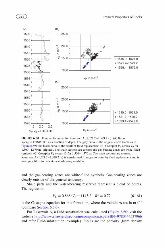
and the gas-bearing zones are white-filled symbols. Gas-bearing zones are
clearly outside of the general tendency.
Shale parts and the water-bearing reservoir represent a cloud of points.
The regression
VS ¼ 0:868UVP 2 1143:2 R2 ¼ 0:77 ð6:161Þis the Castagna equation for this formation, where the velocities are in m s21
(compare Section 6.5.6).
For Reservoir A, a fluid substitution was calculated (Figure 6.60; visit the
website http://www.elsevierdirect.com/companion.jsp?ISBN=9780444537966
and refer Fluid-substitution. example). Inputs are the porosity (from density
1000
1500
2000
2500
(A) (B)
(C)VP in ms−1
VS in
ms−1
1510.0–1521.01521.2–1529.21529.4–1572.0
1000
1500
2000
2500
VP in ms−1
VS in
ms−1
1510.0–1521.01521.2–1529.21529.4–1572.0
1500
1505
1510
1515
1520
1525
1530
1535
1540
1545
1550
1555
1560
1565
15701.5 2.0 2.5VP/VS = DTS/DTP
FIGURE 6.60 Fluid replacement for Reservoir A (1,521.2�1,529.2 m): (A) Ratio
VP/VS 5 DTSP/DTP as a function of depth. The gray curve is the original curve (same as in
Figure 6.59); the black curve is the result of fluid replacement. (B) Crossplot VS versus VP for
1,500�1,570 m (original). The shale sections are crosses and gas-bearing zones are white-filled
symbols. (C) Crossplot VS versus VP for 1,500�1,570 m. The shale sections are crosses.
Reservoir A (1,521.2�1,529.2 m) is transformed from gas to water by fluid replacement and is
now gray filled to indicate water-bearing sandstone.
242 Physical Properties of Rocks
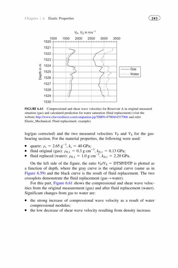
log/gas corrected) and the two measured velocities VP and VS for the gas-
bearing section. For the material properties, the following were used:
� quartz: ρs 5 2.65 g23, ks 5 40 GPa;� fluid original (gas): ρfl,1 5 0.3 g cm23, kfl,1 5 0.13 GPa;� fluid replaced (water): ρfl,1 5 1.0 g cm23, kfl,1 5 2.20 GPa.
On the left side of the figure, the ratio VP/VS 5 DTSP/DTP is plotted as
a function of depth, where the gray curve is the original curve (same as in
Figure 6.59) and the black curve is the result of fluid replacement. The two
crossplots demonstrate the fluid replacement (gas-water).
For this part, Figure 6.61 shows the compressional and shear wave veloc-
ities from the original measurement (gas) and after fluid replacement (water).
Significant changes from gas to water are:
� the strong increase of compressional wave velocity as a result of water
compressional modulus;� the low decrease of shear wave velocity resulting from density increase.
15201000 1500 2000 2500 3000 3500
1521
1522
1523
1524
1525
1526
1527
1528
1529
1530
VP, VS in ms−1
Dep
th in
m
GasWater
FIGURE 6.61 Compressional and shear wave velocities for Reservoir A in original measured
situation (gas) and calculated prediction for water saturation (fluid replacement) (visit the
website http://www.elsevierdirect.com/companion.jsp?ISBN=9780444537966 and refer
Elastic_Mechanical. Fluid replacement. example).
243Chapter | 6 Elastic Properties

Chapter 7
Geomechanical Properties
“Engineering recognizes geophysics as a tool which can often give important infor-
mation about a site as effectively and more cheaply than a very large number of
boreholes.”
D. H. Griffith and R.F. King (1965)
7.1 OVERVIEW, INTRODUCTION
Rock deformation and failure or strength behavior are fundamental problems
in geomechanics. Stress distribution and rock properties control the corre-
sponding processes. A discussion of some fundamental topics is given in a
special section, “Geomechanics,” of The Leading Edge (Sayers and Schutjens,
2007). Petroleum-related rock mechanics is presented in a textbook by Fjaer
et al. (1989).
Examples of geomechanical problems are:
� deformation and failure processes originated by tectonic stress, earth-
quakes, etc.;� landslides and rockfall;� deformation of the underground (settlement) and subsurface constructions
(tunnel, cavern) caused by the pressure of construction in civil
engineering;� slope and dam stability (failure problems);� wellbore stability and fracturing;� reservoir compaction during production and subsidence.
Figure 7.1 illustrates main geomechanical processes in terms of related
properties (rock mechanical and geophysical properties) and their change
during the process.
245Physical Properties of Rocks.
© 2011 Elsevier B.V. All rights reserved.
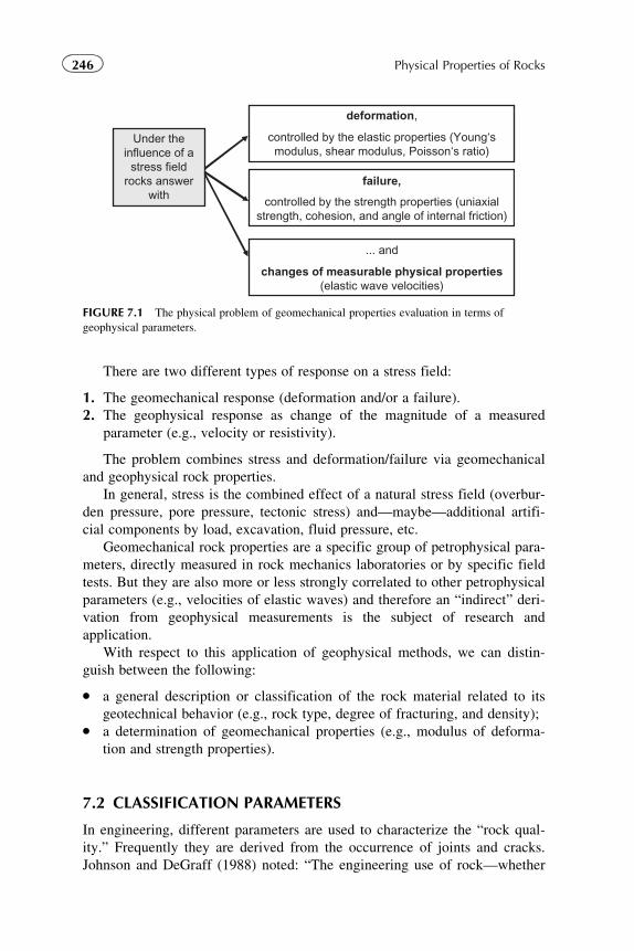
There are two different types of response on a stress field:
1. The geomechanical response (deformation and/or a failure).
2. The geophysical response as change of the magnitude of a measured
parameter (e.g., velocity or resistivity).
The problem combines stress and deformation/failure via geomechanical
and geophysical rock properties.
In general, stress is the combined effect of a natural stress field (overbur-
den pressure, pore pressure, tectonic stress) and—maybe—additional artifi-
cial components by load, excavation, fluid pressure, etc.
Geomechanical rock properties are a specific group of petrophysical para-
meters, directly measured in rock mechanics laboratories or by specific field
tests. But they are also more or less strongly correlated to other petrophysical
parameters (e.g., velocities of elastic waves) and therefore an “indirect” deri-
vation from geophysical measurements is the subject of research and
application.
With respect to this application of geophysical methods, we can distin-
guish between the following:
� a general description or classification of the rock material related to its
geotechnical behavior (e.g., rock type, degree of fracturing, and density);� a determination of geomechanical properties (e.g., modulus of deforma-
tion and strength properties).
7.2 CLASSIFICATION PARAMETERS
In engineering, different parameters are used to characterize the “rock qual-
ity.” Frequently they are derived from the occurrence of joints and cracks.
Johnson and DeGraff (1988) noted: “The engineering use of rock—whether
Under theinfluence of a
stress fieldrocks answer
with
deformation,
controlled by the elastic properties (Young‘smodulus, shear modulus, Poisson‘s ratio)
failure,
controlled by the strength properties (uniaxialstrength, cohesion, and angle of internal friction)
... and
changes of measurable physical properties(elastic wave velocities)
FIGURE 7.1 The physical problem of geomechanical properties evaluation in terms of
geophysical parameters.
246 Physical Properties of Rocks
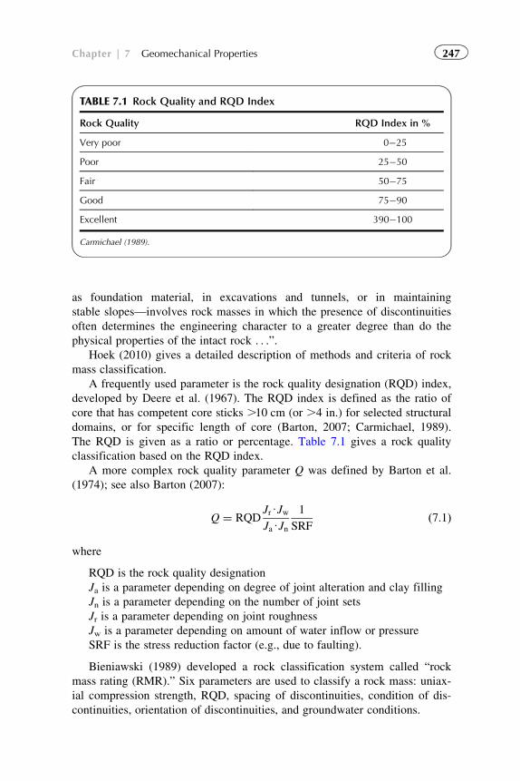
as foundation material, in excavations and tunnels, or in maintaining
stable slopes—involves rock masses in which the presence of discontinuities
often determines the engineering character to a greater degree than do the
physical properties of the intact rock . . .”.Hoek (2010) gives a detailed description of methods and criteria of rock
mass classification.
A frequently used parameter is the rock quality designation (RQD) index,
developed by Deere et al. (1967). The RQD index is defined as the ratio of
core that has competent core sticks .10 cm (or .4 in.) for selected structural
domains, or for specific length of core (Barton, 2007; Carmichael, 1989).
The RQD is given as a ratio or percentage. Table 7.1 gives a rock quality
classification based on the RQD index.
A more complex rock quality parameter Q was defined by Barton et al.
(1974); see also Barton (2007):
Q ¼ RQDJrUJwJaUJn
1
SRFð7:1Þ
where
RQD is the rock quality designation
Ja is a parameter depending on degree of joint alteration and clay filling
Jn is a parameter depending on the number of joint sets
Jr is a parameter depending on joint roughness
Jw is a parameter depending on amount of water inflow or pressure
SRF is the stress reduction factor (e.g., due to faulting).
Bieniawski (1989) developed a rock classification system called “rock
mass rating (RMR).” Six parameters are used to classify a rock mass: uniax-
ial compression strength, RQD, spacing of discontinuities, condition of dis-
continuities, orientation of discontinuities, and groundwater conditions.
TABLE 7.1 Rock Quality and RQD Index
Rock Quality RQD Index in %
Very poor 0�25
Poor 25�50
Fair 50�75
Good 75�90
Excellent 390�100
Carmichael (1989).
247Chapter | 7 Geomechanical Properties
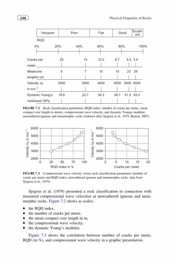
Sjogren et al. (1979) presented a rock classification in connection with
measured compressional wave velocities at unweathered igneous and meta-
morphic rocks. Figure 7.2 shows as scales:
� the RQD index,� the number of cracks per meter,� the mean compact core length in m,� the compressional wave velocity,� the dynamic Young’s modulus.
Figure 7.3 shows the correlation between number of cracks per meter,
RQD (in %), and compressional wave velocity in a graphic presentation.
Cracks per meter
20000 25 50 75 100
3000
4000
5000
6000
RQD index in %
Vel
ocity
VP in
ms−1
20000 5 10 15 20
3000
4000
5000
6000
Vel
ocity
VP in
ms−1
FIGURE 7.3 Compressional wave velocity versus rock classification parameters (number of
cracks per meter and RQD index; unweathered igneous and metamorphic rocks; data from
Sjogren et al., 1979).
meter
lengthin cm
in ms−1
modulusin GPa
Verypoor Poor
RQD
Cracks per 20 14 10.2 6.7 4.4 3.4
Meancore 5 7 10 15 23 29
Velocity VP 3000 3500 4000 4500 5000 5500
Dynamic Young’s 18.8 22.7 30.3 39.7 51.3 63.5
Fair Good Excell-ent
0% 20% 40% 60% 80% 100%
FIGURE 7.2 Rock classification parameters (RQD index, number of cracks per meter, mean
compact core length in meters, compressional wave velocity, and dynamic Youngs modulus;
unweathered igneous and metamorphic rocks (redrawn after Sjogren et al., 1979; Barton, 2007).
248 Physical Properties of Rocks
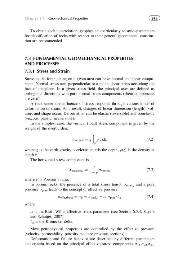
To obtain such a correlation, geophysical–particularly seismic–parameters
for classification of rocks with respect to their general geotechnical constitu-
tion are recommended.
7.3 FUNDAMENTAL GEOMECHANICAL PROPERTIESAND PROCESSES
7.3.1 Stress and Strain
Stress as the force acting on a given area can have normal and shear compo-
nents. Normal stress acts perpendicular to a plane, shear stress acts along the
face of the plane. In a given stress field, the principal axes are defined as
orthogonal directions with pure normal stress components (shear components
are zero).
A rock under the influence of stress responds through various kinds of
deformation or strain. As a result, changes of linear dimension (length), vol-
ume, and shape occur. Deformation can be elastic (reversible) and nonelastic
(viscous, plastic, irreversible).
In the simplest case, the vertical (total) stress component is given by the
weight of the overburden:
σvertical ¼ g
ðz0
ρðzÞdz ð7:2Þ
where g is the earth gravity acceleration, z is the depth, ρ(z) is the density at
depth z.
The horizontal stress component is
σhorizontal ¼ν
12 νσvertical ð7:3Þ
where ν is Poisson’s ratio.
In porous rocks, the presence of a total stress tensor σtotal,ij and a pore
pressure σpore leads to the concept of effective pressure:
σeffective;ij ¼ σij ¼ σtotal;ij 2αUσporeUδij ð7:4Þwhere
α is the Biot�Willis effective stress parameter (see Section 6.5.4; Sayers
and Schutjes, 2007).
δij is the Kronecker delta.
Most petrophysical properties are controlled by the effective pressure
(velocity, permeability, porosity etc.; see previous sections).
Deformation and failure behavior are described by different parameters
and criteria based on the principal effective stress components σ11,σ22,σ33.
249Chapter | 7 Geomechanical Properties
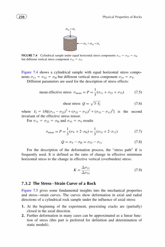
Figure 7.4 shows a cylindrical sample with equal horizontal stress compo-
nents σ11 5 σ22 5 σH but different vertical stress component σ33 5 σV.Different parameters are used for the description of stress effects:
mean effective stress σmean ¼ P ¼ 1
3ðσ11 þ σ22 þ σ33Þ ð7:5Þ
shear stress Q ¼ffiffiffiffiffiffiffiffiffi3UI2
pð7:6Þ
where I2 5 1/6[(σ112 σ22)21 (σ222σ33)
21 (σ332σ11)2] is the second
invariant of the effective stress tensor.
For σ11 5 σ22 5 σH and σ33 5 σV results
σmean ¼ P ¼ 1
3ðσV þ 2UσHÞ ¼
1
3ðσ33 þ 2Uσ11Þ ð7:7Þ
Q ¼ σV 2σH ¼ σ33 2σ11 ð7:8Þ
For the description of the deformation process, the “stress path” K is
frequently used. It is defined as the ratio of change in effective minimum
horizontal stress to the change in effective vertical (overburden) stress:
K ¼ Δσ11
Δσ33
ð7:9Þ
7.3.2 The Stress�Strain Curve of a Rock
Figure 7.5 gives some fundamental insights into the mechanical properties
and stress�strain curves. The curves show deformation in axial and radial
directions of a cylindrical rock sample under the influence of axial stress:
1. At the beginning of the experiment, preexisting cracks are (partially)
closed in the axial direction.
2. Further deformation in many cases can be approximated as a linear func-
tion of stress (this part is preferred for definition and determination of
static moduli).
Vσσ =33
Hσσσ == 2211
FIGURE 7.4 Cylindrical sample under equal horizontal stress components σ11 5 σ22 5 σHbut different vertical stress component σ33 5 σV.
250 Physical Properties of Rocks
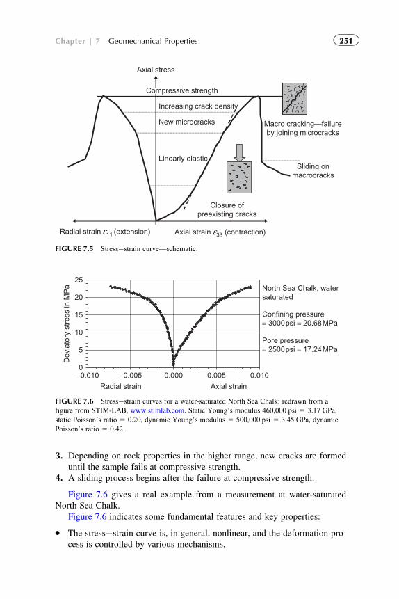
3. Depending on rock properties in the higher range, new cracks are formed
until the sample fails at compressive strength.
4. A sliding process begins after the failure at compressive strength.
Figure 7.6 gives a real example from a measurement at water-saturated
North Sea Chalk.
Figure 7.6 indicates some fundamental features and key properties:
� The stress�strain curve is, in general, nonlinear, and the deformation pro-
cess is controlled by various mechanisms.
Axial strain ε33 (contraction)Radial strain ε11 (extension)
Axial stress
Closure ofpreexisting cracks
Linearly elastic
New microcracks
Increasing crack density
Macro cracking—failureby joining microcracks
Sliding onmacrocracks
Compressive strength
FIGURE 7.5 Stress�strain curve—schematic.
0
5
10
15
20
25
−0.010 −0.005 0.000 0.005 0.010
Radial strain Axial strain
Dev
iato
ry s
tres
s in
MP
a North Sea Chalk, watersaturated
Confining pressure= 3000psi = 20.68MPa
Pore pressure= 2500psi = 17.24MPa
FIGURE 7.6 Stress�strain curves for a water-saturated North Sea Chalk; redrawn from a
figure from STIM-LAB, www.stimlab.com. Static Young’s modulus 460,000 psi 5 3.17 GPa,
static Poisson’s ratio 5 0.20, dynamic Young’s modulus 5 500,000 psi 5 3.45 GPa, dynamic
Poisson’s ratio 5 0.42.
251Chapter | 7 Geomechanical Properties
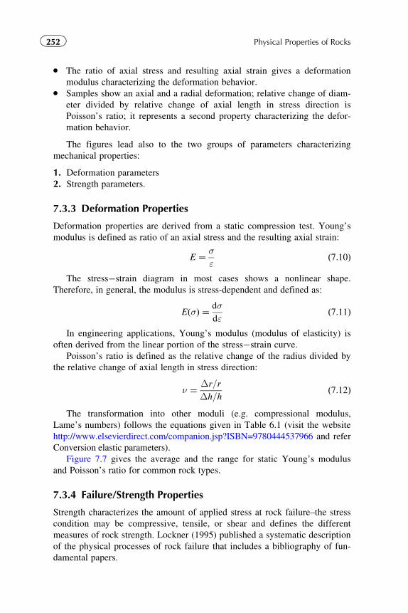
� The ratio of axial stress and resulting axial strain gives a deformation
modulus characterizing the deformation behavior.� Samples show an axial and a radial deformation; relative change of diam-
eter divided by relative change of axial length in stress direction is
Poisson’s ratio; it represents a second property characterizing the defor-
mation behavior.
The figures lead also to the two groups of parameters characterizing
mechanical properties:
1. Deformation parameters
2. Strength parameters.
7.3.3 Deformation Properties
Deformation properties are derived from a static compression test. Young’s
modulus is defined as ratio of an axial stress and the resulting axial strain:
E ¼ σε
ð7:10Þ
The stress�strain diagram in most cases shows a nonlinear shape.
Therefore, in general, the modulus is stress-dependent and defined as:
EðσÞ ¼ dσdε
ð7:11Þ
In engineering applications, Young’s modulus (modulus of elasticity) is
often derived from the linear portion of the stress�strain curve.
Poisson’s ratio is defined as the relative change of the radius divided by
the relative change of axial length in stress direction:
ν ¼ Δr=r
Δh=hð7:12Þ
The transformation into other moduli (e.g. compressional modulus,
Lame’s numbers) follows the equations given in Table 6.1 (visit the website
http://www.elsevierdirect.com/companion.jsp?ISBN=9780444537966 and refer
Conversion elastic parameters).
Figure 7.7 gives the average and the range for static Young’s modulus
and Poisson’s ratio for common rock types.
7.3.4 Failure/Strength Properties
Strength characterizes the amount of applied stress at rock failure–the stress
condition may be compressive, tensile, or shear and defines the different
measures of rock strength. Lockner (1995) published a systematic description
of the physical processes of rock failure that includes a bibliography of fun-
damental papers.
252 Physical Properties of Rocks
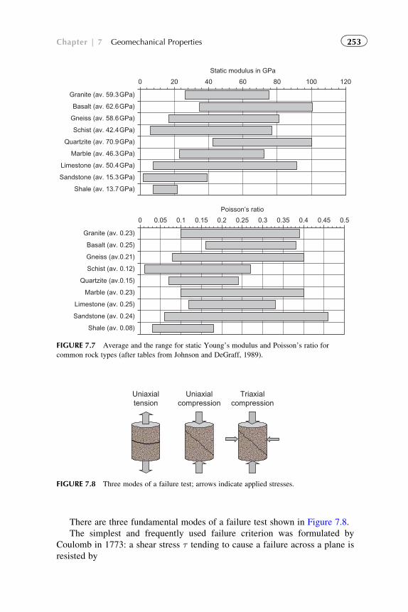
There are three fundamental modes of a failure test shown in Figure 7.8.
The simplest and frequently used failure criterion was formulated by
Coulomb in 1773: a shear stress τ tending to cause a failure across a plane is
resisted by
0 20 40 60 80 100 120
Granite (av. 59.3GPa)
Basalt (av. 62.6GPa)
Gneiss (av. 58.6GPa)
Schist (av. 42.4GPa)
Quartzite (av. 70.9GPa)
Marble (av. 46.3GPa)
Limestone (av. 50.4GPa)
Sandstone (av. 15.3GPa)
Shale (av. 13.7GPa)
Static modulus in GPa
0 0.05 0.1 0.15 0.2 0.25 0.3 0.35 0.4 0.45 0.5
Granite (av. 0.23)
Basalt (av. 0.25)
Gneiss (av.0.21)
Schist (av. 0.12)
Quartzite (av.0.15)
Marble (av. 0.23)
Limestone (av. 0.25)
Sandstone (av. 0.24)
Shale (av. 0.08)
Poisson’s ratio
FIGURE 7.7 Average and the range for static Young’s modulus and Poisson’s ratio for
common rock types (after tables from Johnson and DeGraff, 1989).
Uniaxialtension
Uniaxialcompression
Triaxialcompression
FIGURE 7.8 Three modes of a failure test; arrows indicate applied stresses.
253Chapter | 7 Geomechanical Properties
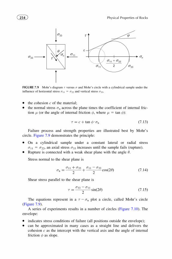
� the cohesion c of the material;� the normal stress σn across the plane times the coefficient of internal fric-
tion μ (or the angle of internal friction φ, where μ 5 tan φ):
τ ¼ cþ tan φUσn ð7:13Þ
Failure process and strength properties are illustrated best by Mohr’s
circle. Figure 7.9 demonstrates the principle:
� On a cylindrical sample under a constant lateral or radial stress
σ11 5 σ22, an axial stress σ33 increases until the sample fails (rupture).� Rupture is connected with a weak shear plane with the angle θ.
Stress normal to the shear plane is
σn ¼σ11 þ σ33
2þ σ11 2σ33
2cosð2θÞ ð7:14Þ
Shear stress parallel to the shear plane is
τ ¼ σ33 2σ11
2sinð2θÞ ð7:15Þ
The equations represent in a τ2σn plot a circle, called Mohr’s circle
(Figure 7.9).
A series of experiments results in a number of circles (Figure 7.10). The
envelope:
� indicates stress conditions of failure (all positions outside the envelope);� can be approximated in many cases as a straight line and delivers the
cohesion c as the intercept with the vertical axis and the angle of internal
friction φ as slope.
2
+
θ c
τ
τ
ϕ
σ33σn σn
σ33
σ33
σ11
σ11
σ11 σ33
FIGURE 7.9 Mohr’s diagram τ versus σ and Mohr’s circle with a cylindrical sample under the
influence of horizontal stress σ11 5 σ22 and vertical stress σ33.
254 Physical Properties of Rocks
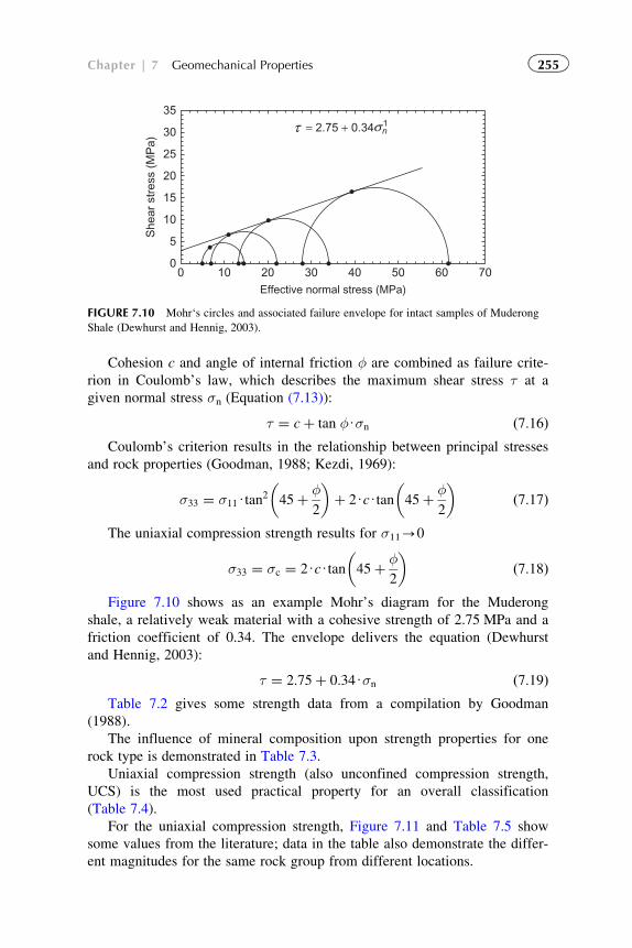
Cohesion c and angle of internal friction φ are combined as failure crite-
rion in Coulomb’s law, which describes the maximum shear stress τ at a
given normal stress σn (Equation (7.13)):
τ ¼ cþ tan φUσn ð7:16ÞCoulomb’s criterion results in the relationship between principal stresses
and rock properties (Goodman, 1988; Kezdi, 1969):
σ33 ¼ σ11Utan2 45þ φ2
� �þ 2UcUtan 45þ φ
2
� �ð7:17Þ
The uniaxial compression strength results for σ11-0
σ33 ¼ σc ¼ 2UcUtan 45þ φ2
� �ð7:18Þ
Figure 7.10 shows as an example Mohr’s diagram for the Muderong
shale, a relatively weak material with a cohesive strength of 2.75 MPa and a
friction coefficient of 0.34. The envelope delivers the equation (Dewhurst
and Hennig, 2003):
τ ¼ 2:75þ 0:34Uσn ð7:19ÞTable 7.2 gives some strength data from a compilation by Goodman
(1988).
The influence of mineral composition upon strength properties for one
rock type is demonstrated in Table 7.3.
Uniaxial compression strength (also unconfined compression strength,
UCS) is the most used practical property for an overall classification
(Table 7.4).
For the uniaxial compression strength, Figure 7.11 and Table 7.5 show
some values from the literature; data in the table also demonstrate the differ-
ent magnitudes for the same rock group from different locations.
Effective normal stress (MPa)
35
30
25
20
15
10
She
ar s
tres
s (M
Pa)
5
00 10 20 30 40 50 60 70
τ σn1 = 2.75 + 0.34
FIGURE 7.10 Mohr‘s circles and associated failure envelope for intact samples of Muderong
Shale (Dewhurst and Hennig, 2003).
255Chapter | 7 Geomechanical Properties
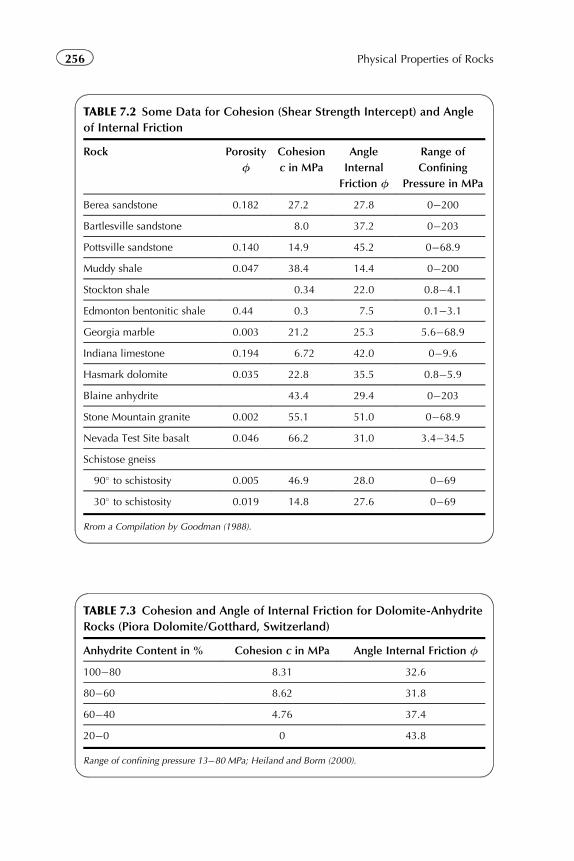
TABLE 7.2 Some Data for Cohesion (Shear Strength Intercept) and Angle
of Internal Friction
Rock Porosity
φCohesion
c in MPa
Angle
Internal
Friction φ
Range of
Confining
Pressure in MPa
Berea sandstone 0.182 27.2 27.8 0�200
Bartlesville sandstone 8.0 37.2 0�203
Pottsville sandstone 0.140 14.9 45.2 0�68.9
Muddy shale 0.047 38.4 14.4 0�200
Stockton shale 0.34 22.0 0.8�4.1
Edmonton bentonitic shale 0.44 0.3 7.5 0.1�3.1
Georgia marble 0.003 21.2 25.3 5.6�68.9
Indiana limestone 0.194 6.72 42.0 0�9.6
Hasmark dolomite 0.035 22.8 35.5 0.8�5.9
Blaine anhydrite 43.4 29.4 0�203
Stone Mountain granite 0.002 55.1 51.0 0�68.9
Nevada Test Site basalt 0.046 66.2 31.0 3.4�34.5
Schistose gneiss
90� to schistosity 0.005 46.9 28.0 0�69
30� to schistosity 0.019 14.8 27.6 0�69
Rrom a Compilation by Goodman (1988).
TABLE 7.3 Cohesion and Angle of Internal Friction for Dolomite-Anhydrite
Rocks (Piora Dolomite/Gotthard, Switzerland)
Anhydrite Content in % Cohesion c in MPa Angle Internal Friction φ
100�80 8.31 32.6
80�60 8.62 31.8
60�40 4.76 37.4
20�0 0 43.8
Range of confining pressure 13�80 MPa; Heiland and Borm (2000).
256 Physical Properties of Rocks
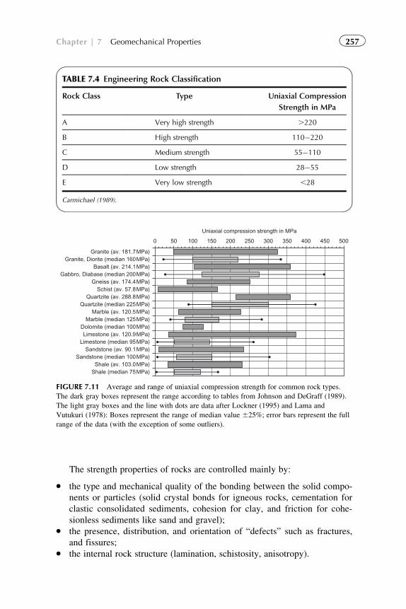
The strength properties of rocks are controlled mainly by:
� the type and mechanical quality of the bonding between the solid compo-
nents or particles (solid crystal bonds for igneous rocks, cementation for
clastic consolidated sediments, cohesion for clay, and friction for cohe-
sionless sediments like sand and gravel);� the presence, distribution, and orientation of “defects” such as fractures,
and fissures;� the internal rock structure (lamination, schistosity, anisotropy).
TABLE 7.4 Engineering Rock Classification
Rock Class Type Uniaxial Compression
Strength in MPa
A Very high strength .220
B High strength 110�220
C Medium strength 55�110
D Low strength 28�55
E Very low strength ,28
Carmichael (1989).
0 50 100 150 200 250 300 350 400 450 500
Granite (av. 181.7MPa)Granite, Diorite (median 160MPa)
Basalt (av. 214.1MPa)Gabbro, Diabase (median 200MPa)
Gneiss (av. 174.4MPa)Schist (av. 57.8MPa)
Quartzite (av. 288.8MPa)Quartzite (median 225MPa)
Marble (av. 120.5MPa)Marble (median 125MPa)
Dolomite (median 100MPa)Limestone (av. 120.9MPa)
Limestone (median 95MPa)Sandstone (av. 90.1MPa)
Sandstone (median 100MPa)Shale (av. 103.0MPa)
Shale (median 75MPa)
Uniaxial compression strength in MPa
FIGURE 7.11 Average and range of uniaxial compression strength for common rock types.
The dark gray boxes represent the range according to tables from Johnson and DeGraff (1989).
The light gray boxes and the line with dots are data after Lockner (1995) and Lama and
Vutukuri (1978): Boxes represent the range of median value 625%; error bars represent the full
range of the data (with the exception of some outliers).
257Chapter | 7 Geomechanical Properties
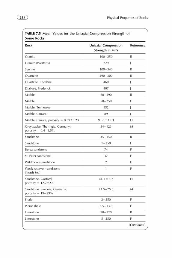
TABLE 7.5 Mean Values for the Uniaxial Compression Strength of
Some Rocks
Rock Uniaxial Compression
Strength in MPa
Reference
Granite 100�250 R
Granite (Westerly) 229 J
Syenite 100�340 R
Quartzite 290�300 R
Quartzite, Cheshire 460 J
Diabase, Frederick 487 J
Marble 60�190 R
Marble 50�250 F
Marble, Tennessee 152 J
Marble, Carrara 89 J
Marble, Carrara; porosity 5 0.6960.23 93.6615.3 H
Greywacke, Thuringia, Germany;porosity 5 0.4�1.5%
34�123 M
Sandstone 35�150 R
Sandstone 1�250 F
Berea sandstone 74 F
St. Peter sandstone 37 F
Wildmoore sandstone 7 F
Weak reservoir sandstone(North Sea)
1 F
Sandstone, Gosford;porosity 5 12.762.4
44.166.7 H
Sandstone, Saxonia, Germany;porosity 5 19�29%
23.5�75.0 M
Shale 2�250 F
Pierre shale 7.5�13.9 F
Limestone 90�120 R
Limestone 5�250 F
(Continued )
258 Physical Properties of Rocks
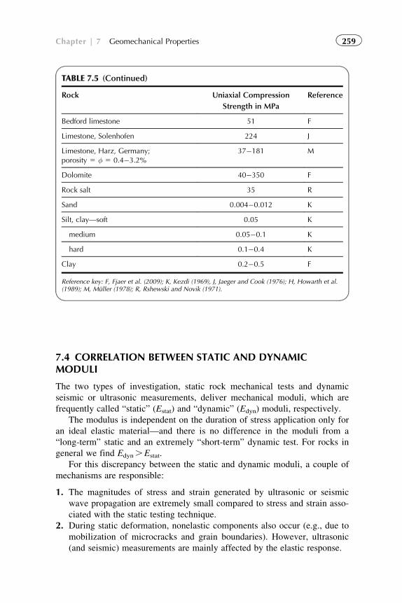
7.4 CORRELATION BETWEEN STATIC AND DYNAMICMODULI
The two types of investigation, static rock mechanical tests and dynamic
seismic or ultrasonic measurements, deliver mechanical moduli, which are
frequently called “static” (Estat) and “dynamic” (Edyn) moduli, respectively.
The modulus is independent on the duration of stress application only for
an ideal elastic material—and there is no difference in the moduli from a
“long-term” static and an extremely “short-term” dynamic test. For rocks in
general we find Edyn.Estat.
For this discrepancy between the static and dynamic moduli, a couple of
mechanisms are responsible:
1. The magnitudes of stress and strain generated by ultrasonic or seismic
wave propagation are extremely small compared to stress and strain asso-
ciated with the static testing technique.
2. During static deformation, nonelastic components also occur (e.g., due to
mobilization of microcracks and grain boundaries). However, ultrasonic
(and seismic) measurements are mainly affected by the elastic response.
TABLE 7.5 (Continued)
Rock Uniaxial Compression
Strength in MPa
Reference
Bedford limestone 51 F
Limestone, Solenhofen 224 J
Limestone, Harz, Germany;porosity 5 φ 5 0.4�3.2%
37�181 M
Dolomite 40�350 F
Rock salt 35 R
Sand 0.004�0.012 K
Silt, clay—soft 0.05 K
medium 0.05�0.1 K
hard 0.1�0.4 K
Clay 0.2�0.5 F
Reference key: F, Fjaer et al. (2009); K, Kezdi (1969), J, Jaeger and Cook (1976); H, Howarth et al.(1989); M, Muller (1978); R, Rshewski and Novik (1971).
259Chapter | 7 Geomechanical Properties
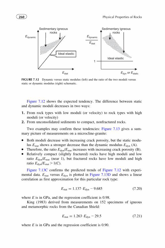
Figure 7.12 shows the expected tendency. The difference between static
and dynamic moduli decreases in two ways:
1. From rock types with low moduli (or velocity) to rock types with high
moduli (or velocity)
2. From unconsolidated sediments to compact, nonfractured rocks.
Two examples may confirm these tendencies: Figure 7.13 gives a sum-
mary picture of measurements on a microcline-granite:
� Both moduli decrease with increasing crack porosity, but the static modu-
lus Estat shows a stronger decrease than the dynamic modulus Edyn (A).� Therefore, the ratio Edyn/Estat increases with increasing crack porosity (B).� Relatively compact (slightly fractured) rocks have high moduli and low
ratio Edyn/Estat (near 1), but fractured rocks have low moduli and high
ratio Edyn/Estat. 1(C).
Figure 7.13C confirms the predicted trends of Figure 7.12 with experi-
mental data. Estat versus Edyn is plotted in Figure 7.13D and shows a linear
correlation as first approximation for this particular rock type:
Estat ¼ 1:137UEdyn 2 9:685 ð7:20Þ
where E is in GPa, and the regression coefficient is 0.98.
King (1983) derived from measurements on 152 specimens of igneous
and metamorphic rocks from the Canadian Shield:
Estat ¼ 1:263UEdyn 2 29:5 ð7:21Þ
where E is in GPa and the regression coefficient is 0.90.
Ideal elastic
Ideal elastic1
EdynamicEdynamic
Edyn or EstaticEstat
Estat
Sedimentary igneousrocks
Sedimentary igneousrocks
FIGURE 7.12 Dynamic versus static modulus (left) and the ratio of the two moduli versus
static or dynamic modulus (right) schematic.
260 Physical Properties of Rocks
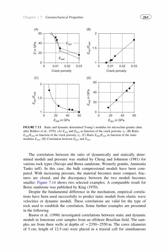
The correlation between the ratio of dynamically and statically deter-
mined moduli and pressure was studied by Cheng and Johnston (1981) for
various rock types (Navajo and Berea sandstone, Westerly granite, Ammonia
Tanks tuff). In this case, the bulk compressional moduli have been com-
pared. With increasing pressure, the material becomes more compact, frac-
tures are closed, and the discrepancy between the two moduli becomes
smaller. Figure 7.14 shows two selected examples. A comparable result for
Boise sandstone was published by King (1970).
Despite the fundamental difference in the mechanism, empirical correla-
tions have been used successfully to predict static moduli from elastic wave
velocities or dynamic moduli. These correlations are valid for the type of
rock used to establish the correlation. Some further examples are presented
in the following.
Bastos et al. (1998) investigated correlations between static and dynamic
moduli in limestone core samples from an offshore Brazilian field. The sam-
ples are from three wells at depths of B2350�2550 m. The cores (diameter
of 5 cm; length of 12.5 cm) were placed in a triaxial cell for simultaneous
0
20
40
60
0 0.01 0.02 0.03
Crack porosity
(A) (B)
(C) (D)
E in
GP
a Edyn
Estat
1
1.5
2
0 20 40 60
Estat in GPa
Edy
n/E
stat
0
20
40
60
0 20 40 60
Edyn in GPa
Est
at in
GP
a
1
1.5
2
0 0.01 0.02 0.03
Crack porosity
Edy
n/E
stat
FIGURE 7.13 Static and dynamic determined Young’s modulus for microcline-granite (data
after Belikov et al., 1970). (A) Estat and Edyn as function of the crack porosity φc. (B) RatioEdyn/Estat as function of the crack porosity φc. (C) Ratio Edyn/Estat as function of the static
modulus Estat. (D) Correlation between Edyn and Estat.
261Chapter | 7 Geomechanical Properties
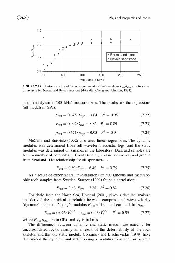
static and dynamic (500 kHz) measurements. The results are the regressions
(all moduli in GPa):
Estat ¼ 0:675UEdyn 2 3:84 R2 ¼ 0:95 ð7:22Þ
kstat ¼ 0:992Ukdyn 2 8:82 R2 ¼ 0:89 ð7:23Þ
μstat ¼ 0:621Uμdyn 2 0:95 R2 ¼ 0:94 ð7:24ÞMcCann and Entwisle (1992) also used linear regressions. The dynamic
modulus was determined from full waveform acoustic logs, and the static
modulus was determined on samples in the laboratory. Data and samples are
from a number of boreholes in Great Britain (Jurassic sediments) and granite
from Scotland. The relationship for all specimens is
Estat ¼ 0:69UEdyn þ 6:40 R2 ¼ 0:75 ð7:25ÞAs a result of experimental investigations of 300 igneous and metamor-
phic rock samples from Sweden, Starzec (1999) found a correlation:
Estat ¼ 0:48UEdyn 2 3:26 R2 ¼ 0:82 ð7:26ÞFor shale from the North Sea, Horsrud (2001) gives a detailed analysis
and derived the empirical correlation between compressional wave velocity
(dynamic) and static Young’s modulus Estat and static shear modulus μstat:
Estat ¼ 0:076UV3:23P μstat ¼ 0:03UV3:30
P R2 ¼ 0:99 ð7:27Þwhere Estat,μstat are in GPa, and VP is in km s21.
The differences between dynamic and static moduli are extreme for
unconsolidated rocks, mainly as a result of the deformability of the rock
skeleton and the low static moduli. Gorjainov and Ljachowickij (1979) have
determined the dynamic and static Young’s modulus from shallow seismic
0.4
0.6
0.8
1.0
0 50 100 150 200 250Pressure in MPa
k sta
t/kdy
n
Berea sandstoneNavajo sandstone
FIGURE 7.14 Ratio of static and dynamic compressional bulk modulus kstat/kdyn as a function
of pressure for Navajo and Berea sandstone (data after Cheng and Johnston, 1981).
262 Physical Properties of Rocks
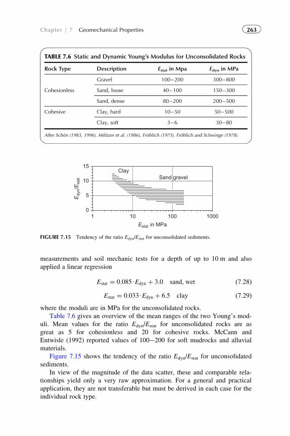
measurements and soil mechanic tests for a depth of up to 10 m and also
applied a linear regression
Estat ¼ 0:085UEdyn þ 3:0 sand; wet ð7:28ÞEstat ¼ 0:033UEdyn þ 6:5 clay ð7:29Þ
where the moduli are in MPa for the unconsolidated rocks.
Table 7.6 gives an overview of the mean ranges of the two Young’s mod-
uli. Mean values for the ratio Edyn/Estat for unconsolidated rocks are as
great as 5 for cohesionless and 20 for cohesive rocks. McCann and
Entwisle (1992) reported values of 100�200 for soft mudrocks and alluvial
materials.
Figure 7.15 shows the tendency of the ratio Edyn/Estat for unconsolidated
sediments.
In view of the magnitude of the data scatter, these and comparable rela-
tionships yield only a very raw approximation. For a general and practical
application, they are not transferable but must be derived in each case for the
individual rock type.
TABLE 7.6 Static and Dynamic Young’s Modulus for Unconsolidated Rocks
Rock Type Description Estat in Mpa Edyn in MPa
Gravel 100�200 300�800
Cohesionless Sand, loose 40�100 150�300
Sand, dense 80�200 200�500
Cohesive Clay, hard 10�50 50�500
Clay, soft 3�6 30�80
After Schon (1983, 1996), Militzer et al. (1986), Frohlich (1975), Frohlich and Schwinge (1978).
Edy
n/E
stat
0
5
10
15
1 10 100 1000Estat in MPa
ClaySand gravel
FIGURE 7.15 Tendency of the ratio Edyn/Estat for unconsolidated sediments.
263Chapter | 7 Geomechanical Properties
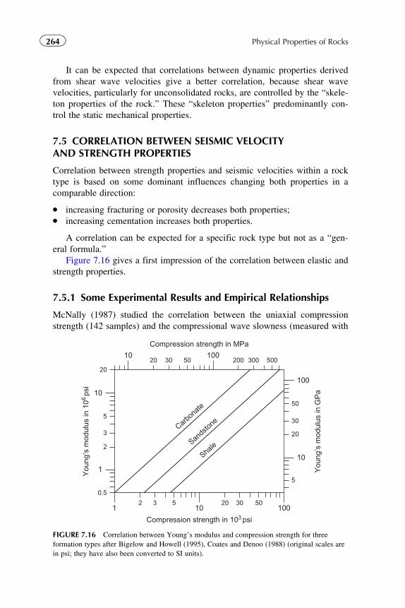
It can be expected that correlations between dynamic properties derived
from shear wave velocities give a better correlation, because shear wave
velocities, particularly for unconsolidated rocks, are controlled by the “skele-
ton properties of the rock.” These “skeleton properties” predominantly con-
trol the static mechanical properties.
7.5 CORRELATION BETWEEN SEISMIC VELOCITYAND STRENGTH PROPERTIES
Correlation between strength properties and seismic velocities within a rock
type is based on some dominant influences changing both properties in a
comparable direction:
� increasing fracturing or porosity decreases both properties;� increasing cementation increases both properties.
A correlation can be expected for a specific rock type but not as a “gen-
eral formula.”
Figure 7.16 gives a first impression of the correlation between elastic and
strength properties.
7.5.1 Some Experimental Results and Empirical Relationships
McNally (1987) studied the correlation between the uniaxial compression
strength (142 samples) and the compressional wave slowness (measured with
2 3 5 20 30 50
Compression strength in 103 psi
1
1 10 100
10
2
3
5
20
0.5
You
ng’s
mod
ulus
in 1
06ps
i
10 10020 30 50 200 300 500
Compression strength in MPa
10
100
20
30
50
5
You
ng’s
mod
ulus
in G
Pa
Carbo
nate
Sands
tone
Shale
FIGURE 7.16 Correlation between Young’s modulus and compression strength for three
formation types after Bigelow and Howell (1995), Coates and Denoo (1988) (original scales are
in psi; they have also been converted to SI units).
264 Physical Properties of Rocks

a sonic logging tool) of fine- to medium-grained sandstone from the German
Creek formation (Queensland, Australia). There is—for this particular geo-
logical situation—a good correlation (Figure 7.17) that is probably controlled
by variation of porosity and grain-contact quality. The resulting regression is
originally with uniaxial compression strength in MPa and Δt in μs ft21
σc ¼ 1277Uexpð20:0367UΔtÞ with R2 ¼ 0:83 ð7:30ÞIn Figure 7.17, data are converted into velocities (m s21) and redrawn as
a plot of uniaxial compression strength versus compressional wave velocity.
Two regressions are calculated:
linear regression σc ¼ 0:050UVP 2 114:5 with R2 ¼ 0:88 ð7:31Þ
power law σc ¼ 3U10211UV3:45P with R2 ¼ 0:86 ð7:32Þ
Jizba (1991) investigated correlations between compressional and shear
wave velocity and uniaxial compression strength. Figure 7.18 shows an
example for a tight sandstone confirming the general tendency for both wave
types. The author noted that scatter in these data is attributed to confining
pressure and clay content.
Horsrud (2001) derived the following empirical correlation especially for
shale (North Sea)
σc ¼ 0:77UV2:93P R2 ¼ 0:99 ð7:33Þ
where σc is in MPa and VP in km s21.
Table 7.7 gives some more empirical relationships between uniaxial com-
pression strength (in MPa) and compressional velocity (in m s21) from the
literature.
0
50
100
150
1000 2000 3000 4000 5000 6000
Velocity VP in ms−1
Str
engt
h in
MP
a
FIGURE 7.17 Uniaxial compression strength versus compressional wave velocity; sandstone
from the German Creek formation, Queensland, Australia. Points are experimental data after
McNally (1987); curves follow the two regression equations.
265Chapter | 7 Geomechanical Properties
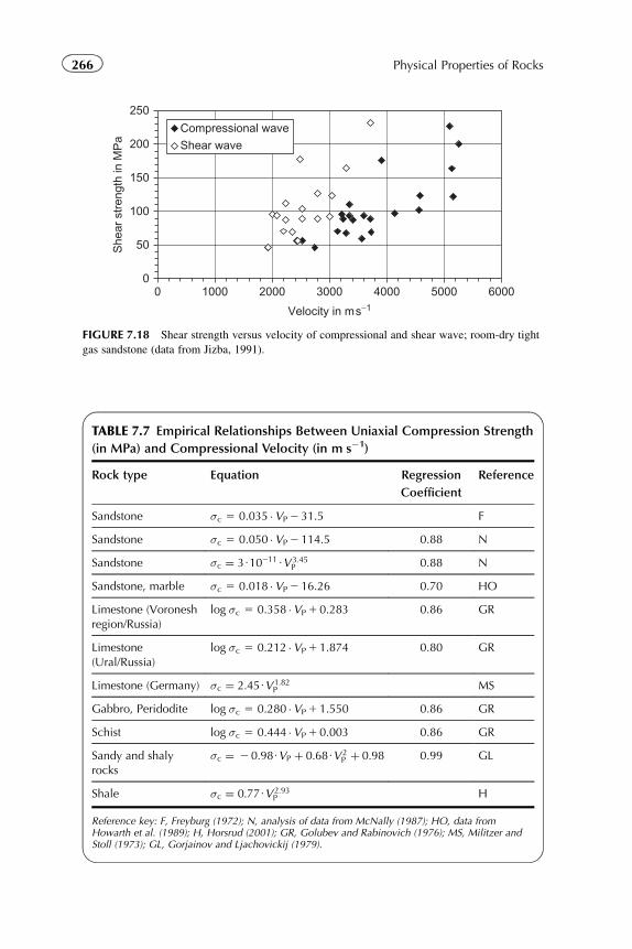
0
50
100
150
200
250
0 1000 2000 3000 4000 5000 6000
Velocity in ms−1
She
ar s
tren
gth
in M
Pa
Compressional waveShear wave
FIGURE 7.18 Shear strength versus velocity of compressional and shear wave; room-dry tight
gas sandstone (data from Jizba, 1991).
TABLE 7.7 Empirical Relationships Between Uniaxial Compression Strength
(in MPa) and Compressional Velocity (in m s�1)
Rock type Equation Regression
Coefficient
Reference
Sandstone σc 5 0.035 �VP2 31.5 F
Sandstone σc 5 0.050 �VP2 114.5 0.88 N
Sandstone σc ¼ 3U10211UV 3:45P 0.88 N
Sandstone, marble σc 5 0.018 �VP2 16.26 0.70 HO
Limestone (Voroneshregion/Russia)
log σc 5 0.358 �VP1 0.283 0.86 GR
Limestone(Ural/Russia)
log σc 5 0.212 �VP1 1.874 0.80 GR
Limestone (Germany) σc ¼ 2:45UV 1:82P MS
Gabbro, Peridodite log σc 5 0.280 �VP1 1.550 0.86 GR
Schist log σc 5 0.444 �VP1 0.003 0.86 GR
Sandy and shalyrocks
σc ¼ 2 0:98UVP þ 0:68UV 2P þ 0:98 0.99 GL
Shale σc ¼ 0:77UV 2:93P H
Reference key: F, Freyburg (1972); N, analysis of data from McNally (1987); HO, data fromHowarth et al. (1989); H, Horsrud (2001); GR, Golubev and Rabinovich (1976); MS, Militzer andStoll (1973); GL, Gorjainov and Ljachovickij (1979).
266 Physical Properties of Rocks
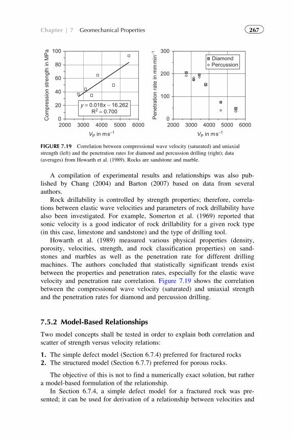
A compilation of experimental results and relationships was also pub-
lished by Chang (2004) and Barton (2007) based on data from several
authors.
Rock drillability is controlled by strength properties; therefore, correla-
tions between elastic wave velocities and parameters of rock drillability have
also been investigated. For example, Somerton et al. (1969) reported that
sonic velocity is a good indicator of rock drillability for a given rock type
(in this case, limestone and sandstone) and the type of drilling tool.
Howarth et al. (1989) measured various physical properties (density,
porosity, velocities, strength, and rock classification properties) on sand-
stones and marbles as well as the penetration rate for different drilling
machines. The authors concluded that statistically significant trends exist
between the properties and penetration rates, especially for the elastic wave
velocity and penetration rate correlation. Figure 7.19 shows the correlation
between the compressional wave velocity (saturated) and uniaxial strength
and the penetration rates for diamond and percussion drilling.
7.5.2 Model-Based Relationships
Two model concepts shall be tested in order to explain both correlation and
scatter of strength versus velocity relations:
1. The simple defect model (Section 6.7.4) preferred for fractured rocks
2. The structured model (Section 6.7.7) preferred for porous rocks.
The objective of this is not to find a numerically exact solution, but rather
a model-based formulation of the relationship.
In Section 6.7.4, a simple defect model for a fractured rock was pre-
sented; it can be used for derivation of a relationship between velocities and
VP in ms−1
Pen
etra
tion
rate
in m
mm
in−1
DiamondPercussion
y = 0.018x − 16.262R2 = 0.700
02000 3000 4000 5000 6000
20
40
60
80
100C
ompr
essi
on s
tren
gth
in M
Pa
VP in ms−1
02000 3000 4000 5000 6000
100
200
300
FIGURE 7.19 Correlation between compressional wave velocity (saturated) and uniaxial
strength (left) and the penetration rates for diamond and percussion drilling (right); data
(averages) from Howarth et al. (1989). Rocks are sandstone and marble.
267Chapter | 7 Geomechanical Properties
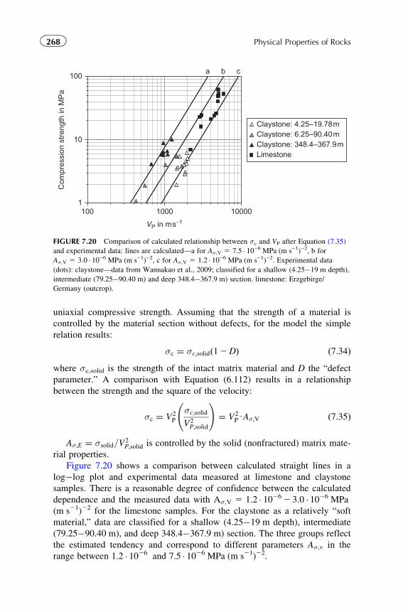
uniaxial compressive strength. Assuming that the strength of a material is
controlled by the material section without defects, for the model the simple
relation results:
σc ¼ σc;solidð12DÞ ð7:34Þwhere σc,solid is the strength of the intact matrix material and D the “defect
parameter.” A comparison with Equation (6.112) results in a relationship
between the strength and the square of the velocity:
σc ¼ V2P
σc;solid
V2P;solid
!¼ V2
PUAσ;V ð7:35Þ
Aσ;E ¼ σsolid=V2P;solid is controlled by the solid (nonfractured) matrix mate-
rial properties.
Figure 7.20 shows a comparison between calculated straight lines in a
log�log plot and experimental data measured at limestone and claystone
samples. There is a reasonable degree of confidence between the calculated
dependence and the measured data with Aσ,V 5 1.2 � 10262 3.0 � 1026 MPa
(m s21)22 for the limestone samples. For the claystone as a relatively “soft
material,” data are classified for a shallow (4.25�19 m depth), intermediate
(79.25�90.40 m), and deep 348.4�367.9 m) section. The three groups reflect
the estimated tendency and correspond to different parameters Aσ,v in the
range between 1.2 � 1026 and 7.5 � 1026 MPa (m s21)22.
VP in ms−1
1
10
100
100001000100
Com
pres
sion
stre
ngth
in M
Pa
Claystone: 4.25–19.78mClaystone: 6.25–90.40mClaystone: 348.4–367.9mLimestone
a b c
FIGURE 7.20 Comparison of calculated relationship between σc and VP after Equation (7.35)
and experimental data: lines are calculated—a for Aσ,V 5 7.5 � 1026 MPa (m s21)22, b for
Aσ,V 5 3.0 � 1026 MPa (m s21)22, c for Aσ,V 5 1.2 � 1026 MPa (m s21)22. Experimental data
(dots): claystone—data from Wannakao et al., 2009; classified for a shallow (4.25�19 m depth),
intermediate (79.25�90.40 m) and deep 348.4�367.9 m) section. limestone: Erzgebirge/
Germany (outcrop).
268 Physical Properties of Rocks
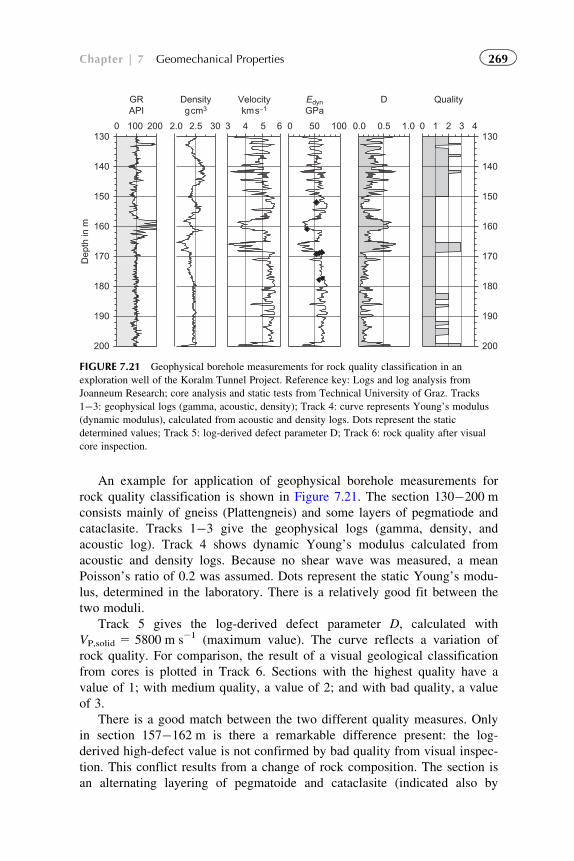
An example for application of geophysical borehole measurements for
rock quality classification is shown in Figure 7.21. The section 130�200 m
consists mainly of gneiss (Plattengneis) and some layers of pegmatiode and
cataclasite. Tracks 1�3 give the geophysical logs (gamma, density, and
acoustic log). Track 4 shows dynamic Young’s modulus calculated from
acoustic and density logs. Because no shear wave was measured, a mean
Poisson’s ratio of 0.2 was assumed. Dots represent the static Young’s modu-
lus, determined in the laboratory. There is a relatively good fit between the
two moduli.
Track 5 gives the log-derived defect parameter D, calculated with
VP,solid 5 5800 m s21 (maximum value). The curve reflects a variation of
rock quality. For comparison, the result of a visual geological classification
from cores is plotted in Track 6. Sections with the highest quality have a
value of 1; with medium quality, a value of 2; and with bad quality, a value
of 3.
There is a good match between the two different quality measures. Only
in section 157�162 m is there a remarkable difference present: the log-
derived high-defect value is not confirmed by bad quality from visual inspec-
tion. This conflict results from a change of rock composition. The section is
an alternating layering of pegmatoide and cataclasite (indicated also by
0 100 200
GRAPI
200
190
180
170
160
150
140
130
200
190
180
170
160
150
140
130
Dep
th in
m
2.0 2.5 30
Densitygcm3
3 4 5 6
Velocitykms−1
0 50 100
EdynGPa
0.0 0.5 0 1 2 3 41.0
D Quality
FIGURE 7.21 Geophysical borehole measurements for rock quality classification in an
exploration well of the Koralm Tunnel Project. Reference key: Logs and log analysis from
Joanneum Research; core analysis and static tests from Technical University of Graz. Tracks
1�3: geophysical logs (gamma, acoustic, density); Track 4: curve represents Young’s modulus
(dynamic modulus), calculated from acoustic and density logs. Dots represent the static
determined values; Track 5: log-derived defect parameter D; Track 6: rock quality after visual
core inspection.
269Chapter | 7 Geomechanical Properties
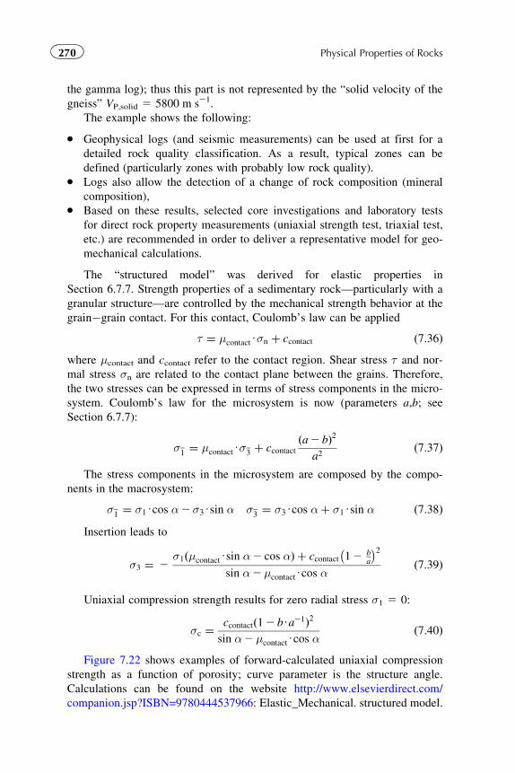
the gamma log); thus this part is not represented by the “solid velocity of the
gneiss” VP,solid 5 5800 m s21.
The example shows the following:
� Geophysical logs (and seismic measurements) can be used at first for a
detailed rock quality classification. As a result, typical zones can be
defined (particularly zones with probably low rock quality).� Logs also allow the detection of a change of rock composition (mineral
composition),� Based on these results, selected core investigations and laboratory tests
for direct rock property measurements (uniaxial strength test, triaxial test,
etc.) are recommended in order to deliver a representative model for geo-
mechanical calculations.
The “structured model” was derived for elastic properties in
Section 6.7.7. Strength properties of a sedimentary rock—particularly with a
granular structure—are controlled by the mechanical strength behavior at the
grain�grain contact. For this contact, Coulomb’s law can be applied
τ ¼ μcontactUσn þ ccontact ð7:36Þwhere μcontact and ccontact refer to the contact region. Shear stress τ and nor-
mal stress σn are related to the contact plane between the grains. Therefore,
the two stresses can be expressed in terms of stress components in the micro-
system. Coulomb’s law for the microsystem is now (parameters a,b; see
Section 6.7.7):
σ1 ¼ μcontactUσ3 þ ccontactða2 bÞ2
a2ð7:37Þ
The stress components in the microsystem are composed by the compo-
nents in the macrosystem:
σ1 ¼ σ1Ucos α2σ3Usin α σ3 ¼ σ3Ucos αþ σ1Usin α ð7:38ÞInsertion leads to
σ3 ¼ 2σ1ðμcontactUsin α2 cos αÞ þ ccontact 12
ba
� �2sin α2μcontactUcos α
ð7:39Þ
Uniaxial compression strength results for zero radial stress σ1 5 0:
σc ¼ccontactð12 bUa21Þ2sin α2μcontactUcos α
ð7:40Þ
Figure 7.22 shows examples of forward-calculated uniaxial compression
strength as a function of porosity; curve parameter is the structure angle.
Calculations can be found on the website http://www.elsevierdirect.com/
companion.jsp?ISBN=9780444537966: Elastic_Mechanical. structured model.
270 Physical Properties of Rocks
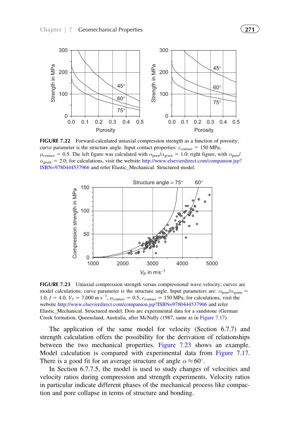
The application of the same model for velocity (Section 6.7.7) and
strength calculation offers the possibility for the derivation of relationships
between the two mechanical properties. Figure 7.23 shows an example.
Model calculation is compared with experimental data from Figure 7.17.
There is a good fit for an average structure of angle α� 60�.In Section 6.7.7.5, the model is used to study changes of velocities and
velocity ratios during compression and strength experiments. Velocity ratios
in particular indicate different phases of the mechanical process like compac-
tion and pore collapse in terms of structure and bonding.
0
100
200
300
0.0 0.1 0.2 0.3 0.4 0.5
Porosity
Str
engt
h in
MP
a
0
100
200
300
0.0 0.1 0.2 0.3 0.4 0.5
Porosity
Str
engt
h in
MP
a
45°
60°
75°
45°
60°
75°
FIGURE 7.22 Forward-calculated uniaxial compression strength as a function of porosity;
curve parameter is the structure angle. Input contact properties: ccontact 5 150 MPa;
μcontact 5 0.5. The left figure was calculated with αpore/αgrain 5 1.0; right figure, with αpore/
αgrain 5 2.0; for calculations, visit the website http://www.elsevierdirect.com/companion.jsp?
ISBN=9780444537966 and refer Elastic_Mechanical. Structured model.
0
50
100
150
1000 2000 3000 4000 5000
VP in ms−1
Com
pres
sion
str
engt
h in
MP
a
Structure angle = 75° 60°
FIGURE 7.23 Uniaxial compression strength versus compressional wave velocity; curves are
model calculations; curve parameter is the structure angle. Input parameters are: αpore/αgrain 5
1.0, f 5 4.0, V3 5 7,000 m s21, μcontact 5 0.5, ccontact 5 150 MPa; for calculations, visit the
website http://www.elsevierdirect.com/companion.jsp?ISBN=9780444537966 and refer
Elastic_Mechanical. Structured model. Dots are experimental data for a sandstone (German
Creek formation, Queensland, Australia, after McNally (1987, same as in Figure 7.17).
271Chapter | 7 Geomechanical Properties

Chapter 8
Electrical Properties
8.1 FUNDAMENTALS
Electrical measurements are an important group of methods in applied geo-
physics. Resistivity measurements in a well by the Schlumberger brothers
were the first commercial type of well logging. Today, the contrast between
conductive formation water and insulating hydrocarbons is the basis for a
saturation determination following Archie’s concept (Archie, 1942).
For a petrophysical characterization of rocks, two electrical parameters
are relevant:
1. Specific electrical resistivity
2. Dielectric permittivity.
For most common resistivity measurements, Ohm’s law gives the back-
ground to determine a resistance RES (in ohms) from a measurement of a
flowing current I (in amperes) and the voltage drop U (in volts):
RES ¼ U
Ið8:1Þ
Electrical resistance is connected with the material property “specific
electrical resistivity” (or its inverse—the conductivity) via a geometry
parameter that considers the geometry of the current distribution. For the
simple case of a cylindrical sample with current flow parallel to the axis, the
relationship is
RES ¼ ρl
Að8:2Þ
where l is the length and A is the cross section of the sample. Specific elec-
trical resistivity ρ is given in ohm meters (ohm m). In this textbook, the sign
R (with a subscript) is used for the specific electrical resistivity following the
commonly used notation in well-logging practice.
273Physical Properties of Rocks.
© 2011 Elsevier B.V. All rights reserved.
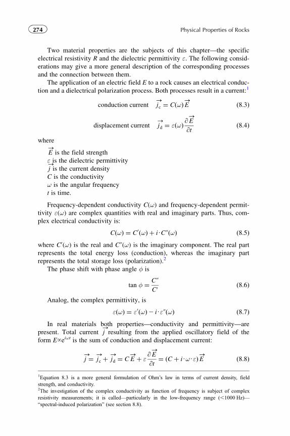
Two material properties are the subjects of this chapter—the specific
electrical resistivity R and the dielectric permittivity ε. The following consid-
erations may give a more general description of the corresponding processes
and the connection between them.
The application of an electric field E to a rock causes an electrical conduc-
tion and a dielectrical polarization process. Both processes result in a current:1
conduction current-jc ¼ CðωÞ-E ð8:3Þ
displacement current-jd ¼ εðωÞ @
-E
@tð8:4Þ
where-E is the field strength
ε is the dielectric permittivity-j is the current density
C is the conductivity
ω is the angular frequency
t is time.
Frequency-dependent conductivity C(ω) and frequency-dependent permit-
tivity ε(ω) are complex quantities with real and imaginary parts. Thus, com-
plex electrical conductivity is:
CðωÞ ¼ C0ðωÞ þ iUCvðωÞ ð8:5Þwhere C0(ω) is the real and Cv(ω) is the imaginary component. The real part
represents the total energy loss (conduction), whereas the imaginary part
represents the total storage loss (polarization).2
The phase shift with phase angle φ is
tan φ ¼ CvC0 ð8:6Þ
Analog, the complex permittivity, is
εðωÞ ¼ ε0ðωÞ2 iUεvðωÞ ð8:7ÞIn real materials both properties—conductivity and permittivity—are
present. Total current-j resulting from the applied oscillatory field of the
form E~eiωt is the sum of conduction and displacement current:
-j ¼ -
jc þ-jd ¼ C
-E þ ε
@-E
@t¼ ðC þ iUωUεÞ-E ð8:8Þ
1Equation 8.3 is a more general formulation of Ohm’s law in terms of current density, fieldstrength, and conductivity.2The investigation of the complex conductivity as function of frequency is subject of complexresistivity measurements; it is called—particularly in the low-frequency range (,1000 Hz)—“spectral-induced polarization” (see section 8.8).
274 Physical Properties of Rocks
The simplest description of this behavior is a parallel circuit of a resistor
and a capacitor. The conductive and dielectric properties are coupled
complex and frequency-dependent properties are:
Frequency-dependent dielectric permittivity
εðωÞ ¼ εðωÞ þ CðωÞiUω
¼ ε0ðωÞ2 i εvðωÞ þ CðωÞω
� �ð8:9Þ
Frequency-dependent conductivity
CðωÞ ¼ CðωÞ þ iUωUε ¼ ½CðωÞ þ ωUεvðωÞ� þ iUωUε0ðωÞ ð8:10ÞAs a consequence of Equations (8.9) and (8.10):
� the real component of electrical conductivity results for low frequencies
(ω-0);� the real component of dielectric permittivity results for high frequencies
(ω-N).
Units and symbols:
Specific electrical resistivity R is given in ohm meters (ohm m).
Electrical conductivity C is the inverse of specific electrical resistivity
and given in Siemens per meter, or S m21.
Dielectric permittivity is the product of dielectric permittivity of vacuum
ε05 8.854 � 10212 F m215 8.854 � 10212 s4 kg21 m23 and (dimensionless)
relative dielectric permittivity εr
ε ¼ ε0Uεr ð8:11ÞRelated topics discussed in the following chapters are:
� resistivity or conductivity of rocks (low-frequency phenomenon);� permittivity of rocks (high-frequency phenomenon);� frequency-dependent electrical properties and phenomena (spectral-
induced polarization, SIP).
8.2 ELECTRICAL PROPERTIES OF ROCK COMPONENTS
8.2.1 Minerals—Solid Components
Table 8.1 shows values of specific electrical resistivity and the permittivity of
some minerals. More detailed compilations are published by Olhoeft (1981),
Beblo et al. (1982), Melnikov et al. (1975), Parchomenko (1965), Katsube and
Collett (1976), and Keller (1989).
Most rock-forming minerals, particularly silicates and carbonates, have
very high specific resistivities (.109 ohm m); they are practical insulators.
Conductive minerals are sulfides and some oxides. They are rare in the
earth’s crust. An important member of the conductive group is graphite.
275Chapter | 8 Electrical Properties
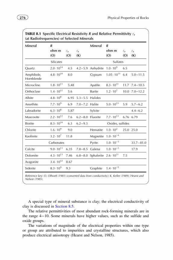
A special type of mineral substance is clay; the electrical conductivity of
clay is discussed in Section 8.5.
The relative permittivities of most abundant rock-forming minerals are in
the range 4�10. Some minerals have higher values, such as the sulfide and
oxide groups.
The variations of magnitude of the electrical properties within one type
or group are attributed to impurities and crystalline structures, which also
produce electrical anisotropy (Hearst and Nelson, 1985).
TABLE 8.1 Specific Electrical Resistivity R and Relative Permittivity εr(at Radiofrequencies) of Selected Minerals
Mineral R
ohm m
(O)
εr(O)
εr(K)
Mineral R
ohm m
(O)
εr(O)
εr(K)
Silicates Sulfates
Quartz 2.0 � 1014 4.5 4.2�5.9 Anhydrite 1.0 � 109 6.5
Amphibole,Hornblende
4.8 � 1010 8.0 Gypsum 1.05 � 1011 6.4 5.0�11.5
Microcline 1.8 � 1011 5.48 Apatite 8.3 � 1011 11.7 7.4�10.5
Orthoclase 1.4 � 1012 5.6 Barite 1.2 � 107 10.0 7.0�12.2
Albite 4.8 � 108 6.95 5.3�5.5 Halides
Anorthite 7.7 � 109 6.9 7.0�7.2 Halite 5.0 � 1013 5.9 5.7�6.2
Labradorite 6.3 � 108 5.87 Sylvite 4.4�6.2
Muscovite 2.2 � 1012 7.6 6.2�8.0 Fluorite 7.7 � 1013 6.76 6.79
Biotite 8.3 � 1010 6.3 6.2�9.3 Oxides, sulfides
Chlorite 1.6 � 109 9.0 Hematite 1.0 � 102 25.0 25.0
Kaolinite 3.2 � 107 11.8 Magnetite 1.0 � 1024
Carbonates Pyrite 1.0 � 1023 33.7�81.0
Calcite 9.0 � 1013 6.35 7.8�8.5 Galena 1.0 � 1023 17.9
Dolomite 4.3 � 1013 7.46 6.8�8.0 Sphalerite 2.6 � 1011 7.5
Aragonite 3.4 � 1012 8.67
Siderite 8.3 � 109 9.3 Graphite 1.4 � 1025
Reference key: O, Olhoeft (1981) (converted data from conductivity); K, Keller (1989); Hearst andNelson (1985).
276 Physical Properties of Rocks
8.2.2 Pore Fluids
Among the pore fluids, water is the only effective conductor. In many cases,
the ionic conduction of the pore water is the dominant conduction mecha-
nism in a porous or fractured rock, and the specific electrical resistivity is
controlled mainly by:
� the chemical composition, concentration, and temperature of the brine or
electrolyte;� the volume fraction (porosity, saturation) and distribution of the electro-
lyte in the rock.
Gases and oil are essentially nonconductors: the specific electrical resis-
tivity is in the order of .109 ohm m. Dortman (1976) gives a specific electri-
cal resistivity for oil Roil 5 109�1016 ohm m.
There also exists a distinct difference of the relative permittivity between
water (εr � 80) and most other fluids (εr 5 1�3) as shown in Table 8.9.
Thus, with respect to the electrical properties, we have two main types of
pore fluids:
1. Water: conducting and high permittivity εr 5 80
2. Oil, gas: nonconducting and low permittivity εr 5 1�3
The specific resistivity of natural waters varies over decades. The highest
values are for rainwater; the lowest are for saturated brines in, for example,
sedimentary saline facies. Table 8.2 shows some mean values.
Figure 8.1 shows the correlation between specific resistivity, concentra-
tion, and temperature for sodium chloride solution (NaCl) in the form of a
nomogram.
The temperature dependence of NaCl solutions can be described by an
empirical relationship (Arps, 1953):
RwðT2Þ ¼ RwðT1ÞT1 þ 21:5
T2 þ 21:5RwðT2Þ ¼ RwðT1Þ
T1 þ 6:77
T2 þ 6:77ð8:12Þ
where T1 and T2, the temperatures in degrees Celsius for the first equation,
and in degrees Fahrenheit for the second.
Bigelow (1992) gives the following empirical equation for water resistiv-
ity Rw (in ohm m) as a function of NaCl concentration CNaCl (in ppm) and
temperature T (in degrees Fahrenheit):
Rw ¼ 0:0123þ 3647:5
C0:955NaCl
� �81:77
T þ 6:77ð8:13Þ
If the solutions contain ions other than Na+ and Cl2 (e.g., K), the so-
called multipliers are applied to calculate an equivalent NaCl concentration
and its conductivity (see chartbooks; Baker Atlas, 1985; Schlumberger,
1989, 2000).
277Chapter | 8 Electrical Properties
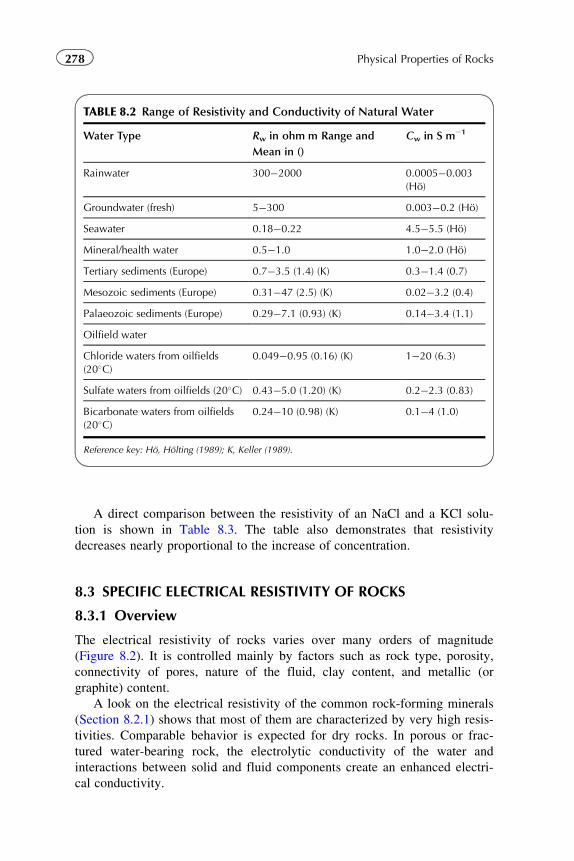
A direct comparison between the resistivity of an NaCl and a KCl solu-
tion is shown in Table 8.3. The table also demonstrates that resistivity
decreases nearly proportional to the increase of concentration.
8.3 SPECIFIC ELECTRICAL RESISTIVITY OF ROCKS
8.3.1 Overview
The electrical resistivity of rocks varies over many orders of magnitude
(Figure 8.2). It is controlled mainly by factors such as rock type, porosity,
connectivity of pores, nature of the fluid, clay content, and metallic (or
graphite) content.
A look on the electrical resistivity of the common rock-forming minerals
(Section 8.2.1) shows that most of them are characterized by very high resis-
tivities. Comparable behavior is expected for dry rocks. In porous or frac-
tured water-bearing rock, the electrolytic conductivity of the water and
interactions between solid and fluid components create an enhanced electri-
cal conductivity.
TABLE 8.2 Range of Resistivity and Conductivity of Natural Water
Water Type Rw in ohm m Range and
Mean in ()
Cw in S m21
Rainwater 300�2000 0.0005�0.003(Ho)
Groundwater (fresh) 5�300 0.003�0.2 (Ho)
Seawater 0.18�0.22 4.5�5.5 (Ho)
Mineral/health water 0.5�1.0 1.0�2.0 (Ho)
Tertiary sediments (Europe) 0.7�3.5 (1.4) (K) 0.3�1.4 (0.7)
Mesozoic sediments (Europe) 0.31�47 (2.5) (K) 0.02�3.2 (0.4)
Palaeozoic sediments (Europe) 0.29�7.1 (0.93) (K) 0.14�3.4 (1.1)
Oilfield water
Chloride waters from oilfields(20�C)
0.049�0.95 (0.16) (K) 1�20 (6.3)
Sulfate waters from oilfields (20�C) 0.43�5.0 (1.20) (K) 0.2�2.3 (0.83)
Bicarbonate waters from oilfields(20�C)
0.24�10 (0.98) (K) 0.1�4 (1.0)
Reference key: Ho, Holting (1989); K, Keller (1989).
278 Physical Properties of Rocks
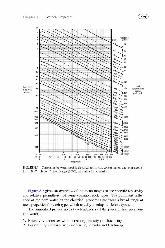
Figure 8.2 gives an overview of the mean ranges of the specific resistivity
and relative permittivity of some common rock types. The dominant influ-
ence of the pore water on the electrical properties produces a broad range of
rock properties for each type, which usually overlaps different types.
The simplified picture notes two tendencies (if the pores or fractures con-
tain water):
1. Resistivity decreases with increasing porosity and fracturing
2. Permittivity increases with increasing porosity and fracturing.
FIGURE 8.1 Correlation between specific electrical resistivity, concentration, and temperature
for an NaCl solution; Schlumberger (2000), with friendly permission.
279Chapter | 8 Electrical Properties
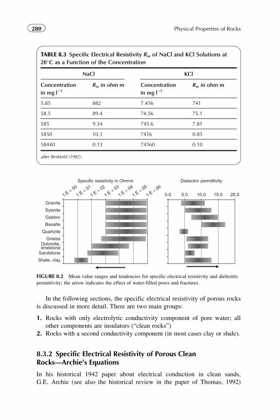
In the following sections, the specific electrical resistivity of porous rocks
is discussed in more detail. There are two main groups:
1. Rocks with only electrolytic conductivity component of pore water; all
other components are insulators (“clean rocks”)
2. Rocks with a second conductivity component (in most cases clay or shale).
8.3.2 Specific Electrical Resistivity of Porous CleanRocks—Archie’s Equations
In his historical 1942 paper about electrical conduction in clean sands,
G.E. Archie (see also the historical review in the paper of Thomas, 1992)
1.E + 00
1.E + 01
1.E + 02
1.E + 03
1.E + 04
1.E + 05
1.E + 06
Granite
Syenite
Gabbro
Basalte
Quartzite
GneissDolomite,limestone
Sandstone
Shale, clay
Specific resistivity in Ohmm
0.0 5.0 10.0 15.0 20.0
Dielectric permittivity
FIGURE 8.2 Mean value ranges and tendencies for specific electrical resistivity and dielectric
permittivity; the arrow indicates the effect of water-filled pores and fractures.
TABLE 8.3 Specific Electrical Resistivity Rw of NaCl and KCl Solutions at
20�C as a Function of the Concentration
NaCl KCl
Concentration
in mg l21
Rw in ohm m Concentration
in mg l21Rw in ohm m
5.85 882 7.456 741
58.5 89.4 74.56 75.1
585 9.34 745.6 7.81
5850 10.3 7456 0.85
58440 0.13 74560 0.10
after Berktold (1982).
280 Physical Properties of Rocks
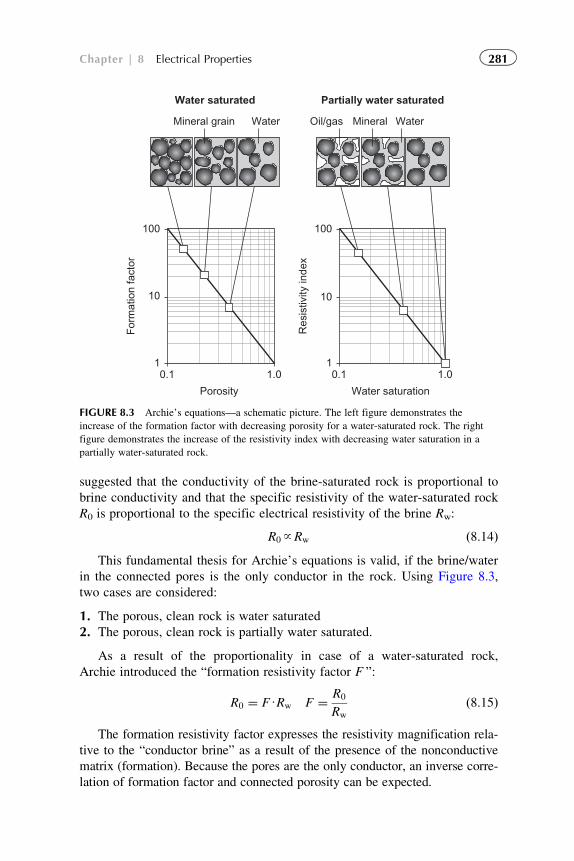
suggested that the conductivity of the brine-saturated rock is proportional to
brine conductivity and that the specific resistivity of the water-saturated rock
R0 is proportional to the specific electrical resistivity of the brine Rw:
R0~Rw ð8:14ÞThis fundamental thesis for Archie’s equations is valid, if the brine/water
in the connected pores is the only conductor in the rock. Using Figure 8.3,
two cases are considered:
1. The porous, clean rock is water saturated
2. The porous, clean rock is partially water saturated.
As a result of the proportionality in case of a water-saturated rock,
Archie introduced the “formation resistivity factor F ”:
R0 ¼ FURw F ¼ R0
Rw
ð8:15Þ
The formation resistivity factor expresses the resistivity magnification rela-
tive to the “conductor brine” as a result of the presence of the nonconductive
matrix (formation). Because the pores are the only conductor, an inverse corre-
lation of formation factor and connected porosity can be expected.
1
10
100
0.1 1.0 0.1 1.0
Porosity
For
mat
ion
fact
or
1
10
100
Water saturation
Res
istiv
ity in
dex
Mineral grain Oil/gas Mineral WaterWater
Water saturated Partially water saturated
FIGURE 8.3 Archie’s equations—a schematic picture. The left figure demonstrates the
increase of the formation factor with decreasing porosity for a water-saturated rock. The right
figure demonstrates the increase of the resistivity index with decreasing water saturation in a
partially water-saturated rock.
281Chapter | 8 Electrical Properties
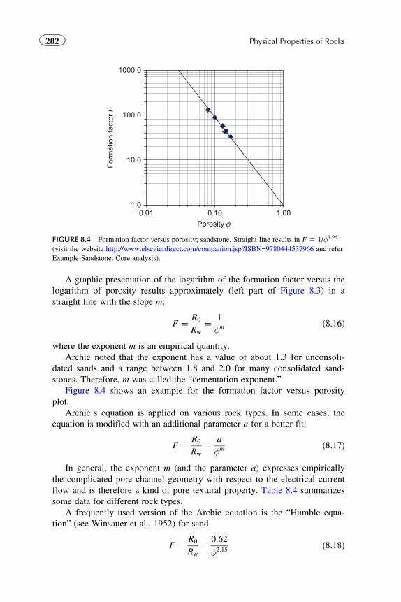
A graphic presentation of the logarithm of the formation factor versus the
logarithm of porosity results approximately (left part of Figure 8.3) in a
straight line with the slope m:
F ¼ R0
Rw
¼ 1
φm ð8:16Þ
where the exponent m is an empirical quantity.
Archie noted that the exponent has a value of about 1.3 for unconsoli-
dated sands and a range between 1.8 and 2.0 for many consolidated sand-
stones. Therefore, m was called the “cementation exponent.”
Figure 8.4 shows an example for the formation factor versus porosity
plot.
Archie’s equation is applied on various rock types. In some cases, the
equation is modified with an additional parameter a for a better fit:
F ¼ R0
Rw
¼ a
φm ð8:17Þ
In general, the exponent m (and the parameter a) expresses empirically
the complicated pore channel geometry with respect to the electrical current
flow and is therefore a kind of pore textural property. Table 8.4 summarizes
some data for different rock types.
A frequently used version of the Archie equation is the “Humble equa-
tion” (see Winsauer et al., 1952) for sand
F ¼ R0
Rw
¼ 0:62
φ2:15ð8:18Þ
1.0
10.0
100.0
1000.0
0.01 0.10 1.00
Porosity φ
For
mat
ion
fact
or F
FIGURE 8.4 Formation factor versus porosity; sandstone. Straight line results in F 5 1/φ1.96
(visit the website http://www.elsevierdirect.com/companion.jsp?ISBN=9780444537966 and refer
Example-Sandstone. Core analysis).
282 Physical Properties of Rocks
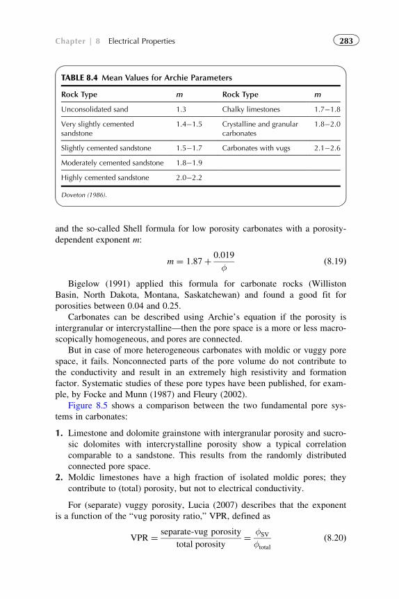
and the so-called Shell formula for low porosity carbonates with a porosity-
dependent exponent m:
m ¼ 1:87þ 0:019
φð8:19Þ
Bigelow (1991) applied this formula for carbonate rocks (Williston
Basin, North Dakota, Montana, Saskatchewan) and found a good fit for
porosities between 0.04 and 0.25.
Carbonates can be described using Archie’s equation if the porosity is
intergranular or intercrystalline—then the pore space is a more or less macro-
scopically homogeneous, and pores are connected.
But in case of more heterogeneous carbonates with moldic or vuggy pore
space, it fails. Nonconnected parts of the pore volume do not contribute to
the conductivity and result in an extremely high resistivity and formation
factor. Systematic studies of these pore types have been published, for exam-
ple, by Focke and Munn (1987) and Fleury (2002).
Figure 8.5 shows a comparison between the two fundamental pore sys-
tems in carbonates:
1. Limestone and dolomite grainstone with intergranular porosity and sucro-
sic dolomites with intercrystalline porosity show a typical correlation
comparable to a sandstone. This results from the randomly distributed
connected pore space.
2. Moldic limestones have a high fraction of isolated moldic pores; they
contribute to (total) porosity, but not to electrical conductivity.
For (separate) vuggy porosity, Lucia (2007) describes that the exponent
is a function of the “vug porosity ratio,” VPR, defined as
VPR ¼ separate-vug porosity
total porosity¼ φSV
φtotal
ð8:20Þ
TABLE 8.4 Mean Values for Archie Parameters
Rock Type m Rock Type m
Unconsolidated sand 1.3 Chalky limestones 1.7�1.8
Very slightly cementedsandstone
1.4�1.5 Crystalline and granularcarbonates
1.8�2.0
Slightly cemented sandstone 1.5�1.7 Carbonates with vugs 2.1�2.6
Moderately cemented sandstone 1.8�1.9
Highly cemented sandstone 2.0�2.2
Doveton (1986).
283Chapter | 8 Electrical Properties
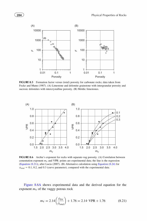
Figure 8.6A shows experimental data and the derived equation for the
exponent mV of the vuggy porous rock
mV ¼ 2:14φSV
φtotal
� �þ 1:76 ¼ 2:14UVPRþ 1:76 ð8:21Þ
0.0
0.2
0.4
0.6
0.8
1.0
(A) (B)
1.5 2.0 2.5 3.0 3.5 4.0mV
VP
R
0.0
0.2
0.4
0.6
0.8
1.0
1.5 2.0 2.5 3.0 3.5 4.0mV
VP
R
0.10.20.3
FIGURE 8.6 Archie’s exponent for rocks with separate-vug porosity. (A) Correlation between
cementation exponent mV and VPR: points are experimental data; the line is the regression
(Equation (8.21)), after Lucia (2007). (B) Alternative calculation using Equation (8.24) for
φtotal 5 0.1, 0.2, and 0.3 (curve parameter), compared with the experimental data.
(A)
1
10
100
1000
10000
0.01 0.1 1Porosity
F
(B)
1
10
100
1000
10000
0.01 0.1 1Porosity
F
FIGURE 8.5 Formation factor versus (total) porosity for carbonate rocks; data taken from
Focke and Munn (1987). (A) Limestone and dolomite grainstone with intergranular porosity and
sucrosic dolomites with intercrystalline porosity. (B) Moldic limestones.
284 Physical Properties of Rocks
An alternative equation can be derived as follows: the connected path for
current flow is controlled by the effective porosity:
φeff ¼ φtotal 2φSV ¼ φtotalð12VPRÞ ð8:22ÞArchie’s equation refers to this connected pore space with the exponent
m only:
F ¼ φ2meff ¼ ½φtotalð12VPRÞ�2m ¼ φ2mV
total ð8:23Þwhere mV is the exponent, if we refer formation factor to total porosity of the
vuggy porous rock. It results as a relationship between the two exponents:
mV ¼ m 1þ logð12VPRÞlog φtotal
� �ð8:24Þ
Figure 8.6B shows a comparison of calculated curves for the assumption
of m 5 2 for the connected porosity and different total porosity of
φtotal 5 0.1, 0.2, and 0.3. Curves cover the experimental data.
Lucia (2007) notes that “in presence of fractures and other touching-vug
pore types, the mV value may be ,1.8.”
Generally, fractured rocks tend to low exponents (m � 1.1�1.3), frequently
connected with a high value of the parameter a in Equation (8.17). Pape et al.
(1985) derived for the fractured Falkenberg Granite the relationship:
F ¼ 4:15
φ1:08 ð8:25Þ
where the porosity is in the range between 0.005 and 0.07 (0.5�7%).
Lovell and Pezard (1990) investigated basalt cores from the Deep Sea
Drilling Program (DSDP) hole 504B and found a 5 6.2 and m 5 1.05 for
fractured samples.
Unconsolidated rocks show exponents m in the order between 1.1 and 1.4
(Figure 8.7). There is a tendency of decrease with increasing sphericity of
the grains (Jackson et al., 1978; Schon, 1996).
If in a porous rock water saturation decreases, then a part of the conduc-
tive pore water is replaced by the nonconductive fluid (gas, air, oil), and
rock resistivity increases. To describe the saturation effect, Archie normal-
ized the resistivity, measured at any saturation Rt with the resistivity of the
total water-saturated rock R0 and defined as resistivity index:
IR ¼ Rt
R0
ð8:26Þ
A logarithmic plot IR versus Sw results approximately again in a straight
line (Figure 8.3 and Figure 8.8) with the slope n:
IR ¼ Rt
R0
¼ 1
Snwð8:27Þ
285Chapter | 8 Electrical Properties
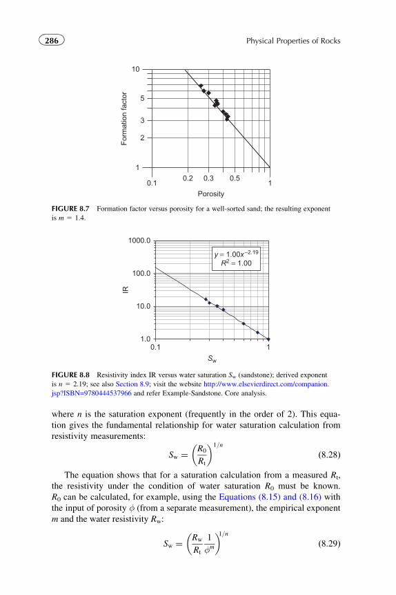
where n is the saturation exponent (frequently in the order of 2). This equa-
tion gives the fundamental relationship for water saturation calculation from
resistivity measurements:
Sw ¼ R0
Rt
� �1=n
ð8:28Þ
The equation shows that for a saturation calculation from a measured Rt,
the resistivity under the condition of water saturation R0 must be known.
R0 can be calculated, for example, using the Equations (8.15) and (8.16) with
the input of porosity φ (from a separate measurement), the empirical exponent
m and the water resistivity Rw:
Sw ¼ Rw
Rt
1
φm
� �1=nð8:29Þ
y = 1.00x−2.19
R2 = 1.00
1.0
10.0
100.0
1000.0
0.1 1
Sw
IR
FIGURE 8.8 Resistivity index IR versus water saturation Sw (sandstone); derived exponent
is n 5 2.19; see also Section 8.9; visit the website http://www.elsevierdirect.com/companion.
jsp?ISBN=9780444537966 and refer Example-Sandstone. Core analysis.
0.1 10.2 0.3 0.5
Porosity
1
10
2
3
5
For
mat
ion
fact
or
FIGURE 8.7 Formation factor versus porosity for a well-sorted sand; the resulting exponent
is m 5 1.4.
286 Physical Properties of Rocks
Techniques and methods are described in textbooks of formation evalua-
tion and well-log interpretation.
Both exponents m and n express the geometry of the only conductor
(brine) in the porous rock and refer to the geometry of the two insulators
(mineral grain, hydrocarbon). When m 5 n, the two insulators (mineral,
hydrocarbon) are interchangeable in terms of rock resistivity.
The saturation exponent n must be determined experimentally in core lab-
oratories. It is controlled by the distribution of the conducting brine in the
pore space, thus depending on the rock texture, wetting properties, and “satu-
ration history” caused by capillary effects.
In water-wet rocks, water adheres to grain surfaces and builds up a more
or less continuous phase in the rock. In oil-wet rocks, the nonconducting oil
becomes the continuous fluid phase, and the water occurs mostly as isolated
droplets. In this case, the resistivity is much higher and the saturation expo-
nent n . 2. A discussion of wettability influences on electrical properties is
given by Anderson (1986) and Sharma et al. (1991).
Different saturating techniques (imbibition, drainage) and techniques of
core preparation also affect the laboratory-determined saturation exponent
(see, for example, de Waal et al., 1989; Sharma et al., 1991; Worthington
and Pallatt, 1990; Worthington et al., 1989). The application of X-ray and
resistivity tomography allows a monitoring of the homogeneous saturation
process along the core axis.
In some cases, the resistivity index versus saturation curve is nonlinear
on a log�log plot. This phenomenon seems to be related to a bimodal (or
multimodal) pore-size distribution, to the presence of microporosity or from
rough grain surface coatings (de Waal et al., 1989; Worthington et al.,
1989). Worthington and Pallatt (1990) investigated the influence of pore
geometry upon the character of the saturation index versus saturation curve
and the behavior of n.
In carbonates, the heterogeneity of the pore space again results in more
complicated plots IR versus Sw for the saturation exponent. Ellis and Singer
(2007) note: “Carbonates are particularly heterogeneous, and are also more
likely to be oil-wet, so that for both reasons the relation between resistivity
and Sw is likely to be complicated, with n not equal to 2 and also varying
with saturation.” For log interpretation of carbonates, Fleury (2002) devel-
oped a double or triple porosity model for micritic and oolithic carbonate.
8.3.3 Pressure Dependence of Formation Factor
If water-filled and conducting pore channels are deformed by external pres-
sure on the rock skeleton, then the porosity decreases, the rock resistivity
increases, and the formation factor increases.
Palmer and Pallatt (1991) analyzed the formation factor versus pressure
relationship for sandstone samples from the North Sea and Alaskan
287Chapter | 8 Electrical Properties

reservoirs. The results show a nonlinear dependency (Figure 8.9A). They fit-
ted the experimental data with an equation relating the actual formation fac-
tor F(p) normalized by its value F400 at a pressure of 400 psi versus the
logarithm of pressure p and found:
FðpÞ ¼ F400ð0:621þ 0:143Ulog pÞ ð8:30ÞFigure 8.9B demonstrates an alternative fit using a power law. A biloga-
rithmic plot F versus p results in a first approximation to a straight line with
the regression:
F ¼ 16:6Up0:055 ð8:31Þor generalized
FðpÞ ¼ Fp¼1
p
p ¼ 1
� �b
ð8:32Þ
where Fp51 is the formation factor at a pressure p 5 1. The exponent b is
the slope of the straight line.
Archer and Jing (1991) investigated both clean and shaly sedimentary
rocks. They found a similar nonlinear relationship between formation factor
and pressure, as well as a noticeable hysteresis effect occurring between the
loading and unloading cycles. This is a result of nonelastic deformation of
the rock skeleton.
8.4 CLEAN ROCKS—THEORIES AND MODELS
8.4.1 Introduction
The electrical conductivity as a tensor depends not only on the volume frac-
tions and the electrical conductivity of rock components, but also on their
0 10 20 30 40
Pressure in MPa
16
17
18
19
20
21
(A) (B)F
1 10 100
Pressure in MPa
10
20
30
FFIGURE 8.9 Formation factor versus overburden pressure dependence. (A) Linear plot, data
after Palmer and Pallatt (1991) (pressure converted from psi in MPa). (B) Fitting by a power law
using a bilogarithmic plot.
288 Physical Properties of Rocks
distribution, geometry, and internal structure. For practical applications, the
empirical Archie equations are dominant.
For a model-based description, the following rock types are relevant:
� Clean rocks, where only the water/brine in the pores or fractures conducts
the electrical current; the matrix material is an insulator.� Porous rocks with a “matrix porosity” and any second porosity type like
fractures or moldic pores in carbonates; this creates a “dual porosity”
system.� Shaly rocks where in addition to the electrolytic conductivity of the con-
nected pores, a second conductivity component (shale conductivity,
excess conductivity or interface conductivity) exists.
The following section is based on the first and second types; shaly rocks
are featured separately in a special Section 8.5.
8.4.2 Layer Models
Layer models resolve a rock as a laminated material with layers of different
conductivity. Layer thickness represents the volume fraction of the
component.
For a current parallel layering (parallel model), results are
the conductivity C8 ¼Xi
ViUCi and the resistivity R8 ¼Xi
ViUR2 1i
!21
ð8:33ÞFor a current perpendicular layering (serial model), results are
the conductivity C> ¼Xi
ViUC2 1i
!21
and the resistivity R> ¼Xi
ViURi
ð8:34Þwhere
Vi is the volume fraction of component i
Ci is the conductivity of component i
Ri is the specific resistivity of component i.
Layer models in case of water-saturated clean porous rocks with one
component (mineral) of zero conductivity result for
� parallel layering in C8 5 φ �Cw or R8 5 φ21 �Rw with a formation factor
F8 5 φ21
� perpendicular layering in C>5 0 or R>5N with a formation factor
F>5N.
289Chapter | 8 Electrical Properties
Thus, this type is not of a practical relevance to model a real homoge-
neous clean porous rock in terms of electrical conductivity.
A generalization following Lichtenecker and Rother (1931) (see also
Section 6.7.1) can be written as
C ¼Xi
ViUCαi
!1α
ð8:35Þ
This equation represents a summary of several individual equations with
the exponent α as a “textural parameter”; for example results
� the parallel model for α 5 1,� the serial model for α 5 21.
For the special case of a water-saturated clean rock (Archie type), the
conductivity is
C0 ¼ φUCαw
� �1α ð8:36Þ
or written as formation factor
F ¼ Cw
C0
¼ φ2 1α ð8:37Þ
Thus, Archie’s “cementation exponent” results as m 5 1/α. The fre-
quently used mean value of m 5 2 results in α 5 0.5.
Layer models for laminated shaly rocks have a specific importance (see
Section 8.5.2).
8.4.3 Inclusion Models—Spheres
A systematic description and discussion of various mixture theories for rock
properties is given by Berryman (1995). Berryman (1995) and Mavko et al.
(1998), for example, can be used as reference for theoretical concepts and
models (self-consistent effective medium theory, differential effective
medium approach). All inclusion models assume a host material with a low
concentration of inclusions. Inclusions are of different shape.
For a two-component composite with spherical inclusions in a host mate-
rial, the so-called Clausius�Mossotti model (see Berryman, 1995) results in
CCM 2C2
CCM þ 2UC2
¼ V1
C1 2C2
C1 þ 2UC2
ð8:38Þ
where
CCM is the conductivity of the composite (Clausius�Mossotti model)
C1 is the conductivity of the inclusion material
C2 is the conductivity of the host material
V1 is the volume fraction of the inclusions.
290 Physical Properties of Rocks
The application on a rock of Archie type with a nonconducting inclusion
representing a mineral grain (C1 5 Cma 5 0) with low concentration of
grains in the conductive host (water) V1 5 12φ results in
CCM 2Cw
CCM þ 2UCw
¼ 12φ2
ð8:39Þ
with the solution
CCM ¼ Cw
2Uφ32φ
ð8:40Þ
Thus, the formation resistivity factor is
F ¼ 32φ2Uφ
ð8:41Þ
This represents materials like a suspension. A porous rock consisting of
insulating matrix substance as host material and fluid as spherical pore inclu-
sion (“Swiss Cheese Model”) results in CCM 5 0 because inclusions are non-
connected. Such a model only works for a host material with conductivity
(see next section).
8.4.4 Nonspherical Inclusions
The generalization of the inclusion shape from a sphere to an ellipsoid cre-
ates different properties of the composite with respect to the field direction
related to the ellipsoid axis system. Therefore, a single ellipsoid or a set of
ellipsoids with identical or preferred orientation originates an anisotropy
effect. If the inclusions are randomly oriented, then isotropy results.
In this section these two cases are discussed. An application presupposes
a conductivity of the host material (matrix porosity or matrix conductivity).
Carbonates in particular frequently have different pore systems. Inclusion
models can describe, for example, the effect of spherical (moldic) or elon-
gated (fractures) inclusions in a host material with interparticle porosity. For
geometric characterization of the ellipsoidic shape, the aspect ratio (see
Figure 6.25) is used. Cheng and Toksoz (1979) report aspect ratios for carbo-
nates in the range α 5 1022�1024.
8.4.4.1 Oriented Ellipsoidic Inclusions
Bruggeman (1935) and Hanai (1960) derived general relationships for the cal-
culation of the properties for heterogeneous mixtures. The Hanai�Bruggeman
equation for conductivity is (see Berryman, 1995)
CHB 2Cma
Cw 2Cma
Cw
CHB
� �L
¼ φ ð8:42Þ
291Chapter | 8 Electrical Properties
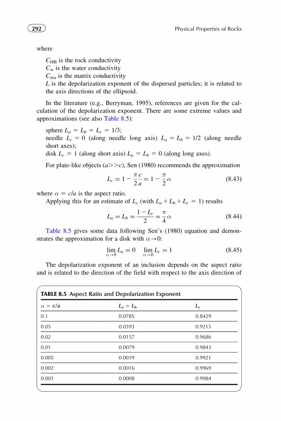
where
CHB is the rock conductivity
Cw is the water conductivity
Cma is the matrix conductivity
L is the depolarization exponent of the dispersed particles; it is related to
the axis directions of the ellipsoid.
In the literature (e.g., Berryman, 1995), references are given for the cal-
culation of the depolarization exponent. There are some extreme values and
approximations (see also Table 8.5):
sphere La 5 Lb 5 Lc 5 1/3;
needle Lc 5 0 (along needle long axis) La 5 Lb 5 1/2 (along needle
short axes);
disk Lc 5 1 (along short axis) La 5 Lb 5 0 (along long axes).
For plate-like objects (a..c), Sen (1980) recommends the approximation
Lc ¼ 12π2
c
a¼ 12
π2α ð8:43Þ
where α 5 c/a is the aspect ratio.
Applying this for an estimate of Lc (with La1 Lb1 Lc 5 1) results
La ¼ Lb ¼12 Lc
2¼ π
4α ð8:44Þ
Table 8.5 gives some data following Sen’s (1980) equation and demon-
strates the approximation for a disk with α-0:
limα-0
La ¼ 0 limα-0
Lc ¼ 1 ð8:45Þ
The depolarization exponent of an inclusion depends on the aspect ratio
and is related to the direction of the field with respect to the axis direction of
TABLE 8.5 Aspect Ratio and Depolarization Exponent
α 5 c/a La 5 Lb Lc
0.1 0.0785 0.8429
0.05 0.0393 0.9215
0.02 0.0157 0.9686
0.01 0.0079 0.9843
0.005 0.0039 0.9921
0.002 0.0016 0.9969
0.001 0.0008 0.9984
292 Physical Properties of Rocks
the ellipsoid. Therefore, different depolarization factors for different direc-
tions lead to anisotropy of conductivity.
This can be applied, for example, on carbonate rocks with a matrix porosity
φma and fracture porosity φfr. If fractures have a preferred orientation, conduc-
tivity is a tensor. The tensor simplifies in the event that the axes of the ellipsoid
coincide with the axes of the Cartesian coordinate system. For generalization,
this tensor can be transformed into any orientation (Moran and Gianzero, 1979).
For a penny-shaped fracture (oblate) with long ellipsoid axes a,b parallel
x-,y-axis and a short axis c{a 5 b parallel z-axis the ellipsoid axes a2b2c
coincide with the coordinate system x2y2z (main-axis system). Then
conductivity components are the solutions of the following equations:
Cx ¼ Cy ðx- and y-directionÞ: Cfl;fr 2Cx
Cfl;fr 2Cma
� �Cma
Cx
� �La¼ 12φfr ð8:46Þ
Cz ðz-directionÞ:Cfl;fr 2Cz
Cfl;fr 2Cma
� �Cma
Cz
� �Lc¼ 12φfr ð8:47Þ
where
φfr is the fracture porosity
Cfl,fr is the conductivity of the fluid in the fracture
Cma ¼ CwUφmmaUS
nw;ma is the matrix conductivity.
The two equations demonstrate the key function of the depolarization
exponent: its dependence on orientation creates the anisotropy.
For graphic presentation, a normalization of the conductivities by matrix
conductivity is comfortable:
x- and y-direction:
Cfl;fr
Cma
2Cx
Cma
Cfl;fr
Cma
2 1
0BB@
1CCA Cma
Cx
� �La¼ 12φfr ð8:48Þ
z-direction:
Cfl;fr
Cma
2Cz
Cma
Cfl;fr
Cma
2 1
0BB@
1CCA Cma
Cz
� �Lc¼ 12φfr ð8:49Þ
Figure 8.10 shows an example. Fractures are oriented in the x�y plane
and are water filled (Cfl,fr 5 Cw). Two different aspect ratios are assumed:
α 5 0.10—this corresponds to the depolarization exponents La 5Lb 5 0.079, Lc 5 0.843.
α 5 0.01—this corresponds to the depolarization exponents La 5Lb 5 0.008, Lc 5 0.984.
293Chapter | 8 Electrical Properties
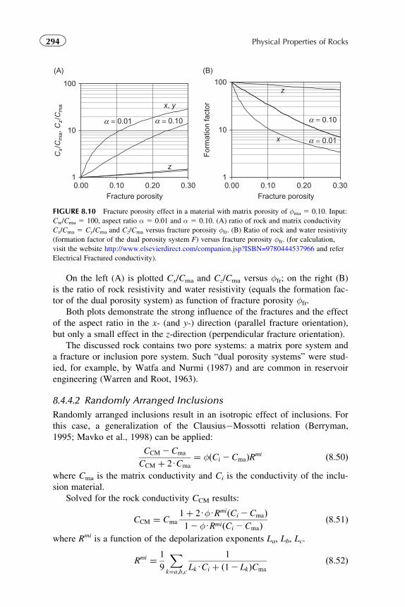
On the left (A) is plotted Cx/Cma and Cz/Cma versus φfr; on the right (B)
is the ratio of rock resistivity and water resistivity (equals the formation fac-
tor of the dual porosity system) as function of fracture porosity φfr.
Both plots demonstrate the strong influence of the fractures and the effect
of the aspect ratio in the x- (and y-) direction (parallel fracture orientation),
but only a small effect in the z-direction (perpendicular fracture orientation).
The discussed rock contains two pore systems: a matrix pore system and
a fracture or inclusion pore system. Such “dual porosity systems” were stud-
ied, for example, by Watfa and Nurmi (1987) and are common in reservoir
engineering (Warren and Root, 1963).
8.4.4.2 Randomly Arranged Inclusions
Randomly arranged inclusions result in an isotropic effect of inclusions. For
this case, a generalization of the Clausius�Mossotti relation (Berryman,
1995; Mavko et al., 1998) can be applied:
CCM 2Cma
CCM þ 2UCma
¼ φðCi 2CmaÞRmi ð8:50Þwhere Cma is the matrix conductivity and Ci is the conductivity of the inclu-
sion material.
Solved for the rock conductivity CCM results:
CCM ¼ Cma
1þ 2UφURmiðCi 2CmaÞ12φURmiðCi 2CmaÞ
ð8:51Þwhere Rmi is a function of the depolarization exponents La, Lb, Lc.
Rmi ¼ 1
9
Xk¼a;b;c
1
LkUCi þ ð12 LkÞCma
ð8:52Þ
1
10
100
(A) (B)
0.00 0.10 0.20 0.30Fracture porosity
1
10
100
0.00 0.10 0.20 0.30Fracture porosity
Cx/C
ma,
Cz/C
ma x, y
z
= 0.01 = 0.10
For
mat
ion
fact
or
x
z
α = 0.10αα
= 0.01α
FIGURE 8.10 Fracture porosity effect in a material with matrix porosity of φma 5 0.10. Input:
Cw/Cma 5 100, aspect ratio α 5 0.01 and α 5 0.10. (A) ratio of rock and matrix conductivity
Cx/Cma 5 Cy/Cma and Cz/Cma versus fracture porosity φfr. (B) Ratio of rock and water resistivity
(formation factor of the dual porosity system F) versus fracture porosity φfr. (for calculation,
visit the website http://www.elsevierdirect.com/companion.jsp?ISBN=9780444537966 and refer
Electrical Fractured conductivity).
294 Physical Properties of Rocks
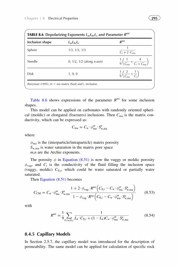
Table 8.6 shows expressions of the parameter Rmi for some inclusion
shapes.
This model can be applied on carbonates with randomly oriented spheri-
cal (moldic) or elongated (fractures) inclusions. Then Cma is the matrix con-
ductivity, which can be expressed as:
Cma ¼ CwUφmmaUS
nw;ma
where
φma is the (interparticle/intraparticle) matrix porosity
Sw,ma is water saturation in the matrix pore space
m,n are the Archie exponents.
The porosity φ in Equation (8.51) is now the vuggy or moldic porosity
φvug, and Ci is the conductivity of the fluid filling the inclusion space
(vuggy, moldic) Cfl,i, which could be water saturated or partially water
saturated.
Then Equation (8.51) becomes
CCM ¼ CwUφmmaUS
nw;ma
1þ 2UφvugURmi Cfl;i 2CwUφm
maUSnw;ma
� 12φvugURmi Cfl;i 2CwUφm
maUSnw;ma
� ð8:53Þ
with
Rmi ¼ 1
9
Xk¼a;b;c
1
LkUCfl;i þ ð12 LkÞCwUφmmaUS
nw;ma
ð8:54Þ
8.4.5 Capillary Models
In Section 2.5.7, the capillary model was introduced for the description of
permeability. The same model can be applied for calculation of specific rock
TABLE 8.6 Depolarizing Exponents La,Lb,Lc and Parameter Rmi
Inclusion shape La,Lb,Lc Rmi
Sphere 1/3, 1/3, 1/31
Ci þ 2UCma
Needle 0, 1/2, 1/2 (along x-axis)1
9
1
Cmaþ 4
Ci þ Cma
� �
Disk 1, 0, 01
9
2
Cmaþ 1
Ci
� �
Berryman (1995); m 5 ma matrix (host) and i, inclusion.
295Chapter | 8 Electrical Properties
resistivity and formation factor. Assuming an electrical current flow in direc-
tion of the capillary with the symbols of Figure 2.24 results:
R0UL
L2¼ Rw
l
πUr2ð8:55Þ
Implementing tortuosity (Equation (2.44)) and porosity (Equation (2.45))
gives the specific electrical resistivity of the water-saturated rock model:
R0 ¼ Rw
T
φð8:56Þ
and the formation resistivity factor is
F ¼ T
φð8:57Þ
Thus, the simple model:
� cannot explain the order of the cementation exponent for real rocks
(B2);� demonstrates the problem of any correlation between hydraulic and electri-
cal conductivity: the hydraulic conductivity or permeability also depends
on the pore (throat) radius, but the electrical conductivity depends only on
the summarized conductive cross sections (expressed by porosity).
A sphere-based capillary model was used by Spangenberg (2001) in order
to model the influence of gas hydrate content on the electrical properties of
porous sediments.
8.5 SHALY ROCKS, SHALY SANDS
“The abnormal conductivity found in shaly reservoir rocks containing an electrolyte is
shown to be a consequence of the electrical double layer in the solution adjacent to
charged clay surfaces. This increased conductivity results from a higher concentration
of ions in the double layer than in the solution in equilibrium with the double layer.”
Winsauer and McCardell (1953)
8.5.1 Introduction: The Shaly Sand Problem
Presence of shale in a reservoir:
� decreases the reservoir quality (porosity, permeability);� creates an additional electrical conductivity component—any formal
application of Archie’s equation results in an overestimate of water
saturation.
296 Physical Properties of Rocks
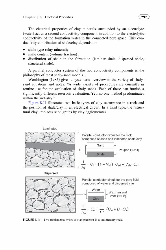
The electrical properties of clay minerals surrounded by an electrolyte
(water) act as a second conductivity component in addition to the electrolytic
conductivity of the formation water in the connected pore space. This con-
ductivity contribution of shale/clay depends on:
� shale type (clay mineral);� shale content (volume fraction) ;� distribution of shale in the formation (laminar shale, dispersed shale,
structural shale).
A parallel conductor system of the two conductivity components is the
philosophy of most shaly-sand models.
Worthington (1985) gives a systematic overview to the variety of shaly-
sand equations and notes: “A wide variety of procedures are currently in
routine use for the evaluation of shaly sands. Each of these can furnish a
significantly different reservoir evaluation. Yet, no one method predominates
within the industry.”
Figure 8.11 illustrates two basic types of clay occurrence in a rock and
the position of shale/clay in an electrical circuit. In a third type, the “struc-
tural clay” replaces sand grains by clay agglomerates.
Parallel conductor circuit for the rockcomposed of sand and laminated shale/clay
Parallel conductor circuit for the pore fluidcomposed of water and dispersed clay
Sand
Shale
Water
Clay
Poupon (1954)
Waxman andSmits (1968)
Laminated
Dispersed
Rt= Ct = (1 − Vsh) Csd + Vsh ⋅ Csh
1
Ro= Co =1
F*1 (Cw + B ⋅ Qv)
FIGURE 8.11 Two fundamental types of clay presence in a sedimentary rock.
297Chapter | 8 Electrical Properties
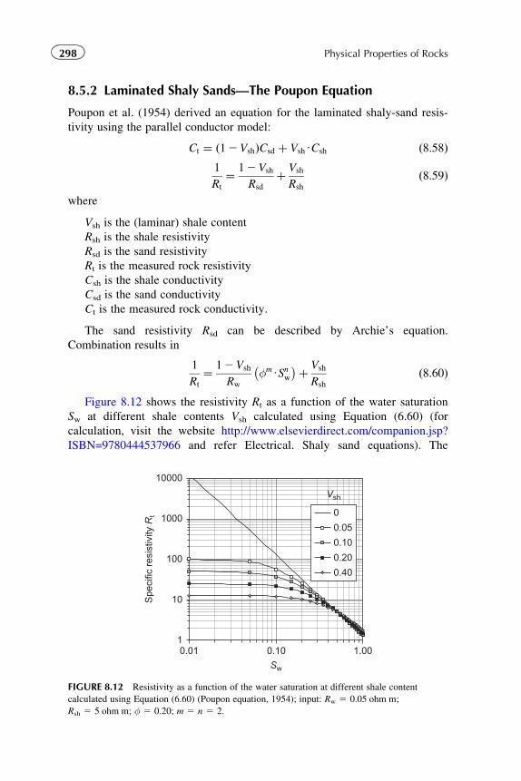
8.5.2 Laminated Shaly Sands—The Poupon Equation
Poupon et al. (1954) derived an equation for the laminated shaly-sand resis-
tivity using the parallel conductor model:
Ct ¼ ð12VshÞCsd þ VshUCsh ð8:58Þ1
Rt
¼ 12Vsh
Rsd
þ Vsh
Rsh
ð8:59Þ
where
Vsh is the (laminar) shale content
Rsh is the shale resistivity
Rsd is the sand resistivity
Rt is the measured rock resistivity
Csh is the shale conductivity
Csd is the sand conductivity
Ct is the measured rock conductivity.
The sand resistivity Rsd can be described by Archie’s equation.
Combination results in
1
Rt
¼ 12Vsh
Rw
φmUSnw� �þ Vsh
Rsh
ð8:60Þ
Figure 8.12 shows the resistivity Rt as a function of the water saturation
Sw at different shale contents Vsh calculated using Equation (6.60) (for
calculation, visit the website http://www.elsevierdirect.com/companion.jsp?
ISBN=9780444537966 and refer Electrical. Shaly sand equations). The
1
10
100
1000
10000
0.01 0.10 1.00
Sw
Spe
cific
res
istiv
ity R
t 0
0.05
0.10
0.20
0.40
Vsh
FIGURE 8.12 Resistivity as a function of the water saturation at different shale content
calculated using Equation (6.60) (Poupon equation, 1954); input: Rw 5 0.05 ohm m;
Rsh 5 5 ohm m; φ 5 0.20; m 5 n 5 2.
298 Physical Properties of Rocks
Excel spreadsheet allows the calculation for variable input parameters and an
application for a fast determination of the water saturation from Rt.
The water saturation results as:
Sw ¼ Rw
1
Rt
2Vsh
Rsh
� �1
φm
1
12Vsh
� �1=nð8:61Þ
For a saturation calculation, the following inputs are necessary:
� The rock resistivity Rt from a resistivity measurement� The shale resistivity Rsh (mostly used is the resistivity of an adjacent
shale bed)� The shale content Vsh (e.g., from a gammalog)� Further for the Archie equation, water resistivity Rw and Archie expo-
nents m,n� . . . and the knowledge: the shale is laminated!
The parallel conductor model assumes a current direction parallel to the
plane of lamination. A promotion of this model for current direction parallel
and perpendicular to the plane of lamination is applied on the interpretation
of measurements with orthogonal induction systems (Section 8.6).
8.5.3 Dispersed Shaly Sand—The Waxman�Smits Equation
In case of dispersed shale, the “shale conductivity” must be added to the
pore fluid conductivity. With this idea, Waxman and Smits (1967, 1968)
developed the dispersed shaly-sand model. They implemented the fundamen-
tal mechanisms of the “shale conductivity” based on cation-exchange pro-
cesses at the clay mineral�electrolyte (water) interface.
For the simplest case of a water-saturated shaly sand, the conductivity is
C0 ¼1
F� ðCw þ BUQvÞ ð8:62Þ
The Waxman�Smits equation uses the following specific terminology:
C0 is the conductivity of the shaly sand (C0 ¼ R2 10 ), if water saturated
Ct is the conductivity of the shaly sand (Ct ¼ R2 1t )
Cw is the conductivity of the formation water (Cw ¼ R2 1w )
φ is porosity
Sw is water saturation
F* is the formation factor of the shaly sand
m,n are Archie exponents
B is the equivalent conductivity of sodium clay-exchange cations (in
S cm2 meq21)
CEC is the cation-exchange capacity (in meq g21)
Qv is the shalyness factor (CEC per unit volume in meq cm23).
299Chapter | 8 Electrical Properties
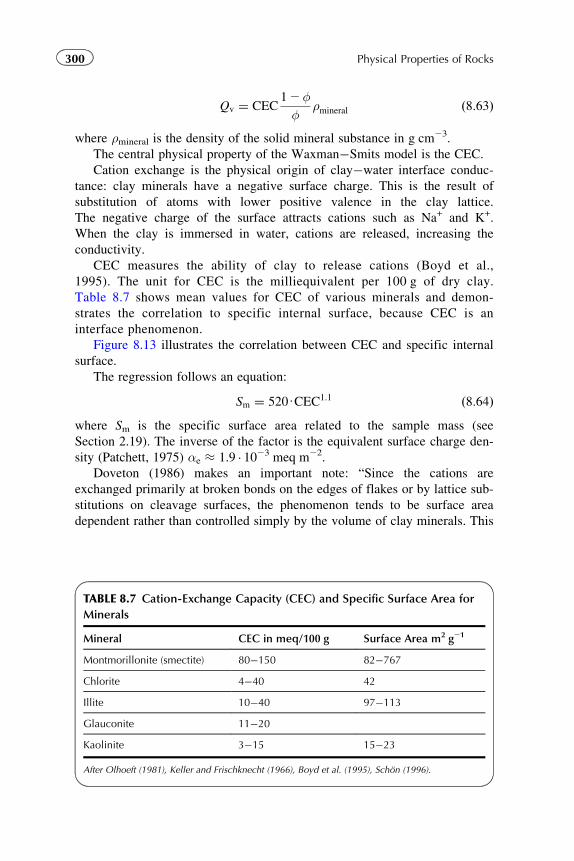
Qv ¼ CEC12φφ
ρmineral ð8:63Þ
where ρmineral is the density of the solid mineral substance in g cm23.
The central physical property of the Waxman�Smits model is the CEC.
Cation exchange is the physical origin of clay�water interface conduc-
tance: clay minerals have a negative surface charge. This is the result of
substitution of atoms with lower positive valence in the clay lattice.
The negative charge of the surface attracts cations such as Na+ and K+.
When the clay is immersed in water, cations are released, increasing the
conductivity.
CEC measures the ability of clay to release cations (Boyd et al.,
1995). The unit for CEC is the milliequivalent per 100 g of dry clay.
Table 8.7 shows mean values for CEC of various minerals and demon-
strates the correlation to specific internal surface, because CEC is an
interface phenomenon.
Figure 8.13 illustrates the correlation between CEC and specific internal
surface.
The regression follows an equation:
Sm ¼ 520UCEC1:1 ð8:64Þwhere Sm is the specific surface area related to the sample mass (see
Section 2.19). The inverse of the factor is the equivalent surface charge den-
sity (Patchett, 1975) αe � 1.9 � 1023 meq m22.
Doveton (1986) makes an important note: “Since the cations are
exchanged primarily at broken bonds on the edges of flakes or by lattice sub-
stitutions on cleavage surfaces, the phenomenon tends to be surface area
dependent rather than controlled simply by the volume of clay minerals. This
TABLE 8.7 Cation-Exchange Capacity (CEC) and Specific Surface Area for
Minerals
Mineral CEC in meq/100 g Surface Area m2 g21
Montmorillonite (smectite) 80�150 82�767
Chlorite 4�40 42
Illite 10�40 97�113
Glauconite 11�20
Kaolinite 3�15 15�23
After Olhoeft (1981), Keller and Frischknecht (1966), Boyd et al. (1995), Schon (1996).
300 Physical Properties of Rocks
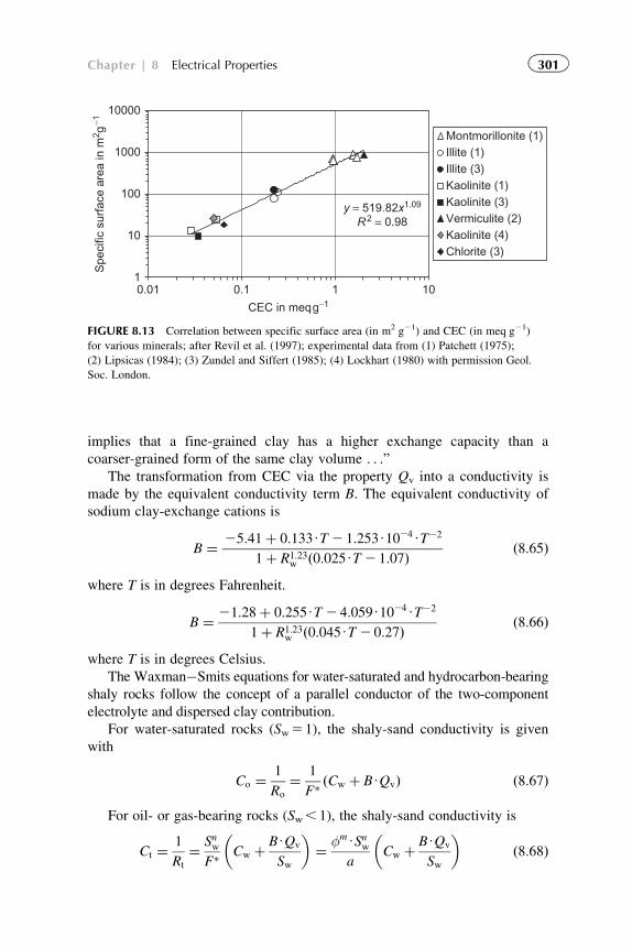
implies that a fine-grained clay has a higher exchange capacity than a
coarser-grained form of the same clay volume . . .”The transformation from CEC via the property Qv into a conductivity is
made by the equivalent conductivity term B. The equivalent conductivity of
sodium clay-exchange cations is
B ¼ 25:41þ 0:133UT 2 1:253U1024UT22
1þ R1:23w ð0:025UT 2 1:07Þ ð8:65Þ
where T is in degrees Fahrenheit.
B ¼ 21:28þ 0:255UT 2 4:059U1024UT22
1þ R1:23w ð0:045UT 2 0:27Þ ð8:66Þ
where T is in degrees Celsius.
The Waxman�Smits equations for water-saturated and hydrocarbon-bearing
shaly rocks follow the concept of a parallel conductor of the two-component
electrolyte and dispersed clay contribution.
For water-saturated rocks (Sw51), the shaly-sand conductivity is given
with
Co ¼1
Ro
¼ 1
F� ðCw þ BUQvÞ ð8:67Þ
For oil- or gas-bearing rocks (Sw, 1), the shaly-sand conductivity is
Ct ¼1
Rt
¼ SnwF� Cw þ BUQv
Sw
� �¼ φmUSnw
aCw þ BUQv
Sw
� �ð8:68Þ
y = 519.82x1.09
R2 = 0.98
1
10
100
1000
10000
0.01 0.1 1 10
CEC in meqg−1
Spe
cific
sur
face
are
a in
m2 g
−1
Montmorillonite (1)Illite (1)Illite (3)Kaolinite (1)Kaolinite (3)Vermiculite (2)Kaolinite (4)Chlorite (3)
FIGURE 8.13 Correlation between specific surface area (in m2 g21) and CEC (in meq g21)
for various minerals; after Revil et al. (1997); experimental data from (1) Patchett (1975);
(2) Lipsicas (1984); (3) Zundel and Siffert (1985); (4) Lockhart (1980) with permission Geol.
Soc. London.
301Chapter | 8 Electrical Properties
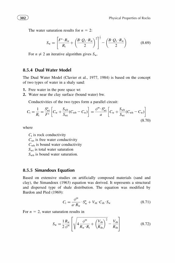
The water saturation results for n 5 2:
Sw ¼ F�URw
Rt
þ BUQvURw
2
� �2" #1
2
2BUQvURw
2
� �ð8:69Þ
For n 6¼ 2 an iterative algorithm gives Sw.
8.5.4 Dual Water Model
The Dual Water Model (Clavier et al., 1977, 1984) is based on the concept
of two types of water in a shaly sand:
1. Free water in the pore space wt
2. Water near the clay surface (bound water) bw.
Conductivities of the two types form a parallel circuit:
Ct ¼1
Rt
¼ SnwtF� Cw þ Swb
SwtðCwb 2CwÞ
� �¼ φmUSnwt
aCw þ Swb
SwtðCwb 2CwÞ
� �ð8:70Þ
where
Ct is rock conductivity
Cwt is free water conductivity
Cwb is bound water conductivity
Swt is total water saturation
Swb is bound water saturation.
8.5.5 Simandoux Equation
Based on extensive studies on artificially composed materials (sand and
clay), the Simandoux (1963) equation was derived. It represents a structural
and dispersed type of shale distribution. The equation was modified by
Bardon and Pied (1969):
Ct ¼φm
aURw
USnw þ VshUCshUSw ð8:71Þ
For n 5 2, water saturation results in
Sw ¼ 1
2
Rw
φm
ffiffiffiffiffiffiffiffiffiffiffiffiffiffiffiffiffiffiffiffiffiffiffiffiffiffiffiffiffiffiffiffiffiffiffiffiffi4
φm
RwURt
þ Vsh
Rsh
� �2s
2Vsh
Rsh
24
35 ð8:72Þ
302 Physical Properties of Rocks
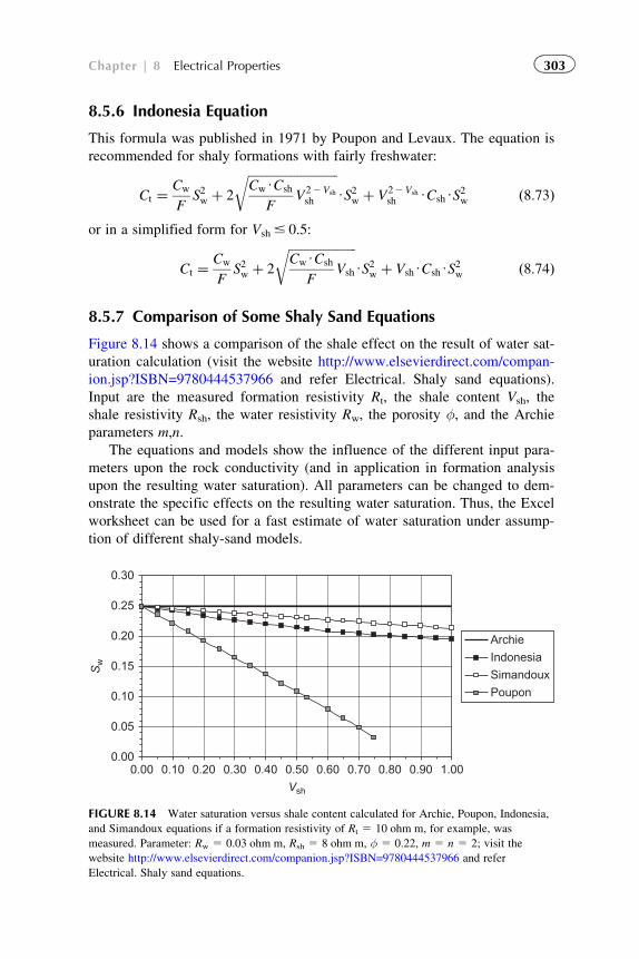
8.5.6 Indonesia Equation
This formula was published in 1971 by Poupon and Levaux. The equation is
recommended for shaly formations with fairly freshwater:
Ct ¼ Cw
FS2w þ 2
ffiffiffiffiffiffiffiffiffiffiffiffiffiffiffiffiffiffiffiffiffiffiffiffiffiffiffiffiffiCwUCsh
FV22Vsh
sh
rUS2w þ V22Vsh
sh UCshUS2w ð8:73Þ
or in a simplified form for Vsh# 0.5:
Ct ¼Cw
FS2w þ 2
ffiffiffiffiffiffiffiffiffiffiffiffiffiffiffiffiffiffiffiffiffiffiCwUCsh
FVsh
rUS2w þ VshUCshUS2w ð8:74Þ
8.5.7 Comparison of Some Shaly Sand Equations
Figure 8.14 shows a comparison of the shale effect on the result of water sat-
uration calculation (visit the website http://www.elsevierdirect.com/compan-
ion.jsp?ISBN=9780444537966 and refer Electrical. Shaly sand equations).
Input are the measured formation resistivity Rt, the shale content Vsh, the
shale resistivity Rsh, the water resistivity Rw, the porosity φ, and the Archie
parameters m,n.
The equations and models show the influence of the different input para-
meters upon the rock conductivity (and in application in formation analysis
upon the resulting water saturation). All parameters can be changed to dem-
onstrate the specific effects on the resulting water saturation. Thus, the Excel
worksheet can be used for a fast estimate of water saturation under assump-
tion of different shaly-sand models.
0.00
0.05
0.10
0.15
0.20
0.25
0.30
0.00 0.10 0.20 0.30 0.40 0.50 0.60 0.70 0.80 0.90 1.00
Vsh
Sw
Archie
Indonesia
Simandoux
Poupon
FIGURE 8.14 Water saturation versus shale content calculated for Archie, Poupon, Indonesia,
and Simandoux equations if a formation resistivity of Rt 5 10 ohm m, for example, was
measured. Parameter: Rw 5 0.03 ohm m, Rsh 5 8 ohm m, φ 5 0.22, m 5 n 5 2; visit the
website http://www.elsevierdirect.com/companion.jsp?ISBN=9780444537966 and refer
Electrical. Shaly sand equations.
303Chapter | 8 Electrical Properties
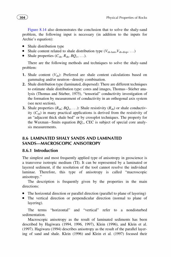
Figure 8.14 also demonstrates the conclusion that to solve the shaly-sand
problem, the following input is necessary (in addition to the inputs for
Archie’s equation):
� Shale distribution type� Shale content related to shale distribution type (Vsh-lam,Vsh-disp, . . .)� Shale properties (Csh, Rsh, BQv, . . .).
There are the following methods and techniques to solve the shaly-sand
problem:
1. Shale content (Vsh): Preferred are shale content calculations based on
gammalog and/or neutron�density combination.
2. Shale distribution type (laminated, dispersed): There are different techniques
to estimate shale distribution type: cores and images, Thomas�Stieber ana-
lysis (Thomas and Stieber, 1975), “tensorial” conductivity investigation of
the formation by measurement of conductivity in an orthogonal axis system
(see next section),
3. Shale properties (Rsh; BQv, . . .): Shale resistivity (Rsh) or shale conductiv-
ity (Csh) in many practical applications is derived from the resistivity of
an “adjacent thick shale bed” or by crossplot techniques. The property for
the Waxman�Smits equation BQv, CEC is subject of special core analy-
sis measurements.
8.6 LAMINATED SHALY SANDS AND LAMINATEDSANDS—MACROSCOPIC ANISOTROPY
8.6.1 Introduction
The simplest and most frequently applied type of anisotropy in geoscience is
a transverse isotropic medium (TI). It can be represented by a laminated or
layered sediment, if the resolution of the tool cannot resolve the individual
laminae. Therefore, this type of anisotropy is called “macroscopic
anisotropy.”
The description is frequently given by the properties in the main
directions:
� The horizontal direction or parallel direction (parallel to plane of layering)� The vertical direction or perpendicular direction (normal to plane of
layering).
The terms “horizontal” and “vertical” refer to a nondisturbed
sedimentation.
Macroscopic anisotropy as the result of laminated sediments has been
described by Hagiwara (1994, 1996, 1997), Klein (1996), and Klein et al.
(1997). Hagiwara (1994) describes anisotropy as the result of the parallel layer-
ing of sand and shale. Klein (1996) and Klein et al. (1997) focused their
304 Physical Properties of Rocks
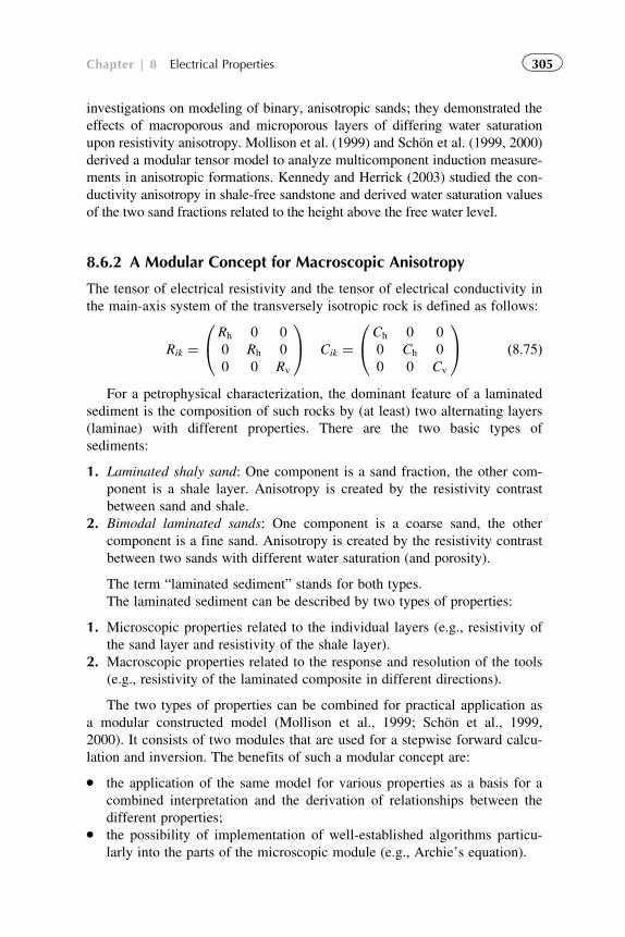
investigations on modeling of binary, anisotropic sands; they demonstrated the
effects of macroporous and microporous layers of differing water saturation
upon resistivity anisotropy. Mollison et al. (1999) and Schon et al. (1999, 2000)
derived a modular tensor model to analyze multicomponent induction measure-
ments in anisotropic formations. Kennedy and Herrick (2003) studied the con-
ductivity anisotropy in shale-free sandstone and derived water saturation values
of the two sand fractions related to the height above the free water level.
8.6.2 A Modular Concept for Macroscopic Anisotropy
The tensor of electrical resistivity and the tensor of electrical conductivity in
the main-axis system of the transversely isotropic rock is defined as follows:
Rik ¼Rh 0 0
0 Rh 0
0 0 Rv
0@
1A Cik ¼
Ch 0 0
0 Ch 0
0 0 Cv
0@
1A ð8:75Þ
For a petrophysical characterization, the dominant feature of a laminated
sediment is the composition of such rocks by (at least) two alternating layers
(laminae) with different properties. There are the two basic types of
sediments:
1. Laminated shaly sand: One component is a sand fraction, the other com-
ponent is a shale layer. Anisotropy is created by the resistivity contrast
between sand and shale.
2. Bimodal laminated sands: One component is a coarse sand, the other
component is a fine sand. Anisotropy is created by the resistivity contrast
between two sands with different water saturation (and porosity).
The term “laminated sediment” stands for both types.
The laminated sediment can be described by two types of properties:
1. Microscopic properties related to the individual layers (e.g., resistivity of
the sand layer and resistivity of the shale layer).
2. Macroscopic properties related to the response and resolution of the tools
(e.g., resistivity of the laminated composite in different directions).
The two types of properties can be combined for practical application as
a modular constructed model (Mollison et al., 1999; Schon et al., 1999,
2000). It consists of two modules that are used for a stepwise forward calcu-
lation and inversion. The benefits of such a modular concept are:
� the application of the same model for various properties as a basis for a
combined interpretation and the derivation of relationships between the
different properties;� the possibility of implementation of well-established algorithms particu-
larly into the parts of the microscopic module (e.g., Archie’s equation).
305Chapter | 8 Electrical Properties
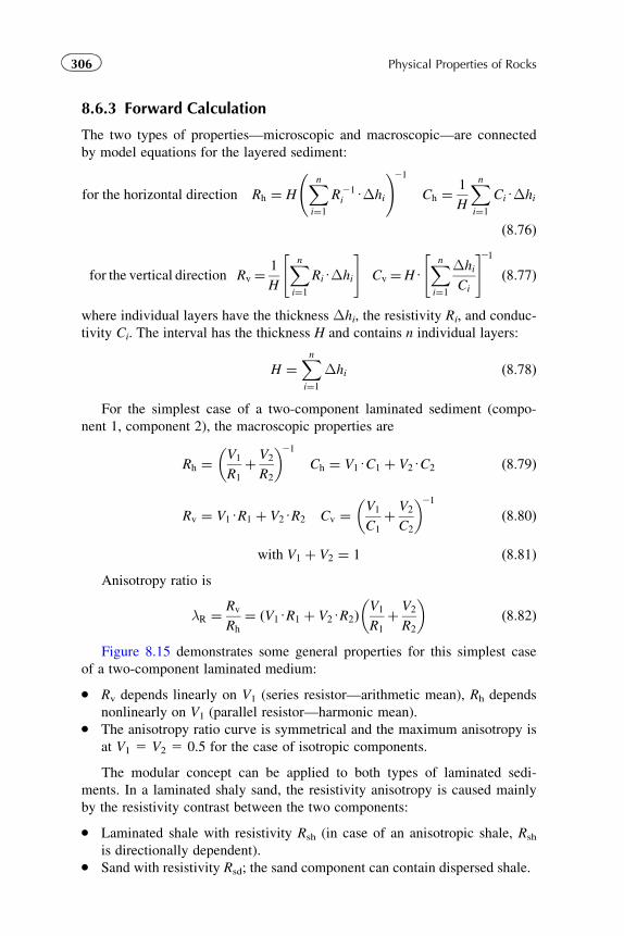
8.6.3 Forward Calculation
The two types of properties—microscopic and macroscopic—are connected
by model equations for the layered sediment:
for the horizontal direction Rh ¼ HXni¼1
R21i UΔhi
!21
Ch ¼1
H
Xni¼1
CiUΔhi
ð8:76Þ
for the vertical direction Rv ¼ 1
H
Xni¼1
RiUΔhi
" #Cv ¼HU
Xni¼1
Δhi
Ci
" #21ð8:77Þ
where individual layers have the thickness Δhi, the resistivity Ri, and conduc-
tivity Ci. The interval has the thickness H and contains n individual layers:
H ¼Xni¼1
Δhi ð8:78Þ
For the simplest case of a two-component laminated sediment (compo-
nent 1, component 2), the macroscopic properties are
Rh ¼V1
R1
þ V2
R2
� �21
Ch ¼ V1UC1 þ V2UC2 ð8:79Þ
Rv ¼ V1UR1 þ V2UR2 Cv ¼V1
C1
þ V2
C2
� �21
ð8:80Þ
with V1 þ V2 ¼ 1 ð8:81ÞAnisotropy ratio is
λR ¼ Rv
Rh
¼ ðV1UR1 þ V2UR2ÞV1
R1
þ V2
R2
� �ð8:82Þ
Figure 8.15 demonstrates some general properties for this simplest case
of a two-component laminated medium:
� Rv depends linearly on V1 (series resistor—arithmetic mean), Rh depends
nonlinearly on V1 (parallel resistor—harmonic mean).� The anisotropy ratio curve is symmetrical and the maximum anisotropy is
at V1 5 V2 5 0.5 for the case of isotropic components.
The modular concept can be applied to both types of laminated sedi-
ments. In a laminated shaly sand, the resistivity anisotropy is caused mainly
by the resistivity contrast between the two components:
� Laminated shale with resistivity Rsh (in case of an anisotropic shale, Rsh
is directionally dependent).� Sand with resistivity Rsd; the sand component can contain dispersed shale.
306 Physical Properties of Rocks
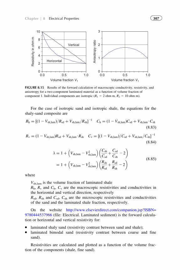
For the case of isotropic sand and isotropic shale, the equations for the
shaly-sand composite are
Rh ¼ ½ð12Vsh;lamÞ=Rsd þ Vsh;lam=Rsh�21 Ch ¼ ð12Vsh;lamÞCsd þ Vsh;lamUCsh
ð8:83Þ
Rv ¼ ð12Vsh;lamÞRsd þ Vsh;lamURsh Cv ¼ ½ð12Vsh;lamÞ=Csd þ Vsh;lam=Csh�21ð8:84Þ
λ ¼ 1þ Vsh;lam 2V2sh;lam
� Csh
Csd
þ Csd
Csh
2 2
� �
¼ 1þ Vsh;lam 2V2sh;lam
� Rsh
Rsd
þ Rsd
Rsh
2 2
� � ð8:85Þ
where
Vsh,lam is the volume fraction of laminated shale
Rh, Rv and Ch, Cv are the macroscopic resistivities and conductivities in
the horizontal and vertical direction, respectively
Rsd, Rsh and Csd, Csh are the microscopic resistivities and conductivities
of the sand and the laminated shale fraction, respectively.
On the website http://www.elsevierdirect.com/companion.jsp?ISBN=
9780444537966 (file: Electrical. Laminated sediment) is the forward calcula-
tion or horizontal and vertical resistivity for:
� laminated shaly sand (resistivity contrast between sand and shale);� laminated bimodal sand (resistivity contrast between coarse and fine
sand).
Resistivities are calculated and plotted as a function of the volume frac-
tion of the components (shale, fine sand).
0
2
4
6
8
10
0.0 0.5 1.0
Volume fraction V1
0.0 0.5 1.0
Volume fraction V1
Res
istiv
ity in
ohm
m
Vertical
Horizontal
0
1
2
3
Ani
sotr
opy
ratio
FIGURE 8.15 Results of the forward calculation of macroscopic conductivity, resistivity, and
anisotropy for a two-component laminated material as a function of volume fraction of
component 1. Individual components are isotropic (R1 5 2 ohm m, R2 5 10 ohm m).
307Chapter | 8 Electrical Properties
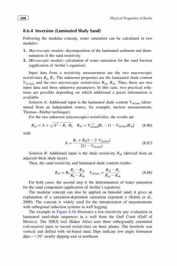
8.6.4 Inversion (Laminated Shaly Sand)
Following the modular concept, water saturation can be calculated in two
modules:
1. Macroscopic module: decomposition of the laminated sediment and deter-
mination of the sand resistivity.
2. Microscopic module: calculation of water saturation for the sand fraction
(application of Archie’s equation).
Input data from a resistivity measurement are the two macroscopic
resistivities Rh, Rv. The unknown properties are the laminated shale content
Vsh,lam and the two microscopic resistivities Rsd, Rsh. Thus, there are two
input data and three unknown parameters. In this case, two practical solu-
tions are possible depending on which additional a priori information is
available.
Solution A: Additional input is the laminated shale content Vsh,lam (deter-
mined from an independent source, for example, nuclear measurements,
Thomas�Stieber technique).
For the two unknown (microscopic) resistivities, the results are
Rsd ¼ AþffiffiffiffiffiffiffiffiffiffiffiffiffiffiffiffiffiffiffiffiffiffiffiA2 2RvURh
pRsh ¼ V 21
sh;lam½Rv 2 ð12Vsh;lamÞRsd� ð8:86Þwith
A ¼ Rv þ Rhð12 2UVsh;lamÞ2ð12Vsh;lamÞ
ð8:87Þ
Solution B: Additional input is the shale resistivity Rsh (derived from an
adjacent thick shale layer).
Then, the sand resistivity and laminated shale content results:
Rsd ¼ Rh
Rv 2Rsh
Rh 2Rsh
Vsh;lam ¼ Rsd 2Rv
Rsd 2Rsh
ð8:88Þ
For both cases, the second step is the determination of water saturation
for the sand component (application of Archie’s equation).
The modular concept can also be applied on bimodal sand; it gives an
explanation of a saturation-dependent saturation exponent n (Schon et al.,
2000). The concept is widely used for the interpretation of measurements
with orthogonal induction systems in well logging.
The example in Figure 8.16 illustrates a low-resistivity pay evaluation in
laminated sand-shale sequences in a well from the Gulf Coast (Gulf of
Mexico). The 3DEX tool (Baker Atlas) uses three orthogonally orientated
coil-receiver pairs to record resistivities on three planes. The borehole was
vertical and drilled with oil-based mud. Dips indicate low angle formation
dips—,10� mostly dipping east or northeast.
308 Physical Properties of Rocks
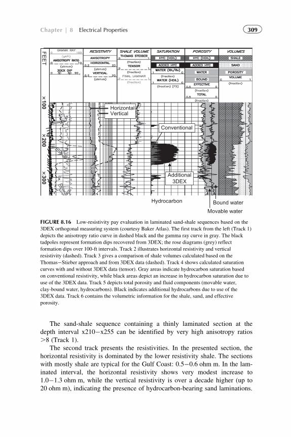
The sand-shale sequence containing a thinly laminated section at the
depth interval x210�x255 can be identified by very high anisotropy ratios
.8 (Track 1).
The second track presents the resistivities. In the presented section, the
horizontal resistivity is dominated by the lower resistivity shale. The sections
with mostly shale are typical for the Gulf Coast: 0.5�0.6 ohm m. In the lam-
inated interval, the horizontal resistivity shows very modest increase to
1.0�1.3 ohm m, while the vertical resistivity is over a decade higher (up to
20 ohm m), indicating the presence of hydrocarbon-bearing sand laminations.
FE
ET
�100
�200
�300
HorizontalVertical
Bound water
Movable water
Hydrocarbon
Conventional
Additional3DEX
FIGURE 8.16 Low-resistivity pay evaluation in laminated sand-shale sequences based on the
3DEX orthogonal measuring system (courtesy Baker Atlas). The first track from the left (Track 1)
depicts the anisotropy ratio curve in dashed black and the gamma ray curve in gray. The black
tadpoles represent formation dips recovered from 3DEX; the rose diagrams (grey) reflect
formation dips over 100-ft intervals. Track 2 illustrates horizontal resistivity and vertical
resistivity (dashed). Track 3 gives a comparison of shale volumes calculated based on the
Thomas�Stieber approach and from 3DEX data (dashed). Track 4 shows calculated saturation
curves with and without 3DEX data (tensor). Gray areas indicate hydrocarbon saturation based
on conventional resistivity, while black areas depict an increase in hydrocarbon saturation due to
use of the 3DEX data. Track 5 depicts total porosity and fluid components (movable water,
clay-bound water, hydrocarbons). Black indicates additional hydrocarbons due to use of the
3DEX data. Track 6 contains the volumetric information for the shale, sand, and effective
porosity.
309Chapter | 8 Electrical Properties
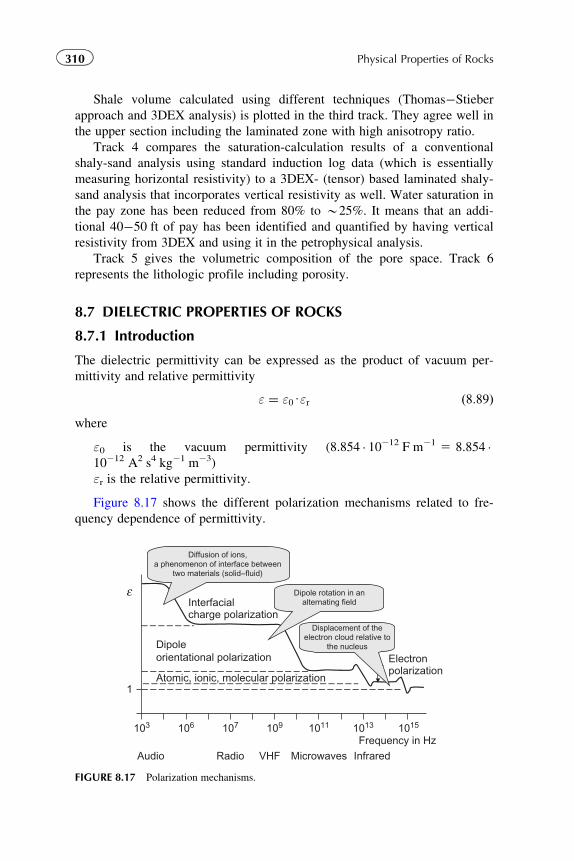
Shale volume calculated using different techniques (Thomas�Stieber
approach and 3DEX analysis) is plotted in the third track. They agree well in
the upper section including the laminated zone with high anisotropy ratio.
Track 4 compares the saturation-calculation results of a conventional
shaly-sand analysis using standard induction log data (which is essentially
measuring horizontal resistivity) to a 3DEX- (tensor) based laminated shaly-
sand analysis that incorporates vertical resistivity as well. Water saturation in
the pay zone has been reduced from 80% to B25%. It means that an addi-
tional 40�50 ft of pay has been identified and quantified by having vertical
resistivity from 3DEX and using it in the petrophysical analysis.
Track 5 gives the volumetric composition of the pore space. Track 6
represents the lithologic profile including porosity.
8.7 DIELECTRIC PROPERTIES OF ROCKS
8.7.1 Introduction
The dielectric permittivity can be expressed as the product of vacuum per-
mittivity and relative permittivity
ε ¼ ε0Uεr ð8:89Þwhere
ε0 is the vacuum permittivity (8.854 � 10212 F m21 5 8.854 �10212 A2 s4 kg21 m23)
εr is the relative permittivity.
Figure 8.17 shows the different polarization mechanisms related to fre-
quency dependence of permittivity.
Interfacialcharge polarization
Electronpolarization
Dipoleorientational polarization
Atomic, ionic, molecular polarization
ε
1
103 106 107 109 1011 1013 1015
Audio Radio VHF Microwaves InfraredFrequency in Hz
Diffusion of ions,a phenomenon of interface between
two materials (solid–fluid)
Dipole rotation in analternating field
Displacement of theelectron cloud relative to
the nucleus
FIGURE 8.17 Polarization mechanisms.
310 Physical Properties of Rocks
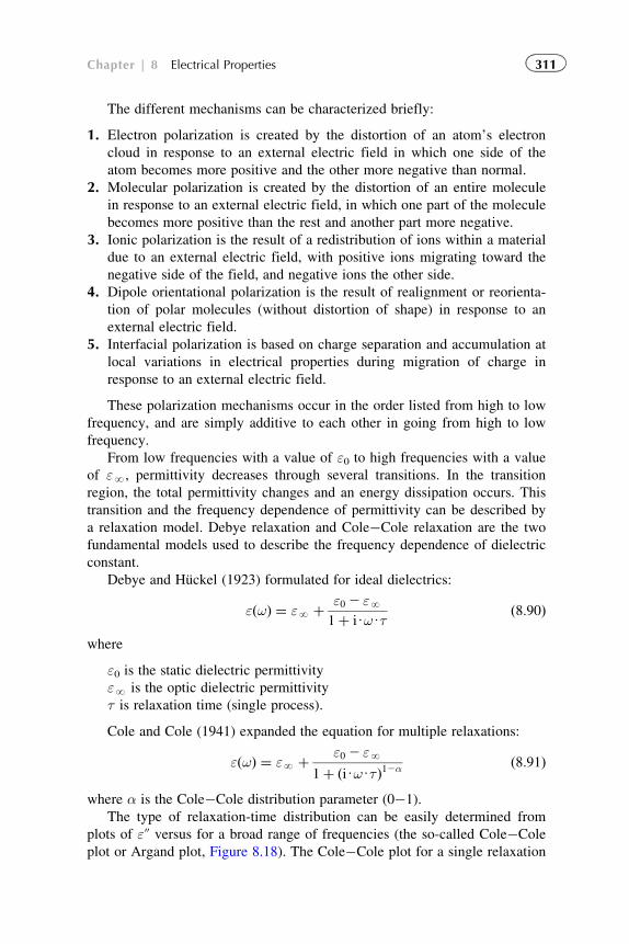
The different mechanisms can be characterized briefly:
1. Electron polarization is created by the distortion of an atom’s electron
cloud in response to an external electric field in which one side of the
atom becomes more positive and the other more negative than normal.
2. Molecular polarization is created by the distortion of an entire molecule
in response to an external electric field, in which one part of the molecule
becomes more positive than the rest and another part more negative.
3. Ionic polarization is the result of a redistribution of ions within a material
due to an external electric field, with positive ions migrating toward the
negative side of the field, and negative ions the other side.
4. Dipole orientational polarization is the result of realignment or reorienta-
tion of polar molecules (without distortion of shape) in response to an
external electric field.
5. Interfacial polarization is based on charge separation and accumulation at
local variations in electrical properties during migration of charge in
response to an external electric field.
These polarization mechanisms occur in the order listed from high to low
frequency, and are simply additive to each other in going from high to low
frequency.
From low frequencies with a value of ε0 to high frequencies with a value
of εN, permittivity decreases through several transitions. In the transition
region, the total permittivity changes and an energy dissipation occurs. This
transition and the frequency dependence of permittivity can be described by
a relaxation model. Debye relaxation and Cole�Cole relaxation are the two
fundamental models used to describe the frequency dependence of dielectric
constant.
Debye and Huckel (1923) formulated for ideal dielectrics:
εðωÞ ¼ εN þ ε0 2 εN1þ iUωUτ
ð8:90Þ
where
ε0 is the static dielectric permittivity
εN is the optic dielectric permittivity
τ is relaxation time (single process).
Cole and Cole (1941) expanded the equation for multiple relaxations:
εðωÞ ¼ εN þ ε0 2 εN1þ ðiUωUτÞ12α ð8:91Þ
where α is the Cole�Cole distribution parameter (0�1).
The type of relaxation-time distribution can be easily determined from
plots of εv versus for a broad range of frequencies (the so-called Cole�Cole
plot or Argand plot, Figure 8.18). The Cole�Cole plot for a single relaxation
311Chapter | 8 Electrical Properties
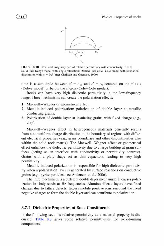
time is a semicircle between ε0 5 εN and ε0 5 ε0 centered on the ε0-axis(Debye model) or below the ε0-axis (Cole�Cole model).
Rocks can have very high dielectric permittivity in the low-frequency
range. Three mechanisms can create the polarization effects:
1. Maxwell�Wagner or geometrical effect.
2. Metallic-induced polarization: polarization of double layer at metallic
conducting grains.
3. Polarization of double layer at insulating grains with fixed charge (e.g.,
clay).
Maxwell�Wagner effect in heterogeneous materials generally results
from a nonuniform charge distribution at the boundary of regions with differ-
ent electrical properties (e.g., grain boundaries and other discontinuities also
within the solid rock matrix). The Maxwell�Wagner effect or geometrical
effect enhances the dielectric permittivity due to charge buildup at grain sur-
faces (acting as an interface with conductivity or permittivity contrast).
Grains with a platy shape act as thin capacitors, leading to very high
permittivity.
Metallic-induced polarization is responsible for high dielectric permittiv-
ity when a polarization layer is generated by surface reactions on conductive
grains (e.g., pyrite particles; see Anderson et al., 2006).
The third mechanism is a different double-layer mechanism. It causes polar-
ization in shaly sands at Hz frequencies. Alumino-silicate layers have fixed
charges due to lattice defects. Excess mobile positive ions surround the fixed
negative charges to form the double layer and can contribute to polarization.
8.7.2 Dielectric Properties of Rock Constituents
In the following sections relative permittivity as a material property is dis-
cussed. Table 8.8 gives some relative permittivities for rock-forming
components.
''ε
∞ε 0ε'ε
2πα ⋅
FIGURE 8.18 Real and imaginary part of relative permittivity with conductivity C 5 0.
Solid line: Debye model with single relaxation; Dashed line: Cole�Cole model with relaxation
distribution with α 5 0.5 (after Chelidze and Gueguen, 1999).
312 Physical Properties of Rocks
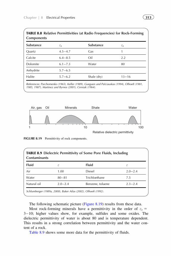
The following schematic picture (Figure 8.19) results from these data.
Most rock-forming minerals have a permittivity in the order of εr 53�10; higher values show, for example, sulfides and some oxides. The
dielectric permittivity of water is about 80 and is temperature dependent.
This results in a strong correlation between permittivity and the water con-
tent of a rock.
Table 8.9 shows some more data for the permittivity of fluids.
TABLE 8.8 Relative Permittivities (at Radio Frequencies) for Rock-Forming
Components
Substance εr Substance εr
Quartz 4.5�4.7 Gas 1
Calcite 6.4�8.5 Oil 2.2
Dolomite 6.1�7.3 Water 80
Anhydrite 5.7�6.5
Halite 5.7�6.2 Shale (dry) 13�16
References: Parchomenko (1965), Keller (1989), Gueguen and Palciauskas (1994), Olhoeft (1981,1985, 1987), Martinez and Byrnes (2001), Cerniak (1964).
Air, gas Oil Minerals Shale Water
1 10 100
Relative dielectric permittivity
FIGURE 8.19 Permittivity of rock components.
TABLE 8.9 Dielectric Permittivity of Some Pore Fluids, Including
Contaminants
Fluid ε Fluid ε
Air 1.00 Diesel 2.0�2.4
Water 80�81 Trichloethane 7.5
Natural oil 2.0�2.4 Benzene, toluene 2.3�2.4
Schlumberger (1989a, 2000), Baker Atlas (2002), Olhoeft (1992).
313Chapter | 8 Electrical Properties
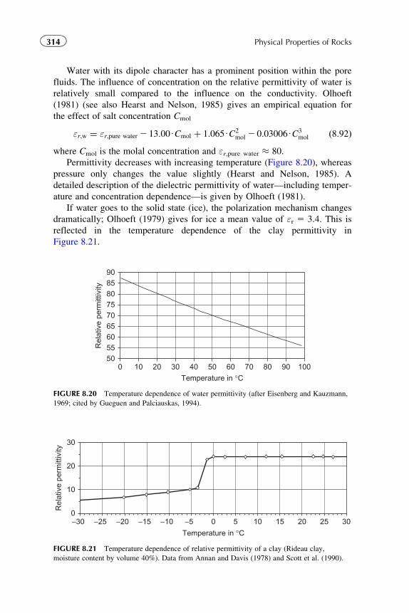
Water with its dipole character has a prominent position within the pore
fluids. The influence of concentration on the relative permittivity of water is
relatively small compared to the influence on the conductivity. Olhoeft
(1981) (see also Hearst and Nelson, 1985) gives an empirical equation for
the effect of salt concentration Cmol
εr;w ¼ εr;pure water 2 13:00UCmol þ 1:065UC2mol 2 0:03006UC3
mol ð8:92Þwhere Cmol is the molal concentration and εr,pure water � 80.
Permittivity decreases with increasing temperature (Figure 8.20), whereas
pressure only changes the value slightly (Hearst and Nelson, 1985). A
detailed description of the dielectric permittivity of water—including temper-
ature and concentration dependence—is given by Olhoeft (1981).
If water goes to the solid state (ice), the polarization mechanism changes
dramatically; Olhoeft (1979) gives for ice a mean value of εr 5 3.4. This is
reflected in the temperature dependence of the clay permittivity in
Figure 8.21.
505560657075808590
0 10 20 30 40 50 60 70 80 90 100
Temperature in °C
Rel
ativ
e pe
rmitt
ivity
FIGURE 8.20 Temperature dependence of water permittivity (after Eisenberg and Kauzmann,
1969; cited by Gueguen and Palciauskas, 1994).
Temperature in °C
Rel
ativ
e pe
rmitt
ivity
0
10
20
30
−5−10−15−20−25−30 0 5 10 15 20 25 30
FIGURE 8.21 Temperature dependence of relative permittivity of a clay (Rideau clay,
moisture content by volume 40%). Data from Annan and Davis (1978) and Scott et al. (1990).
314 Physical Properties of Rocks
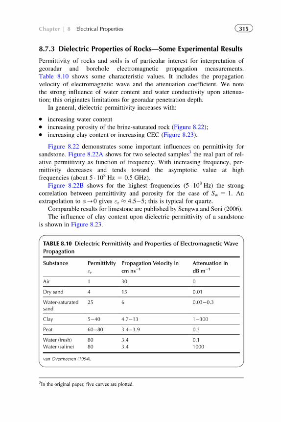
8.7.3 Dielectric Properties of Rocks—Some Experimental Results
Permittivity of rocks and soils is of particular interest for interpretation of
georadar and borehole electromagnetic propagation measurements.
Table 8.10 shows some characteristic values. It includes the propagation
velocity of electromagnetic wave and the attenuation coefficient. We note
the strong influence of water content and water conductivity upon attenua-
tion; this originates limitations for georadar penetration depth.
In general, dielectric permittivity increases with:
� increasing water content� increasing porosity of the brine-saturated rock (Figure 8.22);� increasing clay content or increasing CEC (Figure 8.23).
Figure 8.22 demonstrates some important influences on permittivity for
sandstone. Figure 8.22A shows for two selected samples3 the real part of rel-
ative permittivity as function of frequency. With increasing frequency, per-
mittivity decreases and tends toward the asymptotic value at high
frequencies (about 5 � 108 Hz 5 0.5 GHz).
Figure 8.22B shows for the highest frequencies (5 � 108 Hz) the strong
correlation between permittivity and porosity for the case of Sw 5 1. An
extrapolation to φ-0 gives εr � 4.5�5; this is typical for quartz.
Comparable results for limestone are published by Sengwa and Soni (2006).
The influence of clay content upon dielectric permittivity of a sandstone
is shown in Figure 8.23.
TABLE 8.10 Dielectric Permittivity and Properties of Electromagnetic Wave
Propagation
Substance Permittivity
εr
Propagation Velocity in
cm ns21Attenuation in
dB m21
Air 1 30 0
Dry sand 4 15 0.01
Water-saturatedsand
25 6 0.03�0.3
Clay 5�40 4.7�13 1�300
Peat 60�80 3.4�3.9 0.3
Water (fresh) 80 3.4 0.1
Water (saline) 80 3.4 1000
van Overmeeren (1994).
3In the original paper, five curves are plotted.
315Chapter | 8 Electrical Properties
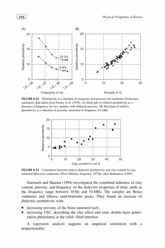
Garrouch and Sharma (1994) investigated the combined influence of clay
content, porosity, and frequency on the dielectric properties of shaly sands in
the frequency range between 10 Hz and 10 MHz. The samples are Berea
sandstone and Ottawa sand-bentonite packs. They found an increase of
dielectric permittivity with:
� increasing porosity of the brine-saturated rock;� increasing CEC, describing the clay effect and ionic double-layer polari-
zation phenomena at the solid�fluid interface.
A regression analysis suggests an empirical correlation with a
proportionality
0
5
10
15
20
0 10 20 30 40 50
Clay content in vol.%
Rel
ativ
e pe
rmitt
ivity
FIGURE 8.23 Correlation between relative dielectric permittivity and clay content for gas-
saturated Mesozoic sandstones (West Siberia), frequency 106 Hz; after Kobranova (1989).
5
10
15
20
0 10 20 30
Porosity in %
Rel
ativ
e pe
rmitt
ivity
5
10
15
20
(A) (B)
1.E + 06
1.E + 07
1.E + 08
1.E + 09
Frequency in Hz
Rel
ativ
e pe
rmitt
ivity
20.0%
6.9%
FIGURE 8.22 Permittivity as a function of frequency and porosity for sandstone (freshwater
saturated); data taken from Pooley et al. (1978). (A) Real part of relative permittivity as a
function of frequency for two samples with different porosity. (B) Real part of relative
permittivity as a function of porosity, measured at frequency 0.5 GHz.
316 Physical Properties of Rocks
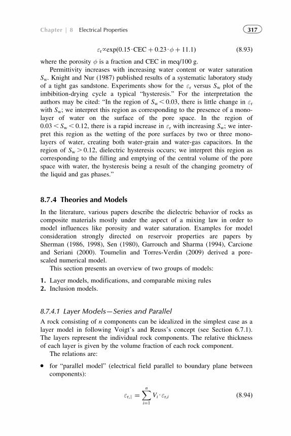
εr~expð0:15UCECþ 0:23Uφþ 11:1Þ ð8:93Þwhere the porosity φ is a fraction and CEC in meq/100 g.
Permittivity increases with increasing water content or water saturation
Sw. Knight and Nur (1987) published results of a systematic laboratory study
of a tight gas sandstone. Experiments show for the εr versus Sw plot of the
imbibition-drying cycle a typical “hysteresis.” For the interpretation the
authors may be cited: “In the region of Sw, 0.03, there is little change in εrwith Sw; we interpret this region as corresponding to the presence of a mono-
layer of water on the surface of the pore space. In the region of
0.03, Sw, 0.12, there is a rapid increase in εr with increasing Sw; we inter-
pret this region as the wetting of the pore surfaces by two or three mono-
layers of water, creating both water-grain and water-gas capacitors. In the
region of Sw. 0.12, dielectric hysteresis occurs; we interpret this region as
corresponding to the filling and emptying of the central volume of the pore
space with water, the hysteresis being a result of the changing geometry of
the liquid and gas phases.”
8.7.4 Theories and Models
In the literature, various papers describe the dielectric behavior of rocks as
composite materials mostly under the aspect of a mixing law in order to
model influences like porosity and water saturation. Examples for model
consideration strongly directed on reservoir properties are papers by
Sherman (1986, 1998), Sen (1980), Garrouch and Sharma (1994), Carcione
and Seriani (2000). Toumelin and Torres-Verdin (2009) derived a pore-
scaled numerical model.
This section presents an overview of two groups of models:
1. Layer models, modifications, and comparable mixing rules
2. Inclusion models.
8.7.4.1 Layer Models—Series and Parallel
A rock consisting of n components can be idealized in the simplest case as a
layer model in following Voigt’s and Reuss’s concept (see Section 6.7.1).
The layers represent the individual rock components. The relative thickness
of each layer is given by the volume fraction of each rock component.
The relations are:
� for “parallel model” (electrical field parallel to boundary plane between
components):
εr;8 ¼Xni¼1
ViUεr;i ð8:94Þ
317Chapter | 8 Electrical Properties
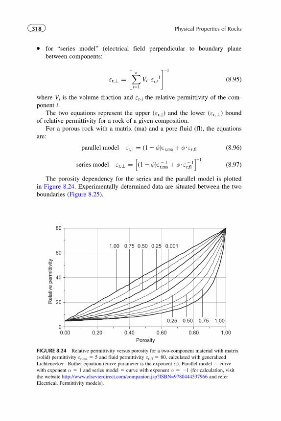
� for “series model” (electrical field perpendicular to boundary plane
between components:
εr;> ¼Xni¼1
ViUε21r;i
" #21
ð8:95Þ
where Vi is the volume fraction and εr,i the relative permittivity of the com-
ponent i.
The two equations represent the upper (εr,8) and the lower (εr,>) bound
of relative permittivity for a rock of a given composition.
For a porous rock with a matrix (ma) and a pore fluid (fl), the equations
are:
parallel model εr;8 ¼ ð12φÞεr;ma þ φUεr;fl ð8:96Þ
series model εr;> ¼ ð12φÞε2 1r;ma þ φUε2 1
r;fl
h i21
ð8:97Þ
The porosity dependency for the series and the parallel model is plotted
in Figure 8.24. Experimentally determined data are situated between the two
boundaries (Figure 8.25).
0
20
40
60
80
0.00 0.20 0.40 0.60 0.80 1.00Porosity
Rel
ativ
e pe
rmitt
ivity
1.00 0.50 0.25 0.001
−0.25 −0.50 −0.75 −1.00
0.75
FIGURE 8.24 Relative permittivity versus porosity for a two-component material with matrix
(solid) permittivity εr,ma 5 5 and fluid permittivity εr,fl 5 80, calculated with generalized
Lichtenecker�Rother equation (curve parameter is the exponent α). Parallel model 5 curve
with exponent α 5 1 and series model 5 curve with exponent α 5 21 (for calculation, visit
the website http://www.elsevierdirect.com/companion.jsp?ISBN=9780444537966 and refer
Electrical. Permittivity models).
318 Physical Properties of Rocks
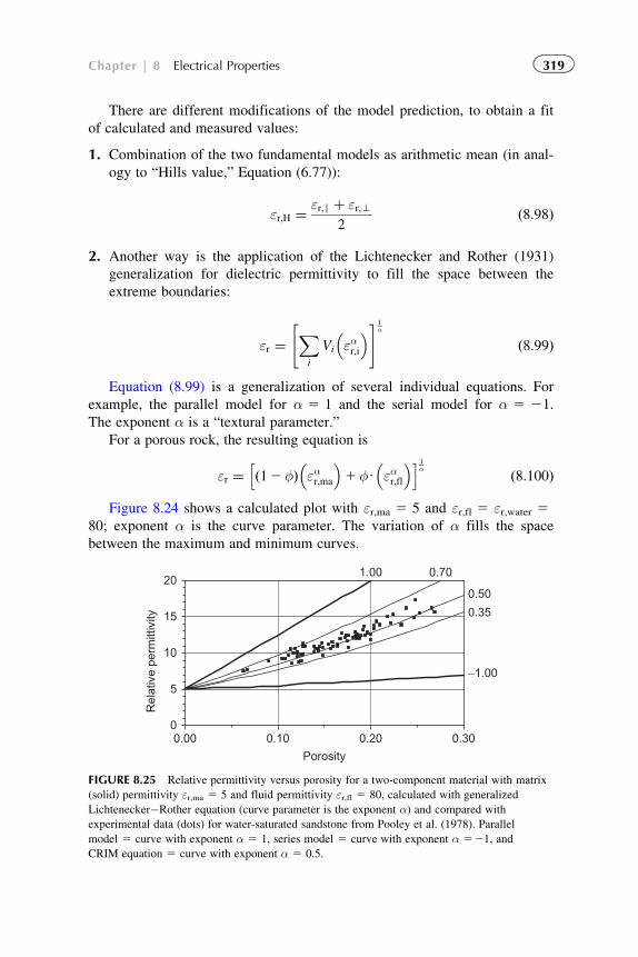
There are different modifications of the model prediction, to obtain a fit
of calculated and measured values:
1. Combination of the two fundamental models as arithmetic mean (in anal-
ogy to “Hills value,” Equation (6.77)):
εr;H ¼ εr;8 þ εr;>2
ð8:98Þ
2. Another way is the application of the Lichtenecker and Rother (1931)
generalization for dielectric permittivity to fill the space between the
extreme boundaries:
εr ¼Xi
Vi εαr;i� " #1
α
ð8:99Þ
Equation (8.99) is a generalization of several individual equations. For
example, the parallel model for α 5 1 and the serial model for α 5 21.
The exponent α is a “textural parameter.”
For a porous rock, the resulting equation is
εr ¼ ð12φÞ εαr;ma
� 1φU εαr;fl
� h i1α ð8:100Þ
Figure 8.24 shows a calculated plot with εr,ma 5 5 and εr,fl 5 εr,water 580; exponent α is the curve parameter. The variation of α fills the space
between the maximum and minimum curves.
0
5
10
15
20
0.00 0.10 0.20 0.30
Porosity
Rel
ativ
e pe
rmitt
ivity
−1.00
0.35
0.50
0.701.00
FIGURE 8.25 Relative permittivity versus porosity for a two-component material with matrix
(solid) permittivity εr,ma 5 5 and fluid permittivity εr,fl 5 80, calculated with generalized
Lichtenecker�Rother equation (curve parameter is the exponent α) and compared with
experimental data (dots) for water-saturated sandstone from Pooley et al. (1978). Parallel
model 5 curve with exponent α 5 1, series model 5 curve with exponent α 521, and
CRIM equation 5 curve with exponent α 5 0.5.
319Chapter | 8 Electrical Properties
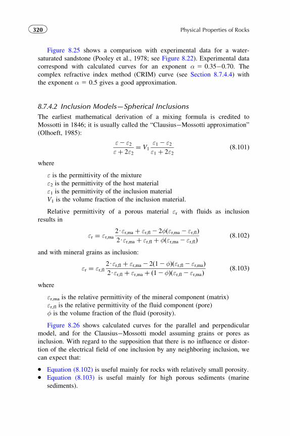
Figure 8.25 shows a comparison with experimental data for a water-
saturated sandstone (Pooley et al., 1978; see Figure 8.22). Experimental data
correspond with calculated curves for an exponent α 5 0.35�0.70. The
complex refractive index method (CRIM) curve (see Section 8.7.4.4) with
the exponent α 5 0.5 gives a good approximation.
8.7.4.2 Inclusion Models—Spherical Inclusions
The earliest mathematical derivation of a mixing formula is credited to
Mossotti in 1846; it is usually called the “Clausius�Mossotti approximation”
(Olhoeft, 1985):
ε2 ε2εþ 2ε2
¼ V1
ε1 2 ε2ε1 þ 2ε2
ð8:101Þ
where
ε is the permittivity of the mixture
ε2 is the permittivity of the host material
ε1 is the permittivity of the inclusion material
V1 is the volume fraction of the inclusion material.
Relative permittivity of a porous material εr with fluids as inclusion
results in
εr ¼ εr;ma
2Uεr;ma þ εr;fl 2 2φðεr;ma 2 εr;flÞ2Uεr;ma þ εr;fl þ φðεr;ma 2 εr;flÞ
ð8:102Þ
and with mineral grains as inclusion:
εr ¼ εr;fl2Uεr;fl þ εr;ma 2 2ð12φÞðεr;fl 2 εr;maÞ2Uεr;fl þ εr;ma þ ð12φÞðεr;fl 2 εr;maÞ
ð8:103Þ
where
εr,ma is the relative permittivity of the mineral component (matrix)
εr,fl is the relative permittivity of the fluid component (pore)
φ is the volume fraction of the fluid (porosity).
Figure 8.26 shows calculated curves for the parallel and perpendicular
model, and for the Clausius�Mossotti model assuming grains or pores as
inclusion. With regard to the supposition that there is no influence or distor-
tion of the electrical field of one inclusion by any neighboring inclusion, we
can expect that:
� Equation (8.102) is useful mainly for rocks with relatively small porosity.� Equation (8.103) is useful mainly for high porous sediments (marine
sediments).
320 Physical Properties of Rocks
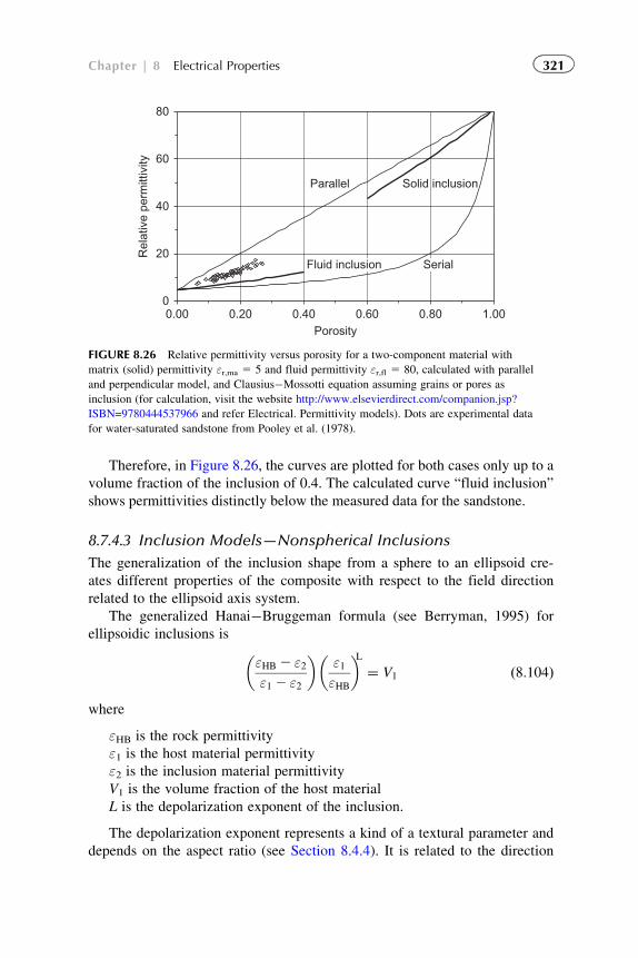
Therefore, in Figure 8.26, the curves are plotted for both cases only up to a
volume fraction of the inclusion of 0.4. The calculated curve “fluid inclusion”
shows permittivities distinctly below the measured data for the sandstone.
8.7.4.3 Inclusion Models—Nonspherical Inclusions
The generalization of the inclusion shape from a sphere to an ellipsoid cre-
ates different properties of the composite with respect to the field direction
related to the ellipsoid axis system.
The generalized Hanai�Bruggeman formula (see Berryman, 1995) for
ellipsoidic inclusions is
εHB 2 ε2ε1 2 ε2
� �ε1εHB
� �L¼ V1 ð8:104Þ
where
εHB is the rock permittivity
ε1 is the host material permittivity
ε2 is the inclusion material permittivity
V1 is the volume fraction of the host material
L is the depolarization exponent of the inclusion.
The depolarization exponent represents a kind of a textural parameter and
depends on the aspect ratio (see Section 8.4.4). It is related to the direction
0
20
40
60
80
0.00 0.20 0.40 0.60 0.80 1.00Porosity
Rel
ativ
e pe
rmitt
ivity
Parallel Solid inclusion
Fluid inclusion Serial
FIGURE 8.26 Relative permittivity versus porosity for a two-component material with
matrix (solid) permittivity εr,ma 5 5 and fluid permittivity εr,fl 5 80, calculated with parallel
and perpendicular model, and Clausius�Mossotti equation assuming grains or pores as
inclusion (for calculation, visit the website http://www.elsevierdirect.com/companion.jsp?
ISBN=9780444537966 and refer Electrical. Permittivity models). Dots are experimental data
for water-saturated sandstone from Pooley et al. (1978).
321Chapter | 8 Electrical Properties
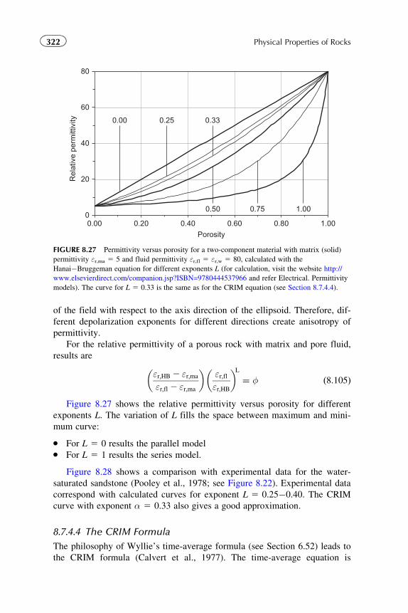
of the field with respect to the axis direction of the ellipsoid. Therefore, dif-
ferent depolarization exponents for different directions create anisotropy of
permittivity.
For the relative permittivity of a porous rock with matrix and pore fluid,
results are
εr;HB 2 εr;ma
εr;fl 2 εr;ma
� �εr;flεr;HB
� �L¼ φ ð8:105Þ
Figure 8.27 shows the relative permittivity versus porosity for different
exponents L. The variation of L fills the space between maximum and mini-
mum curve:
� For L 5 0 results the parallel model� For L 5 1 results the series model.
Figure 8.28 shows a comparison with experimental data for the water-
saturated sandstone (Pooley et al., 1978; see Figure 8.22). Experimental data
correspond with calculated curves for exponent L 5 0.25�0.40. The CRIM
curve with exponent α 5 0.33 also gives a good approximation.
8.7.4.4 The CRIM Formula
The philosophy of Wyllie’s time-average formula (see Section 6.52) leads to
the CRIM formula (Calvert et al., 1977). The time-average equation is
0
20
40
60
80
0.00 0.20 0.40 0.60 0.80
1.000.750.50
1.00Porosity
Rel
ativ
e pe
rmitt
ivity
0.00 0.25 0.33
FIGURE 8.27 Permittivity versus porosity for a two-component material with matrix (solid)
permittivity εr,ma 5 5 and fluid permittivity εr,fl 5 εr,w 5 80, calculated with the
Hanai�Bruggeman equation for different exponents L (for calculation, visit the website http://
www.elsevierdirect.com/companion.jsp?ISBN=9780444537966 and refer Electrical. Permittivity
models). The curve for L 5 0.33 is the same as for the CRIM equation (see Section 8.7.4.4).
322 Physical Properties of Rocks
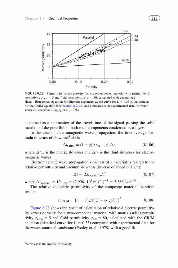
explained as a summation of the travel time of the signal passing the solid
matrix and the pore fluid—both rock components condensed as a layer.
In the case of electromagnetic wave propagation, the time-average for-
mula in terms of slowness4 Δt is
ΔtCRIM ¼ ð12φÞΔtma þ φUΔtfl ð8:106Þwhere Δtma is the matrix slowness and Δtfl is the fluid slowness for electro-
magnetic waves.
Electromagnetic wave propagation slowness of a material is related to the
relative permittivity and vacuum slowness (inverse of speed of light):
Δt ¼ ΔtvacuumUffiffiffiffiεr
p ð8:107Þwhere Δtvacuum 5 1/clight 5 (2.998 � 108 m s21)21 5 3.336 ns m21.
The relative dielectric permittivity of the composite material therefore
results:
εr;CRIM ¼ ð12φÞ ffiffiffiffiffiffiffiffiffiεr;ma
p þ φUffiffiffiffiffiffiffiεr;fl
p� �2 ð8:108ÞFigure 8.28 shows the result of calculation of relative dielectric permittiv-
ity versus porosity for a two-component material with matrix (solid) permit-
tivity εr,ma 5 5 and fluid permittivity εr,fl 5 80, calculated with the CRIM
equation (identical curve for L 5 0.33) compared with experimental data for
the water-saturated sandstone (Pooley et al., 1978) with a good fit.
4Slowness is the inverse of velocity.
0.00 0.10 0.20 0.30
Porosity
0
5
10
15
20
Rel
ativ
e pe
rmitt
ivity
Parallel
0.250.330.40
Serial
FIGURE 8.28 Permittivity versus porosity for a two-component material with matrix (solid)
permittivity εr,ma 5 5 and fluid permittivity εr,fl 5 80, calculated with generalized
Hanai�Bruggeman equation for different exponents L; the curve for L 5 0.33 is the same as
for the CRIM equation (see Section 8.7.4.4) and compared with experimental data for water-
saturated sandstone (Pooley et al., 1978).
323Chapter | 8 Electrical Properties
Coutanceau-Monteil and Jacquin (1993) investigated the permittivity of
sedimentary rock samples in the frequency range from 20 to 1000 MHz. A
comparison of model equations and experimental results shows that the
CRIM model fits the data for water- and brine-saturated quarry limestones,
whereas the Bruggeman�Hanai equation fits the data for water- and brine-
saturated Fontainebleau sandstones fairly well.
A generalization of the CRIM equation for n components gives
εr;CRIM ¼Xni¼1
ViUε2 1
2
r;i
" #2ð8:109Þ
Thus, the CRIM equation is identical with the generalized Lichtenecker
and Rother (1931) Equation (8.100) with α 5 0.5.
8.8 COMPLEX RESISTIVITY—SPECTRAL-INDUCEDPOLARIZATION
8.8.1 Introduction
The phenomenon of induced polarization (IP) was observed by Conrad
Schlumberger in a mining region in France circa 1913, and in about 1929, he
introduced this technique into hydrocarbon borehole logging (see Seigel
et al., 2007). Experimental and theoretical studies by Marshall and Madden
(1959), Pelton et al. (1978), Vinegar and Waxman (1984), Olhoeft (1985),
Ward (1990), Borner (1991), Borner et al. (1993), Borner and Schon (1995),
Vanhala (1997), Titov et al. (2002, 2004), Scott (2006), and others describe
characteristics of this phenomenon.
IP is a current-stimulated electrical phenomenon observed as a delayed
voltage response in earth materials resulting from a capacitive behavior
(Ward, 1990). This delay effect can be described and measured in the time
domain and in the frequency domain. The connection between the two
domains is given by Fourier transformation. Today’s spectral electrical mea-
surements (SIP) are state of the art.
The petrophysical origin of the IP effects is connected with electrochemi-
cal processes of the electronic�ionic interaction, interface properties at the
grain-fluid boundary region, cation-exchange phenomenon, pore constrictiv-
ity, and other effects controlled by rock components, their distribution and
interaction (Figure 8.29).
In the early days, IP was directed mostly on ore mineral exploration.
Later, pore space properties and connected effects became more interesting.
Today, frequency-dependent complex resistivity measurements are gener-
ally directed on problems of pore space characterization and description of
fluid�mineral interactions. Measurements are “sensitive to physico-chemical
mineral�water interaction at the grain surfaces. In comparison to conventional
324 Physical Properties of Rocks
geoelectrics, a complex electrical measurement can also provide—besides
conductivity—information on the electrical capacity and the relaxation process
in the frequency range below some kHz” (Borner, 2006).
Complex conductivity is a frequency-dependent property with a real and
an imaginary component (see Section 8.1; Equation (8.5)). There is presently
no universal theory or equation that describes the frequency-dependent com-
plex conductivity. A review of existing theories is given by Dias (2000).
A popular model is the Cole�Cole model (Pelton et al., 1978). Complex
conductivity as a function of frequency is given as
CðωÞ ¼ C0 1þ mðiωτÞc
1þ ðiωτÞcð12mÞ
� �� �ð8:110Þ
where
C0 is the conductivity at DC (ω-0)
τ is the relaxation time
c is an exponent that typically takes values in the range 0.1�0.6 (Binley
et al., 2005), describing the τ-distribution.
The parameter m is
m ¼ 12C0
CNð8:111Þ
where CN is the conductivity at high frequency (ω-N).
The spectrum of the Cole�Cole model shows a maximum phase angle at
the frequency
ωmaximum ¼ 1
τð12mÞc=2ð8:112Þ
At low frequencies (1023�103 Hz), a main feature observed in many
porous rocks is a nearly constant phase angle combined with a steady
decrease of the resistivity magnitude with frequency (Borner, 1991, 1995,
2006; Borner et al., 1993; Dissado and Hill, 1984; Jonscher, 1981):
C�ðωnÞ ¼ CnðiUωnÞ12p ð8:113Þwhere
Cn is the conductivity magnitude at ω 5 1 Hz
ωn is the normalized angular frequency ωn 5 ω/(ω 5 1)
12 p is the frequency exponent (in the order of 0�0.5).
The relationship between the frequency exponent (12 p) and the
frequency-independent phase angle is
tan φ ¼ CvðωÞC0ðωÞ ¼ tan
π2ð12 pÞ
h iφ ¼ π
2ð12 pÞ ð8:114Þ
325Chapter | 8 Electrical Properties
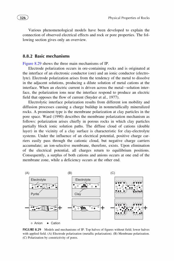
Various phenomenological models have been developed to explain the
connection of observed electrical effects and rock or pore properties. The fol-
lowing section gives only an overview.
8.8.2 Basic mechanisms
Figure 8.29 shows the three main mechanisms of IP.
Electrode polarization occurs in ore-containing rocks and is originated at
the interface of an electronic conductor (ore) and an ionic conductor (electro-
lyte). Electrode polarization arises from the tendency of the metal to dissolve
in the adjacent solutions, producing a dilute solution of metal cations at the
interface. When an electric current is driven across the metal�solution inter-
face, the polarization ions near the interface respond to produce an electric
field that opposes the flow of current (Snyder et al., 1977).
Electrolytic interface polarization results from different ion mobility and
diffusion processes causing a charge buildup in nonmetallically mineralized
rocks. A prominent type is the membrane polarization at clay particles in the
pore space. Ward (1990) describes the membrane polarization mechanism as
follows: polarization arises chiefly in porous rocks in which clay particles
partially block ionic solution paths. The diffuse cloud of cations (double
layer) in the vicinity of a clay surface is characteristic for clay-electrolyte
systems. Under the influence of an electrical potential, positive charge car-
riers easily pass through the cationic cloud, but negative charge carriers
accumulate; an ion-selective membrane, therefore, exists. Upon elimination
of the electrical potential, all charges return to equilibrium positions.
Consequently, a surplus of both cations and anions occurs at one end of the
membrane zone, while a deficiency occurs at the other end.
Anion Cation
Electrolyte
Pyrite
Electrolyte
Clay
- - - - - - - - - -
- - - - - - - - - -
- -
- -
- - -
- - -
- - - - - - - - - -
- - - - - - - - - -
- -
- -
- - -
- - -+ -+ -+ -
------
------
(A) (B) (C)
FIGURE 8.29 Models and mechanisms of IP. Top halves of figures without field; lower halves
with applied field. (A) Electrode polarization (metallic polarization). (B) Membrane polarization.
(C) Polarization by constrictivity of pores.
326 Physical Properties of Rocks
Polarization by constrictivity of pores results from the effect that pore
space is characterized by an alternating change of wide pore bodies and nar-
row pore throats. Pore space builds up a serial connection of active (ion-
selective) and passive (non-ion selective) zones. The zones have different
cation and anion transport numbers, which produce local concentration gradi-
ents under an external electrical field. The electrical current flow therefore
results in a deficiency of anions and surplus of cations at the boundaries of
the thick and thin capillaries.
8.8.3 Traditional Parameters of IP Measurements
IP can be characterized by parameters derived in the time domain and in the
frequency domain.
In time domain “chargeability” is used for description. In the simplest
case it is derived from the following procedure: A primary voltage UE is
applied during an excitation time tE. After this time, the current is switched
off and the decay voltage UIP(t) is measured. Seigel (1959) defined apparent
chargeability as the ratio:
M ¼ UIPðtÞUE
ð8:115Þ
Chargeability is dimensionless, but usually the secondary voltage is in
mV and the primary voltage in V. Thus, the chargeability is given in mV/V
(sometimes the percentage of this value is also used).
Such a definition of chargeability has an infinite number of possibilities
to define the time t. Modern IP methods are directed on a study of the decay
curve shape. One way is to integrate under a portion of the decay curve
between the decay time t1 and t2 and define chargeability as:
Mt2t1¼ 1
UEðt2 2 t1Þðt2t1
UIPðtÞdt ð8:116Þ
Time-domain instruments digitize the signal at high sampling rates and
permit a Fourier analysis into frequency domain in order to study complex
resistivity. In frequency domain, the “frequency effect” parameter is used:
FE ¼ Rðf1Þ2Rðf2ÞRðf2Þ
ð8:117Þ
where R(f1),R(f2) are, respectively, the specific electrical resistivities at fre-
quencies f1, f2 with f1, f2.
The percent frequency effect is PFE 5 FE � 100%.
The “metal factor” (Marshall and Madden, 1959) is defined as:
MF ¼ 2πU105Rðf1Þ2Rðf2ÞRðf1ÞURðf2Þ
¼ 2πU105FE
Rðf1Þð8:118Þ
327Chapter | 8 Electrical Properties
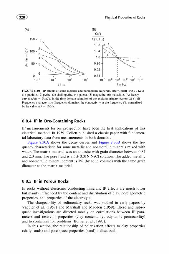
8.8.4 IP in Ore-Containing Rocks
IP measurements for ore prospection have been the first applications of this
electrical method. In 1959, Collett published a classic paper with fundamen-
tal laboratory data from measurements in both domains.
Figure 8.30A shows the decay curves and Figure 8.30B shows the fre-
quency characteristic for some metallic and nonmetallic minerals mixed with
water. The matrix material was an andesite with grain diameter between 0.84
and 2.0 mm. The pore fluid is a 5% 0.01N NaCl solution. The added metallic
and nonmetallic mineral content is 3% (by solid volume) with the same grain
diameter as the matrix material.
8.8.5 IP in Porous Rocks
In rocks without electronic conducting minerals, IP effects are much lower
but mainly influenced by the content and distribution of clay, pore geometric
properties, and properties of the electrolyte.
The chargeability of sedimentary rocks was studied in early papers by
Vaquier et al. (1957) and Marshall and Madden (1959). These and subse-
quent investigations are directed mostly on correlations between IP para-
meters and reservoir properties (clay content, hydrodynamic permeability)
and to contamination problems (Borner et al., 1993).
In this section, the relationship of polarization effects to clay properties
(shaly sands) and pore space properties (sand) is discussed.
150
(A) (B)
11
24
32
34
5
6
100
50
010−2
0.88
0.92
0.96
1.0
1.04
1.08
10−1 100 101 102 103 10410−1
t in s f in Hz100 101
P(t
) in
m V
/V
C(10 Hz)
C(f )
FIGURE 8.30 IP effects of some metallic and nonmetallic minerals, after Collett (1959). Key:
(1) graphite, (2) pyrite, (3) chalkopyrite, (4) galena, (5) magnetite, (6) malachite. (A) Decay
curves (P(t) 5 UIP(T)) in the time domain (duration of the exciting primary current 21 s). (B)
Frequency characteristic (frequency domain); the conductivity at the frequency f is normalized
by its value at f 5 10 Hz.
328 Physical Properties of Rocks
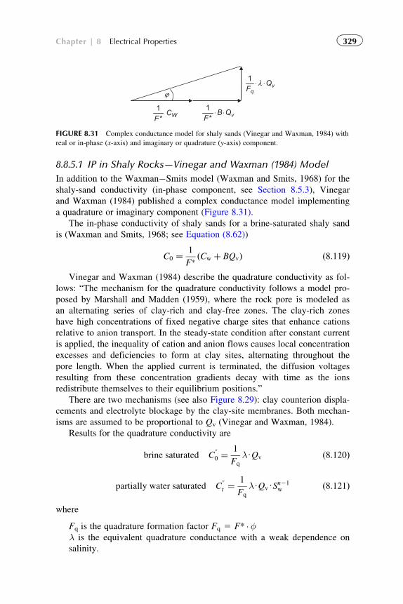
8.8.5.1 IP in Shaly Rocks—Vinegar and Waxman (1984) Model
In addition to the Waxman�Smits model (Waxman and Smits, 1968) for the
shaly-sand conductivity (in-phase component, see Section 8.5.3), Vinegar
and Waxman (1984) published a complex conductance model implementing
a quadrature or imaginary component (Figure 8.31).
The in-phase conductivity of shaly sands for a brine-saturated shaly sand
is (Waxman and Smits, 1968; see Equation (8.62))
C0 ¼ 1
F� ðCw þ BQvÞ ð8:119Þ
Vinegar and Waxman (1984) describe the quadrature conductivity as fol-
lows: “The mechanism for the quadrature conductivity follows a model pro-
posed by Marshall and Madden (1959), where the rock pore is modeled as
an alternating series of clay-rich and clay-free zones. The clay-rich zones
have high concentrations of fixed negative charge sites that enhance cations
relative to anion transport. In the steady-state condition after constant current
is applied, the inequality of cation and anion flows causes local concentration
excesses and deficiencies to form at clay sites, alternating throughout the
pore length. When the applied current is terminated, the diffusion voltages
resulting from these concentration gradients decay with time as the ions
redistribute themselves to their equilibrium positions.”
There are two mechanisms (see also Figure 8.29): clay counterion displa-
cements and electrolyte blockage by the clay-site membranes. Both mechan-
isms are assumed to be proportional to Qv (Vinegar and Waxman, 1984).
Results for the quadrature conductivity are
brine saturated Cv0 ¼
1
Fq
λUQv ð8:120Þ
partially water saturated Cvt ¼
1
Fq
λUQvUSn21w ð8:121Þ
where
Fq is the quadrature formation factor Fq 5 F* �φλ is the equivalent quadrature conductance with a weak dependence on
salinity.
QvFq⋅⋅λ1
CWF*1 QvB
F*⋅⋅1
ϕ
FIGURE 8.31 Complex conductance model for shaly sands (Vinegar and Waxman, 1984) with
real or in-phase (x-axis) and imaginary or quadrature (y-axis) component.
329Chapter | 8 Electrical Properties
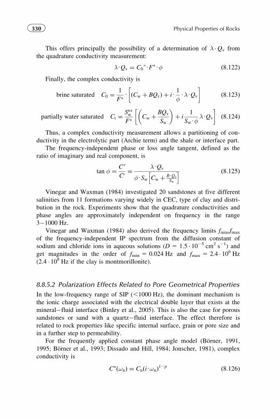
This offers principally the possibility of a determination of λ �Qv from
the quadrature conductivity measurement:
λUQv ¼ C0vUF�Uφ ð8:122ÞFinally, the complex conductivity is
brine saturated C0 ¼1
F� U ðCw þ BQvÞ þ iU1
φUλUQv
� �ð8:123Þ
partially water saturated Ct ¼Sn�wF� Cw þ BQv
Sw
� �þ i
1
SwUφλUQv
� �ð8:124Þ
Thus, a complex conductivity measurement allows a partitioning of con-
ductivity in the electrolytic part (Archie term) and the shale or interface part.
The frequency-independent phase or loss angle tangent, defined as the
ratio of imaginary and real component, is
tan φ ¼ CvC0 ¼
λUQv
φUSw Cw þ BUQv
Sw
h i ð8:125Þ
Vinegar and Waxman (1984) investigated 20 sandstones at five different
salinities from 11 formations varying widely in CEC, type of clay and distri-
bution in the rock. Experiments show that the quadrature conductivities and
phase angles are approximately independent on frequency in the range
3�1000 Hz.
Vinegar and Waxman (1984) also derived the frequency limits fmin,fmax
of the frequency-independent IP spectrum from the diffusion constant of
sodium and chloride ions in aqueous solutions (D 5 1.5 � 1025 cm2 s21) and
get magnitudes in the order of fmin 5 0.024 Hz and fmax 5 2.4 � 106 Hz(2.4 � 108 Hz if the clay is montmorillonite).
8.8.5.2 Polarization Effects Related to Pore Geometrical Properties
In the low-frequency range of SIP (,1000 Hz), the dominant mechanism is
the ionic charge associated with the electrical double layer that exists at the
mineral�fluid interface (Binley et al., 2005). This is also the case for porous
sandstones or sand with a quartz�fluid interface. The effect therefore is
related to rock properties like specific internal surface, grain or pore size and
in a further step to permeability.
For the frequently applied constant phase angle model (Borner, 1991,
1995; Borner et al., 1993; Dissado and Hill, 1984; Jonscher, 1981), complex
conductivity is
C�ðωnÞ ¼ CnðiUωnÞ12p ð8:126Þ
330 Physical Properties of Rocks
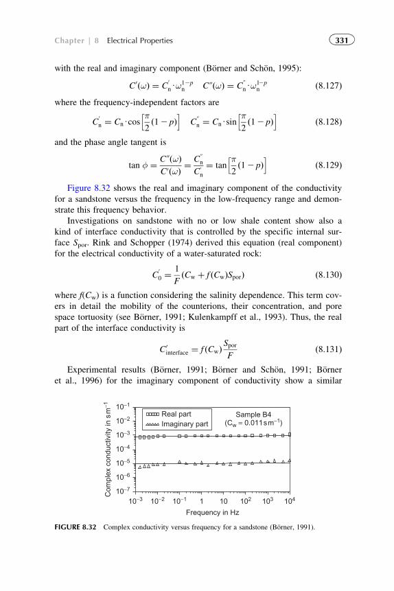
with the real and imaginary component (Borner and Schon, 1995):
C0ðωÞ ¼ C0nUω
12pn CvðωÞ ¼ Cv
nUω12pn ð8:127Þ
where the frequency-independent factors are
C0n ¼ CnUcos
π2ð12 pÞ
h iCvn ¼ CnUsin
π2ð12 pÞ
h ið8:128Þ
and the phase angle tangent is
tan φ ¼ CvðωÞC0ðωÞ ¼
Cvn
C0n
¼ tanπ2ð12 pÞ
h ið8:129Þ
Figure 8.32 shows the real and imaginary component of the conductivity
for a sandstone versus the frequency in the low-frequency range and demon-
strate this frequency behavior.
Investigations on sandstone with no or low shale content show also a
kind of interface conductivity that is controlled by the specific internal sur-
face Spor. Rink and Schopper (1974) derived this equation (real component)
for the electrical conductivity of a water-saturated rock:
C00 ¼
1
FðCw þ f ðCwÞSporÞ ð8:130Þ
where f(Cw) is a function considering the salinity dependence. This term cov-
ers in detail the mobility of the counterions, their concentration, and pore
space tortuosity (see Borner, 1991; Kulenkampff et al., 1993). Thus, the real
part of the interface conductivity is
C0interface ¼ f ðCwÞ
Spor
Fð8:131Þ
Experimental results (Borner, 1991; Borner and Schon, 1991; Borner
et al., 1996) for the imaginary component of conductivity show a similar
10−3 10−2 10−1 1
Frequency in Hz
10 102 103 10410−7
10−6
10−5
10−4
10−3
10−2
10−1
Com
plex
con
duct
ivity
in s
m−1
Real part Sample B4(Cw = 0.011sm−1)Imaginary part
FIGURE 8.32 Complex conductivity versus frequency for a sandstone (Borner, 1991).
331Chapter | 8 Electrical Properties
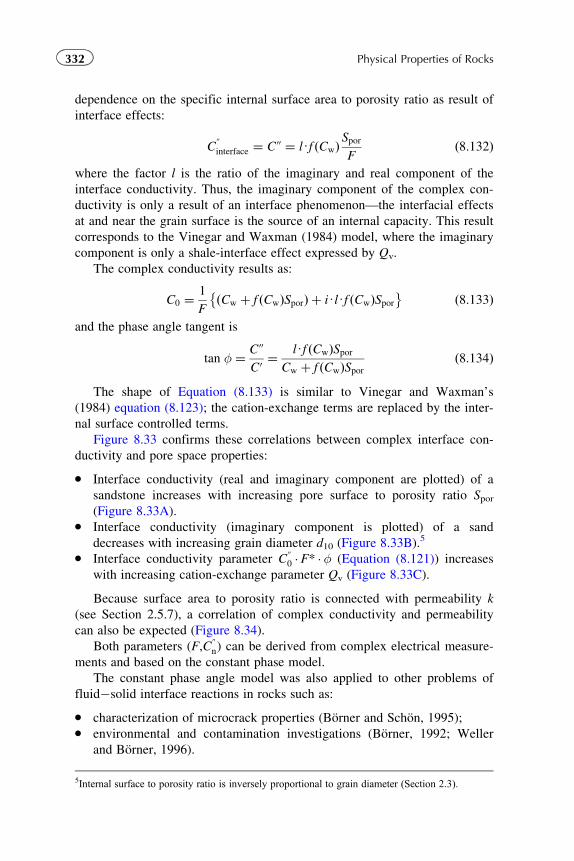
dependence on the specific internal surface area to porosity ratio as result of
interface effects:
Cvinterface ¼ Cv ¼ lUf ðCwÞ
Spor
Fð8:132Þ
where the factor l is the ratio of the imaginary and real component of the
interface conductivity. Thus, the imaginary component of the complex con-
ductivity is only a result of an interface phenomenon—the interfacial effects
at and near the grain surface is the source of an internal capacity. This result
corresponds to the Vinegar and Waxman (1984) model, where the imaginary
component is only a shale-interface effect expressed by Qv.
The complex conductivity results as:
C0 ¼1
FðCw þ f ðCwÞSporÞ þ iUlUf ðCwÞSpor� � ð8:133Þ
and the phase angle tangent is
tan φ ¼ CvC0 ¼
lUf ðCwÞSporCw þ f ðCwÞSpor
ð8:134Þ
The shape of Equation (8.133) is similar to Vinegar and Waxman’s
(1984) equation (8.123); the cation-exchange terms are replaced by the inter-
nal surface controlled terms.
Figure 8.33 confirms these correlations between complex interface con-
ductivity and pore space properties:
� Interface conductivity (real and imaginary component are plotted) of a
sandstone increases with increasing pore surface to porosity ratio Spor(Figure 8.33A).
� Interface conductivity (imaginary component is plotted) of a sand
decreases with increasing grain diameter d10 (Figure 8.33B).5
� Interface conductivity parameter Cv0 �F* �φ (Equation (8.121)) increases
with increasing cation-exchange parameter Qv (Figure 8.33C).
Because surface area to porosity ratio is connected with permeability k
(see Section 2.5.7), a correlation of complex conductivity and permeability
can also be expected (Figure 8.34).
Both parameters (F,Cvn) can be derived from complex electrical measure-
ments and based on the constant phase model.
The constant phase angle model was also applied to other problems of
fluid�solid interface reactions in rocks such as:
� characterization of microcrack properties (Borner and Schon, 1995);� environmental and contamination investigations (Borner, 1992; Weller
and Borner, 1996).
5Internal surface to porosity ratio is inversely proportional to grain diameter (Section 2.3).
332 Physical Properties of Rocks
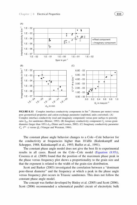
The constant phase angle behavior changes to a Cole�Cole behavior for
the conductivity at frequencies higher than 10 kHz (Kulenkampff and
Schopper, 1988; Kulenkampff et al., 1993; Ruffet et al., 1991).
The constant phase angle model does not give the best fit to experimental
results in all cases. Based on the Cole�Cole model (Equation (8.95)),
Cosenza et al. (2009) found that the position of the maximum phase peak in
the phase versus frequency plot shows a proportionality to the grain size and
that the exponent is related to the width of the grain-size distribution.
Scott and Barker (2003) investigated the correlation between a “dominant
pore-throat diameter” and the frequency at which a peak in the phase angle
versus frequency plot occurs in Triassic sandstones. This does not follow the
constant phase angle model.
The concept was further developed by Binley et al. (2005) and Scott (2006).
Scott (2006) recommended a schematical parallel circuit of electrolytic bulk
1.E − 07
1.E − 06
1.E − 05
1.E − 04
1.E − 03
1.E − 02
(A)
(B) (C)
1.E − 02 1.E − 01 1.E + 00 1.E + 01 1.E + 02
Spor in µm−1
Inte
rfac
e co
nduc
tivity
in S
m−1
Real component
Imaginary component
0.0E + 00
1.0E − 03
2.0E − 03
3.0E − 03
4.0E − 03
5.0E − 03
6.0E − 03
0.0 0.2 0.4 0.6 0.8 1.0
Qv in meqcm−3
C''
F*
in
Sm
−1
1.E − 07
1.E − 06
1.E − 05
1.E − 04
1.E − 03
1.E − 02
1.E − 04
1.E − 03
1.E − 02
1.E − 01
1.E + 00
d10 in mm
Imag
inar
y co
nduc
tivity
in S
m−1
Φ
FIGURE 8.33 Complex interface conductivity components in Sm21 (Siemens per meter) versus
pore geometrical properties and cation-exchange parameter (replotted, units converted). (A)
Complex interface conductivity (real and imaginary component) versus pore surface to porosity
ratio Spor for sandstones (Borner, 1992). (B) Imaginary conductivity component Cv0 versus grain
diameter (larger than 10%) d10 (Slater and Lesmes, 2002). (C) Imaginary conductivity parameter
Cv0 �F* �φ versus Qv (Vinegar and Waxman, 1984).
333Chapter | 8 Electrical Properties
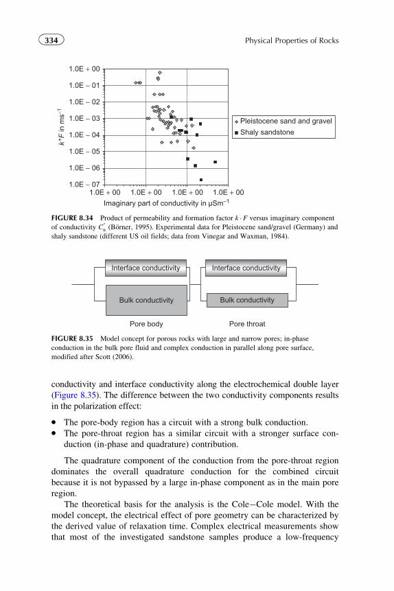
conductivity and interface conductivity along the electrochemical double layer
(Figure 8.35). The difference between the two conductivity components results
in the polarization effect:
� The pore-body region has a circuit with a strong bulk conduction.� The pore-throat region has a similar circuit with a stronger surface con-
duction (in-phase and quadrature) contribution.
The quadrature component of the conduction from the pore-throat region
dominates the overall quadrature conduction for the combined circuit
because it is not bypassed by a large in-phase component as in the main pore
region.
The theoretical basis for the analysis is the Cole�Cole model. With the
model concept, the electrical effect of pore geometry can be characterized by
the derived value of relaxation time. Complex electrical measurements show
that most of the investigated sandstone samples produce a low-frequency
Interface conductivity
Bulk conductivity
Interface conductivity
Bulk conductivity
Pore body Pore throat
FIGURE 8.35 Model concept for porous rocks with large and narrow pores; in-phase
conduction in the bulk pore fluid and complex conduction in parallel along pore surface,
modified after Scott (2006).
1.0E − 07
1.0E − 06
1.0E − 05
1.0E − 04
1.0E − 03
1.0E − 02
1.0E − 01
1.0E + 00
1.0E + 00 1.0E + 00 1.0E + 00 1.0E + 00
Imaginary part of conductivity in µSm−1
k*F
in m
s−1
Pleistocene sand and gravel
Shaly sandstone
FIGURE 8.34 Product of permeability and formation factor k �F versus imaginary component
of conductivity Cvn (Borner, 1995). Experimental data for Pleistocene sand/gravel (Germany) and
shaly sandstone (different US oil fields; data from Vinegar and Waxman, 1984).
334 Physical Properties of Rocks
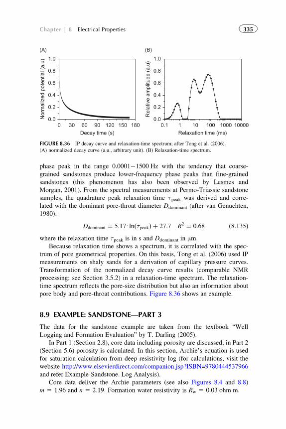
phase peak in the range 0.0001�1500 Hz with the tendency that coarse-
grained sandstones produce lower-frequency phase peaks than fine-grained
sandstones (this phenomenon has also been observed by Lesmes and
Morgan, 2001). From the spectral measurements at Permo-Triassic sandstone
samples, the quadrature peak relaxation time τpeak was derived and corre-
lated with the dominant pore-throat diameter Ddominant (after van Genuchten,
1980):
Ddominant ¼ 5:17UlnðτpeakÞ þ 27:7 R2 ¼ 0:68 ð8:135Þwhere the relaxation time τpeak is in s and Ddominant in μm.
Because relaxation time shows a spectrum, it is correlated with the spec-
trum of pore geometrical properties. On this basis, Tong et al. (2006) used IP
measurements on shaly sands for a derivation of capillary pressure curves.
Transformation of the normalized decay curve results (comparable NMR
processing; see Section 3.5.2) in a relaxation-time spectrum. The relaxation-
time spectrum reflects the pore-size distribution but also an information about
pore body and pore-throat contributions. Figure 8.36 shows an example.
8.9 EXAMPLE: SANDSTONE—PART 3
The data for the sandstone example are taken from the textbook “Well
Logging and Formation Evaluation” by T. Darling (2005).
In Part 1 (Section 2.8), core data including porosity are discussed; in Part 2
(Section 5.6) porosity is calculated. In this section, Archie’s equation is used
for saturation calculation from deep resistivity log (for calculations, visit the
website http://www.elsevierdirect.com/companion.jsp?ISBN=9780444537966
and refer Example-Sandstone. Log Analysis).
Core data deliver the Archie parameters (see also Figures 8.4 and 8.8)
m 5 1.96 and n 5 2.19. Formation water resistivity is Rw 5 0.03 ohm m.
1.0
(A) (B)
Nor
mal
ized
pot
entia
l (a.
u)
0.8
0.6
0.4
0.2
0.00 30 60 90
Decay time (s)120 150 180
1.0
Rel
ativ
e am
plitu
de (
a.u)
0.8
0.6
0.4
0.2
0.00.1 1 10 100 1000
Relaxation time (ms)10000
FIGURE 8.36 IP decay curve and relaxation-time spectrum; after Tong et al. (2006).
(A) normalized decay curve (a.u., arbitrary unit). (B) Relaxation-time spectrum.
335Chapter | 8 Electrical Properties
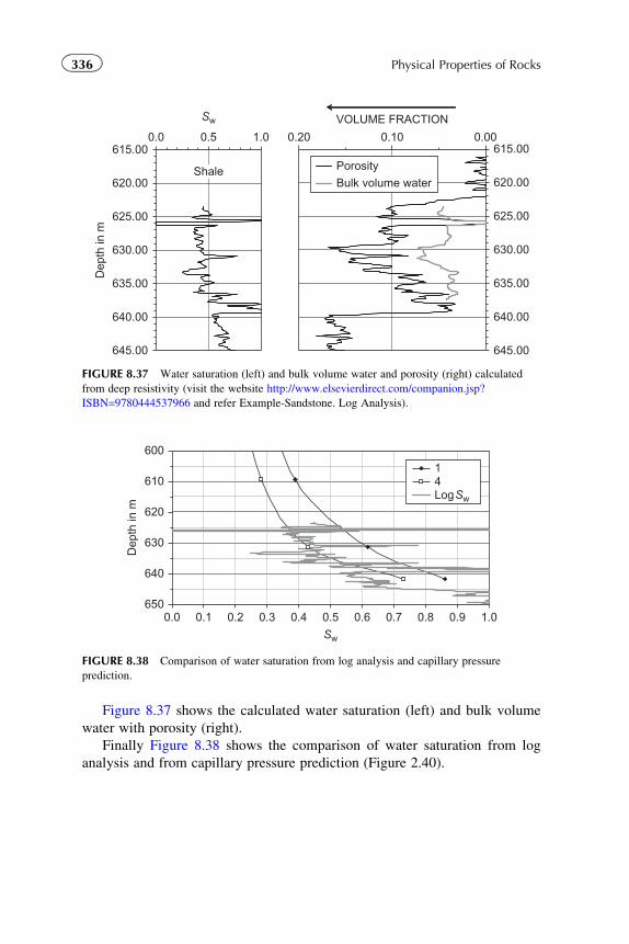
Figure 8.37 shows the calculated water saturation (left) and bulk volume
water with porosity (right).
Finally Figure 8.38 shows the comparison of water saturation from log
analysis and from capillary pressure prediction (Figure 2.40).
615.00
620.00
625.00
630.00
635.00
640.00
645.00
0.000.100.20
VOLUME FRACTION
PorosityBulk volume water
615.00
620.00
625.00
630.00
635.00
640.00
645.00
0.0 0.5 1.0
Sw
Dep
th in
m
Shale
FIGURE 8.37 Water saturation (left) and bulk volume water and porosity (right) calculated
from deep resistivity (visit the website http://www.elsevierdirect.com/companion.jsp?
ISBN=9780444537966 and refer Example-Sandstone. Log Analysis).
600
610
620
630
640
6500.0 0.1 0.2 0.3 0.4 0.5 0.6 0.7 0.8 0.9 1.0
Sw
Dep
th in
m
14LogSw
FIGURE 8.38 Comparison of water saturation from log analysis and capillary pressure
prediction.
336 Physical Properties of Rocks
Chapter 9
Thermal Properties
9.1 INTRODUCTION
To understand the thermal structure of the earth, knowledge of the thermal properties
of the material that constitutes the interior of the earth is indispensable.
Ki-Iti Horai (1971)
Geothermal investigations are related to many questions in geoscience,
ranging from studies of the physical state of the earth, tectonics, seismicity,
and volcanism to practical problems in mining, drilling, geothermal resources,
and geothermal methods used in exploration and environmental geophysics.
Three thermal properties are of fundamental interest in geothermal
investigations:
1. specific heat capacity cp;
2. thermal conductivity λ;3. thermal diffusivity a.
Specific heat capacity characterizes the capability of a material to store
heat. Specific heat capacity is given in J kg21 K21 5 m2 s22 K21 and is
defined as the ratio of the heat input Q to the product of the mass m and the
resulting temperature increase ΔT:
cp ¼ Q
mUΔTð9:1Þ
where the subscript p indicates specific heat capacity at constant pressure.
Thermal conductivity characterizes the heat flow density q as result of a
temperature gradient gradT (Fourier’s law):
q ¼ 2λUgrad T ¼ 2λU@T
@xð9:2Þ
337Physical Properties of Rocks.
© 2011 Elsevier B.V. All rights reserved.
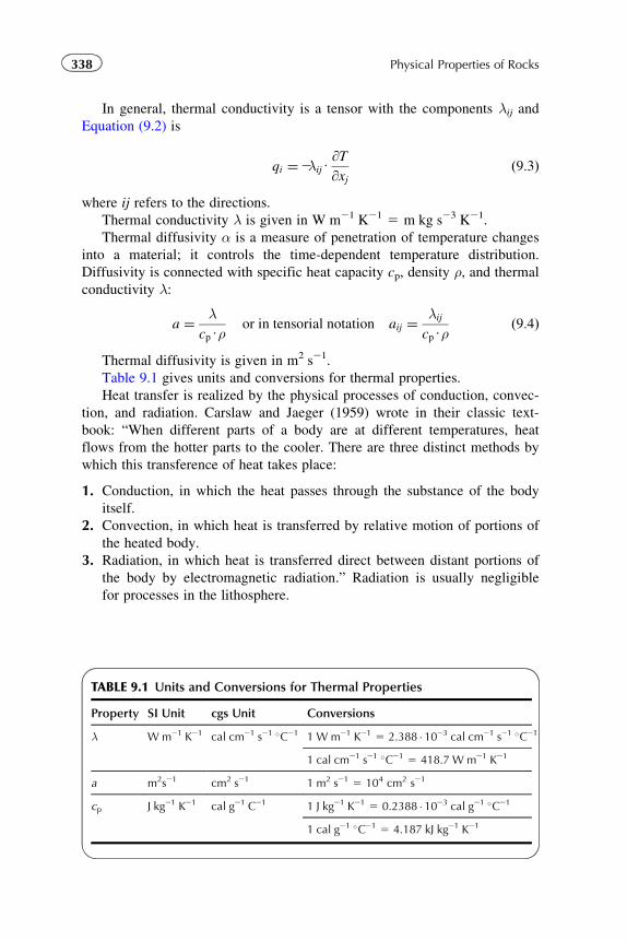
In general, thermal conductivity is a tensor with the components λij andEquation (9.2) is
qi ¼2λijU@T
@xjð9:3Þ
where ij refers to the directions.
Thermal conductivity λ is given in W m21 K21 5 m kg s23 K21.
Thermal diffusivity α is a measure of penetration of temperature changes
into a material; it controls the time-dependent temperature distribution.
Diffusivity is connected with specific heat capacity cp, density ρ, and thermal
conductivity λ:
a ¼ λcpUρ
or in tensorial notation aij ¼λij
cpUρð9:4Þ
Thermal diffusivity is given in m2 s21.
Table 9.1 gives units and conversions for thermal properties.
Heat transfer is realized by the physical processes of conduction, convec-
tion, and radiation. Carslaw and Jaeger (1959) wrote in their classic text-
book: “When different parts of a body are at different temperatures, heat
flows from the hotter parts to the cooler. There are three distinct methods by
which this transference of heat takes place:
1. Conduction, in which the heat passes through the substance of the body
itself.
2. Convection, in which heat is transferred by relative motion of portions of
the heated body.
3. Radiation, in which heat is transferred direct between distant portions of
the body by electromagnetic radiation.” Radiation is usually negligible
for processes in the lithosphere.
TABLE 9.1 Units and Conversions for Thermal Properties
Property SI Unit cgs Unit Conversions
λ Wm21 K21 cal cm21 s21 �C21 1 W m21 K21 5 2.388 � 1023 cal cm21 s21 �C21
1 cal cm21 s21 �C21 5 418.7 W m21 K21
a m2s21 cm2 s21 1 m2 s21 5 104 cm2 s21
cp J kg21 K21 cal g21 C21 1 J kg21 K21 5 0.2388 � 1023 cal g21 �C21
1 cal g21 �C21 5 4.187 kJ kg21 K21
338 Physical Properties of Rocks
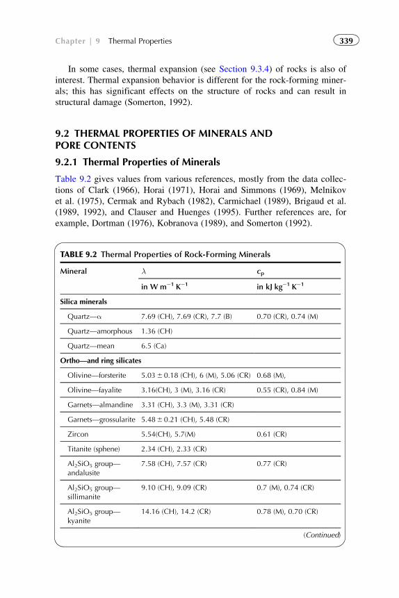
In some cases, thermal expansion (see Section 9.3.4) of rocks is also of
interest. Thermal expansion behavior is different for the rock-forming miner-
als; this has significant effects on the structure of rocks and can result in
structural damage (Somerton, 1992).
9.2 THERMAL PROPERTIES OF MINERALS ANDPORE CONTENTS
9.2.1 Thermal Properties of Minerals
Table 9.2 gives values from various references, mostly from the data collec-
tions of Clark (1966), Horai (1971), Horai and Simmons (1969), Melnikov
et al. (1975), Cermak and Rybach (1982), Carmichael (1989), Brigaud et al.
(1989, 1992), and Clauser and Huenges (1995). Further references are, for
example, Dortman (1976), Kobranova (1989), and Somerton (1992).
TABLE 9.2 Thermal Properties of Rock-Forming Minerals
Mineral λ cp
in W m21 K21 in kJ kg21 K21
Silica minerals
Quartz—α 7.69 (CH), 7.69 (CR), 7.7 (B) 0.70 (CR), 0.74 (M)
Quartz—amorphous 1.36 (CH)
Quartz—mean 6.5 (Ca)
Ortho—and ring silicates
Olivine—forsterite 5.0360.18 (CH), 6 (M), 5.06 (CR) 0.68 (M),
Olivine—fayalite 3.16(CH), 3 (M), 3.16 (CR) 0.55 (CR), 0.84 (M)
Garnets—almandine 3.31 (CH), 3.3 (M), 3.31 (CR)
Garnets—grossularite 5.4860.21 (CH), 5.48 (CR)
Zircon 5.54(CH), 5.7(M) 0.61 (CR)
Titanite (sphene) 2.34 (CH), 2.33 (CR)
Al2SiO5 group—andalusite
7.58 (CH), 7.57 (CR) 0.77 (CR)
Al2SiO5 group—sillimanite
9.10 (CH), 9.09 (CR) 0.7 (M), 0.74 (CR)
Al2SiO5 group—kyanite
14.16 (CH), 14.2 (CR) 0.78 (M), 0.70 (CR)
(Continued)
339Chapter | 9 Thermal Properties
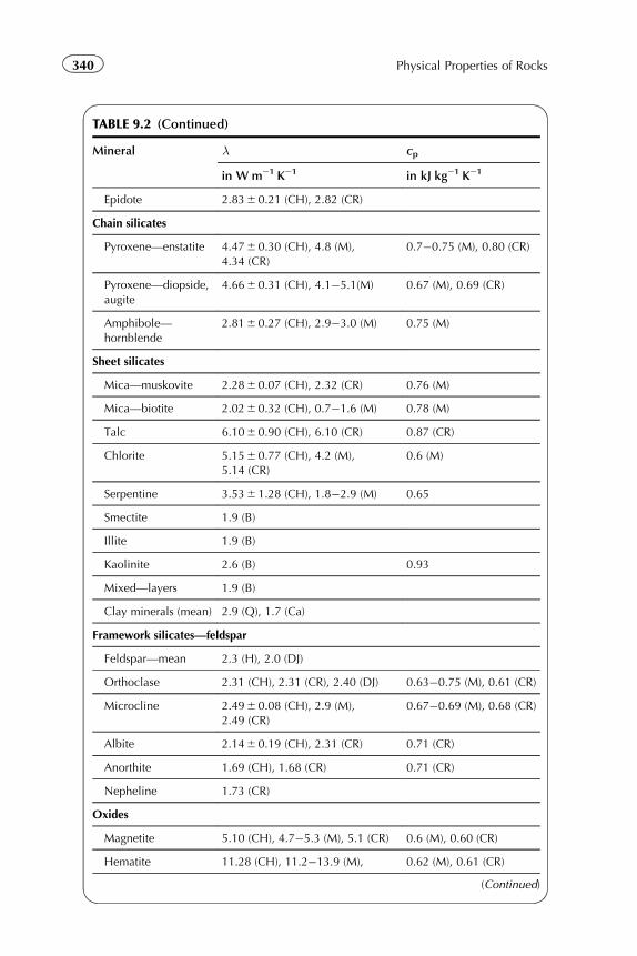
TABLE 9.2 (Continued)
Mineral λ cp
in W m21 K21 in kJ kg21 K21
Epidote 2.836 0.21 (CH), 2.82 (CR)
Chain silicates
Pyroxene—enstatite 4.476 0.30 (CH), 4.8 (M),4.34 (CR)
0.7�0.75 (M), 0.80 (CR)
Pyroxene—diopside,augite
4.666 0.31 (CH), 4.1�5.1(M) 0.67 (M), 0.69 (CR)
Amphibole—hornblende
2.816 0.27 (CH), 2.9�3.0 (M) 0.75 (M)
Sheet silicates
Mica—muskovite 2.286 0.07 (CH), 2.32 (CR) 0.76 (M)
Mica—biotite 2.026 0.32 (CH), 0.7�1.6 (M) 0.78 (M)
Talc 6.106 0.90 (CH), 6.10 (CR) 0.87 (CR)
Chlorite 5.156 0.77 (CH), 4.2 (M),5.14 (CR)
0.6 (M)
Serpentine 3.536 1.28 (CH), 1.8�2.9 (M) 0.65
Smectite 1.9 (B)
Illite 1.9 (B)
Kaolinite 2.6 (B) 0.93
Mixed—layers 1.9 (B)
Clay minerals (mean) 2.9 (Q), 1.7 (Ca)
Framework silicates—feldspar
Feldspar—mean 2.3 (H), 2.0 (DJ)
Orthoclase 2.31 (CH), 2.31 (CR), 2.40 (DJ) 0.63�0.75 (M), 0.61 (CR)
Microcline 2.496 0.08 (CH), 2.9 (M),2.49 (CR)
0.67�0.69 (M), 0.68 (CR)
Albite 2.146 0.19 (CH), 2.31 (CR) 0.71 (CR)
Anorthite 1.69 (CH), 1.68 (CR) 0.71 (CR)
Nepheline 1.73 (CR)
Oxides
Magnetite 5.10 (CH), 4.7�5.3 (M), 5.1 (CR) 0.6 (M), 0.60 (CR)
Hematite 11.28 (CH), 11.2�13.9 (M), 0.62 (M), 0.61 (CR)
(Continued)
340 Physical Properties of Rocks
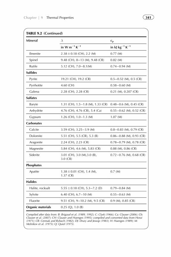
TABLE 9.2 (Continued)
Mineral λ cp
in W m21 K21 in kJ kg21 K21
Ilmenite 2.386 0.18 (CH), 2.2 (M) 0.77 (M)
Spinel 9.48 (CH), 8�13 (M), 9.48 (CR) 0.82 (M)
Rutile 5.12 (CH), 7.0�8.1(M) 0.74�0.94 (M)
Sulfides
Pyrite 19.21 (CH), 19.2 (CR) 0.5�0.52 (M), 0.5 (CR)
Pyrrhotite 4.60 (CH) 0.58�0.60 (M)
Galena 2.28 (CH), 2.28 (CR) 0.21 (M), 0.207 (CR)
Sulfates
Baryte 1.31 (CH), 1.5�1.8 (M), 1.33 (CR) 0.48�0.6 (M), 0.45 (CR)
Anhydrite 4.76 (CH), 4.76 (CR), 5.4 (Ca) 0.55�0.62 (M), 0.52 (CR)
Gypsum 1.26 (CH), 1.0�1.3 (M) 1.07 (M)
Carbonates
Calcite 3.59 (CH), 3.25�3.9 (M) 0.8�0.83 (M), 0.79 (CR)
Dolomite 5.51 (CH), 5.5 (CR), 5.3 (B) 0.86�0.88 (M), 0.93 (CR)
Aragonite 2.24 (CH), 2.23 (CR) 0.78�0.79 (M), 0.78 (CR)
Magnesite 5.84 (CH), 4.6 (M), 5.83 (CR) 0.88 (M), 0.86 (CR)
Siderite 3.01 (CH), 3.0 (M),3.0 (B),3.0 (CR)
0.72�0.76 (M), 0.68 (CR)
Phosphates
Apatite 1.386 0.01 (CH), 1.4 (M),1.37 (CR)
0.7 (M)
Halides
Halite, rocksalt 5.556 0.18 (CH), 5.3�7.2 (D) 0.79�0.84 (M)
Sylvite 6.40 (CH), 6.7�10 (M) 0.55�0.63 (M)
Fluorite 9.51 (CH), 9�10.2 (M), 9.5 (CR) 0.9 (M), 0.85 (CR)
Organic materials 0.25 (Q), 1.0 (B)
Compiled after data from: B: Brigaud et al. (1989, 1992); C: Clark (1966); Ca: Clauser (2006); Cb:Clauser et al. (2007); CH: Clauser and Huenges (1995); compiled and converted data from Horai(1971); CR: Cermak and Rybach (1982); DJ: Drury and Jessop (1983); H: Huenges (1989); M:Melnikov et al. (1975); Q: Quiel (1975).
341Chapter | 9 Thermal Properties
Among the rock-forming minerals, quartz has a high thermal conductiv-
ity. Ore minerals and some accessories (rutile, spinel) have extremely high
values of thermal conductivity.
Low values are found among the mineral group of mica (biotite), nephe-
line, and polyhalite. This originates the dependence of thermal conductivity
on mineral composition of rocks (see Section 9.3.2).
Griffith et al. (1992) and Rzhewski and Novik (1971) note that there is a
difference of the conductivity values between monocrystal, polycrystal, and
fused minerals. For quartz in particular, they report a variation between a
maximum of 11.7 W m21 K21 (monocrystalline), through 3.6 W m21 K21
(polycrystalline), to 1.39 W m21 K21 (fused). The difference between mono-
and polycrystalline results from intergrain contact effects.
The situation in carbonates is comparable: for a model study, Clauser
et al. (2007) recommended 2.8 W m21 K21 for calcite and 3.9 W m21 K21
for dolomite, which are distinctly lower as the “crystal” values in
Table 9.2.
Thermal conductivity is a temperature-dependent property. The character
of this temperature dependence is controlled by the material structure:
� Crystalline solid materials with lattice conductivity are characterized by a
decrease of conductivity with temperature based on Debye’s theory.� Amorphous materials (such as glasses) as well as feldspars are character-
ized by an increase of thermal conductivity with increasing temperature.
This can be demonstrated by the behavior of quartz (Cermak and
Rybach, 1982):
λ ¼ 1
0:1450þ 0:578U1023UTcrystalline quartz ð0�C to 120�CÞ ð9:5Þ
λ ¼ 1:323þ 0:00193UT2 0:67U1025UT2 fused quartz ð2150�C to 60�CÞð9:6Þ
9.2.2 Thermal Properties of Fluids
Table 9.3 shows thermal properties of some pore fluids. There is a strong
difference between the most abundant types—water, oil, and gas.
The table also shows the influence of the temperature upon thermal prop-
erties. Kaye and Laby (1968) (see Griffiths et al., 1992) derived the follow-
ing relationship for thermal conductivity of water:
λwater ¼ 0:56þ 0:002UT 2 1:01U1025UT2 þ 6:71U1029UT3 ð9:7Þwhere thermal conductivity λ is in W m21 K21 and temperature T is in �C.
The influence of pressure on thermal properties of fluids is relatively
small compared with the influence of temperature.
342 Physical Properties of Rocks
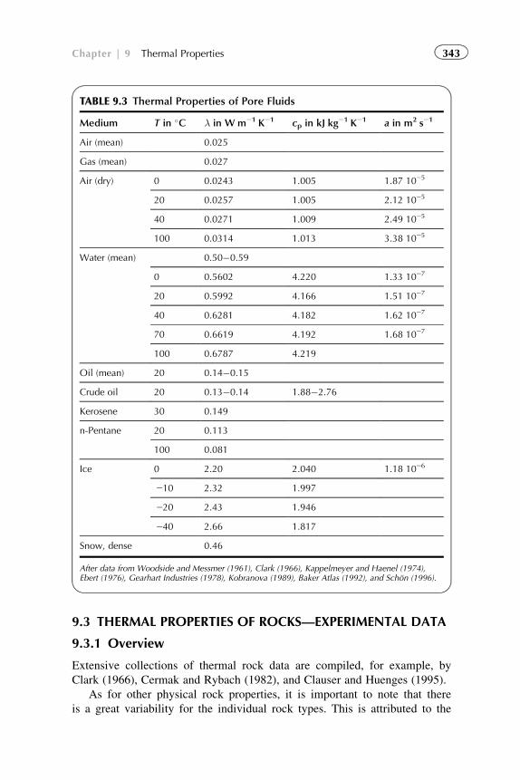
9.3 THERMAL PROPERTIES OF ROCKS—EXPERIMENTAL DATA
9.3.1 Overview
Extensive collections of thermal rock data are compiled, for example, by
Clark (1966), Cermak and Rybach (1982), and Clauser and Huenges (1995).
As for other physical rock properties, it is important to note that there
is a great variability for the individual rock types. This is attributed to the
TABLE 9.3 Thermal Properties of Pore Fluids
Medium T in �C λ in W m21 K21 cp in kJ kg21 K21 a in m2 s21
Air (mean) 0.025
Gas (mean) 0.027
Air (dry) 0 0.0243 1.005 1.87 1025
20 0.0257 1.005 2.12 1025
40 0.0271 1.009 2.49 1025
100 0.0314 1.013 3.38 1025
Water (mean) 0.50�0.59
0 0.5602 4.220 1.33 1027
20 0.5992 4.166 1.51 1027
40 0.6281 4.182 1.62 1027
70 0.6619 4.192 1.68 1027
100 0.6787 4.219
Oil (mean) 20 0.14�0.15
Crude oil 20 0.13�0.14 1.88�2.76
Kerosene 30 0.149
n-Pentane 20 0.113
100 0.081
Ice 0 2.20 2.040 1.18 1026
210 2.32 1.997
220 2.43 1.946
240 2.66 1.817
Snow, dense 0.46
After data from Woodside and Messmer (1961), Clark (1966), Kappelmeyer and Haenel (1974),Ebert (1976), Gearhart Industries (1978), Kobranova (1989), Baker Atlas (1992), and Schon (1996).
343Chapter | 9 Thermal Properties
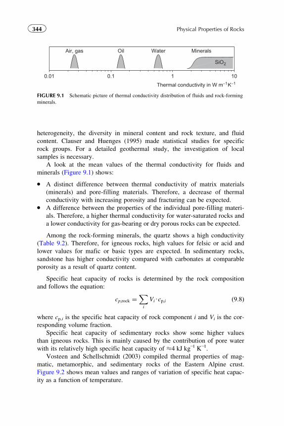
heterogeneity, the diversity in mineral content and rock texture, and fluid
content. Clauser and Huenges (1995) made statistical studies for specific
rock groups. For a detailed geothermal study, the investigation of local
samples is necessary.
A look at the mean values of the thermal conductivity for fluids and
minerals (Figure 9.1) shows:
� A distinct difference between thermal conductivity of matrix materials
(minerals) and pore-filling materials. Therefore, a decrease of thermal
conductivity with increasing porosity and fracturing can be expected.� A difference between the properties of the individual pore-filling materi-
als. Therefore, a higher thermal conductivity for water-saturated rocks and
a lower conductivity for gas-bearing or dry porous rocks can be expected.
Among the rock-forming minerals, the quartz shows a high conductivity
(Table 9.2). Therefore, for igneous rocks, high values for felsic or acid and
lower values for mafic or basic types are expected. In sedimentary rocks,
sandstone has higher conductivity compared with carbonates at comparable
porosity as a result of quartz content.
Specific heat capacity of rocks is determined by the rock composition
and follows the equation:
cp;rock ¼Xi
ViUcp;i ð9:8Þ
where cp,i is the specific heat capacity of rock component i and Vi is the cor-
responding volume fraction.
Specific heat capacity of sedimentary rocks show some higher values
than igneous rocks. This is mainly caused by the contribution of pore water
with its relatively high specific heat capacity of �4 kJ kg21 K21.
Vosteen and Schellschmidt (2003) compiled thermal properties of mag-
matic, metamorphic, and sedimentary rocks of the Eastern Alpine crust.
Figure 9.2 shows mean values and ranges of variation of specific heat capac-
ity as a function of temperature.
Air, gas Oil MineralsWater
0.01 0.1 1 10
Thermal conductivity in W m−1K−1
SiO2
FIGURE 9.1 Schematic picture of thermal conductivity distribution of fluids and rock-forming
minerals.
344 Physical Properties of Rocks
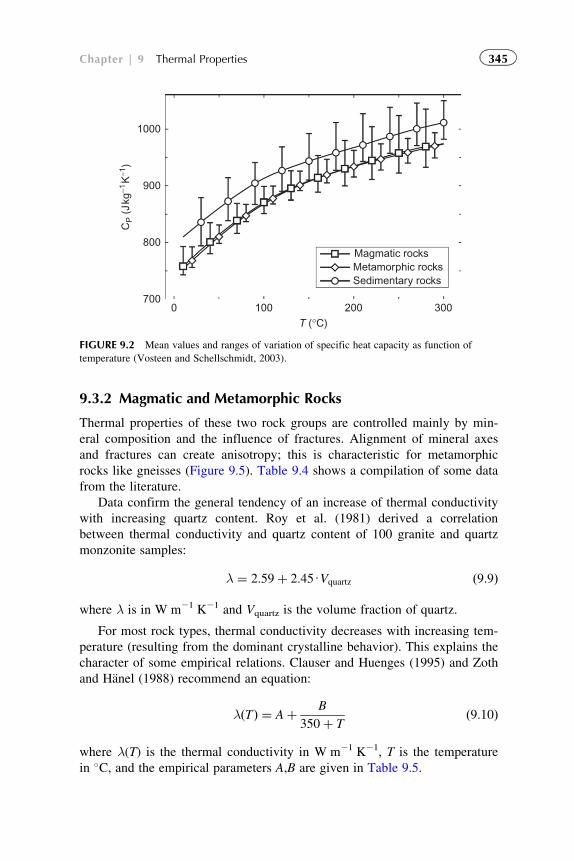
9.3.2 Magmatic and Metamorphic Rocks
Thermal properties of these two rock groups are controlled mainly by min-
eral composition and the influence of fractures. Alignment of mineral axes
and fractures can create anisotropy; this is characteristic for metamorphic
rocks like gneisses (Figure 9.5). Table 9.4 shows a compilation of some data
from the literature.
Data confirm the general tendency of an increase of thermal conductivity
with increasing quartz content. Roy et al. (1981) derived a correlation
between thermal conductivity and quartz content of 100 granite and quartz
monzonite samples:
λ ¼ 2:59þ 2:45UVquartz ð9:9Þ
where λ is in W m21 K21 and Vquartz is the volume fraction of quartz.
For most rock types, thermal conductivity decreases with increasing tem-
perature (resulting from the dominant crystalline behavior). This explains the
character of some empirical relations. Clauser and Huenges (1995) and Zoth
and Hanel (1988) recommend an equation:
λðTÞ ¼ Aþ B
350þ Tð9:10Þ
where λ(T) is the thermal conductivity in W m21 K21, T is the temperature
in �C, and the empirical parameters A,B are given in Table 9.5.
Magmatic rocksMetamorphic rocksSedimentary rocks
0700
100T (°C)
200 300
800
900
1000C
P (
Jkg
−1K
−1)
FIGURE 9.2 Mean values and ranges of variation of specific heat capacity as function of
temperature (Vosteen and Schellschmidt, 2003).
345Chapter | 9 Thermal Properties
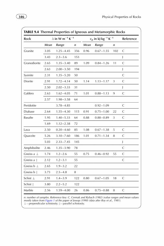
TABLE 9.4 Thermal Properties of Igneous and Metamorphic Rocks
Rock λ in W m21 K21 cp in kJ kg21 K21 Reference
Mean Range n Mean Range n
Granite 3.05 1.25�4.45 356 0.96 0.67�1.55 102 C
3.43 2.3�3.6 153 J
Granodiorite 2.65 1.35�3.40 89 1.09 0.84�1.26 11 C
2.63 2.00�3.50 194 J
Syenite 2.31 1.35�5.20 50 C
Diorite 2.91 1.72�4.14 50 1.14 1.13�1.17 3 C
2.50 2.02�3.33 31 J
Gabbro 2.63 1.62�4.05 71 1.01 0.88�1.13 9 C
2.57 1.98�3.58 64
Peridotite 3.78�4.85 0.92�1.09 C
Diabase 2.64 1.55�4.30 115 0.91 0.75�1.00 22 C
Basalte 1.95 1.40�5.33 64 0.88 0.88�0.89 3 C
1.69 1.12�2.38 72
Lava 2.50 0.20�4.60 85 1.08 0.67�1.38 5 C
Quarzite 5.26 3.10�7.60 186 1.01 0.71�1.34 8 C
5.03 2.33�7.45 145 J
Amphibolite 2.46 1.35�3.90 78 C
Gneiss a > 1.74 1.2�2.6 55 0.75 0.46�0.92 55 C
Gneiss a 8 2.12 1.2�3.1 55 C
Gneiss b > 2.65 1.9�3.2 22
Gneiss b 8 3.73 2.5�4.8 8
Schist > 2.91 1.4�3.9 122 0.80 0.67�1.05 18 C
Schist 8 3.80 2.2�5.2 122
Marble 2.56 1.59�4.00 26 0.86 0.75�0.88 8 C
n: number of samples. Reference key: C, Cermak and Rybach (1982) (value ranges and mean valuesmostly taken from Figure 1 of the paper of Jessop (1990) (data after Roy et al., 1981).>—perpendicular schistosity; 8—parallel schistosity.
346 Physical Properties of Rocks
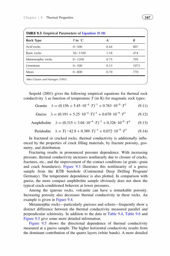
Seipold (2001) gives the following empirical equations for thermal rock
conductivity λ as function of temperature T (in K) for magmatic rock types:
Granite λ ¼ ð0:156þ 5:45U1024UTÞ21 þ 0:763U1029UT3 ð9:11Þ
Gneiss λ ¼ ð0:191þ 5:25U1024UTÞ21 þ 0:670U1029UT3 ð9:12Þ
Amphibolite λ ¼ ð0:315þ 3:04U1024UTÞ21 þ 0:326U1029UT3 ð9:13Þ
Peridodite λ ¼ Tð242:9þ 0:389UTÞ21 þ 0:072U1029UT3 ð9:14ÞIn fractured or cracked rocks, thermal conductivity is additionally influ-
enced by the properties of crack filling materials, by fracture porosity, geo-
metry, and distribution.
Fracturing results in pronounced pressure dependence. With increasing
pressure, thermal conductivity increases nonlinearly due to closure of cracks,
fractures, etc., and the improvement of the contact conditions (at grain�grain
and crack boundaries). Figure 9.3 illustrates this nonlinearity of a gneiss
sample from the KTB borehole (Continental Deep Drilling Program/
Germany). The temperature dependence is also plotted. In comparison with
gneiss, the more compact amphibolite sample obviously does not show the
typical crack-conditioned behavior at lower pressures.
Among the igneous rocks, volcanite can have a remarkable porosity.
Increasing porosity also decreases thermal conductivity in these rocks. An
example is given in Figure 9.4.
Metamorphic rocks—particularly gneisses and schists—frequently show a
distinct difference between the thermal conductivity measured parallel and
perpendicular schistosity. In addition to the data in Table 9.4, Table 9.6 and
Figure 9.5 give some more detailed information.
Figure 9.5 shows the directional dependence of thermal conductivity
measured at a gneiss sample. The higher horizontal conductivity results from
the dominant contribution of the quartz layers (white bands). A more detailed
TABLE 9.5 Empirical Parameters of Equation (9.10)
Rock Type T in �C A B
Acid rocks 0�500 0.64 807
Basic rocks 50�1100 1.18 474
Metamorphic rocks 0�1200 0.75 705
Limestone 0�500 0.13 1073
Mean 0�800 0.70 770
After Clauser and Huenges (1995).
347Chapter | 9 Thermal Properties
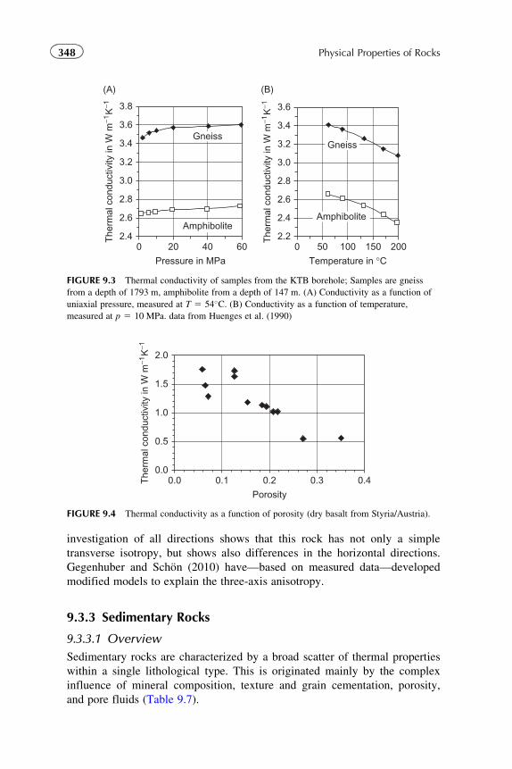
investigation of all directions shows that this rock has not only a simple
transverse isotropy, but shows also differences in the horizontal directions.
Gegenhuber and Schon (2010) have—based on measured data—developed
modified models to explain the three-axis anisotropy.
9.3.3 Sedimentary Rocks
9.3.3.1 Overview
Sedimentary rocks are characterized by a broad scatter of thermal properties
within a single lithological type. This is originated mainly by the complex
influence of mineral composition, texture and grain cementation, porosity,
and pore fluids (Table 9.7).
2.4
2.6
2.8
3.0
3.2
3.4
3.6
3.8
(A) (B)
0 0 50 100 150 20020 40 60
Pressure in MPa
The
rmal
con
duct
ivity
in W
m−1
K−1
2.2
2.4
2.6
2.8
3.0
3.2
3.4
3.6
Temperature in °CT
herm
al c
ondu
ctiv
ity in
W m
−1K
−1
AmphiboliteAmphibolite
GneissGneiss
FIGURE 9.3 Thermal conductivity of samples from the KTB borehole; Samples are gneiss
from a depth of 1793 m, amphibolite from a depth of 147 m. (A) Conductivity as a function of
uniaxial pressure, measured at T 5 54�C. (B) Conductivity as a function of temperature,
measured at p 5 10 MPa. data from Huenges et al. (1990)
0.0
0.5
1.0
1.5
2.0
0.0 0.1 0.2 0.3 0.4
Porosity
The
rmal
con
duct
ivity
in W
m−1
K−1
FIGURE 9.4 Thermal conductivity as a function of porosity (dry basalt from Styria/Austria).
348 Physical Properties of Rocks
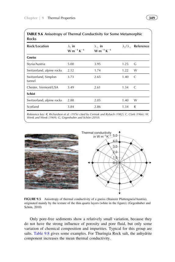
Only pore-free sediments show a relatively small variation, because they
do not have the strong influence of porosity and pore fluid, but only some
variation of chemical composition and impurities. Typical for this group are
salts. Table 9.8 gives some examples. For Thuringia Rock salt, the anhydrite
component increases the mean thermal conductivity.
TABLE 9.6 Anisotropy of Thermal Conductivity for Some Metamorphic
Rocks
Rock/Location λ8 inW m21 K21
λ> in
W m21 K21
λ8/λ> Reference
Gneiss
Styria/Austria 5.00 3.95 1.25 G
Switzerland, alpine rocks 2.12 1.74 1.22 W
Switzerland, Simplontunnel
3.73 2.65 1.40 C
Chester, Vermont/USA 3.49 2.61 1.34 C
Schist
Switzerland, alpine rocks 2.88 2.05 1.40 W
Scotland 3.84 2.86 1.34 R
Reference key: R, Richardson et al. (1976) cited by Cermak and Rybach (1982); C, Clark (1966); W,Wenk and Wenk (1969); G, Gegenhuber and Schon (2010).
0.0
1.0
2.0
3.0
4.0
5.0Thermal conductivity
in W m−1K−1
FIGURE 9.5 Anisotropy of thermal conductivity of a gneiss (Stainzer Plattengneis/Austria),
originated mainly by the texture of the thin quartz layers (white in the figure); (Gegenhuber and
Schon, 2010)
349Chapter | 9 Thermal Properties
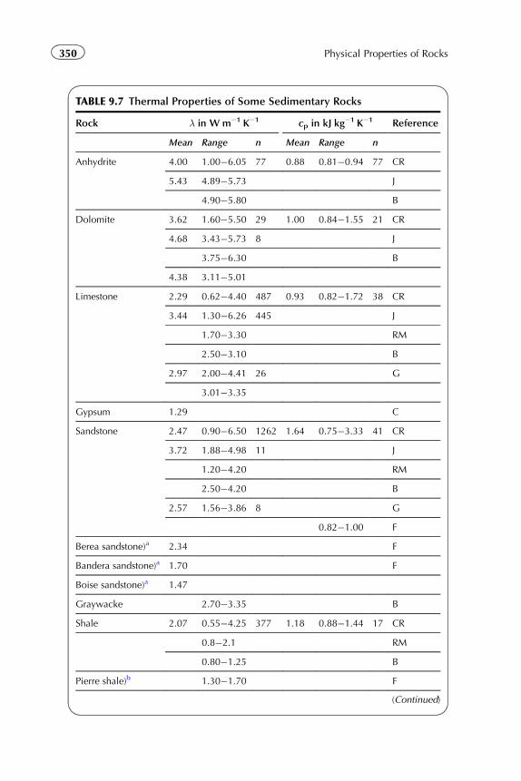
TABLE 9.7 Thermal Properties of Some Sedimentary Rocks
Rock λ in W m21 K21 cp in kJ kg21 K21 Reference
Mean Range n Mean Range n
Anhydrite 4.00 1.00�6.05 77 0.88 0.81�0.94 77 CR
5.43 4.89�5.73 J
4.90�5.80 B
Dolomite 3.62 1.60�5.50 29 1.00 0.84�1.55 21 CR
4.68 3.43�5.73 8 J
3.75�6.30 B
4.38 3.11�5.01
Limestone 2.29 0.62�4.40 487 0.93 0.82�1.72 38 CR
3.44 1.30�6.26 445 J
1.70�3.30 RM
2.50�3.10 B
2.97 2.00�4.41 26 G
3.01�3.35
Gypsum 1.29 C
Sandstone 2.47 0.90�6.50 1262 1.64 0.75�3.33 41 CR
3.72 1.88�4.98 11 J
1.20�4.20 RM
2.50�4.20 B
2.57 1.56�3.86 8 G
0.82�1.00 F
Berea sandstone)a 2.34 F
Bandera sandstone)a 1.70 F
Boise sandstone)a 1.47
Graywacke 2.70�3.35 B
Shale 2.07 0.55�4.25 377 1.18 0.88�1.44 17 CR
0.8�2.1 RM
0.80�1.25 B
Pierre shale)b 1.30�1.70 F
(Continued)
350 Physical Properties of Rocks
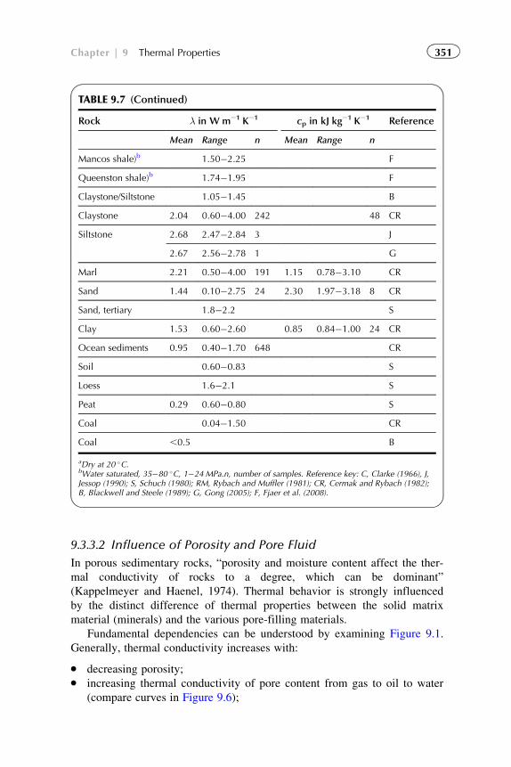
9.3.3.2 Influence of Porosity and Pore Fluid
In porous sedimentary rocks, “porosity and moisture content affect the ther-
mal conductivity of rocks to a degree, which can be dominant”
(Kappelmeyer and Haenel, 1974). Thermal behavior is strongly influenced
by the distinct difference of thermal properties between the solid matrix
material (minerals) and the various pore-filling materials.
Fundamental dependencies can be understood by examining Figure 9.1.
Generally, thermal conductivity increases with:
� decreasing porosity;� increasing thermal conductivity of pore content from gas to oil to water
(compare curves in Figure 9.6);
TABLE 9.7 (Continued)
Rock λ in W m21 K21 cp in kJ kg21 K21 Reference
Mean Range n Mean Range n
Mancos shale)b 1.50�2.25 F
Queenston shale)b 1.74�1.95 F
Claystone/Siltstone 1.05�1.45 B
Claystone 2.04 0.60�4.00 242 48 CR
Siltstone 2.68 2.47�2.84 3 J
2.67 2.56�2.78 1 G
Marl 2.21 0.50�4.00 191 1.15 0.78�3.10 CR
Sand 1.44 0.10�2.75 24 2.30 1.97�3.18 8 CR
Sand, tertiary 1.8�2.2 S
Clay 1.53 0.60�2.60 0.85 0.84�1.00 24 CR
Ocean sediments 0.95 0.40�1.70 648 CR
Soil 0.60�0.83 S
Loess 1.6�2.1 S
Peat 0.29 0.60�0.80 S
Coal 0.04�1.50 CR
Coal ,0.5 B
aDry at 20 �C.bWater saturated, 35�80 �C, 1�24 MPa.n, number of samples. Reference key: C, Clarke (1966), J,Jessop (1990); S, Schuch (1980); RM, Rybach and Muffler (1981); CR, Cermak and Rybach (1982);B, Blackwell and Steele (1989); G, Gong (2005); F, Fjaer et al. (2008).
351Chapter | 9 Thermal Properties
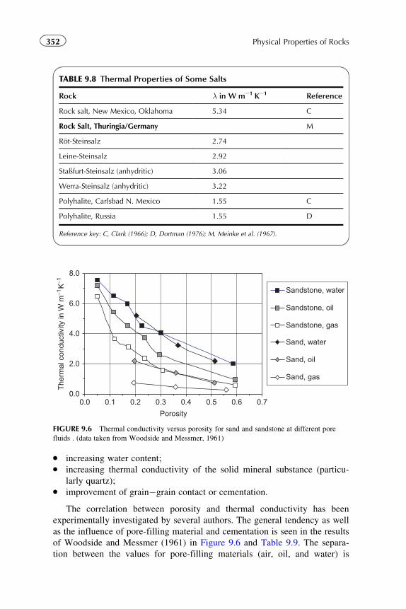
� increasing water content;� increasing thermal conductivity of the solid mineral substance (particu-
larly quartz);� improvement of grain�grain contact or cementation.
The correlation between porosity and thermal conductivity has been
experimentally investigated by several authors. The general tendency as well
as the influence of pore-filling material and cementation is seen in the results
of Woodside and Messmer (1961) in Figure 9.6 and Table 9.9. The separa-
tion between the values for pore-filling materials (air, oil, and water) is
TABLE 9.8 Thermal Properties of Some Salts
Rock λ in W m21 K21 Reference
Rock salt, New Mexico, Oklahoma 5.34 C
Rock Salt, Thuringia/Germany M
Rot-Steinsalz 2.74
Leine-Steinsalz 2.92
Staßfurt-Steinsalz (anhydritic) 3.06
Werra-Steinsalz (anhydritic) 3.22
Polyhalite, Carlsbad N. Mexico 1.55 C
Polyhalite, Russia 1.55 D
Reference key: C, Clark (1966); D, Dortman (1976); M, Meinke et al. (1967).
The
rmal
con
duct
ivity
in W
m−1
K−1
0.0
2.0
4.0
6.0
8.0
0.0 0.1 0.2 0.3 0.4 0.5 0.6 0.7
Porosity
Sandstone, water
Sandstone, oil
Sandstone, gas
Sand, water
Sand, oil
Sand, gas
FIGURE 9.6 Thermal conductivity versus porosity for sand and sandstone at different pore
fluids . (data taken from Woodside and Messmer, 1961)
352 Physical Properties of Rocks
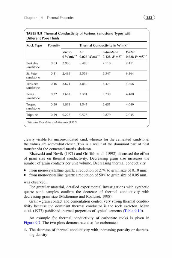
clearly visible for unconsolidated sand, whereas for the cemented sandstone,
the values are somewhat closer. This is a result of the dominant part of heat
transfer via the cemented matrix skeleton.
Rhzewski and Novik (1971) and Griffith et al. (1992) discussed the effect
of grain size on thermal conductivity. Decreasing grain size increases the
number of grain contacts per unit volume. Decreasing thermal conductivity
� from monocrystalline quartz a reduction of 27% to grain size of 0.10 mm;� from monocrystalline quartz a reduction of 50% to grain size of 0.05 mm.
was observed.
For granular material, detailed experimental investigations with synthetic
quartz sand samples confirm the decrease of thermal conductivity with
decreasing grain size (Midtomme and Roaldset, 1998).
Grain�grain contact and cementation control very strong thermal conduc-
tivity because the dominant thermal conductor is the rock skeleton. Mann
et al. (1977) published thermal properties of typical cements (Table 9.10).
An example for thermal conductivity of carbonate rocks is given in
Figure 9.7. The two plots demonstrate also for carbonates:
1. The decrease of thermal conductivity with increasing porosity or decreas-
ing density
TABLE 9.9 Thermal Conductivity of Various Sandstone Types with
Different Pore Fluids
Rock Type Porosity Thermal Conductivity in W mK21
Vacuo Air n-heptane Water
0 WmK21 0.026 WmK21 0.128 WmK21 0.628 WmK21
Berkeleysandstone
0.03 2.906 6.490 7.118 7.411
St. Petersandstone
0.11 2.495 3.559 5.347 6.364
Tensleepsandstone
0.16 2.621 3.040 4.375 5.866
Bereasandstone
0.22 1.683 2.391 3.739 4.480
Teapotsandstone
0.29 1.093 1.545 2.655 4.049
Tripolite 0.59 0.222 0.528 0.879 2.035
Data after Woodside and Messmer (1961).
353Chapter | 9 Thermal Properties
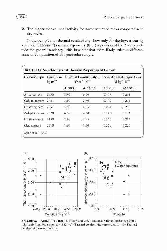
2. The higher thermal conductivity for water-saturated rocks compared with
dry rocks.
In the two plots of thermal conductivity show only for the lowest density
value (2,521 kg m23) or highest porosity (0.11) a position of the λ-value out-
side the general tendency—this is a hint that there likely exists a different
mineral composition of this particular sample.
The
rmal
con
duct
ivity
in W
m−1
K−1
The
rmal
con
duct
ivity
in W
m−1
K−1
1.50
2.00
2.50
3.00
3.50
(B)(A)
0.00 0.05 0.10 0.15
Porosity
DryWater saturated
1.50
2.00
2.50
3.00
3.50
2500 2550 2600 2650 2700
Density in kg m−3
FIGURE 9.7 Analysis of a data set for dry and water-saturated Silurian limestone samples
(Gotland) from Poulsen et al. (1982). (A) Thermal conductivity versus density. (B) Thermal
conductivity versus porosity.
TABLE 9.10 Selected Typical Thermal Properties of Cement
Cement Type Density in
kg m23
Thermal Conductivity in
W m21 K21
Specific Heat Capacity in
kJ kg21 K21
At 20�C At 100�C At 20�C At 100�C
Silica cement 2650 7.70 6.00 0.177 0.212
Calcite cement 2721 3.30 2.70 0.199 0.232
Dolomite cem. 2857 5.30 4.05 0.204 0.238
Anhydrite cem. 2978 6.30 4.90 0.175 0.193
Halite cement 2150 5.70 4.85 0.206 0.214
Clay cement 2810 1.80 1.60 0.200 0.220
Mann et al. (1977).
354 Physical Properties of Rocks
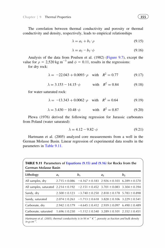
The correlation between thermal conductivity and porosity or thermal
conductivity and density, respectively, leads to empirical relationships
λ ¼ a1 þ b1Uρ ð9:15Þ
λ ¼ a2 2 b2Uφ ð9:16ÞAnalysis of the data from Poulsen et al. (1982) (Figure 9.7), except the
value for ρ 5 2,520 kg m23 and φ 5 0.11, results in the regressions:
for dry rock:
λ ¼ 222:043þ 0:0093Uρ with R2 ¼ 0:77 ð9:17Þ
λ ¼ 3:1532 14:15Uφ with R2 ¼ 0:84 ð9:18Þfor water-saturated rock:
λ ¼ 213:343þ 0:0062Uρ with R2 ¼ 0:64 ð9:19Þ
λ ¼ 3:4302 10:48Uφ with R2 ¼ 0:87 ð9:20ÞPlewa (1976) derived the following regression for Jurassic carbonates
from Poland (water saturated):
λ ¼ 4:122 9:82Uφ ð9:21ÞHartmann et al. (2005) analyzed core measurements from a well in the
German Molasse Basin. Linear regression of experimental data results in the
parameters in Table 9.11.
TABLE 9.11 Parameters of Equations (9.15) and (9.16) for Rocks from the
German Molasse Basin
Lithology a1 b1 a2 b2
All samples, dry 2.7156 0.086 24.1676 0.183 2.9266 0.103 6.2896 0.570
All samples, saturated 2.2146 0.192 22.1516 0.452 3.7016 0.083 3.3046 0.394
Sandy, dry 2.5006 0.123 23.7406 0.250 2.8186 0.178 5.7836 0.898
Sandy, saturated 2.0746 0.263 21.7136 0.618 3.8286 0.106 3.2296 0.541
Carbonate, dry 2.9426 0.179 24.6456 0.412 2.9396 0.097 6.4906 0.489
Carbonate, saturated 1.6966 0.230 21.1126 0.540 3.2896 0.101 2.3526 0.451
Hartmann et al. (2005); thermal conductivity is in W m21 K21, porosity as fraction and bulk densityin g cm23.
355Chapter | 9 Thermal Properties
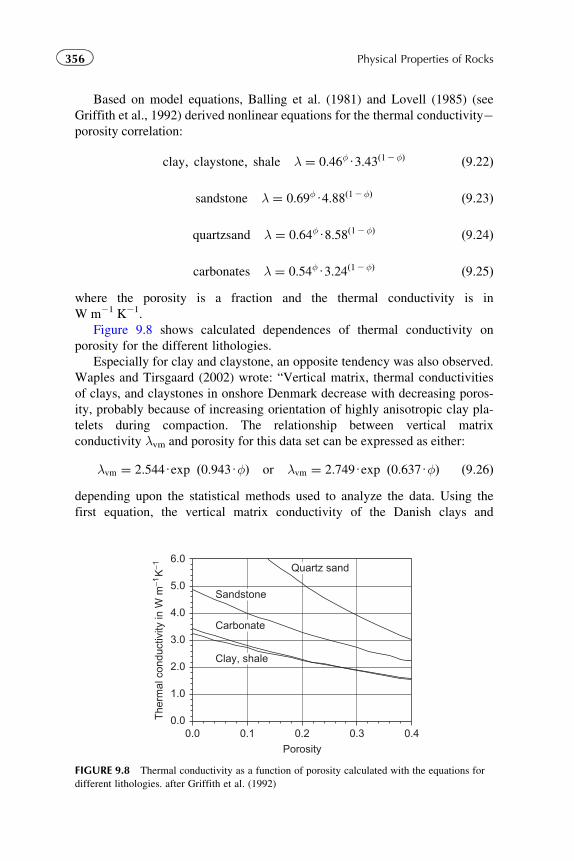
Based on model equations, Balling et al. (1981) and Lovell (1985) (see
Griffith et al., 1992) derived nonlinear equations for the thermal conductivity�porosity correlation:
clay; claystone; shale λ ¼ 0:46φU3:43ð12φÞ ð9:22Þ
sandstone λ ¼ 0:69φU4:88ð12φÞ ð9:23Þ
quartzsand λ ¼ 0:64φU8:58ð12φÞ ð9:24Þ
carbonates λ ¼ 0:54φU3:24ð12φÞ ð9:25Þwhere the porosity is a fraction and the thermal conductivity is in
W m21 K21.
Figure 9.8 shows calculated dependences of thermal conductivity on
porosity for the different lithologies.
Especially for clay and claystone, an opposite tendency was also observed.
Waples and Tirsgaard (2002) wrote: “Vertical matrix, thermal conductivities
of clays, and claystones in onshore Denmark decrease with decreasing poros-
ity, probably because of increasing orientation of highly anisotropic clay pla-
telets during compaction. The relationship between vertical matrix
conductivity λvm and porosity for this data set can be expressed as either:
λvm ¼ 2:544Uexp ð0:943UφÞ or λvm ¼ 2:749Uexp ð0:637UφÞ ð9:26Þdepending upon the statistical methods used to analyze the data. Using the
first equation, the vertical matrix conductivity of the Danish clays and
The
rmal
con
duct
ivity
in W
m−1
K−1
0.0
1.0
2.0
3.0
4.0
5.0
6.0
0.0 0.1 0.2 0.3 0.4Porosity
Quartz sand
Sandstone
Carbonate
Clay, shale
FIGURE 9.8 Thermal conductivity as a function of porosity calculated with the equations for
different lithologies. after Griffith et al. (1992)
356 Physical Properties of Rocks
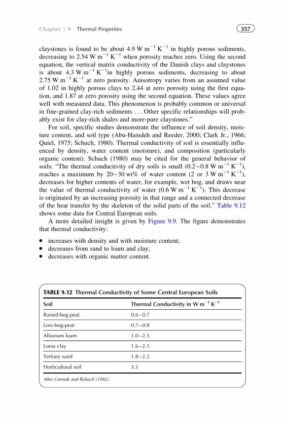
claystones is found to be about 4.9 W m21 K21 in highly porous sediments,
decreasing to 2.54 W m21 K21 when porosity reaches zero. Using the second
equation, the vertical matrix conductivity of the Danish clays and claystones
is about 4.3 W m21 K21in highly porous sediments, decreasing to about
2.75 W m21 K21 at zero porosity. Anisotropy varies from an assumed value
of 1.02 in highly porous clays to 2.44 at zero porosity using the first equa-
tion, and 1.87 at zero porosity using the second equation. These values agree
well with measured data. This phenomenon is probably common or universal
in fine-grained clay-rich sediments . . . Other specific relationships will prob-
ably exist for clay-rich shales and more-pure claystones.”
For soil, specific studies demonstrate the influence of soil density, mois-
ture content, and soil type (Abu-Hamdeh and Reeder, 2000; Clark Jr., 1966;
Quiel, 1975; Schuch, 1980). Thermal conductivity of soil is essentially influ-
enced by density, water content (moisture), and composition (particularly
organic content). Schuch (1980) may be cited for the general behavior of
soils: “The thermal conductivity of dry soils is small (0.2�0.8 W m21 K21),
reaches a maximum by 20�30 wt% of water content (2 or 3 W m21 K21),
decreases for higher contents of water, for example, wet bog, and draws near
the value of thermal conductivity of water (0.6 W m21 K21). This decrease
is originated by an increasing porosity in that range and a connected decrease
of the heat transfer by the skeleton of the solid parts of the soil.” Table 9.12
shows some data for Central European soils.
A more detailed insight is given by Figure 9.9. The figure demonstrates
that thermal conductivity:
� increases with density and with moisture content;� decreases from sand to loam and clay;� decreases with organic matter content.
TABLE 9.12 Thermal Conductivity of Some Central European Soils
Soil Thermal Conductivity in W m21 K21
Raised-bog-peat 0.6�0.7
Low-bog-peat 0.7�0.8
Alluvium loam 1.0�2.5
Loess clay 1.6�2.1
Tertiary sand 1.8�2.2
Horticultural soil 3.3
After Cermak and Rybach (1982).
357Chapter | 9 Thermal Properties
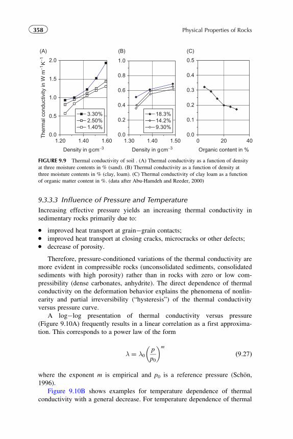
9.3.3.3 Influence of Pressure and Temperature
Increasing effective pressure yields an increasing thermal conductivity in
sedimentary rocks primarily due to:
� improved heat transport at grain�grain contacts;� improved heat transport at closing cracks, microcracks or other defects;� decrease of porosity.
Therefore, pressure-conditioned variations of the thermal conductivity are
more evident in compressible rocks (unconsolidated sediments, consolidated
sediments with high porosity) rather than in rocks with zero or low com-
pressibility (dense carbonates, anhydrite). The direct dependence of thermal
conductivity on the deformation behavior explains the phenomena of nonlin-
earity and partial irreversibility (“hysteresis”) of the thermal conductivity
versus pressure curve.
A log�log presentation of thermal conductivity versus pressure
(Figure 9.10A) frequently results in a linear correlation as a first approxima-
tion. This corresponds to a power law of the form
λ ¼ λ0
p
p0
� �m
ð9:27Þ
where the exponent m is empirical and p0 is a reference pressure (Schon,
1996).
Figure 9.10B shows examples for temperature dependence of thermal
conductivity with a general decrease. For temperature dependence of thermal
0.0
0.5
1.0
1.5
2.0
(A) (B) (C)
1.20 1.40 1.60 1.30 1.40 1.50 0 20 40
Density in gcm−3 Density in gcm−3
3.30%2.50%1.40%
0.0
0.1
0.2
0.3
0.4
0.5
Organic content in %
0.0
0.2
0.4
0.6
0.8
1.0
The
rmal
con
duct
ivity
in W
m−1
K−1
18.3%14.2%9.30%
FIGURE 9.9 Thermal conductivity of soil . (A) Thermal conductivity as a function of density
at three moisture contents in % (sand). (B) Thermal conductivity as a function of density at
three moisture contents in % (clay, loam). (C) Thermal conductivity of clay loam as a function
of organic matter content in %. (data after Abu-Hamdeh and Reeder, 2000)
358 Physical Properties of Rocks
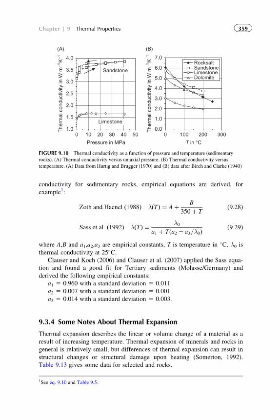
conductivity for sedimentary rocks, empirical equations are derived, for
example1:
Zoth and Haenel ð1988Þ λðTÞ ¼ Aþ B
350þ Tð9:28Þ
Sass et al: ð1992Þ λðTÞ ¼ λ0
a1 þ Tða2 2 a3=λ0Þð9:29Þ
where A,B and a1,a2,a3 are empirical constants, T is temperature in �C, λ0 isthermal conductivity at 25�C.
Clauser and Koch (2006) and Clauser et al. (2007) applied the Sass equa-
tion and found a good fit for Tertiary sediments (Molasse/Germany) and
derived the following empirical constants:
a1 5 0.960 with a standard deviation 5 0.011
a2 5 0.007 with a standard deviation 5 0.001
a3 5 0.014 with a standard deviation 5 0.003.
9.3.4 Some Notes About Thermal Expansion
Thermal expansion describes the linear or volume change of a material as a
result of increasing temperature. Thermal expansion of minerals and rocks in
general is relatively small, but differences of thermal expansion can result in
structural changes or structural damage upon heating (Somerton, 1992).
Table 9.13 gives some data for selected and rocks.
The
rmal
con
duct
ivity
in W
m−1
K−1
The
rmal
con
duct
ivity
in W
m−1
K−1
1.0
1.5
2.0
2.5
3.0
3.5
4.0
0 10 20 30 40 50 0 100 200 300
Pressure in MPa
Sandstone
Limestone0.0
1.0
2.0
3.0
4.0
5.0
6.0
7.0
(B)(A)
T in °C
RocksaltSandstoneLimestoneDolomite
FIGURE 9.10 Thermal conductivity as a function of pressure and temperature (sedimentary
rocks). (A) Thermal conductivity versus uniaxial pressure. (B) Thermal conductivity versus
temperature. (A) Data from Hurtig and Brugger (1970) and (B) data after Birch and Clarke (1940)
1See eq. 9.10 and Table 9.5.
359Chapter | 9 Thermal Properties
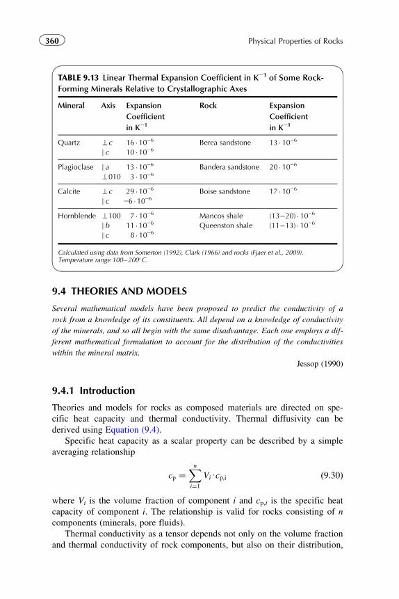
9.4 THEORIES AND MODELS
Several mathematical models have been proposed to predict the conductivity of a
rock from a knowledge of its constituents. All depend on a knowledge of conductivity
of the minerals, and so all begin with the same disadvantage. Each one employs a dif-
ferent mathematical formulation to account for the distribution of the conductivities
within the mineral matrix.
Jessop (1990)
9.4.1 Introduction
Theories and models for rocks as composed materials are directed on spe-
cific heat capacity and thermal conductivity. Thermal diffusivity can be
derived using Equation (9.4).
Specific heat capacity as a scalar property can be described by a simple
averaging relationship
cp ¼Xni¼1
ViUcp;i ð9:30Þ
where Vi is the volume fraction of component i and cp,i is the specific heat
capacity of component i. The relationship is valid for rocks consisting of n
components (minerals, pore fluids).
Thermal conductivity as a tensor depends not only on the volume fraction
and thermal conductivity of rock components, but also on their distribution,
TABLE 9.13 Linear Thermal Expansion Coefficient in K21 of Some Rock-
Forming Minerals Relative to Crystallographic Axes
Mineral Axis Expansion
Coefficient
in K21
Rock Expansion
Coefficient
in K21
Quartz >c 16 � 1026 Berea sandstone 13 � 10268c 10 � 1026
Plagioclase 8a 13 � 1026 Bandera sandstone 20 � 1026>010 3 � 1026
Calcite >c 29 � 1026 Boise sandstone 17 � 10268c 26 � 1026
Hornblende >100 7 � 1026 Mancos shale (13�20) � 10268b 11 � 1026 Queenston shale (11�13) � 10268c 8 � 1026
Calculated using data from Somerton (1992), Clark (1966) and rocks (Fjaer et al., 2009).Temperature range 100�200�C.
360 Physical Properties of Rocks
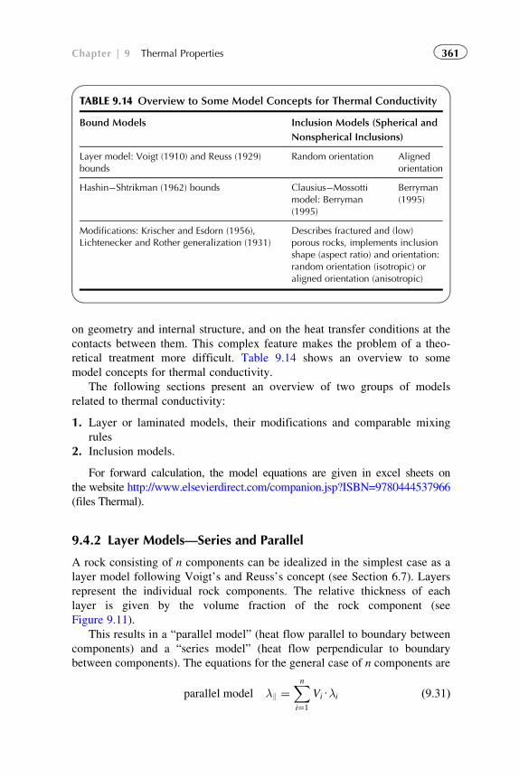
on geometry and internal structure, and on the heat transfer conditions at the
contacts between them. This complex feature makes the problem of a theo-
retical treatment more difficult. Table 9.14 shows an overview to some
model concepts for thermal conductivity.
The following sections present an overview of two groups of models
related to thermal conductivity:
1. Layer or laminated models, their modifications and comparable mixing
rules
2. Inclusion models.
For forward calculation, the model equations are given in excel sheets on
the website http://www.elsevierdirect.com/companion.jsp?ISBN=9780444537966
(files Thermal).
9.4.2 Layer Models—Series and Parallel
A rock consisting of n components can be idealized in the simplest case as a
layer model following Voigt’s and Reuss’s concept (see Section 6.7). Layers
represent the individual rock components. The relative thickness of each
layer is given by the volume fraction of the rock component (see
Figure 9.11).
This results in a “parallel model” (heat flow parallel to boundary between
components) and a “series model” (heat flow perpendicular to boundary
between components). The equations for the general case of n components are
parallel model λ8 ¼Xni¼1
ViUλi ð9:31Þ
TABLE 9.14 Overview to Some Model Concepts for Thermal Conductivity
Bound Models Inclusion Models (Spherical and
Nonspherical Inclusions)
Layer model: Voigt (1910) and Reuss (1929)bounds
Random orientation Alignedorientation
Hashin�Shtrikman (1962) bounds Clausius�Mossottimodel: Berryman(1995)
Berryman(1995)
Modifications: Krischer and Esdorn (1956),Lichtenecker and Rother generalization (1931)
Describes fractured and (low)porous rocks, implements inclusionshape (aspect ratio) and orientation:random orientation (isotropic) oraligned orientation (anisotropic)
361Chapter | 9 Thermal Properties
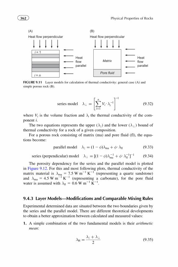
series model λ> ¼Xni¼1
ViUλ21i
" #21ð9:32Þ
where Vi is the volume fraction and λi the thermal conductivity of the com-
ponent i.
The two equations represents the upper (λ8) and the lower (λ>) bound of
thermal conductivity for a rock of a given composition.
For a porous rock consisting of matrix (ma) and pore fluid (fl), the equa-
tions become:
parallel model λ8 ¼ ð12φÞλma þ φUλfl ð9:33Þ
series ðperpendicularÞ model λ> ¼ ½ð12φÞλ21ma þ φUλ21
fl �21 ð9:34ÞThe porosity dependency for the series and the parallel model is plotted
in Figure 9.12. For this and most following plots, thermal conductivity of the
matrix material is λma 5 7.5 W m21 K21 (representing a quartz sandstone)
and λma 5 4.5 W m21 K21 (representing a carbonate), for the pore fluid
water is assumed with λfl 5 0.6 W m21 K21.
9.4.3 Layer Models—Modifications and Comparable Mixing Rules
Experimental determined data are situated between the two boundaries given by
the series and the parallel model. There are different theoretical developments
to obtain a better approximation between calculated and measured values:
1. A simple combination of the two fundamental models is their arithmetic
mean:
λH ¼ λ8 þ λ>
2ð9:35Þ
i = 1
i = n
Heat flow perpendicular
Matrix
Pore fluid
Heat flow perpendicular
(B)(A)
Heatflowparallel
Heatflowparallel
FIGURE 9.11 Layer models for calculation of thermal conductivity: general case (A) and
simple porous rock (B).
362 Physical Properties of Rocks
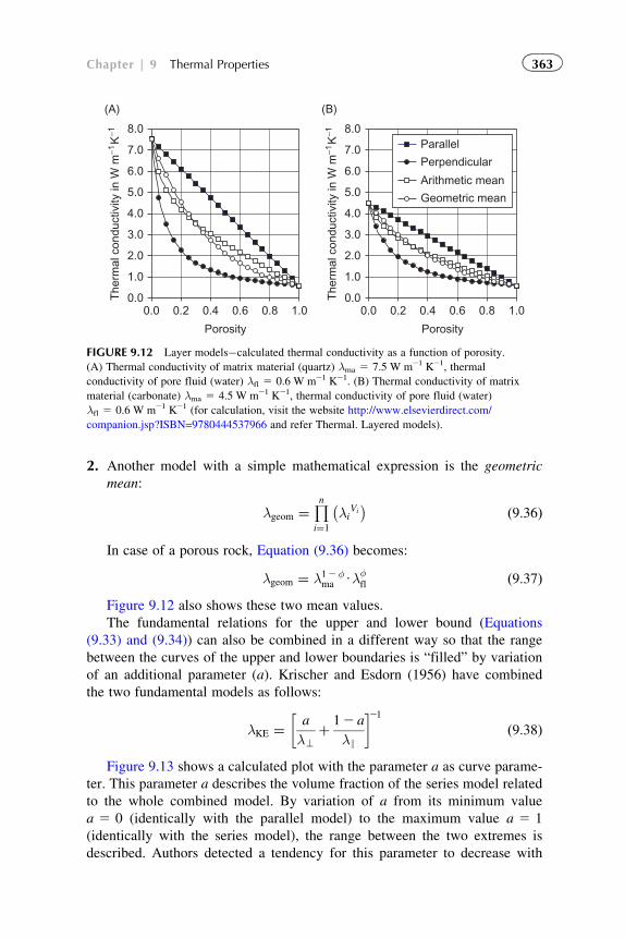
2. Another model with a simple mathematical expression is the geometric
mean:
λgeom ¼ Ln
i¼1
λiVi
� � ð9:36Þ
In case of a porous rock, Equation (9.36) becomes:
λgeom ¼ λ12φma Uλφ
fl ð9:37ÞFigure 9.12 also shows these two mean values.
The fundamental relations for the upper and lower bound (Equations
(9.33) and (9.34)) can also be combined in a different way so that the range
between the curves of the upper and lower boundaries is “filled” by variation
of an additional parameter (a). Krischer and Esdorn (1956) have combined
the two fundamental models as follows:
λKE ¼ a
λ>þ 12 a
λ8
� �21ð9:38Þ
Figure 9.13 shows a calculated plot with the parameter a as curve parame-
ter. This parameter a describes the volume fraction of the series model related
to the whole combined model. By variation of a from its minimum value
a 5 0 (identically with the parallel model) to the maximum value a 5 1
(identically with the series model), the range between the two extremes is
described. Authors detected a tendency for this parameter to decrease with
0.0
1.0
2.0
3.0
4.0
5.0
6.0
7.0
8.0
0.0 0.2 0.4 0.6 0.8 1.0
Porosity
The
rmal
con
duct
ivity
in W
m−1
K−1
0.0
1.0
2.0
3.0
4.0
5.0
6.0
7.0
8.0
0.0 0.2 0.4 0.6 0.8 1.0
PorosityT
herm
al c
ondu
ctiv
ity in
W m
−1K
−1
Parallel
Perpendicular
Arithmetic mean
Geometric mean
(B)(A)
FIGURE 9.12 Layer models�calculated thermal conductivity as a function of porosity.
(A) Thermal conductivity of matrix material (quartz) λma 5 7.5 W m21 K21, thermal
conductivity of pore fluid (water) λfl 5 0.6 W m21 K21. (B) Thermal conductivity of matrix
material (carbonate) λma 5 4.5 W m21 K21, thermal conductivity of pore fluid (water)
λfl 5 0.6 W m21 K21 (for calculation, visit the website http://www.elsevierdirect.com/
companion.jsp?ISBN=9780444537966 and refer Thermal. Layered models).
363Chapter | 9 Thermal Properties
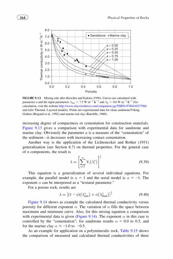
increasing degree of compactness or cementation for construction materials.
Figure 9.13 gives a comparison with experimental data for sandstone and
marine clay. Obviously the parameter a is a measure of the “cementation” of
the sediment—it decreases with increasing contact cementation.
Another way is the application of the Lichtenecker and Rother (1931)
generalization (see Section 6.7) on thermal properties. For the general case
of n components, the result is
λ ¼Xni¼1
Vi λαi
� �" #1α
ð9:39Þ
This equation is a generalization of several individual equations. For
example, the parallel model is α 5 1 and the serial model is α 5 21. Theexponent α can be interpreted as a “textural parameter.”
For a porous rock, results are
λ ¼ ð12φÞ λαmin
� �þ φ λαfluid
� �� 1α ð9:40Þ
Figure 9.14 shows as example the calculated thermal conductivity versus
porosity for different exponent α. The variation of α fills the space between
maximum and minimum curve. Also, for this mixing equation a comparison
with experimental data is given (Figure 9.14). The exponent α in this case is
controlled by the “cementation”; for sandstone results α 5 0.0 to 0.5, and
for the marine clay α �21.0 to 20.5.
As an example for application on a polymineralic rock, Table 9.15 shows
the comparison of measured and calculated thermal conductivities of three
The
rmal
con
duct
ivity
in W
m−1
K−1
0.0
1.0
2.0
3.0
4.0
5.0
6.0
7.0
8.0
0.0 0.2 0.4 0.6 0.8 1.0
Porosity
Sandstone Marine clay
a = 0.00a = 0.25a = 0.50a = 0.75a = 1.00
FIGURE 9.13 Mixing rule after Krischer and Esdorn (1956). Curves are calculated with
parameter a and the input parameters λma 5 7.5 W m21 K21 and λfl 5 0.6 W m21 K21 (for
calculation, visit the website http://www.elsevierdirect.com/companion.jsp?ISBN=9780444537966
and refer Thermal. Layered models). Points are experimental data for clean sandstone/Viking
Graben (Brigaud et al., 1992) and marine red clay (Ratcliffe, 1960).
364 Physical Properties of Rocks
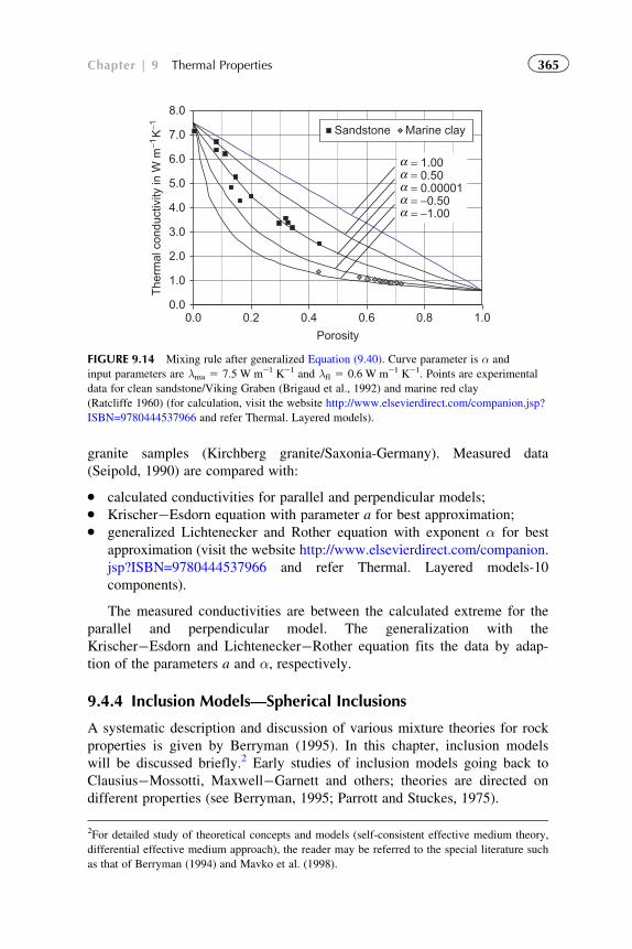
granite samples (Kirchberg granite/Saxonia-Germany). Measured data
(Seipold, 1990) are compared with:
� calculated conductivities for parallel and perpendicular models;� Krischer�Esdorn equation with parameter a for best approximation;� generalized Lichtenecker and Rother equation with exponent α for best
approximation (visit the website http://www.elsevierdirect.com/companion.
jsp?ISBN=9780444537966 and refer Thermal. Layered models-10
components).
The measured conductivities are between the calculated extreme for the
parallel and perpendicular model. The generalization with the
Krischer�Esdorn and Lichtenecker�Rother equation fits the data by adap-
tion of the parameters a and α, respectively.
9.4.4 Inclusion Models—Spherical Inclusions
A systematic description and discussion of various mixture theories for rock
properties is given by Berryman (1995). In this chapter, inclusion models
will be discussed briefly.2 Early studies of inclusion models going back to
Clausius�Mossotti, Maxwell�Garnett and others; theories are directed on
different properties (see Berryman, 1995; Parrott and Stuckes, 1975).
2For detailed study of theoretical concepts and models (self-consistent effective medium theory,
differential effective medium approach), the reader may be referred to the special literature such
as that of Berryman (1994) and Mavko et al. (1998).
The
rmal
con
duct
ivity
in W
m−1
K−1
0.0
1.0
2.0
3.0
4.0
5.0
6.0
7.0
8.0
0.0 0.2 0.4 0.6 0.8 1.0
Porosity
Sandstone Marine clay
= 1.00= 0.50= 0.00001= −0.50= −1.00
ααααα
FIGURE 9.14 Mixing rule after generalized Equation (9.40). Curve parameter is α and
input parameters are λma 5 7.5 W m21 K21 and λfl 5 0.6 W m21 K21. Points are experimental
data for clean sandstone/Viking Graben (Brigaud et al., 1992) and marine red clay
(Ratcliffe 1960) (for calculation, visit the website http://www.elsevierdirect.com/companion.jsp?
ISBN=9780444537966 and refer Thermal. Layered models).
365Chapter | 9 Thermal Properties
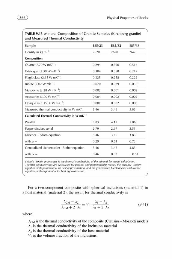
For a two-component composite with spherical inclusions (material 1) in
a host material (material 2), the result for thermal conductivity is
λCM 2λ2
λCM þ 2Uλ2
¼ V1Uλ1 2λ2
λ1 þ 2Uλ2
ð9:41Þ
where
λCM is the thermal conductivity of the composite (Clausius�Mossotti model)
λ1 is the thermal conductivity of the inclusion material
λ2 is the thermal conductivity of the host material
V1 is the volume fraction of the inclusions.
TABLE 9.15 Mineral Composition of Granite Samples (Kirchberg granite)
and Measured Thermal Conductivity
Sample E85/23 E85/32 E85/33
Density in kg m23 2620 2620 2640
Composition
Quartz (7.70 W mK21) 0.294 0.350 0.516
K-feldspar (2.30 W mK21) 0.304 0.358 0.217
Plagioclase (2.15 W mK21) 0.325 0.258 0.222
Biotite (2.02 W mk21) 0.070 0.029 0.036
Muscovite (2.28 W mK21) 0.002 0.001 0.002
Acessories (3.00 W mK21) 0.004 0.002 0.002
Opaque min. (5.00 W mK21) 0.001 0.002 0.005
Measured thermal conductivity in W mK21 3.46 3.46 3.83
Calculated Thermal Conductivity in W mK21
Parallel 3.83 4.15 5.06
Perpendicular, serial 2.79 2.97 3.51
Krischer�Esdorn equation 3.46 3.46 3.83
with a 5 0.29 0.51 0.73
Generalized Lichtenecker�Rother equation 3.46 3.46 3.83
with α 5 0.46 0.02 20.51
Seipold (1990). In brackets is the thermal conductivity of the mineral for model calculation.Thermal conductivities are calculated for parallel and perpendicular model, the Krischer�Esdornequation with parameter a for best approximation, and the generalized Lichtenecker and Rotherequation with exponent α for best approximation.
366 Physical Properties of Rocks
For a porous rock consisting of matrix substance as host material and
fluid as spherical pore inclusion, the result is
λCM 2λma
λCM þ 2Uλma
¼ φλfl 2λma
λfl þ 2Uλma
ð9:42Þwhere
λfl is the thermal conductivity of the pore fluid
λma is the thermal conductivity of the matrix
φ is the porosity.
Solved for λCM results with η 5 λma/λfl:
λCM ¼ λma
ð2ηþ 1Þ2 2Uφðη2 1Þð2ηþ 1Þ þ φðη2 1Þ ð9:43Þ
The assumption of spherical mineral grains suspended in a fluid gives the
relationships:
λCM 2λfl
λCM þ 2Uλfl
¼ ð12φÞ λma 2λfl
λma þ 2Uλfl
ð9:44Þ
λCM ¼ λfl
3η2 2Uφðη2 1Þ3þ φðη2 1Þ ð9:45Þ
With regard to the supposition that there is no influence or distortion of
the thermal field of one inclusion by any neighboring inclusion, we can
expect that:
� Equation (9.43) is useful mainly for rocks with relatively small porosity;� Equation (9.45) is useful mainly for high porous sediments (marine
sediments).
Figure 9.15 shows a comparison of calculated thermal conductivity as
function of porosity with experimental data.
The limitation for both equations is determined by the ratio η. After Beck(1976), Equation (9.43) is applicable up to a porosity of about φ 5 0.15, if
η $ 10. In the case of Figure 9.15, the ratio η is about 12.5.
The applicability of the model is not limited to mixtures of solid matrix
material and fluid pore content. It is also useful for a mixture of two different
solid components, such as for solid spheres in another solid material or
cement. In this case, the porosity must be substituted with the volume fraction
of the other material or cement. Kobranova (1989) has applied the inclusion
model sequentially to a polymineralic rock. The solid matrix in this particular
case consists of 70% quartz, 20% feldspar, and 10% kaolinite. In the first step,
a solid material conductivity is calculated for the quartz�feldspar mixture. In
the next, this solid material is combined with the kaolinite, and in the final
step, this three-component matrix is combined with the pore material.
367Chapter | 9 Thermal Properties
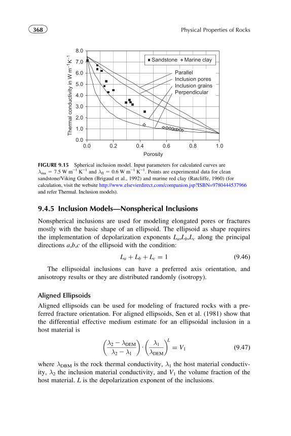
9.4.5 Inclusion Models—Nonspherical Inclusions
Nonspherical inclusions are used for modeling elongated pores or fractures
mostly with the basic shape of an ellipsoid. The ellipsoid as shape requires
the implementation of depolarization exponents La,Lb,Lc along the principal
directions a,b,c of the ellipsoid with the condition:
La þ Lb þ Lc ¼ 1 ð9:46ÞThe ellipsoidal inclusions can have a preferred axis orientation, and
anisotropy results or they are distributed randomly (isotropy).
Aligned Ellipsoids
Aligned ellipsoids can be used for modeling of fractured rocks with a pre-
ferred fracture orientation. For aligned ellipsoids, Sen et al. (1981) show that
the differential effective medium estimate for an ellipsoidal inclusion in a
host material is
λ2 2λDEM
λ2 2λ1
� �U
λ1
λDEM
� �L¼ V1 ð9:47Þ
where λDBM is the rock thermal conductivity, λ1 the host material conductiv-
ity, λ2 the inclusion material conductivity, and V1 the volume fraction of the
host material. L is the depolarization exponent of the inclusions.
The
rmal
con
duct
ivity
in W
m−1
K−1
0.0
1.0
2.0
3.0
4.0
5.0
6.0
7.0
8.0
0.0 0.2 0.4 0.6 0.8 1.0
Porosity
ParallelInclusion poresInclusion grainsPerpendicular
Sandstone Marine clay
FIGURE 9.15 Spherical inclusion model. Input parameters for calculated curves are
λma 5 7.5 W m21 K21 and λfl 5 0.6 W m21 K21. Points are experimental data for clean
sandstone/Viking Graben (Brigaud et al., 1992) and marine red clay (Ratcliffe, 1960) (for
calculation, visit the website http://www.elsevierdirect.com/companion.jsp?ISBN=9780444537966
and refer Thermal. Inclusion models).
368 Physical Properties of Rocks
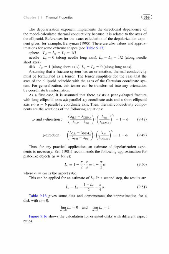
The depolarization exponent implements the directional dependence of
the model-calculated thermal conductivity because it is related to the axes of
the ellipsoid. References for the exact calculation of the depolarization expo-
nent gives, for example, Berryman (1995). There are also values and approx-
imations for some extreme shapes (see Table 9.17):
sphere La 5 Lb 5 Lc 5 1/3
needle Lc 5 0 (along needle long axis), La 5 Lb 5 1/2 (along needle
short axes)
disk Lc 5 1 (along short axis), La 5 Lb 5 0 (along long axes).
Assuming that a fracture system has an orientation, thermal conductivity
must be formulated as a tensor. The tensor simplifies for the case that the
axes of the ellipsoid coincide with the axes of the Cartesian coordinate sys-
tem. For generalization, this tensor can be transformed into any orientation
by coordinate transformation.
As a first case, it is assumed that there exists a penny-shaped fracture
with long ellipsoid axes a,b parallel x,y coordinate axis and a short ellipsoid
axis c{a 5 b parallel z coordinate axis. Then, thermal conductivity compo-
nents are the solutions of the following equations:
x- and y-direction :λfl;fr 2λDEM;x
λfl;fr 2λma
� �U
λma
λDEM;x
� �La¼ 12φ ð9:48Þ
z-direction :λfl;fr 2λDEM;z
λfl;fr 2λma
� �U
λma
λDEM;z
� �Lc¼ 12φ ð9:49Þ
Thus, for any practical application, an estimate of depolarization expo-
nents is necessary. Sen (1981) recommends the following approximation for
plate-like objects (a 5 bcc):
Lc ¼ 12π2Uc
a¼ 12
π2α ð9:50Þ
where α 5 c/a is the aspect ratio.
This can be applied for an estimate of Lc. In a second step, the results are
La ¼ Lb ¼12 Lc
2¼ π
4α ð9:51Þ
Table 9.16 gives some data and demonstrates the approximation for a
disk with α-0:
limα-0
La ¼ 0 and limα-0
Lc ¼ 1
Figure 9.16 shows the calculation for oriented disks with different aspect
ratios.
369Chapter | 9 Thermal Properties
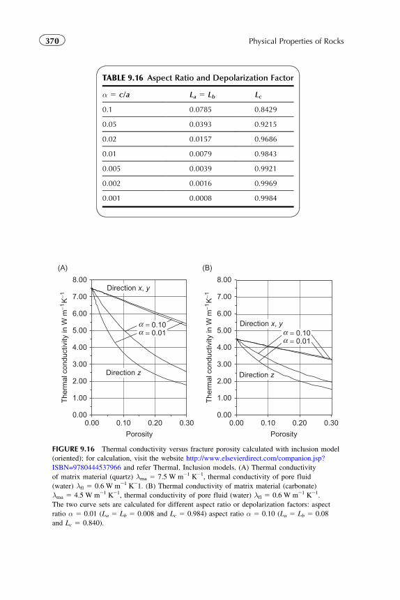
TABLE 9.16 Aspect Ratio and Depolarization Factor
α 5 c/a La 5 Lb Lc
0.1 0.0785 0.8429
0.05 0.0393 0.9215
0.02 0.0157 0.9686
0.01 0.0079 0.9843
0.005 0.0039 0.9921
0.002 0.0016 0.9969
0.001 0.0008 0.9984
0.00
1.00
2.00
3.00
4.00
5.00
6.00
7.00
8.00
0.00 0.10 0.20 0.30
Porosity
Direction z
Direction x, y
Direction x, y
The
rmal
con
duct
ivity
in W
m−1
K−1
0.00
1.00
2.00
3.00
4.00
5.00
6.00
7.00
8.00
0.00 0.10 0.20 0.30
Porosity
The
rmal
con
duct
ivity
in W
m−1
K−1
Direction z
= 0.10= 0.01
αα = 0.10
= 0.01αα
(B)(A)
FIGURE 9.16 Thermal conductivity versus fracture porosity calculated with inclusion model
(oriented); for calculation, visit the website http://www.elsevierdirect.com/companion.jsp?
ISBN=9780444537966 and refer Thermal. Inclusion models. (A) Thermal conductivity
of matrix material (quartz) λma 5 7.5 W m21 K21, thermal conductivity of pore fluid
(water) λfl 5 0.6 W m21 K21. (B) Thermal conductivity of matrix material (carbonate)
λma 5 4.5 W m21 K21, thermal conductivity of pore fluid (water) λfl 5 0.6 W m21 K21.
The two curve sets are calculated for different aspect ratio or depolarization factors: aspect
ratio α 5 0.01 (La 5 Lb 5 0.008 and Lc 5 0.984) aspect ratio α 5 0.10 (La 5 Lb 5 0.08
and Lc 5 0.840).
370 Physical Properties of Rocks
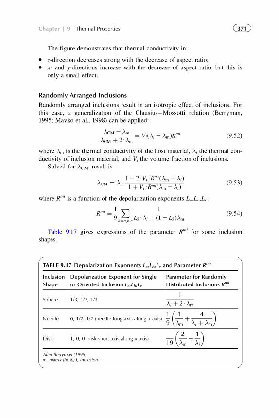
The figure demonstrates that thermal conductivity in:
� z-direction decreases strong with the decrease of aspect ratio;� x- and y-directions increase with the decrease of aspect ratio, but this is
only a small effect.
Randomly Arranged Inclusions
Randomly arranged inclusions result in an isotropic effect of inclusions. For
this case, a generalization of the Clausius�Mossotti relation (Berryman,
1995; Mavko et al., 1998) can be applied:
λCM 2λm
λCM þ 2Uλm
¼ Viðλi 2λmÞRmi ð9:52Þ
where λm is the thermal conductivity of the host material, λi the thermal con-
ductivity of inclusion material, and Vi the volume fraction of inclusions.
Solved for λCM, result is
λCM ¼ λm
12 2UViURmiðλm 2λiÞ1þ ViURmiðλm 2λiÞ
ð9:53Þ
where Rmi is a function of the depolarization exponents La,Lb,Lc:
Rmi ¼ 1
9
Xk¼a;b;c
1
LkUλi þ ð12 LkÞλm
ð9:54Þ
Table 9.17 gives expressions of the parameter Rmi for some inclusion
shapes.
TABLE 9.17 Depolarization Exponents La,Lb,Lc and Parameter Rmi
Inclusion
Shape
Depolarization Exponent for Single
or Oriented Inclusion La,Lb,Lc
Parameter for Randomly
Distributed Inclusions Rmi
Sphere 1/3, 1/3, 1/31
λi þ 2Uλm
Needle 0, 1/2, 1/2 (needle long axis along x-axis)1
9
1
λmþ 4
λi þ λm
� �
Disk 1, 0, 0 (disk short axis along x-axis)19
2
λmþ 1
λi
� �
After Berryman (1995).m, matrix (host); i, inclusion.
371Chapter | 9 Thermal Properties
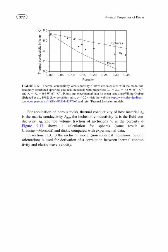
For application on porous rocks, thermal conductivity of host material λmis the matrix conductivity λma, the inclusion conductivity λi is the fluid con-
ductivity λfl, and the volume fraction of inclusions Vi is the porosity φ.Figure 9.17 shows a calculation for spheres (same result as
Clausius�Mossotti) and disks, compared with experimental data.
In section 11.3.1.3 the inclusion model (non spherical inclusions, random
orientation) is used for derivation of a correlation between thermal conduc-
tivity and elastic wave velocity.
The
rmal
con
duct
ivity
in W
m−1
K−1
0.0
2.0
4.0
6.0
8.0
0.00 0.05 0.10 0.15 0.20 0.25 0.30 0.35
Porosity
Disks
Spheres
FIGURE 9.17 Thermal conductivity versus porosity. Curves are calculated with the model for
randomly distributed spherical and disk inclusions with properties: λm 5 λma 5 7.5 W m21 K21
and λi 5 λfl 5 0.6 W m21 K21. Points are experimental data for clean sandstone/Viking Graben
(Brigaud et al., 1992) (low porosities only, φ , 0.2); visit the website http://www.elsevierdirect
.com/companion.jsp?ISBN=9780444537966 and refer Thermal.Inclusion models.
372 Physical Properties of Rocks
Chapter 10
Magnetic Properties
10.1 FUNDAMENTALS AND UNITS
Magnetic properties describe the behavior of any substance under the influ-
ence of a magnetic field. There are two main effects and phenomena:
1. Induced magnetization results when a magnetic field is applied to a mate-
rial with a magnetic susceptibility.
2. Remanent magnetization exists regardless of the presence of an applied
field and occurs within ferri- and ferromagnetic substances, which are
characterized by a natural alignment of magnetic moments.
For induced magnetization, the magnetic susceptibility characterizes the
magnetic response of a material to an external magnetic field.
The volume susceptibility κ is defined as the ratio of the material magne-
tization M per unit volume to the external magnetic field strength H:
κ ¼ M
Hð10:1Þ
The volume susceptibility κ is a dimensionless unit.
The mass susceptibility κg, measured in units of m3 kg21, is defined as
the ratio of the material magnetization per unit mass to the magnetic field
strength, and therefore:
κg ¼κρ
ð10:2Þ
where ρ is the bulk density.
In general, the susceptibility is a tensor of rank two. Unless otherwise
mentioned, the symbol κ means a “mean, quasi-isotropic” susceptibility. For
magnetic anisotropy studies, see, for example, Tarling and Hrouda (1993).
373Physical Properties of Rocks.
© 2011 Elsevier B.V. All rights reserved.
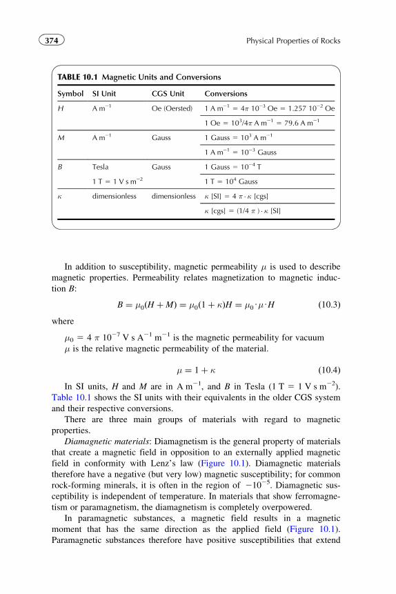
In addition to susceptibility, magnetic permeability μ is used to describe
magnetic properties. Permeability relates magnetization to magnetic induc-
tion B:
B ¼ μ0ðH þMÞ ¼ μ0ð1þ κÞH ¼ μ0UμUH ð10:3Þwhere
μ0 5 4 π 1027 V s A21 m21 is the magnetic permeability for vacuum
μ is the relative magnetic permeability of the material.
μ ¼ 1þ κ ð10:4ÞIn SI units, H and M are in A m21, and B in Tesla (1 T 5 1 V s m22).
Table 10.1 shows the SI units with their equivalents in the older CGS system
and their respective conversions.
There are three main groups of materials with regard to magnetic
properties.
Diamagnetic materials: Diamagnetism is the general property of materials
that create a magnetic field in opposition to an externally applied magnetic
field in conformity with Lenz’s law (Figure 10.1). Diamagnetic materials
therefore have a negative (but very low) magnetic susceptibility; for common
rock-forming minerals, it is often in the region of 21025. Diamagnetic sus-
ceptibility is independent of temperature. In materials that show ferromagne-
tism or paramagnetism, the diamagnetism is completely overpowered.
In paramagnetic substances, a magnetic field results in a magnetic
moment that has the same direction as the applied field (Figure 10.1).
Paramagnetic substances therefore have positive susceptibilities that extend
TABLE 10.1 Magnetic Units and Conversions
Symbol SI Unit CGS Unit Conversions
H A m21 Oe (Oersted) 1 A m21 5 4π 1023 Oe 5 1.257 1022 Oe
1 Oe 5 103/4π A m21 5 79.6 A m21
M A m21 Gauss 1 Gauss 5 103 A m21
1 A m21 5 1023 Gauss
B Tesla Gauss 1 Gauss 5 1024 T
1 T 5 1 V s m22 1 T 5 104 Gauss
κ dimensionless dimensionless κ [SI] 5 4 π �κ [cgs]
κ [cgs] 5 (1/4 π ) �κ [SI]
374 Physical Properties of Rocks
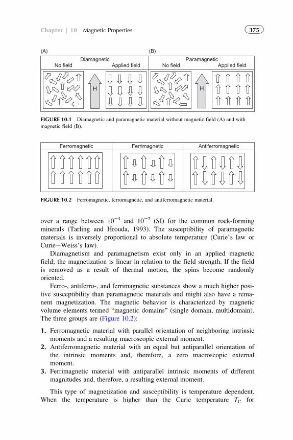
over a range between 1024 and 1022 (SI) for the common rock-forming
minerals (Tarling and Hrouda, 1993). The susceptibility of paramagnetic
materials is inversely proportional to absolute temperature (Curie’s law or
Curie�Weiss’s law).
Diamagnetism and paramagnetism exist only in an applied magnetic
field; the magnetization is linear in relation to the field strength. If the field
is removed as a result of thermal motion, the spins become randomly
oriented.
Ferro-, antiferro-, and ferrimagnetic substances show a much higher posi-
tive susceptibility than paramagnetic materials and might also have a rema-
nent magnetization. The magnetic behavior is characterized by magnetic
volume elements termed “magnetic domains” (single domain, multidomain).
The three groups are (Figure 10.2):
1. Ferromagnetic material with parallel orientation of neighboring intrinsic
moments and a resulting macroscopic external moment.
2. Antiferromagnetic material with an equal but antiparallel orientation of
the intrinsic moments and, therefore, a zero macroscopic external
moment.
3. Ferrimagnetic material with antiparallel intrinsic moments of different
magnitudes and, therefore, a resulting external moment.
This type of magnetization and susceptibility is temperature dependent.
When the temperature is higher than the Curie temperature TC for
Diamagnetic
(A) (B)
No field Applied fieldParamagnetic
No field Applied field
H H
FIGURE 10.1 Diamagnetic and paramagnetic material without magnetic field (A) and with
magnetic field (B).
Ferromagnetic Ferrimagnetic Antiferromagnetic
FIGURE 10.2 Ferromagnetic, ferromagnetic, and antiferromagnetic material.
375Chapter | 10 Magnetic Properties
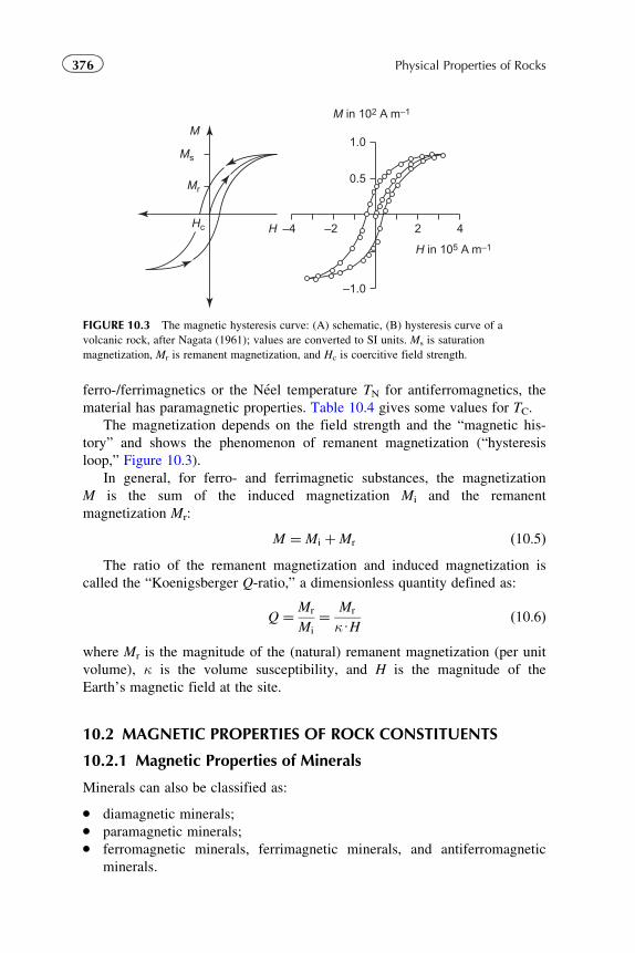
ferro-/ferrimagnetics or the Neel temperature TN for antiferromagnetics, the
material has paramagnetic properties. Table 10.4 gives some values for TC.
The magnetization depends on the field strength and the “magnetic his-
tory” and shows the phenomenon of remanent magnetization (“hysteresis
loop,” Figure 10.3).
In general, for ferro- and ferrimagnetic substances, the magnetization
M is the sum of the induced magnetization Mi and the remanent
magnetization Mr:
M ¼ Mi þMr ð10:5ÞThe ratio of the remanent magnetization and induced magnetization is
called the “Koenigsberger Q-ratio,” a dimensionless quantity defined as:
Q ¼ Mr
Mi
¼ Mr
κUHð10:6Þ
where Mr is the magnitude of the (natural) remanent magnetization (per unit
volume), κ is the volume susceptibility, and H is the magnitude of the
Earth’s magnetic field at the site.
10.2 MAGNETIC PROPERTIES OF ROCK CONSTITUENTS
10.2.1 Magnetic Properties of Minerals
Minerals can also be classified as:
� diamagnetic minerals;� paramagnetic minerals;� ferromagnetic minerals, ferrimagnetic minerals, and antiferromagnetic
minerals.
0.5
H
M
Ms
Mr
Hc
H in 105 A m–1
M in 102 A m–1
–4 –2 2 4
1.0
–1.0
FIGURE 10.3 The magnetic hysteresis curve: (A) schematic, (B) hysteresis curve of a
volcanic rock, after Nagata (1961); values are converted to SI units. Ms is saturation
magnetization, Mr is remanent magnetization, and Hc is coercitive field strength.
376 Physical Properties of Rocks
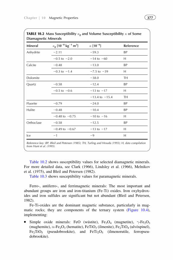
Table 10.2 shows susceptibility values for selected diamagnetic minerals.
For more detailed data, see Clark (1966), Lindsley et al. (1966), Melnikov
et al. (1975), and Bleil and Petersen (1982).
Table 10.3 shows susceptibility values for paramagnetic minerals.
Ferro-, antiferro-, and ferrimagnetic minerals: The most important and
abundant groups are iron and iron-titanium (Fe-Ti) oxides. Iron oxyhydrox-
ides and iron sulfides are significant but not abundant (Bleil and Petersen,
1982).
Fe-Ti-oxides are the dominant magnetic substance, particularly in mag-
matic rocks; they are components of the ternary system (Figure 10.4),
implementing:
� Simple oxide minerals: FeO (wustite), Fe3O4 (magnetite), γ-Fe2O3
(maghemite), α-Fe2O3 (hematite), FeTiO3 (ilmenite), Fe2TiO4 (ulvospinel),
Fe2TiO5 (pseudobrookite), and FeTi2O5 (ilmenorutile, ferropseu-
dobrookite).
TABLE 10.2 Mass Susceptibility κg and Volume Susceptibility κ of Some
Diamagnetic Minerals
Mineral κg [1028 kg21 m3] κ [1026] Reference
Anhydrite 22.11 259.3 BP
20.5 to 22.0 214 to 260 H
Calcite 20.48 213.0 BP
20.3 to 21.4 27.5 to 239 H
Dolomite 238.0 TH
Quartz 20.58 212.4 BP
20.5 to 20.6 213 to 217 H
213.4 to 215.4 TH
Fluorite 20.79 224.0 BP
Halite 20.48 210.4 BP
20.48 to 20.75 210 to 216 H
Orthoclase 20.58 212.5 BP
20.49 to 20.67 213 to 217 H
Ice 21 29 H
Reference key: BP, Bleil and Petersen (1985); TH, Tarling and Hrouda (1993); H, data compilationfrom Hunt et al. (1995).
377Chapter | 10 Magnetic Properties
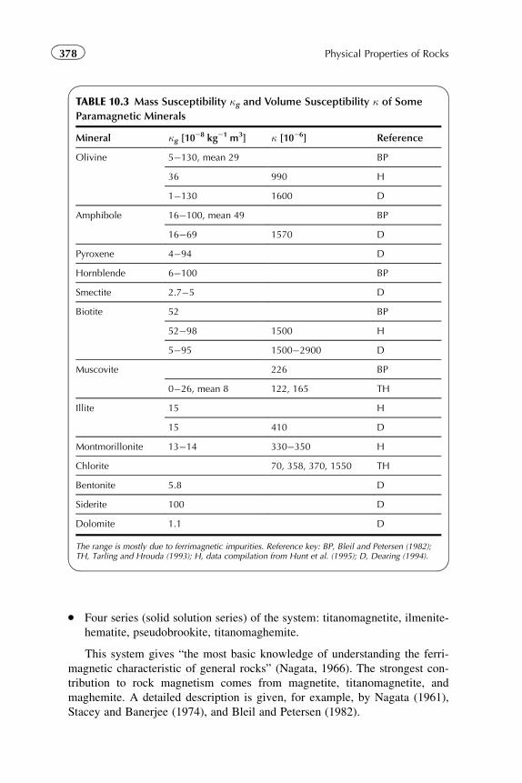
� Four series (solid solution series) of the system: titanomagnetite, ilmenite-
hematite, pseudobrookite, titanomaghemite.
This system gives “the most basic knowledge of understanding the ferri-
magnetic characteristic of general rocks” (Nagata, 1966). The strongest con-
tribution to rock magnetism comes from magnetite, titanomagnetite, and
maghemite. A detailed description is given, for example, by Nagata (1961),
Stacey and Banerjee (1974), and Bleil and Petersen (1982).
TABLE 10.3 Mass Susceptibility κg and Volume Susceptibility κ of Some
Paramagnetic Minerals
Mineral κg [1028 kg21 m3] κ [1026] Reference
Olivine 5�130, mean 29 BP
36 990 H
1�130 1600 D
Amphibole 16�100, mean 49 BP
16�69 1570 D
Pyroxene 4�94 D
Hornblende 6�100 BP
Smectite 2.7�5 D
Biotite 52 BP
52�98 1500 H
5�95 1500�2900 D
Muscovite 226 BP
0�26, mean 8 122, 165 TH
Illite 15 H
15 410 D
Montmorillonite 13�14 330�350 H
Chlorite 70, 358, 370, 1550 TH
Bentonite 5.8 D
Siderite 100 D
Dolomite 1.1 D
The range is mostly due to ferrimagnetic impurities. Reference key: BP, Bleil and Petersen (1982);TH, Tarling and Hrouda (1993); H, data compilation from Hunt et al. (1995); D, Dearing (1994).
378 Physical Properties of Rocks
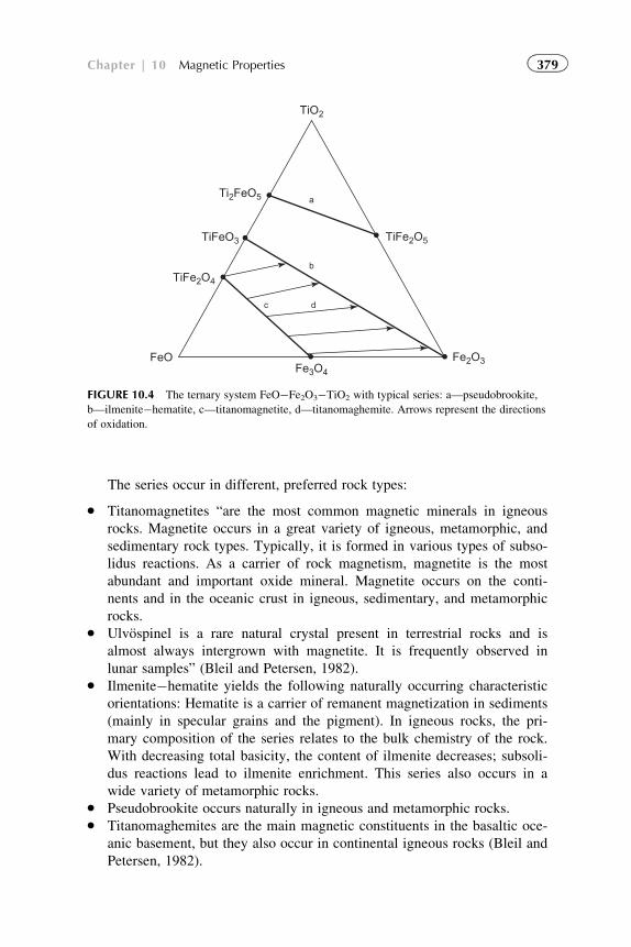
The series occur in different, preferred rock types:
� Titanomagnetites “are the most common magnetic minerals in igneous
rocks. Magnetite occurs in a great variety of igneous, metamorphic, and
sedimentary rock types. Typically, it is formed in various types of subso-
lidus reactions. As a carrier of rock magnetism, magnetite is the most
abundant and important oxide mineral. Magnetite occurs on the conti-
nents and in the oceanic crust in igneous, sedimentary, and metamorphic
rocks.� Ulvospinel is a rare natural crystal present in terrestrial rocks and is
almost always intergrown with magnetite. It is frequently observed in
lunar samples” (Bleil and Petersen, 1982).� Ilmenite�hematite yields the following naturally occurring characteristic
orientations: Hematite is a carrier of remanent magnetization in sediments
(mainly in specular grains and the pigment). In igneous rocks, the pri-
mary composition of the series relates to the bulk chemistry of the rock.
With decreasing total basicity, the content of ilmenite decreases; subsoli-
dus reactions lead to ilmenite enrichment. This series also occurs in a
wide variety of metamorphic rocks.� Pseudobrookite occurs naturally in igneous and metamorphic rocks.� Titanomaghemites are the main magnetic constituents in the basaltic oce-
anic basement, but they also occur in continental igneous rocks (Bleil and
Petersen, 1982).
FeO
TiFe2O4
TiFeO3
Ti2FeO5
TiFe2O5
Fe2O3Fe3O4
TiO2
a
b
c d
FIGURE 10.4 The ternary system FeO�Fe2O3�TiO2 with typical series: a—pseudobrookite,
b—ilmenite�hematite, c—titanomagnetite, d—titanomaghemite. Arrows represent the directions
of oxidation.
379Chapter | 10 Magnetic Properties
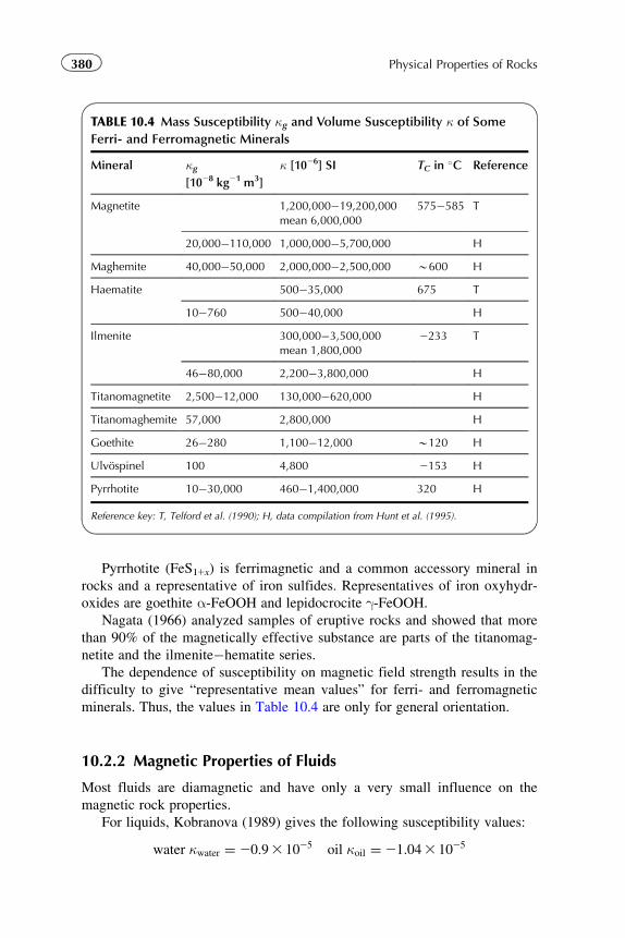
Pyrrhotite (FeS11x) is ferrimagnetic and a common accessory mineral in
rocks and a representative of iron sulfides. Representatives of iron oxyhydr-
oxides are goethite α-FeOOH and lepidocrocite γ-FeOOH.Nagata (1966) analyzed samples of eruptive rocks and showed that more
than 90% of the magnetically effective substance are parts of the titanomag-
netite and the ilmenite�hematite series.
The dependence of susceptibility on magnetic field strength results in the
difficulty to give “representative mean values” for ferri- and ferromagnetic
minerals. Thus, the values in Table 10.4 are only for general orientation.
10.2.2 Magnetic Properties of Fluids
Most fluids are diamagnetic and have only a very small influence on the
magnetic rock properties.
For liquids, Kobranova (1989) gives the following susceptibility values:
water κwater ¼ 20:93 1025 oil κoil ¼21:043 1025
TABLE 10.4 Mass Susceptibility κg and Volume Susceptibility κ of Some
Ferri- and Ferromagnetic Minerals
Mineral κg[1028 kg21 m3]
κ [1026] SI TC in �C Reference
Magnetite 1,200,000�19,200,000mean 6,000,000
575�585 T
20,000�110,000 1,000,000�5,700,000 H
Maghemite 40,000�50,000 2,000,000�2,500,000 B600 H
Haematite 500�35,000 675 T
10�760 500�40,000 H
Ilmenite 300,000�3,500,000mean 1,800,000
2233 T
46�80,000 2,200�3,800,000 H
Titanomagnetite 2,500�12,000 130,000�620,000 H
Titanomaghemite 57,000 2,800,000 H
Goethite 26�280 1,100�12,000 B120 H
Ulvospinel 100 4,800 2153 H
Pyrrhotite 10�30,000 460�1,400,000 320 H
Reference key: T, Telford et al. (1990); H, data compilation from Hunt et al. (1995).
380 Physical Properties of Rocks
Potter (2007) reports a mass susceptibility for formation water (Forties
Field/North sea) of κg,water 5 20.873 1028 kg21 m3 and for crude oil
κg,oil 5 21.023 1028 kg21 m3.
The water mineralization has a small effect because most salts are also
diamagnetic.
Ice has a mean susceptibility of κ 5 293 1026 (Hunt et al., 1995).
Gas components are also diamagnetic, except oxygen, which is paramag-
netic. The low value for air therefore is approximately κair 5 20.043 1025.
For hydrocarbon gases, Kobranova (1989) gives susceptibilities of about
κgas�21028.
10.3 MAGNETIC PROPERTIES OF ROCKS
Fundamental publications and comprehensive reviews about rock magnetism
are, for example: Hunt et al. (1995), Carmichael (1989), Mooney and
Bleifuss (1953), Nagata (1961, 1966), Angenheister and Soffel (1972),
Stacey and Banerjee (1974), Bleil and Petersen (1982), Petersen and Bleil
(1982), and Tarling and Hrouda (1993). Literature is available on palaeo-
magnetism and its applications for geology, geophysics, and archaeology, for
example, Tarling (1983).
10.3.1 Overview—Rock Magnetization
The magnetic properties of rocks are controlled by those mineral constituents
that have a magnetic effect. The fraction of these minerals with respect to
the total rock volume may be small. Therefore, two consequences result
(Carmichael, 1989):
1. “Magnetic properties can be quite variable within a rock type, depending
on chemical inhomogenity, depositional and/or crystallization, and post-
formational conditions.
2. Magnetic properties are not necessarily closely predictable by the litho-
logic rock type (geologic name). This is because the geologic rock name
and the geologic classification are generally given on the basis of the
genesis and the gross mineralogy, but a minor fraction of the mineral
constituents controls the magnetic properties”.
The most abundant minerals in common rocks are paramagnetic or dia-
magnetic. The magnetic rock properties are controlled by the ferrimagnetic
minerals, although their concentration “in major rock types rarely exceeds
10% vol.” (Bleil and Petersen, 1982). Minerals of the Fe-Ti-system are dom-
inant. In sedimentary rocks, the Fe-hydroxides are also important.
Figure 10.5 shows schematically the mineral contribution to the susceptibil-
ity of a rock after Tarling and Hrouda (1993). The authors state: “All mineral
grains within a rock contribute to its total susceptibility, but their individual
381Chapter | 10 Magnetic Properties
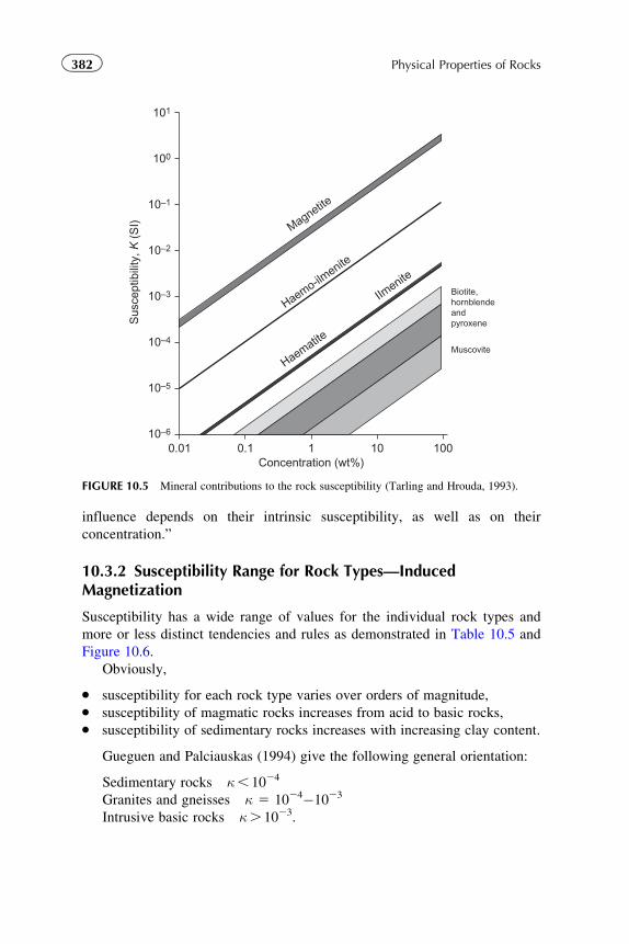
influence depends on their intrinsic susceptibility, as well as on their
concentration.”
10.3.2 Susceptibility Range for Rock Types—InducedMagnetization
Susceptibility has a wide range of values for the individual rock types and
more or less distinct tendencies and rules as demonstrated in Table 10.5 and
Figure 10.6.
Obviously,
� susceptibility for each rock type varies over orders of magnitude,� susceptibility of magmatic rocks increases from acid to basic rocks,� susceptibility of sedimentary rocks increases with increasing clay content.
Gueguen and Palciauskas (1994) give the following general orientation:
Sedimentary rocks κ, 1024
Granites and gneisses κ 5 1024�1023
Intrusive basic rocks κ. 1023.
0.0110–6
10–5
10–4
10–3
10–2
10–1
100
101
0.1 1Concentration (wt%)
Magnetite
Haemo-ilmenite
Haematite
IImenite
Sus
cept
ibili
ty, K
(S
I)
10 100
Biotite,hornblendeandpyroxene
Muscovite
FIGURE 10.5 Mineral contributions to the rock susceptibility (Tarling and Hrouda, 1993).
382 Physical Properties of Rocks
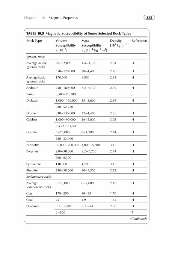
TABLE 10.5 Magnetic Susceptibility of Some Selected Rock Types
Rock Type Volume
Susceptibility
κ [1026]
Mass
Susceptibility
κg [1028 kg21 m3]
Density
[103 kg m23]
Reference
Igneous rocks
Average acidicigneous rocks
38�82,000 1.4�3,100 2.61 H
550�120,000 20�4,400 2.79 H
Average basicigneous rocks
170,000 6,500 2.61 H
Andesite 250�180,000 8.4�6,100 2.99 H
Basalt 8,500�79,100 J
Diabase 1,000�160,000 35�5,600 2.91 H
980�52,780 J
Diorite 630�130,000 22�4,400 2.85 H
Gabbro 1,000�90,000 26�3,000 3.03 H
5,5300�51,500 J
Granite 0�50,000 0�1,900 2.64 H
380�33,900 J
Peridotite 96,000�200,000 3,000�6,200 3.15 H
Porphyry 250�38,000 9.2�7,700 2.74 H
290�6,300 J
Pyroxenite 130,000 4,200 3.17 H
Rhyolite 250�38,000 10�1,500 2.52 H
Sedimentary rocks
Averagesedimentary rocks
0�50,000 0�2,000 2.19 H
Clay 170�250 10�15 1.70 H
Coal 25 1.9 1.35 H
Dolomite (210)�940 (21)�41 2.30 H
0�900 T
(Continued )
383Chapter | 10 Magnetic Properties
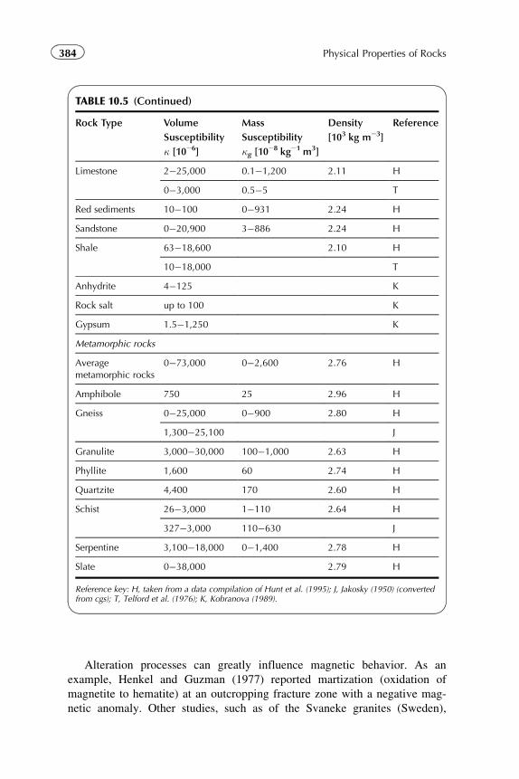
Alteration processes can greatly influence magnetic behavior. As an
example, Henkel and Guzman (1977) reported martization (oxidation of
magnetite to hematite) at an outcropping fracture zone with a negative mag-
netic anomaly. Other studies, such as of the Svaneke granites (Sweden),
TABLE 10.5 (Continued)
Rock Type Volume
Susceptibility
κ [1026]
Mass
Susceptibility
κg [1028 kg21 m3]
Density
[103 kg m23]
Reference
Limestone 2�25,000 0.1�1,200 2.11 H
0�3,000 0.5�5 T
Red sediments 10�100 0�931 2.24 H
Sandstone 0�20,900 3�886 2.24 H
Shale 63�18,600 2.10 H
10�18,000 T
Anhydrite 4�125 K
Rock salt up to 100 K
Gypsum 1.5�1,250 K
Metamorphic rocks
Averagemetamorphic rocks
0�73,000 0�2,600 2.76 H
Amphibole 750 25 2.96 H
Gneiss 0�25,000 0�900 2.80 H
1,300�25,100 J
Granulite 3,000�30,000 100�1,000 2.63 H
Phyllite 1,600 60 2.74 H
Quartzite 4,400 170 2.60 H
Schist 26�3,000 1�110 2.64 H
327�3,000 110�630 J
Serpentine 3,100�18,000 0�1,400 2.78 H
Slate 0�38,000 2.79 H
Reference key: H, taken from a data compilation of Hunt et al. (1995); J, Jakosky (1950) (convertedfrom cgs); T, Telford et al. (1976); K, Kobranova (1989).
384 Physical Properties of Rocks
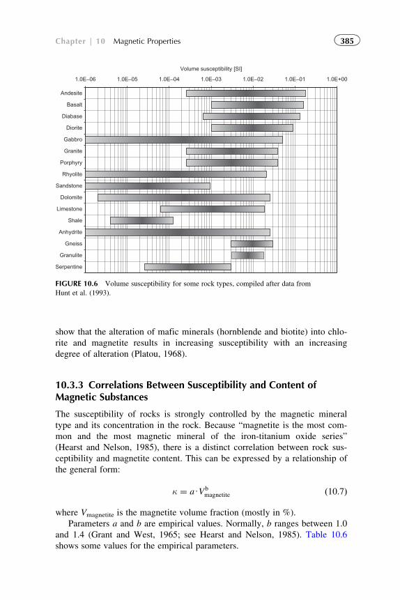
show that the alteration of mafic minerals (hornblende and biotite) into chlo-
rite and magnetite results in increasing susceptibility with an increasing
degree of alteration (Platou, 1968).
10.3.3 Correlations Between Susceptibility and Content ofMagnetic Substances
The susceptibility of rocks is strongly controlled by the magnetic mineral
type and its concentration in the rock. Because “magnetite is the most com-
mon and the most magnetic mineral of the iron-titanium oxide series”
(Hearst and Nelson, 1985), there is a distinct correlation between rock sus-
ceptibility and magnetite content. This can be expressed by a relationship of
the general form:
κ ¼ aUVbmagnetite ð10:7Þ
where Vmagnetite is the magnetite volume fraction (mostly in %).
Parameters a and b are empirical values. Normally, b ranges between 1.0
and 1.4 (Grant and West, 1965; see Hearst and Nelson, 1985). Table 10.6
shows some values for the empirical parameters.
1.0E–06 1.0E–05 1.0E–04 1.0E–03 1.0E–02 1.0E–01 1.0E+00
Andesite
Basalt
Diabase
Diorite
Gabbro
Granite
Porphyry
Rhyolite
Sandstone
Dolomite
Limestone
Shale
Anhydrite
Gneiss
Granulite
Serpentine
Volume susceptibility [SI]
FIGURE 10.6 Volume susceptibility for some rock types, compiled after data from
Hunt et al. (1993).
385Chapter | 10 Magnetic Properties
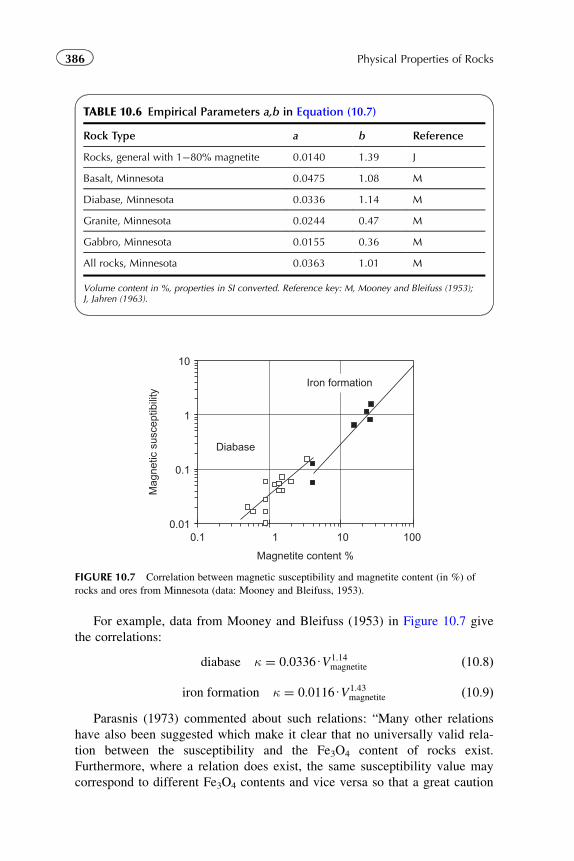
For example, data from Mooney and Bleifuss (1953) in Figure 10.7 give
the correlations:
diabase κ ¼ 0:0336UV1:14magnetite ð10:8Þ
iron formation κ ¼ 0:0116UV1:43magnetite ð10:9Þ
Parasnis (1973) commented about such relations: “Many other relations
have also been suggested which make it clear that no universally valid rela-
tion between the susceptibility and the Fe3O4 content of rocks exist.
Furthermore, where a relation does exist, the same susceptibility value may
correspond to different Fe3O4 contents and vice versa so that a great caution
TABLE 10.6 Empirical Parameters a,b in Equation (10.7)
Rock Type a b Reference
Rocks, general with 1�80% magnetite 0.0140 1.39 J
Basalt, Minnesota 0.0475 1.08 M
Diabase, Minnesota 0.0336 1.14 M
Granite, Minnesota 0.0244 0.47 M
Gabbro, Minnesota 0.0155 0.36 M
All rocks, Minnesota 0.0363 1.01 M
Volume content in %, properties in SI converted. Reference key: M, Mooney and Bleifuss (1953);J, Jahren (1963).
0.01
0.1
1
10
0.1 1 10 100
Magnetite content %
Mag
netic
sus
cept
ibili
ty
Iron formation
Diabase
FIGURE 10.7 Correlation between magnetic susceptibility and magnetite content (in %) of
rocks and ores from Minnesota (data: Mooney and Bleifuss, 1953).
386 Physical Properties of Rocks
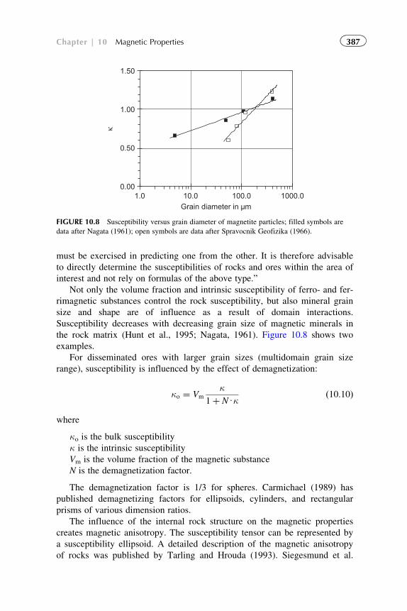
must be exercised in predicting one from the other. It is therefore advisable
to directly determine the susceptibilities of rocks and ores within the area of
interest and not rely on formulas of the above type.”
Not only the volume fraction and intrinsic susceptibility of ferro- and fer-
rimagnetic substances control the rock susceptibility, but also mineral grain
size and shape are of influence as a result of domain interactions.
Susceptibility decreases with decreasing grain size of magnetic minerals in
the rock matrix (Hunt et al., 1995; Nagata, 1961). Figure 10.8 shows two
examples.
For disseminated ores with larger grain sizes (multidomain grain size
range), susceptibility is influenced by the effect of demagnetization:
κo ¼ Vm
κ1þ NUκ
ð10:10Þ
where
κo is the bulk susceptibility
κ is the intrinsic susceptibility
Vm is the volume fraction of the magnetic substance
N is the demagnetization factor.
The demagnetization factor is 1/3 for spheres. Carmichael (1989) has
published demagnetizing factors for ellipsoids, cylinders, and rectangular
prisms of various dimension ratios.
The influence of the internal rock structure on the magnetic properties
creates magnetic anisotropy. The susceptibility tensor can be represented by
a susceptibility ellipsoid. A detailed description of the magnetic anisotropy
of rocks was published by Tarling and Hrouda (1993). Siegesmund et al.
0.00
0.50
1.00
1.50
1.0 10.0 100.0 1000.0Grain diameter in µm
κ
FIGURE 10.8 Susceptibility versus grain diameter of magnetite particles; filled symbols are
data after Nagata (1961); open symbols are data after Spravocnik Geofizika (1966).
387Chapter | 10 Magnetic Properties
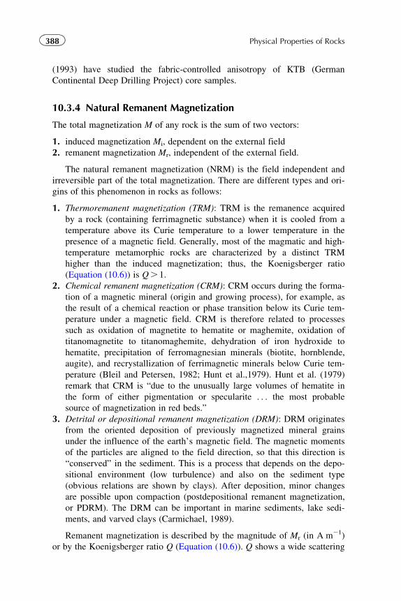
(1993) have studied the fabric-controlled anisotropy of KTB (German
Continental Deep Drilling Project) core samples.
10.3.4 Natural Remanent Magnetization
The total magnetization M of any rock is the sum of two vectors:
1. induced magnetization Mi, dependent on the external field
2. remanent magnetization Mr, independent of the external field.
The natural remanent magnetization (NRM) is the field independent and
irreversible part of the total magnetization. There are different types and ori-
gins of this phenomenon in rocks as follows:
1. Thermoremanent magnetization (TRM): TRM is the remanence acquired
by a rock (containing ferrimagnetic substance) when it is cooled from a
temperature above its Curie temperature to a lower temperature in the
presence of a magnetic field. Generally, most of the magmatic and high-
temperature metamorphic rocks are characterized by a distinct TRM
higher than the induced magnetization; thus, the Koenigsberger ratio
(Equation (10.6)) is Q. 1.
2. Chemical remanent magnetization (CRM): CRM occurs during the forma-
tion of a magnetic mineral (origin and growing process), for example, as
the result of a chemical reaction or phase transition below its Curie tem-
perature under a magnetic field. CRM is therefore related to processes
such as oxidation of magnetite to hematite or maghemite, oxidation of
titanomagnetite to titanomaghemite, dehydration of iron hydroxide to
hematite, precipitation of ferromagnesian minerals (biotite, hornblende,
augite), and recrystallization of ferrimagnetic minerals below Curie tem-
perature (Bleil and Petersen, 1982; Hunt et al.,1979). Hunt et al. (1979)
remark that CRM is “due to the unusually large volumes of hematite in
the form of either pigmentation or specularite . . . the most probable
source of magnetization in red beds.”
3. Detrital or depositional remanent magnetization (DRM): DRM originates
from the oriented deposition of previously magnetized mineral grains
under the influence of the earth’s magnetic field. The magnetic moments
of the particles are aligned to the field direction, so that this direction is
“conserved” in the sediment. This is a process that depends on the depo-
sitional environment (low turbulence) and also on the sediment type
(obvious relations are shown by clays). After deposition, minor changes
are possible upon compaction (postdepositional remanent magnetization,
or PDRM). The DRM can be important in marine sediments, lake sedi-
ments, and varved clays (Carmichael, 1989).
Remanent magnetization is described by the magnitude of Mr (in A m21)
or by the Koenigsberger ratio Q (Equation (10.6)). Q shows a wide scattering
388 Physical Properties of Rocks
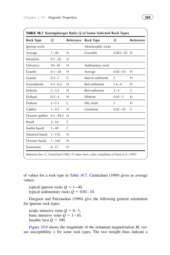
of values for a rock type in Table 10.7. Carmichael (1989) gives as average
values:
typical igneous rocks Q 5 1�40,
typical sedimentary rocks Q 5 0.02�10.
Gueguen and Palciauskas (1994) give the following general orientation
for igneous rock types:
acidic intrusive veins Q 5 0�1,
basic intrusive veins Q 5 1�10,
basaltic lava Q 5 100.
Figure 10.9 shows the magnitude of the remanent magnetization Mr ver-
sus susceptibility κ for some rock types. The two straight lines indicate a
TABLE 10.7 Koenigsberger Ratio Q of Some Selected Rock Types
Rock Type Q Reference Rock Type Q Reference
Igneous rocks Metamorphic rocks
Average 1�40 H Granulite 0.003�50 H
Intrusions 0.1�20 H
Volcanics 30�50 H Sedimentary rocks
Granite 0.1�28 H Average 0.02�10 H
Granite 0.3�1 C Marine sediments 5 H
Granodiorite 0.1�0.2 H Red sediments 1.6�6 H
Dolerite 2�3.5 H Red sediments 2�4 C
Diabase 0.2�4 H Siltstone 0.02�2 H
Diabase 2�3.5 C Silty shale 5 H
Gabbro 1�9.5 H Limestone 0.02�10 C
Oceanic gabbro 0.1�58.4 H
Basalt 5�10 C
Seaflor basalt 1�40 C
Subaerial basalt 1�116 H
Oceanic basalt 1�160 H
Seamounts 8�57 H
Reference key: C, Carmichael (1982), H, taken from a data compilation of Hunt et al. (1995).
389Chapter | 10 Magnetic Properties
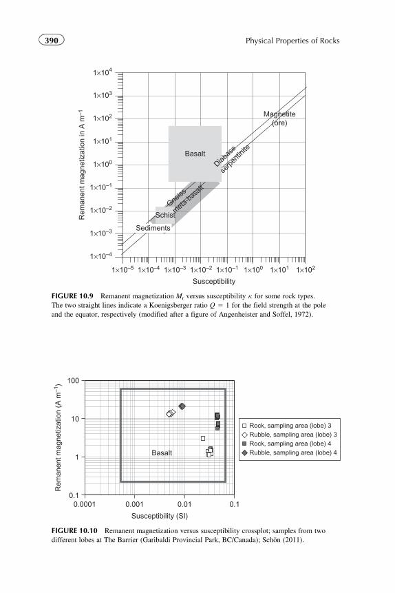
Susceptibility
1×10⁴
1×10³
1×10²
1×101
1×100
1×10⁻¹
1×10⁻²
1×10⁻³
1×10⁻⁴
1×10⁻⁵ 1×10⁻⁴ 1×10⁻³ 1×10⁻² 1×10⁻¹ 1×100 1×101 1×10²
Rem
anen
t mag
netiz
atio
n in
A m
–1
Basalt
Schist
Sediments
Diabas
e
serp
entin
ite
Gneiss
meta-basalt
Magnetite(ore)
FIGURE 10.9 Remanent magnetization Mr versus susceptibility κ for some rock types.
The two straight lines indicate a Koenigsberger ratio Q 5 1 for the field strength at the pole
and the equator, respectively (modified after a figure of Angenheister and Soffel, 1972).
Rock, sampling area (lobe) 3Rubble, sampling area (lobe) 3Rock, sampling area (lobe) 4Rubble, sampling area (lobe) 4
0.1
1
10
100
0.0001 0.001 0.01 0.1
Susceptibility (SI)
Rem
anen
t mag
netiz
atio
n (A
m–1
)
Basalt
FIGURE 10.10 Remanent magnetization versus susceptibility crossplot; samples from two
different lobes at The Barrier (Garibaldi Provincial Park, BC/Canada); Schon (2011).
390 Physical Properties of Rocks
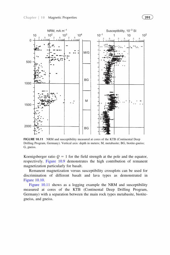
Koenigsberger ratio Q 5 1 for the field strength at the pole and the equator,
respectively. Figure 10.9 demonstrates the high contribution of remanent
magnetization particularly for basalt.
Remanent magnetization versus susceptibility crossplots can be used for
discrimination of different basalt and lava types as demonstrated in
Figure 10.10.
Figure 10.11 shows as a logging example the NRM and susceptibility
measured at cores of the KTB (Continental Deep Drilling Program,
Germany) with a separation between the main rock types metabasite, biotite-
gneiss, and gneiss.
1000
1500
2000
500
0
M/G
BG
M
BG
NRM, mA m–1
10 102 103 1042 5 2 5 2 5
Susceptibility, 10–3 SI10–1 1 10 102
2 5 2 5 2 5
FIGURE 10.11 NRM and susceptibility measured at cores of the KTB (Continental Deep
Drilling Program, Germany). Vertical axis: depth in meters; M, metabasite; BG, biotite-gneiss;
G, gneiss.
391Chapter | 10 Magnetic Properties

Chapter 11
Relationships Between SomePetrophysical Properties
11.1 INTRODUCTION
As shown in the previous chapters, the various physical properties depend on
different influences and contributions (Figure 11.1).
The physical basis for the existence of relationships between the various
physical properties (e.g., between the velocity of elastic waves and the ther-
mal conductivity) is given by:
� correlations between the properties of the individual rock components (cor-
relations between the elastic and thermal properties of minerals and fluids);� correlations of the considered properties (e.g., elastic and thermal rock
properties) with parameters like porosity and fracturing. Such parameters
act as a “connecting bridge” between the properties.
Correlations and relationships can be classified with respect to their
application into two groups:
Group 1: Relationships for derivation of specific rock properties (reser-
voir properties, mechanical properties, etc.) from properties determined
by geophysical methods. Examples are seismic or nuclear measurements
for estimating porosity, electrical measurements for water saturation cal-
culation, or seismic measurements for derivation of rock mechanical
properties. In many cases, a combination of several input properties is
applied. This type represents the majority of applications called “petro-
physical interpretation” and “formation evaluation.”
Group 2: Relationships for the transformation of a measured (geophys-
ical) property (e.g., velocity of seismic waves) into another (geophysical)
property of interest (e.g., thermal conductivity) because it is difficult to
measure that property directly in the field.
Correlations of the first type have been discussed in the previous chapters
for individual parameters. In the following section, a combined application
393Physical Properties of Rocks.
© 2011 Elsevier B.V. All rights reserved.
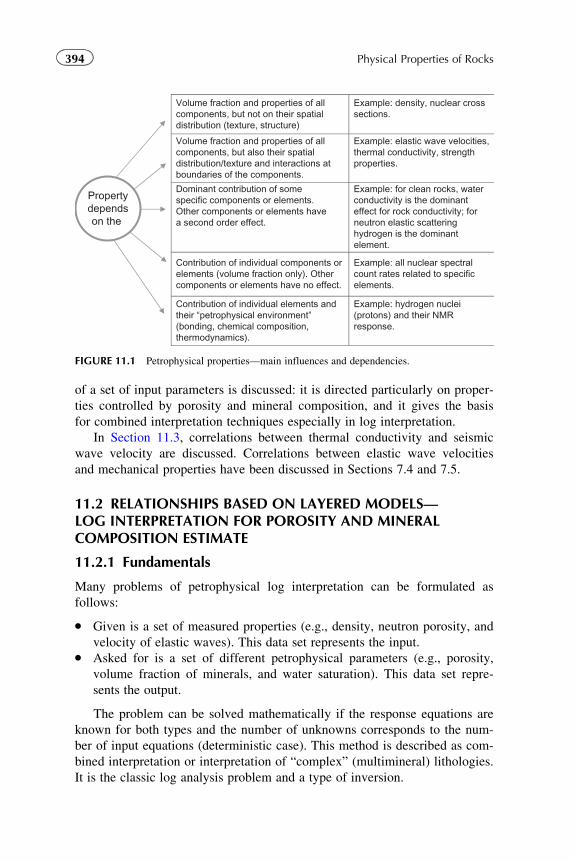
of a set of input parameters is discussed: it is directed particularly on proper-
ties controlled by porosity and mineral composition, and it gives the basis
for combined interpretation techniques especially in log interpretation.
In Section 11.3, correlations between thermal conductivity and seismic
wave velocity are discussed. Correlations between elastic wave velocities
and mechanical properties have been discussed in Sections 7.4 and 7.5.
11.2 RELATIONSHIPS BASED ON LAYERED MODELS—LOG INTERPRETATION FOR POROSITY AND MINERALCOMPOSITION ESTIMATE
11.2.1 Fundamentals
Many problems of petrophysical log interpretation can be formulated as
follows:
� Given is a set of measured properties (e.g., density, neutron porosity, and
velocity of elastic waves). This data set represents the input.� Asked for is a set of different petrophysical parameters (e.g., porosity,
volume fraction of minerals, and water saturation). This data set repre-
sents the output.
The problem can be solved mathematically if the response equations are
known for both types and the number of unknowns corresponds to the num-
ber of input equations (deterministic case). This method is described as com-
bined interpretation or interpretation of “complex” (multimineral) lithologies.
It is the classic log analysis problem and a type of inversion.
Volume fraction and properties of allcomponents, but not on their spatialdistribution (texture, structure)
Example: density, nuclear crosssections.
Volume fraction and properties of allcomponents, but also their spatialdistribution/texture and interactions atboundaries of the components.
Example: elastic wave velocities,thermal conductivity, strengthproperties.
Dominant contribution of somespecific components or elements.Other components or elements havea second order effect.
Example: for clean rocks, waterconductivity is the dominanteffect for rock conductivity; forneutron elastic scatteringhydrogen is the dominantelement.
Contribution of individual components orelements (volume fraction only). Othercomponents or elements have no effect.
Example: all nuclear spectralcount rates related to specificelements.
Contribution of individual elements andtheir “petrophysical environment”(bonding, chemical composition,thermodynamics).
Example: hydrogen nuclei(protons) and their NMRresponse.
Propertydependson the
FIGURE 11.1 Petrophysical properties—main influences and dependencies.
394 Physical Properties of Rocks
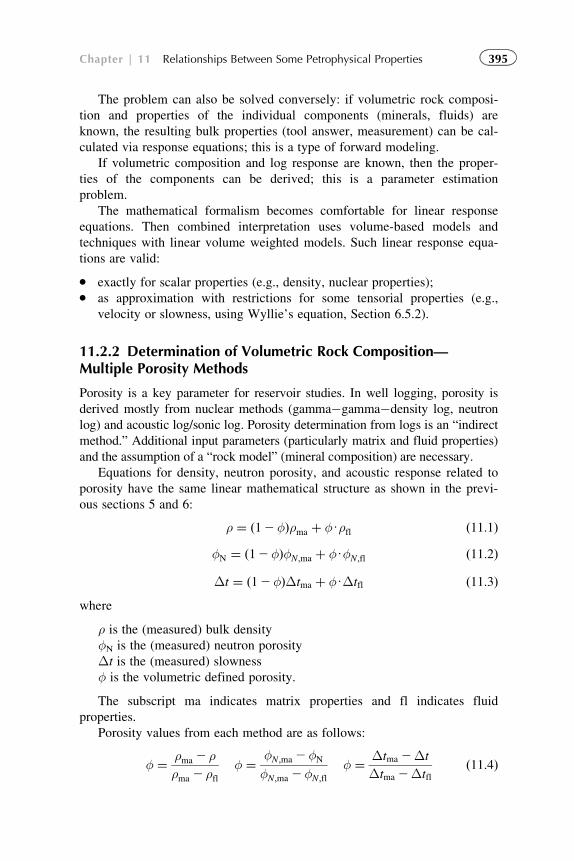
The problem can also be solved conversely: if volumetric rock composi-
tion and properties of the individual components (minerals, fluids) are
known, the resulting bulk properties (tool answer, measurement) can be cal-
culated via response equations; this is a type of forward modeling.
If volumetric composition and log response are known, then the proper-
ties of the components can be derived; this is a parameter estimation
problem.
The mathematical formalism becomes comfortable for linear response
equations. Then combined interpretation uses volume-based models and
techniques with linear volume weighted models. Such linear response equa-
tions are valid:
� exactly for scalar properties (e.g., density, nuclear properties);� as approximation with restrictions for some tensorial properties (e.g.,
velocity or slowness, using Wyllie’s equation, Section 6.5.2).
11.2.2 Determination of Volumetric Rock Composition—Multiple Porosity Methods
Porosity is a key parameter for reservoir studies. In well logging, porosity is
derived mostly from nuclear methods (gamma�gamma�density log, neutron
log) and acoustic log/sonic log. Porosity determination from logs is an “indirect
method.” Additional input parameters (particularly matrix and fluid properties)
and the assumption of a “rock model” (mineral composition) are necessary.
Equations for density, neutron porosity, and acoustic response related to
porosity have the same linear mathematical structure as shown in the previ-
ous sections 5 and 6:
ρ ¼ ð12φÞρma þ φUρfl ð11:1ÞφN ¼ ð12φÞφN;ma þ φUφN;fl ð11:2Þ
Δt ¼ ð12φÞΔtma þ φUΔtfl ð11:3Þwhere
ρ is the (measured) bulk density
φN is the (measured) neutron porosity
Δt is the (measured) slowness
φ is the volumetric defined porosity.
The subscript ma indicates matrix properties and fl indicates fluid
properties.
Porosity values from each method are as follows:
φ ¼ ρma 2 ρρma 2 ρfl
φ ¼ φN;ma 2φN
φN;ma 2φN;fl
φ ¼ Δtma 2Δt
Δtma 2Δtflð11:4Þ
395Chapter | 11 Relationships Between Some Petrophysical Properties
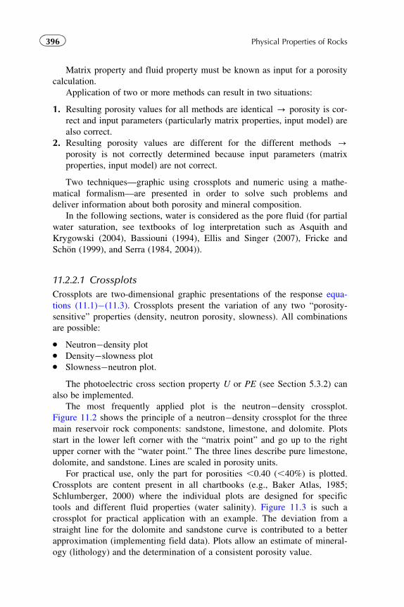
Matrix property and fluid property must be known as input for a porosity
calculation.
Application of two or more methods can result in two situations:
1. Resulting porosity values for all methods are identical - porosity is cor-
rect and input parameters (particularly matrix properties, input model) are
also correct.
2. Resulting porosity values are different for the different methods -porosity is not correctly determined because input parameters (matrix
properties, input model) are not correct.
Two techniques—graphic using crossplots and numeric using a mathe-
matical formalism—are presented in order to solve such problems and
deliver information about both porosity and mineral composition.
In the following sections, water is considered as the pore fluid (for partial
water saturation, see textbooks of log interpretation such as Asquith and
Krygowski (2004), Bassiouni (1994), Ellis and Singer (2007), Fricke and
Schon (1999), and Serra (1984, 2004)).
11.2.2.1 Crossplots
Crossplots are two-dimensional graphic presentations of the response equa-
tions (11.1)�(11.3). Crossplots present the variation of any two “porosity-
sensitive” properties (density, neutron porosity, slowness). All combinations
are possible:
� Neutron�density plot� Density�slowness plot� Slowness�neutron plot.
The photoelectric cross section property U or PE (see Section 5.3.2) can
also be implemented.
The most frequently applied plot is the neutron�density crossplot.
Figure 11.2 shows the principle of a neutron�density crossplot for the three
main reservoir rock components: sandstone, limestone, and dolomite. Plots
start in the lower left corner with the “matrix point” and go up to the right
upper corner with the “water point.” The three lines describe pure limestone,
dolomite, and sandstone. Lines are scaled in porosity units.
For practical use, only the part for porosities ,0.40 (,40%) is plotted.
Crossplots are content present in all chartbooks (e.g., Baker Atlas, 1985;
Schlumberger, 2000) where the individual plots are designed for specific
tools and different fluid properties (water salinity). Figure 11.3 is such a
crossplot for practical application with an example. The deviation from a
straight line for the dolomite and sandstone curve is contributed to a better
approximation (implementing field data). Plots allow an estimate of mineral-
ogy (lithology) and the determination of a consistent porosity value.
396 Physical Properties of Rocks
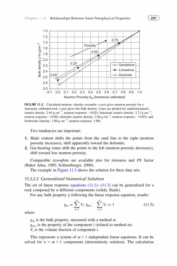
Two tendencies are important:
1. Shale content shifts the points from the sand line to the right (neutron
porosity increases), shift apparently toward the dolomite.
2. Gas-bearing zones shift the points to the left (neutron porosity decreases),
shift toward low neutron porosity.
Comparable crossplots are available also for slowness and PE factor
(Baker Atlas, 1985; Schlumberger, 2000).
The example in Figure 11.3 shows the solution for three data sets.
11.2.2.2 Generalized Numerical Solution
The set of linear response equations (11.1)�(11.3) can be generalized for a
rock composed by n different components (solids, fluids).
For any bulk property g following the linear response equation, results:
gm ¼Xni¼1
ViUgm;i
Xni¼1
Vi ¼ 1 ð11:5Þwhere
gm is the bulk property, measured with a method m
gm,i is the property of the component i (related to method m)
Vi is the volume fraction of component i.
This represents a system of m1 1 independent linear equations. It can be
solved for n 5 m1 1 components (deterministic solution). The calculation
1.0
1.2
1.4
1.6
1.8
2.0
2.2
2.4
2.6
2.8
3.00.0−0.1 0.1 0.2 0.3 0.4 0.5 0.6 0.7 0.8 0.9 1.0
Neutron Porosity N (limestone calibrated)φ
Bul
k de
nsity
in
gcm
−3ρ
Sandstone
Limestone
Dolomite0.00
0.50
Porosity
0.25
0.75
FIGURE 11.2 Calculated neutron�density crossplot: x-axis gives neutron porosity for a
limestone calibrated tool; y-axis gives the bulk density. Lines are plotted for sandstone/quartz
(matrix density: 2.65 g cm23, neutron response: �0.02); limestone (matrix density: 2.71 g cm23,
neutron response: 60.00); dolomite (matrix density: 2.86 g cm23, neutron response: 10.02); and
freshwater (density: 1.00 g cm23, neutron response: 1.00).
397Chapter | 11 Relationships Between Some Petrophysical Properties
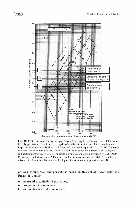
of rock composition and porosity is based on this set of linear equations.
Equations contain:
� measured magnitude of properties,� properties of components,� volume fractions of components.
Pure dolomite,porosity 0.26
Limestone–dolomitemixture, porosity 0.18
Pure limestone,porosity 0.10
B
C
A
BA C
Bul
k de
nsity
b
(gcm
−3 o
r M
gm
−3)
ρf = 1.0 gcm−3 or Mgm−3ρ
Compensated neutron apparent limestone porosity (%)
FIGURE 11.3 Neutron�density crossplot (Baker Atlas Log Interpretation Charts, 1985; with
friendly permission). Data from three depths of a carbonate section are plotted into the chart.
Depth A: measured bulk density ρ 5 2.540 g cm23 and neutron porosity φN 5 0.100. The result
is a pure limestone with porosity φ 5 0.10. Depth B: measured bulk density ρ 5 2.370 g cm23
and neutron porosity φN 5 0.330. The result is a pure dolomite with porosity φ 5 0.26. Depth
C: measured bulk density ρ 5 2.454 g cm23 and neutron porosity φN 5 0.205. The result is a
mixture of dolomite and limestone with a higher limestone content; porosity φ 5 0.18.
398 Physical Properties of Rocks
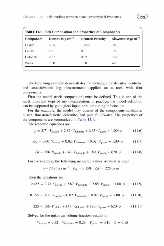
The following example demonstrates the technique for density-, neutron-,
and acoustic/sonic log measurements applied on a rock with four
components.
First the model (rock composition) must be defined. This is one of the
most important steps of any interpretation. In practice, the model definition
can be supported by geological input, core, or cutting information.
For the example, the model may consist of the components sandstone/
quartz, limestone/calcite, dolomite, and pore fluid/water. The properties of
the components are summarized in Table 11.1.
The response equations are
ρ ¼ 2:71UVcalcite þ 2:87UVdolomite þ 2:65UVquartz þ 1:00Uφ ð11:6Þ
φN ¼ 0:00UVcalcite þ 0:02UVdolomite 2 0:02UVquartz þ 1:00Uφ ð11:7Þ
Δt ¼ 156UVcalcite þ 143UVdolomite þ 180UVquartz þ 620Uφ ð11:8Þ
For the example, the following measured values are used as input:
ρ5 2:485 g cm23 φN ¼ 0:158 Δt ¼ 225 μs m23
Then the equations are
2:485 ¼ 2:71UVcalcite þ 2:87UVdolomite þ 2:65UVquartz þ 1:00Uφ ð11:9Þ
0:158 ¼ 0:00UVcalcite þ 0:02UVdolomite 2 0:02UVquartz þ 1:00Uφ ð11:10Þ
225 ¼ 156UVcalcite þ 143UVdolomite þ 180UVquartz þ 620Uφ ð11:11Þ
Solved for the unknown volume fractions results in:
Vcalcite ¼ 0:52 Vdolomite ¼ 0:23 Vquartz ¼ 0:10 φ ¼ 0:15
TABLE 11.1 Rock Composition and Properties of Components
Component Density in g cm23 Neutron Porosity Slowness in µs m21
Quartz 2.65 20.02 180
Calcite 2.71 0 156
Dolomite 2.87 0.02 143
Water 1.00 1.00 620
399Chapter | 11 Relationships Between Some Petrophysical Properties
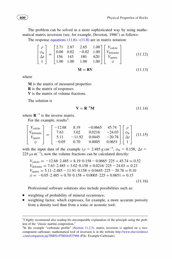
The problem can be solved in a more sophisticated way by using mathe-
matical matrix inversion (see, for example, Doveton, 19861) as follows:
The response equations (11.6)�(11.8) are in matrix notation:
ρφN
Δt
1
2664
3775 ¼
2:71 2:87 2:65 1:000:00 0:02 20:02 1:00156 143 180 620
1:00 1:00 1:00 1:00
2664
3775
Vcalcite
Vdolomite
Vquartz
φ
2664
3775 ð11:12Þ
M ¼ RV ð11:13Þwhere
M is the matrix of measured properties
R is the matrix of responses
V is the matrix of volume fractions.
The solution is
V ¼ R21M ð11:14Þwhere R21 is the inverse matrix.
For the example, results2:
Vcalcite
Vdolomite
Vquartz
φ
2664
3775 ¼
212:68 8:19 20:0665 45:747:63 3:02 0:0216 224:035:11 211:92 0:0445 220:7820:05 0:70 0:0005 0:0651
2664
3775
ρφN
Δt
1
2664
3775 ð11:15Þ
with the input data of the example (ρ 5 2.485 g cm23, φN 5 0.158, Δt 5225 μs m21), now the volume fractions can be calculated directly:
Vcalcite ¼ 212:68U2:485þ 8:19U0:1582 0:0665U225þ 45:74 ¼ 0:52Vdolomite ¼ 7:63U2:485þ 3:02U0:158þ 0:0216U2252 24:03 ¼ 0:23Vquartz ¼ 5:11U2:4852 11:91U0:158þ 0:0445U2252 20:78 ¼ 0:10φ ¼ 20:05U2:485þ 0:70U0:158þ 0:0005U225þ 0:0651 ¼ 0:15
ð11:16ÞProfessional software solutions also include possibilities such as:
� weighting of probability of mineral occurrence;� weighting factor, which expresses, for example, a more accurate porosity
from a density tool than from a sonic or acoustic tool;
1I highly recommend also reading his uncomparable explanation of the principle using the prob-
lem of the “classic martini composition.”2In the example “carbonate profile” (Section 11.2.3), matrix inversion is applied on a two-
component carbonate; mathematical tool of inversion is in the website http://www.elsevierdirect
.com/companion.jsp?ISBN=9780444537966 (File: Example-Carbonate).
400 Physical Properties of Rocks
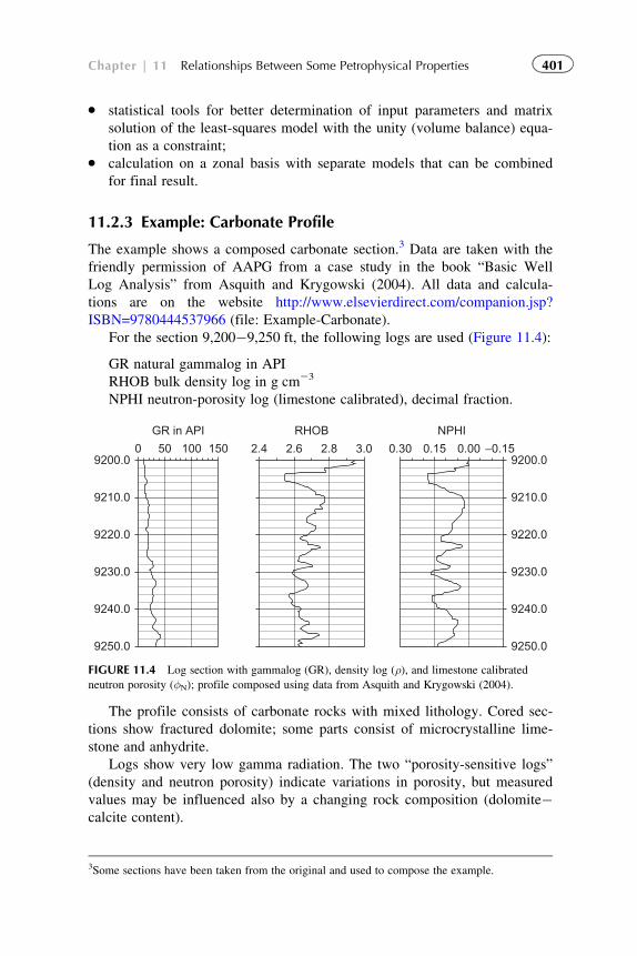
� statistical tools for better determination of input parameters and matrix
solution of the least-squares model with the unity (volume balance) equa-
tion as a constraint;� calculation on a zonal basis with separate models that can be combined
for final result.
11.2.3 Example: Carbonate Profile
The example shows a composed carbonate section.3 Data are taken with the
friendly permission of AAPG from a case study in the book “Basic Well
Log Analysis” from Asquith and Krygowski (2004). All data and calcula-
tions are on the website http://www.elsevierdirect.com/companion.jsp?
ISBN=9780444537966 (file: Example-Carbonate).
For the section 9,200�9,250 ft, the following logs are used (Figure 11.4):
GR natural gammalog in API
RHOB bulk density log in g cm23
NPHI neutron-porosity log (limestone calibrated), decimal fraction.
The profile consists of carbonate rocks with mixed lithology. Cored sec-
tions show fractured dolomite; some parts consist of microcrystalline lime-
stone and anhydrite.
Logs show very low gamma radiation. The two “porosity-sensitive logs”
(density and neutron porosity) indicate variations in porosity, but measured
values may be influenced also by a changing rock composition (dolomite�calcite content).
3Some sections have been taken from the original and used to compose the example.
9200.00 2.4 2.6 2.8 3.0 0.30 0.15 0.00 −0.1550 100 150
9210.0
9220.0
9230.0
9240.0
9250.0
9200.0
9210.0
9220.0
9230.0
9240.0
9250.0
GR in API RHOB NPHI
FIGURE 11.4 Log section with gammalog (GR), density log (ρ), and limestone calibrated
neutron porosity (φN); profile composed using data from Asquith and Krygowski (2004).
401Chapter | 11 Relationships Between Some Petrophysical Properties
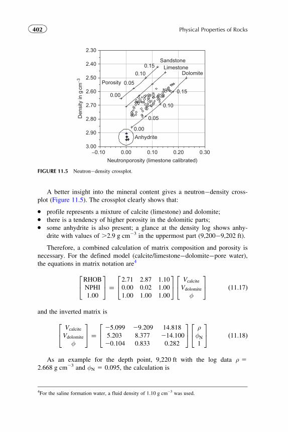
A better insight into the mineral content gives a neutron�density cross-
plot (Figure 11.5). The crossplot clearly shows that:
� profile represents a mixture of calcite (limestone) and dolomite;� there is a tendency of higher porosity in the dolomitic parts;� some anhydrite is also present; a glance at the density log shows anhy-
drite with values of .2.9 g cm23 in the uppermost part (9,200�9,202 ft).
Therefore, a combined calculation of matrix composition and porosity is
necessary. For the defined model (calcite/limestone�dolomite�pore water),
the equations in matrix notation are4
RHOB
NPHI
1:00
24
35 ¼
2:71 2:87 1:100:00 0:02 1:001:00 1:00 1:00
24
35 Vcalcite
Vdolomite
φ
24
35 ð11:17Þ
and the inverted matrix is
Vcalcite
Vdolomite
φ
24
35 ¼
25:099 29:209 14:8185:203 8:377 214:10020:104 0:833 0:282
24
35 ρ
φN
1
24
35 ð11:18Þ
As an example for the depth point, 9,220 ft with the log data ρ 52.668 g cm23 and φN 5 0.095, the calculation is
2.30
2.40
2.50
2.60
2.70
2.80
2.90
3.00−0.10 0.00 0.10 0.20 0.30
Neutronporosity (limestone calibrated)
Den
sity
in g
cm−3
Dolomite
0.00
0.05
0.05
0.00
0.10
0.10
0.15
0.15
Porosity
Anhydrite
SandstoneLimestone
FIGURE 11.5 Neutron�density crossplot.
4For the saline formation water, a fluid density of 1.10 g cm23 was used.
402 Physical Properties of Rocks
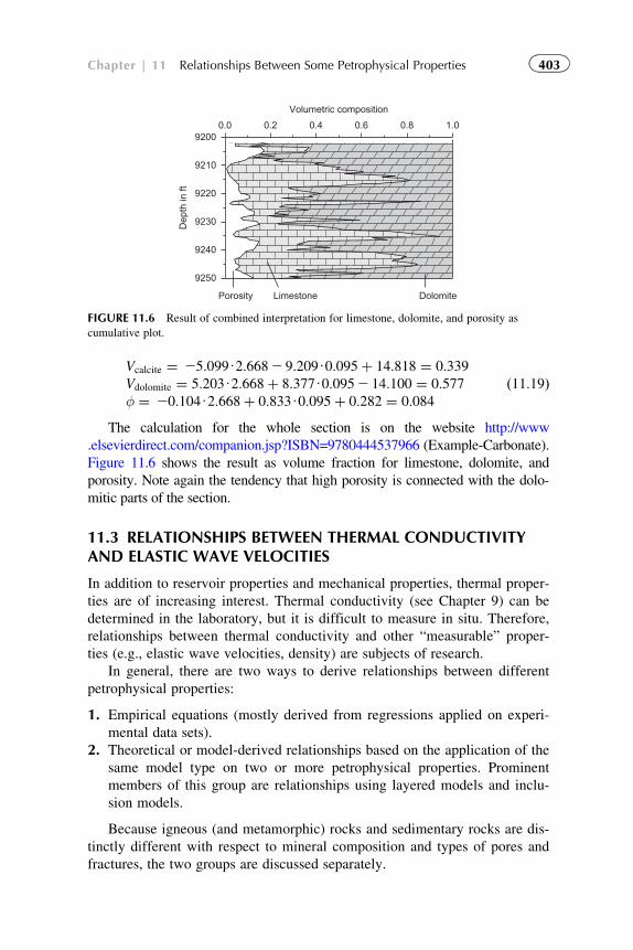
Vcalcite ¼ 25:099U2:6682 9:209U0:095þ 14:818 ¼ 0:339Vdolomite ¼ 5:203U2:668þ 8:377U0:0952 14:100 ¼ 0:577φ ¼ 20:104U2:668þ 0:833U0:095þ 0:282 ¼ 0:084
ð11:19Þ
The calculation for the whole section is on the website http://www
.elsevierdirect.com/companion.jsp?ISBN=9780444537966 (Example-Carbonate).
Figure 11.6 shows the result as volume fraction for limestone, dolomite, and
porosity. Note again the tendency that high porosity is connected with the dolo-
mitic parts of the section.
11.3 RELATIONSHIPS BETWEEN THERMAL CONDUCTIVITYAND ELASTIC WAVE VELOCITIES
In addition to reservoir properties and mechanical properties, thermal proper-
ties are of increasing interest. Thermal conductivity (see Chapter 9) can be
determined in the laboratory, but it is difficult to measure in situ. Therefore,
relationships between thermal conductivity and other “measurable” proper-
ties (e.g., elastic wave velocities, density) are subjects of research.
In general, there are two ways to derive relationships between different
petrophysical properties:
1. Empirical equations (mostly derived from regressions applied on experi-
mental data sets).
2. Theoretical or model-derived relationships based on the application of the
same model type on two or more petrophysical properties. Prominent
members of this group are relationships using layered models and inclu-
sion models.
Because igneous (and metamorphic) rocks and sedimentary rocks are dis-
tinctly different with respect to mineral composition and types of pores and
fractures, the two groups are discussed separately.
0.0 0.2 0.4 0.6 0.8 1.0
Volumetric composition
9250
9240
9230
9220
9210
9200
Dep
th in
ft
Porosity Limestone Dolomite
FIGURE 11.6 Result of combined interpretation for limestone, dolomite, and porosity as
cumulative plot.
403Chapter | 11 Relationships Between Some Petrophysical Properties
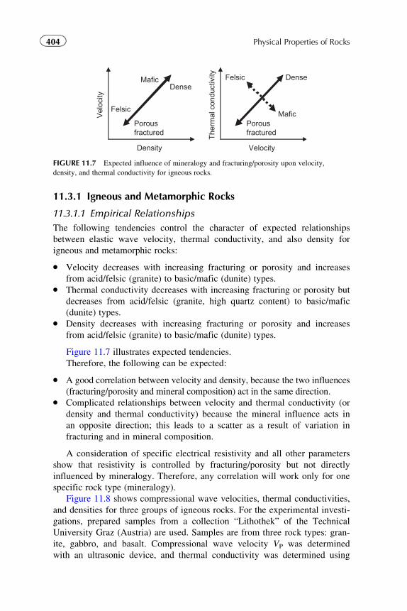
11.3.1 Igneous and Metamorphic Rocks
11.3.1.1 Empirical Relationships
The following tendencies control the character of expected relationships
between elastic wave velocity, thermal conductivity, and also density for
igneous and metamorphic rocks:
� Velocity decreases with increasing fracturing or porosity and increases
from acid/felsic (granite) to basic/mafic (dunite) types.� Thermal conductivity decreases with increasing fracturing or porosity but
decreases from acid/felsic (granite, high quartz content) to basic/mafic
(dunite) types.� Density decreases with increasing fracturing or porosity and increases
from acid/felsic (granite) to basic/mafic (dunite) types.
Figure 11.7 illustrates expected tendencies.
Therefore, the following can be expected:
� A good correlation between velocity and density, because the two influences
(fracturing/porosity and mineral composition) act in the same direction.� Complicated relationships between velocity and thermal conductivity (or
density and thermal conductivity) because the mineral influence acts in
an opposite direction; this leads to a scatter as a result of variation in
fracturing and in mineral composition.
A consideration of specific electrical resistivity and all other parameters
show that resistivity is controlled by fracturing/porosity but not directly
influenced by mineralogy. Therefore, any correlation will work only for one
specific rock type (mineralogy).
Figure 11.8 shows compressional wave velocities, thermal conductivities,
and densities for three groups of igneous rocks. For the experimental investi-
gations, prepared samples from a collection “Lithothek” of the Technical
University Graz (Austria) are used. Samples are from three rock types: gran-
ite, gabbro, and basalt. Compressional wave velocity VP was determined
with an ultrasonic device, and thermal conductivity was determined using
Vel
ocity
Density
Porousfractured
Porousfractured
DenseMafic
Felsic
The
rmal
con
duct
ivity
Velocity
Dense
Mafic
Felsic
FIGURE 11.7 Expected influence of mineralogy and fracturing/porosity upon velocity,
density, and thermal conductivity for igneous rocks.
404 Physical Properties of Rocks
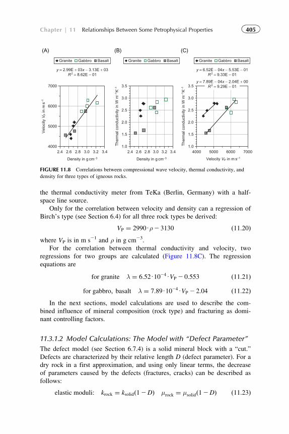
the thermal conductivity meter from TeKa (Berlin, Germany) with a half-
space line source.
Only for the correlation between velocity and density can a regression of
Birch’s type (see Section 6.4) for all three rock types be derived:
VP ¼ 2990Uρ2 3130 ð11:20Þwhere VP is in m s21 and ρ in g cm23.
For the correlation between thermal conductivity and velocity, two
regressions for two groups are calculated (Figure 11.8C). The regression
equations are
for granite λ ¼ 6:52U1024UVP 2 0:553 ð11:21Þ
for gabbro; basalt λ ¼ 7:89U1024UVP 2 2:04 ð11:22ÞIn the next sections, model calculations are used to describe the com-
bined influence of mineral composition (rock type) and fracturing as domi-
nant controlling factors.
11.3.1.2 Model Calculations: The Model with “Defect Parameter”
The defect model (see Section 6.7.4) is a solid mineral block with a “cut.”
Defects are characterized by their relative length D (defect parameter). For a
dry rock in a first approximation, and using only linear terms, the decrease
of parameters caused by the defects (fractures, cracks) can be described as
follows:
elastic moduli: krock ¼ ksolidð12DÞ μrock ¼ μsolidð12DÞ ð11:23Þ
y = 2.99E + 03x − 3.13E + 03R2 = 8.62E − 01
y = 6.52E − 04x − 5.53E − 01R2 = 9.33E − 01
4000
5000
6000
7000
2.4 2.6 2.8 3.0 3.2 3.4
Density in g cm−3
2.4 2.6 2.8 3.0 3.2 3.4
Density in g cm−3
Vel
ocity
VP in
ms−1
Granite Gabbro Basalt Granite Gabbro Basalt Granite Gabbro Basalt
1.0
1.5
2.0
2.5
3.0
3.5
The
rmal
con
duct
ivity
in W
m−1
K−1
1.0
1.5
2.0
2.5
3.0
3.5
The
rmal
con
duct
ivity
in W
m−1
K−1
4000 5000 6000 7000
Velocity VP in m s−1
y = 7.89E − 04x − 2.04E + 00R2 = 9.29E − 01
(A) (B) (C)
FIGURE 11.8 Correlations between compressional wave velocity, thermal conductivity, and
density for three types of igneous rocks.
405Chapter | 11 Relationships Between Some Petrophysical Properties
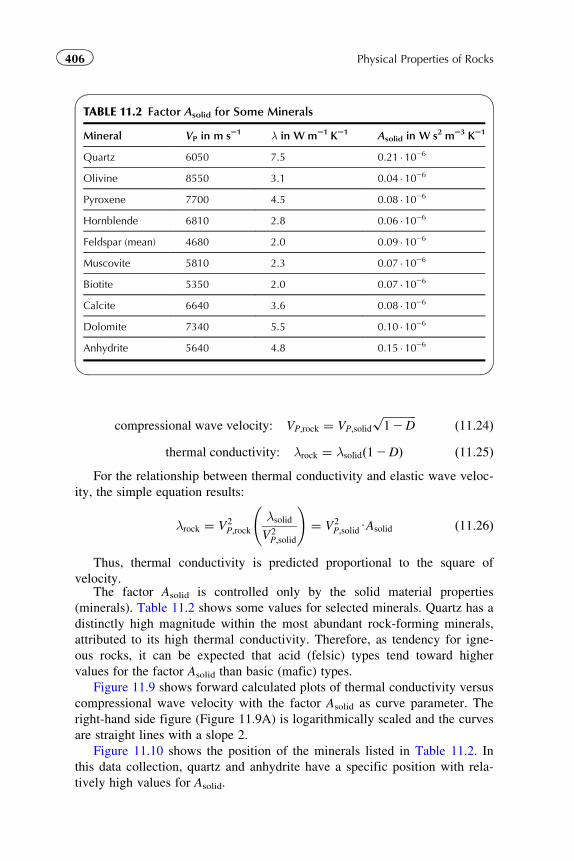
compressional wave velocity: VP;rock ¼ VP;solid
ffiffiffiffiffiffiffiffiffiffiffiffi12D
pð11:24Þ
thermal conductivity: λrock ¼ λsolidð12DÞ ð11:25ÞFor the relationship between thermal conductivity and elastic wave veloc-
ity, the simple equation results:
λrock ¼ V2P;rock
λsolid
V2P;solid
!¼ V2
P;solidUAsolid ð11:26Þ
Thus, thermal conductivity is predicted proportional to the square of
velocity.The factor Asolid is controlled only by the solid material properties
(minerals). Table 11.2 shows some values for selected minerals. Quartz has a
distinctly high magnitude within the most abundant rock-forming minerals,
attributed to its high thermal conductivity. Therefore, as tendency for igne-
ous rocks, it can be expected that acid (felsic) types tend toward higher
values for the factor Asolid than basic (mafic) types.
Figure 11.9 shows forward calculated plots of thermal conductivity versus
compressional wave velocity with the factor Asolid as curve parameter. The
right-hand side figure (Figure 11.9A) is logarithmically scaled and the curves
are straight lines with a slope 2.
Figure 11.10 shows the position of the minerals listed in Table 11.2. In
this data collection, quartz and anhydrite have a specific position with rela-
tively high values for Asolid.
TABLE 11.2 Factor Asolid for Some Minerals
Mineral VP in m s21 λ in W m21 K21 Asolid in W s2 m23 K21
Quartz 6050 7.5 0.21 � 1026
Olivine 8550 3.1 0.04 � 1026
Pyroxene 7700 4.5 0.08 � 1026
Hornblende 6810 2.8 0.06 � 1026
Feldspar (mean) 4680 2.0 0.09 � 1026
Muscovite 5810 2.3 0.07 � 1026
Biotite 5350 2.0 0.07 � 1026
Calcite 6640 3.6 0.08 � 1026
Dolomite 7340 5.5 0.10 � 1026
Anhydrite 5640 4.8 0.15 � 1026
406 Physical Properties of Rocks

The step to rocks is done with Figure 11.11. It shows experimental data
for granite, diorite, gabbro, and basalt in such a plot. The simple model
reflects the general tendency and separates the data clearly into two groups
of different mineral composition represented by the parameter Asolid.
2000 4000 6000 8000
0.0
2.0
4.0
6.0
8.0
10.0
(A) (B)
1000 100002000 5000
0.1
1.0
10.0
0.2
0.5
2
50.18
0.20
0.16
0.14
0.12
0.10
0.08
0.06
0.200.180.160.140.120.100.080.06
Compressional wave velocity in ms−1
Ther
mal
con
duct
ivity
in W
m−1
K−1
Ther
mal
con
duct
ivity
in W
m−1
K−1
Compressional wave velocity in ms−1
Asolid =
Asolid =
FIGURE 11.9 Calculated plots of thermal conductivity versus compressional wave
velocity with the factor Asolid (in 1026 W s2 m23 K21) as curve parameter; (A) linear
and (B) logarithmically scaled axes (for calculations, visit the website http://www
.elsevierdirect.com/companion.jsp?ISBN=9780444537966 and refer Relationships.
Defectmodel).
9000800070006000500040003000
Compressional wave velocity in ms−1
1.0
2.0
3.0
4.0
5.06.07.08.0
The
rmal
con
duct
ivity
in W
m−1
K−1
QuartzOlivinePyroxeneAmphiboleFeldsparMuscoviteBiotiteCalciteDolomiteAnhydrite
Asolid = 0.14 0.12 0.10 × 10⁻⁶ WK−1m−3s2
0.08 × 10⁻⁶ WK−1m−3s2
0.06 × 10⁻⁶ WK−1m−3s2
FIGURE 11.10 Thermal conductivity versus compressional wave velocity. Curves are
calculated for different values for the parameter Asolid 5 (0.06, 0.08, 0.10, 0.12, 0.14) �1026 W K21 m23 s2. The points show the position of the minerals listed in Table 11.2.
407Chapter | 11 Relationships Between Some Petrophysical Properties
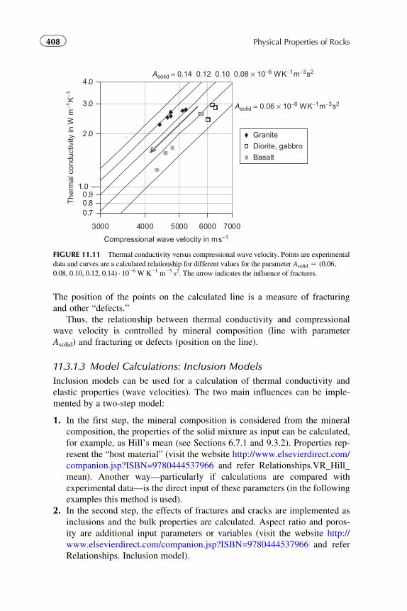
The position of the points on the calculated line is a measure of fracturing
and other “defects.”
Thus, the relationship between thermal conductivity and compressional
wave velocity is controlled by mineral composition (line with parameter
Asolid) and fracturing or defects (position on the line).
11.3.1.3 Model Calculations: Inclusion Models
Inclusion models can be used for a calculation of thermal conductivity and
elastic properties (wave velocities). The two main influences can be imple-
mented by a two-step model:
1. In the first step, the mineral composition is considered from the mineral
composition, the properties of the solid mixture as input can be calculated,
for example, as Hill’s mean (see Sections 6.7.1 and 9.3.2). Properties rep-
resent the “host material” (visit the website http://www.elsevierdirect.com/
companion.jsp?ISBN=9780444537966 and refer Relationships.VR_Hill_
mean). Another way—particularly if calculations are compared with
experimental data—is the direct input of these parameters (in the following
examples this method is used).
2. In the second step, the effects of fractures and cracks are implemented as
inclusions and the bulk properties are calculated. Aspect ratio and poros-
ity are additional input parameters or variables (visit the website http://
www.elsevierdirect.com/companion.jsp?ISBN=9780444537966 and refer
Relationships. Inclusion model).
Compressional wave velocity in ms−1
The
rmal
con
duct
ivity
in W
m−1
K−1
Asolid = 0.14 0.12 0.10 0.08 × 10⁻⁶ WK−1m−3s2
Asolid = 0.06 × 10⁻⁶ WK−1m−3s2
70006000500040003000
1.0
2.0
3.0
4.0
0.90.80.7
Granite
Diorite, gabbro
Basalt
FIGURE 11.11 Thermal conductivity versus compressional wave velocity. Points are experimental
data and curves are a calculated relationship for different values for the parameter Asolid 5 (0.06,
0.08, 0.10, 0.12, 0.14) � 1026 W K21 m23 s2. The arrow indicates the influence of fractures.
408 Physical Properties of Rocks
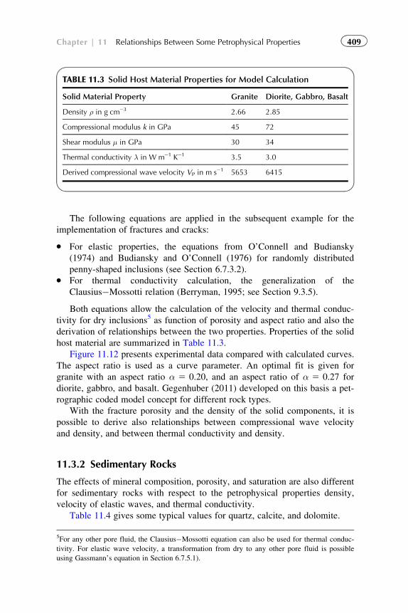
The following equations are applied in the subsequent example for the
implementation of fractures and cracks:
� For elastic properties, the equations from O’Connell and Budiansky
(1974) and Budiansky and O’Connell (1976) for randomly distributed
penny-shaped inclusions (see Section 6.7.3.2).� For thermal conductivity calculation, the generalization of the
Clausius�Mossotti relation (Berryman, 1995; see Section 9.3.5).
Both equations allow the calculation of the velocity and thermal conduc-
tivity for dry inclusions5 as function of porosity and aspect ratio and also the
derivation of relationships between the two properties. Properties of the solid
host material are summarized in Table 11.3.
Figure 11.12 presents experimental data compared with calculated curves.
The aspect ratio is used as a curve parameter. An optimal fit is given for
granite with an aspect ratio α 5 0.20, and an aspect ratio of α 5 0.27 for
diorite, gabbro, and basalt. Gegenhuber (2011) developed on this basis a pet-
rographic coded model concept for different rock types.
With the fracture porosity and the density of the solid components, it is
possible to derive also relationships between compressional wave velocity
and density, and between thermal conductivity and density.
11.3.2 Sedimentary Rocks
The effects of mineral composition, porosity, and saturation are also different
for sedimentary rocks with respect to the petrophysical properties density,
velocity of elastic waves, and thermal conductivity.
Table 11.4 gives some typical values for quartz, calcite, and dolomite.
5For any other pore fluid, the Clausius�Mossotti equation can also be used for thermal conduc-
tivity. For elastic wave velocity, a transformation from dry to any other pore fluid is possible
using Gassmann’s equation in Section 6.7.5.1).
TABLE 11.3 Solid Host Material Properties for Model Calculation
Solid Material Property Granite Diorite, Gabbro, Basalt
Density ρ in g cm23 2.66 2.85
Compressional modulus k in GPa 45 72
Shear modulus μ in GPa 30 34
Thermal conductivity λ in W m21 K21 3.5 3.0
Derived compressional wave velocity VP in m s21 5653 6415
409Chapter | 11 Relationships Between Some Petrophysical Properties
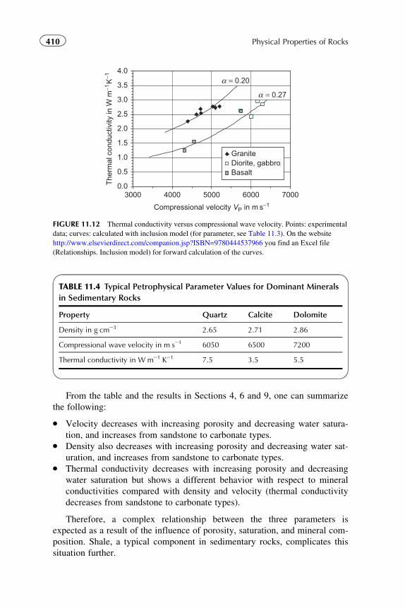
From the table and the results in Sections 4, 6 and 9, one can summarize
the following:
� Velocity decreases with increasing porosity and decreasing water satura-
tion, and increases from sandstone to carbonate types.� Density also decreases with increasing porosity and decreasing water sat-
uration, and increases from sandstone to carbonate types.� Thermal conductivity decreases with increasing porosity and decreasing
water saturation but shows a different behavior with respect to mineral
conductivities compared with density and velocity (thermal conductivity
decreases from sandstone to carbonate types).
Therefore, a complex relationship between the three parameters is
expected as a result of the influence of porosity, saturation, and mineral com-
position. Shale, a typical component in sedimentary rocks, complicates this
situation further.
TABLE 11.4 Typical Petrophysical Parameter Values for Dominant Minerals
in Sedimentary Rocks
Property Quartz Calcite Dolomite
Density in g cm23 2.65 2.71 2.86
Compressional wave velocity in m s21 6050 6500 7200
Thermal conductivity in W m21 K21 7.5 3.5 5.5
0.0
0.5
1.0
1.5
2.0
2.5
3.0
3.5
4.0
3000 4000 5000 6000 7000
GraniteDiorite, gabbroBasalt
α = 0.20
α = 0.27
Compressional velocity VP in m s−1
The
rmal
con
duct
ivity
in W
m−1
K−1
FIGURE 11.12 Thermal conductivity versus compressional wave velocity. Points: experimental
data; curves: calculated with inclusion model (for parameter, see Table 11.3). On the website
http://www.elsevierdirect.com/companion.jsp?ISBN=9780444537966 you find an Excel file
(Relationships. Inclusion model) for forward calculation of the curves.
410 Physical Properties of Rocks
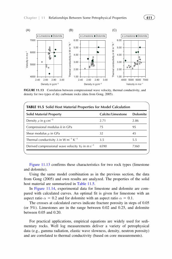
Figure 11.13 confirms these characteristics for two rock types (limestone
and dolomite).
Using the same model combination as in the previous section, the data
from Gong (2005) and own results are analyzed. The properties of the solid
host material are summarized in Table 11.5.
In Figure 11.14, experimental data for limestone and dolomite are com-
pared with calculated curves. An optimal fit is given for limestone with an
aspect ratio α 5 0.2 and for dolomite with an aspect ratio α 5 0.1.
The crosses at calculated curves indicate fracture porosity in steps of 0.05
(or 5%). Limestones are in the range between 0.02 and 0.25, and dolomite
between 0.05 and 0.20.
For practical applications, empirical equations are widely used for sedi-
mentary rocks. Well log measurements deliver a variety of petrophysical
data (e.g., gamma radiation, elastic wave slowness, density, neutron porosity)
and are correlated to thermal conductivity (based on core measurements).
4000
5000
6000
7000
(A) (B) (C)
2.40 2.60 2.80 3.00 3.00
Density in gcm−3
Vel
ocity
in m
s−1
1.00
2.00
3.00
4.00
5.00
6.00
2.40 2.60 2.80
Density in gcm−3
The
rmal
con
duct
ivity
in W
m−1
K−1
70001.00
2.00
3.00
4.00
5.00
6.00
4000 5000 6000
Velocity in ms−1
The
rmal
con
duct
ivity
in W
m−1
K−1
Limestone Dolomite Limestone Dolomite Limestone Dolomite
FIGURE 11.13 Correlation between compressional wave velocity, thermal conductivity, and
density for two types of dry carbonate rocks (data from Gong, 2005).
TABLE 11.5 Solid Host Material Properties for Model Calculation
Solid Material Property Calcite/Limestone Dolomite
Density ρ in g cm23 2.71 2.86
Compressional modulus k in GPa 75 95
Shear modulus μ in GPa 32 45
Thermal conductivity λ in W m21 K21 3.5 5.5
Derived compressional wave velocity VP in m s21 6590 7360
411Chapter | 11 Relationships Between Some Petrophysical Properties
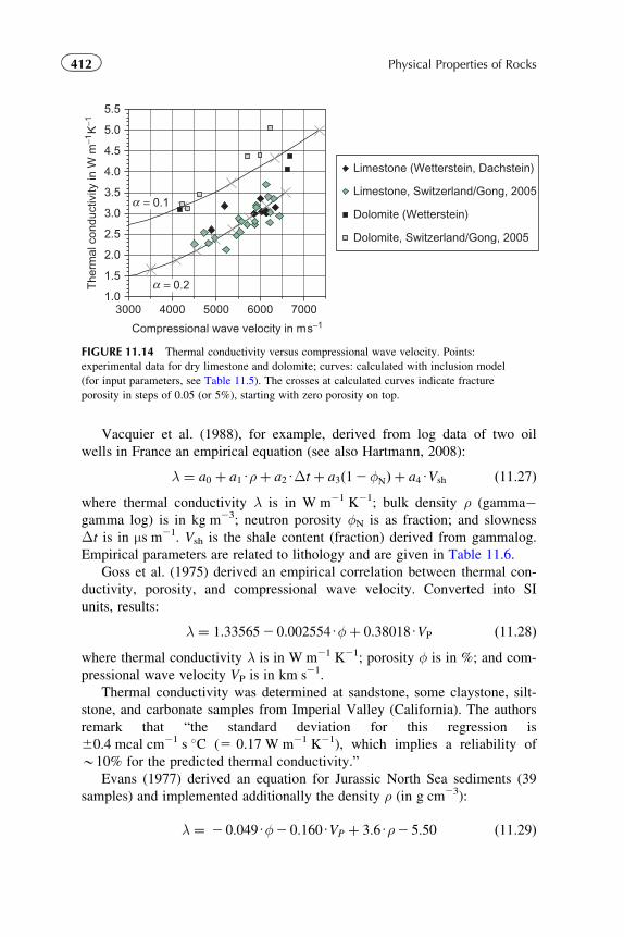
Vacquier et al. (1988), for example, derived from log data of two oil
wells in France an empirical equation (see also Hartmann, 2008):
λ ¼ a0 þ a1Uρþ a2UΔt þ a3ð12φNÞ þ a4UVsh ð11:27Þwhere thermal conductivity λ is in W m21 K21; bulk density ρ (gamma�gamma log) is in kg m23; neutron porosity φN is as fraction; and slowness
Δt is in μs m21. Vsh is the shale content (fraction) derived from gammalog.
Empirical parameters are related to lithology and are given in Table 11.6.
Goss et al. (1975) derived an empirical correlation between thermal con-
ductivity, porosity, and compressional wave velocity. Converted into SI
units, results:
λ ¼ 1:335652 0:002554Uφþ 0:38018UVP ð11:28Þwhere thermal conductivity λ is in W m21 K21; porosity φ is in %; and com-
pressional wave velocity VP is in km s21.
Thermal conductivity was determined at sandstone, some claystone, silt-
stone, and carbonate samples from Imperial Valley (California). The authors
remark that “the standard deviation for this regression is
60.4 mcal cm21 s �C (5 0.17 W m21 K21), which implies a reliability of
B10% for the predicted thermal conductivity.”
Evans (1977) derived an equation for Jurassic North Sea sediments (39
samples) and implemented additionally the density ρ (in g cm23):
λ ¼ 2 0:049Uφ2 0:160UVP þ 3:6Uρ2 5:50 ð11:29Þ
1.0
1.5
2.0
2.5
3.0
3.5
4.0
4.5
5.0
5.5
3000 4000 5000 6000 7000
= 0.1
Compressional wave velocity in ms−1
The
rmal
con
duct
ivity
in W
m−1
K−1
α
= 0.2α
Limestone (Wetterstein, Dachstein)
Limestone, Switzerland/Gong, 2005
Dolomite (Wetterstein)
Dolomite, Switzerland/Gong, 2005
FIGURE 11.14 Thermal conductivity versus compressional wave velocity. Points:
experimental data for dry limestone and dolomite; curves: calculated with inclusion model
(for input parameters, see Table 11.5). The crosses at calculated curves indicate fracture
porosity in steps of 0.05 (or 5%), starting with zero porosity on top.
412 Physical Properties of Rocks
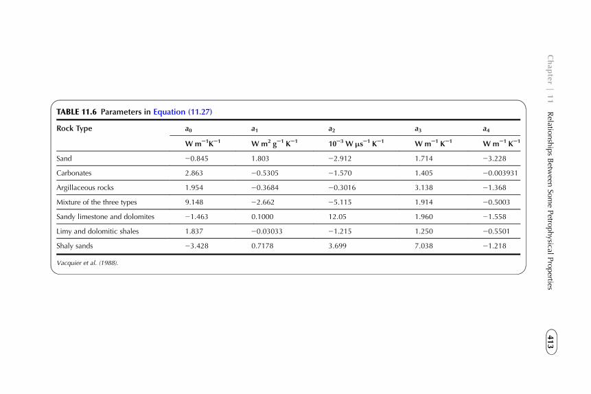
TABLE 11.6 Parameters in Equation (11.27)
Rock Type a0 a1 a2 a3 a4
W m21K21 W m2 g21 K21 1023 W µs21 K21 W m21 K21 W m21 K21
Sand 20.845 1.803 22.912 1.714 23.228
Carbonates 2.863 20.5305 21.570 1.405 20.003931
Argillaceous rocks 1.954 20.3684 20.3016 3.138 21.368
Mixture of the three types 9.148 22.662 25.115 1.914 20.5003
Sandy limestone and dolomites 21.463 0.1000 12.05 1.960 21.558
Limy and dolomitic shales 1.837 20.03033 21.215 1.250 20.5501
Shaly sands 23.428 0.7178 3.699 7.038 21.218
Vacquier et al. (1988).
413
Chapter|11
Relatio
nshipsBetw
eenSo
mePetro
physical
Properties
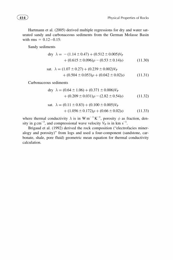
Hartmann et al. (2005) derived multiple regressions for dry and water sat-
urated sandy and carbonaceous sediments from the German Molasse Basin
with rms 5 0.12�0.15:
Sandy sediments
dry λ ¼ 2 ð1:146 0:47Þ þ ð0:5126 0:005ÞVP
þ ð0:6156 0:096Þρ2 ð0:536 0:14Þφ ð11:30Þ
sat: λ ¼ ð1:076 0:27Þ þ ð0:2396 0:002ÞVP
þ ð0:5046 0:053Þρþ ð0:0426 0:02Þφ ð11:31ÞCarbonaceous sediments
dry λ ¼ ð0:646 1:06Þ þ ð0:3716 0:006ÞVP
þ ð0:2096 0:031Þρ2 ð2:826 0:54Þφ ð11:32Þ
sat: λ ¼ ð0:116 0:83Þ þ ð0:1006 0:005ÞVP
þ ð1:0566 0:172Þρþ ð0:666 0:02Þφ ð11:33Þwhere thermal conductivity λ is in Wm2 1K21, porosity φ as fraction, den-
sity in g cm23, and compressional wave velocity VP is in km s21.
Brigaud et al. (1992) derived the rock composition (“electrofacies miner-
alogy and porosity)” from logs and used a four-component (sandstone, car-
bonate, shale, pore fluid) geometric mean equation for thermal conductivity
calculation.
414 Physical Properties of Rocks
Appendix A
Physical Properties ofRock-Forming Minerals
The following table is compiled from logging parameters summarized in log-
ging chartbooks from Baker Atlas and Schlumberger and used with friendly
permission. Parameters:
ρb, bulk density in g cm23
ρlog, log density (gamma�gamma�density) in g cm23
Z/A, ratio atomic number/atomic mass number
PE, photoelectric cross section in barns electron21
Δtp,Δts, slowness for compressional and shear wave in μs ft21 (in μs m21).
Σ, macroscopic cross section in capture units
φN, neutron porosity in porosity units (%). In the first line, the first raw
datum gives the value for epithermal measurement; the second raw, the
value for thermal measurement (Baker Atlas). In the second line, the first
raw datum gives the value for SNP (sidewall) measurement; the second raw,
the value for CNL (compensated neutron) measurement (Schlumberger).
ε, relative dielectric permittivity (Schlumberger, 2000)
λ, thermal conductivity in W m21 K21, data from the compilation of
Clauser and Huenges (1995).
415
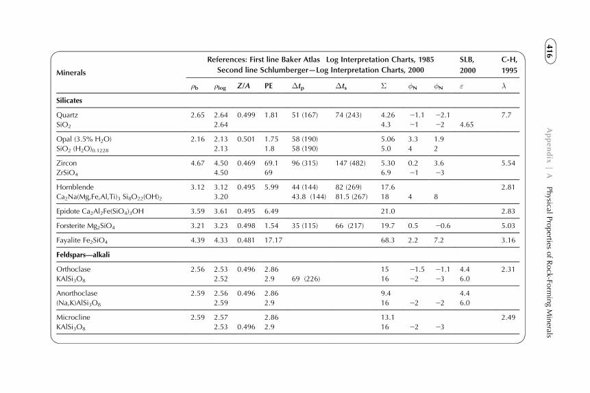
Minerals
References: First line Baker Atlas�Log Interpretation Charts, 1985 SLB,
2000
C-H,
1995Second line Schlumberger—Log Interpretation Charts, 2000
ρb ρlog Z/A PE Δtp Δts Σ φN φN ε λ
Silicates
Quartz 2.65 2.64 0.499 1.81 51 (167) 74 (243) 4.26 21.1 22.1 7.7
SiO2 2.64 4.3 21 22 4.65
Opal (3.5% H2O) 2.16 2.13 0.501 1.75 58 (190) 5.06 3.3 1.9
SiO2 (H2O)0.1228 2.13 1.8 58 (190) 5.0 4 2
Zircon 4.67 4.50 0.469 69.1 96 (315) 147 (482) 5.30 0.2 3.6 5.54
ZrSiO4 4.50 69 6.9 21 23
Hornblende 3.12 3.12 0.495 5.99 44 (144) 82 (269) 17.6 2.81
Ca2Na(Mg,Fe,Al,Ti)3 Si8O22(OH)2 3.20 43.8 (144) 81.5 (267) 18 4 8
Epidote Ca2Al2Fe(SiO4)3OH 3.59 3.61 0.495 6.49 21.0 2.83
Forsterite Mg2SiO4 3.21 3.23 0.498 1.54 35 (115) 66 (217) 19.7 0.5 20.6 5.03
Fayalite Fe2SiO4 4.39 4.33 0.481 17.17 68.3 2.2 7.2 3.16
Feldspars—alkali
Orthoclase 2.56 2.53 0.496 2.86 15 21.5 21.1 4.4 2.31
KAlSi3O8 2.52 2.9 69 (226) 16 22 23 6.0
Anorthoclase 2.59 2.56 0.496 2.86 9.4 4.4
(Na,K)AlSi3O8 2.59 2.9 16 22 22 6.0
Microcline 2.59 2.57 2.86 13.1 2.49
KAlSi3O8 2.53 0.496 2.9 16 22 23
416
Appendix
|A
Physical
Properties
ofRock-Fo
rmingMinerals
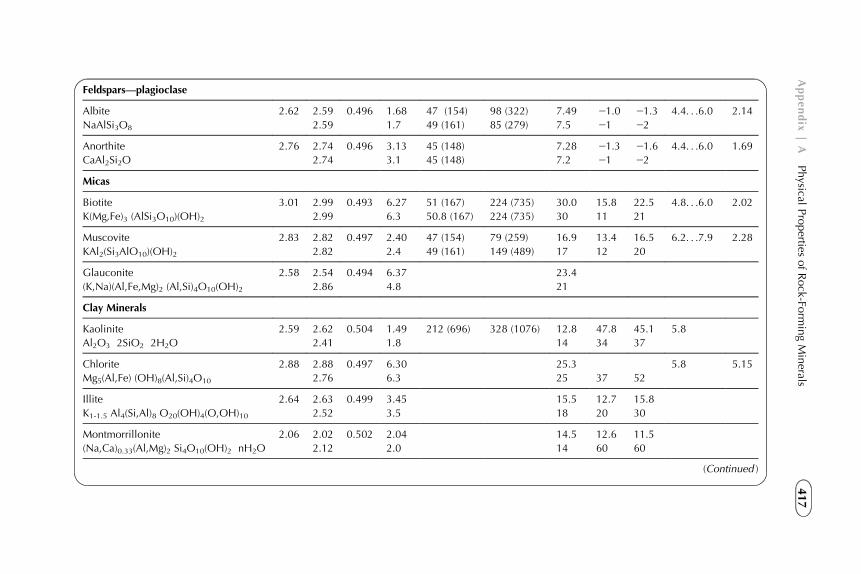
Feldspars—plagioclase
Albite 2.62 2.59 0.496 1.68 47 (154) 98 (322) 7.49 21.0 21.3 4.4. . .6.0 2.14
NaAlSi3O8 2.59 1.7 49 (161) 85 (279) 7.5 21 22
Anorthite 2.76 2.74 0.496 3.13 45 (148) 7.28 21.3 21.6 4.4. . .6.0 1.69
CaAl2Si2O 2.74 3.1 45 (148) 7.2 21 22
Micas
Biotite 3.01 2.99 0.493 6.27 51 (167) 224 (735) 30.0 15.8 22.5 4.8. . .6.0 2.02
K(Mg,Fe)3 (AlSi3O10)(OH)2 2.99 6.3 50.8 (167) 224 (735) 30 11 21
Muscovite 2.83 2.82 0.497 2.40 47 (154) 79 (259) 16.9 13.4 16.5 6.2. . .7.9 2.28
KAl2(Si3AlO10)(OH)2 2.82 2.4 49 (161) 149 (489) 17 12 20
Glauconite 2.58 2.54 0.494 6.37 23.4
(K,Na)(Al,Fe,Mg)2 (Al,Si)4O10(OH)2 2.86 4.8 21
Clay Minerals
Kaolinite 2.59 2.62 0.504 1.49 212 (696) 328 (1076) 12.8 47.8 45.1 5.8
Al2O3 � 2SiO2 � 2H2O 2.41 1.8 14 34 37
Chlorite 2.88 2.88 0.497 6.30 25.3 5.8 5.15
Mg5(Al,Fe) (OH)8(Al,Si)4O10 2.76 6.3 25 37 52
Illite 2.64 2.63 0.499 3.45 15.5 12.7 15.8
K1-1.5 Al4(Si,Al)8 O20(OH)4(O,OH)10 2.52 3.5 18 20 30
Montmorrillonite 2.06 2.02 0.502 2.04 14.5 12.6 11.5
(Na,Ca)0.33(Al,Mg)2 Si4O10(OH)2 � nH2O 2.12 2.0 14 60 60
(Continued )
417
Appendix
|A
Physical
Properties
ofRock-Fo
rmingMinerals
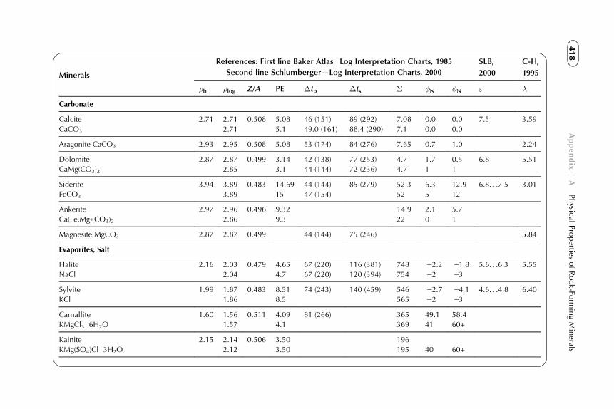
Minerals
References: First line Baker Atlas�Log Interpretation Charts, 1985 SLB,
2000
C-H,
1995Second line Schlumberger—Log Interpretation Charts, 2000
ρb ρlog Z/A PE Δtp Δts Σ φN φN ε λ
Carbonate
Calcite 2.71 2.71 0.508 5.08 46 (151) 89 (292) 7.08 0.0 0.0 7.5 3.59
CaCO3 2.71 5.1 49.0 (161) 88.4 (290) 7.1 0.0 0.0
Aragonite CaCO3 2.93 2.95 0.508 5.08 53 (174) 84 (276) 7.65 0.7 1.0 2.24
Dolomite 2.87 2.87 0.499 3.14 42 (138) 77 (253) 4.7 1.7 0.5 6.8 5.51
CaMg(CO3)2 2.85 3.1 44 (144) 72 (236) 4.7 1 1
Siderite 3.94 3.89 0.483 14.69 44 (144) 85 (279) 52.3 6.3 12.9 6.8. . .7.5 3.01
FeCO3 3.89 15 47 (154) 52 5 12
Ankerite 2.97 2.96 0.496 9.32 14.9 2.1 5.7
Ca(Fe,Mg)(CO3)2 2.86 9.3 22 0 1
Magnesite MgCO3 2.87 2.87 0.499 44 (144) 75 (246) 5.84
Evaporites, Salt
Halite 2.16 2.03 0.479 4.65 67 (220) 116 (381) 748 22.2 21.8 5.6. . .6.3 5.55
NaCl 2.04 4.7 67 (220) 120 (394) 754 22 23
Sylvite 1.99 1.87 0.483 8.51 74 (243) 140 (459) 546 22.7 24.1 4.6. . .4.8 6.40
KCl 1.86 8.5 565 22 23
Carnallite 1.60 1.56 0.511 4.09 81 (266) 365 49.1 58.4
KMgCl3 � 6H2O 1.57 4.1 369 41 60+
Kainite 2.15 2.14 0.506 3.50 196
KMg(SO4)Cl � 3H2O 2.12 3.50 195 40 60+
418
Appendix
|A
Physical
Properties
ofRock-Fo
rmingMinerals
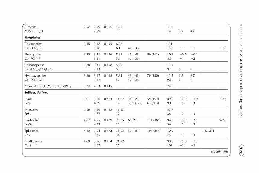
Kieserite 2.57 2.59 0.506 1.83 13.9
MgSO4 �H2O 2.59 1.8 14 38 43
Phosphates
Chlorapatite 3.18 3.18 0.495 6.06 131
Ca5(PO4)3Cl 3.18 6.1 42 (138) 130 21 21 1.38
Fluorapatite 3.20 3.21 0.496 5.82 45 (148) 80 (262) 10.3 20.7 20.2
Ca5(PO4)3F 3.21 5.8 42 (138) 8.5 21 22
Carbonapatite 3.28 3.31 0.498 5.58 11.4
Ca10(PO4)6CO3H2O 3.13 5.6 9.1 5 8
Hydroxyapatite 3.16 3.17 0.498 5.81 43 (141) 70 (230) 11.5 5.5 6.7
Ca5(PO4)3OH 3.17 5.8 42 (138) 9.6 5 8
Monazite (Ce,La,Y, Th,Nd,Pr)PO4 5.27 4.83 0.445 74.5
Sulfides, Sulfates
Pyrite 5.01 5.00 0.483 16.97 38 (125) 59 (194) 89.8 22.2 21.9 19.2
FeS2 4.99 17 39.2 (129) 62 (203) 90 22 23
Marcasite 4.88 4.86 0.483 16.97 87.7
FeS2 4.87 17 88 22 23
Pyrrhotite 4.62 4.55 0.479 20.55 65 (213) 111 (365) 94.6 22.3 22.1 4.60
Fe7S8 4.53 21 94 22 23
Sphalerite 4.10 3.94 0.472 35.93 57 (187) 108 (354) 40.9 7.8. . .8.1
ZnS 3.85 36 25 23 23
Chalkopyrite 4.09 3.96 0.474 26.72 98.8 22.0 21.2
Cu2S 4.07 27 102 22 23
(Continued )
419
Appendix
|A
Physical
Properties
ofRock-Fo
rmingMinerals
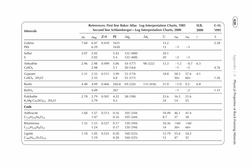
Minerals
References: First line Baker Atlas�Log Interpretation Charts, 1985 SLB,
2000
C-H,
1995Second line Schlumberger—Log Interpretation Charts, 2000
ρb ρlog Z/A PE Δtp Δts Σ φN φN ε λ
Galena 7.60 6.47 0.410 1631 13.2 2.28
PbS 6.39 1630 13 23 23
Sulfur 2.07 2.02 5.43 122 (400) 20.1
S 2.02 5.4 122 (400) 20 22 23
Anhydrite 2.96 2.98 0.499 5.06 54 (177) 98 (322) 12.3 21.2 20.7 6.3
CaSO4 2.98 5.1 50 (164) 21 22 4.76
Gypsum 2.31 2.33 0.511 3.99 53 (174) 18.8 58.5 57.6 4.1
CaSO4 � 2H2O 2.35 4.0 52 (171) 50+ 60+ 1.26
Barite 4.48 4.09 0.466 266.8 69 (226) 133 (436) 21.0 21.0 0.2 6.8
BaSO4 4.09 267 21 22 1.31
Polyhalite 2.78 2.79 0.501 4.32 58 (190) 23.6 16.5 21.6
K2Mg Ca2(SO4)4 � 2H2O 2.79 4.3 24 14 25
Coals
Anthracite 1.60 1.57 0.513 0.16 105 (344) 10.49 46.1 41.4
C720H258N6O16 1.47 0.16 105 (344) 8.7 37 38
Bituminous 1.35 1.33 0.527 0.17 120 (394) 16.36 .60 .60
C532H418N8O41 1.24 0.17 120 (394) 14 50+ 60+
Lignite 1.10 1.05 0.525 0.20 160 (525) 12.79 55.6 54.2
C480H412N7O101 1.19 0.20 160 (525) 13 47 52
420
Appendix
|A
Physical
Properties
ofRock-Fo
rmingMinerals
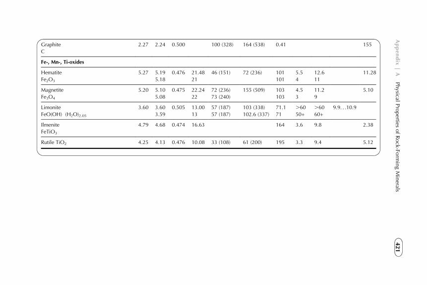
Graphite 2.27 2.24 0.500 100 (328) 164 (538) 0.41 155
C
Fe-, Mn-, Ti-oxides
Hematite 5.27 5.19 0.476 21.48 46 (151) 72 (236) 101 5.5 12.6 11.28
Fe2O3 5.18 21 101 4 11
Magnetite 5.20 5.10 0.475 22.24 72 (236) 155 (509) 103 4.5 11.2 5.10
Fe3O4 5.08 22 73 (240) 103 3 9
Limonite 3.60 3.60 0.505 13.00 57 (187) 103 (338) 71.1 .60 .60 9.9. . .10.9
FeO(OH) � (H2O)2.05 3.59 13 57 (187) 102.6 (337) 71 50+ 60+
Ilmenite 4.79 4.68 0.474 16.63 164 3.6 9.8 2.38
FeTiO3
Rutile TiO2 4.25 4.13 0.476 10.08 33 (108) 61 (200) 195 3.3 9.4 5.12
421
Appendix
|A
Physical
Properties
ofRock-Fo
rmingMinerals

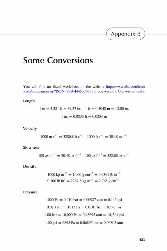
Appendix B
Some Conversions
You will find an Excel worksheet on the website http://www.elsevierdirect
.com/companion.jsp?ISBN=9780444537966 for conversions: Conversion units.
Length
1 m ¼ 3:281 ft ¼ 39:37 in: 1 ft ¼ 0:3048 m ¼ 12:00 in:
1 in: ¼ 0:0833 ft ¼ 0:0254 m
Velocity
1000 m s21 ¼ 3280:8 ft s21 1000 ft s21 ¼ 304:8 m s21
Slowness
100 µs m21 ¼ 30:48 µs ft21 100 µs ft21 ¼ 328:08 µs m21
Density
1000 kg m23 ¼ 1:000 g cm23 ¼ 0:0361 lb in23
0:100 lb in3 ¼ 2767:8 kg m23 ¼ 2:768 g cm23
Pressure
1000 Pa ¼ 0:010 bar ¼ 0:00987 atm ¼ 0:145 psi
0:010 atm ¼ 1013 Pa ¼ 0:0101 bar ¼ 0:147 psi
1:00 bar ¼ 10;000 Pa ¼ 0:98693 atm ¼ 14; 504 psi
1:00 psi ¼ 6895 Pa ¼ 0:06895 bar ¼ 0:06805 atm
423
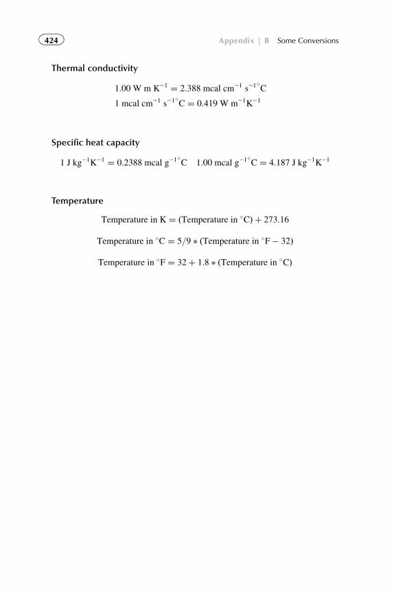
Thermal conductivity
1:00 W m K21 ¼ 2:388 mcal cm21 s21�C
1 mcal cm21 s21�C ¼ 0:419 W m21K21
Specific heat capacity
1 J kg21K21 ¼ 0:2388 mcal g21�C 1:00 mcal g21�C ¼ 4:187 J kg21K21
Temperature
Temperature in K ¼ ðTemperature in �CÞ þ 273:16
Temperature in �C ¼ 5=9 � ðTemperature in �F� 32Þ
Temperature in �F ¼ 32þ 1:8 � ðTemperature in �CÞ
424 Appendix | B Some Conversions
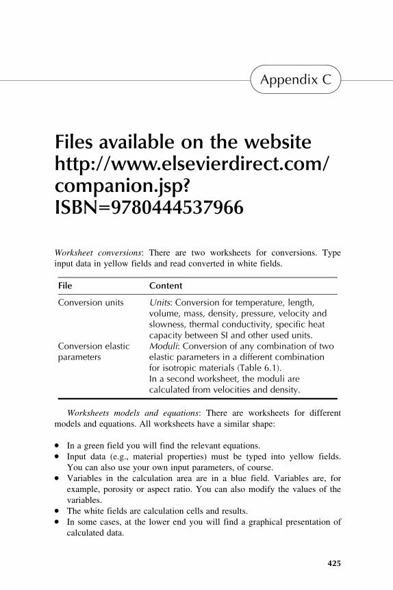
Appendix C
Files available on the websitehttp://www.elsevierdirect.com/companion.jsp?ISBN=9780444537966
Worksheet conversions: There are two worksheets for conversions. Type
input data in yellow fields and read converted in white fields.
File Content
Conversion units Units: Conversion for temperature, length,volume, mass, density, pressure, velocity andslowness, thermal conductivity, specific heatcapacity between SI and other used units.
Conversion elasticparameters
Moduli: Conversion of any combination of twoelastic parameters in a different combinationfor isotropic materials (Table 6.1).In a second worksheet, the moduli arecalculated from velocities and density.
Worksheets models and equations: There are worksheets for different
models and equations. All worksheets have a similar shape:
� In a green field you will find the relevant equations.� Input data (e.g., material properties) must be typed into yellow fields.
You can also use your own input parameters, of course.� Variables in the calculation area are in a blue field. Variables are, for
example, porosity or aspect ratio. You can also modify the values of the
variables.� The white fields are calculation cells and results.� In some cases, at the lower end you will find a graphical presentation of
calculated data.
425
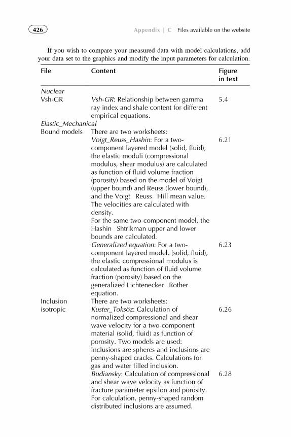
If you wish to compare your measured data with model calculations, add
your data set to the graphics and modify the input parameters for calculation.
File Content Figurein text
NuclearVsh-GR Vsh-GR: Relationship between gamma
ray index and shale content for differentempirical equations.
5.4
Elastic_MechanicalBound models There are two worksheets:
Voigt_Reuss_Hashin: For a two-component layered model (solid, fluid),the elastic moduli (compressionalmodulus, shear modulus) are calculatedas function of fluid volume fraction(porosity) based on the model of Voigt(upper bound) and Reuss (lower bound),and the Voigt�Reuss�Hill mean value.The velocities are calculated withdensity.
6.21
For the same two-component model, theHashin�Shtrikman upper and lowerbounds are calculated.Generalized equation: For a two-component layered model, (solid, fluid),the elastic compressional modulus iscalculated as function of fluid volumefraction (porosity) based on thegeneralized Lichtenecker�Rotherequation.
6.23
Inclusionisotropic
There are two worksheets:Kuster_Toksoz: Calculation ofnormalized compressional and shearwave velocity for a two-componentmaterial (solid, fluid) as function ofporosity. Two models are used:Inclusions are spheres and inclusions arepenny-shaped cracks. Calculations forgas and water filled inclusion.
6.26
Budiansky: Calculation of compressionaland shear wave velocity as function offracture parameter epsilon and porosity.For calculation, penny-shaped randomdistributed inclusions are assumed.
6.28
426 Appendix | C Files available on the website
Additional input parameter is the aspectratio.
Inclusionanisotropic
Hudson’s model: Calculation of thecomponents of the tensor of elasticitybased on the assumption of a VTImedium (horizontal cracks). Additionalinput parameter is the aspect ratio.
6.30
Fluidreplacement
There are two worksheets:Gassmann: The worksheet allows a fluidreplacement based on Gassmann’sequation. Input: compressional andshear wave velocity measured for rocksaturated with fluid 1, porosity,compressional modulus, and density offluid 1 and fluid 2. Output:compressional and shear wave velocityfor the rock saturated with fluid 2.Example: The worksheet gives a logexample for a fluid replacementgas-water.
6.59
Structuredmodel
There are five worksheets for differentvelocity influences:Porosity: Calculation of the porosityeffect upon velocity with the quotient ofpore aspect ratio to grain aspect ratio asparameter.
6.38
Pressure: Calculation of pressure effectupon velocity controlled by parametersof the contact elasticity.
6.40
Tensor: Calculation of the componentsof the “structure tensor” as function ofstructure angle and contact properties.
6.41
Derivation of velocity ratios (VP/VS) andThomson’s anisotropy parameters for thedry rock.Velocity grids: Grids are calculated withthe equations from worksheet Tensor.Two sets of parameters are used as input(parameter f, angle α).
6.42
VP versus strength: Calculation of therelationship between velocity (in thiscase compressional wave velocity) andcompressional strength.
7.23
(Continued )
427Appendix | C Files available on the website
(Continued)
File Content Figurein text
Shuey AVO Using Shuey’s equation, Rpp iscalculated as function of the angle Θ fordifferent cases of wet sand, gas sand,and shale. Input: material parameters ofthe layers.
6.46
ElectricalFracturedconductivity
Calculation of electrical conductivityand formation factor as function offracture porosity. The rock consists oftwo pore systems:
8.11
� Matrix porosity� Fracture porosity (oriented).
Laminatedsediment
Worksheet gives a forward calculation ofthe vertical and horizontal resistivity asfunction of volumetric composition for:
8.18
� laminated shaly sand with shale resis-tivity and sand parameters (waterresistivity, porosity, water saturation,Archie exponents) as input;
� laminated bimodal sand with para-meters for a coarse and a fine sand(water resistivity, porosity, water satu-ration, Archie exponents) as input.
Shaly sandequations
There are two worksheets:Poupon equation: Forward calculation offormation resistivity as function of watersaturation for different shale content Vsh.Calculation based on Poupon’s equationfor laminated shaly sand.
8.13
Shaly sand equation: For a givenformation resistivity and water resistivityas input, you can calculate the resultingwater saturation for the followingequations: Poupon, Simandoux, andIndonesia. Inputs are also Archieparameters, porosity, and shaleresistivity.
8.15
Permittivitymodels
Calculation of relative permittivity asfunction of porosity (two-componentcomposite) with the input parameters
428 Appendix | C Files available on the website
permittivity of solid and of fluid.Worksheet for the following models:� Layered model� Generalized
Lichtenecker�Rother� CRIM equation� Inclusion model (Clausius�Mossotti)
for sphere� Inclusion model (Hanai�Bruggeman)
for ellipsoids with depolarizationexponent as parameter.
8.258.278.28
ThermalLayeredmodels
There are two worksheets:Two components: Calculation of thermalconductivity of a two-componentmaterial (solid, fluid) as function ofporosity. The following equations areused:
9.12
Voigt model (parallel, upper bound),Reuss model (series, lower bound),arithmetic mean, geometric mean,Krischer and Esdorn model withparameter a, generalizedLichtenecker�Rother model withparameter α.
9.13
Ten components: Worksheet forcalculation of thermal conductivity of amaterial consisting of (maximum) 10components. Input: volume fraction andconductivity of components.
9.14
Calculation for following models: Voigtmodel (parallel, upper bound), Reussmodel (series, lower bound), Krischerand Esdorn model with parameter a,generalized Lichtenecker�Rother modelwith parameter α.
Table 9.14
Inclusionmodels
There are three worksheets:Spheres: Calculation of thermalconductivity as function of volumefraction for a two-component materialunder assumption of:
9.15
� spherical pores as inclusion in a solidhost material,
(Continued )
429Appendix | C Files available on the website
(Continued)
File Content Figurein text
� spherical grains as inclusion in a fluidhost material.
Disk random: Calculation of thermalconductivity as function of volumefraction for a two-component materialunder assumption of:
9.17
� spherical pores,� disk-shaped random oriented poresas inclusion in a solid host material.Ellipsoids oriented: Calculation ofthermal conductivity as function ofvolume fraction for a two-componentmaterial under assumption of ellipsoidicinclusions with orientation.
9.16
Calculations deliver thermal conduc-tivity for x-, y-axis and z-axis. Additionalinput parameter is aspect ratio.
RelationshipsVR_Hill_mean Voigt�Reuss�Hill mean value for elastic
properties, velocities, and thermalconductivity is calculated for a10-component mineral composite. Input:elastic parameters, density, thermalconductivity. Variable: volume fractions.
Defect model Based on the defect model, therelationship between thermalconductivity and compressional wavevelocity is calculated.
11.10
The controlling input parameter Asolid
describes the influence of mineralcomposition, whereas the defectparameter D controls the effects offractures, etc. The calculated curves arecompared with some experimental data.
Inclusionmodel
A correlation between thermalconductivity and compressional wavevelocity is calculated based on theapplication of:
11.13
� the Budiansky and O’Connell modelfor elastic properties,
430 Appendix | C Files available on the website
� the Clausius�Mossotti model forthermal conductivity.
Both models have as input the propertiesof the components (solid, inclusion),porosity, and aspect ratio.The calculated curves for two cases arecompared with on some experimentaldata.
Examples:
Examples
Example-Sandstone
The example from the textbook (Darling, 2005)is used to demonstrate core and log dataanalysis.
2.40
Core analysis:� Porosity-permeability regression� Capillary pressure analysis� Application of Leverett’s and Thomeer’s
equation� Derivation of Archie parameters
2.382.392.40
Log analysis:� Calculation of Vshale
� Calculation of porosity� Calculation of water saturation� Permeability estimate.
5.125.135.14
Example-Carbonate
The example demonstrates the calculation ofmineral fraction (calcite, dolomite) and porosityfrom neutron log and density log usingcrossplot and matrix inversion technique.
11.4
Worksheet crossplot presents the density andneutron data; you can move the plot upward tofit with the chartbook plot.
11.5
Worksheet analysis gives the calculation formineral composition and porosity.
11.6
431Appendix | C Files available on the website

References
Abdalla, W., Buckley, J.S., Carnegie, A., Herold, J.E.B., Fordham, E., Graue, A., et al., 2007.
Fundamentals of wettability. Oilfield Rev. Schlumberger 2007, 44�61.
Abu-Hamdeh, N.H., Reeder, R.C., 2000. Soil thermal conductivity: effects of density, moisture,
salt concentration, and organic matter. Soil Sci. Soc. Am. J. 64, 1285�1290.
Ahmed, T., 2001. Reservoir Engineering Handbook. Butterworth-Heinemann, Woburn, MA.
Akbar, M., Vissapraganda, B., Alghamdi, A.I., 2000/2002. A snapshot of carbonate reservoir
evaluation. Oilfield Rev. Winter, 20�41.
Akbar, M., Petricola, M., Watfa, M., Badri, M., Boyd, A., Charara, M., et al., 1995. Classic
interpretation problems: evaluating carbonates. Oilfield Rev. Schlumberger January, 38�57.
Aki, K., Richards, P.G., 1980. Quantitative Seismology: Theory and Methods. W.H. Freeman
and Co., San Francisco, CA.
Akkurt, R., Vinegar, H.J., Tutunjian, P.N., Guillorry, A.J., 1995. NMR logging of natural gas
reservoirs. Transactions of the SPWLA 36th Annual Logging Symposium, paper N.
Akkurt, R., Vinegar, H.J., Tutunjian, P.N., Guillory, A.J., 1996. NMR logging in natural gas
reservoirs. Log Analyst November�December, 33�42.
Akkurt, R., Mardon, D., Gardner, J.S., Marshall, D.M., Solanet, F., 1998. Enhanced diffusion:
expanding the range of NMR direct hydrocarbon-typing applications. Transactions of the
SPWLA 39th Annual Logging Symposium, paper GG.
Al-Awadi, M., Clark, W.J., Herron, M., Zang, T., Zhao, W., Hurley, N., et al., 2009. Dolomite:
perspectives on a perplexing mineral. Oilfield Rev. Schlumberger Autumn 2009, 32�45.
Alexandrov, K.S., Belikov, B.P., Rysova, T.V., 1966. Vycislenie uprugich parametrov gornich
porod po mineralnomu sostavu. Izvestia A. N. SSSR Ser. Geol. Moskva 2, 3�19.
Alger, R.P., Locke, S., Nagel, W.A., Sherman, H., 1971. The dual-spacing neutron log—CNL.
In: 46th Annual Fall Meeting SPE, paper SPE 3565.
Allen, L.S., Mills, W.R., Desai, K.P., Caldwell, R.L., 1972. Some features of dual-spaced
neutron porosity logging. In: 13th Annual Logging Symposium Transactions, Society of
Professional Log Analysts (SPWLA), paper P.
Altunbay, M., Georgi, D., Takezaki, H.M., 1997. Permeability prediction for carbonates: still a
challenge? Presented at the Middle East Oil Show and Conference, 15�18 March, Bahrain,
paper SPE 37753.
Anderson, W.G., 1986. Wettability literature survey, 3: the effect of wettability on the electrical
properties of porous media. J. Pet. Technol. 38, 1371�1378.
Amyx, J.W., Bass, D.M., Whiting, R.L., 1960. Petroleum Reservoir Engineering Physical
Properties. McGraw-Hill, New York, NY.
Anderson, B.I., Barber, T.D., Luling, M.G., Sen, P.N., 2006. Observations of large dielectric
effects on induction logs, or, can source rocks be detected with induction measurements. In:
SPWLA 47th Annual Logging Symposium Transactions, June 4�7, paper OOO.
Angenheister, G., Soffel, H., 1972. Gesteinsmagnetismus und Palaomagnetismus. Gebr.
Borntraeger, Stuttgart.
433
Annan, A.P., Davis, J.L., 1978. High-frequency electrical methods for the detection of
freeze�thaw interfaces. In: Proceedings of 3rd International Conference on Permafrost
Geophysics, Nat. Res. Council, Canada, pp. 495�500.
API, 1959. Recommended Practice for Standard Calibration and Form for Nuclear Logs. API—
American Petroleum Institute, Houston, TX.
Appel, M., 2004. Tutorial nuclear magnetic resonance and formation porosity. Petrophysics
45 (3), 296�307.
Archer, J.S., Jing, X.D., 1991. The influence of reservoir condition measurements of shaly sand
electrical properties on equity studies. In: Transactions of 14th European Formation
Evaluation Symposium of the SPWLA, London, 1�24, paper L.
Archie, G.E., 1942. Electrical resistivity log as an aid in determining some reservoir characteris-
tics. Trans. AIME 31, 350�366.
Archie, G.E., 1950. Introduction to petrophysics of reservoir rocks. AAPG Bull. 34, 943�961.
Armstrong, P., Ireson, D., Chmela, B., Dodds, K., Esmersoy, C., Miller, D., et al., 1994. The
promise of elastic anisotropy. Oilfield Rev. Schlumberger 8, 36�47.
Arns, C.H., Averdunk, H., Bauget, H., Sakellariou, A., Senden, T.J., Sheppard, A.T., et al.,
2004. Digital core laboratory: analysis of core fragments from 3D images. In: SPWLA 45th
Annual Logging Symposium Transactions, Nordwijk, paper EEE.
Arps, J.J., 1953. The effect of temperature on the density and electrical resistivity of sodium
chloride solutions. J. Pet. Technol. 195, 17�20, Technical Note.
Asquith, G., Krygowski, D., 2004. Basic Well Log Analysis, second ed., AAPG Methods in
Exploration Series 16, Tulsa.
Ass’ad, J., Tatham, R., McDonald, J.A., 1992. A physical model study of microcrack-induced
anisotropy. Geophysics 57 (12), 1562�1570.
Assefa, S., McCann, C., Sothcott, J., 1999. Attenuation of P- and S-waves in limestones.
Geophys. Prospect. 47, 359�392.
Athy, L.F., 1930. Density, porosity and compaction of sedimentary rocks. Bull. Am. Ass. Pet.
Geol. 14, 1�24.
Attewell, P.B., Ramana, Y.V., 1966. Wave attenuation and internal friction as functions of
frequency in rocks. Geophysics 31, 1049�1056.
Avseth, P., Mukerji, T., Mavko, G., 2005. Quantitative Seismic Interpretation, Applying Rock
Physics Tools to Reduce Interpretation Risk. Cambridge University Press, New York, NY.
Backus, G.E., 1962. Long-wave anisotropy produced by horizontal layering. J. Geophys. Res.
67, 4427�4440.
Baker Atlas/Baker Hughes, 1985. Log Interpretation Charts. Baker Hughes Inc., Houston, TX.
Baker Atlas/Western Atlas, 1992. Introduction to Wireline Log Analysis. Western Atlas Inc.,
Houston, TX.
Baker Atlas, 2002. Introduction to Wireline Log Analysis. Baker Hughes Inc., Houston, TX.
Baldwin, B., Butler, C.O., 1985. Compaction curves. AAPG Bull. 14, 1�24.
Balling, N., Kristiansen, J.I., Breiner, N., Poulsen, K.D., Rasmussen, R., Saxov, S., 1981.
Geothermal Measurements and Subsurface Temperature Modelling in Denmark, Geologiske
Skrifter. Aarhus University, Aarhus, Denmark, p. 16.
Bang, J., Solstad, A., Mjaaland, S., 2000. Formation electrical anisotropy derived from induction
log measurements in a horizontal well. Presented at the 2000 SPE Annual Technical
Conference and Exhibition, Dallas, Texas, 1�4 October, paper SPE 62908.
Bardon, C., Pied, B., 1969. Formation water saturation in shaly sands. In: SPWLA 10th Annual
Logging Symposium Transactions, Houston, Texas, 25�28 May, paper Z.
434 References
Barson, D., Decoster, E., Grau, J., Herron, M., Herron, S., Guru, U.K., et al., 2005.
Spectroscopy: the key to rapid, reliable petrophysical answers. Oilfield Rev. Schlumberger
Summer 2005.
Barton, N., 2007. Rock Quality, Seismic Velocity, Attenuation and Anisotropy. Taylor &
Francis Group/Balkema, Leiden, The Netherlands.
Barton, C.C., Hsieh, P.A., 1989. Physical and hydrologic-flow properties of fractures. 28th
International Geological Congress Field Trip Guide Book T385, P-36, AGU, Washington.
Barton, N., Lien, R., Lunde, J., 1974. Engineering classification of rock masses for the design of
tunnel support. Rock Mech. 6 (4), 189�239.
Bassiouni, Z., 1994. Theory, measurement, and interpretation of well logs, H.L. Doherty
Memorial Fund of AIME, SPE.
Bastos, A.C., Dillon, L.D., Vasquez, G.F., Soares, J.A., 1998. Core derived acoustic, porosity
and permeability correlations for computation pseudo-logs. In: Harvey, P.K., Lovell, M.A.
(Eds.), Core-Log Integration, 136. Geological Society, London, pp. 141�146, Special
Publication.
Batzle, M., Wang, Z., 1992. Seismic properties of pore fluids. Geophysics 57, 1396�1408.
Beard, D.C., Weyl, P.K., 1973. Influence of texture on porosity and permeability of unconsoli-
dated sand. AAPG Bull. 57, 349�369.
Beblo, M., Schopper, J.R., Haak, V., 1982. Electrical properties. In: Hellwege, K.-H. (Ed.),
Landolt-Bornstein Numerical Data and Functional Relationships in Science and Technology,
New Series, Group V. Geophysics and Space Research, vol. 1, Physical Properties of Rocks,
subvol. Springer-Verlag, Berlin, pp. 239�307.
Beck, A.E., 1976. An improved method of computing the thermal conductivity of fluid-filled
sedimentary rocks. Geophysics 41, 133�144.
Belikov, B.P., Alexandrov, K.S., Rysova, T.W., 1970. Uprugie Svoistva Porodo-Obrasujscich
Mineralov i Gornich Porod. Izdat. Nauka, Moskva.
Berg, R.R., 1970. Method for determining permeability from reservoir rock properties. Trans.
Gulf Coast Ass. Geol. Soc. 20, 303�317.
Berktold, A., 1982. Elektrische Leitfahigkeit von Losungen reiner Salze und von naturlichen
Wassern. In: Landolt-Bornstein Zahlenwerte und Funktionen aus Naturwissenschaft und
Technik, Neue Serie V. Springer-Verlag, Berlin, 1b.
Berryman, J., 1995. Mixture theories for rock properties. In: Arens, T.J. (Ed.), A Handbook of
Physical Constants. American Geophysical Union, pp. 205�228.
Berzon, J.S., 1977. Seismiceskaja Razvedka Vertikalno Sloistych sred Fundamenta. Izdat. Nedra,
Moskva.
Best, A.I., 1995. Classification of rocks and their abundances on the earth, rock physics and
phase relations—a handbook of physical constants. AGU Reference Shelf 3, American
Geophysical Union.
Best, M.E., Katsube, T.J., 1995. Shale permeability and its significance in hydrocarbon explora-
tion. Leading Edge, 165�170.
Bieniawski, Z.T., 1989. Engineering Rock Mass Classifications. John Wiley & Sons, New York, NY.
Bigelow, E.L., 1991. Geological log analysis of a carbonate reservoir. In: SPWLA 14th
European Formation Evaluation Symposium Transactions, London.
Bigelow, E., 1992. Introduction to Wireline Log Analysis. Western Atlas Inc., Houston, TX.
Bigelow, E.L., Howell, E.P., 1995. Practical analysis of formation strength properties in both
consolidated and unconsolidated reservoirs. In: SPWLA 36th Annual Logging Symposium
Transactions, 26�29 June, paper TTT.
435References
Binley, A., Slater, L.D., Fukes, M., Cassaini, G., 2005. Relationship between spectral induced
polarization and hydraulic properties of saturated and unsaturated sandstone. Water Resour.
Res. 41, W12417, doi:10.1029/2005WR004202.
Biot, M.A., 1956a. Theory of propagation of elastic waves in a fluid-saturated porous solid
(I. Low frequency range). J. Acoust. Soc. Am. 28 (2), 168�178.
Biot, M.A., 1956b. Theory of propagation of elastic waves in a fluid-saturated porous solid
(II. Higher frequency range). J. Acoust. Soc. Am. 28 (2), 179�191.
Biot, M.A., 1962. Generalized theory of acoustic propagation in dissipative media. J. Acoust.
Soc. Am. 34 (9), 1254�1264.
Birch, F., 1961. The velocity of compressional waves in rocks to 10 kilobars, part II.
J. Geophys. Res. 66, 2199�2224.
Birch, F., Clarke, H., 1940. The thermal conductivities of rocks and its dependence upon temper-
ature and composition (I., II.). Am. J. Sci. 238, 8�9, 529�558 and 613�635.
Blackwell, D.D., Steele, J.L., 1989. Thermal conductivity of sedimentary rocks: measurement
and significance. In: Naeser, N.D., McCulloh, T.H. (Eds.), Thermal History of Sedimentary
Basins. Springer-Verlag, New York, NY.
Blatt, H., Middleton, G.V., Murray, R.C., 1972. Origin of Sedimentary Rocks. Prentice Hall Inc.
Bleil, U., Petersen, N., 1982. Magnetic properties of minerals. In: Hellwege, K.-H. (Ed.),
Landolt-Bornstein Numerical Data and Functional Relationships in Science and Technology,
New Series, Group V. Geophysics and Space Research, vol. 1, Physical Properties of Rocks,
subvol. B. Springer-Verlag, Berlin, pp. 308�365.
Borner, F., 1991. Untersuchungen zur komplexen elektrischen Leitfahigkeit von Gesteinen im
Frequenzbereich von 1 Millihertz bis 10 Kilohertz, Dissertation�Thesis, Bergakademie
Freiberg.
Borner, F., 1992. Complex conductivity measurements of reservoir properties. In: Proceedings of
the Third European Core Analysis Symposium, Paris, pp. 359�386.
Borner, F., 1995. Estimation of hydraulic conductivity from complex electrical measurements.
In: SCA Conference San Francisco, paper No. 9523.
Borner, F., 2006. Complex conductivity measurements. In: Kirsch, R. (Ed.), Groundwater
Geophysics. Springer-Verlag, Berlin.
Borner, F., Gruhne, M., Schon, J., 1993. Contamination indications derived from electrical
properties in the low frequency range. Geophys. Prospect. 41, 83�98.
Borner, F.D., Schon, J.H., 1991. A relation between the quadrature component of electrical
conductivity and the specific surface area of sedimentary rocks. Log Analyst 32, 612�613.
Borner, F.D., Schon, J.H., 1995. Low frequency complex conductivity measurements of
microcrack properties. Surv. Geophys. 16, 121�135.
Borner, F.D., Schopper, F.D., Weller, A., 1996. Evaluation of transport and storage properties in
the soil and groundwater zone from induced polarization measurements. Geophys. Prospect.
44, 583�602.
Borysenko, A., Clennell, B., Burgar, I., Josh, M., Sedev, R., Ralston, J., et al., 2009. Monitoring
of fluid saturation and oil-water displacement using dielectric and NMR measurements. In:
Transactions on SPWLA 50th Annual Logging Symposium, June 21�24, paper VVV.
Bourbie, T., Coussy, O., Zinzner, B., 1987. Acoustics of Porous Media. Gulf Publishing
Company, Houston, TX.
Boyd, A., Darling, H., Tabanou, J., 1995. The lowdown on low-resistivity pay. Oilfield Rev.
Schlumberger Autumn, 4�10.
Brandt, H., 1955. A study of the speed of sound in porous granular media. J. Appl. Mech. 22,
479�486.
436 References
Bratton, T., Canh, D.V., Que, N.V., Duc, N.V., Gillespie, P., Hunt, D., et al., 2006. The nature
of naturally fractured reservoirs. Oilfield Rev. Schlumberger Summer, 4�23.
Brie, A., Pampuri, F., Marsala, A.F., Meazza, O., 1995. Shear sonic interpretation in gas-bearing
sands. In: 70th SPE Annual Technical Confrence and Exhibition, Dallas, TX, paper
SPE30595.
Brigaud, F., Vasseur, G., Caillet, G., 1989. Use of well log data for predicting detailed in situ
thermal conductivity profiles at well sites and estimation of lateral changes in main
sedimentary units at basin scale. In: Maury, V., Fourmaintraux, D. (Eds.), Rock at Great
Depth. Balkema, Rotterdam.
Brigaud, F., Vasseur, G., Caillet, G., 1992. Thermal state in the north Viking Graben (North
Sea) determined from oil exploration well data. Geophysics 57 (1), 69�88.
Brooks, C., Purcell, W., 1952. Surface area measurements on sedimentary rocks. AIME Pet.
Trans. 195, 289�296.
Brooks, R.J., Corey, A.T., 1964. Hydraulic properties of porous media, Hydrol. Papers 3.
Colorado State University, Fort Collins, CO.
Brown, A., 1997. Porosity variation in carbonates as a function of depth: Mississippian Madison
Group, Williston Basin. In: Kupecz, J.A., Gluyas, J., Bloch, S. (Eds.), Reservoir Quality
Prediction in Sandstones and Carbonates, AAPG Memoir 69, 29�46.
Brown, R., Korringa, J., 1975. On the dependence of the elastic properties of a porous rock on
the compressibility of the pore fluid. Geophysics 40, 608�616.
Bruggeman, D.A.G., 1935. Berechnung verschiedener physikalischer Konstanten von heteroge-
nen Substanzen. I: Dielektrizitatskonstanten und Leitfahigkeiten der Mischkorper aus isotro-
pen Substanzen. Ann. Phys. 24, 636�679.
Brunauer, S., Emmett, P., Teller, E., 1938. Adsorption of gases on multimolecular layers. J. Am.
Chem. Soc. 60 (2), 309�319.
Bucker, Ch., Rybach, L., 1996. A simple method to determine heat production from gamma-ray
logs. Mar. Pet. Geol. 13 (4), 373�375.
Bucker, C., Huenges, E., Lippmann, E., Rauen, A., Wienand, J., Wolter, K.E., 1989.
Gammaspektrometrie und Warmeproduktionsrate, KTB-Report 89-3, Projektleitung KTB im
NLfB, 476.
Buckley, J.S., Fan, T., 2007. Crude oil/brine interfacial tensions. Petrophysics 48 (3), 175�185.
Budiansky, B., O’Connell, R.J., 1976. Elastic moduli of a cracked solid. Int. J. Solids Struct. 12,
81�97.
Bulatova, S.M., Volkova, E.A., Dubrov, E., 1970. Akusticeski Karotas. Izdat. Nedra, Leningrad.
Burianik, M., 2000. Amplitude vs. offset and seismic rock property analysis: a primer. CSEG
Record. November, 6�14.
Calvert, T.J., Rau, R.N., Wells, L.E., 1977. Electromagnetic propagation—a new dimension in
logging. In: 47th Annual California Regional Meeting SPE, paper SPE 6542.
Carcione, J.M., 2001. Wave Fields in Real Media: Wave Propagation in Anisotropic Anelastic
and Porous Media. Pergamon Press.
Carcione, M., Seriani, G., 2000. An electromagnetic modelling tool for the detection of
hydrocarbons in the subsoil. Geophys. Prospect. 48, 231�256.
Carmichael, R.S., 1989. Practical Handbook of Physical Properties of Rocks and Minerals. CRC
Press, Boca Raton, FL.
Carmona, R., Hernandez, J., Marcos, J., Minetto, C., Arro, R., 2010. Application of RMN using
a probabilistic method into the Echoes inversion. Petroleum World, Latin American Energy,
Oil & Gas, Venezuela, Bolivia, Trinidad, Peru, August 29. http://www.petroleumworld.com/
sf09110101.htm.
437References
Carr, H.Y., Purcell, E.M., 1954. Effects of diffusion on free precession in nuclear magnetic
resonance experiments. Phys. Rev. 94, 630�638.
Carslaw, H.S., Jaeger, J.C., 1959. Conduction of Heat in Solids. Clarendon Press, Oxford.
Castagna, J.P., 1993. Amplitude-versus-offset analysis; tutorial and review. In: Castagna, J.P.,
Backus, M.M. (Eds.), Offset-Dependent Reflectivity—Theory and Practice of AVO
Analysis. Society of Exploration Geophysicists.
Castagna, J.P., Batzle, M.L., Eastwood, R.L., 1985. Relationships between compressional-wave
and shear-wave velocities in clastic silicate rocks. Geophysics 50, 571�581.
Castagna, J.P., Batzle, M.L., Kan, T.K., 1993. Rock physics—the link between rock properties
and AVO response. In: Castagna, J.P., Backus, M.L. (Eds.), Offset-Dependent
Reflectivity—Theory and Practice of AVO Analysis. Investigations in Geophysics, 8.
pp. 135�171.
Cattaneo, C., 1938. Sul contatto di due corpi elasticti. Accad. Lincei 27, 342�348, 434�436,
474�478.
Cermak, V., Rybach, L., 1982. Thermal properties. In: Hellwege, K.-H. (Ed.), Landolt-Bornstein
Numerical Data and Functional Relationships in Science and Technology, New Series,
Group V. Geophysics and Space Research, vol. 1, Physical Properties of Rocks, subvol.
A. Springer-Verlag, Berlin, pp. 305�371.
Cermak, V., Bodri, L., Rybach, L., Buntebarth, G., 1990. Relationship between seismic velocity
and heat production: comparison of two sets of data and test of validity. Earth Planet. Sci.
Lett. 99 (1990), 48�57.
Cerniak, G.J., 1964. Dielectriceskie Metody Issledovania Vlashnych Gruntov. Izdat. Nedra,
Moskva.
Chang, Ch., 2004. Empirical rock strength logging in boreholes penetrating sedimentary forma-
tions, geology and earth environmental sciences, Chungnam National University. Daejeon
7 (3), 174�183.
Chang, D., Vinegar, H., Morriss, C., Straley, C., 1997. Effective porosity, producible fluids, and
permeability in Carbonates from NMR logging. Log Analysts 38 (2), 60�72.
Chase, D.M., Schmidt, M.G., Ducheck, M.P., 1985. The Multiparameter Spectroscopy
Instrument Continuous Carbon/Oxygen Log—MSI C/O, Canadian Well Logging Society
10th Formation Evaluation Symposium, Calgary, 1985.
Chelidze, T.L., Gueguen, Y., 1999. Electrical spectroscopy of porous rocks: a review—I.
Theoretical models. Geophys. J. Int. 137, 1�15.
Chen, S., Georgi, D.T., 1997. Permeability from NMR Relaxation Data. Baker Atlas, Houston,
TX, 4 p. (unpublished).
Chen, S., Georgi, D.T., Withjack, E.M., Minetto, C., Olima, O., Gamin, H., H., 2000. Estimation
of oil viscosity with multiple TE dual wait-time MRIL logs. Petrophysics 41 (1), 33�40.
Chen, S., Munkholm, M., Shao, W., Jumagaziyev, D., Begova, N., 2006. Application of NMR
logging for characterizing movable and immovable fractions of viscose oils in Kazakhstan
heavy oil field, 47th Annual SPWLA Logging Symposium Transactions, Paper DD.
Cheng, A., 2008. Future developments in rock physics—a personal view, 17 June, Cambridge
GeoSCIENCES.
Cheng, C.H., 1993. Crack models for a transversely anisotropic medium. J. Geophys. Res. 98,
675�684.
Cheng, C.H., Johnston, D.H., 1981. Dynamic and static moduli. Geophys. Res. Lett. 8 (1),
39�42.
Cheng, C.H., Toksoz, M.N., 1979. Inversion of seismic velocities for the pore aspect ratio
spectrum of a rock. J. Geophys. Res. 84, 7533�7543.
438 References
Chi, X.-G., Han, D., 2009. Lithology and fluid differentiation using a rock physics template.
Leading Edge January, 60�65.
Cholach, P.Y., Schmitt, D.R., 2006. Seismic anisotropy of shales. CSEG Record. September,
39�43.
Chopra, S., Chemingui, N., Miller, R., 2005. An introduction to this special section—carbonates.
Leading Edge May, 488�489.
Choquette, P.W., Pray, L.C., 1970. Geologic nomenclature and classification of porosity in sedi-
mentary carbonates. Bull. Am. Assoc. Petrol. Geol. 54, 207�250.
Christensen, N.J., Salisbury, U.H., 1975. Structure and constitution of the lower oceanic crust.
Rev. Geophys. Space Phys. 13, 57�86.
Clark Jr., S.P., (Ed.), 1966. Handbook of Physical Constants. The Geological Society of
America, Inc., New York.
Clauser, C., 2006. Geothermal energy. In: Heinloth, von K. (Ed.), Landolt-Bornstein Numerical
Data and Functional Relationships in Science and Technology, New Series, Group VIII.
Advanced Materials and Technologies, vol. 3, Energy Technologies, subvol. C: Renewable
Energies. Springer-Verlag, Berlin, pp. 493�604.
Clauser, C., Huenges, E., 1995. Thermal conductivity of rocks and minerals, in: Rock Physics
and Phase Relations�A Handbook of Physical Constants, AGU Reference Shelf 3,
American Geophysical Union.
Clauser, C., Koch, A., 2006. Erstellung statistisch abgesicherter thermischer und hydraulischer
Gesteinseigenschaften fur den flachen und tiefen Untergrund in Deutschland, Phase 1—
Westliche Molasse und nordlich angrenzendes Suddeutsches Schichtstufenland, Bericht zum
BMU-Projekt FKZ 0329985, internet: http://www.geophysik.rwth-aachen.de/html/geothermik_
thermostat.htm (download September 2009)
Clauser, C., Hartmann, A., Koch, A., Mottaghy, D., Pechnig, R., Rath, V., 2007. Erstellung sta-
tistisch abgesicherter thermischer und hydraulischer Gesteinseigenschaften fur den flachen
und tiefen Untergrund in Deutschland, Phase 1—Westliche Molasse und nordlich angren-
zendes Suddeutsches Schichtstufenland, Final report for BMU-Projekt FKZ 0329985,
RWTH Aachen, Archived at the TIB Hannover httb://www.tib-hannover.de, also at http://
www.geophysik.rwth-aachen.de/html/geothermik_thermostat.htm (downloaded Sept. 2009).
Clavier, C., Coates, G., Dumanoir, J., 1977. The theoretical and experimental bases for the “dual
water” model for the interpretation of shaly sands, SPE paper No. 6859.
Clavier, C., Coates, G., Dumanoir, J., 1984. The theoretical and experimental bases for the “dual
water” model for the interpretation of shaly sands. Soc. Pet. Eng. J. 24 (2), 153�168.
Coates, G.R., Denoo, S.A., 1981. Mechanical properties program using borehole analysis and
Mohr’s circle, in SPWLA 22nd Annual Logging Symposium Transactions, Mexico City,
Mexico, 23�26 June, paper DD.
Coates, G.R., Denoo, S., 1988. The producibility answer product. Schlumberger Tech. Rev.
29 (2), 55.
Coates, G.R., Miller, M., Gillen, M., Henderson, G., 1991. The MRIL in Conoco 33-1: an
investigation of a new magnetic resonance imaging log. Presented at the SPWLA 32nd
Annual Logging Symposium, Midland, Texas, 16�19 June, paper DD.
Coates, G.R., Miller, D.L., Mardon, D., Gardener, J.S., 1995. Applying log measurements of
restricted diffusion and T2 to formation evaluation, Transactions 36th Annual Logging
Symposium, paper P.
Coates, G.R., Xiao, L., Prammer, M., 1999. NMR Logging—Principles and Applications. Gulf
Publishing Company, Halliburton Energy Services Publication, Houston, TX, H02308.
Cole, K.S., Cole, R.H., 1941. Dispersion and absorption in dielectrics. J. Chem. Phys. 9, 341.
439References
Collett, L.S., 1959. Laboratory investigation of overvoltage. In: Wait, J.R. (Ed.), Overvoltage
Research and Geophysical Applications. Pergamon Press.
Committee on Fracture Characterization and Fluid Flow, U.S. National Committee for Rock
Mechanics, 1996.
Corey, A.T., 1994. Mechanics of Immiscible Fluids in Porous Media. Water Resources
Publications, Highland Ranch, CO.
Cosentino, L., 2001. Integrated Reservoir Studies. Editions Technip, Paris.
Cosenza, P., Ghorbani, A., Camerlynck, C., Reijiba, F., Guerin, R., Tabbagh, A., 2009. Effective
medium theories for modelling the relationships between electromagnetic properties and
hydrological variables in geomaterials: a review. Near Surface Geophysics 7, 563�578.
Coutanceau-Monteil, N., Jacquin, Ch., 1993. Improvements of the coaxial line technique for
measuring complex dielectric permittivities of centimetric samples in the 20 to 1,000 MHz
range: application to sedimentary rocks. Log Analyst Sept-Oct., 21�33.
Crampin, S., Lovell, J.H., 1991. A decade of shear-wave splitting in the Earth’s crust: what does
it mean? what use can we make of it? and what should we do next? Geophys. J. Int.
107 (3), 387�408.
Dandekar, A.Y., 2006. Petroleum Reservoir Rock and Fluid Properties. Taylor & Francis, Boca
Raton, FL.
Darcy, H., 1856. Les Fontaines Publiques de la Ville de Dijon. V. Dalmont, Paris.
Darling, T., 2005. Well Logging and Formation Evaluation. Gulf Profess. Publish./Elsevier Inc.
de Lima, O.A.L., 1995. Water saturation and permeability from resistivity, dielectric, and porosity
logs. Geophysics 60, 1756�1764.
de Waal, J.A., Smits, R.M., de Graaf, J.D., Schipper, B.A., 1989. Measurement and evaluation of
resistivity index curves, in SPWLA 30th Annual Logging Symposium Transactions, paper II.
Dearing, J.A., 1994. Environmental Magnetic Susceptibility. Chi Publishing, Kenniworth.
Debye, P., Huckel, E., 1923. The theory of electrolytes. I. Lowering of freezing point and related
phenomena. Physikalische Zeitschrift 24, 185�206.
Deere, D.U., Hendron, A.J., Patton, F.D., Cording, E.J., 1967. Design of surface and near surface
construction in rock. In: Fairhurst, C. (Ed.), Failure and breakage of rock. Proc. 8th U.S.
Symp. Rock Mech, New York—Soc. Min. Eng., Am Inst. Min. Metall. Eng., pp. 237�302.
Deresievics, H., 1958. Mechanics of Granular Matter. Advances in Applied Mechanics, vol. V.
Academic Press, New York, NY, 233�306.
Dewar, J., Pickford, S., 2001. Rock physics for the rest of us—an informal discussion. CSEG
Recorder May, 49.
Dewhurst, D.N., Hennig, A.L., 2003. Geomechanical properties related to top seal leakage in the
Carnarvon Basin, Northwest Shelf, Australia. Pet. Geosci. 9, 255�263.
Di Rosa, D., Gyllensten, A., Chen, S., Li, W., Georgi, D.T., Tauk, R., 2006. Use of the NMR
diffusivity log to identify and quantify oil and water in carbonate formations, SPE 101396,
Abu Dhabi International Petroleum Exhibition and Conference held in Abu Dhabi, U.A.E.,
5�8 November.
Di Rosa, D., Gyllensten, A., Chen, S., Li, W., Georgi, D.T., Tauk, R., 2008. Use of the NMR
diffusion log to identify and quantify oil and water in carbonate formations. SPE Reservoir
Evaluation & Engineering April, 238�245.
Dias, C.A., 2000. Developments in a model to describe low-frequency electrical polarization of
rocks. Geophysics 65 (2), 437�451.
Digby, P.J., 1981. The effective elastic moduli of porous granular rocks. J. Appl. Mech. ASME
48, 803�808.
440 References
Dissado, L.A., Hill, R.M., 1984. Anomalous low-frequency dispersion. J. Chem. Soc. Farad.
Trans. 80, 291�319.
Dobrynin, W.M., 1963. Izmenenie fiziceskich svoistv pescanikov pod deistveiem vsestoronnego
davlenija. Trudy MINChGP, vyp. 41, Gostop Moscow.
Dobrynin, W.M., Vendelstejn, B.J., Koshevnikov, D.A., 2004. Petrofizika, Izdatelstvo Neft i
Gaz, Moskva.
Doering, M.A., Smith, D.P., 1974. Locating extraneous water sources with the gamma ray log,
SPE Fall Meeting, paper SPE 5116.
Domenico, S.N., 1976. Effect of brine gas mixture on velocity in unconsolidated sand reservoir.
Geophysics 41, 882�894.
Domenico, S.N., 1977. Elastic properties of unconsolidated porous sand reservoirs. Geophysics
42, 1339�1368.
Dorofeyeva, R.P., 1990. Teplogeneracia gornich porod i radiogennoe teplo Pribaikala
i Sabaikala. Fizika Semli 1, 82�90.
Dortman., N.B., 1976. Fiziceskie Svoistva Gornich Porod i Polesnich Iskopamych. Izdat. Nedra,
Moskva.
Doveton, J.H., 1986. Log Analysis of Subsurface Geology. John Wiley & Sons, New York, NY.
Drury, M.J., Jessop, A.M., 1983. The estimation of rock thermal conductivity from mineral
content—an assesment of techniques. Zbl. Geol. Palaont. Teil. 1, 35�48.
Duffant, K., Landrø, M., 2007. Vp/Vs ratio versus differential stress and rock consolidation—a
comparison between rock models and time-lapse AVO data. Geophysics 72/5, C81�C94.
Dunham R.J., 1962. Classification of carbonate rocks according to depositional texture. In:
Ham, W. E. (Ed.), Classification of carbonate rocks—a symposium. AAPG Memoirs 1,
108�121.
Dunn, K.-J., D.J. Bergman, D.J., Latoracca, G.A., 2002. Nuclear Magnetic Resonance—
Petrophysical and Logging Applications, Handbook of Geophysical Exploration, vol. 32.
Pergamon Press/Elsevier Science, Amsterdam.
Dvorkin, J., Nur, A., 1996. Elasticity of high-porous sandstones: theory for two North Sea data-
sets. Geophysics 61, 1363�1370.
Dvorkin, J., Armbruster, M., Baldwin, Ch., Fang, Q., Derzi, N., Gomez, C., et al., 2008. The
future of rock physics: computational methods vs. lab testing. First Break 26, 63�68.
Eberhart-Phillips, D., Han, D., Zoback, M., 1989. Empirical relationships among seismic velocity,
effective pressure, porosity, and clay content in sandstone. Geophysics 54 (1), 82�89.
Eberli, G.P., Baechle, G.T., Anselmetti, F.S., 2003. Factors controlling elastic properties in
carbonate sediments and rocks. Leading Edge July, 654�660.
Ebert, H. (Ed.), 1976. Physikalisches Taschenbuch, Vieweg und Sohn, Braunschweig.
Eisenberg, D., Kauzman, W., 1969. The Structure and Properties of Water. Oxford University
Press.
Ellis, D.V., 1987. Well Logging for Earth Scientists. Elsevier Science, New York, NY.
Ellis, D.V., Singer, J.M., 2007. Well Logging for Earth Scientists. Springer-Verlag, Dordrecht.
Ellis, D., Case, Ch.R., Chiaramonte, J.M., 2003. Tutorial: porosity from neutron logs I:
measurement. Petrophysics 44 (6), 383�395.
Ellis, D., Case, Ch.R., Chiaramonte, J.M., 2004. Tutorial: porosity from neutron logs II:
interpretation. Petrophysics 45 (1), 73�86.
Endres, A.L., Knight, R., 1989. The effect of microscopic fluid distribution on elastic wave
velocities. Log Analyst Nov-Dec, 437�445.
Engelhardt, W.V., 1960. Der Porenraum der Sedimente, Berlin, Gottingen. Springer-Verlag,
Heidelberg.
441References
England, W.A., Mackenzie, A.S., Mann, D.M., Quigley, D.M., 1987. The movement and
entrapment of petroleum fluids in the subsurface. J. Geol. Soc. London 144, 327�347.
Evans, T., 1977. Thermal properties of North Sea rocks. Log Analyst 18 (2), 3�12.
Fatt, I., 1953. The effect of overburden pressure on relative permeability. Pet. Trans. AIME 198,
325�326.
Fatti, J.L., Smith, G.C., Vail, P.V., Strauss, P.J., Levitt, P.R., 1994. Detection of gas in sandstone
reservoirs using AVO analysis: a 3-D seismic caase history using the Geostack Technique.
Geophysics 59, 1362�1376.
Fehr, A., 2007. NMR- and SIP-Messungen an Gesteinsproben, Diplomarbeit RWTH Aachen.
Fertl, F., 1979. Gamma ray spectral data assists in complex formation evaluation. Log Analyst
September�October, 3�37.
Fertl, W.H., 1983. Gamma ray spectral logging: A new evaluation frontier (part I to VII): World
Oil, series March 1983 to November 1983.
Fertl, W.H., 1987. Log-derived evaluation of shaly clastic reservoirs. J. Pet. Technol. February,
175�186.
Fjaer, E., Holt, R.M., Horsrud, P., Raaen, A.M., Rines, R., 2008. Petroleum Related Rock
Mechanics. second ed. Elsevier Science, Amsterdam.
Fleury, M., 2002. Resistivity in carbonates: new insights, SPE Annual Technical Conference and
Exhibition, San Antonio, Texas, 29 Sept.�2 Oct., paper SPE 77719.
Focke, J.W., Munn, D., 1987. Cementation exponents in Middle Eastern carbonate reservoirs.
SPE Formation Evaluation June, 155�167, paper SPE 13735.
Fowler, S.R., White, R.S., Louden, K.E., 1985. Sediment dewatering in the Makran accretionary
prism. Earth Planet. Sci. Lett. 75, 427�438.
Freedman, R., Heaton, N., 2004. Fluid characterization using nuclear magnetic resonance
logging. Petrophysics 45 (3), 241�250.
Freund, D., Nover, G., 1995. Hydrostatic pressure tests for the permeability-formation factor
relation on crystalline rocks from the KTB drilling project. Surveys in Geophysics 16 (1),
47�62.
Freyburg, E., 1972. Der untere und mittlere Buntsandstein SW-Thuringens in seinen gestein-
stechnischen Eigenschaften. Ber. Dte. Ges. Geol. Wiss. A. 17 (6), 911�919.
Fricke, S., Schon, J., 1999. Praktische Bohrlochgeophysik, Ferd. Enke Verlag Stuttgart.
Frohlich, L., 1975. Einsatzmoglichkeiten und Ergebnisse einer geophysikalischen
Komplexmethodik zur Strukturuntersuchung und Kennwertbestimmung, Diss. Univ. Leipzig
(unpublished).
Frohlich, L., Schwinge, G., 1978. Geophysikalische Messungen zur Losung ingenieur- geolo-
gischer Bauwerksuberwachung fur Wasserspeicher im Lockergesteinsbereich. Zeitschr.
F. Geol. Wiss. 6 (8), 1017�1024.
Fukushima, E., Roeder, S.B.W., 1981. Experimental Pulse NMR. A Nuts and Bolts Approach.
Addison Wesley.
Gardner, G.H.F., Gardner, L.W., Gregory, A.R., 1974. Formation velocity and density—the
diagnostic basis for stratigraphic traps. Geophysics 39, 770�780.
Garrouch, A.A., Sharma, M.M., 1994. The influence of clay content, salinity, stress, and
wettability on the dielectric properties of brine-saturated rocks: 10 Hz to 10 MHz.
Geophysics 59 (6), 909�917.
Gassmann, F., 1951a. Elastic waves through a packing of spheres. Geophysics 16, 673�685.
Gassmann, F., 1951b. Uber die Elastizitat poroser Medien. Vierteljahresschr. d. Naturforsch.
Ges. Zurich 96, 1�22.
442 References
Gassmann, F., 1964. Introduction to seismic travel time methods in anisotropic media. Pure
Appl. Geophys. 58 (II), 63�113.
Gavrilenko, P., Gueguen, Y., 1989. Pressure dependence of permeability: a model for cracked
rocks. Geophys. J. Int. 98, 159�172.
Gearhart Industries, 1978. Formation evaluation data handbook. Edition Forth Worth, USA.
Gebrande, H., Kern, H., Rummel, F., 1982. Elasticity and inelasticity. In: Hellwege, K.-H. (Ed.),
Landolt-Bornstein Numerical Data and Functional Relationships in Science and Technology,
New Series, Group V. Geophysics and Space Research, vol. 1, Physical Properties of Rocks,
subvol. B. Springer-Verlag, Berlin, pp. 1�233.
Geertsma, I., Smith, D.C., 1961. Some aspects of elastic wave propagation in fluid saturated
porous solids. Geophysics 26, 169�181.
Gegenhuber, N., 2011a. An improved method to determine heat production from gamma-ray
logs. Extended abstracts 73rd EAEG 2011 Conference & Exhibition, 23�26 May 2011,
Vienna.
Gegenhuber, N., 2011b. Compressional wave velocity-thermal conductivity correlation: from the
laboratory to logs. Extended abstracts 73rd EAEG 2011 Conference & Exhibition, 23�26
May 2011, Vienna.
Gegenhuber, N.M., Schon, J.H., 2010. Anisotropy of thermal conductivity of a gneiss—
experiments and models, EGU general assembly. EGU 2010-1535, Vienna.
Georgi, D.T., Chen, S., 2007. NMR Contributions to Petrophysics, Manuscript #992. Presented
at 2007 Petrotech Conference, New Delhi, India, January 15�19, 2007.
Georgi, D.T., Menger, S.K., 1994. Reservoir quality, porosity and permeability relationships.
Trans. 14. Mintrop-Seminar (Beilage), DGMK und Ruhr-Universitat Bochum 163/1�163/35.
Georgi, D.T., Kasap, E., Altunbay, M., Tang, X., Cheng, A., 1997. Permeability profiles—key to
reservoir management. In Depth, Baker Atlas June 10, 1�12.
Gilchrist, W.A., 2009. Tutorial: compensated neutron log response issues. Petrophysics 50 (5),
416�426.
Gilchrist, W.A., Prati, E., Pemper, R., Mickael, M.W., Trcka, D., 1999. Introduction of a New
Through-Tubing Multifunction Pulsed Neutron Instrument. In: Trans. SPE 74th Annual
Technical Conference and Exhibition, Houston, 1999, paper SPE 56803.
Gilchrist, W.A., Pemper, R.R., Trcka, D., Frost, E., Wilson, W., 2000. Initial Field Applications
of a New 1.7-Inch Pulsed Neutron Instrument, Paper FF, Trans., SPWLA 41st Annual
Logging Symposium, Dallas, 2000.
Golubev, A., Rabinovich, G.J., 1976. Resultaty primenenia apparatury akusticeskogo karotasa dlja
predelenia procnostych svoistv gornych porod na mestorosdeniach tverdych iskopaemych.
Prikl. Geofiz. Moskva 73, 109�116.
Gommensen, L., Fabricius, I.L., Mukerji, T., Mavko, G., Pedersen, J.M., 2007. Elastic behaviour
of North Sea chalk: a well-log study. Geophys. Prospect. 55, 307�322.
Gong, G., 2005. Physical properties of alpine rocks: a labortatory investigation, Thesis
University of Geneva, These No. 3658.
Goodman, R.E., 1988. Introduction to Rock Mechanics. John Wiley & Sons, New York, NY.
Goodway, W., Chen, T., Downton, J., 1997. Improved AVO fluid detection and lithology
discrimination using Lame petrophysical parameters; “Lambda-Rho”, “Mu-Rho” &
“Lambda/Mu fluid stack”, from P and S inversions, CSEG meeting abstracts, pp. 148�151;
CSEG Recorder, 22(7), 3�5, and SEG meeting abstracts, pp, 183�186.
Gorjainov, N.N., Ljachovickij, F.M., 1979. Seismiceskie Metody v Insenernoi Geologii. Izdat.
Nedra, Moskva.
443References
Goss, R., Combs, J., Timur, A., 1975. Prediction of thermal conductivity in rocks from other
physical parameters and from standard well logs, in SPWLA 16th Annual Logging
Symposium Transactions, New Orleans, Louisiana, 16�19 June, paper MM.
Goulty, N.R., 1998. Relationships between porosity and effective stress in shales. First Break
16 (12), 413�419.
Grant, I.S., West, G.F., 1965. Interpretation Theory in Applied Geophysics. McGraw-Hill,
New York, NY.
Gregory, A.R., 1990. Ultrasonic velocity and attenuation measurements in water-based drilling
muds, paper presented at ASME ETCE Conference, New Orleans, LA, January.
Griffith, D.H., King, R.F., 1965. Applied Geophysics for Engineers and Geologists. Pergamon
Press.
Griffiths, C.M., Brereton, N.R., Beausillon, R., Castillo, D., 1992. Thermal conductivity predic-
tion from petrophysical data: a case study. In: Hurst, A., Griffiths, C.M., Worthington, P.F.
(Eds.), Geological Applications of Wireline Logs II, Geological Society Special Publication
No. 65, pp. 299�315.
Gueguen, Y., Dienes, J., 1989. Transport properties of rocks from statistics and percolation.
Math. Geol. 21 (1), 1�13.
Gueguen, Y., Palciauskas, V., 1994. Introduction to the Physics of Rocks. Princeton University
Press, New Jersey, NJ.
Haack, U., 1982. Radioactivity of rocks. In: Hellwege, K.-H. (Ed.), Landolt-Bornstein Numerical
Data and Functional Relationships in Science and Technology, New Series, Group
V. Geophysics and Space Research, vol.1, Physical Properties of Rocks, subvol.
B. Springer-Verlag, Berlin, pp. 433�481.
Hagiwara, T., 1994. Response of 2 MHz resistivity devices in thinly laminated formations
(anisotropic resistivity and EM log interpretation). Presented at SPE 69th Annual Technical
Conference, pp. 667�675, paper 28426.
Hagiwara, T., 1996. A new method to determine horizontal-resistivity in anisotropic formations
without prior knowledge of relative dip, in SPWLA 37th Annual Logging Symposium
Transactions, New Orleans, LA, paper Q.
Hagiwara, T., 1997. Macroscopic anisotropy approach to analysis of thinly laminated sand/shale
sequences: sensitivity analysis of sand resistivity estimate and environmental corrections,
paper presented at SPE Annual Technical Conference and Exhibition, San Antonio, Texas,
paper SPE 38669.
Hamilton, E.L., 1970. Sound velocity and related properties of marine sediments. North Pacific.
J. Geoph. Res. 75, 4423�4446.
Hamilton, E.L., 1971. Elastic properties of marine sediments. J. Geoph. Res. 76, 579�604.
Hamilton, E.L., 1978. Sound velocity-density relations in sea floor sediments and rocks.
J. Acoust. Soc. Am. 63, 366�377.
Hamilton, E.L., Bachman, R.T., Berger, W.H., Johnson, T.C., Mayere, L.A., 1982. Acoustic and
related properties of calcareous deep-sea sediments, Journ. Sediment. Pet. 52, 0733�0753.
Han, D., Nur, A., Morgan, D., 1986. Effects of porosity and clay content on wave velocities in
sandstones. Geophysics 51 (11), 2093�2107.
Han, X., Pemper, R., Tutt, T., Li, F., 2009. Environmental Corrections and System Calibration
for a new Pulsed-Neutron Mineralogy Instrument, SPWLA 50th Annual Logging
Symposium, June 21�24, paper S.
Hanai, T., 1960. Theory of the dielectric dispersion due to the interfacial polarization and its
application to emulsions. Kolloidzeitschrift 171, 23�31.
444 References
Hara, G., 1935. Theorie der akustischen Schwingungsausbreitung in gekornten Substanzen und
experimentelle Untersuchungen an Kohlepulver, Elektr. Nachrichtentechnik 12 (7), 191�200.
Hartmann, A., 2008. Inversion of geothermal parameters using borehole and core data,
Dissertation (PhD), RWTH Aachen.
Hartmann, A., Rath, V., Clauser, C., 2005. Thermal conductivity from core and well log data.
Int. J. Rock Mech. Min. Sci. 42 (2005), 1042�1055.
Hartmann, D.J., Beaumont, E.A., 1999. Predicting reservoir system quality and performance. In:
Beaumont, E.A., Forster, N.H. (Eds.), AAPG treatise of petroleum geology, exploration for
oil and gas traps, Ch. 9 (9-1 to 9-154).
Hashin, Z., Shtrikman, S., 1962a. A variational approach to the theory of elastic behavior of
polycrystals. J. Mech. Phys. Solids 10, 343�352.
Hashin, Z., Shtrikman, S., 1962a. On some variational principles in anisotropic and
nonhomogenous elasticity. J. Mech. Phys. Solids 10, 335�342.
Hashin, Z., Shtrikman, S., 1963. A variational approach to the elastic behavior of multiphase
materials. J. Mech. Phys. Solids 11, 127�140.
Hazen, A., 1893. Some physical properties of sands and gravels with special reference to
their use in filtration, 24th Ann. Rept., Mass. State Board of Health, Pub. Doc. 34,
pp. 539�556.
He, T., Schmitt, D., 2006. P- and S-wave velocity measurements and pressure sensitivity analysis
of AVA response, CSPG-CSEG-CWLS Joint Convention, May, 398�404.
Hearst, J.R., Nelson, P.H., 1985. Well Logging for Physical Properties. McGraw-Hill,
New York, NY.
Hearst, J.R., Nelson, P.H., Paillet, F.L., 2000. Well Logging for Physical Properties. second ed.
John Wiley & Sons.
Heiland, J., Borm, G., 2000, Triaxiale Hochdruck-Untersuchungen zu Auflockerung und
Entfestigung von Gesteinen; Zweijahresbericht GeoForschungsZentrum Potsdam 1998/1999,
109�114.
Helbig, K., 1958. Elastische Wellen in anisotropen Medien, Gerlands Beitrage z. Geophysik
67 (3), 256�288.
Helbig, K., 1992. Coordinate-free representation of the elastic tensor, EAEG 54th Meeting and
Technical Exhibition, Paris, 1�5 June, paper A049, 80�81.
Helgerud, M.B., Dvorkin, J., Nur, A., Sakai, A., Collett, T., 1999. Elastic wave velocity in
marine sediments with gas hydrates—effective medium modelling. Geophys. Res. Lett. 26,
2021�2024.
Henkel, H., Guzman, M., 1977. Magnetic features of fractured zones. Geoexploration 15,
173�181.
Hertz, H., 1882. Uber die Beruhrung fester elastischer Korper. Journal fur die reine und
angewandte Mathematik, 92, 156-171.
Hertzog, R., Colson, L., Seeman, B., O’Brien, M., Scott, H., McKeon, D., et al., 1987.
Geochemical Logging with Spectrometry Tools, Paper SPE 16792, Trans., SPE 62nd
Annual Technical Conference and Exhibition, Dallas, 1987.
Heseldin, G.M., 1974. A method of averaging capillary pressure curves, SPWLA 15th Annual
Logging Symposium, paper I.
Hoek, E., 2010. Practical Rock Engineering; http://download.rocscience.com/hoek/pdf/Practical_
Rock_Engineering.pdf.
Holting, B., 1989. Hydrogeologie. Ferd. Enke-Verlag, Stuttgart.
Hook, J.R., 2003. Tutorial—an introduction to porosity. Petrophysics 44 (3), 205�S212.
445References
Horai, K., Simmons, G., 1969. Thermal conductivity of rock-forming minerals. Earth and Planet.
Sci. Lett. 6, 359�368.
Horai, K.-I., 1971. Thermal conductivity of rock-forming minerals. J. Geophys. Res. 76 (5),
1278�1308.
Hornby, B.E., 1995. Experimental Determination of the Anisotropic Elastic Properties of Shales,
6 IWSA Workshop, 13th February 1995, pp. 237�269.
Horsrud, P., 2001. Estimating mechanical properties of shale from empirical correlations. SPE
Drill. Comp. June, 68�73.
Howarth, D.F., Adamson, W.R., Berndt, J.R., 1989. Correlation of model tunnel boring and drilling
machine performances with rock properties. Int. J. Rock Mech. Sci. Geomech. 23, 171�175.
Huckenholz, H.G., 1982. The rocks of the earth. In: Hellwege, K.-H. (Ed.), Landolt-Bornstein
Numerical Data and Functional Relationships in Science and Technology, New Series,
Group V. Geophysics and Space Research, vol.1, Physical Properties of Rocks, subvol.
A. Springer-Verlag, Berlin.
Hudson, J.A., 1980. Overall properties of a cracked solid. J. Math. Proc. Cambridge Philos. Soc.
88, 371�384.
Hudson, J.A., 1981. Wave speeds and attenuation of elastic waves in material containing cracks.
Geophys. J. R. Astr. Soc. 64, 133�150.
Hudson, J.A., Knopoff, L., 1989. Predicting the overall properties of composite materials with
small-scale inclusions or cracks. Pageoph 131 (4), 551�576.
Huenges, E., 1989. Vergleich der an Kernen gemessenen Warmeleitfahigkeit mit der aus
Modalanalysen berechneten Warmeleitfahigkeit. KTB Rep. Han. 89-5, F1�F9.
Huenges, E., Burkhard, H., Erbas, K., 1990. Thermal conductivity profile of the KTB pilot
corehole. Sci. Drill. 1, 224�230.
Hunt, C.P., Moskowitz, B.M., Banerjee, S.K., 1995. Magnetic properties of rocks and minerals,
rock physics and phase relations—a handbook of physical constants, AGU Reference Shelf
3, 1995 American Geophysical Union.
Hurst, A., 1990. Natural gamma-ray spectrometry in hydrocarbon-bearing sandstones from the
Norwegian Continental Shelf, Geological Society, London, Special Publ. 1990, 48,
pp. 211�222.
Hurtig, E., Brugger, H., 1970. Warmeleitfahigkeitsmessungen unter einaxialem Druck.
Tectonophysics 10 (1-3), 67�77.
Iwere, F.O., Moreno, J.E., Apaydin, O.G., 2002. Vug characterization and pore volume
compressibility for numerical simulation of vuggy and fractured carbonate reservoirs, SPE
74341, SPE Internat. Petroleum Conf. And Exhib., Mexico.
Jackson, P.D., Taylor, D., Smith, P.M., 1978. Standard resistivity-porosity-particle shape
relationships for marine sands. Geophysics 43 (6), 1250�1268.
Jaeger, J.C., Cook, N.G.W., 1976. Fundamentals of Rock Mechanics. Chapman & Hall, John
Wiley & Sons, New York, NY.
Jahren, C.E., 1963. Magnetic susceptibility of bedded iron-formation. Geophysics 28 (5),
756�766.
Jakosky, J.J., 1950. Exploration Geophysics. second ed. Trija Publishing Comp., Los Angeles, LA.
Japsen, P., Mukerji, T., Mavko, G., 2006. Constraints on velocity-depth trends from rock physics
models. Geophys. Prospect. 55, 135�154.
Jennings, J.W., Lucia, F., 2001. Predicting permeability from well logs in carbonates with a link
to geology for interwell permeability mapping. Presented at SPE Annual Conference and
Exhibition, New Orleans, paper SPE 71336.
446 References
Jessop, A.M., 1990. Thermal Geophysics. Elsevier, Amsterdam.
Jizba, D.L., 1991. Mechanical and acoustic properties of sandstones and shales, PhD Thesis
Stanford University.
Johnson, R.B., DeGraff, J.V., 1988. Principles of Engineering Geology. John Wiley & Sons,
New York, NY.
Johnston, D.H., 1981. Attenuation: a state-of-the-art summary. In: Toksoz, M.N., Johnston, D.H.
(Eds.), Seismic Wave Attenuation, SEG reprint series No. 2, 123�139.
Johnston, D.H., Toksoz, M.N., 1981. Chapter 1—definitions and terminology. In: SEG
Geophysics reprint series No. 2 Seismic Wave Attenuation, SEG Tulsa/Oklahoma, 1�5.
Johnston, D.H., Toksoz, M.N., Timur, A., 1979. Attenuation of seismic waves in dry and satu-
rated rocks—II. mechanisms. Geophysics 44 (4), 691�711.
Johnston, J.E., Christensen, N.I., 1995. Seismic anisotropy of shales. J. Geophys. Res. 100 (B4),
5991�6003.
Jonscher, A.K., 1981. Review: a new understanding of the dielectric relaxation of solids. J. Mat.
Sci. 16, 2037�2060.
Jorden, J.R., Campbell, F.L., 1984. Well logging I—rock properties, borehole environment, mud
and temperature logging, Henry L. Doherty Memorial Fund of AIME, SPE: New York, Dallas.
Kansas Geological Survey, 2010. http://www.kgs.ku.edu/PRS/ReadRocks/GRLog.html.
Kappelmeyer, O., Haenel, R., 1974. Geothermics. Geoexploration Monographs, Series 1—No. 4
Rosenbach, O., Morelli, C. (Eds.), Gebr. Borntraeger, Berlin, Stuttgart.
Kasap, E., Altunbay, M., Georgi, D.T., 1999. Flow units from integrated WFT and NMR data.
In: Schatzinger, R., Jordan, J. (Eds.), Reservoir Characterization—Recent Advances, AAPG
Memoir 71, 179�190.
Katahara, K.W., 1996. Clay mineral elastic properties, 66-th SEG-Meeting, Denver, Expanded
abstracts II, 1691�1694.
Katsube, T.J., Collett, L.S., 1976. Electromagnetic propagation characteristic of rocks. In: Strens
(Ed.), The Physics and Chemistry of Minerals and Rocks. John Wiley & Sons, London,
pp. 279�296.
Katsube, T.J., Connell, S., 1998. Shale permeability characteristics. in Current Research 1998-E.
Geological Survey of Canada 183�192.
Katsube, T.J., Issler, D.R., Cox, W.C., 1998. Shale permeability and its relation to pore-size
distribution. in Current Research 1998-E. Geological Survey of Canada 51�57.
Katsube, T.J., Williamson, M., Best, M.E., 1992. Shale pore structure evolution and its effect on per-
meability, in: Symposium Volume III of the 33rd Annual Symp. of the SPWLA, The Society of
Core Analysts Preprints, Oklahoma City, Oklahoma, 15�17 June, paper SCA-9214, 1�22.
Katz, A.J., Thompson, A.H., 1986. Quantitative prediction of permeability in porous rock. Phys.
Rev. B. 34, 8179�8181.
Kaye, G.W.C., Laby, T.H., 1968. Tables of Physical and Chemical Constants. Longmans,
London.
Kayser, A., Knackstedt, M., Ziauddin, M., 2006. A closer look at pore geometry. Oilfield Rev.
(Schlumberger) Spring, 4�13.
Keller, G.V., 1989. Electrical properties. In: Carmichael, R.S. (Ed.), Practical Handbook of
Physical Properties of Rocks and Minerals. CRC Press, Boca Raton, FL.
Keller, G.V., Frischknecht, F.C., 1966. Electrical Methods in Geophysical Prospecting.
Pergamon Press.
Kennedy, D.W., Herrick, D.C., 2003. Conductivity anisotropy in shale-free sandstone, in
SPWLA 44th Annual Logging Symposium Transactions, Galveston, Texas, paper T.
447References
Kenyon, W.E., 1992. Nuclear magnetic resonance as a petrophysical measurement. Nucl.
Geophys. 6 (2), 153�171.
Kenyon, W.E., 1997. Petrophysical principles of applications of NMR logging. Log Analyst
38 (2), 21�43.
Kenyon, W.E., Day, P.I., Straley, C., Willemsen, J.F., 1986. A three-part study of NMR longitu-
dinal relaxation studies of water saturated sandstones. SPE Form. Eval. September,
626�636, SPE 15643.
Kezdi, A., 1969. Bodenmechanik. Verlag Bauwesen, Berlin.
Khusnullin, M.K., 1973. Application of gamma method for determination of waterflooded strata.
Geol. Neft i Gaza 12, 63�67.
King, M.S., 1966. Wave velocities as a function of overburden pressure and pore fluids.
Geophysics 21, 739�754.
King, M.S., 1970. Static and dynamic elastic moduli of rocks under pressure. In: Somerton,
W.H. (Ed.), Rock Mechanics: Theory and Practice. AIME, New York, NY, pp. 329�351,
chapter 19.
King, M.S., 1983. Static and dynamic elastic properties of rocks from the Canadian Shield,
Intern. J. Rock Mech. Min. Sci. Geomech 20 (5), 237�241.
King, R.L., Bradley, R.W., 1977. Gamma ray log finds bypassed oil zones in six Texas oil fields.
Oil Gas J. April 4, 1977, 92�99.
Kirchberger, L.A., 2001. Investigation of elastic parameters at chosen well locations in the
Vienna Basin, Diploma Thesis, Montanuniversitat Leoben/Austria, unpublished.
Klein, J.D., 1996. Saturation effects on electrical anisotropy. Log Analyst Jan-Feb, 47�49.
Klein, J.D., Martin, P.R., Allen, D.F., 1997. The petrophysics of electrically anisotropic
reservoirs. Log Analyst May-June, 25�36.
Kleinberg, R.L., Vinegar, H.J., 1996. NMR properties of reservoir fluids. Log Analyst
November-December, 20�32.
Kleinberg, R.L., Kenyon, W.E., Mitra, P.P., 1994. Mechanism of NMR relaxation of fluids in
rocks. J. Magn. Reson. Ser. A 108, 206�214.
Klimentos, T., McCann, C., 1990. Relationships among compressional wave attenuation, porosity,
clay content, and permeability in sandstones. Geophysics 55 (8), 998�1014.
Knight, R.J., Nur, A., 1987. Geometrical Effects in the Dielectric Response of Partially
Saturated Sandstones. Log Analyst Nov.-Dec., 513�519.
Knopoff, L., 1964. Q. Rev. Geophys. 2, 625�660.
Knopoff, L., 1965. Attenuation of elastic waves in the earth. In: Mason, W.S. (Ed.), Physical
Acoustics. Academic Press, New York, NY, pp. 287�324.
Kobranova, V.N., 1989. Petrophysics. MIR Publ., Springer-Verlag, Moscow.
Krischer, O., Esdorn, H., 1956. Die Warmeubertragung in feuchten, porigen Stoffen verschie-
dener Struktur. Forsch. a. d. Gebiet d. Ingenieurwesens 22 (1), 1�8.
Kulenkampff, J., Schopper, J.R., 1988. Low frequency complex conductivity—a means for
separating volume and interlayer conductivity, Transactions 12th Europ. Formation
Evaluation Symposium, Oslo.
Kulenkampff, J., Borner, F., Schopper, J.R., 1993. Broad band complex conductivity laboratory
measurements enhancing the evaluation of reservoir properties, Transactions 15th Europ.
Formation Evaluation Symposium, Stavanger 1993.
Kumar, D., 2006. A tutorial on Gassmann fluid substitution: formulation, algorithm, and
Mathlab code. Geohorizons January, 4�12.
Kuster, G.M., Toksoz, M.N., 1974. Velocity and attenuation of seismic waves in two-phase
media, part I: theoretical formulations. Geophysics 39, 587�606.
448 References
Lama, R.D., Vutukuri, V.S., 1978. Handbook on Mechanical Properties of Rocks. Trans Tech
Publications, Clausthal, Germany, 481 pp.
Landau, L., Lifshitz, E.M., 1965. Lehrbuch der Theoretischen Physik. Bd. VII. Akademie
Verlag, Berlin.
Larionov, W.W., 1969. Borehole Radiometry. Izdat. Nedra, Moscow.
Lebedev, M., Toms-Stewart, J., Clenell, B., Perkvukhina, M., Shulakova, V., Paterson, L., et al.,
2009. Direct laboratory observation of patchy saturation and its effects on ultrasonic
velocities. Leading Edge January, 24�27.
Lebedev, T.S., Sapoval V.V.J., Korcin V.A., 1974. Untersuchungen der Geschwindigkeit von
elastischen Wellen in Gesteinen unter den thermodynamischen Bedingungen der tiefen
Erdkruste. Veroffentl. des Zentralinst. Phys. d. Erde, Nr. 22, Akad. d. Wiss. d. DDR,
Potsdam, pp. 17�34.
Lehnert, K., Just, G., 1979. Sekundare Gamma-Anomalien in gasproduzierenden Bohrungen.
Zeitschrift f. Geol. Wiss. 7 (44), 503�511.
Lesmes, D.P., Morgan, F.D., 2001. Dielectric spectroscopy of sedimentary rocks. J. Geophys.
Res. 106, 13329�13346.
Leverett, M.C., 1939. Flow of oil-water mixtures through unconsolidated sands. Trans. AIME
132, 149�171.
Leverett, M.C., 1940. Capillary behavior in porous solids. Trans. AIME 142, 152�169.
Lichtenecker, K., Rother, K., 1931. Die Herleitung des logarithmischen Mischungsgesetzes aus
allgemeinen Prinzipien der stationaren Stromung. Phys. Z. 32, 255�266.
Lindsley, D.A., Andreasen, G.E., Balsley, J.R., 1966. Magnetic properties of rocks and minerals.
In: Handbook of Physical Constants, Mem. Geol. Soc. America 97, 543�552.
Lippmann, E., Bucker, Ch., Huenges, E., Rauen, A., Wienand, J., Wolter, K.E., 1989.
Gesteinsphysik im Feldlabor: Messungen und Ergebnisse, KTB-Report 89-3; Projektleitung
KTB im NLfB, pp. 120�129.
Lipsicas, M., 1984. Molecular and surface interactions in clay intercalates. In: Johnson, D.L.,
Sen, P.N. (Eds.), Physics and Chemistry of Porous Media. American Institute of Physics,
New York, NY, pp. 191�202.
Liu, G., Roaldset, E., 1994. A new decompaction model and its application to the northern
North Sea. First Break 12, 81�89.
Lo, T., Coyner, K.B., Toksoz, M.N., 1986. Experimental determination of elastic anisotropy of
Berea sandstone, Chicopee shale, and Chelmsford granite. Geophysics 51, 164�171.
Lockhart, N.C., 1980. Electrical properties and the surface characteristics and structure of clays.
J. Coll. Inter. Sci. 74, 520�529.
Lockner, D.L., 1995. Rock failure, rock physics and phase relations—a handbook of physical
constants, AGU Reference Shelf 3, American Geophysical Union.
Looyestijn, W.J., 1996. Determination of oil saturation from diffusion NMR logs, Transactions
37th SPWLA Annual Logging Symposium, paper SS.
Looyestijn, W.J., 2008. Wettability index determination from NMR logs. Petrophysics April,
130�145.
Love, A.E.H., 1944. A Treatise on the Mathematical Theory of Elasticity, fourth ed., Dover,
New York.
Lovell, M.A., 1985. Thermal conductivities of marine sediments. Q. J. Eng. Geol. 18 (3),
437�441.
Lovell, M.A., Pezard, P.A., 1990. Electrical properties of basalts from DSDP Hole 504B: a key
to the evaluation of pore space morphology. In: Hurst, A., et al., (Eds.), Geological
Applications of Wireline Logs. Geological Society, London, pp. 339�345.
449References
Lucia, F.J., 1983. Petrophysical parameters estimated from visual descriptions of carbonate
rocks: a field classification of carbonate pore space, SPE: 88-96, paper presented at the
1981 SPE Ann. Conf. and Exhib. San Antonio (SPE 10073).
Lucia, F.J., 1999. Carbonate Reservoir Characterization. Springer-Verlag, Berlin.
Lucia, F.J., 2007. Carbonate Reservoir Characterization, second ed. Springer-Verlag, Berlin.
Luffel, D.L., Hopkins, C.W., Schettler, P.D., 1993. Matrix permeability measurement of gas
productive shales. Presented at the 68th Annual Conference and Exhibition of the SPE,
paper SPE 26633.
MacBeth, C., Schuett, H., 2007. The stress-dependent elastic properties of thermally induced
microfractures in aeolian Rotliegend sandstone. Geophys. Prospect. 55, 323�332.
Mandelbrot, B.B., 1983. Fractal Geometry of Nature. Freeman, New York, NY.
Mann, U., Hantschel, T., Schaefer, R.G., Krooss, B., Leythaeuser, D., Littke, R., et al., 1977.
Petroleum migration: mechanisms, pathways, efficiencies and numerical simulations.
In: Welte, D.H., Horsfield, B., Baker, D. (Eds.), Petroleum and Basin Evolution. Springer-
Verlag, Berlin.
Marion, D., Jizba, D., 1992. Acoustic properties and their dependence on porosity, mineralogy,
and saturation: application to field-scale measurements. In: Worthington, P.F., Chardaire-
Riviere, C. (Eds.), Advances in core evaluation—reservoir management. Proc. 3rd Core
Analysis Symposium, Paris.
Marshall, D.J., Madden, T.R., 1959. Induced polarization, a study of its causes. Geophysics 24,
790�816.
Marshall, D., Gardner, J.S., Mardon, D., Coates, G.R., 1995. Method for correlation NMR
relaxometry and mercury injection data. In: Society of Core Analysts—1995 SCA
Symposium, paper 9511.
Martin, P., Dacy, J., 2004. Effective Qv by NMR core tests. In: SPWLA 45th Annual Logging
Symposium, June 6�9, paper HH.
Martinez, A., Byrnes, A.P., 2001. Modeling dielectric-constant values of geologic materials: an
aid to ground-penetrating radar data collection and interpretation. Kansas Geological
Survey, Current Research in Earth Sciences, Bulletin 247, part I.
Maultsch, S., 2001. Investigations into the effect of fluid fill and anisotropy on the AVO
signatures of reservoir rocks, Diplomarbeit TU Berlin.
Mavko, G., Nur, A., 1979. Wave attenuation in partially saturated rocks. Geophysics 44,
161�178.
Mavko, G., Jizba, D., 1991. Estimating grain-scale fluid effects on velocity dispersion in rocks.
Geophysics 56, 1940�1949.
Mavko, G., Mukerji, T., Dvorkin, J., 1998. The Rock Physics Handbook. Cambridge University
Press.
McCann, D.M., Entwisle, D.C., 1992. Determination of Young’s modulus of the rock mass from
geophysical well logs. In: Hurst, A., Griffiths, C.M., Worthington, P.F. (Eds.), Geological
Applications of Wireline Logs II, 65. Geological Society Special Publication, pp. 317�325.
McDonal, F.J., Angona, F.A., Mills, R.L., Sengbush, R.L., van Norstrand, R.G., White, J.E.,
1958. Attenuation of shear and compressional waves in Pierre shale. Geophysics 23,
421�439.
McNally, G.H., 1987. Estimation of coal measures rock strength using sonic and neutron logs.
Geoexploration 24, 381�395.
Meiboom, S., Gill, D., 1958. Modified spin-echo method for measuring nuclear relaxation times.
Rev. Sci. Instrum. 29, 688�691.
450 References
Meinke, W., Hurtig, E., Weiner, J., 1967. Temperaturverteilung, Warmeleitfahigkeit und
Warmefluß im Thuringer Becken. Geophys. Geol., Leipzig 11, 40�71.
Melnikov, N.W., Rshewski, W.W., Prodotjakonov, M.M., 1975. Spravocnik (kadastr.)
Fiziceskich Svoistv Gornich Porod. Izdat. Nedra, Moskva.
Merkulova, W.M., 1972. Pogloscenie ultrasvukovych voln v gornych porodach v oblasti castot
10�160 kHz. Izvestija A. N. SSSR Fiz. Sem. 22, 20�25.
Mesri, G., Olson, R.E., 1971. Mechanisms controlling the permeability of clays. Clays Clay
Miner. 19, 151�158.
Midtomme, K., Roaldset, E., 1998. The effect of grain size on thermal conductivity of quartz
sands and silts. Pet. Geosci. 4, 165�172.
Militzer, H., Stoll, R., 1973. Einige Beitrage der Geophysik zur Primardatenerfassung im
Bergbau. Neue Bergbautechnik 3 (1), 21�25.
Militzer, H., Schon, J., Stotzner, U., 1986. Angewandte Geophysik im Ingenieur- und Bergbau,
Ferd. Enke Verlag Stuttgart und VEB Deutscher Verlag fur Grundstoffindustrie, Leipzig.
Miller, A., Chen, S., Georgi, D.T., Vozoff, K., 1998. A new method for estimating T2 distribu-
tions from NMR measurements. Magn. Reson. Imaging 16 (5�6), 617�619.
Mindlin, R.D., 1949. Compliance of elastic bodies in contact. J. Appl. Mech. Trans. ASME 71,
259�268.
Mohhammadlou, M., Mork, M.B.E., Langeland, H., 2010. Quantification of shale volume from
borehole logs calibrated by SEM analysis: a case study. First Break 28 (2010), 47�55.
Mollison, R.A., Schon, J., Fanini, O., Gupta, P., Kriegshauser, B., Meyer, W.H., 1999. A model
for hydrocarbon saturation determination from an orthogonal tensor relationship in thinly
laminated anisotropic reservoirs. In: SPWLA 40th Annual Logging Symposium
Transactions, Oslo, Norway, 30 May�3 June, paper OO.
Mooney, H.M., Bleifuss, R., 1953. Magnetic susceptibility measurements in Minnesota. 2.
Analysis of field results. Geophysics 18 (2), 383�393.
Moran, J.H., Gianzero, S., 1979. Effects of formation anisotropy on resistivity-logging measure-
ments. Geophysics 44 (7), 1266�1286.
Muller, B., 1978. Beziehungen zwischen chemischer Zusammensetzung, gesteinstechnischen
Eigenschaften und dem Trennflachengefuge in Karbonatgesteinen. Zeitschr. Geol.
Wissenschaften 6 (7), 897�914.
Murphy, D.P., 2004. Capillary pressure seminar (handout). Seminar held at the 45th SPWLA
Annual Logging Symposium, Noordwijk, Holland, 6�9 June.
Murphy, F.W., 1982. Effects of partial water saturation on attenuation in sandstones. J. Acoust.
Soc. Am. 71, 1458�1468.
Murphy, F.W., 1984. Acoustic measures of partial gas saturation in tight sandstones. J. Geophys.
Res. 89 (11), 549�559.
Nagata, T., 1961. Rock Magnetism. Maruzen Co., Tokyo.
Nagata, T., 1966. Magnetic properties of rocks and minerals. In: Flugge, S. (Ed.), Handbuch der
Physik Bd. XLIX/1 (Geophysik III/1). Springer-Verlag, Berlin, pp. 248�301.
Nagumo, S., 1965. Compaction of sedimentary rock. A consideration by the theory of porous
media. Bull. Earthquake Res. Inst. 43, 339�348.
Neasham, J.W., 1977. The morphology of dispersed clay in sandstone reservoirs and its effect
on sandstone shalyness, pore space and fluid flow properties. Presented at the SPE Annual
Technical Conference and Exhibition, 9�12 October, Denver, Colorado, paper SPE 6858.
Nelson, P.H., 1994. Permeability-porosity relationships in sedimentary rocks. Log Analyst
May�June, 38�61.
451References
Nelson, P.H., 2005. Permeability, porosity, and pore-throat size—a three-dimensional perspec-
tive. Petrophysics December, 452�455.
Nur, A., Wang, Z., 1988. Seismic and acoustic velocities in reservoir rocks, vol. 1, SEG
Geophysics reprint series No. 10, Introduction.
Nur, A., Mavko, G., Dvorkin, J., Galmudi, D., 1998. Critical porosity: a key to relating physical
properties to porosity in rocks. Leading Edge 17, 357�362.
O’Connell, R.J., Budiansky, B., 1974. Seismic velocities in dry and saturated cracked solids.
J. Geophys. Res. 79, 4626�4627.
Ødegaard, E., Avseth, P., 2004. Well log and seismic data analysis using rock physics templates.
First Break 23 (October), 37�43.
Olhoeft, G.R., 1979. Electrical properties. Initial Report on the Petrophysics Laboratory, U.S.
Geol. Survey, Circ. 789.
Olhoeft, G.R., 1981. Electrical properties of rocks. In: Touloukain, Y.S., Judd, W.R., Roy, R.F.
(Eds.), Physical Properties of Rocks and Minerals. McGraw-Hill, New York, NY.
Olhoeft, G.R., 1985. Low frequency electrical properties. Geophysics 50, 2492�2503.
Olhoeft, G.R., 1987. Electrical properties from 10-3 to 10+9 Hz—physics and chemistry. In:
Proc. 2nd Int. Symp. Physics and Chemistry of Porous Media. Schlumberger-Doll,
Ridgefield, pp. 281�298.
Olhoeft, G.R., 1992. Geophysical detection of hydrocarbon and anorganic chemical contamina-
tion. In: Proc. Symposium on the Application of Geophysics to Engineering and
Environmental Problems, 26�29 April, pp. 587�595.
Olhoeft, G.R., Johnson, G.R., 1989. Densities of rocks and minerals. In: Carmichael (Ed.),
Practical Handbook of Physical Properties of Rocks and Minerals, Section II. CRC Press,
Boca Raton, FL.
Oliver, D.W., Frost, E., Fertl, W.H., 1981. Continuous Carbon/Oxygen (C/O) Logging—
Instrumentation, Interpretive Concepts and Field Applications. In: Trans. SPWLA 22nd
Annual Logging Symposium, Mexico City, 1981, paper TT.
Palmer, T., Pallatt, N., 1991. The effect of overburden pressure on formation factor for shaly
sands. In: Trans. 14th European Formation Evaluation Symposium, London, paper M.
Pandit, B.I., King, M.S., 1979. A study of the effects of pore-water salinity on some physical prop-
erties of sedimentary rocks at permafrost temperatures. Can. J. Earth Sci. 16, 1566�1580.
Pape, H., Riepe, L., Schopper, J.R., 1985. Petrophysical detection of microfissures in granites.
In: SPWLA 26th Annual Logging Symposium Transactions, Dallas, Texas, paper P.
Pape, H., Clauser, Ch., Iffland, J., 1999. Permeability prediction based on fractal pore-space
geometry. Geophysics 64 (5), 1447�1460.
Pape, H., Clauser, Ch., Iffland, J., 2000. Variation of permeability with porosity in sandstone
diagenesis interpreted with a fractal pore space model. Pure Appl. Geophys. 157, 603�619.
Parasnis, D.S., 1973. Mining Geophysics. Elsevier, Amsterdam.
Parchomenko, E.J., 1965. Elektriceskie svoistva gornich porod. Izdat. Nauka, Moskva.
Parrot, J.E., Stuckes, A.D., 1977. Thermal conductivity of solids. Phys. Today 30 (2), Pion,
London, 1975.
Patchett, J.G., 1975, An investigation of shale conductivity. In: SPWLA Ann. Symposium, New
Orleans, paper U.
Pelton, W.H., Ward, S.H., Hallof, P.G., Sill, W.R., Nelson, P.H., 1978. Mineral discrimination
and removal of inductive coupling with multifrequency IP. Geophysics 43, 588�609.
Pemper, R., Sommer, A., Guo, P., Jacobi, D., Longo, J., Bliven, S., et al., 2006. A new pulsed
neutron sonde for derivation of formation lithology and mineralogy. In: SPE 102770, paper
presented at 2006 SPE Annual Technical Conference and Exhibition, San Antonio.
452 References
Pemper, R., Han, X., Mendez, F., Jacobi, D., LeCompte, B., Bratovic, M., et al., 2009. The
direct measurement of carbon in wells containing oil and natural gas using pulsed neutron
mineralogy tool. In: SPE 124234, paper presented at 2009 SPE Annual Technical
Conference and Exhibition, New Orleans.
Peselnick, L., Zietz, J., 1959. Internal frition of fine-grained limestones at ultrasonic frequencies.
Geophysics 24, 285�296.
Petersen, N., Bleil, U., 1982. Magnetic properties of rocks. In: Hellwege, K.-H. (Ed.), Landolt-
Bornstein Numerical Data and Functional Relationships in Science and Technology, New
Series, Group V. Geophysics and Space Research, vol. 1, Physical Properties of Rocks,
subvol. B. Springer-Verlag, Berlin, pp. 366�432.
Pittman, E.D., 1992. Relationship of porosity and permeability to various parameters derived
from mercury injection-capillary pressure curves for sandstone. Am. Assoc. Pet. Geol. Bull.
76 (2), 191�198.
Platou, S.W., 1968. On the petrophysical properties of granitic rocks. Geol. Foren. Stockholm
Forhandlingar 90, 427�433.
Plewa, S., 1976. Correlation between thermal conductivity and other physical parameters of
rocks. In: Adam, A. (Ed.), Geoelectric and geothermal studies KAPG Geophysical
monograph. Akad. Kiado, Budapest, pp. 48�52.
Poelchau, H.S., Baker, D.R., Hantschel, T., Horsfield, B., Wygrala, B., 1997. Basin simulation
and design of the conceptual basin model. In: Welte, D.H., Horsfield, B., Baker, D.R.
(Eds.), Petroleum and Basin Evolutions. Springer-Verlag, New York, NY, pp. 3�70.
Pooley, I.Ph., Nooteboom, I.I., De Waal, P.J., 1978. Use of V.H.F. dielectric measurements for
formation analysis. Log Analyst 3, 8�30.
Potter, D.K., 2007. Magnetic susceptibility as a rapid, non-destructive technique for improved
petrophysical parameter prediction. Petrophysics 48 (3), 191�201.
Poulsen, K.D., Saxov, S., Balling, N., Kristiansen, J.I., 1982. Thermal conductivity measure-
ments on Silurian limestones from the Island of Gotland, Sweden. Geol. Foren. Stockholm
Forhandlingar 103 (Pt. 3), 349�356.
Poupon, A., Levaux, J., 1971. Evaluation of water saturation in shaly formations: In: SPWLA
12th Logging Annual Symposium Transactions, paper O1-2, also in Shaly Sand Reprint
Volume, SPWLA, pp. IV, 81�95.
Poupon, A., Loy, M.E., Tixier, M.P., 1954. A contribution to electrical log interpretation in shaly
sands. Trans. AIME 201, 138�145.
Prammer, M.G., Drack, D.E., Bouton, J.C., Gardner, J.S., 1996. Measurement of clay-bound water
and total porosity by magnetic resonance logging. Log Analyst November�December,
61�69.
Quiel, F., 1975. Thermal-IR in geology. Photogram. Eng. Remote Sens. 341�346.
Ratcliffe, E.H., 1960. The thermal conductivities of ocean sediments. J. Geophys. Res. 65 (5),
1535�1541.
Raymer, D.S., Hunt, E.R., Gardner, J.S., 1980. An improved sonic transit time-to-porosity
transform. In: Proc. SPWLA 21st Ann. Meeting, paper P.
Reuss, A., 1929. Berechnung der Fließgrenze von Mischkristallen. Angew. Mathem. Mech. 9,
49�58.
Revil, A., Cathles III, L.M., 1999. Permeability of shaly sands. Water Resour. Res. 35,
651�662.
Revil, A., Pezard, P.A., Darot, M., 1997. Electrical conductivity, spontaneous potential and ionic
diffusion in porous media. In: Lovell, M.A., Harvey, P.K. (Eds.), Geological Society Special
Publication 122, pp. 253�275.
453References
Revil, A., Grauls, D., Brevart, O., 2002. Mechanical compaction of sand/clay mixtures.
J. Geophys. Res. 107 (B11), 2293, ECV11-1�ECV11-15.
Rhzewski, V., Novik, G., 1971. The Physics of Rocks. Mir Publishers, Moscow (translated from
Russian by Chatterjee, A.K.).
Rider, M.H., 1986. The Geological Interpretation of Well Logs. Blackie, Glasgow, London.
Rider, M.H., 1996. The Geological Interpretation of Well Logs, second ed. Whittles Publishing,
Caithness, England.
Rink, M., Schopper, J.R., 1974. Interface conductivity and its implication to electric logging. In:
SPWLA 15th Annual Logging Symposium Transactions, Houston, Texas, paper J.
Rosler, H.J., Lange, H., 1972. Geochemical Tables. Elsevier, Amsterdam.
Rowan E.L., Hayba, D.O., Nelson, Ph.H., Burns, W.M., Houseknecht, D.W., 2003. Sandstone
and shale compaction curves derived from sonic and gamma ray logs in offshore wells,
North Slope, Alaska—parameters for basin modeling. U.S. Geological Survey, Open-File
Report 03-329.
Roy, R.F., Beck, A.E., Touloukian, Y.S., 1981. Thermophysical properties of rocks.
In: Touloukian, Y.S., Ho, C.Y. (Eds.), Physical Properties of Rocks and Minerals, vol. II-2.
McGraw-Hill/CINDAS Data Series on Material Properties.
Ruffet, C., Gueguen, Y., Darot, M., 1991. Complex conductivity measurements and fractal
nature of porosity. Geophysics 56, 758�768.
Rybach, L., 1976. Radioactive heat production; a physical property determined by the chemistry
of rocks. In: Strens, R.G.J. (Ed.), The Physics and Chemistry of Minerals and Rocks. John
Wiley & Sons, London, pp. 309�318.
Rybach, L., Buntebarth, G., 1984. The variation of heat generation, density and seismic velocity
with rock type in the continental lithosphere. Tectonophysics 103, 335�344.
Rybach, L., Cermak, V., 1982. Radioactive heat generation in rocks, Chapter 4.4. In: Hellwege,
K.-H. (Ed.), Landolt-Bornstein Numerical Data and Functional Relationships in Science and
Technology, New Series, Group V. Geophysics and Space Research, vol. 1, Physical
Properties of Rocks, subvol. B. Springer-Verlag, Berlin, pp. 433�481.
Rybach, L., Muffler, L.J.P., 1981. Geothermal Systems: Principles and Case Histories. John
Wiley & Sons, Chichester.
Rzhewski, W.W., Jamscikov, W.S., 1973. Akusticeskie Metody Issledovania i Kontrolja Gornich
Porod v Massive. Izdat. Nauka, Moskva.
Rzhewski, W.W., Novik, G.J., 1978. Osnovy Fiziki Gornich Porod. Izdat. Nauka, Moskva.
Salazar, J.M., Torres-Verdin, C., Alpak, F., Habashy, T.M., Klien, J.D., 2006. Estimation of
permeability from borehole array induction measurements: application to the petrophysical
appraisal of tight gas sands. Petrophysics December, 527�544.
Sams, M.S., Andrea, M., 2001. The effect of clay distribution on the elastic properties of sand-
stone. Geophys. Prospect. 49, 128�150.
Sass, J.H., Lachenbruch, A.H., Moses, T.H., 1992. Heat flow from a scientific research well at
Cajon Pass, California. J. Geophys. Res. 97 (B4), 5017�5030.
Sayers, C.M., Schutjens, P.M.T.M., 2007. An introduction to reservoir geomechanics. Leading
Edge May, 597�601.
Schlumberger, 1982a. Natural Gamma Ray Spectrometry, Essentials of N.G.S. Interpretation.
Schlumberger, 1982b. Well Evaluation Developments—Continental Europe, Schlumberger.
Schlumberger, 1983. Gamma Ray Spectrometry Tool, Schlumberger ATL & Marketing
Brochure.
Schlumberger, 1989a. Log Interpretation Charts. Schlumberger Ed. Serv.
Schlumberger, 1989b. Log Interpretation Principles/Applications. Schlumberger Ed. Serv.
454 References
Schlumberger, 2000. Log Interpretation Charts. Schlumberger Ed. Serv.
Schlumberger, 2008. “Carbonate Advisor” Brochure (www.slb.com/carbonates).
Schoenberg, M., 1994. Transversely isotropic media equivalent to thin isotropic layers. Geophys.
Prospect. 42, 885�915.
Schoenberg, M., Muir, F., 1989. A calculus for finely layered anisotropic media. Geophysics
54 (5), 581�589.
Schon, J., 1964. Modellseismische Untersuchungen im Hinblick auf die Schallgeschwindigkeit
in Lockergesteinen. Freiberger Forschungshefte, C 173. Verlag Grundstoffindustrie, Leipzig.
Schon, J., 1969. Die Ausbreitungsgeschwindigkeit elastischer Wellen in Lockerboden und ihre
Beziehung zu bodenmechanischen Kennwerten. Freiberger Forschungshefte, C 250. Verlag
Grundstoffindustrie, Leipzig.
Schon, J., 1983. Petrophysik. Akademie Verlag, Berlin, Ferd. Enke Verlag Stuttgart.
Schon, J.H., 1996. Physical Properties of Rocks: Fundamentals and Principles of Petrophysics
(Handbook of Geophysical Exploration Series). Pergamon Press, London.
Schon, J.H., Georgi, D.T., 2003, Dispersed shale, shaly-sand permeability—a hydraulic analog
to the Waxman-Smits equation. Presented at the SPWLA 44th Annual Logging Symposium,
22�25 June, paper S.
Schon, J.H., Mollison, R.A., Georgi, D.T., 1999. Macroscopic electrical anisotropy of laminated
reservoirs: a tensor resistivity saturation model. Presented at the SPE Annual Technical
Conference and Exhibition, paper SPE 56509.
Schon, J.H., Georgi, D., Fanini, O., 2000. Anisotropic reservoir characterization (laminated
sands) using orthogonal resistivity, NMR, and formation test data, paper B-16, Trans.
Petrophysics meets Geophysics, 2000, Paris, 6�8 November.
Schon, J.H., Georgi, D.T., Fanini, O., 2001. Imparting directional dependence on log-derived
permeability. In: SPE Ann. Techn. Conf. New Orleans, October, SPE Paper 71721.
Schon, J., Georgi, D., Tang, X., 2005. Elastic wave anisotropy and shale distribution. In:
SPWLA 46th Annual Logging Symposium, New Orleans, paper Q.
Schon, P., 2011. Instability and Failure Mechanisms of the Barrier, Southwest British
Columbia—Master Thesis. Simon Fraser University, Burnaby, BC Canada.
Schopper, J.R. 1982. Porosity and permeability. In: Hellwege, K.-H. (Ed.), Landolt-Bornstein
Numerical Data and Functional Relationships in Science and Technology, New Series,
Group V. Geophysics and Space Research, vol. 1, Physical Properties of Rocks, subvol.
A. Springer-Verlag, Berlin.
Schuch, M., 1980. In: Gottlich, K. (Ed.), Physik des Torfes und der Moorboden. Moor- und
Torfkunde, Stuttgart.
Sclater, J.C., Christie, P.A.F., 1980. Continental stretching: an explanation of the post mid
Cretaceous subsidence of the central North Sea basin. J. Geophys. Res. 85, 3711�3739.
Scott, J.B.T., 2006. The origin of the observed low-frequency electrical polarization in sand-
stones. Geophysics 71 (5), 235�238.
Scott, J.B.T., Barker, R.D., 2003. Determining pore-throat size in Permo-Triassic sandstones
from low-frequency electrical spectroscopy. Geophys. Res. Lett. 30 (9), 1450.
Scott, T.E., 2007. The effects of stress paths on acoustic velocities and 4D seismic imaging.
Leading Edge May, 602�608.
Scott, W.J., Sellmann, P.V., Hunter, J.A., 1990. Geophysics in the study of permafrost. In:
St. Ward (ed.), Geotechnical and environmental geophysics—Investigations in Geophysics
No. 5 SEG, pp. 355�384.
Seigel, H.O., 1959. A theory of induced polarization effects (for step-function excitation). In: Wait,
J.R. (Ed.), Overvoltage Research and Geophysical Applications. Pergamon Press, pp. 4�21.
455References
Seigel, H., Nabighian, M., Parasnis, D.S., Vozoff, K., 2007. The early history of the induced
polarization. Leading Edge 26 (3), 312�322.
Seipold, U., 1990. Pressure and temperature dependence of thermal transport properties of
granites. High Temp.�High Press. 22, 541�548.
Seipold, U., 2001. Der Warmetransport in kristallinen Gesteinen unter Bedingungen der konti-
nentalen Kruste, Scientific Technical Report STR01/13, Geoforschungszentrum (GFZ),
Potsdam.
Sen, P.N., 1980. The dielectric and conductivity response of sedimentary rocks, Soc. of
Petroleum Engineers of AIME, 11p., paper SPE 9379.
Sen, P.N., 1981. Relation of certain geometrical features to the dielectric anomaly of rocks.
Geophysics 46, 1714�1720.
Sen, P.N., Scala, C., Cohen, M.H., 1981. A self-similar model for sedimentary rocks with
application to the dielectric constant for fused glass beard. Geophysics 46, 781�796.
Sen, P.N., Straley, C., Kenyon, W.E., Wittingham, M.S., 1990. Surface-to-volume ratio, charge
density, nuclear magnetic relaxation, and permeability in clay-bearing sandstones.
Geophysics 55, 61�69.
Sengupta, M., Mavko, G., 2003. Impact of flow simulation parameters on saturation scales and
seismic velocity. Geophysics 68 (4), 1267�1280.
Sengwa, R.J., Soni, A., 2006. Low-frequency dielectric dispersion and microwave dielectric
properties of dry and water-saturated limestones of the Jodhpur region. Geophysics 71 (5),
269�277.
Serra, O., 1984. Fundamentals of Well-Log Interpretation. Elsevier, Amsterdam.
Serra, O., 2004. Well Logging. Vol. 1: Data Acquisition and Applications; Vol. 2: Well Logging
and Reservoir Evaluation. Editions Technip, Paris.
Serra, O., 2007. Well Logging. Vol. 3: Well Logging and Reservoir Evaluation. Editions
Technip, Paris.
Sharma, M.M., Garrouch, A., Dunlap, H.F., 1991. Effects of wettability, pore geometry, and
stress on electrical conduction in fluid saturated rocks. Log Analyst September�October,
511�526.
Sherman, M., 1986. A model for the determination of water saturation from dielectric permittiv-
ity measurements. In: SPWLA 27th Annual Logging Symposium Transactions, Houston,
Texas, June 9�13, paper E.
Sherman, M., 1998. A model for the frequency dependence of the dielectric permittivity of reser-
voir rocks. Log Analyst September�October, 358�367.
Shuey, R.T., 1985. A simplification of Zoeppritz equations. Geophysics 50, 609�614.
Siegesmund, S., Vollbrecht, A., 1991. Complete seismic properties obtained from microcrack
fabrics and textures in an amphibolite from the Ivrea Zone, Western Alps, Italy.
Tectonophysics 199, 13�24.
Siegesmund, S., Vollbrecht, A., Chlupac, A., Nover, G., Durrast, H., Muller, J., et al., 1993.
Fabric-controlled anisotropy of petrophysical properties observed in KTB core samples. Sci.
Drill. 4, 31�54.
Sigal, R.F., 2002. The pressure dependence of permeability. Petrophysics March�April,
92�102.
Silaeva, O.O., Samina, O.G., 1969. Pogloscenie Ultrasvuka v Granitach, Izvestija Akad. Nauka
SSSR, Ser. Geofiz. 9, 1354�1359.
Simandoux, P., 1963. Dielectric measurements on porous media: application to the measurement
of water saturation. In: Shaly Sand Reprint Volume, SPWLA, pp. IV 97�124.
456 References
Sjogren, B., Ofsthus, A., Sandberg, I, 1979. Seismic classification of rock mass qualities.
Geophys. Prospect. 27, 409�442.
Skelt, C., Harrison, B., 1995. An integrated approach to saturation height analysis. Presented at
the SPWLA 36th Annual Logging Symposium, 26�29 June, Paris, France, paper NNN.
Slater, L., Lesmes, D.P., 2002. Electrical-hydraulic relationships for unconsolidated sediments.
Water Resour. Res. 38 (10), 1213.
Slatt, R.M., 2006. Stratigraphic reservoir characterization for petroleum geologists, geophysicists
and engineers. In: Cubitt, J. (Ed.), Handbook of Petroleum Exploration and Production,
vol. 6. Elsevier, New York, NY, p. 2006.
Slichter, C.P., 1980. Principles of Magnetic Resonance. second ed. Springer-Verlag.
Smith, T.M., Sondergeld, C.H., Rai, C.S., 2003. Gassmann fluid substitutions: a tutorial.
Geophysics 68, 430�440.
Snyder, D.D., Merkel, R.H., William, J.T., 1977. Complex formation resistivity—the forgotten
half of the resistivity log. In: SPWLA 18th Annual Logging Symposium Transactions,
Houston, Texas, paper Z.
Somerton, W.H., 1992. Thermal Properties and Temperature-Related Behavior of Rock/Fluid
Systems: Developments in Petroleum Science 37. Elsevier, Amsterdam.
Somerton, W.H., Esfandiari, F., Singhal, A., 1969. Further studies of the relation of physical
properties of rock to rock drillability, Soc. Petr. Eng. AIME, Dallas, Texas, paper SPE 2390.
Spangenberg, E., 2001. Modeling of the influence of gas hydrate content on the electrical prop-
erties of porous sediments. J. Geophys. Res. 106 (B4), 6535�6548.
Spravocnik Geofizika, 1966. Izdatelstvo Nedra, Moskva.
Stacey, F.C., Banerjee, S.K., 1974. The Physical Principles of Rock Magnetism. Elsevier,
Amsterdam.
Starzec, P., 1999. Characterization of the physical properties of rocks. Department of Geology
Chalmers University of Technology, Sweden, Publ. A 90.
Stim-Lab/Corelab, 2005. Company paper: Triaxial Testing of Rock, Weakly and Unconsolidated
Sands and Proppants, Duncan OK.
Straley, C., Morriss, C.E., Kenyon, W.E., Howard, J., 1995. NMR in partially saturated rocks:
laboratory insights on free fluid index and comparison with borehole logs. Log Analyst 36,
40�56.
Swanson, B.F., 1981. A simple correlation between permeabilities and mercury capillary pres-
sures. J. Pet. Technol. December, 2498�2504.
Tagiev, K.K., Mustafaev, K.A., 1975. Mechanism pogloscenia energii seismiceskich voln v nefti
i vode. Prikl. Geofiz. 80, 114�119.
Tao, G., King, M.S., Nabi-Bibhendi, M., 1995. Ultrasonic wave propagation in dry and brine-
saturated sandstones as a function of effective stress: laboratory measurements and model-
ing. Geophys. Prospect. 43, 299�327.
Tarling, T.H., 1983. Palaeomagnetism. Chapman & Hall, London.
Tarling, T.H., Hrouda, D.H., 1993. The Magnetic Anisotropy of Rocks. Champan & Hall,
London.
Telford, W.M., Geldart, L.P., Sheriff, R.E., Keys, D.S., 1976. Applied Geophysics. Cambridge
University Press.
Terzaghi, K.V., 1955. Influence of geological factors on the engineering properties of sediments.
Econ. Geol. 15, 557�618.
Thomas, E.C., 1992. 50th anniversary of the Archie equation: Archie left more than just an
equation. Log Analyst May�June, 199�205.
457References
Thomas, E.C., Stieber, S.J., 1975. The distribution of shale in sandstones and its effect upon
porosity. In: SPWLA 16th Annual Logging Symposium Transactions, 4�7 June, paper T.
Thomeer, J.H.M., 1960. Introduction of a pore geometrical factor defined by the capillary
pressure curve. J. Pet. Technol. March, 73�77.
Thomsen, L., 1986. Weak elastic anisotropy. Geophysics 51 (10), 1954�1966.
Thomsen, L., 1995. Elastic anisotropy due to aligned cracks in porous rock. Geophys. Prospect.
3, 805�829.
Tiab, D., Donaldson, E.C., 1996, 2004. Petrophysics. Gulf Publishing Company, Houston, TX.
Timur, A., 1968. An investigation of permeability, porosity, and residual water saturation
relationships for sandstone reservoirs. Log Analyst July�August, 8�17.
Titov, K., Kemna, A.A., Tarasov, V., Levitski, A., 2002. Theoretical and experimental study of
time domain-induced polarization in water-saturated sands. J. Appl. Geophys. 50, 417�433.
Titov, K., Komarov, V., Tarasov, V., Vereecken, H., 2004. Induced polarization of unsaturated
sands determined through time domain measurements. Vadose Zone J. 3, 1160�1168.
Toksoz, M.N.C.H., Cheng, Timur, A., 1976. Velocities of seismic waves in porous rocks.
Geophysics 41 (4), 621�645.
Tong, M., Wang, W., Jiang, Y., 2006. Determining capillary-pressure curve, pore-size distribu-
tion, and permeability from induced polarization of shaley sands. Geophysics 71 (3),
N33�N40.
Toulhoat, T., Bigot, S., Chupeau, J., 1989. In situ fixation of U, Ca, and K pumping through
multilayered aquifers in sandstone�clay sequential successions. Panel Proc. IAEA, Vienna,
March 1989, pp. 77�91.
Toumelin, E., Torres-Verdin, C., 2009. Pore-scale simulation of kHz-GHz electromagnetic dis-
persion of rocks: effects of rock morphology, pore connectivity, and electrical double layers.
In: SPWLA 50th Annual Logging Symposium Transactions, The Woodlands, Texas, 21�24
June, paper RRR.
Turcotte, D.L., 1992. Fractals and Chaos in Geology and Geophysics. Cambridge University
Press.
Vacquier, V., Mathieu, Y., Legendre, E., Blondin, E., 1988. Experiment on estimating thermal
conductivity from oil well logging. Am. Assoc. Pet. Geol. B. 72, 758�764.
van Baaren, J.P., 1979. Quick-look permeability estimates using sidewall samples and porosity
logs. In: 6th Annual European Logging Symp. Trans., SPWLA.
van Genuchten, M.T., 1980. A closed-form equation for predicting the hydraulic conductivity of
unsaturated soils. Soil Sci. Soc. Am. J. 44, 829�898.
van Overmeeren, R.A., 1994. Georadar for hydrogeology. First Break 12, 401�408.
Vanhala, H., 1997. Mapping oil-contaminated sand and till with the spectral induced polarization
(SIP) method. Geophys. Prospect. 45, 303�326.
Vaquier, V., Holmes, C.R., Kintzinger, P.R., Lavergne, M., 1957. Prospecting for groundwater
by induced electrical polarization. Geophysics 22, 660�687.
Veeken, P.C.H., 2007. Seismic Stratigraphy, Basin Analysis and Reservoir Characterization,
Seismic Exploration—vol. 37. Elsevier, Amsterdam.
Vernik, L., 2000. Permeability prediction in poorly consolidated siliciclastics based on porosity
and clay volume logs. Petrophysics March�April, 138�147.
Vernik, L., Liu, X., 1997. Velocity anisotropy in shales: a petrophysical study. Geophysics
62 (2), 521�532.
Vinegar, H.J. 1995. SPWLA Short course notes on NMR, SPWLA Houston 1995.
Vinegar, H.J., Waxman, M.H., 1984. Induced polarization of shaley sands. Geophysics 49,
1267�1287.
458 References
Vinegar, H.J., Akkurt, R., Tutunjian, P., 1996. NMR logging of natural gas reservoirs, US Patent
5,497,087.
Voigt, W., 1910. Lehrbuch der Kristallphysik. Teubner-Verlag, Leipzig.
Volarovic, M.P., Bajuk, E.I., 1977. Elastic properties of rocks. In: Volarovic, M.P., Stiller, H.,
Lebedev, T.S. (Eds.), Issledovanie Fiziceskich svoistv Mineralnogo Vescestva Zemli pri
Vysokich Termodinamiceskich Parametrach. Izdat. Nakova Dumka, Kiev, pp. 43�49.
Volotkin, Y., Looyestijn, W.J., Slijkerman, W.F.J., Hofman, J.P., 2001. A practical approach to
obtain primary drainage capillary pressure curves from NMR core and log data.
Petrophysics July�August, 334�342.
Vosteen, H.D., Schellschmidt, R., 2003. Influence of temperature on thermal conductivity,
thermal capacity and thermal diffusivity for different types of rock. Phys. Chem. Earth 28,
499�509.
Walsh, J.B., 1966. Seismic wave attenuation in rock due to friction. J. Geophys. Res. 71,
2591�2599.
Walsh, J.B., 1981. Effects of pore pressure and confining pressure on fracture permeability. Int.
J. Rock Mech. Min. Sci. Geomech. 18 (5), 429�435.
Wang, Z., 2000. The Gassmann equation revisited: comparing laboratory data with Gassmann’s
predictions, Seismic and Acoustic Velocities in Reservoir Rocks, vol. 3, Recent
Developments, SEG Reprint Series, pp. 1�23.
Wang, Z., 2001. Y2K tutorial, fundamentals of seismic rock physics. Geophysics 66 (2),
398�412.
Wang, Z., 2002. Seismic anisotropy in sedimentary rocks, part 2: laboratory data. Geophysics
67 (5), 1423�1440.
Wang, Z., Nur, A., 1988. Velocity dispersion and the “local flow” mechanism in rocks. In: 58th
Int. SEG meeting, Expand. Abstracts, pp. 928�930.
Wannakao, L., Sriputorn, S., Trirat, J.. 2009. Correlations between mechanical and ultrasonic
wave properties of claystone from Mae Moh coal mine, Rock Mechanics), Fuenkajorn P.
(Ed.), ISBN 978 974 533 624 7.
Waples, D.W., Tirsgaard, H., 2002. Changes in matrix thermal conductivity of clays and clays-
tones as a function of compaction. Pet. Geosci. 8 (4), 365�370.
Ward, St.H., 1990. Resistivity and induced polarization methods. In: Ward, St. (Ed.),
Geotechnical and environmental geophysics—Investigations in Geophysics, No. 5 SEG,
pp. 169�189.
Warren, J.E., Root, P.J., 1963. The behaviour of naturally fractured reservoirs. Soc. Pet. Eng. J.
September, 245�255.
Watfa, M., Nurmi, R., 1987. Calculation of saturation, secondary porosity and producibility in
complex Middle East carbonate reservoirs. In: SPWLA 28th Annual Logging Symposium
Transactions, London, England, paper CC.
Waxman, M.H., Smits, L.J., 1967. Electrical conductivities in oil-bearing shaly sands. Presented at
42nd Annual Fall Meeting: Society of Petroleum Engineers, 8, 107�122, paper SPE 1863-A.
Waxman, M.H., Smits, L.J., 1968. Electrical conductivities in oil bearing shaly sands. SPE J.
8 (2), 107�122.
Wedepohl, K.H., 1969. Handbook of Geochemistry. Springer-Verlag, Berlin.
Weller, A., Borner, F., 1996. Measurements of spectral induced polarization for environmental
purposes. Environ. Geol. 27, 329�334.
Wenk, H.R., Wenk, E., 1969. Physical constants of alpine rocks (density, porosity, specific heat,
thermal diffusivity and conductivity), Beitrage zur Geologie der Schweiz Nr. 45, Leemann
AG. Zurich, pp. 343�357.
459References
Western Atlas, 1996. NMR Terminology Glossary (this compilation contains many references to
original papers).
Westphal, H., Surholt, I., Kiesl, C., Thern, H.F., Kruspe, T., 2005. NMR measurements in
carbonate rocks: problems and an approach to a solution. Pure Applied Geophysics 162,
549�570.
White, J.E., 1983. Underground Sound. Elsevier, Amsterdam.
White, J.E., Sengbush, R.L., 1953. Velocity measurements in near surface formations.
Geophysics 18, 54�69.
White, J.E., Martineau-Nicoletis, L., Monash, C., 1983. Measured anisotropy in Pierre shale.
Geophys. Prospect. 31 (5), 709�725.
Winkler, K.W., Murphy III, W.F., 1995. Acoustic velocity and attenuation in porous rocks, rock
physics and phase relations—a handbook of physical constants. AGU Reference Shelf 3.
Winkler, K.W., Nur, A., 1982. Seismic attenuation: effects of pore fluids and frictional sliding.
Geophysics 47, 1�15.
Winsauer, W.O., McCardell, W.M., 1953. Ionic double-layer conductivity in reservoir rock.
Trans. AIME 198, 129�134.
Winsauer, W.O., Shearin, H.M., Masson, P.H., Williams, M., 1952. Resistivity of brine-saturated
sands in relation to pore geometry. AAPG Bull. 36, 253�277.
Witherspoon, P.A., Wang, J.S.Y., Iwai, K., Gale, J.E., 1980. Validity of cubic law for fluid flow
in a deformable rock fracture. Water Resour. Res. 16, 1016.
Wohlenberg, J. 1982. Density. In: Hellwege, K.-H. (Ed.), Landolt-Bornstein Numerical Data and
Functional Relationships in Science and Technology, New Series, Group V. Geophysics and
Space Research, vol. 1, Physical Properties of Rocks, subvol. A. Springer-Verlag, Berlin.
Woodhouse, R., Warner, H.R., 2004. Improved log analysis in shaly sandstones based on Sw and
hydrocarbon pore volume routine measurements of preserved cores cut in oil-based mud.
Petrophysics 45 (3), 281�295.
Woodside, W., Messmer, J.H., 1961. Thermal conductivity of porous media (I. Unconsolidated
porous sands, II Consolidated rocks.). J. Appl. Phys. 32 (9), 1688�1699.
Worthington, P.F., 1985. The evolution of shaly-sand concepts in reservoir evaluation. Log
Analyst 26 (1), 23�40.
Worthington, P.F., Pallatt, N., 1990. Effect of variable saturation exponent upon the evaluation
of hydrocarbon saturation. Presented at the SPE Annual Technical Conference and
Exhibition, New Orleans, LA, September, paper SPE 20538.
Worthington, P.F., Pallatt, N., Toussaint-Jackson, T.J., 1989. Influence of microporosity on the
evaluation of hydrocarbon saturation. SPE Form. Eval. 4, 203�209.
Wyllie, M.R.J., Gregory, A.R., Gardner, L.W., 1956. Elastic wave velocities in heterogeneous
and porous media. Geophysics 21, 41�70.
Yalcin, M.N., Littke, R., Sachsenhofer, R.F., 1977. Thermal history of sedimentary basins.
In: Welte, D.H., Horsfield, B., Baker, D. (Eds.), Petroleum and Basin Evolution. Springer-
Verlag, Berlin.
Ye, L.S., Kerr, D., Kexian,Y., 1999. Facies architecture of the bluejacket sandstone in the
Eufaula Lake Area, Oklahoma: implications for reservoir characterization of the subsurface
Bartlesville sandstone. In: Schatzinger, R., Jordan, J. (Eds.), Reservoir Characterization—
Recent Advances, AAPG Memoir, 71, 29�44.
Yu, G., 1985. Offset-amplitude variation and controlled-amplitude processing. Geophysics
50 (12), 2697�2708.
Zang, A., Wolter, K., Berkhemer, H., 1989. Strain recovery, microcracks and elastic anisotropy
of drill cores from KTB deep well. Sci. Drill. 1 (3), 115�126.
460 References
Zemanek, J., 1989. Low-resistivity hydrocarbon-bearing sand reservoirs. SPE FE December,
515�521.
Zhang, Q., Lo, S.L., Huang, C.C., Hirasaki, G.J., Kobayashi, R., House, W.V., 1998. Some
exceptions to default NMR rock and fluid properties. Trans. 39th Annual Logging
Symposium, SPWLA, paper FF.
Zimmerman, R.W., King, M.S., 1986. The effect of the extent of freezing on seismic velocities
in unconsolidated permafrost. Geophysics 51 (6), 1285�1290.
Zoeppritz, K., 1919. Erdbebenwellen VIIB, on the reflection and propagation of seismic waves.
Gottinger Nachr. I, 66�84.
Zoth, G., Haenel, R., 1988. Appendix. In: Hanel, R., Rybach, L., Stegena, L. (Eds.), Handbook
of Terrestrial Heatflow Density Determination. Kluwer, Dordrecht.
Zundel, J.P., Siffert, P., 1985. Mechanisme de retention de l’ octylbenzene sulfonate de sodium
sur les mineraux argileux. Solid�Liquid Interactions in Porous Media. Editions Technip,
pp. 447�462.
461References

Index
AAbsolute permeability, 33
Acid reducing conditions, 110
Acoustic impedance, 230f
Poisson’s ratio and, 228�231
sand and, 230f
shale and, 230f
Actinolite, 99t
Air-mercury, capillary pressure, 62t
Air-oil, capillary pressure, 62t
Air-water, capillary pressure, 62t
Albite, 99t
electrical resistivity of, 276t
gamma-gamma interactions, 130t
thermal properties, 339t
Aligned ellipsoids, 368�371
Alkali basalt, 113t
Alkali feldspar, 3t
gamma activity, 119t
Allanite, 117
Alluvium loam, 358t
Almandine, 99t
thermal properties, 339t
Alpha radiation, 108
Aluminosilicates, 8, 312
American Geological Institute, 4�5
American Petroleum Institute
(API), 101
Calibration Facility, 119, 137
units, 118
Amorphous materials, thermal
conductivity, 342
Amphibole, 3t, 378t
electrical resistivity of, 276t
magnetic susceptibility of, 383t
thermal properties, 339t
Amphibolite, 103f
thermal conductivity of, 347
Amplitude-offset patterns, 228f
Andalusite, thermal properties, 339t
Angle of internal friction, 256t
for anhydrite, 256t
for dolomite, 256t
Anhydrite, 99t, 104f, 140, 377t, 406t
angle of internal friction, 256t
gamma-gamma interactions, 130t
Gardner equation coefficients, 172t
magnetic susceptibility of, 383t
permittivities, 313t
thermal properties, 339t, 351t
Anisotropy, 15�16, 181�188
compressional wave, 187�188
fractures and, 183�184
of igneous rocks, 183�184
of laminated sediments, 184�187
layer-induced, 181
macroscopic, 305
of metamorphic rocks, 183�184
permeability, 54
petrofabric origin, 182f
shear wave, 187�188
of thermal conductivity, 349t
gneiss, 349t, 350f
schist, 349t
velocity, 164
Anorthite, 99t
electrical resistivity of, 276t
thermal properties, 339t
Apatite, 3t, 99t, 111t
thermal properties, 339t
API. See American Petroleum
Institute
Aragonite, 99t
electrical resistivity of, 276t
thermal properties, 339t
Archie’s concept, 273
mean values for, 283t
Archie’s equation, 14, 303f
electrical resistivity and, 280�287
schematic picture, 281f
Archie’s exponent, 284f
Argand plot, 311�312
Argillaceous limestones, 27�28, 413t
Arsenopyrite, 99t
Aspect ratio, 292t, 370t
Atlas RockView Analysis, 141�146
Atomic properties, 108t
Augite, 99t
AVO techniques, 226�228
Avogadro’s number, 76�77
463
BBandera sandstone
thermal expansion, 360t
thermal properties, 351t
Barite, 99t
gamma-gamma interactions, 130t
Baryte, thermal properties, 339t
Basalt, 103f
thermal properties, 346t
Basalt, 253f, 386t, 389t
magnetic susceptibility, 383t
Bauxite, 111t
Bentheim sandstone, 38
Bentonite, 111t, 378t
Benzene, 313t
Berea sandstone, 20t
thermal expansion, 360t
thermal properties, 351t
Beryl, 99t
Beta radiation, 108
Bimodal laminated sands, 305
Biot’s characteristic frequency, 212t
Biot model, 207�213
global flow, 213f
Biotite, 3t, 99t, 111t, 113t, 378t, 406t
electrical resistivity of, 276t
gamma-gamma interactions, 130t
thermal conductivity, 366t
thermal properties, 339t
Black shale, 113t
Devonian, 123f
Bluejacket sandstone, 42�43
Boise sandstone, 261
compressional wave velocity, 173f
shear wave velocity, 173f
thermal expansion, 360t
thermal properties, 351t
Bonding properties, 214�226
Bound models, 188f
Brine
compressional modulus, 159t
conductor, 281
density, 159t
elastic properties, 159
Brine-saturated sandstone, 239f
Brine-saturated shale, 187f
Brooks-Corey equation, 65, 66
Budiansky and O’Connell inclusion models,
200�202
Bulk density, 97, 131
Bulk relaxation, 82�84
transverse relaxation and, 83f
Bulk volume fluid, 30�32, 336f
Bulk volume irreducible, 75
Bulk volume movable (BVM), 75
Bureau of Mines, US, 58
Burial compaction, 26
BVM. See Bulk volume movable
CCaAl-pyroxene, 99t
Calcite, 10, 99t, 377t, 406t
composition, 399t
electrical resistivity of, 276t
gamma-gamma interactions, 130t
permittivities, 313t
replacement of, 26
thermal expansion, 360t
thermal properties, 339t
Canadian Shield, 260
Capillary models, clean rock,
295�296
Capillary pressure, 59�70
curves, 48�55, 63f
conversion, 72f
determination, 59
dynamic methods, 59
static methods, 59
drainage curves, 64f
equation, 65�68
fluid distribution and, 68�70
imbibition curves, 64f
measurement, 62f
saturation and, 69f
NMR for, 92�95
properties, 62t
air-mercury, 62t
air-oil, 62t
air-water, 62t
oil-water, 62t
water-gas, 62t
water-oil, 62t
typical gradients, 69t
Capillary tube model, 48�52, 48f, 55f
fundamental equation, 48�50
Carbonate Advisor (Schlumberger), 32
Carbonates, 4, 8�12, 43�45,
89�90, 413t
classification of, 11�12
pore types, 11f
composition, 10�11
density of, 411f
detection, 139
hydrocarbon-bearing, 32f
464 Index
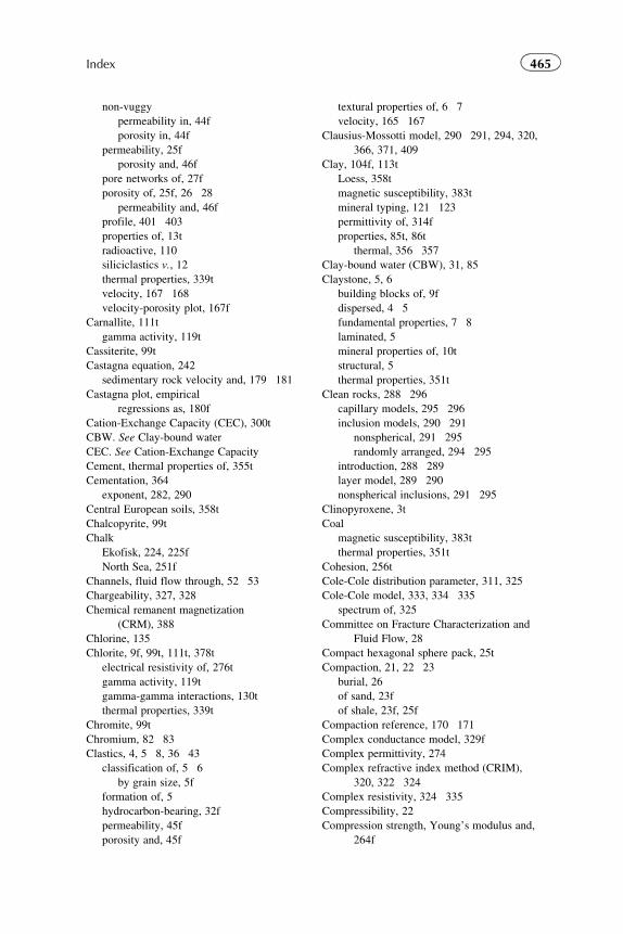
non-vuggy
permeability in, 44f
porosity in, 44f
permeability, 25f
porosity and, 46f
pore networks of, 27f
porosity of, 25f, 26�28
permeability and, 46f
profile, 401�403
properties of, 13t
radioactive, 110
siliciclastics v., 12
thermal properties, 339t
velocity, 167�168
velocity-porosity plot, 167f
Carnallite, 111t
gamma activity, 119t
Cassiterite, 99t
Castagna equation, 242
sedimentary rock velocity and, 179�181
Castagna plot, empirical
regressions as, 180f
Cation-Exchange Capacity (CEC), 300t
CBW. See Clay-bound water
CEC. See Cation-Exchange Capacity
Cement, thermal properties of, 355t
Cementation, 364
exponent, 282, 290
Central European soils, 358t
Chalcopyrite, 99t
Chalk
Ekofisk, 224, 225f
North Sea, 251f
Channels, fluid flow through, 52�53
Chargeability, 327, 328
Chemical remanent magnetization
(CRM), 388
Chlorine, 135
Chlorite, 9f, 99t, 111t, 378t
electrical resistivity of, 276t
gamma activity, 119t
gamma-gamma interactions, 130t
thermal properties, 339t
Chromite, 99t
Chromium, 82�83
Clastics, 4, 5�8, 36�43
classification of, 5�6
by grain size, 5f
formation of, 5
hydrocarbon-bearing, 32f
permeability, 45f
porosity and, 45f
textural properties of, 6�7
velocity, 165�167
Clausius-Mossotti model, 290�291, 294, 320,
366, 371, 409
Clay, 104f, 113t
Loess, 358t
magnetic susceptibility, 383t
mineral typing, 121�123
permittivity of, 314f
properties, 85t, 86t
thermal, 356�357
Clay-bound water (CBW), 31, 85
Claystone, 5, 6
building blocks of, 9f
dispersed, 4�5
fundamental properties, 7�8
laminated, 5
mineral properties of, 10t
structural, 5
thermal properties, 351t
Clean rocks, 288�296
capillary models, 295�296
inclusion models, 290�291
nonspherical, 291�295
randomly arranged, 294�295
introduction, 288�289
layer model, 289�290
nonspherical inclusions, 291�295
Clinopyroxene, 3t
Coal
magnetic susceptibility, 383t
thermal properties, 351t
Cohesion, 256t
Cole-Cole distribution parameter, 311, 325
Cole-Cole model, 333, 334�335
spectrum of, 325
Committee on Fracture Characterization and
Fluid Flow, 28
Compact hexagonal sphere pack, 25t
Compaction, 21, 22�23
burial, 26
of sand, 23f
of shale, 23f, 25f
Compaction reference, 170�171
Complex conductance model, 329f
Complex permittivity, 274
Complex refractive index method (CRIM),
320, 322�324
Complex resistivity, 324�335
Compressibility, 22
Compression strength, Young’s modulus and,
264f
465Index
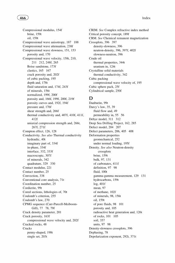
Compressional modulus, 154f
brine, 159t
oil, 159t
Compressional wave anisotropy, 187�188
Compressional wave attenuation, 238f
Compressional wave slowness, 151, 153
porosity and, 170
Compressional wave velocity, 158t, 210,
211�212, 248f, 265
Boise sandstone, 173f
clastics, 165�167
crack porosity and, 202f
of cubic packing, 195
depth and, 178t
fluid saturation and, 174f, 243f
of minerals, 156t
normalized, 199f, 200f
porosity and, 166f, 199f, 200f, 219f
porosity curves and, 192f, 194f
pressure and, 176f
shear strength and, 266f
thermal conductivity and, 407f, 410f, 411f,
412f
uniaxial compression strength and, 266t,
267f, 271f
Compton effect, 126, 128
Conductivity. See also Thermal conductivity
hydraulic, 40t
imaginary part of, 334f
in-phase, 334f
interface, 332, 333f
macroscopic, 307f
of minerals, 342
quadrature, 329�330
Contact modulus, 221
Contact number, 25
Convection, 338
Conventional core analysis, 71t
Coordination number, 25
Cordierite, 99t
Cored sections, lithologies of, 70t
Coulomb’s criterion, 255
Coulomb’s law, 270
CPMG sequence (Carr-Purcell-Meiboom-
Gill), 77�78, 79f
Crack density parameter, 201
Crack porosity, 163f
compressional wave velocity and, 202f
Cracked rocks, 48
Cracks
penny-shaped, 198t
single set, 203t
CRIM. See Complex refractive index method
Critical porosity concept, 189f
CRM. See Chemical remanent magnetization
Crossplots, 396�397
density-slowness, 396
neutron-density, 396, 397f, 402f
slowness-neutron, 396
Crude oil
thermal properties, 344t
uranium in, 124t
Crystalline solid materials
thermal conductivity, 342
Cubic packing
compressional wave velocity of, 195
Cubic sphere pack, 25f
Cylindrical sample, 250f
DDanburite, 99t
Darcy’s law, 35, 39
fluid flow and, 49
permeability in, 55�56
Debye model, 311�312
Deep Sea Drilling Project, 162, 285
Defect model, 204�207
Defect parameters, 206, 405�408
Deformation properties
geomechanical, 252
under normal loading, 195f
Density. See also Neutron-density
crossplots
brine, 159t
bulk, 97, 131
of carbonates, 411f
definition, 97�98
fluid, 100t
gamma-gamma measurement, 129�131
hydrocarbons, 159t
log, 401f
mean, 97
of methane, 102f
of minerals, 98, 156t
oil, 159t
of pore fluids, 98�101
porosity and, 105
radioactive heat generation and, 126t
of rocks, 101�105
soil, 357
units, 97�98
Density-slowness crossplots, 396
Dephasing, 78
Depolarization exponent, 292t, 371t
466 Index
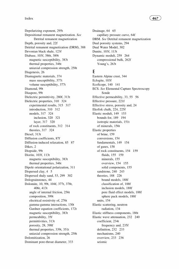
Depolarizing exponent, 295t
Depositional remanent magnetization. See
Detrital remanent magnetization
Depth, porosity and, 22f
Detrital remanent magnetization (DRM), 388
Devonian black shale, 123f
Diabase, 103f, 386t, 389t
magnetic susceptibility, 383t
thermal properties, 346t
uniaxial compression strength, 258t
Diagenesis, 26
Diamagnetic materials, 374
mass susceptibility, 377t
volume susceptibility, 377t
Diamond, 99t
Diaspore, 99t
Dielectric permittivity, 280f, 313t
Dielectric properties, 310�324
experimental results, 315�317
introduction, 310�312
models, 317�324
inclusion, 320�321
layer, 317�320
of rock constituents, 312�314
theories, 317�324
Diesel, 313t
Diffusion coefficients, 87f
Diffusion-induced relaxation, 85�87
Dikes, 2
Diopside, 99t
Diorite, 103f, 113t
magnetic susceptibility, 383t
thermal properties, 346t
Dipole orientational polarization, 311
Dispersed clay, 4�5
Dispersed shaly sand, 53, 299�302
Dolograinstones, 44
Dolomite, 10, 99t, 104f, 377t, 378t,
406t, 413t
angle of internal friction, 256t
composition, 399t
electrical resistivity of, 276t
gamma-gamma interactions, 130t
Gardner equation coefficients, 172t
magnetic susceptibility, 383t
permeability, 35f
permittivities, 313t
porosity, 28, 398f
thermal properties, 339t, 351t
uniaxial compression strength, 258t
Dolomitization, 26
Dominant pore-throat diameter, 333
Drainage, 64�65
capillary pressure curve, 64f
DRM. See Detrital remanent magnetization
Dual porosity systems, 294
Dual Water Model, 302
Dunite, 103f, 113t
Dynamic moduli, 259�264
compressional bulk, 262f
Young’s, 263t
EEastern Alpine crust, 344
Eclogite, 103f
EcoScope, 140�141
ECS. See Elemental Capture Spectroscopy
Sonde
Effective permeability, 33, 55�56
Effective pressure, 221f
Effective stress, porosity and, 24
Ekofisk chalk, 224, 225f
Elastic moduli, 149�153
bounds for, 189�194
isotropic materials, 151t
of minerals, 156t
Elastic properties
of brine, 159
conversions, 154
fundamentals, 149�154
of gases, 158
of rock constituents, 154�159
fluids, 155�159
minerals, 155
overview, 154�155
solid components, 155
sandstone, 240�243
theories, 188�226
bound models, 188f
classification of, 188f
inclusion models, 188f
pore fluid effect models, 188f
sphere pack models, 188f
units, 154
Elastic scattering, neutron
radiation, 134
Elastic stiffness components, 186t
Elastic wave attenuation, 232�240
coefficient, 234t
frequency and, 235f
definition, 232�233
mechanisms, 240
overview, 233�236
seismic
467Index
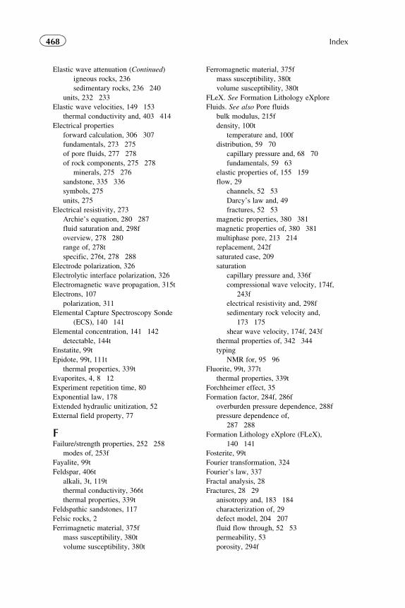
Elastic wave attenuation (Continued)
igneous rocks, 236
sedimentary rocks, 236�240
units, 232�233
Elastic wave velocities, 149�153
thermal conductivity and, 403�414
Electrical properties
forward calculation, 306�307
fundamentals, 273�275
of pore fluids, 277�278
of rock components, 275�278
minerals, 275�276
sandstone, 335�336
symbols, 275
units, 275
Electrical resistivity, 273
Archie’s equation, 280�287
fluid saturation and, 298f
overview, 278�280
range of, 278t
specific, 276t, 278�288
Electrode polarization, 326
Electrolytic interface polarization, 326
Electromagnetic wave propagation, 315t
Electrons, 107
polarization, 311
Elemental Capture Spectroscopy Sonde
(ECS), 140�141
Elemental concentration, 141�142
detectable, 144t
Enstatite, 99t
Epidote, 99t, 111t
thermal properties, 339t
Evaporites, 4, 8�12
Experiment repetition time, 80
Exponential law, 178
Extended hydraulic unitization, 52
External field property, 77
FFailure/strength properties, 252�258
modes of, 253f
Fayalite, 99t
Feldspar, 406t
alkali, 3t, 119t
thermal conductivity, 366t
thermal properties, 339t
Feldspathic sandstones, 117
Felsic rocks, 2
Ferrimagnetic material, 375f
mass susceptibility, 380t
volume susceptibility, 380t
Ferromagnetic material, 375f
mass susceptibility, 380t
volume susceptibility, 380t
FLeX. See Formation Lithology eXplore
Fluids. See also Pore fluids
bulk modulus, 215f
density, 100t
temperature and, 100f
distribution, 59�70
capillary pressure and, 68�70
fundamentals, 59�63
elastic properties of, 155�159
flow, 29
channels, 52�53
Darcy’s law and, 49
fractures, 52�53
magnetic properties, 380�381
magnetic properties of, 380�381
multiphase pore, 213�214
replacement, 242f
saturated case, 209
saturation
capillary pressure and, 336f
compressional wave velocity, 174f,
243f
electrical resistivity and, 298f
sedimentary rock velocity and,
173�175
shear wave velocity, 174f, 243f
thermal properties of, 342�344
typing
NMR for, 95�96
Fluorite, 99t, 377t
thermal properties, 339t
Forchheimer effect, 35
Formation factor, 284f, 286f
overburden pressure dependence, 288f
pressure dependence of,
287�288
Formation Lithology eXplore (FLeX),
140�141
Fosterite, 99t
Fourier transformation, 324
Fourier’s law, 337
Fractal analysis, 28
Fractures, 28�29
anisotropy and, 183�184
characterization of, 29
defect model, 204�207
fluid flow through, 52�53
permeability, 53
porosity, 294f
468 Index
shear, 28
tension, 28
Frequency-dependent conductivity, 275
Frequency-dependent dielectric
permittivity, 275
Frequency-independent phase angle,
325�326
Friction factor, 53
GGabbro, 103f, 113t, 266t, 386t
magnetic susceptibility, 383t
thermal properties, 346t
Galena, 99t
thermal properties, 339t
Gamma radiation, 108
alkali feldspar, 119t
biotite, 119t
carnallite, 119t
characteristic energies, 133t
chlorite, 119t
energy, 127f
fundamentals, 127�129
illite, 119t
interactions, 126�131
kaolinite, 119t
mean API values for, 119t
montmorillonite, 119t
muscovite, 119t
natural spectrum, 118f
origin of, 108�109
plagioclase, 119t
quartz, 119t
sylvite, 119t
Gamma spectrometry, 140t
Gamma-gamma interactions, 130t
albite, 130t
anhydrite, 130t
barite, 130t
biotite, 130t
calcite, 130t
chlorite, 130t
dolomite, 130t
gypsum, 130t
halite, 130t
illite, 130t
kaolinite, 130t
montmorillonite, 130t
muscovite, 130t
orthoclase, 130t
quartz, 130t
siderite, 130t
Gamma-gamma-density measurement,
129�131
Gamma-gamma-PE measurement, 129
Gammalog, 120, 146f, 401f
Gamma-ray index, 120, 121, 121f
Gardner equation coefficients, 172t
Garnets, thermal properties, 339t
Gases, elastic properties of, 158
Gassmann-Biot concept, 212�213
Gassmann’s equation, 15, 207�213
Gassmann’s model, 213f
Gassmann’s model, 207�211
Geomechanical properties
classification, 246�249
deformation, 252
dynamic moduli, 259�264
failure/strength, 252�258
fundamental, 249�258
strain, 249�250
stress, 249�250
model-based relationships, 267�271
overview, 245�246
static moduli, 259�264
Geophysical borehole measurements, 269f
Geophysical methods, 14
German Molasse Basin, 356t
Glacial till permeability, 35f
Glauconite, 99t, 111t
Glaucophane, 99t
Gneiss, 103f, 152, 253f
magnetic susceptibility of, 383t
thermal conductivity of, 347
anisotropy of, 349t, 350f
thermal properties, 346t
Goethite, 380t
Grain diameter, 387f
Grain packing, 7
Grain shape, 7
Grain size
clastic classification and, 5f
parameters, 6�7
permeability and, 37�39
Grain sorting, 7
Grainstones, 44
Granite, 103f, 113t, 253f, 386t
Kirchberg, 366t
magnetic susceptibility, 383t
mineral composition of, 366t
Svaneke, 384�385
thermal conductivity of, 347, 366t
thermal properties, 346t
uniaxial compression strength, 258t
469Index
Granodiorite, 113t
thermal properties, 346t
Granulite, 389t
magnetic susceptibility of, 383t
Graphite, 99t
Gravel, permeability, 35f
Graywacke, 113t
thermal properties, 351t
uniaxial compression strength, 258t
Grossularite, thermal properties, 339t
Gypsum, 99t, 104f
gamma-gamma interactions, 130t
magnetic susceptibility of, 383t
thermal properties, 339t, 351t
Gyromagnetic ratio, 77
HHaematite, 380t
Hagen-Poiseulle’s law, 55
Halite, 99t, 377t
gamma-gamma interactions, 130t
permittivities, 313t
thermal properties, 339t
Hanai-Bruggeman formula, 321
Hashin-Shtrikman bounds,
189�194, 191f
Hedenbergite, 99t
Hertz’s theory, 177, 195f, 220
Heterogeneity, 15�16
Hills value, 319
Homogeneity, 15
Hooke’s law, 149
Horizontal permeability, 42
Hornblende, 99t, 378t, 406t
electrical resistivity of, 276t
thermal expansion, 360t
Hudson inclusion models,
202�204, 205f
Humble equation, 282�283
Hydraulic conductivity, 40t
Hydrocarbons
density, 159t
relative permeability of, 56f
typing, 95�96
Hydrogen, 134
gyromagnetic ratio of, 77
index, 91f, 92t
Hydrogen nuclei, 75
Hydrogeology, permeability and,
39�40
Hysteresis, 317
magnetic, 376f
IIce, 377t, 381
thermal properties, 344t
Igneous rocks, 2�3. See also specific types
anisotropy of, 183�184
classification of, 2�3
empirical relationships, 404�409
Koenigsberger ratio of, 389t
magnetic susceptibility of, 383t
radioactive heat generation of, 125t
radioactivity of, 115
seismic wave attenuation in, 236
thermal properties of, 346t
velocity of, 161�164
Illite, 9f, 99t, 111t, 378t
gamma activity, 119t
gamma-gamma interactions, 130t
properties, 86t
thermal properties, 339t
Ilmenite, 3t, 99t, 380t
thermal properties, 339t
Ilmenite-hematite, 379
Imbibition, 64�65
capillary pressure curve, 64f
defined, 64
Inclusion models, 188f, 196�204
Budiansky and O’Connell, 200�202
calculations, 408�409
clean rock, 290�291
nonspherical, 291�295
randomly arranged, 294�295
of dielectric properties, 320�321
Hudson, 202�204, 205f
Kuster and Toksoz, 197�200
nonspherical, 321�322, 368�372
spherical, 320�321, 365�367
of thermal properties, 365�372
Indonesia equation, 303, 303f
Induced magnetization, 382�385
Inelastic scattering, 132�133
In-phase conduction, 334f
Integral measurements, 118�119
Inter-echo time, 79
Interface conductivity, 332, 333f
Interface properties, 61
Interfacial polarization, 311
Interfacial tension, 57�58
Intermediate rocks, 2
Intermediate wettability, 57, 58
Internal structure model, 214�226
variable, 215f
Interparticle pore network, 43
470 Index
Interval transit time, 172f
Ionic polarization, 311
Irreducible saturation, 50
Isotropic materials, 151t
JJacobsite, 99t
Jurassic shale, 186
KKainite, 111t
Kaolinite, 9f, 99t, 111t
electrical resistivity of, 276t
gamma activity, 119t
gamma-gamma interactions, 130t
properties, 86t
thermal properties, 339t
Karst limestone, 35f
Kerogen, 145
Kerosene, thermal properties of, 344t
Kieserite, 99t
Kirchberg granite, 366t
Klinkenberg effect, 34�35
Koenigsberger ratio, 388�389, 389t
of igneous rocks, 389t
of metamorphic rocks, 389t
of sedimentary rocks, 389t
Kozeny constant, 51�52
Kozeny equation, 54
Kozeny shape factor, 51t
Krischer-Esdorn equation, 365
KTB borehole, 348f
Kuster and Toksoz Inclusion models,
197�200
Kyanite, 99t
thermal properties, 339t
LLabradorite, 99t
electrical resistivity of, 276t
Lambda rho, 231�232
Lame parameters, 150
Lame’s numbers, 252
Laminated clay, 5
Laminated sands, 304�310
bimodal, 305
Laminated sediments, anisotropy of, 184�187
Laminated shaly sand, 54, 298�299,
304�310
inversion, 308�310
Lamination, 43
Langbeinite, 99t, 111t
Large crystalline dolostones, 44
Larmor frequency, 77, 78
Lava, thermal properties, 346t
Layer model, 289�290
of dielectric properties, 317�320
mixing rules, 362�365
parallel, 361�362
petrophysical relationships, 394�403
series, 361�362
of thermal properties, 361�362
Layer-induced anisotropy, 181
Leaching, 26
Leucite, 99t
Leverett function, 65�66, 72
Lichtenecker-Rother equation, 319f, 365
Lignite, 104f
Limestone, 10, 104f, 137, 253f, 266t, 413t
argillaceous, 27�28
Gardner equation coefficients, 172t
initial porosity, 23
Karst, 35f
magnetic susceptibility of, 383t
non-vuggy, 172f
porosity, 398f
Silurian, 355f
thermal properties, 351t
uniaxial compression strength, 258t
Linear thermal expansion, 360t
Lithification, 4
Lithologic profile, 119�120
sedimentary rock velocity
and, 165�169
Lithothek, 404�405
Loam, 104f
alluvium, 358t
Loess clay, 358t
Log analysis, 336f
Longitudinal relaxation, 81, 82f
Longitudinal wave velocity, crack
porosity and, 163f
Low-bog-peat, 358t
Low-resistivity pay evaluation, 309f
MMackenzie River Valley, 169t
Macropores, 12
Macroscopic anisotropy, 305
Macroscopic conductivity, 307f
Macroscopic module, 308
Macrosystems, 215
Mafic rocks, 2
Maghemite, 99t, 380t
471Index
Magmatic rock 1f. See also specific types
mineralogical classification of, 2f
thermal properties of, 345�348
Magnesite, 99t
thermal properties, 339t
Magnetic hysteresis, 376f
Magnetic properties
of fluids, 380�381
of minerals, 376�380
of rock constituents, 376�381
units, 374t
Magnetic susceptibility, 382f, 386f
content and, 385�388
grain diameter and, 387f
of igneous rocks, 383t
of metamorphic rocks, 383t
natural remanent magnetization and, 390f
of sedimentary rocks, 383t
Magnetite, 3t, 99t, 380t, 385
thermal properties, 339t
Magnetization, 88
Malachite, 99t
Marble, 103f, 253f
thermal properties, 346t
uniaxial compression strength, 258t
Marcasite, 99t
Marl, 104f
Mass susceptibility
of diamagnetic materials, 377t
of ferrimagnetic materials, 380t
of ferromagnetic materials, 380t
paramagnetic substances, 378t
Massilon sandstone, 239�240, 239f
Matrix effect, 75
Matrix point, 396
Mavko local flow model, 213f
Maxwell-Wagner, 312
Mean density, 97
Megaelectron volt (MeV), 109f
Mercury, 61
pressure, 95
Mesopores, 12
Mesozoic sandstone, 316f
Metal factor, 327�328
Metamorphic rocks, 3. See also specific types
anisotropy of, 183�184
empirical relationships, 404�409
Koenigsberger ratio of, 389t
magnetic susceptibility of, 383t
radioactivity and, 116
thermal properties of, 345�348, 346t
velocity of, 161�164
Methane, 87f
density of, 102f
MeV. See Megaelectron volt
Mica, thermal properties, 339t
Micaceous sandstones, 117
Microcline, 99t, 111t
electrical resistivity of, 276t
thermal properties, 339t
Microcrack properties, 332
Micropores, 12
Microsystems, 215
Minerals
conductivity of, 342
density of, 98, 156t
elastic moduli, 156t
elastic properties of, 155
electrical properties of, 275�276
in granite, 366t
magnetic properties of, 376�380
potassium in, 109�112
thermal properties, 339�344
rock-forming, 339t
thorium in, 109�112
uranium in, 109�112
wave velocities, 156t
Mississippian Madison Group, 27
Mixing rule, 362�365, 365f
Modulus magnification, 209�210
Mohr’s circle, 255f
Mohr’s diagram, 254f
Molecular diffusion, 85�86
Molecular polarization, 311
Monazite, 111t, 117
Montmorillonite, 8, 9f, 99t, 111t, 378t
gamma activity, 119t
gamma-gamma interactions, 130t
properties, 86t
Mu rho, 231�232
Mudrock line, 179
Multi-exponential decay, 87�89
Multiphase flow, 55�56
Multiphase pore fluids, 213�214
Muscovite, 99t, 111t, 378t, 406t
electrical resistivity of, 276t
gamma activity, 119t
gamma-gamma interactions, 130t
thermal conductivity, 366t
thermal properties, 339t
NNatrolite, 99t
Natural radioactivity, 108�126
472 Index
Natural remanent magnetization, 388�391
susceptibility and, 390f, 391f
Nepheline, 99t
thermal properties, 339t
Neutron radiation, 131�139
elastic scattering, 134
fundamentals, 131�136
inelastic scattering, 132�133
porosity and, 136�138
Neutron-density crossplots, 396,
397f, 402f
NMR. See Nuclear magnetic resonance
Nonreactive fluids, 33
Nonspherical inclusions, 291�295
Non-vuggy carbonates, 44f
Non-vuggy limestone, 172f
Normal loading, deformation under, 195f
North Sea, 42
chalk, 251f
Nuclear magnetic resonance (NMR), 75
applications, 90�96
capillary pressure estimate, 92�95
permeability, 92�95
pore size, 92�95
pore volume partitioning, 90�92
porosity, 90�92
data processing, 88f
fluid typing, 95�96
fundamentals, 76
measurement, 77�80
physical origin, 76�77
of reservoir fluids, 83t
Nuclear measurements, 139�146
Nuclear properties, 107�108
OOctahedral unit, 8
ODF. See Orientation distribution function
Ohm’s law, 274
Oil
compressional modulus, 159t
crude
thermal properties, 344t
uranium in, 124t
density, 159t
shale, 113t
thermal properties, 344t
Oil-water, capillary pressure, 62t
Oil-wet, 57
Olivine, 3t, 378t, 406t
thermal properties, 339t
Oman abyssal plain, 24
Ore-containing rocks, spectral-induced
polarization in, 328
Orientation distribution function (ODF), 186
Oriented ellipsoidic inclusions, 291�294
Orthoclase, 99t, 111t, 377t
electrical resistivity of, 276t
gamma-gamma interactions, 130t
thermal properties, 339t
Orthopyroxene, 3t
Orthorhombic sphere pack, 25t
PPair production, 128�129
Parallel conductor circuits, 297
Parallel model, 317
layer, 361�362
Paramagnetic substances, 374�375
mass susceptibility, 378t
volume susceptibility, 378t
Patchy saturation, 214
Peat
low-bog, 358t
raised-bog, 358t
Pendular region, 60
Penny-shaped cracks, 198t
n-Pentane, thermal properties, 344t
Peridotite, 103f, 113t
magnetic susceptibility, 383t
thermal conductivity of, 347
thermal properties, 346t
Permafrost, 168
seismic velocity, 169t
Permeability, 32�56
absolute, 33
anisotropy, 54
carbonates, 25f
clastics, 45f
in Darcy’s law, 55�56
definitions, 33�35
determining, 32�33
dolomite, 35f
effective, 33, 55�56
equations for, 49�50
fracture, 53
glacial till, 35f
grain size and, 37�39
gravel, 35f
horizontal, 42
hydrogeology and, 39�40
limestone, 35f
log, 148f
mean magnitude ranges, 35f
473Index
Permeability (Continued)
measurement principle, 34f
models, 48�55
capillary tube model, 48�52, 48f
overview, 48
NMR for, 92�95
pore size and, 37�39
pore-throat radius and, 52
porosity and, 37�39
of carbonates, 46f
of clastics, 45f
main influences on, 45
in non-vuggy carbonates, 44f
plots, 37f
pressure and, 47f
relative, 33
curves, 66�67
defined, 56
for hydrocarbons, 56f
for water, 56f
sand, 35f
sandstone, 25f, 35f
sedimentation and, 42
shale, 35f, 41f
influence of, 53�55
vertical, 42
Permittivity
anhydrite, 313t
calcite, 313t
clay, 314f
complex, 274
dielectric, 280f, 313t
dolomite, 313t
electrical resistance, 279
frequency-dependent dielectric, 275
halite, 313t
porosity and, 321f, 322f
quartz, 313t
water, 314f
Permo-Triassic sandstone, 334�335
Petrophysical relationships
introduction, 393�394
layered models, 394�403
Petrophysics, 12�13
Phase angle tangent, 332
Phlogopite, 99t
Phosphate, 111t
thermal properties, 339t
Photoelectric effect, 126, 128
gamma-gamma measurement, 129
Phyllite, 103f
magnetic susceptibility of, 383t
Plagioclase, 3t, 111t
gamma activity, 119t
thermal conductivity, 366t
thermal expansion, 360t
Plutonic rocks, 2
PNC. See Pulsed neutron capture
Poisson’s ratio, 152f, 162f, 252
acoustic impedance and, 228�231
Polarization mechanisms, 310f. See also
Spectral-induced polarization
dipole orientational, 311
electrode, 326
electrolytic interface, 326
electron, 311
interfacial polarization, 311
ionic, 311
molecular, 311
pore geometrical properties and,
330�335
water, 314
Polyhalite, 99t
Polymineralic rock, 364�365
Pore constrictivity polarization, 327
Pore fluids
density of, 98�101
dielectric permittivity of, 313t
electrical properties of, 277�278
multiphase, 213�214
sedimentary rocks
thermal properties, 349�357
velocity and, 173�175
thermal properties of, 344t
Pore geometrical factor, 65
polarization effects related to, 330�335
Pore network
interparticle, 43
vuggy, 43
Pore radius, 49
Pore size
NMR for, 92�95
permeability and, 37�39
Pore space properties
overview, 17
Pore surface area, 29�30
Pore types, carbonate, 11f
Pore volume partitioning, NMR for, 90�92
Pore-body, 51
Pore-throat, 51
permeability and, 52
Poro-perm plot, 37
Poro-perm regression, 70
Porosity, 17�29
474 Index
of artificially mixed wet-packed
unconsolidated sand, 21t
of carbonates, 25f, 26�28
compressional velocity and, 166f, 199f,
200f
compressional wave slowness and, 170
compressional wave velocity and, 219f
crack, 163f
critical, 189f
curves, 192f, 194f
definitions, 18�19
density and, 105
depth and, 22f
lithologies, 27f
profiles, 23
dolomite, 28, 398f
dual, 294
effective stress and, 24
exponential, 23
factor, 218�220
fracture, 294f
influence of, 349�357
initial
limestone, 23
sandstone, 23
shale, 23
limestone, 398f
mean, 20t
measurements
direct, 18
indirect, 18
from neutron measurements, 136�138
NMR for, 90�92
permeability and, 37�39
of carbonates, 46f
of clastics, 45f
main influences on, 45
in non-vuggy carbonates, 44f
plots, 37f
relative permittivity and, 321f, 322f
residual, 23�24
sandstone, 36t, 105f, 316f
secondary, 20
sedimentary rocks
thermal properties, 349�357
velocity and, 165�169
separate vugs, 45f
shear velocity and, 199f
shear wave velocity and, 219f
thermal conductivity and, 348f, 356f, 370f,
372f
sand, 353f
volumetric rock composition and,
395�401
Porous rocks, spectral-induced polarization in,
328�335
Porphyry, magnetic susceptibility, 383t
Postdiagenetic processes, 35
Potassium, 109, 121
heat production rate, 125t
major occurrences of, 112
in minerals, 109�112
in rocks, 113�118
thorium and, 122f
Poupon equation, 298�299, 303f
Power law parameters, 45
Precessing, 78
Pressure. See also Capillary pressure
compressional wave velocity and, 176f
dependence, 46�48
permeability and, 47f
effective, 221f
formation factor and, 287�288
permeability and, 47f
sedimentary rock velocity and, 175�179
thermal conductivity and, 359f
Prophyrite, 103f
Protons, 107
Pseudobrookite, 99t, 379
Pulsed neutron capture (PNC), 135
measurements, 138�139
P-wave velocity, 185
Pyrite, 99t
thermal properties, 339t
Pyroxene, 378t, 406t
thermal properties, 339t
Pyroxenite, 103f
magnetic susceptibility, 383t
Pyrrhotite, 99t, 380t
thermal properties, 339t
QQuadrature conductivity, 329�330
Quartz, 3t, 99t, 342, 377t, 406t
composition, 399t
electrical resistivity of, 276t
gamma activity, 119t
gamma-gamma interactions, 130t
permittivities, 313t
thermal conductivity, 366t
thermal expansion, 360t
thermal properties, 339t
Quartzite, 103f, 253f
magnetic susceptibility of, 383t
475Index
Quartzite (Continued)
thermal properties, 346t
uniaxial compression strength, 258t
RRadiation
alpha, 108
applications, 119�123
lithologic profile, 119�120
beta, 108
gamma, 108
characteristic energies, 133t
interactions, 126�131
natural spectrum, 118f
origin of, 108�109
igneous rocks and, 115
integral measurements, 118�119
metamorphic rocks and, 116
neutron, 131�139
fundamentals, 131�136
inelastic scattering, 132�133
spectral measurements, 118�119
Radiative capture, 135
Radioactive carbonates, 110
Radioactive heat generation, 124�126
density and, 126t
of igneous rocks, 125t
Radioactivity, 116�118
Raised-bog-peat, 358t
Randomly arranged inclusions, 294�295,
371�372
Raymer-Hunt-Gardner equation,
171�172
Real pore geometry, 51�52
Realgar, 99t
Red sediments, 389t
magnetic susceptibility of, 383t
Reflection coefficients, 228
Regular sphere packings, 25t
Relative permeability, 33
curves, 66�67
defined, 56
for hydrocarbons, 56f
for water, 56f
Relaxation process, 80
bulk, 82�84, 83f
diffusion-induced, 85�87
longitudinal, 81, 82f
multi-exponential decay and, 87�89
surface, 81
transverse, 81, 82f, 83f
Relaxation-time spectrum, 335f
Reservoir properties, 14
fundamental, 17
NMR, 83t
pore geometric, 61
from seismic parameters, 226�232
Reservoir Quality index (RQI), 52
Residual porosity, 23�24
Reversible dephasing, 78
Reynolds numbers, 34
Rhyolite, 103f, 113t
magnetic susceptibility, 383t
RMR. See Rock mass rating
Rocks. See specific types
Rock cycle 1f
Rock density, 101�105
Rock magnetization, 381�382
Rock mass rating (RMR), 247
Rock properties
classification, 15t
general characteristics, 12�16
Rock quality designation (RQD), 247, 247t
parameters, 248f
Rock salt
magnetic susceptibility of, 383t
thermal properties of, 353t
uniaxial compression strength, 258t
Rock skeleton, shale, 22
Rock-fabric classification, 44
Rock-fluid system, 188
Rocks
potassium content of, 113�118
thorium content of, 113�118
uranium content of, 113�118
RQD. See Rock quality designation
RQI. See Reservoir Quality index
Rutile, 99t
thermal properties, 339t
SSalt, 104f
rock
magnetic susceptibility of, 383t
thermal properties of, 353t
Thuringia, 349, 353t
uniaxial compression strength, 258t
thermal properties of, 353t
Saltwater, 138
Sand
acoustic impedance and, 230f
artificially mixed wet-packed
unconsolidated
porosity of, 21t
476 Index
bimodal laminated, 305
compaction process for, 23f
dispersed shaly, 53
isotropic, 307
laminated, 304�310
bimodal, 305
laminated shaly, 54
inversion, 308�310
permeability, 35f
shaly, 296�304
complex conductance
model, 329f
composite, 307
equations, 303�304
problem, 296�297
thermal conductivity
porosity and, 353f
thermal properties, 351t
unconsolidated, 177f
Sand-shale sequence, 309
Sandstone, 5, 70�73, 104f, 146�148, 253f, 266t
Bandera
thermal expansion, 360t
thermal properties, 351t
Bentheim, 38
Berea, 20t
thermal expansion, 360t
thermal properties, 351t
Bluejacket, 42�43
Boise, 261
compressional wave velocity, 173f
shear wave velocity, 173f
thermal expansion, 360t
thermal properties, 351t
brine-saturated, 239f
complex conductivity and, 331f
elastic properties of, 240�243
electrical properties, 335�336
feldspathic, 117
Gardner equation coefficients, 172t
initial porosity, 23
magnetic susceptibility of, 383t
Massilon, 239�240, 239f
Mesozoic, 316f
micaceous, 117
permeability, 25f, 35f
Permo-Triassic, 334�335
porosity, 36t, 105f, 316f
thermal conductivity of, 354t
thermal properties, 351t
Triassic, 333
uniaxial compression strength, 258t
Sass equation, 359
Saturation, 30�32
capillary pressure measurement and, 69f
determining, 31
fluid
capillary pressure and, 336f
compressional wave velocity, 174f,
243f
electrical resistivity and, 298f
sedimentary rock velocity and,
173�175
shear wave velocity, 174f, 243f
irreducible, 50
SCAL. See Special core analysis
Schist, 103f, 253f
magnetic susceptibility of, 383t
thermal conductivity of
anisotropy of, 349t
thermal properties, 346t
Seamounts, 389t
Secondary porosity, 20
Sedimentary rocks 1f, 4�12,
409�414. See also specific types
dominant materials in, 401f
Koenigsberger ratio of, 389t
magnetic susceptibility of, 383t
overview of, 4�5
radioactivity of, 116�118
seismic wave attenuation in,
236�240
thermal properties, 348�359, 351t
pore fluid and, 349�357
porosity and, 349�357
velocity of, 164�181
carbonates, 167�168
Castagna equation, 179�181
clastics, 165�167
fluid saturation and, 173�175
lithology and, 165�169
pore fluid and, 173�175
porosity and, 165�169
pressure and, 175�179
temperature and, 179
unconsolidated sediments,
168�169
Sedimentation, permeability and, 42
Seismic parameters, reservoir properties
from, 226�232
Seismic velocity, 264�271
empirical relationships, 264�267
experimental results, 264�267
permafrost, 169t
477Index
Seismic wave attenuation
igneous rocks, 236
sedimentary rocks, 236�240
Separate vugs, 43
porosity, 45f
Series model, 318
layer, 361�362
Serpentine, 99t
magnetic susceptibility of, 383t
thermal properties, 339t
Shale, 6, 104f, 113t, 139, 253f
acoustic impedance and, 230f
brine-saturated, 187f
compaction process for, 23f, 25f
content estimate, 120�121
Devonian black, 123f
Gardner equation coefficients, 172t
indicator, 117
influence of, 40�43
initial porosity, 23
Jurassic, 186
linear regressions, 180t
magnetic susceptibility of, 383t
permeability, 35f, 41f
influence of, 53�55
rock skeleton of, 22
thermal expansion, 360t
thermal properties, 351t
uniaxial compression strength, 258t
Shaly rocks, 296�304
spectral-induced polarization in,
329�330
Shaly sand, 296�304
complex conductance model, 329f
composite, 307
dispersed, 53
equations, 303�304
laminated, 54, 298�299, 304�310
problem, 296�297
Shear fractures, 28
Shear modulus, 154f, 208
Shear strength
compressional velocity and, 266f
Shear velocity
normalized, 199f
porosity and, 199f
Shear wave anisotropy, 187�188
calculated, 205f
Shear wave slowness, 151, 153
Shear wave splitting, 181
in transversely isotropic
rocks, 184f
Shear wave velocity, 210
Boise sandstone, 173f
depth and, 178t
fluid saturation and, 174f
porosity and, 219f
Shell formula, 282�283
Shuey’s equation, 227
Shuey’s method, 231
Siderite, 99t, 378t
electrical resistivity of, 276t
gamma-gamma interactions, 130t
thermal properties, 339t
Silicic rocks, 2
Siliciclastics
carbonates v., 12
properties of, 13t
Sillimanite, 99t
thermal properties, 339t
Silt, uniaxial compression strength, 258t
Siltstone, 5
thermal properties, 351t
Silurian limestone, 355f
Simandoux equation, 302, 303f
Slate, magnetic susceptibility of, 383t
Slowness-neutron crossplots, 396
Smectite, 111t, 378t
thermal properties, 339t
Snell’s law, 227
Sodium chloride, 277, 279f
Soil
Central European, 358t
density, 357
horticultural, 358t
Solid components
elastic properties of, 155
Solid material modulus, 221
Source rock studies, 123
Special core analysis (SCAL), 71
Specific heat capacity, 345f
Specific internal surface, 29�30
Specific internal surface, 50�51
Spectral measurements, 118�119
Spectral-induced polarization, 324�335
basic mechanisms of, 326�327
decay curve, 335f
effects, 328f
in ore-containing rocks, 328
in porous rocks, 328�335
in shaly rocks, 329�330
traditional parameters of, 327
Sphalerite, 99t
Sphene, 111t
478 Index
Sphere pack
compact hexagonal, 25t
cubic, 25f
orthorhombic, 25t
regular, 25t
Sphere pack models, 188f, 194�196
Spin echo, 78�79
Spinel, 99t
thermal properties, 339t
St. Peter sandstone, 20t
uniaxial compression strength, 258t
Static magnetic field, 86
Static moduli, 259�264
compressional bulk, 262f
Young’s, 263t
Stokes’ law, 6
Strain, 249�250
Stress, 249�250
Stress-strain curve, 250�252, 251f
Structural clay, 5
Structure tensor, 217
components of, 222f
Structured model, 214�217
Surface relaxation, 81, 84�85
transverse relaxation and, 83f
Svaneke granites, 384�385
Syenite, 103f, 113t
thermal properties, 346t
uniaxial compression strength, 258t
Sylvite, 99t, 111t
gamma activity, 119t
thermal properties, 339t
TTalc, 99t
thermal properties, 339t
Temperature. See also Thermal properties
dependence, 164
dry bulk moduli and, 179
fluid density and, 100f
sedimentary rock velocity and, 179
specific heat capacity and, 345f
thermal conductivity and, 359f
water permittivity and, 314f
Tension fractures, 28
Tensor elements, 153�154
Ternary systems, 379f
Tertiary sand, 358t
Tetrahedral unit, 8
Textural parameter, 319
Thermal conductivity
amorphous materials, 342
of amphibolite, 347
anisotropy of, 349t
gneiss, 349t, 350f
schist, 349t
of Central European soils, 358t
compressional wave velocity and, 407f,
410f, 411f, 412f
crystalline solid materials, 342
elastic wave velocities and, 403�414
of gneiss, 347
of granite, 347, 366t
of peridotite, 347
porosity and, 348f, 356f, 370f, 372f
sand, 353f
pressure and, 359f
of sandstone, 354t
temperature and, 359f
Thermal diffusivity, 338
Thermal expansion, 359
linear, 360t
Thermal properties. See also Temperature
of cement, 355t
clay, 356�357
conversions, 338t
of fluids, 342
of igneous rocks, 346t
introduction, 337�339
of magmatic rocks, 345�348
of metamorphic rocks, 345�348, 346t
of minerals, 339�344
rock-forming, 339t
models, 360�372
inclusion, 365�372
layer, 361�362
of pore fluids, 344t
of rocks, 343�359
overview, 343�344
of salts, 353t
sandstone, 351t
of sedimentary rocks, 348�359, 351t
pore fluids and, 349�357
porosity and, 349�357
theories, 360�372
units, 338t
Thermoremanent magnetization (TRM), 388
Thomas-Stieber technique, 308, 310
Thomeer’s equation, 67f, 72
Thomsen parameters, 185t, 204
Thorium, 109, 121
heat production rate, 125t
major occurrences of, 112
in minerals, 109�112
479Index
Thorium (Continued)
potassium and, 122f
in rocks, 113�118
3DEX, 308, 310
Thuringia rock salt, 349
thermal properties of, 353t
TIH systems, 183
Time-domain instruments, 327
Tipping field, 78
Titanite, thermal properties, 339t
Titanomaghemites, 379, 380t
Titanomagnetite, 99t, 379, 380t
TIV systems, 183
Toluene, 313t
Tortuosity, 49, 331
Touching vugs, 43
Trachyte, 113t
Transition zone, 59
Transverse plane, 78
Transverse relaxation, 81, 82f
bulk contributions to, 83f
surface contributions to, 83f
Transversely isotropic rocks, shear wave
splitting in, 184f
Tremolite, 99t
Triassic sandstone, 333
Trichloethane, 313t
TRM. See Thermoremanent magnetization
Trona, 99t
Tuffs, 103f
UUltramafic rocks, 2
Ulvospinel, 379, 380t
Unconsolidated rocks, 161
Unconsolidated sand, 177f
Unconsolidated sediments, 263f
velocity, 168�169
Uniaxial compression, 255
strength, 257f
compressional velocity and,
266t, 267f, 271f
mean values, 258t
Uranium
behavior of, 110
in crude oils, 124t
heat production rate, 125t
major occurrences of, 112
in minerals, 109�112
in rocks, 113�118
variable content, 117
Uranium-radium series, 108
VVariable internal structure, 215f
Velocity, 160�161. See also Compressional
wave velocity
anisotropy, 164
elastic wave, 149�153, 403�414
general equation for, 217�220
porosity factor in, 218�220
igneous, 161�164
longitudinal wave, 163f
metamorphic rocks, 161�164
ratios, 223f
sedimentary rock, 164�181
carbonates, 167�168
Castagna equation, 179�181
clastics, 165�167
fluid saturation and, 173�175
lithology and, 165�169
pore fluid and, 173�175
porosity and, 165�169
pressure and, 175�179
temperature and, 179
unconsolidated sediments,
168�169
seismic, 264�271
empirical relationships, 264�267
experimental results, 264�267
permafrost, 169t
shear, 199f
shear wave, 210
Boise sandstone, 173f
depth and, 178t
for fluid saturation, 243f
fluid saturation and, 174f
porosity and, 219f
S-wave, 185
Velocity-density relationships, empirical,
170�172
Velocity-porosity plot, 167f
empirical, 170�172
Venezuelan shale, 20t
Vermiculite, 99t
Vertical permeability, 42
Vienna Basin, 177�178
Vinegar and Waxman model, 329�330
Voigt and Russ bounds, 189�194
Voigt-Reuss-Hill average, 190
Volcanic rocks, 2, 29
Volcanite, 347
Volume susceptibility, 385f
of diamagnetic materials, 377t
of ferrimagnetic materials, 380t
480 Index
of ferromagnetic materials, 380t
paramagnetic substances, 378t
Volumetric rock composition, 395�401
crossplots, 396�397
generalized numerical solution,
397�401
Vugs, 12, 26
separate, 43
porosity, 45f
touching, 43
Vuggy pore network, 43
WWait time, 80
Water
composition, 399t
electrical resistance of, 278t
permittivity, 314f
point, 396
polarization, 314
relative permeability of, 56f
thermal properties, 344t
zone, 59
Water-gas, capillary pressure, 62t
Water-oil, capillary pressure, 62t
Water-wet, 56, 58, 287
Waxman-Smits equation, 299�302, 304
Wettability, 56�58
determination, 58
index, 58
intermediate, 57, 58
Williston Basin, 27
Wollastonite, 99t
Wustite, 99t
Wyllie equation, 170
application of, 171t
Wyllie time-average formula,
322�323
XX-ray diffraction (XRD), 145
XRD. See X-ray diffraction
YYoung’s modulus, 252, 261f, 262
compression strength and, 246f
dynamic, 263t
static, 263t
ZZircon, 111t, 117
thermal properties, 339t
Zoeppritz equations, 227
481Index