Petroleum - CORE

İSTANBUL TECHNICAL UNIVERSITY INSTITUTE OF SCIENCE AND TECHNOLOGY

M.Sc. Thesis by Murat Fatih TUĞAN

Department : Petroleum and Natural Gas Engineering

Programme : Petroleum and Natural Gas Engineering

MAY 2010

ASSESSMENT OF UNCERTAINTIES IN OIL AND GAS RESERVES ESTIMATION BY VARIOUS EVALUATION METHODS

İSTANBUL TECHNICAL UNIVERSITY INSTITUTE OF SCIENCE AND TECHNOLOGY

M.Sc. Thesis by Murat Fatih TUĞAN

(505071504)

Date of submission : 07 May 2010 Date of defence examination: 07-11 June 2010

Supervisor (Chairman) : Prof. Dr. Mustafa ONUR (ITU) Members of the Examining Committee : Prof. Dr. Abdurrahman SATMAN (İTÜ)

Prof. Dr. Altuğ ŞİŞMAN (İTÜ)

MAY 2010


MAYIS 2010

İSTANBUL TEKNİK ÜNİVERSİTESİ FEN BİLİMLERİ ENSTİTÜSÜ

YÜKSEK LİSANS TEZİ Murat Fatih Tuğan

(505071504)

Tezin Enstitüye Verildiği Tarih : 07 Mayıs 2010 Tezin Savunulduğu Tarih : 07-11 Haziran 2010

Tez Danışmanı : Prof. Dr. Mustafa ONUR (İTÜ) Diğer Jüri Üyeleri : Prof. Dr. Abdurrahman SATMAN (İTÜ)

Prof. Dr. Altuğ ŞİŞMAN (İTÜ)

FARKLI YÖNTEMLERLE YAPILAN PETROL VE GAZ REZERV TAHMİNLERİNDEKİ BELİRSİZLİKLERİN DEĞERLENDİRİLMESİ

v

FOREWORD

This work is dedicated to a couple of precious years that I spent in Thrace Region.

Prior to starting, I could not even imagine that concluding this work will be this much difficult. After working at the field in night-shifts, driving to İstanbul in the morning and attending to classes were as tiring as getting permission from the company. However, leaving aside the enormous contributions of this work to my profession, breathing in İstanbul once a week worths this exhaustion.

I would like sincerely to thank my advisor, head of Petroleum and Natural Gas Department of ITU, Prof. Dr. Mustafa Onur for his help and patience in all times and guidance in all stages of preparing this thesis. Without his support and encouragement this study has never been realized. Besides his academic genious, he is a unique guide in my professional life.

Of course, I very much appreciate the moral and spiritual support of my parents: Ahmet Ferit Tuğan and Amire Mine Tuğan besides my sister Cemile Buket Tuğan and my girlfriend Neslihan Köksal.

I would also like to thank Prof. Dr. Abdurrahman Satman, Prof. Dr. Altuğ Şişman and Assist.Prof. Dr. İnanç Türeyen, who have served as committee members of my thesis defense, for their valuable discussions and suggestions.

In addition, I am grateful to my company, TPAO, for its contributions in all phases of this study. Also, I would like to thank Vice-President of TPAO Production Department Mr. Mustafa Yılmaz, my former chief engineer Ms. Nurten Can for their assistance in my attendance to lessons in Istanbul Technical University.

Finally, I would like to thank Mrs. Deniz Yıldırım and Mr. Ahmet Mengen who strongly encouraged me studying Master’s Degree and also meeting with precious person Dr. Onur.

May 2010

Murat Fatih TUĞAN

Petroleum and Natural Gas Engineer

vii

TABLE OF CONTENTS

Page

ABBREVIATIONS ................................................................................................... ix LIST OF TABLES .................................................................................................... xi LIST OF FIGURES ................................................................................................ xiii SUMMARY ............................................................................................................ xvii ÖZET ........................................................................................................................ xix 1. INTRODUCTION .................................................................................................. 1

1.1 Purpose of the Thesis ......................................................................................... 1 1.2 Literature Review ............................................................................................... 2 1.3 Scope of the Thesis............................................................................................. 7

2. REASONS FOR UNCERTAINTY IN OIL AND GAS RESERVES AND THE NEED TO QUANTIFY THE UNCERTAINTIES .................................... 9 2.1 Uncertainty in Rock and Fluid Property Data .................................................. 13 2.2 Uncertainty in Reservoir Geometry and Thickness ......................................... 13 2.3 To Make Decisions That Will Create Value and/or Mitigate Loss in Value ... 16

3. METHODS FOR ESTIMATING OIL AND GAS RESERVES ..................... 19 3.1 Volumetric Methods ......................................................................................... 22

3.1.1 Single phase under-saturated oil reservoirs .............................................. 22 3.1.2 Volumetric dry gas reservoirs ................................................................... 23 3.1.3 Dry gas reservoirs with water influx ......................................................... 24 3.1.4 Volumetric wet-gas and gas-condensate reservoirs .................................. 25

3.2 Reservoir Limit Tests (Ri and Deconvolution Methods) ................................. 27 3.3 Material Balance Methods................................................................................ 31

3.3.1 Gas material balance ................................................................................. 31 3.3.2 Oil material balance .................................................................................. 35

3.4 Rate Analysis Methods ..................................................................................... 36 3.5 Numerical Reservoir Simulation ...................................................................... 43

4. METHODS FOR UNCERTAINTY ASSESSMENTS ..................................... 45 4.1 Monte Carlo Sampling Methods ...................................................................... 47 4.2 Analytic Uncertainty Propagation Methods ..................................................... 49 4.3 Aggregation of Reserves .................................................................................. 52

5. CASE STUDIES ................................................................................................... 57 5.1 A Synthetic Field Example (SF Field) ............................................................. 57

5.1.1 Volumetric method application ................................................................. 60 5.1.2 Reservoir limit tests application ................................................................ 62 5.1.3 Material balance method application ........................................................ 71 5.1.4 Numerical reservoir simulation application .............................................. 81

5.2 Real Field Example (CY Field) ........................................................................ 85 5.2.1 Volumetric method application ................................................................. 87 5.2.2 Material balance method application ........................................................ 94 5.2.3 Numerical reservoir simulation application .............................................. 98

viii

5.3 Real Field Example (LY Field) ...................................................................... 102 5.3.1 Volumetric method application ............................................................... 103 5.1.2 Reservoir limit tests application .............................................................. 106 5.1.3 Material balance method application ...................................................... 113

5.4 Real Field Example (Aggregation of Reserves) ............................................. 120 6. CONCLUSIONS AND RECOMMENDATIONS ........................................... 123 REFERENCES ....................................................................................................... 125 APPENDICES ........................................................................................................ 129

Appendix A Basic Statistical Terms and Mathematical Equations Review ........ 133 Appendix B Estimating Average Reservoir Pressure from Build-up Data ......... 137 Appendix C An Illustration on CLT and Aggregation of Reserves .................... 141 Appendix D A New Approach to Estimate Pore Volume Using PSS Data ........ 145

CURRICULUM VITAE ........................................................................................ 145

ix

ABBREVIATIONS

A : Area AAPG : American Association of Petroleum Geologists AUPM : Analytic Uncertainty Propagation Method Bo : Oil formation volume factor, bbl/stb Bg : Gas formation volume factor, m3/sm3 or cuft/scf Bga : Gas formation volume factor at abandonment BHP : Bottom hole pressure, psi cf : Formation compressibility cg : Gas compressibility, 1/psi co : Oil compressibility, 1/psi ct : Total compressibility, 1/psi cw : Water compressibility, 1/psi dt : Differential Time di : Initial decline rate ri : Radius of investigation, ft CDF : Cumulative Distribution Function CLT : Central Limit Theorem DCA : Decline Curve Analysis DST : Drill Stem Test Ev : Volumetric sweep efficiency EUR : Expected Ultimate Recovery Gp : Cumulative produced gas volume GIIP : Gas Initially In Place, sm3 GWC : Gas Water Contact h : Thickness of reservoir zone, ft hnet : Net thickness of reservoir zone, ft HC : Hydrocarbon ISIP : Initial shut-in pressure, psi kg : Relative permeability of gas ko : Relative permeability of oil Mo : Molecular weight of produced oil MCM : Monte Carlo Method MMstb : Million standard barrels MMscf : Million standard cubic foot OHIP : Original Hydrocarbon in Place n/g : Net to gross ratio P10 : 10 % probability P50 : 50 % probability P90 : 90 % probability p* : Pressure at infinite shut-in, psi pi : Initial pressure, psi pbh : Shut-in bottom-hole pressure, psi

x

pbar : Average reservoir pressure, psi pm(t) : Measured pressure at any place in the wellbore, psi Pr : Reservoir pressure, psi Ps : Pressure at standard conditions, psi pu : Constant-unit-rate response of the reservoir, psi pwf : Flowing bottom-hole pressure, psi PBU : Pressure build-up PDF : Probability Density Function PSS : Pseudo Steady State PV : Pore volume, m3 or bbl qi : Initial volumetric rate, m3/d or bbl/d qm(t) : Measured flow rate at any place in the wellbore qw : Wellstream production rate, scf/d qo : Stock tank liquid production rate, stb/d qg : Surface gas production rate, scf/d RF : Recovery factor, fraction rw : Well bore radius rb : Reservoir Barrels ROIP : Recoverable Oil in Place, STB RGIP : Recoverable Gas in Place, sm3

RHIP : Recoverable Hydrocarbon in Place

S : Skin factor, dimensionless Swc : Connate water saturation, fraction Swc-cutoff : Connate water Saturation cut-off value, fraction So : Oil saturation, fraction Sg : Gas saturation, fraction Sgr : Residual gas saturation, fraction sc : Standard conditions SPE : Society of Petroleum Engineers SPEE : Society of Petroleum Evaluation Engineers stb : Stock tank barrel, stb STOIIP : Stock tank oil initially in place, stb Tbh : Bottom hole temperature, °F Tr : Reservoir temperature, °F Ts : Temperature at standard conditions, °F TCP : Tubing Conveyed Perforation UPC : Uncertainty Percentage Contribution UR : Ultimate Recovery WPC : World Petroleum Congress z : Compressibility factor zr : Compressibility factor at reservoir conditions zs : Compressibility factor at standard conditions μ : Oil viscosity, cp μg : Gas viscosity, cp φ : Porosity, fraction γo : Specific gravity of produced oil

xi

LIST OF TABLES

Page

Table 2.1: Data to be Obtained for Reserves Estimations......................................... 13 Table 2.2: Accuracy and Resolution Values for Various Type of Planimeters ........ 15 Table 2.3: Source and Accuracy of Volumetric Reserves Parameters ...................... 17 Table 5.1: Reservoir Properties for SF-1 .................................................................. 56 Table 5.2: Gas Properties for SF-1 ............................................................................ 57 Table 5.3: Other Rock, Fluid and Wellbore Properties for SF-1 .............................. 57 Table 5.4: Minimum, Maximum and Mode Values for SF-1 ................................... 59 Table 5.5: Calculated Mean, Variance, UPC Markers for SF-1 ............................... 59 Table 5.6: Probabilistic GIIP Results for SF-1 Field Using AUPM ......................... 59 Table 5.7: Probabilistic GIIP Results for SF-1 Field Using MCM ........................... 60 Table 5.8: Test Program Conducted in SF-1 ............................................................. 61 Table 5.9: Pressure and Produced Volume Values for P/z Plot ................................ 70 Table 5.10: Pressure and Produced Volume Values for P/z Plot .............................. 70 Table 5.11: Comparation of Pbar and GIIP values obtained from Ecrin v.4.12

and Petrel 2009.2 .................................................................................... 72 Table 5.12: Alternative Test Program Conducted in SF-1 ........................................ 76 Table 5.13: Effects of Variables in Simulation Study ............................................... 80 Table 5.14: Gas Composition and Properties of CY Field ........................................ 82 Table 5.15: Average Reservoir Properties for CY Field ........................................... 84 Table 5.16: Min, Max and Mode Values for Reservoir Properties of CY Field ....... 84 Table 5.17: Frequency of Sw Values ........................................................................ 85 Table 5.18: hnet Values with Changing Swcut-off Values ....................................... 87 Table 5.19: Mean and Variance Values and Theier Natural Logarithms.................. 89 Table 5.20: Probabilistic GIIP Results for CY Field Using AUPM ......................... 90 Table 5.21: Probabilistic RGIP Results for CY Field Using AUPM ........................ 90 Table 5.22: Contribution of Each Input Variable to the Total Uncertainty .............. 90 Table 5.23: CY Field Pressure and Production Data Measured in March 2007 ....... 91 Table 5.24: CY Field P/Z Graph Data ...................................................................... 92 Table 5.25: Statistical Properties of Each Input Parameter of CY Static Model ...... 96 Table 5.26: Probabilistic GIIP results for CY Field Applying AUPM on Model ..... 96 Table 5.27: Reservoir and Fluid Properties of LY-1 Well ........................................ 99 Table 5.28: Min, Max and Mode Values for Varables of LY Field ........................ 101 Table 5.29: Probable Area Calculations for LY Reservoir ..................................... 101 Table 5.30: Probabilistic STOIIP results for LY Field Using AUPM .................... 102 Table 5.31: Uncertainty Contribution of Each Input Parameter to the STOIIP ...... 103 Table 5.32: Operation Summary for LY-1 Well ..................................................... 104 Table 5.33: Results of LY-1 Well Test Analysis Using Deconvolution ................. 110 Table 5.34: Inputs Used in PSS Relationship ......................................................... 111 Table 5.35: Slope Values and Corresponding STOIIP Results Used in PSS

Relationship .......................................................................................... 112

xii

Table 5.36: tint, tPSS values with corresponding ΔP’int and ΔP’PSS Values ............... 114 Table 5.37: PV and Reservoir Volume calculation using tPSS and tint ..................... 114 Table 5.38: Reservoir pressures calculated from Crump and Hite .......................... 115 Table 5.39: STOIIP values for LY Field using Oil Material Balance ..................... 116 Table 5.40: Real Volumes of Fields to be Probabilistically Aggregated ................ 117 Table 5.41: Input Ranges of The Three Fields to be Probabilistically

Aggregated ........................................................................................... 118 Table 5.42: Markers for The Three Fields to be Probabilistically Aggregated ....... 118 Table 5.43: Probabilistic Aggregation Results for The Fields in Concern ............. 119 Table A.1: Suitability of Markers for Arithmetic Addition .................................... 129 Table C.1: Comparison of Arithmetic Summation Results and Probabilistic

Sum ....................................................................................................... 137

xiii

LIST OF FIGURES

Page

Figure 1.1 : Graphical Representation of P90, P50, P10 Terms on a Probability Curve. ...................................................................................................... 3

Figure 1.2 : Graphical representation of P10, P50, P90 terms on a cumulative distribution or probability curve with values are in ascending order.. ...................................................................................................... 4

Figure 1.3 : Complementary cumulative function representing probability P(R>x) used by SPE. .............................................................................. 5

Figure 1.4 : Reducing the Uncertainty by Modeling, According to SPE’s Convention. ............................................................................................. 7

Figure 2.1 : Comparison of High Random Errors and High Systematic Errors. ...... 10 Figure 2.2 : Reduction of Uncertainty with Increasing Time and Data. ................... 12 Figure 2.3 : Uncertainty in Connection of Different Reservoir Levels. ................... 14 Figure 2.4 : A Polar Planimeter. ............................................................................... 15 Figure 2.5 : Reading the Results from a Polar Planimeter Display. ......................... 15 Figure 3.1 : Best Application of Each Reserves Evaluation Method. ....................... 20 Figure 3.2 : Figure 3.2 : Phase Diagram for Dry Gas Reservoirs ............................. 24 Figure 3.3 : Phase Diagram for Wet Gas Reservoirs. ............................................... 25 Figure 3.4 : Phase Diagram for Retrograde Gas Condensate Reservoirs. ................ 25 Figure 3.5 : Deviations in P/Z Plot. .......................................................................... 33 Figure 3.6 : Backward Analysis Procedure. .............................................................. 39 Figure 3.7 : Traditional Approach, Actual Performance is not Covered by 80 %

Confidence Interval. .............................................................................. 40 Figure 3.8 : Backward 2-Year Scenario, Actual Performance is Covered by 80

% Confidence Interval. ......................................................................... 41 Figure 4.1 : Regardless of the Distribution Types of the Inputs, Summation

Tends to be Normal as a Consequence of CLT .................................... 44 Figure 4.2 : Three Common Distribution Types. ...................................................... 48 Figure 4.3 : The Most Basic Distribution Type (Triangular Distribution). .............. 49 Figure 4.4 : Effect of the Arithmetic Sum of Input Variables on Resulting P90

and P10 Values. .................................................................................... 51 Figure 4.5 : Effect of the Positive Dependency of Inputs on Resulting P90, P10

and Mean Values. ................................................................................. 52 Figure 5.1 : 2D Representation of SF-1 Well and Reservoir System. ...................... 56 Figure 5.2 : Histogram for GIIP. ............................................................................... 60 Figure 5.3 : Pressure and Rate History Plot for SF-1 Well Test. .............................. 62 Figure 5.4 : Conventional Derivative Plot for Build-up 2 and Build-up 3 with

Rate-Normalize Option. ........................................................................ 62 Figure 5.5 : Using Pi = 2399 psia instead of the true value Pi = 2400 psia .............. 63 Figure 5.6 : Using Pi = 2401 psia instead of the true value Pi = 2400 psia .............. 63 Figure 5.7 : Using Pi = 2399.9 psia instead of the true value Pi = 2400 psia .......... 64

xiv

Figure 5.8 : Using true Pi = 2400 psia and exact match of all three build-ups ......... 64 Figure 5.9 : Using Erroneous Pi values Pi = 2399, Pi = 2401 and true Pi = 2400 .... 65 Figure 5.10 : Log-log Deconvolution Plot with Pi = 2400 ....................................... 66 Figure 5.11 : Log-log Deconvolution Plot and Model with Three Boundaries ........ 67 Figure 5.12 : Sensitivity Analysis Setting the Last Boundary at 10000 ft, 5000 ft

and 3000 ft ........................................................................................... 68 Figure 5.13 : Sensitivity Analysis Setting the Last Boundary at 3000 ft, 2800 ft

and 2600 ft ........................................................................................... 68 Figure 5.14 : P/Z method with Pbar from Ecrin 4.12 ................................................ 70 Figure 5.15 : P/Z method with P* Using Semi-Log Plot in Ecrin v.4.12 ................. 71 Figure 5.16 : Calculation of P* Value Using Semi-Log Plot of PBU-3 ................... 71 Figure 5.17 : P/Z Plot for Calculation of GIIP using Ecrin and Petrel ..................... 73 Figure 5.18 : Gas Produced and Pbar Values Obtained from Petrel ......................... 74 Figure 5.19 : History Plot for Alternative Test in SF-1 ............................................ 76 Figure 5.20 : Log-Log Plot for Alternative Test PBU-2 ........................................... 77 Figure 5.21 : Semi-Log Plot for Alternative Test for PBU-2 (48 hours) .................. 77 Figure 5.22 : Semi-Log Plot for Alternative Test for PBU-2 (12 hours) .................. 78 Figure 5.23 : 3-Dimensional View of the Constructed Model for SF-1 ................... 79 Figure 5.24 : Seismic Formation Top Map for CY Field .......................................... 83 Figure 5.25 : Histogram for Sw Values with Swcut-off = 0.70 ................................ 86 Figure 5.26 : Closer Look at Histogram for Sw Values with Swcut-off = 0.70 ...... 86 Figure 5.27 : Histogram for Effective Φ Values with Swcut-off = 0.70 ................... 87 Figure 5.28 : Histogram for hnet Values with Different Cut-off Values on 3

Wells .................................................................................................... 88 Figure 5.29 : Histogram for Average hnet Values with Different Cut-off Values

on 3 Wells ............................................................................................ 88 Figure 5.30 : Histogram for Area .............................................................................. 89 Figure 5.31 : CY Field - P/Z Plot until June 2004 .................................................... 92 Figure 5.32 : CY Field - P/Z Plot with March 2007 Data ......................................... 92 Figure 5.33 : CY Field P/Z Plot until April 2004 ..................................................... 93 Figure 5.34 : CY Field P/Z Plot until June 2004 without Erroneous Data ............... 93 Figure 5.35 : CY Field P/Z Plot until March 2007 without Erroneous Data ............ 94 Figure 5.36 : GIIP Map for CY field ......................................................................... 95 Figure 5.37 : Porosity Map for CY field. .................................................................. 96 Figure 5.38 : hnet Map for CY field with Sw-cut-off ............................................... 97 Figure 5.39 : Histogram for Net Thickness of CY Field ........................................... 97 Figure 5.40 : Swc Map for CY field ......................................................................... 98 Figure 5.41 : Seismic Formation Top Map for LY Field ........................................ 100 Figure 5.42 : Histogram for Effective Porosity ....................................................... 102 Figure 5.43 : Histogram for Water Saturation ........................................................ 102 Figure 5.44 : History Plot for LY-1 Well Test ........................................................ 104 Figure 5.45 : Deconvolution Log-Log Plot for Pi = 3125.5 psia ............................ 105 Figure 5.46 : Deconvolution Log-Log Plot for Pi = 3104 psia (Match Pressure) ... 106 Figure 5.47 : Conventional Derivative log-log Plot for Pressure Build-Up 1 and

Pressure Build-up 2 using Superposition ........................................... 106 Figure 5.48 : Conventional Derivative log-log Plot for Pressure Build-Up-1

using Superposition ............................................................................ 107 Figure 5.49 : Derivative log-log Plot for Pressure Build-Up-2 using

Deconvolution .................................................................................... 108 Figure 5.50 : Sensitivity Analysis for the Last Boundary ....................................... 108

xv

Figure 5.51 : Semi-log Plot for Pressure Build-Up-2 using Deconvolution ........... 109 Figure 5.52 : History Plot and Model Match for LY-1 Well Test .......................... 109 Figure 5.53 : 2D Schematic of LY-1 Well Obtained from Deconvolution

Method ............................................................................................... 110 Figure 5.54 : The Analyzed Period for Slope used in PSS Relationship ................ 111 Figure 5.55 : Slope Estimation for PSS Relationship ............................................. 112 Figure 5.56 : Slope Estimation for PSS Relationship Using Deconvolution

Response ............................................................................................ 112 Figure 5.57 : Determination of Intersection Point and PSS Starting Point in

Deconvolution Analysis .................................................................... 113 Figure 5.58 : Plots of Four Steps in Crump and Hite Method for PBU-1 in LY-1

Well Test ............................................................................................ 115 Figure 5.59 : Pressure versus Oil Produced Plot ..................................................... 116 Figure A.1: Log-Normal Plot for Probabilistic Reserves Estimation ..................... 128 Figure C.1: Histogram for One Dice ...................................................................... 135 Figure C.2: Histogram for Summation of Two Dice .............................................. 135 Figure C.3: Histogram for Multiplication of Four Dice ......................................... 136 Figure C.4: Histogram for Probabilistic Addition .................................................. 137 Figure D.1: PSS Starting Point and Intersection Point ........................................... 139

xvii


SUMMARY

The main target of all oil companies is to increase their income by producing oil and/or gas. The key parameter to produce oil and/or gas is the investments, such as purchasing licences, drilling wells and constructing production facilities. Companies program their investments to a particular field by analyzing the ultimate recovery from that field. In this work, mainly estimating the hydrocarbon potential of reserves more accurately and quantifying the uncertainties arise inevitably during these estimations are discussed detailly.

In this work, firstly several reserves estimation methodologies are presented with their advantages and drawbacks. Moreover, the selection criteria of methods to particular specifications of the field in concern is discussed. After selecting the most suitable method, where the uncertainties arise during the estimation processes and the methods to quantify these uncertainties are presented. Lastly, the errors arise while arithmetic sum is used for addition of reserves are mentioned and as a solution to this problem, probabilistic sum using analytic uncertainty propagation method, is offered.

xix

FARKLI YÖNTEMLERLE YAPILAN PETROL VE GAZ REZERV TAHMİNLERİNDEKİ BELİRSİZLİKLERİN DEĞERLENDİRİLMESİ

ÖZET

Petrol şirketlerinin ana hedefi petrol ve/veya gaz üreterek gelirlerini artırmaktır. Petrol/gaz üretimi için anahtar parametre ise lisans alımları, kuyu sondajları ve üretim tesisi inşaası gibi yatırımlardır. Şirketler belirli bir sahaya yatırımlarını, o sahadan elde edecekleri toplam üretime bakarak planlarlar. Bu çalışmada, rezervlerin hidrokarbon potansiyellerinin nasıl daha isabetli hesaplanabileceği ve kaçınılmaz olan belirsizliklerin nasıl sayısallaştırılabileceği ayrıntılı olarak incelenmektedir.

Bu çalışmada, öncelikle çeşitli rezerv hesaplama yöntemleri, avantaj ve dezavantajlarıyla birlikte sunulmuştur. Bununla birlikte, bu yöntemleri farklı rezerv tiplerinin özelliklerine göre seçimi tartışılmıştır. En uygun yöntemleri seçiminin ardından, belirsizliklerin nerelerden kaynaklandığı ve bu belirsizliklerin sayısallaştırılması için yöntemler sunulmuştur. Son olarak, aritmetik toplamın, rezervlerin toplanmasında kullanılmasından ortaya çıkan hatalardan bahsedilmiş ve bu problemin çözümü olarak analitik belirsizlik yayılma yöntemi ile olasılıklı toplam yöntemi önerilmiştir.

1

1. INTRODUCTION

Probably the most important thing in having an asset is knowing the value of the

asset. Likewise, for a shareholder, knowing the quantity of his/her reserve is one of

the key criteria to manage that reserves appropriately. Just like most other industrial

fields, petroleum industry involves a high level of uncertainty, since it deals with the

subjects that are not visible or touchable.

Uncertainty about a situation often indicates risk that is the possibility of loss or any

undesirable result. Generally, the target is to minimize risk, so that maximize the

probability of success (Goldman, 2000). When dealing with uncertainty, one has to

use a probabilistic treatment. This point has been well stated by Capen (1996) as:

“Uncertainty begs for a probabilistic treatment.”

1.1 Purpose of the Thesis

Actually, this thesis is based on several purposes, which are strongly interrelated to

each other. One of the main purpose is to present various reserves evaluation

methods and the suitability of each method to particular cases. Also, choosing the

most suitable method helps presenting the certainty range more correctly and

sometimes reducing the uncertainty.

The second main purpose is to present an alternative uncertainty quantification

method, analytic uncertainty propagation method, to most-widely known Monte

Carlo method. Moreover, the superiorities of the analytic uncertainty propagation

method is presented by the help of case examples.

The last main purpose is to display how erroneous results can arise using simple

arithmetic sum for addition of reserves. Also, the probabilistic addition method using

analytic uncertainty propagation is presented.

2

1.2 Literature Review

Firstly, it is worth reminding that; this thesis mainly focuses on oil and gas reserves

rather than geothermal and other natural resources reserves. In light of the foregoing,

repeating some definitions about reserves and reserves estimations may be helpful

while going ahead in this text.

According to SPE/WPC/AAPG/SPEE (2007) definitions; “Reserves are those

quantities of petroleum anticipated to be commercially recoverable by application of

development projects to known accumulations from a given date forward under

defined conditions”.

Reserve Estimation is the process by which the economically recoverable

hydrocarbons in a field, area or region are evaluated quantitatively (Demirmen,

2007).

The estimation of petroleum resource quantities involves the interpretation of

volumes and values that have an inherent degree of uncertainty. When the range of

uncertainty is represented by a probability distribution, a low, best, and high estimate

shall be provided (SPE/WPC/AAPG/SPEE, 2007).

Before proceeding with the quantification of uncertainty in oil and gas reserves

estimation problem, we should also note that the oil and gas industry and Society of

Petroleum Engineers (SPE) classify the reserves as proved, probable and possible

reserves. Although various companies and government agencies associate different

levels of uncertainty for classifying their reserves as proved, probable and possible,

they all associate a probability level for each of these classifications based on the

frequency (or relative frequency) distribution or cumulative relative frequency plot

of the reserves (Cronquist, 1991; Capen, 1996). For instance, SPE classifies the

uncertainty markers for reserves as proved, probable, and possible reserves as

follows:

Proved Reserves: By analysis of geoscience and engineering data, it can be

estimated with reasonable certainty to be commercially recoverable, from a given

date forward, from known reservoirs and under defined economic conditions,

operating methods, and government regulations.

3

There should be at least a 90% probability (P90) that the quantities actually

recovered will equal or exceed the low estimate. Meanwhile,

SPE/WPC/AAPG/SPEE (2007) definitions alternatively refer this marker as “1P”.

Probable Reserves: There should be at least a 50% probability (P50) that the

quantities actually recovered will equal or exceed the best estimate. (Proved +

Probable). Alternatively it is referred to as “2P”

Possible Reserves: There should be at least a 10% probability (P10) that the

quantities actually recovered will equal or exceed the high estimate (Proved +

Probable + Possible). Alternatively, it is referred to as “3P”

Figure 1.1 shows the probabilistic reserves definition and terminology used by SPE

and this thesis (to be discussed). The vertical scale of Figure 1.1 represents the

relative frequency and the horizontal axis represents oil or gas reserve value treated

as a random variable.

Figure 1.1 : Graphical Representation of P90, P50, P10 Terms in Probability Curve

However, as disputed by Capen (2001), based on the probability theory and statistics,

it is more appropriate to use P10 instead of P90, and P90 instead of P10 for stating

proved and possible reserves based on the standard cumulative probability curve,

where the values are arranged in an ascending order, SPE’s P90 and P10 values

correspond exactly to P10 and P90 values, respectively, on the cumulative

probability curve. So, SPE’s proved reserve value is equivalent to a cumulative

4

probability of 10% or less, while SPE’s possible reserve value is equivalent to a

cumulative probability of 90% percent or less. From a probabilistic theory and

statistics, it is more appropriate to state the proved reserve as the P10 and the

possible reserves as the P90 using a cumulative probability curve where the

probabilities are arranged in an ascending order as shown in Fig. 1.2. The vertical

axis of Fig. 1.2 represents probability in % values, and the horizontal axis of Fig. 1.2

represents oil or gas reserve value treated as a random variable . It should be noted

that the curve in Fig. 1.2 is noting more than an integral that measures the area under

the distribution curve shown in Fig. 1.1. The mathematical expression of the general

probability definition is given by Eq. 1.1, whereas Eqs. 1.2-1.4 gives the

mathametical expressions for P10, P50, and P90 that are derived from Eq. 1.1.

Moreover, some statistical information for the readers are provided in Appendix A.

Figure 1.2 : Graphical Representation of P10 (or SPE’s P90), P50, P90 (or SPE’s

P10) Terms on a Cumulative Distribution or Probability Curve with Values are in

Ascending Order.

( ) ( )∫=≤=x

RR drrfxRPxF0

)( (1.1)

( ) ( ) ( )90101.010

0PRPPFdrrf R

provedP

R ≤=== ∫=

(1.2)

( ) ( ) ( )50505.050

0PRPPFdrrf R

probableP

R ≤=== ∫=

(1.3)

5

( ) ( ) ( )90909.090

0PRPPFdrrf R

possibleP

R ≤=== ∫=

(1.4)

Here, FR represents the cumulative distribution function of the random variable R

representing the reserve, fR represents the probability density function of R (as

shown in Fig. 1.1), and P(R≤Pr) represents the probability that the random variable R

takes on a value less than or equal to Pr, where r = 10, 50 or, 90.

It should be noted that SPE considers a complementary cumulative distribution

(“probability”) curve where the vertical axis represents 1-FR(x), where FR(x) is

computed using Eq. 1.1. This complementary probability curve is defined by the

following equation:

( ) ( ) ( )∫∞

=≥=−=x

RRc

R drrfxRPxFxF 1)(

(1.5)

It should be noted that )( xRP > represents the probability that the random variable

R takes on a value greater than or equal to x. If we chose P(R>x) = 0.9, then, this

means a 90% probability that the reserves will be greater than your estimate x. SPE

prefers to call this value of x as P90. An example of a complementary cumulative

distribution function is shown in Fig. 1.3 with the designations of SPE’s P90, P50,

and P10.

Figure 1.3 : Complementary Cumulative Function Representing Probability P(R>x)

Used by SPE.

6

There is a long debate on the definitions of reserves. Some authors use standard

definitions,i.e. statistical definitions, on the other hand including SPE, some use

complementary definitions (Murtha, 2001). In fact, there is a motivational base under

using the complementary cumulative function to represent proved, probable and

possible. As discussed previously, in standard definition, proved is represented as

there is a 10 % that the actual recovery will be equal or less than the low estimate,

however by using the complementary definitions proved is represented as there is a

90 % that the actual recovery will be equal or greater than the low estimate. The

latter is more intuitive and persuasive for senior decision makers. Perhaps, this is the

reason why SPE prefer using the probability definitions based on the complementary

cumulative distribution function.

Throughout this thesis, as it is more standard, we will use the standard definition of

cumulative distribution function given by Eq. 1.1 and designate P10, P50, and P90

accordingly to this definition as defined by Eqs. 1.2, 1.3, and 1.4, respectively.

Lastly, in order to compare two uncertain evaluations, understanding the source of

uncertainty is crucial. The uncertainty arises from various sources, such as from our

lack of knowledge regarding the reservoir model and reservoir parameters (e.g.

thickness, area, porosity, etc.) and measurement errors for the parameters of interest

to be used in reserve estimation (Caldwell and Heather, 2001).

Although, the reservoir volume is a fixed quantity which has an exact number, i.e.

deterministic; the ability to estimate that quantity involves uncertainty because of our

lack of complete knowledge of this parameter and due to error in its estimation.

Hence, the estimation of reserves based on uncertain value of reservoir volume

becomes stochastic. For instance, Figure 1.4 shows an example cumulative

distribution for the reservoir volume and the reduction of uncertainty due to

modeling.

7

Figure 1.4 : Reducing the Uncertainty by Modeling, According to SPE’s

Convention.

1.3 Scope of the Thesis

This thesis is divided into six main chapters including this first chapter.

In Chapter 2, mainly the reasons for uncertainty in reserves estimations are

discussed. Where the uncertainties arise and the uncertainty contributions of input

parameters are mentioned. Moreover, why the uncertainties should be quantified is

emphasized.

In Chapter 3, various methods used for reserves estimations besides their advantages

and drawbacks are discussed. Appropriate methods for various reservoir types or

data in hand are offered.

In Chapter 4, methods for quantifying the uncertainties arised during reserves

estimations are mentioned. Besides the long-used Monte Carlo Method, another

approach called Analytic Uncertainty Propagation Method is introduced in this

chapter.

In Chapter 5, reserves estimation methodologies and assessment of uncertaintes

associated to that estimations are illustrated using some example case studies.

Moreover, one real case example is presented about the probabilistic aggregation of

reserves, which significantly reduces the error in total assets belong to countries or

companies.

The last chapter, Chapter 6 is the conclusions and recommendations part of the

thesis. Important results reached during study of the thesis, besides recommendations

are presented in this final chapter.

9

2. REASONS FOR UNCERTAINTY IN OIL AND GAS RESERVES AND

THE NEED TO QUANTIFY THE UNCERTAINTIES

Every estimation from an inexact and incomplete data with a lack of complete model

for a system under consideration always contains uncertainty.

As we always have inexact and incomplete data as well as incomplete model of the

oil and gas field under consideration for which we wish to make reserve estimation,

uncertainty in reserves estimates is inevitable regardless of the method of estimation

used until the abandonment of that field.

As stated above, there are lots of sources of uncertainty concerning the oil and gas

reserve evaluation. In this study, as Caldwell (2001) indicates, sources of

uncertainties are classified under four main categories such as: measurement

inaccuracy, computational approximation, lack of data and stochastic systems.

Measurement Inaccuracy: Typically all measurements in petroleum industry

contain some uncertainty which are caused by imprecision of the instruments used in

measurement, poor calibration of the instruments or may be caused by the human

errors while using those instruments.

Firstly, the low levels of precision in measurements are generally called as “random

errors”. To increase the level of precision, average results can be used generated

from the repeated measurements. However, in petroleum industry, there is little

opportunity to conduct repeated measurements because of the high costs and/or

safety risks concerning the well, equipment and personnel.

Secondly, the data generated from poor calibrated instruments appears as consistent

in the result section, however the data are biased in some direction away from the

correct values. These types of errors, i.e. systematic errors, should be identified to be

corrected.

Lastly, the human factor should be included in all type of measurements conducted

by means of manpower and can be minimized by recruiting qualified personnel.

10

Figure 2.1 : Comparison of High Random Errors and High Systematic Errors After Caldwell and Heather (2001).

According to Bu and Damsleth (1996); “For log measurements with proper

calibrated instruments, the typical relative uncertainty for porosity is 5 %, for water

saturation 20 % and for absolute permeability 100 %, contrasting PVT parameters

where they quote relative uncertainty as low as 2 %”. They also stated in their work

that, 75 % of the reserves uncertainty results from the uncertainty related to structural

geological parameters and 25 % of it results due to uncertainty in petro-physical

parameters.

Computational Approximation: When direct measurements are not available for a

particular input (e.g. connate water saturation, Swc), one should use correlations

(Archie, Humble for Swc case), formulae or plots to calculate the approximate value

of the input. However, these approximations include some uncertainties, hence bring

uncertainty to the results.

Another example is the net pay calculation, which cannot be measured directly.

Porosity/permeability correlations can help detecting cut-off values to calculate net

pay thickness. However, selecting different cut-offs results in significant variations

in reservoir volume calculations.

11

Lack of Data: Nearly in every evaluation, lack of data can be encountered. In order

to complete the missing parts, reasonable assumptions based on personal judgment

come into rescue. At that point, bias arises and affects the evaluation. Besides, the

success of the assumption process depends on the competence, experience,

preferences and motivations of the evaluator. Bias can be identified into four main

types:

Displacement Bias is the shifting of the distribution to higher or lower values and can

be caused by motivational and cognitive biases.

Variability Bias is simply the modification of the shape of the frequency distribution

curve. As stated by Capen (1976), people generally tend to estimate ranges narrower

(central bias), i.e. believing that things are more certain than they really are. This is a

normal human tendency and termed as overconfidence bias.

Motivational Bias is the adjustment of responses because of a personal reward or

punishment, consciously or subconsciously. This type of bias can occur in a way that

by mistaking that, presenting the results in less uncertainty is an indication of

professional success.

Cognitive Bias is resulted from the factors such as knowledge base, subjective

information process and the effects of analogs. This type of bias can be termed as

experience or inexperience bias.

As it seems that all these bias types have a psychological base and just because of

this situation everywhere in the world teamwork is encouraged. That is, sharing all

the information and viewing it from different perspectives. Teamwork generally

reduces the biases in evaluation period.

Stochastic Systems: Factors outside the scope of geosciences and reservoir

engineering sometimes play significant role in the results, such as ultimate recovery

(UR). Changes in oil/gas prices affect the economic limit, hence recoverable reserves

volume. Technologic improvements may be another unknown at the time of ultimate

recovery estimates. Caldwell (2001) emphasizes the importance of stochastic

systems in UR estimations as: “Such uncertainties may dominate those inherent in

the other parameters that we are used to studying. In other words, recovery factor is

the most complex and uncertain variable that we have to deal with since it is a

function of many stochastic systems that are totally unpredictable.”

12

Imagine reserve estimates of two different fields; the first one is an undrilled field

and the other one has many appraisal wells and production wells. Which reserve

estimate will have higher uncertainty?

The answer is the developed field for sure. The unique way of determining the areal

extent of the reservoir is drilling wells. In addition, reservoir heterogeneities may not

be revealed without appraisal wells or production data. As for the recoverable

reserves estimations, reservoir drive mechanism, reservoir pressure, permeability,

fluid saturations, etc. are the main distinctive marks for recovery factor calculations.

One sentence can well summarize this point, the more the data, the more accurate the

reserves estimations (see Figure 2.2).

Figure 2.2 : Reduction of Uncertainty with Increasing Time and Data.

13

2.1 Uncertainty in Rock and Fluid Property Data

To obtain more accurate and reliable estimates of reserves, a multi-disciplinary team

is obviously necessary to estimate each parameter that makes up the reserve

estimation. Some examples for those parameters and the profession that interprets

such data are given in the following table:

Table 2.1 : Data to be Obtained for Reserves Estimations.

Target Data Data to be Interpreted Profession

V Seismic, Core and Log Data Geophysicist and Geologists

(n/g) & φ Core, Log and Test Data Geologists and Petrophysicist, Reservoir Engineer

So, Swc Core and Log Data Petrophysicist, Reservoir Engineer

Bo, Bg Reservoir Fluid Properties Reservoir Engineer

RF Reservoir Rock Type, Fluid Type , Drive Mechanism

Reservoir Engineer

The uncertainties inherent in rock and fluid parameters calculations (porosity, water

saturation and formation volume factor) according to source of estimates are given in

Table 2.3 at the end of this chapter.

2.2 Uncertainty in Reservoir Geometry and Thickness

The vertical extent of a reservoir is determined by fluid contacts and its horizontal

extends are determined from structural and stratigraphic barriers.

In Figure 2.3, there is an illustration showing the potential hazard of a confusion that

the reservoir is a single pressure-connected or three separate layered reservoir where

the former means overestimating HC in place since the downdip limit becomes

erroneously common, that is bottom of the reservoir C, hence average net thickness

erroneously increases. Well data alone are generally not enough to clarify this

situation (Harrel et al., 2004).

14

Figure 2.3 : Uncertainty in Connection of Different Reservoir Levels After Harrel et. al. (2004).

Area of the Reservoir (A)

One can use some analytical methods to determine the quantity of an area with

irregular shape. These methods include: Trapezoidal Method, Stripper Method,

Double-Meridian Triangle Method and all are based on dividing the subject region

into smaller ones with known areas. However, the disadvantages of these methods

are firstly the time consumed for gridding and calculating the area of each grid and

secondly the ignored area outside the outmost grids.

Besides many types of analytical methods, a mechanical method, i.e. using

Planimeters, is the most frequently used method to measure the area of an irregular

shaped region in oil industry. Although, electronic planimeters and softwares are

available for the industry, Polar Planimeters are also in use currently (Figure 2.4).

The measuring wheel rides directly on the measuring surface. It is integrated into a

measuring mechanism with a dial, drum and Vernier readout system with the typical

maximum counting capacity of 4 digits (Figure 2.5).

However, when very small areas have to be evaluated (smaller than 1 sq.in / 6.5

sq.cm. in size on paper) polar or wheel planimeter (mechanical or electronic) become

incompetent since the measuring resolution is rather limited. Table 2.2 shows the

accuracy and resolution values for each type of planimeter.

15

Figure 2.4 : A Polar Planimeter.

Figure 2.5 : Reading the Results from a Polar Planimeter Display.

Table 2.2 : Accuracy and Resolution Values for Various Type of Planimeters After www.lasico.com.

Polar Planimeters

Electronic Planimeters

Rolling Disk Planimeter

Maximum Resolution

0.05 sq. cm 0.038 sq. cm 0.4 sq. mm

Instrumental Accuracy

+/- 0.2% +/- 0.2% +/- 0.2%

16

2.3 To Make Decisions that will Create Value and/or Mitigate Loss

Jonkman et al. (2000) described four different methodologies for maturing of the

projects and subsequent decision making process:

1. Full deterministic (base case + a few sensitivities)

2. Use of ranges in an otherwise deterministic method. (e.g. producing “spider”

or “tornado” plots).

3. Probabilistic approach (Monte Carlo) in the last phase of the analysis based

on ranges for reserves, production behavior, and costs. The method produces

expectation curves for parameters such as net present value (NPV), internal

rate of return, and reserves produced.

4. Decision & Risk Analysis (D&RA) – A fully integrated, multidisciplinary

probabilistic approach based on ranges for the base parameters in the fields of

geology, reservoir properties (porosity, etc.), costs and development

scenarios. Decision & Risk Analysis also includes propagation/aggregation of

uncertainty through various concatenated models and through the varios

decision levels.

As defined by Caldwell et al. (2001) “the term “risk” is associated with the

probability of total loss, while “uncertainty” is associated with the description of the

range of possible outcomes.” The relation between risk and uncertainty is the basis of

decision making, because the target is to get an evaluation of the results of a

decision.

The risk factor enters to the decision making process after quantification of

uncertainty. The risks that a project would end up with loss are weighted against the

possible rewards. Finally, the process results in a decision whether to accept or reject

the project. At this point, Caldwell et al. (2001) make a comment that forms a

boundary between risk and uncertainty. “Risks are evaluated at the monetary level by

comparing reward versus loss probabilities in dollars, not in barrels. The

uncertainties are evaluated at the barrel level, at least initially.”

17

Table 2.3 : Source and Accuracy of Volumetric Reserves Parameters After DeSourcy, 1979.

Factor Source of Estimate Approximate Range

of Expected Accuracy

Area Drill Holes +/- 10-20% Geophysical Data +/- 10-20% Regional Geology +/- 50-80%

Pay Thickness

Cores +/- 5-10% Logs +/- 10-20% Drilling Time & Samples +/- 20-40% Regional Geology +/- 40-60%

Porosity

Cores +/- 5-10% Logs +/- 10-20% Production Data +/- 10-20% Drill Cuttings +/- 20-40% Correlations +/- 30-50%

Water Saturation

Capillary Pressure Data +/- 5-15% Oil Based Cores +/- 5-15% Saturation Logs +/- 10-25% Adjusted Routine Cores +/- 25-50% Correlations +/- 25-60%

FVF PVT Analysis of Fluid Samples +/- 5-10% Correlations +/- 10-30%

19

3. METHODS FOR ESTIMATING OIL AND GAS RESERVES

There are various methods to estimate the oil and gas reserves which are divided into

three main categories by SPE/WPC/AAPG/SPEE - Petroleum Resources

Management Systems 2007.

First category is Anology Methods, which are used generally in early development

and exploration stages. As is known; in these early stages, the directly measured

information about the resource is rather limited. These methods are established under

the assumption of the analogous reservoir, which can be a producing nearby one, is

comparable to the subject reservoir concerning the reservoir and fluid properties.

With the data available from this analogous reservoir, a similar development plan can

be designed for the subject reservoir. The reliability of this methodology directly

depend on the validity of the analogy.

The second category is Volumetric Methods which use the basic rock, fluid and

geometric properties of the reservoir to calculate the amount of the volume of the

hydrocarbons in place and recoverable amount by the help of mathematical

equations. Deterministic or stochastic approach can be used in calculating reserves

by volumetric methods.

Third category is the Performance Based Estimates in which the pressure and rate

behavior of the reservoir are used to estimate reserves. These methods can only be

used if sufficient pressure and production data are available. Material balance,

production decline and other production performance analysis will be discussed later

in the preceding sections of this study.

Regardless of the procedures used discussed above, reserves can be estimated either

by Deterministic Approach or Probabilistic Approach.

Deterministic Estimate is a single value within a range of possible outcomes

obtained from Probabilistic Approach. In other words, it is a single “best-estimate”

value among other possible outcomes. Because, the single values of input parameters

which are the best representative of the reservoir are used in equations to get results.

20

Probabilistic Estimate is a probability density function (PDF) for reserves obtained

from a series of PDFs belonging to each input parameter. The input PDFs are

combined either analytically or by random sampling (typically using Monte Carlo

simulation software) to compute a full range and distribution of potential outcome of

results.

Central Limit Theorem (Rice, 1995) assures that, the distribution of the sum always

approaches log-normal, independent of the probability distribution of input variables.

Therefore, PDFs for reserves are assumed to be log-normal (Capen, 1996). Since the

probabilistic approach is generally used with volumetric methods, this part will be

held in detail in Volumetric Methods part (Chapter 3.1).

Using probabilistic estimates provides an overview of risk analysis so helps in

internal decision-making and public reporting (Cheng et al., 2005).

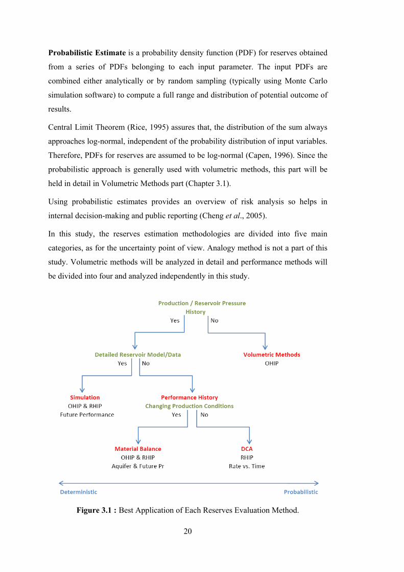
In this study, the reserves estimation methodologies are divided into five main

categories, as for the uncertainty point of view. Analogy method is not a part of this

study. Volumetric methods will be analyzed in detail and performance methods will

be divided into four and analyzed independently in this study.

Figure 3.1 : Best Application of Each Reserves Evaluation Method.

21

The summary of Figure 3.1 above is that; with high uncertainy, using probabilistic

methods will be more meaningful. After a settled performance history has been

attained, uncertainty in data hence reserves estimations will be lessened. However,

the uncertainty on economic limit, thus recoverable reserves persists (Caldwell and

Heather, 1991).

On the other hand, Sipes (1991) states that; with probabilistic analysis; all the wrong

answers are provided besides the right answer. Hence, probability analysis is not an

evaluation of reserves, it is an evaluation of risk.

The answer for the above comments on probabilistic analysis came from Caldwell

and Heather (1991). They stated their thought as; “All the procedures normally

associated with a reserve evaluation are required for the expression of reserves

confidence through probability analysis. The use of probability analysis does not

negate this, but only enhances the expression of the range of answers.”

3.1 Volumetric Methods

The most practical method for reserve estimation is volumetric method, that is using

mathematical equations for estimating recoverable hydrocarbons initially in place.

Volumetric methods are generally used in the early life of the reservoir, in the

absence of sufficient production data. These methods, also can be used to check the

estimates done by other methodologies.

The success of volumetric methods is directly related to the validity of data in hand.

As the field is developed by appraisal or production wells the data representing the

field converge to the real characteristics of the field and hence the estimated quantity

converges to the real unknown quantity.

As discussed in “Gas Reservoir Engineering” by Lee and Wattenbarger (1996); well

logs, core analyses, bottomhole pressure (BHP), fluid sample information and well

tests are used to develop sub-surface structural and statigraphic cross-sectional maps.

Furthermore, these maps give information about the reservoir’s aerial extent and

reservoir discontinuities (e.g. pinchouts, faults, GWC). By the help of these data,

reservoir pore volume (PV) can be estimated.

22

3.1.1 Single Phase Under-Saturated Oil Reservoirs

For a single-phase under-saturated oil reservoir, the following formulation can be

given to calculate Stock Tank Oil Initially in Place (STOIIP) in stb:

(5.615 ft3 = 1 bbl)

o

wc

BShASTOIIP

×−×××

=615.5

)1(φ (3.1)

The variables and units for Eq. 3.1 are as follows:

A reservoir area (ft2)

hnet net reservoir thickness (ft)

φ porosity in fraction

Swc connate water saturation in fraction

Bo oil formation volume factor (rb/stb)

As for Recoverable Oil in Place (ROIP), Eq. 3.1 can be multiplied by a Recovery

Factor (RF) which is a fraction defining the ratio of recoverable oil to the oil in the

reservoir :

FRSTOIIPROIP ×= (3.2)

3.1.2 Volumetric Dry Gas Reservoirs

For a single-phase dry gas reservoir, the formulation is similar with a minor change

in formation volume factor. This time the fluid considered is dry gas and the

formation volume factor for gas (Bg) is used instead of Bo. Then, Gas Initially in

Place (GIIP) in scf can be found by the help of Eq. 3.3:

g

wc

BShAGIIP )1( −×××

=φ

(3.3)

where Bg is computed from:

23

TzPTzpB

isc

scscig ..

..=

(3.4)

Where the subscript “i” refers to initial reservoir conditions and the subscript “sc”

refers to standard conditions.

Notice that if the reservoir volume is to be calculated in stb instead of scf, a

multiplication factor of 7758 should be used.

As for Recoverable Gas in Place (RGIP), the recovery factor comes into concern.

Again, multiplying GIIP with RF (Recoverable Gas/Gas in the Reservoir) gives us

the RGIP:

FRGIIPRGIP ×= (3.5)

Typical recovery factors for volumetric dry gas reservoirs are 80 – 90 % in common

(Lee and Wattenbarger, 1996).

There were two important definitions about this title, going into detail for definitons:

A volumetric reservoir is completely enclosed by low-permeability or completely

impermeable barriers and does not receive pressure support from external sources,

such as an enclosing aquifer. Then neglecting the expansion of rock and connate

water; only the gas expansion resulting from gas production remains as the source of

pressure maintenance (Lee and Wattenbarger, 1996).

Secondly, dry gas means, a reservoir gas primarily composed of methane and some

intermediate-weight HC molecules. As can be seen from dry-gas phase diagram in

Figure 3.2, dry gases do not undergo any phase change by reason of a pressure

reduction. In other words, they are solely gas in the reservoir and also at the separator

conditions. Also note that dry does not refer to the absence of water, but indicates

that no liquid HC form in the reservoir, wellbore or surface equipment during

production. (Lee and Wattenbarger, 1996; Spivey, 2008).

24

Figure 3.2 : Phase Diagram for Dry Gas Reservoirs, After Spivey (2008).

3.1.3 Dry Gas Reservoirs with Water Influx

These types of reservoirs are encountered if the reservoir is subjected to some natural

water influx from an aquifer instead of being completely closed. Following the gas

production, pressure reduction occurs at the reservoir/aquifer boundary. Hence, the

water encroachment occurs. This water influx reduces the pore volume (PV) by an

equal amount of water entering the reservoir and forces that portion to remain

unproduced. In short, the initial gas saturation and the residual gas saturation at the

endpoint of the estimation are necessary to estimate reserves in a gas reservoir with

water influx (Lee and Wattenbarger, 1996).

⎥⎥⎦

⎤

⎢⎢⎣

⎡⎟⎟⎠

⎞⎜⎜⎝

⎛ −+−=

v

v

gi

gr

ga

giVF E

ESS

BB

ER 11 (3.6)

Ev volumetric sweep efficiency

As mentioned by Lee and Wattenbarger (1996), the typical recovery factors for water

drive gas reservoirs are 50 – 70 % in common. This reduction in recovery factor

comparing to the volumetric dry gas reservoirs is caused by trapment of gas by

encroachment of water. Also, the reservoir heterogeneities (e.g. low-permeability

stringers or layering) may reduce gas recovery further.

25

3.1.4 Volumetric Wet-Gas and Gas-Condensate Reservoirs

These types of reservoirs have more intermediate and heavier-weight hydrocarbon

molecules. As a consequence of pressure and temperature reduction in production

phase, formation of liquids in the wellbore and surface equipments occur.

For a wet gas reservoir; estimation of GIIP necessitates the calculation of Bgi. In

detail, because of the gas condensation at surface conditions, gas properties at

surface and reservoir are different. Hence, the knowledge of the gas properties at the

reservoir conditions is necessary. Analysis of recombination of produced surface

fluids is the most accurate method. In fact, using correlations for surface production

fluids data can be enough for general cases.

Figure 3.3 : Phase Diagram for Wet Gas Reservoirs After Spivey (2008).

Figure 3.4 : Phase Diagram for Retrograde Gas Condensate Reservoirs After Spivey

(2008).

26

3.2 Reservoir Limit Tests (Radius of Investigation and Deconvolution Methods)

To identify the limits of the reservoir, the drawdown or build-up should be conducted

until the well reaches Pseudo Steady State (PSS) flow regime.

Using the PSS relationship; reservoir volume, which is inversely proportional to

slope of pressure decline with time, can be estimated (Equation 3.7)

⎟⎠⎞

⎜⎝⎛ΔΔ

⋅

⋅=⋅⋅

tPc

BqhA

t

oφ (3.7)

However, reservoir limits tests are hard to be used for gas reservoirs because of high

and variable gas compressibility and low permeability.

Meanwhile, another method is presented by Whittle and Gringarten (2008) and

Kuchuk (2009), that uses the data at the starting point of unit slope. This method is

expressed in details in Appendix D and an example application is presented in

Chapter 5.3.3.

The equation for minimum required radius can be used to design a test identifying

the reservoir boundaries (Spivey, 2008):

2/1

0324.0 ⎟⎟⎠

⎞⎜⎜⎝

⎛⋅⋅Δ⋅

⋅=t

inv ctkr

μφ (3.8)

However, the above equation may not work well when the well is located near the

boundaries as it assumes the semi-steady state conditions achieved in the drainage

area of the well.

The total compressibility (ct) can be calculated by multiplying each phase saturation

with its compressibility and addition of all plus the formation compressibility:

wwggooft cscscscc ⋅+⋅+⋅+= (3.9)

Errors in pressure/rate measurements, uncertainties in basic well and reservoir

parameters (bad match with the interpretation model or from the non-uniqueness of

the interpretation model) lead to uncertainty in well test analysis results (Azi et al.,

2008).

27

The main objective of Reservoir Limit Tests is to understand the volume of the

reservoir investigated.

At this point deconvolution method comes in handy. Using deconvolution analysis,

more information can be obtained about reservoir properties such as reservoir

boundaries and hydrocarbon volume. Because deconvolution provides an equivalent

constant unit response to be generated from a variable-rate test for the whole duration

of the test, and hence gives chance to interprete and analyze the entire duration of the

test.

Detailed information and some discussions about “Deconvolution Method” are

presented below in a specific title. Moreover, in case studies chapter, deconvolution

method is used in a synthetic field example (Chapter 5.1) and in a real field example

(Chapter 5.3) to show its powers and weaknesses.

Deconvolution Method

Deconvolution has been used in Pressure Transient Analysis since 1960s. It can be

used (Kappa DFA Booklet, 2007):

1) To remove wellbore storage effects and thus arrive earlier at radial flow

2) To turn a noisy production history into an ideal drawdown

3) To prove reserves by finding boundaries when nothing can be seen on

discrete build-ups.

The last item and its strength are definitely our concern in this part of the study.

Onur (2007) summarizes the basic working principle of Deconvolution as such:

“The primary objective of applying pressure/rate deconvolution is to convert the

pressure data response from a variable-rate test or production sequence into an

equivalent pressure profile that would have been obtained if the well were produced

at a constant rate for the entire duration of the production history.”

Hence, instead of variable rates/pressures, a constant rate/pressure response will be

obtained concerning the subject well or reservoir by the help of deconvolution

analysis.

The main disadvantage of deconvolution is that deconvolution is very sensitive to

input parameters. In other words, small uncertainties in inputs of deconvolution

28

analysis lead to large uncertainties in output value. Thankfully, with the recent

studies robust deconvolution algorithms are developed which are more error-tolerant.

In Kappa Engineering Dynamic Flow Analysis Booklet (2007), Deconvolution

Method is described in plain English as such:

“The essence of new deconvolution method is optimization. Instead of optimizing

model parameters at the end of the interpretation, we take a discrete representation of

the derivative we are looking for, and we shift it and bend it until it honors the

selected data after integration, to give us a unit pressure change response from the

derivative, and convolution, to take the rates into account.

Once we get our deconvolved derivative, we integrate to get the pressure response

and show both pressure and derivative on log-log plot. As this is the theoretical

response for a constant rate, we match the deconvolved data with drawdown models,

not superposed models.”

Although robust deconvolution algorithms that minizes the sensitivity to input

parameters are developed, the exactness of initial pressure input stays being a key

parameter to obtain the correct deconvolved response. Especially, the late time

portion of the deconvolved response is affected from the initial pressure. Kappa DFA

Booklet (2007) explains the reason why especially the late portion is affected from

initial pressure selection as: “The early time part of the deconvolution response is

constrained by the build-up data, and the tail end is adjusted to honor other

constraints”.

To determine initial pressure more accurately, tests may be programmed to include

two separate build-ups. As it is expected, derivative plots for seperate build-ups

should give the same response, because those all pressure derivative signals belongs

to same reservoir. Hence, exact match of the deconvolved signals, especially at the

last portion, can only be obtained if the initial pressure value is correct. To illustrate,

using a lower pi, early build-up go below late build-up, and for higher pi, vice versa.

In the light of the foregoing, a trial and error procedure can be applied to obtain the

correct pi. A synthetic case example is presented in Chapter 5.1 and a real case

example is presented in Chapter 5.3, showing the importance of pi and the procedure

to determine it correctly.

29

The well-known convolution integral by Van Everdingen and Hurst (1949) can be

given by following formula, which is an expression of superposition valid for linear

systems:

')'()'()(0

dtdt

ttdptqptp ut

mim ⋅−

⋅−= ∫ (3.10)

The details of the above notations are such:

)(tpm measured pressure at any place in the wellbore (wellhead/sandface)

)(tqm measured flow rate at any place in the wellbore (wellhead/sandface)

ip initial pressure

up constant-unit-rate pressure response of the well/reservoir system if

the well were produced at a constant unit-rate.

i.e. rate normalized pressure response in psi/(STB/D)

If the subject phase is gas, mp , ip and up should be replaced with their real-gas

pseudo-pressure [m(p)] representations, which is defined by Al-Hussainy et al.

(1966).

The main advantage of deconvolution in reserves estimation is that one can find

minimum reservoir volume by fixing the minimum length of last reservoir boundary

if the deconvolved signal did not identify pseudo-state flow regime which is

characterized by unit slope line in the log-log plot of deconvolved Bourdet derivative

versus time. Meanwhile, an illustration of minimum volume calculation process by

using deconvolution, is presented using a synthetic case example in Chapter 5.1 of

case studies section.

30

3.3 Material Balance Methods

This method is simply be defined as the application of the well-known “Conservation

of Matter” principle to hydrocarbon reservoirs by analyzing the pressure behavior of

the reservoir in response to the fluid withdrawal from the reservoir. The method

assumes the reservoir as a tank to estimate the average fluid properties and pressure

history. The prerequisite for using this technique is the reservoir must have reached

semi steady-state conditions (Demirmen, 2007). Furthermore, the reliability of the

method mostly depends on sufficiency and reliability of pressure, production and

PVT data.

3.3.1 Gas Material Balance (Volumetric Depletion)

The reduction in the pressure of the reservoir in concern is directly proportional to

the gas produced from that reservoir, which is equal to the change in volume of

initial gas in that reservoir. Explaining all these in equations:

( ) gpgig BGBBG ⋅=−⋅ (3.11)

G gas initially in place (GIIP)

Gp gas produced cumulative

Bg current gas formation volume factor

Bgi initial gas formation volume factor

Writing Equation 3.11 in another form (Eq 3.12) and introducing Bg as the ratio of

the volume at reservoir conditions to the volume at standard conditions (Eq 3.13), an

equation can be formed that gives the Original Gas in Place (Eq 3.14).

( ) gpgi BGGBG ⋅−=⋅ (3.12)

s

sr

r

r

s

ss

r

rr

sc

rcg T

PTPz

PTRnz

PTRnz

VVB ⋅

×=⋅⋅⋅

⋅⋅⋅

== (3.13)

31

The unknowns of Equation 3.14 are the pressure (p), compressibility factor (z) at that

pressure and cumulative gas produced (Gp), all of which can be obtained from

field/production reports easily.

⎟⎟⎠

⎞⎜⎜⎝

⎛−⋅=

GG

zp

zp p

i

i 1 (3.14)

The situation is a little bit different for Wet Gas Reservoirs and Gas-Condensate

Reservoir. Before proceeding to the discussions about the uncertainties caused by

negligence of liquid phase while estimating volume of gas reservoirs, the definitions

can be found below for gas reservoirs that are not dry.

As mentioned in Volumetric Method section, the word “Dry” does not indicate the

absence of water. Dry means, the hydrocarbon in reservoir is only in gas phase. As

for definitions: “Wet Gas Reservoirs” produce fluids which are single phase in

reservoir and two phases at wellbore and at surface facilities. On the other hand,

“Gas Condensate Reservoirs”, act like wet gas reservoirs until reservoir pressure

decrease below dew point, then two phases exist everywhere (Spivey, 2008).

To overcome the errors caused by negligence of liquid phase rates, an equivalent

wellstream rate (Eqs. 3.15 and 3.16) can be used instead of dry gas rate (Spivey,

2008).

o

oeq M

V γ.133316= (3.15)

oo

ogw q

Mqq ..133316 γ

+= (3.16)

The variables and units for the Eqs. 3.15 and Eq. 3.16 are as follows:

Veq equivalent gas volume at standard conditions (scf/bbl)

qw wellstream production rate (scf/d)

qg surface gas production rate (scf/d)

qo stock tank liquid production rate (stb/d)

oγ specific gravity of produced oil

Mo molecular weight of produced oil

32

One of the main uncertainties in p/z approach is the straightness of p/z vs. Gp plot.

The deviations from straight line behaviour of p/z vs. Gp plot is generally resulted

from one of the items below (Spivey, 2008):

- Extra Energy to the Reservoir

Formation compressibility

Water influx

- Low Permeability

Insufficient shut-in times

- Reservoir Heterogeneity

Areal compartments

Variable layer properties without crossflow

- Changing Drainage Volumes

Well interference

- Wellbore Liquids

- Reduction in HC PV

33

Figure 3.5 : Deviations in p/z Plot After Harrel et al., 2004.

In the early life of the gas reservoirs, various extraordinary effects can not be

encountered easily. According to Harrell et. al. (2004), at least 25 % of the expected

ultimate recovery (EUR) should be produced in order to have a foreseeing in the

extraordinary effects hence the deviations from straight-line behavior. They also add

that, reservoir pressures previously showing abnormal trend should reduce to normal

pressure gradient region. Compaction and partial water-drive are the two evident

examples of drive mechanisms which show p/z trends very similar to pure depletion

drive.

Following some reservoir types are presented for which extra care should be taken

while using p/z method: Over-pressured reservoirs with a pressure gradient higher

than 0.6 psi/ft, reservoirs exhibiting relatively small pressure reduction while

producing, areas having a tendency to water influx, reservoirs producing with high

rates.

Lastly, Harrel et al. (2004) draw attention to over-pressured reservoirs which

typically exhibit linear p/z behavior until a normal pressure gradient is reached.

Volumetric analysis results will be more certain until a second trend realizes below

the normal pressure gradient. Also, liquid loading may become another issue and if

so, assuming low abandonment pressure may result in erroneous estimation of UR.

34

A real field example showing the strengths and drawbacks of p/z method besides the

importance of accurate inputs are presented in Chapter 5.2. Moreover, a synthetic

field is generated and reservoir volume is calculated using different techniques

including p/z method and results are compared in Chapter 5.1.

3.3.2 Oil Material Balance:

An easy to apply method will be presented here, which is valid for slightly

compressible fluids and for closed reservoirs. Using the well-known material balance

relations average pressure (pbar) in the reservoir can be calculated by:

)()( tNatpp pbari ⋅=− (3.17)

Where Np(t) represents the cumulative oil produced in stb and is given by:

∫ ⋅=t

p dqtN0

)()( ττ (3.18)

Also, a can be calculated by Eq. 3.19

it NCa

.1

= (3.19)

Where Ni is the stock tank oil initially in place (STOIIP). To obtain average reservoir

pressure:

)(.)( tNaptp pibar −= (3.20)

Using the relationship in Eq. 3.20 a plot of Pbar(t) vs. Np (t) gives a slope with m= – a

and intercept at pi. Hence, STOIIP can be calculated in stb with Eq. 3.21:

ti cm

NSTOIIP⋅

−==1

(3.21)

As can be deduced from equations presented up to now in this chapter, calculation of

average reservoir pressure is highly crucial while using material balance methods.

Minor errors in average pressure values leads to high errors in reservoir volume

estimations (See Chapter 5 for examples of this phenomenon).

35

Generally, average reservoir pressures are estimated by the help of build-up tests

using various methods. In Appendix B such methods, namely MBH method, Ramey-

Cobb method, Modified Muskat method, Arps-Smith method are mentioned shortly

with their advantages and disadvantahes. Moreover, a newly developed approach

Crump & Hite Method with its application steps will be presented.

3.4 Rate Analysis Methods

During production, drainage area expands and reservoir pressure declines for closed

reservoirs. As a consequence, rate decline phenomenon occurs.

The most important variable in estimating the “Ultimate Recovery” by Decline

Curve Analysis (DCA) is economic limit. That is, the rate/time at which the revenue

of production becomes less than the operating cost.

According to Harrell et al. (2004) the typical errors associated with operating costs

include:

i) Projected operating costs are lower than historic average costs. This attitude

generally results in a lower economic limit rate, hence overestimating the UR.

ii) Recurring well or facility expenses. An accurate determination of periodic

expenses may reduce the errors in operating cost calculations. Mistakenly,

assuming some expenditures as non-recurring will result in low operating

costs hence overestimation of UR.

iii) Constant Unit Cost Assumption. Almost in all production facilities, unit cost

increase over time with declining production. Artificial lift techniques,

compressors, water treatments, etc. will further increase the unit cost, nearing

the end of the producing life. On the other hand, costs of secondary products,

should also be included in calculations, which will decrease the unit cost.

iv) Changes in Recovery Process. In other words, new recovery mechanism put

into service considerably affect the operating costs.

On the contrary, decline curve methodologies have some crucial pitfalls (Spivey,

2008):

Firstly, DCA assumes that, whatever controlled the past performance will remain to

control the future performance and well count remains stable.

36

Secondly, shape of the decline curves vary with reservoir type, drive mechanism and

maturity of production.

Thirdly, decline shapes often applied inappropriately.

To avoid the erroneous results occuring from the changing production conditions, a

plot of rate vs. cumulative production can be preferred over rate vs. time. Moreover,

if rate vs. time plot is preferred and there are lots of down-time (shut-in), using

producing days instead of calender days will be advantegous.

It is worth noting that, if these down-time was a result of work-overs, all decline

trend change. Because, decline slope is a function of rate/drained pore volume.

Moreover, if the decline curve in concern belongs to a field producing with many

wells, change in the well count also brings some uncertainty into the shape of the

new decline.

As for a group of wells, summing forecast of individual well production generates

more reliable results than forecast the sum of the wells’ production. Because

forecasting summed production assumes that everything will remain in the same

proportion. Moreover, the abondonment rates for each well may be different in the

same field in concern.

Arp (1945) derived a formula representing the decline of flow rate:

bi

i

tDbqtq /1)1(

)(⋅⋅+

= (3.22)

The variables and units for the Eqs. 3.22 is as follows:

q(t) oil production rate at time t

qi initial oil production rate

b constant related to decline type (0 < b < 1)

Di initial nominal decline rate

Also D can be calculated by:

qdtdqD /

−= (3.23)

37

On Cartesian Paper:

Exponential – straight line on a plot of log (rate) vs. time

Hyperbolic – concave up curve on a plot of log (rate) vs. time

Exponential Decline:

tDi

ieqtq ..)( −= (3.24)

Using b = 0 converts Arp’s general equation to Exponential Decline equation (Eq.

3.24). Assuming Exponential Decline is applicable for following reservoir types

(Spivey, 2008):

Oil Reservoirs:

- Above Bubble Point Pressure

- Down dip wells with gravity drainage

- Solution gas drive with unfavorable kg/ko

Gas Reservoirs:

- High reservoir pressure (liquid-like compressibilities)

- Wells with liquid-loading problems

Both Oil and Gas Reservoirs:

- Produced with small drawdown relative to reservoir pressure

- Tubing limited wells

Hyperbolic Decline:

bii tDbqtq /1)1.()( ⋅⋅+= (3.25)

Values of b between 0 and 1 converts Arp’s general equation to Hyperbolic Decline

equation. Hyperbolic Decline is applicable for following reservoir types (Spivey,

2008):

38

Oil Reservoirs:

- Solution gas drive with good kg/ko (b = 0.3)

- Gravity drainage with a free surface (b = 0.5)

- Full water drive (b = 0.5)

Water-oil-ratio vs. cumulative oil production plot preferred

Gas Reservoirs:

- Producing pressure = 0 (b = 0.5)

- Producing pressure = 0.1*Pbar (b = 0.4)

Both Oil and Gas Reservoirs:

- Layered no-crossflow reservoirs

- Exponent depends on degree of deliverability/storativity contrast between

layers

- Observed maximum b = 0.8 for depletion

Harmonic Decline:

).1()(

tDqtq

i

i

+= (3.26)

Using b = 1 converts Arp’s general equation to Harmonic Decline equation.

It is worth mentioning that, treating hyperbolically declining reservoirs as

exponentially declining, will cause an underestimation of the reservoir. Tight gas

reservoirs, naturally fractured reservoirs and waterflood reservoirs are the most

abundant examples of reservoirs that can mistakenly be treated as exponentially

declining reservoirs.

The decline exponent “b” is constant excluding gas wells. For gas wells “b” is a

variable and decreases as the reservoir depletes at constant Bottom Hole Pressure

condition (Chen, 2002). In some exceptional condition “b” can be greater than 1.

However, Chen (2002) proved that “average b” is less than 1 over the depletion

stage.

39

There is another concept, Coverage Rate, should be introduced in this chapter. Cheng

et. al. (2005) defines Coverage Rate as: “The percentage by which a set of estimated

confidence intervals with a prescribed level of confidence cover, or bracket, the true

values. It is a measure of reliability of the uncertainty quantification.

Confidence intervals narrow with more production data, however this do not implies

the increase of confidence in the reserves estimate (Cheng et. al., 2005).

Contrary to the expectations, increased production history data does not always

improve the reliability of predicted future performance hence the remaining reserves.

Using the most recent production data minimizes the uncertainty in predicting the

future performance. “Backwards Analysis Scheme” mentioned in Cheng et. al.

(2005) is a way of emphasizing the most recent production data. Using this approach

in DCA minimizes the uncertainty in reserves estimates by eliminating the weak

points in DCA such as changes in operating conditions and other fluctuations in data.

The essence of this approach is to work in backwards fashion and generating

multiple forecasts from the same point in time (Figure 3.6). Then the results are

combined to form an overall probabilistic forecast.

Figure 3.6 : Backward Analysis Procedure After Cheng et al. (2005).

40

Figure 3.7 : Traditional Approach, Actual Performance is not Covered by 80 %

Confidence Interval After Cheng et al., 2005.

In Figure 3.7 and 3.8 show the results of Cheng et al. (2005)’s study conducted in

one well with 19 years of production data. Firstly, traditional approach is used in

Figure 3.7, in which all performance data is used to determine the future

performance. As can be seen performance data is not fully covered by 80 %

confidence interval. However, using Backward Analysis, only 2 year data is used and

data is covered by 80 % confidence interval. According to Cheng et al. (2005), usage

of the most recent 20 % of the production data gives successful results.

Transient-period data are one of the main problems influencing the behavior of

decline curves. Transient-period should be excluded from the analyzed data for a

more reliable forecast of future performance consequently reserve estimation.

However, determining the end of the transient-period (beginning of the stabilized-

period) is a hard issue to overcome, especially with short term production data. At

this point, Backward Approach comes in handy with eliminating this problem by

emphasizing the most recent data. The overall P50 value is determined by averaging

the P50 values. P90 value is determined by taking the minimum of the P90 values

and P10 value is determined by taking the maximum of the P10 values (Cheng et al.,

2005).

41

Figure 3.8 : Backward 2-Year Scenario, Actual Performance is Covered by 80 %

Confidence Interval After Cheng et al. (2005)

The second main problem is the change in operating conditions during production

life. By using the most recent production data, this unfavorable situation will be

minimized and Backward Analysis comes to the rescue again.

In order to reduce the uncertainty in DCA (Spivey, 2008):

- Estimate decline trend on well basis or completion basis

- Include trends in secondary products

- Use analog fields or mature wells

- Select the most appropriate decline model

- Combine DCA with other evaluation techniques

Unfortunately, it should be kept in mind that, Decline Curve Analysis is a

complementary method to check other methodologies, rather than a discrete method.

3.5 Numerical Reservoir Simulation

Numerical reservoir simulation is the most comprehensive method of reserves and

reservoir parameters estimate which can account for complex reservoirs and varying

reservoir and well properties. However, it requires more data than the other methods

discussed above.

42

Reservoir simulation is representing the reservoir with a series of interconnected

cells (grids) each have private rock and fluid properties. By the help of computers,

the specified type of flow is simulated in the created reservoir. Material Balance

calculations and Darcy’s flow calculations for migration of fluids are performed in

each cell. The convergence of the created reservoir to the real case is checked by the

match of the historical data to the simulated data. However, history matches are not

unique, i.e. different reservoir models may response in the similar manner to extent.

Hence models should be checked with different data sources.

43

4. METHODS FOR UNCERTAINTY ASSESMENT

As mentionded previously, uncertainty is inherent in estimation of reserves from

underground oil and gas energy systems. Unfortunately, this is also true regardless of

any method used for estimation, e.g., volumetric, decline curve, or reservoir

simulation methods mentioned in Chapter 3 because the input variables required for

the resource estimation problem always contain uncertainties to some degree that

propagate into resource estimates. Therefore, to make good decisions, one must be

able to accurately assess and manage the uncertainties and risks. Hence, it is vital to

quantify the uncertainty in estimates of oil and gas reserves.

Here, we will limit our study to uncertainty assessment for volumetric methods, but

the methodology given here is general and can be applied to any other methods

different from the volumetric methods that can be used for reserve estimation.

One can use both Monte Carlo (MC) and the analytic uncertainty propagation (AUP)

methods for characterizing and quantifying uncertainty in reserves estimated from

volumetric methods. As to be discussed in the next sections, Monte Carlo is the most

general approach to assess the uncertainty. However, there is a simple and fast

alternative method – which we refer to it as the analytic uncertainty propagation

method (AUPM) – to the MCM for characterizing uncertainty. The validity of the

AUPM for accurately characterizing uncertainty results from the fact the

distributions of reserves for a zone, well, or field to be computed from the volumetric

method tend to be log-normal. This result simply follows from the fundamental

theorem of statistics and probability − the Central Limit Theorem (CLT) (e.g., see

Parzen, 1962), as discussed in Chapter 2. As a consequence of this theorem and the

functional relationship of the volumetric method which involves a product/quotient

of several independent random variables for computing oil and gas reserves, the

resulting distribution of oil and gas reserves is to be nearly log-normal. This result is

in fact valid no matter what form of uncertainty the input variables assume. The same

findings have been reported previously for the assessment of uncertainty in oil or gas

reserves computed from the volumetric methods by Capen (1996, 2001).

44

Figure 4.1 : Regardless of the Distribution Types of the Inputs, Summation Tends to be Normal as a Consequence of CLT.

Central Limit Theorem (CLT): This theorem states that the sum of a sufficiently

large number of identically distributed independent random variables each with finite

mean and variance will be approximately normally distributed (Rice, 1995). The

explanation of this theorem can be found in the following equation series:

)( baba +=+ (4.1)

Considering, a and b are some random variables with uniform distribution; then (a +

b) summation should have a normal distribution according to CLT.

In light of the foregoing; taking natural logarithm of a and b separately and adding

them together gives a result with normal distribution according to CLT:

)ln()ln()ln( baba ⋅=+ (4.2)

Since, ln (a.b) have a normal distribution; (a.b) will have a log-normal distribution

Finally, let us turn again to our topic, which is Volumetric Method for Estimating

Reserves, with the information about CLT in mind. One can see that the resulting

distribution of the Eqs 3.1 (Oil) and 3.3 (Gas), which involve product and quotient of

several independent random variables, should be log-normal providing the number of

input random variables are sufficiently large.

45

The equations for Volumetric Method with natural logarithm are following;

)615.5ln(ln)1ln(lnlnln)ln( oFwc BRShAROIP ⋅−+−+++= φ (4.3)

)ln(ln)1ln(lnlnln)ln( gFwc BRShARGIP −+−+++= φ (4.4)

By the help of Central Limit Theorem and considering that all the inputs above are

independent random variables, the resulting distributions for ln(ROIP) and ln(RGIP)

will tend to be normal. Hence, the distributions of ROIP and RGIP become log-

normal.

A spreadsheet analysis identifying the relationships among variables is generally

useful in modeling the uncertainty, i.e., preparing a spreadsheet that includes the

result in terms of variables in the equational form. However, conventional

spreadsheets allow the user to enter one single value for each variable instead of a

range of values for a correct uncertainty analysis. In order to have a probability

distribution for resulting estimate, user should manually change the variables in

spreadsheet in a time-consuming manner. This situation is the point where

uncertainty quantification methods come in handy (Goldman, 2000).

It is worth mentioning that, quantifying of uncertainty process is totally subjective

because the selection of the values of input parameter and their ranges depend on the

data in hand which are generally inadequate and the expertise of the interpreter.

Moreover, neglecting the correlation among input parameters may lead to large

errors in quantifying uncertainty (see Chapter 4.3).

4.1 Monte Carlo Method (MCM)

Monte Carlo Method is generally referred as the Monte Carlo Simulation. Literally,

“simulation” means an imitation of real-life. Likewise, Monte Carlo Simulation is an

imitation of a real-life system for generating outcomes by using randomly chosen

values from a distribution model as input variables and calculating the results over

and over. Hence, the model is simulated and a probability distribution is derived for

output values. Without such a simulation, the spreadsheet model only reveals a single

outcome. However, by using “Monte Carlo Simulation” add-in for spreadsheets, a

range of possible outcomes with their possibility of occurrence can be obtained.

46

Crystall BallTM, @RiskTM are examples for spreadsheet based Monte Carlo

applications.

Explaining where the name of MC Simulation comes from may help to understand

the idea under this method. MC Simulation was named after the gambling paradise

Monte Carlo, Monaco. That is, where the primary attractions are the casinos, so the

games of chance. Dice, slot, roulette wheels are all exhibit random behavior, just as

MC Simulation exhibits to select variable values.

In all MC spreadsheets, the user is supposed to define a probability distribution for

each input variable. Normal, triangular, log-normal and uniform distribution types

may be familiar, however, there exist many less-familiar types such as, beta, gamma,

Weibull and Pareto. At this point, three main sources come into rescue to determine

the distribution model, which are: fundamental principles, expert opinion and

historical data (Murtha, 1993).

On the other hand, MC simulation has some drawbacks. Murtha (1993) classifies

these drawbacks in three main parts; firstly the price of the software and users need

to learn software, secondly the language of probability and statistics should be well

known and thirdly the results are only as good as the model and the input

assumptions. First two drawbacks are easy to overcome, however, the third should be

dismissed or minimized by carefully selecting models and input parameters.

Monte Carlo Simulation can be used in any type of calculation that includes inputs

with some uncertainty. Hence, MC Simulation can be used within all estimation

methods. For example, in DCA, both the initial productivity, and the decline rate, can

be run in MC simulation as random variables. As a consequence, the production

forecast becomes a band of uncertainty, rather than a single curve.

In short, by running a MC Simulation, the input variables are repeatedly sampled

from the distributions and used in the final equation to calculate scenarios and at last

multiple scenarios are obtained. Lastly, modeling all these scenarios will give the

user a probability distribution for the result, i.e. a histogram showing the occurrence

frequency of all scenarios.

47

4.2 Analytic Uncertainty Propagation Method (AUPM)

Analytic Uncertainty Propagation Method (AUPM) is another way of assessing the

uncertainties in output values by estimating the variance of the function defined by

several random variables. In other words; the function is the result of some products

and quotients of random variables which are independent or correlated. Onur et al.

(2009) define AUPM in their work as: “It is based on a Taylor series approximation

of the function around the mean values of the variables up to first derivatives with

respect to each of the input variables.”

The main superiority of AUPM on MCM is that it does not assume a specific type of

distribution for the input variables (variables does not need to be in uniform, normal

or any type of distribution), only those statistical properties of the distribution for

each random variable specifically the mean, variance (or standard deviation) and

covariance (or correlation coefficient) among variable pairs if the random variables

are correlated are required in the AUPM (Onur et al., 2009).

There exist three different approaches of AUPM for uncertainty assessment. In this

thesis, only the easiest and the most accurate method will be discussed which uses

the equations in natural logarithm base.

Let us start to illustrate AUPM method with transforming the basic equations to

natural logarithm base. For example, take in hand the RGIP equation:

Fg

wc RB

ShARGIP ×−×××

=)1(φ

(4.5)

BgRShARGIP Fwc lnln)1ln(lnlnlnln −+−+++= φ (4.6)

Let RGIPf lnln = , and the number of random variables be M and they are lnX1, lnX2,……, ln XM. The Taylor series expansion will be:

iX

M

iif X

fXfi ln

ln)(lnln ln1

ln ∂∂

⋅−+= ∑=

μμ (4.7)

BgRFSwchARGIP lnlnlnlnlnln )1(ln μμμμμμμ φ −++++= −

(4.8)

48

Then, variance calculated using AUPM:

xj

M

i

M

ijxixjXi

M

iXif ln

1

1 1lnln.ln

1

2ln

2ln 2 σσρσσ ∑∑∑

−

= +==

⋅⋅+= (4.9)

where, the term after the plus sign stands for the correlation between input pairs. As

for the special case without correlation between inputs:

∑=

=M

iXif

1

2ln

2ln σσ

(4.10)

By looking at the above equations, only mean )(μ and variance )( 2σ values needed

to apply AUPM method, contrary to the MCM, in which probability distribution type

also needed. Three common probability density function (PDF) types are given in

Figure 4.2.

Figure 4.2 : Three Common Distribution Types (Rows: 1st CDF, 2nd PDF and 3rd

Histogram) After Murtha (1993).

Now let us look at the calculation of mean and variance values if there is not enough

number of samples. Here, we assume the distribution of variables in RGIP and ROIP

calculations are Triangular, which is the most basic distribution type (Figure 4.3).

49

Figure 4.3 : The Most Basic Distribution Type

3ModeMaxMin

xi++

=μ

(4.11)

18)(

18)()()( 222

2

ModeMaxModeMinMaxMin

ModeMaxMinxi

×+×+×−

++=σ

(4.12)

In order to use Equations 4.8 to 4.10, Xiμ and 2Xiσ should be converted to Xilnμ

and

2ln Xiσ by following formulations:

⎟⎟⎠

⎞⎜⎜⎝

⎛+−= 2

2

ln 1ln21ln

Xi

XiXixi μ

σμμ (4.13)

⎟⎟⎠

⎞⎜⎜⎝

⎛+= 2

22ln 1ln

X

XiXi μ

σσ (4.14)

Then, P10, P50 and P90 values are calculated by AUPM. Notice that, here fln

is

normal hence f is log-normal and f represents RGIP/ROIP functions.

( )ffP lnln10 28.1exp σμ ⋅−= (4.15)

( )ffP lnln90 28.1exp σμ ⋅+= (4.16)

50

901050 .PPP = (4.17)

Recalling that, 2lnln ff σσ = equation holds.

As for the mean and variance values;

⎟⎟⎠

⎞⎜⎜⎝

⎛+=

2exp

2ln

lnf

ff

σμμ

(4.18)

( )[ ]1exp 2ln

22 −⋅= fff σμσ (4.19)

The uncertainty contributions of each input variables to total uncertainty can also be

calculated by UPC approach. Equations 4.20 to 4.22 are used to calculate UPC’s

with correlations in input pairs and without any correlation.

∑∑∑−

= +==

=+1

1 111

M

i

M

ijij

M

ii UPCUPC

(4.20)

2ln

2ln

f

XiiUPC

σσ

= (4.21)

XjXif

XiXiijUPC ln.ln2

ln

lnln2 ρσσσ

⋅⋅= ⋅⋅

(4.22)

4.3 Aggregation of Reserves

This title worths mentioning in a different section, because there is a common

mistake about the aggregation of reserves from individual wells/fields to get a final

proved/possible/probable reserves for fields/companies.

Capen (1996, 2001) summarizes this pitfall in his paper as: “Proved is a purposely

conservative number. Adding conservative numbers brings about still more

conservatism.”

51

Companies or countries always want to know their total reserves. Declarations are

made and investments planned according to those numbers. However, if aggregation

(addition of reserves of several reservoirs) is not done using probabilistic methods,

statistical distortions arise in reserves estimations.

Arithmetic sum will shift P10 marker to a lower value and P90 marker to a higher

value. Fortunately, mean will not be affected from this common mistake (Figure 4.4).

To sum up, using arithmetic sum instead of probabilistic sum results in an erroneous

high uncertainty and this situation gets worsen as the number of added reserves

increase. This difference between arithmetic sum and probabilistic aggregation is

called “the portfolio effect”.

Figure 4.4 : Effect of the Arithmetic Sum of Input Variables on Resulting P90 and P10 Values

The necessity of probabilistic estimates can be well illustrated by a dice example.

Based on basic statistical knowledge, when a die is rolled there is 1/6 probability of

coming up any of the numbers 1 to 6. What is the probability of coming up the same

number when you roll the die twice? It is obviously 1/36, not 1/3, 1/12 or 1/6.

Let’s use this logic to estimate a company’s total assets, that have two independent

fields. Let the P10 value of its first field be X (i.e. 90 % probability of this field’s

volume to be more than or equal to X) and the P10 value of the second field be Y

(i.e. 90 % probability of this field’s volume to be more than or equal to Y). Will P10

value of the total assets of the company be X+Y? The answer is obviously: “No, it is

not!”. The probability of the real volume to be more than or equal to arithmetic sum

52

(X+Y), should be higher than 90 %. From another point of view, P10 marker

corresponds to a reservoir volume higher than arithmetic sum (X+Y) (see Figure

4.4). To sum up in simple words; keeping in mind the reserves volume as proved

value keeps the investor on the safe side, yet there is much more space (90 %)

remains for worse cases (real porosity to be less than and real water saturation to be

higher than expected, etc.), i.e. only if nearly everything goes bad, P10 probability

becomes the real reserves values. When addition of two fields is in concern, the

probability of going everything bad for both fields is much lower. Hence, the total

reserves volume corresponds to same probability marker should be higher.

Dependencies in inputs is another issue to be addressed in reserves estimations,

otherwise final results involve considerable statistical errors. If inputs are positively

dependent (correlated) and this dependency is ignored, the P10 value will be

overestimated and P90 value will be underestimated (Figure 4.5). Moreover, mean of

the distribution will also be underestimated. As for the negative dependency, this

effect will be reversed.,

Considering the high frequency of dependencies in real field data (e.g. porosity and

HC saturation, or area and recovery efficiency), taking into account of this issue in

reserves estimates is highly crucial.

Figure 4.5 : Effect of the Positive Dependency of Inputs on Resulting P90, P10 and Mean Values

Now, it is time to answer the question how can probabilistic aggregation be executed

with dependent variables and without dependent variables?

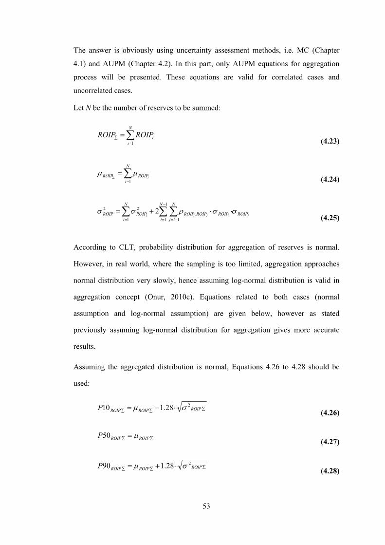
53

The answer is obviously using uncertainty assessment methods, i.e. MC (Chapter

4.1) and AUPM (Chapter 4.2). In this part, only AUPM equations for aggregation

process will be presented. These equations are valid for correlated cases and

uncorrelated cases.

Let N be the number of reserves to be summed:

∑=

∑ =N

iiROIPROIP

1 (4.23)

∑=

=∑

N

iROIPROIP i

1μμ

(4.24)

jijii ROIP

N

i

N

ijROIPROIPROIP

N

iROIPROIP σσρσσ ∑∑∑

−

= +==

⋅⋅+=1

1 1.

1

22 2 (4.25)

According to CLT, probability distribution for aggregation of reserves is normal.

However, in real world, where the sampling is too limited, aggregation approaches

normal distribution very slowly, hence assuming log-normal distribution is valid in

aggregation concept (Onur, 2010c). Equations related to both cases (normal

assumption and log-normal assumption) are given below, however as stated

previously assuming log-normal distribution for aggregation gives more accurate

results.

Assuming the aggregated distribution is normal, Equations 4.26 to 4.28 should be

used:

∑∑∑ ⋅−= ROIPROIPROIPP 228.110 σμ

(4.26)

∑∑ = ROIPROIPP μ50 (4.27)

∑∑∑ ⋅+= ROIPROIPROIPP 228.190 σμ

(4.28)

54

As for the log-normal assumption of aggregated distribution, equations similar to

those used in ROIP/RGIP calculations (Equations 4.29 to 4.19) should be used:

( )∑∑∑ ⋅−= ROIPROIPROIPP ln2

ln 28.1exp10 σμ

(4.29)

( )∑∑ = ROIPROIPP lnexp50 μ (4.30)

( )∑∑∑ ⋅+= ROIPROIPROIPP ln2

ln 28.1exp90 σμ

(4.31)

In order to calculate log-normal mean and variance belong to aggregated ROIP/RGIP

equations 4.13 and 4.14 should be used, respectively.

The aggregation concept is quoted by SPE/WPC/AAPG/SPEE (2007) as: “The

aggregation methods utilized depends on the business purpose. It is recommended

that for reporting purposes, assessment results should not incorporate statistical

aggregation beyond the field, property, or project level. Results reporting beyond this

level should use arithmetic summation by category but should caution that the

aggregate Proved may be a very conservative estimate and aggregate 3P may be very

optimistic depending on the number of items in the aggregate. Aggregates of 2P

results typically have less portfolio effect that may not be significant in mature

properties where the statistical median approaches the mean of the resulting

distribution.”

55

5. CASE STUDIES

In this chapter, the methods mentioned previously in Chapter 3 and 4 will be applied

to the synthetic and real examples and the results will be presented with their

advantages and disadvantages.

As for synthetic examples, pressure data were generated by Ecrin v.4.12 and all test

data, including real examples, interpreted using the well test analysis software Ecrin

v.4.12. Moreover, Petrel 2009.2 was used to model the reservoir/well systems.

To display the effects of variables on results more efficiently, only the variable in

concern is changed while generating data and all other parameters are kept constant

and simple. The differences caused by change in parameters are presented by means

of graphics and numerical results. More decimal digits tried to be used in input

parameters or to present results as much as possible to reduce rounding errors.

5.1 A Synthetic Field Example

Case-1: Rectangular Gas Reservoir Closed with No Flow Boundaries

Our first case is a synthetic gas field with only one producing well called SF-1 . The

reservoir is a closed reservoir and with four no-flow boundaries as in Figure 5.1 and

other reservoir parameters are given in Table 5.1. Gas properties are given in Table

5.2 and other rock, fluid and wellbore properties are given in Table 5.3. Also, test

program assumed to be conducted in SF-1 well is presented in Table 5.4.

56

Figure 5.1 : 2D Representation of SF-1 Well and Reservoir System.

Table 5.1 : Reservoir Properties for SF-1.

Reservoir Properties

Boundary-1 "No Flow" “S” 550 ft

Boundary-2 "No Flow" “E” 660 ft

Boundary-3 "No Flow" “N” 770 ft

Boundary-4 "No Flow" “W” 2800 ft

Net Thickness (hnet) 33 m

Net/Gross 1

Porosity (φ) 0.20

Water Saturation Connate (Swc) 0.45

Bgi 0.00672 rm3/Sm3

pi 2400 psia

Tbh 180 °F

k.h 6350 md.ft

k 58.65 md

57

Table 5.2 : Gas Properties for SF-1.

Gas Properties

Component Mole Fraction

C1 0.9520

C2 0.0180

C3 0.0130

i-C4 0.0040

n-C4 0.0020

neo-C5 0.0000

i-C5 0.0020

n-C5 0.0000

n-C6 0.0040

N2 0.0050

CO2 0.0000

Argon 0.0000

Total 1.0000

S.G 0.601

G.H.V (kcal/sm3) 9587

N.H.V (kcal/sm3) 8651

W.I (kcal/sm3) 12369

Tpc (°R) 356.34

Ppc (psia) 664.15

Table 5.3 : Other Rock, Fluid and Wellbore Properties for SF-1.

Other Rock & Fluid Properties

Water Salinity 40000 ppm

Water Compressibility 2.84E-06 psi-1

Rock Compressibility 3.00E-06 psi-1

Wellbore Storage Coefficient (C) 0.098 bbl/psi

Skin (S) 0.75

58

Now, it is time to apply the methods previously mentioned in Chapter 3,

respectively. Firstly, the reservoir volume will be calculated by volumetric method.

Then, reservoir limits tests will be mentioned and the sensitivity to input parameters

will be illustrated. Meanwhile, using Material Balance Method, both results will be

compared. Lastly, a simple model will be built and simulation results will be

compared with results obtained from other methods.

5.1.1 Volumetric Method Application

Since SF-1 is a synthetic case, all data are known exactly and the result calculated

using the Volumetric Equation will be exact providing any input value is not

rounded. Recalling Eq. 3.3:

g

wc

BShAGIIP )1( −×××

=φ

33 smmillion 229sm 22903135200672.0

)45.01(2.033307,424≅=

−×××=GIIP

Notice that the result came out with 0 % uncertainty. However, in real cases, most of

the input values have uncertainties to some extent and also we will not know the

exact value of GIIP. Hereby, the result should be rounded before it is presented to

eliminate the bias in uncertain digits. Generally gas reserves are declared in

million/billion m3 or cuft and oil reserves are declared in million/billion bbls.

Now, we introduce some uncertainties to the input variables of GIIP equation.

Assuming that all of the variables, excluding RF, has ±25 % uncertainty, i.e. the

minimum possible value is 25 % less than the actual value and the maximum

possible value is 25 % higher than the actual value (Table 5.4) and assuming a

triangular distribution for each of the variables, P10, P90 and P50 values are

calculated using AUPM (Table 5.5).

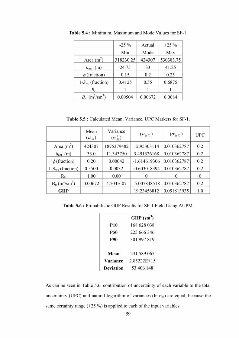
59

Table 5.4 : Minimum, Maximum and Mode Values for SF-1.

-25 % Actual +25 % Min Mode Max

Area (m2) 318230.25 424307 530383.75 hnet (m) 24.75 33 41.25

φ (fraction) 0.15 0.2 0.25 1-Swc (fraction) 0.4125 0.55 0.6875

RF 1 1 1 Bgi (m3/sm3) 0.00504 0.00672 0.0084

Table 5.5 : Calculated Mean, Variance, UPC Markers for SF-1.

Mean

)( Xiμ Variance

)( 2Xiσ

)( ln Xiμ )( ln Xiσ UPC

Area (m2) 424307 1875379482 12.95303114 0.010362787 0.2 hnet (m) 33.0 11.343750 3.491326168 0.010362787 0.2

φ (fraction) 0.20 0.00042 -1.614619306 0.010362787 0.2 1-Swc (fraction) 0.5500 0.0032 -0.603018394 0.010362787 0.2

RF 1.00 0.00 0 0 0 Bg (m3/sm3) 0.00672 4.704E-07 -5.007848518 0.010362787 0.2

GIIP 19.23456812 0.051813935 1.0

Table 5.6 : Probabilistic GIIP Results for SF-1 Field Using AUPM.

GIIP (sm3) P10 168 628 038P50 225 666 346P90 301 997 819

Mean 231 589 065Variance 2.85222E+15Deviation 53 406 148

As can be seen in Table 5.6, contribution of uncertainty of each variable to the total

uncertainty (UPC) and natural logarithm of variances (ln σxi) are equal, because the

same certainty range (±25 %) is applied to each of the input variables.

60

To compare the results obtained from AUPM, the same uncertainty range (±25 %) is

used to generate random numbers (10000 sampling) with normal distribution for

each of the input variables (See Table 5.5 for means and variances).

After using these input variables in Eq. 3.1 totally randomly, GIIP values are

obtained as output values. The histogram for resulting GIIP values are plotted in

Figure 5.2. One can easily note that, the trend of the plot is obviously log-normal

which is the expected result of Central Limit Theorem, stated in Chapter 4.

Moreover, P90, P50 and P10 markers can be calculated by sorting the GIIP results

by ascending order and determining the 90th, 50th and 10th percentiles of whole data,

respectively. This procedure is simply called as Monte Carlo Method.

Figure 5.2 : Histogram for GIIP.

Table 5.7 : Probabilistic GIIP Results for SF-1 Field Using MCM.

GIIP (sm3) P10 168.514.456P50 226.587.430P90 302.467.137

Mean 232.091.796Variance 2,92513E+15Deviation 54084483

61

While comparing Tables 5.6 and Table 5.7, results obtained from AUPM and MCM

are nearly the same.

5.1.2 Reservoir Limit Tests Application

To find the limits of the reservoir and reservoir properties, a well test is programmed

in SF-1 well. The test consists of three build-ups and numerous flow periods with

different rates. Details of the test program can be seen in Table 5.8 and pressure and

rate history is plotted in Figure 5.3.

Table 5.8 : Test Program Conducted in SF-1.

Test Periods

Type Duration (hrs) Rate

Pre-test 2 0

Flow-1 8 32000

Flow-2 8 36000

Flow-3 8 42000

Flow-4 8 49000

PBU-1 24 0

Flow-5 48 52000

PBU-2 72 0

Flow-6 72 64000

PBU-3 72 0

The first step in analyzing a well test should be to plot the conventional derivatives

belong to build-ups (sometimes drawdowns also if drawdown data are of good

quality). Firstly, we plot the derivatives of Build-up 2 and Build-up 3 on the same

graph with using rate-normalize option (Figure 5.4).

Analysis of the plot in Figure 5.4, yields only two boundaries with approximately a

half slope at late times. In order to have an extended derivative plot, deconvolution

method is applied to test data and one single rate signal is tried to be obtained.

62

Figure 5.3 : Pressure and Rate History Plot for SF-1 Well Test.

Figure 5.4 : Conventional Derivative Plot for Build-up 2 and Build-up 3 with Rate-Normalize Option.

As mentioned in Chapter 3.2, Deconvolution Method is very sensitive to input

parameters. Considering the SF-1 test data, Figure 5.5 and Figure 5.6 show the

sensitivity of Deconvolution derivative trend to pi. As can be seen below, with lower

63

pi, early build-up go below late build-up, and for higher pi, vice versa (Kappa DFA

Booklet, 2007).

Figure 5.5 : Using Pi = 2399 psia Instead of the True Value pi = 2400 psia.

Figure 5.6 : Using Pi = 2401 psia Instead of the True Value pi = 2400 psia.

64

Moreover, let us decrease the difference between true pi (2400 psia) and assumed pi

(2399.9 psia). Although the pressure difference is only 0.1 psi, the incoherence in

derivatives of seperate build-ups is distinguishable, as in Figure 5.7.

Figure 5.7 : Using pi = 2399.9 psia Instead of the True Value pi = 2400 psia.

Figure 5.8 : Using true pi = 2400 psia and Exact Match of Both Build-ups.

65

After extracting derivative plots of two build-ups, by the help of a trial and error

procedure to match build-ups, one can find the true pi. As in Figure 5.8, if pi is true

all build-ups match perfectly. However, noise in data may distort the match to some

extent.

Although this topic is not a reserve estimation method alone, why it is so important?

The answer is simple. Because the subject mentioned in this topic helps estimating

reserves more accurately or helps eliminating bias in estimations.

Firstly, the shape of the derivative curve gives us the boundaries and errors in

derivative curve leads to determine erroneous boundary distances (Figure 5.9), hence

reservoir volumes. Moreover, if p/z method is used for determining GIIP, erroneous

pi values leads to erroneous reservoir volumes (See Chapter 3.2).

Figure 5.9 : Using Erroneous pi Values pi = 2399, pi = 2401 and True pi = 2400.

Until this point, how one can extract single rate signal (deconvolved pressure

derivative trend) free of errors is discussed. Our next objective is to obtain the correct

reservoir volume by the help of deconvolution method. As discussed previously,

66

conventional derivative plot does not reveal all of the four boundaries, now let us

analyze the deconvolution log-log plot obtained from the last build-up portion

(Figure 5.10).

Figure 5.10 : Log-log Deconvolution Plot with pi = 2400 psia.

The line at the end of the derivative data is the unit slope line. Comparing the trend

of the derivative data and the unit slope line, the closed system behaviour can not be

deduced directly. On the other hand, three boundary model can be placed on the plot

by looking at the general trend and slope of the last portion which is higher than ½

slope (Figure 5.11).

Model with three boundaries honors the derivative trend except the very last portion.

The line belongs to model deviates from the data and tends to be linear which shows

radial flow. However, data points carry on the upward trend without reaching to unit

slope.

Hence it is obvious that, there is one more missing boundary that makes the model as

a closed system. Using the sensitivity option in Ecrin v.4.12, the last boundary is

tried to be determined.

67

Figure 5.11 : Log-log Deconvolution Plot and Model with Three Boundaries.

In Figure 5.12, the last boundary distance is set at three different values, 10000 ft,

5000 ft and 3000 ft. As can be seen from the figure, only 3000 ft value fits on the

derivative data. Moreover, to be more sensitive, 3000 ft, 2800 ft and 2600 ft values

are tested in Figure 5.13 This time, setting the last boundary at 2800 ft honours the

whole data most effectively.

Using the above methodology, one can determine the size of the reservoir, hence the

reservoir volume and the reserves, providing the data are sufficiently long and

reliable, as in the synthetic case considered here. Note that for the synthetic case, we

determine almost exactly the true, unknown value of the reservoir pore volume and

reserve. However, in cases we do not observe the effect of any or more of the no-

flow boundaries, using the methodology given above we can only determine a

minimum reservoir volume or reserve that supports the deconvolved drawdown

response and the measured pressure history.

68

Figure 5.12 : Sensitivity Analysis Setting the Last Boundary at 10000 ft, 5000 ft and 3000 ft.

Figure 5.13 : Sensitivity Analysis Setting the Last Boundary at 3000 ft, 2800 ft and 2600 ft.

69

5.1.3 Material Balance Method Application

As mentioned in Chapter 3.3, p/z values are used in gas wells to apply material

balance method. Plotting p/z vs. Gp values and extrapolating the line to athmospheric

pressure (14.7 psia) gives GIIP. For gas wells, with todays technology Gp values are

measured with negligible errors by flow computers (Chapter 3.3) and z values can be

estimated with perfect correlations. Only the variable pressure history prones to

uncertainty which actually refers to pbar values, i.e. average reservoir pressure. At

this point, an important question arises: How Pbar values can be obtained with

minimum uncertainty? In Appendix B, we provide various methods that can be used

to estimate the average reservoir pressure from build-up tests, and we discuss the

advantages and disadvantages of each method.

Downhole pressure gauges measure only the bottomhole pressure, not average

reservoir pressure. Reservoir engineers calculate pbar values generally with semi-log

approach or by help of the softwares and analytical methods.

Table 5.9 and Figure 5.14, shows the application of p/z method on SF-1, where pbar

values are obtained from Ecrin v.12. However, in Table 5.10 and Figure 5.15, pbar

values obtained by regressing of the radial flow period in the semi-log graph (Figure

5.16) plotted in Ecrin 4.12, i.e. using p* instead of pbar. The correlation coefficient in

Figure 3 is 1.00, whereas it is 0.99 in Figure 10 since Ecrin 4.12 calculates pbar

values using pi from model, the drainage area from the model and production history.

To sum up, pbar values obtained from Ecrin v.4.12 can be considered more precise,

whereas p* calculated from semi-log plot has some imprecision. This imprecision is

a natural human error caused by the interpretation of the start and end of the linearity

(Radial Flow Period) in semi-log curve.

On the other hand, does pbar value have a higher accuracy as much as its precision?

By comparing the results obtained by p/z method with the volumetric method, one

70

can see the difference approaches to 1.5 % in our case. As mentioned earlier, the

result obtained from volumetric method is assumed to be free of errors. Then there is

some uncertainty in p/z result, hence in pbar values. Since, pbar values are obtained

from Ecrin v.4.12, this uncertainty comes from Ecrin v.4.12. To check the

correctness of pbar values, a simple grid model was constructed using Petrel 2009.2.

Details can be found in following Chapter 5.1.4.

Table 5.9 : Pressure and Produced Volume Values for p/z Plot.

pbar (psia) z p/z (psia) Gp (sm3) Gp (million sm3)

ISIP 2400,00 0,892797 2688,18108 0 0

PBU 1 2399,45 0,892797 2687,56503 53.000 0,053

PBU 2 2398,37 0,892790 2686,37642 157.000 0,157

PBU 3 2396,37 0,892781 2684,16331 349.000 0,349

GIIP 14,7 1 14,7 232 Million 232.39

Figure 5.14 : p/z method with Pbar from Ecrin 4.12.

Table 5.10 : Pressure and Produced Volume Values for p/z Plot.

p* (psia) z p/z (psia) Gp (sm3) Gp (million sm3)

ISIP 2400 0,892797 2688,181076 0 0

PBU 1 2399,58 0,892796 2687,713655 53.000 0,053

PBU 2 2398,26 0,89279 2686,253206 157.000 0,157

PBU 3 2396,36 0,892779 2684,158118 349.000 0,349

GIIP 14,7 1 14,7 227 Million 227.91

71

Figure 5.15 : p/z method with p* Using Semi-Log Plot in Ecrin v.4.12.

Figure 5.16 : Calculation of p* Value Using Semi-Log Plot of PBU-3 (p* = 2396.36 psia).

If the produced volume is relatively high, i.e. in late times, the error between p* and

pbar seems to be negligible and more accurate results will be obtained about the

reservoir volume for the synthetic case considered here. Table 5.11 and Figure 5.17

shows the results obtained by producing SF-1 well for 7 years.

72

Table 5.11 : Comparation of Pbar and GIIP values obtained from Ecrin 4.12 and Petrel 2009.2.

pbar from

Ecrin

pbar from

Petrel

z

Correlation

(Dranchuk)

p/z from Ecrin p/z from Petrel Gp GIIP from

Ecrin

GIIP from

Petrel

(psia) (psia) (psia) (psia) (milyon sm3) (milyon sm3) (milyon sm3)

Initial Shut-in 2400 2400 0.892797 2688.181076 2688.181076 0 - -

End of Test 2396.37 2396.37 0.892781 2684.163305 2684.166106 0.349 232.2 232.4

End of Year 1 2137.40 2137.33 0.893106 2393.220961 2393.142583 25.549 231.6 231.5

End of Year 2 1879.72 1879.55 0.896399 2096.967980 2096.778332 51.099 231.2 231.2

End of Year 3 1624.25 1624.07 0.902632 1799.459802 1799.260385 76.649 230.8 230.7

End of Year 4 1368.36 1368.16 0.911772 1500.769929 1500.550576 102.199 230.4 230.3

End of Year 5 1109.39 1109.15 0.923800 1200.898463 1200.638666 127.749 230.0 229.9

End of Year 6 844.69 844.44 0.938711 899.8403129 899.5739903 153.299 229.6 229.6

End of Year 7 571.56 571.35 0.956514 597.5448347 597.3221511 178.849 229.251355 229.219560

73

Figure 5.17 : p/z Plot for Calculation of GIIP using Ecrin 4.12 and Petrel 2009.2.

74

Figure 5.18 : Gas Produced and pbar Values Obtained from Petrel 2009.2

75

While looking at Table 5.11, pbar values obtained from both Ecrin v.4.12 and Petrel

2009.2 are nearly the same. However, both software give pbar values in two decimal

digits and at early producing times, when the points are so close to origin on p/z line,

two decimal digits are not enough to obtain GIIP 100 % accurately. Again the

convergence in GIIP values obtained from both softwares, to true value can be seen

in Table 5.11. Moreover, the reservoir volume obtained from Ecrin v.4.12 report is

229 million m3 which is exactly the same as in our volumetric estimate.

In summary, the uncertainty in p* value leaded to error in Reservoir Volume up to 1

% (Figure 5.15). Then, why one wants to use P* instead of Pbar? Because, Ecrin and

other softwares give pbar values only if the reservoir model is a closed reservoir with

no flow boundaries. Of course, p/z method is applicable only if the reservoir is

closed; however, it may be necessary to use this method to estimate a premature

field’s reservoir volume for which well tests do not reveal all of the no-flow

boundaries.

Meanwhile, it is worth mentioning that the engineer should be aware of that, results

will have a high level of uncertainty in such a situation. Small uncertainties in

pressures or rates will lead to high uncertainties in results. Also, water encroachment

will cause high errors, if any.

Now, let us compare this case with a well test (Table 5.12) shorter than programmed

previously in Table 4 which will not give a closed reservoir derivative trend. Let the

test ended at the end of second build up and this build-up is programmed as 48 hours,

instead of 72 hours.

76

Table 5.12 : Alternative Test Program Conducted in SF-1.

Test Periods

Type Duration (hrs) Rate

Pre-test 2 0

Flow-1 8 32000

Flow-2 8 36000

Flow-3 8 42000

Flow-4 8 49000

PBU-1 24 0

Flow-5 48 52000

PBU-2 48 0

Figure 5.19 : History Plot for Alternative Test in SF-1.

According to derivative curve plotted in Figure 5.20, nothing can be said about the

last boundary. Model is put using the same three boundaries as the input of data

generation which are 550 ft, 660 ft and 770 ft. Indeed, using only the derivative plot

in Figure 5.20, even matching three boundaries may be rather difficult. Although the

reservoir is closed in reality, we are not aware of this truth by looking at this

alternative well test alone. However, we want to use p/z method to verify the

reservoir volume, let us say, calculated by volumetric methods.

77

Figure 5.20 : Log-Log Plot for Alternative Test PBU-2.

Firstly, we plot the semi-log graph (Figure 5.21) and make a regression for the best

line of radial flow points, p* is obtained exactly the same as in the original 72 hours

build-up (Table 5.10). Even if we exaggerate the case and use 12 hours build-up

instead, we would result in the same p* value which can be seen in Figure 5.22.

Figure 5.21 : Semi-Log Plot for Alternative Test for PBU-2 (48 hours) (p* = 2398.26 psia)

78

Figure 5.22 : Semi-Log Plot for Alternative Test for PBU-2 (12 hours) (p* = 2398.26 psia)

Providing the radial flow period is reached, the length of the build-up seems not so

critical to determine an accurate value of p*. However, the boundary effects can

sometimes mask the radial flow line, hence extrapolating it may be rather difficult.

Meanwhile, instead of methods based on the use of p*, pbar can be calculated from

various methods mentioned in Appendix B and one of the methods, namely Crump

& Hite method, is illustrated in Chapter 5.3.3.

5.1.4 Numerical Reservoir Simulation Application

In this part of the study, a simple grid model was constructed in Petrel 2009.2 and the

same test/production program carried out. For the axis labeling, x-axis was thought

to be east-west direction and y-axis is thought to be north-south direction. Lastly, the

z-axis was assumed to be the depth of the model. The number of cells in x, y and z

directions are 69, 26 and 1, respectively. The length of each cell in x and y direction

is 50 ft, however the length in z direction is 108.2677 ft (33 m), which corresponds to

entire completion length. In other words, the model was constructed with only one

layer. 3-Dimensional view of the model can be seen in Figure 5.23.

79

Figure 5.23 : 3-Dimensional View of the Constructed Model for SF-1.

As for the rock and fluid properties, data given in Table 5.1 was used for all of the

cells as average values. Pressure was assumed to be 2400 psi at the mid-perforation

point. Errors caused by unit conversions are minimized by using maximum digits in

conversion factors and will be ignored throughout this case study.

The most important uncertainty occurred during modeling part is the length of the

reservoir, i.e. the distances to the boundaries. This uncertainty came from using a

limited number of grids and the necessity of these grids to be square. For example

the horizontal extent of the reservoir in x direction is 3460 ft, for the model this

extent is represented as 3350 ft with using 69 cells each has 50 ft length. Moreover,

the extent of the reservoir in y direction is 1320 ft, where it is represented in model

as 1300 ft using 26 cells with 50 ft each.

Let us calculate the volume lost by moderately fine gridding of the model. The actual

volume for SF-1 reservoir is (3460 ft x 1320 ft x 108.2677 ft) 494 480 239 ft3. As for

the model constructed this volume is reduced to 485 580 186 ft3, hence nearly 8.9

MMscf of bulk volume is lost during a moderately fine gridding of a middle-sized

reservoir, i.e. ~1.8 % error in reservoir volume. To illustrate, using the same Φ, Sw

and Bg values this lost in bulk volume corresponds to 145 685 391 scf (~4.13 million

sm3) of natural gas.

80

In order to have a better estimation in pore volume, the “pore volume multiplier”

option is available in Petrel 2009.2. Before proceding to the next step of simulation,

let us use a pore volume multiplier of 1.018328699, which is found by dividing the

actual volume to volume obtained from initial run.

Of course, one cannot know exactly the bulk/pore volume and use pore volume

multiplier option. So, how can an engineer minimize the uncertainty in pore volume

calculations while using simulation method? The answer is increasing the number of

cells to represent the reservoir more accurately. Although, a high number of cells

would bring more accuracy to the model, it will increase the time necessary to run

simulation, drastically.

After eliminating the first uncertainty arose in simulation studies, let us proceed to

the next one, which is uncertainties in fluid and rock properties inputs. In order to

minimize the differences among estimation methods, same fluid and rock properties

are tried to be used. However, among correlation theories there are some basic

differences that leads to high differences in complex calculations. For example, in

Ecrin v.4.12; Bg is calculated to be ~0.00672 rm3/sm3 @ 2400 psi; where in Petrel

2009.2; Bg is calculated to be ~0.00685 rm3/sm3. In order to eliminate this

incoherence, we assumed the value obtained from Ecrin v.4.12 to be more accurate

and used it in volumetric method calculation, hence for simulation study; the same

Bg values will be copied from Ecrin v.4.12 to Petrel 2009.2. Comparative reservoir

volume results by Numerical Simulation (Petrel 2009.2) are displayed in Table 5.13.

Table 5.13 : Effects of Variables in Simulation Study.

Modification Steps in Simulation Study

Gas Volume (Million sm3)

Initial Run 220.84

Pore Volume Multiplier 224.80

PVT Correlations 229.02

81

To show the importance of “Rock Compaction Values” in Reserves estimation, one

more case is run editing the “Rock Compaction Function”. Up to now, the default

values obtained from Newman correlation in Petrel 2009.2 is used to estimate rock

compressibility. This time it is edited as user defined and 0.000003 psi-1 value is

assigned and simulation is run again. This run resulted in only 38 m3 more gas

volume in the reservoir which corresponds to 0.000017 % difference in total

reservoir volume.

Lastly, it is worth mentioning that the disadvantages of Numerical Simulation.

Besides, the time and money consumed for simulation studies, there is one more

drawback concerning the uncertainty point of view. That is the complexity inherent

in simulation studies.

Conducting a simulation study for a field necessitates more and more information as

input. While the number of input parameters increases, the uncertainty in results

increases. A simple solution for this drawback is offered by Aziz (1989): “Keep It

Simple”. In his own words: “Start and end with the simplest model that is consistent

with the nature of the reservoir, the objective of your study, and availability of data.

Classic reservoir engineering, simple analytical models or single-block simulations

are often all you need. At other times, the most sophisticated model available to you

may not serve your needs. Understand model limitations and capabilities.”

Choosing the correct reserves estimation method according to your data and need is

the most crucial point while evaluating reserves. The best application of each method

question is summarized in Figure 3.1.

82

5.2 Real Field Example – CY Field

Case 2: A Real Gas Reservoir with Three Producing Gas Wells

In this part of the thesis, GIIP of a real gas field is tried to be calculated. Because of

the confidentiality, the field will be called as CY Field throughout this study. CY

field is located in the Thrace Basin of Turkey. There are three producing wells in the

field and the produced gas is gathered in one station and processed there. Gas

composition and properties obtained from CY wells can be found in Table 5.14.

Table 5.14 : Gas Composition and Properties of CY Field.

Gas Properties

Component Mole

Fraction C1 97.20 C2 0.06 C3 0.01

i-C4 0.00 n-C4 0.00

neo-C5 0.00 i-C5 0.01 n-C5 0.00 n-C6 0.00 N2 1.65

CO2 0.00 Argon 1.07 Total 1.00 S.G 0.571

G.H.V (kcal/sm3) 8768.8 N.H.V (kcal/sm3) 7895.4

M.W (g/mol) 16.51 Tpc (°R) 340.8 Ppc (psia) 664.5

83

Figure 5.24 : Seismic Formation Top Map for CY Field.

84


Average reservoir properties used in deterministic estimate are displayed in Table

5.15 and one deterministic GIIP value is estimated by using these values.

Table 5.15 : Average Reservoir Properties for CY Field (Calculated at 828 psia and 111 °F)

Bottom hole temperature, °F : 111 Wellbore Radius, rw – ft : 0.254

Porosity - % : 16 Water Saturation, Swc - % : 51 Net Thickness, h – m : 10 Gas formation volume factor, Bgi – m3/m3 : 0.01658

g

wc

BShA

OGIP)1( −×××

=φ

3s 717,214,118

01658.0)51.01(16.010000,500,2 mOGIP =

−×××=

In the next step, redefining these values with a probabilistic point of view, P10, P50

and P90 values are calculated by using AUPM. The minimum, maximum and mode

values for reservoir properties are displayed in Table 5.16.

Table 5.16 : Min, Max and Mode Values for Reservoir Properties of CY Field Min Max Mode

Area (m2) 2,770,000 9,400,000 6,500,000hnet (m) 4.6 6.2 5.8


RF 0.70 0.90 0.80 Bg (m3/sm3) 0.01655 0.01659 0.01658

Area is calculated from the area with high amplitudes in seismic maps (e.g Figure

85

5.24). According to the optimism of the geologist estimated area changes. Statistical

values are given in Table 5.16.

Formation Volume Factor, Bgi, is calculated using the internal correlation option in

Ecrin v.4.12. However, there is some uncertainty in pi value, hence Bgi changes

according to assumed pi values. Here, pi values obtained from the three wells are

considered and Bgi is calculated using these values and results are inserted in Table

5.16.

Other variables, namely hnet, φ and Swc are calculated from high porosity zones in

well logs. When φ and Swc cut-offs are changed, which determine if a zone is

reservoir or not; hnet values change. Moreover, since logging tools read values with a

specified length interval, there exists many φ and Swc data in hand. As for CY Field,

φ and Swc frequency distributions are obtained by plotting the histogram of values

from different measuring points. Moreover, probability distribution of hnet is obtained

by changing Swc cut-off, because Swc is the main controlling parameter in this field

whose formation structure is sandstone. Resulting values are also displayed in Table

5.16.

Table 5.17 : Frequency of Swc Values. Bin Frequency0.3 1 0.35 5 0.4 3 0.45 2 0.5 9 0.55 14 0.6 5 0.65 4 0.7 8

86

Figure 5.25 : Histogram for Swc Values with Swc cut-off = 0.70.

Figure 5.26 : Closer Look at Histogram for Swc Values with Swc cut-off = 0.70.

By looking at Swc histograms in Figure 5.25 and 5.26, min, max and mode values can

be determined as 0.30, 0.70 and 0.51 for CY Field. Hence, (1-Swc) values are

displayed in Table 5.16.

As for effective porosity, another histogram is plotted (Figure 5.27) and min, max

and mode values are determined, which are 0.08, 0.23 and 0.14.

87

Figure 5.27 : Histogram for Effective φ Values with Swc cut-off = 0.70.

The next step is to obtain min, max and mode values for hnet. In order to have a range

of possible values for h, Swc-cut-off value is changed and hnet is calculated for each well

by well logs (Table 5.18 and Figure 5.28 and 5.29). Although, in reality, Swc-cut-off is

well known and it is 0.7, some uncertainty is included into this value for this study.

Table 5.18 : hnet Values with Changing Swc cut-off Values.

Wells/Swc-cutoff 75% 74% 73% 72% 71% 70% 69% 68% 67% 66% 65%

CY 1 9.5 9.5 8.5 8.5 8.5 8.5 8.5 8.5 8.5 8.5 8.5

CY 2 3.8 3.8 3.8 3.8 3.8 3.8 3.7 3.7 3.7 3.7 3.7

CY 3 5.5 5 5 5 5 5 4 3.5 2.5 1.5 1.5

Average hnet 6.27 6.10 5.77 5.77 5.77 5.77 5.40 5.23 4.90 4.57 4.57

88

Figure 5.28 : Histogram for hnet Values with Different Cut-off Values on 3 Wells.

Figure 5.29 : Histogram for Average hnet Values with Different Cut-off Values on 3 Wells.

As for area values, the structure map of reservoir top of CY Field is digitized in

Digger 4 software and area is tried to be estimated by creating boundaries. The area

boundary is assumed as between -460 m (Water-Gas Contact) and -450 m contour.

The histogram associated with the area estimations is created and displayed in Figure

5.30. The min, max and mode values are inserted in Table 5.16.

89

Figure 5.30 : Histogram for Area.

As for recovery factor, two cases are thought. For the first case, RF is used as 1.0,

which will end up with GIIP. For the second case min, max and mode values are

assumed as 0.7, 0.9 and 0.8, respectively, which will end up with RGIP.

The last variable to be analyzed is Bgi, which is a direct function of pressure.

Assuming the correlation used is perfect and changing the initial reservoir pressure,

different Bg values are obtained. Introducing minus/plus 1 psi error range in initial

pressure (878 psia); minimum, maximum and mode values are calculated and

displayed in Table 5.16.

In the first step, mean and variance values (Equations 4.11 and 4.12) and their

natural logarithms (Equations 4.13 and 4.14) are calculated and tabulated below:

Table 5.19 : Mean and Variance Values and Their Natural Logarithms.

Mean

)( Xiμ Variance

)( 2Xiσ

)(ln Xiμ )(ln Xiσ

Area (m2) 6223333 1.84111E+12 15.62059534 0.046441777hnet (m) 5.533333 0.115556 1.708906892 0.003767029

φ (fraction) 0.15000 0.00095 -1.917797578 0.0413551861-Swc (fraction) 0.4967 0.0067 -0.713180664 0.02668899

RF 1.00 0.00 0 0 Bgi (m3/sm3) 0.01657333 7.22222E-11 -4.099960432 2.62937E-07

GIIP 18.79848442 0.118253245

90

Equations 4.15 to 4.17 are used and calculated P10, P90 and P50 values are

displayed in Table 5.20. Also mean, variance and deviation values are displayed in

the same table. Probabilistic RGIP values are also displayed in Table 5.21.

Table 5.20 : Probabilistic GIIP Results for CY Field Using AUPM. GIIP (m3)

P10 93 954 240 P50 145 907 647P90 226 589 469


Table 5.21 : Probabilistic RGIP Results for CY Field Using AUPM. RGIP (m3)

P10 74 705 213 P50 116 574 426P90 181 909 619


Table 5.22 : Contribution of Each Input Variable to the Total Uncertainty.

UPC (GIIP)

(%) UPC (RGIP)

(%)

Area (m2) 0.395047 0.38428 hnet (m) 0.032043 0.03117

φ (fraction) 0.351779 0.342191 1-Swc (fraction) 0.221127 0.220837

RF 0 0.02152 Bgi (m3/sm3) 2.24E-06 2.18E-06 GIIP/RGIP 1.00 1.00

91

5.2.2 Material Balance Application

Fortunately, there are more than 4 year data in hand, hence the results found by

Volumetric Method can be checked.

Table 5.23 : CY Field Pressure and Production Data Measured in March 2007.

CY - 1 p @ 658.5 m 449,8 psia Cum. Production 38,666 Million m3 Kelly Bushing 206.5 m

CY - 2

p @ 641 m 452,4 psia Cum. Production 16,928 Million m3 Kelly Bushing 188.9 m

CY - 3

p @ 657 m 449,8 psia Cum. Production 18,92 Million m3 Kelly Bushing 205 m

Since CY Field consist of 3 seperate wells in same reservoir, BHP’s of each well

should be equal at the same depth. Here, all three pressures extrapolated to 452 m

below mean sea level (-452 m) and the resulting value is 450 psia. Considering this

pressure value, the p/z plot belong to CY Field is updated. The previous estimation

based on June 2004 data and the updated estimation can be seen in Figure 5.31 and

Figure 5.32, respectively. Moreover, the data used in plotting p/z graphs are given in

Table 5.24.

Now, let us look at the uncertainty in GIIP in CY Field at different time steps.

Plotting the graphs for the first year and including the other 3 year with and without

the erroneous data. Here, one can see how producing time affects uncertainty in GIIP

value and how increasing production time compensates erroneous data.

92

Table 5.24 : CY Field P/Z Graph Data.

CY FIELD

Date p, psia

z p/z Cum. Gas Prod,

( at - 452 m) MM sm3 02.05.2003 898 0,911 985,7 0 23.04.2004 815 0,919 886,8 8,7 02.06.2004 829 0,921 898 11,1 10.06.2004 829 0,922 899,1 11,7 20.03.2007 450 0,9586 469,4 74,514

Figure 5.31 : CY Field - p/z Plot until June 2004.

Figure 5.32 : CY Field - p/z Plot with March 2007 Data

93

In Figure 5.33, only April 2004 data, which is erroneous, used to plot p/z. According

to this plot, GIIP value for CY Field is 85.4 million sm3.

Figure 5.33 : CY Field p/z Plot until April 2004.

In Figure 5.34, June 2004 data is used, however April 2004 data is exluded because

of the errors in it. Comparing Figure 5.34 and Figure 5.31, using one erroneous data,

which is actually a small error, leaded to a 4 % reduction in GIIP value.

Figure 5.34 : CY Field p/z Plot until June 2004 without Erroneous Data.

94

However, at extended producing times, uncertainty caused by an erroneous data

becomes much smaller. In Figure 5.35, p/z graph using all data excluding the

erroneous one is plotted.

Figure 5.35 : CY Field p/z Plot until March 2007 without Erroneous Data.

Comparing Figure 5.35 with Figure 5.32, the erroneous data leaded to only 0.7 %

error in GIIP value. Surprisingly, this time the erroneous data did not reduced GIIP

value, on the contrary increased it. Because, it caused the best line to match with a

lower initial pressure value. Comparing the correlation coefficients in Figure 5.31

with Figure 5.34 and Figure 5.35 with Figure 5.32, erroneous data lowers the

correlation coefficient. Hence, correlation coefficient can be a convenient tool to

check the uncertainty in p/z plot.

To sum up, increasing the number of data points reduces uncertainty, however, in

order to lessen the uncertainty in GIIP value, uncertainty in data points should be

lessened, i.e. using more stable and accurate recorders and flow computers.

Moreover, p/z method gives more accurate results at late times as mentioned in

Chapter 3.3.

95

5.2.3 Numerical Reservoir Simulation Application

A static model is formed for CY field and porosity and hnet are distributed throughout

reservoir by looking at the well logs taken from three producing well and from

seismic maps for thickness calculations. In Figure 5.36, GIIP map for each grid is

shown and one can see that GIIP varies with porosity distribution and hnet

distribution by looking at Figures 5.37 and 5.38.

Figure 5.36 : GIIP Map for CY field.

In Table 5.25, reservoir properties are displayed. Net Thickness and Porosity values

are distributed throughout the reservoir, however, the value Swc is taken as a single

value. Also, one single area value is assigned to the reservoir model. The value of Bgi

value is taken as 0.01735 m3/sm3 as for the gas in concern at CY reservoir

conditions.

96

Table 5.25 : Statistical Properties of Each Input Parameter of CY Static Reservoir Model

Min Max Mode Mean Std. Dev Variance hnet (m) 3.3 21.9 5.7 8.64 5.02 25.16

φ (fraction) 0.06 0.21 0.16 0.16 0.04 0.00 RF 1

Bgi (m3/m3) 0.01735 1-Swc (fraction 0.70

Area (km2) 2.66256

GIIP (sm3) From

Simulation 136 223 773

Table 5.26 : Probabilistic GIIP results for CY Field Applying AUPM on Model.

GIIP (sm3) P10 74 428 258 P50 135 980 374P90 248 436 048


Figure 5.37 : Porosity Map for CY field.

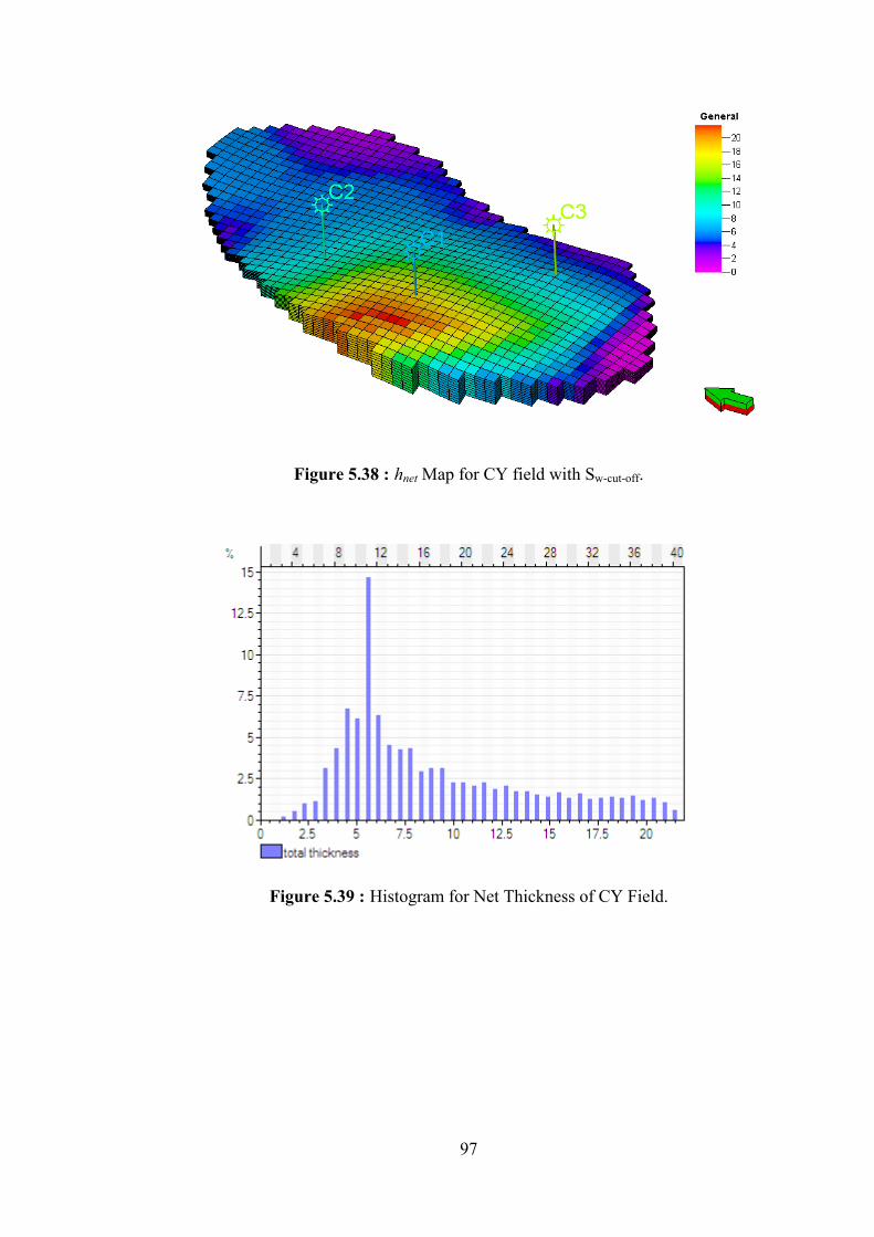
97

Figure 5.38 : hnet Map for CY field with Sw-cut-off.

Figure 5.39 : Histogram for Net Thickness of CY Field.

98

Figure 5.40 : Swc Map for CY field.

5.3 Real Field Example – LY Field

Case 3: A Real Oil Reservoir with One Exploration Well

In this part of the thesis, STOIIP of a real oil field is tried to be calculated. Because

of the confidentiality, the field will be called as LY Field throughout this study. LY

Field is one of the exploratory fields of TPAO. There is only one well drilled in LY

Field. Only cased hole DST’s are conducted in the well, the well is waiting for

further tests while this study is conducted. Only a zone with 16 ft thickness will be

our concern. While Cased Hole DST, this 16 ft interval is straddled by one Bridge

Plug at the bottom and one Test Packer at the top of the test zone, hence the prior test

zones are isolated. Firstly the reservoir and fluid properties belong to LY-1 well test

zone is displayed in Table 5.27.

99

Table 5.27 : Reservoir and Fluid Properties of LY-1 Well.

Bottom hole temperature, °F : 203 Wellbore Radius, rw – ft : 0.3

Porosity - % : 14 Water Saturation, Swc - % : 20 Net Thickness, h – ft : 16 Oil Formation Volume Factor, Boi – bbl/stb : 1.07 Oil Viscosity, µo : 1.67 Total Compressibility, ct – psi-1 : 8.45E-6

Here, only the total compressibility includes some unknowns. Although PVT

analysis was done, i.e. oil compressibility (co) is obtained almost exactly, water and

core analysis were not done. Hence water and formation compressibility values are

only obtained by correlation and ct is uncertain to some extent in this case.


Firstly, an initial STOIIP value is estimated using the average reservoir properties

displayed in Table 5.28. Since area is not tabulated above, using Didger 4 software

an average area value is obtained.

100

Figure 5.41 : Seismic Formation Top Map for LY Field

o

wc

BShASTOIIP

×−×××

=615.5

)1(φ

stbmillion 07.507.1615.5

)20.01(14.016107.1 7

=×

−××××=STOIIP

101

Secondly, by using the min, max and mode values for each input variable (Table

5.28), a probabilistic STOIIP estimate is done using AUPM. Only two variables are

considered as 100 % certain, which are hnet and Bo. On the other hand, RF is not

considered as an input since we are interested in STOIIP in this situation rather than

ROIP. Area estimations are listed in Table 5.29 and an extra data inserted which was

found from deconvolution analysis in the next section (Chapter 5.3.2). Moreover,

since this area is calculated from test results, mode is set at this area value and

AUPM calculations are done based on minimum, maximum and mode values

presented in Table 5.28. Moreover, histograms for effective porosity and water

saturation are given in Figures 5.42 and 5.43, respectively.

Table 5.28 : Min, Max and Mode Values for Varables of LY Field Min Max Mode

Area (m2) 6.8E+5 2.69E+7 8.29E+5 hnet (m) 16 16 16


Bo (bbl/stb) 1.07 1.07 1.07

Table 5.29 : Probable Area Calculations for LY Reservoir with Varying Contour Closures

Contour (ft) m2 ft2 Contour (ft) m2 ft2

5690‐a 63020 678342 5760 1010097 10872594

5690 77854 838013 5770 1182069 12723685

5700 193496 2082774 5780 1375547 14806265

5710 287654 3096282 5790 1642942 17684481

5720 407663 4388048 5800 1885258 20292748

5730 562282 6052353 5810 2161419 23265320

5740 712356 7667736 5820 2502233 26933812

5750 850001 9149335 Deconvolution 76221 829440

102

Figure 5.42 : Histogram for Effective Porosity

Figure 5.43 : Histogram for Water Saturation

Table 5.30 : Probabilistic STOIIP results for LY Field Using AUPM STOIIP (stb)

P10 1.004.865 P50 2.194.008 P90 4.790.366

Mean 2.642.741 Variance 3,14901E+12 Deviation 1774545

103

Table 5.31 : Uncertainty Contribution of Each Input Parameter to the STOIIP Estimation

UPC (STOIIP)

(%)

Area (m2) 0,948781 hnet (m) 0

φ (fraction) 0,043356 1-Swc (fraction) 0,007863

RF 0 Boi (m3/sm3) 0

STOIIP 1.00

As can be deduced from above table, the highest uncertainty is related to area. This

conclusion can also be checked from the histograms and tables given above for LY

field.

5.3.2 Reservoir Limits Tests Application (Deconvolution Method)

Following the run in hole of TCP-DST string with recorders, guns are fired to

perforate 16 ft interval. After the wellbore storage period which lasted for 36 minutes

the well started to produce oil with an average rate of 500 bbl/d for 8 hours.

Following the 15 hours first shut in period, flow after flow test was started. Firstly,

16/64” choke was used and 270 bbl/d flow rate was obtained, then 20/64”, 24/64”,

32/64” chokes were used and 313 bbl/d, 331 bbl/d and 332 bbl/d rates were obtained

respectively. The total production was 444 bbl, of which 420 bbl was oil, 3.6 bbl was

water cushion and 20 bbl was diesel cushion put prior to test. After 18 hours shut-in

time, the DST string was Pulled out of hole. Operation summary for LY-1 Well Test

is given in Table 5.33 and Figure 5.44. Lastly, at the end of the test, totally 54 bbl of

oil was recovered by reverse circulation.

104

Table 5.32 : Operation Summary for LY-1 Well

Operation Duration

(hrs) Oil Rate (bbl/day)

WHP (psig)

BHP (psia)

Water (%)

Perforation (16 ft)

- - 0 977

(cushion) -

64/64” Choke (Wellbore)

0.68 N/A 0 2983 N/A

64/64” Choke (Surface)

7.47 480 6 2638 1

Shut-in 15.22 - 325 3017 -

16/64” Choke 4.32 270 87 2771 0

20/64” Choke 4.69 314 47 2727 0

24/64” Choke 4.56 331 25 2689 0

24/64” Choke 12.09 332 6 2632 0

Shut-in 17.91 - 190 2868 -

Figure 5.44 : History Plot for LY-1 Well Test.

105

For the analysis of LY-1 well test, the last shut-in period of the test is interpreted as a

pressure build-up analysis both with type-curve matching and Horner analyses by

using well test analysis program Ecrin v.4.12.

In the analysis section of the test, firstly models for well, wellbore and reservoir were

selected. The wellbore model was described as Hageman’s Changing Storage and the

reservoir model was assumed as homogenous reservoir. As for the boundaries,

reservoirs were matched as rectangular closed reservoir. Although the initial pressure

calculated in MDT measurements was 3122.5 psia (extrapolated to recorder depth), it

was found to be 3104 psia by matching the derivatives of the two build-ups in

deconvolution method (Figures 5.45 and 5.46). The latter value was used in the

analyses since the former value may be affected by the wellbore conditions during

MDT measurements, i.e. supercharged.

Figure 5.45 : Deconvolution Log-Log Plot for pi = 3125.5 psia (Taken from MDT results)

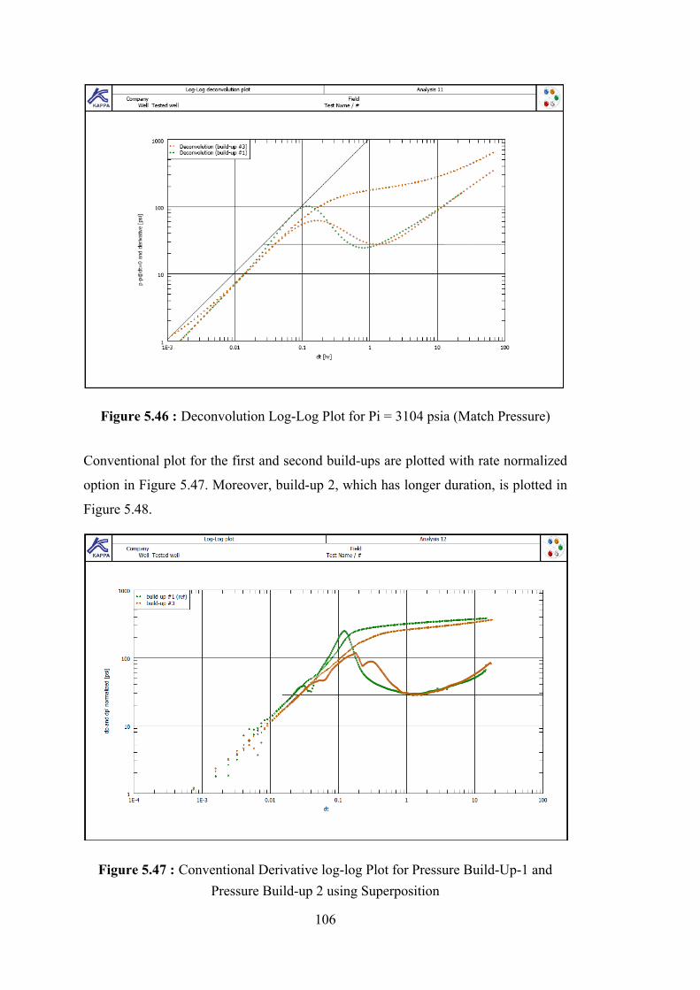
106

Figure 5.46 : Deconvolution Log-Log Plot for Pi = 3104 psia (Match Pressure)

Conventional plot for the first and second build-ups are plotted with rate normalized

option in Figure 5.47. Moreover, build-up 2, which has longer duration, is plotted in

Figure 5.48.

Figure 5.47 : Conventional Derivative log-log Plot for Pressure Build-Up-1 and Pressure Build-up 2 using Superposition

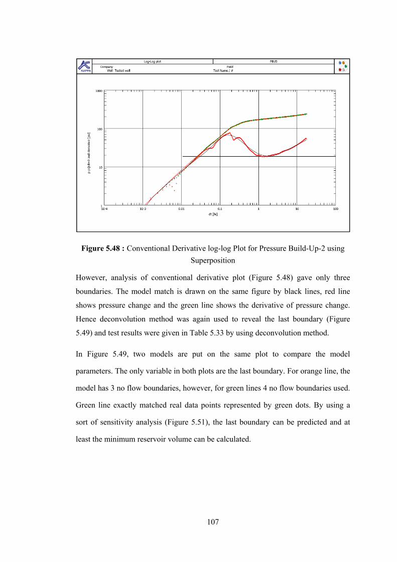
107

Figure 5.48 : Conventional Derivative log-log Plot for Pressure Build-Up-2 using Superposition

However, analysis of conventional derivative plot (Figure 5.48) gave only three

boundaries. The model match is drawn on the same figure by black lines, red line

shows pressure change and the green line shows the derivative of pressure change.

Hence deconvolution method was again used to reveal the last boundary (Figure

5.49) and test results were given in Table 5.33 by using deconvolution method.

In Figure 5.49, two models are put on the same plot to compare the model

parameters. The only variable in both plots are the last boundary. For orange line, the

model has 3 no flow boundaries, however, for green lines 4 no flow boundaries used.

Green line exactly matched real data points represented by green dots. By using a

sort of sensitivity analysis (Figure 5.51), the last boundary can be predicted and at

least the minimum reservoir volume can be calculated.

108

Figure 5.49 : Derivative log-log Plot for Pressure Build-Up-2 using Deconvolution.

Figure 5.50 : Sensitivity Analysis for the Last Boundary.

109

Figure 5.51 : Semi-log Plot for Pressure Build-Up-2 using Deconvolution.

Figure 5.52 : History Plot and Model Match for LY-1 Well Test.

110

Table 5.33 : Results of LY-1 Well Test Analysis Using Deconvolution

Reservoir Pressure, pi – psia @ Recorder Depth : 3104 Permeability x Thickness, kh – mD.ft : 2040 Permeability, k – mD : 128 Skin Factor : -1.55 Wellbore storage constant, C – bbl/psi : 0.0108

Boundary-1 “No Flow” ‘S’ – ft : 215 Boundary-2 “No Flow” ‘E’ – ft : 400 Boundary-3 “No Flow” ‘N’– ft : 217 Boundary-4 “No Flow” ‘W’– ft : 1520

Figure 5.53 : 2D Schematic of LY-1 Well Obtained from Deconvolution Method

By using the boundaries figured above and the other reservoir parameters displayed

in Table 5.26, reservoir volume is found to be 0.247 Million stb. The exactness of

this value is mostly adherent to the correctness of the model match in well test

analysis, hence the deconvolution application.

5.3.3 Material Balance Methods Application

Using Equation 3.7 given previously, as stated in Chapter 3.3, using the PSS

relationship; reservoir volume, which is inversely proportional to slope of pressure

decline with time, can be estimated.

( )wc

tto

t

o S

tPc

qSTOIIP

tPc

qB

hA

tPc

BqhA −⋅

⎟⎠⎞

⎜⎝⎛ΔΔ

⋅=⇒

⎟⎠⎞

⎜⎝⎛ΔΔ

⋅=

⋅⋅⇒

⎟⎠⎞

⎜⎝⎛ΔΔ

⋅

⋅=⋅⋅ 1φφ

111

Table 5.34 : Inputs Used in PSS Relationship (Units are Converted for Consistency).

Inputs Value Units

q 12,5 stb/hr

ct 8,45E-06 psi-1

m (slope) 0,9027 psi/hr

1-Swc 81 %

STOIIP 1.327.366 stb

Figure 5.54 : The Analyzed Period for Slope used in PSS Relationship

Figure 5.55 : Slope Estimation for PSS Relationship

112

Slope for the last drawdown period (See Figure 5.54 and Figure 5.55) is calculated as

0.9027 psi/hr. All other input data are displayed in Table 5.34. Using Equation 3.7,

STOIIP for LY Field is found to be 1.32 Million stb. This value lies between P10 and

P50 values calculated in the first part (Chapter 5.3.1) of this case.

However, the above equation is based on the pseudo steady state flow regime

assumption and we are not sure that the analyzed data is totally in pseudosteady state.

Moreover the pressure data have a high level of noise as can be seen in Figure 5.55

and since the graph is plotted on real time axis, data may have some residual

superposition effects. To reduce these uncertainties, the deconvolution response

obtained from deconvolution analysis, which actually did not match perfectly with

the real data, is used in Equation 3.7 one more time.

Figure 5.56 : Slope Estimation for PSS Relationship Using Deconvolution Response

Table 5.35 : Slope Values and Corresponding STOIIP Results Used in PSS Relationship

Point 1-2 Point 2-3 Point 1-3 m (psi/hr) 6.95645 6.70638 6.79277

STOIIP (stb) 172,245 178,670 176,395

Point 1 Point 2 Point 3

113

Table 5.35 shows STOIIP calculations with slopes obtained from different reference

points. As can be seen, slope changes with time, hence the flow regime is not exactly

pseudo steady state.

The STOIIP calculated from the slope of deconvolution response has given much

more smaller reservoir volumes, however, these results are more consistent with the

results obtained from other methodologies.

Moreover using the model match of history plot obtained by superposition method,

another STOIIP value calculated is found as 196,362 stb with a slope of 6.10205

psi/hr.

A more sophisticated method offered by Whittle and Gringarten (2008) and Kuchuk

(2009) is applied to this example. The deconvolution log-log plot is presented in

Figure 5.57. ΔtPSS and Δtint points are marked on it and corresponding values are

presented in Table 5.36. Lastly, the resulting PV and HC Volumes are presented in

Table 5.37.

Figure 5.57 : Determination of intersection point and PSS starting point in

Deconvolution Analysis

tint

tpss

114

Table 5.36 : tint, tPSS values with corresponding ΔP’int and ΔP’PSS Values

intersection

point PSS

point t (hrs) 3.99257 89.9645 ΔP’ (psi) 18.5022 427.051

Table 5.37 : PV and Reservoir Volume calculations using tPSS and tint approachs

PV (bbl) Reservoir Volume (stb) @ tPSS 311,631 252,424 @ tint 319,211 258,564

Comparing the results obtained by standard PSS approach (0,178 MM stb) with

Whittle and Gringarten (2008)’s approach (0,252 MM stb), latter is more consistent

with the result obtained from volumetric method obtained from deconvolution

boundaries (0,247 MMstb).

Now, let us proceed with the application material balance to LY-1 Field to calculate

STOIIP. As discussed in Chapter 3.3, difference in average reservoir pressure

between two consequent build-ups is directly proportional with the produced volume,

for a fixed reservoir volume. As alerted previously, accuracy in average reservoir

pressure is very important, hence before starting application of material balance

equation, average reservoir pressures for the two build-up periods (Figure 5.58) will

be calculated using Crump and Hite Method (see Appendix B).

Inserting the last bottomhole pressure Pbh = 3017.69 psia @ Δt = 15.2266 hrs,

average reservoir pressure (pbar) for the first build-up is computed as 3033.99 psia.

As for pbar during second build-up, pbh = 2869.22 psia @ Δt = 17.9141 hrs is used

and the result is calculated as pbar = 2926,46 psia.

115

Figure 5.58 : Plots of Four Steps in Crump and Hite Method for PBU-1 in LY-1 Well Test

Now, let us apply oil material balance equation to LY-1 well test. As mentioned in

Chapter 3.3.2, the slope (m) for average pressure vs. cumulative production is

calculated by using three different average pressures obtained from different sources

(Table 5.38 and Figure 5.59). Afterwards, using Eq. 3.21, STOIIP for LY Field is

calculated as displayed in Table 5.39.

Table 5.38 : Reservoir Pressures Calculated from Crump and Hite for Two Build-ups

Pbh Pbar Pbar Cumulative Production Bottom Hole Ecrin v.4.12 Crump & Hite

(psi) (psi) (psi) (MMstb)

Initial 3104 3104 3104 0

PBU-1 3017.72 3048.45 3033.33 0.000145012

PBU-2 2869.22 2920.42 2926.46 0.000479231

116

Figure 5.59 : Pressure versus Oil Produced Plot

Table 5.39 : STOIIP Values for LY Field Using Oil Material Balance

Methods/Reserves Only Two Points

Three Points (Including Pi = 3104 psia)

Slope (m)

Reserves (Million bbl)

Slope (m)

Correlation Coefficient

Reserves (Million bbl)

Ecrin v. 4.12 (Pbar) -383072 0,308932 -383072 1.00 0,308932 Crump and Hite -319760 0,370100 -361620 0,9886 0,327258

BHP -444319 0,266347 -481954 0,9948 0,245549

Using the equations for the Crump and Hite trendline above, STOIIP is calculated as

0,327 million bbls. Using Ecrin v.4.12 and Pbh results have given 0,309 million and

0,245 million bbls, respectively. Hence, reserve volume found by Crump and Hite

pressures are so close to Ecrin v.4.12’s estimation. On the other hand, using Pbh

without converting it to average reservoir pressure, resulted in a very different value.

117

5.4 Real Field Example – Aggregation of Reserves

Case 4: Probabilistic Aggregation of Reserves of Three Real Gas Field

In this part of the thesis, probabilistic GIIP calculations belong to three gas reservoirs

will be probabilistically aggregated and the erroneous results arise from arithmetic

addition will be illustrated. The fields are all in Thrace Region of Turkey and are

thought to be used for underground storage of natural gas, hence reservoir volume

should be exactly known. Actually, since all reservoirs are volumetric gas reservoirs,

and all have production data, real reservoir volumes are approximately known and

displayed in Table 5.40. As can be seen in the same table, one of the fields to be

aggregated is CY Field, that analyzed in Chapter 5.2, and probabilistic results are

taken from the results found in that chapter.

Table 5.40 : Approximate Real Volumes of Fields to be Probabilistically Aggregated.

Approximate Real Volumes

Fields Million sm3

BS Field 162

IB Field 123

CY Field 141

Sum 426

Input parameters for BS Field and IB Fields are determined by setting the mode

value to the average values, nearly known and which gives the true value when used

in Volumetric Equation for GIIP. Minimum values are set at -20 % of the mode

values and Maximum values are set at +20 % of the mode values. However, each of

the CY Field’s inputs are calculated probabilistically in Chapter 5.2, according to

distributions throughout the field.

118

Table 5.41 : Input Ranges of The Three Fields to be Probabilistically Aggregated.

Fields Inputs Min Mode Max B

S Fi

eld

Area (m2) 1600000 2000000 2400000hnet (m) 16 20 24


RF 0.8 1 1.2 Bgi (m3/sm3) 0.00718 0.00898 0.01078

IB F

ield

Area (m2) 1360000 1700000 2040000hnet (m) 11.2 14 16.8


RF 1 1 1 Bgi (m3/sm3) 0.01168 0.0146 0.01752

CY

Fie

ld

Area (m2) 2770000 6500000 9400000hnet (m) 4.6 5.8 6.2


RF 1 1 1 Bgi (m3/sm3) 0.01655 0.01658 0.01659

P10, P50, P90 markers and means, variances and standard deviations are calculated

as in Table 5.42. Recalling that means and variances can be added as discussed in

Chapter 4.2, we calculated the sum for means and variances.

Table 5.42 : Markers for The Three Fields to be Probabilistically Aggregated.

BS Field IB Field CY Field Sum P10 123,913,581 96,625,884 93,954,240 P50 159,997,671 122,016,163 145,907,647 P90 206,589,582 154,078,219 226,589,469

Mean 163,219,005 124,059,945 154,794,818 442,073,769 Variance 1,08354E+15 5,19915E+14 3,00786E+15 4,6113E+15 Deviation 32917119 22801648 54843939

119

Table 5.43 : Probabilistic Aggregation Results for The Fields in Concern

P10 P50 P90 Normal Assumption 355,153,290 442,073,769 528,994,246

Log-Normal Assumption 359,365,979 436,948,746 531,280,693

Arithmetic Sum 314,493,705 427,921,481 587,257,269

Real Sum 426 Million

As discussed in Chapter 4.3, log-normal assumption gives more accurate results for

aggregation of reserves. Moreover, as discussed previously, the arithmetic sum has

given results with a higher uncertainty. Arithmetic sum underestimated P10 value

and overestimated P90 value. P50 value is nearly same as the real sum, because we

selected mode values nearly as the real values. If the input parameters of BS Field

and IB Field are determined in the same way of CY Field, P50 value for the

arithmetic addition would deviate to some extent from the real value. On the other

hand, as presented in Figure 4.3 mean value is not affected from arithmetic sum and

in the same manner, the effect of arithmetic sum on P50 value is minimum.

121

6. CONCLUSIONS AND RECOMMENDATIONS

In this work, we mainly focused on estimating the hydrocarbon potential of reserves

more accurately and the propagation methods of uncertainties arise inevitably during

these estimations.

Selecting the appropriate method for reserve estimation should be the first step in

reserves estimations. Then, the uncertainties inherent in the estimation steps should

be determined and tried to be minimized. Inspite of all struggles with uncertainties,

there remains some and those remainings should be quantified, then reservoir volume

should be presented in a probabilistic fashion to represent all uncertainties.

During quantification of uncertainties, AUPM method can be used instead of most

widely known MCM. In this work, both methods are used and compared. In addition,

the superiorities of AUPM to MCM are presented.

Lastly, if the total reserves were to aggregated belong to a particular

company/country, probabilistic sum should be used to minimize the uncertainty

range and to present probability markers correctly. Arithmetic sum always leads to

errors while aggregating reserves. Only exception to this pitfall is the sımmation of

perfectly correlated reserves. Hence aggregation of reserves should be handled in a

probabilistic fashion. As for probabilistic addition process, AUPM equation is used

in this thesis and this method has given very accurate results.

123

REFERENCES

Al-Hussainy, R., Ramey, H.J.Jr., and Crawford, P.B., 1966. “The Flow of Real Gases Through Porous Media,”: Journal of Petroleum Technology, 624-636.

Archer, R.A., Merad, M.B. and Blasingame, T.A., 2002. “Effects on Well Test Analysis of Pressure and Flowrate Noise,” SPE 77533, presented at the SPE Annual Technical Conference and Exhibition held in San Antonio, Texas, 29 September–2 October.

Arp, J.J., 1945. “Analysis of Decline Curves” Trans. AIME 160, 228-247.

Azi, A.C., Gbo, A., Whittle, T. And Gringarten, A.C., 2008. “Evaluation of Confidence Intervals in Well Test Interpretation Results,” SPE 113888, presented at the SPE Europec/EAGE Annual Conference and Exhibition, Rome, Italy, 9-12 June.

Aziz, K., 1989. “Ten Golden Rules for Simulation Engineers,”: JPT, November.

Bu, T. and Damsleth, E., 1996. “Errors and Uncertainties in Reservoir Performance Predictions,”: SPE 30604, SPE Formation Evaluation, September.

Caldwell R.H. and Heather D.I., 1991. “How to Evaluate Hard-To-Evaluate Reserves,”: SPE 22025: presented at the SPE Hydrocarbon Economics and Evaluation Symposium, Dallas, USA, 11-12 April.

Caldwell R.H. & Heather, D.I., 2001. “Characterizing Uncertainty in Oil and Gas Evaluations,”: SPE 68592: presented at the SPE Hydrocarbon Economics and Evaluation Symposium, Dallas, Texas, 2–3 April.

Capen, E.C., 1976. “The Difficulty of Assessing Uncertainty,” SPE Journal, August, p.843-850.

Capen E.C., 1999. “Probabilistic Reserves: Here at Last?,”: SPE 73828, presented at the SPE Hydrocarbon Economics and Evaluation Symposium, Dallas, 20-23 March.

Capen, E.C., 1996. “A Consistent Probabilistic Definition of Reserves,” SPE 25830.

124

Chen, Y., 2002. “Estimating Gas Decline-Exponent Before Decline-Curve Analysis,”: SPE 75693, presented at the 2002 SPE Gas Technology Symposium, Calgary, Alberta, Canada, 30 April - 2 May.

Cheng, Y., Wang, Y., McVay, D.A. and Lee, W.J., 2005. “Practical Application of a Probabilistic Approach to Estimate Reserves Using Production Decline Data”, SPE 95974, presented at SPE Annual Technical Conference and Exhibition, Dallas, TX USA, 9-12 October.

Crossley, R. Dr., 1997. “Geological Characterization of Reservoirs,”: Robertson Petroleum Training Centre, Short Course Notes Presented to Turkish Petroleum Corporation in Ankara, 29 October - 7 November.

Cronquist, C., 1991. “Reserves and Probabilities: Synergism or Anachronism?”: JPT, SPE 23586.

Crump, J.G. and Hite, R.H., 2006. “A New Method for Estimating Average Reservoir Pressure: The Muskat Plot Revisited,” SPE 102730.

Demirmen, F., 2007. “Reserves Estimation: The Challange for the Industry,” SPE 103434.

DeSourcy, G.J., 1979. “Estimation Methods for Proved Recoverable Reserves of Oil and Gas,” 10th World Petroleum Congress, p.269-277.

Didger v.4, 2008. Golden Software Inc., Colorado, USA.

Ecrin v.4.12., 2009. User Manual, Kappa Engineering software, Sophia Antipolis, France.

Ecrin v.4.12., 2009. Kappa Engineering software, Sophia Antipolis, France.

Goldman, L., 2000. “Risk Analysis and Monte Carlo Simulation,”: Decisioneering, Inc..

Harrel, D.R., Hodgin, J.E. and Wagenhofer, T., 2004. “Oil and Gas Reserves Estimates: Recurring Mistakes and Errors,”: SPE 91069: presented at the SPE Annual Technical Conference and Exhibition held in Houston, Texas, USA, 26-29 September.

Url-1 <http://www.slb.com/welltesting>, accessed at 01.03.2010.

Url-2 <http://www.sparteksystems.com>, accessed at 08.04.2010.

Url-3 < http://www.lasico.com>, accessed at 10.08.2009.

Url-4 < http://www.statistics.com>, accessed at 02.05.2010.

125

Url-5 < http://www.investopedia.com >, accessed at 02.05.2010.

Jonkman, R.M., Bos, C.F.M, Breunese, J.N., Morgan, D.T.K., Spencer, J.A. and Sondena, E., 2000. “Best Practices and Methods in Hydrocarbon Resource Estimation, Production and Emissions Forecasting, Uncertainty Evaluation, and Decision Making”, SPE 77280, presented at SPE European Petroleum Conference, Paris, 24-25 October.

Kappa Engineering, 2007. “Dynamic Flow Analysis”, Sophia Antipolis, France.

Kuchuk, F.J., 2009. “Radius of Investigation for Reserve Estimation from Pressure Transient Well Tests”: SPE 120515, presented at SPE Middle East Oil and Gas Show and Conference, Bahrain, 15-18 March.

Kuchuk, F.J., Onur, M. and Hollaender F., 2010. “Convolution, Deconvolution and Nonlinear Estimation in Pressure Transient Formation and Well Testing”.

Lee, J. and Wattenbarger R.A., 1996. “Gas Reservoir Engineering”: SPE Textbook Series., Richardson, TX, USA.

Murtha, J.A., 1993. “Incorporating Historical Data Into Monte Carlo Simulation,”: SPE 26245, presented at SPE Petroleum Computer Conference in New Orleans, July 11-14.

Onur, M., 2007. “Determination of Reservoir Boundaries and Reservoir Volumes by Deconvolution of Well Test Pressure/Rate Data,” IPETGAS, May 29-31, Ankara/Turkey.

Onur, M., 2009. “Notes on Estimating Average Reservoir Pressure,”: ITU Petroleum and Natural Gas Engineering Department, Course Notes.

Onur, M., 2010a. “A note on the Method of Crump and Hite for Estimating Average Reservoir Pressure,”: ITU Petroleum and Natural Gas Engineering Department Department, Course Notes.

Onur, M., 2010b. “A note on Oil Material Balance Method for Slightly Compressible Fluid,”: ITU Petroleum and Natural Gas Engineering Department Department, Course Notes.

Onur, M., 2010c. “Hacimsel Yöntemlerle Olasılıklı Rezerv Tahminleri,”: Short Course: Presented to Turkish Petroleum Corporation, Ankara/Turkey, April.

126

Onur, M., Çınar, M., Ilk, D., Valkô, P.P., Blasingame T.A. and Hegeman, P.S., 2006. “An Investigation of Recent Deconvolution Methods for Well-Test Data Analysis,” SPE 102575, presented at the SPE Annual Technical Congerence and Exhibition, San Antonio, Texas, 24-27 September.

Onur, M., Sarak, H., and Türeyen, Ö.İ., 2009. “Probabilistic Reserve Estimation Based on Volumetric Methods for Oil, Gas and Geothermal Reservoirs,” presented at IPETGAS, May 13-15, Ankara.

Onur, M., Sarak, H., Türeyen, İ.Ö., 2009. “Hacimsel Yöntemlerle Tahmin Edilen Depolanmış Termal Enerji ve Üretilebilir Güçteki Belirsizliğin Tayin Edilmesi,”; presented at TESKON, May 6-9, Izmir/Turkey.

Onur, M., Türeyen, Ö.İ. and Sarak H., 2009. “Reservoir Engineering & Advanced Geothermal Engineering,”: ITU PNGE Department, Course Notes.

Parzen, E., 1962. “The Central Limit Theorem,”: Modern Probability Theory and Its Applications, John Wiley & Sons, 430.

Petrel v.2009.2, 2009. Schlumberger, TX, USA.

Sipes, L.D. Jr., 1991. “Discussion of How to Evaluate Hard to Evaluate Reserves,” Associated to SPE 22025 (Caldwell and Heather), SPE 23545.

SPE/WPC/AAPG/SPEE, 2007. “Petroleum Resources Management System”

Spivey, J. Dr., 2008. “Gas Reservoir Management,”: Petroskills, Short Course Notes Presented to Turkish Petroleum Corporation in Ankara, 10-14 March.

Van Everdingen, A.F. and Hurst, W., 1949. “Application of the Laplace Transformation to Flow Problems in Reservoirs,”: AIME, 186.

Whittle, T. and Gringarten A., 2008. “The Determination of Minimum Tested Volume from the Deconvolution of Well Test Pressure Transients,”: SPE 22025, presented at the SPE Annual Technical Conference and Exhibition, Denver, Colorado, 21-24 September.

127

APPENDICES

APPENDIX A : Basic Statistical Terms and Equations Review

APPENDIX B: Estimating Average Reservoir Pressure from Build-up Data

APPENDIX C: An Illustration on CLT and Aggregation of Reserves

APPENDIX D: A New Approach to Estimate Pore Volume Using PSS Data

129

APPENDIX A

Basic Statistical Terms and Mathematical Equations Review

Some Statistical Markers (source: www.statistics.com)

Mean (µ)

“For a population or a sample, the mean is the arithmetic average of all values. The

mean is a measure of central tendency or location, i.e. expected value.”

Variance (σ2)

“Variance is a measure of dispersion. It is the average squared distance between the

mean and each item in the population or in the sample.”

Standard Deviation (σ)

“The standard deviation is a measure of dispersion. It is the positive square root of

the variance.”

The higher the standard deviation, the wider the variation of data points around the

mean, hence more uncertainty, and vice versa.

Comparison of Standard Deviation and Variance (σ vs. σ2)

“The advantage of the standard deviation is that it expresses dispersion in the same

units as the original values in the sample or population. On the other hand, the

advantage of variance is that the variance of a sum of independent random variables

is equal to the sum of their variances.”

130

Probability Density Function (PDF):

Probability Density Function (PDF) is a statistical measure that defines a probability

distribution for a random variable and is often denoted as f(x). When the PDF

function is graphically portrayed, the area under the graph will indicate the interval

under which the variable with fall (www.investopedia.com).

As discussed in Chapter 3 and Appendix C, PDF for reserves estimates always be in

log-normal distribution. The log-normality of PDF gives us the power of drawing

P10, P50, P90 on the same straigth line, on a log-normal paper (Figure A.1). The

flatter the line, the more certain the reserves and the smaller the variance. Moreover,

by the help of this linear trend, any probability marker (e.g. P20, P99) can easily be

calculated (Capen, 2001).

Figure A.1 – Log-Normal Plot for Probabilistic Reserves Estimation, after Capen, 2001.

131

Cumulative Distribution Function (CDF):

Cumulative Distribution Function (CDF) is simply an integral that measures the area

under the distribution curve, which has boundary values of 0 and 1.

Recall, SPE’s definitions for proved reserves, which is based on complementary

CDF:

“There should be at least a 90% probability (P90) that the quantities actually

recovered will equal or exceed the low estimate.”

( ) ( ) ( )∫∞

=≥=−=x

RRc

R drrfxRPxFxF 1)( (A.1)

That is equal to the cumulative probability of 10 % or less when looking from the

mathematical side. As for mathematical representation:

( ) ( )∫=≤=x

RR drrfxRPxF0

)( (A.2)

Where )(Rf R is probability distribution function (PDF), which is log-normal.

Aggregation of Probabilities

Means of the distributions can be added. Also, variances can be added to find

variance of the aggregate function. However, standard deviations can not be added.

(For details of aggregation of markers see Table A.1)

Table A.1 – Suitability of Markers for Arithmetic Addition.

Does Arithmetic Addition Generate True Results for All Statistical Markers?

Arithmetic Addition of Variances σ2 True

Arithmetic Addition of Means µ True

Arithmetic Addition of Standard Deviations σ False

Arithmetic Addition of Standard P10 Markers P10 False



133

APPENDIX B

Estimating Average Reservoir Pressure from Build-up Data

There are various methods to find average reservoir pressure from build-up data. Yet,

all of them are cumbersome in particular situations. In this appendix part, common

methodologies to compute average reservoir pressures will be compared by showing

their strengths and weaknesses. Finally, a newly developed more robust method by

Crump & Hite will be introduced and application procedure will be presented.

Average reservoir pressure evaluation methods can be divided into two, according to

the time region the data gathered from (Onur, 2009):

1) Middle Time Region Methods - (MTR Methods)

- Matthews-Brons-Hazebroek Method (MBH method)

- Ramey-Cobb Method

MTR methods are based on extrapolation and correction of MTR pressure data. The

main advantage of these methods is they only need MTR pressure data. The

disadvantages are they need accurate fluid property estimates, they need knowledge

of drainage area shape, size, well location and computation steps are difficult.

The main distinction between MTR methods is MBH method can be used with

relatively short producing times, where Ramey-Comb method needs longer

producing time to reach pseudosteady state.

2) Late Time Region Methods (LTR Methods)

- Modified Muskat Method

- Arps-Smith Method

- Crump and Hite Method

LTR methods are based on extrapolation of post-MTR pressure trend to infinite shut-

in time. The advantages of LTR methods are they do not need accurate fluid property

estimates, drainage area shape, size and well locations. Lastly, they are much easier

to apply than MTR methods. Only disadvantage inherent in LTR methods is they

need post-MTR pressure transient data.

134

Comparing to Arps-Smith method, firstly, Modified Muskat method is much simpler

to apply contrary to its automating difficulties. Secondly, Modified Muskat method is

rather subjective, because some data points should be selected to straighten. Thirdly,

Modified Muskat method is more sensitive to too low estimates than too high

estimates. As for the weak points of Arps-Smith method, it requires LTR data after

all boundaries have been felt and it needs numerical differentiation of pressure with

respect to time. Lastly, Arps-Smith method assumes that pws approaches pavg

exponentially.

The third and the most convenient LTR method is Crump and Hite method. Crump

and Hite method is one of the newest methods to estimate average reservoir pressure,

which is actually an improved version of Muscat Method. According to Crump and

Hite, the solution of buildup pressure can be given by an infinite series solution

expressed in terms of coefficients and eigenvalues as in Equation B.1 (Crump and

Hite, 2006 and Onur, 2010a):

( ) t

iiws

iecptp Δ−∞

=∑−=Δ λ

1 (B.1)

Where:

( )tpws Δ : build-up pressure at time Δt.

ic : coefficient

iλ : eigenvalue associated with the coefficient ci

They indicate that the eignevalues λi increase in magnitude as i increases, and hence

for large values of shut-in time Δt, the series in Eq. 1 can be well approximated by:

tws ecptp Δ−−=Δ 1.)( 1

λ (B.2)

Also, taking the time derivative of B.1:

( ) t

iii

ws iectd

tdp Δ−∞

=∑=Δ

Δ λλ1

(B.3)

135

For large times equation B.3 can be approximated as:

( ) tws ectd

tdp Δ−=ΔΔ

1.1λ

(B.4)

Muskat method uses Equation B.2 in a trial-and-error procedure. However, Arps and

Smith method eliminates the trial-and-error part and uses Eqation B.2 and B.4 as the

basis.

However, Crump and Hite method uses a more general solution for average pressure

estimations. However, Crump and Hite method requires construction of at least four

plots including the derivative plot. The procedure can be summarized in four main

steps.

Step 1: Make a plot of )/ln( tddpws Δ vs. tΔ

For late times, the slope of the expected straight line will be 1λ−

The intercept at Δt = 0 will be ).ln( 11 λc

The value of c1 can be calculated from: ( )

1

ln

1

11

λ

λcec =

Step 2: Make a plot of )..ln( .11

1 tws ectd

dp Δ−−Δ

λλ vs. tΔ




2

ln

2

22

λ

λcec =

Crump and Hite refers tws ectd

dpR Δ−−

Δ= .

1111.. λλ as residual 1.

Step 3: Make a plot of ttws ecectd

dp Δ−Δ− −−Δ

.22

.11

21 ..)..ln( λλ λλ vs. tΔ




3

ln

3

33

λ

λcec =

136

Step 4: Make a plot of tececectd

dp tttws Δ⎭⎬⎫

⎩⎨⎧

−⎥⎦⎤

⎢⎣⎡ −−

ΔΔ−Δ−Δ− vs.....)..(ln .

33.

22.

11321 λλλ λλλ




4

ln

4

44

λ

λcec =

Step 5: The last step, calculate Pext with Equation C:

( ) ( ) t

iiwsext

iectPtp Δ−

=∑−Δ=Δ λ

4

1 (B.5)

Hence, at times large enough, Pext will converge to the average reservoir pressure,

P , because the transient part of the extrapolated pressure decays more rapidly than

the pressure transient itself.

137

APPENDIX C

An Illustration on CLT and Aggregation of Reserves using Dice Example

In this part, by using the random number generation function of Microsoft Excel

2007, 30000 numbers are generated using maximum and minimum values as 6 and 1,

just like rolling a die. In Figure C.1, histogram for rolling one die for 30000 times is

presented. The type of the distribution is uniform as expected.

Figure C.1 – Histogram for One Die.

Now, let us introduce another die to the system, i.e. rolling two dice at the same time

for 30000 times. The histogram for summation of two dice is presented in Figure

C.2.

Figure C.2 – Histogram for Summation of Two Dice.

138

As stated by Rice (1995) (See Chapter 4 for CLT), sum of sufficiently large number

of identically distributed independent random variables, in this example two dice,

normally distributed as in Figure C.2.

In order to obtain a so-called result from a non-linear equation, just like GIIP or

STOIIP equation, 30000 values are generated for 4 times (4 dice multiplication) and

multiplied by each other. As CLT assures, the histogram is nearly log-normal.

Figure C.3 – Histogram for Multiplication of Four Dice.

After sorting the multiplication of 4 dice in ascending order, P10, P50 and P90

markers are determined as 16, 90 and 360 respectively.

In order to illustrate the necessity of probabilistic addition, 4 more number sets are

generated (i.e. adding 4 dices to the system) and values are multiplied. As expected,

P10, P50 and P90 markers are the same, because number of generated values are

much more higher than the number of possible outcomes.

The wrong approach for the problem is using the arithmetic sum for probabilities. By

probabilistic sum, using MCM, the true results are obtained. This procedure is

realized as follows; first step is to randomly select from the first generated set from

multiplication of 4 dice, second step is to select from the second generated set from

multiplication of another 4 dice and third step is adding that two randomly chosen

values. Histogram for probabilistic addition using MCM is presented in Figure C.4.

139

Figure C.4 – Histogram for Probabilistic Addition.

Another method for aggregation of two probability distributions (STOIIP/GIIP) is

AUPM. One of the three approaches of AUPM, that assumes triangular distributions,

will be used here (see Chapter 4.2 ).

Moreover, one can identify that the sum of two log-normally distributed sets have

given a log-normal distribution here, contrary to CLT. The same result arises in

reserves aggregation processes as probabilistic addition of STOIIP or GIIP

probability distributions tend to be log-normal. Onur (2009) emphasizes that

phenomenon in his work by referencing Capen (2001) and Sarak et. al. (2009).

Shortly, he states that, since in real field cases the number of sampling is too limited,

aggregation approaches normal distribution very slowly. Hence assuming log-normal

distribution gives more accurate results in aggregation studies.

Table C.1 : Comparison of Arithmetic Summation Results and Probabilistic Sum.

Markers Arithmetic

Sum

Probabilistic Sum

MCM

1st Run

MCM

2nd Run

AUPM

(log‐normal)

AUPM

(normal)

P10 32 68 68 92 ‐13

P50 180 224 226 230 297

P90 720 630 640 575 609

140

As can be seen from Table C.1 using arithmetic sum instead of probabilistic sum,

significantly underestimated P10 value and overestimated P90 values. Moreover,

assuming normal distribution leaded in erroneous results, even negative results as

can be seen in P10 row in Table C.1.

Meanwhile, results obtained from AUPM log-normal approach are close enough to

results obtained from MCM. Lastly, running MCM twice, i.e. generating all data all

over and aggregating products, had given nearly the same results.

Everything in this dice example are completely compatible to reserves estimation and

aggregation problem. Probability distribution obtained by rolling one die is

analogous to any input used in volumetric method equation, porosity, saturation, etc.

(Equation 3.1). Multiplication of 4 sets of dice is analogous to obtained results from

STOIIIP or GIIP calculation. Lastly addittion of these two sets, each obtained from

rolling 4 dice is analogous to addition of two independent STOIIP/GIIP distribution.

Main ideas stated in this illustration are firstly the necessity of probabilistic addition,

secondly STOIIP/GIIP values tend to be log-normal as stated in CLT and thirdly

results obtained by aggregation of reserves tend to be log-normal.

141

APPENDIX D

A New Approach to Estimate Pore Volume Using PSS Data

A new approach for calculating pore volume is offered by Whittle and Gringarten

(2008) that uses the pressure derivative and time value at the starting point of pseudo

steady state condition. Moreover, Kuchuk (2009) uses the values at the intersection

point of the unit slope line and the Infinite Acting Radial Flow (IARF) line, instead.

Figure D.1 – PSS Starting Point and Intersection Point

The equation offered for this method is:

'int

int' ..24

...24

.Pc

tqPc

tqVtPSSt

PSSp Δ

=Δ

= (D.1)

The variables and units for the above equation are:

tPSS starting time of the pseudosteady-state flow regime

ΔP’PSS value of the derivative at tPSS

tint time at which the PSS flow unit slope intersects IARF zero slope line

ΔP’int derivative of the IARF periof (value at intersection point)

tint

tpss

143

CURRICULUM VITAE

Candidate’s full name: Murat Fatih TUĞAN

Place and date of birth: Elazığ/Turkiye – December 04, 1983

Permanent Address: TPAO – Production Department

Söğütözü/Ankara/Turkiye

Universities and Colleges attended:

2007 – 2010 – Istanbul Technical University

M.Sc., Department of Petroleum and Natural Gas Engineering

2001 – 2006 – Middle East Technical University

B.S., Department of Petroleum and Natural Gas Engineering

Petroleum - CORE

Documents

Transcript of Petroleum - CORE