Physical and Information-Theoretical Limits - CiteSeerX
107
Ultra-Wideband Wireless Communication: Physical and Information-Theoretical Limits Course Reader for ECE 7750 and ECE 7970 Robert C. Qiu Last Update: June 2008 Department of Electrical and Computer Engineering Center for Manufacturing Research Tennessee Technological University Cookeville, TN 38501
-
Upload
khangminh22 -
Category
Documents
-
view
0 -
download
0
Transcript of Physical and Information-Theoretical Limits - CiteSeerX

Ultra-Wideband Wireless Communication:Physical and Information-Theoretical Limits
Course Reader for ECE 7750 and ECE 7970
Robert C. Qiu
Last Update: June 2008
Department of Electrical and Computer Engineering
Center for Manufacturing Research
Tennessee Technological University
Cookeville, TN 38501

2
ACKNOWLEDGEMENT
Acknowledgment
This work is funded by the Office of Naval Research through a grant (N00014-07-1-0529), National Science Foun-dation through a grant (ECS-0622125), the Army Research Laboratory and the Army Research Office through aSTIR grant (W911NF-06-1-0349) and a DURIP grant (W911NF-05-1-0111), and ONR Summer Faculty FellowshipProgram Award. The NSF International Research and Education in Engineering (IREE) program has sponsored theauthor’s visit at Lund University, Sweden during which this book chapter is finalized.
The author wants to thank his sponsors Santanu K. Das (ONR), Brian Sadler (ARL), and Robert Ulman (ARO)for helpful discussions. He also wants to thank his hosts T. C. Yang (Naval Research Lab) and Andrew Molisch(Lund) to provide an ideal research environment. The department chairs Dr. P. K. Rajan (former) and Dr. StephenParke have encouraged this writing of notes. The director of Center for Manufacturing Research (CMR) at TTUhas provided the author with the desired support for carrying out this research. The author also wants to thank hisresearch group members Nan Guo, Chenming Zhou, Qiang Zhang, Zhen Hu, and Peng Zhang for their assistance.The author is indebted to the class graduates of Spring 2008, who have used this class reader. In particular, Zhen Huhas assisted in derivation of Chapter 4.

Contents
1 Introduction 1
1.1 The Mathematical-Physical Framework . . . . . . . . . . . . . . . . . . . . . . . . . . . . . . . . 1
1.2 Capacity and Transient Modal Modulation—from Theory to Practice . . . . . . . . . . . . . . . . . 3
2 Some Mathematical Tools 5
2.1 Fractional Integration and Differentiation . . . . . . . . . . . . . . . . . . . . . . . . . . . . . . . 5
2.2 Abelian and Tauberian Asymptotics . . . . . . . . . . . . . . . . . . . . . . . . . . . . . . . . . . 7
2.3 Fundamental Connection between Fractional Calculus and Diffraction . . . . . . . . . . . . . . . . 8
2.3.1 Problem Arising from Information Theory . . . . . . . . . . . . . . . . . . . . . . . . . . . 8
2.3.2 Diffraction of an Edge by an Impulse . . . . . . . . . . . . . . . . . . . . . . . . . . . . . 9
2.4 A Generalized Multipath as a Fractional Integral Operator . . . . . . . . . . . . . . . . . . . . . . 11
2.4.1 The Generalized Multipath Model with Per-Path Impulse Response . . . . . . . . . . . . . 11
2.4.2 Representation of a Generalized Multipath as a Fractional Integral . . . . . . . . . . . . . . 11
2.5 Calculation of Fractional Integral . . . . . . . . . . . . . . . . . . . . . . . . . . . . . . . . . . . . 12
3 Singular Value Decomposition of Fractional Integral Operator 15
3.1 Complex Exponentials as Eigenfunctions of Linear Time-Invariant Operators . . . . . . . . . . . . 15
3.2 Adjoint of an Integral Operator . . . . . . . . . . . . . . . . . . . . . . . . . . . . . . . . . . . . . 16
3.3 Adjoint and Singular Value Decomposition . . . . . . . . . . . . . . . . . . . . . . . . . . . . . . 16
3.3.1 Linear Shift-Variant (LSI) Systems . . . . . . . . . . . . . . . . . . . . . . . . . . . . . . 17
3
4 CONTENTS
3.3.2 Linear Shift-Invariant (LSIV) System . . . . . . . . . . . . . . . . . . . . . . . . . . . . . 17
3.4 Singular Value Decomposition of the Ordinary Integral Operator . . . . . . . . . . . . . . . . . . . 18
3.5 Estimation of the Singular Values of a Finite Convolution . . . . . . . . . . . . . . . . . . . . . . . 19
3.6 Singular Value Decomposition of Fractional Integral Operator Using Semigroup Property . . . . . . 22
3.7 Exact Asymptotic of Fractional Integral Operators . . . . . . . . . . . . . . . . . . . . . . . . . . . 23
3.8 Exact Singular Value Decomposition of Fraction Integral Operator in Weighted L2-spaces . . . . . 23
3.9 Compressed Sampling for Transient Signals . . . . . . . . . . . . . . . . . . . . . . . . . . . . . . 24
4 Transient Diffraction 29
4.1 Transient Diffraction by Edge . . . . . . . . . . . . . . . . . . . . . . . . . . . . . . . . . . . . . 29
4.1.1 Impulse Response of Edge Diffraction . . . . . . . . . . . . . . . . . . . . . . . . . . . . . 29
4.1.2 Impulse Response of Edge Diffraction . . . . . . . . . . . . . . . . . . . . . . . . . . . . . 31
4.2 Transient Diffraction by Slit . . . . . . . . . . . . . . . . . . . . . . . . . . . . . . . . . . . . . . 36
4.3 Time-Domain Uniform Theory of Diffraction (TD-UTD) Operators . . . . . . . . . . . . . . . . . 55
5 Singular Value Decomposition of Transient Diffraction Operators 57
5.1 Singular Value Decomposition of Uniform Theory of Diffraction (UTD) Operators . . . . . . . . . 57
5.2 Singular Value Decomposition of Edge Impulse Response . . . . . . . . . . . . . . . . . . . . . . 57
6 Transient Modal Modulation and Capacity 59
6.1 Modal Modulation for Short Transient Pulses . . . . . . . . . . . . . . . . . . . . . . . . . . . . . 59
6.2 Capacity: Information-theoretic and Physical Limits . . . . . . . . . . . . . . . . . . . . . . . . . . 60
6.3 Numerical Results . . . . . . . . . . . . . . . . . . . . . . . . . . . . . . . . . . . . . . . . . . . . 61
7 Time Reversal—Exploiting Channel Impulse Response at the Transmitter 63
7.0.1 Time-Reversed Impulse MIMO for Optimum Diversity . . . . . . . . . . . . . . . . . . . . 65
7.0.2 Channel Reciprocity—the Symmetry of Signal Processing . . . . . . . . . . . . . . . . . . 69
7.0.3 Discussions . . . . . . . . . . . . . . . . . . . . . . . . . . . . . . . . . . . . . . . . . . . 69

CONTENTS 5
7.0.4 Summary . . . . . . . . . . . . . . . . . . . . . . . . . . . . . . . . . . . . . . . . . . . . 69
8 Historical Survey 77

6 CONTENTS

List of Figures
2.1 Illustration of the special function I−αeat2 for α ≤ 0 or Iνeat2 for ν > 0 that is defined in (2.1.21).The shape of α = 0 (exactly the second order Gaussian) is different from that of α = −1/2. Theshape of α = −1 corresponds to the first order Gaussian function. . . . . . . . . . . . . . . . . . . 8
2.2 Calculation of a fractional differential Dα defined in (2.1.2) where α can be real. The α is negativein 2.2(a) and 2.2(b). A fractional integral is defined in (2.1.1). Recall that I−α = Dα. . . . . . . . 13
3.1 Illustration of the semi-group property of the fractional integral operator. . . . . . . . . . . . . . . . 27
3.2 (a) Illustration of the approach using the semigroup property. (b) SVD of fractional integral operator I12 , obtained using
four different approaches: (1) solution based on fractional integral in (3.6.5); (2) solution using the direct square root of
the singular values of the self-adjoint operator [1]; (3) the exact asymptotic expression 1/√
πn in (3.7.1); (4) numerical
calculation by directly solving the Volterra integral equation [2]. The dimensions of the signal space of a transient pulse,
which equal the product of a pulse’s duration T and its bandwidth W , is set to be 30, i.e., 2TW + 1 = 30. (c) The first
six eigenfunctions associated with the first six largest singular values of I12 . . . . . . . . . . . . . . . . . . . . . 27
4.1 The wave scattered by a perfectly conducting half-plane. . . . . . . . . . . . . . . . . . . . . . . . 29
4.2 . . . . . . . . . . . . . . . . . . . . . . . . . . . . . . . . . . . . . . . . . . . . . . . . . . . . . 30
4.3 The second order Gaussian pulse. . . . . . . . . . . . . . . . . . . . . . . . . . . . . . . . . . . . 34
4.4 The distorted terms of st (t) and sw (t). . . . . . . . . . . . . . . . . . . . . . . . . . . . . . . . . 34
4.5 The distorted terms of st (t) and sw (t). . . . . . . . . . . . . . . . . . . . . . . . . . . . . . . . . 35
4.6 sw (t) in Zone 1. . . . . . . . . . . . . . . . . . . . . . . . . . . . . . . . . . . . . . . . . . . . . 37
4.7 The zoomed in version of sw (t) at −0.863ns in Zone 1. . . . . . . . . . . . . . . . . . . . . . . . 38
4.8 The zoomed in version of sw (t) at 3.219ns in Zone 1. . . . . . . . . . . . . . . . . . . . . . . . . 39
4.9 The zoomed in version of sw (t) at 3.333ns in Zone 1. . . . . . . . . . . . . . . . . . . . . . . . . 40
4.10 sw (t) in Zone 2. . . . . . . . . . . . . . . . . . . . . . . . . . . . . . . . . . . . . . . . . . . . . 41
7

8 LIST OF FIGURES
4.11 The zoomed in version of sw (t) at 2.357ns in Zone 2. . . . . . . . . . . . . . . . . . . . . . . . . 42
4.12 The zoomed in version of sw (t) at 3.333ns in Zone 2. . . . . . . . . . . . . . . . . . . . . . . . . 43
4.13 sw (t) in Zone 3. . . . . . . . . . . . . . . . . . . . . . . . . . . . . . . . . . . . . . . . . . . . . 44
4.14 The zoomed in version of sw (t) at 3.333ns in Zone 3. . . . . . . . . . . . . . . . . . . . . . . . . 45
4.15 sw (t) in Zone 4. . . . . . . . . . . . . . . . . . . . . . . . . . . . . . . . . . . . . . . . . . . . . 46
4.16 The zoomed in version of sw (t) at 0ns in Zone 4. . . . . . . . . . . . . . . . . . . . . . . . . . . . 47
4.17 The zoomed in version of sw (t) at 3.333ns in Zone 4. . . . . . . . . . . . . . . . . . . . . . . . . 48
4.18 sw (t) in Zone 5. . . . . . . . . . . . . . . . . . . . . . . . . . . . . . . . . . . . . . . . . . . . . 49
4.19 The zoomed in version of sw (t) at 3.333ns in Zone 5. . . . . . . . . . . . . . . . . . . . . . . . . 50
4.20 The wave scattered by two perfectly conducting half-planes with a hole between two edges. . . . . . 51
6.1 Illustration of the modal modulation for UWB transient pulses. . . . . . . . . . . . . . . . . . . . . 60
6.2 A comparison of singular value distribution of a one-wedge channel, obtained using four differentapproaches: (a) exact solution based on fractional integral; (b) exact solution using the direct squareroot of the singular values associated with a two-wedge channel; (c) the exact asymptotic expression1/√πn; (d) numerical calculation by directly solving the Volterra integral equation. The dimen-
sions of the signal space of a transient pulse, which equal the product of a pulse’s duration and itsbandwidth, is set to be 30, i.e., 2TW + 1 = 100. . . . . . . . . . . . . . . . . . . . . . . . . . . . 61
6.3 The orthonormal band-limited eigenfunctions of the channel composed of two consecutive wedges.The product of a pulse’s duration and its bandwidth is 2TW +1 = 30. (a) A comparison of transmit-ted eigen waveforms related to the tenth singular value σn, i.e., Φn(t), n = 10, using closed-formexact expression and calculation; (b) A comparision of the first six eigen waveforms correspondingto the largest energy, i.e., φn(t), n = 1, 2, ..., 6. . . . . . . . . . . . . . . . . . . . . . . . . . . . . 61
6.4 The orthonormal band-limited eigenfunctions of the channel composed of one wedge, related to thefirst six largest singular value σn, i.e., ϕn(t), n = 1, 2, 3, 4, 5, 6. The product of a pulse’s durationand its bandwidth is 2TW + 1 = 30. . . . . . . . . . . . . . . . . . . . . . . . . . . . . . . . . . . 62
7.1 The System Block Diagram of Time-Reversed Impulse MIMO. . . . . . . . . . . . . . . . . . . . . 66
7.2 Channel Reciprocity. . . . . . . . . . . . . . . . . . . . . . . . . . . . . . . . . . . . . . . . . . . 67

Chapter 1
Introduction
1.1 The Mathematical-Physical Framework
The unifying theme is to investigate, in a closed form, the degrees of freedom—the number of non-zero singu-lar values or eigenvalues—for transient, diffraction-limited, volume-to-volume communication, using the singularvalue decomposition (SVD) of a fractional integral operator that is compact and of infinite dimension in a Hilbertspace. The spectrum of a linear operator in an infinite-dimensional Hilbert space is much more complicated thanfor an operator in a finite-dimensional space. Similar to finite-dimensional matrix [3], the SVD of fractional integraloperator is fundamental to our operator approach. The transmitted modulation waveform and the received modu-lation waveform are a function of continuous variables, and can be represented, respectively, in terms of the leftsingular function and the right singular function, corresponding to the same singular value—the eigenmode. Theinformation-theoretical and physical limits can, thus, be studied through this proposed framework. The degrees offreedom of received waveforms are the unifying notion, and are only a finite number, even if those of transmittedwaveforms are an infinite number. In other words, transient diffraction limits the time-space degrees of freedom ofthe communication system. In physics, the minimum number of real parameters which are necessary to completelyspecify a system is called the number of degrees of freedom [4]. In MIMO communication, this number representsthat of parallel single-input single-output (SISO) subchannels. To the best knowledge of the author, the proposed re-search is the first attempt to study the degrees of the freedom of the transient signals in the context of communicationand information theory.
The compact linear operator defines a SVD that is, for such an operator A, given by [1]
Aφn(t) = σnΦn(t) (1.1.1)
where σn is the singular values, φn(t) is the left or input eigenfunction, and Φn(t) is the right or output eigenfunction.Both φn(t) and Φn(t) are orthonormal. As a special case, for the linear time-invariant (LTI) system, the pair of theinput and output eigenfunction is sinusoidal [5], with the eigenfunctions of infinite duration: The Fourier transformis a special case of SVD.
Often, the channel is limited by diffraction that is, in turn, represented by a fractional integral operator in a Hilbertspace. This operator is a compact operator that can be represented by its SVD. The SVD allows to identify theorthogonal SISO subchannels of a MIMO system. The singular values σn are an infinite countable set of real, positivenumbers, and limn→∞ σn → 0, due to the compactness of the operator. Due to the compactness of the fractional
1

2 CHAPTER 1. INTRODUCTION
integral operator, only a finite number of SISO subchannels can effectively be used for the output waveform, evenif the waveform with an infinite number of degrees of freedom is transmitted into the channel. Compact operatorscan be uniformly approximated by a finite dimensional operator within any degree of accuracy [6]. The evaluationof this finite dimension number is a key point to identify the maximum number of SISO subchannels. The followingtheorem [7] is relevant in a Hilbert space (denoted by H). Let A : H → H be a compact linear operator. Then, forε > 0, the number of eigenvalues λ such that |λ| ≥ ε is finite.
The integral operator of (regular) integer order is insufficient for the problem at hand. The integral operator offractional order [8, 9, 10], or fractional integral operator, is needed. Note that the fractional integral operator has aweakly-singular kernel [11]—channel impulse response—that is not square-integral, and is unbounded. To the bestknowledge of the PI, all the classical communication and information theories [12] are based on the assumption thatthe channel impulse response is, at least, square-integrable. This assumption is untrue for transient diffraction. Inother words, transient diffraction requires a mathematical tool beyond the existing information theory.
The analytical tool of obtaining the number of degrees of freedom [4, 13, 14] is the spectral theory of the integralequation in the mathematical discipline of functional analysis [15] - [16] [1, 11, 6, 7]. This problem can be, further,reduced to the SVD of an integral operator. The advantage of reformulating an equation, such as an integral equation,as an ”abstract” problem in a Hilbert space is that many of the important issues become clearer. In the abstractsetting, a function is regarded as a ”point” in some suitable space and an integral operator as a transformation of one”point” into another [17, 18, 11, 19]. Since a point is conceptually simpler than a function, this view has the meritof removing some of the mathematical clutter from the problem, making is possible to see the salient issues moreclearly. It is, thus, easy to visualize elegant general structures which can be translated into results about the originalconcrete problem. One of the aims of this proposal is to bring together strands from different disciplines (such asdiffraction, fractional calculus, transient electromagnetism and information theory), often regarded by researchersas totally unconnected. The rigorous or asymptotic SVD of a general operator is difficult to obtain in a closedform. The fractional integral operator is merely compact, but not self-adjoint [11]. Since operators that are merelycompact, or merely self-adjoint need not possess any eigenvalues, in the general case one needs concentrate oncompact, self-adjoint operators to obtain the sufficiently strong results. Unfortunately, this is not true for our case.Just as for general matrices, the amount that can be said about general compact operators is limited, and the mostsubstantial follows if the operator has some symmetry—self-adjointness. Again, the most powerful compact, self-adjoint operator theory cannot be applied to our case. The proposed research uses a blend of abstract “structure”results and more direct, down-to-earth mathematics [11]. The interplay between these two approaches is a centralfeature of the proposal, and it allows a through account to be given of many of the types of integral equationswhich arise in transient diffraction. The “right” mathematics related to SVD problems is not available until recently,because of the difficulties mentioned above. Fortunately, such a SVD for a fractional integral operator has beenavailable, thanks to the advance of applied mathematics in the last decade [20] - [21]. (See Fig. 3.2.)
The singular value method offers a very interesting alternative, since the types of singular functions, un(t) describingthe transmitted waveforms and vn(t) describing the received waveforms, may be different (Fig. ??). In other words,they lie on the different functional spaces: U and V . This feature is extremely relevant to the UWB, transient pulsesthat will experience waveform distortion during propagation [22]. Besides, the singular values σn of A: U → V , acompact operator, are
√λn, and fall off more slowly than the eigenvalues λn in eigenvalue decomposition (EVD)1
of A∗A, where A∗ is the adjoint of A [11]. For example, for semi-integral I12 ,
σn ∼ 1√n
(1.1.2)
1A∗A is resultant, if time-reversal of the channel impulse response is applied at the transmitter, as a pre-coding filter [22].

1.2. CAPACITY AND TRANSIENT MODAL MODULATION—FROM THEORY TO PRACTICE 3
while
λn ∼ 1n. (1.1.3)
See (3.7.1) also. The number of degrees of freedom—the number of non-zero singular values or eigenvalues—isessentially limited by two facts: (1) singular values or eigenvalues asymptotically fall off to zero; (2) the presence ofnoise or interference. Small singular values or eigenvalues will be buried below the noise level, and singular valuesfall off slower than eigenvalues: SVD offers a higher number of degrees of freedom than that of EVD and are moresuitable for our problem at hand.
1.2 Capacity and Transient Modal Modulation—from Theory to Practice
Once the SVD is obtained, the number of degrees of freedom and channel capacity can be readily derived from theexact or asymptotic distribution of these singular values. For transient modulation, a few modes—each of whichcorresponds to a singular value—are used to exploit transient behavior of channel impulse response. The results inthis proposed research can be used in real life for testbed.

4 CHAPTER 1. INTRODUCTION
Chapter 2
Some Mathematical Tools
2.1 Fractional Integration and Differentiation
A number of definitions of fractional integral and derivative exist [8, 9, 10]. We adopt the definition of the fractionalintegral that arises naturally from (2.4.4). The fractional integral of the order α is defined as
Iαf(x) ≡ 1Γ(α)
∫ x
a
f(t)(x− t)1−α
dt, x > a (2.1.1)
where α > 0 is a real value. This integral is also called Riemann-Liouville fractional integral. The fractional derivateDα is defined as the inverse operator of the fractional integral
Dαf(x) ≡ 1Γ(n− α)
(d
dx
)n ∫ x
a
f(t)(x− t)α−n+1
dt, (2.1.2)
where n = [α] + 1, and [α] denotes the integral part of a number α. We should also use the notation
Dαf = I−αf = (Iα)−1 f, α > 0. (2.1.3)
Sometimes the notation(
ddx
)αf(x) is used to represent both fractional integral and derivative. When α > 0, it
denotes fractional integral, and when α < 0, it represents fractional derivative. When α is an integer, it reduces toordinary integral and derivative. When α = 0, it does nothing. Define the fractional power of a complex variable zas zα = |z|αejα arg(z) with j =
√−1 and arg(z) ∈ [−π, π].
The most important property is the so-called semi-group property:
IαIβ = Iα+β , DαDβ = Dα+β (2.1.4)
which is true even for α+ β ≥ 1.
Let the entire function η(t) =∑∞
n=0 antn have a radius of convergence R > 0. Let
ξ(t) =∞∑0
anΓ(n+ α)Γ(n+ β)
tn (2.1.5)
5
6 CHAPTER 2. SOME MATHEMATICAL TOOLS
where α and β are fixed constants with α > 0. Let S be any positive number less than R. Then, ξ(t) convergesuniformly and absolutely for all t ∈ [−S, S].
When f(t) has the formtλη(t) (2.1.6)
ortλ(ln t)η(t), (2.1.7)
where λ > −1 is real and η(t) =∑∞
0 antn is an entire function, then f(t) has both a fractional integral and a
fractional derivative of any order—a real number, positive or negative [8] [p.89]. If f(t) = tλη(t), then Iνf(t) isgiven by
Iνf(t) = tλ+ν∞∑
n=0
anΓ(n+ λ+ 1)
Γ(n+ λ+ 1 + ν)tn, ν ≥ 0 or ν < 0 (2.1.8)
where Γ(z) =∫∞0 tz−1e−tdt with Re z > 0 is the gamma function and the real part of the complex argument z is
positive. Also, it follows that Γ(z + 1) = zΓ(z).
If f(t) = tλ ln tη(t), then Iνf(t) is given by
Iνf(t) = tλ+ν(ln t)∞∑
n=0
anΓ(n+ λ+ 1)
Γ(n+ λ+ 1 + ν)tn+tλ+ν
∞∑n=0
an[ψ(n+λ+1)−ψ(n+λ+ν+1)]Γ(n+ λ+ 1)
Γ(n+ λ+ 1 + ν)tn
(2.1.9)for ν ≥ 0 or ν < 0, where the psi function ψ(z) is defined [8] [p.299] as the logarithmic derivative of th gammafunction,
ψ(z) = D ln Γ(z) =DΓ(z)Γ(z)
. (2.1.10)
Equations (2.1.8) and (2.1.9) converge, according to (2.1.5), and are sufficient for most practical interest. Let usdefine the space E as the space of all the functions of the form (2.1.6) and (2.1.7). The tλ with λ > −1, polynomials,exponentials, and the sine and cosine functions belong to E, as do Et(λ, a), Ct(λ, a), and St(λ, a) for λ > −1.Some elementary examples are given below.
For f(t) = et, then
Iνet = Iν∞∑
n=0
tn
n!=
∞∑n=0
tn+ν
Γ(n+ ν + 1), ν ≥ 0 or ν < 0 (2.1.11)
where !α = Γ(α + 1) is the factorial notation even when α is not a positive integer. When f(t) = eat and ν islimited to a negative value of −α,
Iαeat = Et(α, a), α > 0 (2.1.12)
is a special function that is tabled extensively in [8]. If α = 1/2, then
I1/2eat = Et(1/2, a) = a−1/2eatErf(at)1/2 (2.1.13)
where Erf x = 2√π
∫ x0 e
−t2dt is the error function, and Erfc x = 1 − Erfx is the complementary error function.
When the fractional integral for α = 1/2 is used for the elementary function such as cosines, higher transcendentalfunctions is led to:
I12 cos(ax) =
√2a
[(cos(ax))C(y) + (sin(ax)S(y)] (2.1.14)

2.2. ABELIAN AND TAUBERIAN ASYMPTOTICS 7
I12 sin(ax) =
√2a
[(sin(ax))C(y) − (cos(ax)S(y)] (2.1.15)
where y =√
2axπ , and C(y) =
∫ y0 cos
12πt
2dt and S(y) =∫ y0 sin
12πt
2dt are Fresnel Sine and Cosine integrals [23],
respectively. Note that MATLAB has the built-in functions for C(y) and S(y). When α > 0, the compact formulasare
Iαcos(ax) = Ct(α, a)= tα
Γ(α+1) 1F2(1, 12 (α+ 1), 1
2(α+ 2);−14a
2t2) (2.1.16)
Iαsin(ax) = St(α, a)= atα
Γ(α+2) 1F2(1, 12(α+ 2), 1
2(α+ 3);−14a
2t2) (2.1.17)
where 1F2 is the hypergeometric function [23, 8]. The table about Ct(α, a) and St(α, a) is detailed in [8]. Note thatMATLAB has the built-in function for such a (generalized) hypergeometric function.
As a special case of (2.1.8), consider an even analytical function, say
H(t) =∞∑
n=0
bnt2n (2.1.18)
and ifF (t) = tλH(t), λ > −1, (2.1.19)
then
IνF (t) = tλ+ν∞∑
n=0
bnΓ(2n + λ+ 1)
Γ(2n + λ+ 1 + ν)t2n, ν ≥ 0 or ν < 0 (2.1.20)
As a simple application of (2.1.20), consider the second Gaussian function F (t) = eat2 =∑∞
n=0(at2)n
n! , then
Iνeat2 = tν∞∑
n=0
Γ(2n+ 1)Γ(2n+ 1 + ν)
(at2)n
n!, ν ≥ 0 or ν < 0 (2.1.21)
Note F (t) = eat2 is used often in UWB communications.
Riemann’s zeta function is defined as [24] [p.46]
ζ(α) =∞∑
n=1
1nα
α > 1. (2.1.22)
2.2 Abelian and Tauberian Asymptotics
We follow [25] for this topic. For the Laplace transform, there is a rule of thumb that shows that for F (s) =∫∞0 e−stf(t)dt, the value of F (s) as s→ ∞ are determined by those of f(t) for t → 0+, while F (s) for s→ 0+ is
determined by f(t) for t→ ∞. Here, by t → 0+, we mean that the limit approaches zero from its right hand.
These ideas are covered by Abelian and Tauberian asymptotics, respectively. Thus, if
8 CHAPTER 2. SOME MATHEMATICAL TOOLS
-4 -3 -2 -1 0 1 2 3 4-1
-0.8
-0.6
-0.4
-0.2
0
0.2
0.4
0.6
0.8
1
time t
Cro
ss-C
orre
latio
n R
xy(t)
Fractional Intergral of the Second Derivative of a Gaussian Function in a Series Form
alpha=0 alpha=0:-0.25:-1
alpha=-1
alpha=-0.75
alpha=-0.5
alpha=-0.25
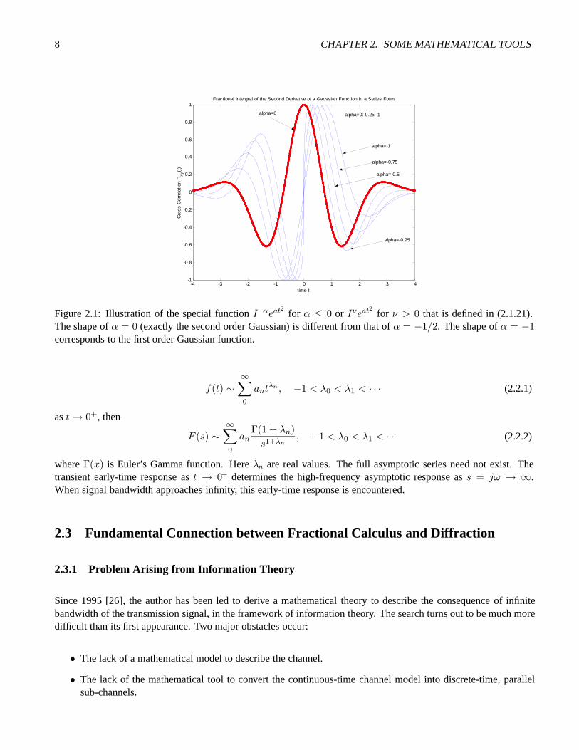
Figure 2.1: Illustration of the special function I−αeat2 for α ≤ 0 or Iνeat2 for ν > 0 that is defined in (2.1.21).The shape of α = 0 (exactly the second order Gaussian) is different from that of α = −1/2. The shape of α = −1corresponds to the first order Gaussian function.
f(t) ∼∞∑0
antλn , −1 < λ0 < λ1 < · · · (2.2.1)
as t → 0+, then
F (s) ∼∞∑0
anΓ(1 + λn)s1+λn
, −1 < λ0 < λ1 < · · · (2.2.2)
where Γ(x) is Euler’s Gamma function. Here λn are real values. The full asymptotic series need not exist. Thetransient early-time response as t → 0+ determines the high-frequency asymptotic response as s = jω → ∞.When signal bandwidth approaches infinity, this early-time response is encountered.
2.3 Fundamental Connection between Fractional Calculus and Diffraction
2.3.1 Problem Arising from Information Theory
Since 1995 [26], the author has been led to derive a mathematical theory to describe the consequence of infinitebandwidth of the transmission signal, in the framework of information theory. The search turns out to be much moredifficult than its first appearance. Two major obstacles occur:
• The lack of a mathematical model to describe the channel.
• The lack of the mathematical tool to convert the continuous-time channel model into discrete-time, parallelsub-channels.

2.3. FUNDAMENTAL CONNECTION BETWEEN FRACTIONAL CALCULUS AND DIFFRACTION 9
In the first problem, the empirical model of wide use is a model suggested by Turin (in 1950s) in his PhD dissertationbreaks down mathematically, since it is not able to catch the so-called pulse distortion of each individual path. Ageneralized multipath model is postulated to fill this gap—now we have a channel model that is valid for infinitepulse bandwidth. This postulated model is consistent with physics, and has been motivated by results from thehigh-frequency radio waves, quasi-optics, and acoustics. The underlying Luneberg-Kline series has an origin fromquantum mechanics and is used to describe the asymptotic behavior of the wave field when the frequency (or signalbandwidth) approaches infinity. The address regarding the first problem reaches its stability in the time frame of2002 and reported in a paper series and book chapters.
In parallel with the above understanding, the singularity of the above postulated model is noticed. The calculationof the pulse response is difficult, due to this singularity that consists of most energy of the path in the neighborhoodof the singularity. Although some numerical tricks are used to circumvent this mathematical problem, the level ofanalysis does not reach its maturity until the recent results of exploiting the fractional calculus to deal with thissingularity.
In fact, the connection between the fractional integration and the diffraction is recognized before. This connectiontraces back to the result one century ago when Abel’s integral equation (a major motivator for fractional calculus) isused.
Until the recent development of fractional integral operator (in 1990s), the rigorous treatment of the second problemseems be within the reach. The singular value decomposition of the fractional integral operator is the mathematicalweapon of our choice. Although abstract, this tool seems sufficient for our dream of an information theory thatcan handle infinite signal bandwidth. It is the recent (2007) recognition of this new connection that triggers thewriting of this introductory lecture notes on fractional calculus and diffraction with related applications. Human’sunderstanding of nature replies on calculus. Our story is just another testimony of this conviction. Only when theunderstanding in mathematics and physics reaches a full circle—the challenges of physics provide new topics tomathematics, while the solution for these problems, in turn, will advance the physical understanding—our sciencewould move to another level.
2.3.2 Diffraction of an Edge by an Impulse
Infinite signal bandwidth implies an impulse. In transient electromagnetic fields, the diffraction process can beregarded as a linear time-invariant (LTI) system. When an perfectly conducting edge is incident by an impulsiveplane wave, the exact expression of the response of this edge to this incident impulse is written in the form of
h(τ) =1
τ + τa
1√τU(τ) (2.3.1)
where U(τ) is Heaviside’s step function, and τa is a parameter independent of τ . A lot can be learned by studyingthis function. First, this function is singular at τ = 0. Second, this function is not square-integrable, that is∫ ∞
−∞|h(t)|2dt→ ∞. (2.3.2)
The second property causes a lot of mathematical difficulty, since this function must be understood as a generalizedfunction (like Dirac’s delta function) or a distribution.
Often we restrict our attention to finite energy functions, that is,∫∞−∞ |x(t)|2dt < ∞. These signals are often called
L2 functions. In developing precise treatment of signals are both power and frequency limited, Gallagar (1966) in

10 CHAPTER 2. SOME MATHEMATICAL TOOLS
his classic [12] has assumed that the impulse response of arbitrary linear-varying filters, h(t, τ), is a L2 function,see page 392 (Section 8.4) of [12]. His assumption is motivated to deal with the arbitrary durations of the appliedsignal, the input duration T or the output duration T0. When either T or T0 or both may be infinite, he is led toalways assume that ∫ ∞
−∞
∫ ∞
−∞h2(t, τ)dtdτ <∞ (2.3.3)
The assumption in (2.3.3) rules out two situations that are quite common in engineering. One is the case whereh(t, τ) contains impulses and the other is the case where T and T0 are both infinite and the filter is time invariant.Thus, in his development, both of these situations must be treated as limiting cases and there is not always a guaranteethat the limit will exist. In Section 8.5 (page 407) of [12], he has made a similar assumption.
A comparison of (2.3.2) with (2.3.3) suggests the unsatisfactory status of the theoretical framework. A new mathe-matical formalism is needed to develop a precise treatment of the troublesome impulse response of a physical channel(2.3.1). This problem cannot be argued away on physical grounds, since we are dealing with mathematical modelsof physical problems. In other words, if we are interested in a signal of infinite bandwidth–resulting in impulseresponse, this problem naturally arise from our radio wave propagation (and also from many similar situations).
Since the energy of the channel impulse response is concentrated in the neighborhood of t → 0+, the asymptoticlimit of this function can be investigated, instead, to simplify the analysis and gain insight. Thus, (2.3.1) is rewrittenas
h(τ) ∼ 1a
1√τU(τ) (2.3.4)
where ∼ denotes the asymptotic limit of the function.
Now let us consider, as input, an arbitrary signal x(t), the output of the edge diffraction (LTI) is
y(t) = x(t) ∗ h(t) =∫ t
−∞x(τ)
1√t− τ
dτ (2.3.5)
where ∗ denotes linear convolution, and the time-independent parameter a in (2.3.4) is dropped for brevity. Forconvention, if we require that x(t) and henceforth y(t) be a causal signal, i.e., identically vanish for t < 0, then(2.3.5) becomes
y(t) =∫ t
0x(τ)
1√t− τ
dτ (2.3.6)
A comparison of (2.3.6) with (2.1.1) leads to the fundamental connection:
y(t) =∫ t
0x(τ)
1√t− τ
dτ ≡ I12x(t) (2.3.7)
where I12 denotes the fractional integral of order 1
2 , or semi-integral for brevity.
The interpretation of (2.3.7) is important. The only approximation that is already made in the derivation of (2.3.7) isthe asymptotic limit introduced in (2.3.4). For t→ 0+, according to Abelian asymptotics (2.2.1), this approximationimplies (2.2.2), i.e., the high-frequency asymptotic limits of the (physical) edge diffraction phenomenon. In otherwords, the time-domain asymptotic (early-time, transient) response of the edge diffraction corresponds to the high-frequency asymptotic limit. In [27], it has been found that the use of this asymptotic limit to approximate the edge(even more generally for wedge) diffraction causes no difference to the exact solution. It is because of this resultthat has motivated us in this research. The fundamental connection of (2.3.7) paves the way for a new mathematicalformalism of using fractional calculus—an old, but lively branch in mathematics analysis.

2.4. A GENERALIZED MULTIPATH AS A FRACTIONAL INTEGRAL OPERATOR 11
Mathematicians are bothered by an still-open question—is possible to find a geometric interpretation of a fractionalderivative of non-integer order? See page 15 of [8]. Equation (2.3.7) provides a physical interpretation for such anfractional integral.
2.4 A Generalized Multipath as a Fractional Integral Operator
2.4.1 The Generalized Multipath Model with Per-Path Impulse Response
The linearity of Maxwell’s equations implies the linearity of the system function. If no mobility is present, thechannel must be time-invariant. Combining the two results leads a linear-time-invariant (LTI) representation ofUWB channels. A generalized multipath is postulated for a class of UWB channels uniquely defined by its channelimpulse response
h(τ) =L∑
l=1
Alhl(τ) ∗ δ(τ − τl) (2.4.1)
where Al and τl are, respectively, the amplitude and delay of the l-th path, and hl(τ) is the per-path impulse re-sponse with its frequency transform Hl(jω), called per-path frequency response. Eq. (2.4.1) can be rewritten in thefrequency domain as
H(jω) =L∑
l=1
AlHl(jω)ejωτl (2.4.2)
where ω = 2πf is the angular frequency and f is the frequency in Hertz. For practical applications, it is oftensufficient to consider a special form
Hl(jω) = (jω)−αl (2.4.3)
hl(τ) =1
Γ(αl)τ−(1−αl)U(τ) (2.4.4)
where αl assumes a positive real value, e.g., αl = 1/2. The U(τ) is Heaviside’s function. The Gamma function isdefined [23] as Γ(z) =
∫∞0 tz−1e−tdt where the real part of z is positive, i.e., �(z) > 0. The function τ−(1−αl)U(τ)
has a singularity at t = 0, and must be treated as a generalized function or distribution [8, 9, 10]. It is also regardedas an unbounded linear operator. In fact, it is the behavior of this operator at t = 0 that determines its singular valuesdistribution.
Eq. (2.4.3) is sufficiently generic for our interest. Almost all the physics-based problems can be modeled bythis model [28, 29, 30, 27, 22, 31]. As pointed in [26], the frequency dependency factor αl can be measuredexperimentally—impossible for infinite bandwidth, however. For a comprehensive review of UWB channel models,we refer to [32] [33] .
2.4.2 Representation of a Generalized Multipath as a Fractional Integral
The mathematical form of (2.4.4) suggests a natural connection with the fractional integration and differentiation, arapidly developing branch in applied mathematics [8, 9, 10]. See Section 2.1 for definition and relevant properties.
When an input pulse x(t) is applied to the channel with the impulse response of (2.4.4), the fractional integral willarise naturally from the expression of the output pulse y(t). Without loss of generality, x(t) is nonzero for t > 0. To

12 CHAPTER 2. SOME MATHEMATICAL TOOLS
simplify the presentation, let us use the first path as an example, ignoring the associated delay for the moment, i.e.,h1(τ) = 1
Γ(α1)τ−(1−α1)U(τ). It follows from (2.4.4) that
y1(t) =∫∞−∞ x(τ)h(t− τ)dτ
=∫∞−∞
1Γ(α1)
x(τ)
(t−τ)(1−α1)U(t− τ)dτ
= 1Γ(α1)
∫ t0
x(τ)
(t−τ)(1−α1)dτ, t > 0(2.4.5)
Comparing the definition of fractional integral (2.1.1) in Section 2.1 with (2.4.5) naturally leads to
y1(t) = 1Γ(α1)
∫ t0
x(τ)
(t−τ)(1−α1)dτ, t > 0= Iα1x(t)
(2.4.6)
which means that the output waveform for the first path is the fractional integral of the input waveform with theorder of α1.
Following the similar procedure for the l-th path, the output waveform is yl(t) = Iαlx(t). When L paths areconsidered all together, the total channel response is
y(t) =L∑
l=1
Al(Iαlx(t)) ∗ δ(τ − τl) (2.4.7)
where Iαl can be treated as linear fractional integral operators that are of infinite dimensions. Single value decompo-sition is used to “diagonalize” these infinite-dimensional operators in 3. Eq. (2.4.7) allows us to handle a transmittedwaveform x(t) that are arbitrary in time duration and bandwidth.
2.5 Calculation of Fractional Integral

2.5. CALCULATION OF FRACTIONAL INTEGRAL 13
-4 -3 -2 -1 0 1 2 3 4-1
-0.8
-0.6
-0.4
-0.2
0
0.2
0.4
0.6
0.8
1
time t
Cro
ss-C
orre
latio
n R
xy(t)
Fractional Intergral of the Second Derivative of a Gaussian Function in a Series Form
alpha=0 alpha=0:-0.25:-1
alpha=-1
alpha=-0.75
alpha=-0.5
alpha=-0.25
(a)
-5 -4 -3 -2 -1 0 1 2 3 4 5-1
-0.8
-0.6
-0.4
-0.2
0
0.2
0.4
0.6
0.8
1Comparision of Different Algorithms
Normalized Time t
Cro
ss-C
orre
latio
n R
xy(t)
alpha=0 alpha=-1/2
Curve Fitting
Convolution
L1
G1
G2
R1, R2
Convolution
(b)
Figure 2.2: Calculation of a fractional differential Dα defined in (2.1.2) where α can be real. The α is negative in2.2(a) and 2.2(b). A fractional integral is defined in (2.1.1). Recall that I−α = Dα.

14 CHAPTER 2. SOME MATHEMATICAL TOOLS

Chapter 3
Singular Value Decomposition of FractionalIntegral Operator
Singular value decomposition (SVD) of a finite-dimension matrix operator [34] is a standard tool in modern algo-rithms. For example, the so-called subspace based algorithm [35] enabled by using SVD modernizes the signalprocessing[36]. This finite-dimension matrix operator, however, cannot apply to the infinite-dimension fractionalintegral operator at hands. Driven by the needs, mathematicians have advanced this tool for the infinite-dimensionoperators, although abstract but powerful. Often, physics problem lead to the singular integral operator as in the caseof diffraction theory. Close the singular integral operator, it is the fractional integral operator. We systematicallyinvestigate the SVD of fractional integral operators, since results are rich in applied mathematics literature.
3.1 Complex Exponentials as Eigenfunctions of Linear Time-Invariant Operators
Communication engineers are much concerned with the class of functions they call signals. These are real functions,r(t), defined everywhere on a real line that they call time. They are square-integrable there,∫ ∞
−∞r2(t)dt = E <∞ (3.1.1)
and the quantity E is called the energy of the signal r(t). It has an important physical intepretation. Signal space S ,is the set of all signals, r(t). It has, of course, just the space L2(−∞,∞) of the mathematician.
The response sf (t), of a linear time-invariant (LTI) system to the sinusoidal input ej2πft is easily calculated. Wehave
sf (t+ T ) = L[ej2πf(t+T )
]= L
[ej2πftej2πfT
]= ej2πfTL
[ej2πft
]= ej2πfT sf (t) (3.1.2)
Theorem 3.1 (Slepian, 1983) [5] All linear time-invariant (LTI) operators have the complex exponentials ej2πft,−∞ < f < ∞, as eigenfunctions. Different linear time-invariant operators are characterized by their eigenvaluesYL(f) (called the transfer function of L).
This theorem is the true genesis of the widespread applicability of Fourier analysis to electrical engineering.
15
16 CHAPTER 3. SINGULAR VALUE DECOMPOSITION OF FRACTIONAL INTEGRAL OPERATOR
3.2 Adjoint of an Integral Operator
Here we follow [37]. Let H represent a linear integral operator. The scalar product (g2,Hf1 can be written as
(g2,Hf1) =∫ β
αf1(x)
∫ β
αg∗2(x
′)h(x′, x)dx′dx (3.2.1)
The adjoint can be expressed as
(H†g2, f1) =∫ β
αf1(x)
[∫ β
αg2(x′)h†(x, x′)dx′
]∗dx (3.2.2)
where h†(x, x′) is the kernel of the adjoint operator. Comparison of (3.2.1) and (3.2.2) shows that
h†(x, x′) = h∗(x′, x) (3.2.3)
Thus the kernel for H† is obtained from the kernel of H by interchanging x and x′ and taking the complex conjugate.
In using (3.2.3), it is important to pay attention to the two arguments. We know g(x′) = [Hf ](x′) =∫h(x′, x)f(x)dx,
so the integral is over the second argument of h(x′, x). Similarly,[H†g](x) =∫h†(x, x′)g(x′)dx′; again, the in-
tegral is over the second argument of the kernel, which is h†(x′, x). With (3.2.3), we can also write [H†g](x) =∫h∗(x′, x)g(x′)dx′. The integral is over the first argument of h∗(x′, x), which is just the conjugate of the kernel
needed to calculate Hf(x′); no explicit interchange is needed in moving from H† to H, if we are careful to associatex with space U and x′ with space V.
3.3 Adjoint and Singular Value Decomposition
SVD is a powerful tool for analyzing linear systems. Here we follow [37]. If the system is described by a continuous-time to continuous-time operator H, SVD requires knowledge of the eigenfunctions of H†H and HH†, denoted byun(r) and vn(rd), respectively. Since H is a mapping from object (transmitter) space U to image (receiver) spaceV, the adjoint operator H† maps from V to U. For an image (communication) system, the adjoint operator convertsa function of (receiver) image coordinates rd to a function of objective (transmitter) coordinates r.
Functions that describes real objects (transmitted signals) and images (received signals) does not have infinite values.A function with finite support and no infinite values is necessarily square-integrable and hence a vector in Hilbertspace L2(S), where S is the region of support of the function in terms of its independent variables (not includingtime dimension). If a transmitted signal is described as a bounded function of q variables (or, q-dimensional vectorvector r, and f(r) is zero outside some region Sf in R
q (q-dimensional real space), then it is square-integrable∫Sf
|f(r)|2dqr <∞. (3.3.1)
Thus the transmitted signal can be regarded as a vector in the Hilbert space L2(Sf ). If the transmitted signal issquare-integrable over the infinite domain, it is a vector in L2(Rq). Similarly, if an received signal g(rd) is definedas a function on R
s and is zero outside a region Sg , then it is corresponds to a vector g in the Hilbert space L2(Sg),which may be L2(Rs) if no support restriction is required.

3.3. ADJOINT AND SINGULAR VALUE DECOMPOSITION 17
3.3.1 Linear Shift-Variant (LSI) Systems
The communication system is a mapping from L2(Sf ) to L2(Sg). If the mapping is further linear, the Riesz repre-sentation theorem suggest that
g(rd) =∫Sf
h(rd, r)f(r)dqr. (3.3.2)
where h(rd, r) is impulse response in electrical engineering, or point response function in imaging science. In amore abstract notation, we can express this integral as
g = Hf (3.3.3)
where f and g are Hilbert-space vectors and H is the linear operator defined in (3.3.4). With noise, the mappingtakes the form g = Hf + n, where n is a random vector whose sample space may be all of V.
For the operator H defined in (3.3.4), the adjoint is given by1
[H†g](r) =∫Sg
h∗(rd, r)g(rd)dsrd. (3.3.4)
where ∗ denotes the complex conjugate. The adjoint impulse response is the response in receiver signal space by apoint source in a transmitter signal space. If that point is at the specific location rd0, then the response is h∗(rd0, r).The adjoint operation is frequently called back projection, since each point is projected back into the transmittersignal space.
If we think of H as a blurring operation for imaging, then H† is a further blurring, but with h(rd, r) replaced byh∗(r, rd).
3.3.2 Linear Shift-Invariant (LSIV) System
Diffraction is an example of a spatial shift-invariant (LSIV) system, implying that there is no preferred origin inspace. Convolution operator and its adjoint can be used. When a spatial system in q dimensions can be described asLSIV, its output is given by
g(rd) =∫∞h(rd − r)f(r)dqr. (3.3.5)
By a change of variables, this integral becomes
g(rd) =∫∞h(r)f(rd − r)dqr. (3.3.6)
Note that the range of integration is infinite in all variables. In shorthand form, (3.3.5)and (3.3.6) can be written asa convolution given by
g(rd) = [h ∗ f ](rd) = h(rd) ∗ f(rd). (3.3.7)
The kernel of the convolution operator can be interpreted as the point spread function in imaging. The adjoint of theconvolution operator is given from (3.3.4), which now becomes
[H†g](r) =∫∞h∗(rd − r)g(rd)dqrd. (3.3.8)
If h(−r) = h∗(r), then these two operations are identical and H is Hermitian.
1Note we have not interchanged the two arguments in h∗(rd, r). See discussions below equation (3.2.3).

18 CHAPTER 3. SINGULAR VALUE DECOMPOSITION OF FRACTIONAL INTEGRAL OPERATOR
Example 3.1
Let the operator K on L2(0, 1) be defined by [11][p.173]
(Kφ)(x) =∫ 1
0log∣∣∣∣√x+
√t
√x−
√t
∣∣∣∣φ(t)dt (0 ≤ x ≤ 1) (3.3.9)
To show that K is a positive operator, consider
(T φ)(x) =∫ x
0
φ(t)√x− t
dt = I12 (0 ≤ x ≤ 1). (3.3.10)
Although the kernel is an unbounded function, it is a Schur kernel and therefore T is a bounded operator on L2(0, 1),with adjoint given by
(T †φ)(x) =∫ 1
x
φ(t)√t− x
dt = (I12 )† (0 ≤ x ≤ 1). (3.3.11)
The kernel of T T † is, for x �= t,
k(x, t) =∫ min(x,t)
0
ds√x− s
√t− s
= 2 log
∣∣∣∣∣√x+
√t√
|x− t|
∣∣∣∣∣ = log∣∣∣∣√x+
√t
√x−
√t
∣∣∣∣ (3.3.12)
the integration being most easily carried out using the substitution u =√x− s+
√t− s. Therefore, K = T T † and
T †φ = 0 gives (T †)2φ = 0 ⇒ φ = 0, implying the positivity.
3.4 Singular Value Decomposition of the Ordinary Integral Operator
The compact linear operator defines a singular value decomposition (SVD). The integral operator operated on func-tion f(t),
∫ t0 f(x)dx, is such a compact linear operator. The SVD for the operator of this kind A is defined as
[1]Aφn(t) = σnΦn(t) (3.4.1)
where σn is the singular values, φn(t) is the left or input eigenfunction, and Φn(t) is the right or output eigenfunction.Both φn(t) and Φn(t) are orthonormal. As a special example related to the linear time-invariant (LTI) system, thepair of the input and output eigenfunction is sinusoidal, for the pulses of infinite duration.
Mapping the square integral functional space L2[0, 1] to itself L2[0, 1], or L2[0, 1] → L2[0, 1], the integral operatorA is defined as
Af(t) :=∫ t
0f(x)dx, 0 ≤ t ≤ 1, (3.4.2)
The inverse operator A−1 corresponds to differentiation. The adjoint operator2 is given by
A∗f(t) :=∫ 1
tf(x)dx, 0 ≤ t ≤ 1, (3.4.3)
2Every bounded linear operator A : X → Y possesses an adjoint operator A∗ : Y → X, that is, (Af, g) = (f, A∗g), where (f, g) =∫ b
af(x)g(x)dx means the scalar inner product. By the bar we denote the complex conjugation.
3.5. ESTIMATION OF THE SINGULAR VALUES OF A FINITE CONVOLUTION 19
Hence, the self-adjoint operator A∗A is defined as
A∗Af(t) :=∫ 1
t
∫ y
0f(x)dxdy, 0 ≤ t ≤ 1, (3.4.4)
and the eigenvalue equation A∗Aϕ(t) = λϕ(t) is equivalent to the boundary value problem for the ordinary differe-nial equation
λϕ′′
+ ϕ = 0 (3.4.5)
with homogeneous boundary conditions ϕ(1) = ϕ′(0) = 0, where the prime ′ denotes differentiation. Note that thesquares σ2 of the singular values of A are given by the eigenvalues λ of the nonnegative self-adjoint operator A∗A.
A nontrivial solution exists only if
σn =√λ =
2(2n − 1)π
, n = 1, 2, ...,∞ (3.4.6)
The pair of the eigenfunctions is given by
φn(t) =√
2cos(2n− 1
2πt), 0 ≤ t ≤ 1 (3.4.7)
and
Φn(t) =√
2sin(2n − 1
2πt), 0 ≤ t ≤ 1. (3.4.8)
As a result, the exact solution is obtained for an integral operator.
3.5 Estimation of the Singular Values of a Finite Convolution
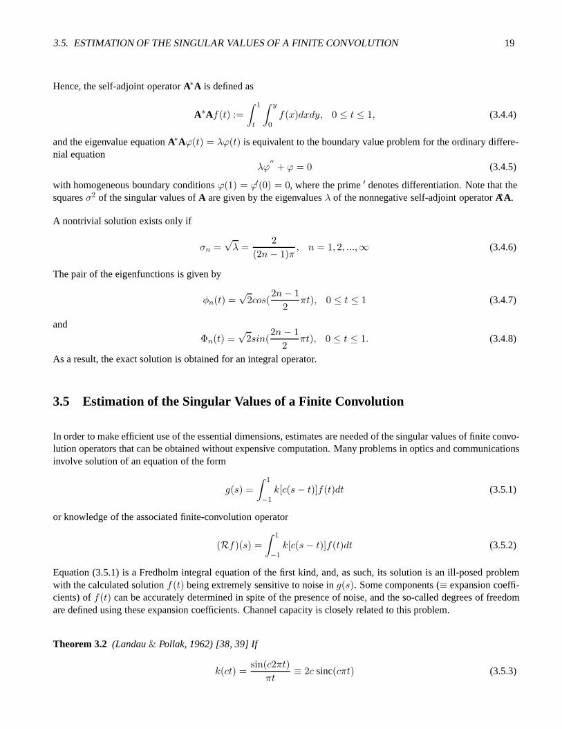
In order to make efficient use of the essential dimensions, estimates are needed of the singular values of finite convo-lution operators that can be obtained without expensive computation. Many problems in optics and communicationsinvolve solution of an equation of the form
g(s) =∫ 1
−1k[c(s − t)]f(t)dt (3.5.1)
or knowledge of the associated finite-convolution operator
(Rf)(s) =∫ 1
−1k[c(s − t)]f(t)dt (3.5.2)
Equation (3.5.1) is a Fredholm integral equation of the first kind, and, as such, its solution is an ill-posed problemwith the calculated solution f(t) being extremely sensitive to noise in g(s). Some components (≡ expansion coeffi-cients) of f(t) can be accurately determined in spite of the presence of noise, and the so-called degrees of freedomare defined using these expansion coefficients. Channel capacity is closely related to this problem.
Theorem 3.2 (Landau & Pollak, 1962) [38, 39] If
k(ct) =sin(c2πt)
πt≡ 2c sinc(cπt) (3.5.3)

20 CHAPTER 3. SINGULAR VALUE DECOMPOSITION OF FRACTIONAL INTEGRAL OPERATOR
and n(c, α) is the number of eigenvalues λn such that λn ≥ α, then
n(c, α) = 4c+2π2
log(α−1 − 1) log c+ o(log c). (3.5.4)
If b is fixed and c, c are chosen such that
c = 4c+2bπ2
log[2(2πc)1/2], (3.5.5)
thenlim
n→∞λn = (1 + eb)−1 (3.5.6)
This famous theorem implies that the λn are distributed in a steplike fashion, i.e.,
λn ∼ 1 if n < 4c (3.5.7)
λn ∼ 0 if n > 4c (3.5.8)
with the change from unity to zero occurring in a strip of width ∼ log n centered on n = 4c. Furthermore, asn→ ∞, the eigenvalues decay exponentially with n.
The implications for solution of (3.5.1) are that coefficients of eigenfunctions corresponding to eigenvalues greaterthan the noise level will be recovered in the presence of noise, but coefficients corresponding to eigenvalues lessthan the noise level will not. Because approximately 4c eigenvalues are essentially unity, then 4c componentswill be found; since the eigenvalues decay exponentially beyond this point, any improvement in the accuracy ofmeasurement of g will increase the number of eigenvalues greater than the noise level only by at most one or two.These features explain the number of degrees of freedom and its independence of noise [40].
The finite Fourier transform operator Fc, in general, is a compact operator, and so possesses a SVD {φn, σn, ϕn}∞n=1.The sets {φn} and {ϕn} form orthonormal bases for the space L2([−1, 1]); the set σ(R) ≡ {σn} consists ofnonnegative scalars arranged so that σn ≥ σn+1 and
Rφn = σnϕn. (3.5.9)
If k(t) is a symmetric operator, then σn = |λn|, where {λn} are the eigenvalues of R.
The SVD can be used to derive a formal solution to (3.5.1). Any left-hand side g(s) can be expanded as an infiniteseries of singular functions
g =∞∑
n=1
bnϕn, (3.5.10)
in which case the solution f can be expanded formally as the infinite series
g =∞∑
n=1
bnσn−1φn =
∞∑n=1
anφn. (3.5.11)
The Fourier transform operator F is defined as
(Ff)(r) =∫ ∞
∞exp(2πjrt)dt. (3.5.12)
3.5. ESTIMATION OF THE SINGULAR VALUES OF A FINITE CONVOLUTION 21
The finite Fourier transform operator Fc is defined by
(Fcf)(r) =∫ 1
−1exp(2πjrt)dt, r ∈ [−c, c]. (3.5.13)
The project on the interval [−c, c] by Pc is defined as
(Pcf)(t) = f(t) t ∈ c[−1, 1] (3.5.14)
= 0 otherwise. (3.5.15)
For convenience, we use P for c = 1. The adjoint of P is denoted by P†. If K(r) is a bounded continuous functionon (−∞,∞), then the associated multiplication operator is defined by
μKf(r) ≡ K(r)f(r). (3.5.16)
The kernel of (3.5.1) is defined only on the interval 2[−1, 1], so we assume that is can be extended to a function k(t)on the entire real line such that ∫ ∞
−∞|k(t)|dt <∞. (3.5.17)
For most kernels of interest, k(t) is analytic away from the origin, so that analytic continuation is a a natural extensionthat has all the required or derived properties. According to Ref. [41], the transform K = Fk of a kernel satisfyinginequality (3.5.17) is a bounded continuous function that vanishes at ∞, so that μK is a well-defined multiplicationoperator. Finally, by the convolution theorem for Fourier integrals, the operator R associated with kernel k satisfies
R : L2[−1, 1] → L2[−1, 1] is a bounded linear operator and
R = PF†μKP. (3.5.18)
Theorem 3.3 (Newsam & Barakat, 1985) [40] If |K(r)| is an even function and constantly decreasing away fromthe origin, then
σn(R) ≤ minc
{|K(c)| + [|K(0)| − |K(c)|]σn(Fc)} . (3.5.19)
Theorem 3.4 (Newsam & Barakat, 1985) [40] If K(r) is a real, nonnegative even function that is constantly de-creasing away from the origin, then
σn(R) ≥ maxc
[K(c)σ2n(Fc)] (3.5.20)
Corollary 3.1 (Newsam & Barakat, 1985) [40] If in addition to the conditions of Theorem 3.3, K(r) decays alge-braically, then an asymptotic upper bound on σn(R) is K(n/4). If K(r) also satisfies the conditions of Theorem3.4, then σn(R) asymptotes to K(n/4).
Corollary 3.1 will give a reasonable estimate tool not only for essential dimension but also of σn(R) for all n. Theapproximations of σn(R) by K(n/4) are not uniformly accurate, they reproduce the general form of σn(R) quitewell [40].

22 CHAPTER 3. SINGULAR VALUE DECOMPOSITION OF FRACTIONAL INTEGRAL OPERATOR
3.6 Singular Value Decomposition of Fractional Integral Operator Using Semi-group Property
The SVD of the fractional integral operator is studied in applied mathematics [42, 43, 44, 45, 20, 46, 47, 48, 49,50, 51, 52, 21], for asymptotic behavior of its singular values, generalizing the work of [53]. Chang, in turn, [53]extends the result of Hille and Tamarkin’s bounds on eigenvalues of fractional integral operators, to singular valuesof ordinary integral operators.
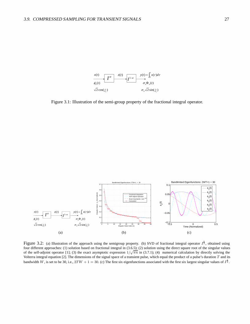
As illustrated in Fig. 3.2(a), the semi-group property of the fractional integral, (2.1.4) for β = 1 − α, implies
IαI1−α = Iα+1−α = I1 = I (3.6.1)
which is exactly an ordinary integral operator. In other words, the ordinary integral operator can be broken into twoconsecutive fractional integral operators3 Iα and I1−α.
As illustrated in Fig. 3.2(a), it follows that
y(t) = (IαI1−α)x(t) = (I1)x(t) =∫ t
bx(τ)dτ ; (3.6.2)
andz(t) = Iαx(t); y(t) = I1−αz(t) (3.6.3)
Fortunately, the SVD of the ordinary integral operator I1 has been made available in Section 3.4. When the lefteigenfunction φn(t) =
√2cos(ant) is treated as the left eigenfunction of the operator Iα in Fig. 3.2(a), the resultant
output of this operator is the right eigenfunction of this operator Iα—a key step in our approach. Here, an = (2n−1)π2
is given by (3.4.6). Formally, it follows that
σnΦn(t) = Iαφn(t), n = 1, 2, ...,∞= Iα
√2cos(ant)
=√
2Ct(α, an)(3.6.4)
from which σn for the operator Iα is to be determined. Defined in (2.1.16), the Ct(α, a) is a special function thatcan be expressed in terms of the hypergeometric function which has been built-in in MATLAB.
For the case of α = 1/2, it follows from (2.1.14) that
I12 cos(anx) =
√2an
[(cos(anx))C(y) + (sin(anx)S(y)] (3.6.5)
where y =√
2anxπ , and C(y) and S(y) Fresnel Sine and Cosine integrals [23], respectively.
In Fig. 3.2, the fractional integral operator I12 has an infinite number of degrees of freedom. When a signal with a
finite number of degrees of freedom NDOF = 2TW +1 = 30 is considered instead, Ky Fan’s inequality [54, 55, 56,57] can be used: For compact operators A and B, we have σm+n−1(AB) ≤ σm(A)σn(B). Let A be the operator with
3The two consecutive fractional integral operators can be, intuitively, viewed as a chain of two LTI systems. But, since the impulseresponses are generalized functions, fractional integral operators must be used for mathematical rigor and validity of the suggested generalizedmultipath model of (2.4.4).
3.7. EXACT ASYMPTOTIC OF FRACTIONAL INTEGRAL OPERATORS 23
NDOF . It is well known [58, 59, 60, 38, 39, 61, 62, 63] that the singular values of A are 1 until their index exceedsNDOF . This Slepian-Landau operator acts like a “gate” with a width of NDOF . When a signal with a finite numberof degrees of freedom NDOF = 2TW + 1 = 30 is considered instead in Fig. 3.2, the infinite-dimensional fractionalintegral operator I
12 is “gated” by the Slepian-Landau operator. This gating effect is vividly illustrated in Fig. 3.2:
the curve of numerical simulation. Physically, every communication system has a finite NDOF . Mathematically,when NDOF → ∞, the asymptotic limit of singular values σn for I
12 can be achieved.
3.7 Exact Asymptotic of Fractional Integral Operators
The asymptotic behavior of the singular values has been studied in applied mathematics [42, 43, 44, 45, 20, 46, 47,48, 49, 50, 51, 52, 21].
Let us denote σn as the singular values of the fraction integral operator Iα. The exact asymptotic behavior is derivedin the Theorem 3.5.
Theorem 3.5 (Dostanic, 1993) [50]: If α > 0, then
limn→∞σn(Iα) =
1(πn)α
(3.7.1)
In (3.7.1), ∼ means asymptotically equal. Eq. (3.7.1) is exact, only asymptotically when n → ∞, while the exactsingular values for an arbitrary integer n ≥ 1 are not known. In practice, (3.7.1) has been found in excellentagreement with numerical simulation (Fig. 3.2), after n > 3. Besides, Dostanic’s theorem does not provide singularfunctions that are needed for modal modulation.
Let �α� be the greatest integer which is not greater than α.
Corollary 3.2 (Dostanic, 1993) [50]: If α > 0, r ∈ C�α�+1, r(0) �= 0, k(x) = r(x)/x1−α and K : L2(0, 1) →L2(0, 1) is the linear operator defined by
Kf(x) =∫ x
0k(x− y)f(y)dy (3.7.2)
then,
limn→∞σn(Iα) ∼ r(0)Γ(α)
1(πn)α
(3.7.3)
3.8 Exact Singular Value Decomposition of Fraction Integral Operator in WeightedL2-spaces
Although (3.7.1) gives the exact asymptotic behavior of the singular values for the fractional integral operator, theexact behavior of the singular values is not known in L2-spaces. Exact SVD of fraction integral operator is onlyavailable in weighted L2-spaces [21], which is sufficient for our problem at hand.
24 CHAPTER 3. SINGULAR VALUE DECOMPOSITION OF FRACTIONAL INTEGRAL OPERATOR
Let U and V be infinite-dimensional Hilbert spaces, and let A : U → V be an injective, compact linear operator.Then, there exists: (1) an orthonormal basis {un(t)} in U ; (2) an orthonormal system {vn(t)} in V ; (3) a non-increasing sequence {σn} of positive numbers with limit 0 for n → ∞. The system {σn, un(t), vn(t)} is called asingular system of the operator A. For the operator A, then the following SVD
Ax(t) =∞∑
n=0
σn(x, un)Uvn(t), x(t) ∈ U (3.8.1)
is valid, where the weight functions ϕ and ψ appear in scalar products
(f, g)U =∫
Ωf(x)g(x)ϕ(x)dx, (f, g)V =
∫Ωf(x)g(x)ψ(x)dx
By exploiting the properties of the generalized Laguerre polynomials, a SVD of the operator Iα is found.
Theorem 3.6 (Gorenflo & Tuan, 1995) [21]: If λ+1/2 > α > 0, ϕ(t) = (1−t1+t)
λ−1/2, ψ(τ) = (1− τ)λ−α−1/2(1+τ)−λ−α+1/2, and Iα : L2((−1, 1);ϕ) → L2((−1, 1);ψ), then, the exact SVD {σn, un(t), vn(t)} of Iα is given by:
σn =(
Γ(n+ λ− α+ 1/2)Γ(n+ α+ λ+ 1/2)
) 12
∼ 1nα, n→ ∞ (3.8.2)
and un(t) and vn(t) are expressed in terms of orthogonal Jacob polynomials [23].
The family {un(t)} is complete in the corresponding space L2((−1, 1);ϕ), and, therefore, is an orthonormal basis ofthe space L2((−1, 1);ϕ). Besides, the family {vn(t)} is orthonormal in L2((−1, 1);ψ). In particular, for λ = 1/2,then Iα, 0 < α < 1, boundedly maps the space L2(−1, 1) into the weighted space L2((−1, 1); (1 − τ2)−α). Noteit is easy to extend the normalized duration (−1, 1) to an finite arbitrary interval for pulse duration.
3.9 Compressed Sampling for Transient Signals
Ultra-wideband (UWB) channels and underwater acoustic (UWA) channels exhibit a sparse impulse response. Thissparsity can be exploited through the framework of compressed sampling (or sensing) (CS) [64, 65, 66]. In UWBchannels, measured channel impulse responses have been used [67]. See also [68] for a tapped-delay line model.There is no justification for this use of CS, from a physics-based channel model. This gap will be filled below. Thisderivation is, although direct in the context of our chapter, of fundamental nature.
Sparsity and Compressibility [69]: We have a vector f ∈ Rn which we expand in an orthogonal basis (such as a
wavelet basis) Ψ = [ψ1ψ2ψn] as follows:
f(t) =n∑
i=1
xiψi(t) (3.9.1)
where x is the coefficient sequence of f , xi = 〈f, φi〉. Here 〈x, y〉 represents the inner product of x and y. It will beconvenient to express f as Ψx (where Ψ is the n× n matrix with ψ1,· · · , ψn as columns).
The implication of sparsity is now clear: when a signal has a sparse expansion, one can discard the small coefficientswithout much perceptual loss. Formally, consider fS(t) obtained as keeping only the terms corresponding to the S

3.9. COMPRESSED SAMPLING FOR TRANSIENT SIGNALS 25
largest values of (xi) in the expansion of (3.9.1). By definition, fS := ΨxS , where xS is the vector of coefficients(xi) with all but the largest S set to zero. This vector is sparse in a strict sense since all but a few of its entries arezero; we will call S-sparse such objects with at most S nonzero entries. Since Ψ is an orthogonal basis, we have
||f − fS||l2 = ||x− xS||l2 (3.9.2)
where ||θ||lp = (∑
i |θi|p)1/p denotes the norm the vector θ. The case of p = 2 is the usual Euclidean l2-distance.
x is compressible in the sense that the sorted magnitudes of the (xi) decay quickly. In particular, the n-th transformcoefficient typically decays as (following the power law)
|x|(n) ≤ R n−1/p, 1 ≤ n ≤ N (3.9.3)
where R > 0 and p > 0.
If x is sparse or compressible, then x is well approximated by xS and, therefore, the error ||f − fS ||l2 is small.In other words, one can “throw away” a large fraction of the coefficients without much loss. This observation hasfundamental significance for signal processing through the framework of compressed sampling.
Compressed Sampling [65]: Suppose that we take measurements
yk = 〈f,Xk〉 , k = 1, · · · ,K (3.9.4)
where Xk are N -dimensional Gaussian vectors with independent standard normal entries. Then, for each f obeyingthe decay estimate above for some 0 < p < 1 and with overwhelming probability, our reconstruction f, defined asthe solution to the constraints yk = 〈f,Xk〉 with minimum l1 norm, obeys
||f − f||l2 ≤ Cp · R · (K/log N)−r, r = 1/p − 1/2. (3.9.5)
where Cp is some constant which only depends on p. Equation (3.9.5) is surprising. It says that if one makesO(KlogN) random measurements of a signal f , and then reconstructs an approximation signal from a limited set ofmeasurements in a manner which requires no prior knowledge or assumptions on the signal (other than its perhapsobeys some sort of power law decay with unknown parameters), one still obtains a reconstruction error which isequally as good as that one would obtain by knowing everything about f and selecting the K largest entries of thecoefficient vector; thus the amount of “oversampling” incurred by this random measurements procedure comparedto the optimal sampling for this level of error is only a multiplicative factor of O(KlogN). The reconstructionalgorithm does not depend upon unknown quantities such as p or R.
Compressibility of Transient Signals: With the above definitions, we are in a position to make our major point: thetransient signals are compressible. Section 3 has shown that the singular values of the SVD for the signals—definedby equation (2.4.3) in Section 2.4.1—follow the power law. Since the singular basis is also an orthogonal basis,these signals are compressible in the sense of (3.9.3).
Since the model defined by equation (2.4.3) in Section 2.4.1 is very general, in reality almost all the (transient)acoustic and electromagnetic signals satisfy this definition either exactly or asymptotically. As a result, this physics-based model justifies the use of compressed sampling for these applications.
Pre-coding Optimization for Transient Signals: Since the transient signals are compressible, as pointed out above.This structure (compressibility) has been exploited in compressed sampling. Time reversal or pre-coding can beemployed at the transmitter, with a goal to minimize the complexity of the receiver, e.g. the sampling rate in thecompressed sampling. In particular, direct detection of data symbols using random samples [67] is promising.

26 CHAPTER 3. SINGULAR VALUE DECOMPOSITION OF FRACTIONAL INTEGRAL OPERATOR
There are many combinations of pre-coding schemes and receiver structures. Let us emphasize the following: (1)time reversal at the transmitter and energy detection at the receiver; (2) zero-forcing at the transmitter and energydetection at the receiver.
After zero-forcing, the equivalent channel is reduced to have the minimum sparsity, or S = 1. The sub-Nyquistsampling rate requirement is much smaller than that compared with the case of without zero-forcing. Time reversalis easier to implement than zero-forcing.
In a nutshell, the channel impulse response can be exploited, through pre-codig, to reduce the complexity of thecompressed sampling based receiver. For UWB systems, the channel is often quasi-static and reciprocal, it is idealto move the complexity from the receiver to the transmitter, through pre-coding. For UWA systems, the slowpropagation velocity of sound will cause the unfocusing problem for longer range.
3.9. COMPRESSED SAMPLING FOR TRANSIENT SIGNALS 27
I 1I)(tx
tdxty
0)()()(tz
)(tn )(tnn
)cos(2n
t )sin(2n
tn
Figure 3.1: Illustration of the semi-group property of the fractional integral operator.
I 1I)(tx
tdxty
0)()()(tz
)(tn )(tnn
)cos(2n
t )sin(2n
tn
(a)
0 5 10 15 20 25 30 35 400
0.1
0.2
0.3
0.4
0.5
0.6
0.7
Singular Value Index (n)
Sin
gula
r V
alue
s σ
n (N
orm
aliz
ed)
Bandlimited Eigenfunctions: 2TW+1 = 30
Fractional IntegrationSelf−Adjoint Operator
Exact Asymptotic (πn)−1/2
Calculated
(b)
−0.5 0 0.5−0.1
−0.05
0
0.05
0.1
Time (Normalized)
φ n(t)
Bandlimited Eigenfunctions: 2WT+1 = 30
φ1(t)
φ2(t)
φ3(t)
φ4(t)
φ5(t)
φ6(t)
(c)
Figure 3.2: (a) Illustration of the approach using the semigroup property. (b) SVD of fractional integral operator I12 , obtained using
four different approaches: (1) solution based on fractional integral in (3.6.5); (2) solution using the direct square root of the singular valuesof the self-adjoint operator [1]; (3) the exact asymptotic expression 1/
√πn in (3.7.1); (4) numerical calculation by directly solving the
Volterra integral equation [2]. The dimensions of the signal space of a transient pulse, which equal the product of a pulse’s duration T and itsbandwidth W , is set to be 30, i.e., 2TW + 1 = 30. (c) The first six eigenfunctions associated with the first six largest singular values of I
12 .

28 CHAPTER 3. SINGULAR VALUE DECOMPOSITION OF FRACTIONAL INTEGRAL OPERATOR
Chapter 4
Transient Diffraction
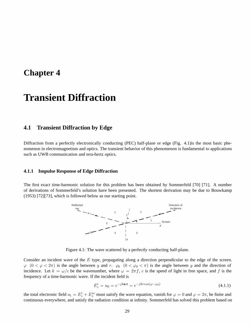
4.1 Transient Diffraction by Edge
Diffraction from a perfectly electronically conducting (PEC) half-plane or edge (Fig. 4.1)is the most basic phe-nomenon in electromagnetism and optics. The transient behavior of this phenomenon is fundamental to applicationssuch as UWB communication and tera-hertz optics.
4.1.1 Impulse Response of Edge Diffraction
The first exact time-harmonic solution for this problem has been obtained by Sommerfeld [70] [71]. A numberof derivations of Sommerfeld’s solution have been presented. The shortest derivation may be due to Bouwkamp(1953) [72][73], which is followed below as our starting point.
Direction ofincidence
Screen1
33
2
1
Reflectedray
r
y
x
14
5
Figure 4.1: The wave scattered by a perfectly conducting half-plane.
Consider an incident wave of the E type, propagating along a direction perpendicular to the edge of the screen.ϕ (0 < ϕ < 2π) is the angle between y and r. ϕ0 (0 < ϕ0 < π) is the angle between y and the direction ofincidence. Let k = ω/c be the wavenumber, where ω = 2πf , c is the speed of light in free space, and f is thefrequency of a time-harmonic wave. If the incident field is
Eiz = u0 = e−jku·r = e−jkrcos(ϕ−ϕ0) (4.1.1)
the total electronic field u1 = Eiz +Esc
z must satisfy the wave equation, vanish for ϕ = 0 and ϕ = 2π, be finite andcontinuous everywhere, and satisfy the radiation condition at infinity. Sommerfeld has solved this problem based on
29
30 CHAPTER 4. TRANSIENT DIFFRACTION
the concept of a two-sheeted Riemann surface [70]. His solution also covers the case of H type, where the unknownis the function u2 = H i
z +Hscz . The final results are
u1
u2
}= ejkr cos(ϕ−ϕ0) 1 + j
2
∫ 2(kr/π)12 cos[(ϕ−ϕ0)/2]
−∞e−jπτ2/2dτ∓ejkr cos(ϕ+ϕ0) 1 + j
2
∫ 2(kr/π)12 cos[(ϕ+ϕ0)/2]
−∞e−jπτ2/2dτ
(4.1.2)
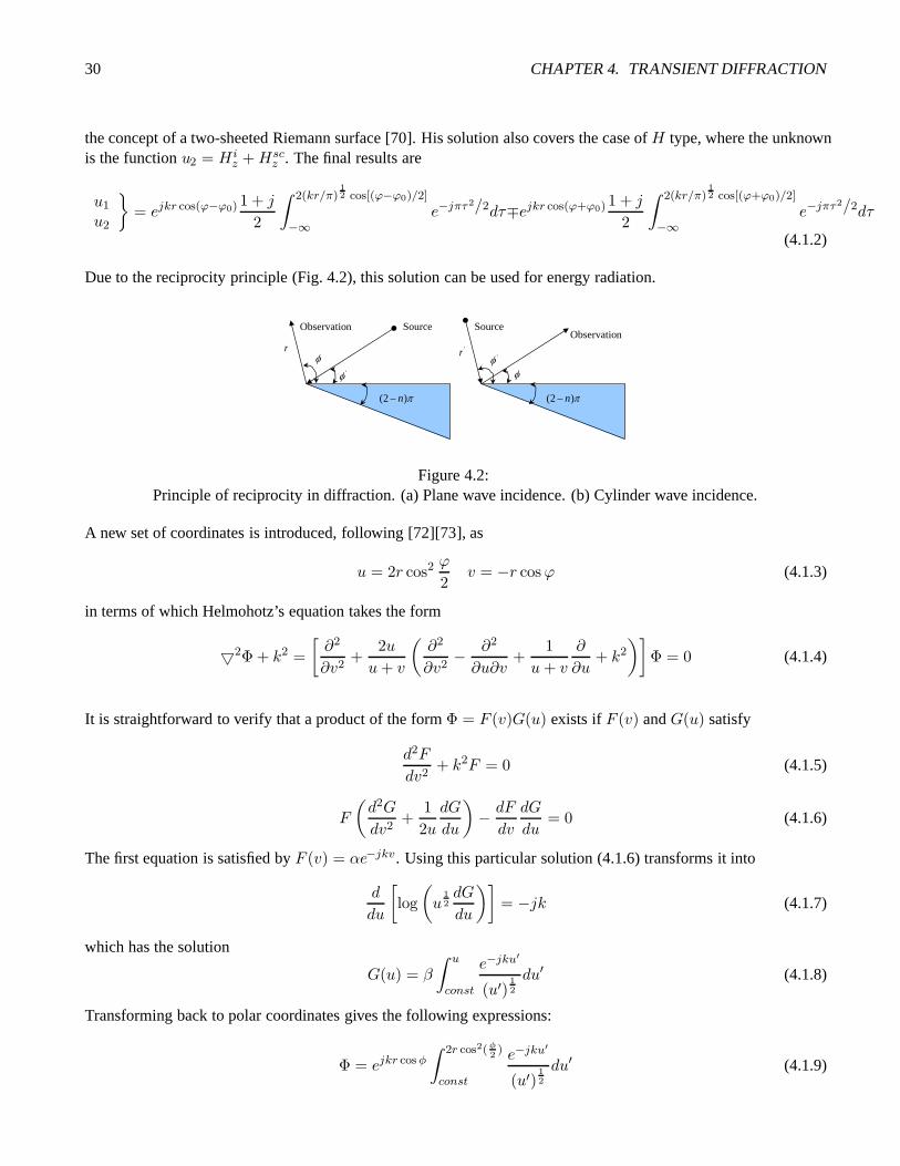
Due to the reciprocity principle (Fig. 4.2), this solution can be used for energy radiation.
SourcenObservationObservatio
Source
'
'r 'r
)2( n )2( n
Figure 4.2:Principle of reciprocity in diffraction. (a) Plane wave incidence. (b) Cylinder wave incidence.
A new set of coordinates is introduced, following [72][73], as
u = 2r cos2 ϕ
2v = −r cosϕ (4.1.3)
in terms of which Helmohotz’s equation takes the form
�2Φ + k2 =[∂2
∂v2+
2uu+ v
(∂2
∂v2− ∂2
∂u∂v+
1u+ v
∂
∂u+ k2
)]Φ = 0 (4.1.4)
It is straightforward to verify that a product of the form Φ = F (v)G(u) exists if F (v) and G(u) satisfy
d2F
dv2+ k2F = 0 (4.1.5)
F
(d2G
dv2+
12udG
du
)− dF
dv
dG
du= 0 (4.1.6)
The first equation is satisfied by F (v) = αe−jkv. Using this particular solution (4.1.6) transforms it into
d
du
[log(u
12dG
du
)]= −jk (4.1.7)
which has the solution
G(u) = β
∫ u
const
e−jku′
(u′)12
du′ (4.1.8)
Transforming back to polar coordinates gives the following expressions:
Φ = ejkr cos φ
∫ 2r cos2(φ2)
const
e−jku′
(u′)12
du′ (4.1.9)

4.1. TRANSIENT DIFFRACTION BY EDGE 31
Other particular solutions of Helmholtz’s equation can be obtained by replacing φ with φ+ φ0 or φ− φ0. It followsthat the linear combination
Φ} = Aejkr cos(ϕ−ϕ0)
∫ 2(kr/π)12 cos[(ϕ−ϕ0)/2]
−∞e−jπτ2/2dτ +Bejkr cos(ϕ+ϕ0)
∫ 2(kr/π)12 cos[(ϕ+ϕ0)/2]
−∞e−jπτ2/2dτ
(4.1.10)obtained by setting ku′ = πτ2/2, is also a solution of this equation. This expression for Φ is precisely of the formof Sommerfeld’s solution. The constants A and B can be determined by applying the boundary conditions satisfiedby Φ. The precedure leads to the values of A and B appearing in (4.1.2).
4.1.2 Impulse Response of Edge Diffraction
The incident field of impulsive wave is the Fourier transform of (4.1.1) given by
Eiz(t) = u0(t) =
12πδ(t− r/c cos(ϕ− ϕ0)) (4.1.11)
Similarly, the time domain impulse response for edge diffraction can be derived from (4.1.2). If r, ϕ and ϕ0 aredetermined, then the first term of RHS of Eqn. 4.1.2 is considered first as
H (k) = ejkr cos(ϕ−ϕ0) 1 + j
2
∫ 2(kr/π)12 cos[(ϕ−ϕ0)/2]
−∞e−jπτ2/2dτ (4.1.12)
If 2 (kr/π)12 cos [(ϕ− ϕ0)/2] > 0, according to the Fresnel Integral,
H (k) = ejkr cos(ϕ−ϕ0) 1 + j
2
[(1 − j) −
∫ ∞
2(kr/π)12 cos[(ϕ−ϕ0)/2]
e−jπτ2/2dτ
](4.1.13)
= ejkr cos(ϕ−ϕ0) − ejkr cos(ϕ−ϕ0) 1 + j
2
∫ ∞
2(kr/π)12 cos[(ϕ−ϕ0)/2]
e−jπτ2/2dτ (4.1.14)
Let x2 = jπτ2. So,
x =√π
2(1 + j) τ (4.1.15)
and,
dτ =2
(1 + j)√πdx (4.1.16)
Let Δ1 = (1 + j) (kr)12 cos [(ϕ− ϕ0)/2]. So H (k) can be simplified as
H (k) = ejkr cos(ϕ−ϕ0) − ejkr cos(ϕ−ϕ0) 1√π
∫ ∞
Δ1
e−x2/2dx (4.1.17)
Because erfc (x) = 2√π
∫∞x e−t2dt, Eqn. 4.1.17 can be further rewritten as,
H (k) = ejkr cos(ϕ−ϕ0) − 12ejkr cos(ϕ−ϕ0)erfc (Δ1) (4.1.18)
32 CHAPTER 4. TRANSIENT DIFFRACTION
From the defintion of Δ1, (Δ1)2 = jkr [cos (ϕ− ϕ0) + 1], so,
H (k) = e(Δ1)2
e−jkr − 12e(Δ1)
2
e−jkrerfc (Δ1) (4.1.19)
Let k = wc , τa = r[cos(ϕ−ϕ0)+1]
c and p = jw, where c is the speed of light. So, Eqn. 4.1.19 is changed to
H (p) = e−p( rc−τa) − 1
2πτ− 1
2a
πτ− 1
2a eτaperfc
(τ
12a p
12
)e−p r
c (4.1.20)
Because of the Laplace transform pairs δ (t− τ) ⇔ e−pτ and 1t+a
1√tu (t) ⇔ πa−
12 eaperfc
(a
12 p
12
)Re (p) ≥ 0,
the time domain impulse response for the first item of RHS of Eqn. 4.1.2 is
h (t) = δ(t−(rc− τa
))− 1
2πτ− 1
2a
(1
t+ τa
1√tu (t)
)∗ δ(t− r
c
)(4.1.21)
where τa = τa,i = r[cos(ϕ−ϕ0)+1]c .
If 2 (kr/π)12 cos [(ϕ− ϕ0)/2] = 0, according to the Fresnel Integral,
H (k) =12e−jkr (4.1.22)
Further, h (t) can be obtained,
h (t) =12δ(t− r
c
)(4.1.23)
If 2 (kr/π)12 cos [(ϕ− ϕ0)/2] < 0, according to the Fresnel Integral,
H (k) = ejkr cos(ϕ−ϕ0) 1 + j
2
∫ ∞
−2(kr/π)12 cos[(ϕ−ϕ0)/2]
e−jπτ2/2dτ (4.1.24)
Based on Eqn. 4.1.15, Eqn. 4.1.16 and Δ2 = − (1 + j) (kr)12 cos [(ϕ− ϕ0)/2], Eqn. 4.1.24 can be simplified as
H (k) =12e(Δ2)2e−jkrerfc (Δ2) (4.1.25)
Further, h (t) can be obtained,
h (t) =1
2πτ− 1
2a
(1
t+ τa
1√tu (t)
)∗ δ(t− r
c
)(4.1.26)
where τa = τa,i = r[cos(ϕ−ϕ0)+1]c .
If g(t) is the input signal, then the output signal is
st (t) = g (t) ∗ h (t) (4.1.27)
4.1. TRANSIENT DIFFRACTION BY EDGE 33
Let h (t) = 1t+τa
1√tu (t). Because 1√
tgoes to infinity when t approach 0, it is infeasible to calculate h (t) ∗ g (t)
directly. According to power series expansion, when∣∣∣ tτa
∣∣∣ < 1,
h (t) =1τa
11 + t
τa
1√tu (t) (4.1.28)
=1τa
( ∞∑n=0
(− t
τa
)n)
1√tu (t) (4.1.29)
=1τa
( ∞∑n=0
(− 1τa
)n (tn−
12
))u (t) (4.1.30)
According to the property of convolution,
h (t) ∗ g (t) =d
dt
((∫ t
0h (τ) dτ
)∗ g (t)
)(4.1.31)
=d
dt
(((1τa
∞∑n=0
(− 1τa
)n 1n+ 1
2
(tn+ 1
2
))u (t)
)∗ g (t)
)(4.1.32)
So, in this way st (t) is obtained. In the other way, because k = wc , Hw (w) = H
(wc
)from Eqn. 4.1.12, sw (t) can
be achieved from the following fomula,
sw (t) = IFT {Hw (w) (FT {g (t)})} (4.1.33)
where, FT {•} means Fourier transform and IFT {•} means inverse fourier transform.
st (t) and sw (t) should be exactly the same from theoretical point of view. If g (t) is the second order Gaussianpulse Fig. 4.3,
g (t) =
(1 − 4π
(t
α
)2)
exp
(−2π
(t
α
)2)
(4.1.34)
and φ = 7π/4, φ0 = π/4 as well as r = 1m, then the distorted terms of st (t) and sw (t) are shown in Fig. 4.4.
Similarly, the time domain impulse response for the second term of RHS of Eqn. 4.1.2 can be obtained as follows.
If 2 (kr/π)12 cos [(ϕ+ ϕ0)/2] > 0, then
h (t) = δ(t−(rc− τa
))− 1
2πτ− 1
2a
(1
t+ τa
1√tu (t)
)∗ δ(t− r
c
)(4.1.35)
If 2 (kr/π)12 cos [(ϕ+ ϕ0)/2] = 0, then
h (t) =12δ(t− r
c
)(4.1.36)
If 2 (kr/π)12 cos [(ϕ+ ϕ0)/2] < 0, then
h (t) =1
2πτ− 1
2a
(1
t+ τa
1√tu (t)
)∗ δ(t− r
c
)(4.1.37)
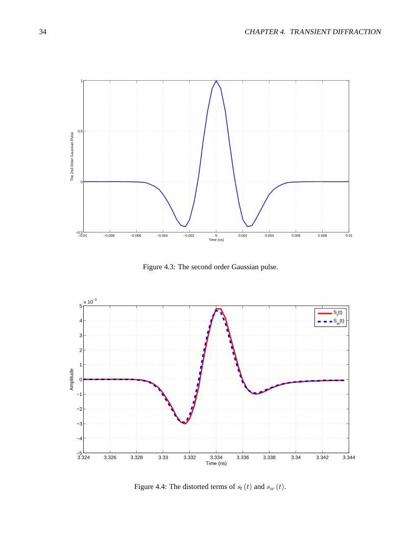
34 CHAPTER 4. TRANSIENT DIFFRACTION
−0.01 −0.008 −0.006 −0.004 −0.002 0 0.002 0.004 0.006 0.008 0.01−0.5
0
0.5
1
Time (ns)
The
2nd
Ord
er G
auss
ian
Pul
se
Figure 4.3: The second order Gaussian pulse.
3.324 3.326 3.328 3.33 3.332 3.334 3.336 3.338 3.34 3.342 3.344−5
−4
−3
−2
−1
0
1
2
3
4
5x 10
−3
Time (ns)
Am
plitu
de
S
t(t)
Sw
(t)
Figure 4.4: The distorted terms of st (t) and sw (t).
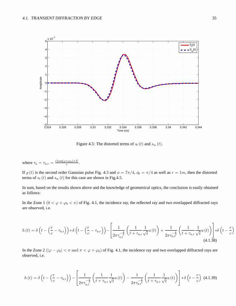
4.1. TRANSIENT DIFFRACTION BY EDGE 35
3.324 3.326 3.328 3.33 3.332 3.334 3.336 3.338 3.34 3.342 3.344−5
−4
−3
−2
−1
0
1
2
3
4
5x 10
−3
Time (ns)
Am
plitu
de
S
t(t)
Sw
(t)
Figure 4.5: The distorted terms of st (t) and sw (t).
where τa = τa,r = r[cos(ϕ+ϕ0)+1]c .
If g (t) is the second order Gaussian pulse Fig. 4.3 and φ = 7π/4, φ0 = π/4 as well as r = 1m, then the distortedterms of st (t) and sw (t) for this case are shown in Fig.4.5.
In sum, based on the results shown above and the knowledge of geometrical optics, the conclusion is easily obtainedas follows:
In the Zone 1 (0 < ϕ+ ϕ0 < π) of Fig. 4.1, the incidence ray, the reflected ray and two overlapped diffracted raysare observed, i.e.
h (t) = δ(t−(rc− τa,i
))+δ(t−(rc− τa,r
))−
⎡⎣ 1
2πτ− 1
2a,i
(1
t+ τa,i
1√tu (t)
)+
1
2πτ− 1
2a,r
(1
t+ τa,r
1√tu (t)
)⎤⎦∗δ (t− r
c
)(4.1.38)
In the Zone 2 (|ϕ− ϕ0| < π and π < ϕ+ ϕ0) of Fig. 4.1, the incidence ray and two overlapped diffracted rays areobserved, i.e.
h (t) = δ(t−(rc− τa,i
))−
⎡⎣ 1
2πτ− 1
2a,i
(1
t+ τa,i
1√tu (t)
)− 1
2πτ− 1
2a,r
(1
t+ τa,r
1√tu (t)
)⎤⎦∗δ (t− r
c
)(4.1.39)

36 CHAPTER 4. TRANSIENT DIFFRACTION
In the Zone 3 (π < ϕ− ϕ0 < 2π − ϕ0) of Fig. 4.1, only two overlapped diffracted rays are observed, i.e.
h (t) =
⎡⎣ 1
2πτ− 1
2a,i
(1
t+ τa,i
1√tu (t)
)+
1
2πτ− 1
2a,r
(1
t+ τa,r
1√tu (t)
)⎤⎦ ∗ δ(t− r
c
)(4.1.40)
In the Zone 4 (ϕ+ ϕ0 = π) of Fig. 4.1, the incidence ray, the attenuated reflected ray and one diffracted ray areobserved, i.e.
h (t) = δ(t−(rc− τa,i
))+
12δ(t−(rc− τa,r
))− 1
2πτ− 1
2a,i
(1
t+ τa,i
1√tu (t)
)∗ δ(t− r
c
)(4.1.41)
In the Zone 5 (ϕ− ϕ0 = π) of Fig. 4.1, the attenuated incidence ray and one diffracted ray are observed, i.e.
h (t) =12δ(t−(rc− τa,i
))+
1
2πτ− 1
2a,r
(1
t+ τa,r
1√tu (t)
)∗ δ(t− r
c
)(4.1.42)
In these situations, τa,i = r[cos(ϕ−ϕ0)+1]c and τa,r = r[cos(ϕ+ϕ0)+1]
c .
In order to verify the above conclusion, g (t) which is the second order gaussian pulse Fig. 4.3 is used as the inputthe signal and the output signal sw (t) is observed.
In the Zone 1 of Fig. 4.1, if φ = 2π/3, φ0 = π/4 as well as r = 1m, then rc = 3.333ns, r
c − τa,i = −0.863nsand r
c − τa,r = 3.219ns. sw (t) is shown in Fig. 4.6. The zoomed in version of sw (t) at −0.863ns is shown in Fig.4.7. The zoomed in version of sw (t) at 3.219ns is shown in Fig. 4.8. The zoomed in version of sw (t) at 3.333ns isshown in Fig. 4.9.
In the Zone 2 of Fig. 4.1, if φ = π, φ0 = π/4 as well as r = 1m, then rc = 3.333ns and r
c − τa,i = 2.357ns. sw (t)is shown in Fig. 4.10. The zoomed in version of sw (t) at 2.357ns is shown in Fig. 4.11. The zoomed in version ofsw (t) at 3.333ns is shown in Fig. 4.12.
In the Zone 3 of Fig. 4.1, if φ = 7π/4, φ0 = π/4 as well as r = 1m, then rc = 3.333ns. sw (t) is shown in Fig.
4.13. The zoomed in version of sw (t) at 3.333ns is shown in Fig. 4.14.
In the Zone 4 of Fig. 4.1, if φ = 3π/4, φ0 = π/4 as well as r = 1m, then rc = 3.333ns, r
c − τa,i = 0ns andrc − τa,r = 3.333ns. sw (t) is shown in Fig. 4.15. The zoomed in version of sw (t) at 0ns is shown in Fig. 4.16.The zoomed in version of sw (t) at 3.333ns is shown in Fig. 4.17.
In the Zone 5 of Fig. 4.1, if φ = 5π/4, φ0 = π/4 as well as r = 1m, then rc = 3.333ns and r
c − τa,i = 3.333ns.sw (t) is shown in Fig. 4.18. The zoomed in version of sw (t) at 3.333ns is shown in Fig. 4.19.
4.2 Transient Diffraction by Slit
The time domain impulse response for two-edge diffraction with a hole between two edges is considered hereaccording to Fig. 4.20. ϕ is the angle between the right side of screen and r. ϕ0 is the angle between the right side

4.2. TRANSIENT DIFFRACTION BY SLIT 37
−5 −4 −3 −2 −1 0 1 2 3 4 5−0.5
0
0.5
1
Time (ns)
Am
plitu
de
Sw
(t) caused by the first term
Sw
(t) caused by the second term
Figure 4.6: sw (t) in Zone 1.

38 CHAPTER 4. TRANSIENT DIFFRACTION
−0.872 −0.87 −0.868 −0.866 −0.864 −0.862 −0.86 −0.858 −0.856 −0.854−0.5
0
0.5
1
Time (ns)
Am
plitu
de
Sw
(t) caused by the first term
Sw
(t) caused by the second term
Figure 4.7: The zoomed in version of sw (t) at −0.863ns in Zone 1.

4.2. TRANSIENT DIFFRACTION BY SLIT 39
3.21 3.212 3.214 3.216 3.218 3.22 3.222 3.224 3.226 3.228−0.5
0
0.5
1
Time (ns)
Am
plitu
de
Sw
(t) caused by the first term
Sw
(t) caused by the second term
Figure 4.8: The zoomed in version of sw (t) at 3.219ns in Zone 1.

40 CHAPTER 4. TRANSIENT DIFFRACTION
3.324 3.326 3.328 3.33 3.332 3.334 3.336 3.338 3.34 3.342−0.03
−0.02
−0.01
0
0.01
0.02
0.03
Time (ns)
Am
plitu
de
Sw
(t) caused by the first term
Sw
(t) caused by the second term
Figure 4.9: The zoomed in version of sw (t) at 3.333ns in Zone 1.

4.2. TRANSIENT DIFFRACTION BY SLIT 41
−5 −4 −3 −2 −1 0 1 2 3 4 5−0.5
0
0.5
1
Time (ns)
Am
plitu
de
Sw
(t) caused by the first term
Sw
(t) caused by the second term
Figure 4.10: sw (t) in Zone 2.

42 CHAPTER 4. TRANSIENT DIFFRACTION
2.348 2.35 2.352 2.354 2.356 2.358 2.36 2.362 2.364 2.366−0.5
0
0.5
1
Time (ns)
Am
plitu
de
Sw
(t) caused by the first term
Sw
(t) caused by the second term
Figure 4.11: The zoomed in version of sw (t) at 2.357ns in Zone 2.

4.2. TRANSIENT DIFFRACTION BY SLIT 43
3.324 3.326 3.328 3.33 3.332 3.334 3.336 3.338 3.34 3.342−0.01
−0.008
−0.006
−0.004
−0.002
0
0.002
0.004
0.006
0.008
0.01
Time (ns)
Am
plitu
de
Sw
(t) caused by the first term
Sw
(t) caused by the second term
Figure 4.12: The zoomed in version of sw (t) at 3.333ns in Zone 2.

44 CHAPTER 4. TRANSIENT DIFFRACTION
−5 −4 −3 −2 −1 0 1 2 3 4 5−3
−2
−1
0
1
2
3
4
5x 10
−3
Time (ns)
Am
plitu
de
Sw
(t) caused by the first term
Sw
(t) caused by the second term
Figure 4.13: sw (t) in Zone 3.

4.2. TRANSIENT DIFFRACTION BY SLIT 45
3.324 3.326 3.328 3.33 3.332 3.334 3.336 3.338 3.34 3.342−5
−4
−3
−2
−1
0
1
2
3
4
5x 10
−3
Time (ns)
Am
plitu
de
Sw
(t) caused by the first term
Sw
(t) caused by the second term
Figure 4.14: The zoomed in version of sw (t) at 3.333ns in Zone 3.
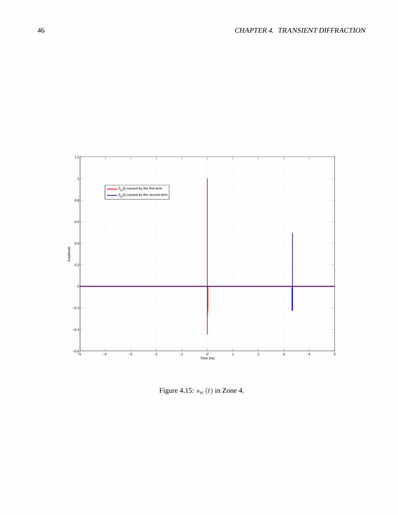
46 CHAPTER 4. TRANSIENT DIFFRACTION
−5 −4 −3 −2 −1 0 1 2 3 4 5−0.6
−0.4
−0.2
0
0.2
0.4
0.6
0.8
1
1.2
Time (ns)
Am
plitu
de
Sw
(t) caused by the first term
Sw
(t) caused by the second term
Figure 4.15: sw (t) in Zone 4.

4.2. TRANSIENT DIFFRACTION BY SLIT 47
−0.01 −0.008 −0.006 −0.004 −0.002 0 0.002 0.004 0.006 0.008 0.01−0.6
−0.4
−0.2
0
0.2
0.4
0.6
0.8
1
1.2
Time (ns)
Am
plitu
de
Sw
(t) caused by the first term
Sw
(t) caused by the second term
Figure 4.16: The zoomed in version of sw (t) at 0ns in Zone 4.
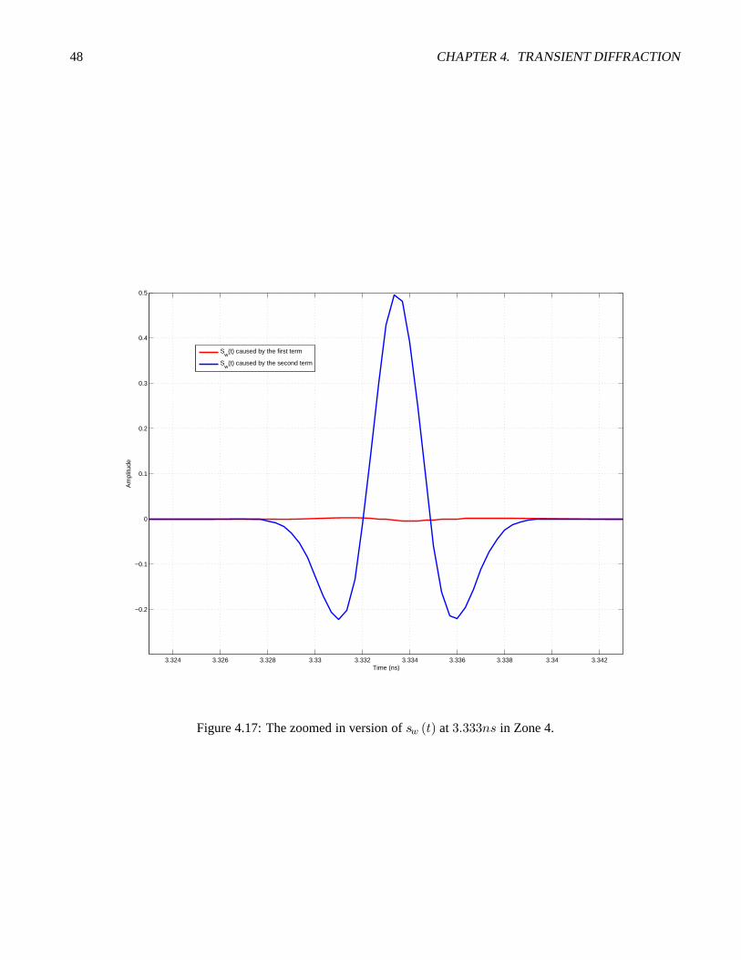
48 CHAPTER 4. TRANSIENT DIFFRACTION
3.324 3.326 3.328 3.33 3.332 3.334 3.336 3.338 3.34 3.342
−0.2
−0.1
0
0.1
0.2
0.3
0.4
0.5
Time (ns)
Am
plitu
de
Sw
(t) caused by the first term
Sw
(t) caused by the second term
Figure 4.17: The zoomed in version of sw (t) at 3.333ns in Zone 4.
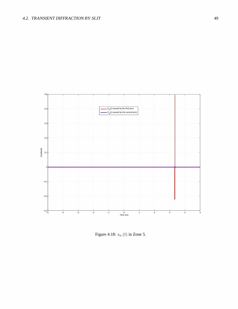
4.2. TRANSIENT DIFFRACTION BY SLIT 49
−5 −4 −3 −2 −1 0 1 2 3 4 5−0.3
−0.2
−0.1
0
0.1
0.2
0.3
0.4
0.5
Time (ns)
Am
plitu
de
Sw
(t) caused by the first term
Sw
(t) caused by the second term
Figure 4.18: sw (t) in Zone 5.

50 CHAPTER 4. TRANSIENT DIFFRACTION
3.324 3.326 3.328 3.33 3.332 3.334 3.336 3.338 3.34 3.342−0.3
−0.2
−0.1
0
0.1
0.2
0.3
0.4
0.5
Time (ns)
Am
plitu
de
Sw
(t) caused by the first term
Sw
(t) caused by the second term
Figure 4.19: The zoomed in version of sw (t) at 3.333ns in Zone 5.
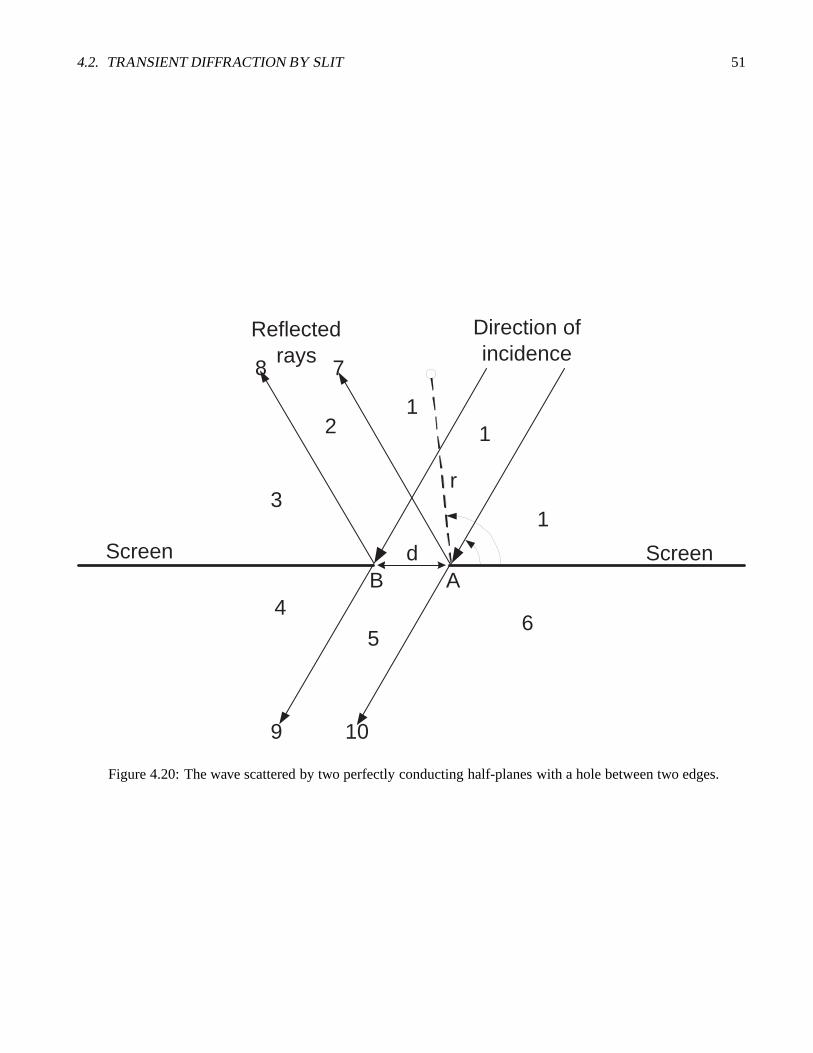
4.2. TRANSIENT DIFFRACTION BY SLIT 51
d
1
112
3
4
56
78
9 10
Screen
Direction ofincidence
Reflectedrays
Screen
r
AB
Figure 4.20: The wave scattered by two perfectly conducting half-planes with a hole between two edges.

52 CHAPTER 4. TRANSIENT DIFFRACTION
of screen and the direction of incidence. The diameter of the hole is d. If A is chosen as the reference point, then thetime delay when the incidence ray arrives at B is τd = d cos ϕ0
c .
The phenomenons of diffraction and reflection in A is studied first. In this case, the incidence ray is considered.
In the Zone 1 of Fig. 4.20, the incidence ray, the reflected ray and two overlapped diffracted rays are observed, i.e.
h (t) = δ(t−(rc− τa,i,A
))+δ(t−(rc− τa,r,A
))−
⎡⎣ 1
2πτ− 1
2a,i,A
(1
t+ τa,i,A
1√tu (t)
)+
1
2πτ− 1
2a,r,A
(1
t+ τa,r,A
1√tu (t)
)⎤⎦∗δ(4.2.1)
In the Zone 2, Zone 3, Zone 5 and Zone 8 of Fig. 4.20, the incidence ray and two overlapped diffracted rays areobserved, i.e.
h (t) = δ(t−(rc− τa,i,A
))−
⎡⎣ 1
2πτ− 1
2a,i,A
(1
t+ τa,i,A
1√tu (t)
)− 1
2πτ− 1
2a,r,A
(1
t+ τa,r,A
1√tu (t)
)⎤⎦ ∗ δ(t− r
c
)(4.2.2)
In the Zone 4 and Zone 9 of Fig. 4.20, only two overlapped diffracted rays are observed because the incidence rayis blocked by the left side of the screen, i.e.
h (t) = −
⎡⎣ 1
2πτ− 1
2a,i,A
(1
t+ τa,i,A
1√tu (t)
)− 1
2πτ− 1
2a,r,A
(1
t+ τa,r,A
1√tu (t)
)⎤⎦ ∗ δ(t− r
c
)(4.2.3)
In the Zone 6 of Fig. 4.20, only two overlapped diffracted rays are observed, i.e.
h (t) =
⎡⎣ 1
2πτ− 1
2a,i,A
(1
t+ τa,i,A
1√tu (t)
)+
1
2πτ− 1
2a,r,A
(1
t+ τa,r,A
1√tu (t)
)⎤⎦ ∗ δ(t− r
c
)(4.2.4)
In the Zone 7 of Fig. 4.20, the incidence ray, the attenuated reflected ray are observed and one diffracted ray areobserved, i.e.
h (t) = δ(t−(rc− τa,i,A
))+
12δ(t−(rc− τa,r,A
))− 1
2πτ− 1
2a,i,A
(1
t+ τa,i,A
1√tu (t)
)∗ δ(t− r
c
)(4.2.5)
In the Zone 10 of Fig. 4.20, the attenuated incidence ray and one diffracted ray are observed, i.e.
h (t) =12δ(t−(rc− τa,i,A
))+
1
2πτ− 1
2a,r,A
(1
t+ τa,r,A
1√tu (t)
)∗ δ(t− r
c
)(4.2.6)
In these situations, τa,i,A = r[cos(ϕ−ϕ0)+1]c and τa,r,A = r[cos(ϕ+ϕ0)+1]
c .
The phenomenons of diffraction and reflection in B is more complex compared with A. In this case, rB which is thedistance between observation point and B is r sin ϕ
sin arctan r sin ϕd+r cos ϕ
. ϕ0,B = π − ϕ0.

4.2. TRANSIENT DIFFRACTION BY SLIT 53
If 0 < ϕ < π, then
ϕB =
{π − arctan r sinϕ
d+r cos ϕr sinϕ
d+r cos ϕ ≥ 0− arctan r sinϕ
d+r cos ϕr sinϕ
d+r cos ϕ < 0(4.2.7)
If π < ϕ < 2π, then
ϕB =
⎧⎨⎩ π − arctan r sin ϕ
d+r cos ϕ
(− r sinϕ
d+r cos ϕ
)≥ 0
2π − arctan r sin ϕd+r cos ϕ
(− r sinϕ
d+r cos ϕ
)< 0
(4.2.8)
τa,i,B =rB[cos(ϕB−ϕ0,B)+1]
c and τa,r,B =rB[cos(ϕB+ϕ0,B)+1]
c . Meanwhile, the incidence ray is not considered here.
In the Zone 1, Zone 2, Zone 5, Zone 6, Zone 7 and Zone 10 of Fig. 4.20, two overlapped diffracted rays are observed,i.e.
h (t) = −
⎡⎣ 1
2πτ− 1
2a,i,B
(1
t+ τa,i,B
1√tu (t)
)− 1
2πτ− 1
2a,r,B
(1
t+ τa,r,B
1√tu (t)
)⎤⎦ ∗ δ(t−(rBc
+ τd
))(4.2.9)
In Zone 3 of Fig. 4.20, the reflected ray and two overlapped diffracted rays are observed, i.e.
h (t) = δ(t−(rBc
− τa,r,B + τd
))−
⎡⎣ 1
2πτ− 1
2a,i,B
(1
t+ τa,i,B
1√tu (t)
)+
1
2πτ− 1
2a,r,B
(1
t+ τa,r,B
1√tu (t)
)⎤⎦∗δ (t− (rBc
+ τd
)(4.2.10)
In Zone 4 of Fig. 4.20, two overlapped diffracted rays are observed, i.e.
h (t) =
⎡⎣ 1
2πτ− 1
2a,i,B
(1
t+ τa,i,B
1√tu (t)
)+
1
2πτ− 1
2a,r,B
(1
t+ τa,r,B
1√tu (t)
)⎤⎦ ∗ δ(t−(rBc
+ τd
))(4.2.11)
In Zone 8 of Fig. 4.20, the attenuated reflected ray and one diffracted ray are observed, i.e.
h (t) =12δ(t−(rBc
− τa,r,B + τd
))− 1
2πτ− 1
2a,i,B
(1
t+ τa,i,B
1√tu (t)
)∗ δ(t−(rBc
+ τd
))(4.2.12)
In Zone 9 of Fig. 4.20, the attenuated incidence ray and one diffracted ray are observed, i.e.
h (t) =12δ(t−(rBc
− τa,i + τd
))+
1
2πτ− 1
2a,r,B
(1
t+ τa,r,B
1√tu (t)
)∗ δ(t−(rBc
+ τd
))(4.2.13)
In sum, the time domain impulse response for two-edge diffraction with a hole between two edges can be obtainedaccording to the principle of superposition of the field as follows.
54 CHAPTER 4. TRANSIENT DIFFRACTION
In the Zone 1 of Fig. 4.20,
h (t) = δ(t−(rc− τa,i,A
))+ δ(t−(rc− τa,r,A
))
−
⎡⎣ 1
2πτ− 1
2a,i,A
(1
t+ τa,i,A
1√tu (t)
)+
1
2πτ− 1
2a,r,A
(1
t+ τa,r,A
1√tu (t)
)⎤⎦ ∗ δ(t− r
c
)
−
⎡⎣ 1
2πτ− 1
2a,i,B
(1
t+ τa,i,B
1√tu (t)
)− 1
2πτ− 1
2a,r,B
(1
t+ τa,r,B
1√tu (t)
)⎤⎦ ∗ δ(t−(rBc
+ τd
))(4.2.14)
In the Zone 2 of Fig. 4.20,
h (t) = δ(t−(rc− τa,i,A
))−
⎡⎣ 1
2πτ− 1
2a,i,A
(1
t+ τa,i,A
1√tu (t)
)− 1
2πτ− 1
2a,r,A
(1
t+ τa,r,A
1√tu (t)
)⎤⎦ ∗ δ(t− r
c
)
−
⎡⎣ 1
2πτ− 1
2a,i,B
(1
t+ τa,i,B
1√tu (t)
)− 1
2πτ− 1
2a,r,B
(1
t+ τa,r,B
1√tu (t)
)⎤⎦ ∗ δ(t−(rBc
+ τd
))(4.2.15)
In the Zone 3 of Fig. 4.20,
h (t) = δ(t−(rc− τa,i,A
))−
⎡⎣ 1
2πτ− 1
2a,i,A
(1
t+ τa,i,A
1√tu (t)
)− 1
2πτ− 1
2a,r,A
(1
t+ τa,r,A
1√tu (t)
)⎤⎦ ∗ δ(t− r
c
)
δ(t−(rBc
− τa,r,B + τd
))−
⎡⎣ 1
2πτ− 1
2a,i,B
(1
t+ τa,i,B
1√tu (t)
)+
1
2πτ− 1
2a,r,B
(1
t+ τa,r,B
1√tu (t)
)⎤⎦ ∗ δ(t−(rBc
+ τd
))(4.2.16)
In the Zone 4 of Fig. 4.20,
h (t) = −
⎡⎣ 1
2πτ− 1
2a,i,A
(1
t+ τa,i,A
1√tu (t)
)− 1
2πτ− 1
2a,r,A
(1
t+ τa,r,A
1√tu (t)
)⎤⎦ ∗ δ(t− r
c
)⎡⎣ 1
2πτ− 1
2a,i,B
(1
t+ τa,i,B
1√tu (t)
)+
1
2πτ− 1
2a,r,B
(1
t+ τa,r,B
1√tu (t)
)⎤⎦ ∗ δ(t−(rBc
+ τd
)) (4.2.17)
In the Zone 5 of Fig. 4.20,
h (t) = δ(t−(rc− τa,i,A
))−
⎡⎣ 1
2πτ− 1
2a,i,A
(1
t+ τa,i,A
1√tu (t)
)− 1
2πτ− 1
2a,r,A
(1
t+ τa,r,A
1√tu (t)
)⎤⎦ ∗ δ(t− r
c
)
−
⎡⎣ 1
2πτ− 1
2a,i,B
(1
t+ τa,i,B
1√tu (t)
)− 1
2πτ− 1
2a,r,B
(1
t+ τa,r,B
1√tu (t)
)⎤⎦ ∗ δ(t−(rBc
+ τd
))(4.2.18)
4.3. TIME-DOMAIN UNIFORM THEORY OF DIFFRACTION (TD-UTD) OPERATORS 55
In the Zone 6 of Fig. 4.20,
h (t) =
⎡⎣ 1
2πτ− 1
2a,i,A
(1
t+ τa,i,A
1√tu (t)
)+
1
2πτ− 1
2a,r,A
(1
t+ τa,r,A
1√tu (t)
)⎤⎦ ∗ δ(t− r
c
)
−
⎡⎣ 1
2πτ− 1
2a,i,B
(1
t+ τa,i,B
1√tu (t)
)− 1
2πτ− 1
2a,r,B
(1
t+ τa,r,B
1√tu (t)
)⎤⎦ ∗ δ(t−(rBc
+ τd
)) (4.2.19)
In the Zone 7 of Fig. 4.20,
h (t) = δ(t−(rc− τa,i,A
))+
12δ(t−(rc− τa,r,A
))− 1
2πτ− 1
2a,i,A
(1
t+ τa,i,A
1√tu (t)
)∗ δ(t− r
c
)
−
⎡⎣ 1
2πτ− 1
2a,i,B
(1
t+ τa,i,B
1√tu (t)
)− 1
2πτ− 1
2a,r,B
(1
t+ τa,r,B
1√tu (t)
)⎤⎦ ∗ δ(t−(rBc
+ τd
)) (4.2.20)
In the Zone 8 of Fig. 4.20,
h (t) = δ(t−(rc− τa,i,A
))−
⎡⎣ 1
2πτ− 1
2a,i,A
(1
t+ τa,i,A
1√tu (t)
)− 1
2πτ− 1
2a,r,A
(1
t+ τa,r,A
1√tu (t)
)⎤⎦ ∗ δ(t− r
c
)
+12δ(t−(rBc
− τa,r,B + τd
))− 1
2πτ− 1
2a,i,B
(1
t+ τa,i,B
1√tu (t)
)∗ δ(t−(rBc
+ τd
))(4.2.21)
In the Zone 9 of Fig. 4.20,
h (t) = −
⎡⎣ 1
2πτ− 1
2a,i,A
(1
t+ τa,i,A
1√tu (t)
)− 1
2πτ− 1
2a,r,A
(1
t+ τa,r,A
1√tu (t)
)⎤⎦ ∗ δ(t− r
c
)
+12δ(t−(rBc
− τa,i + τd
))+
1
2πτ− 1
2a,r,B
(1
t+ τa,r,B
1√tu (t)
)∗ δ(t−(rBc
+ τd
)) (4.2.22)
In the Zone 10 of Fig. 4.20,
h (t) =12δ(t−(rc− τa,i,A
))+
1
2πτ− 1
2a,r,A
(1
t+ τa,r,A
1√tu (t)
)∗ δ(t− r
c
)
−
⎡⎣ 1
2πτ− 1
2a,i,B
(1
t+ τa,i,B
1√tu (t)
)− 1
2πτ− 1
2a,r,B
(1
t+ τa,r,B
1√tu (t)
)⎤⎦ ∗ δ(t−(rBc
+ τd
)) (4.2.23)
4.3 Time-Domain Uniform Theory of Diffraction (TD-UTD) Operators

56 CHAPTER 4. TRANSIENT DIFFRACTION
Chapter 5
Singular Value Decomposition of TransientDiffraction Operators
5.1 Singular Value Decomposition of Uniform Theory of Diffraction (UTD) Oper-ators
5.2 Singular Value Decomposition of Edge Impulse Response
57

58 CHAPTER 5. SINGULAR VALUE DECOMPOSITION OF TRANSIENT DIFFRACTION OPERATORS

Chapter 6
Transient Modal Modulation and Capacity
6.1 Modal Modulation for Short Transient Pulses
As illustrated in Fig. 6.1, the modal modulation first suggested by [74] is the optimum modulation [75]. Theeigenvalue decomposition of the autocorrelation of the channel impulse response is used in [74, 75]. Here, the SVDof the channel impulse response is used to derive the system in Fig. 6.1.
The LTI channel impulse response h(t) defines a singular value decomposition:
φn(t) ∗ h(t) = σnΦn(t) (6.1.1)
where σn is the singular value, and φn(t) and Φn(t) are orthonormal, input and output eigenfunctions, respectively.The SVD of (6.1.1) is postponed to Section 3. Given N degrees of freedom1, the input pulse can be expanded interms of orthonormal basis functions as
x(t) =N∑
n=1
xnφn(t), (6.1.2)
After the input pulse transmits through the LTI channel h(t), the output pulse is expressed as
y(t) =∑N
n=1 xnφn(t) ∗ h(t)=∑N
n=1 xnσnΦn(t)(6.1.3)
The received signal in the presence of the additive white Gaussian noise (AWGN) with the power spectral densityN0 is
r(t) = y(t) + n(t),=∑N
n=1 xnσnΦn(t) + n(t)(6.1.4)
It is well known that the optimum reception [75] is the matched filter y(T − t), and thus, Φn(T − t). The structureof Fig. 6.1 is, thus, derived.
The total transmitted energy is Ex =∑N
n=1 x2n, and the total received energy is Eb =
∑Nn=1 σ
2nx
2n. When the
transmitted signal is ±x(t), the probability of error for this detector is
Pe =1√2π
∫ −√
2Eb/N0
−∞exp(−1
2x2)dx (6.1.5)
1For a pulse of duration of T with a bandwidth of W , N = 2TW + 1 [12].
59

60 CHAPTER 6. TRANSIENT MODAL MODULATION AND CAPACITY
)(th
)(AWGN tn
Tt0
)(*1 tT
)(*2 tT )(*2 tT
)(*1 tTN
)(* tTN
)(*1 tT
)(tN
)(1 tN
)(2 t
)(1 t
)(tx
Tt0
)(tn
)(tnn
1x
2x
1Nx
Nx
11x
22x
11 NN x
)(ty
forclosed
N
nnn txtx
1
)()( N
nnnn
N
nnn
tx
thtxty
1
1
)(
)()()(
)()()( ttht nnn
SVD
NN x
Figure 6.1: Illustration of the modal modulation for UWB transient pulses.
6.2 Capacity: Information-theoretic and Physical Limits
The approaches for capacity calculation for the L2−space and the weighted L2−space are identical. The transmis-sion system generates a set of N parallel sub-channels with channel gain xnσn, n = 1, 2, ..., N , in the presence ofAWGN. The capacity for each sub-channel is Cn = log2(1 + xn
2σn2
N0), bits per channel use. The overall capacity is
C = max∑Nn=1 x2
n≤Ex
N∑n=1
log2(1 +xn
2σn2
N0), bits per channel use (6.2.1)
where σn is solely determined by the nature of the channel: For a large class of channels, including a conductingedge, σn is given in closed form in (3.7.1). The throughput of per channel use is determined by the correspondingspace-time eigenfields that may be arbitrary in time or (space) bandwidth. Water-filling will lead to the optimumenergy allocation xn [76, 77, 12]. Physically, every communication system has a finite N . Mathematically, whenN → ∞, the asymptotic limit of physics-based capacity can be achieved.
If the energy allocation is chosen such that xn/√N0 = σn = 1
nα where α is positive, then the maximum transmissionrate is
R =N∑
n=1
log2(1 +1n2α
), bits per channel use (6.2.2)
which, according to Jensen’s inequality2 [78], implies
R ≤ log2(1 +N∑
n=1
1n2α
), bits per channel use (6.2.3)
If the degree of freedom of the transmission waveform goes unbounded, N → ∞, then it follows that
R ≤ log2(1 +∞∑
n=1
1n2α
), bits per channel use (6.2.4)
which implies, for 2α > 1,R ≤ log2(1 + ζ(2α)), bits per channel use (6.2.5)
where ζ(z) is Riemann’s zeta function defined in (2.1.22). This result is interesting and unexpected. The proper-ties of the famous zeta function can be resorted to to study the fundamental limits for infinitive bandwidth of thetransmission waveform. Note for 2α ≤ 1, Riemann’s zeta function is undefined. We guess that all the physicalwaveforms satisfy the condition that 2α > 1.
2log2(1 + x) is a convex function
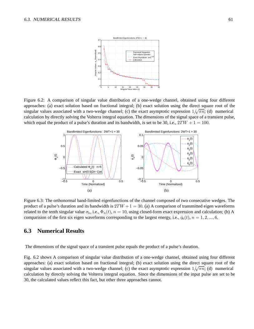
6.3. NUMERICAL RESULTS 61
0 5 10 15 20 25 30 35 400
0.1
0.2
0.3
0.4
0.5
0.6
0.7
Singular Value Index (n)
Sin
gula
r V
alue
s σ
n (N
orm
aliz
ed)
Bandlimited Eigenfunctions: 2TW+1 = 30
Fractional IntegrationSelf−Adjoint Operator
Exact Asymptotic (πn)−1/2
Calculated
Figure 6.2: A comparison of singular value distribution of a one-wedge channel, obtained using four differentapproaches: (a) exact solution based on fractional integral; (b) exact solution using the direct square root of thesingular values associated with a two-wedge channel; (c) the exact asymptotic expression 1/
√πn; (d) numerical
calculation by directly solving the Volterra integral equation. The dimensions of the signal space of a transient pulse,which equal the product of a pulse’s duration and its bandwidth, is set to be 30, i.e., 2TW + 1 = 100.
−0.5 0 0.5−1
−0.5
0
0.5
1
Time (Normalized)
Φn(t
)
Bandlimited Eigenfunctions: 2WT+1 = 30
Calculated Φn(t) n=5
Exact sin(0.5(2n−1)πt
(a)
−0.5 0 0.5−0.1
−0.05
0
0.05
0.1
Time (Normalized)
φ n(t)
Bandlimited Eigenfunctions: 2WT+1 = 30
φ1(t)
φ2(t)
φ3(t)
φ4(t)
φ5(t)
φ6(t)
(b)
Figure 6.3: The orthonormal band-limited eigenfunctions of the channel composed of two consecutive wedges. Theproduct of a pulse’s duration and its bandwidth is 2TW +1 = 30. (a) A comparison of transmitted eigen waveformsrelated to the tenth singular value σn, i.e., Φn(t), n = 10, using closed-form exact expression and calculation; (b) Acomparision of the first six eigen waveforms corresponding to the largest energy, i.e., φn(t), n = 1, 2, ..., 6.
6.3 Numerical Results
The dimensions of the signal space of a transient pulse equals the product of a pulse’s duration.
Fig. 6.2 shows A comparison of singular value distribution of a one-wedge channel, obtained using four differentapproaches: (a) exact solution based on fractional integral; (b) exact solution using the direct square root of thesingular values associated with a two-wedge channel; (c) the exact asymptotic expression 1/
√πn; (d) numerical
calculation by directly solving the Volterra integral equation. Since the dimensions of the input pulse are set to be30, the calculated values reflect this fact, but other three approaches cannot.
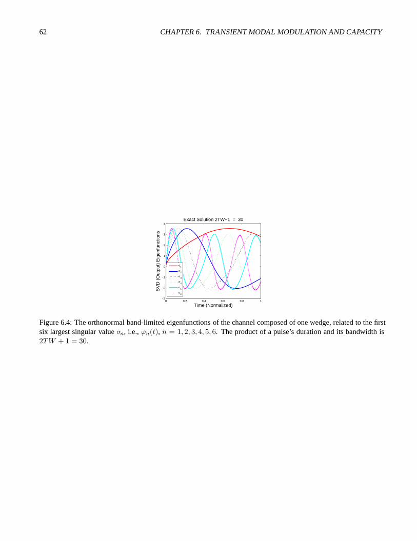
62 CHAPTER 6. TRANSIENT MODAL MODULATION AND CAPACITY
0 0.2 0.4 0.6 0.8 1−3
−2
−1
0
1
2
3
4
Time (Normalized)
SV
D (
Out
put)
Eig
enfu
nctio
ns
Exact Solution 2TW+1 = 30
σ1
σ2
σ3
σ4
σ5
σ6
Figure 6.4: The orthonormal band-limited eigenfunctions of the channel composed of one wedge, related to the firstsix largest singular value σn, i.e., ϕn(t), n = 1, 2, 3, 4, 5, 6. The product of a pulse’s duration and its bandwidth is2TW + 1 = 30.

Chapter 7
Exploiting Channel Impulse Response at theTransmitter—Time Reversal
Often it is more convenient to design a system, based on the channel cross-correlation
Rhh(t) = hforward(−t; r0, r1) ∗ hreverse(t; r1, r0) (7.0.1)
where ∗ denotes linear convolution, and r0 and r1 are the positions of the transceiver. If the channel is reciprocal,i.e.,
hforward(t; r0, r1) = hreverse(t; r1, r0), (7.0.2)
then, Rhh(t) reduces to the auto-correlation of the channel impulse response. As mentioned before, the use ofauto-correlation simplifies the system design based on the channel impulse response only. One good analogy is thespread-spectrum system that uses the auto-correlation of the spreading codes. The channel impulse response can beviewed as a spatial code [84].
Time reversal has been extensively studied in underwater acoustics [79] and ultra-wideband communications [80].We follow [81, 82] for development. Let us consider the system block diagram of the time-reversed impulse MIMOin Fig. 7.1. Energy-detection is used. Let us denote hmn(t) the channel impulse response (CIR) relating the m-thelement at the transmitter to the n-th element at the receiver. The set of impulse responses is called the propagationoperator. If one sends pulsed signal am(t),m = 1, ...,M from the transmit array, the signal bn(t) is obtained in thereceive array as
bn(t) =M∑
m=1
hnm(t) ∗ am(t), n = 1, ..., N (7.0.3)
Or, in matrix form,b(t) = H(t) ∗ a(t) (7.0.4)
where b(t) = [b1(t),b2(t), ...,bN(t)]†, a(t) = [a1(t),a2(t), ...,aM(t)]†, and H(t) is the matrix of N ×M withelements of hnm(t). The notation of “∗” represents element-by-element convolution; the superscript “†” representsthe conjugate transpose (Hermitian) of a vector or matrix. On the other hand, due to the spatial reciprocity, if onesends a signal cm,m = 1, ...,M from the receive array, the signal dn(t), n = 1, ..., N is obtained in the transmitarray. Defining column vectors c and d as a and b, respectively, it follows that
d(t) = H†(t) ∗ c(t) (7.0.5)
63

64CHAPTER 7. EXPLOITING CHANNEL IMPULSE RESPONSE AT THE TRANSMITTER—TIMEREVERSAL
As a consequence, H(t) permits one to calculate the forward propagation of impulses from the transmit array to thereceive array, while H†(t) the backward propagation from the receive array to the transmit array.
A time-reversal focusing is a two-step process: (1) first backward propagation and (2) then forward propagation. Thetwo steps can be regarded as the combination of the backward propagation process described by Eq. (7.0.4) withthe forward propagation process described by Eq. (7.0.5). The time-reversal process begins by sending the N × 1vector p(t) = [p1(t), ...,pN(t)]† from the receive array, where pn(t) is the pulse waveform emitted from the n-thantenna. Then the signal obtained at the transmit array after the backward propagation is expressed according to Eq.(7.0.5) as the M × 1 vector g(t) = [g1(t), ...,gM(t)]† given by
g(t) = H†(t) ∗ p(t) (7.0.6)
where gn(t) is the pulse waveform obtained at them-th antenna of the transmit array. In the second step, the recordedsignal at the transmit array g(t) is time-reversed to yield
g(−t) = H†(−t) ∗ p(−t) (7.0.7)
The time-reversed signals gn(−t), n = 1, 2, ..., N , are modulated with information-bearing pulsed waveforms xkm(t),k = 1, 2, ..., N ,m = 1, 2, ...,M , and the resultant M pulsed waveforms corresponding toN antennas at the transmitarray are given by
qm(t) =M∑
k=1
xmk(t) ∗ gk(−t),m = 1, ...,M (7.0.8)
Or, in matrix form,q(t) = X(t) ∗ g(−t) = X(t) ∗ H†(−t) ∗ p(−t) (7.0.9)
where q(t) = [q1(t), ...,qM(t)]† is an N×1 vector, and the mk-th element of the M ×M matrix X(t) is xmk(t)1.The resultant modulated signal collected in the vector q(t) is again re-transmitted from the transmit array. Bycombining Eq. (7.0.4), Eq. (7.0.7) and Eq. (7.0.9), the signal y(t) obtained at the receive array is expressed as
y(t) = H(t) ∗X(t) ∗ H†(−t) ∗ p(−t) (7.0.10)
where theN×1 vector y(t) has its n-th element yn(t) corresponding to the n-th antenna. y(t) is the signal obtainedin the receive array after time-reversal re-transmission. For brevity, defining Δ(t) = H(t) ∗ X(t) ∗ H†(−t), Eq.(7.0.10) is rewritten as
y(t) = [Δ(t)]N×N ∗ p(−t) (7.0.11)
Here Δ is called generalized time-reversal operator since the element-by-element Fourier transform of H(t) ∗H†(−t), H(ω)H†(ω), is usually called time-reversal operator [83]. Eq. (7.0.10) and Eq. (7.0.11) are sufficientlygeneral for the purpose of this investigation.
To simplify receiver detection, a linear scheme is proposed here; the signal pulses received by the N antennas arepulse-shaped, linearly weighted, and linearly combined:
z(t) =N∑
n=1
wn(t) ∗ yn(t) = w(t)† ∗ y(t) = w(t)† ∗H(t) ∗ X(t) ∗ H†(−t) ∗ p(−t) (7.0.12)
1Some traditional receiver processing functions such as diagonalizing the matrix in Eq. (7.0.11) below are moved to the transmitter tosimplify the receiver structure. Here the transmitter knows the channel and is able to optimize the transmission. These functions are implicitlyabsorbed in X(t) at this point.

65
where w = [w1(t),w2(t), ...,wN(t)]†. The right side of Eq. (7.0.12) is a scalar that also gives
z(t) = tr
{p(−t) ∗w†(t) ∗
[H(t) ∗ X(t) ∗ H†(−t)
]N×N
}(7.0.13)
where “tr” denotes the trace of an matrix. One goal of research is to make z(t) resemble δ(t).
Let us make two observations about Eq. (7.0.10) and Eq. (7.0.11). If the operator Δ(t) is diagonalized and the n-thdiagonal element is Λn(t), then Eq. (7.0.11) is simplified as
yn(t) = Λn(t) ∗ pn(−t) n = 1, 2, ..., rank[Δ(t)] (7.0.14)
In this special case, the whole system can be viewed as N independent channels. Λn(t) is explained as the impulseresponse of the n-th effective channel. If these independent channels are used to carry the same symbols, the linearscheme as defined in Eq. (7.0.12) can be used to maximize the spatio-temporal diversity gain.
On the other hand, Eq. (7.0.14) can be used to maximize the capacity of the channel. The independent parallelchannels in Eq. (7.0.14) can be used for different streams of symbols. In this case the elements of X(t) are usedto represent parallel streams of symbols. If the N channels can carry identical symbol rates, the channel capacityof the MIMO is N times that of a single channel (SISO). Note the rank of the Δ(t) is determined by the channeland numbers of transceiver antennas, and also satisfies rank(Δ(t)) ≤ min(M,N). To simplify the followingdiscussion, without loss of generality we assume M ≥ N .
To gather insight, let us consider these two special applications: (1) the goal is to maximize the diversity gain; (2)the goal is to maximize the channel capacity.
7.0.1 Time-Reversed Impulse MIMO for Optimum Diversity
The objective here is to maximize the z(t) in Eq. (7.0.13). Three limitations are of practical interest: (1) pn(t) =p(t), n = 1, ..., N are identical for the n-th antenna; or p(−t) = αIN×1p(−t). (2)X(t) is diagonal with itsm-th diagonal element xmm(t) = α × p(t), implying that the M antennas send the same waveforms; Here α isinformation-bearing scalar during a symbol interval; or, X(t) = αIM×Mp(t) where IM×M is a M ×M identitymatrix with its diagonal elements being ones. (3) w(t) = IN×1δ(t), implying z(t) =
∑Nn=1 yn(t).
The first two assumptions suggest using qm(t) =N∑
n=1hmn(−t) ∗ [p(−t) ∗ p(t)] as the pre-filter for them-th transmit
antenna. For a chirp signal p(t), p(t) ∗ p(−t) = δ(t), so qm(t) =N∑
n=1hmn(−t). Using a chirp signal we can pay
our attention to the impulse nature of MIMO. Another choice is to choose very short pulses, say pn(t) ≈ δ(t) sothe transmit array does not need to use pulse shaping at all. The two approaches are equivalent but the chirp one isbelieved to be more simple for implementation.
With the three simplifications, Eq. (7.0.13) is derived as
z(t) = tr[1N×Nδ(t) ∗ H(t) ∗ H†(−t)] ∗ α[p(t) ∗ p(−t)] (7.0.15)
where all the entries of 1N×N are ones. The role of 1N×N here is to sum up all the entries of the matrix H(t) ∗H†(−t). Or, Eq. (7.0.15) is given by
z(t) = αΓ(t) ∗ [p(t) ∗ p(−t)] (7.0.16)

66CHAPTER 7. EXPLOITING CHANNEL IMPULSE RESPONSE AT THE TRANSMITTER—TIMEREVERSAL
Figure 7.1: The System Block Diagram of Time-Reversed Impulse MIMO.
where we defineΓ(t) = tr(1N×Nδ(t) ∗H(t) ∗H†(−t)) (7.0.17)
For a chirp pulse or Dirac pulse p(t), Eq. (7.0.16) is reduced to z(t) = αΓ(t).
The elements of H(t) ∗H†(−t) are expressed as
[H(t) ∗ H†(−t)
]nk
=M∑
m=1
h†nm(−t) ∗ hkm(t) n, k = 1, 2, ...N (7.0.18)
The cross-correlations corresponds to terms of n �= k, while the auto-correlations n = k. Eq. (7.0.17) is expandedin a term-by-term form to gather insight:
Γ(t) =N∑
n=1
[M∑
m=1
hnm(−t) ∗ hnm(t)
]︸ ︷︷ ︸
Coherent signal (Sharp Peak)
+N∑
n=1
⎧⎨⎩⎡⎣ M∑
m=1,k =n
hnm(−t)
⎤⎦ ∗
⎡⎣ M∑
k=1,k =n
hkm(t)
⎤⎦⎫⎬⎭︸ ︷︷ ︸
Incoherent signal
(7.0.19)
The first part of Eq. (7.0.19) only involves all the auto-correlations, while the incoherent part all the cross-correlations.All the terms of hmn(−t) ∗hmn(t) reach their maximum at the same time (t = 0), and these peaks give the energiesof each hmn(t). As a result, the coherent part will dominant the total signal at the receiver. A simple scheme suchas energy-detection can be used to detect the information-bearing scalar α in Eq. (7.0.16).
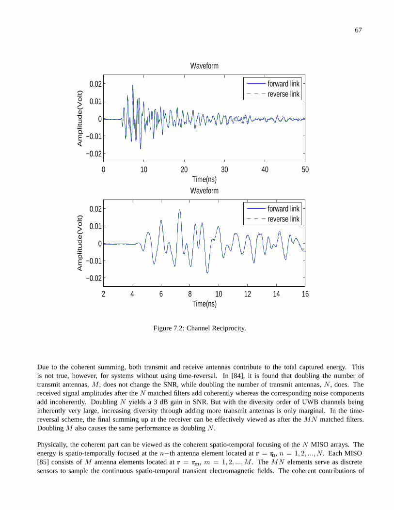
67
0 10 20 30 40 50
−0.02
−0.01
0
0.01
0.02
Time(ns)
Am
plitu
de(V
olt)
Waveform
2 4 6 8 10 12 14 16
−0.02
−0.01
0
0.01
0.02
Time(ns)
Am
plitu
de(V
olt)
Waveform
forward linkreverse link
forward linkreverse link
Figure 7.2: Channel Reciprocity.
Due to the coherent summing, both transmit and receive antennas contribute to the total captured energy. Thisis not true, however, for systems without using time-reversal. In [84], it is found that doubling the number oftransmit antennas, M , does not change the SNR, while doubling the number of transmit antennas, N , does. Thereceived signal amplitudes after the N matched filters add coherently whereas the corresponding noise componentsadd incoherently. Doubling N yields a 3 dB gain in SNR. But with the diversity order of UWB channels beinginherently very large, increasing diversity through adding more transmit antennas is only marginal. In the time-reversal scheme, the final summing up at the receiver can be effectively viewed as after the MN matched filters.Doubling M also causes the same performance as doubling N .
Physically, the coherent part can be viewed as the coherent spatio-temporal focusing of the N MISO arrays. Theenergy is spatio-temporally focused at the n−th antenna element located at r = rn, n = 1, 2, ..., N . Each MISO[85] consists of M antenna elements located at r = rm, m = 1, 2, ...,M . The MN elements serve as discretesensors to sample the continuous spatio-temporal transient electromagnetic fields. The coherent contributions of
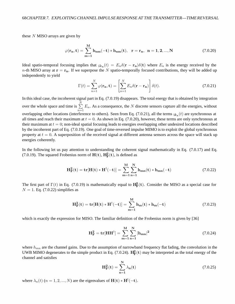
68CHAPTER 7. EXPLOITING CHANNEL IMPULSE RESPONSE AT THE TRANSMITTER—TIMEREVERSAL
these N MISO arrays are given by
ϕ(rn, t) =M∑
m=1
hnm(−t) ∗ hnm(t), r = rn, n = 1,2, ...,N (7.0.20)
Ideal spatio-temporal focusing implies that ϕrn(t) = Enδ(r − rn)δ(t) where En is the energy received by then-th MISO array at r = rn. If we superpose the N spatio-temporally focused contributions, they will be added upindependently to yield
Γ(t) =N∑
n=1
ϕ(rn, t) =
[N∑
n=1
Enδ(r − rn)
]δ(t). (7.0.21)
In this ideal case, the incoherent signal part in Eq. (7.0.19) disappears. The total energy that is obtained by integration
over the whole space and time isN∑
n=1En. As a consequence, the N discrete sensors capture all the energies, without
overlapping other locations (interference to others). Seen from Eq. (7.0.21), all the terms ϕrn(t) are synchronous atall times and reach their maximum at t = 0. As shown in Eq. (7.0.20), however, these terms are only synchronous attheir maximum at t = 0; non-ideal spatial focusing leads to energies overlapping other undesired locations describedby the incoherent part of Eq. (7.0.19). One goal of time-reversed impulse MIMO is to exploit the global synchronousproperty at t = 0. A superposition of the received signal at different antenna sensors across the space will stack upenergies coherently.
In the following let us pay attention to understanding the coherent signal mathematically in Eq. (7.0.17) and Eq.(7.0.19). The squared Frobenius norm of H(t), H2
F(t), is defined as
H2F(t) = tr[H(t) ∗ H†(−t)] =
M∑m=1
N∑n=1
hmn(t) ∗ hmn(−t) (7.0.22)
The first part of Γ(t) in Eq. (7.0.19) is mathematically equal to H2F(t). Consider the MISO as a special case for
N = 1. Eq. (7.0.22) simplifies as
H2F(t) = tr[H(t) ∗ H†(−t)] =
M∑m=1
hm(t) ∗ hm(−t) (7.0.23)
which is exactly the expression for MISO. The familiar definition of the Frobenius norm is given by [36]
H2F = tr[HH†] =
M∑m=1
N∑n=1
|hmn|2 (7.0.24)
where hmn are the channel gains. Due to the assumption of narrowband frequency flat fading, the convolution in theUWB MIMO degenerates to the simple product in Eq. (7.0.24). H2
F(t) may be interpreted as the total energy of thechannel and satisfies
H2F(t) =
N∑n=1
λn(t) (7.0.25)
where λn(t) (n = 1, 2, ..., N ) are the eigenvalues of H(t) ∗ H†(−t).
69
7.0.2 Channel Reciprocity—the Symmetry of Signal Processing
The foundation of time reversal is the so-called channel reciprocity: the impulse response of the forward link,hforward(t), is identical to that of the reverse link, hreverse(t), or
hforward(t; r0, r1) = hreverse(t; r1, r0) (7.0.26)
where r0 and r1 are two observation points. Experimental confirmation has been given in [86]. Fig. 7.2 illustratesthe typical waveforms for both links within the engine [87].
Channel reciprocity is the killer for time reversal for UWA communications, due to the slow propagation velocityof sound. Eq. (7.0.26) is very difficult to satisfy. This is, however, easily met for UWB communications, since thevelocity of radio is six orders of magnitudes larger than that of sound.
7.0.3 Discussions
In the theoretical aspects, we will take advantage of spatio-temporal focusing, a new physical phenomenon governedby transient electromagnetics, which is unique to time-reversed impulse systems. We are particularly interested inextending the current work to the framework of MIMO to improve the spatio-temporal focusing [88, 89, 90].
The similarity of the UWB communications to that of UWA communications motivates a unified view of the twosystems [81]. Common issues include rich multipath and fading. Equalization to compensate for inter-symbol-interference (ISI) is critical. Time-reversal is promising for both. Frequency-shift-keying (FSK) is the primarypractical scheme that works for UWA. Phase-shift-keryng (PSK) is promising for high-data rates, but suffers fromrandom phase noise caused by the ocean [91]. One wonders if the concept of “impulse radio” can be applied to UWAcommunications. Modulation schemes based on carrierless pulses such as pulse position modulation (PPM) havesome advantages, especially for high-frequency UWA communications in the bandwidth of e.g. 25-50 kHz. Therelative bandwidth of this system satisfies the definition of UWB, according to FCC. This large bandwidth justifiesthe use of UWB wireless technologies to UWA communications.
In practice, pairs of chirp waveforms, rather than the impulses, are used for modulation, in both UWA and UWBcommunications [80, 82].
7.0.4 Summary
A theory of time-reversed impulse MIMO is given for UWB communications. One goal of the proposed researchis to investigate time-reversal based non-coherent reception as an alternative to coherent communications. Theapproach takes advantage of the unique characteristics of impulse radio, through a new paradigm of using time-reversal combined with MIMO. In this paradigm, only a noncoherent energy detector is required in the receiver thatwill be cost-effective.
Since time reversal has been demonstrated experimentally [92] over the air indoors, it is interesting to extend thisconcept to other radios such as high-frequency (HF). The channel reciprocity of HF radios is still an open problem.

70CHAPTER 7. EXPLOITING CHANNEL IMPULSE RESPONSE AT THE TRANSMITTER—TIMEREVERSAL

Bibliography
[1] R. Kress, Linear Integral Equations. Berlin: Springer-Verlag, 1989.
[2] C. M. Zhou, Impulsive Radio Propagation and Time Reversed MIMO System for UWB Wireless Communi-cations. PhD Dissertation, Tennessee Technological University, Department of Electrical Engineering, May2008.
[3] R. A. Horn and C. R. Johnson, Topics in Matrix Analysis. Cambridge, UK: ambridge University Press, 1991.
[4] G. Di Francia, “Resolving Power and Information,” J. Opt. Soc. Am., vol. 45, pp. 497–501, July 1955.
[5] D. Slepian, “Some Comments on Fourier Analysis, Uncertainty and Modeling,” SIAM Review, vol. 25, no. 3,pp. 379–393, 1983.
[6] A. Kolmogorov and S. V. Fomine, Elements of the Theory of Functions and Functional Analysis. New York:Dover, 1999.
[7] G. W. Hanson and A. B. Yakovlev, Operators Theory for Electromagnetics. Berlin: Springer-Verlag, 2002.
[8] K. S. Miller and B. Ross, An Introduction to the Fractional Calculus and Fractional Differential Equations.NY: Wiley, 1993.
[9] K. B. Oldham and J. Spanier, The Fractional Calculus: Theory and Applications of Differentiation and Inte-gration to Arbitrary Order. NY: Academic Press, 1974.
[10] S. G. Samko, A. A. Kilbas, and O. I. Marichev, Fractional Integrals and Derivatives: Theory and Applications.Transl. from the Russian. NY: Gordon and Breach Science Publishers, 1993.
[11] D. Porter and D. S. Stirling, Integral Equations: A Practical Treatment, from Spectral Theory to Application.Cambridge, UK: Cambridge Press, 1990.
[12] R. A. Gallager, Information Theory and Reliable Communication. NY: John Wiley, 1966.
[13] D. Miller, “Communicating with Waves between Volumes: Evaluating Orthogonal Spatial Channels and Limitson Coupling Strengths,” Applied Optics, vol. 39, pp. 1681–1699, 2000.
[14] R. Piestun and D. Miller, “Electromagentic Degrees of Freedom of an Optical System,” J. Opt. Soc. Am. A,vol. 17, pp. 892–902, 2000.
[15] E. Hille and J. D. Tamarkin, “On the Characteristic Values of Linear Integral Equations,” Proceedings of theNational Academy of Sciences of the United States of America, vol. 14, no. 12, pp. 911–914, 1928.
[16] P. C. Hansen, Rank-Deficient and Discrete Ill-Posed Problems. Philadelphia, PA: SIAM, 1998.
71

72 BIBLIOGRAPHY
[17] M. Bertero and P. Boccacci, Introduction to Inverse Problems in Imaging. Bristol and Philadephia: Institute ofPhysics Publishing, 1998.
[18] J. A. Cochran, The Analysis of Linear Integral Equations. New York: McGraw-Hill, 1972.
[19] F. Smithies, Integral Equations. Cambridge, UK: Cambridge Press, 1965.
[20] M. Dostanic, “Asymptotic Behavior of Eigenvalues of Certain Integral Operators,” Publ. Inst. Math, Nouv. ser,vol. 59, pp. 83–98, 1996.
[21] R. Gorenflo and V. K. Tuan, “Singular Value Decomposition of Fractional Integration Operators in L2-spaceswith Weights,” J. Inverse and Ill-posed Problems, vol. 3, pp. 1–9, 1995.
[22] R. C. Qiu, H. P. Liu, and X. Shen, “Ultra-Wideband for Multiple Access,” Communications Magazine, pp. 2–9,Feb. 2005.
[23] M. Abramowitz and I. Stegun, eds., Handbook of Mathematical Functions. National Bureau of Standards,1965.
[24] M. Unser and T. Blu, “Fractional Splines and Wavelets,” SIAM Review, vol. 42, no. 1, pp. 43–67, 2000.
[25] C. Pearson, ed., Handbook of Applied Mathematics. New York: Van Nostrand Reinhold, 1983.
[26] R. C. Qiu, Digital Transmission Media: UWB Wireless Channel, MMIC, and Chiral Fiber. PhD thesis, Poly-technic University, Brooklyn, NY, January 1996.
[27] R. C. Qiu, “A Generalized Time Domain Multipath Channel and its Application in Ultra-Wideband (UWB)Wireless Optimal Receiver Design: Part 2 Wave-Based System Analysis,” IEEE Trans. Wireless Communica-tions, vol. 3, pp. 2312–2324, November 2004.
[28] R. C. Qiu and I. T. Lu, “Multipath Resolving with Frequency Dependence for Broadband Wireless ChannelModeling,” IEEE Trans. Veh. Tech., vol. 48, pp. 273–285, January 1999.
[29] R. C. Qiu, “A Study of the Ultra-Wideband Wireless Propagation Channel and Optimum UWB Receiver De-sign (Part 1),” IEEE J. Selected Areas in Commun. (JSAC), the First JASC special issue on UWB Radio, vol. 20,pp. 1628–1637, December 2002.
[30] R. C. Qiu, Design and Analysis of Wireless Networks, ch. Wireless Communications. Nova Science Publishers,June 2004.
[31] R. C. Qiu, C. Zhou, and Q. Liu, “Physics-Based Pulse Distortion for Ultra-Wideband Signals,” IEEE Trans.Veh. Tech., vol. 54, pp. 1546–1554, September 2005.
[32] A. F. Molisch, “Ultra-wideband Propagation Channels,” Proc. IEEE, 2008.
[33] J. Ahmadi-Shokouh and R. C. Qiu, “Ultra-wideband (uwb) communications–a tutorial review,” IEEE Trans.Veh. Tech., 2008.
[34] R. Horn and C. Johnson, Topics in Matrix Analysis. UK: Cambridge University Press, 1991.
[35] S. Kay, Modern Spectral Estimation. Englewood Cliffs, N.: Prentice-Hall, 1988.
[36] G. Golub and C. Van Loan, Matrix Computations. John Hopkins University Press, 1993.
[37] H. H. Barrett and K. J. Myers, Foundations of Image Science. John Wiley, 2004.

BIBLIOGRAPHY 73
[38] H. Landau and H. Widom, “Eigenvalue Distribution of Time and Frequency Limiting,” J. Math. Anal. Appl,vol. 77, no. 2, pp. 469–481, 1980.
[39] H. Landau and H. Pollak, “Prolate Spheroidal Wave Functions, Fourier Analysis and UncertaintyIII: TheDimension of the Space of Essentially Time-and Band-Limited Signals,” Bell Syst. Tech. J, vol. 41, no. 4,pp. 1295–1336, 1962.
[40] G. R. Newsam and R. Barakat, “Essential Dimension as a Well-Defined Number of Degrees of Freedom ofFinite-Convolution Operators Appearing in Optics,” Optical Society of America, Journal, A: Optics and ImageScience, vol. 2, pp. 2040–2045, 1985.
[41] R. Boas, Entire Function. Academic Press, 1954.
[42] V. Faber and G. Wing, “Asymptotic Behavior of Singular Values of Convolution Operators,” Rocky Mt. J. Math,vol. 16, no. 3, pp. 567–574, 1986.
[43] V. Faber and G. M. Wing, “Singular Values of Fractional Integral Operators: a Unification of Theorems ofHille, Tamarkin, and Chang,” Journal of Mathematical Analysis and Applications, vol. 120, no. 2, pp. 745–760, 1986.
[44] V. Faber and G. M. Wing, “Asymptotic Behavior of the Singular Values and Singular Functions of ConvolutionOperators,” Comp. Math. Appl., vol. 12, pp. 733–747, 1986.
[45] V. Faber and G. M. Wing, “Asymptotic Behavior of the Singular Values of Convolution Operators,” RockyMountain J. Math., vol. 16, 1986.
[46] M. Dostanic, “Exact Asymptotic Behavior of the Singular Values of Integral Operators with the Kernel HavingSingularity on the Diagonal,” Publ. Inst. Math. (N.S.), vol. 60(74), pp. 45–64, 1996.
[47] M. R. Dostanic, “An Estimate of Singular Values of Convolution Operators,” Proc. Am. Math. Soc., vol. 123,pp. 1399–1409, May 1995.
[48] M. R. Dostanic, “An Estimation of Singular Values of Convolution Operators,” Proceedings of the AmericanMathematical Society, vol. 123, no. 5, pp. 1399–1409, 1995.
[49] M. R. Dostanic, “Asymptotic Behavior of the Singular Values of Fractional Integral Operators,” Journal ofMathematical Analysis and Applications, vol. 175, no. 2, pp. 380–391, 1993.
[50] M. R. Dostanic and D. Z. Milinkovic, “Asymptotic Behavior of Singular Values of Certain Integral Operators,”Publications de linstitut mathematique, nouvelle serie, tome, vol. 74, pp. 83–98, 1996.
[51] V. Tuan and R. Gorenflo, “Asymptotics of Singular Values of Volterra Integral Operators,” Numer. Funct. Anal.and Optimiz., vol. 17, no. 3, pp. 453–461, 1996.
[52] V. Tuan and R. Gorenflo, “Asymptotics of Singular Values of Fractional Integral Operators,” Inverse Problems,vol. 10, no. 4, pp. 949–955, 1994.
[53] S. H. Chang, “A Generalization of a Theorem of Hille and Tamarkin with Application,” Proc. London Math.Soc., vol. 2, pp. 22–29, 1952.
[54] K. Fan, “Maximum Properties and Inequalities for the Eigenvalues of Completely Continuous Operators,”Proceedings of the National Academy of Sciences of the United States of America, vol. 37, no. 11, pp. 760–766, 1951.

74 BIBLIOGRAPHY
[55] K. Fan, “On a Theorem of Weyl Concerning Eigenvalues of Linear Transformations. II,” Proceedings of theNational Academy of Sciences of the United States of America, vol. 36, no. 1, pp. 31–35, 1950.
[56] K. Fan, “On a Theorem of Weyl Concerning Eigenvalues of Linear Transformations. I,” Proceedings of theNational Academy of Sciences of the United States of America, vol. 35, no. 11, pp. 652–655, 1949.
[57] I. Gohberg and M. G. Krein, Introduction to the Theory of Linear NonselfAdjoint Operators. American Math-ematical Society, 1969.
[58] D. Slepian, “Prolate Spheroidal Wave Functions, Fourier Analysis, and Uncertainty. V-The Discrete Case,” BellSystem Technical Journal, vol. 57, pp. 1371–1430, 1978.
[59] D. Slepian, “On Bandwidth,” Proceedings of the IEEE, vol. 64, no. 3, pp. 292–300, 1976.
[60] D. Slepian, “Prolate Spheroidal Wave Functions, Fourier Analysis and Uncertainty-IV: Extensions to ManyDimensions; Generalized Prolate Spheroidal Functions,” Bell Syst. Tech. J, vol. 43, no. 6, pp. 3009–3058,1964.
[61] H. Landau and H. Pollak, “Prolate Spheroidal Wave Functions, Fourier Analysis and UncertaintyII,” Bell Sys-tem Tech. J, vol. 40, pp. 65–84, 1961.
[62] H. Landau, “Necessary Density Conditions for Sampling and Interpolation of Certain Entire Functions,” ActaMathematica, vol. 117, no. 1, pp. 37–52, 1967.
[63] H. Landau, “The Eigenvalue Behavior of Certain Convolution Equations,” Transactions of the American Math-ematical Society, vol. 115, pp. 242–256, 1965.
[64] E. J. Candes, J. Romberg, and T. Tao, “Robust Uncertainty Principles: Exact Signal Reconstruction FromHighly Incomplete Frequency Information,” IEEE Trans. Inform. Theory, vol. 52, pp. 489–509, Feb. 2006.
[65] E. J. Candes and T. Tao, “Near-Optimal Signal Recovery From Random Projections: Universal EncodingStrategies?,” IEEE Trans. Infor. Theory, vol. 52, no. 12, pp. 5406–5425, 2006.
[66] D. L. Donoho, “Compressed Sensing,” IEEE Trans. Inform. Theory, vol. 52, pp. 1289–306, April 2006.
[67] J. Paredes, G. R. Arce, and Z. Wang, “Ultra-wideband Compressed Sensing: Channel Estimation,” IEEE J.Select. Topics Signal Proc., vol. 1, pp. 383–395, Oct. 2007. first journal paper on UWB CS.
[68] W. Bajwa, J. Haupt, G. Raz, and R. Nowak, “Compressed Channel Sensing,” in 42nd Annual Conf. InformationScicence and System (CISS’08), (Princeton, New Jersey), March 2008.
[69] E. J. Candes and M. B. Wakin, “An Introduction to Compressive Sampling,” IEEE Signal Proc. Mag., pp. 21–30, March 2008.
[70] A. Sommerfeld, “Mathematische Theorie der Diffraction,” Mathematische Annalen, vol. 47, no. 2, pp. 317–374, 1896.
[71] A. Sommerfeld, Lectures on Theoretical Physics: Optics. New York: Academic Press, 1949.
[72] C. J. Bouwkamp, “Diffraction Theory,” tech. rep., New York University, 1953.
[73] J. Van Bladel, Electromagentic Fields. Hemisphere Publishing, 1985.
[74] J. L. Holsinger, “Digital Communication over Fixed Time-Continuous Channels with Memory—With SpecialApplications to Telephone Channels,” tech. rep., MIT Research Lab of Electronics, 1964.

BIBLIOGRAPHY 75
[75] J. M. Cioffi, Digital Communications. http://www.stanford.edu/group/cioffi/, 2007. Course Reader.
[76] R. E. Blahut, Principles and Practice of Information Theory. Reading, MA: Addison-Wesley, 1987.
[77] T. M. Cover and J. A. Thomas, Elements of Information Theory. New York: John Wiley.
[78] S. Boyd and L. Vandenberghe, Convex Optimization. UK: Cambridge Press, 2004.
[79] M. Weisenhorn and W. Hirt, “ML Receiver for Pulsed UWB Signals and Partial Channel State Information,”in IEEE International Conference on Ultra-Wideband, pp. 180–184, September 2005.
[80] M. Fink, “Time Reversed Acoustics,” Scientific American, pp. 91–97, 1999.
[81] R. C. Qiu and et al, “Ultra-Wideband Communications Systems and Testbed,” Final Report to Army ResearchOffice Grant no. W911NF-05-01-0111 (DURIP), Tennessee Tech University, Cookeville, TN, July 2007. 240pages.
[82] R. C. Qiu, “A Theory of Time-Reversed Impulse Multiple-Input Multiple-Output (MIMO) for Ultra-Wideband(UWB) Communications (invited paper),” in 2006 Int’l Conf. UWB, October 2006.
[83] R. C. Qiu, “Exploiting Channel Impulse Response at the Transmitter in a Ultra-Wideband MIMO Systems(invited paper),” in IEEE International Conference on Ultra-Wideband (ICUWB07), (Singapore), 2007.
[84] M. Tanter, J. Aubry, J. Gerber, J. Thomas, and M. Fink, “Optimal focusing by spatio-temporal inverse filter. I.Basic principles,” The Journal of the Acoustical Society of America, vol. 110, p. 37, 2001.
[85] R. C. Qiu, C. Zhou, N. Guo, and J. Q. Zhang, “Time Reversal with MISO for Ultra-Wideband Communications:Experimental Results (invited paper),” in IEEE Radio and Wireless Symposium, (San Diego, CA), 2006.
[86] R. C. Qiu, C. Zhou, J. Q. Zhang, and N. Guo, “Channel Reciprocity and Time-Reversed Propagation for Ultra-Wideband Communications,” IEEE Antenna and Wireless Propagation Letters, vol. 5, no. 1, pp. 269–273,2006.
[87] R. C. Qiu, C. Zhou, J. Q. Zhang, and N. Guo, “Channel Reciprocity and Time-Reversed Propagation for Ultra-Wideband Communications,” in IEEE AP-S International Symposium on Antennas and Propagation,Honolulu,Hawaii, vol. 1, June 2007.
[88] C. Zhou, N. Guo, and R. C. Qiu, “Experimental Results on Multiple-Input Single-Output (MISO) Time Rever-sal for UWB Systems in an Office Environment,” in IEEE Military Communications Conference (MILCOM07),(Orlando, Florida), October 2007.
[89] C. M. Zhou, B. M. Sadler, and R. C. Qiu, “Performance Study on Time Reversed Impulse MIMO for UWBCommunications Based on Realistic Channels,” in IEEE Conf. Military Comm., MILCOM’07, (Orlando, FL),October 2007.
[90] C. M. Zhou, N. Guo, and R. C. Qiu, “A Study on Time Reversed Impulse UWB with Multiple Antennas Basedon Measured Spatial UWB Channels,” IEEE Trans. Vehicular Tech., submitted for publication, 2008.
[91] T. Yang, “Temporal Resolution of Time-Reversal and Passive-Phase Conjugation For Underwater AcousticCommunications,” IEEE J. Ocean. Eng., vol. 28, pp. 229–245, 2003.
[92] R. C. Qiu and et al, “Ultra-wideband Communications Systems and Testbed,” tech. rep., Final Report to ArmyResearch Office, Grant no. W911NF-05-01-0111, 69 pages, TTU, Cookeville, TN, April 2008.

76 BIBLIOGRAPHY

Chapter 8
Historical Survey
77
I. HISTORICAL SURVEY
Our philosophy is to bring together strands from different disciplines (such as diffraction, transient electromag-netism, fractional calculus, and information theory), often regarded by researchers as totally unconnected. Theseamless connection, through the bridge of SVD of fractional integral operator, seems unique to our approach.(1) The fundamental connection between the transient electromagnetism and fractional calculus is made throughrepresentation of a diffracted pulse in terms of a fractional integral, e.g, for one edge-diffracted path. (2) Anotherfundamental connection between information theory and transient electromagnetism is enabled through SVD forthe fractional integral operator: parallel subchannels are resultant, as SVD for a MIMO matrix.
II. DIFFRACTION
The above two fundamental connections unify results from four different disciplines. Diffraction has a longhistory in physics, quasi-optics, and high-frequency electromagnetism. For the problems at hand, for convenience,we can divide the whole history, ordered yearly, into five periods: (1) Physics [1]–[44]; (2) Quasi-optics and high-frequency electromagnetism until Levine and Schwinger (1948) at the MIT Radiation Lab in the World War II[45]–[87]; (3) The theory of geometric diffraction (GTD) by Keller (1958) [88]–[144]; (4) The uniform theoryof geometric diffraction (UTD) by Kouyoumjian and Pathak (1974) [145]–[191]; (5) Modern wireless propagationbeginning with Luebbers (1988) [192]–[293].
III. TRANSIENT DIFFRACTION
Transient diffraction itself is a discipline: its mathematical tool can be very different from that of diffractionthat usually uses time-harmonic analysis. Four periods can be divided: (1) Early times since Lamb (1910) [294]–[354]; (2) Middle times since Felsen and Maculvitz (1973) [355]–[403]; (3) Late times since time-domain GTDof Veruttipong (1990) [215], [401]–[471]; (4) Modern times of applications in UWB communications since FCC’s2002 rulings. It is impossible to have an exhaustive list of the UWB papers, like MIMO.
The unifying notion is the degrees of freedom. This concept traces back to Di Francia (1955), inspired byShannon’s information theory [472]. Three periods are identified. (1) Early work in optics since Di Francia(1955) [473]–[523]; (2) Times since diffracted-limited imaging using SVD by Bertero (1984) [265], [269], [524]–[558]; (3) Modern times since Miller (2000) [559]–[619].
IV. SINGULAR VALUE DECOMPOSITION FOR FRACTIONAL INTEGRAL OPERATORS
The mathematical tool is SVD for the fractional integral operator. Fractional calculus has a long history [620]–[664]. The SVD for integral operators is investigated, tracing back to 1928 [487], [491], [665]–[690]. The workat Los Alamos National Lab on SVD of fractional integral operator [691]–[696] has triggered a new round ofdevelopment [697]–[711].
We need justify the exhaustive list of the references. All these references has been studied by the author andbound in a yearly order. This long list has occurred naturally, in the past decade. In the transient analysis, earlytimes references on exact solutions and late times references on asymptotic, high-frequency analysis are searchedexhaustively. A mathematical model for a generalized multipath has been postulated by the author, to unify theseresults [712], [713] [714] - [715]. When the above two fundamental connections are made, it is natural to searchall the related references to find a most suitable technique.
The proposed approach is fundamentally different from the wideband MIMO work of [716]–[720]. Those worksare based on an empirical fading model, and let the bandwidth increase to the limit of infinity [719]. Thislimit process is not allowed by physics. Infinite bandwidth will cause big problems. Besides, the philosophy ofFranceschetti seems to be related to ours [567], [578]–[580], [593], [611], [721], [722]. The two recent papers [593],[611] are especially relevant. However, our mathematical tool and goals are totally different.
REFERENCES
[1] H. Macdonald, “A Class of Diffraction Problems,” in Proceedings of the London Mathematical Society, vol. 14, pp. 410–427, 1815.[2] J. Feder, DieConfiguration und die zugehorrige Gruppe von 2304 Collineationen und Correlationen. PhD thesis, Strassburg, 1896.[3] A. Sommerfeld, “Mathematische Theorie der Diffraction,” Mathematische Annalen, vol. 47, no. 2, pp. 317–374, 1896.
65

[4] L. Rayleigh, “On the Incidence of Aerial and Electric Waves upon Small Obstacles in the Form of Ellipsoids or Elliptic Cylinders,and on the Passage of Electric Waves Through a Circular Aperture in a Conducting Screen,” Phil. Mag, vol. 44, pp. 28–52, 1897.
[5] L. Rayleigh, “On the Passage of Waves through Apertures in Plane Screens, and Allied Problems,” Philos. Mag, vol. 43, pp. 259–272,1897.
[6] H. Carslaw, “Some Multiform Solutions of the Partial Differential Equations of Physical Mathematics and Their Applications,”Proceedings of the London Mathematical Society, vol. 30, pp. 121–161, 1898.
[7] K. Schwarzschild, “Die Beugung und Polarisation des Lichts durch einen Spalt. I,” Mathematische Annalen, vol. 55, no. 2, pp. 177–247,1901.
[8] E. Whittaker, “On the Functions Associated with the Parabolic Cylinder in Harmonic Analysis,” in Proceedings of the LondonMathematical Society, vol. 1 of 1, pp. 417–427, 1902.
[9] H. Lamb, “On Sommerfeld’s Diffraction Problem; and on Reflection by a Parabolic Mirror,” in Proceedings of the London MathematicalSociety, vol. 2 of 1, pp. 190–203, 1907.
[10] W. Ignatowsky, “Diffraktion und Reflexion, abgeleitet aus den Maxwellschen Gleichungen,” Annalen der Physik, vol. 330, no. 1,pp. 99–117, 1908.
[11] P. Debye, “Der lichtdruck auf kugeln von beliebigern material: Ann,” D. Phys, vol. 30, p. 57, 1909.[12] P. Debye, “Naherungsformeln fur die Zylinderfunktionen fur große Werte des Arguments und unbeschrankt veranderliche Werte des
Index,” Mathematische Annalen, vol. 67, no. 4, pp. 535–558, 1909.[13] G. Watson, “The Harmonic Functions Associated with the Parabolic Cylinder,” in Proceedings of the London Mathematical Society,
vol. 2 of 1, pp. 393–421, 1910.[14] H. Macdonald, “The Diffraction of Electric Waves Round a Perfectly Reflecting Obstacle,” Philosophical Transactions of the Royal
Society of London. Series A, Containing Papers of a Mathematical or Physical Character, vol. 210, pp. 113–144, 1911.[15] H. MacDonald, “The Integration of the Equations of Propagation of Electric Waves,” Proceedings of the London Mathematical Society,
vol. 2, no. 1, p. 91, 1912.[16] T. Bromwich, “Diffraction of Waves by a Wedge,” Proceedings of the London Mathematical Society, vol. 14, pp. 450–463, 1915.[17] F. Whipple, “Diffraction by a Wedge and Kindred Problems,” in Proceedings of the London Mathematical Society, vol. 16, pp. 95–111,
December 1915.[18] A. Rubinowicz, “Die Beugungswelle in der Kirchhoffschen Theorie der Beugungserscheinungen,” Annalen der Physik, vol. 358, no. 12,
pp. 257–278, 1917.[19] G. Watson, “The Harmonic Functions Associated with the Parabolic Cylinder,” in Proceedings of the London Mathematical Society,
vol. 2 of 1, pp. 116–149, 1918.[20] G. Watson, “The Limits of Applicability of the Principle of Stationary Phase,” in Proc. Camb. Philos. Soc, vol. 19, pp. 49–55, 1918.[21] H. Carslaw, “Diffraction of Waves by a Wedge of any Angle,” in Proceedings of the London Mathematical Society, vol. 2 of 1,
pp. 291–306, February 1919.[22] F. Kottler, “Elektromagnetische Theorie der Beugung an schwarzen Schirmen,” Annalen der Physik, vol. 376, no. 15, pp. 457–508,
1923.[23] M. Kline, “Asymptotic Solution of Linear Hyperbolic Partial Differential Equations,” Journal of Rational Mechanics and Analysis,
vol. 3, pp. 315–342, 1934.[24] L. King, “On the Acoustic Radiation Pressure on Circular Discs: Inertia and Diffraction Corrections,” Proceedings of the Royal Society
of London. Series A, Mathematical and Physical Sciences, vol. 153, no. 878, pp. 1–16, 1935.[25] P. Morse and P. Rubenstein, “The Diffraction of Waves by Ribbons and by Slits,” Physical Review, vol. 54, no. 11, pp. 895–898,
1938.[26] W. Pauli, “On Asymptotic Series for Functions in the Theory of Diffraction of Light,” Physical Review, vol. 54, no. 11, pp. 924–931,
1938.[27] Rubinowicz, “On the Anomalous Propagation of Phase in the Focus,” Physical Review, vol. 54, pp. 931–936, 1938.[28] B. Baker and E. Copson, The Mathematical Theory of Huygens’ Principle. UK: Oxford, 1939.[29] J. Stratton and L. Chu, “Diffraction Theory of Electromagnetic Waves,” Physical Review, vol. 56, no. 1, pp. 99–107, 1939.[30] A. Sommerfeld, “Die frei schwingende Kolbenmembran,” Annalen der Physik, vol. 434, no. 5, pp. 389–420, 1942.[31] H. Bethe, “Theory of Diffraction by Small Holes,” Physical Review, vol. 66, no. 7-8, pp. 163–182, 1944.[32] E. Copson, “On an Integral Equation Arising in the Theory of Diffraction,” The Quarterly Journal of Mechanics and Applied
Mathematics, pp. 19–34, 1944.[33] B. Segre, “On Tac-Invariants of Two Curves in a Projective Space,” The Quarterly Journal of Mechanics and Applied Mathematics,
1944.[34] C. Bouwkamp, “A Note on Singularities Occurring at Sharp Edges in Electromagnetic Diffraction Theory,” Physica, vol. 12, no. 7,
pp. 467–474, 1946.[35] E. Copson, “An Integral-Equation Method of Solving Plane Diffraction Problems,” in Proceedings of the Royal Society of London.
Series A, Mathematical and Physical Sciences, vol. 186, pp. 100–118, JSTOR, 1946.[36] E. Copson, “On an Integral Equation Arising in the Theory of Diffraction,” The Quarterly Journal of Mathematics, pp. 19–34, 1946.[37] E. Courses and T. Surveys, “The Equivalent Circuit for a Plane Discontinuity in a Cylindrical Wave Guide,” in Proceedings of the
IRE, vol. 34, pp. 728–742, 1946.[38] F. Friedlander, “Geometrical Optics and Maxwell’s Equations,” in Proc. Cambridge Philos. Soc., vol. 43 of 2, pp. 284–286, 1946.[39] C. Andrews, “Diffraction Pattern of a Circular Aperture at Short Distances,” Physical Review, vol. 71, no. 11, pp. 777–786, 1947.[40] J. Carlson and A. Heins, “The Reflection of an Electromagnetic Plane Wave by an Infinite Set of Plates, I,” Quart. Appl. Math, vol. 4,
pp. 313–329, 1947.[41] A. Heins and J. Carlson, “The Reflection of an Electromagnetic Plane Wave by an Infinite Set of Plates II,” Quart. Appl. Math, vol. 5,
pp. 82–88, 1947.[42] W. Smythe, “The Double Current Sheet in Diffraction,” Physical Review, vol. 72, no. 11, pp. 1066–1070, 1947.
66

[43] A. Heins, “The Radiation and Transmission Properties of a Pair of Semi-Infinite Parallel Plates I,” Quart. Appl. Math., vol. 6,pp. 157–166, 1948.
[44] A. Heins, “The Radiation and Transmission Properties of a Pair of Semi-Infinite Parallel Plates II,” Quart. Appl. A4urk, vol. 6,pp. 215–220, 1948.
[45] H. Levine and J. Schwinger, “On the Theory of Diffraction by an Aperture in an Infinite Plane Screen. I,” Physical Review, vol. 74,no. 8, pp. 958–974, 1948.
[46] F. Friedlander, “Note on the Geometrical Optics of Diffracted Wave Fronts,” in Proc. of the Cambridge Philosophical Society, vol. 45,pp. 395–404, 1949.
[47] H. Levine and J. Schwinger, “On the Theory of Diffraction by an Aperture in an Infinite Plane Screen. II,” Physical Review, vol. 74,no. 8, pp. 1423–1432, 1949.
[48] J. Miles, “On the Diffraction of an Electromagnetic Wave through a Plane Screen,” Journal of Applied Physics, vol. 20, p. 760, 1949.[49] J. Miles, “On Diffraction through a Circular Aperture,” The Journal of the Acoustical Society of America, vol. 21, p. 140, 1949.[50] J. Miles, “Errata: On the Diffraction of an Electromagnetic Wave through a Plane Screen,” Journal of Applied Physics, vol. 21, p. 468,
1949.[51] A. Sommerfeld, Lectures on Theoretical Physics: Optics. New York: Academic Press, 1949.[52] C. Andrews, “Diffraction Pattern in a Circular Aperture Measured in the Microwave Region,” Journal of Applied Physics, vol. 21,
pp. 761–767, 1950.[53] C. Bouwkamp, “On the Diffraction of Electromagnetic Waves by Small Circular Disks and Holes,” Philips Res. Rep, vol. 5, pp. 401–
422, 1950.[54] P. Clemmow, “A Note on The Diffraction of a Cylindrical Wave by a Perfectly Conducting Half-Plane,” The Quarterly Journal of
Mechanics and Applied Mathematics, vol. 3, no. 3, pp. 377–384, 1950.[55] D. Jones, “Note on Diffraction by an Edge,” The Quarterly Journal of Mechanics and Applied Mathematics, vol. 3, no. 4, pp. 420–434,
1950.[56] H. Levine and J. Schwinger, “On the Theory of Electromagnetic Wave Diffraction by an Aperture in an Infinite Plane Conducting
Screen,” Commun. Pure Appl. Math, vol. 3, pp. 355–391, 1950.[57] J. Meixner, “Die Kantenbedingung in der Theorie der Beugung elektromagnetischer Wellen an vollkommen leitenden ebenen
Schirmen,” Annalen der Physik, vol. 441, no. 1, pp. 1–9, 1950.[58] J. Meixner and W. Andrejewski, “Strenge Theorie der Beugung ebener elektromagnetischer Wellen an der vollkommen leitenden
Kreisscheibe ,” Annalen der Physik, vol. 3, pp. 506–518, 1950.[59] A. Price, “Electromagnetic Induction in a Semi-Infinite Conductor with a Plane Boundary,” The Quarterly Journal of Mechanics and
Applied Mathematics, vol. 3, no. 4, pp. 385–410, 1950.[60] R. Spence and C. Wells, “Vector Wave Functions,” in Symposium on the Theory of Electromagnetic Waves, June 1950.[61] A. Aden, “Electromagnetic Scattering from Spheres with Sizes Comparable to the Wavelength,” Journal of Applied Physics, vol. 22,
pp. 601–605, 1951.[62] P. Clemmow, “A Method for the Exact Solution of a Class of Two-Dimensional,” in Proceedings of the Royal Society of London.
Series A, Mathematical and Physical Sciences, vol. 205 of 1081, pp. 286–308, JSTOR, 1951.[63] F. Friedlander, “On the Half-Plane Diffraction Problem,” The Quarterly Journal of Mechanics and Applied Mathematics, vol. 4, no. 3,
pp. 344–357, 1951.[64] M. Kline, “An Asymptotic Solution of Maxwell’s Equations,” Communications on Pure and Applied Mathematics, vol. 4, no. 2-3,
pp. 225–263, 1951.[65] S. Schelkunnoff, “Remarks Concerning Wave Propagation in Stratified Media,” Communications on Pure and Applied Mathematics,
pp. 117–128, 1951.[66] P. Clemmow and C. Munford, “A Table of
√12πe−
12 iπρ
2 ∫∞ρe−
12 iπλ
2dλ for Complex Values of ρ,” Philosophical Transactions of
the Royal Society of London. Series A, Mathematical and Physical Sciences, vol. 245, no. 895, pp. 189–193, 1952.[67] D. Jones, “Diffraction by a Waveguide of Finite Length,” Proc. Camb. Phil. Soc, vol. 48, pp. 118–134, 1952.[68] R. Kodis, “Diffraction Measurements at 1.25 Centimeters,” Journal of Applied Physics, vol. 23, pp. 249–255, 1952.[69] L. Amerio, “Extension of the Notion of ‘Saddle Point’ to Systems of Two Differential Equations in Three Variables,” Communications
on Pure and Applied Mathematics, vol. VI, pp. 435–454, 1953.[70] N. Davy and N. Langton, “The External Magnetic Field of a Single Thick Semi-Infinite Parallel Plate Terminated By a Convex
Semi-Circular Cylinder,” The Quarterly Journal of Mechanics and Applied Mathematics, vol. 6, no. 1, pp. 115–121, 1953.[71] C. Flammer, “The Vector Wave Function Solution of the Diffraction of Electromagnetic Waves by Circular Disks and Apertures. I.
Oblate Spheroidal Vector Wave Functions,” Journal of Applied Physics, vol. 24, pp. 1218–1223, 1953.[72] C. Flammer, “The Vector Wave Function Solution of the Diffraction of Electromagnetic Waves by Circular Disks and Apertures. II.
The Diffraction Problems,” Journal of Applied Physics, vol. 24, pp. 1224–1231, 1953.[73] D. Jones, “Diffraction by a Thick Semi-Infinite Plate,” in Proceedings of the Royal Society of London. Series A, Mathematical and
Physical Sciences, vol. 217 of 1129, pp. 153–175, 1953.[74] T. Senior, “The Diffraction of a Dipole Field by a Perfectly Conducting Half-Plane,” The Quarterly Journal of Mechanics and Applied
Mathematics, vol. 6, no. 1, pp. 101–114, 1953.[75] F. Oberhettinger, “Diffraction of Waves by a Wedge,” Communications on Pure and Applied Mathematics, vol. 7, pp. 551–563, 1954.[76] J. Wait, “On the Theory of an Antenna with an Infinite Corner Reflector,” Canadian Journal of Physics, vol. 32, no. 6, pp. 365–371,
1954.[77] F. Friedlander and J. Keller, “Asymptotic Expansions of Solutions of (V2+k2)u=0,” Communications on Pure and Applied Mathematics,
vol. 8, pp. 387–394, 1955.[78] D. Jones, “The Scattering of a Scalar Wave by a Semi-Infinite Rod of Circular Cross Section,” Philosophical Transactions of the
Royal Society of London. Series A, Mathematical and Physical Sciences, vol. 247, no. 934, pp. 499–528, 1955.
67

[79] M. Kline, “Asymptotic Solutions of Maxwell’s Equations Involving Fractional Powers of the Frequency,” Communications on Pureand Applied Mathematics, vol. 8, pp. 595–614, 1955.
[80] D. Jones, “A Critique of the Variational Method in Scattering Problems,” IEEE Transactions on Antennas and Propagation, vol. 4,no. 3, pp. 297–301, 1956.
[81] J. Keller, “Diffraction of a Convex Cylinder,” IEEE Transactions on Antennas and Propagation, vol. 4, no. 3, pp. 312–321, 1956.[82] J. Keller, R. Lewis, and B. Seckler, “Asymptotic Solution of Some Diffraction Problems,” Communications on Pure and Applied
Mathematics, vol. 9, pp. 207–265, 1956.[83] F. Oberhettinger, “On Asymptotic Series for Functions Occurring in the Theory of Diffraction of Waves by Wedges,” Communications
on Pure and Applied Mathematics, vol. 34, pp. 245–255, 1956.[84] B. van der Pol, “On Discontinuous Electromagnetic Waves and the Occurrence of a Surface Wave,” IEEE Transactions on Antennas
and Propagation, vol. 4, no. 3, pp. 288–293, 1956.[85] T. Wu, “High-Frequency Scattering,” Physical Review, vol. 104, no. 5, pp. 1201–1212, 1956.[86] R. F. Miller, “The Diffraction of an Electromagnetic Wave by a Circular Aperture,” in Proc. IEE, vol. 104C, pp. 87–95, 1957.[87] C. Pekeris and Z. Alterman, “Radiation Resulting from an Impulsive Current in a Vertical Antenna Placed on a Dielectric Ground,”
Journal of Applied Physics, vol. 28, pp. 1317–1325, 1957.[88] J. Keller, “A Geometrical Theory of Diffraction: Calculus of Variations and its Applications,” in Proc. Symp. on Applications of
Mathematics, vol. 8, pp. 27–52, 1958.[89] L. Peters Jr, “End-Fire Echo Area of Long, Thin Bodies,” IEEE Transactions on Antennas and Propagation, vol. 6, no. 1, pp. 133–139,
1958.[90] H. Bremmer, “The Surface-Wave Concept in Connection with Propagation Trajectories Associated with Sommerfeld Problem,” IEEE
Transactions on Antennas and Propagation, vol. 7, no. 5, pp. 175–182, 1959.[91] R. King and T. Wu, The Scattering and Diffraction of Waves. Harvard University Press, 1959.[92] B. Levy and J. Keller, “Diffraction by a Smooth Object,” Communications on Pure and Applied Mathematics, vol. 12, pp. 159–209,
1959.[93] W. Anderson and R. Moore, “Frequency Spectra of Transient Electromagnetic Pulses in a Conducting Medium,” IEEE Transactions
on Antennas and Propagation, vol. 8, no. 6, pp. 603–607, 1960.[94] R. Buchal and J. Keller, “Boundary Layer Problems in Diffraction Theory,” Communications on Pure and Applied Mathematics,
vol. 13, pp. 85–114, 1960.[95] J. Keller, “Backscattering from a Finite Cone,” IEEE Transactions on Antennas and Propagation, vol. 8, no. 2, pp. 175–182, 1960.[96] A. Peters and J. Stoker, “Solitary Waves in Liquids Having Non-Constant Density,” Communications on Pure and Applied Mathematics,
vol. 13, pp. 115–164, 1960.[97] S. Seshadri and T. Wu, “High-frequency Diffraction of Electromagnetic Waves by a Circular Aperture in an Infinite Plane Conducting
Screen,” IEEE Transactions on Antennas and Propagation, vol. 8, no. 1, pp. 27–36, 1960.[98] W. Williams, “Propagation of Electromagnetic Surface Waves along Wedge Surfaces,” The Quarterly Journal of Mechanics and
Applied Mathematics, vol. 13, no. 3, pp. 278–284, 1960.[99] E. Glaser, “Signal Detection by Adaptive Filters,” IEEE Transactions on Information Theory, vol. 7, no. 2, pp. 87–98, 1961.
[100] R. Harrington, Time-Harmonic Electricmagnetic Fields. New York: McGraw Hill, 1961.[101] C. Morawetz, “The Decay of Solutions of the Exterior Initial-Boundary Value Problem for the Wave Equation,” Comm. Pure Appl.
Math, vol. 14, pp. 561–568, 1961.[102] C. Burroughs, “DC Signaling in Conducting Media,” IRE Trans. Antennas Propagation, vol. 9, pp. 328–334, 1962.[103] J. Keller, “Diffraction by Polygonal Cylinders,” in Electromagnetic Waves (R. Langer, ed.), pp. 129–138, 1962.[104] M. Kline, “Electromagnetic Theory and Geometrical Optics,” in Electromagnetic Waves (R. Langer, ed.), pp. 3–32, 1962.[105] J. Keller, “Geometric Theory of Diffraction,” J. Opt. Soc. Am., vol. 52, pp. 116–130, Feb. 1962.[106] M. Bachynski, “Scale-Model Investigations of Electromagnetic Wave Propagation over Natural Obstacles,” RCA Review, vol. 105–144,
1963.[107] K. Mei and J. Van Bladel, “Scattering by Perfectly-Conducting Rectangular Cylinders,” IEEE Transactions on Antennas and
Propagation, vol. 11, no. 2, pp. 185–192, 1963.[108] M. Papadopoulos, “Diffraction of Singular Fields by a Half-Plane,” Archive for Rational Mechanics and Analysis, vol. 13, no. 1,
pp. 279–295, 1963.[109] M. Andreasen, “Scattering from Parallel Metallic Cylinders with Arbitrary Cross Sections,” IEEE Transactions on Antennas and
Propagation, vol. 12, no. 6, pp. 746–754, 1964.[110] E. Brookner, “Multidimensional Ambiguity Functions of Linear, Interferometer, Antenna Arrays,” IEEE Transactions on Antennas
and Propagation, vol. 12, no. 5, pp. 551–561, 1964.[111] Y. Chen, “Diffraction by a Smooth Transparent Object,” Journal of Mathematical Physics, vol. 5, pp. 820–832, 1964.[112] V. Bevc, “Behavior of Separation Constants for Finite Gyromagnetic Plasmas,” IEEE Transactions on Antennas and Propagation,
vol. 13, no. 6, pp. 918–926, 1965.[113] T. Faulkner, “Diffraction of Singular Fields by a Wedge,” Archive for Rational Mechanics and Analysis, vol. 18, no. 3, pp. 196–204,
1965.[114] J. Keller and E. Hansen, “Survey of the Theory of Diffraction of Short Waves by Edges,” Acta Phys. Polonica, vol. 27, pp. 217–234,
1965.[115] R. Kleinman, “The Dirichlet Problem for the Helmboltz Equation,” Archive for Rational Mechanics and Analysis, vol. 18, no. 3,
pp. 205–229, 1965.[116] M. Kline and I. Kay, Electromagnetic Theory and Geometrical Optics. New York: John Wiley, 1965.[117] C. Knop, “On Plasma Diagnostics with Electromagnetic Pulses,” IEEE Transactions on Antennas and Propagation, vol. 13, no. 4,
pp. 647–649, 1965.
68

[118] D. Moffatt and E. Kennaugh, “The Axial Echo Area of a Perfectly Conducting Prolate Spheroid,” IEEE Transactions on Antennasand Propagation, vol. 13, no. 3, pp. 401–409, 1965.
[119] T. Wu and R. King, “The Cylindrical Antenna with Nonreflecting Resistive Loading,” IEEE Transactions on Antennas and Propagation,vol. 13, no. 3, pp. 369–373, 1965.
[120] S. Weiner and S. Borison, “Radar Scattering from Blunted Cone Tips,” IEEE Transactions on Antennas and Propagation, vol. 14,no. 6, pp. 774–781, 1966.
[121] P. Wolfe, “Diffraction of a Scalar Wave by a Plane Screen,” SIAM Journal on Applied Mathematics, vol. 14, pp. 577–599, May 1966.[122] P. Wolfe, “A New Approach to Edge Diffraction,” SIAM Journal on Applied Mathematics, vol. 15, pp. 1434–1469, November 1967.[123] D. Yen and J. Bazer, “The Riemann Matrix of (2+1)-Dimensional Symmetric-Hyperbolic Systems,” Communications on Pure and
Applied Mathematics, vol. 20, pp. 329–363, 1967.[124] V. Aidala and D. Bolle, “Scattering by a Finite Perfectly Conducting Wedge,” IEEE Transactions on Antennas and Propagation,
vol. 16, no. 6, pp. 776–777, 1968.[125] R. Rudduck and L. Tsai, “Aperture Reflection Coefficient of TEM and TE Mode Parallel-Plate Waveguides,” IEEE Transactions on
Antennas and Propagation, vol. 16, no. 1, pp. 83–89, 1968.[126] H. Yee, L. Felsen, and J. Keller, “Ray Theory of Reflection from the Open End of a Waveguide,” SIAM Journal on Applied Mathematics,
vol. 16, pp. 268–300, March 1968.[127] H. Dougherty, “An Expansion of the Helmholtz Integral and Its Evaluation,” Radio Science, vol. 4, no. 11, pp. 991–995, 1969.[128] H. Dougherty, “Radio Wave Propagation for Irregular Boundaries,” Radio Science, vol. 4, no. 11, pp. 997–1004, 1969.[129] R. Handelsman and N. Bleistein, “Uniform Asymptotic Expansions of Integrals that Arise in the Analysis of Precursors,” Archive for
Rational Mechanics and Analysis, vol. 35, no. 4, pp. 267–283, 1969.[130] L. LeBlanc, R. Co, and R. Portsmouth, “Narrow-Band Sampled-Data Techniques for Detection via the Underwater Acoustic
Communication Channel,” IEEE Transactions on Communications, vol. 17, no. 4, pp. 481–488, 1969.[131] S. Schretter and D. Bolle, “Surface Currents Induced on a Wedge Under Plane Wave Illumination: An Approximation,” IEEE
Transactions on Antennas and Propagation, vol. 17, no. 2, pp. 246–248, 1969.[132] H. Yee and L. Felson, “Ray-Optical Analysis of Electromagnetic Scattering in Waveguides,” IEEE Transactions on Microwave Theory
and Techniques, vol. 17, no. 9, pp. 671–683, 1969.[133] J. Bowman, “Comparison of Ray Theory with Exact Theory for Scattering by Open Wave Guides,” SIAM, J., vol. 18, no. 4, pp. 818–
829, 1970.[134] H. Dougherty, “The Application of Stationary Phase to Radio Propagation for Finite Limits of Integration,” Radio Science, vol. 5,
no. 1, pp. 1–6, 1970.[135] H. Dougherty, “Diffractino by Irregular Apertures,” Radio Science, vol. 5, no. 1, pp. 55–60, 1970.[136] D. Hodge, “Spectral and Transient Response of a Circular Disk to Plane Electromagnetic Waves,” IEEE Transactions on Antennas
and Propagation, vol. 19, no. 4, pp. 558–561, 1971.[137] F. Oberhettinger and R. Dressler, “Electromagnetic Fields in the Presence of Ideally Conducting Conical Structures,” Electromagnetic
Fields in the Presence of Conical Structures, vol. 22, pp. 937–950, 1971.[138] G. Deschamps, “Ray Techniques in Electromagnetics,” in Proceedings of the IEEE, vol. 60 of 9, pp. 1022–1035, 1972.[139] J. Thompson, “Closed Solutions for Wedge Diffraction,” SIAM Journal on Applied Mathematics, vol. 22, no. 2, 1972.[140] A. Carlson, “Shadow-Zone Diffraction Patterns for Triangular Obstacles,” IEEE Transactions on Antennas and Propagation, vol. 121–
124, 1973.[141] R. Fante and R. Taylor, “Effect of Losses on Transient Propagation in Dispersive Media–A Systems Study,” IEEE Transactions on
Antennas and Propagation, vol. 21, no. 6, pp. 918–918, 1973.[142] S. Lee, V. Jamnejad, and R. Mittra, “An Asymptotic Series for Early Time Response in Transient Problems,” IEEE Transactions on
Antennas and Propagation, vol. 21, no. 6, pp. 895–899, 1973.[143] D. Moffatt, R. Paul, and R. Voss, “Correction to” The Echo Area of a Perfectly Conducting Prolate Spheroid,” IEEE Transactions on
Antennas and Propagation, vol. 21, no. 2, pp. 255–256, 1973.[144] A. Ramm, “Eigenfunction Expansion of a Discrete Spectrum in Diffraction Problems,” Radiotekhnika i Elektronika, vol. 18, pp. 364–
369, 1973.[145] R. Kouyoumjian and P. Pathak, “A Uniform Geometrical Theory of Diffraction for an Edge in a Perfectly Conducting Surface,”
vol. 62, pp. 1448–1461, 1974.[146] L. Marin, “Natural-Mode Representation of Transient Scattering from Rotationally Symmetric Bodies,” IEEE Transactions on Antennas
and Propagation, vol. 22, no. 2, pp. 266–274, 1974.[147] D. Wang and D. Kleitman, “A Note on n-Edge-Connectivity,” SIAM Journal on Applied Mathematics, vol. 26, no. 2, p. 313, 1974.[148] R. Kouyoumjian, The Geometrical Theory of Diffraction and Its Application, pp. 165–215. New York: Springer-Verlag, 1975.[149] D. Moffatt and R. Mains, “Detection and Discrimination of Radar Targets,” IEEE Transactions on Antennas and Propagation, vol. 23,
no. 3, pp. 358–367, 1975.[150] R. Altes, “Sonar for Generalized Target Description and Its Similarity to Animal Echolocation Systems,” The Journal of the Acoustical
Society of America, vol. 59, pp. 97–105, 1976.[151] J. Godfrey, H. Hartley, G. Moussally, and R. Moore, “Terrain Modeling using the Half-Plane Geometry with Applications to ILS
Glide Slope Antennas,” IEEE Transactions on Antennas and Propagation, vol. 24, no. 3, pp. 370–378, 1976.[152] J. Boersma and S. Lee, “High-Frequency Diffraction of a Line-Source Field by a Half-Plane: Solutions by Ray Techniques,” IEEE
Transactions on Antennas and Propagation, vol. 25, no. 2, pp. 171–179, 1977.[153] W. Ko and R. Mittra, “A New Approach Based on a Combination of Integral Equation and Asymptotic Techniques for Solving
Electromagnetic Scattering Problems,” IEEE Transactions on Antennas and Propagation, vol. 25, no. 2, pp. 187–197, 1977.[154] Y. Rahmat-Samii and R. Mittra, “A Spectral Domain Interpretation of High Frequency Diffraction Phenomena,” IEEE Transactions
on Antennas and Propagation, vol. 25, no. 5, pp. 676–687, 1977.
69
[155] J. Bolomey, C. Durix, and D. Lesselier, “Time Domain Integral Equation Approach for Inhomogeneous and Dispersive Slab Problems,”IEEE Transactions on Antennas and Propagation, vol. 26, no. 5, pp. 658–667, 1978.
[156] S. Lee, Y. Rahmat-Samii, and R. Menendez, “GTD, Ray Field, and Comments on Two Papers,” IEEE Transactions on Antennas andPropagation, vol. 26, no. 2, pp. 352–354, 1978.
[157] M. Plonus, R. Williams, and S. Wang, “Radar Cross Section of Curved Plates using Geometrical and Physical Diffraction Techniques,”IEEE Transactions on Antennas and Propagation, vol. 26, no. 3, pp. 488–493, 1978.
[158] J. Bolomey, C. Durix, and D. Lesselier, “Determination of Conductivity Profiles by Time-Domain Reflectometry,” IEEE Transactionson Antennas and Propagation, vol. 27, no. 2, pp. 244–248, 1979.
[159] H. Bremmer, “The Jumps of Discontinuous Solutions of the Wave Equation,” Communications on Pure and Applied Mathematics,pp. 419–433, 1979.
[160] D. Hodge, “Scattering by Circular Metallic Disks,” IEEE Transactions on Antennas and Propagation, vol. 28, no. 5, pp. 707–712,1980.
[161] F. Ikegami and S. Yoshida, “Analysis of Multipath Propagation Structure in Urban Mobile Radio Environments,” IEEE Transactionson Antennas and Propagation, vol. 28, no. 4, pp. 531–537, 1980.
[162] G. James, Geometrical Theory of Diffraction for Electromagnetic Waves. London: Peter Peregrinus, 1980.[163] K. Chen and D. Westmoreland, “Impulse Response of a Conducting Sphere Based on Singularity Expansion Method,” in Proceedings
of the IEEE, vol. 69, pp. 747–750, 1981.[164] A. Tijhuis, “Iterative Determination of Permittivity and Conductivity Profiles of a Dielectric Slab in the Time Domain,” IEEE
Transactions on Antennas and Propagation, vol. 29, no. 2, pp. 239–245, 1981.[165] M. Assis, “Effect of Lateral Profile on Diffraction by Natural Obstacles,” Radio Science, vol. 17, no. 5, pp. 1051–1054, 1982.[166] J. Bolomey, D. Lesselier, and G. Peronnet, “Practical Problems in the Time-Domain Probing of Lossy Dielectric Media,” IEEE
Transactions on Antennas and Propagation, vol. 30, no. 5, pp. 993–998, 1982.[167] K. Chamberlin and R. Luebbers, “An Evaluation of Longley-Rice and GTD Propagation Models,” IEEE Transactions on Antennas
and Propagation, vol. 30, no. 6, pp. 1093–1098, 1982.[168] L. Greenstein and B. Czekaj-Augun, “Performance Comparisons Among Digital Radio Techniques Subjectedto Multipath Fading,”
IEEE Transactions on Communications, vol. 30, no. 5, pp. 1184–1197, 1982.[169] R. Luebbers, V. Ungvichian, and L. Mitchell, “GTD Terrain Reflection Model Applied to ILS Glide Scope,” IEEE Transactions on
Aerospace and Electronic Systems, pp. 11–20, 1982.[170] W. Burnside and K. Burgener, “High Frequency Scattering by a Thin Lossless Dielectric Slab,” IEEE Transactions on Antennas and
Propagation, vol. 31, no. 1, pp. 104–110, 1983.[171] V. Koshparenok, P. Melezhik, and V. Poedinchuk, A.and Shestopalov, “The Rigorous Solution of the Two-Dimensional Problem of
Diffraction By a Finite Number of Curvilinear Screens,” USSR Computational Mathematics and Mathematical Physics, vol. 23, no. 6,pp. 140–144, 1983.
[172] S. Lee and R. Mittra, “Fourier Transform of a Polygonal Shape Function and Its Application in Electromagnetics,” IEEE Transactionson Antennas and Propagation, vol. 31, no. 1, pp. 99–103, 1983.
[173] F. Sikta, W. Burnside, L. Peters Jr, and T. Chu, “First-Order Equivalent Current and Corner Diffraction Scattering from Flat PlateStructures,” IEEE Transactions on Antennas and Propagation, vol. 31, pp. 584–589, 1983.
[174] N. Amitay and L. Greenstein, “Multipath Outage Performance of Digital Radio Receivers using Finite-Tap Adaptive Equalizers,” IEEETransactions on Communications, vol. 32, no. 5, pp. 597–608, 1984.
[175] B. Foo, S. Chaudhuri, and W. Boerner, “A High Frequency Inverse Scattering Model to Recover the Specular Point Curvature fromPolarimetric Scattering Matrix Data,” IEEE Transactions on Antennas and Propagation, vol. 32, no. 11, pp. 1174–1178, 1984.
[176] F. Ikegami, S. Yoshida, T. Takeuchi, and M. Umehira, “Propagation Factors Controlling Mean Field Strength on Urban Streets,” IEEETransactions on Antennas and Propagation, vol. 32, no. 8, pp. 822–829, 1984.
[177] R. Luebbers, “Finite Conductivity Uniform GTD Versus Knife Edge Diffraction in Prediction of Propagation Path Loss,” IEEETransactions on Antennas and Propagation, vol. 32, no. 1, pp. 70–76, 1984.
[178] R. Luebbers, “Propagation Prediction for Hilly Terrain using GTD Wedge Diffraction,” IEEE Transactions on Antennas andPropagation, vol. 32, no. 9, pp. 951–955, 1984.
[179] H. Meckelburg and H. Ansorge, “The Luneburg-Kline Expansion Determined from Bandlimited Scattering Data,” IEEE Transactionson Antennas and Propagation, vol. 33, no. 7, pp. 805–809, 1985.
[180] S. Chaudhuri, B. Foo, and W. Boerner, “A Validation Analysis of Huynen’s Target-Descriptor Interpretations of the Mueller MatrixElements in Polarimetric Radar Returns using Kennaugh’s Physical Optics Impulse Response Formulation,” IEEE Transactions onAntennas and Propagation, vol. 34, no. 1, pp. 11–20, 1986.
[181] J. Chen and E. Walton, “Comparison of Two Target Classification Techniques,” IEEE Transactions on Aerospace and ElectronicSystems, vol. 1, pp. 15–22, 1986.
[182] H. Shirai and L. Felsen, “High-Frequency Multiple Diffraction by a Flat Strip: Higher Order Asymptotics,” IEEE Transactions onAntennas and Propagation, vol. 34, no. 9, pp. 1106–1112, 1986.
[183] B. Ulriksson, “Conversion of Frequency-Domain Data to the Time Domain,” in Proceedings of the IEEE, vol. 74, pp. 74–77, 1986.[184] J. Bowman, T. Senior, and L. Uslenghi, Electromagnetic and Acoustic Scattering by Simple Shapes. New York: Hemisphere, 1987.[185] S. Chia, E. Green, and A. Baran, “Propagation and Bit Error Ratio Measurements for a Microcellular System,” Journal of the Institution
of Electronic and Radio Engineers, vol. 57, no. 6, pp. 255–266, 1987.[186] A. Michaeli, “A Uniform GTD Solution for the Far-Field Scattering by Polygonal Cylinders and Strips,” IEEE Transactions on
Antennas and Propagation, vol. 35, no. 8, pp. 983–986, 1987.[187] R. Rojas, “Comparison between Two Asymptotic Methods,” IEEE Transactions on Antennas and Propagation, vol. 35, no. 12,
pp. 1489–1492, 1987.[188] R. Weyker and D. Dudley, “Asymptotic Model-Based Identification of an Acoustically Rigid Sphere,” Wave Motion, vol. 9, pp. 77–97,
1987.
70
[189] M. Herman and J. Volakis, “High Frequency Scattering by a Double Impedance Wedge,” IEEE Transactions on Antennas andPropagation, vol. 36, no. 5, pp. 664–678, 1988.
[190] M. Herman and J. Volakis, “High Frequency Scattering from Polygonal Impedance Cylinders and Strips,” IEEE Transactions onAntennas and Propagation, vol. 36, no. 5, pp. 679–689, 1988.
[191] H. Ikuno and L. Felsen, “Complex Ray Interpretation of Reflection from Concave-Convex Surfaces,” IEEE Transactions on Antennasand Propagation, vol. 36, no. 9, pp. 1260–1280, 1988.
[192] R. Luebbers, “Comparison of Lossy Wedge Diffraction Coefficients with Application to Mixed Path Propagation Loss Prediction,”IEEE Transactions on Antennas and Propagation, vol. 36, no. 7, pp. 1031–1034, 1988.
[193] J. Walfisch and H. Bertoni, “A Theoretical Model of UHF Propagation in Urban Environments,” IEEE Transactions on Antennas andPropagation, vol. 36, no. 12, pp. 1788–1796, 1988.
[194] R. Luebbers, “A Heuristic UTD Slope Diffraction Coefficient for Rough Lossy Wedges,” IEEE Transactions on Antennas andPropagation, vol. 37, no. 2, pp. 206–211, 1989.
[195] R. Luebbers, W. Foose, and G. Reyner, “Comparison of GTD Propagation Model Wide-Band Path Loss Simulation with Measurements,”IEEE Transactions on Antennas and Propagation, vol. 37, no. 4, pp. 499–505, 1989.
[196] L. Medgyesi-Mitschang and D. Wang, “Hybrid Methods for Analysis of Complex Scatterers,” in Proceedings of the IEEE, vol. 77 of5, pp. 770–779, 1989.
[197] H. Shamansky, A. Dominek, and L. Peters Jr, “Electromagnetic Scattering by a Straight Thin Wire,” IEEE Transactions on Antennasand Propagation, vol. 37, no. 8, pp. 1019–1025, 1989.
[198] R. Tiberio, G. Manara, G. Pelosi, and R. Kouyuoumjian, “High-Frequency Electromagnetic Scattering of Plane Waves from DoubleWedges,” IEEE Transactions on Antennas and Propagation, vol. 37, no. 9, pp. 1172–1180, 1989.
[199] R. Tiberio, G. Pelosi, G. Manara, and P. Pathak, “High-Frequency Scattering from a Wedge with Impedance Faces Illuminated by aLine Source, Part I: Diffraction,” IEEE Transactions on Antennas and Propagation, vol. 37, no. 2, pp. 212–218, 1989.
[200] C. Chrysanthou and H. Bertoni, “Variability of Sector Averaged Signals for UHF Propagatino in Cities,” IEEE Transactions onVehicular Technology, vol. 39, no. 4, pp. 352–358, 1990.
[201] H. Cung, P. Cohen, and P. Boulanger, “Multiscale Edge Detection and Classification in Range Images,” in IEEE InternationalConference on Robotics and Automation, pp. 2038–2044, 1990.
[202] Y. Das, J. McFee, J. Toews, and G. Stuart, “Analysis of an Electromagnetic Induction Detector for Real-Time location of BuriedObjects,” IEEE Transactions on Geoscience and Remote Sensing, vol. 28, no. 3, pp. 278–288, 1990.
[203] L. Ivrissimtzis and R. Marhefka, “Edge Wave Diffraction for Flat Plates,” in Antennas and Propagation Society InternationalSymposium, 1990. AP-S.’Merging Technologies for the 90’s’. Digest., pp. 1562–1565, 1990.
[204] D. McNamara, C. Pistorius, and J. Malherbe, Introduction to the Uniform Geometrical Theory of Diffraction . Boston, MA: ArchtechHouse, 1990.
[205] G. Turhan-Sayan and A. Dominek, “Frequency Domain Mechanism Extraction,” IEEE Transactions on Antennas and Propagation,vol. 38, no. 10, pp. 1716–1719, 1990.
[206] W. Braun and U. Dersch, “A Physical Mobile Radio Channel Model,” IEEE Transactions on Vehicular Technology, vol. 40, no. 2,pp. 472–482, 1991.
[207] N. Chamberlain, E. Walton, and F. Garber, “Radar Target Identification of Aircraft using Polarization-Diverse Features,” IEEETransactions on Aerospace and Electronic Systems, vol. 27, no. 1, pp. 58–67, 1991.
[208] S. Chia and P. Snow, “Low Base Station Antenna Radiowave Propagation Measurements at 900 MHz and 1700 MHz on Flat, OpenTerrain,” British Telecom Technology Journal, vol. 9, no. 2, pp. 84–92, 1991.
[209] T. Hansen, “Corner Diffraction Coefficients for the Quarter Plane,” IEEE Transactions on Antennas and Propagation, vol. 39, no. 7,pp. 976–984, 1991.
[210] K. Hill and P. Pathak, “A UTD Solution for the EM Diffraction by a Corner in a Plane Angular Sector,” in Proc. IEEE, 1991.[211] L. Ivrissimtzis and R. Marhefka, “A Note on Double Edge Diffraction for Parallel Wedges,” IEEE Transactions on Antennas and
Propagation, vol. 39, no. 10, pp. 1532–1537, 1991.[212] A. Rustako Jr., N. Amitay, G. Owens, and R. Roman, “Radio Propagation at Microwave Frequencies for Line-of-Sight Microcellular
Mobile and Personal Communications,” IEEE Transactions on Vehicular Technology, vol. 40, no. 1, pp. 203–210, 1991.[213] M. Schneider and R. Luebbers, “A General, Uniform Double Wedge Diffraction Coefficient,” IEEE Transactions on Antennas and
Propagation, vol. 39, no. 1, pp. 8–14, 1991.[214] H. Bertoni and L. Maciel, “Theoretical Prediction of Slow Fading Statistics in Urban Environments,” in Proceedings of ICUPC’92,
pp. 1–4, 1992.[215] S. Cloude, P. Smith, A. Miline, D. Parkes, and K. Trafford, “Analysis of Time Domain Ultra Wideband Radar Signals,” in Proceedings
of the Ultrawideband Radar Meeting (I. J. Lahaie, ed.), vol. 1631, pp. 111–122, 1992.[216] W. Honcharenko, H. Bertoni, and J. Dailing, “Theoretical Prediction of UHF Propagation within Office Buildings,” in Proceedings of
ICUPC’92, pp. 102–105, 1992.[217] W. Honcharenko, H. Bertoni, J. Dailing, J. Qian, and H. Yee, “Mechanisms Governing UHF Propagation on Single Floors in Modern
Office Buildings,” IEEE Transactions on Vehicular Technology, vol. 41, no. 4, pp. 496–504, 1992.[218] I. Jouny, “Target Description using Wavelet Transform,” in Proceedings of Acoustics, Speech, and Signal Processing, ICASSP-92.,
vol. 4, pp. 289–292, IEEE, 1992.[219] M. Lebherz, W. Wiesbeck, and W. Krank, “A Versatile Wave Propagation Model for the VHF/UHF Range Considering Three-
Dimensional Terrain,” IEEE Transactions on Antennas and Propagation, vol. 40, no. 10, pp. 1121–1131, 1992.[220] L. Maciel, H. Bertoni, and H. Xia, “Propagation over Buildings for Paths Oblique to the Street Grid,” in Proceedings of PIMRC’92,
pp. 75–79, IEEE, 1992.[221] K. Nabulsi and D. Dudley, “Hybrid Formulations for Scattering from the Dielectric Slab,” IEEE Transactions on Antennas and
Propagation, vol. 40, no. 8, pp. 959–965, 1992.[222] P. Pathak, “High-Frequency Techniques for Antenna Analysis,” in Proceedings of the IEEE, vol. 80 of 1, pp. 44–65, 1992.
71

[223] I. Smirnov, “Solvability of Integral Differential Equations in the Problem of Diffraction by a Perfectly Conducting Flat Screen,”Radiotekhnika i Elektronika, vol. 37, no. 1, pp. 32–35, 1992.
[224] G. Somers and P. Pathak, “Uniform GTD Solution for the Diffraction by Metallic Tapes on Panelled Compact-Range Reflectors,” inProceedings of the IEEE, vol. 139 of 3, pp. 297–305, 1992.
[225] M. Walker and W. Helton, “High Frequency Inverse Scattering and the Luneberg-Kline Asymptotic Expansion,” IEEE Transactionson Antennas and Propagation, vol. 40, no. 4, pp. 450–453, 1992.
[226] H. Xia and H. Bertoni, “Diffraction of Cylindrical and Plane Waves by an Array of Absorbing Half-Screens,” IEEE Transactions onAntennas and Propagation, vol. 40, no. 2, pp. 170–177, 1992.
[227] H. Xia, H. Bertoni, L. Maciel, A. Lindsay-Stewart, R. Rowe, and L. Grindstaff, “Radio Propagation Measurements and Modeling forLine-of-Sight Microcellular Systems,” IEEE Trans. Antennas and Propagation, pp. 349–354, 1992.
[228] H. Xia, H. Bertoni, L. Maciel, and R. Rowe, “Urban and Suburban Microcellular Propagation,” in Proceedings of ICUPC’92, pp. 5–9,1992.
[229] D. Bouche, F. Molinet, and R. Mittra, “Asymptotic and Hybrid Techniques for Electromagnetic Scattering,” in Proceedings of theIEEE, vol. 81 of 12, pp. 1658–1684, 1993.
[230] A. Goldsmith and L. Greenstein, “A Measurement-Based Model for Predicting Coverage Areas of Urban Microcells,” IEEE Journalon Selected Areas in Communications, vol. 11, no. 7, pp. 1013–1023, 1993.
[231] W. Honcharenko, H. Bertoni, and J. Dailing, “Mechanisms Governing Propagation Between Different Floors in Buildings,” IEEETransactions on Antennas and Propagation, vol. 41, no. 6, pp. 787–790, 1993.
[232] G. Lampard and T. Vu-Dinh, “The Effect of Terrain on Radio Propagation in Urban Microcells,” IEEE Transactions on VehicularTechnology, vol. 42, no. 3, pp. 314–317, 1993.
[233] H. Li and S. Yang, “Using Range Profiles as Feature Vectors to Identify Aerospace Objects,” IEEE Transactions on Antennas andPropagation, vol. 41, no. 3, pp. 261–268, 1993.
[234] L. Maciel and H. Xia, “Unified Approach to Prediction of Propagation over Buildings for All Ranges of Base Station Antenna Height,”IEEE Transactions on Vehicular Technology, vol. 42, no. 1, pp. 41–45, 1993.
[235] G. Manara, R. Tiberio, G. Pelosi, and P. Pathak, “High-Frequency Scattering from a Wedge with Impedance Faces Illuminated by aLine Source, Part II: Surface Waves,” IEEE Transactions on Antennas and Propagation, vol. 41, no. 7, pp. 877–883, 1993.
[236] A. Moghaddar and E. Walton, “Time-Frequency Distribution Analysis of Scattering from Waveguide Cavities,” IEEE Transactions onAntennas and Propagation, vol. 41, no. 5, pp. 677–680, 1993.
[237] Y. Smirnov, “On the Solvability of Vector Problems of Diffraction in Domains Connected through an Opening in a Screen,”Computational Mathematics and Mathematical Physics, vol. 33, no. 9, pp. 1263–1273, 1993.
[238] S. Tan and H. Tan, “UTD Propagation Model in an Urban Street Scene for Microcellular Communications,” IEEE Transactions onElectromagnetic Compatibility, vol. 35, no. 4, pp. 423–428, 1993.
[239] H. Xia, H. Bertoni, L. Maciel, A. Lindsay-Stewart, and R. Rowe, “Radio Propagation Characteristics for Line-of-Sight Microcellularand Personal Communications,” IEEE Transactions on Antennas and Propagation, vol. 41, no. 10, pp. 1439–1447, 1993.
[240] H. Bertoni, W. Honcharenko, L. Maciel, and H. Xia, “UHF Propagation Prediction for Wireless Personal Communications,” inProceedings of the IEEE, vol. 82 of 9, pp. 1333–1359, 1994.
[241] U. Dersch and E. Zollinger, “Physical Characteristics of Urban Micro-Cellular Propagation,” IEEE Transactions on Antennas andPropagation, vol. 42, no. 11, pp. 1528–1539, 1994.
[242] G. Dural and D. Moffatt, “ISAR Imaging to Identify Basic Scattering Mechanisms,” IEEE Transactions on Antennas and Propagation,vol. 42, no. 1, pp. 99–110, 1994.
[243] V. Erceg, A. Rustako Jr., and R. Roman, “Diffraction Around Corners and Its Effects on the Microcell Coverage Area in Urban andSuburban Environments at 900 MHz, 2 GHz, and 4 GHz,” IEEE Transactions on Vehicular Technology, vol. 43, no. 3, pp. 762–766,1994.
[244] R. Grosskopf, “Prediction of Urban Propagation Loss,” IEEE Transactions on Antennas and Propagation, vol. 42, no. 5, pp. 658–665,1994.
[245] W. Honcharenko and H. Bertoni, “Transmission and Reflection Characteristics at Concrete Block Walls in the UHF Bands Proposedfor Future PCS,” IEEE Transactions on Antennas and Propagation, vol. 42, no. 2, pp. 232–239, 1994.
[246] S. Kim, B. Bougerolles, and H. Bertoni, “Transmission and Reflection Properties of Interior Walls,” in Third Annual InternationalConference on Universal Personal Communications, pp. 124–128, 1994.
[247] M. Lawton and J. McGeehan, “The Application of a Deterministic Ray Launching Algorithm for the Prediction of Radio ChannelCharacteristics in Small-Cell Environments,” IEEE Transactions on Vehicular Technology, vol. 43, no. 4, pp. 955–968, 1994.
[248] L. Maciel and H. Bertoni, “Cell Shape for Microcellular Systems in Residential and Commercial Environments,” IEEE Transactionson Vehicular Technology, vol. 43, pp. 270–278, May 1994.
[249] A. Moghaddar, Y. Ogawa, and E. Walton, “Estimating the Time-Delay and Frequency Decay Parameter of Scattering Componentsusing a Modified MUSIC Algorithm,” IEEE Transactions on Antennas and Propagation, vol. 42, no. 10, pp. 1412–1418, 1994.
[250] M. Neve and G. Rowe, “Contributions towards the Development of a UTD-Based Model for Cellular Radio Propagation Prediction,”in IEE Proceedings of MicroWaves, Antennas and Propagation, vol. 141, pp. 407–414, 1994.
[251] S. Saunders and F. Bonar, “Prediction of Mobile Radio Wave Propagation over Buildings of Irregular Heights and Spacings,” IEEETransactions on Antennas and Propagation, vol. 42, no. 2, pp. 137–144, 1994.
[252] S. Seidel and T. Rappaport, “Site-Specific Propagation Prediction for Wireless In-Building Personal Communication System Design,”IEEE Transactions on Vehicular Technology, vol. 43, no. 4, pp. 879–891, 1994.
[253] Y. Smirnov, “The Solvability of Vector Integro-Differential Equations for the Problem of the Diffraction of an Electromagnetic Fieldby Screens of Arbitrary shape,” Computational Mathematics and Mathematical Physics, vol. 34, no. 10, pp. 1265–1276, 1994.
[254] M. Walker and J. Helton, “Application of Signal Subspace Algorithms to Scattered Geometric Optics and Edge-Diffracted Signals,”IEEE Transactions on Signal Processing, vol. 42, no. 9, pp. 2217–2226, 1994.
[255] M. Wang, Geometrical Theory of Diffraction (Chinese). Xi’An, China: Xidian University Press, 1994.
72
[256] H. Xia, H. Bertoni, L. Maciel, A. Lindsay-Stewart, and R. Rowe, “Microcellular Propagation Characteristics for Personal Communi-cations in Urban and Suburban Environments,” IEEE Transactions on Vehicular Technology, vol. 43, no. 3, pp. 743–752, 1994.
[257] L. Potter, D. Chiang, R. Carriere, and M. Gerry, “A GTD-Based Parametric Model for Radar Scattering,” IEEE Transactions onAntennas and Propagation, vol. 43, no. 10, pp. 1058–1067, 1995.
[258] S. Tan and H. Tan, “Propagation Model for Microcellular Communications Applied to Path Loss Measurements in Ottawa City Streets,”IEEE Transactions on Vehicular Technology, vol. 44, no. 2, pp. 313–317, 1995.
[259] P. Holm, “UTD-Diffraction Coefficients for Higher Order Wedge Diffracted Fields,” IEEE Transactions on Antennas and Propagation,vol. 44, no. 6, pp. 879–888, 1996.
[260] T. Kurner, D. Cichon, and W. Wiesbeck, “Evaluation and Verification of the VHF/UHF Propagation Channel Based on a 3-D-WavePropagation Model,” IEEE Transactions on Antennas and Propagation, vol. 44, no. 3, pp. 393–404, 1996.
[261] G. Pelosi, G. Manara, and P. Nepa, “Diffraction by a Wedge with Variable-Impedance Faces,” IEEE Transactions on Antennas andPropagation, vol. 44, no. 10, pp. 1334–1340, 1996.
[262] S. Tan and H. Tan, “A Microcellular Communications Propagation Model Based on the Uniform Theory of Diffraction and MultipleImage Theory,” IEEE Transactions on Antennas and Propagation, vol. 44, no. 10, pp. 1317–1326, 1996.
[263] J. Andersen, “UTD Multiple-Edge Transition Zone Diffraction,” IEEE Transactions on Antennas and Propagation, vol. 45, no. 7,pp. 1093–1097, 1997.
[264] F. Capolino, I. Albani, S. Maci, and R. Tiberio, “Double Diffraction at a Pair of Coplanar Skew Edges,” IEEE Transactions onAntennas and Propagation, vol. 45, no. 8, pp. 1219–1226, 1997.
[265] G. Hsiao and R. Kleinman, “Mathematical Foundations for Error Estimation in Numericalsolutions of Integral Equations inElectromagnetics,” IEEE Transactions on Antennas and Propagation, vol. 45, no. 3, pp. 316–328, 1997.
[266] A. Kanatas, I. Kountouris, G. Kostaras, and P. Constantinou, “A UTD Propagation Model in Urban Microcellular Environments,”IEEE Transactions on Vehicular Technology, vol. 46, no. 1, pp. 185–193, 1997.
[267] M. Otero and R. Rojas, “Two-Dimensional Green’s Function for a Wedge with Impedance Faces,” IEEE Transactions on Antennasand Propagation, vol. 45, no. 12, pp. 1799–1809, 1997.
[268] J. Yu and N. Myung, “TM Scattering by a Wedge with Concaved Edge,” IEEE Transactions on Antennas and Propagation, vol. 45,no. 8, pp. 1315–1316, 1997.
[269] R. Pierri and F. Soldovieri, “On the Information Content of the Radiated Fields in the Near Zone over Bounded Domains,” InverseProblems, vol. 14, no. 2, pp. 321–337, 1998.
[270] H. Anderson, “Building Corner Diffraction Measurements and Predictions using UTD,” IEEE Transactions on Antennas andPropagation, vol. 46, no. 2, pp. 292–293, 1998.
[271] M. Born and E. Wolf, Principles of Optics: Electromagnetic Theory of Propagation, Interference and Diffraction of Light. UK:Cambridge University Press, sixth ed., 1998.
[272] G. Liang and H. Bertoni, “A New Approach to 3-D Ray Tracing for Propagation Prediction in Cities,” IEEE Transactions on Antennasand Propagation, vol. 46, no. 6, pp. 853–863, 1998.
[273] L. Piazzi and H. Bertoni, “A Path Loss Formulation for Wireless Applications Considering Terrain Effects for Urban Environments,”in IEEE Vehicular Technology Conference, vol. 1, pp. 159–163, 1998.
[274] S. Torrico, H. Bertoni, and R. Lang, “Modeling Tree Effects on Path Loss in a Residential Environment,” IEEE Transactions onAntennas and Propagation, vol. 46, no. 6, pp. 872–880, 1998.
[275] H. Mokhtari and P. Lazaridis, “Comparative Study of Lateral Profile Knife-Edge Diffraction and Ray Tracing Technique using GTDin Urban Environment,” IEEE Transactions on Vehicular Technology, vol. 48, no. 1, pp. 255–261, 1999.
[276] J. Rouviere, N. Douchin, P. Combes, and T. Oneracert, “Diffraction by Lossy Dielectric Wedges using Both Heuristic UTD Formulationsand FDTD,” IEEE Transactions on Antennas and Propagation, vol. 47, no. 11, pp. 1702–1708, 1999.
[277] P. Runkle, L. Carin, L. Couchman, T. Yoder, and J. Bucaro, “Multiaspect Target Identification with Wave-Based Matched Pursuits andContinuous Hidden Markov Models,” IEEE Transactions on Pattern Analysis and Machine Intelligence, vol. 21, no. 12, pp. 1371–1378,1999.
[278] P. Holm, “A New Heuristic UTD Diffraction Coefficient for Nonperfectly Conducting Wedges,” IEEE Transactions on Antennas andPropagation, vol. 48, no. 8, pp. 1211–1219, 2000.
[279] D. Jones, “A Simplifying Technique in the Solution of a Class of Diffraction Problems,” The Quarterly Journal of Mathematics,vol. 3, no. 1, pp. 189–196, 2001.
[280] E. Jones, P. Runkle, N. Dasgupta, L. Couchman, and L. Carin, “Genetic Algorithm Wavelet Design for Signal Classification,” IEEETransactions on Pattern Analysis and Machine Intelligence, vol. 23, no. 8, pp. 890–895, 2001.
[281] N. Tsingos, T. Funkhouser, A. Ngan, and I. Carlbom, “Modeling Acoustics in Virtual Environments using the Uniform Theory ofDiffraction,” in Proceedings of the 28th Annual Conference on Computer Graphics and Interactive Techniques, pp. 545–552, 2001.
[282] C. Tzaras and S. Saunders, “An Improved Heuristic UTD Solution for Multiple-Edge Transition Zone Diffraction,” IEEE Transactionson Antennas and Propagation, vol. 49, no. 12, pp. 1678–1682, 2001.
[283] H. Bertoni, Radio Propagation for Modern Wireless Systems. New Jersey: Prentice Hall, 2002.[284] J. Hansen, “A Novel Stochastic Millimeter-Wave Indoor Radio Channel Model,” IEEE Journal on Selected Areas in Communications,
vol. 20, no. 6, pp. 1240–1246, 2002.[285] L. Juan-Llacer and J. Rodriguez, “A UTD-PO Solution for Diffraction of Plane Waves by an Array of Perfectly Conducting Wedges,”
IEEE Transactions on Antennas and Propagation, vol. 50, no. 9, pp. 1207–1211, 2002.[286] K. Borges and F. Moreira, “Wideband Characterization of Urban Propagation Channels using TD-UTD,” in IMOC 2003, pp. 391–395,
2003.[287] J. Hansen and P. Leuthold, “The Mean Received Power in Ad Hoc Networks and Its Dependence on Geometrical Quantities,” IEEE
Transactions on Antennas and Propagation, vol. 51, no. 9, pp. 2413–2419, 2003.[288] P. Pathak, “Brief Summary of Research in High Frequency Methods at OSU-ESL,” IEEE Antennas and Propagation Society
International Symposium, vol. 4, no. 602–605, 2003.
73
[289] H. Bateman, “Some Integral Equations of Potential Theory,” Journal of Applied Physics, vol. 17, p. 91, 2004.[290] J. Hansen and M. Reitzner, “Efficient Indoor Radio Channel Modeling Based on Integral Geometry,” IEEE Transactions on Antennas
and Propagation, vol. 52, no. 9, pp. 2456–2463, 2004.[291] C. Huang, R. Kodis, and H. Levine, “Diffraction by Apertures,” Journal of Applied Physics, vol. 26, pp. 151–165, 2004.[292] Y. Tan, S. Tantum, and L. Collins, “Cramer-Rao Lower Bound for Estimating Quadrupole Resonance Signals in Non-Gaussian Noise,”
IEEE Signal Processing Letters, vol. 11, no. 5, pp. 490–493, 2004.[293] Y. Umul, “Modified Theory of Physical Optics,” Optics Express, vol. 12, no. 20, pp. 4959–4972, 2004.[294] H. Lamb, “On the Diffraction of a Solitary Wave,” in Proceedings of the London Mathematical Society, vol. 2, pp. 422–437, February
1910.[295] F. Friedlander, “On the Reflexion of a Spherical Sound Pulse by a Parabolic Mirror,” in Proc. Cambridge Philos. Soc., 1942.[296] F. Friedlander, “The Diffraction of Sound Pulses. I. Diffraction by a Semi-Infinite Plane,” in Proceedings of the Royal Society of
London. Series A, Mathematical and Physical Sciences, vol. 186, pp. 322–344, JSTOR, September 1946.[297] F. Friedlander, “The Diffraction of Sound Pulses. II. Diffraction by an Infinite Wedge,” in Proceedings of the Royal Society of London.
Series A, Mathematical and Physical Sciences, vol. 186, pp. 344–351, JSTOR, September 1946.[298] F. Friedlander, “The Diffraction of Sound Pulses. III. Note on an Integral Occurring in the Theory of Diffraction by a Semi-Infinite
Screen,” in Proceedings of the Royal Society of London. Series A, Mathematical and Physical Sciences, vol. 186, pp. 352–355, JSTOR,September 1946.
[299] F. Friedlander, “The Diffraction of Sound Pulses. IV. On a Paradox in the Theory of Reflexion,” in Proceedings of the Royal Societyof London. Series A, Mathematical and Physical Sciences, vol. 186, pp. 356–367, JSTOR, September 1946.
[300] J. Keller and A. Blank, “Diffraction and Reflection of Pulses by Wedges and Corners,” Communications on Pure and AppliedMathematics: A Journal, pp. 75–94, 1949.
[301] J. Miles, “On the Diffraction of an Acoustic Pulse by a Wedge,” in Proceedings of the Royal Society of London. Series A, Mathematicaland Physical Sciences, vol. 212, pp. 543–547, JSTOR, May 1952.
[302] I. Kay, “The Diffraction of an Arbitrary Pulse by a Wedge,” Communications on Pure and Applied Mathematics, vol. VI, pp. 419–434,1953.
[303] J. Wait, “Diffraction of a Spherical Wave Pulse by a Half Plane Screen,” Canadian Journal of Physics, vol. 35, no. 5, pp. 693–696,1957.
[304] J. Wait, “The Transient Behavior of the Electromagnetic Ground Wave on a Spherical Earth,” IEEE Transactions on Antennas andPropagation, vol. 5, no. 2, pp. 198–202, 1957.
[305] B. Josephson and G. Carlson, “Distance Dependence, Fading Characteristics and Pulse Distortion of 3000-MC Trans-Horizon Signals,”IEEE Transactions on Antennas and Propagation, vol. 6, no. 2, pp. 173–175, 1958.
[306] B. Levy and J. Keller, “Propagation of Electromagnetic Pulses around the Earth,” IEEE Transactions on Antennas and Propagation,vol. 6, no. 1, pp. 56–61, 1958.
[307] F. Oberhettinger, “On the Diffraction and Reflection of Waves and Pulses by Wedges and Corners,” Journal of Research of the NationalBureau of Standards, vol. 61, pp. 343–365, November 1958.
[308] P. Richards, “Transients in Conducting Media,” IEEE Transactions on Antennas and Propagation, vol. 6, no. 2, pp. 178–182, 1958.[309] J. Johler and L. Walters, “Propagation of a Ground Wave Pulse around a Finitely Conducting Spherical Earth from a Damped Sinusoidal
Source Current,” IEEE Transactions on Antennas and Propagation, vol. 7, no. 1, pp. 1–10, 1959.[310] V. Papadopoulos, “The Diffraction and Refraction of Plane Pulses,” IEEE Transactions on Antennas and Propagation, vol. 7, no. 5,
pp. 78–87, 1959.[311] V. Weston, “Pulse Return from a Sphere,” IEEE Transactions on Antennas and Propagation, vol. 7, no. 5, pp. 43–51, 1959.[312] A. De Hoop and H. Frankena, “Radiation of Pulses Generated by a Vertical Electric Dipole above a Plane, Non-Conducting, Earth,”
Appl. sci. Res., vol. 8, pp. 369–377, 1960.[313] J. Galejs, “Impulse Excitation of a Conducting Medium,” IEEE Transactions on Antennas and Propagation, vol. 8, no. 2, pp. 227–228,
1960.[314] W. Welch, “Reciprocity Theorems for Electromagnetic Fields Whose Time Dependence Is Arbitrary,” IEEE Transactions on Antennas
and Propagation, vol. 8, no. 1, pp. 68–73, 1960.[315] S. Zisk, “Electromagnetic Transients in Conducting Media,” IEEE Transactions on Antennas and Propagation, vol. 8, no. 2, pp. 229–
230, 1960.[316] C. Burrows, “Transient Response in an Imperfect Dielectric,” IEEE Transactions on Antennas and Propagation, vol. 11, no. 3,
pp. 286–296, 1963.[317] J. Johler, “The Propagation Time of a Radio Pulse,” IEEE Transactions on Antennas and Propagation, vol. 11, no. 6, pp. 661–668,
1963.[318] C. Harrison Jr, “Transient Electromagnetic Field Propagation Through Infinite Sheets, Into Spherical Shells, and Into Hollow Cylinders,”
IEEE Transactions on Antennas and Propagation, vol. 12, no. 3, pp. 319–334, 1964.[319] C. Harrison Jr, M. Houston, R. King, and T. Wu, “The Propagation of Transient Electromagnetic Fields Into a Cavity Formed by Two
Imperfectly Conducting Sheets,” IEEE Transactions on Antennas and Propagation, vol. 13, no. 1, pp. 149–158, 1965.[320] C. Harrison Jr and C. Papas, “On the Attenuation of Transient Fields by Imperfectly Conducting Spherical Shells,” IEEE Transactions
on Antennas and Propagation, vol. 13, no. 6, pp. 960–966, 1965.[321] C. Harrison Jr and C. Williams Jr, “Transients in Wide-Angle Conical Antennas,” IEEE Transactions on Antennas and Propagation,
vol. 13, no. 2, pp. 236–246, 1965.[322] E. Kennaugh and D. Moffatt, “Transient and Impulse Response Approximations,” Proceedings of the IEEE, vol. 53, no. 8, pp. 893–901,
1965.[323] E. Lewis, J. Rasmussen, and J. Stahmann, “Waveforms and Relative Phase Stability of Transients Radiated from a Helicopter-Supported
Antenna Wire,” IEEE Transactions on Antennas and Propagation, vol. 13, no. 2, pp. 257–261, 1965.
74
[324] H. Schmitt, “Pulse Dispersion in a Gyrotropic Plasma,” IEEE Transactions on Antennas and Propagation, vol. 13, no. 6, pp. 934–942,1965.
[325] J. Wait, “Propagation of Electromagnetic Pulses in Terrestrial Waveguides,” IEEE Transactions on Antennas and Propagation, vol. 13,no. 6, pp. 904–918, 1965.
[326] C. Case and R. Haskell, “Transient Reflected Signals from an Anisotropic Plasma,” IEEE Transactions on Antennas and Propagation,vol. 14, no. 6, pp. 802–803, 1966.
[327] H. Schmitt, C. Harrison, and C. Williams, “Calculated and Experimental Response of Thin Cylindrical Antennas to Pulse Excitation,”IEEE Transactions on Antennas and Propagation, vol. 14, no. 2, pp. 120–127, 1966.
[328] A. Ferro and R. Rustay, “Transient Plane Wave Magnetic Field Attenuation Through an Infinite Plate using a Simplified LaplaceTransform Function,” IEEE Transactions on Antennas and Propagation, vol. 15, no. 3, pp. 448–452, 1967.
[329] C. Harrison Jr and R. King, “On the Transient Response of an Infinite Cylindrical Antenna,” IEEE Transactions on Antennas andPropagation, vol. 15, no. 2, pp. 301–302, 1967.
[330] R. Haskell and C. Case, “Transient Signal Propagation in Lossless, Isotropic Plasmas,” IEEE Transactions on Antennas andPropagation, vol. 15, no. 3, pp. 458–464, 1967.
[331] J. Johler, “Propagation of an Electromagnetic Pulse from a Nuclear Burst,” IEEE Transactions on Antennas and Propagation, vol. 15,no. 2, pp. 256–263, 1967.
[332] R. Lewis, N. Bleistein, and D. Ludwig, “Uniform Asymptotic Theory of Creeping Waves,” Communications on Pure and AppliedMathematics, vol. 20, pp. 295–328, 1967.
[333] J. Nicolis, “The Distortion of Electromagnetic Pulses undergoing Total Internal Reflection in a Stratified Troposphere,” IEEETransactions on Antennas and Propagation, vol. 15, no. 5, pp. 706–708, 1967.
[334] S. Hong and S. Borison, “Short-Pulse Scattering by a Cone-Direct and Inverse,” IEEE Transactions on Antennas and Propagation,vol. 16, no. 1, pp. 98–102, 1968.
[335] S. Hong, S. Borison, and D. Ford, “Short-Pulse Scattering by a Long Wire,” IEEE Transactions on Antennas and Propagation, vol. 16,no. 3, pp. 338–342, 1968.
[336] J. Rheinstein, “Backscatter from Spheres: A Short Pulse View,” IEEE Transactions on Antennas and Propagation, vol. 16, no. 1,pp. 89–97, 1968.
[337] B. Ronnang, “Distortion of an Electromagnetic Pulse Carrier Propagating in an Anisotropic Homogeneous Plasma,” IEEE Transactionson Antennas and Propagation, vol. 16, no. 1, pp. 146–147, 1968.
[338] C. Case and K. Casey, “Transient Signal Propagation Through an Inhomogeneous Plasma(Transient Signal Propagation Through ColdInhomogeneous Plasma with Electron Density Decreasing Exponentially in Direction of Propagation),” IEEE Transactions on Antennasand Propagation, vol. 17, pp. 86–89, 1969.
[339] C. Case and R. Haskell, “Transient Waves in Anisotropic Plasmas,” IEEE Transactions on Antennas and Propagation, vol. 17, no. 5,pp. 674–675, 1969.
[340] L. Felsen, “Transients in Dispersive Media, Part I: Theory,” IEEE Transactions on Antennas and Propagation, vol. 17, no. 2, pp. 191–200, 1969.
[341] S. Kozaki and Y. Mushiake, “Propagation of the Electromagnetic Pulse with Gaussian Envelope in Inhomogeneous Ionized Media,”IEEE Transactions on Antennas and Propagation, vol. 17, no. 5, pp. 686–688, 1969.
[342] J. Wait, “Distortion of Electromagnetic Pulses at Totally Reflecting Layers,” IEEE Transactions on Antennas and Propagation, vol. 17,no. 3, pp. 385–388, 1969.
[343] G. Whitman and L. Felsen, “Transients in Dispersive Media, Part II: Excitation of Space Waves and Surface Waves in a BoundedCold Magneto Plasma,” IEEE Transactions on Antennas and Propagation, vol. 17, no. 2, pp. 200–208, 1969.
[344] C. Bennett Jr and W. Weeks, “Transient Scattering from Conducting Cylinders,” IEEE Transactions on Antennas and Propagation,vol. 18, no. 5, pp. 627–633, 1970.
[345] E. Dubois, “Sommerfeld Pre- and Postcursors in the Contex of Waveguide Transients,” IEEE Transactions on Microwave Theory andTechniques, vol. 18, no. 8, pp. 455–460, 1970.
[346] S. Kozaki and Y. Mushiake, “Propagation of Electromagnetic Pulse having a Gaussian Envelope in Longitudinally InhomogeneousAnisotropic Ionized Media,” IEEE Transactions on Antennas and Propagation, vol. 18, no. 2, pp. 259–264, 1970.
[347] R. McIntosh and S. El-Khamy, “Compression of Transmitted Pulses in Plasmas,” IEEE Transactions on Antennas and Propagation,vol. 18, no. 2, pp. 236–241, 1970.
[348] R. McIntosh and S. El-Khamy, “Optimum Pulse Transmission Through a Plasma Medium,” IEEE Transactions on Antennas andPropagation, vol. 18, no. 5, pp. 666–671, 1970.
[349] L. Felsen, “Asymptotic Theory of Pulse Compression in Dispersive Media,” IEEE Transactions on Antennas and Propagation, vol. 19,no. 3, pp. 424–432, 1971.
[350] J. McRary, “Amplitude Distribution of an Electromagnetic Pulse Propagated Through the Atmosphere,” IEEE Transactions on Antennasand Propagation, vol. 19, no. 1, pp. 155–156, 1971.
[351] D. Merewether, “Transient Currents Induced on a Metallic Body of Revolution by an Electromagnetic Pulse,” IEEE Transactions onElectromagnetic Compatibility, pp. 41–44, 1971.
[352] G. Millman and C. Bell, “Ionospheric Dispersion of an FM Electromagnetic Pulse,” IEEE Transactions on Antennas and Propagation,vol. 19, no. 1, pp. 152–155, 1971.
[353] L. Felsen, “Solution near the Wavefront of Transient Fields in Inhomogeneous Dispersive Media,” IEEE Transactions on Antennasand Propagation, vol. 20, no. 2, pp. 219–221, 1972.
[354] A. Nicolson, C. Bennett, and D. Lamensdorf, “Applications of Time-Domain Metrology to the Automation of Broad-Band MicrowaveMeasurements,” IEEE Transactions on Microwave Theory and Techniques, vol. 20, no. 1, pp. 3–10, 1972.
[355] L. Felsen and N. Marcuvitz, Radiation and Scattering of Waves. Wiley-IEEE Press, 1973.[356] E. Miller and M. Van Blaricum, “The Short-Pulse Response of a Straight Wire,” IEEE Transactions on Antennas and Propagation,
vol. 21, no. 3, pp. 396–398, 1973.
75
[357] F. Tesche, “On the Analysis of Scattering and Antenna Problems using the Singularity Expansion Technique,” IEEE Transactions onAntennas and Propagation, vol. 21, no. 1, pp. 53–62, 1973.
[358] L. Felsen, “Diffraction of the Pulsed Field from an Arbitrarily Oriented Electric or Magnetic Dipole by a Perfectly Conducting Wedge,”SIAM Journal on Applied Mathematics, vol. 26, no. 2, pp. 306–312, 1974.
[359] G. Franceschetti and C. Papas, “Pulsed Antennas,” IEEE Transactions on Antennas and Propagation, vol. 22, no. 5, pp. 651–661,1974.
[360] K. Gray, “An Exact Solution for the Impulse Response of a Uniform Plasma Half Space,” IEEE Transactions on Antennas andPropagation, vol. 22, no. 6, pp. 819–821, 1974.
[361] K. Gray, “Transient Reflection from a Plasma Half Space When Losses are Considered,” IEEE Transactions on Antennas andPropagation, vol. 23, no. 2, pp. 298–300, 1975.
[362] R. Schafer and R. Kouyoumjian, “Transient Currents on a Cylinder Illuminated by an Impulsive Plane Wave,” IEEE Transactions onAntennas and Propagation, vol. 23, no. 5, pp. 627–638, 1975.
[363] J. Young, “Radar Imaging from Ramp Response Signatures,” IEEE Transactions on Antennas and Propagation, vol. 24, no. 3,pp. 276–282, 1976.
[364] K. Chan and L. Felsen, “The Pulsed Field Due to an Electric Dipole in the Presence of a Perfectly Conducting Wedge,” IEEETransactions on Antennas and Propagation, vol. 25, no. 3, pp. 420–423, 1977.
[365] C. Bennett and G. Ross, “Time-Domain Electromagnetics and Its Applications,” in Proceedings of the IEEE, vol. 66, pp. 299–318,1978.
[366] J. Harris, “Diffraction by a Crack of a Cylindrical Longitudinal Pulse,” Journal of Applied Mathematics and Physics (ZAMP), vol. 31,no. 3, pp. 367–383, 1980.
[367] M. Kanda, “The Time-Domain Characteristics of a Traveling-Wave Linear Antenna with Linear and Nonlinear Parallel Loads,” IEEETransactions on Antennas and Propagation, vol. 28, no. 2, pp. 267–276, 1980.
[368] M. Kanda, “Transients in a Resistively Loaded Linear Antenna Compared with Those in a Conical Antenna and a TEM Horn,” IEEETransactions on Antennas and Propagation, vol. 28, no. 1, pp. 132–136, 1980.
[369] E. Kennaugh, “Opening Remarks,” IEEE Transactions on Antennas and Propagation, vol. 29, no. 2, pp. 190–191, 1981.[370] D. Moffatt, J. Young, A. Ksienski, C. Rhoads, and H. Lin, “Transient Response Characteristics in Identification and Imaging,” IEEE
Transactions on Antennas and Propagation, vol. 29, pp. 192–205, 1981.[371] E. Heyman and L. Felsen, “Creeping Waves and Resonances in Transient Scattering by Smooth Convex Objects,” IEEE Transactions
on Antennas and Propagation, vol. 31, no. 3, pp. 426–437, 1983.[372] C. Eftimiu and P. Huddleston, “The Transient Response of Finite Open Circular Cylinders,” IEEE Transactions on Antennas and
Propagation, vol. 32, no. 4, pp. 356–363, 1984.[373] L. Felsen, “Progressing and Oscillatory Waves for Hybrid Synthesis of Source Excited Propagation and Diffraction,” IEEE Transactions
on Antennas and Propagation, vol. 32, no. 8, pp. 775–796, 1984.[374] M. Morgan, “Singularity Expansion Representations of Fields and Currents in Transient Scattering,” IEEE Transactions on Antennas
and Propagation, vol. 32, no. 5, pp. 466–473, 1984.[375] E. Walton, “High-Resolution Frequency Determination of Discrete Signal Components,” Radio Science, vol. 19, pp. 909–911, 1984.[376] E. Walton and J. Young, “The Ohio State University Compact Radar Cross-Section Measurement Range,” IEEE Transactions on
Antennas and Propagation, vol. 32, no. 11, pp. 1218–1223, 1984.[377] W. Burnside, B. Dewitt, and B. Hollmann, “Analysis of Time Domain Scattering by a Flat Plate,” IEEE Transactions on Antennas
and Propagation, vol. 33, no. 8, pp. 917–922, 1985.[378] D. Dudley, “A State-Space Formulation of Transient Electromagnetic Scattering,” IEEE Transactions on Antennas and Propagation,
vol. 33, no. 10, pp. 1127–1130, 1985.[379] L. Felsen, “Comments on Early Time SEM,” IEEE Transactions on Antennas and Propagation, vol. 33, no. 1, pp. 118–119, 1985.[380] E. Heyman and L. Felsen, “Non-Dispersive Closed Form Approximations for Transient Propagation and Scattering of Ray Fields,”
Wave Motion, vol. 7, no. 4, pp. 335–358, 1985.[381] E. Heyman and F. L., “A Wavefront Interpretation of the Singularity Expansion Method,” IEEE Transactions on Antennas and
Propagation, vol. 33, no. 7, pp. 706–718, 1985.[382] D. Pozar, Y. Kang, D. Schaubert, and R. McIntosh, “Optimization of the Transient Radiation from a Dipole Array,” IEEE Transactions
on Antennas and Propagation, vol. 33, no. 1, pp. 69–75, 1985.[383] Y. Yang, J. Kong, and Q. Gu, “Time-Domain Perturbational Analysis of Nonuniformly Coupled Transmission Lines,” IEEE Transactions
on Microwave Theory and Techniques, vol. 33, no. 11, pp. 1120–1130, 1985.[384] H. Shirai and L. Felsen, “Wavefront and Resonance Analysis of Scattering by a Perfectly Conducting Flat Strip,” IEEE Transactions
on Antennas and Propagation, vol. 34, no. 10, pp. 1196–1207, 1986.[385] H. Shrai and L. Felsen, “Modified GTD for Generating Complex Resonances for Flat Strips and Disks,” IEEE Transactions on
Antennas and Propagation, vol. 34, no. 6, pp. 779–791, 1986.[386] A. Dominek, L. Peters Jr, and W. Burnside, “A Time Domain Technique for Mechanism Extraction,” IEEE Transactions on Antennas
and Propagation, vol. 35, no. 3, pp. 305–312, 1987.[387] E. Heyman, “Weakly Dispersive Spectral Theory of Transients, Part III: Applications,” IEEE Transactions on Antennas and
Propagation, vol. 35, no. 11, pp. 1258–1266, 1987.[388] E. Heyman and L. Felsen, “Weakly Dispersive Spectral Theory of Transients, Part I: Formulation and Interpretation,” IEEE Transactions
on Antennas and Propagation, vol. 35, no. 1, pp. 80–86, 1987.[389] E. Heyman and L. Felsen, “Weakly Dispersive Spectral Theory of Transients, Part II: Evaluation of the Spectral Integral,” IEEE
Transactions on Antennas and Propagation, vol. 35, no. 5, pp. 574–580, 1987.[390] M. Hurst and R. Mittra, “Scattering Center Analysis via Prony’s Method,” IEEE Transactions on Antennas and Propagation, vol. 35,
no. 8, pp. 986–988, 1987.
76

[391] F. Tseng and T. Sarkar, “Deconvolution of the Impulse Response of a Conducting Sphere by the Conjugate Gradient Method,” IEEETransactions on Antennas and Propagation, vol. 35, no. 1, pp. 105–110, 1987.
[392] E. Walton, “Comparison of Fourier and Maximum Entropy Techniques for High-Resolution Scattering Studies,” Radio Science,, vol. 22,pp. 350–356, 1987.
[393] A. Dominek and L. Peters Jr, “RCS Measurement of Small Circular Holes,” IEEE Transactions on Antennas and Propagation, vol. 36,no. 10, pp. 1495–1497, 1988.
[394] R. Rojas, “Electromagnetic Diffraction of an Obliquely Incident Plane Wave Field by a Wedge with Impedance Faces,” IEEETransactions on Antennas and Propagation, vol. 36, no. 7, pp. 956–970, 1988.
[395] A. Dominek, H. Shamansky, and N. Wang, “Scattering from Three-Dimensional Cracks,” IEEE Transactions on Antennas andPropagation, vol. 37, no. 5, pp. 586–591, 1989.
[396] B. Friedlander and B. Porat, “Detection of Transient Signals by the Gabor Representation,” IEEE Transactions on Signal Processing,vol. 37, no. 2, pp. 169–180, 1989.
[397] N. Gharsallah, E. Rothwell, K. Chen, and D. Nyquist, “Identification of the Natural Resonance Frequencies of a Conducting Spherefrom a Measured Transient Response,” IEEE Transactions on Antennas and Propagation, vol. 38, no. 1, pp. 141–143, 1990.
[398] E. Rothwell and W. Sun, “Time Domain Deconvolution of Transient Radar Data,” IEEE Transactions on Antennas and Propagation,vol. 38, no. 4, pp. 470–475, 1990.
[399] E. Sun and W. Rusch, “Time-Domain Physical-Optics Analysis of Large Reflector Antennas,” in Antennas and Propagation SocietyInternational Symposium, pp. 26–29, 1990.
[400] F. Tesche, “On the Inclusion of Loss in Time-Domain Solutions of Electromagnetic Interaction Problems,” IEEE Transactions onElectromagnetic Compatibility, vol. 32, no. 1, pp. 1–4, 1990.
[401] T. Veruttipong, “Time Domain Version of the Uniform GTD,” IEEE Transactions on Antennas and Propagation, vol. 38, no. 11,pp. 1757–1764, 1990.
[402] P. Barnes and F. Tesche, “On the Direct Calculation of a Transient Plane Wave Reflected from a Finitely Conducting Half Space,”IEEE Transactions on Electromagnetic Compatibility, vol. 33, no. 2, pp. 90–96, 1991.
[403] R. Carriere and R. Moses, “High-Resolution Parametric Modeling of Canonical Radar Scatterers with Application to Radar TargetIdentification,” in IEEE International Conference on Systems Engineering, 1991, pp. 13–16, 1991.
[404] A. Dominek, “Transient Scattering Analysis for a Circular Disk,” IEEE Transactions on Antennas and Propagation, vol. 39, no. 6,pp. 815–819, 1991.
[405] M. Morgan and N. Walsh, “Ultra-Wide-Band Transient Electromagnetic Scattering Laboratory,” IEEE Transactions on Antennas andPropagation, vol. 39, no. 8, pp. 1230–1234, 1991.
[406] Y. Ogawa, H. Yamada, and K. Itoh, “A Time-Domain Superresolution Technique for Antenna Measurements and Scattering Studies,”in International Symposium of Antennas and Propagation Society, pp. 1198–1201, 1991.
[407] H. Yamada, M. Ohmiya, Y. Ogawa, and K. Itoh, “Superresolution Techniques for Time-Domain Measurements with a NetworkAnalyzer,” IEEE Transactions on Antennas and Propagation, vol. 39, no. 2, pp. 177–183, 1991.
[408] A. Bhattacharyya, “Transient Response of a Wedge with Two-Face Impedances: A Uniform Time-Domain GTD Solution andApplications,” in International Symposium on Electromagnetic Compatibility, pp. 499–502, IEEE, 1992.
[409] L. Carin and L. Felsen, “Design-Oriented Parametrization of Truncated Periodic-Strip Gratings,” IEEE Microwave and Guided WaveLetters, vol. 2, no. 9, pp. 367–369, 1992.
[410] R. Carriere and R. Moses, “High Resolution Radar Target Modeling using a Modified Prony Estimator,” IEEE Transactions onAntennas and Propagation, vol. 40, no. 1, pp. 13–18, 1992.
[411] M. Frisch and H. Messer, “The Use of the Wavelet Transform in the Detection of an Unknown Transient Signal,” IEEE Transactionson Information Theory, vol. 38, no. 2, pp. 892–897, 1992.
[412] H. Kim and H. Ling, “Wavelet Analysis of Electromagnetic Backscatter Data,” Electronics Letters, vol. 28, no. 3, pp. 279–281, 1992.[413] H. Ling and H. Kim, “Wavelet Analysis of Backscattering Data from an Open-Ended Waveguide Cavity,” IEEE Microwave and
Guided Wave Letters, vol. 2, no. 4, pp. 140–142, 1992.[414] L. Carin and L. Felsen, “Efficient Analytical-Numerical Modeling of Ultra-Wideband Pulsed Plane Wave Scattering from a Large
Strip Grating,” International Journal of Numerical Modelling: Electronic Networks, Devices and Fields, vol. 6, pp. 3–17, 1993.[415] L. Carin and L. Felsen, “Time Harmonic and Transient Scattering by Finite Periodic Flat Strip Arrays: Hybrid (Ray)-(Floquet Mode)-
(MOM) Algorithm,” IEEE Transactions on Antennas and Propagation, vol. 41, no. 4, pp. 412–421, 1993.[416] L. Carin, L. Felsen, and M. McClure, “Time-Domain Design-Oriented Parametrization of Truncated Periodic Strip Gratings,” IEEE
Microwave and Guided Wave Letters, vol. 3, no. 4, pp. 110–112, 1993.[417] L. Felsen and F. Niu, “Spectral Analysis and Synthesis Options for Short Pulse Radiation from a Point Dipole in a Grounded Dielectric
Layer,” IEEE Transactions on Antennas and Propagation, vol. 41, no. 6, pp. 747–754, 1993.[418] W. Foose, “Application of the Geometrical Theory of Diffraction to Predicting Channel Impulse Responses for Cellular Systems,” in
IEEE Vehicular Technology Conference, pp. 503–507, 1993.[419] H. Kim and H. Ling, “Wavelet Analysis of Radar Echo from Finite-Size Targets,” IEEE Transactions on Antennas and Propagation,
vol. 41, no. 2, pp. 200–207, 1993.[420] D. Kralj and L. Carin, “Short-Pulse Scattering Measurements from Dielectric Spheres using Photoconductively Switched Antennas,”
Appl. Phys. Lett., vol. 62, no. 11, pp. 1301–1303, 1993.[421] H. Ling, J. Moore, D. Bouche, and V. Saavedra, “Time-Frequency Analysis of Backscattered Data from a Coated Strip with a Gap,”
IEEE Transactions on Antennas and Propagation, vol. 41, no. 8, pp. 1147–1150, 1993.[422] F. Niu and L. Felsen, “Asymptotic Analysis and Numerical Evaluation of Short Pulse Radiation from a Point Dipole in a Grounded
Dielectric Layer,” IEEE Transactions on Antennas and Propagation, vol. 41, no. 6, pp. 762–769, 1993.[423] F. Niu and L. Felsen, “Time-Domain Leaky Modes on Layered Media: Dispersion Characteristics and Synthesis of Pulsed Radiation,”
IEEE Transactions on Antennas and Propagation, vol. 41, no. 6, pp. 755–761, 1993.
77

[424] L. Carin and L. Felsen, “Wave-Oriented Data Processing for Frequency- and Time-Domain Scattering by Nonuniform TruncatedArrays,” IEEE Antennas and Propagation Magazine, vol. 36, no. 3, pp. 29–43, 1994.
[425] R. Ianconescu and E. Heyman, “Pulsed Beam Diffraction by a Perfectly Conducting Wedge: Exact Solution,” IEEE Transactions onAntennas and Propagation, vol. 42, no. 10, pp. 1377–1385, 1994.
[426] R. Ianconescu and E. Heyman, “Pulsed Field Diffraction by a Perfectly Conducting Wedge: A Spectral Theory of Transients Analysis,”IEEE Transactions on Antennas and Propagation, vol. 42, no. 6, pp. 781–789, 1994.
[427] S. Kozono, “Received Signal-Level Characteristics in a Wide-Band Mobile Radio Channel,” IEEE Transactions on VehicularTechnology, vol. 43, no. 3, pp. 480–486, 1994.
[428] K. Nikoskinen, M. Ermutlu, and I. Lindell, “Transient Image Theory for 2-D and 3-D Conducting Wedge Problems,” IEEE Transactionson Antennas and Propagation, vol. 42, no. 11, pp. 1515–1520, 1994.
[429] E. Rothwell, K. Chen, D. Nyquist, P. Ilavarasan, J. Ross, R. Bebermeyer, and Q. Li, “A General E-Pulse Scheme Arising from the DualEarly-Time/Late-Time Behavior of Radar Scatterers,” IEEE Transactions on Antennas and Propagation, vol. 42, no. 9, pp. 1336–1341,1994.
[430] E. Rothwell, K. Chen, D. Nyquist, J. Ross, and R. Bebermeyer, “A Radar Target Discrimination Scheme using the Discrete WaveletTransform for Reduced Data Storage,” IEEE Transactions on Antennas and Propagation, vol. 42, no. 7, pp. 1033–1037, 1994.
[431] E. Sun and W. Rusch, “Time-Domain Physical-Optics,” IEEE Transactions on Antennas and Propagation, vol. 42, no. 1, pp. 9–15,1994.
[432] M. Gerry and E. Walton, “Decomposition of Frequency Domain RCS Data using a Damped Exponential Model,” in Proceedings ofAntennas and Propagation, vol. 3, IEEE, 1995.
[433] E. Heyman and R. Ianconescu, “Pulsed Beam Diffraction by a Perfectly Conducting Wedge: Local Scattering Models,” IEEETransactions on Antennas and Propagation, vol. 43, no. 5, pp. 519–528, 1995.
[434] B. Hu and M. Nuss, “Imaging with Terahertz Waves,” Optics Letters, vol. 20, pp. 1716–1718, Aug. 1995.[435] P. Rousseau and R. Burkholder, “A Hybrid Approach for Calculating the Scattering from Obstacles within Large, Open Cavities,”
IEEE Transactions on Antennas and Propagation, vol. 43, no. 10, pp. 1068–1075, 1995.[436] P. Rousseau and P. Pathak, “Time-Domain Uniform Geometrical Theory of Diffraction for a Curved Wedge,” IEEE Transactions on
Antennas and Propagation, vol. 43, no. 12, pp. 1375–1382, 1995.[437] P. Rousseau and P. Pathak, “TD-UTD Slope Diffraction for a Perfectly Conducting Curved Wedge,” in Antennas and Propagation
Society International Symposium, vol. 2, pp. 856–859, 1995.[438] E. Sun, “Transient Analysis of Large Paraboloidal Reflector Antennas,” IEEE Transactions on Antennas and Propagation, vol. 43,
no. 12, pp. 1491–1496, 1995.[439] W. Zhang, “A More Rigorous UTD-Based Expression for Multiple Diffractions by Buildings,” in IEE Proceedings of Microwaves,
Antennas and Propagation, vol. 142, pp. 481–484, 1995.[440] Q. Li, E. Rothwell, K. Chen, and D. Nyquist, “Scattering Center Analysis of Radar Targets using Fitting Scheme and Genetic
Algorithm,” IEEE Transactions on Antennas and Propagation, vol. 44, no. 2, pp. 198–207, 1996.[441] P. Rousseau and P. Pathak, “TD-UTD for Scattering from a Smooth Convex Surface,” in Antennas and Propagation Society International
Symposium, vol. 3, pp. 2084–2087, 1996.[442] H. Chou, P. Pthak, and P. Rousseau, “Analytical Solution for Early-Time,” IEEE Transactions on Antennas and Propagation, vol. 45,
no. 5, pp. 829–836, 1997.[443] Q. Li, E. Rothwell, K. Chen, and D. Nyquist, “Radar Target Discrimination Schemes using Time-Domain and Frequency-Domain
Methods for Reduced Data Storage,” IEEE Transactions on Antennas and Propagation, vol. 45, no. 6, pp. 995–1000, 1997.[444] M. McClure and L. Carin, “Matching Pursuits with a Wave-Based Dictionary,” IEEE Transactions on Signal Processing, vol. 45,
no. 12, pp. 2912–2927, 1997.[445] M. McClure, R. Qiu, and L. Carin, “On the Superresolution Identification of Observables from Swept-Frequency Scattering Data,”
IEEE Transactions on Antennas and Propagation, vol. 45, no. 4, pp. 631–641, 1997.[446] Y. Yao, “A Time-Domain Ray Model for Predicting indoor Wideband Radio Channel Propagation Characteristics. Universal Personal
Communications Record,” in Proceedings of the IEEE, vol. 2, pp. 848–852, 1997.[447] W. Zhang, “A Wide-Band Propagation Model Based on UTD for Cellular Mobile Radio Communications,” IEEE Transactions on
Antennas and Propagation, vol. 45, no. 11, pp. 1669–1678, 1997.[448] Q. Li, P. Ilavarasan, J. Ross, E. Rothwell, K. Chen, and D. Nyquist, “Radar Target Identification using a Combined Early-Time/Late-
Time E-Pulse Technique,” IEEE Transactions on Antennas and Propagation, vol. 46, no. 9, pp. 1272–1278, 1998.[449] P. Bharadwaj, P. Runkle, and L. Carin, “Target Identification with Wave-Based Matched Pursuits and Hidden Markov Models,” IEEE
Transactions on Antennas and Propagation, vol. 47, no. 10, pp. 1543–1554, 1999.[450] L. Carin, N. Geng, M. McClure, J. Sichina, and L. Nguyen, “Ultra-Wideband Synthetic Aperture Radar for Mine Field Detection,”
IEEE Transactions on Antennas and Propagation, vol. 41, pp. 18–33, February 1999.[451] P. Gao and L. Collins, “A Comparison of Optimal and Suboptimal Processors for Classification of Buried Metal Objects,” IEEE Signal
Processing Letters, vol. 6, no. 8, pp. 216–218, 1999.[452] M. Gerry, L. Potter, I. Gupta, and A. Van Der Merwe, “A Parametric Model for Synthetic Aperture Radar Measurements,” IEEE
Transactions on Antennas and Propagation, vol. 47, no. 7, pp. 1179–1188, 1999.[453] P. Johansen, “Time-Domain Vesion of the Physical Theory of Dffraction,” IEEE Transactions on Antennas and Propagation, vol. 47,
no. 2, pp. 261–270, 1999.[454] C. Rego, F. Hasselmann, and J. Moreira, “A Comparison between Asymptotic Methods for Time-Domain Analysis of Reflector
Antennas,” in Proceedings of COMPUMAG-12th Conference on the Computation of Electromagnetic Fields, pp. 152–153, 1999.[455] C. Rego, J. Hasselmann, and F. Moreira, “Time-Domain Analysis of a Reflector Antenna Illuminated by a Gaussian Pulse,” Journal
of Microwaves and Optoelectronics, vol. 1, pp. 20–28, September 1999.[456] C. Rego, F. Hasselmann, and F. Moreira, “Time Domain Analysis of a Reflector Antenna Illuminated by a Gaussian Pulse,” in
Proceedings of IEEE MTT-S IMOC, pp. 483–486, 1999.
78

[457] P. Gao and L. Collins, “A Theoretical Performance Analysis and Simulation of Time-Domain EMI Sensor Data for Land MineDetection,” IEEE Transactions on Geoscience and Remote Sensing, vol. 38, no. 4, pp. 2042–2055, 2000.
[458] C. Rego and J. Hasselmann, “Time-Domain Analysis of Pulse-Excited Reflector Antennas,” in Antennas and Propagation SocietyInternational Symposium, vol. 4, pp. 2046–2049, IEEE, 2000.
[459] W. Van Cappellen, R. de Jongh, and L. Ligthart, “Potentials of Ultra-Short-Pulse Time-Domain Scattering Measurements,” IEEEAntennas and Propagation Magazine, vol. 42, no. 4, pp. 35–45, 2000.
[460] P. Bharadwaj, P. Runkle, L. Carin, J. Berrie, and J. Hughes, “Multiaspect Classification of Airborne Targets via Physics-Based HMMsand Matching Pursuits,” IEEE Transactions on Aerospace and Electronic Systems, vol. 37, no. 2, pp. 595–606, 2001.
[461] T. Dogaru, L. Collins, and L. Carin, “Optimal Time-Domain Detection of a Deterministic Target Buried under a Randomly RoughInterface,” IEEE Transactions on Antennas and Propagation, vol. 49, no. 3, pp. 313–326, 2001.
[462] N. Geng, A. Sullivan, and L. Carin, “Fast Multipole Method for Scattering from an Arbitrary PEC Target Above or Buried in a LossyHalf Space,” IEEE Transactions on Antennas and Propagation, vol. 49, no. 5, pp. 740–748, 2001.
[463] C. Rego and F. Hasselmann, “Time Domain Analysis of Pulse-Excited Reflector Antennas-UAT Approach,” in Antennas andPropagation Society International Symposium, pp. 376–379, 2001.
[464] C. Rego and F. Hasselmann, “Time Domain 3-D Vector Analysis of Pulse-Excited Perfectly Conducting Wedges: the UAT Approach,”in Proceedings of IEEE MTT-S IMOC, pp. 417–420, 2001.
[465] D. Yanting, P. Runkle, L. Carin, R. Damarla, A. Sullivan, M. Ressler, and J. Sichina, “Multi-Aspect Detection of Surface and Shallow-Buried Unexploded Ordnance via Ultra-Wideband Synthetic Aperture Radar,” IEEE Trans. on Geosci. Remote Sensing, vol. 39, no. 6,pp. 1259–1270, 2001.
[466] X. Zhu and L. Carin, “Multiresolution Time-Domain Analysis of Plane-Wave Scattering From General Three-Dimensional Surfaceand Subsurface Dielectric Targets,” IEEE Transactions on Antennas and Propagation, vol. 49, no. 11, pp. 1568–1578, 2001.
[467] A. Attiya, E. El-Diwany, A. Shaarawi, and I. Besieris, “Diffraction of a Transverse Electric X-Wave by Conducting Objects,” Journalof Electromagnetic Waves and Applications, vol. 38, pp. 167–198, 2002.
[468] T. Dogaru and L. Carin, “Application of Haar-Wavelet-Based Multiresolution Time-Domain Schemes to Electromagnetic ScatteringProblems,” IEEE Transactions on Antennas and Propagation, vol. 50, no. 6, pp. 774–784, 2002.
[469] X. Liao, P. Runkle, and L. Carin, “Identification of Ground Targets from Sequential High-Range-Resolution Radar Signatures,” IEEETransactions on Aerospace and Electronic Systems, vol. 38, no. 4, pp. 1230–1242, 2002.
[470] C. Rego, J. Hasselmann, and J. Moreira, “Equivalent Edge Currents for the Time-Domain Analysis of Reflector Antennas,” in Antennasand Propagation Society International Symposium, vol. 4, pp. 152–155, IEEE, 2002.
[471] P. Rousseau and P. Pathak, “A Time Domain Uniform Geometrical Theory of Slope Diffraction for a Curved Wedge,” Turk J ElecEngin, vol. 10, no. 2, pp. 385–398, 2002.
[472] R. A. Gallager, Information Theory and Reliable Communication. NY: John Wiley, 1966.[473] G. Di Francia, “Resolving Power and Information,” J. Opt. Soc. Am., vol. 45, pp. 497–501, July 1955.[474] D. Slepian, “Some Comments on Fourier Analysis, Uncertainty and Modeling,” SIAM Review, vol. 25, no. 3, pp. 379–393, 1983.[475] G. Di Francia, “Directivity, Super-Gain and Information,” IEEE Transactions on Antennas and Propagation,[legacy, pre-1988], vol. 4,
no. 3, pp. 473–478, 1956.[476] K. Miyamoto, “On Gabor’s Expansion Theorem,” J. Opt. Soc. Am, vol. 50, pp. 856–858, 1960.[477] A. Fox and T. Li, “Resonant Modes in a Maser Interferometer,” Advances in Quantum Electronics, pp. 453–488, 1961.[478] H. Landau and H. Pollak, “Prolate Spheroidal Wave Functions, Fourier Analysis and UncertaintyII,” Bell System Tech. J, vol. 40,
pp. 65–84, 1961.[479] D. Slepian and H. Pollack, “Prolate Spheroidal Wave Functions, Fourier Analysis and Uncertainty-I,” Bell System Tech. J, vol. 40,
pp. 43–64, 1961.[480] H. Landau and H. Pollak, “Prolate Spheroidal Wave Functions, Fourier Analysis and UncertaintyIII: The Dimension of the Space of
Essentially Time-and Band-Limited Signals,” Bell Syst. Tech. J, vol. 41, no. 4, pp. 1295–1336, 1962.[481] A. Fox and T. Li, “Modes in a Maser Interferometer with Curved Mirrors,” Quantum Electronics, pp. 80–89, 1964.[482] W. Fuchs, “On the Eigenvalues of an Integral Equation Arising in the Theory of Band-Limited Signals,” J. Math. Anal. Appl, vol. 9,
pp. 317–330, 1964.[483] H. Gamo, Progress in Optics, Vol. III, ch. Matrix Treatment of Partial Coherence, pp. 189–301. Amsterdam, The Netherlands:
North-Holland, 1964.[484] J. Heurtley, “Hyperspheroidal Functions-Optical Resonators with Circular Mirrors,” in Symposium on Quasi-Optics, pp. 367–375,
North-Holland, 1964.[485] D. Slepian, “Prolate Spheroidal Wave Functions, Fourier Analysis and Uncertainty-IV: Extensions to Many Dimensions; Generalized
Prolate Spheroidal Functions,” Bell Syst. Tech. J, vol. 43, no. 6, pp. 3009–3058, 1964.[486] W. Streifer and H. Gamo, “On the Schmidt Expansion for Optical Resonator Modes,” in Symposium on Quasi-Optics, pp. 351–365,
1964.[487] H. Landau, “The Eigenvalue Behavior of Certain Convolution Equations,” Transactions of the American Mathematical Society, vol. 115,
pp. 242–256, 1965.[488] W. Streifer, “Optical Resonator Modes-Rectangular Reflectors of Spherical Curvature,” J. Opt. Soc. Am, vol. 55, pp. 868–877, 1965.[489] C. Barnes, “Object Restoration in a Diffraction-Limited Imaging System,” J. Optical Society of America, vol. 56, pp. 575–578, May
1966.[490] W. Lukosz, “Optical Systems with Resolving Powers Exceeding the Classical Limit,” J. Optical Society of America, vol. 56, pp. 1463–
1472, Nov. 1966.[491] H. Landau, “Necessary Density Conditions for Sampling and Interpolation of Certain Entire Functions,” Acta Mathematica, vol. 117,
no. 1, pp. 37–52, 1967.[492] A. Walther, “Gabor’s Theorem and Energy Transfer through Lenses,” J. Optical Society of America, vol. 57, pp. 639–644, May 1967.[493] G. di Francia, “Degrees of Freedom of an Image,” J. Opt. Soc. Am, vol. 59, no. 7, pp. 799–804, 1969.
79

[494] W. Montgomery, “Basic Duality in the Algebraic Formulation of Electromagnetic Diffraction,” J. Opt. Soc. Am, vol. 59, pp. 804–811,1969.
[495] D. Tufts and J. Francis, “Designing Digital Low-Pass Filters–Comparison of Some Methods and Criteria,” IEEE Transactions onAudio and Electroacoustics, vol. 18, no. 4, pp. 487–494, 1970.
[496] B. Frieden, Progress in Optics, Vol. IX, ch. Ch. 8: Evaluation, Design and Extrapolation Methods for Optical Signals, Based on Useof the Prolate Functions, pp. 311–407. Amsterdam, The Netherlands: North-Holland, 1971.
[497] A. Papoulis and M. Bertran, “Digital Filtering and Prolate Functions,” IEEE Transactions on Circuits and Systems, [legacy, pre-1988],vol. 19, no. 6, pp. 674–681, 1972.
[498] F. Gori and G. Guattari, “Shannon Number and Degrees of Freedom of an Image,” Optics Communications, vol. 7, no. 2, pp. 163–165,1973.
[499] M. Bendinelli, A. Consortini, L. Ronchi, and B. Frieden, “Degrees of Freedom and Eigenfunctions for the Noisy Image,” J. Opt. Soc.Am, vol. 64, no. 11, pp. 1498–1502, 1974.
[500] F. Gori, “Integral Equations for Incoherent Imagery,” J. Opt. Soc. Am, vol. 64, no. 9, pp. 1237–1243, 1974.[501] L. Ronchi and A. Consortini, “Degrees of Freedom of Images in Coherent and Incoherent Illustration,” Alta Frequenza, vol. 43,
pp. 1034–1036, 1974.[502] F. Gori and C. Palma, “On the Eigenvalues of the Sinc 2 Kernel,” Journal of Physics A: Mathematical and General, vol. 8, no. 11,
pp. 1709–1719, 1975.[503] D. Slepian, “On Bandwidth,” Proceedings of the IEEE, vol. 64, no. 3, pp. 292–300, 1976.[504] V. Galindo-Israel and R. Mittra, “A New Series Representation for the Radiation Integral with Application to Reflector Antennas,”
IEEE Transactions on Antennas and Propagation,[legacy, pre-1988], vol. 25, no. 5, pp. 631–641, 1977.[505] R. Mager and N. Bleistein, “An Examination of the limited Aperture Problem of Physical Optics Inverse Scattering,” IEEE Transactions
on Antennas and Propagation, [legacy, pre-1988], vol. 26, no. 5, pp. 695–699, 1978.[506] D. Slepian, “Prolate Spheroidal Wave Functions, Fourier Analysis, and Uncertainty. V-The Discrete Case,” Bell System Technical
Journal, vol. 57, pp. 1371–1430, 1978.[507] R. Mittra, Y. Rahmat-Samii, V. Galindo-Israel, and R. Norman, “An Efficient Technique for the Computation of Vector Secondary
Patterns of Offset Paraboloid Reflectors,” IEEE Transactions on Antennas and Propagation, [legacy, pre-1988], vol. 27, no. 3, pp. 294–304, 1979.
[508] O. Bucci, G. Delia, and G. Franceschetti, “Computation of Radiation from Reflector Antennas-An Optimal Strategy,” Alta Frequenza,vol. 49, pp. 390–399, 1980.
[509] O. Bucci, G. Delia, and G. Franceschetti, “Fast Analysis of Large Antennas-A new Computational Philosophy,” IEEE Transactionson Antennas and Propagation, vol. 28, pp. 306–310, 1980.
[510] H. Landau and H. Widom, “Eigenvalue Distribution of Time and Frequency Limiting,” J. Math. Anal. Appl, vol. 77, no. 2, pp. 469–481,1980.
[511] O. Bucci, G. Franceschetti, and R. Pierri, “Reflector Antenna Fields–An Exact Aperture-Like Approach,” IEEE Transactions onAntennas and Propagation,[legacy, pre-1988], vol. 29, no. 4, pp. 580–586, 1981.
[512] F. Gori and L. Ronchi, “Degrees of Freedom for Scatterers with Circular Cross Section,” Journal of the Optical Society of America,vol. 71, no. 3, pp. 250–258, 1981.
[513] M. Bertero, P. Boccacci, and E. Pike, “Resolution in Diffraction-limited Imaging, a Singular Value Analysis, II. The Case of IncoherentIllumination,” Optica Acta, vol. 29, no. 12, pp. 1599–1611, 1982.
[514] M. Bertero and E. Pike, “Resolution in Diffraction-limited Imaging, a Singular Value Analysis, I. The Case of Coherent Illumination,”Optica Acta, vol. 29, no. 6, pp. 727–746, 1982.
[515] N. Bojarski, “A Survey of the Physical Optics Inverse Scattering Identity,” IEEE Transactions on Antennas and Propagation,[legacy,pre-1988], vol. 30, no. 5, pp. 980–989, 1982.
[516] A. Starikov, “Effective Number of Degrees of Freedom of Partially Coherent Sources,” J. Optical Society of America, Journal, vol. 72,pp. 1533–1544, Nov. 1982.
[517] D. Thomson, “Spectrum Estimation and Harmonic Analysis,” Proceedings of the IEEE, vol. 70, no. 9, pp. 1055–1096, 1982.[518] E. Wolf, “New Theory of Partia Coherence in the Space-frequency domain. Part I: Spectra and Cross Spectra of Steady-state Sources,”
J. Optical Society of America, vol. 72, pp. 343–351, March 1982.[519] M. Bertero, C. de Mol, F. Gori, and L. Ronchi, “Number of Degrees of Freedom in Inverse Diffraction,” Journal of Modern Optics,
vol. 30, no. 8, pp. 1051–1065, 1983.[520] T. Beu and R. Campeanu, “Prolate Radial Spheroidal Wave Functions,” COMPUTER PHYSICS COMMUNICATIONS, vol. 30, pp. 177–
185, 1983.[521] F. Grunbaum, “Differential Operators Commuting with Convolution Integral Operators,” Journal of Mathematical Analysis and
Application, vol. 91, pp. 80–93, 1983.[522] M. Ovidio, “Efficient Computation of the Far Field of Parabolic Reflectors by Pseudo-Sampling Algorithm,” IEEE Trans. Antennas
and Propagation, vol. 31, no. 6, 1983.[523] B. Ta, C. Ri, M. Ac, R. Wdm, and N. Coordinates, “Prolate Angular Spheroidal Wave-Functions,” Computer physics communications,
vol. 30, no. 2, pp. 187–192, 1983.[524] M. Bertero, C. de Mol, E. Pike, and J. Walker, “Resolution in Diffraction-limited Imaging, a Singular Value Analysis, IV. The Case
of Uncertain Localization or Non-uniform Illumination of the Object,” OPTICA ACTA, vol. 31, no. 8, pp. 923–946, 1984.[525] O. Bucci and G. Massa, “Exact Sampling Approach for Reflector Antennas Analysis,” IEEE Transactions on Antennas and
Propagation,[legacy, pre-1988], vol. 32, no. 11, pp. 1259–1262, 1984.[526] A. Devaney, “Geophysical Diffraction Tomography,” IEEE Transactions on Geoscience and Remote Sensing, pp. 3–13, 1984.[527] A. Louis, “Orthogonal Function Series Expansions and the Null Space of the Radon Transform,” SIAM Journal on Mathematical
Analysis, vol. 15, pp. 621–633, 1984.
80
[528] E. Pike, J. Mcwhirter, M. Bertero, and C. de Mol, “Generalised Information Theory for Inverse Problems in Signal Processing,” IEEProceedings. Part F. Communications, Radar and Signal Processing, vol. 131, no. 6, pp. 660–667, 1984.
[529] E. Pike, M. McWhirter, M. Bertero, and C. de Mol, “Generalized Information Theory for Inverse Problems in Signal Processing,”IEE Proc. F,, vol. 131, pp. 660–667, 1984.
[530] R. Barakat and G. Newsam, “Algorithms for Reconstruction of Partially Known, Band-Limited Fourier-Transform Pairs from NoisyData,” J. Opt. Soc. Am. A, vol. 2, 1985.
[531] R. Barakat and G. Newsam, “Algorithms for Reconstruction of Partially Known, Band-Limited Fourier-Transform Pairs from NoisyData, I. The Prototypical Linear Problem,” J. Integral Eq, vol. 9, pp. 49–76, 1985.
[532] R. Barakat and G. Newsam, “Algorithms for Reconstruction of Partially Known, Band-Limited Fourier-Transform Pairs from NoisyData, II. The Nonlinear Problem of Phase Retrieval,” J. Integral Eq, vol. 9, pp. 77–125, 1985.
[533] F. Gori and G. Guattari, “Signal Restoration for Linear Systems with Weighted Inputs: Singular Value Analysis for two Cases ofLow-Pass Filtering,” Inverse Problems, vol. 1, no. 1, pp. 67–85, 1985.
[534] G. R. Newsam and R. Barakat, “Essential Dimension as a Well-Defined Number of Degrees of Freedom of Finite-ConvolutionOperators Appearing in Optics,” Optical Society of America, Journal, A: Optics and Image Science, vol. 2, pp. 2040–2045, 1985.
[535] A. Yaghjian and R. Wittmann, “The Receiving Antenna as a Linear Differential Operator: Application to Spherical Near-FieldScanning,” IEEE Transactions on Antennas and Propagation, [legacy, pre-1988], vol. 33, no. 11, pp. 1175–1185, 1985.
[536] O. Brander and B. DeFacio, “A Generalisation of Slepian’s Solution for the Singular Value Decomposition of Filtered FourierTransforms,” Inverse Problems, vol. 2, pp. L9–L14, 1986.
[537] S. Luttrell, “An Optimisation of the Metropolis Algorithm for Multibit Marked Random Field,” Inverse Problems, vol. 2, pp. L15–L17,1986.
[538] R. Barakat and J. Reif, “Lower Bounds on the Computational Efficiency of Optical Computing Systems,” Appl. Opt., vol. 26, pp. 1015–1018, 1987.
[539] O. Bucci and G. Franceschetti, “On the Spatial Bandwidth of Scattered Fields,” IEEE Transactions on Antennas and Propaga-tion,[legacy, pre-1988], vol. 35, no. 12, pp. 1445–1455, 1987.
[540] C. Groetsch and C. Vogel, “Asymptotic Theory of Filtering for Linear Operator Equations with Discrete Noisy Data,” Mathematicsof Computation, vol. 49, no. 180, pp. 499–506, 1987.
[541] M. Bertero, T. Poggio, and V. Torre, “Ill-Posed Problems in Early Vision,” Proceedings of the IEEE, vol. 76, no. 8, pp. 869–889,1988.
[542] O. Bucci and G. Di Massa, “The Truncation Error in the Application of Sampling Series to Electromagnetic Problems,” IEEETransactions on Antennas and Propagation, vol. 36, no. 7, pp. 941–949, 1988.
[543] I. Daubechies, “Time-Frequency Localization Operators: a Geometric Phase Space Approach,” IEEE Transactions on InformationTheory, vol. 34, no. 4, pp. 605–612, 1988.
[544] O. Bucci and G. Franceschetti, “On the Degrees of Freedom of Scattered Fields,” IEEE Transactions on Antennas and Propagation,vol. 37, no. 7, pp. 918–926, 1989.
[545] C. Dietrich, “Optimum Selection of Basis Functions for Ill-Posed Inverse Problems,” IN: ModelCARE 90: Calibration and Reliabilityin Groundwater Modelling. IAHS Publication, no. 195, 1990.
[546] C. Lin and Y. Kiang, “Inverse Scattering for Conductors by the Equivalent Source Method,” IEEE Transactions on Antennas andPropagation, vol. 44, no. 3, pp. 310–316, 1996.
[547] O. Bucci and T. Isernia, “Electromagnetic Inverse Scattering: Retrievable Information and Measurement Strategies,” Radio Sci, vol. 32,no. 6, pp. 2123–2137, 1997.
[548] A. den Dekker and A. van den Bos, “Resolution: a Survey,” Journal of the Optical Society of America A, vol. 14, no. 3, pp. 547–557,1997.
[549] T. Habashy, A. Friberg, and E. Wolf, “Application of the Coherent-Mode Representation to a Class of Inverse Source Problems,”Inverse Probl, vol. 13, pp. 47–61, 1997.
[550] D. Mendlovic and A. Lohmann, “Space–Bandwidth Product Adaptation and Its Application to Superresolution: Fundamentals,” Journalof the Optical Society of America A, vol. 14, no. 3, pp. 558–562, 1997.
[551] D. Mendlovic, A. Lohmann, and Z. Zalevsky, “Space–Bandwidth Product Adaptation and Its Application to Superresolution:Examples,” Journal of the Optical Society of America A, vol. 14, no. 3, pp. 563–567, 1997.
[552] O. Bucci, C. Gennarelli, and C. Savarese, “Representation of Electromagnetic Fields over Arbitrary Surfaces by a Finite andNonredundant Number of Samples,” IEEE Transactions on Antennas and Propagation, vol. 46, no. 3, pp. 351–359, 1998.
[553] J. Conchello, “Superresolution and Convergence Properties of the Expectation-Maximization Algorithm for Maximum-LikelihoodDeconvolution of Incoherent Images,” Journal of the Optical Society of America A, vol. 15, no. 10, pp. 2609–2619, 1998.
[554] C. Herley and P. Wong, “Minimum Rate Sampling and Reconstruction of Signals with Arbitrary frequency support,” IEEE Transactionson Information Theory, vol. 45, no. 5, pp. 1555–1564, 1999.
[555] T. View, “A Two Probes Scanning Phaseless Near-Field Far-Field Transformation Technique,” IEEE Transactions on Antennas andPropagation, vol. 47, no. 5, pp. 792–802, 1999.
[556] Y. Xu, S. Haykin, and R. Racine, “Multiple Window Time-Frequency Distribution and Coherence of EEGusing Slepian Sequencesand Hermite Functions,” IEEE Transactions on Biomedical Engineering, vol. 46, no. 7, pp. 861–866, 1999.
[557] C. Chiu and W. Chen, “Electromagnetic Imaging for an Imperfectly Conducting Cylinder by the Genetic Algorithm [MedicalApplication],” IEEE Transactions on Microwave Theory and Techniques, vol. 48, no. 11 Part 1, pp. 1901–1905, 2000.
[558] F. Hlawatsch, G. Matz, H. Kirchauer, and W. Kozek, “Time-Frequency Formulation, Design, and Implementation of Time-VaryingOptimal Filters for Signal Estimation,” IEEE Transactions on Signal Processing,[see also IEEE Transactions on Acoustics, Speech,and Signal Processing ], vol. 48, no. 5, pp. 1417–1432, 2000.
[559] D. Miller, “Communicating with Waves between Volumes: Evaluating Orthogonal Spatial Channels and Limits on Coupling Strengths,”Applied Optics, vol. 39, pp. 1681–1699, 2000.
81
[560] R. Pierri, A. Brancaccio, and F. De Blasio, “Multifrequency Dielectric Profile Inversion for a Cylindrically Stratified Medium,” IEEETransactions on Geoscience and Remote Sensing, vol. 38, no. 4 Part 1, pp. 1716–1724, 2000.
[561] R. Piestun and D. Miller, “Electromagnetic Degrees of Freedom of an Optical System,” JOSA A, vol. 17, no. 5, pp. 892–902, 2000.[562] R. Piestun and D. Miller, “Electromagentic Degrees of Freedom of an Optical System,” J. Opt. Soc. Am. A, vol. 17, pp. 892–902,
2000.[563] E. Sabo, Z. Zalevsky, D. Mendlovic, N. Konforti, and I. Kiryuschev, “Superresolution Optical System with Two Fixed Generalized
Damman Gratings,” Appl. Opt, vol. 39, pp. 5318–5325, 2000.[564] R. Tumbar, R. Stack, and D. Brady, “Wave-Front Sensing with a Sampling Field Sensor,” Appl. Opt, vol. 39, pp. 72–84, 2000.[565] Z. Zalevsky, D. Mendlovic, and A. Lohmann, “Understanding Superresolution in Wigner Space,” Journal of the Optical Society of
America A, vol. 17, no. 12, pp. 2422–2430, 2000.[566] F. Cakrak and P. Loughlin, “Multiple Window Time-Varying Spectral Analysis,” IEEE Transactions on Signal Processing, [see also
IEEE Transactions on Acoustics, Speech, and Signal Processing], vol. 49, no. 2, pp. 448–453, 2001.[567] M. Franceschetti and J. Bruck, “A Group Membership Algorithm with a Practical Specification,” IEEE Transactions on Parallel and
Distributed Systems, vol. 12, no. 11, pp. 1190–1200, 2001.[568] R. Pierri, A. Liseno, and F. Soldovieri, “Shape Reconstruction from PO Multifrequency Scattered Fields Via the Singular Value
Decomposition Approach,” IEEE Transactions on Antennas and Propagation, vol. 49, no. 9, pp. 1333–1343, 2001.[569] E. Sabo, Z. Zalevsky, D. Mendlovic, N. Konforti, and I. Kiryuschev, “Superresolution Optical System using Three Fixed Generalized
Gratings: Experimental Results,” Journal of the Optical Society of America A, vol. 18, no. 3, pp. 514–520, 2001.[570] S. Olhede and A. Walden, “Generalized Morse wavelets,” IEEE Transactions on Signal Processing, [see also IEEE Transactions on
Acoustics, Speech, and Signal Processing], vol. 50, no. 11, pp. 2661–2670, 2002.[571] F. Dickey, L. Romero, J. DeLaurentis, and A. Doerry, “Super-Resolution, Degrees of Freedom and Synthetic Aperture Radar,” Radar,
Sonar and Navigation, IEE Proceedings-, vol. 150, no. 6, pp. 419–429, 2003.[572] G. Micolau, M. Saillard, and P. Borderies, “DORT Method as Applied to Ultrawideband Signals for Detection of Buried Objects,”
IEEE Transactions on Geoscience and Remote Sensing, vol. 41, no. 8, pp. 1813–1820, 2003.[573] J. Solomon, Z. Zalevsky, and D. Mendlovic, “Superresolution by Use of Code Division Multiplexing,” Appl. Opt, vol. 42, pp. 1451–
1462, 2003.[574] A. Thaning, P. Martinsson, M. Karelin, and A. Friberg, “Limits of Diffractive Optics by Communication Modes,” Journal of Optics
A: Pure and Applied Optics, vol. 5, no. 3, pp. 153–158, 2003.[575] J. Bolomey, O. Bucci, L. Casavola, G. DElia, M. Migliore, and A. Ziyyat, “Reduction of Truncation Error in Near-Field Measurements
of Antennas of Base-Station Mobile Communication Systems,” IEEE TRANSACTIONS ON ANTENNAS AND PROPAGATION, vol. 52,no. 2, p. 593, 2004.
[576] A. Burvall, P. Martinsson, and A. Friberg, “Communication Modes Applied to Axicons,” Optical Express, vol. 12, pp. 377–383, Feb.2004.
[577] C. Florens, M. Franceschetti, and R. McEliece, “Lower Bounds on Data Collection Time in Sensory Networks,” Selected Areas inCommunications, IEEE Journal on, vol. 22, no. 6, pp. 1110–1120, 2004.
[578] M. Franceschetti, “Stochastic Rays Pulse Propagation,” IEEE Transactions on Antennas and Propagation, vol. 52, no. 10, pp. 2742–2752, 2004.
[579] M. Franceschetti, J. Bruck, and L. Schulman, “A Random Walk Model of Wave Propagation,” IEEE Transactions on Antennas andPropagation, vol. 52, no. 5, pp. 1304–1317, 2004.
[580] M. Franceschetti, M. Cook, and J. Bruck, “A Geometric Theorem for Network Design,” IEEE Transactions on Computers, vol. 53,no. 4, pp. 483–489, 2004.
[581] M. Jezek and Z. Hradil, “Reconstruction of Spatial, Phase, and Coherence Properties of Light,” Journal of the Optical Society ofAmerica A, vol. 21, no. 8, pp. 1407–1416, 2004.
[582] A. Stern and B. Javidi, “Shannon Number and Information Capacity of Three-Dimensional Integral Imaging,” Journal of the OpticalSociety of America A, vol. 21, no. 9, pp. 1602–1612, 2004.
[583] B. Stupfel, S. Vermersch, C. Atomique, and F. Le Barp, “Plane-Wave Synthesis by an Antenna-Array and RCS Determination:Theoretical Approach and Numerical Simulations,” IEEE Transactions on Antennas and Propagation, vol. 52, no. 11, pp. 3086–3095,2004.
[584] F. Elbahhar, A. Rivenq-Menhaj, and J. Rouvaen, “Multi-User Ultra-Wide Band Communication System Based on Modified Gegenbauerand Hermite Functions,” Wireless Personal Communications, vol. 34, no. 3, pp. 255–277, 2005.
[585] K. Khare and N. George, “Sampling-Theory Approach to Eigenwavefronts of Imaging Systems,” Journal of the Optical Society ofAmerica A, vol. 22, no. 3, pp. 434–438, 2005.
[586] O. Leveque and I. Telatar, “Information-Theoretic Upper Bounds on the Capacity of Large Extended Ad Hoc Wireless Networks,”IEEE Transactions on Information Theory, vol. 51, no. 3, pp. 858–865, 2005.
[587] S. Marano and M. Franceschetti, “Ray Propagation in a Random Lattice: A Maximum Entropy, Anomalous Diffusion Process,” IEEETransactions on Antennas and Propagation, vol. 53, no. 6, pp. 1888–1896, 2005.
[588] A. Poon, R. Brodersen, and D. Tse, “Degrees of Freedom in Multiple-Antenna Channels: A Signal Space Approach,” IEEE Transactionson Information Theory, vol. 51, no. 2, pp. 523–536, 2005.
[589] S. Ahmad, A. Jovicic, and P. Viswanath, “On Outer Bounds to the Capacity Region of Wireless Networks,” IEEE/ACM Transactionson Networking (TON), vol. 14, pp. 2770–2776, 2006.
[590] A. Burvall, H. Barrett, C. Dainty, and K. Myers, “Singular-Value Decomposition for Through-Focus Imaging Systems,” Journal ofthe Optical Society of America A, vol. 23, no. 10, pp. 2440–2448, 2006.
[591] A. Burvall, H. Barrett, C. Dainty, and K. Myers, “Singular-Value Decomposition for Through-Focus Imaging Systems,” J. Opt. Soc.Am. A, vol. 23, pp. 2440–2448, Oct. 2006.
[592] O. Dousse, M. Franceschetti, and P. Thiran, “On the Throughput Scaling of Wireless Relay Networks,” IEEE/ACM Transactions onNetworking (TON), vol. 14, pp. 2756–2761, 2006.
82

[593] M. Franceschetti and K. Chakraborty, “Maxwell Meets Shannon: Space-time Duality in Multiple Antenna Channels,” in Fourty-FourthAllerton Conference on Communication Computing and Control, (Monticello, Illinois), 2006.
[594] L. Hanlen and M. Fu, “Wireless Communication Systems with Spatial Diversity: a Volumetric Model,” IEEE Transactions on WirelessCommunications, vol. 5, no. 1, pp. 133–142, 2006.
[595] A. Martini, M. Franceschetti, and A. Massa, “Ray Propagation in Nonuniform Random Lattices,” Journal of the Optical Society ofAmerica A, vol. 23, no. 9, pp. 2251–2261, 2006.
[596] P. Martinsson, H. Lajunen, and A. Friberg, “Scanning Optical Near-field Resolution Nnalyzed in Terms of Communication modes,”Optics Express, vol. 14, no. 23, pp. 11392–11401, 2006.
[597] R. Meester, “Critical Node Lifetimes in Random Networks via the Chen-Stein Method,” IEEE Transactions on Information Theory,vol. 52, no. 6, pp. 2831–2837, 2006.
[598] V. Mico, Z. Zalevsky, and J. Garcia, “Supersolution Optical System by Common-Path Interferometry,” Optical Express, vol. 14,pp. 5168–5177, June 2006.
[599] V. Mico, Z. Zalevsky, P. Garcıa-Martınez, and J. Garcıa, “Synthetic Aperture Superresolution with Multiple Off-Axis Holograms,”Journal of the Optical Society of America A, vol. 23, no. 12, pp. 3162–3170, 2006.
[600] V. Mico, Z. Zalevsky, P. Garcıa-Martınez, and J. Garcıa, “Superresolved Imaging in Digital Holography by Superposition of TiltedWavefronts,” Applied Optics, vol. 45, no. 5, pp. 822–828, 2006.
[601] M. Migliore, “On the Role of the Number of Degrees of Freedom of the Field in MIMO Channels,” IEEE Transactions on Antennasand Propagation, vol. 54, no. 2 Part 2, pp. 620–628, 2006.
[602] M. Migliore, “Restoring the Symmetry Between Space Domain and Time Domain in the Channel Capacity of MIMO CommunicationSystems,” in Proc. 2006 IEEE Antennas & Propagation International Symposium, pp. 333–336, July 2006.
[603] A. Poon, D. Tse, and R. Brodersen, “Impact of Scattering on the Capacity, Diversity, and Propagation Range of Multiple-AntennaChannels,” IEEE Transactions on Information Theory, vol. 52, no. 3, pp. 1087–1100, 2006.
[604] S. Withington, G. Saklatvala, and M. Hobson, “Scattering Coherent and Partially Coherent Space-Time Pulses through Few-modesOptical Systems,” J. Opt. Soc. Am. A, vol. 23, no. 11, pp. 2775–2783, 2006.
[605] J. Xu and R. Janaswamy, “Electromagnetic Degrees of Freedom in 2-D Scattering Envionments,” IEEE Trans. Antennas andPropagation, vol. 54, pp. 3882–3894, Dec. 2006.
[606] A. OzgUr, O. LEvEque, and E. Preissmann, “Scaling Laws for One-and Two-Dimensional Random Wireless Networks in the Low-Attenuation Regime,” IEEE Transactions on Information Theory, vol. 53, no. 10, pp. 3573–3585, 2007.
[607] A. OzgUr, O. LEvEque, and D. Tse, “Hierarchical Cooperation Achieves Optimal Capacity Scaling in Ad Hoc Networks,” IEEETransactions on Information Theory, vol. 53, no. 10, pp. 3549–3572, 2007.
[608] G. Atia, M. Sharif, and V. Saligrama, “On Optimal Outage in Relay Channels With General Fading Distributions,” IEEE Transactionson Information Theory, vol. 53, no. 10, pp. 3786–3797, 2007.
[609] E. Ben-Eliezer, N. Konforti, and E. Marom, “Super Resolution Imaging with Noise Reduction and Aberration Elimination via RandomStrucured Illustration and Processing,” Optical Express, vol. 15, pp. 3849–3863, April 2007.
[610] E. Ben-Eliezer and E. Marom, “Aberration-Free Superresolution Imaging via Binary Speckle Pattern Encoding and Processing,”Journal of the Optical Society of America A, vol. 24, no. 4, pp. 1003–1010, 2007.
[611] M. Franceschetti, M. Migliore, and P. Minero, “The Capacity of Wireless Networks: Information-theoretic and Physical Limits,”submitted to IEEE Transactions on Information Theory, 2007.
[612] G. Indebetouw, Y. Tada, J. Rosen, and G. Brooker, “Scanning Holographic Microscopy with Resolution Exceeding the Rayleigh Limitof the Objective by Superposition of Off-Axis Holograms,” Applied Optics, vol. 46, no. 6, pp. 993–1000, 2007.
[613] E. Marengo, F. Gruber, and F. Simonetti, “Time-Reversal MUSIC Imaging of Extended Targets,” IEEE Transactions on ImageProcessing, vol. 16, no. 8, pp. 1967–1984, 2007.
[614] E. Marengo, R. Hernandez, and H. Lev-Ari, “Intensity-Only Signal-Subspace-Sased Imaging,” Journal of the Optical Society ofAmerica A, vol. 24, no. 11, pp. 3619–3635, 2007.
[615] P. Martinsson, H. Lajunen, and A. Friberg, “Communication Modes with Partially Coherent Fields,” Journal of the Optical Society ofAmerica A, vol. 24, no. 10, pp. 3336–3342, 2007.
[616] D. Miller, “Fundamental Limit for Optical Components,” Journal of the Optical Society of America B, vol. 24, no. 10, pp. 1–18, 2007.[617] R. Solimene and R. Pierri, “Number of Degrees of Freedom of the Radiated Field over Multiple Bounded Domains,” Optics Letters,
vol. 32, no. 21, pp. 3113–3115, 2007.[618] F. Simonetti, M. Fleming, and E. Marengo, “Illustration of the Role of Multiple Scattering in Subwavelength Imaging From Far-Field
Measurements,” Journal of the Optical Society of America A, vol. 25, no. 2, pp. 292–303, 2008.[619] D. Miller, “Communicating with Waves between Volumes: How Many Different Spatial Channels Are There?,” SPIE Proceedings
Series, pp. 111–114.[620] T. Bromwich, “Symbolical Methods in the Theory of Conduction of Heat,” in Proceedings of the Cambridge Philosophical Society,
pp. 411–427, 1921.[621] W. Brenke, “An Application of Abel’s Integral Equation,” The American Mathematical Monthly, vol. 29, no. 2, pp. 58–60, 1922.[622] H. Davis, “Fractional Operations as Applied to a Class of Volterra Integral Equations,” American Journal of Mathematics, vol. 46,
no. 2, pp. 95–109, 1924.[623] J. Carson, “The Heaviside Operational Calculus,” Bull. Amer. Math. Soc., vol. 32, pp. 43–68, 1926.[624] N. Wiener, “The Operational Calculus,” Mathematische Annalen, vol. 95, no. 1, pp. 557–584, 1926.[625] H. Davis, “The Application of Fractional Operators to Functional Equations,” American Journal of Mathematics, vol. 49, no. 1,
pp. 123–142, 1927.[626] G. Hardy and J. Littlewood, “Some Properties of Fractional Integrals. I.,” Mathematische Zeitschrift, vol. 27, no. 1, pp. 565–606,
1928.[627] E. Post, “Generalized Differentiation,” Transactions of the American Mathematical Society, vol. 32, no. 4, pp. 723–781, 1930.
83

[628] G. Hardy and J. Littlewood, “Some Properties of Fractional Integrals. II.,” Mathematische Zeitschrift, vol. 34, no. 1, pp. 403–439,1932.
[629] H. Poritsky, “Heaviside’s Operational Calculus–Its Applications and Foundations,” The American Mathematical Monthly, vol. 43,no. 6, pp. 331–344, 1936.
[630] E. Love and L. Young, “On Fractional Integration by Parts,” in Proceedings of the London Mathematical Society, vol. 44, pp. 1–35,1937.
[631] E. R. Love, “Fractional Integration, and Almost Periodic Functions,” in Proceedings of the London Mathematical Society, vol. 2,pp. 363–397, 1938.
[632] A. Erdelyi, “Transformation of Hypergeometric Integrals by Means of Fractional Integration by Parts,” The Quarterly Journal ofMathematics, pp. 176–189, 1939.
[633] A. Erdelyi, “On Fractional Integration and Its Application to the Theory of Hankel Transforms,” The Quarterly Journal of Mathematics,pp. 293–303, 1940.
[634] A. Erdelyi and H. Kober, “Some Remarks on Hankel Transforms,” The Quarterly Journal of Mathematics, pp. 212–221, 1940.[635] H. Kober, “On Fractional Integrals and Derivatives,” The Quarterly Journal of Mathematics, pp. 193–211, 1940.[636] P. Civin, “Inequalities for Trigonometric Integrals,” Duke Math. J., vol. 8, no. 4, pp. 656–665, 1941.[637] H. Kober, “On Dirichlet’s Singular Integral and Fourier Transforms,” The Quarterly Journal of Mathematics, pp. 78–85, 1941.[638] H. Kober, “On a Theorem of Schur and On Fractional Integrals of Purely Imaginary Order,” Transactions of the American Mathematical
Society, vol. 50, no. 1, pp. 160–174, 1941.[639] I. I. Hirschman, “Fractional Integration,” American Journal of Mathematics, vol. 75, no. 3, pp. 531–546, 1953.[640] B. Kuttner, “Some Theorems on Fractional Derivatives,” in Proceedings of the London Mathematical Society, vol. 3, pp. 480–497,
1953.[641] R. Buschman, “Fractional Integration,” Math. Japan, pp. 99–106, 1964.[642] A. Erdelyi, “Some Integral Equations Involving Finite Parts of Divergent Integrals,” Glasgow Math. J., pp. 50–54, 1967.[643] E. Love, “Some Integral Equations Involving Hypergeometric Functions,” in Proc. Edinbourgh Math. Soc., vol. 15, pp. 169–198, 1967.[644] E. Love, “Two More Hypergeometric Integral Equations,” in Proc. Cambridge Philos. Soc., vol. 63, pp. 1055–1076, 1967.[645] G. V. Welland, “Fractional Differentiation of Functions with Lacunary Fourier Series,” in Proceedings of the American Mathematical
Society, vol. 19, pp. 135–141, 1968.[646] A. Zygmund, Trigonometric Series Volume I, II. Cambridge University Press, 1968.[647] A. Erdelyi and A. McBride, “Fractional Integrals of Distributions,” SIAM Journal on Mathematical Analysis, pp. 547–557, 1970.[648] H. Kober, “New Properties of the Weyl Extended Integral,” in Proceedings of the London Mathematical Society, vol. 3, pp. 557–575,
1970.[649] T. Osler, “The Fractional Derivative of a Composite Function,” SIAM Journal on Mathematical Analysis, pp. 288–293, 1970.[650] T. Osler, “Leibniz Rule for Fractional Derivatives Generalized and an Application to Infinite Series,” SIAM Journal on Applied
Mathematics, vol. 18, no. 3, pp. 658–674, 1970.[651] M. Gaer and L. Rubel, “The Fractional Derivative Via Entire Functions,” Journal of Mathematical Analysis and Applications, pp. 289–
301, 1971.[652] E. Love, “Fractional Derivatives of Imaginary Order,” Journal of the London Mathematical Society, vol. 2, no. 2, pp. 241–259, 1971.[653] T. Osler, “Taylor’s Series Generalized for Fractional Derivatives and Applications,” SIAM Journal on Mathematical Analysis, pp. 37–48,
1971.[654] M. Shinbrot, “Fractional Derivatives of Solutions of the Navier-Stokes Equations,” Archive for Rational Mechanics and Analysis,
vol. 40, no. 2, pp. 139–154, 1971.[655] T. Osler, “A Further Extension of the Leibniz Rule to Fractional Derivatives and its Relation to Parseval’s Formula,” SIAM Journal
on Mathematical Analysis, vol. 3, no. 1, pp. 1–16, 1972.[656] T. Osler, “An Integral Analogue of Taylor’s Series and Its Use in Computing Fourier Transforms,” Mathematics of Computation,
vol. 26, no. 118, pp. 449–460, 1972.[657] T. Osler, “The Integral Analog of the Leibniz Rule,” Mathematics of Computation, vol. 26, no. 120, pp. 903–915, 1972.[658] P. Rooney, “On the Ranges of Certain Fractional Integrals,” Can. J. Math., pp. 1198–1216, 1972.[659] T. Osler, “A Correction to Leibniz Rule for Fractional Derivatives,” SIAM Journal on Mathematical Analysis, vol. 4, no. 3, pp. 456–459,
1973.[660] J. L. Lavoie, T. J. Osler, and R. Tremblay, “Fractional Derivatives and Special Functions,” SIAM Review, vol. 18, no. 2, pp. 240–268,
1976.[661] B. Ross, “Fractional Calculus,” Mathematics Magazine, vol. 50, no. 3, pp. 115–122, 1977.[662] K. S. Miller and B. Ross, An Introduction to the Fractional Calculus and Fractional Differential Equations. NY: Wiley, 1993.[663] K. B. Oldham and J. Spanier, The Fractional Calculus: Theory and Applications of Differentiation and Integration to Arbitrary Order.
NY: Academic Press, 1974.[664] S. G. Samko, A. A. Kilbas, and O. I. Marichev, Fractional Integrals and Derivatives: Theory and Applications. Transl. from the
Russian. NY: Gordon and Breach Science Publishers, 1993.[665] E. Hille and J. D. Tamarkin, “On the Characteristic Values of Linear Integral Equations,” Proceedings of the National Academy of
Sciences of the United States of America, vol. 14, no. 12, pp. 911–914, 1928.[666] S. Chang, “On the Distribution of the Characteristic Values and Singular Values of Linear Integral Equations,” Trans. Amer. Math.
Soc., pp. 351–367, 1949.[667] S. H. Chang, “A Generalization of a Theorem of Hille and Tamarkin with Application,” Proc. London Math. Soc., vol. 2, pp. 22–29,
1952.[668] F. Smithies, Integral Equations. Cambridge, UK: Cambridge Press, 1965.[669] J. A. Cochran, The Analysis of Linear Integral Equations. New York: McGraw-Hill, 1972.[670] D. S. Jones, Methods in Electromagnetic Wave Propagation. UK: Oxford University Press, 1979.
84
[671] H. Bateman, “The Theory of Integral Equations,” Proceedings of the London Mathematical Society, pp. 91–115, 1906.[672] E. Schmidt, “Zur Theorie der linearen und nichtlinearen Integralgleichungen,” Mathematische Annalen, vol. 63, no. 4, pp. 433–476,
1907.[673] E. Picard, “Sur un theoreme general relatif aux equations integrales de premiere espece et sur quelques problemes de physique
mathematique,” Rendiconti del Circolo Matematico di Palermo, vol. 29, pp. 79–97, 1910.[674] F. Smithies, “The Eigen-Values and Singular Values of Integral Equations,” Proceedings of the London Mathematical Society, vol. 2,
no. 4, pp. 255–279, 1938.[675] K. Fan, “On a Theorem of Weyl Concerning Eigenvalues of Linear Transformations. I,” Proceedings of the National Academy of
Sciences of the United States of America, vol. 35, no. 11, pp. 652–655, 1949.[676] H. Weyl, “Inequalities Between the Two Kinds of Eigenvalues of a Linear Transformation,” Proceedings of the National Academy of
Sciences of the United States of America, vol. 35, no. 7, pp. 408–411, 1949.[677] K. Fan, “On a Theorem of Weyl Concerning Eigenvalues of Linear Transformations. II,” Proceedings of the National Academy of
Sciences of the United States of America, vol. 36, no. 1, pp. 31–35, 1950.[678] A. Horn, “On the Singular Values of a Product of Completely Continuous Operators,” Proceedings of the National Academy of
Sciences, vol. 36, no. 7, pp. 374–375, 1950.[679] G. Polya, “Remark on Weyl’s Note” Inequalities Between the Two Kinds of Eigenvalues of a Linear Transformation”,” Proceedings
of the National Academy of Sciences of the United States of America, vol. 36, no. 1, pp. 49–51, 1950.[680] K. Fan, “Maximum Properties and Inequalities for the Eigenvalues of Completely Continuous Operators,” Proceedings of the National
Academy of Sciences of the United States of America, vol. 37, no. 11, pp. 760–766, 1951.[681] M. Kac, “Distribution of Eigenvalues of Certain Integral Operators,” Michigan Math. J, vol. 3, no. 2, pp. 141–148, 1955.[682] M. A. Najmark, Lineare Differintegraloperatoren. Berlin: Akademie, 1960.[683] M. Rosenblatt, “Some Results on the Asymptotic Behavior of Eigenvalues for a Class of Integral Equations with Translation Kernels,”
J. Math. Mech, vol. 12, no. 4, pp. 619–628, 1963.[684] H. Widom, “Asymptotic Behavior of the Eigenvalues of Certain Integral Equations,” Transactions of the American Mathematical
Society, vol. 109, no. 2, pp. 278–295, 1963.[685] H. Widom, “Asymptotic Behavior of the Eigenvalues of Certain Integral Equations. II,” Archive for Rational Mechanics and Analysis,
vol. 17, no. 3, pp. 215–229, 1964.[686] I. Gohberg and M. G. Krein, Introduction to the Theory of Linear NonselfAdjoint Operators. American Mathematical Society, 1969.[687] M. Birman and M. Solomjak, “Asymptotic Behavior of the Spectrum of Weakly Polar Integral Operators,” Izvestiya: Mathematics,
vol. 4, no. 5, pp. 1151–1168, 1970.[688] J. Cochran, “The Nuclearity of Operators Generated by Holder Continuous Kernels,” Proc. Cambridge Phil. Soc, vol. 75, pp. 351–356,
1974.[689] M. Birman and M. Solomyak, “Estimates of Singular Numbers of Integral Operators,” Russian Mathematical Surveys, vol. 32, no. 1,
pp. 15–89, 1977.[690] F. A. Grunbaum, “Differential Operators Commuting with Convolution Integral Operators,” Journal of Mathematical Analysis and
Applications, vol. 91, pp. 80–93, 1983.[691] R. Allen, W. Boland, V. Faber, and G. Wing, “Singular Values and Condition Numbers of Galerkin Matrices Arising from Linear
Integral Equations of the First Kind,” J. Math. Anal. Appl, vol. 109, no. 2, pp. 564–590, 1985.[692] M. G. Wing, “Condition Numbers of Matrices Arising from the Numerical Solution of Linear Integral Equations of the First Kind,”
J. Integral Equations, vol. 9, no. 1, pp. 191–204, 1985.[693] V. Faber and G. Wing, “Asymptotic Behavior of Singular Values of Convolution Operators,” Rocky Mt. J. Math, vol. 16, no. 3,
pp. 567–574, 1986.[694] V. Faber and G. M. Wing, “Singular Values of Fractional Integral Operators: a Unification of Theorems of Hille, Tamarkin, and
Chang,” Journal of Mathematical Analysis and Applications, vol. 120, no. 2, pp. 745–760, 1986.[695] V. Faber and G. M. Wing, “Asymptotic Behavior of the Singular Values and Singular Functions of Convolution Operators,” Comp.
Math. Appl., vol. 12, pp. 733–747, 1986.[696] V. Faber and G. M. Wing, “Asymptotic Behavior of the Singular Values of Convolution Operators,” Rocky Mountain J. Math., vol. 16,
1986.[697] D. Porter and D. S. Stirling, Integral Equations: A Practical Treatment, from Spectral Theory to Application. Cambridge, UK:
Cambridge Press, 1990.[698] M. Dostanic, “Asymptotic Behavior of Eigenvalues of Certain Integral Operators,” Publ. Inst. Math, Nouv. ser, vol. 59, pp. 83–98,
1996.[699] M. Dostanic, “Exact Asymptotic Behavior of the Singular Values of Integral Operators with the Kernel Having Singularity on the
Diagonal,” Publ. Inst. Math. (N.S.), vol. 60(74), pp. 45–64, 1996.[700] M. R. Dostanic, “An Estimate of Singular Values of Convolution Operators,” Proc. Am. Math. Soc., vol. 123, pp. 1399–1409, May
1995.[701] M. R. Dostanic, “Asymptotic Behavior of the Singular Values of Fractional Integral Operators,” Journal of Mathematical Analysis
and Applications, vol. 175, no. 2, pp. 380–391, 1993.[702] R. Gorenflo and V. K. Tuan, “Singular Value Decomposition of Fractional Integration Operators in L2-spaces with Weights,” J. Inverse
and Ill-posed Problems, vol. 3, pp. 1–9, 1995.[703] M. Cuer, Basic methods of tomography and inverse problems, ch. Problem III, an Illustrative Problem on Abel’s Integral Equation,
pp. 643–67. Bristol, UK: Adam Hilger, 1987.[704] F. Cobos and T. Kuhn, “Eigenvalues of Weakly Singular Integral Operators,” Journal of the London Mathematical Society, vol. 2,
no. 2, pp. 323–335, 1990.[705] C. Oehring, “Asymptotics of Singular Numbers of Smooth Kernels via Trigonometric Transforms,” Journal of the London Mathematical
Analysis and Applications, vol. 145, pp. 573–605, 1990.
85

[706] J. Newman and M. Solomyak, “Two-Sided Estimates on Singular Values for a Class of Integral Operators on the Semi-Axis,” IntegralEquations and Operator Theory, vol. 20, no. 3, pp. 335–349, 1994.
[707] V. Tuan and R. Gorenflo, “Asymptotics of Singular Values of Fractional Integral Operators,” Inverse Problems, vol. 10, no. 4, pp. 949–955, 1994.
[708] M. R. Dostanic, “An Estimation of Singular Values of Convolution Operators,” Proceedings of the American Mathematical Society,vol. 123, no. 5, pp. 1399–1409, 1995.
[709] B. N. Al-Saqabi and V. K. Tuan, “Solution of a Fractional Differintegral Equation,” Integral Transforms and Special Functions, vol. 4,no. 4, pp. 321–326, 1996.
[710] M. R. Dostanic and D. Z. Milinkovic, “Asymptotic Behavior of Singular Values of Certain Integral Operators,” Publications de linstitutmathematique, nouvelle serie, tome, vol. 74, pp. 83–98, 1996.
[711] V. Tuan and R. Gorenflo, “Asymptotics of Singular Values of Volterra Integral Operators,” Numer. Funct. Anal. and Optimiz., vol. 17,no. 3, pp. 453–461, 1996.
[712] R. C. Qiu, Digital Transmission Media: UWB Wireless Channel, MMIC, and Chiral Fiber. PhD thesis, Polytechnic University,Brooklyn, NY, January 1996.
[713] R. C. Qiu, H. P. Liu, and X. Shen, “Ultra-Wideband for Multiple Access,” Communications Magazine, pp. 2–9, Feb. 2005.[714] M. McClure, R. C. Qiu, and L. Carin, “On the Superresolution of Observables from Swept-Frequency Scattering Data,” IEEE Trans.
Antenna Propagation, vol. 45, pp. 631–641, April 1997.[715] C. M. Zhou and R. C. Qiu, “Pulse Distortion and Optimum Transmit Waveform for UWB Cognitive Radio,” IEEE Trans. Vehicular
Tech., submitted for publication, 2008.[716] E. Telatar and D. Tse, “Capacity and Mutual Information of Wideband Multipath Fading Channels,” IEEE Trans. Inform. Theory,
vol. 46, pp. 1384–1400, July 2000.[717] V. G. Subramanian and B. Hajek, “Broad-Band Fading Channels: Signal Burstiness and Capacity,” IEEE Trans. Inform. Theory,
vol. 48, pp. 809–827, April 2002.[718] S. Verdu, “Spetral Efficiency in the Wideband Regime,” IEEE Trans. Inform. Theory, vol. 48, pp. 1319–1343, June 2002.[719] A. Porrat, D. N. C. Tse, and S. Nacu, “Channel Uncertainty in Ultra-Wideband Communication System,” IEEE Trans. Inform. Theory,
vol. 53, pp. 194–208, Jan. 2007.[720] L. Zheng, D. Tse, and M. Medard, “Channel Coherence in the Low-SNR Regime,” IEEE Trans. Inform. Theory, vol. 53, pp. 976–997,
March 2007.[721] M. Franceschetti, “A Note on Leveque and Telatar’s Upper Bound on the Capacity of Wireless Ad Hoc Networks,” IEEE Trans. Inf.
Theory, vol. 53, no. 9, pp. 3207–3211, 2007.[722] M. Franceschetti, O. Dousse, D. Tse, and P. Thiran, “Closing the Gap in the Capacity of Wireless Networks via Percolation Theory,”
IEEE Trans. Inf. Theory, vol. 53, no. 3, pp. 1009–1018, 2007.
86