phylogeny of geophagine cichlids from south america - CORE

PHYLOGENY OF GEOPHAGINE CICHLIDS FROM SOUTH AMERICA

(PERCIFORMES: LABROIDEI)

A Dissertation

by

HERNÁN LÓPEZ FERNÁNDEZ

Submitted to the Office of Graduate Studies of Texas A&M University

in partial fulfillment of the requirements for the degree of

DOCTOR OF PHILOSOPHY

August 2004

Major Subject: Wildlife and Fisheries Sciences

PHYLOGENY OF GEOPHAGINE CICHLIDS FROM SOUTH AMERICA

(PERCIFORMES: LABROIDEI)

A Dissertation

by

HERNÁN LÓPEZ FERNÁNDEZ

Submitted to Texas A&M University in partial fulfillment of the requirements

for the degree of

DOCTOR OF PHILOSOPHY Approved as to style and content by:

___________________________ ___________________________ Kirk O. Winemiller Rodney L. Honeycutt

(Co-Chair of Committee) (Co-Chair of Committee)

__________________________ ___________________________ Melanie L. J. Stiassny John D. McEachran

(Member) (Member)

___________________________ ___________________________ James B. Woolley Lee A. Fitzgerald

(Member) (Member)

___________________________ Robert D. Brown

(Head of Department)

August 2004

Major Subject: Wildlife and Fisheries Sciences

iii

ABSTRACT

Phylogeny of Geophagine Cichlids from South America (Perciformes: Labroidei).

(August 2004)

Hernán López Fernández, B.S., Universidad de Los Andes, Venezuela

Co-Chairs of Advisory Committee: Dr. Kirk O. Winemiller Dr. Rodney L. Honeycutt

Three new species of cichlid fishes of the genus Geophagus, part of the

Neotropical subfamily Geophaginae, are described from the Orinoco and Casiquiare

drainages in Venezuela. Phylogenetic relationships among 16 genera and 30 species of

Geophaginae are investigated using 136 morphological characters combined with DNA

sequences coding for the mitochondrial gene NADH dehydrogenase subunit 4 (ND4)

and the nuclear Recombination Activating Gene 2 (RAG2). Data from previous studies

are integrated with the new dataset by incorporating published DNA sequences from the

mitochondrial genes cytochrome b and 16S and the microsatellite flanking regions Tmo-

M27 and Tmo-4C4. Total-evidence analysis revealed that Geophaginae is monophyletic

and includes eighteen genera grouped into two major clades. In the first clade, the tribe

Acarichthyini (genera Acarichthys and Guianacara) is sister-group to a clade in which

Gymnogeophagus, ‘Geophagus’ steindachneri, and Geophagus sensu stricto are sister to

‘Geophagus’ brasiliensis and Mikrogeophagus; all these are in turn sister-group to

Biotodoma, Dicrossus and Crenicara. In the second clade, Satanoperca, Apistogramma

(including Apistogrammoides), and Taeniacara are sister to Crenicichla and Biotoecus.

Monophyly and significantly short branches at the base of the phylogeny indicate that

genera within Geophaginae differentiated rapidly within a relatively short period. High

morphological, ecological, and behavioral diversity within the subfamily suggest that

geophagine divergence may be the result of adaptive radiation.

iv

In memory of Mom, to Dad, to Diego

In memory of “El Chino” Foong

To Don Taphorn

v

ACKNOWLEDGEMENTS

I am indebted to a large number of people and institutions without whom this

dissertation would remain just an idea. Above all, Kirk Winemiller, Rodney Honeycutt,

and Melanie Stiassny have been involved to such extent that I feel this work is as much

theirs as it is mine, although all mistakes and opinions are product of my stubbornness.

Kirk started it all when he invited me to be his student some seven years ago, and since

then, he has been advisor, professor, colleague, and friend. In Texas, and from

Venezuela to West Africa, the times spent with Kirk will remain some of the best and

more stimulating of my life. Rodney has been gracious enough to frequently exchange

mammals for cichlids with an enthusiasm and passion that turns research into an

adventure. Working with him has been one of the most fortunate and inspiring turns of

this research. Melanie took this project as her own from the beginning and has made

sure that everything I ever needed was there for me, from lessons on anatomy and

systematics to lessons on life. It has been an honor to work with all of them and to come

to see them as colleagues, friends, and role models. John McEachran, Jim Woolley, and

Lee Fitzgerald formed the rest of a superb committee. Thoughts from classes and many

conversations with all of them are present everywhere in this dissertation, and have

shaped many of my thoughts about fish, systematics, and evolution.

Working with a group of fishes that spans an entire continent was possible only

through the help of many museums and willing friends and colleagues that loaned

specimens and/or collected tissues. For the loan of specimens from their collections, I

am grateful to Melanie Stiassny (American Museum of Natural History, New York),

Donald Taphorn (Museo de Ciencias Naturales de Guanare, Venezuela), Erica Pellegrini

Caramaschi and Paulo Buckup (Museu Nacional do Rio de Janeiro, Brazil), Patrice

Pruvost and Yves Fermon (Museum National d’Histoire Naturelle, Paris), Patrick

Campbell (The Natural History Museum, London), John McEachran (Texas Cooperative

Wildlife Collection, College Station), Frank Pezold (Northeastern Louisiana University,

Monroe), and Roberto Reis (Museu de Zoologia do PUCRS, Porto Alegre, Brazil). For

vi

providing tissue samples for DNA sequencing, I am indebted to Nate Lovejoy and Stuart

Willis (University of Manitoba, Canada), Izeni Farias (Universidade do Amazonas,

Brazil), Angela Ambrosio and Eloísa Revaldaves (Universidade Estadual de Maringá,

Brazil), and Yves Fermon (Museum National d’Histoire Naturelle, Paris). Collections in

the field were possible thanks to the help of Kirk Winemiller, Albrey Arrington, Stuart

Willis, Craig Layman, Tom Turner, José Vicente Montoya, David Hoeinghaus, Carmen

Montaña, Leslie Kelso-Winemiller, Jennifer Arrington, and Hugo López. Fishing

permits in Venezuela were granted by the Servicio Autónomo para los Recursos

Pesqueros y Acuícolas of the Venezuelan Ministerio del Ambiente.

Funding for the field portion of this research came mostly through grants from

the National Geographic Society and the National Science Foundation to Kirk

Winemiller. DNA sequencing and other laboratory research was funded partially by a

Jordan Endowment Fund from the American Cichlid Association, a faculty mini-grant

from Texas A&M University to Kirk Winemiller, and grants from the National Science

Foundation to Rodney Honeycutt. Research on cichlid morphology was partially

possible thanks to a Collection Study Grant from the American Museum of Natural

History and two Axelrod Fellowships from the Department of Ichthyology at the

American Museum.

I have been fortunate to interact with many friends and colleagues that made this

experience much more than just graduate school. In the Winemiller lab, years of

morning coffee with Albrey Arrington were an intellectual treat and built a strong

friendship. Stuart Willis was partner of many an adventure and remains an

unconditional friend and colleague. I benefited enormously from the time spent with

David Jepsen, José Vicente Montoya, David Hoeinghaus, Craig Layman, Senol Akin,

Jenny Birnbaum, and Steve Zeug. In the Honeycutt lab, I could not have done anything

if April Harlin and Diane Rowe had not been willing to drop everything to help a clumsy

beginner to grasp the basics of PCR and DNA sequencing. Joe Gillespie offered

invaluable help with the alignment of mitochondrial ribosomal sequences. Discussions

with April Harlin, Anthony Cognato, Diane Rowe, Iván Castro, Stuart Willis, Joe

vii

Gillespie, Isabel Landim, Brian Langerhans, Cliff Rhuel, Bob Schelly, Izeni Farias, José

Vicente Montoya, Thom DeWitt, Larry Frabota, Colleen Ingram, the Systematics

Discussion Group, and the Ecology of Adaptive Radiations seminar at Texas A&M have

benefited my work and shaped many ideas.

Over the years in College Station I met some truly brilliant people and some have

become very close friends. April Harlin and Anthony Cognato, Dawn Sherry, Iván

Castro, Kirk and Leslie Winemiller, Don, Lyn and Anne Willis, Al and Pat Gillogly, and

Duane and Judy Schlitter have treated me like family. For their friendship of years, I am

especially grateful to José Vicente Montoya, Alexandre Garcia, Scott Brandes, Dave

Jepsen, Tammy McGuire, Rob Powell, Gage Dayton, Rebecca Belcher, Lance and Eve

Fontaine, Magui Mieres, Stacey Allison, and Damion Marx.

Finally, my family and friends from Venezuela have been always close and

supportive during this long process. I am deeply grateful to my father, Hugo, and my

brother Diego, who saw the beginning of all this, and have believed in me even when I

doubted. Don Taphorn started my formal education as an ichthyologist, and has always

made sure that I do not stray from the path. María Alexandra Rujano, Luis Gabaldón,

Cecilia Rodríguez, Saberio Pérez, Josmary Muñoz, Tatiana Páez, Alfonso Llobet,

Mariana Escovar, Ximena Daza, and Jesús Molinari have managed to be close, despite

the long distance.

viii

TABLE OF CONTENTS

Page

ABSTRACT .................................................................................................. iii

DEDICATION .............................................................................................. iv

ACKNOWLEDGEMENTS .......................................................................... v

TABLE OF CONTENTS .............................................................................. viii

LIST OF FIGURES....................................................................................... x

LIST OF TABLES ........................................................................................ xiii

CHAPTER

I INTRODUCTION....................................................................... 1

Systematics of Neotropical cichlids ................................ 3 Taxonomic, ecomorphological, and reproductive

diversity of Geophaginae ................................................ 5 II Geophagus abalios, G. dicrozoster AND G. winemilleri

(PERCIFORMES: CICHLIDAE), THREE NEW SPECIES FROM VENEZUELA ................................................................ 9

Introduction ..................................................................... 9 Material and methods ...................................................... 10 Geophagus abalios n. sp. ................................................ 13 Geophagus dicrozoster n. sp. .......................................... 22 Geophagus winemilleri n. sp. .......................................... 30 Key to the Venezuelan species of Geophagus ................ 39 Discussion ....................................................................... 40 III MOLECULAR PHYLOGENY AND RATES OF

EVOLUTION OF GEOPHAGINE CICHLIDS FROM SOUTH AMERICA (PERCIFORMES: LABROIDEI).............. 43

Introduction ..................................................................... 43 Materials and methods .................................................... 45 Results ............................................................................. 53 Discussion ....................................................................... 72

ix

CHAPTER Page

IV MORPHOLOGY, MOLECULES, AND CHARACTER CONGRUENCE IN THE TOTAL EVIDENCE PHYLOGENY OF SOUTH AMERICAN GEOPHAGINE CICHLIDS (PERCIFORMES: LABROIDEI) ............................................... 80

Introduction ..................................................................... 80 Methods........................................................................... 84 Results ............................................................................. 90 Discussion ....................................................................... 101 V CONCLUSION ........................................................................... 112

Phylogenetic relationships .............................................. 112 Taxonomic implications.................................................. 115 Character congruence and molecular evolution .............. 117 Adaptive radiation and future research ........................... 118 LITERATURE CITED.................................................................................. 121

APPENDIX I ......................................................................................... 141

APPENDIX II ......................................................................................... 142

APPENDIX III ......................................................................................... 163

APPENDIX IV ......................................................................................... 170

VITA ......................................................................................... 178

x

LIST OF FIGURES

FIGURE Page

2.1 Diagrammatic representation of scale nomenclature, head markings, and lateral bar patterns of Geophagus as used in this paper ............................................................................................... 11

2.2 Diagrammatic representation of preopercular markings and

lateral bars distinguishing Geophagus species within the G. surinamensis complex .................................................................... 13

2.3 Geophagus abalios Holotype. ........................................................ 14

2.4 Geophagus abalios ......................................................................... 15

2.5 Geophagus abalios, lower pharyngeal toothplate on occlusal view 19

2.6 Known distribution area of Geophagus abalios n. sp., G. dicrozoster n. sp., and G. brachybranchus in Venezuela............... 23

2.7 Geophagus dicrozoster Holotype................................................... 24

2.8 Geophagus dicrozoster................................................................... 25

2.9 Geophagus dicrozoster, occlusal aspect of lower pharyngeal tooth plate....................................................................................... 28

2.10 Geophagus winemilleri Holotype................................................... 32

2.11 Geophagus winemilleri .................................................................. 33

2.12 Geophagus winemilleri, lower pharyngeal toothplate in occlusal view ................................................................................................ 36

2.13 Known distribution area of Geophagus winemilleri n. sp., G.

grammepareius, and G. taeniopareius in Venezuela ..................... 39 3.1 ND4 saturation plots showing transitions (filled circles) and

transversions (empty circles).......................................................... 55 3.2 Topologies derived from DNA sequences of the mitochondrial

gene ND4........................................................................................ 56 3.3 Topologies from DNA sequences of the nuclear gene RAG2 ....... 59

xi

FIGURE Page

3.4 Topologies from the combined ND4 and RAG2 datasets.............. 60

3.5 Consensus of the most parsimonious topologies derived from equally weighted and transition/transversion weighted analysis of the combined 3960 bp of the mitochondrial ND4, cytochrome b and 16S and the nuclear RAG2, Tmo-M27 and Tmo-4C4. ............ 62

3.6 50% majority rule Bayesian topology derived from the combined

3960 bp of the mitochondrial ND4, cytochrome b and 16S and the nuclear RAG2, Tmo-M27 and Tmo-4C4 .................................. 63

4.1 Topologies derived from analysis of morphological data.............. 92

4.2 Topologies derived from analysis of total-evidence dataset .......... 94

4.3 50% majority rule Bayesian topology derived from the reduced total evidence matrix (RTE) from which the cytochrome b partition was removed .................................................................... 99

4.4 Strict consensus topology from 2MP trees derived from the

reduced total evidence matrix (RTE) from which the cytochrome b partition was removed ................................................................. 100

II.1 Semi-diagrammatic illustration of dorsal (left) and lateral (right)

view of the neurocrania of a) Cichla intermedia (AMNH, Uncatalogued); b) Geophagus dicrozoster (MCNG 40623); c) Crenicichla af. lugubris (AMNH, Uncatalogued). ........................ 151

II.2 Semi-diagrammatic illustration of the anterior portion of the

suspensorium in left lateral view, highlighting features of the palatine and associated dermal bones............................................. 153

II.3 Semi-diagrammatic illustration of the first epibranchial and the

associated pharyngobranchial in right, approximately antero-dorsal view ..................................................................................... 154

II.4 Semi-diagrammatic illustration of second epibranchial in left,

approximately antero-dorsal view.................................................. 155 II.5 Semi-diagrammatic illustration of fourth epibranchial in left,

approximately antero-dorsal view.................................................. 157

xii

FIGURE Page II.6 Semi-diagrammatic illustration of the post-temporal and

proximal extrascapula in left, lateral view ..................................... 159 II.7 Semi-diagrammatic illustration of infraorbital series in left,

lateral view ..................................................................................... 161

xiii

LIST OF TABLES

TABLE Page

2.1 Morphometrics of Geophagus winemilleri, G. abalios, and G. dicrozoster ...................................................................................... 16

3.1 List of taxa for which ND4 and RAG2 were sequenced in this

study with collection localities and accession numbers to GenBank......................................................................................... 46

3.2 Results of the Kishino-Hasegawa and Shimodaira-Hasegawa

tests comparing Kullander’s (1998) morphology-based phylogeny with the molecular phylogenies obtained in this study 65

3.3 Assessment of rate heterogeneity among clades by the Two

Cluster Test (Takezaki, Rzhetsky and Nei 1995)........................... 67 3.4 Branch Length Test of rate heterogeneity (Takezaki, Rzhetsky

and Nei 1995) ................................................................................. 70 4.1 Support for genus-level trees obtained from the total matrix

through A) successive approximation using parsimony (Figure 4.2A) and B) Bayesian analysis (Figure 4.2B)............................... 95

4.2 Pairwise Spearman’s correlation of Partitioned Bremer Support

values for each partition in the successive approximation analysis of the total matrix ........................................................................... 97

4.3 Pairwise Spearman’s correlation of Partitioned Bremer Support

values for each partition in Bayesian analysis of the total matrix.. 97

1

CHAPTER I

INTRODUCTION

Cichlid fishes are one of the largest and most diverse families of vertebrates.

Their explosive radiations in the East African Great Lakes are some of the most

astonishing examples of adaptive radiation among vertebrates (e.g. Barlow 2000;

Schluter 2000), and have rightfully become models in the study of evolutionary biology

(e.g. Meyer 1993; Stiassny and Meyer 1999; Kornfield and Smith 2000; Verheyen et al.

2003). Unfortunately, interest in the East African radiations has largely eclipsed the

study of riverine cichlids, and little is known about the evolution of this large portion of

the family. Fluviatile cichlids are highly diverse, and new species are continually

described from West and Central Africa (e.g. Lamboj and Snoeks 2000; Lamboj and

Stiassny 2003; Lamboj 2004;), and especially from the Neotropics (e.g. Kullander 1980;

1986; 1988; 1989; 1990; Kullander et al. 1992; Lucena and Kullander 1992; López-

Fernández and Taphorn 2004). According to Reis et al. (2003), 406 species of

Neotropical cichlids were described by the end of the year 2002, and they estimated

another 165 remaining to be described.

This dissertation provides a systematic analysis of the Neotropical cichlid

subfamily Geophaginae, offering the most resolved genus-level phylogeny available to

date. Clarification of phylogenetic relationships within the geophagine clade is required

for studying the evolutionary biology of these ecologically and morphologically diverse

cichlids. The present work establishes the systematic foundation for comparative study

of the evolution of geophagine diversity. Chapter I summarizes the status of systematic

knowledge of geophagine cichlids, briefly describes geophagine taxonomic diversity,

and introduces the remarkable ecological, behavioral, and morphological diversity of the

clade. This chapter aims to highlight the potential of geophagines as a model system for

_______________

This dissertation follows the style and format of Evolution.

2

the study of evolutionary ecology of riverine tropical fishes. Chapter II provides a

description of 3 new species of Geophagus from the Orinoco and Casiquiare drainages

of Venezuela (López-Fernández and Taphorn 2004). This chapter underscores the need

for intense taxonomic work on geophagine cichlids, and provides an example of how to

use taxonomic descriptions as summaries of knowledge about particular taxa. When

presented in this manner, species descriptions provide a starting point for future

biological research. The establishment of a phylogeny provides an interpretive

framework for detailed studies of geophagine evolution, therefore, chapters III and IV

pertain to the reconstruction of phylogenetic relationships within Geophaginae. Chapter

III is a molecular study of phylogenetic relationships derived from analyses of combined

mitochondrial and nuclear DNA sequences. This chapter also includes a comparison of

relative rates of molecular evolution among Neotropical cichlid clades, especially among

geophagine genera. Finally, the phylogenetic evidence is used to evaluate the hypothesis

that patterns of divergence within these Neotropical riverine cichlids provide evidence of

an adaptive radiation. Chapter IV explores geophagine relationships with the combined

analysis of molecular and morphological characters. This is the first comprehensive

total-evidence analysis of a Neotropical cichlid clade. The relative contribution of

different kinds of data and congruence among partitions are analyzed, and a provisional,

but completely resolved, phylogeny of Geophaginae is proposed. Finally, taxonomic

and evolutionary implications of the proposed phylogeny are addressed, as well as

aspects of cichlid evolution that may affect our ability to recover a strongly supported

geophagine phylogeny. Chapter V summarizes the main conclusions of this study, and

suggests an integrative approach for studying the evolutionary history of the geophagine

adaptive radiation.

3

SYSTEMATICS OF NEOTROPICAL CICHLIDS

Several informal attempts have been made to classify the genera of the American

Cichlidae (e.g. Kullander 1983; 1986; 1996; Kullander and Nijssen 1989; Kullander and

Silfvergrip 1991). Only recently, however, formal cladistic analyses of the Neotropical

clades have been carried on by Kullander (1998) and Farias et al. (1998; 1999; 2000;

2001), leading to some understanding of high-level relationships among major groups

(see also Stiassny 1991; Casciotta and Arratia 1993). Using a morphology-based

phylogeny, Kullander (1998) subdivided the Neotropical Cichlidae and the African

genus Heterochromis into six subfamilies and several tribes. The subfamilies

Retroculinae (genus Retroculus) and Cichlinae (Cichla, Crenicichla, and Teleocichla)

constituted the basal clades of the American assemblage. Heterochromidinae

(Heterochromis) was nested between these two and Astronotinae (Astronotus and

Chateobranchus), which constituted the sister group to the rest of the Neotropical

assemblage. The more derived subfamilies, Geophaginae and Cichlasomatinae, included

all the remaining genera within the American cichlids. Cichlasomatinae comprised three

tribes (Acaroniini, Heroini, and Cichlasomatini), and included more than 25 genera.

Geophaginae were divided into three tribes: Acarichthyini (genera Acarichthys and

Guianacara), Crenicaratini (Biotoecus, Crenicara, Dicrossus, and Mazarunia), and

Geophagini (Geophagus, Mikrogeophagus, ‘Geophagus’ brasiliensis, ‘Geophagus’

steindachneri, Gymnogeophagus, Satanoperca, Biotodoma, Apistogramma,

Apistogrammoides and Taeniacara). Recent molecular (Farias et al. 1999) and total

evidence analyses including Kullander’s morphological data (Farias et al. 2000; 2001)

showed Heterochromis to be part of a monophyletic African clade, which in turn is sister

to the entire Neotropical assemblage. Additionally, Crenicichla was nested within

Geophaginae, and Chaetobranchus and Chaetobranchopsis were weakly placed between

Geophaginae and Cichlasomatinae. Despite the contribution of these analyses to the

clarification of higher-level relationships, the lack of relevant taxa limits the

phylogenetic resolution of these studies and leaves many questions of geophagine

4

relationships unanswered. Although geophagine monophyly seems indisputable, there is

considerable disagreement between morphological and molecular evidence when

analyzed separately, and the relationships within Geophaginae are not clear.

Kullander (1998) defined Geophaginae based on the combination of six

ambiguous morphological synapomorphies that appear together only in that clade but are

individually observed in other Neotropical taxa. Within the subfamily, the tribe

Crenicaratini is diagnosed by seven non-unique synapomorphies and contains small

species with many autapomorphic characters and loss of osteological features (Kullander

1990). This condition may be related to the small size, and difficulties in determining

homology could complicate the establishment of valid relationships (Buckup 1993).

Unfortunately, Farias et al.’s studies (2000; 2001) included either Crenicara or

Biotoecus, but never analyzed them together, and failed to include Dicrossus, thus

leaving Crenicaratini monophyly untested. Kullander’s Acarichthyini were

characterized by two unique synapomorphies, and monophyly is supported by most

molecular and combined evidence (Farias et al. 1999; 2000). The tribe Geophagini was

characterized by the combination of four synapomorphies, two of them unambiguous.

This clade was relatively well supported by morphological features (Kullander 1998),

especially by the possession of an epibranchial lobe, a laminar, anteroventral expansion

of the first epibranchial bone, supporting a connective tissue pad (Kullander’s character

5, state 1). No other group of cichlids or any other fish group is known to bear such a

structure (Kullander 1998). The epibranchial lobe of the Geophagini is probably present

in the Crenicaratini, but it is not clear from Kullander’s (1998) character descriptions if

he considers the structures in both groups as homologous. Kullander’s analysis was

based on an extensive taxon sampling of cichlids, and his proposed geophagine

relationships were based on the analysis of 13 genera of geophagines (sensu Kullander)

plus Crenicichla and Teleocichla. The studies of Farias et al. (1999; 2000; 2001) are not

suited for testing Kullander’s hypothesis, because taxon sampling is insufficient. Farias

et al. (2000) included only 11 genera in their molecular total evidence analysis and 9 in

the combined analysis of molecular and morphological data. Their second (Farias et al.

5

2001) study included just 8 of the 18 genera of Geophaginae. All their total evidence

analyses lacked the genera Satanoperca, Biotoecus, Crenicara, Dicrossus, and the

‘Geophagus’ steindachneri group, and several additional genera were present in some

analyses but absent in others (Farias et al. 2000; 2001). Clearly, exclusion of these taxa

makes it impossible to test the monophyly of Kullander’s (1998) tribes Crenicaratini and

Geophagini, and impedes further resolution of internal relationships within the

subfamily. Better taxon sampling and incorporation of new data are requisites to clarify

relationships within Geophaginae.

TAXONOMIC, ECOMORPHOLOGICAL, AND REPRODUCTIVE DIVERSITY OF

GEOPHAGINAE

Geophaginae is a mostly South American clade that includes 18 genera and over

180 described species (Kullander 2003), with many remaining to be described (Weidner

2000). Only two species in the ‘Geophagus’ steindachneri group (‘G.’ pellegrini and

‘G.’ crassilabris) reach the southern portion of Panama, and the genus as a whole has a

trans-Andean distribution, with the Lake of Maracaibo being its eastern-most limit. All

other genera are exclusively South American. Only Satanoperca (7 described species),

Crenicichla (74), and Apistogramma (53) are common in the Orinoco, Amazonas, La

Plata, and the Guianas basins, with the remaining genera having more restricted ranges.

Geophagus sensu stricto (14), Biotodoma (2), Biotoecus (2), Dicrossus (2), and

Mikrogeophagus (2) are present in both the Orinoco and Amazonas basins, although the

latter has a disjunct distribution, being in the Orinoco and the upper Madeira drainages,

but not in the main Amazon stem. Guianacara (4) is present in black waters of the

Orinoco basin and in the Guianas. Acarichthys (1) is widespread in the Amazon and the

Guianas, and Crenicara (2) and Apistogrammoides (1) are restricted to the Amazon.

The ‘Geophagus’ brasiliensis group (4) is restricted to the Atlantic drainages of Brazil

and Uruguay, and Gymnogeophagus (9) is present only in the La Plata basin (i.e.

Paraguay, Uruguay and Paraná drainages). The remaining genera have very localized

6

distributions, with Taeniacara (1) being known only from the Rio Negro (Brazil),

Mazarunia from the Mazaruni river (Guyana), and Teleocichla (7) from the Rio Xingu

(Brazil) (see Kullander 2003 for more details on distribution).

A common phenomenon in the history of geophagine taxonomy was the

description of genera and species with broad distributions, sometimes spanning almost

all of South America (e.g. Geophagus Heckel, Geophagus surinamensis (Bloch 1791),

Satanoperca jurupari (Heckel 1840), see Gosse 1975). Recent taxonomic work,

however, has revealed that these widely distributed genera and species actually included

large numbers of unrecognized taxa (e.g. Kullander 1983; 1986; Kullander and Nijssen

1989; López-Fernández and Taphorn 2004). Although taxonomic knowledge of

geophagine cichlids has improved significantly in the last three decades (e.g. Kullander

1986, 1988, 1989, 1998; Kullander and Nijssen 1989), a thorough description of

geophagine diversity is not available. For example, Kullander’s (1986) partial revision

of the genus Geophagus (sensu Gosse 1975) resurrected the genus Satanoperca.

Kullander also restricted Geophagus to taxa with paired caudal extensions of the swim

bladder lined by epihemal ribs, leaving some species of Geophagus without formal

generic assignment. These species are part of two distinct genera in need of description

and, in this study, are treated as the ‘Geophagus’ steindachneri and ‘Geophagus’

brasiliensis groups, which are distinguished from Geophagus sensu stricto (Kullander

1986). Species-level taxonomy also has improved significantly (e.g. references), but

large numbers of species are still in need of description. Apparent lack of morphological

variation among species seems to be an important factor disguising the high species

richness of some genera. For example, the species Geophagus surinamensis was

thought to be largely distributed over the Orinoco, Amazon and Guianas drainages, but

recent revisions have revealed a complex of 10 described species (Kullander and Nijssen

1989; Kullander et al. 1992; López-Fernández and Taphorn 2004) with many more still

in need of description. Recent revisions of museum collections and field exploration in

relatively inaccessible places are revealing additional diversity, and many species are

known that have not yet been described. Current knowledge of geophagine diversity is

7

sufficient to establish the generic relationships within the group, and to begin unraveling

their potentially complex evolutionary history, but this work needs a parallel and

continuous effort of basic taxonomic research, oriented both towards a better

understanding of the clade’s biology and to its conservation.

In addition to their taxonomic diversity, geophagine cichlids are highly versatile

in their ecology, morphology, and reproductive strategies. Much of geophagine

morphological variability may be associated with feeding mode and habitat use. The

typical geophagine feeding behavior involves sifting of the substrate using the branchial

apparatus in a “winnowing” behavior (Laur and Ebeling 1983; Drucker and Jensen

1991), expelling the sand or mud through the opercular openings while food particles are

ingested. The epibranchial lobe of some geophagine taxa has been hypothesized to be an

adaptation involved in benthic invertebrate feeding, but has never been studied from a

functional or ecomorphological point of view (Lowe-McConnell 1991). Other

morphological features, such as the ventrally flattened body, and the relatively dorsal

position of the eyes are also indication of geophagine substrate-based feeding (e.g.

Winemiller et al. 1995). Broad morphological variation exists among substrate-sifting

geophagines (e.g. Geophagus, Satanoperca, Biotodoma), and this variation may reflect

diversity in feeding mechanics. Some taxa deviate significantly from the general

geophagine plan, and have undergone body-size reduction (e.g. Apistogramma,

Biotoecus, Dicrossus), possibly involving a change from substrate sifting to invertebrate

picking. Crenicichla has an elongate body and its feeding habits are predatory, with

many piscivorous species. Most Geophaginae are generally found in shallow, clear, or

black waters with muddy or sandy bottoms throughout tropical and subtropical South

America (e.g. Lowe-McConnell 1969; 1991; Goulding 1988; Weidner 2000). Within

this general kind of habitat, however, there is extensive variation. Large bodied

substrate sifters are usually associated to relatively open waters with little structure and

slow currents (e.g. Geophagus, Satanoperca), whereas dwarf taxa tend to be associated

with very shallow water and highly complex structure formed by leaf-litter and woody

debris (e.g. Biotoecus, Apistogramma). Some taxa inhabit clear, relatively deep waters

8

in association with rocky shores (e.g. Guianacara) or fast currents (e.g. Teleocichla).

Life histories among geophagines are also highly variable, and their reproductive

biology and parental care behaviors include numerous variations of a generalized

equilibrium strategy involving high reproductive investment (Winemiller and Taphorn

1989; Winemiller and Rose 1993). Typical monogamous pairs with substrate spawning

are found in Crenicichla, Biotodoma, Guianacara, and several species of other genera

(e.g. Cichocki 1976; 1977; Weidner 2000). Geophagus, Gymnogeophagus,

‘Geophagus’ brasiliensis, and some species of Satanoperca take either the eggs or larvae

into one or both parents’ mouth for incubation (e.g. Weidner 2000; López-Fernández

and Taphorn 2004). Species of the ‘Geophagus’ steindachneri group are polygynous,

and the eggs are fertilized after the female takes them in her mouth (Weidner 2000).

“Dwarf” geophagines can be typical substrate spawners (e.g. Biotoecus) or polygynous

harem-forming (Apistogramma) (e.g. Linke and Staeck 1984; Barlow 2000). Crenicara

punctulatum is a protogynous species in which social structure may influence sex change

(Carruth 2000). Integration of geophagine morphological, ecological, and behavioral

diversity into a coherent picture of the group’s evolutionary history can only be done in

an explicit phylogenetic context, and providing this context is the central goal of this

dissertation.

9

CHAPTER II

Geophagus abalios, G. dicrozoster AND G. winemilleri (PERCIFORMES:

CICHLIDAE), THREE NEW SPECIES FROM VENEZUELA*

INTRODUCTION

Gosse (1975) divided the South American genus Geophagus Heckel into several

genera based on the number of supraneural bones. Biotodoma Eigenmann & Kennedy

has 2 supraneurals, Gymnogeophagus de Miranda-Ribeiro has 0 and Geophagus has 1.

Gosse’s definitions were later revised by Kullander (1986), who resurrected Satanoperca

(Heckel) as distinct from Geophagus, and restricted the latter to include only species

with paired caudal extensions of the swim bladder lined by 6-12 epihemal “ribs”, and

more caudal than precaudal vertebrae (see also Kullander & Nijssen 1989; Kullander et

al. 1992). Kullander’s generic assignments have been corroborated by recent

phylogenetic analyses of geophagine cichlids (Kullander 1998; Farias et al. 1999, 2000,

2001). As currently recognized, the genus Geophagus sensu stricto (Kullander 1986;

Kullander & Nijssen 1989) includes eleven described species, and numerous others

remain unnamed (e.g. Kullander 1986; Kullander & Nijssen 1989; Kullander et al. 1992;

Weidner 2000).

Since Kullander (1986) and Kullander and Nijssen (1989), most populations of

Geophagus referred to as G. surinamensis (Bloch) (Gosse 1975) have been recognized

as different taxa. The Geophagus surinamensis “complex” includes 7 described species

(G. surinamensis, G. brokopondo Kullander and Nijssen, G. brachybranchus Kullander

and Nijssen, G. camopiensis Pellegrin, G. proximus (Castelnau), G. megasema Heckel

and G. altifrons Heckel) and an undetermined number of undescribed species with deep

_______________

*Reprinted with permission from “Geophagus abalios, G. dicrozoster and G. winemilleri (Perciformes: Cichlidae), three new species from Venezuela,” by Hernán López-Fernández and Donald C. Taphorn. Zootaxa 439:1-27. 2004 by Magnolia Press.

10

bodies and heads, a mid-flank spot of variable size, and either with infraorbital stripe

absent (e.g. G. surinamensis) or limited to a preopercular black mark (e.g. G.

brachybranchus). Geophagus species outside the G. surinamensis complex have a

complete infraorbital stripe, including G. grammepareius Kullander and Taphorn, G.

taeniopareius Kullander and Royero, G. argyrostictus Kullander G. harreri Gosse and

probably several undescribed species known to the aquarium trade (Weidner 2000).

Originally described from Surinam (Kullander & Nijssen 1989), Geophagus

brachybranchus was identified from the Cuyuní drainage by S. O. Kullander and DCT

(Taphorn et al. 1997), and is the only described species of the G. surinamensis complex

known to occur in Venezuela. Other populations of Geophagus in the country have

traditionally been identified as G. surinamensis (e.g. Mago-Leccia 1970; Axelrod 1971;

Machado-Allison 1987), which is restricted to the Surinam and Marowijne rivers in

eastern Surinam (Kullander & Nijssen 1989), or G. altifrons (Royero et al. 1992;

Machado-Allison et al. 1993), which has an Amazonian distribution (Kullander 1986).

These populations actually represented three undescribed species: two were identified by

S. O. Kullander and D. C. Taphorn (1996 unpubl.) and the third by HLF and D. C.

Taphorn (2002 unpubl.) during recent surveys of collections at the Museo de Ciencias

Naturales de Guanare. Specimens of these three species appear to have been known for

some time in the German aquarium trade, and two of them were referred to as

Geophagus ‘stripetail’ or G. ‘Rio Negro I’, and G. sp “Columbia”, respectively

(Weidner 2000). In this paper, we described these three new species from the Orinoco

and Casiquiare drainages of Venezuela; provide maps of their known distribution, and a

key for the identification of the Venezuelan species of Geophagus.

MATERIALS AND METHODS

All measurements were taken using dial calipers to the nearest 0.1 mm when

linear distance was less than 130 mm, and with a tape measure to the nearest mm when

more than 130 mm. Counts of fin rays and scales were made under a dissecting scope.

11

Counts and measurement procedures follow those described in Kullander (1986) and

Kullander and Nijssen (1989). Following Kullander et al. (1992) and Kullander (1996),

scales in a horizontal row were counted on the row immediately above that one

containing the lower lateral line (E1); rows above E1 (epaxial scales) are numbered E2

and higher, and rows below E1 are numbered H1 (hypaxial scales) and higher (Figure

2.1). Vertebral counts were made from x-rayed and/or cleared and stained specimens

following protocols in Dingerkus and Uhler (1977) or Taylor and Van Dyke (1985).

Museum abbreviations: MCNG, Museo de Ciencias Naturales de Guanare,

Guanare; AMNH, American Museum of Natural History, New York.

FIG. 2.1. Diagrammatic representation of scale nomenclature, head markings, and lateral bar patterns of Geophagus as used in this paper. Abbreviations are as follows: E1, first epaxial longitudinal series of scales, used to count number of longitudinal scales; E6, last epaxial longitudinal series of scales; H1-H5, hypaxial longitudinal series of scales; IOS, infraorbital stripe; MLS, mid-lateral spot; POM, preopercular mark; ULL, upper lateral line; LLL, lower lateral line; 1-7, lateral bars. Scale nomenclature after Kullander (1992, 1996). Infraorbital, preopercular and mid-lateral black markings are observable both in live and preserved specimens; lateral bar patterns are generally visible only on preserved specimens, and sometimes on stressed live specimens.

12

Geophagus abalios N. SP

Holotype

MCNG 47600, 163.0 mm SL; Venezuela: Apure: Río Cinaruco: Laguna Larga

(6.5339°N 67.4150°W); K. Winemiller, H. López-Fernández, D.A. Arrington, L. Kelso-

Winemiller, H. López-Chirico and J. Arrington, 1-3 Jan 1999.

Paratypes

MCNG 30939, 3, 86.0-115.0; Venezuela: Anzoátegui: Río Orinoco: Laguna

Tineo (8.1903°N 63.4722°W); M.A. Rodríguez, 04 April 1987. - MCNG 33723, 3, 54.3-

132.0; Venezuela: Bolívar: Río Orinoco: Laguna Bartolico (7.6417°N 66.1167°W);

M.A. Rodríguez, 13 Jan 1987. - MCNG 35035, 1, 74.4 mm SL; Venezuela: Amazonas:

Río Casiquiare: Playa Macanilla (2.4331°N 66.4547°W); K.O. Winemiller and D.

Jepsen, 31 Jan 1997. - MCNG 40878, 1, 112.1 mm SL; Venezuela: Apure: Río

Cinaruco: Laguna Guayaba; D.A. Arrington and J. Arrington, 12 April 1999. - MCNG

41124, 2, 45.5-55.5 mm SL; Venezuela: Apure: Río Cinaruco; D.A. Arrington and J.

Arrington 14 April 1999. – AMNH 233634 (ex-MCNG 44865), 1, 96.3 mm SL;

Venezuela: Apure: Río Cinaruco (6.5333°N 67.4164°W); D.A. Arrington and J.A.

Arrington, 16 March 1999. - MCNG 47602 (ex-MCNG 6278), 1, 151.0 mm SL;

Venezuela: Apure: Rio Cinaruco: Hato Las Delicias (6.5750°N 67.2361°W); D.C.

Taphorn, C. Lilyestrom and B. Stergios, 11 Jan 1982. – MCNG 47601, 2, 96.3-160.0

mm SL; collected with holotype. - AMNH 93052, 2, 132.9-150.0 mm SL; Venezuela:

Amazonas: Río Mavaca: small tributary on left bank; C.J. Ferraris and R. Royero, 10

March 1989.

13

FIG. 2.2. Diagrammatic representation of preopercular markings and lateral bars distinguishing

Geophagus species within the G. surinamensis complex. a, G. dicrozoster, n. sp.; b, G. abalios n. sp.; c, G. winemilleri n. sp.; d, G. brokopondo; e, G. brachybranchus; f, G. surinamensis; g, G. proximus; h, G. megasema; i, G. camopiensis, and j, G. altifrons. Preopercular markings are visible in both live and preserved individuals; lateral bar patterns are generally visible only in preserved specimens.

14

FIG. 2.3. Geophagus abalios Holotype. MCNG 47600, 163.0 mm SL; Venezuela: Apure: Río Cinaruco: Laguna Larga (6.5339°N 67.4150°W).

15

FIG. 2.4. Geophagus abalios. Uncatalogued specimen, adult in breeding coloration immediately after capture at the type locality: Laguna Larga, Río Cinaruco, Apure State, Venezuela. 6.3335°N, 67.2471°W.

Diagnosis

The lack of head markings distinguishes G. abalios n. sp. (Figures 2.2, 2.3 and

2.4) from Geophagus grammepareius, G. taeniopareius, G. harreri and G. argyrostictus,

which have a complete infraorbital stripe, and from G. dicrozoster n. sp., G. winemilleri

n. sp., G. brachybranchus and G. proximus, which have a black preopercular marking.

Preserved specimens of Geophagus abalios can be distinguished from all other

Geophagus species without head markings except G. brokopondo by the possession of

six vertical, parallel bars on the flank (Figures 2.1 and 2.2); it can be distinguished from

G. brokopondo by the anterior three bars, which are medially bisected by a clearer area,

giving the impression of two thinner bars, whereas in the latter species all bars are solid;

additionally, the sixth bar in G. abalios is elongate and restricted to the dorsal half of the

caudal peduncle, above the lower lateral line, and in G. brokopondo the line covers the

entire caudal peduncle (Figures 2.2b and 2.2d).

TABLE 2.1. Morphometrics of Geophagus winemilleri, G. abalios, and G. dicrozoster. Numbers in bold highlight morphometric differences among the species. Geophagus abalios Geophagus dicrozoster Geophagus winemilleri

n Mean Min Max Stdev n Mean Min Max Stdev n Mean Min Max Stdev

SL 17 107.9 45.5 192.0 42.5 20 129.7 44.8 202.0 51.0 15 86.6 37.0 195.0 54.7

Percent SL

Head length 17 31.3 31.0 34.0 0.7 20 31.1 29.5 32.5 0.8 15 31.9 30.3 33.8 1.2

Body depth 17 40.7 36.0 46.2 2.9 20 38.8 32.6 42.4 2.4 15 38.9 34.3 44.6 3.7

Caudal peduncle depth 17 12.8 11.9 13.7 0.5 20 12.0 10.6 13.0 0.6 15 12.0 11.1 13.1 0.5

Caudal peduncle length 17 19.2 16.7 21.8 1.5 20 20.9 16.7 24.4 1.5 15 19.3 17.5 21.2 0.9

Pectoral fin length 17 35.2 31.9 40.5 2.9 20 33.9 28.6 39.0 2.8 15 33.6 27.5 39.8 4.0

Pelvic fin length 17 45.3 27.2 79.4 13.1 20 42.8 24.1 64.9 13.8 15 39.6 27.3 69.4 15.0

Last D spine length 17 17.4 14.1 19.6 1.4 19 17.0 11.6 20.2 2.8 15 15.8 12.2 20.2 2.5

Percent HL

Snout length 17 46.5 38.2 59.7 5.4 20 46.7 36.4 54.9 4.9 15 43.4 34.1 54.8 5.8

Orbital diameter 17 31.1 26.8 41.6 3.9 20 31.3 25.8 38.6 3.6 15 33.8 28.3 39.6 3.3

Head depth 17 100.0 91.9 113.0 6.6 20 100.7 84.3 112.3 8.8 15 98.6 80.8 120.3 12.6

Head width 17 41.6 39.5 45.7 1.7 20 42.2 40.1 44.4 1.1 15 43.0 40.5 46.2 1.8

Interorbital width 17 25.3 20.8 28.3 2.3 20 25.7 19.3 29.9 3.0 15 23.1 17.7 33.0 4.3

Preorbital depth 17 35.6 25.0 43.8 5.9 20 35.3 22.9 43.0 6.2 15 29.0 19.2 42.1 7.7

16

17

Description

Based on holotype (163.0 mm SL) and 16 paratypes 45.5-192.0 mm SL with

notes on variation among smaller specimens. Measurements and counts are summarized

in Table 2.1. Sexes appear to be isomorphic.

Shape. Moderately elongate; dorsal outline more convex than ventral outline;

head slightly broader ventrally than dorsally, chest flat; specimens 45.0 mm SL and

smaller more elongate, with rounder nape; interorbital area moderately concave. Dorsal

head profile straight, slightly concave in front of orbit, straight or slightly convex in

specimens smaller than 112.0 mm SL, then sloping to dorsal-fin origin; dorsal-fin base

descending, slightly convex to last ray, dorsal caudal peduncle forming a moderately

concave curve to caudal-fin base. Ventral head profile straight, slightly descending to

pelvic-fin insertion; chest slightly convex in one specimen 192.0 mm SL; straight,

horizontal from pelvic-fin insertion to origin of anal fin; anal-fin base straight,

ascending; ventral caudal peduncle straight to slightly concave, slightly ascending or

horizontal in specimens 45.0 mm SL and smaller; ventral caudal peduncle 1.5-1.6 times

in dorsal. Lips moderately wide, lower without caudally expanded fold (see Kullander et

al. 1992; Figure 3). Maxilla reaching at most one third of the distance between nostril

and orbit; ascending premaxillary process reaching slightly above midline of orbit.

Opercule, preopercule, cleithrum, postcleithrum, and post-temporal lacking serration.

Scales. E1 33(4), 34(10), 35(3); scales between upper lateral line and dorsal fin

5.5-7.5 anteriorly, 2.5 posteriorly. Scales between lateral lines 2. Scales on upper lateral

line 21(1), 22(4), 23(9), 24(1) and lower lateral line 13(1), 14(3), 15(6), 16(5). Anterior

1/3-1/2 of cheek naked, remainder with ctenoid scales; cheek scale rows 8-9. Opercule

and subopercule covered with ctenoid scales. Interopercule with ctenoid scales caudally,

otherwise naked. Single postorbital column of cycloid scales. Occipital and flank scales

ctenoid. Circumpeduncular scale rows 7 above upper, 9 below lower lateral lines,

ctenoid.

Fin scales. Pectoral and pelvic fins naked. Dorsal fin with double or triple

columns of ctenoid scales along interradial membranes to one third to one half of fin

18

height. Scaly pad at base of dorsal fin formed by irregularly arranged small, ctenoid

scales extending from first spine to fifth to seventh soft ray; specimens 55.5 mm SL or

smaller, pad scales are cycloid or moderately ctenoid. Anal fin scaled on anterior

section of soft portion, scales ctenoid, arranged in a single column along interradial

membranes to one quarter to one third of fin height; anal fin naked in specimens 55.5

mm SL or less. Scaly pad on base of anal fin, scales small, ctenoid. Caudal fin entirely

scaled except the tip of rays, and membranes between D3 and V3, scales ctenoid.

Accessory caudal fin extension of lateral line between V4-V5, absent on dorsal lobe.

Fins. Dorsal XVII-11(1), XVII-12(1), XVIII-10(2), XVIII-11(6), XVIII-12(5),

XIX-11(2); anal III-8(14), III-9(3). Spines increasing in length from first to sixth, equal

length to ninth, then slightly shorter; lose membranes behind spine tips (lappets) acutely

pointed, up to 1/3 the length of spines. Soft portion moderately expanded and pointed,

reaching about 1/3 of caudal-fin length, rays 3-6 longest but not produced into filaments;

specimens 56.0 mm SL and smaller with rounded soft portion, not quite reaching caudal-

fin base. Anal fin pointed, with 2nd and 3rd soft rays slightly produced, not reaching

caudal fin or barely beyond its base in specimens 90.6 and 192.0 mm SL. Caudal fin

emarginate with lobes of approximately the same length and without filaments; one

specimen 112.1 mm SL with slightly produced rays D8 and V8. Pectoral fin elongate,

more or less triangular, longest at 4th ray, reaching 1st or 2nd anal-fin soft rays, then

progressively shorter ventrally. Pelvic fin triangular, first ray produced into a filament

reaching 5th anal-fin soft ray; in one specimen 112.1 mm SL reaching over 1/2 of caudal-

fin length; specimens 45.5 mm SL or less with rays only slightly produced, reaching at

most 1st spine of anal fin.

Teeth. Outer row of upper jaw with 10-28, blunt, slightly recurved unicuspid

teeth; much larger than in inner rows, extending along most of premaxillary length. 2-3

inner rows, separated by a clear gap from outer row; teeth very thin, pointed, straight or

slightly recurved unicuspids. Inner rows parallel to outer over its length, not forming a

tight pad. Outer row of lower jaw with 6-25 unicuspid, blunt, slightly recurved

unicuspids; medial 4-5 teeth larger than rest on outer row, cylindrical, slightly recurved,

19

blunt and more labially positioned than rest of row. Inner rows 3-4, only on medial third

of dentary, separated from outer row by distinct gap; teeth long, thin, straight or slightly

recurved, much smaller than outer row.

Gills. External rakers on first gill arch; 9(5), 10(3) on epibranchial lobe, 1 in

angle and 12(7), 13(2) on ceratobranchial, none on hypobranchial. Microbranchiospines

on the outer face of second to fourth arches. Gill filaments with narrow basal skin cover.

Tooth plates. Lower pharyngeal tooth plate elongate; width of bone 80% of

length; dentigerous area 80% of width; 30 teeth in posterior row, 10 in median row.

Anteriormost teeth subconical or subcylindrical, erect; most teeth laterally compressed

and with small, low ridge rostrally, cusps on caudal half of teeth; lateral marginal teeth

on anterior half like anteriormost, on caudal half smaller and thinner; posteromedial

teeth much larger, nearly round in circumference, posterior cusps, almost blunt (Figure

2.5). Ceratobranchial 4 with 4 toothplates with 11, 28, 6 and 4 teeth.

FIG. 2.5. Geophagus abalios, lower pharyngeal toothplate on occlusal view. From MCNG 40636, 70.5 mm SL; scale bar 1 mm.

20

Vertebrae. 14+18=32(1), 14+19=33(1), 15+18=33(3), 15+19=34(5),

15+20=35(1), 16+18=34(4); 11-13 epihemal ribs.

Color pattern in alcohol (Figure 2.3)

Base color grayish yellow; nape, snout and upper lip darker gray, fading caudally

to base color towards cheek; lower lip yellowish white. No markings on the head,

preopercule immaculate. Opercule darker on dorsal third; lower half of opercule and

subopercule dusky yellow; silvery white in some specimens, probably depending on

preservation. Ventrally, gill cover yellowish white; white in some specimens;

branchiostegal membrane grayish. Chest white laterally and ventrally; in best preserved

specimens white extends ventrally to base of caudal fin and to scale row H3 on caudal

peduncle (Figure 2.1). Flanks with 6, dorso-ventrally directed, yellowish-gray bars

fading or disappearing ventrally (Figure 2.2b). Bar 1 expands from the 4th or 5th

predorsal scale to the base of the 4th dorsal-fin spine; its anterior edge delimited by the

extrascapular and its posterior edge descending vertically and disappearing ventrally at

the pectoral-fin insertion. Bar 2 extends between the 6th and 8th dorsal-fin spines, and

runs vertically to H7. Bar 3 extends between the 10th and 13th dorsal-fin spines, and runs

parallel to bar 2, fading ventrally at H6-H7. Bars 1-3 are generally bisected dorso-

ventrally by a lighter column about 1 scale wide, giving the appearance of being two

narrow bars in some specimens; this feature may be lost on poorly preserved specimens.

A diffuse, blackish medial spot coincides with bar 3, extending rostro-caudally between

scales 11-12 and 14-15 of E3 and dorso-ventrally between E3 and E1, such that the

upper lateral line traverses the upper-most row of scales of the spot. Bar 4 extends

between the bases of dorsal-fin spines 13-14 to 16-18, descends vertically and fades at

H4-H5. Bar 5 extends between the first soft ray and ray 4-5 of dorsal fin, it descends

vertically and disappears at H3-H4; in other specimens the bar is located between the

last dorsal-fin spine and ray 3. Bar 6 extends from the base of the 6-7 (4-5 in some

specimens) dorsal-fin rays and extends to the base of the caudal fin; bar is restricted to

21

dorsal portion of caudal peduncle, above lower lateral line, and is longer horizontally

than vertically (Figure 2.2b).

Dorsal fin dusky, lappets dark gray or blackish, forming a dark edge along fin;

soft and posterior third of spinous portion white-spotted on interradial membranes; four

distinguishable longitudinal, parallel, grayish stripes alternate with light stripes along

most of fin, turning almost hyaline rostrally; number of stripes increases with size to 6 in

a 192.0 mm SL specimen. Anal fin hyaline to slightly dusky; 4 longitudinal, parallel

gray stripes along soft portion of fin (5 in largest specimen). Caudal fin dusky, with

round, whitish spots increasing in size towards dorsal edge; spots develop into horizontal

stripes in larger specimens and a 192.0 mm SL specimen shows virtually no spots;

specimens 55.5 mm SL and smaller with 4 dark, vertical bars. Pectoral fin immaculate.

Pelvic fin whitish gray, dusky distally; dusky in largest specimen (192.0 mm SL), spine

and first ray whitish gray to dusky.

Live colors (Figure 2.4)

Background color greenish gray, breeding specimens more metallic gray. Head

without markings except for iridescent blue on the upper lip, continued as a stripe

extending to the corner of the preopercule, and a slight marking of the same color on the

ventral edge of orbit. A variable number of iridescent blue spots on the preopercule

apparently limited to breeding specimens. Six yellow stripes extend between the base of

dorsal and H4-5; in adult, breeding specimens, dorsal-most stripes appear as brownish-

orange vermiculations and spots. Ventrum distinctly white; breeding adults with bright

orange or red chest. Dorsal and anal fins reddish with faint iridescent blue horizontal

banding that turns brighter during breeding; caudal brownish red with iridescent blue

spots and bands in no clear pattern; pelvic reddish orange with iridescent blue banding,

first ray white or very light blue. An aquarium photograph in Weidner (2000: 148,

Figure 2.1) of an unidentified Geophagus from Venezuela is undoubtedly of a mature

adult of G. abalios.

22

Distribution and habitat (Figure 2.6)

Geophagus abalios is commonly found in black or clear water rivers in the

llanos, and is known from the Apure, Cinaruco-Capanaparo, and Aguaro-Guariquito

drainages. Its current northern-most collection locality is “Las Majaguas” dam in the

Río Cojedes, where it was probably introduced by recommendation of the Venezuelan

ichthyologist A. Fernández-Yépez. According to his account (Fernández-Yépez and

Anton 1966), Geophagus species were not naturally present in the reservoir, and he

recommended the introduction of "Geophagus surinamensis" along with some other

species, presumably for sport fishing purposes. G. abalios reaches the Andean piedmont

to the west, and is the only Geophagus found in clear to white water seasonal lagoons

along the main-stem of the Orinoco to the east (Rodríguez and Lewis Jr. 1990, 1994).

The species appears restricted to the Caura drainage on the Guyana Shield, but it extends

into the tributaries of the middle and upper Orinoco, including the Ventuari, Mavaca,

and along the Río Casiquiare, nearly to the headwaters of the Río Negro.

Etymology

From the Greek a, not or without and balios, spotted. In reference to the lack of

preopercular markings. To be regarded as an adjective in masculine form.

Geophagus dicrozoster N. SP.

Holotype

MCNG 40996, 193.0 mm SL; Venezuela: Apure: Río Cinaruco: Laguna Larga

(6.5339°N 67.4150°W); D.A. Arrington and J. Arrington, 13 April 1999.

Paratypes

MCNG 30020, 7, 44.8-138.0 mm SL; Venezuela: Bolívar: Río Caroní:

Campamento Guri; J.D.Williams and K.M. Ryan, 14 April 1994. – AMNH 233636 (ex-

MCNG 40853), 1, 154.0 mm SL; Venezuela: Apure: Río Cinaruco: Laguna Oheros;

23

FIG. 2.6. Known distribution area of Geophagus abalios n. sp. (▲), G. dicrozoster n. sp.(●), and G. brachybranchus (□) in Venezuela. One dot may represent more than one collection locality.

D.A. Arrington and J. Arrington, 12 April 1999. - MCNG 40311, 22, 12.2-84.6

mm SL (2 measured); Venezuela: Apure: Rio Cinaruco: Laguna Guayaba (6.5897°N

67.2400°W); D.A. Arrington and J. Arrington, 16 March 1999. – AMNH 233635 (ex-

MCNG 47603), 5, 109.6-178.0 mm SL; Venezuela: Apure: Río Cinaruco: Laguna Larga

(6.5339°N 67.4150°W); K. Winemiller, H. López-Fernández, A. Arrington, L. Kelso-

Winemiller, H. López-Chirico and J. Arrington, 1-3 Jan 1999. – MCNG 47604, 4, 177.0-

202.0 mm SL; Venezuela: Apure: Río Cinaruco.

24

FIG. 2.7. Geophagus dicrozoster Holotype. MCNG 40996, 193.0 mm SL; Venezuela: Apure: Río Cinaruco: Laguna Larga (6.5339°N 67.4150°W).

Diagnosis

A preopercular mark distinguishes Geophagus dicrozoster n. sp. (Figures 2.2, 2.7

and 2.8) from G. grammepareius, G. taeniopareius, G. argyrostictus and G. harreri,

which have a complete infraorbital stripe (Figure 2.1), and from G. abalios n. sp., G.

brokopondo, G. surinamensis, G. megasema, G. camopiensis, and G. altifrons, which

lack head markings. Preserved specimens of G. dicrozoster can be distinguished from

other species with preopercular mark by the possession of seven vertical, parallel lateral

bars, as opposite to G. winemilleri n. sp. (4 bars) and G. brachybranchus and G.

proximus (no bars) (Figure 2.2).

25

Description

Based on holotype (120.2 mm SL) and the 19 paratypes 63.4 -202.0 mm SL with

notes on variation among smaller specimens. Measurements and counts are summarized

in Table 2.1. Sexes appear to be isomorphic.


head broader ventrally than dorsally; specimens 63.4 mm SL and smaller more elongate;

interorbital area moderately concave. Dorsal head profile moderately convex, ascending

to dorsal-fin origin, except in front of orbit where slightly concave, in specimens smaller

than 65.0 mm SL, straight from orbit to dorsal-fin origin; dorsal-fin base descending,

arched to last ray, then forming a horizontal, moderately concave line to caudal-fin

insertion. Ventral head profile straight, slightly descending to chest; slightly convex to

pelvic-fin insertion; straight, horizontal from pelvic-fin insertion to origin of anal fin;

anal-fin base slightly convex, ascending; ventral caudal peduncle moderately concave,

slightly ascending or horizontal in specimens 64.0 mm SL and smaller.

FIG. 2.8. Geophagus dicrozoster. Uncatalogued specimen, young adult immediately after capture at the type locality: Laguna Larga, Río Cinaruco, Apure State, Venezuela. 6.3335°N, 67.2471°W.

26

Lips moderately wide, lower with slightly caudally expanded fold (see Kullander

et al. 1992, Figure 3). Maxilla reaching 1/3-2/3 of the distance between nostril and orbit;

ascending premaxillary process reaching slightly above midline of orbit. Opercule,

preopercule, cleithrum, postcleithrum, and post-temporal lacking serration.

Scales. E1 34(3), 35(7), 36(8), 38(2); scales between upper lateral line and

dorsal fin 6.5-8.5 anteriorly, 2.5-3.5 posteriorly. Scales between lateral lines 2. Scales

on upper lateral line 19(1), 20(7), 21(8), 22(4) and lower lateral line 14(1), 15(4), 16(3),

17(9), 18(3). Anterior half of cheek naked, remainder with ctenoid scales; cheek scale

rows 9-10. Opercule covered with ctenoid scales. Caudo-ventral area of subopercule

naked, remainder with ctenoid scales. Interopercule with cycloid scales caudally. Single

postorbital column of ctenoid scales, particularly in largest specimens. Occipital and

flank scales ctenoid. Circumpeduncular scale rows 7-9 above upper, 9-11 below lower

lateral line, ctenoid.

Fin scales Anal, pectoral and pelvic fins naked. Dorsal fin scaled on spinous and

soft portions, scales ctenoid, and arranged in double or triple columns along interradial

membranes up to one third to one half of fin height. Scaly pad at base of dorsal formed

by irregularly arranged small, ctenoid scales extending from first spine to third to

seventh soft ray. Anal scaleless, scaly pad on base of anal absent, at most a few small

scales on base of anterior portion of fin, moderately ctenoid. Caudal fin scaled along its

entire surface, except the tip of rays, and part of membranes between D3 and V3, scales

ctenoid. Accessory caudal fin extension of lateral line between V4-V5, absent on dorsal

lobe.

Fins. Dorsal XVI-12(2), XVI-13(1), XVII-11(2), XVII-12(9), XVII-13(1),

XVIII-11(2), XVIII-12(2); anal III-7(1), III-8(18), III-9(1). Dorsal-fin spines increasing

in length from first to sixth, equal length to ninth, then slightly shorter; lappets pointed,

short; soft portion round, reaching just beyond caudal-fin insertion; moderately pointed

in a 202.0 mm SL, and reaching about a third of caudal-fin length; rays 4-6 longest but

not produced into filaments; in specimens 63.0 mm SL and smaller dorsal fin not

reaching caudal-fin insertion. Anal fin round, moderately pointed in largest specimens,

27

with rays 2-5 longest, not reaching caudal fin or barely beyond its base in largest

specimens. Caudal fin emarginate with lobes of approximately the same length and

without filaments; one specimen 120.2 mm SL with slightly produced ray D8. Pectoral

fin elongate, more or less triangular, longest at 4th ray, reaching 1st or 2nd anal-fin spines,

then progressively shorter ventrally. Pelvic fin triangular, first ray produced into a

filament reaching 3rd anal-fin soft ray; in a specimen 202.0 mm SL almost reaching

caudal-fin insertion; specimens 45.5 mm SL or less with slightly or not produced rays,

reaching at most 1st anal-fin spine.

Teeth. Outer row of upper jaw with 17-26 approximately cylindrical, frequently

blunt, slightly recurved, unicuspid teeth; larger than in inner rows, extending along most

of premaxillary length; 6-7 inner rows, separated by a clear gap from outer row; teeth on

outer row thin, slightly recurved unicuspids, forming a pad. Outer row of lower jaw

with 16-22 blunt, slightly recurved unicuspid teeth; median 3 teeth more labially

positioned than rest of row; inner rows 6 (4 in small specimens), forming a pad,

separated from outer row by distinct gap; teeth thin, slightly recurved unicuspids.

Gills. External rakers on first gill arch; 10(11), 11(1) on epibranchial lobe, 1 in

angle and 12(3), 13(7), 14(2) on ceratobranchial, none on hypobranchial.

Microbranchiospines on the outer face of second to fourth arches. Gill filaments with

narrow basal skin cover.

Tooth plates. Lower pharyngeal tooth plate elongate (Figure 2.9); width of bone

80-82% of length; dentigerous area 80% of width; 28 teeth in posterior row, 11 in

median row. Anteriormost teeth subconical, laterally compressed and erect; cusps

posterior, slightly curved rostrad, small rostral edge ridge; lateral marginal teeth with

same cusp pattern, teeth thinner and more laterally compressed towards caudal edge of

plate; posteromedial teeth much larger, almost cylindrical, cusps posterior, almost blunt.

Ceratobranchial 4 with 5 toothplates with 4-6, 5-7, 5-13, 6-11 and 3-7 teeth; one of two

specimens with 7 toothplates with 6, 4, 5, 5, 4, 3 and 3 teeth on left side.

Vertebrae. 14+18=32(1), 14+19=33(10), 15+18=33(3), 15+19=34(1); 11-12

epihemal ribs.

28

FIG. 2.9. Geophagus dicrozoster, occlusal aspect of lower pharyngeal tooth plate. From MCNG 40623, 88.4 mm SL; scale bar 1 mm.


Background color grayish yellow; nape, snout, upper lip and naked portion of

cheek darker gray, scaled portion of cheek lighter; lower lip yellowish white. Vertical,

blackish mark in the corner of the preopercule, continued into the interopercule as a faint

spot; indistinguishable or faded in specimens smaller than 65.0 mm SL. Opercule with a

dark, brown spot on dorsal edge, reaching first scale of upper lateral line, otherwise

uniformly dusky yellow or silvery white in some specimens probably depending on

preservation. Ventrally, gill cover dusky yellow or yellowish white in some specimens;

branchiostegal membrane also yellowish, grayish brown in one specimen 202.0 mm SL.

Chest yellow laterally and ventrally, white in many specimens, juveniles with distinctive

silvery-white chest region; in best preserved specimens dusky yellow or white extends

ventrally to base of caudal fin and to H3 on caudal peduncle flanks. Flanks with 7,

dorso-ventrally directed, dark-gray bars fading or disappearing ventrally (Figure 2.2a).

Bar 1 expands from the 7th-8th predorsal scale to the base of the dorsal fin between spines

4-5 forming an inverted triangle; its anterior edge roughly delimited by the extrascapular

29

and its posterior edge descending ventrally to the pectoral-fin insertion. Bar 2 extends

between the base of dorsal-fin spines 6-7 and 9, and runs vertically to H6-7. Bar 3

extends between the base of dorsal-fin spines 10-11 and 12-13, descends ventrally and

slightly caudally oriented, fading progressively to H6-7. A well-demarked, black medial

spot is located on bar 3, extending rostro-caudally between scales 11 and 14-15 of E3

and dorso-ventrally between the lower half of E4 and E1, such that the upper lateral line

traverses the dorsal 1/4 –1/3 of the spot. Bar 4 extends between the bases of dorsal-fin

spines 14-15 to 17, and descends ventro-caudally to the upper lateral line, where it

merges with bar 5 such that the two bars form a “Y” shaped figure (Figure 2.2a); in

specimens 50.0 mm SL or less, bar 4 may appear as a spot on the base of the dorsal, not

quite reaching bar 5. Bar 5 extends between the base of dorsal-fin spine 18 and ray 1 or

rays 1-2 and rays 4-5, it descends vertically fading at H1-2. Bar 6 extends from the base

of the 7-8 dorsal fin rays to the second postdorsal scale in the caudal peduncle, descends

vertically and fades at H1-2. Bar 7 covers the area between the last 4-5 lower lateral line

scales and the base of the caudal fin, disappearing ventrally at H2.

Dorsal fin dusky, lappets dark gray or blackish, forming a faint dark edge along

fin; dorsal fin immaculate except a few indistinct whitish spots in the membranes of

caudal half of soft portion; in specimens 63.0 mm SL or smaller, three dusky

longitudinal, parallel, stripes alternate with light stripes along soft portion of dorsal fin.

Anal fin hyaline to slightly dusky; 4 longitudinal, parallel gray bands along soft portion;

largest specimen with dark gray lappets. Caudal fin gray-brown, with whitish

longitudinal bands of variable length and elongate spots, forming no evident pattern;

specimens up to 85.0 mm SL with 4 dark, vertical bands that gradually turn into the

above described pattern with increasing size. Pectoral fin immaculate. Pelvic fin dusky,

darker distally; spine and first ray whitish gray to dusky.

30


Dark markings as in alcohol specimens. Background color yellowish olive

green; head silvery with yellow on gill cover, snout gray, upper lip iridescent blue

extending behind lips to preopercular mark. Dorsal fin reddish with faint iridescent blue

spots, especially on the soft portion; some specimens with proximal third of spiny

portion yellow, probably due to breeding condition; anal fin red or reddish with

distinctive iridescent blue horizontal banding; caudal fin reddish with a variable pattern

of iridescent blue stripes and spots. Five to seven faint, yellow horizontal stripes

alternating with olive green along body, but not always distinct.


Geophagus dicrozoster is common in the black waters of the Caura and Caroní

drainages of the Guyana Shield; it is also present in all major tributaries of the middle

and upper Orinoco, including the drainages of the Cataniapo, Ventuari, Atabapo,

Ocamo, and Mavaca, as well as the Casiquiare and the headwaters of the Río Negro. In

the llanos, G. dicrozoster is restricted to the moderately black-watered Río Cinaruco,

although further collections will likely show its presence in the nearby Río Capanaparo

and its tributaries. No specimens have been captured from white water, or from llanos

clear water drainages as the Aguaro-Guariquito.

Etymology

From the Greek dikros, forked, and zoster, belt. Given in reference to the “Y”

formed by lateral bars 4 and 5. To be regarded as an adjective in masculine form.

Geophagus winemilleri N. SP.

Holotype

MCNG 35486, 195.0 mm SL; Venezuela: Amazonas: Río Siapa: Laguna Yocuta,

(2.1347° N 66.3742° W); K. Winemiller and D. Jepsen, 21 Jan 1997.

31

Paratypes

MCNG 12227, 9, 24.5-47.3 mm SL (4 measured); Venezuela: Amazonas: Río

Casiquiare: El Porvenir, approx. 60 Km. from confluence with Río Negro (2.0833°N

66.5°W); L. Nico, E. Conde, P. Cardozo, G. Aymard and B. Stergios, 15 April 1985. –

AMNH 233637 (ex-MCNG 12301), 1, 188.0 mm SL; Venezuela: Amazonas: Caño

Emoni, 2 Km. upstream from confluence with Río Siapa (2.1167°N 66.3333°W); L.

Nico, E. Conde, P. Cardozo, G. Aymard and B. Stergios, 17 April 1985. - MCNG 37858,

29, 19.2-149.0 mm SL (5 measured); Venezuela: Amazonas: Río Casiquiare: Isla

Cuamate, past Solano (2.0083°N 66.8994°W); L. Nico, S. Walsh, A. Arrington and A.

Añez 07 Jan 1998. – AMNH 233638 (ex-MCNG 42016), 13, 18.0–113.6 mm SL (2

measured); Venezuela: Amazonas: Río Negro: Punta de Barbosa community (1.9844°N

67.1183°W); L. Nico, H. Jelks and H. López-Fernández, 06 Jan 1999. - MCNG 42386,

2, 97.9-118.3 mm SL; Venezuela: Amazonas: Río Negro: Mavajaté rapids (1.9872°N

67.1233°W); L. Nico, H. Jelks, A. Barbarino, et al., 18 Jan 1999.

Diagnosis

A preopercular mark distinguishes Geophagus winemilleri (Figures 2.2, 2.10 and

2.11) from G. grammepareius, G. taeniopareius, G. argyrostictus and G. harreri, which

have a complete infraorbital stripe, and from G. abalios n. sp., G. brokopondo, G.

surinamensis, G. megasema, G. camopiensis, and G. altifrons, which lack head

markings. Preserved specimens of G. winemilleri can be distinguished from other

species with preopercular mark by the possession of 4 ventrally-inclined, parallel lateral

bars, as opposite to G. dicrozoster n. sp. (7 bars) and G. brachybranchus and G.

proximus (no bars) (Figure 2.2).

32

FIG. 2.10. Geophagus winemilleri Holotype. MCNG 35486, 195.0 mm SL. Venezuela: Amazonas: Río Siapa: Laguna Yocuta, (2.1347° N 66.3742° W).

33

FIG. 2.11. Geophagus winemilleri. AMNH 233638, adult paratype immediately after capture at comunidad Punta Barbosa, Río Negro headwaters, Amazonas State, Venezuela. 1.9844°N, 67.1183°W.

Description

Based on holotype (195.0 mm SL) with notes on variation in 14 paratypes 41.8 to

188.0 mm SL. Measurements and counts are summarized in Table 2.1. Sexes appear to

be isomorphic.


head broader ventrally than dorsally; specimens 45.0 mm SL and smaller with rounder

nape; interorbital area moderately concave. Dorsal head profile slightly curved above

upper lip, then straight, steeply ascending to orbit, slightly convex or straight (specimens

smaller than 118.0 mm SL) in front of orbit, then sloping to dorsal-fin origin;

descending, slightly convex to last ray of dorsal fin, then straight, almost horizontal to

caudal-fin base. Ventral head profile straight, slightly descending; chest moderately

34

convex; straight, horizontal from pelvic-fin insertion to origin of anal fin; anal-fin base

straight, slightly ascending; ventral caudal peduncle straight, slightly ascending; caudal

peduncle about 1.5 times longer ventrally than dorsally. Lips moderately wide, lower

with slightly caudally expanded fold (see Kullander et al. 1992, Figure 3). Maxilla not

quite reaching middle vertical line between nostril and orbit; ascending premaxillary

process reaching lower half of orbit. Opercule, preopercule, cleithrum, postcleithrum,

and post-temporal lacking serration.

Scales. E1 32(1), 34(5), 35(9); scales between upper lateral line and dorsal fin

6.5-7.5 anteriorly, 2.5 posteriorly. Scales between lateral lines 2. Scales on upper lateral

line 21(1), 22(4), 23(5), 24(3), 25(2) and lower lateral line 13(1), 14(5), 15(5), 16(2).

Anterior 1/3 to 1/2 of cheek naked, remainder with ctenoid scales; cheek scale rows 7-8.

Opercule and subopercule covered with ctenoid scales; interopercule naked except

caudo-dorsal region with ctenoid scales. Single postorbital column of mostly ctenoid

scales. Occipital and flank scales ctenoid. Circumpeduncular scale rows 7 above upper,

9 below lower lateral lines, ctenoid.

Fin scales. Anal, pectoral and pelvic fins naked. Dorsal fin scaled in spinous

and soft portions, scales ctenoid, arranged in double or triple columns along interradial

membranes to ¼-½ of fin height. Scaly pad at base of dorsal fin formed by irregularly

arranged, small, ctenoid scales extending from 2nd or 3rd spine to 5th or 6th ray. Reduced

scaly pad on anterior portion of base of anal fin, from second spine to second or third

ray, scales small, ctenoid. Caudal fin scaled in its entire surface, except the tip of rays,

and membranes between D2 and V2, scales ctenoid. Accessory caudal fin extensions of

lateral line between D3-D4 and V4-V5.

Fins. Dorsal XVIII-10(1), XVIII-11(4), XVIII-12(2), XIX-10(2), XIX-11(5),

XIX-1(1); anal III-7(2), III-8(13). Spines increasing in length from first to sixth, equal

length to ninth, then slightly shorter; lappets acutely pointed, up to ¼ the length of

spines. Soft portion pointed, reaching the base of caudal fin, except for rays 4-5,

reaching about ½ of caudal-fin length; specimens smaller than 76.3 mm SL with rounded

soft portion, not quite reaching caudal-fin insertion. Anal fin with 3rd soft ray

35

moderately produced, reaching about ¼ of caudal-fin length, otherwise scarcely reaches

base of caudal fin. Caudal fin emarginate with lobes of approximately the same length

and without filaments in studied specimens. Pectoral fin elongate, more or less

triangular, longest at 4th ray, reaching 1st or 2nd anal-fin soft rays, then progressively

shorter ventrally. Pelvic fin triangular, first ray produced into a filament reaching 1/3 of

caudal peduncle length; in one specimen 149.0 mm SL reaching 1/3 of caudal-fin length;

specimens 45.5 mm SL or less without produced rays, not reaching base of anal fin.

Teeth. Outer row of upper jaw with 19-31, slightly recurved, unicuspid teeth;

slightly larger than in inner rows, extending along most of premaxillary length. Three to

four inner rows with no clear gap separating them from outer row; teeth unicuspid, very

thin, pointy, straight or slightly recurved. Inner rows parallel to outer on all its length,

not forming a pad. Outer row of lower jaw with 7-28 unicuspid, blunt, slightly recurved,

unicuspids; outer row restricted to median 1/3 of dentary length in holotype and large

specimens, but extending farther in specimens 118.0 mm SL and smaller. Inner rows 3-

4, separated from outer row by distinct gap; teeth long, thin, straight or slightly recurved

unicuspids, smaller than outer row, and forming a pad on median region of dentary.

Gills. External rakers on first gill arch; 9(2), 10(4), 11(4) on epibranchial lobe, 1

in angle and 11(1), 12(6), 13(3) on ceratobranchial, none on hypobranchials.

Microbranchiospines on the outer face of second to fourth arches; gill filaments with

narrow basal skin cover.

Tooth plates. Lower pharyngeal tooth plate elongate (Figure 2.12); width of

bone 84% of length; dentigerous area 76% of width; 30 teeth in posterior row, 11 in

median row. Anteriormost teeth subconical, erect, laterally compressed; cusps on caudal

half, slightly curved anteriorly, small rostral edge ridge; lateral marginal teeth as

anteriorly on rostral edge, gradually flatter and smaller caudally; posteromedial teeth

much larger, nearly round in circumference, medial or slightly posterior cusps, almost

blunt. Ceratobranchial 4 with 5 toothplates with 4, 14, 6, 6 and 2 teeth.

36

FIG. 2.12. Geophagus winemilleri, lower pharyngeal toothplate in occlusal view.

From MCNG 12227, 41.7 mm SL; scale bar 1 mm.

Vertebrae. 14+19=33(1), 14+20=34(1), 15+19=34(13); 11-13 epihemal ribs.


Base color grayish yellow; nape, snout and upper lip dark gray, fading caudally

to base color towards cheek; lower lip yellowish white. The only marking on the head is

a vertical, dark mark in the corner of the preopercule, roughly parallel to its caudal edge,

fading ventrally but continued into the interopercule in large specimens;

indistinguishable or faded in specimens smaller than 70 mm SL. Gill cover slightly

darker than base color. Flanks with four, broad, ventro-caudally directed, yellowish-

gray bars running from dorsal to ventral regions and disappearing below the lower lateral

line (Figure 2.2c). Bar 1 expands from the 4th or 5th scale, anterior to dorsal-fin origin, to

the base of the 5th or 6th dorsal-fin spine, extends over the anterior portion of the flank

and disappears in the region caudal to the pectoral-fin insertion. Bar 2 extends from the

7th or 8th to the 11th or 12th dorsal-fin spine, runs parallel to bar 1 and disappears

approximately at the level of H1. A blackish medial spot coincides with bar 2, extending

rostro-caudally between the scales 10 and 13 of E3 and dorso-ventrally between the

lower half of E3 and E1, such that the upper lateral line borders the dorsal edge of the

37

spot. Bar 3 extends between the 13th or 14th dorsal-fin spine to the 1st or 2nd soft ray, and

runs parallel to bar 2 to H1 or H2, where it fades. Bar 4 extends between the base of the

3rd and the last dorsal-fin ray, and disappears in H1; in some specimens bar 4 can start at

the base of the 1st or 2nd dorsal-fin ray and then appears merged with bar 3 at its base, but

it is clearly separated ventrally (Figs. 1, 2c). A fifth, faded vertical bar can generally be

distinguished covering the caudal-most 4 or 5 columns of scales of the caudal peduncle,

but this bar tends to turn into a grayish colored area in larger specimens.

Dorsal fin hyaline to smoky, lappets dark gray or blackish; soft portion with

white spotting on the interradial membranes, forming a more or less parallel pattern of

horizontal stripes; in specimens 149.0 mm SL and smaller, 3 longitudinal, parallel,

grayish stripes alternate with hyaline stripes along most of the dorsal fin, fading into an

increasingly indistinguishable pattern rostrally. Anal fin dusky to grayish; two

longitudinal, parallel darker stripes along soft portion of fin. Caudal fin dusky, with

indistinct pattern ranging from round spots to longitudinal, whitish stripes, or a

combination of both; specimens 45.5 mm SL and smaller with 2 or 3 blackish, vertical

bands. Pectoral fin immaculate. Pelvic fin dusky to dark gray, spine and first ray

whitish to slightly dusky.


Live specimens show the same dark markings as described for preserved

individuals. Snout gray turning bluish gray in the cheek, gill cover yellow with

iridescent blue spots on each scale, lips yellowish white. Flanks are bluish silver with

five longitudinal yellow stripes between base of dorsal fin and H1. Dorsal and anal fins

brownish red with iridescent blue longitudinal banding; pelvic fin bright red with

iridescent blue banding, first ray white; caudal fin red, with large iridescent blue to white

spots. An aquarium picture in Weidner (2000: 125, Figure 3: Geophagus sp. “Rio Negro

I”) shows unpaired fins and pelvic with a much brighter red than specimens

photographed shortly after capture in the wild (HLF pers. obs.).

38


Geophagus winemilleri is an uncommonly caught species (a revision of nearly

400 lots of Geophagus at MCNG resulted in only 6 lots of this species), known only

from the black waters of the lower Casiquiare drainage and the headwaters of the Río

Negro in southern Venezuela (Figure 2.13). The scarcity of collections does not allow

determining whether the species reaches the Orinoco main-stem. Individuals of this

species are commonly sold in the market at the town of Barcelos, Brazil, in the middle-

course of the Río Negro (HLF pers. obs.). An undescribed species known in the German

aquarium trade as G. sp. “Rio Negro I” or G. sp. “stripetail” (Weidner 2000) corresponds

well with the characters of G. winemilleri; according to Weidner’s locality data, the

species might extend as south as the Archipelago das Anavilhanas, near the confluence

of the Rio Negro with the Amazonas.

Etymology

Named for Dr. Kirk O. Winemiller, who led the field expeditions to the Río

Casiquiare region during which most of the type specimens of G. winemilleri were

collected, and in recognition of his nearly two decades of contributions to ecology and

tropical fish biology, many of which have been based on Venezuelan fishes.

39

FIG. 2.13. Known distribution area of Geophagus winemilleri n. sp. (▲), G. grammepareius (■), and G. taeniopareius (●) in Venezuela. One dot may represent more than one collection locality.

KEY TO THE VENEZUELAN SPECIES OF GEOPHAGUS

1 Infraorbital stripe complete (Figure 2.1), extending from ventral edge of orbit to edge

of preopercule or dorsal half of interopercule ……….……………………...……..…….2

- Infraorbital stripe absent, or reduced to dark mark on preopercule (Figure 2.1)

…..…………………………………………………………………………………...…...3

40

2 Dorsal fin base with sheath of scales; faint horizontal stripes on flank

……...……………………………………………………..…….……… G. taeniopareius

- Dorsal fin base without sheath of scales; no horizontal markings on flank

……..………………………………………………..……….….…… G. grammepareius

3 Base of gill filaments on first gill arch largely covered by broad flap of skin; no

discernible lateral bars on preserved specimens (Figure 2.2e); Cuyuní river drainage

…………………..…………………………………………………… G. brachybranchus

- Base of gill filaments on first gill arch with narrowly covered with skin at base; 4 to 7

lateral bars on preserved specimens; Orinoco or Río Negro drainages

………………….………………….....…………………………………………………..4

4 Seven dark pes on flank, with pes 4 and 5 forming a “Y” pattern; ventral caudal

peduncle contained 1.1 to 1.3 times in dorsal caudal peduncle; subopercule

caudoventrally naked (Figure 2.2a)…………………………..………..….. G. dicrozoster

- Fewer than seven bars on flank; ventral caudal peduncle contained 1.5 to 1.6 times in

caudal peduncle; subopercule fully scaled ...…………………………………….………5

5 Dorsal lobe of caudal fin with accessory lateral line extension between rays D3 and

D4; preopercular mark present; four, broad and parallel, caudo-ventrally inclined lateral

bars on flank (Figure 2.2c)……………...………….…………….….……. G. winemilleri

- Dorsal lobe of caudal fin without accessory lateral line extension; preopercular mark

absent; six, vertical and parallel bars on flank (Figure 2.2b)...………….....…. G. abalios

DISCUSSION

Three species of Geophagus from the “surinamensis complex” are described,

elevating the described species in the genus to fourteen, and the known Venezuelan

species to six. The new species Geophagus abalios, G. dicrozoster and G. winemilleri

41

are diagnosable from species outside the G. surinamensis complex by the lack of a

complete infraorbital stripe (Figs. 1, 2), which can be absent (G. abalios) or reduced to a

preopercular mark (G. dicrozoster, G. winemilleri). The combination of coloration and

squamation characters distinguishes the three species from each other, and from the

other seven described species within the G. surinamensis complex (Figure 2.2). Lateral

bar patterns have been used as diagnostic characters in other genera of Neotropical

cichlids, notably Mesonauta (Kullander & Silfvergrip 1991; Schindler 1998) and

Apistogramma (e.g. Kullander 1980). It is clear from the present paper that some

species of Geophagus present well-defined and stable patterns of lateral bars, and these

can be used as diagnostic characters. Color photographs of aquarium specimens suggest

that double-bar patterns and the lack of a preopercular mark, as observed in G. abalios n.

sp., occur together in yet undescribed species (e.g. Weidner 2000, Geophagus sp.

“Maicuru”, G. sp. “Porto Franco”, G. sp. “Tapajós Orange Head”). This apparent

consistency may reflect underlying phylogenetic relationships within Geophagus, and

may provide useful sets of characters for future phylogenetic analysis within the genus.

Although little is known of the ecology of Geophagus abalios and G.

dicrozoster, it appears that they share many essential aspects of their biology. Field

observations in the Río Cinaruco (south-western Venezuelan llanos) indicate that both

species are mouthbrooders (HLF unpubl.). Both species are among the most abundant in

samples from lagoon, or to a lesser extent, channel habitats over bare sandy bottoms,

although they can be abundant in structured habitats with submerged wood or rocks

(Arrington 2002). On at least one occasion, G. dicrozoster was captured in rapids near

the headwaters of the Río Negro (K. Winemiller et al. unpubl.). Preliminary diet

analyses indicate that, at least qualitatively, both species share a diet of benthic insect

larvae dominated by chironomids (Diptera), trichopterans and ephemeropterans (HLF

unpubl.). Given the great similarity of these species in overall morphology, color

patterns, feeding modes, and probably reproductive behavior, it is remarkable that they

seem to share the same habitats in an extensive manner. The ecology of G. winemilleri

is almost entirely unknown: all available records and observations indicate that it

42

inhabits black waters with sandy bottoms, and it probably is a “larvophilous” mouth

brooder (Weidner 2000).

Geophagus abalios and G. dicrozoster are sympatric in most of their known

distribution, and frequently are found in the same habitats, particularly in the Cinaruco

river, southern Apure State (HLF unpubl.). Their syntopy will probably be shown to be

more extensive once they are distinguished in collections, where they are commonly

referred to as G. surinamensis or G. altifrons (e.g. Mago-Leccia 1970; Machado-Allison

1987; 1993; Royero et al. 1992). The broad distribution of both species in the Orinoco

basin suggests they should be as common in Colombia as they are in the Venezuelan

portion of the basin. It is not clear from current distributional knowledge whether the

range of G. abalios and G. dicrozoster extends further south than the headwaters of the

Río Negro. The known distribution of G. winemilleri is restricted to the lower

Casiquiare and the upper Río Negro, but the species may be present in the Río Ventuari

drainage of the middle Orinoco basin (D. C. Taphorn and C. Montaña unpubl.). The fish

diversity of the middle Orinoco and its tributaries is poorly known, and further

collections are needed to clarify whether G. winemilleri is present in the upper

Casiquiare and upper-middle Orinoco region. G. winemilleri is known to occur in the

middle Río Negro (HLF pers. obs.). Weidner (2000) indicates that all aquarium imports

come from the Río Negro and refers to a case in which the species was caught in the

Archipelago das Anavilhanas, just north of Manaus. Further taxonomic, phylogenetic

and distributional studies in the Río Negro will be necessary before a fruitful discussion

of the biogeographic history of Geophagus in this region is possible.

43

CHAPTER III

MOLECULAR PHYLOGENY AND RATES OF EVOLUTION OF

GEOPHAGINE CICHLIDS FROM SOUTH AMERICA (PERCIFORMES:

LABROIDEI)

INTRODUCTION

The Neotropical cichlid subfamily Geophaginae encompasses 18 genera and over

180 described species (Kullander 2003), with many more in need of description (e.g.

Kullander 2003; López-Fernández and Taphorn 2004). Although knowledge of

geophagine biology is limited, this group of fishes displays diverse ecology,

morphology, and reproductive behavior. Their overall morphological and behavioral

diversity suggests ecomorphological specialization for feeding and habitat use (e.g.

Winemiller et al. 1995; López-Fernández unpubl.). For instance, some taxa share a

common feeding mode based on sifting of benthic invertebrates (e.g. Lowe-McConnell

1991; Winemiller et al. 1995), while others are strict piscivores. Geophagines also

exhibit a variety of reproductive modes, from typical substrate spawners to

mouthbrooding, and are the only riverine cichlids approaching the reproductive

versatility of lacustrine cichlids (e.g. Wimberger et al. 1998; Barlow 2000; Weidner

2000). Several genera and species of geophagines are syntopic in South American rivers

(e.g. Winemiller et al. 1995; Arrington and Winemiller 2003), thus ecomorphological

and behavioral specialization may facilitate niche partitioning within species-rich

ecological communities. Such extensive ecological specialization may constitute an

adaptive radiation. According to Schluter (2000), an adaptive radiation results from the

fast divergence of a monophyletic lineage into multiple, ecologically specialized

descendants. In an adaptive radiation, relationships among taxa should display short

branch lengths at the base of the phylogeny, reflecting rapid differentiation. Therefore, a

phylogeny for Geophaginae is required to determine if the subfamily constitutes an

44

adaptive radiation, and to frame investigations of ecological and morphological

divergence within the adequate phylogenetic context.

Recent phylogenetic analyses of the Cichlidae (Kullander 1998; Farias et al.

1999, 2000, 2001) have improved understanding of high-level relationships within the

Neotropical clade (e.g., definition of subfamilies), yet even here there are disagreements.

Using a morphology-based phylogeny, Kullander (1998) subdivided the Neotropical

Cichlidae and the African genus Heterochromis into six subfamilies. The Retroculinae

(genus Retroculus) and Cichlinae (Cichla, Crenicichla, and Teleocichla) constituted the

basal clades of the American assemblage. The African Heterochromidinae

(Heterochromis) was nested between the latter two and Astronotinae (Astronotus and

Chateobranchus), thus rendering the Neotropical cichlids paraphyletic. The more

derived subfamilies Geophaginae and Cichlasomatinae included all the remaining genera

within the American cichlids. Geophaginae included 16 genera and were divided into

three tribes: Acarichthyini (Acarichthys and Guianacara), Crenicaratini (Biotoecus,

Crenicara, Dicrossus, and Mazarunia), and Geophagini (Geophagus, Mikrogeophagus,

`Geophagus` brasiliensis, `Geophagus` steindachneri, Gymnogeophagus, Satanoperca,

Biotodoma, Apistogramma, Apistogrammoides and Taeniacara). Cichlasomatinae

included two large, sister subclades: the Cichlasomini and the Heroini.

In disagreement with the definition of Kullander, molecular studies (Farias et al.

1998, 1999) and total evidence analyses (Farias et al. 2000, 2001), including Kullander’s

morphological data, found the Neotropical Cichlidae to be monophyletic and

Heterochromis to be basal to the African clade. Farias et al. (1999, 2000, 2001) also

found the genera Crenicichla and Teleocichla nested within Geophaginae, expanding the

subfamily to 18 genera, and challenging the previously proposed relationship between

Crenicichla, Teleocichla and the basal genus Cichla (Stiassny 1987, 1991; Kullander

1998). Although Farias et al.’s studies have convincingly supported monophyly of

Geophaginae, suprageneric arrangements of taxa are unclear, and the internal

relationships within the subfamily are currently not established. Farias et al. (1999,

2001) also found that geophagine cichlids had significantly faster rates of molecular

45

evolution than other Neotropical cichlids. However, the focus of their analysis was on

the higher-level relationships within the Cichlidae, and their sampling of Geophaginae

was limited. Thus far, no comprehensive assessment has been provided for either the

relationships among geophagine genera, or the degree of rate heterogeneity observed

among taxa. If such rate heterogeneity is extensive within the group, the derivation of

phylogenies with some techniques can be difficult (Felsenstein 1978, 2004).

A molecular phylogeny of Geophaginae was reconstructed by integrating

published molecular data from four loci and including new sequences from the

mitochondrial gene ND4 and the nuclear gene RAG2. In addition, taxon sampling was

expanded with respect to previous studies to include 16 of the 18 genera and 30 species

of geophagines. These data are used to: (1) evaluate relationships among genera of

Geophaginae; (2) explore the extent of rate heterogeneity within geophagine cichlids;

and (3) evaluate the evidence supporting an adaptive radiation for the group.

MATERIALS AND METHODS

Taxon sampling

DNA sequence data were collected for a fragment of the mitochondrial ND4

(NADH dehydrogenase subunit 4) gene and of the nuclear RAG 2 (Recombination

Activating Gene 2) gene. Specimens examined included 21 genera and 38 species of

Neotropical cichlids, and when possible, sequences were obtained from two individuals

of each species. Ingroup samples included 16 of 18 genera and 30 species (Table 3.1) of

Geophaginae sensu Farias et al. (1999, 2000, 2001), excluding only the genera

Teleocichla and Mazarunia, for which tissue samples could not be obtained. The genus

Geophagus sensu lato actually includes three distinct genera, of which two are in need of

description (e.g. Kullander 1986; Kullander and Nijssen, 1989). Each of these genera is

represented by one species in this study, and they are referred to as ‘Geophagus’

brasiliensis and ‘Geophagus’ steindachneri, which must not be confused with the genus

Geophagus sensu stricto. One species of each of the genera Cichlasoma, Mesonauta and

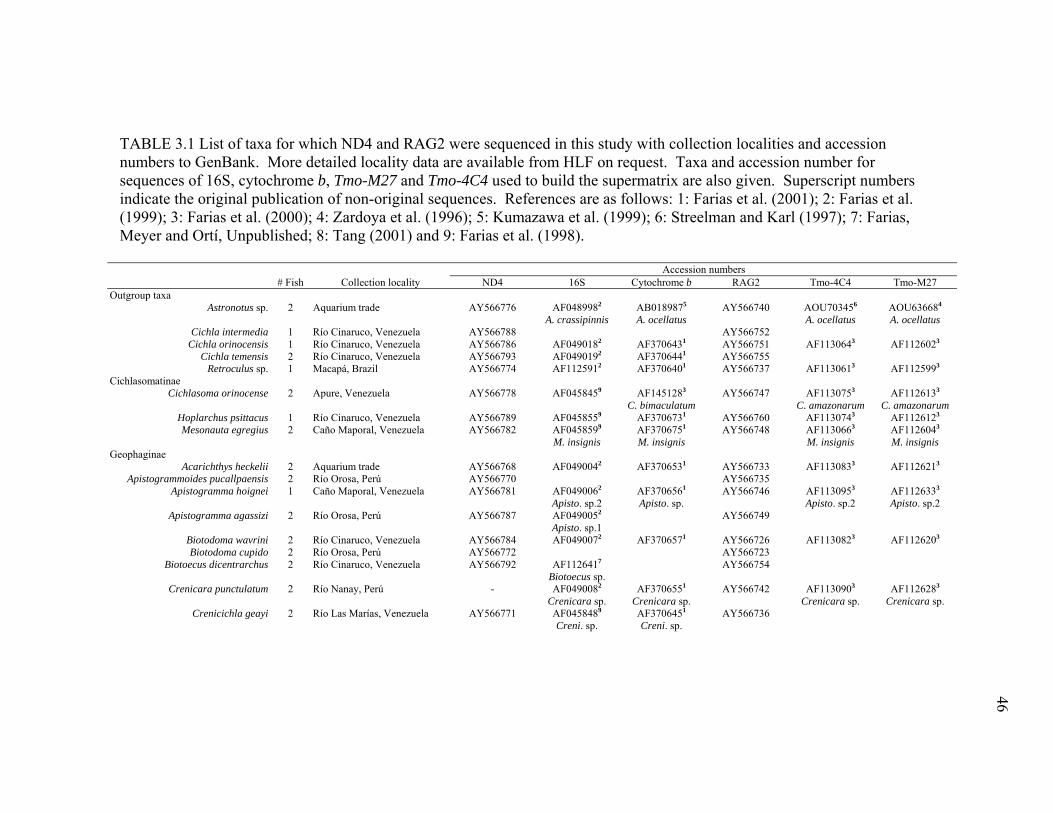
TABLE 3.1 List of taxa for which ND4 and RAG2 were sequenced in this study with collection localities and accession numbers to GenBank. More detailed locality data are available from HLF on request. Taxa and accession number for sequences of 16S, cytochrome b, Tmo-M27 and Tmo-4C4 used to build the supermatrix are also given. Superscript numbers indicate the original publication of non-original sequences. References are as follows: 1: Farias et al. (2001); 2: Farias et al. (1999); 3: Farias et al. (2000); 4: Zardoya et al. (1996); 5: Kumazawa et al. (1999); 6: Streelman and Karl (1997); 7: Farias, Meyer and Ortí, Unpublished; 8: Tang (2001) and 9: Farias et al. (1998).

46

Accession numbers # Fish Collection locality ND4 16S Cytochrome b RAG2 Tmo-4C4 Tmo-M27

Outgroup taxa Astronotus sp.

2 Aquarium trade AY566776 AF0489982

A. crassipinnis

AB0189875

A. ocellatus

AY566740 AOU703456

A. ocellatus

AOU636684

A. ocellatus Cichla intermedia 1 Río Cinaruco, Venezuela AY566788 AY566752

Cichla orinocensis 1 Río Cinaruco, Venezuela AY566786 AF0490182 AF3706431 AY566751 AF1130643 AF1126023

Cichla temensis 2 Río Cinaruco, Venezuela

AY566793 AF0490192 AF3706441 AY566755Retroculus sp.

1 Macapá, Brazil

AY566774 AF1125912 AF3706401 AY566737 AF1130613 AF1125993

CichlasomatinaeCichlasoma orinocense 2 Apure, Venezuela AY566778 AF0458459 AF1451283

C. bimaculatum AY566747 AF1130753

C. amazonarum AF1126133

C. amazonarum Hoplarchus psittacus 1 Río Cinaruco, Venezuela AY566789 AF0458559 AF3706731 AY566760 AF1130743 AF1126123

Mesonauta egregius 2 Caño Maporal, Venezuela AY566782 AF0458599

M. insignis AF3706751

M. insignis AY566748 AF1130663

M. insignis AF1126043

M. insignis Geophaginae

Acarichthys heckelii 2 Aquarium trade AY566768 AF0490042 AF3706531 AY566733 AF1130833 AF1126213

Apistogrammoides pucallpaensis 2 Río Orosa, Perú AY566770 AY566735Apistogramma hoignei 1 Caño Maporal, Venezuela AY566781 AF0490062

Apisto. sp.2 AF3706561 Apisto. sp.

AY566746 AF1130953 Apisto. sp.2

AF1126333 Apisto. sp.2

Apistogramma agassizi 2 Río Orosa, Perú AY566787 AF0490052 Apisto. sp.1

AY566749

Biotodoma wavrini 2 Río Cinaruco, Venezuela

AY566784 AF0490072 AF3706571 AY566726 AF1130823 AF1126203

Biotodoma cupido 2 Río Orosa, Perú AY566772 AY566723Biotoecus dicentrarchus 2 Río Cinaruco, Venezuela AY566792 AF1126417

Biotoecus sp. AY566754

Crenicara punctulatum 2 Río Nanay, Perú - AF0490082 Crenicara sp.

AF3706551 Crenicara sp.

AY566742 AF1130903 Crenicara sp.

AF1126283 Crenicara sp.

Crenicichla geayi 2 Río Las Marías, Venezuela AY566771 AF0458489

Creni. sp. AF3706451

Creni. sp. AY566736

TABLE 3.1 Continued

47

Accession numbers # Fish Collection locality ND4 16S Cytochrome b RAG2 Tmo-4C4 Tmo-M27

Crenicichla af. lugubris 2 Río Cinaruco, Venezuela AY566785 AF0490022 C. lugubris

AF3706461

C. regani AY566750 AF1130873

C. regani AF1126253

C. regani Crenicichla sveni 2

Apure, Venezuela AY566779 AF2859398 C. lepidota

AY566743 U703356

C. saxatilis CSU636674

C. saxatilis Crenicichla af. wallacii 2 Río Cinaruco, Venezuela

AY566790 AY566753

Dicrossus sp. 2 Aquarium trade AY566767 AY566731Geophagus brachybranchus 2 Río Cuyuní, Venezuela AY566763 AY566727Geophagus grammepareius 1 Río Claro, Venezuela AY566796 AF1126427

G. argyrostictus AY566724 AF1130923

G. argyrostictus

AF1126303

G. argyrostictus Geophagus abalios 2 Río Cinaruco, Venezuela AY566795 AF0458509

G. altifrons AY566757 AF1130913

G. altifrons AF1126293

G .altifrons Geophagus dicrozoster 2 Río Cinaruco, Venezuela AY566794 AF0490092

G. cf. proximus AY566756

Geophagus surinamensis 2 Haut Maroni, French Guiana AY566777 AF1125972

Geophagus sp. AF3706581

Geophagus sp. AY566741 AF1130933

Geophagus AF1126313

Geophagus sp. ‘Geophagus' brasiliensis 2 Aquarium trade AY566766 AF0490162 AF3706591 AY566732 AF113088 AF112626

‘Geophagus' steindachneri 2 Aquarium trade, origin not known

AY566765 AF3706601 AY566730

Guianacara n. sp. ‘Caroni’ 2 Río Claro, Venezuela AY566762 AF0490102 Guianacara sp.

AF3706541

Guianacara sp. AY566725 AF1130843

Guianacara sp. AF1126223

Guianacara sp. Gymnogeophagus balzanii 1 Aquarium trade, probably from

Uruguay - AF1125947

G. gymnogenys AF3706611

G. gymnogenys AY566739 AF1130853

G. gymnogenys

AF1126233

G. gymnogenys Gymnogeophagus rhabdotus 2 Aquarium trade, probably from

Uruguay AY566775 AF0490112

G. labiatus AF3706621

G. labiatus AY566738

Mikrogeophagus altispinosus 2 Aquarium trade AY566764 AF0458572 AY566729 AF1130893 AF1126273

Mikrogeophagus ramirezi 2 Caño Maporal, Venezuela AY566780 AY566744Satanoperca daemon 2 Río Cinaruco, Venezuela AY566791 AF0490132

S. acuticeps AF3706631

S. acuticeps AY566758

Satanoperca jurupari 2 Río Orosa & R. Nanay, Perú AY566783 AF0490142 AF3706641 AY566745Satanoperca mapiritensis 2 Río Pao & R. Morichal Largo,

Venezuela AY566761 AY566728

Satanoperca pappaterra 2 Río Paraná, Brazil

AY566773 AY566759Taeniacara candidi 2 Aquarium trade AY566769 AF1125922 AF3706651 AY566734 AF1130943 AF1126323

48

Hoplarchus were added to the ingroup to further test geophagine monophyly

against its sister-group Cichlasomatinae (Kullander 1998; Farias et al. 2000, 2001).

Based on previous knowledge of cichlid relationships (Oliver 1984; Stiassny 1991;

Kullander 1998; Farias et al. 1999, 2000, 2001), three species of Cichla and one of

Astronotus and Retroculus were used as outgroups. Throughout the paper, references to

both ingroup and outgroup pertain to the above designation of taxa. Whenever possible,

more than one species per genus were sampled to test genus-level monophyly, and to

improve robustness and resolution of the analysis (e.g. Graybeal 1998; Zwickl and Hillis

2002).

In addition to new data from the ND4 and RAG2 genes, a “supermatrix” (Gatesy

et al. 2002) was derived from previously published sequences of the mitochondrial

protein-coding cytochrome b and the ribosomal 16S genes, the nuclear microsatellite

flanking-region Tmo-M27, and the nuclear locus Tmo-4C4 (See Table 3.1 for references

and accession numbers). The supermatrix allowed for a total-evidence analysis of all

molecular data available for Geophaginae. Given the objective of resolving genus-level

relationships, species-level taxonomic mismatches between new data and published

sequences were circumvented by creating composites of species to improve resolution at

the genus level. Whenever possible, species combinations in the supermatrix (Table 3.1)

were based on previous knowledge of intra-generic phylogeny as well as phylogenetic

analyses from the new data, which supported genus-level monophyly. For example,

Satanoperca daemon was combined with S. acuticeps following Kullander and Ferreira

(1988), and Gymnogeophagus rhabdotus with G. labiatus based on Wimberger et al.

(1998). However, a lack of explicit phylogenetic information often caused decisions to

be based on rather arbitrary criteria that helped reduce the amount of missing data. This

approach, thus, should satisfy the objective of providing a robust analysis of inter-

generic relationships, but species-level relationships recovered from the supermatrix are

necessarily spurious and are not being reported. When published sequences were

lacking for a genus or locus, that part of the matrix was coded as missing data (?).

49

Molecular methods

The DNeasy kit (Qiagen) was used to extract total genomic DNA from muscle

tissues stored in 95% ethanol. The mitochondrial ND4 gene (~650 bp) was amplified

using standard PCR protocols (94°C denaturation, 60 sec., 48°C annealing 60 sec., 77°C

extension 45 sec. for 35 cycles) and directly sequenced using primers Nap 2 (Arévalo et

al. 1994) and ND4LB (Bielawsky et al. 2002) and the internal sequencing primer Geo-

ND4F (5’ TCCTCCCCCTRATAATTCTKGC 3’), specifically designed for this study.

The nuclear RAG 2 gene (~1000 bp) was amplified using a touchdown PCR protocol

(94°C, 30 sec. denaturation, 62°C, 60°C, and 58°C, 2 cycles each; then 56°C for 25

cycles, 60 sec. annealing, and 72°C 90 sec. extension). PCR products were gel extracted

using the Quiaquick kit (Qiagen) before sequencing. Amplification and external

sequencing primers (F2 & R7) were from Lovejoy and Collette (2001) and the internal

sequencing primers Geo IF (5' AGGTCCTACATGCCTACATGC) and GeoIR (5'

GGGGCTGCCTTGCARAAGC) were developed specifically for this study. Forward

and reverse DNA strands were sequenced with fluorescent-labeled dideoxynucleotide

terminators (BigDye, PE Biosystems) following the protocol of Sanger et al. (1977) and

using an automated ABI Prism 377 or 3100 sequencer (PE Biosystems).

Alignment

All new sequences were compared to published DNA sequences using NCBI’s

BLAST search to confirm their identity. Since cichlid sequences of ND4 and RAG2

were not available before this study, sequences significantly matching the expected

nucleotide regions in any teleosts were considered accurate and included in the analyses.

Forward and reverse sequences were edited and aligned in Sequencher 4.0 (Genecodes),

and a consensus sequence was constructed for each specimen of each taxon.

Unambiguous sequences of the ND4 fragment could not be obtained for the geophagine

taxa Crenicara punctulatum and Gymnogeophagus balzanii, thus they were removed

from the ND4 matrix and treated as missing data in the combined analyses (Table 3.1).

Preliminary multiple alignment of all sequences was determined with Clustal X

50

(Thompson et al. 1994), using default gap penalties. Several gap penalties were used to

account for any indels involving codons and overall higher level of nonsynonymous

substitutions observed for ND4. The 16S fragment was aligned using the secondary

structural model of Xenopus laevis predicted by the Gutell Lab at the University of

Texas at Austin (Cannone et al. 2002: http://www.rna.icmb.utexas.edu). A total of 29

base pairs in regions of ambiguous structural alignment were excluded because

positional homology could not be established. The alignments of microsatellite flanking

region Tmo-M27 and nuclear locus Tmo-4C4 were checked for unnecessary gaps or

obvious alignment mistakes, but otherwise were used unmodified. GenBank accession

numbers for new sequences used in this study are given in Table 3.1; a Nexus file with

the alignments for all loci is available from HLF on request.

Phylogenetic analyses

A total of four different datasets were analyzed using maximum parsimony and

Bayesian approaches: ND4, RAG2, ND4 and RAG2 combined (Total Evidence dataset),

and all six genes (ND4, cytochrome b, 16S, RAG2, Tmo-4C4 and Tmo-M27) combined

in the supermatrix described above and in Table 3.1. Each dataset was analyzed

following the procedures described below:

Parsimony analyses. Parsimony analyses, both equally and differentially

weighted, were performed in PAUP* v4.0b10 (Swofford, 2002) using 100 replicates of

heuristic search with random addition sequence and Tree Bisection and Reconnection

(TBR) branch swapping. As a means to partially accommodate rate heterogeneity and

saturation effects at certain positions under parsimony, two-parameter step matrices were

used to differentially weight transitions and transversions for each of the six aligned

gene fragments. Transition/transversion ratios were estimated using ML on a Neighbor-

Joining tree constructed using the HKY85 model of nucleotide substitution (Hasegawa et

al. 1985) in PAUP*. Support for the parsimony-derived topologies was estimated with

nonparametric bootstrap (Felsenstein 1985) and Bremer support indices (Bremer 1988,

1994) with searches performed in PAUP*. Bootstrap included 100 pseudoreplicates and

51

10 heuristic search replicates under the same conditions of the original search, for both

the equally and differentially weighted analyses. Bremer support was estimated only for

the strict consensus tree of the unweighted MP analysis with topological constraints

implemented in MacClade 4.0 (Maddison and Maddison 2000) and 100 replicates of

heuristic search using random addition sequences and TBR.

Bayesian analyses. Bayesian phylogenetic analyses of each of the four data sets

(ND4, RAG2, Total evidence and the supermatrix) were run in MrBayes 3.0b4

(Huelsenbeck and Ronquist 2001; Ronquist and Huelsenbeck 2003). This version of

MrBayes implements a modified Metropolis coupled Markov Chain Monte Carlo (MC3)

algorithm that independently samples trees and the parameters of the model of evolution

from each data partition (Ronquist and Huelsenbeck 2003). The program produces

topologies of the combined data, but uses separate models of evolution for each

partition. Initial models of molecular evolution were selected using nested Likelihood

Ratio Tests as implemented in ModelTest (Posada and Crandall 1998). Once the general

model was obtained for each partition, specific parameters of nucleotide substitution

were left to vary using default priors, thus each model could accommodate several

possible rate models (Huelsenbeck and Imennov 2002). For each data set, phylogenetic

analyses were run for 2 x 106 generations, sampling every 100 generations for a total of

20,000 samples per run (Leaché and Reeder 2002).

Log-likelihood values of each sample against the number of generations were

plotted, and the Markov chain was considered to have attained stationarity when log-

likelihood estimates reached a stable value (Huelsenbeck and Ronquist 2001; Leaché

and Reeder 2002). All samples with likelihood values below the stationarity level were

discarded as burn-in. Three methods were applied to each data set to avoid estimating

phylogenies corresponding to local optima. 1) The MC3 algorithm implemented in

MrBayes was employed. This approach facilitates an efficient search of tree space by

using three incrementally heated chains along with the cold chain from which

parameters are derived. Heated chains reduce the height of suboptimal peaks and fill

valleys between peaks; by randomly swapping with the heated chains, the cold chain can

52

more effectively explore tree space, reducing the chance of being trapped on local

suboptimal peaks (Geyer and Thompson 1995; Huelsenbeck and Ronquist 2001;

Ronquist and Huelsenbeck 2003). 2) For each data set, the MC3 analyses were repeated

with different starting trees until not less than four runs converged on the same mean

stationarity value. Samples were then used from the four runs which converged on the

highest likelihood. 3) For each of the four convergent analyses, 50% majority rule

consensus trees were separately estimated, and mean values calculated for the

parameters of nucleotide substitution.

Comparison of molecular and morphological topologies

Kullander (1998) proposed a classification of Geophaginae based on his analysis

of 91 morphological characters. Likelihood-based tests of Kishino-Hasegawa (KH,

Kishino and Hasegawa 1989) and Shimodaira-Hasegawa (SH, Shimodaira and

Hasegawa 1999), as implemented in PAUP*, were used to compare the MP and

Bayesian topologies with that of Kullander’s morphological analysis. Kullander used a

consensus of character states for each genus, and taxon sampling was slightly different

between his analysis and this study; to make the topologies more comparable, the trees

were modified such that a single branch represented each genus, and Taeniacara candidi

was removed because it was not included in Kullander’s study. Topological tests were

performed using the ND4, RAG2 and total evidence datasets, but due to the amount of

missing data (e.g. Satanoperca, Biotoecus), meaningful comparisons using the

supermatrix dataset could not be performed. In addition, topological comparisons with

Farias et al.’s (1999, 2000, 2001) molecular trees were not performed due to their

reduced taxon sampling.

Rates of molecular evolution

The two cluster test (TCT) and the branch length test (BLT) of Takezaki et al.

(1995) in the LINTRE program (1995, http://www.bio.psu.edu/People/Faculty/Nei/Lab)

were performed. These tests offer two different approaches to test whether a group of

53

sequences evolves in a clock-like fashion. The TCT is a generalized version of the

relative-rate test (RRT, Li and Bousquet 1992; Tajima 1993) that allows one to evaluate

whether a lineage in a phylogeny evolves significantly faster than other lineages. The

TCT is less sensitive to unbalanced tree topology than the original RRT (Robinson et al.

1998). The BLT tests whether the branch length of a lineage is significantly longer or

shorter than the average branch length across the tree (Takezaki et al. 1995), thus

detecting whether a lineage evolves significantly faster or slower than the others do.

Accuracy and power of the tests increase when the tree is rooted with the nearest

outgroup (Robinson et al. 1998), and when taxon sampling is increased (Robinson et al.

1998; Sorhannus and Van Bell 1999). With this in mind, Astronotus was used as the

outgroup following the results of Farias et al. (2000), and performed the tests including

all species in the phylogeny.

RESULTS

ND4

The aligned ND4 dataset included 648 base pairs. A single codon deletion was

found in Retroculus sp. at position 126, and in all species of Cichla and in Biotodoma

cupido at position 130. Homogeneity of nucleotide composition was not rejected by the

X2 test (X2 = 90.111, df = 105, p > 0.8) as implemented in PAUP* 4.0b10 (Swofford

2002). The HKY85 model of substitution revealed an overall transition/transversion

ratio of 2.23, which was used for the weighted parsimony analysis. The largest overall

genetic distance (uncorrected sequence divergence = 41.52%) occurred among the

geophagine taxa Crenicichla wallacii and Dicrossus sp., and the smallest divergence

(4.78%) between Geophagus brachybranchus and G. surinamensis. Sequence

divergence between geophagine cichlids and outgroup taxa ranged between 16.2%

(Guianacara n. sp. ‘Caroní’ x Cichla orinocense) and 36.8% (Crenicichla wallacii x

Cichla intermedia). Divergence between geophagine and cichlasomine taxa varied

between 18.3% (Cichlasoma orinocense x Geophagus brachybranchus) and 37.9%

54

(Mesonauta egregius x Crenicichla wallacii). Saturation plots for 648 bp and 36 taxa of

ND4 (Figure 3.1) showed an overall saturation of transitions beyond 15-20% divergence,

a pattern mostly due to the effect of high rates of change at third positions.

Transversions showed little or no overall saturation, as only third positions showed a

tendency to saturate beyond 30 to 35% divergence.

Unweighted parsimony analysis of ND4 consisted of 395 informative sites for 36

taxa and produced 2 most parsimonious (MP) trees of 2770 steps with a global

consistency index (CI) of 0.30, retention index (RI) of 0.39, and rescaled consistency

index (RC) of 0.12. The difference between the two unweighted MP trees was the

position of species within the genus Geophagus. Transition/transversion weighted

parsimony included 403 informative sites, producing a single MP tree of 3918.91 steps

and CI = 0.32, RI = 0.41 and RC = 0.13. Both unweighted and weighted parsimony

analyses produced essentially the same topology (Figure 3.2A), with a weakly supported

monophyletic Geophaginae. The best supported relationships within the subfamily were

a clade uniting Satanoperca, Apistogramma (including Apistogrammoides) and

Taeniacara (the “Satanoperca clade” from here on), and the monophyly of most genera.

The unweighted analysis produced a paraphyletic Mikrogeophagus, which was

monophyletic in the weighted topology. A general time reversible model of molecular

evolution was used for the Bayesian analysis, including invariants and gamma-

approximated site-specific rate heterogeneity (GTR + I + Г). Four independent runs

converged in the same likelihood range after approximately 25,000 generations; the first

50,000 (500 trees) were discarded as burn in. Fifty percent majority rule topologies and

model parameters for each run (19,500 trees/samples per run) were identical, thus all

trees were combined into the final topology (Figure 3.2B). The Bayesian analysis

produced a monophyletic Geophaginae, recovered the “Satanoperca clade” as did the

MP analysis, and supported a sistergroup relationship between Geophagus and

‘Geophagus’ steindachneri. Most other support was given to the monophyly of various

genera.

FIG. 3.1. ND4 saturation plots showing transitions (filled circles) and transversions (empty circles). A) first positions; B) second positions; C) third positions; D) all positions. Graphs represent absolute number of nucleotide substitutions against uncorrected percent sequence divergence (p-distance) from pairwise taxa comparisons.

55

FIG. 3.2. Topologies derived from DNA sequences of the mitochondrial gene ND4. A) Consensus of most parsimonious topologies derived from equally weighted (2 MP trees) and transition/transversion weighted (1 MP tree) analysis of a 648 bp of the mitochondrial NADH dehydrogenase subunit 4 (ND4). Boostrap support, based on 100 pseudoreplicates, for unweighted/weighted analyses is given above branches (only scores >50% are shown); Bremer decay indices for the equally weighted analysis are given below branches. Support values for nodes a-c are given to the right of the tree. See text for tree statistics. B) 50% majority rule Bayesian topology derived from ND4 sequences with a GTR + I + Γ general model of evolution. The topology resulted from combining 78,000 trees from 4 independent runs of 2 x 106 generations sampling every 100 trees with burn in of 50,000 generations/500 trees for each analysis. Posterior probabilities are given above branches. Highlighted clade (see discussion): SC = Satanoperca clade. 56

57

RAG2

The RAG2 dataset included 976 base pairs, with no differences in length among

the 38 taxa included. Homogeneity of base pairs was not rejected by the X2 test (X2 =

7.498, df = 111, p = 1.0), and the HKY85 model of nucleotide substitution resulted in a

transition/transversion ratio of 2.41. The largest overall genetic distance (7.2%)

occurred among the geophagine taxa Apistogramma hoignei and Biotodoma cupido, and

the smallest between Geophagus brachybranchus and G. surinamensis, which showed

no difference in their sequences for the RAG2 fragment. Sequence divergence between

geophagine cichlids and outgroup taxa ranged between 6.7% (Acarichthys heckelii x

Retroculus sp.) and 2.6% (Acarichthys heckelii x Cichla temensis). Divergence between

geophagine and cichlasomine taxa varied between 6.4% (Apistogramma hoignei x

Mesonauta egregius) and 3.0% (Acarichthys heckelii x Hoplarchus psittacus).

Saturation plots for the aligned 976 bp from 38 taxa revealed no apparent saturation of

nucleotide substitution at any codon position (plots not shown).

Unweighted parsimony analysis of RAG2 included 155 parsimony informative

sites for 38 taxa, producing 152 MP trees of 483 steps and CI = 0.70, RI = 0.71 and RC

= 0.50. The transition/transversion weighted analyses included 159 informative sites and

produced 36 MP trees of 681.99 steps and CI = 0.71, RI = 0.73 and RC = 0.52. The

strict consensus trees of both analyses were virtually identical as was overall bootstrap

support (Figure 3.3A). Three multi-genus clades were unresolved at the base of a

monophyletic Geophaginae: the Tribe Acarichthyini (Acarichthys and Guianacara), the

“Satanoperca clade,” and a clade including Biotodoma, Mikrogeophagus, Geophagus

sensu lato, Gymnogeophagus, Crenicara and Dicrossus, referred to as the “Big clade”

from here on. RAG2 Bayesian analyses were run using a GTR + I + Г model of

nucleotide substitution. Of six independent runs, two converged at a lower likelihood

range than the other four and were discarded. The four analyses converging at highest

likelihood values were then used for tree construction as described for ND4, but in this

case the first 1,000 trees were discarded as burn in. As before, 50% majority rule

consensus trees and parameters of sequence evolution for each of the four analyses were

58

identical, thus topologies were combined onto a single tree (Figure 3.3B). The Bayesian

topology was essentially identical to the parsimony tree, except for the incorporation of

Crenicichla and Biotoecus at the base of the “Big clade”, thus leaving the geophagine

phylogeny as a polytomy of three clades, each with at least two genera (Figure 3.3B, and

see discussion)

Total evidence

The combined datasets of ND4 and RAG2 produced a matrix of 1624 bp for 38

taxa. Since ND4 sequences were not available for Crenicara punctulatum and

Gymnogeophagus balzanii (see methods), these were treated as missing data. The

unweighted parsimony analysis included 550 informative positions and produced 1 MP

tree of length 3304 with CI = 0.36, RI = 0.42 and RC = 0.15. The

transition/transversions weighted parsimony analysis consisted of 562 informative sites

and produced 1 MP tree of 4667.94 steps with CI = 0.37, RI 0.44 and RC = 0.16 (Figure

3.4A). The total evidence parsimony analyses produced a monophyletic Geophaginae

with poorly resolved internal relationships, but with some common elements with the

independent analyses, particularly the “Satanoperca clade” and some components of the

“Big clade”. Bayesian total evidence analyses were performed under unlinked GTR + I

+ Г models of nucleotide substitution for each partition. The final topology (Figure

3.4B) was derived exactly as described for ND4; parameters of sequence evolution for

ND4 and RAG2 were not different from those estimated during the individual analyses.

The Bayesian topology was similar to the RAG2 Bayesian tree, but completely resolved:

the Tribe Acarichthyini was basal to a clade in which the “Big clade,” with (weakly

supported) Crenicichla and Biotoecus at its base, was sister to the “Satanoperca clade”..

FIG. 3.3. Topologies from DNA sequences of the nuclear gene RAG2. A) Consensus of most parsimonious topologies derived from equally weighted (152 MP trees) and transition/transversion weighted (36 MP trees) analysis of a 976 bp of the nuclear Recombination Activation Gene 2 (RAG2). Boostrap support, based on 100 pseudoreplicates, for unweighted/weighted analyses is given above branches (only scores >50% are shown); Bremer decay indices for the equally weighted analysis are given below branches. Support values for nodes a-o are given to the right of the tree. See text for tree statistics. B) 50% majority rule Bayesian topology using RAG2 sequences with a GTR + I + Γ general model of evolution. The topology resulted from combining 76,000 trees from 4 independent runs of 2 x 106 generations sampling every 100 trees with burn in of 100,000 generations/1000 trees for each analysis. Posterior probabilities are given above branches. Highlighted clades (see discussion): BC = Big clade; CrC = Crenicarine clade; GC = Geophagus clade; MkC = Mikrogeophagus clade; SC = Satanoperca clade; TA = Tribe Acarichthyini. 59

FIG. 3.4. Topologies from the combined ND4 and RAG2 datasets. A) Consensus of most parsimonious topologies derived from equally weighted (1 MP tree) and transition/transversion weighted (1 MP tree) analysis of the combined 1624 bp of the mitochondrial ND4 and the nuclear RAG2. Boostrap support, based on 100 pseudoreplicates, for unweighted/weighted analyses is given above branches (only scores >50% are shown); Bremer decay indices for the equally weighted analysis are given below branches. Support values for nodes a-j are given to the right of the tree. See text for tree statistics. B) 50% majority rule Bayesian topology using ND4 and RAG2 sequences with unlinked GTR + I + Γ general models of evolution. The topology resulted from combining 78,000 trees from 4 independent runs of 2 x 106 generations sampling every 100 trees with burn in of 50,000 generations/500 trees for each analysis. Posterior probabilities are given above branches. Highlighted clades (see discussion): BC = Big clade; CrC = Crenicarine clade; GC = Geophagus clade; MkC = Mikrogeophagus clade; SC = Satanoperca clade; TA = Tribe Acarichthyini. 60

61

Super matrix

The supermatrix (Table 3.1 and see methods) contained sequences from six

molecular markers: ND4, RAG2, cytochrome b, 16S, Tmo-M27 and Tmo-4C4, for a total

of 3960 aligned base pairs from 38 taxa, of which several are composites of more than

one species. The unweighted parsimony analysis contained 1161 informative sites, and

recovered 2 MP trees of 6215 steps with CI = 0.40, RI = 0.39 and RC = 0.16. For ND4

and RAG2 the same transition/transversion ratios as for other analyses were used, and

the following ratios were calculated for the remaining partitions: cytochrome b = 2.27,

16S = 2.32, Tmo-M27 = 3.90, Tmo-4C4 = 1.90. The weighted parsimony analysis

included 1185 informative sites, producing a single MP tree of 6225 steps with CI =

0.40, RI = 0.39 and RC = 0.16 (Figure 3.5). Parsimony analysis of the supermatrix

strongly supported geophagine monophyly and recovered the “Satanoperca clade”, but

otherwise failed to recover relationships found in analyses of RAG2 and the total

evidence dataset; all new relationships found in the analysis were weakly supported.

Bayesian analysis of the supermatrix was performed using unlinked models of

nucleotide substitution for each one of the six partitions. A GTR + I + Г model was used

in all cases, except for Tmo-M27, for which the HKY85 + Г model was employed. Four

independent runs produced identical model parameters and partial topologies, thus all

samples were combined after discarding the first 500 trees of each run as burn in (Figure

3.6). Bayesian analysis of all the molecular data produced a monophyletic Geophaginae

with Guianacara at the base of a three-clade polytomy. This polytomy included a

mildly supported clade including Crenicichla, Biotoecus and Acarichthys, and the “Big

clade” and “Satanoperca clade”, both with strong support.

62

FIG. 3.5. Consensus of most parsimonious topologies derived from equally weighted (2 MP trees) and transition/transversion weighted (1 MP tree) analysis of the combined 3960 bp of the mitochondrial ND4, cytochrome b and 16S and the nuclear RAG2, Tmo-M27 and Tmo-4C4. Boostrap support, based on 100 pseudoreplicates, for unweighted/weighted analyses is given above branches (only scores >50% are shown); Bremer decay indices for the equally weighted analysis are given below branches. See text for tree statistics. Highlighted clades (see discussion): CrC = Crenicarine clade; SC = Satanoperca clade.

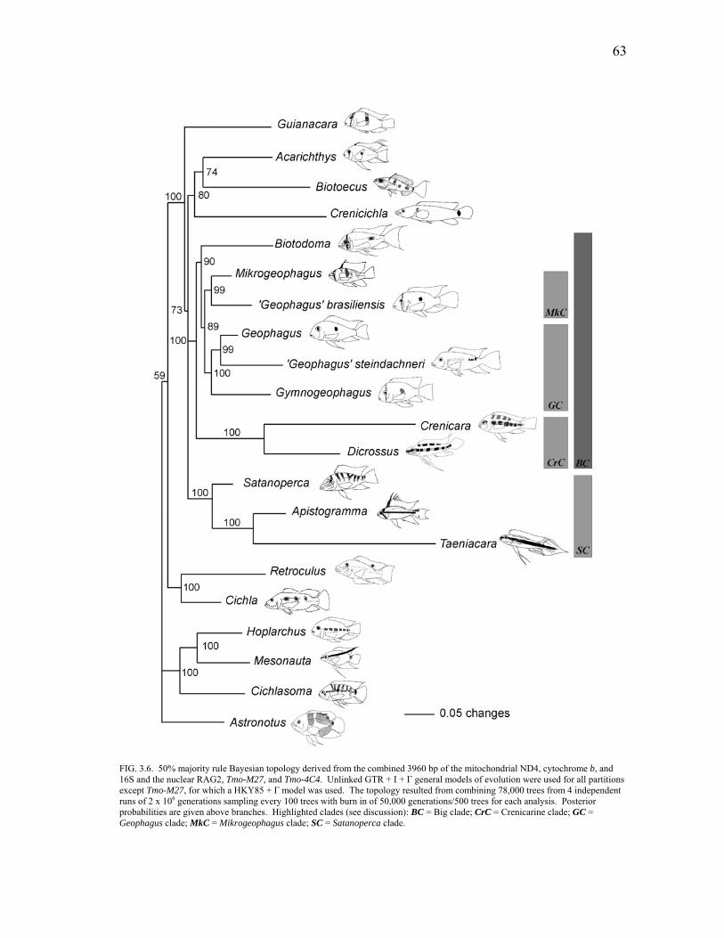
63

FIG. 3.6. 50% majority rule Bayesian topology derived from the combined 3960 bp of the mitochondrial ND4, cytochrome b, and 16S and the nuclear RAG2, Tmo-M27, and Tmo-4C4. Unlinked GTR + I + Γ general models of evolution were used for all partitions except Tmo-M27, for which a HKY85 + Γ model was used. The topology resulted from combining 78,000 trees from 4 independent runs of 2 x 106 generations sampling every 100 trees with burn in of 50,000 generations/500 trees for each analysis. Posterior probabilities are given above branches. Highlighted clades (see discussion): BC = Big clade; CrC = Crenicarine clade; GC = Geophagus clade; MkC = Mikrogeophagus clade; SC = Satanoperca clade.

64

With the exception of the most basal nodes, this analysis resolved most of the

intergeneric relationships within Geophaginae, and defined three subclades within the

subfamily.

Comparison of molecular and morphological topologies

The KH and SH tests indicated that all molecular phylogenies were significantly

more likely than Kullander’s (1998) morphological topology (Table 3.2). Based on the

KH tests, of all parsimony topologies, only the ND4 tree was found to be more likely

than both Kullander’s and the Bayesian ND4 tree. In contrast, the Bayesian topologies

of the RAG2 and TE datasets were significantly more likely than either Kullander’s or

the parsimony topologies. The SH tests, expected to be more conservative (Shimodaira

and Hasegawa, 1999), did not reject the hypothesis of equal likelihood when Kullander’s

topology was compared to either of the ND4 trees. The Bayesian RAG2 and TE

topologies were consistently better than Kullander’s tree according to the SH test. The

parsimony and Bayesian topologies based on RAG2 were not significantly different (SH

test), but the TE Bayesian topology was found to be significantly more likely than the

TE parsimony tree. These findings suggest an effect of ND4 in determining

incongruence between the total evidence trees.

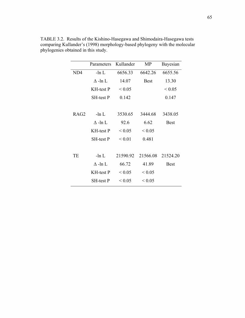
65

TABLE 3.2. Results of the Kishino-Hasegawa and Shimodaira-Hasegawa tests comparing Kullander’s (1998) morphology-based phylogeny with the molecular phylogenies obtained in this study.

Parameters Kullander MP Bayesian

ND4 -ln L 6656.33 6642.26 6655.56

∆ -ln L 14.07 Best 13.30

KH-test P < 0.05 < 0.05

SH-test P 0.142 0.147

RAG2 -ln L 3530.65 3444.68 3438.05

∆ -ln L 92.6 6.62 Best

KH-test P < 0.05 < 0.05

SH-test P < 0.01 0.481

TE -ln L 21590.92 21566.08 21524.20

∆ -ln L 66.72 41.89 Best

KH-test P < 0.05 < 0.05

SH-test P < 0.05 < 0.05

66

Rate heterogeneity

The TCT analysis revealed significant rate heterogeneity among lineages (ND4:

Q = 1719.5, df = 35, p < 0.0001; RAG2: Q = 9200, df = 37, p < 0.0001), with numerous

rate differences revealed among taxa for both ND4 and RAG2 (Table 3.3). As found by

Farias et al. (1999, 2000, 2001), geophagine cichlids showed overall faster rates of

molecular evolution than other Neotropical taxa in both mitochondrial and nuclear

genes. It is interesting that Retroculus, an outgroup genus morphologically similar to

large-bodied geophagines, also revealed significantly fast rates of ND4 evolution,

although this was not the case for RAG2. Extensive rate heterogeneity occurred among

and within genera of geophagines as well, but patterns were not always the same in both

genes. Crenicichla and Taeniacara showed the fastest mitochondrial rates, whereas

Apistogramma had the fastest nuclear rates. Rate heterogeneity was also detected within

genera in both genes, particularly in Crenicichla, Apistogramma, Satanoperca, and

Biotodoma. The BLT indicated that rate heterogeneity is much more extensive in ND4

than in RAG2. In ND4, the genera Biotodoma, Dicrossus, Crenicichla, Apistogramma,

and Taeniacara showed at least one species with significantly longer branches than

average (Table 3.4), indicating an accelerated rate of molecular evolution. In contrast,

Guianacara, Acarichthys, Mikrogeophagus, and Geophagus sensu lato showed

significantly shorter branches than average. Interestingly, all non-geophagine taxa, with

the exception of Retroculus (p>0.05), showed significantly shorter branches and thus

lower rates of evolution in the mitochondrial gene. RAG2 showed a less heterogeneous

pattern of evolution, and only Biotodoma and Apistogramma (including

Apistogrammoides) showed accelerated rates of molecular evolution, whereas

Guianacara, Acarichthys and one species of Geophagus sensu stricto showed

significantly lower rates. Of the non-geophagine taxa, only Cichla had significantly

shorter branches, whereas the rest were not significantly different from the average

length.

TABLE 3.3. Assessment of rate heterogeneity among clades by the Two Cluster Test (Takezaki, Rzhetsky and Nei, 1995). Q-values evaluate overall rate heterogeneity; P-values determined from the chi-square distribution. Model used for TCT was Tamura Nei + Г as implemented in LINTRE. Gene (df) TCT Clades contributing to rate heterogeneity and their rate relationships P-value

ND4 (35) Q = 1719.5 Crenicichla af. wallacii > C. geayi (26) <0.001

P <0.0001 Crenicichla af. wallacii, C. geayi > C. sveni, C. af. lugubris <0.001

Crenicichla > Taeniacara <0.001

Crenicichla, Taeniacara > Retroculus <0.001

Crenicichla, Taeniacara, Retroculus > All geophagines <0.001

All geophagines, Retroculus > Hoplarchus, Mesonauta <0.001

Mesonauta > Cichla <0.05

Biotodoma cupido > B. wavrini <0.001

Apistogramma agassizi > Apistogrammoides, Apistogramma hoignei <0.001

Apistogramma> Satanoperca <0.001

Satanoperca pappaterra > Biotoecus <0.01

Acarichthys > ‘Geophagus’ steindachneri <0.001

Gymnogeophagus > Guianacara <0.001

Mikrogeophagus > Geophagus <0.001

Guianacara, Mikrogeophagus, Geophagus, Gymnogeophagus > ‘Geophagus’ brasiliensis <0.001

67

TABLE 3.3. Continued Gene (df) TCT Clades contributing to rate heterogeneity and their rate relationships P-value

Acarichthys, Biotodoma, Dicrossus, ‘Geophagus’ steindachneri, Satanoperca,

Apistogramma > Biotoecus, Satanoperca pappaterra

<0.01

Acarichthys, Biotodoma, Biotoecus, Dicrossus, ‘Geophagus’ steindachneri, Satanoperca,

Apistogramma > Guianacara, Mikrogeophagus, Geophagus, ‘Geophagus’ brasiliensis,

Gymnogeophagus

<0.001

RAG2 (37) Q= 9200 Mesonauta> Hoplarchus <0.001

P <0.0001 Cichla intermedia > C. temensis <0.05

Retroculus > Cichla <0.05

All geophagines > Retroculus, Cichla <0.001

All other geophagines > Acarichthys <0.001

Crenicichla geayi > C. sveni <0.001

Crenicichla sveni, C. geayi > C. af. wallacii <0.01

Biotodoma, Mikrogeophagus, Crenicara, Dicrossus, Geophagus, ‘Geophagus’

brasiliensis, ‘G.’ steindachneri, Gymnogeophagus > Crenicichla

<0.01

Apistogrammoides > Apistogramma hoignei <0.001

Apistogramma agassizi > Apistogrammoides, A. hoignei <0.01

Apistogramma, Apistogrammoides > Taeniacara <0.001

Satanoperca > S. daemon <0.001

68

TABLE 3.3. Continued Gene (df) TCT Clades contributing to rate heterogeneity and their rate relationships P-value

Satanoperca, Apistogramma, Taeniacara > Guianacara, Biotoecus <0.001

Biotoecus > Guianacara <0.001

Crenicara > Dicrossus <0.01

Biotodoma cupido > B. wavrini <0.01

Biotodoma > ‘Geophagus’ brasiliensis <0.001

Biotodoma , ‘Geophagus’ brasiliensis > Mikrogeophagus, Geophagus , ‘Geophagus’

steindachneri

<0.001

Gymnogeophagus > ‘Geophagus’ steindachneri <0.01

‘Geophagus’ steindachneri, Gymnogeophagus > Geophagus <0.001

Geophagus grammepareius > Geophagus <0.01

Guianacara, Biotoecus, Satanoperca, Apistogramma, Taeniacara > Biotodoma,

Mikrogeophagus, Crenicara, Dicrossus, Geophagus, ‘Geophagus’ brasiliensis, ‘G.’

steindachneri, Gymnogeophagus, Crenicichla

<0.001

69

70

TABLE 3.4. Branch Length Test of rate heterogeneity (Takezaky, Rzhetsky and Nei, 1995). P-values are reported followed by a sign indicating rate increase (+) or rate decrease (-) in comparison with the average rate for all taxa. Model used for BLT was Tamura Nei + Г as implemented in LINTRE . BLT, P-value, Rate of evolution

Taxon name

df = 35

ND4

df = 37

RAG2

Guianacara n.sp. ‘Caroní’ <0.001 - <0.05 -

Acarichthys heckelii <0.01 - <0.001 -

Biotodoma wavrini NS NS

Biotodoma cupido <0.001 + <0.05 +

Mikrogeophagus altispinosus NS NS

Mikrogeophagus ramirezi <0.05 - NS

Biotoecus dicentrarchus NS NS

Crenicara punctulatum N/A NS

Dicrossus sp. <0.01 + NS

Geophagus surinamensis <0.001 - NS

Geophagus brachybranchus <0.001 - NS

Geophagus abalios <0.001 - NS

Geophagus dicrozoster <0.001 - <0.05 -

Geophagus grammepareius <0.001 - NS

‘Geophagus’ brasiliensis <0.001 - NS

‘Geophagus’ steindachneri <0.001 - NS

Satanoperca pappaterra NS NS

Satanoperca jurupari NS NS

Satanoperca mapiritensis NS NS

Satanoperca daemon NS NS

Gymnogeophagus rhabdotus NS NS

Gymnogeophagus balzanii N/A NS

Crenicichla af. wallacii <0.001 + NS

71

TABLE 3.4. Continued BLT, P-value, Rate of evolution

Taxon name

df = 35

ND4

df = 37

RAG2

Crenicichla sveni <0.001 + NS

Crenicichla af. lugubris <0.001 + NS

Crenicichla geayi <0.001 + NS

Apistogrammoides pucallpaensis NS <0.001 +

Apistogramma agassizi <0.001 + <0.001 +

Apistogramma hoignei NS <0.01 +

Taeniacara candidi <0.001 + NS

Hoplarchus psittacus <0.001 - NS

Mesonauta egregius <0.001 - NS

Cichlasoma orinocense <0.001 - NS

Retroculus sp. NS NS

Cichla orinocensis <0.001 - <0.001 -

Cichla intermedia <0.001 - <0.05 -

Cichla temensis <0.001 - <0.001 -

72

DISCUSSION

Phylogenetic relationships of Geophaginae

Under both parsimony and Bayesian analyses, the ND4 matrix produced a

monophyletic Geophaginae, albeit with questionable support (Figure 3.2); analyses of all

other datasets, both MP and Bayesian, indicated stronger support for geophagine

monophyly (Figures 3.3-3.6). With the exception of ND4, all analyses recovered a

monophyletic cichlasomatine clade in which Hoplarchus and Mesonauta were grouped

in accordance with previous studies of the tribe Heroini (Kullander 1998; Farias et al.

1999, 2000, 2001). Analyses of ND4 supported monophyly of most geophagine genera,

and a sister-group relationship between Geophagus sensu stricto and ‘Geophagus’

steindachneri, but failed to provide any other well-supported intergeneric associations.

Within the geophagine clade, most combined analyses consistently found two

monophyletic groups including 12 of the 16 genera in this study and a weakly supported

clade including the remaining four genera. The overall arrangement of taxa in the

molecular trees (Figs. 2-6) is in disagreement with the topology described by Kullander

(1998, see KH and SH tests in Table 3.2). For convenience of discussion, each major

group diagnosed by the molecular data will be examined separately in the following

paragraphs.

The “Satanoperca clade.” The relationship uniting Satanoperca with the sister-

taxa Apistogramma and Taeniacara (the “Satanoperca clade”) was consistent in all

analyses, and support for it was generally high (Figures 3.2-3.6). Farias et al. (1999,

2000, 2001), using 16S and cytochrome b sequences, observed a similar pattern in

independent analyses, but found an alternative arrangement of Apistogramma grouping

with Crenicichla in their total evidence analysis (Farias et al. 2000, 2001). In contrast to

the molecular data, a “Satanoperca clade” was not supported by previous morphological

analyses (Kullander 1998). The consistency and high support for the “Satanoperca

clade” in all of this study’s analyses, however, provides strong support for the

monophyly of this clade. Within Apistogramma, the ND4, RAG2 and total evidence

73

analyses (i.e. those with no missing data) coincided in grouping A. hoignei with the

monotypic Apistogrammoides, suggesting the latter includes an exceptional,

autapomorphic species of Apistogramma that does not warrant separate generic status.

One point of incongruence between the ND4 and RAG2 datasets is the placement of

Satanoperca pappaterra as sister to Biotoecus by the ND4 gene (Figure 3.2), whereas

both the RAG2 and total evidence analyses place this taxon as part of a monophyletic

Satanoperca (Figures 3.3-3.4). There are at least three explanations for this

incongruence. First, the sequence shared between S. pappaterra and Biotoecus is the

result of a pseudogene. This seems unlikely. Base composition of ND4 sequences for

these two taxa is similar to that of other taxa examined, as well as to previously reported

data for ND4 in fish (Bielawski et al. 2002). In addition, no electropherograms revealed

evidence of multiple sequences, and all primers (external and internal), when used in

independent combinations of PCR amplifications, resulted in similar sequences. Second,

the close ND4 relationship may have resulted from contamination. This also appears

unlikely. Uncorrected genetic distance between S. pappaterra and Biotoecus (p =

24.9%) is not very different from the distance between Biotoecus and the other species

of Satanoperca (S. daemon = 22.3%, S. mapiritensis = 25.2%, S. jurupari = 24.6%).

Third, it is possible that S. pappaterra and Biotoecus are more similar in rates of ND4

evolution relative to other species of Satanoperca. Although the BLT for rate

heterogeneity does support this hypothesis (Table 3.4), comparisons with the TCT

revealed a slower rate of change in S. pappaterra and Biotoecus relative to the other

species of Satanoperca (Table 3.3). In such cases of heterogeneity, relationships can be

obscured (i.e. highly heterogeneous rates, frequent non-synonymous amino acid

substitutions). This notion is reinforced by the fact that the unweighted parsimony

analysis of ND4 was unable to recover a monophyletic Mikrogeophagus, whereas the

weighted and the Bayesian analyses did find the genus to be monophyletic. Finally,

ND4 may simply be too noisy for comparisons involving high levels of divergence as in

the case of Satanoperca pappaterra relative to its congeners.

74

The “Big clade.” Supported by parsimony and Bayesian results from RAG2 and

most combined analyses, the “Big clade” included Biotodoma, Mikrogeophagus,

Geophagus sensu lato, Gymnogeophagus, Crenicara, and Dicrossus (Figures 3.3, 3.4B-

3.6). Four elements, with various degrees of resolution depending on the analysis, are

contained within this group. 1) A monophyletic genus Biotodoma, 2) a

“Mikrogeophagus clade” in which that genus is sister to ‘Geophagus’ brasiliensis, 3) the

“Geophagus clade,” including a basal ‘Geophagus’ steindachneri and a sister-group

relationship to Gymnogeophagus, and 4) the “crenicarine clade” containing Crenicara

and Dicrossus. Highest resolution of relationships within the “Big clade” were obtained

from the Bayesian analysis of the supermatrix (Figure 3.6), with a pectinate arrangement

of the “crenicarine clade” at the base, followed by Biotodoma and then a clade

containing the sister “Mikrogeophagus” and “Geophagus” clades. The “crenicarine

clade” partially corresponds to the tribe Crenicaratini of Kullander (1998), but he had

originally included Biotoecus, which appeared elsewhere in this study’s analyses. Based

these results, recognition of a separate tribe seems unwarranted, as crenicarines group

within a larger clade containing other genera. The relationship between

“Mikrogeophagus” and “Geophagus brasiliensis” represents an association not found by

other studies. Given this study’s increased taxon sampling and overall increase in

sequence data, one might expect more resolution within Geophaginae.

Acarichthys, Guianacara, Crenicichla and Biotoecus. The sister-group

relationship between Acarichthys and Guianacara (tribe Acarichthyini in Kullander’s

classification) has been repeatedly proposed, both by morphological (Kullander 1998),

molecular (Farias et al. 1999), and some (Farias et al. 2000), but not all (Farias et al.

2001), total evidence analyses. Although supported by both RAG2 and the Bayesian

total evidence results, the ND4, parsimony total evidence, and supermatrix analyses

failed to support the monophyly of this clade. Failure to recover this clade could be due

to scarcity of data, as Acarichthys is a monotypic genus, and only one species of

Guianacara was included. Therefore, better taxon sampling may provide better support

for the relationship (Graybeal 1998; Zwickl and Hillis 2002). Nonetheless, when other

75

studies have identified this clade, support has been comparatively low with respect to

other relationships (e.g. Farias et al. 1999, Figure 3; Farias et al. 2001, Figure 4). In the

final Bayesian analysis, Guianacara occurred at the base of Geophaginae, and

Acarichthys weakly grouped with Biotoecus, as sister to Crenicichla. Interestingly, a

sister-group relationship of Crenicichla, Teleocichla and the Acarichthyini was observed

by Farias et al (1999) in their 16S phylogenetic analysis. A clear pattern emerged in

which Guianacara and Acarichthys appear as “peripheral” genera, not immediately

related to the bulk of the geophagine diversity found in the “Satanoperca clade” and in

the “Big clade”. The same scenario seems likely for Crenicichla and Biotoecus. The

phylogenetic position of these two genera within Geophaginae remains elusive. The

Bayesian RAG2 and total evidence analyses grouped them at the base of the “Big clade”

with moderate support (55 to 77% posterior probability), but this arrangement

disappeared in the 6-gene analysis, where they grouped with Acarichthys. Although the

general morphology of both genera is superficially similar (e.g. elongate, shallow

bodies), there is no clear indication that they are closely related. In previous studies,

Crenicichla sometimes grouped with Apistogramma (e.g. Farias et al. 2000, 2001, total

evidence), but the consistency of the “Satanoperca clade” seems to rule out that

possibility. Resolution of relationships of these four genera likely will require increased

taxon sampling, especially for Crenicichla and Guianacara, as Acarichthys is monotypic

and Biotoecus has only two known species.

In summary, the most resolved molecular phylogeny of Geophaginae was

obtained by Bayesian analysis of the supermatrix dataset, including six different

molecular markers (Figure 3.6). Within the monophyletic Geophaginae, two lineages

were well supported; the first was the “Big clade,” with the crenicarine clade at the base,

followed by Biotodoma as sister to a dichotomy in which the “Mikrogeophagus clade”

was sister to a pectinate “Geophagus clade” with Gymnogeophagus at the base. The

second strongly supported clade was the consistently recovered “Satanoperca clade”.

The “Big clade” and the “Satanoperca clade” found in this study include most of the

taxa formerly assigned to the Tribe Geophagini (Kullander 1998), but also contain

76

genera from Kullander’s Tribe Crenicaratini. Finally, a third, weakly supported clade

included a sister relationship between Crenicichla and a dichotomy of Acarichthys and

Biotoecus. In agreement with previous molecular and total evidence work (Farias et al.

1998, 1999, 2000, 2001), the genus Crenicichla was found to be part of the geophagine

clade, but no clear support for its position within the subfamily was found. Kullander’s

tribe Acarichthyini was not consistently recovered in this analysis, and Guianacara was

left either at the base of the geophagine clade (Bayesian tree) or as sister to

Gymnogeophagus (MP tree) in the six-gene analyses. In conclusion, two, well-

supported supra-generic groupings within Geophaginae were found, but the relationships

of the genera Crenicichla, Biotoecus, Acarichthys and Guianacara remain uncertain and

demand further study. Newly observed relationships in this analyses are probably the

combined result of increased datasets and taxon sampling. The general tendency in this

study was to find improved resolution in the combined, larger datasets, and additional

data should further resolve geophagine relationships.

ND4 versus RAG2 and Parsimony versus Bayesian analysis

A strikingly different pattern was observed between ND4 and RAG2. Whereas

ND4 yielded comparatively low resolution and parsimony and Bayesian analyses were

inconsistent with each other (Figure 3.2), RAG2 was highly consistent and offered high

resolution at deep levels within the geophagine phylogeny (Figure 3.3). ND4 alone was

able to recover a monophyletic Geophaginae and the “Satanoperca clade,” but it was

otherwise limited to establishing genus-level monophyly. Basal relationships within

Geophaginae were unresolved, and resolution outside the group was poor. On the other

hand, RAG2 recovered not only geophagine monophyly, but also the major clades

within it. RAG2 was the only dataset generating a hypothesis of relationship for

Crenicichla and Biotoecus, albeit with low support.

The lack of resolution and inconsistency found in ND4 are likely the result of

saturation effects and/or rate heterogeneity. ND4 showed saturation of third position

transitions and overall transitional saturation beyond 15% divergence (Figure 3.1), a

77

pattern congruent with observations in cichlid cytochrome b (Farias et al. 2001) and

characiform 16S (Ortí and Meyer 1997). Saturation at third positions reduces resolution

at deep levels in the phylogeny, but can still be informative on relationships among

closely related, recently diverged lineages (Farias et al. 2001), thus the relatively well

supported monophyly of most genera. The extensive rate heterogeneity found in ND4

(Tables 3.3 and 3.4) showed short (e.g. Geophagus) and long branches (e.g. Crenicichla)

within the geophagine tree. This situation potentially can create long branch attraction,

making parsimony analyses inherently inconsistent (Felsenstein 1978, 2004). RAG2

showed no evidence of nucleotide saturation, and its rates of molecular evolution were

less heterogeneous (Table 3.4). RAG2 produced highly resolved, consistent, and well

supported topologies both under parsimony and Bayesian methods.

Parsimony-derived topologies of the different datasets were incongruent, and

with the exception of RAG2 (Figure 3.3), they were inconsistent with the Bayesian

topologies. Results consistently showed that, whenever mitochondrial genes were

involved (particularly ND4 and cytochrome b), parsimony performed poorly due to the

effects of saturation and extensive rate heterogeneity in the mitochondrial genes (see

Tables 3.3 and 3.4, and Farias et al. 2001). Bayesian analyses were congruent among

themselves, and resolution and support generally increased with the amount of data.

Because Bayesian analyses incorporate explicit models of nucleotide substitution, they

should present the advantages of maximum likelihood analysis when confronted with

non-homogeneous patterns of molecular evolution (e.g. Holder and Lewis 2003;

Felsenstein 2004). Although not completely resolved, the Bayesian topology derived

from the 6-gene matrix (Figure 3.6) offered the most resolved and best-supported

hypothesis of geophagine relationships.

78

Implications of the molecular phylogeny: Are geophagine cichlids an adaptive

radiation?

According to Schluter (2000), adaptive radiations are characterized by four

features: common ancestry, rapid speciation, phenotype-environment correlation, and

trait utility. Based on this definition, Geophaginae may provide an example of an

adaptive radiation of Neotropical cichlids. Geophaginae clearly are a monophyletic

clade, both according to the results presented in this paper and to previous research (e.g.

Farias et al. 2000). More revealing is the fact that, judging from the Bayesian

phylograms, their phylogeny is characterized by short basal branches (Figures 3.2B,

3.3B, 3.4B and 3.6). These short branches can indicate either lack of information to

resolve basal relationships, or fast differentiation at the base of the tree (e.g. Kontula et

al 2003). Considering that we used nearly 4,000 base pairs from six different genes and

obtained a robust topology with the combined analysis, it seems unlikely that the short

basal branches are due only to lack of data. Instead, it seems reasonable to assume that a

short period of fast diversification characterized the origin of geophagine diversity,

allowing little time for character fixation, and thus resulting in small amounts of

phylogenetic information associated with that period. Geophagines thus seem to fulfill

Schluter’s requirements of monophyly and rapid divergence.

It is also interesting that patterns of molecular evolution in the group are

characterized by strong lineage-specific rate heterogeneity, suggesting a different

evolutionary trajectory for each genus after its differentiation. It is possible, though in

need of further study, that these differences in evolutionary patterns reflect adaptive

divergence. This explanation warrants further investigation because geophagine cichlids

possess remarkably diverse life history, ecological, and behavioral specializations.

Geophagine reproductive strategies range from large-bodied, mouth-brooding,

monogamous species with relatively large generation times (e.g. Geophagus) to small-

bodied, polygynous substrate spawners that reach sexual maturity much earlier (e.g.

Apistogramma). The importance of ecological specialization in the evolution of the

group is also evident in the association between form and function in relation to trophic

79

biology and habitat use. Ecomorphological patterns range from deep bodied fishes with

ventrally-oriented mouths that ingest and sift sandy substrates for invertebrates (e.g.

Geophagus, Satanoperca), to elongate piscivores with terminal mouths (Crenicichla),

and small species that inhabit highly structured habitats and feed mostly on epibenthic

invertebrates (e.g. Taeniacara, Biotoecus, Apistogramma). Ecomorphology may

determine both lineage-specific evolutionary trajectories and patterns of community

assembly. Although inconclusive, these patterns strongly suggest a correlation between

phenotype and environment, which is Schluter’s third requisite to consider a clade as an

adaptive radiation. At present, evidence of the fourth requisite, trait utility, is almost

completely lacking. Explicit analyses of functional morphology and ecological

performance of geophagines are needed. In conclusion, geophagine cichlids provide an

outstanding group for the investigation of adaptive radiation of fishes in fluviatile

habitats.

80

CHAPTER IV

MORPHOLOGY, MOLECULES AND CHARACTER CONGRUENCE IN THE

TOTAL-EVIDENCE PHYLOGENY OF SOUTH AMERICAN GEOPHAGINE

CICHLIDS (PERCIFORMES: LABROIDEI)

The problems of phylogeny reconstruction in the face of muted morphological variation are manifold, yet without a sound phylogenetic framework our understanding of the behaviour, ecology and evolution of these fascinating fishes is greatly diminished. There is clearly great incentive to continue with phylogenetic studies of the family Cichlidae.

⎯M. L. J. Stiassny 1991

INTRODUCTION

The subfamily Geophaginae constitutes an adaptive radiation of 18 genera and

over 180 described species with remarkable morphological, ecological and reproductive

diversity (Chapter III). Overall geophagine morphological and behavioral diversity

strongly suggest ecomorphological specialization for feeding and habitat use (e.g.

Winemiller 1995; Chapter III), and their reproductive versatility ranges from substrate

spawning to mouth brooding, and from monogamy to polygyny in various combinations

(e.g. Wimberger et al. 1998; Barlow 2000; Weidner 2000). Syntopy of genera and

species in South American rivers indicates that ecomorphological specialization may

also be related to niche partitioning in highly diverse ecological communities (e.g.

Winemiller and Pianka 1990; Winemiller 1991; Arrington 2002).

Phylogenetic studies of cichlids have traditionally focused on higher-level

relationships within the family Cichlidae, and have been based on morphological

characters (e.g. Cichocki 1976; Stiassny 1981, 1987, 1991; Oliver 1984; Kullander

1998). However, limited morphological variation and extensive convergence among

81

cichlid taxa result in extensive homoplasy and decreased phylogenetic resolution (e.g.

Stiassny 1987, 1991). Morphological convergence is rampant among cichlids due to the

enormous ecological versatility of the group, which has undergone frequent adaptive

modifications associated with trophic ecology, habitat use, reproductive biology, and

behavior (e.g. Cichocki 1976; Winemiller et al. 1995; Rüber and Adams 2001).

Ecologically significant variation in cichlids can be derived from relatively minor

morphological modifications (see Stiassny 1991 for a review), leaving a relatively

limited set of morphological characters to use in phylogenetics. Despite these

drawbacks, morphological analysis frequently has provided a robust diagnosis of the

higher-level evolutionary relationships (e.g. Stiassny 1991; Kullander 1998).

Recent molecular studies (e.g. Meyer 1993; Zardoya et al. 1996; Roe et al. 1997;

Martin and Bermingham 1998; Farias et al. 1999; Verheyen et al. 2003), and some that

employ total evidence analysis combining molecular and morphological data (Farias et

al. 2000, 2001) have elucidated higher-level relationships within the Cichlidae.

Furthermore, independently derived molecular data offer a broader context for the

evaluation of underlying homology in morphological data. From the interaction of

molecular and morphological datasets, congruence of homologous characters should

emerge, allowing morphology to contribute to overall phylogenetic resolution (e.g.

Chippindale and Wiens 1994; Wiens and Reeder 1995; Baker and DeSalle 1997; Baker

et al. 1998; Hillis and Wiens 2000). Although incongruence is expected to occur among

separate analyses of different data (e.g. Brower et al. 1996), it cannot be predicted a

priori. Only combined analyses can uncover underlying homology from characters that

appear homoplastic when examined separately (Cognato and Vogler 2001; Damgaard

and Cognato 2003; Hodges and Zamudio 2004). Under these circumstances, homoplasy

inherent to each partition is accommodated in the totality of the data, allowing the

common phylogenetic signal to dominate the analysis, frequently producing better

resolution and better supported trees (Chippindale and Wiens 1994; Wiens and Reeder

1995; Brower et al. 1996; Baker et al. 2001).

82

A total evidence approach, combining molecular and morphological data, should

favor the emergence of congruent phylogenetic signal above the pervasive homoplasy of

cichlid morphology, resulting in the “sound phylogenetic framework” needed to

understand cichlid evolution. Building upon improved understanding of higher-level

relationships, the next logical step is to clarify the phylogeny within groups of cichlids.

Large numbers of morphological characters, derived from taxonomic and high-level

phylogeny studies, are potentially available for the analysis of clades within the

Cichlidae (e.g. Pellegrin 1904; Regan 1905a, 1905b, 1920; Cichocki 1976; Greenwood

1979; Stiassny 1981, 1987, 1991; Kullander 1983, 1998; Oliver 1984; Casciotta and

Arratia 1993a, 1993b). These characters, however, need careful evaluation as high-level

studies usually include reduced taxon sampling, and may overlook important variation

essential for phylogenetic resolution at lower levels. The combination of diverse

phylogenetic information, along with currently available molecular datasets (Chapter

III), should provide resolved and well-supported hypotheses of relationships within

groups of cichlids.

The subfamily Geophaginae was formally proposed by Kullander (1998) based

on a morphological phylogenetic analysis of Neotropical taxa. In his classification, the

subfamily included 16 genera divided into three tribes: Acarichthyini (genera

Acarichthys and Guianacara), Crenicaratini (Biotoecus, Crenicara, Dicrossus, and

Mazarunia), and Geophagini (Geophagus, Mikrogeophagus, ‘Geophagus’ brasiliensis,

‘Geophagus’ steindachneri, Gymnogeophagus, Satanoperca, Biotodoma,

Apistogramma, Apistogrammoides, and Taeniacara). In Kullander’s analysis, the

subfamily was sister to the subfamily Cichlasomatinae, which included most of the

remaining Neotropical cichlid diversity; the genera Retroculus (tribe Retroculinae),

Cichla and Crenicichla (Cichlinae), Astronotus and Chaetobranchus (Astronotinae), and

the African Heterochromis, were arrayed at the base of a paraphyletic Neotropical

cichlid assemblage.

Molecular (Farias et al. 1998, 1999) and total evidence studies including

Kullander’s morphological data (Farias et al. 2000, 2001), however, have challenged the

83

above classification. Farias et al. (1999, 2000, 2001) repeatedly found the Neotropical

Cichlidae to be monophyletic and Heterochromis to be basal to the African clade. The

genera Crenicichla and Teleocichla were nested within Geophaginae, expanding the

limits of the subfamily, and challenging a proposed relationship between Crenicichla,

Teleocichla and the basal genus Cichla (Cichocki 1976; Stiassny 1987, 1991).

Monophyly of Geophaginae sensu Farias et al. (2000) has been confirmed by an

expanded molecular study of the group (Chapter III) with analysis of a molecular matrix

of six loci including 16 genera and 30 species of geophagines and representatives of all

other Neotropical clades. Chapter III’s phylogeny significantly improved resolution of

genus-level relationships within the subfamily, and revealed the existence of at least two

well-defined clades within Geophaginae, but often with low support. The study also

revealed the existence of extremely short branches at the base of the tree and significant

heterogeneity of rates of molecular evolution among genes and taxa. Further resolution

of geophagine relationships is a requisite for the study of the evolutionary biology of

their adaptive radiation.

In this chapter, a new and extensive morphological dataset of geophagine

cichlids is aimed at resolving the genus-level relationships within the subfamily. The

morphological dataset includes characters described in previous studies, but most have

been modified for better representation of morphological variation within the subfamily

Geophaginae. Additionally, a number of characters are proposed here for the first time

after examination of a large number of geophagine and other Neotropical taxa. The

study includes a large amount of well-known osteological characters derived from

previous studies of cichlid phylogenetics (e.g. Cichocki 1976; Oliver 1984; Kullander

1998). Additionally, an important amount of recently proposed characters of external

morphology was added, including squamation and scale structure (Lippitsch 1993, 1995,

1998), squamation in the lateral line (Webb 1990), and color pattern (e.g. Kullander

1990; Kullander et al. 1992; López-Fernández and Taphorn 2004). The morphological

dataset of 136 characters was combined with the six-loci molecular dataset of Chapter III

in a total-evidence analysis of over 4,000 characters. The main goal is to improve

84

resolution and support for the genus-level phylogeny of geophagine cichlids by

incorporating morphological information. Additionally, the topologies produced by

molecular, morphological and combined data under parsimony and Bayesian paradigms

are contrasted, congruence among different partitions of molecular and morphological

data is analyzed, and the potential role that character incongruence and the pattern of

geophagine evolution may have on the phylogenetic inference of relationships within the

clade is discussed.

METHODS

Taxon sampling

DNA sequence data and morphological characters were collected for 21 genera

and 38 species of Neotropical cichlids. Ingroup taxa included 30 species and 16 of the

18 genera of the subfamily Geophaginae (Farias et al. 1999, 2000, 2001; Chapter III).

The genera Teleocichla and Mazarunia were not included in the study because

specimens and tissue samples were not available. The genus Geophagus sensu lato was

divided into Geophagus sensu stricto (Kullander 1986, and see López-Fernández and

Taphorn 2004), ‘Geophagus’ brasiliensis and ‘Geophagus’ steindachneri. The latter

two are undescribed genera, each including several species. One species of each of the

genera Cichlasoma, Mesonauta and Hoplarchus were added to the ingroup to test

geophagine monophyly against its sister group Cichlasomatinae (Kullander 1998, 2000,

2001). Outgroup taxa included three species of Cichla and one of Astronotus and

Retroculus, respectively (Oliver 1984; Stiassny 1991; Kullander 1998; Farias et al. 1999,

2000, 2001). Throughout the paper, the terms ingroup and outgroup will refer to the

above listing of taxa.

Molecular dataset

DNA data consisted of a combined supermatrix of three mitochondrial and three

nuclear genes amounting to approximately 4,000 nucleotides (Chapter III). The

85

molecular dataset included sequences of the nuclear gene RAG2 for all species, and of

the mitochondrial gene ND4 for 36 of the 38 species in this study. Additionally, it

contained published sequences of the mitochondrial genes 16S and Cytochrome b, the

microsatellite flanking region Tmo-M27, and the nuclear marker Tmo-4C4 for most

geophagine genera. Due to differences in taxon sampling among published studies and

this one, sequences of different species were combined in order to increase resolution at

the genus level. Details about DNA sequencing protocols, alignment, criteria to

combine sequences into the supermatrix, and accession numbers are given in Chapter III

(Table 3.1).

Morphological dataset

One hundred and thirty six characters of external morphology and osteology

were analyzed both separately and in combination with the molecular supermatrix. Most

external morphological characters were based on Lippitsch (1993). A few were added

from the descriptions of lateral line configuration in Webb (1990), and previous

descriptions of color pattern (Kullander 1986, 1990, 1998; Kullander and Ferreira 1988;

Kullander and Nijssen 1989; Kullander and Silfvergrip 1991; Kullander et al. 1992).

Osteological characters were based on a revision of the extensive literature on cichlid

morphology, but were derived mostly from Cichocki (1976), Oliver (1984), Stiassny

(1987, 1991), Casciotta and Arratia (1993a) and Kullander (1998). This study’s revision

of geophagine morphological diversity produced several additional characters used for

the first time in this study. Descriptions of all morphological characters, illustrations,

and detailed bibliographic references are given in Appendix II.

Most morphology-based efforts to elucidate cichlid phylogenies have focused on

higher-level relationships within the family (e.g. Stiassny 1987, 1991), within specific

African clades (e.g. Oliver 1984; Lippitsch 1993, 1995), Neotropical clades (e.g.

Cichocki 1976; Casciotta and Arratia 1993), or a combination of the two (Kullander

1998). Additionally, an extensive description of characters has been published, but not

included in formal phylogenetic analyses (e.g. Pellegrin 1904; Regan 1920; Kullander

86

1980, 1983, 1986, 1990; Kullander and Nijssen 1989). A significant portion of these

studies was reviewed in search of previously proposed characters that could be of

relevance for establishing the phylogeny of Geophaginae. Understandably, these studies

present a diversity of approaches to character description, often lack uniformity in

nomenclature, and sometimes have described characters in a way that does not allow

their direct use in phylogenetics. Numerous characters were redescribed such that they

could be used in the context of the present analysis. Characters that did not vary within

the taxa examined were excluded, and in several cases, the original characters were split

into several characters to facilitate coding or clarify the delimitation of character states.

For example, Lippitsch’s (1993) character 44 included both scale size and squamation

pattern: lateral chest scales can be equal or smaller than flank scales; if they are smaller,

they can be imbricating or not. The character was divided into size of lateral chest scales

(character 16, Appendix II) and juxtaposition pattern of lateral chest scales (character 17,

Appendix II).

Description and scoring of external morphology characters was based on direct

observation of formalin-fixed, ethanol-preserved specimens. Meristic characters were

evaluated on both sides of each specimen to account for variability. Osteological

characters were analyzed in cleared and stained specimens (Dingerkus and Uhler 1977;

Taylor and Van Dyke 1985) and/or dry, articulated skeletons. Whenever possible,

observations were made on several individuals per species to account for intraspecific

variability. A complete list of the material examined for morphological analysis is given

in Appendix III, and cross-references to voucher specimens from which molecular data

were obtained are given where appropriate. Detailed collection localities and other

museum data for catalogued material are available from the NEODAT project website

(www.neodat.org) and/or from HLF on request. Uncatalogued specimens used for

morphological analysis and voucher specimens used for tissue sampling are or will be

deposited at the American Museum of Natural History, New York.

All morphological characters were polarized using the outgroup method, keeping

multistate characters unordered. Details on polarity decisions for each character are

87

given in the character description (Appendix II). The coded matrix of morphological

characters is given in Appendix IV. Although the focus of the analysis is placed at the

generic level, whenever possible several species per genus were analyzed, providing

explicit tests of monophyly for the genera, and facilitating coding when genera are

polymorphic for a character (see Wiens 2000).

Phylogenetic analyses

The molecular dataset was analyzed in a previous study (Chapter III), thus in this

paper the morphological dataset was analyzed by itself and in combination with the

molecular supermatrix. Both parsimony and Bayesian phylogenetic methods were

performed on each dataset according to the following procedures.

Parsimony analyses. Parsimony analyses, both equally and successively

weighted, were performed in PAUP* (Swofford 2002) using 100 replicates of heuristic

search with random addition sequence and Tree Bisection and Reconnection branch

swapping (TBR). In previous analyses of the molecular data (Chapter III) transition to

transversion ratios were used to reweight characters under parsimony, but morphological

data do not allow for an equivalent weighting rationale. Given this limitation, a

posteriori differential weighting was performed (Chippindale and Wiens 1994: 286) by

successive approximation (SA) analyses (Farris 1969), using the maximum value of the

rescaled consistency index (rc) of each character as implemented in PAUP*. SA favors

topologies in which homoplasy of the most consistent characters is minimized (Chase

and Palmer 1997), thus helping reduce the effect of sequence saturation and rate

heterogeneity in the molecular data, and assigning higher weights to the least

homoplastic characters in the morphological dataset (Felsenstein 2004). Support for

parsimony-derived topologies was estimated with non-parametric bootstrap (Felsenstein

1985) and Bremer support indices (Bremer 1988,1994) with searches performed in

PAUP*. Bootstrap values were derived from 100 pseudoreplicates, each with 10

heuristic searches using random addition sequence and TBR. Bremer support was

88

estimated using topological constraints implemented in MacClade (Maddison and

Maddison, 2000) under the same conditions of the original heuristic search in PAUP*.

Bayesian analyses. Bayesian analyses of the morphological and the total

evidence datasets were performed in MrBayes 3.0b4 (Huelsenbeck and Ronquist 2001;

Ronquist and Huelsenbeck 2003). This version of MrBayes incorporates a modified

Metropolis coupled Markov Chain Montecarlo (MC3) that allows the independent use of

different models of evolution for each partition, including morphological characters

(Ronquist and Huelsenbeck 2003). The inclusion of morphology is achieved through the

implementation of Lewis’ (2001) likelihood model for discrete morphological

characters. This model assumes equal state frequencies, and can be combined with a

gamma distribution to account for evolutionary rate heterogeneity among characters, but

the model does not include an invariants estimate, because invariant characters are

normally removed from morphological datasets (Nylander et al. 2004). Given these

features of the model, the morphological partition was analyzed using a GTR + Г

substitution model that does not favor any particular direction of character change. This

model approximates the conditions of a parsimony analysis with equal weights and

unordered characters. More detailed and flexible models for morphological character

evolution have been used (Nylander et al. 2004), but are not currently available in

software packages. Nucleotide substitution models were the same as used in Chapter III.

Parameters of substitution in all models and all partitions were unlinked and left to vary

freely under MrBayes default priors, so that each model could accommodate several

possible rate parameters (Huelsenbeck and Imennov 2002). Each Bayesian analysis was

run for 2 x 106 generations, sampling every 100 generations for a total of 20,000

trees/samples per run. Log-likelihood values for each sample were plotted against the

number of generations to determine whether the Markov chains had attained stationarity

by reaching a stable likelihood value (Huelsenbeck and Ronquist 2001; Leaché and

Reeder 2002). Samples with values below the stationarity level were discarded as burn-

in. Three methods to avoid deriving phylogenies from suboptimal peaks of tree space

were applied, including 1) the MC3 algorithm of MrBayes; 2) the MC3 searches repeated

89

with different starting trees, until not less than four independent searches converged to

the same likelihood; and 3) for each of the four convergent runs, independently

estimating 50% majority rule trees, and comparing the parameter values for each

partition. Further details of each procedure are given in Chapter III.

Partitioned Bremer Support

To explore the effect of different partitions on the inferred phylogenies and to

evaluate the degree of congruence between partitions, the local (node level) support for

each topology was compared by calculating Partitioned Bremer Support (PBS) for each

node (Baker and DeSalle 1997; Baker et al. 1998). PBS reveals if a partition in the

simultaneous analysis supports the total evidence tree, and indicates how much each

partition contributes to the overall Bremer support of each node. A positive value of

PBS shows support for a particular node by a given partition, while a negative value

indicates that the most parsimonious explanation of the data in that partition is not

congruent with the combined tree. PBS values were calculated using 100 heuristic

search replicates in TreeRot, version 2 (Sorenson 1999). The total tree length and each

partition’s length in the Bayesian total-evidence tree were calculated in PAUP* using the

“describe trees” function, and subsequently entering the constraints file obtained from

TreeRot. PBS values from the total-evidence analyses were also used to summarize the

overall congruence between each partition using the method of Sota and Vogler (2001).

PBS values obtained from each simultaneous analysis were compared using Spearman’s

ranked correlations. This procedure allows for a comparison of the support offered by

each partition in the simultaneous and separate analyses. A positive correlation indicates

congruent support between partitions, whereas a negative correlation indicates opposing

support. Lack of correlation indicates that support is not associated with the partitions

being tested (Cognato and Vogler 2001; Damgaard and Cognato 2003). Spearman’s

correlations were calculated in SPSS® version 11.0 for Windows®.

90

Internal Branch Tests

Internal Branch Tests (IBT) were used to determine whether the short basal

branches in the geophagine phylogeny (Chapter III) represent credible relationships or a

polytomy in which apparent relationships are spurious. IBTs are oriented to establish

the reliability of a tree by determining whether the length of its internal branches is

significantly different from zero (Nei and Kumar 2000). A bootstrap-based IBT was

used, in which a distribution of internal branch lengths for the topology being tested is

created, and used to determine whether the branches are significantly positive (Dopazo

1994; Sitnikova et al. 1995, Sitnikova 1996). The IBT was performed in MEGA2

version 2.1 (Kumar et al. 2001), using the combined molecular data set to build distance-

based trees under Neighbor Joining (NJ) and Minimum Evolution (ME). Trees were

produced under the Kimura-2-parameter (1980) and the Tamura-Nei (1993) models of

nucleotide substitution, both with and without a gamma distribution to account for

among-site rate heterogeneity (Swofford et al. 1996; Felsenstein 2004).

RESULTS

Phylogenetic relationships

Morphology. A total of 136 morphological characters were analyzed using both

unweighted parsimony and successive approximation. The unweighted analysis resulted

in eight most parsimonious (MP) trees of 638 steps and global consistency index (CI) of

0.34, retention index (RI) of 0.64 and rescaled consistency index (RC) of 0.22. The

eight alternative trees differed in the position of the genera Geophagus, Satanoperca,

and Gymnogeophagus with respect to each other, but were otherwise identical, as was

the successive approximation tree. The strict consensus tree of the morphological

analysis (Figure 4.1A) showed a monophyletic, but weakly supported, Geophaginae

including Crenicichla at the base of the tree. Most intergeneric relationships had low or

moderate support, except for three clades that grouped the genera Acarichthys and

Guianacara (tribe Acarichthyini [Kullander 1998] from here on), Apistogramma

91

(including Apistogrammoides) and Taeniacara, and Dicrossus and Crenicara

(crenicarine clade from here on, see Chapter III), respectively. Four independent

Bayesian searches converged in the same likelihood after approximately 5 x 105

generations or 5,000 trees, and the first 10,000 trees were discarded as burn in. Fifty

percent majority rule topologies and model parameters for each of four runs were

identical, thus all trees were combined into the final topology (Figure 4.1B). The

Bayesian analysis recovered a monophyletic Geophaginae, including Crenicichla at the

base as in the MP analysis. The two trees were generally similar, but the Bayesian

analysis placed the clade including Acarichthys, Guianacara and Biotodoma near the

base of the tree, whereas it was part of the main clade in the MP analysis.

Combined analyses. The combined analysis (CA) of the morphological and

molecular datasets included 4096 characters, of which 1292 were parsimony

informative. The equal-weight parsimony analysis produced 2 MP trees of 6918 steps

and CI = 0.33, RI = 0.42 and RC = 0.17. Both trees were completely resolved and

showed a monophyletic Geophaginae, but the relationships within the subfamily were

markedly different, showing incongruent intergeneric relationships, and rendering the

strict consensus tree unresolved at the base (not shown). The successive approximation

tree was identical to one of the equal weight topologies, but support was weak for most

inter-generic nodes within Geophaginae (Figure 4.2A, Table 4.1).

FIG. 4.1. Topologies derived from analysis of morphological data. A) Strict consensus of 8 MP topologies derived from 136 equally weighted morphological characters. Topologies differed in the position of the genera Geophagus, Satanoperca and Gymnogeophagus, but were otherwise identical, as was the successive approximation tree. Bootstrap support based on 100 pseudoreplicates is given above branches; Bremer support values based on 100 replicates of heuristic search are given below branches. See text for tree statistics. B) 50% majority rule Bayesian topology derived from morphological data analyzed under Lewis (2001) stochastic model of morphological evolution using a GTR model allowing for different rates among characters. The topology resulted from combining 40,000 trees from four independent runs of 2 x 106 generations sampling every 100 trees with burn in of 1 x 106 generations/10,000 trees for each analysis. Highlighted clades (see discussion): TA = tribe Acarichthyini, SBT = Small-bodied taxa. 92

93

In general, bootstrap and global Bremer support values were congruent with each

other, and strongly supported the crenicarine clade and clades uniting ‘Geophagus’

steindachneri with Geophagus sensu stricto, and Apistogramma with Taeniacara,

respectively.

Four independent Bayesian searches with the combined data converged in the

same likelihood value after approximately 100,000 generations; the first 2,000 trees were

discarded as burn in. A fifty percent majority rule consensus was built with the

combined trees from all four runs (Figure 4.2B, Table 4.1). The Bayesian topology was

essentially identical to that obtained with the molecular data alone (Chapter III, Figure

3.6), with the exception that the Cichlasomatinae was grouped as sister to Geophaginae.

The monophyletic Geophaginae had Guianacara at the base of the tree. The remainder

of the subfamily was grouped in an unresolved tricotomy including a poorly supported

clade uniting Acarichthys, Biotoecus and Crenicichla, the “Satanoperca” clade

(Satanoperca, Apistogramma and Taeniacara), and the “Big clade,” that included

several subclades: The “Mikrogeophagus’ clade (Mikrogeophagus and ‘Geophagus’

brasiliensis), the “Geophagus” clade (Gymnogeophagus, ‘Geophagus’ steindachneri,

Geophagus sensu stricto), the crenicarine clade, and Biotodoma. Most posterior

probabilities were high, but several nodes were weakly supported.

FIG. 4.2. Topologies derived from analysis of total-evidence dataset. A) Successive approximation topology from 2MP trees derived from 4096 characters of morphology and six molecular loci (nuclear: RAG2, Tmo-M27, Tmo-4C4; mitochondrial: ND4, cytochrome b, 16S). Bootstrap support based on 100 pseudoreplicates, Bremer decay indices, and Partitioned Bremer Support values based on 100 replicates of heuristic search for each partition are given in Table 1 for each numbered node on the tree. See text for tree statistics. B) 50% majority rule Bayesian topology derived from data analyzed using unlinked models of morphological evolution/nucleotide substitution for each partition. The topology resulted from combining 72,000 trees from four independent runs of 2 x 106 generations sampling every 100 trees with burn in of 200,000 generations/2,000 trees for each analysis. Posterior probabilities, Bremer decay indices, and Partitioned Bremer Support values based on 100 replicates of heuristic search for each partition are given in Table 1 for each numbered node on the tree. Highlighted clades (see discussion): TA = tribe Acarichthyini, BC = Big clade, SC = “Satanoperca clade”, CC = “Crenicichla clade”, GC = “Geophagus clade”, CrC = “Crenicarine clade”, MkC = “Mikrogeophagus clade”. 94

TABLE 4.1. Support for genus-level trees obtained from the total matrix through A) successive approximation using parsimony (Figure 4.2A) and B) Bayesian analysis (Figure 4.2B). BS = Bootstrap values, DI = Bremer support values (Decay Index), PP = Posterior probabilities. Partitioned Bremer support values for each partition under both analysis methods are shown. Node numbers refer to node labels for the respective trees in Figure 4.2.

Partitioned Bremer Support

Parsimony (A) Bayesian (B) Morphology RAG2 Tmo-M27 Tmo-4C4 Cytochrome b 16S ND4

BS DI PP DI A B A B A B A B A B A B A B

Node 1 <50 1 52 -70 0 -25 7 4.5 0 1 0.5 -4.5 -17.5 -8.5 3 -10 8 -27.5

Node 2

96 12 67 -70 2.7 -25 11.8 4.5 0 1 3.2 -4.5 -9.7 -8.5 -2.2 -10 6.2 -27.5

Node 3 <50 0 98 -64 -7 -14.5 3.5 -0.5 0 1 -0.5 -3 -3.5 -5 3 -12.5 4.5 -29.5

Node 4 <50 0 100 -70 -7 -25 3.5 4.5 0 1 -0.5 -4.5 -3.5 -8.5 3 -10 4.5 -27.5

Node 5 <50 0 89 -67 -7 -16.5 3.5 8 0 1 -0.5 -2.5 -3.5 -16 3 -10.5 4.5 -30.5

Node 6 <50 3 59 -70 8.5 -25 3.5 4.5 0 1 2 -4.5 -7.5 -8.5 -0.5 -10 -3 -27.5

Node 7 <50 0 76 -70 -7 -18 3.5 1 0 1 -0.5 -4 -3.5 -5 3 -13 4.5 -32

Node 8 72 6 100 -58 10.5 -22.3 -5 16.3 0 1 1.5 -1.3 3.5 -18.2 -2.5 -12.2 -2 -21.3

Node 9 <50 0 100 -70 -7 -32 3.5 8 0 1 -0.5 -5 -3.5 -12 3 -7 4.5 -23

Node 10 97 20 100 -50 1 -24 16.5 21 3 4 9.5 5 -7.5 -16 5 -5 -7.5 -35

Node 11 <50 0 100 -70 -7 -32 3.5 8 0 1 -0.5 -5 -3.5 -12 3 -7 4.5 -23

Node 12 <50 0 72 -70 -7 -25 3.5 4.5 0 1 -0.5 -4.5 -3.5 -8.5 3 -10 4.5 -27.5

Node 13 <50 1 100 -52 0 -14 7 11 0 2 0.5 -5 -17.5 -24 3 -5 8 -17

Node 14 100 18 100 -48 11 -23 6.5 16 1 1 -0.5 -3 -15.5 -21 5 -6 10.5 -12

Node 15 99 22 100 -53 2 -30 11.5 19 0 0 1.5 -2 -12.5 -20 4 -7 15.5 -13

Node 16 98 17 100 -65 -5 -23 14.5 8 -1 2 2.5 -5 -11.5 -20 3 -7 14.5 -20

Node 17 77 5 100 -55 2 -29.5 3.5 12 1 1 -0.5 -4 -11.5 -12.5 3 -7 7.5 -15

Node 18 99 15 - - -4.5 - 7.5 - 0 - 0.5 - -4 - 3 - 12.5 -

Total -20.8 -403.8 108.8 150.3 4 21 17.2 -57.3 -135.7 -224.2 44.8 -149.2 101.7 -408.8

95

96

Partitioned Bremer Support and modified combined analyses

Evaluation of PBS values from the combined analyses revealed some

incongruence among partitions (Table 4.1). Negative PBS values in at least some nodes

of all partitions indicate that homoplasy is common across the data. Negative values

were, not surprisingly, much more frequent in the Bayesian tree than in the parsimony

topology. This is because the former is far removed from the most-parsimonious

topology, and is derived using a method at odds with a parsimony-based measure of

support. Although one might argue that using PBS on a topology not derived by

parsimony is not informative, or is “unfair,” the exercise produces some interesting

results, as will be shown below. Pairwise comparisons of PBS values between partitions

(Tables 4.2 and 4.3) showed both positive and negative values, which indicate that even

though there is incongruence among partitions, there are also important elements of

agreement in their phylogenetic information. Significantly positive correlations among

several partitions, both in the parsimony and Bayesian analyses, indicate strong

congruence within the data. Significantly negative correlations were all associated with

the cytochrome b partition, in both the parsimony and Bayesian topologies. Cytochrome

b was significantly incongruent with RAG2 and ND4 in both analyses, and additionally

with morphology under parsimony and 16S under Bayesian analysis. Correlations to all

other partitions also were negative, albeit non-significant. Since no other partition

showed a systematic negative correlation with the remainder of the data, it seemed clear

that the phylogenetic signal in cytochrome b was in strong conflict with the overall

dataset, thus the partition was removed from the dataset and the simultaneous analysis

repeated with a reduced total evidence matrix (RTE)

97

TABLE 4.2. Pairwise Spearman’s correlation of Partitioned Bremer Support values for each partition in the successive approximation analysis of the total matrix. ** P < 0.01; * P< 0.05.

Morphology RAG2 Tmo-M27 Tmo-4C4 Cyt b 16S ND4

Morphology - 0.270 0.395 0.579* -0.518* -0.084 0.154

RAG2 - 0.026 0.647** -0.696** 0.426 0.537*

Tmo-M27 - -0.122 -0.186 0.473* -0.213

Tmo-4C4 - -0.375 -0.179 0.043

Cyt b - -0.362 -0.670**

16S - 0.314

ND4 -

TABLE 4.3. Pairwise Spearman’s correlation of Partitioned Bremer Support values for each partition in the Bayesian analysis of the total matrix. ** P < 0.01; * P< 0.05.

Morphology RAG2 Tmo-M27 Tmo-4C4 Cyt b 16S ND4

Morphology - -0.121 0.434 0.285 -0.122 -0.283 -0.268

RAG2 - 0.165 0.373 -0.866** 0.675* 0.535*

Tmo-M27 - -0.227 -0.285 0.424 -0.179

Tmo-4C4 - -0.103 -0.224 -0.203

Cyt b - -0.689** -0.675*

16S - 0.531*

ND4 -

98

The RTE dataset included 2971 characters, of which 885 were parsimony

informative. The parsimony analysis resulted in 2 MP trees of 4877 steps with CI =

0.38, RI = 0.46 and RC = 0.18. The MP trees differed only in the position of

‘Geophagus’ steindachneri, which was alternatively placed as sister to

Gymnogeophagus or Geophagus sensu stricto. The latter arrangement was supported by

bootstrap analysis, but had no Bremer support (Figure 4.3). The parsimony topology

was completely resolved and almost identical to the tree obtained by parsimony when all

data were included, but for the majority of nodes, support was increased by the removal

of the cytochrome b partition (Figures 4.2A and 4.3, Table 4.1). Geophaginae

monophyly was strongly supported, and all genera were grouped into two large clades,

although with low support. The first clade included the sister-group relationship

between the tribe Acarichthyini and the “Big clade;” the second clade grouped the

“Satanoperca” clade with a weakly supported group uniting Crenicichla and Biotoecus

(the “Crenicichla” clade from here on). Bayesian analyses converged on the same

likelihood after approximately 1 x 106 generations, thus the first 10,000 trees were

discarded as burn in and a majority rule consensus tree was built by combining all

remaining trees. Bayesian analysis without cytochrome b produced a topology very

similar to the parsimony tree, although not as completely resolved (Figure 4.4). The

strongly supported Geophaginae included a tricotomy of the Acarichthyini, the Big clade

as sister to the “Satanoperca” clade, and finally the “Crenicichla” clade. Within the Big

clade, the “Geophagus” clade was strongly supported, but the “Mikrogeophagus” clade

was paraphyletic, including Crenicara and Dicrossus. All disagreement between the

parsimony and Bayesian trees was located at deep branches of the phylogeny. PBS

analysis of the RTE topologies (not shown) revealed the mitochondrial gene ND4 and

the nuclear locus Tmo-4C4 had most of the negative values in the parsimony analysis;

the Bayesian tree showed a similar pattern, but in addition, all 16S values were negative.

Despite this apparently large incongruence, no correlation was significantly negative in

either analysis, and further removal of data was not deemed appropriate.

.

99

FIG. 4.3. 50% majority rule Bayesian topology derived from the reduced total evidence matrix (RTE) from which the cytochrome b partition was removed. Analysis consisted of 2971 characters of morphology and five molecular loci (nuclear: RAG2, Tmo-M27, Tmo-4C4; mitochondrial: ND4, 16S). The topology resulted from combining 40,000 trees from four independent runs of 2 x 106 generations sampling every 100 trees with burn in of 1 x 106 generations/10,000 trees for each analysis; posterior probabilities are given by each node. See text for tree statistics. Highlighted clades (see discussion): TA = tribe Acarichthyini, BC = Big clade, SC = “Satanoperca clade”, CC = “Crenicichla clade”, GC = “Geophagus clade”, CrC = “Crenicarine clade”.

100

FIG. 4.4. Strict consensus topology from 2MP trees derived from the reduced total evidence matrix (RTE) from which the cytochrome b partition was removed. Analysis consisted of 2971 characters of morphology and five molecular loci (nuclear: RAG2, Tmo-M27, Tmo-4C4; mitochondrial: ND4, 16S). Bootstrap support based on 100 pseudoreplicates is given above branches; Bremer support values based on 100 replicates of heuristic search are given below branches. See text for tree statistics. Highlighted clades (see discussion): TA = tribe Acarichthyini, BC = Big clade, SC = “Satanoperca clade”, CC = “Crenicichla clade”, GC = “Geophagus clade”, CrC = “Crenicarine clade”, MkC = “Mikrogeophagus clade”.

101

Internal Branch Tests

Although MEGA2 does not allow for the use of pre-defined trees, the topologies

obtained by NJ and ME (not shown) were not radically different from those obtained by

parsimony and Bayesian analyses using the molecular data. Under all models of

nucleotide substitution, with and without a gamma distribution to account for among-site

rate heterogeneity, the IBTs consistently found the length of basal branches non-

significantly different from zero. With the exception of the branch at the base of the

clade uniting ‘Geophagus’ steindachneri and Geophagus sensu stricto, all intergeneric

relationships showed branches with confidence probabilities much lower than 95% (Nei

and Kumar, 2000; Kumar et al. 2001). These results clearly suggest that geophagine

basal branches are extremely short, and explain the low support obtained for the deeper

nodes in the tree.

DISCUSSION

Phylogenetic relationships of Geophaginae: Morphological analyses

Both morphology and total-evidence analyses produced a monophyletic

Geophaginae, but relationships derived from the morphological and the combined

analyses were markedly different. Monophyly of all genera was supported by the

morphological data, except in the case of Apistogrammoides, which was grouped with

Apistogramma, thus corroborating previous molecular results (Chapter III). When

analyzed alone, the morphological dataset grouped all the small-bodied taxa, the so-

called “dwarf cichlids,” into a monophyletic clade (SBT in Figure 4.1A,B), and failed to

recover most of the intergeneric groupings found under total evidence. The dwarf

cichlid clade included Mikrogeophagus, Apistogramma, Taeniacara, Dicrossus,

Crenicara and Biotoecus, and was poorly supported by six ambiguous synapomorphies

(Characters 24, 51-54, 110). Neither the total evidence nor the molecular analyses

supported a clade of small-bodied taxa. Morphological characters supporting this clade

are probably correlated with body-size reduction, and do not represent true secondary

102

homologies (sensu de Pinna, 1991). Other studies have found that body-size reduction

usually determines the parallel “miniaturization” of certain structures, creating non-

homologous, convergent derived conditions (e.g. Buckup 1993). Perhaps the best

illustration of the bias introduced by miniaturization is the grouping of Dicrossus,

Crenicara, and Biotoecus (Figure 4.1A,B). This relationship was first found by

Kullander (1998) in his morphological analysis, but has never been recovered from any

molecular or total evidence analysis (Farias et al. 1999, 2000, 2001, Chapter III).

Instead, the total evidence analyses suggest that Biotoecus is related to Crenicichla and

has no close relationship with the crenicarine clade (Figures 4.3 and 4.4, and see below).

The interaction of morphological characters with the molecular dataset produced

different topologies than those obtained from morphology alone and heightened support

for most clades. Numerous other studies have found that the combination of

morphology and molecules often produces arrangements not recovered by either data

type alone, and increases overall support (see Brower et al. 1996; Baker and DeSalle

1997; 1998; Wiley et al. 1998; Hodges and Zamudio 2004).

A remarkable difference between this study’s morphological results and previous

morphology-based analysis of Neotropical cichlids is the finding of Crenicichla being

grouped with Geophaginae. In previous morphological analyses, Stiassny (1987, 1991),

Casciotta and Arratia (1993a), and Kullander (1998) found Crenicichla to be sister to

Cichla. Stiassny (1987) proposed the most comprehensive analysis of characters uniting

the two genera, including both myological and osteological traits. Several of Stiassny’s

osteological characters were found to be more variable than expected, both in and

outside Cichla and Crenicichla (e.g. urohyal morphology, Stiassny’s character 2, was

not included in this study because its high variability did not allow for a satisfactory

coding scheme). In some cases, new character states were identified, with the

consequence of reducing support for the former hypothesis (e.g. vomerine head

morphology, Stiassny’s character 5, this study’s character 88). In this study, Crenicichla

is unambiguously placed within Geophaginae by sharing the possession of a reduced

number of concavities in the frayed zone of the fourth upper pharyngeal toothplate

103

(Character 113, state 1). This study is the first one to find congruence between

morphological and molecular evidence regarding the relationships of Crenicichla.

Finally, this study indicates that the genus Teleocichla, sister to Crenicichla (Stiassny

1987; Farias et al. 2000), also belongs in Geophaginae.

Phylogenetic relationships of Geophaginae: Total-evidence analyses

Total evidence analyses of morphological and molecular data produced similar

topologies, differing only in the way the tribe Acarichthyini, Crenicichla and Biotoecus,

and the grouping of some taxa within the “Big clade” (Figure 4.2A, B). Some of this

disagreement disappeared with the removal of the cytochrome b partition, revealing that

incongruence among the data was to an extent responsible for the lack of resolution in

the phylogeny. The following paragraphs elaborate on the phylogenetic relationships of

Geophaginae based on the RTE dataset (i.e. without cytochrome b). Clade nomenclature

followed that used in Chapter III, but is expanded when necessary.

The “Big clade.” Despite contradictory support (low on the MP tree and high on

the Bayesian tree), the monophyly of the “Big clade” seems well established. Both

parsimony and Bayesian analyses recovered the “Geophagus clade” (Figures 4.2B, 4.3

and 4.4), in which Gymnogeophagus is sister to a clade formed by ‘Geophagus’

steindachneri and Geophagus sensu stricto. Among previous studies, only Kullander’s

(1998) included all these taxa, and he found ‘G.’ steindachneri to group with

Satanoperca, whereas Gymnogeophagus grouped with Apistogramma, and Geophagus

sensu stricto remained unresolved at the base of the tribe Geophagini. Morphological

analyses produced yet different arrangements (Figure 4.1), but none of the results

suggested a relationship between ‘Geophagus’ steindachneri and Satanoperca or

between Gymnogeophagus and Apistogramma. The consistency of this study’s

molecular (Chapter III) and total evidence results (Figures 4.3 and 4.4) strongly suggests

that the “Geophagus clade” is likely a monophyletic unit, even though support for its

monophyly is not very high (see also next section of the discussion). The remaining

relationships within the “Big clade” are less clear, although there is some evidence to

104

prefer the parsimony topology. Both MP and Bayesian analyses recovered the

crenicarine clade, but the relationships of this group to other genera are not strongly

resolved. The parsimony analysis grouped the crenicarines with Biotodoma, but with

low bootstrap and marginal Bremer support values. Alternatively, the Bayesian tree

showed the crenicarines grouped with Mikrogeophagus, placing Biotodoma at the base

of the “Big clade,” but with the lowest posterior probability in the tree. It seems

favoring the parsimony results is cautious and advisable in this particular case for at least

two reasons, including 1) it has been repeatedly suggested that support from posterior

probabilities is inflated, misrepresenting the actual support that a dataset provides for

clade monophyly (e.g. Suzuki et al. 2002; Douady et al. 2003; Simmons et al. 2004); and

2) the total-evidence parsimony topology (Figure 4.4) supports the monophyly of the

“Mikrogeophagus clade” (Mikrogeophagus + ‘Geophagus’ brasiliensis), which was

repeatedly found in most of this study’s analyses (Figures 3.3, 3.4 and 3.6). Although

the parsimony topology is provisionally preferred, only additional data and taxon

sampling could further clarify relationships within the “Big clade”.

The tribe Acarichthyini, the “Crenicichla clade,” and the “Satanoperca clade.”

Previous molecular analyses (Chapter III, Figures 4.5 and 6) suggested that these clades

were located at the base of Geophaginae, but no clear relationships could be determined.

Analysis of the RTE dataset recovered the tribe Acarichthyini (Acarichthys +

Guianacara) both under parsimony and Bayesian analyses. Unlike previous molecular

analyses (Chapter III), the Acarichthyini were not related to Crenicichla and Biotoecus,

suggesting the morphological dataset had an effect on the results. Nonetheless,

Acarichthys and Guianacara were grouped only by ambiguous morphological

synapomorphies of squamation (character 31, reversal to state 0), color pattern (character

75, state 1) and osteology (character 114, state 2; character 122, state 1). Kullander

(1998) formally proposed the tribe Acarichthyini based on characters of the first

epibranchial bone (his character 14), the lower pharyngeal jaw (his character 20), the

shared expansion of the basisphenoid and the parasphenoid wing (his character 36, and

see also Kullander and Nijssen, 1989), and the infraorbital series (his character 44).

105

Evaluation of these characters revealed wide variation and perhaps ontogenetic

variability as well. Particularly, the basisphenoid expansion varies among species of

Guianacara (e.g. Guianacara sphenozona, G. n. sp. ‘caroni’), and as interpreted here,

the parasphenoid wing is expanded in several other taxa (e.g. Geophagus, and see

Appendix III). Additionally, the basisphenoid shape varies independently from the

parasphenoid. Differences between our character states and those of Kullander are

probably due to differences in taxon sampling when evaluating morphological

characters. However, regardless of the characters used the tribe Acarichthyini is

frequently recovered in both morphological and molecular analyses (Kullander 1998;

Farias et al. 1999, Farias et al. 2000, Chapter III). RTE parsimony and Bayesian

analyses in this study consistently recovered the tribe (Figures 4.3 and 4.4), although

with unclear resolution of its relation to other geophagines. The parsimony analysis

placed it as sister to the “Big clade,” but with low support, whereas the Bayesian

analysis left it as part of a tricotomy at the base of Geophaginae.

Crenicichla and Biotoecus were grouped as a weakly supported clade by the

parsimony total evidence (Figure 4.2A, Table 4.1) and by both RTE analyses. In

contrast with the molecular dataset and the Bayesian total evidence analysis, genera in

the Acarichthyini and the “Crenicichla clade” do not appear to be related. Despite its

weak support, the “Crenicichla clade” is unambiguously defined by the absence of

divergent ridges anterior to NLF0 (character 76, state 1), the lack of frontal crest

(character 77, state 1), and the possession of a cartilaginous pharyngobranchial 1

(character 104, state 1). No other clade in this study is supported by three unambiguous

morphological synapomorphies. Interestingly, the grouping of the two genera also was

recovered by the parsimony analysis of the molecular supermatrix alone (Chapter III,

Figure 3.5). Relationship of the “Crenicichla clade” to other geophagines is not clearly

resolved, but some evidence supports its sister relationship with the “Satanoperca

clade,” instead of Acarichthys, as previously suggested by the molecular supermatrix

analysis (Chapter III).

106

The “Satanoperca clade” (Satanoperca, Apistogramma and Taeniacara) is the

most consistently recovered intergeneric arrangement among geophagines (see Chapter

III, and figures in this paper), but recovered relationships to other geophagines are

weakly supported. The parsimony RTE analysis grouped the “Satanoperca” and

“Crenicichla” clades, and three ambiguous morphological apomorphies supported that

arrangement. On the other hand, Bayesian analysis grouped it with the “Big clade,” with

weak support and no morphological apomorphies. Based on support, and presence of

some morphological synapomorphies, the parsimony topology is provisionally preferred,

but more evidence will be needed to corroborate whether the “Satanoperca” and

“Crenicichla” clades are sister to each other.

In summary, the MP analysis of the reduced total evidence dataset produced the

most resolved and supported hypothesis of relationships among geophagine cichlids

(Figure 4.3). Monophyly of the subfamily was strongly supported by all analyses, and

its sister-group relationship with the Cichlasomatinae was well supported (Figures 4.3

and 4.4), including five unambiguous morphological characters (43, 50, 55, 117, 119).

In the MP topology, two large, sister clades encompassed all genera within

Geophaginae. In the first of these, the tribe Acarichthyini (Acarichthys + Guianacara)

was placed as sister to the “Big clade.” Within the latter, the “Geophagus clade”

(‘Geophagus’ steindachneri + Geophagus sensu stricto, and both sister to

Gymnogeophagus) was sister to the “Mikrogeophagus clade” (Mikrogeophagus +

‘Geophagus’ brasiliensis), and in turn, the “Geophagus” and “Mikrogeophagus” clades

were sister to the crenicarine clade and Biotodoma. The second main clade within

Geophaginae was formed by the sister relationship between the “Satanoperca clade”

(Satanoperca + Apistogramma and Taeniacara) and the “Crenicichla clade”

(Crenicichla + Biotoecus). Alternatively, but with very low support, the Bayesian

analysis suggested the sister relationship of the “Satanoperca clade” and the “Big clade,”

leaving the Acarichthyini and the “Crenicichla clade” unresolved in a polytomy at the

base of the tree (Figure 4.4).

107

Phylogenetic relationships recovered in this study were derived from the largest

data set and taxon sample of geophagine cichlids analyzed to date. Some of these

relationships have important implications for the definition and classification of the

subfamily Geophaginae. The inclusion of the genus Crenicichla is justified both on

molecular and morphological evidence, reconciling formerly opposed hypotheses of

relationships (e.g. Stiassny 1987, 1991; Kullander 1998; Farias et al. 2000). These

results confirm those of Farias (e.g. 1999, 2000) and justify the expansion of the

subfamily from 16 to 18 genera by the addition of Crenicichla and its sister taxon

Teleocichla. Likewise, the results refute the reality of the subfamily Cichlinae (Cichla,

Crenicichla, Teleocichla) erected by Kullander (1998), thus leaving the relationships of

Cichla in need of further study. The topologies suggest Cichla may be related to

Retroculus (e.g. morphological characters 45 and 121, but see Farias et al. 2000), but

that problem must be left for a study of basal relationships among cichlids, with proper

taxon sampling. The tribe Acarichthyini (Kullander 1998) was well supported, and

appears to be related to the “Big clade,” but a more extensive analysis of morphology

within Guianacara is needed to better understand the synapomorphies supporting the

group (see above), as Acarichthys appears to be a monotypic genus. The relationship of

Crenicichla with Biotoecus, and the monophyly of the “Big clade” suggest that the tribes

Crenicaratini and Geophagini, as proposed by Kullander (1998), do not reflect actual

relationships within Geophaginae. The Crenicaratini originally included Dicrossus,

Crenicara and Biotoecus, but all combined data consistently grouped Dicrossus and

Crenicara with the “Big clade.” Kullander’s Geophagini grouped all genera, with the

exception of those in the Acarichthyini and Crenicaratini, but the inclusion of the

crenicarine clade and the separation of Satanoperca and Apistogramma from the “Big

clade”, renders the Geophagini paraphyletic.

Finally, the arrangement of multi-generic lineages at the base of the geophagine

tree is not entirely clear, and further data will be needed to offer stronger support for

relationships. Likewise, a better-supported phylogeny of the subfamily will be needed

before any definitive effort of revising geophagine classification is made. The

108

parsimony topology is provisionally accepted because it offers a more resolved

hypothesis, supported by several morphological synapomorphies. In contrast, Bayesian

relationships were less resolved ad supported by fewer morphological apomorphies.

Additionally, because support for relationships at the base of the Bayesian tree (e.g. “Big

clade” + “Satanoperca clade”) is particularly weak, and posterior probabilities may

represent inflated support (Suzuki et al. 2002; Douady et al. 2003; Simmons et al. 2004),

basal relationships based on Bayesian analysis must be considered cautiously.

Furthermore, the total-evidence parsimony analysis recovered relationships congruent

with those from other analyses performed in this study, whereas the Bayesian topology

did not. Nonetheless, both MP and Bayesian hypotheses showed weakly supported

supra-generic arrangements at the base of the tree. The generality of this observation

suggests that low support is not due to lack of data or potential problems associated with

phylogenetic methods, but to the characteristics of the geophagine phylogeny itself.

Several elements that characterize geophagine evolution appear to complicate the

recovery of a well-supported phylogeny, and offer important insight into the

evolutionary history of this group of Neotropical cichlids.

Limitations for the resolution of geophagine phylogeny

Incongruence. Removal of the cytochrome b partition determined a moderate but

generalized increase in support for the parsimony topology, especially for nodes within

Geophaginae (Figures 4.2A and 4.3, Table 4.1). The RTE dataset also produced very

similar topologies under both parsimony and Bayesian analysis, which was not the case

when cytochrome b was included in the dataset. It must be remembered that the

cytochrome b, 16S, Tmo-M27 and Tmo-4C4 partitions are incomplete, and have

important amounts of missing data. Although phylogenetic analyses have frequently

shown great resistance to error due to missing data (Wiens and Reeder 1995), it is not

possible to predict the effect of an incomplete matrix on a particular analysis. Under

total-evidence, missing data may increase incongruence of a given partition if reduced

109

taxon sampling causes a biased representation of homoplasy and/or homology within the

data.

Although parsimony seems to perform adequately even with large amounts of

missing data (Wiens and Reeder 1995), the author is not aware of any study that has

addressed the effect of missing data on maximum likelihood or Bayesian analyses. When

cytochrome b is included, it appears that the parsimony analysis downplays the

conflicting effect of this partition, favoring the interaction of the congruent signal from

the other partitions. PBS values (Table 4.1) suggest that the topology is dominated by

the congruent signal of most partitions, treating cytochrome b characters as non-

informative homoplasy. This topological congruence is obtained at a cost, however,

because support for nodes within Geophaginae is lower in the total evidence analysis

than it is in the RTE. Ultimately, removal of cytochrome b does have a positive effect

on the overall topology by increasing support for most of its nodes, even if the topology

itself is not very different. In the Bayesian analysis, incongruence from cytochrome b is

not being downplayed by the signal in other partitions, essentially because in the

Bayesian analysis (as in Maximum Likelihood), topologies are not exclusively

determined by synapomorphy, but by all characters (Felsenstein 1988, 2004; Lewis

2001). This interpretation seems appropriate, as the removal of cytochrome b causes an

evident shift of Bayesian results towards the parsimony topology. Whether differences

in support (under parsimony) or topology (under Bayesian analysis) are due to the

cytochrome b partition having a different evolutionary history, to the effect of missing

data, or to some other source of homoplasy cannot be determined until a complete data

set is available for analysis. I prefer to provisionally accept the phylogeny obtained by

removing cytochrome b, until a more complete dataset can be analyzed and the sources

of incongruence can be studied.

Adaptive radiation. Support for the basal branches in the geophagine phylogeny,

as measured by Bremer support, bootstrap and posterior probabilities, is lower than

support for branches near the tips, and especially lower than support for clades outside

the subfamily. The IBTs of the molecular data corroborate the weakness of the basal

110

geophagine relationships, and confirm the previous conclusion that basal branches are

extremely short (Chapter III). Short branches at the base of a tree may be the

consequence of lack of information for that particular level of the phylogeny, but are

also the characteristic signature of a period of rapid differentiation associated with

adaptive radiation (e.g. Hodges 1997; Jackman et al. 1997; Kontula et al. 2003). Even

after removal of the cytochrome b partition, the analysis includes the majority of genera

within Geophaginae, nearly 3,000 base pairs from five different loci, and a substantial

morphological dataset. It is unlikely that low support for basal branches results from

lack of data. Short, weak basal branches could result from reduced character fixation

during a short, fast period of adaptive radiation that gave place to the geophagine genera.

Furthermore, previous studies have repeatedly shown that geophagine cichlids evolve at

significantly faster rates than other Neotropical cichlids, and that rate heterogeneity is

pervasive at the molecular level (Farias et al. 1999, 2000; Chapter III). The group

appears to have experienced extensive parallelisms at the morphological level (e.g. body

size reduction, see above), adding to the extensive homoplasy within the clade. The

combination of short branches, rate heterogeneity, and morphological homoplasy

undoubtedly hinders the process of phylogenetic inference, and complicates the

estimation of a well-supported phylogeny (e.g. Felsenstein 1978; Tateno et al. 1982;

Hillis and Wiens 2000).

An evolutionary process with the characteristics of an adaptive radiation implies

that complete phylogenetic resolution, if attainable, may not produce basal nodes with

the strong statistical support found for more recent (e.g. species-level divergence) or

slower diversification events (e.g. the cichlasomatine diversification, see Chapter III). It

is evident that some relationships repeatedly found in the data, but with consistently low

support are likely to represent real relationships for which not many characters are

available (e.g. the “Big clade”, “Mikrogeophagus clade”). Resolving uncertain

relationships and establishing further support for weak relationships within the

geophagine clade will require the addition of yet more data, and the improvement of

taxon sampling (Graybeal 1998; Rannala et al. 1998; Zwickl and Hillis 2002). The

111

former should include slow-evolving, nuclear genes, which are more likely to contain

informative characters for diversification events near the base of the tree (e.g. Springer et

al. 2001). The latter should include better sampling of species-poor genera like

Guianacara, Biotoecus, Dicrossus and Crenicara. Additionally, samples of the genus

Teleocichla should help further resolve the relationship between Crenicichla and

Biotoecus, and the position of these genera within Geophaginae. The current limitations

of the geophagine phylogeny are essential for understanding the evolution of this clade

of fluviatile cichlids. A phylogeny difficult to recover is part of a complex evolutionary

puzzle in which ecological, behavioral and morphological diversity are also

fundamental. Integrating phylogenetics with a clear understanding of the biology of

these fishes should reveal the evolutionary processes behind this virtually unknown

adaptive radiation.

112

CHAPTER V

CONCLUSION

Geophagine cichlids from South America constitute a species-rich clade of 18

genera with remarkable ecological, anatomical, and behavioral diversity. As such, this

group of riverine Neotropical cichlids offers a unique opportunity for studying

evolutionary processes and the origin of diversity in freshwater tropical fishes. The

fundamental goal of this dissertation was to produce a sound phylogenetic hypothesis of

geophagine relationships, and to this end, I used a total-evidence approach combining

molecular and morphological data. Additionally, aspects of geophagine molecular

evolution and generalities of the clade’s evolutionary process were analyzed. The

resulting total-evidence parsimony tree is the best estimate of geophagine relationships

to date. Analysis of evolutionary patterns also supports monophyly of the subfamily

Geophaginae and reveals a rapid diversification, providing further evidence for an

adaptive radiation. The main findings of this study are summarized in the following

paragraphs. Each section offers a brief discussion of remaining aspects on which

research should focus in the future.

PHYLOGENETIC RELATIONSHIPS

DNA sequences of the mitochondrial ND4 and the nuclear RAG2 genes were

analyzed separately, in combination, and as part of a super-matrix in which they were

combined with published sequences of the mitochondrial 16S and cytochrome b genes,

the microsatellite flanking region Tmo-M27, and the nuclear fragment Tmo-4C4.

Molecular data were analyzed alone and in combination with a morphological matrix of

136 external and osteological characters. Molecular and morphological data were

collected for 38 species of Neotropical cichlids from all major lineages, and included 16

of 18 genera and 30 species of Geophaginae, representing the largest and best

113

taxonomically sampled phylogenetic analysis of the group to date. All molecular,

morphological, and total-evidence phylogenetic analyses performed in this study found

the subfamily Geophaginae to be monophyletic. The generic composition and internal

relationships within the subfamily differ from that proposed by Kullander (1998) based

on morphological analysis. Resolution of relationships within the clade significantly

expands the results of previous molecular and total-evidence studies by Farias et al.

(2000, 1999, 2001) due to the expanded dataset and improved taxon sampling.

Parsimony analysis of the combined molecular and morphological data produced

the most resolved and best supported topology (Figure 4.4), recovering relationships not

found by analyses of the separate datasets. Although support for basal nodes is often

low, this phylogeny is, for the time being, the best estimate of geophagine relationships.

In this tree, a strongly supported, monophyletic Geophaginae includes two large clades,

each in turn including two sister, multi-genus lineages. The first clade contains the tribe

Acarichthyini (Kullander 1998), formed by the genera Acarichthys and Guianacara.

The Acarichthyini is sister to the “Big clade,” in which the “Geophagus clade” (genera

Gymnogeophagus, ‘Geophagus’ steindachneri, Geophagus sensu stricto) is sister to the

“Mikrogeophagus clade” (‘Geophagus’ brasiliensis, Mikrogeophagus), and both are

sister to a monophyletic group including the crenicarine clade (Dicrossus, Crenicara)

and Biotodoma. The second large clade within Geophaginae includes the “Satanoperca”

and “Crenicichla” clades; in the former, Taeniacara is sister to Apistogramma

(including Apistogrammoides) and both are sister to Satanoperca; in the latter,

Crenicichla and Biotoecus are sister to each other.

The phylogeny coincides with Kullander’s (1998) and some of Farias et al.’s

(1999, 2000) analyses in recovering a monophyletic tribe Acarichthyini, which was

supported by both morphological and molecular synapomorphies. Other aspects of the

tree differ from previous hypotheses. The best supported is the inclusion of Crenicichla

within Geophaginae, a relationship previously found through molecular analysis, but

never on the basis of morphological characters. In this analysis, both molecular and

morphological datasets unambiguously place Crenicichla among the geophagines. By

114

implication, the genus Teleocichla is also included within Geophaginae, as its sister

relationship to Crenicichla is well established on both molecular and morphological

evidence. The relationship of Biotoecus and Crenicichla, supported by three

unambiguous morphological synapomorphies, also was reported here for the first time.

The remaining inter-generic relationships were not proposed before, and resulted from

the increased taxon sampling in comparison to previous analyses. Despite low support

(Figure 4.4.), the “Big clade” was consistently recovered by several analyses (see

chapters III and IV), and its monophyly seems apparent, if not by support, at least by a

criterion of repeatability (Chen et al. 2003). Within the “Big clade,” the existence of

three groups seems clear, but support for relationships among them is far from strong.

The sister relationship of Crenicara and Dicrossus is well supported; the genus

Mazarunia likely belongs in this clade, as its close relationship to both Dicrossus and

Crenicara is well established (Kullander 1990). The sister relationship of the

crenicarine clade to Biotodoma is weakly supported, and further analysis is be needed to

confirm the position of that genus. The “Geophagus” and “Mikrogeophagus” clades

also were repeatedly recovered. Despite low support, their consistent recovery suggests

a monophyletic relationship, but this conclusion is more tentative. Relationships within

the “Satanoperca clade” are among the best supported within Geophaginae, and the

clade was recovered by all molecular and total evidence analyses. The sister-group

relationship between the “Crenicichla” and “Satanoperca” clades is weakly supported,

and the alternative arrangement as sister to the “Big clade” found by the Bayesian

analysis (Figure 4.3) should not be discarded until an enlarged dataset is analyzed. In

conclusion, relationships within Geophaginae are completely resolved by analysis of the

present dataset, but basal relationships are less strongly supported. Complete resolution

and high support for all basal nodes may not be attainable, due to the fast diversification

process associated with an adaptive radiation at the base of the tree. Only a small

amount of informative characters is available to resolve basal relationships, suggesting a

low rate of character fixation during the diversification events at the base of the

geophagine radiation. Further analysis, using both an enlarged dataset that includes

115

slow-evolving genes, informative at the base of the tree, and improved taxon sampling,

is recommended.

TAXONOMIC IMPLICATIONS

Three new species of Geophagus sensu stricto were described from the Orinoco

and Casiquiare drainages of Venezuela (Chapter II, López-Fernández and Taphorn

2004), raising the total number of species in the genus to 14. Although not explicitly

stated in chapter II, the descriptions attempted to summarize current knowledge about

the taxa. I believe that alpha-level taxonomic work is necessary for rapid and accurate

identification of specimens, detecting lacunae of information about taxa, and the

establishment of a starting point for studies of systematics, ecology, evolutionary

biology, or biogeography (see also López-Fernández and Winemiller 2000, 2003). To

this end, a series of steps were taken to describe the species. 1) As far as possible,

descriptions included external morphological characters previously coded for use in

phylogenetic analysis of geophagines (see Chapter IV and Appendix III). This approach

allows ready expansion of the available phylogenetic matrix by standardizing characters

used to describe new taxa. 2) Diagnoses of new species were complemented with

illustrations of relevant diagnostic characters for all taxa in the genus, and keys were

provided for all Venezuelan taxa. Ideally, this should be done for all taxa in the genus,

but it was evident that such characters are not available from the scarce literature, and

specimens of all species were not available for comparison. 3) Nomenclature for

diagnostic characters was standardized with respect to previous studies or created when

necessary. This is intended to create a standard for future taxonomic work, such that

studies can be more easily integrated when expanding phylogenetic datasets and

identification keys. 4) A summary of available information on geographic distribution

was given in the form of maps complemented with lists of museum lots examined, to

facilitate re-examination of collection material. 5) Finally, in a more informal way, all

116

available ecological and reproductive information was provided in the specific

descriptions and in the discussion.

Above the species level, the phylogeny resulting from this study has some

significant implications for the taxonomy of Geophaginae. At the broadest level, the

inclusion of the genera Crenicichla and Teleocichla confirms Farias et al.’s findings

(1999, 2000, 2001) and elevates the number of valid geophagine genera to 18 (but see

below). The inclusion of Crenicichla within Geophaginae implies that Kullander’s

(1998) subfamily Cichlinae (Cichla, Crenicichla, and Teleocichla) is not a valid taxon,

and the phylogenetic position of Cichla with respect to other Neotropical taxa remains

unresolved (but see Farias et al. 2000, 2001; Stiassny 1987, 1991). Within Geophaginae,

the tribe Acarichthyini (Kullander 1998) was relatively well supported, but the

remainder of Kullander’s geophagine classification is at odds with the phylogeny. The

nesting of the crenicarine clade (Crenicara and Dicrossus) within the “Big clade”

renders Kullander’s tribes Crenicaratini and Geophagini paraphyletic. Paraphyly of

these taxa was further indicated by the grouping of Biotoecus (formerly part of the

Crenicaratini) with Crenicichla, and by the association of Satanoperca and

Apistogramma outside of the “Big clade” (but see Figure 4.3 for an alternative

arrangement). Finally, Apistogrammoides pucallpaensis was nested within

Apistogramma in all phylogenetic analysis, indicating that the monotypic

Apistogrammoides Meinken 1965 should be considered a junior synonym of

Apistogramma Regan 1913. Other than including Crenicichla and Teleocichla in

Geophaginae, recognizing the paraphyly of the Cichlinae, and synonymizing

Apistogrammoides, it seems the most cautious course of action to wait until a more

strongly supported phylogenetic hypothesis is available before proposing a new

classification of Geophaginae.

117

CHARACTER CONGRUENCE AND MOLECULAR EVOLUTION

Character congruence among molecular and morphological partitions under total-

evidence was examined in both parsimony and Bayesian topologies. The addition of

morphology improved overall resolution and support for the phylogeny. When analyzed

alone, the morphological dataset produced a topology significantly different from the

molecular or total-evidence topologies. Disagreement was attributed to extensive

morphological convergence among taxa that have undergone body-size reduction. When

morphology was analyzed in the broader context of total-evidence, underlying homology

emerged and the combined analysis produced the most resolved and supported topology.

The cytochrome b partition was found to be incongruent with all other partitions

in the total-evidence analysis. Removal of this part of the molecular data did not change

the parsimony topology, but increased support for several of its nodes. On the other

hand, removal of cytochrome b data caused the Bayesian total-evidence tree to shift

towards the parsimony topology. Convergence of the Bayesian tree towards the

parsimony hypothesis suggests that cytochrome b contains significant homoplasy.

Because Bayesian analysis uses all characters for topology reconstruction (Lewis 2001;

Felsenstein 2004), homoplasy has a disproportionate effect on the result. Yet, parsimony

accounts only for synapomorphic characters, thus downplaying the effect of homoplasy

on the final topology. The cytochrome b partition has a large amount of missing data,

thus it is not possible to know if incongruence is caused by the absence of characters or

if it is due to some peculiarity associated with the evolution of this mitochondrial gene.

Consideration of the above factors determined the provisional acceptance of the

parsimony topology as the best estimate of geophagine phylogeny; additionally,

Bayesian posterior probabilities are known to overestimate phylogenetic support, thus

the parsimony topology provided a more conservative hypothesis of relationships.

Expanding on the results of Farias et al. (1999, 2000), Geophaginae were found

to evolve significantly faster than other Neotropical cichlids. It also was found that rate

heterogeneity within the group is extensive among and within genera, and among genes.

118

The fastest rates of evolution for the mitochondrial gene ND4 were found in Crenicichla

and Taeniacara, but Apistogramma rates were fastest in the nuclear gene RAG2. ND4

was more extensively heterogeneous than RAG2, although some genera presented either

significantly accelerated or decelerated rates of evolution in both genes. Statistical

analysis of branch lengths under several models of molecular evolution showed that

internal (basal) branches are, for the most part, not significantly different from zero.

These results partially explain the weak support found for most basal branches, as they

indicate that phylogenetic information associated with the base of the tree is scarce; they

also are indicative of fast divergence of geophagine genera from their common ancestor.

ADAPTIVE RADIATION AND FUTURE RESEARCH

Short branches at the base of a phylogenetic tree may either result from lack of

data or reflect rapid differentiation with reduced fixation of characters. The dataset from

which the geophagine phylogeny was derived included 136 morphological characters

and DNA sequences from five loci it is unlikely that a lack of data is the cause of short

basal branches. Instead, the results suggest that Geophaginae radiated rapidly with

limited character fixation during their initial burst of diversity, resulting in a phylogeny

inherently difficult to recover due to scarcity of synapomorphies at the base of the tree.

Origin of the geophagine genera is likely the result of adaptive radiation into unoccupied

ecological space. Sudden ecological opportunity may appear through (1) development

of novel phenotypic characters that open ecological niches previously unoccupied, (2)

through the creation of new, ecologically unexploited habitat, or (3) a combination of

these and other factors (see Schluter 2000). Geophagine cichlids fulfill the phylogenetic

requirements of Schluter’s (2000) definition of adaptive radiation, i.e. monophyly and

rapid divergence. Future studies into geophagine evolution must address whether the

diverse ecomorphological, life history, and behavioral traits of geophagine cichlids

fulfill the requisites of correlation with the environment and of having adaptive value. A

research program should focus on using the phylogeny as the appropriate evolutionary

119

context for discerning the historical circumstances and evolutionary trajectories of

geophagine adaptive radiation.

The establishment of divergence dates for nodes in the phylogeny should provide

a temporal anchor to place the geophagine radiation in the complex geological and

hydrological history of South America (e.g. Lundberg et al. 1998). This task constitutes

a significant challenge due to the pervasive heterogeneity of rates of molecular

evolution, which complicates accurate estimation of divergence times based on

molecular clocks (e.g. Kumar and Hedges 1998; Bromham et al. 2000). Additionally,

the fossil record for cichlids in general and Neotropical clades in particular is scarce and

poorly dated (Woodward 1898, 1939; Cockerell 1923; Schaeffer 1947; Bardack 1961;

Casciotta and Arratia 1993), making it difficult to establish reliable calibration points for

a molecular clock. Studies of evolutionary patterns in morphology and ecology probably

hold the most promising prospects for future research. Ecological traits associated with

feeding, habitat use, and life histories are remarkably diverse, and each of these elements

of geophagine biology offers a distinct avenue for comparative research on geophagine

evolution. Many geophagine cichlids feed by some form of substrate sifting to retain

benthic invertebrates that constitute their diet. This pattern of feeding varies across

genera, however, and some taxa are invertebrate pickers or piscivores. Although most

geophagines inhabit clear or black waters with slow currents, habitats range from

shallow, lentic waters with varying degrees of structural complexity to reophilic

conditions. The generalized equilibrium life-history strategy of cichlids (Winemiller and

Taphorn 1989; Winemiller and Rose 1993) underwent several modifications in

geophagines, with reproductive modes approaching the versatility of those seen in

cichlids from the African Great Lakes. Many communities harbor several genera and

species of geophagine cichlids that reveal patterns of resource partitioning and niche

differentiation. The origin of geophagine ecological diversity and the environmental

conditions associated with its appearance are one of the most interesting aspects in the

evolution of these cichlids. A great deal is known about functional morphology of

cichlids and related fishes, particularly with regard to feeding (e.g. Barel 1983;

120

Wainwright 1988; Drucker and Jensen 1991) and locomotion. This knowledge provides

a platform to develop better understanding of geophagine biomechanics and

ecomorphological patterns of resource use in the wild (e.g. Winemiller 1989, 1991;

Winemiller et al. 1995). Studies of biomechanics and functional morphology should be

used to establish the adaptive value of morphological traits associated with feeding and

habitat use (e.g. Wainwright 1987, 1994; Winemiller 1991; Westneat 1995, 1997).

Phylogeny-based comparative methods should be used to remove similarity due to

phylogenetic relatedness from studies of ecomorphological patterns. Covariation of

ecological, behavioral, and morphological traits independently from phylogeny should

indicate which character associations are adaptive and not simply ancestral traits (e.g.

Felsenstein 1985; Coddington 1988; Harvey and Pagel 1991). Ecomorphological

studies, of both geophagine taxa and fish communities, including geophagines, should

clarify the ecological role of geophagine cichlids in the communities of which they are

part. Furthermore, ecomorphological studies should elucidate mechanisms of resource

partitioning and the basis of coexistence of syntopic geophagine genera and species in

riverine environments of South America. Study of Geophaginae offers an exceptional

opportunity to study adaptive radiation in riverine cichlids, and a unique view into the

evolution of one of the most successful and diverse groups of vertebrates.

121

LITERATURE CITED

Arévalo, E., S. Davis, and J. Sites 1994. Mitochondrial DNA sequence divergence and

phylogenetic relationships among eight chromosome races of Sceloporus grammicus

complex (Phrynosomatidae) in Central Mexico. Syst. Biol. 43:387-418.

Arrington, D. A. 2002. Evaluation of the relationship between habitat structure,

community structure, and community assembly in a Neotropical blackwater river.

Ph.D. dissertation, Texas A&M University, College Station.

Arrington, D. A., and K. O. Winemiller. 2003. Diel changeover in sandbank fish

assemblages in a neotropical floodplain river. J. Fish Biol. 63:442-459.

Axelrod, H. R. 1971. Expedition Río Aguaro, Venezuela 1971. Trop. Fish Hobby. XX:6-

19,84-97.

Baker, R., and R. DeSalle. 1997. Multiple sources of character information and the

phylogeny of Hawaiian drosophilids. Syst. Biol. 46:654-673.

Baker, R., G. Wilkinson, and R. DeSalle. 2001. Phylogenetic utility of different types of

molecular data used to infer evolutionary relationships among stalked-eyed flies

(Diopsidae). Syst. Biol. 50:87-105.

Baker, R., X. Yu, and R. DeSalle. 1998. Assessing the relative contribution of molecular

and morphological characters in simultaneous analysis trees. Mol. Phylog. Evol.

9:427-436.

Bardack, D. 1961. New tertiary teleosts from Argentina. Am. Mus. Novi. 2041:1-27.

Barel, C. D. N. 1983. Towards a constructional morphology of cichlid fishes (Teleostei,

Perciformes). Netherl. J. Zool. 33:357-424.

122

Barel, C. D. N., M. J. P. Van Oijen, F. Witte, and E. Witte-Maas. 1977a. An introduction

to the taxonomy and morphology of the haplochromine Cichlidae from Lake

Victoria. Netherl. J. Zool. 27:1-65.

---. 1977b. An introduction to the taxonomy and morphology of the Haplochromine

Cichlidae from Lake Victoria. A manual to Greenwood's revision papers. Netherl.

J. Zool. 27:333-389.

Barlow, G. W. 2000. The cichlid fishes: nature's grand experiment in evolution. Perseus

publishing, Cambridge.

Bielawsky, J., A. Brault, and J. Gold. 2002. Phylogenetic relationships within the genus

Pimephales as inferred from ND4 and ND4L nucleotide sequences. J. Fish Biol.

61:293-297.

Bremer, K. 1988. The limits of amino-acid sequence data in angiosperm phylogenetic

reconstruction. Evolution 42:795-803.

---. 1994. Branch support and tree stability. Cladistics 10:295-304.

Bromham, L., D. Penny, A. Rambaut, and M. D. Hendy. 2000. The power of relative

rates tests depends on the data. J. Mol. Evol. 50:296-301.

Brower, A. V. Z., R. DeSalle, and A. P. Vogler. 1996. Gene trees, species trees and

systematics: a cladistic perspective. Ann. Rev. Ecol. Syst. 27:423-450.

Buckup, P. 1993. Phylogenetic interrelationships and reductive evolution in neotropical

characidiin fishes (Characiformes, Ostariophysi). Cladistics 9:305-341.

Carruth, L. 2000. Freshwater cichlid Crenicara punctulata is a protogynous sequential

hermaphrodite. Copeia 2000:71-82.

123

Casciotta, J. R., and G. Arratia. 1993a. Tertiary cichlid fishes from Argentina and

reassessment of the phylogeny of New World cichlids (Perciformes: Labroidei).

Kaupia 2:195-240.

---. 1993b. Jaws and teeth of American cichlids. J. Morph. 217:1-36.

Chase, M. W., and J. D. Palmer. 1997. Leapfrog radiation in floral and vegetative traits

among twig epiphytes in the orchid subtribe Oncidiinae. Pp. 331-352 in T. J.

Givnish and K. J. Sytsma, eds. Molecular evolution and adaptive radiation.

Cambridge University Press, Cambridge.

Chen, W., C. Bonillo, and G. Lecointre. 2003. Repeatability of clades as a criterion of

reliability: a case study for molecular phylogeny of Acanthomorpha (Teleostei) with

larger number of taxa. Mol. Phylog. Evol. 26:262-288.

Chippindale, P., and J. A. Wiens. 1994. Weighting, partitioning, and combining

characters in phylogenetic analysis. Syst. Biol. 43:278-287.

Cichocki, F. 1976. Cladistic history of cichlid fishes and reproductive strategies of the

American genera Acarichthys, Biotodoma and Geophagus. Ph.D. dissertation, The

University of Michigan, Ann Arbor.

---. 1977. Tidal cycling and parental behavior of the cichlid fish, Biotodoma cupido.

Env. Biol. Fishes 1:159-169.

Cockerell, T. 1923. A fossil cichlid fish from the republic of Haiti. Proc. U. S. Nat. Mus

63:1-2.

Coddington, J. A. 1988. Cladistic tests of adaptational hypotheses. Cladistics 1988:3-22.

124

Cognato, A., and A. P. Vogler. 2001. Exploring data interaction and nucleotide

alignment in a multiple gene analysis of Ips (Coleoptera: Scolytinae). Syst. Biol.

50:758-780.

Damgaard, J., and A. Cognato. 2003. Sources of character conflict in a clade of water

striders (Heteroptera: Gerridae). Cladistics 19:512-526.

de Pinna, M. C. C. 1991. Concepts and tests of homology in the cladistic paradigm.

Cladistics 7:367-394.

Dingerkus, G., and L. D. Uhler. 1977. Enzyme clearing of alcian blue stained whole

small vertebrates for demonstration of cartilage. Stain Technol. 52:229-232.

Dopazo, J. 1994. Estimating errors and confidence intervals for branch lengths in

phylogenetic trees by a bootstrap approach. J. Mol. Evol. 38:300-304.

Douady, C., F. Delsuc, Y. Boucher, W. Doolittle, and E. Douzery. 2003. Comparison of

Bayesian and maximum likelihood bootstrap measures of phylogenetic reliability.

Mol. Biol. Evol. 20:248-254.

Drucker, E. G., and J. S. Jensen. 1991. Functional analysis of a specialized prey

processing behavior: winnowing by surfperches (Teleostei: Embiotocidae). J.

Morph. 210:267-287.

Farias, I. P., G. Ortí, and A. Meyer. 2000. Total evidence: molecules, morphology, and

the phylogenetics of cichlid fishes. J. exp. Zool. 288:76-92.

---. 2001. The Cytochrome b gene as a phylogenetic marker: the limits of resolution for

analyzing relationships among cichlid fishes. J. Mol. Evol. 53:89-103.

125

Farias, I. P., G. Ortí, I. Sampaio, H. Schneider, and A. Meyer. 1999. Mitochondrial DNA

phylogeny of the family Cichlidae: monophyly and fast molecular evolution of the

Neotropical assemblage. J. Mol. Evol. 48:703-711.

Farias, I. P., H. Schneider, and I. Sampaio. 1998. Molecular phylogeny of Neotropical

cichlids: the relationships of Cichlasomines and Heroines. Pp. 499-508 in L. R.

Malabarba, R. E. Reis, R. P. Vari, Z. M. Lucena and C. A. S. Lucena, eds.

Phylogeny and classification of Neotropical fishes. EDIPUCRS, Porto Alegre,

Brazil.

Farris, J. S. 1969. A successive approximation approach to character weighting. Syst.

Zool. 18:374-385.

Felsenstein, J. 1978. Cases in which parsimony or compatibility methods will be

positively misleading. Syst. Zool. 27:401-410.

---. 1985a. Confidence limits on phylogenies: an approach using the bootstrap. Evolution

39:783-791.

---. 1985b. Phylogenies and the comparative method. Am. Nat. 125:1-15.

---. 1988. Phylogenies from molecular sequences: inference and reliability. Ann. Rev.

Genet. 22:521-565.

---. 2004. Inferring phylogenies. Sinauer Associates, Inc., Sunderland, MA.

Fernández Yépez, A., and J. Anton. 1966. Estudio (análisis) ictiológico "Las Majaguas",

Hoyas de los ríos Cojedes-Sarare, Edo. Portuguesa. Ministerio de Obras Públicas,

Dirección de Obras Hidráulicas, Sistema de Riego "Las Majaguas", Caracas.

126

Gatesy, J., C. Matthee, R. DeSalle, and C. Hayashi. 2002. Resolution of a

supertree/supermatrix paradox. Syst. Biol. 51:652-664.

Geyer, C., and E. Thompson. 1995. Annealing Markov Chain Montecarlo with

applications to ancestral inference. J. Am. Stat. Assoc. 90:909-920.

Gosse, J. P. 1975. Révision du genre Geophagus (Pisces, Cichlidae). Mem. Acad.

Royale des Sci. d'Outre-Mer. Classe des Sci. Nat. Med. XIX-3:1-172 + 18.

Goulding, M., M. Carvalho, and E. Ferreira. 1988. Rio Negro, rich life in poor waters.

SPB Academic Publishing, The Hague, The Netherlands.

Graybeal, A. 1998. Is it better to add taxa or characters to a difficult phylogenetic

problem? Syst. Biol. 47:9-17.

Greenwood, P. H. 1979. Towards a phyletic classification of the 'genus' Haplochromis

(Pisces, Cichlidae) and related taxa. Part I. Bull.Br.Mus.Nat. Hist.(Zool) 35:265-

322.

Harvey, P. H., and M. Pagel. 1991. The comparative method in evolutionary biology.

Oxford University Press, Oxford.

Hasegawa, M., H. Kishino, and T. Yano. 1985. Dating the human-ape splitting by a

molecular clock of mitochondrial DNA. J. Mol. Evol. 22:160-174.

Hillis, D. M., and J. J. Wiens. 2000. Molecules versus morphology in systematics:

conflicts, artifacts, and misconceptions. Pp. 1-19 in J. J. Wiens, ed. Phylogenetic

analysis of morphological data. Smithsonian Institution Press, Washington.

Hodges, S. 1997. Rapid radiation due to a key innovation in columbines

(Ranunculaceae: Aquilegia). Pp. 391-406 in T. J. Givnish and K. J. Sytsma, eds.

127

Molecular evolution and adaptive radiation. Cambridge University Press,

Cambridge.

Hodges, W., and K. Zamudio. 2004. Horned lizard (Phrynosoma) phylogeny inferred

from mitochondrial genes and morphological characters: understanding conflicts

using multiple approaches. Mol. Phylog. Evol. (In Press).

Holder, M., and P. Lewis. 2003. Phylogeny estimation: traditional and Bayesian

approaches. Nature reviews genetics 4:275-284.

Huelsenbeck, J. P., and N. Imennov. 2002. Geographic origin of human mitochondrial

DNA: accommodating phylogenetic uncertainty and model comparison. Syst. Biol.

51:155-165.

Huelsenbeck, J. P., and F. Ronquist. 2001. MRBAYES: Bayesian inference of

phylogenetic trees. Bioinformatics 17:754-755.

Jackman, T., J. B. Losos, A. Larson, and K. de Queiroz. 1997. Phylogenetic studies of

convergent adaptive radiations in Caribbean Anolis lizards. Pp. 535-558 in T. J.

Givnish and K. J. Sytsma, eds. Molecular evolution and adaptive radiation.

Cambridge University Press, Cambridge.

Kimura, M. 1980. A simple method for estimating evolutionary rate of base substitutions

through comparative studies of nucleotide sequences. J. Mol. Evol. 16:111-120.

Kishino, H., and M. Hasegawa. 1989. Evaluation of the maximum likelihood estimate of

the evolutionary tree topologies from DNA sequence data, and the branching order

in Hominoidea. J. Mol. Evol. 29:170-179.

128

Kontula, T., S. Kirilchik, and R. Väinöla. 2003. Endemic diversification of the

monophyletic cottoid fish species flock in Lake Baikal explored with mtDNA

sequencing. Mol. Phylog. Evol. 27:143-155.

Kornfield, I., and P. Smith. 2000. African cichlid fishes: model systems for evolutionary

biology. Ann. Rev. Ecol. Syst. 31:163-96.

Kullander, S. O. 1980. A taxonomical study of the genus Apistogramma Regan, with a

revision of Brazilian and Peruvian species (Teleostei: Percoidei: Cichlidae). Bonner

Zoologische Monographien 14:1-152.

---. 1983. A revision of the South American cichlid genus Cichlasoma (Teleostei:

Cichlidae). Swedish Museum of Natural History, Stockholm.

---. 1986. Cichlid fishes of the Amazon River drainage of Peru. Swedish Museum of

Natural History, Stockholm.

---. 1988. Teleocichla, a new genus of South American reophilic cichlid fishes with six

new species (Teleostei: Cichlidae). Copeia 1988:196-230.

---. 1989. Biotoecus Eigenmann and Kennedy (Teleostei: Cichlidae): description of a

new species from the Orinoco basin and revised generic diagnosis. J. Nat. Hist.

23:225-260.

---. 1990. Mazarunia mazarunii (Teleostei: Cichlidae),a new genus and species from

Guyana, South America. Ichthyol. Explor. Freshwaters 1:3-14.

---. 1996. Heroina isonycterina, a new genus and species of cichlid fish from Western

Amazonia, with comments on cichlasomine systematics. Ichthyol. Explor.

Freshwaters 7:149-172.

129

---. 1998. A phylogeny and classification of the Neotropical Cichlidae (Teleostei:

Perciformes). Pp. 461-498 in L. R. Malabarba, R. E. Reis, R. P. Vari, Z. M. Lucena

and C. A. S. Lucena, eds. Phylogeny and classification of Neotropical fishes.

EDIPUCRS, Porto Alegre, Brazil.

---. 2003. Family Cichlidae (Cichlids). Pp. 605-656 in R. RE, S. O. Kullander and C. J.

Ferraris Jr, eds. Check list of the freshwater fishes of South and Central America.

Museu de Ciências e Tecnologia - Pontifícia Universidade Católica do Rio Grande

do Sul, Porto Alegre, Brazil.

Kullander, S. O., and E. J. G. Ferreira. 1988. A new Satanoperca species (Teleostei,

Cichlidae) from the Amazon River basin in Brazil. Cybium 12:343-355.

Kullander, S. O., and H. Nijssen. 1989. The cichlids of Surinam. E.J. Brill, Leiden, The

Netherlands.

Kullander, S. O., R. Royero, and D. Taphorn. 1992. Two new species of Geophagus

(Teleostei: Cichlidae) from the Rio Orinoco Drainage in Venezuela. Ichthyol.

Explor. Freshwaters 3:359-375.

Kullander, S. O., and A. M. C. Silfvergrip. 1991. Review of the South American cichlid

genus Mesonauta Gunther (Teleostei, Cichlidae) with descriptions of two new

species. Rev. Suisse Zool. 98:407-448.

Kullander, S. O., and W. Staeck. 1990. Crenicara latruncularium (Teleostei, Cichlidae),

a new cichlid species from Brazil and Bolivia. Cybium 14:161-173.

Kumar, S., and S. B. Hedges. 1998. A molecular timescale for vertebrate evolution.

Nature 392:917-920.

130

Kumazawa, Y., M. Yamaguchi, and M. Nishida. 1999. Mitochondrial molecular clocks

and the origin of euteleostean biodiversity: familial radiation of perciforms may

have predated the Cretaceous/Tertiary boundary. Pp. 35-52 in M. Kato, ed. The

biology of biodiversity. Springer-Verlag, Tokyo.

Lamboj, A. 2004. Pelvicachromis signatus and Pelvicachromis rubrolabiatus, two new

cichlid species (Teleostei, Perciformes) from Guinea, West Africa. Zootaxa 454:1-

12.

Lamboj, A., and J. Snoeks. 2000. Divandu albimarginatus, a new genus and species of

cichlid (Teleostei: Cichlidae) from Congo and Gabon, Central Africa. Ichthyol.

Explor. Freshwaters 11:355-360.

Lamboj, A., and M. L. J. Stiassny. 2003. Three new Parananochromis species

(Teleostei, Cichlidae) from Gabon and Cameroon, Central Africa. Zootaxa 209:1-

19.

Laur, D., and A. Ebeling. 1983. Predator-prey relationships in surfperches. Env. Biol.

Fishes 8:219-229.

Leaché, A., and T. Reeder. 2002. Molecular systematics of the Eastern Fence Lizard

(Sceloporus undulatus): a comparison of Parsimony, Likelihood and Bayesian

approaches. Syst. Biol. 51:44-68.

Lewis, P. 2001. A likelihood approach to estimating phylogeny from discrete

morphological character data. Syst. Biol. 50:913-925.

Li, P., and J. Bousquet. 1992. Relative-rate test for nucleotide substitutions between two

lineages. Mol. Biol. Evol. 9:1185-1189.

131

Linke, H., and W. Staeck. 1984. Amerikanische cichliden I. Kleine buntbarsche. Tetra

Verlag, Berlin.

Lippitsch, E. 1990. Scale morphology and squamation patterns in cichlids (Teleostei,

Perciformes): A comparative study. J. Fish Biol.:265-291.

---. 1993. A phyletic study on lacustrine haplochromine fishes (Perciformes, Cichlidae)

of East Africa, based on scale and squamation characters. J. Fish Biol.:903-946.

---. 1995. Scale and squamation character polarity and phyletic assessment in the family

cichlidae. J. Fish Biol. 47:91-106.

---. 1998. Phylogenetic studies of cichlid fishes in Lake Tanaganyica: a lepidological

approach. J. Fish Biol. 53:752-766.

López-Fernández, H., and K. O. Winemiller. 2000. A review of Venezuelan species of

Hypophthalmus (Siluriformes: Pimelodidae). Ichthyol. Explor. Freshwaters 11:35-

46.

---. 2003. Morphological variation in Acestrorhynchus microlepis and A. falcatus

(Characiformes: Acestrorhynchidae), reassessment of A. apurensis and distribution

of Acestrorhynchus in Venezuela. Ichthyol. Explor. Freshwaters 14:193-208.

López-Fernández, H., and D. C. Taphorn. 2004. Geophagus abalios, G. dicrozoster and

G. winemilleri (Perciformes: Cichlidae), three new species from Venezuela. Zootaxa

439:1-27.

Lovejoy, N. R., and B. B. Collette. 2001. Phylogenetic relationships of New World

needlefishes (Teleostei: Belonidae) and the biogeography of transitions between

marine and freshwater habitats. Copeia 2001:324-338.

132

Lowe-McConnell, R. H. 1969. The cichlid fishes of Guyana, South America, with notes

on their ecology and breeding behaviour. Zool. J. Linn. Soc. 48:255-302.

---. 1991. Ecology of cichlids in South American and African waters, excluding the

African Great Lakes. Pp. 62-85 in M. H. A. Keenleyside, ed. Cichlid fishes:

behavior, ecology and evolution. Chapman Hall, London.

Lucena, C. A. S. d., and S. O. Kullander. 1992. The Crenicichla (Teleostei: Cichlidae)

species of the Uruguai River drainage in Brazil. Ichthyol. Explor. Freshwaters 3:97-

160.

Lundberg, J. G., L. G. Marshall, J. Guerrero, and M. C. Malabarba. 1998. The stage for

Neotropical fish diversification: a history of tropical South American rivers. Pp. 13-

48 in L. R. Malabarba , R. E. Reis, R. P. Vari , Z. M. Lucena and C. A. S. Lucena,

eds. Phylogeny and classification of Neotropical fishes. EDIPUCRS, Porto Alegre,

Brazil.

Machado-Allison, A. 1987. Los peces de los llanos de Venezuela. Un ensayo sobre su

historia natural. Universidad Central de Venezuela, Caracas.

Machado-Allison, A., C. Lasso, and R. Royero. 1993. Inventario preliminar y aspectos

ecológicos de los peces de los Ríos Aguaro y Guariquito (Parque Nacional), Estado

Guárico, Venezuela. Mem. Soc. Cien. Nat. La Salle LIII:55-80.

Maddison, W., and D. R. Maddison. 2000. MacClade: Analysis of phylogeny and

character evolution. Sinauer Associates, Sunderland, MA.

133

Mago-Leccia, F. 1970. Lista de los peces de Venezuela, incluyendo un estudio

preliminar sobre la ictiogeografía del país. Ministerio de Agricultura y Cría, Oficina

Nacional de Pesca, Caracas.

Martin, A. P., and E. Bermingham. 1998. Systematics and evolution of Lower Central

American Cichlids inferred from analysis of cytochrome b gene sequences. Mol.

Phylog. Evol. 9:192-203.

Meyer, A. 1993. Phylogenetic relationships and evolutionary processes in East African

cichlid fishes. TREE 8:279-284.

Nei, M., and S. Kumar. 2000. Molecular evolution and phylogenetics. Oxford University

Press, New York.

Nylander, J., F. Ronquist, J. P. Huelsenbeck, and J. Nieves-Aldrey. 2004. Bayesian

phylogenetic analysis of combined data. Syst. Biol. 53:47-67.

Oliver, M. 1984. Systematics of African cichlid fishes: determination of the most

primitive taxon, and studies on the haplochromines of lake Malawi. Ph.D.

dissertation, Yale University, New Haven, CT.

Ortí, G., and A. Meyer. 1997. The radiation of characiform fishes and the limits of

resolution of mitochondrial ribosomal DNA sequences. Syst. Biol. 46:75-100.

Pellegrin, J. 1904. Contribution à l'étude anatomique, biologique et taxonomique de

poissons de la famille des Cichlidés. Mém. Soc. Zool. France 16:41-399.

Posada, D., and K. Crandall. 1998. Modeltest: testing the model of DNA substitution.

Bioinformatics 14:817-818.

134

Rannala, B., J. P. Huelsenbeck, Z. Yang, and R. Nielsen. 1998. Taxon sampling and the

accuracy of large phylogenies. Syst. Biol. 47:702-710.

Regan, C. T. 1905a. A revision of the fishes of the South-American cichlid genera

Acara, Nannacara, Acaropsis, and Astronotus. Ann. Mag. Nat. Hist. 88:329-347.

---. 1905b. A revision of the South-American cichlid genera Crenacara, Batrachops, and

Crenicichla. Proc. Zool. Soc. Lond. 1:152-168.

---. 1920. The classification of the fishes of the family Cichlidae. I. The Tanganyika

genera. Ann. Mag. Nat. Hist. 9:33-53.

Reis, R., S. Kullander, and C. Ferraris Jr. 2003. Check list of the freshwater fishes of

South and Central America. Pontifícia Universidade Católica do Rio Grande do Sul,

Porto Alegre, Brazil.

Robinson, M., M. Gouy, C. Gautier, and D. Mouchiroud. 1998. Sensitivity of the relative

rate test to taxonomic sampling. Mol. Biol. Evol. 15:1091-1098.

Rodríguez, M., and W. M. Lewis Jr. 1990. Diversity and species composition of fish

communities of Orinoco floodplain lakes. Nat. Geo. Res. Expl. 6:319-328.

---. 1994. Regulation and stability in fish assemblages of Neotropical floodplain lakes.

Oecologia 99:166-180.

Roe, K. J., D. Conkel, and C. Lydeard. 1997. Molecular systematics of Middle American

Cichlid fishes and the evolution of trophic-types in 'Cichlasoma (Amphilophus)' and

'C.(Thorichthys)'. Mol. Phylog. Evol. 7:366-376.

Ronquist, F., and J. P. Huelsenbeck. 2003. MrBayes 3: Bayesian phylogenetic inference

under mixed models. Bioinformatics 19:1572-1574.

135

Royero, R., A. Machado-Allison, B. Chernoff, and D. Machado-Aranda. 1992. Peces del

Río Atabapo, Territorio Federal Amazonas, Venezuela. Acta Biol. Venez. 14:41-55.

Rüber, L., and D. Adams. 2001. Evolutionary convergence of body shape and trophic

morphology in cichlids from Lake Tanganyika. J. Evol. Biol. 14:325-332.

Sanger, F., S. Nicklen, and A. Coulson. 1977. DNA sequencing with chain-termination

inhibitors. Proc. Nat. Acad. Sci. USA 74:5463-5467.

Schaeffer, B. 1947. Cretaceous and tertiary actynopterygian fishes from Brazil. Bull.

Am. Mus. Nat. Hist. 89:1-39.

Schindler, I. 1998. Mesonauta guyanae, spec. nov., a new cichlid fish from the Guyana

Shield, South America (Teleostei: Cichlidae). Z. Fischk. 5:3-12.

Schluter, D. 2000. The ecology of adaptive radiation. Oxford University Press, New

York.

Shimodaira, H., and M. Hasegawa. 1999. Multiple comparisons of Log-likelihoods with

applications to phylogenetic inference. Mol. Biol. Evol. 16:1114-1116.

Simmons, M., K. Pickett, and M. Miya. 2004. How meaningful are Bayesian support

values. Mol. Biol. Evol. 21:188-199.

Sitnikova, T. 1996. Bootstrap method of Interior-Branch test for phylogenetic trees. Mol.

Biol. Evol. 13:605-611.

Sitnikova, T., A. Rzhetsky, and M. Nei. 1995. Interior-branch and bootstrap tests of

phylogenetic trees. Mol. Biol. Evol. 12:319-333.

136

Sorhannus, U., and C. Van Bell. 1999. Testing for equality of molecular evolutionary

rates: a comparison between a relative-rate test and a likelihood ratio test. Mol. Biol.

Evol. 16:849-855.

Sota, T., and A. P. Vogler. 2001. Incongruence of mitochondrial and nuclear gene trees

in the carabid beetles Ohomopterus. Syst. Biol. 50:39-59.

Springer, M., R. DeBry, C. Douady, H. Amrine, O. Madsen, W. de Jong, and M.

Stanhope. 2001. Mitochondrial versus nuclear gene sequences in deep-level

mammalian phylogeny reconstruction. Mol. Biol. Evol. 18:132-143.

Stiassny, M. L. J. 1981. The phyletic status of the family Cichlidae (Pisces:

Perciformes): a comparative anatomical investigation. Netherl. J. Zool. 31:275-314.

---. 1987. Cichlid familial intrarelationships and the placement of the neotropical genus

Cichla (Perciformes, Labroidei). J. Nat. Hist. 21:1311-1331.

---. 1991. Phylogenetic intrarelationships of the family Cichlidae: an overview. Pp. 1-35

in Keenleyside, ed. Cichlid Fishes: Behaviour, ecology and evolution. Chapman

Hall, London.

---. 1992. Atavisms, phylogenetic character reversals, and the origin of evolutionary

novelties. Netherl. J. Zool. 42:260-276.

Stiassny, M. L. J., and A. Meyer. 1999. Cichlids of the Rift Lakes. Sci. Am. 280:64-69.

Streelman, J., and S. Karl. 1997. Reconstructing labroid evolution with single-copy

nuclear DNA. Proc. R. Soc. Lond. B 264:1011-1020.

Suzuki, Y., G. Glazko, and M. Nei. 2002. Overcredibility of molecular phylogenies

obtained by Bayesian phylogenetics. Proc. Nat. Acad. Sci. USA 99:16138-16143.

137

Swofford, D. L. 2002. PAUP* Phylogenetic analysis using parsimony and other

methods. Sinauer Associates, Inc., Sunderland, MA.

Swofford, D. L., G. Olsen, P. J. Waddell, and D. M. Hillis. 1996. Phylogenetic

inference. Pp. 407-514 in D. M. Hillis, C. Moritz and B. K. Mable, eds. Molecular

systematics. Sinauer Associates Inc., Sunderland, MA.

Tajima, F. 1993. Simple methods for testing the molecular evolutionary clock

hypothesis. Genetics 135:599-607.

Takezaki, N., A. Rzhetsky, and M. Nei. 1995. Phylogenetic test of the molecular clock

and linearized trees. Mol. Biol. Evol. 12:823-833.

Tamura, K., and M. Nei. 1993. Estimation of the number of nucleotide substitutions in

the control region of mitochondrial DNA in humans and chimpanzees. Mol. Biol.

Evol. 10:512-526.

Tang, K. 2001. Phylogenetic relationships among damselfishes (Teleostei:

Pomacentridae) as determined by mitochondrial DNA data. Copeia 2001:591-601.

Taphorn, D. C., R. Royero, A. Machado-Allison, and F. Mago-Leccia. 1997. Lista

actualizada de los peces de agua dulce de Venezuela. Pp. 55-100 in E. LaMarca, ed.

Vertebrados actuales y fósiles de Venezuela. Museo de Ciencia y Tecnología de

Mérida, Mérida, Venezuela.

Tateno, Y., M. Nei, and F. Tajima. 1982. Accuracy of estimated phylogenetic trees from

molecular data. I. Distantly related species. J. Mol. Evol. 18:387-404.

Taylor, W., and G. Van Dyke. 1985. Revised procedures for staining and clearing small

fishes and other vertebrates for bone and cartilage study. Cybium 9:107-119.

138

Thompson, J., D. Higgins, and T. Gibson. 1994. Clustal W: improving the sensitivity of

progressive multiple sequence alignment through sequence weighting, position

specific gap penalties and weight matrix choice. Nuc. Acid. Res. 22:4673-4680.

Verheyen, E., W. Salzburger, J. Snoeks, and A. Meyer. 2003. Origin of the superflock of

cichlid fishes from Lake Victoria, East Africa. Science 300:325-329.

Wainwright, P. C. 1987. Biomechanical limits to ecological performance: mollusc-

crushing by the Caribbean hogfish, Lachnolaimus maximus (Labridae). J.

Zool.,Lond. 213:283-297.

---. 1988. Morphology and ecology: functional basis of feeding constraints in Caribbean

labrid fishes. Ecology 69:635-645.

---. 1994. Functional morphology as a tool in ecological research. Pp. 42-59 in P. C.

Wainwright and S. M. Reilly, eds. Ecological Morphology: Integrative Organismal

Biology. University of Chicago Press, Chicago.

Webb, J. F. 1990. Ontogeny and phylogeny of the trunk lateral line system in cichlid

fishes. J. Zool.,Lond. 221:405-418.

Weidner, T. 2000. South American Eartheaters. Cichlid Press, El Paso, TX.

Westneat, M. W. 1995. Feeding, function, and phylogeny: analysis of historical

biomechanics in labrid fishes using comparative methods. Syst. Biol. 44:361-383.

Westneat, M. W., and J. A. Walker. 1997. Motor patterns of labriform locomotion:

kinematic and electromyographic analysis of pectoral fin swimming in the labrid

fish Gomphosus varius. J. exp. Biol. 200:1881-1893.

139

Wiens, J. J. 1998. Combining data sets with different phylogenetic histories. Syst. Biol.

47:568-581.

---. 2000. Coding morphological variation within species and higher taxa for

phylogenetic analyses. Pp. 115-145 in J. J. Wiens, ed. Phylogenetic analysis of

morphological data. Smithsonian Institution Press, Washington DC.

Wiens, J., and T. Reeder. 1995. Combining data sets with different numbers of taxa for

phylogenetic analysis. Syst. Biol. 44:548-558.

Wiley, E., G. D. Johnson, and W. W. Dimmick. 1998. The phylogenetic relationships of

lampridiform fishes (Teleostei: Acanthomorpha), based on total-evidence analysis

of morphological and molecular data. Mol. Phylog. Evol. 10:417-425.

Wimberger, P. H., R. E. Reis, and K. R. Thornton. 1998. Mitochondrial phylogenetics,

biogeography, and evolution of parental care and mating systems in

Gymnogeophagus (Perciformes: Cichlidae). Pp. 509-518 in L. R. Malabarba , R. E.

Reis, R. P. Vari , Z. M. Lucena and C. A. S. Lucena, eds. Phylogeny and

classification of Neotropical fishes. EDIPUCRS, Porto Alegre, Brazil.

Winemiller, K. O. 1991. Ecomorphological diversification in lowland freshwater fish

assemblages from five biotic regions. Ecol. Monogr. 61:343-365.

---. 1992. Ecomorphology of freshwater fishes. Nat. Geo. Res. Expl. 8:308-327.

Winemiller, K. O., L. C. Kelso-Winemiller, and A. L. Brenkert. 1995. Ecomorphological

diversification and convergence in fluvial cichlid fishes. Env. Biol. Fishes 44:235-

261.

140

Winemiller, K. O., and E. R. Pianka. 1990. Organization in natural assemblages of desert

lizards and tropical fishes. Ecol. Monogr. 60:27-55.

Winemiller, K. O., and K. A. Rose. 1993. Why do most fish produce so many tiny

offspring? Am. Nat. 142:585-603.

Winemiller, K. O., and D. C. Taphorn. 1989. La evolución de las estrategias de vida en

los peces de los llanos occidentales de Venezuela. Biollania 6:77-122.

Woodward, A. 1898. Consideraçoes sobre alguns peixes terciarios dos schistos de

Taubaté, estado de S. Paulo, Brazil. Revista do Museu Paulista 3:63-70.

---. 1939. Tertiary fishes from Maranhao, Brazil. Ann. Mag. Nat. Hist. 3:450-453.

Zardoya, R., D. Vollmer, C. Craddock, J. Streelman, S. Karl, and A. Meyer. 1996.

Evolutionary conservation of microsatellite flanking regions and their use in the

phylogeny of cichlid fishes (Pisces: Perciformes). Proc. R. Soc. Lond. B 263:1589-

1598.

Zwickl, D., and D. M. Hillis. 2002. Increased taxon sampling greatly reduces

phylogenetic error. Syst. Biol. 51:588-598.

141

APPENDIX I

CATALOGUE NUMBERS FOR DISTRIBUTION MAPS Catalogue numbers from MCNG used to draw the distribution maps in Figures 2.9 and 2.13. Details on each locality are given with each species description and/or are available at the Neodat project website (http://www.neodat.org). Geophagus abalios. MCNG 6111, 6660, 7023, 7681, 7827, 9390, 10118, 10195, 11413, 12359, 13220, 15892, 15979, 18643, 18652, 18684, 18734, 18767, 20060, 20238, 20300, 20631, 24241, 24303, 24757, 25952, 27197, 27962, 28076, 28081, 28139, 28158, 29781, 29866, 29880, 29939, 29959, 29987, 30680, 30714, 30728, 30745, 30769, 30801, 30855, 30882, 30921, 30939, 31010, 31018, 31027, 31061, 31073, 31096, 31182, 31221, 31231, 31255, 31288, 31326, 31342, 31349, 31364, 31366, 32668, 32682, 32836, 33153, 33157, 33173, 33197, 33211, 33269, 33851, 33976, 35209, 36769, 37650, 38232, 38317, 38707, 38735, 40385, 40591, 40878, 40976, 41368, 43979, 44865, 44866, 43825, 45028, 45029, 45034, 45040, 44690. Geophagus dicrozoster. 6219, 6278, 12135, 16388, 18156, 20143, 20191, 21422, 21598, 21599, 21783, 22013, 22300, 22356, 22460, 22874, 22904, 23012, 23750, 24387, 25902, 26343, 26454, 27130, 27792, 29582, 29714, 30010, 30020, 30040, 30045, 30054, 30062, 30462, 36629, 36682, 36770, 36790, 36808, 37858, 37975, 8225, 38423, 38503, 38785, 39240, 39271, 39334, 39355, 39364, 39406, 39531, 39545, 39550, 39572, 39591, 39613, 39633, 39671, 39692, 39735, 39777, 39822, 39853, 39872, 39910, 39924, 39952, 40007, 40022, 40068, 40219, 40343, 40383, 40414, 40453, 40482, 40776, 40815, 40839, 41019, 41111, 41124, 41127, 41145, 41151, 41158, 41170, 41176, 41208, 41226, 41284, 41318, 41352, 41363, 41384, 41389, 41422, 41428, 41442, 41445, 41487, 41502, 41533, 41565, 41668, 42424, 44862, 44863, 44864, 44589, 44600, 44607, 44612, 45030, 45033, 45035, 45037, 45039, 44699, 44762, 44773. Geophagus winemilleri. 12227, 12301, 35486, 37858, 42016, 42386. Geophagus brachybranchus. 1023, 13542, 16506, 29535, 45103. Geophagus grammepareius. 17247, 18096, 18183, 18243, 18263, 18296, 18310, 18318, 18349, 18407, 18408, 18553, 18571, 18598, 18755, 18792, 18921, 18922, 18943, 18945, 19330, 19476, 25480, 34396, 34413, 47545. Geophagus taeniopareius. 7631, 12461, 12541, 16389, 17719, 21512, 21603, 22168, 22367, 22428, 22459, 22506, 22509, 22578, 22723, 22875, 23013, 23199, 24304, 24397, 25700, 27168, 28862, 34814, 38523, 46033, 46395, 46420, 46467, 46521, 46543.

142

APPENDIX II

DESCRIPTION OF MORPHOLOGICAL CHARACTERS

References to the original papers where the characters were proposed are given when appropriate. To the best of our knowledge, characters without bibliographic reference are proposed here for the first time in a phylogenetic context. Numbers in brackets correspond to character states used in this paper. Refer to Appendix III for the coded matrix of characters states in the 38 taxa included in this study. SQUAMATION PATTERNS 1 Operculum squamation (Lippitsch 1993: Ch. 1). Fully scaled [0], Kullander (1986: 190, Fig. 65); partially scaled [1]. State 1 does not include the naked “opercular spot” (Lippitsch 1993), which is characteristic of most African cichlids (Stiassny 1991), and was not observed in the taxa studied. 2 Opercular scales (Lippitsch 1993: Ch. 2, modified). Cycloid [0]; ctenoid [1]. Degrees of ctenoidi were considered as different character states by Lippitsch (1993); because we were unable to establish clear limits between degrees of ctenoidi, we have preferred to code the character as binary. 3 Subopercule squamation (Lippitsch 1993: Ch. 4). Fully scaled [0], Lippitsch (1993: 912, Fig. 2a); caudo-ventral rim naked [1], Lippitsch (1993: 912, Fig. 2a). State 1 restricted to cases in which the space left between the outermost row of scales and the edge of the subopercle is wide enough to contain another row of scales. 4 Subopercule scales (Lippitsch 1993: Ch. 5, modified as Ch. 2). Cycloid [0]; ctenoid [1]. 5 Interopercule squamation (Lippitsch 1993: Ch. 6). Caudo-dorsally scaled [0]; caudally scaled [1], Lippitsch (1993: 913, Fig. 3b); fully scaled [2], Lippitsch (1993: 913, Fig. 3a); scaleless [3]. 6 Interopercule scales (Lippitsch 1993: Ch. 7, modified as Ch. 2). Cycloid [0]; ctenoid [1]. 7 Cheek squamation (Lippitsch 1993: Ch. 10). Fully scaled [0], Kullander (1986: 196, Fig. 68); rostral half naked [1]; rostro-ventrally naked [2], Kullander (1986: 130, Fig. 35); rostrally naked [3]; ventrally naked [4]; scaleless [5]. A rostral half naked (state 1) implies a straight, almost vertical line separating the caudal, scaled region from the rostral naked area. A rostrally naked cheek (state 3) lacks scales in the rostral-most portion of the cheek, but the naked area never reaches as much as half of the cheek, and the line separating the scaled from the naked portion is of irregular shape. A fully scaled

143

cheek was considered the plesiomorphic state based on Astronotus and two of the three species of Cichla. 8 Cheek scales (Lippitsch 1993: Ch. 11. modified as Ch. 2). Cycloid [0]; Ctenoid [1]. 9 Postorbital squamation (Lippitsch 1993: Ch. 12). Single column [0], Lippitsch (1993: 915, Fig. 5a); more than 2 columns [1]; 2 columns [2] Lippitsch (1993: 915, Fig. 5b). Character restricted to scales immediately behind the orbit. The outgroup is highly variable, the plesiomorphic state was defined based on Lippitsch (1995). 10 Postorbital scales. Cycloid [0]; Ctenoid [1]. 11 Size of occipital scales compared to dorsal scales (Lippitsch 1993: Ch. 17, modified). Smaller [0]; equal [1]. Dorsal scales refer to scales above the upper lateral line (ULL). Lippitsch’s character was multistate, but we could not distinguish between her “not significant, significant, and extremely small scales”. 12 Dorsal scales (Lippitsch 1993: Ch. 20, modified as Ch. 2). Cycloid [0]; ctenoid [1]. Polarity based on Astronotus and on basal cichlids and most labroids (Lippitsch, 1995). 13 Flank scales (Lippitsch 1993: Ch. 25). Circular [0]; ovoid, long axis vertical [1]; ovoid, long axis horizontal [2]. Evaluated on scales below the ULL and behind the caudal edge of the pectoral fin. 14 Lower median of caudal peduncle squamation (Lippitsch 1993: Ch. 41). 3 rows [0]; 2 rows [1]; 4 rows [2]; 5 rows [3]; 6 rows [4]; 7 rows [5]; 8 rows [6]; 11 rows [7]. Involves the number of scale rows between the lower lateral line (LLL, not included) and the row of scales posterior to the base of the anal fin (not included). Because the character was polymorphic among outgroup taxa, polarity was based on the Malagasy cichlid Ptychochromis. Cichlids from Madagascar are well established as the most basal members of the family (Stiassny 1991; Kullander 1998; Farias et al. 1999, 2000), and have been used before to determine plesiomorphic states (e.g. Lippitsch 1995). 15 Scales on lateral chest (Lippitsch 1993: Ch. 43, modified as Ch. 2). Ctenoid [0]; cycloid [1]. The lateral chest area is located caudal to the gill cover, ventral to the insertion of the pectoral fin, and rostral to the imaginary line between the pectoral and pelvic fin insertions. 16 Size of lateral chest scales compared to flank scales (Lippitsch 1993: Ch. 44, part, modified as Ch. 11). Smaller [0], Greenwood (1979: 271, Fig. 1); equal [1], Greenwood (1979: 272, Fig. 2). 17 Juxtaposition pattern of lateral chest scales (Lippitsch 1993: Ch. 44, part). Imbricating [0]; not imbricating [1].

144

18 Transition from chest to flank scales (Lippitsch 1993: Ch. 45). Gradual [0]; abrupt [1], Greenwood (1979: 272, Fig. 2). A gradual transition implies that scales in the chest and flank are the same size, or that change in size occurs across several rows of scales. An abrupt change implies two rows of differently sized scales lying next to each other, see also Lippitsch (1990: 280). 19 Ventral chest squamation (Lippitsch 1993: Ch. 46). Fully scaled [0]; scaleless [1]. Involves the area between the insertion of the pelvic fins and the ventral margin of the branchiostegal membrane. 20 Chest scales (Lippitsch 1993: Ch. 47, modified as Ch. 2). Cycloid [0]; Ctenoid [1]. 21 Size of ventral chest scales compared to lateral chest scales (48). Smaller [0]; equal [1]. In state 0, ventral scales are less than half the size of the lateral chest scales. 22 Juxtaposition pattern of ventral chest scales (Lippitsch 1993: Ch. 48). Imbricating [0]; not imbricating [1]. 23 Transition from ventral to lateral chest scales (Lippitsch 1993: Ch. 49). Gradual [0]; abrupt [1]. Evaluated as character 18. 24 Squamation between pelvic fins (Lippitsch 1993: Ch. 51). Irregular [0]; biserial [1]; uniserial [2]. Interpreted from Lippitsch (1993: 915) as the number of scale rows between the insertion of the pelvic fins. Irregular arrangement involves a variable number of scales not arranged in a clear pattern, usually with several scales between the pelvics. Uniserial and biserial involve one or two rows of scales between the pelvic fins, respectively. 25 Large interpelvic scale (Lippitsch 1993: Ch. 52). Absent [0]; present [1]. 26 Scales on belly (Lippitsch 1993: Ch. 54, modified as Ch. 2). Ctenoid [0]; cycloid [1]. Involves the area caudal to the base of the pelvic fins and rostral to the anus. 27 Size of belly scales compared to flank scales (Lippitsch 1993: Ch. 55). Smaller [0]; equal [1]. Evaluated as character 16. 28 Transition from belly to flank scales (Lippitsch 1993: Ch. 56). Gradual [0]; abrupt [1]. Evaluated as character 18. 29 Scales on anal-genital region (Lippitsch 1993: Ch. 58, modified as Ch. 2). Ctenoid [0]; cycloid [1]. See comments on character 2. Restricted to scales immediately surrounding the anus and the urogenital papilla.

145

30 Caudal fin squamation (Lippitsch 1993: Ch. 65). Fully scaled [0]; partially scaled [1]. 31 Scales on caudal fin (Lippitsch 1993: Ch. 66, modified as Ch. 2). Cycloid [0]; Ctenoid [1]. 32 Pattern of caudal fin squamation (Lippitsch 1993: Ch. 67, modified). Rays densely covered [0]; single rows on inter-radial membranes [1]; staggered rows on inter-radial membranes [2]. 33 Squamation of pectoral fin (Lippitsch 1993: Ch. 73). Scaleless [0]; partially scaled [1]. Polarity based on Astronotus, Cichla intermedia, and Lippitsch (1993). 34 Squamation of dorsal fin (Lippitsch 1993: Ch. 60, part, modified as Ch. 11). Scaled [0]; scaleless [1]. 35 Scaled portion of dorsal fin (Lippitsch 1993: Ch. 60, part). Soft portion only [0]; both soft and spinous portions [1]. Characters 35 to 37 are inapplicable for taxa with naked dorsal fin. 36 Scales on dorsal fin (Lippitsch 1993: Ch. 61, modified as Ch. 2). Ctenoid [0], cycloid [1]. 37 Squamation pattern of dorsal fin (Lippitsch 1993: Ch. 62). Double or multiple rows on inter-radial membranes [0]; single rows on inter-radial membranes [1]. 38 Squamation pattern on base of dorsal fin (Lippitsch 1993: Ch. 63). With scaly pad [0]; without pad or sheath [1], (Kullander et al. 1992: 363, Fig. 2); with vestigial sheath [2]; with well developed sheath [3], (Kullander et al. 1992: 363, Fig. 2). In our interpretation of Lippitsch (1993) character, a scaly pad refers to a distinct area at the base of the dorsal fin, with scales smaller than those on the flanks. Contrary to a sheath, the pad does not cover any portion of the fin. 39 Scales on pad or sheath of dorsal fin (Lippitsch 1993: Ch. 64, modified as Ch. 2). Ctenoid [0]; cycloid [1]. 40 Squamation of anal fin (Lippitsch 1993: Ch. 68, part). Scaled [0]; scaleless [1]. 41 Scaled portion of anal fin (Lippitsch 1993: Ch. 68, part). Soft portion only [1]; both soft and spiny portions [1]. Characters 41 to 43 inapplicable for taxa with naked anal fin. Polarity based on Astronotus. 42 Scales on anal fin (Lippitsch 1993: Ch. 69, modified as Ch. 2). Ctenoid [0]; cycloid [1].

146

43 Squamation pattern of anal fin (Lippitsch 1993: Ch. 70). Multiple rows on inter-radial membranes [0]; single rows on inter-radial membranes [1]. 44 Squamation pattern on base of anal fin (Lippitsch 1993: Ch. 71). With scaly pad [0]; without pad or sheath [1]; with vestigial sheath [2]; with well developed sheath [3]. 45 Scales on pad or sheath of anal fin (Lippitsch 1993: Ch. 72, modified as Ch. 2). Cycloid [0]; Ctenoid [1]. DERMAL BONES 46 Preopercular edge. Smooth [0]; serrated [1]. Serration of dermal bones has been used as a taxonomic character (e.g. Kullander 1980, 1990; Kullander & Staeck 1990), but not used in phylogenetic analysis (but see Kullander 1990). 47 Supracleithral edge. Smooth [0]; serrated [1]. 48 Post-temporal edge. Smooth [0]; serrated [1]. LIPS 49 Lower lip fold at the symphyseal zone. Discontinuous [0]; continuous [1]. 50 Type of lip fold (Stiassny 1987). [0] Type I, African; [1] type II, American. See also Kullander (1983, 1986). LATERAL LINE SYSTEM AND ASSOCIATED SQUAMATION 51, 52, 53, 54 Opening of the frontal pores. Multiple [0]; single [1]. The opening of the frontal pores NLF0 (50), NLF1 (51), NLF2 (52) and NLF3 (53) (see Barel et al. 1977: 91, Fig. 8) at the skin surface can have single or multiple openings. Generally, the four openings share the same state, except in Biotodoma, Gymnogeophagus and Cichlasoma, which suggest there is independence between pores. 55 Number of preopercular lateralis canal foramina (Stiassny 1987; 1991: Ch. 17). [0] 7; [1] 6; [2] 5. See also Kullander (1998: Ch. 47). 56 Number of lateralis canals on the dentary (Casciotta and Arratia 1993a: Ch. 15). [0] 5; [1] 4. See also Kullander (1983: Ch, 3; 1998, Ch. 45, 46). 57 Trunk canal pattern of the lateral line. D4 [0]; D1 [1]; D2 [2]; D3 [3]; D8 [4]; D8.5 [5]; D9 [6]; continuous lateral line [7]. Characters 54 to 59 refer to the original analysis of lateral line configuration and ontogeny of Webb (1990: 412-413, Fig. 4 and Table 1)

147

and are explained in detail in that paper. Condition D8.5 (State 5) is described from Apistogrammoides pucallpaensis; it consists of a lower lateral line with pored scales as in Webb’s condition D9, and an upper lateral line with only a few tubed scales rostrally as in Webb’s condition D8. The continuous lateral line condition (State 7) has been amply discussed regarding the phylogenetic position of Cichla (Stiassny 1981, 1987, 1991); we have considered it autapomorphic, regardless of whether it has truly arisen de novo, or is an atavistic expression of a basal percomorph condition (Stiassny 1992). 58 Number of overlapping tubed scales. 4 or less [0]; 7 or more [1]. Overlapping refers to scales in the ULL and LLL that are located in the same column. Scales are normally not arranged in straight columns, but forming a zigzag pattern. Scales were considered to be in the same column when located in the same dorso-ventral zigzagging line. 59 Number of ULL pitted scales caudally from last tubed ULL scale. 7 or less [0]; 15 or more [1]. Scale types were evaluated following descriptions in Webb (1990: 409). 60 Number of scale rows between ULL and LLL. 2 or 3 [0]; 4 or 5 [1]. Although there is no apparent discontinuity between the two states, we did not find any taxon with an intermediate condition. Specimens of some species may have 2 or 3 (Retroculus), or 4 or 5 rows of scales (Cichla intermedia), but we did not find any taxon with 3 or 4 rows. 61 Number of scale rows between ULL and dorsal origin. 6-7 rows [0]; 1 row [1]; 2 rows [2]; 3 rows [3]; 4 rows [4]; 5 rows [5]; 8-11 rows [6]; 12 rows [7]; 14 rows [8]; 18 rows [9]. See comments on character 57. States including a range of counts represent taxa with individuals presenting any of the numbers included in the range; states with a single number of scales rows represent taxa in which we did not observe individual variation. 62 Number of scale rows between last ULL tubed scale and base of the dorsal fin. 2-5 rows [0], 0.5 rows [1], 1 row [2], 11 or more [3]. See comments on character 58. A 0.5 row is determined by the presence of a single scale approximately half the size of a normal flank scale. 63 Dorsal caudal ramus (Kullander 1998: Ch. 78). Absent [0]; present between caudal rays D3 and D4 [1]; present between caudal rays D2 and D3 [2]. 64 Ventral caudal ramus. Present between caudal rays V4 and V5 [0]; present between caudal rays V3 and V4 [1]; absent [2]. COLOR PATTERN 65 Caudal spot (Kullander 1998: Ch. 88, part). Present [0]; absent [1]. Involves a dark mark, ocellated or not, on the base of the caudal peduncle. Characters 63 and 64 inapplicable if caudal spot is absent.

148

66 Caudal spot position. Dorsal [0]; medial [1]. 67 Caudal spot type. Ocellus [0]; blotch [1]; Dicrossus band [2]. The “Dicrossus band” refers to a single, faint, vertical band only present in Dicrossus and Biotoecus. 68 Dorsal spot. Absent [0]; present [1]. The so-called “Tilapia spot” (Trewavas 1983 in Kullander 1998); among Neotropical taxa, an equivalent dark blotch at the base of the soft portion of the dorsal fin is found only in Retroculus. Kullander indicates its presence in Heros (Kullander 1998) and we have observed a comparable character in some specimens of Hoplarchus and Mikrogeophagus altispinosus. It is difficult to ascertain whether the spot observed in these derived Neotropical taxa is homologous with the dorsal spot found in many African and Madagascan taxa. 69 Suborbital stripe. Absent [0]; complete, extending from the lower edge of the orbit to the interopercule [1]; from the lower edge of the orbit to the preopercule (inclusive) [2]; limited to the cheek [3]; limited to the preopercule [4]; complete except for the preopercule [5]. 70 Supraorbital stripe. Absent [0]; directed caudad [1]; directed rostrad [2]. 71 Postorbital stripe. Absent [0]; present [1]; present, Dicrossus type [2]. The “Dicrossus type” consists of an isosceles triangular shaped blotch with its base on the caudal edge of the orbit and its tip pointing caudad. 72 Preorbital stripe (Kullander 1998: Ch. 89, modified). Absent [0]; present, Apistogramma type [1]; present, Dicrossus type [2]. The Apistogramma stripe is thin, dark with smooth or irregular edges, directed rostrally but slightly inclined ventrally; the Dicrossus stripe is broad, sharp-edged and directed rostrally. 73 Lateral band. Present [0]; absent [1]. A lateral band is a more or less distinguishable, frequently spotted, dark band running from behind the opercle to the base of the caudal fin; it is sometimes continued on the head by the postorbital and preorbital stripes. Character evaluation in some taxa can be confounded by ontogenetic stage, for example, in Cichla, the band is present in juveniles, but disappears (C. orinocensis, C. temensis) or is modified (C. intermedia) in the adults. We have coded Cichla based on adult specimens. 74 Body bars. Faint [0]; forming a spotted, interrupted midline [1]; camouflage-like [2]; barred [3]; forming a checkerboard pattern [4]. Most cichlids present a faint pattern of vertical bars on the flanks, and generally, the spots forming the lateral band coincide with the body bars. 75 First dorsal ray membranes. Immaculate [0]; black or dark colored [1].

149

NEUROCRANIUM 76 Presence of divergent frontal ridges anterior to NLF0 (Cichocki 1976: Ch. 3, modified). Present [0]; absent [1]. See also Stiassny (1991:12-13) (Figure II.1). 77 Presence of medial frontal crest. Present [0]; absent [1]. (Figure II.1). 78 Composition of the pharyngeal apophysis of the basicranium (Regan 1920). Consisting of parasphenoid only [0]; consisting of both the parasphenoid and the basioccipital [1]. See also Cichocki (1976: Ch. 6) and Kullander (1998: Ch. 28) for a discussion of the pharyngeal apophysis in Neotropical cichlids. 79 Expansion of the dorsal parasphenoid wing (Kullander and Nijssen 1989). Absent [0]; present [1]. Kullander & Nijssen (1989, Fig. 47) indicated that an expansion in both the parasphenoid wing and the basisphenoid were synapomorphic for Acarichthys and Guianacara (see also Kullander 1998: Ch. 36). We found an expanded parasphenoid wing is common among geophagines, and not necessarily associated with a basisphenoid expansion (see character 5) (Figure II.1). 80 Basisphenoid expansion. Present [0]; absent [1]. Kullander and Nijssen (1989) (Figure II.1). 81 Caudal expansion of the mesethmoid. Absent [0]; present [1]. In lateral view, the mesethmoid covers less than 1/5 of the orbit diameter (e.g. Cichla, Retroculus); in the derived condition, it can cover up to ¼ of the total orbital diameter (Figure II.1). 82 Sphenotic foramen and canal, borne on the anterodorsal region of the expanded postorbital process of the neurocranium (Stiassny 1987, Fig. 6). Absent [0]; present [1]. 83 Opening of NLF4. Single pore [0]; 2 opposed pores at the end of the tubes formed by a broken canal [1]. (Figure II.1). 84 Opening of NLF5. Single pore [0]; double pore [1]; NLF5 absent [2]. (Figure II.1). 85 Line of the sphenotic-pterotic canal. [0] moderately angled (140-160 degrees); [1] sharply angled (120 degrees or less); [2] approximately straight (180 degrees) (Figure II.1). 86 Suture between the vomerine wing and the parasphenoid bar (Stiassny 1991: Ch. 8, Fig. 1.12). [0] interdigitating; [1] straight. 87 Mesethmoid-Vomer interaction (Casciotta and Arratia 1993: Ch. 2). [0] sutured; [1] not sutured.

150

88 Shape of the rostral margin of the vomerine head (Stiassny 1987: Ch. 5, Fig. 5, modified). [0] Ridged; [1] indented; [2] flat. (Figure II.1). SUSPENSORIUM 89 Foramen on the lateral face of the ascending process of the premaxilla (Cichocki 1976: Ch. 15). [0] absent; [1] present. 90 Development of the dermal splint of the palatine shaft (Kullander 1998: Ch. 50). [0] Long, largely contiguous with the rostral edge of the ectopterygoid; [1] Short, reaching the ectopterygoid, but not contiguous with it; [2] Absent, the caudal end of the palatine is lined across the ectopterygoid. (Figure II.2). 91 Shape of the maxillary process of the palatine (Kullander 1998: Ch. 51). [0] flattened dorsoventrally; [1] cylindrical. 92 Morphology of the posteroventral palatine laminar expansion (Cichocki 1976: Ch. 20, modified). [0] narrow, thick, and largely contiguous with the anterodorsal margin of the endopterygoid; [1] approximately triangular, with a gap between the lamina and the anterodorsal edge of the endopterygoid; [2] well developed, largely contiguous with the anterodorsal margin of the endopterygoid; [3] thin and narrow, contiguity with the endopterygoid restricted to its extreme ventral margin or not contacting it at all; [4] lamina absent, the palatine and the endopterygoid are not contiguous. (Figure II.2). 93 Axial lateral palatine ridge (Cichocki 1976: Ch. 21, modified). [0] present; [1] absent.

151

FIG. II.1. Semi-diagrammatic illustration of dorsal (left) and lateral (right) view of the neurocrania of a) Cichla intermedia (AMNH, Uncatalogued); b) Geophagus dicrozoster (MCNG 40623); c) Crenicichla af. lugubris (AMNH, Uncatalogued). Scale bar = 5 mm. Abbreviations: Bph = basisphenoid; DFR = divergent frontal ridges; FC = frontal crest; Meth = mesethmoid; NLF4-5 = neurocranial lateral line foramina; PphW = parasphenoid wing; Sph-Pt = sphenotic-pterotic canal; V = vomerine head.

152

94 Structure of the axial lateral palatine ridge. [0] single, reduced ridge separating the maxillary process of the palatine from the posteroventral expansion; [1] single, well developed ridge in the same position as in state 0; [2] bifurcated, well developed ridge with an axial arm as in states 0 and 1, and an additional maxillary or anteriorly directed ridge following the caudo-rostral direction of the maxillary process; [3] lack of medial ridge, but presence of a reduced ridge following the contour of the maxillary process. (Figure A.2). 95 Suture between hyomandibular and metapterygoid (Oliver 1984: Ch. 24). [0] present; [1] absent. See also Stiassny (1987, Fig. 7). 96 Pointy extension in the anterodorsal corner of the interoperculum, in medial view. [0] absent; [1] present. PHARYNGEAL OSTEOLOGY 97 Relative direction of the uncinate process of the first epibranchial in relation to the anterior arm (Cichocki 1976: Ch. 30, modified). [0] caudally directed; [1] approximately parallel. See also Stiassny (1991: 26-27) and Kullander (1998: Ch. 3). 98 Relative lengths of the anterior arm and uncinate process of first epibranchial (Oliver 1984: Ch. 1). [0] approximately equal; [1] uncinate process longer than the anterior arm; [2] uncinate process shorter than anterior arm. See also Oliver (1984: Ch. 9), Stiassny (1991: Ch. 1, 24) and Kullander (1998: Ch. 1). 99 Deep indentation in the dorsal margin of the uncinate process of the first epibranchial (Kullander 1998: Ch. 3). [0] Absent; [1] present. Mentioned by Kullander (1998: Ch. 3, special condition of state 2) for Satanoperca, but he did not offer a detailed description. We interpreted a fold, forming a sharp angle at the base of the uncinate process, as the indentation referred to by Kullander. 100 Relative widths of the uncinate process and anterior arm of epibranchial 1 (Kullander 1998: Ch. 4). [0] uncinate process wider; [1] both processes approximately equal. See Kullander (1986, Fig. 37 and 107). 101 Development of an anterior laminar expansion (lobe) of epibranchial 1 (Cichocki 1976: Ch. 32). [0] absent; [1] present, fully developed; [2] present, reduced; [3] present, deep instead of laminar. (Figure II.3)

153

FIG. II.2. Semi-diagrammatic illustration of the anterior portion of the suspensorium in left lateral view, highlighting features of the palatine and associated dermal bones. a) Retroculus lapidifer (MNRJ, Uncatalogued); b) Crenicichla af. lugubris (AMNH, Uncatalogued); c) Crenicara latruncularium (AMNH 39751); d) Biotodoma cupido (AMNH 39940); e) Apistogramma hoignei (AMNH, Uncatalogued); f) Geophagus dicrozoster (MCNG 40623). Scale bar = 1 mm. Abbreviations: ALR = axial lateral ridge of the palatine; DS = dermal splint of the palatine; Ect = ectopterygoid; End = endopterygoid; MR = maxillary ridge of the palatine; Q = quadrate. .

154

FIG. II.3. Semi-diagrammatic illustration of the first epibranchial and the associated pharyngobranchial in right, approximately antero-dorsal view. Position of the pharyngobranchial is not necessarily natural. a) Cichla temensis (AMNH, uncatalogued); b) Retroculus lapidifer (MNRJ, Uncatalogued), above: approximately rostral view, below: anterodorsal view; c) Geophagus dicrozoster (MCNG 40623); d) Crenicara latruncularium (AMNH 39751). Scale bar = 1 mm. Abbreviations: AA = anterior arm of epibranchial 1; IAC = interarcual cartilage; PhB-1 = pharyngobranchial 1; UP = uncinate process (posterior arm) of epibranchial 1.

155

FIG. II.4. Semi-diagrammatic illustration of second epibranchial in left, approximately antero-dorsal view. a) Cichla temensis (AMNH, Uncatalogued); b) Crenicichla af. lugubris (AMNH, Uncatalogued); c) Mikrogeophagus ramirezi (AMNH, Uncatalogued); d) Geophagus dicrozoster (MCNG 40623). Scale bar = 1 mm. Abbreviations: BE = bony expansion of the second epibranchial; CC = cartilage cap.

156

102 Rostral margin of epibranchial 2 bearing an antero-ventral laminar expansion. [0] expansion present, with reduced cartilage cap; [1] expansion present without cartilage cap; [2] expansion and cartilage reduced; [3] expansion present with fully developed, axe-shaped cartilage cap. (Figure II.4). 103 Presence and shape of the interarcual cartilage (Kullander 1998: Ch. 22). [0] Present, globular; [1] present, elongate; [2] absent. 104 Condition of the first pharyngobranchial. [0] Bony, [1] cartilaginous. 105 Lateral expansion at the base of pharyngobranchial 1. [0] Absent, [1] present. 106 Rostrocaudal flattening of pharyngobranchial 1. [0] Absent, [1] present. 107 Gill rakers on ceratobranchials. [0] Present; [1] absent. 108 Shape of expansion of EB4. [0] Expansion large, giving an approximately square shape to inner half of epibranchial 4; [1] expansion triangular; [2] expansion follows the contour of epibranchial 4. (Figure II.5)

157

FIG. II.5. Semi-diagrammatic illustration of fourth epibranchial in left, approximately antero-dorsal view. a) Cichla temensis (AMNH, Uncatalogued); b) Geophagus dicrozoster (MCNG 40623). Scale bar = 1 mm. Abbreviations: LE = laminar expansion of the fourth epibranchial.

158

109 Fourth ceratobranchial toothplates (Cichocki 1976: Ch. 39). [0] Absent; [1] present, separated from the outer gill rakers. See also Stiassny (1991: Ch. 3). 110 Unicuspid teeth on external gill rakers of ceratobranchial 4. [0] Present; [1] absent. 111 Lateral gill rakers on ceratobranchial 5 (Cichocki 1976: Ch. 40, Fig. 1.21). [0] Absent; [1] present, attenuate, ossified at least at the base and lacking teeth; [2] present, forming low, rounded, and heavily ossified tooth plates. 112 Suture of the lower pharyngeal jaws (Casciotta and Arratia 1993a: Ch. 16). [0] Fully sutured along the saggital axis; [1] not fully sutured. Kullander (1998) indicates that this character may change ontogenetically. 113 Number of concavities in the frayed zone at the caudal edge of the fourth upper pharyngeal toothplate (Casciotta and Arratia 1993a: Ch. 17, Fig. 24A,B). [0] 3 or more; [1] 2; [2] 1. See also Casciotta and Arratia (1993, Fig. 12-13). PECTORAL GIRDLE 114 Anteriorly directed spinous process on the distal postcleithrum (Stiassny 1987: Ch. 3, Fig. 2). [0] Absent; [1] present; [2] present, reduced to short, blunt process directed anteriorly. Kullander (1998, Ch: 49) added state 2. 115 Relative length of the medial process of the proximal extrascapula. [0] about 2 times in distal process; [1] of approximately equal length as the distal process; [2] at least 4.5-5.0 times in distal process. (Figure II.6).

159

FIG. II.6. Semi-diagrammatic illustration of the post-temporal and proximal extrascapula in left, lateral view. a) Retroculus lapidifer (MNRJ, Uncatalogued); b) Cichla temensis (AMNH, Uncatalogued), c) Satanoperca mapiritensis (MCNG 37262). Scale bar =1 mm. Abbreviations: DP = distal process of the medial extrascapula; MExs = medial extrascapula; MP = medial process of the medial extrascapula; Ptt = post-temporal.

160

INFRAORBITAL SERIES Nomenclature used to identify the elements of the infraorbital series is generally not comparable among the work of different authors. Following outgroup analysis, we have adopted the nomenclature used by Kullander (1986). The plesiomorphic condition among Neotropical cichlids is the possession of seven infraorbitals, including two lacrimal ossicles, as found in Cichla, Astronotus, and Retroculus (e.g. see Kullander 1998; Farias et al. 1999, 2000, 2001). The nomenclature of individual ossicles is as follows (and see Fig. 11a): 1 = anteriormost lacrimal, 2 = second lacrimal, (1+2) = the fused lacrimals, 3 to 6 = infraorbitals beyond lachrymal, 7 = dermosphenotic. Any combination of numbers in parentheses indicates fusion of the corresponding elements (Figure II.7). The following infraorbital characters are derived and modified from Cichocki (1976, characters 45, 46 and 48, Figs. 1.24 to 1.26), Oliver (1984, character 17, Fig. 5), and Kullander (1998, character 3). See also Kullander (1986, Fig. 102) and Kullander (1996, Fig. 13A-C). 116 Infraorbitals 4, 5 and 6. [0] All unfused; [1] (4+5), 6; [2] (4+5+6). 117 Lacrimals. [0], unfused; [1] fused. 118 Infraorbital 3. [0] present, [1] absent. 119 Number of canals in the lacrimal. [0] 3+1 (three on 1, one on 2), [1] 4, [2] 3. 120 Direction of the posterior canal of the lacrimal. [0] posteroventrally directed, [1] posterodorsally directed. 121 Posterior canal of the lacrimal. [0] Extensively open along the caudal margin, forming a half tube; [1] canal terminates in a single pore. 122 Ratio of depth to length of the lacrimal. [0] longer than deep; [1] deeper than long; [2] approximately as long as deep. 123 Notch in the anterodorsal edge of the lachrymal. [0] present, [1] absent. See also Oliver (1984: Fig. 5) and Cichocki (1976: Fig. 1.24). 124 Shape of infraorbital 3. [0] Tubular; [1] tubular, with a ventrally directed laminar expansion; [2] tubular, with ventral and dorsally directed laminar expansions. 125 Association between lacrimal (1+2 or 2) and infraorbital 3. [0] contiguous, but not overlapping; [1] overlapping.

161

FIG. II.7. Semi-diagrammatic illustration of infraorbital series in left, lateral view. a) Cichla temensis (AMNH, Uncatalogued); b) Geophagus dicrozoster (MCNG 40623); c) Satanoperca mapiritensis (MCNG 37262); d) Biotodoma cupido (AMNH 39940). Scale bar = 5 mm. Nomenclature: 1-7 = plesiomorphic number of infraorbital ossicles, where 1 and 2 are separate lacrimals, and 7 is the dermosphenotic; 1+2 = derived, “fused” lacrimals; 4+5 = fusion of ossicles 4 and 5; 4+5+6 = fusion of ossicles 4, 5, and 6.

162

126 Pointed dorso-caudal laminar expansion of the lacrimal contiguous with the anterodorsal edge of infraorbital 3. [0] Absent; [1] present. AXIAL SKELETON 127 Number of predorsal bones (Cichocki 1976: Ch. 50). [0] 2, [1] 1, [2] 0. See also Stiassny (1991: Ch. 25) and Kullander (1998: Ch. 67). 128 Procurrent spinous process on the anterodorsal margin of the first dorsal fin pterygiophore (Cichocki 1976: Ch. 51). [0] Absent; [1] present. 129 Total vertebral number (Cichocki 1976: Ch. 57, modified). [0] 32 or more, [1] 26-29, [2] 23-24. See also Stiassny (1987: Ch. 4). 130 Number of anterior vertebrae (Cichocki 1976: Ch. 57, modified). [0] 10-15, [1] 18-24. 131 Number of anterior vertebrae with centra exhibiting relative frontal compression (Cichocki 1976: Ch. 58). [0] 3, [1] 4, [2] 2, [3] 1, [4] 0. 132 Development of parhypurapophysis (Cichocki 1976: Ch. 60). [0] Well developed, terminating at about the mid-longitudinal axis of the vertebral; [1] absent; [2] reduced, terminating not more than one half the distance from its base to mid-vertebral axis. 133 Number of epihemal caudal ribs (Kullander 1998: Ch. 75). [0] 0, [1] 7 or more. 134 Development of vertebral hypapophyses (Pellegrin 1904, Fig. 8). [0] Short, paired; [1] long, co-ossified distally; [2] absent. See also Kullander (1998: Ch. 77). 135 Vertebrae bearing expanded hypapophyses (Pellegrin 1904). [0] 4; [1] 3. 136 Parapophyses of first 2 caudal vertebrae fused, and in turn fused to first anal pterygiophore. [0] Absent; [1] present.

163

APPENDIX III

MATERIAL EXAMINED List of material examined for morphological analysis and vouchers specimens for tissue samples used for DNA sequencing. For each genus the following information is given: species name, museum acronym and catalogue number; collection year; preparation mode and number of exemplars (A = alcohol, CS = cleared and stained, DS = dry skeleton, numbers in parentheses indicate number of voucher specimens from which tissue samples for DNA sequencing was taken); country of collection, drainage or state/county, collection locality. Catalogue numbers starting with an H are cross-referenced with museum numbers, and indicate the samples used for DNA sequencing from the tissue collection, Laboratory of Wildlife Genetics, Department of Wildlife and Fisheries Sciences, Texas A&M University. Museum abbreviations are as follows: AMNH – American Museum of Natural History, New York, USA; BM (NH) = British Museum (Natural History), London, UK; MCNG = Museo de Ciencias Naturales de Guanare, Guanare, Venezuela; MNHN = Muséum National d’Histoire Naturelle, Paris, France; MNRJ = Museu Nacional do Rio de Janeiro, Brazil; NLU = North Eastern Louisiana University, Monroe, USA; TCWC = Texas Cooperative Wildlife Collection, College Station, USA. Uncatalogued material will be deposited at the Department of Ichthyology of the American Museum of Natural History, unless otherwise indicated. More detailed locality data, if available, can be found at the Neodat project’s website (www.neodat.org), on the websites of each museum, or on request from HLF. OUTGROUP TAXA Astronotus crasspinnis: (AMNH 221982); 1987; A = 1, CS = 1; Argentina, no further data. Astronotus sp.: (TCWC 7502.28); 1993; A = 1; Venezuela, Portuguesa, Caño Maraca at Finca Urriola. - (AMNH Uncatalogued, H6297-6298); 2001; A = 2(2); Aquarium trade. Cichla intermedia: (AMNH Uncatalogued); 2002; DS = 1; Venezuela, Apure, Río Cinaruco, Pica Raya reef. - (AMNH Uncatalogued); 2002; DS = 1; Venezuela, Apure, Río Cinaruco. - (AMNH Uncatalogued); 2001; A = 1; Venezuela, Apure, Río Cinaruco. - (MCNG 39581); 1999; CS = 1; Venezuela, Apure, Río Cinaruco. - (MCNG 41117); 1999; CS = 1; Venezuela, Apure, Río Cinaruco. - (H6238, No voucher); 2000; Venezuela, Apure, Río Cinaruco at Payara hole (reef point). Cichla orinocensis: (AMNH Uncatalogued); 2002; DS = 1; Venezuela, Apure, Río Cinaruco, Laguna Larga N shore. - (AMNH Uncatalogued); 2002; DS = 1; Venezuela, Apure, Río Cinaruco. - (TCWC 8312.08); 1994; A = 2, CS = 3; Venezuela, Bolívar, Río Caroní, NE Guri reservoir near dam F. - (TCWC 7500.37); 2001; A = 1; Venezuela,

164

Apure, Río Apure at Laguna Larga. - (H6237, No voucher); 2000; Venezuela, Apure, Río Cinaruco at Payara hole (reef point). Cichla temensis: (AMNH Uncatalogued); 2002; DS = 1; Venezuela, Apure, Río Cinaruco, Laguna Larga. - (AMNH Uncatalogued); 1994; A = 7, CS = 3; Venezuela, Apure, Río Cinaruco. - (AMNH Uncatalogued); 2000; A = 1; Venezuela, Apure, Río Cinaruco, Laguna Larga at mouth of Caño Largo. - (AMNH Uncatalogued); 2000; A = 1; Venezuela, Apure, Río Cinaruco at Laguna Larga. - (H6239, No voucher); 2000; Venezuela, Apure, Río Cinaruco at Payara hole (reef point). Retroculus lapidifer: (BM(NH) 1970.10.28:59); 1968; A = 1; Brazil, Mattogrosso, Rio das Mortes, Xaventina Island. - (MNRJ Uncatalogued); 1999; A = 3, CS = 2; Brazil, Goiás, Rio Maranhão, at Cachoeria do Macadinho. - (MNRJ SM 21-521 E. P. Caramaschi); 1999; A = 1; Brazil, Rio Tocantins, Serra da Mesa reservoir at dam. Retroculus sp.: (H6293, No known voucher); No date; Brazil, Macapá. CICHLASOMATINAE Cichlasoma orinocense: (AMNH Uncatalogued, H6209-6210); 2000; CS, T = 2; Venezuela, Apure, road from La Pedrera (Táchira State) to Guasdualito, a few minutes after Las Guacas. - (AMNH Uncatalogued, H6211); 2000; A = 2(2); Venezuela, Apure, Caño Maporal at iron bridge on road to UNELLEZ modulo. Hoplarchus psittacus: (AMNH Uncatalogued); 2002; DS = 1; Venezuela, Apure, Río Cinaruco. - (AMNH Uncatalogued); 2002; DS = 1; Venezuela, Apure, Río Cinaruco. - (MCNG 39961); 1999; A = 7, CS = 2; Venezuela, Apure, Río Cinaruco, Laguna Oheros. - (MCNG Uncatalogued, H6241); 2000; A = 1(1); Venezuela, Apure, Río Cinaruco, Caño at mouth of Laguna Larga. Mesonauta egregius: (AMNH Uncatalogued, H6226-6227); 2000; A = 3(3), CS = 1(1); Venezuela, Apure, Caño Maporal at iron bridge on road to UNELLEZ modulo. GEOPHAGINAE Acarichthys heckelii: (AMNH 14352); 1937; A = 3, CS = 2; Guyana, Essequibo, Essequibo river at Rockstone. - (AMNH 221358); 1977; A = 1; Brazil, Amazonas, branch of the Rio Janauacá at mouth of Lago do Castanho. - (AMNH Uncatalogued, H6288-6289); 2000; A = 2(2); Aquarium trade. Apistogrammoides pucallpaensis: (AMNH Uncatalogued, H6203-6204); 1999; A = 8(4), CS = 2; Perú, Río Orosa, Pacaurillo and/or Madre Selva reserve.

165

Apistogramma hoignei: (AMNH Uncatalogued); 2000; A = 1; Venezuela, Apure, road from La Pedrera (Táchira State) to Guasdualito, a few minutes after Las Guacas. - (AMNH Uncatalogued, H6223); 2000; A = 4(3); Venezuela, Apure, Caño Maporal at iron bridge on the road to UNELLEZ modulo. Apistogramma agassizi: (AMNH 21582); No date; CS = 1; Peru, Amazon basin. - (AMNH Uncatalogued, H6199-6200); 1999; A = 3(3); Perú, Río Orosa, Pacaurillo and/or Madre Selva reserve. Biotodoma cupido: (AMNH 40148); 1964; A = 1; Bolivia, Beni, Arroyo Grande, 2 km W Guayamerín, ca. 1.5 km above mouth. - (AMNH 215177); No date; A = 47; Guyana, Demerara, Malali. - (AMNH 39940); 1964; A = 10, CS = 2; Bolivia, Beni, Río Iténez, 2 km SE Costa Marques, Brazil. - (AMNH 43359); 1935; CS = 1; Guyana, Demerara, Malali. - (AMNH Uncatalogued; H6195-6196); 1999; A = 3, T = 3; Perú, Río Orosa, Pacaurillo reserve. Biotodoma wavrini: (AMNH Uncatalogued); 1999; A = 17, CS = 2; Venezuela, Apure, Río Cinaruco at Laguna Larga. - (MCNG 41367, H6202); 1999; A = 1(1); Venezuela, Apure, Río Cinaruco at Laguna Larga. - (AMNH Uncatalogued, H6230); 2000, A = 6(6); Venezuela, Apure, Río Cinaruco at Payara hole (reef point). - (AMNH Uncatalogued); 2000, A = 2; Venezuela, Apure, Río Cinaruco, Laguna Larga at mouth of Caño Largo. Biotoecus dicentrarchus: (AMNH 221350); 1977; A = 1; Brazil, Amazonas, Ilha de Marchantaria. - (NLU 75944); 1999; A = 20; Venezuela, Apure, Rio Cinaruco at Laguna Larga. - (AMNH Uncatalogued); 1999; A = 1; Venezuela, Apure, Río Cinaruco. - (AMNH Uncatalogued, H6249-6250); 2000; A = 12(6), CS = 4; Venezuela, Apure, Río Cinaruco at Laguna Larga. Crenicara punctulatum: (AMNH 78126); 1987; A = 1; Peru, Loreto, Rio Tahuayo, tributary of Rio Amazonas, at Huasi village. - (AMNH 39917); 1964; CS = 2; Bolivia, Beni, Pond in arroyo below lower campo of Pampa de Meio, ca. 12 km SE Costa Marques, Brazil. Crenicara latruncularium: (AMNH 39751); 1964; A = 13, CS = 2; Bolivia, Beni, Río Iténez, 2 km SE Costa Marques, Brazil. - (AMNH Uncatalogued, H6301-6302); 2003; A = 2(2); Aquarium trade. Crenicichla geayi: (AMNH Uncatalogued, H6207-6208); 2000; A = 1(1), CS = 1(1); Venezuela, Portuguesa, Río Las Marías at Quebrada Seca. Crenicichla af. lugubris: (AMNH Uncatalogued); 2002; DS = 1; Venezuela, Apure, Río Cinaruco, Caño Largo. - (AMNH Uncatalogued); 2002; DS = 1; Venezuela, Apure, Río Cinaruco. - (AMNH Uncatalogued); 2002; DS = 1; Venezuela, Apure, Río Cinaruco. -

166

(MCNG 40225); 1999; A = 1; Venezuela, Apure, Río Cinaruco at Laguna Larga. - (MCNG 41034); 1999; A = 1; Venezuela, Apure, Río Cinaruco at Laguna Estrechura. - (MCNG 40122); 1999; CS = 1; Venezuela, Apure, Río Cinaruco at Laguna Las Guayabas. - (H6230, No voucher); 2000; Venezuela, Apure, Río Cinaruco at Payara hole (reef point). - (H6242, No voucher); 2000; Venezuela, Apure, Río Cinaruco at Laguna Larga. Crenicichla sveni: (AMNH Uncatalogued, H6213-6214); 2000; A = 2(2), CS = 2(2); Venezuela, Apure, road between Guasdualito and Elorza. Crenicichla af. wallacii: (AMNH Uncatalogued, H6244-6245); 2000; A = 2(2), CS = 2(2); Venezuela, Apure, Río Cinaruco at Laguna Larga. - (AMNH Uncatalogued); 2000; A = 2; Venezuela, Apure, Río Cinaruco, Laguna Larga at mouth of Caño Largo. Dicrossus filamentosus: (MCNG 12190); 1985; A = 12, CS = 5; Venezuela, Amazonas, Caño Iguarapo, aprox. 1 km above mouth, near Piedra de Culimacare of Río Casiquiare. Dicrossus sp.: (H6285, Sample is voucher); 2000; Aquarium trade. Geophagus abalios: (AMNH Uncatalogued); 2002; DS = 1; Venezuela, Apure, Río Cinaruco. - (AMNH Uncatalogued); 2002; DS = 1; Venezuela, Apure, Río Cinaruco. - (MCNG 40636); 1999; CS = 1; Venezuela, Apure, Río Cinaruco. - (H6259-6260, No vouchers); 2000; Venezuela, Apure, Río Cinaruco at Laguna Larga. Geophagus brachybranchus: (AMNH 72130); 1982; A = 2; Guyana, Essequibo, sandbar on N bank of Cuyuní river, just W of Caowrie creek mouth. - (AMNH 215202); No date; A = 19; Guyana, Demerara, Demerara river at Wismar. - (AMNH 72098); 1982; A = 2; Guyana, Essequibo, Kartabo point, between Cuyuní river mouth and Mazaruni river mouth. - (AMNH 54944); 1979; CS = 3; Surinam, Nickerie, Camp Hydro, ca. km 370, ca. 30 km N Tiger Falls. - (AMNH 54881); 1979; A = 26; Surinam, Nickerie, Toeboeroe creek, km 220, 300-900 m from mouth. - (AMNH Uncatalogued, H6271-6272); 2000; A = 3(3); Surinam, Nickerie, Toeboeroe creek, km 220, 300-900 m from mouth. Geophagus dicrozoster: (AMNH Uncatalogued); 2002; DS = 1; Venezuela, Apure, Río Cinaruco, Caño Largo. - (AMNH Uncatalogued); 2002; DS = 1; Venezuela, Apure, Río Cinaruco. - (AMNH Uncatalogued, H6255-6256); 2000; A = 5(4); Venezuela, Apure, Río Cinaruco at Laguna Larga. - (AMNH Uncatalogued); 2000; A = 1; Venezuela, Apure, Río Cinaruco at Payara hole (reef point). Geophagus grammepareius: (MCNG 34396); 1994; A = 2, CS = 3; Venezuela, Bolívar, Río Caroní near Río Claro. - (AMNH Uncatalogued, H6265); 2000; A = 1(1); Venezuela, Bolívar, Río Claro at bridge on the road to Guri.

167

Geophagus surinamensis: (MNHN 2001.2275); 2001; A = 2; French Guiana, Antécume Pata, Upper Maroni river. - (MNHN 2001.2279, H6299); 2001; A = 2(1); French Guiana, Antécume Pata, Upper Maroni river. - (MNHN 2001.2280, H6300); 2001; A = 2(1); French Guiana, Antécume Pata, Upper Maroni river. - (MNHN 2001.2281); 2001; A = 3, CS = 2; French Guiana, Antécume Pata, Upper Maroni river. ‘Geophagus’ brasiliensis: (AMNH 222386); 1991; A = 7, CS = 3; Brazil, Sâo Paulo, Rio Pardo at Riberão Preto. - (AMNH Uncatalogued, H6286-6287); 2000; A = 2(2; Aquarium trade. ‘Geophagus’ steindachneri: (MCNG 758); 1976; A = 11, CS = 2; Venezuela, Trujillo, Río Motatán at Puente 3 de febrero. - (AMNH Uncatalogued, H6283-6284); 2001; A = 2(2); Aquarium trade. Guianacara n. sp. ‘caroni’: (AMNH 91068); 1990; CS = 1; Venezuela, Bolívar, Río Paragua above second rapids above Río Carapo mouth. - (AMNH Uncatalogued, H6266-6267); 2000; A = 27(5), CS = 2; Venezuela, Bolívar, Río Claro, at bridge on the way to Guri. Gymnogeophagus balzanii: (AMNH 1278); 1901; A = 1, CS = 1; Paraguay, Río Paraguay at Asunción. – (AMNH Uncatalogued, H6296); 2001; Aquarium trade. Gymnogeophagus rhabdotus: (AMNH Uncatalogued, H6296); 2001; A = 1(1). Aquarium trade. - (AMNH 12348); 1933; A = 5, CS = 3; Argentina, Buenos Aires. - (AMNH Uncatalogued, H6294-6295); 2001; A = 2(2). Aquarium trade. Mikrogeophagus altispinosus: (AMNH Uncatalogued, H6278-6279); 2000; A = 5(5), CS = 2; Aquarium trade. Mikrogeophagus ramirezi: (AMNH Uncatalogued); 2000; A = 1; Venezuela, probably Monagas State, no other data available. - (AMNH Uncatalogued, H6217-6218); 2000; A = 4(4), CS = 2(2); Venezuela, Apure, Caño Maporal at iron bridge on the way to UNELLEZ modulo. Satanoperca daemon: (AMNH Uncatalogued); 2002; DS = 1; Venezuela, Apure, Río Cinaruco. - (AMNH Uncatalogued); 2002; DS = 1; Venezuela, Apure, Río Cinaruco. - (AMNH Uncatalogued); 2002; DS = 1; Venezuela, Apure, Río Cinaruco. - (AMNH Uncatalogued); 2000; A = 5; Venezuela, Apure, Río Cinaruco, Laguna Larga at mouth of Caño Largo. - (AMNH Uncatalogued); 1999; A = 6, CS =1; Venezuela, Apure, Río Cinaruco at Laguna Larga. - (MCNG 37255); 1997; A = 1, CS = 1; Venezuela, Guárico, Aguaro-Guariquito National Park, Caño Charcotico. - (AMNH Uncatalogued, H6261-6261); 2000; A = 2(2); Venezuela, Apure, Río Cinaruco at Laguna Larga. - (MCNG Uncatalogued, H6248); 2000; A = 1(1); Venezuela, Apure, Río Cinaruco at Laguna Larga.

168

Satanoperca jurupari: (AMNH 12752); 1934; A = 8, CS = 1; Brazil, Amazonas, Rio Livramento, tributary of Rio Madeira. - (AMNH Uncatalogued, H6198); 1999; A = 1(1); Perú, Río Orosa at Yanashi. - (H6198, No voucher); 1999; Perú, Caño Santa Rita, Nanay drainage. Satanoperca mapiritensis: (AMNH Uncatalogued, H6263-6264); 2000; A = 2(2); Venezuela, Bolívar, Río Pao at the most E cross with road between Maripa and Ciudad Bolívar. - (AMNH Uncatalogued, H6274-6275); 2000; A = 4(4); Venezuela, Anzoátegui, Río Morichal Largo. - (AMNH Uncatalogued); 1999; CS =1; Venezuela, Apure, Río Cinaruco at Laguna Larga. Satanoperca pappaterra: (AMNH 40103); 1964; A = 8, CS = 2; Brazil, Rondonia, Overflow pond of Rio Guaporé 1 km W Costa Marques. (H6309-6310, No vouchers);2000; Brazil, Rio Paraná. Taeniacara candidi: (AMNH Uncatalogued, H6290-6291); 2000; A = 2(2), CS = 1; Aquarium trade. ADDITIONAL MATERIAL EXAMINED African taxa Paratilapia mellandi: (AMNH 9011); 1925; A = 4; Angola, Cunene river at Capelongo. Paratilapia polleni: (AMNH 217760); 1988 or 1990; CS = 1; No further data. Ptychochromis oligacanthus: (AMNH 97028); 1990; A= 3, CS = 2; Madagascar, Tamatave, Bay Lake, 1 km S of turnoff from Marolambo-Mananjary road. Ptychochromoides katria: (AMNH 93700); 1990; CS = 5; Madagascar, River Novosivolo below Zule’s village, large side-pool off mainstream. Tylochromis leonensis: (AMNH 59650); 1990; A = 11; Sierra Leone, River Taia, Taiama Bridge. Tylochromis variabilis: (AMNH 57162); 1915; CS = 1; Congo, Stanleyville. Outgroup Cichla ocellaris: (AMNH 97396); No date; CS = 1; No further data.

169

Cichlasomatinae Heros n. sp. ‘common’ (AMNH Uncatalogued); 2002; DS = 1; Venezuela, Apure, Río Cinaruco. - (AMNH Uncatalogued); 2002; DS = 1; Venezuela, Apure, Río Cinaruco. Mesonauta festivum: (AMNH 40053); 1964; CS = 3; Bolivia, Beni, Río Baures, 500 miles above mouth, on left. Geophaginae Biotodoma af. cupido: (AMNH 12751); 1934; A = 2; Brazil, Amazonas, Rio Livramento, tributary of Rio Madeira. Guianacara sphenozona: (AMNH 54857); 1979; A = 5; Surinam, Nickerie, Kabelebo river, 1 km S Avanavero falls. - (AMNH 54763); 1979; A = 18; Surinam, Nickerie, Kapoeri creek, ca. 7 km from junction of Corintijn [Corantijn] river. - (AMNH 17635); 1938; A = 4; Guyana, Essequibo, blackwater creek at Essequibo river headwaters. - (AMNH 54939); 1979; CS = 5; Surinam, Nickerie, Camp Hydro, ca. km 370, ca. 30 km N Tiger Falls. Gymnogeophagus gymnogenys: (AMNH 57055); 1985; A = 2, CS = 1; Brazil, Rio Grande do Sul, near Porto Alegre. Geophagus harreri: (AMNH 16434); 1939; A = 2; Surinam, Marowijne, Litani river near Tapoute. Geophagus megasema: (AMNH 39936); 1964; A = 1; Bolivia, Beni, Río Iténez 5 km SW Costa Marques, Brazil. Geophagus taeniopareius: (AMNH 56180); 1981; A = 2, CS = 2; Venezuela, Amazonas, Río Cataniapo, ca. 800 m from mouth, near Puerto Ayacucho. Satanoperca leucosticta: (AMNH 215096); 1935; A = 8; Guyana, Demerara, Demerara river at Wismar. - (AMNH 7090); 1908; A = 3; Guyana, Demerara, Maduni creek.- (AMNH 214849); 1934; A = 2; Guyana, Demerara, Demerara river at Malali. - (AMNH 215206); No date; Guyana, Demerara, Demerara river at Wismar.

APPENDIX IV

CODED MATRIX OF MORPHOLOGICAL CHARACTERS 1 1 1 1 1 1 1 1 1 1 2 2 2 2 2 2 2 2 2 2 3 3 3 3 3 3 3 3 3 3 4 1 2 3 4 5 6 7 8 9 0 1 2 3 4 5 6 7 8 9 0 1 2 3 4 5 6 7 8 9 0 1 2 3 4 5 6 7 8 9 0 Acarichthys heckelii 0 0 0 0 0 0 0 0 0 0 0 1 1 0 0 0 0 0 0 0 0 0 1 2 1 0 0 0 0 1 0 1 0 1 - - - 1 - 1 Apistogramma agassizi 0 1 0 1 2 0 4 0 0 1 0 1 1 0 0 0 0 0 0 0 1 0 1 2 1 0 0 0 0 1 0 1 0 1 - - - 1 - 1 Apistogramma hoignei 0 1 0 0 2 0 0 0 0 1 0 1 1 0 0 0 0 0 0 0 1 0 0 2 1 0 0 0 0 1 0 1 0 1 - - - 1 - 1 Apistogrammoides pucallpaensis 0 1 0 0 2 0 0 0 0 1 0 1 1 0 0 0 0 0 0 1 1 0 0 2 1 0 0 0 0 1 0 1 0 1 - - - 1 - 1 Astronotus sp. 0 0 0 0 0 0 0 0 2 0 1 0 0 5 1 0 0 0 0 0 1 0 0 0 0 0 0 0 1 0 1 0 0 0 0 0 0 0 0 0 Biotodoma cupido 0 0 0 0 3 - 2 0 0 0 0 1 1 2 0 0 0 0 0 0 0 0 1 0 1 0 1 0 0 1 1 1 0 1 - - - 1 - 1 Biotodoma wavrini 0 0 1 0 3 - 3 0 0 0 0 1 1 2 0 0 0 0 0 0 0 0 1 2 1 0 0 0 0 1 0 1 0 1 - - - 1 - 1 Biotoecus dicentrarchus 1 0 1 0 3 - 2 0 0 0 0 1 1 0 1 0 1 1 1 - - - - 2 0 1 0 0 0 1 0 1 0 1 - - - 1 - 1 Cichla intermedia 0 0 0 1 1 0 0 0 1 1 0 1 0 7 0 0 0 0 0 0 0 0 1 0 0 0 1 0 1 1 0 0 0 1 - - - 0 1 0 Cichla orinocensis 0 0 0 1 1 1 0 0 1 1 0 1 0 6 0 0 0 0 0 0 0 0 0 0 0 0 1 0 1 0 1 0 1 0 0 1 0 0 1 0 Cichla temensis 0 0 0 0 0 0 2 0 1 1 0 1 2 7 0 0 0 0 0 0 0 0 0 0 0 0 0 0 0 0 1 0 1 0 0 1 0 0 1 0 Cichlasoma orinocense 0 1 0 1 2 1 0 1 0 1 0 1 1 0 0 1 0 0 0 1 0 0 1 0 1 0 0 0 0 1 1 1 0 0 0 0 1 2 0 0 Crenicara punctulatum 1 1 1 1 0 1 0 1 0 1 0 1 1 0 0 0 0 0 0 1 1 0 0 2 1 0 0 0 0 1 1 1 0 1 - - - 1 - 1 Crenicichla geayi 0 0 0 0 0 0 0 0 0 0 0 1 1 0 0 1 0 1 0 0 1 0 0 0 0 1 0 1 1 1 0 1 0 1 - - - 1 - 1 Crenicichla af. lugubris 0 0 0 0 0 0 0 0 1 0 0 0 2 8 1 0 0 1 0 0 1 0 0 0 1 1 0 1 1 1 0 1 0 1 - - - 1 - 1 Crenicichla sveni 0 0 0 0 0 0 0 0 1 0 0 0 1 4 1 0 0 0 0 0 0 0 1 1 0 1 0 0 1 1 0 2 0 1 - - - 1 - 1 Crenicichla af. wallacei 0 0 0 0 0 0 0 0 1 0 0 0 1 4 1 0 0 1 0 0 1 0 0 0 1 1 0 1 1 1 0 1 0 1 - - - 1 - 1 Dicrossus sp. 1 1 1 0 0 0 ? ? 0 ? 0 1 1 0 0 0 0 0 0 1 1 0 0 2 1 0 1 0 0 1 0 1 0 1 - - - 1 - 1 Geophagus abalios 0 1 0 1 1 1 1 1 0 1 0 1 1 2 0 0 0 0 0 0 0 0 1 0 0 0 0 0 0 0 1 0 0 0 1 0 0 0 0 0

170

1 1 1 1 1 1 1 1 1 1 2 2 2 2 2 2 2 2 2 2 3 3 3 3 3 3 3 3 3 3 4 1 2 3 4 5 6 7 8 9 0 1 2 3 4 5 6 7 8 9 0 1 2 3 4 5 6 7 8 9 0 1 2 3 4 5 6 7 8 9 0 Geophagus brachybranchus 0 1 0 1 0 0 1 1 0 1 1 1 1 2 0 0 0 0 0 0 0 0 1 0 0 0 0 0 0 0 1 0 0 0 1 0 0 0 0 1 Geophagus dicrozoster 0 1 1 1 1 0 1 1 0 0 0 1 1 3 0 0 0 0 0 0 0 0 1 0 0 0 0 0 0 0 1 0 0 0 1 0 0 0 0 1 Geophagus grammepareius 1 1 0 0 0 0 1 0 0 0 1 1 1 2 0 0 0 0 0 0 0 0 1 0 0 0 0 0 1 0 1 0 0 1 - - - 1 - 1 Geophagus surinamensis 0 1 0 1 0 1 1 1 0 0 0 1 1 2 0 0 0 0 0 0 0 0 1 0 1 0 1 0 0 0 1 0 0 0 1 0 0 1 - 0 ‘Geophagus’ brasiliensis 0 0 1 0 1 0 0 0 0 0 0 1 1 0 0 0 0 0 0 0 1 0 0 0 1 0 0 0 0 1 1 1 0 1 - - - 1 - 1 ‘Geophagus’ steindachneri 0 1 0 1 3 - 0 0 0 1 0 1 1 0 0 0 0 0 0 0 0 0 1 0 1 0 0 0 0 1 1 1 0 0 0 0 1 3 0 1 Guianacara n. sp. ‘caroni’ 0 0 0 0 0 0 0 0 0 0 0 1 1 0 0 0 0 0 0 0 0 0 0 2 1 0 0 0 0 1 0 1 0 1 - - - 1 - 1 Gymnogeophagus balzanii 1 0 1 0 0 0 0 0 0 0 0 1 1 2 0 0 0 1 0 1 1 0 0 0 1 0 0 0 0 1 1 1 0 0 1 0 1 1 - 0 Gymnogeophagus rhabdotus 1 0 1 0 3 - 1 0 0 0 0 1 1 1 0 0 0 0 0 0 0 0 1 0 1 0 0 0 0 1 1 1 0 1 - - - 1 - 1 Hoplarchus psittacus 0 0 0 0 1 0 0 0 0 0 0 1 1 3 0 0 0 0 0 0 0 0 1 0 0 0 0 0 1 1 1 1 0 0 0 1 1 0 1 0 Mesonauta egregius 0 0 0 0 2 0 0 0 0 0 0 1 1 0 0 1 0 0 0 1 0 0 0 0 0 0 0 0 - 1 1 1 0 0 0 0 1 0 0 0 Mikrogeophagus altispinosa 0 1 0 1 1 0 0 1 0 1 0 1 1 0 0 0 0 0 0 1 1 0 0 2 0 0 0 0 0 1 1 1 0 1 - - - 1 - 1 Mikrogeophagus ramirezi 0 1 0 1 1 0 0 0 0 1 0 1 1 0 0 0 0 0 0 1 1 0 0 2 1 0 0 0 0 1 1 1 0 1 - - - 1 - 1 Retroculus sp. 0 1 1 1 0 1 1 0 0 1 0 1 1 3 0 0 0 0 0 0 0 1 1 0 0 1 0 1 1 0 1 0 1 0 1 0 1 0 0 1 Satanoperca daemon 1 0 0 0 0 0 0 0 0 0 0 1 1 2 0 0 0 0 0 0 0 0 1 0 1 0 1 0 1 1 0 1 0 1 - - - 1 - 1 Satanoperca jurupari 1 1 1 1 0 1 0 1 0 1 0 1 1 6 0 0 0 0 0 1 1 0 0 0 1 0 0 0 0 1 1 1 0 1 - - - 1 - 1 Satanoperca mapiritensis 1 1 0 1 0 0 0 1 0 1 0 1 1 0 0 1 0 0 0 0 1 0 0 0 1 0 1 0 0 1 1 1 0 1 - - - 1 - 1 Satanoperca pappaterra 1 1 0 1 0 0 0 1 0 1 0 1 1 0 0 0 0 0 0 0 1 0 0 0 1 0 1 0 0 1 1 1 0 1 - - - 1 - 1 Taeniacara candidi 0 0 ? ? 1 0 0 0 0 0 0 1 1 1 1 0 0 0 0 0 1 0 0 2 1 0 0 0 0 1 1 1 0 1 - - - 1 – 1

171

4 4 4 4 4 4 4 4 5 5 5 5 5 5 5 5 5 5 5 6 6 6 6 6 6 6 6 6 6 7 7 7 7 7 7 7 7 7 7 8

1 2 3 4 5 6 7 8 9 0 1 2 3 4 5 6 7 8 9 0 1 2 3 4 5 6 7 8 9 0 1 2 3 4 5 6 7 8 9 0 Acarichthys heckelii - - - 1 - 0 0 0 0 1 0 0 0 0 1 0 0 0 0 0 5 0 1 2 1 - - 0 1 1 0 0 0 0 1 0 0 0 1 0 Apistogramma agassizi - - - 1 - 0 0 0 1 1 1 1 1 1 1 1 4 0 0 0 2 1 1 2 0 1 1 0 1 0 1 1 1 0 1 0 0 0 0 1 Apistogramma hoignei - - - 1 - 0 0 0 1 1 1 1 1 1 1 ? 4 0 0 0 2 1 1 2 0 1 1 0 1 1 1 1 0 1 1 0 0 0 0 1 Apistogrammoides pucallpaensis - - - 1 - 0 0 0 1 1 1 1 1 1 1 1 5 0 1 0 2 1 1 2 0 1 1 0 1 1 1 1 1 0 1 0 0 0 0 1 Astronotus sp. 0 0 0 0 1 0 0 0 0 0 0 0 0 0 0 0 0 0 0 0 0 0 0 0 0 0 0 0 0 0 0 0 0 2 ? 0 0 0 0 1 Biotodoma cupido - - - 1 - 0 0 1 0 1 0 0 1 0 1 0 3 0 0 0 0 0 0 2 1 - - 0 1 1 0 0 1 0 0 0 0 0 0 1 Biotodoma wavrini - - - 1 - 0 0 0 0 1 0 0 0 0 1 0 0 0 0 0 5 0 1 2 1 - - 0 1 1 0 0 0 0 0 0 0 0 0 1 Biotoecus dicentrarchus - - - 1 - 0 0 0 0 1 1 1 1 1 2 1 6 - - 0 1 2 1 2 0 1 2 0 0 0 2 0 0 1 1 1 1 0 0 0 Cichla intermedia 1 1 0 0 0 0 0 0 0 0 0 0 0 0 0 0 7 - 0 - 8 3 1 0 0 0 0 0 0 0 0 0 1 0 0 0 0 1 0 0 Cichla orinocensis 1 1 0 0 0 0 0 0 0 0 0 0 0 0 0 0 0 0 0 1 7 3 1 0 0 0 0 0 0 0 0 0 1 1 0 0 0 1 0 0 Cichla temensis 1 1 0 0 0 0 0 0 0 0 0 0 0 0 0 0 7 - - - 8 - 0 0 0 0 0 0 0 0 1 1 1 3 0 0 0 1 0 0 Cichlasoma orinocense 0 0 1 2 1 0 ? ? 0 1 0 1 0 0 1 1 1 0 0 0 3 0 1 2 0 0 0 0 0 0 0 1 1 0 ? 0 0 0 0 1 Crenicara punctulatum - - - 1 - 1 0 1 0 1 1 1 1 1 1 1 2 0 0 0 3 2 1 2 0 1 - 0 0 3 0 1 0 4 0 0 0 0 1 1 Crenicichla geayi - - - 1 - 1 0 0 0 1 0 0 0 0 1 0 1 0 0 1 6 0 0 2 0 0 0 0 0 0 1 1 1 0 0 1 1 0 0 1 Crenicichla af. lugubris - - - 1 - 1 0 0 0 1 0 0 0 0 1 0 1 0 0 1 9 3 0 2 0 0 1 0 3 0 1 1 1 0 0 1 1 0 0 1 Crenicichla sveni - - - 1 - 1 0 0 0 1 0 0 0 0 1 0 1 0 0 0 0 0 1 2 0 0 0 0 0 0 1 1 1 0 0 1 1 0 0 1 Crenicichla af. wallacei - - - 1 - 1 1 0 0 1 1 1 1 1 1 ? 1 0 0 0 6 0 0 2 0 0 0 0 0 0 1 1 0 0 0 1 1 0 0 1 Dicrossus sp. - - - 1 - 1 1 1 0 1 1 1 1 1 1 1 4 0 0 0 3 2 1 2 0 1 2 0 0 0 2 2 0 4 0 0 0 0 1 1 Geophagus abalios 0 0 1 0 1 0 0 0 0 1 0 0 0 0 1 0 0 0 0 0 6 0 0 0 1 - - 0 0 0 0 0 1 0 0 0 0 0 1 1

172

4 4 4 4 4 4 4 4 4 5 5 5 5 5 5 5 5 5 5 6 6 6 6 6 6 6 6 6 6 6 7 7 7 7 7 7 7 7 7 8

1 2 3 4 5 6 7 8 9 0 1 2 3 4 5 6 7 8 9 0 1 2 3 4 5 6 7 8 9 0 1 2 3 4 5 6 7 8 9 0 Geophagus brachybranchus - - - 1 - 0 0 0 0 1 0 0 0 0 1 0 0 0 0 0 0 2 1 0 1 - - 0 0 0 0 0 1 0 0 0 0 0 1 1 Geophagus dicrozoster - - - 1 - 0 0 0 0 1 0 0 0 0 1 0 0 - 0 0 6 0 0 0 1 - - 0 4 0 0 0 1 0 0 0 0 0 1 1 Geophagus grammepareius - - - 1 - 0 0 ? 0 1 0 0 0 0 1 0 0 0 0 0 0 2 1 1 1 - - 0 2 0 0 0 1 0 0 0 0 0 1 1 Geophagus surinamensis 0 0 1 1 - 0 0 0 0 1 0 0 0 0 1 0 0 0 0 0 0 0 1 0 0 - - 0 0 0 0 0 1 0 0 0 0 0 1 1 ‘Geophagus’ brasiliensis - - - 1 - 0 0 0 0 1 0 0 0 0 1 0 0 0 0 0 3 2 1 0 0 1 1 0 2 1 0 0 0 0 0 0 0 0 1 1 ‘Geophagus’ steindachneri - - - 3 1 0 0 0 0 1 0 0 0 0 1 0 0 0 0 0 4 2 0 0 0 1 1 0 3 1 0 0 0 0 0 0 0 0 1 0 Guianacara n. sp. ‘caroni’ - - - 1 - 0 0 0 0 1 0 0 0 0 1 0 0 0 0 0 4 2 1 2 1 - - 0 1 1 0 0 0 0 1 0 0 0 1 1 Gymnogeophagus balzanii 0 0 1 1 - 0 0 0 0 1 0 0 1 1 1 0 0 0 0 0 5 0 0 0 1 - - 0 3 2 0 0 1 0 0 0 0 0 1 1 Gymnogeophagus rhabdotus - - - 1 - 0 0 0 0 1 1 1 1 1 1 ? ? ? ? 0 4 2 ? ? 1 - - 0 3 1 0 0 1 0 0 0 0 0 1 1 Mesonauta egregius 0 0 1 3 1 0 0 0 0 1 1 1 1 1 1 1 1 0 0 0 4 0 2 1 1 0 0 0 0 0 1 1 1 0 0 0 0 0 0 0 Hoplarchus psittacus 0 0 1 3 1 0 0 0 0 1 0 0 0 0 1 1 0 0 0 1 6 0 1 2 0 0 1 1 0 0 1 1 1 1 0 0 0 0 0 0 Mikrogeophagus altispinosa - - - 1 - 1 0 0 0 1 1 1 1 1 1 0 2 0 0 0 3 2 1 0 1 - - 1 2 1 0 0 1 0 1 0 0 0 1 1 Mikrogeophagus ramirezi - - - 1 - 0 0 0 0 1 1 1 1 1 1 ? 1 0 0 0 3 2 0 0 0 1 1 0 2 1 0 0 0 0 1 0 0 0 0 1 Retroculus sp. - - - 0 0 0 0 ? 0 0 0 0 0 ? 0 1 0 1 0 0 0 0 0 1 1 - - 1 0 1 0 0 0 0 0 0 0 0 0 0 Satanoperca daemon - - - 1 - 0 1 0 0 1 0 0 0 0 1 0 0 0 0 0 5 0 1 0 0 0 0 0 0 2 0 0 1 0 0 0 0 0 0 1 Satanoperca jurupari - - - 1 - 0 0 0 0 1 0 0 0 0 1 0 0 0 0 0 4 2 0 0 0 0 1 0 0 2 0 0 0 0 0 0 0 0 0 1 Satanoperca mapiritensis - - - 1 - 0 0 0 0 1 0 0 0 0 1 0 0 0 0 0 4 2 1 0 0 0 1 0 0 0 0 0 1 0 0 0 0 0 1 1 Satanoperca pappaterra - - - 1 - 0 1 0 0 1 0 0 0 0 1 0 0 0 0 0 5 2 1 0 0 0 1 0 0 0 0 0 1 1 0 0 0 0 0 ? Taeniacara candidi - - - 1 - 0 ? ? 1 1 1 ? 1 1 2 1 4 0 0 0 1 1 1 2 0 1 1 0 1 0 1 1 1 0 0 0 0 0 0 1

173

1 1 1 1 1 1 1 1 1 1 1 1 1 1 1 1 1 1 1 1 1 8 8 8 8 8 8 8 8 8 9 9 9 9 9 9 9 9 9 9 0 0 0 0 0 0 0 0 0 0 1 1 1 1 1 1 1 1 1 1 2 1 2 3 4 5 6 7 8 9 0 1 2 3 4 5 6 7 8 9 0 1 2 3 4 5 6 7 8 9 0 1 2 3 4 5 6 7 8 9 0 Acarichthys heckelii 0 0 0 0 0 0 0 0 1 0 1 2 0 1 ? 0 1 0 0 0 0 3 0 0 1 1 0 0 1 1 0 0 1 2 2 1 1 0 1 1 Apistogramma agassizi 1 0 0 0 0 0 1 0 0 0 0 3 0 0 1 0 1 0 0 0 1 0 1 0 0 0 0 0 0 1 1 0 2 0 0 1 1 1 1 1 Apistogramma hoignei 1 0 0 0 0 1 1 0 0 0 0 3 0 1 1 1 1 1 0 0 1 0 1 0 0 1 0 0 0 1 1 0 2 0 2 1 1 1 1 1 Apistogrammoides pucallpaensis 1 0 0 0 0 0 1 0 0 0 0 3 1 - 1 1 1 1 0 0 1 0 1 0 1 1 0 0 0 1 1 0 2 0 0 1 1 1 1 1 Astronotus sp. 0 0 0 0 0 0 0 0 0 0 0 0 0 0 0 0 1 0 0 0 0 0 0 0 0 1 0 0 0 0 0 0 0 0 0 1 0 0 0 0 Biotodoma cupido 1 0 0 0 0 0 0 0 0 0 1 1 0 1 1 1 1 1 0 1 1 3 1 0 1 0 0 0 1 1 0 0 1 2 2 2 1 0 1 1 Biotodoma wavrini 0 0 0 0 0 0 0 0 0 0 1 1 0 1 1 1 1 1 0 0 1 3 1 0 1 1 0 0 1 1 0 0 1 2 2 2 1 0 1 1 Biotoecus dicentrarchus 1 0 0 0 0 1 0 0 0 1 1 1 0 1 1 ? 1 1 0 1 0 3 0 1 0 0 1 0 0 1 0 0 ? ? ? - 1 1 2 0 Cichla intermedia 1 1 0 1 0 0 0 1 0 0 0 0 0 1 0 0 0 0 0 0 0 2 0 0 0 0 0 1 0 0 0 1 0 1 1 0 0 0 0 0 Cichla orinocensis 1 1 0 1 0 0 0 1 0 0 0 0 0 1 0 0 0 0 0 0 0 2 0 0 0 0 0 1 0 0 0 1 0 1 1 0 0 0 0 0 Cichla temensis 1 1 0 1 0 0 0 1 0 0 0 0 0 1 0 0 0 0 0 0 0 2 0 0 0 0 0 1 1 0 0 1 0 1 1 0 0 0 0 0 Cichlasoma orinocense 1 0 0 0 0 0 0 0 1 0 1 1 0 1 1 1 1 2 0 0 0 ? 0 0 0 1 0 0 1 0 0 0 0 0 0 1 1 0 1 1 Crenicara punctulatum 1 0 0 0 0 1 1 0 1 1 1 1 0 1 1 0 0 1 0 1 2 0 0 0 1 1 0 0 0 1 0 0 1 0 0 2 1 0 1 1 Crenicichla geayi 1 1 1 0 2 1 0 2 0 2 0 4 1 0 ? 0 1 1 0 1 0 1 0 1 1 1 0 2 1 0 1 0 1 1 ? ? ? 0 ? ? Crenicichla af. lugubris 1 0 1 0 2 0 0 2 0 2 0 4 1 - 1 0 1 1 0 1 0 1 0 1 0 0 0 2 1 0 2 0 1 1 0 0 1 0 1 1 Crenicichla sveni 1 1 1 0 2 0 0 1 0 2 0 4 1 - 1 0 1 1 0 1 0 1 0 1 1 1 0 2 1 0 2 0 1 1 1 0 1 0 1 1 Crenicichla af. wallacei 1 1 1 0 0 0 0 2 0 2 0 4 1 - 1 ? 1 1 0 1 0 1 ? ? ? ? 0 2 1 0 2 0 1 ? 1 0 1 0 1 1 Dicrossus sp. 1 0 0 0 0 1 0 0 1 1 1 1 0 1 1 ? 0 1 0 0 2 0 2 0 0 0 1 0 0 1 0 0 1 0 0 2 1 0 1 1 Geophagus abalios 0 0 0 0 1 0 0 0 1 0 1 2 0 2 0 1 1 0 0 0 1 3 1 0 1 1 0 0 1 1 0 0 1 0 2 1 1 0 1 1

174

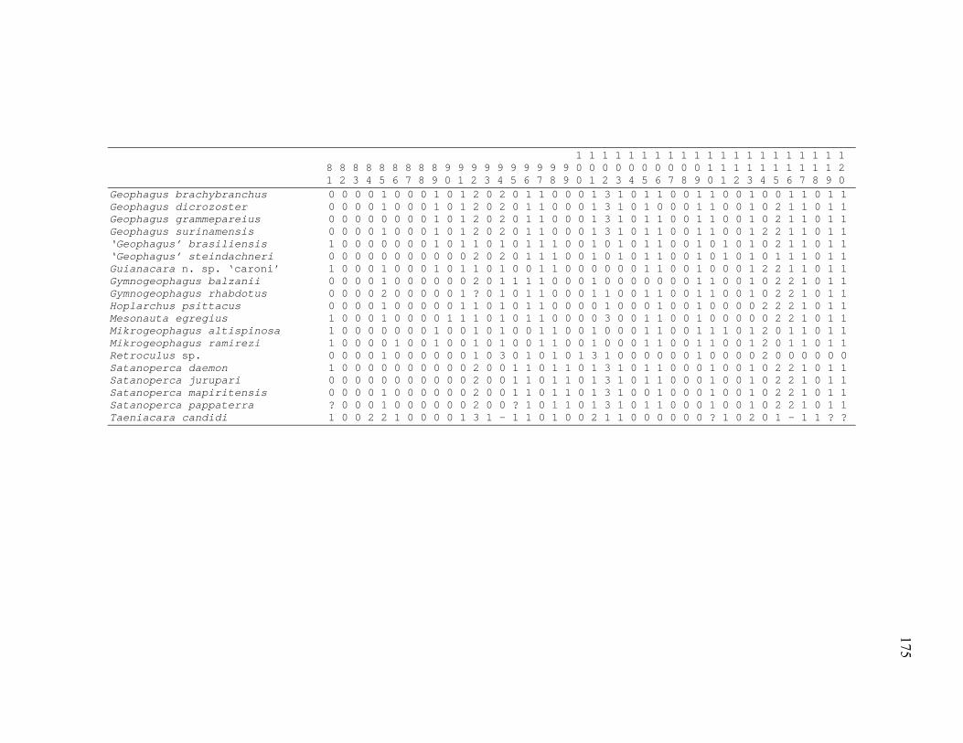
1 1 1 1 1 1 1 1 1 1 1 1 1 1 1 1 1 1 1 1 1 8 8 8 8 8 8 8 8 8 9 9 9 9 9 9 9 9 9 9 0 0 0 0 0 0 0 0 0 0 1 1 1 1 1 1 1 1 1 1 2 1 2 3 4 5 6 7 8 9 0 1 2 3 4 5 6 7 8 9 0 1 2 3 4 5 6 7 8 9 0 1 2 3 4 5 6 7 8 9 0 Geophagus brachybranchus 0 0 0 0 1 0 0 0 1 0 1 2 0 2 0 1 1 0 0 0 1 3 1 0 1 1 0 0 1 1 0 0 1 0 0 1 1 0 1 1 Geophagus dicrozoster 0 0 0 0 1 0 0 0 1 0 1 2 0 2 0 1 1 0 0 0 1 3 1 0 1 0 0 0 1 1 0 0 1 0 2 1 1 0 1 1 Geophagus grammepareius 0 0 0 0 0 0 0 0 1 0 1 2 0 2 0 1 1 0 0 0 1 3 1 0 1 1 0 0 1 1 0 0 1 0 2 1 1 0 1 1 Geophagus surinamensis 0 0 0 0 1 0 0 0 1 0 1 2 0 2 0 1 1 0 0 0 1 3 1 0 1 1 0 0 1 1 0 0 1 2 2 1 1 0 1 1 ‘Geophagus’ brasiliensis 1 0 0 0 0 0 0 0 1 0 1 1 0 1 0 1 1 1 0 0 1 0 1 0 1 1 0 0 1 0 1 0 1 0 2 1 1 0 1 1 ‘Geophagus’ steindachneri 0 0 0 0 0 0 0 0 0 0 0 2 0 2 0 1 1 1 0 0 1 0 1 0 1 1 0 0 1 0 1 0 1 0 1 1 1 0 1 1 Guianacara n. sp. ‘caroni’ 1 0 0 0 1 0 0 0 1 0 1 1 0 1 0 0 1 1 0 0 0 0 0 0 1 1 0 0 1 0 0 0 1 2 2 1 1 0 1 1 Gymnogeophagus balzanii 0 0 0 0 1 0 0 0 0 0 0 2 0 1 1 1 1 0 0 0 1 0 0 0 0 0 0 0 1 1 0 0 1 0 2 2 1 0 1 1 Gymnogeophagus rhabdotus 0 0 0 0 2 0 0 0 0 0 1 ? 0 1 0 1 1 0 0 0 1 1 0 0 1 1 0 0 1 1 0 0 1 0 2 2 1 0 1 1 Hoplarchus psittacus 0 0 0 0 1 0 0 0 0 0 1 1 0 1 0 1 1 0 0 0 0 1 0 0 0 1 0 0 1 0 0 0 0 2 2 2 1 0 1 1 Mesonauta egregius 1 0 0 0 1 0 0 0 0 1 1 1 0 1 0 1 1 0 0 0 0 3 0 0 1 1 0 0 1 0 0 0 0 0 2 2 1 0 1 1 Mikrogeophagus altispinosa 1 0 0 0 0 0 0 0 1 0 0 1 0 1 0 0 1 1 0 0 1 0 0 0 1 1 0 0 1 1 1 0 1 2 0 1 1 0 1 1 Mikrogeophagus ramirezi 1 0 0 0 0 1 0 0 1 0 0 1 0 1 0 0 1 1 0 0 1 0 0 0 1 1 0 0 1 1 0 0 1 2 0 1 1 0 1 1 Retroculus sp. 0 0 0 0 1 0 0 0 0 0 0 1 0 3 0 1 0 1 0 1 3 1 0 0 0 0 0 0 1 0 0 0 0 2 0 0 0 0 0 0 Satanoperca daemon 1 0 0 0 0 0 0 0 0 0 0 2 0 0 1 1 0 1 1 0 1 3 1 0 1 1 0 0 0 1 0 0 1 0 2 2 1 0 1 1 Satanoperca jurupari 0 0 0 0 0 0 0 0 0 0 0 2 0 0 1 1 0 1 1 0 1 3 1 0 1 1 0 0 0 1 0 0 1 0 2 2 1 0 1 1 Satanoperca mapiritensis 0 0 0 0 1 0 0 0 0 0 0 2 0 0 1 1 0 1 1 0 1 3 1 0 0 1 0 0 0 1 0 0 1 0 2 2 1 0 1 1 Satanoperca pappaterra ? 0 0 0 1 0 0 0 0 0 0 2 0 0 ? 1 0 1 1 0 1 3 1 0 1 1 0 0 0 1 0 0 1 0 2 2 1 0 1 1 Taeniacara candidi 1 0 0 2 2 1 0 0 0 0 1 3 1 - 1 1 0 1 0 0 2 1 1 0 0 0 0 0 0 ? 1 0 2 0 1 - 1 1 ? ?

175

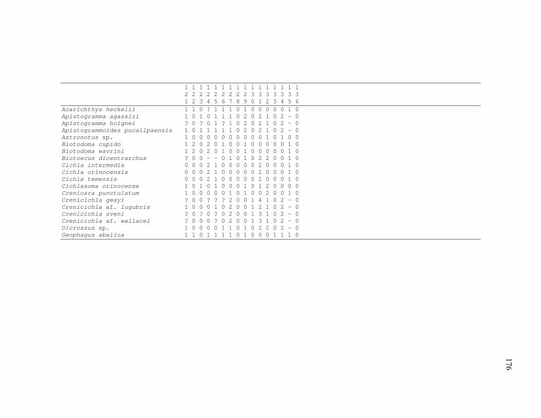
1 1 1 1 1 1 1 1 1 1 1 1 1 1 1 1 2 2 2 2 2 2 2 2 2 3 3 3 3 3 3 3 1 2 3 4 5 6 7 8 9 0 1 2 3 4 5 6 Acarichthys heckelii 1 1 0 ? 1 1 1 0 1 0 0 0 0 0 1 0 Apistogramma agassizi 1 0 1 0 1 1 1 0 2 0 2 1 0 2 – 0 Apistogramma hoignei ? 0 ? 0 1 ? 1 0 2 0 2 1 0 2 – 0 Apistogrammoides pucallpaensis 1 0 1 1 1 1 1 0 2 0 2 1 0 2 – 0 Astronotus sp. 1 0 0 0 0 0 0 0 0 0 0 1 0 1 0 0 Biotodoma cupido 1 2 0 2 0 1 0 0 1 0 0 0 0 0 1 0 Biotodoma wavrini 1 2 0 2 0 1 0 0 1 0 0 0 0 0 1 0 Biotoecus dicentrarchus ? 0 0 - - 0 1 0 1 0 2 2 0 0 1 0 Cichla intermedia 0 0 0 2 1 0 0 0 0 0 2 0 0 0 1 0 Cichla orinocensis 0 0 0 2 1 0 0 0 0 0 2 0 0 0 1 0 Cichla temensis 0 0 0 2 1 0 0 0 0 0 2 0 0 0 1 0 Cichlasoma orinocense 1 0 1 0 1 0 0 0 1 0 1 2 0 0 0 0 Crenicara punctulatum 1 0 0 0 0 0 1 0 1 0 0 2 0 0 1 0 Crenicichla geayi ? 0 0 ? ? ? 2 0 0 1 4 1 0 2 – 0 Crenicichla af. lugubris 1 0 0 0 1 0 2 0 0 1 2 1 0 2 – 0 Crenicichla sveni ? 0 ? 0 ? 0 2 0 0 1 3 1 0 2 – 0 Crenicichla af. wallacei ? 0 0 0 ? 0 2 0 0 1 3 1 0 2 – 0 Dicrossus sp. 1 0 0 0 0 1 1 0 1 0 2 2 0 2 – 0 Geophagus abalios 1 1 0 1 1 1 1 0 1 0 0 0 1 1 1 0

176

1 1 1 1 1 1 1 1 1 1 1 1 1 1 1 1 2 2 2 2 2 2 2 2 2 3 3 3 3 3 3 3 1 2 3 4 5 6 7 8 9 0 1 2 3 4 5 6 Geophagus brachybranchus 1 1 0 1 1 1 1 0 1 0 0 0 1 1 1 0 Geophagus dicrozoster 1 1 0 1 1 1 1 0 1 0 0 0 1 1 1 0 Geophagus grammepareius 1 1 0 1 1 1 1 0 1 0 0 0 1 1 1 0 Geophagus surinamensis 1 1 0 1 1 1 1 0 1 0 0 0 1 1 1 0 ‘Geophagus’ brasiliensis ? 2 0 0 0 1 1 0 1 0 2 2 0 0 1 0 ‘Geophagus’ steindachneri 1 1 0 1 1 1 1 0 1 0 2 0 0 1 1 0 Guianacara n. sp. ‘caroni’ 1 1 0 2 1 1 0 0 1 0 0 0 0 0 1 0 Gymnogeophagus balzanii 1 1 0 1 1 1 2 1 1 0 0 0 0 1 1 0 Gymnogeophagus rhabdotus 1 2 0 1 1 1 2 1 1 0 0 2 0 1 1 0 Hoplarchus psittacus 1 2 0 0 1 0 0 0 1 0 0 2 0 1 1 1 Mesonauta egregius 1 2 0 0 1 0 0 0 1 0 0 1 0 1 1 1 Mikrogeophagus altispinosa 1 0 0 2 1 0 1 0 1 0 0 2 0 0 1 0 Mikrogeophagus ramirezi 1 0 0 0 0 0 1 0 1 0 0 2 0 0 1 0 Retroculus sp. 0 1 0 1 0 1 0 0 0 0 0 0 0 0 0 0 Satanoperca daemon 1 1 0 0 1 1 1 0 1 0 1 0 0 1 1 0 Satanoperca jurupari 1 1 0 1 1 1 1 0 1 0 1 0 0 1 1 0 Satanoperca mapiritensis 1 1 0 1 1 1 1 0 1 0 1 0 0 1 1 0 Satanoperca pappaterra 1 1 0 ? 1 1 1 0 1 0 1 0 0 1 1 0 Taeniacara candidi ? 0 0 - - 0 1 0 2 0 2 1 0 2 – 0

177

178

VITA

Hernán López Fernández

Apartado Postal 506, Mérida 5101, Edo. Mérida, Venezuela

Education

2004 PhD. Wildlife and Fisheries Sciences, Texas A&M University

1998 B.S. Biology, Universidad de Los Andes, Venezuela

Honors, Awards & Fellowships

2004 Ph.D. Student Award. Wildlife and Fisheries Sciences, Texas A&M University

2003 Best Oral Presentation, Neotropical Ichthyological Association

2001, 2003 Axelrod Fellowship, Department of Ichthyology, American Museum of

Natural History

1991-1996 “Award to Talent” Program, Undergraduate Scholarship, Fundación Gran

Mariscal de Ayacucho (Venezuelan Government)

Peer Reviewed Publications

López-Fernández, H. & D.C. Taphorn. 2004. Geophagus abalios, G.

dicrozoster and G. winemilleri (Perciformes: Cichlidae), three new species from

Venezuela. Zootaxa, 439: 1-27.

López-Fernández, H. & K. O. Winemiller. 2003. Morphological variation in

Acestrorhynchus microlepis and A. falcatus (Characiformes: Acestrorhynchidae),

reassessment of A. apurensis and distrinution of Acestrorhynchus in Venezuela.

Ichthyological Exploration of Freshwaters, 14: 193-208.

López-Fernández, H. & K. O. Winemiller. 2000. A review of Venezuelan

species of Hypophthalmus (Siluriformes: Pimelodidae). Ichthyological Exploration of

Freshwaters, 11:35-46.

phylogeny of geophagine cichlids from south america - CORE

Documents

Transcript of phylogeny of geophagine cichlids from south america - CORE