Pheromone and volatile lures for detecting the European house borer ( Hylotrupes bajulus ) and a...
70
Australian Forestry Australian Forestry is published by the Institute of Foresters of Australia (IFA) for technical, scientific and professional communication relating to forestry in Australia and adjacent geographic regions. The views expressed in this journal are not necessarily those of the IFA. The journal is included in the Register of Refereed Journals maintained by the Australian Government Department of Education, Science and Training. The IFA gratefully acknowledges a grant provided by the Australian Government and State and Territory forestry and forest products agencies through the Forestry and Forest Products Committee to assist in the preparation and production of Australian Forestry. Managing Editor: Dr Brian Turner Production Editor: Mr Alan Brown Editorial Panel: Dr Stuart Davey Dr Ross Florence Dr Graeme Siemon Mr Neil (Curly) Humphreys Dr Ian Bevege Dr John Herbohn Dr Grant Wardell-Johnson Dr Humphrey Elliott Contributions Contributions to this journal are sought covering any aspect of forest ecology, forest management, forest policy and land use related to Australia and the South Pacific region. Contributions related to the performance of Australian tree genera elsewhere in the world are also welcome. Instructions to authors are given inside the back cover of each issue. Contributions should be sent to the Executive Director at the address below. This issue This issue of Australian Forestry presents the sixth paper in the series titled ‘Achievements in the genetic improvement of forest trees in Australia and New Zealand’, which was introduced in the last issue. Journal subscriptions 2008 A$250 including GST within Australia A$280 per year in all other countries The above prices are for hardcopy. For information about options for electronic access and pricing, please contact the Executive Director at the address below. All correspondence relating to subscriptions should be addressed to: Executive Director, The Institute of Foresters of Australia, PO Box 7002, Yarralumla, ACT 2600, Australia. Phone: 61 2 6281 3992. Fax: 61 2 6281 4693. Email: [email protected] Web: http://www.forestry.org.au Cover The front cover features African mahogany, Khaya senegalensis. This is a promising plantation tree for northern Australia, tolerant of difficult sites and producing a high-value timber. The story behind the recognition of its promise, and work to realise its potential, are described by Garth Nikles on pages 68–69 of Volume 69 of Australian Forestry. He also selected the photos and prepared the captions. Photo 1. Butt logs (mainly), from selected trees in 32-y-old, unmanaged stands of African mahogany grown in the Darwin region of the Northern Territory (NT). They were used in a study of sawn timber recovery, timber drying schedules and wood properties, and for manufacturers’ evaluations of the timber. (Photo by courtesy of Don Reilly.) Photo 2. Award-winning set of chess table and chairs made from timber from a sample of the logs of Photo 1. It won three ‘Australian Furniture of the Year Awards, 2004’ sponsored by the Furniture Industry Association of Australia: the Queensland and national awards in the category ‘Excellence in furniture using Australian plantation timber’; and the Queensland ‘Best-of-the-best’ (across categories) award. (Photo by courtesy of Ray Burgess, Sight Photographics, via the manufacturer, Paragon Furniture, Brisbane.) Photo 3. A rooted cutting of African mahogany at 10 mo from planting in a clone test established in the Darwin region of the NT in January 2005. At 12 mo from planting, some trees were nearly 3.5 m high. (Photo by courtesy of Beau Robertson.) Photo 4. Pods on a graft of African mahogany in a clonal seed orchard planted near Darwin in December 2001. The pods are about 35 mm in diameter some 3 mo after flowering. (Photo by courtesy of Beau Robertson.) Photo 5. Part of an unmanaged stand of African mahogany aged 25 y derived from natural-stand seed. It was established on back-filled land following surface mining for bauxite at Weipa, Queensland. The central, dominant tree is 48 cm dbhob and one of 36 superior trees selected so far and used in the conservation and genetic improvement program at Weipa. (Photo by courtesy of Alan Bragg.) Photo 6. A pruned, 8-y-old stand of African mahogany, derived from unimproved seed, planted privately at 5 m × 2.5 m (800 trees ha –1 ), not thinned, near Bowen, in coastal central Queensland. The tree being measured had a dbhob of 17.1 cm. (Photo by courtesy of Geoff Dickinson.) ISSN 0004-9158
-
Upload
independent -
Category
Documents
-
view
2 -
download
0
Transcript of Pheromone and volatile lures for detecting the European house borer ( Hylotrupes bajulus ) and a...

Australian ForestryAustralian Forestry is published by the Institute of Foresters of Australia (IFA) for technical, scientific andprofessional communication relating to forestry in Australia and adjacent geographic regions. The views expressedin this journal are not necessarily those of the IFA. The journal is included in the Register of Refereed Journalsmaintained by the Australian Government Department of Education, Science and Training.
The IFA gratefully acknowledges a grant provided by the Australian Government and State and Territory forestryand forest products agencies through the Forestry and Forest Products Committee to assist in the preparation andproduction of Australian Forestry.
Managing Editor: Dr Brian Turner Production Editor: Mr Alan Brown
Editorial Panel: Dr Stuart Davey Dr Ross Florence Dr Graeme SiemonMr Neil (Curly) Humphreys Dr Ian Bevege Dr John HerbohnDr Grant Wardell-Johnson Dr Humphrey Elliott
Contributions
Contributions to this journal are sought covering any aspect of forest ecology, forest management, forest policyand land use related to Australia and the South Pacific region. Contributions related to the performance ofAustralian tree genera elsewhere in the world are also welcome. Instructions to authors are given inside the backcover of each issue. Contributions should be sent to the Executive Director at the address below.
This issue
This issue of Australian Forestry presents the sixth paper in the series titled ‘Achievements in the geneticimprovement of forest trees in Australia and New Zealand’, which was introduced in the last issue.
Journal subscriptions 2008
A$250 including GST within Australia A$280 per year in all other countries
The above prices are for hardcopy. For information about options for electronic access and pricing, please contactthe Executive Director at the address below.
All correspondence relating to subscriptions should be addressed to: Executive Director, The Institute ofForesters of Australia, PO Box 7002, Yarralumla, ACT 2600, Australia. Phone: 61 2 6281 3992.Fax: 61 2 6281 4693. Email: [email protected] Web: http://www.forestry.org.au
Cover
The front cover features African mahogany, Khaya senegalensis. This is a promising plantation tree for northernAustralia, tolerant of difficult sites and producing a high-value timber. The story behind the recognition of itspromise, and work to realise its potential, are described by Garth Nikles on pages 68–69 of Volume 69 ofAustralian Forestry. He also selected the photos and prepared the captions.Photo 1. Butt logs (mainly), from selected trees in 32-y-old, unmanaged stands of African mahogany grown in theDarwin region of the Northern Territory (NT). They were used in a study of sawn timber recovery, timber dryingschedules and wood properties, and for manufacturers’ evaluations of the timber. (Photo by courtesy of Don Reilly.)Photo 2. Award-winning set of chess table and chairs made from timber from a sample of the logs of Photo 1. Itwon three ‘Australian Furniture of the Year Awards, 2004’ sponsored by the Furniture Industry Association ofAustralia: the Queensland and national awards in the category ‘Excellence in furniture using Australian plantationtimber’; and the Queensland ‘Best-of-the-best’ (across categories) award. (Photo by courtesy of Ray Burgess,Sight Photographics, via the manufacturer, Paragon Furniture, Brisbane.)Photo 3. A rooted cutting of African mahogany at 10 mo from planting in a clone test established in the Darwinregion of the NT in January 2005. At 12 mo from planting, some trees were nearly 3.5 m high. (Photo by courtesyof Beau Robertson.)Photo 4. Pods on a graft of African mahogany in a clonal seed orchard planted near Darwin in December 2001.The pods are about 35 mm in diameter some 3 mo after flowering. (Photo by courtesy of Beau Robertson.)Photo 5. Part of an unmanaged stand of African mahogany aged 25 y derived from natural-stand seed. It wasestablished on back-filled land following surface mining for bauxite at Weipa, Queensland. The central, dominanttree is 48 cm dbhob and one of 36 superior trees selected so far and used in the conservation and geneticimprovement program at Weipa. (Photo by courtesy of Alan Bragg.)Photo 6. A pruned, 8-y-old stand of African mahogany, derived from unimproved seed, planted privately at 5 m ×2.5 m (800 trees ha–1), not thinned, near Bowen, in coastal central Queensland. The tree being measured had adbhob of 17.1 cm. (Photo by courtesy of Geoff Dickinson.)
ISSN 0004-9158

ACN 083 197 586
Australian Forestry
Volume 70 Number 2, 2007
ISSN 0004-9158
The Journal of the Institute of Foresters of Australia

Australian Forestry, Volume 70 Number 2, June 2007
Contents
73 Guest editorial: Collaboration between the Australian and New Zealand Institutes of ForestersIan Ferguson
75 Achievements in forest tree genetic improvement in Australia and New Zealand6: Genetic improvement and conservation of Araucaria cunninghamii in QueenslandMark J. Dieters, D. Garth Nikles and Murray G. Keys
86 Physical and mechanical properties of plantation-grown Acacia auriculiformis of three different agesS.R. Shukla, R.V. Rao, S.K. Sharma, P. Kumar, R. Sudheendra and S. Shashikala
93 A regionalised growth model for Eucalyptus globulus plantations in south-eastern AustraliaYue Wang and Thomas G. Baker
108 Developing a carbon stocks and flows model for Australian wood productsGary P. Richards, Chris Borough, David Evans, Ainslie Reddin, Fabiano Ximenes and David Gardner
120 Predicting wood value in Queensland Caribbean pine plantations using a decision support systemKerrie Catchpoole, Marks R. Nester and Kevin Harding
125 Forest valuation and the AASB 141 accounting standardIan Ferguson and Jerry Leech
134 Short communication: Pheromone and volatile lures for detecting the European house borer(Hylotrupes bajulus) and a manual sampling methodAaron D. Gove, Richard Bashford and Cameron J. Brumley
137 Book review: Terania Creek: Rainforest WarsBrian Turner
138 Book review: The Forest Certification HandbookPeter Kanowski

73Ian Ferguson
Australian Forestry 2007 Vol. 70 No. 2 pp. 73–74
Guest editorial
Collaboration between the Australian and New Zealand Institutes of Foresters
The ANZIF Conference held in June 2007 marked some 27 yearssince the first such conference involving collaboration betweenthe Institute of Foresters of Australia (IFA) and the New ZealandInstitute of Forestry (NZIF). Closer collaboration to helpunderpin the scientific basis of forestry, policy directions andstandards of forest management within our region has beendiscussed by the membership and boards of the institutes. Whathas been achieved to date and what directions should future trans-Tasman collaboration take?
The first ANZIF Conference was held at Rotorua in 1980, withenthusiastic collaboration between Wink Sutton of the NewZealand Institute of Forestry (NZIF) and me. We shared the view,as did our respective institute governing boards, that our twoeconomies would become increasingly integrated and that wehad much to learn from each other in relation to forestry.Subsequent meetings were held in Hobart in 1985, Christchurchin 1991, Canberra in 1997 and Queenstown in 2003, with CoffsHarbour the location in June 2007. The increasing frequencyperhaps reflects an increasing awareness of the interwovenenvironment in which the institutes now operate.
If the published reports and personal memories of these meetingsare any guide, they were professionally useful and convivial. Theywere not, of course, the only source of interchange betweenmembers of the two institutes, thanks in part to the decline ofreal (i.e. deflated) costs of air travel between the two countries.But ANZIF is distinctive in embracing all elements of forestry1
in membership and attendance, rather than involving a highlyspecialised audience or single topic. Both institutes are rightlyproud of their orientation towards the professional practice offorest management and the forest science to guide it, withoutbeing precious or exclusive about that orientation.
Many changes have occurred in forestry and other interchangesbetween the two countries over this period. The extent of trans-Tasman changes of employment of members and potentialmembers has grown as privatisation, commercialisation andformal collaborations have proceeded. The 2003 conferencecoincided with the 20th anniversary of Closer EconomicRelations between the two countries — a relationship that hasresulted ‘in unprecedented integration’ between the twoeconomies according to the Director-General of the NewZealand Ministry for Agriculture and Forestry2. Industrial
plantation and forest industry ownership now reflects thatintegration, as well as the growing trends in globalisation. Therespective national institutes of forest research are collaboratingthrough a partnership under the Ensis flag. Through that and othercollaborative arrangements, regular interchanges exist in treebreeding, forest and timber disease and pest issues, valuation,fire protection and other areas. The Primary IndustriesMinisterial Council and Natural Resource ManagementMinisterial Council include New Zealand representation and havereplaced the earlier Australian Forestry Council.
Understandably, both institutes have been somewhat passivetowards these changes because most have been beyond the reachof their influence. The aftermath of the 2007ANZIF Conferenceprovides a timely opportunity to review the relationship betweenthe institutes and to chart some future strategies in the light offurther changes of similar character in the future. Three questionsloom large in addressing these changes:
1. Would a strengthened and/or more formal relationship helpthe respective institutes to meet their aims and objectives?
2. Would a strengthened and/or more formal relationshipprovide better services and/or lower costs to members?
3. What form should such a relationship or structure take andshould it be restricted to the two nations?
Effectiveness
Most of the policy issues of concern to the respective institutesrelate to specific state and national concerns, so these are notprimarily the basis for a strengthened relationship. Some issues,such as illegal logging, forest practices in neighbouringcountries, international trade and marketing, poverty alleviationand climate change are of mutual concern. It might heighten thepublic standing of both institutes if they could speak with acommon voice on these matters. Certification seems likely tobecome much more common within both countries and in ournear neighbours. This raises issues concerning mutual recogni-tion of registration (Registered Professional Forester (RPF) andRegistered Forestry Consultant (RFC)) schemes, nationalplantation standards, valuers and certifiers, and mutual offeringsfor professional development, both in relation to plantations inthe two countries and more generally in the South Pacific andAsian regions.
Regrettably, the history of mutual recognition of standards fortimber grading suggests that mutual policy goals are not alwayssimple to achieve, as witness the recent advent of differentstandards in the two countries. However, recognition andacceptance of irreconcilable differences is as essential toeffectiveness of an integrating entity as adopting commonground, as the Australian history of differences between the IFA’sstate divisions has shown from time to time.
1‘Forestry’, according to the IFA website, is ‘the practical application of scientific,economic and social principles to the establishment and management of ecosystemsdominated by trees, or at least where trees are major components of an ecosystem’.The NZIF website defines it as ‘the art and science of managing forests so as tosecure a wide range of environmental and socio-economic benefits’. Users of MSWord© software (and the institute boards) may wish to contrast these definitionswith those in the Word© dictionary which collectively limit the scope greatly.2See Stephen Jacobi (2003) ANZIF — Seeing the woods through the weeds. NewZealand Journal of Forestry 48(2), 2–3, http://www.nzjf.org/contents.php?volume_issue=j48_2

74 Collaboration between the Australian and New Zealand Institutes of Foresters
Australian Forestry 2007 Vol. 70 No. 2 pp. 73–74
Efficiency
Efficiencies, be they in lower costs, better services, or both,loom large in any consideration of the future of two relativelysmall institutes. The IFA currently has about 1240 members,NZIF 750. Some growth in membership is likely to follow fromthe harvesting and marketing of the increased potential supplyof wood over the next two decades, together with (hopefully)some increase in fire management and farm forestry roles. Thatgrowth is unlikely to be dramatic, being limited by the economiesof scale we are now seeing materialise. The combined number,though still relatively small, offers scope to explore and developefficiencies in administration, communication and registration,so there is a pressing need to look for cost savings and/or serviceimprovements within current costs.
Administration is in some ways the most difficult area of changebecause the two Institutes have somewhat different systems andannual charges at present. The IFA has a full-time ExecutiveDirector and Member Services Manager, and the NZIF only apart-time administrator. Consequently annual IFA membershipfees are almost twice those of the NZIF for voting members.Both use extensive voluntary and quasi-voluntary support (viahonoraria) for editing, and in the case of the NZIF for BoardSecretary work. A detailed investigation would be appropriatebecause there are potential economies of scale and scopeinvolved. Location of the administration should not matter muchin an era of increasing reliance on electronic communication,especially if the head of any joint body or arrangement rotatedbetween the countries, assisted by each president.
Communication is an area most likely to undergo radical changeover the next decade or two. Older members may lament it butpurely newsletter-type publications will be replaced by internetnewsletters, as witness the uptake and success of the FridayOffcuts, published by Innovatek Ltd in partnership with theAustralian Plantation Products and Paper Industry Council (A3P),Ensis, and others.
The scientific publications of both institutes are available onthe web but unfortunately they are not indexed by the leadingglobal abstracting services and will therefore be ignored by thescientific community. This indexing has become essential in thescientific world3 and, in my view, dooms both journals to thescrap heap of history, unless changed. Efficiencies are alsoneeded with respect to editing, which I suspect has outstrippedor will soon outstrip volunteer or quasi-volunteer efforts. Amerger would provide scale for two publications (one scientificand one professional) to replace the present four, greaterattractiveness to libraries, greater administrative assistance tothe editorial panels, and a better opportunity to bear the costsinvolved.
As noted earlier, registration is an area likely to increasesubstantially over the next decade or two, in line with the earlierobservations regarding certification and illegal logging and poorforest practices in neighbouring countries. Privatisation andcommercialisation in combination with certification and anincreasingly litigious world will also push this along. The two
systems of the institutes differ, but not so radically that commonground could not be found. That common ground might also assistemployment interchanges and opportunities across the Tasmanbecause the two economies are seldom exactly synchronised.The annual NZIF charges for registration on a continuing basisappear to be higher than those of the IFA.
Structure
If there is a role for greater integration between the IFA andNZIF, what form should it take? The devil is in the detail, and thepreceding sections have charted some of the detail that needs tobe worked through jointly before seizing on some grand plan.Greater integration need not imply a merger, although in my viewthat might well be a long-term (10-year) goal if my concernsabout the future membership, financial viability, communicationand employment trends are shared. There are many potentialintermediate steps, especially in communication and administra-tion, that would assist in strengthening the bridges between thetwo institutes. Such moves could be managed by a joint not-for-profit company with a board consisting of a chair and the twopresidents overseeing joint administration services operatingunder supply contracts to the parent institutes.
Nothing would dissuade each side more quickly and absolutelythan to propose a take-over of one institute by the other. Main-taining national identities and regional structures is therefore aparamount consideration in any discussion of greater integration.That means the governing bodies and their key committees wouldneed to operate on a federal system, with an agreed hierarchy ofpowers, especially in relation to policies and practices that areoften inherently national or regional in character.
If, in the long run, a merger was to be contemplated, thoughtmight also be given to our near-neighbours and their involvement,building on the IFA board’s recent initiative in launching theTropical Forest Interest Group. Clearly, that would be a second-order issue until the trans-Tasman house is in order. But manyof the arguments extend to our near neighbours with even greaterforce because of their stage of development. Extension to a SouthPacific entity would obviously need support and funding fromour two governments and/or aid agencies.
Conclusion
If the Australian and New Zealand memberships and theirrespective boards share any of the concerns expressed above,the two institutes need to chart some strategies to investigatethe issues prior to the next ANZIF conference, so that joint actionmight then be considered and set in motion. This requires a lotof detailed work by small joint committees based on clear termsof reference and reporting requirements, with some championsto drive them along. This may seem like an old fart’s ‘hastenslowly’ dictum, but is as much a case of ‘hasten surely’ — thereis much at stake; not least, survival of the institutes.
Ian Ferguson FIFA
Professor Emeritus of Forest ScienceThe University of Melbourne
1 See Alan Brown (2006) Visited a library lately? The Forester 49(4), 26.
75Mark J. Dieters, D. Garth Nikles and Murray G. Keys
Australian Forestry 2007 Vol. 70 No. 2 pp. 75–85
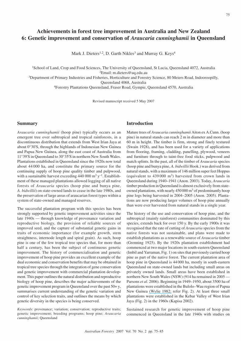
Achievements in forest tree improvement in Australia and New Zealand6: Genetic improvement and conservation of Araucaria cunninghamii in Queensland
Mark J. Dieters1,2, D. Garth Nikles3 and Murray G. Keys4
1School of Land, Crop and Food Sciences, The University of Queensland, St Lucia, Queensland 4072, Australia2Email: [email protected]
3Department of Primary Industries and Fisheries, Horticulture and Forestry Science, 80 Meiers Road, Indooroopilly,Queensland 4068, Australia
4Forestry Plantations Queensland, Fraser Road, Gympie, Queensland 4570, Australia
Revised manuscript received 5 May 2007
Summary
Araucaria cunninghamii (hoop pine) typically occurs as anemergent tree over subtropical and tropical rainforests, in adiscontinuous distribution that extends from West Irian Jaya atabout 0°30'S, through the highlands of Indonesian New Guineaand Papua New Guinea, along the east coast of Australia from11°39'S in Queensland to 30°35'S in northern New South Wales.Plantations established in Queensland since the 1920s now totalabout 44 000 ha, and constitute the primary source for thecontinuing supply of hoop pine quality timber and pulpwood,with a sustainable harvest exceeding 440 000 m3 y–1. Establish-ment of these managed plantations allowed logging of all nativeforests of Araucaria species (hoop pine and bunya pine,A. bidwillii) on state-owned lands to cease in the late 1980s, andthe preservation of large areas of araucarian forest types within asystem of state-owned and managed reserves.
The successful plantation program with this species has beenstrongly supported by genetic improvement activities since thelate 1940s — through knowledge of provenance variation andreproductive biology, the provision of reliable sources ofimproved seed, and the capture of substantial genetic gains intraits of economic importance (for example growth, stemstraightness, internode length and spiral grain). As such, hooppine is one of the few tropical tree species that, for more thanhalf a century, has been the subject of continuous geneticimprovement. The history of commercialisation and geneticimprovement of hoop pine provides an excellent example of thedual economic and conservation benefits that may be obtained intropical tree species through the integration of gene conservationand genetic improvement with commercial plantation develop-ment. This paper outlines the natural distribution and reproductivebiology of hoop pine, describes the major achievements of thegenetic improvement program in Queensland over the past 50+ y,summarises current understanding of the genetic variation andcontrol of key selection traits, and outlines the means by whichgenetic diversity in the species is being conserved.
Keywords: provenance; variation; conservation; reproductive traits;genetic improvement; breeding programs; hoop pine; Araucariacunninghamii; Queensland
Introduction
Mature trees of Araucaria cunninghamii Aiton ex A.Cunn. (hooppine) in natural stands can reach 2 m in diameter and more than60 m in height. The timber is firm, strong and finely textured(Swain 1928), and has been used for a variety of applicationsfrom flooring, framing, cladding, panelling, plywood, veneersand furniture through to taint-free food sticks, pulpwood andmatch splints. In the past, all of the timber of Araucaria species(hoop pine and bunya pine, A. bidwillii Hook.) was derived fromnatural stands, with a maximum of 146 million super feet Hoppus(equivalent to 439 000 m3) harvested from crown lands inQueensland during 1940–1941 (Anon. 2003). Today, Araucariatimber production in Queensland is almost exclusively from state-owned plantations, with nearly 450 000 m3 of predominantly hooppine logs being harvested in 2004–2005 (Anon. 2005). Planta-tions are now producing larger volumes of hoop pine annuallythan were ever harvested from natural stands in a single year.
The history of the use and conservation of hoop pine, and thesubtropical (mainly rainforest) communities dominated by thisspecies, extends back for over 150 y. By the early 1900s it wasrecognised that the rate of cutting of Araucaria species from thenative forests was not sustainable, and plans were made toestablish plantations as a renewable source of Araucaria timber(Grenning 1925). By the 1920s plantation establishment hadcommenced at two major locations in south-eastern Queensland(Imbil and Yarraman, Fig. 1) on sites that previously carried hooppine as part of the native forest. The current plantation area ofhoop pine in Queensland is 44 000 ha, mostly in south-easternQueensland on state-owned lands but including small areas onprivately owned lands. Small areas have been established innorthern New South Wales (NSW) (914 ha remained in 2005 —Parsons et al. 2006). Beginning in 1949–1950, about 3500 ha ofplantations were established in the Bulolo–Wau region of PapuaNew Guinea (Wylie 1982; refer Fig. 2). At least three smallplantations were established in the Kebar Valley of West IrianJaya (Fig. 2) in the 1960s (Kapisa 2002).
Sustained research for genetic improvement of hoop pinecommenced in Queensland in the late 1940s with studies on

76 Genetic improvement and conservation of Araucaria cunninghamii
Australian Forestry 2007 Vol. 70 No. 2 pp. 75–85
Mts Suckling and Dayman, and Bulolo–Wau regions of PNG(Gray 1973, Fig. 2).
The distribution is highly disjunct and encompasses diverseenvironmental types. Soils range from Rudosols to Ferrosols(McKenzie et al. 2004) developed on a broad suite of parentmaterials including sands, igneous and metamorphic rocks; meanannual rainfall varies from 750–1600 mm in Australia to 1600 to>5800 mm in PNG; and altitude extends from sea level to 1000 min Australia and 500–2800 m in PNG (Howcroft 1978; Boland etal. 1985). The species occurs in six of the Queensland bioregionsdefined by Sattler and Williams (1999) (Fig. 3) and in five foresttypes in NSW (refer to subsequent section on ‘Conservation ofgenetic resources’). However, the species is sensitive to fire andsevere frost, being limited to sites where the mean temperaturein the coldest month is >2°C (Jovanovic and Booth 2002).
Reproductive biology
A brief account of some key aspects of the reproductive biologyof hoop pine is provided here; Nikles et al. (in press) give moredetail. As is common in many coniferous species, hoop pine ismonoecious (cones of both sexes occur on the one tree), unisexual(the female and male cones are separate) and is predominantly across-pollinated (that is, outcrossing) species. However, a numberof unusual features of the reproductive biology and growth habitsof hoop pine have affected the genetic improvement program.Some of these features and how they have been accommodatedare outlined below.
Normally, planted trees do not produce substantial pollen cropsuntil some 25 y of age, but female cones are produced from aroundage 12 y, and relatively regularly. No reliable means has beenfound to close the age gap between male and female reproduction,so mixed-generation mating has been adopted in the breedingprogram to reduce the length of breeding cycles.
Provenances differ by several months in their periods of anthesis.For example, in some provenances anthesis occurs as early asDecember and January while in others anthesis is delayed untilApril–June. Such provenances are reproductively isolated. Thismeans that seed orchards can be effectively isolated fromcontaminating pollen if located within plantations of hoop pinethat have been established using planting stock of a differentanthesis period. Similarly, the long time-lag between plantingand production of pollen has potential advantages for the isolationof seed orchards. If seed orchards are established in the midst ofyoung plantations, the delay in the onset of male flowering in thelatter provides a window of up to 25 y when there is effectiveisolation from contaminant pollen. As a consequence of thesetwo features, seed orchards need not be established on sitesisolated from the main plantation program, which in turn makestheir maintenance and protection much easier.
Hoop pine has fixed shoot systems. Thus a shoot, once differen-tiated as a lateral shoot, always remains as a branch or branchlet(of plagiotropic habit); shoots emanating, under certainconditions, from leaf axils between branch whorls on the mainstem, however, take on and retain an upright, tree-like, i.e.orthotropic, habit. Consequently, if lateral shoots are grafted ontoseedling rootstock, trees with a plagiotropic (branch-like) form
0 100 km
Figure 1. The location (•) of some provenance tests (Imbil, Yarraman)and provenance seed collections of Araucaria cunninghamii in south-eastern Queensland and northern New South Wales, and of grafted seedorchards (Imbil, Yarraman and Toolara)
reproductive biology and means to control crossing (Nikles etal. 1988). Later, many thousands of hectares of plantations weresearched for superior trees, resulting in >200 000 trees beingplanted in progeny tests since the 1950s and the establishment ofmany clonal seed orchards since 1965. All new plantations since1985 have been established with stock from orchard seed, yieldinglarge genetic gains. Technologies have been developed foroperational controlled crossing — enabling family forestry to beimplemented through seedlings of superior families — and forvegetative propagation via stem cuttings, though the latter is notcurrently in use. Provenance variation, provenance hybridisationand genetic parameters of the species have also been studied.These achievements, background information and the conserva-tion status of hoop pine are outlined in this paper.
Natural distribution
Hoop pine typically occurs naturally as an emergent in manyrainforests and some woodlands and shrublands from theSausapor region of West Irian Jaya (Indonesia, 0°30'S) throughIndonesian New Guinea and Papua New Guinea (PNG), and alongthe eastern coast of Queensland from Captain Billy Creek(11°39'S) to the upper reaches of the Macleay River in northernNSW (30°35'S; refer Figs 1, 2 and 3). However, it is naturallymost abundant in south-eastern Queensland and northern NSWwithin 300 km of Brisbane (Fig. 3) and the Telefomin–Oksapmin,

77Mark J. Dieters, D. Garth Nikles and Murray G. Keys
Australian Forestry 2007 Vol. 70 No. 2 pp. 75–85
result. This type of plagiotropic graft, ifmade using branch tips taken from thepollen-bearing portion of the crown on asexually mature tree, will produce pollenwithin a few years of grafting.
Grafts with an orthotropic growth habitare produced for clone banks and seedorchards by grafting scions excised froma short length (40–50 mm) of leadingshoot taken from the main stem of treesolder than 12 y. Each orthotropic scioncomprises a few leaves and tissue as deepas the outer xylem in order to includeaxillary meristems (Burrows 1987). Theseorthotropic grafts tend to produce femalestrobili within 2 y of grafting, but littlepollen for up to 10–15 y after grafting.
The differential flowering patterns inplagiotropic and orthotropic grafts isthought to be related to the position in thecrown from which the grafting material isobtained. Mature hoop pine trees tend toproduce female reproductive structures inonly the upper part of the crown and pollenin only the central part of the crown; thisis thought to be an adaptation to minimiseself-pollination.
Viable seeds can be quickly produced from a clonal hoop pineseed orchard established with a mixture both plagiotropic andorthotropic grafts. The plagiotropic grafts provide the main sourceof pollen in the earlier life of the orchard, and the orthotropicgrafts act as the seed parents. As the orchard ages, the orthotropicgrafts increasingly supplement pollen production as well asproducing increasing amounts of seed. Cooler, drier sites havebeen found to be the most suitable for seed production; neworchards established on these sites have produced reasonablequantities of viable seed within 5 y of field-grafting. This is oneexample of how the fixed shoot systems in hoop pine have beenused to assist the development of genetically improved seedsupplies.
Mature trees will produce juvenile coppice when felled or girdled— thus clonal propagation strategies similar to those usedeffectively in tropical eucalypts could potentially be used in hooppine. However, as a consequence of the fixed shoot systems andstrong apical dominance in hoop pine, this species cannot behedged efficiently, and multiplication rates using cuttings or tissueculture are very low compared to those possible with many Pinusand Eucalyptus species. Consequently, although juvenile shoots(obtained from coppice shoots or seedlings) can be propagatedreadily by the rooting of cuttings, vegetative propagation ofplanting stock using cuttings has not been cost effective.
Genetic variation
Provenance variation
Provenance trials planted in south-eastern and northernQueensland between 1929 and 1956 were reviewed by Reilly
Queensland bioregions in which hoop pine occurs:
BRB – Brigalow Belt
CQC – Central Queensland Coast
CYP – Cape York Peninsula
EIU – Einasleigh Uplands
SEQ – Southeast Queensland
WET – Wet Tropics
0 400 km
BRISBANE
Figure 3. The approximate natural distribution of Araucariacunninghamii in Australia. (Adapted from Jovanovic and Booth (2002)by T. Jovanovic in 2007 for this paper.) The identified bioregions inwhich the species occurs are those in Queensland (Sattler and Williams1999).
Figure 2. The approximate distribution of Araucaria cunninghamii in New Guinea showingthe three regions of most widespread occurrence in Papua New Guinea (Telefomin–Oksapmin,Bulolo–Wau and Mts Suckling and Dayman) and four occurrences (of many) in eastern CapeYork Peninsula, Queensland, mentioned in the text. Map compiled from data on occurrencesof the species given by Gray (1973) and Howcroft (1978).

78 Genetic improvement and conservation of Araucaria cunninghamii
Australian Forestry 2007 Vol. 70 No. 2 pp. 75–85
(1974). Most of the provenances included in these trials werefrom areas in south-eastern Queensland, but a few trials alsoincluded some PNG and NSW (Dorrigo; Fig. 1) provenances.The most promising provenances for growth and stem straightnesswere from Jimna, Emu Vale and Gallangowan (Fig. 1).
The results were subsequently confirmed by a more compre-hensive series of trials established between 1971 and 1973throughout Queensland and northern NSW (Nikles and Newton1983). These trials included more than 400 open-pollinatedfamilies from about 40 provenances. Based on stem volume at20 y and stem straightness at 15 y (unpublished data), the mostpromising provenances on sites in south-eastern Queensland werethose from Goodnight Scrub, Jimna, Miva and Yarraman (Fig. 1).This information was used to modify the breeding strategy (see‘Breeding strategy’ below).
Genetic parameters
Estimates of genetic parameters for key selection traits in hooppine have been published by a number of authors, including Deanet al. (1988), Dieters et al. (1990), Eisemann et al. (1990) andHarding and Woolaston (1991). Estimates obtained from a reviewof over 20 control- and open-pollinated progeny tests(unpublished results, Table 1) indicate that growth traits andstraightness have low but useful heritability, while the heritabilityof internode length is much higher. Importantly, the geneticcorrelations between these traits are either favourable or close tozero, so there is considerable scope for the concurrent geneticimprovement in growth, stem straightness and internode length.
Studies by Eisemann et al. (1990) and Harding and Woolaston(1991) indicate that spiral grain angle maximises at around 8 y
of age in hoop pine, is under a moderate level of genetic control,and is either uncorrelated or favourably genetically correlatedwith stem straightness, internode length and growth traits. Fundingsupplied by the Forest and Wood Products Research andDevelopment Corporation allowed examination of the geneticcontrol of spiral grain as assessed in bark windows (Harris 1984;Sorensson et al. 1997; Kain 2003) and of its relationship withother key selection traits (Table 2). Results from this study indicatethat spiral grain as assessed using bark windows is under amoderate level of genetic control, and consequently selectionshould lead to rapid reductions in grain angle, thereby reducingthe severity of distortion in sawn timber. The results also indicatea favourable association between spiral grain and stemstraightness, but unfortunately adverse genetic associationsbetween spiral grain angle and both growth traits and internodelength. These results contrast with earlier findings (op. cit.) basedon 12 mm bark-to-bark cores taken from a much smaller numberof trees, and indicate that joint improvement in all four traits willbe difficult. Follow-up studies are being conducted to confirmthe direction and strength of additive genetic correlations betweenspiral grain and the other key selection traits (growth, internodelength and stem straightness).
Genetic improvement
Production of genetically improved seed
The first practical steps towards providing a source of geneticallyimproved seed began in 1955 with the establishment of seedproduction areas (SPAs) by heavily thinning selected areas ofthe plantation estate. With the exception of 1976–1977, the SPAs
Table 1. Average heritability estimates (bold, on diagonal), genetic correlations (above diagonal) and phenotypic correlations (below diagonal) from multivariate analyses of individual progeny tests of Araucaria cunninghamii. The age at measurement is indicated in parentheses.
Trait Height (4 y)
Height (8 y)
Diameter (8 y)
Diameter (12 y)
Straightness (8 y)
Internode length (8 y)
Height (4 y) 0.20 0.86 0.79 0.69 0.23 –0.25– Height (8 y) 0.82 0.21 0.83 0.58 0.06 –0.43– Diameter (8 y) 0.82 0.65 0.22 0.93 0.24 –0.21– Diameter (12 y) 0.73 0.70 0.87 0.25 0.11 –0.26– Straightness (8 y) 0.14 0.17 0.16 0.21 0.19 –0.05– Internode length (8 y) 0.31 0.43 0.27 0.29 0.04 –0.48–
Table 2. Heritability and correlations (and standard errors) of spiral grain (assessed in bark-windows), height, volume under bark, stem straightness and internode length assessed at 8 y of age in three trials of Araucaria cunninghamii grown in south-eastern Queensland (Ex728TBS). Heritability is on the diagonal (bold), genetic correlations above the diagonal and phenotypic correlations below the diagonal.
Trait Height (se) Volume (se) Straightness (se) Internode length (se) Spiral grain (se)
Height 0.31 (0.08) 0.88 (0.06) –0.10 (0.25) 0.37 (0.18) –0.44 (0.19) Volume 0.89 (0.01) 0.25 (0.07) –0.24 (0.25) 0.20 (0.21) –0.41 (0.20) Straightness 0.15 (0.04) 0.17 (0.04) –0.13 (0.05) 0.11 (0.23) –0.28 (0.26) Internode length 0.38 (0.04) 0.25 (0.04) –0.06 (0.04) 0.36 (0.09) –0.35 (0.19) Spiral grain 0.12 (0.05) 0.18 (0.05) –0.01 (0.05) 0.06 (0.05) –0.30 (0.09)
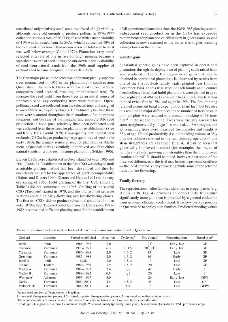
79Mark J. Dieters, D. Garth Nikles and Murray G. Keys
Australian Forestry 2007 Vol. 70 No. 2 pp. 75–85
contributed only relatively small amounts of seed of high viability,although being old enough to produce pollen. In 1976/1977collection season a total of 2023 kg of seed with a mean viabilityof 41% was harvested from the SPAs, which represented 40% ofthe total seed collection in that season when the total seed harvestwas well below average (Gould 1979). Plantation ‘crop trees’selected at a rate of one in five for high pruning became asignificant source of seed during the run-down in the availabilityof seed from natural stands from the 1960s until supplies oforchard seed became adequate in the early 1980s.
The first major phase in the selection of phenotypically superiortrees commenced in 1957 in the plantations of south-easternQueensland. The selected trees were assigned to one of threecategories (seed orchard, breeding, or other seed-tree). Toincrease the seed yield from these trees as an initial source ofimproved seed, any competing trees were removed. Open-pollinated seed was collected from the selected trees and assignedto one of three seed-quality classes. Unfortunately because thesetrees were scattered throughout the plantations, often in remotelocations, and because of the irregular and unpredictable seedproduction in hoop pine, relatively little open-pollinated seedwas collected from these trees for plantation establishment (Sleeand Reilly 1967; Gould 1979). Consequently, until clonal seedorchards (CSOs) began producing large quantities of seed in theearly 1980s, the primary source of seed for plantation establish-ment in Queensland was essentially unimproved seed from eithernatural stands or crop trees in mature plantations (Nikles 1996).
Eleven CSOs were established in Queensland between 1965 and2001 (Table 3). Establishment of the first CSO was delayed untila suitable grafting method had been developed and then byuncertainty caused by the appearance of graft incompatibility(Haines and Dieters 1990; Dieters and Haines 1991) in the verydry spring of 1963. Field grafting of the first CSO (Imbil 1,Table 3) did not commence until 1965. Grafting of the secondCSO (Taromeo) started in 1970, and this orchard had separatesections containing early-flowering and late-flowering clones.The first two CSOs did not produce substantial amounts of pollenuntil 1979–1980. The seed collected from the CSOs since 1981–1982 has provided sufficient planting stock for the establishment
of all operational plantations since the 1984/1985 planting season.Subsequent seed production in the CSOs has exceededrequirements for plantation establishment in Queensland, so seedcollection is now restricted to the better (i.e. higher breedingvalue) clones in the orchard.
Genetic gain
Substantial genetic gains have been captured in operationalplantations through the deployment of planting stock raised fromseed produced in CSOs. The magnitude of gains that may beobtained in operational plantations is illustrated by results fromone of the first full-sib family trials, planted near Imbil inDecember 1964. In this trial, trees of each family and a control(seed collected in a local Imbil plantation), were planted in up tofour replicates of 49-tree (7 rows × 7 trees) plots. The trial wasthinned twice, first in 1984 and again in 1994. The first thinningretained a constant basal area per plot of 25 m2 ha–1; but becausethis resulted in major differences in the number of trees in eachplot, all plots were reduced to a constant stocking of 18 treesplot–1 in the second thinning. Trees were visually assessed forstem straightness at 8 y of age (1 = crooked, … 8 = straight), andall remaining trees were measured for diameter and height at35 y of age. If total productivity (i.e. the standing volume at 35 yplus the volume removed in the two thinning operations) andstem straightness are examined (Fig. 4), it can be seen thatgenetically improved material (for example, the ‘mean offamilies’) is faster growing and straighter than the unimproved‘routine control’. It should be noted, however, that some of theobserved differences in this trial may be due to provenance effects— the local control is early flowering while some of the selectedtrees are late flowering.
Family forestry
The reproduction of elite families identified in progeny tests (e.g.H20 × I108, Fig. 4) provides an opportunity to capturesignificantly more gain than is provided by a general collectionfrom an open-pollinated seed orchard. It has now become possiblein Queensland to deploy elite families. Predicted breeding values
Table 3. Inventory of clonal seed orchards of Araucaria cunninghamii established in Queensland
Orchard Location Period established Area (ha) Cycle no.1 No. clones2 Flowering time Breed type3
Imbil 1 Imbil 1965–1968 7.0 1 23* Early, late GF Taromeo Yarraman 1970–1973 6.3 1, 1.5 30*, 21* Early, late GF Yarraman Yarraman 1986–1988 2.0 1.5, 2 13* Late GF Grenning Yarraman 1987–1988 2.0 1.5, 2 16* Early GF Imbil 2 Imbil 1988 2.0 1.5, 2 13 Late GF Tinana Toolara 1988–1989 1.9 1.5, 2 20 Late GF Valley A Yarraman 1989–1992 2.4 1, 2 41 Early I Valley B Yarraman 1989–1992 0.8 1, 2 20 Late I Wongabel Atherton 1995–1997 3.0 1 26 Early–late GFN Geritz Yarraman 2000–2001 4.5 1.5, 2 45 Late GFI Paddock 30 Yarraman 2000–2001 4.1 1.5 7 Late GFIW
1Parents used are from different cycles of breeding: 1 = untested, first-generation parents; 1.5 = tested, superior, first-generation parents; 2 = untested, second-generation parents 2The original numbers of clones included; the marker * indicates orchards which have been fully or partially culled 3Breed type – G = growth, F = form, I = internode length, W = wood quality (primarily spiral grain), N = northern Queensland or PNG provenance origin.

80 Genetic improvement and conservation of Araucaria cunninghamii
Australian Forestry 2007 Vol. 70 No. 2 pp. 75–85
are being used to select parents for the operational-scaleproduction of families from known, high-performing parents. Thecriteria used to select parents for inclusion in the family forestryprogram aim to at least maintain the gains achieved in growthand stem straightness, while placing emphasis on improving bothinternode length and spiral grain. We aim to increase averageinternode length (above about 6 m on the stem) to ≥1.2 m and tokeep maximum spiral grain angle <4°. A special clonal seedorchard was established in 2001 (Paddock 30 — Table 3) for theproduction of fully control-pollinated seed from parents with highgenetic merit. Pollination commenced in this orchard in 2003,with 58, 58 and 241 kg of control-pollinated seed collected in2005, 2006 and 2007 respectively. The 2007 collection of control-pollinated seed represents 85% of the annual seed requirement,with an average of 285 kg of seed required per year over the lastfour years.
Breeding strategy
A major change in the direction of the breeding program wasmade in 1990 following the adoption of a multiple-populationbreeding strategy. Prior to this time the genetic improvement ofhoop pine had been managed within a single large breedingpopulation. The primary factors driving this change were:
• most of the superior provenances of hoop pine were so poorlyrepresented in the initial breeding population that selection ofnew plus trees was required to adequately capture the yieldbenefits of these provenances
• the new plus trees could form a separate, unrelated population
• there was a strong commercial drive towards the developmentof a long-internode breed (Dieters et al. 1990)
• there was a case for developing a population adapted to thetropical north or for use in producing hybrids with southernprovenances.
The four breeding populations adopted under this strategy aredescribed below. Mating and selection are confined withinpopulations for breeding, but crosses can be made between thepopulations for deployment purposes.
First southern population (FSP). This consists of (i) 400 first-generation plus trees selected phenotypically (from 1957 to thelate 1970s) in southern Queensland provenances (mainly thosefrom the Mary and Brisbane River valleys — Fig. 1), many ofwhich have now been progeny tested, and (ii) second- and third-generation progeny of the original, selected parents nowrepresented in field trials.
Second southern population (SSP). Two hundred and forty-fourfirst-generation selections were assembled in the late 1980s andearly 1990s by phenotypic selection within plantations of knownsuperior (southern Queensland) provenances. Most trees selectedare from the Jimna provenance. Unfortunately the other superiorprovenances which were identified in the provenance trials werenot well represented in plantations suitable for plus-tree selection.
Long-internode population (LIP). One hundred and twenty-twoindividuals (81 first-generation and 41 second-generation trees)were selected in the late 1980s. These trees had an averageinternode length in the upper crown (i.e. above 6 m) of 2–3 m,combined with good stem quality and vigour. Very long internodetrees (i.e. >3 m) were available for selection, but most wererejected because such trees generally were not sufficientlystraight. Some individuals in this population are also representedin the FSP. The purpose of the LIP was to enable the rapiddevelopment of a long-internode breed (Dieters et al. 1990) andmany of these trees were grafted into the Valley CSO (Table 3).
Northern provenances population (NPP). One hundred and fifty-one first-generation trees selected at a relatively low intensity inplantations established with seed from the northern provenancesof Papua New Guinea (several provenances; 63 trees selected)and far-northern Queensland (Coen — 60 trees, Gillies — 18trees and Cape Flattery — 10 trees: see Fig. 2 for these locations).
The intensity of genetic improvement activities with hoop pinein Queensland has been significantly reduced since 2002, whenthe last series of progeny trials was established. Economicconsiderations dictated that continued, intensive breeding of hooppine could not be justified — long rotations (now >50 y), breedingcycles of about 15–20 y, and a lead time from selection to seedproduction of at least 10 y mean that returns from further breedingwill not be realised for at least 75 years. As a result geneticimprovement activities now focus on selection of elite parents(based on the performance of their progeny in field trials) foruse in the production of superior families by operationalcontrolled crossing for subsequent deployment in plantations. Itis anticipated that up to 80% of future hoop pine plantationsestablished by Forestry Plantations Queensland (the government-owned corporation now responsible for plantation forestry inQueensland) will be derived from superior full-sib families.
Future directions
A detailed review of the hoop pine breeding populations plannedfor 2007/2008 will use data collected from all progeny tests
Figure 4. Mean total volume (sum of standing volume, plus volumeremoved by thinning) at 35 y of age, and mean stem straightness at 8 yof age, of families in an Araucaria cunninghamii progeny trialestablished near Imbil in December 1964.
900
850
800
750
700
650
600
550
5002.2 2.4 2.6 2.8 3.0 3.2 3.4 3.6 3.8
Routine control
HG x HA
H13 x HB
Mean of families
HD x HB
HB x H20
H2 x H1
H20 x I108
HD x H13H2 x I108
I108 x THG x H10
H2 x HAHG x H13
H2 x H10H20 x HA
H13 x H10I108 x H10
Tota
l volu
me p
roduction a
t 35 y
after
pla
nting (
m3 h
a–
1)
Stem straightness at 8 y after planting (1 = crooked, 8 = straight)

81Mark J. Dieters, D. Garth Nikles and Murray G. Keys
Australian Forestry 2007 Vol. 70 No. 2 pp. 75–85
currently over 8.5 y of age. After completion of this reviewForestry Plantations Queensland is expected to reassess itsinvestment in the continued genetic improvement of hoop pine.
Options that may be explored include:
• maintenance of a low-intensity breeding program possiblyrelying on wind-pollinated mating, and/or
• establishment of a small elite breeding population that will betargeted to future seed requirements via family forestry.
There is likely to be on-going investment in the development ofenhanced deployment systems (e.g. family forestry), butinvestment by traditional sources in research to underpin the on-going genetic improvement of this species will probably cease.Alternative funding sources will be needed if the genetic diversitycurrently preserved in the breeding populations of this species inQueensland is to be maintained.
Conservation of genetic resources
The Queensland regional ecosystems (REs) which contain or maycontain hoop pine, by land tenure types, in each bioregion asdefined in Sattler and Williams (1999), are summarised in Table4. The current ‘biodiversity status’ of these forests in each RE islisted as either ‘not of concern’, ‘of concern’ or ‘endangered’.Of the relevant REs listed in Table 4, five are shown to be‘endangered’, and in a sixth the biodiversity status is currentlyunder review. However, in no case is the extent of such REs lessthan 1000 ha, and the others range from 4100 ha to 9600 ha.
In NSW vegetation has been mapped, in a manner different tothat adopted in Queensland, using the regional ecosystems model(EPA 2005). Nevertheless, rainforest types broadly analogous toseveral of those recognised as including hoop pine in south-eastern Queensland are identifiable in NSW (John Hunter, NSWNational Parks and Wildlife Service, pers. comm. 2002). These,five in number, with the numbers of subtypes involved, are dryrainforest (5), riverine rainforest (1), littoral rainforest (2), warmtemperate rainforest (2) and cool temperate rainforest (2), for atotal of 12 subtypes. Of these, three riverine or littoral subtypesare considered ‘endangered’ in terms of conservation status, whilethree of the others are ‘of concern’ and the remaining six are ‘ofno concern at present’ (John Hunter, NSW NPWS, pers. comm.2002).
It is evident that while some REs that include hoop pine areconsidered to be endangered, within the natural range of thespecies in Australia it is not under any serious threat — over236 000 ha of natural forests (potentially containing hoop pine)are preserved on lands controlled by the Queensland governmentalone (Table 4). Moreover, it is expected that social, politicaland legal constraints on further clearing or logging of rainforestsin Queensland and NSW will continue to be tightened, such thatstands on private (i.e. freehold) lands are unlikely to be greatlydiminished in the future.
Although considerable areas of rainforest containing hoop pinehave been cleared for agriculture and other land uses in NSWand Queensland, substantial areas of native forests in which thisspecies is dominant have been protected within a network ofpublicly-owned national parks, forest reserves and state forests.
Hence, throughout the range of hoop pine in Australia, large areasof natural stands remain intact, and the species as a whole is notendangered. The extent of conservation of native stands of hooppine, particularly on non-government lands, however, is moreserendipitous than designed. Although hoop pine often occurson highly fertile soils that would be desirable for conversion toagriculture, many of these sites are also very steep and thereforeunsuitable for intensive agriculture. Swain (1928, p.68) notes:‘private timber estates … although holding only 25% of the soft-wood volume, have contributed a larger yield than the State’sown much more important [forest estate]’, largely due to ‘thegenerally better accessibility, and because of the haste to realiseupon the stumpage values in order to convert the land to farmingends.’ While conversion to agriculture of privately-owned forestsdominated by Araucaria has almost eliminated this forest typein some REs (Table 4) and has undoubtedly led to furtherfragmentation of the natural stands, significant areas of nativeforests have been retained on private lands.
The management of state-owned Araucaria forest lands early inthe 20th century could have followed one of two paths, asdescribed by Swain (1928, p. 18):
there are only two economic policies from which to choose —the first, to cut out the natural stagnant and over-mature hoopand bunya stands within these ten years from 1928 to 1938,when the pine-milling industry would suddenly disappear, orto ration the cut over a more extended period, and by dilutionand import ease the decline in our small resources down to thepoint at which the incline of the new plantations of ForestService creation can assume the responsibility for providingincreasing supplies of log material. This latter policy has beenchosen.
This deliberate policy of reducing the harvest from natural standswhile at the same time investing in the development of a viableplantation program has lead to the preservation of large areas ofnatural Araucaria forests in Queensland. The volume of logsnow harvested from the hoop pine plantations exceeds the highestannual removals from native forests, recorded in the 1940s. Hencethese plantations provide:
• an alternative source of high quality timber from a relativelysmall land base, thereby allowing native forests to be excludedfrom logging
• an ongoing source of revenue, which is able (indirectly viafinancial returns to the state government) to support non-profitforest-based activities by government agencies, including theconservation and management of native stands
• an addition to the genetic conservation base, as some arederived from seed collected from natural stands that wereheavily logged or cleared and are no longer extant in the wild.
The breeding and deployment program with hoop pine constitutesan important component of the genetic conservation of this speciesin Queensland. As outlined previously, 876 first-generation plustrees of many provenances are represented in the four breedingpopulations. These genotypes are preserved in grafted clone banksand clonal seed orchards. This method of gene conservation hasthe advantage of preserving genotypes with known performance(McCutchan 1999). As pointed out by Dvorak (1999) in thecontext of southern pines, but nevertheless relevant here, ‘these

82 Genetic improvement and conservation of Araucaria cunninghamii
Australian Forestry 2007 Vol. 70 No. 2 pp. 75–85
Table 4. Regional ecosystems (REs) within Queensland bioregions that contain or may contain natural stands of Araucaria cunninghamii, and their areas in hectares by land tenure. (Note that the actual areas of A. cunninghamii forest types are less as the species does not occur throughout each RE, even when it is characteristic as in those REs in bold below). Data extracted from EPA (2005).
Bioregion and regional ecosystem
Nationalpark00
State† Free-hold
Lease-hold
Other Short description of RE and examples of some occurrences in for example particular national parks (NPs) where hoop pine may be present
Cape York Peninsula Bioregion 03.02.12, A‡ 122 19 7609 40 16 AMVF§ on coastal dunefields and beach ridges. Heathlands Resources Reserve,
Shelburne Bay coast (Captain Billy Landing area), Temple Bay coast north, C. Flattery and C. Bedford sand ridges
03.05.04�4, A?
228 316 1711 AMVF on sand sheets. Heathlands R’ces Res., Shelburne Bay coastal plains, e.g. Captain Billy Landing
03.12.02, B 2310 15 1 1 ANVF on granitic ridges and mountains — southern area. C. Melville NPs incl. Altanmoui Ra. and part of Starcke Holding, C. Bedford and S to Hopevale Mission
185 635 1433 3473 ANVF on granitic ridges and mountains — northern area. Mungkan Kandju NP, McIlwraith Ra. near Coen
Wet Tropics Bioregion 07.12.10, B 242 629 14 499 576 NVF on granitic foothills and uplands S of Herbert R., Seaview and Paluma
Ranges, Tully Gorge NP, Hann Tableland
07.12.46, B 425 3 MVF on steep rock granite talus and boulder slopes of Great Palm Island
Central Queensland Coast Bioregion
08.11.02, B 348 16 2082 91 4 NMVF on coastal hills and low ranges on sediments +/– volcanics. Eungella and Mt Ossa NPs
08.12.02, A 9298 11028 4385 5903 538 N-CNVF on drier uplands and coastal ranges on igneous rocks, Eungella–Pioneer Peaks areas
08.12.03, A 7244 21405 18961 13482 704 N/MRf on low to medium ranges on igneous rocks. Major Rf type in many NPs in Mackay region
08.12.10, B 197 101 2170 37 2 Shrub/heathland, emergent hoop pine on exposed igneous plateaus, Homevale and Pioneer Peaks NPs
08.12.11, B? 11763 187 934 955 2361 SDMVF/T in coastal areas and islands on various igneous rocks. Brampton Is., Whitsunday Is. etc. NPs
08.12.18, A 13869 7109 4161 274 597 N-CNVF on coastal ranges and islands on igneous rocks. Whitsunday region NPs, Conway, Dryander Ra.
Einasleigh Uplands Bioregion 09.12.34, A 702 1584 9486 1121 SEVT on slopes of steep hills on volcanics in the SE of the bioregion. Leichardt
and Hervey Ranges
09.12.35, A 1074 30396 1 Open woodland on granitic hills in SE of the bioregion. W of Hidden Valley (WSW of Mt Spec)
Brigalow Belt Bioregion
11.11.05, A 2472 2444 18538 10109 852 MVF on hilly terrain with steep slopes; sedimentary rocks. Goodedulla and Rundle Ra. NPs
11.12.04, A 10767 4102 21559 18393 2733 SEVT and MVF on low hills and ranges on igneous rocks. NPs, e.g. Cape Upstart, Magnetic Is., Mt Archer
11.12.12, B 299 2 5 76 Araucarian woodland on islands, headlands and coastal hills with igneous rocks, Magnetic Is., Cape Upstart NPs
11.12.16, B 2631 322 1861 1407 Low woodland–shrubland on islands and coastal hills; igneous rocks. Bowling Green Bay, Magnetic Is. NPs
† State-controlled land includes both state forests and forest reserves ‡ Biodiversity status: A = no concern at present; B = of concern; C = endangered; ? = under review. For definitions, see www.epa.qld.gov.au/nature_conservation/biodiversity/regional_ecosystems/introduction_and_status (accessed 17 April 2007) and EPA (2005) § A = Araucarian, C = complex, D = deciduous, E = evergreen, F = forest, L = low, M = microphyll, N = notophyll, Rf = rainforest, S = semi-, T = thicket, V = vine

83Mark J. Dieters, D. Garth Nikles and Murray G. Keys
Australian Forestry 2007 Vol. 70 No. 2 pp. 75–85
clone banks only have value when their genetic composition iswell documented and the genetic material is accessible’. Ex situconservation of hoop pine in Queensland is currently facingchallenges brought on by a rapid reduction in funding fortraditional tree improvement activities and by organisationalsegregation of research and operational forestry activities. Short-term instability brought on by institutional change can vitiateviable long-term ex situ gene conservation programs. In thesecircumstances information, knowledge and material can be
rapidly and easily lost, thereby nullifying many years ofconscientious scientific endeavour. Continued effective long-termconservation of genetic resources will pose significant challengesin a future increasingly dominated by commercial imperatives.Consequently, in situ conservation will ‘remain fundamentallyimportant for the conservation of forest genetic diversity’(Kanowski 2000, p. 283).
Table 4. (continued)
Bioregion and regional ecosystem
Nationalpark00
State† Free-hold
Lease-hold
Other Short description of RE and examples of some occurrences in for example particular national parks (NPs) where hoop pine may be present
South-eastern Queensland Bioregion 12.03.01, C 104 1970 6148 236 597 Gallery rainforest (NVF) on alluvial plains to about 100 km inland. Extensively
cleared. Great Sandy NP
12.03.11, B 1054 18710 31038 3979 10905 Open forest to woodland on sub/coastal alluvial plains mostly S of Bundaberg. Great Sandy and other NPs
12.05.13, C 179 3487 1179 92 31 M-NVF on remnant Tertiary surfaces. Yarraman–Tarong–Boat Mt. Heavily cleared
12.08.04, A 7024 2736 4464 81 30 CNVF on basalts. Areas in Bunya Mts, Lamington, Main Range, Mt Barney NPs; near Levers Plateau
12.08.13, B 2891 7574 3873 153 77 M and M/NVF on igneous rocks. Areas in Bunya Mts, Moogerah Peaks NPs. Isis and Kalpowar scrubs
12.08.21, C 965 150 2907 20 62 LMVF and SEVT on igneous rocks. Small areas in Bunya Mts NP and Lockyer Valley in S of bioregion
12.09-10.15, C
136 1591 3584 26 46 SEVT on sedimentary rocks. Extensively cleared. In for example Lockyer and Fassifern valleys
12.09-10.16,C?
835 4978 3535 70 184 AM-NVF on sedimentary rocks. Extensively cleared. Seaview Ra.,Tinana Ck, Flinders Peak, Mt Barney
12.11.10, A 1392 25979 11589 322 708 NVF on metamorphics and volcanics in coastal/subcoastal ranges, Enoggera Ck, Mary Valley, Pinbarren
12.11.11, A 7994 6266 111 72 AMVF on metamorphics and volcanics. Extensively cleared. Imbil–Kilkivan–Nanango. W foothills of D’Aguilar Ra.
12.11.12, B 5226 1331 2354 87 102 ACMVF on interbedded metamorphics and volcanics. Woolooga; hoop pine may invade eucalypt forest, e.g. in Goodnight Scrub
12.11.13, B 12 1567 562 9 3 SEVT on interbedded metamorphics and volcanics. Fire and weeds threats on edges. Goodnight Scrub
12.12.01, B 327 5464 1838 23 20 SNVF in gullies on igneous rocks. Often present on margins. Brisbane FP, Kondalilla NP, Mt Eerwah
12.12.13, A 937 29347 8803 1364 415 ACM-NVF on igneous rocks. Hills near Somerset Dam, Burnett Ra. (Goomeri-Biggenden), Mt Perry Ra.
12.12.16, A 490 17965 5044 145 195 NVF on igneous rocks. Includes Mt Mee, Yandina, Bauple areas in S; Bulburin, Kroombit Tops in N
12.12.17, C 0 715 374 4 1 SEVT on igneous rocks. Further clearing, fire and weed invasion threats. Nangur, Mt Beppo
12.12.18, B 243 2976 2243 710 61 SEVT on igneous rocks. Comment as next above. Central, Gayndah part of bioregion; Kroombit Tops NP
Total areas 83i551 182i276 181i002 100i425 25i373
† State-controlled land includes both state forests and forest reserves ‡ Biodiversity status: A = no concern at present; B = of concern; C = endangered; ? = under review. For definitions, see www.epa.qld.gov.au/nature_conservation/biodiversity/regional_ecosystems/introduction_and_status (accessed 17 April 2007) and EPA (2005) § A = Araucarian, C = complex, D = deciduous, E = evergreen, F = forest, L = low, M = microphyll, N = notophyll, Rf = rainforest, S = semi-, T = thicket, V = vine

84 Genetic improvement and conservation of Araucaria cunninghamii
Australian Forestry 2007 Vol. 70 No. 2 pp. 75–85
Although much of the native hoop pine in the Bulolo and Wauvalleys in PNG has been harvested, this is not the case for mostof the numerous occurrences of the species elsewhere in PNGnor in Indonesian New Guinea (Howcroft 1978). Thesepopulations remain largely intact because they are frequentlyremote and occur on mountain tops and or steep terrain (Gray1973; Kapisa 2002). Some preliminary work has been done onin situ and ex situ conservation in PNG and Indonesian NewGuinea (Howcroft 1978; Kapisa 2002), but more work is required.
The formal conservation status of hoop pine in New Guinea isunknown; in the Bulolo–Wau area the existence of plantationsbased on local provenances provides some insurance, but thelong-term future of these plantations may be in doubt. Naturalstands in other regions are largely inaccessible and this shouldprovide a modicum of protection by default, at least in the mediumterm. Several PNG provenances are represented in Queenslandexperimental plantings and this will offer a reasonable degree oflong-term ex situ genetic conservation.
Acknowledgements
We are pleased to recognise the contributions made to the programin various periods by foresters R.G. Florence, R.J. Gould,M.D. Higgins (dec.), J.R. McWilliam, D.I. Nicholson, J.J. Reillyand J.B. Schaumberg. Also, we acknowledge the skilledsupervision and/or labour provided in the field at various periodsby R. Allen, D. Bickle, G. Buchanan, T.R. Chard, T. Frodsham,L. Geritz, N. Halpin, J. Huth, M. Johnson, R. Larsen,D. Rasmussen, H. Trace, R. Trace and A. Soanes; and theassistance of R. Eisemann, S. Jarvis, R. Newton and R. Woolastonwith data handling and analyses during the first phase of theprogram. J. Huth also assisted in obtaining information on thevolumes of hoop and bunya pines harvested over the years inQueensland from annual reports of the government forestryauthority. Ms Rosemary Niehus and Ms Eda Addicott of theQueensland Environmental Protection Agency in Brisbane andMareeba respectively are warmly thanked for assistance throughthe extraction of areal data and provision and interpretation ofinformation for Table 4. T. Jovanovic of Ensis and cartographersA. Knight and T. Nguyen of Forestry Plantations Queensland arethanked for producing the maps for Figures 1, 3 and 2 respectively.J. Hunter and P.G. Richards of the NSW National Parks andWildlife Service provided the information on the conservationstatus of hoop pine in NSW, and D.I. Nicholson also assisted byproviding information on, and seed collections from, hoop pineoccurrences in northern Queensland over many years. Inconducting the program, we have also benefited from advice andguidance given by peers and senior colleagues. We thank thereviewers D.I. Bevege and M.U. Slee for very useful suggestionsthat considerably improved this paper.
ReferencesAnon. (2003) Queensland Forestry — Excerpts, Annual Reports and
Yearbooks 1860 to 2003. Published as a CD by DPI Forestry,Department of Primary Industries, Brisbane.
Anon. (2005) DPI Forestry Yearbook 2005. DPI Forestry, Departmentof Primary Industries and Fisheries, Queensland Government,Brisbane, 110 pp.
Boland, D.J., Brooker, M.I.H., Chippendale, G.M., Hall, N., Hyland,B.P.M., Johnston, R.D., Kleinig, D.A. and Turner, J.D. (1985)Forest Trees of Australia. Thomas Nelson Australia and CSIRO,Melbourne, 687 pp.
Burrows, G.E. (1987) Leaf axil anatomy in the Araucariaceae.Australian Journal of Botany 35, 631–640.
Dean, C.A., Nikles, D.G. and Harding, K.J. (1988) Estimates of geneticparameters and gains expected from selection in hoop pine insouth-east Queensland. Silvae Genetica 37, 243–247.
Dieters, M.J. and Haines, R.J. (1991) The influence of rootstock familyand scion genotype on graft incompatibility in Araucariacunninghamii Ait. ex D.Don. Silvae Genetica 40, 141–146.
Dieters, M.J., Woolaston, R.R. and Nikles, D.G. (1990) Internode lengthin hoop pine: genetic parameters and prospects for developing along internode breed. New Zealand Journal of Forestry Science20, 138–147.
Dieters, M.J., Johnson, M.J. and Nikles, D.G. (2000) Inter-provenancehybrids of hoop pine (Araucaria cunninghamii). In: Dungey, H.S.,Dieters, M.J. and Nikles, D.G. (eds) Hybrid Breeding and Geneticsof Forest Trees. QFRI/CRC-SPF Symposium, 9–14 April 2000,Noosa, Queensland. Department of Primary Industries, Brisbane,pp. 413–418.
Dvorak, W.S. (1999) Do we really need conservation programs for thesouthern pines? In: Bowen, M. and Stine, M. (compilers)Proceedings of 25th Biennial Southern Forest Tree ImprovementConference, 11–14 July, New Orleans, LA. National TechnicalInformation Service, Springfield, VA., pp. 1–5.
Eisemann, R.L., Harding, K.J. and Eccles, D.B. (1990) Geneticparameters and predicted selection response for growth and woodproperties in a population of Araucaria cunninghamii. SilvaeGenetica 39, 206–216.
EPA (Environmental Protection Agency) (2005) Regional ecosystemdescription database (REDD). Version 5.0. Updated December2005. Database maintained by Queensland Herbarium, the Agency,Brisbane. http://www.epa.qld.gov.au/nature_conservation/biodiversity/regional_ecosystems/.
Gould, R.J. (1979) Hoop pine seed sources — past, present and future.In: Fisher, W.J., Pegg, R.E. and Harvey, A.M. (eds) Planning,Establishment and Management of Hoop Pine Plantations. Vol.1, Proceedings of the 1979 Routine-Research conference held atYarraman 4 April and Gympie 9–13 July, 1979. Department ofForestry, Brisbane, pp. 76–86.
Gray, B. (1973) Distribution of Araucaria in Papua New Guinea.Research Bulletin No. 1. Papua New Guinea Department ofForestry, Port Moresby, 56 pp.
Grenning, V. (1925) The Softwood Problem in Queensland. QueenslandForest Service Bulletin No. 6. Queensland Forest Service,Brisbane, 21 pp.
Haines, R.J. and Dieters, M.J. (1990) The progression and distributionof graft incompatibility in Araucaria cunninghamii Ait. ex D.Don.Silvae Genetica 39, 62–66.
Harding, K.J. and Woolaston, R.R. (1991) Genetic parameters for woodand growth properties in Araucaria cunninghamii. Silvae Genetica40, 232–237.
Harris, J.M. (1984) Non-destructive assessment of spiral grain instanding trees. New Zealand Journal of Forestry Science 14,395–399.

85Mark J. Dieters, D. Garth Nikles and Murray G. Keys
Australian Forestry 2007 Vol. 70 No. 2 pp. 75–85
Howcroft, N.H.S. (1978) A review of Araucaria cunninghamii Ait. exLambert in Papua New Guinea and Irian Jaya. In: Nikles, D.G.,Burley, J. and Barnes, R.D. (eds) Proceedings of a Joint Workshopon Progress and Problems of Genetic Improvement of TropicalForest Trees. IUFRO Working Parties S2.02-08 and S2.03-01. 4–7April 1977, Brisbane. CFI, University of Oxford, England, pp.827–847.
Jovanovic, T. and Booth, T.H. (2002) Improved Species ClimaticProfiles. Publication No. 02/095, Rural Industries Research andDevelopment Corporation (RIRDC), Canberra, vi + 68 pp.
Kain, D. (2003) Genetic parameters and improvement strategies forthe Pinus elliottii var. elliottii × Pinus caribaea var. hondurensishybrid in Queensland, Australia. PhD thesis, The AustralianNational University, Canberra, ACT, 456 pp.
Kanowski, P.J. (2000) Politics, policies and the conservation of forestgenetic diversity. In: Young, A., Boshier, D. and Boyle, T. (eds)Forest Conservation Genetics: Principles and Practice. CSIROPublishing and CABI Publishing, Victoria and Wallingford,pp. 275–288.
Kapisa, N. (2002) Natural distribution of Araucaria cunninghamii inKebar, Manokwari, Papua, Indonesia. In: Rimbawanto, A. andSusanto, M. (eds) Proceedings of the International Conferenceon Advances in Genetic Improvement of Tropical Tree Species.Yogyakarta, Indonesia, 1–3 October 2002. Centre for ForestBiotechnology and Tree Improvement, Yogyakarta, pp. 99–103.
McCutchan, B.G. (1999) Gene conservation: an industrial view. In:Bowen, M. and Stine, M. (compilers) Proceedings 25th BiennialSouthern Forest Tree Improvement Conference. 11–14 July, NewOrleans, LA. National Technical Information Service, Springfield,VA., pp. 6–22.
McKenzie, N., Jacquier, D., Isbell, R. and Brown, K. (2004) AustralianSoils and Landscapes. CSIRO Publishing, Melbourne, 416 pp.
Nikles, D.G. (1996) The first 50 years of the evolution of forest treeimprovement in Queensland. In: Dieters, M.J., Matheson, A.C.,Nikles, D.G., Harwood, C.E. and Walker, S.M. (eds) TreeImprovement for Sustainable Tropical Forestry. ProceedingsQFRI-IUFRO Conference, Caloundra, Queensland, Australia. 27October–1 November 1996. Queensland Forestry ResearchInstitute, Gympie, pp. 51–64.
Nikles, D.G. and Newton, R.S. (1983) Distribution, genetic variation,genetic improvement and conservation of Araucaria cunninghamiiAiton ex D.Don. Silvicultura 30, 277–286.
Nikles, D.G., Haines, R.J. and Dieters, M.J. (1988) Reproductivebiology, genetic improvement and conservation of hoop pine(Araucaria cunninghamii) in Queensland. In: Proceedings of theInternational Forestry Conference for the Australian Bicentenary1988, 25 April–1 May 1988, Albury-Wodonga, NSW. TheAustralian Forest Development Institute, Volume 3, 15 pp.
Nikles, D.G., Dieters, M.J., Johnson, M.J., Setiawati, Y.G.B. and Doley,D.D. (in press) The reproductive biology of hoop pine (Araucariacunninghamii Ait. ex D.Don) and its significance in a geneticimprovement programme. In: Bieleski, R.L. and Wilcox, M.D.(eds) The Araucariaceae. Proceedings of International AraucariaSymposium, Auckland, New Zealand, 14–17 March 2002. TheInternational Dendrological Society, pp. 200–211.
Parsons, M., Gavran, M. and Davidson, J. (2006) Australia’s Plantations2006. Bureau of Rural Sciences, Department of Agriculture,Fisheries and Forestry, Canberra, 56 pp.
Reilly, J.J. (1974) Geographic Variation of Hoop Pine. Research PaperNo. 4, Department of Forestry, Brisbane, Queensland, 34 pp.
Sattler, P. and Williams, R. (eds) (1999) The Conservation Status ofQueensland’s Bioregional Ecosystems. Environmental ProtectionAgency, Brisbane.
Slee, M.U. and Reilly, J.J. (1967). The production of improved treeseed in Queensland. In: Proceedings of the World Symposium onMan-Made Forests, Canberra, Australia, 14–24 April 1967.FO.MMF:67-10/2, FAO, Rome, pp. 1183–1202.
Sorensson C.T., Burdon, R.D., Cown, D.J., Jefferson, P.A. andShelbourne, C.J.A. (1997) Incorporating spiral grain into NewZealand’s radiata pine breeding programme. In: Burdon, R.D. andMoore, J.M. (eds) IUFRO ’97 Genetics of Radiata Pine.Proceedings of NZ FRI-IUFRO Conference 1–4 December andWorkshop 5 December, Rotorua, New Zealand. Bulletin No. 203,FRI, Rotorua, pp. 180–199.
Swain, E.H.F. (1928) The Timbers and Forest Products of Queensland.Queensland Forest Service, Brisbane, 500 pp.
Wylie, F.R. (1982) Insect problems of Araucaria plantations in Australiaand Papua New Guinea. Australian Forestry 45, 125–131.

86 Wood properties of Acacia auriculiformis
Australian Forestry 2007 Vol. 70 No. 2 pp. 86–92
Physical and mechanical properties of plantation-grownAcacia auriculiformis of three different ages
S.R. Shukla1,2, R.V. Rao1, S.K. Sharma1, P. Kumar1, R. Sudheendra1 and S. Shashikala1
1Wood Properties and Uses Division, Institute of Wood Science and Technology, Bangalore 560 003, India2Email: [email protected]
Revised manuscript received 2 August 2006
Summary
We assessed the physical and mechanical properties of timber ofplantation-grown 8-, 12- and 13-y-old trees of Acacia auriculiformisA.Cunn. ex Benth. from Sirsi, Karnataka, India. The timber ofthe 13-y-old trees was dense, very strong, moderately tough, stablein service and hard, and it compared favourably with teak inseveral properties. The results suggest that it can be used for toolhandles, oars, paddles, packing cases, ammunition boxes, etc. Itwas also found suitable for the rural construction industry wheretimbers of small diameter can be used. If trees are allowed togrow older to attain greater size the range of potential uses willincrease.
Keywords: plantations; wood properties; shrinkage; mechanicalproperties; modulus of elasticity; Acacia auriculiformis
Introduction
Acacia auriculiformis A.Cunn. ex Benth. is native to savannasof Papua New Guinea, islands of Torres Strait and northernAustralia. In natural stands it is a vigorous tree, reaching a heightof 30 m with a trunk up to 60 cm in diameter. Because of itsability to grow on very poor soil and in areas with an extendeddry season, it has been introduced into countries such as India,Indonesia, Malaysia, Tanzania and Nigeria.
Acacia auriculiformis was introduced into India about three orfour decades ago. In 1990, provenances with straight boles fromPapua New Guinea and northern Queensland were planted in theUttar Kannad and Dharwad districts of Karnataka, India, andtheir performance was considered good (Rai 1995). The specieshas also been grown as an avenue tree in other parts of India, viz.Tamil Nadu, Bihar, Orissa and West Bengal, and in fuelwoodplantations in Dharwad and other areas of Karnataka. The treesare useful for shade, for ornament, for screening boundaries andfor windbreaks, as well as for agroforestry and for mitigatingsoil erosion. The tree produces a considerable amount of litterfrom branches and dead leaves that can be gathered for fuel. It isone of the species recommended for firewood farming in degradedlands (Chaturvedi 1985) because of its excellent quality asfirewood. The wood burns without smoke or sparks and has acalorific value of 4800–4900 cal kg–1 (20.1–20.5 MJ kg–1) (Anon.1980). The timber also provides a good pulp yield (Guha andPant 1966).
Recently this species has become popular among both publicand private-sector planters1. As the planting has been a pioneeringeffort, there is not much scientific information available aboutthe tree’s performance in this region. Information on growth rateand wood properties — which is helpful in evaluating its potentialfor various end-uses — is essential for informed investment inextensive plantation programs. An understanding of the woodproperties and their variation with age (Rao et al. 2004) providesa basis for assessing opportunities for value-added uses.
Comments on properties and processing of wood of A. auriculiformishave been provided by Rajan et al. (1979), Ananthnarayana etal. (1987), Kumar et al. (1987) and Shukla et al. (1990). Keatingand Bolza (1982) provided some details of wood characteristics.Kazmi et al. (1990) discussed the properties of the wood for thepurpose of identification. Verghese et al. (1999) reported limitedquantitative information pertaining to fibre and vessel morphol-ogy in 15-y-old trees from Maharashtra. Rao et al. (2004, 2007)described anatomical variation in 8–13-y-old trees.
Because of the lack of systematic information on physical andmechanical properties in relation to tree age, we have investigatedthose properties. In this paper, we present information on thephysical and mechanical properties of wood from trees 8, 12and 13 y old, and compare them with published values for teak.
Material and methods
Sampling
Five logs each of 8-, 12- and 13-y-old plantation-grownA. auriculiformis were procured from Sirsi, Uttar Kannad(Karnataka) to provide wood for evaluation of the physical andmechanical properties of the species. The stands from which thelogs were obtained were grown from a single unspecified seedsource and in the same locality. Table 1 shows the details of
1 Rao, R.V., Rao, K.S., Shukla, S.R., Kothiyal Vimal, Kumar, P., Sudheendra,R., Chandrashekhar, M.N., Jayakumar, M.N., Malkhede, S.K, Madhav Ambadi,Mohamed Amanulla, B.K. and Sathishchandra, K.M. (2005) Evaluation ofphysical and mechanical properties of Acacia auriculiformis × A. mangiumhybrid, A. mangium × A. auriculiformis hybrid, A. auriculiformis (Spring Valeprovenance and local) and A. mangium. Report to The Mysore Papermills Ltd,Bhadravathi, Karnataka, India, 37 pp. (unpublished).

87S.R. Shukla, R.V. Rao, S.K. Sharma, P. Kumar, R. Sudheendra and S. Shashikala
Australian Forestry 2007 Vol. 70 No. 2 pp. 86–92
environmental factors at the stands. Average, minimum andmaximum girths and average length of logs from each age groupof trees are given in Table 2.
All the logs were marked and numbered on the top end and sawndirectly into full-length scantling of 6.25 cm × 6.25 cm cross-section to obtain the maximum number of test specimens fromeach log. One or two scantlings were obtained per log. Eachscantling was halved along the radius of the log to provide samplesfor green and air-dry testing based on IS: 2455 (Anon. 1974).
Measurement of properties
Small clear specimens were tested, in both green and air-drystates, for the following physical and mechanical properties usingthe procedure given in IS: 1708 (Anon. 1986).
Physical properties
(i) Moisture content. Moisture content was measured using testspecimens of 2 cm × 2 cm × 2.5 cm on the basis of oven-dryweight as per the standard procedure. The numbers ofspecimens taken to determine moisture content in the greenand air-dry states were 525 and 580 respectively.
(ii) Density and specific gravity. Density (colloquially ‘weight’or ‘heaviness’) in both the green and air-dry condition wascalculated from the weight of specimens in the greencondition and their volume in the green condition, andsimilarly the air-dry weight and air-dry volume (adjusted to12% EMC) respectively. Specific gravity was estimated fromvolume at test (green or air dry) and oven-dry weight usingthe standard mercury displacement method. Specific gravitybased on green volume is referred to here as standard specificgravity. The numbers of specimens taken to determine bothdensity and specific gravity in green and air-dry states were531 and 578 respectively.
(iii) Shrinkage. For the measurement of shrinkage, true radial,tangential, longitudinal and volumetric samples wereprepared. The specimen size for volumetric shrinkage was2 cm × 2 cm × 6 cm, while for radial, tangential andlongitudinal shrinkage the specimen size was 2 cm × 2 cm ×5 cm. Specimens were weighed in the green condition to0.001 g accuracy and their length was measured to 0.002 cmaccuracy using Mitutoyo digital screw gauge calipers of0.001 cm accuracy. Specimens were allowed to air dry, andperiodically weighed and lengths measured until no furtherloss of weight was observed. The specimens were then ovendried and the dimensions measured. The numbers ofspecimens taken to determine radial, tangential, longitudinaland volumetric shrinkage from the green to an oven-dry statewere 164, 160, 151 and 162 respectively.
Mechanical properties
The mechanical testing was conducted on a computer-controlledUniversal Timber Testing Machine (UTM) as described below:
(i) Static bending strength. The size of specimens was 2 cm ×2 cm × 30 cm with a span length of 28 cm. The loading wasapplied at a constant rate of 1.0 mm min–1 on the tangentialsurface of the sample. The numbers of specimens used ingreen and air-dry states were 159 and 162 respectively. Threedifferent static bending strength parameters, fibre stress atelastic limit (FS at LP in MPa), modulus of rupture (MORin MPa) and modulus of elasticity (MOE in MPa) werecomputed using the equations:
FS at LP = 3 × P × l / 2 × b × h2 (a),
MOR = 3 × Pmax × l / 2 × b × h2 (b),
MOE = P × l3 / 4 × D × b × h3 (c),
where P = load at the limit of proportionality (kN); Pmax =maximum load (kN), l = span of the test specimen (mm),b = breadth of the test specimen (mm), h = depth of the testspecimen (mm) and D = deflection at the limit ofproportionality (mm).
(ii) Compressive strength parallel to grain. The size ofspecimens was 2 cm × 2 cm × 8 cm in length, and the rate ofloading was 0.6 mm min–1. The numbers of specimens usedin green and air-dry conditions were 124 and 156respectively. The compressive strength parallel to the grain(maximum crushing stress, MCS) was calculated by theequation:
σcpl = Pmax /A ,
where σcpl = MCS (MPa), Pmax = maximum crushing load at
Table 1. Environmental factors at Sirsi, Uttar Kannada (Karnataka, India) near the Acacia auriculiformis study site
Factor Value
Latitude 14.96°N Longitude 74.72°E Altitude 600 m asl Maximum daily temperature 23–28°C Annual rainfall 2500 mm Soil type Deep, clayey soil on laterite plateau Drainage Good (well drained)
Table 2. Length and girth of five logs in each age group
Girth (diameter) at breast height (cm) Tree/log no. Age (y)
Average available length of log (m)
Mean Minimum Maximum
T1–T5 8 4.55 38.2 (12.2) 32 (10.2) 42 (13.4) T6–T10 12 4.55 42.8 (13.6) 36 (11.5) 44 (14.0) T11–T15 13 4.24 50.8 (16.2) 46 (14.6) 53 (16.9)

88 Wood properties of Acacia auriculiformis
Australian Forestry 2007 Vol. 70 No. 2 pp. 86–92
break point (kN) and A = area of cross section of thespecimen on which force was applied (mm2).
(iii) Compressive strength perpendicular to grain. The size ofspecimens was 2 cm × 2 cm × 10 cm. Load was applied atthe 2 cm × 2 cm cross-section on the tangential surface at arate of 0.6 mm min–1. The numbers of specimens used ingreen and air-dry conditions were 117 and 147 respectively.The compressive strength perpendicular to the grain(compressive stress at limit of proportionality — CS at LPin MPa) was calculated by the equation:
CS at LP = P/A ,
where P = load at the limit of proportionality (kN) and A =area of cross-section of specimen on which force was applied(mm2).
(iv) Hardness under static indentation. The size of specimenswas 5 cm × 5 cm × 5 cm. Load (kN) required to penetrateinto the specimen a steel bar with an hemispherical end or asteel ball of 1.128 cm diameter to a depth of 0.564 cm wasrecorded. Measurements were made at the centre of theradial, tangential and end faces; no splitting or chippingoccurred. The rate of loading was kept constant at 6 mmmin–1. The numbers of specimens used in green and air-dryconditions were 125 and 115 respectively.
(v) Shear strength parallel to grain. The size of specimens was5 cm × 5 cm × 6 cm. The specimens were notched at oneend to produce shear failure in an area of 5 cm × 5 cm in theradial or tangential plane. The numbers of specimens usedin green and air-dry conditions were 50 and 36 respectively.The shear strength parallel to the grain in radial andtangential planes (maximum shearing stress — MSS in MPa)was calculated by the equation:
MSS = Pmax /A ,
where Pmax = maximum load required for shearing the area(kN) and A = shearing area of the specimen on which forcewas applied (mm2).
(vi) Tensile strength perpendicular to grain. The size of speci-mens was 5 cm × 5 cm × 6 cm. The specimens were notchedon the two surfaces perpendicular to the grain so as toproduce a failure on an area of 5 cm × 2 cm. The numbersof specimens used in green and air-dry conditions were 21and 26 respectively. The tensile strength perpendicular tothe grain in radial and tangential planes (TS in MPa) wascalculated by the equation:
TS = Pmax /A ,
where Pmax = maximum load required for failure perpen-dicular to grain (kN) and A = area of the specimen on whichforce was applied (mm2).
(vii) Nail- and screw-holding power. Nails of 50 mm length and2.50 mm shank diameter and screws of 50 mm length and 8gauge were used for testing. The size of the specimens was5 cm × 5 cm × 15 cm. The numbers of specimens used ingreen and air-dry conditions were 31 (in total from trees ofall three ages) and 19 (from 13-y-old trees only) respectively.Nails and screws were driven in for 25 mm at right-anglesto the surface of specimens. Two nails or screws were drivenon each of the radial and tangential surfaces and one oneach end. The maximum load required (kN) to pull out thenails or screws was recorded for radial, tangential and end
surfaces. The average values of radial and tangential surfaceswere named ‘side values’.
Statistical design and analysis
The three stands from which each of which five logs were obtainedwere aged 8, 12 and 13 y respectively. Although the stands weregrowing near each other in an apparently-uniform environment,the effects of tree age on the sample logs are inevitably con-founded with unquantified effects of the stand environments.Although in discussion in this paper we attribute differencesbetween the three sets of sample logs to the effects of stand age,it is important to recognise that stand effects are due to bothstand age and stand environment: the field design does not permitthese factors to be separated. The comparison with teak has similarconstraints.
Results and discussion
General properties and description of wood
Average thickness of the bark for the entire tree was measured as4.2 mm, 4.8 mm and 5.4 mm for the 8-, 12- and 13-y age classesrespectively. The sapwood and heartwood were distinct. Theheartwood, which is yellowish-brown in colour, occupied onaverage 76–85% of the area of each cross-section. The wood ismoderately hard and moderately dense, with shallowlyinterlocked grain and medium texture. Fine lines of parenchymasimulate the presence of growth rings; the actual growth ringsare indistinct. Wood structure is diffuse porous. Axial parenchymais paratracheal, vasicentric and also diffuse-in-aggregate. Raysare very fine and closely spaced.
Physical and mechanical properties
Air-dry values were adjusted to a sample moisture content of12% using the method of Sekhar and Rajput (1968) whererelevant.
Average values of the physical and mechanical properties asdetermined in green and air-dry conditions are presented inTable 3 for 8-, 12- and 13-y-old trees, along with thecorresponding values for ‘standard teak’, Tectona grandis (Sekharand Rawat 1966), for the purpose of comparison.
Average standard specific gravity was highest in 13-y-old trees(0.62) followed by 12-y (0.60) and 8-y-old trees (0.57) as shownin Figure 1. In other studies, 14-y-old trees from Mudigere,Karnataka, had an average specific gravity of 0.72 (air-dry)(Kumar et al. 1987), whereas 9-y-old trees from Gaya, Bihar,had a specific gravity of 0.62 (Shukla et al. 1990). Verghese etal. (1999) reported that specific gravity was 0.59 for 15-y-oldplantations from Wada, Maharashtra. Keating and Bolza (1982)reported that the specific gravity of timber obtained fromIndonesia was 0.58–0.64. Mohd Noor Mahat (1999) reportedvariation in specific gravity (0.53–0.61) of different provenancestested in Malaysia. Thus specific gravity appears to be widelyinfluenced by age, environmental factors and seed origin.
Longitudinal shrinkage was lowest in the 8-y-old trees andvolumetric shrinkage was highest in the 13-y-old trees (Table 2).

89S.R. Shukla, R.V. Rao, S.K. Sharma, P. Kumar, R. Sudheendra and S. Shashikala
Australian Forestry 2007 Vol. 70 No. 2 pp. 86–92
Radial and tangential shrinkage were more or less age-independent. Figure 1 shows the variation of modulus of rupture(MOR), modulus of elasticity (MOE) and maximum crushingstress (MCS) parallel to the grain in the green and air-dry statefor all the tree ages. MOR, MOE and MCS increased with treeage from 8 to 13 y. Improvement factors (I.F.), indicating thepercentage increase in the observed values of various mechanicalproperties from the green to air-dry state, were also calculatedand are listed in Table 3. Air-dry values for most mechanicalproperties were substantially higher than the corresponding greenvalues except for MCS (of 8-y-old trees), tension perpendicularto grain, and nail-holding powers. Hardness and tension valuesdetermined in radial, tangential and end directions and tension
perpendicular to the grain appear to be independent of age,whereas the shear values were found to be age related, beinghighest for the 13-y-old specimens. Nail-holding power was age-related only in end grain, whereas screw-holding power was age-related for all the directions studied and highest in the 13-y-oldtrees.
A comparison with teak using suitability indices
The data obtained on testing the samples in green and air-dryconditions were used to calculate ‘suitability’ indices, assigninga value of 100 to teak as a reference. From Table 4, it can be seenthat the suitability of even 8-y-old acacia in ‘strength as a beam’
Table 3. Average physical and mechanical properties of Acacia auriculiformis of 8-, 12- and 13-y-old trees and Tectona grandis (teak) in green and air-dry condition
Acacia auriculiformis
8 y 12 y 13 y Tectona grandis
Properties
Green Air-dry I.F.
Green Air-dry I.F.
Green Air-dry I.F.
Green Air-dry I.F.
MC (%) 54 12 — 48 12 — 44 12 — 76 12 — Density# (kg m–3) 875 665 — 869 711 — 883 729 — 1056 672 — Specific gravity 0.570 0.590 — 0.603 0.616 — 0.625 0.645 — 0.596 0.604 — Longitudinal shrinkage (%) 0.53 — — 0.61 — — 0.61 — — — — — Radial shrinkage (%) 2.66 — — 2.66 — — 2.64 — — 2.30 — — Tangential shrinkage (%) 5.34 — — 5.06 — — 5.43 — — 4.80 — — Volumetric shrinkage (%) 7.84 — — 7.35 — — 8.22 — — 6.80 — — Static bending
FS at LP (MPa) 48.6 61.1 26 57.5 66.1 15 63.1 72.7 15 49.9 63.9 28 MOR (MPa) 73.9 99.7 35 87.8 100.7 15 91.6 106.6 16 82.5 94.1 14 MOE (GPa) 8.9 9.8 11 10.8 11.4 6 10.9 13.0 19 10.8 11.7 9
Compression parallel to grain: max. stress (MCS) (MPa)
32 12 (61)
36 45 25
37 50 34
41 52 28
Compression perpendicular to grain: compression stress at LP (CS at LP) (MPa)
6.6 9.6 45
7.1 10.1 41
7.9 11.0 39
8.4 9.9 17
Hardness (static indentation) Radial (kN) 3.6 3.7 4 3.2 3.6 13 3.6 4.8 31 5.5 4.9 (10) Tangential (kN) 3.7 3.8 1.6 3.4 4.0 18 3.7 4.9 32 5.4 5.1 (5) End (kN) 3.6 3.6 0.3 3.1 3.2 2.6 3.9 4.0 3 4.8 4.8 (0.4)
Shearing stress parallel to grain (MSS)
Radial (MPa) 5.0 8.2 64 6.1 — 6.8 6.9 2.4 8.8 9.5 8 Tangential (MPa) 6.7 9.1 35 6.8 — 7.7 9.0 17 9.8 10.6 8
Tensile stress perpendicular to grain (TS)
Radial (MPa) 3.2 3.1 (4) 2.6 1.3 (42) 2.7 1.2 (55) 6.7 5.6 (16) Tangential (MPa) 3.5 4.1 17 2.9 1.9 (36) 3.8 2.0 (47) 7.9 6.5 (18)
Nail-holding power Side (kN) 0.92 *— — 0.81 *— — 0.96 0.62 (35) 1.25 — — End (kN) 0.34 *— — 0.54 *— — 0.71 0.52 (27) 0.89 — —
Screw-holding power Side (kN) 2.49 *— — 2.70 *— — 3.02 2.99 (1.0) 3.25 — — End (kN) 1.31 *— — 1.57 *— — 1.69 2.37 40 2.32 — —
FS at LP = Fibre stress at limit of proportionality MOR = Modulus of rupture MOE = Modulus of elasticity MSS = Maximum shearing stress I.F. = Improvement factor (%) Numbers in brackets indicate negative values #Colloquially density may be referred to as ‘weight’ or ‘heaviness’ *Insufficient samples were available to obtain these figures directly. Estimates used in the preparation of Table 4 were calculated using the method of Rajput et al. (1991).

90 Wood properties of Acacia auriculiformis
Australian Forestry 2007 Vol. 70 No. 2 pp. 86–92
is better than teak. The suitability as a post was found to be 95for 13-y-old trees, an improvement over 8- and 12-y-old trees.The shock-resistance ability of the 12- and 13-y-old trees wascomparable to that of teak. Retention of shape was best (89) in12-y-old trees. The 13-y-old trees had the highest comparativerating for shear (79) of three age classes. Surface hardness valueswere 97 and 85 in 13- and 8-y-old trees respectively. The 12-y-old trees were less refractory than those of other ages. Samplesof requisite dimensions were not available for testing the nail-and screw-holding powers of air-dry samples from 8- and 12-y-old trees due to the small girth of those trees, so values werecomputed from a strength–specific gravity relationship (Rajputet al. 1991). While nail-holding power was found to beindependent of age, the screw-holding power was better for 12-
and 13-y-old trees than for 8-y-old trees. In terms of density, 8-y-old trees are similar to standard teak. The suitability indicespresented by Kumar et al. (1987) for 14-y-old trees differ fromthe results of this trial.
Safe working stresses and a comparison with teak
Safe working stresses were determined for the acacia wood whenused in internal, external and wet conditions (using standarddiscount factors, as a safety measure), and results are presentedin Table 5 along with standard teak values for comparison. Thestresses are those relevant in load-bearing situations in the threedifferent conditions. This information is important for usingtimber from trees of different species, different ages and different
0
20
40
60
80
100
120
140
Green Air-dry Green Air-dry Green Air-dry
8 y 12 y 13 y
Age of tree and test condition
MO
R, M
OE
(×
10
2),
MC
S (
MP
a)
0.500
0.550
0.600
0.650
0.700
Sp
ecific
gra
vity
MOR MOE MCS Specific gravity
Figure 1. Specific gravity, modulus of rupture (MOR), modulus of elasticity (MOE) and maximum crushing stressparallel to grain (MCS) in plantation-grown Acacia auriculiformis 8-, 12- and 13-y-old in green and air-dry condition
Table 4. Suitability of various properties of green Acacia auriculiformis wood from trees of three different ages (8, 12 and 13 y) compared with Tectona grandis (teak) from 14 locations rated as 100. Both green and air-dry data have been taken into account in preparing this table.
Suitability index value Property
8 y 12 y 13 y
Strength as a beam 104# 116# 123# Stiffness as a beam 091# 104# 109# Suitability as a post 071# 090# 095# Shock-resisting ability 089# 095# 100# Retention of shape 085# 089# 083# Shear 072# 062# 079# Surface hardness 085# 084# 097# Splitting coefficient 057# 037# 044# Nail-holding power 077# 085# 064# Screw-holding power 073# 081# 082# Density (colloquially ‘weight’) 099# 106# 109#
# Figures based on data computed from a strength — specific gravity relationship using the method described by Rajput et al. (1991)

91S.R. Shukla, R.V. Rao, S.K. Sharma, P. Kumar, R. Sudheendra and S. Shashikala
Australian Forestry 2007 Vol. 70 No. 2 pp. 86–92
girth classes, assuming that the material is available in the requiredsizes. On comparing the safe working stresses of A. auriculiformisof different ages with the corresponding values for teak in thetable, it is seen that the extreme fibre stresses in beams of 12-and 13-y-old trees are higher than those of teak in all threeconditions. Other safe working stresses like shear along the grain,horizontal shear in beams, maximum compressive stress parallelto the grain and compressive stress perpendicular to the grain forthe 13-y-old trees are comparable with values for teak.
It is customary in studies of the wood properties of a species tocompare the data for the timber with the available publishedinformation and to group the species with others having similarproperties (Sekhar and Gulati 1972). In this study, the data maybe used to compare the timber from trees of different ages withthat of other species. Thus the timber of 8-y-old A. auriculiformiswas dense (as in Acer spp., Tectona grandis, Acacia leucophloea),strong (as in Acacia arabica, Anogeissus pendula), not tough(as in Dalbergia sissoo, Adina cardifolia, Chlorophora excelsa),and stable in service and moderately hard (as in Bridelia retusa,Morus serrata, Schima wallichi). Timber of 12-y-old trees wasdense, very strong, not tough, stable and moderately hard.Similarly 13-y-old A. auriculiformis was dense, very strong,moderately tough (as in Acrocarpus fraxinifolius, Canariumbengalense), stable and hard.
Suitability for different end uses
Indices of suitability for different uses were calculated (Sekharand Gulati 1972) for A. auriculiformis of all three ages. The timberis well suited for tool handles, oars and paddles, as the relevantvalues are comparable to those of teak or better. The figuresindicating suitability for construction purposes are veryencouraging, and trees of greater size can be used for this purpose:the larger trees are required because recovery after sawing willbe greater and costs of milling will be correspondingly reduced.The suitability figures relevant to furniture and ammunition boxesare encouraging, and are independent of age. Similarly, thesuitability figures suggest the potential use of the wood for lightpacking cases. The data on nail and screw-holding should beused cautiously: it was found that pre-boring would minimiseproblems of splitting, and for most of the uses mentioned aboveit is important that the timber should not split when nailed orscrewed. Preliminary studies on natural durability by Nagaveniand Anathapadmanabha (1991) showed that the wood of the
species was highly resistant and can safely be used in decay-prone environments. Turnery articles, furniture, handicrafts andartifacts were made to confirm the multi-purpose nature of thespecies.
Conclusion
Investigations of physical and mechanical properties ofplantation-grown A. auriculiformis of three different ages (8, 12and 13 y) from Sirsi, Karnataka, indicate that the wood can beused for tool handles in workshops, factories and the agriculturalsector; oars and paddles; light packing cases; ammunition boxes;etc. It can also satisfy the requirements of the rural constructionindustry where timbers of small diameter can be used. If the treesare allowed to grow to greater age and size, the wood will havean expanded range of applications. Processing technologies likeseasoning and preservation have to be studied to maximiseopportunities for value-adding and improving sapwood durability.
Acknowledgements
The authors thank the Director and the Group Coordinator(Research), Institute of Wood Science and Technology,Bangalore, for their keen interest and encouragement given duringthe project work. We acknowledge the financial support givenby ICFRE, Dehra Dun, to undertake this project. We also thankMr Saibaba, IFS, the then Deputy Conservator of Forests,Karnataka Forest Department, Sirsi, for the supply ofA. auriculiformis logs. The results presented in this paper are apart of ICFRE Project No. IWST0001/WPU001 entitled ‘Studyof anatomical, physical and mechanical properties of plantationgrown Acacia auriculiformis, Acacia mangium, Tecomellaundulata and Eucalyptus tereticornis clones’.
ReferencesAnon. (1974) IS: 2455. Methods of Sampling of Model Trees and Logs
and their Conversion for Timber Testing. Bureau of IndianStandards, New Delhi. 18 pp.
Anon. (1980) Firewood Crops, Shrub and Tree Species for EnergyProduction. National Academy of Science. Washington, DC. 2volumes.
Table 5. Safe working stresses of 8-, 12- and 13-y-old Acacia auriculiformis compared with values for Tectona grandis (teak)
Location
Inside Outside Wet Strength property
8 y 12 y 13 y Teak
8 y 12 y 13 y Teak
8 y 12 y 13 y Teak
Extreme fibre stress in beams (MPa) 14.7 17.6 18.3 16.5 12.3 14.6 15.3 13.7 9.9 11.7 12.2 11.0 Shear along grain (MPa) 0.92 1.01 1.13 1.46 0.92 1.01 1.13 1.46 0.92 1.13 1.13 1.46 Horizontal shear in beams (MPa) 0.64 0.71 0.79 1.02 0.64 0.71 0.79 1.02 0.64 0.71 0.79 1.02 Maximum compressive stress parallel to grain (MPa)
8.05 7.8 9.3 10.2 7.2 7.9 8.2 9.0 5.8 6.5 6.7 7.4
Compressive stress perpendicular to grain (MPa)
3.8 4.1 4.5 4.8 3.0 3.2 3.5 3.7 2.4 2.6 2.9 3.0

92 Wood properties of Acacia auriculiformis
Australian Forestry 2007 Vol. 70 No. 2 pp. 86–92
Anon. (1986) IS: 1708. Methods of Testing of Small Clear Specimensof Timber. Parts 1–18. Bureau of Indian Standards, New Delhi.64 pp.
Ananthnarayana, A.K., Kumar, P., Chandrasekhar, T. and Bhaskar, R.P.(1987) Kiln drying schedule for Acacia auriculiformis. Journalof Indian Academy of Wood Science 19, 81–85.
Chaturvedi, A.N. (1985) Fire-wood Farming on Degraded Lands inthe Gangetic Plain. UP Forest Bulletin No. 50, 52 pp.
Guha, S.R.D. and Pant, P.C. (1966) Pulping of Acacia auriculiformis.Indian Forester 82, 51–55.
Kazmi, S.M.H., Dayal, R. and Singh Roop (1990) Wood anatomy ofexotics grown in India 5 — Acacia auriculiformis A.Cunn. exBenth. (Leguminosae). Journal of Timber DevelopmentAssociation (India) 36(2), 5–9.
Keating, W.G. and Bolza, E. (1982) Characteristics, Properties andUses of Timbers. Vol. 1. Southeast Asia, Northern Australia andthe Pacific. Inkata Press, Melbourne, Sydney and London, 362 pp.
Kumar, P., Ananthanarayana, A.K. and Sharma, S.N. (1987) Physicaland mechanical properties of Acacia auriculiformis fromKarnataka. Indian Forester 113, 567–573.
Mohd Noor Mahat (1999) Genetic Variation of Growth and SelectedWood Properties of Four-year-old Acacia auriculiformisProvenances of Serdang, Malaysia. Institute of Wood Scienceand Technology, Bangalore.
Nagaveni, H.C. and Anathapadmanabha, H.S. (1991) Natural durabilityof Acacia auriculiformis against brown and white rot. Journal ofIndian Academy of Wood Science 22, 35–36.
Rai, S.N. (1995) Note on trial of Australian acacias in Karnataka. IndianForester 121, 423–424.
Rajan, B.K.C., Kushalappa, K.A. and Khan, K.A.R. (1979) Wood ofAcacia auriculiformis for turnery and lacquer coating. My Forest15, 83–86.
Rajput, S.S., Shukla, N.K., Gupta, V.K. and Jain, J.D. (1991) TimberMechanics: Strength, Classification and Grading of Timber.ICFRE Publication No. 4, New Forest, Dehra Dun, 189 pp.
Rao, R.V., Shukla, S.R., Sharma, S.K., Hemavathi, T.R., Kumar, P.,Dubey, Y.M., Singh Dhyan, Sudheendra, R., Sujatha, M.,Shashikala, S. and Maddurappa (2004) Study of anatomical,physical and mechanical properties of plantation-grown Acaciaauriculiformis, Acacia mangium, Tecomella undulata andEucalyptus tereticornis clones. Project No.: IWST0001WPU001,Institute of Wood Science and Technology, Bangalore, 105 pp.
Rao, R.V., Shashikala, S. and Srinivas, Y.B. (2007) Variation in woodanatomical properties among different age groups of Acaciaauriculiformis. Indian Journal of Forestry 30(3) (in press).
Sekhar, A.C. and Gulati, A.S. (1972) Suitability indices of Indiantimbers for industrial and engineering uses. Indian Forest Records(N.S.), Timber Mechanics 2, 1–62.
Sekhar, A.C. and Rajput, S.S. (1968) A note on strength adjustmentfor moisture content in wood. Indian Forester 94, 263–266.
Sekhar, A.C. and Rawat, B.S. (1966) Physical and mechanical propertiesof teak from different locations in India and neighbouring areas.Indian Forest Records (N.S.), Timber Mechanics 1, 197–212.
Shukla, N.K., Lal Mohan, Singh, R.S. and Khanduri, A.K. (1990)Physical and mechanical properties of Acacia auriculiformis,Fernandoa adenophylla and Melia azedarach. Journal of TimberDevelopment Association (India) 36(2), 31–45.
Verghese, M., Nicodemus, A. and Subramanian, K. (1999). Growth andwood traits of plantation-grown Acacia mangium, A. auriculiformisand A. crassicarpa from Thane, Maharashtra. Indian Forester125, 923–928.

93Yue Wang and Thomas G. Baker
Australian Forestry 2007 Vol. 70 No. 2 pp. 93–107
A regionalised growth model for Eucalyptus globulus plantationsin south-eastern Australia
Yue Wang1,2 and Thomas G. Baker1
1School of Forest and Ecosystem Science, The University of Melbourne, PO Box 137, Heidelberg, Victoria 3084, Australia2Email: [email protected]
Revised manuscript received 13 February 2007
Summary
A whole-stand distribution growth and yield model was developedfor Eucalyptus globulus plantations in south-eastern Australia.The model was developed and parameterised using growthmeasurements from permanent sample or experimental plotsestablished within plantation estates across the Gippsland, CentralVictorian and Green Triangle regions. Regional variation of standheight and basal area growth, and mortality, was statistically testedusing selected base models and indicator variables. Stand-levelcomponent models were constructed for projecting the standheights, basal areas and stockings sampled in inventories intothe future. Tree-level component models were developed forestimating the relationship between height and diameter, stemtaper, and bark thickness at 1.3 m height from ground. To derivethe diameter distributions of trees at any age, models weredeveloped for predicting the 0th, 25th, 50th and 95th percentilesof cumulative diameter distributions. The Weibull distribution-based diameter distributions are estimated using the diameterpercentiles and quadratic mean diameter predicted at the ages ofinterest (parameter recovery). In general, the developed modelsrepresent the mean growth of the E. globulus plantations in thethree regions, and the observed and predicted yield trajectoriesagreed well for stand height, basal area and stocking. The accuracyof the developed stand models was evaluated using anindependent data set. In general, for a prediction interval of 5 yor less, average bias in stand height, basal area and volumepredictions is within ±1.0 m, ±0.5 m2 ha–1 and ±1.0 m3 ha–1
respectively. The models are reliable for projecting the standparameters sampled in inventories at ages 5 or 6 y to the end ofthe rotation at about age 10 y. The developed growth model isparticularly useful for strategic planning and wood flow analysis.
Keywords: plantations; management; growth models; yield; regions;size; frequency distribution; planning; wood; flow; Eucalyptus globulus
Introduction
Australia’s total plantation area of 1.74 million ha (Mha) atDecember 2005 consisted of 0.74 Mha (43%) hardwoods and0.99 Mha (57%) softwoods (Parsons et al. 2006). Between 1995and 2005, there was a rapid expansion (0.54 Mha) of the totalhardwood area, particularly in southern Australia whereEucalyptus globulus (Labill.), total 0.45 Mha, is mainly planted
in Western Australia, South Australia and Victoria, while E. nitens(Deane and Maiden), total 0.14 Mha, is usually planted inTasmania. In Victoria and South Australia, industrial plantationsof E. globulus have been established mainly in the Gippsland,Central Victorian and Green Triangle regions, with smaller-scalefarm-forestry plantations in north-eastern Victoria.
Most E. globulus plantations are managed for pulpwoodproduction on a nominal rotation of 10 y. Typical establishmentsilviculture includes soil cultivation by ripping, discing and/ormounding, pre-planting weed control, planting at a stocking of1000–1200 trees ha–1, and fertiliser application. GenerallyE. globulus tolerates a wide range of site conditions (Beadle andInions 1990), and has rapid growth (maximum mean annualincrement up to 40 m3 ha–1) on favourable sites (e.g. Inions 1992;Duncan et al. 2000). However, across the range of sites planted(about 600–1000+ mm annual rainfall), water availability is aprimary limitation to growth.
Effective management of a plantation estate requires periodicinventories as a basis for assessing the yield potential (siteproductivity) of individual stands, and for predicting woodavailability. Stand growth models for these purposes have beentraditionally developed using repeated measurements frompermanent sample plots established across the plantationpopulation where the model will be applied (i.e. forest growthand yield models, Vanclay 1994). Many stand growth modelshave been developed around the world for different species andforest types (e.g. Clutter et al. 1983). However, there are fewpublished models for E. globulus plantations in Australia, mainlybecause of the relatively short history of this industry, and becausethe plantations are owned and managed by numerous organisa-tions, a situation that is not conducive to sharing data for modeldevelopment.
The recent collaborative development of a ‘Blue Gum(E. globulus) Plantation Management System’ (Strandgard et al.2005) provided an opportunity to develop E. globulus standgrowth models for application across south-eastern Australia.The primary objective was to develop the growth models thatcan be used for projecting stand characteristics sampled inplantation inventories into the future for strategic planning andwood flow analysis. This paper presents the methods used andthe developed models.

94 A growth model for Eucalyptus globulus plantations
Australian Forestry 2007 Vol. 70 No. 2 pp. 93–107
Plantation regions and previous modelling
There are 15 regions in the Australian National PlantationInventory (Parsons et al. 2006). E. globulus growth data fromthe Central Gippsland, and East Gippsland/Bombala (Victoria/New South Wales), Central Victorian and Green Triangle (Vic-toria/South Australia) regions were available for the present study.The Gippsland data were combined, and therefore the plantationregions for model development were Gippsland (GL), CentralVictoria (CV) and Green Triangle (GT).
Forest growth and yield models vary in structural complexityand output detail, and from whole-stand to individual-treeresolution. Depending on the availability of data and applicationrequirements, different methods may be used to develop forestgrowth models (Vanclay 1994). Previous growth modelling forE. globulus plantations in Australia, based on limited data,includes:
• A set of whole-stand growth models developed for south-eastern Australia (Wong et al. 2000). These models consist ofthree stand-level component models for predicting the temporaldevelopment of stand height, basal area and volume. Modelswere developed separately for E. globulus, E. nitens andE. viminalis, and a grouping of E. botryoides, E. grandis andE. saligna (Salignae series) using data from permanent plotsin 12 plantation species trials in Gippsland and some data fromsouth-eastern South Australia.
• A whole-stand growth model developed for south-westernWestern Australia (Inions 1992). Because of the lack of growth
data from permanent plots, the model was parameterised mainlyusing data from temporary plots. Component models weredeveloped for estimating stand basal area and volumerespectively. A stand height growth and site index model wasalso developed using height growth data derived from stemanalysis of 87 trees sampled in 57 plots.
• An individual-tree, distance-independent growth model fornorthern Tasmania (Goodwin and Candy 1986). This modelwas developed using a limited data set from a single plantation.Component models for predicting tree height and diameterincrements were derived. Diameter distributions of trees weremodelled using a Beta probability stocking function, and standmortality was approximated by the 3/2 self-thinning rule.
Most other published forest growth and yield models forE. globulus plantations have been developed in Portugal andSpain. These include stand-level models (e.g. Tome et al. 1995,1997), tree-level growth models (e.g. Soares and Tome 2003)and a tree cohort model (i.e. Garcia and Ruiz 2003).
Materials and methods
The main variables and mathematical expressions used in thispaper are defined in Table 1.
Data description
Three data sets were used for model development:
Table 1. Mathematical expressions, and abbreviations and definitions of variables
Symbol Explanation or definition
dbhob Tree diameter (cm) over bark at 1.3 m height dbhub Tree diameter (cm) under bark at 1.3 m height H Total tree height (m)
MDH Dominant height or stand height (m), defined as the mean H of the largest-diameter 100 trees ha–1 S Site index (m), defined as stand height at the reference age of 10 years MDD Dominant diameter (cm), defined as the mean dbhob of the largest-diameter 100 trees ha–1 Dq Quadratic mean diameter (dbhob, cm) N, BA, V Stand stocking (trees ha–1), basal area (m2 ha–1), volume (m3 ha–1) at any age
MDH1 and MDH2 Stand height (m) at stand age T1 and T2 years respectively BA1 and BA2 Stand basal area (m2 ha–1) at stand age T1 and T2 years respectively N1 and N2 Stand stocking (trees ha–1) at stand age T1 and T2 years respectively
D0, D25, D50 and D95 0th, 25th, 50th and 95th percentiles (cm) of cumulative diameter (dbhob) distributions
h Height (m) along tree stem above the ground (0 � h � H) dh Stem diameter under bark (cm) at height h (m) DBT1.3 Double bark thickness at 1.3 m height from ground (cm)
ln Natural logarithmic transformation exp The base of natural logarithms (� 2.71828)
�0 Intercept parameter in a regression model �0, �0, …, �k Slope parameters associated with each predictor variable in a regression model
��0 Estimated intercept parameter in a regression model
��1, ��2, …,�� k Estimated slope parameters in a regression model n Total number of observations used in a regression rmse Root mean squared error of a regression model R2
Adj Adjusted coefficient of determination of a regression model

95Yue Wang and Thomas G. Baker
Australian Forestry 2007 Vol. 70 No. 2 pp. 93–107
1. Permanent plot data. This data set of repeated measurementsof trees in permanent sample plots established by eachcollaborating organisation included:
• trial (series) information: seedlots, planting stocking,planting date and silvicultural treatments
• site and plot information: aspect, average slope, plotdimensions or area
• multiple measurements of trees: attributes recorded at eachmeasurement include the identification number, status codesfor health and mortality, diameter of all trees, and totalheight of a subset of trees.
The data set was used for the model selection and param-eterisation in developing the stand-level component models,and also for the tree height–diameter relationship. Summarystatistics for these data are presented in Table 2.
2. Stem taper data. Two sets of sectional stem diameter datafrom felled trees were available. The first set included 66trees sampled across Victoria, and the second set included189 trees sampled in central Gippsland. For each sampletree, stem diameter measurements (over and under bark) wererecorded at 0.1 or 0.3 m (stump height), 1.3 m, 2.5 m, andthereafter at 1 or 2 m intervals along the stem, until a 2-cmtop diameter was reached. These data were used to develop
the stem taper model and the bark thickness prediction model.Summary statistics for these data are presented in Table 3.
3. Additional permanent plot data. This data set was providedat a later stage of model development, and included infor-mation similar to that in the first set. In total, 579 plots infirst-rotation E. globulus plantations on ex-agricultural sitesin the Central Victoria region were available. Among these,338 plots with three or more measurements were used. Thesedata were reserved for evaluating the prediction accuracy ofthe developed models.
Model structure and strategy for yield projection
A size-class growth model based on diameter distribution(Vanclay 1994) was used in this study because:
• size distribution information is essential for analysing thestructure of plantations and making management decisions (e.g.estimating product assortment, or harvesting and transportationcosts)
• the developed model should be flexible to permit analysis ofalternative management options (e.g. spacing, thinning)
• available data including tree- and plot-level information shouldbe used efficiently.
Table 3. Summary statistics1 for the two sets of sample trees used to develop the stem taper model
Statistic Victoria various Gippsland
Number of trees 66 189 Age (y) 5 – 8.7 – 30.2 6.4 – 11.0 – 25.1 dbhob (cm) 6.2 – 27.4 – 57.8 7.6 – 18.6 – 34.6 Height (m) 10.0 – 23.4 – 40.0 9.7 – 17.9 – 28.4 Volume (m3) 0.011 – 0.676 – 2.959 0.002 – 0.182 – 0.765 Measurements per tree 8 – 13.3 – 19 8 – 16.1 – 26
1Minimum – mean – maximum
Table 2. Summary statistics1 for permanent sample plot data used to develop the stand-level component models
Region Statistic
Green Triangle Central Victoria Gippsland
Number of sites 52 20 14 Number of plots 138 192 338 Plot area (ha) 0.033 – 0.041 – 0.101 0.024 – 0.033 – 0.038 0.010 – 0.036 – 0.040
Total number of measurements 362 1049 949 Number of measurements per plot 2 – 2.8 – 8 4 – 6.3 – 9 1 – 3.4 – 7 Measurement interval (y) 1 – 1.3 – 3 1 – 1.1 – 2 1 – 2.3 – 6.4
Planting stocking (trees ha–1) 1000 – 1143 – 1301 960 – 1127 – 1300 900 – 1054 – 1236
Age (y) 1.0 – 3.2 – 12.0 2.0 – 5.1 – 10.0 1.8 – 6.5 –12.4 Stand height (m) 1.2 – 8.6 – 32.6 2.5 – 10.5 – 26.3 1.7 – 12.3 – 31.1 Stocking (trees ha–1) 706 – 1143 – 1297 582 – 940 – 1295 398 – 1050 – 1200 Basal area (m2 ha–1) 2.1 – 21.3 – 49.3 0.2 – 19.5 – 33.1 0.0 – 19.9 – 37.1 Volume (m3 ha–1) 2.7 – 76.2 – 336.2 0.2 – 43.3 – 249.3 0.0 – 53.7 – 328.9 Site index (m) 9.7 – 22.7 – 28.8 11.0 – 17.5 – 26.5 7.7 – 16.9 – 27.6
1Minimum – mean – maximum

96 A growth model for Eucalyptus globulus plantations
Australian Forestry 2007 Vol. 70 No. 2 pp. 93–107
A basic requirement for growth models based on diameterdistributions is the integration of the estimates of total yield offorest stands and the predictions of size class distribution ofindividual trees (Chang 1987). This is usually achieved bypredicting stand attributes using stand-level component models,and then recovering the parameters of a theoretical distributionfor tree diameters from the stand attributes predicted at any targetage. Various approaches have been developed for such tasks(Vanclay 1994).
Yields may be predicted by using algebraic difference equations(ADE) to project the current stand conditions observed ininventories into the future (Clutter et al. 1983). In general, thisapproach uses the functional form of Y2 = f (Y1, T1, T2), where Y2is stand yield predicted at age T2 years, and Y1 is the measuredyield at age T1 years. Desirable properties of an ADE model foryield projection include mathematical consistency, projection pathinvariance and flexibility in functional form (e.g. polymorphicversus anamorphic models). The stand-level component modelsused in existing growth models for E. globulus plantations (i.e.Inions 1992; Tome et al. 1997; Wong et al. 2000) and forE. nitens plantations (e.g. Candy 1997) were constructed usingthe ADE approach. To estimate an ADE model, the data need tobe arranged into measurement pairs. Borders et al. (1988) studiedthe effect of different data arrangements on model estimation. Inthe present study, all possible measurement pairs with non-decreasing ages were used.
To develop the size class growth model, stand-level componentmodels were first developed to predict the temporal developmentof stand height, basal area and stocking respectively. Tree-levelcomponent models were also developed for estimating the height–diameter relationship, under-bark diameters along the stem (taper)and stem bark thickness of individual trees. For these purposes,various functional (model) forms were initially evaluated, andthe best model form was then selected as the base model for eachof the modelled stand or tree characteristics. Details of thispreliminary modelling and the evaluation of alternative modelforms have been reported by Strandgard et al. (2005). The basemodels then selected for each of the stand and tree componentmodels are presented in Tables 4 and 5 respectively.
Diameter distributions
The cumulative density function of the three-parameter Weibulldistribution was used to model tree diameter distributions overtime:
p(x) = 1− exp[−
(x− ab
)c], (1)
where x represents the response variable (i.e. tree diameter atbreast height over bark (dbhob)); a, b, c are the location, scaleand shape parameters respectively; and a ≤ x > ∞. The Weibulldistribution is superior to other theoretical distributions because
Table 4. Functional forms selected for the stand-level component models
Component model Functional form
Stand height growth/site index
Stand basal area projection
Stand stocking projection
�2 �� 1�
�1� �1
���2
100
�2���1
100
�2���2
MDH2 � �1
�1 �
�1 �
�MDH1
�1
�1��2���2��1���2
BA2 � BA��1��2��3
1 � exp��
�1
�3� �2
�3� �
��1 �
��1
�2
��3��
Table 5. Functional forms selected for the tree-level component models
Component model Functional form
Height–diameter
Stem taper
Double bark thickness at 1.3 m height
� � 13 � �1 � MDH�1 � exp���2 � dbhob�
1 � exp���2 � MDD�
��3
� � �0 � �1
1 � �2�� �3�� �4�
2
DBT13 � �1 � exp��2 � �3
dbhob
�

97Yue Wang and Thomas G. Baker
Australian Forestry 2007 Vol. 70 No. 2 pp. 93–107
of its flexibility in shape and ease of parameterisation (e.g. Baileyand Dell 1973). Weibull distribution-based diameter distributionsmay be estimated by different methods (Clutter et al. 1983). Inthis study, parameter recovery methods based on momentestimators (ME) (Nanang 1998) and percentile estimators (PE)(Da Silva 1986) were initially evaluated. The PE-based methodswere found to be superior and consequently were adopted (seeStrandgard et al. 2005 for detailed discussions). The method hasbeen used for modelling diameter distributions for variousapplications in plantations, including testing growth responsesto fertiliser application (Bailey et al. 1989), studying the impactof inter-specific competition (Knowe 1992) and investigating theeffect of site preparation (Knowe and Stein 1995).
The PE-based procedures for modelling diameter distributionsover time involve recovering the three parameters of the Weibulldistribution analytically from tree diameter percentiles of D0, D25,D50, D95 and Dq (see Table 1 for definitions) at the predictionages:
1. The location parameter is estimated using D0 and D50, andthe sample size (n) (i.e. average number of trees included inthe sample plots):
a = n1/3D0 −D50
n1/3 − 1. (2)
2. The shape parameter is estimated using D25 and D95, and theestimated location parameter (a):
c = 2.343088
ln(D95 − a)− ln(D25 − a). (3)
3. The scale parameter is estimated using the estimated locationand shape parameters and the quadratic mean diameter (Dq)by solving the positive root of:
b = a�1
�2+
√( a�2
)2(�2
1 − �2
)+ D
2q
�2, (4)
where Γ1 = Γ(1 + 1/c ), Γ2 = Γ(1 + 2/c ) and Γ is the Gammafunction.
To apply the PE procedure, models are required for predictingD0, D25, D50 and D95 at any age of interest. These models aredeveloped by relating the observed percentiles of cumulativedistributions of tree diameters to stand characteristics such asMDH, MDD, S, BA, N and Dq.
Regional differences
The nonlinear extra sum of squares method (Bates and Watts1988) was used to test for regional differences in the parametersof selected models for stand height, basal area and stocking. Themethod has been widely used in forestry, for example to test taperequations (Huang 1994), tree volume equations (Pillsbury et al.1995) and tree height–diameter relationships (Huang et al. 2000).Application of the method requires fitting the tested models withdummy variables for indexing every region being compared (fullmodel), as well as the tested models with no dummy variable or
dummy variables for indexing two or more regions combined(i.e. restricted or reduced models). The dummy variables are usedto separate data in regressions. For example, a dummy variable(x) is needed for testing the difference between two regions (i.e.x = 1 if data are from Region 1, otherwise x = 0 for Region 2).The dummy variables are then related to each of the parametersof a tested model using linear equations. The regional differencein the parameters of the tested model is statistically tested usingthe sum of squared errors of nonlinear regressions for estimatingthe full and reduced models and associated degrees of freedomrespectively.
The appropriate statistic for testing the null hypothesis that thereis no difference in the parameters of a tested model between anypairs of regions is:
F = sse(r)− sse(f)
df(r)− df(f)× df(f)
sse(f), (5)
where sse(f) and sse(r) are the sum of squared errors from theregressions for the full and reduced models respectively, and df(f)and df(r) are the degrees of freedom associated with sse(f) andsse(r) respectively. Under the null hypothesis, F follows an F-distribution with the degrees of freedom df1 = df(r) – df(f ) anddf2 = df(f). If the resultant F ≥ F [1 – α; df1, df2], where F[1 – α;df1, df2] is the 100(1 – α) percentile from an F-distribution withthe degrees of freedom df1 and df2, the null hypothesis is rejected,indicating a significant difference in the parameters of a testedmodel between the regions. Therefore, the model should beestimated separately for each region. If F < F[1 – α; df1, df2], thenull hypothesis is accepted, indicating no significant differencein the parameters of a tested model between the regions, and themodel should be estimated by pooling the data from the regionscompared.
For each base component model, the test procedure was used tocompare all three regions, and each pair among the three regions.The final stand height, basal area and stocking projection modelswere determined and parameterised based on the results of thetests.
Model parameterisation
The underlying statistical assumptions required for justifyingregression analysis, including independent and identicallydistributed (iid) random errors with a normal distribution andconstant variances, may not be met when repeated measurementsfrom permanent plots are used (West et al. 1984). Thus theparameter estimates of regression models derived using theordinary least squares (ols) method may be biased andinconsistent, and hypothesis tests performed for determining thebest model and predictor variables invalid. To address theseproblems, the feasible generalised least squares (fgls) methodwas used whenever initial ols regressions indicated a potentialviolation of the underlying statistical assumptions. The fglsmethod allows variance-covariance structures (i.e. hetero-scedasticity and/or autocorrelation) to be specified that bettermodel the variability of the data (Greene 1990). The parameterestimates obtained using the fgls method are unbiased, consistentand asymptotically normally distributed. For example, Rivas et al.
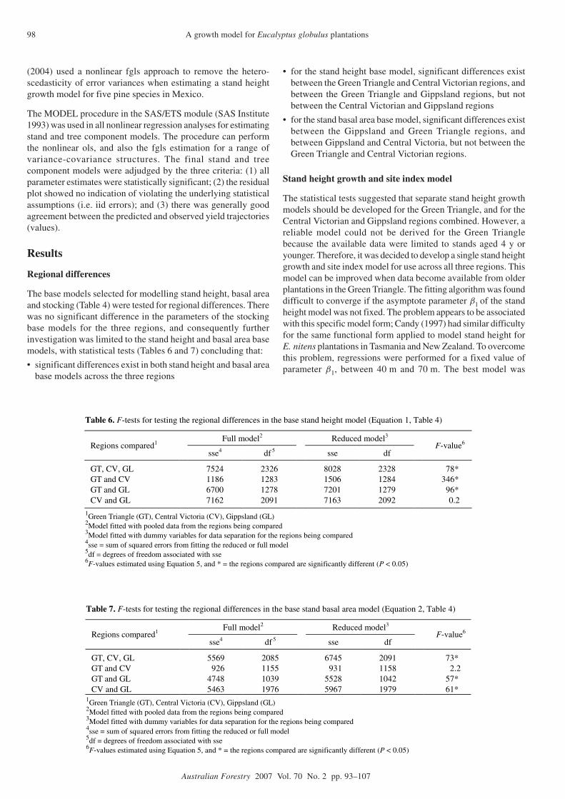
98 A growth model for Eucalyptus globulus plantations
Australian Forestry 2007 Vol. 70 No. 2 pp. 93–107
(2004) used a nonlinear fgls approach to remove the hetero-scedasticity of error variances when estimating a stand heightgrowth model for five pine species in Mexico.
The MODEL procedure in the SAS/ETS module (SAS Institute1993) was used in all nonlinear regression analyses for estimatingstand and tree component models. The procedure can performthe nonlinear ols, and also the fgls estimation for a range ofvariance-covariance structures. The final stand and treecomponent models were adjudged by the three criteria: (1) allparameter estimates were statistically significant; (2) the residualplot showed no indication of violating the underlying statisticalassumptions (i.e. iid errors); and (3) there was generally goodagreement between the predicted and observed yield trajectories(values).
Results
Regional differences
The base models selected for modelling stand height, basal areaand stocking (Table 4) were tested for regional differences. Therewas no significant difference in the parameters of the stockingbase models for the three regions, and consequently furtherinvestigation was limited to the stand height and basal area basemodels, with statistical tests (Tables 6 and 7) concluding that:
• significant differences exist in both stand height and basal areabase models across the three regions
• for the stand height base model, significant differences existbetween the Green Triangle and Central Victorian regions, andbetween the Green Triangle and Gippsland regions, but notbetween the Central Victorian and Gippsland regions
• for the stand basal area base model, significant differences existbetween the Gippsland and Green Triangle regions, andbetween Gippsland and Central Victoria, but not between theGreen Triangle and Central Victorian regions.
Stand height growth and site index model
The statistical tests suggested that separate stand height growthmodels should be developed for the Green Triangle, and for theCentral Victorian and Gippsland regions combined. However, areliable model could not be derived for the Green Trianglebecause the available data were limited to stands aged 4 y oryounger. Therefore, it was decided to develop a single stand heightgrowth and site index model for use across all three regions. Thismodel can be improved when data become available from olderplantations in the Green Triangle. The fitting algorithm was founddifficult to converge if the asymptote parameter β1 of the standheight model was not fixed. The problem appears to be associatedwith this specific model form; Candy (1997) had similar difficultyfor the same functional form applied to model stand height forE. nitens plantations in Tasmania and New Zealand. To overcomethis problem, regressions were performed for a fixed value ofparameter β1, between 40 m and 70 m. The best model was
Table 6. F-tests for testing the regional differences in the base stand height model (Equation 1, Table 4)
Full model2 Reduced model3 Regions compared1
sse4 df.5
sse df F-value6
GT, CV, GL 7524 2326 8028 2328 078* GT and CV 1186 1283 1506 1284 346* GT and GL 6700 1278 7201 1279 096* CV and GL 7162 2091 7163 2092 000.2
1Green Triangle (GT), Central Victoria (CV), Gippsland (GL) 2Model fitted with pooled data from the regions being compared 3Model fitted with dummy variables for data separation for the regions being compared 4sse = sum of squared errors from fitting the reduced or full model 5df = degrees of freedom associated with sse 6F-values estimated using Equation 5, and * = the regions compared are significantly different (P < 0.05)
Table 7. F-tests for testing the regional differences in the base stand basal area model (Equation 2, Table 4)
Full model2 Reduced model3 Regions compared1
sse4 df.5
sse df F-value6
GT, CV, GL 5569 2085 6745 2091 73* GT and CV 0926 1155 0931 1158 02.2 GT and GL 4748 1039 5528 1042 57* CV and GL 5463 1976 5967 1979 61*
1Green Triangle (GT), Central Victoria (CV), Gippsland (GL) 2Model fitted with pooled data from the regions being compared 3Model fitted with dummy variables for data separation for the regions being compared 4sse = sum of squared errors from fitting the reduced or full model 5df = degrees of freedom associated with sse 6F-values estimated using Equation 5, and * = the regions compared are significantly different (P < 0.05)

99Yue Wang and Thomas G. Baker
Australian Forestry 2007 Vol. 70 No. 2 pp. 93–107
adjudged by fit statistics (e.g. R2Adj rmse), and accuracy statistics
estimated using a cross-validation procedure for prediction (e.g.mean error, mean relative error and mean squared error).
The regression residuals from the ols fit showed no indication ofviolating the underlying assumptions (Fig. 1a). Therefore, thenonlinear fgls regression was not considered, and the best standheight growth model was:
MDH2 = β1
[1−
(1−
(MDH1
β1
)1/β2)T2/T1
]β2, (6)
where β1 = 50.0, β2 = 0.8903, R 2Adj = 0.88, and rmse= 1.76 m
(Table 8).
The corresponding site index model was obtained by replacingMDH2 and T2 with site index (S) and the reference age (i.e. 10 y),respectively:
S = β1
[1−
(1−
(MDH
β1
)1/β2)10/T ]β2
, (7)
where MDH is the stand height measured at any age T y.
There was generally good agreement between predicted andobserved MDH trajectories (Fig. 1b).
Stand basal area model
The statistical tests suggested that separate stand basal areamodels should be developed for Gippsland, and for the CentralVictorian and Green Triangle regions combined. An indicatorvariable (x) was used to index the data records and the threeparameters in the basal area base model (i.e. Equation 2 inTable 4) were replaced by the following linear functions:
β1 = a0 + a1x ,
β2 = b0 + b1x ,
β3 = c0 + c1x ,
(8)
where x = 1 if a data record was from Gippsland, and x = 0 if the
data record was from the Central Victorian or Green Triangleregion. The extended model was estimated using the MODELprocedure in SAS. Regression residuals from the initial ols fitindicated increasing variance as the initial stand age T1 increased.A weighting function of T1
–α, α = 0.5, 1.0, 1.5 and 2.0 was thenspecified for the nonlinear fgls regressions, and with α = 1 bestfor improvement of the residual plot (Fig. 1c) and fit statistics.
The parameter estimates for Equation 8 were:
β1 = 2.4445− 0.00146x ,
β2 = 0.05855− 0.0605x ,
β3 = 0.9594− 0.5506x ,
with R 2Adj = 0.96 and rmse = 1.63 m2 ha–1 (Table 8).
Parameter estimates for the stand basal area model (Equation 2in Table 4) were thus:
1. β1 = 2.4431, β2 = –0.00195 and β3 = 0.4088 for the Gippslandregion
2. β1 = 2.4445, β2 = 0.05855 and β3 = 0.9594 for the CentralVictorian or Green Triangle regions.
In general, there was good agreement between predicted andobserved basal growth trajectories, for example as presented inFigure 1d for Gippsland (i.e. x = 1) with S = 10, 15, 20, 25 and30 m.
Stand stocking model
Measurements from the three regions were pooled to estimatethe stand stocking projection model (i.e. Equation 3 in Table 4).To test if there was any effect of site quality on stand stocking, alinear function was used to relate the parameterof the model tothe site index (S) values of individual plots (i.e. β1 = a0 + a1S).However, the slope parameter estimate was not statisticallysignificant, and the relationship was not subsequently used. Theregression residuals derived from the ols fit indicated no violationof the underlying assumptions (Fig. 1e) and therefore the fglsregression was not pursued.
Table 8. Parameter estimates and fit statistics for the stand-level component models
Parameter estimate (standard error) Fit statistic Component model
Response variable
0β 1β 2β 3β
n rmse 2
AdjR
Stand height (Eqn 6)
MDH2 — 50.0 (NA 1) 0.8903 (0.0101) — 2170 1.758 0.877
Stand basal area (Eqn 2 in Table 4)2
BA2 — 2.4445 – 0.00146 x (0.041, 0.003)
0.05855 – 0.0605 x (0.002, 0.006)
0.9594 – 0.5506 x (0.012, 0.060)
2094 1.634 0.962
Stand stocking (Eqn 9)
N2 — 0.3387 (0.009) — — 2024 24.111 0.977
Diameter percentiles D0 3.8386 (0.264) 0.02863 (0.002) –0.1001 (0.030) –0.06909 (0.016) 1245 2.012 0.555 (Eqn 17) D25 7.6138 (0.203) 0.03867 (0.002) –0.1164 (0.011) –0.06122 (0.006) 1245 1.452 0.855 D50 8.7702 (0.162) 0.05166 (0.001) –0.1423 (0.009) –0.06640 (0.005) 1245 1.239 0.921 D95 10.9861 (0.203) 0.06992 (0.002) –0.1944 (0.011) –0.06579 (0.006) 1245 1.591 0.918
1Standard error not available when a parameter was fixed during fitting 2x is the region indicator: Gippsland (x = 1), Central Victoria (x = 0) and Green Triangle (x = 0)

100 A growth model for Eucalyptus globulus plantations
Australian Forestry 2007 Vol. 70 No. 2 pp. 93–107
Figure 1. Stand height (MDH), basal area (BA) and stocking (N) component models: (a), (c) and (e) regression residualsversus predicted values; and (b), (d) and (f) observed versus predicted growth trajectories for different initial values
4 16 20 24 288 12 32
6
–6
–4
–2
0
2
4
Predicted MDH (m)
Resid
ual (m
)
0
5
10
15
20
25
30
35
0 2 4 6 8 10 12
Age (y)
MD
H (
m)
(b)
(d)
(f)
(a)
(c)
(e)
–16
–10
–4
2
8
14
Resid
ual (m
2 h
a–
1)
0 10 20 30 40 50
Predicted BA (m2 ha–1)
0
4
8
12
16
20
24
28
32
36
0 2 4 6 8 10 12
Age (y)
BA
(m
2 h
a–
1)
0
200
400
600
800
1000
1200
1400
1600
0 2 4 6 8 10 12
Age (y)
Sto
ckin
g (
trees h
a–
1)
–160
–80
0
80
160
200 400 600 800 1000 1200 1400
Predicted stocking (trees ha–1)
Resid
ual (t
rees h
a–
1)

101Yue Wang and Thomas G. Baker
Australian Forestry 2007 Vol. 70 No. 2 pp. 93–107
The estimated stand stocking projection (mortality) model was:
N2 =[ 1√
N1
+ β1
(( T2
100
)2 −( T1
100
)2)]−2, (9)
where β1 = 0.3387, R 2Adj = 0.98, and rmse= 24.1 trees ha–1
(Table 8).
Stand stocking predictions for the initial stocking of 600, 800,1000, 1200 and 1400 trees ha–1, overlain with the observedstocking trajectories, are presented in Figure 1f.
Tree height–diameter model
A relationship between tree height and diameter is required whereactual or predicted diameter distributions are the basis forcalculation of individual tree volumes (and then by summationto total stand volume, or volume by size classes) using either atree volume or stem taper equation. Stand characteristics such asage, stocking, basal area or dominant height can improve treeheight–diameter relationships (e.g. Bi et al. 2000; Staudhammerand LeMay 2000).
Alternative functional forms were initially evaluated forestimating the tree height–diameter relationship (see Strandgardet al. 2005 for detailed discussion). For each of the model formsevaluated, different strategies were tested to include standvariables to improve predictions of tree height. In general, standheight (MDH) or site index (S), and dominant diameter (MDD,Table 1) improved predictions of tree height, but stand age,stocking or basal area did not. The following modification of theChapman-Richards function after Bi et al. (2000), i.e. Equation 1in Table 5, was found to be best:
H = 1.3+ β1 ×MDH(1− exp(−β2 × dbhob)
1− exp(−β2 ×MDD)
)β3, (10)
where β1 = 0.9148, β2 = 0.1504, β3 = 1.6079, R 2Adj = 0.97 and
rmse = 1.01 m (Table 9). The regression residuals showed noindication of violating the underlying assumptions (Fig. 2a). Inthis model, the intercept is fixed at 1.3 to account for treedbhob = 0 cm at H = 1.3 m.
In the developed height–diameter relationship, the predictorvariables of MDH and MDD provide measures of siteproductivity and stocking respectively; the prediction of treeheight can thus be improved over different site and stocking
conditions. For a given dbhob, the predicted height increases asMDH increases, but decreases as MDD increases. It must benoted that the height–diameter relationship was developed usingtree data sampled mainly from plantations with diameters andtotal heights of trees smaller than 35 cm and 30 m respectively,and height predictions for trees outside these ranges need to bevalidated.
Tree stem taper model
Alternative functional forms of stem taper models were initiallyexamined, including those of Max and Burkhart (1986) and Kozak(1988). The extended segmented taper model suggested byGoodwin and Thompson (2003) was found to be the mostappropriate for the available data, and was selected as the basemodel for further evaluation (i.e. Equation 2 in Table 5).
To determine the parameters of the base stem taper model,Goodwin and Thompson (2003) first related the parameters β1and β3 analytically to tree height (H). This was realised byimposing the constraints that when h = H, dh = 0 (i.e. the predictedstem diameter is zero if the sectional height input for predictionis total height), and that when h = h1, dh = d1 (e.g. h = 1.3 m, thendh = dbhub), where h1 ≠ H. These constraints gave:
β0 = −β1
1+ β2H+ β3H + β4H
2 , (11)
β3 =dbhub
H − 1.3− β1β2
(1+ 1.3β2)(1+ β2H)
− β4(H + 1.3) .
(12)
They then related the parameters β1, β2 and β4 to tree heightthrough the best species-specific relationship selected using atwo-stage modelling approach. For E. globulus plantations inTasmania, the relationships selected were:
β1 = γ1H , (13)
β2 =γ2
H, (14)
β4 = λ0 +λ1
H, (15)
where γ1, γ2, λ0, and λ1 are parameters to be estimated.
Table 9. Parameter estimates and fit statistics for tree-level component models (see Table 5 for model forms)
Parameter estimate (standard error) Fit statistic Component model
Response variable
0β 1β 2β 3β 4β
n rmse 2
AdjR
Height–diameter H — 0.9148 (0.001)
0.1504 (0.002)
1.6079 (0.012)
— 25831 1.007 0.971
Stem taper dh Eqn 111 0.4459 H (0.005)
85.3142 / H (4.231)
Eqn 122 0.0228 + 0.4185 / H (0.023, 0.042)
4001 1.118 0.983
Double bark thickness
DBT1.3 — 1.0511 (0.051)
1.7910 (1.135)
19.5889 (3.241)
— 191 0.659 0.618
1The taper model parameter 0β is estimated using Equation 11 2The taper model parameter 4β is estimated using Equation 12

102 A growth model for Eucalyptus globulus plantations
Australian Forestry 2007 Vol. 70 No. 2 pp. 93–107
application (SAS Institute 1993). The constraint, h1 =1.3 m, and d1 = dbhub were used in all fittings. Theresults confirmed that Equations 13–15 were alsoappropriate and the parameter estimates for theserelationships were:
β1 = 0.4459H ,
β2 =85.3142
H,
β4 = 0.02280+ 0.4185
H.
The resultant stem taper model had rmse = 1.12 cm,and R2
Adj = 0.98 (Table 9). The residual plot is shownin Figure 2b.
In application, the parameters β0, β1, β2 , β3, and β4will be first predicted from the observed H and dbhubof a sample tree using Equations 11–15. The predictedparameters are then applied to the taper model(Equation 2 in Table 5) for estimating the under-barkstem diameters along the stem, and correspondingsectional volumes. When the sectional height to bepredicted is total height, the predicted volume will betotal under-bark volume of a sample tree. To validatethe model, we showed in a separate study using asequential accuracy testing approach (Wang and Baker2005) that the predictions of under-bark stem diametersderived from this stem taper model would have anacceptable accuracy for most expected applications.
Tree stem bark thickness model
Tree dbhub and total height are required as inputs tothe developed stem taper model for predictingunderbark stem diameters. Dbhub is estimated as thedifference between dbhob and double bark thickness(DBT1.3), but because the latter is not commonlymeasured during inventory, a bark thickness predictionmodel is then required. The best model found for thispurpose based on the available data was:
DBT1.3 = β1 × exp(β2 −
β3
dbhob
), (16)
where β 1 = 1.0511, β 2 = 1.7910, β 3 = 19.5889,R 2
Adj = 0.62, and rmse = 0.66 cm (Table 9). The residualplot is shown in Figure 2c.
Diameter percentiles models
Quadratic mean diameter (Dq), stand basal area (BA) and age(T) were identified as the best stand variables for predicting thepercentiles D0, D25, D50 and D95 of the cumulative diameterdistribution at any age. The base model selected on the basis offit statistics and residual analysis was:
Dpct = [β0 + β1Dq × T ][1− exp
((β2 + β3BA)T
)], (17)
where Dpct, is the predicted value for D0, D25, D50 or D95.
In the present study, alternative relationships for the parametersβ1, β2 and β4 were firstly compared with those selected byGoodwin and Thompson (2003, i.e. Equations 13–15) using theavailable data. This was implemented by estimating the basemodel (Equation 2 in Table 5) and the relationships specifiedfor β0, β1, β2, β3 and β4 (i.e. Equations 11–15) using the nonlinearsimultaneous equations fitting procedure in the SAS/ETS
–3.0
–2.0
–1.0
0.0
1.0
2.0
3.0
0 5 10 15 20 25 30 35
Predicted height (m)
Re
sid
ua
l (m
)
–6
–4
–2
0
2
6
0 5 10 15 20 25 30 35 40
Predicted DUB (cm)
4
Re
sid
ua
l (c
m)
–3.0
–2.0
–1.0
0.0
1.0
3.0
0 1 2 3 4 5 6
Predicted DBT1.3 (cm)
2.0
Re
sid
ua
l (c
m)
(a)
(b)
(c)
Figure 2. Regression residuals graphed against the predicted valuesfor (a) tree height-diameter model (Equation 1, Table 5), (b) stem tapermodel (Equation 2, Table 5), and (c) bark thickness model (Equation 3,Table 5)

103Yue Wang and Thomas G. Baker
Australian Forestry 2007 Vol. 70 No. 2 pp. 93–107
The fit statistics and parameter estimates of the prediction modelsare presented in Table 8. In application, BA and N at age T arefirst predicted from the stand basal area and stocking projectionmodels respectively (i.e. Models 2 and 3 respectively in Table 4).Dq is then calculated based on the predicted BA and N.
Model application
The developed stand- and tree-level component models, togetherwith the models for predicting the four percentiles of diameterdistributions can be used to construct a whole-stand distributiongrowth and yield model (Vanclay 1994, p. 23). This size-classgrowth model can be used for projecting the characteristics ofplantations sampled in inventories into the future for wood flowanalysis and management planning. The procedures are:
1. Estimate the site index (S) for a sample plot or site from thestand height (MDH) measured at age T y using the site indexmodel (Equation 7).
2. Set the measured stand height, basal area and stocking, theestimate of site index and the inventory age to be the initialstand conditions (i.e. MDH1, BA1, N1 and T1) respectivelyfor the three stand-level models (i.e. Equations 1–3 inTable 4).
3. Predict stand height, basal area and stocking at the predictionage T2 (i.e. MDH2, BA2, and N2) from the stand-level modelsrespectively with their parameter estimates (Table 8).
4. Estimate stand volume (V2) at T2 using the following standvolume equation (Wong et al. 2000):
V2 = 0.3983× BA2 − 0.0661×MDH2
+ 0.35366× BA2 ×MDH2 .(18)
5. Estimate the diameter percentiles at age T2 (D0, D25, D50 andD95) using Equation 17 and their parameter estimatesrespectively (Table 8), where BA = BA2, T = T2, andDq = (40 000/π) (BA2/N2).
6. Predict the location and shape parameters of the Weibulldistribution at age T2 (a and c) using Equations 2 and 3.Negative values for a should be set to zero.
7. Solve Equation 4 for theWeibull scale parameter b (i.e.positive root of Equation 4) using the estimated a, c and Dq.
8. Predict the probabilities (fi) of diameter occurrence by 1 cmintervals of tree dbhob as:
fi = exp[−
(Li − ab
)c]− exp[−
(Ui − ab
)c], (19)
where Li and Ui are the lower and upper limits respectively
for i th diameter class i = 1, ..., k, and k is the total number ofdiameter classes. In application, the lower limit of the firstdiameter class should be set to the location parameter a (i.e.L1 = a and U1 = a + 1), which corresponds to the estimatedminimum tree diameter, and k should be determined withthe condition of Σk
i =1 fi = 1.
9. Estimate the stocking for each diameter class by multiplyingthe estimated fi with the stand stocking, N2, predicted as atStep 3.
10. Estimate the volumes for each diameter class. For this, meanvolume for a tree corresponding to the mid-point of eachdiameter class can be determined using the developed height–diameter relationship (Equation 10) and taper model(Equation 2 in Table 5 with parameter estimates as in Table 9).
11. Reset the initial conditions (predictor variables) at age T1 ofthe stand-level models to be the predicted values at age T2obtained in Step 3 (i.e. MDH2, BA2, N2), and prediction ageto be T2 + 1 (if annual predictions are required), and repeatSteps 2 to 10 until the target age or prediction interval isreached.
In this procedure, the predictions from the stand-level modelsare used as a control, and the stand stocking, basal area andvolume derived from the predicted diameter distributions areadjusted to be compatible with the stand-level predictions (Fig. 3).This approach has been widely used (e.g. Nepal and Somers 1992;Cao and Baldwin 1999; Wang and Hamilton 2003), and anappropriate algorithm and computer program is required foriterative adjustments.
Accuracy evaluation
The prediction accuracy of the stand growth models developedin the present study was evaluated using measurements from thereserved permanent plot data set described earlier. Stand(dominant) height, dominant diameter (MDD) and basal areavalues were calculated for every combination of plots andmeasurements. Volumes of individual trees were estimated usingthe height–diameter relationship developed in this study, and anexisting tree volume equation (Wong et al. 1999). Stand volumesfor each combination of plots and measurements were the sumof volumes of individual trees. Because stand-level modelsdeveloped have the algebraic difference equation form, thecalculated stand characteristics were rearranged into measurementpairs with non-decreasing ages for yield predictions. Summarystatistics for the last measurement data from the 338 permanentplots used are presented in Table 10.
Table 10. Summary statistics for the last measurements of permanent sample plots (n = 338) used for accuracy evaluation
Statistic Age (y)
MDH (m)
BA (m2 ha–1)
V (m3 ha–1)
MAI
(m3 ha–1) S
(m)
Mean 5.8 11.3 13.4 061.3 10.5 16.9 Minimum 4.9 04.6 02.2 006.3 01.2 08.0 Maximum 7.0 18.6 29.4 170.1 34.2 25.6
Eileen

104 A growth model for Eucalyptus globulus plantations
Australian Forestry 2007 Vol. 70 No. 2 pp. 93–107
Stand-level
growth prediction Diameter distribution
parameter recovery
Initial diameter distribution
estimation
Diameter distribution adjustment
(compatible with stand estimates)
Is prediction
age reached?
Stand
initiation
Output: stand and
size class yield
estimates
Prediction specificationIn
vento
ryG
row
th p
redic
tion
Wood flo
ws a
naly
sis
No
Yes
Figure 3. Flowchart illustrating application of the developed growth model
Table 11. Overall accuracy of predictions derived from stand growth models (n = 1997)
Accuracy measure1 Mean Minimum Maximum
Stand height: MD (m) –0.66 –5.85 4.13 MPD (%) –7.34 –68.72 28.32 MSD 2.82 0.05 33.61
Stand basal area: MD (m2 ha–1) 0.31 –3.96 7.48 MPD (%) 1.56 –63.53 45.91 MSD 2.28 0.05 33.96
Stand volume: MD (m3 ha–1) 1.01 –36.4 46.1 MPD (%) 1.06 –86.52 56.21 MSD 115.91 0.04 607.53
1MD = Mean difference between observed and predicted values MPD = Mean percent difference between observed and predicted values MSD = Mean squared difference between observed and predicted values

105Yue Wang and Thomas G. Baker
Australian Forestry 2007 Vol. 70 No. 2 pp. 93–107
For each stand characteristic evaluated, threestatistics were used to measure the predictionaccuracy (Table 11):
1. Mean difference (bias) (MD = Σ(yi – yi) /n), where yi and yi are the measured andpredicted values respectively, and n is thetotal number of measurement pairs usedfor the comparison. MD measures theoverall unbiasedness of predictions.
2. Mean percent difference (MPD(%) =[Σ(yi – yi)/yi] × 100/n). MPD measuresthe overall mean bias in a relative unit.
3. Mean squared difference (MSD = Σ(yi –yi)
2/n). MSD measures the total accuracyof prediction, which accounts for bothunbiasedness and precision of prediction(Reynolds 1984).
Mean bias for predicted stand heights wasrelatively small (–0.7 m), mean per cent biaswas about –7.3% of the observed values, andthe overall accuracy, accounting for both biasand imprecision was 2.8. Similarly, mean biasin predicted stand basal areas was relativelysmall (0.3 m2 ha–1), and about 1.6% of theobserved values with an overall accuracy of2.3. Mean bias in predicted stand volumes was1.0 m3 ha–1, about 1.1% of observed values.The corresponding MSD was 116; thatindicates relatively high variation in predictedstand volume. However, for a predictioninterval of 5 y or less, average bias inpredictions should be expected to be within±1.0 m for stand height, ±0.5 m2 ha–1 for basalarea, and ±1.0 m3 ha–1 for stand volumes, ifthe developed models are applied to predictfuture wood yields for a plantation populationbased on the inputs (current stand charac-teristics) observed in a large number of sampleplots established across the population. Graphsof predicted versus observed stand height,basal area and volume for the stand-levelcomponent models applied to the validationdata set are presented in Figure 4.
Discussion
The stand- and tree-level models developedhere for E. globulus plantations are the bestrepresentation of the long-term growth measurements (yieldtrajectories) from the Gippsland, Central Victorian and GreenTriangle regions that were made available to the present study.Predictions derived from the developed stand-level modelsrepresent the mean growth for plantations: (i) in the range ofclimatic (e.g. rainfall distribution patterns) and edaphic conditions(dominantly former agricultural sites) sampled in these regions,(ii) established and managed with similar silvicultural practices(planting stocking 1000–1200 trees ha–1, unthinned), and (iii)for the age range represented by the data (less than about age
12 y), used in model selection and parameterisation. Thesemodels should be validated before being applied to plantationsgrown under different conditions. Wang and LeMay (1996) andWang et al. (1996) developed statistical testing approaches forsuch applications.
The stand yields predicted from the developed models generallyagreed well with observed values from the permanent sampleplots, which are independent of model parameterisation. Accuracyevaluation indicated that for a prediction interval of 5 y or less,
2
4
6
8
10
12
14
16
18
20
22
2
4
6
8
10
12
14
16
18
20
22
2 4 6 8 10 12 14 16 18 20 22
Observed MDH (m)
2 4 6 8 10 12 14 16 18 20 22
Observed BA (m2 ha–1)
Pre
dic
ted
MD
H (
m)
Pre
dic
ted
BA
(m
2 h
a–
1)
0
20
40
60
80
100
120
140
160
180
0 20 40 60 80 100 120 140 160 180
Observed V (m3 ha–1)
Pre
dic
ted
V (
m3
ha
–1)
Figure 4. Predicted versus observed stand height (MDH), basal area (BA) and volume(V) for the stand-level component models applied to the validation data set

106 A growth model for Eucalyptus globulus plantations
Australian Forestry 2007 Vol. 70 No. 2 pp. 93–107
the average biases in predictions were generally small and within8.0% of measured stand heights, 3.0% of measured basal areasand 2.0% of measured stand volumes. Thus these models arereliable for projecting mid-rotation (i.e. 5–6 y) inventory data torotation age (i.e. about 10 y) for wood flow analysis and strategicor management planning. Greater accuracy is expected forpredictions over intervals 2–3 y from pre-harvest inventory fortactical planning of wood flows.
The stand and tree models, together with the Weibull distribution-based diameter distribution model, are useful for deriving yieldestimates by size (dbhob) classes. This information is essentialfor analysing the structure of managed plantations and makingmanagement decisions, particularly those associated with productassortment, recovery and harvesting costs.
The models may be extended to simulate the response ofE. globulus plantations to a range of silvicultural options fordetermining optimal management regimes. However, additionalcomponent models need to be developed for stand initiation undera range of silvicultural treatments (e.g. different plantingdensities). Also, models that can predict growth responses todifferent silvicultural treatments, particularly spacing andthinning, need to be developed using growth data from permanentplots in experimental trials.
The models can also be extended to incorporate the keyenvironmental variables that are known to affect tree growth, soproviding improved site-specific predictions and providingsensitivity to variation in climate. For example, Wang et al. (2007)used a non-linear mixed-effects modelling approach to incor-porate rainfall and temperature into a stand height growth modelfor E. globulus plantations in Central Victoria.
The development of stand growth models should be undertakenas a continuous process in order to make use of new data frompermanent sample plots representing different site and silvi-cultural conditions, and reflecting the results of tree improvement.We suggest that where there is a diversity of plantation investors,owners and managers such as there is for E. globulus in southernAustralia, model development and validation can be undertakenmost efficiently as a collaborative effort and that publicationcontributes generally to long-term confidence in this industry.
Acknowledgements
The work presented in this paper was undertaken as part of theBlue Gum Plantation Management System (BGPMS) project(PN03.3903) funded by the Forest and Wood Products Researchand Development Corporation. We thank staff at the School ofForest and Ecosystem Science, The University of Melbourne,particularly I. Wild, M. Strandgard and D. Chong for their commentsand advice on the design of the BGPMS. We also thank thecollaborating organisations and their representatives for providingdata, particularly Forestry SA, Hancock Victorian PlantationsPty Limited through Grand Ridge Plantations Pty Ltd, MidwayPty Ltd, Timbercorp Ltd, the Victorian Department of PrimaryIndustries and the Victorian Department of Sustainability andEnvironment.
ReferencesBailey, R.L. and Dell, T.R. (1973) Quantifying diameter distributions
with the Weibull function. Forest Science 19, 97–104.
Bailey, R.L., Burgan, T.M. and Jokela, E.J. (1989) Fertilized mid-rotation aged slash pine plantations — stand structure and yieldprediction model. Southern Journal of Applied Forestry 13, 76–80.
Bates, D.M. and Watts, D.G. (1988) Nonlinear Regression Analysisand its Applications. John Wiley and Sons, New York.
Beadle, C.L. and Inions, G.B. (1990) Limits to growth of eucalyptsand their biology of production. In: Dargavel, J. and Semple, N.(eds) Prospects for Australian Forest Plantations. ANU, Canberra,pp. 183–194.
Bi, H., Jurskis, V. and O’Gara, J. (2000) Improving height predictionof regrowth eucalypts by incorporating mean size of site trees ina modified Chapman-Richards equation. Australian Forestry 63,255–266.
Borders, B.E., Bailey, R.L. and Clutter, M.L. (1988) Forest growthmodel: parameter estimation using real growth series. In: Ek, A.R.,Shifley, S.R. and Burk, T.E. (eds) Proceedings of the IUFROForest Growth and Modeling and Prediction Conference,Minneapolis, MN, 24–28 August 1987. USDA Forest ServiceGeneral Technical Report NC-120, pp. 660–667.
Candy, S.G. (1997) Growth and yield models for Eucalyptus nitensplantations in Tasmania and New Zealand. Tasforests 9, 167–198.
Cao, Q.V. and Baldwin, V.C., Jr. (1999) A new algorithm for standtable projection models. Forest Science 45, 506–511.
Chang, S.J. (1987) Consistent growth and yield prediction throughintegration of whole stand and diameter distribution models. In:Ek, A.R., Shifley, S.R. and Burk, T.E. (eds) Proceedings of theIUFRO Forest Growth and Modeling and Prediction Conference,Minneapolis, MN, 24–28 August 1987. USDA Forest ServiceGeneral Technical Report NC-120, pp. 239–246.
Clutter, J.L., Fortson, J.C., Pienaar, L.V., Brister, G.H. and Bailey, R.L.(1983) Timber Management: A Quantitative Approach. JohnWiley and Sons, New York, 139 pp.
Da Silva, J.A.A. (1986) Dynamics of stand structure in fertilized slashpine plantations. PhD thesis, University of Georgia, Athens, GA,139 pp.
Duncan, M.J., Baker, T.G., Appleton, R. and Stokes, R.C. (2000)Growth of Eucalypt Plantation Species across Twelve Sites inGippsland, Victoria. Department of Natural Resources andEnvironment, Victoria, 46 pp.
Garcia, O. and Ruiz, F. (2003) A growth model for eucalypt in Galicia,Spain. Forest Ecology and Management 173, 49–62.
Goodwin, A.N. and Candy, S.G. (1986) Single-tree and stand growthmodels for a plantation of Eucalyptus globulus Labill. in northernTasmania. Australian Forest Research 16, 131–144.
Goodwin, A.N. and Thompson, D.N. (2003) A modified hyperbolictree taper model. Internal report to Forestry Tasmania, 35 pp.[Journal publication pending]
Greene, W.H. (1990) Econometric Analysis. MacMillan PublishingCompany, New York, 781 pp.
Huang, S. (1994) Ecologically-Based Individual Tree VolumeEstimation for Major Alberta Tree Species. Land and ForestServices Technical Report, Publication No. T/288, Edmonton,Alberta, Canada.

107Yue Wang and Thomas G. Baker
Australian Forestry 2007 Vol. 70 No. 2 pp. 93–107
Huang, S., Price, D. and Titus, S.J. (2000) Development of ecoregion-based height–diameter models for white spruce in boreal forests.Forest Ecology and Management 129, 125–141.
Inions, G. (1992) Studies on the growth and yield of plantationEucalyptus globulus in south-west Western Australia. PhD thesis,The University of Western Australia, 301 pp.
Knowe, S.A. (1992) Predicting the impact of inter-specific competitionin young loblolly pine plantations with diameter distributionmodels. Forest Ecology and Management 55, 65–82.
Knowe, S.A., and Stein, W.I. (1995) Predicting the effects of sitepreparation and protection on development of young Douglas-firplantations. Canadian Journal of Forest Research 25, 1538–1547.
Kozak, A. (1988) A variable-exponent taper model. Canadian Journalof Forest Research 18, 1363–1368.
Max, T.A. and Burkhart, H.A. (1986) Segmented polynomial regressionapplied to taper models. Forest Science 22, 283–289.
Nanang, D.M. (1998). Suitability of the Normal, Log-normal andWeibull distributions for fitting diameter distributions of neemplantations in northern Ghana. Forest Ecology and Management103, 1–7.
Nepal, S.K. and Somers, G.L. (1992) A generalised approach to standtable projection. Forest Science 38, 120–133.
Parsons, M., Gavran, M. and Davidson, J. (2006) Australia’s Plantations2006. Bureau of Rural Sciences, Department of Agriculture,Fisheries and Forestry, Canberra, 56 pp. http://adl.brs.gov.au/mapserv/plant/Plantations_100dpi.pdf.
Pillsbury, N.H., McDonald, P.M. and Simon, V. (1995) Reliability oftanoak volume equations when applied to different areas. WesternJournal of Applied Forestry 10, 72–78.
Reynolds, M.R. Jr. (1984) Estimating the error in model predictions.Forest Science 30, 454–469.
Rivas, J.J.C., Gonzalez, J.G.A., Gonzalez, A.D.R. and Gadow, K.V.(2004) Compatible height and site index models for five pinespecies in El Salto, Durango (Mexico). Forest Ecology andManagement 201, 145–160.
SAS Institute Inc. (1993) SAS/STAT User’s Guide. Version 8, SASInstitute Inc., Cary, NC.
Soares, P. and Tome, M. (2003) GLOBTREE: and individual tree growthmodel for Eucalyptus globulus in Portugal. In: Amaro, A., Reed,D. and Soares, P. (eds) Modelling Forest Systems. CABInternational, Oxon, Chapter 6, pp. 97–110.
Staudhammer, C. and LeMay, V. (2000) Height prediction equationsusing diameter and stand stocking measures. Forestry Chronicle76, 303–309.
Strandgard, M., Wang, Y., Chong, D., Wild, I. and Baker, T. (2005)Blue Gum Plantation Management System. Project PN 03.3903.Forest and Wood Products Research and Development Corpora-tion, Melbourne, 82 pp. http://www.fwprdc.org.au/content/pdfs/PN03.3903.pdf.
Tome, M., Falcao, A., Carvalho, A. and Amaro, A. (1995) A globalgrowth model for eucalypt plantations in Portugal. Lesnictvi-Forestry 41, 197–205.
Tome, M., Falcao, A. and Amaro, A. (1997) GLOBULUS V1.0.0: Aregionalised growth model for eucalypt plantations in Portugal.In: Oriega, A. and Gezan, S. (eds) Modelling Growth of Fast-Grown Tree Species. Proceedings of IUFRO Conference, 3–5September 1997, Valdivia, Chile. Universidad Austral de Chile,pp. 138–145.
Vanclay, J.K. (1994) Modelling Forest Growth and Yield: Applicationsto Mixed Tropical Forests. CAB International, Oxon, UK.
Wang, Y. and Baker, T.G. (2005) Developing and validating tapermodels for Eucalyptus globulus plantations using a sequentialaccuracy testing approach. Forest Biometry, Modelling andInformation Science 1, 51–62.
Wang, Y. and Hamilton, F. (2003) Projecting stand attributes of regrowthash eucalypts sampled in forest inventory. Australian Forestry66, 75–86.
Wang, Y. and LeMay, V.M. (1996) Sequential accuracy testing plansfor the applicability testing of existing tree volume equations.Canadian Journal of Forest Research 26, 525–536.
Wang, Y., LeMay, V.M. and Marshall, P.L. (1996). The relativeefficiency and reliability of some parametric and non-parametricsequential accuracy testing plans. Canadian Journal of ForestResearch 26, 1724–1730.
Wang, Y., LeMay, V.M. and Baker, T.G. (2007) Modelling andprediction of dominant height and site index of Eucalyptusglobulus plantations using a non-linear mixed-effects modelapproach. Canadian Journal of Forest Research (in press).
West, P.W., Ratkowsky, D.A. and Davis, A.W. (1984) Problems ofhypothesis testing with multiple measurements from individualsampling units. Forest Ecology and Management 7, 207–224.
Wong, J., Baker, T.G., Duncan, M.J., Stackpole, D.J. and Stokes, R.C.(1999) Individual Tree Volume Functions for Plantation Eucalypts.Report No. 99/037. Centre for Forest and Tree Technology,Department of Natural Resources and Environment, Victoria.
Wong, J., Baker, T., Duncan, M., McGuire, D. and Bulman, P. (2000)Forecasting Growth of Key Agroforestry Species in South-EasternAustralia. Publication No. 00/68, RIRDC, Canberra, 59 pp.

108 A carbon stocks and flows model for Australia
Australian Forestry 2007 Vol. 70 No. 2 pp. 108–119
Developing a carbon stocks and flows model for Australian wood products
Gary P. Richards1,2,3, Chris Borough4, David Evans5, Ainslie Reddin1, Fabiano Ximenes6 and David Gardner6
1Australian Greenhouse Office, GPO Box 787, Canberra, ACT 2601, Australia2The Fenner School of Environment and Society, The Australian National University, Canberra, ACT 0200, Australia
3Email: [email protected] Consulting, PO Box 262, Deakin West, ACT 2600, Australia
[email protected] for Greenhouse Accounting, Forest Resources Research, NSW Department of Primary Industries, PO Box 100,
Beecroft, NSW 2119, Australia
Revised manuscript received 8 February 2007
Summary
This paper describes the development of a model for estimatingAustralia’s stocks and flows of carbon in harvested woodproducts, including estimates of atmospheric emissions. Themodel estimates emissions in various forms, including those fromwood products contained in Australia, encompassing bothdomestically produced (net of exports) and imported woodproducts. This estimate is the basis of Australia’s NationalGreenhouse Gas Inventory report on wood products. The modelcan also estimate emissions from all (and only) wood productsproduced in Australia, and a third variant that presumes emissionsfrom wood products at the time of harvest.
The model represents a collaborative effort, involving relevantCommonwealth and state government agencies, industry groupsand research bodies. The model uses available statistics on logflows from forest harvest and estimates of the carbon content ofthe various wood products processed (for example, sawn timber,plywood, pulp and paper and woodchips) to determine carboninputs to wood products. The model uses estimates of the decayperiod of various classes of wood product to calculate the poolof carbon in wood products. Crosschecking with independentinput data was done wherever possible to test the robustness ofvarious input data used in the model development.
The model is built in Microsoft Excel with all rate and ageparameters easily accessed and varied for sensitivity testing usingthe @Risk software. Wood products in use are assigned to young-,medium- and old-age pools. Simulated losses of wood productsfrom their service life occur from each of the young-, medium-and old-age pools. Material leaving service is either transferredto bioenergy, added to landfill, recycled or emitted to the atmos-phere. Losses of carbon can also occur from the landfill pool.
The recorded imports and exports of wood products are used tocalculate emissions under two approaches. The first is from woodproducts produced in Australia (but not necessarily remainingwithin Australia), and the second from wood products stored inAustralia (wherever they were produced). Further simulations,with and without consideration of storage and emissions fromlandfill, are then run for each approach. The results show that an
accounting approach that presumes emissions from woodproducts at harvest over-estimates emissions to the atmospherewhen compared with approaches that consider the service life ofwood products. The storage of wood products in landfill is alsosignificant.
Keywords: models; forest products; stocks; lifespan; carbon; flow;greenhouse gases; Australia
Introduction
Wood product carbon emissions are included under the 1996(Revised) Intergovernmental Panel on Climate Change (IPCC)Guidelines for the United Nations Framework Convention onClimate Change (IPCC 1997). They are reported in the LandUse, Land Use Change and Forestry part of Australia’s NationalGreenhouse Gas Inventory (NGGI) where they arise from theservice life of products. The Waste section of the NGGI reportsemissions from landfill.
Under the inventory guidelines countries may elect to reportharvested wood products, but only if the national stock ofproducts is increasing. Although wood products may be reportedin an NGGI, they are excluded from accounting under the KyotoProtocol (UNFCCC 1997). This is prescribed in the MarrakechAccords (UNFCCC 2002) and the IPCC Good Practice Guidancefor Land Use, Land Use Change and Forestry (IPCC 2003). TheMarrakech Accords defer further decisions on the accountingtreatment of harvested wood products to future negotiations.Some later technical documentation has been prepared (UNFCCC2003) and submissions on potential accounting treatments sought.The IPCC 2006 Inventory Guidelines (IPCC 2006) provide somemethodological guidance, but do not specify accountingtreatments. The methodological guidance expands on that of theearly IPCC (Dakar) workshop (Brown et al. 1998) that consideredpotential accounting treatments.
Australia’s NGGI reports emissions when (in the year ofinventory) and from where (the country) they occur. Therefore,Australia’s NGGI reports emissions from wood products held inAustralia. Internationally, accounting options under considerationinclude treating the transfer of carbon in harvested wood across

109Gary P. Richards, Chris Borough, David Evans, Ainslie Reddin, Fabiano Ximenes and David Gardner
Australian Forestry 2007 Vol. 70 No. 2 pp. 108–119
national boundaries as a carbon credit (stocks increase) in thereceiving country, and as a stock loss (treated as an emission) inthe producing country. Other options include the producingcountries monitoring and reporting emissions from harvestedwood products they produce as emissions occur in other countries.
This paper focuses on developing a national wood productscarbon account for Australia’s NGGI, and provides contrastingoutcomes for accounting treatments beyond those of when andwhere the emissions occur. To consider the life cycle effects ofharvested wood products after their service life (that are reportedas Waste under the IPCC Guidelines) the model is extended toinclude disposal in landfill.
Countries other than Australia report on wood products in theirNGGIs (for example, USEPA 2006) or have otherwise preparednational estimates (for example, Pingoud et al. 2003). The inputdata, modelling methods and accounting frameworks used varyconsiderably. As developing the Australian model did not drawon these international parallels, they are not reviewed here.
A national database of domestic wood production and trade,including import and export quantities, has been kept since 1944by the Australian Bureau of Agriculture and Resource Economics(ABARE). This consistent and detailed collection of time-seriesdata provides a sound basis for developing a national woodproducts model. Jaakko Pöyry Consulting were initially engagedby the National Carbon Accounting System (NCAS) to developa national carbon accounting model for wood products, and thatwork provides the forerunner model to that adapted and describedhere. The early model development is reported in detail in theNational Carbon Accounting System Technical Reports No. 8(Jaakko Pöyry 1999) and No. 24 (Jaakko Pöyry 2000). Updatesand model refinement were subsequently undertaken by MBACConsulting and the NCAS. Jaakko Pöyry provided a qualityassurance review of the model as described here.
Approaches to carbon accounting
Accounting approaches for carbon emissions from timberharvesting and wood products reported in this paper include:
1. Presumed emissions at harvest
This approach records all domestic and exported wood and woodproducts and associated emissions in an Australian account, andtherefore reflects the wood product produced in Australia. Nowood products carbon pools develop using this approach. Thisis the IPCC default approach.
2. From wood products grown in Australia (wherever theproduct decays)
This approach accounts for all wood products and their emissionsarising from wood grown in Australia, regardless of the countryin which the product finally decays. Both the destination ofexported raw material and wood products, and the final productsthat they are converted into, need to be known. This approachneeds a division of all wood products grown in Australia intotwo categories: wood remaining in Australia, and wood exportedfrom Australia. However, as only the destination and not the fate
of wood products exported from Australia is known, it ispresumed here that the life cycle of products will be the same asif they were kept in Australia.
This assumption may not hold where products exported fromAustralia are used for different end-uses and are affected bydifferent environments at their final destination. Decay rates foreach country would be needed to determine the rate at whichcarbon is released into the atmosphere under local conditions,and these processes separately modelled. An added complicationis the need to track wood products re-imported to Australia (forexample, Australian woodchips exported to Japan, converted topaper, and subsequently imported by Australia). For simplicity,and because of lack of knowledge of product use and decay inother countries, decomposition of all products is treated accordingto Australian uses and conditions.
3. From wood products stored in Australia (wherever thesource)
This approach accounts for emissions from all wood productswithin Australia, regardless of their country of origin. Exportedwood products are accounted for by the importing country. Theamount of material exported is deducted from the total production,with total imports added, to derive the amount of materialavailable for emissions within Australia. The origin of importedwood products is irrelevant. However, Australia must monitorthe total flow of imported wood products into various pools.
Model components
Information for the following components of the model has beenobtained and examined:
• log flow from the forest: current annual production data wereobtained by species groupings and product classes, for example,sawlogs, veneer logs, pulp logs, roundwood and other(including sleepers etc.)
• fibre flow from processing: data on the intake of raw materialsto the various processing options and the output of productsand by-products have been used in the model to estimate thetotal tonnes of carbon produced each year under various endproduct classes
• import and export quantities of wood products
• recycling
• entry to and decomposition in landfill
• use for bioenergy
• other losses to the atmosphere.
Life cycles, wood flows and the wood productscarbon pool
Estimates of the life cycles and wood flows for each class ofwood product are reported in Jaakko Pöyry (1999, 2000), andmethods for estimating the existing pool of carbon in woodproducts proposed. Data for annual log removals are availablethrough the Australian Forests Products Statistics publishedquarterly by ABARE. Data are also available through the LeviesManagement Unit of the Australian Department of Agriculture,

110 A carbon stocks and flows model for Australia
Australian Forestry 2007 Vol. 70 No. 2 pp. 108–119
Fisheries and Forests, for the Forest and Wood Products Researchand Development Corporation (FWPRDC). Relevant state forestservices also publish data on log removals, and these provide avaluable crosscheck on ABARE data.
ABARE includes cypress pine in coniferous logs and does notprovide separate figures for these species. The volume of cypresspine log removals was estimated by applying a conversion factorto sawnwood consumption.
Wood flow
The model develops wood flows separately for each sector ofthe forest products industry and these are integrated to accountfor cross-linkages. This is important in accounting for waste orby-products which themselves may be used as resources by otherparts of the industry. In conjunction with the wood flows and theestimated life cycle of timber products, this model enables thetotal and future carbon pools to be estimated. Import and exportdata were obtained from the ABARE reports by end-usecategories. Details of the flows can be found in Jaakko Pöyry(1999, 2000).
In broad terms, the parts of the model developed for each sectorare similar, using:
• an estimate of raw materials input, whether of sawlogs,woodchips ex-sawmill or pulp logs
• an estimate of the products of processing, for example, ‘x’%sawdust, shavings or sander dust for on-site energy generationor compost, ‘y’% woodchips for other manufacturing processes,‘z’% of sawn timber products, panel products, paper, etc.
• an estimate of the fraction of products by product categories,depending on whether their expected end-use is long-term orshort-term; for example, framing timber, dry dressed boards,cases and pallet stock, panel products for use in houseconstruction, panelboards for use in furniture and cabinets,newsprint paper, writing and printing paper, etc.
• a final figure for total Australian consumption by end-usecategories, converted to wood-fibre content (oven-dry weight)and to tonnes of carbon.
Teatment of bark
Bark has not been separately accounted for in this study. Weregarded all bark as being a part of logging slash (harvestingresidue) and accounted for under in-forest logging operations,for the following reasons:
• logs are sold with log volumes recorded on an underbark basis
• in most hardwood operations, logs are debarked in the field
• in softwood operations, some bark is lost before the logs reachthe mill; most of this loss occurs during mechanised delimbingand log docking operations
• most softwood bark recovered at the mill is used for gardenmulch which has decay characteristics similar to those oflogging slash.
Softwood bark is a significant source of carbon, with total barkvarying from about 35% of underbark log volume (not oven-dryweight) in Caribbean pine to 20% in radiata pine and hoop pine.
As the fraction of softwood bark used for energy co-generationis likely to increase, it may be reasonable to review this treatmentin future.
While this approach is suitable for accounting for wood productsat a continental scale, it is a general assumption that should notbe applied when calculating a stand-based carbon balance. Thefraction of bark removed from the site may have a significantimpact on stand carbon balance.
Basic density and carbon content
Estimates of basic density and carbon content (Table 1) arerelevant to all the processing options, and the choice of valueshas a significant bearing on the outcome. For all sawn timber,treated softwood and hardwood poles, etc., weighted basicdensities for the species involved have been applied across eachcategory. Basic density is defined as oven-dry weight divided bygreen volume and the values adopted are based on Ilic et al.(2000). A different approach was used for board products andpaper, however, because these have been subjected to varyingamounts of compression during manufacture: their basic densitieswere derived from the air-dry density of the finished products.
The carbon content of dry matter is assigned values ranging from0.4 to 0.53 of the oven-dry (bone-dry) weight in the literature. Afigure of 0.5 is used in the model: this value is commonly usedelsewhere and is a median value among those of Gifford (2001).
Values for manufacturing parameters other than basic densityand carbon content came from interviews with representativesof various industry associations and individual sawmillingcompanies. The issues addressed included:
• recoveries of green sawn timber, sawdust and chip
• sawn sizes and corresponding dressed sizes
• the range and proportions of products produced.
Weighted averages of the information received provided realisticestimates for the various species and industry sectors excepthardwood sawmilling.
Wood flows from processing
Wood flows in the various wood products produced in Australiahave been developed under the following species or industryheadings:
• Softwood sawmilling
• Hardwood sawmilling
• Cypress sawmilling
• Plywood
• Particleboard and medium-density fibreboard (MDF)
• Pulp and paper
• Preservative-treated softwood
• Hardboard
• Hardwood poles, sleepers and miscellaneous
• Export of woodchips and logs.

111Gary P. Richards, Chris Borough, David Evans, Ainslie Reddin, Fabiano Ximenes and David Gardner
Australian Forestry 2007 Vol. 70 No. 2 pp. 108–119
Softwood sawmilling
Softwood processing is very efficient, and nearly all softwoodmills now have no waste. All slabs and edgings are chipped forpaper pulp or panelboard feedstock, and sawdust and shavingsare used for boiler fuel to provide energy for kiln drying. Thedestinations of sawlogs and sawn timber products were derivedfrom representative sawmills in South Australia, Tasmania,Queensland and the ACT, and from Pine Australia. Import andexport figures were derived from ABARE’s Forest ProductsStatistics. The basic density of 415 kg m–3 used (‘chips and logsfor export: softwood logs’) is from Ilic et al. (2000) and Gardnerand Ximenes (pers. obs.), being a weighted average of therespective densities at harvest of radiata pine, slash pine,Caribbean pine and hoop pine.
Hardwood sawmilling
Hardwood plantation production has been included in the totalhardwood removals. Most of this material is currently of pulplog quality, but more sawlogs will be harvested as the resourcematures. The hardwood sawmilling sector is far more complexand varied than any of the other sectors of the industry. There areat least ten major forest species throughout the country, all havingdifferent densities and shrinkage rates, and to a great extent havingdifferent end-uses. Assumptions on the product outturn fromhardwood sawmilling were based on information from the
Victorian Association of Forest Industries and a large sawmillingcompany running mills in Queensland, NSW and Tasmania. Dataon sawlog volumes produced, imports and exports were fromABARE.
A basic density of 630 kg m–3 was assumed for hardwoodsawlogs. This is an average of data for the following tencommonly logged hardwoods: spotted gum (Corymbiamaculata), blackbutt (Eucalyptus pilularis), rose gum or floodedgum (E. grandis), jarrah (E. marginata), karri (E. diversicolor),mountain ash (E. regnans), alpine ash (E. delegatensis), silvertopash (E. sieberi), brown barrel (E. fastigata) and messmatestringybark (E. obliqua). The basic density assumed for polesand sleepers was 790 kg m–3. This is an average of figures forspotted gum, ironbark, and blackbutt — the main species used.Hardwood chips have lower average density than sawlogs, polesor sleepers as they contain a wider range of species as well asyounger regrowth and plantation material. An average basicdensity of 630 kg m–3 was adopted.
Cypress sawmilling
The quantity of logs removed is small and the data are includedin the coniferous forest information in ABARE quarterly reports.Some cypress pine chips are used in panelboard manufacture,but the products are principally green framing, high-value flooringand dressed panelling.
Table 1. The basic densities, and moisture and carbon contents used in the model
Property and product Value
Carbon fraction
Softwood sawn timber: fraction of dry matter that is carbon, by weight 0.50
Particleboard: fraction of dry matter that is carbon, by weight 0.40
MDF: fraction of dry matter that is carbon, by weight 0.40
Basic density (kg m–3)*
Softwood sawn timber 460
Hardwood sawn timber 630
Cypress sawn timber 600
Plywood (softwood and hardwood) and veneer 540
Particleboard 520
Medium-density fibreboard (MDF) 600
Hardboard 930
Softboard 230
Pulp and paper: paper 1000
Pulp and paper: softwood 430
Pulp and paper: hardwood 500
Pulp and paper: wastepaper 1000
Pulp and paper: pulp 1000
Paper and paperboard imports and exports, on average 1000
Chips and logs for export: softwood logs 415
Chips and logs for export: hardwood logs 630
Hardwood poles, sleepers and miscellaneous 790
Moisture content of green wood (ratios)
Softwood chips — weight of water : weight of wood substance 1.10
Hardwood chips — weight of water : weight of wood substance 0.90
*Basic density = (mass of oven-dry wood in kg) / (volume of green wood in m3)
112 A carbon stocks and flows model for Australia
Australian Forestry 2007 Vol. 70 No. 2 pp. 108–119
Plywood (softwood and hardwood) and veneer
The Australian plywood industry is based principally onplantation-grown softwood and about 8% hardwood, both nativeand plantation grown. As well as plywood veneer, sliced or rotary-peeled decorative veneer is produced in small quantities forfurniture, door and panel overlays. This production is not recordedseparately by ABARE. Jaakko Pöyry (2000) estimated annualproduction to be less than 10 000 m3. Data used in the model forplywood were from ABARE and the Plywood Association ofAustralia.
Particleboard and medium-density fibreboard (MDF)
The characteristics of these two wood panelboards, includingtheir density, are different, but their feedstock and end-use productcategories are similar. Input is either small logs unsuited to saw-milling, or woodchips produced as a by-product of sawmilling.Most of the feedstock is from softwood plantations, althoughsome regrowth hardwood is being used in a plant in Tasmaniaand some cypress pine is being used in a plant in Queensland.The industry source used for information on processing assump-tions in the model was the Australian Wood Panels Association.
Pulp and paper
Plantation-grown softwood fibre provides the major resource,but hardwood fibre and recycled fibre are also important.Accounting for this sector is complicated as recycled fibre isexported and pulp is imported. While ABARE data provide someinformation, the Pulp and Paper Manufacturers Federation ofAustralia (PPMFA) provided more detailed figures. Productiondata in this study are derived from assumed raw material use andconversion figures rather than reported industry figures. Themodel-derived paper production estimates are 15% lower thanthe ABARE or PPMFA figures. This is because the modelcalculates the wood-only raw material for pulp and paper in oven-dry tonnes. The ABARE and PPMFA reported figures are in air-dry tonnes which contain about 10% moisture and 2–25% ofnon-wood fillers depending on the process.
A complicating factor in the assumptions on waste with the pulpand paper stream is that mills vary dramatically in their recoveryaccording to type. Kraft pulp mills typically have a low yield offibre (≈ 50%) whereas thermomechanical mills have a high yield(≈ 95%). The manufacture of paper from recycled material alsoresults in a lower yield of fibre. Based on weighted inputs, ayield of 70% was adopted.
Preservative-treated softwood
Both hardwood and softwood can be treated with preservative,but only softwood has been assigned a separate category in thisproject. This is because treated sawn softwood has some usecategories which are different to those for untreated softwood.Hardwood is usually treated so the sapwood can be protectedagainst borer attack or decay, and its use is then the same as foruntreated hardwood.
Treated softwood poles and posts have also been included withsawn softwood, but treated hardwood poles and piles have been
included with sleepers and other miscellaneous hardwoodproducts. The information used in the model was obtained fromthe Timber Preservers Association of Australia.
Hardboard
Hardwood is used for feedstock; supplies are derived from pulplogs and sawmill residue.
Hardwood poles, sleepers and miscellaneous
The existing stock of hardwood transmission poles in Australiais reputed to number about 6 000 000 and production is estimatedto be about 100 000 poles yearly, equivalent to about 75 000 m3
of log. Railway sleepers also represent a large resource, andalthough concrete sleepers are now used for all new work, timbersleepers will continue to be used to maintain secondary lines.‘Miscellaneous’ includes products such as mining, fencing andlandscaping timbers.
Log and woodchip exports
Export woodchips form a significant portion of the annual harvestfrom Australian forests. The ABARE quarterly forest productsstatistics report both bone-dry tonnes (BDt) of softwood chipsand BDt of hardwood chips exported. The model used theABARE-reported export figures directly in bone-dry tonnes.
Total exports of coniferous logs reported by ABARE consist ofboth sawlog and pulp log. New South Wales exports about7000 m3 of short poles annually.
Lifespan of timber products (recycling and landfill)
The lifespan of wood products must be considered whenascertaining the quantity of carbon stored in timber products.We have given considerable attention to subdividing the varioustimber products pools into different classes based on productand decay rates. The decay rates used assume that losses ofmaterial from service will increase with product age. Thereforethe entry and exit of material from production to loss from eachproduct pool is tracked and aged according to three age classes— young, medium and old. The fraction of material lost annuallyfrom each pool may vary (for example, there may be little lossfrom young pools (excluding those to the medium-age class)).Material is lost at a constant rate and may be placed in landfill,recycled, used for bioenergy or lost to the atmosphere (forexample, burnt with no energy capture) (Fig. 1).
For shorter-term products, the impact of the size of historic stocksis slight as recent additions to the pools are the major source ofmaterial available for loss. For long-term products, an estimateof the size of the historic pool is essential, but difficult. The sizeof the housing pool uses housing starts data. Other pools are alsoonly estimates. The fraction of the pool that has stemmed fromAustralian-grown wood is needed to implement an approach thatseparately deals with imported wood products. However, thiscomponent is difficult to estimate and estimates should be treatedwith some caution.

113Gary P. Richards, Chris Borough, David Evans, Ainslie Reddin, Fabiano Ximenes and David Gardner
Australian Forestry 2007 Vol. 70 No. 2 pp. 108–119
Lifespan pools assumed for the carbon model
Very short-term products — Pool 1
• Softwood — pallets and cases
• Plywood — formboard
• Paper and paper products
Age1 (y): young = 1; medium = 2; old = 3
Short-term products — Pool 2
• Hardwood — pallets and palings
• Particleboard and MDF — shop fitting, DIY, miscellaneous
• Hardboard — packaging
Age (y): young = 3; medium = 6; old = 10
Medium-term products — Pool 3
• Plywood — other (noise barriers)
• Particleboard and MDF — kitchen and bathroom cabinets,furniture
• Preservative-treated pine — decking and palings
• Hardwood — sleepers and other miscellaneous hardwoodproducts
Age (y): young = 10; medium = 20; old = 30
Long-term products — Pool 4
• Preservative treated pine — poles and roundwood
• Softwood — furniture
• Hardwood — poles, piles and girders
Age (y): young = 20; medium = 30; old = 50
Very long-term products — Pool 5
• Softwood — framing, dressed products (flooring, lining,mouldings)
• Cypress — green framing, dressed products (flooring, lining)
• Hardwood — green framing, dried framing, flooring andboards, furniture timber
• Plywood — structural, laminated veneer lumber (LVL),flooring, bracing, lining
• Particleboard and MDF — flooring and lining
• Hardboard — weathertex, lining, bracing, underlay
• Preservative-treated pine — sawn structural timber
Age (y): young = 30; medium = 50; old =90
Recycle Biofuel
Available for loss
Available for loss
Available for loss
Young age Mid age Old age
Landfill (all
available for loss)
Years
Po
ol siz
e (
kt
of
ca
rbo
n)
Atmosphere
Figure 1. Major pools and flows in the wood products model
1‘Age’ is the upper bound of the age class.

114 A carbon stocks and flows model for Australia
Australian Forestry 2007 Vol. 70 No. 2 pp. 108–119
A specified fraction of material may be lost yearly (an exponentialloss) from each age class of each product pool. The amount lostfrom each age class for each product pool can be capped anddifferent fractions can be lost according to age. This feature ofthe model provides for ‘steps’ in product loss rather than usingeither a simple linear or exponential loss applied to a wholeproduct pool, irrespective of the average age of the pool. If inputsvary over time the average age of products will vary, and this isrepresented by the amounts of material in each age class of eachproduct pool.
Initial stock assumptions
Input data were available for the model since 1944. This had thebenefit of allowing the model to establish new equilibrium poolsas the input material may be ‘turned-over’ several times beforean equilibrium stock is reached for recent years. Initial stockestimation (for 1944) is most important for Pool 5 as this materialmay remain in use now.
Model parameterisation
Once the data on production inputs, processing flows and initialstocks were determined other parameters needed for the modelincluded the:
• age at which material moved from young to medium and frommedium to old pools
• fraction of each age class for each product pool exposed toloss
• rate of loss from each age class in each product pool
• fraction of losses from each age class in each product pool toeach of landfill, recycling, bioenergy and the atmosphere
• rate of loss from landfill.
The estimates used for the model are presented in Tables 2 and 3.
Many of the estimates are based on expert judgement. In fact,often little empirical basis or opportunity for verification ofestimates exists. The maximum possible loss of carbon in woodproducts placed in landfill was based on research carried out bythe CRC for Greenhouse Accounting (unpublished) in two landfillsites in Sydney.
To understand the impact of uncertainties, Monte Carlo analysisusing the Palisade @Risk software (Palisade 1997) was applied.This approach is also able to identify model sensitivities. Throughthis, it is possible to identify where uncertainty in parameterestimation may be most significant for a probability distributionof expected outcomes, and to focus future data collection on areasthat will best reduce uncertainties.
Model results
By integrating the carbon pools, life cycles and wood flows ofwood products, the model enabled the total carbon pools andemissions to the atmosphere to be estimated. Table 4 shows theannual additions and losses and carbon pool sizes for the threeaccounting approaches.
Table 4 shows the significant potential of wood products to actas a store of carbon when the presumed ‘emissions at harvest’result is compared with the other two accounting options. Asemissions do eventually occur from stocks built up in the carbonstores, when a sufficiently large stock of carbon is emitting,estimates of emissions may exceed those from the presumedemission at harvest. When this occurs is a function of the rates ofboth input and decomposition (the higher the rates the earlierthis will occur) and when inputs to the carbon stocks are firstrecorded.
Uncertainty analysis
With the consistent and comprehensive monitoring of woodproduction in Australia since 1944, and the confidence in thisdata gained through cross-verification with other datasets, littleuncertainty is likely to be derived from the production data. Themost likely sources of uncertainty will be the allocation todecomposition and recycling pools, and the rates of decompo-sition in those pools. To test the relative importance of the poolages and decomposition rates, Monte Carlo analysis was undertakenusing the @Risk add-in software (Palisade 1997) to the Excelspreadsheet wood products carbon model. The principal modelparameters of interest were the decomposition rates within pools
Table 2. The maximum fraction of each pool available for loss (that is, exposed to decomposition, see Fig. 1) and decomposition rates (annual loss as a fraction of the amount of material exposed to decomposition in each pool)
Young Medium Old Lifespan
pool Available
for loss Loss (y–1)
Available for loss
Loss (y–1)
Available for loss
Loss (y–1)
Landfill loss
(y–1)
1 0.60 1.000 0.65 0.500 0.90 0.333 0.002 2 0.30 0.333 0.50 0.167 0.90 0.100 0.002 3 0.15 0.100 0.65 0.050 0.45 0.033 0.002 4 0.25 0.050 0.65 0.033 0.80 0.020 0.002 5 0.20 0.033 0.55 0.020 0.95 0.011 0.002
Table 3. Fraction of annual losses from each lifespan pool to landfill, recycling and biofuel
Lifespan pool
Landfill Recycling Bioenergy
1 0.44 0.49 0.04 2 0.75 0.20 0.05 3 0.95 0.05 0 4 0.85 0.15 0 5 0.85 0.10 0.05
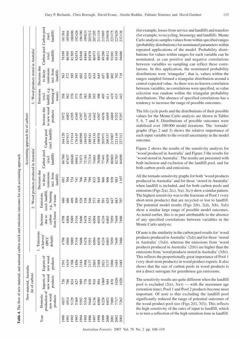
115Gary P. Richards, Chris Borough, David Evans, Ainslie Reddin, Fabiano Ximenes and David Gardner
Australian Forestry 2007 Vol. 70 No. 2 pp. 108–119
(for example, losses from service and landfill) and transfers(for example, to recycling, bioenergy and landfill). MonteCarlo analysis samples values from within specified ranges(probability distributions) for nominated parameters withinrepeated applications of the model. Probability distri-butions for values within ranges for each variable can benominated, as can positive and negative correlationsbetween variables so sampling can reflect these corre-lations. In this application, the nominated probabilitydistributions were ‘triangular’, that is, values within theranges sampled formed a triangular distribution around acentral expected value. As there was no known correlationbetween variables, no correlations were specified, so valueselection was random within the triangular probabilitydistributions. The absence of specified correlations has atendency to increase the range of possible outcomes.
The life cycle pools and the distributions of their possiblevalues for the Monte Carlo analysis are shown in Tables5, 6, 7 and 8. Distributions of possible outcomes werestabilised over 100 000 model iterations. The ‘tornado’graphs (Figs 2 and 3) shows the relative importance ofeach input variable to the overall uncertainty in the modeloutcome.
Figure 2 shows the results of the sensitivity analysis for‘wood produced in Australia’ and Figure 3 the results for‘wood stored in Australia’. The results are presented withboth inclusion and exclusion of the landfill pool, and forboth carbon pools and emissions.
All the tornado sensitivity graphs for both ‘wood productsproduced in Australia’ and for those ‘stored in Australia’when landfill is included, and for both carbon pools andemissions (Figs 2(a), 2(c), 3(a), 3(c)) show a similar pattern.The highest sensitivity was to the fractions of Pool 1 (veryshort-term products) that are recycled or lost to landfill.The potential model results (Figs 2(b), 2(d), 3(b), 3(d))show a similar large range of possible model outcomes.As noted earlier, this is in part attributable to the absenceof any specified correlations between variables in theMonte Carlo analysis.
Of note is the similarity in the carbon pool results for ‘woodproducts produced in Australia’ (2(d)) and for those ‘storedin Australia’ (3(d)), whereas the emissions from ‘woodproducts produced in Australia’ (2(b)) are higher than theemissions from ‘wood products stored in Australia’ (3(b)).This reflects the proportionally great importance of Pool 1(very short-term products) in wood product exports. It alsoshows that the size of carbon pools in wood products isnot a direct surrogate for greenhouse gas emissions.
The sensitivity results are quite different when the landfillpool is excluded (2(e), 3(e)) — with the maximum age(retention time), Pool 1 and Pool 2 products become mostimportant. Of note is that excluding the landfill poolsignificantly reduced the range of potential outcomes ofthe wood product pool size (Figs 2(f), 3(f)). This reflectsthe high sensitivity of the rates of input to landfill, whichis in turn a reflection of the high retention time in landfill.
Tab
le 4
. The
flo
w o
f ne
w m
ater
ial,
and
nati
onal
car
bon
stoc
k an
d em
issi
ons
outc
omes
for
eac
h ac
coun
ting
app
roac
h
Acc
ount
ing
appr
oach
(kt
of
carb
on)
New
mat
eria
l, A
ustr
alia
(k
t of
carb
on)
2. ‘
Woo
d pr
oduc
ts p
rodu
ced
in A
ustr
alia
’ 3.
‘W
ood
prod
ucts
sto
red
in A
ustr
alia
’
Yea
r
Dom
esti
c pr
oduc
tion
of
new
woo
d pr
oduc
ts
Impo
rts
of
new
woo
d pr
oduc
ts
Exp
orts
of
new
woo
d pr
oduc
ts
1.
‘E
mis
sion
s at
har
vest
’ (I
PC
C
defa
ult)
In
crea
se
due
to
carb
on
from
for
est
Em
issi
ons
(exc
l. la
ndfi
ll,
e.g.
, bur
ning
of
was
te
Dec
reas
e du
e to
dec
ay
(em
issi
ons
incl
. fro
m
land
fill
)
Car
bon
pool
(e
xcl.
land
fill
)
Car
bon
pool
(i
ncl.
land
fill
)
Inc
reas
e du
e to
new
woo
d pr
oduc
ts
Em
issi
ons
(exc
l. la
ndfi
ll, e
.g.
burn
ing
of
was
te)
Dec
reas
e du
e to
dec
ay
(em
issi
ons
incl
. fro
m
land
fill
)
Car
bon
pool
(e
xcl.
land
fill
)
Car
bon
pool
(i
ncl.
land
fill
)
1990
4 837
72
6 1 5
91
4 7
98
4 7
98
480
691
66 7
60
164 1
20
3 9
72
358
563
79 3
99
181 5
61
1991
4 914
78
6 1 6
19
4 8
04
4 8
04
486
704
67 6
37
167 9
13
4 0
82
362
572
80 3
95
185 0
44
1992
5 129
82
4 1 7
08
5 0
89
5 0
89
499
724
68 6
40
171 9
14
4 2
95
370
585
81 5
05
188 6
96
1993
5 369
82
7 1 8
56
5 3
16
5 3
16
509
741
69 8
11
176 1
45
4 3
40
373
593
82 6
74
192 4
26
1994
5 592
98
9 2 1
84
5 6
06
5 6
06
528
766
71 0
71
180 5
90
4 3
97
378
602
83 8
48
196 1
90
1995
5 516
77
8 1 9
98
5 4
78
5 4
78
538
784
72 1
81
184 9
25
4 2
97
383
614
84 8
63
199 8
33
1996
5 640
83
8 2 1
37
5 5
51
5 5
51
546
799
73 3
14
189 3
41
4 3
41
389
625
85 8
78
203 5
12
1997
6 136
91
0 2 6
03
6 0
94
6 0
94
573
833
74 6
61
194 1
34
4 4
42
393
634
86 9
73
207 2
95
1998
6 080
89
4 2 4
68
6 0
38
6 0
38
581
849
76 0
06
198 9
78
4 5
07
398
645
88 0
71
211 1
19
1999
6 228
1 0
69
2 621
6 216
6 216
59
1 86
6 77
441
20
3 971
4 676
40
5 65
7 89
280
21
5 095
20
00
6 8
52
944
3 137
6 803
6 803
62
5 90
8 79
039
20
9 337
4 659
41
1 66
9 90
412
21
9 038
20
01
7 0
89
870
3 090
7 059
7 059
64
7 93
9 80
803
21
5 007
4 869
41
9 60
2 91
691
22
3 175
20
02
7 7
17
1 020
3 4
85
7 6
49
7 6
49
683
983
82 7
83
221 1
16
5 2
52
433
702
93 1
95
227 6
29
2003
7 262
1 0
20
3 485
7 686
7 686
70
7 1 1
07
84 6
99
227 3
12
5 2
97
443
718
94 6
86
232 1
36

116 A carbon stocks and flows model for Australia
Australian Forestry 2007 Vol. 70 No. 2 pp. 108–119
Table 5. Uncertainty ranges of pool age (y) used in the Monte Carlo analysis
Lower bound Expected value* Upper bound Life cycle pool
Young Medium Old
Young Medium Old
Young Medium Old
Very short term 0.5 1 2 1 2 3 1.5 3 4 Short term 1 3 5 2 6 10 3 9 15 Medium term 5 15 20 10 20 30 15 25 40 Long term 15 20 40 20 30 50 25 40 60 Very long term 20 40 75 30 50 90 40 60 105
*As assigned in the text under the heading ‘Life spans for the carbon model’
Table 7. Uncertainty ranges of annual decomposition rate used in the Monte Carlo analysis
Age Life cycle
pool Lower bound
Expected value (as in Table 2)
Upper bound
Young 1 2.0000 1.000 0.6670 2 1.0000 0.333 0.3330 3 0.2000 0.100 0.0670 4 0.0670 0.050 0.0400 5 0.0500 0.033 0.0250
Medium 1 1.0000 0.500 0.3330 2 0.3330 0.167 0.1110 3 0.0670 0.050 0.0400 4 0.0500 0.033 0.0200 5 0.0250 0.020 0.0170
Old 1 0.5000 0.333 0.2500 2 0.2000 0.100 0.0670
3 0.0500 0.033 0.0250 4 0.0250 0.020 0.0170 5 0.0130 0.011 0.0100
Landfill 0.0015 0.002 0.0025
Conclusions
With the comprehensive and consistent collections of forestproduction statistics since 1944 it was possible to build a robustmodel of carbon stocks and flows for wood products by derivingsuitable conversion factors, allocating products to decompositionpools, and estimating the rates of decomposition for each pool.The benefits of a long run of wood products records is that, forall but the long-term pools, products pools have reached anequilibrium for recent years. In the longer-term pools, where thisis not the case, the model will be more sensitive (more so for
stocks than emissions) to the initial conditions. As pool size isdirectly proportional to the emissions, it is important to note thatthe model is sensitive to the time when inputs to the pools begin.The longer the pools have to increase (that is, the earlier themodel begins) the larger the overall carbon store that willexperience the same rate of emissions.
The inclusion or exclusion of the landfill carbon store (andtherefore emissions from landfill) is clearly very significant. Theincrease in the landfill carbon store provides a base for additionalemissions. Depending on the balance of rates of emission against
Table 8. Uncertainty ranges for destination fraction used in the Monte Carlo analysis for ‘wood products produced in Australia’ accounting approach
Landfill Recycle Biofuel Life cycle
pool Lower
bound Expected
value Upper bound
Lower bound
Expected value
Upper bound
Lower bound
Expected value
Upper bound
1 0.38 0.44 0.50 0.45 0.49 0.53 0.63 0.04 0.05 2 0.60 0.75 0.90 0.18 0.20 0.22 0.04 0.05 0.06 3 0.80 0.95 1.10 0.40 0.05 0.06 - 0 - 4 0.70 0.85 1.00 0.13 0.15 0.17 - 0 - 5 0.70 0.85 1.00 0.09 0.10 0.11 0.04 0.05 0.06
Table 6. Uncertainty ranges of pool size (as fractions) exposed to de-composition used in the Monte Carlo analysis
Age Life cycle
pool Lower bound
Expected value (as in Table 2)
Upper bound
Young 1 0.500 0.600 0.700 2 0.250 0.300 0.350 3 0.120 0.150 0.180 4 0.225 0.250 0.275 5 0.175 0.200 0.225
Medium 1 0.550 0.650 0.750 2 0.400 0.500 0.600 3 0.550 0.650 0.750 4 0.550 0.650 0.750 5 0.450 0.550 0.650
Old 1 0.800 0.900 1.100 2 0.800 0.900 1.100
3 0.400 0.450 0.500 4 0.700 0.800 0.900 5 0.800 0.950 1.150

117Gary P. Richards, Chris Borough, David Evans, Ainslie Reddin, Fabiano Ximenes and David Gardner
Australian Forestry 2007 Vol. 70 No. 2 pp. 108–119
–0
.9–
0.8
–0
.7–
0.6
–0
.5–
0.4
–0
.3–
0.2
–0
.10
0.1
Ma
xim
um
ag
e o
f m
id-a
ge
po
ol 2
pro
du
cts
Ma
xim
um
ag
e o
f yo
un
g p
oo
l 5
pro
du
cts
Fra
ctio
n o
f p
oo
l 4
pro
du
cts
lo
st
fro
m s
erv
ice
ea
ch
ye
ar
to la
nd
fill
Ma
xim
um
ag
e o
f m
id-a
ge
po
ol 1
pro
du
cts
Fra
ctio
n o
f yo
un
g p
oo
l 1
pro
du
cts
exp
ose
d t
o d
eca
y (
lost)
Fra
ctio
n o
f p
oo
l 3
pro
du
cts
lo
st
fro
m s
erv
ice
ea
ch
ye
ar
to la
nd
fill
Ma
xim
um
ag
e o
f yo
un
g p
oo
l 2
pro
du
cts
Ma
xim
um
ag
e o
f yo
un
g p
oo
l 1
pro
du
cts
Fra
ctio
n o
f p
oo
l 5
pro
du
cts
lo
st
fro
m s
erv
ice
ea
ch
ye
ar
to la
nd
fill
Ma
xim
um
ag
e o
f la
nd
fill
po
ol
Fra
ctio
n o
f p
oo
l 1
pro
du
cts
lo
st
fro
m s
erv
ice
ea
ch
ye
ar
to r
ecycle
Fra
ctio
n o
f p
oo
l 1
pro
du
cts
lo
st
fro
m s
erv
ice
ea
ch
ye
ar
to la
nd
fill
Re
gre
ssio
n s
en
sitiv
ity
–0
.10
0.1
0.2
0.3
0.4
0.5
0.6
0.7
0.8
0.9
Ma
xim
um
ag
e o
f m
id-a
ge
po
ol 2
pro
du
cts
Fra
ctio
n o
f yo
un
g p
oo
l 1
pro
du
cts
exp
ose
d t
o d
eca
y (
lost)
Fra
ctio
n o
f p
oo
l 4
pro
du
cts
lo
st
fro
m s
erv
ice
ea
ch
ye
ar
to la
nd
fill
Ma
xim
um
ag
e o
f m
id-a
ge
po
ol 1
pro
du
cts
Fra
ctio
n o
f p
oo
l 3
pro
du
cts
lo
st
fro
m s
erv
ice
ea
ch
ye
ar
to la
nd
fill
Ma
xim
um
ag
e o
f yo
un
g p
oo
l 2
pro
du
cts
Fra
ctio
n o
f p
oo
l 5
yo
un
g p
rod
ucts
exp
ose
d t
o d
eca
y (
lost)
Ma
xim
um
ag
e o
f yo
un
g p
oo
l 1
pro
du
cts
Ma
xim
um
ag
e o
f la
nd
fill
po
ol
Ma
xim
um
ag
e o
f yo
un
g p
oo
l 5
pro
du
cts
Fra
ctio
n o
f p
oo
l 1
pro
du
cts
lo
st
fro
m s
erv
ice
ea
ch
ye
ar
to r
ecycle
Fra
ctio
n o
f p
oo
l 1
pro
du
cts
lo
st
fro
m s
erv
ice
ea
ch
ye
ar
to la
nd
fill
Re
gre
ssio
n s
en
sitiv
ity
–0
.5–
0.4
–0
.3–
0.2
–0
.10
0.1
0.2
0.3
0.4
Maxim
um
age o
f young p
ool 4 p
roducts
Fra
ction o
f pool 1 p
roducts
lost
from
serv
ice e
ach y
ear
to r
ecycle
Fra
ction o
f m
id-a
ge p
ool 1 p
roducts
exposed to d
ecay (
lost)
Fra
ction o
f young p
ool 5 p
roducts
exposed t
o d
ecay (
lost)
Maxim
um
age o
f young p
ool 3 p
roducts
Fra
ction o
f m
id-a
ge p
ool 2 p
roducts
exposed to d
ecay (
lost)
Maxim
um
age o
f m
id-a
ge p
ool 2 p
roducts
Fra
ction o
f pool 1 y
oung p
roducts
exposed t
o d
ecay (
lost)
Maxim
um
age o
f young p
ool 5 p
roducts
Maxim
um
age o
f m
id-a
ge p
ool 1 p
roducts
Maxim
um
age o
f young p
ool 1 p
roducts
Maxim
um
age o
f young p
ool 2 p
roducts
Re
gre
ssio
n s
en
sitiv
ity
Lik
elih
oo
d o
f o
utc
om
e (
%)
Pool size in 2003 (’000 ktC)
10
15
20
25
30
35
40
45
50
55
60
65
70
75
80
85
90
95
5
0
20
40
60
80
10
0
12
0
19
0
20
0
21
0
22
0
23
0
24
0
25
0
Lik
elih
oo
d o
f o
utc
om
e (
%)
10
15
20
25
30
35
40
45
50
55
60
65
70
75
80
85
90
95
5
Pool size in 2003 (’000 ktC)
0
0.5
1.0
1.5
Lik
elih
oo
d o
f o
utc
om
e (
%)
10
15
20
25
30
35
40
45
50
55
60
65
70
75
80
85
90
95
5
Emissions in 2003 (’000 ktC)
(a)
Carb
on e
mis
sio
ns inclu
din
g those fro
m landfill
(b)
Ca
rbo
n e
mis
sio
ns in
clu
din
g t
ho
se
fro
m la
nd
fill
(d)
Ca
rbo
n p
oo
l in
clu
din
g t
ha
t in
la
nd
fill
(c)
Ca
rbo
n p
oo
l in
clu
din
g t
ha
t in
la
nd
fill
(f)
Ca
rbo
n p
oo
l e
xclu
din
g t
ha
t in
la
nd
fill
(e)
Ca
rbo
n p
oo
l e
xclu
din
g t
ha
t in
la
nd
fill
Fig
ure
2. R
esul
ts o
f th
e @
Ris
k se
nsit
ivit
y an
alys
is f
or t
he ‘
woo
d pr
oduc
ts p
rodu
ced
in A
ustr
alia
’ ac
coun
ting
app
roac
h. T
he t
orna
do g
raph
s ar
e tr
unca
ted
at 1
2 fa
ctor
s.N
egat
ive
sens
itiv
ity
indi
cate
s a
nega
tive
cor
rela
tion
wit
h th
e ou
tput
res
ult.

118 A carbon stocks and flows model for Australia
Australian Forestry 2007 Vol. 70 No. 2 pp. 108–119
–0
.9–
0.8
–0
.7–
0.6
–0
.5–
0.4
–0
.3–
0.2
–0
.10
0.1
Re
gre
ssio
n s
en
sitiv
ity
–0
.10
0.1
0.2
0.3
0.4
0.5
0.6
0.7
0.8
0.9
Re
gre
ssio
n s
en
sitiv
ity
–0
.5–
0.4
–0
.3–
0.2
–0
.10
0.1
0.2
0.3
0.4
Re
gre
ssio
n s
en
sitiv
ity
Lik
elih
oo
d o
f o
utc
om
e (
%)
Pool size in 2003 (’000 ktC)
10
15
20
25
30
35
40
45
50
55
60
65
70
75
80
85
90
95
5
Lik
elih
oo
d o
f o
utc
om
e (
%)
10
15
20
25
30
35
40
45
50
55
60
65
70
75
80
85
90
95
5
Pool size in 2003 (’000 ktC)
Lik
elih
oo
d o
f o
utc
om
e (
%)
10
15
20
25
30
35
40
45
50
55
60
65
70
75
80
85
90
95
5
Emissions in 2003 (’000 ktC)
Fra
ctio
n o
f p
oo
l 1
pro
du
cts
lo
st
fro
m s
erv
ice
ea
ch
ye
ar
to la
nd
fill
Fra
ctio
n o
f p
oo
l 1
pro
du
cts
lo
st
fro
m s
erv
ice
ea
ch
ye
ar
to r
ecycle
Fra
ctio
n o
f p
oo
l 5
pro
du
cts
lo
st
fro
m s
erv
ice
ea
ch
ye
ar
to la
nd
fill
Ma
xim
um
ag
e o
f la
nd
fill
po
ol
Ma
xim
um
ag
e o
f yo
un
g p
oo
l 1
pro
du
cts
Fra
ctio
n o
f p
oo
l 3
pro
du
cts
lo
st
fro
m s
erv
ice
ea
ch
ye
ar
to la
nd
fill
Fra
ctio
n o
f p
oo
l 4
pro
du
cts
lo
st
fro
m s
erv
ice
ea
ch
ye
ar
to la
nd
fill
Ma
xim
um
ag
e o
f yo
un
g p
oo
l 5
pro
du
cts
Ma
xim
um
ag
e o
f yo
un
g p
oo
l 2
pro
du
cts
Ma
xim
um
ag
e o
f m
id-a
ge
po
ol 1
pro
du
cts
Ma
xim
um
ag
e o
f m
id-a
ge
po
ol 2
pro
du
cts
Fra
ctio
n o
f yo
un
g p
oo
l 1
pro
du
cts
exp
ose
d t
o d
eca
y (
lost)
Fra
ctio
n o
f p
oo
l 1
pro
du
cts
lo
st
fro
m s
erv
ice
ea
ch
ye
ar
to la
nd
fill
Fra
ctio
n o
f p
oo
l 1
pro
du
cts
lo
st
fro
m s
erv
ice
ea
ch
ye
ar
to r
ecycle
Fra
ctio
n o
f p
oo
l 5
pro
du
cts
lo
st
fro
m s
erv
ice
ea
ch
ye
ar
to la
nd
fill
Ma
xim
um
ag
e o
f la
nd
fill
po
ol
Ma
xim
um
ag
e o
f yo
un
g p
oo
l 1
pro
du
cts
Ma
xim
um
ag
e o
f yo
un
g p
oo
l 2
pro
du
cts
Fra
ctio
n o
f p
oo
l 3
pro
du
cts
lo
st
fro
m s
erv
ice
ea
ch
ye
ar
to la
nd
fill
Fra
ctio
n o
f p
oo
l 4
pro
du
cts
lo
st
fro
m s
erv
ice
ea
ch
ye
ar
to la
nd
fill
Ma
xim
um
ag
e o
f m
id-a
ge
po
ol 1
pro
du
cts
Ma
xim
um
ag
e o
f yo
un
g p
oo
l 5
pro
du
cts
Fra
ctio
n o
f yo
un
g p
oo
l 1
pro
du
cts
exp
ose
d t
o d
eca
y (
lost)
Ma
xim
um
ag
e o
f m
id-a
ge
po
ol 2
pro
du
cts
Ma
xim
um
ag
e o
f yo
un
g p
oo
l 1
pro
du
cts
Ma
xim
um
ag
e o
f yo
un
g p
oo
l 5
pro
du
cts
Ma
xim
um
ag
e o
f m
id-a
ge
po
ol 1
pro
du
cts
Fra
ctio
n o
f yo
un
g p
oo
l 1
pro
du
cts
exp
ose
d t
o d
eca
y (
lost)
Ma
xim
um
ag
e o
f yo
un
g p
oo
l 2
pro
du
cts
Ma
xim
um
ag
e o
f m
id-a
ge
po
ol 2
pro
du
cts
Fra
ctio
n o
f yo
un
g p
oo
l 5
pro
du
cts
exp
ose
d t
o d
eca
y (
lost)
Ma
xim
um
ag
e o
f yo
un
g p
oo
l 3
pro
du
cts
Fra
ctio
n o
f m
id-a
ge
po
ol 1
pro
du
cts
exp
ose
d t
o d
eca
y (
lost)
Fra
ctio
n o
f m
id-a
ge
po
ol 2
pro
du
cts
exp
ose
d t
o d
eca
y (
lost)
Ma
xim
um
ag
e o
f yo
un
g p
oo
l 4
pro
du
cts
Fra
ctio
n o
f p
oo
l 1
pro
du
cts
lo
st
fro
m s
erv
ice
ea
ch
ye
ar
to r
ecycle
0
0.2
0.4
0.6
0.8
1.0
20
5
21
0
21
5
22
0
22
5
23
0
23
5
24
0
24
5
25
0 0
20
40
60
80
10
0
12
0
(a)
Ca
rbo
n e
mis
sio
ns in
clu
din
g t
ho
se
fro
m la
nd
fill
(b)
Ca
rbo
n e
mis
sio
ns in
clu
din
g t
ho
se
fro
m la
nd
fill
(d)
Ca
rbo
n p
oo
l in
clu
din
g t
ha
t in
la
nd
fill
(c)
Ca
rbo
n p
oo
l in
clu
din
g t
ha
t in
la
nd
fill
(f)
Ca
rbo
n p
oo
l e
xclu
din
g t
ha
t in
la
nd
fill
(e)
Ca
rbo
n p
oo
l e
xclu
din
g t
ha
t in
la
nd
fill
Fig
ure
3. R
esul
ts o
f th
e @
Ris
k se
nsit
ivit
y an
alys
is f
or t
he ‘
woo
d pr
oduc
ts s
tore
d in
Aus
tral
ia’
acco
unti
ng a
ppro
ach.
The
tor
nado
gra
phs
are
trun
cate
d at
12
fact
ors.
Neg
ativ
e se
nsit
ivit
y in
dica
tes
a ne
gati
ve c
orre
lati
on w
ith
the
outp
ut r
esul
t.

119Gary P. Richards, Chris Borough, David Evans, Ainslie Reddin, Fabiano Ximenes and David Gardner
Australian Forestry 2007 Vol. 70 No. 2 pp. 108–119
the rates of input material, future annual emissions from thiscarbon store could potentially exceed inputs.
The emissions estimates derived in this paper consider onlycarbon pools and carbon pool changes (losses being consideredas emissions); no corrections for global warming potentials havebeen applied. If the forms of gas containing carbon in emissionsare considered, atmospheric emissions in the form of methanehave a global warming potential (CO2 equivalence) 21 times thatof CO2. Losses of carbon as methane would therefore be ofpotential significance.
The effects of the accounting approach (‘emissions at harvest’,‘wood products produced in Australia’, or ‘wood products storedin Australia’) show that adopting the method that presumesemissions at harvest gives a greater emission than otherapproaches. This difference in outcome reflects the real-worlddelay in actual emissions following harvest because many woodproducts are stored in service for a significant time; the delay isincreased when retention in landfill is also considered.
Highest emissions arise from the effects of ‘wood productsproduced in Australia’ compared with ‘wood products stored inAustralia’. This would be expected because Australian exportstend to be short-term (pulp and chip) products, while imports arelonger-term products. The results highlight the importance oflandfill as a carbon storage mechanism, and the uncertaintiesassociated with this store. This uncertainty, and the possibleeffects on greenhouse gas emissions of increased methaneproduction (though potentially captured on emission) point toclear directions for future research.
Priority areas for further research and development identifiedduring the model development and sensitivity analysis include:
• the lifespan of timber products (both long-term products suchas framing timber in housing and products with a shorterlifespan such as paper and packaging)
• the methods of final disposal of wood products, some of which(for example, landfills) may significantly extend the life ofproducts before carbon release
• the rate and extent of decomposition of wood and paper inlandfill
• the method for determining the level of carbon sequestered inhousing
• the fraction of carbon that is lost as either carbon dioxide ormethane.
ReferencesBrown, S., Lim, B. and Schlamadinger, B. (1998) Evaluating
Approaches for Estimating Net Emissions of Carbon Dioxide fromForest Harvesting and Wood Products. Meeting Report, IPCC/OECD/IEA Programme on National Greenhouse Gas Inventories,Dakar, Senegal, 5–7 May 1998. http://www.ipcc-nggip.iges.or.jp/public/mtdocs/pdfiles/dakar.pdf.
Gifford, R. (2001) Carbon Content of Above-ground Tissues of Forestand Woodland Trees. NCAS Technical Report No. 22. AustralianGreenhouse Office, Canberra, 28 pp.
Ilic, J., Boland, D.J., McDonald, M. and Downes, G. (2000) WoodDensity — State of Knowledge. NCAS Technical Report No. 18.Australian Greenhouse Office, Canberra, 55 pp.
IPCC (Intergovernmental Panel on Climate Change) (1997) GreenhouseGas Inventory Workbook: Revised 1996 IPCC Guidelines forNational Greenhouse Gas Inventories. Institute for GlobalEnvironmental Strategies (IGES), Hayama, Kanagawa, Japan.
IPCC (Intergovernmental Panel on Climate Change) (2003) GoodPractice Guidance for Land Use, Land-Use Change and Forestry.Penman, J., Gtarsky, M., Hiraishi, T., Krug, T., Kruger, D., Pipatti,R., Buendia, L., Miwa, K., Ngara, T., Tanabe, K. and Wagner, F.(eds). Prepared by the National Greenhouse Gas InventoriesProgramme. Institute for Global Environmental Strategies (IGES),Hayama, Kanagawa, Japan. http://www.grida.no/climate/gpg/english.htm.
IPCC (Intergovernmental Panel on Climate Change) (2006) 2006 IPCCGuidelines for National Greenhouse Gas Inventories. Vol. 4.Agriculture, Forestry and other Land Use. Eggleston, H.S.,Buendia, L., Miwa, K., Ngara, T. and Tanabe, K. (eds). Preparedby the National Greenhouse Gas Inventories Programme. Institutefor Global Environmental Strategies (IGES), Hayama, Kanagawa,Japan.
Jaakko Pöyry (1999) Usage and Life Cycle Analysis of Wood Products.NCAS Technical Report No. 8. Australian Greenhouse Office,Canberra, 78 pp.
Jaakko Pöyry (2000) Analysis of Wood Product Accounting Optionsfor the National Carbon Accounting System. NCAS TechnicalReport No. 24. Australian Greenhouse Office, Canberra, 37 pp.
Palisade Corporation (1997) @Risk for Windows. Version 3.5.2Newfield, NY.
Pingoud, K, Perala, A.-L., Soimakallio, S. and Pussinen, A. (2003)Greenhouse Gas Impacts of Harvested Wood Products: Evaluationand Development of Methods. Espoo 2003. VTT Tiedotteita –Research Notes 2189, http://www.vtt.fi/vtt_show_record.jps?target=julk&form=sdefe&search=48482, 136 pp.
UNFCCC (United Nations Framework Convention on Climate Change)(1997) The Kyoto Protocol. Reprinted as UNEP/IUC/98/2, 1998,Climate Change Secretariat, Bonn, Germany. Also http://unfccc.int/resource/docs/convkp/kpeng.pdf.
UNFCCC (United Nations Framework Convention on Climate Change)(2002) [Marrakech Accords]. Report of the Conference of theParties on its Seventh Session, held at Marrakesh from 29 Octoberto 10 November 2001. Part one: Proceedings; Part two Addendum— Action taken by the Conference of the Parties. Volume I. andII. United Nations, Geneva. Documents FCCC/CP/2001/13,FCCC/CP/2001/13/Add.1, FCCC/CP/2001/13/Add.2. http://unfccc.int/resource/docs/cop7/13.pdf, 68 pp.
UNFCCC (United Nations Framework Convention on Climate Change)(2003) Estimation, Reporting and Accounting of Harvested WoodProducts. Technical Paper FCCC/TP/2003/7, 23 October 2003.Available from site library http://unfccc.int/documentation/documents/advanced_search/items/3594.php.
USEPA (US Environmental Protection Agency) (2006) Inventory ofUS Greenhouse Gas Emissions and Sinks: 1990–2004. TheAgency, 1200 Pennsylvania Avenue, NW, Washington DC, USA.

120 Predicting wood value using a decision support system
Australian Forestry 2007 Vol. 70 No. 2 pp. 120–124
Predicting wood value in Queensland Caribbean pine plantationsusing a decision support system
Kerrie Catchpoole1,2, Marks R. Nester3 and Kevin Harding4
1Forestry Plantations Queensland, PO Box 3196, South Brisbane, Queensland 4101, Australia2Email: [email protected]
3Forestry Plantations Queensland, PO Box 1339, Gympie, Queensland 4570, Australia4Department of Primary Industries and Fisheries, Horticulture and Forestry Science, PO Box 1085, Townsville,
Queensland 4810, Australia
Revised manuscript received 19 April 2007
Summary
A decision support system has been developed in Queensland toevaluate how changes in silvicultural regimes affect wood quality,and specifically the graded recovery of structural timber. Modelsof tree growth, branch architecture and wood properties weredeveloped from data collected in routine Caribbean pine planta-tions and specific silvicultural experiments. These models wereincorporated in software that simulates the conversion of standingtrees into logs, and the logs into boards, and generates detaileddata on knot location and basic density distribution. The structuralgrade of each board was determined by simulating the machinestress-grading process, and the predicted graded recoveryprovided an indicator of wood value. The decision support systemimproves the basis of decision-making by simulating the perform-ance of elite genetic material under specified silvicultural regimesand by predicting links between wood quality and general standattributes such as stocking and length of rotation.
Keywords: plantations; management; silviculture; models; conversion;computer software; wood properties
Introduction
A decision support system (DSS) that allows managers ofcommercial plantations to evaluate the effect of varioussilvicultural regimes on the graded recovery of structural timberhas been developed in Queensland by staff of Forestry PlantationsQueensland (FPQ) and the Department of Primary Industries andFisheries (DPI&F). The DSS is focussed on tropical andsubtropical commercial softwoods destined for sawlog andstructural timber markets, and initially has been calibrated forCaribbean pine (Pinus caribaea var. hondurensis).
The DSS provides a suite of software tools that evaluatessilvicultural scenarios and simulates the effects of changes instocking and rotation age on the branch architecture and woodproperties of logs and boards destined for structural timberproducts. Development entailed constructing models forCaribbean pine that describe stand growth, taper, brancharchitecture, wood density and wood stiffness for a range ofstockings and rotation ages, using data collected from specific
silvicultural experiments and routine plantations. These modelsare applied in conversion software1 that uses commercial sawingpatterns and specified log lengths to simulate cutting each treeinto logs and then into boards. The size and location of all knotsand the distribution of density in each board are outputs from theconversion software and are used in separate grading softwareto predict the structural Machine Graded Pine (MGP) grade ofeach board based on Australian Standard 1720.1 (SAA 1997).The DSS links graded recovery with stand parameters such asstocking and clearfall age to assist plantation managementdecision-making in relation to clonal selection and silviculturaloptions.
A number of similar decision support systems exist for differentspecies. Wood quality and the location and dimension of branchescan influence the recovery of timber from logs and in turn affectthe grades of timber obtained from a given tree (Leban et al.1999; Maguire et al. 1999; Pinto et al. 2003; Todoroki 2003). Inorder to understand the relationship between branching patterns,wood quality and graded recovery it has been advantageous toassess these properties at the tree and stand level, and link themto silvicultural practices in computer-based decision supportsystems. For example, models of wood properties such as basicdensity, spiral grain, ring width and mechanical properties havebeen developed for Norway spruce (Picea abies) for use inconversion software to link tree height, crown development, woodquality and branch architecture to the quality of sawn boards(Houllier et al. 1995; Lindström 2000). Conversion software hasbeen developed for radiata pine (Pinus radiata) that links woodproperties with sawing and end-use of timber (Todoroki 1996),and detailed models of branching were developed andincorporated in conversion software to determine the influenceof branching on timber value (Pont et al. 1999).
This paper provides an overview of the decision support systemdeveloped by FPQ and DPI&F and discusses its developmentand potential applications.
1In the context of this paper, ‘conversion software’ refers to specific softwarethat is designed to model the process of cutting trees into logs and boards.

121Kerrie Catchpoole, Marks R. Nester and Kevin Harding
Australian Forestry 2007 Vol. 70 No. 2 pp. 120–124
Components of the decision support system
The DSS consists of a suite of models and custom-built computersoftware tools (Fig. 1), and relies on the input of external dataand models. One of the software tools called STEPS (SoftwareTools for Evaluating Plantation Scenarios), developed as part ofthe DSS, was previously described in detail by Catchpoole andNester (2003, 2004). STEPS provides a user-friendly interfaceto evaluate a range of silvicultural scenarios in economic terms.The French Win-Epifn software (Leban et al. 1999; Meredieu etal. 1999) developed by the Institut Nationale de ReserchesAgronomique (INRA) has been adopted as the conversionsoftware. Win-Epifn was used to simulate the cutting of treesinto logs and boards and to assign the virtual board details(dimensions, knot sizes and positions) that are used in separateboard grading software. The grading software was specificallywritten to incorporate the Australian grading rules for MachineGraded Pine and assigns a structural grade to each board. Thesestructural grades and the graded recovery provide an indicationof wood value. The graded recovery estimates that are generatedby the grading software can be returned to STEPS to enable theinternal rate of return and net present value to be predicted.However, this function of the DSS has not yet been developed,as shown by the dashed line in Figure 1.
STEPS: The financial evaluation component
STEPS is a financial evaluation software tool developed usingVisual Basic for Applications in Microsoft Excel®. It allows theeconomic outcomes of various silvicultural scenarios to beanalysed and compared. The program takes into account growthand yield, all costs that occur over a rotation including costsassociated with thinnings and pruning, and specifications of thetimber products and prices applicable at thinning and clearfall.The user may provide parameters including site index, thinningage, clearfall age, pruning strategies and stocking to evaluatesilvicultural scenarios by estimating internal rate of return andnet present value. Options include the choice of discount rateand whether or not the net present value is calculated over onerotation or an infinite number of rotations. STEPS is currentlybeing used by Forestry Plantations Queensland as a stand-alone
software tool to evaluate silvicultural scenarios for purposes ofstrategic planning. It allows the simultaneous comparison ofeconomic and growth parameters to select optimum silviculturalregimes for specified estate areas.
Win-Epifn: The conversion software component
The French-developed conversion software called Win-Epifn©
INRA was customised for commercially grown Caribbeanpine in Queensland and was used to simulate the process of sawingtrees into logs and structural timber. It requires standard inventorydata (i.e. tree height, diameter, age and stocking), models ofbranch architecture, models of wood properties, and a selectionof optimised sawing patterns that vary according to log small-end diameter. The individual board descriptions that are generatedinclude board dimensions, the within-tree position of each board,the position and size of each knot, and the distribution of within-board density on the four sides of every board.
Branch models used in the conversion software
Considerable research has been undertaken in modelling brancharchitecture in Pinus radiata (Pont et al. 1999), Picea mariana(Lemieux et al. 2001) and Picea abies (Mäkinen et al. 2003).The purpose of the branch models is to characterise the relevantbranch architecture for each branch in the tree, and relate this toknot size and distribution for descriptions of individual boards.The models of branch architecture predict branch diameter,branch height, branch position (orientation within the whorl andbranch angle) and number of branches per whorl.
As models for Pinus caribaea var. hondurensis grown inQueensland were not available, they were developed for thisproject (Catchpoole et al. 2002) using data from a broad-scaledirect thinning trial in south-eastern Queensland.
Wood property models used in the conversion software
Substantial research has been undertaken to model various woodproperties in a range of species. Models for radiata pine estimatewood density distribution and spiral grain (Tian and Cown 1996),
External data/models
STEPS
Branch models
Wood property models
Conversion software
(Win-Epifn)
Grading software
(STEPSGrader)
Grading rules
Internal rate of return and net present
value
Graded recoveries for structural
timber
Figure 1. Structure of the decision support system

122 Predicting wood value using a decision support system
Australian Forestry 2007 Vol. 70 No. 2 pp. 120–124
and strength and stiffness (Burdon et al. 2001). In Norway spruce,properties modelled include wood density distribution (Lindström2000), spiral grain (Kliger 2002) and ring width (Saint-Andre etal. 2000). In Queensland, research has been undertaken toestimate genetic parameters for wood quality traits in Caribbeanpine (Harding et al. 1991) and more recently into variation inwood properties of the interspecific slash × Caribbean pine F1hybrid (Harding and Copley 2000).
The models of wood properties used in this project predict within-tree distributions of basic density and ring width, and weredeveloped from data collected from sawing studies andmechanical testing of timber from routine Caribbean pineplantations.
STEPSGrader: The grading software component
The grading software, called STEPSGrader, has been custom-built by FPQ and was developed in Microsoft Excel®. Data onwood density, ring width, knot size and knot location from theconversion software are used to predict wood stiffness (modulusof elasticity — MOE) of mechanically stress-graded pine timber.User-specified MOE thresholds and the predicted minimum MOEof a board are used in the grading software to assign MGPstructural grades to each board. MGP 15 is the highest stiffnessgrade, and timber of this grade is of higher value to industry thangrades MGP 12 and MGP 10. The standards for machine stressgrading (SAASANZ 2006) were used when setting the gradingrules in STEPSGrader. The grading software outputs aresummarised in terms of graded recovery at the log, tree and standlevel. The recovery achieved in the various structural grades canbe assigned a value to provide an estimate of the total value ofthe wood recovered.
Development and application of the DSS
The development and application of STEPS has been describedby Catchpoole and Nester (2004). This section therefore focuseson the development and application of the conversion softwareand the grading software components of the DSS. The conversionsoftware is species-dependent, and customisation for a particularspecies is done by supplying either a suite of model parametersor a suite of detailed data files. It was decided that maximumflexibility could be achieved by customising the conversionsoftware for Caribbean pine using data files as inputs, becausethis allowed independence from the software developer (INRA).The customisation process involved the following steps:
1. developing and evaluating models for tree height, diameterat breast height, height to first dead branch, height to firstlive branch, height to first live whorl, whorl height, numberof branches per whorl, individual branch diameter and branchinsertion angle (Catchpoole et al. 2002)
2. developing models for within-tree wood density and ringwidth
3. from each model listed in 1 and 2, generating files ofsimulated data in the format required as input by theconversion software
4. incorporating sawing patterns based on Queenslandcommercial pine operations.
Steps 1–3 were undertaken with minimal assistance from thesoftware developer, INRA. Data were readily available from long-term experiments to develop the models for tree growth, brancharchitecture and wood properties. Developing the models andgenerating the input files, however, was time consuming giventhe limited availability of staff with mathematical andprogramming expertise. INRA assisted in Step 4 to ‘hardwire’the sawing patterns into the conversion software.
Input files were created for the stocking classes of 100 stems ha–1
(sph), 200 sph, 300 sph, 500 sph and 750 sph, and rotation agesranging from 15 to 32 y. These were efficiently and automaticallygenerated using a combination of Unix, Maple and MicrosoftExcel platforms. Simulations were performed for each of theinput files using the conversion software. The options selectedin the software to model the conversion process included cuttingeach tree systematically into logs up to a top diameter of 10 cmunder bark, an initial stump height of 15 cm and a log length ofeither 490 cm or 610 cm. Each log was then virtually sawn intoboards using a sawing pattern that was available in the softwareand varied depending on small-end diameter. The conversionsoftware produced outputs in graphical and tabular formats atthe stand, tree, log and board level. At the board level this includeddetailed descriptions of knot size and location on the four sidesof every board, as well as knot area ratio and board densityprofiles. The tabular outputs were exported to other softwarepackages for analysis, and were used in STEPSGrader wherestructural machine grades were assigned to each board.
These simulations have been completed and the results areundergoing validation. This has involved a thorough analysis toensure that all tabular output from the conversion softwareincluding that on knot size and location, knot area ratio calcula-tions, board dimensions and wood density profiles makes senseagainst the data provided in the input files. This check revealedthat the conversion software required several modifications toadequately model Caribbean pine grown in Queensland. Win-Epifn was developed for northern-hemisphere species such asDouglas-fir and Sitka spruce; customisation for Caribbean pinerequired the ability to accurately model trees that produce multiplebranch whorls per year and may also produce foxtails (elongatedsections of stem producing no branches for several growingseasons).
Several limitations of the DSS need to be recognised wheninterpreting the results from STEPSGrader; these include anassumption that trees are straight and free of internal defect suchas resin shake and streak. Such limitations are inherent in theconversion software, but they could have considerable effect onthe graded recovery from P. caribaea var. hondurensis incircumstances where these defects are important. Becauseaccurately modelling these defects is complex and difficult, astandard discount for downgrade due to resin defects anddistortion is necessary. The cross-checking of results from theconversion and grading software and validation of the gradedrecoveries against actual sawmill recoveries will continue forseveral months.
The outputs of this DSS have many potential applications forcommercial forest growers, particularly those focusing on

123Kerrie Catchpoole, Marks R. Nester and Kevin Harding
Australian Forestry 2007 Vol. 70 No. 2 pp. 120–124
production of solid wood for the structural timber market. Thesystem is sophisticated in its ability to link stand silvicultureparameters with wood quality and can be used to:
• evaluate the effect of spacing and resulting branch architectureon graded recovery. This could be used simply for predictingvolume distributions across structural grades, or in decision-making to determine optimum spacing to achieve a desiredvolume of boards of a particular structural grade
• evaluate the effects of a change in rotation age on wood quality.The models that have been developed can be confidentlyapplied to rotations aged from 15 to 32 y, and therefore inputfiles for the conversion software can be created for any agewithin this range. This allows the effects of rotation age onwithin-tree density, knot area ratio, stiffness and in turn gradedrecovery to be assessed
• provide a better understanding of the wood quality of an existingresource for the purposes of short- to medium-term planning
• evaluate individual genotypes. The models will be modified tosuit the genotypes of interest, and the results of simulatedsawing and grading used to choose among genotypes as analternative to or in conjunction with selection indexes.
Conclusion
The value of recovered wood product is predicted in this decisionsupport system by integrating data and models that describe treegrowth, branch architecture, wood properties and the stiffness oftimber to generate a distribution of graded timber recoveries.These graded recoveries are linked to silviculture through thetree growth, branch architecture and wood property models thatare supplied for different stockings and clearfall ages. Thecomplex suite of such models required in this decision supportsystem is species-dependent. Customisation of the software forother species requires relevant data and capacity to develop therequired models. Such a process is potentially time consuming,particularly if data need to be collected in the field. As with mostdecision support systems it is necessary for the user to have agood understanding of the input models and their limitations inorder to be able to reliably interpret the outputs.
ReferencesBurdon, R.D., Britton, A.J. and Walford, G.B. (2001) Wood stiffness
and bending strength in relation to density in four nativeprovenances of Pinus radiata. New Zealand Journal of ForestryScience 31, 130–146.
Catchpoole, K.J. and Nester, M.R. (2003) STEPS Version 3.01. SoftwareTools for Evaluating Plantation Scenarios. User Manual.Department of Primary Industries, Brisbane, Queensland, 86 pp.
Catchpoole, K.J. and Nester, M.R. (2004) A financial calculator:software for evaluating plantation scenarios. Australian Forestry67, 191–193.
Catchpoole, K.J., Andrew, I., Nester, M.R., Harding, K.J. and Hogg, B.(2002) Development of branch models for use in a silviculturaldecision support system. In: Connection between Forest Resourcesand Wood Quality: Modelling Approaches and SimulationSoftware. Fourth workshop, IUFRO Working Party S5.01.04,8–15 September 2002. British Columbia, Canada. INRA-ENGREF, Centre de Recherche de Nancy, 54280 Champenoux,France, 9 pp.
Harding, K.J. and Copley, T.R. (2000) Wood property variation inQueensland-grown slash × Caribbean pine hybrids. In: Dungey,H.S., Dieters, M.J. and Nikles, D.G. (eds) Hybrid Breeding andGenetics of Forest Trees. Proceedings of QFRI/CRC-SPFSymposium, Noosa, Queensland, Australia, 9–14 April 2000.Department of Primary Industries, Brisbane, pp. 160–167.
Harding, K.J., Kanowski, P.J. and Woolaston, R.R. (1991) Preliminarygenetic parameter estimates for some wood quality traits of Pinuscaribaea var. hondurensis in Queensland, Australia. SilvaeGenetica 40, 152–156.
Houllier, F., Leban, J.M. and Colin, F. (1995) Linking growth modellingto timber quality assessment for Norway spruce. Forest Ecologyand Management 74, 91–102.
Kliger, R. (2002) Spiral grain on logs under bark reveals twist-proneraw material. Forest Products Journal 51, 67–73.
Leban, J.M., Dhote, J.F. and Herve, J.C. (1999) Modelling past growthand timber quality in forest stands. State-of-art in France forNorway spruce. Perspective application for some other softwoodspecies and for oak stem morphology. In: Nepveu, G. (ed.)Connection between Silviculture and Wood Quality throughModelling Approaches and Simulation Software. Third Workshop,IUFRO WP S5.01-04. Londe-Les-Maures, France. INRA-ENGREF, Centre de Recherche de Nancy, 54280 Champenoux,France, pp. 478–487.
Lemieux, H., Beaudoin, M. and Zhang, S.Y. (2001) Characterizationand modelling of knots in black spruce (Picea mariana) logs.Wood and Fiber Science 33, 465–475.
Lindström, H. (2000) Intra-tree models of basic density in Norwayspruce as an input to simulation software. Silva Fennica 34,411–421.
Maguire, D.A., Johnston, S.R. and Cahill, J. (1999) Predicting branchdiameters on second-growth Douglas-fir from tree-leveldescriptors. Canadian Journal Forest Research 29, 1829–1840.
Mäkinen, H., Ojansuu, R., Sairanen, P. and Yli-Kojola, H. (2003)Predicting branch characteristics of Norway spruce (Picea abiesL. Karst) from simple stand and tree measurements. Forestry 76,525–546.
Meredieu, C., Dreyfus, P., Saint-Andre, L. and Leban, J.M. (1999) Achain of models from tree growth to properties of boards for Pinusnigra ssp. laricio Arn.: simulation using CAPSIS©
INRA and
WinEpifn©INRA
. In: Nepveu, G. (ed.) Connection betweenSilviculture and Wood Quality through Modelling Approaches andSimulation Software. Third workshop, IUFRO WP S5.01-04, LaLonde-Les-Maures, France. INRA-ENGREF, Centre deRecherche de Nancy, 54280 Champenoux, France, pp. 505–513.
Pinto, I., Pereira, H. and Usenius, A. (2003) Analysis of log shape andinternal knots in twenty maritime pine (Pinus pinaster Ait.) stemsbased on visual scanning and computer aided reconstruction.Annals of Forest Science 60, 137–144.
Pont, D., Grace, J.C. and Todoroki, C.L. (1999) Modelling the influenceof radiata pine branching characteristics on visual timber grade.In: Nepveu, G. (ed.) Connection between Silviculture and WoodQuality through Modelling Approaches and Simulation Software.Third workshop, IUFRO WP S5.01-04, La Londe-Les-Maures,France. INRA-ENGREF, Centre de Recherche de Nancy, 54280Champenoux, France, pp. 63–71.
SAA (Standards Association of Australia) (1997) Timber Structures.Part 1: Design Methods. AS 1720.1, Standards Australia, Sydney,179 pp.

124 Predicting wood value using a decision support system
Australian Forestry 2007 Vol. 70 No. 2 pp. 120–124
SAASANZ (Standards Association of Australia and StandardsAssociation of New Zealand) (2006) Timber — MechanicallyStress-graded for Structural Purposes. AS/NZS 1748, StandardsAustralia/Standards New Zealand, Sydney and Wellington 12 pp.
Saint-Andre, L., Herve, J.C. and Leban, J.M. (2000) Modelling thenumber of rings in individual logs of Norway spruce. ScandinavianJournal of Forest Research 15, 135–143.
Tian, X. and Cown, D. (1996) Radiata pine wood properties model. In:Connection between Silviculture and Wood Quality throughModelling Approaches and Simulation Software. Secondworkshop, IUFRO WP S5.01-04, 26–31 August. Kruger NationalPark, South Africa. INRA-ENGREF, Centre de Recherche deNancy, 54280 Champenoux, France, pp. 95–103.
Todoroki, C.L. (1996) Developments of the sawing simulation software,AUTOSAW, linking wood properties, sawing and lumber end-use. In: Connection between Silviculture and Wood Qualitythrough Modelling Approaches and Simulation Software. Secondworkshop, IUFRO WP S5.01-04, 26–31 August. Kruger NationalPark, South Africa. INRA-ENGREF, Centre de Recherche deNancy, 54280 Champenoux, France, pp. 241–247.
Todoroki, C.L. (2003) Importance of maintaining defect cores. NewZealand Journal of Forestry Science 33, 25–34.

125Ian Ferguson and Jerry Leech
Australian Forestry 2007 Vol. 70 No. 2 pp. 125–133
Forest valuation and the AASB 141 accounting standard
Ian Ferguson1,2 and Jerry Leech1,3,4
1School of Forest and Ecosystem Science, The University of Melbourne, Parkville, Victoria 3010, Australia2Email: [email protected]
3Forestry Systems, Box 1632, Mount Gambier SA 5290, Australia4Southern Cross University, PO Box 157, Lismore, NSW 2480, Australia
Revised manuscript received 28 April 2007
Summary
This paper examines issues relating to forest valuation using theAustralian Accounting Standards Board accounting standardAASB 141 for large and medium-sized forestry entities. Currentpractices generally follow AASB 141:25 that states that anindependent valuation of land may (emphasis added) be deductedfrom the present value of the combined asset to yield a value forthe living trees (i.e. value of the biological asset), from whichgains or losses relative to the previous year may be brought toaccount in the income statement. Such an approach distorts theincome statement by gains and losses that are arbitrarily one-sided because the value of the living trees becomes a residualwhose value is influenced by any movements in land value,sometimes masking the inherent productivity and value of theliving trees.
The paper reviews key terminology and principles of AASB 141and other standards, including the definitions of biological assets,non-current assets, fair value, active markets, combined assets,and highest and best use.
In the absence of an active market for medium and large forestryassets, which is generally the case in Australia and New Zealand,the estimation of fair value using the present value of expectedcash flows is central to valuation. Whatever the respective formof ownership, land and living trees constitute a combined assetin which the roles are inseparable biologically. To be consistentwith the use of fair value of the combined asset based on thepresent value of expected cash flows, the planning horizon needsto be extended to a uniform future year for the entire asset. Thisis to enable the optimum schedule of wood and cash flows andhence the maximum present value to be estimated.
We describe an operational method to derive the present value ofthe living trees (the biological asset value as rigidly defined inAASB 141) by discounting the cash flows relating solely to thoseliving trees, in essence the current crop. Segmenting those cashflows from those used in evaluating the present value of thecombined asset can do this. Assuming the going concern is viable,such that forestry is the highest and best use, the remaining issueis how to ensure that the fair value of the combined asset isproperly reflected in the balance sheet. This can be done bydeducting the present value of the living trees (i.e. the value of
the biological asset) from that of the combined asset (after dueadjustment for land improvements). The resulting present valueof ‘future rotations’ should then be shown as a non-current assetunder ‘property, plant and equipment’.
Finally, the discount rates used in forest valuations generally allowfor taxation (and risk) in using a weighted average of the discountrates for equity and debt. Post-tax evaluation of cash flows istherefore recommended, rather than pre-tax, subject to avoidingdouble counting of any tax liabilities or debts elsewhere in theaccounts.
Keywords: valuation; assets; accounting; standards; terminology; cashflow analysis; stock accounting; tenure systems; discount rates
Introduction
Corporations law prescribes that the Australian AccountingStandards Board (hereafter AASB) Standard AASB 141‘Agriculture’ be used in preparing the annual financial statementsrequired of most private and public forestry entities under thatlaw. Accounting standards such as AASB 141 prescribe theprocesses to be used in ‘general purpose financial reporting’ andaim to meet the needs of a broad array of stakeholders byproviding information for making and evaluating decisions aboutthe allocation of scarce resources. For example, providers ofresources may want to know whether the reporting entity isachieving its stated objectives in the use of resourceseconomically and efficiently. Recipients of goods and services,and stakeholders with review and oversight responsibilities, maywant to assess the ability of the reporting entity to continue inthe future and whether it is making those goods and serviceseconomically and efficiently. The standards and reports aretherefore not aimed simply at the valuation of the business orspecific assets but at a much wider set of financial evaluationsusing accrual accounting and, in most cases, assuming the entitywill continue as a going concern. Nevertheless, the specifiedprocesses in AASB 141 have considerable significance for thevaluation of forestry assets when an ‘independent valuation’ isrequired which, as discussed later, is generally the case.
Following its decision to adopt the International AccountingStandards, the AASB adopted substantially all the InternationalAccounting Standard (hereafter IAS) IAS 41 ‘Agriculture’

126 Forest valuation
Australian Forestry 2007 Vol. 70 No. 2 pp. 125–133
content and wording, except where Australian legislation had tobe accommodated in AASB 141. Its application to accounting inagriculture became mandatory commencing 1 January 2005. NewZealand adopted the international standard IAS 41, commencingin 2006.
Dowling and Godfrey (2001) provide a survey and review of theaccounting practices applicable to forests, among other things,at the time of introduction of the previous so-called SGARA1
Standard (AASB 1037). Herbohn (2006) provides a later surveyand review of the adoption of the SGARA Standard andimplications of AASB 141. Forestry entities have encountered anumber of issues in implementing the changes relating to the useof AASB 141 and these form the focus for this paper. However,the AASB 141 Standard applies to a wider array of assets thanforests, including vineyards and orchards. These may also beaffected by these issues but are beyond the scope of this paper.
The Association of Consulting Foresters of Australia (ACFA)has issued its interpretation of the previous AASB 1037 Standard(ACFA 2004, 2005). ACFA recognised that these interpretationsdid not necessarily represent the views of AASB and were subjectto change as understanding evolved and as the AASB standardsevolved. The introduction of the new and, in some respects,different AASB 141 necessitated revision of the ACFA forestvaluation standard. This paper was intended to assist that revision,which will shortly become publicly available (ACFA 2007).
Whereas AASB 1037 required either an ‘independent valuation’or a ‘directors’ valuation’, AASB 141 does not specify either.Nevertheless, most governing boards or authorities use‘independent valuations’ if financially prudent, because theyreduce the risks to directors or the controlling authority. AustralianSecurities and Investment Commission (2006) guidelines statethat an ‘independent valuation’ intended for publication to asection of the public and issued for a purpose regulated by thecorporation law should be an objective and unbiased assessment,independent of any interested party. The aim of this paper is toexamine issues pertaining to an independent valuation of aforestry asset, to indicate the problems that stem from currentpractices in applying AASB 141, and to recommend an opera-tional method to overcome the issues.
The issues emerging with respect to the application of AASB141 and, to a large extent, its forerunner AASB 1037, affect manyforestry entities that are required to report according to thisstandard and some potentially have a major effect on financialreporting of profit or loss. Differing interpretations of the AASB141 Standard and its forerunner AASB 1037 by relevant entitiesare adding to the uncertainties of valuation. Our principal focusrelates to the valuation of large and medium-sized forests because,as noted in ACFA (2004), it is not appropriate to value these bysimple application of the market prices to the log volumes of theliving trees because an active market does not exist for suchproperties. Under these circumstances, the estimation of ‘fairvalue’ becomes a critical element.
Current valuation practices
Present value is currently the valuation method used by mostlarge and medium-sized forestry entities in Australia and NewZealand (ACFA 2004, 2005 and NZIF 1999) because the marketfor such assets is not active (AASB 141.8) — the frequency andasset characteristics of sales are irregular — and because market-determined values or sector benchmarks are insufficient in numberto provide a usable alternative. Most purchases are therefore basedon an assessment of present value of expected cash flows, oftenacross a wide array of age classes, site productivities and(sometimes) locations relative to customers. The use of presentvalue also links to the methods typically used for the preparationof business plans, as well as sale or acquisition valuations bythese entities. These assessments almost invariably value theforest as a going concern, unless it is to be broken up and sold inseparate parts.
AASB 116 ‘Property, Plant and Equipment’ has a set of‘Australian Guidance’ notes attached to it that are not a formalpart of that standard but include an important guiding principle(G2) that valuations of assets should be based on the ‘highestand best use’, the application of which to forestry assets is thesubject of detailed examination in a later section. Prior to the1990s, the issue of highest and best use did not need much furtherconsideration by consultants as real prices for marginal farmingland were relatively stable and low, or even declining as structuraladjustment of farming in some areas proceeded through naturalattrition.
That trend has changed, especially over the past ten years. Ruralland values in a number of areas have increased, mainly reflectingcompetition for potential forestry land by managed investmentcompanies in Australia (see Paton and Associates 2005) and bythe apparent prosperity of dairy farming in New Zealand (seeManley 2004). These trends have highlighted a major issue forforest valuation — that of valuing the living trees in a consistentand accurate manner. Few detailed studies are available but Wilton(2005) and a Jaako Pöyry report2 illustrate the issue.
Wilton’s report deals with a relatively small New Zealand estateof about 415 ha of pruned radiata pine (Pinus radiata D.Don)planted in 1996 and 1997 (see Forest Enterprises 2007 for details).Wilton applied the last sentence of AASB 141:25 (‘… the fairvalue of raw land and land improvements may be deducted fromthe fair value of the combined assets to arrive at the fair value ofbiological assets’) in calculating the values of the living trees atthe beginning and end of the period3 and then derived the gain orloss by subtraction. In the case cited, land values rose fromNZ$850 000 to $1 325 000, an increase of NZ$475 000, due tothe increased profitability of grazing in the area. Applying theseland values would imply that the value of the living trees (the
1SGARA is an acronym for a self-generating and regenerating asset.
2Jaako Pöyry (2005) Valuation of Evergreen Forest Limited’s forest assets as at30 June 2005. Letter from W. Liley, JP Management Consulting (Asia-Pacific)Ltd, Auckland to David Sayer , Evergreen Forest Ltd, dated 10 July 2005,previously available on the then Evergreen Forest Ltd’s website.3The context of the analysis and use of rating valuations for land suggest thatthe duration of the period was one year.
127Ian Ferguson and Jerry Leech
Australian Forestry 2007 Vol. 70 No. 2 pp. 125–133
biological asset) declined by NZ$364 937 despite an increasefrom NZ$2 287 554 to $2 397 617 in the present value of thecombined asset (i.e. a gain of NZ$100 063).
The Jaako Pöyry report concerns a sequence of valuations fromJune 2002 to June 2005 of a much larger and more varied estateof radiata pine owned by (then) Evergreen Forests Ltd in NewZealand. In addition to the effect of falling log prices, andrevisions of transport and harvest costs and of yield tables, thisreport noted a similar effect on the value of living trees on freeholdland, when calculated according to the last sentence of AASB141:25, due to progressively increasing land prices.
The Jaako Pöyry report goes on to argue that the land is notcapable of supporting viable grazing at those increased pricesand therefore attributes part of the increase in land value tospeculation on long-term capital gains, a point reiterated by Liley(2002). This raises an important but peripheral issue in relationto valuation. If speculation is the primary reason for investmentin land, whether carrying trees or not, then AASB 141 is not theappropriate standard for valuation of the entity — AASB 140‘Investment Property’ should be applied unless, subject to certainqualifying conditions, it is owner-occupied, in which case AASB116 ‘Property, Plant and Equipment’ applies. If it is not theprimary reason, but nevertheless a factor, the consultant and entityowner would need to make an assessment whether they believedthe speculation component was likely to be realisable in assessingand valuing the highest and best use according to the principlesoutlined earlier.
Returning to the principal issue relating to the use of AASB141:25 to value the living trees, the nub of our argument is thatwhile there may be cases involving small areas of forest whereAASB 141:25 can be applied appropriately, it is not generallyapplicable, nor need it be, noting the use of the word ‘may’ in theearlier quotation from AASB 141:25.
If one were to accept the deduction method, the value of livingtrees automatically becomes the complement of the value of the‘raw land’ in the best alternative use (i.e. the residual value afterdeducting the land value from that of the combined asset). Areferee has argued that this treatment as a residual is valid, drawingan analogy between this value and the value of equity in thebalance sheet in which equity is calculated as the differencebetween shareholders’ funds and liabilities. But that is a mis-leading analogy for a combined asset in which the different partshave to be valued separately. To do so would require that bothshareholders’ funds and liabilities be allocated to the respectiveparts. That brings us back to the nub of this problem because thededuction method assumes that growing trees confers noeconomic benefits or disbenefits, which is a one-sided distortionof the valuation of one part over the other.
The issue is one of an inconsistency in valuation method for livingtrees in the income statement, not a particular outcome in termsof gains or losses. Other things being equal, if real land priceswere to fall, gains would arise in the value of living trees,irrespective of the production by the living trees and resultantcash flows. In a medium to large forestry entity that is a goingconcern, a valuation method for living trees that is captive toannual fluctuations in real land price through the application of
AASB 141:25 will be inconsistent from year to year and beinaccurate.
How should the balance sheet most appropriately reflect the fairvalue, given that the living trees part has to be segmented andshown separately as a ‘biological asset’ (previously SGARA) inthe asset statement? Clarification leading to a greater consistencyof approach4 is urgently needed.
The terminology used in AASB standards and in AASB 141, inparticular, is critical to consideration of the issues relating tovaluation of forestry assets. In the next section of this paper, wedeal with some initial terminology and definitions, including thoseof biological assets, living trees, non-current assets and, mostimportantly, fair value. In the subsequent sections, we deal firstwith combined assets such as living trees and land, because thatsets the scene for the principles involved in the section on thehighest and best use. Successive sections then deal with valuingplantations held under single ownership of land and living trees,under forestry rights, and where land is leased. These sectionsprovide a consistent basis for valuation of forestry assets. In thenext two sections, an operational method for valuing all forms ofplantation ownership is developed and its application to valuingcommercial native forests considered. Sections dealing withdiscount rates and further concerns follow.
Terminology and definitions
In AASB 141, a biological asset ‘is a living animal or plant’.This term replaces the so-called SGARA term of AASB1037but is essentially the same thing with respect to its application toforest valuation. For clarity and greater specificity, relative toother well-established forestry terminology, we have coined theterm living trees to apply to the biological asset (previouslySGARA) involved in a forest. The other major component of aforestry asset is land, which is a specific non-current asset (seedefinition in AASB 101) under the Property, Plant and EquipmentStandard (AASB 116), as are other forms of property, plant andequipment.
‘Fair value’ is defined in AASB 141.8 as follows:
Fair value ‘is the amount for which an asset could be exchanged,or a liability settled, between knowledgeable, willing parties inan arm’s length transaction’.
If an active market does not exist, as is generally the case formany forestry entities, AASB 141.18 specifies the followingmethods that are to be used wherever market-determined pricesand benchmarks are available for the forest or other biologicalasset, in its present condition:
18. If an active market does not exist, an entity uses one ormore of the following, when available, in determining fair value:
4The Productivity Commission (2005) report Financial Performance of Govern-ment Trading Enterprises cites three of the five Australian state forestryenterprises that use present value, another two that use an immediate liquidationapproach, one current cost, and one historical cost, all ostensibly under AASB1037. Herbohn’s (2006) survey suggests a somewhat greater acceptance ofpresent value among commercial forestry entities under AASB 1037, albeitsubject to a number of qualifications.

128 Forest valuation
Australian Forestry 2007 Vol. 70 No. 2 pp. 125–133
(a) the most recent market transaction price, provided that therehas not been a significant change in economic circumstancesbetween the date of that transaction and the reporting date;
(b) market prices for similar assets with adjustment to reflectdifferences; and
(c) sector benchmarks such as the value of an orchard expressedper export tray, bushel, or hectare, and the value of cattleexpressed per kilogram of meat.
For many forestry and other biological assets no active marketfor the asset exists and market-determined prices or sectorbenchmarks may not exist — for example, many medium andlarge forestry assets spanning large areas and varied age-classes.Hence AASB 141.20–22 specify:
20. In some circumstances, market-determined prices or valuesmay not be available for a biological asset in its presentcondition. In these circumstances, an entity uses the presentvalue of expected net cash flows from the asset discounted at acurrent market-determined pre-tax rate in determining fair value.
21. The objective of a calculation of the present value ofexpected net cash flows is to determine the fair value of abiological asset in its present location and condition. An entityconsiders this in determining an appropriate discount rate to beused and in estimating expected net cash flows. The presentcondition of a biological asset excludes any increases in valuefrom additional biological transformation and future activitiesof the entity, such as those related to enhancing the futurebiological transformation, harvesting, and selling.
22. An entity does not include any cash flows for financing theassets, taxation, or re-establishing biological assets after harvest(for example, the cost of replanting trees in a plantation forestafter harvest).
The issue of valuation based on estimates of present value hasbeen a matter of debate outside and within the InternationalAccounting Board (see IAS 141: Basis for Conclusions,especially pp. 5–7), especially in relation to biological assetsand ‘financial instruments’ that include a wide range of itemsfrom cash and trade receivables, to interest and currency options,swaps and other financial derivatives. This debate is partly dueto the uncertainty attached to the future values of forestry assets(e.g. volumes harvested and their prices) and financial instrumentsbut also in some cases to reservations held about the use of market-determined prices. The recently approved section 48A ofAASB139 ‘Financial Instruments: Recognition and Measure-ment’ provides a useful basis for elaborating on the key conditionsfor estimating fair value of financial instruments using the presentvalue of expected cash flows. These conditions appear to us toapply equally well to forestry investments:
48A. The best evidence of fair value is quoted prices in anactive market. If the market for a financial instrument is notactive, an entity establishes fair value by using a valuationtechnique. The objective of using a valuation technique is toestablish what the transaction price would have been on themeasurement date in an arm’s length exchange motivated bynormal business considerations. Valuation techniques includeusing recent arm’s length market transactions betweenknowledgeable, willing parties, if available, reference to thecurrent fair value of another instrument that is substantially thesame, discounted cash flow analysis and option pricing models.
If there is a valuation technique commonly used by marketparticipants to price the instrument and that technique has beendemonstrated to provide reliable estimates of prices obtainedin actual market transactions, the entity uses that technique.The chosen valuation technique makes maximum use of marketinputs and relies as little as possible on entity specific inputs. Itincorporates all factors that market participants would considerin setting a price and is consistent with accepted economicmethodologies for pricing financial instruments.
Periodically, an entity calibrates the valuation technique andtests it for validity using prices from any observable currentmarket transactions in the same instrument (i.e. withoutmodification or repackaging) or based on any availableobservable market data.
AASB 141.24 acknowledges that, in some cases, cost mayapproximate fair value, one of the specific examples being thatof an immature plantation. AASB 141.18–24 outlines, but doesnot specifically prescribe, a hierarchy among the methods to beused where an active market does not exist because, as theinternational Accounting Standards Board puts it in the discussionof the IAS 41 (IASB 2005), ‘… a detailed hierarchy would notprovide sufficient flexibility to appropriately deal with all thecircumstances that may arise …’. Even so, the IAS 41 discussionmakes it clear that whatever method is used, account must betaken of all available market-determined prices and values. TheACFA Standard for valuing forests prescribes the reporting ofsuch comparative information in independent valuations.
The estimation of the present value of forestry assets is furthercomplicated by the fact that they are effectively ‘combined assets’.
Combined assets
Regardless of the ownership of the living trees (the biologicalasset) and land on which they stand, forests represent a combinedasset in the sense that the trees cannot exist without the land.This has major implications for the valuation of forestry assets.AASB 141.25 recognises that forestry and other biological assetsmay be combined assets and states:
25. Biological assets are often physically attached to land (forexample, trees in a plantation forest). There may be no separatemarket for biological assets that are attached to the land but anactive market may exist for the combined assets, that is, for thebiological assets, raw land, and land improvements, as apackage. An entity may use information regarding the combinedassets to determine fair value for the biological assets. Forexample, the fair value of raw land and land improvements maybe deducted from the fair value of the combined assets to arriveat the fair value of biological assets.
In the case of large and medium-sized forestry entities (otherthan those involving a ‘forestry right’ restricted solely to thecurrent living trees), the planning horizon for expected cash flowsfrom the going concern needs to be set to the same future year(i.e. planning horizon) across all stands. If the planning horizonis not set to the same future year across all age classes, it is notpossible to optimise the future wood flows (and hence netrevenues to the combined asset) with industry demands and futuredevelopment, as is typically used in business planning and inevaluation of purchase prices. To do otherwise, in a plantation

129Ian Ferguson and Jerry Leech
Australian Forestry 2007 Vol. 70 No. 2 pp. 125–133
estate with a range of age classes up to that of final harvest, wouldlead to a progressively diminishing wood flows over time as thewood supply from intermediate thinnings progressively ceases,as a result of no replanting after final harvest.
The methods used for business planning and the evaluation ofpurchase (or sales) price for large and medium forestry entitiesare well established. The forest is divided into a set of stands(generally according to age, site productivity and location) forwhich inventory estimates are available as to the currentcharacteristics. Computer-based models founded on empiricaldata and subject to field checking are used to forecast standgrowth, mortality and the expected yields by log assortmentclasses at any given age. These are embedded in mathematicalprogramming or simulation models that optimise the present valuemathematically or iteratively by matching the possible futurewood flows of the array of different log assortments againstindustry demands and future development over a fixed planninghorizon. The length of that horizon varies from 10 to 50 y (ormore) according to the predominant log assortments (e.g.pulpwood versus sawlog), growth rate of the species concerned,stand treatment (pruning, thinning etc.) and legal requirements(e.g. sustainable yield). The individual stand computations mayextend beyond the planning horizon to the year of final harvestof the current crop or infinite series thereof (after Faustmann)and then discounted back to the planning horizon, or there maybe an assumption of liquidation at the end of the horizon. In eithercase, the present or terminal value of the combined asset in thestand at the end of the planning horizon is effectively included asrevenue at that time.
Assuming fair value is calculated on the above basis, the presentvalue of the living trees can be calculated from the same cashflow data by segmenting those data to include only those costsand revenues relating to living trees at the time of the valuation.To put this another way, the fair value of the biological asset isbased on a present value calculation for the current crop of livingtrees.
AASB 141.26 requires that the change in fair value of the livingtrees must be included in the profit or loss for the relevant period,whereas the changes in the values of non-current assets are not.Land improvements (buildings etc.) that do not have living treesbut are potentially saleable separately from the combined assetof land and living trees can be valued independently of thecombined asset.
The issue taken up in the next section is how to address theprinciple of valuing according to highest and best use, a principlewhich underpins all forestry valuations of a combined asset.
Valuing highest and best use
From the accounting standard’s perspective for a going concern,the valuation of an asset is based on the premise of using thehighest and best use as the benchmark, as the Australian GuidanceNote G2 to AASB 116 sets out:
… The fair value of an asset is determined by reference to itshighest and best use, that is, the use of the asset that is physicallypossible, legally permissible, financially feasible, and whichresults in the highest value …
The independent valuation of land normally rests on appraisalsbased on market evidence by professionally qualified valuers.This is clearly a component relevant to the determination ofhighest and best use. When dealing with the value of a combinedasset such as land and living trees, however, it is not the onlyconsideration.
The appropriate comparison in determining the highest and bestuse is between the present value of the combined asset and thatof the best alternative use or uses of the separate components.Among other things, the present value of the best alternative usedepends on when it would be most opportune to harvest or removethe living trees, less the cost of rehabilitating the site, which variesconsiderably depending on age and the fair value of the land. Ifall the trees were very young, immediate clearing of living treesmay be appropriate. For large estates, progressive harvesting ofage classes over a number of years may be needed in order tobest realise the potential value of the living trees. Thus, assumingthere is no legal or other barrier to the opportunity to changeuses (see AASB 116.G2), the present value of the best alternativeuse is the optimum discounted salvage value of the living treesless the costs of rehabilitation plus the value of the land in thebest alternative use, as and when that land is expected to becomeavailable.
If the present value of the combined asset exceeds or equals thatof the best alternative use, the highest and best use is to maintainthe combined asset and value it accordingly. If less, the presentvalue of the alternative use is the appropriate valuation. Havingestablished how the principle of highest and best use might bestbe applied, we now turn to examine how valuation practices mightbe framed consistently across all forms of ownership but avoidingthe difficulties posed by AASB 141.25. We will confine our initialanalysis to that of plantation estates where the entity owns bothland and living trees. We later address ownership under forestryrights (legal ownership of living trees but not the land) and leasedland before describing the operational method, its application tocommercial native forests and the choice of discount rate.
Single ownership of land and living trees
The problem relates to the general application of the wording ofAASB 141.25 that ‘… the fair value of raw land and landimprovements may be deducted from the fair value of thecombined assets to arrive at the fair value of biological assets’by consultants undertaking independent valuations. Theunderlying issue is that living trees and similar long-lived plantcrops are seldom separable physically from the land until finalharvest without incurring a considerable decrease in productvalue. Separating them into the respective values of the livingtrees (the biological asset) and ‘raw land’ (the non-current asset),and then treating the two components as though they areindependent, is confounding the principle that the combined assetshould be valued on a fair value basis in its highest and best use,consistent with the valuation of other property and assets.
Clearly, a separate complementary entry of the present value of‘future rotations’ is needed to ensure the values of land and livingtrees sum to the fair value of the combined asset (after appropriateseparate recognition of land improvements). This is the onlymechanism that can ensure that the calculation of the biological

130 Forest valuation
Australian Forestry 2007 Vol. 70 No. 2 pp. 125–133
asset value plus the present value of future rotations is consistentwith the fair value of the combined asset as determined by presentvalue calculation.
As noted earlier, land improvements (e.g. buildings) that areseparable should continue to be valued independently of thepresent value calculations and shown separately as non-currentassets under property, plant and equipment on the balance sheet.
Forestry rights
In managing a forestry right involving an existing large ormedium-sized plantation, the entity uses both land and livingtrees as a combined asset, notwithstanding the different ownershipof land and living trees. In arm’s length transactions betweenknowledgeable and willing parties, the purchase price for aforestry right is almost invariably based on the present value ofthe expected cash flows. The same method also generally formsthe basis for later annual valuations.
If the forestry right covers only the harvest life of the youngestliving trees, then the present value of the living trees is simplyconfined to the living trees. Any harvest of future cropssubsequent to the harvest life of the initial set of living treesconfers no value because the valuation of a biological asset isrestricted to the living trees. The subsequent crop may, of course,confer costs if replanting is a legal requirement of the forestryright, but that will have been factored in calculating the price tobe paid for the forestry right.
If the duration of the forestry right extends beyond the harvestlife of the youngest living trees, the present value of futurerotations should be accounted for as in the preceding section.The proposed method of valuation for forestry rights is thereforeconsistent with that proposed for single ownership of land andliving trees.
Leased land
Under AASB 117.15, because land has an indefinite life and titledoes not normally transfer to the lessee at the end of the lease, itis treated as an operational lease and expensed5, unlike buildingswhich may be treated as a finance lease or an operating lease,depending on the conditions on the lease. Similarly, leases inwhich the lessor effectively retains much of the risks and benefitspertaining to the land, such as certain types of sharing and jointventure6 arrangements, are treated as operating leases. These donot appear as assets or liabilities in the balance sheet of the lesseebecause the lessee does not effectively own the assets. For these,the minimum annual lease payments are recognised as a directexpense, as are contingent rents7. Thus, it is appropriate to value
the present value of the living trees (i.e. biological asset) andthat of the present value of future rotations (if applicable) in thesame manner as above.
Many of the questions posed to the ACFA Forest Valuation Sub-Committee about the interpretation of AASB 141 relate to theforest value being perceived to be different on leased land to thaton owned land because of the practices adopted to date.
We now detail an operational method for valuation of forestryassets that is consistent across all types of ownership, based onthe principles developed in the preceding sections.
Operational method
The following method conforms to the provisions of AASB 141and the analogy with AASB 139.48A noted earlier and providesa more appropriate and accurate valuation method for mediumto large forestry entities where no active market for the forestryasset exists. The choice of the discount rate to be used is takenup in a later section.
1. Optimise the present value of the combined asset by mathe-matical programming or simulation to determine the bestschedule of wood flows over an extended uniform planninghorizon for both current and future tree crops and the presentvalue thereof (i.e. the fair value of the combined asset).
2. Segment those cash flows in (1) that relate solely to the livingtrees at the time of valuation and calculate their present value(i.e. the value of the biological asset, as defined in theAASB 141 standard). This value is used to calculate theannual change in value of the living trees which goes to theincome statement and thus to profit or loss.
3. Determine the value of land improvements from independentdata to the above and bring to account as a non-current assetunder property, plant and equipment.
4. Deduct the value of land improvements from the presentvalue of the combined asset (i.e. No. 1 above) to derive thepresent value of living trees plus future rotations.
5. Deduct the value of the living trees (i.e. No. 2) from thepresent value of the adjusted value of the combined asset(i.e. No. 4) and bring to account this present value of futurerotations as a non-current asset under property, plant andequipment.
6. Where the land is owned by the reporting entity, periodicrevaluations of land in the best alternative use should bedisclosed in notes to these estimates but not shown as a non-current asset under property, plant and equipment, to avoiddouble counting of assets.
Native and other forests
In principle, the valuation of medium to large-sized commercial8
native forest entities using even-aged silviculture is exactly the5We acknowledge the assistance of an anonymous referee in clarifying thispoint.6Joint venture in forestry practice sometimes involves complete control by thelessee and therefore does not qualify as a ‘joint venture’ under AASB 131 butin some cases control is shared jointly.7Contingent rent is that portion of lease payments that is not fixed in amountbut is based on the future amount of a factor that changes with the passage oftime (e.g. percentage of future sales, amount of future use, future price indices,future market rates of interest) — see AASB 117.
8AASB 141 is limited to ‘Agricultural activity’ which is defined as ‘themanagement by an entity of the biological transformation of biological assetsfor sale, into agricultural produce, or into additional biological assets.’ Whilethere may be some ambiguity inherent in the last phrase, the intent of thedefinition is clearly to exclude non-commercial forest uses, among others.

131Ian Ferguson and Jerry Leech
Australian Forestry 2007 Vol. 70 No. 2 pp. 125–133
same as that recommended above, although the planning horizonmay be much longer.
For a medium- to large-sized native forest entity in which uneven-aged forests are harvested under selection, gap or group selectionsilviculture, the present value would be calculated over successivecutting cycles to a fixed and long-distant planning horizon, butthe process is otherwise similar in principle.
The accounting treatment of coppice rotations following the firstor later rotations of coppicing species is nominally morecomplicated because the coppice remains a ‘biological asset’ afterharvesting and thus the value of the living trees (the biologicalasset or SGARA) is tied to the number of coppice rotationsexpected until the coppice is removed and new seedlings areplanted. In all other respects, the recommended method holdsfor coppice.
A number of other lesser issues arise in the interpretation of theprovisions of AASB 141 and these are taken up in ACFA (2007).However, one issue concerning the choice of discount rate is ofgreater importance and demands review here.
Discount rates
AASB 141.20 states that a ‘current market-determined pre-taxrate be used’ in determining the fair value through an analysis ofthe present value of expected cash flows. Nevertheless, someuncertainty appears to exist among standard-makers as to theappropriate approach regarding pre-tax or post-tax discount ratesbecause, in discussing general principles on fair valuemeasurement, the IASB (2006) discussion paper notes that ‘…after-tax cash flows should be discounted using an after-taxdiscount rate’.
Any due diligence concerning sale or purchase of a forest assetis normally carried out on a post-tax basis. Most valuers of forestsuse some variant of the weighted average cost of capital acrossboth debt and equity in such valuations and in annual financialvaluations. In doing so, taxation is implicitly recognised, as thedifferences between discount rates relating to debt versus thoserelating to equity are clearly not solely a matter of risk, but ratherof both risk and taxation treatment. A generic sector approach tothe treatment of cash flows net of taxation based on present andexpected future rates of taxation would be appropriate to theevaluation of the fair value of the combined asset. Fair valuemeasurement is an evaluation made in the hypothetical setting ofa transaction between a willing buyer and a willing seller anddoes not recognise the taxation circumstances of the particularentity. However, pre-tax is presently the mandated basis fordetermination of the fair value of the biological asset.
The argument has been made that if taxation rates are stable, theAASB 141 Standard reference to pre-tax is of no consequencebecause the effects would be the same for successive valuationsand thus be cancelled out in the calculation of gains and lossesand the consequent impact on the income statement. This is notso. The discount rate plays a pivotal role in determining theoptimum set of future wood flows in the planning modelsdescribed earlier. The wood flows or resulting expected cashflows will differ between evaluations of present value using pre-tax and post-tax discount rates. Furthermore, the present value
of expected cash flows over the relatively long planning horizonsthat typify most forestry investments is very sensitive to the valueof the discount rate.
The post-tax approach outlined above for an independentvaluation needs to be distinguished from the pre-tax approachgenerally used in the preparation of an entity’s financial report.The latter is necessary because financing and related taxconsiderations may affect deferred tax assets or deferred taxliabilities. In our view, however, an independent valuation of theliving trees and future rotations should consider sector or genericfinancing considerations consistent with the assumptionsunderlying the post-tax discount rate. These considerations maydiffer from those used by the entity. The valuer’s approach onthese matters should always be guided by the need for an objectiveand unbiased assessment of fair value in the context of the sectoror generic class of investment.
As noted earlier, the choice of discount rate is critical to theestimation of fair value using a present-value approach. The useof a pre-tax discount rate may result in a material underestimateof fair value using a present-value approach. Hence an indepen-dent valuation should be based on a post-tax discount rate andpost-tax cash flows.
We recommend that post-tax discount rates be applied to post-tax cash flows when estimating the fair value of a medium tolarge forestry going concern based on a present net valueapproach.
Future changes to standard
The method outlined above is pragmatic in nature because of theneed to adhere to existing accounting standards. We havetherefore sought to adhere to the AASB 141 Standard and toprovide a consistent and accurate basis of valuation, not just ofthe living trees (the value of the biological asset or SGARA) butalso for the other components of the combined asset: one thatcan be applied to all types of forests and ownerships.
Two possible changes to AASB 141 would alleviate furtherconcerns we have about its use in forest valuation:
1. Recognition and materiality of future crops9
Under AASB 141, the focus placed on valuing the living trees(the biological asset) is presumably because they are assets forwhich ‘future economic benefits will eventuate’ and ‘can bemeasured reliably’, whereas those associated with future cropsare not viewed as having those properties. Yet in assessing thepresent value of a going concern of a medium or large forestryentity, one has to make a whole array of predictions of futuregrowth, mortality, prices and costs over a long period. A one-year-old stand of trees is recognised but, for a going concern, isit materially different from one which is yet to be planted theyear following the current final harvest? The assumptions maderegarding future values of living trees are no different to those
9 Thanks are due to another anonymous referee for assistance in clarifying thissection.
132 Forest valuation
Australian Forestry 2007 Vol. 70 No. 2 pp. 125–133
for subsequent crops and the discrimination therefore seemsarbitrary and does not match established practice in estimatingfair value for purposes other than general-purpose financialreporting.
This benign neglect of future crops in the AASB 141 Standardhas other implications that are undesirable. Many consultantssimply assume that future crops are present value neutral —implying that they contribute no material (see AASB 1038) value.In our experience, while the values of future crops on somespecific areas may not be material, others can be materiallypositive or negative. Manley’s (2002) survey of effective discountrates used in New Zealand valuations shows an increasing trendwith stand age for valuations involving predominantly immatureforest compared with those for predominantly mature forest. Thisindicates that many predominantly immature or ‘greenfield’plantations could not pass the economic test set by the choice ofdiscount rate for mature plantations — a point that is explicitlymade by Colley (2002) and based on valuations carried out byhis company, and Liley (2002). This suggests to us that consultantsare factoring in differences in risk for the two situations in waysthat are inappropriate to the valuation of both.
The IASB’s (2006) Fair Value Measurement: Discussion Papersuggests that a hierarchy may be established regarding thereliability of input data used in present calculations and also notesthat techniques such as stochastic modelling and certaintyequivalents are suitable options for the recognition of risks, inaddition to the widely used risk-adjusted discount rate. Thesechanges might, if approved, enable recognition of the value offuture crops in a manner different to that proposed here, whilemaintaining consistency with the value of the combined asset.
2. Unrealised gains or losses
When calculated according to AASB 141, the value of thebiological asset does not reflect only the value of the living trees— it also reflects the inherent contribution of the land to the timeof final harvest because the biological asset is inseparable fromit over that period. True, whatever the contribution of the land, itis netted out in calculating the annual gains or losses to be broughtto account in the income statement and profit or loss, whichprovides some comfort for the resulting estimate. However,Ferguson and Houghton (1996), Dowling and Godfrey (2001),the Productivity Commission (2005) and Herbohn (2006), amongothers, have expressed concerns because the annual change inthe values of the biological asset is not a realised value in thecontext of a going concern, yet it is treated as one by incorporatingit in the income statement. This creates two potential problemsfor users of these financial statements:
1. ‘... users may develop unrealistic expectations of distributableprofits, creating pressure for entities to declare and paydividends, when no funds are available’ (Herbohn 2006)
2. an increased volatility of earnings (Dowling and Godfrey2001).
Mindful of the potential for misinterpretation, Forestry PlantationsQueensland, a government trading enterprise, has created aspecial ‘Plantation Growing Timber Unrealised Revenue Reserve’to show the annual changes in value of the biological asset. This
ensures that any such gains shown in the income statement andprofit or loss are clearly understood not to be available fordistribution. We recognise that current practice accords withcurrent accounting trends to try to ‘mark to market’ all values inthe balance sheet and support that goal. That is a different matter,however, to protecting the unsuspecting stakeholder fromconfusing an as-yet unrealisable value with a realisable value.Valuation would be better based on the present value of thecombined asset, with the annual change brought to account solelyin an appropriately labelled unrealised reserve under non-currentassets.
Acknowledgements
The authors wish to acknowledge the considerable contributionof two anonymous referees to this paper.
The senior author is a non-executive director of two plantationentities and a former chair of another. Both authors have beenconsultants to various plantation and native forest entities.However, the views expressed in this paper are solely those ofthe authors.
ReferencesACFA (2004) An Australian Standard for Valuing Commercial Forests. 48 pp.
Available for download from www.australianconsultingforesters.org .ACFA (2005) Supplement 1 to ‘An Australian Standard for Valuing
Commercial Forests’. 10 pp. Available for download fromwww.australianconsultingforesters.org .
ACFA (2007) An Australian Standard for Valuing Commercial Forests.In press. To be available for download fromwww.australianconsultingforesters.org .
Australian Securities and Investment Commission (2006) ASIC PracticeNotes pn 42.5 . Available for download from www.asic.com.au .
Colley, M. (2002) Current valuation issues in New Zealand. NewZealand Journal of Forestry 47(1), 7–9.
Dowling, C. and Godfrey, J. (2001) AASB sows the seeds of change: asurvey of SGARA measurement methods. Australian AccountingReview 11(1), 45–51.
Ferguson, I.S. and Houghton, K. (1996) Valuation of Forest Assets.Special Report, May 1996, Auditor-General of South Australia,Adelaide, 46 pp.
Forest Enterprises Ltd (2007) Hampton Forest Investment. Availablefor download from www.forestenterprises.co.nz/exist/investment_details/hampton.htm
Herbohn, K.F. (2006) Accounting for SGARAs; a stocktake ofcompliance with AASB 141 Agriculture. Australian AccountingReview 16(2), 62–76.
IASB (2005) International Accounting Standard 41, Agriculture: Basisfor Conclusions. International Accounting Standards Board,London, 14 pp.
IASB (2006) Fair Value Measurements. Discussion paper Parts 1 and2. International Accounting Standards Board, London. Availablefor download from www.iasb.org.
Liley, B. (2002) The current status of forest valuation in NZ. NewZealand Journal of Forestry 47(1), 4–7.
Manley, B. (2002) Relationship between discount rates to be appliedto before-tax and after-tax cashflows. New Zealand Journal ofForestry 47(1), 28–32.
Manley, B. (2004) What’s the future for the Central North Island? NewZealand Journal of Forestry 49(3), 2–4.
NZIF (New Zealand Institute of Forestry) (1999) Forest ValuationStandards. The Institute, Christchurch, Sections A–E, variouspages.

133Ian Ferguson and Jerry Leech
Australian Forestry 2007 Vol. 70 No. 2 pp. 125–133
Paton and Associates (2005) Submission to Plantation Forestry TaxationReview. Letter from Sam Paton dated 10 August 2005. Availablefor download from www.treasury.gov.au/documents/1000/PDF/042_Paton.PDF.
Productivity Commission (2005) Financial Performance of GovernmentTrading Enterprises 1999–00 to 2003–04. Research Paper,Productivity Commission, Canberra, 366 pp. Available fordownload from www.pc.gov.au .
Wilton, S. (2005) Current investment valuation, issues and an alternativemethodology to allocate the total investment value between landand trees. Mimeo. The author, Forest Enterprises Ltd, PO Box128, Masterton, New Zealand. 11 pp.

134 Detecting exotic wood-boring beetles
Australian Forestry 2007 Vol. 70 No. 2 pp. 134–136
Short communication
Pheromone and volatile lures for detecting the European house borer(Hylotrupes bajulus) and a manual sampling method
Aaron D. Gove1,2,3, Richard Bashford4 and Cameron J. Brumley1
1Entomology Branch, Western Australian Department of Agriculture, Baron-Hay Court, South Perth, WA 6151, Australia2Present address: Department of Environmental Biology, Curtin University of Technology, GPO Box U1987,
Perth, WA 6845, Australia3 Email: [email protected]
4Forestry Tasmania, GPO Box 207, Hobart, Tasmania 7052, Australia
Revised manuscript received 30 January 2007
Summary
We evaluated commercially available cross-vane traps(‘Intercept’), loaded with either synthetic pheromone or acombination of (+)-α-pinene and (-)-verbenone in terms of theirability to detect European house borer (Hylotrupes bajulus,‘EHB’), and compared their effectiveness with a manual searchmethod. We employed pairs of traps at 45 sites, 28 of which hadpreviously been identified as infested using manual searchmethods. In a four-month trapping period, a total of only sixfemale adult EHB were detected from three sites, all of whichhad previously been identified during the manual survey. Wesuggest that the general sedentary behaviour of the beetle and itstendency to reinfest the same individual host tree limits theprobability of it being intercepted by chemical lure traps in thefield. Although labour-intensive, manual search methods remainthe most reliable means of identifying local EHB infestations.
Keywords: trapping; attractants; pheromone traps; insect pests; woodborers; Coleoptera; Hylotrupes bajulus
Introduction
European house borer (Hylotrupes bajulus L., Cerambycidae)(EHB) is a native of northern Africa, but is now widespread,with a range which includes Europe, North and South America,South Africa, Asia Minor, China and Russia (Dürr 1954; Duffy1968). EHB is a pest of seasoned softwood, with larvae having adevelopmental stage of up to a decade. Adults are capable ofreinfesting the same host timber and do not require an adult diet.The flight season occurs in the warmer months (Dürr 1957). Thespecies was detected in New South Wales, Queensland andVictoria in the 1950s following the importation of prefabricatedhouses from Europe. This incursion was eradicated about 20 ylater.
Beginning in January 2004, EHB was detected in several deadpine trees throughout a 75 km × 35 km region surrounding Perth,
Western Australia (31°57'S, 115°52'E). This is the first recordof EHB in Western Australia. These initial detections were madeby the sighting of distinct oval exit-holes (about 5–10 mm long,running with the grain), and subsequent splitting of timbersamples to obtain larvae. To improve our surveillance capability,we investigated the use of chemical lures and cross-vane trapsduring the EHB flight season of 2004. Much research has beenundertaken to test the attractiveness of sex pheromones andmonoterpenoids to EHB (Fettköther et al. 1995, 2000; Reddy etal. 2005a,b) within laboratory or similar enclosed conditions.Here we present results of the first test of the ability of thesechemicals to attract wild EHB in the field.
Materials and methods
Upon initial discovery of EHB in Western Australia in January2004, we found that the exit holes of newly emergent adult beetleshad a distinct shape and alignment: a hole of 5–10 mm long and2–4 mm wide, running with the wood grain. Consequently alldead pine trees (Pinus pinaster Aiton and P. radiata D. Don)within the general Perth area (and subsequently more widely)were manually surveyed. Where likely exit holes were sighted,dead trees were dissected. This involved cutting sections ofbranch or trunk which contained exit holes into bolts 300–500 mmlong which were then split into sections 10 mm in diameter. Alllarvae present were identified using Duffy’s monographs (1957,1963). While exit holes were identified prior to the trapping,tree dissection occurred after trapping unless otherwise stated(below).
In mid-November 2004, 45 pairs of cross-vane traps (‘Intercept’,IPM Technologies, Oregon, USA) were placed in the field,covering an area 70 km (N–S) × 35 km (E–W) around the Pertharea. The cross-vane trap has been shown to be more effectivethan other trap designs for trapping woodborers (McIntosh et al.2001). Twenty-three pairs were placed in sites known to beinfested with EHB, based on the survey method described above.

135Aaron D. Gove, Richard Bashford and Cameron J. Brumley
Australian Forestry 2007 Vol. 70 No. 2 pp. 134–136
In these sites, traps were placed within 20 m of infested material.Eighteen pairs were placed at sites not found to be infested byprevious manual surveys. The remaining four pairs were placedat sites that had been infested but were cleared of all materialknown to be infested before or during the trapping period. Trapswere placed with the lures 1.2 m above ground.
The pheromone-based trap consisted of a synthetic pheromonelure based on pheromone isolated from male EHB (3R-hydroxy-6-2Kt, Fettköther et al. 1995, 2000), which has been shown toattract male and female beetles in laboratory and glasshouse trials(Fettköther et al. 2000; Reddy et al. 2005a,b). The other trapconsisted of a host-plant volatile lure, which contained both an(+)-α-pinene and (-)-verbenone lure. Verbenone is a constituentof EHB larval frass known to attract and stimulate ovipositioningin EHB females (Evans and Higgs 1975; Fettköther et al. 2000).α-pinene effectively attracts EHB under laboratory conditions(Fettköther et al. 2000; Reddy et al. 2005b) and is often used intrapping programs for wood-boring beetles (e.g. Byers et al. 1989;McIntosh et al. 2001; USDA-APHIS-PPQ 2003). Release rateswere α-pinene, 300 mg day–1; verbenone, 1.5 mg day–1; OHBpheromone 3 mg day–1. The traps forming each pair were no lessthan 10 m apart, as recommended by Bashford (2003).
The sampling period was between November 2004 and March2005, during the beetle’s flight season. Lures were replaced atthe end of two months and traps were serviced every two weeks.Adult EHB were identified using Bense’s key (1995).
Results
A total of six adult EHB, all females, were trapped with chemicallures at three sites. Four were caught in a single pheromone trap,and one individual was captured in each of two host-plant volatiletraps. All three of these sites were found to be EHB-infested,following dissection of dead pine wood. Chemical lures did notdetect EHB at the other 20 sites known to be infested, nor didthey detect any new sites of infestation.
Based on emergence from laboratory-housed timber, female:maleratio was 0.602 (97/161, n = 258). The EHB pheromone traphad, as expected, a clear bias towards detection of females (P =(0.602) 4 = 0.020). Although verbenone may select towards thesampling of females, the low trapping number (n = 6) means wecannot comment further on any potential bias.
Discussion
Although the pheromones and monoterpenoids used in this studyhave previously demonstrated attractiveness to EHB adults(Fettköther et al. 1995, 2000; Reddy et al. 2005a,b), we haveperformed the first test of such chemicals in field conditions withwild beetles. The numbers of beetles caught in chemical trapsduring the sampling period were very low compared to othersimilar trapping regimes for other beetle species (e.g. Byers etal. 1989; Turchin and Odendaal 1996; de Groot and Nott 2001,2004; McIntosh et al. 2001). We believe that this is due toinfrequent long-distance flight by female EHB and the highfrequency with which adult EHB reinfest the same host timber.Fettköther et al. (2000) have described the beetle as having ‘avery sedentary behaviour using already successful breeding sites’
and therefore adult flight is not always essential. We thereforesuggest that the probability of intercepting the beetle in flight islimited.
The range of effectiveness of lures is also an important issue, asall previous EHB-luring trials have been performed with therelease of beetles only a few metres from the lures, and effective-ness has been recognised as decreasing significantly after only3.5 m (Reddy et al. 2005a). Given the density of conspecificsand potential host trees, and the suitability of the current hosttree in an infested pine plantation, for example, any chemicaltrap needs to compete with substantial chemical noise not presentin laboratory trials. The combination of both male sex pheromonesand monoterpenes has recently been shown to be more attractiveto female adults than pheromones or plant volatiles alone (Reddyet al. 2005a).
Apart from manual surveys of wood from which wood-boringbeetles have emerged, chemical lures and flight intercept trapsare the only means of early detection of colonising beetles.Although manual surveys are labour intensive, our results showthat they are effective in the detection of EHB-infested sites whenthe beetle is well established in a region. Manual survey methodsalso have the advantage that they can be carried out during theentire year — not just during the flight season. Given that EHBspends most of its lifetime as larvae, the likelihood of detectionat this life-cycle stage is particularly high.
As we did not employ control traps (i.e. traps without anychemical lure) in this study, we cannot quantify precisely theeffectiveness of the chemical lures versus the trap itself. However,given that all six adults trapped were females, we suggest thatthe trapping is not due simply to beetles colliding with the trappanes during flight, particularly given that male :female ratios inthe population at large are male-biased and that males areresponsible for discovery of new hosts (Fettköther et al. 2000).Although the number of sampled individuals is very low (n = 6),complete dominance by female beetles is statistically significant.Although the small size of this sample is undesirable, this was adirect consequence of the ineffectiveness of the trapping regime.
Acknowledgements
We thank Mike Grimm for his important role in establishing thistrial, and for generously encouraging and facilitating its progresstowards a manuscript. Richard Johnston and Mark Castalanelliprovided invaluable assistance in establishing and maintainingthe field studies. András Szito provided essential taxonomicsupport. Gadi V.P. Reddy kindly provided access to unpublishedmanuscripts.
ReferencesBashford, R. (2003) The Use of Static Traps for the Detection and
Monitoring of Exotic Forest Insects. J.W. Gottstein Memorial TrustFund, Clayton South, http://www.gottsteintrust.org/media/rbashford.pdf.
Bense, U. (1995) Longhorn Beetles: Illustrated Key to theCerambycidae and Vesperidae of Europe. Margraf Verlag,Weikersheim, Germany.

136 Detecting exotic wood-boring beetles
Australian Forestry 2007 Vol. 70 No. 2 pp. 134–136
Byers, J.A., Anderbrant, O. and Lofqvist, J. (1989) Effective attractionradius: a method for comparing species attractants and determiningdensities of fly insects. Journal of Chemical Biology 15, 749–765.
de Groot, P. and Nott, R. (2001) Evaluation of traps of six differentdesigns to capture pine sawyer beetles (Coleoptera:Cerambycidae).Agricultural and Forest Entomology 3, 107–111.
de Groot, P. and Nott, R.W. (2004) Response of the whitespotted sawyerbeetle, Monochamus s. scutellatus and associated woodborers topheromones of some ips and bark beetles. Journal of AppliedEntomology 128, 483–487.
Duffy, E.A.J. (1957) A Monograph of the Immature Stages of AfricanTimber Beetles (Cerambycidae). British Museum (NaturalHistory), London.
Duffy, E.A.J. (1963) A Monograph of the Immature Stages ofAustralasian Timber Beetles (Cerambycidae). British Museum(Natural History), London.
Dürr, H.J.R. (1954) The European House Borer Hylotrupes bajulus(L.) (Coleoptera: Cerambycidae) and its Control in the WesternCape Province. Department of Agriculture, South Africa.
Dürr, H.J.R. (1957) The morphology and bionomics of the Europeanhouseborer. Entomology Memoirs 4, 1–136.
Evans, D.A. and Higgs, M.D. (1975) Mono-oxygenated monoterpenesfrom the frass of the wood-boring beetle Hylotrupes bajulus (L.).Tetrahedron Letters 41, 3585–3586.
Fettköther, R., Dettner, K., Schroeder, F., Meyer, H., Francke, W. andNoldt, U. (1995) The male pheromone of the old house borerHylotrupes bajulus (L.) (Coleoptera: Cerambycidae): identifica-tion and female response. Experientia 51, 270–277.
Fettköther, R., Reddy, G.V.P., Noldt, U. and Dettner, K. (2000) Effectof host and larval frass volatiles on behavioural response of theold house borer, Hylotrupes bajulus (L.) (Coleoptera:Cerambycidae),in a wind tunnel bio-assay. Chemoecology 10, 1–10.
McIntosh, R.L., Katinic, P.J., Allison, J.D., Borden, J.H. and Downey,D.L. (2001) Comparative efficacy of five types of traps forwoodborers in the Cerambycidae, Buprestidae and Siricidae.Agricultural and Forest Entomology 3, 113–120.
Reddy, G.V.P., Fettköther, R., Noldt, U. and Dettner, K. (2005a) Captureof female Hylotrupes bajulus as influenced by trap type andpheromone blend. Journal of Chemical Ecology 31, 2169–2177.
Reddy, G.V.P., Fettköther, R., Noldt, U. and Dettner, K. (2005b)Enhancement of attraction and trap catches of the old-house borer,Hylotrupes bajulus (Coleoptera: Cerambycidae), by combinationof male sex pheromone and monoterpenes Pest ManagementScience 61, 699–704.
Turchin, P. and Odendaal, F.J. 1996: Measuring the effective samplingarea of a pheromone trap for monitoring population density ofsouthern pine beetle (Coleoptera: Scolytidae). EnvironmentalEntomology 25, 582–588.
USDA-APHIS-PPQ (2003) National exotic woodborer/bark beetlesurvey plan 2003/2004. United States Department of Agriculture,USA.

137Book reviews
Australian Forestry 2007 Vol. 70 No. 2 pp. 137–138
Book reviews
Terania Creek: Rainforest Wars
Nigel TurveyGlass House Books, Carindale, Queensland
190 pages, ISBN 9781876819354, ISBN 1 876819 35 9, Softcover $28
cFor many readers of this journal, the names Terania Creek, theNightcap and the Washpool recall images of confusing confron-tations between loggers, ‘hippies’ and police that appeared ontheir TV screens around 1980. For northern NSW foresters ofthe time, they are names associated with a perception of thebeginning of the end of professionalism in forestry when thebest intent and practice of the professionals could be overturnedand negated by the political whims of born-again conserva-tionists. In scenes that have been repeated again and againthroughout Australia, it is not surprising that foresters who havegone through the experience have ended up cynical, shell-shocked and weary and not a little confused as to how this couldhave happened in their quiet neck of the woods and what theycould have done to prevent it.
In 1990 Ian Watson wrote about the events of Terania Creek,among the first forest confrontations to attract the media’sattention (Watson 1990). He interviewed mostly timber industryworkers and conservationists, and analysed the battle as onebetween the middle-class intellectual values of the latter andthe working-class utilitarian values of the former. Many of hisinterviews were conducted only a few years after the events, sothe passion and immediacy are evident. Through his quotes hegives a graphic account of the strong feelings of the antagonists.
Sixteen years later we have another account of the events, thistime by a forester educated in Ireland but who has spent most ofhis professional life in Australia. Nigel Turvey is probably betterknown as a forest soils scientist than an historian, but in thisslim volume he brings his considerable research skills to bearon demystifying the Terania Creek conflict and subsequentevents which ended in the banning of rainforest logging in NewSouth Wales. Like Ian Watson, he interviewed a wide range ofparticipants, including foresters, policemen and politicians. Hehas reviewed and referenced an impressive array of documenta-tion. His account is easy to read and is broken down somewhatthematically but more or less chronologically. In places hedisconcertingly drops threads and then picks them up in a laterchapter, resulting in a need to repeat details to restore the context.
Turvey begins by briefly setting the scene — the mystique ofthe primeval rainforest and the confusion over what the publicperceives as ‘rainforest’. He unfolds the saga from the decisionto selectively log in 1979 a 77-ha compartment in Terania Creekwhich happened to be adjacent to the farm recently acquired bythe Nicholsons to escape the city. The confrontations in thebush are recounted from the perspectives of the various players,as are the behind-the-scenes manoeuvring by both sides to keepthe media engaged and sympathetic to their respective views,
despite the competing news events such as the LindyChamberlain case.
The judicial inquiry set up in 1979 by Premier Wran followinghis call to halt logging in Terania Creek receives a lesscomprehensive treatment by Turvey. Ross Florence (pers.comm.) notes that ‘there were 116 hearing days and 170organisations/persons granted leave to appear — yet his accountof the hearings focuses almost entirely on the stripping of LenWebb’s credibility’.
Turvey gives a plausible account of the split in the NSW Cabinetbetween those supporting the jobs of the timber workers and thoseopposed to logging the rainforest, including the pivotal role playedby Premier Wran’s wife. Wran announced in 1982 a permanentban on rainforest logging in NSW and began a process of movingstate forest lands into national parks. To date almost a millionhectares have been transferred by this political solution.
In the main, Turvey’s account is balanced and factual, withoutnegating the importance of emotions and feelings in the ‘war’.Importantly for readers of this journal he pays particularattention to the role of foresters and the Forestry Commissionand the impact the conflict had on both. The public saw forestersas aligned with the timber industry (they all wore hard hats onthe TV) which stood in dogged opposition to the saviours ofthe last remaining remnants of the rainforest, and the urbansentiment swung towards the latter. In his final chapter entitled‘Lessons and Landscapes’, Nigel places some of the blame onthe poor communication and ‘hubris’ of the foresters andsawmillers.
This is a book which should be read by any who wonder why theforestry profession has suffered ‘the slings and arrows ofoutrageous fortune’, who wonder how and why politicaldecisions are made in forest conflicts and who have a desire tounderstand what really was happening in the far north-east ofNew South Wales around 1980. The book is well presented withsome interesting photographs, including one of an attractiveprotester wearing a policeman’s cap while giving the owner ascalp massage. A classic indeed!
ReferenceWatson, I. (1990) Fighting over the Forests. Allen & Unwin, Sydney,
173 pp.
Brian TurnerThe Australian National University, CanberraEmail: [email protected]

138 Book reviews
Australian Forestry 2007 Vol. 70 No. 2 pp. 137–138
The Forest Certification Handbook
Ruth Nussbaum and Markku SimulaEarthscan, London
Second edition 2005, hardback, 288 pages, ISBN 1844071235 / 9781844071234£35.96 from the Earthscan shop, http://shop.earthscan.co.uk/?&v=2
cThis book is titled a ‘handbook’ and, as it notes on page 1, ‘isnot designed to be read from cover to cover, but rather to beused as a reference book that provides information on whicheveraspect of certification is of interest to a particular reader at aparticular time’. This second edition appeared ten years afterthe first, marking a decade in which forest certification movedfrom fringe to mainstream in forest policy, but remains little— if any — less contested.
The handbook remains a valuable sourcebook for those who areconsidering, or need to engage with, forest certification. In theAustralian case, that’s now many more than those working inforestry a decade ago, with a total of about 15 certificates issuedunder the Australian Forestry Standard (AFS) and ForestStewardship Council schemes, totalling around 5.7 and 0.5million ha, respectively. More than 100 000 ha of forest arenow certified in each jurisdiction other than the ACT, NSW andthe NT — illustrating the relevance of forest certification tomany Australian forest managers, as well as to forest policy.
The Forest Certification Handbook is in four parts: ‘1. Howforest certification schemes work’; ‘2. Forest certification inpractice’; ‘3. Existing forest certification schemes’; and ‘4.Forest certification in context’. Australian readers are likely tofind Parts 1, 2 and 4 most useful; Part 3 appears somewhat dated(even allowing for the delay in this review, for which the revieweris regrettably and apologetically responsible), and doesn’taddress — for example — the AFS. The authors each haveextensive direct certification experience, in businesses builtlargely around the certification industry, and they do a thoroughjob of outlining the mechanics, the politics and the potentialand limitations of forest certification.
The handbook is probably most valuable for those who are newto forest certification, or those who feel the need for a broaderview of the certification arena than can be elicited from morespecific scheme-focused information or most academiccritiques. The handbook is studiously non-partisan in terms ofcertification schemes, although strongly pro-certification as apolicy instrument. It does, however, recognise and discuss thelimitations of certification. The sections discussing ‘newapplications of forest certification’ — to carbon and otherenvironmental services markets — are timely in the Australiancontext, as elsewhere.
While Parts 1 and 2, in particular, are likely to remain quitedurable because of their focus on process; a next edition couldusefully shift the Part 3 content to a form that is more easilykept current, such as a website. While the introductory chapterand Part 4 will age somewhat in terms of detail, the overalldiscussion of policy and operating contexts is constructed insuch a way as to remain valuable.
In summary, like many handbooks, The Forest CertificationHandbook should find a place in the libraries of forest policyand management organisations in both the public and privatesectors, and of individuals whose work causes them to engagewith forest certification.
Peter Kanowski
The Australian National University, CanberraEmail: [email protected]

Australian Forestry
Notice to contributors
ScopeAustralian Forestry provides a vehicle for formal publications in all areas of interest to the Institute of Foresters of Australia. Theeditors welcome original scientific and technical contributions, reviews, suitably argued opinions, short communications and reviewsof books on topics related to forest research, forest management and forest policy in Australia and the South Pacific region.Papers relating to any aspect of knowledge or management of forest species and land use matters of interest to the region will beparticularly valued. It is a condition of submission of original papers that they have not been accepted for publication elsewhere.The Editorial Panel evaluates the suitability of material for publication. All papers submitted to the journal will be reviewed byreferees nominated by the panel.Criteria for the assessment of papers centre on the suitability of the topic for publication in Australian Forestry, technical andscientific quality of the work, clarity and conciseness of presentation, appropriateness of the conclusions on the basis of theevidence presented, and suitability of the material for printing.
ManuscriptsContributions should be printed with double spacing on one side of the paper only. Three copies of each paper should be submitted.Following review, please submit the revised manuscript as one hard copy and an electronic file or files. The latter should be in Wordor RTF, and should include tables and illustrations. The latter should also be supplied in their original files (e.g. in Excel) or asphotographs. Low-resolution files are not acceptable.
TitleThe title should be brief and where possible begin with a word suitable for indexing.
SummaryThe summary should follow immediately after the author’s address and should concisely describe the nature of the work, theprincipal results and conclusions. It should normally not exceed 5% of the length of the paper and should be suitable for reproductionby abstracting journals. If possible provide several keywords drawn from the CAB thesaurus; if this is not available it will be helpfulto look at the keywords assigned to similar articles in Forestry Abstracts or in previous issues of this journal.
PresentationAuthors should follow the pattern of presentation used in this issue. Tables and figures should be numbered with arabic numerals.Photographs should be identified as figures, and numbered in a single sequence with line drawings. Photographic prints should be ofhigh quality on gloss paper, with a full range of tones and good contrast. The preferred placement of tables and figures in the textshould be marked with for example ‘Figure 1 near here’. Actual tables and figures should be gathered at the end of the paper.
IllustrationsGraphical material may be submitted as computer-generated graphics or line drawings. Diagrams should be provided in postscript(ps) or encapsulated postscript (eps) format if possible. If diagrams are supplied only as hard copy, they should be camera ready,with labels applied at an appropriate size, printed by high quality (e.g. laser) printer. Where possible, figures (including all labels)will be printed within a single column width.
ReferencesReferences should be cited in the text by author and year of publication. Three or more authors should be referred to by the seniorauthor et al. The reference list should cite the full title of the publication. Please follow the style used in recent issues of thisjournal.
SubmissionsPlease forward your submission to: Executive Director, The Institute of Foresters of Australia, PO Box 7002, Yarralumla ACT2600, Australia.
Copyright protectionFor the protection of authors and the IFA, a simple form of copyright agreement has been developed and is available on requestfrom the Executive Director. A copy of the agreement will be sent to the senior author or his or her agent with the typeset proofs;it should be signed by the senior author or agent on behalf of all co-authors and returned to the office of the IFA. Under the termsof this agreement the IFA will obtain an interest in copyright only if the article is published by the institute.
OffprintsA copy of the final paper in portable document format (pdf), and guidelines for the distribution of copies, will be provided toauthors after publication of their paper.Correspondence on editorial matters should be addressed to the Managing Editor, Dr Brian Turner, C/- The Institute of Foresters ofAustralia.