Phase Changes in Subtree Varieties in Random Recursive and Binary Search Trees

PHASE CHANGES IN SUBTREE VARIETIES IN RANDOM

RECURSIVE AND BINARY SEARCH TREES

QUNQIANG FENG∗, HOSAM M. MAHMOUD† , AND ALOIS PANHOLZER‡

Abstract. We study the variety of subtrees lying on the fringe of recursive trees and binarysearch trees by analyzing the distributional behavior of Xn,k, which counts the number of subtreesof size k in a random tree of size n, with k = k(n) dependent on n. Using analytic methods we cancharacterize for both tree families the phase change behavior of Xn,k as follows. In the subcriticalcase, when k(n)/

√n → 0, we show that Xn,k is (after normalization) asymptotically normally

distributed, whereas in the supercritical case, when k(n)/√

n → ∞, Xn,k converges to 0. In thecritical case, when k(n) = Θ(

√n ), we show that if k/

√n approaches a limit then Xn,k converges in

distribution to a Poisson random variable, whereas if k/√

n does not approach a finite nonzero limit,the size oscillates and does not converge in distribution to any random variable. This provides forrecursive trees and binary search trees an understanding of the complete spectrum of phases of Xn,k

and the gradual change from the subcritical to the supercritical phase.

Key words. random trees, recurrence, moments, Riccati equation

AMS subject classifications. 05C05, 60C05, 60F05

1. Introduction. The occurrence of patterns in random objects is an importantarea of modern research. The prime example is the interest one may have in thenumber of occurrences of a word in a given text, or the occurrence of words of acertain length in that text. Applications abound in linguistics where one wishes toanalyze grammatical frequencies, or in genetics where one tries to identify genes instrands of DNA. The equivalent and equally important view in random trees is to findpatterns (which are trees of a certain size or a certain shape) in a given tree generatedrandomly. This area has already attracted attention in the recent literature on randomtrees (see Flajolet, Gourdon, and Martınez, 1997, Chyzak, Drmota, Klausner and Kok,2007+, and Feng, Mahmoud, and Su, 2007). In this paper we investigate this area fortwo of the most important random tree models. We look at the number of subtreesof a certain size on the fringe of random recursive trees, and random binary searchtrees.

The random recursive tree is a naturally growing structure that underlies manystochastic phenomena, such as contagion, and algorithms such as the Union-Findalgorithm. For numerous applications of recursive trees we refer the reader to thesurvey in Smythe and Mahmoud (1994). The binary search tree is another naturallygrowing structure that underlies many algorithms, such as combinatorial sorting andsearching algorithms and serves well as a data structure that supports fast retrieval ofdata. For numerous applications of binary search trees we refer the reader to Knuth(1998) or Mahmoud (2000).

2. Scope. We consider the variety of sizes that appear on the fringe of trees.For both classes of random recursive trees and binary search trees we analyze therandom variable Xn,k, which counts the number of subtrees of size k in a randomtree of size n, with both k fixed or k = k(n) dependent on n. For k fixed it was

∗Department of Statistics and Finance, University of Science and Technology of China, Hefei230026, China ([email protected]).

†Department of Statistics, The George Washington University, Washington, D.C. 20052, U.S.A.([email protected]).

‡Institut fur Diskrete Mathematik und Geometrie, Technische Universitat Wien, Wiedner Haupt-str. 8-10/104, 1040 Wien, Austria ([email protected]).

1

2 Q. FENG, H. M. MAHMOUD AND A. PANHOLZER

shown in Feng, Mahmoud, and Su (2007) for recursive trees by using the contractionmethod and modeling via Polya urns, and in Flajolet, Gourdon, and Martınez (1997)for binary search trees by using analytic techniques, that Xn,k is (after normalization)asymptotically normal distributed. Furthermore, in Feng, Mahmoud, and Su (2007)the three “phases” of Xn,k could be identified for recursive tree by computing explicitformulas for the first two moments of Xn,k.

To show the characterization of the distributional behavior of Xn,k for k = k(n)dependent on n obtained in the present paper we utilize analytic methods based onfunctional equations for generating functions. Such methods proved to be very ef-fective in combinatorial analysis. It is a well accepted folklore that when analyticmethods are applicable, they provide fuller asymptotic expansion (hence better ap-proximation) than purely probabilistic methods; contrast, for example, the very de-tailed asymptotic expansion in Panholzer and Prodinger (1998) with the probabilisticapproach in Lent and Mahmoud (1996).

The result we establish for recursive trees is the following.

Theorem 2.1. Let Xn,k be the number of subtrees of size k on the fringe of arandom recursive tree of size n.

(a) In the subcritical case, when k/√

n → 0,

Xn,k − nk(k+1)

√(2k2−1)n

k(k+1)2(2k+1)

D−→ N (0, 1).

(b) We are in the critical case when k = Θ(√

n ). In the critical case, whenk/

√n → c > 0,

Xn,kD−→ Poi

( 1

c2

)

,

and if k/√

n does not converge to a limit, no limiting distribution exists forXn,k.

(c) In the supercritical case, when k/√

n → ∞,

Xn,kD−→ 0.

The analytic method employed for recursive trees extends naturally to binarysearch trees, which we include in this paper, and possibly to other tree classes, too,which we leave for future research. The result we establish for binary search trees isthe following.

Theorem 2.2. Let Xn,k be the number of subtrees of size k on the fringe of arandom binary search tree of size n.

(a) In the subcritical case, when k/√

n → 0,

Xn,k − 2n(k+1)(k+2)

√2k(4k2+5k−3)n

(k+1)(k+2)2(2k+1)(2k+3)

D−→ N (0, 1).

https://www.researchgate.net/publication/23632873_Average-case_analysis_of_multiple_Quickselect_An_algorithm_for_finding_order_statistics?el=1_x_8&enrichId=rgreq-94b73e51-eea8-4b60-87d3-2d964cd059c4&enrichSource=Y292ZXJQYWdlOzIyMDUzMzQ1MjtBUzo5ODU3MDI3OTU4Nzg1MkAxNDAwNTEyMzk1MjE2

SUBTREE VARIETIES IN RANDOM TREES 3

(b) We are in the critical case when k = Θ(√

n ). In the critical case, whenk/

√n → c > 0,

Xn,kD−→ Poi

( 2

c2

)

,

and if k/√

n does not converge to a limit, no limiting distribution exists forXn,k.

(c) In the supercritical case, when k/√

n → ∞,

Xn,kD−→ 0.

We remark that Xn,k can also be interpreted as the number of nodes in a randomtree of size n, which have exactly k descendants (if we assume that a node itself iscounted as its own descendant). From this point of view the “counterpart” of Xn,k

are the level polynomials Ln,k, i.e., the random variable that counts the number ofnodes in a random tree of size n, which have exactly k ascendants. The distributionalbehavior Ln,k, i.e., the number of nodes at level k in a random tree of size n, has beenanalyzed recently for recursive trees and binary search trees by Fuchs, Hwang, andNeininger (2006).

The rest of the paper is organized as follows. In Section 3 we first give thedefinition of random recursive trees, and derive a partial differential equation for thenumber of subtrees of a given size (possibly dependent on n). This involves setting upa basic stochastic recurrence based on a decomposition property of random recursivetrees. In Subsection 3.1 we show how to compute the exact moments. The critical andsupercritical cases fall out directly from the raw moments, as shown in Subsections 3.2and 3.3. However, the subcritical case needs centering (and scaling) to get a Gaussianlimit. Therefore, to reach the limit distribution via moments, we need to have themcentered. This is done in Subsection 3.4, where several technical subsections arededicated to deriving estimates for the centered moments (Subsections 3.4.1–3.4.4).

Having seen the mechanics of the method applied to recursive trees, the pre-sentation for binary search trees is brief, and sketched in sections modeled after theexposition of recursive trees: starting with the definition of random binary searchtrees and its partial differential equation in Section 4, then moving on to the exactmoments (Section 4.1). Then we show how to compute the limit distributions in thecritical and supercritical cases (Sections 4.2 and 4.3). The subcritical case is dealtwith in Subsection 4.4, and the string of technical estimates is in Subsections 4.4.1–4.4.5). We conclude in Section 5 with a few remarks on the choice of an analyticmethodology.

2.1. Notation. In the discourse we shall use the following notation. The symbol[[A]] denotes Iverson’s bracket for the predicate A, i. e. [[A]] = 1, if A is true and 0otherwise. For any number x, and nonnegative integer m, the notation xm standsfor the falling factorial x(x − 1) . . . (x − m + 1); we interpret x0 as 1. The notation{

rs

}

stands for the rth Stirling number (of the second kind) of order s. The operator

[zn] extracts the nth coefficients when applied to a function, that is, [zn]f(z) is thecoefficient of zn in the power series expansion of f(z).

For probabilistic convergence we useD−→ to denote convergence in distribution.

The standard random variables Poi(λ) (the Poisson distributed with parameter λ)


and N (µ, σ2) (the normally distributed with mean µ and variance σ2) appear in theresults as limiting random variables. Other standard nomenclature is employed, andwe assume it is familiar to the reader, and needing no special mention here.

3. The variety of subtree sizes in a recursive tree. The random recursivetree is an outgrowth from a single node labeled 1. Progressively, nodes are added instages: At the nth stage a node in the existing tree is chosen at random as a parentfor the nth entrant (labeled n). In this context random means that all nodes in thetree of size n− 1 are equally likely parents. According to this construction algorithm,the nodes along any root-to-leaf path carry increasing labels, hence these trees arealso members of the class of increasing trees.

The model of randomness in the growth of random recursive trees induces a uni-form distribution on the trees: All (n−1)! recursive trees of size n are generated withequal probability. Many important properties of recursive trees have been analyzedfrom the convenient viewpoint of recurrence occurring naturally in the stochasticgrowth. Nonetheless, the uniform distribution of the trees also gave rise to analysesbased on generating functions and analytic methods such as integral transforms (seeBergeron, Flajolet and Salvy (1992)).

Let Xn,k be the number of nodes in a random recursive tree of size n that arethe roots of subtrees of size k. (A subtree rooted at a node is the entire structure ofdescendant nodes from the given one.) Equivalently, Xn,k is the number of subtreeson the fringe of the recursive tree with size k. Our count of the size of a subtreeincludes its root. Thus, for example, a leaf roots a subtree of size 1. Applicationsof Xn,k include finding out the number of participants in a chain letter scheme, whowill attain a certain profit (see Gastwirth and Bhattacharya, 1984), or the numberof copies of a particular ancient text in a philological study (see Najock and Heyde,1982).

We denote by Tn = (n − 1)! the number of different recursive trees of size n. LetMk(z, v) be the moment generating function

Mk(z, v) =∑

n≥1

∑

m≥0

P{Xn,k = m}Tn

zn

n!vm =

∑

n≥1

∑

m≥0

P{Xn,k = m}zn

nvm.

According to the recursive nature of these trees, we can read the probabilities thatthe subtrees have certain sizes right off the definition. For all k ≥ 1, the probabilitiesP{Xn,k = m} satisfy (for n > k)

P{Xn,k = m} =∑

r≥1

1

r!

∑

n1+···+nr=n−1

ni≥1, 1≤i≤r

(n − 1

n1, . . . , nr

)Tn1

· · ·Tnr

Tn

×∑

m1+···+mr=m

mi≥0, 1≤i≤r

P{Xn1,k = m1} · · ·P{Xnr,k = mr},

with initial values P{Xk,k = 1} = 1, and P{Xn,k = 0} = 1, for 1 ≤ n < k.

Multiply this recurrence by Tnzn−1

(n−1)!vm and sum up over n > k and m ≥ 0 to

obtain the following functional equation, for k ≥ 1,

∂

∂zMk(z, v) = eMk(z,v) + (v − 1)zk−1,(3.1)

with initial condition Mk(0, v) = 0.

https://www.researchgate.net/publication/239283437_Two_Probability_Models_of_Pyramid_or_Chain_Letter_Schemes_Demonstrating_that_Their_Promotional_Claims_are_Unreliable?el=1_x_8&enrichId=rgreq-94b73e51-eea8-4b60-87d3-2d964cd059c4&enrichSource=Y292ZXJQYWdlOzIyMDUzMzQ1MjtBUzo5ODU3MDI3OTU4Nzg1MkAxNDAwNTEyMzk1MjE2


It can be easily checked that the function

Mk(z, v) =(v − 1)zk

k+ log

1

1 −∫ z

0e

(v−1)tk

k dt

(3.2)

is a solution to the partial differential equation (3.1), that also satisfies the initialconditions. The solution (3.2) can be found by using the substitution Q(z, v) :=exp(Mk(z, v)) in (3.1), which leads to a solvable Riccati differential equation.

From the solution (3.2) we can obtain the rth factorial moments, which directlyfurnish a limiting distribution for the critical and supercritical cases.

3.1. Exact moments. To get the rth factorial moments we use the substitutionw := v − 1 in Mk(z, v), and extract coefficients:

E(X

r

n,k

)= E

(Xn,k(Xn,k − 1) · · · (Xn,k − r + 1)

)= nr! [znwr]Mk(z, 1 + w).

In order to expand Mk(z, 1 + w) around w = 0 we consider

log

(

1

1 −∫ z

0e

wtk

k dt

)

= log

(

1

1 −∫ z

0

∑

j≥0wjtkj

j! kj dt

)

= log1

1 − z+ log

(

1

1 − z1−z

∑

j≥1wjzkj

j! kj(kj+1)

)

,

and obtain from (3.2):

Mk(z, 1 + w) = log1

1 − z+

wzk

k+ log

(

1

1 − z1−z

∑

j≥1wjzkj

j! kj(kj+1)

)

.(3.3)

Next we extract coefficients and get for r ≥ 1:

[wr] log

(

1

1 − z1−z

∑

j≥1wjzkj

j! kj(kj+1)

)

= [wr]∑

ℓ≥1

(z

1−z

)ℓ

ℓ

∑

j≥1

wjzkj

j! kj(kj + 1)

ℓ

=∑

ℓ≥1

(z

1−z

)ℓ

ℓ

∑

j1+···+jℓ=r

jq≥1, 1≤q≤ℓ

zkr

kr∏ℓ

i=1 ji!∏ℓ

i=1(jik + 1)

=

r∑

ℓ=1

(z

1−z

)ℓ

ℓ× zkr

kr

∑

j1+···+jℓ=r

jq≥1, 1≤q≤ℓ

1∏ℓ

i=1 ji!∏ℓ

i=1(jik + 1)

=1

r!

r∑

ℓ=1

(z

1−z

)ℓ

ℓ× zkr

kr

∑

j1+···+jℓ=r

jq≥1, 1≤q≤ℓ

(r

j1, . . . , jℓ

)1

∏ℓi=1(jik + 1)

.


This immediately leads from (3.3) to the following formula for the rth coefficients(r ≥ 1):

[wr]Mk(z, v) =zk

k[[r = 1]]

+1

r!

r∑

ℓ=1

(z

1−z

)ℓ

ℓ× zkr

kr

∑

j1+···+jℓ=r

jq≥1, 1≤q≤ℓ

(r

j1, . . . , jℓ

)1

∏ℓ

i=1(jik + 1).(3.4)

The formula (3.4) gives

E(Xn,k) = n[znw]Mk(z, 1 + w)

= n[zn]

(zk

k+

zk+1

k(k + 1)(1 − z)

)

= n(1

k[[n = k]] +

1

k(k + 1)[[n ≥ k + 1]]

)

,

and thus the following result ensues for the expectation of Xn,k, as given in Feng,Mahmoud and Su (2007):

E(Xn,k) =

nk(k+1) , for n ≥ k + 1;

1, for n = k;0, for 1 ≤ n < k.

(3.5)

Owing to the explicit form of (3.4) we also get the following closed form solutionfor the rth factorial moments with r ≥ 2:

E(X

r

n,k

)= nr![znwr]Mk(z, v)

=[[n ≥ kr + 1]]n

kr

r∑

ℓ=1

(n − kr − 1

ℓ − 1

)

ℓ

×∑

j1+···+jℓ=r

jq≥1, 1≤q≤ℓ

(r

j1, . . . , jℓ

)1

∏ℓ

i=1(jik + 1).(3.6)

As an example, we compute the second factorial moment:

E(Xn,k(Xn,k − 1)

)=

n(n − 2k − 1)

k2(k + 1)2− n

k2(2k + 1), for n ≥ 2k + 1,

and is 0 otherwise.

In view of the classical relation

E(Xr

n,k

)=

r∑

ℓ=1

{r

ℓ

}

E(X

ℓ

n,k

),

one could also get (at least in principle) closed formulas for every ordinary rth moment.


3.2. The critical case. We are in the critical case when k = Θ(√

n ). Thereare two flavors within this case: one flavor is when k/

√n converges to a limit, such

as for example the case k = 3⌊√n + log n⌋, the other flavor is when k is asymptoticto g(n)

√n with g(n) being a function of bounded variation, but oscillating and not

converging to any limit, such as for example the case k = ⌊(2 + sin n)√

n + 6⌋.Firstly, we consider the critical case having the flavor n

k2 → λ, for some λ > 0. Itis evident from (3.5) that we have E(Xn,k) → λ. Next we consider a fixed r ≥ 2. Wesplit the sum appearing in (3.6) as follows:

E(X

r

n,k

)=

[[n ≥ kr + 1]]n

kr×

(n − kr − 1

r − 1

)

r

∑

j1+···+jr=r

jq≥1, 1≤q≤r

(r

j1,...,jr

)

∏r

i=1(jik + 1)

︸︷︷︸

=:A

+[[n ≥ kr + 1]]n

kr

r−1∑

ℓ=1

(n − kr − 1

ℓ − 1

)

ℓ

∑

j1+···+jℓ=r

jq≥1, 1≤q≤ℓ

(r

j1,...,jℓ

)

∏ℓ

i=1(jik + 1)

︸︷︷︸

=:B

.

For large n we can drop Iverson’s brackets in both A and B. Using

∑

r≥0

∑

j1+···+jℓ=r

jq≥1, 1≤q≤ℓ

(r

j1, . . . , jℓ

)zr

r!= (ez − 1)ℓ,

we obtain the inequality

∑

j1+···+jℓ=r

jq≥1, 1≤q≤ℓ

(r

j1, . . . , jℓ

)

= r![zr](ez − 1)ℓ ≤ r![zr]eℓz = ℓr,

and further by trivial estimates:

B ≤r−1∑

ℓ=1

nℓ

ℓ! krkℓℓr

≤ rr−1

k

r−1∑

ℓ=1

1

kr−1−ℓ

( n

k2

)ℓ 1

(ℓ − 1)!

≤ rr−1

k× n

k2

∑

ℓ≥0

(nk2

)ℓ

ℓ!

=rr−1 n

k3e

n

k2 ,

Since nk2 → λ, we further have

B = O(1

k

)

= O( 1√

n

)

.


The expression A simplifies considerably, since the only possible composition ofr in r integers jq ≥ 1 is obtained for j1 = · · · = jr = 1; thus for large n we have

A =n

kr×

(n − kr − 1

r − 1

)

r× r!

(k + 1)r

=nr

k2r

(

1 + O(k

n

)

+ O(1

k

))

=( n

k2

)r(1 + O

( 1√n

))

.

Therefore, if nk2 → λ, we also get for every r ≥ 1:

E(X

r

n,k

)=( n

k2

)r

+ O( 1√

n

)

→ λr.

Since λr are the moments of Poi(λ), and convergence of all moments to a randomvariable uniquely characterized by its moments implies weak convergence, we get

Xn,kD−→ Poi(λ).

This proves the convergence part of Theorem 2.1 (b), where we used the substitutionc := 1√

λ, and thus k√

n→ c. When k is of the order

√n, but fluctuations persist, as

in the case involving sinusoids mentioned at the beginning of this subsection, all themoments oscillate, and no limit distribution can exist.

3.3. The supercritical case. We consider the supercritical case in passing, asit does not require additional effort. Assume that k := kn grows with n such thatnk2 = o(1).

Crude estimates for (3.6) are sufficient for our purpose. We get for r ≥ 2:

E(X

r

n,k

)≤ n

kr

r∑

ℓ=1

nℓ−1

ℓ!

∑

j1+···+jℓ=r

jq≥1, 1≤q≤ℓ

(r

j1, . . . , jℓ

)1

kℓ=

1

kr

r∑

ℓ=1

nℓ

ℓ! kℓℓr

≤ rr−1r∑

ℓ=1

1

kr−ℓ

( n

k2

)ℓ 1

(ℓ − 1)!≤ rr−1 n

k2

∑

ℓ≥0

(nk2

)ℓ

ℓ!

= rr−1 n

k2e

n

k2 .

Since nk2 → 0, we have that for all r ≥ 1: E

(X

r

n,k

)→ 0. Again we have convergence

of all moments, and subsequently convergence of Xn,k to a degenerate distributionwith mass at 0. Part (c) of Theorem 2.1 is proved. Because the limit is constant, thisconvergence is in probability, too.

3.4. The subcritical case. For the critical and supercritical cases, it was suf-ficient to work with raw moments and establish their convergence to the momentsof a known simple distribution. For the subcritical case, we need centering and scal-ing, too. We appeal to the method of recursive moments (see Chern, Hwang andTsai, 2002), although here we are not forced to “pump out” the behaviour of themoments in an inductive way, but we are able to obtain exact (but rather involved)


expression for the moments directly by extracting coefficients of the moment generat-ing function of the centered random variable. Consider the centered random variableXn,k := Xn,k − E(Xn,k) and introduce the generating function

Mk(z, s) :=∑

n≥1

E(eXn,ks

)zn

n=∑

n≥1

e−E(Xn,k)sE(eXn,ks

)zn

n.

Using the explicit formula for E(Xn,k) as given by (3.5) we obtain by routinemanipulations

Mk(z, s) = Mk

(e−

sk(k+1) z, es

)+(1 − e

ksk+1)zk

k+∑

1≤n<k

zn

n−∑

1≤n<k

(e−

sk(k+1) z

)n

n.

Plugging in the formula for Mk(z, v) given by (3.2) we further obtain after sim-plifications:

Mk(z, s) = log

1

1 −∫ e

− sk(k+1) z

0e

(es−1)tk

k dt

+∑

1≤n≤k

zn

n−∑

1≤n≤k

(e−

sk(k+1) z

)n

n.(3.7)

In the following chain of technical subsections, we analyze the centered moments,identify the main contribution and put upper bounds on the negligible terms.

3.4.1. Expanding around s = 0. We first expand∫ e

− sk(k+1) z

0e

(es−1)tk

k dt arounds = 0 and z = 1:

∫ e− s

k(k+1) z

0

e(es−1)tk

k dt

=

∫ e− s

k(k+1) z

0

∑

j≥0

(es − 1)jtkj

j! kjdt =

∑

j≥0

(es − 1)je−s(kj+1)k(k+1) zkj+1

j! (kj + 1)kj

= e−s

k(k+1) z +∑

j≥1


j! (kj + 1)kj

= z +∑

j≥1

[


j! (kj + 1)kj+

(−1)jsjz

j! kj(k + 1)j

]

= z +∑

j≥1

[

∑

m≥j

{m

j

}j! sm

m!

j! (kj + 1)kj

∑

m≥0

(−1)m(kj + 1)msm

km(k + 1)mm!zkj+1 +

(−1)jsjz

j! kj(k + 1)j

]

= z +∑

ℓ≥1

sℓ( ℓ∑

j=1

ℓ−j∑

m=0

{ℓ−m

j

}

(−1)m(kj + 1)mzkj+1

m! (ℓ − m)! (kj + 1)kj+m(k + 1)m+

(−1)ℓz

ℓ! kℓ(k + 1)ℓ

)

= z +∑

ℓ≥1

sℓ

( ℓ∑

j=1

ℓ−j∑

m=0

{ℓ−m

j

}

(−1)m(kj + 1)m

m! (ℓ − m)! (kj + 1)kj+m(k + 1)m


×kj+1∑

i=0

(−1)i

(kj + 1

i

)

(1 − z)i +(−1)ℓ

ℓ! kℓ(k + 1)ℓ+

(−1)ℓ−1

ℓ! kℓ(k + 1)ℓ(1 − z)

)

= z +∑

ℓ≥1

sℓ(ℓk+1∑

i=0

(−1)i(1 − z)i

ℓ∑

j=1

ℓ−j∑

m=0

{ℓ−m

j

}

(−1)m(kj + 1)m(kj+1

i

)

m! (ℓ − m)! (kj + 1)kj+m(k + 1)m

+(−1)ℓ

ℓ! kℓ(k + 1)ℓ+

(−1)ℓ−1

ℓ! kℓ(k + 1)ℓ(1 − z)

)

.

So, we obtain the following simple structure for the integral considered:

∫ e− s

k(k+1) z

0

e(es−1)tk

k dt = z +∑

ℓ≥1

sℓ

ℓk+1∑

i=0

cℓ,i(k) (1 − z)i,

where the functions cℓ,i(k) are given by

cℓ,i(k) = (−1)i

ℓ∑

j=1

ℓ−j∑

m=0

{ℓ−m

j

}

(−1)m(kj + 1)m(kj+1

i

)

m! (ℓ − m)! (kj + 1)kj+m(k + 1)m

+(−1)ℓ[[i = 0]]

ℓ! kℓ(k + 1)ℓ+

(−1)ℓ−1[[i = 1]]

ℓ! kℓ(k + 1)ℓ.(3.8)

Next we consider

log

1

1 −∫ e

− sk(k+1) z

0e

(es−1)tk

k dt

= log1

1 − z+ log

(

1

1 − 11−z

∑

ℓ≥1 sℓ∑ℓk+1

i=0 cℓ,i(k)(1 − z)i

)

,

and extract coefficients. This gives for r ≥ 1:

[sr] log

1

1 −∫ e

− sk(k+1) z

0e

(es−1)tk

k dt

= [sr] log

(

1

1 − 11−z

∑

ℓ≥1 sℓ∑ℓk+1

i=0 cℓ,i(k)(1 − z)i

)

=

r∑

m=1

1

m[sr]

1

1 − z

∑

ℓ≥1

sℓ

ℓk+1∑

i=0

(1 − z)icℓ,i(k)

m

=

r∑

m=1

1

m(1 − z)m

∑

r1+···+rm=r

rq≥1, 1≤q≤m

m∏

j=1

rjk+1∑

i=0

(1 − z)icrj ,i(k)

=

r∑

m=1

1

m(1 − z)m

rk+m∑

t=0

(1 − z)t ×∑

r1+···+rm=r

rq≥1, 1≤q≤m

∑

t1+···+tm=t

0≤tq≤rqk+1

1≤q≤m

m∏

j=1

crj ,tj(k),


and thus

[sr] log

1

1 −∫ e

− sk(k+1) z

0e

(es−1)tk

k dt

=rk∑

p=−r

fr,p(k)(1 − z)p,

with

fr,p(k) :=r∑

m=max{1,−p}

1

m

∑

r1+···+rm=r

rq≥1, 1≤q≤m

∑

t1+···+tm=p+m

0≤tq≤rqk+1, 1≤q≤m

m∏

j=1

crj ,tj(k),

where the functions cℓ,i(k) are defined by (3.8).Since

[sr]∑

1≤n≤k

(e−

sk(k+1) z

)n

n=

∑

1≤n≤k

zn

n[sr]e−

snk(k+1) =

∑

1≤n≤k

zn (−1)rnr−1

r! kr(k + 1)r,

we obtain for the coefficients at sr of Mk(z, s) as given by (3.7), for r ≥ 1:

[sr]Mk(z, s) =

rk∑

p=−r

fr,p(k)(1 − z)p +∑

1≤n≤k

zn (−1)r−1nr−1

r! kr(k + 1)r,

which can be written as

[sr]Mk(z, s) =r∑

p=1

1

(1 − z)pfr,p(k) +

rk∑

n=0

gr,n(k)zn,

with

fr,p(k) := fr,−p(k) =

r∑

m=p

1

m

∑

r1+···+rm=r

rq≥1, 1≤q≤m

∑

t1+···+tm=m−p


m∏

j=1

crj ,tj(k),(3.9)

for 1 ≤ p ≤ r, and

gr,n(k) := (−1)n

rk∑

p=n

(p

n

)

fr,p(k) +(−1)r−1nr−1

r!kr(k + 1)r[[1 ≤ n ≤ k]].

This representation of [sr]Mk(z, s) immediately leads to the following explicitformula for the rth moments of Xn,k, which is valid for n ≥ rk + 1:

E(Xr

n,k

)= r!n[znsr]Mk(z, s) = r!n

r∑

p=1

fr,p(k)

(n + p − 1

p − 1

)

,(3.10)

where the functions fr,p(k) are given by (3.9).We now examine the functions cℓ,i(k) as given by (3.8). Using the identity

ℓ∑

m=j

(ℓ

m

){m

j

}

=

{ℓ + 1

j + 1

}

,


we get by very crude estimates:

∣∣∣∣∣∣

(−1)i

ℓ∑

j=1

ℓ−j∑

m=0

{ℓ−m

j

}

(−1)m(kj + 1)m(kj+1

i

)

m! (ℓ − m)! (kj + 1)kj+m(k + 1)m

∣∣∣∣∣∣

≤ℓ∑

j=1

(kj+1

i

)

(kj + 1)kj

ℓ−j∑

m=0

{ℓ−m

j

}

(kj + 1)m

m! (ℓ − m)! km(k + 1)m

≤ℓ∑

j=1

ki(j + 1)i

ℓ! i! kj+1

ℓ−j∑

m=0

{ℓ−m

j

}

(j + 1)m(

ℓm

)

(k + 1)m

≤ℓ∑

j=1

ki(j + 1)i(j + 1)ℓ−j

ℓ! i! kj+1

ℓ−j∑

m=0

(ℓ

m

){ℓ − m

j

}

=

ℓ∑

j=1

ki(j + 1)i(j + 1)ℓ−j

ℓ! i! kj+1

{ℓ + 1

j + 1

}

≤ ki(ℓ + 1)i(ℓ + 1)ℓ−1

ℓ! i! k2

ℓ+1∑

j=2

{ℓ + 1

j

}

(3.11)

≤ (ℓ + 1)ℓBℓ+1

(ℓ + 1)!× (ℓ + 1)i

i!ki−2,

where Bℓ denote the Bell numbers (number of partitions of a set with ℓ elements).Since

∣∣∣∣

(−1)ℓ

kℓ(k + 1)ℓℓ!

∣∣∣∣≤ 1

k2=

1

k2

{ℓ + 1

1

}

,

we can add this summand in the preceding computations at step (3.11) and thus getthe same bound. Therefore, we arrive at the following bound, which holds uniformlyfor all ℓ, i and k:

|cℓ,i(k)| ≤ qℓ,iki−2, with qℓ,i :=

(ℓ + 1)ℓBℓ+1

(ℓ + 1)!× (ℓ + 1)i

i!.

The two functions that exert the most influence on the asymptotic distributioncℓ,i(k), and which can be computed easily from (3.8), are

c1,0(k) =1

k(k + 1)− 1

k(k + 1)= 0,

c2,0(k) =ν(k)

2, with ν(k) :=

2k2 − 1

k(k + 1)2(2k + 1).

3.4.2. Estimates for fr,p(k). We next treat the functions fr,p(k) as givenby (3.9). Since 1 ≤ p ≤ r holds in (3.10), this implies that in the compositionsappearing in the definition of fr,p(k) we always have rq, tq ≤ r for all 1 ≤ q ≤ m.Thus, we obtain the following estimate, which holds for all 1 ≤ p ≤ r and all rq, tq:

|crj ,tj(k)| ≤ qrj ,tj

ktj−2 ≤ crktj−2,


with the universal constant

cr :=(r + 1)2rBr+1

(r + 1)!.(3.12)

This gives for 1 ≤ p ≤ r the estimate∣∣∣∣∣∣∣

∑

r1+···+rm=r

rq≥1, 1≤q≤m

∑

t1+···+tm=m−p


m∏

j=1

crj ,tj(k)

∣∣∣∣∣∣∣

≤∑

r1+···+rm=r

rq≥1, 1≤q≤m

∑

t1+···+tm=m−p


m∏

j=1

crktj−2

= cmr k−p−m

∑

r1+···+rm=r

rq≥1, 1≤q≤m

∑

t1+···+tm=m−p


1

≤ cmr k−p−m

∑

r1+···+rm=r

rq≥1, 1≤q≤m

∑

t1+···+tm=m−p

tq≥0, 1≤q≤m

1

= cmr k−p−m[zr]

(z

1 − z

)m

[zm−p]

(1

1 − z

)m

= cmr k−p−m

(r − 1

p − 1

)(2m − p − 1

m − 1

)

≤ cmr

(2m − 2

m − 1

)(r − 1

m − 1

)

k−p−m,

and further

∣∣∣fr,p(k)

∣∣∣ =

∣∣∣∣∣∣∣

r∑

m=p

1

m

∑

r1+···+rm=r

rq≥1, 1≤q≤m

∑

t1+···+tm=m−p


m∏

j=1

crj ,tj(k)

∣∣∣∣∣∣∣

≤r∑

m=p

1

mcmr

(2m − 2

m − 1

)(r − 1

m − 1

)

k−p−m

≤(

2r − 2

r − 1

)

(r − 1)! crr

r∑

m=p

1

kp+m=

(2r − 2

r − 1

)

(r − 1)! crr

1

k2p

r−p∑

q=0

1

kq

≤(

2r − 2

r − 1

)

(r − 1)! crr

1

k2pr.

Thus, we obtain the following estimate, which holds for all 1 ≤ p ≤ r and r, k ≥ 1:

∣∣∣fr,p(k)

∣∣∣ ≤ κr

1

k2p,

with

κr :=

(2r − 2

r − 1

)

r! crr.

The constants cr appearing here are given by (3.12).


3.4.3. Cancelation of fr,p(k). We shall demonstrate that the functions fr,p(k)

as defined by (3.9) satisfy fr,p(k) = 0 for all p ≥ ⌊ r2⌋ + 1. We will do this by simply

showing that for every composition m, r1, . . . , rm, t1, . . . , tm of r and m − p respec-tively there exists a factor c1,0(k), which is zero, and thus the product

∏m

j=1 crj ,tj(k)

vanishes.

Let us take p ≥ ⌊ r2⌋ + 1. This implies then by (3.9) that also m ≥ ⌊ r

2⌋ + 1. Weconsider now an arbitrary but fixed composition m, r1, . . . , rm, t1, . . . , tm with rq ≥ 1and tq ≥ 0, such that r1 + · · ·+ rm = r and t1 + · · ·+ tm = m− p. We define the setsT = {q : tq = 0} and R = {q : rq = 1}. Then the relations

|T | ≥ m − (m − p) = p, and |R| ≥ 2m − r

hold. Otherwise, if |T | ≤ p− 1 this would imply∑m

q=1 tq ≥ m− p + 1 > m− p, and if

|R| ≤ 2m − r − 1 this would imply∑r

q=1 rq ≥ (2m − r − 1) + 2(m − (2m − r − 1)) =r + 1 > r, which is a contradiction to the choice of rq and tq.

Next we consider the set R ∩ T = {q : tq = 0 ∧ rq = 1}. Since |R ∪ T | ≤ m, weget by a simple application of the inclusion-exclusion-principle for p ≥ ⌊ r

2⌋ + 1 theestimate

|R ∩ T | = |R| + |T | − |R ∪ T | ≥ 2m − r + p − m = m + p − r ≥ 2⌊r

2

⌋

− r + 2 ≥ 1.

The latter equation guarantees that in every composition there exists a number q,such that rq = 1 and tq = 0, and consequently there is always a factor c1,0(k) = 0 inevery product

∏m

j=1 crj ,tj(k). Hence, we have

fr,p(k) = 0, for p ≥⌊r

2

⌋

+ 1.

We also consider the special case r = 2d and p = d, i. e. we examine

f2d,d(k) =

2d∑

m=d

1

m

∑

r1+···+rm=2d

rq≥1, 1≤q≤m

∑

t1+···+tm=m−d


m∏

j=1

crj ,tj(k).

If m ≥ d + 1, we can show by arguments as above that there always exists a factorc1,0(k) = 0 in every product

∏m

j=1 crj ,tj(k). Thus all summands with m ≥ d + 1 are

zero. This gives

f2d,d(k) =1

d

∑

r1+···+rd=2d

rq≥1, 1≤q≤d

∑

t1+···+td=0

0≤tq≤rqk+1, 1≤q≤d

d∏

j=1

crj ,tj(k) =

1

d

∑

r1+···+rd=2d

rq≥1, 1≤q≤d

d∏

j=1

crj ,0(k).

Now, since c1,0(k) = 0, we see that the only non-zero contribution is obtained ifr1 = · · · = rd = 2, which implies

f2d,d(k) =1

dcd2,0(k) =

νd(k)

d2d,

with ν(k) = 2k2−1k(k+1)2(2k+1) .


3.4.4. Asymptotics of the centered moments. Summarizing the results ofthe previous subsections we have for r ≥ 1 that for all n ≥ rk + 1 the rth centeredmoments are given by

E(Xr

n,k

)= r!n

⌊ r2 ⌋∑

p=1

fr,p(k)

(n + p − 1

p − 1

)

,

with

|fr,p(k)| ≤ κr

k2p, and f2d,d(k) =

νd(k)

d2d.

We are now going to evaluate the centered moments asymptotically for the sub-

critical case, i. e. k2

n= o(1); thus we may always assume that we choose n large

enough, such that (d−1)2

n≤ 1 and k2

n≤ 1

2 are satisfied.We consider the case r = 2d with d ≥ 1, which gives

E(X2d

n,k

)= (2d)!

νd(k)

d2d× (n + d − 1)d−1n

(d − 1)!+

d−1∑

p=1

(2d)! f2d,p(k)

(n + p − 1

p − 1

)

n

=(2d)!

d! 2dνd(k)nd

(1 + R(n, k)

),

with

R(n, k) :=

d−1∏

j=1

(1 +

j

n

)− 1 +

d−1∑

p=1

2dd! f2d,p(k)

νd(k)nd−1

(n + p − 1

p − 1

)

.

We obtain the simple estimate∣∣∣∣∣∣

d−1∏

j=1

(

1 +j

n

)

− 1

∣∣∣∣∣∣

=

d−1∏

j=1

(

1 +j

n

)

− 1 ≤(1 +

d − 1

n

)d−1 − 1

≤ e(d−1)2

n − 1 ≤ (d − 1)2

ne

(d−1)2

n

≤ (d − 1)2e

n.

Using the trivial bounds

1

12k2≤ ν(k) ≤ 1

k2,

which hold for all k ≥ 1, we obtain the following estimates:

∣∣∣∣∣∣∣∣

d−1∑

p=1

2dd! f2d,p(k)

(n + p − 1

p − 1

)

νd(k)nd−1

∣∣∣∣∣∣∣∣

≤ 2dd!κ2d

d−1∑

p=1

np−1∏p−1

j=1

(1 + j

n

)

νd(k)nd−1k2p

≤ 2dd!κ2de(d−1)2

n

d−1∑

p=1

1

nd−pνd(k)k2p


≤ 2dd!κ2ded−1∑

p=1

12dk2d

nd−pk2p

= (24)dd!κ2dek2

n

d−2∑

q=0

(k2

n

)q

≤ (24)dd!κ2dek2

n× 1

1 − k2

n

≤ 2e(24)dd!κ2d

k2

n.

Combining these estimates yields in the subcritical case:

|R(n, k)| ≤ (d − 1)2e

n+ 2e(24)dd!κ2d

k2

n= o(1),

and further

E(X2d

n,k

)∼ (2d)!

2dd!

(ν(k)n

)d, for d ≥ 1.

We have to consider also the case r = 2d + 1 with d ≥ 0, which gives

∣∣∣E(X2d+1

n,k

)∣∣∣ =

∣∣∣∣∣(2d + 1)!n

d∑

p=1

f2d+1,p(k)

(n + p − 1

p − 1

)∣∣∣∣∣

≤ (2d + 1)!

d∑

p=1

κ2d+1

k2p

np

(p − 1)!

p−1∏

j=1

(

1 +j

n

)

≤ (2d + 1)!κ2d+1e(d−1)2

n

d∑

p=1

( n

k2

)p

≤ (2d + 1)!κ2d+1e( n

k2

)dd−1∑

q=0

(k2

n

)q

≤ (2d + 1)!κ2d+1e( n

k2

)d 1

1 − k2

n

≤ 2e[(2d + 1)!

]κ2d+1

( n

k2

)d

≤ 2e(12)d[(2d + 1)!

]κ2d+1

(ν(k)n

)d,

and thus

E(X2d+1

n,k

)= O

((ν(k)n)d

), for d ≥ 0.

Therefore, considering

Xn,k√

ν(k)n=

Xn,k − E(Xn,k)√

ν(k)n,

with ν(k) = 2k2−1k(k+1)2(2k+1) , we have for k = o(

√n ):

E

(( Xn,k√

ν(k)n

)2d

)

→ (2d)!

d! 2d, for d ≥ 1,


and

E

(( Xn,k√

ν(k)n

)2d+1)

= O

(

1√

ν(k)n

)

= O( k√

n

)→ 0, for d ≥ 0.

For the subcritical case the moments ofXn,k√ν(k)n

converge to the moments of a standard

normal distribution, which proves the convergence

Xn,k − nk(k+1)

√(2k2−1)n

k(k+1)2(2k+1)

D−→ N (0, 1).

Part (a) of Theorem 2.1 has been established.

4. The variety of subtree sizes in binary search trees. A binary searchtree is constructed from the permutation (π1, . . . , πn) of the set {1, 2, . . . , n} by thefollowing algorithm. The first element of the permutation is inserted in an empty tree,a root node is allocated for it. A subsequent element πj (with j ≥ 2) is directed tothe left subtree if πj < π1, otherwise it is directed to the right subtree. In whicheversubtree πj goes, it is subjected to the same insertion algorithm recursively, until itis inserted in an empty subtree, in which case a node is allocated for it and linkedappropriately as a left (right) child if its rank is less than (at least as much as) thevalue of the last node on the path.

Several models of randomness are in common use on binary trees. The uniformmodel in which all trees are equally likely has been proposed for applications in formallanguages, compilers, computer algebra, etc. (see Kemp (1984)). However, for thesearching and sorting algorithms alluded to the random permutation model is consid-ered to be more appropriate. In this model of randomness we assume that the tree isbuilt from permutations of {1, . . . , n}, where a uniform probability model is imposedon the permutations instead of the trees. When all n! permutations are equally likelyor random, binary search trees are not equally likely. Several permutations give riseto the same tree, favoring shorter and well balanced trees rather than scrawny and tallshapes, which is a desirable property in searching and sorting algorithms (see Mah-moud (1992)). The term random binary search tree will refer to a binary search treebuilt from a random permutation. The random permutation model is not restrictive,as it covers a rather wide variety of instances, such as when the input is a sampledrawn from any continuous probability distribution, and the construction algorithmis concerned only with the ranks of the keys, not their actual values.

Let Xn,k be the random variable that counts the number of subtrees of size k onthe fringe of a random binary search tree of size n, and let Mk(z, v) be its generatingfunction

Mk(z, v) =∑

n≥1

∑

m≥0

P{Xn,k = m}znvm.

The binary dichotomy of the ranks in the permutation (relative to the first element)preserves the probabilistic structure in the conditionally independent subtrees. Forall n > k ≥ 1 the probabilities P{Xn,k = m} satisfy the following recurrence:

P{Xn,k = m} =1

n

∑

n1+n2=n−1m1+m2=m

m1,m2≥0,n1,n2≥0

P{Xn1,k = m1}P{Xn2,k = m2},


with initial values P{Xk,k = 1} = 1, and P{Xn,k = 0} = 1, for 1 ≤ n < k. Aftermultiplication with nzn−1vm and summing up over n > k and m ≥ 0, we obtain afunctional equation for the generating function and find

∂

∂zMk(z, v) =

(1 + Mk(z, v)

)2+ (v − 1)kzk−1,

for k ≥ 1, with initial condition Mk(0, v) = 0.Substituting Qk(z, v) := Mk(z, v) + 1 we obtain the Riccati differential equation

∂

∂zQk(z, v) = Q2

k(z, v) + (v − 1)kzk−1, Qk(0, v) = 1.

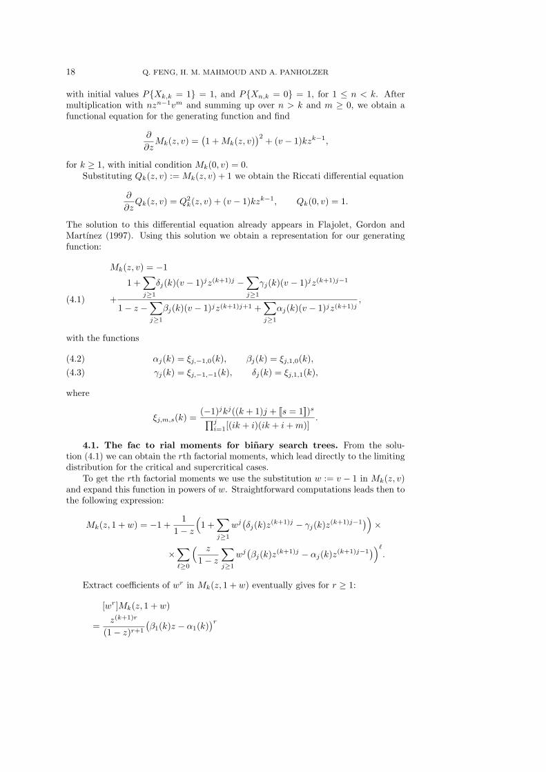
The solution to this differential equation already appears in Flajolet, Gordon andMartınez (1997). Using this solution we obtain a representation for our generatingfunction:

Mk(z, v) = −1

+

1 +∑

j≥1

δj(k)(v − 1)jz(k+1)j −∑

j≥1

γj(k)(v − 1)jz(k+1)j−1

1 − z −∑

j≥1

βj(k)(v − 1)jz(k+1)j+1 +∑

j≥1

αj(k)(v − 1)jz(k+1)j,(4.1)

with the functions

αj(k) = ξj,−1,0(k), βj(k) = ξj,1,0(k),(4.2)

γj(k) = ξj,−1,−1(k), δj(k) = ξj,1,1(k),(4.3)

where

ξj,m,s(k) =(−1)jkj((k + 1)j + [[s = 1]])s

∏ji=1[(ik + i)(ik + i + m)]

.

4.1. The fac to rial moments for binary search trees. From the solu-tion (4.1) we can obtain the rth factorial moments, which lead directly to the limitingdistribution for the critical and supercritical cases.

To get the rth factorial moments we use the substitution w := v − 1 in Mk(z, v)and expand this function in powers of w. Straightforward computations leads then tothe following expression:

Mk(z, 1 + w) = −1 +1

1 − z

(

1 +∑

j≥1

wj(δj(k)z(k+1)j − γj(k)z(k+1)j−1

))

×

×∑

ℓ≥0

( z

1 − z

∑

j≥1

wj(βj(k)z(k+1)j − αj(k)z(k+1)j−1

))ℓ

.

Extract coefficients of wr in Mk(z, 1 + w) eventually gives for r ≥ 1:

[wr]Mk(z, 1 + w)

=z(k+1)r

(1 − z)r+1

(β1(k)z − α1(k)

)r


+z(k+1)rr−1∑

ℓ=1

1

(1 − z)ℓ+1

∑

j1+···+jℓ=r

ji≥1

ℓ∏

i=1

(βji

(k)z − αji(k))

+z(k+1)r−1r−1∑

j=1

(δj(k)z − γj(k)

)r−j∑

ℓ=1

1

(1 − z)ℓ+1

×∑

j1+···+jℓ=r−j

ji≥1

ℓ∏

i=1

(βji

(k)z − αji(k))

+z(k+1)r−1

1 − z

(δr(k)z − γr(k)

).

Using(β1(k)z − α1(k)

)r=(β1(k) − α1(k)

)r+(β1(k) − α1(k)

)r

×r∑

m=1

(r

m

)

(−1)m( β1(k)

β1(k) − α1(k)

)m

(1 − z)m,

and analogous expansions, and [zn] 1(1−z)α+1 =

(n+α

n

), we can expand the above ex-

pression also around z = 1 and get the following formula for the rth factorial momentof Xn,k, which is valid for all n ≥ (k + 1)r and r ≥ 1:

E(X

r

n,k

)

= r! [znwr]Mk(z, 1 + w)

= r!

(n − kr

r

)( 2

(k + 1)(k + 2)

)r

+r!( 1

(k + 1)(k + 2)

)rr∑

p=1

(n − (k + 1)r + p − 1

p − 1

)(r

p − 1

)(k

2

)r+1−p

+r!r∑

p=1

(n − (k + 1)r + p − 1

p − 1

) r−1∑

ℓ=max(1,p−1)

(−1)ℓ+1−p

×∑

j1+···+jℓ=r

ji≥1

ℓ∏

i=1

(βji

(k) − αji(k))

×∑

1≤i1<···<iℓ+1−p≤ℓ

ℓ+1−p∏

q=1

( βjiq(k)

βjiq(k) − αjiq

(k)

)

+ r!

r∑

p=1

(n − (k + 1)r + p

p − 1

)min(r+1−p,r−1)∑

j=1

(δj(k) − γj(k)

)

×r−j∑

ℓ=max(1,p−1)

(−1)ℓ+1−p∑

j1+···+jℓ=r−j

ji≥1

ℓ∏

i=1

(βji

(k) − αji(k))

×∑

1≤i1<···<iℓ+1−p≤ℓ

ℓ+1−p∏

q=1

( βjiq(k)

βjiq(k) − αjiq

(k)

)

−r!

r−1∑

p=1

(n − (k + 1)r + p

p − 1

)min(r−p,r−1)∑

j=1

δj(k)


×r−j∑

ℓ=max(1,p)

(−1)ℓ−p∑

j1+···+jℓ=r−j

ji≥1

ℓ∏

i=1

(βji

(k) − αji(k))

×∑

1≤i1<···<iℓ−p≤ℓ

ℓ−p∏

q=1

( βjiq(k)

βjiq(k) − αjiq

(k)

)

+ r!(δr(k) − γr(k)

).(4.4)

This yields in particular to results for the expectation and the variance:

E(Xn,k) =2(n + 1)

(k + 1)(k + 2), for n ≥ k + 1,(4.5)

V(Xn,k) =2k(4k2 + 5k − 3)(n + 1)

(k + 1)(k + 2)2(2k + 1)(2k + 3), for n ≥ 2(k + 1).

4.2. The critical case. We consider the critical case and assume that k := kn

grows with n such that nk2 → λ, for some λ > 0.

Finding the limiting distribution requires some estimates on the functions appear-ing in (4.4). Using the definition of αj(k), βj(k), γj(k) and δj(k) given by (4.2)–(4.3)the following estimates, which hold for all k ≥ 2 and j ≥ 1, are not hard to show:

|βj(k) − αj(k)| ≤ 2

kj+1,

∣∣∣∣

βj(k)

βj(k) − αj(k)

∣∣∣∣≤ 4jk,(4.6)

|δj(k) − γj(k)| ≤ 3

kj, |δj(k)| ≤ 1

kj−1.(4.7)

We can now deduce the asymptotic behavior of the rth factorial moments of Xn,k

by inspecting the summands of (4.4). Considering a fixed r ≥ 1 we trivially obtainfor the first summand:

r!

(n − kr

r

)(2

(k + 1)(k + 2)

)r

=

(2n

k2

)r (

1 + O(1

k

)

+(k

n

))

= (2λ)r(

1 + O( 1√

n

))

.

Let us denote by B the remaining summands of (4.4). They can then be estimatedfor fixed r ≥ 1 by using (4.6) and (4.7), which finally gives

|B| = O(1

k

)

= O( 1√

n

)

.

Summarizing, we obtain for all r ≥ 1 and sequences (n, k) such that nk2 → λ the

following asymptotic expansion:

E(X

r

n,k

)= (2λ)r

(

1 + O( 1√

n

))

.

This shows convergence in distribution of Xn,k to a Poisson random variable with pa-rameter 2λ. Thus we proved the convergence asserted in Theorem 2.2 Part (b), wherewe used the substitution c := 1√

λ, and thus k√

n→ c. When we have a critical case

with k/√

n not converging to a limit, all factorial (and ordinary) moments oscillate,and no limit distribution exists for Xn,k.


4.3. The supercritical case. Again by using the estimates (4.6) and (4.7) onecan show E(Xn,k) → 0, for n

k2 = o(1) under the natural restriction n > k. Thus, wehave convergence of Xn,k to a degenerate distribution with mass at 0.

4.4. The subcritical case. We consider the centered random variables Xn,k :=Xn,k − E(Xn,k) and introduce the generating function

Mk(z, s) :=∑

n≥1

E(eXn,ks

)zn =

∑

n≥1

e−E(Xn,k)sE(eXn,ks

)zn.

Using the explicit formula for E(Xn,k) as given by (4.5) we obtain

Mk(z, s) = e−2s

(k+1)(k+2) Mk

(e−

2s(k+1)(k+2) z, es

)+ (1 − e

ksk+2 )zk

+∑

1≤n<k

zn −∑

1≤n<k

e−2(n+1)s

(k+1)(k+2) zn,

which further leads by using (4.1) and (4.2)–(4.3) to:

Mk(z, s) =e−

2s(k+1)(k+2) U

V− e−

2s(k+1)(k+2) + (1 − e

ksk+2 )zk

+∑

1≤n<k

zn −∑

1≤n<k

e−2(n+1)s

(k+1)(k+2) zn,

with the expressions

U := 1 +∑

j≥1

δj(k)(es − 1)je−2js

k+2 z(k+1)j

−∑

j≥1

γj(k)(es − 1)je−2((k+1)j−1)s

(k+1)(k+2) z(k+1)j−1,

V := 1 − e−2s

(k+1)(k+2) z −∑

j≥1

βj(k)(es − 1)je−2((k+1)j+1)s

(k+1)(k+2) z(k+1)j+1

+∑

j≥1

αj(k)(es − 1)je−2js

k+2 z(k+1)j .

4.4.1. Expanding around s = 0. We expand Mk(z, s) around s = 0 andz = 1. It is straightforward, though rather laborious, to come up with the followingrepresentation:

Mk

(e−

2s(k+1)(k+2) z, es

)= −1 +

∑

ℓ≥0 sl∑ℓ(k+1)

i=0 dℓ,i(k)(1 − z)i

1 − z −∑ℓ≥1 sℓ∑ℓ(k+1)+1

i=0 cℓ,i(k)(1 − z)i,

where the functions dℓ,i(k) and cℓ,i(k) are given as follows:

dℓ,i(k) = (−1)i

ℓ∑

j=1

ℓ−j∑

m=0

j!{

ℓ−mj

}

(−1)m

m! (ℓ − m)! (k + 2)m

×((

(k + 1)j − 1

i

)(

(2j)mδj(k) − (2((k + 1)j − 1))mγj(k)

(k + 1)m

)


+

((k + 1)j − 1

i − 1

)

(2j)mδj(k)[[i ≥ 1]]

)

, for ℓ ≥ 1,(4.8)

d0,0(k) = 1,

cℓ,i(k) = (−1)i

ℓ∑

j=1

ℓ−j∑

m=0

{l−m

j

}

j!(−1)m

m! (ℓ − m)! (k + 2)m

×((

(k + 1)j

i

)( (2((k + 1)j + 1))mβj(k)

(k + 1)m− (2j)mαj(k)

)

+

((k + 1)j

i − 1

)(2((k + 1)j + 1))mβj(k)

(k + 1)m[[i ≥ 1]]

)

+(−1)ℓ2ℓ

ℓ!(k + 1)ℓ(k + 2)ℓ[[i = 0]] − (−1)ℓ2ℓ

ℓ!(k + 1)ℓ(k + 2)ℓ[[i = 1]].(4.9)

Thus, Mk(z, s) can be written as

Mk(z, s) =e−

2s(k+1)(k+2)

(∑

ℓ≥0 sℓ∑ℓ(k+1)

i=0 dℓ,i(k)(1 − z)i)

1 − z −∑ℓ≥1 sℓ∑ℓ(k+1)+1

i=0 cℓ,i(k)(1 − z)i− e−

2s(k+1)(k+2)

+(1 − eks

k+2 )zk +∑

1≤n<k

zn −∑

1≤n<k

e−2(n+1)s

(k+1)(k+2) zn.(4.10)

The only interesting part in equation (4.10) is the first summand, since the remainingsummands do not give a contribution for n > k (the remainder is a polynomial in zof degree k). The first summand of (4.10) can be expanded around s = 0 and z = 1and finally leads for r ≥ 1 to the following representation:

[sr]e−

2s(k+1)(k+2)

(∑

ℓ≥0 sℓ∑ℓ(k+1)

i=0 dℓ,i(k)(1 − z)i)

1 − z −∑ℓ≥1 sℓ∑ℓ(k+1)+1

i=0 cℓ,i(k)(1 − z)i

=

r∑

p=0

1

(1 − z)p+1fr,p(k) +

r−1∑

p=0

1

(1 − z)p+1gr,p(k) +

r(k+1)−1∑

p=0

hr,p(k)zp,

with

fr,p(k) =

r∑

m=p

∑

r1+···+rm=r

rq≥1

∑

t1+···+tm=m−p

0≤tq≤rq(k+1)+1

m∏

j=1

crj ,tj(k),(4.11)

gr,p(k) =

r∑

c=1

r−c∑

a=p

( r−c∑

m=a

∑

r1+···+rm=r−c

rq≥1

∑

t1+···+tm=m−a

0≤tq≤rq(k+1)+1

m∏

j=1

crj ,tj(k))

×

c∑

b=⌈ a−p

k+1 ⌉

(−1)c−b2c−bdb,a−p(k)

(k + 1)c−b(k + 2)c−b(c − b)!

,(4.12)

and certain functions hr,p(k), which are of course irrelevant for our purpose.This leads also to the required representation

[sr]Mk(z, s) =r∑

p=0

1

(1 − z)p+1fr,p(k) +

r−1∑

p=0

1

(1 − z)p+1gr,p(k) +

r(k+1)−1∑

p=0

hr,p(k)zp,


where the functions fr,p(k) and gr,p(k) are defined by (4.11) and (4.12). The functions

hr,p(k) are irrelevant and thus not given explicitly.The representation in the last display gives the following explicit formula for the

rth moments of Xn,k, which is valid for n ≥ r(k + 1):

E(Xr

n,k

)= r! [znsr]Mk(z, s) = r!

r∑

p=0

(n + p

p

)

fr,p(k) + r!

r∑

p=0

(n + p

p

)

gr,p(k),

where the functions fr,p(k) and gr,p(k) are given by (4.11) and (4.12).

4.4.2. Estimates for cℓ,i(k) and dℓ,i(k). One obtains easily the following esti-mates of the functions cℓ,i(k) and dℓ,i(k) given by (4.8) and (4.9):

|dℓ,i(k)| ≤ 2ℓ2(2ℓ)2ℓ+1Bℓ(2ℓ)iki−1, for ℓ ≥ 1, i ≥ 0, k ≥ 1,

|cℓ,i(k)| ≤ Bℓ22ℓ+3ℓℓ+3(2ℓ)iki−2, for ℓ ≥ 1, i ≥ 0, k ≥ 1.

Moreover, we have the following values:

c1,0(k) = 0, and c2,0(k) =ν(k)

2,

with

ν(k) :=2k(4k2 + 5k − 3)

(k + 1)(k + 2)2(2k + 1)(2k + 3).

4.4.3. Estimates for fr,p(k) and gr,p(k). It is possible to give suitable esti-mates on the growth of fr,p(k) and gr,p(k): There exist constants κr and ηr (dependingonly on r), such that

|fr,p(k)| ≤ κr

1

k2p, and |gr,p(k)| ≤ ηr

1

k2p+2,

for all 0 ≤ p ≤ r (respectively 0 ≤ p ≤ r − 1) and k ≥ 1.For instance one can choose the constants

κr =(2r − 1)! (r + 1)

r!crr, ηr = 2r+2

(2r − 1

r − 1

)

r! rcrr dr,

with

cr := Br22r+3rr+3(2r)r, and dr := 2Brr

r(2r)3r+1.

4.4.4. Cancelation of fr,p(k). Using the same “combinatorial argumentation”as made for recursive trees we can show:

fr,p(k) = 0, for p ≥⌊r

2

⌋

+ 1;

gr,p(k) = 0, for p ≥⌈r

2

⌉

.

Furthermore, one can show

f2d,d(k) = cd2,0(k) =

νd(k)

2d.


4.4.5. Asymptotics of the centered moments. In view of the developmentin subsection 4.4.3 we obtain the explicit formulas for the rth moments of Xn,k:

E(X2d

n,k

)= (2d)!

((n + d

d

)

f2d,d(k)

+d−1∑

p=0

(n + p

p

)(f2d,p(k) + g2d,p(k)

))

, d ≥ 1,

E(X2d+1

n,k

)= (2d + 1)!

d∑

p=0

(n + p

p

)

(f2d+1,p(k) + g2d+1,p(k)), d ≥ 0.

Using the previous estimates we can easily show that, for k2

n→ 0,

E(X2d

n,k

)→ (2d)!

d! 2dndνd(k),

E(X2d+1

n,k

)= O

(( n

k2

)d)

= O(ndνd(k)

).

Therefore, considering

Xn,k√

ν(k)n=

Xn,k − E(Xn,k)√

ν(k)n,

with ν(k) = 2k(4k2+5k−3)(k+1)(k+2)2(2k+1)(2k+3) , we have for k = o(

√n):

E

(( Xn,k√

ν(k)n

)2d

)

→ (2d)!

d! 2d, for d ≥ 1,

E

(( Xn,k√

ν(k)n

)2d+1)

= O( k√

n

)→ 0, for d ≥ 0.

Whence, for the subcritical case we have

Xn,k − 2n(k+1)(k+2)

√2k(4k2+5k−3)n

(k+1)(k+2)2(2k+1)(2k+3)

D−→ N (0, 1),

completing the proof for the subcritical case (Part (a) of Theorem 2.2).

5. Concluding remarks. Several methods have recently come into the reper-toire of the analysis of algorithms, and there is a question of the choice when itcomes to an analysis like the one we conducted in this investigation. For example,the contraction method (introduced in Rosler, 1991), Polya urns (Johnson and Kotz,1977), the Chen-Stein method (Barbour, Holst, and Janson ,1992), methods for ad-ditive functions in subtrees (Devroye, 1991 and Devroye, 2003) are all attractive forthis kind of analysis. These methods have been used successfully in the analysis ofalgorithms, (see for example Neininger, 2002, or Rosler and Ruschendorf, 2001 forapplications of the contraction method). However, Experience shows that several ofthese methods will work with ease in some of the phases, but not systematically acrossall the phases. For instance, in our multi-phase problem Polya urns work well in the


very low range (small fixed k), as was attempted in Feng, Mahmoud and Su (2007).The difficulty in this method is that one needs a detailed description of the fringe interms of urns that are different from each other for each k, and that become morecomplex as k increases. As for the contraction method , again it can be used in thecase of small fixed k, but does not lend itself easily to k = kn → ∞ in the subcriticalcase when k increases but at rate slower than

√n. The difficulty stems from com-

plicated toll functions. It is not clear how to apply the contraction method in thecritical case. The same applies to the other methods above. It is our experience thatthe analytic methods, based on generating functions, are systematic enough to coverall the ranges.

Acknowledgment. The work of the first author (Q. Feng) is supported by theNational Natural Science Foundation of China (Grant No. 10371117) and the SpecialFoundation of USTC. The work of the third author (A. Panholzer) is supported bythe Austrian Science Foundation FWF (Grant No. S9608-N13).

REFERENCES

[1] Barbour, A., Lars Holst, L. and Janson S. (1992). Poisson Approximation. Oxford UniversityPress.

[2] Bergeron, F. Flajolet, P. and Salvy, B. (1992). Varieties of increasing trees. Lecture Notes in

Computer Science, 581, 24–48. Springer, Berlin.[3] Chern, H., Hwang, H. and Tsai, T. (2002). An asymptotic theory for Cauchy-Euler differential

equations with applications to the analysis of algorithms. Journal of Algorithms, 44, 177–225.

[4] Chyzak, F., Drmota, M., Klausner, T. and Kok, G. (2007+). The distribution of patterns inrandom trees, Combinatorics, Probability and Computing, to appear.

[5] Devroye, L. (1991). Limit laws for local counters in random binary search trees. Random Struc-

tures and Algorithms, 3, 303–315.[6] Devroye, L. (2003). Limit laws for sums of functions of subtrees of random binary search trees.

SIAM Journal on Computing, 32, 152–171[7] Feng, Q., Mahmoud, H. and Su, C. (2007). On the variety of subtrees in a random recursive

tree. Technical Report, The George Washington University.[8] Flajolet, P., Gourdon, X. and Martınez, C. (1997). Patterns in random binary search trees.

Random Structures and Algorithms, 11, 223–244.[9] Fuchs, M., Hwang, H.-K. and Neininger, R. (2006). Profiles of random trees: Limit theorems

for random recursive trees and binary search trees. Algorithmica, 46, 367–407.[10] Gastwirth, J. and Bhattacharya, P. (1984). Two probability models of pyramids or chain letter

schemes demonstrating that their promotional claims are unreliable. Operations Research,32, 527–536.

[11] Johnson, N. and Kotz, S. (1977). Urn models and Their Applications. Wiley, New York.[12] Kemp, R. (1984). Fundamentals of the Average Case Analysis of Particular Algorithms. Wiley,

New York.[13] Knuth, D. (1998). The Art of Computer Programming, Vol. 3: Sorting and Searching, 2nd ed.

Addison-Wesley, Reading, Massachusetts.[14] Lent, J. and Mahmoud, H. (1996). Average-case analysis of multiple Quickselect: An algorithm

for finding order statistics. Statistics and Probability Letters, 28, 299–310.[15] Mahmoud, H. (1992). Evolution of Random Search Trees. Wiley, New York.[16] Mahmoud, H. (2000). Sorting: A Distribution Theory. Wiley, New York.[17] Najock, D. and Heyde, C. (1982). On the number of terminal vertices in certain random trees

with an application to stemma construction in philology. Journal of Applied Probability,19, 675–680.

[18] Neininger, R. (2002). The Wiener index of random trees. Combinatorics, Probability and Com-

puting, 11, 587–597.[19] Rosler, U. (1991). A limit theorem for “Quicksort”. RAIRO Inform. Theor. Appl., 25, 85–100.[20] Rosler, U. and Ruschendorf, L. (2001). The contraction method for recursive algorithms. Algo-

rithmica, 29, 3–33.[21] Panholzer, A. and Prodinger, H. (1998). A generating functions approach for the analysis of


grand averages for multiple QUICKSELECT. Random Structures and Algorithms, 13,189–209.

[22] Smythe, R. and Mahmoud, H. (1994). A survey of recursive trees. Theorya Imovirnosty ta

Matemika Statystika, 51, 1–29 (in Ukrainian); an English translation appears in Theory

of Probability and Its Applications (1996).

Phase Changes in Subtree Varieties in Random Recursive and Binary Search Trees

Documents

Transcript of Phase Changes in Subtree Varieties in Random Recursive and Binary Search Trees