1

Person Identification from the EEG using Nonlinear

Signal Classification M. Poulos,1 M. Rangoussi,3 N. Alexandris,1 A. Evangelou 2

1 Dept. of Informatics, University of Piraeus 2 Dept of Exp. Physiology, School of Medicine, University of Ioannina 3 Dept. of Electronics, TEI Piraeus

Abstract: This paper focuses on the person identification problem based on features

extracted from the ElectroEncephaloGram (EEG). The EEG signal of a healthy, in principle,

individual is processed via nonlinear (bilinear) methods and classified by an artificial neural

network classifier. As it can be seen in the experimental part, the use of an appropriate

bilinear model yields an improvement of the classification scores as compared to those

obtained via purely linear processing. Use of a bilinear, rather than a purely linear, model is

prompted by the existence of non-linear components in the EEG signal – a conjecture already

investigated in previous research works. The novelty of the present work lies in the

comparison between the linear and the bilinear results, obtained from real field EEG data,

aiming towards identification of healthy subjects rather than classification of pathological

cases for diagnosis. An improvement of correct classification scores, shown to be statistically

significant, is obtained via bilinear modeling. Results are indicative of the potential of

methods that exploit information lying in the non-linear components of the EEG.

Keywords: EEG, Person Identification, Non-Linear Processing, Bilinear Model, LVQ Neural

Network.

1. Introduction

The objective of this work is to extract individual-specific information from a person’s

EEG and to use this information, in the form of appropriate features, to develop a person

identification method. Potential applications of this method are, for example, information

encoding and decoding or access to secure information. EEG recording is non-invasive and

medically safe; it therefore constitutes a viable and, under certain conditions, attractive

2

alternative to currently existing forms of person identification based on fingerprints, blood

tests or retinal scanning.

The first efforts to extract individual-specific information from the EEG signal began

as early as in the 1930’s, [1, 2], but the first results became available only after the 1960’s.

More specifically, the research carried out addressed three classes of cases. In the first class,

the research was carried out among members of the same family [3, 4, 5]. In the second class,

the common characteristics between monozygotic and dizygotic twins [6, 7, 8, 9] were

researched while in the third class, different EEGs from the same person were compared, with

the objective of extracting the common characteristics among them (personal EEG invariants)

[10, 11, 12, 13].

The research in alpha and beta EEG rhythm activities, which was first held by Vogel,

[14], and thereafter by other researchers, [15, 16, 17], proved that alpha and beta rhythms are

significant frequencies because they contain the relevant individual-specific characteristics.

These characteristics were claimed by the researchers to be genetically induced.

The methods used to reach these conclusions relied on teaching aids supported by

visual observations, which were unsatisfactory. Thereafter, thanks to the development of

computer technology, it became possible for the signal to be digitized and analyzed with

parametric or non-parametric methods, while the development of Pattern Recognition

methods, such as the Artificial Neural Networks, among others, facilitated classification tasks.

Most of this pioneering as well as other more recent research, however, focused on the

classification of genetically and/or pathologically induced EEG variants due, for example, to

epilepsy or schizophrenia, for diagnostic purposes, [18, 19]. To this end, recent research

involving both linear and non-linear approaches and a neural network classification scheme

has reached a 71% classification score, [19]. A key observation in these approaches is the fact

that a given pathological EEG signal is distinguishable from a healthy EEG signal in the

domain of features extracted after processing via standard signal analysis methods (Fourier

Transform, AR modeling). Diagnosis of a specific pathology is therefore based on the

detection of the specific variation pattern, which serves as a classification feature.

In contrast, the present work focuses on healthy as opposed to pathological cases and

aims to establish a one – to – one correspondence between individual-specific information

and certain appropriate features of the recorded EEG. Research carried out on this problem by

the authors has yielded satisfactory results, based on features extracted from the EEG either

parametrically, [12, 13], or non parametrically, [10, 11]. Here we aim to improve the

classification results of the parametric method proposed in [12] by exploiting the non-linear

3

component present in the EEG signal. This is implemented using a set of augmented linear /

non-linear model parameters as features for improved classification.

The bilinear model employed here was first developed in control theory, [20], as an

extension of the standard linear model. The construction of this model best describes the

input-output relationship of a deterministic non-linear system, [21], and the bilinear

parameters have been shown to approximate to a reasonable accuracy the general Volterra

series expansion. However, the structural theory behind the non-linear features of a bilinear

system is analogous to that of linear systems.

The augmented set of linear and bilinear model parameters, estimated from the EEG

data, is used as the feature vector upon which classification is based. A Learning Vector

Quantizer (LVQ) neural network is employed for classification in the present work. LVQ was

preferred to other candidate types of networks, such as Multi-layer Perceptron (MLP),

because of its non-linear classification properties. Indeed, LVQ lends itself nicely to the EEG

classification problem, as it was seen (i) in our experimental results when comparing LVQ to

MLP, and (ii) in similar results reported in existing works, such as [22, 23, 24, 25]. As an

example, Pfurtscheller’s group, [25], has explored satisfactorily local adaptive classifiers

based on LVQ neural networks. Specifically, the Pfurtscheller technique classifies via the

LVQ network EEG vectors produced by the contra-lateral blocking of the mu-rhythm, [25].

In order to evaluate the statistical significance of the classification scores obtained in the

experimental part, the chi-square test was applied to the results. The two feature extraction

methods presented are also compared in terms of their Cramer coefficient of mean square

contingency, φ1. Results are seen to be statistically significant at the a = 99.5% level of

significance.

As a final comment we should point out that the proposed method belongs to a family

of identification / classification methods that can yield more or less satisfactory correct

classification scores, but who can not produce the type of deterministic identification result

that a DNA identification method would produce. This is due to the fact that the biochemical

basis of the EEG phenomena is as yet essentially unknown.

2. Methods and Materials

The methods employed for signal analysis and feature extraction, along with the

classification step by appropriate neural network classifiers are given in this section. The

4

section is divided into four paragraphs. In the first paragraph, the choice of a bilinear model

and the estimation of its parameters are considered. Data acquisition, to be used in the

experimental part, is outlined in the second paragraph. Preprocessing of the EEG signals and

feature extraction is described in the third paragraph. In the fourth paragraph is described the

experimental setup for the classification of the EEGs based on the extracted features, through

an artificial neural network classifier.

2.1 The bilinear model – type and parameterization

In order to model the linear component of an EEG signal, known to represent the

major part of its power – especially in the alpha rhythm frequency band – a linear, rational

model of the autoregressive – moving average type, ARMA(p, q), is fitted to the digitized

EEG signal x(t). This signal is treated as a superposition of a signal component (deterministic)

plus additive noise (random). Noise is mainly due to imperfections in the recording process.

This model can be written as

xt+ ∑i = 1

p aixt-i = ∑

i = 0

q ci et-i , (1)

where c0 = 1 , {et} is an independent, identically distributed driving noise process with zero

mean and unknown variance σ2e and model parameters {ai , i = 1, 2,..., p; ci , i= 1, 2,..., q}

are unknown constants with respect to time.

It should be noted here that the assumption of time invariance for the model of the EEG

signal can be satisfied by restricting the signal basis of the method to a signal "window" or

"horizon" of appropriate length.

In order to explain a further part of power lying in the non-linear components of the

EEG signal, we incorporate a bilinear part in the above model. The general Bilinear

Autoregressive Moving Average model of orders (p, q, k, m), denoted by BL(p, q, k, m) takes

the form

xt + ∑i = 1

pai xt-i = ∑

i = 0

qci et-i + ∑

i = 1

k ∑j = 1

mbij xt-i et-j (2)

5

where c0 = 1 , {et} is an independent, identically distributed driving noise process with zero

mean and unknown variance σ2e , model parameters { ai , i = 1, 2, …, p}, { ci , i = 1, 2, …,

q} and { bi,j , i = 1, 2, …, k; j = 1, 2,…, m}are unknown constants with respect to time.

It can be seen that (2) is produced from (1) with the addition of the extra bilinear

components {xt-i et-j} on the right - hand side. Equation (2) may be considered as an extension

of the ARMA model into the non-linear class of models. In this way a composite model is

considered which contains both the non-linear and the linear component. As for the choice of

the bilinear model, this should be considered as a first step when moving from linearity to non-

linearity. Linear, bilinear or other more complex non-linear models can usually serve as (more

or less successful) approximations, when dealing with real world data. In the light of this

understanding, the bilinear is the simpler among other candidate non-linear models in terms of

computing spectra, covariances, etc.; hence its adoption in modeling EEG signals, [19].

In this work, a bilinear model of the specific form BL(p, 0, k, m) is adopted. The

elimination of the MA part of the model is a compromise in the model type in order to

facilitate the parameter estimation step. This choice simplifies (1) into:

xt + ∑i=1

pai xt-i = α + ∑

i=1

k ∑j=1

mbij xt-i et-j + et , (3)

A scalar parameter α is inserted in (3), in order to allow fitting of the model to non-zero mean

data. In our case, EEG data are made zero mean by subtraction of the sample mean from each

EEG data record before further processing; a can therefore be omitted from the model.

The choice of the order of the linear models is usually based on information theory

criteria such as the Akaike Information Criterion (AIC) which is given by:

AIC(r) = (N-M) log σ2e + 2 r , (4)

where σ2e = 1

N-M ∑t = M+1

N e

2t , (5)

N is the length of the data record, M is the maximal order employed in the model, (N-M) is

the number of data samples used for calculating the likelihood function and r is the number of

independent parameters present in the model. The optimal order r* is the minimizer of AIC(r).

We have used the AIC to determine the order of the linear part of the model in (3), i.e.

the optimal order p of the AR part of the model. For each candidate order p in a range of

values [pmin, pmax], the AIC(p) was computed from the residuals of each record in the

6

ensemble of the EEG records available. This is because we deal with recordings of real world

data rather than the output of an ideal linear model. We have thus seen that AIC(p) takes on

its minimum values for model orders p ranging between 8 and 12, record-dependent. In view

of this findings, which are in agreement to previous research, [19], we have set the model

order of the AR part to p = 8, for parsimony purposes. Figure 1 shows the AIC(p) values

computed from a set of five typical EEG segments.

Fig. 1 AIC(p) values computed from a set of five typical EEG segments.

Given the AR part model order p, the bilinear part model orders m and k have been set

experimentally to k = 2 and m = 3, after having investigated the power of the residuals in the

matrix area of values of (k, m) ranging from (1, 1) to (4, 4). Higher values have not been

considered, however, due to practical considerations (total number of parameters). It should

also be noted here that no (k, m) pair have shown a clear advantage over other candidate pairs,

over all EEG records. Therefore, the values (k, m) = (2, 3) have been adopted without any

claim of optimality, global or local.

The parameter estimation procedure necessary in order to fit a model of the type of (3)

to EEG data is essentially the repeated residuals parameter estimation method of Subba Rao,

7

[26]. The basic steps are outlined here for the sake of completeness of the presentation. In the

following we assume that

• orders (p, m, k) of the parts of the model in (3) are given and fixed,

• {et} is an independent identically distributed random process with zero mean,

• {x1, x2,..., xN} denotes a realization of the time series {xt} of length N (a record of

EEG data, in our case).

For more compact notation, let us concatenate all model parameters in a single parameter

vector Θ = [ θ1, θ2, . . ., θr ] T, formed as follows :

• θi = ai, i = 1,…, p ,

• θp+1 = b11, θp+2 = b12 , . . . , θp+mk = bmk , (6)

where r = p + mk. If g denotes time point g = max(p, m, k) + 1, the joint probability density function of the

random variables {eg+1, eg+2, . . ., eN} given by:

P{eg+1, eg+2, . . ., eN} = 1

(2πσ2e)

N-g2

exp

-

1

2 σ2e

∑t = g+1

N e

2t . (7)

As the Jacobian of the transformation from {eg+1, eg+2,..., eN} to {xg+1, xg+2,..., xN} is

unity, the likelihood function of {xg+1, xg+2,..., xN} is the same as the joint probability

density function of {eg+1, eg+2,..., eN}. In light of (7) maximization of the likelihood

function is approximately equivalent to minimization of the function Q(Θ)

Q(Θ) = ∑t = g+1

N e

2t (8)

with respect to the parameter vector Θ. Minimization of Q(Θ) with respect to Θ yields the

conditional maximum likelihood estimate of Θ, conditioned on the data {xt} . It can be seen

that (8) is of the least squares type; the purpose of the approximation involved from (7) to (8)

is indeed to obtain an expression easier to minimize than the exact likelihood formula.

For given (p, k, m), the parameters of a BL(p, 0, k, m) model are estimated by linear

minimization, using standard least squares techniques, such as the Householder

transformation, [27]. Q(Θ) is expressed in terms of the unknown parameters by the following

equation:

8

Q(Θ) = ∑ t = g+1

N

xt + ∑

i = 1

pai xt-i - ∑

i = 1

m ∑ j = 1

kbij xt-i et-j

2

, (9)

where et is given by (3) after omitting scalar parameter a.

For the initialization of the minimization, the first residuals will be obtained from the

linear only part of the model, as follows:

et = xt - ∑i = 1

p ai xt-i . (10)

Thus, the estimation of the unknown parameter vector Θ may be carried out based on the

values of { xt } and the initial values of the residuals { et } solving the following set of first

order derivative equations:

dQ(Θ)d(θi)

= 0, i = 1, 2,…, r . (11)

The standard least-squares technique was selected as opposed to the non-linear

minimization method of Newton - Raphson because it can estimate Θ more efficiently. The

parameter estimation procedure for the BL(p, 0, k, m) model can be put into the following

steps:

Step 1. Use the given signal { xt } (EEG data record) to estimate a p-th order AR model.

Step 2. Estimate the residuals { êt }of the fitted AR model, according to (10).

Step 3. Use { êt } in (9) and apply the least squares method to estimate Θ̂ of the BL(p, 0, k,

m) model.

Step 4. Use Θ̂ in (3) to re-estimate the residuals { êt }. Re-apply Step 3 using this new set of

re-estimated residuals { êt } to obtain the new value of Θ̂ .

Step 5. Repeat Steps 3 and 4 until the estimated parameter vector Θ̂ converges.

Convergence of the algorithm described above is not guaranteed, as it was verified in

the experimental part. For those EEG records where convergence is not achieved, we resort to

the non-linear minimization of Q(Θ) via the Newton-Raphson method. It has been seen in the

9

experimental part that in almost all such cases, the parameters have converged. In the rare

cases where convergence failed to occur, the specific EEG records were deleted from the set.

When applying the Newton-Raphson minimization, the parameter estimate Θ̂ obtained

through the least squares minimization is used as the initial point of the iteration. The first and

second derivatives of Q(Θ) are estimated and the respective derivative matrices G(Θ) and

H(Θ) are formed and used in the iteration

Θ(k+1) = Θ(k) - [H(Θ)(k)]-1 G(Θ)(k) , (12)

where Θ(k)

is the estimate produced at the k-th step of the iteration. The convergence

threshold, which is the euclidean distance between every two consecutive estimates

|| Θ(k+1)

- Θ(k)

||2 , is taken to be 0.1.

2.2 Data Acquisition

Fig. 2 An example of a 30 sec long EEG record (sampling rate 128 Hz), from subject A.

A number of forty five (45) EEG recordings were taken from each of a set of four (4)

subjects, referred to as A, B, C and D. In addition, one EEG recording was taken from each of

seventy five (75) different subjects, to form a group named X. The final pool of EEG recordings

thus contained 4 x 45 + 75 x 1 = 255 recordings.

10

All recordings were taken using a digital electroencephalograph with the PHY-100

Stellate software. Subjects were at rest, with closed eyes. Voltage difference (in µV) was

recorded between leads O2 and CZ (one channel). All EEG recordings lasted for three (3)

continuous minutes, thus producing a 23040 samples long record each, at a 128 Hz sampling

rate. Recordings were filtered using a 1 – 30 Hz low pass filter to retain spectral information

present in the four major EEG rhythms (alpha, beta, delta and theta).

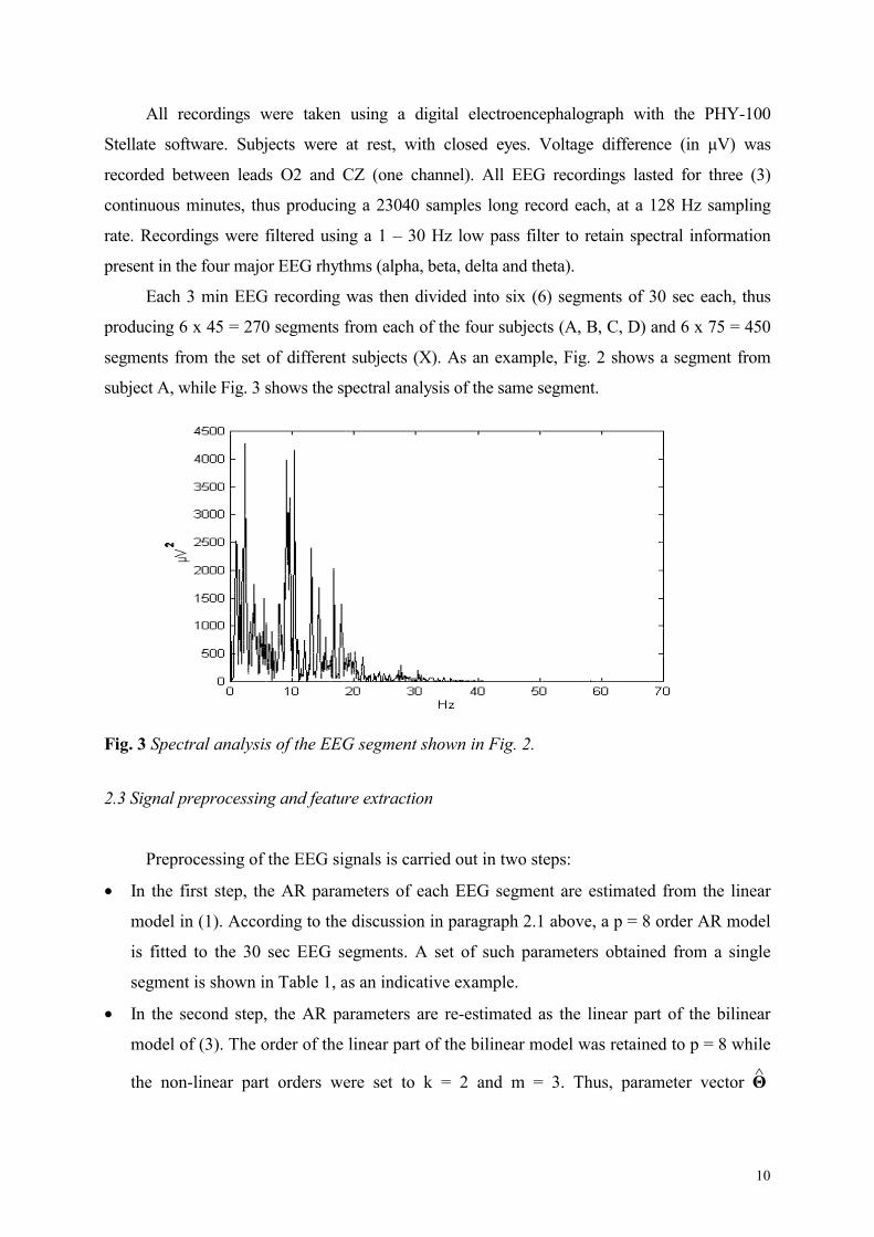
Each 3 min EEG recording was then divided into six (6) segments of 30 sec each, thus

producing 6 x 45 = 270 segments from each of the four subjects (A, B, C, D) and 6 x 75 = 450

segments from the set of different subjects (X). As an example, Fig. 2 shows a segment from

subject A, while Fig. 3 shows the spectral analysis of the same segment.

Fig. 3 Spectral analysis of the EEG segment shown in Fig. 2. 2.3 Signal preprocessing and feature extraction

Preprocessing of the EEG signals is carried out in two steps:

• In the first step, the AR parameters of each EEG segment are estimated from the linear

model in (1). According to the discussion in paragraph 2.1 above, a p = 8 order AR model

is fitted to the 30 sec EEG segments. A set of such parameters obtained from a single

segment is shown in Table 1, as an indicative example.

• In the second step, the AR parameters are re-estimated as the linear part of the bilinear

model of (3). The order of the linear part of the bilinear model was retained to p = 8 while

the non-linear part orders were set to k = 2 and m = 3. Thus, parameter vector Θ̂

11

consisting of p+mk = 14 elements are constructed. The parameter estimation procedure

proceeds as follows:

A segment is selected at random from the six segments of each EEG recording. If

convergence of the bilinear parameters is achieved using the least-squares

technique, the segment is retained as representative of the recording. Otherwise

another segment is selected, until all six segments are exhausted.

If none of the six segments of an EEG recording converges, the iterative Newton-

Raphson technique is applied, again on a per segment basis. If the Newton-

Raphson technique fails to converge for all six segments, then this EEG recording

is altogether deleted from the set.

In our experimental work we have seen that the parameter estimation step converged

using least squares in 249 out of the 255 EEG recordings while the Newton-Raphson

minimization was necessary only for the 6 EEG recordings left. No case has shown up where

a recording had to be deleted. As an example, application of the aforementioned algorithm to

the data shown in Fig. 2 has yielded the bilinear parameters of the BL(8, 0, 2, 3) model given

in Table 2.

Fig. 4 Pole positions relative to the unit circle on the 2-D complex plane. Example of

five EEG records from subject A. Pure AR poles: (+). Poles of the AR part of the bilinear

model: (o).

12

It must be noted that the AR part of the bilinear model obtained after convergence is

different from the purely linear AR model fitted to the data during the initialization step of the

parameter estimation procedure. To investigate the nature of this difference, the pole positions

of the AR part, considered as an all-pole filter, are computed and shown in Fig. 4, relatively to

the unit circle, on the complex 2-D plane. Results from five different EEG recordings are

shown therein, as a typical example. All poles lie inside the unit circle, exhibiting the causal

and stable behavior expected from physical systems. Moreover, poles are seen to move from

their initial positions (roots of the pure AR model parameter polynomial) to their final

positions (roots of the polynomial of the AR part of the bilinear model) which lie closer to the

unit circle, as a rule. This behavior indicates the presence of damped sinusoidals in the EEG

signal, in agreement to the physiological model for the EEG.

2.4 Classification Experiments

The final step of the proposed method is to use the estimated bilinear parameter vectors

as feature vectors, in order to train and then to test an artificial neural network classifier.

The neural network selected and employed in our work is the Learning Vector

Quantizer (LVQ). LVQ was proposed by Kohonen, [28], as a supervised extension of the

more general family of unsupervised classifiers named Self-Organizing Maps (SOMs). The

training of LVQ is a two step procedure. In the first step, initial positions of the class

representatives (or codebook vectors) are determined in the r-dimensional space using

standard clustering algorithms such as the K-Means or the LBG algorithm, with a given

number of classes. In the second step, class representative positions are iteratively updated so

that the total classification error of the training set of vectors is minimized. To this end,

codebook vectors are directed towards the data vectors of the same class and distanced from

the data vectors of different classes. A euclidean distance measure is used for calculating

distances. Specifically, every time a member of the training set, feature vector ti, is incorrectly

classified, the two codebook vectors involved (correct rc(i-1) and incorrect rw

(i-1) ) are updated

as follows:

rc(i) = rc

(i-1) + a(i) [ ti - rc(i-1) ],

rw(i) = rw

(i-1) - a(i) [ ti - rw(i-1) ].

The rate of the update, or learning rate, a, controls the speed of convergence and is a

descending function of "time" or iteration index (i).

13

The class separating surfaces obtained in this way, are nearly optimal in the bayesian

sense. Different rules applied when "moving" (updating) class representatives during the

training iteration produce different versions of the LVQ training algorithm. The version

employed here, namely LVQ1, is chosen for its properties of quick convergence and

robustness of the class representatives positions over extended learning periods.

As stated in the Introduction, this type of network was selected among other candidate

types, such as the Multi-Layer Perceptron, because it has the ability to classify incoming

vectors into classes that are not linearly separable in the r-dimensional space, where r is the

number of the parameters. This is a desirable property, given the nature of our feature space.

Another interesting property of LVQ is that it is designed to be a good classifier rather than a

good vector quantizer. This is reflected in the training process, where effort is put into moving

class representatives to such positions as to minimize classification error and not total

quantization error (distortion).

Fig. 5 Sammon mapping of the Learning Vector Quantizer neural network codebook vectors

from the 14-D space to the 2-D space. Bilinear feature vectors, test case [A, X].

As an example, Fig. 5 shows the codebook vectors obtained after training of the LVQ

network with the training set of test case of subject A versus group X. The parameter set used

is the bilinear set, including vectors of dimensionality 14 x 1. For visualization purposes

14

codebook vectors are non-linearly mapped in the two-dimensional space using the Sammon's

mapping algorithm, [29]. Sammon's mapping algorithm transforms in a non-linear way an n-

dimensional vector space into a vector space of a lower dimension, while preserving relative

vector distances but not topology. This means that relative distances between vectors in the

higher dimension are replicated in the lower dimension, but the shape of original clusters is

deformed in general. It should be noted that if classification is done in the Sammon's mapping

domain, performance is comparable with the performance of Principal Component Analysis

(PCA).

Two different LVQ network architectures are employed in two different test cases, as

described in the following:

Test Case 1

Test case 1 aims to differentiate between an individual of interest among a pool of other

individuals. Four different individuals of interest, A, B, C and D participate in four examples

of this test case, where group X serves as the pool class in all four cases. Taking these into

account we use the LVQ classifier in a setup of two target classes. In the training process, a

group of twenty (20) feature vectors which belong to a specific subject (A or B or C or D)

along with a group of thirty (30) vectors of group X were used as the training set. Feature

vectors Θ̂ contain either linear (AR only) or bilinear parameters. They are of dimensionality 8

x 1 or 14 x 1, respectively, according to the analysis in paragraph 2.1. Four (4) different LVQ

networks are thus trained using the linear feature vectors, while four (4) different networks are

trained using the bilinear vectors. Each network has two target classes [A, X], [B, X], [C, X]

or [D, X], respectively. In this experimental setup, a successfully classified feature vector

would thus be classified as belonging to class A or B or C or D, respectively. Class X serves

as a non-specific class for feature vectors not classified in the class of interest (A or B or C or

D, respectively). In the testing process, all remaining feature vectors (255 – 110 = 145

vectors) are classified by the four trained networks. Training and test sets are thus disjoined.

Table 3 tabulates training set and the test set sizes for test case [A, X].

The architecture of the LVQ network used to classify the AR feature vectors (model

order p = 8) is shown in Fig. 6. Input vectors of dimensionality 8 x 1 are weighted and fed to

the first layer of neurons, known as the competitive layer. These neurons compete for inputs

in a "greedy" way; hence the layer name. Four (4) such neurons form the competitive layer in

our case. The output of the competitive layer, which is in fact a grouping of the inputs into

15

subclasses, is fed to the second linear layer, which groups subclasses into target classes. The

weights connecting the two layers take on binary values of zero or one, indicating mere class

membership and not actual weighting. Two target classes exist here, the class of interest (A or

B or C or D, respectively) and class X, serving as the "complement" or "denial" of the class of

interest. Therefore, the linear layer consists of two (2) neurons, which group the four

subclasses into two target classes. An analogous architecture with six (6) competitive neurons

is used with the bilinear feature vectors whose dimensionality is 14 x 1. The learning rate

used in the training process is in the order of 10-3. Training iterations are terminated when

either the classification error falls below 10-2 or a maximum number of 3000 epochs is

reached.

Fig. 6 Architecture of the LVQ neural network employed for the classification for AR input

vectors of dimensionality 8.

Test Case 2

16

Test case 2 addresses a more realistic, multi-target setup, where four individuals of

interest, namely A, B, C and D, are to be classified (as opposed to identified), in contrast to

test case 1. This test is carried out to verify that the proposed neural network has the ability to

correctly classify EEG features within a multi-person group. Let us consider a specific

individual of interest, for example A. All experiments in test case 1 and in test case 2 aim to

differentiate between A and an "adversary" group of other individuals – group X in test case 1

or groups B, C and D in test case 2. The essential difference of the two test cases is that in test

case 2 the "adversary" group is structured in the sense that it contains three formed clusters of

EEGs while in test case 1 the "adversary" group is not structured, i.e., it contains one EEG

from each one of 75 different subjects.

The LVQ network architecture for this test case has twelve (12) neurons in the

competitive layer and four (4) neurons in the linear layer, since it has four target classes. The

input vectors are of the same types (AR and bilinear) as in test case 1. Twenty (20) feature

vectors of each one of the classes A, B, C and D are used as the training set, whose size is

thus eighty (80) vectors. In the testing procedure, the remaining twenty-five (25) vectors of

each one of classes A, B, C and D, one hundred (100) vectors in all, are used as the test set.

3. Results

3.1 Classification Results

In this paragraph we present the classification results obtained in experiments conducted

on real field EEG recordings along with their statistical evaluation.

Results of Test Case 1

Results are tabulated in Tables 4-7 for the test cases [A, X], [B, X], [C, X] and [D, X],

respectively. Each table compares scores obtain in the classification step when feature vectors

are extracted (i) linearly (AR parameters) and (ii) non-linearly (bilinear parameters).

As it can be seen in the diagonal entries of Tables 4-7, correct positive classification

scores (i.e., subject A classified as A, B as B, etc.), ranging from 68% to 76% when based on

linear features, move to the range of 76% to 88% when the bilinear parameters are included.

Incorrect negative scores (i.e., subject A classified as X, B as X, etc.) exhibit the analogous

decrease, being complementary to the correct positive answers. The off-diagonal entries of

17

Tables 4-7 show that correct negative classification scores (subjects from group X classified

as X) exhibit a case-dependent behavior when moving from linear to bilinear parameters:

They decrease in the first two test cases (Tables 4 and 5) while they remain constant in the

last two test cases (Tables 6 and 7). Finally, incorrect positive classification scores (subject

from group X classified as A, X as B, etc.) exhibit a behavior complementary to that of

incorrect negative scores.

Results of Test Case 2:

Results are tabulated in Tables 8 and 9 for the multi-target test of four classes [A, B, C,

D]. Each table compares scores obtain in the classification step when feature vectors are

extracted (i) linearly (AR parameters) and (ii) non-linearly (bilinear parameters).

Correct recognition scores are shown along the diagonal of the table entries. For example,

in Table 8 (linear case), for subject A correct classification score is 17/25 or 68%, for subject B

it is 14/25 or 56%, for subject C it is 20/25 or 80% and for subject D it is 17/25 or 68%.

Incorrect recognition scores are shown in the off-diagonal entries. For example, out of a total of

eight (8) incorrect recognitions of subject A, two (2) of these are recognized incorrectly as

belonging to subject B, three (3) to subject C and three (3) to subject D. The classification

scores based on bilinear features, shown in Table 9, are interpreted analogously. We can see

that inclusion of the bilinear parameters results in a consistent improvement of correct scores

(diagonal entries) with respective reduction of incorrect scores (off-diagonal entries) across all

four classes.

3.2 Statistical Evaluation

The results of a classification experiment can be put into a two-ways contingency table,

[30]. A two-ways contingency table is structured on the basis of two criteria, along its two

dimensions. Here we use "subject belongs to class i" as the first criterion (vertical dimension)

and "subject is classified into class j" as the second criterion (horizontal dimension). An ideal

classification method should produce a diagonal matrix of classification scores ("subject

belongs to class i" and "subject is classified into class i"), corresponding to full dependency

between the two above criteria, while practical methods would tend to this behavior.

Evaluation of the statistical significance of the classification results is thus transformed into a

hypothesis testing problem: The null hypothesis of independence of the two criteria is tested

18

against the alternative hypothesis of dependence. The test statistic used for this purpose is the

χ2. Statistically significant classification results correspond to rejection of the null hypothesis

at a satisfactory level of significance.

Let the contingency matrix S be of dimensions (r x c), meaning r rows and c columns,

and let the (i, j)-th entry of S, { S(i, j) = fij ; i = 1, …, r; j = 1, 2, …, c } denote observed

frequency of occurrence of the event (i, j) ("subject belongs to class i" and "is classified into

class j") and { eij ; i = 1, …, r; j = 1, 2, …, c } denote expected frequency of occurrence of the

event (i, j). Then the test statistic is given by

χ2 = ∑i=1

r ∑

j=1

c

(fij - eij)2

eij (13)

which asymptotically follows the χ2 distribution with (r-1)(c-1) degrees of freedom. When

unknown, expected frequencies can be estimated from S using

eij = Ri Cj

N (14)

where N is the total number of events in S, Ri is the sum across the i-th row of S and Cj is the

sum across the j-th column of S.

The degree of dependence between the two criteria can also be measured by the Cramer

coefficient [30] of mean square contingency,

.φ1 = [ χ2

N min(r-1, c-1)]1/2 (15)

Coefficient φ1 takes on values between 0 (independence) and 1 (full dependence). Two

classification methods can in fact be compared in terms of their Cramer coefficient, as to the

statistical significance of their results. Note that for 2x2 contingency tables, (15) becomes

φ1 = [ χ2 N ]

1/2 (16)

In all four tests of test case 1, the results form 2 x 2 contingency tables. Expected

frequencies accompany observed frequencies in the cells of Tables 4-7. As it can be seen in

Table 10, the χ2 values of the test statistic, as computed from the results in Tables 4-7, are

[23.01, 28.19, 30.81, 12.70], respectively, for the linear feature vectors and [30.87, 22.96,

31.37, 17.46] for the bilinear feature vectors. As an example, for the correct positive

classification cell (1,1) of Table 4 (AR features), χ2 test value is computed as

χ2 = (19-9.64)2

9.64 +(6-15.36)2

15.36 + (8-17.36)2

17.36 + (37-27.64)2

27.64 = 23.01.

19

From the tables of the χ2 distribution with one (1) degree of freedom and at the 99.5%

level of significance, we obtain the critical value 7.879, which is lower than all test statistic

values. The null hypothesis of independence is therefore rejected for all four cases and for

both types of feature vectors. Furthermore, φ1 coefficient takes on values [0.57, 0.63, 0.66,

0.43] for the four experiments based on AR feature vectors and [0.67, 0.57, 0.67, 0.50] for the

bilinear feature vectors. These values indicate positive correlation between the two criteria of

the contingency table, at measures ranging around 50 – 60 %, with an improvement when

bilinear features are used.

In test case 2, a 4 x 4 contingency table is formed. From the entries in Tables 8 and 9

the test statistic values of 109.97 and 158.05 are obtained, respectively, while the critical

value from the χ2 distribution tables for 9 degrees of freedom and at the 99.5% level, is

23.589, (see bottom part of Table 10). Again the null hypothesis of independence is clearly

rejected for both methods. Coefficient φ1 takes on values 0.6054 for the AR features and

0.7258 for the bilinear features, clearly indicating the positive correlation between the two

criteria along with an improvement when bilinear features are used.

4. Discussion and Conclusion

A non-linear (bilinear) model is fitted to the EEG data and the estimated model

parameters are used as classification features, for EEG based person identification purposes.

An LVQ neural network classifier is used to classify input vectors from both linear and

bilinear fitted models, aiming to compare results and conclude on the appropriateness of each

one of these features. Experiments make use of four (4) groups of EEGs recorded from four

(4) healthy adult individuals and a fifth group containing EEGs from a pool of different

individuals. Two-classes and four-classes experiments show that utilization of the bilinear

model parameters as features improves correct classification scores at the cost of increased

complexity and computations. Improvement is more pronounced in the four-classes

classification experiments. Results are seen to be statistically significant at the 99.5% level of

significance, via the χ2 test for contingency.

The results of this study are in agreement with those of previous research, [19], aiming

to improve scores of classification of pathological EEGs, based on non-linear parameters. The

present work shows that the bilinear model improves correct classification scores when facing

EEGs of healthy individuals as well.

20

The classification scores obtained here are not high enough to allow for a direct

implementation and exploitation of the proposed method in the field. At the same time,

however, the results are encouraging in the sense that they show the potential of methods that

exploit information lying in the non-linear components of the EEG. Further investigation of

the non-linear aspects of the EEG may lead to interesting results as to the problem of person

identification. The results obtained in the present work along with the results obtain in our

previous research, [10, 11, 12, 13], corroborate the long existing line of research showing

evidence that the EEG carries individual-specific information which can be successfully

exploited for purposes of person identification and authentication.

As a final comment, it may also be interesting to apply the proposed method to groups

of subjects with pathological EEGs, in the sense that comparative analysis between "healthy"

and "pathological" results may reveal useful information about the specific pathologies and

their differential diagnosis.

Acknowledgments

This study was supported by the Department of Informatics, University of Piraeus,

Piraeus, Greece, Department of Experimental Physiology, School of Medicine, University of

Ioannina, Ioannina, Greece, and Department of Electronics, TEI Piraeus, Piraeus, Greece.

REFERENCES

1. Davis H, Davis P. A. Action potentials of the brain in normal persons and in normal states

of cerebral activity. Archives of Neurological Psychiatry, 1936; 36: 1214-1224.

2. Berger H. Das Elektrenkephalogramm des Menschen. Nova Acta Leopoldina, Bd. 6. Nr.

1938; 38.

3. Anoklin A, Steinlein, O, Fisher C, Mao Y et al. A genetic study of the human low-voltage

electroencephalogram. Human Genetics, 1992; 90: 99-112..

4. Eischen S, Luckritz J, Polish J. Spectral analysis of EEG from Families. Biological

Psycholology, 1995; 41: 61-68.

5. Sviderskaya NE,, Korol’kova, TA. Genetic Features of the spatial organization the human

cerabral cortex. Neuroscience and Behavioral Physiology, 1995; 25: 5: 370-376.

6. Juel-Nielsen N, Harvand B. The electroenceplalogram in univular twins brought up apart.

Acta genet. (Basel) 1958; 8: 57- 64.

21

7. Lykken DT. Research with twins: the concepts of emergenesis. Psychophysiology 1982; 19:

361-373.

8. Vogel F, Schalt E, Krunger J, Klarich G. Relationship between behavior maturation

measured by the “Baum” test and EEG frequency. A pilot study on monozygotic and

dizygotic twins. Hum Genet 1982; 62: 60-65.

9. Stassen HH, Bomben G, Propping P. Genetic aspects of the EEG an investigation into the

within-pair similarity of monozygotic and dizygotic twins with a new method of analysis.

Electroencephalography and Clinical Neurophysiology 1987; 66: 489-501.

10. Poulos M, Rangousi M, Kafetzopoulos E. Person identification via the EEG using

computational geometry algorithms. In: Theodoridis S, Pitas A, Stouraitis N, Kalouptsidis

N, eds. Proceedings of the Ninth European Signal Processing (EUSIPCO’98), Rhodes,

Greece 1998; 4: 2125-2128.

11. Poulos M, Rangoussi M, Alexandris N. Neural network based person identification using

EEG features. In: Proceedings of the International Conference On Acoustics, Speech, and

Signal Processing (ICCASP99). Arizona USA 1999; 2: 2089.

12. Poulos M, Rangoussi M, Chrissicopoulos V, Evangelou A. Person identification based on

parametric processing on the EEG. In: Proceedings of the Sixth International Conference

on Electronics, Circuits and Systems (ICECS99). Institute of Electrical and Electronics

Engineers, Pafos, Cyprus 1999; 1: 283-286

13. Poulos M, Rangoussi M, Chrissicopoulos V, Evangelou A. Parametric person identification

from the EEG using computational geometry. In: Proceedings of the Sixth International

Conference on Electronics Circuits and Systems (ICECS99). Institute of Electrical and

Electronics Engineers, Pafos, Cyprus 1999; 2: 1005-1012.

14. Vogel F. The Genetic basis of the normal (EEG). Human Genetic. 1970; 10: 91-114.

15. Buchbaum M. S. Gershon, E.S. Genetic factors in EEG, sleep and evoked potentials. In:

Human consciousness and its transformations, Ed. Davidson, Phenomen Press, 1978.

16. Lennox W, Gibbs E, Gibbs F. The brain-pattern, an hereditary trait. The Journal of Heredity

1990; 36:233-243.

17. Plomin R. The role of inheritance in behavior. Science 1990; 248: 183-188.

18. Gibbs FA, Gibbs EL, Lennox WG., Electroencephalographic classification of epileptic

patient and control subjects. Arch Neural Psychiatric 1943; 50: 111-128.

19. Hazarika N, Tsoi A, Sergejew, A. Nonlinear Considerations in EEG signal Classification.

IEEE Transactions on signal Processing 1997; 45: 829- 836.

20. Brocket RW. Volterra series and geometric control theory. Automatica 1976; 12: 167-176.

22

21. Granger CW, Andersen AP. Introduction to bilinear Time series Models. Cottingen:

Vandenhoeck- Ruprecht, 1978a.

22. Anderson CW.. Effects of variations in neural network topology and output averaging on

the discrimination of mental tasks spontaneus electroencephalogram. Journal of Intelligent

Systems 1997; 7: 165-190.

23. Poulos M, Rangoussi M, Alexandris N, Evangelou A. On the use of EEG features towards

person identification via neural networks. Medical Informatics & the Internet in Medicine

2001. To be published.

24. Kalcher J, Flotzinger D, Neuper C, Pfurtscheller G. Graz brain-computer interface II.

Medical & Biological Engineering & Computing 34; 382-388.

25. Pfurtscheller G, Flotzinger D, Kalcher J. Brain-Computer Interface: a new communication

device for handicapped persons" Journal of Microcomputer Applications, 1993; 16: 293-

299.

26. Subba Rao T. On the estimation of bilinear time series models. Bull Inst. Int. Stat, 1977;

41:

27. Gill PE, Murray W, Wright MH. Practical optimization. San Diego: Academic, 1981.

28. Kohonen T. Self-Organizing Maps, Berlin, Heidelberg: Springer-Verlag, 1995.

29. Sammon JW. A nonlinear mapping for data structure analysis. IEEE Trans Comput 1969; 5:

401-9.

30. Zar JH. Biostatistical Analysis, New Jersey, USA: Prentice-Hall, 1999.

23

Table 1. Example of the AR(8) parameters and the corresponding poles of the 8th order filter,

from an EEG of subject A.

AR Parameters Poles

a1 -0.7677 0.8224

a2 -0.0803 0.6338 + 0.3656i

a3 0.0663 0.6338 - 0.3656i

a4 0.0210 0.1093 + 0.6576i

a5 -0.0232 0.1093 - 0.6576i

a6 0.0421 -0.4623 + 0.4629i

a7 0.0151 -0.4623 - 0.4629i

a8 -0.0516 -0.6163

24

Table 2. Example of the bilinear parameters and the corresponding poles of the 8th order AR

part filter, from an EEG of subject A.

Bilinear Parameters Poles of the AR part

a1 -0.7303 x 101 0.8865

a2 -0.1150 x 101 0.6646 + 0.4296 i

a3 0.725 x 10-1 0.6646 - 0.4296 i

a4 -0.379 x 10-1 0.0506 + 0.7161 i

a5 0.577 x 10-1 0.0506 - 0.7161 i

a6 0.388 x 10-1 -0.6764

a7 -0.234 x 10-1 -0.4551 + 0.4404 i

a8 -0.776 x 10-1 -0.4551 - 0.4404 i

b11 0.4 x 10-3

b12 -0.18 x 10-2

b13 0.5 x 10-3

b21 0.13 x 10-2

b22 0.3 x 10-3

b23 0.1 x 10-3

25

Table 3. Training set and test set sizes in the test case of subject A versus group X. Test cases

[B, X], [C, X] and [D, X] use sets of same sizes.

Class Training set Test set Total

A 20 25 45

X 30 45 75

Total 50 70 120

26

Table 4. Test case 1, subject A versus group X. Classification scores based on linear (AR)

and non-linear (bilinear) feature vectors.

AR feature vectors Bilinear feature vectors

Classified as: ⇒

Belongs to class:

⇓

A X A X Total

A 1925 (76%)

[9.64]

625 (24%)

[15.36]

2225 (88%)

[11.43]

325 (12%)

[13.57] 25

X 845 (18%)

[17.36]

3745 (82%)

[27.64]

1045 (22%)

[20.57]

3545 (78%)

[24.43] 45

Total 27 43 32 38 70

27

Table 5. Test case 1, subject B versus group X. Classification scores based on linear (AR)

and non-linear (bilinear) feature vectors.

AR feature vectors Bilinear feature vectors

Classified as: ⇒

Belongs to class:

⇓

B X B X Total

B 2025 (80%)

[9.64]

525 (20%)

[15.36]

2125 (84%)

[11.45]

425 (16%)

[13.57] 25

B 745 (15%)

[17.36]

3845 (85%)

[27.64]

1145 (24%)

[20.57]

3445 (76%)

[24.43] 45

Total 27 43 32 38 70

28

Table 6. Test case 1, subject C versus group X. Classification scores based on linear (AR)

and non-linear (bilinear) feature vectors.

AR feature vectors Bilinear feature vectors

Classified as: ⇒

Belongs to class:

⇓

C X C X Total

C 1925 (76%)

[9.29]

625 (24%)

[12.14]

2125 (84%)

[10]

425 (16%)

[15] 25

X 745 (16%)

[16.71]

3845 (84%)

[21.86]

745 (16%)

[18]

3845 (84%)

[27] 45

Total 26 34 28 42 70

29

Table 7. Test case 1, subject D versus group X. Classification scores based on linear (AR)

and non-linear (bilinear) feature vectors.

AR feature vectors Bilinear feature vectors

Classified as: ⇒

Belongs to class:

⇓

D X D X Total

D 1725 (68%)

[10]

825 (32%)

[15]

1925 (76%)

[10.71]

625 (24%)

[14.29] 25

X 1145 (24%)

[18]

3445 (76%)

[27]

1145 (24%)

[19.29]

3445 (76%)

[25.71] 45

Total 28 42 30 40 70

30

Table 8. Test case 2, subjects A, B, C and D. Classification scores based on linear (AR)

feature vectors. Expected relative frequencies of occurrence in brackets.

AR feature vectors

Classified as: ⇒

Belongs to class:

⇓

A B C D Total

A 1725 (68%)

[8.50]

225 (8%)

[4.50]

325 (12%)

[6.75]

325 (12% )

[5.25] 25

B 825 (32%)

[8.50]

1425 (56%)

[4.50]

225 (8%)

[6.75]

125 (4%)

[5.25] 25

C 425 (16%)

[8.50]

125 (4%)

[4.50]

2025 (80%)

[6.75]

0%

[5.25] 25

D 525 (20%)

[8.50]

125 (4%)

[4.50]

225 (8%)

[6.75]

1725 (68%)

[5.25] 25

Total 34 18 27 21 100

31

Table 9. Test case 2, subjects A, B, C and D. Classification scores based on non-linear

(bilinear) feature vectors. Expected relative frequencies of occurrence in brackets.

Bilinear feature vectors

Classified as: ⇒

Belongs to class:

⇓

A B C D Total

A 1825 (72%)

[6.25]

225 (8%)

[6.50]

525 (20%)

[7.50]

0%

[4.75] 25

B 425 (16%)

[6.25]

2025 (80% )

[6.50]

125 (4%)

[7.50]

0%

[4.75] 25

C 225 (8%)

[6.25]

225 (8%)

[6.50]

2125 (84%)

[7.50]

0%

[4.75] 25

D 125 (4%)

[6.25]

225 (8%)

[6.50]

325 (12%)

[7.50]

1925 (76%)

[4.75] 25

Total 25 26 30 19 100

32

Table 10. Chi-square test evaluation of the results in Tables 4 - 9. Critical χ2 values from

χ2 tables (a = 0.995 level of significance) in brackets, along with the Cramer coefficient

φ.

AR feature vectors Bilinear feature vectors

χ2 statistic χ2 statistic

[χ2(1, 0.995)] [χ2

(1, 0.995)]

Features

⇒

Test cases:

⇓ φ value

Probability

φ value

Probability

A-X

23.01

[7.879]

0.57

P<0.001

30.87

[7.879]

0.67

P<0.001

B-X

28.19

[7.879]

0.63

P<0.001

22.96

[7.879]

0.57

P<0.001

C-X

30.81

[7.879]

0.66

P<0.001

31.37

[7.879]

0.67

P<0.001

D-X

12.70

[7.879]

0.43

P<0.001

17.46

[7.879]

0.50

P<0.001

χ2 statistic χ2 statistic

[χ2(9, 0.995)] [χ2

(9, 0.995)]

phi (φ)

Probability

phi (φ)

Probability

A-B-C-D

109.97

[23.589]

0.6054

P<0.001

158.05

[23.589]

0.7258

P<0.001