Performance Modelling and Simulation of Three-Tier Applications in Cloud and Multi-Cloud...
22
Performance Modelling and Simulation of Three-Tier Applications in Cloud and Multi-Cloud Environments Nikolay Grozev and Rajkumar Buyya Cloud Computing and Distributed Systems (CLOUDS) Laboratory, Department of Computer Science and Information Systems, The University of Melbourne, Parkville, Australia Email: [email protected], [email protected] A significant number of Cloud applications follow the 3-tier architectural pattern. Many of them serve customers worldwide and must meet non-functional requirements such as reliability, responsiveness and Quality of Experience (QoE). Thus the flexibility and scalability offered by clouds make them a suitable deployment environment. Latest developments show that using multiple clouds can further increase an application’s reliability and user experience to a level that has not been achievable before. However, the research in scheduling and provisioning 3-tier applications in clouds and across clouds is still in its infancy. To foster the research efforts in the area, we propose an analytical performance model of 3-tier applications in Cloud and Multi-Cloud environments. It takes into account the performance of the persistent storage and the heterogeneity of cloud data centres in terms of Virtual Machine (VM) performance. Furthermore, it allows for modelling of heterogeneous workloads directed to different data centres. Based on our model, we have extended the CloudSim simulator, through which we validate the plausibility of our approach. The conducted experiments with the RUBiS workload show that the predicted performance characteristics by the simulation approximate well those of the modelled system. Keywords: Cloud Computing; Simulation; Performance Model; Multi-Cloud Received – April 2013; revised – July 2013 1. INTRODUCTION Cloud computing is an IT model enabling on-demand access to computing resources as a subscription service. Cloud service providers create and maintain large data centres to provide their clients with on-demand computing resources [1, 2]. Clients access and use external resources dynamically in a pay-as-you-go manner. This proves to be very appealing to businesses as it provides greater flexibility and efficiency than maintaining local infrastructure that is underutilized most of the time while at times it may be insufficient. Many view Cloud computing as an extension of Grid computing, which also envisions on-demand access to a pool of computing resources. One major distinction between the two is the type of applications that are usually hosted. Grids are used for resource intensive batch processing applications, while Cloud applications are much more general purpose and also include interactive online applications [3]. Practice has shown that Clouds are suitable for interactive 3- tier applications. By 3-tier architecture we denote the architecture of the application, not the data centre. Enterprises hosting 3-tier applications in cloud environments range from e-commerce businesses like ebay [4], hosted in a hybrid cloud [5], to government agency web sites, including the US Department of Treasury, hosted in Amazon EC2 [6]. However, the cloud deployment of such applications also raises several challenges. A cloud service interruption may have a severe impact on clients who are left without access to essential resources [2], as highlighted by several recent Cloud outages [7, 8]. Furthermore, for many applications the geographical location of the serving data centre is essential because of either legislative or network latency considerations. Such reliability, legal and QoE requirements are of special importance for large interactive applications which serve customers The Computer Journal, 2013
-
Upload
independent -
Category
Documents
-
view
3 -
download
0
Transcript of Performance Modelling and Simulation of Three-Tier Applications in Cloud and Multi-Cloud...
Performance Modelling andSimulation of Three-Tier Applications
in Cloud and Multi-CloudEnvironments
Nikolay Grozev and Rajkumar Buyya
Cloud Computing and Distributed Systems (CLOUDS) Laboratory,Department of Computer Science and Information Systems,
The University of Melbourne, Parkville, Australia
Email: [email protected], [email protected]
A significant number of Cloud applications follow the 3-tier architecturalpattern. Many of them serve customers worldwide and must meet non-functionalrequirements such as reliability, responsiveness and Quality of Experience (QoE).Thus the flexibility and scalability offered by clouds make them a suitabledeployment environment. Latest developments show that using multiple cloudscan further increase an application’s reliability and user experience to a levelthat has not been achievable before. However, the research in scheduling andprovisioning 3-tier applications in clouds and across clouds is still in its infancy.To foster the research efforts in the area, we propose an analytical performancemodel of 3-tier applications in Cloud and Multi-Cloud environments. It takes intoaccount the performance of the persistent storage and the heterogeneity of clouddata centres in terms of Virtual Machine (VM) performance. Furthermore, itallows for modelling of heterogeneous workloads directed to different data centres.Based on our model, we have extended the CloudSim simulator, through whichwe validate the plausibility of our approach. The conducted experiments withthe RUBiS workload show that the predicted performance characteristics by the
simulation approximate well those of the modelled system.
Keywords: Cloud Computing; Simulation; Performance Model; Multi-Cloud
Received – April 2013; revised – July 2013
1. INTRODUCTION
Cloud computing is an IT model enabling on-demandaccess to computing resources as a subscription service.Cloud service providers create and maintain largedata centres to provide their clients with on-demandcomputing resources [1, 2]. Clients access and useexternal resources dynamically in a pay-as-you-gomanner. This proves to be very appealing to businessesas it provides greater flexibility and efficiency thanmaintaining local infrastructure that is underutilizedmost of the time while at times it may be insufficient.
Many view Cloud computing as an extension of Gridcomputing, which also envisions on-demand access toa pool of computing resources. One major distinctionbetween the two is the type of applications thatare usually hosted. Grids are used for resourceintensive batch processing applications, while Cloudapplications are much more general purpose and alsoinclude interactive online applications [3]. Practice
has shown that Clouds are suitable for interactive 3-tier applications. By 3-tier architecture we denotethe architecture of the application, not the datacentre. Enterprises hosting 3-tier applications in cloudenvironments range from e-commerce businesses likeebay [4], hosted in a hybrid cloud [5], to governmentagency web sites, including the US Department ofTreasury, hosted in Amazon EC2 [6]. However, thecloud deployment of such applications also raises severalchallenges.
A cloud service interruption may have a severeimpact on clients who are left without access toessential resources [2], as highlighted by severalrecent Cloud outages [7, 8]. Furthermore, for manyapplications the geographical location of the servingdata centre is essential because of either legislative ornetwork latency considerations. Such reliability, legaland QoE requirements are of special importance forlarge interactive applications which serve customers
The Computer Journal, 2013
nikolay
Textbox
Authors' version of the article. Accepted for publication on 22/Aug/2013
2 N. Grozev and R. Buyya
worldwide and need to be continuously available. Thussome large-scale applications need to use multipleclouds (i.e. a Multi-Cloud) [1]. This has beenexemplified by several industry reports including IBM’scase study about the usage of three private data centresto host the website of the Australian Open tennischampionships [9].
There are significant differences between the charac-teristics of batch processing and interactive 3-tier ap-plications. In essence, while batch processing programsexecute without any user interaction, interactive appli-cations have to respond to user interactions constantlyand in a timely manner. This imposes substantially dif-ferent requirements for application scheduling and pro-visioning. Foster et al. highlight that Clouds, unlikeGrids, are especially suitable for interactive real-timeapplications [3]. Hence, the development of provisioningand scheduling techniques for interactive applications isan important research area. Unfortunately, most re-search works in the area focus on resource intensiveGrid-like batch processing applications, leaving inter-active ones beyond their scope. For example, Sotiriadiset al. present a literature review of meta-schedulingapproaches in cloud environments and discuss their ap-plicability in the area of cross-cloud scheduling [10].They overview 18 meta-scheduling approaches, all ofwhich schedule batch processing applications and noneof them schedules interactive ones. In addition, in ourprevious work we have also outlined that most existingapproaches for application brokering across clouds spe-cialise in batch processing applications only [11]. Thisis not reflective of the more general nature of Clouds,which in contrast to Grids tend to host a wider rangeof business applications, many of which are interactiveand follow the 3-tier reference architecture.
There are many impediments to the research ininteractive application provisioning and scheduling inClouds. Firstly, installing and configuring differentmiddleware and software components (e.g. applicationand database servers and load balancers) can becomplex and laborious. Another problem is theselection of appropriate workloads and populating thedatabase with suitable data in order to test differentscenarios in practice. Last but not least, the incurredfinancial costs for repeatedly performing multiple testson large scale applications can be significant.
Historically, similar problems have been encounteredby researchers in the area of batch processingapplications in Grids and Clouds. These have beenresolved by introducing formal performance models andsimulation environments that allow for the evaluation ofsolutions without deploying and executing large scalesystems. For example, previous works on distributedsystems simulation have significantly fostered theresearch efforts and have been used in both academiaand industry for quick evaluation of new approaches.Unfortunately, existing simulators like GridSim [12],CloudSim [13] and GreenCloud [14] can only be used to
simulate batch processing and infrastructure utilisationworkloads and are not suitable for interactive 3-tierapplications.
With this work, we aim to fill this gap and makecontributions that bring the benefits of modelling andsimulation to the area of 3-tier application provisioningand scheduling in Cloud and Multi-Cloud. Morespecifically we (i) propose a novel analytical modelfor 3-tier applications; (ii) define algorithms forimplementing a simulator based on the model; (iii)describe our enhancement of CloudSim supportingmodelling and simulation of such applications and (iv)validate our model through comparison with an actualsystem. In this work we walk the entire path fromdefining an abstract, theoretical performance model toimplementing a full scale simulator based on the model,which is used to validate its adequacy. To the best ofour knowledge, this is the first work in the area to doso. We identify and address the shortcomings of existingapproaches and thus in our model we incorporate thefollowing aspects, which are not accounted for by mostrelated works:
• Performance Variability — in a cloud environ-ment, VMs’ performance can vary depending ontheir placement among the physical hosts. VMswith equal characteristics may observe significantperformance differences [15].
• Disk I/O performance — many 3-tier applica-tions perform a huge amount of disk operations,which often cause a performance bottleneck.
• Usage Patterns — applications’ workload changeover time. We describe it analytically andimplement utilities in the simulation environmentto generate workload based on an analyticaldescription.
The rest of the paper is organized as follows: InSection 2 we describe related works and compare thepresent one to them. In Section 3 we provide asuccinct description of the targeted class of applications,define the scope and assumptions of this work andsummarise our model. Section 4 formally defines theperformance model. Section 5 describes the design ofa simulator following this model. Section 6 describesseveral use cases of our model. Section 7 evidencesthe plausibility of our simulator through experiments.Section 8 concludes and defines avenues for future work.
2. RELATED WORK
Urgaonkar et al. discuss a model for multi-tier webapplications which represents how web requests areprocessed at the different tiers [16]. This seminalwork has been the basis for many other efforts in thearea. Their model is represented as a linear network ofqueues - Q1, Q2...Qm. Each queue corresponds to anarchitectural tier. A request comes to a tier’s queue Qiand after being served it is transferred to the queue of
The Computer Journal, 2013
Performance Modelling and Simulation of Three-Tier Applications ... 3
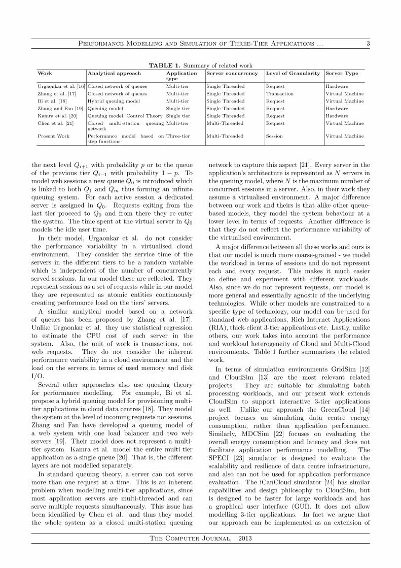
TABLE 1. Summary of related workWork Analytical approach Application
typeServer concurrency Level of Granularity Server Type
Urgaonkar et al. [16] Closed network of queues Multi-tier Single Threaded Request Hardware
Zhang et al. [17] Closed network of queues Multi-tier Single Threaded Transaction Virtual Machine
Bi et al. [18] Hybrid queuing model Multi-tier Single Threaded Request Virtual Machine
Zhang and Fan [19] Queuing model Single tier Single Threaded Request Hardware
Kamra et al. [20] Queuing model, Control Theory Single tier Single Threaded Request Hardware
Chen et al. [21] Closed multi-station queuingnetwork
Multi-tier Multi-Threaded Request Virtual Machine
Present Work Performance model based onstep functions
Three-tier Multi-Threaded Session Virtual Machine
the next level Qi+1 with probability p or to the queueof the previous tier Qi−1 with probability 1 − p. Tomodel web sessions a new queue Q0 is introduced whichis linked to both Q1 and Qm thus forming an infinitequeuing system. For each active session a dedicatedserver is assigned in Q0. Requests exiting from thelast tier proceed to Q0 and from there they re-enterthe system. The time spent at the virtual server in Q0
models the idle user time.
In their model, Urgaonkar et al. do not considerthe performance variability in a virtualised cloudenvironment. They consider the service time of theservers in the different tiers to be a random variablewhich is independent of the number of concurrentlyserved sessions. In our model these are reflected. Theyrepresent sessions as a set of requests while in our modelthey are represented as atomic entities continuouslycreating performance load on the tiers’ servers.
A similar analytical model based on a networkof queues has been proposed by Zhang et al. [17].Unlike Urgaonkar et al. they use statistical regressionto estimate the CPU cost of each server in thesystem. Also, the unit of work is transactions, notweb requests. They do not consider the inherentperformance variability in a cloud environment and theload on the servers in terms of used memory and diskI/O.
Several other approaches also use queuing theoryfor performance modelling. For example, Bi et al.propose a hybrid queuing model for provisioning multi-tier applications in cloud data centres [18]. They modelthe system at the level of incoming requests not sessions.Zhang and Fan have developed a queuing model ofa web system with one load balancer and two webservers [19]. Their model does not represent a multi-tier system. Kamra et al. model the entire multi-tierapplication as a single queue [20]. That is, the differentlayers are not modelled separately.
In standard queuing theory, a server can not servemore than one request at a time. This is an inherentproblem when modelling multi-tier applications, sincemost application servers are multi-threaded and canserve multiple requests simultaneously. This issue hasbeen identified by Chen et al. and thus they modelthe whole system as a closed multi-station queuing
network to capture this aspect [21]. Every server in theapplication’s architecture is represented as N servers inthe queuing model, where N is the maximum number ofconcurrent sessions in a server. Also, in their work theyassume a virtualised environment. A major differencebetween our work and theirs is that alike other queue-based models, they model the system behaviour at alower level in terms of requests. Another difference isthat they do not reflect the performance variability ofthe virtualised environment.
A major difference between all these works and ours isthat our model is much more coarse-grained - we modelthe workload in terms of sessions and do not representeach and every request. This makes it much easierto define and experiment with different workloads.Also, since we do not represent requests, our model ismore general and essentially agnostic of the underlyingtechnologies. While other models are constrained to aspecific type of technology, our model can be used forstandard web applications, Rich Internet Applications(RIA), thick-client 3-tier applications etc. Lastly, unlikeothers, our work takes into account the performanceand workload heterogeneity of Cloud and Multi-Cloudenvironments. Table 1 further summarises the relatedwork.
In terms of simulation environments GridSim [12]and CloudSim [13] are the most relevant relatedprojects. They are suitable for simulating batchprocessing workloads, and our present work extendsCloudSim to support interactive 3-tier applicationsas well. Unlike our approach the GreenCloud [14]project focuses on simulating data centre energyconsumption, rather than application performance.Similarly, MDCSim [22] focuses on evaluating theoverall energy consumption and latency and does notfacilitate application performance modelling. TheSPECI [23] simulator is designed to evaluate thescalability and resilience of data centre infrastructure,and also can not be used for application performanceevaluation. The iCanCloud simulator [24] has similarcapabilities and design philosophy to CloudSim, butis designed to be faster for large workloads and hasa graphical user interface (GUI). It does not allowmodelling 3-tier applications. In fact we argue thatour approach can be implemented as an extension of
The Computer Journal, 2013
4 N. Grozev and R. Buyya
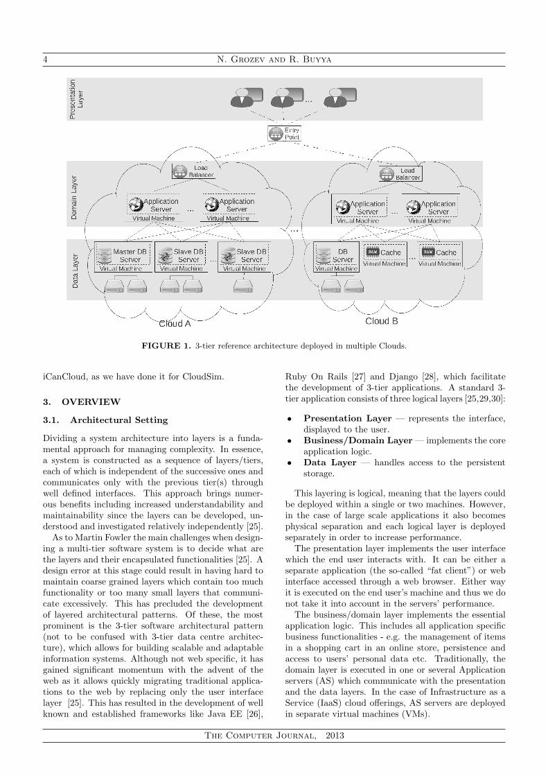
FIGURE 1. 3-tier reference architecture deployed in multiple Clouds.
iCanCloud, as we have done it for CloudSim.
3. OVERVIEW
3.1. Architectural Setting
Dividing a system architecture into layers is a funda-mental approach for managing complexity. In essence,a system is constructed as a sequence of layers/tiers,each of which is independent of the successive ones andcommunicates only with the previous tier(s) throughwell defined interfaces. This approach brings numer-ous benefits including increased understandability andmaintainability since the layers can be developed, un-derstood and investigated relatively independently [25].
As to Martin Fowler the main challenges when design-ing a multi-tier software system is to decide what arethe layers and their encapsulated functionalities [25]. Adesign error at this stage could result in having hard tomaintain coarse grained layers which contain too muchfunctionality or too many small layers that communi-cate excessively. This has precluded the developmentof layered architectural patterns. Of these, the mostprominent is the 3-tier software architectural pattern(not to be confused with 3-tier data centre architec-ture), which allows for building scalable and adaptableinformation systems. Although not web specific, it hasgained significant momentum with the advent of theweb as it allows quickly migrating traditional applica-tions to the web by replacing only the user interfacelayer [25]. This has resulted in the development of wellknown and established frameworks like Java EE [26],
Ruby On Rails [27] and Django [28], which facilitatethe development of 3-tier applications. A standard 3-tier application consists of three logical layers [25,29,30]:
• Presentation Layer — represents the interface,displayed to the user.
• Business/Domain Layer — implements the coreapplication logic.
• Data Layer — handles access to the persistentstorage.
This layering is logical, meaning that the layers couldbe deployed within a single or two machines. However,in the case of large scale applications it also becomesphysical separation and each logical layer is deployedseparately in order to increase performance.
The presentation layer implements the user interfacewhich the end user interacts with. It can be either aseparate application (the so-called “fat client”) or webinterface accessed through a web browser. Either wayit is executed on the end user’s machine and thus we donot take it into account in the servers’ performance.
The business/domain layer implements the essentialapplication logic. This includes all application specificbusiness functionalities - e.g. the management of itemsin a shopping cart in an online store, persistence andaccess to users’ personal data etc. Traditionally, thedomain layer is executed in one or several Applicationservers (AS) which communicate with the presentationand the data layers. In the case of Infrastructure as aService (IaaS) cloud offerings, AS servers are deployedin separate virtual machines (VMs).
The Computer Journal, 2013
Performance Modelling and Simulation of Three-Tier Applications ... 5
The data layer facilitates access to the persistentstorage. It is independent from the other two layers,as the persistent data often outlives the applicationsthat use it and in some cases it can even serve morethan one application. The data layer is executed in oneor several database servers (DB).
Traditionally, the data layer has been the mostarchitecturally challenging part of a 3-tier application,since it is hard to scale horizontally as demandrises. For example, this is the case when thedata tier is implemented with traditional transactionalrelational databases, which are widespread in virtuallyevery application domain. Several approaches likemaster-slave replication, caching, NoSQL and NewSQLdatabases [31] have been used to mitigate this issue andhave been widely adopted in cloud environments as well.
This architectural pattern is very generic and thereare a lot of possible adjustments that can improve theoverall system performance. For example, the numberof AS servers can be different and can increase ordecrease dynamically in response to the demand. Asdiscussed, the data layer can be composed of bothtransactional relational databases, caches and novelapproaches like NoSQL and NewSQL databases. In thiswork we introduce a general modelling and simulationapproach that encompasses all of them, and can be usedto evaluate different design alternatives - e.g. use ofcaching vs master-slave replication in the data layer.
In this work we consider two main scenarios: (i) a 3-tier application is deployed within a single data centreand (ii) a 3-tier application is deployed in multipleClouds (i.e. a Multi-Cloud) with additional redirectionof users to appropriate data centres. Clouds A and Bon Figure 1 depict two possible deployments. For eachapplication in a data centre, requests arrive througha single load balancer, which can be implemented indifferent ways. For example, it can be deployed in a VMor provided by the Cloud as a service. Load balancersdistribute the incoming workload to a set of applicationserver VMs deployed in the Cloud. Consequently,clients establish sessions with the assigned applicationservers. The AS servers communicate with the serversfrom the DB layer. Each DB server has one or severalhard disks attached, which are used to store persistentdata. In the Multi-Cloud scenario, client requests cometo a global entry point, from where they are distributedto data centres, each of which has the aforementionedsoftware stack deployed as depicted in Figure 1.
3.2. Assumptions and Scope
In this work we consider stateful (i.e. maintainingsession data) 3-tier applications. Examples of sessiondata are user preferences, shopping carts and historyof user actions. Also, we assume that the DB serversare deployed in separate VMs. Alternatively, persistentstorage could be provided by a cloud provider asa service. There is a plethora of vendor specific
Database-as-a-Service (DBaaS) solutions and relyingon them can easily lead to vendor lock-in. Hence itis an industry best practice to use database serversdeployed in separate VMs [32]. Furthermore, manyDBaaS solutions like Amazon RDS [33] actually provideVM instances to customers, and thus they can berepresented by our model as well.
Very few cloud providers offer their clients non-virtualised physical servers which are optimised for aspecific purpose (e.g. running a database). This canbe considered an exception form the general practice ofbuilding cloud data centres from commodity hardwareand providing it to clients in the from of virtualisedresources [1, 2] and hence most cloud simulators donot represent application execution in non-virtualisedenvironments. An example of such cloud service is theOracle Database Cloud, which offers database hostingon Oracle Exadata Database Servers [34, 35]. Suchscenario can still be represented by our approach bymodelling a host with the desired characteristics andallocating a single VM to it, which utilises all itsresources. Since in the model we do not considervirtualisation overhead, this will be equal to runningthe workload on the host directly.
In this work we consider 3-tier applications deployedin cloud and Multi-Cloud environments. In the relatedliterature there is a certain terminological ambiguityregarding the terms Inter-Cloud Federation and Multi-Cloud. In essence, an Inter-Cloud Federation isachieved when cloud providers voluntarily interconnectand share their infrastructure [11, 36–38]. Thisoften raises interoperability issues, since resources likeVMs need to be transparently migrated from oneprovider’s infrastructure to another. Often this needsto be transparent to the cloud clients. In contrast,the concept of Multi-Cloud does not depend on anunderlying collaboration of cloud providers. In a Multi-Cloud environment a cloud client uses and distributesworkload among independent clouds [11, 36, 39]. Inthe current cloud landscape, where there is no inter-operation between major competing cloud vendorslike Amazon and Google, the Multi-Cloud approachis much more feasible than the federation. In thisconfiguration, cloud interoperability is not a problem,as cloud clients do not rely on underlying cloud providercollaboration. The main problem is working withthe different management APIs of all cloud providers.Industry developments in the area of Multi-Cloudservices like RigthScale [40], Enstratius [41], Scalr [42]and Multi-Cloud libraries like JClouds [43], ApacheLibCloud [44] and Apache DeltaCloud [45] provideunified APIs for managing diverse cloud infrastructureand hence simplify system development [11]. Thereforein this work we focus our attention on workloaddistribution across clouds.
We consider that the load balancers implement“Sticky load balancing” policies. That is, after asession between a client and an application server is
The Computer Journal, 2013
6 N. Grozev and R. Buyya
established, all subsequent requests from this session areredirected to the same AS server. This is a reasonableassumption, since session sharing among servers oftenleads to overall performance degradation.
Clouds have made it possible for many clients toexecute complex and time consuming analysis over hugeamounts of data (i.e. “Big Data”) [46]. Often thereis a standard 3-tier web application serving as a front-end for accessing the data intensive analytical back end.Thus we can largely classify two types of data processing- synchronous (a.k.a online) and asynchronous (a.k.aoffline). The synchronous data processing is concernedwith performing data retrieval or manipulation in realtime - e.g. extracting a list of items from online shopand passing them to the AS server for display to theuser. In this case the user interactions are blockeduntil the operations are complete. Asynchronousdata processing is concerned with running long batchprocessing jobs in the background. In this case userinteractions are not blocked while the jobs are running.In this work we address synchronous data processing asit is in the standard 3-tier reference model.
We have outlined modelling data centre heterogeneityas one of our goals. More specifically in this work wefocus one the following aspects of heterogeneity:
• Workload heterogeneity — for a Multi-Cloud ap-plication, sessions arrive with different frequenciesbased on the cloud geographical location, time zoneetc.
• Cloud offerings heterogeneity — different cloudproviders offer different VMs in terms of their CPU,memory and disk capacity.
• VM consolidation policies — different cloudproviders have different policies for placing VMson physical hosts, which can affect CPU and diskperformance.
• Differences in the hardware capacity of the usedphysical hosts/nodes.
Finally, when multiple data centres are used weassume that the workload is distributed among datacentres based on its geographical origin and do notmodel the work of the entry point. That is, clientsdirectly submit their sessions to the nearby data centre.
3.3. Essence of the Model
We propose a session based analytical approach forperformance modelling. The workload is representedin terms of user sessions established between users andapplication servers. Each session incurs performanceload on the application and the database servers. Theworkload of a given server at any point in time is definedas the sum of the workloads of the served sessions.Sessions make use of CPU time and RAM on theapplication servers and CPU, RAM and disk I/O on thedatabase servers. We assume that the disk operationson the application server are negligible - e.g. logging,
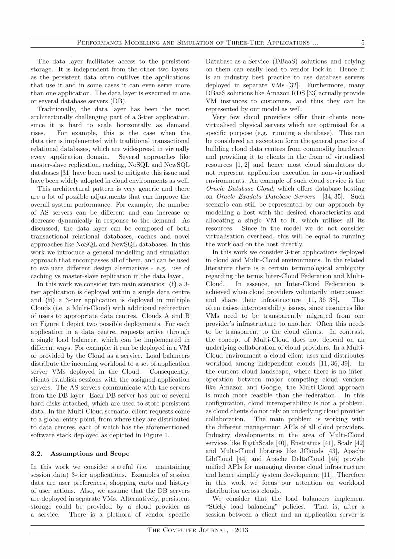
FIGURE 2. RAM load represented as stacked sessions’load.
loading configuration files etc.A key problem is how to represent the workloads (in
terms of CPU, RAM and I/O) incurred by a session.Logically, they should be represented as continuousfunctions of time so that workload changes over timecan be modelled. Since we are aiming to implementa discrete event simulator, we aim to represent thesecontinuous functions in a discrete manner. Oneapproach is to use stepwise functions. That way,by using a finite number of values one can define acontinuous function of time.
Figure 2 depicts how a server’s RAM usage can becomposed of the RAM usage of three sessions andthe underlying software stack - i.e. operating systemand middleware. The system’s RAM footprint can bedefined as the used RAM, when no sessions are beingserved. The RAM usage of the sessions is representedby stepwise functions and the system’s RAM usage isconsidered to be constant. Similar diagrams could bedrawn for the CPU utilizations as well. The sameapproach can be used to represent the I/O utilizationof a given hard disk on a DB server. That is,the utilisation of a hard disk is defined by the I/Ooperations performed on it by the sessions using thisdisk on any of the DB servers. A minor differenceis that the CPU and I/O capacity are not constantand change over time, because as discussed VMs canobserver performance variability.
The frequency of the establishment of sessions isanother aspect to model. Typically such phenomena aremodelled with Poisson distribution representing thatsessions arrive with some predefined frequency λ [47,48].Furthermore, Paxson and Floyd have found that eventslike user arrivals/logins are well modelled with a Poissonprocess for fixed time intervals [49]. However, in thecase of a large scale application it is not typical toobserve constant arrival rates at all times. Moreover,in a Multi-Cloud environment the workload of the
The Computer Journal, 2013
Performance Modelling and Simulation of Three-Tier Applications ... 7
different data centres may be substantially different.For example, a data centre in the US will have higherarrival rates during the working hours in the US timezones and lower otherwise. Thus we model sessionestablishment rates for a given data centre as a Poissondistribution of a frequency function of time λ(t), whichis also a stepwise function. If λ(t) is a constant function,the arrival rates remain with pure Poisson distribution,and thus our approach is more general than the usualone. Our approach allows to model demand fluctuationsand spikes over time and to evaluate how the modelledsystem behaves in such cases.
If we have several different types of sessions in termsof the incurred performance, we can model the arrivalrate of each of these as a separate Poisson distributionover a different frequency function.
4. ANALYTICAL MODEL
4.1. Session Model
We take a session based approach and instead of jobsor requests, the unit of workload in our model is asession, which represents a series of consecutive useractions incurring system load. Each session is assignedto an application server VM and can use the availableDB servers in the data centre for the application.
Unlike jobs, a session generates variable workloadover time. For example, for the first few minutesafter its establishment a session may utilize heavily theprocessor of the application server, for the next fiveminutes it may incur very low resource consumption,and over the next five minutes it may incur significantdisk I/O on a database server. In contrast, a job isusually modelled in terms of the required resources(CPU, RAM etc.) and there are no requirements asto how these resources are provided over time. Moreformally, a session is defined with the following variablesand functions:
Ideal Session Durationτi denotes the ideal duration of a session si measuredin seconds. It is the session duration given that allresources for its execution are available. If there aremore sessions than a tier can handle, there will be someresource pre-emption and eventually the session will beserved in more than τi seconds or will fail. By ∆i wedenote the time by which si has exceeded τi and weconsider it as a measure of application responsiveness.
Data ItemIn order to model the locality of disk operations, weneed to represent the data resident on the disks. Thus,we introduce the notion of data item, which representsan entity stored on a disk. Examples of data items arefiles and portions of database records, which are oftenaccessed and stored together (e.g. a database shard).In the model, we consider that a finite number of data
items d1...dn is specified.
Step SizeWe define a common step size δ for all stepwise functionsin our model. Generally we would aim for small value ofδ, since that would make the simulation more refined.
CPU Load of the Application ServerBy νas(t) we denote the CPU load on the applicationserver caused by the session. It is measured in millionsinstructions per second (MIPS) and represents theaverage number of CPU instructions required by thesession over time. At a given point in time, the required
number of operations can be defined as n(t)2ε where n(t)
is the number of instructions required by a sessionin the time interval [t − ε, t + ε] after its start givena small predefined ε > 0. The ε value is an inputparameter to the model (e.g. ε = 0.001). Based onthat, we can formally define the values of the stepwisefunction νas for the j-the step (i.e. t ∈ [(j− 1)δ, jδ)) as
νas(t) = 1δ
jδ∫(j−1)δ
n(x)2ε dx.
Memory Load of the Application ServerThe stepwise function φas(t) denotes the RAM usagein the application server by the session over time and isdefined analogously to νas(t). φas(t) defines how manymegabytes of memory the session uses t seconds afterits start.
CPU Load of the Database ServersBy νdb(t, dk) we denote the number of CPU operationsneeded for the processing of data item dk by some ofthe database servers. It is measured in MIPS and isdefined analogously to νas(t).
Memory Load of the Database Serversφdb(t, dk) defines the RAM usage needed for theprocessing of data item dk by a database server andis formally defined analogously to φas(t).
Disk I/O LoadBy σdb(t, dk) we denote the number of required disk I/Ooperations on data item dk over time. It is measuredin Millions of Input/Output Operations Per Second(MIOPS). The number of I/O operations with dk at
time t can be defined as n(t,dk)2ε where n(t, dk) is the
number of instructions with data item dk required bya session in the time interval [t − ε, t + ε] and giventhe predefined ε > 0. Analogously to νas, we candefine the “averaged” step values of the σdb functionsfor the j-the step (i.e. t ∈ [(j − 1)δ, jδ)) as σdb(t, dk) =
1δ
jδ∫(j−1)δ
n(x,dk)2ε dx.
The Computer Journal, 2013
8 N. Grozev and R. Buyya
Network delay and “think times”Within our architectural settings, we can largely classifytwo types of network: (i) the internal data centrenetwork, used to connect application tiers within acloud and (ii) the network between the end users andthe serving data centre.
Nowadays the internal data centre network usuallyhas sophisticated topology and offers high speed andlow latency [50]. Moreover, previous research inmulti-tier applications shows that inter-tier networkperformance typically does not cause significantperformance penalty compared to CPU, RAM andI/O utilisation [51, 52]. In fact Lloyd et al. haveempirically shown that for a multi-tier application ina cloud environment, the outgoing and incoming VMnetwork transfer between tiers explain respectively only0.75% and 0.74% of the overall performance variability.In contrast, they have found that CPU load and diskreads and writes explain respectively over 71%, 37%and 14% of the observed performance [53]. Hence wewill consider the effect of the internal network to benegligible and will not present it in our model.
In contrast, the delays caused by the wide areanetwork connecting end users with the serving datacentre can be significant. Similarly, users’ “thinktimes” are typically present and need to be modelled.From the perspective of the servers both the externalnetwork delays and the “think times” result in idleperiods, during which the servers are not utilised bythe session. More formally, if a session is idle (eitherbecause of a network delay or user’s inactivity) duringthe time period [t1, t2], then the number of requiredCPU instructions by the AS server will be n(t) = 0 fort ∈ [t1, t2]. Since νas(t) is dependent on n(t) its valuefor this time interval will be affected accordingly. Thevalues of νdb and σdb, representing the CPU and diskutilisation of a DB server, for an idle time period canbe defined analogously. The values of φas and φdb foran idle period can be defined as the amount of sessiondata kept in the memory by the respective AS and DBservers during these periods.
4.2. Modelling Resource Contention
Resource contention appears when some of a server’sresources (e.g. CPU) are insufficient to serve all itssessions timely. Although clouds offer seemingly endlessresource pools, it is still possible for an application toexperience resource shortage. Firstly, some applicationsallocate resources statically and given a substantialworkload their capacity can be exceeded. Secondly,public online applications can experience a sudden andunexpected demand peak. In some cases resources cannot be provisioned quickly enough and thus the alreadyprovisioned servers experience contention. Thirdly,in many 3-tier deployment models, the data tier cannot scale horizontally. For example when a singlerelational DB server is used without any replication or
sharding. In such cases the DB servers can experiencecontention. To explore what is the system performancein such cases, we need to be able to model and simulatecontentions. Next, we describe how different resourcecontentions are handled in our model.
CPU resource contentionWhen the CPU resources of a server are insufficient,standard process/thread scheduling policies are used toassign processing time to each session. For the timeperiods that the session is preempted in a tier, it is alsoconsidered preempted on the other application tier. Inother words resource preemption in one tier is reflectedby an overall slowdown of the entire session, which isrepresentative of synchronous data processing.
I/O resource contentionWhen the I/O throughput of the DB server isinsufficient, standard I/O scheduling policies are used toassign I/O processing to each session. Alike with CPU,an I/O preemption in one tier leads to a preemtion inthe other tier as well.
RAM resource contentionRAM resource contention occurs when at a given pointin time the sum of the sessions’ and the system’smemory usages exceed the amount of memory theserver has. When RAM resource contention appearsthe server stops, resulting in “out of memory” error.Consequently all sessions served on this server fail and itstops accepting new ones. The work of the other servershowever continues. For simplicity in our model we donot consider the usage of swapped disk space. Themodelled behaviour is representative of an operatingsystem going out of memory and killing the process ofthe server.
4.3. Session Arrival Model
As discussed, we model the arrival of a session of agiven type in a data centre as a Poisson distribution of afrequency function - Po(λ(t)), where λ(t) is representedas a stepwise function of time. In a Multi-Cloudscenario, the arrival rates in each Cloud should bedefined. Hence frequency functions need to be specifiedper data centre. This allows for modelling differentworkloads coming at different times within each datacentre. Thus we can represent workload influencingfactors like time zone differences. Formally, for eachsession type sti and data centre dcj , the number ofarrivals can be modelled as Po(λij(t)), where λij(t) isa user specified function modelling the arrival rate.
4.4. Performance Variability across Clouds
The VM performance in a Multi-Cloud environment canvary significantly. The two main factors for this are:
The Computer Journal, 2013
Performance Modelling and Simulation of Three-Tier Applications ... 9
• VM setup - a typical VM configuration allows aVM to use additional (but still limited) resources interms of CPU and I/O if the host machine providesfor that. Thus in the model it is important tospecify what is the set-up of the VMs with respectto sharing hardware resources.
• VM consolidation - if the VM setup allowsfor opportunistic usage of host resources, then itis important to note what the VM consolidationpolicy of each cloud provider is.
In order to adequately model the variability of theVM performance in a Multi-Cloud environment, weneed to note both these characteristics for every datacentre. In the implementation section we discuss furtherhow these policies can be specified.
5. SIMULATOR IMPLEMENTATION
The previously described analytical model allowsfor coarse grained performance analysis of 3-tierapplications. In this section, we describe ourimplementation in terms of algorithms and datastructures which extend the CloudSim [13] environmentto support our model. CloudSim is a mature simulationenvironment and by extending it our approach can makeuse of all of its existing features like VM placementpolicies and energy consumption evaluation.
5.1. Representation of Disk I/O Operations
To represent an application’s performance in terms ofaccess to persistence storage, we extended CloudSim tosupport disk operations. This was done at three levels:
• Host — we extended the base CloudSim Host(physical machine) entity by adding hard disks toit. Each disk is represented as an extension ofthe Processing Element (Pe) component. A Pe inCloudSim models a core of a processor.
• VM — in a similar fashion, we also extended theVMs to support disk operations. We also extendedthe schedulers that distribute VM resources amongthe executing jobs to distribute the available I/Ooperations.
• Cloudlet (Job) — each job (cloudlet in terms ofCloudSim) has been extended to define a numberof required I/O operations. Also each cloudletis associated with the data item it uses. Lastly,each cloudlet defines a boolean value, showing if itmodifies the data item or not.
Users are allowed to specify the policies for sharingI/O operations among VMs in a Host and cloudlets ina VM the same way they do it for CPU.
5.2. Provisioning of I/O Operations
Disk I/O operations need to be distributed at twolevels. Firstly, a Host should distribute the available
disk operations among the VM s using the disks.Secondly, VM s should distribute their portion of theI/O operations among the jobs/cloudlets deployed inthem. There is clear analogy between distributingI/O and CPU operations among VM s and cloudlets.Furthermore, as we represent hard disks as extendedProcessing Elements (Pe) we could directly reuse thealready existing CloudSim policies for CPU scheduling.
However, unlike CPU, I/O operations are localised.I/O operations on a data item stored on one drive cannot be executed on another, while CPU operations canbe executed on every available CPU. Since CloudSimdoes not support such locality in the assignment ofCPU operations, directly reusing these policies will leadto erroneous simulation behaviour. To overcome thisproblem we assign a separate scheduler to each of thehard disks of a Host. Thus disk operations can beprovisioned per disk. This allows for VMs to haveaccess only to a portion of the available disks and toachieve locality. We have also implemented locality inan extension to the job/cloudlet scheduling policies, sothat jobs utilise only the disks, where the correspondingdata items reside.
5.3. Representing Sessions and Contention
In the analytical model, we represented a session asseveral stepwise functions defining its resource demandson the servers. Within each step, a session has constantresource requirements in terms of CPU, RAM and I/Ooperations. To bring this concept to the simulationenvironment, we represent the behaviour of each sessionwithin a step as one cloudlet executed by the AS serverand several cloudlets on the DB servers. Each of theDB cloudlets is associated with the data item it uses.The breakdown of a session’s behaviour for a given stepinto DB cloudlets is based on the data items it accessesduring this period. For example if a session accessesthree data items during a given step, then there will bethree DB cloudlets for this step.
In other words for each session and for each step inthe simulation we have one cloudlet assigned to the ASserver and several cloudlets assigned to the DB servers.Thus in terms of implementation the step values of νas,φas, νdb, φdb, σdb define the corresponding cloudlets’resource requirements in terms of CPU, RAM and I/O.
The assignment of cloudlets to DB servers isbased on the data items they use - cloudlets areassigned to servers which have access to their data.This assignment is done by a new simulation entityDBCloudletScheduler. The default implementation ofthis entity assigns each DB cloudlet to the first serverwhich has access to its data item. By specifying acustom DBCloudletScheduler one can simulate differentpolicies in the data layer. For example, cloudletsperforming read operations could be redirected to slavedatabase servers, or can be cancelled if the data theyretrieve is in a cache.
The Computer Journal, 2013

10 N. Grozev and R. Buyya
FIGURE 3. Session representation.
Formally, for a given session the required amount ofCPU operations in the AS cloudlet corresponding to
the step interval [ti, ti+δ] isti+δ∫ti
νas(t) dt, which simply
equals δνas(ti) as νas(t) is a stepwise function has aconstant value within this interval. The other resourcerequirements (CPU and RAM of a server and I/O on adisk) of the cloudlets are defined analogously.
Each session is represented with two equal-sizedqueues - one for the AS server and one for the DBservers. The elements of both queues correspond tothe steps in the model. The elements of the AS queueare single cloudlets, which are executed sequentially.The elements of the DB queue are sets of cloudlets,whose members execute simultaneously. Cloudletsfrom subsequent elements of the DB queue executesequentially. The cloudlets from the correspondingelements of both queues are associated with the samestart time, and no cloudlet is submitted to the serversbefore its start time has passed.
This is depicted in Figure 3. For each session si onthe diagram the j-th element of the AS queue is sasij and
the j-th element of the DB queue is the set {sdbij1...sdbijlij}where lij is the set size. Cloudlets associated with the j-th step are submitted only if all their start times havepassed and all cloudlets from the previous steps havefinished execution.
After a session si is submitted, the cloudlets formthe heads of both queues are set the current simulationtime tcur as start times. The head of the AS queue sasi1 isdirectly submitted to the assigned AS server. Cloudletssdbi11...s
dbi1li1
from the head of the DB queue are sent tothe DBCloudletScheduler, which submits them to theDB servers in accordance with the DB layer architecture- e.g. Master-Slave, caching etc. The cloudlets fromthe next elements of the queues sasi2 , s
dbi21...s
dbi2li2
are setstarting time tcurr + σ. This procedure is defined inAlgorithm 1.
Upon the completion of every submitted cloudlet andthe elapse of the start time of every cloudlet, which has
not been yet submitted, the heads of the two queuesare inspected. If all cloudlets from the two heads havefinished and the start times of the cloudlets form thenext queue elements have passed, then the followingactions are taken:
1. the heads of the queues are removed;2. the cloudlets from the new heads are submitted;3. the cloudlets from the next elements (after the
heads) of the queues are set to have starting timesσ seconds after the present moment.
Algorithm 2 defines formally the previously describedprocedure for updating a session. The two keyinvariants of this algorithm are:
• No cloudlet is submitted before its start timeand the start time of its counterparts from bothqueues have come. Formally, no cloudlet c ∈{sasij , sdbij1...sdbijlij} is submitted before the start
times for all sasij , sdbij1...s
dbijlij
have elapsed. Thisensures that even if one of the servers is quick tofinish its cloudlets, this will not lead to prematureexhaustion of the session’s cloudlets and the sessionwill still take at least its predefined ideal time.
• No cloudlet is submitted before all its predecessorsand all predecessors of its counterparts fromboth queues have finished. Thus if there iscontention/bottleneck in any of the tiers this willresult in an overall delay of the whole session.
As a consequence a bottleneck in a tier results in anoverall delay of the served sessions.
CloudSim is a discrete event simulator and one canassociate custom logic with every event. This allowed usto check throughout the simulation if the memory usagewithin a server exceeds its capacity. In accordance withthe described model, in such a case the VM simulationentity is stopped and all of its running sessions aremarked as failed.
The Computer Journal, 2013
Performance Modelling and Simulation of Three-Tier Applications ... 11
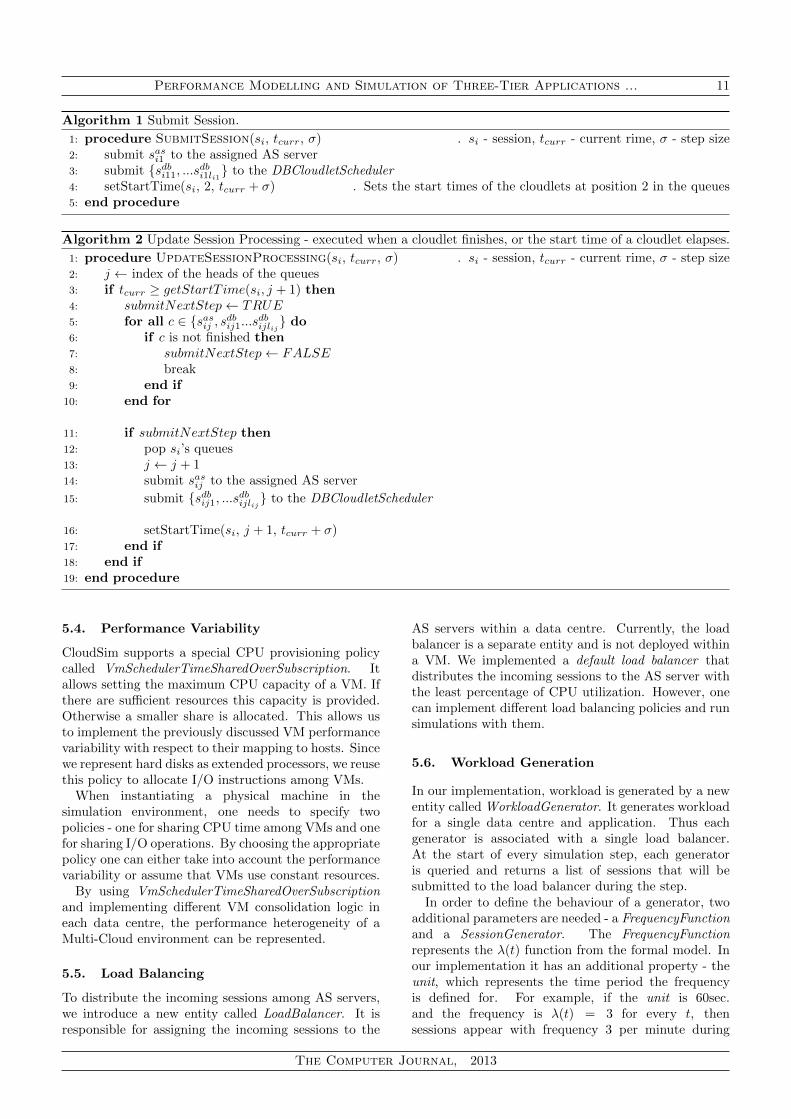
Algorithm 1 Submit Session.
1: procedure SubmitSession(si, tcurr, σ) . si - session, tcurr - current rime, σ - step size2: submit sasi1 to the assigned AS server3: submit {sdbi11, ...sdbi1li1} to the DBCloudletScheduler4: setStartTime(si, 2, tcurr + σ) . Sets the start times of the cloudlets at position 2 in the queues5: end procedure
Algorithm 2 Update Session Processing - executed when a cloudlet finishes, or the start time of a cloudlet elapses.
1: procedure UpdateSessionProcessing(si, tcurr, σ) . si - session, tcurr - current rime, σ - step size2: j ← index of the heads of the queues3: if tcurr ≥ getStartT ime(si, j + 1) then4: submitNextStep← TRUE5: for all c ∈ {sasij , sdbij1...sdbijlij} do6: if c is not finished then7: submitNextStep← FALSE8: break9: end if
10: end for
11: if submitNextStep then12: pop si’s queues13: j ← j + 114: submit sasij to the assigned AS server
15: submit {sdbij1, ...sdbijlij} to the DBCloudletScheduler
16: setStartTime(si, j + 1, tcurr + σ)17: end if18: end if19: end procedure
5.4. Performance Variability
CloudSim supports a special CPU provisioning policycalled VmSchedulerTimeSharedOverSubscription. Itallows setting the maximum CPU capacity of a VM. Ifthere are sufficient resources this capacity is provided.Otherwise a smaller share is allocated. This allows usto implement the previously discussed VM performancevariability with respect to their mapping to hosts. Sincewe represent hard disks as extended processors, we reusethis policy to allocate I/O instructions among VMs.
When instantiating a physical machine in thesimulation environment, one needs to specify twopolicies - one for sharing CPU time among VMs and onefor sharing I/O operations. By choosing the appropriatepolicy one can either take into account the performancevariability or assume that VMs use constant resources.
By using VmSchedulerTimeSharedOverSubscriptionand implementing different VM consolidation logic ineach data centre, the performance heterogeneity of aMulti-Cloud environment can be represented.
5.5. Load Balancing
To distribute the incoming sessions among AS servers,we introduce a new entity called LoadBalancer. It isresponsible for assigning the incoming sessions to the
AS servers within a data centre. Currently, the loadbalancer is a separate entity and is not deployed withina VM. We implemented a default load balancer thatdistributes the incoming sessions to the AS server withthe least percentage of CPU utilization. However, onecan implement different load balancing policies and runsimulations with them.
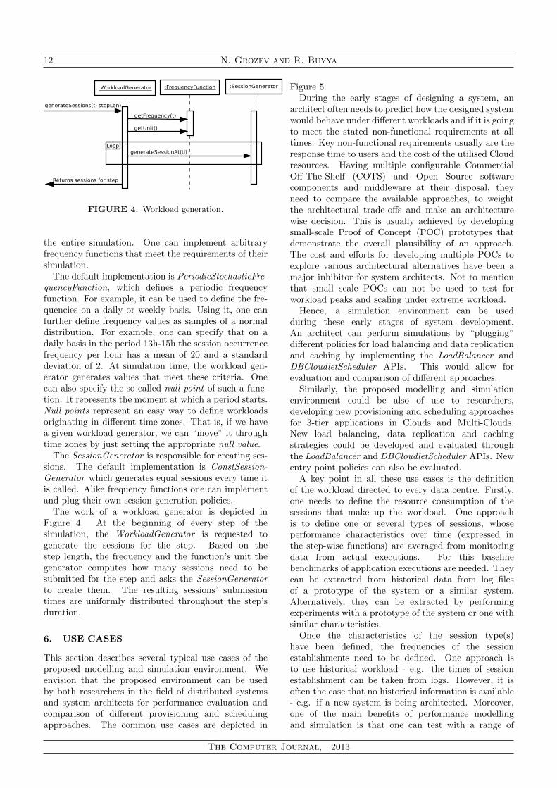
5.6. Workload Generation
In our implementation, workload is generated by a newentity called WorkloadGenerator. It generates workloadfor a single data centre and application. Thus eachgenerator is associated with a single load balancer.At the start of every simulation step, each generatoris queried and returns a list of sessions that will besubmitted to the load balancer during the step.
In order to define the behaviour of a generator, twoadditional parameters are needed - a FrequencyFunctionand a SessionGenerator. The FrequencyFunctionrepresents the λ(t) function from the formal model. Inour implementation it has an additional property - theunit, which represents the time period the frequencyis defined for. For example, if the unit is 60sec.and the frequency is λ(t) = 3 for every t, thensessions appear with frequency 3 per minute during
The Computer Journal, 2013
12 N. Grozev and R. Buyya
FIGURE 4. Workload generation.
the entire simulation. One can implement arbitraryfrequency functions that meet the requirements of theirsimulation.
The default implementation is PeriodicStochasticFre-quencyFunction, which defines a periodic frequencyfunction. For example, it can be used to define the fre-quencies on a daily or weekly basis. Using it, one canfurther define frequency values as samples of a normaldistribution. For example, one can specify that on adaily basis in the period 13h-15h the session occurrencefrequency per hour has a mean of 20 and a standarddeviation of 2. At simulation time, the workload gen-erator generates values that meet these criteria. Onecan also specify the so-called null point of such a func-tion. It represents the moment at which a period starts.Null points represent an easy way to define workloadsoriginating in different time zones. That is, if we havea given workload generator, we can “move” it throughtime zones by just setting the appropriate null value.
The SessionGenerator is responsible for creating ses-sions. The default implementation is ConstSession-Generator which generates equal sessions every time itis called. Alike frequency functions one can implementand plug their own session generation policies.
The work of a workload generator is depicted inFigure 4. At the beginning of every step of thesimulation, the WorkloadGenerator is requested togenerate the sessions for the step. Based on thestep length, the frequency and the function’s unit thegenerator computes how many sessions need to besubmitted for the step and asks the SessionGeneratorto create them. The resulting sessions’ submissiontimes are uniformly distributed throughout the step’sduration.
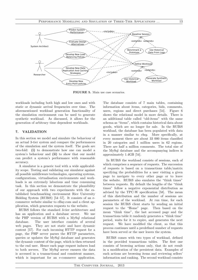
6. USE CASES
This section describes several typical use cases of theproposed modelling and simulation environment. Weenvision that the proposed environment can be usedby both researchers in the field of distributed systemsand system architects for performance evaluation andcomparison of different provisioning and schedulingapproaches. The common use cases are depicted in
Figure 5.During the early stages of designing a system, an
architect often needs to predict how the designed systemwould behave under different workloads and if it is goingto meet the stated non-functional requirements at alltimes. Key non-functional requirements usually are theresponse time to users and the cost of the utilised Cloudresources. Having multiple configurable CommercialOff-The-Shelf (COTS) and Open Source softwarecomponents and middleware at their disposal, theyneed to compare the available approaches, to weightthe architectural trade-offs and make an architecturewise decision. This is usually achieved by developingsmall-scale Proof of Concept (POC) prototypes thatdemonstrate the overall plausibility of an approach.The cost and efforts for developing multiple POCs toexplore various architectural alternatives have been amajor inhibitor for system architects. Not to mentionthat small scale POCs can not be used to test forworkload peaks and scaling under extreme workload.
Hence, a simulation environment can be usedduring these early stages of system development.An architect can perform simulations by “plugging”different policies for load balancing and data replicationand caching by implementing the LoadBalancer andDBCloudletScheduler APIs. This would allow forevaluation and comparison of different approaches.
Similarly, the proposed modelling and simulationenvironment could be also of use to researchers,developing new provisioning and scheduling approachesfor 3-tier applications in Clouds and Multi-Clouds.New load balancing, data replication and cachingstrategies could be developed and evaluated throughthe LoadBalancer and DBCloudletScheduler APIs. Newentry point policies can also be evaluated.
A key point in all these use cases is the definitionof the workload directed to every data centre. Firstly,one needs to define the resource consumption of thesessions that make up the workload. One approachis to define one or several types of sessions, whoseperformance characteristics over time (expressed inthe step-wise functions) are averaged from monitoringdata from actual executions. For this baselinebenchmarks of application executions are needed. Theycan be extracted from historical data from log filesof a prototype of the system or a similar system.Alternatively, they can be extracted by performingexperiments with a prototype of the system or one withsimilar characteristics.
Once the characteristics of the session type(s)have been defined, the frequencies of the sessionestablishments need to be defined. One approach isto use historical workload - e.g. the times of sessionestablishment can be taken from logs. However, it isoften the case that no historical information is available- e.g. if a new system is being architected. Moreover,one of the main benefits of performance modellingand simulation is that one can test with a range of
The Computer Journal, 2013
Performance Modelling and Simulation of Three-Tier Applications ... 13
FIGURE 5. Main use case scenarios.
workloads including both high and low ones and withstatic or dynamic arrival frequencies over time. Theaforementioned workload generation functionality ofthe simulation environment can be used to generatesynthetic workload. As discussed, it allows for thegeneration of arbitrary time dependent workloads.
7. VALIDATION
In this section we model and simulate the behaviour ofan actual 3-tier system and compare the performancesof the simulation and the system itself. The goals aretwo-fold: (i) to demonstrate how one can model asystem’s behaviour and (ii) to show that our modelcan predict a system’s performance with reasonableaccuracy.
A simulator is a generic tool with a wide applicabil-ity scope. Testing and validating our simulator againstall possible middleware technologies, operating systems,configurations, virtualisation environments and work-loads is an extremely laborious and time consumingtask. In this section we demonstrate the plausibilityof our approach with two experiments with the es-tablished benchmarking environment Rice UniversityBidding System (RUBiS) [54–57]. It consists of an e-commerce website similar to eBay.com and a client ap-plication, which generates requests to the website.
RUBiS follows the standard 3-tier architecture andhas an application and a database server. We usethe PHP version of RUBiS with a MySql relationaldatabase. The user interface consists of severalweb pages. They are not static and have dynamiccontent [57]. For each incoming HTTP request for apage, the PHP server parses the HTTP parameters,queries or updates the MySql database and generatesthe dynamic content of the page, which is then returnedto the end user. Hence each page request induces loadto both servers. The MySql server ensures the datais accessed in a transactional and consistent manner,which is important for an e-commerce application.
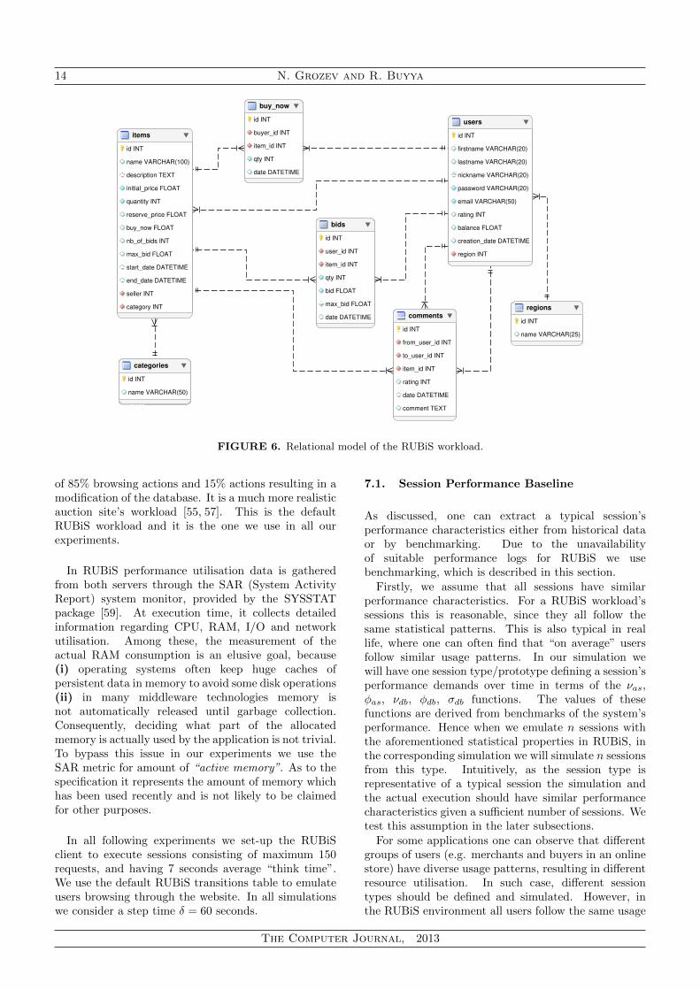
The database consists of 7 main tables, containinginformation about items, categories, bids, comments,users, regions and direct purchases [54]. Figure 6shows the relational model in more details. There isan additional table called “old-items” with the sameschema as “items”, which contains historical data aboutgoods, which are no longer for sale. In the RUBiSworkload, the database has been populated with datain a manner similar to ebay. More specifically, atevery moment there are about 33 000 items classifiedin 20 categories and 1 million users in 62 regions.There are half a million comments. The total size ofthe MySql database and the accompanying indices isapproximately 1.4GB [54].
In RUBiS the workload consists of sessions, each ofwhich comprises a sequence of requests. The successionof requests is based on a transactions table/matrixspecifying the probabilities for a user visiting a givenpage to navigate to every other page or to leavethe website. RUBiS also emulates the “think times”between requests. By default the lengths of the “thinktimes” follow a negative exponential distribution asadvised by the TPC-W specification [58]. The meanof this distribution and the number of sessions areparameters of the workload. At run time, for eachsession the RUBiS client starts by sending an initialrequest to the “Home” page. Then based on themean “think time”, the last accessed page and thetransactions table it randomly generates a “think time”period, waits for it to expire, and generates the nextrequest. We have modified the client, so that thisprocess continues until a predefined number of requestshave been served or the user leaves the system.
RUBiS comes with two types of workload, definedin the provided transactions tables. The first oneconsists of browsing actions only, that do not resultin a modification of the persistent data. Examples ofsuch actions are browsing items and reviewing sellers’information and ranking. The second workload consists
The Computer Journal, 2013
14 N. Grozev and R. Buyya
FIGURE 6. Relational model of the RUBiS workload.
of 85% browsing actions and 15% actions resulting in amodification of the database. It is a much more realisticauction site’s workload [55, 57]. This is the defaultRUBiS workload and it is the one we use in all ourexperiments.
In RUBiS performance utilisation data is gatheredfrom both servers through the SAR (System ActivityReport) system monitor, provided by the SYSSTATpackage [59]. At execution time, it collects detailedinformation regarding CPU, RAM, I/O and networkutilisation. Among these, the measurement of theactual RAM consumption is an elusive goal, because(i) operating systems often keep huge caches ofpersistent data in memory to avoid some disk operations(ii) in many middleware technologies memory isnot automatically released until garbage collection.Consequently, deciding what part of the allocatedmemory is actually used by the application is not trivial.To bypass this issue in our experiments we use theSAR metric for amount of “active memory”. As to thespecification it represents the amount of memory whichhas been used recently and is not likely to be claimedfor other purposes.
In all following experiments we set-up the RUBiSclient to execute sessions consisting of maximum 150requests, and having 7 seconds average “think time”.We use the default RUBiS transitions table to emulateusers browsing through the website. In all simulationswe consider a step time δ = 60 seconds.
7.1. Session Performance Baseline
As discussed, one can extract a typical session’sperformance characteristics either from historical dataor by benchmarking. Due to the unavailabilityof suitable performance logs for RUBiS we usebenchmarking, which is described in this section.
Firstly, we assume that all sessions have similarperformance characteristics. For a RUBiS workload’ssessions this is reasonable, since they all follow thesame statistical patterns. This is also typical in reallife, where one can often find that “on average” usersfollow similar usage patterns. In our simulation wewill have one session type/prototype defining a session’sperformance demands over time in terms of the νas,φas, νdb, φdb, σdb functions. The values of thesefunctions are derived from benchmarks of the system’sperformance. Hence when we emulate n sessions withthe aforementioned statistical properties in RUBiS, inthe corresponding simulation we will simulate n sessionsfrom this type. Intuitively, as the session type isrepresentative of a typical session the simulation andthe actual execution should have similar performancecharacteristics given a sufficient number of sessions. Wetest this assumption in the later subsections.
For some applications one can observe that differentgroups of users (e.g. merchants and buyers in an onlinestore) have diverse usage patterns, resulting in differentresource utilisation. In such case, different sessiontypes should be defined and simulated. However, inthe RUBiS environment all users follow the same usage
The Computer Journal, 2013
Performance Modelling and Simulation of Three-Tier Applications ... 15
0 50 100 150 200 250 300
05
10
15
20
25
30
Time in seconds
%C
PU
utilisation
100 sessions
1 session
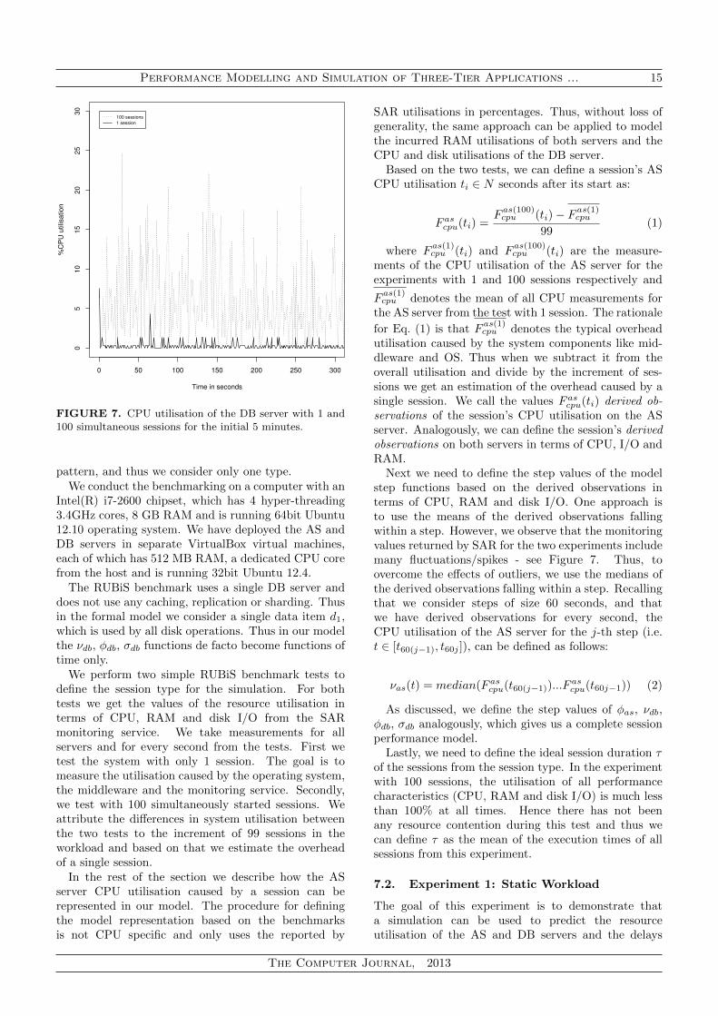
FIGURE 7. CPU utilisation of the DB server with 1 and100 simultaneous sessions for the initial 5 minutes.
pattern, and thus we consider only one type.We conduct the benchmarking on a computer with an
Intel(R) i7-2600 chipset, which has 4 hyper-threading3.4GHz cores, 8 GB RAM and is running 64bit Ubuntu12.10 operating system. We have deployed the AS andDB servers in separate VirtualBox virtual machines,each of which has 512 MB RAM, a dedicated CPU corefrom the host and is running 32bit Ubuntu 12.4.
The RUBiS benchmark uses a single DB server anddoes not use any caching, replication or sharding. Thusin the formal model we consider a single data item d1,which is used by all disk operations. Thus in our modelthe νdb, φdb, σdb functions de facto become functions oftime only.
We perform two simple RUBiS benchmark tests todefine the session type for the simulation. For bothtests we get the values of the resource utilisation interms of CPU, RAM and disk I/O from the SARmonitoring service. We take measurements for allservers and for every second from the tests. First wetest the system with only 1 session. The goal is tomeasure the utilisation caused by the operating system,the middleware and the monitoring service. Secondly,we test with 100 simultaneously started sessions. Weattribute the differences in system utilisation betweenthe two tests to the increment of 99 sessions in theworkload and based on that we estimate the overheadof a single session.
In the rest of the section we describe how the ASserver CPU utilisation caused by a session can berepresented in our model. The procedure for definingthe model representation based on the benchmarksis not CPU specific and only uses the reported by
SAR utilisations in percentages. Thus, without loss ofgenerality, the same approach can be applied to modelthe incurred RAM utilisations of both servers and theCPU and disk utilisations of the DB server.
Based on the two tests, we can define a session’s ASCPU utilisation ti ∈ N seconds after its start as:
F ascpu(ti) =Fas(100)cpu (ti)− F as(1)cpu
99(1)
where Fas(1)cpu (ti) and F
as(100)cpu (ti) are the measure-
ments of the CPU utilisation of the AS server for theexperiments with 1 and 100 sessions respectively and
Fas(1)cpu denotes the mean of all CPU measurements for
the AS server from the test with 1 session. The rationale
for Eq. (1) is that Fas(1)cpu denotes the typical overhead
utilisation caused by the system components like mid-dleware and OS. Thus when we subtract it from theoverall utilisation and divide by the increment of ses-sions we get an estimation of the overhead caused by asingle session. We call the values F ascpu(ti) derived ob-servations of the session’s CPU utilisation on the ASserver. Analogously, we can define the session’s derivedobservations on both servers in terms of CPU, I/O andRAM.
Next we need to define the step values of the modelstep functions based on the derived observations interms of CPU, RAM and disk I/O. One approach isto use the means of the derived observations fallingwithin a step. However, we observe that the monitoringvalues returned by SAR for the two experiments includemany fluctuations/spikes - see Figure 7. Thus, toovercome the effects of outliers, we use the medians ofthe derived observations falling within a step. Recallingthat we consider steps of size 60 seconds, and thatwe have derived observations for every second, theCPU utilisation of the AS server for the j-th step (i.e.t ∈ [t60(j−1), t60j ]), can be defined as follows:
νas(t) = median(F ascpu(t60(j−1))...Fascpu(t60j−1)) (2)
As discussed, we define the step values of φas, νdb,φdb, σdb analogously, which gives us a complete sessionperformance model.
Lastly, we need to define the ideal session duration τof the sessions from the session type. In the experimentwith 100 sessions, the utilisation of all performancecharacteristics (CPU, RAM and disk I/O) is much lessthan 100% at all times. Hence there has not beenany resource contention during this test and thus wecan define τ as the mean of the execution times of allsessions from this experiment.
7.2. Experiment 1: Static Workload
The goal of this experiment is to demonstrate thata simulation can be used to predict the resourceutilisation of the AS and DB servers and the delays
The Computer Journal, 2013
16 N. Grozev and R. Buyya
AS server, CPUDB server, CPUDB server, Disk
0 200 400 600 800 1000 1200 1400
02
04
06
08
01
00
300 sessions
Time in seconds
% U
tilis
atio
n
0 200 400 600 800 1000 1200 1400
600 sessions
FIGURE 8. CPU and disk utilisations with 300 and 600 simultaneous sessions. The plotted values are averaged for every90 seconds.
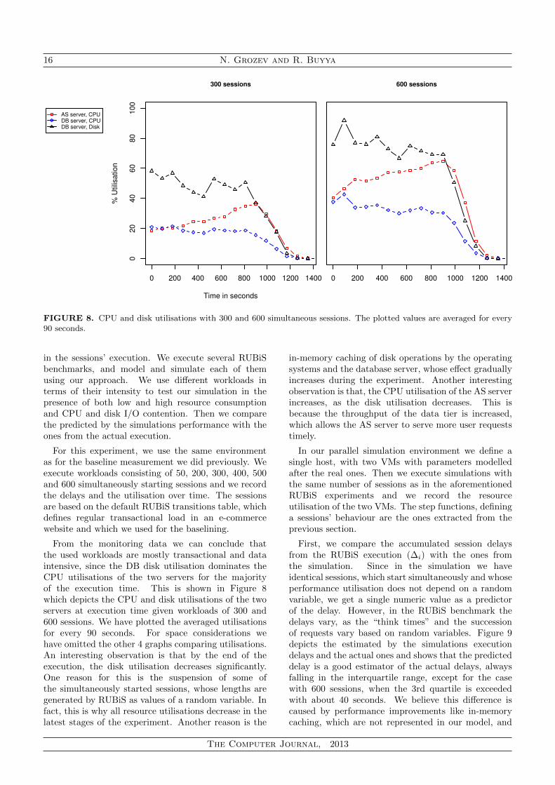
in the sessions’ execution. We execute several RUBiSbenchmarks, and model and simulate each of themusing our approach. We use different workloads interms of their intensity to test our simulation in thepresence of both low and high resource consumptionand CPU and disk I/O contention. Then we comparethe predicted by the simulations performance with theones from the actual execution.
For this experiment, we use the same environmentas for the baseline measurement we did previously. Weexecute workloads consisting of 50, 200, 300, 400, 500and 600 simultaneously starting sessions and we recordthe delays and the utilisation over time. The sessionsare based on the default RUBiS transitions table, whichdefines regular transactional load in an e-commercewebsite and which we used for the baselining.
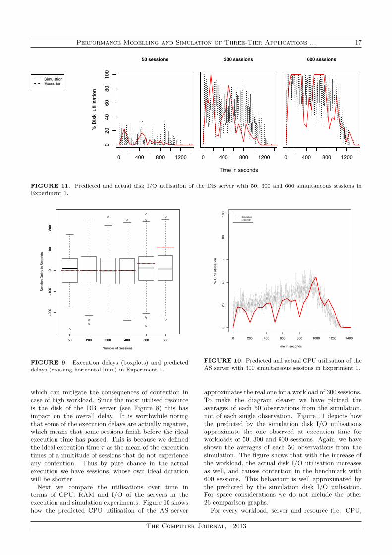
From the monitoring data we can conclude thatthe used workloads are mostly transactional and dataintensive, since the DB disk utilisation dominates theCPU utilisations of the two servers for the majorityof the execution time. This is shown in Figure 8which depicts the CPU and disk utilisations of the twoservers at execution time given workloads of 300 and600 sessions. We have plotted the averaged utilisationsfor every 90 seconds. For space considerations wehave omitted the other 4 graphs comparing utilisations.An interesting observation is that by the end of theexecution, the disk utilisation decreases significantly.One reason for this is the suspension of some ofthe simultaneously started sessions, whose lengths aregenerated by RUBiS as values of a random variable. Infact, this is why all resource utilisations decrease in thelatest stages of the experiment. Another reason is the
in-memory caching of disk operations by the operatingsystems and the database server, whose effect graduallyincreases during the experiment. Another interestingobservation is that, the CPU utilisation of the AS serverincreases, as the disk utilisation decreases. This isbecause the throughput of the data tier is increased,which allows the AS server to serve more user requeststimely.
In our parallel simulation environment we define asingle host, with two VMs with parameters modelledafter the real ones. Then we execute simulations withthe same number of sessions as in the aforementionedRUBiS experiments and we record the resourceutilisation of the two VMs. The step functions, defininga sessions’ behaviour are the ones extracted from theprevious section.
First, we compare the accumulated session delaysfrom the RUBiS execution (∆i) with the ones fromthe simulation. Since in the simulation we haveidentical sessions, which start simultaneously and whoseperformance utilisation does not depend on a randomvariable, we get a single numeric value as a predictorof the delay. However, in the RUBiS benchmark thedelays vary, as the “think times” and the successionof requests vary based on random variables. Figure 9depicts the estimated by the simulations executiondelays and the actual ones and shows that the predicteddelay is a good estimator of the actual delays, alwaysfalling in the interquartile range, except for the casewith 600 sessions, when the 3rd quartile is exceededwith about 40 seconds. We believe this difference iscaused by performance improvements like in-memorycaching, which are not represented in our model, and
The Computer Journal, 2013
Performance Modelling and Simulation of Three-Tier Applications ... 17
Simulation
Execution
0 400 800 1200
020
40
60
80
10
0
50 sessions
% D
isk
utilisatio
n
0 400 800 1200
300 sessions
Time in seconds
0 400 800 1200
600 sessions
FIGURE 11. Predicted and actual disk I/O utilisation of the DB server with 50, 300 and 600 simultaneous sessions inExperiment 1.
50 200 300 400 500 600
−200
−100
0100
200
Number of Sessions
Sessio
n D
ela
y in S
econds
50 200 300 400 500 600
−200
−100
0100
200
FIGURE 9. Execution delays (boxplots) and predicteddelays (crossing horizontal lines) in Experiment 1.
which can mitigate the consequences of contention incase of high workload. Since the most utilised resourceis the disk of the DB server (see Figure 8) this hasimpact on the overall delay. It is worthwhile notingthat some of the execution delays are actually negative,which means that some sessions finish before the idealexecution time has passed. This is because we definedthe ideal execution time τ as the mean of the executiontimes of a multitude of sessions that do not experienceany contention. Thus by pure chance in the actualexecution we have sessions, whose own ideal durationwill be shorter.
Next we compare the utilisations over time interms of CPU, RAM and I/O of the servers in theexecution and simulation experiments. Figure 10 showshow the predicted CPU utilisation of the AS server
0 200 400 600 800 1000 1200 1400
020
40
60
80
100
Time in seconds
% C
PU
utilisation
Simulation
Execution
FIGURE 10. Predicted and actual CPU utilisation of theAS server with 300 simultaneous sessions in Experiment 1.
approximates the real one for a workload of 300 sessions.To make the diagram clearer we have plotted theaverages of each 50 observations from the simulation,not of each single observation. Figure 11 depicts howthe predicted by the simulation disk I/O utilisationsapproximate the one observed at execution time forworkloads of 50, 300 and 600 sessions. Again, we haveshown the averages of each 50 observations from thesimulation. The figure shows that with the increase ofthe workload, the actual disk I/O utilisation increasesas well, and causes contention in the benchmark with600 sessions. This behaviour is well approximated bythe predicted by the simulation disk I/O utilisation.For space considerations we do not include the other26 comparison graphs.
For every workload, server and resource (i.e. CPU,
The Computer Journal, 2013
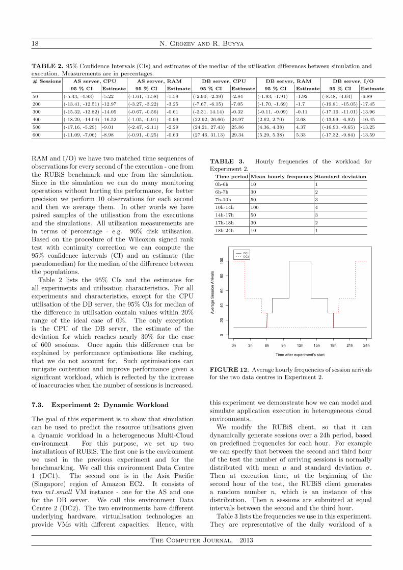
18 N. Grozev and R. Buyya
TABLE 2. 95% Confidence Intervals (CIs) and estimates of the median of the utilisation differences between simulation andexecution. Measurements are in percentages.# Sessions AS server, CPU AS server, RAM DB server, CPU DB server, RAM DB server, I/O
95 % CI Estimate 95 % CI Estimate 95 % CI Estimate 95 % CI Estimate 95 % CI Estimate
50 (-5.43, -4.93) -5.22 (-1.61, -1.58) -1.59 (-2.90, -2.39) -2.84 (-1.93, -1.91) -1.92 (-8.48, -4.64) -6.89
200 (-13.41, -12.51) -12.97 (-3.27, -3.22) -3.25 (-7.67, -6.15) -7.05 (-1.70, -1.69) -1.7 (-19.81, -15.05) -17.45
300 (-15.32, -12.82) -14.05 (-0.67, -0.56) -0.61 (-2.31, 14.14) -0.32 (-0.11, -0.09) -0.11 (-17.16, -11.01) -13.96
400 (-18.29, -14.04) -16.52 (-1.05, -0.91) -0.99 (22.92, 26.66) 24.97 (2.62, 2.70) 2.68 (-13.99, -6.92) -10.45
500 (-17.16, -5.29) -9.01 (-2.47, -2.11) -2.29 (24.21, 27.43) 25.86 (4.36, 4.38) 4.37 (-16.90, -9.65) -13.25
600 (-11.09, -7.06) -8.98 (-0.91, -0.25) -0.63 (27.46, 31.13) 29.34 (5.29, 5.38) 5.33 (-17.32, -9.84) -13.59
RAM and I/O) we have two matched time sequences ofobservations for every second of the execution - one fromthe RUBiS benchmark and one from the simulation.Since in the simulation we can do many monitoringoperations without hurting the performance, for betterprecision we perform 10 observations for each secondand then we average them. In other words we havepaired samples of the utilisation from the executionsand the simulations. All utilisation measurements arein terms of percentage - e.g. 90% disk utilisation.Based on the procedure of the Wilcoxon signed ranktest with continuity correction we can compute the95% confidence intervals (CI) and an estimate (thepseudomedian) for the median of the difference betweenthe populations.
Table 2 lists the 95% CIs and the estimates forall experiments and utilisation characteristics. For allexperiments and characteristics, except for the CPUutilisation of the DB server, the 95% CIs for median ofthe difference in utilisation contain values within 20%range of the ideal case of 0%. The only exceptionis the CPU of the DB server, the estimate of thedeviation for which reaches nearly 30% for the caseof 600 sessions. Once again this difference can beexplained by performance optimisations like caching,that we do not account for. Such optimisations canmitigate contention and improve performance given asignificant workload, which is reflected by the increaseof inaccuracies when the number of sessions is increased.
7.3. Experiment 2: Dynamic Workload
The goal of this experiment is to show that simulationcan be used to predict the resource utilisations givena dynamic workload in a heterogeneous Multi-Cloudenvironment. For this purpose, we set up twoinstallations of RUBiS. The first one is the environmentwe used in the previous experiment and for thebenchmarking. We call this environment Data Centre1 (DC1). The second one is in the Asia Pacific(Singapore) region of Amazon EC2. It consists oftwo m1.small VM instance - one for the AS and onefor the DB server. We call this environment DataCentre 2 (DC2). The two environments have differentunderlying hardware, virtualisation technologies anprovide VMs with different capacities. Hence, with
TABLE 3. Hourly frequencies of the workload forExperiment 2.
Time period Mean hourly frequency Standard deviation
0h-6h 10 1
6h-7h 30 2
7h-10h 50 3
10h-14h 100 4
14h-17h 50 3
17h-18h 30 2
18h-24h 10 1
020
40
60
80
100
Time after experiment's start
Ave
rage S
essio
n A
rriv
als
0h 3h 6h 9h 12h 15h 18h 21h 24h
DC1
DC2
FIGURE 12. Average hourly frequencies of session arrivalsfor the two data centres in Experiment 2.
this experiment we demonstrate how we can model andsimulate application execution in heterogeneous cloudenvironments.
We modify the RUBiS client, so that it candynamically generate sessions over a 24h period, basedon predefined frequencies for each hour. For examplewe can specify that between the second and third hourof the test the number of arriving sessions is normallydistributed with mean µ and standard deviation σ.Then at execution time, at the beginning of thesecond hour of the test, the RUBiS client generatesa random number n, which is an instance of thisdistribution. Then n sessions are submitted at equalintervals between the second and the third hour.
Table 3 lists the frequencies we use in this experiment.They are representative of the daily workload of a
The Computer Journal, 2013
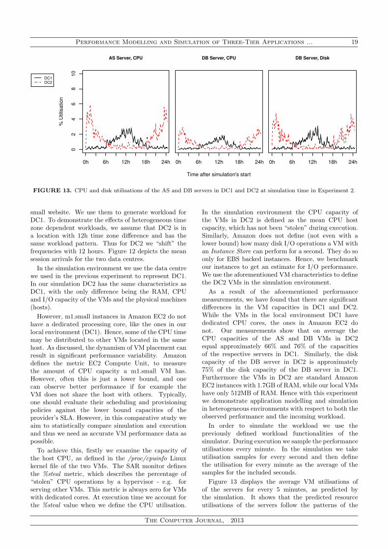
Performance Modelling and Simulation of Three-Tier Applications ... 19
DC1
DC2
02
46
81
0
AS Server, CPU%
Utilisa
tio
n
0h 6h 12h 18h 24h
DB Server, CPU
Time after simulation's start
0h 6h 12h 18h 24h
DB Server, Disk
0h 6h 12h 18h 24h
FIGURE 13. CPU and disk utilisations of the AS and DB servers in DC1 and DC2 at simulation time in Experiment 2.
small website. We use them to generate workload forDC1. To demonstrate the effects of heterogeneous timezone dependent workloads, we assume that DC2 is ina location with 12h time zone difference and has thesame workload pattern. Thus for DC2 we “shift” thefrequencies with 12 hours. Figure 12 depicts the meansession arrivals for the two data centres.
In the simulation environment we use the data centrewe used in the previous experiment to represent DC1.In our simulation DC2 has the same characteristics asDC1, with the only difference being the RAM, CPUand I/O capacity of the VMs and the physical machines(hosts).
However, m1.small instances in Amazon EC2 do nothave a dedicated processing core, like the ones in ourlocal environment (DC1). Hence, some of the CPU timemay be distributed to other VMs located in the samehost. As discussed, the dynamism of VM placement canresult in significant performance variability. Amazondefines the metric EC2 Compute Unit, to measurethe amount of CPU capacity a m1.small VM has.However, often this is just a lower bound, and onecan observe better performance if for example theVM does not share the host with others. Typically,one should evaluate their scheduling and provisioningpolicies against the lower bound capacities of theprovider’s SLA. However, in this comparative study weaim to statistically compare simulation and executionand thus we need as accurate VM performance data aspossible.
To achieve this, firstly we examine the capacity ofthe host CPU, as defined in the /proc/cpuinfo Linuxkernel file of the two VMs. The SAR monitor definesthe %steal metric, which describes the percentage of“stolen” CPU operations by a hypervisor - e.g. forserving other VMs. This metric is always zero for VMswith dedicated cores. At execution time we account forthe %steal value when we define the CPU utilisation.
In the simulation environment the CPU capacity ofthe VMs in DC2 is defined as the mean CPU hostcapacity, which has not been “stolen” during execution.Similarly, Amazon does not define (not even with alower bound) how many disk I/O operations a VM withan Instance Store can perform for a second. They do soonly for EBS backed instances. Hence, we benchmarkour instances to get an estimate for I/O performance.We use the aforementioned VM characteristics to definethe DC2 VMs in the simulation environment.
As a result of the aforementioned performancemeasurements, we have found that there are significantdifferences in the VM capacities in DC1 and DC2.While the VMs in the local environment DC1 havededicated CPU cores, the ones in Amazon EC2 donot. Our measurements show that on average theCPU capacities of the AS and DB VMs in DC2equal approximately 66% and 76% of the capacitiesof the respective servers in DC1. Similarly, the diskcapacity of the DB server in DC2 is approximately75% of the disk capacity of the DB server in DC1.Furthermore the VMs in DC2 are standard AmazonEC2 instances with 1.7GB of RAM, while our local VMshave only 512MB of RAM. Hence with this experimentwe demonstrate application modelling and simulationin heterogeneous environments with respect to both theobserved performance and the incoming workload.
In order to simulate the workload we use thepreviously defined workload functionalities of thesimulator. During execution we sample the performanceutilisations every minute. In the simulation we takeutilisation samples for every second and then definethe utilisation for every minute as the average of thesamples for the included seconds.
Figure 13 displays the average VM utilisations ofof the servers for every 5 minutes, as predicted bythe simulation. It shows that the predicted resourceutilisations of the servers follow the patterns of the
The Computer Journal, 2013
20 N. Grozev and R. Buyya
TABLE 4. 95% Confidence Intervals (CIs) and estimates of the median of the utilisation differences between simulation andexecution in DC1 and DC2. Measurements are in percentages.
Data centre AS server, CPU AS server, RAM DB server, CPU DB server, RAM DB server, I/O
95 % CI Estimate 95 % CI Estimate 95 % CI Estimate 95 % CI Estimate 95 % CI Estimate
DC1 (-0.43, -0.37) -0.4 (-4.06, -3.97) -4.02 (-0.35, -0.31) -0.33 (-1.06, -0.89) -0.97 (-1.16, -0.97) -1.07
DC2 (0.65, 0.74) 0.7 (-10.46, -10.31) -10.39 (-2.78, -2.71) -2.75 (-7.12, -7.07) -7.1 (0.49, 0.58) 0.53
workloads shown in Figure 12. As a result of theheterogeneity of the hardware and VM capacities inthe two data centres, the utilisations of the servers inthe two data centres differ significantly. For example,the CPU utilisation of the AS server in DC2 at thepeak times of the workload exceeds almost twice theutilisation of the DC1 server at its peak workloadtime. This is because, the average CPU capacity ofthe AS server in DC2 is about 66% of the one inDC1. Similarly, the disk utilisation during the workloadpeak of the DB server in DC2 is much higher thanthe one in DC1, as a result of having only 76% of thedisk capacity of DC1. Given intensive workloads, thisperformance heterogeneity can easily result in differentcontentions and consequently application performancein the different data centres.
Table 4 lists the 95% CIs and the estimations ofthe medians of the differences of the utilisations ofthe servers in DC1 and DC2. As in the previousexperiment we use the procedure of the Wilcoxon signedrank test with continuity correction to compute the95% confidence intervals (CI) and the estimates. Fromthe table we can see that the estimated error (thepseudomedian of the differences) is less than 11% forall characteristics. The accumulated delay for everysimulated session in this experiment is 0. This isrepresentative of the fact, that at execution time therewere no resource contentions with the given workload.
8. CONCLUSION AND FUTURE WORK
We have introduced a new approach for performancemodelling of 3-tier applications and their workload inCloud and Multi-Cloud environments. Unlike others,our model is coarse grained and session based and doesnot represent each and every user interaction. Thus it issuitable for quick prototyping and testing of scheduling,provisioning and load balancing approaches. We haveimplemented a CloudSim extension realising this model,which can be used for performance evaluation withoutthe need to deploy large scale prototypes.
By definition a system model is a simplifieddescription of the original system, and as such ourmodel makes some simplifying assumptions. To validateit, we have conducted two experiments demonstratingthe plausibility of our approach by comparing thesimulation results with the results from an actualsystem execution. By using both public Cloudand private in-house infrastructures with differentvirtualisation environments, settings, and workload
dynamism we demonstrated the plausibility of ourapproach in a wide range of environments.
Our future work will focus on: (i) modelling the entrypoint, which distributes the incoming workload amongclouds (ii) modelling asynchronous data processing,that would allow “Big Data” jobs to be represented(iii) incorporation of our model in other simulationenvironments and (iv) evaluation of the energyconsumption impact caused by an application.
In fact CloudSim already supports power consump-tion modelling [13]. Moreover, Guerout et al. have de-fined DVFS (Dynamic Voltage and Frequency Scaling)aware extension of CloudSim allowing to test the effectof different DVFS approaches on data centre power con-sumption [60]. All of these functionalities have been im-plemented in the core CloudSim components (i.e. phys-ical machines/hosts and processing elements/CPU) andthus can be reused by all extensions. Hence, while ourapproach is focused on application performance mod-elling and simulation, it can already be used to evaluatethe energy consumption impact of application executionin different data centres with respect to their VM con-solidation and DVFS management policies. We plan tostudy these aspects in more details in the future.
ACKNOWLEDGEMENTS
We thank Rodrigo Calheiros, Amir Vahid Dastjerdiand the rest of the CLOUDS lab members for theircomments on improving the paper.
FUNDING
This research is partially supported by research grantsfrom the Australian Research Council (ARC) forDiscovery Projects (DP1093678 and DP130101378).
REFERENCES
[1] Buyya, R., Yeo, C. S., Venugopal, S., Broberg, J.,and Brandic, I. (2009) Cloud computing and emergingIT platforms: Vision, hype, and reality for deliveringcomputing as the 5th utility. Future GenerationComputer Systems, 25, 599–616.
[2] Armbrust, M. et al. (2010) A view of cloud computing.Communications of the ACM, 53, 50–58.
[3] Foster, I., Zhao, Y., Raicu, I., and Lu, S.(2008) Cloud Computing and Grid Computing 360-Degree Compared. Proceedings of Grid ComputingEnvironments Workshop (GCE 2008), 16 November,Austin, Texas, US, pp. 1–10. IEEE Computer SocietyPress.
The Computer Journal, 2013

Performance Modelling and Simulation of Three-Tier Applications ... 21
[4] Ebay (June 21, 2013). Ebay. http://ebay.com/.[5] Ebay Tech Blog (June 21, 2013). Cloud Bursting for
Fun and Profit. http://ebaytechblog.com/2011/03/
28/cloud-bursting-for-fun-and-profit/.[6] Amazon (February 13, 2013). Public Sector Case
Studies. http://aws.amazon.com/publicsector/
customer-experiences/.[7] Amazon (August 6, 2012). Summary of the AWS
Service Event in the US East Region. http://aws.
amazon.com/message/67457/.[8] Microsoft (June 14, 2012). Windows Azure
Service Disruption Update. http://blogs.
msdn.com/b/windowsazure/archive/2012/03/01/
windows-azure-service-disruption-update.aspx.[9] IBM (May 31, 2013). IBM takes Australian Open
data onto private cloud. http://www-07.ibm.com/
innovation/au/ausopen/.[10] Sotiriadis, S., Bessis, N., and Antonopoulos, N.
(2011) Towards Inter-cloud Schedulers: A Surveyof Meta-scheduling Approaches. Proceedings of theInternational Conference on P2P, Parallel, Grid,Cloud and Internet Computing (3PGCIC), 26-28October, Barcelona, Catalonia, Spain, pp. 59–66. IEEEComputer Society Press.
[11] Grozev, N. and Buyya, R. (2012) Inter-CloudArchitectures and Application Brokering: Taxonomyand Survey. Software: Practice and Experience, (inpress).
[12] Buyya, R. and Murshed, M. (2002) GridSim: a toolkitfor the modeling and simulation of distributed resourcemanagement and scheduling for Grid computing. Con-currency and Computation: Practice and Experience,14, 1175–1220.
[13] Calheiros, R. N., Ranjan, R., Beloglazov, A., Rose,C. A. F. D., and Buyya, R. (2011) CloudSim: atoolkit for modeling and simulation of cloud computingenvironments and evaluation of resource provisioningalgorithms. Software: Practice and Experience, 41, 23–50.
[14] Kliazovich, D. and Bouvry, P. and Khan, S. U.(2012) GreenCloud: a packet-level simulator of energy-aware cloud computing data centers. The Journal ofSupercomputing, 62, 1263–1283.
[15] Dejun, J., Pierre, G., and Chi, C.-H. (2009) EC2 Per-formance Analysis for Resource Provisioning of Service-Oriented Applications. Proceedings of the Interna-tional Conference on Service-Oriented Computing (IC-SOC 2009), 23-27 November, Stockholm, Sweden, pp.197–207. Springer-Verlag, Berlin, Heidelberg.
[16] Urgaonkar, B., Pacifici, G., Shenoy, P., Spreitzer, M.,and Tantawi, A. (2005) An Analytical Model for Multi-Tier Internet Services and its Applications. Proceedingsof the International Conference on Measurement andModeling of Computer Systems ACM SIGMETRICS2005, 6-10 June, Banff, Alberta, Canada SIGMET-RICS ’05, pp. 291–302. ACM, New York, NY, USA.
[17] Zhang, Q., Cherkasova, L., and Smirni, E. (2007)A Regression-Based Analytic Model for DynamicResource Provisioning of Multi-Tier Applications.Proceedings of the 4th International Conference onAutonomic Computing (ICAC 2007), 11-15 June,Jacksonville, Florida, US, june 27. IEEE ComputerSociety.
[18] Bi, J., Zhu, Z., Tian, R., and Wang, Q. (2010)Dynamic Provisioning Modeling for Virtualized Multi-tier Applications in Cloud Data Center. Proceedings ofthe 3rd International Conference on Cloud Computing(CLOUD 2010), 5-10 July, Miami, Forida, US, pp. 370–377. IEEE Computer Society Press.
[19] Zhang, Z. and Fan, W. (2008) Web server loadbalancing: A queueing analysis. European Journal ofOperational Research, 186, 681–693.
[20] Kamra, A., Misra, V., and Nahum, E. (2004) Yaksha:A Self-Tuning Controller for Managing the Performanceof 3-Tiered Web sites. Proceedings of the 12th IEEEInternational Workshop on Quality of Service (IWQOS2004), 7-9 June, Montreal, Canada, pp. 47–56. IEEEComputer Society Press.
[21] Chen, Y., Iyer, S., Liu, X., Milojicic, D., and Sahai, A.(2007) SLA Decomposition: Translating Service LevelObjectives to System Level Thresholds. Proceedingsof the 4th International Conference on AutonomicComputing (ICAC 2007), 11-15 June, Jacksonville,Florida, US, pp. 3–13. IEEE Computer Society.
[22] Lim, S.-H., Sharma, B., Nam, G., Kim, E. K.,and Das, C. (2009) MDCSim: A multi-tier datacenter simulation, platform. Proceedings of the IEEEInternational Conference on Cluster Computing andWorkshops (CLUSTER ’09), 31 August - 4 September,New Orleans, LA, US, pp. 1–9. IEEE Computer SocietyPress.
[23] Sriram, I. (2009) SPECI, a Simulation Tool ExploringCloud-Scale Data Centres. In Jaatun, M., Zhao, G.,and Rong, C. (eds.), Cloud Computing, Lecture Notesin Computer Science, 5931, pp. 381–392. Springer,Berlin Heidelberg.
[24] Nunez, A., Vazquez-Poletti, J., Caminero, A., Castane,G., Carretero, J., and Llorente, I. (2012) iCanCloud: AFlexible and Scalable Cloud Infrastructure Simulator.Journal of Grid Computing, 10, 185–209.
[25] Fowler, M. (2003) Patterns of enterprise applicationarchitecture. Addison-Wesley, New York, NY, US.
[26] Java EE (June 21, 2013). Java EE. http:
//oracle.com/technetwork/java/javaee/overview/
index.html.
[27] Ruby on Rails (June 21, 2013). Ruby on Rails. http:
//rubyonrails.org/.
[28] Django (June 21, 2013). Django. https://
djangoproject.com/.
[29] Ramirez, A. O. (2000) Three-Tier Architecture. LinuxJournal, 2000.
[30] Aarsten, A., Brugali, D., and Menga, G. (1996) Pat-terns for three-tier client/server applications. Proceed-ings of Pattern Languages of Programs (PLoP ’96), 4-6 September, Monticello, Illinois, US. Addison-Wesley,Reading, Massachusetts, US.
[31] Cattell, R. (2010) Scalable SQL and NoSQL DataStores. SIGMOD Record, 39, 12–27.
[32] Adler, B. (February 13, 2013). Building ScalableApplications In the Cloud. http://rightscale.
com/info_center/white-papers/RightScale_White_
Paper_Building_Scalable_Applications.pdf.
[33] Amazon (February 13, 2013). Amazon RelationalDatabase Service (Amazon RDS). http://aws.
amazon.com/rds/.
The Computer Journal, 2013
22 N. Grozev and R. Buyya
[34] Oracle (May 31, 2013). Oracle Database and theOracle Database Cloud. http://www.oracle.com/
technetwork/database/database-cloud/public/
oracle-db-and-db-cloud-service-wp-1844127.pdf.
[35] Oracle (May 31, 2013). Oracle Database Cloud Ser-vice. http://www.oracle.com/us/solutions/cloud/
overview/database-cloud-service-wp-1844123.
pdf.
[36] Ferrer A. J. et al. (2012) OPTIMIS: A holistic approachto cloud service provisioning. Future GenerationComputer Systems, 28, 66–77.
[37] Arjuna Agility (June 14, 2012). What Is Federation.http://arjuna.com/what-is-federation.
[38] Rochwerger, B. et al. (2009) The RESERVOIR Modeland Architecture for Open Federated Cloud Comput-ing. IBM Journal of Research and Development, 53,1–11.
[39] Petcu, D. (2013) Multi-Cloud: expectations andcurrent approaches. Proceedings of the internationalworkshop on Multi-cloud applications and federatedclouds (MultiCloud ’13), 22 April, Prague, CzechRepublic, pp. 1–6. ACM, New York, NY, US.
[40] RightScale (June 14, 2012). RightScale. http://
rightscale.com/.
[41] Enstratius (May 31, 2013). Enstratius. https://
enstratius.com/.
[42] Scalr (June 14, 2012). Scalr. http://scalr.net/.
[43] JClouds (June 14, 2012). JClouds. http://jclouds.
org/.
[44] Apache Foundation (June 14, 2012). Apache Libcloud.http://libcloud.apache.org/.
[45] Apache Foundation (June 14, 2012). Apache DeltaCloud. http://deltacloud.apache.org/.
[46] Helland, P. (2012) Condos and Clouds. ACM Queue,10, 20–35.
[47] Cao, J., Andersson, M., Nyberg, C., and Kihl, M.(2003) Web server performance modeling using anM/G/1/K*PS queue. Proceedings of the 10th Inter-national Conference on Telecommunications (ICT’03),February 23 - March 1, Tahiti, Papeete, French Poly-nesia, pp. 1501–1506. IEEE Computer Society Press.
[48] Robertson, A., Wittenmark, B., and Kihl, M. (2003)Analysis and design of admission control in Web-server systems. Proceedings of the American ControlConference (ACC ’03), 4-6 June, Denver, Colorado,US, pp. 254–259. IEEE Computer Society Press.
[49] Paxson, V. and Floyd, S. (1995) Wide area traffic: thefailure of Poisson modeling. IEEE/ACM Transactionson Networking, 3, 226–244.
[50] Ilyadis, N. (2012) The evolution of next-generationdata center networks for high capacity computing.Proceedings of the Symposium on VLSI Circuits(VLSIC’12), 13-15 June, Honolulu, Hawaii, US, pp.1–5. IEEE Computer Society Press.
[51] Jung, G., Swint, G., Parekh, J., Pu, C., andSahai, A. (2006) Detecting Bottleneck in n-Tier ITApplications Through Analysis. In State, R., Meer,S., O’Sullivan, D., and Pfeifer, T. (eds.), Large ScaleManagement of Distributed Systems, Lecture Notes inComputer Science, 4269, pp. 149–160. Springer, BerlinHeidelberg.
[52] Malkowski, S., Jayasinghe, D., Hedwig, M., Park, J.,Kanemasa, Y., and Pu, C. (2010) Empirical analysis ofdatabase server scalability using an N-tier benchmarkwith read-intensive workload. Proceedings of the ACMSymposium on Applied Computing (SAC ’10), 22-26March, Sierre, Switzerland SAC’10, pp. 1680–1687.ACM, New York, NY, US.
[53] Lloyd, W., Pallickara, S., David, O., Lyon, J., Arabi,M., and Rojas, K. (2013) Performance implications ofmulti-tier application deployments on Infrastructure-as-a-Service clouds: Towards performance modeling.Future Generation Computer Systems, 29, 1254–1264.
[54] RUBiS (March 15, 2013). RUBiS: Rice UniversityBidding System. http://rubis.ow2.org/.
[55] Amza, C., Chanda, A., Cox, A., Elnikety, S., Gil,R., Rajamani, K., Zwaenepoel, W., Cecchet, E., andMarguerite, J. (2002) Specification and implementationof dynamic Web site benchmarks. Proceedingsof the IEEE International Workshop on WorkloadCharacterization (WWC-6), 27-27 October, Austin,Texas, US, pp. 3–13. IEEE Computer Society Press.
[56] TR02-388 (2002) Bottleneck Characterization of Dy-namic Web Site Benchmarks. Technical report. Depart-ment of Computer Science Rice University, Houston,Texas, US.
[57] Cecchet, E. and Chanda, A. and Elnikety, S.and Marguerite, J. and Zwaenepoel, W. (2003)Performance Comparison of Middleware Architecturesfor Generating Dynamic Web Content. Proceedingsof the ACM/IFIP/USENIX International Conferenceon Middleware (Middleware ’03), 16-20 June, Rio deJaneiro, Brazil Middleware ’03, pp. 242–261. Springer-Verlag, New York, NY, US.
[58] TPC BenchmarkTM W 1.8 (2002) TPC BENCH-MARK W (Web Commerce). Specification, version 1.8.Transaction Processing Performance Council (TPC),San Francisco, California, US.
[59] SYSSTAT (March 15, 2013). SYSSTAT. http://
sebastien.godard.pagesperso-orange.fr/.
[60] Guerout, T., Monteil, T., Costa, G. D., Calheiros,R. N., Buyya, R., and Alexandru, M. (2013) Energy-aware simulation with DVFS . Simulation ModellingPractice and Theory, (in press).
The Computer Journal, 2013