Performance Improvement of Indoor Channel Models in ...

7 IV April 2019

https://doi.org/10.22214/ijraset.2019.4155

International Journal for Research in Applied Science & Engineering Technology (IJRASET) ISSN: 2321-9653; IC Value: 45.98; SJ Impact Factor: 6.887

Volume 7 Issue IV, Apr 2019- Available at www.ijraset.com

862 ©IJRASET: All Rights are Reserved

Performance Improvement of Indoor Channel Models in Wireless Networks

Yuvraj Singh Ranawat Assistant Professor, Mewar University, Chittorgarh, India

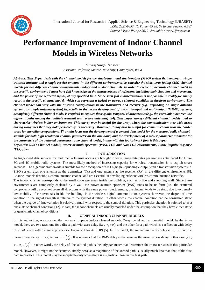
Abstract: This Paper deals with the channel models for the single-input and single-output (SISO) system that employs a single transmit antenna and a single receive antenna in the different environments. so consider the short-term fading SISO channel models for two different channel environments: indoor and outdoor channels. In order to create an accurate channel model in the specific environment, I must have full knowledge on the characteristics of reflectors, including their situation and movement, and the power of the reflected signal, at any specified time. Since such full characterization is not possible in reality,we simply resort to the specific channel model, which can represent a typical or average channel condition in thegiven environment. The channel model can vary with the antenna configuration in the transmitter and receiver (e.g., depending on single antenna system or multiple antenna system).Especially in the recent development of the multi-input and multi-output (MIMO) systems, acompletely different channel model is required to capture their spatio-temporal characteristics(e.g., the correlation between the different paths among the multiple transmit and receive antennas) [24]. This paper surveys different channel models used to characterise wireless indoor environment. This survey may be useful for the army, where the communication over wide areas during wargames that they hold periodically, is necessary. Moreover, it may also be useful for communication near the border areas for surveillance operations. The main focus was the development of a general data model for the measured radio channel, suitable for both high resolution channel parameter on the one hand, and the development of a robust parameter estimator for the parameters of the designed parametric radio channel model, in line with this logical work flow is this paper. Keywords: SISO Channel models, Power azimuth spectrum (PAS), LOS and Non-LOS environments, Finite impulse response (FIR) filter

I. INTRODUCTION As high-speed data services for multimedia Internet access are brought to focus, huge date rates per user are anticipated for future 3G and 4G mobile radio systems. The most likely method of increasing capacity for wireless transmission is to exploit smart antennas. The algebraic framework is suitable for the description of SISO (single-input-single-output) radio transmission systems. A SISO system uses one antenna as the transmitter (Tx) and one antenna as the receiver (Rx) in the different environments [8]. Channel models describe a communication channel and are essential in developing efficient wireless communication networks. The indoor channel corresponds to the small coverage areas inside the building, such as office and shopping mall. Since these environments are completely enclosed by a wall, the power azimuth spectrum (PAS) tends to be uniform (i.e., the scattered components will be received from all directions with the same power). Furthermore, the channel tends to be static due to extremely low mobility of the terminals inside the building. In the wireless digital communication systems, however, the degree of time variation in the signal strength is relative to the symbol duration. In other words, the channel condition can be considered static when the degree of time variation is relatively small with respect to the symbol duration. This particular situation is referred to as a quasi-static channel condition [12]. In fact, the indoor channels are usually modeled under the assumption that they have either static or quasi-static channel conditions.

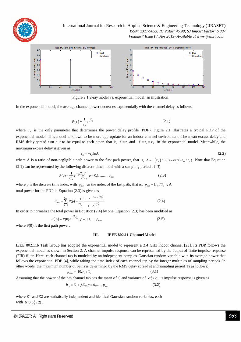
II. GENERAL INDOOR CHANNEL MODELS In this subsection, we consider the two most popular indoor channel models: 2-ray model and exponential model. In the 2-ray model, there are two rays, one for a direct path with zero delay (i.e., 0 0 ), and the other for a path which is a reflection with delay of 1 0 , each with the same power (see Figure 2.1 for its PDP) [5]. In this model, the maximum excess delay is 1m and the

mean excess delay is given as 12

. It is obvious that the RMS delay is the same as the mean excess delay in this case (i.e.,

12

. In other words, the delay of the second path is the only parameter that determines the characteristics of this particular

model. However, it might not be accurate, simply because a magnitude of the second path is usually much less than that of the first path in practice. This model may be acceptable only when there is a significant loss in the first path.




Figure 2.1 2-ray model vs. exponential model: an illustration.

In the exponential model, the average channel power decreases exponentially with the channel delay as follows:

(2.1)

where d is the only parameter that determines the power delay profile (PDP). Figure 2.1 illustrates a typical PDP of the exponential model. This model is known to be more appropriate for an indoor channel environment. The mean excess delay and RMS delay spread turn out to be equal to each other, that is, d and d , in the exponential model. Meanwhile, the maximum excess delay is given as lnAm d (2.2) where A is a ratio of non-negligible path power to the first path power, that is, A P / P(0) exp( / )m m d . Note that Equation

(2.1) can be represented by the following discrete-time model with a sampling period of sT

max1(p) ,p 0,1,.........,pspTP e

(2.3)

where p is the discrete time index with maxp as the index of the last path, that is, max [ / ]m sp T . A total power for the PDP in Equation (2.3) is given as

max 1

max

0

1 1(p) .1

s

s

Tpp

total Tp

eP Pe

(2.4)

In order to normalize the total power in Equation (2.4) by one, Equation (2.3) has been modified as

max(0)e , 0,1,......spT

P p P p p

(2.5)

where P(0) is the first path power.

III. IEEE 802.11 Channel Model IEEE 802.11b Task Group has adopted the exponential model to represent a 2.4 GHz indoor channel [23]. Its PDP follows the exponential model as shown in Section 2. A channel impulse response can be represented by the output of finite impulse response (FIR) filter. Here, each channel tap is modeled by an independent complex Gaussian random variable with its average power that follows the exponential PDP [4], while taking the time index of each channel tap by the integer multiples of sampling periods. In other words, the maximum number of paths is determined by the RMS delay spread st and sampling period Ts as follows: max [10. / T ]sp (3.1) Assuming that the power of the pth channel tap has the mean of 0 and variance of 2 / 2p , its impulse response is given as

1 2 max. , 0,......,ph Z j Z p p (3.2)

where Z1 and Z2 are statistically independent and identical Gaussian random variables, each with 2(0, / 2)pN .

1d

d

P e




Asopposedto the exponentialmodel inwhichthemaximumexcessdelayiscomputedbya path of the least non-negligible power level, themaximumexcess delay in IEEE802.11 channelmodel is fixed to 10 times the RMS delay spread. In this case, the power of each channel tap is given as /2 2

0spT

p e (3.3)

where 20 is the power of the first tap, which is determined so as to make the average received

power equal to one, yielding

max

/20 1 /

11

s

s

T

p T

ee

(3.4)

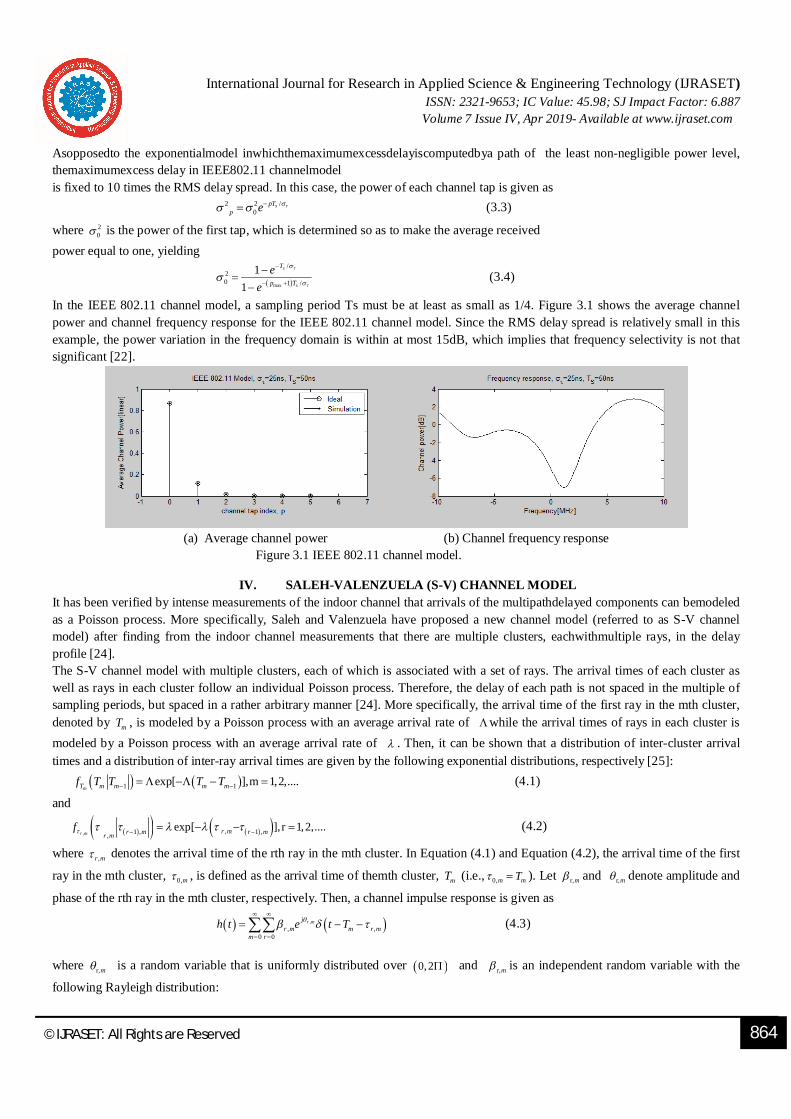
In the IEEE 802.11 channel model, a sampling period Ts must be at least as small as 1/4. Figure 3.1 shows the average channel power and channel frequency response for the IEEE 802.11 channel model. Since the RMS delay spread is relatively small in this example, the power variation in the frequency domain is within at most 15dB, which implies that frequency selectivity is not that significant [22].

(a) Average channel power (b) Channel frequency response

Figure 3.1 IEEE 802.11 channel model.

IV. SALEH-VALENZUELA (S-V) CHANNEL MODEL It has been verified by intense measurements of the indoor channel that arrivals of the multipathdelayed components can bemodeled as a Poisson process. More specifically, Saleh and Valenzuela have proposed a new channel model (referred to as S-V channel model) after finding from the indoor channel measurements that there are multiple clusters, eachwithmultiple rays, in the delay profile [24]. The S-V channel model with multiple clusters, each of which is associated with a set of rays. The arrival times of each cluster as well as rays in each cluster follow an individual Poisson process. Therefore, the delay of each path is not spaced in the multiple of sampling periods, but spaced in a rather arbitrary manner [24]. More specifically, the arrival time of the first ray in the mth cluster, denoted by mT , is modeled by a Poisson process with an average arrival rate of while the arrival times of rays in each cluster is modeled by a Poisson process with an average arrival rate of . Then, it can be shown that a distribution of inter-cluster arrival times and a distribution of inter-ray arrival times are given by the following exponential distributions, respectively [25]: 1 1exp[ ],m 1,2,....

mT m m m mf T T T T (4.1)

and

, ,1 , 1 ,,exp[ ], r 1,2,....

r m r mr m r mr mf (4.2)

where ,r m denotes the arrival time of the rth ray in the mth cluster. In Equation (4.1) and Equation (4.2), the arrival time of the first

ray in the mth cluster, 0,m , is defined as the arrival time of themth cluster, mT (i.e., 0,m mT ). Let r,m and r,m denote amplitude and

phase of the rth ray in the mth cluster, respectively. Then, a channel impulse response is given as

,, ,

0 0

r mjr m m r m

m rh t e t T

(4.3)

where r,m is a random variable that is uniformly distributed over 0,2 and r,m is an independent random variable with the

following Rayleigh distribution:




2 2, ,

,

/2,, ,2 / r m r m

r m r mr m r mf e (4.4)

In Equation (4.4), ,r m is the average power of the rth ray in the mth cluster, which is given as

, //2 2, 0,0

r mmTr m e e (4.5)

where and denote time constants for exponential power attenuation in the cluster and ray, respectively, while 20,0 denotes the

average power of the first ray in the first cluster [21]. the S-V channelmodel is a double exponential delay model in which average cluster power decays exponentially by following a term /mTe in Equation (4.5)while average ray power in each cluster also decays exponentially by following a term , /r me in Equation (4.5). Once the average power of the first ray in the first cluster, 2

0,0 , is

given, the average power of the rest of rays can be determined by Equation (4.5), which subsequently allows for determining the Rayleigh channel coefficients by Equation (4.4). In case that a path loss is not taken into account, without loss of generality, the average power of the first ray in the first cluster is set to one. Even if there are an infinite number of clusters and rays in the channel impulse response of Equation (4.3), there exist only a finite number of the non-negligible numbers of clusters and rays in practice. Therefore, we limit the number of clusters and rays to M and R, respectively. Meanwhile, a log-normal random variable X, that is,

21020log 0, xX N � , can be introduced to Equation (4.3), so as to reflect the effect of long-term fading as

,, ,

0 0

r mM R

jr m m r m

m rh t X e t T

(4.6)

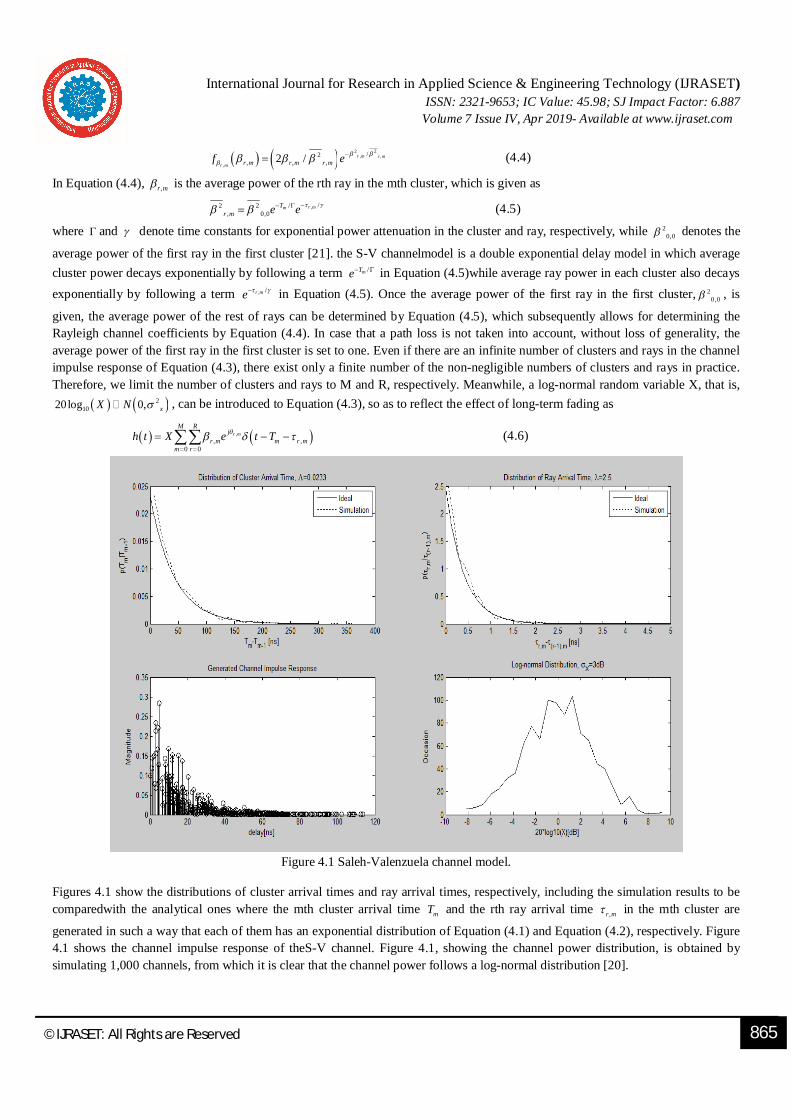
Figure 4.1 Saleh-Valenzuela channel model.

Figures 4.1 show the distributions of cluster arrival times and ray arrival times, respectively, including the simulation results to be comparedwith the analytical ones where the mth cluster arrival time mT and the rth ray arrival time ,r m in the mth cluster are

generated in such a way that each of them has an exponential distribution of Equation (4.1) and Equation (4.2), respectively. Figure 4.1 shows the channel impulse response of theS-V channel. Figure 4.1, showing the channel power distribution, is obtained by simulating 1,000 channels, from which it is clear that the channel power follows a log-normal distribution [20].




V. UWB CHANNEL MODEL According to measurements of broadband indoor channel, it has been found that amplitudes of multipath fading follow the log-normal or Nakagami distribution rather than the Rayleigh distribution, even if they also show the same phenomenon of clustering as in the Saleh- Valenzuela (S-V) channel model. Based on these results, SG3a UWB multipath model has been proposed by modifying the S-V model in such a way that the multi-cluster signals are subject to independent log-normal fading while the multi-path signals in each cluster are also subject to independent log-normal fading [25]. The ith sample function of a discrete-time impulse response in the UWB multi-path channel model is given as

, ,0 0

M Ri i i

i i r m m r mm r

h t X a t T

(5.1)

where , ,, ,i i

i r m r mX a T and ,

ir m are defined as the same as in Equation (4.6), nowwith the index i to represent the ith generated

sample function of the channel. For simplicity of exposition, the index i in Equation (5.1) will be eliminated in the following discussion. As in the S-V channel model, the arrival time distributions of clusters and rays are given by two different Poisson processes of Equation (4.1) and Equation (4.2), respectively. The UWB channel model is different from the S-V channel model in that clusters and rays are subject to independent log-normal fading rather than Rayleigh fading. More specifically, a channel coefficient is given as , , ,r m r m m r mp (5.2)

where m represents log-normal fading of the mth cluster with the variance of 21 while ,r m represents log-normal fading of the

rth ray with the variance of 22 in the mth cluster. Note that independent fading is assumed for clusters and rays. In Equation (5.2),

,r mp is a binary discrete random variable to represent an arbitrary inversion of the pulse subject to reflection, that is, taking a value

of +1 or -1 equally likely. As compared to the channel coefficients of the S-V channel model in Equation (4.3) which has a uniformlydistributed phase over 0,2 , those of UWB channel model have the phase of either or , making the channel

coefficient always real [14]. Furthermore, we note that amplitude of each ray is given by a product of the independent log-normal random variables, m and ,r m . Since a product of the independent log-normal random variables is also a log-normal random

variable, a distribution of the channel coefficient , 1 2 / 20, 10 r m z z

m r m also follows a log-normal distribution, that is,

2 210 , , 1 220log ( ) ,m r m r mN � , with its average power given as

,2 //

, 0r mmT

m r mE e e (5.3)

where 0 represents the average power of the first ray in the first cluster.Meanwhile, mean of the channel amplitude for the rth ray in the mth cluster can be found as

2 21 20 ,

,

ln 1010ln 10 / 10 /ln 10 20

m r mr m

T

(5.4)

Besides the same set of channel parameters as in the S-V channel model, including the cluster arrival rate , ray arrival rate , cluster attenuation constant , ray attenuation constant , standard deviation x of the overall multipath shadowing with a log-normal distribution, additional channel parameters such as the standard deviations of log-normal shadowing for the clusters and rays, denoted as 1 and 2 , respectively, are required for the UWB channel model. Note that a complete model of the multipath channel h(t) in Equation (5.1) is given as a real number. Some proper modifications such as downconversion and filtering are required for implementing the UWB channel in simulation studies, since its bandwidth cannot be limited due to arbitrary arrival times. All the channel characteristics for UWB channel model, including mean excess delay, RMS delay spread, the number of significant paths within 10dB of peak power (denoted as 10dBNP ), and PDP, must be determined so as to be consistent with the measurements in practice.




Target channel characteristics CM1 CM2 CM3 CM4

Mean excess delay (nsec) 5.05 10.38 14.18

RMS delay (nsec) 5.28 8.03 14.28 25

10dBNP 35

NP(85%) 24 36.1 61.54 Model parameters (1/nsec) 0.0233 0.4 0.0667 0.0667

(1/nsec) 2.5 0.5 2.1 2.1

7.1 5.5 14.00 24.00 4.3 6.7 7.9 12

1 (dB) 3.3941 3.3941 3.3941 3.3941

2 (dB) 3.3941 3.3941 3.3941 3.3941

x (dB) 3 3 3 3

Model parameters

Mean excess delay (nsec) 5.0 9.9 15.9 30.1

RMS delay (nsec) 5 8 15 25

10dBNP 12.5 15.3 24.9 41.2

NP(85%) 20.8 33.9 64.7 123.3 Channel energy mean (dB) -0.4 -0.5 0.0 0.3 Channel energy std (dB) 2.9 3.1 3.1 2.7

Table 5.1 UWB channel parameters and model characteristics [25].

Table 5.1 summarizes the SG3a model parameters and characteristics that represent thetarget UWB channel for four different types of channel models, denoted as CM1, CM2,CM3, and CM4. Each of these channel models varies depending on distance and whether LOS exists or not. Here, NP(85%) represents the number of paths that contain 85% of the total energy. CM1 and CM2 are based on measurements for LOS and Non-LOS environments over the distance of 0–4m, respectively. CM3 is based on measurement for a Non-LOS environment over the distance of 4–10m. CM4 does not deal with any realistic channel measurement, but it has been set up with the intentionally long RMS delay spread so as to model the worst-case Non-LOS environment [26]. CM1 shows the best channel characteristics with the short RMS delay spread of 5.28ns since it deals with a short distance under an LOS environment. Due to the Non-LOS environment, CM2 shows the longer RMS delay spread of 8.03ns, even if it has the short range of distance as in the CM1. Meanwhile, CM3 represents the worse channel with the RMS delay spread of 14.28; it has a longer distance under a Non-LOS environment.

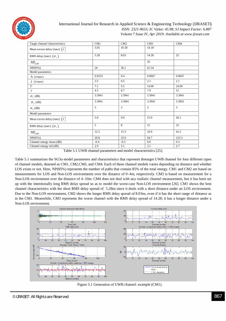
Figure 5.1 Generation of UWB channel: example (CM1).




Figure 5.1 shows UWB channel model are used to set the UWB channel parameters as listed in Table 5.1, to convert the continuous-time UWB channel into the corresponding discrete-time one, and to generate a UWB channel model, respectively. It shows the UWB channel characteristics by simulating 100 CM1 channels. Here, the sampling period has been set to 167 ps. In the current measurement, the RMS delay spread turns out to be around 5 ns, which nearly coincides with the target value of CM1 channel in Table 5.1. The same observation is made for the mean excess delay [24].

VI. CONCLUSION In conclusion, it has been verified that the current channel model properly realizes the target channel characteristics. A key observation is that, the accuracy of the models depends on the accuracy of the database and the details of the objects present within the environment. Despite enormous efforts and progress till date, much work remains in the understanding and characterisation of wireless communication channels. A proper system design requires accurate and reliable. Radio channel models for efficient performance under complex environments. In addition, the next generation wireless systems also place stringent demands on the design of a radio system.

REFERENCES [1] Sklar, B. (2002) Digital Communications: Fundamentals and Applications 2/E, Prentice Hall. [2] Rappaport, T.S. (2001) Wireless Communications: Principles and Practice 2/E, Prentice Hall. [3] Greenwood, D. and Hanzo, L. (1994) Characterization of mobile radio channels. Chapter 2, Mobile Radio Communications (ed. R. Steele), Pentech Press-

IEEE Press, London. [4] Friis, H.T. (1946) A note on a simple transmission formula. Proc. IRE, 34(5), 254–256. [5] Lee, W.C.Y. (1985) Mobile Communications Engineering, McGraw Hill, New York. [6] Okumura, Y., Ohmori, E., Kawano, T., and Fukuda, K. (1968) Field strength and its variability in VHF and UHF land mobile radio service. Rev. Elec.

Commun. Lab., 16, 825–873. [7] Hata, M. (1980) Empirical formula for propagation loss in land mobile radio services IEEE Trans. Veh. Technol., 29(3), 317–325. [8] Erceg, V., Greenstein, L.J., Tjandra, S.Y. et al. (1999) An empirically based path loss model for wireless channels in suburban environments. IEEE J. Select.

Areas Commun., 17(7), 1205–1211. [9] IEEE (2007) 802.16j-06/013r3. Multi-Hop Relay System Evaluation Methodology (Channel Model and Performance Metric). [10] IEEE (2001) 802.16.3c-01/29r4. Channel Models for Fixed Wireless Applications. [11] IST (2004) 4-027756. WINNER II, D1.1.1 WINNER II Interim Channel Models. [12] Recommendation (1997) ITU-R M.1225. Guidelines for Evaluation of Radio Transmission Technologies for IMT-2000. [13] Clarke, R.H. (1968) A statistical theory of mobile radio reception. Bell System Tech. J., 47, 987–1000. [14] Capoglu, I.R., Li,Y., and Swami, A. (2005) Effect of doppler spread in OFDM based UWB systems. IEEE Trans. Wireless Commun., 4(5), 2559–2567. [15] Stuber, G.L. (1996) Principles of Mobile Communication, Kluwer Academic Publishers. [16] Tepedelenliglu, C. and Giannakis, G.B. (2001) On velocity estimation and correlation properties of narrow-band mobile communication channels. IEEE Trans.

Veh. Technol., 50(4), 1039–1052. [17] Andersen, J.B., Rappaport, T.S., and Yoshida, S. (1995) Propagation measurements and models for wireless communications channels. IEEE Commun. Mag.,

33(1), 42–49. [18] Bajwa, A.S. and Parsons, J.D. (1982) Small-area characterisation of UHF urban and suburban mobile radio propagation. Inst. Elec. Eng. Proc., 129(2), 102–

109. [19] Bello, P.A. (1963) Characterization of randomly time-variant linear channels. IEEE Trans. Commun., 11(4), 360–393. [20] Black, D.M. and Reudink, D.O. (1972) Some characteristics of mobile radio propagation at 836 MHz in the Philadelphia area. IEEE Trans. Veh. Technol.,

21(2), 45–51. [21] Corazza, G.E. and Vatalaro, F. (1994) A statistical model for land mobile satellite channels and its application to nongeo stationary orbit systems systems. IEEE

Trans. Veh. Technol., 43(3), 738–742. [22] Akki, A.S. and Haber, F. (1986) A statistical model of mobile-to-mobile land communication channel. IEEE Trans. Veh. Technol., 35(1), 2–7. [23] IEEE (1996) P802.11-97/96. Tentative Criteria for Comparison of Modulation Methods. [24] Saleh, A.M. and Valenzuela, R.A. (1987) A statistical model for indoor multipath propagation. IEEE J. Select. Areas Commun., 5(2), 128–137. [25] IEEE (2003) 802.15-02/490R-L. Channel Modeling sub-committee. Report finals. [26] Smith, J.I. (1975)Acomputer generated multipath fading simulation for mobile radio. IEEE Trans. Veh. Technol., 24(3), 39–40.

Performance Improvement of Indoor Channel Models in ...

Documents

Transcript of Performance Improvement of Indoor Channel Models in ...