1

Performance and Complexity Analysis ofEigencombining, Statistical Beamforming,

and Maximal-Ratio CombiningConstantin Siriteanu, and Steven D. Blostein, Senior Member, IEEE

Abstract—For receive-side maximal-ratio combining (MRC)and maximum-average-SNR beamforming (BF), the wireless-channel fading correlation impacts symbol-detection performance— decreasing correlation improves/degrades MRC/BF perfor-mance — whereas the numerical complexity of these methodsis fixed — high/low for MRC/BF. Matching signal processingcomplexity to the actual correlation conditions, and thus to theachievable performance, is possible with a superset of MRCand BF known as maximal-ratio eigencombining (MREC). Forimperfectly known and correlated fading gains, new closed-form expressions are derived for the probability density functionof the MREC output signal-to-noise ratio, as well as for theoutage probability (OP) and average error probability. Thesenew expressions permit seamless evaluation for any correlationvalue of MREC, MRC, and BF performance measures such asthe amount of fading, deep-fade probability, diversity and arraygains, and OP. Our results confirm that, in realistic scenarios,adaptive MREC can achieve MRC-like performance for BF-likecomplexity.

Index Terms—Adaptive antenna arrays, array gain, chan-nel estimation, diversity gain, eigencombining, Rayleigh fading,Laplacian power azimuth spectrum, lognormal azimuth spread,numerical complexity, statistical beamforming.

I. INTRODUCTION

SMART-antenna-based wireless communications systemspromise tremendous benefits in terms of data rate, user

capacity, cell coverage, link quality, and transmitted signalenergy [1] [2] [3] [4] [5] [6]. For receive-side smart anten-nas, two conventional signal processing algorithms are: 1)maximum average signal-to-noise ratio (SNR) beamforming,also referred to as statistical beamforming (BF) [7] [8, Section9.2.2], whereby the received signal vector is linearly combinedwith the dominant eigenvector of the correlation matrix ofthe channel gain vector; and 2) maximal-ratio combining(MRC) [6] [9], whereby the received signal vector is linearlycombined with the channel gain vector.

BF and MRC are designed for particular spatial fading cor-relation conditions and only then yield significant performancegains over the single-input single-output (SISO) transceiver.The fading gains on the different received signal brancheshave to be fully correlated (coherent) for BF, and uncorrelatedfor MRC [8, Section 9.2.2] [9] [10] [11] [12] [13] [14].

Constantin Siriteanu is with the School of Computer Science andEngineering, Seoul National University, Seoul, South Korea. (email:costi@cse.snu.ac.kr).

Steven D. Blostein is with the Department of Electrical andComputer Engineering, Queen’s University, Kingston, Canada (email:steven.blostein@queensu.ca).

However, actual signal arrival is characterized by a Lapla-cian power azimuth spectrum (p.a.s.) with small-to-moderate,lognormally-distributed, and slowly-varying azimuth spread(AS) [12, Section 4.2] [14]. The resulting variable antennacorrelation yields unsteady BF and MRC performance, al-though the numerical complexity is fixed [13, Table II, p. 922].Whereas BF may periodically underperform, MRC may haveexcessive numerical complexity, which leads to inefficienthardware usage [11].

Eigencombining, also known as eigenbeamforming [15],permits matching numerical complexity to actual channelcorrelation, and thus to the achievable performance [11] [12][13] [14] [16] [17]. Maximal-ratio eigencombining (MREC)actually applies the principles of both BF and MRC: first, thereceived signal vector is projected onto dominant eigenvectorsof the channel gain correlation matrix (i.e., the Karhunen–Loeve Transform — KLT [18]); then, the resulting signals areprocessed according to the maximal-ratio combining criterion.The number of eigenvectors used in the KLT is referred to asthe MREC order, and determines the numerical complexity ofthe algorithm [12] [13].

Recently, several authors have analyzed, simulated, andimplemented in digital devices receive-side eigencombining[10] [11] [13] [12] [15] [19]. They compared the performanceand complexity of BF, MRC, and MREC for perfectly knownchannel (p.k.c.), and also for imperfectly known channel(i.k.c.) whose fading gains are estimated by employing pilot-symbol-aided modulation (PSAM) at the transmitter and inter-polation at the receiver [12, Sections 2.5, 3.6]. Importantly, BFand MRC were demonstrated to be performance-equivalent tospecial cases of MREC, which helps simplify their analysis[13] [12].

Although this paper focuses on receive-side eigencom-bining, i.e., on single-input multiple-output (SIMO) sys-tems, transmit-side statistical eigenprocessing (i.e., for MISO,MIMO) has also recently been evaluated [14]. Finally, eigen-combining has also been shown to benefit CDMA ‘rake’receivers affected by high inter-tap correlation [20].

As mentioned above, MREC can be viewed as a supersetof MRC and BF. For MRC in perfectly known Rayleighfading channel, closed-form expressions for the probabilitydensity function (p.d.f.) and the cumulative distribution func-tion (c.d.f.) of the output SNR as well as for the outageprobability (OP) that appear in [3] [4] [6] [21] [22] applyfor correlated channel gains, but only when the eigenvaluesof the channel correlation matrix are all-distinct or all-equal.

2

However, in practice, the channel fading is imperfectly knownand subsets of nearly-equal eigenvalues can occur [13, Fig. 1][12, Fig. 4.1].

For estimated fading but perfectly-known related correlationmatrices, optimum (exact) MRC is described in [12, AppendixA]. Given perfect knowledge of the channel eigenstructure(i.e., eigenvectors and eigenvalues), exact MREC is describedin [13, Section III.D]. A simple, yet nonclosed-form, exact-MREC average error probability (AEP) expression that coversthe case when some eigenvalues may be equal appears in [13,Eqn. (7), p. 919].

For i.k.c. and correlated fading, the suboptimum (approx-imate) implementation of MRC described in [13, SectionIII.C.1] has typically been analyzed with difficulty. Theperformance-equivalence between this combining method andapproximate MREC — which is described in [13, SectionIII.C.1] — has produced a valuable, yet involved, closed-formAEP expression [13, Eqn. (37)] that allows for subsets of equaleigenvalues for the channel correlation matrix.

From here on, only exact (i.e., not approximate) MREC,BF, and MRC are considered. We derive new closed-formexpressions for the p.d.f. of the output SNR, as well as for theOP and AEP, that apply seamlessly (for i.k.c. and for arbitraryrelative eigenvalue magnitudes, i.e., any correlation betweenchannel gains). These new expressions generalize those de-rived previously for MRC, BF, and MREC for ideal cases suchas p.k.c. or uncorrelated spatial fading, and for special casessuch as those of all-equal or all-unequal correlation-matrixeigenvalues [3] [4] [5] [6] [13] [14].

The newly-derived expressions are then applied to study theexact-MREC performance, including BF and MRC as specialcases, for i.k.c., and for continuous AS ranges (wherein somechannel eigenvalues can become equal, a situation that cannotbe handled with previous expressions [3] [4] [5]). We firstlook at qualitative performance indicators such as the amountof fading (AF) [6, Eqn. (2.5), p. 18] and deep-fade probability[23, p. 55]. Then we evaluate quantitative indicators such asthe diversity gain [1, Sections 1.2.2, 5.2] and array gain [1,Sections 1.2.1, 5.3]. We find that low-order MREC can achievenear-MRC performance and thus can greatly outperform BF.

We already mentioned that the numerical complexity of BFand MRC is fixed whereas their performance varies with thespatial correlation changes caused by fluctuating AS [13, Fig.3]. The numerical complexities incurred by MREC, MRC,and BF — due to partial KLT (in BF and MREC), signalcombining, and estimation of the time-varying channel gainsand of the channel fading eigenstructure — were compared in[11] [13] [12] [14] [16] [17]. Adaptation of the MREC order,i.e., of the numerical complexity, to the correlation fluctuationsin typical urban environments has previously been shown toyield near-MRC AEP performance, i.e., much better than BF,and lower average computational requirements [11] [13] [16][17]. Using the new closed-form expressions derived hereinwe prove that exact MREC can also achieve near-MRC OPperformance for significant computational savings.

The outline of this paper is as follows. Section II in-troduces the signal model, the combining methods (MREC,MRC, BF), and their relationships. Then, using a partial-

fraction expansion of the reversed moment generating function(r.m.g.f.) for the exact-MREC output SNR we obtain closed-form expressions for the p.d.f. and c.d.f. of this SNR, andthen for the OP and AEP. Special cases of relative eigen-value magnitudes (all equal, all distinct) are considered inthe Appendix. In Section III our newly-derived performance-measure expressions are employed to comparatively evaluatethe amount of fading, deep-fade probability, array gain, anddiversity gain for MREC, MRC, and BF. Section IV comparesthe performance and numerical complexity of MRC and BFvs. MREC optimally adapted to the actual channel correla-tion, for a typical urban scenario with Laplacian p.a.s. andlognormal AS.

II. SYMBOL-DETECTION PERFORMANCEMEASURES FOR EXACT MREC (MRC, BF)

A. Signal, Channel, and Noise Models

Although the following analysis applies for any multibranchreceiver, including the CDMA ‘rake’ [6], numerical examplesare presented only for antenna arrays in frequency-flat fadingchannels.

Consider the signal model from [13, Section II], where thesignal transmitted by a mobile station over a fading channelwith Laplacian power azimuth spectrum (p.a.s.) [14, Eqn. (15)]and lognormal azimuth spread (AS) [14, Eqn. (17)] is receivedat the base station with an L-element antenna array. The signalmodel is given by the L-dimensional vector equation

y =√

Es b h+ n, (1)

where: Es is the energy transmitted per symbol; b are equiprob-able, unit-energy, M–PSK symbols; h is the channel fadinggain vector, hereafter assumed zero-mean complex Gaussian(unless stated otherwise) with correlation matrix Rh, i.e., h∼Nc

(0,Rh

); n is the zero-mean, complex Gaussian, spatially-

and temporally-white noise with variance N0 per dimension,i.e., n ∼ Nc (0,N0 I). We assume perfectly known the matrixU containing the eigenvectors ui, i = 1, . . . ,L

4= 1 : L, of

Rh, and the diagonal matrix ΛΛΛ formed with correspondingeigenvalues λ1 ≥ λ2 ≥ ·· · ≥ λL. The components of y aredenoted hereafter as (signal) branches. The average per-branchper-symbol signal-to-noise ratio (SNR) is Γs

4= Es

N0σ2

hi, where

σ2hi

is the variance of the ith component of the channelgain vector, assumed to be the same on all branches for ournumerical results.

B. MREC, MRC, and BF

Maximal-ratio eigencombining (MREC) of order N ≤ L,denoted hereafter with MRECN , has been described in [13,Section III.A.1] for perfectly-known channel (p.k.c.) as con-sisting of the following steps:

1) Karhunen–Loeve Transform (KLT) the L-dimensional re-ceived signal vector y using the L×N full-column-rankmatrix UN formed with the first N eigenvectors of Rh.Mathematically, this can be written as y =

√Es bh + n

where y = UN y, h = UN h, n = UN n. The componentsof y and h are denoted as eigenbranches and eigengains,

3

respectively. Since the columns of UN are orthonormal,for y, h, and n the components are uncorrelated, andh∼Nc (0,ΛΛΛ), n∼Nc (0,N0 I).

2) Combine the N-dimensional vector y with the eigen-gain vector h, according to the maximal-ratio combining(MRC) criterion [9].

The practical case of imperfectly-known channel (i.k.c.)occurs when the fading gains are estimated, e.g., through trans-mitter pilot-symbol-aided modulation (PSAM), and receiverinterpolation [12, Sections 2.5.1, 2.5.2, 3.6]. The numericalresults shown herein employ the following estimation methods,which are detailed in [12, Section 3.6]: 1) SINC PSAM:a simple but suboptimum method wherein the interpolatorvector components are computed using a sinc function; 2)MMSE PSAM: a complex but optimum method whereinthe interpolator is derived according to the minimum mean-squared-error criterion.

Given eigengain estimates and perfect knowledge of thechannel eigenstructure, implementation of optimal (exact)MREC is described in [13, Section III.D]. A comparative anal-ysis of the performance and complexity of exact MREC, MRC,and BF is the goal in this paper. Therefore, let us now brieflyreview the relation of MREC with MRC and BF. MREC can beviewed as a superset of the traditional BF and MRC methods inthat MRECN=1 represents statistical beamforming (BF) — anapproach traditionally deployed at compact antennas in low-AS environments to take advantage of array gain — whereasMRECN=L, i.e., full MREC, is performance-equivalent withMRC of the original branches [13, Section III.D.2]. MRCis traditionally deployed at widely-spaced antennas, to takeadvantage of diversity gain. Given channel gain estimatesas well as knowledge of the channel correlation matrix andthe cross-correlation matrix of the channel gain vector andits estimate, the optimal implementation of MRC, denotedhereafter as exact MRC, is detailed in [12, Appendix A].

C. Symbol-Detection Performance Measures and AnalysisMethods

Let us denote with γ the symbol-detection signal-to-noiseratio (SNR) at the output of a signal combiner, and let p(γ)denote the probability density function (p.d.f.) of this SNR.The OP represents the probability that the probability of error,Pe(γ), exceeds a threshold [6, Section 1.1.2, p. 5], i.e.,

Po4= Pr [Pe(γ) > Pe,th] . (2)

If the threshold SNR, γth, can be found so that Pe,th = Pe(γth)then the OP is also given by

Po4= Pr(γ < γth) =

Z γth

0p(γ) dγ, (3)

which is the cumulative distribution function (c.d.f.) of γevaluated at γth.

For M–PSK transmission and maximum-likelihood symboldetection the symbol error probability is given by [6, Eqn.8.22, p. 198]

Pe(γ) =1π

Z M−1M π

0exp

(−γ

gPSK

sin2 φ

)dφ, gPSK

4= sin2 π

M. (4)

Then, the average error probability (AEP) [5, Eqn. 14.3-4, p.817] [6, Eqn. 8.102, p. 219] is

Pe4=

Z ∞

0Pe(γ) p(γ) dγ (5)

=1π

Z M−1M π

0

Z ∞

0exp

(−γ

gPSK

sin2 φ

)p(γ)dγdφ. (6)

=1π

Z −M−1M π

0Fγ

(gPSK

sin2 φ

)dφ, (7)

where Fγ(s)4= Ee−sγ is the reversed moment generating

function (r.m.g.f.) of the SNR [6, Eqn. (1.2), p. 4]. Ther.m.g.f. can be readily computed for various fading types [6,Table 2.2, p. 19]. The AEP derivation approach from (7) willbe adopted in Section II-F.

D. The P.D.F. of the Output SNR for Exact MREC

First, our assumptions of Gaussian noise and channel gainsimply that the channel eigengains, hi ∼ Nc(0,λi), and theirPSAM-based estimates, gi ∼Nc(0,σ2

gi), are jointly-Gaussian.

Then, the exact-MREC output SNR is given by [13, Eqn.(22)]

γ =N

∑i=1

γi, (8)

where γi represents the SNR for the ith eigenbranch — i.e.,the SNR obtained having knowledge of gi and of the involvedcorrelations — which is given by [13, Eqn. (19)]

γi4=

EsN0

λi |µi|2EsN0

λi (1−|µi|2)+1· |gi|2

σ2gi

, (9)

where µi4= σhi gi/

√σ2

hiσ2

giis the correlation coefficient of hi

and gi. The correlations required in (9) have been expressedfor SINC and MMSE PSAM in [24, Tables 1, 2]. Eqn. (8)indicates that the combiner maximizes the MREC SNR, whichjustifies the title of “exact MREC”.

Since gi is Gaussian, the eigenbranch SNR γi from (9) hasexponential p.d.f.

p(γi) =

1/Γi e−γi/Γi , for γi ≥ 0,0 , otherwise,

(10)

average

Γi4= Eγi=

EsN0

λi |µi|2EsN0

λi (1−|µi|2)+1, (11)

and variance [5, Eqn. (2.1-113), p. 42]

var(γi) = E(γi−Γi)2= Γ2

i . (12)

For p.k.c. we have µi = 1, which reduces the SNR γi from (9)to γi = Es

N0|hi|2, and its average to Γi = Es

N0λi.

For i.k.c., the r.m.g.f. of γi from (9) can be readily deter-mined as [6, Table 2.2, p. 19]

Fi(s)4= Ee−sγi=

Z ∞

0e−sγi p(γi) dγi =

11+ sΓi

. (13)

4

Then, using the independence of γi, i = 1 : N, and (13), ther.m.g.f. of the output SNR γ from (8) can be written as

Fγ(s) =N

∏i=1

11+ sΓi

. (14)

For certain azimuth spread (AS) values some eigenvalues ofRh can become equal [13, Fig. 1]. Then, let Ξ1 , Ξ2 , . . . , ΞNddenote the distinct values in the set Γ1 , Γ2 , . . . , ΓN , so that

Fγ(s) =Nd

∏k=1

1(1+ sΞk)rk

, (15)

where rk denotes the algebraic multiplicity of Ξk, k = 1 : Nd,with ∑Nd

k=1 rk = N. Applying to (15) the partial fraction expan-sion from [25, §2.102, pp. 56–57] yields

Fγ(s) =1A

Nd

∑k=1

rk

∑l=1

ck, l1

(s+1/Ξk)l , (16)

where A4= ∏Nd

k=1 Ξrkk = ∏N

i=1 Γi, and the factor ck, l is given by

ck, l4=

A(rk− l)!

D(rk−l)

s

[Fγ(s) ·

(s+

1Ξk

)rk]∣∣∣∣

s=−1/Ξk

,

with D(n)s [G(s)]

4= dn[G(s)]

dsn , i.e., the nth derivative of G(s). Then,ck, l can be expressed in closed-form as [12, Eqn. (3.166), p.114]

ck, l = (−1)rk−l ·∑Ωi

Nd

∏j=1j 6=k

d j ·(

1Ξ j− 1

Ξk

)−(r j+i j)

, (17)

for k = 1 : Nd, l = 1 : rk, where Ωi stands for the set of integersi j, j = 1 : Nd, j 6= k

∣∣∣∣0 ≤ i j ≤ rk − l,∑Ndj=1j 6=k

i j = rk − l

, and

d j =(r j−1+i j

i j

)is the binomial coefficient.

Now, using the Laplace transform pair

1

(s+1/Ξk)l

L←→ γ l−1 e−γ/Ξk

(l−1)!, (18)

the inverse Laplace transform of (16) yields the followingnovel closed-form expression for the p.d.f. of γ for exactMREC, in the most general case when some eigenvalues cancoincide:

p(γ) =1A

Nd

∑k=1

rk

∑l=1

ck, l · γ l−1 e−γ/Ξk

(l−1)!. (19)

The Appendix specializes the above derivations for channelcorrelation matrix with all-equal or all-distinct eigenvalues.

Since MRECN=1 represents BF and since MRECN=L (fullMREC) is performance-equivalent with MRC, Eqn. (19) alsodescribes BF and MRC performance. Our MREC-based ap-proach greatly simplifies MRC performance analysis for cor-related and imperfectly-known channel gains. The Appendixshows how Eqn. (19) reduces to more particular expressionsderived previously for MRC.

E. Exact-MREC Output SNR C.D.F., and OP

The c.d.f. of γ can now be obtained from (19) as

P(γ) =1A

Nd

∑k=1

rk

∑l=1

ck, l Ξlk

[1− e−γ/Ξk

l

∑n=1

(γ/Ξk)n−1

(n−1)!

]. (20)

Since the c.d.f. depends implicitly on Γs, we will also write itas P(γ;Γs).

Using this c.d.f. expression, the outage probability (OP),defined in (2) can be written in closed-form for exact MREC(MRC and BF) as follows

Po = P(γ = γth;Γs). (21)

The Appendix specializes (20) and (21) to the special casesof all-equal and all-distinct eigenvalues, matching previously-derived expressions.

F. Exact-MREC AEP

Substituting (14) in the r.m.g.f.-based average error prob-ability (AEP) derivation procedure described in Section II-Cyields the following expression for the AEP of exact-MREC[13, Eqn. (28)]:

Pe,N =1π

Z M−1M π

0Fγ

(gPSK

sin2 φ

)dφ =

1π

Z M−1M π

0

N

∏i=1

(1+Γi

gPSK

sin2 φ

)−1

dφ. (22)

Although a nonclosed-form, this finite-limit-integral AEP ex-pression can be readily computed. Note that (22) extends toi.k.c. the results obtained for p.k.c. in [6, Section 9.2.3] [14,Eqn. (82)].

A closed-form MREC AEP expression can also be derived,as follows. Using the first equality in (22) along with (16), theexact-MREC AEP expression for the most general case whensome eigenvalues may be equal can be recast in the followingcanonical form

Pe,N =1A

Nd

∑k=1

rk

∑l=1

ck, l ·Ξlk · Il(Ξk), (23)

where

Il(Ξk)4=

1π

Z M−1M π

0

[1+Ξk

gPSK

sin2 φ

]−l

dφ (24)

is expressed in closed-form in the Appendix — see (35).Note that (23) is not as straightforward to compute as (22)is, because the factors ck, l from (17) depend on the relativemagnitudes of the eigenvalues of Rh. The Appendix alsospecializes the above AEP expressions to the special casesof all-equal and all-distinct eigenvalues, matching previousresults.

G. Extensions to Other Modulation, System, and Fading Cases

As indicated in [6, Chapter 8] [26, Chapter 4], the bit orsymbol error probabilities, or tight bounds on them, can bewritten similarly to (4) for modulations other than M–PSK(e.g., M–QAM). Furthermore, the symbol-detection SNR foroptimum combining can be written as a sum of possibly-correlated exponentially-distributed branch SNRs also forMISO and MIMO systems, e.g., for transmit MRC [1, Eqn.

5

(5.30), p. 96], and space-time block coding [1, Eqn. (5.38), p.97]. Such a combiner-output-SNR expression can be recastas a sum of uncorrelated exponentially-distributed randomvariables with averages given by the eigenvalues of the channelgain vector correlation matrix [26, Eqn. (4.4.6), p. 53]. Then,performance measures (SNR p.d.f., OP, and AEP) for thesemodulations and systems can be derived as above.

Finally, for Ricean fading [6, Chapter 2] the approachesdescribed above apply after replacing correlations with auto-covariances and crosscorrelations with crosscovariances. Fur-thermore, the p.d.f. and r.m.g.f. of the eigenbranch SNR γi canthen be derived from [6, Table 2.2, p. 19]. Therefore, an AEPexpression similar to (22) is readily obtainable. However, ther.m.g.f. of the MREC output SNR can be written in a productform whose terms contain a fraction, similarly to (14), butalso an exponential factor. Consequently, it is not known howthis r.m.g.f. could be recast as a sum of its component terms,as in (16), and closed-form expressions for the performancemeasures discussed above could not be obtained.

III. PERFORMANCE EVALUATION FOR EXACTMREC VS. MRC AND BF

A. Settings for Numerical Experiments

The following performance evaluation for MREC, BF(i.e., MRECN=1), MRC (i.e., MRECN=L), and SISO (i.e.,MRECL=N=1) employs the expressions derived in Section IIfor the p.d.f. and c.d.f. of the output SNR, as well as forthe OP and AEP. Consider a receiving uniform linear array(ULA) with L = 5 and normalized interelement distance dn = 1(i.e., the actual distance equals half of the carrier wavelength),and intended signal arriving with Laplacian power azimuthspectrum (p.a.s.) [14] with mean angle of arrival θc = 0 (theintended signal arrives from the direction perpendicular onthe antenna array). The channel gains have equal variance.The maximum normalized Doppler shift (Doppler shift dividedby the symbol frequency) is set to 0.01 [12, Eqn. (2.48),p. 21] [13, Table I]. Channel estimation relies on SINC orMMSE PSAM with slot length Ms = 7 (6 data symbols, 1pilot symbol) and interpolator length T = 11 (the pilot samplesfrom 11 surrounding slots are interpolated to yield the requiredestimate) [12, Section 3.6, p. 81].

B. Evaluation of the P.D.F. of the Output SNR

An L-element antenna array collects L times more intended-signal energy than each of its constituent elements, on averageover the fading. Suitable combining of the received signals cantransform this additional received intended-signal energy intoarray gain, as discussed later. For now, of interest are onlythe effects of channel gain correlation and combiner type onthe p.d.f. of the combiner output SNR. Thus, the numericalresults discussed in this subsection have been obtained underthe condition that the average output SNR for a SIMO ULAand a SISO receive antenna are equal. This is equivalent toassuming that, when an L-element ULA is employed, L timesless energy is transmitted than in the SISO case.

Fig. 1 shows several p.d.f.-related plots computed us-ing (19), for p.k.c., vs. the output SNR, γ, and the azimuth

Fig. 1. Output-SNR p.d.f. for p.k.c. and equal average SNR for SISO andfor SIMO ULA employing BF, MRC, and MREC.

spread (AS) [13]. The surface represents the p.d.f. of the outputSNR of MRECN=3, denoted hereafter as pMREC,N=3(γ;AS).Also shown are the peaks of the SNR p.d.f. surfaces corre-sponding to SISO, BF, and MRC, and MRECN=2:4 becausethey reveal the shapes of the corresponding surfaces, circum-venting the need to plot each of them separately. Furthermore,the peak of the p.d.f. indicates the most likely SNR value,providing insight into the performance.

Fig. 1 indicates that:

• For AS = 0, all combiners yield the same output-SNRp.d.f., which decreases when γ increases. The explanationfollows. For AS = 0 the channel gains are coherent andso Γ1 6= 0 and Γ2:L = 0 — see Proposition 1 in [12, p.54] [14]. Then, MRECN=2:L reduces to BF, whose outputSNR is exponentially distributed — see (10). The SISOand BF SNR p.d.f.s also coincide at AS = 0 because weassumed equal average output SNR for SISO and theSIMO ULA.

• The p.d.f. of the SISO output SNR is AS-independent, asexpected;

• pSISO, BF(γ ↑;∀AS) ↓, i.e., when γ increases the output-SNR p.d.f. decreases, at any AS value, i.e., for SISO andBF the SNR p.d.f. is a decreasing function of γ;

• maxγ [pBF(γ,AS ↑)] ↑, i.e., BF yields higher probabilitiesof low SNR values (worse performance) with increasingAS, due to increasing mismatch between the BF weights— the components of the dominant eigenvector of Rh,see [13, Eqn. (5), for N = 1] [14, Eqn. (32)] — and thecorresponding channel gains. This diminishes the arraygain, as discussed later.

• For AS 6= 0 the SNR p.d.f. plots for MRECN≥2 havedifferent shapes than for SISO and BF, which is due todifferent distribution types — compare (10) and (19).

• argmaxγ[pMRECN=3(γ;AS ↑44

0 )] ↑, and

argmaxγ[pMRECN=3

(γ;AS ↑44

12)] ≈ 7 dB, because

MRECN=3 collects the intended-signal and noise energy

6

along the first N = 3 channel eigenvectors. At very lowAS, the intended-signal energy is concentrated along asingle eigenvector, as shown later in the top subplot inFig. 2 — see also [13, Fig. 1] [14, Fig. 1]. For increasingAS, the intended-signal energy is distributed moreuniformly over the channel eigenvectors. Combiningthe corresponding (uncorrelated) channel eigengainsincreases the likelihood of higher SNR values. On theother hand,argmaxγ

[pMRECN=3

(γ;AS ↑60

46)] ≈ 6.25 dB, i.e., lower

than argmaxγ[pMRECN=3

(γ;AS ↑44

12)] ≈ 7 dB, because

for AS ∈ [46, 60] eigenvalues λ1, λ2, λ3 convey lessthan 70% of the total average intended-signal energy,as shown in the top subplot in Fig. 2 as well as in[13, Fig. 1] [14, Fig. 1]. The remainder is loss due tomismatch between combiner weights and channel gains.This high-AS degrading effect is more pronounced forsmaller N.

• argmaxγ[pMRC(γ,AS ↑60

0 )] ↑, and

argmaxγ[pMRC

(γ,AS ↑60

42)] ≈ 9.25 dB, because

MRC inherently takes advantage of the intended-signalenergy arriving over all L eigenvectors.

• Interestingly, for AS below a certain value, whichincreases with increasing N, pMREC,N(γ;AS) ≈pMRC(γ;AS), i.e., MRECN can perform as well asMRC.

For i.k.c. we obtained similar p.d.f. plots as above for p.k.c.However, MMSE PSAM yields:• argmaxγ

[pMRECN=3

(γ,AS ↑28

0)]↑

• argmaxγ[pMRECN=3

(γ,AS ↑28

18)]≈ 6.25 dB

• argmaxγ[pMRECN=3

(γ,AS ↑60

30)]≈ 5.5 dB,

implying some performance degradation compared to p.k.c.On the other hand, the simple SINC PSAM method yields amore significant deterioration:• argmaxγ

[pMRECN=3

(γ,AS ↑44

0)]↑

• argmaxγ[pMRECN=3

(γ,AS ↑44

14)]≈ 3.25 dB

• argmaxγ[pMRECN=3

(γ,AS ↑60

46)]≈ 2.5 dB.

Comparing these results with those described above forp.k.c. indicates that channel estimation results in someextra combiner–channel mismatch loss for MRECN<L.Channel knowledge imperfection also deteriorates theMRC performance: argmaxγ

[pMRC, p.k.c. (γ,AS = 60)

] ≈9.25 dB, argmaxγ [pMRC, MMSE (γ,AS = 60)]≈ 7.75 dB, andargmaxγ [pMRC, SINC (γ,AS = 60)]≈ 5.5 dB.

C. Amount of Fading (AF)

Given the distribution of the output SNR of a combiner, γ,one can measure fading severity by the amount of fading (AF),which is defined as [6, Eqn. (2.5), p. 18]

AF(γ) 4=var(γ)

(Eγ)2 =Eγ2− (Eγ)2

(Eγ)2 . (25)

The AF describes the variability of the SNR relative to itsaverage, and is typically independent of Eγ [6, p. 18]. TheRayleigh fading SISO case yields AF = 1, and thus provides aconvenient reference. Smaller AF indicates less severe fadingexperienced at the combiner output, i.e., better performance.

For Rayleigh fading and exact MREC, the individual eigen-branch SNRs, i.e., γi, i = 1 : L, defined in (9) are mutuallyuncorrelated and exponentially-distributed random variables,with averages and variances expressed in (11) and (12),respectively. The exact-MREC output SNR defined in (8) isgiven by the sum of the these individual SNRs. Then, it canbe shown that the AF for order-N exact-MREC satisfies thefollowing inequalities:

1N≤ AF(γ;N) = ∑N

i=1 Γ2i(

∑Ni=1 Γi

)2 ≤ 1. (26)

Based on [27, §3.2.9, p. 11], the lower bound is achievedfor identically distributed eigenbranches, i.e., when Γ1 = Γ2 =. . . = ΓN . For N = L, this implies independent and identicallydistributed (i.i.d.) channel gains, based on Proposition 2 in [12,p. 54] [14]. The upper bound in (26) is achieved when Γ1 6= 0and Γ2 = . . . = ΓL = 0, which implies coherent branches, basedon Proposition 1 in [12, p. 54] [14].

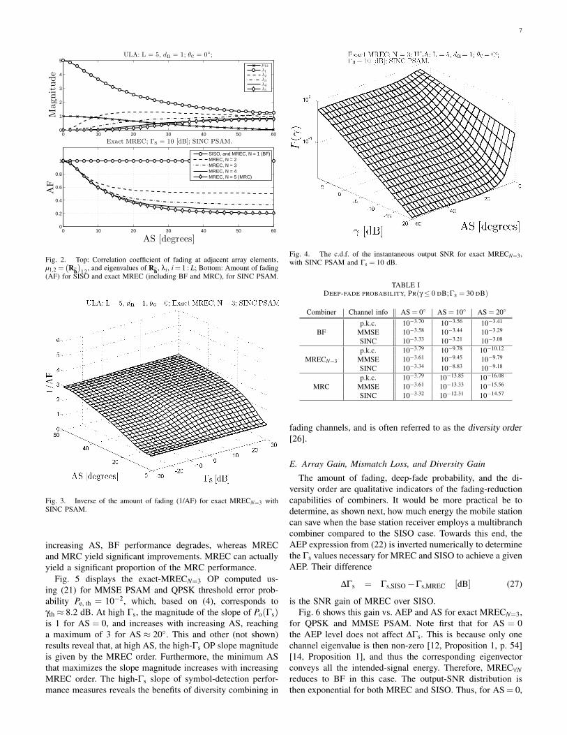
Fig. 2 displays vs. the AS the following: 1) in the topsubplot, the correlation coefficient of the channel gains atadjacent antenna elements, µ12, and the eigenvalues of Rh,λi, i = 1 : L; 2) in the bottom subplot, the AF for SISOand an ULA with exact MREC (including BF and MRC),for SINC PSAM. Note first, that due to the continuouschanges in the relative magnitudes of the eigenvalues, thisfigure could not have been obtained using previously-availableSNR p.d.f. expressions [3] [4]. Then, note that, as SISO, BFyields AF = 1, i.e., no fading reduction. On the other hand,the fading-reduction capabilities of MRECN=2 equal those ofMRC for AS≤ 6, and improve further before reaching a floorfor AS≈ 25. This floor is inversely proportional to the MRECorder, which is in agreement with the lower bound in (26). Theintuitive explanation is that, for large AS, MREC combinesN uncorrelated channel eigengains of similar strengths, thusreducing fading N-fold — see also Section 1 of the Appendix.

Fig. 3 shows 1/AF computed using (26) for exactMRECN=3 with SINC PSAM. Similar (not shown) resultshave been obtained for MMSE PSAM. Very small AS yieldsAF≈ 1, ∀N, reflecting a lack of diversity, whereas AS ↑ yields[AF−1] ↑N

1 , at any value of Γs.

D. Evaluation of SNR C.D.F., Deep-Fade Probability, and OP

Fig. 4 plots the output-SNR c.d.f. computed using (20) forexact MRECN=3, SINC PSAM, unit-variance channel gains(assumed hereafter for ULA and SISO), and Γs = Es/N0 =10 dB. The slope of P(γ;AS = 0) is unitary (also for allother MREC orders, as other results, not shown here, haveindicated). On the other hand, the slope of P(γ;AS ↑20

0 )increases. For large AS this slope becomes proportional tothe MREC order, N.

The c.d.f. of the combiner output SNR can be used toevaluate receiver performance in fading channels through thedeep-fade probability [23, p. 55]. A deep fade is defined asthe situation in which, although Γs is large, the output SNRis subunitary (i.e., below 0 dB). Table I shows this probabilityfor exact BF, MRECN=3, and MRC, for Γs = 30 dB and AS =0,10,20. For AS = 0, BF, MREC, and MRC coincide. With

7

0 10 20 30 40 50 600

1

2

3

4

5

Magnit

ude

ULA: L = 5, dn = 1; θc = 0;

µ12

λ1

λ2

λ3

λ4

λ5

0 10 20 30 40 50 600

0.2

0.4

0.6

0.8

1

AS [degrees]

AF

Exact MREC; Γs = 10 [dB]; SINC PSAM.

SISO, and MREC, N = 1 (BF)MREC, N = 2MREC, N = 3MREC, N = 4MREC, N = 5 (MRC)

Fig. 2. Top: Correlation coefficient of fading at adjacent array elements,µ1,2 =

(Rh

)12, and eigenvalues of Rh, λi, i = 1 : L; Bottom: Amount of fading

(AF) for SISO and exact MREC (including BF and MRC), for SINC PSAM.

Fig. 3. Inverse of the amount of fading (1/AF) for exact MRECN=3 withSINC PSAM.

increasing AS, BF performance degrades, whereas MRECand MRC yield significant improvements. MREC can actuallyyield a significant proportion of the MRC performance.

Fig. 5 displays the exact-MRECN=3 OP computed us-ing (21) for MMSE PSAM and QPSK threshold error prob-ability Pe, th = 10−2, which, based on (4), corresponds toγth ≈ 8.2 dB. At high Γs, the magnitude of the slope of Po(Γs)is 1 for AS = 0, and increases with increasing AS, reachinga maximum of 3 for AS ≈ 20. This and other (not shown)results reveal that, at high AS, the high-Γs OP slope magnitudeis given by the MREC order. Furthermore, the minimum ASthat maximizes the slope magnitude increases with increasingMREC order. The high-Γs slope of symbol-detection perfor-mance measures reveals the benefits of diversity combining in

Fig. 4. The c.d.f. of the instantaneous output SNR for exact MRECN=3,with SINC PSAM and Γs = 10 dB.

TABLE IDEEP-FADE PROBABILITY, PR(γ≤ 0 DB;ΓS = 30 DB)

Combiner Channel info AS = 0 AS = 10 AS = 20

p.k.c. 10−3.70 10−3.56 10−3.41

BF MMSE 10−3.58 10−3.44 10−3.29

SINC 10−3.33 10−3.21 10−3.08

p.k.c. 10−3.79 10−9.78 10−10.12

MRECN=3 MMSE 10−3.61 10−9.45 10−9.79

SINC 10−3.34 10−8.83 10−9.18

p.k.c. 10−3.79 10−13.85 10−16.08

MRC MMSE 10−3.61 10−13.33 10−15.56

SINC 10−3.32 10−12.31 10−14.57

fading channels, and is often referred to as the diversity order[26].

E. Array Gain, Mismatch Loss, and Diversity Gain

The amount of fading, deep-fade probability, and the di-versity order are qualitative indicators of the fading-reductioncapabilities of combiners. It would be more practical be todetermine, as shown next, how much energy the mobile stationcan save when the base station receiver employs a multibranchcombiner compared to the SISO case. Towards this end, theAEP expression from (22) is inverted numerically to determinethe Γs values necessary for MREC and SISO to achieve a givenAEP. Their difference

∆Γs = Γs,SISO−Γs,MREC [dB] (27)

is the SNR gain of MREC over SISO.Fig. 6 shows this gain vs. AEP and AS for exact MRECN=3,

for QPSK and MMSE PSAM. Note first that for AS = 0the AEP level does not affect ∆Γs. This is because only onechannel eigenvalue is then non-zero [12, Proposition 1, p. 54][14, Proposition 1], and thus the corresponding eigenvectorconveys all the intended-signal energy. Therefore, MREC∀Nreduces to BF in this case. The output-SNR distribution isthen exponential for both MREC and SISO. Thus, for AS = 0,

8

Fig. 5. Outage probability for exact MRECN=3, MMSE PSAM, QPSK, andPe, th = 10−2, i.e., γth ≈ 8.2 dB.

10−4

10−3

10−2

10−1 0

1020

3040

5060

5

10

15

20

25

30

AS [degrees]

QPSK; ULA: L = 5, dn = 1, θc = 0; Exact MREC, N = 3; MMSE PSAM.

AEP

∆Γs

[dB

]

Fig. 6. Reduction in the average per-symbol SNR required to attain a givenAEP with MRECN=3 instead of SISO, for QPSK and MMSE PSAM.

MREC can only provide an average-output-SNR gain overSISO. Such increase is commonly known as array gain [1,Sections 1.2.2, 5.2].

Let us investigate further the MREC array gain. Using (8),the average output SNR for exact MRECN can be written as

Γ 4= Eγ=

N

∑i=1

Γi, (28)

where Γi > 0, i = 1 : N, are the eigenbranch average SNRs,defined in (11). Then, the array gain is the ratio of the MRECand SISO average output SNRs, i.e.,

AGMREC =ΓΓ0

, (29)

which, for identically-distributed and perfectly-known channel

0 10 20 30 40 50 60

2

4

6

8

10

12

14

16

18

20

22

∆Γs

[dB

]

AS [degrees]

QPSK; ULA: L = 5, dn = 1, θc = 0; Exact MREC, AEP = 0.001; MMSE PSAM.

MREC, N = 5 (MRC)

MREC, N = 4

MREC, N = 3

MREC, N = 2

MREC, N = 1 (BF)

Fig. 7. SNR gain achieved with exact MRECN=1:5 over SISO, for QPSKand MMSE PSAM, and AEP = 10−3.

gains, can be written as

AGMREC = 10log10

(L

∑Ni=1 λi

∑Li=1 λi

)∈ [10log10 N, 10log10 L]. (30)

The upper bound is achieved for coherent channel gains,i.e., for AS = 0 the MREC array gain is proportional to thenumber of branches, L. Fig. 6 actually reveals that ∆Γs ≈ 7≈10 log10 L

∣∣∣∣L=5

dB at AS = 0.

The MREC array gain lower bound from (30), i.e.,10 log10 N, is achieved for uncorrelated channel gains. Lowcorrelation is incurred for large AS, as shown in the top subplotin Fig. 2. Thus, when AS increases from zero to large values,AGMREC,N diminishes from 10log10 L to 10log10 N.

Let us first consider the case of BF, i.e., MRECN=1. Then,the array gain decreases from 10log10 L to 0. This is verifiedin Fig. 7, which displays contours obtained by slicing atAEP = 10−3 surfaces as that shown in Fig. 6 for all N = 1 : L.Recall that BF does not offer fading reduction over SISO.Thus, the ∆Γs plot shown in Fig. 7 for BF actually representsarray gain only. For AS = 0 the BF weight vector (thedominant eigenvector) is perfectly aligned with the channelgain vector, and thus BF maximizes the array gain. Withincreasing AS there is an increasing mismatch between theBF weights and the channel gains. The mismatch loss willdiminish and ultimately cancel the BF array gain.

Also for MREC1<N<L there can be noticeable mismatchloss, as Fig. 7 indicates. Actually, after ∆Γs peaks at an ASvalue proportional to N, ∆Γs suffers a reduction inversely-proportional to N. The explanation for the mismatch loss inMREC1<N<L is a simple generalization of the explanationgiven above for BF. Assuming p.k.c., the MRECN<L weightvector with respect to the received signal vector y can beshown to be UN UH

N h, i.e., nonidentical to the channel vector,h, which would be required for perfect combining. Nonethe-less, given N, these two vectors nearly coincide for AS below

9

the value for which most of the intended-signal energy arrivesalong the N selected eigenvectors. For higher AS, intended-signal energy arrives from directions unaccounted for by theweight vector deployed by MRECN , yielding higher mismatchloss. Higher N ensures that this mismatch loss begins affectingperformance at higher AS, and that the loss is smaller. Clearly,there is no such mismatch loss for full MREC (MRC) becausethe receiver weight vector matches the channel vector. This isconfirmed by the line corresponding to MRC in Fig. 7.

Figs. 6 and 7 show that ∆Γs initially increases with ASincreasing from zero, which represents diversity gain [1,Sections 1.2.2, 5.2]. Increasing AS yields decreasing channelgain correlation, and thus the peaks of the SNR p.d.f. occur atlarger SNR values — see Fig. 1. This reduces the amount offading, the deep-fade probability, and increases the magnitudeof the slope of AEP(Γs), i.e., the diversity order. In Fig. 6, theSNR is larger for smaller AEP because the AEP slopes forMRECN=3 and SISO are 3 and 1, respectively, which meansthat the AEP decreases much faster with Γs for MRECN=3than for SISO.

Fig. 7 indicates that for AS < 4, MRECN=2 generatesalmost the same SNR gain as MRECN=3:5 (which includesMRC). Furthermore, for AS < 10, MRECN=3 generates al-most the same SNR gain as MRECN=4:5. Finally, for AS <18, MRECN=4 generates almost the same SNR gain as MRC.On the other hand, throughout the shown AS range, MRECN>1greatly outperforms BF.

IV. PERFORMANCE AND COMPLEXITYCOMPARISON OF BF, MRC, AND ADAPTIVE MREC,

FOR RANDOM AZIMUTH SPREAD

The above numerical results suggest that MREC perfor-mance can be maximized by suitable selection of its order,N. However, the order impacts MREC numerical complexity,which translates into certain baseband processing resourcerequirements [11] [12, Chapter 5]. The numerical complexityof MRC and MRECN , in terms of the number of complexmultiplications and additions required per detected symbolfor interpolation, combining, and (only in MREC) for KLT,are reproduced in [12, Table 3.7, p. 132] [13, Table II]. Werecently found that MREC performance does not degradesignificantly when the channel eigenstructure is updated byfeeding received-signal samples into the deflation-based pro-jection approximation subspace tracking (PASTd) algorithm[17]. Furthermore, PASTd-based eigenstructure tracking doesnot increase the complexity of adaptive MREC significantlybecause of PASTd’s simplicity and because the eigenstructurechanges very slowly (see [13, Eqn. (3)]).

Previous studies have indicated that exact and approximateimplementations of MREC with SINC and MMSE PSAM havesimilar complexities, due to the decorrelating effect of the KLT— see [12, Section 3.12] [13] [16] [17]. On the other hand,MRC can have much higher computational complexity forexact vs. approximate combining, and for MMSE vs. SINCPSAM estimation.

Fig. 8 plots the numerical complexities computed from[13, Table II] for SISO, BF, MRECN=1:L, and MRC, for

1 2 3 4 50

50

100

150

200

250

300

SINC interpolation

# M

ult./

Add

. Ops

.

MRCMRECBFSISO

1 2 3 4 50

50

100

150

200

250

300

MMSE interpolation

MREC order, N

# M

ult./

Add

. Ops

.

MRCMRECBFSISO

Fig. 8. Numerical complexity for SISO, BF, MRECN=1:L, and MRC, forexact combining, L = 5, and interpolator length T = 11; top subplot is forSINC interpolation, bottom subplot is for MMSE interpolation.

L = 5, interpolator length T = 11, SINC and MMSE PSAM,and exact combining implementation. Note that for MMSEPSAM, MRC is much more complex than even full-MREC,because the channel gain vector required for MRC is estimatedusing matrix operations [12, Eqn. (3.113), p. 83], whereas theeigengains required for MREC are estimated separately, asvectorial inner products [12, Eqn. (3.107), p. 82]. On the otherhand, SINC PSAM inherently separates the estimation of thecomponents of both the channel gain and eigengain vectors,so that the complexities of exact MRC and full-MREC aresimilar.

To minimize MREC complexity and achieve near-MRCperformance we apply the simple and effective bias–variancetradeoff criterion (BVTC) [11] [12, Section 5.2.2] [13] [17][18] for exact-MREC order selection. For realistic perfor-mance and complexity comparisons, a sufficient number(10000) of independent lognormal AS samples for a typicalurban scenario [13, Section II] have been generated with [13,Eqn. (2)]. The produced random AS sequence had an averageof 9.81, a standard deviation of 13.4, and Pr(1 < AS <20)≈ 0.83. For exact SISO, BF, MRC, and adaptive MRECwith MMSE PSAM, Fig. 9 shows the means over the ASsamples of the outage probabilities for QPSK — computedwith (21), for Pe, th = 10−2, or, equivalently, for γth = 8.2 —and of the computational complexities (computed from [13,Table II]). For reference, the lower subplot also displays ascaled version of the MREC order output by the BVTC, i.e.,10N. Note that, since the numerical complexities of SISO, BF,and MRC are AS- and Γs-independent, they have not requiredaveraging. On the other hand, for MREC, the order output bythe BVTC (and thus the numerical complexity) depends on ASand Γs. Fig. 9 indicates that the BVTC MREC order increaseswith increasing Γs, which improves MREC performance butalso increases complexity.

Fig. 9 shows that throughout the SNR range, adaptive

10

5 10 15 20 2510

−3

10−2

10−1

100

Mea

nPo

QPSK; ULA: L = 5, dn = 1; θc = 0; MMSE PSAM. Pe,th = 10−2⇐⇒ γth = 8.2155 [dB]

SISO

BF

adaptive MREC

MRC

5 10 15 20 250

50

100

150

200

250

300

350

Γs [dB]

#M

ult./

Add.

Ops.

MRC complexity

adaptive-MREC complexity

10 N (from BVTC)

BF complexity

SISO complexity

Fig. 9. Top: Outage probability for QPSK, averaged over 10,000 lognormalazimuth spread samples, for exact SISO, BF, MRC, and MREC adaptedwith the BVTC, for L = 5, and MMSE interpolation with T = 11. Bottom:Corresponding numerical complexity.

MREC yields MRC-like performance, which can be muchbetter than for BF due to diversity gain and additional arraygain. The outage probability performance level Po = 10−1, forinstance, is achieved with SISO for Γs ≈ 22 dB and with BFfor Γs ≈ 16 dB. Thus, BF produces an array gain of about 6 dBover SISO, which is about 1 dB lower than that achievable in

ideal conditions, i.e., 10 log10 L∣∣∣∣L=5

≈ 7 dB, for L = 5 coherent

and perfectly known channel gains. MRC and BVTC-basedadaptive MREC yield an extra 4 dB gain. At Γs = 12 dB, theBVTC outputs an average order of Navg ≈ 2.86 for MREC.Then, based on [13, Table II], we found that for MMSEPSAM, BVTC MREC is 2.86 and 3.96 times more complexthan BF and SISO, respectively, but 5.92 times less complexthan MRC.

For SINC PSAM and the same random AS sequence, other(not shown) numerical results have indicated that Po = 10−1

is achieved with MRC and with BVTC-based adaptive MRECof average order Navg ≈ 3.02 for Γs ≈ 14 dB, with BF forΓs ≈ 18 dB, and with SISO for Γs ≈ 24 dB. Thus, therelative performances of these combining methods has notchanged compared to the case of MMSE PSAM. However,while Po = 10−1 is achieved for MMSE PSAM with adaptiveMREC with Navg ≈ 2.86 at Γs ≈ 12 dB, SINC PSAM requiresNavg ≈ 3.02 at Γs ≈ 14 dB, i.e., not only a 2 dB performanceloss but also an increase of about 6% in complexity. SISOand BF experience the same performance loss but no com-plexity change for SINC PSAM vs. MMSE PSAM. On theother hand, exact MRC experiences a 2 dB performance losscompensated by a 3.6-fold complexity reduction with SINCPSAM compared to MMSE PSAM.

Numerical results analogous to those from Fig. 9 haveappeared for the AEP, based on analysis and simulations, in[12, Fig. 4.5, p. 149] [13, Fig. 2]. Results that show the AEPvs. time for temporally-correlated samples of lognormal AS

appear in [11, Figs. 5] [12, Fig. 4.6, p. 151] [13, Fig. 3] [17,Figs. 4, 5]. In [12, Chapter 5] [11] we demonstrated for fixed-point FPGA-based implementations that the lower averagecomplexity of adaptive MREC vs. MRC translates into reducedprocessing resource requirements and power consumption forthe former. It has also been found that adaptive MREC couldbenefit from the AS independence among subscriber stations[11, Figs. 5–9] [12, Figs. 5.5–5.15, pp. 170–187]. Subscribersexperiencing high AS can be allocated more base-stationeigenprocessing modules [11, Section 2.5, p. 4] [12, p. 170]for better performance, which yields azimuth spread diversity.

V. SUMMARY AND CONCLUSIONS

This contribution completes earlier performance and nu-merical complexity studies of receive-side optimum (exact)maximal-ratio eigencombining (MREC) vs. statistical beam-forming (BF) and maximal-ratio combining (MRC). A novelclosed-form expression has been derived for the p.d.f. of theoutput signal-to-noise ratio of MREC that applies seamlesslyfor perfectly or imperfectly known channel gains and arbi-trary fading correlation value, i.e., any combination of arrayinterelement distance, mean angle of arrival, power azimuthspectrum (p.a.s.) type, and azimuth spread (AS) value. Thisexpression also applies to BF and MRC for smart antennareceivers as well as to MRC and MREC for correlated ’rake’receiver taps in CDMA systems. This p.d.f. expression hasbeen used to derive widely-applicable closed-form expressionsfor the outage probability (OP) and the average error prob-ability (AEP) of MREC, BF, and MRC. The advantages ofMREC over BF and MRC have been analyzed in terms of theamount of fading, deep-fade probability, diversity and arraygains, OP, and numerical complexity. For realistic (Laplacian)base-station p.a.s. and lognormal AS, optimum channel fadingestimation, and optimum combining implementation, adaptiveMREC has been shown to achieve near-optimum averageperformance at a fraction of the MRC complexity. Thus,adaptive MREC emerges as a practical alternative to theconventional, BF and MRC, approaches, for smarter antennasas well as for more efficient CDMA receivers.

APPENDIXSPECIAL-CASE CLOSED-FORM EXPRESSIONS FOR

PERFORMANCE MEASURES FOR EXACT MREC1) The Case when All Eigenvalues are Equal: In this case,

Γi4= Γ , i = 1 : N, and the r.m.g.f. expression from (14) reduces

to [3, Eqn. (5.2-14), p. 319] [4, Eqn. (10-61), p. 310]

Fγ(s) =1

(1+ sΓ)N , (31)

whose inverse Laplace transform is

p(γ) =γN−1 e−γ/Γ

(N−1)! ΓN . (32)

Substituting this into the outage probability (OP) definitionfrom (3) yields for exact MREC the following closed-form OPexpression [3, Eqn. (5.2-15), p. 319] [4, Eqn. (10-64), p. 310]:

Po = 1− eγth/ΓN−1

∑n=0

1n!

(γth

Γ

)n. (33)

11

Furthermore, with the notation ϒ 4= ΓgPSK, the finite-limit

integral exact-MREC AEP expression for M–PSK from (22)becomes

Pe =1π

Z M−1M π

0

(1+ϒ

1sin2 φ

)−N

dφ. (34)

With the notations ξ 4=

√ϒ

ϒ+1 , α 4= ξ/ tan π

M , and ϕ 4= tan−1α,

the above can be written in closed-form as [6, Eqns. 5A.17–19,pp. 127–8]

Pe =M−1

M− ξ

π

N−1

∑n=0

(2nn

) (1−ξ2

4

)n

×

×

π2

+ϕ+ sinϕn

∑i=1

4(n−i) [cosϕ]2(n−i)+1

(2(n−i)n−i

)[2(n− i)+1]

(35)

where(a

b

)represents the binomial coefficient, i.e.,

(ab

) 4=

a!(a−b)!b! , and a!

4= a · (a−1) · (a−2) · · · ·3 ·2 ·1.

BPSK implies ϕ = 0, and so (35) reduces to Proakis’expression [5, Appendix C, Eqn. C-18, p. 955]

Pe =12

[1−ξ

N−1

∑n=0

(2nn

)(1−ξ2

4

)n]

, (36)

which can also be written as [6, Eqn. 5A.4b, p. 125]

Pe =[

12

(1−ξ)]N N−1

∑n=0

(N−1+n

n

)[12

(1+ξ)]n

. (37)

2) The Case when All Eigenvalues are Distinct: In thiscase, Nd = N and rk = 1, ∀k = 1 : N, so that (16) and (17)yield

Fγ(s) =N

∑i=1

ci1

1+ sΓi, (38)

where

ci =N

∏j 6=i

Γi

Γi−Γ j. (39)

Then, the p.d.f. of γ, i.e., the inverse Laplace transform ofFγ(s), has the simple closed-form expression

p(γ) =N

∑i=1

ci1Γi

e−γ/Γi . (40)

For p.k.c. the above reduces to [4, Eqn. 10-60, p. 308]. TheOP for M–PSK and exact MREC is, from (3) and (40),

Po =N

∑i=1

ci

(1− e−γth/Γi

). (41)

The AEP is obtainable as follows, using (23) and (24):

Pe =12

N

∑i=1

ci

(1−

√Γi gPSK

Γi gPSK +1

). (42)

For BPSK this reduces to [19, Eqn. (16)]. For BPSK, p.k.c.,and uncorrelated branches, (42) reduces to the ideal-MRCAEP-formula proposed by Proakis in [5, Eqn. 14.5-28, p.847].

REFERENCES

[1] A. Paulraj, R. Nabar, and D. Gore, Introduction to Space-Time WirelessCommunications. Cambridge, UK: Cambridge University Press, 2005.

[2] H. L. V. Trees, Optimum Array Processing: Part IV of Detection,Estimation, and Modulation Theory. New York, NY: John Wiley &Sons, Inc., 2002.

[3] W. C. Jakes, Ed., Microwave Mobile Communications. New York, NY:John Wiley and Sons, 1974.

[4] W. C. Y. Lee, Mobile Communications Engineering. Englewood Cliffs,NJ: McGraw-Hill, 1982.

[5] J. G. Proakis, Digital Communications, 4th ed. New York, NY:McGraw-Hill, Inc., 2001.

[6] M. K. Simon and M.-S. Alouini, Digital Communication over FadingChannels. A Unified Approach to Performance Analysis. Baltimore,Maryland: John Wiley and Sons, 2000.

[7] S. Choi, J. Choi, H.-J. Im, and B. Choi, “A novel adaptive beamformingalgorithm for antenna array CDMA systems with strong interferers,”IEEE Transactions on Vehicular Technology, vol. 51, no. 5, pp. 808–816, September 2002.

[8] R. Vaughan and J. B. Andersen, Channels, Propagation and Antennasfor Mobile Communications. London, UK: The Institution of ElectricalEngineers, 2003.

[9] D. G. Brennan, “Linear diversity combining techniques,” Proceedingsof the IEEE, vol. 91, no. 2, pp. 331 – 356, February 2003.

[10] J. Choi and S. Choi, “Diversity gain for CDMA systems equipped withantenna arrays,” IEEE Transactions on Vehicular Technology, vol. 52,no. 3, pp. 720–725, May 2003.

[11] C. Siriteanu, S. D. Blostein, and J. Millar, “FPGA-based communica-tions receivers for smart antenna array embedded systems,” EURASIPJournal on Embedded Systems. Special Issue on Field-ProgrammableGate Arrays in Embedded Systems, vol. 2006, pp. Article ID 81 309, 13pages, 2006.

[12] C. Siriteanu, “Maximal-ratio eigen-combining for smarter antenna arraywireless communication receivers,” Ph.D. dissertation, Queen’s Univer-sity, Kingston, Canada, 2006.

[13] C. Siriteanu and S. D. Blostein, “Maximal-ratio eigen-combining forsmarter antenna arrays,” IEEE Transactions on Wireless Communica-tions, vol. 6, no. 3, pp. 917 – 925, March 2007.

[14] C. Sun, J. Cheng, and T. Ohira, Eds., Handbook on Advancements inSmart Antenna Technologies for Wireless Networks. Chapter ‘Eigencom-bining: A Unified Approach to Antenna Array Signal Processing’ by C.Siriteanu and S. D. Blostein. New York, NY: Idea Group, Inc., 2009.

[15] C. Brunner, W. Utschick, and J. A. Nossek, “Exploiting the short-termand long-term channel properties in space and time: eigenbeamformingconcepts for the BS in WCDMA,” European Transactions on Telecom-munications. Special Issue on Smart Antennas, vol. 12, no. 5, pp. 365–378, 2001.

[16] C. Siriteanu and S. D. Blostein, “Diversity combining and eigencombin-ing performance and complexity comparison for estimated channels,” inProc. 24th Biennial Symposium on Communications, Queen’s University,Kingston, Canada, 2008, pp. 128–133.

[17] C. Siriteanu, G. Xin, and S. D. Blostein, “Performance and complexitycomparison of MRC and PASTd-based statistical beamforming andeigencombining,” in Proc. 14th Asia–Pacific Conference on Commu-nications (APCC’08), Tokyo, Japan, Session 16-PM1-A, 2008.

[18] J. Jelitto and G. Fettweis, “Reduced dimension space-time processingfor multi-antenna wireless systems,” IEEE Wireless Communications,vol. 9, no. 6, pp. 18–25, December 2002.

[19] F. A. Dietrich and W. Utschick, “Maximum ratio combining of corre-lated Rayleigh fading channels with imperfectly known channel,” IEEECommunications Letters, vol. 7, no. 9, pp. 419–421, September 2003.

[20] F. Patenaude, J. Lodge, and J.-Y. Chouinard, “Eigen analysis of wide-band fading channel impulse responses,” IEEE Transactions on Vehicu-lar Technology, vol. 48, no. 2, pp. 593 – 606, March 1999.

[21] V. A. Aalo, “Performance of maximal-ratio diversity systems in acorrelated Nakagami-fading environment,” IEEE Transactions on Com-munications, vol. 43, no. 8, pp. 2360–2369, August 1995.

[22] P. Lombardo, G. Fedele, and M. M. Rai, “MRC performance for binarysignals in Nakagami fading with general branch correlation,” IEEETransactions on Communications, vol. 47, no. 1, pp. 44 – 52, January1999.

[23] D. Tse and P. Viswanath, Fundamentals of Wireless Communication.Cambridge, UK: Cambridge University Press, 2005.

[24] C. Siriteanu and S. D. Blostein, “Maximal-ratio eigencombining: aperformance analysis,” Canadian Journal of Electrical and ComputerEngineering, vol. 29, no. 1/2, pp. 15–22, January–April 2004.

12

[25] I. S. Gradshteyn and I. M. Ryzhik, Table of Integrals, Series, andProducts, 4th ed. New York, NY: Academic Press, 1965.

[26] E. G. Larsson and P. Stoica, Space-Time Block Coding for WirelessCommunications. Cambridge, UK: Cambridge University Press, 2003.

[27] M. Abramowitz and I. A. Stegun, Eds., Handbook of MathematicalFunctions with Formulas, Graphs and Mathematical Tables. New York,NY 10014: Dover Publications, Inc., 1995.

Constantin (Costi) Siriteanu was born in Sibiu,Romania, in 1972. He received his B.S. and M.S.degrees in Electrical Engineering, from “GheorgheAsachi” Technical University, Iasi, Romania, in 1995and 1996, respectively. Between 1995 and 1997he was a part-time engineer with the ResearchInstitute for Automation, Iasi, Romania, working ondata transmission over power lines. Between 1996and 1998 he was a Research Assistant with theDepartment of Automatic Control and ComputerScience, “Gheorghe Asachi” Technical University,

Iasi, Romania, working on digital control systems. Constantin received hisPh.D. degree in Electrical Engineering from Queen’s University, Kingston,Canada, in October 2006. Between September 2006 and February 2008 hewas a post-doctoral researcher at Hanyang University, Seoul, South Korea,where he also taught a graduate course on MIMO systems. Subsequently,Constantin was a Visiting Assistant Professor for a term at KyungpookNational University, Daegu, Korea. Since June 2008, Dr. Siriteanu is a ‘BrainKorea 21st Century’ Assistant Professor at Seoul National University. Hisresearch interests are in reduced-complexity signal processing for multi-branchtransceivers for wireless communications.

Steven D. Blostein (SM ’83, M ’88, SM ’96)received his B.S. degree in Electrical Engineeringfrom Cornell University, Ithaca, NY, in 1983, and theM.S. and Ph.D. degrees in Electrical and ComputerEngineering from the University of Illinois, Urbana-Champaign, in 1985 and 1988, respectively. He hasbeen on the faculty at Queen’s University since 1988and currently holds the position of Professor andHead of the Department of Electrical and ComputerEngineering. From 1999-2003, he was the leader ofthe Multi-Rate Wireless Data Access Major Project

sponsored by the Canadian Institute for Telecommunications Research. Hehas also been a consultant to industry and government in the areas of imagecompression, target tracking, radar imaging and wireless communications. Hespent 1994-1995 at Lockheed Martin Electronic Systems in Montreal and2006 at Communications Research Centre in Ottawa. His current interestslie in the application of signal processing to wireless communications sys-tems, including smart antennas, MIMO systems, and space-time-frequencyprocessing for MIMO-OFDM systems. He has been a member of the Samsung4G Wireless Forum as well as an invited distinguished speaker at RyersonUniversity and at Samsung Advanced Institute of Technology. He served asChair of IEEE Kingston Section (1994), Chair of the Biennial Symposiumon Communications (2000,06,08), Associate Editor for IEEE Transactionson Image Processing (1996-2000), and Publications Chair for IEEE ICASSP2004. He is currently serving as an Editor of IEEE Transactions on WirelessCommunications. He is a registered Professional Engineer in Ontario and aSenior Member of IEEE.