PC44 Time of Use Pilots: End of Pilot Evaluation
109
PC44 Time of Use Pilots: End-of-Pilot Evaluation PREPARED BY Sanem Sergici Ahmad Faruqui Nicholas Powers Sai Shetty Ziyi Tang PREPARED FOR Maryland Public Service Commission
-
Upload
khangminh22 -
Category
Documents
-
view
4 -
download
0
Transcript of PC44 Time of Use Pilots: End of Pilot Evaluation
PC44 Time of Use Pilots: End-of-Pilot Evaluation PREPARED BY
Sanem Sergici
Ahmad Faruqui
Nicholas Powers
Sai Shetty
Ziyi Tang
PREPARED FOR
Maryland Public Service Commission

AUTHORS
Sanem Sergici, Ph.D. Dr. Sanem Sergici is a Principal in The Brattle Group’s Boston, MA office specializing in program design and evaluation in the areas of rate design, energy efficiency, demand response, and electrification. Dr. Sergici has been at the forefront of the design and impact analysis of innovative retail pricing, enabling technology, and behavior-based energy efficiency pilots and programs in many states and regions including District of Columbia, Connecticut, Florida, Illinois, Maryland, Michigan, Ontario, CA and New Zealand. She has led numerous studies that were instrumental in regulatory approvals of Advanced Metering Infrastructure (AMI) investments and smart rate offerings for electricity customers. She has expertise in resource planning; economic analysis of distributed energy resources (DERs); their impact on the distribution system operations and assessment of emerging utility business models and regulatory frameworks.
Ahmad Faruqui, Ph.D. Dr. Ahmad Faruqui’s consulting practice focuses on ways to enhance customer engagement. He advises clients on matters related to rate design, load flexibility, energy efficiency, demand response, distributed energy resources, demand forecasting, decarbonization, and electrification. He has worked for over 150 clients on five continents, and provided expert testimony and appeared before regulatory bodies, governments, and legislative councils. Dr. Faruqui has authored or coauthored more than 100 papers on energy economics in peer-reviewed and trade journals and is the co-editor of four books on industrial structural change, customer choice, and electricity pricing.
Nicholas Powers, Ph.D. Dr. Powers has broad experience in applying econometric analysis to a variety of economic questions in the electric and other industries. His electricity experience includes several key analyses of price effects, market power, and anticompetitive behavior. In addition, he conducts econometric analysis of innovative pricing programs in the electric industry. He has supported expert testimony in three separate litigation proceedings arising from the California electricity crisis of 2000–2001. He has also overseen the statistical analyses in several New Source Review cases and performed damages and other analyses in energy-related litigation proceedings. Dr. Powers also has extensive experience estimating cartel impacts in large-scale price-fixing cases, and conducting analysis for and submitting expert reports in regulatory proceedings in other industries.

NOTICE
• This report was prepared for Maryland Public Service Commission, in accordance with The Brattle Group’s engagement terms, and is intended to be read and used as a whole and not in parts.
• The report reflects the analyses and opinions of the authors and does not necessarily reflect those of The Brattle Group’s clients or other consultants.
• The authors are grateful for the support and collaboration of Joint Utility staff throughout the analysis process.
• There are no third party beneficiaries with respect to this report, and The Brattle Group does not accept any liability to any third party in respect of the contents of this report or any actions taken or decisions made as a consequence of the information set forth herein.
Table of Contents
Executive Summary................................................................................................. 1
I. Introduction ....................................................................................................... 1A. Purpose ............................................................................................................................................ 2 B. Pilot Overview, Including Key Differences From Previous Pilots ..................................................... 3 C. Methodology .................................................................................................................................... 6 D. Description of Data .......................................................................................................................... 7
1. Enrollment and Attrition Summary ......................................................................................... 7 2. Control Group Balance .......................................................................................................... 11
II. Two-Year Pilot Impact Evaluation Results ........................................................ 17A. Introduction ................................................................................................................................... 17 B. Baltimore Gas & Electric ................................................................................................................ 18
1. Main Impact Results .............................................................................................................. 18 2. Testing for Differences Between Years 1 and 2 .................................................................... 21 3. Subgroup Analysis ................................................................................................................. 23
C. Pepco Maryland ............................................................................................................................. 27 1. Main Impact Results .............................................................................................................. 27 2. Testing for Differences Between Years 1 and 2 .................................................................... 29 3. Subgroup Analysis ................................................................................................................. 31
D. DPL Maryland ................................................................................................................................. 34 1. Main Impact Results .............................................................................................................. 34 2. Testing for Differences Between Years 1 and 2 .................................................................... 37 3. Subgroup Analysis ................................................................................................................. 39
E. Potential Implications of COVID-19 for the Analysis ..................................................................... 42 1. Changes to Load Shapes ........................................................................................................ 42 2. Discussion .............................................................................................................................. 45
F. Price Response Results .................................................................................................................. 46 G. Bill Impact Analysis ........................................................................................................................ 49
III. Summary ......................................................................................................... 52
– Supplemental Analyses ..................................................................... A-1

PC44 Time of Use Pilots: End of Pilot Evaluation brattle.com | i
Executive Summary _________
This report presents the findings from an impact evaluation of three time-of-use (TOU) pricing pilots that were conducted in the state of Maryland as part of the Public Service Commission’s PC 44 proceedings. A Work Group created by the Commission helped design the pilots. Three utilities ran the pilots: BGE, Pepco, and DPL. In this report, they are referenced as the Joint Utilities (JUs).
This report updates the Year One Evaluation report that was filed with the Commission on September 15, 2020. It assessed the impact of TOU rates during the first year of the pilot (which ran from June 2019 to May 2020).1
The pilots ran for two years, from June 2019 to May 31, 2021. The years were divided into two periods, summer and the rest of the year, which was labeled non-summer. While there is a long history of TOU pilots in the U.S., the PC44 pilots have several features that are noteworthy:
• The TOU rates had sizeable differentials between peak and off-peak periods. The ratio of peak to off-peak prices ranged from 4.2:1 to 5.8:1 across the JUs. The rates were designed to provide customers a strong incentive to save money by consuming power during the substantially less expensive off-peak period.
• The peak periods were relatively short in duration, allowing customers to respond more easily by reducing peak usage and shifting some of it to off-peak periods. In the summer, the peak period ran from 2 pm to 7 pm on weekdays. All weekend hours were off-peak as were all the hours on holidays. In the non-summer season, the peak period ran from 6 am to 9 am.
• The TOU rates applied to the combined costs of generation, transmission, and distribution and not just to generation costs, which has sometimes been the case for other TOU pilots.
• A distinguishing feature of the pilots was that they were designed to separately measure the impact of TOU rates on low and moderate income (LMI) customers from the impact on non-LMI customers. These two customer groups were allocated to separate treatment cells, allowing their responses to be measured in parallel.
• The pilots featured a quasi-experimental design. Specifically, customers were randomly chosen for recruitment and given the opportunity to opt into the pilot by signing on to a TOU rate. Using a large pool of eligible customers that were not targeted for recruitment, a “matched control group” was created by utilizing a widely-used technique known as “propensity score matching” in order to minimize pre-pilot differences between the treatment and customer groups.
1 Sanem Sergici, Ahmad Faruqui, Nicholas Powers, Sai Shetty, and Jingchen Jiang, “PC44 Time of Use Pilots: Year One
Evaluation.” September 15, 2020. (“Year One Evaluation”) Available at https://www.brattle.com/wp-content/uploads/2021/05/19973_pc44_time_of_use_pilots_-_year_one_evaluation.pdf

PC44 Time of Use Pilots: End of Pilot Evaluation brattle.com | ii
• During the recruitment phase, customers who were randomly chosen for recruitment in the pilot were provided with a personalized estimate of their potential savings under the TOU rate, based on their load profiles. Based on their pre-pilot consumption patterns, about two-thirds of the customers who chose to participate would have seen a decrease in their bills even without changing their behavior. In the report, these customers are called “structural winners.”
• Treatment customers were sent emails on a weekly basis that reminded them about the timing of the peak period and provided tips on how to curtail peak loads and to shift some of that load to the off-peak period. The e-mails also provided customers with information on their weekly peak energy usage in recent weeks. This tool, known as “Behavioral Load Shaping,” was combined with the TOU rate price signal to facilitate changes in behavior. The impacts quantified in the pilot thus represent the combined effect of TOU rates and information.
• An unexpected development in the non-summer season was the outbreak of COVID-19. In Maryland, the pandemic broke out in March 2020 and affected all customers in the pilots, whether they were on TOU rates or on standard rates. While we were not able to isolate the impact of COVID-19 on customers’ responsiveness to TOU rates, we undertook supplementary data analysis to shed light on this question.
Results This report presents the results of the final impact evaluation of the pilots, covering a full two-year study period. It also discusses how the results differed across the two years of the pilot.
In the beginning, enrollment rates in the pilots ranged from 0.5% to 1.9% across the JUs. About two-thirds of the customers who enrolled would have experienced bill reductions by switching to TOU rates without changing their load behavior. This was true of both the LMI and non-LMI customers. Over time, some customers dropped out of the pilot for various reasons, including returning to the standard residential rate, switching to a retail supplier, or moving. In percentage terms, the attrition rate ranged from 24% to 32% across the three JUs as of the end of the pilot.
TOU rates provide customers an incentive to lower their consumption in peak hours, relative to what they would have consumed on their prior flat rate, and to shift some of that consumption to the off-peak hours. Behavioral messaging would further stimulate a change in customer behavior.
The results from the two-year impact analysis of the PC44 TOU pilots reveal that customers respond to the TOU price schedule by reducing their peak period consumption in both summer and non-summer seasons. In analyzing three utilities, two seasons, and two groups, we find that this result holds for ten of twelve customer groups comprised of three utilities, two seasons, and LMI and non-LMI customers.

PC44 Time of Use Pilots: End of Pilot Evaluation brattle.com | iii
The impact evaluation yields the following seven conclusions:
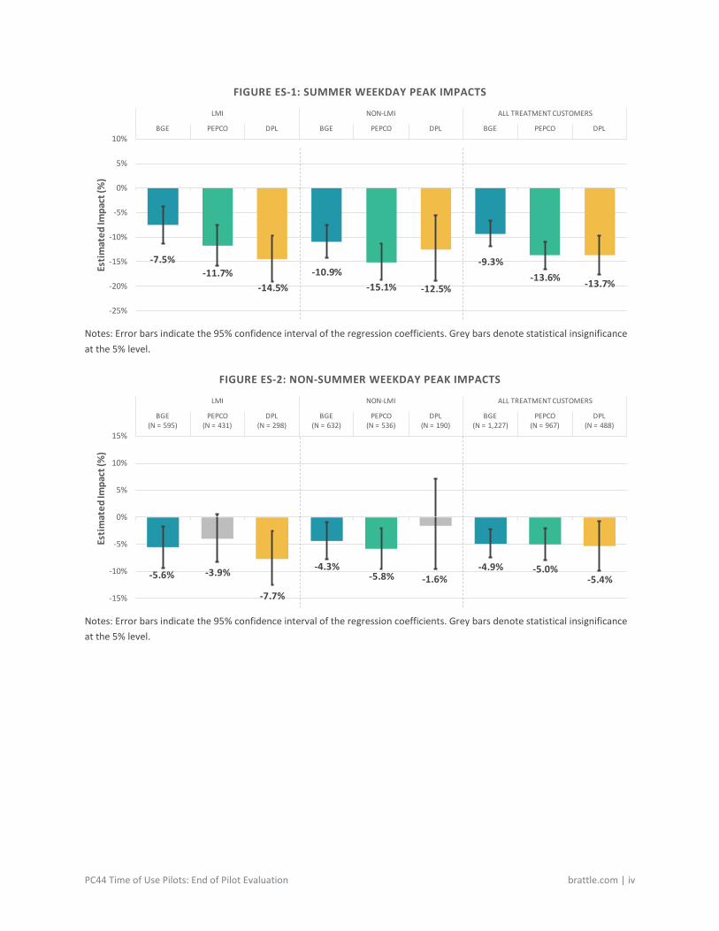
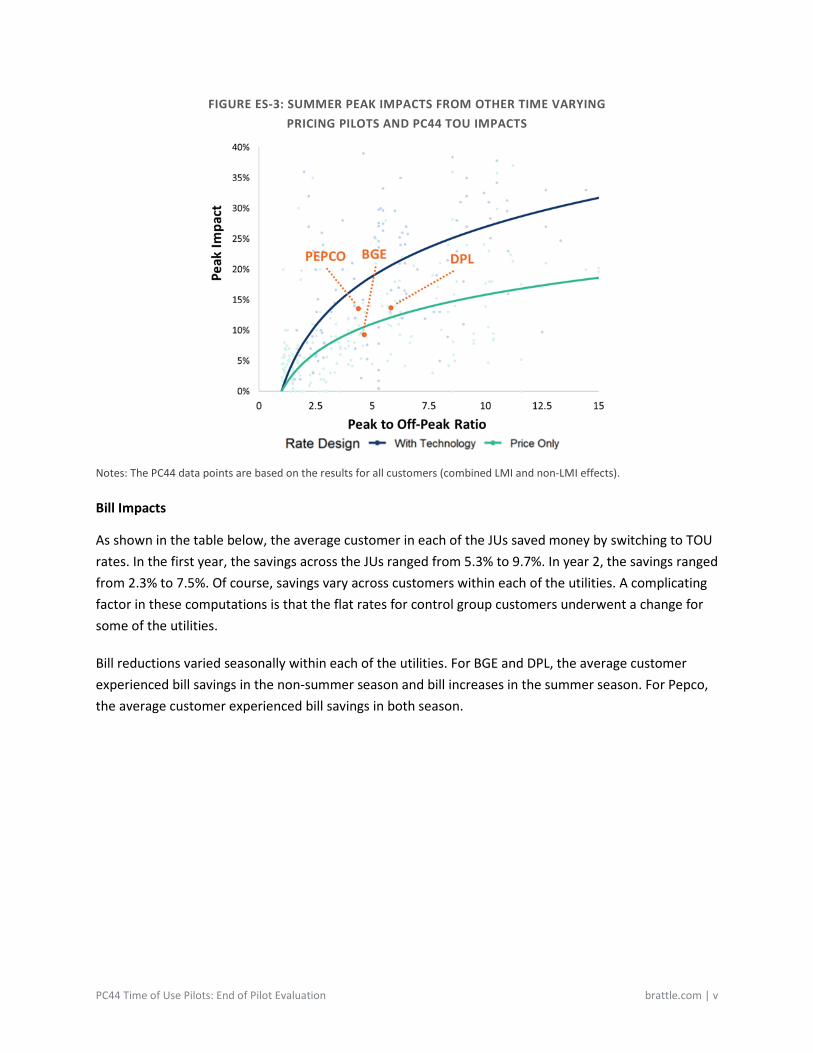
1. Across the JUs, TOU rates reduce peak demand in the summer season from 9.3% to 13.7% and by 4.9% to 5.4% for the non-summer season, as shown in Figures ES-1 and ES-2. These results are comparable to the impacts estimated in other pilots for similar peak to off-peak price ratios, as shown in Figure ES-3.
2. Daily energy consumption during the summer season goes down for two of three utilities. The weekday reductions range from 3.0% to 4.6%. Daily non-summer weekday does not change by a statistically significant amount for any of the JUs.
3. The reductions in peak demand observed during the pilots and the substitution and daily price elasticities estimated from the TOU pilots are consistent with the results derived in other TOU pilots.
4. LMI customers respond to the TOU price signals. Across all three utilities and both seasons, the LMI response is similar in magnitude to that of non-LMI customers.
5. Surprisingly, off-peak usage did not go up, even though off-peak prices were lower. Off-peak usage fell during summer weekends fell from 2 pm to 7 pm. This result, while unexpected, may be an artifact of pilot customers not fully internalizing the message from the Behavioral Load Shaping tool, despite its emphasis on encouraging conservation during peak hours. Another potential explanation might be customers’ use of a single smart thermostat schedule for both weekdays and weekends.
6. For the most part, weekday peak impacts did not change significantly during the second year of the study period, in spite of the onset of the COVID-19 pandemic. Furthermore, the onset of the pandemic does not appear to have resulted in increased customer attrition from the pilots. These results suggest that customers still see the value in and can respond to the incentives embedded in TOU rate structures despite having to work from home.
7. Structural winners’ peak reductions were comparable to those of other customers in most cases, indicating that structural winners still respond to the incentives embedded in price signals.
PC44 Time of Use Pilots: End of Pilot Evaluation brattle.com | iv
FIGURE ES-1: SUMMER WEEKDAY PEAK IMPACTS
Notes: Error bars indicate the 95% confidence interval of the regression coefficients. Grey bars denote statistical insignificance at the 5% level.
FIGURE ES-2: NON-SUMMER WEEKDAY PEAK IMPACTS
Notes: Error bars indicate the 95% confidence interval of the regression coefficients. Grey bars denote statistical insignificance at the 5% level.
-7.5%-11.7%
-14.5%-10.9%
-15.1% -12.5%
-9.3%-13.6% -13.7%
-25%
-20%
-15%
-10%
-5%
0%
5%
10%BGE PEPCO DPL BGE PEPCO DPL BGE PEPCO DPL
LMI NON-LMI ALL TREATMENT CUSTOMERSEs
timat
ed Im
pact
(%)
-5.6% -3.9%
-7.7%
-4.3%-5.8% -1.6%
-4.9% -5.0%-5.4%
-15%
-10%
-5%
0%
5%
10%
15%
BGE(N = 595)
PEPCO(N = 431)
DPL(N = 298)
BGE(N = 632)
PEPCO(N = 536)
DPL(N = 190)
BGE(N = 1,227)
PEPCO(N = 967)
DPL(N = 488)
LMI NON-LMI ALL TREATMENT CUSTOMERS
Estim
ated
Impa
ct (%
)
PC44 Time of Use Pilots: End of Pilot Evaluation brattle.com | v
FIGURE ES-3: SUMMER PEAK IMPACTS FROM OTHER TIME VARYING PRICING PILOTS AND PC44 TOU IMPACTS
Notes: The PC44 data points are based on the results for all customers (combined LMI and non-LMI effects).
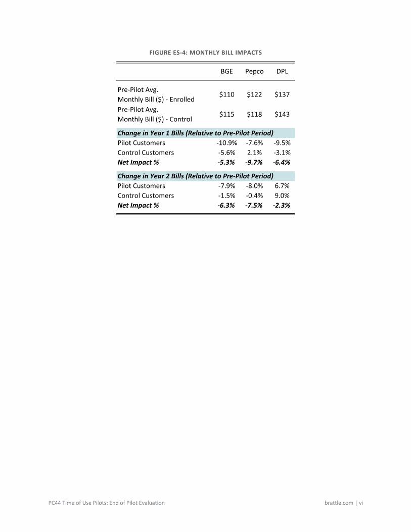
Bill Impacts
As shown in the table below, the average customer in each of the JUs saved money by switching to TOU rates. In the first year, the savings across the JUs ranged from 5.3% to 9.7%. In year 2, the savings ranged from 2.3% to 7.5%. Of course, savings vary across customers within each of the utilities. A complicating factor in these computations is that the flat rates for control group customers underwent a change for some of the utilities.
Bill reductions varied seasonally within each of the utilities. For BGE and DPL, the average customer experienced bill savings in the non-summer season and bill increases in the summer season. For Pepco, the average customer experienced bill savings in both season.
PC44 Time of Use Pilots: End of Pilot Evaluation brattle.com | vi
FIGURE ES-4: MONTHLY BILL IMPACTS
BGE Pepco DPL
Pre-Pilot Avg. Monthly Bill ($) - Enrolled
$110 $122 $137
Pre-Pilot Avg. Monthly Bill ($) - Control
$115 $118 $143
Change in Year 1 Bills (Relative to Pre-Pilot Period)Pilot Customers -10.9% -7.6% -9.5%Control Customers -5.6% 2.1% -3.1%Net Impact % -5.3% -9.7% -6.4%
Change in Year 2 Bills (Relative to Pre-Pilot Period)Pilot Customers -7.9% -8.0% 6.7%Control Customers -1.5% -0.4% 9.0%Net Impact % -6.3% -7.5% -2.3%

PC44 Time of Use Pilots: End of Pilot Evaluation brattle.com | 1
I. Introduction _________
This report presents the results of the evaluation, measurement, and verification (EM&V) of the PC44 Time-of-Use (“TOU”) pilots. The Maryland Public Service Commission (“PSC” or “the Commission”) initiated Public Conference 44 (“PC44”) on September 26, 2016 for the purposes of ensuring that the “electric distribution systems in Maryland are customer-centered, affordable, reliable, and environmentally sustainable.”2 In furtherance of that goal, the Commission instituted a Rate Design Work Group (“Work Group”) to “explore time-varying rates for traditional electric service…and considering pilot programs for driving desired results through performance-based compensation.”3 It was the Commission’s hope that these pilots would “more effectively reintroduce time-varying rates to Maryland customers, and better reach the potential to incent the real-time, peak shaving behavior now enabled by the deployment of Advanced Metering Infrastructure available to more than 80 percent of Maryland electric customers.”4 The PC44 TOU pilots were designed in a collaborative Work Group process that took place in late 2018 and early 2019.
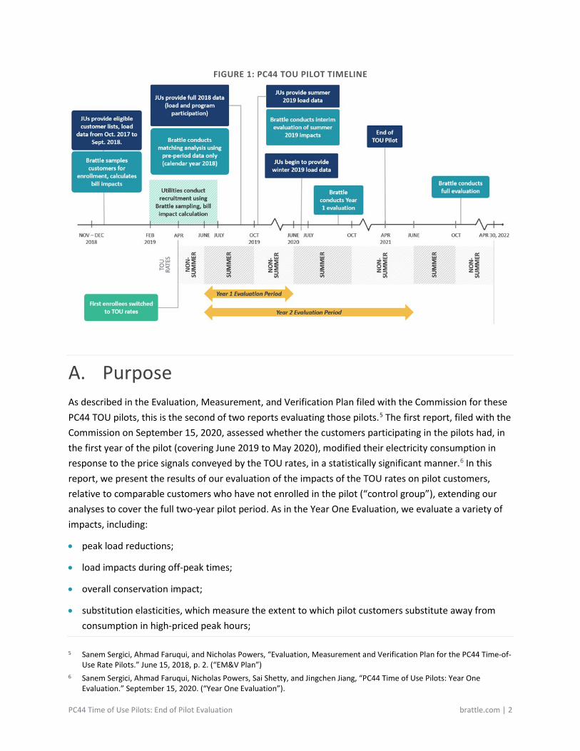
Pilot customers began transferring to the TOU rates beginning in April of 2019. The analysis in this report examines the impact of TOU pricing on enrolled customers over the course of the two years of the pilot, covering the period from June 1, 2019 through May 31, 2021. A timeline with key pilot milestones, as well as milestones for the evaluation, measurement, and verification (“EM&V”) of the pilot, is presented in Figure 1.
2 PC 44 Notice, September 26, 2016, ML212176, p. 1. 3 PC 44 Notice, September 26, 2016, ML212176, p. 3. 4 Letter Order Regarding PC44 - Rate Design Workgroup Report, November 28, 2017, ML 217978, p. 2.
PC44 Time of Use Pilots: End of Pilot Evaluation brattle.com | 2
FIGURE 1: PC44 TOU PILOT TIMELINE
A. Purpose As described in the Evaluation, Measurement, and Verification Plan filed with the Commission for these PC44 TOU pilots, this is the second of two reports evaluating those pilots.5 The first report, filed with the Commission on September 15, 2020, assessed whether the customers participating in the pilots had, in the first year of the pilot (covering June 2019 to May 2020), modified their electricity consumption in response to the price signals conveyed by the TOU rates, in a statistically significant manner.6 In this report, we present the results of our evaluation of the impacts of the TOU rates on pilot customers, relative to comparable customers who have not enrolled in the pilot (“control group”), extending our analyses to cover the full two-year pilot period. As in the Year One Evaluation, we evaluate a variety of impacts, including:
• peak load reductions;
• load impacts during off-peak times;
• overall conservation impact;
• substitution elasticities, which measure the extent to which pilot customers substitute away from consumption in high-priced peak hours;
5 Sanem Sergici, Ahmad Faruqui, and Nicholas Powers, “Evaluation, Measurement and Verification Plan for the PC44 Time-of-
Use Rate Pilots.” June 15, 2018, p. 2. (“EM&V Plan”) 6 Sanem Sergici, Ahmad Faruqui, Nicholas Powers, Sai Shetty, and Jingchen Jiang, “PC44 Time of Use Pilots: Year One
Evaluation.” September 15, 2020. (“Year One Evaluation”).

PC44 Time of Use Pilots: End of Pilot Evaluation brattle.com | 3
• demand elasticities, which measures the extent to which customers conserve in response to higher average prices; and
• weekday peak load impacts for various sub-groups.
B. Pilot Overview, Including Key Differences from Previous Pilots
Three Maryland utilities are conducting the PC44 TOU pilots: Baltimore Gas & Electric (“BGE”); Pepco Maryland (“Pepco”), and Delmarva Power & Light Maryland (“DPL”). We refer to the three utilities as the Joint Utilities (“JUs”) for the rest of this report. While each JU is conducting its own TOU pilot, the three pilots share the same fundamental design features:
• opt-in enrollment by eligible customers who were randomly selected for recruitment into the pilot;
• a seasonal rate structure, in which summer rates apply from June to September and “non-summer” (or sometimes referred to as “winter”) rates apply from October to May;
• season-specific definition of peak hours, in which the peak is from 2 PM to 7 PM on non-holiday weekdays in the summer months, and from 6 AM to 9 AM on non-holiday weekdays in the non-summer months. In both seasons, all other hours, including weekends, are off-peak; and
• the peak and off-peak rates as set by each utility vary, but are designed to be revenue neutral on an annual basis in the absence of load shifting.
PC44 Time of Use Pilots: End of Pilot Evaluation brattle.com | 4
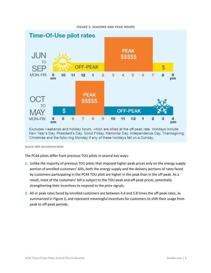
FIGURE 2: SEASONS AND PEAK HOURS
Source: BGE recruitment letter
The PC44 pilots differ from previous TOU pilots in several key ways:
1. Unlike the majority of previous TOU pilots that imposed higher peak prices only on the energy supply portion of enrolled customers’ bills, both the energy supply and the delivery portions of rates faced by customers participating in the PC44 TOU pilot are higher in the peak than in the off-peak. As a result, most of the customers’ bill is subject to the TOU peak and off-peak prices, potentially strengthening their incentives to respond to the price signals.
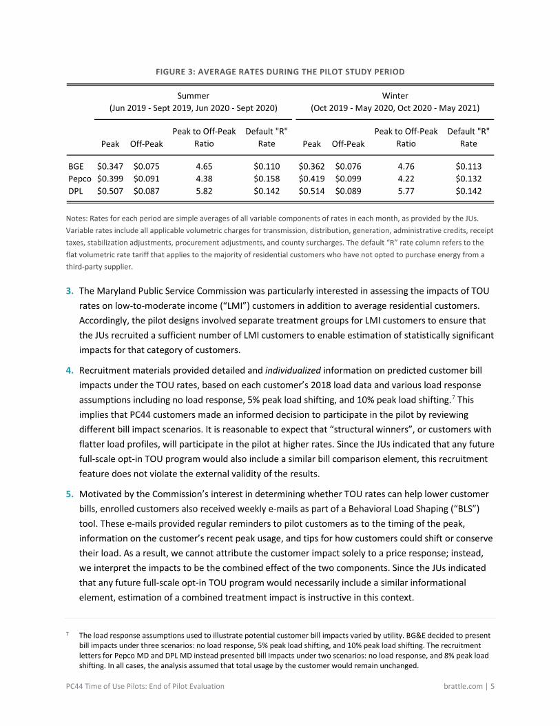
2. All-in peak rates faced by enrolled customers are between 4.4 and 5.8 times the off-peak rates, as summarized in Figure 3, and represent meaningful incentives for customers to shift their usage from peak to off-peak periods.
PC44 Time of Use Pilots: End of Pilot Evaluation brattle.com | 5
FIGURE 3: AVERAGE RATES DURING THE PILOT STUDY PERIOD
Summer (Jun 2019 - Sept 2019, Jun 2020 - Sept 2020)
Winter (Oct 2019 - May 2020, Oct 2020 - May 2021)
Peak Off-PeakPeak to Off-Peak
RatioDefault "R"
Rate Peak Off-PeakPeak to Off-Peak
RatioDefault "R"
Rate
BGE $0.347 $0.075 4.65 $0.110 $0.362 $0.076 4.76 $0.113Pepco $0.399 $0.091 4.38 $0.158 $0.419 $0.099 4.22 $0.132DPL $0.507 $0.087 5.82 $0.142 $0.514 $0.089 5.77 $0.142
Notes: Rates for each period are simple averages of all variable components of rates in each month, as provided by the JUs. Variable rates include all applicable volumetric charges for transmission, distribution, generation, administrative credits, receipt taxes, stabilization adjustments, procurement adjustments, and county surcharges. The default “R” rate column refers to the flat volumetric rate tariff that applies to the majority of residential customers who have not opted to purchase energy from a third-party supplier.
3. The Maryland Public Service Commission was particularly interested in assessing the impacts of TOU rates on low-to-moderate income (“LMI”) customers in addition to average residential customers. Accordingly, the pilot designs involved separate treatment groups for LMI customers to ensure that the JUs recruited a sufficient number of LMI customers to enable estimation of statistically significant impacts for that category of customers.
4. Recruitment materials provided detailed and individualized information on predicted customer bill impacts under the TOU rates, based on each customer’s 2018 load data and various load response assumptions including no load response, 5% peak load shifting, and 10% peak load shifting.7 This implies that PC44 customers made an informed decision to participate in the pilot by reviewing different bill impact scenarios. It is reasonable to expect that “structural winners”, or customers with flatter load profiles, will participate in the pilot at higher rates. Since the JUs indicated that any future full-scale opt-in TOU program would also include a similar bill comparison element, this recruitment feature does not violate the external validity of the results.
5. Motivated by the Commission’s interest in determining whether TOU rates can help lower customer bills, enrolled customers also received weekly e-mails as part of a Behavioral Load Shaping (“BLS”) tool. These e-mails provided regular reminders to pilot customers as to the timing of the peak, information on the customer’s recent peak usage, and tips for how customers could shift or conserve their load. As a result, we cannot attribute the customer impact solely to a price response; instead, we interpret the impacts to be the combined effect of the two components. Since the JUs indicated that any future full-scale opt-in TOU program would necessarily include a similar informational element, estimation of a combined treatment impact is instructive in this context.
7 The load response assumptions used to illustrate potential customer bill impacts varied by utility. BG&E decided to present
bill impacts under three scenarios: no load response, 5% peak load shifting, and 10% peak load shifting. The recruitment letters for Pepco MD and DPL MD instead presented bill impacts under two scenarios: no load response, and 8% peak load shifting. In all cases, the analysis assumed that total usage by the customer would remain unchanged.
PC44 Time of Use Pilots: End of Pilot Evaluation brattle.com | 6
C. Methodology _________
In the first year report, we described in detail the methodology that we used in estimating first year impacts. We will not repeat that full description here, but refer the reader to that report, which is publicly available.
We do highlight one addition to our methodology, in which we test for changes to the TOU impacts over time. Two full years of customer data under TOU rates allows for additional analysis. All things being equal, additional data should allow us to estimate more precisely the impact of the TOU pilot. In addition, the longer dataset allows us to test whether the impacts changed between Years 1 and 2 of the pilot. There are a number of behavioral reasons why the effects could have changed, including customer fatigue, customer learning, and the effects of the COVID-19 pandemic. We briefly describe each of these potential reasons in turn:
• Customer fatigue – It is plausible that as the pilot continued into Year 2, the pilot participants – all of whom had voluntarily opted in to the pilot – invested less effort into shifting or reducing their electricity usage, as the novelty of the pilot wore off.
• Customer learning – At the same time, it would not be surprising to see that some pilot participants become more adept at shifting or conserving electricity usage in response to the TOU pilot over time. In particular, since the current pilot involves the BLS tool, with regular communications suggesting strategies to shifting or reducing electricity usage, one could imagine that the customers’ ability to save on their electricity bills improves over time.
• COVID-19 – Finally, the advent of the COVID-19 pandemic in early 2020 could have affected customer response to the TOU rates as customer lifestyles have changed drastically since then. As we will demonstrate later in this report, the JUs’ residential electricity customers have generally changed their electricity usage patterns since the onset of the pandemic, as they began to spend more time at home. It is therefore possible that the impacts of the pilot would have been different under pandemic conditions, if, for example, customers spent more time at home during the peak summer hours during Year 2.
Unfortunately, it is not possible to disentangle these effects, since enrollment happened in a relatively short window (all customers’ first exposure to the TOU rates occurred in the same window between April and July of 2019), and COVID-19-related restrictions on movement and changes to daily schedules came into effect on a statewide basis at roughly the same time (March 2020). Accordingly, when we test for differences between the peak load impacts experienced during the first and second years of the study period, we are measuring the net effect of the factors described here, which is nevertheless of interest.
PC44 Time of Use Pilots: End of Pilot Evaluation brattle.com | 7
We carry out this analysis by introducing an augmented regression specification using an interaction term that measures the additive impact during year two.8 This additive impact can be either positive or negative, and consists of both a point estimate representing the difference between the average effect in years two and one, as well as a standard error, which allows for hypothesis testing. These parameters allow us to test whether there is sufficient evidence (beyond statistical noise) to conclude that the effects of the TOU pilot changed in its second year.
D. Description of Data _________
The first-year report also included a detailed description of the datasets that we use to evaluate the impacts of the pilot. We again refer the reader to that report for additional detail, and to Appendix A.2 of this report for additional detail on data cleaning and processing. However, we include in this report two updates to our discussion of the data: one with respect to enrollment and attrition and a one with respect to control group balance.
1. Enrollment and Attrition Summary
Our ability to quantify the impact of the pilot rates depends on having a large enough sample size to detect an average impact that stands out from inevitable variation or statistical “noise.” During the pilot design stage, we undertook statistical power calculations to determine the sample sizes required to estimate a minimum detectable peak impact of 6% at the 5% statistical significance and 80% power.9 The resulting sample size target was 700 customers for each of the LMI and non-LMI treatments, and for each of the JUs.10 While JUs were largely able to meet this target (with the exception of DPL), it is natural to observe some attrition during the pilot, for various reasons. Figure 4 below presents the cumulative attrition statistics over the course of the pilot. As of June 1, 2020 (the end of the Year 1 study period), 21% of BGE, 16% of Pepco and 15% of DPL treatment customers had left the pilot.
8 We described this interaction term technique in our Year One Evaluation (see p. 13 and equation 1’). In the Year One
Evaluation and in the current report, we also use this interaction term technique to test whether the TOU effects vary along certain measurable dimensions, including weather conditions and customer characteristics.
9 Note that these sample size assumptions are different from those filed in the EM&V report and have been revised following lower than expected initial recruitment statistics, by relaxing some of the earlier highly conservative assumptions.
Maps summarizing the geographic dispersion of recruited customers appear in Appendix A.1. 10 Our use of the term “non-LMI” refers to enrolled customers who indicated at the time of enrollment that their household
income exceeded the LMI threshold of $74,000. This LMI threshold, provided by the JUs, is equal to 80% of the median state income of $92,500 in 2017. See “Income Limits 2017,” Maryland Department of Housing and Community Development, at p. 2.
PC44 Time of Use Pilots: End of Pilot Evaluation brattle.com | 8
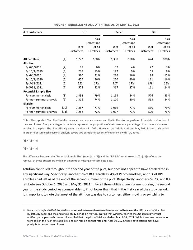
FIGURE 4: ENROLLMENT AND ATTRITION AS OF MAY 31, 2021
Notes: The reported “Enrolled” total includes all customers who ever enrolled in the pilot, regardless of the date or duration of their enrollment. The percentages in the table represent the proportion of customers as a percentage of customers who ever enrolled in the pilot. The pilot officially ended on March 31, 2021. However, we include April and May 2021 in our study period in order to ensure each seasonal analysis covers two complete seasons of experience with TOU rates.
[8] = [1] – [4]
[9] = [1] – [5]
The difference between the “Potential Sample Size” (rows [8] - [9]) and the “Eligible” totals (rows [10] - [11]) reflects the removal of those customers with high amounts of missing or incomplete data.
Attrition continued throughout the second year of the pilot, but does not appear to have accelerated in any significant way. Specifically, another 5% of BGE enrollees, 4% of Pepco enrollees, and 1% of DPL enrollees had left as of the end of the second summer of the pilot. Respectively, another 6%, 7%, and 8% left between October 1, 2020 and May 31, 2021.11 For all three utilities, unenrollment during the second year of the study period was comparable to, if not lower than, that in the first year of the study period. It is important to note that most of the attrition was due to customers either moving or switching to
11 Note that roughly half of the attrition observed between these two dates occurred between the official end of the pilot
(March 31, 2021) and the end of our study period on May 31. During that window, each of the JUs sent a letter that notified participants who were still enrolled that the pilot officially ended on March 31, 2021. While those customers who were still on the PC44 rate at pilot’s end can remain on that rate until April 30, 2022, those notifications may have precipitated some unenrollment.
# of customers BGE Pepco DPL
# of Customers
As a Percentage
of All Enrollees
# of Customers
As a Percentage
of All Enrollees
# of Customers
As a Percentage
of All Enrollees
All Enrollees [1] 1,772 100% 1,380 100% 674 100%Attrition
By 6/1/2019 [2] 98 6% 57 4% 22 3%By 10/1/2019 [3] 235 13% 127 9% 55 8%By 6/1/2020 [4] 380 21% 226 16% 98 15%By 10/1/2020 [5] 456 26% 270 20% 111 16%By 3/31/2021 [6] 522 29% 317 23% 139 21%By 5/31/2021 [7] 574 32% 367 27% 161 24%
Potential Sample SizeFor summer analysis [8] 1,392 79% 1,154 84% 576 85%For non-summer analysis [9] 1,316 74% 1,110 80% 563 84%
EligibleFor summer analysis [10] 1,357 77% 1,069 77% 530 79%For non-summer analysis [11] 1,282 72% 1,007 73% 509 76%
PC44 Time of Use Pilots: End of Pilot Evaluation brattle.com | 9
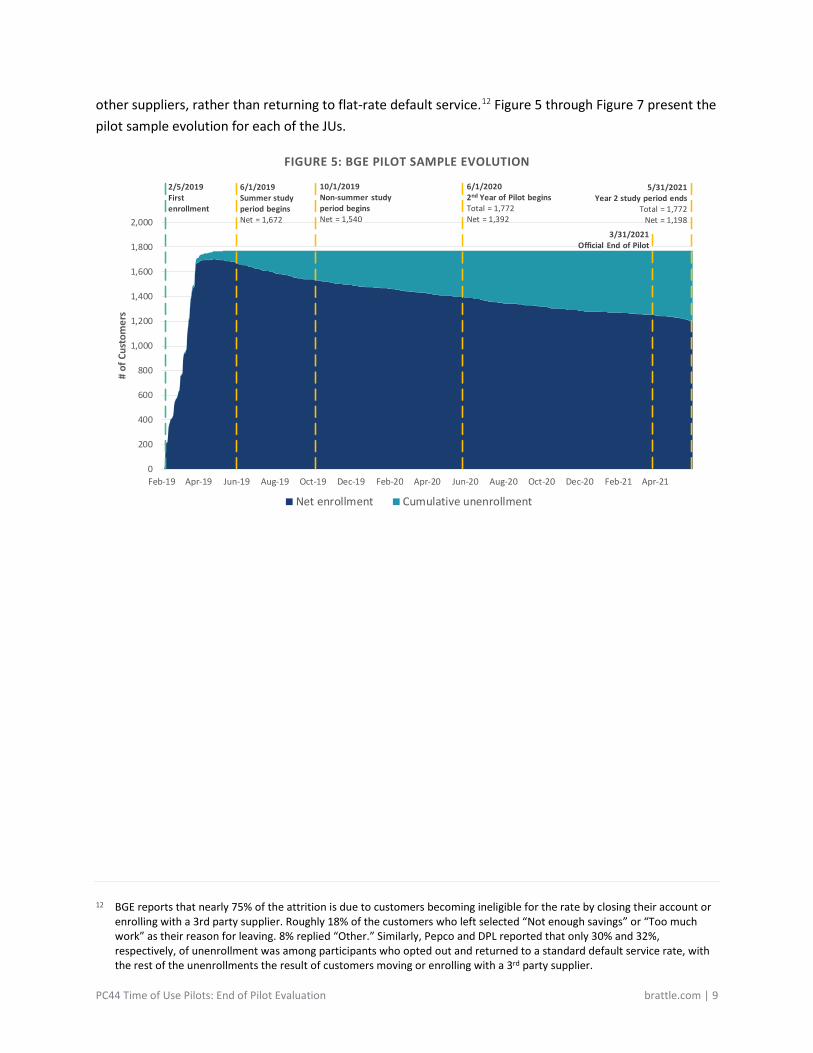
other suppliers, rather than returning to flat-rate default service.12 Figure 5 through Figure 7 present the pilot sample evolution for each of the JUs.
FIGURE 5: BGE PILOT SAMPLE EVOLUTION
12 BGE reports that nearly 75% of the attrition is due to customers becoming ineligible for the rate by closing their account or
enrolling with a 3rd party supplier. Roughly 18% of the customers who left selected “Not enough savings” or “Too much work” as their reason for leaving. 8% replied “Other.” Similarly, Pepco and DPL reported that only 30% and 32%, respectively, of unenrollment was among participants who opted out and returned to a standard default service rate, with the rest of the unenrollments the result of customers moving or enrolling with a 3rd party supplier.
0
200
400
600
800
1,000
1,200
1,400
1,600
1,800
2,000
Feb-19 Apr-19 Jun-19 Aug-19 Oct-19 Dec-19 Feb-20 Apr-20 Jun-20 Aug-20 Oct-20 Dec-20 Feb-21 Apr-21
# of
Cus
tom
ers
Net enrollment Cumulative unenrollment
10/1/2019 Non-summer study period beginsNet = 1,540
6/1/20202nd Year of Pilot beginsTotal = 1,772Net = 1,392
2/5/2019First enrollment
6/1/2019 Summer study period beginsNet = 1,672
5/31/2021Year 2 study period ends
Total = 1,772Net = 1,198
3/31/2021Official End of Pilot
PC44 Time of Use Pilots: End of Pilot Evaluation brattle.com | 10
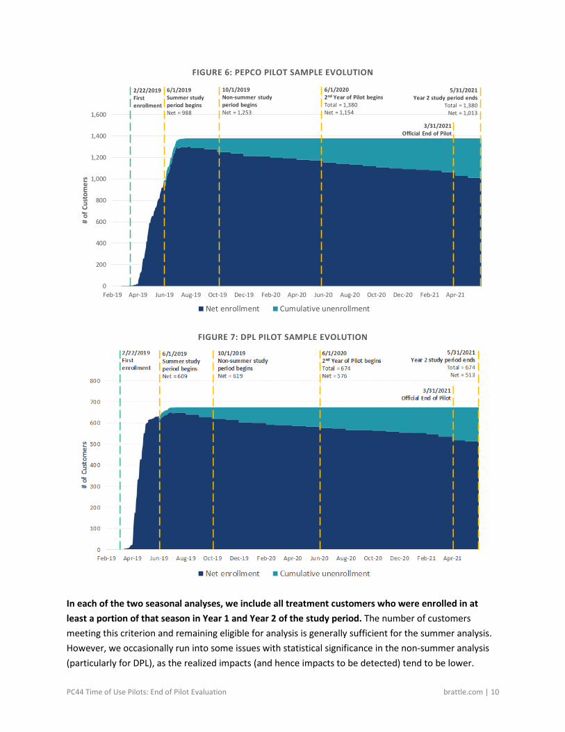
FIGURE 6: PEPCO PILOT SAMPLE EVOLUTION
FIGURE 7: DPL PILOT SAMPLE EVOLUTION
In each of the two seasonal analyses, we include all treatment customers who were enrolled in at least a portion of that season in Year 1 and Year 2 of the study period. The number of customers meeting this criterion and remaining eligible for analysis is generally sufficient for the summer analysis. However, we occasionally run into some issues with statistical significance in the non-summer analysis (particularly for DPL), as the realized impacts (and hence impacts to be detected) tend to be lower.
0
200
400
600
800
1,000
1,200
1,400
1,600
Feb-19 Apr-19 Jun-19 Aug-19 Oct-19 Dec-19 Feb-20 Apr-20 Jun-20 Aug-20 Oct-20 Dec-20 Feb-21 Apr-21
# of
Cus
tom
ers
Net enrollment Cumulative unenrollment
10/1/2019 Non-summer study period beginsNet = 1,253
6/1/20202nd Year of Pilot beginsTotal = 1,380Net = 1,154
2/22/2019First enrollment
6/1/2019 Summer study period beginsNet = 988
5/31/2021Year 2 study period ends
Total = 1,380Net = 1,013
3/31/2021Official End of Pilot

PC44 Time of Use Pilots: End of Pilot Evaluation brattle.com | 11
2. Control Group Balance
The customer sample we use to evaluate the effects of the pilot consists of two groups of customers:
• those pilot customers who were enrolled in the pilot for a significant amount of time and for whom load data is of sufficiently high quality; and
• a set of matched control customers who, based on pre-pilot observable data including hourly load and various demographic and utility participation variables, are as similar as possible to our treatment group. This group is comprised of the single closest match to each pilot participant included in the group described in the previous bullet.13
While the approach remains unchanged, the sample of customers whose data we use to conduct our analysis has changed in some minor ways since the completion of the first report. First, as described above, there has been some limited attrition of pilot customers since the inception of the pilot. Second, a number of control customers (roughly 10% of the matched controls used in the analysis underlying our Year One Evaluation) who were matched in the Year 1 analysis have since moved out of their homes or switched to a retail supplier, thereby making them “ineligible” as control customers. For each pilot customer who lost their matched control, we identify the remaining eligible control customer who is most similar, using the propensity score methodology described in our Year One Evaluation.
In order to ensure that these changes to the set of customers we use to evaluate the pilot impacts do not compromise the validity of the control group used to represent the “but-for” usage of the treatment customers, we repeat the balancing diagnostics we provided in the Year One Evaluation, applied to the updated customer sample. The following charts and tables confirm that the objective of the matching analysis is maintained with this updated sample.
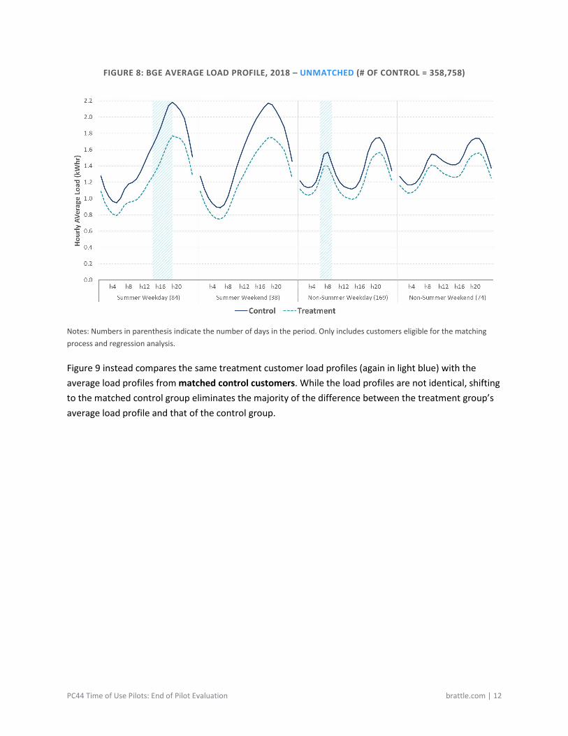
First, for each utility, we present two graphs. Beginning with BGE, Figure 8 compares the average load profiles of the “treatment” customers in light blue with the average load profiles of all potential control customers (residential customers who the utility did not approach about the pilot) in dark blue. The figure depicts four such average load profiles, one for each combination of season (summer or non-summer) and day type (weekdays and weekends). While the shape of the load profiles of the potential control group is similar to that of the treatment group, the average load is uniformly higher than that of the treatment group, indicating that there are some substantial differences between the two groups.
13 A more detailed description of the matching methodology appears in the Year One Evaluation, at pp. 10-11.
PC44 Time of Use Pilots: End of Pilot Evaluation brattle.com | 12
FIGURE 8: BGE AVERAGE LOAD PROFILE, 2018 – UNMATCHED (# OF CONTROL = 358,758)
Notes: Numbers in parenthesis indicate the number of days in the period. Only includes customers eligible for the matching process and regression analysis.
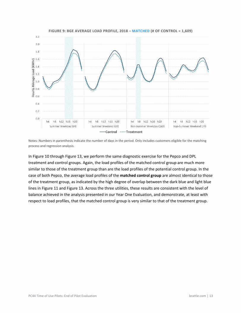
Figure 9 instead compares the same treatment customer load profiles (again in light blue) with the average load profiles from matched control customers. While the load profiles are not identical, shifting to the matched control group eliminates the majority of the difference between the treatment group’s average load profile and that of the control group.
PC44 Time of Use Pilots: End of Pilot Evaluation brattle.com | 13
FIGURE 9: BGE AVERAGE LOAD PROFILE, 2018 – MATCHED (# OF CONTROL = 1,609)
Notes: Numbers in parenthesis indicate the number of days in the period. Only includes customers eligible for the matching process and regression analysis.
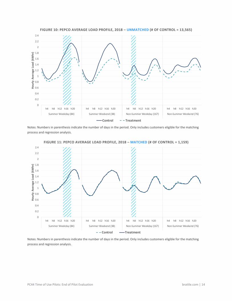
In Figure 10 through Figure 13, we perform the same diagnostic exercise for the Pepco and DPL treatment and control groups. Again, the load profiles of the matched control group are much more similar to those of the treatment group than are the load profiles of the potential control group. In the case of both Pepco, the average load profiles of the matched control group are almost identical to those of the treatment group, as indicated by the high degree of overlap between the dark blue and light blue lines in Figure 11 and Figure 13. Across the three utilities, these results are consistent with the level of balance achieved in the analysis presented in our Year One Evaluation, and demonstrate, at least with respect to load profiles, that the matched control group is very similar to that of the treatment group.
PC44 Time of Use Pilots: End of Pilot Evaluation brattle.com | 14
FIGURE 10: PEPCO AVERAGE LOAD PROFILE, 2018 – UNMATCHED (# OF CONTROL = 13,565)
Notes: Numbers in parenthesis indicate the number of days in the period. Only includes customers eligible for the matching process and regression analysis.
FIGURE 11: PEPCO AVERAGE LOAD PROFILE, 2018 – MATCHED (# OF CONTROL = 1,159)
Notes: Numbers in parenthesis indicate the number of days in the period. Only includes customers eligible for the matching process and regression analysis.
0
0.2
0.4
0.6
0.8
1
1.2
1.4
1.6
1.8
2
2.2
2.4
h4 h8 h12 h16 h20 h4 h8 h12 h16 h20 h4 h8 h12 h16 h20 h4 h8 h12 h16 h20
Summer Weekday (84) Summer Weekend (38) Non-Summer Weekday (167) Non-Summer Weekend (76)
Hour
ly A
vera
ge L
oad
(kW
hr)
Control Treatment
0
0.2
0.4
0.6
0.8
1
1.2
1.4
1.6
1.8
2
2.2
2.4
h4 h8 h12 h16 h20 h4 h8 h12 h16 h20 h4 h8 h12 h16 h20 h4 h8 h12 h16 h20
Summer Weekday (84) Summer Weekend (38) Non-Summer Weekday (167) Non-Summer Weekend (76)
Hour
ly A
vera
ge L
oad
(kW
hr)
Control Treatment
PC44 Time of Use Pilots: End of Pilot Evaluation brattle.com | 15
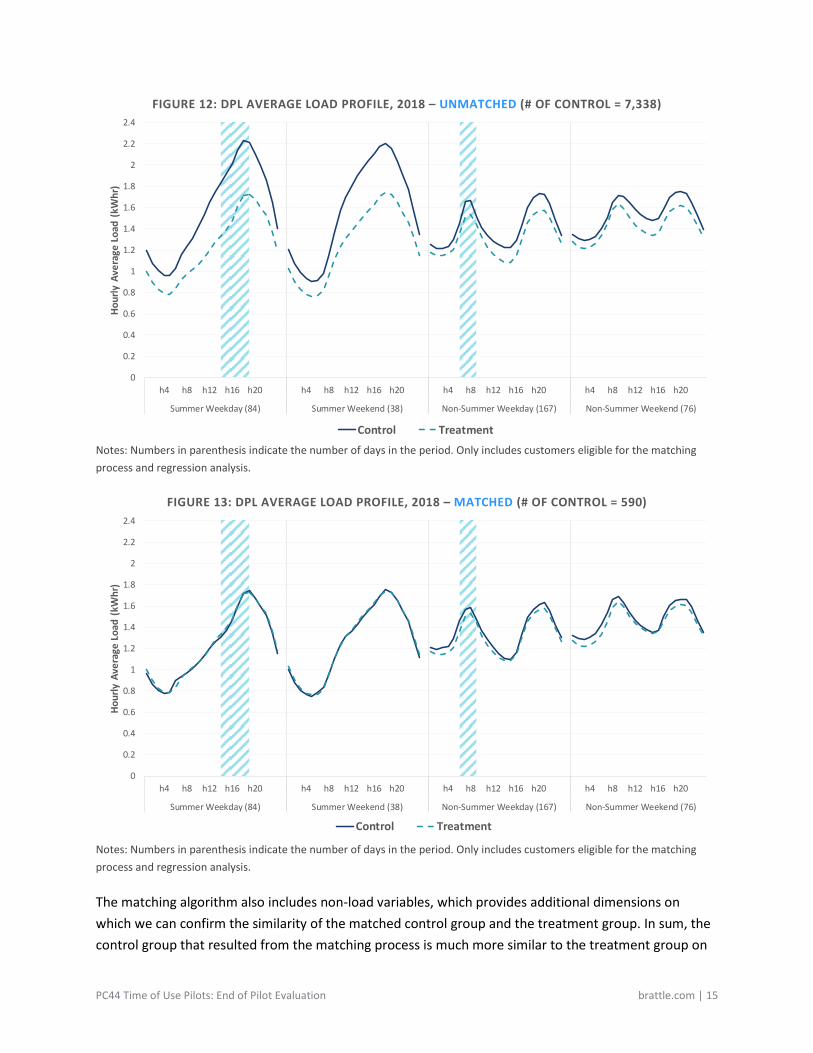
FIGURE 12: DPL AVERAGE LOAD PROFILE, 2018 – UNMATCHED (# OF CONTROL = 7,338)
Notes: Numbers in parenthesis indicate the number of days in the period. Only includes customers eligible for the matching process and regression analysis.
FIGURE 13: DPL AVERAGE LOAD PROFILE, 2018 – MATCHED (# OF CONTROL = 590)
Notes: Numbers in parenthesis indicate the number of days in the period. Only includes customers eligible for the matching process and regression analysis.
The matching algorithm also includes non-load variables, which provides additional dimensions on which we can confirm the similarity of the matched control group and the treatment group. In sum, the control group that resulted from the matching process is much more similar to the treatment group on
0
0.2
0.4
0.6
0.8
1
1.2
1.4
1.6
1.8
2
2.2
2.4
h4 h8 h12 h16 h20 h4 h8 h12 h16 h20 h4 h8 h12 h16 h20 h4 h8 h12 h16 h20
Summer Weekday (84) Summer Weekend (38) Non-Summer Weekday (167) Non-Summer Weekend (76)
Hour
ly A
vera
ge L
oad
(kW
hr)
Control Treatment
0
0.2
0.4
0.6
0.8
1
1.2
1.4
1.6
1.8
2
2.2
2.4
h4 h8 h12 h16 h20 h4 h8 h12 h16 h20 h4 h8 h12 h16 h20 h4 h8 h12 h16 h20
Summer Weekday (84) Summer Weekend (38) Non-Summer Weekday (167) Non-Summer Weekend (76)
Hour
ly A
vera
ge L
oad
(kW
hr)
Control Treatment
PC44 Time of Use Pilots: End of Pilot Evaluation brattle.com | 16
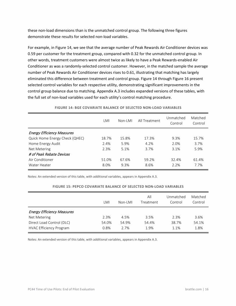
these non-load dimensions than is the unmatched control group. The following three figures demonstrate these results for selected non-load variables.
For example, in Figure 14, we see that the average number of Peak Rewards Air Conditioner devices was 0.59 per customer for the treatment group, compared with 0.32 for the unmatched control group. In other words, treatment customers were almost twice as likely to have a Peak Rewards-enabled Air Conditioner as was a randomly-selected control customer. However, in the matched sample the average number of Peak Rewards Air Conditioner devices rises to 0.61, illustrating that matching has largely eliminated this difference between treatment and control group. Figure 14 through Figure 16 present selected control variables for each respective utility, demonstrating significant improvements in the control group balance due to matching. Appendix A.3 includes expanded versions of these tables, with the full set of non-load variables used for each utility’s control matching procedure.
FIGURE 14: BGE COVARIATE BALANCE OF SELECTED NON-LOAD VARIABLES
Notes: An extended version of this table, with additional variables, appears in Appendix A.3.
FIGURE 15: PEPCO COVARIATE BALANCE OF SELECTED NON-LOAD VARIABLES
Notes: An extended version of this table, with additional variables, appears in Appendix A.3.
LMI Non-LMI All Treatment Unmatched
ControlMatched Control
Energy Efficiency MeasuresQuick Home Energy Check (QHEC) 18.7% 15.8% 17.3% 9.3% 15.7%Home Energy Audit 2.4% 5.9% 4.2% 2.0% 3.7%Net Metering 2.3% 5.1% 3.7% 3.1% 5.9%# of Peak Rebate DevicesAir Conditioner 51.0% 67.6% 59.2% 32.4% 61.4%Water Heater 8.0% 9.3% 8.6% 2.2% 7.7%
LMI Non-LMIAll
Treatment Unmatched
ControlMatched Control
Energy Efficiency MeasuresNet Metering 2.3% 4.5% 3.5% 2.3% 3.6%Direct Load Control (DLC) 54.0% 54.9% 54.4% 38.7% 54.1%HVAC Efficiency Program 0.8% 2.7% 1.9% 1.1% 1.8%

PC44 Time of Use Pilots: End of Pilot Evaluation brattle.com | 17
FIGURE 16: DPL COVARIATE BALANCE OF SELECTED NON-LOAD VARIABLES
Notes: An extended version of this table, with additional variables, appears in Appendix A.3.
II. Two-Year Pilot Impact Evaluation Results _________
A. Introduction In this section, we present the results of our impact evaluation, covering the entire two-year study period. This section is primarily organized by utility, and by season within each utility subsection. For each utility, we focus on the impact results from our preferred econometric specification and dataset.14 In each utility sub-section, we also test for differences in the impacts between the first and second years of the pilot, as described above in the methodology section. For each utility, we also present a series of “subgroup analyses” that investigate how the peak weekday impact results differ across various periods and customer groups.
After discussing the impact results for each utility, we also briefly discuss the implications for the pilot from the COVID-19 pandemic, which undoubtedly had effects on the electricity consumption of Maryland customers, as we will demonstrate. Finally, we will discuss the results of our price elasticity analysis.
Before discussing the results, a brief reminder of the expected impacts of TOU rates is appropriate. Broadly speaking, we expect the significantly higher peak prices experienced by TOU customers to induce them to lower their consumption in peak hours, relative to what they would have consumed on a flat rate. At the same time, we generally expect the lower prices faced by TOU customers in the off-peak period to induce additional consumption, again relative to what they would have consumed on a flat rate. The extent to which these predictions are borne out depends on the relative magnitude of the peak to off-peak differential, but also on the price responsiveness of electricity customers. Total
14 To test the sensitivity of our main impact results, we estimate several alternative specifications. While the results of these
sensitivity specifications differ somewhat from our primary results, any differences are modest; the sensitivity results are broadly supportive of the same fundamental conclusions from the results presented here. These sensitivity results are presented in the Appendix A.8.
LMI Non-LMIAll
Treatment Unmatched
ControlMatched Control
Energy Efficiency MeasuresNet Metering 2.7% 4.8% 3.5% 1.2% 4.3%Direct Load Control (DLC) 36.8% 47.6% 40.9% 18.8% 40.1%Appliance Recycle 0.2% 1.6% 0.8% 0.3% 0.9%

PC44 Time of Use Pilots: End of Pilot Evaluation brattle.com | 18
consumption can decrease, increase, or remain more or less unchanged, depending on factors including relative prices, the length of the peak windows, and other factors already discussed. In the PC44 TOU pilots, the presence of the behavioral load shaping (“BLS”) tool and information provision to the customers add an additional factor that is of particular interest.
For simplicity and clarity, in the exposition that follows, we illustrate the key impacts of our econometric analysis in a graphical format. In the graphs that follow, the error bars denote the 95% confidence interval of the estimated impact. This provides a sense of the precision of each of our estimates; roughly speaking we can be 95% confident that the true effect of the treatment lies within the range depicted by the error bar.15 Relatedly, when the column depicting a point estimate is shaded gray, the 95% confidence interval includes zero, indicating a lack of statistical significance for that impact estimate. In other words, for impact estimates that are “grayed out,” we are less than 95% confident that there is a measurable effect of the pilot for that customer group and time period.
For those readers who are interested in the econometric details, the underlying regression tables are available in Appendix A.4 and A.5. Estimated impacts, including confidence intervals, appear in Appendix A.6, while sensitivity analyses appear in Appendix A.8.
B. Baltimore Gas & Electric
1. Main Impact Results
i. Summer Analysis
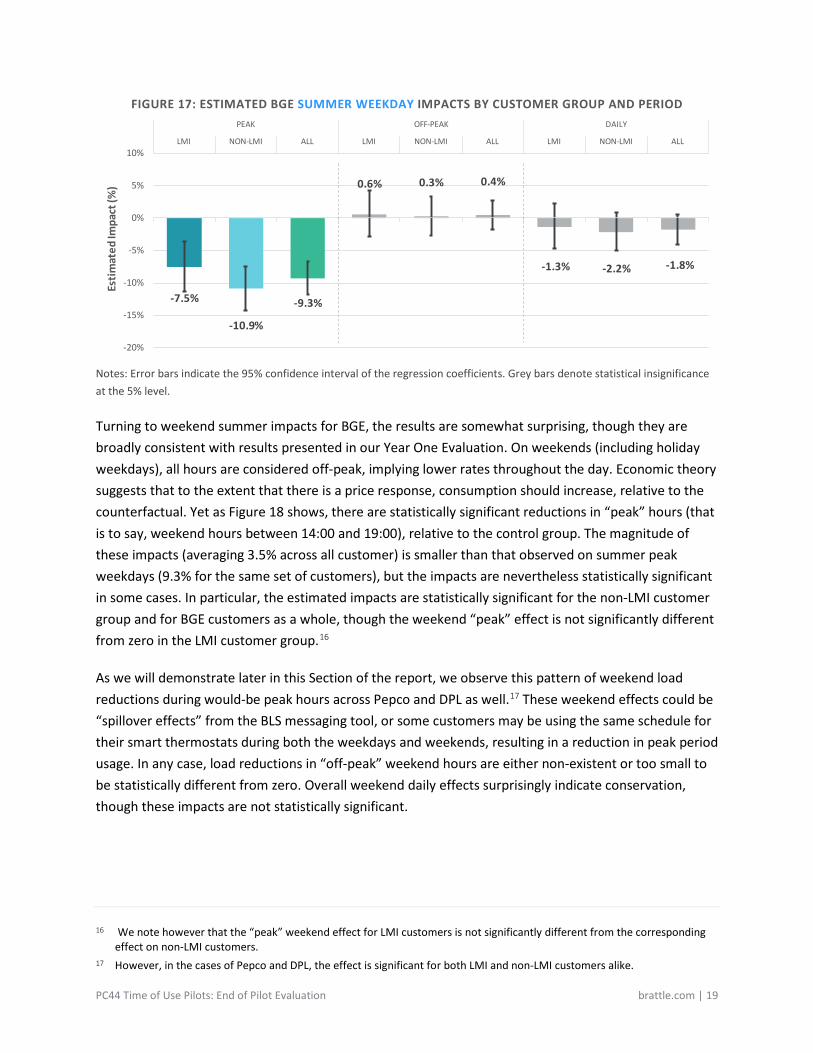
We begin our discussion of the primary impact results by presenting the summer results for BGE, which we summarize in Figure 17. Across the two-year study period, weekday peak impacts across all pilot customers averaged a 9.3% reduction. This is in effect a weighted average of the LMI peak load reduction (7.5%) and the non-LMI peak load reduction (10.9%). This is an important finding; the LMI impact itself is statistically different from zero, and the difference between the LMI and non-LMI groups is not statistically significant. The left-most panel of Figure 17 presents these weekday peak impacts.
At the same time, as the middle panel of Figure 17 indicates, we find little evidence that BGE treatment customers (regardless of household income level) altered their weekday off-peak consumption in response to the TOU pilot. In aggregate, as depicted in the right-most panel of Figure 17, there was some conservation on weekdays. On average, the pilot reduced customers’ summer weekday consumption by 1.8%, an effect that was not statistically significant, whether for the full set of BGE customers or either customer sub-group.
15 As described above, the treatment is a move from the pre-pilot rate to the TOU rate, in conjunction with the information
provided by the BLS tool.
PC44 Time of Use Pilots: End of Pilot Evaluation brattle.com | 19
FIGURE 17: ESTIMATED BGE SUMMER WEEKDAY IMPACTS BY CUSTOMER GROUP AND PERIOD
Notes: Error bars indicate the 95% confidence interval of the regression coefficients. Grey bars denote statistical insignificance at the 5% level.
Turning to weekend summer impacts for BGE, the results are somewhat surprising, though they are broadly consistent with results presented in our Year One Evaluation. On weekends (including holiday weekdays), all hours are considered off-peak, implying lower rates throughout the day. Economic theory suggests that to the extent that there is a price response, consumption should increase, relative to the counterfactual. Yet as Figure 18 shows, there are statistically significant reductions in “peak” hours (that is to say, weekend hours between 14:00 and 19:00), relative to the control group. The magnitude of these impacts (averaging 3.5% across all customer) is smaller than that observed on summer peak weekdays (9.3% for the same set of customers), but the impacts are nevertheless statistically significant in some cases. In particular, the estimated impacts are statistically significant for the non-LMI customer group and for BGE customers as a whole, though the weekend “peak” effect is not significantly different from zero in the LMI customer group.16
As we will demonstrate later in this Section of the report, we observe this pattern of weekend load reductions during would-be peak hours across Pepco and DPL as well.17 These weekend effects could be “spillover effects” from the BLS messaging tool, or some customers may be using the same schedule for their smart thermostats during both the weekdays and weekends, resulting in a reduction in peak period usage. In any case, load reductions in “off-peak” weekend hours are either non-existent or too small to be statistically different from zero. Overall weekend daily effects surprisingly indicate conservation, though these impacts are not statistically significant.
16 We note however that the “peak” weekend effect for LMI customers is not significantly different from the corresponding
effect on non-LMI customers. 17 However, in the cases of Pepco and DPL, the effect is significant for both LMI and non-LMI customers alike.
-7.5%
-10.9%
-9.3%
0.6% 0.3% 0.4%
-1.3% -2.2% -1.8%
-20%
-15%
-10%
-5%
0%
5%
10%LMI NON-LMI ALL LMI NON-LMI ALL LMI NON-LMI ALL
PEAK OFF-PEAK DAILYEs
timat
ed Im
pact
(%)

PC44 Time of Use Pilots: End of Pilot Evaluation brattle.com | 20
FIGURE 18: ESTIMATED BGE SUMMER WEEKEND IMPACTS BY CUSTOMER GROUP AND PERIOD
Notes: Error bars indicate the 95% confidence interval of the regression coefficients. Grey bars denote statistical insignificance at the 5% level.
ii. Non-summer Analysis
On October 1, 2019, the pilot rates changed, along with the definition of the peak. The peak moved from a five-hour period covering the afternoon and early evening in the summer to a 3-hour window, again on weekdays, covering the hours 6 AM to 9 AM. This new rate schedule was in effect from October 1, 2019 through May 31, 2020, and again during the corresponding dates during the second year of the study period.
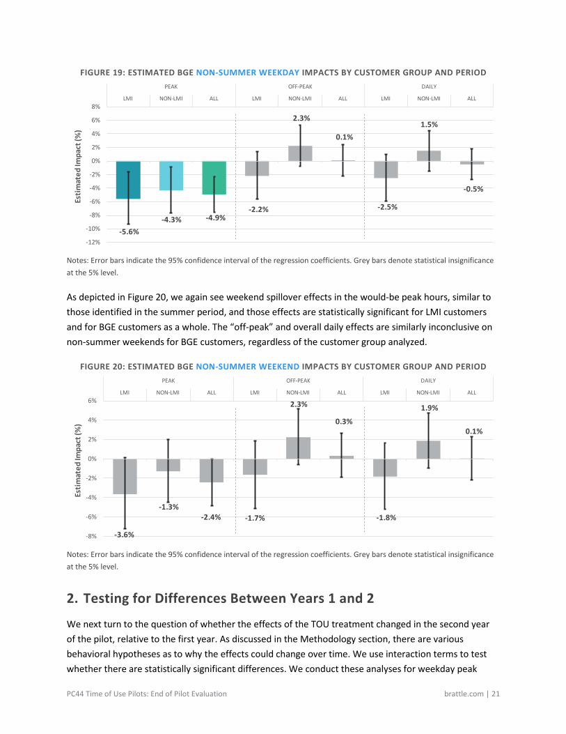
In the non-summer period, the weekday peak impacts experienced by BGE pilot customers were lower than those experienced in the summer. The average impact for pilot customers was a 4.9% reduction, as displayed in Figure 19. Here, the 5.6% estimated reduction for LMI customers is actually larger than the 4.3% reduction for non-LMI customers, though the difference between the two groups is not statistically significant. For both groups, as well as for pilot customers as a whole, the estimated effects are significantly different from zero. The off-peak and daily conservation impacts are generally not statistically significant; there are no conclusive effects with respect to either off-peak or overall impact reductions on non-summer weekdays.
-2.8% -4.1%-3.5%
0.8%
-0.4%
0.2%
-0.1% -1.2%-0.6%
-8%
-6%
-4%
-2%
0%
2%
4%
6%LMI NON-LMI ALL LMI NON-LMI ALL LMI NON-LMI ALL
PEAK OFF-PEAK DAILYEs
timat
ed Im
pact
(%)
PC44 Time of Use Pilots: End of Pilot Evaluation brattle.com | 21
FIGURE 19: ESTIMATED BGE NON-SUMMER WEEKDAY IMPACTS BY CUSTOMER GROUP AND PERIOD
Notes: Error bars indicate the 95% confidence interval of the regression coefficients. Grey bars denote statistical insignificance at the 5% level.
As depicted in Figure 20, we again see weekend spillover effects in the would-be peak hours, similar to those identified in the summer period, and those effects are statistically significant for LMI customers and for BGE customers as a whole. The “off-peak” and overall daily effects are similarly inconclusive on non-summer weekends for BGE customers, regardless of the customer group analyzed.
FIGURE 20: ESTIMATED BGE NON-SUMMER WEEKEND IMPACTS BY CUSTOMER GROUP AND PERIOD
Notes: Error bars indicate the 95% confidence interval of the regression coefficients. Grey bars denote statistical insignificance at the 5% level.
2. Testing for Differences Between Years 1 and 2
We next turn to the question of whether the effects of the TOU treatment changed in the second year of the pilot, relative to the first year. As discussed in the Methodology section, there are various behavioral hypotheses as to why the effects could change over time. We use interaction terms to test whether there are statistically significant differences. We conduct these analyses for weekday peak
-5.6%-4.3% -4.9%
-2.2%
2.3%
0.1%
-2.5%
1.5%
-0.5%
-12%
-10%
-8%
-6%
-4%
-2%
0%
2%
4%
6%
8%LMI NON-LMI ALL LMI NON-LMI ALL LMI NON-LMI ALL
PEAK OFF-PEAK DAILYEs
timat
ed Im
pact
(%)
-3.6%
-1.3%-2.4% -1.7%
2.3%
0.3%
-1.8%
1.9%
0.1%
-8%
-6%
-4%
-2%
0%
2%
4%
6%LMI NON-LMI ALL LMI NON-LMI ALL LMI NON-LMI ALL
PEAK OFF-PEAK DAILY
Estim
ated
Impa
ct (%
)
PC44 Time of Use Pilots: End of Pilot Evaluation brattle.com | 22
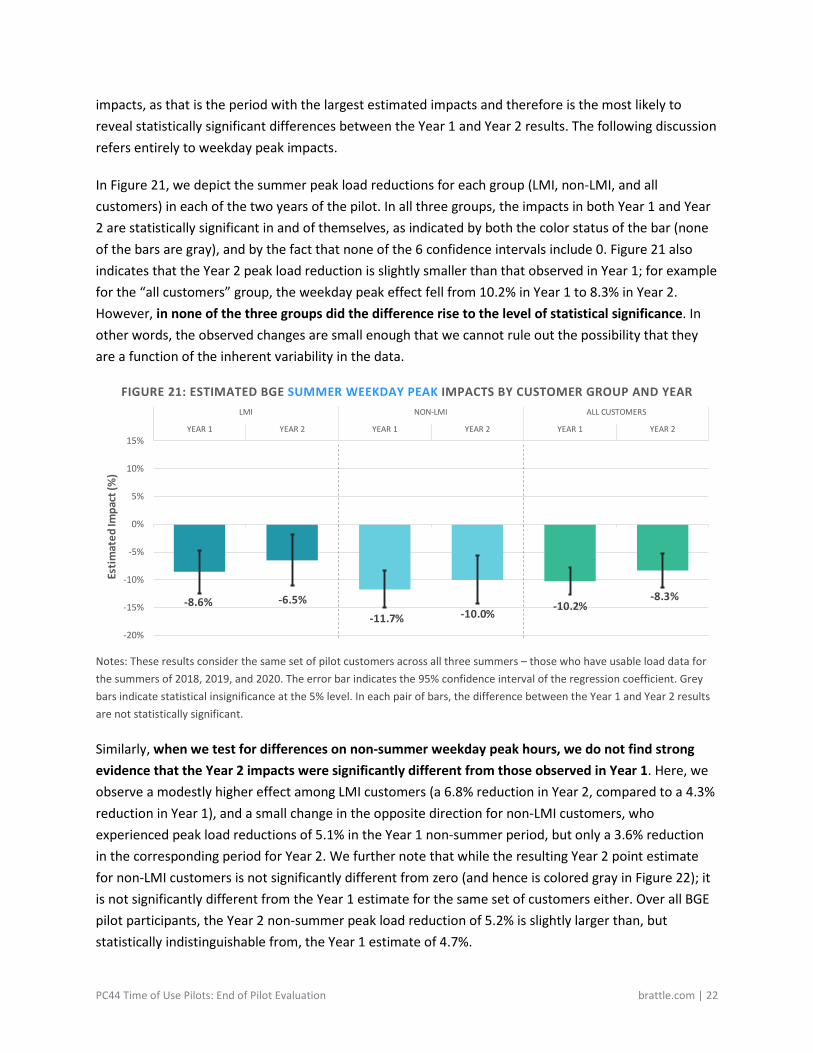
impacts, as that is the period with the largest estimated impacts and therefore is the most likely to reveal statistically significant differences between the Year 1 and Year 2 results. The following discussion refers entirely to weekday peak impacts.
In Figure 21, we depict the summer peak load reductions for each group (LMI, non-LMI, and all customers) in each of the two years of the pilot. In all three groups, the impacts in both Year 1 and Year 2 are statistically significant in and of themselves, as indicated by both the color status of the bar (none of the bars are gray), and by the fact that none of the 6 confidence intervals include 0. Figure 21 also indicates that the Year 2 peak load reduction is slightly smaller than that observed in Year 1; for example for the “all customers” group, the weekday peak effect fell from 10.2% in Year 1 to 8.3% in Year 2. However, in none of the three groups did the difference rise to the level of statistical significance. In other words, the observed changes are small enough that we cannot rule out the possibility that they are a function of the inherent variability in the data.
FIGURE 21: ESTIMATED BGE SUMMER WEEKDAY PEAK IMPACTS BY CUSTOMER GROUP AND YEAR
Notes: These results consider the same set of pilot customers across all three summers – those who have usable load data for the summers of 2018, 2019, and 2020. The error bar indicates the 95% confidence interval of the regression coefficient. Grey bars indicate statistical insignificance at the 5% level. In each pair of bars, the difference between the Year 1 and Year 2 results are not statistically significant.
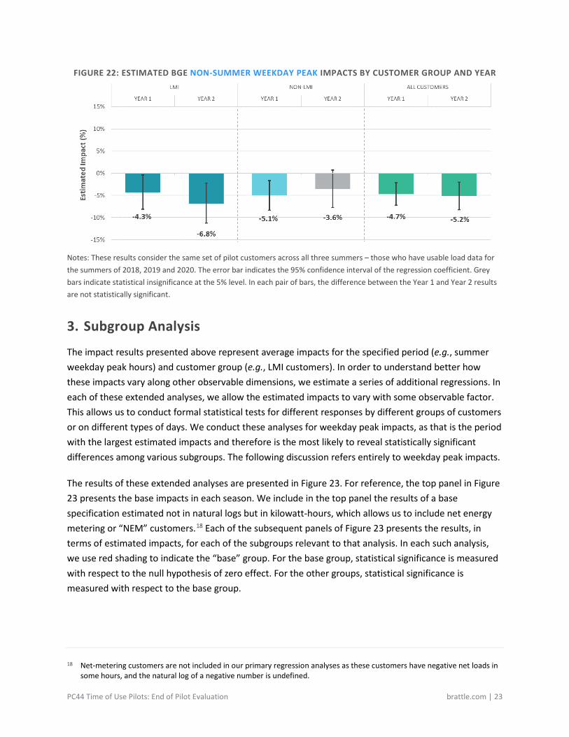
Similarly, when we test for differences on non-summer weekday peak hours, we do not find strong evidence that the Year 2 impacts were significantly different from those observed in Year 1. Here, we observe a modestly higher effect among LMI customers (a 6.8% reduction in Year 2, compared to a 4.3% reduction in Year 1), and a small change in the opposite direction for non-LMI customers, who experienced peak load reductions of 5.1% in the Year 1 non-summer period, but only a 3.6% reduction in the corresponding period for Year 2. We further note that while the resulting Year 2 point estimate for non-LMI customers is not significantly different from zero (and hence is colored gray in Figure 22); it is not significantly different from the Year 1 estimate for the same set of customers either. Over all BGE pilot participants, the Year 2 non-summer peak load reduction of 5.2% is slightly larger than, but statistically indistinguishable from, the Year 1 estimate of 4.7%.
-8.6% -6.5%-11.7% -10.0%
-10.2%-8.3%
-20%
-15%
-10%
-5%
0%
5%
10%
15%YEAR 1 YEAR 2 YEAR 1 YEAR 2 YEAR 1 YEAR 2
LMI NON-LMI ALL CUSTOMERS
Estim
ated
Impa
ct (%
)
PC44 Time of Use Pilots: End of Pilot Evaluation brattle.com | 23
FIGURE 22: ESTIMATED BGE NON-SUMMER WEEKDAY PEAK IMPACTS BY CUSTOMER GROUP AND YEAR
Notes: These results consider the same set of pilot customers across all three summers – those who have usable load data for the summers of 2018, 2019 and 2020. The error bar indicates the 95% confidence interval of the regression coefficient. Grey bars indicate statistical insignificance at the 5% level. In each pair of bars, the difference between the Year 1 and Year 2 results are not statistically significant.
3. Subgroup Analysis
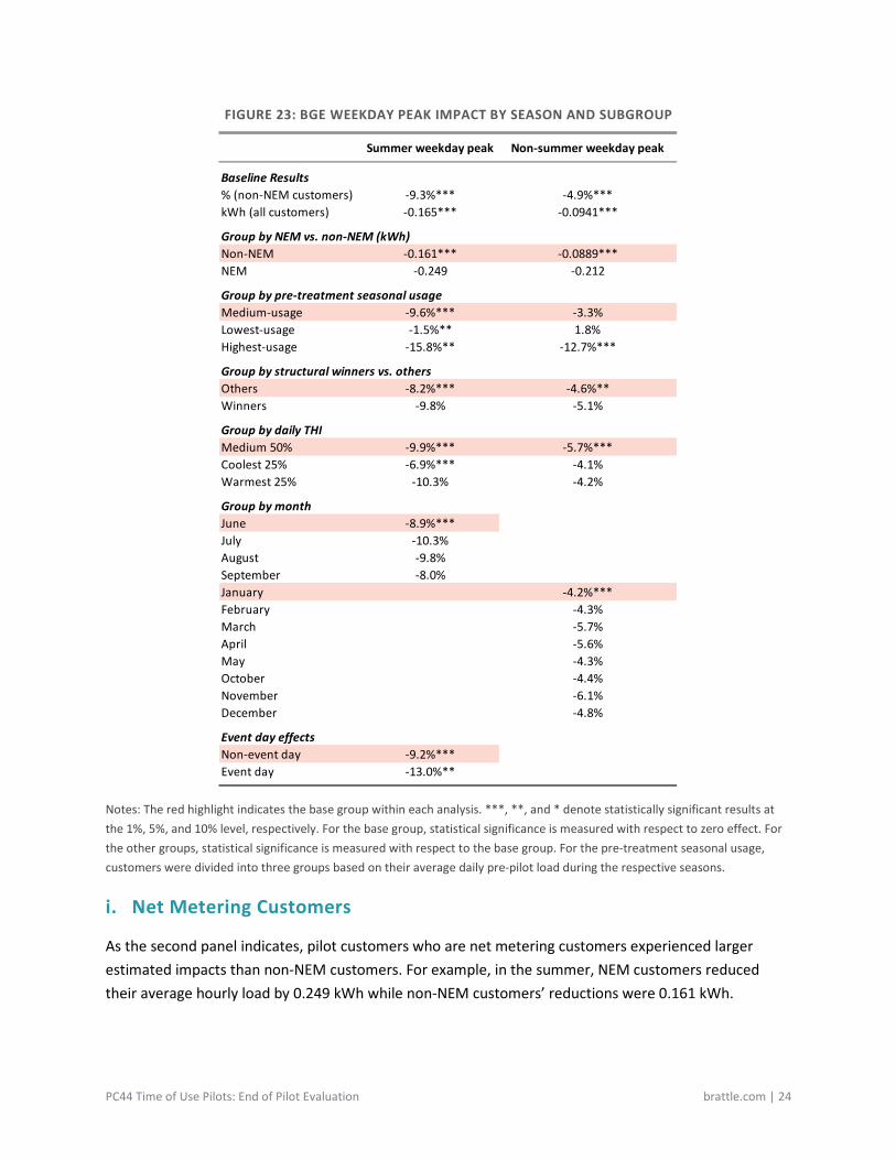
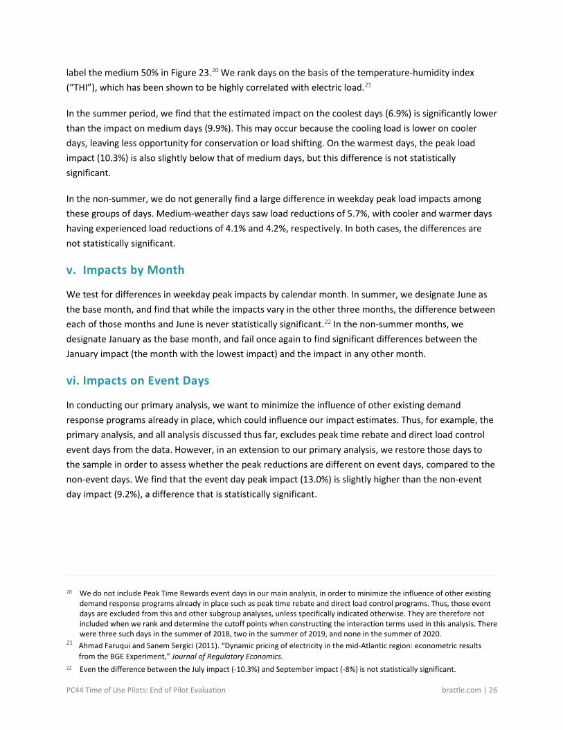
The impact results presented above represent average impacts for the specified period (e.g., summer weekday peak hours) and customer group (e.g., LMI customers). In order to understand better how these impacts vary along other observable dimensions, we estimate a series of additional regressions. In each of these extended analyses, we allow the estimated impacts to vary with some observable factor. This allows us to conduct formal statistical tests for different responses by different groups of customers or on different types of days. We conduct these analyses for weekday peak impacts, as that is the period with the largest estimated impacts and therefore is the most likely to reveal statistically significant differences among various subgroups. The following discussion refers entirely to weekday peak impacts.
The results of these extended analyses are presented in Figure 23. For reference, the top panel in Figure 23 presents the base impacts in each season. We include in the top panel the results of a base specification estimated not in natural logs but in kilowatt-hours, which allows us to include net energy metering or “NEM” customers.18 Each of the subsequent panels of Figure 23 presents the results, in terms of estimated impacts, for each of the subgroups relevant to that analysis. In each such analysis, we use red shading to indicate the “base” group. For the base group, statistical significance is measured with respect to the null hypothesis of zero effect. For the other groups, statistical significance is measured with respect to the base group.
18 Net-metering customers are not included in our primary regression analyses as these customers have negative net loads in
some hours, and the natural log of a negative number is undefined.
PC44 Time of Use Pilots: End of Pilot Evaluation brattle.com | 24
FIGURE 23: BGE WEEKDAY PEAK IMPACT BY SEASON AND SUBGROUP
Notes: The red highlight indicates the base group within each analysis. ***, **, and * denote statistically significant results at the 1%, 5%, and 10% level, respectively. For the base group, statistical significance is measured with respect to zero effect. For the other groups, statistical significance is measured with respect to the base group. For the pre-treatment seasonal usage, customers were divided into three groups based on their average daily pre-pilot load during the respective seasons.
i. Net Metering Customers
As the second panel indicates, pilot customers who are net metering customers experienced larger estimated impacts than non-NEM customers. For example, in the summer, NEM customers reduced their average hourly load by 0.249 kWh while non-NEM customers’ reductions were 0.161 kWh.
Summer weekday peak Non-summer weekday peak
Baseline Results% (non-NEM customers) -9.3%*** -4.9%***kWh (all customers) -0.165*** -0.0941***
Group by NEM vs. non-NEM (kWh)Non-NEM -0.161*** -0.0889***NEM -0.249 -0.212
Group by pre-treatment seasonal usageMedium-usage -9.6%*** -3.3%Lowest-usage -1.5%** 1.8%Highest-usage -15.8%** -12.7%***
Group by structural winners vs. othersOthers -8.2%*** -4.6%**Winners -9.8% -5.1%
Group by daily THIMedium 50% -9.9%*** -5.7%***Coolest 25% -6.9%*** -4.1%Warmest 25% -10.3% -4.2%
Group by monthJune -8.9%***July -10.3%August -9.8%September -8.0%January -4.2%***February -4.3%March -5.7%April -5.6%May -4.3%October -4.4%November -6.1%December -4.8%
Event day effectsNon-event day -9.2%***Event day -13.0%**

PC44 Time of Use Pilots: End of Pilot Evaluation brattle.com | 25
However, these differences are not significant in either season, perhaps due to the relatively small sample of NEM customers.19
ii. Pre-Pilot Customer Usage
We also test whether pilot impacts varied in conjunction with the size of the customer’s pre-pilot load. To that end, for each season we divide the set of pilot customers included in the analysis into three evenly sized groups based on their average daily pre-pilot load during the respective seasons. Here, the relative effects vary by season. In the summer, the highest-usage customers saw peak reductions of 15.8%, while medium- and low-usage customers saw reductions of 9.6% and 1.5%, respectively. The effect for the lowest-usage and highest-usage customers were both significantly different from that of medium-usage customers.
In the non-summer, the order is unchanged, with the largest load reductions experienced by the highest-usage customers. In fact, the impacts for medium-usage customers are not significantly different from zero, and the estimated impact for low-usage customers is actually positive (though not significant). This suggests that the highest-usage customers, whose 12.7% peak load reductions actually exceeded the average summer impact, are driving the overall non-summer weekday peak results for the BGE pilot.
iii. Structural Winners vs. Others
As explained above, during the enrollment phase, BGE provided targeted customers with information regarding their projected bill savings under the TOU pilot tariff with and without load shifting behavior, based on their 2018 usage. As indicated in our Year One Evaluation, enrollment rates were higher among these “structural winners,” those who could expect savings without any change in behavior or load consumption patterns. This raised the possibility that a large share of the enrolled pilot customers would not respond to the incentives embedded in the pilot rates. We thus test whether the peak load impact for these automatic winners differed from the impact for others, who faced potential bill increases if they did not shift load or reduce consumption.
Our results reveal that there is not a significant difference in the load reductions realized by these two groups. In fact, structural winners saw slightly larger load impacts in both summer (9.8% vs 8.2% for others) and non-summer (5.1% vs 4.6%), though these differences are not statistically significant.
iv. Weather-Related Variations in Impact
We similarly test whether pilot customers’ ability or willingness to reduce their peak load varied with the weather. Specifically, we identified the 25% coolest and 25% warmest days and allowed the peak impacts to vary from those that we measure on days with more typical or average weather, which we
19 There are 62 BGE pilot customers with NEM, each of which we matched to a control customer who also has NEM.
PC44 Time of Use Pilots: End of Pilot Evaluation brattle.com | 26
label the medium 50% in Figure 23.20 We rank days on the basis of the temperature-humidity index (“THI”), which has been shown to be highly correlated with electric load.21
In the summer period, we find that the estimated impact on the coolest days (6.9%) is significantly lower than the impact on medium days (9.9%). This may occur because the cooling load is lower on cooler days, leaving less opportunity for conservation or load shifting. On the warmest days, the peak load impact (10.3%) is also slightly below that of medium days, but this difference is not statistically significant.
In the non-summer, we do not generally find a large difference in weekday peak load impacts among these groups of days. Medium-weather days saw load reductions of 5.7%, with cooler and warmer days having experienced load reductions of 4.1% and 4.2%, respectively. In both cases, the differences are not statistically significant.
v. Impacts by Month
We test for differences in weekday peak impacts by calendar month. In summer, we designate June as the base month, and find that while the impacts vary in the other three months, the difference between each of those months and June is never statistically significant.22 In the non-summer months, we designate January as the base month, and fail once again to find significant differences between the January impact (the month with the lowest impact) and the impact in any other month.
vi. Impacts on Event Days
In conducting our primary analysis, we want to minimize the influence of other existing demand response programs already in place, which could influence our impact estimates. Thus, for example, the primary analysis, and all analysis discussed thus far, excludes peak time rebate and direct load control event days from the data. However, in an extension to our primary analysis, we restore those days to the sample in order to assess whether the peak reductions are different on event days, compared to the non-event days. We find that the event day peak impact (13.0%) is slightly higher than the non-event day impact (9.2%), a difference that is statistically significant.
20 We do not include Peak Time Rewards event days in our main analysis, in order to minimize the influence of other existing
demand response programs already in place such as peak time rebate and direct load control programs. Thus, those event days are excluded from this and other subgroup analyses, unless specifically indicated otherwise. They are therefore not included when we rank and determine the cutoff points when constructing the interaction terms used in this analysis. There were three such days in the summer of 2018, two in the summer of 2019, and none in the summer of 2020.
21 Ahmad Faruqui and Sanem Sergici (2011). “Dynamic pricing of electricity in the mid-Atlantic region: econometric results from the BGE Experiment,” Journal of Regulatory Economics.
22 Even the difference between the July impact (-10.3%) and September impact (-8%) is not statistically significant.
PC44 Time of Use Pilots: End of Pilot Evaluation brattle.com | 27
C. Pepco Maryland
1. Main Impact Results
i. Summer Analysis
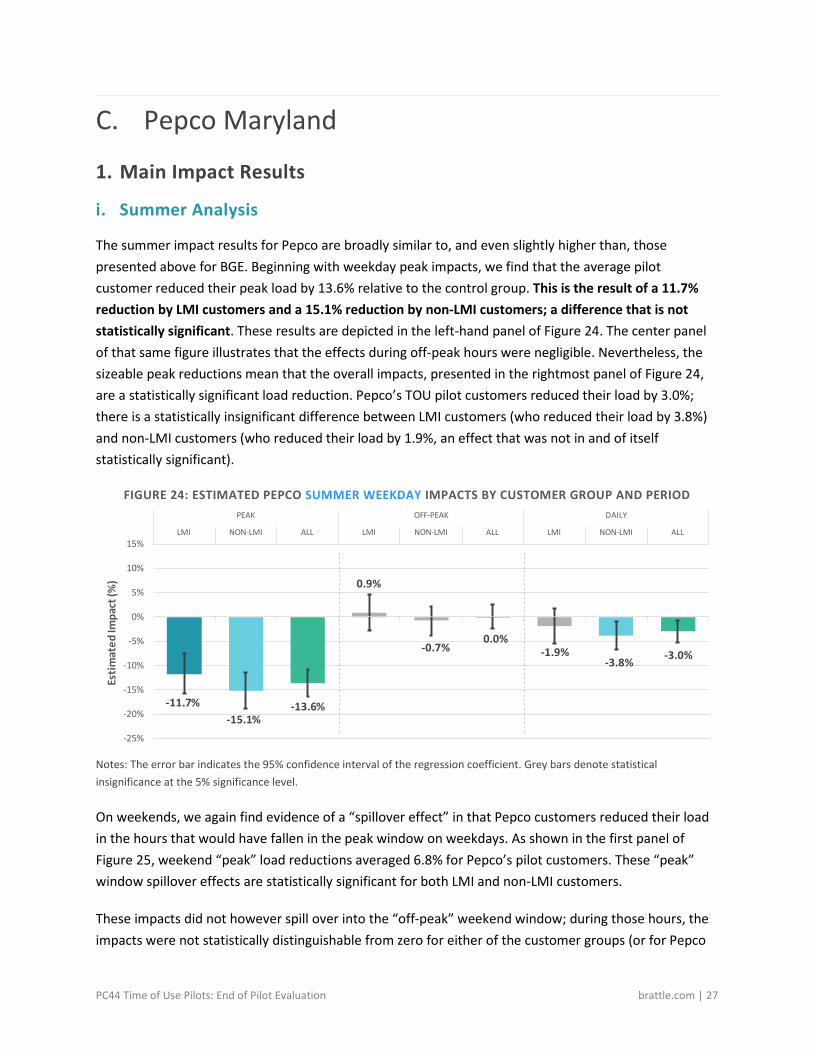
The summer impact results for Pepco are broadly similar to, and even slightly higher than, those presented above for BGE. Beginning with weekday peak impacts, we find that the average pilot customer reduced their peak load by 13.6% relative to the control group. This is the result of a 11.7% reduction by LMI customers and a 15.1% reduction by non-LMI customers; a difference that is not statistically significant. These results are depicted in the left-hand panel of Figure 24. The center panel of that same figure illustrates that the effects during off-peak hours were negligible. Nevertheless, the sizeable peak reductions mean that the overall impacts, presented in the rightmost panel of Figure 24, are a statistically significant load reduction. Pepco’s TOU pilot customers reduced their load by 3.0%; there is a statistically insignificant difference between LMI customers (who reduced their load by 3.8%) and non-LMI customers (who reduced their load by 1.9%, an effect that was not in and of itself statistically significant).
FIGURE 24: ESTIMATED PEPCO SUMMER WEEKDAY IMPACTS BY CUSTOMER GROUP AND PERIOD
Notes: The error bar indicates the 95% confidence interval of the regression coefficient. Grey bars denote statistical insignificance at the 5% significance level.
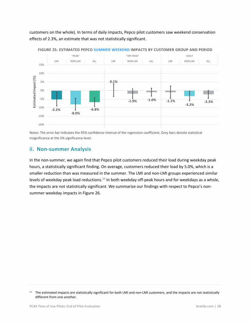
On weekends, we again find evidence of a “spillover effect” in that Pepco customers reduced their load in the hours that would have fallen in the peak window on weekdays. As shown in the first panel of Figure 25, weekend “peak” load reductions averaged 6.8% for Pepco’s pilot customers. These “peak” window spillover effects are statistically significant for both LMI and non-LMI customers.
These impacts did not however spill over into the “off-peak” weekend window; during those hours, the impacts were not statistically distinguishable from zero for either of the customer groups (or for Pepco
-11.7%-15.1%
-13.6%
0.9%
-0.7%0.0%
-1.9%-3.8% -3.0%
-25%
-20%
-15%
-10%
-5%
0%
5%
10%
15%LMI NON-LMI ALL LMI NON-LMI ALL LMI NON-LMI ALL
PEAK OFF-PEAK DAILY
Estim
ated
Impa
ct (%
)
PC44 Time of Use Pilots: End of Pilot Evaluation brattle.com | 28
customers on the whole). In terms of daily impacts, Pepco pilot customers saw weekend conservation effects of 2.3%, an estimate that was not statistically significant.
FIGURE 25: ESTIMATED PEPCO SUMMER WEEKEND IMPACTS BY CUSTOMER GROUP AND PERIOD
Notes: The error bar indicates the 95% confidence interval of the regression coefficient. Grey bars denote statistical insignificance at the 5% significance level.
ii. Non-summer Analysis
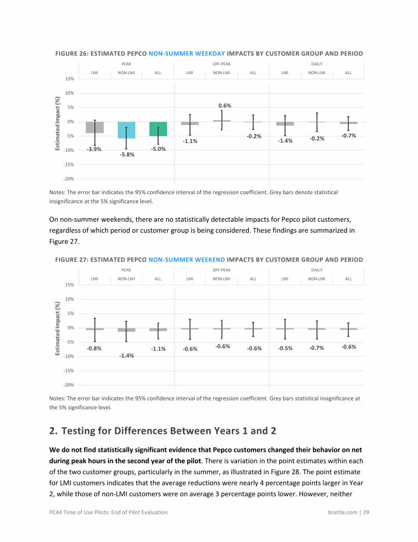
In the non-summer, we again find that Pepco pilot customers reduced their load during weekday peak hours, a statistically significant finding. On average, customers reduced their load by 5.0%, which is a smaller reduction than was measured in the summer. The LMI and non-LMI groups experienced similar levels of weekday peak load reductions.23 In both weekday off-peak hours and for weekdays as a whole, the impacts are not statistically significant. We summarize our findings with respect to Pepco’s non-summer weekday impacts in Figure 26.
23 The estimated impacts are statistically significant for both LMI and non-LMI customers, and the impacts are not statistically
different from one another.
-5.2%-8.0%
-6.8%
0.1%
-1.9% -1.0% -1.1%-3.2%
-2.3%
-20%
-15%
-10%
-5%
0%
5%
10%
15%LMI NON-LMI ALL LMI NON-LMI ALL LMI NON-LMI ALL
"PEAK" "OFF-PEAK" DAILY
Estim
ated
Impa
ct (%
)
PC44 Time of Use Pilots: End of Pilot Evaluation brattle.com | 29
FIGURE 26: ESTIMATED PEPCO NON-SUMMER WEEKDAY IMPACTS BY CUSTOMER GROUP AND PERIOD
Notes: The error bar indicates the 95% confidence interval of the regression coefficient. Grey bars denote statistical insignificance at the 5% significance level.
On non-summer weekends, there are no statistically detectable impacts for Pepco pilot customers, regardless of which period or customer group is being considered. These findings are summarized in Figure 27.
FIGURE 27: ESTIMATED PEPCO NON-SUMMER WEEKEND IMPACTS BY CUSTOMER GROUP AND PERIOD
Notes: The error bar indicates the 95% confidence interval of the regression coefficient. Grey bars statistical insignificance at the 5% significance level.
2. Testing for Differences Between Years 1 and 2
We do not find statistically significant evidence that Pepco customers changed their behavior on net during peak hours in the second year of the pilot. There is variation in the point estimates within each of the two customer groups, particularly in the summer, as illustrated in Figure 28. The point estimate for LMI customers indicates that the average reductions were nearly 4 percentage points larger in Year 2, while those of non-LMI customers were on average 3 percentage points lower. However, neither
-3.9%-5.8%
-5.0%-1.1%
0.6%
-0.2%-1.4% -0.2% -0.7%
-20%
-15%
-10%
-5%
0%
5%
10%
15%LMI NON-LMI ALL LMI NON-LMI ALL LMI NON-LMI ALL
PEAK OFF-PEAK DAILYEs
timat
ed Im
pact
(%)
-0.8%-1.4%
-1.1% -0.6% -0.6% -0.6% -0.5% -0.7% -0.6%
-20%
-15%
-10%
-5%
0%
5%
10%
15%LMI NON-LMI ALL LMI NON-LMI ALL LMI NON-LMI ALL
PEAK OFF-PEAK DAILY
Estim
ated
Impa
ct (%
)

PC44 Time of Use Pilots: End of Pilot Evaluation brattle.com | 30
difference is statistically significant. The point estimate for all customers as a whole is nearly identical between Year 1 and Year 2.
FIGURE 28: ESTIMATED PEPCO SUMMER WEEKDAY PEAK IMPACTS BY CUSTOMER GROUP AND YEAR
Notes: These results consider the same set of pilot customers across all three summers – those who have usable load data for the summers of 2018, 2019, and 2020. The error bar indicates the 95% confidence interval of the regression coefficient. Grey bars indicate statistical insignificance at the 5% level. In each pair of bars, the difference between the Year 1 and Year 2 results are not statistically significant.
Similarly, any differences in the non-summer weekday peak reductions between the first and second years are insignificant, in the statistical sense – they are small enough that we cannot conclude with any confidence that they are anything more than the effects of random variation. Figure 29 summarizes the comparison between the Year 1 and Year 2 results.
FIGURE 29: ESTIMATED PEPCO NON-SUMMER WEEKDAY PEAK IMPACTS BY CUSTOMER GROUP AND YEAR
Notes: These results consider the same set of pilot customers across all three summers – those who have usable load data for the summers of 2018, 2019, and 2020. The error bar indicates the 95% confidence interval of the regression coefficient. Grey bars indicate statistical insignificance at the 5% level. In each pair of bars, the difference between the Year 1 and Year 2 results are not statistically significant.
-9.8%
-13.5% -16.6% -13.7%-13.6% -13.6%
-25%
-20%
-15%
-10%
-5%
0%
5%
10%
15%YEAR 1 YEAR 2 YEAR 1 YEAR 2 YEAR 1 YEAR 2
LMI NON-LMI ALL CUSTOMERS
Estim
ated
Impa
ct (%
)
-4.0%-3.9% -5.4%
-6.2%-4.8% -5.2%
-15%
-10%
-5%
0%
5%
10%
15%YEAR 1 YEAR 2 YEAR 1 YEAR 2 YEAR 1 YEAR 2
LMI NON-LMI ALL CUSTOMERS
Estim
ated
Impa
ct (%
)

PC44 Time of Use Pilots: End of Pilot Evaluation brattle.com | 31
3. Subgroup Analysis
As we reported above for BGE, we also estimated for Pepco a series of supplementary regressions using interaction terms in order to provide some insight into the extent to which the average weekday peak impacts reported above vary along different dimensions. In what follows, we discuss those results, which we summarize in Figure 30.24
24 Our discussion of the Pepco subgroup analysis is similar to that of the BGE subgroup analysis above. For reference, the top
panel in Figure 30 presents the baseline impacts in each season. We include in that top panel the results of a base specification estimated not in natural logs but in kilowatt-hours, which allows us to include NEM customers. Each of the subsequent panels of Figure 30 presents the results, in terms of estimated impacts, for each of the subgroups relevant to that analysis. In each such analysis, we use red shading to indicate the “base” group. For the base group, we report statistical significance with respect to the null hypothesis of zero effect. For the other groups, we report statistical significance with respect to the base group.
For further details on the rationale or interpretation of various aspects of the subgroup analysis, please refer to the corresponding BGE discussion above.
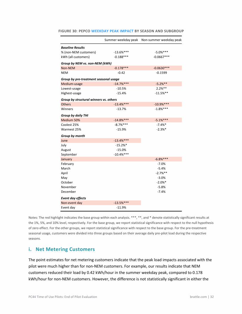
PC44 Time of Use Pilots: End of Pilot Evaluation brattle.com | 32
FIGURE 30: PEPCO WEEKDAY PEAK IMPACT BY SEASON AND SUBGROUP
Notes: The red highlight indicates the base group within each analysis. ***, **, and * denote statistically significant results at the 1%, 5%, and 10% level, respectively. For the base group, we report statistical significance with respect to the null hypothesis of zero effect. For the other groups, we report statistical significance with respect to the base group. For the pre-treatment seasonal usage, customers were divided into three groups based on their average daily pre-pilot load during the respective seasons.
i. Net Metering Customers
The point estimates for net metering customers indicate that the peak load impacts associated with the pilot were much higher than for non-NEM customers. For example, our results indicate that NEM customers reduced their load by 0.42 kWh/hour in the summer weekday peak, compared to 0.178 kWh/hour for non-NEM customers. However, the difference is not statistically significant in either the
Summer weekday peak Non-summer weekday peak
Baseline Results% (non-NEM customers) -13.6%*** -5.0%***kWh (all customers) -0.188*** -0.0667***
Group by NEM vs. non-NEM (kWh)Non-NEM -0.178*** -0.0630***NEM -0.42 -0.1599
Group by pre-treatment seasonal usageMedium-usage -14.7%*** -5.2%**Lowest-usage -10.5% 2.2%**Highest-usage -15.4% -11.5%**
Group by structural winners vs. othersOthers -13.4%*** -10.9%***Winners -13.7% -1.8%***
Group by daily THIMedium 50% -14.8%*** -5.1%***Coolest 25% -8.7%*** -7.4%*Warmest 25% -15.9% -2.3%*
Group by monthJune -13.4%***July -15.2%*August -15.0%September -10.4%***January -6.8%***February -7.0%March -5.4%April -2.7%**May -3.0%October -2.0%*November -5.8%December -7.4%
Event day effectsNon-event day -13.5%***Event day -11.9%

PC44 Time of Use Pilots: End of Pilot Evaluation brattle.com | 33
summer or non-summer. This is likely an artifact of the relatively small sample size of NEM pilot customers.25
ii. Pre-Pilot Customer Usage
After using pre-pilot load to identify the heaviest and lightest users in each season, we explore whether the weekday peak impacts varied in conjunction with usage by allowing for separate impact estimates for low users, medium users, and high-usage customers. In the summer, the differences were small in magnitude and not statistically significant, as the estimated impacts range from 10.5% to 15.4% across the three groups. In the non-summer, there was a wider range of impacts. While medium-usage customers saw load reductions of 5.2%, the lowest-usage customers saw load increases of 2.2%, a difference that is statistically significant.26 In contrast, the highest-usage customers saw load reductions of 11.5%, a difference (relative to the medium group) that is also statistically significant.
iii. Structural Winners vs. Others
We test whether the “structural winners” – those who could expect bill increases on the PC44 TOU rate without changing their load levels or patterns – nevertheless saw peak impacts. In the summer, we find that the load impacts of the two groups are statistically indistinguishable, as structural winners saw peak load reductions of 13.7% while other enrollees saw peak load reductions of 13.4%. In the non-summer, on the other hand, structural winners’ load reductions (1.8%) were significantly smaller than those of other enrolled customers (10.9%).
iv. Weather-Related Variations in Impact
The pilot’s weekday peak impacts varied with weather conditions, especially in the summer. Employing the same interaction term-based approach described above, we find that for Pepco, the weekday peak impacts in the summer increased with the temperature. On medium-THI days, the impact was a 14.8% reduction. However, on cooler days the reduction was smaller, at 8.7%, while on the warmest days, the reduction was larger, at 15.9%. The cool-day impact is significantly different from the medium-day impact, though the warm-day impact is not. In the non-summer, there is some evidence of the impact differing in conjunction with weather conditions. The impacts ranged from 2.3% on the warmest days to 7.4% on the coolest days. In the case of both cool and warm days, the difference is marginally significant.
v. Impacts by Month
We then identify some differences in weekday peak impacts by month, in both the summer and the winter. First, the peak reduction of 10.4% in September was significantly lower than June’s 13.4% 25 For example, only 48 of the 1,069 pilot customers included in the summer regression for this NEM subgroup analysis were
NEM customers. 26 This 1.8% load increase is not statistically different from zero either.
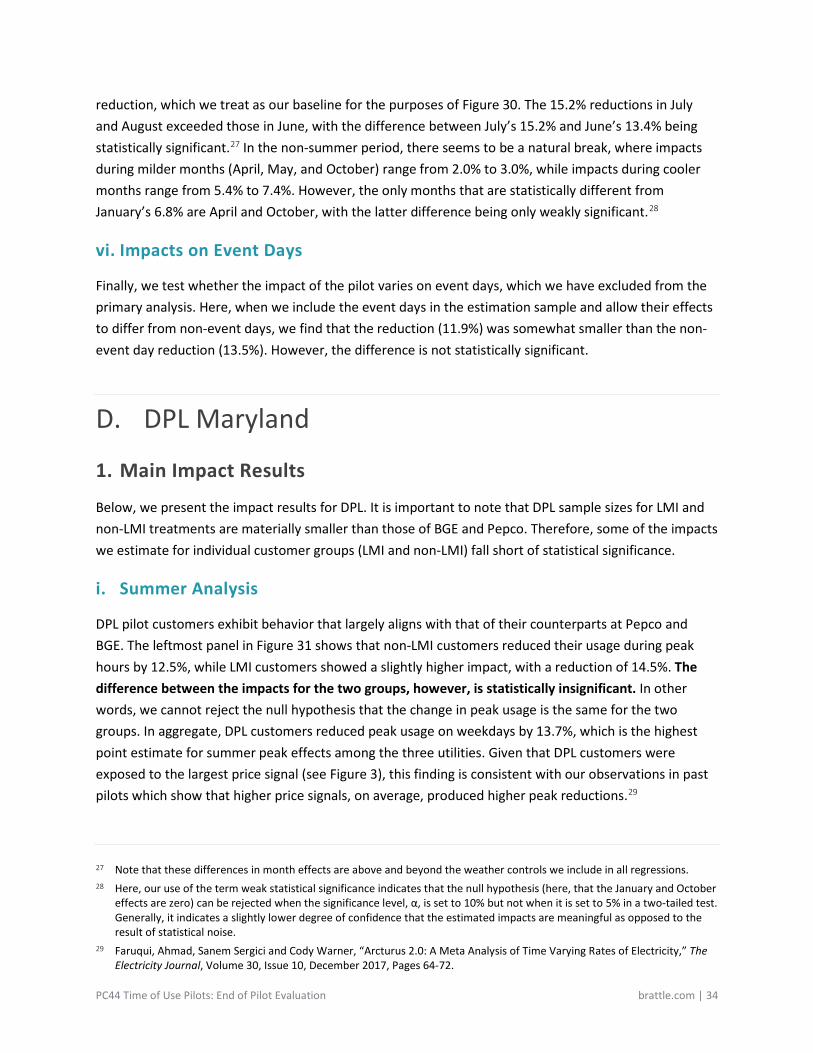
PC44 Time of Use Pilots: End of Pilot Evaluation brattle.com | 34
reduction, which we treat as our baseline for the purposes of Figure 30. The 15.2% reductions in July and August exceeded those in June, with the difference between July’s 15.2% and June’s 13.4% being statistically significant.27 In the non-summer period, there seems to be a natural break, where impacts during milder months (April, May, and October) range from 2.0% to 3.0%, while impacts during cooler months range from 5.4% to 7.4%. However, the only months that are statistically different from January’s 6.8% are April and October, with the latter difference being only weakly significant.28
vi. Impacts on Event Days
Finally, we test whether the impact of the pilot varies on event days, which we have excluded from the primary analysis. Here, when we include the event days in the estimation sample and allow their effects to differ from non-event days, we find that the reduction (11.9%) was somewhat smaller than the non-event day reduction (13.5%). However, the difference is not statistically significant.
D. DPL Maryland
1. Main Impact Results
Below, we present the impact results for DPL. It is important to note that DPL sample sizes for LMI and non-LMI treatments are materially smaller than those of BGE and Pepco. Therefore, some of the impacts we estimate for individual customer groups (LMI and non-LMI) fall short of statistical significance.
i. Summer Analysis
DPL pilot customers exhibit behavior that largely aligns with that of their counterparts at Pepco and BGE. The leftmost panel in Figure 31 shows that non-LMI customers reduced their usage during peak hours by 12.5%, while LMI customers showed a slightly higher impact, with a reduction of 14.5%. The difference between the impacts for the two groups, however, is statistically insignificant. In other words, we cannot reject the null hypothesis that the change in peak usage is the same for the two groups. In aggregate, DPL customers reduced peak usage on weekdays by 13.7%, which is the highest point estimate for summer peak effects among the three utilities. Given that DPL customers were exposed to the largest price signal (see Figure 3), this finding is consistent with our observations in past pilots which show that higher price signals, on average, produced higher peak reductions.29
27 Note that these differences in month effects are above and beyond the weather controls we include in all regressions. 28 Here, our use of the term weak statistical significance indicates that the null hypothesis (here, that the January and October
effects are zero) can be rejected when the significance level, α, is set to 10% but not when it is set to 5% in a two-tailed test. Generally, it indicates a slightly lower degree of confidence that the estimated impacts are meaningful as opposed to the result of statistical noise.
29 Faruqui, Ahmad, Sanem Sergici and Cody Warner, “Arcturus 2.0: A Meta Analysis of Time Varying Rates of Electricity,” The Electricity Journal, Volume 30, Issue 10, December 2017, Pages 64-72.
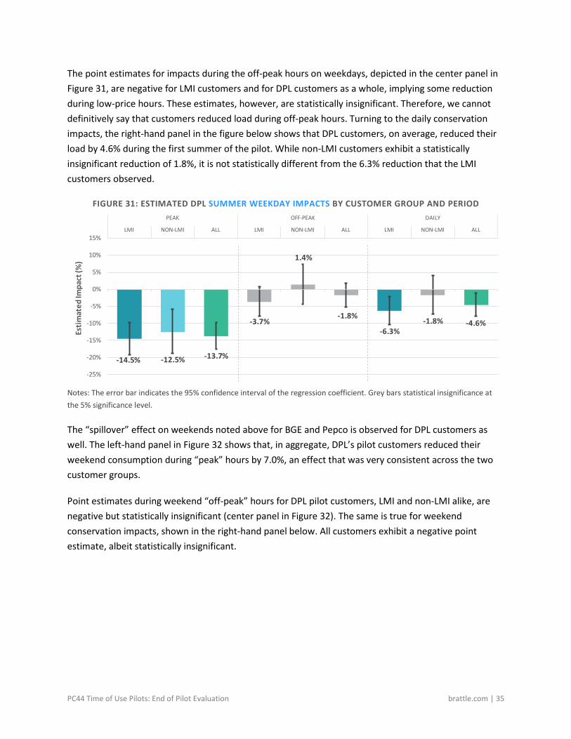
PC44 Time of Use Pilots: End of Pilot Evaluation brattle.com | 35
The point estimates for impacts during the off-peak hours on weekdays, depicted in the center panel in Figure 31, are negative for LMI customers and for DPL customers as a whole, implying some reduction during low-price hours. These estimates, however, are statistically insignificant. Therefore, we cannot definitively say that customers reduced load during off-peak hours. Turning to the daily conservation impacts, the right-hand panel in the figure below shows that DPL customers, on average, reduced their load by 4.6% during the first summer of the pilot. While non-LMI customers exhibit a statistically insignificant reduction of 1.8%, it is not statistically different from the 6.3% reduction that the LMI customers observed.
FIGURE 31: ESTIMATED DPL SUMMER WEEKDAY IMPACTS BY CUSTOMER GROUP AND PERIOD
Notes: The error bar indicates the 95% confidence interval of the regression coefficient. Grey bars statistical insignificance at the 5% significance level.
The “spillover” effect on weekends noted above for BGE and Pepco is observed for DPL customers as well. The left-hand panel in Figure 32 shows that, in aggregate, DPL’s pilot customers reduced their weekend consumption during “peak” hours by 7.0%, an effect that was very consistent across the two customer groups.
Point estimates during weekend “off-peak” hours for DPL pilot customers, LMI and non-LMI alike, are negative but statistically insignificant (center panel in Figure 32). The same is true for weekend conservation impacts, shown in the right-hand panel below. All customers exhibit a negative point estimate, albeit statistically insignificant.
-14.5% -12.5% -13.7%
-3.7%
1.4%
-1.8%
-6.3%-1.8% -4.6%
-25%
-20%
-15%
-10%
-5%
0%
5%
10%
15%LMI NON-LMI ALL LMI NON-LMI ALL LMI NON-LMI ALL
PEAK OFF-PEAK DAILY
Estim
ated
Impa
ct (%
)
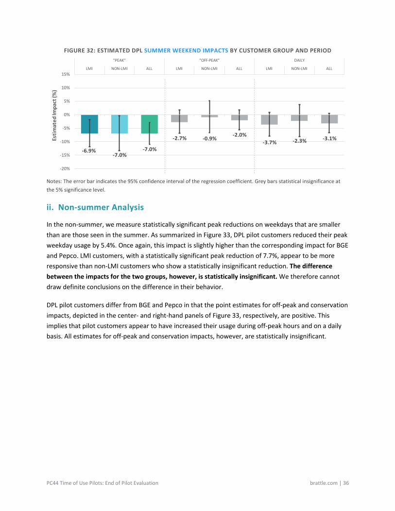
PC44 Time of Use Pilots: End of Pilot Evaluation brattle.com | 36
FIGURE 32: ESTIMATED DPL SUMMER WEEKEND IMPACTS BY CUSTOMER GROUP AND PERIOD
Notes: The error bar indicates the 95% confidence interval of the regression coefficient. Grey bars statistical insignificance at the 5% significance level.
ii. Non-summer Analysis
In the non-summer, we measure statistically significant peak reductions on weekdays that are smaller than are those seen in the summer. As summarized in Figure 33, DPL pilot customers reduced their peak weekday usage by 5.4%. Once again, this impact is slightly higher than the corresponding impact for BGE and Pepco. LMI customers, with a statistically significant peak reduction of 7.7%, appear to be more responsive than non-LMI customers who show a statistically insignificant reduction. The difference between the impacts for the two groups, however, is statistically insignificant. We therefore cannot draw definite conclusions on the difference in their behavior.
DPL pilot customers differ from BGE and Pepco in that the point estimates for off-peak and conservation impacts, depicted in the center- and right-hand panels of Figure 33, respectively, are positive. This implies that pilot customers appear to have increased their usage during off-peak hours and on a daily basis. All estimates for off-peak and conservation impacts, however, are statistically insignificant.
-6.9%-7.0%
-7.0%
-2.7% -0.9%-2.0%
-3.7% -2.3% -3.1%
-20%
-15%
-10%
-5%
0%
5%
10%
15%LMI NON-LMI ALL LMI NON-LMI ALL LMI NON-LMI ALL
"PEAK" "OFF-PEAK" DAILYEs
timat
ed Im
pact
(%)
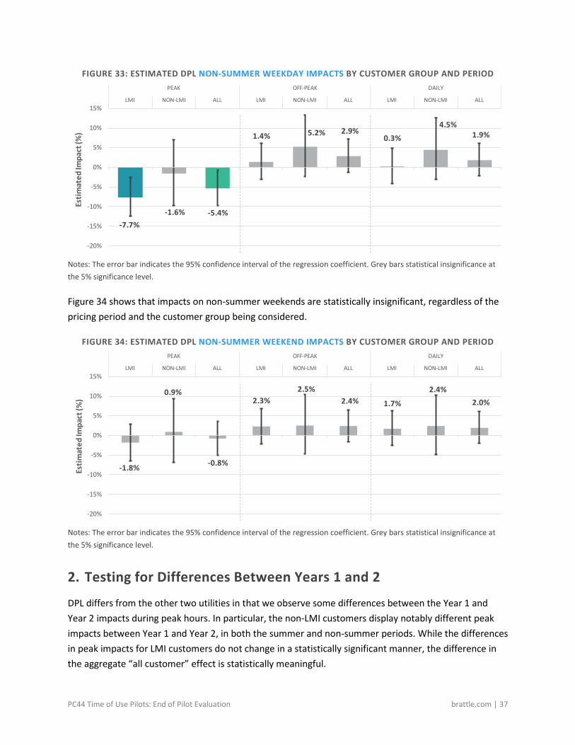
PC44 Time of Use Pilots: End of Pilot Evaluation brattle.com | 37
FIGURE 33: ESTIMATED DPL NON-SUMMER WEEKDAY IMPACTS BY CUSTOMER GROUP AND PERIOD
Notes: The error bar indicates the 95% confidence interval of the regression coefficient. Grey bars statistical insignificance at the 5% significance level.
Figure 34 shows that impacts on non-summer weekends are statistically insignificant, regardless of the pricing period and the customer group being considered.
FIGURE 34: ESTIMATED DPL NON-SUMMER WEEKEND IMPACTS BY CUSTOMER GROUP AND PERIOD
Notes: The error bar indicates the 95% confidence interval of the regression coefficient. Grey bars statistical insignificance at the 5% significance level.
2. Testing for Differences Between Years 1 and 2
DPL differs from the other two utilities in that we observe some differences between the Year 1 and Year 2 impacts during peak hours. In particular, the non-LMI customers display notably different peak impacts between Year 1 and Year 2, in both the summer and non-summer periods. While the differences in peak impacts for LMI customers do not change in a statistically significant manner, the difference in the aggregate “all customer” effect is statistically meaningful.
-7.7%-1.6% -5.4%
1.4% 5.2% 2.9%0.3%
4.5%1.9%
-20%
-15%
-10%
-5%
0%
5%
10%
15%LMI NON-LMI ALL LMI NON-LMI ALL LMI NON-LMI ALL
PEAK OFF-PEAK DAILYEs
timat
ed Im
pact
(%)
-1.8%
0.9%
-0.8%
2.3%2.5%
2.4% 1.7%
2.4%2.0%
-20%
-15%
-10%
-5%
0%
5%
10%
15%LMI NON-LMI ALL LMI NON-LMI ALL LMI NON-LMI ALL
PEAK OFF-PEAK DAILY
Estim
ated
Impa
ct (%
)
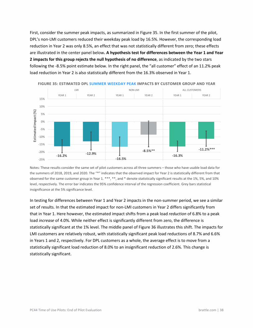
PC44 Time of Use Pilots: End of Pilot Evaluation brattle.com | 38
First, consider the summer peak impacts, as summarized in Figure 35. In the first summer of the pilot, DPL’s non-LMI customers reduced their weekday peak load by 16.5%. However, the corresponding load reduction in Year 2 was only 8.5%, an effect that was not statistically different from zero; these effects are illustrated in the center panel below. A hypothesis test for differences between the Year 1 and Year 2 impacts for this group rejects the null hypothesis of no difference, as indicated by the two stars following the -8.5% point estimate below. In the right panel, the “all customer” effect of an 11.2% peak load reduction in Year 2 is also statistically different from the 16.3% observed in Year 1.
FIGURE 35: ESTIMATED DPL SUMMER WEEKDAY PEAK IMPACTS BY CUSTOMER GROUP AND YEAR
Notes: These results consider the same set of pilot customers across all three summers – those who have usable load data for the summers of 2018, 2019, and 2020. The “*” indicates that the observed impact for Year 2 is statistically different from that observed for the same customer group in Year 1. ***, **, and * denote statistically significant results at the 1%, 5%, and 10% level, respectively. The error bar indicates the 95% confidence interval of the regression coefficient. Grey bars statistical insignificance at the 5% significance level.
In testing for differences between Year 1 and Year 2 impacts in the non-summer period, we see a similar set of results. In that the estimated impact for non-LMI customers in Year 2 differs significantly from that in Year 1. Here however, the estimated impact shifts from a peak load reduction of 6.8% to a peak load increase of 4.0%. While neither effect is significantly different from zero, the difference is statistically significant at the 1% level. The middle panel of Figure 36 illustrates this shift. The impacts for LMI customers are relatively robust, with statistically significant peak load reductions of 8.7% and 6.6% in Years 1 and 2, respectively. For DPL customers as a whole, the average effect is to move from a statistically significant load reduction of 8.0% to an insignificant reduction of 2.6%. This change is statistically significant.
-16.2% -12.9%-16.5%
-8.5%**-16.3%
-11.2%***
-25%
-20%
-15%
-10%
-5%
0%
5%
10%
15%YEAR 1 YEAR 2 YEAR 1 YEAR 2 YEAR 1 YEAR 2
LMI NON-LMI ALL CUSTOMERS
Estim
ated
Impa
ct (%
)
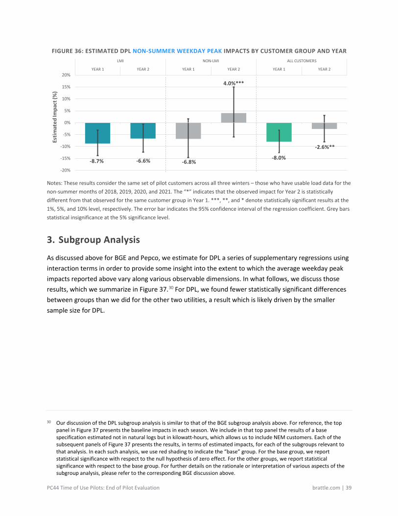
PC44 Time of Use Pilots: End of Pilot Evaluation brattle.com | 39
FIGURE 36: ESTIMATED DPL NON-SUMMER WEEKDAY PEAK IMPACTS BY CUSTOMER GROUP AND YEAR
Notes: These results consider the same set of pilot customers across all three winters – those who have usable load data for the non-summer months of 2018, 2019, 2020, and 2021. The “*” indicates that the observed impact for Year 2 is statistically different from that observed for the same customer group in Year 1. ***, **, and * denote statistically significant results at the 1%, 5%, and 10% level, respectively. The error bar indicates the 95% confidence interval of the regression coefficient. Grey bars statistical insignificance at the 5% significance level.
3. Subgroup Analysis
As discussed above for BGE and Pepco, we estimate for DPL a series of supplementary regressions using interaction terms in order to provide some insight into the extent to which the average weekday peak impacts reported above vary along various observable dimensions. In what follows, we discuss those results, which we summarize in Figure 37.30 For DPL, we found fewer statistically significant differences between groups than we did for the other two utilities, a result which is likely driven by the smaller sample size for DPL.
30 Our discussion of the DPL subgroup analysis is similar to that of the BGE subgroup analysis above. For reference, the top
panel in Figure 37 presents the baseline impacts in each season. We include in that top panel the results of a base specification estimated not in natural logs but in kilowatt-hours, which allows us to include NEM customers. Each of the subsequent panels of Figure 37 presents the results, in terms of estimated impacts, for each of the subgroups relevant to that analysis. In each such analysis, we use red shading to indicate the “base” group. For the base group, we report statistical significance with respect to the null hypothesis of zero effect. For the other groups, we report statistical significance with respect to the base group. For further details on the rationale or interpretation of various aspects of the subgroup analysis, please refer to the corresponding BGE discussion above.
-8.7% -6.6% -6.8%
4.0%***
-8.0%
-2.6%**
-20%
-15%
-10%
-5%
0%
5%
10%
15%
20%YEAR 1 YEAR 2 YEAR 1 YEAR 2 YEAR 1 YEAR 2
LMI NON-LMI ALL CUSTOMERSEs
timat
ed Im
pact
(%)
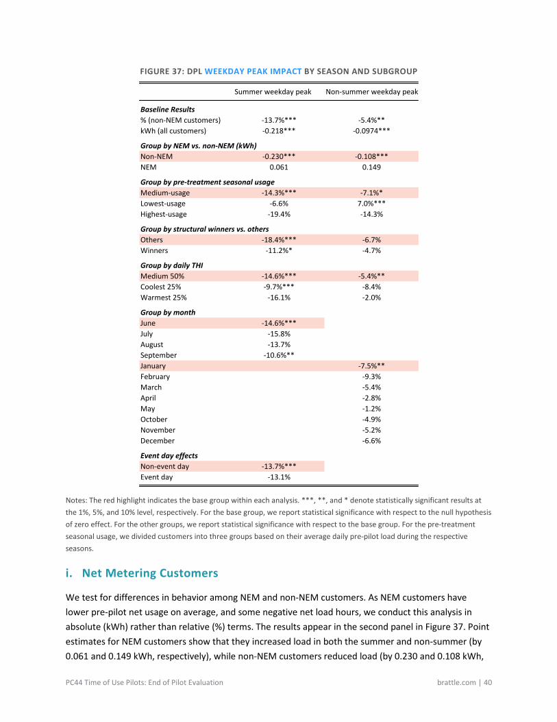
PC44 Time of Use Pilots: End of Pilot Evaluation brattle.com | 40
FIGURE 37: DPL WEEKDAY PEAK IMPACT BY SEASON AND SUBGROUP
Notes: The red highlight indicates the base group within each analysis. ***, **, and * denote statistically significant results at the 1%, 5%, and 10% level, respectively. For the base group, we report statistical significance with respect to the null hypothesis of zero effect. For the other groups, we report statistical significance with respect to the base group. For the pre-treatment seasonal usage, we divided customers into three groups based on their average daily pre-pilot load during the respective seasons.
i. Net Metering Customers
We test for differences in behavior among NEM and non-NEM customers. As NEM customers have lower pre-pilot net usage on average, and some negative net load hours, we conduct this analysis in absolute (kWh) rather than relative (%) terms. The results appear in the second panel in Figure 37. Point estimates for NEM customers show that they increased load in both the summer and non-summer (by 0.061 and 0.149 kWh, respectively), while non-NEM customers reduced load (by 0.230 and 0.108 kWh,
Summer weekday peak Non-summer weekday peak
Baseline Results% (non-NEM customers) -13.7%*** -5.4%**kWh (all customers) -0.218*** -0.0974***
Group by NEM vs. non-NEM (kWh)Non-NEM -0.230*** -0.108***NEM 0.061 0.149
Group by pre-treatment seasonal usageMedium-usage -14.3%*** -7.1%*Lowest-usage -6.6% 7.0%***Highest-usage -19.4% -14.3%
Group by structural winners vs. othersOthers -18.4%*** -6.7%Winners -11.2%* -4.7%
Group by daily THIMedium 50% -14.6%*** -5.4%**Coolest 25% -9.7%*** -8.4%Warmest 25% -16.1% -2.0%
Group by monthJune -14.6%***July -15.8%August -13.7%September -10.6%**January -7.5%**February -9.3%March -5.4%April -2.8%May -1.2%October -4.9%November -5.2%December -6.6%
Event day effectsNon-event day -13.7%***Event day -13.1%
PC44 Time of Use Pilots: End of Pilot Evaluation brattle.com | 41
respectively). However, in part due to the small number of NEM customers participating in the pilot, the difference in impacts is statistically insignificant in both seasons. Therefore, we cannot make conclusory statements on any differences in behavior.
ii. Pre-Pilot Customer Usage
We test for differences in customers’ peak impacts based on their level of load consumption. We split customers into three groups based on their pre-pilot average daily load. The fourth panel in Figure 32 summarizes our findings for the three subgroups. In the summer, we do see some differences in the magnitude of reductions, with the lowest usage group having reduced peak load by 6.6% while the highest usage group reduced peak load by 19.4%. There is no statistical difference in the reduction between the groups, however. In the non-summer, medium usage customers, our base comparison group, reduced usage by 7.1%. The highest usage customers showed no statistical difference in reduction when compared to the medium usage cohort. The lowest usage group appear to have increased their usage during peak hours by 7.0%,31 and this result is statistically different from that exhibited by the medium usage customers.
iii. Structural Winners vs. Others
Similar to the analysis conducted for BGE and Pepco, we test whether structural winners – customers identified prior to the pilot as beneficiaries of the PC44 pilot rates – responded differently to TOU pricing. Point estimates indicate that these customers reduced peak usage – by 11.2% in the summer and by 4.7% in the non-summer – less than others (reductions of 18.4% in the summer and 6.7% in the non-summer). The difference in impacts, however, is statistically insignificant in the summer and only weakly significant in the non-summer.
iv. Weather-related Variations in Impact
There is evidence that the TOU peak impacts as measured in the DPL pilot vary with weather conditions. In the summer, the impacts on the warmest days (a 16.1% reduction) were consistent with those on more typical weather days, when the average reduction was 14.6%. However, the reductions on cooler summer days, at 9.7%, were significantly lower, perhaps because there was less discretionary peak load to reduce or shift on those days.
In the non-summer months, peak impacts also varied with weather. The impact on days with more typical levels of THI was a 5.4% reduction, which is consistent with the average over the entire non-summer. However, on warmer (higher-THI) days, the load reductions were significantly smaller, at 2.0%. In fact, on these days, the load reductions were not significantly different from zero. On the other hand, on cooler days, when the electric heating load would tend to be higher, the peak reduction was higher, at 8.4%. This difference, relative to the medium-THI days, is not statistically significant.
31 The 7% peak non-summer weekday impact for the lowest usage customer group is not statistically different from zero.
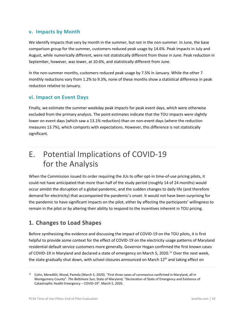
PC44 Time of Use Pilots: End of Pilot Evaluation brattle.com | 42
v. Impacts by Month
We identify impacts that vary by month in the summer, but not in the non-summer. In June, the base comparison group for the summer, customers reduced peak usage by 14.6%. Peak impacts in July and August, while numerically different, were not statistically different from those in June. Peak reduction in September, however, was lower, at 10.6%, and statistically different from June.
In the non-summer months, customers reduced peak usage by 7.5% in January. While the other 7 monthly reductions vary from 1.2% to 9.3%, none of these months show a statistical difference in peak reduction relative to January.
vi. Impact on Event Days
Finally, we estimate the summer weekday peak impacts for peak event days, which were otherwise excluded from the primary analysis. The point estimates indicate that the TOU impacts were slightly lower on event days (which saw a 13.1% reduction) than on non-event days (where the reduction measures 13.7%), which comports with expectations. However, this difference is not statistically significant.
E. Potential Implications of COVID-19 for the Analysis
When the Commission issued its order requiring the JUs to offer opt-in time-of-use pricing pilots, it could not have anticipated that more than half of the study period (roughly 14 of 24 months) would occur amidst the disruption of a global pandemic, and the sudden changes to daily life (and therefore demand for electricity) that accompanied the pandemic’s onset. It would not have been surprising for the pandemic to have significant impacts on the pilot, either by affecting the participants’ willingness to remain in the pilot or by altering their ability to respond to the incentives inherent in TOU pricing.
1. Changes to Load Shapes
Before synthesizing the evidence and discussing the impact of COVID-19 on the TOU pilots, it is first helpful to provide some context for the effect of COVID-19 on the electricity usage patterns of Maryland residential default service customers more generally. Governor Hogan confirmed the first known cases of COVID-19 in Maryland and declared a state of emergency on March 5, 2020.32 Over the next week, the state gradually shut down, with school closures announced on March 12th and taking effect on
32 Cohn, Meredith; Wood, Pamela (March 5, 2020). "First three cases of coronavirus confirmed in Maryland, all in
Montgomery County". The Baltimore Sun; State of Maryland, "Declaration of State of Emergency and Existence of Catastrophic Health Emergency – COVID-19". March 5, 2020.

PC44 Time of Use Pilots: End of Pilot Evaluation brattle.com | 43
March 16th.33 As people spent more time at home during the weekday daytime hours (and perhaps to a lesser extent during weekend hours), we would expect load patterns to shift, with increases in midday consumption and some possible offsetting reductions in the early mornings and evenings.
These predictions are largely borne out in the data, as presented in the illustrative figures that follow. Figure 38 through Figure 40 display average weekday load profiles for each of four representative months of the calendar year, using data from the full pool of potential control customers.34 The figures depict load shapes for each year since 2018; note that the charts are not weather-normalized. In each chart, load profiles from months preceding the pandemic are depicted with blue and green dashed lines, while load profiles observed since the pandemic are colored in shades of red.
Each figure begins with April, depicting in the leftmost panel the load profile for the first calendar month (April 2020) that fell entirely in the pandemic period; corresponding load profiles from 2018, 2019, and 2021 also are displayed. Across all three utilities, we see that the April load profiles are substantially flatter during daytime hours after the onset of the pandemic, with less pronounced morning peaks, and less of a drop-off between those peaks and lower-load hours in the mid-afternoon. The evening peaks, however, are at similar levels to those observed prior to the pandemic. This is especially apparent in April, when 2020 midday loads are substantially above the 2018 and 2019 levels, despite the evening peaks being at similar levels. The same general shift in load shapes is apparent in October (another “shoulder” month, depicted in the third panel of each figure) as well, with even flatter profiles during the daytime hours.
In July (the second panel in each of the three figures), changes to the load shapes are not as stark. However, it does appear that the difference between the early-morning trough and the late-afternoon peak is even greater in 2020 than it was in 2018 and 2019, across all three utilities. This change is consistent with residential customers spending more hours at home in the afternoons, when air conditioning usage is highest, due to more pandemic-induced working from home.
Finally, the fourth panel of each figure depicts January load profiles from each of the last four years. Again, the changes to the load profile are subtle but there are nevertheless perceptible differences. First, the morning peak occurs 1-2 hours later in 2021 than it did in the three preceding years, which is again consistent with increased prevalence of residential customers working from home and starting their days later. We again see less of a drop-off in electricity usage between the morning peak and the mid-afternoon valley as well. The changes across all four months described are present to varying degrees across all three JUs.
33 Swanson, Ian (March 12, 2020). "Maryland confirms community spread, will close schools". TheHill 34 For this examination of general effects of COVID-19 on load profiles, we focus on this group in order to avoid having the
impacts of the PC44 pilots influence this cross-year comparison.
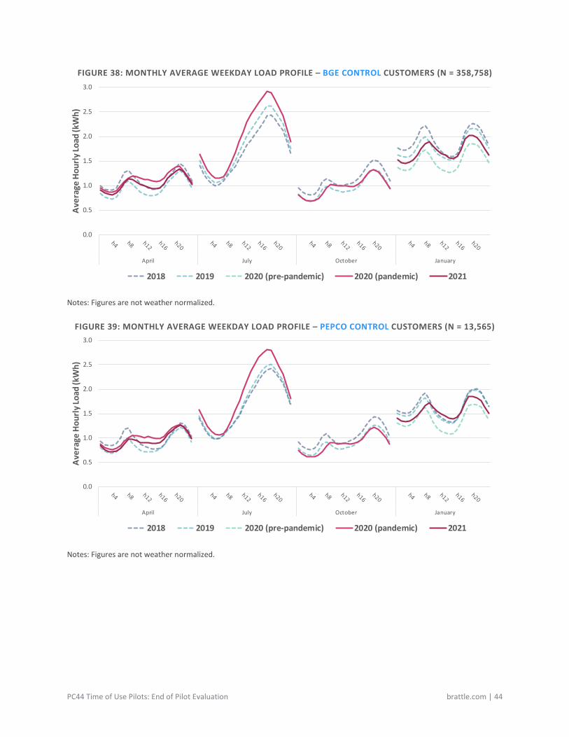
PC44 Time of Use Pilots: End of Pilot Evaluation brattle.com | 44
FIGURE 38: MONTHLY AVERAGE WEEKDAY LOAD PROFILE – BGE CONTROL CUSTOMERS (N = 358,758)
Notes: Figures are not weather normalized.
FIGURE 39: MONTHLY AVERAGE WEEKDAY LOAD PROFILE – PEPCO CONTROL CUSTOMERS (N = 13,565)
Notes: Figures are not weather normalized.
0.0
0.5
1.0
1.5
2.0
2.5
3.0
April July October January
Aver
age
Hour
ly Lo
ad (k
Wh)
2018 2019 2020 (pre-pandemic) 2020 (pandemic) 2021
0.0
0.5
1.0
1.5
2.0
2.5
3.0
April July October January
Aver
age
Hour
ly Lo
ad (k
Wh)
2018 2019 2020 (pre-pandemic) 2020 (pandemic) 2021
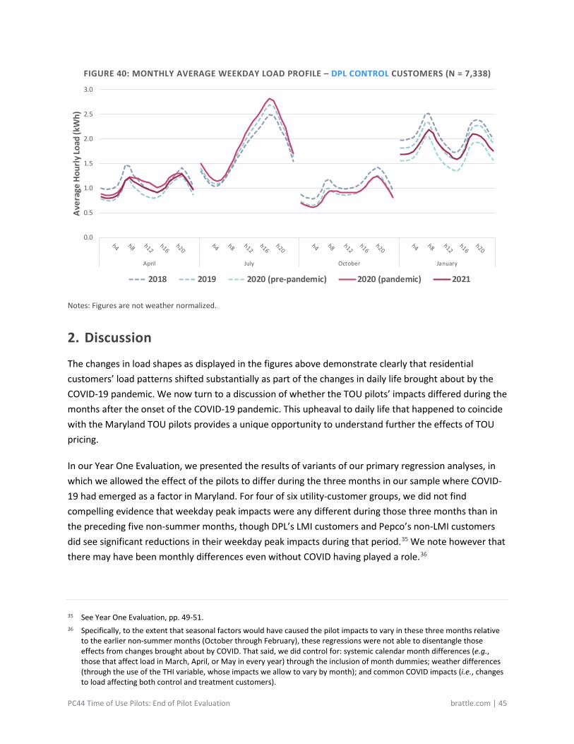
PC44 Time of Use Pilots: End of Pilot Evaluation brattle.com | 45
FIGURE 40: MONTHLY AVERAGE WEEKDAY LOAD PROFILE – DPL CONTROL CUSTOMERS (N = 7,338)
Notes: Figures are not weather normalized.
2. Discussion
The changes in load shapes as displayed in the figures above demonstrate clearly that residential customers’ load patterns shifted substantially as part of the changes in daily life brought about by the COVID-19 pandemic. We now turn to a discussion of whether the TOU pilots’ impacts differed during the months after the onset of the COVID-19 pandemic. This upheaval to daily life that happened to coincide with the Maryland TOU pilots provides a unique opportunity to understand further the effects of TOU pricing.
In our Year One Evaluation, we presented the results of variants of our primary regression analyses, in which we allowed the effect of the pilots to differ during the three months in our sample where COVID-19 had emerged as a factor in Maryland. For four of six utility-customer groups, we did not find compelling evidence that weekday peak impacts were any different during those three months than in the preceding five non-summer months, though DPL’s LMI customers and Pepco’s non-LMI customers did see significant reductions in their weekday peak impacts during that period.35 We note however that there may have been monthly differences even without COVID having played a role.36
35 See Year One Evaluation, pp. 49-51. 36 Specifically, to the extent that seasonal factors would have caused the pilot impacts to vary in these three months relative
to the earlier non-summer months (October through February), these regressions were not able to disentangle those effects from changes brought about by COVID. That said, we did control for: systemic calendar month differences (e.g., those that affect load in March, April, or May in every year) through the inclusion of month dummies; weather differences (through the use of the THI variable, whose impacts we allow to vary by month); and common COVID impacts (i.e., changes to load affecting both control and treatment customers).
0.0
0.5
1.0
1.5
2.0
2.5
3.0
April July October January
Aver
age
Hour
ly Lo
ad (k
Wh)
2018 2019 2020 (pre-pandemic) 2020 (pandemic) 2021
PC44 Time of Use Pilots: End of Pilot Evaluation brattle.com | 46
As the COVID-19 pandemic and working from home continued into the summer, there was some concern among the various stakeholders involved in the TOU pilots that pilot participants would find it unattractive to remain in the pilot, as the prospect of paying elevated rates for summer air conditioning during peak hours could have driven pilot participants to unenroll. However, as discussed previously, we did not generally see evidence that attrition increased during the summer of 2020.
COVID remained a factor for the entire second year of our study period. As we describe above, econometric analysis cannot reliably disentangle the effects of customer fatigue, learning through increased customer experience with TOU rates, and the pandemic. We note only that in testing for differences between Year 1 and Year 2, as discussed above, we found that only one of six customer-utility groups (non-LMI customers in DPL’s service territory) displayed a weekday peak load impact that was any different between Year 1 and Year 2. While not definitive, these results are therefore suggestive that customers on TOU rates are able and willing to respond to the incentives embedded in the rate differences under atypical conditions.
F. Price Response Results In addition to the difference-in-differences impacts that are the focus of the results presented to this point, we estimated a series of regressions that measure the price responsiveness of the pilot participants. This analysis is vital in order to be able to estimate the impact of rates other than those tested in the pilot. For each utility, customer group, and season, we estimate the following two parameters of interest:37
• the substitution elasticity, which measures the extent to which changes to the ratio of peak to off-peak prices results in changes in the ratio of peak to off-peak consumption on weekdays; and
• the daily demand elasticity, which measures the extent to which changes in the daily average price38 result in changes to the total amount consumed in a day.
We generally expect both elasticities to be negative. The results of this analysis are summarized in Figure 41 and Figure 44.
37 We described the price response methodology in greater detail in the Methodology section of our Year One Evaluation (pp.
13-15). Tables from the regressions underlying the analyses summarized in this section appear in Appendix A.7. 38 In calculating the daily average price, we focus on the primary components of the bill and thus exclude various
administrative charges. We need to weight peak and off-peak prices in order to calculate average daily prices for pilot customers. To do this, we exploit variation at the customer and month levels in consumption patterns; we weight the peak and off-peak price for each customer and month based on that customer’s pre-pilot shares for the corresponding month in the pre-pilot period.
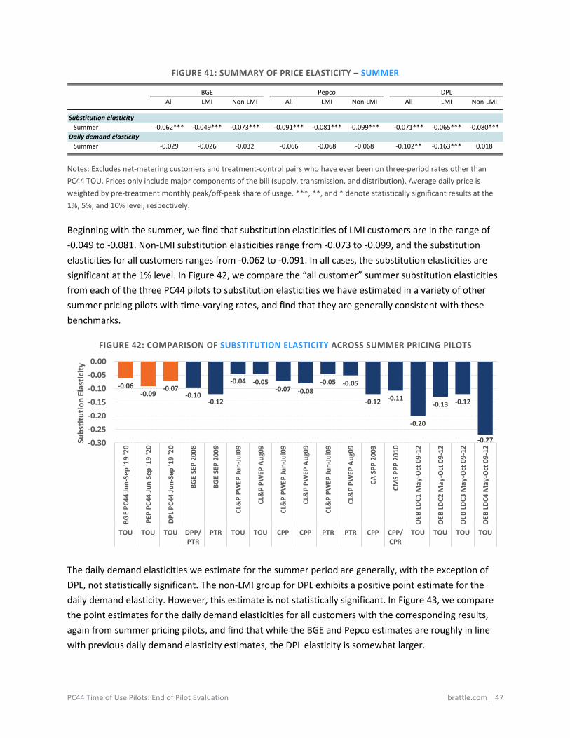
PC44 Time of Use Pilots: End of Pilot Evaluation brattle.com | 47
FIGURE 41: SUMMARY OF PRICE ELASTICITY – SUMMER
Notes: Excludes net-metering customers and treatment-control pairs who have ever been on three-period rates other than PC44 TOU. Prices only include major components of the bill (supply, transmission, and distribution). Average daily price is weighted by pre-treatment monthly peak/off-peak share of usage. ***, **, and * denote statistically significant results at the 1%, 5%, and 10% level, respectively.
Beginning with the summer, we find that substitution elasticities of LMI customers are in the range of -0.049 to -0.081. Non-LMI substitution elasticities range from -0.073 to -0.099, and the substitution elasticities for all customers ranges from -0.062 to -0.091. In all cases, the substitution elasticities are significant at the 1% level. In Figure 42, we compare the “all customer” summer substitution elasticities from each of the three PC44 pilots to substitution elasticities we have estimated in a variety of other summer pricing pilots with time-varying rates, and find that they are generally consistent with these benchmarks.
FIGURE 42: COMPARISON OF SUBSTITUTION ELASTICITY ACROSS SUMMER PRICING PILOTS
The daily demand elasticities we estimate for the summer period are generally, with the exception of DPL, not statistically significant. The non-LMI group for DPL exhibits a positive point estimate for the daily demand elasticity. However, this estimate is not statistically significant. In Figure 43, we compare the point estimates for the daily demand elasticities for all customers with the corresponding results, again from summer pricing pilots, and find that while the BGE and Pepco estimates are roughly in line with previous daily demand elasticity estimates, the DPL elasticity is somewhat larger.
BGE Pepco DPLAll LMI Non-LMI All LMI Non-LMI All LMI Non-LMI
Substitution elasticitySummer -0.062*** -0.049*** -0.073*** -0.091*** -0.081*** -0.099*** -0.071*** -0.065*** -0.080***
Daily demand elasticitySummer -0.029 -0.026 -0.032 -0.066 -0.068 -0.068 -0.102** -0.163*** 0.018
-0.06-0.09
-0.07-0.10
-0.12
-0.04 -0.05-0.07 -0.08
-0.05 -0.05
-0.12 -0.11
-0.20
-0.13 -0.12
-0.27-0.30-0.25-0.20-0.15-0.10-0.050.00
BGE
PC44
Jun-
Sep
'19
'20
PEP
PC44
Jun-
Sep
'19
'20
DPL P
C44
Jun-
Sep
'19
'20
BGE
SEP
2008
BGE
SEP
2009
CL&
P PW
EP Ju
n-Ju
l09
CL&
P PW
EP A
ug09
CL&
P PW
EP Ju
n-Ju
l09
CL&
P PW
EP A
ug09
CL&
P PW
EP Ju
n-Ju
l09
CL&
P PW
EP A
ug09
CA S
PP 2
003
CMS
PPP
2010
OEB
LDC
1 M
ay-O
ct 0
9-12
OEB
LDC
2 M
ay-O
ct 0
9-12
OEB
LDC
3 M
ay-O
ct 0
9-12
OEB
LDC
4 M
ay-O
ct 0
9-12
TOU TOU TOU DPP/PTR
PTR TOU TOU CPP CPP PTR PTR CPP CPP/CPR
TOU TOU TOU TOU
Subs
titut
ion
Elas
ticity
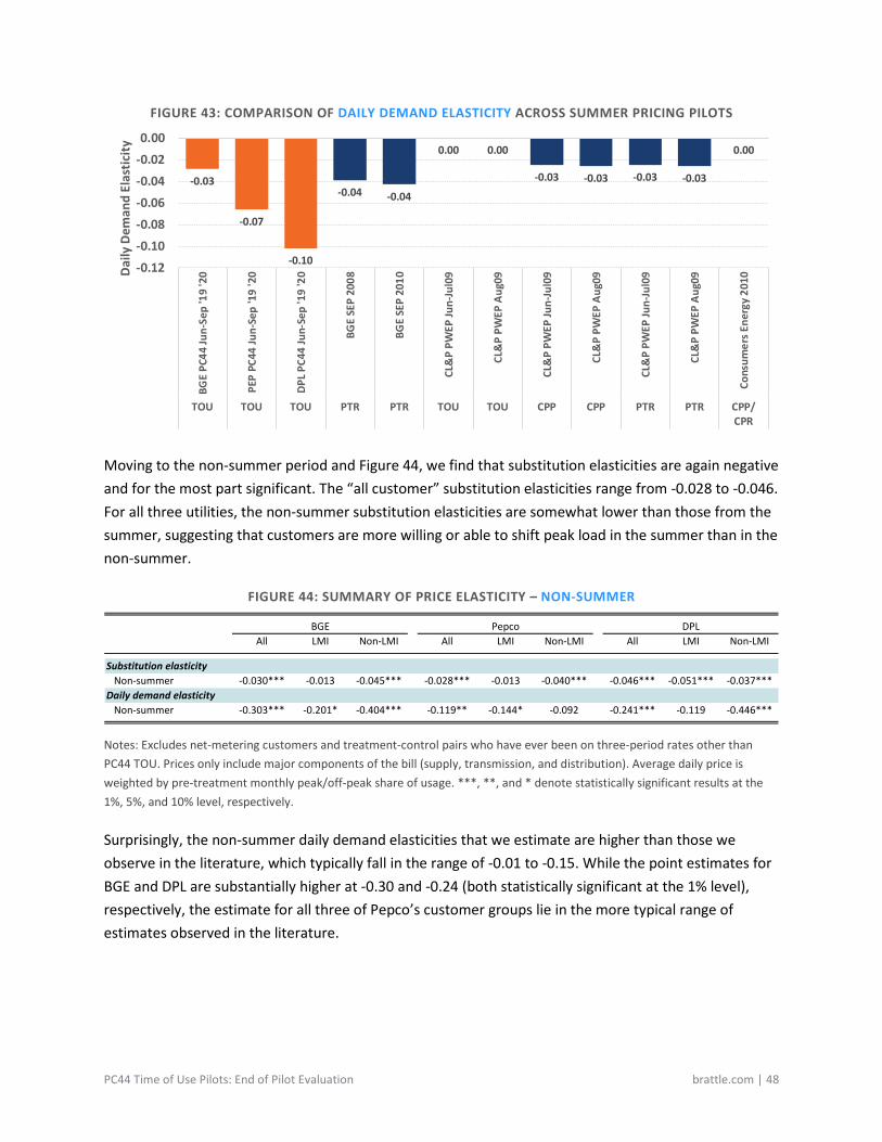
PC44 Time of Use Pilots: End of Pilot Evaluation brattle.com | 48
FIGURE 43: COMPARISON OF DAILY DEMAND ELASTICITY ACROSS SUMMER PRICING PILOTS
Moving to the non-summer period and Figure 44, we find that substitution elasticities are again negative and for the most part significant. The “all customer” substitution elasticities range from -0.028 to -0.046. For all three utilities, the non-summer substitution elasticities are somewhat lower than those from the summer, suggesting that customers are more willing or able to shift peak load in the summer than in the non-summer.
FIGURE 44: SUMMARY OF PRICE ELASTICITY – NON-SUMMER
Notes: Excludes net-metering customers and treatment-control pairs who have ever been on three-period rates other than PC44 TOU. Prices only include major components of the bill (supply, transmission, and distribution). Average daily price is weighted by pre-treatment monthly peak/off-peak share of usage. ***, **, and * denote statistically significant results at the 1%, 5%, and 10% level, respectively.
Surprisingly, the non-summer daily demand elasticities that we estimate are higher than those we observe in the literature, which typically fall in the range of -0.01 to -0.15. While the point estimates for BGE and DPL are substantially higher at -0.30 and -0.24 (both statistically significant at the 1% level), respectively, the estimate for all three of Pepco’s customer groups lie in the more typical range of estimates observed in the literature.
-0.03
-0.07
-0.10
-0.04 -0.04
0.00 0.00
-0.03 -0.03 -0.03 -0.03
0.00
-0.12-0.10-0.08-0.06-0.04-0.020.00
BGE
PC44
Jun-
Sep
'19
'20
PEP
PC44
Jun-
Sep
'19
'20
DPL P
C44
Jun-
Sep
'19
'20
BGE
SEP
2008
BGE
SEP
2010
CL&
P PW
EP Ju
n-Ju
l09
CL&
P PW
EP A
ug09
CL&
P PW
EP Ju
n-Ju
l09
CL&
P PW
EP A
ug09
CL&
P PW
EP Ju
n-Ju
l09
CL&
P PW
EP A
ug09
Cons
umer
s Ene
rgy
2010
TOU TOU TOU PTR PTR TOU TOU CPP CPP PTR PTR CPP/CPR
Dai
ly D
eman
d El
astic
ity
BGE Pepco DPLAll LMI Non-LMI All LMI Non-LMI All LMI Non-LMI
Substitution elasticityNon-summer -0.030*** -0.013 -0.045*** -0.028*** -0.013 -0.040*** -0.046*** -0.051*** -0.037***
Daily demand elasticityNon-summer -0.303*** -0.201* -0.404*** -0.119** -0.144* -0.092 -0.241*** -0.119 -0.446***
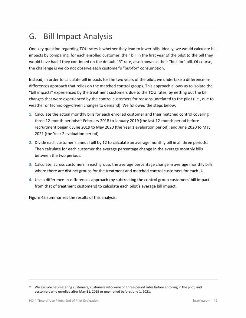
PC44 Time of Use Pilots: End of Pilot Evaluation brattle.com | 49
G. Bill Impact Analysis One key question regarding TOU rates is whether they lead to lower bills. Ideally, we would calculate bill impacts by comparing, for each enrolled customer, their bill in the first year of the pilot to the bill they would have had if they continued on the default “R” rate, also known as their “but-for” bill. Of course, the challenge is we do not observe each customer’s “but-for” consumption.
Instead, in order to calculate bill impacts for the two years of the pilot, we undertake a difference-in-differences approach that relies on the matched control groups. This approach allows us to isolate the “bill impacts” experienced by the treatment customers due to the TOU rates, by netting out the bill changes that were experienced by the control customers for reasons unrelated to the pilot (i.e., due to weather or technology-driven changes to demand). We followed the steps below:
1. Calculate the actual monthly bills for each enrolled customer and their matched control covering three 12-month periods:39 February 2018 to January 2019 (the last 12-month period before recruitment began); June 2019 to May 2020 (the Year 1 evaluation period); and June 2020 to May 2021 (the Year 2 evaluation period).
2. Divide each customer’s annual bill by 12 to calculate an average monthly bill in all three periods. Then calculate for each customer the average percentage change in the average monthly bills between the two periods.
3. Calculate, across customers in each group, the average percentage change in average monthly bills, where there are distinct groups for the treatment and matched control customers for each JU.
4. Use a difference-in-differences approach (by subtracting the control group customers’ bill impact from that of treatment customers) to calculate each pilot’s average bill impact.
Figure 45 summarizes the results of this analysis.
39 We exclude net-metering customers, customers who were on three-period rates before enrolling in the pilot, and
customers who enrolled after May 31, 2019 or unenrolled before June 1, 2021.
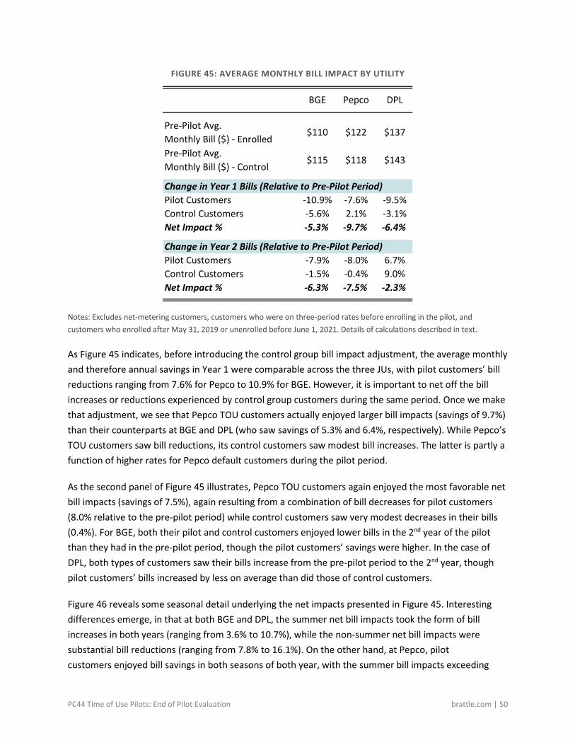
PC44 Time of Use Pilots: End of Pilot Evaluation brattle.com | 50
FIGURE 45: AVERAGE MONTHLY BILL IMPACT BY UTILITY
Notes: Excludes net-metering customers, customers who were on three-period rates before enrolling in the pilot, and customers who enrolled after May 31, 2019 or unenrolled before June 1, 2021. Details of calculations described in text.
As Figure 45 indicates, before introducing the control group bill impact adjustment, the average monthly and therefore annual savings in Year 1 were comparable across the three JUs, with pilot customers’ bill reductions ranging from 7.6% for Pepco to 10.9% for BGE. However, it is important to net off the bill increases or reductions experienced by control group customers during the same period. Once we make that adjustment, we see that Pepco TOU customers actually enjoyed larger bill impacts (savings of 9.7%) than their counterparts at BGE and DPL (who saw savings of 5.3% and 6.4%, respectively). While Pepco’s TOU customers saw bill reductions, its control customers saw modest bill increases. The latter is partly a function of higher rates for Pepco default customers during the pilot period.
As the second panel of Figure 45 illustrates, Pepco TOU customers again enjoyed the most favorable net bill impacts (savings of 7.5%), again resulting from a combination of bill decreases for pilot customers (8.0% relative to the pre-pilot period) while control customers saw very modest decreases in their bills (0.4%). For BGE, both their pilot and control customers enjoyed lower bills in the 2nd year of the pilot than they had in the pre-pilot period, though the pilot customers’ savings were higher. In the case of DPL, both types of customers saw their bills increase from the pre-pilot period to the 2nd year, though pilot customers’ bills increased by less on average than did those of control customers.
Figure 46 reveals some seasonal detail underlying the net impacts presented in Figure 45. Interesting differences emerge, in that at both BGE and DPL, the summer net bill impacts took the form of bill increases in both years (ranging from 3.6% to 10.7%), while the non-summer net bill impacts were substantial bill reductions (ranging from 7.8% to 16.1%). On the other hand, at Pepco, pilot customers enjoyed bill savings in both seasons of both year, with the summer bill impacts exceeding
BGE Pepco DPL
Pre-Pilot Avg. Monthly Bill ($) - Enrolled
$110 $122 $137
Pre-Pilot Avg. Monthly Bill ($) - Control
$115 $118 $143
Change in Year 1 Bills (Relative to Pre-Pilot Period)Pilot Customers -10.9% -7.6% -9.5%Control Customers -5.6% 2.1% -3.1%Net Impact % -5.3% -9.7% -6.4%
Change in Year 2 Bills (Relative to Pre-Pilot Period)Pilot Customers -7.9% -8.0% 6.7%Control Customers -1.5% -0.4% 9.0%Net Impact % -6.3% -7.5% -2.3%
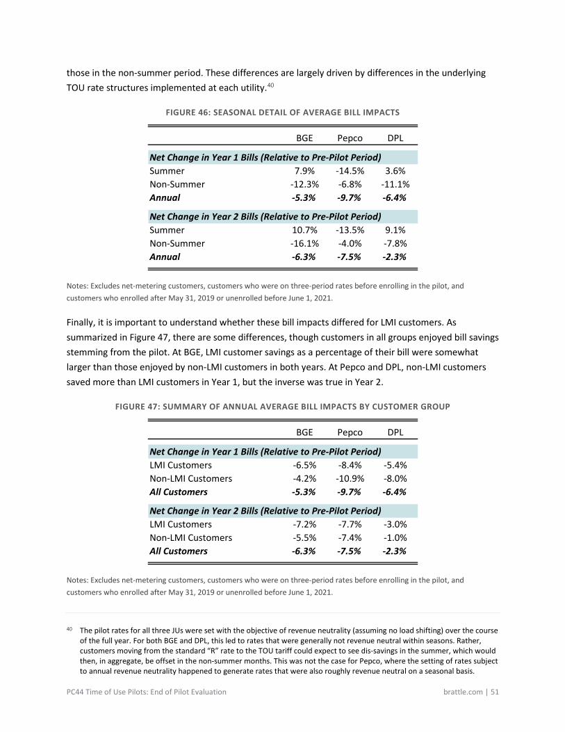
PC44 Time of Use Pilots: End of Pilot Evaluation brattle.com | 51
those in the non-summer period. These differences are largely driven by differences in the underlying TOU rate structures implemented at each utility.40
FIGURE 46: SEASONAL DETAIL OF AVERAGE BILL IMPACTS
Notes: Excludes net-metering customers, customers who were on three-period rates before enrolling in the pilot, and customers who enrolled after May 31, 2019 or unenrolled before June 1, 2021.
Finally, it is important to understand whether these bill impacts differed for LMI customers. As summarized in Figure 47, there are some differences, though customers in all groups enjoyed bill savings stemming from the pilot. At BGE, LMI customer savings as a percentage of their bill were somewhat larger than those enjoyed by non-LMI customers in both years. At Pepco and DPL, non-LMI customers saved more than LMI customers in Year 1, but the inverse was true in Year 2.
FIGURE 47: SUMMARY OF ANNUAL AVERAGE BILL IMPACTS BY CUSTOMER GROUP
Notes: Excludes net-metering customers, customers who were on three-period rates before enrolling in the pilot, and customers who enrolled after May 31, 2019 or unenrolled before June 1, 2021.
40 The pilot rates for all three JUs were set with the objective of revenue neutrality (assuming no load shifting) over the course
of the full year. For both BGE and DPL, this led to rates that were generally not revenue neutral within seasons. Rather, customers moving from the standard “R” rate to the TOU tariff could expect to see dis-savings in the summer, which would then, in aggregate, be offset in the non-summer months. This was not the case for Pepco, where the setting of rates subject to annual revenue neutrality happened to generate rates that were also roughly revenue neutral on a seasonal basis.
BGE Pepco DPL
Net Change in Year 1 Bills (Relative to Pre-Pilot Period)Summer 7.9% -14.5% 3.6%Non-Summer -12.3% -6.8% -11.1%Annual -5.3% -9.7% -6.4%
Net Change in Year 2 Bills (Relative to Pre-Pilot Period)Summer 10.7% -13.5% 9.1%Non-Summer -16.1% -4.0% -7.8%Annual -6.3% -7.5% -2.3%
BGE Pepco DPL
Net Change in Year 1 Bills (Relative to Pre-Pilot Period)LMI Customers -6.5% -8.4% -5.4%Non-LMI Customers -4.2% -10.9% -8.0%All Customers -5.3% -9.7% -6.4%
Net Change in Year 2 Bills (Relative to Pre-Pilot Period)LMI Customers -7.2% -7.7% -3.0%Non-LMI Customers -5.5% -7.4% -1.0%All Customers -6.3% -7.5% -2.3%
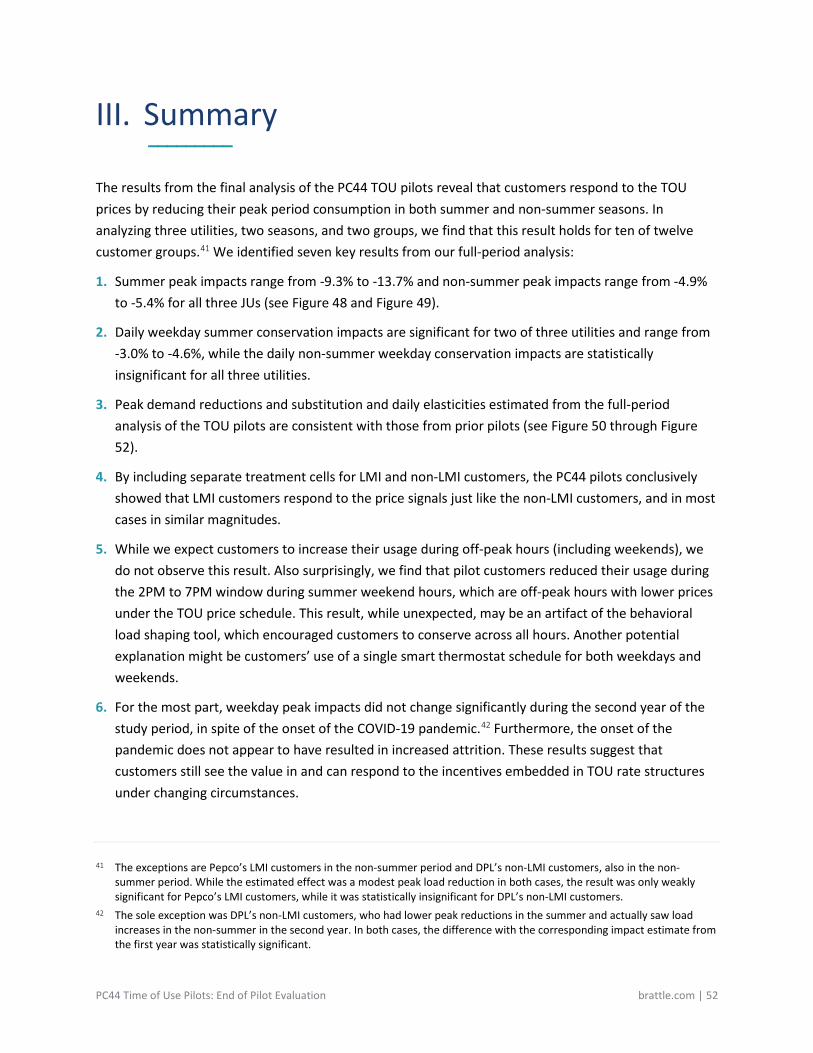
PC44 Time of Use Pilots: End of Pilot Evaluation brattle.com | 52
III. Summary _________
The results from the final analysis of the PC44 TOU pilots reveal that customers respond to the TOU prices by reducing their peak period consumption in both summer and non-summer seasons. In analyzing three utilities, two seasons, and two groups, we find that this result holds for ten of twelve customer groups.41 We identified seven key results from our full-period analysis:
1. Summer peak impacts range from -9.3% to -13.7% and non-summer peak impacts range from -4.9% to -5.4% for all three JUs (see Figure 48 and Figure 49).
2. Daily weekday summer conservation impacts are significant for two of three utilities and range from -3.0% to -4.6%, while the daily non-summer weekday conservation impacts are statistically insignificant for all three utilities.
3. Peak demand reductions and substitution and daily elasticities estimated from the full-period analysis of the TOU pilots are consistent with those from prior pilots (see Figure 50 through Figure 52).
4. By including separate treatment cells for LMI and non-LMI customers, the PC44 pilots conclusively showed that LMI customers respond to the price signals just like the non-LMI customers, and in most cases in similar magnitudes.
5. While we expect customers to increase their usage during off-peak hours (including weekends), we do not observe this result. Also surprisingly, we find that pilot customers reduced their usage during the 2PM to 7PM window during summer weekend hours, which are off-peak hours with lower prices under the TOU price schedule. This result, while unexpected, may be an artifact of the behavioral load shaping tool, which encouraged customers to conserve across all hours. Another potential explanation might be customers’ use of a single smart thermostat schedule for both weekdays and weekends.
6. For the most part, weekday peak impacts did not change significantly during the second year of the study period, in spite of the onset of the COVID-19 pandemic.42 Furthermore, the onset of the pandemic does not appear to have resulted in increased attrition. These results suggest that customers still see the value in and can respond to the incentives embedded in TOU rate structures under changing circumstances.
41 The exceptions are Pepco’s LMI customers in the non-summer period and DPL’s non-LMI customers, also in the non-
summer period. While the estimated effect was a modest peak load reduction in both cases, the result was only weakly significant for Pepco’s LMI customers, while it was statistically insignificant for DPL’s non-LMI customers.
42 The sole exception was DPL’s non-LMI customers, who had lower peak reductions in the summer and actually saw load increases in the non-summer in the second year. In both cases, the difference with the corresponding impact estimate from the first year was statistically significant.
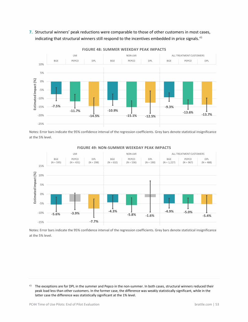
PC44 Time of Use Pilots: End of Pilot Evaluation brattle.com | 53
7. Structural winners’ peak reductions were comparable to those of other customers in most cases, indicating that structural winners still respond to the incentives embedded in price signals.43
FIGURE 48: SUMMER WEEKDAY PEAK IMPACTS
Notes: Error bars indicate the 95% confidence interval of the regression coefficients. Grey bars denote statistical insignificance at the 5% level.
FIGURE 49: NON-SUMMER WEEKDAY PEAK IMPACTS
Notes: Error bars indicate the 95% confidence interval of the regression coefficients. Grey bars denote statistical insignificance at the 5% level.
43 The exceptions are for DPL in the summer and Pepco in the non-summer. In both cases, structural winners reduced their
peak load less than other customers. In the former case, the difference was weakly statistically significant, while in the latter case the difference was statistically significant at the 1% level.
-7.5%-11.7%
-14.5%-10.9%
-15.1% -12.5%
-9.3%-13.6% -13.7%
-25%
-20%
-15%
-10%
-5%
0%
5%
10%BGE PEPCO DPL BGE PEPCO DPL BGE PEPCO DPL
LMI NON-LMI ALL TREATMENT CUSTOMERS
Estim
ated
Impa
ct (%
)
-5.6% -3.9%
-7.7%
-4.3%-5.8% -1.6%
-4.9% -5.0%-5.4%
-15%
-10%
-5%
0%
5%
10%
15%
BGE(N = 595)
PEPCO(N = 431)
DPL(N = 298)
BGE(N = 632)
PEPCO(N = 536)
DPL(N = 190)
BGE(N = 1,227)
PEPCO(N = 967)
DPL(N = 488)
LMI NON-LMI ALL TREATMENT CUSTOMERS
Estim
ated
Impa
ct (%
)
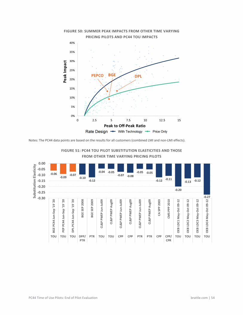
PC44 Time of Use Pilots: End of Pilot Evaluation brattle.com | 54
FIGURE 50: SUMMER PEAK IMPACTS FROM OTHER TIME VARYING PRICING PILOTS AND PC44 TOU IMPACTS
Notes: The PC44 data points are based on the results for all customers (combined LMI and non-LMI effects).
FIGURE 51: PC44 TOU PILOT SUBSTITUTION ELASTICITIES AND THOSE FROM OTHER TIME VARYING PRICING PILOTS
-0.06-0.09
-0.07-0.10
-0.12
-0.04 -0.05-0.07 -0.08
-0.05 -0.05
-0.12 -0.11
-0.20
-0.13 -0.12
-0.27-0.30-0.25-0.20-0.15-0.10-0.050.00
BGE
PC44
Jun-
Sep
'19
'20
PEP
PC44
Jun-
Sep
'19
'20
DPL P
C44
Jun-
Sep
'19
'20
BGE
SEP
2008
BGE
SEP
2009
CL&
P PW
EP Ju
n-Ju
l09
CL&
P PW
EP A
ug09
CL&
P PW
EP Ju
n-Ju
l09
CL&
P PW
EP A
ug09
CL&
P PW
EP Ju
n-Ju
l09
CL&
P PW
EP A
ug09
CA S
PP 2
003
CMS
PPP
2010
OEB
LDC
1 M
ay-O
ct 0
9-12
OEB
LDC
2 M
ay-O
ct 0
9-12
OEB
LDC
3 M
ay-O
ct 0
9-12
OEB
LDC
4 M
ay-O
ct 0
9-12
TOU TOU TOU DPP/PTR
PTR TOU TOU CPP CPP PTR PTR CPP CPP/CPR
TOU TOU TOU TOU
Subs
titut
ion
Elas
ticity
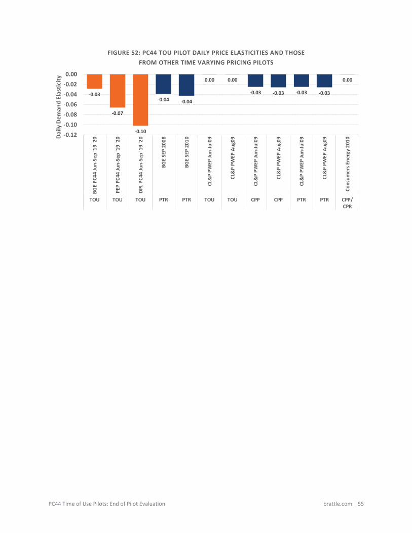
PC44 Time of Use Pilots: End of Pilot Evaluation brattle.com | 55
FIGURE 52: PC44 TOU PILOT DAILY PRICE ELASTICITIES AND THOSE FROM OTHER TIME VARYING PRICING PILOTS
-0.03
-0.07
-0.10
-0.04 -0.04
0.00 0.00
-0.03 -0.03 -0.03 -0.03
0.00
-0.12-0.10-0.08-0.06-0.04-0.020.00
BGE
PC44
Jun-
Sep
'19
'20
PEP
PC44
Jun-
Sep
'19
'20
DPL P
C44
Jun-
Sep
'19
'20
BGE
SEP
2008
BGE
SEP
2010
CL&
P PW
EP Ju
n-Ju
l09
CL&
P PW
EP A
ug09
CL&
P PW
EP Ju
n-Ju
l09
CL&
P PW
EP A
ug09
CL&
P PW
EP Ju
n-Ju
l09
CL&
P PW
EP A
ug09
Cons
umer
s Ene
rgy
2010
TOU TOU TOU PTR PTR TOU TOU CPP CPP PTR PTR CPP/CPR
Dai
ly D
eman
d El
astic
ity
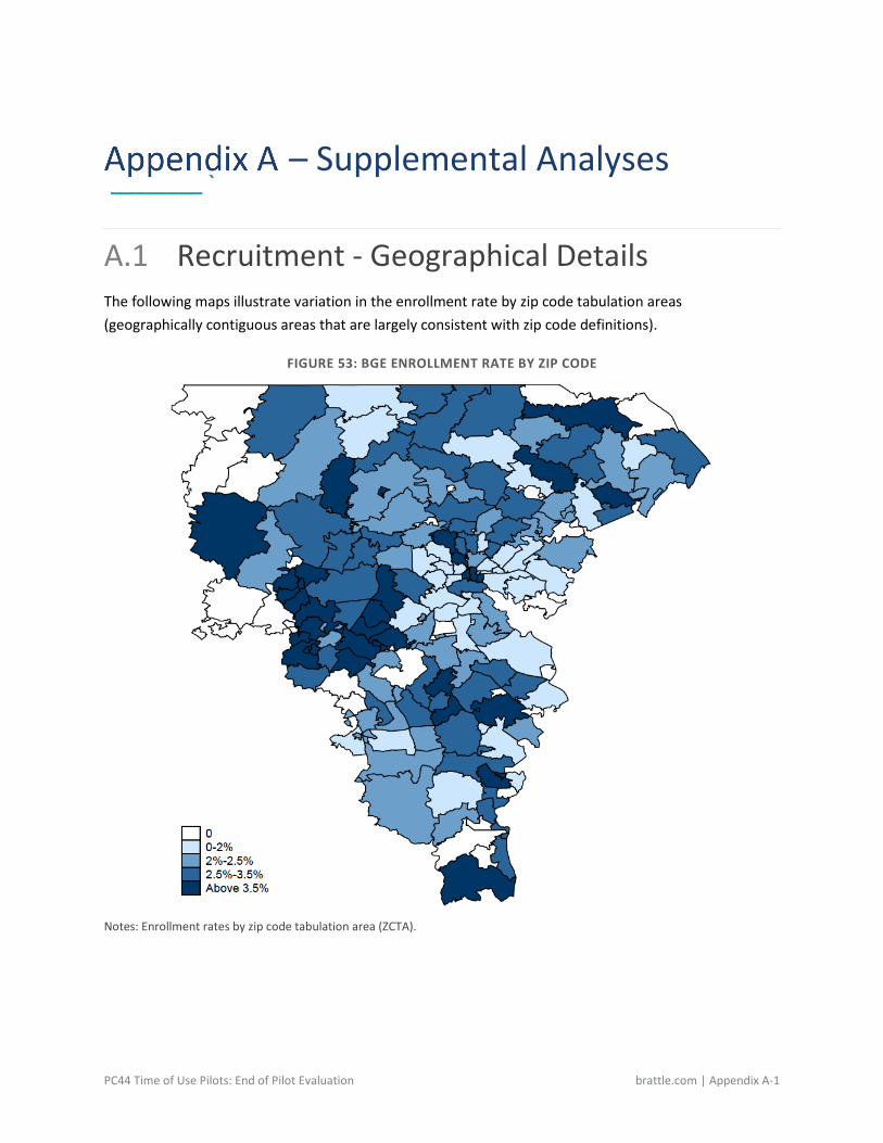
PC44 Time of Use Pilots: End of Pilot Evaluation brattle.com | Appendix A-1
– Supplemental Analyses _________ ̀
A.1 Recruitment - Geographical Details The following maps illustrate variation in the enrollment rate by zip code tabulation areas (geographically contiguous areas that are largely consistent with zip code definitions).
FIGURE 53: BGE ENROLLMENT RATE BY ZIP CODE
Notes: Enrollment rates by zip code tabulation area (ZCTA).

PC44 Time of Use Pilots: End of Pilot Evaluation brattle.com | Appendix A-2
FIGURE 54: PEPCO ENROLLMENT RATE BY ZIP CODE
Notes: Enrollment rates by zip code tabulation area (ZCTA).
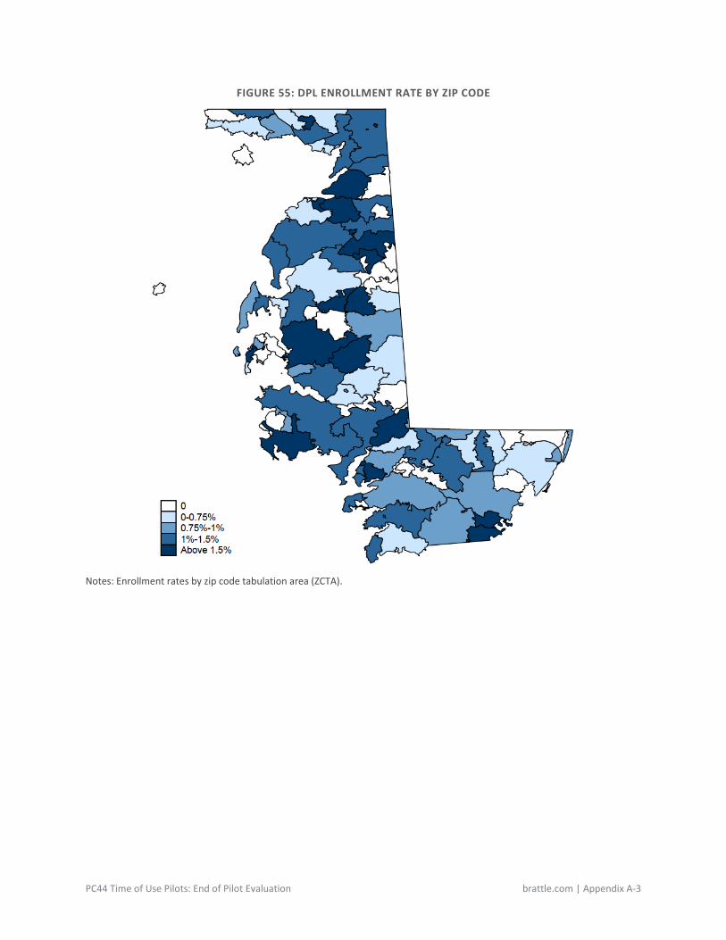
PC44 Time of Use Pilots: End of Pilot Evaluation brattle.com | Appendix A-3
FIGURE 55: DPL ENROLLMENT RATE BY ZIP CODE
Notes: Enrollment rates by zip code tabulation area (ZCTA).
PC44 Time of Use Pilots: End of Pilot Evaluation brattle.com | Appendix A-4
A.2 Data Cleaning and Processing We applied a series of criteria to exclude customers with data issues that had the potential to undermine our identification strategy. We first removed customers with account or tariff-related issues, as follows:
• Control customers
– whose account with the relevant JU started after January 1, 2018;
– who closed their account between January 1, 2018 and May 31, 2021; or
– who switched rates between January 1, 2018 and May 31, 2021, including volunteer enrollees to the PC44 TOU tariff.
• Targeted non-enrollees (used in the propensity score estimation in choosing a matched control group)
– who closed their account in 2018;
– who switched to a third-party supplier during the recruitment period (between February 1, 2019 and May 31, 2019)
• Pilot enrollees
– who unenrolled by June 1, 2019; and
– who unenrolled between June 1, 2019 and September 30, 2019 (excluded from the non-summer analysis only).
Then we implemented the following steps to exclude customers with insufficient load data:
• We set all hours with exactly zero load to missing.
• If a customer’s load is missing in one or more hours on a given day, we drop that customer-day.
• Enrolled and control customers are dropped from the analysis if
– They have incomplete load data on more than 10 days in any of the three summers, each 122 days long, used in the summer analysis. OR
– They have incomplete load data on more than 20 days in any of the non-summer periods: Jan – May 2018, Oct 2018 – Jan 2019 (274 days total) Oct 2019 – May 2020 (244 days total) Oct 2020 – May 2021 (243 days total).
• Targeted non-enrollees are dropped from the logit estimate if
– They have incomplete load data on more than 10 days in summer (Jun – Sept) 2018 (122 days total) OR
– They have incomplete load data on more than 20 days in non-summer (Jan – May and Oct – Dec) 2018 (243 days total).
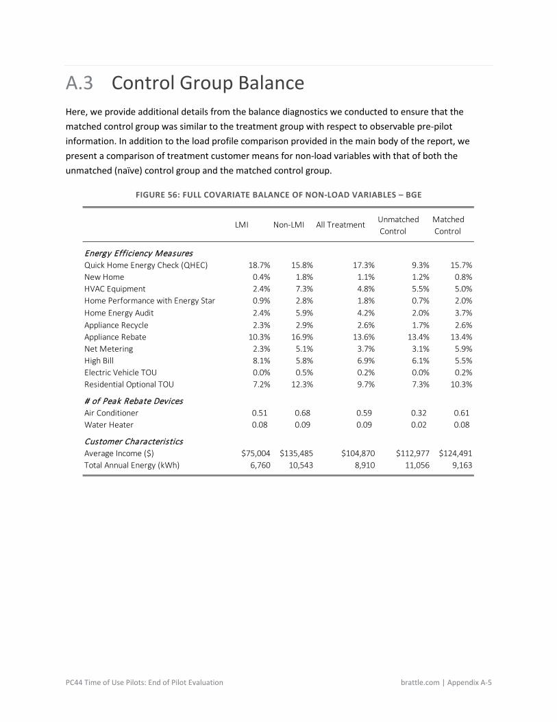
PC44 Time of Use Pilots: End of Pilot Evaluation brattle.com | Appendix A-5
A.3 Control Group Balance Here, we provide additional details from the balance diagnostics we conducted to ensure that the matched control group was similar to the treatment group with respect to observable pre-pilot information. In addition to the load profile comparison provided in the main body of the report, we present a comparison of treatment customer means for non-load variables with that of both the unmatched (naïve) control group and the matched control group.
FIGURE 56: FULL COVARIATE BALANCE OF NON-LOAD VARIABLES – BGE
LMI Non-LMI All Treatment Unmatched Control
Matched Control
Energy Efficiency MeasuresQuick Home Energy Check (QHEC) 18.7% 15.8% 17.3% 9.3% 15.7%New Home 0.4% 1.8% 1.1% 1.2% 0.8%HVAC Equipment 2.4% 7.3% 4.8% 5.5% 5.0%Home Performance with Energy Star 0.9% 2.8% 1.8% 0.7% 2.0%Home Energy Audit 2.4% 5.9% 4.2% 2.0% 3.7%Appliance Recycle 2.3% 2.9% 2.6% 1.7% 2.6%Appliance Rebate 10.3% 16.9% 13.6% 13.4% 13.4%Net Metering 2.3% 5.1% 3.7% 3.1% 5.9%High Bill 8.1% 5.8% 6.9% 6.1% 5.5%Electric Vehicle TOU 0.0% 0.5% 0.2% 0.0% 0.2%Residential Optional TOU 7.2% 12.3% 9.7% 7.3% 10.3%
# of Peak Rebate DevicesAir Conditioner 0.51 0.68 0.59 0.32 0.61 Water Heater 0.08 0.09 0.09 0.02 0.08
Customer CharacteristicsAverage Income ($) $75,004 $135,485 $104,870 $112,977 $124,491Total Annual Energy (kWh) 6,760 10,543 8,910 11,056 9,163
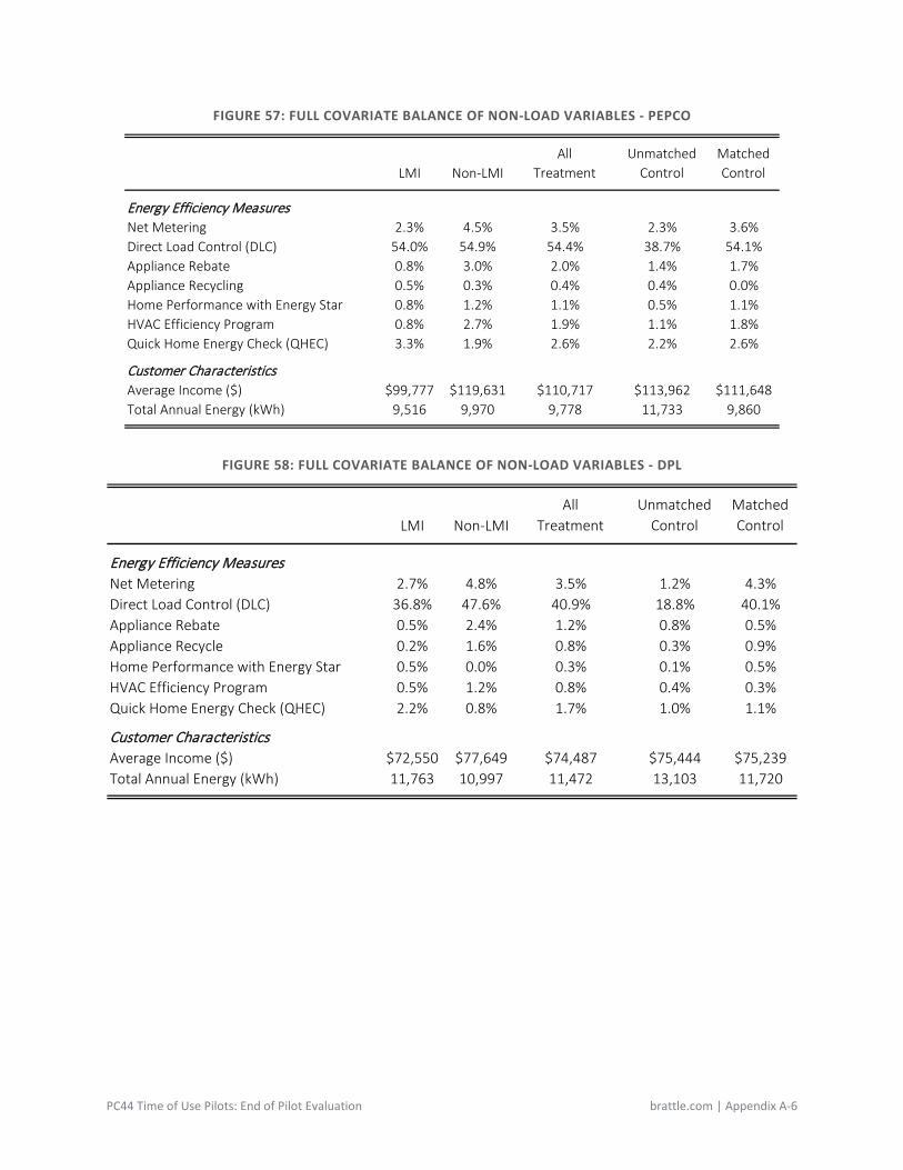
PC44 Time of Use Pilots: End of Pilot Evaluation brattle.com | Appendix A-6
FIGURE 57: FULL COVARIATE BALANCE OF NON-LOAD VARIABLES - PEPCO
FIGURE 58: FULL COVARIATE BALANCE OF NON-LOAD VARIABLES - DPL
LMI Non-LMIAll
Treatment Unmatched
ControlMatched Control
Energy Efficiency MeasuresNet Metering 2.3% 4.5% 3.5% 2.3% 3.6%Direct Load Control (DLC) 54.0% 54.9% 54.4% 38.7% 54.1%Appliance Rebate 0.8% 3.0% 2.0% 1.4% 1.7%Appliance Recycling 0.5% 0.3% 0.4% 0.4% 0.0%Home Performance with Energy Star 0.8% 1.2% 1.1% 0.5% 1.1%HVAC Efficiency Program 0.8% 2.7% 1.9% 1.1% 1.8%Quick Home Energy Check (QHEC) 3.3% 1.9% 2.6% 2.2% 2.6%
Customer CharacteristicsAverage Income ($) $99,777 $119,631 $110,717 $113,962 $111,648Total Annual Energy (kWh) 9,516 9,970 9,778 11,733 9,860
LMI Non-LMIAll
Treatment Unmatched
ControlMatched Control
Energy Efficiency MeasuresNet Metering 2.7% 4.8% 3.5% 1.2% 4.3%Direct Load Control (DLC) 36.8% 47.6% 40.9% 18.8% 40.1%Appliance Rebate 0.5% 2.4% 1.2% 0.8% 0.5%Appliance Recycle 0.2% 1.6% 0.8% 0.3% 0.9%Home Performance with Energy Star 0.5% 0.0% 0.3% 0.1% 0.5%HVAC Efficiency Program 0.5% 1.2% 0.8% 0.4% 0.3%Quick Home Energy Check (QHEC) 2.2% 0.8% 1.7% 1.0% 1.1%
Customer CharacteristicsAverage Income ($) $72,550 $77,649 $74,487 $75,444 $75,239Total Annual Energy (kWh) 11,763 10,997 11,472 13,103 11,720
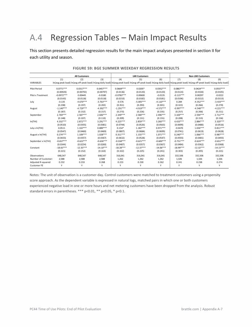
PC44 Time of Use Pilots: End of Pilot Evaluation brattle.com | Appendix A-7
A.4 Regression Tables – Main Impact Results This section presents detailed regression results for the main impact analyses presented in section II for each utility and season.
FIGURE 59: BGE SUMMER WEEKDAY REGRESSION RESULTS
Notes: The unit of observation is a customer-day. Control customers were matched to treatment customers using a propensity score approach. As the dependent variable is expressed in natural logs, matched pairs in which one or both customers experienced negative load in one or more hours and net metering customers have been dropped from the analysis. Robust standard errors in parentheses. *** p<0.01, ** p<0.05, * p<0.1.
(1) (2) (3) (4) (5) (6) (7) (8) (9)VARIABLES ln(avg peak load) ln(avg off-peak load) ln(avg daily load) ln(avg peak load) ln(avg off-peak load) ln(avg daily load) ln(avg peak load) ln(avg off-peak load) ln(avg daily load)
Pilot Period 0.0771*** 0.0317*** 0.0457*** 0.0669*** 0.0205* 0.0352*** 0.0867*** 0.0424*** 0.0557***(0.00920) (0.00792) (0.00797) (0.0136) (0.0120) (0.0120) (0.0124) (0.0104) (0.0105)
Pilot x Treatment -0.0972*** 0.00445 -0.0180 -0.0783*** 0.00600 -0.0135 -0.115*** 0.00297 -0.0222(0.0143) (0.0118) (0.0118) (0.0210) (0.0182) (0.0181) (0.0196) (0.0152) (0.0153)
July -0.135 -4.670*** -3.763*** -0.576 -5.005*** -4.110*** 0.284 -4.352*** -3.433***(0.238) (0.197) (0.202) (0.351) (0.293) (0.301) (0.322) (0.266) (0.270)
August -1.140*** -4.729*** -4.392*** -1.291*** -4.919*** -4.572*** -0.997*** -4.548*** -4.221***(0.187) (0.152) (0.157) (0.273) (0.226) (0.235) (0.257) (0.206) (0.211)
September 2.769*** 2.587*** 2.606*** 2.349*** 2.580*** 2.496*** 3.169*** 2.594*** 2.711***(0.148) (0.107) (0.110) (0.209) (0.151) (0.155) (0.208) (0.153) (0.156)
ln(THI) 4.332*** 2.872*** 3.291*** 4.225*** 2.859*** 3.260*** 4.433*** 2.884*** 3.320***(0.0510) (0.0355) (0.0381) (0.0744) (0.0526) (0.0563) (0.0699) (0.0480) (0.0516)
July x ln(THI) 0.0511 1.102*** 0.889*** 0.154* 1.182*** 0.971*** -0.0470 1.026*** 0.811***(0.0547) (0.0460) (0.0469) (0.0807) (0.0684) (0.0699) (0.0741) (0.0619) (0.0628)
August x ln(THI) 0.274*** 1.109*** 1.028*** 0.311*** 1.155*** 1.071*** 0.240*** 1.066*** 0.987***(0.0433) (0.0357) (0.0367) (0.0632) (0.0528) (0.0547) (0.0593) (0.0481) (0.0493)
September x ln(THI) -0.657*** -0.622*** -0.626*** -0.558*** -0.621*** -0.600*** -0.751*** -0.624*** -0.651***(0.0344) (0.0254) (0.0260) (0.0487) (0.0357) (0.0367) (0.0484) (0.0362) (0.0368)
Constant -18.65*** -12.35*** -14.10*** -18.28*** -12.37*** -14.06*** -18.99*** -12.32*** -14.15***(0.221) (0.152) (0.163) (0.322) (0.225) (0.241) (0.303) (0.205) (0.221)
Observations 648,547 648,547 648,547 316,041 316,041 316,041 332,506 332,506 332,506Number of Customers 2,588 2,588 2,588 1,262 1,262 1,262 1,326 1,326 1,326Adjusted R-squared 0.232 0.233 0.268 0.223 0.230 0.262 0.241 0.238 0.274Customer FE Y Y Y Y Y Y Y Y Y
All Customers LMI Customers Non-LMI Customers
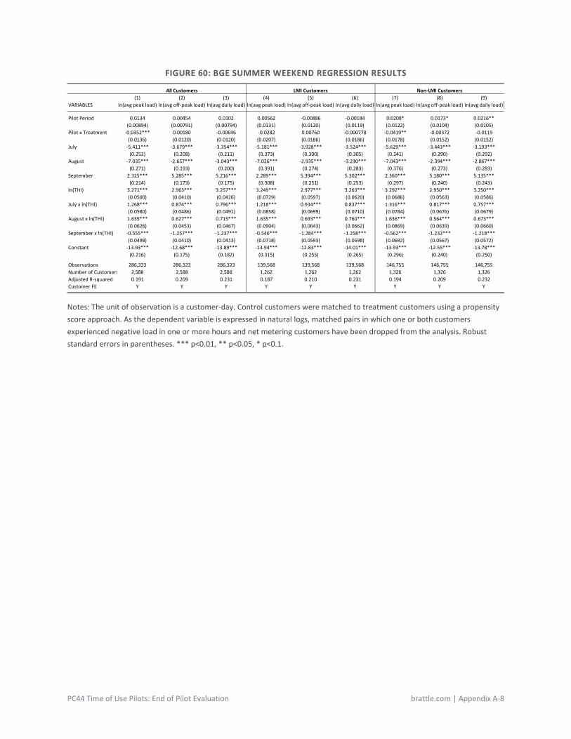
PC44 Time of Use Pilots: End of Pilot Evaluation brattle.com | Appendix A-8
FIGURE 60: BGE SUMMER WEEKEND REGRESSION RESULTS
Notes: The unit of observation is a customer-day. Control customers were matched to treatment customers using a propensity score approach. As the dependent variable is expressed in natural logs, matched pairs in which one or both customers experienced negative load in one or more hours and net metering customers have been dropped from the analysis. Robust standard errors in parentheses. *** p<0.01, ** p<0.05, * p<0.1.
(1) (2) (3) (4) (5) (6) (7) (8) (9)VARIABLES ln(avg peak load) ln(avg off-peak load) ln(avg daily load) ln(avg peak load) ln(avg off-peak load) ln(avg daily load) ln(avg peak load) ln(avg off-peak load) ln(avg daily load)
Pilot Period 0.0134 0.00454 0.0102 0.00562 -0.00886 -0.00184 0.0208* 0.0173* 0.0216**(0.00894) (0.00791) (0.00794) (0.0131) (0.0120) (0.0119) (0.0122) (0.0104) (0.0105)
Pilot x Treatment -0.0352*** 0.00180 -0.00646 -0.0282 0.00760 -0.000778 -0.0419** -0.00372 -0.0119(0.0136) (0.0120) (0.0120) (0.0207) (0.0186) (0.0186) (0.0178) (0.0152) (0.0152)
July -5.411*** -3.679*** -3.354*** -5.181*** -3.928*** -3.524*** -5.629*** -3.443*** -3.193***(0.252) (0.208) (0.211) (0.373) (0.300) (0.305) (0.341) (0.290) (0.292)
August -7.035*** -2.657*** -3.043*** -7.026*** -2.935*** -3.230*** -7.043*** -2.394*** -2.867***(0.271) (0.193) (0.200) (0.391) (0.274) (0.283) (0.376) (0.273) (0.283)
September 2.325*** 5.285*** 5.216*** 2.289*** 5.394*** 5.302*** 2.360*** 5.180*** 5.135***(0.214) (0.173) (0.175) (0.308) (0.251) (0.253) (0.297) (0.240) (0.243)
ln(THI) 3.271*** 2.963*** 3.257*** 3.249*** 2.977*** 3.263*** 3.292*** 2.950*** 3.250***(0.0500) (0.0410) (0.0426) (0.0729) (0.0597) (0.0620) (0.0686) (0.0563) (0.0586)
July x ln(THI) 1.268*** 0.874*** 0.796*** 1.218*** 0.934*** 0.837*** 1.316*** 0.817*** 0.757***(0.0580) (0.0486) (0.0491) (0.0858) (0.0699) (0.0710) (0.0784) (0.0676) (0.0679)
August x ln(THI) 1.635*** 0.627*** 0.715*** 1.635*** 0.693*** 0.760*** 1.636*** 0.564*** 0.673***(0.0626) (0.0453) (0.0467) (0.0904) (0.0643) (0.0662) (0.0869) (0.0639) (0.0660)
September x ln(THI) -0.555*** -1.257*** -1.237*** -0.546*** -1.284*** -1.258*** -0.562*** -1.232*** -1.218***(0.0498) (0.0410) (0.0413) (0.0718) (0.0593) (0.0598) (0.0692) (0.0567) (0.0572)
Constant -13.93*** -12.68*** -13.89*** -13.94*** -12.83*** -14.01*** -13.93*** -12.55*** -13.78***(0.216) (0.175) (0.182) (0.315) (0.255) (0.265) (0.296) (0.240) (0.250)
Observations 286,323 286,323 286,323 139,568 139,568 139,568 146,755 146,755 146,755Number of Customers 2,588 2,588 2,588 1,262 1,262 1,262 1,326 1,326 1,326Adjusted R-squared 0.191 0.209 0.231 0.187 0.210 0.231 0.194 0.209 0.232Customer FE Y Y Y Y Y Y Y Y Y
All Customers LMI Customers Non-LMI Customers

PC44 Time of Use Pilots: End of Pilot Evaluation brattle.com | Appendix A-9
FIGURE 61: BGE NON-SUMMER WEEKDAY REGRESSION RESULTS
Notes: The unit of observation is a customer-day. Control customers were matched to treatment customers using a propensity score approach. As the dependent variable is expressed in natural logs, matched pairs in which one or both customers experienced negative load in one or more hours and net metering customers have been dropped from the analysis. Robust standard errors in parentheses. *** p<0.01, ** p<0.05, * p<0.1.
(1) (2) (3) (4) (5) (6) (7) (8) (9)VARIABLES ln(avg peak load) ln(avg off-peak load) ln(avg daily load) ln(avg peak load) ln(avg off-peak load) ln(avg daily load) ln(avg peak load) ln(avg off-peak load) ln(avg daily load)
Pilot Period -0.0253*** 0.00158 -0.00329 -0.0175 0.0120 0.00643 -0.0327*** -0.00828 -0.0124(0.00937) (0.00851) (0.00844) (0.0142) (0.0131) (0.0130) (0.0123) (0.0109) (0.0109)
Pilot x Treatment -0.0506*** 0.000832 -0.00467 -0.0571*** -0.0221 -0.0254 -0.0444** 0.0224 0.0148(0.0139) (0.0118) (0.0117) (0.0210) (0.0182) (0.0181) (0.0183) (0.0151) (0.0150)
February 1.148*** 1.001*** 1.017*** 1.108*** 1.029*** 1.034*** 1.185*** 0.975*** 1.001***(0.0523) (0.0472) (0.0469) (0.0727) (0.0674) (0.0668) (0.0750) (0.0662) (0.0658)
March 1.095*** 0.534*** 0.590*** 1.080*** 0.645*** 0.683*** 1.108*** 0.430*** 0.503***(0.0595) (0.0614) (0.0593) (0.0867) (0.0928) (0.0891) (0.0818) (0.0811) (0.0788)
April 1.007*** -0.894*** -0.629*** 1.185*** -0.570*** -0.324*** 0.839*** -1.198*** -0.916***(0.0833) (0.0846) (0.0820) (0.122) (0.129) (0.125) (0.114) (0.110) (0.107)
May -2.480*** -6.793*** -6.259*** -2.364*** -6.383*** -5.876*** -2.590*** -7.177*** -6.618***(0.126) (0.132) (0.129) (0.187) (0.200) (0.195) (0.169) (0.174) (0.170)
October -2.004*** -6.133*** -5.534*** -1.954*** -5.785*** -5.230*** -2.050*** -6.460*** -5.820***(0.0970) (0.111) (0.106) (0.146) (0.169) (0.162) (0.129) (0.144) (0.139)
November 0.993*** 0.407*** 0.472*** 1.093*** 0.605*** 0.654*** 0.899*** 0.221*** 0.301***(0.0597) (0.0586) (0.0573) (0.0870) (0.0859) (0.0839) (0.0819) (0.0796) (0.0780)
December 0.606*** -0.225*** -0.0894** 0.571*** -0.177*** -0.0520 0.638*** -0.270*** -0.125**(0.0432) (0.0412) (0.0395) (0.0609) (0.0586) (0.0558) (0.0613) (0.0580) (0.0558)
ln(THI) -0.784*** -0.904*** -0.885*** -0.741*** -0.845*** -0.827*** -0.825*** -0.960*** -0.940***(0.0141) (0.0146) (0.0143) (0.0199) (0.0210) (0.0206) (0.0198) (0.0201) (0.0198)
February x ln(THI) -0.311*** -0.272*** -0.275*** -0.298*** -0.278*** -0.279*** -0.323*** -0.265*** -0.272***(0.0139) (0.0124) (0.0123) (0.0194) (0.0177) (0.0175) (0.0200) (0.0174) (0.0173)
March x ln(THI) -0.310*** -0.158*** -0.173*** -0.306*** -0.187*** -0.197*** -0.315*** -0.131*** -0.150***(0.0158) (0.0277) (0.0267) (0.0230) (0.0423) (0.0406) (0.0217) (0.0360) (0.0347)
April x ln(THI) -0.308*** 0.188*** 0.121*** -0.353*** 0.105*** 0.0429 -0.266*** 0.266*** 0.194***(0.0158) (0.0153) (0.0267) (0.0230) (0.0223) (0.0406) (0.0217) (0.0208) (0.0347)
May x ln(THI) 0.545*** 1.630*** 1.498*** 0.515*** 1.525*** 1.400*** 0.572*** 1.729*** 1.590***(0.0158) (0.0153) (0.0149) (0.0230) (0.0223) (0.0219) (0.0217) (0.0208) (0.0204)
October x ln(THI) 0.437*** 1.464*** 1.317*** 0.424*** 1.376*** 1.240*** 0.449*** 1.546*** 1.389***(0.0115) (0.0153) (0.0149) (0.0162) (0.0223) (0.0219) (0.0165) (0.0208) (0.0204)
November x ln(THI) -0.288*** -0.129*** -0.146*** -0.314*** -0.180*** -0.193*** -0.264*** -0.0806*** -0.102***(0.0115) (0.0109) (0.0149) (0.0162) (0.0154) (0.0219) (0.0165) (0.0153) (0.0204)
December x ln(THI) -0.163*** 0.0665*** 0.0300*** -0.153*** 0.0526*** 0.0190 -0.172*** 0.0797*** 0.0404***(0.0115) (0.0109) (0.0104) (0.0162) (0.0154) (0.0146) (0.0165) (0.0153) (0.0148)
Constant 3.010*** 3.481*** 3.420*** 2.746*** 3.170*** 3.112*** 3.258*** 3.773*** 3.709***(0.0552) (0.0576) (0.0567) (0.0779) (0.0826) (0.0812) (0.0779) (0.0800) (0.0788)
Observations 1,274,282 1,274,282 1,274,282 617,480 617,480 617,480 656,802 656,802 656,802Number of Customers 2,454 2,454 2,454 1,190 1,190 1,190 1,264 1,264 1,264Adjusted R-squared 0.188 0.186 0.198 0.174 0.174 0.185 0.203 0.199 0.211Customer FE Y Y Y Y Y Y Y Y Y
All Customers LMI Customers Non-LMI Customers
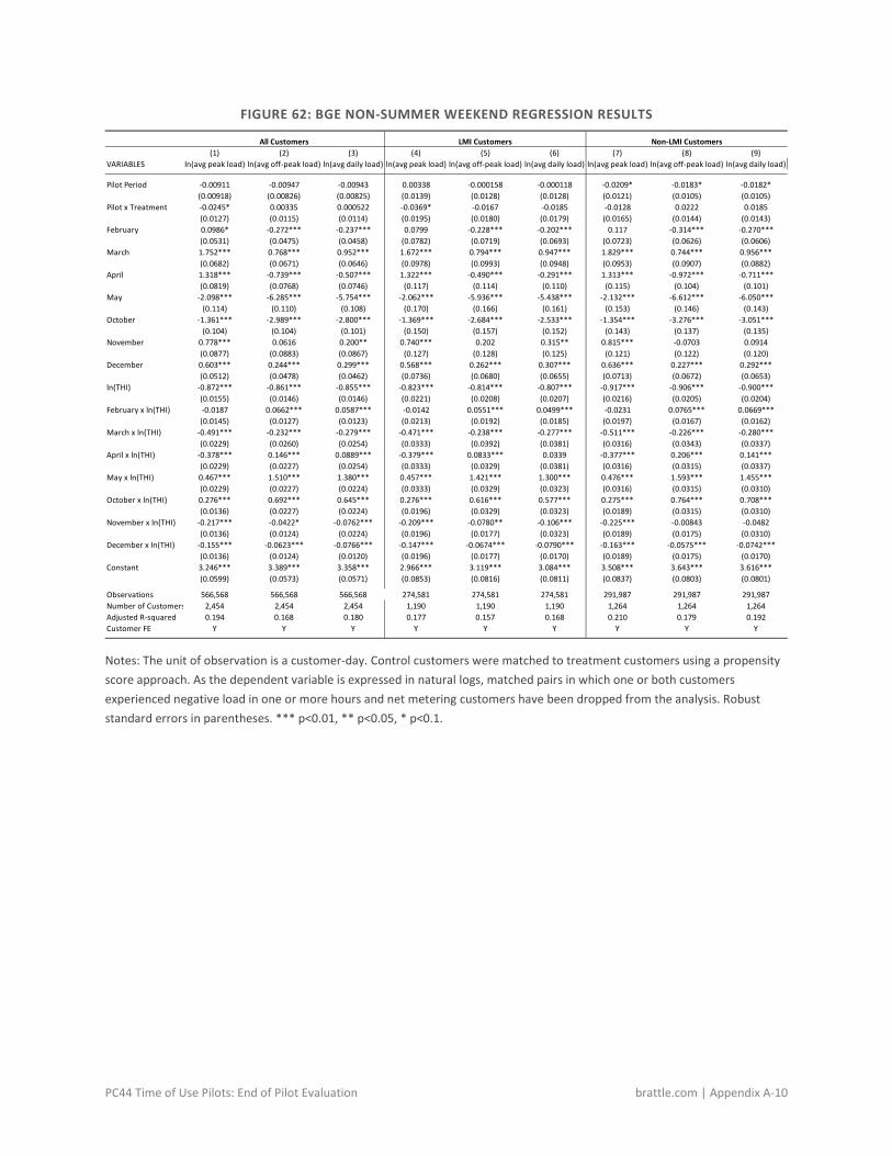
PC44 Time of Use Pilots: End of Pilot Evaluation brattle.com | Appendix A-10
FIGURE 62: BGE NON-SUMMER WEEKEND REGRESSION RESULTS
Notes: The unit of observation is a customer-day. Control customers were matched to treatment customers using a propensity score approach. As the dependent variable is expressed in natural logs, matched pairs in which one or both customers experienced negative load in one or more hours and net metering customers have been dropped from the analysis. Robust standard errors in parentheses. *** p<0.01, ** p<0.05, * p<0.1.
(1) (2) (3) (4) (5) (6) (7) (8) (9)VARIABLES ln(avg peak load) ln(avg off-peak load) ln(avg daily load) ln(avg peak load) ln(avg off-peak load) ln(avg daily load) ln(avg peak load) ln(avg off-peak load) ln(avg daily load)
Pilot Period -0.00911 -0.00947 -0.00943 0.00338 -0.000158 -0.000118 -0.0209* -0.0183* -0.0182*(0.00918) (0.00826) (0.00825) (0.0139) (0.0128) (0.0128) (0.0121) (0.0105) (0.0105)
Pilot x Treatment -0.0245* 0.00335 0.000522 -0.0369* -0.0167 -0.0185 -0.0128 0.0222 0.0185(0.0127) (0.0115) (0.0114) (0.0195) (0.0180) (0.0179) (0.0165) (0.0144) (0.0143)
February 0.0986* -0.272*** -0.237*** 0.0799 -0.228*** -0.202*** 0.117 -0.314*** -0.270***(0.0531) (0.0475) (0.0458) (0.0782) (0.0719) (0.0693) (0.0723) (0.0626) (0.0606)
March 1.752*** 0.768*** 0.952*** 1.672*** 0.794*** 0.947*** 1.829*** 0.744*** 0.956***(0.0682) (0.0671) (0.0646) (0.0978) (0.0993) (0.0948) (0.0953) (0.0907) (0.0882)
April 1.318*** -0.739*** -0.507*** 1.322*** -0.490*** -0.291*** 1.313*** -0.972*** -0.711***(0.0819) (0.0768) (0.0746) (0.117) (0.114) (0.110) (0.115) (0.104) (0.101)
May -2.098*** -6.285*** -5.754*** -2.062*** -5.936*** -5.438*** -2.132*** -6.612*** -6.050***(0.114) (0.110) (0.108) (0.170) (0.166) (0.161) (0.153) (0.146) (0.143)
October -1.361*** -2.989*** -2.800*** -1.369*** -2.684*** -2.533*** -1.354*** -3.276*** -3.051***(0.104) (0.104) (0.101) (0.150) (0.157) (0.152) (0.143) (0.137) (0.135)
November 0.778*** 0.0616 0.200** 0.740*** 0.202 0.315** 0.815*** -0.0703 0.0914(0.0877) (0.0883) (0.0867) (0.127) (0.128) (0.125) (0.121) (0.122) (0.120)
December 0.603*** 0.244*** 0.299*** 0.568*** 0.262*** 0.307*** 0.636*** 0.227*** 0.292***(0.0512) (0.0478) (0.0462) (0.0736) (0.0680) (0.0655) (0.0713) (0.0672) (0.0653)
ln(THI) -0.872*** -0.861*** -0.855*** -0.823*** -0.814*** -0.807*** -0.917*** -0.906*** -0.900***(0.0155) (0.0146) (0.0146) (0.0221) (0.0208) (0.0207) (0.0216) (0.0205) (0.0204)
February x ln(THI) -0.0187 0.0662*** 0.0587*** -0.0142 0.0551*** 0.0499*** -0.0231 0.0765*** 0.0669***(0.0145) (0.0127) (0.0123) (0.0213) (0.0192) (0.0185) (0.0197) (0.0167) (0.0162)
March x ln(THI) -0.491*** -0.232*** -0.279*** -0.471*** -0.238*** -0.277*** -0.511*** -0.226*** -0.280***(0.0229) (0.0260) (0.0254) (0.0333) (0.0392) (0.0381) (0.0316) (0.0343) (0.0337)
April x ln(THI) -0.378*** 0.146*** 0.0889*** -0.379*** 0.0833*** 0.0339 -0.377*** 0.206*** 0.141***(0.0229) (0.0227) (0.0254) (0.0333) (0.0329) (0.0381) (0.0316) (0.0315) (0.0337)
May x ln(THI) 0.467*** 1.510*** 1.380*** 0.457*** 1.421*** 1.300*** 0.476*** 1.593*** 1.455***(0.0229) (0.0227) (0.0224) (0.0333) (0.0329) (0.0323) (0.0316) (0.0315) (0.0310)
October x ln(THI) 0.276*** 0.692*** 0.645*** 0.276*** 0.616*** 0.577*** 0.275*** 0.764*** 0.708***(0.0136) (0.0227) (0.0224) (0.0196) (0.0329) (0.0323) (0.0189) (0.0315) (0.0310)
November x ln(THI) -0.217*** -0.0422* -0.0762*** -0.209*** -0.0780** -0.106*** -0.225*** -0.00843 -0.0482(0.0136) (0.0124) (0.0224) (0.0196) (0.0177) (0.0323) (0.0189) (0.0175) (0.0310)
December x ln(THI) -0.155*** -0.0623*** -0.0766*** -0.147*** -0.0674*** -0.0790*** -0.163*** -0.0575*** -0.0742***(0.0136) (0.0124) (0.0120) (0.0196) (0.0177) (0.0170) (0.0189) (0.0175) (0.0170)
Constant 3.246*** 3.389*** 3.358*** 2.966*** 3.119*** 3.084*** 3.508*** 3.643*** 3.616***(0.0599) (0.0573) (0.0571) (0.0853) (0.0816) (0.0811) (0.0837) (0.0803) (0.0801)
Observations 566,568 566,568 566,568 274,581 274,581 274,581 291,987 291,987 291,987Number of Customers 2,454 2,454 2,454 1,190 1,190 1,190 1,264 1,264 1,264Adjusted R-squared 0.194 0.168 0.180 0.177 0.157 0.168 0.210 0.179 0.192Customer FE Y Y Y Y Y Y Y Y Y
All Customers LMI Customers Non-LMI Customers
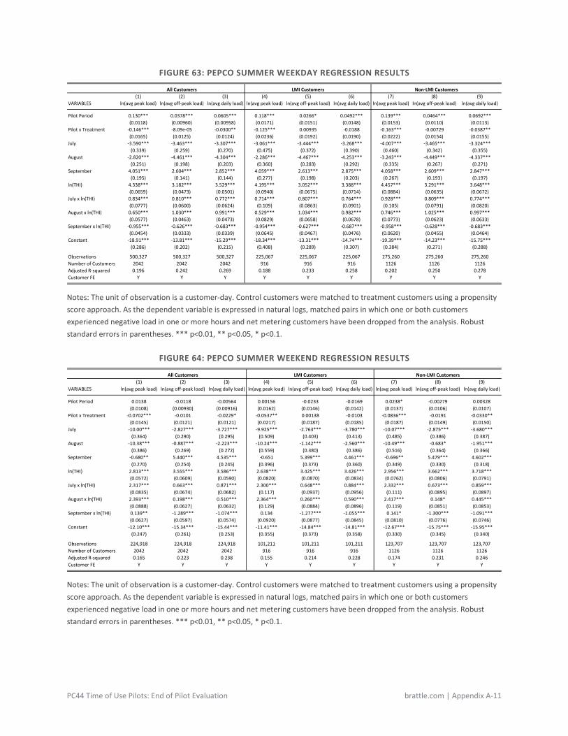
PC44 Time of Use Pilots: End of Pilot Evaluation brattle.com | Appendix A-11
FIGURE 63: PEPCO SUMMER WEEKDAY REGRESSION RESULTS
Notes: The unit of observation is a customer-day. Control customers were matched to treatment customers using a propensity score approach. As the dependent variable is expressed in natural logs, matched pairs in which one or both customers experienced negative load in one or more hours and net metering customers have been dropped from the analysis. Robust standard errors in parentheses. *** p<0.01, ** p<0.05, * p<0.1.
FIGURE 64: PEPCO SUMMER WEEKEND REGRESSION RESULTS
Notes: The unit of observation is a customer-day. Control customers were matched to treatment customers using a propensity score approach. As the dependent variable is expressed in natural logs, matched pairs in which one or both customers experienced negative load in one or more hours and net metering customers have been dropped from the analysis. Robust standard errors in parentheses. *** p<0.01, ** p<0.05, * p<0.1.
All Customers LMI Customers Non-LMI Customers(1) (2) (3) (4) (5) (6) (7) (8) (9)
VARIABLES ln(avg peak load) ln(avg off-peak load) ln(avg daily load) ln(avg peak load) ln(avg off-peak load) ln(avg daily load) ln(avg peak load) ln(avg off-peak load) ln(avg daily load)
Pilot Period 0.130*** 0.0378*** 0.0605*** 0.118*** 0.0266* 0.0492*** 0.139*** 0.0464*** 0.0692***(0.0118) (0.00960) (0.00958) (0.0171) (0.0151) (0.0148) (0.0153) (0.0110) (0.0113)
Pilot x Treatment -0.146*** -8.09e-05 -0.0300** -0.125*** 0.00935 -0.0188 -0.163*** -0.00729 -0.0387**(0.0165) (0.0125) (0.0124) (0.0236) (0.0192) (0.0190) (0.0222) (0.0154) (0.0155)
July -3.590*** -3.463*** -3.307*** -3.061*** -3.444*** -3.268*** -4.007*** -3.465*** -3.324***(0.339) (0.259) (0.270) (0.475) (0.372) (0.390) (0.460) (0.342) (0.355)
August -2.820*** -4.461*** -4.304*** -2.286*** -4.467*** -4.253*** -3.243*** -4.449*** -4.337***(0.251) (0.198) (0.203) (0.360) (0.283) (0.292) (0.335) (0.267) (0.271)
September 4.051*** 2.604*** 2.852*** 4.059*** 2.613*** 2.875*** 4.058*** 2.609*** 2.847***(0.195) (0.141) (0.144) (0.277) (0.198) (0.203) (0.267) (0.193) (0.197)
ln(THI) 4.338*** 3.182*** 3.529*** 4.195*** 3.052*** 3.388*** 4.457*** 3.291*** 3.648***(0.0659) (0.0473) (0.0501) (0.0940) (0.0675) (0.0714) (0.0884) (0.0635) (0.0672)
July x ln(THI) 0.834*** 0.810*** 0.772*** 0.714*** 0.807*** 0.764*** 0.928*** 0.809*** 0.774***(0.0777) (0.0600) (0.0624) (0.109) (0.0863) (0.0901) (0.105) (0.0791) (0.0820)
August x ln(THI) 0.650*** 1.030*** 0.991*** 0.529*** 1.034*** 0.982*** 0.746*** 1.025*** 0.997***(0.0577) (0.0463) (0.0473) (0.0829) (0.0658) (0.0678) (0.0773) (0.0623) (0.0633)
September x ln(THI) -0.955*** -0.626*** -0.683*** -0.954*** -0.627*** -0.687*** -0.958*** -0.628*** -0.683***(0.0454) (0.0333) (0.0339) (0.0645) (0.0467) (0.0476) (0.0620) (0.0455) (0.0464)
Constant -18.91*** -13.81*** -15.29*** -18.34*** -13.31*** -14.74*** -19.39*** -14.23*** -15.75***(0.286) (0.202) (0.215) (0.408) (0.289) (0.307) (0.384) (0.271) (0.288)
Observations 500,327 500,327 500,327 225,067 225,067 225,067 275,260 275,260 275,260Number of Customers 2042 2042 2042 916 916 916 1126 1126 1126Adjusted R-squared 0.196 0.242 0.269 0.188 0.233 0.258 0.202 0.250 0.278Customer FE Y Y Y Y Y Y Y Y Y
All Customers LMI Customers Non-LMI Customers(1) (2) (3) (4) (5) (6) (7) (8) (9)
VARIABLES ln(avg peak load) ln(avg off-peak load) ln(avg daily load) ln(avg peak load) ln(avg off-peak load) ln(avg daily load) ln(avg peak load) ln(avg off-peak load) ln(avg daily load)
Pilot Period 0.0138 -0.0118 -0.00564 0.00156 -0.0233 -0.0169 0.0238* -0.00279 0.00328(0.0108) (0.00930) (0.00916) (0.0162) (0.0146) (0.0142) (0.0137) (0.0106) (0.0107)
Pilot x Treatment -0.0702*** -0.0101 -0.0229* -0.0537** 0.00138 -0.0103 -0.0836*** -0.0191 -0.0330**(0.0145) (0.0121) (0.0121) (0.0217) (0.0187) (0.0185) (0.0187) (0.0149) (0.0150)
July -10.00*** -2.827*** -3.727*** -9.925*** -2.763*** -3.780*** -10.07*** -2.875*** -3.680***(0.364) (0.290) (0.295) (0.509) (0.403) (0.413) (0.485) (0.386) (0.387)
August -10.38*** -0.887*** -2.223*** -10.24*** -1.142*** -2.560*** -10.49*** -0.683* -1.951***(0.386) (0.269) (0.272) (0.559) (0.380) (0.386) (0.516) (0.364) (0.366)
September -0.680** 5.440*** 4.535*** -0.651 5.399*** 4.461*** -0.696** 5.479*** 4.602***(0.270) (0.254) (0.245) (0.396) (0.373) (0.360) (0.349) (0.330) (0.318)
ln(THI) 2.813*** 3.555*** 3.586*** 2.638*** 3.425*** 3.426*** 2.956*** 3.662*** 3.718***(0.0572) (0.0609) (0.0590) (0.0820) (0.0870) (0.0834) (0.0762) (0.0806) (0.0791)
July x ln(THI) 2.317*** 0.663*** 0.871*** 2.300*** 0.648*** 0.884*** 2.332*** 0.673*** 0.859***(0.0835) (0.0674) (0.0682) (0.117) (0.0937) (0.0956) (0.111) (0.0895) (0.0897)
August x ln(THI) 2.393*** 0.198*** 0.510*** 2.364*** 0.260*** 0.590*** 2.417*** 0.148* 0.445***(0.0888) (0.0627) (0.0632) (0.129) (0.0884) (0.0896) (0.119) (0.0851) (0.0853)
September x ln(THI) 0.139** -1.289*** -1.074*** 0.134 -1.277*** -1.055*** 0.141* -1.300*** -1.091***(0.0627) (0.0597) (0.0574) (0.0920) (0.0877) (0.0845) (0.0810) (0.0776) (0.0746)
Constant -12.10*** -15.34*** -15.44*** -11.41*** -14.84*** -14.81*** -12.67*** -15.75*** -15.95***(0.247) (0.261) (0.253) (0.355) (0.373) (0.358) (0.330) (0.345) (0.340)
Observations 224,918 224,918 224,918 101,211 101,211 101,211 123,707 123,707 123,707Number of Customers 2042 2042 2042 916 916 916 1126 1126 1126Adjusted R-squared 0.165 0.223 0.238 0.155 0.214 0.228 0.174 0.231 0.246Customer FE Y Y Y Y Y Y Y Y Y

PC44 Time of Use Pilots: End of Pilot Evaluation brattle.com | Appendix A-12
FIGURE 65: PEPCO NON-SUMMER WEEKDAY REGRESSION RESULTS
Notes: The unit of observation is a customer-day. Control customers were matched to treatment customers using a propensity score approach. As the dependent variable is expressed in natural logs, matched pairs in which one or both customers experienced negative load in one or more hours and net metering customers have been dropped from the analysis. Robust standard errors in parentheses. *** p<0.01, ** p<0.05, * p<0.1.
All Customers LMI Customers Non-LMI Customers(1) (2) (3) (4) (5) (6) (7) (8) (9)
VARIABLES ln(avg peak load) ln(avg off-peak load) ln(avg daily load) ln(avg peak load) ln(avg off-peak load) ln(avg daily load) ln(avg peak load) ln(avg off-peak load) ln(avg daily load)
Pilot Period 0.00560 0.0315*** 0.0272*** -0.00175 0.0242* 0.0199 0.0111 0.0373*** 0.0331***(0.0114) (0.00973) (0.00961) (0.0176) (0.0145) (0.0144) (0.0137) (0.0123) (0.0120)
Pilot x Treatment -0.0510*** -0.00181 -0.00732 -0.0397* -0.0112 -0.0136 -0.0598*** 0.00585 -0.00213(0.0157) (0.0128) (0.0126) (0.0233) (0.0185) (0.0182) (0.0203) (0.0171) (0.0168)
February 1.435*** 1.320*** 1.366*** 1.501*** 1.331*** 1.390*** 1.381*** 1.310*** 1.346***(0.0503) (0.0463) (0.0459) (0.0710) (0.0670) (0.0661) (0.0682) (0.0620) (0.0616)
March 1.555*** 1.305*** 1.328*** 1.669*** 1.429*** 1.455*** 1.463*** 1.206*** 1.226***(0.0672) (0.0677) (0.0661) (0.0983) (0.0988) (0.0961) (0.0883) (0.0891) (0.0871)
April 1.312*** 0.362*** 0.511*** 1.363*** 0.549*** 0.679*** 1.271*** 0.212 0.374***(0.0892) (0.102) (0.0984) (0.133) (0.154) (0.149) (0.118) (0.131) (0.127)
May -2.554*** -6.595*** -6.098*** -2.481*** -6.057*** -5.605*** -2.613*** -7.030*** -6.496***(0.139) (0.165) (0.159) (0.208) (0.237) (0.229) (0.178) (0.222) (0.213)
October -1.150*** -5.027*** -4.452*** -1.205*** -4.681*** -4.160*** -1.106*** -5.306*** -4.687***(0.106) (0.136) (0.130) (0.161) (0.201) (0.191) (0.134) (0.176) (0.168)
November 0.823*** 0.576*** 0.606*** 0.903*** 0.654*** 0.687*** 0.758*** 0.513*** 0.540***(0.0567) (0.0605) (0.0585) (0.0825) (0.0868) (0.0840) (0.0756) (0.0815) (0.0788)
December 0.397*** -0.223*** -0.130** 0.474*** -0.211*** -0.104 0.335*** -0.232*** -0.152**(0.0506) (0.0542) (0.0515) (0.0736) (0.0770) (0.0734) (0.0677) (0.0735) (0.0697)
ln(THI) -0.483*** -0.609*** -0.589*** -0.497*** -0.632*** -0.611*** -0.472*** -0.591*** -0.572***(0.0108) (0.0124) (0.0121) (0.0155) (0.0177) (0.0172) (0.0143) (0.0165) (0.0161)
February x ln(THI) -0.393*** -0.356*** -0.369*** -0.410*** -0.358*** -0.374*** -0.380*** -0.355*** -0.365***(0.0136) (0.0123) (0.0122) (0.0192) (0.0178) (0.0176) (0.0185) (0.0165) (0.0164)
March x ln(THI) -0.439*** -0.357*** -0.365*** -0.469*** -0.388*** -0.396*** -0.414*** -0.333*** -0.339***(0.0181) (0.0177) (0.0173) (0.0265) (0.0259) (0.0253) (0.0237) (0.0233) (0.0228)
April x ln(THI) -0.389*** -0.122*** -0.162*** -0.405*** -0.169*** -0.204*** -0.376*** -0.0848** -0.128***(0.0235) (0.0260) (0.0253) (0.0353) (0.0394) (0.0382) (0.0310) (0.0336) (0.0327)
May x ln(THI) 0.566*** 1.575*** 1.453*** 0.546*** 1.441*** 1.330*** 0.582*** 1.683*** 1.553***(0.0348) (0.0409) (0.0395) (0.0523) (0.0587) (0.0569) (0.0447) (0.0547) (0.0527)
October x ln(THI) 0.229*** 1.187*** 1.048*** 0.240*** 1.100*** 0.973*** 0.220*** 1.258*** 1.108***(0.0271) (0.0340) (0.0325) (0.0414) (0.0501) (0.0480) (0.0342) (0.0439) (0.0419)
November x ln(THI) -0.243*** -0.173*** -0.181*** -0.264*** -0.193*** -0.202*** -0.227*** -0.157*** -0.164***(0.0152) (0.0159) (0.0154) (0.0222) (0.0228) (0.0221) (0.0203) (0.0214) (0.0208)
December x ln(THI) -0.112*** 0.0598*** 0.0349** -0.133*** 0.0563*** 0.0276 -0.0954*** 0.0627*** 0.0409**(0.0137) (0.0144) (0.0137) (0.0199) (0.0203) (0.0194) (0.0184) (0.0195) (0.0185)
Constant 1.580*** 2.161*** 2.085*** 1.620*** 2.240*** 2.160*** 1.548*** 2.097*** 2.025***(0.0423) (0.0494) (0.0480) (0.0608) (0.0708) (0.0687) (0.0561) (0.0657) (0.0639)
Observations 996,283 996,236 996,243 444,180 444,180 444,180 552,103 552,056 552,063Number of Customers 1934 1934 1934 862 862 862 1072 1072 1072Adjusted R-squared 0.143 0.147 0.156 0.152 0.164 0.174 0.137 0.136 0.144Customer FE Y Y Y Y Y Y Y Y Y
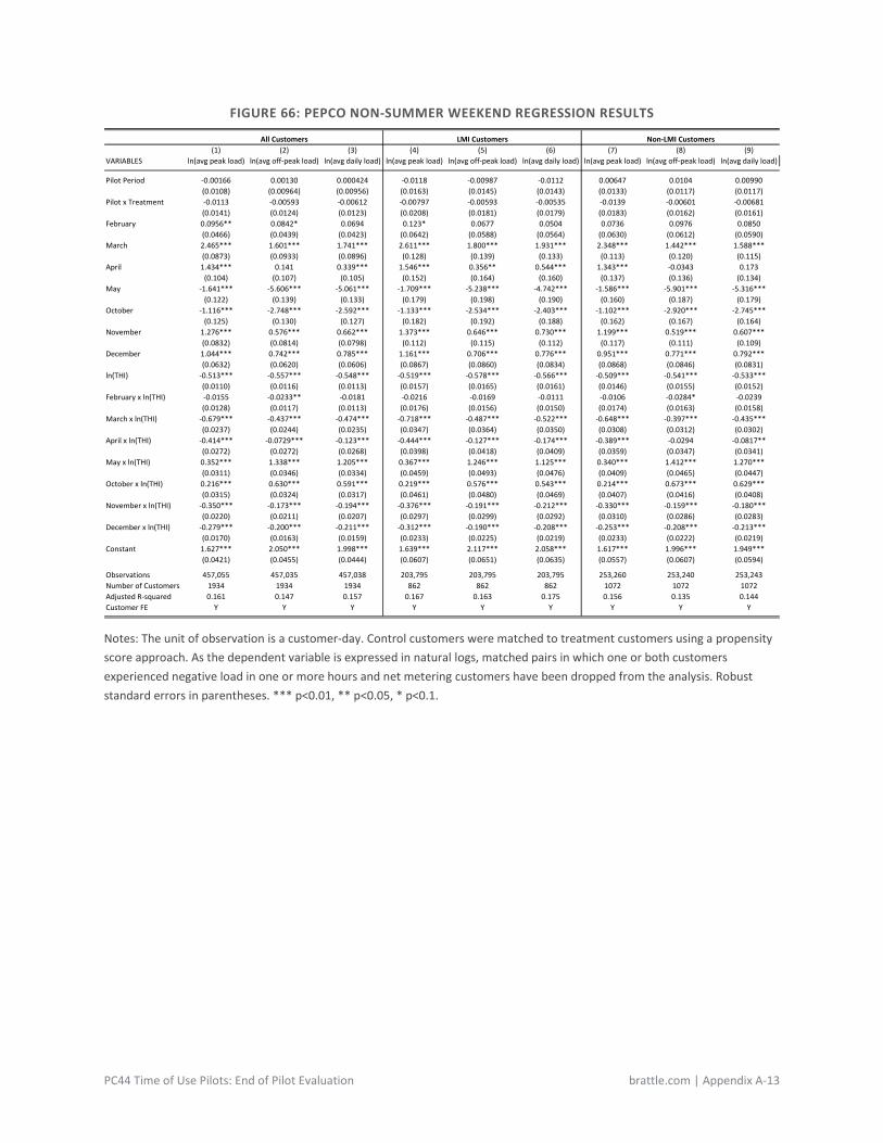
PC44 Time of Use Pilots: End of Pilot Evaluation brattle.com | Appendix A-13
FIGURE 66: PEPCO NON-SUMMER WEEKEND REGRESSION RESULTS
Notes: The unit of observation is a customer-day. Control customers were matched to treatment customers using a propensity score approach. As the dependent variable is expressed in natural logs, matched pairs in which one or both customers experienced negative load in one or more hours and net metering customers have been dropped from the analysis. Robust standard errors in parentheses. *** p<0.01, ** p<0.05, * p<0.1.
All Customers LMI Customers Non-LMI Customers(1) (2) (3) (4) (5) (6) (7) (8) (9)
VARIABLES ln(avg peak load) ln(avg off-peak load) ln(avg daily load) ln(avg peak load) ln(avg off-peak load) ln(avg daily load) ln(avg peak load) ln(avg off-peak load) ln(avg daily load)
Pilot Period -0.00166 0.00130 0.000424 -0.0118 -0.00987 -0.0112 0.00647 0.0104 0.00990(0.0108) (0.00964) (0.00956) (0.0163) (0.0145) (0.0143) (0.0133) (0.0117) (0.0117)
Pilot x Treatment -0.0113 -0.00593 -0.00612 -0.00797 -0.00593 -0.00535 -0.0139 -0.00601 -0.00681(0.0141) (0.0124) (0.0123) (0.0208) (0.0181) (0.0179) (0.0183) (0.0162) (0.0161)
February 0.0956** 0.0842* 0.0694 0.123* 0.0677 0.0504 0.0736 0.0976 0.0850(0.0466) (0.0439) (0.0423) (0.0642) (0.0588) (0.0564) (0.0630) (0.0612) (0.0590)
March 2.465*** 1.601*** 1.741*** 2.611*** 1.800*** 1.931*** 2.348*** 1.442*** 1.588***(0.0873) (0.0933) (0.0896) (0.128) (0.139) (0.133) (0.113) (0.120) (0.115)
April 1.434*** 0.141 0.339*** 1.546*** 0.356** 0.544*** 1.343*** -0.0343 0.173(0.104) (0.107) (0.105) (0.152) (0.164) (0.160) (0.137) (0.136) (0.134)
May -1.641*** -5.606*** -5.061*** -1.709*** -5.238*** -4.742*** -1.586*** -5.901*** -5.316***(0.122) (0.139) (0.133) (0.179) (0.198) (0.190) (0.160) (0.187) (0.179)
October -1.116*** -2.748*** -2.592*** -1.133*** -2.534*** -2.403*** -1.102*** -2.920*** -2.745***(0.125) (0.130) (0.127) (0.182) (0.192) (0.188) (0.162) (0.167) (0.164)
November 1.276*** 0.576*** 0.662*** 1.373*** 0.646*** 0.730*** 1.199*** 0.519*** 0.607***(0.0832) (0.0814) (0.0798) (0.112) (0.115) (0.112) (0.117) (0.111) (0.109)
December 1.044*** 0.742*** 0.785*** 1.161*** 0.706*** 0.776*** 0.951*** 0.771*** 0.792***(0.0632) (0.0620) (0.0606) (0.0867) (0.0860) (0.0834) (0.0868) (0.0846) (0.0831)
ln(THI) -0.513*** -0.557*** -0.548*** -0.519*** -0.578*** -0.566*** -0.509*** -0.541*** -0.533***(0.0110) (0.0116) (0.0113) (0.0157) (0.0165) (0.0161) (0.0146) (0.0155) (0.0152)
February x ln(THI) -0.0155 -0.0233** -0.0181 -0.0216 -0.0169 -0.0111 -0.0106 -0.0284* -0.0239(0.0128) (0.0117) (0.0113) (0.0176) (0.0156) (0.0150) (0.0174) (0.0163) (0.0158)
March x ln(THI) -0.679*** -0.437*** -0.474*** -0.718*** -0.487*** -0.522*** -0.648*** -0.397*** -0.435***(0.0237) (0.0244) (0.0235) (0.0347) (0.0364) (0.0350) (0.0308) (0.0312) (0.0302)
April x ln(THI) -0.414*** -0.0729*** -0.123*** -0.444*** -0.127*** -0.174*** -0.389*** -0.0294 -0.0817**(0.0272) (0.0272) (0.0268) (0.0398) (0.0418) (0.0409) (0.0359) (0.0347) (0.0341)
May x ln(THI) 0.352*** 1.338*** 1.205*** 0.367*** 1.246*** 1.125*** 0.340*** 1.412*** 1.270***(0.0311) (0.0346) (0.0334) (0.0459) (0.0493) (0.0476) (0.0409) (0.0465) (0.0447)
October x ln(THI) 0.216*** 0.630*** 0.591*** 0.219*** 0.576*** 0.543*** 0.214*** 0.673*** 0.629***(0.0315) (0.0324) (0.0317) (0.0461) (0.0480) (0.0469) (0.0407) (0.0416) (0.0408)
November x ln(THI) -0.350*** -0.173*** -0.194*** -0.376*** -0.191*** -0.212*** -0.330*** -0.159*** -0.180***(0.0220) (0.0211) (0.0207) (0.0297) (0.0299) (0.0292) (0.0310) (0.0286) (0.0283)
December x ln(THI) -0.279*** -0.200*** -0.211*** -0.312*** -0.190*** -0.208*** -0.253*** -0.208*** -0.213***(0.0170) (0.0163) (0.0159) (0.0233) (0.0225) (0.0219) (0.0233) (0.0222) (0.0219)
Constant 1.627*** 2.050*** 1.998*** 1.639*** 2.117*** 2.058*** 1.617*** 1.996*** 1.949***(0.0421) (0.0455) (0.0444) (0.0607) (0.0651) (0.0635) (0.0557) (0.0607) (0.0594)
Observations 457,055 457,035 457,038 203,795 203,795 203,795 253,260 253,240 253,243Number of Customers 1934 1934 1934 862 862 862 1072 1072 1072Adjusted R-squared 0.161 0.147 0.157 0.167 0.163 0.175 0.156 0.135 0.144Customer FE Y Y Y Y Y Y Y Y Y
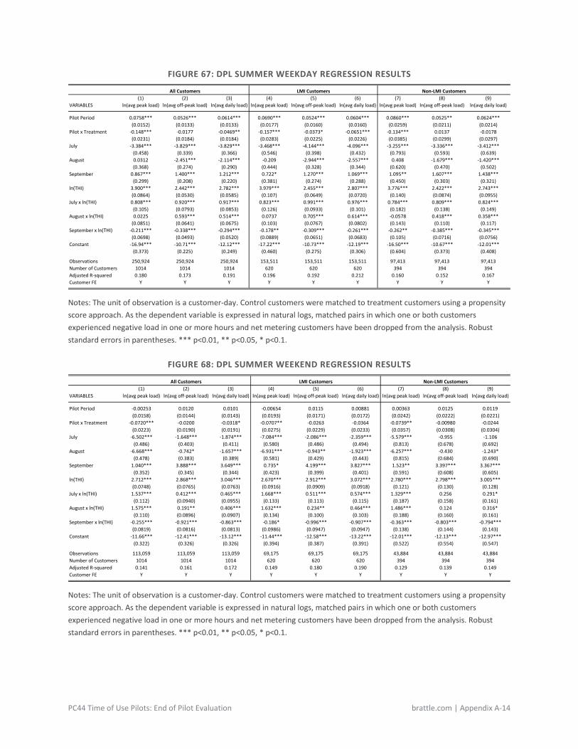
PC44 Time of Use Pilots: End of Pilot Evaluation brattle.com | Appendix A-14
FIGURE 67: DPL SUMMER WEEKDAY REGRESSION RESULTS
Notes: The unit of observation is a customer-day. Control customers were matched to treatment customers using a propensity score approach. As the dependent variable is expressed in natural logs, matched pairs in which one or both customers experienced negative load in one or more hours and net metering customers have been dropped from the analysis. Robust standard errors in parentheses. *** p<0.01, ** p<0.05, * p<0.1.
FIGURE 68: DPL SUMMER WEEKEND REGRESSION RESULTS
Notes: The unit of observation is a customer-day. Control customers were matched to treatment customers using a propensity score approach. As the dependent variable is expressed in natural logs, matched pairs in which one or both customers experienced negative load in one or more hours and net metering customers have been dropped from the analysis. Robust standard errors in parentheses. *** p<0.01, ** p<0.05, * p<0.1.
All Customers LMI Customers Non-LMI Customers(1) (2) (3) (4) (5) (6) (7) (8) (9)
VARIABLES ln(avg peak load) ln(avg off-peak load) ln(avg daily load) ln(avg peak load) ln(avg off-peak load) ln(avg daily load) ln(avg peak load) ln(avg off-peak load) ln(avg daily load)
Pilot Period 0.0758*** 0.0526*** 0.0614*** 0.0690*** 0.0524*** 0.0604*** 0.0860*** 0.0525** 0.0624***(0.0152) (0.0133) (0.0133) (0.0177) (0.0160) (0.0160) (0.0259) (0.0211) (0.0214)
Pilot x Treatment -0.148*** -0.0177 -0.0469** -0.157*** -0.0373* -0.0651*** -0.134*** 0.0137 -0.0178(0.0231) (0.0184) (0.0184) (0.0283) (0.0225) (0.0226) (0.0385) (0.0299) (0.0297)
July -3.384*** -3.829*** -3.829*** -3.468*** -4.144*** -4.096*** -3.255*** -3.336*** -3.412***(0.458) (0.339) (0.366) (0.546) (0.398) (0.432) (0.793) (0.593) (0.639)
August 0.0312 -2.451*** -2.114*** -0.209 -2.944*** -2.557*** 0.408 -1.679*** -1.420***(0.368) (0.274) (0.290) (0.444) (0.328) (0.344) (0.620) (0.470) (0.502)
September 0.867*** 1.400*** 1.212*** 0.722* 1.270*** 1.069*** 1.095** 1.607*** 1.438***(0.299) (0.208) (0.220) (0.381) (0.274) (0.288) (0.450) (0.303) (0.321)
ln(THI) 3.900*** 2.442*** 2.782*** 3.979*** 2.455*** 2.807*** 3.776*** 2.422*** 2.743***(0.0864) (0.0530) (0.0585) (0.107) (0.0649) (0.0720) (0.140) (0.0874) (0.0955)
July x ln(THI) 0.808*** 0.920*** 0.917*** 0.823*** 0.991*** 0.976*** 0.784*** 0.809*** 0.824***(0.105) (0.0793) (0.0853) (0.126) (0.0933) (0.101) (0.182) (0.138) (0.149)
August x ln(THI) 0.0225 0.593*** 0.514*** 0.0737 0.705*** 0.614*** -0.0578 0.418*** 0.358***(0.0851) (0.0641) (0.0675) (0.103) (0.0767) (0.0802) (0.143) (0.110) (0.117)
September x ln(THI) -0.211*** -0.338*** -0.294*** -0.178** -0.309*** -0.261*** -0.262** -0.385*** -0.345***(0.0698) (0.0493) (0.0520) (0.0889) (0.0651) (0.0683) (0.105) (0.0716) (0.0756)
Constant -16.94*** -10.71*** -12.12*** -17.22*** -10.73*** -12.19*** -16.50*** -10.67*** -12.01***(0.373) (0.225) (0.249) (0.460) (0.275) (0.306) (0.604) (0.373) (0.408)
Observations 250,924 250,924 250,924 153,511 153,511 153,511 97,413 97,413 97,413Number of Customers 1014 1014 1014 620 620 620 394 394 394Adjusted R-squared 0.180 0.173 0.191 0.196 0.192 0.212 0.160 0.152 0.167Customer FE Y Y Y Y Y Y Y Y Y
All Customers LMI Customers Non-LMI Customers(1) (2) (3) (4) (5) (6) (7) (8) (9)
VARIABLES ln(avg peak load) ln(avg off-peak load) ln(avg daily load) ln(avg peak load) ln(avg off-peak load) ln(avg daily load) ln(avg peak load) ln(avg off-peak load) ln(avg daily load)
Pilot Period -0.00253 0.0120 0.0101 -0.00654 0.0115 0.00881 0.00363 0.0125 0.0119(0.0158) (0.0144) (0.0143) (0.0193) (0.0171) (0.0172) (0.0242) (0.0222) (0.0221)
Pilot x Treatment -0.0720*** -0.0200 -0.0318* -0.0707** -0.0263 -0.0364 -0.0739** -0.00980 -0.0244(0.0223) (0.0190) (0.0191) (0.0275) (0.0229) (0.0233) (0.0357) (0.0308) (0.0304)
July -6.502*** -1.648*** -1.874*** -7.084*** -2.086*** -2.359*** -5.579*** -0.955 -1.106(0.486) (0.403) (0.411) (0.580) (0.486) (0.494) (0.813) (0.678) (0.692)
August -6.668*** -0.742* -1.657*** -6.931*** -0.943** -1.923*** -6.257*** -0.430 -1.243*(0.478) (0.383) (0.389) (0.581) (0.429) (0.443) (0.815) (0.684) (0.690)
September 1.040*** 3.888*** 3.649*** 0.735* 4.199*** 3.827*** 1.523** 3.397*** 3.367***(0.352) (0.345) (0.344) (0.423) (0.399) (0.401) (0.591) (0.608) (0.605)
ln(THI) 2.712*** 2.868*** 3.046*** 2.670*** 2.912*** 3.072*** 2.780*** 2.798*** 3.005***(0.0748) (0.0765) (0.0763) (0.0916) (0.0909) (0.0918) (0.121) (0.130) (0.128)
July x ln(THI) 1.537*** 0.412*** 0.465*** 1.668*** 0.511*** 0.574*** 1.329*** 0.256 0.291*(0.112) (0.0940) (0.0955) (0.133) (0.113) (0.115) (0.187) (0.158) (0.161)
August x ln(THI) 1.575*** 0.191** 0.406*** 1.632*** 0.234** 0.464*** 1.486*** 0.124 0.316*(0.110) (0.0896) (0.0907) (0.134) (0.100) (0.103) (0.188) (0.160) (0.161)
September x ln(THI) -0.255*** -0.921*** -0.863*** -0.186* -0.996*** -0.907*** -0.363*** -0.803*** -0.794***(0.0819) (0.0816) (0.0813) (0.0986) (0.0947) (0.0947) (0.138) (0.144) (0.143)
Constant -11.66*** -12.41*** -13.12*** -11.44*** -12.58*** -13.22*** -12.01*** -12.13*** -12.97***(0.322) (0.326) (0.326) (0.394) (0.387) (0.391) (0.522) (0.554) (0.547)
Observations 113,059 113,059 113,059 69,175 69,175 69,175 43,884 43,884 43,884Number of Customers 1014 1014 1014 620 620 620 394 394 394Adjusted R-squared 0.141 0.161 0.172 0.149 0.180 0.190 0.129 0.139 0.149Customer FE Y Y Y Y Y Y Y Y Y
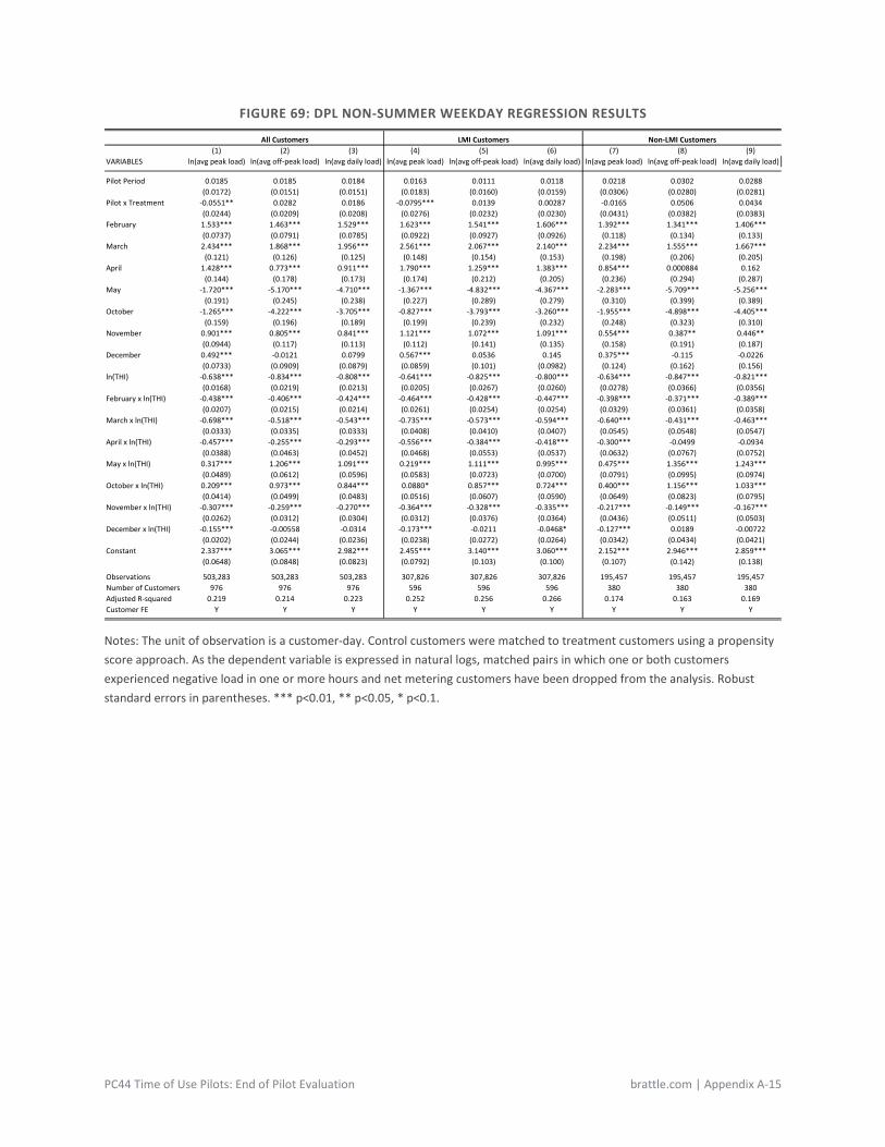
PC44 Time of Use Pilots: End of Pilot Evaluation brattle.com | Appendix A-15
FIGURE 69: DPL NON-SUMMER WEEKDAY REGRESSION RESULTS
Notes: The unit of observation is a customer-day. Control customers were matched to treatment customers using a propensity score approach. As the dependent variable is expressed in natural logs, matched pairs in which one or both customers experienced negative load in one or more hours and net metering customers have been dropped from the analysis. Robust standard errors in parentheses. *** p<0.01, ** p<0.05, * p<0.1.
All Customers LMI Customers Non-LMI Customers(1) (2) (3) (4) (5) (6) (7) (8) (9)
VARIABLES ln(avg peak load) ln(avg off-peak load) ln(avg daily load) ln(avg peak load) ln(avg off-peak load) ln(avg daily load) ln(avg peak load) ln(avg off-peak load) ln(avg daily load)
Pilot Period 0.0185 0.0185 0.0184 0.0163 0.0111 0.0118 0.0218 0.0302 0.0288(0.0172) (0.0151) (0.0151) (0.0183) (0.0160) (0.0159) (0.0306) (0.0280) (0.0281)
Pilot x Treatment -0.0551** 0.0282 0.0186 -0.0795*** 0.0139 0.00287 -0.0165 0.0506 0.0434(0.0244) (0.0209) (0.0208) (0.0276) (0.0232) (0.0230) (0.0431) (0.0382) (0.0383)
February 1.533*** 1.463*** 1.529*** 1.623*** 1.541*** 1.606*** 1.392*** 1.341*** 1.406***(0.0737) (0.0791) (0.0785) (0.0922) (0.0927) (0.0926) (0.118) (0.134) (0.133)
March 2.434*** 1.868*** 1.956*** 2.561*** 2.067*** 2.140*** 2.234*** 1.555*** 1.667***(0.121) (0.126) (0.125) (0.148) (0.154) (0.153) (0.198) (0.206) (0.205)
April 1.428*** 0.773*** 0.911*** 1.790*** 1.259*** 1.383*** 0.854*** 0.000884 0.162(0.144) (0.178) (0.173) (0.174) (0.212) (0.205) (0.236) (0.294) (0.287)
May -1.720*** -5.170*** -4.710*** -1.367*** -4.832*** -4.367*** -2.283*** -5.709*** -5.256***(0.191) (0.245) (0.238) (0.227) (0.289) (0.279) (0.310) (0.399) (0.389)
October -1.265*** -4.222*** -3.705*** -0.827*** -3.793*** -3.260*** -1.955*** -4.898*** -4.405***(0.159) (0.196) (0.189) (0.199) (0.239) (0.232) (0.248) (0.323) (0.310)
November 0.901*** 0.805*** 0.841*** 1.121*** 1.072*** 1.091*** 0.554*** 0.387** 0.446**(0.0944) (0.117) (0.113) (0.112) (0.141) (0.135) (0.158) (0.191) (0.187)
December 0.492*** -0.0121 0.0799 0.567*** 0.0536 0.145 0.375*** -0.115 -0.0226(0.0733) (0.0909) (0.0879) (0.0859) (0.101) (0.0982) (0.124) (0.162) (0.156)
ln(THI) -0.638*** -0.834*** -0.808*** -0.641*** -0.825*** -0.800*** -0.634*** -0.847*** -0.821***(0.0168) (0.0219) (0.0213) (0.0205) (0.0267) (0.0260) (0.0278) (0.0366) (0.0356)
February x ln(THI) -0.438*** -0.406*** -0.424*** -0.464*** -0.428*** -0.447*** -0.398*** -0.371*** -0.389***(0.0207) (0.0215) (0.0214) (0.0261) (0.0254) (0.0254) (0.0329) (0.0361) (0.0358)
March x ln(THI) -0.698*** -0.518*** -0.543*** -0.735*** -0.573*** -0.594*** -0.640*** -0.431*** -0.463***(0.0333) (0.0335) (0.0333) (0.0408) (0.0410) (0.0407) (0.0545) (0.0548) (0.0547)
April x ln(THI) -0.457*** -0.255*** -0.293*** -0.556*** -0.384*** -0.418*** -0.300*** -0.0499 -0.0934(0.0388) (0.0463) (0.0452) (0.0468) (0.0553) (0.0537) (0.0632) (0.0767) (0.0752)
May x ln(THI) 0.317*** 1.206*** 1.091*** 0.219*** 1.111*** 0.995*** 0.475*** 1.356*** 1.243***(0.0489) (0.0612) (0.0596) (0.0583) (0.0723) (0.0700) (0.0791) (0.0995) (0.0974)
October x ln(THI) 0.209*** 0.973*** 0.844*** 0.0880* 0.857*** 0.724*** 0.400*** 1.156*** 1.033***(0.0414) (0.0499) (0.0483) (0.0516) (0.0607) (0.0590) (0.0649) (0.0823) (0.0795)
November x ln(THI) -0.307*** -0.259*** -0.270*** -0.364*** -0.328*** -0.335*** -0.217*** -0.149*** -0.167***(0.0262) (0.0312) (0.0304) (0.0312) (0.0376) (0.0364) (0.0436) (0.0511) (0.0503)
December x ln(THI) -0.155*** -0.00558 -0.0314 -0.173*** -0.0211 -0.0468* -0.127*** 0.0189 -0.00722(0.0202) (0.0244) (0.0236) (0.0238) (0.0272) (0.0264) (0.0342) (0.0434) (0.0421)
Constant 2.337*** 3.065*** 2.982*** 2.455*** 3.140*** 3.060*** 2.152*** 2.946*** 2.859***(0.0648) (0.0848) (0.0823) (0.0792) (0.103) (0.100) (0.107) (0.142) (0.138)
Observations 503,283 503,283 503,283 307,826 307,826 307,826 195,457 195,457 195,457Number of Customers 976 976 976 596 596 596 380 380 380Adjusted R-squared 0.219 0.214 0.223 0.252 0.256 0.266 0.174 0.163 0.169Customer FE Y Y Y Y Y Y Y Y Y
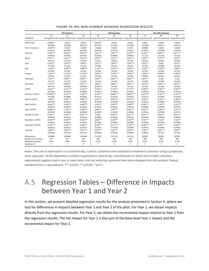
PC44 Time of Use Pilots: End of Pilot Evaluation brattle.com | Appendix A-16
FIGURE 70: DPL NON-SUMMER WEEKEND REGRESSION RESULTS
Notes: The unit of observation is a customer-day. Control customers were matched to treatment customers using a propensity score approach. As the dependent variable is expressed in natural logs, matched pairs in which one or both customers experienced negative load in one or more hours and net metering customers have been dropped from the analysis. Robust standard errors in parentheses. *** p<0.01, ** p<0.05, * p<0.1.
A.5 Regression Tables – Difference in Impacts between Year 1 and Year 2
In this section, we present detailed regression results for the analysis presented in Section II, where we test for differences in impacts between Year 1 and Year 2 of the pilot. For Year 1, we obtain impacts directly from the regression results. For Year 2, we obtain the incremental impact relative to Year 1 from the regression results. The net impact for Year 2 is the sum of the base level Year 1 impact and the incremental impact for Year 2.
All Customers LMI Customers Non-LMI Customers(1) (2) (3) (4) (5) (6) (7) (8) (9)
VARIABLES ln(avg peak load) ln(avg off-peak load) ln(avg daily load) ln(avg peak load) ln(avg off-peak load) ln(avg daily load) ln(avg peak load) ln(avg off-peak load) ln(avg daily load)
Pilot Period 0.0340** 0.0201 0.0222 0.0373** 0.0125 0.0161 0.0287 0.0319 0.0318(0.0160) (0.0148) (0.0147) (0.0172) (0.0161) (0.0160) (0.0300) (0.0271) (0.0271)
Pilot x Treatment -0.00772 0.0234 0.0198 -0.0186 0.0225 0.0172 0.00969 0.0250 0.0240(0.0221) (0.0202) (0.0201) (0.0244) (0.0223) (0.0221) (0.0412) (0.0376) (0.0377)
February 0.381*** 0.438*** 0.393*** 0.421*** 0.343*** 0.314*** 0.318*** 0.587*** 0.517***(0.0645) (0.0764) (0.0742) (0.0745) (0.0887) (0.0853) (0.113) (0.135) (0.132)
March 3.573*** 3.242*** 3.332*** 3.742*** 3.537*** 3.601*** 3.310*** 2.777*** 2.911***(0.134) (0.174) (0.166) (0.162) (0.203) (0.194) (0.224) (0.304) (0.290)
April 2.023*** 1.074*** 1.299*** 2.421*** 1.462*** 1.695*** 1.391*** 0.460 0.671**(0.156) (0.172) (0.170) (0.186) (0.201) (0.197) (0.262) (0.296) (0.296)
May -1.545*** -4.798*** -4.388*** -1.179*** -4.419*** -4.002*** -2.118*** -5.393*** -4.994***(0.184) (0.195) (0.192) (0.230) (0.244) (0.239) (0.285) (0.306) (0.301)
October -1.025*** -2.772*** -2.570*** -0.602*** -2.193*** -1.980*** -1.690*** -3.680*** -3.495***(0.181) (0.209) (0.204) (0.226) (0.251) (0.245) (0.283) (0.345) (0.337)
November 1.359*** 0.594*** 0.689*** 1.559*** 0.841*** 0.922*** 1.045*** 0.206 0.322(0.117) (0.127) (0.124) (0.143) (0.154) (0.151) (0.186) (0.206) (0.203)
December 1.134*** 0.926*** 0.937*** 1.206*** 0.982*** 0.991*** 1.021*** 0.840*** 0.853***(0.0772) (0.0995) (0.0954) (0.0915) (0.119) (0.113) (0.129) (0.166) (0.160)
ln(THI) -0.542*** -0.757*** -0.734*** -0.539*** -0.754*** -0.731*** -0.546*** -0.760*** -0.738***(0.0136) (0.0194) (0.0188) (0.0167) (0.0240) (0.0231) (0.0224) (0.0320) (0.0310)
February x ln(THI) -0.0968*** -0.122*** -0.109*** -0.109*** -0.0969*** -0.0879*** -0.0773** -0.161*** -0.141***(0.0182) (0.0208) (0.0203) (0.0212) (0.0243) (0.0235) (0.0317) (0.0365) (0.0359)
March x ln(THI) -1.003*** -0.875*** -0.902*** -1.052*** -0.955*** -0.975*** -0.926*** -0.749*** -0.788***(0.0370) (0.0461) (0.0442) (0.0447) (0.0538) (0.0515) (0.0616) (0.0806) (0.0773)
April x ln(THI) -0.610*** -0.330*** -0.389*** -0.720*** -0.433*** -0.495*** -0.436*** -0.167** -0.222***(0.0419) (0.0445) (0.0442) (0.0501) (0.0522) (0.0513) (0.0698) (0.0764) (0.0767)
May x ln(THI) 0.288*** 1.131*** 1.029*** 0.184*** 1.027*** 0.922*** 0.452*** 1.296*** 1.197***(0.0479) (0.0498) (0.0490) (0.0597) (0.0619) (0.0609) (0.0742) (0.0780) (0.0771)
October x ln(THI) 0.149*** 0.620*** 0.567*** 0.0297 0.466*** 0.411*** 0.337*** 0.861*** 0.814***(0.0469) (0.0531) (0.0521) (0.0580) (0.0636) (0.0624) (0.0738) (0.0879) (0.0861)
November x ln(THI) -0.416*** -0.203*** -0.228*** -0.468*** -0.268*** -0.289*** -0.335*** -0.103* -0.134**(0.0318) (0.0335) (0.0329) (0.0389) (0.0406) (0.0398) (0.0509) (0.0547) (0.0540)
December x ln(THI) -0.326*** -0.262*** -0.266*** -0.344*** -0.275*** -0.278*** -0.300*** -0.242*** -0.246***(0.0213) (0.0267) (0.0257) (0.0255) (0.0319) (0.0306) (0.0355) (0.0447) (0.0431)
Constant 1.925*** 2.815*** 2.731*** 2.007*** 2.901*** 2.814*** 1.796*** 2.681*** 2.600***(0.0516) (0.0743) (0.0716) (0.0636) (0.0919) (0.0884) (0.0843) (0.122) (0.118)
Observations 230,886 230,886 230,886 141,204 141,204 141,204 89,682 89,682 89,682Number of Customers 976 976 976 596 596 596 380 380 380Adjusted R-squared 0.202 0.189 0.197 0.232 0.228 0.237 0.163 0.143 0.149Customer FE Y Y Y Y Y Y Y Y Y
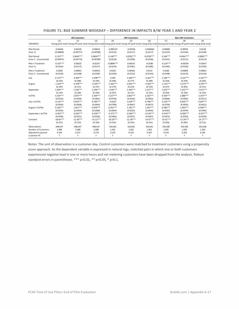
PC44 Time of Use Pilots: End of Pilot Evaluation brattle.com | Appendix A-17
FIGURE 71: BGE SUMMER WEEKDAY – DIFFERENCE IN IMPACTS B/W YEAR 1 AND YEAR 2
Notes: The unit of observation is a customer-day. Control customers were matched to treatment customers using a propensity score approach. As the dependent variable is expressed in natural logs, matched pairs in which one or both customers experienced negative load in one or more hours and net metering customers have been dropped from the analysis. Robust standard errors in parentheses. *** p<0.01, ** p<0.05, * p<0.1.
All Customers LMI Customers Non-LMI Customers(1) (2) (3) (4) (5) (6) (7) (8) (9)
VARIABLES ln(avg peak load) ln(avg off-peak load) ln(avg daily load) ln(avg peak load) ln(avg off-peak load) ln(avg daily load) ln(avg peak load) ln(avg off-peak load) ln(avg daily load)
Pilot Period 0.00346 0.00105 0.00624 -0.000147 -0.00766 -0.000660 0.00689 0.00934 0.0128(Year 1) (0.00894) (0.00777) (0.00780) (0.0132) (0.0117) (0.0117) (0.0122) (0.0103) (0.0104)
Pilot Period 0.153*** 0.0642*** 0.0824*** 0.140*** 0.0591*** 0.0749*** 0.166*** 0.0691*** 0.0895***(Year 2 - Incremental) (0.00975) (0.00779) (0.00789) (0.0134) (0.0109) (0.0109) (0.0141) (0.0111) (0.0113)
Pilot x Treatment -0.107*** 0.00102 -0.0225* -0.0896*** 0.00319 -0.0186 -0.124*** -0.00104 -0.0263*(Year 1) (0.0143) (0.0117) (0.0117) (0.0210) (0.0181) (0.0180) (0.0195) (0.0150) (0.0150)
Pilot x Treatment 0.0206 0.00691 0.00916 0.0226 0.00566 0.0101 0.0186 0.00809 0.00823(Year 2 - Incremental) (0.0139) (0.0108) (0.0109) (0.0194) (0.0153) (0.0154) (0.0198) (0.0153) (0.0154)
July 0.712*** -3.903*** -2.948*** 0.204 -4.304*** -3.361*** 1.196*** -3.522*** -2.555***(0.235) (0.188) (0.195) (0.346) (0.277) (0.289) (0.318) (0.254) (0.263)
August -1.324*** -4.478*** -4.165*** -1.463*** -4.691*** -4.365*** -1.191*** -4.275*** -3.975***(0.187) (0.151) (0.157) (0.274) (0.223) (0.233) (0.257) (0.205) (0.211)
September 1.904*** 2.336*** 2.238*** 1.549*** 2.349*** 2.157*** 2.243*** 2.322*** 2.315***(0.145) (0.106) (0.109) (0.207) (0.151) (0.155) (0.203) (0.150) (0.152)
ln(THI) 4.334*** 2.875*** 3.294*** 4.227*** 2.862*** 3.263*** 4.436*** 2.888*** 3.324***(0.0510) (0.0356) (0.0381) (0.0745) (0.0526) (0.0563) (0.0699) (0.0481) (0.0517)
July x ln(THI) -0.142*** 0.924*** 0.700*** -0.0237 1.019*** 0.798*** -0.255*** 0.834*** 0.607***(0.0540) (0.0438) (0.0454) (0.0796) (0.0647) (0.0672) (0.0730) (0.0593) (0.0612)
August x ln(THI) 0.318*** 1.051*** 0.976*** 0.352*** 1.102*** 1.023*** 0.286*** 1.003*** 0.930***(0.0433) (0.0354) (0.0366) (0.0634) (0.0523) (0.0544) (0.0592) (0.0479) (0.0492)
September x ln(THI) -0.455*** -0.563*** -0.539*** -0.371*** -0.566*** -0.519*** -0.534*** -0.560*** -0.557***(0.0338) (0.0251) (0.0256) (0.0483) (0.0357) (0.0367) (0.0472) (0.0354) (0.0359)
Constant -18.66*** -12.36*** -14.12*** -18.29*** -12.39*** -14.07*** -19.01*** -12.34*** -14.17***(0.221) (0.152) (0.163) (0.323) (0.224) (0.241) (0.303) (0.205) (0.221)
Observations 648,547 648,547 648,547 316,041 316,041 316,041 332,506 332,506 332,506Number of Customers 2,588 2,588 2,588 1,262 1,262 1,262 1,326 1,326 1,326Adjusted R-squared 0.243 0.237 0.274 0.233 0.233 0.267 0.254 0.242 0.281Customer FE Y Y Y Y Y Y Y Y Y
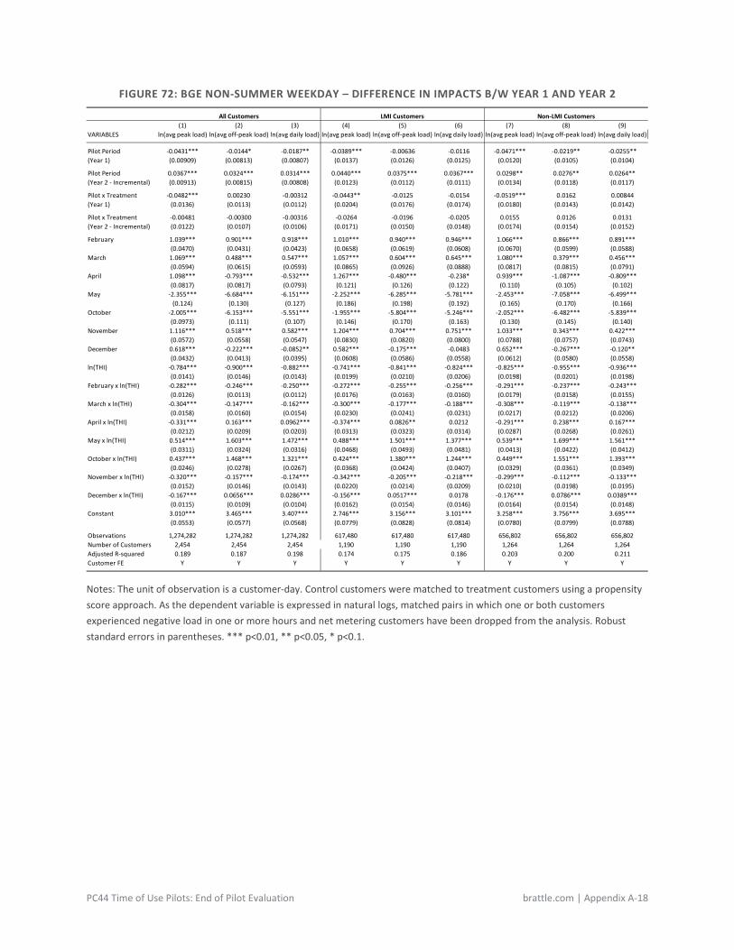
PC44 Time of Use Pilots: End of Pilot Evaluation brattle.com | Appendix A-18
FIGURE 72: BGE NON-SUMMER WEEKDAY – DIFFERENCE IN IMPACTS B/W YEAR 1 AND YEAR 2
Notes: The unit of observation is a customer-day. Control customers were matched to treatment customers using a propensity score approach. As the dependent variable is expressed in natural logs, matched pairs in which one or both customers experienced negative load in one or more hours and net metering customers have been dropped from the analysis. Robust standard errors in parentheses. *** p<0.01, ** p<0.05, * p<0.1.
All Customers LMI Customers Non-LMI Customers(1) (2) (3) (4) (5) (6) (7) (8) (9)
VARIABLES ln(avg peak load) ln(avg off-peak load) ln(avg daily load) ln(avg peak load) ln(avg off-peak load) ln(avg daily load) ln(avg peak load) ln(avg off-peak load) ln(avg daily load)
Pilot Period -0.0431*** -0.0144* -0.0187** -0.0389*** -0.00636 -0.0116 -0.0471*** -0.0219** -0.0255**(Year 1) (0.00909) (0.00813) (0.00807) (0.0137) (0.0126) (0.0125) (0.0120) (0.0105) (0.0104)
Pilot Period 0.0367*** 0.0324*** 0.0314*** 0.0440*** 0.0375*** 0.0367*** 0.0298** 0.0276** 0.0264**(Year 2 - Incremental) (0.00913) (0.00815) (0.00808) (0.0123) (0.0112) (0.0111) (0.0134) (0.0118) (0.0117)
Pilot x Treatment -0.0482*** 0.00230 -0.00312 -0.0443** -0.0125 -0.0154 -0.0519*** 0.0162 0.00844(Year 1) (0.0136) (0.0113) (0.0112) (0.0204) (0.0176) (0.0174) (0.0180) (0.0143) (0.0142)
Pilot x Treatment -0.00481 -0.00300 -0.00316 -0.0264 -0.0196 -0.0205 0.0155 0.0126 0.0131(Year 2 - Incremental) (0.0122) (0.0107) (0.0106) (0.0171) (0.0150) (0.0148) (0.0174) (0.0154) (0.0152)
February 1.039*** 0.901*** 0.918*** 1.010*** 0.940*** 0.946*** 1.066*** 0.866*** 0.891***(0.0470) (0.0431) (0.0423) (0.0658) (0.0619) (0.0608) (0.0670) (0.0599) (0.0588)
March 1.069*** 0.488*** 0.547*** 1.057*** 0.604*** 0.645*** 1.080*** 0.379*** 0.456***(0.0594) (0.0615) (0.0593) (0.0865) (0.0926) (0.0888) (0.0817) (0.0815) (0.0791)
April 1.098*** -0.793*** -0.532*** 1.267*** -0.480*** -0.238* 0.939*** -1.087*** -0.809***(0.0817) (0.0817) (0.0793) (0.121) (0.126) (0.122) (0.110) (0.105) (0.102)
May -2.355*** -6.684*** -6.151*** -2.252*** -6.285*** -5.781*** -2.453*** -7.058*** -6.499***(0.124) (0.130) (0.127) (0.186) (0.198) (0.192) (0.165) (0.170) (0.166)
October -2.005*** -6.153*** -5.551*** -1.955*** -5.804*** -5.246*** -2.052*** -6.482*** -5.839***(0.0973) (0.111) (0.107) (0.146) (0.170) (0.163) (0.130) (0.145) (0.140)
November 1.116*** 0.518*** 0.582*** 1.204*** 0.704*** 0.751*** 1.033*** 0.343*** 0.422***(0.0572) (0.0558) (0.0547) (0.0830) (0.0820) (0.0800) (0.0788) (0.0757) (0.0743)
December 0.618*** -0.222*** -0.0852** 0.582*** -0.175*** -0.0483 0.652*** -0.267*** -0.120**(0.0432) (0.0413) (0.0395) (0.0608) (0.0586) (0.0558) (0.0612) (0.0580) (0.0558)
ln(THI) -0.784*** -0.900*** -0.882*** -0.741*** -0.841*** -0.824*** -0.825*** -0.955*** -0.936***(0.0141) (0.0146) (0.0143) (0.0199) (0.0210) (0.0206) (0.0198) (0.0201) (0.0198)
February x ln(THI) -0.282*** -0.246*** -0.250*** -0.272*** -0.255*** -0.256*** -0.291*** -0.237*** -0.243***(0.0126) (0.0113) (0.0112) (0.0176) (0.0163) (0.0160) (0.0179) (0.0158) (0.0155)
March x ln(THI) -0.304*** -0.147*** -0.162*** -0.300*** -0.177*** -0.188*** -0.308*** -0.119*** -0.138***(0.0158) (0.0160) (0.0154) (0.0230) (0.0241) (0.0231) (0.0217) (0.0212) (0.0206)
April x ln(THI) -0.331*** 0.163*** 0.0962*** -0.374*** 0.0826** 0.0212 -0.291*** 0.238*** 0.167***(0.0212) (0.0209) (0.0203) (0.0313) (0.0323) (0.0314) (0.0287) (0.0268) (0.0261)
May x ln(THI) 0.514*** 1.603*** 1.472*** 0.488*** 1.501*** 1.377*** 0.539*** 1.699*** 1.561***(0.0311) (0.0324) (0.0316) (0.0468) (0.0493) (0.0481) (0.0413) (0.0422) (0.0412)
October x ln(THI) 0.437*** 1.468*** 1.321*** 0.424*** 1.380*** 1.244*** 0.449*** 1.551*** 1.393***(0.0246) (0.0278) (0.0267) (0.0368) (0.0424) (0.0407) (0.0329) (0.0361) (0.0349)
November x ln(THI) -0.320*** -0.157*** -0.174*** -0.342*** -0.205*** -0.218*** -0.299*** -0.112*** -0.133***(0.0152) (0.0146) (0.0143) (0.0220) (0.0214) (0.0209) (0.0210) (0.0198) (0.0195)
December x ln(THI) -0.167*** 0.0656*** 0.0286*** -0.156*** 0.0517*** 0.0178 -0.176*** 0.0786*** 0.0389***(0.0115) (0.0109) (0.0104) (0.0162) (0.0154) (0.0146) (0.0164) (0.0154) (0.0148)
Constant 3.010*** 3.465*** 3.407*** 2.746*** 3.156*** 3.101*** 3.258*** 3.756*** 3.695***(0.0553) (0.0577) (0.0568) (0.0779) (0.0828) (0.0814) (0.0780) (0.0799) (0.0788)
Observations 1,274,282 1,274,282 1,274,282 617,480 617,480 617,480 656,802 656,802 656,802Number of Customers 2,454 2,454 2,454 1,190 1,190 1,190 1,264 1,264 1,264Adjusted R-squared 0.189 0.187 0.198 0.174 0.175 0.186 0.203 0.200 0.211Customer FE Y Y Y Y Y Y Y Y Y

PC44 Time of Use Pilots: End of Pilot Evaluation brattle.com | Appendix A-19
FIGURE 73: PEPCO SUMMER WEEKDAY – DIFFERENCE IN IMPACTS B/W YEAR 1 AND YEAR 2
Notes: The unit of observation is a customer-day. Control customers were matched to treatment customers using a propensity score approach. As the dependent variable is expressed in natural logs, matched pairs in which one or both customers experienced negative load in one or more hours and net metering customers have been dropped from the analysis. Robust standard errors in parentheses. *** p<0.01, ** p<0.05, * p<0.1.
All Customers LMI Customers Non-LMI Customers(1) (2) (3) (4) (5) (6) (7) (8) (9)
VARIABLES ln(avg peak load) ln(avg off-peak load) ln(avg daily load) ln(avg peak load) ln(avg off-peak load) ln(avg daily load) ln(avg peak load) ln(avg off-peak load) ln(avg daily load)
Pilot Period 0.0412*** 0.0136 0.0247** 0.0257 0.00383 0.0136 0.0538*** 0.0216* 0.0337***(Year 1) (0.0116) (0.00984) (0.00979) (0.0161) (0.0140) (0.0137) (0.0144) (0.0113) (0.0114)
Pilot Period 0.175*** 0.0474*** 0.0705*** 0.182*** 0.0458*** 0.0712*** 0.169*** 0.0487*** 0.0700***(Year 2 - Incremental) (0.0156) (0.0110) (0.0114) (0.0219) (0.0162) (0.0165) (0.0192) (0.0131) (0.0136)
Pilot x Treatment -0.146*** -0.00159 -0.0307** -0.103*** 0.0120 -0.0124 -0.181*** -0.0127 -0.0458***(Year 1) (0.0164) (0.0127) (0.0126) (0.0231) (0.0184) (0.0182) (0.0217) (0.0155) (0.0154)
Pilot x Treatment -0.000439 0.00291 0.00138 -0.0416 -0.00595 -0.0131 0.0335 0.0102 0.0133(Year 2 - Incremental) (0.0192) (0.0136) (0.0139) (0.0273) (0.0202) (0.0204) (0.0245) (0.0168) (0.0171)
July -1.639*** -2.774*** -2.300*** -1.291*** -2.829*** -2.353*** -1.905*** -2.716*** -2.242***(0.316) (0.233) (0.244) (0.449) (0.335) (0.354) (0.426) (0.310) (0.323)
August -2.400*** -4.259*** -4.027*** -1.919*** -4.268*** -3.983*** -2.772*** -4.238*** -4.048***(0.249) (0.195) (0.200) (0.357) (0.276) (0.285) (0.335) (0.265) (0.271)
September 3.033*** 2.384*** 2.498*** 3.076*** 2.411*** 2.536*** 3.016*** 2.377*** 2.484***(0.191) (0.140) (0.143) (0.269) (0.196) (0.199) (0.263) (0.194) (0.198)
ln(THI) 4.344*** 3.181*** 3.528*** 4.190*** 3.049*** 3.383*** 4.473*** 3.291*** 3.650***(0.0659) (0.0473) (0.0501) (0.0939) (0.0674) (0.0713) (0.0886) (0.0638) (0.0674)
July x ln(THI) 0.390*** 0.651*** 0.540*** 0.311*** 0.665*** 0.553*** 0.449*** 0.637*** 0.526***(0.0725) (0.0541) (0.0566) (0.103) (0.0778) (0.0819) (0.0976) (0.0719) (0.0748)
August x ln(THI) 0.556*** 0.983*** 0.928*** 0.447*** 0.988*** 0.920*** 0.640*** 0.977*** 0.931***(0.0574) (0.0455) (0.0466) (0.0823) (0.0643) (0.0663) (0.0772) (0.0620) (0.0631)
September x ln(THI) -0.717*** -0.574*** -0.600*** -0.725*** -0.579*** -0.607*** -0.715*** -0.573*** -0.597***(0.0445) (0.0331) (0.0336) (0.0625) (0.0462) (0.0467) (0.0611) (0.0457) (0.0466)
Constant -18.95*** -13.80*** -15.29*** -18.33*** -13.30*** -14.72*** -19.47*** -14.23*** -15.76***(0.286) (0.202) (0.215) (0.408) (0.289) (0.307) (0.384) (0.273) (0.289)
Observations 500,258 500,258 500,258 225,055 225,055 225,055 275,203 275,203 275,203Number of Customers 2042 2042 2042 916 916 916 1126 1126 1126Adjusted R-squared 0.209 0.244 0.273 0.199 0.235 0.262 0.217 0.252 0.283Customer FE Y Y Y Y Y Y Y Y Y
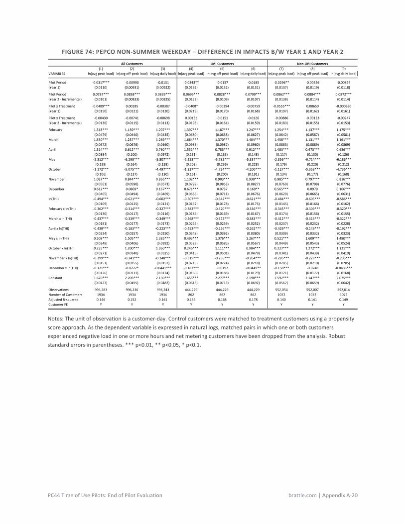
PC44 Time of Use Pilots: End of Pilot Evaluation brattle.com | Appendix A-20
FIGURE 74: PEPCO NON-SUMMER WEEKDAY – DIFFERENCE IN IMPACTS B/W YEAR 1 AND YEAR 2
Notes: The unit of observation is a customer-day. Control customers were matched to treatment customers using a propensity score approach. As the dependent variable is expressed in natural logs, matched pairs in which one or both customers experienced negative load in one or more hours and net metering customers have been dropped from the analysis. Robust standard errors in parentheses. *** p<0.01, ** p<0.05, * p<0.1.
All Customers LMI Customers Non-LMI Customers(1) (2) (3) (4) (5) (6) (7) (8) (9)
VARIABLES ln(avg peak load) ln(avg off-peak load) ln(avg daily load) ln(avg peak load) ln(avg off-peak load) ln(avg daily load) ln(avg peak load) ln(avg off-peak load) ln(avg daily load)
Pilot Period -0.0317*** -0.00990 -0.0131 -0.0343** -0.0157 -0.0185 -0.0296** -0.00526 -0.00874(Year 1) (0.0110) (0.00931) (0.00922) (0.0162) (0.0132) (0.0131) (0.0137) (0.0119) (0.0118)
Pilot Period 0.0787*** 0.0858*** 0.0839*** 0.0695*** 0.0828*** 0.0799*** 0.0862*** 0.0884*** 0.0872***(Year 2 - Incremental) (0.0101) (0.00833) (0.00825) (0.0133) (0.0109) (0.0107) (0.0138) (0.0114) (0.0114)
Pilot x Treatment -0.0489*** 0.00185 -0.00387 -0.0408* -0.00394 -0.00759 -0.0555*** 0.00650 -0.000880(Year 1) (0.0150) (0.0121) (0.0120) (0.0219) (0.0170) (0.0168) (0.0197) (0.0162) (0.0161)
Pilot x Treatment -0.00430 -0.00741 -0.00698 0.00135 -0.0151 -0.0126 -0.00886 -0.00123 -0.00247(Year 2 - Incremental) (0.0136) (0.0115) (0.0113) (0.0195) (0.0161) (0.0159) (0.0183) (0.0155) (0.0153)
February 1.318*** 1.159*** 1.207*** 1.397*** 1.187*** 1.247*** 1.254*** 1.137*** 1.175***(0.0479) (0.0440) (0.0435) (0.0680) (0.0638) (0.0627) (0.0642) (0.0587) (0.0581)
March 1.550*** 1.237*** 1.269*** 1.664*** 1.370*** 1.404*** 1.458*** 1.131*** 1.161***(0.0672) (0.0676) (0.0660) (0.0985) (0.0987) (0.0960) (0.0883) (0.0889) (0.0869)
April 1.514*** 0.612*** 0.760*** 1.551*** 0.783*** 0.912*** 1.483*** 0.473*** 0.636***(0.0884) (0.100) (0.0972) (0.131) (0.153) (0.148) (0.117) (0.130) (0.126)
May -2.312*** -6.298*** -5.807*** -2.258*** -5.782*** -5.337*** -2.356*** -6.714*** -6.186***(0.139) (0.164) (0.158) (0.208) (0.236) (0.228) (0.179) (0.220) (0.212)
October -1.172*** -5.075*** -4.497*** -1.227*** -4.724*** -4.200*** -1.127*** -5.358*** -4.736***(0.106) (0.137) (0.130) (0.161) (0.200) (0.191) (0.134) (0.177) (0.168)
November 1.037*** 0.844*** 0.866*** 1.102*** 0.903*** 0.930*** 0.985*** 0.797*** 0.816***(0.0561) (0.0590) (0.0573) (0.0799) (0.0853) (0.0827) (0.0760) (0.0798) (0.0776)
December 0.612*** 0.0869* 0.167*** 0.671*** 0.0737 0.169** 0.565*** 0.0979 0.166***(0.0465) (0.0494) (0.0469) (0.0666) (0.0711) (0.0676) (0.0629) (0.0665) (0.0631)
ln(THI) -0.494*** -0.621*** -0.602*** -0.507*** -0.642*** -0.621*** -0.484*** -0.605*** -0.586***(0.0109) (0.0125) (0.0121) (0.0157) (0.0178) (0.0173) (0.0145) (0.0166) (0.0162)
February x ln(THI) -0.362*** -0.314*** -0.327*** -0.382*** -0.320*** -0.336*** -0.345*** -0.309*** -0.320***(0.0130) (0.0117) (0.0116) (0.0184) (0.0169) (0.0167) (0.0174) (0.0156) (0.0155)
March x ln(THI) -0.437*** -0.339*** -0.349*** -0.468*** -0.372*** -0.383*** -0.412*** -0.313*** -0.322***(0.0181) (0.0177) (0.0173) (0.0265) (0.0259) (0.0252) (0.0237) (0.0232) (0.0228)
April x ln(THI) -0.439*** -0.183*** -0.223*** -0.452*** -0.226*** -0.262*** -0.429*** -0.149*** -0.192***(0.0234) (0.0257) (0.0250) (0.0348) (0.0392) (0.0380) (0.0309) (0.0332) (0.0323)
May x ln(THI) 0.509*** 1.505*** 1.385*** 0.493*** 1.376*** 1.267*** 0.521*** 1.609*** 1.480***(0.0348) (0.0406) (0.0392) (0.0523) (0.0585) (0.0567) (0.0449) (0.0543) (0.0524)
October x ln(THI) 0.235*** 1.200*** 1.060*** 0.246*** 1.111*** 0.984*** 0.227*** 1.272*** 1.121***(0.0271) (0.0340) (0.0325) (0.0415) (0.0501) (0.0479) (0.0341) (0.0439) (0.0419)
November x ln(THI) -0.299*** -0.241*** -0.248*** -0.315*** -0.256*** -0.264*** -0.285*** -0.229*** -0.235***(0.0151) (0.0155) (0.0151) (0.0216) (0.0224) (0.0218) (0.0205) (0.0210) (0.0205)
December x ln(THI) -0.171*** -0.0222* -0.0441*** -0.187*** -0.0192 -0.0449** -0.158*** -0.0248 -0.0435***(0.0126) (0.0131) (0.0124) (0.0180) (0.0188) (0.0179) (0.0171) (0.0177) (0.0168)
Constant 1.620*** 2.205*** 2.130*** 1.655*** 2.277*** 2.198*** 1.592*** 2.147*** 2.075***(0.0427) (0.0495) (0.0482) (0.0613) (0.0713) (0.0692) (0.0567) (0.0659) (0.0642)
Observations 996,283 996,236 996,243 444,229 444,229 444,229 552,054 552,007 552,014Number of Customers 1934 1934 1934 862 862 862 1072 1072 1072Adjusted R-squared 0.146 0.152 0.161 0.154 0.168 0.178 0.140 0.141 0.149Customer FE Y Y Y Y Y Y Y Y Y
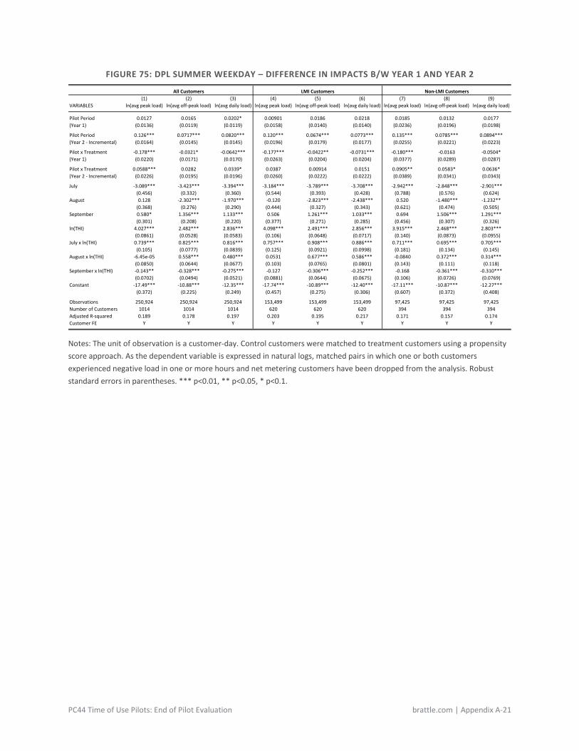
PC44 Time of Use Pilots: End of Pilot Evaluation brattle.com | Appendix A-21
FIGURE 75: DPL SUMMER WEEKDAY – DIFFERENCE IN IMPACTS B/W YEAR 1 AND YEAR 2
Notes: The unit of observation is a customer-day. Control customers were matched to treatment customers using a propensity score approach. As the dependent variable is expressed in natural logs, matched pairs in which one or both customers experienced negative load in one or more hours and net metering customers have been dropped from the analysis. Robust standard errors in parentheses. *** p<0.01, ** p<0.05, * p<0.1.
All Customers LMI Customers Non-LMI Customers(1) (2) (3) (4) (5) (6) (7) (8) (9)
VARIABLES ln(avg peak load) ln(avg off-peak load) ln(avg daily load) ln(avg peak load) ln(avg off-peak load) ln(avg daily load) ln(avg peak load) ln(avg off-peak load) ln(avg daily load)
Pilot Period 0.0127 0.0165 0.0202* 0.00901 0.0186 0.0218 0.0185 0.0132 0.0177(Year 1) (0.0136) (0.0119) (0.0119) (0.0158) (0.0140) (0.0140) (0.0236) (0.0196) (0.0198)
Pilot Period 0.126*** 0.0717*** 0.0820*** 0.120*** 0.0674*** 0.0773*** 0.135*** 0.0785*** 0.0894***(Year 2 - Incremental) (0.0164) (0.0145) (0.0145) (0.0196) (0.0179) (0.0177) (0.0255) (0.0221) (0.0223)
Pilot x Treatment -0.178*** -0.0321* -0.0642*** -0.177*** -0.0422** -0.0731*** -0.180*** -0.0163 -0.0504*(Year 1) (0.0220) (0.0171) (0.0170) (0.0263) (0.0204) (0.0204) (0.0377) (0.0289) (0.0287)
Pilot x Treatment 0.0588*** 0.0282 0.0339* 0.0387 0.00914 0.0151 0.0905** 0.0583* 0.0636*(Year 2 - Incremental) (0.0226) (0.0195) (0.0196) (0.0260) (0.0222) (0.0222) (0.0389) (0.0341) (0.0343)
July -3.089*** -3.423*** -3.394*** -3.184*** -3.789*** -3.708*** -2.942*** -2.848*** -2.901***(0.456) (0.332) (0.360) (0.544) (0.393) (0.428) (0.788) (0.576) (0.624)
August 0.128 -2.302*** -1.970*** -0.120 -2.823*** -2.438*** 0.520 -1.480*** -1.232**(0.368) (0.276) (0.290) (0.444) (0.327) (0.343) (0.621) (0.474) (0.505)
September 0.580* 1.356*** 1.133*** 0.506 1.261*** 1.033*** 0.694 1.506*** 1.291***(0.301) (0.208) (0.220) (0.377) (0.271) (0.285) (0.456) (0.307) (0.326)
ln(THI) 4.027*** 2.482*** 2.836*** 4.098*** 2.491*** 2.856*** 3.915*** 2.468*** 2.803***(0.0861) (0.0528) (0.0583) (0.106) (0.0648) (0.0717) (0.140) (0.0873) (0.0955)
July x ln(THI) 0.739*** 0.825*** 0.816*** 0.757*** 0.908*** 0.886*** 0.711*** 0.695*** 0.705***(0.105) (0.0777) (0.0839) (0.125) (0.0921) (0.0998) (0.181) (0.134) (0.145)
August x ln(THI) -6.45e-05 0.558*** 0.480*** 0.0531 0.677*** 0.586*** -0.0840 0.372*** 0.314***(0.0850) (0.0644) (0.0677) (0.103) (0.0765) (0.0801) (0.143) (0.111) (0.118)
September x ln(THI) -0.143** -0.328*** -0.275*** -0.127 -0.306*** -0.252*** -0.168 -0.361*** -0.310***(0.0702) (0.0494) (0.0521) (0.0881) (0.0644) (0.0675) (0.106) (0.0726) (0.0769)
Constant -17.49*** -10.88*** -12.35*** -17.74*** -10.89*** -12.40*** -17.11*** -10.87*** -12.27***(0.372) (0.225) (0.249) (0.457) (0.275) (0.306) (0.607) (0.372) (0.408)
Observations 250,924 250,924 250,924 153,499 153,499 153,499 97,425 97,425 97,425Number of Customers 1014 1014 1014 620 620 620 394 394 394Adjusted R-squared 0.189 0.178 0.197 0.203 0.195 0.217 0.171 0.157 0.174Customer FE Y Y Y Y Y Y Y Y Y
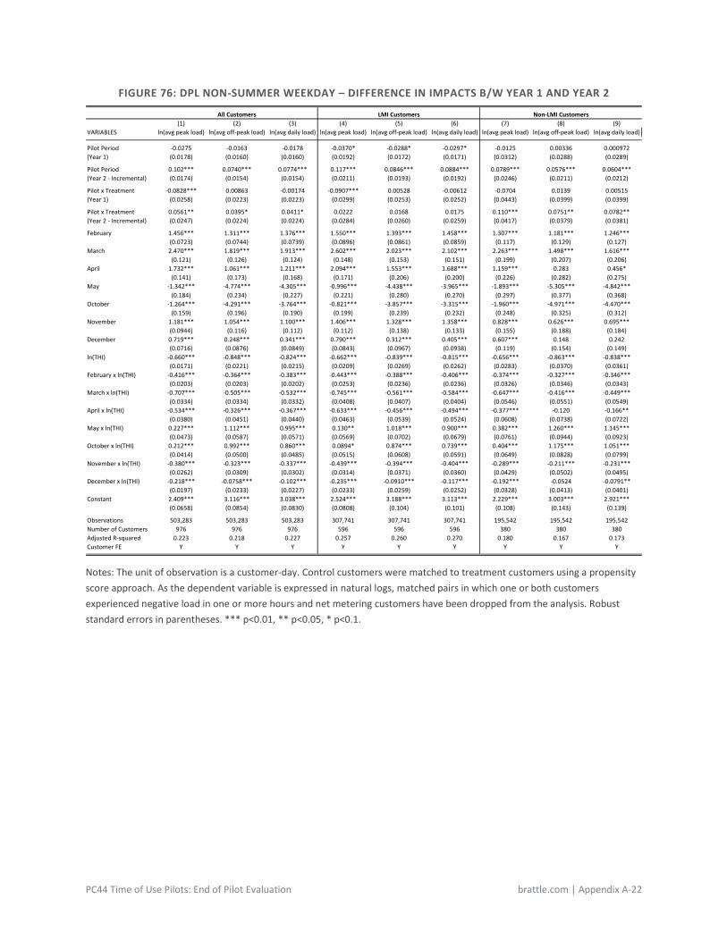
PC44 Time of Use Pilots: End of Pilot Evaluation brattle.com | Appendix A-22
FIGURE 76: DPL NON-SUMMER WEEKDAY – DIFFERENCE IN IMPACTS B/W YEAR 1 AND YEAR 2
Notes: The unit of observation is a customer-day. Control customers were matched to treatment customers using a propensity score approach. As the dependent variable is expressed in natural logs, matched pairs in which one or both customers experienced negative load in one or more hours and net metering customers have been dropped from the analysis. Robust standard errors in parentheses. *** p<0.01, ** p<0.05, * p<0.1.
All Customers LMI Customers Non-LMI Customers(1) (2) (3) (4) (5) (6) (7) (8) (9)
VARIABLES ln(avg peak load) ln(avg off-peak load) ln(avg daily load) ln(avg peak load) ln(avg off-peak load) ln(avg daily load) ln(avg peak load) ln(avg off-peak load) ln(avg daily load)
Pilot Period -0.0275 -0.0163 -0.0178 -0.0370* -0.0288* -0.0297* -0.0125 0.00336 0.000972(Year 1) (0.0178) (0.0160) (0.0160) (0.0192) (0.0172) (0.0171) (0.0312) (0.0288) (0.0289)
Pilot Period 0.102*** 0.0740*** 0.0774*** 0.117*** 0.0846*** 0.0884*** 0.0789*** 0.0576*** 0.0604***(Year 2 - Incremental) (0.0174) (0.0154) (0.0154) (0.0211) (0.0193) (0.0192) (0.0246) (0.0211) (0.0212)
Pilot x Treatment -0.0828*** 0.00863 -0.00174 -0.0907*** 0.00528 -0.00612 -0.0704 0.0139 0.00515(Year 1) (0.0258) (0.0223) (0.0223) (0.0299) (0.0253) (0.0252) (0.0443) (0.0399) (0.0399)
Pilot x Treatment 0.0561** 0.0395* 0.0411* 0.0222 0.0168 0.0175 0.110*** 0.0751** 0.0782**(Year 2 - Incremental) (0.0247) (0.0224) (0.0224) (0.0284) (0.0260) (0.0259) (0.0417) (0.0379) (0.0381)
February 1.456*** 1.311*** 1.376*** 1.550*** 1.393*** 1.458*** 1.307*** 1.181*** 1.246***(0.0723) (0.0744) (0.0739) (0.0896) (0.0861) (0.0859) (0.117) (0.129) (0.127)
March 2.470*** 1.819*** 1.913*** 2.602*** 2.023*** 2.102*** 2.263*** 1.498*** 1.616***(0.121) (0.126) (0.124) (0.148) (0.153) (0.151) (0.199) (0.207) (0.206)
April 1.732*** 1.061*** 1.211*** 2.094*** 1.553*** 1.688*** 1.159*** 0.283 0.456*(0.141) (0.173) (0.168) (0.171) (0.206) (0.200) (0.226) (0.282) (0.275)
May -1.342*** -4.774*** -4.305*** -0.996*** -4.438*** -3.965*** -1.893*** -5.305*** -4.842***(0.184) (0.234) (0.227) (0.221) (0.280) (0.270) (0.297) (0.377) (0.368)
October -1.264*** -4.291*** -3.764*** -0.821*** -3.857*** -3.315*** -1.960*** -4.971*** -4.470***(0.159) (0.196) (0.190) (0.199) (0.239) (0.232) (0.248) (0.325) (0.312)
November 1.181*** 1.054*** 1.100*** 1.406*** 1.328*** 1.358*** 0.828*** 0.626*** 0.695***(0.0944) (0.116) (0.112) (0.112) (0.138) (0.133) (0.155) (0.188) (0.184)
December 0.719*** 0.248*** 0.341*** 0.790*** 0.312*** 0.405*** 0.607*** 0.148 0.242(0.0716) (0.0876) (0.0849) (0.0843) (0.0967) (0.0938) (0.119) (0.154) (0.149)
ln(THI) -0.660*** -0.848*** -0.824*** -0.662*** -0.839*** -0.815*** -0.656*** -0.863*** -0.838***(0.0171) (0.0221) (0.0215) (0.0209) (0.0269) (0.0262) (0.0283) (0.0370) (0.0361)
February x ln(THI) -0.416*** -0.364*** -0.383*** -0.443*** -0.388*** -0.406*** -0.374*** -0.327*** -0.346***(0.0203) (0.0203) (0.0202) (0.0253) (0.0236) (0.0236) (0.0326) (0.0346) (0.0343)
March x ln(THI) -0.707*** -0.505*** -0.532*** -0.745*** -0.561*** -0.584*** -0.647*** -0.416*** -0.449***(0.0334) (0.0334) (0.0332) (0.0408) (0.0407) (0.0404) (0.0546) (0.0551) (0.0549)
April x ln(THI) -0.534*** -0.326*** -0.367*** -0.633*** -0.456*** -0.494*** -0.377*** -0.120 -0.166**(0.0380) (0.0451) (0.0440) (0.0463) (0.0539) (0.0524) (0.0608) (0.0738) (0.0722)
May x ln(THI) 0.227*** 1.112*** 0.995*** 0.130** 1.018*** 0.900*** 0.382*** 1.260*** 1.145***(0.0473) (0.0587) (0.0571) (0.0569) (0.0702) (0.0679) (0.0761) (0.0944) (0.0923)
October x ln(THI) 0.212*** 0.992*** 0.860*** 0.0894* 0.874*** 0.739*** 0.404*** 1.175*** 1.051***(0.0414) (0.0500) (0.0485) (0.0515) (0.0608) (0.0591) (0.0649) (0.0828) (0.0799)
November x ln(THI) -0.380*** -0.323*** -0.337*** -0.439*** -0.394*** -0.404*** -0.289*** -0.211*** -0.231***(0.0262) (0.0309) (0.0302) (0.0314) (0.0371) (0.0360) (0.0429) (0.0502) (0.0495)
December x ln(THI) -0.218*** -0.0758*** -0.102*** -0.235*** -0.0910*** -0.117*** -0.192*** -0.0524 -0.0791**(0.0197) (0.0233) (0.0227) (0.0233) (0.0259) (0.0252) (0.0328) (0.0413) (0.0401)
Constant 2.409*** 3.116*** 3.038*** 2.524*** 3.188*** 3.113*** 2.229*** 3.003*** 2.921***(0.0658) (0.0854) (0.0830) (0.0808) (0.104) (0.101) (0.108) (0.143) (0.139)
Observations 503,283 503,283 503,283 307,741 307,741 307,741 195,542 195,542 195,542Number of Customers 976 976 976 596 596 596 380 380 380Adjusted R-squared 0.223 0.218 0.227 0.257 0.260 0.270 0.180 0.167 0.173Customer FE Y Y Y Y Y Y Y Y Y
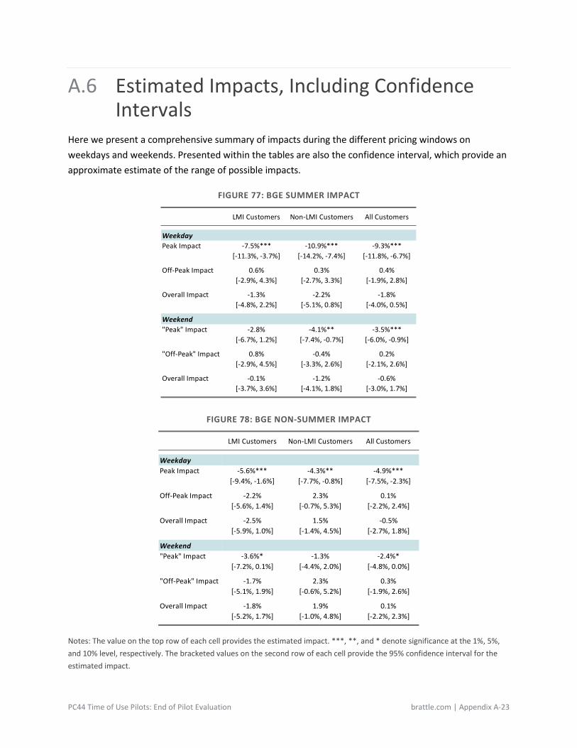
PC44 Time of Use Pilots: End of Pilot Evaluation brattle.com | Appendix A-23
A.6 Estimated Impacts, Including Confidence Intervals
Here we present a comprehensive summary of impacts during the different pricing windows on weekdays and weekends. Presented within the tables are also the confidence interval, which provide an approximate estimate of the range of possible impacts.
FIGURE 77: BGE SUMMER IMPACT
FIGURE 78: BGE NON-SUMMER IMPACT
Notes: The value on the top row of each cell provides the estimated impact. ***, **, and * denote significance at the 1%, 5%, and 10% level, respectively. The bracketed values on the second row of each cell provide the 95% confidence interval for the estimated impact.
LMI Customers Non-LMI Customers All Customers
WeekdayPeak Impact -7.5%*** -10.9%*** -9.3%***
[-11.3%, -3.7%] [-14.2%, -7.4%] [-11.8%, -6.7%]
Off-Peak Impact 0.6% 0.3% 0.4%[-2.9%, 4.3%] [-2.7%, 3.3%] [-1.9%, 2.8%]
Overall Impact -1.3% -2.2% -1.8%[-4.8%, 2.2%] [-5.1%, 0.8%] [-4.0%, 0.5%]
Weekend"Peak" Impact -2.8% -4.1%** -3.5%***
[-6.7%, 1.2%] [-7.4%, -0.7%] [-6.0%, -0.9%]
"Off-Peak" Impact 0.8% -0.4% 0.2%[-2.9%, 4.5%] [-3.3%, 2.6%] [-2.1%, 2.6%]
Overall Impact -0.1% -1.2% -0.6%[-3.7%, 3.6%] [-4.1%, 1.8%] [-3.0%, 1.7%]
LMI Customers Non-LMI Customers All Customers
WeekdayPeak Impact -5.6%*** -4.3%** -4.9%***
[-9.4%, -1.6%] [-7.7%, -0.8%] [-7.5%, -2.3%]
Off-Peak Impact -2.2% 2.3% 0.1%[-5.6%, 1.4%] [-0.7%, 5.3%] [-2.2%, 2.4%]
Overall Impact -2.5% 1.5% -0.5%[-5.9%, 1.0%] [-1.4%, 4.5%] [-2.7%, 1.8%]
Weekend"Peak" Impact -3.6%* -1.3% -2.4%*
[-7.2%, 0.1%] [-4.4%, 2.0%] [-4.8%, 0.0%]
"Off-Peak" Impact -1.7% 2.3% 0.3%[-5.1%, 1.9%] [-0.6%, 5.2%] [-1.9%, 2.6%]
Overall Impact -1.8% 1.9% 0.1%[-5.2%, 1.7%] [-1.0%, 4.8%] [-2.2%, 2.3%]
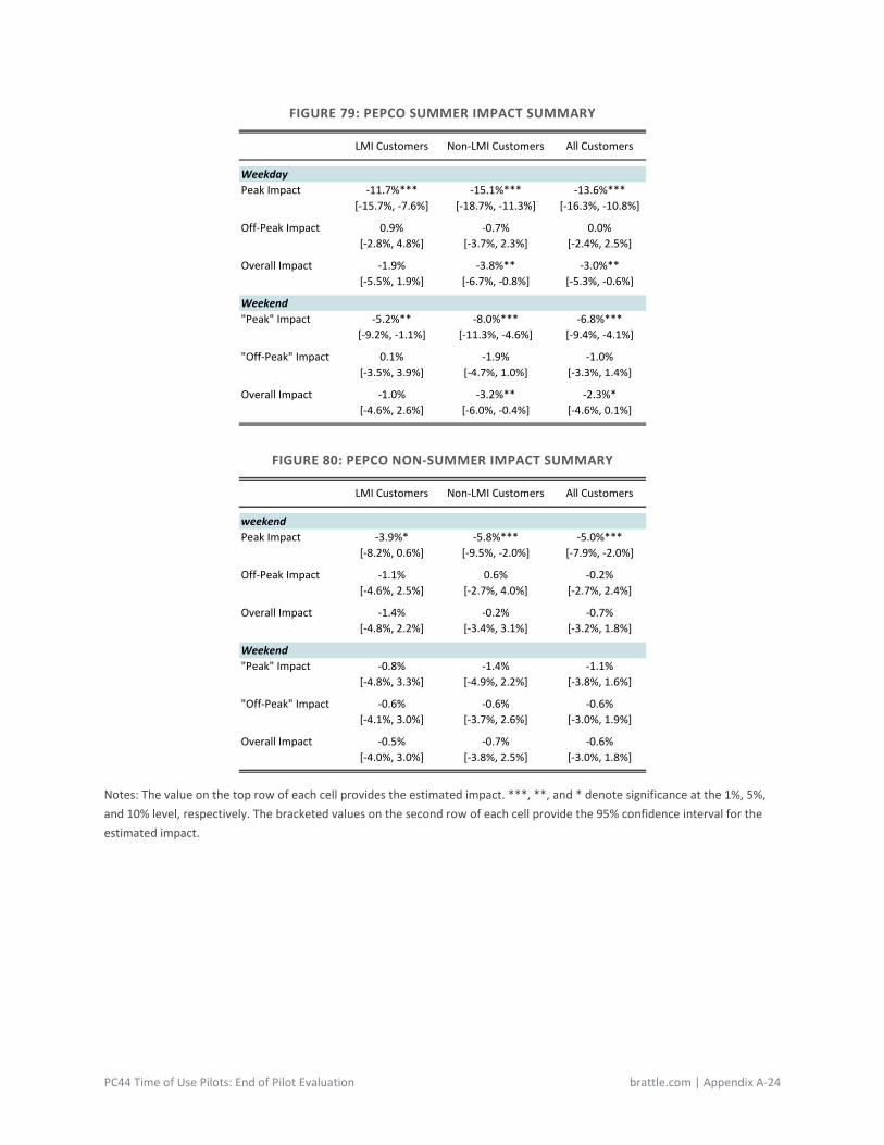
PC44 Time of Use Pilots: End of Pilot Evaluation brattle.com | Appendix A-24
FIGURE 79: PEPCO SUMMER IMPACT SUMMARY
FIGURE 80: PEPCO NON-SUMMER IMPACT SUMMARY
Notes: The value on the top row of each cell provides the estimated impact. ***, **, and * denote significance at the 1%, 5%, and 10% level, respectively. The bracketed values on the second row of each cell provide the 95% confidence interval for the estimated impact.
LMI Customers Non-LMI Customers All Customers
WeekdayPeak Impact -11.7%*** -15.1%*** -13.6%***
[-15.7%, -7.6%] [-18.7%, -11.3%] [-16.3%, -10.8%]
Off-Peak Impact 0.9% -0.7% 0.0%[-2.8%, 4.8%] [-3.7%, 2.3%] [-2.4%, 2.5%]
Overall Impact -1.9% -3.8%** -3.0%**[-5.5%, 1.9%] [-6.7%, -0.8%] [-5.3%, -0.6%]
Weekend"Peak" Impact -5.2%** -8.0%*** -6.8%***
[-9.2%, -1.1%] [-11.3%, -4.6%] [-9.4%, -4.1%]
"Off-Peak" Impact 0.1% -1.9% -1.0%[-3.5%, 3.9%] [-4.7%, 1.0%] [-3.3%, 1.4%]
Overall Impact -1.0% -3.2%** -2.3%*[-4.6%, 2.6%] [-6.0%, -0.4%] [-4.6%, 0.1%]
LMI Customers Non-LMI Customers All Customers
weekendPeak Impact -3.9%* -5.8%*** -5.0%***
[-8.2%, 0.6%] [-9.5%, -2.0%] [-7.9%, -2.0%]
Off-Peak Impact -1.1% 0.6% -0.2%[-4.6%, 2.5%] [-2.7%, 4.0%] [-2.7%, 2.4%]
Overall Impact -1.4% -0.2% -0.7%[-4.8%, 2.2%] [-3.4%, 3.1%] [-3.2%, 1.8%]
Weekend"Peak" Impact -0.8% -1.4% -1.1%
[-4.8%, 3.3%] [-4.9%, 2.2%] [-3.8%, 1.6%]
"Off-Peak" Impact -0.6% -0.6% -0.6%[-4.1%, 3.0%] [-3.7%, 2.6%] [-3.0%, 1.9%]
Overall Impact -0.5% -0.7% -0.6%[-4.0%, 3.0%] [-3.8%, 2.5%] [-3.0%, 1.8%]
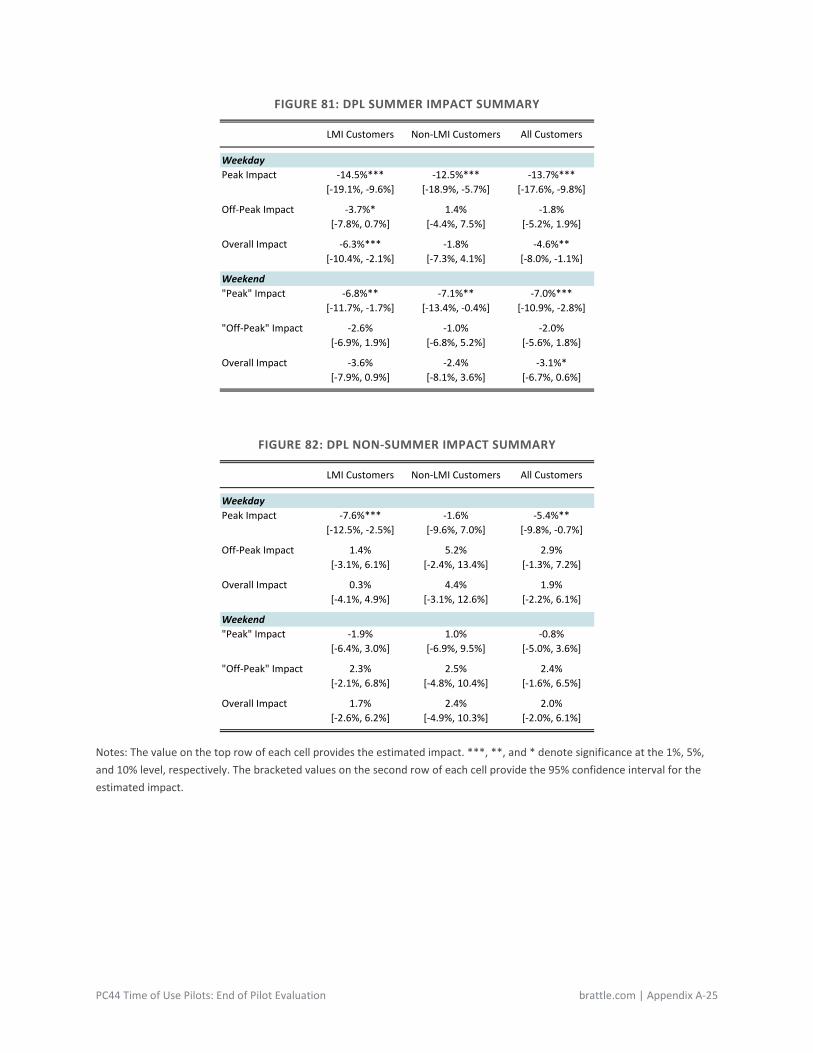
PC44 Time of Use Pilots: End of Pilot Evaluation brattle.com | Appendix A-25
FIGURE 81: DPL SUMMER IMPACT SUMMARY
FIGURE 82: DPL NON-SUMMER IMPACT SUMMARY
Notes: The value on the top row of each cell provides the estimated impact. ***, **, and * denote significance at the 1%, 5%, and 10% level, respectively. The bracketed values on the second row of each cell provide the 95% confidence interval for the estimated impact.
LMI Customers Non-LMI Customers All Customers
WeekdayPeak Impact -14.5%*** -12.5%*** -13.7%***
[-19.1%, -9.6%] [-18.9%, -5.7%] [-17.6%, -9.8%]
Off-Peak Impact -3.7%* 1.4% -1.8%[-7.8%, 0.7%] [-4.4%, 7.5%] [-5.2%, 1.9%]
Overall Impact -6.3%*** -1.8% -4.6%**[-10.4%, -2.1%] [-7.3%, 4.1%] [-8.0%, -1.1%]
Weekend"Peak" Impact -6.8%** -7.1%** -7.0%***
[-11.7%, -1.7%] [-13.4%, -0.4%] [-10.9%, -2.8%]
"Off-Peak" Impact -2.6% -1.0% -2.0%[-6.9%, 1.9%] [-6.8%, 5.2%] [-5.6%, 1.8%]
Overall Impact -3.6% -2.4% -3.1%*[-7.9%, 0.9%] [-8.1%, 3.6%] [-6.7%, 0.6%]
LMI Customers Non-LMI Customers All Customers
WeekdayPeak Impact -7.6%*** -1.6% -5.4%**
[-12.5%, -2.5%] [-9.6%, 7.0%] [-9.8%, -0.7%]
Off-Peak Impact 1.4% 5.2% 2.9%[-3.1%, 6.1%] [-2.4%, 13.4%] [-1.3%, 7.2%]
Overall Impact 0.3% 4.4% 1.9%[-4.1%, 4.9%] [-3.1%, 12.6%] [-2.2%, 6.1%]
Weekend"Peak" Impact -1.9% 1.0% -0.8%
[-6.4%, 3.0%] [-6.9%, 9.5%] [-5.0%, 3.6%]
"Off-Peak" Impact 2.3% 2.5% 2.4%[-2.1%, 6.8%] [-4.8%, 10.4%] [-1.6%, 6.5%]
Overall Impact 1.7% 2.4% 2.0%[-2.6%, 6.2%] [-4.9%, 10.3%] [-2.0%, 6.1%]

PC44 Time of Use Pilots: End of Pilot Evaluation brattle.com | Appendix A-26
A.7 Regression Tables – Elasticity Results This section details regression results for the price response analyses presented in section II. For each utility, we include tables for substitution elasticity and daily demand elasticity regressions for summer and non-summer weekdays.
FIGURE 83: SUMMER WEEKDAY SUBSTITUTION ELASTICITY – BGE
Notes: Excludes net-metering customers and treatment-control pairs who have ever been on three-period rates other than PC44 TOU. Prices only include major components of the bill (supply, transmission, and distribution). Average daily price is weighted by pre-treatment monthly peak/off-peak share of usage. Robust standard errors in parentheses. *** p<0.01, ** p<0.05, * p<0.1.
All Customers LMI Customers Non-LMI Customers(1) (2) (3)
VARIABLES ln(peak to off-peak load) ln(peak to off-peak load) ln(peak to off-peak load)
Pilot Period 0.0142*** 0.0208*** 0.00764(0.00534) (0.00741) (0.00768)
Peak to off-Peak Price Ratio -0.0615*** -0.0494*** -0.0734***(0.00592) (0.00784) (0.00882)
July 0.0177*** 0.0115* 0.0237***(0.00470) (0.00684) (0.00647)
August 0.00541 0.00644 0.00443(0.00471) (0.00704) (0.00629)
September -0.0526*** -0.0450*** -0.0601***(0.00481) (0.00728) (0.00631)
Peak/Off-Peak THI Differential 0.0214*** 0.0205*** 0.0222***(0.000671) (0.00100) (0.000895)
July x THI_Diff 0.0133*** 0.0142*** 0.0124***(0.000902) (0.00135) (0.00120)
August x THI_Diff 0.0146*** 0.0144*** 0.0148***(0.000892) (0.00135) (0.00117)
September x THI_Diff 0.00342*** 0.00296** 0.00386***(0.000789) (0.00121) (0.00101)
Constant 0.0775*** 0.0709*** 0.0839***(0.00513) (0.00729) (0.00721)
Observations 511,849 252,949 258,900Number of Customers 2,046 1,012 1,034Adjusted R-squared 0.038 0.034 0.044Customer FE Y Y Y
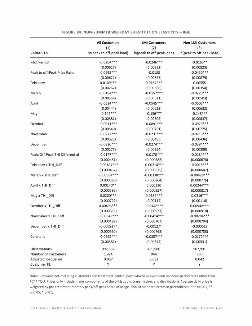
PC44 Time of Use Pilots: End of Pilot Evaluation brattle.com | Appendix A-27
FIGURE 84: NON-SUMMER WEEKDAY SUBSTITUTION ELASTICITY – BGE
Notes: Excludes net-metering customers and treatment-control pairs who have ever been on three-period rates other than PC44 TOU. Prices only include major components of the bill (supply, transmission, and distribution). Average daily price is weighted by pre-treatment monthly peak/off-peak share of usage. Robust standard errors in parentheses. *** p<0.01, ** p<0.05, * p<0.1.
All Customers LMI Customers Non-LMI Customers(1) (2) (3)
VARIABLES ln(peak to off-peak load) ln(peak to off-peak load) ln(peak to off-peak load)
Pilot Period -0.0204*** -0.0246*** -0.0165**(0.00627) (0.00952) (0.00823)
Peak to off-Peak Price Ratio -0.0295*** -0.0133 -0.0450***(0.00622) (0.00875) (0.00879)
February 0.0109*** 0.0164*** 0.00555(0.00262) (0.00386) (0.00354)
March -0.0194*** -0.0157*** -0.0229***(0.00358) (0.00511) (0.00503)
April -0.0524*** -0.0545*** -0.0503***(0.00444) (0.00622) (0.00632)
May -0.142*** -0.136*** -0.148***(0.00581) (0.00805) (0.00837)
October -0.0911*** -0.0891*** -0.0929***(0.00540) (0.00751) (0.00775)
November -0.0222*** -0.0231*** -0.0213***(0.00325) (0.00485) (0.00436)
December -0.0330*** -0.0274*** -0.0384***(0.00277) (0.00394) (0.00389)
Peak/Off-Peak THI Differential -0.0177*** -0.0170*** -0.0184***(0.000481) (0.000682) (0.000678)
February x THI_Diff -0.00184*** -0.00214*** -0.00155**(0.000467) (0.000675) (0.000647)
March x THI_Diff -0.00384*** -0.00338*** -0.00428***(0.000580) (0.000864) (0.000776)
April x THI_Diff 0.00140** 0.000330 0.00244***(0.000592) (0.000857) (0.000817)
May x THI_Diff 0.0200*** 0.0182*** 0.0216***(0.000792) (0.00114) (0.00110)
October x THI_Diff 0.00496*** 0.00448*** 0.00542***(0.000653) (0.000937) (0.000910)
November x THI_Diff -0.00348*** -0.00414*** -0.00284***(0.000499) (0.000707) (0.000704)
December x THI_Diff -0.000937* -0.00127* -0.000618(0.000550) (0.000768) (0.000788)
Constant -0.0265*** -0.0357*** -0.0177***(0.00381) (0.00544) (0.00531)
Observations 997,897 489,906 507,991Number of Customers 1,924 944 980Adjusted R-squared 0.037 0.032 0.042Customer FE Y Y Y
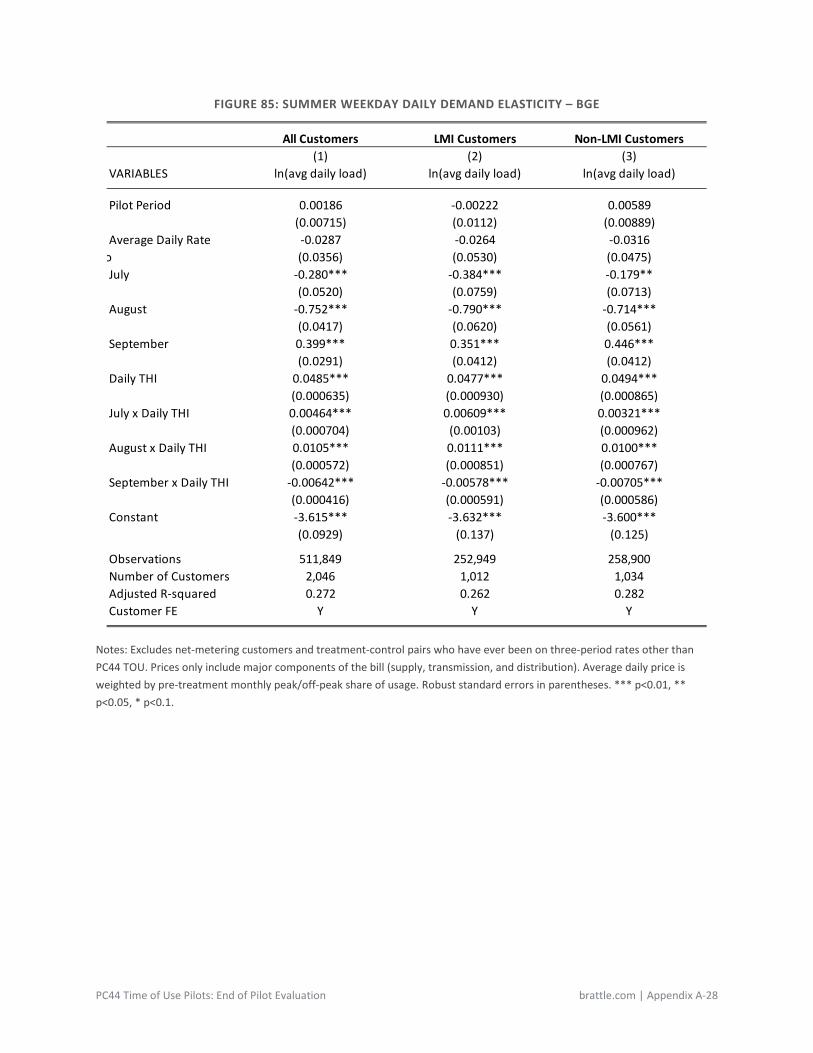
PC44 Time of Use Pilots: End of Pilot Evaluation brattle.com | Appendix A-28
FIGURE 85: SUMMER WEEKDAY DAILY DEMAND ELASTICITY – BGE
Notes: Excludes net-metering customers and treatment-control pairs who have ever been on three-period rates other than PC44 TOU. Prices only include major components of the bill (supply, transmission, and distribution). Average daily price is weighted by pre-treatment monthly peak/off-peak share of usage. Robust standard errors in parentheses. *** p<0.01, ** p<0.05, * p<0.1.
All Customers LMI Customers Non-LMI Customers(1) (2) (3)
VARIABLES ln(avg daily load) ln(avg daily load) ln(avg daily load)
Pilot Period 0.00186 -0.00222 0.00589(0.00715) (0.0112) (0.00889)
Average Daily Rate -0.0287 -0.0264 -0.0316o (0.0356) (0.0530) (0.0475)July -0.280*** -0.384*** -0.179**
(0.0520) (0.0759) (0.0713)August -0.752*** -0.790*** -0.714***
(0.0417) (0.0620) (0.0561)September 0.399*** 0.351*** 0.446***
(0.0291) (0.0412) (0.0412)Daily THI 0.0485*** 0.0477*** 0.0494***
(0.000635) (0.000930) (0.000865)July x Daily THI 0.00464*** 0.00609*** 0.00321***
(0.000704) (0.00103) (0.000962)August x Daily THI 0.0105*** 0.0111*** 0.0100***
(0.000572) (0.000851) (0.000767)September x Daily THI -0.00642*** -0.00578*** -0.00705***
(0.000416) (0.000591) (0.000586)Constant -3.615*** -3.632*** -3.600***
(0.0929) (0.137) (0.125)
Observations 511,849 252,949 258,900Number of Customers 2,046 1,012 1,034Adjusted R-squared 0.272 0.262 0.282Customer FE Y Y Y
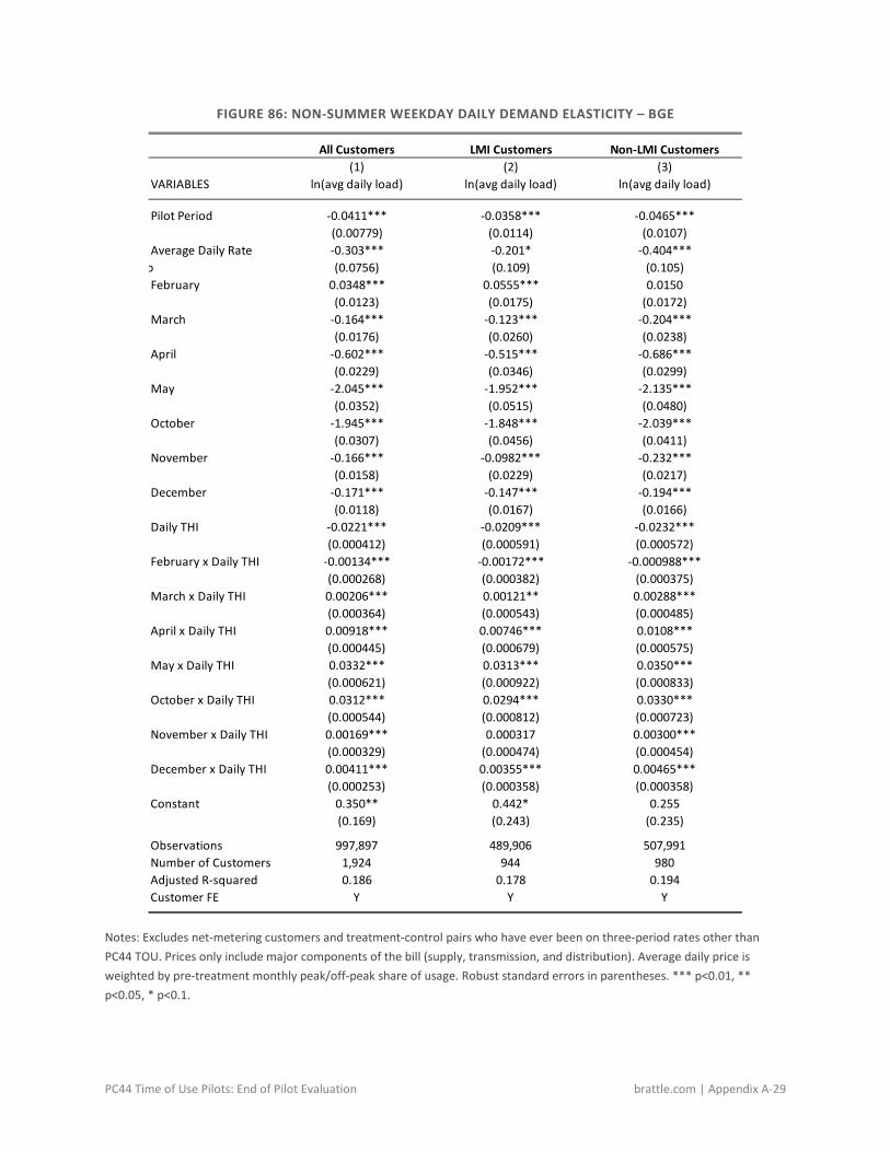
PC44 Time of Use Pilots: End of Pilot Evaluation brattle.com | Appendix A-29
FIGURE 86: NON-SUMMER WEEKDAY DAILY DEMAND ELASTICITY – BGE
Notes: Excludes net-metering customers and treatment-control pairs who have ever been on three-period rates other than PC44 TOU. Prices only include major components of the bill (supply, transmission, and distribution). Average daily price is weighted by pre-treatment monthly peak/off-peak share of usage. Robust standard errors in parentheses. *** p<0.01, ** p<0.05, * p<0.1.
All Customers LMI Customers Non-LMI Customers(1) (2) (3)
VARIABLES ln(avg daily load) ln(avg daily load) ln(avg daily load)
Pilot Period -0.0411*** -0.0358*** -0.0465***(0.00779) (0.0114) (0.0107)
Average Daily Rate -0.303*** -0.201* -0.404***o (0.0756) (0.109) (0.105)February 0.0348*** 0.0555*** 0.0150
(0.0123) (0.0175) (0.0172)March -0.164*** -0.123*** -0.204***
(0.0176) (0.0260) (0.0238)April -0.602*** -0.515*** -0.686***
(0.0229) (0.0346) (0.0299)May -2.045*** -1.952*** -2.135***
(0.0352) (0.0515) (0.0480)October -1.945*** -1.848*** -2.039***
(0.0307) (0.0456) (0.0411)November -0.166*** -0.0982*** -0.232***
(0.0158) (0.0229) (0.0217)December -0.171*** -0.147*** -0.194***
(0.0118) (0.0167) (0.0166)Daily THI -0.0221*** -0.0209*** -0.0232***
(0.000412) (0.000591) (0.000572)February x Daily THI -0.00134*** -0.00172*** -0.000988***
(0.000268) (0.000382) (0.000375)March x Daily THI 0.00206*** 0.00121** 0.00288***
(0.000364) (0.000543) (0.000485)April x Daily THI 0.00918*** 0.00746*** 0.0108***
(0.000445) (0.000679) (0.000575)May x Daily THI 0.0332*** 0.0313*** 0.0350***
(0.000621) (0.000922) (0.000833)October x Daily THI 0.0312*** 0.0294*** 0.0330***
(0.000544) (0.000812) (0.000723)November x Daily THI 0.00169*** 0.000317 0.00300***
(0.000329) (0.000474) (0.000454)December x Daily THI 0.00411*** 0.00355*** 0.00465***
(0.000253) (0.000358) (0.000358)Constant 0.350** 0.442* 0.255
(0.169) (0.243) (0.235)
Observations 997,897 489,906 507,991Number of Customers 1,924 944 980Adjusted R-squared 0.186 0.178 0.194Customer FE Y Y Y
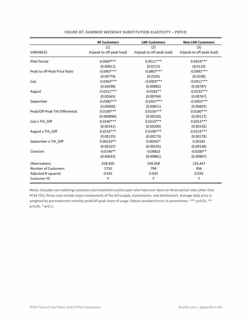
PC44 Time of Use Pilots: End of Pilot Evaluation brattle.com | Appendix A-30
FIGURE 87: SUMMER WEEKDAY SUBSTITUTION ELASTICITY – PEPCO
Notes: Excludes net-metering customers and treatment-control pairs who have ever been on three-period rates other than PC44 TOU. Prices only include major components of the bill (supply, transmission, and distribution). Average daily price is weighted by pre-treatment monthly peak/off-peak share of usage. Robust standard errors in parentheses. *** p<0.01, ** p<0.05, * p<0.1.
All Customers LMI Customers Non-LMI Customers(1) (2) (3)
VARIABLES ln(peak to off-peak load) ln(peak to off-peak load) ln(peak to off-peak load)
Pilot Period 0.0469*** 0.0511*** 0.0433***(0.00811) (0.0113) (0.0110)
Peak to off-Peak Price Ratio -0.0907*** -0.0807*** -0.0991***(0.00774) (0.0105) (0.0109)
July -0.0363*** -0.0303*** -0.0411***(0.00598) (0.00882) (0.00787)
August -0.0211*** -0.0182** -0.0233***(0.00565) (0.00794) (0.00767)
September -0.0383*** -0.0357*** -0.0403***(0.00600) (0.00811) (0.00825)
Peak/Off-Peak THI Differential 0.0169*** 0.0156*** 0.0180***(0.000896) (0.00130) (0.00117)
July x THI_Diff 0.0240*** 0.0223*** 0.0253***(0.00141) (0.00200) (0.00192)
August x THI_Diff 0.0216*** 0.0196*** 0.0233***(0.00125) (0.00173) (0.00170)
September x THI_Diff 0.00210** 0.00242* 0.00182(0.00107) (0.00145) (0.00148)
Constant -0.0146** -0.00822 -0.0200**(0.00633) (0.00881) (0.00867)
Observations 428,405 194,958 233,447Number of Customers 1750 794 956Adjusted R-squared 0.032 0.030 0.034Customer FE Y Y Y
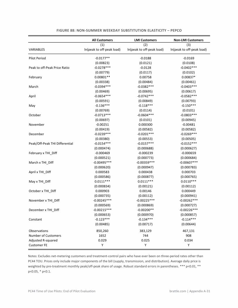
PC44 Time of Use Pilots: End of Pilot Evaluation brattle.com | Appendix A-31
FIGURE 88: NON-SUMMER WEEKDAY SUBSTITUTION ELASTICITY – PEPCO
Notes: Excludes net-metering customers and treatment-control pairs who have ever been on three-period rates other than PC44 TOU. Prices only include major components of the bill (supply, transmission, and distribution). Average daily price is weighted by pre-treatment monthly peak/off-peak share of usage. Robust standard errors in parentheses. *** p<0.01, ** p<0.05, * p<0.1.
All Customers LMI Customers Non-LMI Customers(1) (2) (3)
VARIABLES ln(peak to off-peak load) ln(peak to off-peak load) ln(peak to off-peak load)
Pilot Period -0.0177** -0.0188 -0.0169(0.00823) (0.0121) (0.0108)
Peak to off-Peak Price Ratio -0.0278*** -0.0128 -0.0402***(0.00779) (0.0117) (0.0102)
February 0.00801** 0.00758 0.00837*(0.00338) (0.00484) (0.00461)
March -0.0394*** -0.0382*** -0.0403***(0.00469) (0.00695) (0.00617)
April -0.0654*** -0.0742*** -0.0582***(0.00591) (0.00849) (0.00793)
May -0.136*** -0.118*** -0.150***(0.00769) (0.0114) (0.0101)
October -0.0713*** -0.0604*** -0.0803***(0.00697) (0.0101) (0.00945)
November -0.00251 0.000300 -0.00481(0.00419) (0.00582) (0.00582)
December -0.0239*** -0.0201*** -0.0269***(0.00380) (0.00553) (0.00505)
Peak/Off-Peak THI Differential -0.0154*** -0.0157*** -0.0152***(0.000474) (0.000688) (0.000627)
February x THI_Diff -0.000469 -0.000239 -0.000659(0.000521) (0.000773) (0.000684)
March x THI_Diff -0.00495*** -0.00359*** -0.00607***(0.000620) (0.000947) (0.000783)
April x THI_Diff 0.000583 0.000438 0.000703(0.000586) (0.000877) (0.000765)
May x THI_Diff 0.0111*** 0.0111*** 0.0110***(0.000834) (0.00121) (0.00112)
October x THI_Diff 0.000903 0.00146 0.000449(0.000735) (0.00112) (0.000941)
November x THI_Diff -0.00245*** -0.00225*** -0.00262***(0.000569) (0.000869) (0.000727)
December x THI_Diff -0.00215*** -0.00200** -0.00226***(0.000653) (0.000970) (0.000857)
Constant -0.123*** -0.134*** -0.114***(0.00485) (0.00717) (0.00644)
Observations 850,260 383,129 467,131Number of Customers 1652 744 908Adjusted R-squared 0.029 0.025 0.034Customer FE Y Y Y
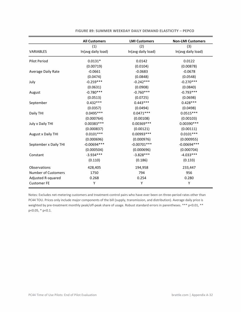
PC44 Time of Use Pilots: End of Pilot Evaluation brattle.com | Appendix A-32
FIGURE 89: SUMMER WEEKDAY DAILY DEMAND ELASTICITY – PEPCO
Notes: Excludes net-metering customers and treatment-control pairs who have ever been on three-period rates other than PC44 TOU. Prices only include major components of the bill (supply, transmission, and distribution). Average daily price is weighted by pre-treatment monthly peak/off-peak share of usage. Robust standard errors in parentheses. *** p<0.01, ** p<0.05, * p<0.1.
All Customers LMI Customers Non-LMI Customers(1) (2) (3)
VARIABLES ln(avg daily load) ln(avg daily load) ln(avg daily load)
Pilot Period 0.0131* 0.0142 0.0122(0.00719) (0.0104) (0.00878)
Average Daily Rate -0.0661 -0.0683 -0.0678(0.0474) (0.0848) (0.0548)
July -0.259*** -0.242*** -0.270***(0.0631) (0.0908) (0.0840)
August -0.780*** -0.760*** -0.793***(0.0513) (0.0725) (0.0698)
September 0.432*** 0.443*** 0.428***(0.0357) (0.0494) (0.0498)
Daily THI 0.0495*** 0.0471*** 0.0515***(0.000764) (0.00108) (0.00103)
July x Daily THI 0.00383*** 0.00369*** 0.00390***(0.000837) (0.00121) (0.00111)
August x Daily THI 0.0101*** 0.00993*** 0.0101***(0.000696) (0.000976) (0.000955)
September x Daily THI -0.00694*** -0.00701*** -0.00694***(0.000504) (0.000696) (0.000704)
Constant -3.934*** -3.828*** -4.033***(0.110) (0.186) (0.133)
Observations 428,405 194,958 233,447Number of Customers 1750 794 956Adjusted R-squared 0.268 0.254 0.280Customer FE Y Y Y
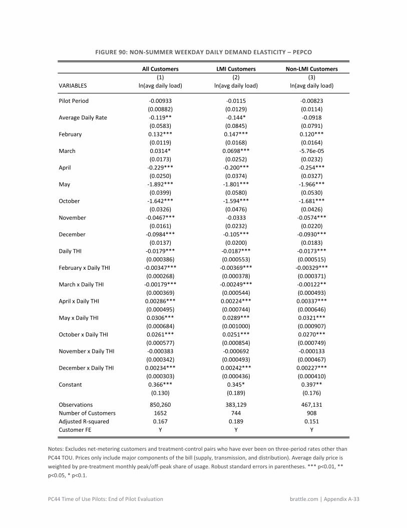
PC44 Time of Use Pilots: End of Pilot Evaluation brattle.com | Appendix A-33
FIGURE 90: NON-SUMMER WEEKDAY DAILY DEMAND ELASTICITY – PEPCO
Notes: Excludes net-metering customers and treatment-control pairs who have ever been on three-period rates other than PC44 TOU. Prices only include major components of the bill (supply, transmission, and distribution). Average daily price is weighted by pre-treatment monthly peak/off-peak share of usage. Robust standard errors in parentheses. *** p<0.01, ** p<0.05, * p<0.1.
All Customers LMI Customers Non-LMI Customers(1) (2) (3)
VARIABLES ln(avg daily load) ln(avg daily load) ln(avg daily load)
Pilot Period -0.00933 -0.0115 -0.00823(0.00882) (0.0129) (0.0114)
Average Daily Rate -0.119** -0.144* -0.0918(0.0583) (0.0845) (0.0791)
February 0.132*** 0.147*** 0.120***(0.0119) (0.0168) (0.0164)
March 0.0314* 0.0698*** -5.76e-05(0.0173) (0.0252) (0.0232)
April -0.229*** -0.200*** -0.254***(0.0250) (0.0374) (0.0327)
May -1.892*** -1.801*** -1.966***(0.0399) (0.0580) (0.0530)
October -1.642*** -1.594*** -1.681***(0.0326) (0.0476) (0.0426)
November -0.0467*** -0.0333 -0.0574***(0.0161) (0.0232) (0.0220)
December -0.0984*** -0.105*** -0.0930***(0.0137) (0.0200) (0.0183)
Daily THI -0.0179*** -0.0187*** -0.0173***(0.000386) (0.000553) (0.000515)
February x Daily THI -0.00347*** -0.00369*** -0.00329***(0.000268) (0.000378) (0.000371)
March x Daily THI -0.00179*** -0.00249*** -0.00122**(0.000369) (0.000544) (0.000493)
April x Daily THI 0.00286*** 0.00224*** 0.00337***(0.000495) (0.000744) (0.000646)
May x Daily THI 0.0306*** 0.0289*** 0.0321***(0.000684) (0.001000) (0.000907)
October x Daily THI 0.0261*** 0.0251*** 0.0270***(0.000577) (0.000854) (0.000749)
November x Daily THI -0.000383 -0.000692 -0.000133(0.000342) (0.000493) (0.000467)
December x Daily THI 0.00234*** 0.00242*** 0.00227***(0.000303) (0.000436) (0.000410)
Constant 0.366*** 0.345* 0.397**(0.130) (0.189) (0.176)
Observations 850,260 383,129 467,131Number of Customers 1652 744 908Adjusted R-squared 0.167 0.189 0.151Customer FE Y Y Y

PC44 Time of Use Pilots: End of Pilot Evaluation brattle.com | Appendix A-34
FIGURE 91: SUMMER WEEKDAY SUBSTITUTION ELASTICITY – DPL
Notes: Excludes net-metering customers and treatment-control pairs who have ever been on three-period rates other than PC44 TOU. Prices only include major components of the bill (supply, transmission, and distribution). Average daily price is weighted by pre-treatment monthly peak/off-peak share of usage. Robust standard errors in parentheses. *** p<0.01, ** p<0.05, * p<0.1.
All Customers LMI Customers Non-LMI Customers(1) (2) (3)
VARIABLES ln(peak to off-peak load) ln(peak to off-peak load) ln(peak to off-peak load)
Pilot Period 0.00810 0.00273 0.0165(0.00709) (0.00783) (0.0127)
Peak to off-Peak Price Ratio -0.0708*** -0.0650*** -0.0800***(0.00818) (0.00932) (0.0149)
July -0.0362*** -0.0386*** -0.0323**(0.00825) (0.0103) (0.0129)
August -0.0251*** -0.0257*** -0.0241*(0.00775) (0.00946) (0.0127)
September -0.0286*** -0.0254** -0.0335***(0.00803) (0.00994) (0.0129)
Peak/Off-Peak THI Differential 0.00552*** 0.00658*** 0.00386*(0.00126) (0.00157) (0.00198)
July x THI_Diff 0.0245*** 0.0245*** 0.0245***(0.00171) (0.00214) (0.00271)
August x THI_Diff 0.0228*** 0.0228*** 0.0229***(0.00156) (0.00195) (0.00249)
September x THI_Diff -0.000390 -0.00100 0.000582(0.00138) (0.00173) (0.00217)
Constant 0.181*** 0.205*** 0.144***(0.00844) (0.01000) (0.0145)
Observations 250,924 153,499 97,425Number of Customers 1014 620 394Adjusted R-squared 0.024 0.024 0.023Customer FE Y Y Y
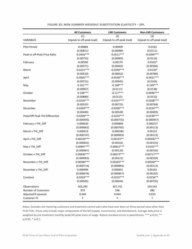
PC44 Time of Use Pilots: End of Pilot Evaluation brattle.com | Appendix A-35
FIGURE 92: NON-SUMMER WEEKDAY SUBSTITUTION ELASTICITY – DPL
Notes: Excludes net-metering customers and treatment-control pairs who have ever been on three-period rates other than PC44 TOU. Prices only include major components of the bill (supply, transmission, and distribution). Average daily price is weighted by pre-treatment monthly peak/off-peak share of usage. Robust standard errors in parentheses. *** p<0.01, ** p<0.05, * p<0.1.
All Customers LMI Customers Non-LMI Customers(1) (2) (3)
VARIABLES ln(peak to off-peak load) ln(peak to off-peak load) ln(peak to off-peak load)
Pilot Period -0.00884 -0.00409 -0.0163(0.00811) (0.00989) (0.0111)
Peak to off-Peak Price Ratio -0.0456*** -0.0511*** -0.0369***(0.00753) (0.00965) (0.0110)
February -0.00500 -0.00174 -0.0101*(0.00371) (0.00462) (0.00596)
March -0.0231*** -0.0294*** -0.0130*(0.00510) (0.00652) (0.00780)
April -0.0505*** -0.0558*** -0.0421***(0.00721) (0.00945) (0.0103)
May -0.161*** -0.168*** -0.149***(0.00907) (0.0117) (0.0138)
October -0.108*** -0.117*** -0.0946***(0.00889) (0.0115) (0.0132)
November -0.0226*** -0.0237*** -0.0208***(0.00555) (0.00725) (0.00784)
December -0.0209*** -0.0200*** -0.0224***(0.00449) (0.00549) (0.00693)
Peak/Off-Peak THI Differential -0.0208*** -0.0220*** -0.0190***(0.000595) (0.000735) (0.000957)
February x THI_Diff 0.000630 0.000868 0.000257(0.000662) (0.000765) (0.00113)
March x THI_Diff 0.000419 -0.000280 0.00152(0.000747) (0.000903) (0.00123)
April x THI_Diff 0.00339*** 0.00233** 0.00506***(0.000841) (0.00101) (0.00135)
May x THI_Diff 0.00897*** 0.00822*** 0.0102***(0.000967) (0.00120) (0.00156)
October x THI_Diff 0.00690*** 0.00673*** 0.00717***(0.000963) (0.00121) (0.00150)
November x THI_Diff 0.00380*** 0.00265*** 0.00560***(0.000714) (0.000893) (0.00113)
December x THI_Diff 0.000999 0.000601 0.00162(0.000676) (0.000857) (0.00102)
Constant -0.0203*** -0.0233*** -0.0156**(0.00505) (0.00644) (0.00735)
Observations 503,283 307,741 195,542Number of Customers 976 596 380Adjusted R-squared 0.040 0.044 0.033Customer FE Y Y Y
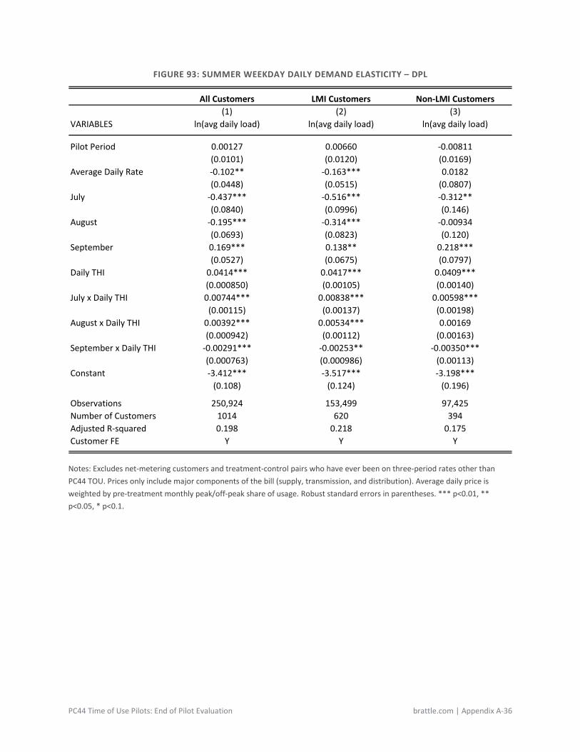
PC44 Time of Use Pilots: End of Pilot Evaluation brattle.com | Appendix A-36
FIGURE 93: SUMMER WEEKDAY DAILY DEMAND ELASTICITY – DPL
Notes: Excludes net-metering customers and treatment-control pairs who have ever been on three-period rates other than PC44 TOU. Prices only include major components of the bill (supply, transmission, and distribution). Average daily price is weighted by pre-treatment monthly peak/off-peak share of usage. Robust standard errors in parentheses. *** p<0.01, ** p<0.05, * p<0.1.
All Customers LMI Customers Non-LMI Customers(1) (2) (3)
VARIABLES ln(avg daily load) ln(avg daily load) ln(avg daily load)
Pilot Period 0.00127 0.00660 -0.00811(0.0101) (0.0120) (0.0169)
Average Daily Rate -0.102** -0.163*** 0.0182(0.0448) (0.0515) (0.0807)
July -0.437*** -0.516*** -0.312**(0.0840) (0.0996) (0.146)
August -0.195*** -0.314*** -0.00934(0.0693) (0.0823) (0.120)
September 0.169*** 0.138** 0.218***(0.0527) (0.0675) (0.0797)
Daily THI 0.0414*** 0.0417*** 0.0409***(0.000850) (0.00105) (0.00140)
July x Daily THI 0.00744*** 0.00838*** 0.00598***(0.00115) (0.00137) (0.00198)
August x Daily THI 0.00392*** 0.00534*** 0.00169(0.000942) (0.00112) (0.00163)
September x Daily THI -0.00291*** -0.00253** -0.00350***(0.000763) (0.000986) (0.00113)
Constant -3.412*** -3.517*** -3.198***(0.108) (0.124) (0.196)
Observations 250,924 153,499 97,425Number of Customers 1014 620 394Adjusted R-squared 0.198 0.218 0.175Customer FE Y Y Y
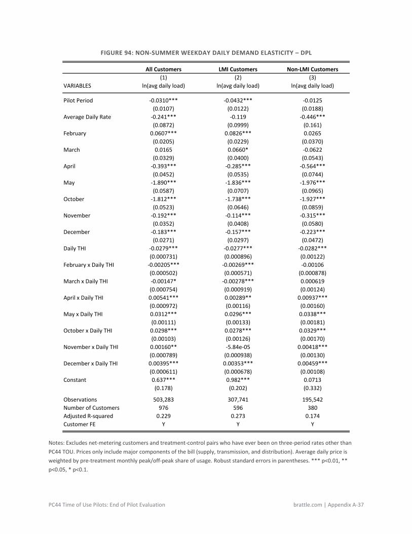
PC44 Time of Use Pilots: End of Pilot Evaluation brattle.com | Appendix A-37
FIGURE 94: NON-SUMMER WEEKDAY DAILY DEMAND ELASTICITY – DPL
Notes: Excludes net-metering customers and treatment-control pairs who have ever been on three-period rates other than PC44 TOU. Prices only include major components of the bill (supply, transmission, and distribution). Average daily price is weighted by pre-treatment monthly peak/off-peak share of usage. Robust standard errors in parentheses. *** p<0.01, ** p<0.05, * p<0.1.
All Customers LMI Customers Non-LMI Customers(1) (2) (3)
VARIABLES ln(avg daily load) ln(avg daily load) ln(avg daily load)
Pilot Period -0.0310*** -0.0432*** -0.0125(0.0107) (0.0122) (0.0188)
Average Daily Rate -0.241*** -0.119 -0.446***(0.0872) (0.0999) (0.161)
February 0.0607*** 0.0826*** 0.0265(0.0205) (0.0229) (0.0370)
March 0.0165 0.0660* -0.0622(0.0329) (0.0400) (0.0543)
April -0.393*** -0.285*** -0.564***(0.0452) (0.0535) (0.0744)
May -1.890*** -1.836*** -1.976***(0.0587) (0.0707) (0.0965)
October -1.812*** -1.738*** -1.927***(0.0523) (0.0646) (0.0859)
November -0.192*** -0.114*** -0.315***(0.0352) (0.0408) (0.0580)
December -0.183*** -0.157*** -0.223***(0.0271) (0.0297) (0.0472)
Daily THI -0.0279*** -0.0277*** -0.0282***(0.000731) (0.000896) (0.00122)
February x Daily THI -0.00205*** -0.00269*** -0.00106(0.000502) (0.000571) (0.000878)
March x Daily THI -0.00147* -0.00278*** 0.000619(0.000754) (0.000919) (0.00124)
April x Daily THI 0.00541*** 0.00289** 0.00937***(0.000972) (0.00116) (0.00160)
May x Daily THI 0.0312*** 0.0296*** 0.0338***(0.00111) (0.00133) (0.00181)
October x Daily THI 0.0298*** 0.0278*** 0.0329***(0.00103) (0.00126) (0.00170)
November x Daily THI 0.00160** -5.84e-05 0.00418***(0.000789) (0.000938) (0.00130)
December x Daily THI 0.00395*** 0.00353*** 0.00459***(0.000611) (0.000678) (0.00108)
Constant 0.637*** 0.982*** 0.0713(0.178) (0.202) (0.332)
Observations 503,283 307,741 195,542Number of Customers 976 596 380Adjusted R-squared 0.229 0.273 0.174Customer FE Y Y Y
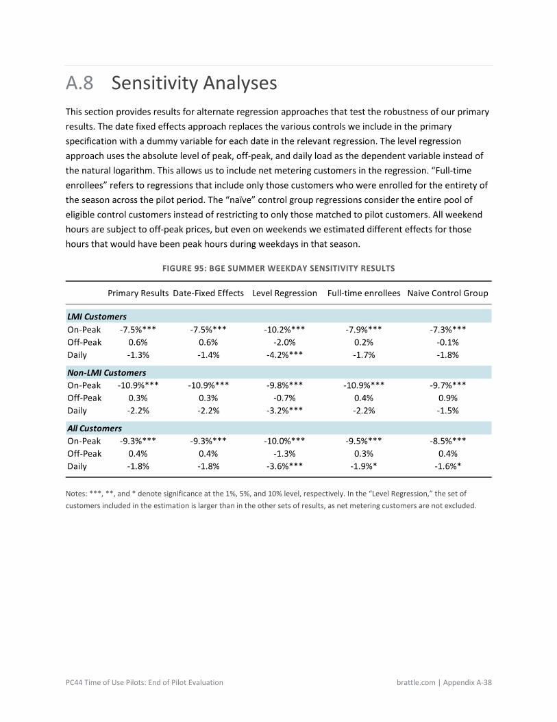
PC44 Time of Use Pilots: End of Pilot Evaluation brattle.com | Appendix A-38
A.8 Sensitivity Analyses This section provides results for alternate regression approaches that test the robustness of our primary results. The date fixed effects approach replaces the various controls we include in the primary specification with a dummy variable for each date in the relevant regression. The level regression approach uses the absolute level of peak, off-peak, and daily load as the dependent variable instead of the natural logarithm. This allows us to include net metering customers in the regression. “Full-time enrollees” refers to regressions that include only those customers who were enrolled for the entirety of the season across the pilot period. The “naïve” control group regressions consider the entire pool of eligible control customers instead of restricting to only those matched to pilot customers. All weekend hours are subject to off-peak prices, but even on weekends we estimated different effects for those hours that would have been peak hours during weekdays in that season.
FIGURE 95: BGE SUMMER WEEKDAY SENSITIVITY RESULTS
Notes: ***, **, and * denote significance at the 1%, 5%, and 10% level, respectively. In the “Level Regression,” the set of customers included in the estimation is larger than in the other sets of results, as net metering customers are not excluded.
Primary Results Date-Fixed Effects Level Regression Full-time enrollees Naive Control Group
LMI CustomersOn-Peak -7.5%*** -7.5%*** -10.2%*** -7.9%*** -7.3%***Off-Peak 0.6% 0.6% -2.0% 0.2% -0.1%Daily -1.3% -1.4% -4.2%*** -1.7% -1.8%
Non-LMI CustomersOn-Peak -10.9%*** -10.9%*** -9.8%*** -10.9%*** -9.7%***Off-Peak 0.3% 0.3% -0.7% 0.4% 0.9%Daily -2.2% -2.2% -3.2%*** -2.2% -1.5%
All CustomersOn-Peak -9.3%*** -9.3%*** -10.0%*** -9.5%*** -8.5%***Off-Peak 0.4% 0.4% -1.3% 0.3% 0.4%Daily -1.8% -1.8% -3.6%*** -1.9%* -1.6%*
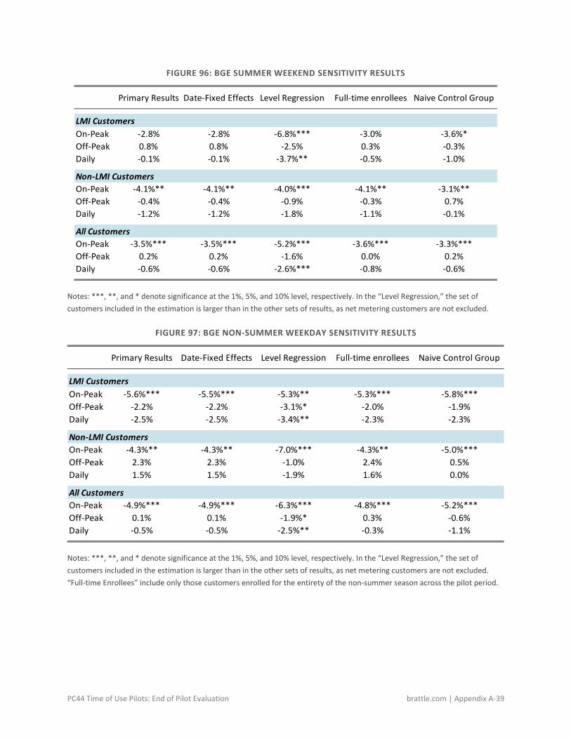
PC44 Time of Use Pilots: End of Pilot Evaluation brattle.com | Appendix A-39
FIGURE 96: BGE SUMMER WEEKEND SENSITIVITY RESULTS
Notes: ***, **, and * denote significance at the 1%, 5%, and 10% level, respectively. In the “Level Regression,” the set of customers included in the estimation is larger than in the other sets of results, as net metering customers are not excluded.
FIGURE 97: BGE NON-SUMMER WEEKDAY SENSITIVITY RESULTS
Notes: ***, **, and * denote significance at the 1%, 5%, and 10% level, respectively. In the “Level Regression,” the set of customers included in the estimation is larger than in the other sets of results, as net metering customers are not excluded. “Full-time Enrollees” include only those customers enrolled for the entirety of the non-summer season across the pilot period.
Primary Results Date-Fixed Effects Level Regression Full-time enrollees Naive Control Group
LMI CustomersOn-Peak -2.8% -2.8% -6.8%*** -3.0% -3.6%*Off-Peak 0.8% 0.8% -2.5% 0.3% -0.3%Daily -0.1% -0.1% -3.7%** -0.5% -1.0%
Non-LMI CustomersOn-Peak -4.1%** -4.1%** -4.0%*** -4.1%** -3.1%**Off-Peak -0.4% -0.4% -0.9% -0.3% 0.7%Daily -1.2% -1.2% -1.8% -1.1% -0.1%
All CustomersOn-Peak -3.5%*** -3.5%*** -5.2%*** -3.6%*** -3.3%***Off-Peak 0.2% 0.2% -1.6% 0.0% 0.2%Daily -0.6% -0.6% -2.6%*** -0.8% -0.6%
Primary Results Date-Fixed Effects Level Regression Full-time enrollees Naive Control Group
LMI CustomersOn-Peak -5.6%*** -5.5%*** -5.3%** -5.3%*** -5.8%***Off-Peak -2.2% -2.2% -3.1%* -2.0% -1.9%Daily -2.5% -2.5% -3.4%** -2.3% -2.3%
Non-LMI CustomersOn-Peak -4.3%** -4.3%** -7.0%*** -4.3%** -5.0%***Off-Peak 2.3% 2.3% -1.0% 2.4% 0.5%Daily 1.5% 1.5% -1.9% 1.6% 0.0%
All CustomersOn-Peak -4.9%*** -4.9%*** -6.3%*** -4.8%*** -5.2%***Off-Peak 0.1% 0.1% -1.9%* 0.3% -0.6%Daily -0.5% -0.5% -2.5%** -0.3% -1.1%
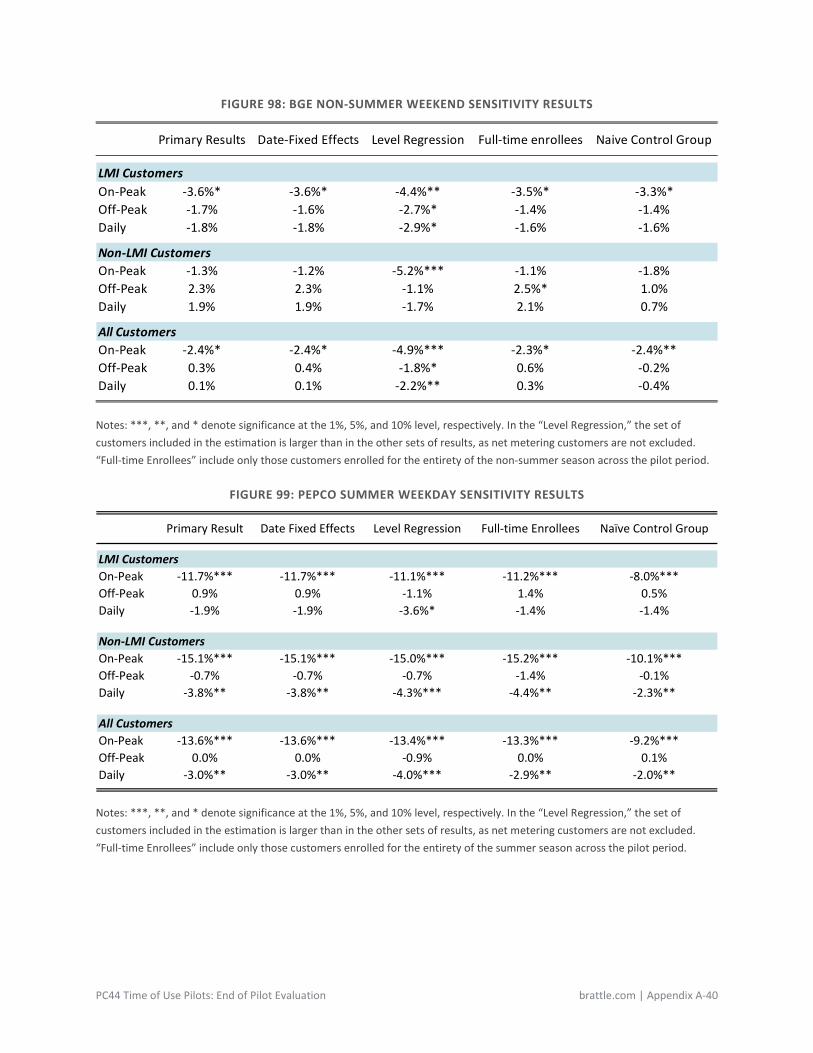
PC44 Time of Use Pilots: End of Pilot Evaluation brattle.com | Appendix A-40
FIGURE 98: BGE NON-SUMMER WEEKEND SENSITIVITY RESULTS
Notes: ***, **, and * denote significance at the 1%, 5%, and 10% level, respectively. In the “Level Regression,” the set of customers included in the estimation is larger than in the other sets of results, as net metering customers are not excluded. “Full-time Enrollees” include only those customers enrolled for the entirety of the non-summer season across the pilot period.
FIGURE 99: PEPCO SUMMER WEEKDAY SENSITIVITY RESULTS
Notes: ***, **, and * denote significance at the 1%, 5%, and 10% level, respectively. In the “Level Regression,” the set of customers included in the estimation is larger than in the other sets of results, as net metering customers are not excluded. “Full-time Enrollees” include only those customers enrolled for the entirety of the summer season across the pilot period.
Primary Results Date-Fixed Effects Level Regression Full-time enrollees Naive Control Group
LMI CustomersOn-Peak -3.6%* -3.6%* -4.4%** -3.5%* -3.3%*Off-Peak -1.7% -1.6% -2.7%* -1.4% -1.4%Daily -1.8% -1.8% -2.9%* -1.6% -1.6%
Non-LMI CustomersOn-Peak -1.3% -1.2% -5.2%*** -1.1% -1.8%Off-Peak 2.3% 2.3% -1.1% 2.5%* 1.0%Daily 1.9% 1.9% -1.7% 2.1% 0.7%
All CustomersOn-Peak -2.4%* -2.4%* -4.9%*** -2.3%* -2.4%**Off-Peak 0.3% 0.4% -1.8%* 0.6% -0.2%Daily 0.1% 0.1% -2.2%** 0.3% -0.4%
Primary Result Date Fixed Effects Level Regression Full-time Enrollees Naïve Control Group
LMI CustomersOn-Peak -11.7%*** -11.7%*** -11.1%*** -11.2%*** -8.0%***Off-Peak 0.9% 0.9% -1.1% 1.4% 0.5%Daily -1.9% -1.9% -3.6%* -1.4% -1.4%
Non-LMI CustomersOn-Peak -15.1%*** -15.1%*** -15.0%*** -15.2%*** -10.1%***Off-Peak -0.7% -0.7% -0.7% -1.4% -0.1%Daily -3.8%** -3.8%** -4.3%*** -4.4%** -2.3%**
All CustomersOn-Peak -13.6%*** -13.6%*** -13.4%*** -13.3%*** -9.2%***Off-Peak 0.0% 0.0% -0.9% 0.0% 0.1%Daily -3.0%** -3.0%** -4.0%*** -2.9%** -2.0%**
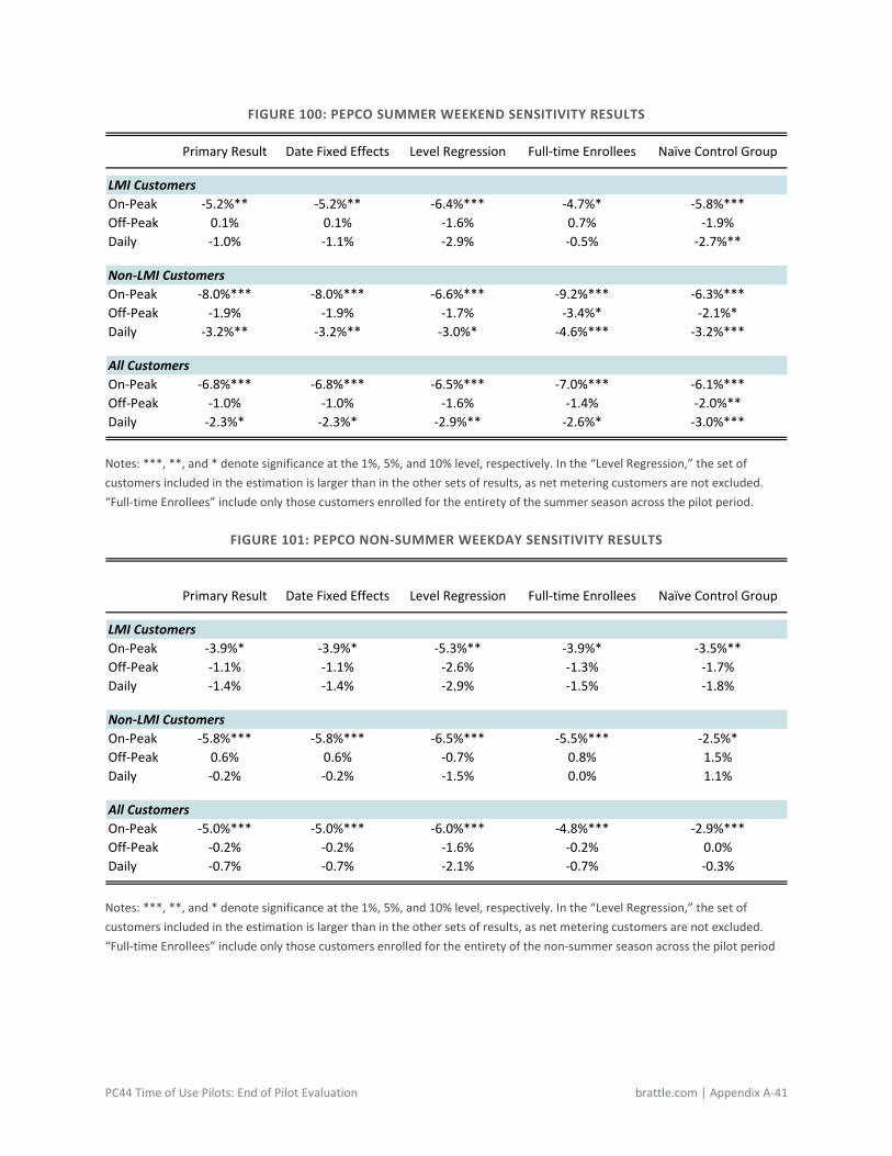
PC44 Time of Use Pilots: End of Pilot Evaluation brattle.com | Appendix A-41
FIGURE 100: PEPCO SUMMER WEEKEND SENSITIVITY RESULTS
Notes: ***, **, and * denote significance at the 1%, 5%, and 10% level, respectively. In the “Level Regression,” the set of customers included in the estimation is larger than in the other sets of results, as net metering customers are not excluded. “Full-time Enrollees” include only those customers enrolled for the entirety of the summer season across the pilot period.
FIGURE 101: PEPCO NON-SUMMER WEEKDAY SENSITIVITY RESULTS
Notes: ***, **, and * denote significance at the 1%, 5%, and 10% level, respectively. In the “Level Regression,” the set of customers included in the estimation is larger than in the other sets of results, as net metering customers are not excluded. “Full-time Enrollees” include only those customers enrolled for the entirety of the non-summer season across the pilot period
Primary Result Date Fixed Effects Level Regression Full-time Enrollees Naïve Control Group
LMI CustomersOn-Peak -5.2%** -5.2%** -6.4%*** -4.7%* -5.8%***Off-Peak 0.1% 0.1% -1.6% 0.7% -1.9%Daily -1.0% -1.1% -2.9% -0.5% -2.7%**
Non-LMI CustomersOn-Peak -8.0%*** -8.0%*** -6.6%*** -9.2%*** -6.3%***Off-Peak -1.9% -1.9% -1.7% -3.4%* -2.1%*Daily -3.2%** -3.2%** -3.0%* -4.6%*** -3.2%***
All CustomersOn-Peak -6.8%*** -6.8%*** -6.5%*** -7.0%*** -6.1%***Off-Peak -1.0% -1.0% -1.6% -1.4% -2.0%**Daily -2.3%* -2.3%* -2.9%** -2.6%* -3.0%***
Primary Result Date Fixed Effects Level Regression Full-time Enrollees Naïve Control Group
LMI CustomersOn-Peak -3.9%* -3.9%* -5.3%** -3.9%* -3.5%**Off-Peak -1.1% -1.1% -2.6% -1.3% -1.7%Daily -1.4% -1.4% -2.9% -1.5% -1.8%
Non-LMI CustomersOn-Peak -5.8%*** -5.8%*** -6.5%*** -5.5%*** -2.5%*Off-Peak 0.6% 0.6% -0.7% 0.8% 1.5%Daily -0.2% -0.2% -1.5% 0.0% 1.1%
All CustomersOn-Peak -5.0%*** -5.0%*** -6.0%*** -4.8%*** -2.9%***Off-Peak -0.2% -0.2% -1.6% -0.2% 0.0%Daily -0.7% -0.7% -2.1% -0.7% -0.3%
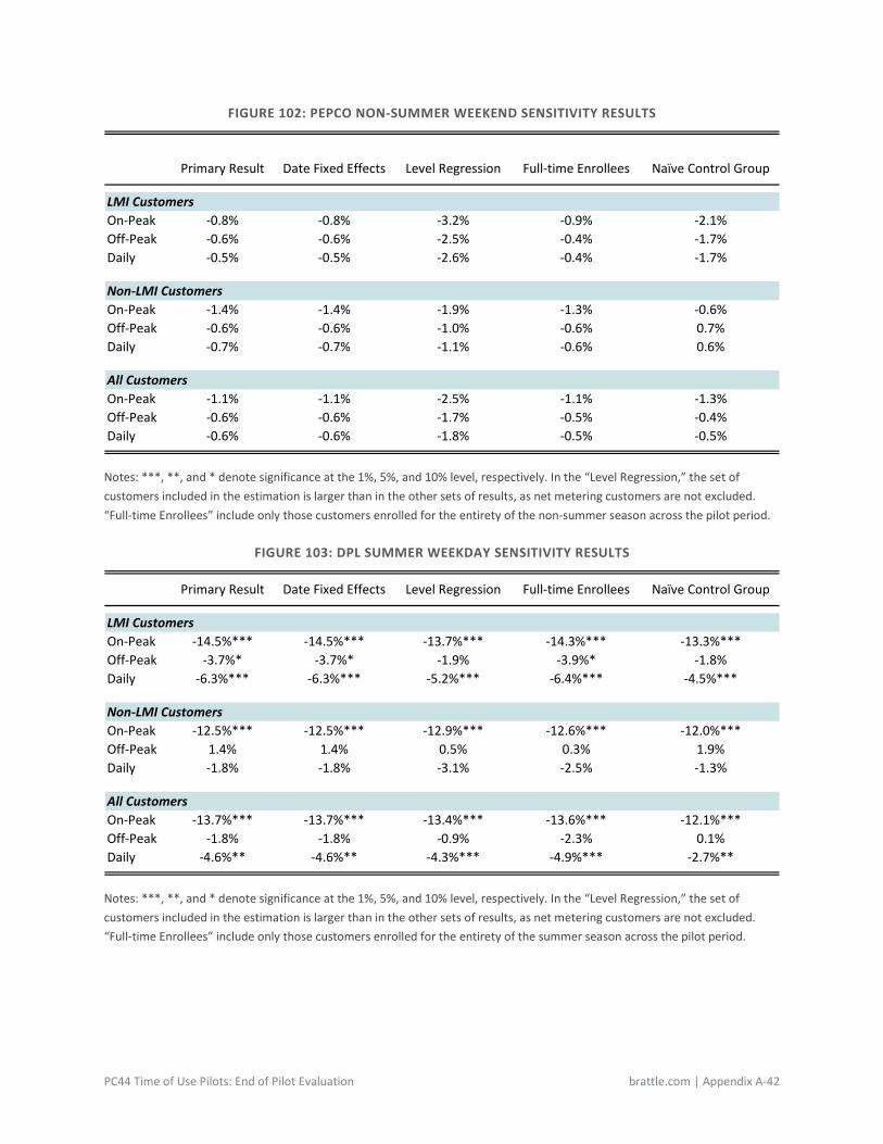
PC44 Time of Use Pilots: End of Pilot Evaluation brattle.com | Appendix A-42
FIGURE 102: PEPCO NON-SUMMER WEEKEND SENSITIVITY RESULTS
Notes: ***, **, and * denote significance at the 1%, 5%, and 10% level, respectively. In the “Level Regression,” the set of customers included in the estimation is larger than in the other sets of results, as net metering customers are not excluded. “Full-time Enrollees” include only those customers enrolled for the entirety of the non-summer season across the pilot period.
FIGURE 103: DPL SUMMER WEEKDAY SENSITIVITY RESULTS
Notes: ***, **, and * denote significance at the 1%, 5%, and 10% level, respectively. In the “Level Regression,” the set of customers included in the estimation is larger than in the other sets of results, as net metering customers are not excluded. “Full-time Enrollees” include only those customers enrolled for the entirety of the summer season across the pilot period.
Primary Result Date Fixed Effects Level Regression Full-time Enrollees Naïve Control Group
LMI CustomersOn-Peak -0.8% -0.8% -3.2% -0.9% -2.1%Off-Peak -0.6% -0.6% -2.5% -0.4% -1.7%Daily -0.5% -0.5% -2.6% -0.4% -1.7%
Non-LMI CustomersOn-Peak -1.4% -1.4% -1.9% -1.3% -0.6%Off-Peak -0.6% -0.6% -1.0% -0.6% 0.7%Daily -0.7% -0.7% -1.1% -0.6% 0.6%
All CustomersOn-Peak -1.1% -1.1% -2.5% -1.1% -1.3%Off-Peak -0.6% -0.6% -1.7% -0.5% -0.4%Daily -0.6% -0.6% -1.8% -0.5% -0.5%
Primary Result Date Fixed Effects Level Regression Full-time Enrollees Naïve Control Group
LMI CustomersOn-Peak -14.5%*** -14.5%*** -13.7%*** -14.3%*** -13.3%***Off-Peak -3.7%* -3.7%* -1.9% -3.9%* -1.8%Daily -6.3%*** -6.3%*** -5.2%*** -6.4%*** -4.5%***
Non-LMI CustomersOn-Peak -12.5%*** -12.5%*** -12.9%*** -12.6%*** -12.0%***Off-Peak 1.4% 1.4% 0.5% 0.3% 1.9%Daily -1.8% -1.8% -3.1% -2.5% -1.3%
All CustomersOn-Peak -13.7%*** -13.7%*** -13.4%*** -13.6%*** -12.1%***Off-Peak -1.8% -1.8% -0.9% -2.3% 0.1%Daily -4.6%** -4.6%** -4.3%*** -4.9%*** -2.7%**
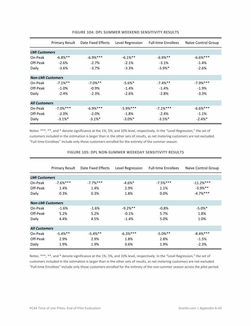
PC44 Time of Use Pilots: End of Pilot Evaluation brattle.com | Appendix A-43
FIGURE 104: DPL SUMMER WEEKEND SENSITIVITY RESULTS
Notes: ***, **, and * denote significance at the 1%, 5%, and 10% level, respectively. In the “Level Regression,” the set of customers included in the estimation is larger than in the other sets of results, as net metering customers are not excluded. “Full-time Enrollees” include only those customers enrolled for the entirety of the summer season.
FIGURE 105: DPL NON-SUMMER WEEKDAY SENSITIVITY RESULTS
Notes: ***, **, and * denote significance at the 1%, 5%, and 10% level, respectively. In the “Level Regression,” the set of customers included in the estimation is larger than in the other sets of results, as net metering customers are not excluded. “Full-time Enrollees” include only those customers enrolled for the entirety of the non-summer season across the pilot period.
Primary Result Date Fixed Effects Level Regression Full-time Enrollees Naïve Control Group
LMI CustomersOn-Peak -6.8%** -6.9%*** -6.1%** -6.9%** -6.6%***Off-Peak -2.6% -2.7% -2.1% -3.1% -1.4%Daily -3.6% -3.7% -3.3% -3.9%* -2.6%
Non-LMI CustomersOn-Peak -7.1%** -7.0%** -5.6%* -7.4%** -7.9%***Off-Peak -1.0% -0.9% -1.4% -1.4% -1.9%Daily -2.4% -2.3% -2.6% -2.8% -3.3%
All CustomersOn-Peak -7.0%*** -6.9%*** -5.9%*** -7.1%*** -6.6%***Off-Peak -2.0% -2.0% -1.8% -2.4% -1.1%Daily -3.1%* -3.1%* -3.0%* -3.5%* -2.4%*
Primary Result Date Fixed Effects Level Regression Full-time Enrollees Naïve Control Group
LMI CustomersOn-Peak -7.6%*** -7.7%*** -4.6%* -7.5%*** -11.2%***Off-Peak 1.4% 1.4% 2.9% 1.1% -3.9%**Daily 0.3% 0.3% 1.8% 0.0% -4.7%***
Non-LMI CustomersOn-Peak -1.6% -1.6% -9.2%** -0.8% -5.0%*Off-Peak 5.2% 5.2% -0.1% 5.7% 1.8%Daily 4.4% 4.5% -1.4% 5.0% 1.0%
All CustomersOn-Peak -5.4%** -5.4%** -6.3%*** -5.0%** -8.4%***Off-Peak 2.9% 2.9% 1.8% 2.8% -1.5%Daily 1.9% 1.9% 0.6% 1.9% -2.3%
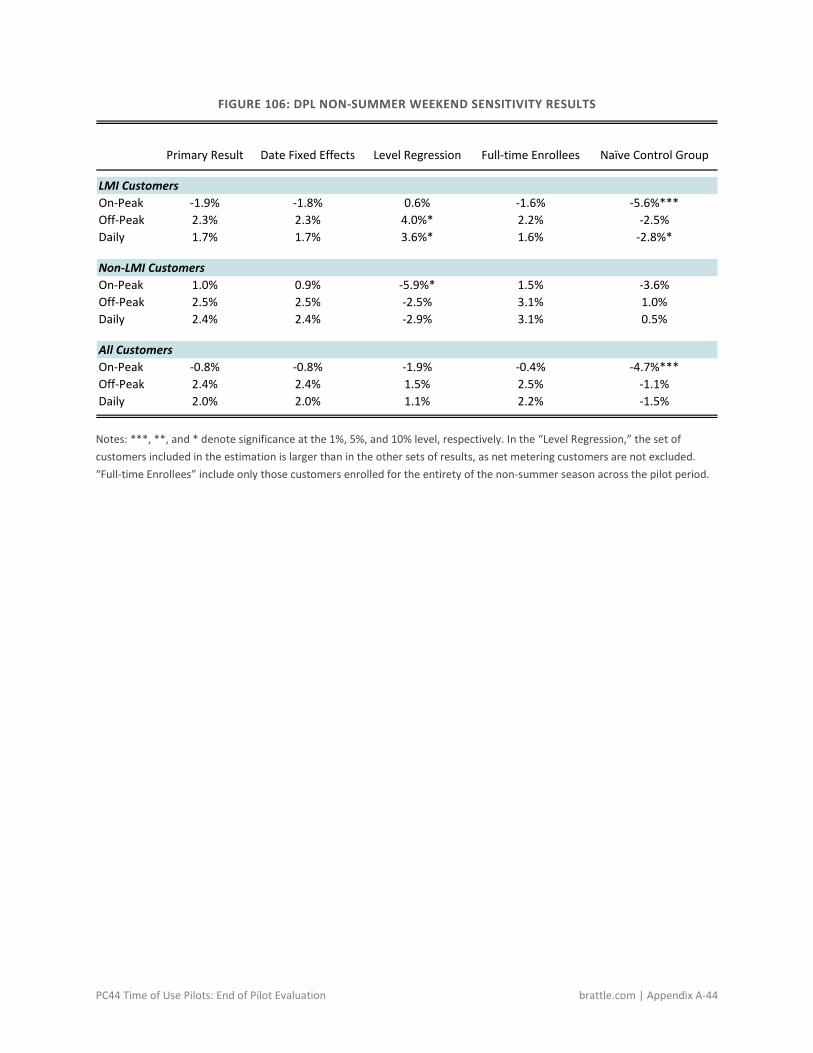
PC44 Time of Use Pilots: End of Pilot Evaluation brattle.com | Appendix A-44
FIGURE 106: DPL NON-SUMMER WEEKEND SENSITIVITY RESULTS
Notes: ***, **, and * denote significance at the 1%, 5%, and 10% level, respectively. In the “Level Regression,” the set of customers included in the estimation is larger than in the other sets of results, as net metering customers are not excluded. “Full-time Enrollees” include only those customers enrolled for the entirety of the non-summer season across the pilot period.
Primary Result Date Fixed Effects Level Regression Full-time Enrollees Naïve Control Group
LMI CustomersOn-Peak -1.9% -1.8% 0.6% -1.6% -5.6%***Off-Peak 2.3% 2.3% 4.0%* 2.2% -2.5%Daily 1.7% 1.7% 3.6%* 1.6% -2.8%*
Non-LMI CustomersOn-Peak 1.0% 0.9% -5.9%* 1.5% -3.6%Off-Peak 2.5% 2.5% -2.5% 3.1% 1.0%Daily 2.4% 2.4% -2.9% 3.1% 0.5%
All CustomersOn-Peak -0.8% -0.8% -1.9% -0.4% -4.7%***Off-Peak 2.4% 2.4% 1.5% 2.5% -1.1%Daily 2.0% 2.0% 1.1% 2.2% -1.5%