Progress in Oceanography 57 (2003) 405–427www.elsevier.com/locate/pocean

Patterns of biomass-size spectra from oligotrophic waters ofthe Northwest Atlantic

Renato A. Quinonesa,b,∗, Trevor Plattc, Jaime Rodrı´guezd

a Centro de Investigacio´n Oceanogra´fica en el Pacı´fico Sur-Oriental (COPAS-FONDAP), Universidad de Concepcio´n, Casilla160-C, Concepcio´n, Chile

b Departamento de Oceanografı´a, Universidad de Concepcio´n, Casilla 160-C, Concepcio´n, Chilec Biological Oceanography Division, Bedford Institute of Oceanography, Box 1006, Dartmouth, Nova Scotia, Canada, B2Y 4A2

d Departamento de Ecologı´a, Facultad de Ciencias, Universidad de Ma´laga, 29071-Ma´laga, Spain

Received 30 July 2002; revised 18 February 2003; accepted 10 May 2003

Abstract

The study of the distribution of biomass by size provides an ataxonomic approach for analyzing the structure of thepelagic ecosystem. However, empirical data regarding planktonic size-structure in offshore areas are scarce. Here, wereport the results of a study of the planktonic biomass size-distribution at several stations located within two regions(Sargasso Sea and New England Seamounts Area) of the Northwest Atlantic. The biomass size-spectra covered a body-size range from bacteria to mesozooplankton and a depth range from the surface to 400 m. It is shown that the slopeof the normalized biomass size-spectrum (NBS-spectrum) varies depending on whether volume or carbon units areused. The transformation from volume to carbon units makes the slope of the NBS-spectrum approximately 0.15 unitsmore negative. The distribution of normalized-biomass by size was linear (plotted on a log–log scale) at all stations.The slopes of the NBS-spectra (volume scale) ranged from�0.96 to �1.01. There were no significant differencesamong the slopes of the NBS-spectra within either of the two areas studied. In addition, no significant differences weredetected between the stations in the Sargasso Sea and those located in the New England Seamounts area. Apart froma tendency towards a decrease in the intercept of the normalized-biomass axis of the size-spectra in deeper waters, theNBS-spectra were also very similar through depth. The slopes of the NBS-spectra in biovolume units are not signifi-cantly different from�1.0 (p � 0.01), and therefore are in agreement with Sheldon’s Linear Biomass Hypothesis. Bycontrast, the slopes of the NBS-spectra in carbon units are significantly different (p � 0.01) from �1.0 (range=–1.09 to –1.17; all stations together= –1.14) and their numerical values are in close agreement with Platt and Denman’smodel and with the findings ofRodrıguez and Mullin, 1986a) for the North Pacific Central Gyre. The results of this studysupport the hypothesis that the planktonic size-structure of offshore oligotrophic systems is a conservative property. 2003 Elsevier Ltd. All rights reserved.

∗ Corresponding author. Centro de Investigacio´n Oceanogra´fica en el Pacı´fico Sur-Oriental (COPAS-FONDAP), Universidad deConcepcio´n, Casilla 160-C, Concepcio´n, Chile. Fax:+56-41-256571.

E-mail address:rquinone@udec.cl (R.A. Quinones).

0079-6611/03/$ - see front matter 2003 Elsevier Ltd. All rights reserved.doi:10.1016/S0079-6611(03)00108-3

406 R.A. Quinones et al. / Progress in Oceanography 57 (2003) 405–427

Contents

1. Introduction . . . . . . . . . . . . . . . . . . . . . . . . . . . . . . . . . . . . . . . . . . . . . . . . . . . . . . . . . 406

2. Materials and methods . . . . . . . . . . . . . . . . . . . . . . . . . . . . . . . . . . . . . . . . . . . . . . . . . . . 4072.1. Image analysis . . . . . . . . . . . . . . . . . . . . . . . . . . . . . . . . . . . . . . . . . . . . . . . . . . . . . . 4082.2. Bacterioplankton biomass . . . . . . . . . . . . . . . . . . . . . . . . . . . . . . . . . . . . . . . . . . . . . . . 4082.3. Nano- and microplankton biomass . . . . . . . . . . . . . . . . . . . . . . . . . . . . . . . . . . . . . . . . . . 4092.4. Mesozooplankton biomass . . . . . . . . . . . . . . . . . . . . . . . . . . . . . . . . . . . . . . . . . . . . . . . 4102.5. Preservation effect . . . . . . . . . . . . . . . . . . . . . . . . . . . . . . . . . . . . . . . . . . . . . . . . . . . 4102.6. Biomass size-spectra construction and statistical considerations . . . . . . . . . . . . . . . . . . . . . . . . 411

3. Results . . . . . . . . . . . . . . . . . . . . . . . . . . . . . . . . . . . . . . . . . . . . . . . . . . . . . . . . . . . . 412

4. Discussion . . . . . . . . . . . . . . . . . . . . . . . . . . . . . . . . . . . . . . . . . . . . . . . . . . . . . . . . . . 4124.1. Methodological considerations . . . . . . . . . . . . . . . . . . . . . . . . . . . . . . . . . . . . . . . . . . . . 4144.2. Volume and carbon size-spectra: the importance of units . . . . . . . . . . . . . . . . . . . . . . . . . . . . 4174.3. Linearity of biomass spectra in oligotrophic closed to steady-state systems . . . . . . . . . . . . . . . . . 4224.4. A global comparison between North Atlantic and North Pacific size-spectra . . . . . . . . . . . . . . . . 424

1. Introduction

The analysis of the distribution of biomass by size is an ataxonomic approach to study the structure andfunction of the pelagic ecosystem (Platt, 1985; Quinones, 1994; Rodrıguez, 1994). In this formulation,every individual in the system is assigned to one of a series of size-classes. The high degree of aggregationof such an approach reduces the complexity of the system to a manageable level.

Although this approach can be traced back to the pioneer work of Elton (1927), the first theoreticalmodels about the size structure of the pelagic ecosystem were proposed by Kerr (1974); Sheldon, Sutcliffeand Paranajape (1977) and Platt and Denman (1977, 1978). Whereas the two first models were based onthe trophic-level concept, the last stands on the consideration of a continuous flow of energy from smallto large organisms. Kerr and Sheldon’s models propose that biomass is constant when organisms areorganized in logarithmic size classes. On the other side, Platt and Denman’s model predicts a slight decreaseof biomass with organism size, and proposes an allometric structure for the pelagic ecosystem (Platt &Denman, 1977, 1978).

However, the direct empirical test of these global models remains elusive due to the tremendous scale(space and time) differences existing among the components of the pelagic ecosystem (from virus towhales). The testing of the global models requires, at least, to fulfill the following two criteria: first, toselect a representative part of the pelagic ecosystem, and, second, to select an ecosystem that approachesthe steady-state conditions usually assumed in the theoretical global models. In relation to the first critierion,the planktonic community is adequate due to the large size range covered by planktonic organisms (typicallyfrom less than 1 µm to several mm) (Platt, Lewis, & Geider, 1984) and the functional diversity andecological integrity of the community, which includes all kinds of trophic modes and ecological processes(Kerr & Dickie, 2001; Rinaldo, Maritan, Cavender-Bares, & Chisholm, 2002). Furthermore, although noreal ecosystem is in a perfect steady-state, the open oligotrophic waters of the ocean are probably one ofthe few marine systems allowing such an assumption.

According to the indicated requirements, the most complete empirical test of the global theoretical modelsis that of Rodrıguez and Mullin (1986a). Their study was carried out in the oligotrophic waters of theNorth Pacific Central Gyre and covered a size range from picoflagellates to large macrozooplantonic

407R.A. Quinones et al. / Progress in Oceanography 57 (2003) 405–427

euphasiids. Their results were in agreement with the predictions of Platt and Denman’s model, sincebiomass (as the log of carbon content) decreases allometrically with the log of body size (carbon units)in this ecosystem. Working with the phytoplanktonic fraction of the same data set, Platt, Lewis and Geider(1984) had previously found that the Platt and Denman’s model fit the observed size-biomass distributionvery well. This result was confirmed by the analysis of Rodrıguez and Mullin (1986a), which demonstratedthe tight coupling and continuity between the autotrophic (phytoplankton) and heterotrophic (zooplankton)components included in the analysis of the planktonic community.

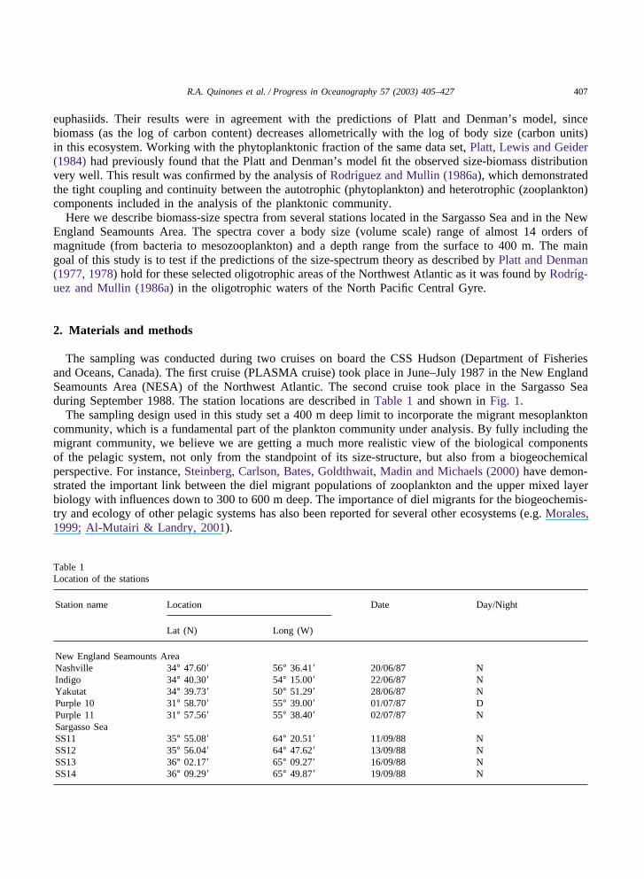
Here we describe biomass-size spectra from several stations located in the Sargasso Sea and in the NewEngland Seamounts Area. The spectra cover a body size (volume scale) range of almost 14 orders ofmagnitude (from bacteria to mesozooplankton) and a depth range from the surface to 400 m. The maingoal of this study is to test if the predictions of the size-spectrum theory as described by Platt and Denman(1977, 1978) hold for these selected oligotrophic areas of the Northwest Atlantic as it was found by Rodrıg-uez and Mullin (1986a) in the oligotrophic waters of the North Pacific Central Gyre.

2. Materials and methods

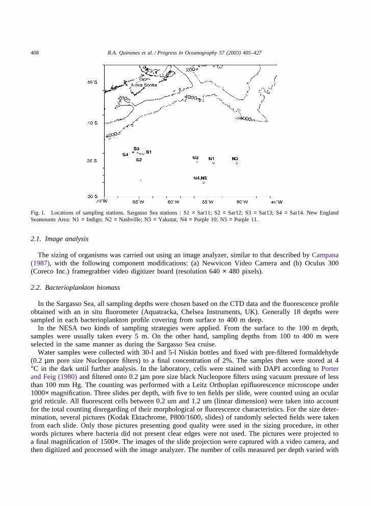
The sampling was conducted during two cruises on board the CSS Hudson (Department of Fisheriesand Oceans, Canada). The first cruise (PLASMA cruise) took place in June–July 1987 in the New EnglandSeamounts Area (NESA) of the Northwest Atlantic. The second cruise took place in the Sargasso Seaduring September 1988. The station locations are described in Table 1 and shown in Fig. 1.

The sampling design used in this study set a 400 m deep limit to incorporate the migrant mesoplanktoncommunity, which is a fundamental part of the plankton community under analysis. By fully including themigrant community, we believe we are getting a much more realistic view of the biological componentsof the pelagic system, not only from the standpoint of its size-structure, but also from a biogeochemicalperspective. For instance, Steinberg, Carlson, Bates, Goldthwait, Madin and Michaels (2000) have demon-strated the important link between the diel migrant populations of zooplankton and the upper mixed layerbiology with influences down to 300 to 600 m deep. The importance of diel migrants for the biogeochemis-try and ecology of other pelagic systems has also been reported for several other ecosystems (e.g. Morales,1999; Al-Mutairi & Landry, 2001).

Table 1Location of the stations

Station name Location Date Day/Night

Lat (N) Long (W)

New England Seamounts AreaNashville 34° 47.60� 56° 36.41� 20/06/87 NIndigo 34° 40.30� 54° 15.00� 22/06/87 NYakutat 34° 39.73� 50° 51.29� 28/06/87 NPurple 10 31° 58.70� 55° 39.00� 01/07/87 DPurple 11 31° 57.56� 55° 38.40� 02/07/87 NSargasso SeaSS11 35° 55.08� 64° 20.51� 11/09/88 NSS12 35° 56.04� 64° 47.62� 13/09/88 NSS13 36° 02.17� 65° 09.27� 16/09/88 NSS14 36° 09.29� 65° 49.87� 19/09/88 N

408 R.A. Quinones et al. / Progress in Oceanography 57 (2003) 405–427

Fig. 1. Locations of sampling stations. Sargasso Sea stations : S1 = Sar11; S2 = Sar12; S3 = Sar13; S4 = Sar14. New EnglandSeamounts Area: N1 = Indigo; N2 = Nashville; N3 = Yakutat; N4 = Purple 10; N5 = Purple 11.

2.1. Image analysis

The sizing of organisms was carried out using an image analyzer, similar to that described by Campana(1987), with the following component modifications: (a) Newvicon Video Camera and (b) Oculus 300(Coreco Inc.) framegrabber video digitizer board (resolution 640 × 480 pixels).

2.2. Bacterioplankton biomass

In the Sargasso Sea, all sampling depths were chosen based on the CTD data and the fluorescence profileobtained with an in situ fluorometer (Aquatracka, Chelsea Instruments, UK). Generally 18 depths weresampled in each bacterioplankton profile covering from surface to 400 m deep.

In the NESA two kinds of sampling strategies were applied. From the surface to the 100 m depth,samples were usually taken every 5 m. On the other hand, sampling depths from 100 to 400 m wereselected in the same manner as during the Sargasso Sea cruise.

Water samples were collected with 30-l and 5-l Niskin bottles and fixed with pre-filtered formaldehyde(0.2 µm pore size Nucleopore filters) to a final concentration of 2%. The samples then were stored at 4°C in the dark until further analysis. In the laboratory, cells were stained with DAPI according to Porterand Feig (1980) and filtered onto 0.2 µm pore size black Nucleopore filters using vacuum pressure of lessthan 100 mm Hg. The counting was performed with a Leitz Orthoplan epifluorescence microscope under1000× magnification. Three slides per depth, with five to ten fields per slide, were counted using an oculargrid reticule. All fluorescent cells between 0.2 um and 1.2 um (linear dimension) were taken into accountfor the total counting disregarding of their morphological or fluorescence characteristics. For the size deter-mination, several pictures (Kodak Ektachrome, P800/1600, slides) of randomly selected fields were takenfrom each slide. Only those pictures presenting good quality were used in the sizing procedure, in otherwords pictures where bacteria did not present clear edges were not used. The pictures were projected toa final magnification of 1500×. The images of the slide projection were captured with a video camera, andthen digitized and processed with the image analyzer. The number of cells measured per depth varied with

409R.A. Quinones et al. / Progress in Oceanography 57 (2003) 405–427

the availability of high quality pictures ranging from 15 to 200, but generally around 60 bacteria weremeasured at each depth. Cell volume was calculated using the following formula:

V � (p /4)W2(L�W /3) (1)

where L is the length of major axis, and W is the length of minor axis.To convert the bacterial biovolume to biomass, a conversion factor of 0.380 g C cm�3 (Lee & Fuhrman,

1987) was used.

2.3. Nano- and microplankton biomass

At each station, water from surface to 400 m was taken with 30 l Niskin bottles. The depths to besampled were chosen according to the heterogeneity of the fluorescence and density (st) profiles obtainedusually less than 1 h before sampling. Generally 18 different depths were sampled at each station.

From the water obtained, an aliquot (500 ml) was taken to quantify microplankton sufficiently small topass a 35 µm mesh netting. In addition, 20 l were passed through a 35 µm mesh using reverse filtrationto concentrate the microplankters larger than 35 µm. The samples were fixed with formaldehyde-seawatersolution to a final concentration of 2% and buffered with sodium borate.

To diminish the time spent in sample analysis, aggregate samples were made. The water column wasdivided in the following four strata: Mixed layer, Thermocline, Stratum I, and Stratum II. The division ofthe water column was based on the CTD data. Below the thermocline the water column was divided inhalf, into Strata I and II. Table 2 shows the depths of each of the strata at every station. The aggregatesamples were made by mixing the original samples in proportion to the segment of the water columnthey represented.

An aliquot of 100 or 50 ml of each aggregate sample (concentrated and non-concentrated) was sedi-mented using the Uthermol technique (Lund, Kipling, & LeCren, 1958) for 48–72 h. To improve the imageand to facilitate the separation between living and non-living matter, the samples in the settling chamberswere stained with bengal rose. Subsequently, the organisms were observed under 125×, 200×, 500×, and1250× magnifications. The counting and sizing of organisms was carried out using image analysis. Anocular micrometer and a Newporton Graticule (May, 1965) were also used for direct sizing and counting.The subsampling in the slides was conducted through transects whose starting position was selected ran-

Table 2Vertical strata used in the division of the water column for the bacterio- to microplankton spectra

Station name Depth range (m)

Mixed layer Thermocline Stratum I Stratum II

New England Seamounts AreaNashville 0–26 26–67 67–233.5 233.5–400Indigo 0–26 26–75 75–237.5 237.5–400Yakutat 0–23 23–90 90–245.0 245.0–400Purple 10 0–15 15–106 106–253.0 253.0–400Purple 11 0–17 17–90 90–245.0 245.0–400Sargasso SeaSS11 0–48 48–150 150–275.0 275.0–400SS12 0–48 48–103 103–251.5 251.5–400SS13 0–45 45–114 114–257.0 257.0–400SS14 0–56 56–175 175–287.5 287.5–400

410 R.A. Quinones et al. / Progress in Oceanography 57 (2003) 405–427

domly. Approximately 200 organisms were sized at each magnification. The volume of the organisms wasestimated assuming basic geometrical shapes following the recommendations of the Baltic Marine Environ-ment Protection Commission (1983). Biovolumes were converted to carbon using the equation ofStrathmann (1967)

logC � �0.460 � 0.866logV (2)

where C is cell carbon (pg) and V is cell volume (µm3).

2.4. Mesozooplankton biomass

During the cruise to the NESA, collections were made with 55 cm or 73 cm diameter ring nets (meshsize 75 µm; vertical tows), and 62 cm diameter bongo nets (mesh size 253 µm and 505 µm; oblique tows).In the Sargasso Sea, the vertical collections were carried out with 72 cm diameter ring nets (mesh size 75µm; vertical tows) and with Bongo nets specially designed (Bedford Institute of Oceanography) for verticaltowing (61 cm diameter, mesh size 253 µm). Oblique tows were carried out with regular Bongo nets (61cm diameter, mesh size 253 µm). All nets were equipped with flowmeters. In both cruises the tows alwayscovered from 400 m deep to the surface.

In the NESA, the catch from each side of the bongo was generally split with a plankton splitter. Themesozooplankton was size fractionated using sieves of 8000, 4000, 2000, 1000, 505, 253, and 153 µm mesh.In the Sargasso Sea, the catch from one of bongo sides was fixed with formaldehyde (final concentration 4%formaldehyde-seawater solution) and the catch from the other side of the Bongo was used to estimatemesozooplankton biomass. The mesozooplankton was size fractionated using sieves of 8000, 4000, 2000,1000, 500, 250, 125, and 74 µm mesh.

Mesozooplankton size fractions were then filtered onto pre-weighed, pre-combusted (450 °C) glass fiberfilters (Reeve Angel 934 AH). The zooplankters were quickly rinsed with distilled water. The filters werethen dried for 36 h in an oven at 60 °C and kept in desiccators until further analysis. The size-fractionswere weighed, on the land, in an electronic balance. The carbon content of the mesozooplankton size-fractions was determined using a Perkin Elmer 240-B CHN Elemental Analyzer.

To convert mesozooplankton biomass to biovolume, the following equation from Wiebe (1988) was used:

logF � �1.842 � 0.865logD (3)

where F is displacement volume (cc m�3), and D is dry weight (mg m�3).To change the scale from length to weight as carbon, the following regression was used (Rodriguez &

Mullin, 1986a):

logT � 2.23logG�5.58 (r2 � 0.98) (4)

where T is organism size (µg C) and G is the geometric mean (µm) of the mesh size retaining the organismand the next largest mesh size.

2.5. Preservation effect

It is known that fixatives can cause shrinkage, swelling or even loss of certain species (e.g. Hewes,Reid, & Holm-Hansen, 1984; Hobro & Willen, 1977; Sukhanova & Ratkova, 1977; Hallfors, Melvasalo,Niemi, & Viljamaa, 1979; Menden-Deuer, Lessard, & Satterberg, 2001). However, since the informationpublished on the subject is very controversial and there is no correction factor suitable for the wide rangeof organisms covered in this study, we did not attempt to make any corrections due to the effect of fixation.Therefore, our estimates of bacterio-, nano-, and microplankton biomass might be underestimated.

411R.A. Quinones et al. / Progress in Oceanography 57 (2003) 405–427

2.6. Biomass size-spectra construction and statistical considerations

Once the biomass and sizing estimates were finished, the data were organized in size-spectra composedof a maximum of 25 size classes (bacterioplankton = 4 size classes; nano- and microplankton = 14 sizeclasses; mesozooplankton = 7 size classes). Size spectra were constructed both in biovolume and carbonunits.

From a vertical standpoint, we presented the data in two manners. First, we constructed size-spectrafrom bacterioplankton to microplankton dividing the water column, as explained above, in four strata:mixed layer, thermocline, Stratum I and Stratum II. The bacterioplankton biomass per depth was integratedto cover each of the four strata. Secondly, we constructed size–spectra from bacterioplankton to meso-zooplankton and covering a depth from surface to 400 m. In this case, the biomass of each size-classcorresponding to the bacterioplankton to microplankton size range was averaged using a weighted meanaccording to the segment of the water column covered by each strata. Since the mesozooplankton sampling(i.e. vertical and oblique tows) covered from 400 m deep to the surface, the seven mesozooplankton sizeclasses were incorporated into the integrated size spectrum directly.

To analyze the size-distribution of biomass, the spectra were normalized and plotted on a log–log scaleas described by Platt and Denman (1977, 1978). This normalization is required since the width of the sizeclasses varies through the size-spectra. In brief, the procedure consists of taking the variable of interestm(s) in the size class characterized by the weight or volume (s) and dividing it by the width of the sizeclass, �s. Thus the normalized version of the variable m is equal to :

M(s) � m(s) /�s (5)

A detailed analysis about constructing normalized and unnormalized size spectra can be found in Blanco,Echeverrıa and Garcıa (1994).

Vidondo, Prairie, Blanco and Duarte (1997) have argued in favor of using the Pareto type II distributionfor representing and modeling size-spectra. In order to adequately apply such an approach each particleshould contribute one point to the Pareto plot and, therefore, all the information contained in the obser-vations is used. The Pareto approximation is ideal for automatic sizing instruments such as flow cytometersand electronic or laser particle counters. In our case, the nature of the information collected at the meso-plankton size range did not allow us to use this approach because the mesoplankton biomass was sizefractionated and weighted as a “bulk” property per size-class and each organism was not sorted out andsized or weighted individually. Moreover, some size-classes of the nanoplankton size-range cannot beincorporated into the Pareto model because when using the Newporton Graticule (May, 1965) the observerdirectly classifies the organisms analyzed under the microscope into previously defined size classes.Although in theory it is possible to estimate the parameters of the underlying Pareto distribution from theNBS-spectra, this procedure is not recomended from a statistical standpoint (Vidondo et al., 1997).

In consequence, since our experimental methods were defined under the formalism of the NormalizedBiomass Size Spectrum approach of Platt and Denman (1977, 1978), the “normalized biomass” function(b) will be used to describe the size distribution of planktonic biomass.

Regression analysis was carried out using least-squares (Model I) regression. For biomass size-distri-bution data, where the independent variable (i.e. body size) is not under the control of the investigator andis subjected to error, Model II (i.e. both variables show random variation) would be more appropriate(Laws & Archie, 1981). However, we have decided to use Model I because it permitted us to test differencesbetween regression lines and also made the comparison with other published spectra easier. Furthermore,if the correlation coefficient is high (r � 0.95), as in most of the cases in this study, it will make verylittle difference which regression model is used (Laws & Archie, 1981; Prothero, 1986). Prior to the com-parison of regression lines, the necessary assumption of homogeneity of variance was tested using Bartlett’stest. After passing the Bartlett’s test, an F test for multiple comparisons among slopes and elevations, as

412 R.A. Quinones et al. / Progress in Oceanography 57 (2003) 405–427

described by Zar (1984), was used in comparing linear regression equations. In addition, a t-test was usedto test if the slopes of the normalized biomass size-spectra were significantly different from �1 (Sokal &Rohlf, 1981).

3. Results

Although the samples are from two different seasons and regions, the normalized biomass size-spectra(NBS-spectra) from all the stations studied are very similar (see Figs. 2 and 3). A linear NBS-spectrumseems to be appropriate to describe the distribution of biomass by size at all stations. A certain degree ofdeviation from linearity, mainly associated with interfaces between the different methodologies used, canbe observed in the spectra.

Table 3 shows the regression parameters for the whole size-spectrum studied, viz. from bacteria tomesozooplankton, and covering a depth range from surface to 400 m. The slopes of the NBS-spectra amongthe stations in the NESA, as well as among those in the Sargasso Sea, are not significantly different (p� 0.4). Moreover, there are no significant differences in the slope of the NBS-spectra between the stationslocated in the Sargasso Sea and those located in the NESA (p � 0.4).

The bacterio- to microplankton NBS-spectra are also remarkably similar through depth (Figs. 4 and 5).Tables 4 and 5 show the regression parameters of the NBS-spectra from each of the vertical strata studied.It has been suggested that, when comparing ecosystems, the intercept of the normalized-biomass axis isan indicator of the total biomass in the system provided that the slopes are similar (Sprules & Munawar,1986; Gasol, Guerrero, & Pedros-Alio, 1991). In fact we observed that there is a tendency towards adecrease in the intercept of the normalized-biomass axis of the spectra in deep waters. This is a consequenceof the fact that more biomass is present in the mixed layer and thermocline strata than in the deep strata.The slopes of the NBS-spectra do not vary greatly with depth and there is a slight tendency to have morenegative slopes with increasing depth. This similarity in the shape of the size-spectra through depth hasbeen observed in offshore zones of tropical oceans (Sheldon, Prakash, & Sutcliffe, 1972; Tseytlin, 1981).

Depending on the size range of organisms, we have measured biomass as biovolume (bacterio-, nano-,and microplankton), dry weight (micro- and mesozooplankton) and carbon content (micro- andmesozooplankton). Since the carbon content of many organisms is size dependent (e.g. phytoplankton),the slope of the biomass spectrum would vary depending on whether volume or carbon units are used.Table 6 and Figs. 6 and 7 show the biomass NBS-spectra constructed in this study expressed in carbonunits. It can be seen that the slopes of the NBS-spectra are more negative by approximately 0.15 whendescribed in carbon units than when described in volume units (compare Table 3 with Table 6). Thisvariation of the slope has been noted in a microbial size-spectrum from the North Sea (Geider, 1988). Theslopes of the NBS-spectra in biovolume units are not significantly different from �1.0 (t-test, p � 0.01),and therefore in agreement with the Linear Biomass Hypothesis (Sheldon, Prakash & Sutcliffe, 1972). Bycontrast, the slopes of the NBS-spectra in carbon units are significantly different from �1.0 (t-test, p �0.01). The slopes of the NBS-spectra, in carbon units, from this study (Table 6) are in close agreementwith Platt and Denman’s model and with the findings of Platt, Lewis and Geider (1984) and Rodriguez &Mullin, 1986a) for the North Pacific Central Gyre.

4. Discussion

Our results show that there is a log2-log2 linear relation between Normalized Biomass and body size ofplanktonic organisms, from bacteria to mesozooplankton, in the oligotrophic waters studied from the North

413R.A. Quinones et al. / Progress in Oceanography 57 (2003) 405–427

Fig. 2. Normalized biomass size-spectra in volume units from the stations in the New England Seamounts Area. The size range ofthe spectra covered from bacteria to mesozooplankton. Minimum body size considered: 4.200 × 10�3 um (log2 scale = �7.8954um3). Maximum body considered 2.681 × 1011 um3 (log2 scale = 37.9638 um3). Nominal size of the smallest size class = 2.595 ×10�3 um3 (log2 scale = �5.2681 um3). Nominal size of the largest size class = 1.508 × 1011 um3 (log2 scale = 37.1338 um3). Depthrange: 0–400 m.

414 R.A. Quinones et al. / Progress in Oceanography 57 (2003) 405–427

Fig. 3. Normalized biomass size-spectra in volume units from the stations in the Sargasso Sea. The size range of the spectra coveredfrom bacteria to mesozooplankton. Minimum body size considered: 4.200 × 10�3 (log2 scale = �7.8954 um3). Maximum body sizeconsidered 2.681 × 1011 um3 (log2 scale = 37.9638 um3). Nominal size of the smallest size class = 2.595 × 10�3 um3 (log2 scale =�5.2681 um3). Nominal size of the largest size class = 1.508 × 1011 um3 (log2 scale = 37.1338 um3). Depth range: 0–400 m. Notethat station Sar 11 only covers from 4.2 × 10�3 to 5.0 × 105 um3 (i.e. log2 scale = �7.8954–18.9309 um3).

Atlantic. This confirms the general form of the empirical model found by Rodrıguez and Mullin (1986a)for the planktonic community of the North Pacific Central Gyre.

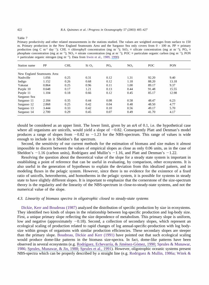
It is important to remark that during the sampling period, the level of primary productivity, chlorophyll,and nutrients observed in the oceanographic stations (Table 7) are within the range of oligotrophic valuesexpected for the Sargasso Sea, as well as for the oceanic Northwest Atlantic (e.g. Menzel & Ryther, 1960;Glover, Smith, & Shapiro, 1985; Bidigare, Marra, Dickey, Iturriaga, Baker, Smith et al., 1990; Prezelin &Glover, 1991). Even though there are some differences among stations, and also between the Sargasso Seaand the NESA, in general they can be considered as typical representatives of offshore oligotrophic areas.

4.1. Methodological considerations

The most conspicuous deviation from a linear NBS-spectrum found in our research occurs at the bound-ary between bacterioplankton and nanoplankton, that is to say between the techniques used in epifluoresc-ence and inverted microscopy. It seems that the Uthermol technique does not work well with very small

415R.A. Quinones et al. / Progress in Oceanography 57 (2003) 405–427

Table 3Regression parameters for the normalized biomass size-spectra in volume units from the New England Seamounts Area and theSargasso Sea (Model: log2 Y = log2 a + b log2 X). Size range: 4.2 x 10-3 - 2.7 x 1011 µm3 (from bacteria to mesozooplankton).Depth range covered 400 m. Unnormalized biovolume expressed in µm3 m-3. All regressions are significant at p�0.01

Station name Slope log2 a r2 N Std. Err. Std. Err.X coeff. Y est.

New England SeamountsAreaNashville �0.981 31.608 0.992 25 0.018 1.077Indigo �0.998 31.664 0.988 25 0.022 1.303Yakutat �0.997 31.808 0.992 25 0.017 1.033Purple 10 �1.010 31.917 0.992 25 0.018 1.084Purple 11 �0.991 31.937 0.993 25 0.018 1.052Combined NESA �0.996 31.787 0.991 125 0.008 1.090Sargasso SeaSargasso 11a �0.976 31.443 0.965 17 0.048 1.393Sargasso 12 �0.983 31.754 0.987 24 0.023 1.374Sargasso 13 �0.995 31.747 0.990 25 0.020 1.183Sargasso 14 �0.961 31.314 0.993 23 0.017 0.991Combined Sarg. Sea �0.979 31.563 0.989 89 0.011 1.205All Stations this study �0.989 31.690 0.990 214 0.007 1.137

a Note: only covers a size range from 4.2 × 10�3 to 4.99 × 105 µm3.

cells due to problems in achieving complete sedimentation of cells (e.g. Reid, 1983; Hewes, Reid & Holm-Hansen, 1984), and also to the difficulty in distinguishing between plankters and detrital particles (Paerl,1978). In addition, an unknown proportion of small fragile cells is completely destroyed by fixation pro-cedures (e.g. Hobro & Willen, 1977; Hewes, Reid & Holm-Hansen, 1984). Therefore, it is very likely thatthe biomass of the three smallest size classes of the nanoplankton size range (i.e. lower limit of the sizeclasses: 0.98, 2.76, 7.81 µm3 respectively) is underestimated throughout this study. It is also likely thatour smallest size class in the bacterioplankton size range (i.e. 0.0042–0.048 µm3) is underestimated dueto the resolution of light microscopy and/or the efficiency of the filters used. Organisms close to 0.2 µm,which are likely to be overlooked in this study, can be very numerous. Indeed, it is known that in oligo-trophic waters the concentration of viruses (size range between 0.002–0.2 µm) can be of the order of 2× 106 virus ml�1 (e.g. Suttle, Chan, & Cottrell, 1990; Hara, Koike, Terauchi, Kamiya, & Tanoue, 1996).Therefore, the linearity of the NBS-spectra below 0.4 µm continues to be an open question.

Unfortunately, at this point it is impossible to make a quantitative estimate of the degree of biomassunderestimation at the smallest end of the spectrum. A large underestimation would imply that the “ real”normalized biomass spectra would have a more negative slope than those reported. In contrast, anotherpossible source of error might be an underestimation of the gelatinous component of the spectra, due toboth sampling methodology (e.g. Vinogradov, 1997) and the fact that the zooplankton biomass was directlymeasured as dry weight and carbon content and not as biovolume. If the gelatinous plankton were underesti-mated, then some of the larger size classes would be underestimated, implying that the “ real” normalizedsize spectra would have a more positive slope than those reported. In both cases, however, the effect ofthe underestimated biomass of few size classes on the numerical value of the slope of the NBS spectrawould be buffered to a certain degree by the rest of the biomass spectra.

It is evident that one of the most complex issues when constructing size spectra that simultaneouslycover a size range as wide as the one presented in this study is the operational impossibility to conduct

416 R.A. Quinones et al. / Progress in Oceanography 57 (2003) 405–427

Fig. 4. Normalized biomass size-spectra in volume units for each of the depth strata at each station in the New England SeamountsArea. The size range of the spectra covered from bacteria to microplankton. Size range: 4.2 × 10�3 to 5.0 × 105 µm3. Depth range:0–400 m. Symbols: � Mixed layer; + Thermocline; � Stratum I; � Stratum II. Regression lines: — Mixed layer; – – Thermo-cline; - - - - Stratum I; – - – Stratum II.

417R.A. Quinones et al. / Progress in Oceanography 57 (2003) 405–427

Fig. 5. Normalized biomass size-spectra in volume units for each of the depth strata at each station in the Sargasso Sea. The sizerange of the spectra covered from bacteria to microplankton. Size range: 4.2 × 10�3 to 5.0 × 105 µm3. Depth range: 0–400 m.Symbols: � Mixed layer; + Thermocline; � Stratum I; � Stratum II. Regression lines: — Mixed layer; – – Thermocline; - - - -Stratum I; – - – Stratum II.

perfect sampling and to use the optimum preservation method as well as ideal carbon/volume conversionfactors for each of the size classes throughout the whole size-spectrum.

On the other hand, important advances have been achieved in quantifying the size spectra from bacteria tophytoplankton by the use of flowcitometry (e.g. Gin, Chisholm, & Olson, 1999; Cavender-Bares, Rinaldo, &Chislom, 2001), although this technique is not free of shortcomings such as the conversion of light scatterto size for individuals cells (Gin, Chisholm & Olson, 1999).

An alternative explanation to account for the appearance of deviations from linearity of the NBS-spectra,and for changes in the spectral slope within the spectra, is the occurrence of abrupt changes in the scalingcoefficient a of the allometric relationship between specific respiration and size (Platt, 1985). It is knownthat unicellular, heterothermic and homothermic organisms have characteristic values of a (Fenchel, 1974).Therefore, if different parts of the biomass size-spectrum were composed of mostly one type of organisms(e.g. unicellulars) abrupt changes would occur at the boundary where a new value of a takes over(Platt, 1985).

4.2. Volume and carbon size-spectra: the importance of units

The fact that the way in which biomass is expressed can alter the slope of the biomass size-spectra hasimportant implications for the question about the numerical value of the theoretical slope for a steady-state system.

418 R.A. Quinones et al. / Progress in Oceanography 57 (2003) 405–427

Table 4Regression parameters for the microplankton NBS-spectra in volume units from the New England Seamounts Area (Model: log2 Y= log2 A + b log2 X). Size range : 4.2 × 103�4.99 × 105 µm3. ML = Mixed Layer; TC = Thermocline; S-I=Stratum I; S-II =Stratum II. Unnormalized biovolume expressed in µm3 m�3. All regressions are significant at p � 0.01

Station Stratum Slope Intercept r2 N Std. Err. Std. Err.Slope Y est.

Nashville ML �1.042 32.716 0.970 17 0.047 1.379Nashville TC �0.987 32.637 0.970 17 0.045 1.307Nashville S-I �1.071 31.679 0.975 17 0.044 1.290Nashville S-II �1.086 31.282 0.965 17 0.053 1.543Indigo ML �1.051 32.425 0.959 17 0.056 1.631Indigo TC �1.011 32.316 0.947 17 0.061 1.797Indigo S-I �1.084 31.839 0.975 17 0.044 1.301Indigo S-II �1.101 31.713 0.960 17 0.057 1.688Yakutat ML �1.059 32.210 0.960 17 0.055 1.630Yakutat TC �1.011 32.701 0.965 17 0.049 1.442Yakutat S-I �1.050 31.779 0.981 17 0.037 1.102Yakutat S-II �1.137 31.950 0.980 17 0.042 1.225Purple 10 ML �1.074 32.735 0.971 17 0.048 1.398Purple 10 TC �1.024 32.434 0.966 17 0.049 1.435Purple 10 S-I �1.044 32.042 0.974 17 0.043 1.274Purple 10 S-II �1.087 31.709 0.964 17 0.054 1.593Purple 11 ML �0.974 32.481 0.965 17 0.048 1.407Purple 11 TC �0.972 32.561 0.967 17 0.046 1.352Purple 11 S-I �1.030 31.455 0.958 17 0.055 1.624Purple 11 S-II �1.072 31.820 0.978 17 0.042 1.222

Table 5Regression parameters for the microplankton NBS-spectra in volume units from the Sargasso Sea (Model: log2 Y = log2 A + blog2 X). Size range: 4.20 × 10�3�4.99 × 105 µm3. ML = Mixed Layer; TC = Thermocline; S-I=Stratum I; S-II = Stratum II.Unnormalized biovolume expressed in µm3 m�3. All regressions are significant at p � 0.01

Station Stratum Slope Intercept r2 N Std. err. X Std. err. Y Est.coeff.

SS11 ML �0.959 31.911 0.971 17 0.043 1.249SS11 TC �1.059 31.569 0.954 17 0.060 1.754SS11 S-I �1.014 30.994 0.957 17 0.057 1.628SS11 S-II �0.946 31.086 0.953 17 0.054 1.575SS12 ML �0.954 32.109 0.952 17 0.055 1.613SS12 TC �0.971 31.901 0.948 17 0.059 1.712SS12 S-I �1.004 31.563 0.932 17 0.070 2.042SS12 S-II �1.038 31.551 0.946 17 0.064 1.875SS13 ML �1.003 32.425 0.969 17 0.046 1.342SS13 TC �1.027 32.174 0.964 17 0.051 1.497SS13 S-I �0.983 31.418 0.958 17 0.053 1.557SS13 S-II �1.061 31.442 0.953 17 0.061 1.776SS14 ML �0.970 31.521 0.937 17 0.065 1.891SS14 TC �0.884 30.937 0.952 17 0.051 1.496SS14 S-I �0.965 30.992 0.949 16 0.060 1.591SS14 S-II �0.975 30.317 0.976 17 0.040 1.160

419R.A. Quinones et al. / Progress in Oceanography 57 (2003) 405–427

Table 6Regression parameters for the normalized biomass size-spectra in carbon units from the New England Seamounts Area and theSargasso Sea (Model: log2 Y = log2 A + b log2 X). Size range: 1.6 × 10�9�1.33 × 103 µg C ind�1 (from bacteria to mesozooplankton).For the calculations biomass was expressed in µg C m�3. Normalized biomass (m�3). Depth range covered 400 m. All regressionsare significant at p � 0.01

Station Slope Intercept r2 N Std. err. slope Std. err. Y est.

New England SeamountAreaNashville �1.145 7.084 0.993 25 0.020 1.039Indigo �1.156 6.837 0.989 25 0.025 1.271Yakutat �1.156 7.013 0.992 25 0.021 1.085Purple 10 �1.175 6.735 0.991 25 0.022 1.148Purple 11 �1.151 7.253 0.992 25 0.021 1.079Combined NESA �1.156 6.984 0.991 125 0.0097 1.102Sargasso SeaSargasso 11a �1.091 7.916 0.968 18 0.049 1.377Sargasso 12 �1.125 7.497 0.985 24 0.029 1.493Sargasso 13 �1.141 7.158 0.989 25 0.025 1.279Sargasso 14 �1.091 7.808 0.993 23 0.019 0.970Combined Sargasso Sea �1.117 7.508 0.987 89 0.0136 1.266All stations this study �1.141 7.182 0.989 214 0.008 1.185

a Note: only covers a size range from 1.6 × 10�9 to 6.15 × 10�2 µg C ind�1.

When size is described in volume units, the Northwest Atlantic normalized biomass size-spectra haveslope values very close to –1 (Tables 4 and 5). This is in agreement with the hypothesis of Sheldon,Prakash and Sutcliffe (1972) and Sheldon, Sutcliffe and Paranajape (1977) which proposes an inverserelation between density and size of pelagic organisms and, consequently, a constant (or size-independent)distribution of biomass among logarithmic size classes. Basically, Sheldon’s hypothesis stands on theassumption that under equilibrium conditions the biomass of predator and prey is similar and growth andpredation are in balance (Sheldon, Nival, & Rassoulzadegan, 1986).

There are, however, other explanations for the observed slope value. The “–1” slope was also found byDuarte, Agusti and Peters (1987) for the size (volume) distribution of the maximum density achieved byorganisms under culture conditions. Their explanation stands on geometrical considerations about the sizedependence of the average distance between organisms. This would imply that populations at or close totheir maximum density should experience density-dependent mortality if the individuals are to increasein size.

In addition, Blanco, Echeverrıa and Garcıa (1994) have shown that if the biomass in the ocean is distrib-uted among logarithmic size classes like a random variable, then the slope of the Normalized Biomassspectrum (or the Density spectrum) tends to the value –1 as the ratio between the “order of variation ofindividual size” and the “order of variation of the random variable” (i.e. biomass) increases. In this case,the system distributes its biomass among the size classes with negligible variations in comparison with thevariation implicit in the size range. This would be the case for the size distribution of biomass in a completeplanktonic community, whose size range varies along many orders of magnitude between bacteria and mac-rozooplankton.

In contrast, the slopes of the normalized biomass size-spectra expressed in carbon units are significantlymore negative than –1. Moreover, the slopes are very close to the theoretical value predicted by the modelof Platt and Denman (1977, 1978) and to that found by Rodrıguez & Mullin, 1986a) in the Central Gyrewaters of the North Pacific. In fact, these two values (�1.22 and –1.16, respectively) are not statistically

420 R.A. Quinones et al. / Progress in Oceanography 57 (2003) 405–427

Fig. 6. Normalized biomass size-spectra in carbon units from the stations in the New England Seamounts Area. Size range: 1.6 ×10�9 to 1.33 × 103 µg C ind�1 (from bacteria to mesozooplankton). Depth range: 0–400 m.

421R.A. Quinones et al. / Progress in Oceanography 57 (2003) 405–427

Fig. 7. Normalized biomass size-spectra in carbon units from the stations in the Sargasso Sea. Size range: 1.6 × 10�9 to 1.33 ×103 µg C ind�1 (from bacteria to mesozooplankton). Depth range: 0–400 m. Station Sar 11 only covers from 1.6 × 10�9 to 6.15 ×10�2 µg C ind�1.

different and the same can be concluded in relation with the Sheldon’s spectrum slope after its conversionto carbon units (�1.16 instead of –1.0). In any case, both theoretical and empirical considerations limitour ability to discriminate between these two proposed slopes.

First, consider the uncertainty associated with the selection of parameters for the calculation of the slopein Platt and Denman’s model. Platt and Denman (1977, 1978) used the following expression to estimatethe slope of the NBS-spectrum:

b � �(1�x � aA � q) (6)

where b is the slope of the NBS-spectrum; x is the exponent for the weight dependence of turnover time;a is proportionality constant for the biomass-scaled turnover time; A is proportionality constant for biomass-scaled metabolic rate; and q is an exponent for feeding efficiency.

The parameter a is the most critical one from an ecosystem structure point of view (Platt, 1985). FromFenchel’s (1974) data, Platt and Denman (1978) estimated that the product aA has a value of 0.5 forheterotherms and 0.1 for unicells. To estimate the theoretical slope, they used an aA of 0.5, which forplanktonic studies, where there is an important contribution from unicellular organisms to total biomass,

422 R.A. Quinones et al. / Progress in Oceanography 57 (2003) 405–427

Table 7Primary productivity and other related measurements in the stations studied. The values are weighted averages from surface to 150m. Primary production in the New England Seamounts Area and the Sargasso Sea only covers from 0 - 100 m. PP = primaryproduction (mg C m-3 day�1); CHL = chlorophyll concentration (mg m�3); SiO3 = silicate concentration (mg at m�3); PO4 =phosphate concentration (mg at m�3); NO3 = nitrate concentration (mg at m�3); POC = particulate organic carbon (mg m�3); PON= particulate organic nitrogen (mg m�3). Data from Irwin et al., 1989, 1990)

Station name PP CHL Si O3 PO4 NO3 POC PON

New England Seamounts AreaNashville 1.056 0.25 0.31 0.12 1.31 92.20 9.40Indigo 1.152 0.26 0.68 0.12 1.18 88.20 13.18Yakutat 0.864 0.25 0.96 0.11 1.00 89.17 9.37Purple 10 0.648 0.17 1.21 0.13 0.44 91.48 15.55Purple 11 1.104 0.18 0.66 0.12 0.45 85.17 12.98Sargasso SeaSargasso 11 2.184 0.35 0.44 0.08 0.58 48.47 6.23Sargasso 12 2.868 0.25 0.42 0.04 0.48 48.50 4.77Sargasso 13 3.444 0.33 0.42 0.10 0.56 49.17 5.70Sargasso 14 2.700 0.29 0.45 0.07 0.49 41.70 4.17

should be considered as an upper limit. The lower limit, given by an aA of 0.1, i.e. the hypothetical casewhere all organisms are unicells, would yield a slope of �0.82. Consequently Platt and Denman’s modelproduces a range of slopes from �0.82 to �1.23 for the NBS-spectrum. This range of values is wideenough to include in it Sheldon’s flat spectrum.

Second, the sensitivity of our current methods for the estimation of biomass and size makes it almostimpossible to discern between the values of empirical slopes as close as only 0.06 units, as in the case ofSheldon’s �1.16 (carbon units), Rodrıguez and Mullin’s �1.16, and Platt and Denman’s �1.22.

Resolving the question about the theoretical value of the slope for a steady state system is important inestablishing a point of reference that can be useful in evaluating, by comparison, other ecosystems. It isalso useful in the generation of hypotheses to explain the deviation from this idealized pattern, and inmodeling fluxes in the pelagic system. However, since there is no evidence for the existence of a fixedratio of unicells, heterotherms, and homotherms in the pelagic system, it is possible for systems in steadystate to have slightly different slopes. It is important to emphasize that the cornerstone of the size-spectrumtheory is the regularity and the linearity of the NBS-spectrum in close-to-steady-state systems, and not thenumerical value of the slope.

4.3. Linearity of biomass spectra in oligotrophic closed to steady-state systems

Dickie, Kerr and Boudreau (1987) analyzed the distribution of specific production by size in ecosystems.They identified two kinds of slopes in the relationship between log-specific production and log-body size.First, a unique primary slope reflecting the size dependence of metabolism. This primary slope is uniform,low and negative (approximately �0.18). Second, a collection of secondary slopes, which represent anecological scaling of production related to rapid changes of log annual-specific-production with log body-size within groups of organisms with similar production efficiencies. These secondary slopes are steeperthan the primary slope. Boudreau, Dickie and Kerr (1991) have pointed out that such ecological scalingwould produce dome-like patterns in the biomass size-spectra. In fact, dome-like patterns have beenobserved in several ecosystems (e.g. Rodrıguez, Echevarrıa, & Jimenez-Gomez, 1990; Sprules & Munawar,1986; Sprules, Munawar, & Jin, 1988; Sprules et al., 1991). However, oligotrophic oceanic systems presentNBS-spectra which can be properly described by a straight line (e.g. Rodriguez & Mullin, 1986a; Witek &

423R.A. Quinones et al. / Progress in Oceanography 57 (2003) 405–427

Krajewska-Soltys, 1989; this study). In fact, in addition to linearity perhaps the second most characteristicfeature of the size structure of plankton in the oligotrophic ocean seems to be the similarity betweenprimary and secondary scales. The linearity of the NBS-spectra in oligotrophic oceanic waters suggeststhe dominance of the metabolic scaling over the ecological scaling in these areas. It is interesting to notethat the primary slope of the normalized biomass spectra seems to be strongly related to the slope of thenormalized metabolic spectra as shown empirically by Quinones (1992) and Quinones, Blanco, Echevarria,Fernandez-Puelles, Gilabert, Rodriquez et al. (1994) in planktonic communities from the North Atlanticand Mediterranean Sea, respectively.

The complete absence or scarcity of conspicuous dome-like patterns in the biomass size-distribution insome pelagic ecosystems can also be explained in trophodynamic terms by several hypotheses that are notmutually exclusive. First, if the food web in a particular system is unstructured (sensu Isaacs, 1972, 1973)the domes, if any, will tend to be minor. Second, the dome-like patterns will also be less conspicuous insystems with a more structured food web but where there is a large range of prey/predator body-size ratios(Thiebaux & Dickie, 1993). Indeed, the assumption of a constant prey/predator ratio for the pelagic eco-system is erroneous as shown by Longhurst, 1989, 1991). Third, if the trophic positions (i.e. groups oforganisms having a common production efficiency, Boudreau & Dickie, 1992) are not sufficiently charac-terized by different size ranges, the domes will not be conspicuous in the biomass size-spectra.

Evidently, not all observed dome-like patterns are produced by the secondary scaling described by Dickieet al. (1987). In fact, dome-like patterns may result from mere methodological artifacts (Garcıa, Jimenez-Gomez, Rodrıguez, Bautista, Estrada, Garcıa-Braun et al., 1994). In addition, some observed dome-likepatterns in pelagic systems could be the by-product of the propagation of a peak of biomass or energy(Silvert & Platt, 1978, 1980; Han & Straskraba, 2001) through the size-spectrum. Waves of energy changingthe shape of the biomass spectrum have been observed both in coastal (Rodrıguez, Jimenez-Gomez, Bauti-sta, & Rodrıguez, 1987; Jimenez, Rodrıguez, Jimenez-Gomez, & Bautista, 1989) and oceanic waters(Rodrıguez & Mullin, 1986b).

In our study we found that the biomass size spectra of the bacterioplankton to microplankton size-rangepresented more noticeable non-linearities and variability within the oceanographic stations when analyzedby depth strata (Figs. 4 and 5) than the integrated spectra (Figs. 2 and 3). The spectra by depth strata aresimply reflecting the spatial heterogeneity of the system and its effect on the vertical distribution of speciesand functional groups through the water column according to their life strategies. The integrated spectraincorporates two factors that generate a more linear and smooth spectra. First, the vertical heterogeneitydiminishes due to the fact that the biomass of each size-class corresponding to the bacterioplankton tomicroplankton size range is averaged using a weighted mean according to the segment of the water columncovered by each strata. Second, the inclusion of the mesozooplankton size range. The mesozooplanktonsampling (i.e. vertical and oblique tows) is deep enough (400 m deep to the surface) to obtain a representa-tive sample of the whole mesozooplankton community of the system diminishing the vertical heterogeneityin the zooplankton distribution produced by the diel vertical migrants. It is known that important depth-dependent changes in the size structure of both microbial (Gin, Chisholm & Olson, 1999) and zooplankton(Rodriguez & Mullin, 1986b) size spectra take place in oligotrophic marine ecosystems.

In both the analyses of Rodrıguez & Mullin, 1986a) and this study, there is a clear continuity betweenthe microplankton and zooplankton size distributions, although changes in the size structure of zooplanktoncan be found at different time scales (Rodrıguez & Mullin, 1986b). The bacterial size-spectrum from theNorth Atlantic (there is no equivalent in the North Pacific study) is too limited to be useful in this compari-son. Recent analyses (Gin, Chisholm & Olson, 1999; Cavender-Bares, Rinaldo & Chislom, 2001) havetaken advantage of flow cytometry to describe the size-abundance spectrum of microbial populations includ-ing phototrophic prokaryota, a particularly well-represented group in open oligotrophic waters. Their resultsshow that the slopes of the size spectra of the microbial communities are absolutely consistent with resultsobtained (this study) or predicted from the complete planktonic community from open oligotrophic oceans

424 R.A. Quinones et al. / Progress in Oceanography 57 (2003) 405–427

(Rodriguez & Mullin, 1986a; Witek & Krajewska-Soltys, 1989). On the other hand, linearity can be lostat the secondary scaling of primary producers in other oceanic regions. For example, in Antarctic watersRodrıguez, Jimenez-Gomez, Blanco and Figueroa (2002) have described a non-linear size spectrum dueto the limitation of life conditions for the phototrophic picoplankton (cyanobacteria and prochlorophyta).In cases like this the mathematical description of the spectrum requires the use of a different model, suchas the Pareto model (Vidondo, Prairie, Blanco & Duarte, 1997).

4.4. A global comparison between North Atlantic and North Pacific size-spectra

There are some differences in the size range analyzed in the size-spectra from the North Pacific CentralGyre (Rodrıguez & Mullin, 1986a) and the Northwest Atlantic (this study) that may affect their directcomparison. The inclusion of bacteria in the Atlantic spectra extends both the size and the abundanceranges. In terms of carbon units, the smallest body size covered by our spectra is 10�9 µg C, whereasRodrıguez and Mullin’s reaches only 10�4µg C. The upper size limit (i.e. mesozooplankton) was similarin both spectra: 103 µg C. Normalized Biomass (an estimation of numerical abundance) of the smallestorganisms included in the Atlantic spectrum reaches 1010 m�3 whereas it is 104 l�1 in the Pacific. However,the Y-intercept (the abundance of organisms with nominal size = 1 µgC) is almost exactly the same inboth ecosystems once expressed in common units: 102 m�3 (Northwest Atlantic) and 10�1 l�1 (NorthPacific Central Gyre). This suggests that it is possible to generalize the size structure of plankton in theoligotrophic ocean, not only in terms of the slope of the normalized biomass spectrum but also in terms ofits intercept, a parameter that is related to the total biomass of the system, independently of biogeographicaldifferences in species composition.

Acknowledgements

We dedicate this paper to the memory of Michael Mullin for his significant contribution and support tothe development of a size-based approach to the structure and function of marine ecosystems.We thank William Li and Paul Dickie for providing us with most of the bacterial counts from the PLASMAcruise, and Edward Horne for the CTD and fluorescence data. Brian Irwin and Mark Hodgson providedexcellent technical assistance. We are grateful to three anonymus reviewers for comments and suggestions.Renato Quinones was supported by the Killam Trust, IDRC (Canada) and the FONDAP Program(CONICYT, Chile). This article is a contribution to the SCOR/IOC WG 119.

References

Al-Mutairi, H., & Landry, M. R. (2001). Active export of carbon and nitrogen at Station ALOHA by diel migrant zooplankton. Deep-Sea Research (Part II, Topical Studies in Oceanography), 48(8-9), 2083–2103.

Baltic Marine Environment Protection Commission—Helsinki Commission (1983). Guidelines for the Baltic Monitoring Programmefor the second stage. Baltic Sea Environment Proceedings, 12, 111–127.

Bidigare, R. R., Marra, J., Dickey, T. D., Iturriaga, R., Baker, K. S., Smith, R. C., & Pak, H. (1990). Evidence for phytoplanktonsuccession and chromatic adaptation in the Sargasso Sea during spring 1985. Marine Ecology Progress Series, 60, 113–122.

Blanco, J. M., Echeverrıa, F., & Garcıa, C. (1994). Dealing with size spectra: Some conceptual and mathematical problems. ScientiaMarina (Barcelona), 58, 17–29.

Boudreau, P. R., Dickie, L. M., & Kerr, S. (1991). Body-size spectra of production and biomass as system-level indicators of ecologicaldynamics. Journal of Theoretical Biology, 152, 329–339.

Boudreau, P. R., & Dickie, L. M. (1992). Biomass spectra of aquatic ecosystems in relation to fisheries yield. Canadian Journal ofFisheries and Aquatic Sciences, 49, 1528–1538.

425R.A. Quinones et al. / Progress in Oceanography 57 (2003) 405–427

Campana, S. E. (1987). Image analysis for microscope-based observations: An inexpensive configuration. Canadian Technical Reportof Fisheries and Aquatic Sciences, 1569, iv + pp 20.

Cavender-Bares, K. K., Rinaldo, A., & Chislom, S. W. (2001). Microbial size spectra from natural and nutrient enriched ecosystems.Limnology and Oceanography, 46, 778–789.

Dickie, L. M., Kerr, S. R., & Boudreau, P. R. (1987). Size-dependent processes underlying regularities in ecosystem structure.Ecological Monographs, 57, 233–250.

Duarte, C. M., Agusti, S., & Peters, H. (1987). An upper limit to the abundance of aquatic organisms. Oecologia, 74, 272–276.Elton, C. (1927). Animal Ecology. New York: McMillan.Fenchel, T. (1974). Intrinsic rate of natural increase: The relationship with body size. Oecologia, 14, 317–326.Garcıa, C. M., Jimenez-Gomez, F., Rodrıguez, J., Bautista, B., Estrada, M., Garcıa-Braun, J., Gasol, J. M., Gomez Figueiras, F.,

Guerrero, F., Jimenez Montes, F., Li, W. K. W., Lopez Diaz, J. M., Santiago, G., & Varela, M. (1994). The size structure andfunctional composition of ultraplankton and nanoplankton at a frontal station in the Alboran Sea. Working Group 2 and 3 Report.Scientia Marina, 58, 43–52.

Gasol, J. M., Guerrero, R., & Pedros-Alio, C. (1991). Seasonal variations in size structure and prokaryotic dominance in sulfureousLake Ciso. Limnology and Oceanography, 36, 860–872.

Geider, R. J. (1988). Abundances of autotrophic and heterotrophic nanoplankton and the size distribution of microbial biomass inthe southwestern North Sea in October 1986. Journal of Experimental Marine Biology and Ecology, 123, 127–145.

Gin, K. Y. H., Chisholm, S. W., & Olson, R. J. (1999). Seasonal and depth variation in microbial size spectra at the Bermuda Atlantictime series station. Deep-Sea Research I, 46, 1221–1245.

Glover, H. E., Smith, A. E., & Shapiro, L. (1985). Diurnal variations in photosynthetic rates: comparisons of ultraphytoplankton witha larger phytoplankton size fraction. Journal of Plankton Research, 7, 519–535.

Hallfors, G., Melvasalo, T., Niemi, A., & Viljamaa, H. (1979). Effect of different fixatives and preservatives on phytoplankton counts.Publ. Water Research Institute National Board of Waters, Findland, 34, 25–34.

Han, B. P., & Straskraba, M. (2001). Size dependence of biomass spectra and abundance spectra: the optimal distributions. EcologicalModelling, 145, 175–187.

Hara, S., Koike, I., Terauchi, K., Kamiya, H., & Tanoue, E. (1996). Abundance of viruses in deep oceanic waters. Marine EcologyProgress Series, 145, 269–277.

Hewes, C. D., Reid, F. M. H., & Holm-Hansen, O. (1984). The quantitative analysis of nanoplankton: a study of methods. Journalof Plankton Research, 6, 601–613.

Hobro, R., & Willen, E. (1977). Phytoplankton countings. Intercalibration results and recomendations for routine work. InternationaleRevue der Gesamten Hydrobiologie, 62, 805–811.

Irwin, B., Caverhill, C., Anning, J., Macdonald, A., Hodgson, M., Horne, E.P.W., & Platt, T. (1989). Productivity localised aroundseamounts in the Atlantic (Plasma) during June and July 1987. Canadian Data Report of Fisheries and Aquatic Sciences No.732: p 227.

Irwin, B., Anning, J., Caverhill, C., Hodgson, M., Macdonald, A., & Platt, T. (1990). Primary production in the Northern SargassoSea in September 1988. Canadian Data Report of Fisheries and Aquatic Sciences No. 798: 93 p.

Isaacs, J. D. (1972). Unstructured marine food webs and “pollutant analogues” . Fishery Bulletin, 70, 1053–1059.Isaacs, J. D. (1973). Potential trophic biomasses and trace-substance concentrations in unstructured marine food webs. Marine Biology,

22, 97–104.Jimenez, F., Rodrıguez, J., Jimenez-Gomez, F., & Bautista, B. (1989). Bottlenecks in the propagation of a fluctuation up the planktonic

size-spectrum in Mediterranean Coastal waters. Scientia Marina, 53, 269–275.Kerr, S. R. (1974). Theory of size distribution in ecological communities. Journal of the Fisheries Research Board of Canada, 31,

1859–1862.Kerr, S. R., & Dickie, L. M. (2001). The biomass spectrum. A predator-prey theory of aquatic production. New York: Columbia

University Press.Laws, E. A., & Archie, J. W. (1981). Appropriate use of regression analysis in marine biology. Marine Biology, 65, 13–16.Lee, S., & Fuhrman, J. A. (1987). Relationships between biovolume and biomass of naturally derived marine bacterioplankton.

Applied and Environmental Microbiology, 53, 1298–1303.Longhurst, A.R. (1989). Pelagic Ecology: Definition of pathways for material and energy flux. In: M.M. Denis (Ed.), Oceanologie:

Actualite et prospective, (pp. 263–288). Marseille: Centre d’Oceanologie de Marseille.Longhurst, A. R. (1991). Role of the marine biosphere in the global carbon cycle. Limnology and Oceanography, 36, 1507–1526.Lund, J. W. G., Kipling, C., & LeCren, E. D. (1958). The inverted microscope method of estimating algal numbers and the statistical

basis of estimations by counting. Hydrobiologia, 11, 143–170.May, K. R. (1965). A new graticule for particle counting and sizing. Journal of Scientific Instruments, 42, 500–501.Menden-Deuer, S., Lessard, E. J., & Satterberg, J. (2001). Effect of preservation on dinoflagellate and diatom cell volume, and

consequences for carbon biomass predictions. Marine Ecology Progress Series, 222, 41–50.

426 R.A. Quinones et al. / Progress in Oceanography 57 (2003) 405–427

Menzel, D. W., & Ryther, J. H. (1960). The annual cycle of primary production in the Sargasso Sea off Bermuda. Deep Sea Research,6, 351–367.

Morales, C. (1999). Short communication. Carbon and nitrogen fluxes in the oceans: The contribution by zooplankton migrants toactive transport in the North Atlantic during the Joint Global Ocean Flux Study. Journal of Plankton Research, 21(9), 1799–1808.

Paerl, H. W. (1978). Effectiveness of various counting methods in detecting viable phytoplankton. New Zealand Journal of Marineand Freshwater Research, 12(1), 67–72.

Platt, T. (1985). Structure of the marine ecosystem: Its allometric basis. In R. E. Ulanowicz, & T. Platt (Eds.), Ecosystem theory forbiological oceanography. Canadian Bulletin of Fisheries and Aquatic Sciences, 213, 55–64.

Platt, T., & Denman, K. (1977). Organization in the pelagic ecosystem. Helgolander Wissenschaftliche Meeresuntersuchungen, 30,575–581.

Platt, T., & Denman, K. (1978). The structure of pelagic ecosystems. Rapports et Proces-Verbaux des Reunions du Conseil Inter-national pour l’Exploration de la Mer, 173, 60–65.

Platt, T., Lewis, M., & Geider, R. (1984). Thermodynamics of the pelagic ecosystem: Elementary closure conditions for biologicalproduction in the open ocean. In M. J. R. Fasham (Ed.), Flows of energy and materials in marine ecosystems (pp. 49–84). NewYork: Plenum Publishing Corporation.

Porter, K. G., & Feig, Y. S. (1980). The use of DAPI for identifying and counting aquatic microflora. Limnology and Oceanography,25, 943–948.

Prezelin, B. B., & Glover, H. E. (1991). Variability in time/space estimates of phytoplankton, biomass and productivity in the SargassoSea. Journal of Plankton Research, 13, 45–67.

Prothero, J. (1986). Methodological aspects of scaling in biology. Journal of Theoretical Biology, 118, 259–292.Quinones, R. A. (1992). Size-distribution of planktonic biomass and metabolic activity in the pelagic system. Ph. D. Thesis, Dalhousie

University, Halifax, Canada. pp 225.Quinones, R. A. (1994). A comment on the use of allometry in the study of pelagic ecosystem processes. Scientia Marina, 58, 11–16.Quinones, R. A., Blanco, J. M., Echevarrıa, F., Fernandez-Puelles, M. L., Gilabert, J., Rodriguez, V., & Valdes, L. (1994). Metabolic

size-spectra at a frontal station in the Alboran Sea. Scientia Marina, 58, 53–58.Reid, F. M. H. (1983). Biomass estimation of components of the marine nanoplankton and picoplankton by the Utermohl settling

technique. Journal of Plankton Research, 5, 235–252.Rinaldo, A., Maritan, A., Cavender-Bares, K. K., & Chisholm, S. W. (2002). Cross-scale ecological dynamics and microbial size

spectra in marine ecosystems. Proceedings of the Royal Society of London B, 269, 2051–2059.Rodrıguez, J. (1994). Some comments on the size based structural analisis of the pelagic ecosystem. Scientia Marina, 58, 1–10.Rodrıguez, J., & Mullin, M. (1986a). Relation between biomass and body weight of plankton in a steady state oceanic ecosystem.

Limnology and Oceanography, 31, 361–370.Rodrıguez, J., & Mullin, M. (1986b). Diel and interannual variation of size-distribution of oceanic zooplanktonic biomass. Ecology,

67, 215–222.Rodrıguez, J., Jimenez-Gomez, F., Bautista, B., & Rodrıguez, V. (1987). Planktonic biomass spectra dynamics during a winter

production pulse in Mediterranean coastal waters. Journal of Plankton Research, 9, 1183–1194.Rodrıguez, J., Echevarrıa, F., & Jimenez-Gomez, F. (1990). Physiological and ecological scalings of body size in an oligotrophic,

high mountain lake (La Caldera. Sierra Nevada, Spain). Journal of Plankton Research, 12, 593–599.Rodrıguez, J., Jimenez-Gomez, F., Blanco, J. M., & Figueroa, F. L. (2002). Physical gradients and spatial variability of the size

structure and composition of phytoplankton in the Gerlache Strait (Antarctica). Deep-Sea Research II, 49, 693–706.Sheldon, R. W., Prakash, A., & Sutcliffe, W. H. Jr. (1972). The size distribution of particles in the ocean. Limnology and Oceanogra-

phy, 17, 327–340.Sheldon, R. W., Sutcliffe, W. H. Jr, & Paranajape, M. A. (1977). Structures of pelagic food chain and relationship between plankton

and fish production. Journal of the Fisheries Research Board of Canada, 34, 2344–2355.Sheldon, R. W., Nival, P., & Rassoulzadegan, F. (1986). An experimental investigation of a flagellate-ciliate-copepod food chain

with some observations relevant to the linear biomass hypothesis. Limnology and Oceanography, 31, 184–188.Silvert, W., & Platt, T. (1978). Energy flux in the pelagic ecosystem: a time dependent equation. Limnology and Oceanography, 18,

813–816.Silvert, W., & Platt, T. (1980). Dynamic energy-flow model of the particle size-distribution in pelagic ecosystems. In W. C. Kerfoot

(Ed.), Evolution and ecology of zooplankton communities (pp. 754–763). Hanover, New Hampshire: The University Press ofNew England.

Sokal, R. R., & Rohlf, F. J. (1981). Biometry: The principles and practice of statistics in biological research. (2nd ed). San Francisco:W. H. Freeman and Company.

Sprules, W. G., & Munawar, M. (1986). Plankton size spectra in relation to ecosystem productivity, size, and perturbation. CanadianJournal of Fisheries and Aquatic Sciences, 43, 1789–1794.

Sprules, W. G., Munawar, M., & Jin, E. H. (1988). Plankton community structure and size spectra in the Georgian Bay and NorthChannel ecosystems. Hydrobiologia, 163, 135–140.

427R.A. Quinones et al. / Progress in Oceanography 57 (2003) 405–427

Sprules, W. G., Brandt, S. B., Stewart, D. J., Munawar, M., Jin, E. H., & Love, J. (1991). Biomass size-spectrum of the LakeMichigan pelagic food web. Canadian Journal of Fisheries and Aquatic Sciences, 48, 105–115.

Steinberg, D. K., Carlson, C. A., Bates, N. R., Goldthwait, S. A., Madin, L. P., & Michaels, A. F. (2000). Zooplankton verticalmigration and the active transport of dissolved organic and inorganic carbon in the Sargasso Sea. Deep-Sea Research (Part I,Oceanographic Research Papers), 47(1), 137–158.

Strathmann, R. R. (1967). Estimating the organic carbon content of phytoplankton from cell volume or plasma volume. Limnologyand Oceanography, 12, 411–418.

Sukhanova, I. N., & Ratkova, T. N. (1977). Comparison of phytoplankton numbers in samples collected by the double filtrationmethod and by the standard precipitation method. Marine Biology, 17, 455–457.

Suttle, C. A., Chan, A. M., & Cottrell, M. T. (1990). Infection of phytoplankton by viruses and reduction of primary productivity.Nature, 347, 467–469.

Thiebaux, M. L., & Dickie, L. M. (1993). Structure of the body-size spectrum of the biomass in aquatic ecosystems : A consequenceof allometry in predator-prey interactions. Canadian Journal of Fisheries and Aquatic Sciences, 50, 1308–1317.

Tseytlin, V. B. (1981). Size distribution of pelagic organisms in tropical ocean regions. Oceanology, 21, 86–90.Vidondo, B., Prairie, Y. T., Blanco, J. M., & Duarte, C. M. (1997). Some aspects of the analysis of size spectra in aquatic ecology.

Limnology and Oceanography, 42, 184–192.Vinogradov, M. E. (1997). Some Problems of Vertical Distribution of Meso- and Macroplankton in the Ocean. Advances in Marine

Biology, 32, 1–92.Wiebe, P. H. (1988). Functional regression equations for zooplankton displacement volume, wet weight, dry weight, and carbon: a

correction. Fishery Bulletin, 86, 833–835.Witek, Z., & Krajewska-Soltys, A. (1989). Some examples of epipelagic plankton size structure in high latitude oceans. Journal of

Plankton Research, 11, 1143–1155.Zar, J. H. (1984). Biostatistical analysis. New Jersey: Prentice-Hall.