Path-dependent scenario trees for multistage stochastic programmes in finance

Quantitative Finance, 2010, 1–17, iFirst

Path-dependent scenario trees for multistage

stochastic programmes in finance

GIORGIO CONSIGLI*, GAETANO IAQUINTA and VITTORIO MORIGGIA

Department of Mathematics, Statistics and Computer Science, University of Bergamo,Via dei Caniana, 24127 Bergamo, Italy

(Received 19 February 2009; in final form 29 July 2010)

The formulation of dynamic stochastic programmes for financial applications generallyrequires the definition of a risk–reward objective function and a financial stochastic model torepresent the uncertainty underlying the decision problem. The solution of the optimizationproblem and the quality of the resulting strategy will depend critically on the adopted financialmodel and its consistency with observed market dynamics. We present a recursive scenarioapproximation approach suitable for financial management problems, leading to a minimalyet sufficient representation of the randomness underlying the decision problem. The methodrelies on the definition of a benchmark probability space generated through Monte Carlosimulation and the implementation of a scenario reduction scheme. The procedure is tested onan interest rate vector process capturing market and credit risk dynamics in the fixed incomemarket. The collected results show that a limited number of scenarios is sufficient to capturethe exposure of the decision maker to interest rate and default risk.

Keywords: Stochastic programming; Financial applications; Scenario generation; Monte Carlomethods; Interest credit risk

1. Introduction

Stochastic programming (SP) approaches are increasinglybeing adopted to address different types of financialplanning problems: from the classical asset-liability man-agement problem (Consigli and Dempster 1998,Di Domenica et al. 2007, Zenios and Ziemba 2007b),large enterprise-wide risk management problems (Zeniosand Ziemba 2007a), to financial engineering applications(King 2002, Consigli et al. 2006) and complex portfoliomanagement problems (Consigli 2007). We discuss in thisarticle a credit portfolio problem with securities exposedto default risk (Jobst and Zenios 2005, Abaffy et al. 2007).The solution of the above decision problems imply thedefinition of the economic and financial factors affectingthe financial position and the introduction of a decisionparadigm leading to a stochastic optimization problem.

The following steps support the development of apractical financial planning tool. (i) The mathematicalrepresentation of the problem on a given decisionuniverse. (ii) The definition of the financial risk sources(the risk factors) and the introduction of an associated

stochastic model (the risk model) describing their evolu-

tion (the risk process). (iii) Estimation through an

appropriate statistical procedure of the associated risk

measures. (iv) The introduction of an approximation

scheme leading to a scenario tree over the problem

horizon. (v) The generation of a stochastic programminginstance of the problem. (vi) Its solution. We are

interested specifically in steps (ii) to (iv).The numerical implementation of the problem requires,

in general, the time and state discretization of a financial

process typically defined in continuous time and space

(Consigli and Dempster 1998, Dupacova et al. 2001,

Dempster et al. 2003): in this way we introduce a relevant

trade-off between problem solution accuracy and com-

putational efficiency (see the comprehensive set of con-

tributions of Zenios and Ziemba 2007b on this point).The risk model (step (ii)) captures the market evolution

of the financial factors underlying the decision problem.

The associated risk process provides a key input for two

large application areas in finance, namely risk manage-

ment and fund management. Risk management applica-

tions will typically require the specification of the current

risk exposure, the profile of which the decision

maker wishes to evaluate at a given horizon, and a set*Corresponding author. Email: [email protected]

Quantitative FinanceISSN 1469–7688 print/ISSN 1469–7696 online � 2010 Taylor & Francis

http://www.informaworld.comDOI: 10.1080/14697688.2010.518154

of risk factors, leading to the solution of a risk measure-ment (RM) problem (Szego 2004). In this case, RM spansfrom the definition of the current asset and liability (AL)position to the derivation, at a given time horizon, of arelevant set of risk measures (such as the value-at-risk, theaverage value-at-risk, etc. (Pflug and Romisch 2007)). TheStrategic Investment Committee of a fund manager(Dempster et al. 2003) is in a similar position when anew strategic asset allocation is to be revised on a set ofglobal and market-specific model portfolios. In addition,for asset allocation problems as well as portfolio man-agement problems, the risk model must consider thefinancial risk originating from a market benchmarkadopted to characterize the states-of-the-world the fundmanager intends to outperform (in active asset manage-ment) or simply replicate (in passive asset management).

In either case we first have the introduction of astochastic model for the risk process, then the derivationof an R-valued financial process capturing the riskexposure of the decision maker and finally the develop-ment of a scenario approximation scheme (Consigli andDempster 1998) leading to a finite discrete event treestructure. We refer at times to the above financial processas the benchmark process or benchmark portfolio processand the associated family of probability distributions overthe decision planning horizon as the benchmark proba-bility distributions. The proposed scenario approximationmethod employs a reduction scheme with respect to thosedistributions.

Step (iv) above can be directly associated with thedefinition of a scenario tree, a discrete representation ofthe risk process underlying the financial managementproblem. We do not address in this work points (v) and(vi) above to emphasize the generality of the scenarioalgorithm, which may be interfaced to alternative opti-mization methods (Pflug 2001, Dempster et al. 2003,Di Domenica et al. 2007).

Several techniques are currently in use to generatescenarios for the solution of decision problems underuncertainty. We refer to Dupacova et al. (2001) as anearly reference for an overview of scenario generationmethods. More recently, Kaut and Wallace (2007) pro-vide a review of scenario-based approximation methods,suggesting a general evaluation scheme.

The methods reported by Dupacova et al. (2003) andHeitsch and Romisch (2003) formulate and then solve theevent tree approximation problem as a distance minimi-zation problem in an appropriate metric space of prob-ability measures. They employ a scenario reductiontechnique leading to the definition of a finite set ofrepresentative scenarios. The reduction algorithm can beimplemented via backward recursion or forward expan-sion. The approximation algorithm of Heitsch andRomisch (2003) and Hochreiter and Pflug (2007) relieson the iterative solution of typically nonlinear optimiza-tion problems (sometimes referred to as scenario optimi-zation) and convergence analysis is strictly linked to thesolution of the formulated stochastic program. Themethod presented in this article also relies on the defini-tion of a benchmark probability space and the

implementation of a scenario reduction scheme based

on forward expansion. Here, however, we do not take

into account the optimization problem and focus directly

on the risk factors and benchmark process evolution.Hochreiter and Pflug (2007) discuss extensively the

relationship between the scenario generation method they

propose and the scenario reduction method of Heitsch

and Romisch (2003): both methods are based on a

probability metric minimization. They apply a backward

recursive procedure based on a multidimensional facility

location problem, which is shown to be equivalent to a

scenario generation procedure. We have a distance

minimization procedure (typical of scenario reduction

methods) within a scenario generation method.An alternative approach (also based on the definition

of a benchmark distribution and the derivation of an

optimal approximation scheme leading to a minimal

distance between the statistical moments of the original

and the discrete distribution) is the moment matching

algorithm proposed by Hoyland and Wallace (2001) and

Kaut and Wallace (2007). As the number of stages and

the number of random variables in the model increase, the

above method may prove extremely expensive from a

computational viewpoint. Furthermore, as shown by

Hochreiter and Pflug (2007), the matching of the first

four moments may prove insufficient to identify the

probability distribution.Dempster and Thompson (1999) were the first to

integrate the definition of the event tree and the optimi-

zation of the associated stochastic program, relying on the

statistical properties of the expected value of perfect

information (EVPI (Consigli and Dempster 1998,

Dempster et al. 2003)). Specifically, for financial planning

problems, the EVPI algorithm has been shown to identify

a set of financial scenarios relevant for the definition of an

optimal contingency plan (Di Domenica et al. 2007).The approach proposed by Pennanen (2005) and

Pennanen and Koivu (2005) provides a viable method

to generate scenario trees in the presence of continuous

distributions and has proven effective for financial

problems without, however, linking the stochastic process

discretization to the objective function of the mathemat-

ical program. Kouwenberg (2001) analyses the interaction

between alternative scenario generation techniques and

optimal strategies for a pension fund asset-liability

management problem, suggesting the integration of a

conditional moment matching technique and a forward

tree generation method. An underlying Markov process

for financial returns is assumed.More recently, SP-based financial management meth-

ods have increasingly been relying on an efficient

integration of simulation tools (Mak et al. 1999,

Glasserman 2003), widely adopted in the financial indus-

try, and dynamic optimization methods (Di Domenica

et al. 2007, Mulvey et al. 2007). Scenario generation is

regarded in this context as an intermediate step between

the introduction of a corporate simulator and the solution

of an optimal control strategy. Mulvey and Thorlacius

(1998) first emphasized the need to introduce an accurate

2 G. Consigli et al.

economic and financial model in an integrated riskmanagement tool (the CAP:Link system).

We present below a scenario reduction algorithm thattakes directly into account the financial risk estimated ona simulated benchmark distribution: from a financialviewpoint this will describe the dynamic evolution of thenon-diversifiable risk process (Consigli 2002, Glasserman2003) for the given decision problem and motivates theadoption of an R-valued financial process in the forwardaccretion algorithm. The introduction of the benchmarkprocess has a financial motivation and leads to a scenarioreduction scheme in one dimension that simplifies theconvergence analysis and also generates a unique treetopology for the risk process without implementing anyoptimization step. We depart in this respect from previousscenario reduction schemes.

The method builds on the evidence (Dempster et al.2003, Hochreiter and Pflug 2007) that a limited number ofscenarios may be sufficient to yield an efficient solution ofdynamic decision problems. The main contribution of thearticle refers to the definition of a computationallyefficient scenario reduction procedure with a strongfinancial rationale, able to integrate in a multistageframework a risk model specified in analytic form(Dempster et al. 2003, Szego 2004, Mulvey et al. 2007),the definition of an approximation problem with respectto a benchmark probability space (Hoyland and Wallace2001, Heitsch and Romisch 2003, Hochreiter and Pflug2007), and the introduction of a forward samplingheuristic to discriminate between financially relevantscenarios (Dempster and Thompson 1999) withoutimposing any restriction on the dimensionality of therisk process and its probability distribution.

The article is structured essentially in two parts.In section 2 we describe, for the case of a credit riskmanagement portfolio, the scenario procedure integratinga Monte Carlo application and the definition of a discreteevent tree structure. In section 3 we apply the method anddiscuss the numerical evidence on a representativecorporate portfolio. The article is completed by theconclusions.

2. Scenario approximation

Scenario approximation translates a set of perhapscontinuous stochastic dynamics into a discrete event treestructure. Let !2 (�,�,P) denote the random vectorprocess embodying the dynamics of the risk process andx2X�Rn the set of market securities. In a discretesetting, � :¼ {0, 1, . . . ,T }, X¼

Qt2� Xt is specified as a

product space with Xt � Rnt , and the sample space� :¼

Qt2��t is endowed with a filtration � ¼

St2� �t

that we assume is generated by the random process. Fornon-anticipativity, each decision xt is required to beadapted to the current sigma algebra {xt | �t} (Consigliand Dempster 1998, Dupacova et al. 2001). In financialapplications the sample space � is typically continuous toreflect the dynamics of the risk factors. We refer here tothe risk process as the random process of the financial

factors embodying the risk sources of the problem: aninterest rate process for fixed income portfolios (Bertocchiet al. 2007), an equity benchmark process for equityportfolios (Consigli et al. 2007), and the credit spreaddynamics for portfolios exposed to credit risk (Abaffyet al. 2007) provide common examples (see also Dempster(2002) and Szego (2004) as more general references). Weregard scenario approximation as an efficient statisticalprocedure to approximate in a discrete framework theprobability space (�, �, P). Although in principle allprobabilistic quantities of a process can be determinedfrom an underlying probability space, in the formulationof the probability space, we explicitly refer to theprobability measure induced by the random process, orsimply to the process distribution on the space of possibleoutputs, to link explicitly the space characterization to theadopted financial model. This allows a comparison ofdifferent random processes without regard to the under-lying probability space, focusing on the generic probabil-ity structure of the problem, and supports the adoption ofsimulation methods for the definition of the set offinite-dimensional distributions we wish to focus on inthe approximation scheme. The solution of a risk mea-surement problem typically entails a preliminary choice ofalternative distributional models P2� associated with anaccurate risk assessment of the current financial position.The class � will consist of all probability distributionsfulfilling specific moment conditions and leading tominimum risk limit violations (with respect to thevalue-at-risk at a given confidence interval, for instance)for given current position x02X0 (Dempster 2002, Szego2004, Pflug and Romisch 2007). Alternatively, the class �

will include probability distributions associated withmarket portfolios xM2X adopted as benchmarks.

We consider the classical Monte Carlo (MC) method(Consigli 2002, Glasserman 2003, Szego 2004) as thereference simulation-based approach and present a sce-nario reduction method that, relying on the MC outputand a set of sampling criteria, yields an expansion forwardin time from an initial scenario structure over a pre-specified planning horizon. An efficient integration of aMC simulation tool and the scenario generation method,prior to any optimization step, characterizes modernapplications in several financial areas (see as recentreferences, Dempster 2002 and Zenios and Ziemba2007a, b). We refer to Glasserman (2003) as a generalreference for the description of the key methodologicalsteps supporting a MC-based simulation system. Wedescribe the scenario algorithm for the specific case of abenchmark portfolio exposed to market and credit risk.

2.1. Credit risk

The risk model is now presented in sufficient detail toclarify the approximation scheme for this specific problemand at the same time underline its generality.

Assume an investment universe of fixed income secu-rities belonging to different risk categories k2K. The riskprocess !2��Rn generating the core uncertainty of the

Multistage stochastic programmes in finance 3

problem is assumed to satisfy the stochastic differentialequations (s.d.e.)

d!kðtÞ ¼ �kð!, tÞdtþXl2K

qklð!, tÞdzl ðtÞ, k 2 K: ð1Þ

The s.d.e. (1) for the risk factors !kt , with initial state

!kð0Þ ¼ !k0, provides a model driven by l2K random

processes zl(t) with generic probability distributions,covariances qkl(!,t) and mean function �k(!, t).Alternative models can be accommodated in this setting:from a simple one-factor continuous process to severalcorrelated processes, stochastic volatility processes as wellas discontinuous processes (Cox et al. 1985, Dempsteret al. 2003, Abaffy et al. 2007, Consigli et al. 2007). Themodel developed specifically for the case study presentedin section 3 includes the one-year interest rate and creditspreads, one for each rating class k. Credit spreadsdetermine the expected credit losses from holding asecurity in a specific risk class k¼ 0, 1, 2, . . . ,K, wherefor k¼ 0 we have a default-free security and for k¼K weidentify a pre-default state. All processes, given the initialstates !(0) at time 0, are correlated.

From system (1), bond returns are derived according toa canonical duration-convexity approximation:

�kðt,!Þ :¼vkðt,!Þ

vkðt� DtÞ� 1

¼ ½��kt�dtdRkt�dt þ Rk

t�dtdtþ 0:5�kt�dtðdRkt�dtÞ

2�,

where �k and �k define, respectively, the duration andconvexity of the risky positions at the beginning of eachtime stage. Rk(t) represents the yield return at time t onthe risk exposure to class k: Rk(t)¼!0(t)þ!k(t), k40, in(1). The trade-off between price returns in this market andcredit losses due to defaults is captured by introducing awealth equation, defined at time 0, by a benchmarkportfolio and a cash account W(0)¼

Pk Xk(0)þC(0):

Xk(0) is the time-0 market value of the position in class k.The cash account C(t) will over time incorporate the cashflows generated by the fixed income securities net of anydefault loss L(t). For t¼Dt, . . . ,T, we have

Wðt,!Þ ¼X

k¼0,1,...,K

Xk0

Ys�t

ð1þ �ks ð!ÞÞ

!þ Cðt,!Þ, ð2Þ

Cðt,!Þ ¼ Cðt� DtÞert�Dtð!ÞDt þX

k¼0,1,...,K

ckðtÞ � Lðt,!Þ, ð3Þ

Lðt,!Þ ¼X

k¼1,...,K

lkðt,!Þ ¼X

k¼1,...,K

ckðtÞð1� e�½�h�t!khð!ÞDt�Þ:

ð4Þ

In the first equation, the wealth at time t depends on theinvestment return of the benchmark portfolio andthe cash balance. The wealth process closely reflects thebehavior of the total return indices based on the marketcapitalization of the constituent securities interest flows.The cash balance evolution C(t) will depend on the cashflows ck(t) generated by the fixed income securities andthe associated credit losses lk(t) for each risk class k.

The losses are random and also depend on the behavior ofthe credit spreads as indicated in equation (4). We refer toJobst and Zenios (2005), Abaffy et al. (2007) andBertocchi et al. (2007) for a more detailed discussion oncredit risky portfolios. The model is quite general andalternative specifications of the s.d.e. (1) will lead todifferent market and loss scenarios accommodating arange of possible wealth—profit and loss—distributionsat the horizon. The above set of equations is firstimplemented in the Monte Carlo system and then in thescenario generator, taking the conditional tree structureinto account.

Remark 1 (remark on risk neutrality): Several recentstochastic programming applications in finance (see, forinstance, Dempster et al. 2003 and Pennanen and King2004) have emphasized the importance of the classical no-arbitrage condition of price dynamics in the market,specifically for pricing purposes. The absence of arbitrageopportunities can be regarded as a dynamic equilibriumcondition that any financial market should satisfy. It hasnevertheless been pointed out (Dempster et al. 2003,Consigli 2007) that portfolio optimization problems mustseek the definition of an optimal strategy taking fully intoaccount the structure of risk premiums in the market, thusrelying on the natural or real world probabilities.Similarly, the estimation of the exposure to financialrisk factors must be performed without modifying theprobability space for actual market dynamics. Riskmeasurement and control applications, therefore, do notrequire, in general, any process transformation in arisk-neutral probability space and security prices arederived taking fully into account market risk premiums.From a methodological viewpoint it must also be stressedthat, in financial management problems with several assetclasses and underlying risk factors, the introduction ofrisk-neutral probabilities in the event tree is not viableand would rule out the introduction of sampling proce-dures along the tree. The alternative technique based on adrift adjustment of the process (1) can be accommodatedin the proposed scenario algorithm.

2.2. Monte Carlo simulation

The set of equations (1) to (4) defines the fundamentalelements of a Monte Carlo simulation technique. The riskprocess (1) determines the price dynamics for the giveninvestment universe: price returns in (2) and default losses(4) on individual securities will depend entirely on theadopted risk model (Abaffy et al. 2007). The risk modelselection for the specific decision problem is typicallybased on the introduction of out-of-sample tests andmarket validation techniques (Dempster 2002). In amultivariate setting the risk process (1) defines thefinancial risk generator to be considered for the determi-nation of an optimal event tree approximation. In theproposed approach, however, the high-dimensional riskis transformed into one dimension by introducing thefinancial wealth process in (2). This simplification hasfinancial foundations. The tree expansion algorithm will


primarily monitor the wealth process behavior, driven inprinciple only by systematic credit risk factors, then theindividual risk factors in (1) for model validationpurposes. Credit risk management (Crouhy et al. 2000,Dempster 2002, Szego 2004) is primarily concerned withthe accurate approximation of the credit loss distributionat a given risk horizon. For risk measurement purposes,the MC method translates a current portfolio allocationinto a p&l distribution at a given risk horizon T:PðWT � zÞ ¼

R z�1

WTð!ÞdP!, leading to the estimation

of statistical moments such as the expected terminalwealth �MC

t and variance �2,MCt at time t. The wealth

distribution at the horizon is generated by explicitly rulingout any rebalancing decision over the planning horizon.In general, for a given benchmark portfolio the terminaldistribution provides a picture of the risk exposurerelevant for a fund manager. Additional, now canonical,risk percentiles are represented by the value-at-risk(VaRMC

� ðtÞ) and the average value-at-risk (AVaRMC� ðtÞ)

with a given confidence interval � (Pflug andRomisch 2007).

The wealth distribution generated through the MCmethod defines the benchmark distribution PMC drivingthe scenario tree approximation. We propose a forwardscenario reduction scheme, which is shown next, toachieve a good approximation with limited computationalcost.

2.3. Tree expansion

The procedure described next is directed to enriching theevent tree forward in time to include financial scenariosrelevant for risk control purposes (Consigli and Dempster1998, Dempster and Thompson 1999, Di Domenica et al.2007, Mulvey et al. 2007). The method employs aselection scheme aimed at avoiding the inclusion ofredundant scenarios in the optimization problem, focus-ing only on financial scenarios with a sufficient (in a senseto be specified) impact on the problem solution. Themethod is described for the case of a universe of fixedincome securities. The procedure remains quite general,however, and can be adapted to general benchmarkdistributions whenever these rely on an analytical riskprocess representation.

We assume a discretization of the planning horizonspecified by t¼ 0, 1, . . . ,T for a total of T periods.Contrary to the MC model the time discretization for astochastic programming problem will typically considermonthly or quarterly stages over annual horizons.Consigli and Dempster (1998) model a 10-year pensionfund problem with 10 annual stages. Here we considermonthly stages over a one-year horizon.

Following the tree notation of King (2002), nodes alongthe tree, for 1� t�T, are denoted by j2 Jt and for t¼ 0the root node is labeled j¼ 1. The root node is associatedwith the trivial partition J0¼� corresponding to theentire probability space. Leaf nodes j2 JT correspondone-to-one to the atoms !2�. The number of differentpaths from the root to the leaf nodes defines the set ofscenarios S for the problem. For t� 1, every j2 Jt has a

unique ancestor D( j)2 Jt�1, and for t�T� 1 a non-empty set of child nodes C( j)2 Jtþ1. The probabilitydistribution P is defined on the leaf nodes of the scenariotree so that

Pj2JT

pj ¼ 1 and, for each non-terminal node,pj¼

Pm2D( j)pm, 8j2 Jt, t¼T� 1, . . . , 0. Each node

receives a probability mass equal to the combined massof all paths passing through it. In this discrete setting theexpected value of Wt is EðWtÞ ¼

Pj2Jt

pjWj and theconditional expectation of Wtþ1 given the informationavailable at t is E(Wtþ1 | Jt)¼

Pm2D( j)( pm/pj)Wm. We

denote the interest rate realizations in node j by !j, while!j,T identifies the set of paths departing from j up to thehorizon T. The same notation applies to the otherfinancial processes. From equation (2), the wealth attime t, Wj2Jt ¼ Xj þ Cj, is the sum of the benchmarkportfolio value and the cash balance at time t. The valuein node j of investment i maturing at time Ti�T is vj,Ti

.We assume a convex objective function of the terminal

wealth f (WT) and, for t¼ 0, 1, . . . ,T� 1, we denote by@f (!j,T) and @f (!D( j )), respectively, the variations of theobjective function at the horizon and on the child nodesD( j) induced by a new scenario departing from nodej2 Jt, t¼ 0, 1, . . . ,T� 1. Moving forward along the sce-nario tree the two quantities are evaluated node-by-nodeand used to discriminate between potential scenarios.

2.3.1. Criterion 1: Informative scenarios. Decision-makers are particularly interested in the many practicalproblems on market scenarios, the negligence of whichwould carry a relatively high opportunity cost. In fundmanagement applications the portfolio manager may notbe interested in market movements leading to minorvariations of the financial benchmark. In risk manage-ment problems, limited portfolio losses are oftenneglected by the risk manager. On the other hand,scenarios expected to have a relatively high impact onthe financial position are essential to the definition of aneffective contingency plan.

For t : 0, 1, . . . ,T� 1, the rule is based on the definitionof a positive, decreasing function (t), t¼ 0, 1, . . . ,T� 1,

j@f!t,Tj � ðtÞ: ð5Þ

The nature of the function (t) varies depending on theproblem: below we provide evidence of the effectivenessof the criterion for the credit risk management problem.

2.3.2. Criterion 2: Marginally decreasing relevant

scenarios. The second sampling criterion also has aneconomic and statistical rationale. The former can beunderstood by considering the decreasing informationvalue that additional scenarios are expected to have onthe definition of an optimal contingency plan. From astatistical viewpoint, the criterion will limit the terminalwealth dispersion (that will in general be induced by thefirst criterion).

Focusing on the sequence of two-stage subtrees andrelying on the estimation of the sensitivity function@f (!D( j)), new scenarios are locally evaluated.


For t¼ 0, 1, . . . ,T� 1, j2 Jt, we require

j@f ð!Dð j ÞÞj � j@f ð!Dð j Þ�1Þj: ð6Þ

The first and second criteria indirectly affect the rangeand the dispersion of the portfolio value and theassociated wealth distribution, independently from thestochastic model introduced for !. Following criterion 1in (5) and criterion 2 in (6), a scenario is accepted, fort¼ 0, 1, . . . ,T� 1, if, for every new scenario, f (!D( j)) isdecreasing and f!j,T

� ðtÞ. The two criteria compensateone another. The first has a clear financial meaning butmay in general slow down the algorithm termination andaffect its accuracy. The second is consistent with anassumption of decreasing marginal cost of additionaluncertainty and improves the convergence to the simu-lated distribution. In the case problem in section 3 wepresent evidence of the impact of the two samplingcriteria.

2.3.3. Criterion 3: Tail accuracy. The third criterioninduces the acceptance of only those scenarios leading toa reduction in the difference between simulated andscenario generated tail percentiles. For t¼ 0, . . . ,T� 1,we require a decreasing difference between the simulatedand the scenario dependent �-percentiles of the terminalwealth: jq�ðW

MCT Þ � q�ðW

STÞj with respect to new scenar-

ios. Consistent with recent regulatory constraints (Szego2004, Pflug and Romisch 2007), this criterion is essentiallymotivated by the widespread adoption of tail riskmeasures in financial allocation problems (Consigli2002, Jobst and Zenios 2005, Consigli et al. 2007).

The tree expansion method relies on relatively simpleideas from an economic viewpoint, which however proverather effective in capturing the financial risk underlyingthe problem. The application in section 3 considers a creditrisk measurement exercise. The financial risk is generatedthroughMonte Carlo from a given specification of the riskprocess, then mapped into a benchmark position to yieldan approximation of the profit and loss distribution at thehorizon. Following the presented sampling criteria thescenario tree topology will be determined by the adoptedone-dimensional mapping, and the risk factor scenariosyielding the same wealth scenario in (2) will be treated asequivalent. The adoption of a benchmark investmentcomposition is thus critical, but strongly supported byfinancial practice as previously mentioned.

In practical applications the risk model may beexogenously implemented and validated out-of-sampleagainst market dynamics (Consigli 2002). The introduc-tion of a scenario selection procedure taking the simulateddistribution as input aims in such a case at integrating therisk measurement and control steps relying only oninformation available prior to optimization. The rationalefor limiting the method description at this point istwofold: the generated scenarios will be typically vali-dated against observed market dynamics and expected tobe consistent with the MC estimated risk measures.Furthermore, scenario analysis can be performed, what-ever subsequent optimization approach is adopted.

Varying the stage partition and the time horizon alterna-tive paradigms such as stochastic control and policy ruleoptimization can be considered (Mulvey et al. 2007,Zenios and Ziemba 2007b).

2.4. Algorithm for selective forward scenario reduction

The procedure starts by generating at random a small treeover the entire planning horizon. Then, traveling node bynode forward in time, the current tree structure isexpanded depending on the selection criteria until thehorizon is reached or a termination criterion is met.Scenarios are always randomly generated relying on theMC simulator. No specific protocol is followed to achievefast termination of the method but we just move stage bystage and within each stage node by node. For everyadditional branch, respecting the conditionality along thetree, the algorithm will generate all financial quantitiesrequired by the problem and evaluate criteria (5) and (6).As new scenarios are included in the tree the set ofscenario probabilities is updated to maintain posterioruniform scenario probabilities at each iteration in thesample tree (Consigli and Dempster 1998, Dempster andThompson 1999).

Tree expansion algorithm

for t¼ 1, . . . ,T� 1 begin

for j2 Jt begini¼ 0repeat

generate !j,T // a new scenario from node j tothe horizon

compute j,T // the associated coefficientprocess

compute Xj,T // the benchmark portfolio valuecompute Wj,T // the wealth valuecompute Et[ f (WD( j))] // the objective on the

child nodes of jestimate @f (!D( j)) // on the following stagecompute Et[f (WT)] // at the horizonestimate @f (!j,T) // at the horizonestimate VaR(WT, �) // at the horizonif (termination) then STOPi¼ iþ 1if(i4max iterations) then next j2 Jt

until(criterion 1 and criterion 2 and criterion 3)D( j)¼D( j)þ 1 // add the new scenario

end // for jend // for t

The computational performance of the proceduredepends on a number of parameters that may influencescenarios rejection. The maximum number of branchesfrom any node at the current stage and the maximumnumber of resamples from the current node, beforemoving to the following node, provide relevant parame-ters. As we move forward in time the branching degree isrequired, in general, to be non-increasing. The termina-tion criterion implemented in the current version of the


algorithm is defined by the Euclidean distance betweena set of moments simulated through MC and thosegenerated by the above procedure. Let mMC

k :¼

f�MCWt

, �2,MCWt

,VaR�,MCWtg, k¼ 1, 2, 3, denote the benchmark

wealth mean, variance and value-at-risk (VaR) at the �confidence interval, respectively, generated by the MCsimulator at time t¼ 1, . . . ,T. Consider the associatedscenario-based risk estimates mS

k :¼ f�SWT

, �2,SWT,VaR�,SWT

g

on the wealth distribution PS generated through theapproximation procedure. Additional risk measures canbe considered (Pflug and Romisch 2007) to yield a moreaccurate tail calibration.

The algorithm is stopped as soon as

dEðWTÞ ¼X

k¼1,2,3

ðmMCk �mS

kÞ2

" #1=2

� �, ð7Þ

with � a given tolerance. The Kolmogorov–Smirnov (KS)test (Campbell et al. 1997) is applied to PMC and PS to testthe convergence between the approximated and the MCsimulated distributions. Ex post the distance between therisk process marginal distributions (Pflug 2001, Heitschand Romisch 2003, Pflug and Romisch 2007) and thesignificance of the generated risk process scenarios withrespect to the simulated distributions can also be tested.

3. Case study: Corporate portfolio

The analysis is conducted on a representative credit riskportfolio (table 1). The following steps support thealgorithm implementation: given a benchmark portfolio,the planning horizon and a time discretization over suchan horizon, the decision maker will (i) identify the riskfactors affecting such portfolio, (ii) introduce a stochasticfinancial model, (iii) generate by Monte Carlo theportfolio and wealth distributions, (iv) specify an initialdiscrete tree and run the scenario generation algorithm,and (v) derive the wealth scenarios and evaluate theobjective function and other risk measures. We assume aone-year horizon, monthly stages and a linear objectivefunction with s¼ 1, 2, . . . ,S scenarios: E[W(T)] :¼P

s2Sps[X(T, s)þC(T, s)�L(T, s)], where ps are the sce-nario probabilities,X(T, s) the terminal value of the bench-mark portfolio, and C(T, s) and L(T, s) the associatedcash balances and expected losses in scenario s dueto default provisions and actual defaults at the horizon.

All numerical results for Monte Carlo simulation andscenario generation are derived using Matlab version 7.4running on a ACER with an Intel Centrino Duoprocessor T5500 (1.66 GHz) and 1 GB of RAM.

We present a set of results specifically computed on arepresentative market position in liquid Euro-denomi-nated bonds spanning the rating range from AAAgovernment bonds to CCC-C corporate bonds (Abaffyet al. 2007, Bertocchi et al. 2007). Ratings are usuallyalphanumeric indicators specified by international ratingagencies such as Standard and Poor, Moody’s and Fitch,defining the credit merit of the bond issuer and thus thelikelihood of possible defaults over a given risk horizon.Alternative portfolio structures and a much largeruniverse might have been considered. We assume that,depending on the considered financial managementproblem, the decision maker will evaluate market scenar-ios for such a representative financial position and baseher optimal strategy on the resulting scenarios.

The portfolio value is assessed at the beginning ofJanuary 2007. The results consider a normalized nominalportfolio value of 100 with an associated market value of101.183. Over the following year a number of events mayseverely affect the value of the portfolio, to be taken intoaccount in the definition of an efficient portfolio strategy.We refer to Abaffy et al. (2007) for an extended discussionon the characterization of portfolio risk.

3.1. MC simulation results

We consider eight risk factors in the model k¼ 0, 1, . . . , 7:the risk-free interest rate plus the one-year spreadprocesses for the seven rating classes from AAA toCCC-C; see model (1). For k¼ 0 the behavior of the shortrate !0(t) will drive all securities in the economy. Fork¼ 1, 2, . . . , 7, the AAA,AA,. . .,CCC corporate securitieswill, in general, pay an increasing positive premium abovethe base interest rate. The corporate bond prices, forevery rating class, are driven by two correlated processes!0(t)þ!k(t), k¼ 1, . . . ,K. Credit spreads affect not onlythe price behavior according to equation (1) but also theexpected loss, specified as the product between thelikelihood of default and loss upon default (see as ageneral reference Duffie and Singleton 1999) according toequation (4).

The above set of risk processes is simulated and theprice evolution for every security in the portfolio

Table 1. Credit-risky representative portfolio, 2 January 2007.

Issuer Coupon Time to F.V. Market MarketID Coupon frequency maturity Rating (mln) price value

ID24 4.250 2 4/01/2014 AAA 15.0 101.896 15,284,400ID25 3.000 1 18/06/2012 AA 10.0 94.607 9,460,720ID7 6.125 1 26/05/2010 A 8.5 106.235 9,029,975ID11 4.625 1 6/05/2013 BBB 3.5 99.803 3,493,115ID30 7.375 1 14/07/2016 BB 4.0 108.001 4,320,052ID47 5.125 1 10/12/2012 B 2.5 95.102 2,377,552ID23 7.250 1 3/07/2013 CCC 2.0 98.898 1,977,978


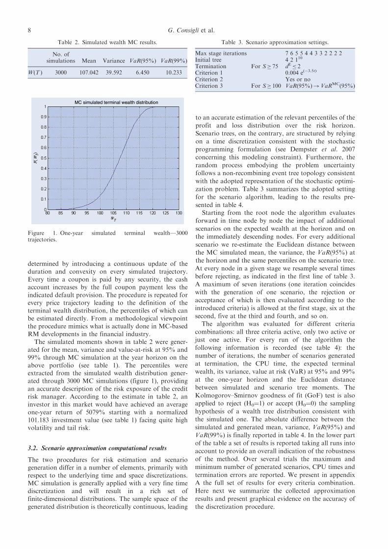
determined by introducing a continuous update of theduration and convexity on every simulated trajectory.Every time a coupon is paid by any security, the cashaccount increases by the full coupon payment less theindicated default provision. The procedure is repeated forevery price trajectory leading to the definition of theterminal wealth distribution, the percentiles of which canbe estimated directly. From a methodological viewpointthe procedure mimics what is actually done in MC-basedRM developments in the financial industry.

The simulated moments shown in table 2 were gener-ated for the mean, variance and value-at-risk at 95% and99% through MC simulation at the year horizon on theabove portfolio (see table 1). The percentiles wereextracted from the simulated wealth distribution gener-ated through 3000 MC simulations (figure 1), providingan accurate description of the risk exposure of the creditrisk manager. According to the estimate in table 2, aninvestor in this market would have achieved an averageone-year return of 5079% starting with a normalized101.183 investment value (see table 1) facing quite highvolatility and tail risk.

3.2. Scenario approximation computational results

The two procedures for risk estimation and scenariogeneration differ in a number of elements, primarily withrespect to the underlying time and space discretizations.MC simulation is generally applied with a very fine timediscretization and will result in a rich set offinite-dimensional distributions. The sample space of thegenerated distribution is theoretically continuous, leading

to an accurate estimation of the relevant percentiles of the

profit and loss distribution over the risk horizon.

Scenario trees, on the contrary, are structured by relying

on a time discretization consistent with the stochasticprogramming formulation (see Dempster et al. 2007

concerning this modeling constraint). Furthermore, the

random process embodying the problem uncertainty

follows a non-recombining event tree topology consistent

with the adopted representation of the stochastic optimi-

zation problem. Table 3 summarizes the adopted setting

for the scenario algorithm, leading to the results pre-

sented in table 4.Starting from the root node the algorithm evaluates

forward in time node by node the impact of additional

scenarios on the expected wealth at the horizon and on

the immediately descending nodes. For every additional

scenario we re-estimate the Euclidean distance between

the MC simulated mean, the variance, the VaR(95%) at

the horizon and the same percentiles on the scenario tree.

At every node in a given stage we resample several timesbefore rejecting, as indicated in the first line of table 3.

A maximum of seven iterations (one iteration coincides

with the generation of one scenario, the rejection or

acceptance of which is then evaluated according to the

introduced criteria) is allowed at the first stage, six at the

second, five at the third and fourth, and so on.The algorithm was evaluated for different criteria

combinations: all three criteria active, only two active orjust one active. For every run of the algorithm the

following information is recorded (see table 4): the

number of iterations, the number of scenarios generated

at termination, the CPU time, the expected terminal

wealth, its variance, value at risk (VaR) at 95% and 99%

at the one-year horizon and the Euclidean distance

between simulated and scenario tree moments. The

Kolmogorov–Smirnov goodness of fit (GoF) test is alsoapplied to reject (H0¼1) or accept (H0¼0) the sampling

hypothesis of a wealth tree distribution consistent with

the simulated one. The absolute difference between the

simulated and generated mean, variance, VaR(95%) and

VaR(99%) is finally reported in table 4. In the lower part

of the table a set of results is reported taking all runs into

account to provide an overall indication of the robustness

of the method. Over several trials the maximum andminimum number of generated scenarios, CPU times and

termination errors are reported. We present in appendix

A the full set of results for every criteria combination.

Here next we summarize the collected approximation

results and present graphical evidence on the accuracy of

the discretization procedure.

Table 2. Simulated wealth MC results.

No. ofsimulations Mean Variance VaR(95%) VaR(99%)

W(T ) 3000 107.042 39.592 6.450 10.233

Figure 1. One-year simulated terminal wealth—3000trajectories.

Table 3. Scenario approximation settings.

Max stage iterations 7 6 5 5 4 4 3 3 2 2 2 2Initial tree 4 2 110

Termination For S� 75 dE� 2Criterion 1 0.004 e(�3.5t)

Criterion 2 Yes or noCriterion 3 For S� 100 VaR(95%)!VaRMC(95%)


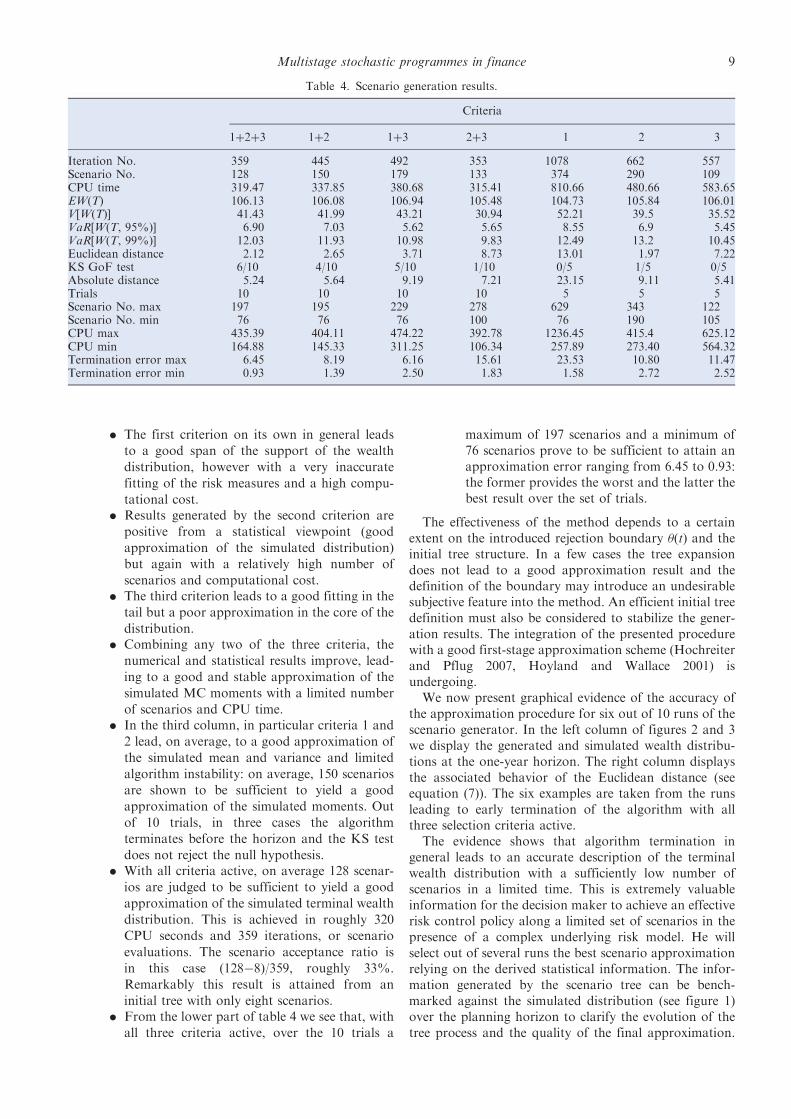
. The first criterion on its own in general leads

to a good span of the support of the wealth

distribution, however with a very inaccurate

fitting of the risk measures and a high compu-

tational cost.. Results generated by the second criterion are

positive from a statistical viewpoint (good

approximation of the simulated distribution)

but again with a relatively high number of

scenarios and computational cost.. The third criterion leads to a good fitting in the

tail but a poor approximation in the core of the

distribution.. Combining any two of the three criteria, the

numerical and statistical results improve, lead-

ing to a good and stable approximation of the

simulated MC moments with a limited number

of scenarios and CPU time.. In the third column, in particular criteria 1 and

2 lead, on average, to a good approximation of

the simulated mean and variance and limited

algorithm instability: on average, 150 scenarios

are shown to be sufficient to yield a good

approximation of the simulated moments. Out

of 10 trials, in three cases the algorithm

terminates before the horizon and the KS test

does not reject the null hypothesis.. With all criteria active, on average 128 scenar-

ios are judged to be sufficient to yield a good

approximation of the simulated terminal wealth

distribution. This is achieved in roughly 320

CPU seconds and 359 iterations, or scenario

evaluations. The scenario acceptance ratio is

in this case (128�8)/359, roughly 33%.

Remarkably this result is attained from an

initial tree with only eight scenarios.. From the lower part of table 4 we see that, with

all three criteria active, over the 10 trials a

maximum of 197 scenarios and a minimum of76 scenarios prove to be sufficient to attain anapproximation error ranging from 6.45 to 0.93:the former provides the worst and the latter thebest result over the set of trials.

The effectiveness of the method depends to a certainextent on the introduced rejection boundary (t) and theinitial tree structure. In a few cases the tree expansiondoes not lead to a good approximation result and thedefinition of the boundary may introduce an undesirablesubjective feature into the method. An efficient initial treedefinition must also be considered to stabilize the gener-ation results. The integration of the presented procedurewith a good first-stage approximation scheme (Hochreiterand Pflug 2007, Hoyland and Wallace 2001) isundergoing.

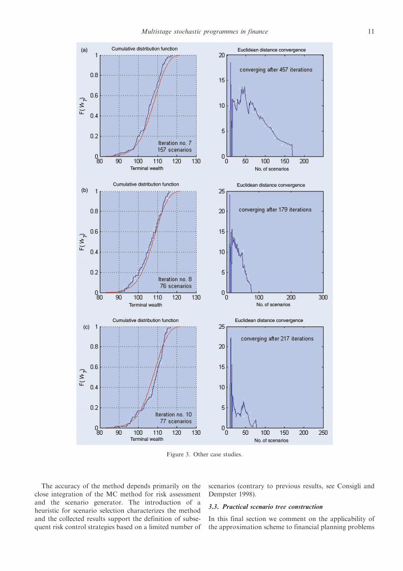
We now present graphical evidence of the accuracy ofthe approximation procedure for six out of 10 runs of thescenario generator. In the left column of figures 2 and 3we display the generated and simulated wealth distribu-tions at the one-year horizon. The right column displaysthe associated behavior of the Euclidean distance (seeequation (7)). The six examples are taken from the runsleading to early termination of the algorithm with allthree selection criteria active.

The evidence shows that algorithm termination ingeneral leads to an accurate description of the terminalwealth distribution with a sufficiently low number ofscenarios in a limited time. This is extremely valuableinformation for the decision maker to achieve an effectiverisk control policy along a limited set of scenarios in thepresence of a complex underlying risk model. He willselect out of several runs the best scenario approximationrelying on the derived statistical information. The infor-mation generated by the scenario tree can be bench-marked against the simulated distribution (see figure 1)over the planning horizon to clarify the evolution of thetree process and the quality of the final approximation.

Table 4. Scenario generation results.

Criteria

1þ2þ3 1þ2 1þ3 2þ3 1 2 3

Iteration No. 359 445 492 353 1078 662 557Scenario No. 128 150 179 133 374 290 109CPU time 319.47 337.85 380.68 315.41 810.66 480.66 583.65EW(T) 106.13 106.08 106.94 105.48 104.73 105.84 106.01V[W(T)] 41.43 41.99 43.21 30.94 52.21 39.5 35.52VaR[W(T, 95%)] 6.90 7.03 5.62 5.65 8.55 6.9 5.45VaR[W(T, 99%)] 12.03 11.93 10.98 9.83 12.49 13.2 10.45Euclidean distance 2.12 2.65 3.71 8.73 13.01 1.97 7.22KS GoF test 6/10 4/10 5/10 1/10 0/5 1/5 0/5Absolute distance 5.24 5.64 9.19 7.21 23.15 9.11 5.41Trials 10 10 10 10 5 5 5Scenario No. max 197 195 229 278 629 343 122Scenario No. min 76 76 76 100 76 190 105CPU max 435.39 404.11 474.22 392.78 1236.45 415.4 625.12CPU min 164.88 145.33 311.25 106.34 257.89 273.40 564.32Termination error max 6.45 8.19 6.16 15.61 23.53 10.80 11.47Termination error min 0.93 1.39 2.50 1.83 1.58 2.72 2.52


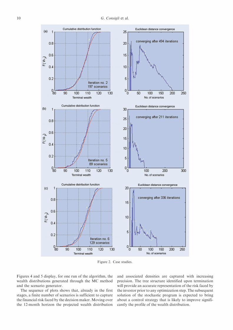
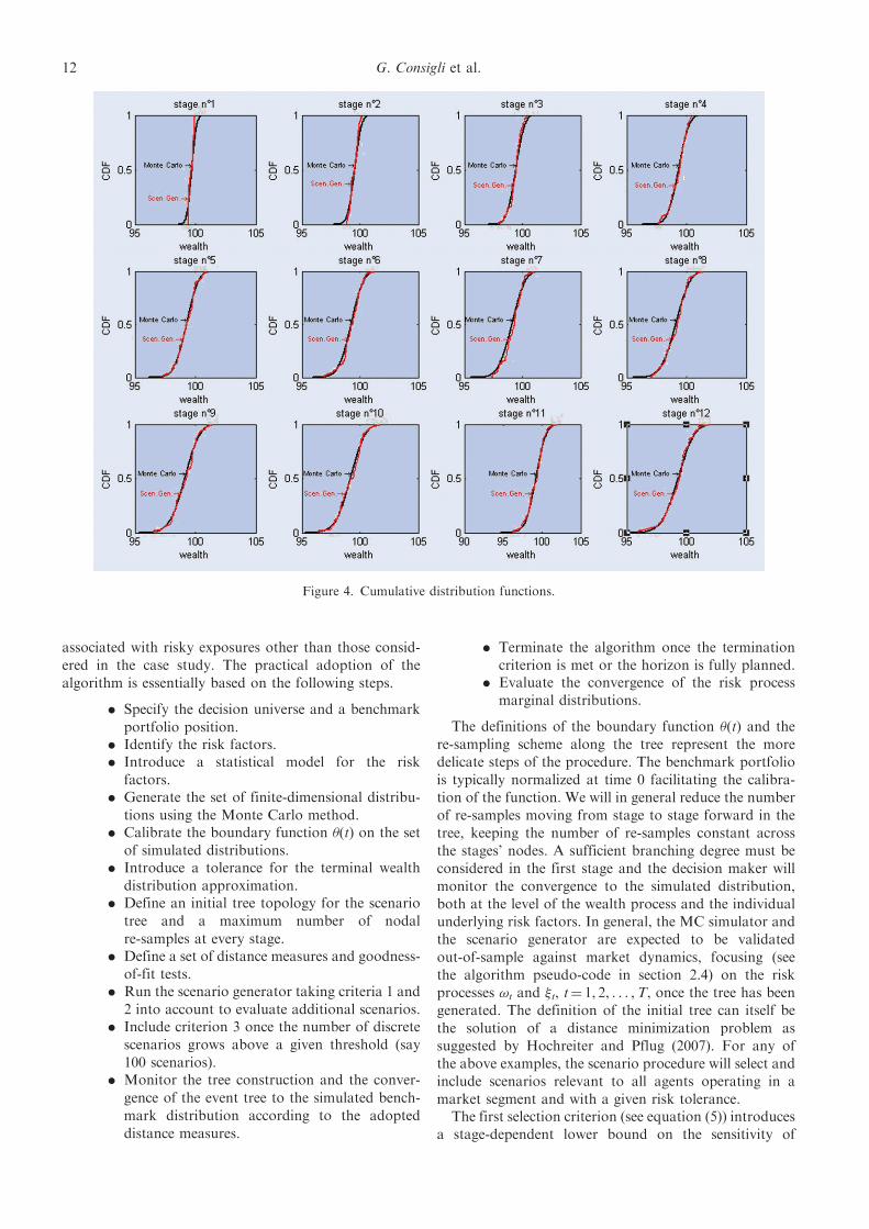
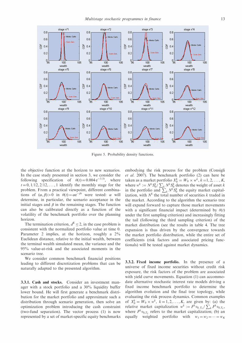
Figures 4 and 5 display, for one run of the algorithm, thewealth distributions generated through the MC methodand the scenario generator.

The sequence of plots shows that, already in the firststages, a finite number of scenarios is sufficient to capturethe financial risk faced by the decisionmaker.Moving overthe 12-month horizon the projected wealth distribution

and associated densities are captured with increasingprecision. The tree structure identified upon terminationwill provide an accurate representation of the risk faced bythe investor prior to any optimization step. The subsequentsolution of the stochastic program is expected to bringabout a control strategy that is likely to improve signifi-cantly the profile of the wealth distribution.

Figure 2. Case studies.


The accuracy of the method depends primarily on theclose integration of the MC method for risk assessmentand the scenario generator. The introduction of aheuristic for scenario selection characterizes the methodand the collected results support the definition of subse-quent risk control strategies based on a limited number of

scenarios (contrary to previous results, see Consigli andDempster 1998).

3.3. Practical scenario tree construction

In this final section we comment on the applicability ofthe approximation scheme to financial planning problems

Figure 3. Other case studies.


associated with risky exposures other than those consid-

ered in the case study. The practical adoption of the

algorithm is essentially based on the following steps.

. Specify the decision universe and a benchmark

portfolio position.. Identify the risk factors.. Introduce a statistical model for the risk

factors.. Generate the set of finite-dimensional distribu-

tions using the Monte Carlo method.. Calibrate the boundary function (t) on the set

of simulated distributions.. Introduce a tolerance for the terminal wealth

distribution approximation.. Define an initial tree topology for the scenario

tree and a maximum number of nodal

re-samples at every stage.. Define a set of distance measures and goodness-

of-fit tests.. Run the scenario generator taking criteria 1 and

2 into account to evaluate additional scenarios.. Include criterion 3 once the number of discrete

scenarios grows above a given threshold (say

100 scenarios).. Monitor the tree construction and the conver-

gence of the event tree to the simulated bench-

mark distribution according to the adopted

distance measures.

. Terminate the algorithm once the terminationcriterion is met or the horizon is fully planned.

. Evaluate the convergence of the risk processmarginal distributions.

The definitions of the boundary function (t) and the

re-sampling scheme along the tree represent the moredelicate steps of the procedure. The benchmark portfoliois typically normalized at time 0 facilitating the calibra-tion of the function. We will in general reduce the number

of re-samples moving from stage to stage forward in thetree, keeping the number of re-samples constant acrossthe stages’ nodes. A sufficient branching degree must beconsidered in the first stage and the decision maker will

monitor the convergence to the simulated distribution,both at the level of the wealth process and the individualunderlying risk factors. In general, the MC simulator andthe scenario generator are expected to be validated

out-of-sample against market dynamics, focusing (seethe algorithm pseudo-code in section 2.4) on the riskprocesses !t and t, t¼ 1, 2, . . . ,T, once the tree has beengenerated. The definition of the initial tree can itself be

the solution of a distance minimization problem assuggested by Hochreiter and Pflug (2007). For any ofthe above examples, the scenario procedure will select andinclude scenarios relevant to all agents operating in a

market segment and with a given risk tolerance.The first selection criterion (see equation (5)) introduces

a stage-dependent lower bound on the sensitivity of

Figure 4. Cumulative distribution functions.


the objective function at the horizon to new scenarios.In the case study presented in section 3, we consider thefollowing specification of (t)¼ 0.004 e�3.5t, wheret¼ 0, 1/12, 2/12, . . . , 1 identify the monthly stage for theproblem. From a practical viewpoint, different combina-tions of (�,�)40 in (t)¼ �e��t were tested: � willdetermine, in particular, the scenario acceptance in theinitial stages and � in the remaining stages. The functioncan also be calibrated directly as a function of thevolatility of the benchmark portfolio over the planninghorizon.

The termination criterion, dE� 2, in the case problem isconsistent with the normalized portfolio value at time 0.Parameter 2 implies, at the horizon, roughly a 2%Euclidean distance, relative to the initial wealth, betweenthe terminal wealth simulated mean, the variance and the95% value-at-risk and the associated moments in thescenario tree.

We consider common benchmark financial positionsleading to different discretization problems that can benaturally adapted to the presented algorithm.

3.3.1. Cash and stocks. Consider an investment man-ager with a stock portfolio and a 30% liquidity bufferlower bound. He will first generate a benchmark distri-bution for the market portfolio and approximate such adistribution through scenario generation, then solve anoptimization problem introducing the cash constraint(two-fund separation). The vector process (1) is nowrepresented by a set of market-specific equity benchmarks

embodying the risk process for the problem (Consigli

et al. 2007). The benchmark portfolio (2) can here be

taken as a market portfolio Xk0 ¼W0 � wk, k¼1, 2, . . . ,K,

where wk :¼ NkSk0=P

k NkSk

0 denotes the weight of asset k

in the portfolio andP

k NkSk

0 the equity market capital-

ization, with Nk the total number of securities k traded in

the market. According to the algorithm the scenario tree

will expand forward to capture those market movements

with a significant financial impact (determined by (t)under the first sampling criterion) and increasingly fitting

the tail (following the third sampling criterion) of the

market distribution (see the results in table 4. The tree

expansion is thus driven by the convergence towards

the market portfolio distribution, while the entire set of

coefficients (risk factors and associated pricing func-

tionals) will be tested against market dynamics.

3.3.2. Fixed income portfolio. In the presence of auniverse of fixed income securities without credit risk

exposure, the risk factors of the problem are associated

with yield curve movements. Equation (1) can accommo-

date alternative stochastic interest rate models driving a

fixed income benchmark portfolio to determine the

algorithm evolution and the final tree topology, while

evaluating the risk process dynamics. Common examples

of Xk0 ¼W0 � wk, k¼ 1, 2, . . . ,K, are given by: (a) the

relative market capitalization wk :¼ Fkv0,Tk=P

k Fkv0,Tk

,

where Fkv0,Tkrefers to the market capitalization; (b) an

equally weighted portfolio with w1¼w2¼ �� ¼wK

Figure 5. Probability density functions.


with respect to K maturity buckets; and (c) exogenousweights relative to the issuers’ market positions.

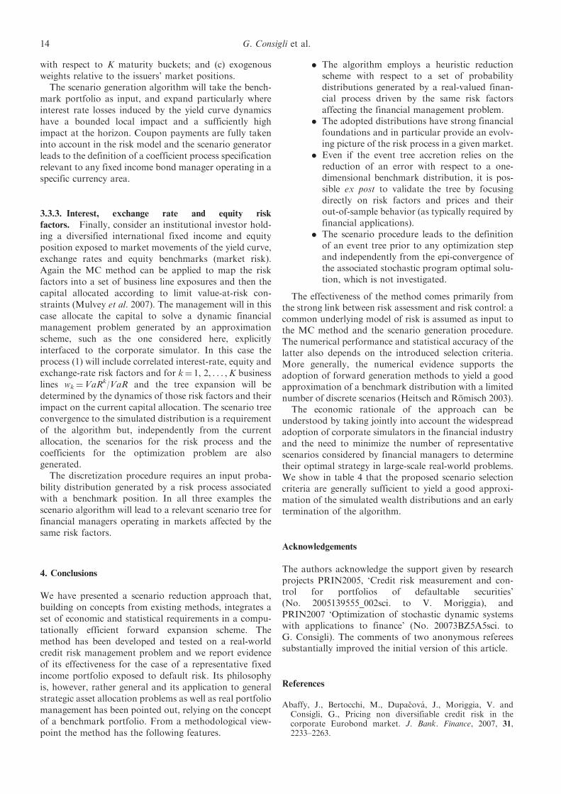
The scenario generation algorithm will take the bench-mark portfolio as input, and expand particularly whereinterest rate losses induced by the yield curve dynamicshave a bounded local impact and a sufficiently highimpact at the horizon. Coupon payments are fully takeninto account in the risk model and the scenario generatorleads to the definition of a coefficient process specificationrelevant to any fixed income bond manager operating in aspecific currency area.

3.3.3. Interest, exchange rate and equity risk

factors. Finally, consider an institutional investor hold-ing a diversified international fixed income and equityposition exposed to market movements of the yield curve,exchange rates and equity benchmarks (market risk).Again the MC method can be applied to map the riskfactors into a set of business line exposures and then thecapital allocated according to limit value-at-risk con-straints (Mulvey et al. 2007). The management will in thiscase allocate the capital to solve a dynamic financialmanagement problem generated by an approximationscheme, such as the one considered here, explicitlyinterfaced to the corporate simulator. In this case theprocess (1) will include correlated interest-rate, equity andexchange-rate risk factors and for k¼ 1, 2, . . . ,K businesslines wk¼VaRk/VaR and the tree expansion will bedetermined by the dynamics of those risk factors and theirimpact on the current capital allocation. The scenario treeconvergence to the simulated distribution is a requirementof the algorithm but, independently from the currentallocation, the scenarios for the risk process and thecoefficients for the optimization problem are alsogenerated.

The discretization procedure requires an input proba-bility distribution generated by a risk process associatedwith a benchmark position. In all three examples thescenario algorithm will lead to a relevant scenario tree forfinancial managers operating in markets affected by thesame risk factors.

4. Conclusions

We have presented a scenario reduction approach that,building on concepts from existing methods, integrates aset of economic and statistical requirements in a compu-tationally efficient forward expansion scheme. Themethod has been developed and tested on a real-worldcredit risk management problem and we report evidenceof its effectiveness for the case of a representative fixedincome portfolio exposed to default risk. Its philosophyis, however, rather general and its application to generalstrategic asset allocation problems as well as real portfoliomanagement has been pointed out, relying on the conceptof a benchmark portfolio. From a methodological view-point the method has the following features.

. The algorithm employs a heuristic reductionscheme with respect to a set of probabilitydistributions generated by a real-valued finan-cial process driven by the same risk factorsaffecting the financial management problem.

. The adopted distributions have strong financialfoundations and in particular provide an evolv-ing picture of the risk process in a given market.

. Even if the event tree accretion relies on thereduction of an error with respect to a one-dimensional benchmark distribution, it is pos-sible ex post to validate the tree by focusingdirectly on risk factors and prices and theirout-of-sample behavior (as typically required byfinancial applications).

. The scenario procedure leads to the definitionof an event tree prior to any optimization stepand independently from the epi-convergence ofthe associated stochastic program optimal solu-tion, which is not investigated.

The effectiveness of the method comes primarily fromthe strong link between risk assessment and risk control: acommon underlying model of risk is assumed as input tothe MC method and the scenario generation procedure.The numerical performance and statistical accuracy of thelatter also depends on the introduced selection criteria.More generally, the numerical evidence supports theadoption of forward generation methods to yield a goodapproximation of a benchmark distribution with a limitednumber of discrete scenarios (Heitsch and Romisch 2003).

The economic rationale of the approach can beunderstood by taking jointly into account the widespreadadoption of corporate simulators in the financial industryand the need to minimize the number of representativescenarios considered by financial managers to determinetheir optimal strategy in large-scale real-world problems.We show in table 4 that the proposed scenario selectioncriteria are generally sufficient to yield a good approxi-mation of the simulated wealth distributions and an earlytermination of the algorithm.

Acknowledgements

The authors acknowledge the support given by researchprojects PRIN2005, ‘Credit risk measurement and con-trol for portfolios of defaultable securities’(No. 2005139555_002sci. to V. Moriggia), andPRIN2007 ‘Optimization of stochastic dynamic systemswith applications to finance’ (No. 20073BZ5A5sci. toG. Consigli). The comments of two anonymous refereessubstantially improved the initial version of this article.

References

Abaffy, J., Bertocchi, M., Dupacova, J., Moriggia, V. andConsigli, G., Pricing non diversifiable credit risk in thecorporate Eurobond market. J. Bank. Finance, 2007, 31,2233–2263.


Bertocchi, M., Moriggia, V. and Dupacova, J., Bond portfoliomanagement via stochastic programming. In Handbook ofAsset and Liability Management, edited by S.A. Zenios andW.T. Ziemba, Vol. 1, pp. 305–336, 2007 (North-Holland:Amsterdam).

Campbell, J.Y., Lo, W.A. and MacKinlay, A.C., TheEconometrics of Financial Markets, 1997 (PrincetonUniversity Press: Princeton).

Consigli, G., Tail estimation and mean–VaR portfolio selectionin markets subject to financial instability. J. Bank. Finance,2002, 26(7), 1355–1382.

Consigli, G., Asset and liability management for individualinvestors. In Handbook of Asset and Liability Management:Applications and Case Studies, edited by S.A. Zenios andW.T. Ziemba, Vol. 2, pp. 751–828, 2007 (North-Holland:Amsterdam).

Consigli, G. and Dempster, M.A.H., Dynamic stochasticprogramming for asset-liability management. Ann. Oper.Res., 1998, 81, 131–161.

Consiglio, A., Saunders, D. and Zenios, S.A., Asset and liabilitymanagement models for insurance products with guarantees:The UK case. J. Bank. Finance, 2006, 30, 645–667.

Consigli, G., MacLean, L.M., Zhao, Y. and Ziemba, W.T.,The bond-equity yield as risk indicator in financial markets.J. RISK, 2007, 11(3), 3–24.

Cox, J.C., Ingersoll, J.E. and Ross, S.A., A theory of the termstructure of interest rates. Econometrica, 1985, 53, 385–407.

Crouhy, M., Galai, D. and Mark, R., A comparative analysis ofcurrent credit risk models. J. Bank. Finance, 2000, 24, 59–117.

Dempster, M.A.H. (ed.), Risk Management: Value at Risk andBeyond, 2002 (Cambridge University Press: Cambridge).

Dempster, M.A.H. and Thompson, R.T., EVPI-based impor-tance sampling solution procedures for multistage stochasticprogrammes on parallel MIMD architectures. Ann. Oper.Res., 1999, 90, 161–184.

Dempster, M.A.H., Germano, M., Medova, E.A. andVillaverde, M., Global asset liability management. Br.Actuar. J., 2003, 9(1), 137–195.

Dempster, M.A.H., Germano, M., Medova, E.,Rietbergen, M.I., Sandrini, F. and Scrowston, M.,Designing minimum guaranteed return funds. Quant.Finance, 2007, 7(2), 245–256.

Di Domenica, N., Lucas, C., Mitra, G. and Valente, P., Scenariogeneration for stochastic programming and simulation:A modelling perspective. IMA J. Mgmt Math., 2007, 10, 1–38.

Duffie, D. and Singleton, K.J., Modeling term structures ofdefaultable bonds. Rev. Financial Stud., 1999, 12, 687–720.

Dupacova, J., Stochastic programming: Minimax approach.In Encyclopedia of Optimization, edited by Ch.A. Floudas andP.M. Pardalos, pp. 327–330, 2001 (Kluwer: Dordrecht).

Dupacova, J., Consigli, G. and Wallace, S.W., Scenarios formultistage stochastic programmes. Ann. Oper. Res., 2001, 100,25–53.

Dupacova, J., Grwe, N. and Romisch, W., Scenario reduction instochastic programming: An approach using probabilitymetrics. Math. Progr. A, 2003, 95, 493–511.

Glasserman, P., Monte Carlo Methods in Financial Engineering,2003 (Springer: New York).

Heitsch, H. and Romisch, W., Scenario reduction algorithms instochastic programming. Comput. Optimiz. Applic., 2003, 24,187–206.

Hochreiter, R. and Pflug, G.Ch., Financial scenario generationfor stochastic multi-stage decision processes as facilitylocation problems. Ann. Oper. Res., 2007, 152(1), 252–272.

Hoyland, K. and Wallace, S.W., Generating scenario trees formultistage decision problems. Mgmt Sci., 2001, 47, 295–307.

Jobst, N.J. and Zenios, S.A., On the simulation of portfolios ofinterest rate and credit risk sensitive securities. EJOR, 2005,161(2), 298–324.

Kaut, M. and Wallace, S.W., Evaluation of scenario generationmethods for stochastic programming. Pacif. J. Optimiz., 2007,3(2), 257–271.

King, A.J., Duality and martingales: A stochastic programmingperspective on contingent claims. Math. Progr. B, 2002, 91,543–562.

Kouwenberg, R., Scenario generation and stochastic program-ming models for asset liability management. Eur. J. Oper.Res., 2001, 134, 279–292.

Mak, W.M., Morton, D.P. and Wood, R.K., Monte Carlobounding techniques for determining solution quality instochastic programs. Oper. Res. Lett., 1999, 24, 47–56.

Mulvey, J.M. and Thorlacius, The Towers Perrin global capitalmarket scenario generation system: CAP:Link. In WorldwideAsset and Liability Modeling, edited by W.T. Ziemba andJ.M. Mulvey, 1998 (Cambridge University Press: Cambridge).

Mulvey, J.M., Pauling, B., Britt, S. and Morin, F., Dynamicfinancial analysis for multinational insurance companies.In Handbook of Asset and Liability Management:Applications and Case Studies, edited by S.A. Zenios andW.T. Ziemba, Vol. 2, pp. 543–589, 2007 (North-Holland:Amsterdam).

Pennanen, T., Epi-convergent discretizations ofmultistage stochastic programs. Math. Oper. Res., 2005,30(1), 245–256.

Pennanen, T. and King, A.J., Arbitrage pricing of Americancontingent claims in incomplete markets: A convex optimiza-tion approach. Stochastic programming E-Print series, 2004.Available online at: www.speps.info.

Pennanen, T. and Koivu, M., Epi-convergent discretizationsof stochastic programs via integration quadratures.Numer. Math., 2005, 100(1), 141–163.

Pflug, G.Ch., Optimal scenario tree generation for multiperiodfinancial planning. Math. Progr. B, 2001, 89, 251–271.

Pflug, G.Ch. and Romisch, W., Modeling, Measuring andManaging Risk, 2007 (World Scientific: Singapore).

Szego, G., Risk Measures for the 21st Century, 2004 (Wiley:New York).

Zenios, S.A. and Ziemba, W.T., Handbook of Asset and LiabilityManagement: Theory and Methodology, Vol. 1, 2007a(North-Holland: Amsterdam).

Zenios, S.A. and Ziemba, W.T., Handbook of Asset and LiabilityManagement: Applications and Case Studies, Vol. 2, 2007b(North-Holland: Amsterdam).

Appendix A: Scenario generation results

We present in this appendix the full set of numericalevidence collected on the presented case study consideringdifferent combinations of the selection criteria imple-mented in the scenario generation procedure leading totable 4. We refer to the main body of the article for theinformation provided in each table and the derivedconclusions and evidence. Here we only recall that, inthe given version, scenario trees with possibly differenttopologies are considered representative of the underlyingcontinuous distribution if the algorithm converges andthe KS turns out to be 0. The preferable scenario treedepending on the optimization problem at hand will bethe one with the smallest moments distance in theEuclidean metric. Tables A1–A7 show the differentproperties of the introduced criteria and their relevanceto the convergence speed of the algorithm.


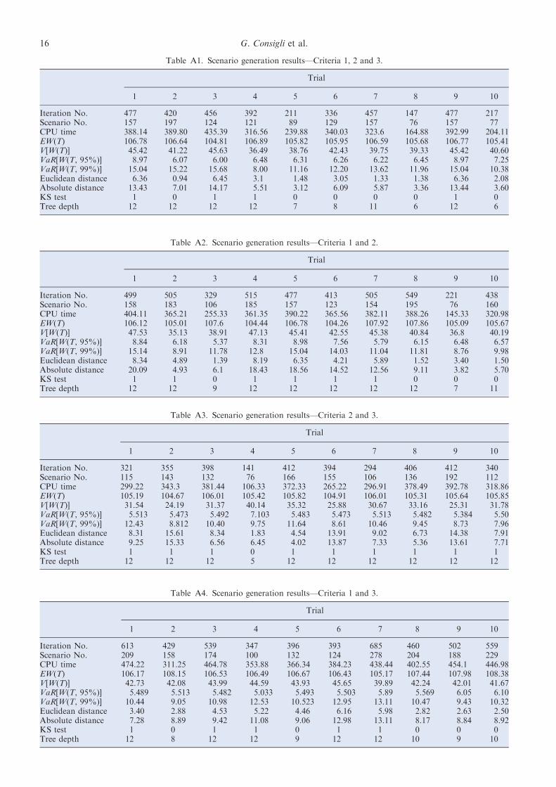
Table A1. Scenario generation results—Criteria 1, 2 and 3.

Trial

1 2 3 4 5 6 7 8 9 10

Iteration No. 477 420 456 392 211 336 457 147 477 217Scenario No. 157 197 124 121 89 129 157 76 157 77CPU time 388.14 389.80 435.39 316.56 239.88 340.03 323.6 164.88 392.99 204.11EW(T) 106.78 106.64 104.81 106.89 105.82 105.95 106.59 105.68 106.77 105.41V[W(T)] 45.42 41.22 45.63 36.49 38.76 42.43 39.75 39.33 45.42 40.60VaR[W(T, 95%)] 8.97 6.07 6.00 6.48 6.31 6.26 6.22 6.45 8.97 7.25VaR[W(T, 99%)] 15.04 15.22 15.68 8.00 11.16 12.20 13.62 11.96 15.04 10.38Euclidean distance 6.36 0.94 6.45 3.1 1.48 3.05 1.33 1.38 6.36 2.08Absolute distance 13.43 7.01 14.17 5.51 3.12 6.09 5.87 3.36 13.44 3.60KS test 1 0 1 1 0 0 0 0 1 0Tree depth 12 12 12 12 7 8 11 6 12 6

Table A2. Scenario generation results—Criteria 1 and 2.

Trial

1 2 3 4 5 6 7 8 9 10



Trial

1 2 3 4 5 6 7 8 9 10



Trial

1 2 3 4 5 6 7 8 9 10



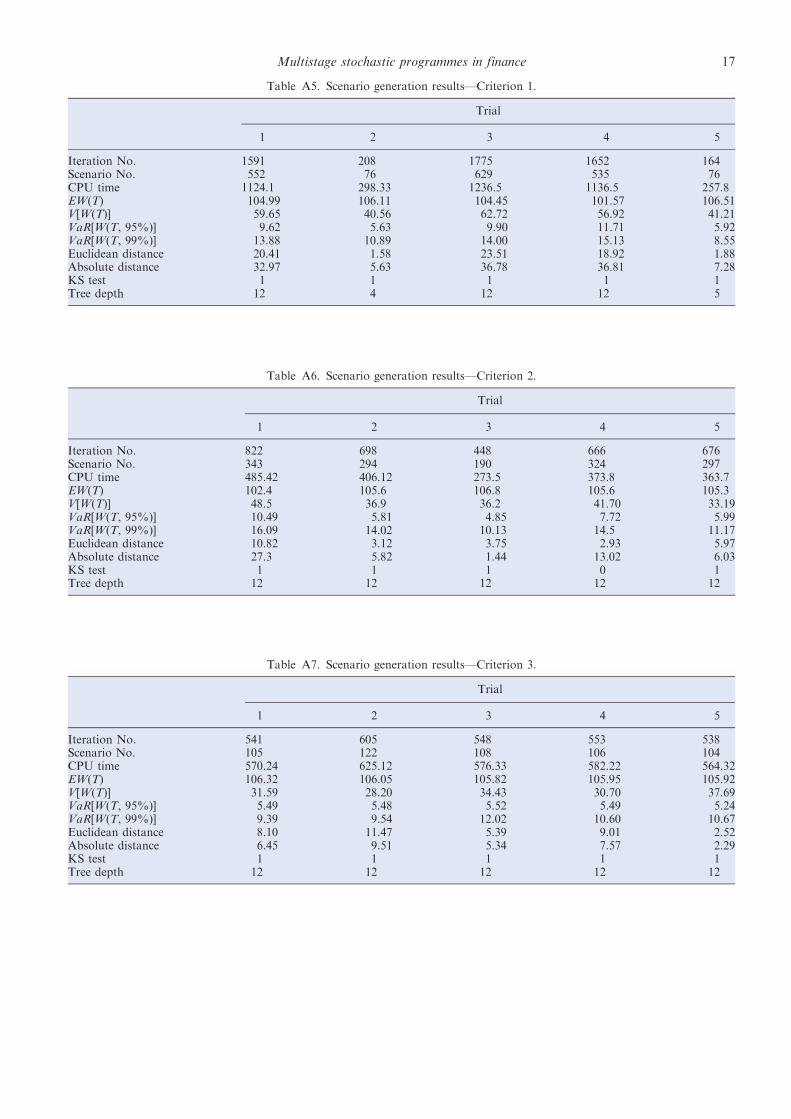
Table A5. Scenario generation results—Criterion 1.

Trial

1 2 3 4 5

Iteration No. 1591 208 1775 1652 164Scenario No. 552 76 629 535 76CPU time 1124.1 298.33 1236.5 1136.5 257.8EW(T) 104.99 106.11 104.45 101.57 106.51V[W(T)] 59.65 40.56 62.72 56.92 41.21VaR[W(T, 95%)] 9.62 5.63 9.90 11.71 5.92VaR[W(T, 99%)] 13.88 10.89 14.00 15.13 8.55Euclidean distance 20.41 1.58 23.51 18.92 1.88Absolute distance 32.97 5.63 36.78 36.81 7.28KS test 1 1 1 1 1Tree depth 12 4 12 12 5


Trial

1 2 3 4 5



Trial

1 2 3 4 5



Path-dependent scenario trees for multistage stochastic programmes in finance

Documents

Transcript of Path-dependent scenario trees for multistage stochastic programmes in finance