An Introduction to Einstein's General Relativity," copyright JB ...
Upload
khangminh22Category
view
0download
0
ÉCOLE DOCTORALE SCIENCE FONDAMENTALES APPLIQUEÉS
Géoazur UMR 7329
Thèse de doctorat
Présentée en vue de l’obtention du grade de docteur en Chimie
de L’UNIVERSITÉ COTE D’AZUR par
Anna Maria ORANI
Développements analytiques pour la détermination des
concentrations et de l’origine des contaminants
inorganiques dans des environnements marins
Dirigée par Pr. Olivier THOMAS
et codirigée par Dr. Emilia VASSILEVA et Dr. Aurélie BARATS
Soutenue le 15 Décembre 2017
Devant le jury composé de :
Dr. Aurélie BARATS, Maître de conférences, Géoazur, Université Côte d’Azur co-directrice de thèse
Prof. Ewa BULSKA, Chemistry Department, University of Warsow rapporteur
Prof. Veselin J. KMETOV, Analytical Chemistry Department, University of Plovdiv rapporteur
Prof. Christophe RENAC, Géoazur, Université Côte d’Azur examinateur, président du jury
Prof. Olivier P. THOMAS, National University of Ireland Galway directeur de thèse
Dr. Emilia VASSILEVA, Research scientist, Environment Laboratories, IAEA co-directrice de thèse


Development and application of analytical methodologies for trace elements pollution assessment in different compartments of the marine environment

AKNOWLEDGMENTS
First of all I would like to express my gratitude to Prof. Ewa Bulska, Prof. Veselin Kmetov, and Prof.
Christophe Renac for their interest in my PhD work and for taking the time to review my thesis. I am
confident that their suggestions will be of great help for my future.
This PhD comes to an end after a tortuous path, full of challenges but most importantly full of
interesting experiences. A real life-changing adventure during which I have learnt a lot!
Many people helped me in this period, fighting for and with me and for this reason I will be forever
grateful to each of them, starting from my supervisors:
-My PhD director Olivier Thomas, who accepted this role and never gave up even in the middle of many
administrative challenges!
-My PhD co-director Emilia Vassileva, who encouraged me to start a PhD in the first place and with her
precious teaching always supported my work and believed in me.
-My second PhD co-director Aurélie Barats, who helped and encouraged me even during the most
difficult periods, with many advices and positive attitude.
Special thanks go to Prof Petko Mandjukov and Dr Irena Wysocka, for sharing their knowledge with me
and for their crucial contribution to this PhD work and to Ms Sabine Azemard for her constant help.
I would like to thank all the fellows and office mates I have been the pleasure to work with, in France
and Ireland, which have contributed to accumulate many wonderful memories!
Je voudrais remercier toute la famille Calabro, pour m’avoir accueilli à bras ouverts ces dernières années
et pour être toujours un gros point de référence, ma deuxième famille !
Ancora una volta vorrei ringraziare la mia meravigliosa famiglia e le mie fantastiche amiche che mi sono
stati vicino (da lontano). Il loro sostegno è stato fondamentale in questi anni, e lo sarà per sempre.
Voglio dedicare questa tesi a Kevin, che mi ha supportato (e sopportato) in questi anni, garantendomi
amore incondizionato, condividendo con me le tante soddisfazioni ma soprattutto insegnandomi a non
mollare e perseverare sempre!

CONTENTS PART I: GENERAL INTRODUCTION .............................................................................................................. 11
1. Trace elements in the environment.................................................................................................... 13
1.1. Trace elements in the aquatic system ........................................................................................ 13
1.2. Trace elements speciation .......................................................................................................... 16
1.2.1. Arsenic ................................................................................................................................. 17
1.2.2. Mercury ............................................................................................................................... 20
1.3. Trace elements isotopes ............................................................................................................. 22
1.3.1. Pb Isotopic ratios ................................................................................................................. 24
2. Trace elements monitoring programs ................................................................................................ 26
2.1. Trace elements in sediments ........................................................................................................... 27
2.1.1. Sediment components and classification ................................................................................. 27
2.1.2. Factors affecting TE accumulation in sediments ...................................................................... 29
2.1.3. TE monitoring in sediments ...................................................................................................... 32
2.2. Trace elements in marine organisms ............................................................................................... 33
2.2.1. Bivalves ..................................................................................................................................... 33
2.2.2. Sponges ..................................................................................................................................... 35
3. Trace elements analysis ...................................................................................................................... 38
3.1. Atomic Absorption Spectrometry .................................................................................................... 40
3.2. Inductively Coupled Plasma Mass Spectrometry ............................................................................. 41
REFERENCES ................................................................................................................................................ 44
PART II: SCIENTIFIC PUBLICATIONS ............................................................................................................. 69
FIRST BLOCK ................................................................................................................................................ 71
Paper 1 .................................................................................................................................................... 71
Paper 2 .................................................................................................................................................... 81
Paper 3 .................................................................................................................................................... 95
SECOND BLOCK ......................................................................................................................................... 115
Paper 4 .................................................................................................................................................. 115
Paper 5 .................................................................................................................................................. 150
THIRD BLOCK ............................................................................................................................................. 201
Paper 6 .................................................................................................................................................. 201
Paper 7 .................................................................................................................................................. 254
Conclusion and future perspectives ......................................................................................................... 297

11 PART I: GENERAL INTRODUCTION
PART I: GENERAL INTRODUCTION
In this first part of the thesis, some general information is discussed. These concepts are useful for the
understanding of the general picture presented in this PhD.
The origin and fate of TE in different compartments of the aquatic system are presented as well as a
brief description of analytical techniques used during the present work.

12 PART I: GENERAL INTRODUCTION
13 PART I: GENERAL INTRODUCTION
1. TRACE ELEMENTS IN THE ENVIRONMENT
The IUPAC Compendium of Chemical Terminology defines trace element as “any element having an
average concentration of less than about 100 parts per million atoms or less than 100 µg g-1’’ (McNaught
and Wilkinson, 1997). Among TE, some are oligo elements and are thus considered essential for various
biochemical and physiological functions within a certain range of concentrations. Metals/metalloids
considered by World Health Organization to be essential for human health are: chromium, cobalt,
copper, iron, molybdenum, selenium and zinc (WHO, 1996)(WHO, 1996).On the other hand, other TE
are considered toxic at any concentration (Hg, Pb, Cd) (WHO/FAO/IAEA, 1996).
These elements are naturally present in the ecosystem because of natural processes such as
weathering and erosion but also volcanic activity. Nevertheless, in the last decades, several
anthropogenic activities have increased the loads of these elements in the environment (Bagul, 2015).
Main anthropogenic sources of TE include metal mining, mineral processing, smelting, coal mining,
power generation but also municipal waste incinerators, industrial waste of many types and petroleum
utilization. Specifically, in coastal systems, the anthropogenic sources can be represented by building of
infrastructure, land reclamation for port and industrial development, habitat modification, tourism and
recreational activities (Rao et al., 2006). The levels of TE in the environment are thus dominated by
several concomitant processes, related to the origin but also to the different fates of these components
in through environmental compartments.
1.1. Trace elements in the aquatic system
Trace elements have been transported along the hydrological cycle since the first occurrence of
water on the planet. Water provides the medium for weathering of the continents as well as the
medium for transport them in other environmental compartments (Salomons and Förstner, 1984).
Along the way to the oceans, trace elements undergo different processes, due to environmental
changes that affect their distribution in dissolved and particulate phases. TE under the form of
particulates may accumulate in rivers and lakes and from there reach the coast through estuarine
systems. Several important processes take place in the interfaces river/ocean as well as in the
continental shelf. In these areas (often hosting harbors and industrial centers), TE from natural and
anthropogenic origins are accumulated. Once the riverine or atmospheric TE loads have entered the
oceans, they take part in an intricate group of geochemical processes, ultimately ending their path as
14 PART I: GENERAL INTRODUCTION
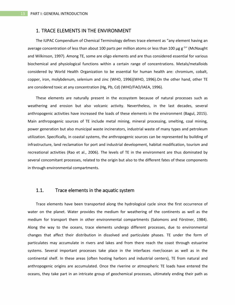
accumulated substance by marine sediments. An illustration of these complex patterns is shown in
figure 1. The residence time of TE in aquatic environment varies from a few days (rivers and
atmosphere) to several thousands of years (oceans) (Salomons and Förstner, 1984).
Figure 1. Movement of trace metals in the hydrological cycle. Copyright Springer
Intrinsic water characteristics such as physiochemical and biological properties have a great
influence on the geochemical cycle of elements in the oceans (Elderfield, 2003). Trace elements can be
found in the environment under the form of free cations (Mn+), which is the most bioavailable form
especially for aquatic organisms such as phytoplankton (Bruland and Lohan, 2003). Others are more
often under the form of oxyanions, such as MoO42- and AsO4
2-. In aquatic ecosystems, trace elements are
very often bound to ligands. Most natural waters have a certain capacity to reduce the bioavailability,
and thus the toxicity, of such elements, due to the presence of ligands complexing the free ions
(Salomons and Förstner, 1984). Nevertheless, some of the complexes can, in turn, be bio-available, such
as those accumulated by the marine biota (Vicente-Martorell et al., 2009; Strady et al., 2011). Water
contamination can thus have a direct effect on the food chain as well as be biomagnified through it
(Bocher et al., 2003; Majer et al., 2014). The understanding of TE cycle in the aquatic system is of prime
15 PART I: GENERAL INTRODUCTION
interest to address the right correction actions and help decision makers in the process of efficient
restoration of natural conditions.
The behavior of trace elements in the water column is governed by several factors. Direct
precipitation of dissolved elements is possible as a consequence of changes in physiochemical condition,
such as pH, oxidation potential or concentrations of precipitating substances. These circumstances can
occur as a consequence of water mixing processes, loss or addition of gasses as well as the mixing of
water with solids (Rose and Hawkes, 1979). An example is the precipitation of U, V, Cu, Se, and Ag as
metal or lower-valency oxide because of reduction usually caused by an encounter with organic matter
or mixing with reducing waters or gases. The redox potential Eh thus plays a crucial role in the behavior
of trace elements in aquatic environments. In natural system, Eh is often a measure of total dissolved
oxygen, although other dissolved species can act as oxidizing (NO3-, SO4
2-) and reducing (Fe2+, Mn2+)
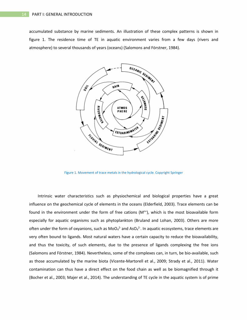
agents (Plant and Raiswell, 1983). The pH also influences the mineral dissolution and precipitation
reactions, additionally affecting the complexing process. The speciation of many elements in the surface
environment may be represented in Eh vs pH diagrams (Plant and Raiswell, 1983). An example is shown
in Figure 2.
Figure 2. Potential-pH diagram for Cu in water. Full lines separate the stability fields for copper species. The y-axis is the
potential in Volts with respect to hydrogen electrode (Nolan and Cadien, 2012)
TE occurrence of TE in the particulate or dissolved phase of water affects directly their assimilation
by organisms and thus their involvement in marine biogeochemical cycles. Additionally, their solubility is
influenced by their source, so the way through which they reach the water column. For example, trace
16 PART I: GENERAL INTRODUCTION
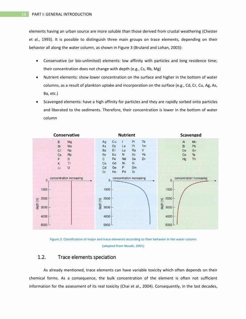
elements having an urban source are more soluble than those derived from crustal weathering (Chester
et al., 1993). It is possible to distinguish three main groups on trace elements, depending on their
behavior all along the water column, as shown in Figure 3 (Bruland and Lohan, 2003):
• Conservative (or bio-unlimited) elements: low affinity with particles and long residence time;
their concentration does not change with depth (e.g., Cs, Rb, Mg)
• Nutrient elements: show lower concentration on the surface and higher in the bottom of water
columns, as a result of plankton uptake and incorporation on the surface (e.g., Cd, Cr, Cu, Ag, As,
Ba, etc.)
• Scavenged elements: have a high affinity for particles and they are rapidly sorbed onto particles
and liberated to the sediments. Therefore, their concentration is lower in the bottom of water
column
Figure.3. Classification of major and trace elements according to their behavior in the water column
(adapted from Nozaki, 2001)
1.2. Trace elements speciation
As already mentioned, trace elements can have variable toxicity which often depends on their
chemical forms. As a consequence, the bulk concentration of the element is often not sufficient
information for the assessment of its real toxicity (Chai et al., 2004). Consequently, in the last decades,
Conservative Nutrient Scavenged

17 PART I: GENERAL INTRODUCTION
researches have been focusing on the analysis of chemical species of several TE to evaluate their impact
on the environment (Sánchez Uría, 1998; Leermakers et al., 2005; Semeniuk et al., 2016). Among toxic
elements, arsenic and mercury are two of the most studied elements regarding chemical speciation in
environmental samples.
1.2.1. Arsenic
Arsenic (As) is classified as metalloid as it presents characteristics of both, metallic and non-metallic
element (Phillips, 1990). It is associated with igneous and sedimentary rocks, particularly with sulfidic
ores as it is strongly chalcophile. Several anthropogenic activities such as metals and alloys
manufacturing, petroleum refining and burning of wastes and fossil fuels, have contributed to a strong
legacy of As pollution throughout the world (Melamed, 2005). Several As-containing compounds are
produced by industry and have been used to manufacture products for agricultural applications such as
insecticides, herbicides, and fungicides. Numerous species of As can occur in the environment and the
interconversion of species from toxic to less harmful and vice versa is possible as a consequence of some
physical-chemical changes such as biological activity, changes in redox potential, or pH. To determine
the actual risk represented by this element in the environment, a proper study should include
identifying and quantifying both the total quantity of arsenic and the specific chemical forms present in
the sample (Gong, 2002).
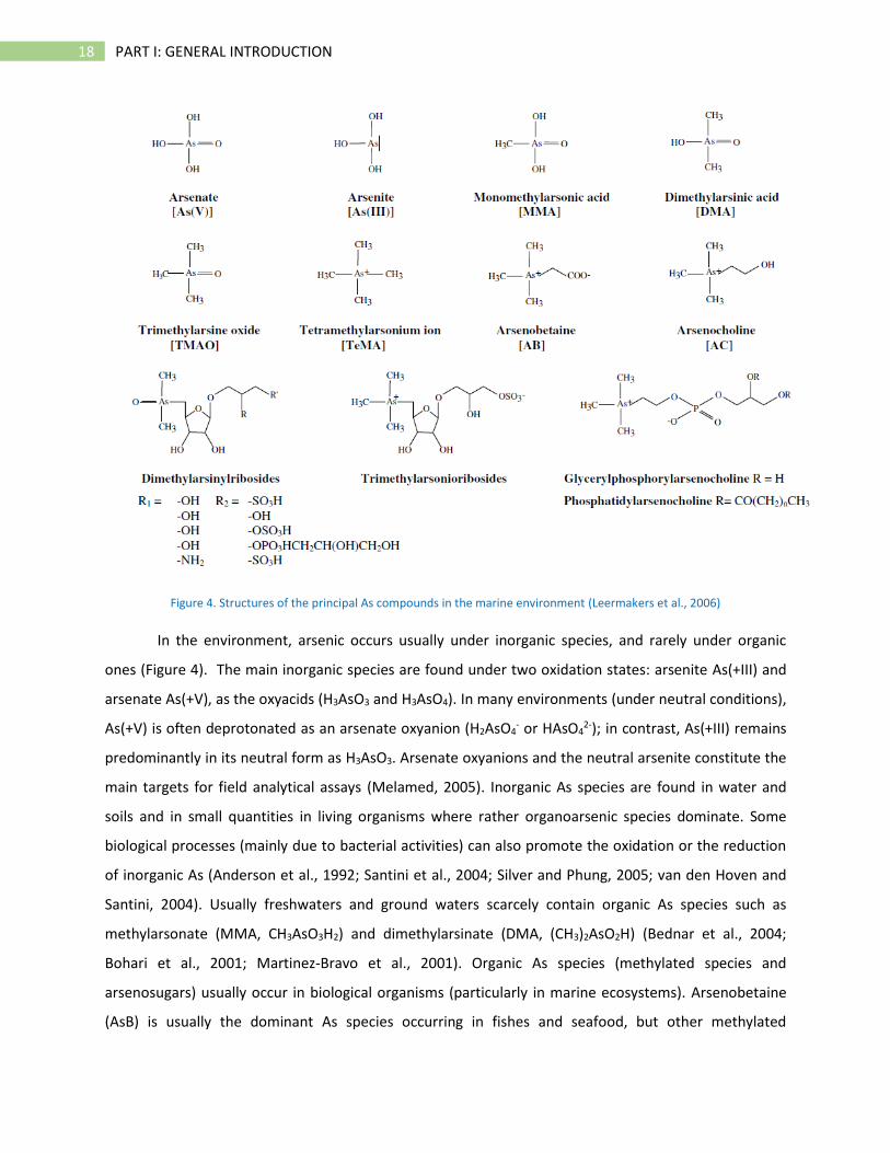
18 PART I: GENERAL INTRODUCTION
Figure 4. Structures of the principal As compounds in the marine environment (Leermakers et al., 2006)
In the environment, arsenic occurs usually under inorganic species, and rarely under organic
ones (Figure 4). The main inorganic species are found under two oxidation states: arsenite As(+III) and
arsenate As(+V), as the oxyacids (H3AsO3 and H3AsO4). In many environments (under neutral conditions),
As(+V) is often deprotonated as an arsenate oxyanion (H2AsO4- or HAsO4
2-); in contrast, As(+III) remains
predominantly in its neutral form as H3AsO3. Arsenate oxyanions and the neutral arsenite constitute the
main targets for field analytical assays (Melamed, 2005). Inorganic As species are found in water and
soils and in small quantities in living organisms where rather organoarsenic species dominate. Some
biological processes (mainly due to bacterial activities) can also promote the oxidation or the reduction
of inorganic As (Anderson et al., 1992; Santini et al., 2004; Silver and Phung, 2005; van den Hoven and
Santini, 2004). Usually freshwaters and ground waters scarcely contain organic As species such as
methylarsonate (MMA, CH3AsO3H2) and dimethylarsinate (DMA, (CH3)2AsO2H) (Bednar et al., 2004;
Bohari et al., 2001; Martinez-Bravo et al., 2001). Organic As species (methylated species and
arsenosugars) usually occur in biological organisms (particularly in marine ecosystems). Arsenobetaine
(AsB) is usually the dominant As species occurring in fishes and seafood, but other methylated
19 PART I: GENERAL INTRODUCTION
compounds are also found in marine biota (Nam et al., 2010; Grotti et al., 2010). Biological processes
promoted by some microorganisms or bacteria enhance the methylation of inorganic species in organic
ones, such as MMA, DMA, trimethylarsine [TMA, (CH3)3As] (Bentley and Chasteen, 2002; Cullen and
Reimer, 1989; Irgolic and Stockton, 1987). Arsenic is essential for some organisms, e.g., 12 to 25 μg of
total As per day is required by humans, but it is also toxic at low and high concentration (WHO, 2006).
Chronic As exposure increases the risk of cancer and skin pigmentation. Arsenic has great notoriety as a
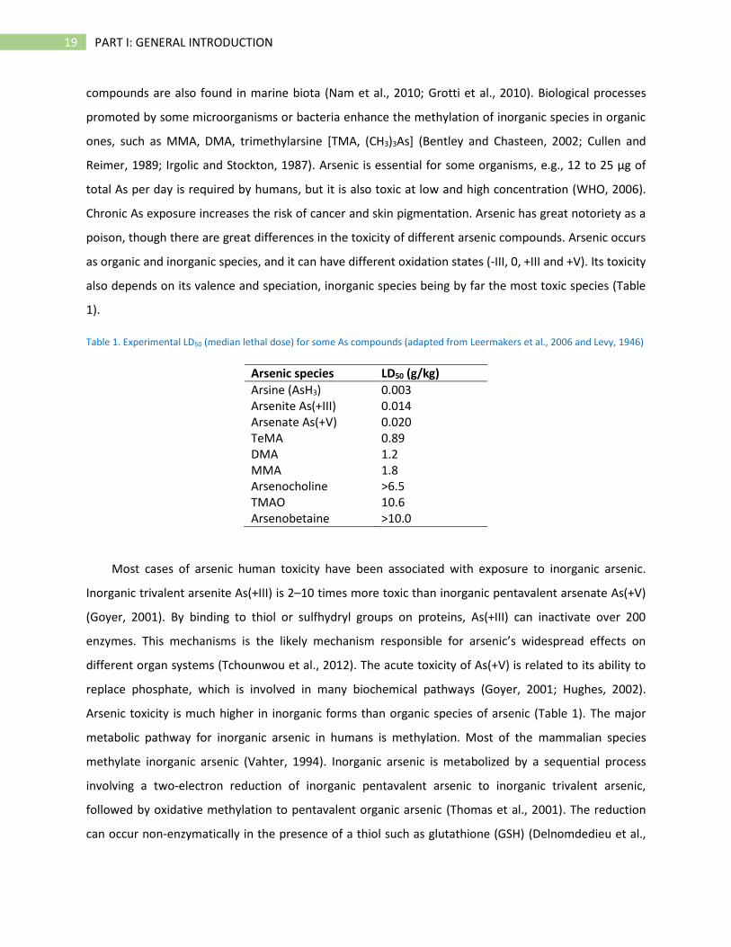
poison, though there are great differences in the toxicity of different arsenic compounds. Arsenic occurs
as organic and inorganic species, and it can have different oxidation states (-III, 0, +III and +V). Its toxicity
also depends on its valence and speciation, inorganic species being by far the most toxic species (Table
1).
Table 1. Experimental LD50 (median lethal dose) for some As compounds (adapted from Leermakers et al., 2006 and Levy, 1946)
Arsenic species LD50 (g/kg)
Arsine (AsH3) 0.003 Arsenite As(+III) 0.014 Arsenate As(+V) 0.020 TeMA 0.89 DMA 1.2 MMA 1.8 Arsenocholine >6.5 TMAO 10.6 Arsenobetaine >10.0
Most cases of arsenic human toxicity have been associated with exposure to inorganic arsenic.
Inorganic trivalent arsenite As(+III) is 2–10 times more toxic than inorganic pentavalent arsenate As(+V)
(Goyer, 2001). By binding to thiol or sulfhydryl groups on proteins, As(+III) can inactivate over 200
enzymes. This mechanisms is the likely mechanism responsible for arsenic’s widespread effects on
different organ systems (Tchounwou et al., 2012). The acute toxicity of As(+V) is related to its ability to
replace phosphate, which is involved in many biochemical pathways (Goyer, 2001; Hughes, 2002).
Arsenic toxicity is much higher in inorganic forms than organic species of arsenic (Table 1). The major
metabolic pathway for inorganic arsenic in humans is methylation. Most of the mammalian species
methylate inorganic arsenic (Vahter, 1994). Inorganic arsenic is metabolized by a sequential process
involving a two-electron reduction of inorganic pentavalent arsenic to inorganic trivalent arsenic,
followed by oxidative methylation to pentavalent organic arsenic (Thomas et al., 2001). The reduction
can occur non-enzymatically in the presence of a thiol such as glutathione (GSH) (Delnomdedieu et al.,
20 PART I: GENERAL INTRODUCTION
1994; Scott et al., 1993). However in human livers, some specific enzymes have been isolated,
suggesting that the reduction occurs using enzymatic reaction (Radabaugh and Aposhian, 2000;
Zakharyan et al., 2001). The species produced as a result of these reactions are then expelled along with
urine.
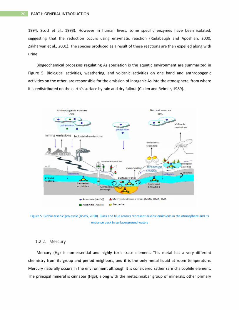
Biogeochemical processes regulating As speciation is the aquatic environment are summarized in
Figure 5. Biological activities, weathering, and volcanic activities on one hand and anthropogenic
activities on the other, are responsible for the emission of inorganic As into the atmosphere, from where
it is redistributed on the earth’s surface by rain and dry fallout (Cullen and Reimer, 1989).
Figure 5. Global arsenic geo-cycle (Bossy, 2010). Black and blue arrows represent arsenic emissions in the atmosphere and its
entrance back in surface/ground waters
1.2.2. Mercury
Mercury (Hg) is non-essential and highly toxic trace element. This metal has a very different
chemistry from its group and period neighbors, and it is the only metal liquid at room temperature.
Mercury naturally occurs in the environment although it is considered rather rare chalcophile element.
The principal mineral is cinnabar (HgS), along with the metacinnabar group of minerals; other primary
21 PART I: GENERAL INTRODUCTION
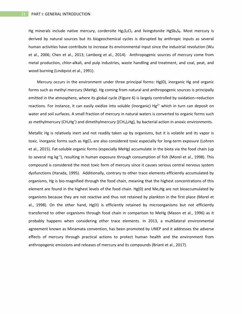
Hg minerals include native mercury, corderoite Hg3S2Cl2 and livingstonite HgSb4S8. Most mercury is
derived by natural sources but its biogeochemical cycles is disrupted by anthropic inputs as several
human activities have contribute to increase its environmental input since the industrial revolution (Wu
et al., 2006; Chen et al., 2013; Lamborg et al., 2014). Anthropogenic sources of mercury come from
metal production, chlor-alkali, and pulp industries, waste handling and treatment, and coal, peat, and
wood burning (Lindqvist et al., 1991).
Mercury occurs in the environment under three principal forms: Hg(0), inorganic Hg and organic
forms such as methyl mercury (MeHg). Hg coming from natural and anthropogenic sources is principally
emitted in the atmosphere, where its global cycle (Figure 6) is largely controlled by oxidation–reduction
reactions. For instance, it can easily oxidize into soluble (inorganic) Hg2+ which in turn can deposit on
water and soil surfaces. A small fraction of mercury in natural waters is converted to organic forms such
as methylmercury (CH3Hg+) and dimethylmercury [(CH3)2Hg], by bacterial action in anoxic environments.
Metallic Hg is relatively inert and not readily taken up by organisms, but it is volatile and its vapor is
toxic. Inorganic forms such as HgCl2 are also considered toxic especially for long-term exposure (Lohren
et al., 2015). Fat-soluble organic forms (especially MeHg) accumulate in the biota via the food chain (up
to several mg kg-1), resulting in human exposure through consumption of fish (Morel et al., 1998). This
compound is considered the most toxic form of mercury since it causes serious central nervous system
dysfunctions (Harada, 1995). Additionally, contrary to other trace elements efficiently accumulated by
organisms, Hg is bio-magnified through the food chain, meaning that the highest concentrations of this
element are found in the highest levels of the food chain. Hg(0) and Me2Hg are not bioaccumulated by
organisms because they are not reactive and thus not retained by plankton in the first place (Morel et
al., 1998). On the other hand, Hg(II) is efficiently retained by microorganisms but not efficiently
transferred to other organisms through food chain in comparison to MeHg (Mason et al., 1996) as it
probably happens when considering other trace elements. In 2013, a multilateral environmental
agreement known as Minamata convention, has been promoted by UNEP and it addresses the adverse
effects of mercury through practical actions to protect human health and the environment from
anthropogenic emissions and releases of mercury and its compounds (Briant et al., 2017).
22 PART I: GENERAL INTRODUCTION
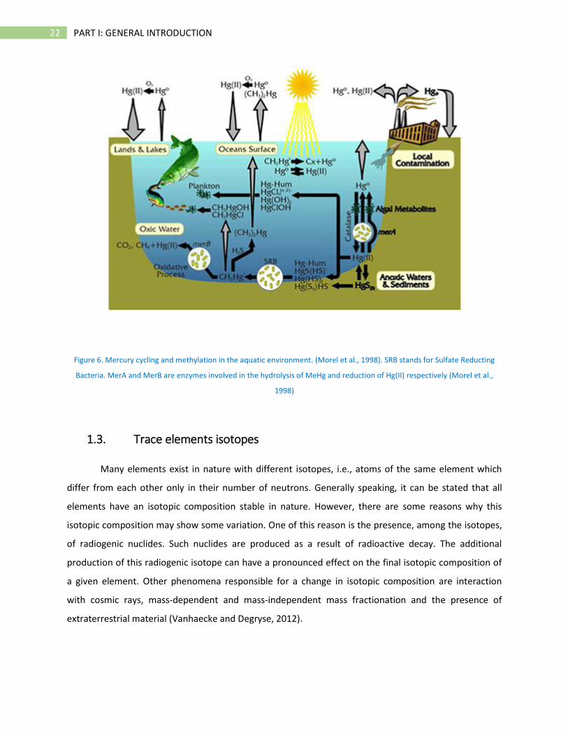
Figure 6. Mercury cycling and methylation in the aquatic environment. (Morel et al., 1998). SRB stands for Sulfate Reducting
Bacteria. MerA and MerB are enzymes involved in the hydrolysis of MeHg and reduction of Hg(II) respectively (Morel et al.,
1998)
1.3. Trace elements isotopes
Many elements exist in nature with different isotopes, i.e., atoms of the same element which
differ from each other only in their number of neutrons. Generally speaking, it can be stated that all
elements have an isotopic composition stable in nature. However, there are some reasons why this
isotopic composition may show some variation. One of this reason is the presence, among the isotopes,
of radiogenic nuclides. Such nuclides are produced as a result of radioactive decay. The additional
production of this radiogenic isotope can have a pronounced effect on the final isotopic composition of
a given element. Other phenomena responsible for a change in isotopic composition are interaction
with cosmic rays, mass-dependent and mass-independent mass fractionation and the presence of
extraterrestrial material (Vanhaecke and Degryse, 2012).
23 PART I: GENERAL INTRODUCTION
As already stated, some elements show natural variation in their isotopic composition as a
consequence of the presence, among its isotopes, of radiogenic nuclides (Ault et al., 1970). A radiogenic
nuclide is continuously produced as long as the parent radionuclide is available, leading to an increase of
its relative abundance with respect to other isotopes of the same element. The presence of one
radiogenic isotope within the same element affects the general isotopic composition and the relative
abundance of other isotopes. Mass fractionation is related to the fact that different isotopes can
participate with different efficiency to chemical and physical processes. These differences in efficiency
are related to slight differences in equilibrium for each different isotopic molecule (thermodynamic
effect) or in the rate with which the isotopes participate in a process or reaction (kinetic effect)
(Vanhaecke and Degryse, 2012). As a result, the isotopic composition of such element will be different at
the end of the process in comparison to the isotopic composition at the beginning of it. These effects
need to be considered when measurements of isotopic ratios are performed. Most of the time the
phenomenon of mass fractionation shows linear dependency with the mass of the isotope: but for some
elements it constitutes a hot topic of research (Vanhaecke and Degryse, 2012).
When measuring isotope ratios by ICP-MS, the effect known as mass discrimination has to be taken
into consideration. As a result of differences in the efficiency of ion extraction, transmission and
detection as a function of analyte mass, an isotope ratio measured with ICP-MS may show significant
bias with respect to the corresponding true value (Vanhaecke et al., 2009). This effect is constant and
needs to be corrected during the measurement session. For this purpose, several correction models
have been developed, often involving a mathematical correction based on the measurement of a
certified external isotopic standard (e.g. NIST 981 or NIST 982). Another method involves the use of an
internal standard, with similar mass to the analyte, directly added in the sample to be analyzed. For
example, in Pb isotopic analysis, a Tl standard is added to the sample solution and the bias between the
measured 203Tl/205Tl and the corresponding true value is used to determine the mass discrimination per
mass unit, which is in turn used to correct the Pb ratio data (Vanhaecke et al., 2009).
The measurement of isotopic ratios finds application for numerous elements, especially in
provenance studies. Sr, Pb, Nd and U are only few examples of elements used for this application,
measurable by ICP-MS (Debord et al., 2017; Kingson et al., 2017; Vio et al., 2018).
24 PART I: GENERAL INTRODUCTION
1.3.1. Pb Isotopic ratios
Lead is perhaps the most popular among elements partly radiogenic accessible via ICP-MS. It has
four stable isotopes, three of which are radiogenic. The decay chain of 238U (t1/2=4.468 x 109 years), 235U
(t1/2=0.407 x 109 years) and 232Th (t1/2=14.010 x 109 years) finally results in 206Pb, 207Pb and 208Pb
respectively. 204Pb is the only natural isotope, and its abundance is constant since the formation of the
solar system (Komárek et al., 2008). As a consequence, the final Pb isotopic composition depends on the
original U/Pb and U/Th elemental ratios, becoming characteristic of a particular geographical location.
For this reason, Pb isotope ratios find application in provenance studies in several fields (Sjåstad et al.,
2011; Nakata et al., 2015; Dudás et al., 2016; Shepherd et al., 2016; Sjåstad et al., 2016). In
environmental science, the use of Pb isotope ratios is a well-known tool, helping scientist to determine
the actual presence of Pb pollution and to track the source of anthropogenic inputs. There is a
substantial difference between isotopic composition of crustal Pb and that in ores. Pb isotope ratios
analysis provides thus an excellent tool to distinguish between local Pb and Pb pollution derived from
ores (e.g., anti-knock compounds added to petrol or for industrial use) (Monna et al., 1995; Bollhöfer
and Rosman, 2000; Bollhöfer and Rosman, 2001). In environmental samples such as aerosol, sediments
and snow, the final isotopic composition is the result of natural and one or more anthropogenic inputs.
A way to verify such a possibility is to plot the results in the so called three isotope graph (Figure 7),
which is a graphical representation of two different ratios with a common term e.g 208Pb/204Pb vs
206Pb/204Pb.
25 PART I: GENERAL INTRODUCTION
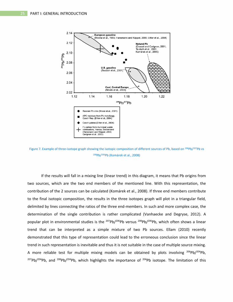
Figure 7. Example of three-isotope graph showing the isotopic composition of different sources of Pb, based on 206Pb/207Pb vs
208Pb/206Pb (Komárek et al., 2008)
If the results will fall in a mixing line (linear trend) in this diagram, it means that Pb origins from
two sources, which are the two end members of the mentioned line. With this representation, the
contribution of the 2 sources can be calculated (Komárek et al., 2008). If three end members contribute
to the final isotopic composition, the results in the three isotopes graph will plot in a triangular field,
delimited by lines connecting the ratios of the three end-members. In such and more complex case, the
determination of the single contribution is rather complicated (Vanhaecke and Degryse, 2012). A
popular plot in environmental studies is the 207Pb/206Pb versus 208Pb/206Pb, which often shows a linear
trend that can be interpreted as a simple mixture of two Pb sources. Ellam (2010) recently
demonstrated that this type of representation could lead to the erroneous conclusion since the linear
trend in such representation is inevitable and thus it is not suitable in the case of multiple source mixing.
A more reliable test for multiple mixing models can be obtained by plots involving 206Pb/204Pb,
207Pb/204Pb, and 208Pb/204Pb, which highlights the importance of 204Pb isotope. The limitation of this
26 PART I: GENERAL INTRODUCTION
approach arises from the difficult determination of 204Pb using ICP-MS, as it is the least abundant isotope
(about 1.4% natural abundance) and it is affected by 204Hg isobaric interference.
2. TRACE ELEMENTS MONITORING PROGRAMS
Environmental monitoring describes the processes and activities that are put in place in order to
assess the quality of the environment. All monitoring strategies and programs have reasons and
justifications which are often designed to establish the current status of an environment or to establish
trends in environmental parameters. The ecological, economic and social importance of marine
ecosystems being undeniable, a well-planned approach of managing the marine space is essential to
achieve sustainability (Jonathan and Gobert, 2016). In parallel with growing concern for environmental
conditions, several ocean monitoring programs have been introduced, at national and international
levels (Kennish, 1994). Environmental assessment programs have a crucial role in the management of
pollution sources and the preservation of marine habitats. The piece of coasts to be managed may be
under actual pressure, such as eutrophication and pollution, or it may be under threat of pressure from
some proposed development. Historically, most of the water quality investigations have attempted to
assess trace elements in aquatic systems by direct analysis of water samples. Many studies have dealt
with the determination of total and dissolved TE concentrations through the analysis of filtered and non-
filtered water (Cidu and Frau, 2009; Bu et al., 2017). Concentration associated with suspended
particulate matters (SPM) is usually indirectly determined as the difference between results obtained by
non-filtered water and filtered one. In most of aquatic systems, TE concentrations in SPM are much
higher (several order of magnitude) than those in the water samples. Some of the most toxic trace
elements (e.g., Hg, As, Cd, Pb and Zn) are strongly associated with sediments and plankton which means
that their distribution, mobility and bioavailability in the aquatic ecosystem cannot be solely evaluated
by their determination in water (Horowitz, 1991). In Europe, the recent Environmental Quality Standard
Directive 2008/105/EC (EQSD, 2008) marked an important step in the use of sediments and biota in
environmental monitoring programs, in the frame of Water Framework Directive 2000/60/EC (WFD).
Analysis of TE in sediments and biota is widely recognized as an effective approach in water-quality
monitoring to provide baseline regional values for local monitoring, for describing the actual
contamination levels as well as to identify areas of particular concern (Carere et al., 2012). Most of the
toxic substances listed in the principal environmental ranking, accumulate in both sediments and biota.
27 PART I: GENERAL INTRODUCTION
Is therefore of crucial importance to include sediments, suspended or bed sediments, and biota in a
proper environmental monitoring program.
2.1. Trace elements in sediments
Since sediments can act as reservoirs for many trace elements, they are often included in the
planning and design of environmental monitoring (Carere et al., 2012; Quevauviller, 2016). One of the
great application of sediment analysis in monitoring programs is related to the capability of this final
sink to accumulate trace elements and thus providing an historical record of contamination; this
property being often observed in sediment cores (Kljaković-Gašpić et al., 2008; Karbassi et al., 2005; Sun
et al., 2012; Vallius, 2014). Additionally, under changing environmental and physiochemical conditions
(e.g. pH, dissolved oxygen, bacterial actions), TE bound to sediments can be released in the water
column, increasing their harmful effect in the environment and food chain (Le Pape et al., 2012; Tripti et
al., 2013; Joung and Shiller, 2016).
2.1.1. Sediment components and classification
Marine sediments have very heterogeneous composition, depending on their origin and their
geographical localization. The accumulation of TE in sediments depends directly on the nature of
sediments. Three main types of sediments can be distinguished based on sources and components
(Fütterer et al., 2006): (1) lithogenous (terrigenous or volcanogenic) sediments, transported and
dissolved into the oceans as detrital particles; (2) biogenous sediments, formed directly by accumulation
of skeletal parts of marine organisms; and (3) hydrogenous sediments, which precipitate directly out of
solution as new formations.
Terrigenous material can be transported for several hundreds of kilometers in the form of
weathered minerals, by wind. The latter only transport particles of fine grain size, such as silt and clay.
Clay minerals constitute up to 50% of entire terrigenous sediments and they are of special importance
because of their capability to absorb and release ions (Fütterer et al., 2006). Despite all regional
variabilities, the clay mineral composition is rather constant, including only a few basic minerals (Table
2). Regarding the biogenic sediments, they can be considered as all solid hard materials formed in the
biosphere. The amount of carbonate deposited in the oceans today is almost entirely derived from
biogenic processes. Despite the great variability of marine organisms, only a small group produces hard
parts which can contribute to sediment formation in substantial amount. Relevant for sediment
formation are only carbonate minerals in the form of aragonite, Mg-calcite and calcite, as well as
28 PART I: GENERAL INTRODUCTION
biogenic opal in the form of amorphous SiO2·nH2O. Hydrogeneous sediments represent a negligible
contribution to sediment classification, in comparison with previous types. They are mostly formed as
direct inorganic precipitates from seawater, like sodium chloride.
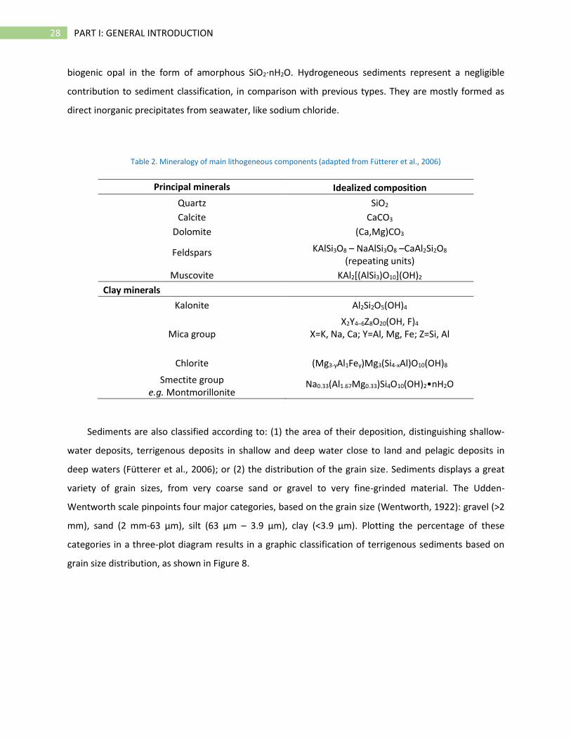
Table 2. Mineralogy of main lithogeneous components (adapted from Fütterer et al., 2006)
Principal minerals Idealized composition
Quartz SiO2
Calcite CaCO3
Dolomite (Ca,Mg)CO3
Feldspars KAlSi3O8 – NaAlSi3O8 –CaAl2Si2O8 (repeating units)
Muscovite KAl2[(AlSi3)O10](OH)2
Clay minerals
Kalonite Al2Si2O5(OH)4
Mica group X2Y4–6Z8O20(OH, F)4
X=K, Na, Ca; Y=Al, Mg, Fe; Z=Si, Al
Chlorite (Mg3-yAl1Fey)Mg3(Si4-xAl)O10(OH)8
Smectite group e.g. Montmorillonite
Na0.33(Al1.67Mg0.33)Si4O10(OH)2•nH2O
Sediments are also classified according to: (1) the area of their deposition, distinguishing shallow-
water deposits, terrigenous deposits in shallow and deep water close to land and pelagic deposits in
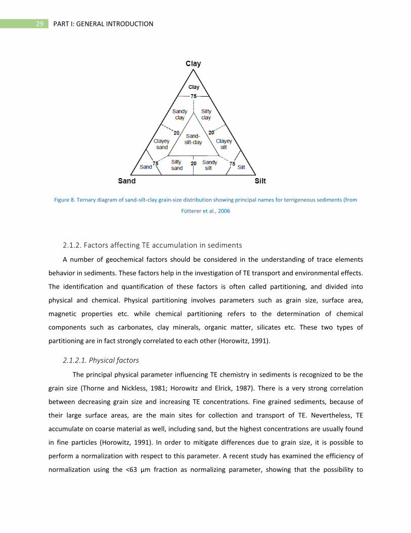
deep waters (Fütterer et al., 2006); or (2) the distribution of the grain size. Sediments displays a great
variety of grain sizes, from very coarse sand or gravel to very fine-grinded material. The Udden-
Wentworth scale pinpoints four major categories, based on the grain size (Wentworth, 1922): gravel (>2
mm), sand (2 mm-63 µm), silt (63 µm – 3.9 µm), clay (<3.9 µm). Plotting the percentage of these
categories in a three-plot diagram results in a graphic classification of terrigenous sediments based on
grain size distribution, as shown in Figure 8.
29 PART I: GENERAL INTRODUCTION
Figure 8. Ternary diagram of sand-silt-clay grain-size distribution showing principal names for terrigeneous sediments (from
Fütterer et al., 2006
2.1.2. Factors affecting TE accumulation in sediments
A number of geochemical factors should be considered in the understanding of trace elements
behavior in sediments. These factors help in the investigation of TE transport and environmental effects.
The identification and quantification of these factors is often called partitioning, and divided into
physical and chemical. Physical partitioning involves parameters such as grain size, surface area,
magnetic properties etc. while chemical partitioning refers to the determination of chemical
components such as carbonates, clay minerals, organic matter, silicates etc. These two types of
partitioning are in fact strongly correlated to each other (Horowitz, 1991).
2.1.2.1. Physical factors
The principal physical parameter influencing TE chemistry in sediments is recognized to be the
grain size (Thorne and Nickless, 1981; Horowitz and Elrick, 1987). There is a very strong correlation
between decreasing grain size and increasing TE concentrations. Fine grained sediments, because of
their large surface areas, are the main sites for collection and transport of TE. Nevertheless, TE
accumulate on coarse material as well, including sand, but the highest concentrations are usually found
in fine particles (Horowitz, 1991). In order to mitigate differences due to grain size, it is possible to
perform a normalization with respect to this parameter. A recent study has examined the efficiency of
normalization using the <63 µm fraction as normalizing parameter, showing that the possibility to
30 PART I: GENERAL INTRODUCTION
misinterpretation is quite high. The reason is that this fraction is unlikely to accurately embody the clay
content, which represents a major factor in TE adsorption in sediments (Szava-Kovats, 2008). The
correlation between grain size and TE content was observed in a broad range of sizes such as <16, <70,
<125 µm among others (Beeson, 1984; Horowitz and Elrick, 1987). Additionally different tendency can
be observed for different elements, i.e. different slopes when the element concentration is plotted
against percentage of fine grain-sized portion of the sediment. The element distribution in different
granulometric fractions of the sediment can be very specific and characteristic, thus allowing the
differentiation of samples from diverse origins.
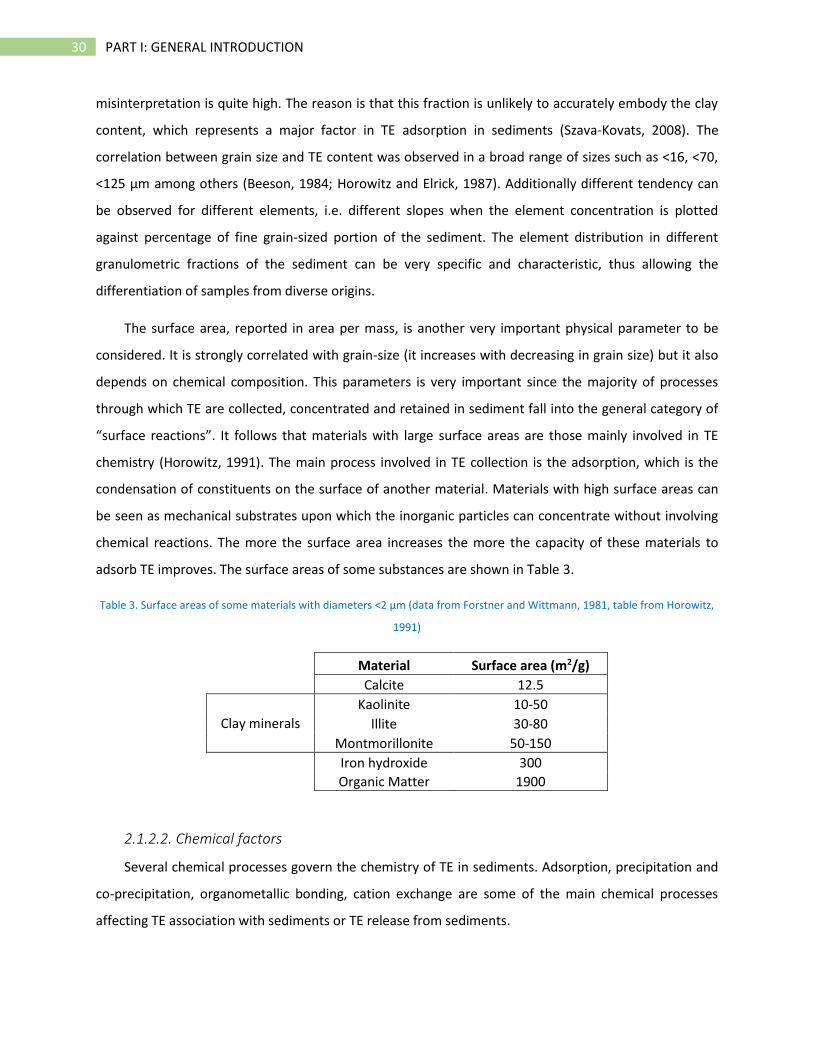
The surface area, reported in area per mass, is another very important physical parameter to be
considered. It is strongly correlated with grain-size (it increases with decreasing in grain size) but it also
depends on chemical composition. This parameters is very important since the majority of processes
through which TE are collected, concentrated and retained in sediment fall into the general category of
“surface reactions”. It follows that materials with large surface areas are those mainly involved in TE
chemistry (Horowitz, 1991). The main process involved in TE collection is the adsorption, which is the
condensation of constituents on the surface of another material. Materials with high surface areas can
be seen as mechanical substrates upon which the inorganic particles can concentrate without involving
chemical reactions. The more the surface area increases the more the capacity of these materials to
adsorb TE improves. The surface areas of some substances are shown in Table 3.
Table 3. Surface areas of some materials with diameters <2 µm (data from Forstner and Wittmann, 1981, table from Horowitz,
1991)
Material Surface area (m2/g)
Calcite 12.5
Clay minerals
Kaolinite 10-50
Illite 30-80
Montmorillonite 50-150
Iron hydroxide 300
Organic Matter 1900
2.1.2.2. Chemical factors
Several chemical processes govern the chemistry of TE in sediments. Adsorption, precipitation and
co-precipitation, organometallic bonding, cation exchange are some of the main chemical processes
affecting TE association with sediments or TE release from sediments.
31 PART I: GENERAL INTRODUCTION
Most of TE behave as cations and are readily sorbed and released on and from surfaces of materials
with net negative charge, such as clay minerals, iron and manganese hydroxides and organic matter.
This process is called cation exchange and it occurs thanks to the sorptive capacity of different anionic
sites such as SiOH, Al(OH)2, AlOH (clay minerals) and -COOH or –OH groups (from organic matter) among
others (Forstner and Wittmann, 1981). The cation exchange capacity (CEC) determines the ability of a
material to hold cations, and it has be proven to be correlated with grain size and surface area. Some of
the materials with the highest CEC are manganese hydroxide, humic acids and iron hydroxide (Horowitz,
1991). Bearing in mind the strong relation between physical and chemical properties, a number of
compounds and substances most important in TE behavior in sediments can be identified. These
materials (or geochemical substrates) are characterized by large surface areas, high CEC and they are
mostly concentrated in the finer size fractions.
• Fe and Mn oxides are well known for acting as excellent TE scavengers in solutions (Gadde and
Laitinen, 1974), they are mostly found in sediments under the form of nodules, micro-nodules
and coating. They have been proven to be important concentrators of TE in aquatic systems
(Jones and Browser, 1987; Forstner, 1982; Horowitz and Elrick, 1987).
• Organic matters (OM), generally named humic substances (humic acids, fulvic acids, humins) are
well known for concentrate TE in soils and sediments (Hirner et al., 1990; Rieuwerts et al.,
1998). The capacity of organic matter to concentrate TE varies with the constituent and the type
of OM but also to the stability of the TE-organic compound formed. The concentration of
aquatic organic matter is indicated measuring the total organic carbon. Negative or no-
correlation between OM and some TE were also reported in the literature (Wang and Qin, 2006)
showing a very variable interaction which might depends on the source (natural or
anthropogenic) of both, OM and TE (Wang, 2008).
• Clay minerals are the main components of fine-grained sediments, characterized by large
surface areas per unit mass. They are considered to be the major reasons for enrichment of TE
in sediments. The actual role of clays in TE transport and accumulation depends on a number of
factors, such as valence of TE, ionic radium, type of mineral (Förstner et al., 1989). It has been
proposed that clay minerals might simply provide a mechanical substrate for other materials,
such as OM and second minerals, and the latter carry out the actual concentration of TE
(Horowitz and Elrick, 1987; Horowitz, 1991).
32 PART I: GENERAL INTRODUCTION
2.1.3. TE monitoring in sediments
Several trace and major elements have been analyzed in sediment samples in many parts of the
world as a mean to provide environmental assessment. Considering that TE natural occur in sediments
as primary components of minerals, it is often needed to set a background local level in order to be able
to determine whether a high concentration is due to natural or anthropogenic input. It is rather difficult
to set a “normal” trace elements concentration, as the natural background play an important role and
the concentration ranges can be very wide for the majority of elements, even in pristine areas. For
instance concentrations between 1.4-4.9, 673-5075 and 55-389 mg kg-1 for Cd, Cu and Co respectively in
sediments from the Tigris River (Varol, 2011); Vallius et al. (2007) reported values between 7.3-19.1 and
46-83 mg kg-1 for As and Cr respectively in surface sediment from the Finnish coast of the Baltic Sea
while Parra et al. (2015) measured concentrations between 41-1476, 8-17, 6-15, 17-36, 9-20 mg kg-1 for
Cu, Ni, Co, Pb and As respectively in marine sediments from Chile.
The “quantification” of sediment pollution thus needs to be assessed after the evaluation of the
extent of TE naturally present in the considered area. For this purpose a chemical normalization is often
performed, with respect to reference elements such as Fe and Al (Abrahim and Parker, 2008; Karbassi et
al., 2007) but also Mn, Ti and Sc (Zahra et al., 2014; Salati and Moore, 2010) and Li (Aloupi and Angelidis,
2001). The background (BG) concentration can be taken from reported natural abundances in the earth
crust or taking as a reference the TE concentration measured in a proved uncontaminated place form
the same area of study. Geochemical normalization has extensively been used to calculate enrichment
and to reduce heavy metal variability caused by grain size and mineralogy of sediments (Zahra et al.,
2014). Using both, background concentrations and normalizing elements, some parameters such as
Enrichment Factors, Geoaccumulation Indices, Metal Pollution Indices and Pollution Load indices can be
calculated in order to evaluate the extent of metal contamination in the sediments. the results are then
evaluated following specific criteria (Guan et al., 2016).
The application of such parameters is nowadays very often used in monitoring studies involving
lake, river and marine sediments ad proved to be useful tool in TE pollution assessment. For instance
Guan et al. (2016) found rather high Co concentrations in river sediments from the Yellow river (max 339
mg kg -1) but being the BG level around 280 the final enrichment was not considered substantial.
Opposite conclusions were drawn for Cu, with max sample and BG concentrations of about 44 and 1.9
33 PART I: GENERAL INTRODUCTION
mg kg -1 respectively. As a result the calculated parameters revealed significant anthropogenic influence
for Cu (and other elements) but not for Co.
This approach has also been used for the study of sediment core samples, in order to evaluate a
possible TE enrichment during the history, evaluating the vertical variation. In this case the BG value is
often taken from the deepest sediment layer collected in the studied area (Veerasingam et al., 2015).
Nevertheless even though a high concentration of TE might not reflect anthropogenic influence it
can still represents a threat for other compartments of the environment, adversely affecting for
example the aquatic organisms. In order to evaluate such a possibility, sediment quality assessment
guidelines are very useful to screen sediment contamination by comparing sediment contaminant
concentration with the corresponding quality guideline (Macdonald et al., 1996). Quality guidelines and
threshold values for marine sediments (but also for water and some biota) are provided by national and
international institution such as EPA (Environmental Protection Agency).
2.2. Trace elements in marine organisms
TE accumulation by living organisms is based on the fundamental characteristics of living cells to
take up elements from a solution against a gradient of concentration. This is perhaps most obvious for
marine (or generally aquatic) organisms which obtain their nutrients directly from water (mollusks,
algae, sponges for instance) (Bowen, 1966). Several studies have been published on the use of different
biota and marine organisms to monitor TE in the ecosystem. Aquatic biota represent an incredible
source of diversity in their biochemical adaptations to the environment and they are of increasing
interest to scientists for several applications (Carpenè et al., 2017). Generally the selected organisms
need to have some characteristics, such as being representative of the water body, accumulating one or
more priority substances, being sampled on a regular basis without endangering the population of the
organism itself. Additionally an adequate amount of sample needs to be available for chemical analysis
(AMPS Expert Group, 2005).
2.2.1. Bivalves
Among marine organisms, mollusks such as oysters, mussels, scallops, clams and snails have been
often used in monitoring TE contamination in the marine environment. These organisms are known for
accumulating toxic elements. Since some of them are consumed as seafood in many countries, they can
present a tangible risk for human health (He and Wang, 2013). In terms of human consumption, oysters
are often the most important farming species, followed by clams, mussels and scallops. Bivalves have
34 PART I: GENERAL INTRODUCTION
been also employed as biomonitors of TE pollution in coastal environments because of their widespread
distribution (Wang and Lu, 2017). Wide surveys such as the US Mussel Watch Program were put in
place, involving the measurement of TE and other contaminants in different species of mussels and
oysters and providing a database with results from long term studies (Cantillo, 1998).
Oysters are known to especially accumulate great amounts of Zn and Cu, both essential elements
for these organisms. The accumulation varies according to oyster species and elemental availability. Cu
and Zn concentrations in oysters collected in relatively clean places were reported to be around 50-100
and 500-2000 µg g-1 respectively (Baudrimont et al., 2005; Wang et al., 2011; Ochoa et al., 2013).
However, very high concentrations of these two elements (>10000 µg g-1) were found in China and
Australia in ecosystems known contaminated by Zn and Cu due to industrial releases (Weng and Wang,
2014 ;Birch et al., 2014). An interesting study recently investigated the Cu and Zn speciation in oysters,
finding out that the excess of these elements is “stored” in the organisms tissue in O- and N- complexes,
as a way of detoxification (Tan et al., 2015). It has also been reported that Ni, Cr and Pb do not
concentrate at such high extent in these organisms, never reaching values reported for Cu and Zn (Wang
and Lu, 2017). Pb concentrations reported for oysters are generally lower than 4 µg g-1 , but there were
a few cases where Pb tissue concentrations were high (e.g., up to 58.2 µg g-1 in Persian Gulf, (Heidari et
al., 2013), suggesting a potential Pb contamination in the region. Ni is not often reported but it is
generally found in quite low concentration (2-4 µg g-1), except for a study of Weng and Wang, 2014 in
which concentrations up to 43 µg g-1 are reported for oysters from Jiuzhen, China.
Mussels have also been extensively used in TE monitoring studies but again, as for oysters, limited
studies have been focused on the comparison of accumulation properties for different species of
mussels (Wang and Lu, 2017). Mussels are often used as biomonitors of Cd contamination as they
present a response in their accumulation proportional to the external concentration. Nevertheless, Cd is
more efficiently removed from mussel’s tissue compared to oyster (Wang and Lu, 2017). Cd
concentrations in mussels are usually lower than 2 µg g-1but some high concentrations (>60 µg g-1) were
found in the Gulf of Maine (USA) by Chen et al. (2016). In contrast to oysters, mussels are known to
regulate their Cu and Zn tissue concentrations. The values reported for mussels are thus generally lower
that those reported for oysters for these two elements. In this regards, bivalves show different
accumulation properties and such characteristics have to be taken into considerations when these
organisms are used as biomonitors of TE pollution. Among bivalves, clams are generally less studied but
35 PART I: GENERAL INTRODUCTION
they are considered to have a behavior similar to mussels, with respect to TE accumulation (Wang and
Lu, 2017).
Marine organisms have a crucial role in the conversion of TE chemical forms. As already seen in
previous paragraphs, the mobility and toxicity of some TE and their bio-availability depends on their
chemical forms. The conversion of a given species from a chemical form to another one, can happen as a
result of biochemical process, e.g. within the organism’s tissue. For example inorganic mercury is
transformed into organic mercury compounds by aquatic micro-organisms and accumulates in the food
chain (Hartwig and Jahnke, 2012). The organic mercury compounds, of which methyl-mercury is the
most common, are of special concern because of their great toxicity (Coulibaly et al., 2016) since they
accumulate in living organisms and damage their central nervous system (Lauwerys et al., 2007). Hg,
especially mono methyl-Hg, is also recognized to be biomagnified through the food chain. In this
context, it is not surprising that several studies have been focusing on Hg speciation analysis in marine
organisms (Leermakers et al., 2005; Spada et al., 2012; Azemard and Vassileva, 2015; Krata et al., 2016;
Lang et al., 2017). On the contrary, other elements such as arsenic are transformed in less toxic species
by the action of living organisms, as illustrated in paragraph 1.2.1. This is probably the most evident
characteristic that differentiates As and Hg, and highlights the important role of biological processes in
the aquatic environment.
2.2.2. Sponges
Sponges (Phylum Porifera) are an aquatic filter-feeding group of animals. The group consists of about
15000 species distinguished in three classes (Hooper and van Soest, 2002): the glass sponges (Class
Hexactinellida)
• the calcareous sponges (Class Calcarea)
• the demosponges (Class Demospongiae)
Adult sponges come in a variety of colors, sizes and shapes including arborescent (tree-like),
flabellate (fan-shaped), caliculate (cup shaped), tubular (tube shaped), globular (ball shaped), and
amorphous (shapeless) among others. Sponges occupy both freshwater and marine environments, from
shallow to abysmal depths, and are common in coral reef, mangroves, and seagrass ecosystems. Some
years ago a study proved the ancient origin of sponges, which were shown to be the most primitive
metazoans (Clark, 1968). The ancient origin of sponges was also proved by the existence of a poriferan
fossil record going back to the Early Vendian (~580 Mya) (Li et al., 1998), and by sponge biomarker
36 PART I: GENERAL INTRODUCTION
record going back to the Cryogenian period (~750 Mya) (Love et al., 2009). Sponges represent a very
important component of the benthic community, and their role in the marine ecosystem is of crucial
importance for other organisms such as corals (Wulff, 2001; Diaz and Rutzler, 2001). Sponges have
shown to be able to enhance coral survival, to have an important role in carbon and nitrogen cycles in
the ocean (Bell, 2008) and to provide habitat for other organisms.
In environmental chemistry, sponges can be used as bioindicators of marine pollution but, studies
focusing on sponges are limited in comparison to other marine organisms, such as mussels, oysters,
clams. Recently these organisms gained scientists attention as possible biomonitors of TE contamination
since they are abundant and widespread, long-living, sessile, and easily sampled and they have shown
high tolerance for several pollutants. Additionally sponge communities can remain stable for long time
periods, making them suitable model organisms for long and short-term monitoring studies. Sponges
are filter feeding organisms, capable to pump very high quantities of seawater (100-1200 mL h-1 g-1).
These filtering capacity are larger than most of other marine organisms (Olesen and Weeks, 1994) such
as bivalves (Negri et al., 2006; Gentric et al., 2016). Sponges have also shown a high capacity for TE
accumulation in a large time scale (Patel et al., 1985; Padovan et al., 2012) and revealed high tolerance
for several pollutants (de Mestre et al., 2012; Batista et al., 2014). They can be considered as ‘‘biological
particle traps’’ as they are able to concentrate a wide range of pollutants from both the suspended and
dissolved phases, often showing high bio-concentration factors (Berthet et al., 2005; Cebrian et al.,
2003). The detection of large quantities of TE in sponges suggests the existence of detoxification
systems (Aly et al., 2013). All these characteristics make them suitable as a model organisms for
monitoring studies, and their use as TE biomonitors has been proposed in several areas (Negri et al.,
2006; Venkateswara Rao et al., 2009; Illuminati et al., 2016). Sponges have also been reported as
efficient environmental remediators of different toxic compounds such as the bacterium Escherichia coli
(Milanese et al., 2003) and the lindane, an organochlorine pesticide (Aresta et al., 2015). These
characteristics, combined with recent interests in sponges as a source of novel pharmaceuticals and
bioactive compounds (Anjum et al., 2016; Laport et al., 2009), indicate the possibility for a self-financing
remediation program (Gifford et al., 2007).
A common way to evaluate the organisms’ capability to quantitatively accumulate TE is the
calculation of bioaccumulation and bioconcentration factors (BAF and BCF). Specifically BAF and BCF are
calculated as the ratios between contaminant’s concentrations found in the organism and the
corresponding concentration found in water and sediment, respectively (Gobas, 2001).
37 PART I: GENERAL INTRODUCTION
Most of TE have been shown to be highly accumulated in several sponges species, showing higher
BCF >1. The differences in TE accumulation among sponges seem to be strictly dependent on both, the
species and the considered element. Among TE, Cu and Zn are usually highly accumulated in sponges
because of their essential role: required for sponges growth (Cebrian et al., 2007; Mayzel et al., 2014).
The range of their concentrations can be very wide depending on sponge specie and element availability
in the environment. For example, Cu and Zn were reported to range between 0.2 and 19 mg kg-1 and 2
and 1397 mg kg-1 respectively in sponges from Southeast Brazil (Batista et al., 2014). Arsenic was also
shown to be highly accumulated in different species of sponges, proving its important role in sponge’s
biological processes. High As concentrations were reported in sponges: higher than 100 mg kg-1 by Pan
et al. (2011), but also higher than those usually reported for fishes and other marine organisms such as
algae and shellfish (Llorente-Mirandes et al., 2010). Cd was also recognized to be accumulated in
sponges: e.g. in all the 16 sponge species analyzed by Mayzel et al. (2014) (BCF up to 60), or in different
species of Antarctic sponges analyzed by Negri et al. (2006) and Bargagli et al. (1996). Other elements
such as Mo, Ag, Cr and Pb are also often included in studies involving sponges, showing very variable
accumulation properties, depending on the species. For example, Gentric et al (2016) reported values up
to 12, 1.2, 6.2 and 6.8 mg kg-1 for Cr, Mo, Ni and Pb, consistently higher than a specie of oyster collected
from the same place. Pan et al. (2011) measured TE in different sponges and sediments from Red Sea,
showing bioconcentration factors up to 74, 22, 3, 56 and 5 for Cd, Zn, Ag, Cu and As respectively. A
particular behavior was observed in the specie Acanthella acuta with regards to Ag, showing very high
concentrations in sponge tissue as well as a longer detoxification process (Genta-Jouve et al., 2012).
38 PART I: GENERAL INTRODUCTION
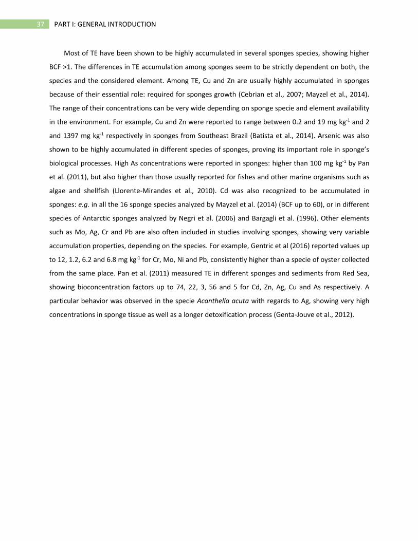
Figure 9. Comparison of TE measured in six sponges species (Cacospongia scalaris, Spongia officinalis, Spongia agaricina,
Agelas oroides, Chondrosia reniformis Nardo and Cliona viridis) and a common mussel (Mytilus galloprovincialis). Adapted from
Perez et al., 2003.
In conclusion, several properties make sponges good models for biomonitor TE pollution in coastal
ecosystems. Among TE, Cu and Zn seem to be better accumulated in oysters and mussels. Sponges have
shown to be better accumulators of other elements such as As, Ag and Ni.
3. TRACE ELEMENTS ANALYSIS
As a consequence of the increasing interest in TE analyses in different matrices, several
techniques have been developed in the last decades. The main challenges are linked to the need for
precise and accurate determination of these low-level analytes occurring usually in complex matrices
with particular chemical and physical features. Accurate TE determination in environmental samples is
of primary interest, as national, European and international legislations have reduced the maximum
concentration of several analytes in different environmental samples. A variety of techniques based on
different principles can be applied : electroanalytical methods, atomic spectrometry, X-ray and nuclear
techniques (Brown and Milton, 2005).
Atomic spectrometry techniques, such as Atomic Absorption Spectrometry (AAS), Inductively
Coupled Plasma Atomic Emission Spectrometry (ICP-AES) and Inductively Coupled Plasma Mass
Spectrometry (ICP-MS) are very sensitive and capable of determining several elements within a limited
amount of sample in a few minutes. These methodologies are extremely useful for the determination of
39 PART I: GENERAL INTRODUCTION
total amount of TE in environmental samples (Bermejo-Barrera et al., 1996; Damiano et al., 2011; Barats
et al., 2014; Wysocka and Vassileva, 2016; Wang et al., 2017). The atomic spectrometric techniques used
in this study (AAS and ICP-MS) imply the atomization and ionization of the samples, and their analysis
according to their interaction with electromagnetic radiation or their mass (Brown and Milton, 2005).
Very often the analysis of environmental samples by AAS and ICP-MS implies a sample preparation step:
e.g., microwave digestion and solid-liquid extraction. This step might be responsible for systematic bias
due to analyte loss, contamination, variability in analyte recovery. This preparation can represent a
significant contribution to the total uncertainty (Barwick and Ellison, 1999). The increasing need for
reliable data on TE concentration in a variety of environmental matrices has led to the production of
several Certified Reference Materials (CRMs) used to assess the quality of the analytical method both in
the development and in the application stages. The use of CRMs, when available, is especially needed
when sample preparation is needed, to verify the correctness of the procedure and to identify the
source of possible errors related to recovery and contaminations. The use of procedural blanks is also of
crucial importance for the assessment of the method quality and to check possible contaminations
occurring during the sample preparation.
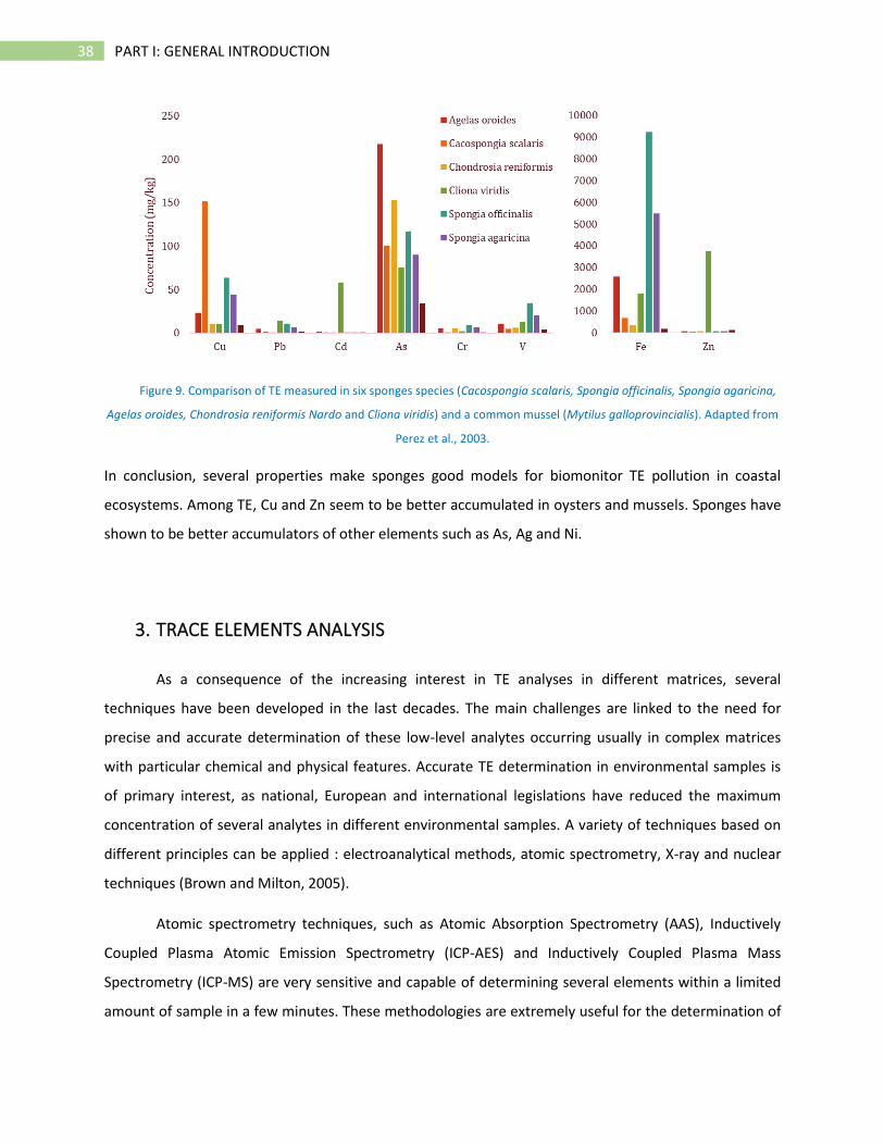
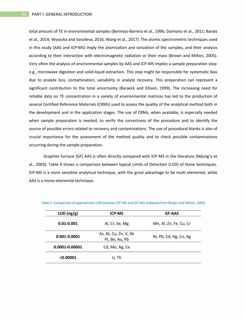
Graphite furnace (GF) AAS is often directly compared with ICP-MS in the literature (Ndung’u et
al., 2003). Table 4 shows a comparison between typical Limits of Detection (LOD) of these techniques.
ICP-MS is a more sensitive analytical technique, with the great advantage to be multi elemental, while
AAS is a mono-elemental technique.
Table 4. Comparison of approximate LOD between ICP-MS and GF-AAS (Adapted from Brown and Milton, 2005)
LOD (ng/g) ICP-MS GF-AAS
0.01-0.001 Al, Cr, Se, Mg Mn, Al, Zn, Fe, Cu, Cr
0.001-0.0001 As, Ni, Cu, Zn, V, Sb
Ni, Pb, Cd, Hg, Co, Ag Pt, Be, Au, Pb
0.0001-0.00001 Cd, Mo, Ag, Ce
<0.00001 U, Th
40 PART I: GENERAL INTRODUCTION
3.1. Atomic Absorption Spectrometry
AAS is particularly indicated for the measurement of major elements. It can be used with Flame
(F-AAS) or Graphite Furnace (GF-AAS or ET-AAS) atomizers. F-AAS typically works with liquid, and it is
relatively inexpensive and simple to operate. It requires a large sample volume (around 10 mL). This
analytical method is not indicated for some refractory elements such as Zr, As and Se, since the flame
working temperature are not sufficiently high, but it is particularly indicated for the measurement of
major elements in sediment and soil samples previously mineralised, e.g. in sediments such as Fe, Zn
and Mn (10-10000 mg Kg-1) (Loring and Rantala, 1992). GF-AAS exibits LOD typically 10-100 times lower
compared to F-AAS (Brown and Milton, 2005). The atomization takes place in a graphite furnace at
higher temperature than atomization in the flame and the samples can be liquid or solid. Solid Sampling
(SS) GF-AAS is very promising and finds already several application (Belarra et al., 2002). Since the
sample preparation step is not necessary, the risk of contamination and losses of analyte are removed.
Relatively small quantities of solid (50-500 mg) may be analysed. Many of the interferences from which
GF-AAS used to suffer (mostly associated with the sample matrix) can now be overcome with a
combination of background correction and matrix modification (Brown and Milton, 2005). Another
advantage of the use of (SS) GF-AAS is the possibility to work with fast programs, in which drying and
pyrolisis steps are drastically shortened or even eliminated (Mandjukov et al., 2015). This aspect not
only represents an advantage since it reduces the analysis time, but it also reduces the possibility of
analyte losses, especially for volatile elements such as Hg and As. The recent introduction in the market
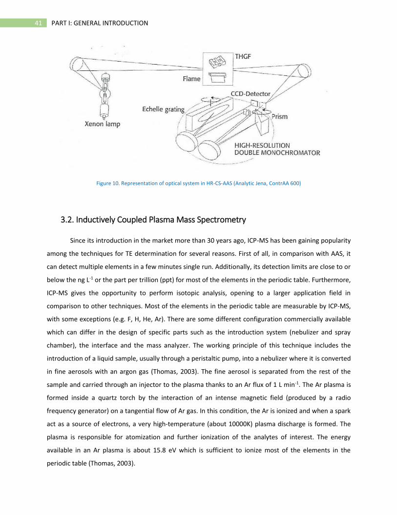
of instruments equipped with High Resolution Continuos Source (HR-CS) and a charged coupled device
(CCD) array detector has allowed several limitation due to classical line sources (LS) to be overcome
(Figure 8). The continuous background covering the spectral range observed by the array detector is
corrected automatically using correction pixels on both sides of the analytical line. In difference, the
structured background can be corrected using reference spectra and a least-squares algorithm (Welz et
al., 2007). In such configuration, it is possible to monitor not only the absorbance over time, as in classic
LS AAS but a 3D information is also provided, about absorbance over time and over wavelength. This
helps in avoiding interferences and generally in the method development stage.
41 PART I: GENERAL INTRODUCTION
Figure 10. Representation of optical system in HR-CS-AAS (Analytic Jena, ContrAA 600)
3.2. Inductively Coupled Plasma Mass Spectrometry
Since its introduction in the market more than 30 years ago, ICP-MS has been gaining popularity
among the techniques for TE determination for several reasons. First of all, in comparison with AAS, it
can detect multiple elements in a few minutes single run. Additionally, its detection limits are close to or
below the ng L-1 or the part per trillion (ppt) for most of the elements in the periodic table. Furthermore,
ICP-MS gives the opportunity to perform isotopic analysis, opening to a larger application field in
comparison to other techniques. Most of the elements in the periodic table are measurable by ICP-MS,
with some exceptions (e.g. F, H, He, Ar). There are some different configuration commercially available
which can differ in the design of specific parts such as the introduction system (nebulizer and spray
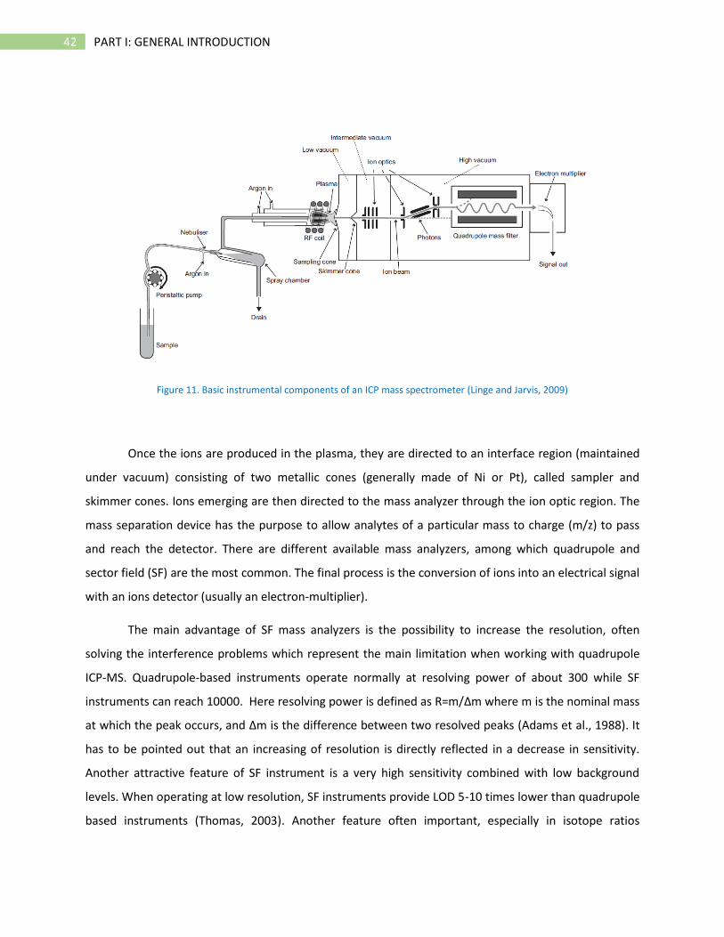
chamber), the interface and the mass analyzer. The working principle of this technique includes the
introduction of a liquid sample, usually through a peristaltic pump, into a nebulizer where it is converted
in fine aerosols with an argon gas (Thomas, 2003). The fine aerosol is separated from the rest of the
sample and carried through an injector to the plasma thanks to an Ar flux of 1 L min-1. The Ar plasma is
formed inside a quartz torch by the interaction of an intense magnetic field (produced by a radio
frequency generator) on a tangential flow of Ar gas. In this condition, the Ar is ionized and when a spark
act as a source of electrons, a very high-temperature (about 10000K) plasma discharge is formed. The
plasma is responsible for atomization and further ionization of the analytes of interest. The energy
available in an Ar plasma is about 15.8 eV which is sufficient to ionize most of the elements in the
periodic table (Thomas, 2003).
42 PART I: GENERAL INTRODUCTION
Figure 11. Basic instrumental components of an ICP mass spectrometer (Linge and Jarvis, 2009)
Once the ions are produced in the plasma, they are directed to an interface region (maintained
under vacuum) consisting of two metallic cones (generally made of Ni or Pt), called sampler and
skimmer cones. Ions emerging are then directed to the mass analyzer through the ion optic region. The
mass separation device has the purpose to allow analytes of a particular mass to charge (m/z) to pass
and reach the detector. There are different available mass analyzers, among which quadrupole and
sector field (SF) are the most common. The final process is the conversion of ions into an electrical signal
with an ions detector (usually an electron-multiplier).
The main advantage of SF mass analyzers is the possibility to increase the resolution, often
solving the interference problems which represent the main limitation when working with quadrupole
ICP-MS. Quadrupole-based instruments operate normally at resolving power of about 300 while SF
instruments can reach 10000. Here resolving power is defined as R=m/Δm where m is the nominal mass
at which the peak occurs, and Δm is the difference between two resolved peaks (Adams et al., 1988). It
has to be pointed out that an increasing of resolution is directly reflected in a decrease in sensitivity.
Another attractive feature of SF instrument is a very high sensitivity combined with low background
levels. When operating at low resolution, SF instruments provide LOD 5-10 times lower than quadrupole
based instruments (Thomas, 2003). Another feature often important, especially in isotope ratios
43 PART I: GENERAL INTRODUCTION
measurements is the precision of the obtained result, normally expressed by RSD% (Relative Standard
Deviation). Typical RSD obtained using Q-ICP-MS is in the range of 0.1-1% while it reaches 0.04% in SF
based instruments (with single detector) and up to 0.01% when the instrument is equipped with multi-
collector (Roehl et al., 1995; Quetel et al., 2000; Galy et al., 2003; Yang et al., 2003). (Q) ICPMS are
rather used for quantification of trace elements whereas (SF) ICPMS and (MC) ICPMS are the best
techniques for isotopic measurements of TE.
ICP-MS is often coupled with other techniques in order to perform trace element speciation
analysis. For instance, High Performance Liquid Chromatography (HPLC) coupled with ICP-MS has been
extensively used in the speciation analysis of arsenic and mercury in different matrices (Jagtap et al.,
2011; Raber et al., 2012; Stiboller et al., 2015; Jagtap and Maher, 2015). HPLC-ICP-MS has become the
main analytical technique of speciation analysis in the last 20 years. This hyphenated technique is robust
and sensitive and it is capable to give a complete picture of the elemental species in solution
(Francesconi and Sperling, 2005). When performing speciation analysis on sediments and biota samples,
a solid-liquid extraction procedure is usually required before HPLC-ICP-MS analysis. This step is crucial
and delicate as it has to preserve the chemical forms separating the analyte from the interfering matrix
without loss, contamination, or change of speciation, and with the minimum of interferences
(Leermakers et al., 2005).
44 PART I: GENERAL INTRODUCTION
REFERENCES
Abrahim, G.M.S., Parker, R.J., 2008. Assessment of heavy metal enrichment factors and the degree of contamination in marine sediments from Tamaki Estuary, Auckland, New Zealand. Environ. Monit. Assess. 136, 227–238. https://doi.org/10.1007/s10661-007-9678-2
Adams, F., Gijbels, R., Van Grieken, R., 1988. Inorganic Mass Spectrometry. John Wiley & Sons.
Aide, M.T., Aide, C., 2012. Rare Earth Elements: Their Importance in Understanding Soil Genesis. ISRN Soil Sci. 2012, 1–11. https://doi.org/10.5402/2012/783876
Alleman, L.Y., Hamelin, B., Véron, A.J., Miquel, J.-C., Heussner, S., 2000. Lead sources and transfer in the coastal Mediterranean: evidence from stable lead isotopes in marine particles. Deep Sea Res. Part II Top. Stud. Oceanogr. 47, 2257–2279. https://doi.org/10.1016/S0967-0645(00)00024-2
Aloupi, M., Angelidis, M.., 2001. Geochemistry of natural and anthropogenic metals in the coastal sediments of the island of Lesvos, Aegean Sea. Environ. Pollut. 113, 211–219. https://doi.org/10.1016/S0269-7491(00)00173-1
Aly, W., Williams, I.D., Hudson, M.D., 2013. Metal contamination in water, sediment and biota from a semi-enclosed coastal area. Environ. Monit. Assess. 185, 3879–3895. https://doi.org/10.1007/s10661-012-2837-0
AMPS Expert Group, 2005. Contributions of the Expert Group on Analysis and Monitoring of Priority Substances to the Water Framework Directive. EU Report EUR 21587.
Anderson, G.L., Williams, J., Hille, R., 1992. The purification and characterization of arsenite oxidase from Alcaligenes faecalis, a molybdenum-containing hydroxylase. J. Biol. Chem. 267, 23674–23682.
Andrewes, P., Demarini, D.M., Funasaka, K., Wallace, K., Lai, V.W.M., Sun, H., Cullen, W.R., Kitchin, K.T., 2004. Do arsenosugars pose a risk to human health? The comparative toxicities of a trivalent and pentavalent arsenosugar. Environ. Sci. Technol. 38, 4140–4148. https://doi.org/10.1021/es035440f
Angelidis, M.O., Radakovitch, O., Veron, A., Aloupi, M., Heussner, S., Price, B., 2011. Anthropogenic metal contamination and sapropel imprints in deep Mediterranean sediments. Mar. Pollut. Bull. 62, 1041–1052. https://doi.org/10.1016/j.marpolbul.2011.02.030
Anjum, K., Abbas, S.Q., Shah, S.A., Akhter, N., Batool, S., Hassan, S.S., 2016. Marine Sponges as a Drug Treasure. Biomol. Ther. 24, 347–362.
Araújo, M.F., Conceição, A., Barbosa, T., Lopes, M.T., Humanes, M., 2003. Elemental composition of marine sponges from the Berlengas Natural Park, western Portuguese coast. X-Ray Spectrom. 32, 428–433. https://doi.org/10.1002/xrs.660
Aresta, A., Marzano, C.N., Lopane, C., Corriero, G., Longo, C., Zambonin, C., Stabili, L., 2015. Analytical investigations on the lindane bioremediation capability of the demosponge Hymeniacidon perlevis. Mar. Pollut. Bull. 90, 143–149. https://doi.org/10.1016/j.marpolbul.2014.11.003
Armstrong-Altrin, J.S., Verma, S.P., Madhavaraju, J., Lee, Y. Il, Ramasamy, S., 2003. Geochemistry of Upper Miocene Kudankulam Limestones, Southern India. Int. Geol. Rev. 45, 16–26. https://doi.org/10.2747/0020-6814.45.1.16
45 PART I: GENERAL INTRODUCTION
Ashraf, A., Saion, E., Gharibshahi, E., Kamari, H.M., Yap, C.K., Hamzah, M.S., Elias, M.S., 2017. Distribution of Trace Elements in Core Marine Sediments of Coastal East Malaysia by Instrumental Neutron Activation Analysis. Appl. Radiat. Isot. 122, 96–105. https://doi.org/10.1016/j.apradiso.2017.01.006
Ashraf, A., Saion, E., Gharibshahi, E., Mohamed Kamari, H., Chee Kong, Y., Suhaimi Hamzah, M., Suhaimi Elias, M., 2016. Rare earth elements in core marine sediments of coastal East Malaysia by instrumental neutron activation analysis. Appl. Radiat. Isot. 107, 17–23. https://doi.org/10.1016/j.apradiso.2015.09.004
ATSDR, 2007. Toxicological Profile for Arsenic, U.S Public Health Service, Agency for Toxic Substances and Disease Registry. https://doi.org/http://dx.doi.org/10.1155/2013/286524
Ault, W.U., Senechal, R.G., Erlebach, W.E., 1970. Isotopic Composition as a Natural Tracer of Lead in the Environment: Discussions Follow. Environ. Sci. Technol. 4, 305–313. https://doi.org/10.1021/es60039a001
Azemard, S., Vassileva, E., 2015. Determination of methylmercury in marine biota samples with advanced mercury analyzer: Method validation. Food Chem. 176, 367–375. https://doi.org/10.1016/j.foodchem.2014.12.085
Azizur Rahman, M., Hasegawa, H., Peter Lim, R., 2012. Bioaccumulation, biotransformation and trophic transfer of arsenic in the aquatic food chain. Environ. Res. 116, 118–135. https://doi.org/10.1016/j.envres.2012.03.014
Bagul V. R., S.D.N., 2015. New perspective on heavy metal pollution of water. J. Chem. Pharm. Res. 7, 700–705.
Barats, A., Féraud, G., Potot, C., Philippinini, V., Travi, Y., Durrieu, G., Dubar, M., Simler, R., 2014. Naturally dissolved arsenic concentrations in the Alpine/Mediterranean Var River watershed (France). Sci. Total Environ. 473–474, 422–436. https://doi.org/10.1016/J.SCITOTENV.2013.12.007
Bargagli, R., Nelli, L., Ancora, S., Focardi, S., 1996. Elevated cadmium accumulation in marine organisms from Terra Nova Bay (Antarctica). Polar Biol. 16, 513–520. https://doi.org/10.1007/BF02329071
Barwick, V.J., Ellison, S.L.R., 1999. Measurement uncertainty: Approaches to the evaluation of uncertainties associated with recovery†. Analyst 124, 981–990. https://doi.org/10.1039/a901845j
Batista, D., Muricy, G., Rocha, R.C., Miekeley, N.F., 2014. Marine sponges with contrasting life histories can be complementary biomonitors of heavy metal pollution in coastal ecosystems. Environ. Sci. Pollut. Res. 21, 5785–5794. https://doi.org/10.1007/s11356-014-2530-7
Baudrimont, M., Schäfer, J., Marie, V., Maury-Brachet, R., Bossy, C., Boudou, A., Blanc, G., 2005. Geochemical survey and metal bioaccumulation of three bivalve species (Crassostrea gigas, Cerastoderma edule and Ruditapes philippinarum) in the Nord Médoc salt marshes (Gironde estuary, France). Sci. Total Environ. https://doi.org/10.1016/j.scitotenv.2004.07.009
Beauchemin, D., 2008. Inductively coupled plasma mass spectrometry. Anal. Chem. 80, 4455–4486.
Bednar, A.J., Garbarino, J.R., Burkhardt, M.R., Ranville, J.F., Wildeman, T.R., 2004. Field and laboratory arsenic speciation methods and their application to natural-water analysis. Water Res. 38, 355–364. https://doi.org/10.1016/j.watres.2003.09.034
46 PART I: GENERAL INTRODUCTION
Beeson, R., 1984. The use of the fine fractions of stream sediments in geochemical exploration in arid and semi-arid terrains. J. Geochemical Explor. 22, 119–132. https://doi.org/10.1016/0375-6742(84)90009-8
Belarra, M.A., Resano, M., Vanhaecke, F., Moens, L., 2002. Direct solid sampling with electrothermal vaporization/atomization: What for and how? TrAC - Trends Anal. Chem. 21, 828–839. https://doi.org/10.1016/S0165-9936(02)01206-2
Bell, J.J., 2008. The functional roles of marine sponges. Estuar. Coast. Shelf Sci. 79, 341–353. https://doi.org/10.1016/j.ecss.2008.05.002
Bennett, W.W., Teasdale, P.R., Panther, J.G., Welsh, D.T., Zhao, H., Jolley, D.F., 2012. Investigating arsenic speciation and mobilization in sediments with DGT and DET: A mesocosm evaluation of oxic-anoxic transitions. Environ. Sci. Technol. 46, 3981–3989. https://doi.org/10.1021/es204484k
Bentley, R., Chasteen, T.G., 2002. Microbial Methylation of Metalloids: Arsenic, Antimony, and Bismuth. Microbiol. Mol. Biol. Rev. 66, 250–271.
Bermejo-Barrera, P., Barciela-Alonso, M.C., Moreda-Piñeiro, J., González-Sixto, C., Bermejo-Barrera, a., 1996. Determination of trace metals (As, Cd, Hg, Pb and Sn) in marine sediment slurry samples by electrothermal atomic absorption spectrometry using palladium as a chemical modifier. Spectrochim. Acta Part B At. Spectrosc. 51, 1235–1244. https://doi.org/10.1016/0584-8547(96)01487-5
Bermudez-Lugo, O., 2014. 2012 Minerals Yearbook, Usgs- 2012 Minerals Yearbook.
Berthet, B., Mouneyrac, C., Pérez, T., Amiard-Triquet, C., 2005. Metallothionein concentration in sponges (Spongia officinalis) as a biomarker of metal contamination. Comp. Biochem. Physiol. - C Toxicol. Pharmacol. 141, 306–313. https://doi.org/10.1016/j.cca.2005.07.008
Bhuiyan, M.A.H., Parvez, L., Islam, M.A., Dampare, S.B., Suzuki, S., 2010. Heavy metal pollution of coal mine-affected agricultural soils in the northern part of Bangladesh. J. Hazard. Mater. 173, 384–392. https://doi.org/10.1016/j.jhazmat.2009.08.085
Birch, G.F., Melwani, A., Lee, J.H., Apostolatos, C., 2014. The discrepancy in concentration of metals (Cu, Pb and Zn) in oyster tissue (Saccostrea glomerata) and ambient bottom sediment (Sydney estuary, Australia). Mar. Pollut. Bull. 80, 263–274. https://doi.org/10.1016/j.marpolbul.2013.12.005
Bocher, P., Caurant, F., Miramand, P., Cherel, Y., Bustamante, P., 2003. Influence of the diet on the bioaccumulation of heavy metals in zooplankton-eating petrels at Kerguelen archipelago, Southern Indian Ocean. Polar Biol. 26, 759–767. https://doi.org/10.1007/s00300-003-0552-6
Bohari, Y., Astruc, A., Astruc, M., Cloud, J., 2001. Improvements of hydride generation for the speciation of arsenic in natural freshwater samples by HPLC-HG-AFS. J. Anal. At. Spectrom. 16, 774–778. https://doi.org/10.1039/B101591P
Bollhöfer, A., Rosman, K.J.., 2000. Isotopic source signatures for atmospheric lead: the Southern Hemisphere. Geochim. Cosmochim. Acta 64, 3251–3262. https://doi.org/10.1016/S0016-7037(00)00436-1
Bollhöfer, A., Rosman, K.J.R., 2001. Isotopic source signatures for atmospheric lead: The Northern Hemisphere. Geochim. Cosmochim. Acta 65, 1727–1740. https://doi.org/10.1016/S0016-7037(00)00630-X

47 PART I: GENERAL INTRODUCTION
Bossy, A., 2010. Origines de l’arsenic dans les eaux, sols et sédiments du district aurifère de St-Yrieix-la-Perche (Limousin, France) : contribution du lessivage des phases porteuses d’arsenic. Université de Limoges.
Bowen, H.J.M., 1966. The Uptake and Excretion of Elements by Organisms, in: Trace Elements in Biochemistry. Academic Press London, pp. 85–101.
Bremner, J.M., Willis, J.P., 1993. Mineralogy and geochemistry of the clay fraction of sediments from the Namibian continental margin and the adjacent hinterland. Mar. Geol. 115, 85–116. https://doi.org/10.1016/0025-3227(93)90076-8
Briant, N., Chouvelon, T., Martinez, L., Brach-Papa, C., Chiffoleau, J.F., Savoye, N., Sonke, J., Knoery, J., 2017. Spatial and temporal distribution of mercury and methylmercury in bivalves from the French coastline. Mar. Pollut. Bull. 114, 1096–1102. https://doi.org/10.1016/j.marpolbul.2016.10.018
Briefing, 1980. Namibia in the frontline: the political economy of decolonisation in South Africa’s colony. Rev. Afr. Polit. Econ. https://doi.org/10.1080/03056248008703415
Broadley, M.R., White, P.J., Hammond, J.P., Zelko, I., Lux, A., 2007. Zinc in plants. New Phytol. 173, 677–702. https://doi.org/10.1111/j.1469-8137.2007.01996.x
Brongersma-Sanders, M., Stephan, K.M., Kwee, T.., De Bruin, M., 1980. DISTRIBUTION OF MINOR ELEMENTS IN CORES FROM THE SOUTH- WEST AFRICA SHELF WITH NOTES ON PLANKTON AND FISH MORTALITY Along the coast of Southwest Africa a belt of olive-green diatomaceous muds is f o u n d between 19 ° S and 25 ° S , bordered on the wester. Mar. Geol. 37, 91–132.
Brown, J.L., Kitchin, K.T., George, M., 1997. Dimethylarsinic acid treatment alters six different rat biochemical parameters: Relevance to arsenic carcinogenesis. Teratog. Carcinog. Mutagen. 17, 71–84. https://doi.org/10.1002/(SICI)1520-6866(1997)17:2<71::AID-TCM3>3.0.CO;2-B
Brown, J.S., 1962. Ore leads and isotopes. Econ. Geol. 57, 673–720. https://doi.org/10.2113/gsecongeo.57.5.673
Brown, R.J.C., Milton, M.J.T., 2005. Analytical techniques for trace element analysis: An overview. TrAC - Trends Anal. Chem. 24, 266–274. https://doi.org/10.1016/j.trac.2004.11.010
Bruland, K.W., Bertine, K., Koide, M., Goldberg, E.D., 1974. History of metal pollution in southern California coastal zone. Environ. Sci. Technol. 8, 425–432. https://doi.org/10.1021/es60090a010
Bruland, K.W., Lohan, M.C., 2003. Controls of trace metals in seawater, in: Treatise on Geochemistry. Elsevier Ltd, pp. 23–47.
Bryan, G.W., Langston, W.J., 1992. Bioavailability, accumulation and effects of heavy metals in sediments with special reference to United Kingdom estuaries: a review. Environ. Pollut. 76, 89–131. https://doi.org/10.1016/0269-7491(92)90099-V
Bu, H., Song, X., Guo, F., 2017. Dissolved trace elements in a nitrogen-polluted river near to the Liaodong Bay in Northeast China. Mar. Pollut. Bull. 114, 547–554. https://doi.org/10.1016/j.marpolbul.2016.09.003
Cabon, J.Y., Cabon, N., 2000. Speciation of major arsenic species in seawater by flow injection hydride generation atomic absorption spectrometry. Fresenius. J. Anal. Chem. 368, 484–9. https://doi.org/10.1007/s002160000526
48 PART I: GENERAL INTRODUCTION
Cabrita, M.T., Padeiro, A., Amaro, E., dos Santos, M.C., Leppe, M., Verkulich, S., Hughes, K.A., Peter, H.-U., Canário, J., 2017. Evaluating trace element bioavailability and potential transfer into marine food chains using immobilised diatom model species Phaeodactylum tricornutum , on King George Island, Antarctica. Mar. Pollut. Bull. 121, 192–200. https://doi.org/10.1016/j.marpolbul.2017.05.059
Caccia, V.G., Millero, F.J., Palanques, A., 2003. The distribution of trace metals in Florida Bay sediments. Mar. Pollut. Bull. 46, 1420–1433. https://doi.org/10.1016/S0025-326X(03)00288-1
Calvert, S.E., Price, N.B., 1970. Minor Metal Contents of Recent Organic-rich Sediments off South West Africa. Nature 227, 593–595.
Cantillo, A.Y., 1998. Comparison of results of Mussel Watch Programs of the United States and France with Worldwide Mussel Watch Studies. Mar. Pollut. Bull. 36, 712–717. https://doi.org/10.1016/S0025-326X(98)00049-6
Carere, M., Dulio, V., Hanke, G., Polesello, S., 2012. Guidance for sediment and biota monitoring under the Common Implementation Strategy for the Water Framework Directive. TrAC - Trends Anal. Chem. 36, 15–24. https://doi.org/10.1016/j.trac.2012.03.005
Carpenè, E., Andreani, G., Isani, G., 2017. Trace elements in unconventional animals: A 40-year experience. J. Trace Elem. Med. Biol. 43, 169–179. https://doi.org/10.1016/j.jtemb.2017.02.003
Caumette, G., Koch, I., Reimer, K.J., 2012. Arsenobetaine formation in plankton: a review of studies at the base of the aquatic food chain. J. Environ. Monit. 14, 2841. https://doi.org/10.1039/c2em30572k
Cebrian, E., Martí, R., Uriz, J.M., Turon, X., 2003. Sublethal effects of contamination on the Mediterranean sponge Crambe crambe: Metal accumulation and biological responses. Mar. Pollut. Bull. 46, 1273–1284. https://doi.org/10.1016/S0025-326X(03)00190-5
Cebrian, E., Uriz, M.-J., Turon, X., 2007. Sponges as biomonitors of heavy metals in spatial and temporal surveys in northwestern mediterranean: multispecies comparison. Environ. Toxicol. Chem. 26, 2430–2439. https://doi.org/10.1897/07-292.1
Cebrian, E., Uriz, M.J., 2007. Contrasting effects of heavy metals on sponge cell behavior. Arch. Environ. Contam. Toxicol. 53, 552–558. https://doi.org/10.1007/s00244-006-0257-2
Chai, Z.F., Zhang, Z.Y., Feng, W.Y., Chen, C.Y., Xu, D.D., Hou, X.L., 2004. Study of chemical speciation of trace elements by molecular activation analysis and other nuclear techniques. J. Anal. At. Spectrom. 19, 26–33. https://doi.org/10.1039/B307337H
Charlesworth, M.E., Chenery, S., Mellor, A., Service, M., 2006. Isotopic composition and concentration of Pb in suspended particulate matter of the Irish Sea reveals distribution and sources. Mar. Pollut. Bull. 52, 81–88. https://doi.org/10.1016/j.marpolbul.2005.08.009
Chen, C.Y., Darren, M.., Williams, J.J., Fisher, N.S., 2016. Metal Bioaccumulation by Estuarine Food Webs in New England, USA. J. Mar. Sci. Engeneer 4, 41. https://doi.org/10.1016/j.cell.2016.05.007.Mapping
Chen, C.Y., Stemberger, R.S., Klaue, B., Blum, J.D., Pickhardt, P.C., Folt, C.L., 2000. Accumulation of heavy metals in food web components across a gradient of lakes. Limnol. Oceanogr. 45, 1525–1536. https://doi.org/10.4319/lo.2000.45.7.1525
49 PART I: GENERAL INTRODUCTION
Chen, L., Liu, M., Fan, R., Ma, S., Xu, Z., Ren, M., He, Q., 2013. Mercury speciation and emission from municipal solid waste incinerators in the Pearl River Delta, South China. Sci. Total Environ. 447, 396–402. https://doi.org/10.1016/j.scitotenv.2013.01.018
Chester, R., Murphy, K.J.T., Lin, F.J., Berry, A.S., Bradshaw, G.A., Corcoran, P.A., 1993. Factors controlling the solubilities of trace metals from non-remote aerosols deposited to the sea surface by the “dry” deposition mode. Mar. Chem. 42, 107–126. https://doi.org/10.1016/0304-4203(93)90241-F
Ciardullo, S., Aureli, F., Raggi, A., Cubadda, F., 2010. Arsenic speciation in freshwater fish: Focus on extraction and mass balance. Talanta 81, 213–221. https://doi.org/10.1016/j.talanta.2009.11.060
Cidu, R., Frau, F., 2009. Distribution of trace elements in filtered and non filtered aqueous fractions: Insights from rivers and streams of Sardinia (Italy). Appl. Geochemistry 24, 611–623. https://doi.org/10.1016/j.apgeochem.2008.12.013
Clark, H., 1968. On the Spongiae ciliatae as infusoria flagellata, or observations on the structure, animality and relationship of Leucosolenia botryoides, Bowerbank. Ann. Mag. Nat. Hist. 4, 133–142.
Clowes, L.A., Francesconi, K.A., 2004. Uptake and elimination of arsenobetaine by the mussel Mytilus edulis is related to salinity. Comp. Biochem. Physiol. - C Toxicol. Pharmacol. 137, 35–42. https://doi.org/10.1016/j.cca.2003.11.003
Coulibaly, M., Bamba, D., Yao, N.A., Zoro, E.G., El Rhazi, M., 2016. Some aspects of speciation and reactivity of mercury in various matrices. Comptes Rendus Chim. 19, 832–840. https://doi.org/10.1016/j.crci.2016.02.005
Covelli, S., Fontolan, G., 1997. Application of a normalization procedure in determining regional geochemical baselines. Environ. Geol. 30, 34–45. https://doi.org/10.1007/s002540050130
Crompton, T.R., Crompton, T.R., 1989. Chapter 8 – Organometallic compounds, in: Analysis of Seawater. pp. 336–359. https://doi.org/10.1016/B978-0-407-01610-1.50011-4
Cullen, W.R., Reimer, K.J., 1989. Arsenic speciation in the environment. Chem. Rev. 89, 713–764. https://doi.org/10.1021/cr00094a002
Dahms, S., van der Bank, F.H., Greenfield, R., 2014. A baseline study of metal contamination along the Namibian coastline for Perna perna and Choromytilus meridionalis. Mar. Pollut. Bull. 85, 297–305. https://doi.org/10.1016/j.marpolbul.2014.05.037
Damiano, S., Papetti, P., Menesatti, P., 2011. Accumulation of heavy metals to assess the health status of swordfish in a comparative analysis of Mediterranean and Atlantic areas. Mar. Pollut. Bull. 62, 1920–1925. https://doi.org/10.1016/j.marpolbul.2011.04.028
De Gregori H., I., Pinochet C., H., Arancibia J., M., Vidal B., A., 1996. Grain Size Effect on Trace Metals Distribution in Sediments from Two Coastal Areas of Chile. Bull. Environ. Contam. Toxicol. 57, 163–170. https://doi.org/10.1007/s001289900170
de Mestre, C., Maher, W., Roberts, D., Broad, A., Krikowa, F., Davis, A.R., 2012. Sponges as sentinels: Patterns of spatial and intra-individual variation in trace metal concentration. Mar. Pollut. Bull. 64, 80–89. https://doi.org/10.1016/j.marpolbul.2011.10.020
Debord, J., Pourmand, A., Jantzi, S., Panicker, S., Almirall, J., 2017. Profiling of Heroin and Assignment of
50 PART I: GENERAL INTRODUCTION
Provenance by 87 Sr/ 86 Sr Isotope Ratio Analysis. Inorganica Chim. Acta. https://doi.org/10.1016/j.ica.2017.07.049
Delnomdedieu, M., Basti, M.M., Otvos, J.D., Thomas, D.J., 1994. Reduction and binding of arsenate and dimethylarsinate by glutathione: a magnetic resonance study. Chem. Biol. Interact. 90, 139–155. https://doi.org/10.1016/0009-2797(94)90099-X
Denton, G.R.W., Concepcion, L.P., Wood, H.R., Morrison, R.J., 2006. Trace metals in marine organisms from four harbours in Guam. Mar. Pollut. Bull. 52, 1784–1804. https://doi.org/10.1016/j.marpolbul.2006.09.010
Diaz, M.C., Rutzler, K., 2001. Sponges: an essential component of Caribbean coral reefs. Bull. Mar. Sci. 69, 535–546.
Drivelos, S.A., Georgiou, C.A., 2012. Multi-element and multi-isotope-ratio analysis to determine the geographical origin of foods in the European Union. TrAC Trends Anal. Chem. 40, 38–51. https://doi.org/10.1016/j.trac.2012.08.003
Dudás, F.Ö., LeBlanc, S.A., Carter, S.W., Bowring, S.A., 2016. Pb and Sr concentrations and isotopic compositions in prehistoric North American teeth: A methodological study. Chem. Geol. 429, 21–32. https://doi.org/10.1016/j.chemgeo.2016.03.003
Duncan, E.G., Maher, W.A., Foster, S.D., 2015. Contribution of arsenic species in unicellular algae to the cycling of arsenic in marine ecosystems. Environ. Sci. Technol. 49, 33–50. https://doi.org/10.1021/es504074z
Edmonds, J.S., Francesconi, K.A., Stick, R. V, 1993. Arsenic compounds from marine organisms. Nat. Prod. Rep. 10, 421–428.
Edmonds, J.S., Shibata, Y., Francesconi, K. a, Rippingale, R.J., Morita, M., 1997. Arsenic transformations in short marine food chains studied by HPLC-ICP MS. Appl. Organomet. Chem. 11, 281–287. https://doi.org/10.1002/(sici)1099-0739(199704)11:4<281::aid-aoc581>3.3.co;2-j
Elbaz-Poulichet, F., Holliger, P., Martin, J.M., Petit, D., 1986. Stable lead isotopes ratios in major french rivers and estuaries. Sci. Total Environ. 54, 61–76. https://doi.org/10.1016/0048-9697(86)90256-1
Elderfield, H., 2003. Introduction to Volume 6, in: Turekian, K.K., Holland, H.D. (Eds.), Treatise on Geochemistry. Elsevier Ltd, pp. 15–27.
Ellam, R.M., 2010. The graphical presentation of lead isotope data for environmental source apportionment. Sci. Total Environ. 408, 3490–3492. https://doi.org/10.1016/j.scitotenv.2010.03.037
Ellwood, M.J., Maher, W.A., 2003. Measurement of arsenic species in marine sediments by high-performance liquid chromatography-inductively coupled plasma mass spectrometry. Anal. Chim. Acta 477, 279–291. https://doi.org/10.1016/s0003-2670(02)01414-9
Esslemont, G., 2000. Heavy metals in seawater, marine sediments and corals from the Townsville section, Great Barrier Reef Marine Park, Queensland. Mar. Chem. 71, 215–231. https://doi.org/10.1016/S0304-4203(00)00050-5
Fang, T.-H., Hsiao, S.-H., Nan, F.-H., 2014. Nineteen trace elements in marine copepods collected from the coastal waters off northeastern Taiwan. Cont. Shelf Res. 91, 70–81.

51 PART I: GENERAL INTRODUCTION
https://doi.org/10.1016/j.csr.2014.09.003
FAO, 2007. Fishery Country Profile- The Republic of Namibia [WWW Document]. URL http://www.fao.org/fi/oldsite/FCP/en/NAM/profile.htm
FLETCHER, C.J.N., SWAINBANK, I.G., COLMAN, T.B., 1993. Metallogenic evolution in Wales: constraints from lead isotope modelling. J. Geol. Soc. London. 150, 77–82. https://doi.org/10.1144/gsjgs.150.1.0076
Forstner, U., 1982. Chemical forms of metal enrichment in recent sediments, in: Amstutz, G. (Ed.), Ore Genesis. Springer-Verlag New York, pp. 269–284.
Förstner, U., Ahlf, W., Calmano, W., 1989. Studies on the transfer of heavy metals between sedimentary phases with a multi-chamber device: Combined effects of salinity and redox variation. Mar. Chem. 28, 145–158. https://doi.org/10.1016/0304-4203(89)90192-8
Forstner, U., Wittmann, G., 1981. Metal pollution in the aquatic environment, 2nd revise. ed. Springer-Verlag New York.
Foster, S., Maher, W., 2016. Arsenobetaine and thio-arsenic species in marine macroalgae and herbivorous animals: Accumulated through trophic transfer or produced in situ? J. Environ. Sci. 49, 131–139. https://doi.org/10.1016/j.jes.2016.06.003
Francesconi, K.A., Sperling, M., 2005. Speciation analysis with HPLC-mass spectrometry: time to take stock. Analyst 130, 998. https://doi.org/10.1039/b504485p
Francesconi, K. a., 2010. Arsenic species in seafood: Origin and human health implications. Pure Appl. Chem. 82, 373–381. https://doi.org/10.1351/PAC-CON-09-07-01
Fütterer, D.K., Cojan, I., Renard, M., 2006. The solid phase of marine sediments, in: Marine Geochemistry. pp. 1–25.
Gadde, R.R., Laitinen, H.A., 1974. Studies of Heavy Metal Adsorption by Hydrous Iron and Manganese Oxides. Anal. Chem. 46, 2022–2026. https://doi.org/10.1021/ac60349a004
Galy, A., Pomies, C., Day, J.A., Pokrovsky, O.S., Schott, J., 2003. High precision measurement of germanium isotope ratio variations by multiple collector-inductively coupled plasma mass spectrometry. J. Anal. At. Spectrom. 18, 115–119. https://doi.org/10.1039/B210233A
Gazave, E., Carteron, S., Chenuil, A., Richelle-Maurer, E., Boury-Esnault, N., Borchiellini, C., 2010. Polyphyly of the genus Axinella and of the family Axinellidae (Porifera: Demospongiaep). Mol. Phylogenet. Evol. 57, 35–47. https://doi.org/10.1016/j.ympev.2010.05.028
Genta-Jouve, G., Cachet, N., Oberhänsli, F., Noyer, C., Teyssié, J.L., Thomas, O.P., Lacoue-Labarthe, T., 2012. Comparative bioaccumulation kinetics of trace elements in Mediterranean marine sponges. Chemosphere 89, 340–349. https://doi.org/10.1016/j.chemosphere.2012.04.052
Gentric, C., Rehel, K., Dufour, A., Sauleau, P., 2016. Bioaccumulation of metallic trace elements and organic pollutants in marine sponges from the South Brittany Coast, France. J. Environ. Sci. Heal. Part A 51, 213–219. https://doi.org/10.1080/10934529.2015.1094327
Gifford, S., Dunstan, R.H., O’Connor, W., Koller, C.E., MacFarlane, G.R., 2007. Aquatic zooremediation: deploying animals to remediate contaminated aquatic environments. Trends Biotechnol. 25, 60–65. https://doi.org/10.1016/j.tibtech.2006.12.002
52 PART I: GENERAL INTRODUCTION
Giusti, L., Zhang, H., 2002. Heavy metals and arsenic in sediments, mussels and marine water from Murano (Venice, Italy). Environ. Geochem. Health 24, 47–65. https://doi.org/10.1023/A:1013945117549
Gobas, F., 2001. Assessing Bioaccumulation Factors of Persistent Organic Pollutants in Aquatic Food-Chains, in: Persistent Organic Pollutants: Environmental Behaviour and Pathways of Human Exposure. pp. 145–165. https://doi.org/10.1007/978-1-4615-1571-5_6
Gong, Z., 2002. Arsenic speciation analysis. Talanta 58, 77–96. https://doi.org/10.1016/S0039-9140(02)00258-8
Goodenough, K.M., Schilling, J., Jonsson, E., Kalvig, P., Charles, N., Tuduri, J., Deady, E.A., Sadeghi, M., Schiellerup, H., M??ller, A., Bertrand, G., Arvanitidis, N., Eliopoulos, D.G., Shaw, R.A., Thrane, K., Keulen, N., 2016. Europe’s rare earth element resource potential: An overview of REE metallogenetic provinces and their geodynamic setting. Ore Geol. Rev. 72, 838–856. https://doi.org/10.1016/j.oregeorev.2015.09.019
Goran, P., 1981. The Carcinogenicity of Arsenic. Environ. Health Perspect. 40, 93–100.
Goyer, R.A., 2001. Toxic effects of metals, in: Klaassen, C.D. (Ed.), Casarett and Doull’s Toxicology: The Basic Science of Poisons. McGraw-Hill Publisher, pp. 811–867.
Grotti, M., Lagomarsino, C., Goessler, W., Francesconi, K.A., 2010. Arsenic speciation in marine organisms from Antarctic coastal environments. Environ. Chem. 7, 207–214. https://doi.org/10.1071/EN09131
Grotti, M., Soggia, F., Lagomarsino, C., Riva, S.D., Goessler, W., Francesconi, K.A., 2008. Natural variability and distribution of trace elements in marine organisms from Antarctic coastal environments. Antarct. Sci. 20, 39–52. https://doi.org/doi:10.1017/S0954102007000831
Grousset, F.E., Quetel, C.R., Thomas, B., Buat-Menard, P., Donard, O.F.X., Bucher, A., 1994. Transient Pb Isotopic Signatures in the Western European Atmosphere. Environ. Sci. Technol. 28, 1605–1608. https://doi.org/10.1021/es00058a011
Guan, Q., Cai, A., Wang, F., Wang, L., Wu, T., Pan, B., Song, N., Li, F., Lu, M., 2016. Heavy metals in the riverbed surface sediment of the Yellow River, China. Environ. Sci. Pollut. Res. 23, 24768–24780. https://doi.org/10.1007/s11356-016-7712-z
Guyonnet, D., Planchon, M., Rollat, A., Escalon, V., Tuduri, J., Charles, N., Vaxelaire, S., Dubois, D., Fargier, H., 2015. Material flow analysis applied to rare earth elements in Europe. J. Clean. Prod. 107, 215–228. https://doi.org/10.1016/J.JCLEPRO.2015.04.123
Hansmann, W., Köppel, V., 2000. Lead-istopes as tracers of pollutants in soils. Chem. Geol. 171, 123–144. https://doi.org/10.1016/S0009-2541(00)00230-8
Harada, M., 1995. Minamata Disease: Methylmercury Poisoning in Japan Caused by Environmental Pollution. Crit. Rev. Toxicol. 25, 1–24. https://doi.org/10.3109/10408449509089885
Hartwig, A., Jahnke, G., 2012. Toxic metals and metalloids in foods, in: Chemical Contaminants and Residues in Food. Elsevier, pp. 233–249. https://doi.org/10.1533/9780857095794.2.233
Hatje, V., Bruland, K.W., Flegal, A.R., 2016. Increases in Anthropogenic Gadolinium Anomalies and Rare Earth Element Concentrations in San Francisco Bay over a 20 Year Record. Environ. Sci. Technol. 50,

53 PART I: GENERAL INTRODUCTION
4159–4168. https://doi.org/10.1021/acs.est.5b04322
He, M., Wang, W.X., 2013. Bioaccessibility of 12 trace elements in marine molluscs. Food Chem. Toxicol. 55, 627–636. https://doi.org/10.1016/j.fct.2013.01.046
Heidari, B., Bakhtiari, A.R., Shirneshan, G., 2013. Concentrations of Cd, Cu, Pb and Zn in soft tissue of oyster (Saccostrea cucullata) collected from the Lengeh Port coast, Persian Gulf, Iran: A comparison with the permissible limits for public health. Food Chem. 141, 3014–3019. https://doi.org/10.1016/j.foodchem.2013.06.002
Hinrichs, J., Dellwig, O., Brumsack, H.-J., 2002. Lead in sediments and suspended particulate matter of the German Bight: natural versus anthropogenic origin. Appl. Geochemistry 17, 621–632. https://doi.org/10.1016/S0883-2927(01)00124-X
Hirner, A.V., Kritsotakis, K., Tobschall, H.J., 1990. Metal-organic associations in sediments—I. Comparison of unpolluted recent and ancient sediments and sediments affected by anthropogenic pollution. Appl. Geochemistry 5, 491–505. https://doi.org/10.1016/0883-2927(90)90023-X
Holser, W.T., 1997. Evaluation of the application of rare-earth elements to paleoceanography. Palaeogeogr. Palaeoclimatol. Palaeoecol. 132, 309–323. https://doi.org/10.1016/S0031-0182(97)00069-2
Hong, S., Khim, J.S., Park, J., Son, H.S., Choi, S.D., Choi, K., Ryu, J., Kim, C.Y., Chang, G.S., Giesy, J.P., 2014. Species- and tissue-specific bioaccumulation of arsenicals in various aquatic organisms from a highly industrialized area in the Pohang City, Korea. Environ. Pollut. 192, 27–35. https://doi.org/10.1016/j.envpol.2014.05.004
Hooper, J., van Soest, R., 2002. Systena porifera. A guide to the Classification of Sponges. Kluwer Academic/Plenum publishers, New York.
Hornung, H., Krom, M.D., Cohen, Y., 1989. Trace metal distribution in sediments and benthic fauna of Haifa Bay, Israel. Estuar. Coast. Shelf Sci. 29, 43–56. https://doi.org/10.1016/0272-7714(89)90072-3
Horowitz, A.J., 1991. A Primer on Sediment-Trace Element Chemistry. U.S.G.S. Open-File Rep. 2nd Editio, 136 (2 fiche).
Horowitz, A.J., Elrick, K.A., 1987. The relation of stream sediment surface area, grain size and composition to trace element chemistry. Appl. Geochemistry 2, 437–451. https://doi.org/10.1016/0883-2927(87)90027-8
Hsieh, M.W., Liu, C.L., Chen, J.H., Jiang, S.J., 2010. Speciation analysis of arsenic and selenium compounds by CE-dynamic reaction cell-ICP-MS. Electrophoresis 31, 2272–2278. https://doi.org/10.1002/elps.200900632
Hughes, M.F., 2002. Arsenic toxicity and potential mechanisms of action. Toxicol. Lett. 133, 1–16. https://doi.org/10.1016/S0378-4274(02)00084-X
Illuminati, S., Annibaldi, A., Truzzi, C., Scarponi, G., 2016a. Heavy metal distribution in organic and siliceous marine sponge tissues measured by square wave anodic stripping voltammetry. Mar. Pollut. Bull. 111, 476–482. https://doi.org/10.1016/j.marpolbul.2016.06.098
Illuminati, S., Annibaldi, A., Truzzi, C., Scarponi, G., 2016b. Heavy metal distribution in organic and

54 PART I: GENERAL INTRODUCTION
siliceous marine sponge tissues measured by square wave anodic stripping voltammetry. Mar. Pollut. Bull. 111, 476–482. https://doi.org/10.1016/j.marpolbul.2016.06.098
Irgolic, K.J., Stockton, R.A., 1987. Element-specific detectors for liquid chromatography: The determination of arsenic compounds. Mar. Chem. 22, 265–278.
Jagtap, R., Krikowa, F., Maher, W., Foster, S., Ellwood, M., 2011. Measurement of methyl mercury (I) and mercury (II) in fish tissues and sediments by HPLC-ICPMS and HPLC-HGAAS. Talanta 85, 49–55. https://doi.org/10.1016/j.talanta.2011.03.022
Jagtap, R., Maher, W., 2015. Measurement of mercury species in sediments and soils by HPLC-ICPMS. Microchem. J. https://doi.org/10.1016/j.microc.2015.01.010
Jonathan, R., Gobert, S., 2016. Trace Elements in Marine Environments: Occurrence, Threats and Monitoring with Special Focus on the Coastal Mediterranean. J. Environ. Anal. Toxicol. in press.
Jones, B., Browser, C., 1987. The mineralogy and related chemistry of lake sediments, in: Lerman, A. (Ed.), Lakes: Chemistry, Geology, Physics. Springer-Verlag New York, pp. 179–235.
Joung, D.J., Shiller, A.M., 2016. Temporal and spatial variations of dissolved and colloidal trace elements in Louisiana Shelf waters. Mar. Chem. 181, 25–43. https://doi.org/10.1016/j.marchem.2016.03.003
Jung, H.S., Lim, D., Choi, J.Y., Yoo, H.S., Rho, K.C., Lee, H.B., 2012. Rare earth element compositions of core sediments from the shelf of the South Sea, Korea: Their controls and origins. Cont. Shelf Res. 48, 75–86. https://doi.org/10.1016/j.csr.2012.08.008
Jung, S., Mezger, K., 2003. Petrology of basement-dominated terranes: I. Regional metamorphic T-t path from U-Pb monazite and Sm-Nd garnet geochronology (Central Damara orogen, Namibia). Chem. Geol. 198, 223–247. https://doi.org/10.1016/S0009-2541(03)00037-8
Karbassi, A.R., Monavari, S.M., Nabi Bidhendi, G.R., Nouri, J., Nematpour, K., 2007. Metal pollution assessment of sediment and water in the Shur River. Environ. Monit. Assess. 147, 107. https://doi.org/10.1007/s10661-007-0102-8
Karbassi, A.R., Nabi-Bidhendi, G.R., Bayati, I., 2005. Environmental Geochemistry of Heavy Metals in Sediment Core Off Bushehr, Persian Gulf. Iran J.Environmen.Health.Sci. Eng. 2, 255–260.
Keren, R., Lavy, A., Ilan, M., 2016. Increasing the Richness of Culturable Arsenic-Tolerant Bacteria from Theonella swinhoei by Addition of Sponge Skeleton to the Growth Medium. Microb. Ecol. 71, 873–886. https://doi.org/10.1007/s00248-015-0726-0
Keren, R., Lavy, A., Mayzel, B., Ilan, M., 2015. Culturable associated-bacteria of the sponge Theonella swinhoei show tolerance to high arsenic concentrations. Front. Microbiol. 6, 1–11. https://doi.org/10.3389/fmicb.2015.00154
Keren, R., Mayzel, B., Lavy, A., Polishchuk, I., Levy, D., Fakra, S.C., Pokroy, B., Ilan, M., 2017. Sponge-associated bacteria mineralize arsenic and barium on intracellular vesicles. Nat. Commun. 8, 14393. https://doi.org/10.1038/ncomms14393
KeyToNature, 2015. Marine Species Identification Portal [WWW Document]. URL http://species-identification.org/index.php (accessed 7.4.17).
Kingson, O., Bhutani, R., Dash, J.K., Sebastian, S., Balakrishnan, S., 2017. Resolving the conundrum in origin of the Manipur Ophiolite Complex, Indo-Myanmar range: Constraints from Nd isotopic ratios
55 PART I: GENERAL INTRODUCTION
and elemental concentrations in serpentinized peridotite. Chem. Geol. 460, 117–129. https://doi.org/10.1016/j.chemgeo.2017.04.021
Kljaković-Gašpić, Z., Bogner, D., Ujević, I., 2008. Trace metals (Cd, Pb, Cu, Zn and Ni) in sediment of the submarine pit Dragon ear (Soline Bay, Rogoznica, Croatia). Environ. Geol. 58, 751. https://doi.org/10.1007/s00254-008-1549-9
Komárek, M., Ettler, V., Chrastný, V., Mihaljevič, M., 2008. Lead isotopes in environmental sciences: A review. Environ. Int. 34, 562–577. https://doi.org/10.1016/j.envint.2007.10.005
Krata, A., Vassileva, E., Bulska, E., 2016. Reference measurements for total mercury and methyl mercury content in marine biota samples using direct or species-specific isotope dilution inductively coupled plasma mass spectrometry. Talanta 160, 562–569. https://doi.org/10.1016/j.talanta.2016.07.033
Kucuksezgin, F., Gonul, L.T., Tasel, D., 2014. Total and inorganic arsenic levels in some marine organisms from Izmir Bay (Eastern Aegean Sea): A risk assessment. Chemosphere 112, 311–316. https://doi.org/10.1016/j.chemosphere.2014.04.071
Kulaksiz, S., Bau, M., 2011. Rare earth elements in the Rhine River, Germany: First case of anthropogenic lanthanum as a dissolved microcontaminant in the hydrosphere. Environ. Int. 37, 973–979. https://doi.org/10.1016/j.envint.2011.02.018
Lai, V.W.M., Cullen, W.R., Ray, S., 1999. Arsenic speciation in scallops. Mar. Chem. 66, 81–89. https://doi.org/10.1016/S0304-4203(99)00025-0
Lamborg, C.H., Hammerschmidt, C.R., Bowman, K.L., Swarr, G.J., Munson, K.M., Ohnemus, D.C., Lam, P.J., Heimburger, L.-E., Rijkenberg, M., Saito, M.A., 2014. A global ocean inventory of anthropogenic mercury based on water column measurements. Nature 512, 65–68. https://doi.org/10.1038/nature13563
Lang, T., Kruse, R., Haarich, M., Wosniok, W., 2017. Mercury species in dab (Limanda limanda) from the North Sea, Baltic Sea and Icelandic waters in relation to host-specific variables. Mar. Environ. Res. 124, 32–40. https://doi.org/10.1016/j.marenvres.2016.03.001
Laport, M.S., Santos, O.C., Muricy, G., 2009. Marine sponges: potential sources of new antimicrobial drugs. Curr. Pharm. Biotechnol. 10, 86–105.
Larsen, M.M., Blusztajn, J.S., Andersen, O., Dahllöf, I., 2012. Lead isotopes in marine surface sediments reveal historical use of leaded fuel. J. Environ. Monit. 14, 2893. https://doi.org/10.1039/c2em30579h
Lauwerys, R.R., Haufroid, V., Hoet, P., Lison, D., 2007. Toxicologie industrielle et intoxications professionnelles, Fifth. ed. Masson, Paris, Paris.
Le Pape, P., Ayrault, S., Quantin, C., 2012. Trace element behavior and partition versus urbanization gradient in an urban river (Orge River, France). J. Hydrol. 472–473, 99–110. https://doi.org/10.1016/j.jhydrol.2012.09.042
Leermakers, M., Baeyens, W., De Gieter, M., Smedts, B., Meert, C., De Bisschop, H.C., Morabito, R., Quevauviller, P., 2006. Toxic arsenic compounds in environmental samples: Speciation and validation. TrAC - Trends Anal. Chem. 25, 1–10. https://doi.org/10.1016/j.trac.2005.06.004
56 PART I: GENERAL INTRODUCTION
Leermakers, M., Baeyens, W., Quevauviller, P., Horvat, M., 2005. Mercury in environmental samples: Speciation, artifacts and validation. TrAC Trends Anal. Chem. 24, 383–393. https://doi.org/10.1016/j.trac.2004.01.001
Levy, G.A., 1946. The toxicity of arsine administered by intraperitoneal injection. Levvy GA. Toxic. arsine Adm. by intraperitoneal Inject. Br. J. Pharmacol. Chemother. 287–290.
Li, C.-W., Chen, J.-Y., Hua, T.-E., 1998. Precambrian Sponges with Cellular Structures. Science (80-. ). 279, 879–882. https://doi.org/10.1126/science.279.5352.879
Li, X., Wai, O.W.H., Li, Y.S., Coles, B.J., Ramsey, M.H., Thornton, I., 2000. Heavy metal distribution in sediment profiles of the Pearl River estuary, South China. Appl. Geochemistry 15, 567–581. https://doi.org/10.1016/S0883-2927(99)00072-4
Liang, T., Li, K., Wang, L., 2014. State of rare earth elements in different environmental components in mining areas of China. Environ. Monit. Assess. 186, 1499–1513. https://doi.org/10.1007/s10661-013-3469-8
Lindqvist, O., Johansson, K., Bringmark, L., Timm, B., Aastrup, M., Andersson, A., Hovsenius, G., Håkanson, L., Iverfeldt, Å., Meili, M., 1991. Mercury in the Swedish environment --- Recent research on causes, consequences and corrective methods. Water. Air. Soil Pollut. 55, xi--261. https://doi.org/10.1007/BF00542429
Linge, K.L., Jarvis, K.E., 2009. Quadrupole ICP-MS: Introduction to Instrumentation, Measurement Techniques and Analytical Capabilities. Geostand. Geoanalytical Res. 33, 445–467. https://doi.org/10.1111/j.1751-908X.2009.00039.x
Liu, L., Wang, Z., Ju, F., Zhang, T., 2015. Co-occurrence correlations of heavy metals in sediments revealed using network analysis. Chemosphere 119, 1305–1313. https://doi.org/10.1016/j.chemosphere.2014.01.068
Llorente-Mirandes, T., Ruiz-Chancho, M.J., Barbero, M., Rubio, R., López-Sánchez, J.F., 2010. Measurement of arsenic compounds in littoral zone algae from the Western Mediterranean Sea. Occurrence of arsenobetaine. Chemosphere 81, 867–875. https://doi.org/10.1016/j.chemosphere.2010.08.007
Lohren, H., Blagojevic, L., Fitkau, R., Ebert, F., Schildknecht, S., Leist, M., Schwerdtle, T., 2015. Toxicity of organic and inorganic mercury species in differentiated human neurons and human astrocytes. J. Trace Elem. Med. Biol. 32, 200–208. https://doi.org/10.1016/j.jtemb.2015.06.008
Longo, C., Corriero, G., Licciano, M., Stabili, L., 2010. Bacterial accumulation by the Demospongiae Hymeniacidon perlevis: A tool for the bioremediation of polluted seawater. Mar. Pollut. Bull. 60, 1182–1187. https://doi.org/10.1016/j.marpolbul.2010.03.035
Loring, D.H., Rantala, R.T.T., 1992. Manual for the geochemical analyses of marine sediments and suspended particulate matter. Earth Sci. Rev. 32, 235–283. https://doi.org/10.1016/0012-8252(92)90001-A
Love, G.D., Grosjean, E., Stalvies, C., Fike, D.A., Grotzinger, J.P., Bradley, A.S., Kelly, A.E., Bhatia, M., Meredith, W., Snape, C.E., Bowring, S.A., Condon, D.J., Summons, R.E., 2009. Fossil steroids record the appearance of Demospongiae during the Cryogenian period. Nature 457, 718–721. https://doi.org/10.1038/nature07673
57 PART I: GENERAL INTRODUCTION
Lu, X., Wang, L., Lei, K., Huang, J., Zhai, Y., 2009. Contamination assessment of copper, lead, zinc, manganese and nickel in street dust of Baoji, NW China. J. Hazard. Mater. 161, 1058–1062. https://doi.org/10.1016/j.jhazmat.2008.04.052
Luoma, S.N., Rainbow, P.S., 2005. Why is metal bioaccumulation so variable? Biodynamics as a unifying concept. Environ. Sci. Technol. 39, 1921–1931. https://doi.org/10.1021/es048947e
Macdonald, D.D., Carr, R.S., Calder, F.D., Long, E.R., Ingersoll, C.G., 1996. Development and evaluation of sediment quality guidelines for Florida coastal waters. Ecotoxicology 5, 253–78. https://doi.org/10.1007/BF00118995
Magnusson, B., Ornemark, U., 2014. Eurachem Guide: The Fitness for Purpose of Analytical Methods – a Laboratory Guide to Method Validation and Related Topics. EURACHEM.
Majer, A.P., Petti, M.A.V., Corbisier, T.N., Ribeiro, A.P., Theophilo, C.Y.S., Ferreira, P.A. de L., Figueira, R.C.L., 2014. Bioaccumulation of potentially toxic trace elements in benthic organisms of Admiralty Bay (King George Island, Antarctica). Mar. Pollut. Bull. 79, 321–325. https://doi.org/10.1016/j.marpolbul.2013.12.015
Mandal, B.K., Suzuki, K.T., 2002. Arsenic round the world: A review. Talanta 58, 201–235. https://doi.org/10.1016/S0039-9140(02)00268-0
Mandjukov, P., Orani, A.M., Han, E., Vassileva, E., 2015. Determination of total mercury for marine environmental monitoring studies by solid sampling continuum source high resolution atomic absorption spectrometry. Spectrochim. Acta - Part B At. Spectrosc. 103–104, 24–33. https://doi.org/10.1016/j.sab.2014.11.006
Mapani, B., Ellmies, R., Kamona, F., Kříbek, B., Majer, V., Knésl, I., Pašava, J., Mufenda, M., Mbingeneeko, F., 2009. Human health risks associated with historic ore processing at Berg Aukas, Grootfontein area, Namibia. Communs geol. Surv. Namibia 14, 25–40. https://doi.org/10.1016/j.jafrearsci.2010.07.007
Martinez-Bravo, Y., Roig-Navarro, A.F., Lopez, F.J., Hernandez, F., 2001. Multielemental determination of arsenic, selenium and chromium(VI) species in water by high-performance liquid chromatography-inductively coupled plasma mass spectrometry. J. Chromatogr. A 926, 265–274.
Mason, R.P., Reinfelder, J.R., Morel, F.M.M., 1996. Uptake, Toxicity, and Trophic Transfer of Mercury in a Coastal Diatom. Environ. Sci. Technol. 30, 1835–1845. https://doi.org/10.1021/es950373d
Mayzel, B., Aizenberg, J., Ilan, M., 2014. The elemental composition of demospongiae from the Red Sea, Gulf of Aqaba. PLoS One 9. https://doi.org/10.1371/journal.pone.0095775
McArthur, J.M., Walsh, J.N., 1984. Rare-earth geochemistry of phosphorites. Chem. Geol. 47, 191–220. https://doi.org/10.1016/0009-2541(84)90126-8
McLennan, S.M., 1989. Rare earth elements in sedimentary rocks; influence of provenance and sedimentary processes. Rev. Mineral. Geochemistry 21, 169–200.
McNaught, A.D., Wilkinson, A., 1997. Compendium of Chemical Terminology. The gold book. Blackwell Science, London. https://doi.org/10.1351/goldbook.I03352
Melamed, D., 2005. Monitoring arsenic in the environment: a review of science and technologies with the potential for field measurements. Anal. Chim. Acta 532, 1–13.
58 PART I: GENERAL INTRODUCTION
https://doi.org/10.1016/j.aca.2004.10.047
Mil-Homens, M., Vale, C., Brito, P., Naughton, F., Drago, T., Raimundo, J., Anes, B., Schmidt, S., Caetano, M., 2017. Insights of Pb isotopic signature into the historical evolution and sources of Pb contamination in a sediment core of the southwestern Iberian Atlantic shelf. Sci. Total Environ. 586, 473–484. https://doi.org/10.1016/j.scitotenv.2017.01.204
Milanese, M., Chelossi, E., Manconi, R., Sarà, A., Sidri, M., Pronzato, R., 2003. The marine sponge Chondrilla nucula Schmidt, 1862 as an elective candidate for bioremediation in integrated aquaculture. Biomol. Eng. 20, 363–368. https://doi.org/10.1016/S1389-0344(03)00052-2
Mileusnić, M., Mapani, B.S., Kamona, A.F., Ružičić, S., Mapaure, I., Chimwamurombe, P.M., 2014. Assessment of agricultural soil contamination by potentially toxic metals dispersed from improperly disposed tailings, Kombat mine, Namibia. J. Geochemical Explor. 144, 409–420. https://doi.org/10.1016/j.gexplo.2014.01.009
Ministry of Environment and Tourism, 2008. Strategic Environmental Assessment (SEA) of the coastal areas of the Erongo and Kunene regions.
Mitra, N., Rezvan, Z., Seyed Ahmad, M., Gharaie Mohamad Hosein, M., 2012. Studies of Water Arsenic and Boron Pollutants and Algae Phytoremediation in Three Springs, Iran. Int. J. Ecosyst. 2, 32–37. https://doi.org/10.5923/j.ije.20120203.01
Miyashita, S., Murota, D.C., Kondo, B.K., 2016. Arsenic metabolism in cyanobacteria. Environ. Chem. 13, 577–589.
Miyashita, S., Shimoya, M., Kamidate, Y., Kuroiwa, T., Shikino, O., Fujiwara, S., Francesconi, K.A., Kaise, T., 2009. Rapid determination of arsenic species in freshwater organisms from the arsenic-rich Hayakawa River in Japan using HPLC-ICP-MS. Chemosphere 75, 1065–1073. https://doi.org/10.1016/j.chemosphere.2009.01.029
Monna, F., Ben Othman, D., Luck, J.M., 1995. Pb isotopes and Pb, Zn and Cd concentrations in the rivers feeding a coastal pond (Thau, southern France): constraints on the origin(s) and flux(es) of metals. Sci. Total Environ. 166, 19–34. https://doi.org/10.1016/0048-9697(95)04514-2
MONNA, F., BENOTHMAN, D., LUCK, J., 1995. Pb isotopes and Pb, Zn and Cd concentrations in the rivers feeding a coastal pond (Thau, southern France): constraints on the origin(s) and flux(es) of metals. Sci. Total Environ. 166, 19–34. https://doi.org/10.1016/0048-9697(95)04514-2
Monna, F., Hamer, K., Lévêque, J., Sauer, M., 2000. Pb isotopes as a reliable marker of early mining and smelting in the Northern Harz province (Lower Saxony, Germany). J. Geochemical Explor. 68, 201–210. https://doi.org/10.1016/S0375-6742(00)00005-4
Monna, F., Poujol, M., Losno, R., Dominik, J., Annegarn, H., Coetzee, H., 2006. Origin of atmospheric lead in Johannesburg, South Africa. Atmos. Environ. 40, 6554–6566. https://doi.org/10.1016/j.atmosenv.2006.05.064
Morel, F.M.M., Kraepiel, A.M.L., Amyot, M., 1998. THE CHEMICAL CYCLE AND BIOACCUMULATION OF MERCURY. Annu. Rev. Ecol. Syst. 29, 543–566. https://doi.org/10.1146/annurev.ecolsys.29.1.543
Müller, W.E.G., Batel, R., Lacorn, M., Steinhart, H., Simat, T., Lauenroth, S., Hassanein, H., Schröder, H.C., 1998. Accumulation of cadmium and zinc in the marine sponge Suberites domuncula and its potential consequences on single-strand breaks and on expression of heat-shock protein: A natural

59 PART I: GENERAL INTRODUCTION
field study. Mar. Ecol. Prog. Ser. 167, 127–135. https://doi.org/10.3354/meps167127
Nakata, H., Nakayama, S.M.M., Ikenaka, Y., Mizukawa, H., Ishii, C., Yohannes, Y.B., Konnai, S., Darwish, W.S., Ishizuka, M., 2015. Metal extent in blood of livestock from Dandora dumping site, Kenya: Source identification of Pb exposure by stable isotope analysis. Environ. Pollut. 205, 8–15. https://doi.org/10.1016/j.envpol.2015.05.003
Nam, S.H., Oh, H.J., Min, H.S., Lee, J.H., 2010. A study on the extraction and quantitation of total arsenic and arsenic species in seafood by HPLC-ICP-MS. Microchem. J. 95, 20–24. https://doi.org/10.1016/j.microc.2009.08.009
Ndung’u, K., Franks, R.P., Bruland, K.W., Flegal, A.R., 2003. Organic complexation and total dissolved trace metal analysis in estuarine waters: comparison of solvent-extraction graphite furnace atomic absorption spectrometric and chelating resin flow injection inductively coupled plasma-mass spectrometric analysis. Anal. Chim. Acta 481, 127–138. https://doi.org/10.1016/S0003-2670(03)00063-1
Nearing, M.M., Koch, I., Reimer, K.J., 2014. Complementary arsenic speciation methods: A review. Spectrochim. Acta - Part B At. Spectrosc. 99, 150–162. https://doi.org/10.1016/j.sab.2014.07.001
Negri, A., Burns, K., Boyle, S., Brinkman, D., Webster, N., 2006. Contamination in sediments, bivalves and sponges of McMurdo Sound, Antarctica. Environ. Pollut. 143, 456–467. https://doi.org/10.1016/j.envpol.2005.12.005
Nieboer, E., Richardson, D.H.S., 1980. The replacement of the nondescript term “heavy metals” by a biologically and chemically significant classification of metal ions. Environ. Pollut. Ser. B, Chem. Phys. 1, 3–26. https://doi.org/10.1016/0143-148X(80)90017-8
Nolan, L., Cadien, K., 2012. Chemical Mechanical Polish for Nanotechnology. Nanofabrication Tech. Princ.
Nozaki, Y., 2001. Elemental distribution: Overview, in: Steele, J.H., Thorpe, S.A., Turekian, K.K. (Eds.), Encyclopedia of the Ocean Sciences, Vol. 2. Academic Press London, pp. 840–845. https://doi.org/http://dx.doi.org/10.1006/rwos.2001.0402
Ochoa, V., Barata, C., Riva, M.C., 2013. Heavy metal content in oysters (Crassostrea gigas) cultured in the Ebro Delta in Catalonia, Spain. Environ. Monit. Assess. 185, 6783–6792. https://doi.org/10.1007/s10661-013-3064-z
Olesen, T.M.E., Weeks, J.M., 1994. Accumulation of Cd by the marine sponge Halichondria panicea pallas: effects upon filtration rate and its relevance for biomonitoring. Bull. Environ. Contam. Toxicol. 52, 722–728. https://doi.org/10.1007/BF00195494
Olmedo, P., Pla, A., Hern??ndez, A.F., Barbier, F., Ayouni, L., Gil, F., 2013. Determination of toxic elements (mercury, cadmium, lead, tin and arsenic) in fish and shellfish samples. Risk assessment for the consumers. Environ. Int. 59, 63–72. https://doi.org/10.1016/j.envint.2013.05.005
Orris, G.J., Grauch, R.I., 2002. Rare Earth Element Mines, Deposits, and Occurrences.
Ortega, G.S., Pécheyran, C., Bérail, S., Donard, O.F.X., 2012. A fit-for purpose procedure for lead isotopic ratio determination in crude oil, asphaltene and kerogen samples by MC-ICPMS. J. Anal. At. Spectrom. 27, 1447. https://doi.org/10.1039/c2ja30143a
60 PART I: GENERAL INTRODUCTION
Ostrom, K.M., Simpson, T.L., 1978. Calcium and the release from dormancy of freshwater sponge gemmules. Dev. Biol. 64, 332–338. https://doi.org/10.1016/0012-1606(78)90083-0
Padovan, A., Munksgaard, N., Alvarez, B., McGuinness, K., Parry, D., Gibb, K., 2012. Trace metal concentrations in the tropical sponge Spheciospongia vagabunda at a sewage outfall: Synchrotron X-ray imaging reveals the micron-scale distribution of accumulated metals. Hydrobiologia 687, 275–288. https://doi.org/10.1007/s10750-011-0916-9
Pan, K., Lee, O.O., Qian, P.Y., Wang, W.X., 2011. Sponges and sediments as monitoring tools of metal contamination in the eastern coast of the Red Sea, Saudi Arabia. Mar. Pollut. Bull. 62, 1140–1146. https://doi.org/10.1016/j.marpolbul.2011.02.043
Parra, S., Bravo, M.A., Quiroz, W., Querol, X., Paipa, C., 2015. Distribution and pollution assessment of trace elements in marine sediments in the Quintero Bay (Chile). Mar. Pollut. Bull. 99, 256–263. https://doi.org/10.1016/j.marpolbul.2015.07.066
Parsons, J.G., Martinez-Martinez, A., Peralta-Videa, J.R., Gardea-Torresdey, J.L., 2008. Speciation and uptake of arsenic accumulated by corn seedlings using XAS and DRC-ICP-MS. Chemosphere 70, 2076–2083. https://doi.org/10.1016/j.chemosphere.2007.08.069
Patel, B., Balani, M., Patel, S., 1985. Sponge “sentinel” of heavy metals. Sci. Total Environ. 41, 143–152.
Perez, T., Longet, D., Schembri, T., Rebouillon, P., Vacelet, J., 2005. Effects of 12 years’ operation of a sewage treatment plant on trace metal occurrence within a Mediterranean commercial sponge (Spongia officinalis, Demospongiae). Mar. Pollut. Bull. 50, 301–309. https://doi.org/10.1016/j.marpolbul.2004.11.001
Perez, T., Vacelet, J., Rebouillon, P., 2004. In situ comparative study of several Mediterranean sponges as potential biomonitors for heavy metals. Boll. Mus. Ist. Biol. Univ. Genova 68, 517–525.
Phillips, D.J.H., 1990. Arsenic in aquatic organisms: a review, emphasising chemical speciation. Aquat. Toxicol. 16, 151–186.
Piper, D.Z., 1974. Rare earth elements in the sedimentary cycle: A summary. Chem. Geol. 14, 285–304. https://doi.org/10.1016/0009-2541(74)90066-7
Plant, J.A., Raiswell, R., 1983. Principles of environmental geochemistry, in: Thornton, I. (Ed.), Applied Environmental Geochemistry. Academic Press London.
Pourret, O., Davranche, M., Gruau, G., Dia, A., 2007. Rare earth elements complexation with humic acid. Chem. Geol. 243, 128–141. https://doi.org/10.1016/j.chemgeo.2007.05.018
Quetel, C.R., Prohaska, T., Hamester, M., Kerl, W., Taylor, P.D.P., 2000. Examination of the performance exhibited by a single detector double focusing magnetic sector ICP-MS instrument for uranium isotope abundance ratio measurements over almost three orders of magnitude and down to pg[space]g-1 concentration levels. J. Anal. At. Spectrom. 15, 353–358. https://doi.org/10.1039/A907084B
Quevauviller, P., 2016. Marine Chemical Monitoring. Policies, techniques and metrological principles. John Wiley & Sons.
Raber, G., Stock, N., Hanel, P., Murko, M., Navratilova, J., Francesconi, K.A., 2012. An improved HPLC-ICPMS method for determining inorganic arsenic in food: Application to rice, wheat and tuna fish.
61 PART I: GENERAL INTRODUCTION
Food Chem. 134, 524–532. https://doi.org/10.1016/j.foodchem.2012.02.113
Radabaugh, T.R., Aposhian, H.V., 2000. Enzymatic Reduction of Arsenic Compounds in Mammalian Systems: Reduction of Arsenate to Arsenite by Human Liver Arsenate Reductase. Chem. Res. Toxicol. 13, 26–30. https://doi.org/10.1021/tx990115k
Rainbow, P., 2002. Trace metal concentrations in aquatic invertebrates: why and so what? Environ. Pollut. 120, 497–507. https://doi.org/10.1016/S0269-7491(02)00238-5
Rainbow, P.S., 1997. Trace Metal Accumulation in Marine Invertebrates: Marine Biology or Marine Chemistry? J. Mar. Biol. Assoc. United Kingdom 77, 195–210. https://doi.org/doi:10.1017/S0025315400033877
Rand, G.M., Wells, P.G., McCarthy, L.S., 1995. Introduction to aquatic ecology, in: Rand, G.M. (Ed.), Fundamentals of Aquatic Toxicology. Taylor and Francis, London, pp. 3–53.
Resongles, E., Casiot, C., Freydier, R., Dezileau, L., Viers, J., Elbaz-Poulichet, F., 2014. Persisting impact of historical mining activity to metal (Pb, Zn, Cd, Tl, Hg) and metalloid (As, Sb) enrichment in sediments of the Gardon River, Southern France. Sci. Total Environ. 481, 509–521. https://doi.org/10.1016/j.scitotenv.2014.02.078
Rezaee, K., Saion, E.B., Wood, A.K., Abdi, M.R., 2010. Rare earth elements determination and distribution patterns in surface marine sediments of the South China Sea by INAA, Malaysia. J. Radioanal. Nucl. Chem. 283, 823–829. https://doi.org/10.1007/s10967-009-0421-z
Rieuwerts, J.S., Thornton, I., Farago, M.E., Ashmore, M.R., 1998. Factors influencing metal bioavailability in soils: preliminary investigations for the development of a critical loads approach for metals. Chem. Speciat. Bioavailab. 10, 61–75. https://doi.org/10.3184/095422998782775835
Roehl, R., Gomez, J., Woodhouse, L.R., 1995. Correction of mass bias drift in inductively coupled plasma mass spectrometry measurements of zinc isotope ratios using gallium as an isotope ratio internal standard. J. Anal. At. Spectrom. 10, 15–23. https://doi.org/10.1039/JA9951000015
Roose, P., Albaigés, J., Bebianno, M.J., Camphuysen, C., Cronin, M., de Leeuw, J., Gabrielsen, G., Hutchinson, T., Hylland, K., Jansson, B., Jenssen, B.M., Schulz-Bull, D., Szefer, P., Webster, L., Bakke, T., Janssen, C., 2011. Monitoring Chemical Pollution in Europe’s Seas: Programmes, practices and priorties for Research. Mar. Board Position 108.
Rose, A.W., Hawkes, H.E., 1979. Geochemistry in mineral exploration. Academic Press.
Roussiez, V., Ludwig, W., Probst, J.-L., Monaco, A., 2005. Background levels of heavy metals in surficial sediments of the Gulf of Lions (NW Mediterranean): An approach based on 133Cs normalization and lead isotope measurements. Environ. Pollut. 138, 167–177. https://doi.org/10.1016/j.envpol.2005.02.004
Sakko, A.L., 1998. The influence of the Benguela upwelling system on Namibia’s marine biodiversity. Biodivers. & Conserv. 7, 419–433. https://doi.org/10.1023/A:1008867310010
Salati, S., Moore, F., 2010. Assessment of heavy metal concentration in the Khoshk River water and sediment, Shiraz, Southwest Iran. Environ. Monit. Assess. 164, 677–689. https://doi.org/10.1007/s10661-009-0920-y
Salaün, P., Planer-Friedrich, B., van den Berg, C.M.G., 2007. Inorganic arsenic speciation in water and

62 PART I: GENERAL INTRODUCTION
seawater by anodic stripping voltammetry with a gold microelectrode. Anal. Chim. Acta 585, 312–322. https://doi.org/10.1016/j.aca.2006.12.048
Salomons, W., Förstner, U., 1984. Metals in the Hydrocycle. Springer-Verlag Berlin Heidelberg. https://doi.org/https://doi.org/10.1007/978-3-642-69325-0
Sánchez Uría, J., 1998. Inorganic and methylmercury speciation in environmental samples. Talanta 47, 509–524. https://doi.org/10.1016/S0039-9140(98)00116-7
Santini, J.M., Streimann, I.C.A., Hoven, R.N. vanden, 2004. Bacillus macyae sp. nov., an arsenate-respiring bacterium isolated from an Australian gold mine. Int. J. Syst. Evol. Microbiol. 54, 2241–2244.
Santos-Gandelman, J.F., Giambiagi-Demarval, M., Muricy, G., Barkay, T., Laport, M.S., 2014. Mercury and methylmercury detoxification potential by sponge-associated bacteria. Antonie van Leeuwenhoek, Int. J. Gen. Mol. Microbiol. 106, 585–590. https://doi.org/10.1007/s10482-014-0224-2
Schaeffer, R., Francesconi, K.A., Kienzl, N., Soeroes, C., Fodor, P., Váradi, L., Raml, R., Goessler, W., Kuehnelt, D., 2006. Arsenic speciation in freshwater organisms from the river Danube in Hungary. Talanta 69, 856–865. https://doi.org/10.1016/j.talanta.2005.11.025
Scott, N., Hatlelid, K.M., MacKenzie, N.E., Carter, D.E., 1993. Reactions of arsenic(III) and arsenic(V) species with glutathione. Chem. Res. Toxicol. 6, 102–106. https://doi.org/10.1021/tx00031a016
Semeniuk, D.M., Maldonado, M.T., Jaccard, S.L., 2016. Chromium uptake and adsorption in marine phytoplankton – Implications for the marine chromium cycle. Geochim. Cosmochim. Acta 184, 41–54. https://doi.org/10.1016/j.gca.2016.04.021
Semlali, R.M., Dessogne, J.-B., Monna, F., Bolte, J., Azimi, S., Navarro, N., Denaix, L., Loubet, M., Chateau, C., van Oort, F., 2004. Modeling Lead Input and Output in Soils Using Lead Isotopic Geochemistry. Environ. Sci. Technol. 38, 1513–1521. https://doi.org/10.1021/es0341384
Shepherd, T.J., Dirks, W., Roberts, N.M.W., Patel, J.G., Hodgson, S., Pless-Mulloli, T., Walton, P., Parrish, R.R., 2016. Tracing fetal and childhood exposure to lead using isotope analysis of deciduous teeth. Environ. Res. 146, 145–153. https://doi.org/10.1016/j.envres.2015.12.017
Shiomi, K., Aoyama, M., Yamanaka, H., Kikuchi, T., 1988. Chemical Forms of Arsenic in Sponges, Sea-Anemones and Sea Hare. Comp. Biochem. Physiol. C-Pharmacology Toxicol. Endocrinol. 90, 361–365.
Silver, S., Phung, L.T., 2005. Genes and Enzymes Involved in Bacterial Oxidation and Reduction of Inorganic Arsenic. Appl. Environ. Microbiol. 71.
Sjåstad, K.-E., Lucy, D., Andersen, T., 2016. Lead isotope ratios for bullets, forensic evaluation in a Bayesian paradigm. Talanta 146, 62–70. https://doi.org/10.1016/j.talanta.2015.07.070
Sjåstad, K.-E., Simonsen, S.L., Andersen, T., 2011. Use of lead isotopic ratios to discriminate glass samples in forensic science. J. Anal. At. Spectrom. 26, 325. https://doi.org/10.1039/c0ja00054j
Søndergaard, J., Asmund, G., Larsen, M.M., 2015. Trace elements determination in seawater by ICP-MS with on-line pre-concentration on a Chelex-100 column using a “standard” instrument setup. MethodsX 2, 323–330. https://doi.org/10.1016/j.mex.2015.06.003
Song, Y.H., Choi, M.S., 2009. REE geochemistry of fine-grained sediments from major rivers around the
63 PART I: GENERAL INTRODUCTION
Yellow Sea. Chem. Geol. 266, 337–351. https://doi.org/10.1016/j.chemgeo.2009.06.019
Spada, L., Annicchiarico, C., Cardellicchio, N., Giandomenico, S., Di Leo, A., 2012. Mercury and methylmercury concentrations in Mediterranean seafood and surface sediments, intake evaluation and risk for consumers. Int. J. Hyg. Environ. Health 215, 418–426. https://doi.org/10.1016/j.ijheh.2011.09.003
Split, P.M., Delta, A., 2010. Sediment Quality Guidelines for the Protection of Aquatic Life, Canadian Council of Ministers of the Environment.
Stiboller, M., Raber, G., Francesconi, K.A., 2015. Simultaneous determination of glycine betaine and arsenobetaine in biological samples by HPLC/ICPMS/ESMS and the application to some marine and freshwater fish samples. Microchem. J. 122, 172–175. https://doi.org/10.1016/j.microc.2015.04.022
Strady, E., Schäfer, J., Baudrimont, M., Blanc, G., 2011. Tracing cadmium contamination kinetics and pathways in oysters (Crassostrea gigas) by multiple stable Cd isotope spike experiments. Ecotoxicol. Environ. Saf. 74, 600–606. https://doi.org/10.1016/j.ecoenv.2010.10.020
Sulochanan, B., Krishnakumar, P.K., Prema, D., Kaladharan, P., Valsala, K.K., Bhat, G.S., Muniyandi, K., 2007. Trace metal contamination of the marine environment in Palk Bay and Gulf of Mannar. J. Mar. Biol. Assoc. India 49, 12–18.
Sun, M., Liu, G., Wu, Q., Liu, W., 2013. Speciation analysis of inorganic arsenic in coal samples by microwave-assisted extraction and high performance liquid chromatography coupled to hydride generation atomic fluorescence spectrometry. Talanta 106, 8–13. https://doi.org/10.1016/j.talanta.2012.12.012
Sun, Q., Liu, D., Liu, T., Di, B., Wu, F., 2012. Temporal and spatial distribution of trace metals in sediments from the northern Yellow Sea coast, China: Implications for regional anthropogenic processes. Environ. Earth Sci. 66, 697–705. https://doi.org/10.1007/s12665-011-1277-4
Suner, M.A., Devesa, V., Munoz, O., Velez, D., Montoro, R., 2001. Application of column switching in high-performance liquid chromatography with on-line thermo-oxidation and detection by HG-AAS and HG-AFS for the analysis of organoarsenical species in seafood samples. J. Anal. At. Spectrom. 16, 390–397. https://doi.org/10.1039/B007518N
Szava-Kovats, R.C., 2008. Grain-size normalization as a tool to assess contamination in marine sediments: Is the <63μm fraction fine enough? Mar. Pollut. Bull. 56, 629–632. https://doi.org/10.1016/j.marpolbul.2008.01.017
Tan, Q.G., Wang, Y., Wang, W.X., 2015. Speciation of Cu and Zn in two colored oyster species determined by x-ray absorption spectroscopy. Environ. Sci. Technol. 49, 6919–6925. https://doi.org/10.1021/es506330h
Tang, J., Johannesson, K.H., 2010. Ligand extraction of rare earth elements from aquifer sediments: Implications for rare earth element complexation with organic matter in natural waters. Geochim. Cosmochim. Acta 74, 6690–6705. https://doi.org/10.1016/j.gca.2010.08.028
Taylor, S.R., 1964. Abundance of chemical elements in the continental crust: a new table. Geochim. Cosmochim. Acta 28, 1273–1285. https://doi.org/10.1016/0016-7037(64)90129-2
Taylor, V.F., Jackson, B.P., Siegfried, M.R., Navratilova, J., Francesconi, K.A., Kirshtein, J., Voytek, M.,
64 PART I: GENERAL INTRODUCTION
2012. Arsenic speciation in food chains from mid-Atlantic hydrothermal vents. Environ. Chem. 9, 130–138. https://doi.org/10.1071/EN11134
Tchounwou, P.B., Yedjou, C.G., Patlolla, A.K., Sutton, D.J., 2012. Heavy Metals Toxicity and the Environment. Mol. Clin. Environ. Toxicol. 101, 1–30. https://doi.org/10.1007/978-3-7643-8340-4
Thomas, D.J., Styblo, M., Lin, S., 2001. The Cellular Metabolism and Systemic Toxicity of Arsenic. Toxicol. Appl. Pharmacol. 176, 127–144. https://doi.org/10.1006/taap.2001.9258
Thomas, R., 2003. Practical guide to ICP-MS: a tutorial for beginners. CRC Press.
Thorne, L.T., Nickless, G., 1981. The relation between heavy metals and particle size fractions within the severn estuary (U.K.) inter-tidal sediments. Sci. Total Environ. 19, 207–213. https://doi.org/10.1016/0048-9697(81)90017-6
Tian, Y., Chen, M.-L., Chen, X.-W., Wang, J.-H., Hirano, Y., Sakamoto, H., Setsu, I., 2010. Arsenic speciation with gradient hydride generation interfacing liquid chromatography and atomic absorption spectrometry. J. Anal. At. Spectrom. 25, 48–54. https://doi.org/10.1039/B913198A
Tomlinson, D.L., Wilson, J.G., Harris, C.R., Jeffrey, D.W., 1980. Problems in the assessment of heavy-metal levels in estuaries and the formation of a pollution index. Helgoländer Meeresuntersuchungen 33, 566–575. https://doi.org/10.1007/BF02414780
Tompkins-MacDonald, G.J., Gallin, W.J., Sakarya, O., Degnan, B., Leys, S.P., Boland, L.M., 2009. Expression of a poriferan potassium channel: insights into the evolution of ion channels in metazoans. J. Exp. Biol. 212, 761–767. https://doi.org/10.1242/jeb.026971
Tripti, M., Gurumurthy, G.P., Balakrishna, K., Chadaga, M.D., 2013. Dissolved trace element biogeochemistry of a tropical river, Southwestern India. Environ. Sci. Pollut. Res. 20, 4067–4077. https://doi.org/10.1007/s11356-012-1341-y
Tsimplis, M.N., Baker, T.F., 2000. Sea level drop in the Mediterranean Sea: An indicator of deep water salinity and temperature changes? Geophys. Res. Lett. 27, 1731–1734. https://doi.org/10.1029/1999GL007004
Turekian, K.K., Wedepohl, K.H., 1961. Distribution of the Elements in Some Major Units of the Earth’s Crust. Geol. Soc. Am. Bull. 72, 175–192. https://doi.org/10.1130/0016-7606(1961)72
UN DOALOS (Division for Ocean Affairs and the Law of the Sea), 2016. First Global Integrated Marine Assessment (first World Ocean Assessment) [WWW Document]. URL http://www.un.org/depts/los/global_reporting/WOA_RegProcess.htm
UNEP, 2011. Abidjan Convention. Convention for Co-operation in the Protection and Development of the Marine and Coastal environment of the West and Central African Region [WWW Document].
UNEP regional seas, 2017 [WWW Document], n.d. URL http://www.unep.org/regionalseas/ (accessed 7.13.17).
US EPA, 2006. Marine Sediment Screening Benchmarks, Region III.
V.E Vaskovsky, O.D. Korotchenko, L.P.K. and V.S.L., 1972. Arsenic in the lipid extracts of marine invertebrates. Comp. Biochem. Physiol. C-Pharmacology Toxicol. Endocrinol. 41, 777–784.
Vahter, M., 1994. Species differences in the metabolism of arsenic compounds. Appl. Organomet. Chem.
65 PART I: GENERAL INTRODUCTION
8, 175–182. https://doi.org/10.1002/aoc.590080304
Vallius, H., 2014. Heavy metal concentrations in sediment cores from the northern Baltic Sea: Declines over the last two decades. Mar. Pollut. Bull. 79, 359–364. https://doi.org/10.1016/j.marpolbul.2013.11.017
Vallius, H., Ryabchuk, D., Kotilainen, A., Distribution, A., 2007. Distribution of heavy metals and arsenic in soft surface sediments of the coastal area off Kotka, North-eastern Gulf of Finland, Baltic Sea. Geol. Surv. Finland, Spec. Pap. 45, 33–48.
van den Hoven, R.N., Santini, J.M., 2004. Arsenite oxidation by the heterotroph Hydrogenophaga sp. str. NT-14: the arsenite oxidase and its physiological electron acceptor. Biochim. Biophys. Acta (BBA)- Bioenergertics 1656, 148–155.
Vanhaecke, F., Degryse, P., 2012. The Isotopic Composition of the Elements, in: Isotopic Analysis: Fundamentals and Applications Using ICP-MS. John Wiley and sons, pp. 1–29. https://doi.org/10.1002/9783527650484
Varol, M., 2011. Assessment of heavy metal contamination in sediments of the Tigris River (Turkey) using pollution indices and multivariate statistical techniques. J. Hazard. Mater. 195, 355–364. https://doi.org/10.1016/j.jhazmat.2011.08.051
Veerasingam, S., Vethamony, P., Mani Murali, R., Fernandes, B., 2015. Depositional record of trace metals and degree of contamination in core sediments from the Mandovi estuarine mangrove ecosystem, west coast of India. Mar. Pollut. Bull. 91, 362–367. https://doi.org/10.1016/j.marpolbul.2014.11.045
Venkateswara Rao, J., Srikanth, K., Pallela, R., Gnaneshwar Rao, T., 2009. The use of marine sponge, Haliclona tenuiramosa as bioindicator to monitor heavy metal pollution in the coasts of Gulf of Mannar, India. Environ. Monit. Assess. 156, 451–459. https://doi.org/10.1007/s10661-008-0497-x
Véron, A., Flament, P., Bertho, M.L., Alleman, L., Flegal, R., Hamelin, B., 1999. Isotopic evidence of pollutant lead sources in northwestern France. Atmos. Environ. 33, 3377–3388. https://doi.org/10.1016/S1352-2310(98)00376-8
Vicente-Martorell, J.J., Galindo-Riaño, M.D., García-Vargas, M., Granado-Castro, M.D., 2009. Bioavailability of heavy metals monitoring water, sediments and fish species from a polluted estuary. J. Hazard. Mater. 162, 823–836. https://doi.org/10.1016/j.jhazmat.2008.05.106
Vio, L., Martelat, B., Isnard, H., Nonell, A., Chartier, F., 2018. Multi-elemental Nd, Sm, Eu, Gd isotope ratio measurements by stop-flow isotachophoresis coupled to MC-ICPMS. Talanta 176, 582–588. https://doi.org/10.1016/j.talanta.2017.08.013
Wahlen, R., McSheehy, S., Scriver, C., Mester, Z., 2004. Arsenic speciation in marine certified reference materials - Part 2. The quantification of water-soluble arsenic species by high-performance liquid chromatography-inductively coupled plasma mass spectrometry. J. Anal. At. Spectrom. 19, 876–882. https://doi.org/10.1039/b402482f
Wall, F., Niku-Paavola, V.N., Storey, C., M??ller, A., Jeffries, T., 2008. Xenotime-(Y) from carbonatite dykes at Lofdal, Namibia: Unusually low LREE:HREE ratio in carbonatite, and the first dating of xenotime overgrowths on zircon. Can. Mineral. 46, 861–877. https://doi.org/10.3749/canmin.46.4.861
66 PART I: GENERAL INTRODUCTION
Wang, G., Zeng, C., Zhang, F., Zhang, Y., Scott, C.A., Yan, X., 2017. Traffic-related trace elements in soils along six highway segments on the Tibetan Plateau: Influence factors and spatial variation. Sci. Total Environ. 581–582, 811–821. https://doi.org/10.1016/j.scitotenv.2017.01.018
Wang, W.-X., Lu, G., 2017. Heavy Metals in Bivalve Mollusks, in: Chemical Contaminants and Residues in Food. Elsevier, pp. 553–594. https://doi.org/10.1016/B978-0-08-100674-0.00021-7
Wang, X., Qin, Y., 2006. Spatial distribution of metals in urban topsoils of Xuzhou (China): controlling factors and environmental implications. Environ. Geol. 49, 905–914. https://doi.org/10.1007/s00254-005-0122-z
Wang, X.S., 2008. Correlations between heavy metals and organic carbon extracted by dry oxidation procedure in urban roadside soils. Environ. Geol. 54, 269–273. https://doi.org/10.1007/s00254-007-0814-7
Wang, Y., Wang, S., Xu, P., Liu, C., Liu, M., Wang, Y., Wang, C., Zhang, C., Ge, Y., 2015. Review of arsenic speciation, toxicity and metabolism in microalgae. Rev. Environ. Sci. Bio/Technology 14, 427–451. https://doi.org/10.1007/s11157-015-9371-9
Wang, Z.H., Lin, Q., Qang, X.., Liu-Dong, L.I., 2011. The variation features of heavy metal contents in oyster samples from the coast of South China Sea and their safety assessment. J. Fish. China 35, 291–297.
Watkins, R.T., Nathan, Y., Bremner, J.M., 1995. Rare earth elements in phosphorite and associated sediment from the Namibian and South African continental shelves. Mar. Geol. 129, 111–128. https://doi.org/10.1016/0025-3227(95)00107-7
Weis, P., Weis, J.S., 1999. Accumulation of metals in consumers associated with chromated copper arsenate-treated wood panels. Mar. Environ. Res. 48, 73–81. https://doi.org/10.1016/S0141-1136(99)00028-8
Weisz, J.B., Lindquist, N., Martens, C.S., 2008. Do associated microbial abundances impact marine demosponge pumping rates and tissue densities? Oecologia 155, 367–376. https://doi.org/10.1007/s00442-007-0910-0
Welz, B., Borges, D.L.G., Lepri, F.G., Vale, M.G.R., Heitmann, U., 2007. High-resolution continuum source electrothermal atomic absorption spectrometry — An analytical and diagnostic tool for trace analysis. Spectrochim. Acta Part B At. Spectrosc. 62, 873–883. https://doi.org/10.1016/j.sab.2007.03.009
Weng, N., Wang, W.X., 2014. Variations of trace metals in two estuarine environments with contrasting pollution histories. Sci. Total Environ. 485–486, 604–614. https://doi.org/10.1016/j.scitotenv.2014.03.110
Wentworth, C.K., 1922. A Scale of Grade and Class Terms for Clastic Sediments. J. Geol. 30, 377–392. https://doi.org/10.1086/622910
WHO, 2006. Arsenic in Drinking-water.
WHO, 1996. Trace Elements in Human Nutrition and Health. Geneva, Switzerland.
WHO/FAO/IAEA, 1996. Trace Elements in Human Nutrition and Health. Geneva, Switzerland.
Wu, X., Gao, M., Wang, L., Luo, Y., Bi, R., Li, L., Xie, L., 2014. The arsenic content in marketed seafood

67 PART I: GENERAL INTRODUCTION
and associated health risks for the residents of Shandong, China. Ecotoxicol. Environ. Saf. 102, 168–173. https://doi.org/10.1016/j.ecoenv.2014.01.028
Wu, Y., Wang, S., Streets, D.G., Hao, J., Chan, M., Jiang, J., 2006. Trends in Anthropogenic Mercury Emissions in China from 1995 to 2003. Environ. Sci. Technol. 40, 5312–5318. https://doi.org/10.1021/es060406x
Wulff, J., 2001. Assessing and monitoring coral reef sponges: why and how? Bull. Mar. Sci. 69.
Wysocka, I., Vassileva, E., 2016. Determination of cadmium, copper, mercury, lead and zinc mass fractions in marine sediment by isotope dilution inductively coupled plasma mass spectrometry applied as a reference method. Microchem. J. 128, 198–207. https://doi.org/10.1016/j.microc.2016.05.002
Xu, Y., Sun, Q., Yi, L., Yin, X., Wang, A., Li, Y., Chen, J., 2014. The source of natural and anthropogenic heavy metals in the sediments of the Minjiang River Estuary (SE China): Implications for historical pollution. Sci. Total Environ. 493, 729–736. https://doi.org/10.1016/j.scitotenv.2014.06.046
Xu, Z., Lim, D., Choi, J., Yang, S., Jung, H., 2009. Rare earth elements in bottom sediments of major rivers around the Yellow Sea: implications for sediment provenance. Geo-Marine Lett. 29, 291–300. https://doi.org/10.1007/s00367-009-0142-x
Yamaoka, Y., Carmona, M.L., Oclarit, J.M., Jin, K., Shibata, Y., 2006. Characterization of water-soluble organoarsenic compounds in marine sponges. Appl. Organomet. Chem. 20, 545–548. https://doi.org/10.1002/aoc
Yamaoka, Y., Carmona, M.L., Oclarit, J.M., Jin, K., Shibata, Y., 2001. Arsenic compounds in marine sponge (haliclona permolis, Halichondria japonica, Halichondria okadai and Haliclona sp. white) from Seto Inland Sea, Japan. Appl. Organomet. Chem. 15, 261–265. https://doi.org/10.1002/aoc.135
Yang, L., Mester, Z., Sturgeon, R.E., 2003. Comparison of sector field- and quadrupole-ICP-MS for the determination of DBT and TBT in sediment following GC separation. J. Anal. At. Spectrom. 18, 1365–1370. https://doi.org/10.1039/b304705a
Zahra, A., Hashmi, M.Z., Malik, R.N., Ahmed, Z., 2014. Enrichment and geo-accumulation of heavy metals and risk assessment of sediments of the Kurang Nallah—Feeding tributary of the Rawal Lake Reservoir, Pakistan. Sci. Total Environ. 470–471, 925–933. https://doi.org/10.1016/j.scitotenv.2013.10.017
Zakharyan, R.A., Sampayo-Reyes, A., Healy, S.M., Tsaprailis, G., Board, P.G., Liebler, D.C., Aposhian, H.V., 2001. Human Monomethylarsonic Acid (MMAV) Reductase Is a Member of the Glutathione-S-transferase Superfamily. Chem. Res. Toxicol. 14, 1051–1057. https://doi.org/10.1021/tx010052h
Zhang, W., Chen, L., Zhou, Y., Wu, Y., Zhang, L., 2016a. Biotransformation of inorganic arsenic in a marine herbivorous fish Siganus fuscescens after dietborne exposure. Chemosphere 147, 297–304. https://doi.org/10.1016/j.chemosphere.2015.12.121
Zhang, W., Feng, H., Chang, J., Qu, J., Xie, H., Yu, L., 2009. Heavy metal contamination in surface sediments of Yangtze River intertidal zone: An assessment from different indexes. Environ. Pollut. 157, 1533–1543. https://doi.org/10.1016/j.envpol.2009.01.007
Zhang, W., Guo, Z., Zhou, Y., Chen, L., Zhang, L., 2016b. Comparative contribution of trophic transfer and biotransformation on arsenobetaine bioaccumulation in two marine fish. Aquat. Toxicol. 179, 65–

68 PART I: GENERAL INTRODUCTION
71. https://doi.org/10.1016/j.aquatox.2016.08.017
Zhang, W., Guo, Z., Zhou, Y., Liu, H., Zhang, L., 2015. Biotransformation and detoxification of inorganic arsenic in Bombay oyster Saccostrea cucullata. Aquat. Toxicol. 158, 33–40. https://doi.org/10.1016/j.aquatox.2014.10.021
69 PART II: SCIENTIFIC PUBLICATIONS
PART II: SCIENTIFIC PUBLICATIONS
The second part of the thesis is focused on the presentation of the scientific publication originated from
this PhD work. Some of the papers are already published in peer reviewed journals; some others are
under revisions or ready to be submitted.
The part can be in turn divided in three main blocks:
1. The first block is represented by the first three publications. These are related to the
development and validation of analytical methodologies for the determination of some TE in
sediments and biota samples by SS-HR.CS-AAS. Special attention was given to very important
metrological concepts applied in the validation part.
2. The second block includes two publications on the application of TE measurements in surface
and core sediment samples, collected in the Namibian region. These studies represent a first
baseline monitoring of TE distribution and historical variation in the Namibian coastal area.
3. The third block consists of two publications regarding the TE accumulation and As speciation in
marine sponges, and the study of these marine organisms as possible bio-monitors of TE
pollutions in different coastal environments.

70 PART II: SCIENTIFIC PUBLICATIONS

71 PART II: SCIENTIFIC PUBLICATIONS
FIRST BLOCK
Paper 1
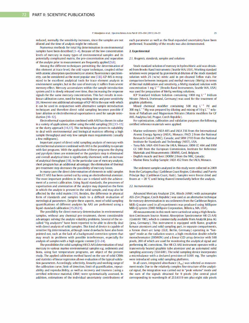
72 PART II: SCIENTIFIC PUBLICATIONS

73 PART II: SCIENTIFIC PUBLICATIONS
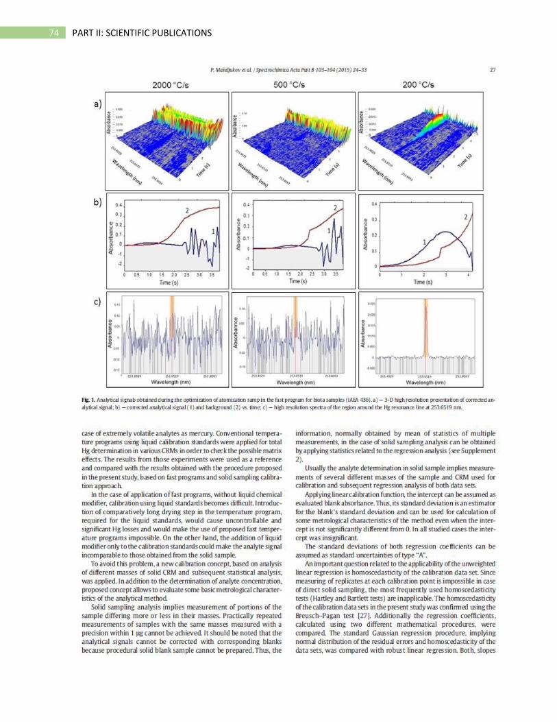
74 PART II: SCIENTIFIC PUBLICATIONS
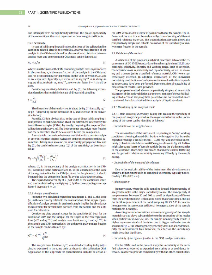
75 PART II: SCIENTIFIC PUBLICATIONS
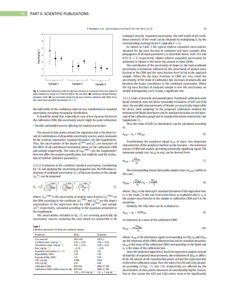
76 PART II: SCIENTIFIC PUBLICATIONS
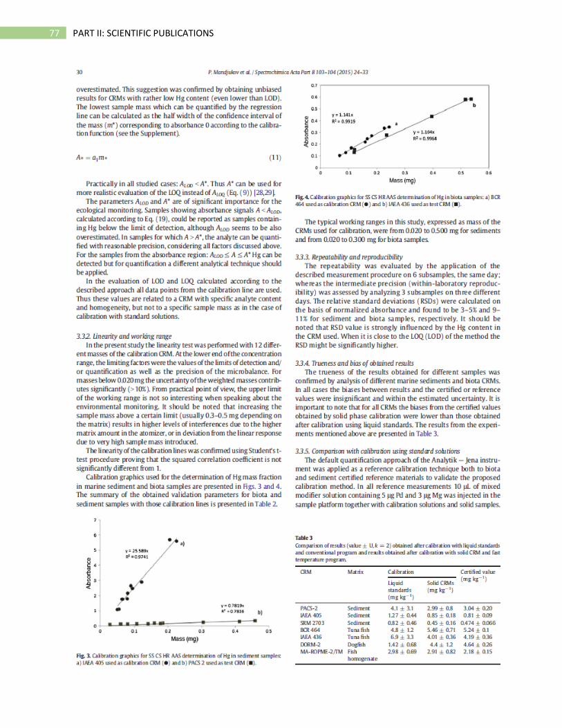
77 PART II: SCIENTIFIC PUBLICATIONS
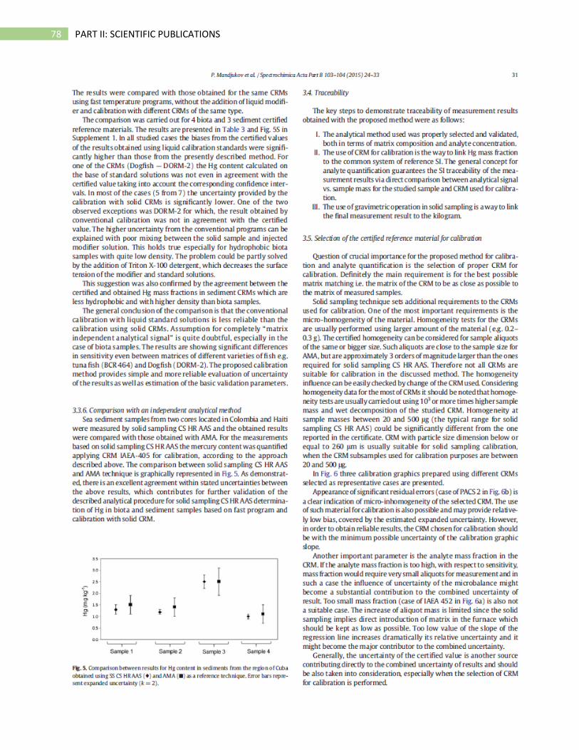
78 PART II: SCIENTIFIC PUBLICATIONS
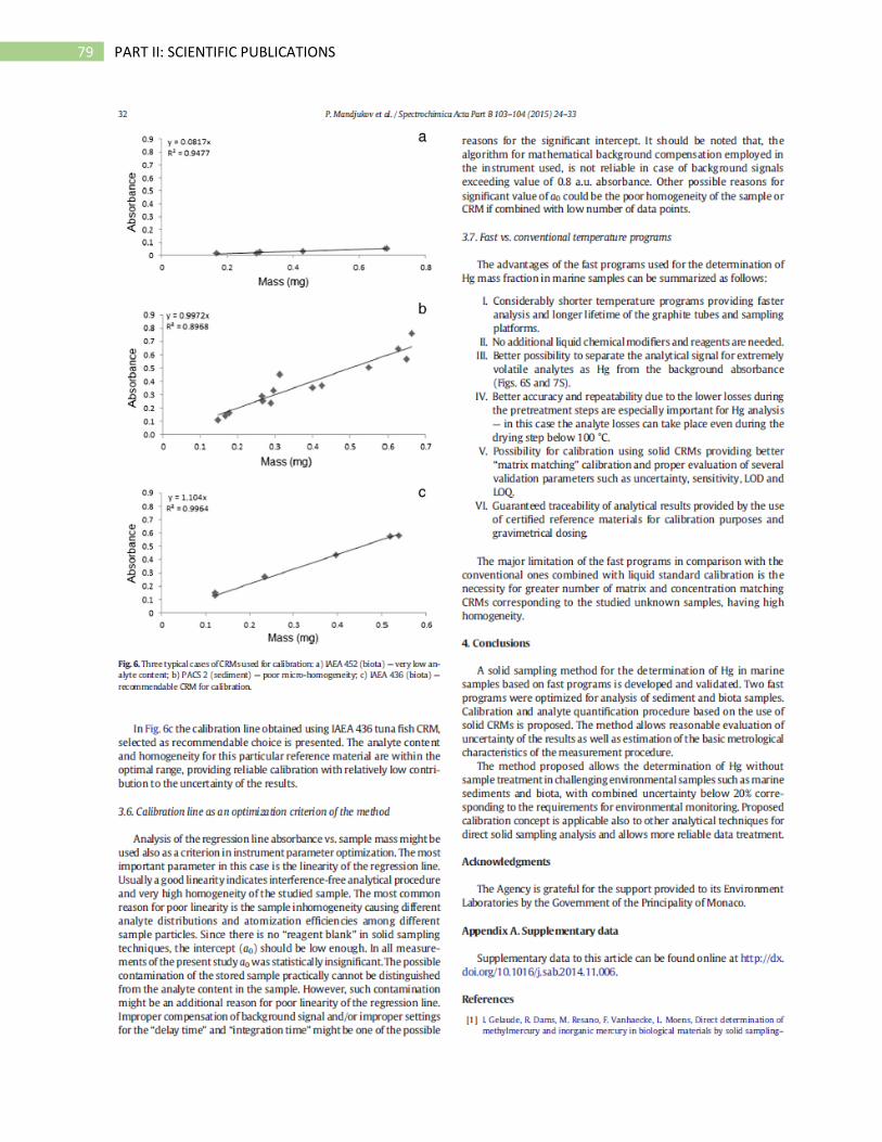
79 PART II: SCIENTIFIC PUBLICATIONS
80 PART II: SCIENTIFIC PUBLICATIONS
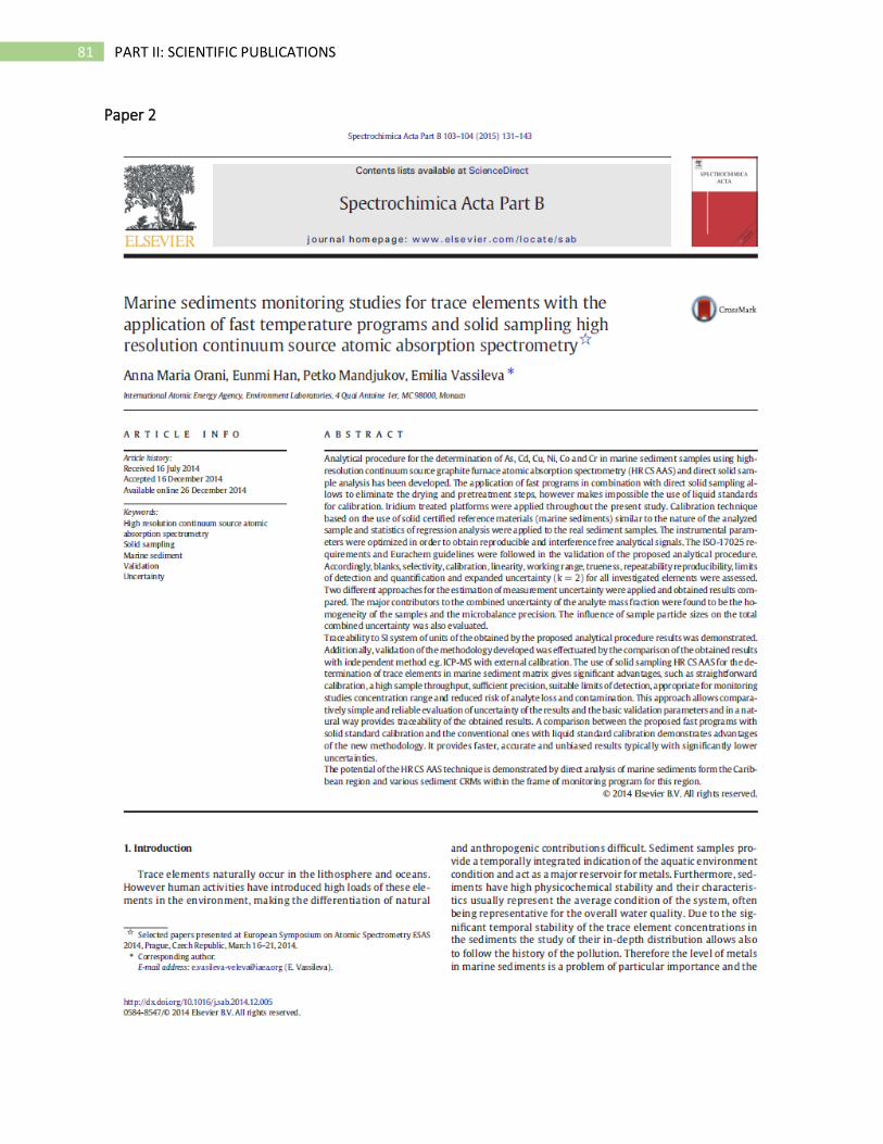
81 PART II: SCIENTIFIC PUBLICATIONS
Paper 2
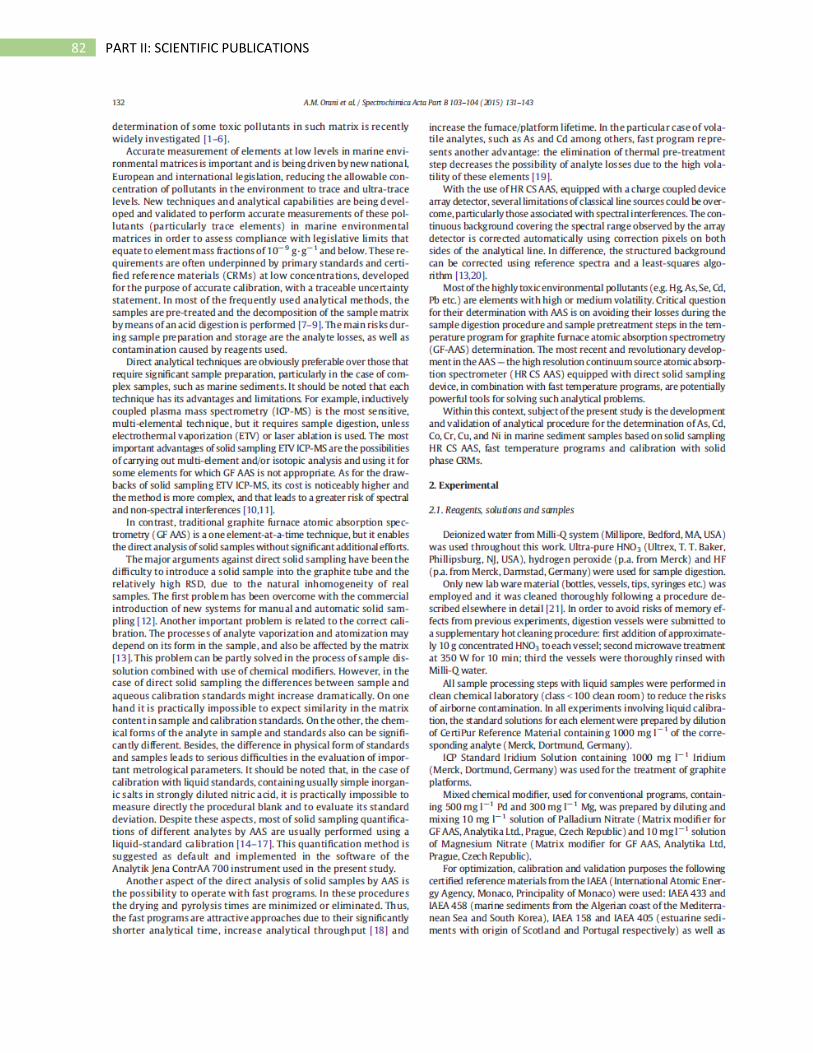
82 PART II: SCIENTIFIC PUBLICATIONS

83 PART II: SCIENTIFIC PUBLICATIONS

84 PART II: SCIENTIFIC PUBLICATIONS
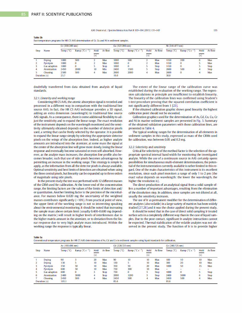
85 PART II: SCIENTIFIC PUBLICATIONS
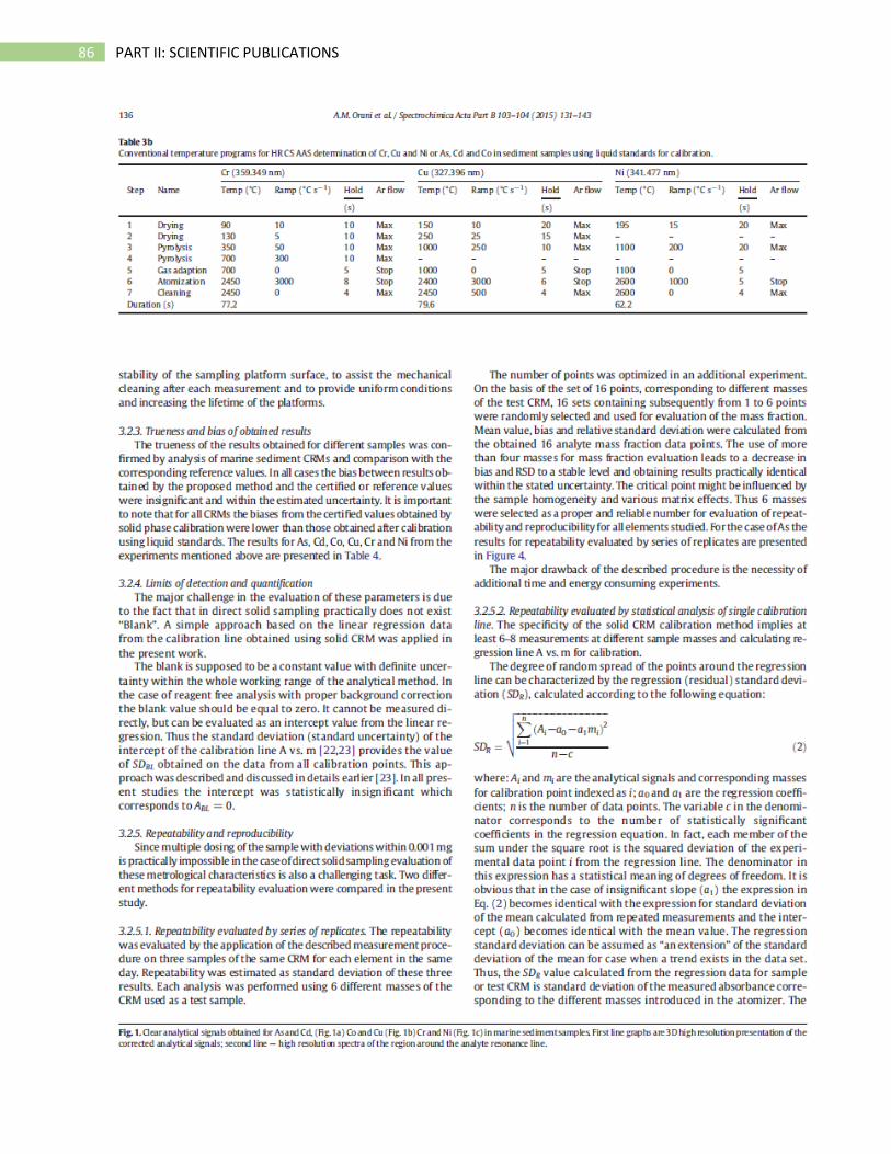
86 PART II: SCIENTIFIC PUBLICATIONS
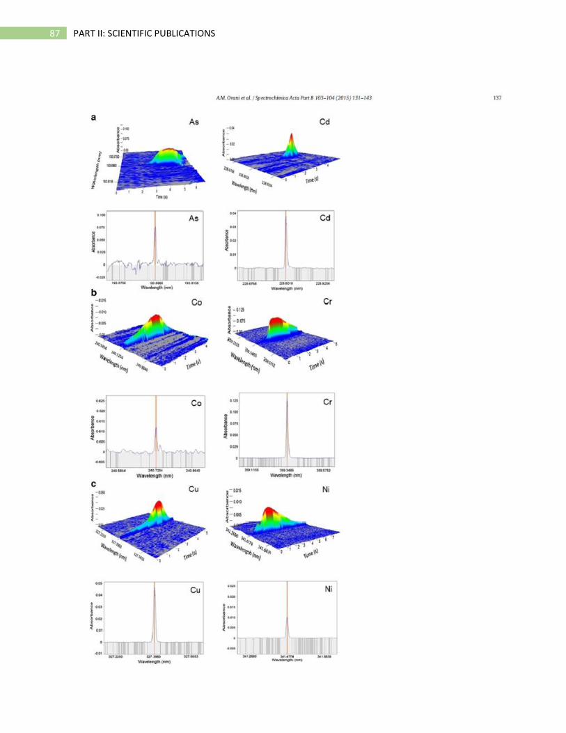
87 PART II: SCIENTIFIC PUBLICATIONS
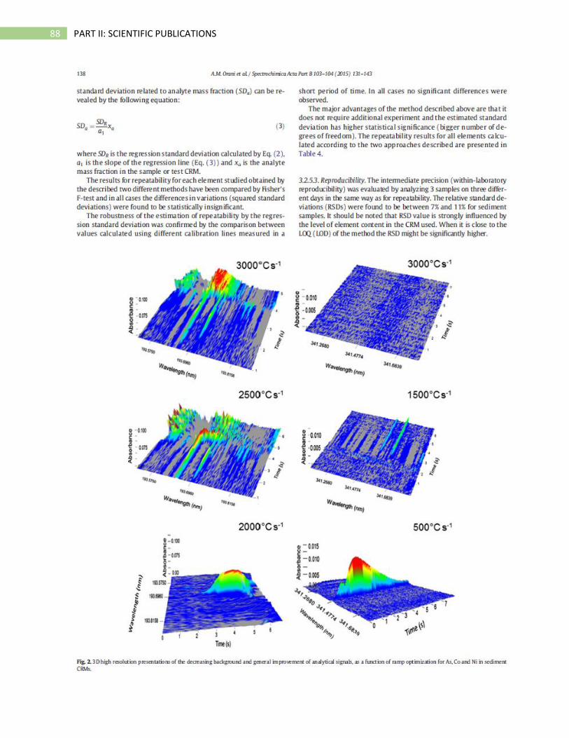
88 PART II: SCIENTIFIC PUBLICATIONS
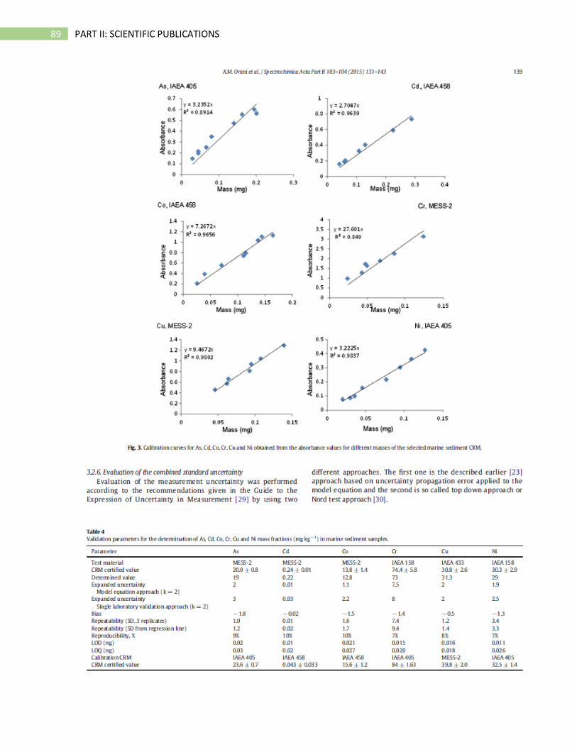
89 PART II: SCIENTIFIC PUBLICATIONS
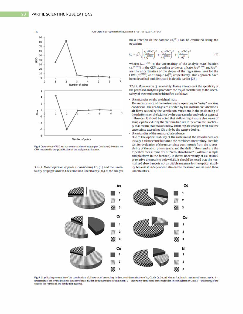
90 PART II: SCIENTIFIC PUBLICATIONS

91 PART II: SCIENTIFIC PUBLICATIONS
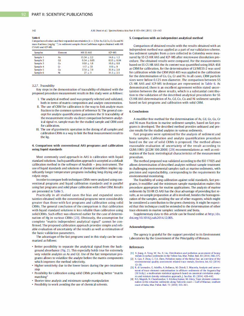
92 PART II: SCIENTIFIC PUBLICATIONS
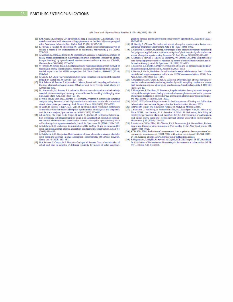
93 PART II: SCIENTIFIC PUBLICATIONS

94 PART II: SCIENTIFIC PUBLICATIONS
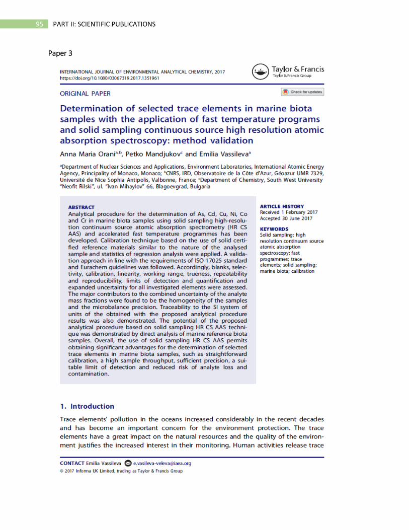
95 PART II: SCIENTIFIC PUBLICATIONS
Paper 3
96 PART II: SCIENTIFIC PUBLICATIONS

97 PART II: SCIENTIFIC PUBLICATIONS
98 PART II: SCIENTIFIC PUBLICATIONS
99 PART II: SCIENTIFIC PUBLICATIONS
100 PART II: SCIENTIFIC PUBLICATIONS
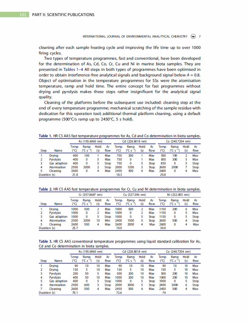
101 PART II: SCIENTIFIC PUBLICATIONS
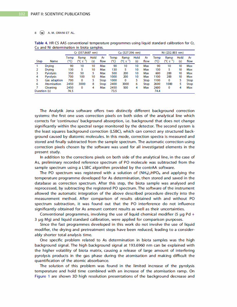
102 PART II: SCIENTIFIC PUBLICATIONS
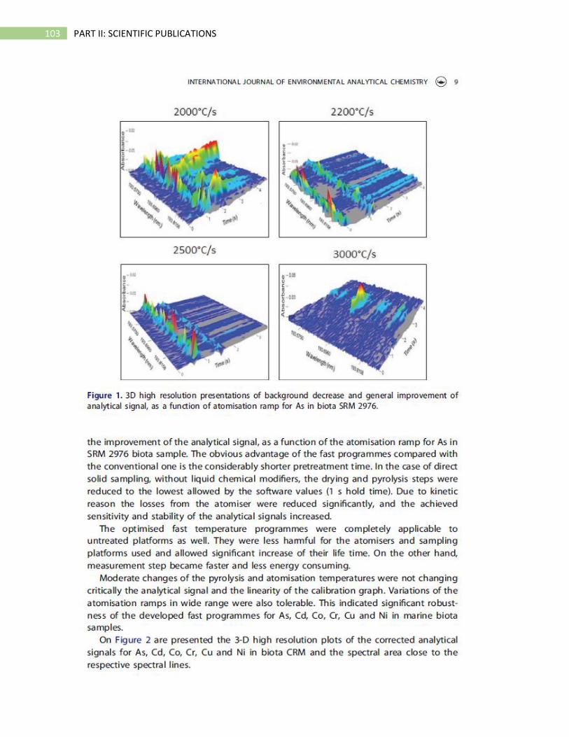
103 PART II: SCIENTIFIC PUBLICATIONS
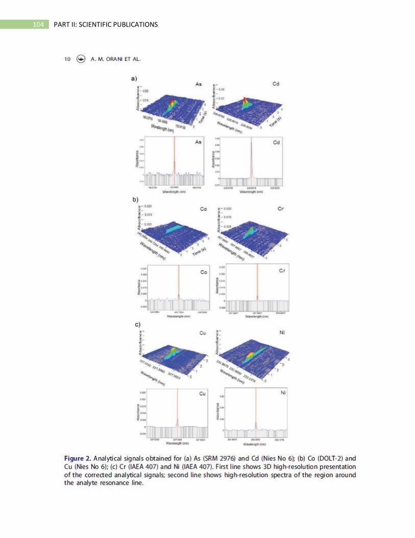
104 PART II: SCIENTIFIC PUBLICATIONS
105 PART II: SCIENTIFIC PUBLICATIONS
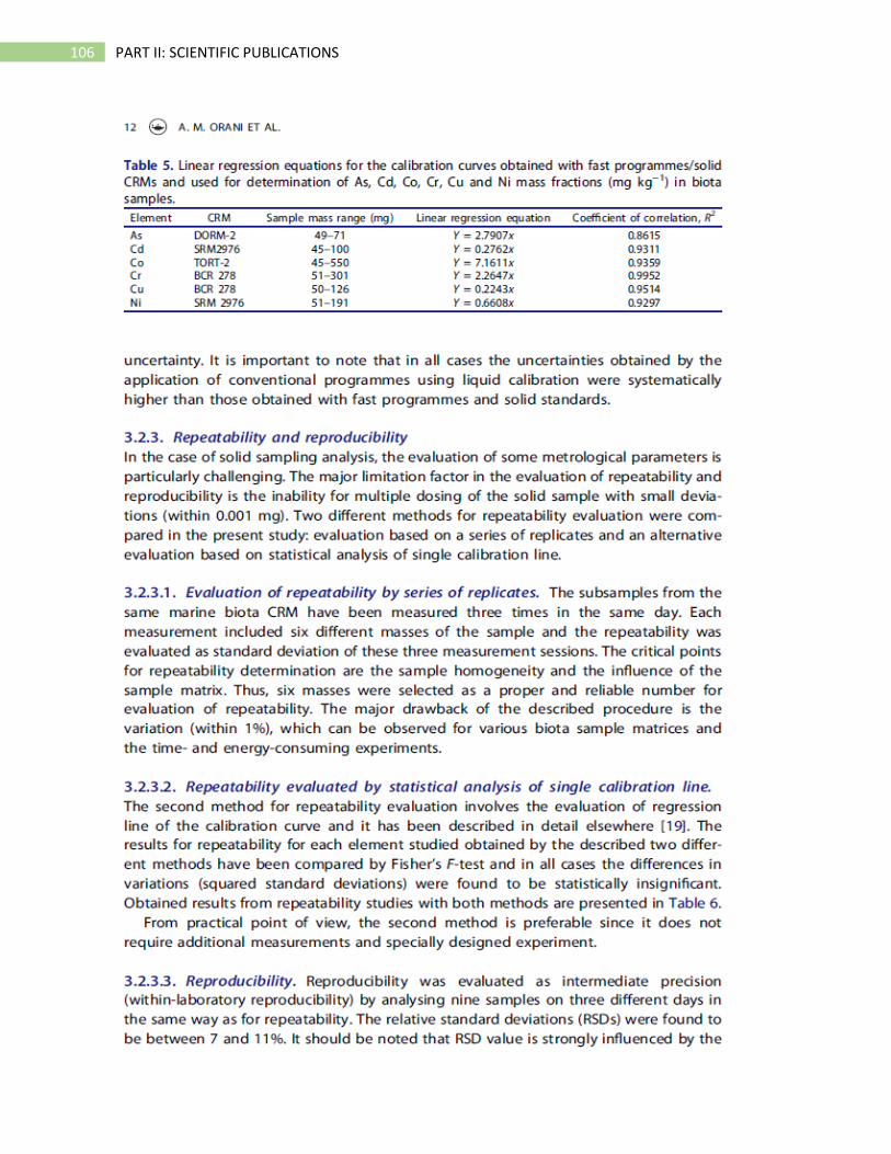
106 PART II: SCIENTIFIC PUBLICATIONS
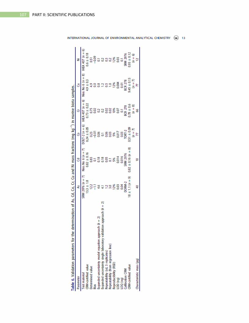
107 PART II: SCIENTIFIC PUBLICATIONS
108 PART II: SCIENTIFIC PUBLICATIONS
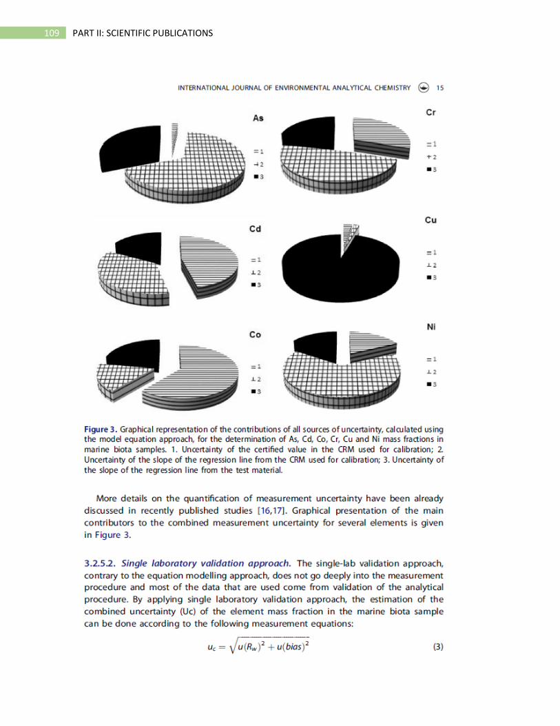
109 PART II: SCIENTIFIC PUBLICATIONS

110 PART II: SCIENTIFIC PUBLICATIONS
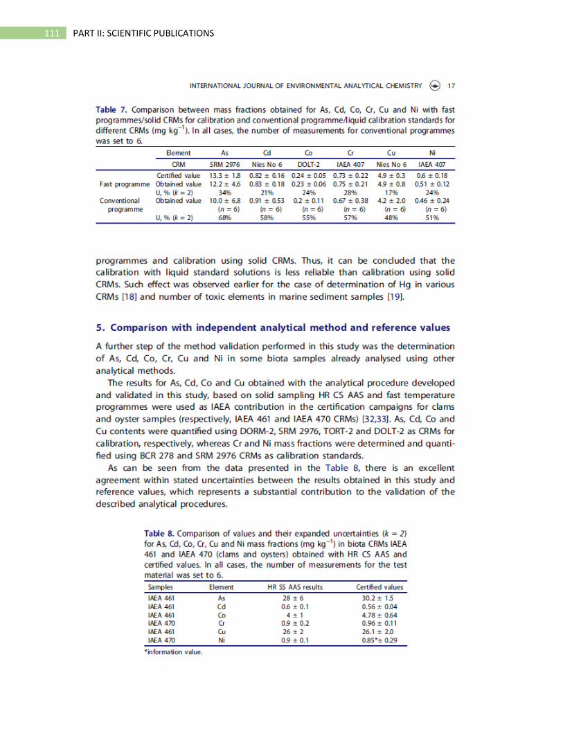
111 PART II: SCIENTIFIC PUBLICATIONS
112 PART II: SCIENTIFIC PUBLICATIONS
113 PART II: SCIENTIFIC PUBLICATIONS
114 PART II: SCIENTIFIC PUBLICATIONS
115 PART II: SCIENTIFIC PUBLICATIONS
SECOND BLOCK
Paper 4 Submitted to peer reviewed journal Marine Pollution Bulletin (Elsevier) - accepted
Baseline study on trace and rare earth elements in marine sediments collected along the Namibian coast
Anna Maria Orani a,b, Emilia Vassileva *a, Irena Wysocka a,c, Michael O. Angelidis a,d, Martina Rozmaric a Deon Louw e
a International Atomic Energy Agency, Environment Laboratories, 4 Quai Antoine 1er, Monaco, Principality of
Monaco
b Université de Nice Sophia Antipolis, CNRS, IRD, Observatoire de la Côte d’Azur, Géoazur UMR 7329, 250 rue Albert Einstein, Sophia Antipolis 06560 Valbonne, France
c Polish Geological Institute National Research Institute, Rakowiecka 4, 00-975 Warsaw, Poland
d University of the Aegean, Department of Environment Lofos Panepistimiou, 81100 Mytilini, Greece
e Ministry of Fisheries and Marine Resources, National Marine Information Research Centre, Strand Street, Swakopmund, Namibia
Abstract
Namibia is a fast-growing country with extensive mineral extraction activities used in diamond,
fluorspar, uranium, and metals production. In order to assess the impact of land based human activities
on the Namibian coastal marine environment, 25 elements were analyzed in 22 surface sediment
samples collected along the coast. By applying a variety of pollution assessment indices (Enrichment
Factor, Igeo and Pollution Load Index), it was concluded that As, Cd and Sb were considerably enriched
in the sediments from several sampling sites, while Cu, Pb and Zn showed very high enrichment at the
vicinity of the Walvis Bay harbor. Pearson’s correlation and Principal Component Analysis were used to
investigate common metal sources. Additionally, the determination of Pb isotope ratios confirmed the
contribution of land based human activities at Walvis Bay and Lüderitz as sources of Pb pollution. The
analysis of REEs did not reveal any important enrichment due to anthropogenic activities in the region,
but provides a needed baseline for further investigations, since previous mineralogical studies indicated
that Namibia has substantial REEs resources.
Keywords: Benguela, surface sediments, trace elements, REEs, Pb isotope ratios
116 PART II: SCIENTIFIC PUBLICATIONS
Studies show that sediment analysis is an appropriate approach for the assessment of trace element
pollution in marine environments, since it can provide a temporally integrated indication of the
environmental conditions of a given area (Caccia et al., 2003). Marine ecosystems can become
contaminated by trace metals from numerous and diverse sources. However, anthropogenic activities
such as mining and industrial processing of ores and metals, still remain a major source of increased
amount of trace elements (De Gregori H. et al., 1996). These anthropogenic inputs can accumulate in
local sediments at concentrations up to five orders of magnitude above that found in the the overlying
water (Bryan and Langston, 1992), and then transferred to aquatic organisms, causing direct toxicity to
aquatic life and indirect toxicity to the human population through consumption of contaminated
seafood. Recognizing the importance of this kind of contamination, trace element determination in
marine sediments has been included as a standard procedure in marine pollution monitoring programs
at national and regional levels since the late 70’s (Roose et al., 2011) (“UNEP regional seas, 2017,” n.d.).
However, although important information on the level and temporal trends of trace element
concentrations in sediment has been collected for several coastal areas (UN DOALOS, 2016), there are
still important geographical gaps around the world that need to be investigated. In the framework of the
Convention for Co-operation in the Protection and Development of the Marine and Coastal environment
of the West and Central African Region (Abidjan Convention), marine pollution monitoring, is an issue of
priority (UNEP, 2011). Unfortunately, marine pollution monitoring programmes have not yet been
implemented in most coastal areas of the West and Central African Region; therefore, it is of the upmost
importance to establish baseline information for trace element concentrations in the larger marine
environment off the coast of the Namibian marine coastal zone.
The Namibian marine environment is remarkable in several ways. It is part of one of the four major
eastern boundary regions (Benguela, California, Northwest Africa and Peru) upwelling systems in the
world and is exceptionally productive in supporting abundant marine life (Sakko, 1998). Namibia has an
exceptionally low, and geographically very concentrated, coastal population compared to other
countries, with five coastal towns on a coastline of 1500 km, including two harbour towns (Walvis Bay
and Lüderitz). Potential human threats to Namibian biodiversity, and generally to its marine ecosystems,
can be related to naval and fishing activities, diamond and other mining activities (Sakko, 1998). The
exploitation of minerals and other natural resources has been the backbone of the Namibian economy
for many years and the mining sector maintains its importance to the gross national product (Ministry of
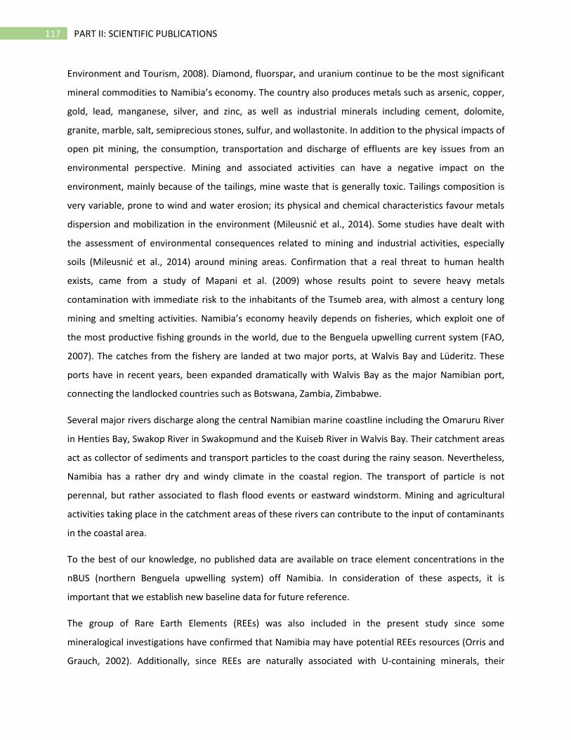
117 PART II: SCIENTIFIC PUBLICATIONS
Environment and Tourism, 2008). Diamond, fluorspar, and uranium continue to be the most significant
mineral commodities to Namibia’s economy. The country also produces metals such as arsenic, copper,
gold, lead, manganese, silver, and zinc, as well as industrial minerals including cement, dolomite,
granite, marble, salt, semiprecious stones, sulfur, and wollastonite. In addition to the physical impacts of
open pit mining, the consumption, transportation and discharge of effluents are key issues from an
environmental perspective. Mining and associated activities can have a negative impact on the
environment, mainly because of the tailings, mine waste that is generally toxic. Tailings composition is
very variable, prone to wind and water erosion; its physical and chemical characteristics favour metals
dispersion and mobilization in the environment (Mileusnić et al., 2014). Some studies have dealt with
the assessment of environmental consequences related to mining and industrial activities, especially
soils (Mileusnić et al., 2014) around mining areas. Confirmation that a real threat to human health
exists, came from a study of Mapani et al. (2009) whose results point to severe heavy metals
contamination with immediate risk to the inhabitants of the Tsumeb area, with almost a century long
mining and smelting activities. Namibia’s economy heavily depends on fisheries, which exploit one of
the most productive fishing grounds in the world, due to the Benguela upwelling current system (FAO,
2007). The catches from the fishery are landed at two major ports, at Walvis Bay and Lüderitz. These
ports have in recent years, been expanded dramatically with Walvis Bay as the major Namibian port,
connecting the landlocked countries such as Botswana, Zambia, Zimbabwe.
Several major rivers discharge along the central Namibian marine coastline including the Omaruru River
in Henties Bay, Swakop River in Swakopmund and the Kuiseb River in Walvis Bay. Their catchment areas
act as collector of sediments and transport particles to the coast during the rainy season. Nevertheless,
Namibia has a rather dry and windy climate in the coastal region. The transport of particle is not
perennal, but rather associated to flash flood events or eastward windstorm. Mining and agricultural
activities taking place in the catchment areas of these rivers can contribute to the input of contaminants
in the coastal area.
To the best of our knowledge, no published data are available on trace element concentrations in the
nBUS (northern Benguela upwelling system) off Namibia. In consideration of these aspects, it is
important that we establish new baseline data for future reference.
The group of Rare Earth Elements (REEs) was also included in the present study since some
mineralogical investigations have confirmed that Namibia may have potential REEs resources (Orris and
Grauch, 2002). Additionally, since REEs are naturally associated with U-containing minerals, their
118 PART II: SCIENTIFIC PUBLICATIONS
determination in these areas with long history of U mining, is of great interest. The distribution patterns
of REEs has often been applied to geological studies of river and marine ecosystems (Song and Choi,
2009; Rezaee et al., 2010) since they are a reliable tool for determining depositional processes and
sediment provenance (Xu et al., 2009); Jung et al., 2012). In the last decade the use of REEs in the
industry have increased as these elements find application in the production of several modern devices,
such as superconductors, electronic components, luminescent materials and car components. As a
consequence of their increased use, the potential anthropogenic influence on REEs natural distribution
has extended their geochemistry into the field of environmental chemistry (Kulaksiz and Bau, 2011);
Hatje et al., 2016), leading scientists to refer to these elements as “new emerging pollutants”.
The aim of this study was to assess the ecological risk associated with trace elements concentrations in
sediments along the Namibian coast and thus provide a record for present and future evaluations of the
state of the Namibian marine environment. For this purpose, the concentration of selected trace
elements, including rare earth elements (REEs) and lead isotopic ratios was determined in 22 sediment
samples collected along the Namibian coast.
All sample handling was carried out in class 10 laminar hoods. Ultrapure water with resistivity > 18 MΩ
was obtained from Milli-Q Element system (Millipore, USA) and was used throughout this work to dilute
concentrated acids. Trace grade HNO3, HF, H2O2 and ultrapure HNO3 were purchased from Fisher
Scientific (Hampton, USA). TraceCert standard solutions for Al, Zn, Mn and Fe used for Flame AAS
calibration, TraceCert Hg standard solution for AMA calibration and TraceCert multielemental standard
for ICP-MS calibration, were purchased from Sigma Aldrich (Buchs, Switzerland) in concentrations of
1000 mg/L (mono-elemental standards) and 10 mg/L (multielemental standard). The Certified Reference
Material MESS-2 (Estuarine sediment, National Research Council, Canada) was used for assessing data
accuracy. The Standard Reference Material SRM 981 from the National Institute of Standards and
Technology (NIST, USA) with the natural Pb isotopic composition was used for correction of the
instrumental mass discrimination when measuring Pb isotope ratios. All Teflon and PE lab ware used in
the sample preparation and analysis, was pre-cleaned with a procedure consisting of at least 24h bath in
10% HNO3 and careful rinsing with MilliQ water.
Following a request for assistance from the Environmental Division of the Ministry of Fisheries and
Marine Resources (MFMR), the IAEA Environment Laboratories participated in a scientific sampling
expedition in May 2014, during a survey along the Namibian coast, together with the National Marine
Information and Research Centre (NatMIRC). Furthermore, additional sediment samples were collected,
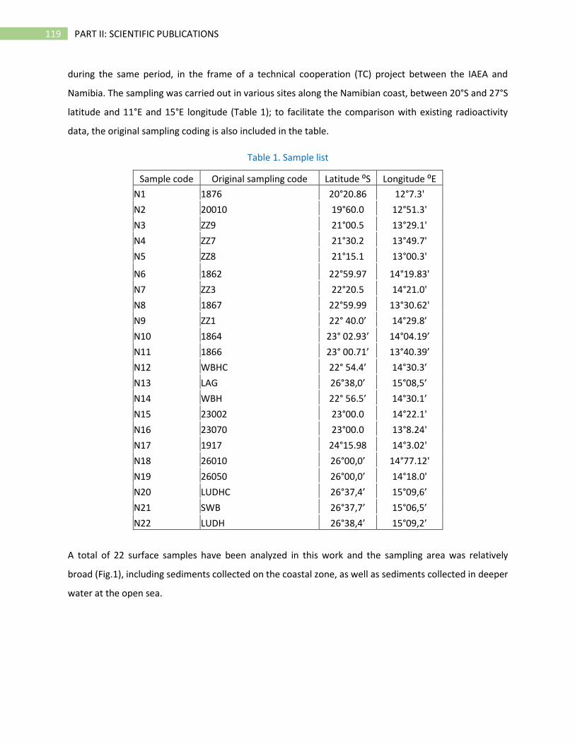
119 PART II: SCIENTIFIC PUBLICATIONS
during the same period, in the frame of a technical cooperation (TC) project between the IAEA and
Namibia. The sampling was carried out in various sites along the Namibian coast, between 20°S and 27°S
latitude and 11°E and 15°E longitude (Table 1); to facilitate the comparison with existing radioactivity
data, the original sampling coding is also included in the table.
Table 1. Sample list
Sample code Original sampling code Latitude ⁰S Longitude ⁰E
N1 1876 20°20.86 12°7.3'
N2 20010 19°60.0 12°51.3'
N3 ZZ9 21°00.5 13°29.1'
N4 ZZ7 21°30.2 13°49.7'
N5 ZZ8 21°15.1 13°00.3'
N6 1862 22°59.97 14°19.83'
N7 ZZ3 22°20.5 14°21.0'
N8 1867 22°59.99 13°30.62'
N9 ZZ1 22° 40.0’ 14°29.8’
N10 1864 23° 02.93’ 14°04.19’
N11 1866 23° 00.71’ 13°40.39’
N12 WBHC 22° 54.4’ 14°30.3’
N13 LAG 26°38,0’ 15°08,5’
N14 WBH 22° 56.5’ 14°30.1’
N15 23002 23°00.0 14°22.1'
N16 23070 23°00.0 13°8.24'
N17 1917 24°15.98 14°3.02'
N18 26010 26°00,0’ 14°77.12'
N19 26050 26°00,0’ 14°18.0'
N20 LUDHC 26°37,4’ 15°09,6’
N21 SWB 26°37,7’ 15°06,5’
N22 LUDH 26°38,4’ 15°09,2’
A total of 22 surface samples have been analyzed in this work and the sampling area was relatively
broad (Fig.1), including sediments collected on the coastal zone, as well as sediments collected in deeper
water at the open sea.
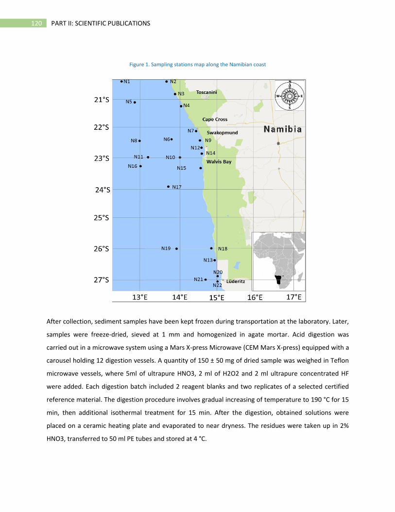
120 PART II: SCIENTIFIC PUBLICATIONS
Figure 1. Sampling stations map along the Namibian coast
After collection, sediment samples have been kept frozen during transportation at the laboratory. Later,
samples were freeze-dried, sieved at 1 mm and homogenized in agate mortar. Acid digestion was
carried out in a microwave system using a Mars X-press Microwave (CEM Mars X-press) equipped with a
carousel holding 12 digestion vessels. A quantity of 150 ± 50 mg of dried sample was weighed in Teflon
microwave vessels, where 5ml of ultrapure HNO3, 2 ml of H2O2 and 2 ml ultrapure concentrated HF
were added. Each digestion batch included 2 reagent blanks and two replicates of a selected certified
reference material. The digestion procedure involves gradual increasing of temperature to 190 °C for 15
min, then additional isothermal treatment for 15 min. After the digestion, obtained solutions were
placed on a ceramic heating plate and evaporated to near dryness. The residues were taken up in 2%
HNO3, transferred to 50 ml PE tubes and stored at 4 °C.
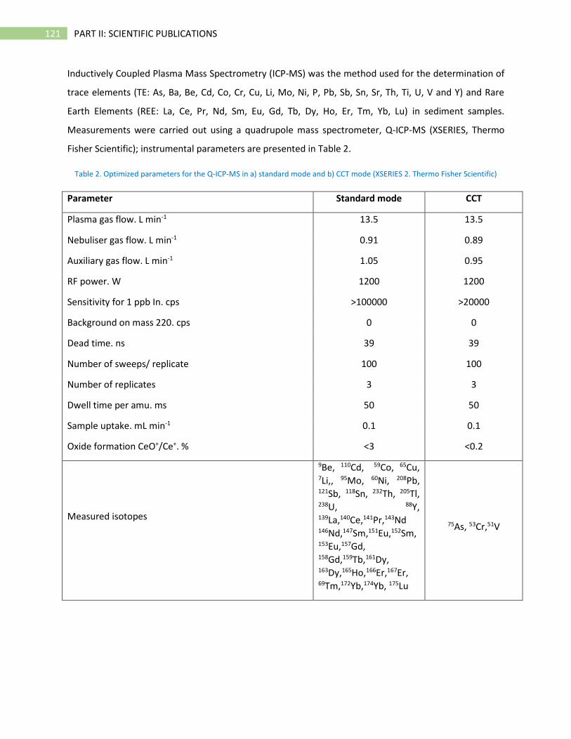
121 PART II: SCIENTIFIC PUBLICATIONS
Inductively Coupled Plasma Mass Spectrometry (ICP-MS) was the method used for the determination of
trace elements (TE: As, Ba, Be, Cd, Co, Cr, Cu, Li, Mo, Ni, P, Pb, Sb, Sn, Sr, Th, Ti, U, V and Y) and Rare
Earth Elements (REE: La, Ce, Pr, Nd, Sm, Eu, Gd, Tb, Dy, Ho, Er, Tm, Yb, Lu) in sediment samples.
Measurements were carried out using a quadrupole mass spectrometer, Q-ICP-MS (XSERIES, Thermo
Fisher Scientific); instrumental parameters are presented in Table 2.
Table 2. Optimized parameters for the Q-ICP-MS in a) standard mode and b) CCT mode (XSERIES 2. Thermo Fisher Scientific)
Parameter Standard mode CCT
Plasma gas flow. L min-1 13.5 13.5
Nebuliser gas flow. L min-1 0.91 0.89
Auxiliary gas flow. L min-1 1.05 0.95
RF power. W 1200 1200
Sensitivity for 1 ppb In. cps >100000 >20000
Background on mass 220. cps 0 0
Dead time. ns 39 39
Number of sweeps/ replicate 100 100
Number of replicates 3 3
Dwell time per amu. ms 50 50
Sample uptake. mL min-1 0.1 0.1
Oxide formation CeO+/Ce+. % <3 <0.2
Measured isotopes
9Be, 110Cd, 59Co, 65Cu, 7Li,, 95Mo, 60Ni, 208Pb, 121Sb, 118Sn, 232Th, 205Tl, 238U, 88Y, 139La,140Ce,141Pr,143Nd
146Nd,147Sm,151Eu,152Sm,153Eu,157Gd, 158Gd,159Tb,161Dy, 163Dy,165Ho,166Er,167Er,
69Tm,172Yb,174Yb, 175Lu
75As, 53Cr,51V
122 PART II: SCIENTIFIC PUBLICATIONS
Determination of Pb isotope ratios was performed on digested samples by means of High Resolution
Sector Field ICP-MS (NuAttom, NuInstruments Ltd., Wrexham, UK); the instrument parameters are
presented in Table 3.
Table 3. Optimized ICP-SFMS instrumental parameters for Pb isotopic ratio determinations (Attom, Nu Instruments)
Parameter Value
Coolant gas flow 13.5 L min-1
Auxiliary gas flow 0.8 L min-1
Nebulizer gas flow 29.6 psi
Plasma power 1300 W
Sensitivity for 1 ng g-1 (208Pb) > 800000 cps
Background on mass 220 < 2 cps
Dead time 14 ± 2 (k=2) ns
Acquisition Mode Peak Jumping
Number of sweeps 500
Number of cycles 25
Dwell time per isotope (ms) 1000
Measured isotopes 202Hg, 204Pb, 206Pb, 207Pb, 208Pb
Mass resolution 300
Oxide Formation CeO+/Ce+ <1%
Determination of Al, Fe, Mn and Zn was carried out by Flame Atomic Absorption Spectroscopy (ContrAA
700, Analytik Jena, Germany) on the same digested solutions used for ICP-MS, using external calibration.
Mercury was determined in sediment samples directly, using a solid AAS analyzer (AMA 254, Altech,
USA), therefore no digestion was needed. Total Organic Carbon (TOC) and Total Inorganic Carbon (TIC)
were determined by means of acidification and combustion in a one-unit carbon analysis system (Vario
EL Cube, Elementar, Langenselbold, Germany). The analytical methods used in this study were properly
selected and validated, both in terms of matrix composition and analyte concentration. All possible
sources of uncertainty of obtained monitoring results were carefully identified. Afterwards, the
uncertainty components were quantified and the combined uncertainty calculated. Combined standard
uncertainties were obtained by propagating together individual uncertainty components according to
the ISO/GUM guide (Magnusson and Örnemark eds, 2014). All uncertainties indicated in the final results
are expanded uncertainties:
(1) U = k · uc
123 PART II: SCIENTIFIC PUBLICATIONS
where uc is the combined standard uncertainty and k is a coverage factor equal to 2.
A principal requirement of the standard ISO 17025 (ISO/IEC 17025, 2017) is for laboratories to produce
measurements that are traceable to a common system of reference, SI system, and ensure
comparability of measurement results. The way to demonstrate traceability in the present study was the
use of an uncertainty budget, where all the parameters influencing the final result were systematically
assessed. In addition, the use of CRM throughout the whole analytical procedure and bias (recovery)
estimation was the way to link obtained trace elements mass fraction to the common system of
reference SI. CRM with similar matrix were used also in the validation of sample preparation step.
Different approaches are proposed to evaluate the anthropogenic influence on trace elements content
in the sediments. In this work we are using three widely used approaches: Enrichment Factor (EF), Geo-
accumulation Index (Igeo) and Pollution Load Index (PLI), as already described in details elsewhere
(Zahra et al., 2014; Guan et al., 2016). Graphical representation of trace elements results is given in Fig.
2.
As it can be seen from this representation, As, Cd, Cr and Ni show high variability in terms of contents.
The ranges of mass fractions were 2.4-42 mg kg-1for As, 0.2-12 mgkg-1 for Cd, 45-270 mg kg-1 for Cr,
31-580 mgkg-1for Mn and 12-61 mg kg-1for Ni. On the other hand, Pb, Zn and Cu show significantly
higher levels only in sampling station N14, while Hg was consistently low along the coastline.
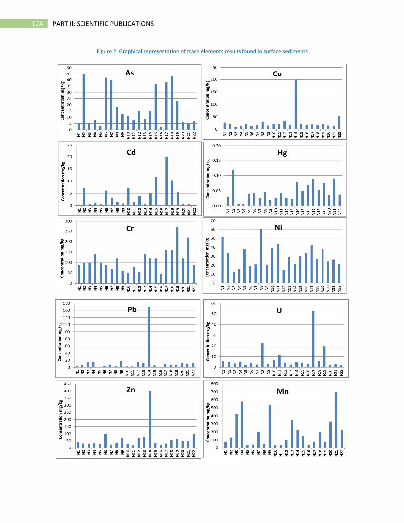
124 PART II: SCIENTIFIC PUBLICATIONS
Figure 2. Graphical representation of trace elements results found in surface sediments
125 PART II: SCIENTIFIC PUBLICATIONS
A summary of trace and major elements results is presented in Table 1S (supplementary file) and results
of grain size distribution and organic carbon is presented in Table 2S. In order to facilitate the
interpretation of such results and to highlight common patterns, a Person’s correlation test has been
performed. The correlation matrix is presented in Table 3S. High correlation coefficients between
different metals, considered significantly different from zero at 95% confidence interval, mean common
sources, mutual dependence, and identical behavior during transport (Guan et al., 2016).
Unexpectedly, no significant correlation between organic carbon (TOC) and analyzed trace and major
elements was found. The property of organic matter to influence the content of some trace metals in
environmental samples has been reported in several studies (Wang and Qin, 2006; Kljaković-Gašpić et
al., 2008) but the relation between these two components is still considered complex and very variable
(Wang, 2008). Among toxic elements, As and Cd showed a similar pattern, displaying the highest
contents (up to 12 mg kg-1Cd and 45 mgkg-1As) at the Walvis Bay and Swakopmund regions (Fig. 2) and,
Pearson’s test confirmed a positive correlation between their patterns (R2 = 0.73); Arsenic showed
significant correlation only with Cd, while Cd presented significant correlation also with some other
elements such as Mo, Th and U. Bremner and Willis, (1993) already highlighted an unusual Cd
distribution in unconsolidated continental-margin sediments in the Namibian coast, reporting values up
to 60 mg kg-1precisely in the region between Walvis Bay and Swakopmund (Bremner and Willis, 1993).
The authors suggested a possible source of Cd as impurity of Zn minerals coming from Ugab River but no
correlation between Cd and Zn was found in this study (R2 = 0.02). On the other hand, positive
correlation with As patterns might suggest a possible enrichment caused by anthropogenic activities. Ni
and Cr seem to have more homogeneous distributions along the coast, even with values comparable to
those previously measured by Bremner and Willis; additionally, these elements did not show any
significant correlation with other toxic elements.
N14 was the only sampling station where very high mass fractions of Pb, Zn and Cu were found.
Maximum concentration of 87±9 mg kg-1Cu and 49±16 mg kg-1Pb were found by Bremner and Willis in
surface sediment samples collected in the same area while samples analyzed in this study presented
much higher concentrations: 200±20 and 170±20 mg kg-1for Cu and Pb respectively. Very high positive
correlation between Cu and Pb (R2 = 0.96) can be observed, suggesting a common source of
contamination. Interestingly also Zn correlates positively with both Pb and Cu, reaching values up to
400±40 mg kg-1in sample N14. No significant correlation was found with carbonate content, meaning
that the enrichment of Pb, Cu and Zn cannot be justified with the presence of carbonate minerals. It has

126 PART II: SCIENTIFIC PUBLICATIONS
to be pointed out that upwelling systems are naturally characterized by metal enrichment as a
consequence of high metal inputs from plankton but the metal content in Namibian coast was
previously suggested to be intimately related to organic matter content (Calvert and Price, 1970). In
consideration of the fact that no positive correlation was found between organic content and trace
elements concentration in surface samples, it is reasonable to assume that metal enrichments found in
coastal stations is mainly related to anthropogenic metals inputs from land based sources.
The analysis of EF, Igeo and PLI corroborate the hypothesis of anthropogenic contribution in some of the
sampling stations. The background values considered for the calculation of EF and Igeo were those
measured on the bottom of a small core sampled offshore, at station N16. Following the evaluation
criteria of EF described elsewhere (Guan et al., 2016), it was possible to identify As significant
enrichment in nine sampling stations: N2, N6, N7, N8, N10, N12, N15, N17 and N18 with EF between 6
and 9; the N11, N14 and N19 sites were found to be moderately enriched in As (EF = 3-4). Exactly the
same sites were found to be moderately/ significantly enriched in Cd with EF between 3 and 24. Pb
showed significant/very high enrichment in two locations around Walvis Bay (N12 and N14) with EF
equal to 7 and 45 respectively; additionally, N14 was the only sampling site presenting Cu and Zn
enrichment. Among toxic elements also Mo and Sb presented significant enrichment in some locations,
reaching values up to 28 and 16 respectively. Some of the calculated EFs are presented in Fig. 3.
Figure 3. Graphical representation of some enrichment factors calculated for surface samples
Figure 4. Cu, Cd, Pb As, Zn, Sb and Mo Igeo indices calculated for each sampling site. Dotted line represents the limit above
which the sample can be considered moderately/strongly contaminated
0
5
10
15
20
25
30
35
40
45
50
N1 N2 N3 N4 N5 N6 N7 N8 N9 N10N11N12N13N14N15N16N17N18N19N20N21N22
Enri
chm
en
t Fa
cto
r
Sampling site
Cu
Cd
Pb
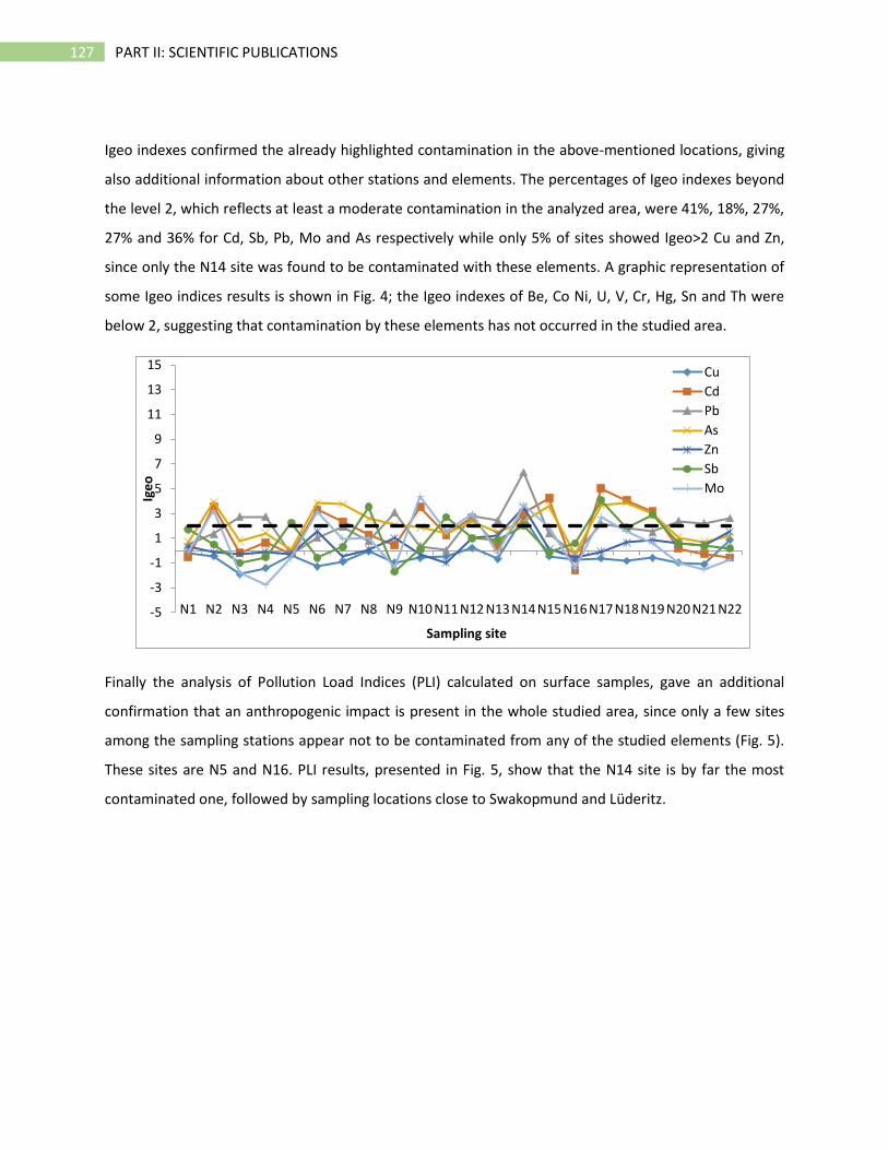
127 PART II: SCIENTIFIC PUBLICATIONS
Igeo indexes confirmed the already highlighted contamination in the above-mentioned locations, giving
also additional information about other stations and elements. The percentages of Igeo indexes beyond
the level 2, which reflects at least a moderate contamination in the analyzed area, were 41%, 18%, 27%,
27% and 36% for Cd, Sb, Pb, Mo and As respectively while only 5% of sites showed Igeo>2 Cu and Zn,
since only the N14 site was found to be contaminated with these elements. A graphic representation of
some Igeo indices results is shown in Fig. 4; the Igeo indexes of Be, Co Ni, U, V, Cr, Hg, Sn and Th were
below 2, suggesting that contamination by these elements has not occurred in the studied area.
Finally the analysis of Pollution Load Indices (PLI) calculated on surface samples, gave an additional
confirmation that an anthropogenic impact is present in the whole studied area, since only a few sites
among the sampling stations appear not to be contaminated from any of the studied elements (Fig. 5).
These sites are N5 and N16. PLI results, presented in Fig. 5, show that the N14 site is by far the most
contaminated one, followed by sampling locations close to Swakopmund and Lüderitz.
-5
-3
-1
1
3
5
7
9
11
13
15
N1 N2 N3 N4 N5 N6 N7 N8 N9 N10 N11 N12 N13 N14 N15 N16 N17 N18 N19 N20 N21 N22
Ige
o
Sampling site
Cu
Cd
Pb
As
Zn
Sb
Mo
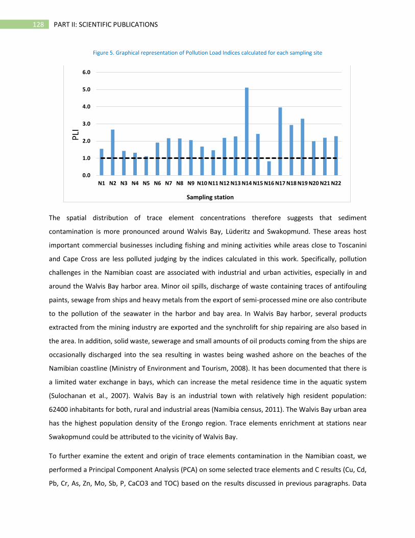
128 PART II: SCIENTIFIC PUBLICATIONS
Figure 5. Graphical representation of Pollution Load Indices calculated for each sampling site
The spatial distribution of trace element concentrations therefore suggests that sediment
contamination is more pronounced around Walvis Bay, Lüderitz and Swakopmund. These areas host
important commercial businesses including fishing and mining activities while areas close to Toscanini
and Cape Cross are less polluted judging by the indices calculated in this work. Specifically, pollution
challenges in the Namibian coast are associated with industrial and urban activities, especially in and
around the Walvis Bay harbor area. Minor oil spills, discharge of waste containing traces of antifouling
paints, sewage from ships and heavy metals from the export of semi-processed mine ore also contribute
to the pollution of the seawater in the harbor and bay area. In Walvis Bay harbor, several products
extracted from the mining industry are exported and the synchrolift for ship repairing are also based in
the area. In addition, solid waste, sewerage and small amounts of oil products coming from the ships are
occasionally discharged into the sea resulting in wastes being washed ashore on the beaches of the
Namibian coastline (Ministry of Environment and Tourism, 2008). It has been documented that there is
a limited water exchange in bays, which can increase the metal residence time in the aquatic system
(Sulochanan et al., 2007). Walvis Bay is an industrial town with relatively high resident population:
62400 inhabitants for both, rural and industrial areas (Namibia census, 2011). The Walvis Bay urban area
has the highest population density of the Erongo region. Trace elements enrichment at stations near
Swakopmund could be attributed to the vicinity of Walvis Bay.
To further examine the extent and origin of trace elements contamination in the Namibian coast, we
performed a Principal Component Analysis (PCA) on some selected trace elements and C results (Cu, Cd,
Pb, Cr, As, Zn, Mo, Sb, P, CaCO3 and TOC) based on the results discussed in previous paragraphs. Data
0.0
1.0
2.0
3.0
4.0
5.0
6.0
N1 N2 N3 N4 N5 N6 N7 N8 N9 N10 N11 N12 N13 N14 N15 N16 N17 N18 N19 N20 N21 N22
PLI
Sampling station
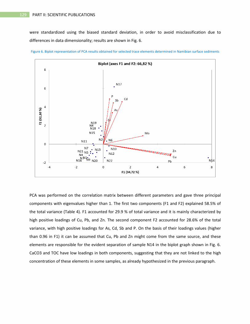
129 PART II: SCIENTIFIC PUBLICATIONS
were standardized using the biased standard deviation, in order to avoid misclassification due to
differences in data dimensionality; results are shown in Fig. 6.
Figure 6. Biplot representation of PCA results obtained for selected trace elements determined in Namibian surface sediments
PCA was performed on the correlation matrix between different parameters and gave three principal
components with eigenvalues higher than 1. The first two components (F1 and F2) explained 58.5% of
the total variance (Table 4). F1 accounted for 29.9 % of total variance and it is mainly characterized by
high positive loadings of Cu, Pb, and Zn. The second component F2 accounted for 28.6% of the total
variance, with high positive loadings for As, Cd, Sb and P. On the basis of their loadings values (higher
than 0.96 in F1) it can be assumed that Cu, Pb and Zn might come from the same source, and these
elements are responsible for the evident separation of sample N14 in the biplot graph shown in Fig. 6.
CaCO3 and TOC have low loadings in both components, suggesting that they are not linked to the high
concentration of these elements in some samples, as already hypothesized in the previous paragraph.
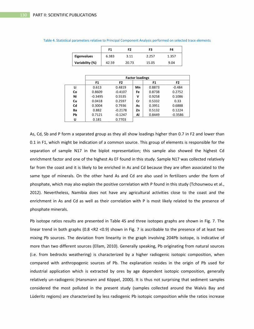
130 PART II: SCIENTIFIC PUBLICATIONS
Table 4. Statistical parameters relative to Principal Component Analysis performed on selected trace elements
F1 F2 F3 F4
Eigenvalues 6.383 3.11 2.257 1.357
Variability (%) 42.59 20.73 15.05 9.04
Factor loadings
F1 F2
F1 F2
Li 0.613 0.4819 Mn 0.8873 -0.484 Co 0.8609 -0.4107 Fe 0.8738 0.2752 Ni -0.3495 0.5535 V 0.9258 0.1086 Cu 0.0418 0.2597 Cr 0.5332 0.33 Cd 0.3004 0.7936 As 0.3951 0.6888 Ba 0.882 -0.2178 Zn 0.5132 0.1224 Pb 0.7121 -0.1247 Al 0.8449 -0.3586
U 0.181 0.7703
As, Cd, Sb and P form a separated group as they all show loadings higher than 0.7 in F2 and lower than
0.1 in F1, which might be indication of a common source. This group of elements is responsible for the
separation of sample N17 in the biplot representation; this sample also showed the highest Cd
enrichment factor and one of the highest As EF found in this study. Sample N17 was collected relatively
far from the coast and it is likely to be enriched in As and Cd because they are often associated to the
same type of minerals. On the other hand As and Cd are also used in fertilizers under the form of
phosphate, which may also explain the positive correlation with P found in this study (Tchounwou et al.,
2012). Nevertheless, Namibia does not have any agricultural activities close to the coast and the
enrichment in As and Cd as well as their correlation with P is most likely related to the presence of
phosphate minerals.
Pb isotope ratios results are presented in Table 4S and three isotopes graphs are shown in Fig. 7. The
linear trend in both graphs (0.8 <R2 <0.9) shown in Fig. 7 is ascribable to the presence of at least two
mixing Pb sources. The deviation from linearity in the graph involving 204Pb isotope, is indicative of
more than two different sources (Ellam, 2010). Generally speaking, Pb originating from natural sources
(i.e. from bedrocks weathering) is characterized by a higher radiogenic isotopic composition, when
compared with anthropogenic sources of Pb. The explanation resides in the origin of Pb used for
industrial application which is extracted by ores by age dependent isotopic composition, generally
relatively un-radiogenic (Hansmann and Köppel, 2000). It is thus not surprising that sediment samples
considered the most polluted in the present study (samples collected around the Walvis Bay and
Lüderitz regions) are characterized by less radiogenic Pb isotopic composition while the ratios increase
131 PART II: SCIENTIFIC PUBLICATIONS
in absolute 206Pb/204Pb and 208Pb/204Pb values for samples collected in less contaminated areas.
Among the samples analyzed in this study the N14 showed by far the lowest values of Pb isotope ratios
(206Pb/204Pb = 17.68 and 206Pb/207Pb = 1.125); this was also the sample characterized by the highest
measured Pb content. Samples N12, N13, N20 and N22 also can be grouped together on the basis of
their isotopic composition (18.1<206Pb/204Pb<18.5 and 1.155<206Pb/207Pb<1.180) while other samples
presented higher ratio values (206Pb/204Pb>18.78 and 206Pb/207Pb>1.191).
Because of the lack in the literature of Pb isotope ratios data in Namibia coastal area, the interpretation
of these results is particularly challenging. The Pb isotopic composition of the most contaminated
samples is similar to the one measured in aerosol coming from Namib Desert, which could be influenced
by Pb emissions from the Tsumeb mine and smelter (Bollhöfer and Rosman, 2000). Pb isotopic
composition of Tsumeb ores were reported from Brown (Brown, 1962) and it is characterized by a high
radiogenic contribution, with 206Pb/204Pb and 206Pb/207Pb ratios of 18.29 and 1.15 respectively. Another
probable source of Pb in the most contaminated area is related to gasoline. The average 206Pb/207Pb in
the most contaminated samples was found to be closer to European gasoline signature (1.080-1.156)
than to the South African one (1.055-1.083) as already reported in surface sediment sample from Cape
Town (Larsen et al., 2012). The lack of published data on this subject makes difficult any further
interpretation of these results.

132 PART II: SCIENTIFIC PUBLICATIONS
Figure 7 Three isotope graph representation of Pb isotope ratios results in sediment surface samples: a) 206Pb/204Pb vs 208Pb/204Pb, R2= 0.8049 and b) 206Pb/204Pb vs 206Pb/207Pb, R2= 0.9771
a)
b)
N5
N13
N9
N18
N7N16
N14
N17 N4
N19
N3N12
N15
N20
N2
N22
N6
N1
N21
N10
N11
N8
37.8
38.0
38.2
38.4
38.6
38.8
39.0
39.2
39.4
39.6
39.8
40.0
17.4 17.6 17.8 18.0 18.2 18.4 18.6 18.8 19.0 19.2 19.4 19.6 19.8
20
8P
b/2
04P
b
206Pb/204Pb
N5
N13
N9
N18
N7N16
N14
N17N4N19
N3
N12
N15
N20
N2
N22
N6
N1
N21
N10
N11
N8
1.120
1.140
1.160
1.180
1.200
1.220
1.240
17.4 17.6 17.8 18.0 18.2 18.4 18.6 18.8 19.0 19.2 19.4 19.6 19.8
20
6P
b/2
07P
b
206Pb/204Pb
Aerosol Namib desert
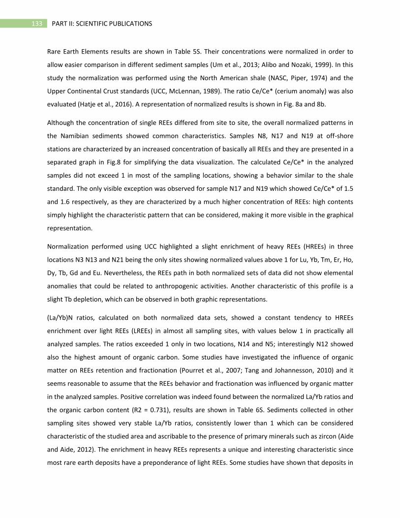
133 PART II: SCIENTIFIC PUBLICATIONS
Rare Earth Elements results are shown in Table 5S. Their concentrations were normalized in order to
allow easier comparison in different sediment samples (Um et al., 2013; Alibo and Nozaki, 1999). In this
study the normalization was performed using the North American shale (NASC, Piper, 1974) and the
Upper Continental Crust standards (UCC, McLennan, 1989). The ratio Ce/Ce* (cerium anomaly) was also
evaluated (Hatje et al., 2016). A representation of normalized results is shown in Fig. 8a and 8b.
Although the concentration of single REEs differed from site to site, the overall normalized patterns in
the Namibian sediments showed common characteristics. Samples N8, N17 and N19 at off-shore
stations are characterized by an increased concentration of basically all REEs and they are presented in a
separated graph in Fig.8 for simplifying the data visualization. The calculated Ce/Ce* in the analyzed
samples did not exceed 1 in most of the sampling locations, showing a behavior similar to the shale
standard. The only visible exception was observed for sample N17 and N19 which showed Ce/Ce* of 1.5
and 1.6 respectively, as they are characterized by a much higher concentration of REEs: high contents
simply highlight the characteristic pattern that can be considered, making it more visible in the graphical
representation.
Normalization performed using UCC highlighted a slight enrichment of heavy REEs (HREEs) in three
locations N3 N13 and N21 being the only sites showing normalized values above 1 for Lu, Yb, Tm, Er, Ho,
Dy, Tb, Gd and Eu. Nevertheless, the REEs path in both normalized sets of data did not show elemental
anomalies that could be related to anthropogenic activities. Another characteristic of this profile is a
slight Tb depletion, which can be observed in both graphic representations.
(La/Yb)N ratios, calculated on both normalized data sets, showed a constant tendency to HREEs
enrichment over light REEs (LREEs) in almost all sampling sites, with values below 1 in practically all
analyzed samples. The ratios exceeded 1 only in two locations, N14 and N5; interestingly N12 showed
also the highest amount of organic carbon. Some studies have investigated the influence of organic
matter on REEs retention and fractionation (Pourret et al., 2007; Tang and Johannesson, 2010) and it
seems reasonable to assume that the REEs behavior and fractionation was influenced by organic matter
in the analyzed samples. Positive correlation was indeed found between the normalized La/Yb ratios and
the organic carbon content (R2 = 0.731), results are shown in Table 6S. Sediments collected in other
sampling sites showed very stable La/Yb ratios, consistently lower than 1 which can be considered
characteristic of the studied area and ascribable to the presence of primary minerals such as zircon (Aide
and Aide, 2012). The enrichment in heavy REEs represents a unique and interesting characteristic since
most rare earth deposits have a preponderance of light REEs. Some studies have shown that deposits in
134 PART II: SCIENTIFIC PUBLICATIONS
Lofdal (carbonatite-dykes), located at about 450 km northeast of Windhoek and Okorusu (carbonatite-
associated) display REEs enrichment (Wall et al., 2008). Especially, Xenotime present in Lofdal deposits
seems to be precious source of heavy rare earths and could be the first sustainable supply of HREEs
outside of China. Table 6S also shows a significant correlation between Y, Th, U, P and REEs as they
naturally occur together in the same minerals, such as Xenotime and Monazite. The pattern found in
sediment samples analyzed in the present study resembles the pattern found in Xenotime minerals
collected in Lofdal (Wall et al., 2008), confirming that the input of REEs in the analyzed area is uniquely
related to geochemical background.
In conclusion the present work provides a baseline study of metal contamination in the Namibian coast.
The highest values of the Pollution Load Index (PLI) were found around Walvis Bay and Swakopmund,
suggesting that trace element concentrations in those areas are influenced by human activities. Among
toxic elements, the highest Enrichment Factor (EF) were determined for As, Cd and Sb in several
sampling sites while Cu, Pb and Zn showed very high enrichment only in one site, located on the Walvis
Bay harbor. Other elements such as Cr, Co and Ni, even when presenting high values compared to other
studies, did not show substantial enrichment, suggesting non-anthropogenic sources. No significant
correlation was found between any of the elements determined in this study and organic carbon,
suggesting that the upwelling current, which is usually rich in both trace elements and organic matter,
did not influence the metal content in sediment samples analyzed in this work. The determination of Pb
isotope ratios, gave confirmation that the high enrichment of Pb at Walvis Bay and Lüderitz, derives
from anthropogenic activities, and it is probably related to anthropogenic activities around the main
harbor including spilling of products delivered to the main harbors. Pearson’s correlation and Principal
Component Analysis (PCA) applied to the results highlighted common sources for As, Cd and Sb and a
common source for Zn, Pb and Cu. REEs concentrations in the sediment samples showed high variability,
but they followed a common characteristic pattern, with no significant anomalies. These results suggest
that this group of elements is not influenced by anthropogenic activities and it is characteristic of the
geochemical background of the area.
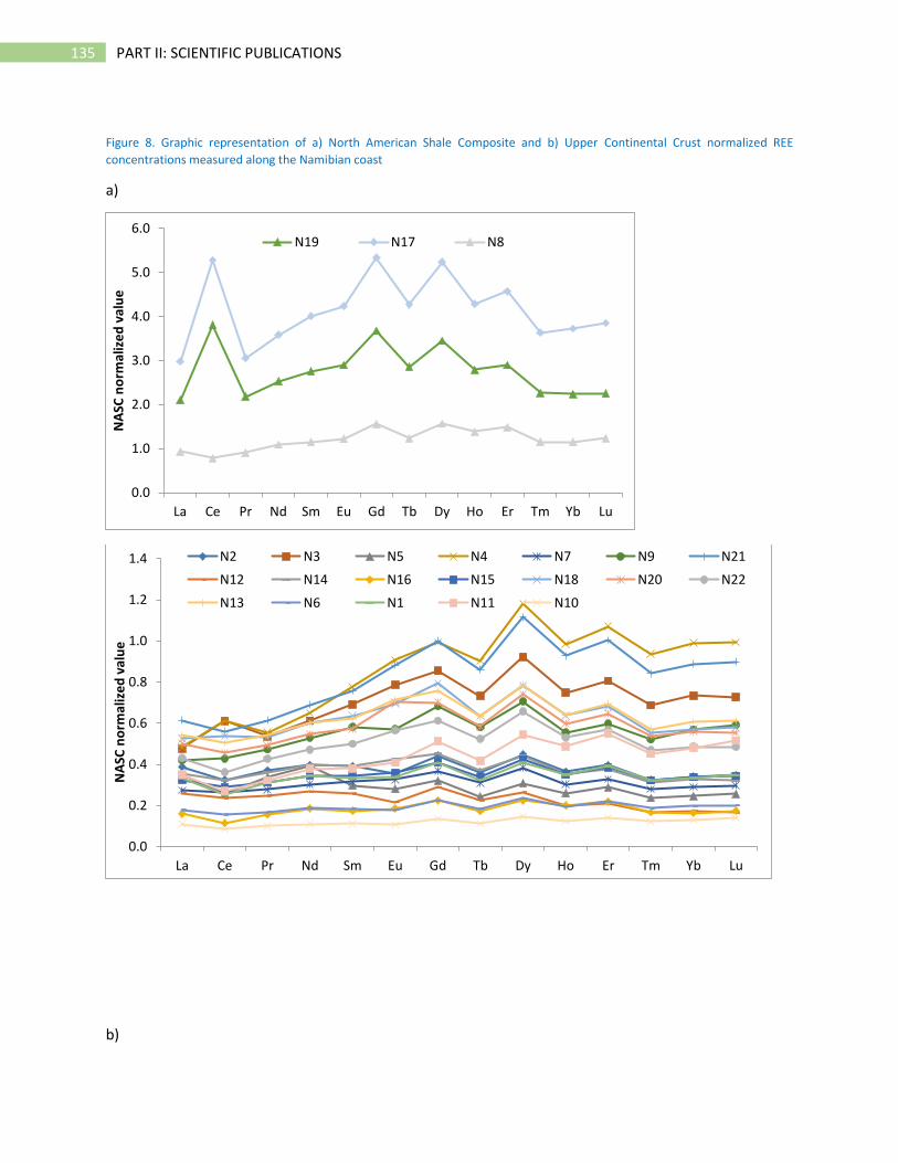
135 PART II: SCIENTIFIC PUBLICATIONS
Figure 8. Graphic representation of a) North American Shale Composite and b) Upper Continental Crust normalized REE
concentrations measured along the Namibian coast
a)
b)
0.0
1.0
2.0
3.0
4.0
5.0
6.0
La Ce Pr Nd Sm Eu Gd Tb Dy Ho Er Tm Yb Lu
NA
SC n
orm
aliz
ed
val
ue
N19 N17 N8
0.0
0.2
0.4
0.6
0.8
1.0
1.2
1.4
La Ce Pr Nd Sm Eu Gd Tb Dy Ho Er Tm Yb Lu
NA
SC n
orm
aliz
ed
val
ue
N2 N3 N5 N4 N7 N9 N21
N12 N14 N16 N15 N18 N20 N22
N13 N6 N1 N11 N10
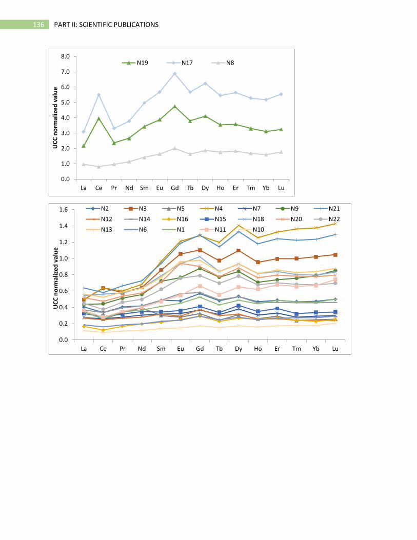
136 PART II: SCIENTIFIC PUBLICATIONS
0.0
1.0
2.0
3.0
4.0
5.0
6.0
7.0
8.0
La Ce Pr Nd Sm Eu Gd Tb Dy Ho Er Tm Yb Lu
UC
C n
orm
aliz
ed
val
ue
N19 N17 N8
0.0
0.2
0.4
0.6
0.8
1.0
1.2
1.4
1.6
La Ce Pr Nd Sm Eu Gd Tb Dy Ho Er Tm Yb Lu
UC
C n
orm
aliz
ed
val
ue
N2 N3 N5 N4 N7 N9 N21
N12 N14 N16 N15 N18 N20 N22
N13 N6 N1 N11 N10
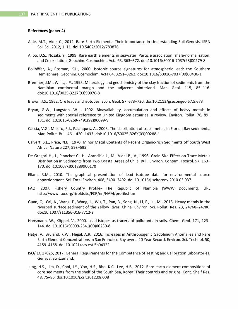
137 PART II: SCIENTIFIC PUBLICATIONS
References (paper 4)
Aide, M.T., Aide, C., 2012. Rare Earth Elements: Their Importance in Understanding Soil Genesis. ISRN Soil Sci. 2012, 1–11. doi:10.5402/2012/783876
Alibo, D.S., Nozaki, Y., 1999. Rare earth elements in seawater: Particle association, shale-normalization, and Ce oxidation. Geochim. Cosmochim. Acta 63, 363–372. doi:10.1016/S0016-7037(98)00279-8
Bollhöfer, A., Rosman, K.J.., 2000. Isotopic source signatures for atmospheric lead: the Southern Hemisphere. Geochim. Cosmochim. Acta 64, 3251–3262. doi:10.1016/S0016-7037(00)00436-1
Bremner, J.M., Willis, J.P., 1993. Mineralogy and geochemistry of the clay fraction of sediments from the Namibian continental margin and the adjacent hinterland. Mar. Geol. 115, 85–116. doi:10.1016/0025-3227(93)90076-8
Brown, J.S., 1962. Ore leads and isotopes. Econ. Geol. 57, 673–720. doi:10.2113/gsecongeo.57.5.673
Bryan, G.W., Langston, W.J., 1992. Bioavailability, accumulation and effects of heavy metals in sediments with special reference to United Kingdom estuaries: a review. Environ. Pollut. 76, 89–131. doi:10.1016/0269-7491(92)90099-V
Caccia, V.G., Millero, F.J., Palanques, A., 2003. The distribution of trace metals in Florida Bay sediments. Mar. Pollut. Bull. 46, 1420–1433. doi:10.1016/S0025-326X(03)00288-1
Calvert, S.E., Price, N.B., 1970. Minor Metal Contents of Recent Organic-rich Sediments off South West Africa. Nature 227, 593–595.
De Gregori H., I., Pinochet C., H., Arancibia J., M., Vidal B., A., 1996. Grain Size Effect on Trace Metals Distribution in Sediments from Two Coastal Areas of Chile. Bull. Environ. Contam. Toxicol. 57, 163–170. doi:10.1007/s001289900170
Ellam, R.M., 2010. The graphical presentation of lead isotope data for environmental source apportionment. Sci. Total Environ. 408, 3490–3492. doi:10.1016/j.scitotenv.2010.03.037
FAO, 2007. Fishery Country Profile- The Republic of Namibia [WWW Document]. URL http://www.fao.org/fi/oldsite/FCP/en/NAM/profile.htm
Guan, Q., Cai, A., Wang, F., Wang, L., Wu, T., Pan, B., Song, N., Li, F., Lu, M., 2016. Heavy metals in the riverbed surface sediment of the Yellow River, China. Environ. Sci. Pollut. Res. 23, 24768–24780. doi:10.1007/s11356-016-7712-z
Hansmann, W., Köppel, V., 2000. Lead-istopes as tracers of pollutants in soils. Chem. Geol. 171, 123–144. doi:10.1016/S0009-2541(00)00230-8
Hatje, V., Bruland, K.W., Flegal, A.R., 2016. Increases in Anthropogenic Gadolinium Anomalies and Rare Earth Element Concentrations in San Francisco Bay over a 20 Year Record. Environ. Sci. Technol. 50, 4159–4168. doi:10.1021/acs.est.5b04322
ISO/IEC 17025, 2017. General Requirements for the Competence of Testing and Calibration Laboratories. Geneva, Switzerland.
Jung, H.S., Lim, D., Choi, J.Y., Yoo, H.S., Rho, K.C., Lee, H.B., 2012. Rare earth element compositions of core sediments from the shelf of the South Sea, Korea: Their controls and origins. Cont. Shelf Res. 48, 75–86. doi:10.1016/j.csr.2012.08.008
138 PART II: SCIENTIFIC PUBLICATIONS
Kljaković-Gašpić, Z., Bogner, D., Ujević, I., 2008. Trace metals (Cd, Pb, Cu, Zn and Ni) in sediment of the submarine pit Dragon ear (Soline Bay, Rogoznica, Croatia). Environ. Geol. 58, 751. doi:10.1007/s00254-008-1549-9
Kulaksiz, S., Bau, M., 2011. Rare earth elements in the Rhine River, Germany: First case of anthropogenic lanthanum as a dissolved microcontaminant in the hydrosphere. Environ. Int. 37, 973–979. doi:10.1016/j.envint.2011.02.018
Larsen, M.M., Blusztajn, J.S., Andersen, O., Dahllöf, I., 2012. Lead isotopes in marine surface sediments reveal historical use of leaded fuel. J. Environ. Monit. 14, 2893. doi:10.1039/c2em30579h
Mapani, B., Ellmies, R., Kamona, F., Kříbek, B., Majer, V., Knésl, I., Pašava, J., Mufenda, M., Mbingeneeko, F., 2009. Human health risks associated with historic ore processing at Berg Aukas, Grootfontein area, Namibia. Communs geol. Surv. Namibia 14, 25–40. doi:10.1016/j.jafrearsci.2010.07.007
McLennan, S.M., 1989. Rare earth elements in sedimentary rocks; influence of provenance and sedimentary processes. Rev. Mineral. Geochemistry 21, 169–200.
Mileusnić, M., Mapani, B.S., Kamona, A.F., Ružičić, S., Mapaure, I., Chimwamurombe, P.M., 2014. Assessment of agricultural soil contamination by potentially toxic metals dispersed from improperly disposed tailings, Kombat mine, Namibia. J. Geochemical Explor. 144, 409–420. doi:10.1016/j.gexplo.2014.01.009
Ministry of Environment and Tourism, 2008. Strategic Environmental Assessment (SEA) of the coastal areas of the Erongo and Kunene regions.
Orris, G.J., Grauch, R.I., 2002. Rare Earth Element Mines, Deposits, and Occurrences.
Piper, D.Z., 1974. Rare earth elements in the sedimentary cycle: A summary. Chem. Geol. 14, 285–304. doi:10.1016/0009-2541(74)90066-7
Pourret, O., Davranche, M., Gruau, G., Dia, A., 2007. Rare earth elements complexation with humic acid. Chem. Geol. 243, 128–141. doi:10.1016/j.chemgeo.2007.05.018
Rezaee, K., Saion, E.B., Wood, A.K., Abdi, M.R., 2010. Rare earth elements determination and distribution patterns in surface marine sediments of the South China Sea by INAA, Malaysia. J. Radioanal. Nucl. Chem. 283, 823–829. doi:10.1007/s10967-009-0421-z
Roose, P., Albaigés, J., Bebianno, M.J., Camphuysen, C., Cronin, M., de Leeuw, J., Gabrielsen, G., Hutchinson, T., Hylland, K., Jansson, B., Jenssen, B.M., Schulz-Bull, D., Szefer, P., Webster, L., Bakke, T., Janssen, C., 2011. Monitoring Chemical Pollution in Europe’s Seas: Programmes, practices and priorties for Research. Mar. Board Position 108.
Sakko, A.L., 1998. The influence of the Benguela upwelling system on Namibia’s marine biodiversity. Biodivers. & Conserv. 7, 419–433. doi:10.1023/A:1008867310010
Song, Y.H., Choi, M.S., 2009. REE geochemistry of fine-grained sediments from major rivers around the Yellow Sea. Chem. Geol. 266, 337–351. doi:10.1016/j.chemgeo.2009.06.019
Sulochanan, B., Krishnakumar, P.K., Prema, D., Kaladharan, P., Valsala, K.K., Bhat, G.S., Muniyandi, K., 2007. Trace metal contamination of the marine environment in Palk Bay and Gulf of Mannar. J. Mar. Biol. Assoc. India 49, 12–18.
Tang, J., Johannesson, K.H., 2010. Ligand extraction of rare earth elements from aquifer sediments:

139 PART II: SCIENTIFIC PUBLICATIONS
Implications for rare earth element complexation with organic matter in natural waters. Geochim. Cosmochim. Acta 74, 6690–6705. doi:10.1016/j.gca.2010.08.028
Tchounwou, P.B., Yedjou, C.G., Patlolla, A.K., Sutton, D.J., 2012. Heavy Metals Toxicity and the Environment. Mol. Clin. Environ. Toxicol. 101, 1–30. doi:10.1007/978-3-7643-8340-4
Um, I. kwon, Choi, M.S., Bahk, J.J., Song, Y.H., 2013. Discrimination of sediment provenance using rare earth elements in the ulleung basin, east/japan sea. Mar. Geol. 346, 208–219. doi:10.1016/j.margeo.2013.09.007
UN DOALOS (Division for Ocean Affairs and the Law of the Sea), 2016. First Global Integrated Marine Assessment (first World Ocean Assessment) [WWW Document]. URL http://www.un.org/depts/los/global_reporting/WOA_RegProcess.htm
UNEP, 2011. Abidjan Convention. Convention for Co-operation in the Protection and Development of the Marine and Coastal environment of the West and Central African Region [WWW Document].
UNEP regional seas, 2017 [WWW Document], n.d. URL http://www.unep.org/regionalseas/ (accessed 7.13.17).
Wall, F., Niku-Paavola, V.N., Storey, C., M??ller, A., Jeffries, T., 2008. Xenotime-(Y) from carbonatite dykes at Lofdal, Namibia: Unusually low LREE:HREE ratio in carbonatite, and the first dating of xenotime overgrowths on zircon. Can. Mineral. 46, 861–877. doi:10.3749/canmin.46.4.861
Wang, X., Qin, Y., 2006. Spatial distribution of metals in urban topsoils of Xuzhou (China): controlling factors and environmental implications. Environ. Geol. 49, 905–914. doi:10.1007/s00254-005-0122-z
Wang, X.S., 2008. Correlations between heavy metals and organic carbon extracted by dry oxidation procedure in urban roadside soils. Environ. Geol. 54, 269–273. doi:10.1007/s00254-007-0814-7
Xu, Z., Lim, D., Choi, J., Yang, S., Jung, H., 2009. Rare earth elements in bottom sediments of major rivers around the Yellow Sea: implications for sediment provenance. Geo-Marine Lett. 29, 291–300. doi:10.1007/s00367-009-0142-x
Zahra, A., Hashmi, M.Z., Malik, R.N., Ahmed, Z., 2014. Enrichment and geo-accumulation of heavy metals and risk assessment of sediments of the Kurang Nallah—Feeding tributary of the Rawal Lake Reservoir, Pakistan. Sci. Total Environ. 470–471, 925–933. doi:10.1016/j.scitotenv.2013.10.017

140 PART II: SCIENTIFIC PUBLICATIONS
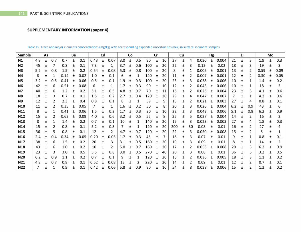
141 PART II: SCIENTIFIC PUBLICATIONS
SUPPLEMENTARY INFORMATION (paper 4)
Table 1S. Trace and major elements concentrations (mg/kg) with corresponding expanded uncertainties (k=2) in surface sediment samples
Sample As Be Cd Co Cr Cu Hg Li Mo
N1 4.8 ± 0.7 0.7 ± 0.1 0.43 ± 0.07 3.0 ± 0.5 90 ± 10 27 ± 4 0.030 ± 0.004 21 ± 3 1.9 ± 0.3 N2 45 ± 7 0.8 ± 0.1 7.3 ± 1 3.7 ± 0.6 100 ± 20 22 ± 3 0.12 ± 0.02 18 ± 3 19 ± 3 N3 5.2 ± 0.8 1.5 ± 0.2 0.54 ± 0.08 5.3 ± 0.8 100 ± 20 8 ± 1 0.005 ± 0.001 13 ± 2 0.59 ± 0.09 N4 8 ± 1 0.14 ± 0.02 1.0 ± 0.1 6 ± 1 140 ± 20 11 ± 2 0.007 ± 0.001 12 ± 2 0.30 ± 0.05 N5 3.2 ± 0.5 0.41 ± 0.06 0.5 ± 0.1 1.9 ± 0.3 100 ± 20 23 ± 3 0.038 ± 0.006 10 ± 1 1.4 ± 0.2 N6 42 ± 6 0.51 ± 0.08 6 ± 1 1.7 ± 0.3 90 ± 10 12 ± 2 0.043 ± 0.006 10 ± 1 18 ± 3 N7 40 ± 6 1.2 ± 0.2 3.1 ± 0.5 4.8 ± 0.7 70 ± 11 16 ± 2 0.025 ± 0.004 23 ± 3 4.1 ± 0.6 N8 18 ± 3 0.7 ± 0.1 1.5 ± 0.2 2.7 ± 0.4 120 ± 20 29 ± 4 0.047 ± 0.007 7 ± 1 4.2 ± 0.6 N9 12 ± 2 2.3 ± 0.4 0.8 ± 0.1 8 ± 1 59 ± 9 15 ± 2 0.021 ± 0.003 27 ± 4 0.8 ± 0.1 N10 11 ± 2 0.35 ± 0.05 7 ± 1 1.6 ± 0.2 50 ± 8 20 ± 3 0.026 ± 0.004 6.2 ± 0.9 43 ± 6 N11 8 ± 1 0.41 ± 0.06 1.5 ± 0.2 1.7 ± 0.3 80 ± 10 22 ± 3 0.043 ± 0.006 5.1 ± 0.8 6.2 ± 0.9 N12 15 ± 2 0.63 ± 0.09 4.0 ± 0.6 3.2 ± 0.5 55 ± 8 35 ± 5 0.027 ± 0.004 14 ± 2 16 ± 2 N13 8 ± 1 1.4 ± 0.2 0.7 ± 0.1 10 ± 1 140 ± 20 19 ± 3 0.023 ± 0.003 27 ± 4 1.8 ± 0.3 N14 15 ± 2 0.8 ± 0.1 5.2 ± 0.8 7 ± 1 120 ± 20 200 ± 30 0.08 ± 0.01 16 ± 2 27 ± 4 N15 36 ± 5 0.8 ± 0.1 12 ± 2 4.7 ± 0.7 120 ± 20 22 ± 3 0.050 ± 0.008 15 ± 2 8 ± 1 N16 2.4 ± 0.4 0.34 ± 0.05 0.20 ± 0.03 1.7 ± 0.3 45 ± 7 18 ± 3 0.07 ± 0.01 9 ± 1 0.8 ± 0.1 N17 38 ± 6 1.5 ± 0.2 20 ± 3 3.1 ± 0.5 160 ± 20 19 ± 3 0.09 ± 0.01 8 ± 1 14 ± 2 N18 43 ± 6 1.0 ± 0.2 10 ± 2 5.0 ± 0.7 160 ± 20 17 ± 2 0.053 ± 0.008 20 ± 3 6.2 ± 0.9 N19 23 ± 3 3.0 ± 0.5 5.5 ± 0.8 3.0 ± 0.5 270 ± 40 20 ± 3 0.08 ± 0.01 36 ± 5 3.2 ± 0.5 N20 6.2 ± 0.9 1.1 ± 0.2 0.7 ± 0.1 9 ± 1 120 ± 20 15 ± 2 0.036 ± 0.005 18 ± 3 1.1 ± 0.2 N21 4.8 ± 0.7 0.8 ± 0.1 0.52 ± 0.08 13 ± 2 220 ± 30 14 ± 2 0.09 ± 0.01 12 ± 2 0.7 ± 0.1 N22 7 ± 1 0.9 ± 0.1 0.42 ± 0.06 5.8 ± 0.9 90 ± 10 54 ± 8 0.038 ± 0.006 15 ± 2 1.3 ± 0.2
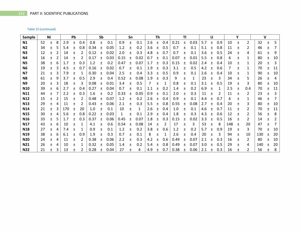
142 PART II: SCIENTIFIC PUBLICATIONS
Table 1S (continued)
Sample Ni Pb Sb Sn Th Tl U Y V
N1 52 ± 8 2.9 ± 0.4 0.8 ± 0.1 0.9 ± 0.1 2.6 ± 0.4 0.21 ± 0.03 5.7 ± 0.9 10 ± 2 32 ± 5 N2 34 ± 5 5.4 ± 0.8 0.34 ± 0.05 1.2 ± 0.2 3.6 ± 0.5 0.7 ± 0.1 5.1 ± 0.8 11 ± 2 46 ± 7 N3 12 ± 2 14 ± 2 0.12 ± 0.02 2.0 ± 0.3 4.8 ± 0.7 0.7 ± 0.1 3.6 ± 0.5 24 ± 4 61 ± 9 N4 16 ± 2 14 ± 2 0.17 ± 0.03 0.15 ± 0.02 0.7 ± 0.1 0.07 ± 0.01 5.5 ± 0.8 6 ± 1 80 ± 10 N5 38 ± 6 1.7 ± 0.3 1.2 ± 0.2 0.47 ± 0.07 1.7 ± 0.3 0.15 ± 0.02 2.4 ± 0.4 10 ± 1 20 ± 3 N6 19 ± 3 4.5 ± 0.7 0.16 ± 0.02 0.7 ± 0.1 1.9 ± 0.3 3.1 ± 0.5 4.2 ± 0.6 7 ± 1 70 ± 11 N7 21 ± 3 7.9 ± 1 0.30 ± 0.04 2.5 ± 0.4 3.3 ± 0.5 0.9 ± 0.1 2.6 ± 0.4 10 ± 1 90 ± 10 N8 61 ± 9 3.7 ± 0.5 2.9 ± 0.4 0.52 ± 0.08 1.9 ± 0.3 9 ± 1 23 ± 3 34 ± 5 26 ± 4 N9 20 ± 3 18 ± 3 0.08 ± 0.01 3.4 ± 0.5 7 ± 1 0.8 ± 0.1 3.1 ± 0.5 19 ± 3 80 ± 10 N10 39 ± 6 2.7 ± 0.4 0.27 ± 0.04 0.7 ± 0.1 1.1 ± 0.2 1.4 ± 0.2 6.9 ± 1 2.5 ± 0.4 70 ± 11 N11 44 ± 7 2.2 ± 0.3 1.6 ± 0.2 0.33 ± 0.05 0.9 ± 0.1 2.0 ± 0.3 11 ± 2 11 ± 2 23 ± 3 N12 15 ± 2 15 ± 2 0.48 ± 0.07 1.2 ± 0.2 2.6 ± 0.4 0.9 ± 0.1 4.4 ± 0.7 6 ± 1 46 ± 7 N13 29 ± 4 11 ± 2 0.43 ± 0.06 2.1 ± 0.3 5.5 ± 0.8 0.55 ± 0.08 2.7 ± 0.4 20 ± 3 80 ± 10 N14 21 ± 3 170 ± 20 1.0 ± 0.1 10 ± 1 2.6 ± 0.4 1.0 ± 0.1 4.6 ± 0.7 11 ± 2 70 ± 11 N15 30 ± 4 5.6 ± 0.8 0.22 ± 0.03 1 ± 0.1 2.9 ± 0.4 1.8 ± 0.3 4.3 ± 0.6 12 ± 2 56 ± 8 N16 33 ± 5 1.7 ± 0.3 0.37 ± 0.06 0.45 ± 0.07 1.8 ± 0.3 0.15 ± 0.02 3.3 ± 0.5 16 ± 2 14 ± 2 N17 43 ± 6 10 ± 1 4.1 ± 0.6 0.54 ± 0.08 14 ± 2 17 ± 3 53 ± 8 148 ± 20 47 ± 7 N18 27 ± 4 7.4 ± 1 0.9 ± 0.1 1.2 ± 0.2 3.8 ± 0.6 1.2 ± 0.2 5.7 ± 0.9 19 ± 3 70 ± 10 N19 38 ± 6 6.1 ± 0.9 1.9 ± 0.3 0.7 ± 0.1 8 ± 1 2.6 ± 0.4 20 ± 3 94 ± 10 130 ± 20 N20 24 ± 4 11 ± 2 0.38 ± 0.06 2.2 ± 0.3 4.2 ± 0.6 0.49 ± 0.07 2.1 ± 0.3 16 ± 2 80 ± 10 N21 26 ± 4 10 ± 1 0.32 ± 0.05 1.4 ± 0.2 5.4 ± 0.8 0.49 ± 0.07 3.0 ± 0.5 29 ± 4 140 ± 20 N22 21 ± 3 13 ± 2 0.28 ± 0.04 27 ± 4 4.9 ± 0.7 0.38 ± 0.06 2.1 ± 0.3 16 ± 2 56 ± 8

143 PART II: SCIENTIFIC PUBLICATIONS
Table 1S (continued)
Sample Al Ba Fe Mn P Sr Ti Zn
N1 36000 ± 5000 90 ± 10 13000 ± 2000 80 ± 10 1400 ± 200 1500 ± 200 1500 ± 200 43 ± 6 N2 23000 ± 3000 170 ± 30 17000 ± 2000 130 ± 20 3700 ± 600 230 ± 40 1800 ± 300 31 ± 5 N3 42000 ± 6000 290 ± 40 18000 ± 2700 420 ± 60 2600 ± 400 140 ± 20 5000 ± 700 29 ± 4 N4 40000 ± 6000 290 ± 40 22000 ± 3000 580 ± 90 700 ± 100 160 ± 20 330 ± 50 33 ± 5 N5 13000 ± 2000 40 ± 6 8300 ± 1200 31 ± 5 1300 ± 200 200 ± 30 600 ± 100 29 ± 4 N6 22000 ± 3000 140 ± 20 12000 ± 2000 42 ± 6 2600 ± 400 1100 ± 200 900 ± 100 100 ± 20 N7 23000 ± 3000 210 ± 30 20000 ± 3000 200 ± 30 1900 ± 300 160 ± 20 2500 ± 400 25 ± 4 N8 9800 ± 1000 55 ± 8 6900 ± 1000 44 ± 7 29000 ± 4000 190 ± 30 860 ± 100 37 ± 5 N9 57000 ± 9000 210 ± 30 32000 ± 5000 540 ± 80 1200 ± 200 500 ± 80 6800 ± 1000 70 ± 11 N10 10000 ± 2000 190 ± 30 3600 ± 500 37 ± 5 1500 ± 200 440 ± 70 530 ± 80 27 ± 4 N11 8400 ± 1000 40 ± 6 5700 ± 900 36 ± 5 12000 ± 2000 200 ± 30 600 ± 100 17 ± 3 N12 13000 ± 2000 170 ± 30 15000 ± 2000 100 ± 20 1400 ± 200 130 ± 20 1300 ± 200 70 ± 11 N13 51000 ± 8000 330 ± 50 44000 ± 6600 350 ± 50 2000 ± 300 190 ± 30 4600 ± 700 80 ± 10 N14 25000 ± 4000 220 ± 30 26000 ± 4000 230 ± 30 4100 ± 600 220 ± 30 2600 ± 400 400 ± 60 N15 24000 ± 4000 220 ± 30 20000 ± 3000 150 ± 20 3800 ± 600 220 ± 30 2200 ± 300 38 ± 6 N16 8000 ± 1000 70 ± 10 5000 ± 800 36 ± 5 1600 ± 200 190 ± 30 700 ± 100 23 ± 3 N17 19000 ± 3000 120 ± 20 17000 ± 2000 80 ± 10 56500 ± 8000 170 ± 30 1800 ± 300 32 ± 5 N18 32000 ± 5000 290 ± 40 31000 ± 4600 200 ± 30 3800 ± 600 1000 ± 100 3200 ± 500 54 ± 8 N19 24000 ± 4000 140 ± 20 86000 ± 13000 80 ± 10 16500 ± 2000 1000 ± 200 2300 ± 300 61 ± 9 N20 54000 ± 8000 240 ± 40 35000 ± 5000 330 ± 50 1800 ± 300 1100 ± 200 4200 ± 600 51 ± 8 N21 40000 ± 6000 310 ± 50 37000 ± 6000 700 ± 100 2300 ± 400 1200 ± 200 7400 ± 1100 47 ± 7 N22 45000 ± 7000 240 ± 40 25000 ± 4000 220 ± 30 1100 ± 200 200 ± 30 2700 ± 400 100 ± 20
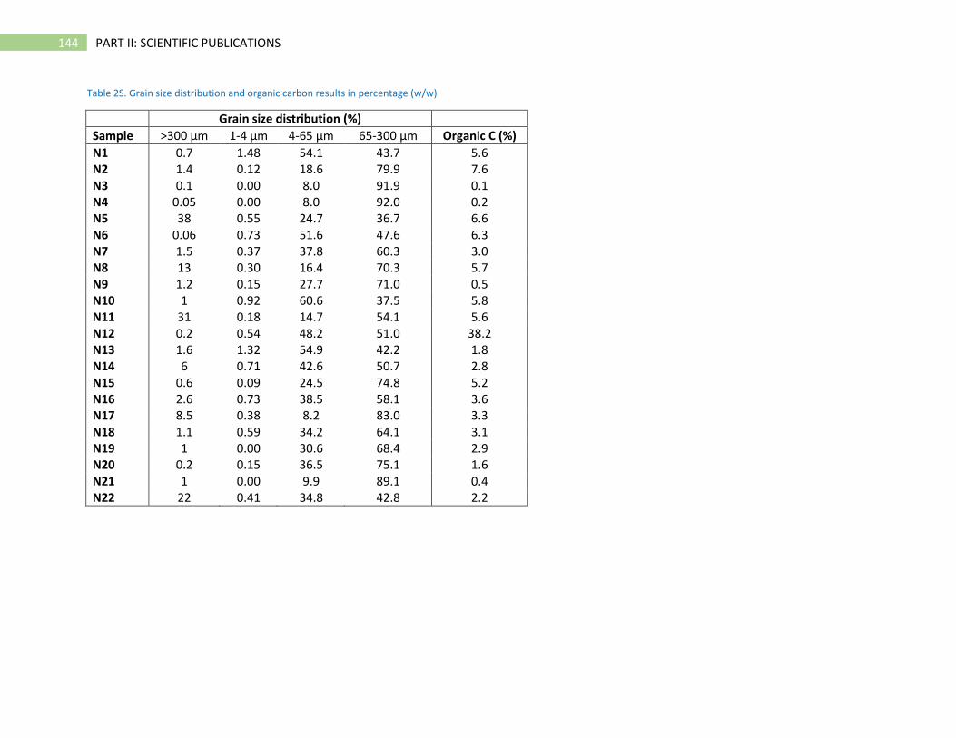
144 PART II: SCIENTIFIC PUBLICATIONS
Table 2S. Grain size distribution and organic carbon results in percentage (w/w)
Grain size distribution (%) Sample >300 µm 1-4 µm 4-65 µm 65-300 µm Organic C (%)
N1 0.7 1.48 54.1 43.7 5.6 N2 1.4 0.12 18.6 79.9 7.6 N3 0.1 0.00 8.0 91.9 0.1 N4 0.05 0.00 8.0 92.0 0.2 N5 38 0.55 24.7 36.7 6.6 N6 0.06 0.73 51.6 47.6 6.3 N7 1.5 0.37 37.8 60.3 3.0 N8 13 0.30 16.4 70.3 5.7 N9 1.2 0.15 27.7 71.0 0.5 N10 1 0.92 60.6 37.5 5.8 N11 31 0.18 14.7 54.1 5.6 N12 0.2 0.54 48.2 51.0 38.2 N13 1.6 1.32 54.9 42.2 1.8 N14 6 0.71 42.6 50.7 2.8 N15 0.6 0.09 24.5 74.8 5.2 N16 2.6 0.73 38.5 58.1 3.6 N17 8.5 0.38 8.2 83.0 3.3 N18 1.1 0.59 34.2 64.1 3.1 N19 1 0.00 30.6 68.4 2.9 N20 0.2 0.15 36.5 75.1 1.6 N21 1 0.00 9.9 89.1 0.4 N22 22 0.41 34.8 42.8 2.2
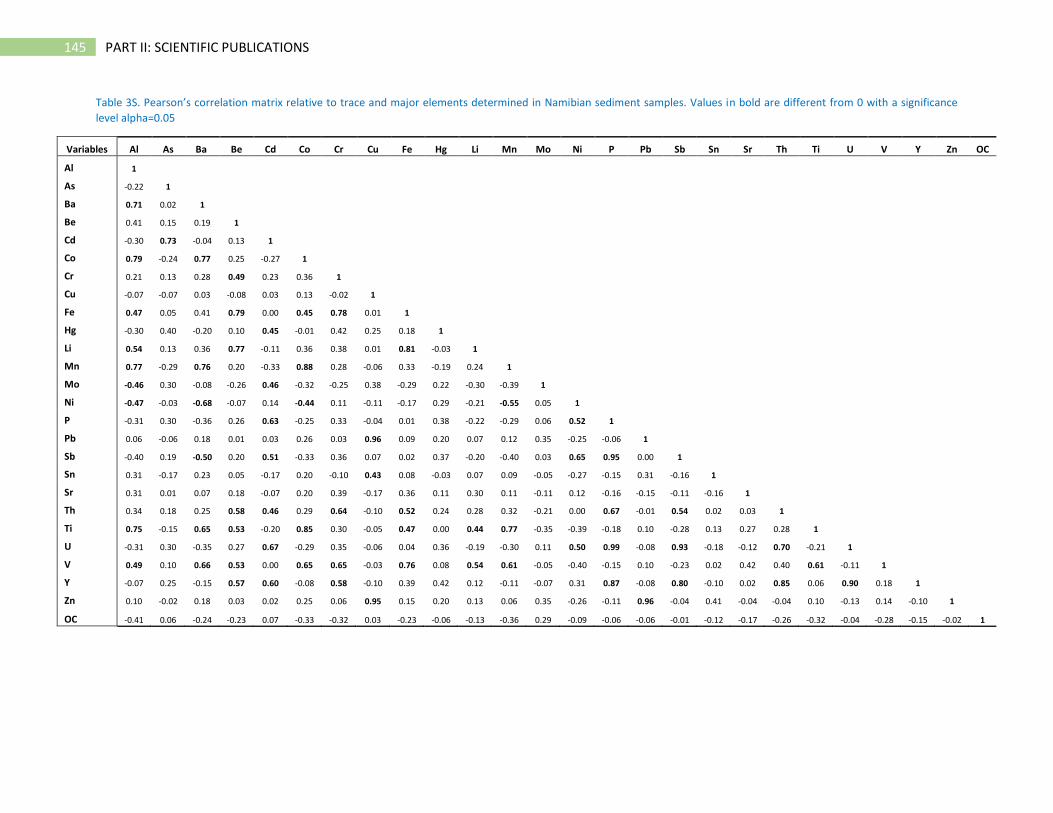
145 PART II: SCIENTIFIC PUBLICATIONS
Table 3S. Pearson’s correlation matrix relative to trace and major elements determined in Namibian sediment samples. Values in bold are different from 0 with a significance
level alpha=0.05
Variables Al As Ba Be Cd Co Cr Cu Fe Hg Li Mn Mo Ni P Pb Sb Sn Sr Th Ti U V Y Zn OC
Al 1
As -0.22 1
Ba 0.71 0.02 1
Be 0.41 0.15 0.19 1
Cd -0.30 0.73 -0.04 0.13 1
Co 0.79 -0.24 0.77 0.25 -0.27 1
Cr 0.21 0.13 0.28 0.49 0.23 0.36 1
Cu -0.07 -0.07 0.03 -0.08 0.03 0.13 -0.02 1
Fe 0.47 0.05 0.41 0.79 0.00 0.45 0.78 0.01 1
Hg -0.30 0.40 -0.20 0.10 0.45 -0.01 0.42 0.25 0.18 1
Li 0.54 0.13 0.36 0.77 -0.11 0.36 0.38 0.01 0.81 -0.03 1
Mn 0.77 -0.29 0.76 0.20 -0.33 0.88 0.28 -0.06 0.33 -0.19 0.24 1
Mo -0.46 0.30 -0.08 -0.26 0.46 -0.32 -0.25 0.38 -0.29 0.22 -0.30 -0.39 1
Ni -0.47 -0.03 -0.68 -0.07 0.14 -0.44 0.11 -0.11 -0.17 0.29 -0.21 -0.55 0.05 1
P -0.31 0.30 -0.36 0.26 0.63 -0.25 0.33 -0.04 0.01 0.38 -0.22 -0.29 0.06 0.52 1
Pb 0.06 -0.06 0.18 0.01 0.03 0.26 0.03 0.96 0.09 0.20 0.07 0.12 0.35 -0.25 -0.06 1
Sb -0.40 0.19 -0.50 0.20 0.51 -0.33 0.36 0.07 0.02 0.37 -0.20 -0.40 0.03 0.65 0.95 0.00 1
Sn 0.31 -0.17 0.23 0.05 -0.17 0.20 -0.10 0.43 0.08 -0.03 0.07 0.09 -0.05 -0.27 -0.15 0.31 -0.16 1
Sr 0.31 0.01 0.07 0.18 -0.07 0.20 0.39 -0.17 0.36 0.11 0.30 0.11 -0.11 0.12 -0.16 -0.15 -0.11 -0.16 1
Th 0.34 0.18 0.25 0.58 0.46 0.29 0.64 -0.10 0.52 0.24 0.28 0.32 -0.21 0.00 0.67 -0.01 0.54 0.02 0.03 1
Ti 0.75 -0.15 0.65 0.53 -0.20 0.85 0.30 -0.05 0.47 0.00 0.44 0.77 -0.35 -0.39 -0.18 0.10 -0.28 0.13 0.27 0.28 1
U -0.31 0.30 -0.35 0.27 0.67 -0.29 0.35 -0.06 0.04 0.36 -0.19 -0.30 0.11 0.50 0.99 -0.08 0.93 -0.18 -0.12 0.70 -0.21 1
V 0.49 0.10 0.66 0.53 0.00 0.65 0.65 -0.03 0.76 0.08 0.54 0.61 -0.05 -0.40 -0.15 0.10 -0.23 0.02 0.42 0.40 0.61 -0.11 1
Y -0.07 0.25 -0.15 0.57 0.60 -0.08 0.58 -0.10 0.39 0.42 0.12 -0.11 -0.07 0.31 0.87 -0.08 0.80 -0.10 0.02 0.85 0.06 0.90 0.18 1
Zn 0.10 -0.02 0.18 0.03 0.02 0.25 0.06 0.95 0.15 0.20 0.13 0.06 0.35 -0.26 -0.11 0.96 -0.04 0.41 -0.04 -0.04 0.10 -0.13 0.14 -0.10 1
OC -0.41 0.06 -0.24 -0.23 0.07 -0.33 -0.32 0.03 -0.23 -0.06 -0.13 -0.36 0.29 -0.09 -0.06 -0.06 -0.01 -0.12 -0.17 -0.26 -0.32 -0.04 -0.28 -0.15 -0.02 1
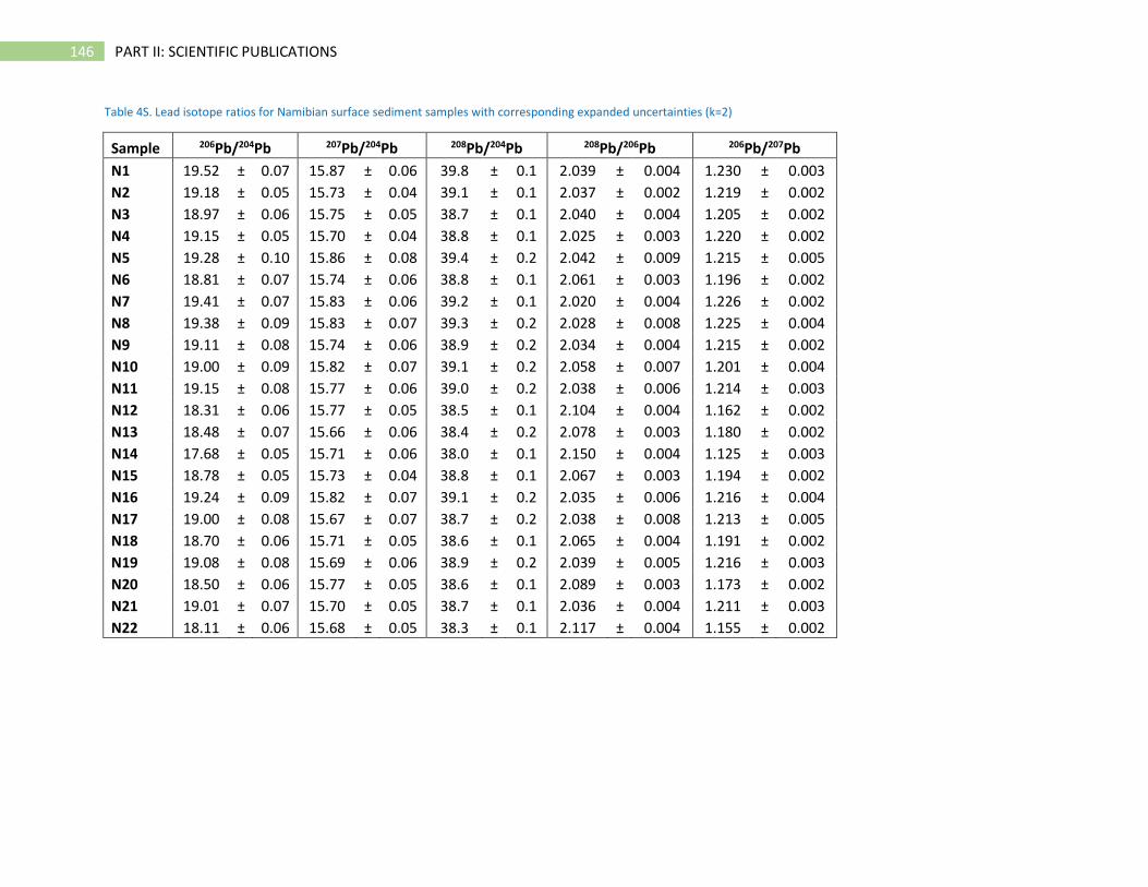
146 PART II: SCIENTIFIC PUBLICATIONS
Table 4S. Lead isotope ratios for Namibian surface sediment samples with corresponding expanded uncertainties (k=2)
Sample 206Pb/204Pb 207Pb/204Pb 208Pb/204Pb 208Pb/206Pb 206Pb/207Pb
N1 19.52 ± 0.07 15.87 ± 0.06 39.8 ± 0.1 2.039 ± 0.004 1.230 ± 0.003
N2 19.18 ± 0.05 15.73 ± 0.04 39.1 ± 0.1 2.037 ± 0.002 1.219 ± 0.002
N3 18.97 ± 0.06 15.75 ± 0.05 38.7 ± 0.1 2.040 ± 0.004 1.205 ± 0.002
N4 19.15 ± 0.05 15.70 ± 0.04 38.8 ± 0.1 2.025 ± 0.003 1.220 ± 0.002
N5 19.28 ± 0.10 15.86 ± 0.08 39.4 ± 0.2 2.042 ± 0.009 1.215 ± 0.005
N6 18.81 ± 0.07 15.74 ± 0.06 38.8 ± 0.1 2.061 ± 0.003 1.196 ± 0.002
N7 19.41 ± 0.07 15.83 ± 0.06 39.2 ± 0.1 2.020 ± 0.004 1.226 ± 0.002
N8 19.38 ± 0.09 15.83 ± 0.07 39.3 ± 0.2 2.028 ± 0.008 1.225 ± 0.004
N9 19.11 ± 0.08 15.74 ± 0.06 38.9 ± 0.2 2.034 ± 0.004 1.215 ± 0.002
N10 19.00 ± 0.09 15.82 ± 0.07 39.1 ± 0.2 2.058 ± 0.007 1.201 ± 0.004
N11 19.15 ± 0.08 15.77 ± 0.06 39.0 ± 0.2 2.038 ± 0.006 1.214 ± 0.003
N12 18.31 ± 0.06 15.77 ± 0.05 38.5 ± 0.1 2.104 ± 0.004 1.162 ± 0.002
N13 18.48 ± 0.07 15.66 ± 0.06 38.4 ± 0.2 2.078 ± 0.003 1.180 ± 0.002
N14 17.68 ± 0.05 15.71 ± 0.06 38.0 ± 0.1 2.150 ± 0.004 1.125 ± 0.003
N15 18.78 ± 0.05 15.73 ± 0.04 38.8 ± 0.1 2.067 ± 0.003 1.194 ± 0.002
N16 19.24 ± 0.09 15.82 ± 0.07 39.1 ± 0.2 2.035 ± 0.006 1.216 ± 0.004
N17 19.00 ± 0.08 15.67 ± 0.07 38.7 ± 0.2 2.038 ± 0.008 1.213 ± 0.005
N18 18.70 ± 0.06 15.71 ± 0.05 38.6 ± 0.1 2.065 ± 0.004 1.191 ± 0.002
N19 19.08 ± 0.08 15.69 ± 0.06 38.9 ± 0.2 2.039 ± 0.005 1.216 ± 0.003
N20 18.50 ± 0.06 15.77 ± 0.05 38.6 ± 0.1 2.089 ± 0.003 1.173 ± 0.002
N21 19.01 ± 0.07 15.70 ± 0.05 38.7 ± 0.1 2.036 ± 0.004 1.211 ± 0.003
N22 18.11 ± 0.06 15.68 ± 0.05 38.3 ± 0.1 2.117 ± 0.004 1.155 ± 0.002
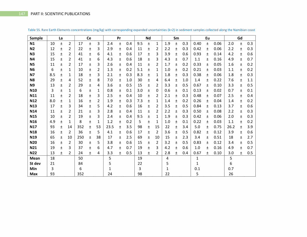
147 PART II: SCIENTIFIC PUBLICATIONS
Table 5S. Rare Earth Elements concentrations (mg/kg) with corresponding expanded uncertainties (k=2) in sediment samples collected along the Namibian coast
Sample La Ce Pr Nd Sm Eu Gd
N1 10 ± 2 17 ± 3 2.4 ± 0.4 9.5 ± 1 1.9 ± 0.3 0.40 ± 0.06 2.0 ± 0.3 N2 12 ± 2 22 ± 3 2.9 ± 0.4 11 ± 2 2.2 ± 0.3 0.42 ± 0.06 2.2 ± 0.3 N3 15 ± 2 41 ± 6 4.1 ± 0.6 17 ± 3 3.9 ± 0.6 0.93 ± 0.14 4.2 ± 0.6 N4 15 ± 2 41 ± 6 4.3 ± 0.6 18 ± 3 4.3 ± 0.7 1.1 ± 0.16 4.9 ± 0.7 N5 11 ± 2 17 ± 3 2.6 ± 0.4 11 ± 2 1.7 ± 0.2 0.33 ± 0.05 1.6 ± 0.2 N6 6 ± 1 10 ± 2 1.3 ± 0.2 5.1 ± 1 1.0 ± 0.2 0.21 ± 0.03 1.1 ± 0.2 N7 8.5 ± 1 18 ± 3 2.1 ± 0.3 8.3 ± 1 1.8 ± 0.3 0.38 ± 0.06 1.8 ± 0.3 N8 29 ± 4 52 ± 8 7.0 ± 1.0 30 ± 4 6.4 ± 1.0 1.4 ± 0.22 7.6 ± 1.1 N9 13 ± 2 29 ± 4 3.6 ± 0.5 15 ± 2 3.3 ± 0.5 0.67 ± 0.10 3.3 ± 0.5 N10 3 ± 1 6 ± 1 0.8 ± 0.1 3.0 ± 0 0.6 ± 0.1 0.13 ± 0.02 0.7 ± 0.1 N11 11 ± 2 18 ± 3 2.5 ± 0.4 10 ± 2 2.1 ± 0.3 0.48 ± 0.07 2.5 ± 0.4 N12 8.0 ± 1 16 ± 2 1.9 ± 0.3 7.3 ± 1 1.4 ± 0.2 0.26 ± 0.04 1.4 ± 0.2 N13 17 ± 3 34 ± 5 4.2 ± 0.6 16 ± 2 3.5 ± 0.5 0.84 ± 0.13 3.7 ± 0.6 N14 11 ± 2 21 ± 3 2.8 ± 0.4 11 ± 2 2.2 ± 0.3 0.50 ± 0.08 2.2 ± 0.3 N15 10 ± 2 19 ± 3 2.4 ± 0.4 9.5 ± 1 1.9 ± 0.3 0.42 ± 0.06 2.0 ± 0.3 N16 4.9 ± 1 8 ± 1 1.2 ± 0.2 5 ± 1 1.0 ± 0.1 0.22 ± 0.03 1.1 ± 0.2 N17 93 ± 14 352 ± 53 23.5 ± 3.5 98 ± 15 22 ± 3.4 5.0 ± 0.75 26.2 ± 3.9 N18 16 ± 2 36 ± 5 4.1 ± 0.6 17 ± 2 3.6 ± 0.5 0.82 ± 0.12 3.9 ± 0.6 N19 65 ± 10 250 ± 38 17 ± 2.5 69 ± 10 15 ± 2.3 3.4 ± 0.51 18 ± 2.7 N20 16 ± 2 30 ± 5 3.8 ± 0.6 15 ± 2 3.2 ± 0.5 0.83 ± 0.12 3.4 ± 0.5 N21 19 ± 3 37 ± 6 4.7 ± 0.7 19 ± 3 4.2 ± 0.6 1.0 ± 0.16 4.9 ± 0.7 N22 13 ± 2 24 ± 4 3.3 ± 0.5 13 ± 2 2.8 ± 0.4 0.67 ± 0.10 3.0 ± 0.5
Mean 18 50 5 19 4 1 5 St dev 21 84 5 22 5 1 6 Min 3 6 1 3 1 0.1 0.7 Max 93 352 24 98 22 5 26
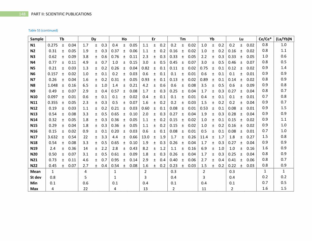
148 PART II: SCIENTIFIC PUBLICATIONS
Table 5S (continued)
Sample Tb Dy Ho Er Tm Yb Lu Ce/Ce* (La/Yb)N
N1 0.275 ± 0.04 1.7 ± 0.3 0.4 ± 0.05 1.1 ± 0.2 0.2 ± 0.02 1.0 ± 0.2 0.2 ± 0.02 0.8 1.0
N2 0.31 ± 0.05 1.9 ± 0.3 0.37 ± 0.06 1.1 ± 0.2 0.16 ± 0.02 1.0 ± 0.2 0.16 ± 0.02 0.8 1.1
N3 0.62 ± 0.09 3.8 ± 0.6 0.76 ± 0.11 2.3 ± 0.3 0.33 ± 0.05 2.2 ± 0.3 0.33 ± 0.05 1.0 0.6
N4 0.77 ± 0.11 4.9 ± 0.7 1.0 ± 0.15 3.0 ± 0.5 0.45 ± 0.07 3.0 ± 0.5 0.46 ± 0.07 0.8 0.5
N5 0.21 ± 0.03 1.3 ± 0.2 0.26 ± 0.04 0.82 ± 0.1 0.11 ± 0.02 0.75 ± 0.1 0.12 ± 0.02 0.9 1.4
N6 0.157 ± 0.02 1.0 ± 0.1 0.2 ± 0.03 0.6 ± 0.1 0.1 ± 0.01 0.6 ± 0.1 0.1 ± 0.01 0.9 0.9
N7 0.26 ± 0.04 1.6 ± 0.2 0.31 ± 0.05 0.93 ± 0.1 0.13 ± 0.02 0.89 ± 0.1 0.14 ± 0.02 0.8 0.9
N8 1.048 ± 0.16 6.5 ± 1.0 1.4 ± 0.21 4.2 ± 0.6 0.6 ± 0.08 3.5 ± 0.5 0.6 ± 0.09 0.9 0.8
N9 0.49 ± 0.07 2.9 ± 0.4 0.57 ± 0.08 1.7 ± 0.3 0.25 ± 0.04 1.7 ± 0.3 0.27 ± 0.04 0.8 0.7
N10 0.097 ± 0.01 0.6 ± 0.1 0.1 ± 0.02 0.4 ± 0.1 0.1 ± 0.01 0.4 ± 0.1 0.1 ± 0.01 0.7 0.8
N11 0.355 ± 0.05 2.3 ± 0.3 0.5 ± 0.07 1.6 ± 0.2 0.2 ± 0.03 1.5 ± 0.2 0.2 ± 0.04 0.9 0.7
N12 0.19 ± 0.03 1.1 ± 0.2 0.21 ± 0.03 0.60 ± 0.1 0.08 ± 0.01 0.53 ± 0.1 0.08 ± 0.01 0.9 1.5
N13 0.54 ± 0.08 3.3 ± 0.5 0.65 ± 0.10 2.0 ± 0.3 0.27 ± 0.04 1.9 ± 0.3 0.28 ± 0.04 0.9 0.9
N14 0.32 ± 0.05 1.8 ± 0.3 0.36 ± 0.05 1.1 ± 0.2 0.15 ± 0.02 1.0 ± 0.1 0.15 ± 0.02 0.9 1.1
N15 0.29 ± 0.04 1.8 ± 0.3 0.36 ± 0.05 1.1 ± 0.2 0.15 ± 0.02 1.0 ± 0.2 0.16 ± 0.02 0.9 1.0
N16 0.15 ± 0.02 0.9 ± 0.1 0.20 ± 0.03 0.6 ± 0.1 0.08 ± 0.01 0.5 ± 0.1 0.08 ± 0.01 0.7 1.0
N17 3.632 ± 0.54 22 ± 3.3 4.4 ± 0.66 13.0 ± 1.9 1.7 ± 0.26 11.4 ± 1.7 1.8 ± 0.27 1.5 0.8
N18 0.54 ± 0.08 3.3 ± 0.5 0.65 ± 0.10 1.9 ± 0.3 0.26 ± 0.04 1.7 ± 0.3 0.27 ± 0.04 0.9 0.9
N19 2.4 ± 0.36 14 ± 2.2 2.8 ± 0.43 8.2 ± 1.2 1.1 ± 0.16 6.9 ± 1.0 1.0 ± 0.16 1.6 0.9
N20 0.50 ± 0.07 3.1 ± 0.5 0.61 ± 0.09 1.8 ± 0.3 0.26 ± 0.04 1.7 ± 0.3 0.25 ± 0.04 0.8 0.9
N21 0.73 ± 0.11 4.6 ± 0.7 0.95 ± 0.14 2.9 ± 0.4 0.40 ± 0.06 2.7 ± 0.4 0.41 ± 0.06 0.8 0.7
N22 0.45 ± 0.07 2.7 ± 0.4 0.54 ± 0.08 1.6 ± 0.2 0.23 ± 0.03 1.5 ± 0.2 0.22 ± 0.03 0.8 0.9
Mean 1 4 1 2 0.3 2 0.3 1 1
St dev 0.8 5 1 3 0.4 3 0.4 0.2 0.2
Min 0.1 0.6 0.1 0.4 0.1 0.4 0.1 0.7 0.5
Max 4 22 4 13 2 11 2 1.6 1.5
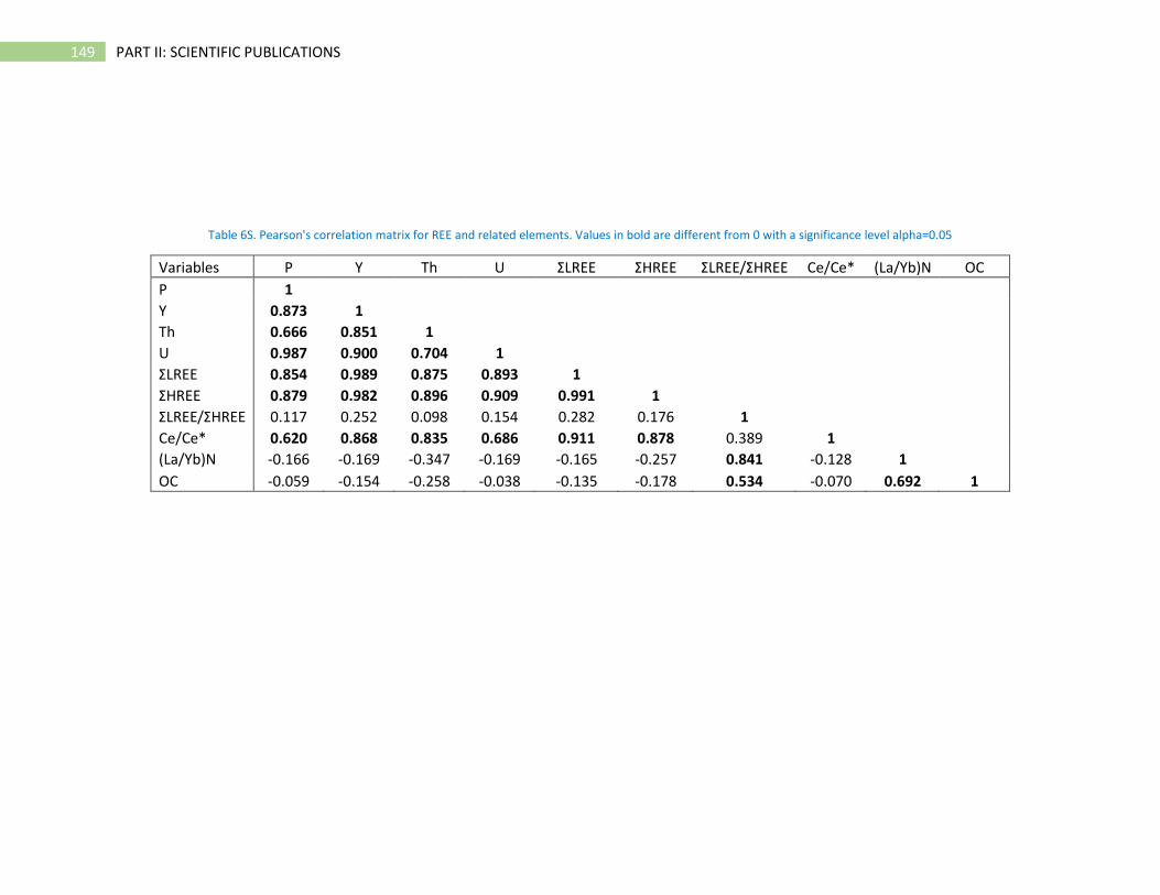
149 PART II: SCIENTIFIC PUBLICATIONS
Table 6S. Pearson's correlation matrix for REE and related elements. Values in bold are different from 0 with a significance level alpha=0.05
Variables P Y Th U ΣLREE ΣHREE ΣLREE/ΣHREE Ce/Ce* (La/Yb)N OC
P 1
Y 0.873 1 Th 0.666 0.851 1
U 0.987 0.900 0.704 1 ΣLREE 0.854 0.989 0.875 0.893 1
ΣHREE 0.879 0.982 0.896 0.909 0.991 1 ΣLREE/ΣHREE 0.117 0.252 0.098 0.154 0.282 0.176 1
Ce/Ce* 0.620 0.868 0.835 0.686 0.911 0.878 0.389 1 (La/Yb)N -0.166 -0.169 -0.347 -0.169 -0.165 -0.257 0.841 -0.128 1
OC -0.059 -0.154 -0.258 -0.038 -0.135 -0.178 0.534 -0.070 0.692 1
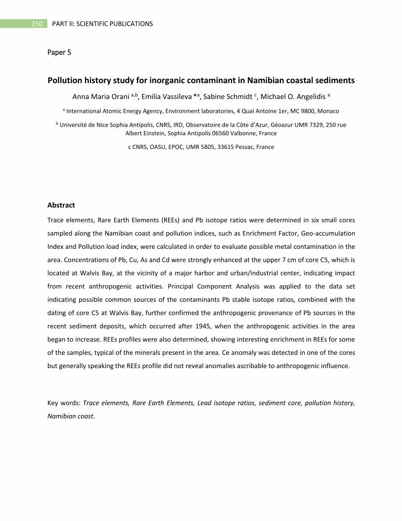
150 PART II: SCIENTIFIC PUBLICATIONS
Paper 5
Pollution history study for inorganic contaminant in Namibian coastal sediments
Anna Maria Orani a,b, Emilia Vassileva *a, Sabine Schmidt c, Michael O. Angelidis a
a International Atomic Energy Agency, Environment laboratories, 4 Quai Antoine 1er, MC 9800, Monaco
b Université de Nice Sophia Antipolis, CNRS, IRD, Observatoire de la Côte d’Azur, Géoazur UMR 7329, 250 rue
Albert Einstein, Sophia Antipolis 06560 Valbonne, France
c CNRS, OASU, EPOC, UMR 5805, 33615 Pessac, France
Abstract
Trace elements, Rare Earth Elements (REEs) and Pb isotope ratios were determined in six small cores
sampled along the Namibian coast and pollution indices, such as Enrichment Factor, Geo-accumulation
Index and Pollution load index, were calculated in order to evaluate possible metal contamination in the
area. Concentrations of Pb, Cu, As and Cd were strongly enhanced at the upper 7 cm of core C5, which is
located at Walvis Bay, at the vicinity of a major harbor and urban/industrial center, indicating impact
from recent anthropogenic activities. Principal Component Analysis was applied to the data set
indicating possible common sources of the contaminants Pb stable isotope ratios, combined with the
dating of core C5 at Walvis Bay, further confirmed the anthropogenic provenance of Pb sources in the
recent sediment deposits, which occurred after 1945, when the anthropogenic activities in the area
began to increase. REEs profiles were also determined, showing interesting enrichment in REEs for some
of the samples, typical of the minerals present in the area. Ce anomaly was detected in one of the cores
but generally speaking the REEs profile did not reveal anomalies ascribable to anthropogenic influence.
Key words: Trace elements, Rare Earth Elements, Lead isotope ratios, sediment core, pollution history,
Namibian coast.
151 PART II: SCIENTIFIC PUBLICATIONS
1. Introduction
Runoff material from the continent plays a key role on the mineralogy of costal marine sediments. At
drainage basins and coastal zones with important urban, industrial and mining activities, runoff material
is enriched in trace elements, which are transported to the sea and accumulate on the marine
sediments following flocculation of the colloidal constituents and suspended particle sedimentation
(Gibbs 1986). As a result marine sediments constitute an archive of trace element inputs to the marine
coastal environment and may be used as tools for establishing the effects of anthropogenic and natural
processes on depositional environments (Harikumar and Nasir, 2010), and often used to study the
pollution history of aquatic ecosystems (Valette-Silver, 1993, A.R.Karbassi, 2005; Kljaković-Gašpić et al.,
2008, Sun et al., 2012; Vallius, 2014; Veerasingam et al., 2015). Trace element pollution in the coastal
marine environment is an issue of major concern because of the toxicity to marine organisms and the
potential threat to the health of local population through the consumption of contaminated seafood
((Harikumar and Nasir, 2010; Maggi et al., 2012; Di Lena, et al 2017, Korkmaz et al 2017, Kuranchie-
Mensah, 2016, Nkpaa, K.W. 2016).
The coastal marine environment of Namibia is part of one of four major upwelling systems in the world
and is exceptionally productive, supporting abundant marine life (Sakko, 1998). Namibia has low, but
geographically very concentrated coastal population compared to other countries. Growing economic
development and human activities along the coast lead to unprecedented migration, resulting to
uncontrolled urban development and generation of untreated domestic and industrial effluents, which
are discharged to the sea, Furthermore, the exploitation of mineral resources has been the backbone of
the Namibian economy for many years as it is reflected to its contribution to the gross national product
of the country (Ministry of Environment and Tourism, 2008), diamond, fluorspar, and uranium being the
most significant mineral commodities to Namibia’s economy. In 2012 the country was ranked sixth in
terms of the total value of diamond production and fifth ranked producer of uranium (Bermudez-Lugo,
2014). Over the recent years the increasing profitability in the uranium market has seen several new
Namibian uranium projects emerge. Mining activities together with urban centers developed at the
Namibian coastline, appear to have an impact on the geochemistry of trace elements in coastal surface
sediments, indicating possible contaminations from land based pollution sources. (Orani et al,
submitted) In view of further investigation of trace element accumulation in the area, as well as to
study historic records of metal accumulation in the Namibian marine coastal environment, six sediment
cores were taken and analyzed for key trace elements and Rare Earth Elements. Pb stable isotopes were
also determined to provide additional information on the provenance of trace elements (natural vs
152 PART II: SCIENTIFIC PUBLICATIONS
anthropogenic) (Díaz-Somoano et al., 2009; Larsen et al., 2012, Xu et al., 2014; Mil-Homens et al., 2017).
Also, several contamination indices were calculated (Enrichment Factors, Geo-accumulation Index and
Pollution Load Index) in order to evaluate the extent of pollution and identify potential land based
pollution sources.
2. Experimental
2.1. Reagents and materials
All sample handling was carried out in class 10 laminar hoods. Ultrapure water with resistivity > 18 MΩ
was obtained from Milli-Q Element system (Millipore, USA) and was used throughout this work to dilute
concentrated acids.
Trace grade HNO3, HF and ultrapure HNO3 were purchased from Fisher Scientific (Hampton, USA).
Standard solutions for Al, Zn, Mn and Fe used for Flame AAS calibration and multielemental standard
TraceCert used for ICP-MS external calibration, were purchased from Sigma Aldridrich (Buchs,
Switzerlans) in concentrations of 1000 and 10 mg/L respectively. The Certified Reference Material MESS-
2 (Estuarine sediment, National Research Council, Canada) was used for assessing data accuracy. The
Standard Reference Material SRM 981 from the National Institute of Standards and Technology (NIST,
USA) with the natural Pb isotopic composition was used for correction of the instrumental mass
discrimination when measuring Pb isotope ratios.
All Teflon and PE lab ware used in the sample preparation and analysis, was pre-cleaned with a
procedure consisting of at least 24h bath in 10% HNO3 and careful rinsing with MilliQ water.
2.2. Instrumentation
Trace elements (TE: As, Ba, Cd, Co, Cr, Cu, Li, Ni, Pb, Sb, Sn, Sr, Th, U, and V) were determined by
Inductively Coupled Plasma Quadrupole Mass Spectrometry (Q-ICP-MS, XSERIES, Thermo Fisher
Scientific. The instrument was equipped with a micromist nebulizer (0.2 ml/min, Glass Expansion) and a
cyclonic spray chamber cooled by Peltier cooling system ESI. Instrument is also equipped with collision
cell technology (CCT) for interference removal; high purity He was used as collision gas. Before
measurements, the method parameters in normal and collision modes were optimized for maximum
153 PART II: SCIENTIFIC PUBLICATIONS
intensity and precision of each single isotope. As, Cr and V were measured in CCT mode, whereas the
rest of trace elements and REE determined in sediment samples were measured in normal mode.
Determination of Pb isotope ratios has been performed on digested samples by means of High
Resolution Sector Field ICP-MS (NuAttom, NuInstruments Ltd., Wrexham, UK). The Standard Reference
Material SRM 981 from the National Institute of Standards and Technology (NIST, USA) with the natural
Pb isotopic composition was used for correction of the instrumental mass discrimination and verification
of the developed analytical procedure. Instrumental conditions for TE, REEs and Pb isotope ratios were
described in detail in the previous paper (Orani et al., paper 4).
Determination of Al, Fe, Mn and Zn was carried out by Flame Atomic Absorption Spectroscopy (ContrAA
700, Analytik Jena, Germany) on the same digested solutions used for ICP-MS, using external calibration.
Temperature programs were developed and optimized for each of the studied elements. Calibration
curves were daily prepared using proper dilution of commercially available standard solutions. The
method blanks and CRMs prepared with each batch of samples were measured at the beginning and at
the end of each measurement sequence to validate samples measurements.
Mercury was determined in sediment samples directly, using a solid AAS analyzer (AMA 254, Altech,
USA), therefore no digestion was needed. A portion of about 100 mg of sediment was measured. The
internal calibration of the instrument was checked every day using an external standard solution and a
CRM (MESS-2) sampled at different intake masses, in order to verify the linearity of the calibration. The
instrument was recalibrated if any of the checks failed. Organic Carbon (TOC) was measured by means
of acidification and combustion in a one-unit carbon analysis system (Vario EL Cube, Elementar,
Langenselbold, Germany).
Results were analyzed using XLSTAT (version 2014.05.5, Addinsoft, Paris, France). Regression analysis
(Pearson’s Product-Moment Correlation) was used to examine relationships between trace metals
content and other parameters such as organic matter in order to identify common sources of pollution;
in all cases, the level of significance was set at p<0.05. Principal component analysis (PCA) was used to
further investigate results patterns.
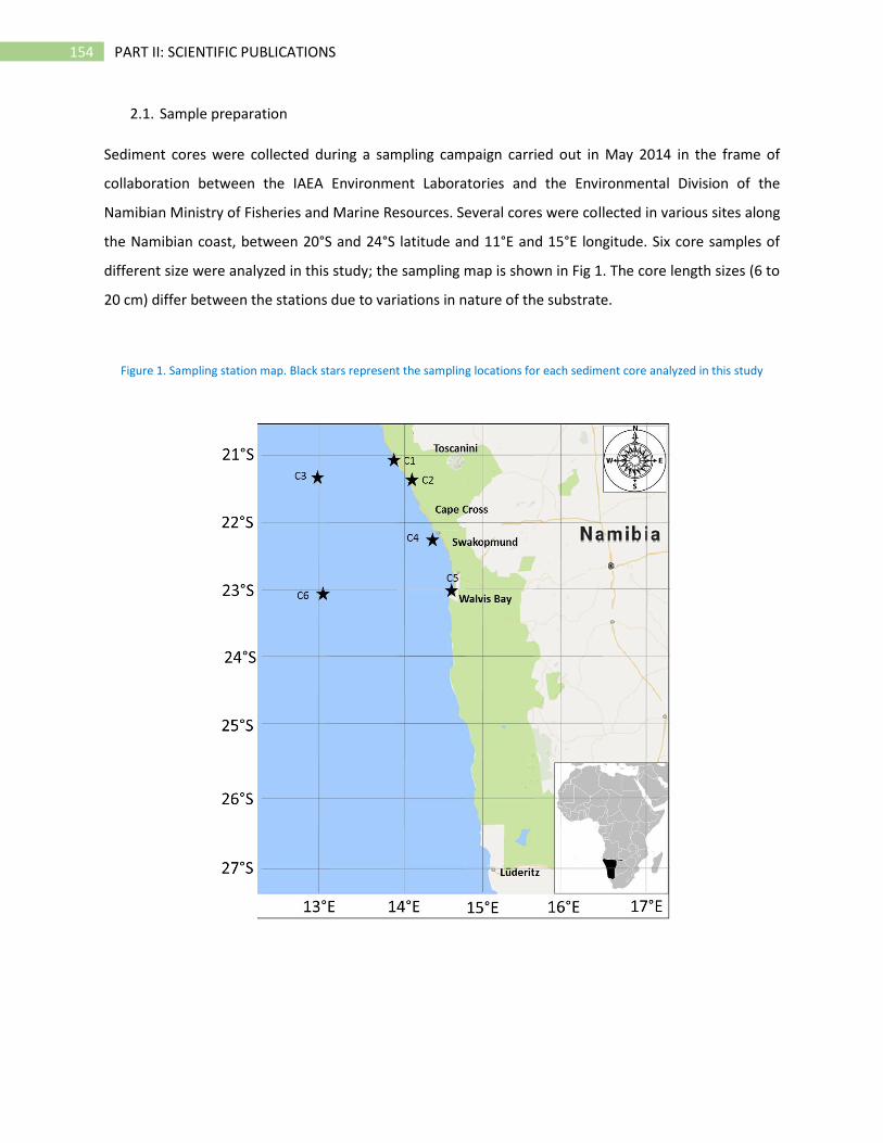
154 PART II: SCIENTIFIC PUBLICATIONS
2.1. Sample preparation
Sediment cores were collected during a sampling campaign carried out in May 2014 in the frame of
collaboration between the IAEA Environment Laboratories and the Environmental Division of the
Namibian Ministry of Fisheries and Marine Resources. Several cores were collected in various sites along
the Namibian coast, between 20°S and 24°S latitude and 11°E and 15°E longitude. Six core samples of
different size were analyzed in this study; the sampling map is shown in Fig 1. The core length sizes (6 to
20 cm) differ between the stations due to variations in nature of the substrate.
Figure 1. Sampling station map. Black stars represent the sampling locations for each sediment core analyzed in this study
155 PART II: SCIENTIFIC PUBLICATIONS
Sediments were collected using a MC-200-4 MiniMulti-Corer; samples were sliced per 1cm up to 10cm
and per 2cm after 10cm length. After collection, sediments were packed in plastic bags, labelled and
kept frozen during transportation at the laboratory. Later, samples were freeze-dried, sieved at 1 mm
and crushed in agate mortar to homogenize. Acid digestion was carried out in a microwave system using
a Mars X-press Microwave (CEM Mars X-press) equipped with a carousel holding 12 digestion vessels. A
quantity of 150 ± 50 mg of dried sample was weighed in Teflon microwave vessels, where 5ml of
ultrapure HNO3, 2 ml of H2O2 and 2 ml ultrapure concentrated HF were added. Each digestion batch
included two reagent blanks and two replicates of certified reference material MESS-2 (estuarine
sediment, National Research Council, Canada). The digestion procedure involves gradual increasing of
temperature to 190 °C for 15 min period, then isothermal treatment for additional 15 min. After
digestion, obtained solutions were placed on a ceramic heating plate and evaporated to near dryness.
The residues were taken up in 2% HNO3, transferred to 50 ml PE tubes and stored at 4 °C.
2.4. Risk assessment methods of TE sediment contamination
To assess pollution state of an area, calculation is very often based on comparing data with background
reference levels of the same element. The most accurate approach involves the use of background levels
measured in uncontaminated sediments of the same area with mineralogical and textural characteristics
similar to those shown by contaminated samples (Hornung et al., 1989; Abrahim and Parker, 2008). Very
often the uncontaminated samples used as background levels are taken from the bottom of sediment
cores collected in uncontaminated areas. The background reference levels used for normalization
purposes in this study were those measured in the bottom of sample C6, which shows stable values for
most of the elements along the 7 cm of the core. Additionally the grain size distribution is also very
similar to the one measured in the majority of core samples analyzed in our work (Varol, 2011).
Different parameters can be calculated to evaluate the anthropogenic influence on trace elements
content in the sediments. In this work three parameters were evaluated: Enrichment Factors (EF), Geo-
accumulation Index (Igeo) and Pollution Load Index (PLI). When the calculation of these parameters is
applied to sediment cores, it is possible to evaluate potential historical differences
EF are used for studying heavy metal contamination and sources in sediments (Xu et al., 2014; Resongles
et al., 2014) and their calculation implies the use of a normalizing element. Al is the normalizing
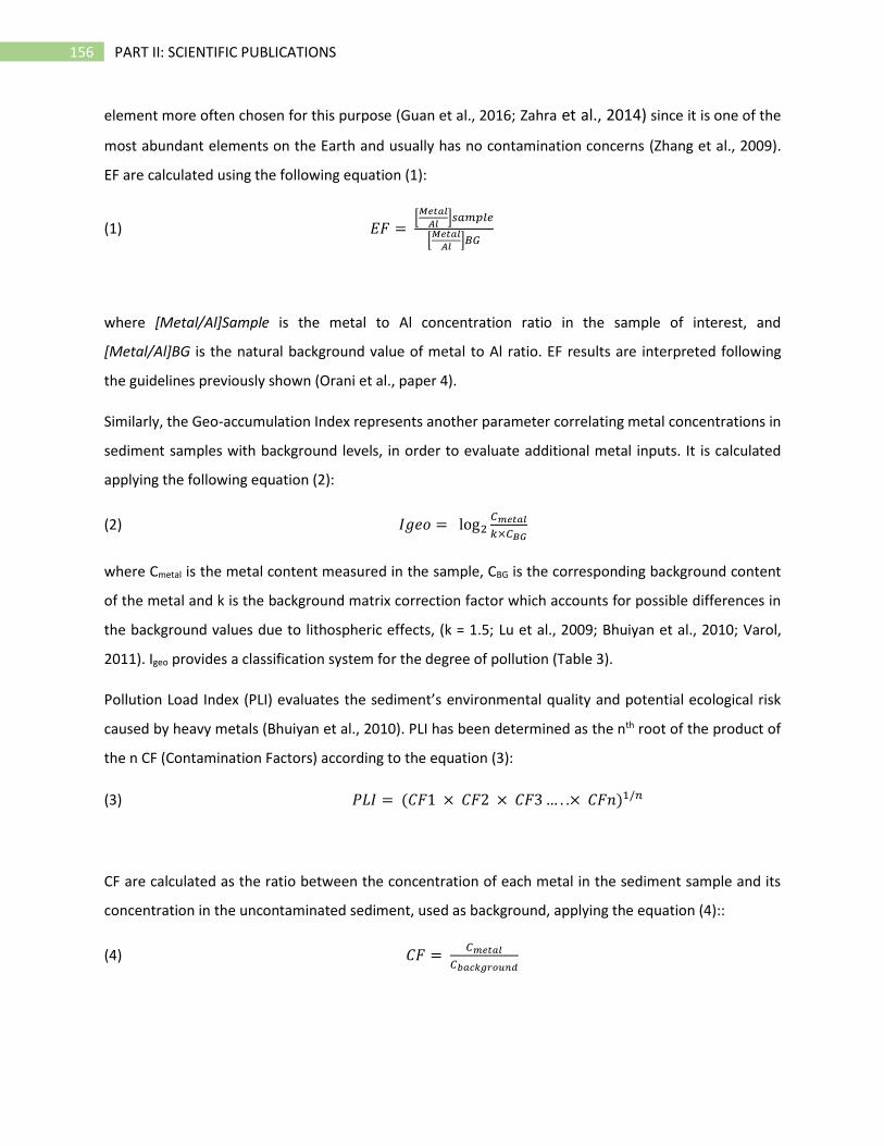
156 PART II: SCIENTIFIC PUBLICATIONS
element more often chosen for this purpose (Guan et al., 2016; Zahra et al., 2014) since it is one of the
most abundant elements on the Earth and usually has no contamination concerns (Zhang et al., 2009).
EF are calculated using the following equation (1):
(1) 𝐸𝐹 = [
𝑀𝑒𝑡𝑎𝑙
𝐴𝑙]𝑠𝑎𝑚𝑝𝑙𝑒
[𝑀𝑒𝑡𝑎𝑙
𝐴𝑙]𝐵𝐺
where [Metal/Al]Sample is the metal to Al concentration ratio in the sample of interest, and
[Metal/Al]BG is the natural background value of metal to Al ratio. EF results are interpreted following
the guidelines previously shown (Orani et al., paper 4).
Similarly, the Geo-accumulation Index represents another parameter correlating metal concentrations in
sediment samples with background levels, in order to evaluate additional metal inputs. It is calculated
applying the following equation (2):
(2) 𝐼𝑔𝑒𝑜 = log2𝐶𝑚𝑒𝑡𝑎𝑙
𝑘×𝐶𝐵𝐺
where Cmetal is the metal content measured in the sample, CBG is the corresponding background content
of the metal and k is the background matrix correction factor which accounts for possible differences in
the background values due to lithospheric effects, (k = 1.5; Lu et al., 2009; Bhuiyan et al., 2010; Varol,
2011). Igeo provides a classification system for the degree of pollution (Table 3).
Pollution Load Index (PLI) evaluates the sediment’s environmental quality and potential ecological risk
caused by heavy metals (Bhuiyan et al., 2010). PLI has been determined as the nth root of the product of
the n CF (Contamination Factors) according to the equation (3):
(3) 𝑃𝐿𝐼 = (𝐶𝐹1 × 𝐶𝐹2 × 𝐶𝐹3 … . .× 𝐶𝐹𝑛)1/𝑛
CF are calculated as the ratio between the concentration of each metal in the sediment sample and its
concentration in the uncontaminated sediment, used as background, applying the equation (4)::
(4) 𝐶𝐹 = 𝐶𝑚𝑒𝑡𝑎𝑙
𝐶𝑏𝑎𝑐𝑘𝑔𝑟𝑜𝑢𝑛𝑑
157 PART II: SCIENTIFIC PUBLICATIONS
This empirical index provides a simple, comparative means for assessing the level of heavy metal
pollution. When PLI > 1, it means that a pollution exists; otherwise, if PLI < 1, the analyzed sample can be
considered unpolluted (Tomlinson et al., 1980).
1.1. Dating
The age-depth model of core C5 was established based on 210Pb excess (210Pbxs; T1/2 = 22.3 years), a
naturally - occurring radionuclide which is incorporated rapidly into the sediment from atmospheric
fallout and water column scavenging. The activities of 210Pb and 226Ra were measured using a well-type,
low background germanium detector (CANBERRA) equipped of a Cryocycle (Schmidt and De Deckker,
2015). 210Pb activity was determined by the direct measurement of its gamma decay energy at 46.5 keV,
while 226Ra was estimated as the weighted average of two 214Pb peaks at 295.2 keV and 352 keV and a
214Be peak at 609.3 keV. 210Pbxs was determined by subtracting the activity supported by its parent
isotope, 226Ra, from the total measured 210Pb activity in sediment. Sediment accumulation rate (SAR,
0.07 cm yr-1) was calculated from the sedimentary profiles of 10Pbxs plotted against depth. The
deposition time, in years, was calculated by dividing the depth of each sediment layer by the SAR. The
deposition year for each sediment layer was subsequently estimated based on the 2014 sampling date
for the sediment-water interface.
2.6. Lead isotope ratios
The determination of lead isotope ratios has been proven to be a very helpful tool in the assessment of
Pb source in the environment. Lead has a partially radiogenic isotopic composition as three of its stable
isotopes (206Pb, 207Pb and 208Pb) are the final results of radioactive decay of 235U, 232Th and 238U
respectively (Vanhaecke and Degryse, 2012). The fourth isotope 204Pb is the only natural one, and its
abundance has remained constant since the origin of solar system (Komárek et al., 2008).
Because of its partially radiogenic nature, Pb isotopic composition is characteristic of a given
geographical origin or geochemical profile and it is often used for provenance studies in several fields
(Sjåstad et al., 2011; Drivelos and Georgiou, 2012; Ortega et al., 2012).Since natural and anthropogenic
Pb sources will show different Pb isotope composition in a given area, this analytical tool is often used in
environmental science as efficient way to evaluate the actual occurrence of Pb pollution. Additionally
the analysis of Pb isotope ratios can represent an efficient way to track the pollution source, as different
Pb inputs show a different and specific Pb isotope composition (Hinrichs et al., 2002). A popular way to
158 PART II: SCIENTIFIC PUBLICATIONS
present Pb isotope ratios results is the so-called three isotope graph (e.g., 206Pb/207Pb vs. 208Pb/206Pb)
which is used for distinguishing between separate Pb sources. Additionally, several models for assessing
the relative contribution of separate Pb sources have been proposed (Monna et al., 2000; Semlali et al.,
2004) and in all of them the knowledge of Pb isotopic composition of both natural background and
pollution sources is needed.
2.7. Rare Earth Elements
The Rare Earth Elements (REEs) are a group of elements including the series of lantanides, Sc and Y. They
are often grouped together as they have similar behavior in most of environmental systems. The
distribution patterns of REE has often been applied to geological studies of river and marine ecosystems
(Song and Choi, 2009; Rezaee et al., 2010) since they can be used as reliable tool for determining
depositional processes and sediment provenance (Xu et al., 2009; Jung et al., 2012). Some members of
this group are used in various components of some modern devices, such as high-strength magnets,
hard disk drives, smartphones screens and batteries, among others (Guyonnet et al., 2015). The demand
of these components is constantly increasing due to their widespread applications. Recycling of post-
consumer and components will increasingly contribute to the supply in the future but most probably it
will not be sufficient and the mining of natural deposits will continue to represent the major source of
REEs (Goodenough et al., 2016). Mining extraction from ores as well as the processes involved in the
production of different materials, have contributed to the increased release of these elements in the
environment, causing contamination in soils and waters(Liang et al., 2014). As a consequence of their
increased widespread use, the potential anthropogenic influence on REE natural distribution has
extended their application from geochemistry to environmental chemistry (Kulaksiz and Bau, 2011;
Hatje et al., 2016), leading scientists to refer to these elements as “new emerging pollutants”. A recent
paper has, for the first time, given baseline data for REEs in the Namibian coastal sediment (Orani et al.,
2017, submitted) but, to the best of our knowledge, no data are available in the literature about REEs
profiles in Namibian sediment samples. Some studies have been focusing on the determination of REEs
in phosphorite, quite widespread around Namibia and generally South Africa (McArthur and Walsh,
1984; Watkins et al., 1995) and data published on surface sediments have shown a particular trend, with
heavy REEs (HREEs) enrichment over the light ones.
159 PART II: SCIENTIFIC PUBLICATIONS
REEs results are often presented after normalization to a standard material, in order to be able to easily
recognize possible element anomalies in the pattern (Kulaksiz and Bau, 2011). The REEs results obtained
in this study were normalized using the American Shale Composite (Piper, 1974); some indices can be
calculated to better interpret the results, such as the La/Yb ratio which show possible enrichment in
LREEs over the HREEs (Hatje et al., 2016).
2.8 Data Quality Assurance
The analytical methods used in this study were properly selected and validated, both in terms of matrix
composition and analyte concentration. All possible sources of uncertainty of obtained results were
carefully identified. Afterwards, the uncertainty components were quantified and the combined
uncertainty calculated according to the ISO/GUM guide (Magnusson and Ornemark, 2014).
A principal requirement of the standard ISO 17025 (ISO/IEC, 2005) is for laboratories to produce
measurements that are traceable to a common system of reference, SI system, and ensure
comparability of measurement results. The way to demonstrate traceability in the present study was the
use of an uncertainty budget, where all the parameters influencing the final result were systematically
assessed. In addition the use of CRM throughout the whole analytical procedure and bias (recovery)
estimation was the way to link obtained trace elements mass fraction to the common system of
reference SI. CRM with similar matrix were also used in the validation of sample preparation step.
3. Results and discussion
In order to perform a complementary study on the historical variation in TE contamination in Namibia
coastal area, analysis on 6 core samples, collected at different stations along the coast, were performed.
A total of 54 samples were collected at different depths; sampling map is shown in Fig 1. Most of the
sediments measured in this study were classified as silty sand, with about 30-50% of grain size
distribution between 1-65 µm. Grain size of samples from cores C1 and C2 was mainly characterized by
particles between 65 and 300 µm.

160 PART II: SCIENTIFIC PUBLICATIONS
3.1. Distribution of trace elements in core samples
A summary of TE and Total Organic Carbon results is presented in Table 1S (supplementary information).
The core samples C4 and C5 show the highest variability in TE contents along the depth (Fig.1S,
supplementary information), suggesting different inputs of these elements during the period covered by
the analyzed cores. Particularly in C5, Pb ranged between 47 and 220 mg/kg and Cu ranged between 43
and 240 mg/kg. Higher concentrations for both Cu and Pb were measured in the first 7 cm while the
lower 7 cm exhibit a more stable content for both elements (Fig 2). Zn also had higher concentrations in
the surface layers (up to 380 mg/kg in the upper 3 cm) in the same core. The core C4 is characterized by
high variability in As, Zn and Cd contents; very interestingly some of these analytes showed higher
concentrations in the bottom of the sediment core. Generally speaking the cores C3 and C6 were
characterized by a very constant trend of almost all elements along their depth. Some analytes like Li, Co
and Hg show very low variability in all the studied cores, suggesting a unique source, most probably
natural.
Figure 2. Graphical representation of Pb and Cu content variation along the core C5
0
2
4
6
8
10
12
14
0 100 200 300
De
pth
(cm
)
mg kg-1Core C5
Pb
Cu

161 PART II: SCIENTIFIC PUBLICATIONS
Higher metals concentrations at the upper layers of the core C5, which is located at the vicinity of the
harbor of Walvis Bay, suggest recent accumulation of these metals as a result of anthropogenic
activities. However, in order to strengthen the interpretation of these results and to highlight possible
common patterns in the distribution of trace elements, a Pearson’s correlation test was performed for
each analyzed core: high correlation coefficients between different metals mean common sources,
mutual dependence, and identical behavior during transport (Guan et al., 2016). As already mentioned,
Cu, Zn, As and Cd appear to have similar patterns along the core C5 and the Pearson’s correlations
confirm a positive correlation between these elements (p<0.05). Among toxic elements, Pb showed
positive correlation with Cr, Co and Ni in samples C2, C4 and C5 while As and Cd exhibit positive
correlation in samples C5, C2 and C3 and negative correlation in sample C1. Organic Carbon (OC)
showed very variable correlations, in the different cores. Organic Carbon was found to be positively
correlated with Ni, Cu, As, Cd, Zn and V in sample C4, where the percentage of OC ranged from 1.3 and
5.2; additionally a positive correlation with Cr, Co was found in sample C6. No correlation between TOC
and any of the analyzed TE was found in sample C3 while in sample C5 the only analyte correlating with
TOC was Cd. The property of organic matter to influence the concentration of some trace metals in
environmental samples has been reported in several studies (Wang and Qin, 2006; Kljaković-Gašpić et
al., 2008) but the relation between these two components is still considered complex and very variable
(Wang, 2008).
It has to be pointed out that upwelling systems are naturally characterized by metal enrichment as a
consequence of high metal inputs from plankton but the metal content in Namibian coast was
previously suggested to be intimately related to organic matter content (Calvert and Price, 1970). From
the simple observation of trace elements variation along the analyzed cores, it is already clear that at
least samples C4 and C5 were subject to different element inputs, most probably of anthropogenic
origin given the location of these sampling stations. It appears equally clear that samples C1, C3 and C6
did not show significant changes in most of the analytes concentrations. In order to be able to clearly
state weather an anthropogenic input influenced the TE contents during the time in the analyzed region,
different indices of sediment contamination were evaluated.
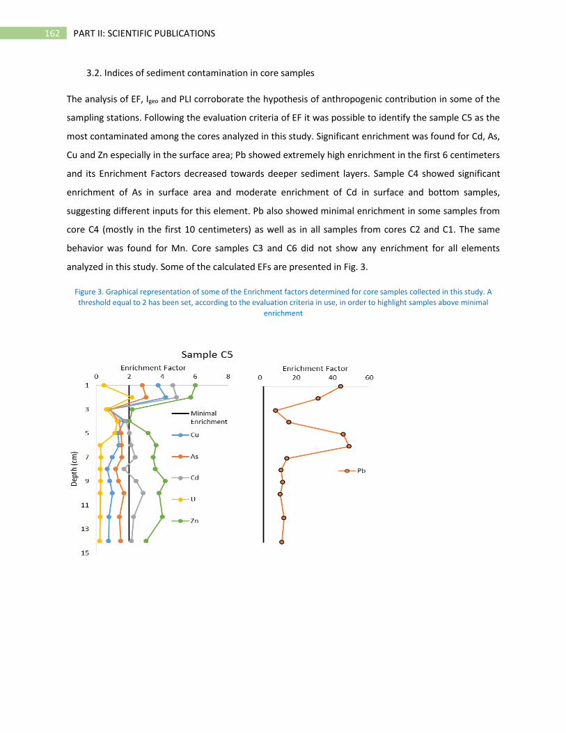
162 PART II: SCIENTIFIC PUBLICATIONS
3.2. Indices of sediment contamination in core samples
The analysis of EF, Igeo and PLI corroborate the hypothesis of anthropogenic contribution in some of the
sampling stations. Following the evaluation criteria of EF it was possible to identify the sample C5 as the
most contaminated among the cores analyzed in this study. Significant enrichment was found for Cd, As,
Cu and Zn especially in the surface area; Pb showed extremely high enrichment in the first 6 centimeters
and its Enrichment Factors decreased towards deeper sediment layers. Sample C4 showed significant
enrichment of As in surface area and moderate enrichment of Cd in surface and bottom samples,
suggesting different inputs for this element. Pb also showed minimal enrichment in some samples from
core C4 (mostly in the first 10 centimeters) as well as in all samples from cores C2 and C1. The same
behavior was found for Mn. Core samples C3 and C6 did not show any enrichment for all elements
analyzed in this study. Some of the calculated EFs are presented in Fig. 3.
Figure 3. Graphical representation of some of the Enrichment factors determined for core samples collected in this study. A
threshold equal to 2 has been set, according to the evaluation criteria in use, in order to highlight samples above minimal
enrichment
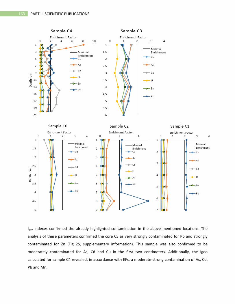
163 PART II: SCIENTIFIC PUBLICATIONS
Igeo indexes confirmed the already highlighted contamination in the above mentioned locations. The
analysis of these parameters confirmed the core C5 as very strongly contaminated for Pb and strongly
contaminated for Zn (Fig 2S, supplementary information). This sample was also confirmed to be
moderately contaminated for As, Cd and Cu in the first two centimeters. Additionally, the Igeo
calculated for sample C4 revealed, in accordance with EFs, a moderate-strong contamination of As, Cd,
Pb and Mn.
164 PART II: SCIENTIFIC PUBLICATIONS
Finally the analysis of Pollution Load Indices (PLI) calculated on core samples, gave the ultimate
confirmation that an anthropogenic contamination exists mostly on samples C5 and C4 (Fig 3S,
supplementary information). The PLI values calculated for these samples were between 3 and 5 while
values for remaining cores were found to be around 2 for samples C1 and C2.
In accordance with the analysis of surface sediments in the study area (Orani et al, submitted), the
spatial distribution of trace elements in the cores suggests that only areas around Walvis Bay and
Swakopmund could be considered as contaminated . Especially in the case of sample C5, collected in the
Walvis Bay harbor, the contamination seems to be recent, in the upper 6 centimeters of the sediment
core, which marks a period between 1945(±7) and 2014. Walvis Bay has had a varied pollution history
because of its strategic position and the access to different natural resources, which have been
exploited during mane years. It is located at the edge of the Namib Desert and is Namibia's principal
harbor hosting the important fishing activities. The region receives less than 20 millimeters average
precipitation per year, making it one of the driest cities on earth. The exploitation of Namibian natural
resources, especially mining activities, have drastically increased after 1945 (Briefing, 1980). Since the
Second World War the exploitation and industrialization of different areas has markedly increased,
especially attracting transnational mining corporations. Bearing in mind this historical background, it is
not surprising that in economically important areas, such as the Walvis Bay, trace element inputs have
recently increased as a consequence of bigger anthropogenic activities.
3.3. Trace elements source analysis based on PCA
To further examine the extent and origin of trace elements contamination in the area, a PCA analysis
was performed on core samples C5, which appear to be the most contaminated among the samples
analyzed in this work. Data used for PCA were standardized using the biased standard deviation, in order
to avoid misclassification due to differences in data dimensionality; biplot results are shown in Fig 4.
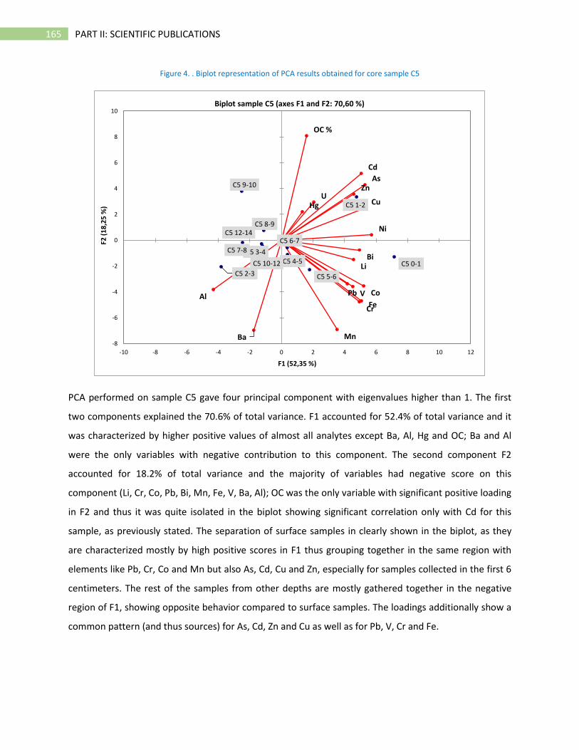
165 PART II: SCIENTIFIC PUBLICATIONS
Figure 4. . Biplot representation of PCA results obtained for core sample C5
PCA performed on sample C5 gave four principal component with eigenvalues higher than 1. The first
two components explained the 70.6% of total variance. F1 accounted for 52.4% of total variance and it
was characterized by higher positive values of almost all analytes except Ba, Al, Hg and OC; Ba and Al
were the only variables with negative contribution to this component. The second component F2
accounted for 18.2% of total variance and the majority of variables had negative score on this
component (Li, Cr, Co, Pb, Bi, Mn, Fe, V, Ba, Al); OC was the only variable with significant positive loading
in F2 and thus it was quite isolated in the biplot showing significant correlation only with Cd for this
sample, as previously stated. The separation of surface samples in clearly shown in the biplot, as they
are characterized mostly by high positive scores in F1 thus grouping together in the same region with
elements like Pb, Cr, Co and Mn but also As, Cd, Cu and Zn, especially for samples collected in the first 6
centimeters. The rest of the samples from other depths are mostly gathered together in the negative
region of F1, showing opposite behavior compared to surface samples. The loadings additionally show a
common pattern (and thus sources) for As, Cd, Zn and Cu as well as for Pb, V, Cr and Fe.
C5 0-1
C5 1-2
C5 2-3
C5 3-4C5 4-5
C5 5-6
C5 6-7C5 7-8
C5 8-9
C5 9-10
C5 10-12
C5 12-14
Li
Cr
Co
Ni
Cu
As
Cd
Pb
Bi
U
Mn
Fe
Zn
Hg
V
Ba
Al
OC %
-8
-6
-4
-2
0
2
4
6
8
10
-10 -8 -6 -4 -2 0 2 4 6 8 10 12
F2 (
18
,25
%)
F1 (52,35 %)
Biplot sample C5 (axes F1 and F2: 70,60 %)
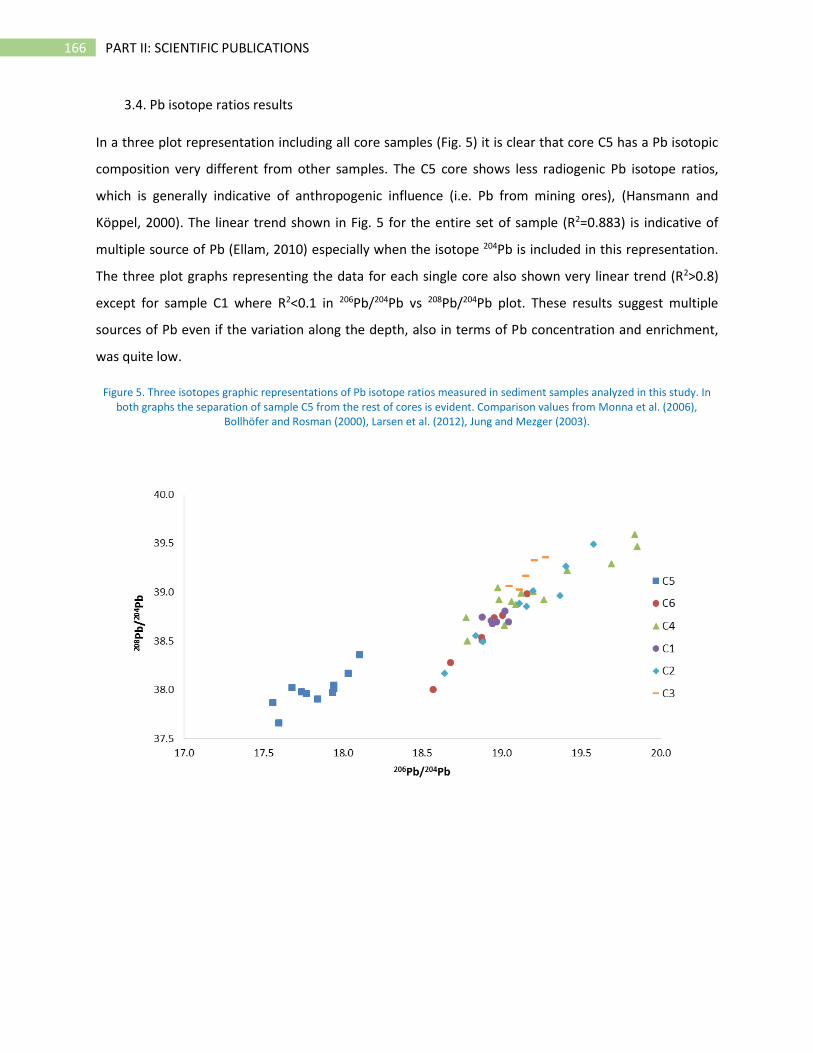
166 PART II: SCIENTIFIC PUBLICATIONS
3.4. Pb isotope ratios results
In a three plot representation including all core samples (Fig. 5) it is clear that core C5 has a Pb isotopic
composition very different from other samples. The C5 core shows less radiogenic Pb isotope ratios,
which is generally indicative of anthropogenic influence (i.e. Pb from mining ores), (Hansmann and
Köppel, 2000). The linear trend shown in Fig. 5 for the entire set of sample (R2=0.883) is indicative of
multiple source of Pb (Ellam, 2010) especially when the isotope 204Pb is included in this representation.
The three plot graphs representing the data for each single core also shown very linear trend (R2>0.8)
except for sample C1 where R2<0.1 in 206Pb/204Pb vs 208Pb/204Pb plot. These results suggest multiple
sources of Pb even if the variation along the depth, also in terms of Pb concentration and enrichment,
was quite low.
Figure 5. Three isotopes graphic representations of Pb isotope ratios measured in sediment samples analyzed in this study. In both graphs the separation of sample C5 from the rest of cores is evident. Comparison values from Monna et al. (2006),
Bollhöfer and Rosman (2000), Larsen et al. (2012), Jung and Mezger (2003).
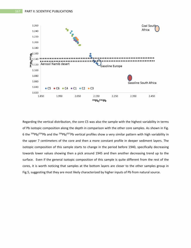
167 PART II: SCIENTIFIC PUBLICATIONS
Regarding the vertical distribution, the core C5 was also the sample with the highest variability in terms
of Pb isotopic composition along the depth in comparison with the other core samples. As shown in Fig.
6 the 206Pb/204Pb and the 206Pb/207Pb vertical profiles show a very similar pattern with high variability in
the upper 7 centimeters of the core and then a more constant profile in deeper sediment layers. The
isotopic composition of this sample starts to change in the period before 1940, specifically decreasing
towards lower values showing then a pick around 1945 and then another decreasing trend up to the
surface. Even if the general isotopic composition of this sample is quite different from the rest of the
cores, it is worth noticing that samples at the bottom layers are closer to the other samples group in
Fig.5, suggesting that they are most likely characterized by higher inputs of Pb from natural source.
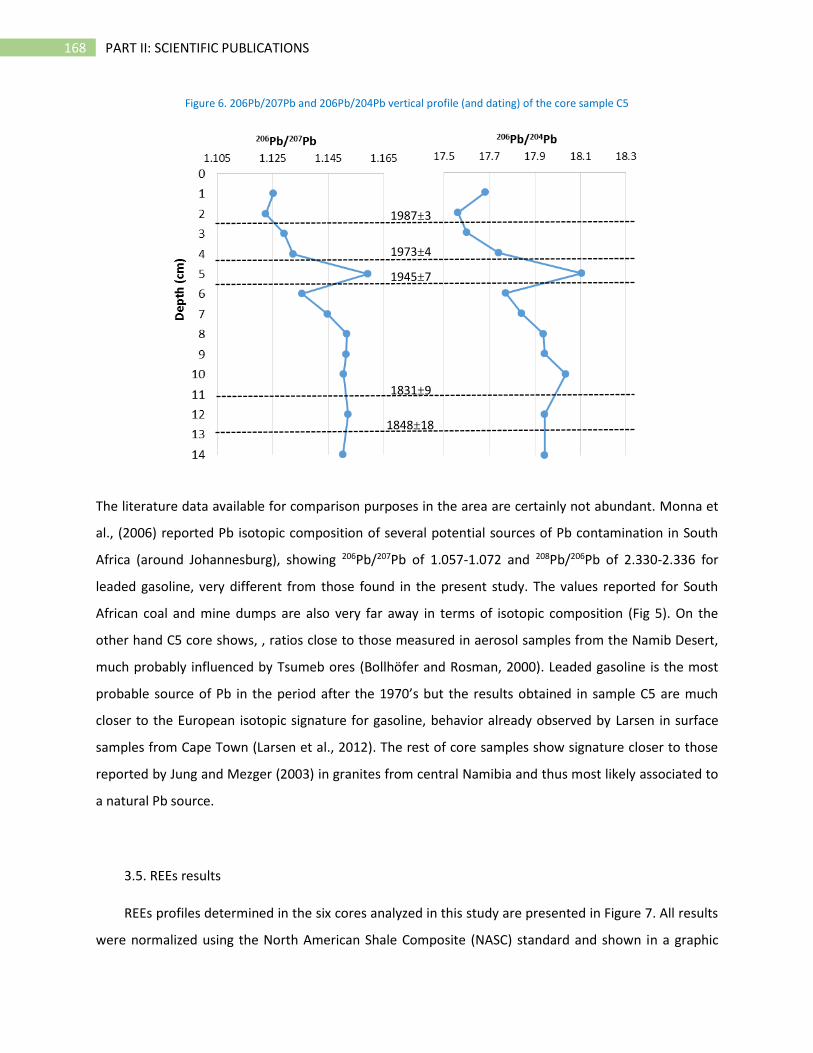
168 PART II: SCIENTIFIC PUBLICATIONS
Figure 6. 206Pb/207Pb and 206Pb/204Pb vertical profile (and dating) of the core sample C5
The literature data available for comparison purposes in the area are certainly not abundant. Monna et
al., (2006) reported Pb isotopic composition of several potential sources of Pb contamination in South
Africa (around Johannesburg), showing 206Pb/207Pb of 1.057-1.072 and 208Pb/206Pb of 2.330-2.336 for
leaded gasoline, very different from those found in the present study. The values reported for South
African coal and mine dumps are also very far away in terms of isotopic composition (Fig 5). On the
other hand C5 core shows, , ratios close to those measured in aerosol samples from the Namib Desert,
much probably influenced by Tsumeb ores (Bollhöfer and Rosman, 2000). Leaded gasoline is the most
probable source of Pb in the period after the 1970’s but the results obtained in sample C5 are much
closer to the European isotopic signature for gasoline, behavior already observed by Larsen in surface
samples from Cape Town (Larsen et al., 2012). The rest of core samples show signature closer to those
reported by Jung and Mezger (2003) in granites from central Namibia and thus most likely associated to
a natural Pb source.
3.5. REEs results
REEs profiles determined in the six cores analyzed in this study are presented in Figure 7. All results
were normalized using the North American Shale Composite (NASC) standard and shown in a graphic
1945±7
1973±4
1848±18
1987±3
1831±9

169 PART II: SCIENTIFIC PUBLICATIONS
representation in which is easier to detect element anomalies. The study of REEs profiles is of particular
interest for this area since some mineralogical investigations have confirmed that Namibia may have
potential REEs resources (Orris and Grauch, 2002). Additionally, since REEs are naturally associated with
U-containing minerals, their determination in these areas with long history of U mining, is of great
interest.
Figure 7. Graphical representation of REEs pattern in each core sample. Results were normalized to NASC standard
Although single element concentrations were quite different from site to site, the overall pattern of
each core was generally quite consistent. The samples C3, C4 and C6 did not show enrichment with
respect to NASC values, as all normalized results were consistently below 1 and no elemental anomalies
were observed. Samples C1 and C2 showed a slight enrichment in HREEs (Dy, Ho, Er, Tm, Yb, Lu) over
LREEs, behavior very characteristic of the area and already observed in Lofdal (carbonatite-dykes)
deposits, located 450 km northeast of Windoek (Wall et al., 2008). The pattern shown by samples C1
170 PART II: SCIENTIFIC PUBLICATIONS
and C2 resembles the one found for xenotime from Lofdal deposits and it is probable that these two
samples are richer in xenotime minerals than other core samples collected along the coast.
The sample C4 was the only one, among analyzed cores, which show an non-homogeneous pattern.
Looking at Figure 7 it is clear that, even if the normalized values rarely exceed 1, the biggest differences
in REEs pattern was observed for the deepest samples (from 14 to 20 cm depth). To better appreciate
this trend, an additional graphic representation is shown in Figure 8, where normalized REEs values are
directly plotted against the core depth. Apart from a general increase of REEs concentrations in bottom
samples, a positive Ce anomaly is also detectable at 16 cm depth. The Ce/Ce* ratio was then calculated
(Armstrong-Altrin et al., 2003) according the following equation:
𝐶𝑒
𝐶𝑒 ∗= 2 × [
𝐶𝑒
𝐶𝑒𝑠ℎ𝑎𝑙𝑒] [
𝐿𝑎
𝐿𝑎𝑠ℎ𝑎𝑙𝑒+
𝑆𝑚
𝑆𝑚𝑠ℎ𝑎𝑙𝑒]
−1
The calculated ratio exceeded 1 at 7-8 cm as well as in the last 4 cm of the C4 sample. Cerium anomaly is
linked to the fact that unlike the other REEs, Ce also presents +4 oxidation state, additional to the more
common +3. Changes in the redox condition in the water column can thus be the reason for positive or
negative Ce anomalies. Ce(IV) is highly insoluble in seawater which means that in oxidizing condition a
precipitation of this element is expected and thus an higher (positive anomaly) concentration in
sediments (Hatje et al., 2016). This anomaly is thus related to changes in the water column condition; it
can be finally stated that REEs analysis did not show anomalies ascribable to anthropogenic sources.
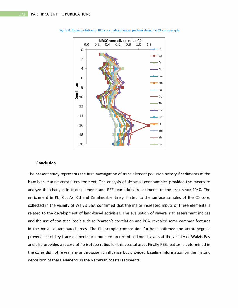
171 PART II: SCIENTIFIC PUBLICATIONS
Figure 8. Representation of REEs normalized values pattern along the C4 core sample
Conclusion
The present study represents the first investigation of trace element pollution history if sediments of the
Namibian marine coastal environment. The analysis of six small core samples provided the means to
analyze the changes in trace elements and REEs variations in sediments of the area since 1940. The
enrichment in Pb, Cu, As, Cd and Zn almost entirely limited to the surface samples of the C5 core,
collected in the vicinity of Walvis Bay, confirmed that the major increased inputs of these elements is
related to the development of land-based activities. The evaluation of several risk assessment indices
and the use of statistical tools such as Pearson’s correlation and PCA, revealed some common features
in the most contaminated areas. The Pb isotopic composition further confirmed the anthropogenic
provenance of key trace elements accumulated on recent sediment layers at the vicinity of Walvis Bay
and also provides a record of Pb isotope ratios for this coastal area. Finally REEs patterns determined in
the cores did not reveal any anthropogenic influence but provided baseline information on the historic
deposition of these elements in the Namibian coastal sediments.
172 PART II: SCIENTIFIC PUBLICATIONS
References (paper 5)
Abrahim, G.M.S., Parker, R.J., 2008. Assessment of heavy metal enrichment factors and the degree of contamination in marine sediments from Tamaki Estuary, Auckland, New Zealand. Environ. Monit. Assess. 136, 227–238. https://doi.org/10.1007/s10661-007-9678-2
Adams, F., Gijbels, R., Van Grieken, R., 1988. Inorganic Mass Spectrometry. John Wiley & Sons.
Aide, M.T., Aide, C., 2012. Rare Earth Elements: Their Importance in Understanding Soil Genesis. ISRN Soil Sci. 2012, 1–11. https://doi.org/10.5402/2012/783876
Alleman, L.Y., Hamelin, B., Véron, A.J., Miquel, J.-C., Heussner, S., 2000. Lead sources and transfer in the coastal Mediterranean: evidence from stable lead isotopes in marine particles. Deep Sea Res. Part II Top. Stud. Oceanogr. 47, 2257–2279. https://doi.org/10.1016/S0967-0645(00)00024-2
Aloupi, M., Angelidis, M.., 2001. Geochemistry of natural and anthropogenic metals in the coastal sediments of the island of Lesvos, Aegean Sea. Environ. Pollut. 113, 211–219. https://doi.org/10.1016/S0269-7491(00)00173-1
Aly, W., Williams, I.D., Hudson, M.D., 2013. Metal contamination in water, sediment and biota from a semi-enclosed coastal area. Environ. Monit. Assess. 185, 3879–3895. https://doi.org/10.1007/s10661-012-2837-0
AMPS Expert Group, 2005. Contributions of the Expert Group on Analysis and Monitoring of Priority Substances to the Water Framework Directive. EU Report EUR 21587.
Anderson, G.L., Williams, J., Hille, R., 1992. The purification and characterization of arsenite oxidase from Alcaligenes faecalis, a molybdenum-containing hydroxylase. J. Biol. Chem. 267, 23674–23682.
Andrewes, P., Demarini, D.M., Funasaka, K., Wallace, K., Lai, V.W.M., Sun, H., Cullen, W.R., Kitchin, K.T., 2004. Do arsenosugars pose a risk to human health? The comparative toxicities of a trivalent and pentavalent arsenosugar. Environ. Sci. Technol. 38, 4140–4148. https://doi.org/10.1021/es035440f
Angelidis, M.O., Radakovitch, O., Veron, A., Aloupi, M., Heussner, S., Price, B., 2011. Anthropogenic metal contamination and sapropel imprints in deep Mediterranean sediments. Mar. Pollut. Bull. 62, 1041–1052. https://doi.org/10.1016/j.marpolbul.2011.02.030
Anjum, K., Abbas, S.Q., Shah, S.A., Akhter, N., Batool, S., Hassan, S.S., 2016. Marine Sponges as a Drug Treasure. Biomol. Ther. 24, 347–362.
Araújo, M.F., Conceição, A., Barbosa, T., Lopes, M.T., Humanes, M., 2003. Elemental composition of marine sponges from the Berlengas Natural Park, western Portuguese coast. X-Ray Spectrom. 32, 428–433. https://doi.org/10.1002/xrs.660
Aresta, A., Marzano, C.N., Lopane, C., Corriero, G., Longo, C., Zambonin, C., Stabili, L., 2015. Analytical investigations on the lindane bioremediation capability of the demosponge Hymeniacidon perlevis. Mar. Pollut. Bull. 90, 143–149. https://doi.org/10.1016/j.marpolbul.2014.11.003
Armstrong-Altrin, J.S., Verma, S.P., Madhavaraju, J., Lee, Y. Il, Ramasamy, S., 2003. Geochemistry of Upper Miocene Kudankulam Limestones, Southern India. Int. Geol. Rev. 45, 16–26. https://doi.org/10.2747/0020-6814.45.1.16
Ashraf, A., Saion, E., Gharibshahi, E., Kamari, H.M., Yap, C.K., Hamzah, M.S., Elias, M.S., 2017. Distribution of Trace Elements in Core Marine Sediments of Coastal East Malaysia by Instrumental
173 PART II: SCIENTIFIC PUBLICATIONS
Neutron Activation Analysis. Appl. Radiat. Isot. 122, 96–105. https://doi.org/10.1016/j.apradiso.2017.01.006
Ashraf, A., Saion, E., Gharibshahi, E., Mohamed Kamari, H., Chee Kong, Y., Suhaimi Hamzah, M., Suhaimi Elias, M., 2016. Rare earth elements in core marine sediments of coastal East Malaysia by instrumental neutron activation analysis. Appl. Radiat. Isot. 107, 17–23. https://doi.org/10.1016/j.apradiso.2015.09.004
ATSDR, 2007. Toxicological Profile for Arsenic, U.S Public Health Service, Agency for Toxic Substances and Disease Registry. https://doi.org/http://dx.doi.org/10.1155/2013/286524
Ault, W.U., Senechal, R.G., Erlebach, W.E., 1970. Isotopic Composition as a Natural Tracer of Lead in the Environment: Discussions Follow. Environ. Sci. Technol. 4, 305–313. https://doi.org/10.1021/es60039a001
Azemard, S., Vassileva, E., 2015. Determination of methylmercury in marine biota samples with advanced mercury analyzer: Method validation. Food Chem. 176, 367–375. https://doi.org/10.1016/j.foodchem.2014.12.085
Azizur Rahman, M., Hasegawa, H., Peter Lim, R., 2012. Bioaccumulation, biotransformation and trophic transfer of arsenic in the aquatic food chain. Environ. Res. 116, 118–135. https://doi.org/10.1016/j.envres.2012.03.014
Bagul V. R., S.D.N., 2015. New perspective on heavy metal pollution of water. J. Chem. Pharm. Res. 7, 700–705.
Barats, A., Féraud, G., Potot, C., Philippinini, V., Travi, Y., Durrieu, G., Dubar, M., Simler, R., 2014. Naturally dissolved arsenic concentrations in the Alpine/Mediterranean Var River watershed (France). Sci. Total Environ. 473–474, 422–436. https://doi.org/10.1016/J.SCITOTENV.2013.12.007
Bargagli, R., Nelli, L., Ancora, S., Focardi, S., 1996. Elevated cadmium accumulation in marine organisms from Terra Nova Bay (Antarctica). Polar Biol. 16, 513–520. https://doi.org/10.1007/BF02329071
Barwick, V.J., Ellison, S.L.R., 1999. Measurement uncertainty: Approaches to the evaluation of uncertainties associated with recovery†. Analyst 124, 981–990. https://doi.org/10.1039/a901845j
Batista, D., Muricy, G., Rocha, R.C., Miekeley, N.F., 2014. Marine sponges with contrasting life histories can be complementary biomonitors of heavy metal pollution in coastal ecosystems. Environ. Sci. Pollut. Res. 21, 5785–5794. https://doi.org/10.1007/s11356-014-2530-7
Baudrimont, M., Schäfer, J., Marie, V., Maury-Brachet, R., Bossy, C., Boudou, A., Blanc, G., 2005. Geochemical survey and metal bioaccumulation of three bivalve species (Crassostrea gigas, Cerastoderma edule and Ruditapes philippinarum) in the Nord Médoc salt marshes (Gironde estuary, France). Sci. Total Environ. https://doi.org/10.1016/j.scitotenv.2004.07.009
Beauchemin, D., 2008. Inductively coupled plasma mass spectrometry. Anal. Chem. 80, 4455–4486.
Bednar, A.J., Garbarino, J.R., Burkhardt, M.R., Ranville, J.F., Wildeman, T.R., 2004. Field and laboratory arsenic speciation methods and their application to natural-water analysis. Water Res. 38, 355–364. https://doi.org/10.1016/j.watres.2003.09.034
Beeson, R., 1984. The use of the fine fractions of stream sediments in geochemical exploration in arid and semi-arid terrains. J. Geochemical Explor. 22, 119–132. https://doi.org/10.1016/0375-
174 PART II: SCIENTIFIC PUBLICATIONS
6742(84)90009-8
Belarra, M.A., Resano, M., Vanhaecke, F., Moens, L., 2002. Direct solid sampling with electrothermal vaporization/atomization: What for and how? TrAC - Trends Anal. Chem. 21, 828–839. https://doi.org/10.1016/S0165-9936(02)01206-2
Bell, J.J., 2008. The functional roles of marine sponges. Estuar. Coast. Shelf Sci. 79, 341–353. https://doi.org/10.1016/j.ecss.2008.05.002
Bennett, W.W., Teasdale, P.R., Panther, J.G., Welsh, D.T., Zhao, H., Jolley, D.F., 2012. Investigating arsenic speciation and mobilization in sediments with DGT and DET: A mesocosm evaluation of oxic-anoxic transitions. Environ. Sci. Technol. 46, 3981–3989. https://doi.org/10.1021/es204484k
Bentley, R., Chasteen, T.G., 2002. Microbial Methylation of Metalloids: Arsenic, Antimony, and Bismuth. Microbiol. Mol. Biol. Rev. 66, 250–271.
Bermejo-Barrera, P., Barciela-Alonso, M.C., Moreda-Piñeiro, J., González-Sixto, C., Bermejo-Barrera, a., 1996. Determination of trace metals (As, Cd, Hg, Pb and Sn) in marine sediment slurry samples by electrothermal atomic absorption spectrometry using palladium as a chemical modifier. Spectrochim. Acta Part B At. Spectrosc. 51, 1235–1244. https://doi.org/10.1016/0584-8547(96)01487-5
Bermudez-Lugo, O., 2014. 2012 Minerals Yearbook, Usgs- 2012 Minerals Yearbook.
Berthet, B., Mouneyrac, C., Pérez, T., Amiard-Triquet, C., 2005. Metallothionein concentration in sponges (Spongia officinalis) as a biomarker of metal contamination. Comp. Biochem. Physiol. - C Toxicol. Pharmacol. 141, 306–313. https://doi.org/10.1016/j.cca.2005.07.008
Bhuiyan, M.A.H., Parvez, L., Islam, M.A., Dampare, S.B., Suzuki, S., 2010. Heavy metal pollution of coal mine-affected agricultural soils in the northern part of Bangladesh. J. Hazard. Mater. 173, 384–392. https://doi.org/10.1016/j.jhazmat.2009.08.085
Birch, G.F., Melwani, A., Lee, J.H., Apostolatos, C., 2014. The discrepancy in concentration of metals (Cu, Pb and Zn) in oyster tissue (Saccostrea glomerata) and ambient bottom sediment (Sydney estuary, Australia). Mar. Pollut. Bull. 80, 263–274. https://doi.org/10.1016/j.marpolbul.2013.12.005
Bocher, P., Caurant, F., Miramand, P., Cherel, Y., Bustamante, P., 2003. Influence of the diet on the bioaccumulation of heavy metals in zooplankton-eating petrels at Kerguelen archipelago, Southern Indian Ocean. Polar Biol. 26, 759–767. https://doi.org/10.1007/s00300-003-0552-6
Bohari, Y., Astruc, A., Astruc, M., Cloud, J., 2001. Improvements of hydride generation for the speciation of arsenic in natural freshwater samples by HPLC-HG-AFS. J. Anal. At. Spectrom. 16, 774–778. https://doi.org/10.1039/B101591P
Bollhöfer, A., Rosman, K.J.., 2000. Isotopic source signatures for atmospheric lead: the Southern Hemisphere. Geochim. Cosmochim. Acta 64, 3251–3262. https://doi.org/10.1016/S0016-7037(00)00436-1
Bollhöfer, A., Rosman, K.J.R., 2001. Isotopic source signatures for atmospheric lead: The Northern Hemisphere. Geochim. Cosmochim. Acta 65, 1727–1740. https://doi.org/10.1016/S0016-7037(00)00630-X
Bossy, A., 2010. Origines de l’arsenic dans les eaux, sols et sédiments du district aurifère de St-Yrieix-la-
175 PART II: SCIENTIFIC PUBLICATIONS
Perche (Limousin, France) : contribution du lessivage des phases porteuses d’arsenic. Université de Limoges.
Bowen, H.J.M., 1966. The Uptake and Excretion of Elements by Organisms, in: Trace Elements in Biochemistry. Academic Press London, pp. 85–101.
Bremner, J.M., Willis, J.P., 1993. Mineralogy and geochemistry of the clay fraction of sediments from the Namibian continental margin and the adjacent hinterland. Mar. Geol. 115, 85–116. https://doi.org/10.1016/0025-3227(93)90076-8
Briant, N., Chouvelon, T., Martinez, L., Brach-Papa, C., Chiffoleau, J.F., Savoye, N., Sonke, J., Knoery, J., 2017. Spatial and temporal distribution of mercury and methylmercury in bivalves from the French coastline. Mar. Pollut. Bull. 114, 1096–1102. https://doi.org/10.1016/j.marpolbul.2016.10.018
Briefing, 1980. Namibia in the frontline: the political economy of decolonisation in South Africa’s colony. Rev. Afr. Polit. Econ. https://doi.org/10.1080/03056248008703415
Broadley, M.R., White, P.J., Hammond, J.P., Zelko, I., Lux, A., 2007. Zinc in plants. New Phytol. 173, 677–702. https://doi.org/10.1111/j.1469-8137.2007.01996.x
Brongersma-Sanders, M., Stephan, K.M., Kwee, T.., De Bruin, M., 1980. DISTRIBUTION OF MINOR ELEMENTS IN CORES FROM THE SOUTH- WEST AFRICA SHELF WITH NOTES ON PLANKTON AND FISH MORTALITY Along the coast of Southwest Africa a belt of olive-green diatomaceous muds is f o u n d between 19 ° S and 25 ° S , bordered on the wester. Mar. Geol. 37, 91–132.
Brown, J.L., Kitchin, K.T., George, M., 1997. Dimethylarsinic acid treatment alters six different rat biochemical parameters: Relevance to arsenic carcinogenesis. Teratog. Carcinog. Mutagen. 17, 71–84. https://doi.org/10.1002/(SICI)1520-6866(1997)17:2<71::AID-TCM3>3.0.CO;2-B
Brown, J.S., 1962. Ore leads and isotopes. Econ. Geol. 57, 673–720. https://doi.org/10.2113/gsecongeo.57.5.673
Brown, R.J.C., Milton, M.J.T., 2005. Analytical techniques for trace element analysis: An overview. TrAC - Trends Anal. Chem. 24, 266–274. https://doi.org/10.1016/j.trac.2004.11.010
Bruland, K.W., Bertine, K., Koide, M., Goldberg, E.D., 1974. History of metal pollution in southern California coastal zone. Environ. Sci. Technol. 8, 425–432. https://doi.org/10.1021/es60090a010
Bruland, K.W., Lohan, M.C., 2003. Controls of trace metals in seawater, in: Treatise on Geochemistry. Elsevier Ltd, pp. 23–47.
Bryan, G.W., Langston, W.J., 1992. Bioavailability, accumulation and effects of heavy metals in sediments with special reference to United Kingdom estuaries: a review. Environ. Pollut. 76, 89–131. https://doi.org/10.1016/0269-7491(92)90099-V
Bu, H., Song, X., Guo, F., 2017. Dissolved trace elements in a nitrogen-polluted river near to the Liaodong Bay in Northeast China. Mar. Pollut. Bull. 114, 547–554. https://doi.org/10.1016/j.marpolbul.2016.09.003
Cabon, J.Y., Cabon, N., 2000. Speciation of major arsenic species in seawater by flow injection hydride generation atomic absorption spectrometry. Fresenius. J. Anal. Chem. 368, 484–9. https://doi.org/10.1007/s002160000526
Cabrita, M.T., Padeiro, A., Amaro, E., dos Santos, M.C., Leppe, M., Verkulich, S., Hughes, K.A., Peter, H.-
176 PART II: SCIENTIFIC PUBLICATIONS
U., Canário, J., 2017. Evaluating trace element bioavailability and potential transfer into marine food chains using immobilised diatom model species Phaeodactylum tricornutum , on King George Island, Antarctica. Mar. Pollut. Bull. 121, 192–200. https://doi.org/10.1016/j.marpolbul.2017.05.059
Caccia, V.G., Millero, F.J., Palanques, A., 2003. The distribution of trace metals in Florida Bay sediments. Mar. Pollut. Bull. 46, 1420–1433. https://doi.org/10.1016/S0025-326X(03)00288-1
Calvert, S.E., Price, N.B., 1970. Minor Metal Contents of Recent Organic-rich Sediments off South West Africa. Nature 227, 593–595.
Cantillo, A.Y., 1998. Comparison of results of Mussel Watch Programs of the United States and France with Worldwide Mussel Watch Studies. Mar. Pollut. Bull. 36, 712–717. https://doi.org/10.1016/S0025-326X(98)00049-6
Carere, M., Dulio, V., Hanke, G., Polesello, S., 2012. Guidance for sediment and biota monitoring under the Common Implementation Strategy for the Water Framework Directive. TrAC - Trends Anal. Chem. 36, 15–24. https://doi.org/10.1016/j.trac.2012.03.005
Carpenè, E., Andreani, G., Isani, G., 2017. Trace elements in unconventional animals: A 40-year experience. J. Trace Elem. Med. Biol. 43, 169–179. https://doi.org/10.1016/j.jtemb.2017.02.003
Caumette, G., Koch, I., Reimer, K.J., 2012. Arsenobetaine formation in plankton: a review of studies at the base of the aquatic food chain. J. Environ. Monit. 14, 2841. https://doi.org/10.1039/c2em30572k
Cebrian, E., Martí, R., Uriz, J.M., Turon, X., 2003. Sublethal effects of contamination on the Mediterranean sponge Crambe crambe: Metal accumulation and biological responses. Mar. Pollut. Bull. 46, 1273–1284. https://doi.org/10.1016/S0025-326X(03)00190-5
Cebrian, E., Uriz, M.-J., Turon, X., 2007. Sponges as biomonitors of heavy metals in spatial and temporal surveys in northwestern mediterranean: multispecies comparison. Environ. Toxicol. Chem. 26, 2430–2439. https://doi.org/10.1897/07-292.1
Cebrian, E., Uriz, M.J., 2007. Contrasting effects of heavy metals on sponge cell behavior. Arch. Environ. Contam. Toxicol. 53, 552–558. https://doi.org/10.1007/s00244-006-0257-2
Chai, Z.F., Zhang, Z.Y., Feng, W.Y., Chen, C.Y., Xu, D.D., Hou, X.L., 2004. Study of chemical speciation of trace elements by molecular activation analysis and other nuclear techniques. J. Anal. At. Spectrom. 19, 26–33. https://doi.org/10.1039/B307337H
Charlesworth, M.E., Chenery, S., Mellor, A., Service, M., 2006. Isotopic composition and concentration of Pb in suspended particulate matter of the Irish Sea reveals distribution and sources. Mar. Pollut. Bull. 52, 81–88. https://doi.org/10.1016/j.marpolbul.2005.08.009
Chen, C.Y., Darren, M.., Williams, J.J., Fisher, N.S., 2016. Metal Bioaccumulation by Estuarine Food Webs in New England, USA. J. Mar. Sci. Engeneer 4, 41. https://doi.org/10.1016/j.cell.2016.05.007.Mapping
Chen, C.Y., Stemberger, R.S., Klaue, B., Blum, J.D., Pickhardt, P.C., Folt, C.L., 2000. Accumulation of heavy metals in food web components across a gradient of lakes. Limnol. Oceanogr. 45, 1525–1536. https://doi.org/10.4319/lo.2000.45.7.1525

177 PART II: SCIENTIFIC PUBLICATIONS
Chen, L., Liu, M., Fan, R., Ma, S., Xu, Z., Ren, M., He, Q., 2013. Mercury speciation and emission from municipal solid waste incinerators in the Pearl River Delta, South China. Sci. Total Environ. 447, 396–402. https://doi.org/10.1016/j.scitotenv.2013.01.018
Chester, R., Murphy, K.J.T., Lin, F.J., Berry, A.S., Bradshaw, G.A., Corcoran, P.A., 1993. Factors controlling the solubilities of trace metals from non-remote aerosols deposited to the sea surface by the “dry” deposition mode. Mar. Chem. 42, 107–126. https://doi.org/10.1016/0304-4203(93)90241-F
Ciardullo, S., Aureli, F., Raggi, A., Cubadda, F., 2010. Arsenic speciation in freshwater fish: Focus on extraction and mass balance. Talanta 81, 213–221. https://doi.org/10.1016/j.talanta.2009.11.060
Cidu, R., Frau, F., 2009. Distribution of trace elements in filtered and non filtered aqueous fractions: Insights from rivers and streams of Sardinia (Italy). Appl. Geochemistry 24, 611–623. https://doi.org/10.1016/j.apgeochem.2008.12.013
Clark, H., 1968. On the Spongiae ciliatae as infusoria flagellata, or observations on the structure, animality and relationship of Leucosolenia botryoides, Bowerbank. Ann. Mag. Nat. Hist. 4, 133–142.
Clowes, L.A., Francesconi, K.A., 2004. Uptake and elimination of arsenobetaine by the mussel Mytilus edulis is related to salinity. Comp. Biochem. Physiol. - C Toxicol. Pharmacol. 137, 35–42. https://doi.org/10.1016/j.cca.2003.11.003
Coulibaly, M., Bamba, D., Yao, N.A., Zoro, E.G., El Rhazi, M., 2016. Some aspects of speciation and reactivity of mercury in various matrices. Comptes Rendus Chim. 19, 832–840. https://doi.org/10.1016/j.crci.2016.02.005
Covelli, S., Fontolan, G., 1997. Application of a normalization procedure in determining regional geochemical baselines. Environ. Geol. 30, 34–45. https://doi.org/10.1007/s002540050130
Crompton, T.R., Crompton, T.R., 1989. Chapter 8 – Organometallic compounds, in: Analysis of Seawater. pp. 336–359. https://doi.org/10.1016/B978-0-407-01610-1.50011-4
Cullen, W.R., Reimer, K.J., 1989. Arsenic speciation in the environment. Chem. Rev. 89, 713–764. https://doi.org/10.1021/cr00094a002
Dahms, S., van der Bank, F.H., Greenfield, R., 2014. A baseline study of metal contamination along the Namibian coastline for Perna perna and Choromytilus meridionalis. Mar. Pollut. Bull. 85, 297–305. https://doi.org/10.1016/j.marpolbul.2014.05.037
Damiano, S., Papetti, P., Menesatti, P., 2011. Accumulation of heavy metals to assess the health status of swordfish in a comparative analysis of Mediterranean and Atlantic areas. Mar. Pollut. Bull. 62, 1920–1925. https://doi.org/10.1016/j.marpolbul.2011.04.028
De Gregori H., I., Pinochet C., H., Arancibia J., M., Vidal B., A., 1996. Grain Size Effect on Trace Metals Distribution in Sediments from Two Coastal Areas of Chile. Bull. Environ. Contam. Toxicol. 57, 163–170. https://doi.org/10.1007/s001289900170
de Mestre, C., Maher, W., Roberts, D., Broad, A., Krikowa, F., Davis, A.R., 2012. Sponges as sentinels: Patterns of spatial and intra-individual variation in trace metal concentration. Mar. Pollut. Bull. 64, 80–89. https://doi.org/10.1016/j.marpolbul.2011.10.020
Debord, J., Pourmand, A., Jantzi, S., Panicker, S., Almirall, J., 2017. Profiling of Heroin and Assignment of

178 PART II: SCIENTIFIC PUBLICATIONS
Provenance by 87 Sr/ 86 Sr Isotope Ratio Analysis. Inorganica Chim. Acta. https://doi.org/10.1016/j.ica.2017.07.049
Delnomdedieu, M., Basti, M.M., Otvos, J.D., Thomas, D.J., 1994. Reduction and binding of arsenate and dimethylarsinate by glutathione: a magnetic resonance study. Chem. Biol. Interact. 90, 139–155. https://doi.org/10.1016/0009-2797(94)90099-X
Denton, G.R.W., Concepcion, L.P., Wood, H.R., Morrison, R.J., 2006. Trace metals in marine organisms from four harbours in Guam. Mar. Pollut. Bull. 52, 1784–1804. https://doi.org/10.1016/j.marpolbul.2006.09.010
Diaz, M.C., Rutzler, K., 2001. Sponges: an essential component of Caribbean coral reefs. Bull. Mar. Sci. 69, 535–546.
Drivelos, S.A., Georgiou, C.A., 2012. Multi-element and multi-isotope-ratio analysis to determine the geographical origin of foods in the European Union. TrAC Trends Anal. Chem. 40, 38–51. https://doi.org/10.1016/j.trac.2012.08.003
Dudás, F.Ö., LeBlanc, S.A., Carter, S.W., Bowring, S.A., 2016. Pb and Sr concentrations and isotopic compositions in prehistoric North American teeth: A methodological study. Chem. Geol. 429, 21–32. https://doi.org/10.1016/j.chemgeo.2016.03.003
Duncan, E.G., Maher, W.A., Foster, S.D., 2015. Contribution of arsenic species in unicellular algae to the cycling of arsenic in marine ecosystems. Environ. Sci. Technol. 49, 33–50. https://doi.org/10.1021/es504074z
Edmonds, J.S., Francesconi, K.A., Stick, R. V, 1993. Arsenic compounds from marine organisms. Nat. Prod. Rep. 10, 421–428.
Edmonds, J.S., Shibata, Y., Francesconi, K. a, Rippingale, R.J., Morita, M., 1997. Arsenic transformations in short marine food chains studied by HPLC-ICP MS. Appl. Organomet. Chem. 11, 281–287. https://doi.org/10.1002/(sici)1099-0739(199704)11:4<281::aid-aoc581>3.3.co;2-j
Elbaz-Poulichet, F., Holliger, P., Martin, J.M., Petit, D., 1986. Stable lead isotopes ratios in major french rivers and estuaries. Sci. Total Environ. 54, 61–76. https://doi.org/10.1016/0048-9697(86)90256-1
Elderfield, H., 2003. Introduction to Volume 6, in: Turekian, K.K., Holland, H.D. (Eds.), Treatise on Geochemistry. Elsevier Ltd, pp. 15–27.
Ellam, R.M., 2010. The graphical presentation of lead isotope data for environmental source apportionment. Sci. Total Environ. 408, 3490–3492. https://doi.org/10.1016/j.scitotenv.2010.03.037
Ellwood, M.J., Maher, W.A., 2003. Measurement of arsenic species in marine sediments by high-performance liquid chromatography-inductively coupled plasma mass spectrometry. Anal. Chim. Acta 477, 279–291. https://doi.org/10.1016/s0003-2670(02)01414-9
Esslemont, G., 2000. Heavy metals in seawater, marine sediments and corals from the Townsville section, Great Barrier Reef Marine Park, Queensland. Mar. Chem. 71, 215–231. https://doi.org/10.1016/S0304-4203(00)00050-5
Fang, T.-H., Hsiao, S.-H., Nan, F.-H., 2014. Nineteen trace elements in marine copepods collected from the coastal waters off northeastern Taiwan. Cont. Shelf Res. 91, 70–81.
179 PART II: SCIENTIFIC PUBLICATIONS
https://doi.org/10.1016/j.csr.2014.09.003
FAO, 2007. Fishery Country Profile- The Republic of Namibia [WWW Document]. URL http://www.fao.org/fi/oldsite/FCP/en/NAM/profile.htm
FLETCHER, C.J.N., SWAINBANK, I.G., COLMAN, T.B., 1993. Metallogenic evolution in Wales: constraints from lead isotope modelling. J. Geol. Soc. London. 150, 77–82. https://doi.org/10.1144/gsjgs.150.1.0076
Forstner, U., 1982. Chemical forms of metal enrichment in recent sediments, in: Amstutz, G. (Ed.), Ore Genesis. Springer-Verlag New York, pp. 269–284.
Förstner, U., Ahlf, W., Calmano, W., 1989. Studies on the transfer of heavy metals between sedimentary phases with a multi-chamber device: Combined effects of salinity and redox variation. Mar. Chem. 28, 145–158. https://doi.org/10.1016/0304-4203(89)90192-8
Forstner, U., Wittmann, G., 1981. Metal pollution in the aquatic environment, 2nd revise. ed. Springer-Verlag New York.
Foster, S., Maher, W., 2016. Arsenobetaine and thio-arsenic species in marine macroalgae and herbivorous animals: Accumulated through trophic transfer or produced in situ? J. Environ. Sci. 49, 131–139. https://doi.org/10.1016/j.jes.2016.06.003
Francesconi, K.A., Sperling, M., 2005. Speciation analysis with HPLC-mass spectrometry: time to take stock. Analyst 130, 998. https://doi.org/10.1039/b504485p
Francesconi, K. a., 2010. Arsenic species in seafood: Origin and human health implications. Pure Appl. Chem. 82, 373–381. https://doi.org/10.1351/PAC-CON-09-07-01
Fütterer, D.K., Cojan, I., Renard, M., 2006. The solid phase of marine sediments, in: Marine Geochemistry. pp. 1–25.
Gadde, R.R., Laitinen, H.A., 1974. Studies of Heavy Metal Adsorption by Hydrous Iron and Manganese Oxides. Anal. Chem. 46, 2022–2026. https://doi.org/10.1021/ac60349a004
Galy, A., Pomies, C., Day, J.A., Pokrovsky, O.S., Schott, J., 2003. High precision measurement of germanium isotope ratio variations by multiple collector-inductively coupled plasma mass spectrometry. J. Anal. At. Spectrom. 18, 115–119. https://doi.org/10.1039/B210233A
Gazave, E., Carteron, S., Chenuil, A., Richelle-Maurer, E., Boury-Esnault, N., Borchiellini, C., 2010. Polyphyly of the genus Axinella and of the family Axinellidae (Porifera: Demospongiaep). Mol. Phylogenet. Evol. 57, 35–47. https://doi.org/10.1016/j.ympev.2010.05.028
Genta-Jouve, G., Cachet, N., Oberhänsli, F., Noyer, C., Teyssié, J.L., Thomas, O.P., Lacoue-Labarthe, T., 2012. Comparative bioaccumulation kinetics of trace elements in Mediterranean marine sponges. Chemosphere 89, 340–349. https://doi.org/10.1016/j.chemosphere.2012.04.052
Gentric, C., Rehel, K., Dufour, A., Sauleau, P., 2016. Bioaccumulation of metallic trace elements and organic pollutants in marine sponges from the South Brittany Coast, France. J. Environ. Sci. Heal. Part A 51, 213–219. https://doi.org/10.1080/10934529.2015.1094327
Gifford, S., Dunstan, R.H., O’Connor, W., Koller, C.E., MacFarlane, G.R., 2007. Aquatic zooremediation: deploying animals to remediate contaminated aquatic environments. Trends Biotechnol. 25, 60–65. https://doi.org/10.1016/j.tibtech.2006.12.002

180 PART II: SCIENTIFIC PUBLICATIONS
Giusti, L., Zhang, H., 2002. Heavy metals and arsenic in sediments, mussels and marine water from Murano (Venice, Italy). Environ. Geochem. Health 24, 47–65. https://doi.org/10.1023/A:1013945117549
Gobas, F., 2001. Assessing Bioaccumulation Factors of Persistent Organic Pollutants in Aquatic Food-Chains, in: Persistent Organic Pollutants: Environmental Behaviour and Pathways of Human Exposure. pp. 145–165. https://doi.org/10.1007/978-1-4615-1571-5_6
Gong, Z., 2002. Arsenic speciation analysis. Talanta 58, 77–96. https://doi.org/10.1016/S0039-9140(02)00258-8
Goodenough, K.M., Schilling, J., Jonsson, E., Kalvig, P., Charles, N., Tuduri, J., Deady, E.A., Sadeghi, M., Schiellerup, H., M??ller, A., Bertrand, G., Arvanitidis, N., Eliopoulos, D.G., Shaw, R.A., Thrane, K., Keulen, N., 2016. Europe’s rare earth element resource potential: An overview of REE metallogenetic provinces and their geodynamic setting. Ore Geol. Rev. 72, 838–856. https://doi.org/10.1016/j.oregeorev.2015.09.019
Goran, P., 1981. The Carcinogenicity of Arsenic. Environ. Health Perspect. 40, 93–100.
Goyer, R.A., 2001. Toxic effects of metals, in: Klaassen, C.D. (Ed.), Casarett and Doull’s Toxicology: The Basic Science of Poisons. McGraw-Hill Publisher, pp. 811–867.
Grotti, M., Lagomarsino, C., Goessler, W., Francesconi, K.A., 2010. Arsenic speciation in marine organisms from Antarctic coastal environments. Environ. Chem. 7, 207–214. https://doi.org/10.1071/EN09131
Grotti, M., Soggia, F., Lagomarsino, C., Riva, S.D., Goessler, W., Francesconi, K.A., 2008. Natural variability and distribution of trace elements in marine organisms from Antarctic coastal environments. Antarct. Sci. 20, 39–52. https://doi.org/doi:10.1017/S0954102007000831
Grousset, F.E., Quetel, C.R., Thomas, B., Buat-Menard, P., Donard, O.F.X., Bucher, A., 1994. Transient Pb Isotopic Signatures in the Western European Atmosphere. Environ. Sci. Technol. 28, 1605–1608. https://doi.org/10.1021/es00058a011
Guan, Q., Cai, A., Wang, F., Wang, L., Wu, T., Pan, B., Song, N., Li, F., Lu, M., 2016. Heavy metals in the riverbed surface sediment of the Yellow River, China. Environ. Sci. Pollut. Res. 23, 24768–24780. https://doi.org/10.1007/s11356-016-7712-z
Guyonnet, D., Planchon, M., Rollat, A., Escalon, V., Tuduri, J., Charles, N., Vaxelaire, S., Dubois, D., Fargier, H., 2015. Material flow analysis applied to rare earth elements in Europe. J. Clean. Prod. 107, 215–228. https://doi.org/10.1016/J.JCLEPRO.2015.04.123
Hansmann, W., Köppel, V., 2000. Lead-istopes as tracers of pollutants in soils. Chem. Geol. 171, 123–144. https://doi.org/10.1016/S0009-2541(00)00230-8
Harada, M., 1995. Minamata Disease: Methylmercury Poisoning in Japan Caused by Environmental Pollution. Crit. Rev. Toxicol. 25, 1–24. https://doi.org/10.3109/10408449509089885
Hartwig, A., Jahnke, G., 2012. Toxic metals and metalloids in foods, in: Chemical Contaminants and Residues in Food. Elsevier, pp. 233–249. https://doi.org/10.1533/9780857095794.2.233
Hatje, V., Bruland, K.W., Flegal, A.R., 2016. Increases in Anthropogenic Gadolinium Anomalies and Rare Earth Element Concentrations in San Francisco Bay over a 20 Year Record. Environ. Sci. Technol. 50,

181 PART II: SCIENTIFIC PUBLICATIONS
4159–4168. https://doi.org/10.1021/acs.est.5b04322
He, M., Wang, W.X., 2013. Bioaccessibility of 12 trace elements in marine molluscs. Food Chem. Toxicol. 55, 627–636. https://doi.org/10.1016/j.fct.2013.01.046
Heidari, B., Bakhtiari, A.R., Shirneshan, G., 2013. Concentrations of Cd, Cu, Pb and Zn in soft tissue of oyster (Saccostrea cucullata) collected from the Lengeh Port coast, Persian Gulf, Iran: A comparison with the permissible limits for public health. Food Chem. 141, 3014–3019. https://doi.org/10.1016/j.foodchem.2013.06.002
Hinrichs, J., Dellwig, O., Brumsack, H.-J., 2002. Lead in sediments and suspended particulate matter of the German Bight: natural versus anthropogenic origin. Appl. Geochemistry 17, 621–632. https://doi.org/10.1016/S0883-2927(01)00124-X
Hirner, A.V., Kritsotakis, K., Tobschall, H.J., 1990. Metal-organic associations in sediments—I. Comparison of unpolluted recent and ancient sediments and sediments affected by anthropogenic pollution. Appl. Geochemistry 5, 491–505. https://doi.org/10.1016/0883-2927(90)90023-X
Holser, W.T., 1997. Evaluation of the application of rare-earth elements to paleoceanography. Palaeogeogr. Palaeoclimatol. Palaeoecol. 132, 309–323. https://doi.org/10.1016/S0031-0182(97)00069-2
Hong, S., Khim, J.S., Park, J., Son, H.S., Choi, S.D., Choi, K., Ryu, J., Kim, C.Y., Chang, G.S., Giesy, J.P., 2014. Species- and tissue-specific bioaccumulation of arsenicals in various aquatic organisms from a highly industrialized area in the Pohang City, Korea. Environ. Pollut. 192, 27–35. https://doi.org/10.1016/j.envpol.2014.05.004
Hooper, J., van Soest, R., 2002. Systena porifera. A guide to the Classification of Sponges. Kluwer Academic/Plenum publishers, New York.
Hornung, H., Krom, M.D., Cohen, Y., 1989. Trace metal distribution in sediments and benthic fauna of Haifa Bay, Israel. Estuar. Coast. Shelf Sci. 29, 43–56. https://doi.org/10.1016/0272-7714(89)90072-3
Horowitz, A.J., 1991. A Primer on Sediment-Trace Element Chemistry. U.S.G.S. Open-File Rep. 2nd Editio, 136 (2 fiche).
Horowitz, A.J., Elrick, K.A., 1987. The relation of stream sediment surface area, grain size and composition to trace element chemistry. Appl. Geochemistry 2, 437–451. https://doi.org/10.1016/0883-2927(87)90027-8
Hsieh, M.W., Liu, C.L., Chen, J.H., Jiang, S.J., 2010. Speciation analysis of arsenic and selenium compounds by CE-dynamic reaction cell-ICP-MS. Electrophoresis 31, 2272–2278. https://doi.org/10.1002/elps.200900632
Hughes, M.F., 2002. Arsenic toxicity and potential mechanisms of action. Toxicol. Lett. 133, 1–16. https://doi.org/10.1016/S0378-4274(02)00084-X
Illuminati, S., Annibaldi, A., Truzzi, C., Scarponi, G., 2016a. Heavy metal distribution in organic and siliceous marine sponge tissues measured by square wave anodic stripping voltammetry. Mar. Pollut. Bull. 111, 476–482. https://doi.org/10.1016/j.marpolbul.2016.06.098
Illuminati, S., Annibaldi, A., Truzzi, C., Scarponi, G., 2016b. Heavy metal distribution in organic and
182 PART II: SCIENTIFIC PUBLICATIONS
siliceous marine sponge tissues measured by square wave anodic stripping voltammetry. Mar. Pollut. Bull. 111, 476–482. https://doi.org/10.1016/j.marpolbul.2016.06.098
Irgolic, K.J., Stockton, R.A., 1987. Element-specific detectors for liquid chromatography: The determination of arsenic compounds. Mar. Chem. 22, 265–278.
Jagtap, R., Krikowa, F., Maher, W., Foster, S., Ellwood, M., 2011. Measurement of methyl mercury (I) and mercury (II) in fish tissues and sediments by HPLC-ICPMS and HPLC-HGAAS. Talanta 85, 49–55. https://doi.org/10.1016/j.talanta.2011.03.022
Jagtap, R., Maher, W., 2015. Measurement of mercury species in sediments and soils by HPLC-ICPMS. Microchem. J. https://doi.org/10.1016/j.microc.2015.01.010
Jonathan, R., Gobert, S., 2016. Trace Elements in Marine Environments: Occurrence, Threats and Monitoring with Special Focus on the Coastal Mediterranean. J. Environ. Anal. Toxicol. in press.
Jones, B., Browser, C., 1987. The mineralogy and related chemistry of lake sediments, in: Lerman, A. (Ed.), Lakes: Chemistry, Geology, Physics. Springer-Verlag New York, pp. 179–235.
Joung, D.J., Shiller, A.M., 2016. Temporal and spatial variations of dissolved and colloidal trace elements in Louisiana Shelf waters. Mar. Chem. 181, 25–43. https://doi.org/10.1016/j.marchem.2016.03.003
Jung, H.S., Lim, D., Choi, J.Y., Yoo, H.S., Rho, K.C., Lee, H.B., 2012. Rare earth element compositions of core sediments from the shelf of the South Sea, Korea: Their controls and origins. Cont. Shelf Res. 48, 75–86. https://doi.org/10.1016/j.csr.2012.08.008
Jung, S., Mezger, K., 2003. Petrology of basement-dominated terranes: I. Regional metamorphic T-t path from U-Pb monazite and Sm-Nd garnet geochronology (Central Damara orogen, Namibia). Chem. Geol. 198, 223–247. https://doi.org/10.1016/S0009-2541(03)00037-8
Karbassi, A.R., Monavari, S.M., Nabi Bidhendi, G.R., Nouri, J., Nematpour, K., 2007. Metal pollution assessment of sediment and water in the Shur River. Environ. Monit. Assess. 147, 107. https://doi.org/10.1007/s10661-007-0102-8
Karbassi, A.R., Nabi-Bidhendi, G.R., Bayati, I., 2005. Environmental Geochemistry of Heavy Metals in Sediment Core Off Bushehr, Persian Gulf. Iran J.Environmen.Health.Sci. Eng. 2, 255–260.
Keren, R., Lavy, A., Ilan, M., 2016. Increasing the Richness of Culturable Arsenic-Tolerant Bacteria from Theonella swinhoei by Addition of Sponge Skeleton to the Growth Medium. Microb. Ecol. 71, 873–886. https://doi.org/10.1007/s00248-015-0726-0
Keren, R., Lavy, A., Mayzel, B., Ilan, M., 2015. Culturable associated-bacteria of the sponge Theonella swinhoei show tolerance to high arsenic concentrations. Front. Microbiol. 6, 1–11. https://doi.org/10.3389/fmicb.2015.00154
Keren, R., Mayzel, B., Lavy, A., Polishchuk, I., Levy, D., Fakra, S.C., Pokroy, B., Ilan, M., 2017. Sponge-associated bacteria mineralize arsenic and barium on intracellular vesicles. Nat. Commun. 8, 14393. https://doi.org/10.1038/ncomms14393
KeyToNature, 2015. Marine Species Identification Portal [WWW Document]. URL http://species-identification.org/index.php (accessed 7.4.17).
Kingson, O., Bhutani, R., Dash, J.K., Sebastian, S., Balakrishnan, S., 2017. Resolving the conundrum in origin of the Manipur Ophiolite Complex, Indo-Myanmar range: Constraints from Nd isotopic ratios
183 PART II: SCIENTIFIC PUBLICATIONS
and elemental concentrations in serpentinized peridotite. Chem. Geol. 460, 117–129. https://doi.org/10.1016/j.chemgeo.2017.04.021
Kljaković-Gašpić, Z., Bogner, D., Ujević, I., 2008. Trace metals (Cd, Pb, Cu, Zn and Ni) in sediment of the submarine pit Dragon ear (Soline Bay, Rogoznica, Croatia). Environ. Geol. 58, 751. https://doi.org/10.1007/s00254-008-1549-9
Komárek, M., Ettler, V., Chrastný, V., Mihaljevič, M., 2008. Lead isotopes in environmental sciences: A review. Environ. Int. 34, 562–577. https://doi.org/10.1016/j.envint.2007.10.005
Krata, A., Vassileva, E., Bulska, E., 2016. Reference measurements for total mercury and methyl mercury content in marine biota samples using direct or species-specific isotope dilution inductively coupled plasma mass spectrometry. Talanta 160, 562–569. https://doi.org/10.1016/j.talanta.2016.07.033
Kucuksezgin, F., Gonul, L.T., Tasel, D., 2014. Total and inorganic arsenic levels in some marine organisms from Izmir Bay (Eastern Aegean Sea): A risk assessment. Chemosphere 112, 311–316. https://doi.org/10.1016/j.chemosphere.2014.04.071
Kulaksiz, S., Bau, M., 2011. Rare earth elements in the Rhine River, Germany: First case of anthropogenic lanthanum as a dissolved microcontaminant in the hydrosphere. Environ. Int. 37, 973–979. https://doi.org/10.1016/j.envint.2011.02.018
Lai, V.W.M., Cullen, W.R., Ray, S., 1999. Arsenic speciation in scallops. Mar. Chem. 66, 81–89. https://doi.org/10.1016/S0304-4203(99)00025-0
Lamborg, C.H., Hammerschmidt, C.R., Bowman, K.L., Swarr, G.J., Munson, K.M., Ohnemus, D.C., Lam, P.J., Heimburger, L.-E., Rijkenberg, M., Saito, M.A., 2014. A global ocean inventory of anthropogenic mercury based on water column measurements. Nature 512, 65–68. https://doi.org/10.1038/nature13563
Lang, T., Kruse, R., Haarich, M., Wosniok, W., 2017. Mercury species in dab (Limanda limanda) from the North Sea, Baltic Sea and Icelandic waters in relation to host-specific variables. Mar. Environ. Res. 124, 32–40. https://doi.org/10.1016/j.marenvres.2016.03.001
Laport, M.S., Santos, O.C., Muricy, G., 2009. Marine sponges: potential sources of new antimicrobial drugs. Curr. Pharm. Biotechnol. 10, 86–105.
Larsen, M.M., Blusztajn, J.S., Andersen, O., Dahllöf, I., 2012. Lead isotopes in marine surface sediments reveal historical use of leaded fuel. J. Environ. Monit. 14, 2893. https://doi.org/10.1039/c2em30579h
Lauwerys, R.R., Haufroid, V., Hoet, P., Lison, D., 2007. Toxicologie industrielle et intoxications professionnelles, Fifth. ed. Masson, Paris, Paris.
Le Pape, P., Ayrault, S., Quantin, C., 2012. Trace element behavior and partition versus urbanization gradient in an urban river (Orge River, France). J. Hydrol. 472–473, 99–110. https://doi.org/10.1016/j.jhydrol.2012.09.042
Leermakers, M., Baeyens, W., De Gieter, M., Smedts, B., Meert, C., De Bisschop, H.C., Morabito, R., Quevauviller, P., 2006. Toxic arsenic compounds in environmental samples: Speciation and validation. TrAC - Trends Anal. Chem. 25, 1–10. https://doi.org/10.1016/j.trac.2005.06.004

184 PART II: SCIENTIFIC PUBLICATIONS
Leermakers, M., Baeyens, W., Quevauviller, P., Horvat, M., 2005. Mercury in environmental samples: Speciation, artifacts and validation. TrAC Trends Anal. Chem. 24, 383–393. https://doi.org/10.1016/j.trac.2004.01.001
Levy, G.A., 1946. The toxicity of arsine administered by intraperitoneal injection. Levvy GA. Toxic. arsine Adm. by intraperitoneal Inject. Br. J. Pharmacol. Chemother. 287–290.
Li, C.-W., Chen, J.-Y., Hua, T.-E., 1998. Precambrian Sponges with Cellular Structures. Science (80-. ). 279, 879–882. https://doi.org/10.1126/science.279.5352.879
Li, X., Wai, O.W.H., Li, Y.S., Coles, B.J., Ramsey, M.H., Thornton, I., 2000. Heavy metal distribution in sediment profiles of the Pearl River estuary, South China. Appl. Geochemistry 15, 567–581. https://doi.org/10.1016/S0883-2927(99)00072-4
Liang, T., Li, K., Wang, L., 2014. State of rare earth elements in different environmental components in mining areas of China. Environ. Monit. Assess. 186, 1499–1513. https://doi.org/10.1007/s10661-013-3469-8
Lindqvist, O., Johansson, K., Bringmark, L., Timm, B., Aastrup, M., Andersson, A., Hovsenius, G., Håkanson, L., Iverfeldt, Å., Meili, M., 1991. Mercury in the Swedish environment --- Recent research on causes, consequences and corrective methods. Water. Air. Soil Pollut. 55, xi--261. https://doi.org/10.1007/BF00542429
Linge, K.L., Jarvis, K.E., 2009. Quadrupole ICP-MS: Introduction to Instrumentation, Measurement Techniques and Analytical Capabilities. Geostand. Geoanalytical Res. 33, 445–467. https://doi.org/10.1111/j.1751-908X.2009.00039.x
Liu, L., Wang, Z., Ju, F., Zhang, T., 2015. Co-occurrence correlations of heavy metals in sediments revealed using network analysis. Chemosphere 119, 1305–1313. https://doi.org/10.1016/j.chemosphere.2014.01.068
Llorente-Mirandes, T., Ruiz-Chancho, M.J., Barbero, M., Rubio, R., López-Sánchez, J.F., 2010. Measurement of arsenic compounds in littoral zone algae from the Western Mediterranean Sea. Occurrence of arsenobetaine. Chemosphere 81, 867–875. https://doi.org/10.1016/j.chemosphere.2010.08.007
Lohren, H., Blagojevic, L., Fitkau, R., Ebert, F., Schildknecht, S., Leist, M., Schwerdtle, T., 2015. Toxicity of organic and inorganic mercury species in differentiated human neurons and human astrocytes. J. Trace Elem. Med. Biol. 32, 200–208. https://doi.org/10.1016/j.jtemb.2015.06.008
Longo, C., Corriero, G., Licciano, M., Stabili, L., 2010. Bacterial accumulation by the Demospongiae Hymeniacidon perlevis: A tool for the bioremediation of polluted seawater. Mar. Pollut. Bull. 60, 1182–1187. https://doi.org/10.1016/j.marpolbul.2010.03.035
Loring, D.H., Rantala, R.T.T., 1992. Manual for the geochemical analyses of marine sediments and suspended particulate matter. Earth Sci. Rev. 32, 235–283. https://doi.org/10.1016/0012-8252(92)90001-A
Love, G.D., Grosjean, E., Stalvies, C., Fike, D.A., Grotzinger, J.P., Bradley, A.S., Kelly, A.E., Bhatia, M., Meredith, W., Snape, C.E., Bowring, S.A., Condon, D.J., Summons, R.E., 2009. Fossil steroids record the appearance of Demospongiae during the Cryogenian period. Nature 457, 718–721. https://doi.org/10.1038/nature07673

185 PART II: SCIENTIFIC PUBLICATIONS
Lu, X., Wang, L., Lei, K., Huang, J., Zhai, Y., 2009. Contamination assessment of copper, lead, zinc, manganese and nickel in street dust of Baoji, NW China. J. Hazard. Mater. 161, 1058–1062. https://doi.org/10.1016/j.jhazmat.2008.04.052
Luoma, S.N., Rainbow, P.S., 2005. Why is metal bioaccumulation so variable? Biodynamics as a unifying concept. Environ. Sci. Technol. 39, 1921–1931. https://doi.org/10.1021/es048947e
Macdonald, D.D., Carr, R.S., Calder, F.D., Long, E.R., Ingersoll, C.G., 1996. Development and evaluation of sediment quality guidelines for Florida coastal waters. Ecotoxicology 5, 253–78. https://doi.org/10.1007/BF00118995
Magnusson, B., Ornemark, U., 2014. Eurachem Guide: The Fitness for Purpose of Analytical Methods – a Laboratory Guide to Method Validation and Related Topics. EURACHEM.
Majer, A.P., Petti, M.A.V., Corbisier, T.N., Ribeiro, A.P., Theophilo, C.Y.S., Ferreira, P.A. de L., Figueira, R.C.L., 2014. Bioaccumulation of potentially toxic trace elements in benthic organisms of Admiralty Bay (King George Island, Antarctica). Mar. Pollut. Bull. 79, 321–325. https://doi.org/10.1016/j.marpolbul.2013.12.015
Mandal, B.K., Suzuki, K.T., 2002. Arsenic round the world: A review. Talanta 58, 201–235. https://doi.org/10.1016/S0039-9140(02)00268-0
Mandjukov, P., Orani, A.M., Han, E., Vassileva, E., 2015. Determination of total mercury for marine environmental monitoring studies by solid sampling continuum source high resolution atomic absorption spectrometry. Spectrochim. Acta - Part B At. Spectrosc. 103–104, 24–33. https://doi.org/10.1016/j.sab.2014.11.006
Mapani, B., Ellmies, R., Kamona, F., Kříbek, B., Majer, V., Knésl, I., Pašava, J., Mufenda, M., Mbingeneeko, F., 2009. Human health risks associated with historic ore processing at Berg Aukas, Grootfontein area, Namibia. Communs geol. Surv. Namibia 14, 25–40. https://doi.org/10.1016/j.jafrearsci.2010.07.007
Martinez-Bravo, Y., Roig-Navarro, A.F., Lopez, F.J., Hernandez, F., 2001. Multielemental determination of arsenic, selenium and chromium(VI) species in water by high-performance liquid chromatography-inductively coupled plasma mass spectrometry. J. Chromatogr. A 926, 265–274.
Mason, R.P., Reinfelder, J.R., Morel, F.M.M., 1996. Uptake, Toxicity, and Trophic Transfer of Mercury in a Coastal Diatom. Environ. Sci. Technol. 30, 1835–1845. https://doi.org/10.1021/es950373d
Mayzel, B., Aizenberg, J., Ilan, M., 2014. The elemental composition of demospongiae from the Red Sea, Gulf of Aqaba. PLoS One 9. https://doi.org/10.1371/journal.pone.0095775
McArthur, J.M., Walsh, J.N., 1984. Rare-earth geochemistry of phosphorites. Chem. Geol. 47, 191–220. https://doi.org/10.1016/0009-2541(84)90126-8
McLennan, S.M., 1989. Rare earth elements in sedimentary rocks; influence of provenance and sedimentary processes. Rev. Mineral. Geochemistry 21, 169–200.
McNaught, A.D., Wilkinson, A., 1997. Compendium of Chemical Terminology. The gold book. Blackwell Science, London. https://doi.org/10.1351/goldbook.I03352
Melamed, D., 2005. Monitoring arsenic in the environment: a review of science and technologies with the potential for field measurements. Anal. Chim. Acta 532, 1–13.
186 PART II: SCIENTIFIC PUBLICATIONS
https://doi.org/10.1016/j.aca.2004.10.047
Mil-Homens, M., Vale, C., Brito, P., Naughton, F., Drago, T., Raimundo, J., Anes, B., Schmidt, S., Caetano, M., 2017. Insights of Pb isotopic signature into the historical evolution and sources of Pb contamination in a sediment core of the southwestern Iberian Atlantic shelf. Sci. Total Environ. 586, 473–484. https://doi.org/10.1016/j.scitotenv.2017.01.204
Milanese, M., Chelossi, E., Manconi, R., Sarà, A., Sidri, M., Pronzato, R., 2003. The marine sponge Chondrilla nucula Schmidt, 1862 as an elective candidate for bioremediation in integrated aquaculture. Biomol. Eng. 20, 363–368. https://doi.org/10.1016/S1389-0344(03)00052-2
Mileusnić, M., Mapani, B.S., Kamona, A.F., Ružičić, S., Mapaure, I., Chimwamurombe, P.M., 2014. Assessment of agricultural soil contamination by potentially toxic metals dispersed from improperly disposed tailings, Kombat mine, Namibia. J. Geochemical Explor. 144, 409–420. https://doi.org/10.1016/j.gexplo.2014.01.009
Ministry of Environment and Tourism, 2008. Strategic Environmental Assessment (SEA) of the coastal areas of the Erongo and Kunene regions.
Mitra, N., Rezvan, Z., Seyed Ahmad, M., Gharaie Mohamad Hosein, M., 2012. Studies of Water Arsenic and Boron Pollutants and Algae Phytoremediation in Three Springs, Iran. Int. J. Ecosyst. 2, 32–37. https://doi.org/10.5923/j.ije.20120203.01
Miyashita, S., Murota, D.C., Kondo, B.K., 2016. Arsenic metabolism in cyanobacteria. Environ. Chem. 13, 577–589.
Miyashita, S., Shimoya, M., Kamidate, Y., Kuroiwa, T., Shikino, O., Fujiwara, S., Francesconi, K.A., Kaise, T., 2009. Rapid determination of arsenic species in freshwater organisms from the arsenic-rich Hayakawa River in Japan using HPLC-ICP-MS. Chemosphere 75, 1065–1073. https://doi.org/10.1016/j.chemosphere.2009.01.029
Monna, F., Ben Othman, D., Luck, J.M., 1995. Pb isotopes and Pb, Zn and Cd concentrations in the rivers feeding a coastal pond (Thau, southern France): constraints on the origin(s) and flux(es) of metals. Sci. Total Environ. 166, 19–34. https://doi.org/10.1016/0048-9697(95)04514-2
MONNA, F., BENOTHMAN, D., LUCK, J., 1995. Pb isotopes and Pb, Zn and Cd concentrations in the rivers feeding a coastal pond (Thau, southern France): constraints on the origin(s) and flux(es) of metals. Sci. Total Environ. 166, 19–34. https://doi.org/10.1016/0048-9697(95)04514-2
Monna, F., Hamer, K., Lévêque, J., Sauer, M., 2000. Pb isotopes as a reliable marker of early mining and smelting in the Northern Harz province (Lower Saxony, Germany). J. Geochemical Explor. 68, 201–210. https://doi.org/10.1016/S0375-6742(00)00005-4
Monna, F., Poujol, M., Losno, R., Dominik, J., Annegarn, H., Coetzee, H., 2006. Origin of atmospheric lead in Johannesburg, South Africa. Atmos. Environ. 40, 6554–6566. https://doi.org/10.1016/j.atmosenv.2006.05.064
Morel, F.M.M., Kraepiel, A.M.L., Amyot, M., 1998. THE CHEMICAL CYCLE AND BIOACCUMULATION OF MERCURY. Annu. Rev. Ecol. Syst. 29, 543–566. https://doi.org/10.1146/annurev.ecolsys.29.1.543
Müller, W.E.G., Batel, R., Lacorn, M., Steinhart, H., Simat, T., Lauenroth, S., Hassanein, H., Schröder, H.C., 1998. Accumulation of cadmium and zinc in the marine sponge Suberites domuncula and its potential consequences on single-strand breaks and on expression of heat-shock protein: A natural
187 PART II: SCIENTIFIC PUBLICATIONS
field study. Mar. Ecol. Prog. Ser. 167, 127–135. https://doi.org/10.3354/meps167127
Nakata, H., Nakayama, S.M.M., Ikenaka, Y., Mizukawa, H., Ishii, C., Yohannes, Y.B., Konnai, S., Darwish, W.S., Ishizuka, M., 2015. Metal extent in blood of livestock from Dandora dumping site, Kenya: Source identification of Pb exposure by stable isotope analysis. Environ. Pollut. 205, 8–15. https://doi.org/10.1016/j.envpol.2015.05.003
Nam, S.H., Oh, H.J., Min, H.S., Lee, J.H., 2010. A study on the extraction and quantitation of total arsenic and arsenic species in seafood by HPLC-ICP-MS. Microchem. J. 95, 20–24. https://doi.org/10.1016/j.microc.2009.08.009
Ndung’u, K., Franks, R.P., Bruland, K.W., Flegal, A.R., 2003. Organic complexation and total dissolved trace metal analysis in estuarine waters: comparison of solvent-extraction graphite furnace atomic absorption spectrometric and chelating resin flow injection inductively coupled plasma-mass spectrometric analysis. Anal. Chim. Acta 481, 127–138. https://doi.org/10.1016/S0003-2670(03)00063-1
Nearing, M.M., Koch, I., Reimer, K.J., 2014. Complementary arsenic speciation methods: A review. Spectrochim. Acta - Part B At. Spectrosc. 99, 150–162. https://doi.org/10.1016/j.sab.2014.07.001
Negri, A., Burns, K., Boyle, S., Brinkman, D., Webster, N., 2006. Contamination in sediments, bivalves and sponges of McMurdo Sound, Antarctica. Environ. Pollut. 143, 456–467. https://doi.org/10.1016/j.envpol.2005.12.005
Nieboer, E., Richardson, D.H.S., 1980. The replacement of the nondescript term “heavy metals” by a biologically and chemically significant classification of metal ions. Environ. Pollut. Ser. B, Chem. Phys. 1, 3–26. https://doi.org/10.1016/0143-148X(80)90017-8
Nolan, L., Cadien, K., 2012. Chemical Mechanical Polish for Nanotechnology. Nanofabrication Tech. Princ.
Nozaki, Y., 2001. Elemental distribution: Overview, in: Steele, J.H., Thorpe, S.A., Turekian, K.K. (Eds.), Encyclopedia of the Ocean Sciences, Vol. 2. Academic Press London, pp. 840–845. https://doi.org/http://dx.doi.org/10.1006/rwos.2001.0402
Ochoa, V., Barata, C., Riva, M.C., 2013. Heavy metal content in oysters (Crassostrea gigas) cultured in the Ebro Delta in Catalonia, Spain. Environ. Monit. Assess. 185, 6783–6792. https://doi.org/10.1007/s10661-013-3064-z
Olesen, T.M.E., Weeks, J.M., 1994. Accumulation of Cd by the marine sponge Halichondria panicea pallas: effects upon filtration rate and its relevance for biomonitoring. Bull. Environ. Contam. Toxicol. 52, 722–728. https://doi.org/10.1007/BF00195494
Olmedo, P., Pla, A., Hern??ndez, A.F., Barbier, F., Ayouni, L., Gil, F., 2013. Determination of toxic elements (mercury, cadmium, lead, tin and arsenic) in fish and shellfish samples. Risk assessment for the consumers. Environ. Int. 59, 63–72. https://doi.org/10.1016/j.envint.2013.05.005
Orris, G.J., Grauch, R.I., 2002. Rare Earth Element Mines, Deposits, and Occurrences.
Ortega, G.S., Pécheyran, C., Bérail, S., Donard, O.F.X., 2012. A fit-for purpose procedure for lead isotopic ratio determination in crude oil, asphaltene and kerogen samples by MC-ICPMS. J. Anal. At. Spectrom. 27, 1447. https://doi.org/10.1039/c2ja30143a
188 PART II: SCIENTIFIC PUBLICATIONS
Ostrom, K.M., Simpson, T.L., 1978. Calcium and the release from dormancy of freshwater sponge gemmules. Dev. Biol. 64, 332–338. https://doi.org/10.1016/0012-1606(78)90083-0
Padovan, A., Munksgaard, N., Alvarez, B., McGuinness, K., Parry, D., Gibb, K., 2012. Trace metal concentrations in the tropical sponge Spheciospongia vagabunda at a sewage outfall: Synchrotron X-ray imaging reveals the micron-scale distribution of accumulated metals. Hydrobiologia 687, 275–288. https://doi.org/10.1007/s10750-011-0916-9
Pan, K., Lee, O.O., Qian, P.Y., Wang, W.X., 2011. Sponges and sediments as monitoring tools of metal contamination in the eastern coast of the Red Sea, Saudi Arabia. Mar. Pollut. Bull. 62, 1140–1146. https://doi.org/10.1016/j.marpolbul.2011.02.043
Parra, S., Bravo, M.A., Quiroz, W., Querol, X., Paipa, C., 2015. Distribution and pollution assessment of trace elements in marine sediments in the Quintero Bay (Chile). Mar. Pollut. Bull. 99, 256–263. https://doi.org/10.1016/j.marpolbul.2015.07.066
Parsons, J.G., Martinez-Martinez, A., Peralta-Videa, J.R., Gardea-Torresdey, J.L., 2008. Speciation and uptake of arsenic accumulated by corn seedlings using XAS and DRC-ICP-MS. Chemosphere 70, 2076–2083. https://doi.org/10.1016/j.chemosphere.2007.08.069
Patel, B., Balani, M., Patel, S., 1985. Sponge “sentinel” of heavy metals. Sci. Total Environ. 41, 143–152.
Perez, T., Longet, D., Schembri, T., Rebouillon, P., Vacelet, J., 2005. Effects of 12 years’ operation of a sewage treatment plant on trace metal occurrence within a Mediterranean commercial sponge (Spongia officinalis, Demospongiae). Mar. Pollut. Bull. 50, 301–309. https://doi.org/10.1016/j.marpolbul.2004.11.001
Perez, T., Vacelet, J., Rebouillon, P., 2004. In situ comparative study of several Mediterranean sponges as potential biomonitors for heavy metals. Boll. Mus. Ist. Biol. Univ. Genova 68, 517–525.
Phillips, D.J.H., 1990. Arsenic in aquatic organisms: a review, emphasising chemical speciation. Aquat. Toxicol. 16, 151–186.
Piper, D.Z., 1974. Rare earth elements in the sedimentary cycle: A summary. Chem. Geol. 14, 285–304. https://doi.org/10.1016/0009-2541(74)90066-7
Plant, J.A., Raiswell, R., 1983. Principles of environmental geochemistry, in: Thornton, I. (Ed.), Applied Environmental Geochemistry. Academic Press London.
Pourret, O., Davranche, M., Gruau, G., Dia, A., 2007. Rare earth elements complexation with humic acid. Chem. Geol. 243, 128–141. https://doi.org/10.1016/j.chemgeo.2007.05.018
Quetel, C.R., Prohaska, T., Hamester, M., Kerl, W., Taylor, P.D.P., 2000. Examination of the performance exhibited by a single detector double focusing magnetic sector ICP-MS instrument for uranium isotope abundance ratio measurements over almost three orders of magnitude and down to pg[space]g-1 concentration levels. J. Anal. At. Spectrom. 15, 353–358. https://doi.org/10.1039/A907084B
Quevauviller, P., 2016. Marine Chemical Monitoring. Policies, techniques and metrological principles. John Wiley & Sons.
Raber, G., Stock, N., Hanel, P., Murko, M., Navratilova, J., Francesconi, K.A., 2012. An improved HPLC-ICPMS method for determining inorganic arsenic in food: Application to rice, wheat and tuna fish.

189 PART II: SCIENTIFIC PUBLICATIONS
Food Chem. 134, 524–532. https://doi.org/10.1016/j.foodchem.2012.02.113
Radabaugh, T.R., Aposhian, H.V., 2000. Enzymatic Reduction of Arsenic Compounds in Mammalian Systems: Reduction of Arsenate to Arsenite by Human Liver Arsenate Reductase. Chem. Res. Toxicol. 13, 26–30. https://doi.org/10.1021/tx990115k
Rainbow, P., 2002. Trace metal concentrations in aquatic invertebrates: why and so what? Environ. Pollut. 120, 497–507. https://doi.org/10.1016/S0269-7491(02)00238-5
Rainbow, P.S., 1997. Trace Metal Accumulation in Marine Invertebrates: Marine Biology or Marine Chemistry? J. Mar. Biol. Assoc. United Kingdom 77, 195–210. https://doi.org/doi:10.1017/S0025315400033877
Rand, G.M., Wells, P.G., McCarthy, L.S., 1995. Introduction to aquatic ecology, in: Rand, G.M. (Ed.), Fundamentals of Aquatic Toxicology. Taylor and Francis, London, pp. 3–53.
Resongles, E., Casiot, C., Freydier, R., Dezileau, L., Viers, J., Elbaz-Poulichet, F., 2014. Persisting impact of historical mining activity to metal (Pb, Zn, Cd, Tl, Hg) and metalloid (As, Sb) enrichment in sediments of the Gardon River, Southern France. Sci. Total Environ. 481, 509–521. https://doi.org/10.1016/j.scitotenv.2014.02.078
Rezaee, K., Saion, E.B., Wood, A.K., Abdi, M.R., 2010. Rare earth elements determination and distribution patterns in surface marine sediments of the South China Sea by INAA, Malaysia. J. Radioanal. Nucl. Chem. 283, 823–829. https://doi.org/10.1007/s10967-009-0421-z
Rieuwerts, J.S., Thornton, I., Farago, M.E., Ashmore, M.R., 1998. Factors influencing metal bioavailability in soils: preliminary investigations for the development of a critical loads approach for metals. Chem. Speciat. Bioavailab. 10, 61–75. https://doi.org/10.3184/095422998782775835
Roehl, R., Gomez, J., Woodhouse, L.R., 1995. Correction of mass bias drift in inductively coupled plasma mass spectrometry measurements of zinc isotope ratios using gallium as an isotope ratio internal standard. J. Anal. At. Spectrom. 10, 15–23. https://doi.org/10.1039/JA9951000015
Roose, P., Albaigés, J., Bebianno, M.J., Camphuysen, C., Cronin, M., de Leeuw, J., Gabrielsen, G., Hutchinson, T., Hylland, K., Jansson, B., Jenssen, B.M., Schulz-Bull, D., Szefer, P., Webster, L., Bakke, T., Janssen, C., 2011. Monitoring Chemical Pollution in Europe’s Seas: Programmes, practices and priorties for Research. Mar. Board Position 108.
Rose, A.W., Hawkes, H.E., 1979. Geochemistry in mineral exploration. Academic Press.
Roussiez, V., Ludwig, W., Probst, J.-L., Monaco, A., 2005. Background levels of heavy metals in surficial sediments of the Gulf of Lions (NW Mediterranean): An approach based on 133Cs normalization and lead isotope measurements. Environ. Pollut. 138, 167–177. https://doi.org/10.1016/j.envpol.2005.02.004
Sakko, A.L., 1998. The influence of the Benguela upwelling system on Namibia’s marine biodiversity. Biodivers. & Conserv. 7, 419–433. https://doi.org/10.1023/A:1008867310010
Salati, S., Moore, F., 2010. Assessment of heavy metal concentration in the Khoshk River water and sediment, Shiraz, Southwest Iran. Environ. Monit. Assess. 164, 677–689. https://doi.org/10.1007/s10661-009-0920-y
Salaün, P., Planer-Friedrich, B., van den Berg, C.M.G., 2007. Inorganic arsenic speciation in water and
190 PART II: SCIENTIFIC PUBLICATIONS
seawater by anodic stripping voltammetry with a gold microelectrode. Anal. Chim. Acta 585, 312–322. https://doi.org/10.1016/j.aca.2006.12.048
Salomons, W., Förstner, U., 1984. Metals in the Hydrocycle. Springer-Verlag Berlin Heidelberg. https://doi.org/https://doi.org/10.1007/978-3-642-69325-0
Sánchez Uría, J., 1998. Inorganic and methylmercury speciation in environmental samples. Talanta 47, 509–524. https://doi.org/10.1016/S0039-9140(98)00116-7
Santini, J.M., Streimann, I.C.A., Hoven, R.N. vanden, 2004. Bacillus macyae sp. nov., an arsenate-respiring bacterium isolated from an Australian gold mine. Int. J. Syst. Evol. Microbiol. 54, 2241–2244.
Santos-Gandelman, J.F., Giambiagi-Demarval, M., Muricy, G., Barkay, T., Laport, M.S., 2014. Mercury and methylmercury detoxification potential by sponge-associated bacteria. Antonie van Leeuwenhoek, Int. J. Gen. Mol. Microbiol. 106, 585–590. https://doi.org/10.1007/s10482-014-0224-2
Schaeffer, R., Francesconi, K.A., Kienzl, N., Soeroes, C., Fodor, P., Váradi, L., Raml, R., Goessler, W., Kuehnelt, D., 2006. Arsenic speciation in freshwater organisms from the river Danube in Hungary. Talanta 69, 856–865. https://doi.org/10.1016/j.talanta.2005.11.025
Scott, N., Hatlelid, K.M., MacKenzie, N.E., Carter, D.E., 1993. Reactions of arsenic(III) and arsenic(V) species with glutathione. Chem. Res. Toxicol. 6, 102–106. https://doi.org/10.1021/tx00031a016
Semeniuk, D.M., Maldonado, M.T., Jaccard, S.L., 2016. Chromium uptake and adsorption in marine phytoplankton – Implications for the marine chromium cycle. Geochim. Cosmochim. Acta 184, 41–54. https://doi.org/10.1016/j.gca.2016.04.021
Semlali, R.M., Dessogne, J.-B., Monna, F., Bolte, J., Azimi, S., Navarro, N., Denaix, L., Loubet, M., Chateau, C., van Oort, F., 2004. Modeling Lead Input and Output in Soils Using Lead Isotopic Geochemistry. Environ. Sci. Technol. 38, 1513–1521. https://doi.org/10.1021/es0341384
Shepherd, T.J., Dirks, W., Roberts, N.M.W., Patel, J.G., Hodgson, S., Pless-Mulloli, T., Walton, P., Parrish, R.R., 2016. Tracing fetal and childhood exposure to lead using isotope analysis of deciduous teeth. Environ. Res. 146, 145–153. https://doi.org/10.1016/j.envres.2015.12.017
Shiomi, K., Aoyama, M., Yamanaka, H., Kikuchi, T., 1988. Chemical Forms of Arsenic in Sponges, Sea-Anemones and Sea Hare. Comp. Biochem. Physiol. C-Pharmacology Toxicol. Endocrinol. 90, 361–365.
Silver, S., Phung, L.T., 2005. Genes and Enzymes Involved in Bacterial Oxidation and Reduction of Inorganic Arsenic. Appl. Environ. Microbiol. 71.
Sjåstad, K.-E., Lucy, D., Andersen, T., 2016. Lead isotope ratios for bullets, forensic evaluation in a Bayesian paradigm. Talanta 146, 62–70. https://doi.org/10.1016/j.talanta.2015.07.070
Sjåstad, K.-E., Simonsen, S.L., Andersen, T., 2011. Use of lead isotopic ratios to discriminate glass samples in forensic science. J. Anal. At. Spectrom. 26, 325. https://doi.org/10.1039/c0ja00054j
Søndergaard, J., Asmund, G., Larsen, M.M., 2015. Trace elements determination in seawater by ICP-MS with on-line pre-concentration on a Chelex-100 column using a “standard” instrument setup. MethodsX 2, 323–330. https://doi.org/10.1016/j.mex.2015.06.003
Song, Y.H., Choi, M.S., 2009. REE geochemistry of fine-grained sediments from major rivers around the

191 PART II: SCIENTIFIC PUBLICATIONS
Yellow Sea. Chem. Geol. 266, 337–351. https://doi.org/10.1016/j.chemgeo.2009.06.019
Spada, L., Annicchiarico, C., Cardellicchio, N., Giandomenico, S., Di Leo, A., 2012. Mercury and methylmercury concentrations in Mediterranean seafood and surface sediments, intake evaluation and risk for consumers. Int. J. Hyg. Environ. Health 215, 418–426. https://doi.org/10.1016/j.ijheh.2011.09.003
Split, P.M., Delta, A., 2010. Sediment Quality Guidelines for the Protection of Aquatic Life, Canadian Council of Ministers of the Environment.
Stiboller, M., Raber, G., Francesconi, K.A., 2015. Simultaneous determination of glycine betaine and arsenobetaine in biological samples by HPLC/ICPMS/ESMS and the application to some marine and freshwater fish samples. Microchem. J. 122, 172–175. https://doi.org/10.1016/j.microc.2015.04.022
Strady, E., Schäfer, J., Baudrimont, M., Blanc, G., 2011. Tracing cadmium contamination kinetics and pathways in oysters (Crassostrea gigas) by multiple stable Cd isotope spike experiments. Ecotoxicol. Environ. Saf. 74, 600–606. https://doi.org/10.1016/j.ecoenv.2010.10.020
Sulochanan, B., Krishnakumar, P.K., Prema, D., Kaladharan, P., Valsala, K.K., Bhat, G.S., Muniyandi, K., 2007. Trace metal contamination of the marine environment in Palk Bay and Gulf of Mannar. J. Mar. Biol. Assoc. India 49, 12–18.
Sun, M., Liu, G., Wu, Q., Liu, W., 2013. Speciation analysis of inorganic arsenic in coal samples by microwave-assisted extraction and high performance liquid chromatography coupled to hydride generation atomic fluorescence spectrometry. Talanta 106, 8–13. https://doi.org/10.1016/j.talanta.2012.12.012
Sun, Q., Liu, D., Liu, T., Di, B., Wu, F., 2012. Temporal and spatial distribution of trace metals in sediments from the northern Yellow Sea coast, China: Implications for regional anthropogenic processes. Environ. Earth Sci. 66, 697–705. https://doi.org/10.1007/s12665-011-1277-4
Suner, M.A., Devesa, V., Munoz, O., Velez, D., Montoro, R., 2001. Application of column switching in high-performance liquid chromatography with on-line thermo-oxidation and detection by HG-AAS and HG-AFS for the analysis of organoarsenical species in seafood samples. J. Anal. At. Spectrom. 16, 390–397. https://doi.org/10.1039/B007518N
Szava-Kovats, R.C., 2008. Grain-size normalization as a tool to assess contamination in marine sediments: Is the <63μm fraction fine enough? Mar. Pollut. Bull. 56, 629–632. https://doi.org/10.1016/j.marpolbul.2008.01.017
Tan, Q.G., Wang, Y., Wang, W.X., 2015. Speciation of Cu and Zn in two colored oyster species determined by x-ray absorption spectroscopy. Environ. Sci. Technol. 49, 6919–6925. https://doi.org/10.1021/es506330h
Tang, J., Johannesson, K.H., 2010. Ligand extraction of rare earth elements from aquifer sediments: Implications for rare earth element complexation with organic matter in natural waters. Geochim. Cosmochim. Acta 74, 6690–6705. https://doi.org/10.1016/j.gca.2010.08.028
Taylor, S.R., 1964. Abundance of chemical elements in the continental crust: a new table. Geochim. Cosmochim. Acta 28, 1273–1285. https://doi.org/10.1016/0016-7037(64)90129-2
Taylor, V.F., Jackson, B.P., Siegfried, M.R., Navratilova, J., Francesconi, K.A., Kirshtein, J., Voytek, M.,
192 PART II: SCIENTIFIC PUBLICATIONS
2012. Arsenic speciation in food chains from mid-Atlantic hydrothermal vents. Environ. Chem. 9, 130–138. https://doi.org/10.1071/EN11134
Tchounwou, P.B., Yedjou, C.G., Patlolla, A.K., Sutton, D.J., 2012. Heavy Metals Toxicity and the Environment. Mol. Clin. Environ. Toxicol. 101, 1–30. https://doi.org/10.1007/978-3-7643-8340-4
Thomas, D.J., Styblo, M., Lin, S., 2001. The Cellular Metabolism and Systemic Toxicity of Arsenic. Toxicol. Appl. Pharmacol. 176, 127–144. https://doi.org/10.1006/taap.2001.9258
Thomas, R., 2003. Practical guide to ICP-MS: a tutorial for beginners. CRC Press.
Thorne, L.T., Nickless, G., 1981. The relation between heavy metals and particle size fractions within the severn estuary (U.K.) inter-tidal sediments. Sci. Total Environ. 19, 207–213. https://doi.org/10.1016/0048-9697(81)90017-6
Tian, Y., Chen, M.-L., Chen, X.-W., Wang, J.-H., Hirano, Y., Sakamoto, H., Setsu, I., 2010. Arsenic speciation with gradient hydride generation interfacing liquid chromatography and atomic absorption spectrometry. J. Anal. At. Spectrom. 25, 48–54. https://doi.org/10.1039/B913198A
Tomlinson, D.L., Wilson, J.G., Harris, C.R., Jeffrey, D.W., 1980. Problems in the assessment of heavy-metal levels in estuaries and the formation of a pollution index. Helgoländer Meeresuntersuchungen 33, 566–575. https://doi.org/10.1007/BF02414780
Tompkins-MacDonald, G.J., Gallin, W.J., Sakarya, O., Degnan, B., Leys, S.P., Boland, L.M., 2009. Expression of a poriferan potassium channel: insights into the evolution of ion channels in metazoans. J. Exp. Biol. 212, 761–767. https://doi.org/10.1242/jeb.026971
Tripti, M., Gurumurthy, G.P., Balakrishna, K., Chadaga, M.D., 2013. Dissolved trace element biogeochemistry of a tropical river, Southwestern India. Environ. Sci. Pollut. Res. 20, 4067–4077. https://doi.org/10.1007/s11356-012-1341-y
Tsimplis, M.N., Baker, T.F., 2000. Sea level drop in the Mediterranean Sea: An indicator of deep water salinity and temperature changes? Geophys. Res. Lett. 27, 1731–1734. https://doi.org/10.1029/1999GL007004
Turekian, K.K., Wedepohl, K.H., 1961. Distribution of the Elements in Some Major Units of the Earth’s Crust. Geol. Soc. Am. Bull. 72, 175–192. https://doi.org/10.1130/0016-7606(1961)72
UN DOALOS (Division for Ocean Affairs and the Law of the Sea), 2016. First Global Integrated Marine Assessment (first World Ocean Assessment) [WWW Document]. URL http://www.un.org/depts/los/global_reporting/WOA_RegProcess.htm
UNEP, 2011. Abidjan Convention. Convention for Co-operation in the Protection and Development of the Marine and Coastal environment of the West and Central African Region [WWW Document].
UNEP regional seas, 2017 [WWW Document], n.d. URL http://www.unep.org/regionalseas/ (accessed 7.13.17).
US EPA, 2006. Marine Sediment Screening Benchmarks, Region III.
V.E Vaskovsky, O.D. Korotchenko, L.P.K. and V.S.L., 1972. Arsenic in the lipid extracts of marine invertebrates. Comp. Biochem. Physiol. C-Pharmacology Toxicol. Endocrinol. 41, 777–784.
Vahter, M., 1994. Species differences in the metabolism of arsenic compounds. Appl. Organomet. Chem.

193 PART II: SCIENTIFIC PUBLICATIONS
8, 175–182. https://doi.org/10.1002/aoc.590080304
Vallius, H., 2014. Heavy metal concentrations in sediment cores from the northern Baltic Sea: Declines over the last two decades. Mar. Pollut. Bull. 79, 359–364. https://doi.org/10.1016/j.marpolbul.2013.11.017
Vallius, H., Ryabchuk, D., Kotilainen, A., Distribution, A., 2007. Distribution of heavy metals and arsenic in soft surface sediments of the coastal area off Kotka, North-eastern Gulf of Finland, Baltic Sea. Geol. Surv. Finland, Spec. Pap. 45, 33–48.
van den Hoven, R.N., Santini, J.M., 2004. Arsenite oxidation by the heterotroph Hydrogenophaga sp. str. NT-14: the arsenite oxidase and its physiological electron acceptor. Biochim. Biophys. Acta (BBA)- Bioenergertics 1656, 148–155.
Vanhaecke, F., Degryse, P., 2012. The Isotopic Composition of the Elements, in: Isotopic Analysis: Fundamentals and Applications Using ICP-MS. John Wiley and sons, pp. 1–29. https://doi.org/10.1002/9783527650484
Varol, M., 2011. Assessment of heavy metal contamination in sediments of the Tigris River (Turkey) using pollution indices and multivariate statistical techniques. J. Hazard. Mater. 195, 355–364. https://doi.org/10.1016/j.jhazmat.2011.08.051
Veerasingam, S., Vethamony, P., Mani Murali, R., Fernandes, B., 2015. Depositional record of trace metals and degree of contamination in core sediments from the Mandovi estuarine mangrove ecosystem, west coast of India. Mar. Pollut. Bull. 91, 362–367. https://doi.org/10.1016/j.marpolbul.2014.11.045
Venkateswara Rao, J., Srikanth, K., Pallela, R., Gnaneshwar Rao, T., 2009. The use of marine sponge, Haliclona tenuiramosa as bioindicator to monitor heavy metal pollution in the coasts of Gulf of Mannar, India. Environ. Monit. Assess. 156, 451–459. https://doi.org/10.1007/s10661-008-0497-x
Véron, A., Flament, P., Bertho, M.L., Alleman, L., Flegal, R., Hamelin, B., 1999. Isotopic evidence of pollutant lead sources in northwestern France. Atmos. Environ. 33, 3377–3388. https://doi.org/10.1016/S1352-2310(98)00376-8
Vicente-Martorell, J.J., Galindo-Riaño, M.D., García-Vargas, M., Granado-Castro, M.D., 2009. Bioavailability of heavy metals monitoring water, sediments and fish species from a polluted estuary. J. Hazard. Mater. 162, 823–836. https://doi.org/10.1016/j.jhazmat.2008.05.106
Vio, L., Martelat, B., Isnard, H., Nonell, A., Chartier, F., 2018. Multi-elemental Nd, Sm, Eu, Gd isotope ratio measurements by stop-flow isotachophoresis coupled to MC-ICPMS. Talanta 176, 582–588. https://doi.org/10.1016/j.talanta.2017.08.013
Wahlen, R., McSheehy, S., Scriver, C., Mester, Z., 2004. Arsenic speciation in marine certified reference materials - Part 2. The quantification of water-soluble arsenic species by high-performance liquid chromatography-inductively coupled plasma mass spectrometry. J. Anal. At. Spectrom. 19, 876–882. https://doi.org/10.1039/b402482f
Wall, F., Niku-Paavola, V.N., Storey, C., M??ller, A., Jeffries, T., 2008. Xenotime-(Y) from carbonatite dykes at Lofdal, Namibia: Unusually low LREE:HREE ratio in carbonatite, and the first dating of xenotime overgrowths on zircon. Can. Mineral. 46, 861–877. https://doi.org/10.3749/canmin.46.4.861
194 PART II: SCIENTIFIC PUBLICATIONS
Wang, G., Zeng, C., Zhang, F., Zhang, Y., Scott, C.A., Yan, X., 2017. Traffic-related trace elements in soils along six highway segments on the Tibetan Plateau: Influence factors and spatial variation. Sci. Total Environ. 581–582, 811–821. https://doi.org/10.1016/j.scitotenv.2017.01.018
Wang, W.-X., Lu, G., 2017. Heavy Metals in Bivalve Mollusks, in: Chemical Contaminants and Residues in Food. Elsevier, pp. 553–594. https://doi.org/10.1016/B978-0-08-100674-0.00021-7
Wang, X., Qin, Y., 2006. Spatial distribution of metals in urban topsoils of Xuzhou (China): controlling factors and environmental implications. Environ. Geol. 49, 905–914. https://doi.org/10.1007/s00254-005-0122-z
Wang, X.S., 2008. Correlations between heavy metals and organic carbon extracted by dry oxidation procedure in urban roadside soils. Environ. Geol. 54, 269–273. https://doi.org/10.1007/s00254-007-0814-7
Wang, Y., Wang, S., Xu, P., Liu, C., Liu, M., Wang, Y., Wang, C., Zhang, C., Ge, Y., 2015. Review of arsenic speciation, toxicity and metabolism in microalgae. Rev. Environ. Sci. Bio/Technology 14, 427–451. https://doi.org/10.1007/s11157-015-9371-9
Wang, Z.H., Lin, Q., Qang, X.., Liu-Dong, L.I., 2011. The variation features of heavy metal contents in oyster samples from the coast of South China Sea and their safety assessment. J. Fish. China 35, 291–297.
Watkins, R.T., Nathan, Y., Bremner, J.M., 1995. Rare earth elements in phosphorite and associated sediment from the Namibian and South African continental shelves. Mar. Geol. 129, 111–128. https://doi.org/10.1016/0025-3227(95)00107-7
Weis, P., Weis, J.S., 1999. Accumulation of metals in consumers associated with chromated copper arsenate-treated wood panels. Mar. Environ. Res. 48, 73–81. https://doi.org/10.1016/S0141-1136(99)00028-8
Weisz, J.B., Lindquist, N., Martens, C.S., 2008. Do associated microbial abundances impact marine demosponge pumping rates and tissue densities? Oecologia 155, 367–376. https://doi.org/10.1007/s00442-007-0910-0
Welz, B., Borges, D.L.G., Lepri, F.G., Vale, M.G.R., Heitmann, U., 2007. High-resolution continuum source electrothermal atomic absorption spectrometry — An analytical and diagnostic tool for trace analysis. Spectrochim. Acta Part B At. Spectrosc. 62, 873–883. https://doi.org/10.1016/j.sab.2007.03.009
Weng, N., Wang, W.X., 2014. Variations of trace metals in two estuarine environments with contrasting pollution histories. Sci. Total Environ. 485–486, 604–614. https://doi.org/10.1016/j.scitotenv.2014.03.110
Wentworth, C.K., 1922. A Scale of Grade and Class Terms for Clastic Sediments. J. Geol. 30, 377–392. https://doi.org/10.1086/622910
WHO, 2006. Arsenic in Drinking-water.
WHO, 1996. Trace Elements in Human Nutrition and Health. Geneva, Switzerland.
WHO/FAO/IAEA, 1996. Trace Elements in Human Nutrition and Health. Geneva, Switzerland.
Wu, X., Gao, M., Wang, L., Luo, Y., Bi, R., Li, L., Xie, L., 2014. The arsenic content in marketed seafood

195 PART II: SCIENTIFIC PUBLICATIONS
and associated health risks for the residents of Shandong, China. Ecotoxicol. Environ. Saf. 102, 168–173. https://doi.org/10.1016/j.ecoenv.2014.01.028
Wu, Y., Wang, S., Streets, D.G., Hao, J., Chan, M., Jiang, J., 2006. Trends in Anthropogenic Mercury Emissions in China from 1995 to 2003. Environ. Sci. Technol. 40, 5312–5318. https://doi.org/10.1021/es060406x
Wulff, J., 2001. Assessing and monitoring coral reef sponges: why and how? Bull. Mar. Sci. 69.
Wysocka, I., Vassileva, E., 2016. Determination of cadmium, copper, mercury, lead and zinc mass fractions in marine sediment by isotope dilution inductively coupled plasma mass spectrometry applied as a reference method. Microchem. J. 128, 198–207. https://doi.org/10.1016/j.microc.2016.05.002
Xu, Y., Sun, Q., Yi, L., Yin, X., Wang, A., Li, Y., Chen, J., 2014. The source of natural and anthropogenic heavy metals in the sediments of the Minjiang River Estuary (SE China): Implications for historical pollution. Sci. Total Environ. 493, 729–736. https://doi.org/10.1016/j.scitotenv.2014.06.046
Xu, Z., Lim, D., Choi, J., Yang, S., Jung, H., 2009. Rare earth elements in bottom sediments of major rivers around the Yellow Sea: implications for sediment provenance. Geo-Marine Lett. 29, 291–300. https://doi.org/10.1007/s00367-009-0142-x
Yamaoka, Y., Carmona, M.L., Oclarit, J.M., Jin, K., Shibata, Y., 2006. Characterization of water-soluble organoarsenic compounds in marine sponges. Appl. Organomet. Chem. 20, 545–548. https://doi.org/10.1002/aoc
Yamaoka, Y., Carmona, M.L., Oclarit, J.M., Jin, K., Shibata, Y., 2001. Arsenic compounds in marine sponge (haliclona permolis, Halichondria japonica, Halichondria okadai and Haliclona sp. white) from Seto Inland Sea, Japan. Appl. Organomet. Chem. 15, 261–265. https://doi.org/10.1002/aoc.135
Yang, L., Mester, Z., Sturgeon, R.E., 2003. Comparison of sector field- and quadrupole-ICP-MS for the determination of DBT and TBT in sediment following GC separation. J. Anal. At. Spectrom. 18, 1365–1370. https://doi.org/10.1039/b304705a
Zahra, A., Hashmi, M.Z., Malik, R.N., Ahmed, Z., 2014. Enrichment and geo-accumulation of heavy metals and risk assessment of sediments of the Kurang Nallah—Feeding tributary of the Rawal Lake Reservoir, Pakistan. Sci. Total Environ. 470–471, 925–933. https://doi.org/10.1016/j.scitotenv.2013.10.017
Zakharyan, R.A., Sampayo-Reyes, A., Healy, S.M., Tsaprailis, G., Board, P.G., Liebler, D.C., Aposhian, H.V., 2001. Human Monomethylarsonic Acid (MMAV) Reductase Is a Member of the Glutathione-S-transferase Superfamily. Chem. Res. Toxicol. 14, 1051–1057. https://doi.org/10.1021/tx010052h
Zhang, W., Chen, L., Zhou, Y., Wu, Y., Zhang, L., 2016a. Biotransformation of inorganic arsenic in a marine herbivorous fish Siganus fuscescens after dietborne exposure. Chemosphere 147, 297–304. https://doi.org/10.1016/j.chemosphere.2015.12.121
Zhang, W., Feng, H., Chang, J., Qu, J., Xie, H., Yu, L., 2009. Heavy metal contamination in surface sediments of Yangtze River intertidal zone: An assessment from different indexes. Environ. Pollut. 157, 1533–1543. https://doi.org/10.1016/j.envpol.2009.01.007
Zhang, W., Guo, Z., Zhou, Y., Chen, L., Zhang, L., 2016b. Comparative contribution of trophic transfer and biotransformation on arsenobetaine bioaccumulation in two marine fish. Aquat. Toxicol. 179, 65–
196 PART II: SCIENTIFIC PUBLICATIONS
71. https://doi.org/10.1016/j.aquatox.2016.08.017
Zhang, W., Guo, Z., Zhou, Y., Liu, H., Zhang, L., 2015. Biotransformation and detoxification of inorganic arsenic in Bombay oyster Saccostrea cucullata. Aquat. Toxicol. 158, 33–40. https://doi.org/10.1016/j.aquatox.2014.10.021
SUPPLEMENTARY INFORMATION (Paper 5)
Table 1S. Summary of major and trace elements presented in mg/kg ± Ue (n=3, k=2) and Total Organic Carbon (% w/w)
measured in sediment cores from Namibia.
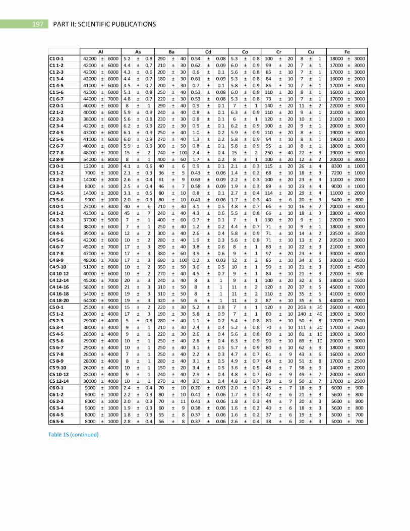
197 PART II: SCIENTIFIC PUBLICATIONS
Table 1S (continued)
C1 0-1 42000 ± 6000 5.2 ± 0.8 290 ± 40 0.54 ± 0.08 5.3 ± 0.8 100 ± 20 8 ± 1 18000 ± 3000
C1 1-2 42000 ± 6000 4.4 ± 0.7 210 ± 30 0.62 ± 0.09 6.0 ± 0.9 99 ± 20 7 ± 1 17000 ± 3000
C1 2-3 42000 ± 6000 4.3 ± 0.6 200 ± 30 0.6 ± 0.1 5.6 ± 0.8 85 ± 10 7 ± 1 17000 ± 3000
C1 3-4 42000 ± 6000 4.4 ± 0.7 180 ± 30 0.61 ± 0.09 5.3 ± 0.8 84 ± 10 7 ± 1 16000 ± 2000
C1 4-5 41000 ± 6000 4.5 ± 0.7 200 ± 30 0.7 ± 0.1 5.8 ± 0.9 86 ± 10 7 ± 1 17000 ± 3000
C1 5-6 42000 ± 6000 5.1 ± 0.8 250 ± 40 0.53 ± 0.08 6.0 ± 0.9 110 ± 20 8 ± 1 16000 ± 2000
C1 6-7 44000 ± 7000 4.8 ± 0.7 220 ± 30 0.53 ± 0.08 5.3 ± 0.8 73 ± 10 7 ± 1 17000 ± 3000
C2 0-1 40000 ± 6000 8 ± 1 290 ± 40 0.9 ± 0.1 7 ± 1 140 ± 20 11 ± 2 22000 ± 3000
C2 1-2 40000 ± 6000 5.9 ± 0.9 240 ± 40 0.8 ± 0.1 6.3 ± 0.9 110 ± 20 9 ± 1 21000 ± 3000
C2 2-3 38000 ± 6000 5.6 ± 0.8 230 ± 30 0.8 ± 0.1 6 ± 1 120 ± 20 10 ± 1 21000 ± 3000
C2 3-4 42000 ± 6000 6.2 ± 0.9 220 ± 30 0.9 ± 0.1 6.2 ± 0.9 100 ± 20 9 ± 1 20000 ± 3000
C2 4-5 43000 ± 6000 6.1 ± 0.9 250 ± 40 1.0 ± 0.2 5.9 ± 0.9 110 ± 20 8 ± 1 19000 ± 3000
C2 5-6 41000 ± 6000 6.0 ± 0.9 270 ± 40 1.3 ± 0.2 5.8 ± 0.9 94 ± 10 8 ± 1 19000 ± 3000
C2 6-7 40000 ± 6000 5.9 ± 0.9 300 ± 50 0.8 ± 0.1 5.8 ± 0.9 95 ± 10 8 ± 1 18000 ± 3000
C2 7-8 48000 ± 7000 15 ± 2 740 ± 100 2.4 ± 0.4 15 ± 2 250 ± 40 22 ± 3 19000 ± 3000
C2 8-9 54000 ± 8000 8 ± 1 400 ± 60 1.7 ± 0.2 8 ± 1 100 ± 20 12 ± 2 20000 ± 3000
C3 0-1 12000 ± 2000 4.1 ± 0.6 40 ± 6 0.9 ± 0.1 2.1 ± 0.3 115 ± 20 26 ± 4 8300 ± 1000
C3 1-2 7000 ± 1000 2.1 ± 0.3 36 ± 5 0.43 ± 0.06 1.4 ± 0.2 68 ± 10 18 ± 3 7200 ± 1000
C3 2-3 14000 ± 2000 2.6 ± 0.4 61 ± 9 0.63 ± 0.09 2.2 ± 0.3 100 ± 20 23 ± 3 11000 ± 2000
C3 3-4 8000 ± 1000 2.5 ± 0.4 46 ± 7 0.58 ± 0.09 1.9 ± 0.3 89 ± 10 23 ± 4 9000 ± 1000
C3 4-5 14000 ± 2000 3.1 ± 0.5 80 ± 10 0.8 ± 0.1 2.7 ± 0.4 114 ± 20 29 ± 4 11000 ± 2000
C3 5-6 9000 ± 1000 2.0 ± 0.3 80 ± 10 0.41 ± 0.06 1.7 ± 0.3 40 ± 6 20 ± 3 5400 ± 800
C4 0-1 23000 ± 3000 40 ± 6 210 ± 30 3.1 ± 0.5 4.8 ± 0.7 66 ± 10 16 ± 2 20000 ± 3000
C4 1-2 42000 ± 6000 45 ± 7 240 ± 40 4.3 ± 0.6 5.5 ± 0.8 66 ± 10 18 ± 3 28000 ± 4000
C4 2-3 37000 ± 5000 7 ± 1 400 ± 60 0.7 ± 0.1 7 ± 1 130 ± 20 9 ± 1 22000 ± 3000
C4 3-4 38000 ± 6000 7 ± 1 250 ± 40 1.2 ± 0.2 4.4 ± 0.7 71 ± 10 9 ± 1 18000 ± 3000
C4 4-5 39000 ± 6000 12 ± 2 300 ± 40 2.6 ± 0.4 5.8 ± 0.9 71 ± 10 14 ± 2 23500 ± 3500
C4 5-6 42000 ± 6000 10 ± 2 280 ± 40 1.9 ± 0.3 5.6 ± 0.8 71 ± 10 13 ± 2 20500 ± 3000
C4 6-7 45000 ± 7000 17 ± 3 290 ± 40 3.8 ± 0.6 8 ± 1 83 ± 10 22 ± 3 21000 ± 3000
C4 7-8 47000 ± 7000 17 ± 3 380 ± 60 3.9 ± 0.6 9 ± 1 97 ± 20 23 ± 3 30000 ± 4000
C4 8-9 48000 ± 7000 17 ± 3 690 ± 100 0.2 ± 0.03 12 ± 2 85 ± 10 34 ± 5 30000 ± 4500
C4 9-10 51000 ± 8000 10 ± 2 350 ± 50 3.6 ± 0.5 10 ± 1 90 ± 10 21 ± 3 31000 ± 4500
C4 10-12 40000 ± 6000 10 ± 2 270 ± 40 4.5 ± 0.7 9 ± 1 84 ± 10 21 ± 3 22000 ± 300
C4 12-14 45000 ± 7000 20 ± 3 240 ± 40 8 ± 1 9 ± 1 100 ± 20 32 ± 5 38000 ± 5500
C4 14-16 58000 ± 9000 21 ± 3 310 ± 50 8 ± 1 11 ± 2 120 ± 20 37 ± 5 45000 ± 7000
C4 16-18 54000 ± 8000 19 ± 3 310 ± 50 8 ± 1 11 ± 2 110 ± 20 35 ± 5 41000 ± 6000
C4 18-20 64000 ± 9000 19 ± 3 320 ± 50 6 ± 1 11 ± 2 87 ± 10 35 ± 5 44000 ± 7000
C5 0-1 25000 ± 4000 15 ± 2 220 ± 30 5.2 ± 0.8 7 ± 1 120 ± 20 203 ± 30 26000 ± 4000
C5 1-2 26000 ± 4000 17 ± 3 190 ± 30 5.8 ± 0.9 7 ± 1 80 ± 10 240 ± 40 19000 ± 3000
C5 2-3 29000 ± 4000 5 ± 0.8 280 ± 40 1.1 ± 0.2 5.4 ± 0.8 80 ± 10 50 ± 8 17000 ± 2500
C5 3-4 30000 ± 4000 9 ± 1 210 ± 30 2.4 ± 0.4 5.2 ± 0.8 70 ± 10 111 ± 20 17000 ± 2600
C5 4-5 28000 ± 4000 9 ± 1 220 ± 30 2.6 ± 0.4 5.6 ± 0.8 80 ± 10 81 ± 10 19000 ± 3000
C5 5-6 29000 ± 4000 10 ± 1 250 ± 40 2.8 ± 0.4 6.3 ± 0.9 90 ± 10 89 ± 10 20000 ± 3000
C5 6-7 29000 ± 4000 10 ± 1 250 ± 40 3.1 ± 0.5 5.7 ± 0.9 80 ± 10 62 ± 9 18000 ± 3000
C5 7-8 28000 ± 4000 7 ± 1 250 ± 40 2.2 ± 0.3 4.7 ± 0.7 61 ± 9 43 ± 6 16000 ± 2000
C5 8-9 28000 ± 4000 8 ± 1 280 ± 40 3.1 ± 0.5 4.9 ± 0.7 64 ± 10 51 ± 8 17000 ± 2500
C5 9-10 26000 ± 4000 10 ± 1 150 ± 20 3.4 ± 0.5 3.6 ± 0.5 48 ± 7 58 ± 9 14000 ± 2000
C5 10-12 28000 ± 4000 9 ± 1 240 ± 40 2.9 ± 0.4 4.8 ± 0.7 60 ± 9 49 ± 7 20000 ± 3000
C5 12-14 30000 ± 4000 10 ± 1 270 ± 40 3.0 ± 0.4 4.8 ± 0.7 59 ± 9 50 ± 7 17000 ± 2500
C6 0-1 9000 ± 1000 2.4 ± 0.4 70 ± 10 0.20 ± 0.03 2.0 ± 0.3 45 ± 7 18 ± 3 6000 ± 900
C6 1-2 9000 ± 1000 2.2 ± 0.3 80 ± 10 0.41 ± 0.06 1.7 ± 0.3 42 ± 6 21 ± 3 5600 ± 800
C6 2-3 8000 ± 1000 2.0 ± 0.3 70 ± 11 0.41 ± 0.06 1.8 ± 0.3 44 ± 7 20 ± 3 5600 ± 800
C6 3-4 9000 ± 1000 1.9 ± 0.3 60 ± 9 0.38 ± 0.06 1.6 ± 0.2 40 ± 6 18 ± 3 5600 ± 800
C6 4-5 8000 ± 1000 1.8 ± 0.3 55 ± 8 0.37 ± 0.06 1.6 ± 0.2 37 ± 6 19 ± 3 5000 ± 700
C6 5-6 8000 ± 1000 2.8 ± 0.4 56 ± 8 0.37 ± 0.06 2.6 ± 0.4 38 ± 6 20 ± 3 5000 ± 700
CrAl Ba FeCdAs CuCo
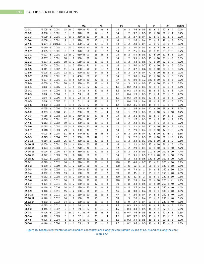
198 PART II: SCIENTIFIC PUBLICATIONS
Figure 1S. Graphic representation of Cd and Zn concentrations along the core sample C5 and of Cd, As and Zn along the core
sample C4
TOC %
C1 0-1 0.005 ± 0.001 13 ± 2 460 ± 70 12 ± 2 14 ± 2 3.6 ± 0.5 61 ± 9 27 ± 4 0.1%
C1 1-2 0.006 ± 0.001 8 ± 1 370 ± 50 14 ± 2 14 ± 2 3.2 ± 0.5 70 ± 10 30 ± 4 0.2%
C1 2-3 0.009 ± 0.001 9 ± 1 350 ± 50 14 ± 2 14 ± 2 2.7 ± 0.4 62 ± 9 31 ± 5 0.2%
C1 3-4 0.008 ± 0.001 7 ± 1 320 ± 50 13 ± 2 14 ± 2 2.6 ± 0.4 60 ± 9 29 ± 4 0.1%
C1 4-5 0.004 ± 0.0006 8 ± 1 360 ± 60 13 ± 2 14 ± 2 2.8 ± 0.4 63 ± 9 29 ± 4 0.1%
C1 5-6 0.010 ± 0.002 11 ± 2 320 ± 50 13 ± 2 14 ± 2 2.0 ± 0.3 57 ± 9 29 ± 4 0.2%
C1 6-7 0.005 ± 0.001 9 ± 1 320 ± 50 13 ± 2 14 ± 2 2.5 ± 0.4 70 ± 11 33 ± 5 0.2%
C2 0-1 0.007 ± 0.001 12 ± 2 630 ± 90 16 ± 2 14 ± 2 5.5 ± 0.8 80 ± 10 31 ± 5 0.2%
C2 1-2 0.007 ± 0.001 10 ± 2 530 ± 80 14 ± 2 14 ± 2 3.5 ± 0.5 70 ± 10 31 ± 5 0.1%
C2 2-3 0.007 ± 0.001 10 ± 2 510 ± 80 15 ± 2 14 ± 2 4.3 ± 0.6 70 ± 10 32 ± 5 0.2%
C2 3-4 0.004 ± 0.001 11 ± 2 470 ± 71 14 ± 2 14 ± 2 5.0 ± 0.7 70 ± 10 34 ± 5 0.2%
C2 4-5 0.011 ± 0.002 11 ± 2 450 ± 70 13 ± 2 13 ± 2 3.7 ± 0.6 70 ± 10 34 ± 5 0.2%
C2 5-6 0.008 ± 0.001 12 ± 2 420 ± 60 14 ± 2 14 ± 2 2.7 ± 0.4 70 ± 10 35 ± 5 0.2%
C2 6-7 0.008 ± 0.001 11 ± 2 400 ± 60 13 ± 2 14 ± 2 3.0 ± 0.4 70 ± 10 34 ± 5 0.2%
C2 7-8 0.007 ± 0.001 31 ± 5 400 ± 60 37 ± 5 37 ± 6 8.0 ± 1.2 180 ± 30 33 ± 5 0.2%
C2 8-9 0.009 ± 0.001 20 ± 3 350 ± 50 19 ± 3 20 ± 3 3.2 ± 0.5 80 ± 10 40 ± 6 0.2%
C3 0-1 0.04 ± 0.006 9 ± 1 35 ± 5 42 ± 6 1.6 ± 0.2 2.4 ± 0.4 20 ± 3 27 ± 4 6.6%
C3 1-2 0.03 ± 0.004 6 ± 1 23 ± 3 27 ± 4 1.5 ± 0.2 1.5 ± 0.2 16 ± 2 21 ± 3 4.1%
C3 2-3 0.03 ± 0.004 9 ± 1 53 ± 8 38 ± 6 2.6 ± 0.4 1.9 ± 0.3 23 ± 4 31 ± 5 2.5%
C3 3-4 0.04 ± 0.006 8 ± 1 23 ± 3 38 ± 6 1.9 ± 0.3 1.9 ± 0.3 20 ± 3 23 ± 3 2.9%
C3 4-5 0.05 ± 0.007 11 ± 2 51 ± 8 47 ± 7 3.0 ± 0.4 2.8 ± 0.4 28 ± 4 30 ± 5 1.7%
C3 5-6 0.022 ± 0.003 8 ± 1 35 ± 5 34 ± 5 1.4 ± 0.2 3.5 ± 0.5 15 ± 2 23 ± 3 3.0%
C4 0-1 0.025 ± 0.004 23 ± 3 200 ± 30 21 ± 3 8 ± 1 2.6 ± 0.4 90 ± 10 23 ± 3 5.2%
C4 1-2 0.053 ± 0.008 21 ± 3 230 ± 30 23 ± 4 10 ± 1 2.3 ± 0.3 90 ± 10 64 ± 10 1.2%
C4 2-3 0.016 ± 0.002 12 ± 2 350 ± 50 17 ± 3 13 ± 2 2.1 ± 0.3 61 ± 9 34 ± 5 0.3%
C4 3-4 0.006 ± 0.001 12 ± 2 450 ± 70 13 ± 2 10 ± 2 1.7 ± 0.3 60 ± 9 29 ± 4 1.7%
C4 4-5 0.013 ± 0.002 19 ± 3 460 ± 70 18 ± 3 13 ± 2 2.3 ± 0.3 59 ± 9 35 ± 5 2.7%
C4 5-6 0.013 ± 0.002 18 ± 3 360 ± 50 18 ± 3 11 ± 2 2.1 ± 0.3 70 ± 10 38 ± 6 1.6%
C4 6-7 0.018 ± 0.003 29 ± 4 300 ± 40 26 ± 4 14 ± 2 2.9 ± 0.4 80 ± 10 42 ± 6 2.8%
C4 7-8 0.023 ± 0.003 31 ± 5 340 ± 50 28 ± 4 17 ± 2 2.9 ± 0.4 80 ± 10 60 ± 9 3.6%
C4 8-9 0.025 ± 0.004 57 ± 9 330 ± 50 42 ± 6 19 ± 3 2.2 ± 0.3 90 ± 10 60 ± 9 2.2%
C4 9-10 0.014 ± 0.002 26 ± 4 430 ± 60 30 ± 4 15 ± 2 2.3 ± 0.3 100 ± 10 58 ± 9 2.8%
C4 10-12 0.009 ± 0.001 25 ± 4 340 ± 50 28 ± 4 14 ± 2 2.1 ± 0.3 95 ± 10 36 ± 5 4.3%
C4 12-14 0.023 ± 0.003 31 ± 5 270 ± 40 35 ± 5 12 ± 2 2.9 ± 0.4 90 ± 10 80 ± 10 4.7%
C4 14-16 0.024 ± 0.004 37 ± 6 330 ± 50 40 ± 6 14 ± 2 3.3 ± 0.5 110 ± 20 100 ± 10 4.4%
C4 16-18 0.022 ± 0.003 39 ± 6 320 ± 50 39 ± 6 14 ± 2 3.1 ± 0.5 110 ± 20 90 ± 10 3.9%
C4 18-20 0.022 ± 0.003 13 ± 2 350 ± 50 41 ± 6 16 ± 2 4.2 ± 0.6 120 ± 20 100 ± 10 4.1%
C5 0-1 0.079 ± 0.012 16 ± 2 220 ± 30 21 ± 3 170 ± 30 4.6 ± 0.7 70 ± 11 370 ± 60 5.2%
C5 1-2 0.059 ± 0.009 15 ± 2 160 ± 20 21 ± 3 130 ± 20 22 ± 3 61 ± 9 380 ± 60 2.1%
C5 2-3 0.034 ± 0.005 11 ± 2 170 ± 30 13 ± 2 40 ± 6 7.3 ± 1 54 ± 8 160 ± 30 3.2%
C5 3-4 0.062 ± 0.009 13 ± 2 190 ± 30 16 ± 2 70 ± 10 15 ± 2 55 ± 8 150 ± 20 2.9%
C5 4-5 0.052 ± 0.008 14 ± 2 170 ± 30 16 ± 2 200 ± 30 12 ± 2 63 ± 9 220 ± 30 2.6%
C5 5-6 0.075 ± 0.011 16 ± 2 180 ± 30 18 ± 3 220 ± 30 2.8 ± 0.4 66 ± 10 270 ± 41 4.2%
C5 6-7 0.071 ± 0.011 15 ± 2 180 ± 30 17 ± 3 70 ± 11 3.3 ± 0.5 65 ± 10 250 ± 40 2.4%
C5 7-8 0.069 ± 0.010 14 ± 2 150 ± 20 14 ± 2 52 ± 8 2.7 ± 0.4 54 ± 8 260 ± 40 4.1%
C5 8-9 0.076 ± 0.011 15 ± 2 150 ± 20 16 ± 2 56 ± 8 3.0 ± 0.4 57 ± 9 300 ± 40 4.3%
C5 9-10 0.076 ± 0.011 13 ± 2 130 ± 20 13 ± 2 47 ± 7 2.6 ± 0.4 54 ± 8 260 ± 40 2.2%
C5 10-12 0.078 ± 0.012 14 ± 2 180 ± 30 15 ± 2 59 ± 9 2.6 ± 0.4 55 ± 8 290 ± 40 3.4%
C5 12-14 0.082 ± 0.012 14 ± 2 150 ± 20 15 ± 2 58 ± 9 2.7 ± 0.4 56 ± 8 230 ± 40 3.6%
C6 0-1 0.073 ± 0.011 9 ± 1 36 ± 5 33 ± 5 1.7 ± 0.3 3.3 ± 0.5 14 ± 2 24 ± 4 1.6%
C6 1-2 0.045 ± 0.007 9 ± 1 39 ± 6 33 ± 5 1.7 ± 0.3 3.3 ± 0.5 16 ± 2 22 ± 3 2.0%
C6 2-3 0.025 ± 0.004 9 ± 1 41 ± 6 33 ± 5 1.9 ± 0.3 3.6 ± 0.5 16 ± 2 22 ± 3 1.3%
C6 3-4 0.022 ± 0.003 8 ± 1 37 ± 6 30 ± 4 1.6 ± 0.2 3.7 ± 0.5 15 ± 2 23 ± 3 1.3%
C6 4-5 0.026 ± 0.004 8 ± 1 34 ± 5 32 ± 5 1.5 ± 0.2 3.4 ± 0.5 15 ± 2 21 ± 3 1.3%
C6 5-6 0.026 ± 0.004 9 ± 1 35 ± 5 33 ± 5 1.5 ± 0.2 3.6 ± 0.5 16 ± 2 22 ± 3 1.0%
Li V ZnMn UPbNiHg
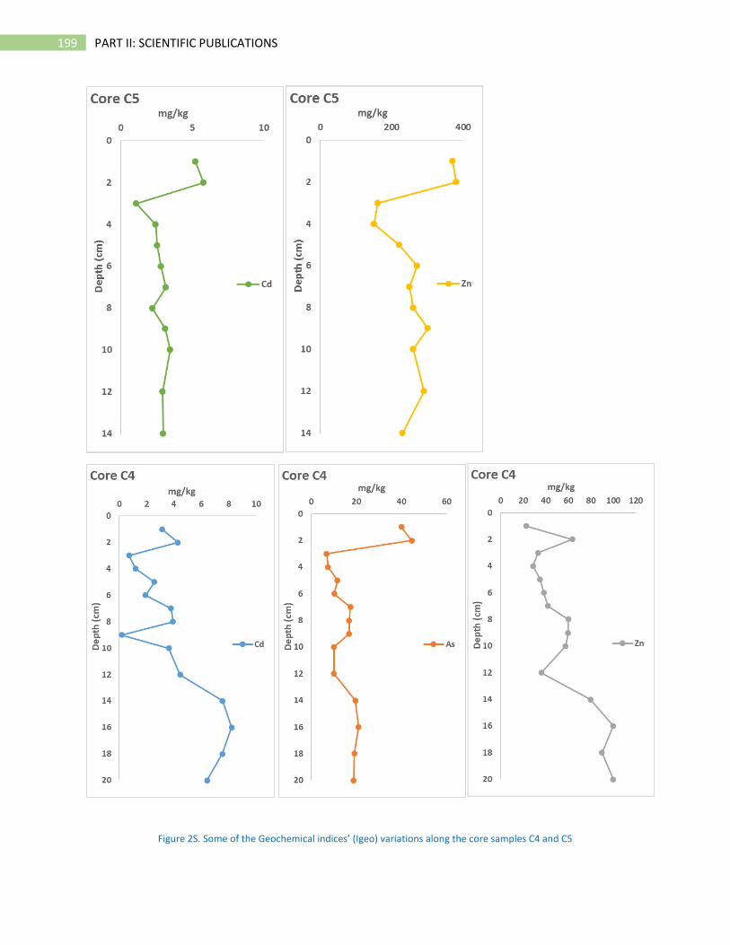
199 PART II: SCIENTIFIC PUBLICATIONS
Figure 2S. Some of the Geochemical indices’ (Igeo) variations along the core samples C4 and C5
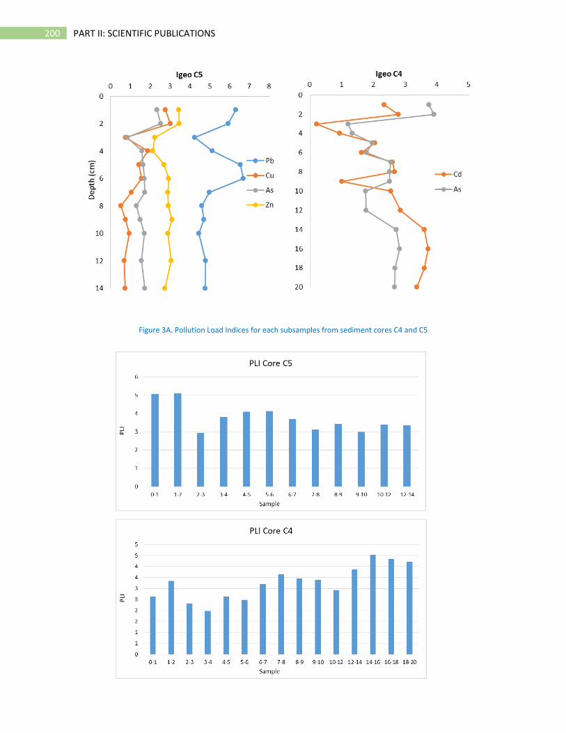
200 PART II: SCIENTIFIC PUBLICATIONS
Figure 3A. Pollution Load Indices for each subsamples from sediment cores C4 and C5
201 PART II: SCIENTIFIC PUBLICATIONS
THIRD BLOCK
Paper 6 Submitted to the peer reviewed journal Marine Pollution Bulletin (Elsevier)
Marine sponges as a powerful tool for trace elements biomonitoring studies in
coastal environment
Anna Maria Orani * a,b, Aurélie Barats a, Emilia Vassilevab, Olivier P. Thomas c
a Université Nice Sophia Antipolis, CNRS, IRD, Observatoire de la Côte d’Azur, Géoazur, UMR 7329, 250 rue Albert
Einstein, Sophia Antipolis 06560 Valbonne, France
b International Atomic Energy Agency, Environment Laboratories, 4 Quai Antoine 1er, MC 9800, Monaco
c National University of Ireland Galway, Marine Biodiscovery, School of Chemistry, University Road, Galway,
Ireland
Abstract
The use of marine sponges as trace elements (TE) biomonitors is evaluated in this study. Six sponge
species from the French Mediterranean coast and in two locations in the Irish coast were analyzed for
Ag, As, Ba, Cd, Cu, Mo, Ni, V, Pb and Zn contents. Intra and inter-species variability in TE accumulation
were examined. Results show that C. damicornis accumulates significantly more As and Cu than others
sponge species; C. nucula more Ni and Mo and A. acuta more Ag. Among Irish samples H. perlevis
showed higher accumulation properties for most of TE (particularly for Zn) in comparison to H. panicea.
Additionally, BCF, calculated using TE levels in sediment samples, were >1 in all species for most of TE.
The determination of Pb isotope ratios revealed a natural Pb sources for Mediterranean and Kilkieran
Bay’s samples while it highlighted anthropogenic Pb inputs in sponges and sediment from Belfast
Keywords: marine sponges, trace elements, biomonitoring, lead isotope ratios, marine environment
202 PART II: SCIENTIFIC PUBLICATIONS
1. Introduction
The occurrence of trace elements (TE) in aquatic environments is related to natural sources, but also to
anthropogenic inputs due to industrial developments and other human activities. TE contaminations
occur worldwide and the assessment of the pollution status is usually required, leading to the
publication of several studies on this subject (Li et al., 2000; Caccia et al., 2003; Fang et al., 2014; Parra
et al., 2015; Cabrita et al., 2017; Ashraf et al., 2017). An ideal biomonitor should be a natural
accumulator of the element of interest and possibly with high concentration factor, in order to highlight
possible difference between times or sites (Rainbow, 2002). Environmental surveys are often performed
on water samples but, in marine ecosystems, the very low TE concentrations and the salinity of the
seawater cause measurement limitations (Søndergaard et al., 2015). Monitoring studies on TE
contamination are also focused on sediments and biota. Sediments act as sink and reservoirs of
contaminants thus displaying higher TE contents and do not present problems related to short residence
time such as for water (Varol, 2011; Liu et al., 2015). Marine organisms are also relevant tools for
characterizing the state of a marine ecosystem because they are recognized to accumulate TE. They can
be a good tool especially in rocky shores where sediments do not occur. Sessile and active filter feeding
invertebrates are often used to determine temporal and spatial variation of TE in aquatic systems (Weis
and Weis, 1999; Denton et al., 2006; Dahms et al., 2014). Historically, bivalves are considered as ideal
biomonitor organisms as exemplified by the “mussel watch program” (Cantillo, 1998) which is also
supported by the bivalve use as common seafood. More recently, sponges gained scientists attention as
possible biomonitors of TE contamination because they are abundant and widespread, long-living,
sessile, easily sampled and they have shown high tolerance for several pollutants (de Mestre et al.,
2012; Batista et al., 2014). Additionally sponge communities can remain stable for long time periods,
making them suitable model organisms for monitoring studies. Sponges are filter feeding organisms,
pumping huge quantities of seawater (100-1200 mL h-1 g-1 larger than for most of other marine
organisms (Olesen and Weeks, 1994). Sponges have a high capacity for TE accumulation for a long
period of time (Patel et al., 1985; Padovan et al., 2012), exhibiting higher filtering capacity than bivalves
(Negri et al., 2006; Gentric et al., 2016). They are considered as ‘‘biological particle traps’’ as they are
able to concentrate a wide range of pollutants from both the suspended and dissolved phases, showing
high bio-concentration factors (Perez et al., 2005; Cebrian et al., 2003). The detection of large quantities
of TE in sponges suggests the existence of detoxification systems (Aly et al., 2013). These characteristics
make them suitable as a model organisms for monitoring studies, and their use has been proposed in
several fields of study (Negri et al., 2006; Venkateswara Rao et al., 2009; Illuminati et al., 2016). Sponges
203 PART II: SCIENTIFIC PUBLICATIONS
have also been reported as efficient environmental remediators of different toxic compounds such as
the bacterium Escherichia coli (Milanese et al., 2003) and the organochlorine pesticide lindane (Aresta et
al., 2015). These characteristics, combined with recent interest in sponges as a source of novel
pharmaceuticals and bioactive compounds (Anjum et al., 2016), indicate the possibility for a self-
financing remediation program (Gifford et al., 2007).
The main objective of this work was the assessment of TE pollution in different sponge species collected
in different areas. A comparative study on TE bioaccumulation have been performed on six sponge
species collected in the Southern French Mediterranean coast and in Ireland. These areas have been
selected because of their differences in terms of TE biogeochemical background and anthropogenic
inputs. The bioaccumulation potential of these sponges was examined for a broad range of TE,
comparing with values measured in sediment samples collected in the same area. Additionally,
measurements of Pb isotope ratios were performed for the first time in sponges and allowed us to give
insights on the principal sources of Pb contamination in the studied zones.
2. Materials and methods
2.1. Sampling
Sponge and sediment samples were collected in three sampling sites: the Mediterranean coast, in the
Grotte du Lido at Villefranche sur Mer, France (N 43° 41' 59.0'', E 07° 19' 31.5''), and two coastal sites in
Ireland, Greenisland at the Belfast Lough (N54°41’24.383”, O 5° 51’ 36.633”) and in Kilkieran Bay (N 53°
21’ 22.625’’, O 9° 42’ 17.153”) (Fig. 1). Sediment samples were collected during each sampling session,
using an acid pre-cleaned polyethylene tube. Sponges were collected using a plastic knife and placed in
separate plastic bag. Sponge specimens of similar size were selected in order to reduce intra-species
variations due to sponge age. At least, three specimens with similar size of each sponge species were
randomly selected in each collection. Sediments and four species of Mediterranean sponges (Acanthella
acuta, Cymbaxinella damicornis, Chondrilla nucula and Haliclona fulva) were collected by scuba diving at
20m for two different periods of the year (February and September 2016). During the first sampling,
three specimens of C. damicornis were collected in the center of the cave while the remaining two
specimens were from the entrance. During the second sampling, three specimens of C. nucula were
collected at 5m depth while three other specimens were taken at 20m. In Ireland, sediments and two
species of sponges (Halichondria panicea and Hymeniacidon perlevis) were hand-sampled in intertidal
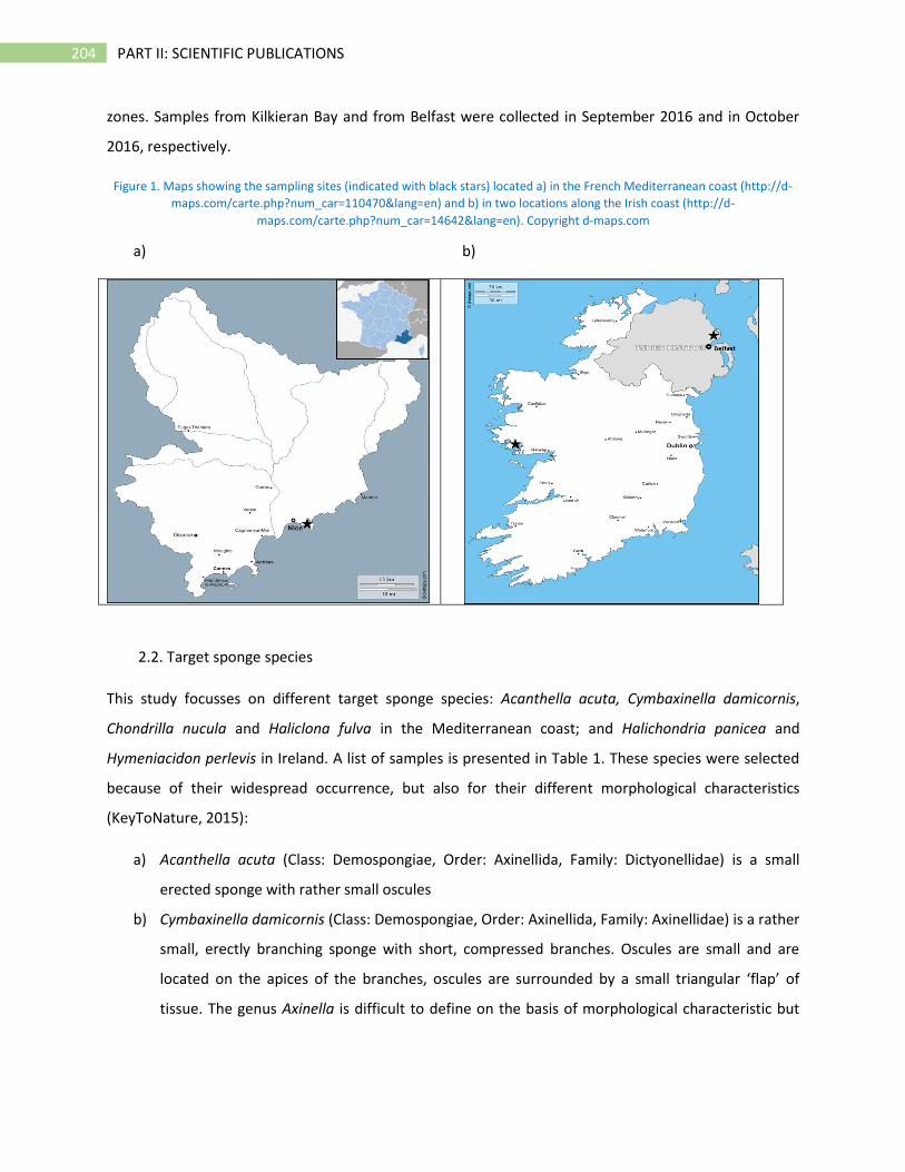
204 PART II: SCIENTIFIC PUBLICATIONS
zones. Samples from Kilkieran Bay and from Belfast were collected in September 2016 and in October
2016, respectively.
Figure 1. Maps showing the sampling sites (indicated with black stars) located a) in the French Mediterranean coast (http://d-
maps.com/carte.php?num_car=110470&lang=en) and b) in two locations along the Irish coast (http://d-
maps.com/carte.php?num_car=14642&lang=en). Copyright d-maps.com
a) b)
2.2. Target sponge species
This study focusses on different target sponge species: Acanthella acuta, Cymbaxinella damicornis,
Chondrilla nucula and Haliclona fulva in the Mediterranean coast; and Halichondria panicea and
Hymeniacidon perlevis in Ireland. A list of samples is presented in Table 1. These species were selected
because of their widespread occurrence, but also for their different morphological characteristics
(KeyToNature, 2015):
a) Acanthella acuta (Class: Demospongiae, Order: Axinellida, Family: Dictyonellidae) is a small
erected sponge with rather small oscules
b) Cymbaxinella damicornis (Class: Demospongiae, Order: Axinellida, Family: Axinellidae) is a rather
small, erectly branching sponge with short, compressed branches. Oscules are small and are
located on the apices of the branches, oscules are surrounded by a small triangular ‘flap’ of
tissue. The genus Axinella is difficult to define on the basis of morphological characteristic but
205 PART II: SCIENTIFIC PUBLICATIONS
for the specie analyzed in this study the name Cymbaxinella damicornis was recently proposed
by (Gazave et al., 2010), following the phylocode.
c) Chondrilla nucula (Class: Demospongiae, Order: Chondrillida, Family: Chondrillidae) is
amorphous, with globular lobes, or thickly incrusting, up to about 1 cm thick, spreading
horizontally, with pronounced, deeply incised and lacunose, meandering lobes. The color is
dark-brown to walnut-brown.
d) Haliclona fulva (Class: Demospongiae, Order: Haplosclerida, Family: Chalinidae). The surface of
the specimen is irregular and slightly hispid. The ectosomal and choanosomal skeletons have a
regular, delicate, unispicular, and isotropic reticulation. Color is dark orange.
e) Halichondria panicea (Class: Demospongiae, Order: Suberitida, Family: Halichondriidae).
Intertidal or shallow-subtidal, thickly encrusting, massive or occasionally branching sponge, with
typical volcanoe-shaped oscular chimneys. Surface smooth, consistency firm, texture crumb-of-
bread. Basically light orange-yellow or pale yellowish green.
f) Hymeniacidon perlevis (Class: Demospongiae, Order: Suberitida, Family: Halichondriidae). One
of the most common species along the Atlantic coasts of Western Europe. It is orange and has
an irregular surface, often with lower or higher irregular projections; oscules are inconspicuous.
Table 1. List of specimens collected and analyzed in the present study
Sampling site Sponge specie Number of specimens Code
Villefranche-sur-mer
Halichlona fulva 6 HA.F
Axinella damicornis 7 CY.D
Acanthella acuta 6 AC.A
Chondrilla nucula 9 CH.N
Kilkieran Bay Halichondria panicea 4 HA.P
Hymeniacidon perlevis 3 Hy.P
Belfast Lough Halichondria panicea 6 HA.P Bel
Hymeniacidon perlevis 7 Hy.P Bel
2.3. Sample preparation
All solutions were prepared with doubly deionized water obtained from Millipore water purification
system (Elix & Synergy) (resistivity of 18.2 MΩ cm−1, Total Organic Carbon < 5 μg L−1 and microorganisms
< 0.1 UFC ml-1). All PTFE and Teflon containers used for sample preparation and analysis were pre-
206 PART II: SCIENTIFIC PUBLICATIONS
cleaned using a procedure consisting of 24 h bath in 10% HNO3 (prepared from proper dilution of 65%
analytical grade HNO3, Fisher Chemicals) and careful rinsing three times with Milli-Q water. Sediment
and sponge samples were freeze-dried, ground in agate mortar and kept in a desiccator in closed PTFE
tubes.
Analysis for TE and Pb isotope ratios determination were performed using preliminary validated
methods. For trace elements analysis by ICP-MS, a microwave digestion was carried out into a closed
microwave system (Ethos One, Milestone). Teflon reactors were filled with an aliquot of about 0.05 g of
sponge sample or 0.1 g of sediment sample (bulk samples), and with 5 mL of HNO3 (Trace Metal Grade,
67 to 70% w/w, Fisher Chemical) and 2 mL of HF (Ultra Trace Elemental Analysis 47-51% w/w, Optima,
Fisher Chemical). Temperature program used for acid digestion consisted of a 20 min ramp temperature
up to 180 °C, followed by an isothermal phase of 30 min. The mineralized solutions were then
transferred to PE pre-cleaned tubes and gravimetrically diluted with Milli-Q water, up to a final volume
of 50 mL. These solutions were further diluted 15 times in Milli-Q water prior to ICP-MS analyses.
Similar digestions and analyses were performed on two Certified Reference Materials (CRMs) to assure a
quality control of the entire analytical procedure: TORT-2 (Lobster hepatopancreas, NRC, Canada) and
MESS-2 (Estuarine sediment, NRC, Canada), weighting systematically 50 and 100 mg respectively. At
least one procedural blank and one CRM were included in each digestion run and analyzed with the rest
of the samples. A summary of results obtained for CRMs analyzed in this study, is presented in Table 2;
Cd and Ag in MESS-2 were below limits of quantification, therefore they are not listed in the table with
other analytes.
One specimen of each sponge’s specie and one sediment sample for each location were selected for Pb
isotope ratios analysis. An aliquot of about 100 mg of sponge or sediment sample was decomposed in 5
mL ultrapure HNO3 (Fisher scientific, Hampton, USA) and 2 mL of ultrapure HF (Fisher scientific,
Hampton, USA) using the Mars X-press Microwave (CEM Mars X-press) equipped with a 12 vessels
carousel. After the digestion, obtained solutions were placed on a ceramic heating plate, under laminar
hood, and evaporated to near dryness. The residues were taken up in 2% HNO3, transferred to 50 ml PE
tubes and stored at 4 °C. Solutions for Pb isotope ratios determination were properly diluted with 2%
HNO3 in class 100 clean room.
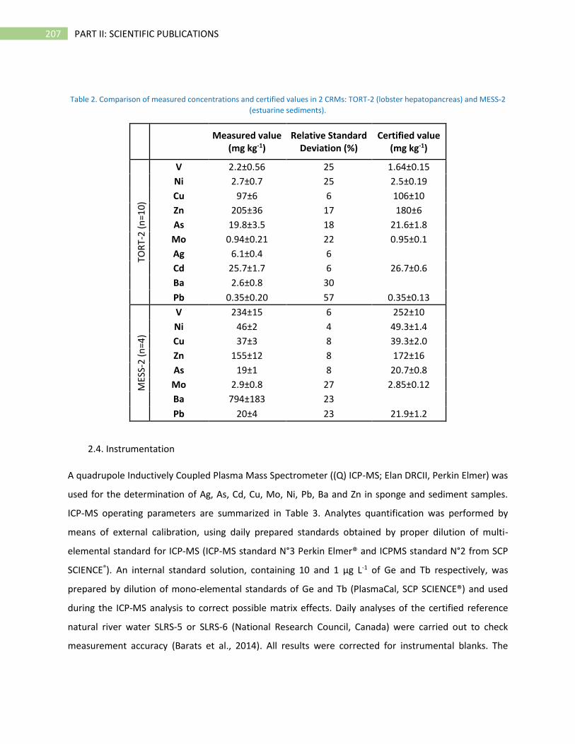
207 PART II: SCIENTIFIC PUBLICATIONS
Table 2. Comparison of measured concentrations and certified values in 2 CRMs: TORT-2 (lobster hepatopancreas) and MESS-2
(estuarine sediments).
Measured value
(mg kg-1) Relative Standard
Deviation (%) Certified value
(mg kg-1) TO
RT-
2 (
n=1
0)
V 2.2±0.56 25 1.64±0.15
Ni 2.7±0.7 25 2.5±0.19
Cu 97±6 6 106±10
Zn 205±36 17 180±6
As 19.8±3.5 18 21.6±1.8
Mo 0.94±0.21 22 0.95±0.1
Ag 6.1±0.4 6
Cd 25.7±1.7 6 26.7±0.6
Ba 2.6±0.8 30
Pb 0.35±0.20 57 0.35±0.13
MES
S-2
(n
=4)
V 234±15 6 252±10
Ni 46±2 4 49.3±1.4
Cu 37±3 8 39.3±2.0
Zn 155±12 8 172±16
As 19±1 8 20.7±0.8
Mo 2.9±0.8 27 2.85±0.12
Ba 794±183 23
Pb 20±4 23 21.9±1.2
2.4. Instrumentation
A quadrupole Inductively Coupled Plasma Mass Spectrometer ((Q) ICP-MS; Elan DRCII, Perkin Elmer) was
used for the determination of Ag, As, Cd, Cu, Mo, Ni, Pb, Ba and Zn in sponge and sediment samples.
ICP-MS operating parameters are summarized in Table 3. Analytes quantification was performed by
means of external calibration, using daily prepared standards obtained by proper dilution of multi-
elemental standard for ICP-MS (ICP-MS standard N°3 Perkin Elmer® and ICPMS standard N°2 from SCP
SCIENCE®). An internal standard solution, containing 10 and 1 µg L-1 of Ge and Tb respectively, was
prepared by dilution of mono-elemental standards of Ge and Tb (PlasmaCal, SCP SCIENCE®) and used
during the ICP-MS analysis to correct possible matrix effects. Daily analyses of the certified reference
natural river water SLRS-5 or SLRS-6 (National Research Council, Canada) were carried out to check
measurement accuracy (Barats et al., 2014). All results were corrected for instrumental blanks. The
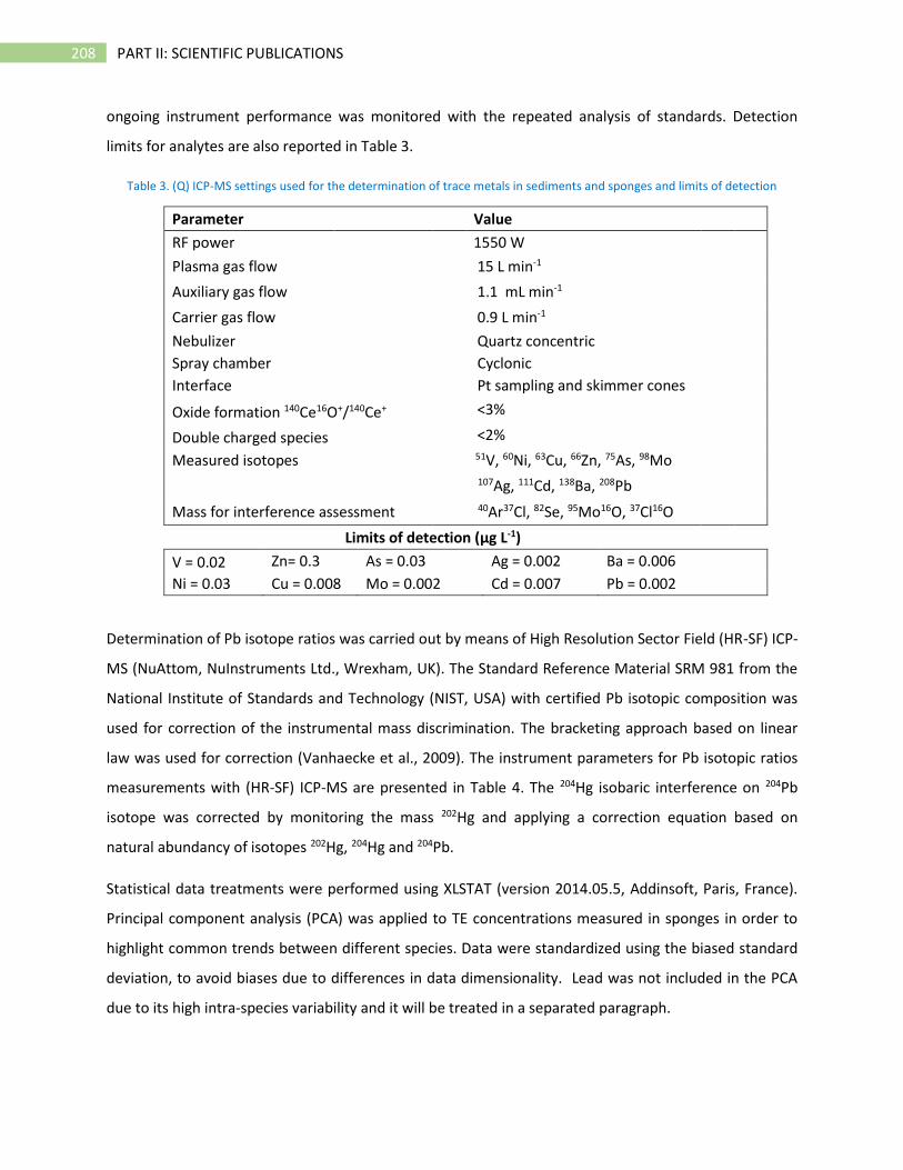
208 PART II: SCIENTIFIC PUBLICATIONS
ongoing instrument performance was monitored with the repeated analysis of standards. Detection
limits for analytes are also reported in Table 3.
Table 3. (Q) ICP-MS settings used for the determination of trace metals in sediments and sponges and limits of detection
Parameter Value
RF power
1550 W
Plasma gas flow
15 L min-1
Auxiliary gas flow
1.1 mL min-1
Carrier gas flow
0.9 L min-1
Nebulizer
Quartz concentric
Spray chamber
Cyclonic
Interface
Pt sampling and skimmer cones
Oxide formation 140Ce16O+/140Ce+ <3%
Double charged species <2%
Measured isotopes
51V, 60Ni, 63Cu, 66Zn, 75As, 98Mo
107Ag, 111Cd, 138Ba, 208Pb
Mass for interference assessment 40Ar37Cl, 82Se, 95Mo16O, 37Cl16O
Limits of detection (µg L-1)
V = 0.02 Zn= 0.3 As = 0.03 Ag = 0.002 Ba = 0.006
Ni = 0.03 Cu = 0.008 Mo = 0.002 Cd = 0.007 Pb = 0.002
Determination of Pb isotope ratios was carried out by means of High Resolution Sector Field (HR-SF) ICP-
MS (NuAttom, NuInstruments Ltd., Wrexham, UK). The Standard Reference Material SRM 981 from the
National Institute of Standards and Technology (NIST, USA) with certified Pb isotopic composition was
used for correction of the instrumental mass discrimination. The bracketing approach based on linear
law was used for correction (Vanhaecke et al., 2009). The instrument parameters for Pb isotopic ratios
measurements with (HR-SF) ICP-MS are presented in Table 4. The 204Hg isobaric interference on 204Pb
isotope was corrected by monitoring the mass 202Hg and applying a correction equation based on
natural abundancy of isotopes 202Hg, 204Hg and 204Pb.
Statistical data treatments were performed using XLSTAT (version 2014.05.5, Addinsoft, Paris, France).
Principal component analysis (PCA) was applied to TE concentrations measured in sponges in order to
highlight common trends between different species. Data were standardized using the biased standard
deviation, to avoid biases due to differences in data dimensionality. Lead was not included in the PCA
due to its high intra-species variability and it will be treated in a separated paragraph.
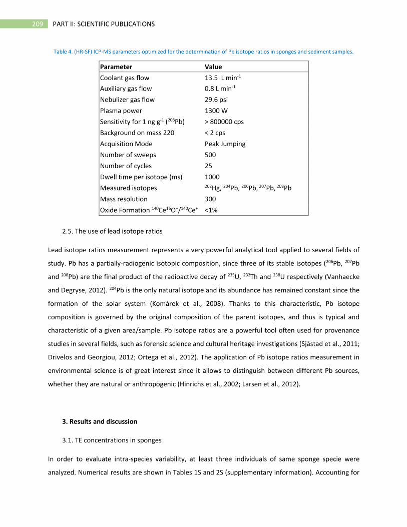
209 PART II: SCIENTIFIC PUBLICATIONS
Table 4. (HR-SF) ICP-MS parameters optimized for the determination of Pb isotope ratios in sponges and sediment samples.
Parameter Value
Coolant gas flow 13.5 L min-1
Auxiliary gas flow 0.8 L min-1
Nebulizer gas flow 29.6 psi
Plasma power 1300 W
Sensitivity for 1 ng g-1 (208Pb) > 800000 cps
Background on mass 220 < 2 cps
Acquisition Mode Peak Jumping
Number of sweeps 500
Number of cycles 25
Dwell time per isotope (ms) 1000
Measured isotopes 202Hg, 204Pb, 206Pb, 207Pb, 208Pb
Mass resolution 300
Oxide Formation 140Ce16O+/140Ce+ <1%
2.5. The use of lead isotope ratios
Lead isotope ratios measurement represents a very powerful analytical tool applied to several fields of
study. Pb has a partially-radiogenic isotopic composition, since three of its stable isotopes (206Pb, 207Pb
and 208Pb) are the final product of the radioactive decay of 235U, 232Th and 238U respectively (Vanhaecke
and Degryse, 2012). 204Pb is the only natural isotope and its abundance has remained constant since the
formation of the solar system (Komárek et al., 2008). Thanks to this characteristic, Pb isotope
composition is governed by the original composition of the parent isotopes, and thus is typical and
characteristic of a given area/sample. Pb isotope ratios are a powerful tool often used for provenance
studies in several fields, such as forensic science and cultural heritage investigations (Sjåstad et al., 2011;
Drivelos and Georgiou, 2012; Ortega et al., 2012). The application of Pb isotope ratios measurement in
environmental science is of great interest since it allows to distinguish between different Pb sources,
whether they are natural or anthropogenic (Hinrichs et al., 2002; Larsen et al., 2012).
3. Results and discussion
3.1. TE concentrations in sponges
In order to evaluate intra-species variability, at least three individuals of same sponge specie were
analyzed. Numerical results are shown in Tables 1S and 2S (supplementary information). Accounting for
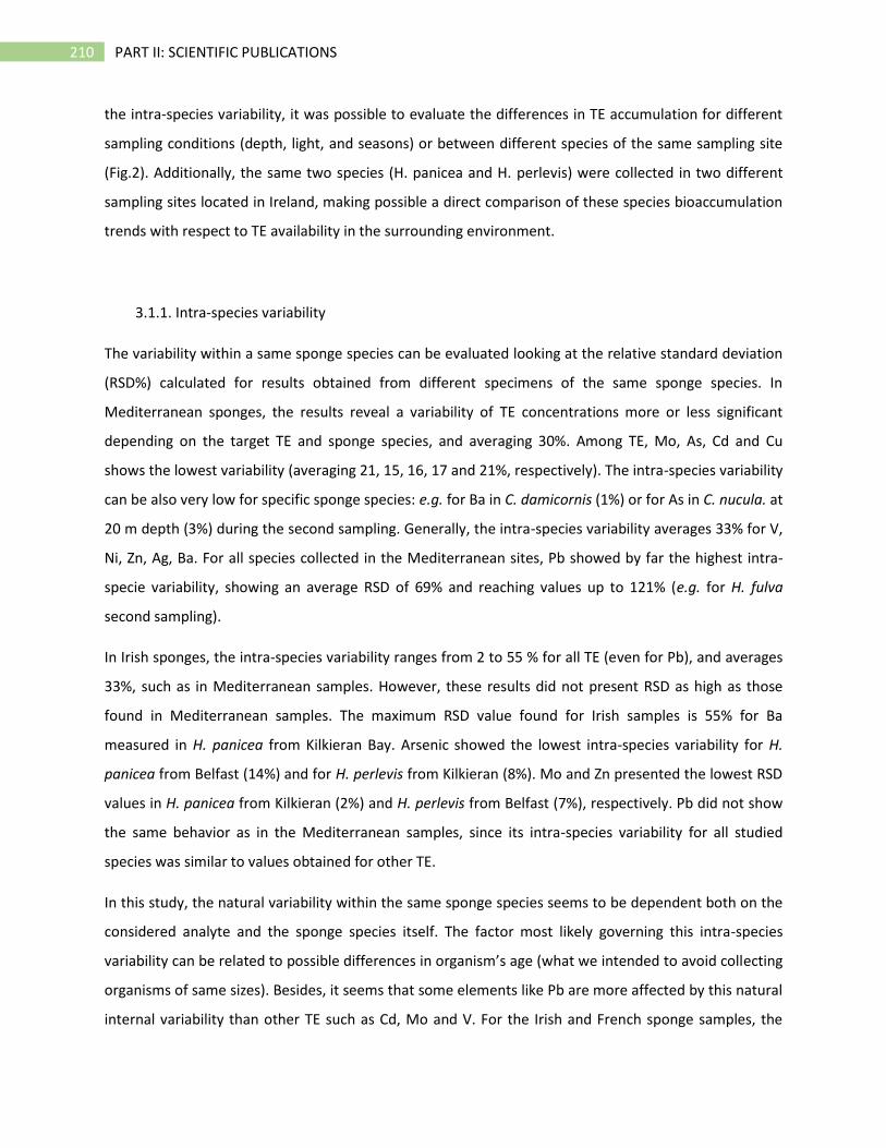
210 PART II: SCIENTIFIC PUBLICATIONS
the intra-species variability, it was possible to evaluate the differences in TE accumulation for different
sampling conditions (depth, light, and seasons) or between different species of the same sampling site
(Fig.2). Additionally, the same two species (H. panicea and H. perlevis) were collected in two different
sampling sites located in Ireland, making possible a direct comparison of these species bioaccumulation
trends with respect to TE availability in the surrounding environment.
3.1.1. Intra-species variability
The variability within a same sponge species can be evaluated looking at the relative standard deviation
(RSD%) calculated for results obtained from different specimens of the same sponge species. In
Mediterranean sponges, the results reveal a variability of TE concentrations more or less significant
depending on the target TE and sponge species, and averaging 30%. Among TE, Mo, As, Cd and Cu
shows the lowest variability (averaging 21, 15, 16, 17 and 21%, respectively). The intra-species variability
can be also very low for specific sponge species: e.g. for Ba in C. damicornis (1%) or for As in C. nucula. at
20 m depth (3%) during the second sampling. Generally, the intra-species variability averages 33% for V,
Ni, Zn, Ag, Ba. For all species collected in the Mediterranean sites, Pb showed by far the highest intra-
specie variability, showing an average RSD of 69% and reaching values up to 121% (e.g. for H. fulva
second sampling).
In Irish sponges, the intra-species variability ranges from 2 to 55 % for all TE (even for Pb), and averages
33%, such as in Mediterranean samples. However, these results did not present RSD as high as those
found in Mediterranean samples. The maximum RSD value found for Irish samples is 55% for Ba
measured in H. panicea from Kilkieran Bay. Arsenic showed the lowest intra-species variability for H.
panicea from Belfast (14%) and for H. perlevis from Kilkieran (8%). Mo and Zn presented the lowest RSD
values in H. panicea from Kilkieran (2%) and H. perlevis from Belfast (7%), respectively. Pb did not show
the same behavior as in the Mediterranean samples, since its intra-species variability for all studied
species was similar to values obtained for other TE.
In this study, the natural variability within the same sponge species seems to be dependent both on the
considered analyte and the sponge species itself. The factor most likely governing this intra-species
variability can be related to possible differences in organism’s age (what we intended to avoid collecting
organisms of same sizes). Besides, it seems that some elements like Pb are more affected by this natural
internal variability than other TE such as Cd, Mo and V. For the Irish and French sponge samples, the
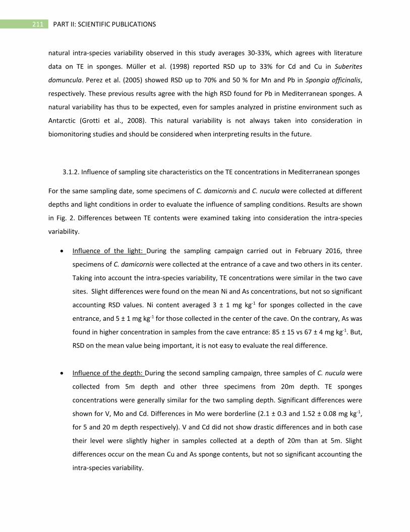
211 PART II: SCIENTIFIC PUBLICATIONS
natural intra-species variability observed in this study averages 30-33%, which agrees with literature
data on TE in sponges. Müller et al. (1998) reported RSD up to 33% for Cd and Cu in Suberites
domuncula. Perez et al. (2005) showed RSD up to 70% and 50 % for Mn and Pb in Spongia officinalis,
respectively. These previous results agree with the high RSD found for Pb in Mediterranean sponges. A
natural variability has thus to be expected, even for samples analyzed in pristine environment such as
Antarctic (Grotti et al., 2008). This natural variability is not always taken into consideration in
biomonitoring studies and should be considered when interpreting results in the future.
3.1.2. Influence of sampling site characteristics on the TE concentrations in Mediterranean sponges
For the same sampling date, some specimens of C. damicornis and C. nucula were collected at different
depths and light conditions in order to evaluate the influence of sampling conditions. Results are shown
in Fig. 2. Differences between TE contents were examined taking into consideration the intra-species
variability.
• Influence of the light: During the sampling campaign carried out in February 2016, three
specimens of C. damicornis were collected at the entrance of a cave and two others in its center.
Taking into account the intra-species variability, TE concentrations were similar in the two cave
sites. Slight differences were found on the mean Ni and As concentrations, but not so significant
accounting RSD values. Ni content averaged 3 ± 1 mg kg-1 for sponges collected in the cave
entrance, and 5 ± 1 mg kg-1 for those collected in the center of the cave. On the contrary, As was
found in higher concentration in samples from the cave entrance: 85 ± 15 vs 67 ± 4 mg kg-1. But,
RSD on the mean value being important, it is not easy to evaluate the real difference.
• Influence of the depth: During the second sampling campaign, three samples of C. nucula were
collected from 5m depth and other three specimens from 20m depth. TE sponges
concentrations were generally similar for the two sampling depth. Significant differences were
shown for V, Mo and Cd. Differences in Mo were borderline (2.1 ± 0.3 and 1.52 ± 0.08 mg kg-1,
for 5 and 20 m depth respectively). V and Cd did not show drastic differences and in both case
their level were slightly higher in samples collected at a depth of 20m than at 5m. Slight
differences occur on the mean Cu and As sponge contents, but not so significant accounting the
intra-species variability.
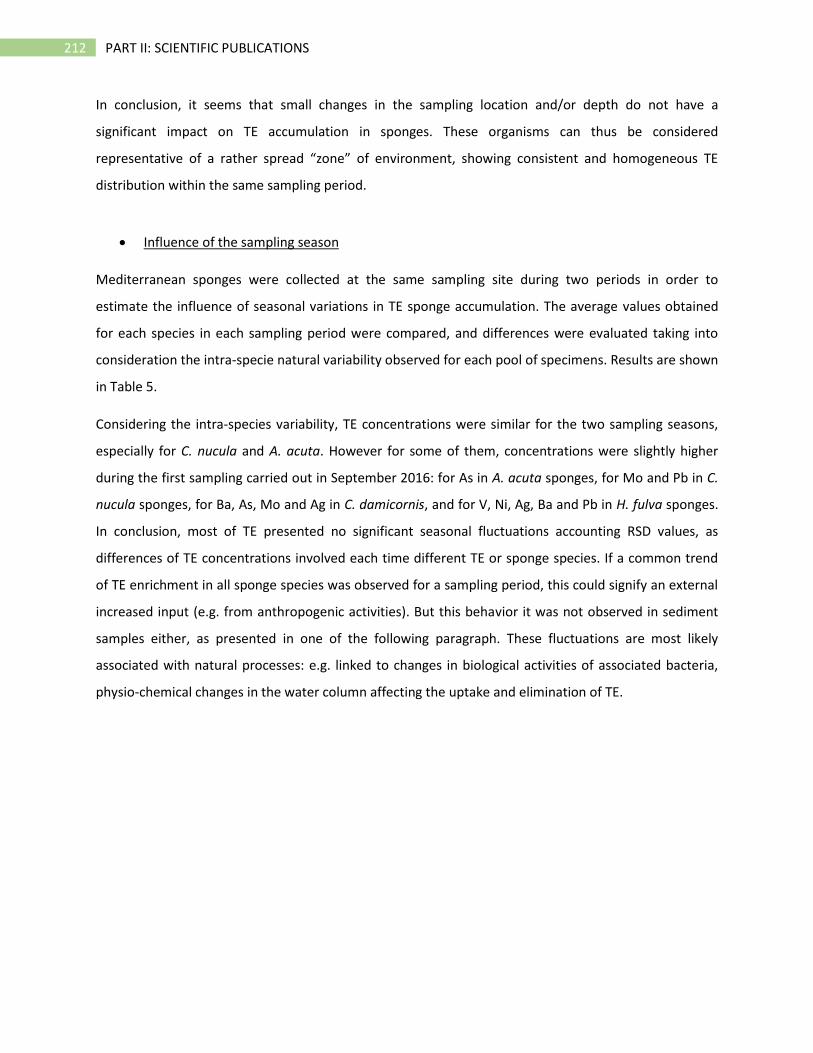
212 PART II: SCIENTIFIC PUBLICATIONS
In conclusion, it seems that small changes in the sampling location and/or depth do not have a
significant impact on TE accumulation in sponges. These organisms can thus be considered
representative of a rather spread “zone” of environment, showing consistent and homogeneous TE
distribution within the same sampling period.
• Influence of the sampling season
Mediterranean sponges were collected at the same sampling site during two periods in order to
estimate the influence of seasonal variations in TE sponge accumulation. The average values obtained
for each species in each sampling period were compared, and differences were evaluated taking into
consideration the intra-specie natural variability observed for each pool of specimens. Results are shown
in Table 5.
Considering the intra-species variability, TE concentrations were similar for the two sampling seasons,
especially for C. nucula and A. acuta. However for some of them, concentrations were slightly higher
during the first sampling carried out in September 2016: for As in A. acuta sponges, for Mo and Pb in C.
nucula sponges, for Ba, As, Mo and Ag in C. damicornis, and for V, Ni, Ag, Ba and Pb in H. fulva sponges.
In conclusion, most of TE presented no significant seasonal fluctuations accounting RSD values, as
differences of TE concentrations involved each time different TE or sponge species. If a common trend
of TE enrichment in all sponge species was observed for a sampling period, this could signify an external
increased input (e.g. from anthropogenic activities). But this behavior it was not observed in sediment
samples either, as presented in one of the following paragraph. These fluctuations are most likely
associated with natural processes: e.g. linked to changes in biological activities of associated bacteria,
physio-chemical changes in the water column affecting the uptake and elimination of TE.
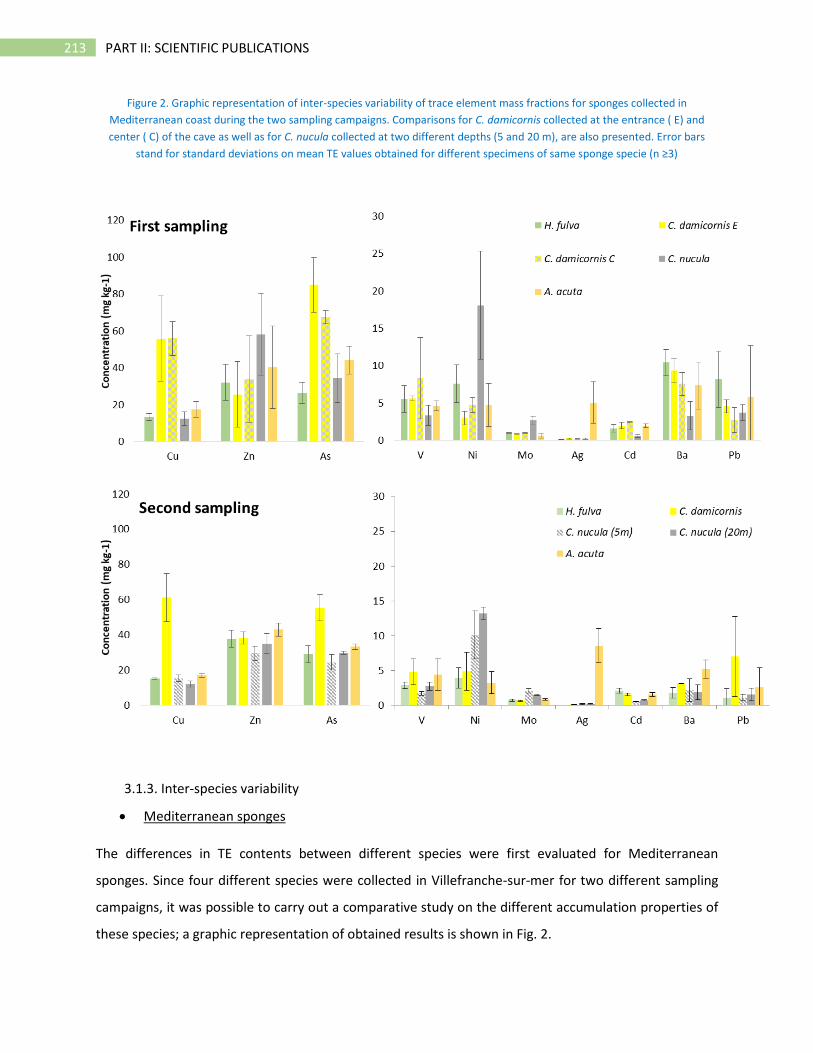
213 PART II: SCIENTIFIC PUBLICATIONS
Figure 2. Graphic representation of inter-species variability of trace element mass fractions for sponges collected in
Mediterranean coast during the two sampling campaigns. Comparisons for C. damicornis collected at the entrance ( E) and
center ( C) of the cave as well as for C. nucula collected at two different depths (5 and 20 m), are also presented. Error bars
stand for standard deviations on mean TE values obtained for different specimens of same sponge specie (n ≥3)
3.1.3. Inter-species variability
• Mediterranean sponges
The differences in TE contents between different species were first evaluated for Mediterranean
sponges. Since four different species were collected in Villefranche-sur-mer for two different sampling
campaigns, it was possible to carry out a comparative study on the different accumulation properties of
these species; a graphic representation of obtained results is shown in Fig. 2.
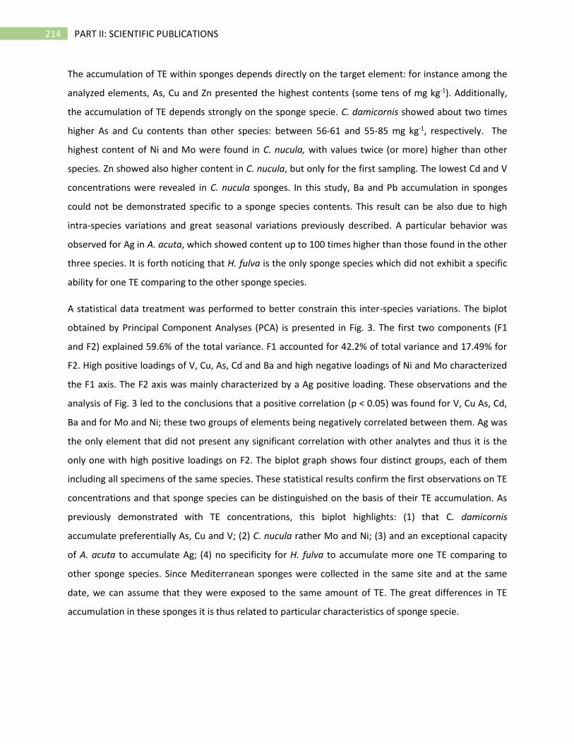
214 PART II: SCIENTIFIC PUBLICATIONS
The accumulation of TE within sponges depends directly on the target element: for instance among the
analyzed elements, As, Cu and Zn presented the highest contents (some tens of mg kg-1). Additionally,
the accumulation of TE depends strongly on the sponge specie. C. damicornis showed about two times
higher As and Cu contents than other species: between 56-61 and 55-85 mg kg-1, respectively. The
highest content of Ni and Mo were found in C. nucula, with values twice (or more) higher than other
species. Zn showed also higher content in C. nucula, but only for the first sampling. The lowest Cd and V
concentrations were revealed in C. nucula sponges. In this study, Ba and Pb accumulation in sponges
could not be demonstrated specific to a sponge species contents. This result can be also due to high
intra-species variations and great seasonal variations previously described. A particular behavior was
observed for Ag in A. acuta, which showed content up to 100 times higher than those found in the other
three species. It is forth noticing that H. fulva is the only sponge species which did not exhibit a specific
ability for one TE comparing to the other sponge species.
A statistical data treatment was performed to better constrain this inter-species variations. The biplot
obtained by Principal Component Analyses (PCA) is presented in Fig. 3. The first two components (F1
and F2) explained 59.6% of the total variance. F1 accounted for 42.2% of total variance and 17.49% for
F2. High positive loadings of V, Cu, As, Cd and Ba and high negative loadings of Ni and Mo characterized
the F1 axis. The F2 axis was mainly characterized by a Ag positive loading. These observations and the
analysis of Fig. 3 led to the conclusions that a positive correlation (p < 0.05) was found for V, Cu As, Cd,
Ba and for Mo and Ni; these two groups of elements being negatively correlated between them. Ag was
the only element that did not present any significant correlation with other analytes and thus it is the
only one with high positive loadings on F2. The biplot graph shows four distinct groups, each of them
including all specimens of the same species. These statistical results confirm the first observations on TE
concentrations and that sponge species can be distinguished on the basis of their TE accumulation. As
previously demonstrated with TE concentrations, this biplot highlights: (1) that C. damicornis
accumulate preferentially As, Cu and V; (2) C. nucula rather Mo and Ni; (3) and an exceptional capacity
of A. acuta to accumulate Ag; (4) no specificity for H. fulva to accumulate more one TE comparing to
other sponge species. Since Mediterranean sponges were collected in the same site and at the same
date, we can assume that they were exposed to the same amount of TE. The great differences in TE
accumulation in these sponges it is thus related to particular characteristics of sponge specie.
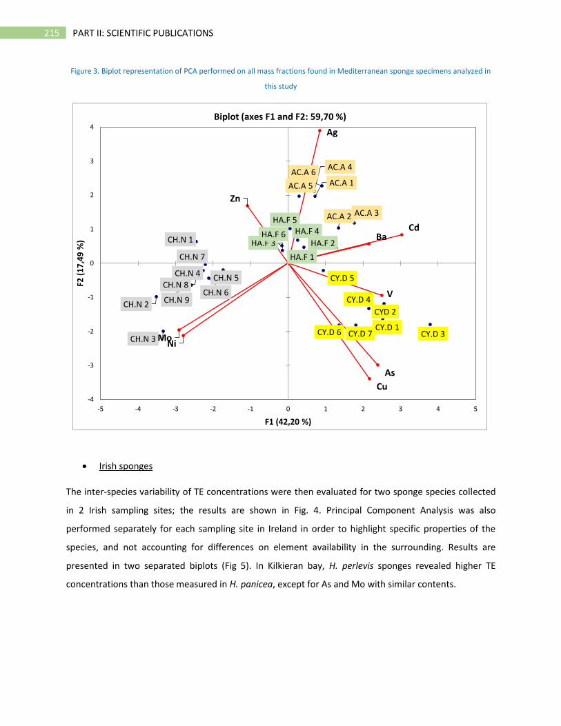
215 PART II: SCIENTIFIC PUBLICATIONS
Figure 3. Biplot representation of PCA performed on all mass fractions found in Mediterranean sponge specimens analyzed in
this study
• Irish sponges
The inter-species variability of TE concentrations were then evaluated for two sponge species collected
in 2 Irish sampling sites; the results are shown in Fig. 4. Principal Component Analysis was also
performed separately for each sampling site in Ireland in order to highlight specific properties of the
species, and not accounting for differences on element availability in the surrounding. Results are
presented in two separated biplots (Fig 5). In Kilkieran bay, H. perlevis sponges revealed higher TE
concentrations than those measured in H. panicea, except for As and Mo with similar contents.
HA.F 1
HA.F 2HA.F 3
HA.F 4HA.F 5
HA.F 6
CY.D 1
CYD 2
CY.D 3
CY.D 4
CY.D 5
CY.D 6 CY.D 7
AC.A 1
AC.A 2 AC.A 3
AC.A 4
AC.A 5
AC.A 6
CH.N 1
CH.N 2
CH.N 3
CH.N 4 CH.N 5
CH.N 6
CH.N 7
CH.N 8
CH.N 9V
Ni
Cu
Zn
As
Mo
Ag
CdBa
-4
-3
-2
-1
0
1
2
3
4
-5 -4 -3 -2 -1 0 1 2 3 4 5
F2 (
17
,49
%)
F1 (42,20 %)
Biplot (axes F1 and F2: 59,70 %)
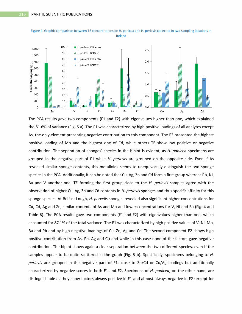
216 PART II: SCIENTIFIC PUBLICATIONS
Figure 4. Graphic comparison between TE concentrations on H. panicea and H. perlevis collected in two sampling locations in
Ireland
The PCA results gave two components (F1 and F2) with eigenvalues higher than one, which explained
the 81.6% of variance (Fig. 5 a). The F1 was characterized by high positive loadings of all analytes except
As, the only element presenting negative contribution to this component. The F2 presented the highest
positive loading of Mo and the highest one of Cd, while others TE show low positive or negative
contribution. The separation of sponges’ species in the biplot is evident, as H. panicea specimens are
grouped in the negative part of F1 while H. perlevis are grouped on the opposite side. Even if As
revealed similar sponge contents, this metalloids seems to unequivocally distinguish the two sponge
species in the PCA. Additionally, it can be noted that Cu, Ag, Zn and Cd form a first group whereas Pb, Ni,
Ba and V another one. TE forming the first group close to the H. perlevis samples agree with the
observation of higher Cu, Ag, Zn and Cd contents in H. perlevis sponges and thus specific affinity for this
sponge species. At Belfast Lough, H. pervelis sponges revealed also significant higher concentrations for
Cu, Cd, Ag and Zn, similar contents of As and Mo and lower concentrations for V, Ni and Ba (Fig. 4 and
Table 6). The PCA results gave two components (F1 and F2) with eigenvalues higher than one, which
accounted for 87.1% of the total variance. The F1 was characterized by high positive values of V, Ni, Mo,
Ba and Pb and by high negative loadings of Cu, Zn, Ag and Cd. The second component F2 shows high
positive contribution from As, Pb, Ag and Cu and while in this case none of the factors gave negative
contribution. The biplot shows again a clear separation between the two-different species, even if the
samples appear to be quite scattered in the graph (Fig. 5 b). Specifically, specimens belonging to H.
perlevis are grouped in the negative part of F1, close to Zn/Cd or Cu/Ag loadings but additionally
characterized by negative scores in both F1 and F2. Specimens of H. panicea, on the other hand, are
distinguishable as they show factors always positive in F1 and almost always negative in F2 (except for
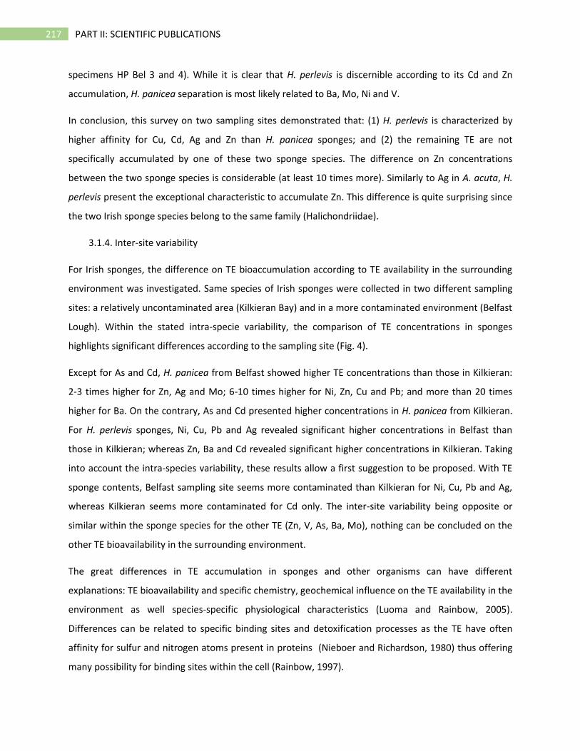
217 PART II: SCIENTIFIC PUBLICATIONS
specimens HP Bel 3 and 4). While it is clear that H. perlevis is discernible according to its Cd and Zn
accumulation, H. panicea separation is most likely related to Ba, Mo, Ni and V.
In conclusion, this survey on two sampling sites demonstrated that: (1) H. perlevis is characterized by
higher affinity for Cu, Cd, Ag and Zn than H. panicea sponges; and (2) the remaining TE are not
specifically accumulated by one of these two sponge species. The difference on Zn concentrations
between the two sponge species is considerable (at least 10 times more). Similarly to Ag in A. acuta, H.
perlevis present the exceptional characteristic to accumulate Zn. This difference is quite surprising since
the two Irish sponge species belong to the same family (Halichondriidae).
3.1.4. Inter-site variability
For Irish sponges, the difference on TE bioaccumulation according to TE availability in the surrounding
environment was investigated. Same species of Irish sponges were collected in two different sampling
sites: a relatively uncontaminated area (Kilkieran Bay) and in a more contaminated environment (Belfast
Lough). Within the stated intra-specie variability, the comparison of TE concentrations in sponges
highlights significant differences according to the sampling site (Fig. 4).
Except for As and Cd, H. panicea from Belfast showed higher TE concentrations than those in Kilkieran:
2-3 times higher for Zn, Ag and Mo; 6-10 times higher for Ni, Zn, Cu and Pb; and more than 20 times
higher for Ba. On the contrary, As and Cd presented higher concentrations in H. panicea from Kilkieran.
For H. perlevis sponges, Ni, Cu, Pb and Ag revealed significant higher concentrations in Belfast than
those in Kilkieran; whereas Zn, Ba and Cd revealed significant higher concentrations in Kilkieran. Taking
into account the intra-species variability, these results allow a first suggestion to be proposed. With TE
sponge contents, Belfast sampling site seems more contaminated than Kilkieran for Ni, Cu, Pb and Ag,
whereas Kilkieran seems more contaminated for Cd only. The inter-site variability being opposite or
similar within the sponge species for the other TE (Zn, V, As, Ba, Mo), nothing can be concluded on the
other TE bioavailability in the surrounding environment.
The great differences in TE accumulation in sponges and other organisms can have different
explanations: TE bioavailability and specific chemistry, geochemical influence on the TE availability in the
environment as well species-specific physiological characteristics (Luoma and Rainbow, 2005).
Differences can be related to specific binding sites and detoxification processes as the TE have often
affinity for sulfur and nitrogen atoms present in proteins (Nieboer and Richardson, 1980) thus offering
many possibility for binding sites within the cell (Rainbow, 1997).
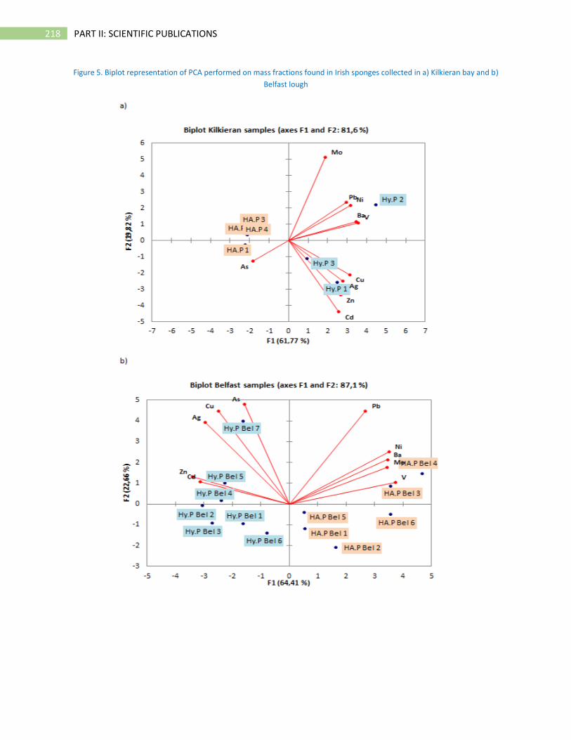
218 PART II: SCIENTIFIC PUBLICATIONS
Figure 5. Biplot representation of PCA performed on mass fractions found in Irish sponges collected in a) Kilkieran bay and b)
Belfast lough
219 PART II: SCIENTIFIC PUBLICATIONS
3.2. TE bioaccumulation in sponges
A common way to interpret the accumulation of TE in organisms’ tissue is the calculation of Bio-
Concentration Factors (BCF). These two parameters are useful in the evaluation of the sponge ability to
accumulate the analyte with respect to its availability in the environment. According to the classic
definition given by (Rand et al., 1995), the bioconcentration is defined as the uptake of a chemical by an
organism from the abiotic environment (non-living chemical and physical components of the
environment that affect the living organisms, for instance sunlight, soil, water and pollution). The
bioaccumulation, on the other hand, is defined as the uptake from abiotic and/or biotic (food)
environment, that is from all sources. Usually BCF for sponges are calculated as the ratio between the
chemical concentration measured in the organism and the one measured in local sediment (Negri et al.,
2006; Mayzel et al., 2014; Pan et al., 2011). A BCF value of 1 was set as threshold for all analytes, with
results equal or above 1 being considered indicative of bioconcentration. When TE concentration in
seawater is included in the study, the BAF are also calculated by dividing the TE sponge’s content by the
one found in seawater (Padovan et al., 2012; Venkateswara Rao et al., 2009; Batista et al., 2014).
3.2.1. Bio-Concentration Factors (BCF)
TEs concentration found in sediments from the three sampling sites are shown in Table 5. Overall, the
values are typical of uncontaminated areas, based on the principal environmental regulations (US EPA,
2006; Split and Delta, 2010). It has to be pointed out that the grain size distribution appeared to be quite
inhomogeneous, and the appearance was typical of sandy samples. These characteristics might explain
the relatively low values and the high standard deviation for some elements among replicates collected
in the same station (especially for Irish samples). Higher concentrations of V, Ni, Cu, Zn, and Ba were
observed for sediments collected in Irish sites than in the French one. Similar Ag contents were
measured in sediments regardless of the sampling site. Cd and Pb presented higher concentrations in
the French site. Finally, the French site and Kilkieran sampling site presented similar Mo and As contents
in sediments, higher than those from the Belfast site. Comparing the two Irish sites, sediments revealed
similar concentrations for most TE, except Ni, Cd, As and Mo. As and Mo revealed higher concentrations
in sediments from Kilkieran, whereas Ni and Cd exhibited higher concentrations in Belfast’s samples.
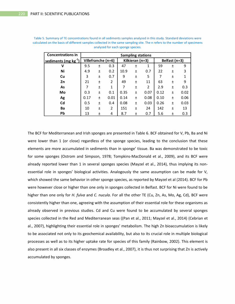
220 PART II: SCIENTIFIC PUBLICATIONS
Table 5. Summary of TE concentrations found in all sediments samples analyzed in this study. Standard deviations were
calculated on the basis of different samples collected in the same sampling site. The n refers to the number of specimens
analyzed for each sponge species.
The BCF for Mediterranean and Irish sponges are presented in Table 6. BCF obtained for V, Pb, Ba and Ni
were lower than 1 (or close) regardless of the sponge species, leading to the conclusion that these
elements are more accumulated in sediments than in sponge’ tissue. Ba was demonstrated to be toxic
for some sponges (Ostrom and Simpson, 1978; Tompkins-MacDonald et al., 2009), and its BCF were
already reported lower than 1 in several sponges species (Mayzel et al., 2014), thus implying its non-
essential role in sponges’ biological activities. Analogously the same assumption can be made for V,
which showed the same behavior in other sponge species, as reported by Mayzel et al (2014). BCF for Pb
were however close or higher than one only in sponges collected in Belfast. BCF for Ni were found to be
higher than one only for H. fulva and C. nucula. For all the other TE (Cu, Zn, As, Mo, Ag, Cd), BCF were
consistently higher than one, agreeing with the assumption of their essential role for these organisms as
already observed in previous studies. Cd and Cu were found to be accumulated by several sponges
species collected in the Red and Mediterranean seas ((Pan et al., 2011; Mayzel et al., 2014) (Cebrian et
al., 2007), highlighting their essential role in sponges’ metabolism. The high Zn bioaccumulation is likely
to be associated not only to its geochemical availability, but also to its crucial role in multiple biological
processes as well as to its higher uptake rate for species of this family (Rainbow, 2002). This element is
also present in all six classes of enzymes (Broadley et al., 2007), it is thus not surprising that Zn is actively
accumulated by sponges.
V 9.5 ± 0.3 47 ± 1 59 ± 9
Ni 4.9 ± 0.2 10.9 ± 0.7 22 ± 3
Cu 3 ± 0.7 9 ± 5 7 ± 1
Zn 21 ± 2 49 ± 11 63 ± 9
As 7 ± 1 7 ± 2 2.9 ± 0.3
Mo 0.3 ± 0.1 0.35 ± 0.07 0.12 ± 0.02
Ag 0.17 ± 0.01 0.14 ± 0.08 0.10 ± 0.06
Cd 0.5 ± 0.4 0.08 ± 0.03 0.26 ± 0.03
Ba 10 ± 2 151 ± 24 142 ± 13Pb 13 ± 4 8.7 ± 0.7 5.6 ± 0.3
Sampling stations
Villefranche (n=6) Kilkieran (n=3) Belfast (n=3)
Concentrations in
sediments (mg kg-1
)
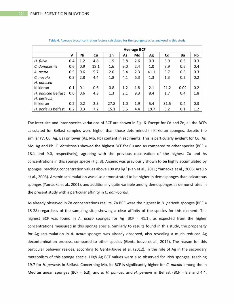
221 PART II: SCIENTIFIC PUBLICATIONS
Table 6. Average bioconcentration factors calculated for the sponge species analyzed in this study
Average BCF
V Ni Cu Zn As Mo Ag Cd Ba Pb
H. fulva 0.4 1.2 4.8 1.5 3.8 2.6 0.3 3.9 0.6 0.3
C. damicornis 0.6 0.9 18.1 1.6 9.0 2.4 1.0 3.9 0.6 0.4
A. acuta 0.5 0.6 5.7 2.0 5.4 2.3 41.1 3.7 0.6 0.3
C. nucula 0.3 2.8 4.4 1.8 4.1 6.3 1.3 1.3 0.2 0.2 H. panicea Kilkieran 0.1 0.1 0.6 0.8 1.2 1.8 2.1 21.2 0.02 0.2
H. panicea Belfast 0.6 0.6 4.3 1.3 2.1 9.3 8.4 1.7 0.4 1.8 H. perlevis Kilkieran 0.2 0.2 2.5 27.8 1.0 1.9 5.4 31.5 0.4 0.3
H. perlevis Belfast 0.2 0.3 7.2 15.1 3.5 4.4 19.7 3.2 0.1 1.2
The inter-site and inter-species variations of BCF are shown in Fig. 6. Except for Cd and Zn, all the BCFs
calculated for Belfast samples were higher than those determined in Kilkieran sponges, despite the
similar (V, Cu, Ag, Ba) or lower (As, Mo, Pb) content in sediments. This is particularly evident for Cu, As,
Mo, Ag and Pb. C. damicornis showed the highest BCF for Cu and As compared to other species (BCF =
18.1 and 9.0, respectively), agreeing with the previous observation of the highest Cu and As
concentrations in this sponge specie (Fig. 3). Arsenic was previously shown to be highly accumulated by
sponges, reaching concentration values above 100 mg kg-1 (Pan et al., 2011; Yamaoka et al., 2006; Araújo
et al., 2003). Arsenic accumulation was also demonstrated to be higher in demosponges than calcareous
sponges (Yamaoka et al., 2001), and additionally quite variable among demosponges as demonstrated in
the present study with a particular affinity in C. damicornis.
As already observed in Zn concentrations results, Zn BCF were the highest in H. perlevis sponges (BCF =
15-28) regardless of the sampling site, showing a clear affinity of the species for this element. The
highest BCF was found in A. acuta sponges for Ag (BCF = 41.1), as expected from the higher
concentrations measured in this sponge specie. Similarly to results found in this study, the propensity
for Ag accumulation in A. acuta sponges was already observed, also revealing a much reduced Ag
decontamination process, compared to other species (Genta-Jouve et al., 2012). The reason for this
particular behavior resides, according to Genta-Jouve et al. (2012), in the role of Ag in the secondary
metabolism of this sponge specie. High Ag BCF values were also observed for Irish sponges, reaching
19.7 for H. perlevis in Belfast. Concerning Mo, its BCF is significantly higher for C. nucula among the in
Mediterranean sponges (BCF = 6.3), and in H. panicea and H. perlevis in Belfast (BCF = 9.3 and 4.4,
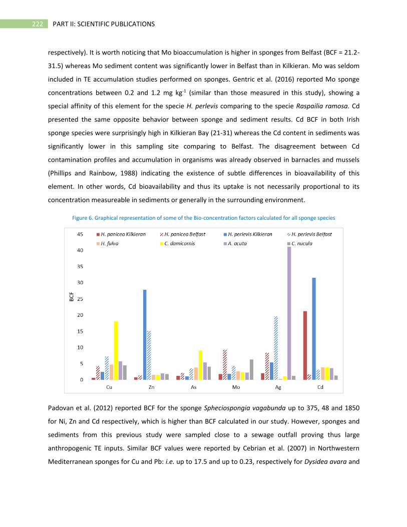
222 PART II: SCIENTIFIC PUBLICATIONS
respectively). It is worth noticing that Mo bioaccumulation is higher in sponges from Belfast (BCF = 21.2-
31.5) whereas Mo sediment content was significantly lower in Belfast than in Kilkieran. Mo was seldom
included in TE accumulation studies performed on sponges. Gentric et al. (2016) reported Mo sponge
concentrations between 0.2 and 1.2 mg kg-1 (similar than those measured in this study), showing a
special affinity of this element for the specie H. perlevis comparing to the specie Raspailia ramosa. Cd
presented the same opposite behavior between sponge and sediment results. Cd BCF in both Irish
sponge species were surprisingly high in Kilkieran Bay (21-31) whereas the Cd content in sediments was
significantly lower in this sampling site comparing to Belfast. The disagreement between Cd
contamination profiles and accumulation in organisms was already observed in barnacles and mussels
(Phillips and Rainbow, 1988) indicating the existence of subtle differences in bioavailability of this
element. In other words, Cd bioavailability and thus its uptake is not necessarily proportional to its
concentration measureable in sediments or generally in the surrounding environment.
Figure 6. Graphical representation of some of the Bio-concentration factors calculated for all sponge species
Padovan et al. (2012) reported BCF for the sponge Spheciospongia vagabunda up to 375, 48 and 1850
for Ni, Zn and Cd respectively, which is higher than BCF calculated in our study. However, sponges and
sediments from this previous study were sampled close to a sewage outfall proving thus large
anthropogenic TE inputs. Similar BCF values were reported by Cebrian et al. (2007) in Northwestern
Mediterranean sponges for Cu and Pb: i.e. up to 17.5 and up to 0.23, respectively for Dysidea avara and
223 PART II: SCIENTIFIC PUBLICATIONS
Chondrosia reniformis, values comparable with maximum BCF for Cu of 18 in C. damicornis), and similar
than usual BCF for Pb (except in Belfast). Pan et al. (2011) measured TE in different sponges and
sediments from Red Sea, showing maximum BCF of 74, 22, 3, 56 and 5 for Cd, Zn, Ag, Cu and As
respectively. These results were higher than those reported in the present study for Cd and Cu, lower for
Ag and overall comparable for Zn and As. Mayzel et al. (2014) analyzed 16 sponges species and reported
BCF consistently lower than 1 for Ba (except for one specie) and V; additionally the study shows BCF>1
for As, Cd and Zn . A significant As BCF of 477 was previously measured in only one sponge specie,
Theonella swinhoei, which was explained by the presence of a particular bacterium (Mayzel et al., 2014).
It is worth noticing that T. swinhoei is a slow growing and long lived specie so As concentration could be
linked to the age of the sponge and thus responsible for the elevated BCF. Negri et al. (2006) reported
also BCF comparable with the present study for Cu, Pb and Zn (not considering H. perlevis), but much
higher BCF were reported for As (up to 19) and Cd (up to 690). Results from our study as well as
literature data thus support the evidence that the variability in TE accumulation (and bioconcentration)
in sponges occurs at many scales including within and between species, within and between locations,
and related to the targeted TE.
3.2.2. Sponges as tool for biomonitoring studies
In order to better appreciate the extent of TE bio-concentration in sponges, the results are compared
with values determined in other organisms, potentially used as monitors of TE in coastal/marine
environment. The great advantages of sponges comparing to other “common” biomonitors like bivalves
is that they are simple organisms without complex organs and tissues. It is thus reasonable to think that
sponge tissues show low intra-individual variation in TE concentrations (de Mestre et al., 2012).
In a baseline study lead in the Pacific Ocean in Guam harbors, sponges were shown to accumulate
consistently higher amounts of Ag, As, Cd, Cu, Ni, Pb and Zn in comparison to seaweeds, but not in
comparison to oysters or other bivalves (Denton et al., 2006). Aly et al., (2013) found out that most of TE
in sponge specimens of H. oculata from Poole Harbour (UK) were accumulated much more efficiently
than in species of bivalve Cerastoderma edule, a common cockle. The latter showed TE concentrations
lower than sediment for almost all analytes while the sponge exhibited very high bioconcentration
factors. A study published by Perez et al., (2004) also shows that sponges from Mediterranean coast
concentrate more TE than mussels (Mytilus galloprovialis), exception made for Zn . According to the
target TE, concentrations measured in sponges were from 6 to 145 times higher than those measured in
mussels. Gentric et al. (2016) reported also higher concentration values of Mo, Ni, and Pb in H. perlevis
224 PART II: SCIENTIFIC PUBLICATIONS
and R. ramosa collected in Northern France, in comparison with Crassostrea gigas (oyster). On the other
hand, this oyster specie showed much higher content of Cu and Zn in comparison with all the sponges
species analyzed in the mentioned study. Cu and Zn concentrations in oysters were shown to reach
more than >10000 mg kg-1 (Weng and Wang, 2014; Birch et al., 2014). Other benthic organisms such as
macroalgae, gastropods and nemertean were shown to accumulate TE in extent more or less
comparable to sponges. (Majer et al., 2014) reported BCF values up to 2, 8, 2, 0.4, 1.6 and 5.6 for As, Cd,
Cu, Ni, Pb and Zn respectively, for different benthic organisms collected in Antarctica. Corals also shown
interesting TE accumulation properties, with BCF reaching 22 for Cd, 7 for Pb, 24 for Cu and 66 for Zn
(Esslemont, 2000).
In conclusion, elements such as Ag, As, Mo and Cd seem to have more affinity for sponges in comparison
to other organisms. Even if Cu and Zn are often better accumulated by other organisms in comparison to
sponges, these TE are also significantly bioconcentrated in sponges. This and previous studies
demonstrate that sponges are a good tool to biomonitor the TE level, especially since they are
widespread in coastal ecosystems.
3.3. Source of lead in sponges
In the Mediterranean site, as already mentioned, Pb showed an unusual high variability within the
species. The initial hypothesis is that the sponge samples were exposed to different Pb sources in
different extent, thus leading to very high differences even among specimens of the same species. In
order to evaluate this possibility, the analysis of Pb isotope ratios was performed in sponge and
sediment samples. Results are shown in Fig 7. Results clearly show that all samples have been exposed
to the same Pb source, as the isotopic compositions are practically undistinguishable. The absence of
multiple Pb sources is also confirmed by the lack of any linear trend in the presented graph (R2=0.2624)
(Ellam, 2010). Being the result of only one source, the isotopic composition found in our samples is likely
to be associated to a natural source. Results are indeed more radiogenic than those reported for
gasoline in France (Monna et al., 1995) or average French industrial Pb (Véron et al., 1999). Results are
closer to Pb isotopic composition measured in pre-industrial sediments discharged by the major French
rivers (206Pb/207Pb = 1.197-1.206, Elbazpoulichet et al., 1986) and to Miocene siltstone and Jurassic
limestone analyzed by Monna et al., (1995).
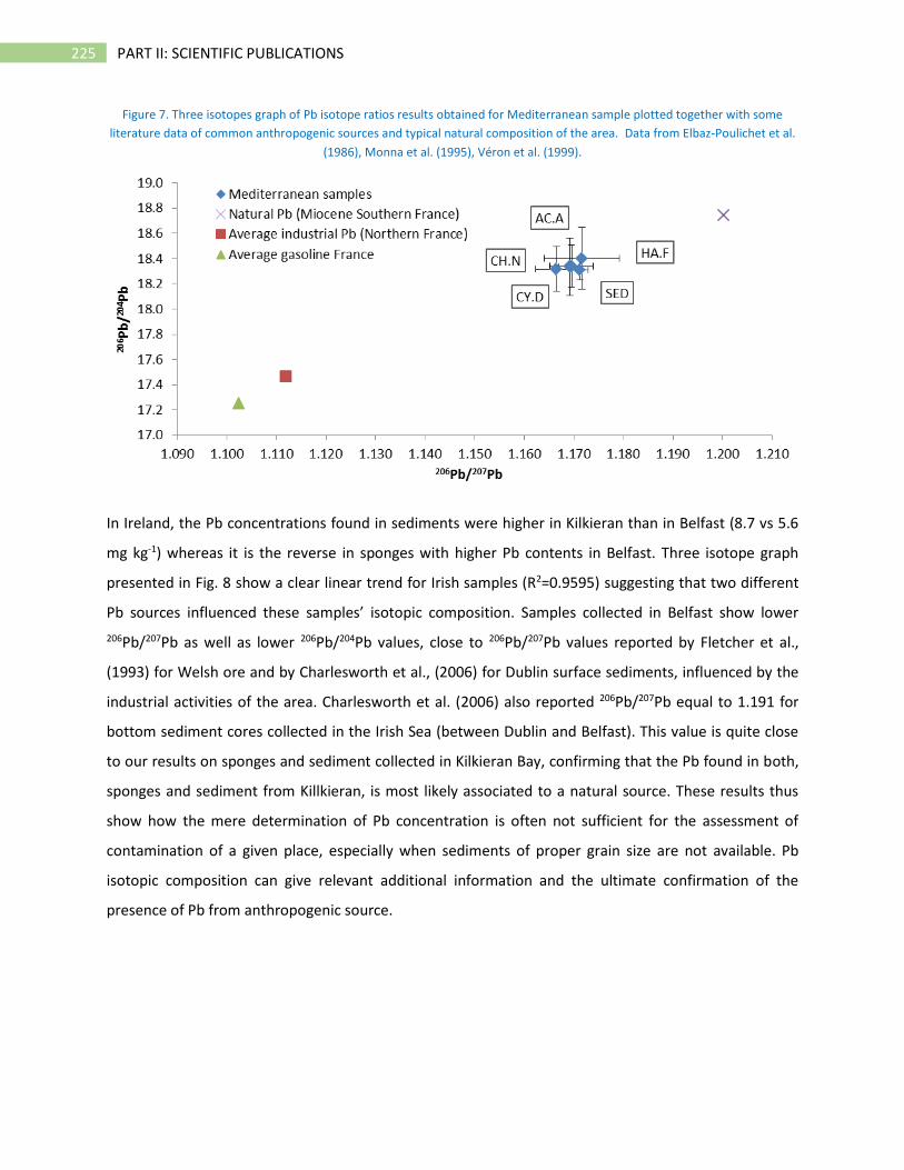
225 PART II: SCIENTIFIC PUBLICATIONS
Figure 7. Three isotopes graph of Pb isotope ratios results obtained for Mediterranean sample plotted together with some
literature data of common anthropogenic sources and typical natural composition of the area. Data from Elbaz-Poulichet et al.
(1986), Monna et al. (1995), Véron et al. (1999).
In Ireland, the Pb concentrations found in sediments were higher in Kilkieran than in Belfast (8.7 vs 5.6
mg kg-1) whereas it is the reverse in sponges with higher Pb contents in Belfast. Three isotope graph
presented in Fig. 8 show a clear linear trend for Irish samples (R2=0.9595) suggesting that two different
Pb sources influenced these samples’ isotopic composition. Samples collected in Belfast show lower
206Pb/207Pb as well as lower 206Pb/204Pb values, close to 206Pb/207Pb values reported by Fletcher et al.,
(1993) for Welsh ore and by Charlesworth et al., (2006) for Dublin surface sediments, influenced by the
industrial activities of the area. Charlesworth et al. (2006) also reported 206Pb/207Pb equal to 1.191 for
bottom sediment cores collected in the Irish Sea (between Dublin and Belfast). This value is quite close
to our results on sponges and sediment collected in Kilkieran Bay, confirming that the Pb found in both,
sponges and sediment from Killkieran, is most likely associated to a natural source. These results thus
show how the mere determination of Pb concentration is often not sufficient for the assessment of
contamination of a given place, especially when sediments of proper grain size are not available. Pb
isotopic composition can give relevant additional information and the ultimate confirmation of the
presence of Pb from anthropogenic source.
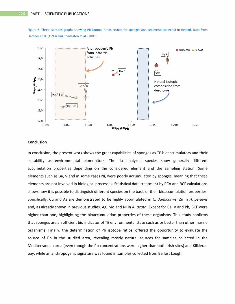
226 PART II: SCIENTIFIC PUBLICATIONS
Figure 8. Three isotopes graphs showing Pb isotope ratios results for sponges and sediments collected in Ireland. Data from
Fletcher et al. (1993) and Charleston et al. (2006).
Conclusion
In conclusion, the present work shows the great capabilities of sponges as TE bioaccumulators and their
suitability as environmental biomonitors. The six analyzed species show generally different
accumulation properties depending on the considered element and the sampling station. Some
elements such as Ba, V and in some cases Ni, were poorly accumulated by sponges, meaning that these
elements are not involved in biological processes. Statistical data treatment by PCA and BCF calculations
shows how it is possible to distinguish different species on the basis of their bioaccumulation properties.
Specifically, Cu and As are demonstrated to be highly accumulated in C. damicornis, Zn in H. perlevis
and, as already shown in previous studies, Ag, Mo and Ni in A. acuta. Except for Ba, V and Pb, BCF were
higher than one, highlighting the bioaccumulation properties of these organisms. This study confirms
that sponges are an efficient bio indicator of TE environmental state such as or better than other marine
organisms. Finally, the determination of Pb isotope ratios, offered the opportunity to evaluate the
source of Pb in the studied area, revealing mostly natural sources for samples collected in the
Mediterranean area (even though the Pb concentrations were higher than both Irish sites) and Kilkieran
bay, while an anthropogenic signature was found in samples collected from Belfast Lough.
227 PART II: SCIENTIFIC PUBLICATIONS
References (paper 6)
Abrahim, G.M.S., Parker, R.J., 2008. Assessment of heavy metal enrichment factors and the degree of contamination in marine sediments from Tamaki Estuary, Auckland, New Zealand. Environ. Monit. Assess. 136, 227–238. https://doi.org/10.1007/s10661-007-9678-2
Adams, F., Gijbels, R., Van Grieken, R., 1988. Inorganic Mass Spectrometry. John Wiley & Sons.
Aide, M.T., Aide, C., 2012. Rare Earth Elements: Their Importance in Understanding Soil Genesis. ISRN Soil Sci. 2012, 1–11. https://doi.org/10.5402/2012/783876
Alleman, L.Y., Hamelin, B., Véron, A.J., Miquel, J.-C., Heussner, S., 2000. Lead sources and transfer in the coastal Mediterranean: evidence from stable lead isotopes in marine particles. Deep Sea Res. Part II Top. Stud. Oceanogr. 47, 2257–2279. https://doi.org/10.1016/S0967-0645(00)00024-2
Aloupi, M., Angelidis, M.., 2001. Geochemistry of natural and anthropogenic metals in the coastal sediments of the island of Lesvos, Aegean Sea. Environ. Pollut. 113, 211–219. https://doi.org/10.1016/S0269-7491(00)00173-1
Aly, W., Williams, I.D., Hudson, M.D., 2013. Metal contamination in water, sediment and biota from a semi-enclosed coastal area. Environ. Monit. Assess. 185, 3879–3895. https://doi.org/10.1007/s10661-012-2837-0
AMPS Expert Group, 2005. Contributions of the Expert Group on Analysis and Monitoring of Priority Substances to the Water Framework Directive. EU Report EUR 21587.
Anderson, G.L., Williams, J., Hille, R., 1992. The purification and characterization of arsenite oxidase from Alcaligenes faecalis, a molybdenum-containing hydroxylase. J. Biol. Chem. 267, 23674–23682.
Andrewes, P., Demarini, D.M., Funasaka, K., Wallace, K., Lai, V.W.M., Sun, H., Cullen, W.R., Kitchin, K.T., 2004. Do arsenosugars pose a risk to human health? The comparative toxicities of a trivalent and pentavalent arsenosugar. Environ. Sci. Technol. 38, 4140–4148. https://doi.org/10.1021/es035440f
Angelidis, M.O., Radakovitch, O., Veron, A., Aloupi, M., Heussner, S., Price, B., 2011. Anthropogenic metal contamination and sapropel imprints in deep Mediterranean sediments. Mar. Pollut. Bull. 62, 1041–1052. https://doi.org/10.1016/j.marpolbul.2011.02.030
Anjum, K., Abbas, S.Q., Shah, S.A., Akhter, N., Batool, S., Hassan, S.S., 2016. Marine Sponges as a Drug Treasure. Biomol. Ther. 24, 347–362.
Araújo, M.F., Conceição, A., Barbosa, T., Lopes, M.T., Humanes, M., 2003. Elemental composition of marine sponges from the Berlengas Natural Park, western Portuguese coast. X-Ray Spectrom. 32, 428–433. https://doi.org/10.1002/xrs.660
Aresta, A., Marzano, C.N., Lopane, C., Corriero, G., Longo, C., Zambonin, C., Stabili, L., 2015. Analytical investigations on the lindane bioremediation capability of the demosponge Hymeniacidon perlevis. Mar. Pollut. Bull. 90, 143–149. https://doi.org/10.1016/j.marpolbul.2014.11.003
Armstrong-Altrin, J.S., Verma, S.P., Madhavaraju, J., Lee, Y. Il, Ramasamy, S., 2003. Geochemistry of Upper Miocene Kudankulam Limestones, Southern India. Int. Geol. Rev. 45, 16–26. https://doi.org/10.2747/0020-6814.45.1.16
Ashraf, A., Saion, E., Gharibshahi, E., Kamari, H.M., Yap, C.K., Hamzah, M.S., Elias, M.S., 2017.
228 PART II: SCIENTIFIC PUBLICATIONS
Distribution of Trace Elements in Core Marine Sediments of Coastal East Malaysia by Instrumental Neutron Activation Analysis. Appl. Radiat. Isot. 122, 96–105. https://doi.org/10.1016/j.apradiso.2017.01.006
Ashraf, A., Saion, E., Gharibshahi, E., Mohamed Kamari, H., Chee Kong, Y., Suhaimi Hamzah, M., Suhaimi Elias, M., 2016. Rare earth elements in core marine sediments of coastal East Malaysia by instrumental neutron activation analysis. Appl. Radiat. Isot. 107, 17–23. https://doi.org/10.1016/j.apradiso.2015.09.004
ATSDR, 2007. Toxicological Profile for Arsenic, U.S Public Health Service, Agency for Toxic Substances and Disease Registry. https://doi.org/http://dx.doi.org/10.1155/2013/286524
Ault, W.U., Senechal, R.G., Erlebach, W.E., 1970. Isotopic Composition as a Natural Tracer of Lead in the Environment: Discussions Follow. Environ. Sci. Technol. 4, 305–313. https://doi.org/10.1021/es60039a001
Azemard, S., Vassileva, E., 2015. Determination of methylmercury in marine biota samples with advanced mercury analyzer: Method validation. Food Chem. 176, 367–375. https://doi.org/10.1016/j.foodchem.2014.12.085
Azizur Rahman, M., Hasegawa, H., Peter Lim, R., 2012. Bioaccumulation, biotransformation and trophic transfer of arsenic in the aquatic food chain. Environ. Res. 116, 118–135. https://doi.org/10.1016/j.envres.2012.03.014
Bagul V. R., S.D.N., 2015. New perspective on heavy metal pollution of water. J. Chem. Pharm. Res. 7, 700–705.
Barats, A., Féraud, G., Potot, C., Philippinini, V., Travi, Y., Durrieu, G., Dubar, M., Simler, R., 2014. Naturally dissolved arsenic concentrations in the Alpine/Mediterranean Var River watershed (France). Sci. Total Environ. 473–474, 422–436. https://doi.org/10.1016/J.SCITOTENV.2013.12.007
Bargagli, R., Nelli, L., Ancora, S., Focardi, S., 1996. Elevated cadmium accumulation in marine organisms from Terra Nova Bay (Antarctica). Polar Biol. 16, 513–520. https://doi.org/10.1007/BF02329071
Barwick, V.J., Ellison, S.L.R., 1999. Measurement uncertainty: Approaches to the evaluation of uncertainties associated with recovery†. Analyst 124, 981–990. https://doi.org/10.1039/a901845j
Batista, D., Muricy, G., Rocha, R.C., Miekeley, N.F., 2014. Marine sponges with contrasting life histories can be complementary biomonitors of heavy metal pollution in coastal ecosystems. Environ. Sci. Pollut. Res. 21, 5785–5794. https://doi.org/10.1007/s11356-014-2530-7
Baudrimont, M., Schäfer, J., Marie, V., Maury-Brachet, R., Bossy, C., Boudou, A., Blanc, G., 2005. Geochemical survey and metal bioaccumulation of three bivalve species (Crassostrea gigas, Cerastoderma edule and Ruditapes philippinarum) in the Nord Médoc salt marshes (Gironde estuary, France). Sci. Total Environ. https://doi.org/10.1016/j.scitotenv.2004.07.009
Beauchemin, D., 2008. Inductively coupled plasma mass spectrometry. Anal. Chem. 80, 4455–4486.
Bednar, A.J., Garbarino, J.R., Burkhardt, M.R., Ranville, J.F., Wildeman, T.R., 2004. Field and laboratory arsenic speciation methods and their application to natural-water analysis. Water Res. 38, 355–364. https://doi.org/10.1016/j.watres.2003.09.034
Beeson, R., 1984. The use of the fine fractions of stream sediments in geochemical exploration in arid
229 PART II: SCIENTIFIC PUBLICATIONS
and semi-arid terrains. J. Geochemical Explor. 22, 119–132. https://doi.org/10.1016/0375-6742(84)90009-8
Belarra, M.A., Resano, M., Vanhaecke, F., Moens, L., 2002. Direct solid sampling with electrothermal vaporization/atomization: What for and how? TrAC - Trends Anal. Chem. 21, 828–839. https://doi.org/10.1016/S0165-9936(02)01206-2
Bell, J.J., 2008. The functional roles of marine sponges. Estuar. Coast. Shelf Sci. 79, 341–353. https://doi.org/10.1016/j.ecss.2008.05.002
Bennett, W.W., Teasdale, P.R., Panther, J.G., Welsh, D.T., Zhao, H., Jolley, D.F., 2012. Investigating arsenic speciation and mobilization in sediments with DGT and DET: A mesocosm evaluation of oxic-anoxic transitions. Environ. Sci. Technol. 46, 3981–3989. https://doi.org/10.1021/es204484k
Bentley, R., Chasteen, T.G., 2002. Microbial Methylation of Metalloids: Arsenic, Antimony, and Bismuth. Microbiol. Mol. Biol. Rev. 66, 250–271.
Bermejo-Barrera, P., Barciela-Alonso, M.C., Moreda-Piñeiro, J., González-Sixto, C., Bermejo-Barrera, a., 1996. Determination of trace metals (As, Cd, Hg, Pb and Sn) in marine sediment slurry samples by electrothermal atomic absorption spectrometry using palladium as a chemical modifier. Spectrochim. Acta Part B At. Spectrosc. 51, 1235–1244. https://doi.org/10.1016/0584-8547(96)01487-5
Bermudez-Lugo, O., 2014. 2012 Minerals Yearbook, Usgs- 2012 Minerals Yearbook.
Berthet, B., Mouneyrac, C., Pérez, T., Amiard-Triquet, C., 2005. Metallothionein concentration in sponges (Spongia officinalis) as a biomarker of metal contamination. Comp. Biochem. Physiol. - C Toxicol. Pharmacol. 141, 306–313. https://doi.org/10.1016/j.cca.2005.07.008
Bhuiyan, M.A.H., Parvez, L., Islam, M.A., Dampare, S.B., Suzuki, S., 2010. Heavy metal pollution of coal mine-affected agricultural soils in the northern part of Bangladesh. J. Hazard. Mater. 173, 384–392. https://doi.org/10.1016/j.jhazmat.2009.08.085
Birch, G.F., Melwani, A., Lee, J.H., Apostolatos, C., 2014. The discrepancy in concentration of metals (Cu, Pb and Zn) in oyster tissue (Saccostrea glomerata) and ambient bottom sediment (Sydney estuary, Australia). Mar. Pollut. Bull. 80, 263–274. https://doi.org/10.1016/j.marpolbul.2013.12.005
Bocher, P., Caurant, F., Miramand, P., Cherel, Y., Bustamante, P., 2003. Influence of the diet on the bioaccumulation of heavy metals in zooplankton-eating petrels at Kerguelen archipelago, Southern Indian Ocean. Polar Biol. 26, 759–767. https://doi.org/10.1007/s00300-003-0552-6
Bohari, Y., Astruc, A., Astruc, M., Cloud, J., 2001. Improvements of hydride generation for the speciation of arsenic in natural freshwater samples by HPLC-HG-AFS. J. Anal. At. Spectrom. 16, 774–778. https://doi.org/10.1039/B101591P
Bollhöfer, A., Rosman, K.J.., 2000. Isotopic source signatures for atmospheric lead: the Southern Hemisphere. Geochim. Cosmochim. Acta 64, 3251–3262. https://doi.org/10.1016/S0016-7037(00)00436-1
Bollhöfer, A., Rosman, K.J.R., 2001. Isotopic source signatures for atmospheric lead: The Northern Hemisphere. Geochim. Cosmochim. Acta 65, 1727–1740. https://doi.org/10.1016/S0016-7037(00)00630-X
230 PART II: SCIENTIFIC PUBLICATIONS
Bossy, A., 2010. Origines de l’arsenic dans les eaux, sols et sédiments du district aurifère de St-Yrieix-la-Perche (Limousin, France) : contribution du lessivage des phases porteuses d’arsenic. Université de Limoges.
Bowen, H.J.M., 1966. The Uptake and Excretion of Elements by Organisms, in: Trace Elements in Biochemistry. Academic Press London, pp. 85–101.
Bremner, J.M., Willis, J.P., 1993. Mineralogy and geochemistry of the clay fraction of sediments from the Namibian continental margin and the adjacent hinterland. Mar. Geol. 115, 85–116. https://doi.org/10.1016/0025-3227(93)90076-8
Briant, N., Chouvelon, T., Martinez, L., Brach-Papa, C., Chiffoleau, J.F., Savoye, N., Sonke, J., Knoery, J., 2017. Spatial and temporal distribution of mercury and methylmercury in bivalves from the French coastline. Mar. Pollut. Bull. 114, 1096–1102. https://doi.org/10.1016/j.marpolbul.2016.10.018
Briefing, 1980. Namibia in the frontline: the political economy of decolonisation in South Africa’s colony. Rev. Afr. Polit. Econ. https://doi.org/10.1080/03056248008703415
Broadley, M.R., White, P.J., Hammond, J.P., Zelko, I., Lux, A., 2007. Zinc in plants. New Phytol. 173, 677–702. https://doi.org/10.1111/j.1469-8137.2007.01996.x
Brongersma-Sanders, M., Stephan, K.M., Kwee, T.., De Bruin, M., 1980. DISTRIBUTION OF MINOR ELEMENTS IN CORES FROM THE SOUTH- WEST AFRICA SHELF WITH NOTES ON PLANKTON AND FISH MORTALITY Along the coast of Southwest Africa a belt of olive-green diatomaceous muds is f o u n d between 19 ° S and 25 ° S , bordered on the wester. Mar. Geol. 37, 91–132.
Brown, J.L., Kitchin, K.T., George, M., 1997. Dimethylarsinic acid treatment alters six different rat biochemical parameters: Relevance to arsenic carcinogenesis. Teratog. Carcinog. Mutagen. 17, 71–84. https://doi.org/10.1002/(SICI)1520-6866(1997)17:2<71::AID-TCM3>3.0.CO;2-B
Brown, J.S., 1962. Ore leads and isotopes. Econ. Geol. 57, 673–720. https://doi.org/10.2113/gsecongeo.57.5.673
Brown, R.J.C., Milton, M.J.T., 2005. Analytical techniques for trace element analysis: An overview. TrAC - Trends Anal. Chem. 24, 266–274. https://doi.org/10.1016/j.trac.2004.11.010
Bruland, K.W., Bertine, K., Koide, M., Goldberg, E.D., 1974. History of metal pollution in southern California coastal zone. Environ. Sci. Technol. 8, 425–432. https://doi.org/10.1021/es60090a010
Bruland, K.W., Lohan, M.C., 2003. Controls of trace metals in seawater, in: Treatise on Geochemistry. Elsevier Ltd, pp. 23–47.
Bryan, G.W., Langston, W.J., 1992. Bioavailability, accumulation and effects of heavy metals in sediments with special reference to United Kingdom estuaries: a review. Environ. Pollut. 76, 89–131. https://doi.org/10.1016/0269-7491(92)90099-V
Bu, H., Song, X., Guo, F., 2017. Dissolved trace elements in a nitrogen-polluted river near to the Liaodong Bay in Northeast China. Mar. Pollut. Bull. 114, 547–554. https://doi.org/10.1016/j.marpolbul.2016.09.003
Cabon, J.Y., Cabon, N., 2000. Speciation of major arsenic species in seawater by flow injection hydride generation atomic absorption spectrometry. Fresenius. J. Anal. Chem. 368, 484–9. https://doi.org/10.1007/s002160000526
231 PART II: SCIENTIFIC PUBLICATIONS
Cabrita, M.T., Padeiro, A., Amaro, E., dos Santos, M.C., Leppe, M., Verkulich, S., Hughes, K.A., Peter, H.-U., Canário, J., 2017. Evaluating trace element bioavailability and potential transfer into marine food chains using immobilised diatom model species Phaeodactylum tricornutum , on King George Island, Antarctica. Mar. Pollut. Bull. 121, 192–200. https://doi.org/10.1016/j.marpolbul.2017.05.059
Caccia, V.G., Millero, F.J., Palanques, A., 2003. The distribution of trace metals in Florida Bay sediments. Mar. Pollut. Bull. 46, 1420–1433. https://doi.org/10.1016/S0025-326X(03)00288-1
Calvert, S.E., Price, N.B., 1970. Minor Metal Contents of Recent Organic-rich Sediments off South West Africa. Nature 227, 593–595.
Cantillo, A.Y., 1998. Comparison of results of Mussel Watch Programs of the United States and France with Worldwide Mussel Watch Studies. Mar. Pollut. Bull. 36, 712–717. https://doi.org/10.1016/S0025-326X(98)00049-6
Carere, M., Dulio, V., Hanke, G., Polesello, S., 2012. Guidance for sediment and biota monitoring under the Common Implementation Strategy for the Water Framework Directive. TrAC - Trends Anal. Chem. 36, 15–24. https://doi.org/10.1016/j.trac.2012.03.005
Carpenè, E., Andreani, G., Isani, G., 2017. Trace elements in unconventional animals: A 40-year experience. J. Trace Elem. Med. Biol. 43, 169–179. https://doi.org/10.1016/j.jtemb.2017.02.003
Caumette, G., Koch, I., Reimer, K.J., 2012. Arsenobetaine formation in plankton: a review of studies at the base of the aquatic food chain. J. Environ. Monit. 14, 2841. https://doi.org/10.1039/c2em30572k
Cebrian, E., Martí, R., Uriz, J.M., Turon, X., 2003. Sublethal effects of contamination on the Mediterranean sponge Crambe crambe: Metal accumulation and biological responses. Mar. Pollut. Bull. 46, 1273–1284. https://doi.org/10.1016/S0025-326X(03)00190-5
Cebrian, E., Uriz, M.-J., Turon, X., 2007. Sponges as biomonitors of heavy metals in spatial and temporal surveys in northwestern mediterranean: multispecies comparison. Environ. Toxicol. Chem. 26, 2430–2439. https://doi.org/10.1897/07-292.1
Cebrian, E., Uriz, M.J., 2007. Contrasting effects of heavy metals on sponge cell behavior. Arch. Environ. Contam. Toxicol. 53, 552–558. https://doi.org/10.1007/s00244-006-0257-2
Chai, Z.F., Zhang, Z.Y., Feng, W.Y., Chen, C.Y., Xu, D.D., Hou, X.L., 2004. Study of chemical speciation of trace elements by molecular activation analysis and other nuclear techniques. J. Anal. At. Spectrom. 19, 26–33. https://doi.org/10.1039/B307337H
Charlesworth, M.E., Chenery, S., Mellor, A., Service, M., 2006. Isotopic composition and concentration of Pb in suspended particulate matter of the Irish Sea reveals distribution and sources. Mar. Pollut. Bull. 52, 81–88. https://doi.org/10.1016/j.marpolbul.2005.08.009
Chen, C.Y., Darren, M.., Williams, J.J., Fisher, N.S., 2016. Metal Bioaccumulation by Estuarine Food Webs in New England, USA. J. Mar. Sci. Engeneer 4, 41. https://doi.org/10.1016/j.cell.2016.05.007.Mapping
Chen, C.Y., Stemberger, R.S., Klaue, B., Blum, J.D., Pickhardt, P.C., Folt, C.L., 2000. Accumulation of heavy metals in food web components across a gradient of lakes. Limnol. Oceanogr. 45, 1525–1536. https://doi.org/10.4319/lo.2000.45.7.1525

232 PART II: SCIENTIFIC PUBLICATIONS
Chen, L., Liu, M., Fan, R., Ma, S., Xu, Z., Ren, M., He, Q., 2013. Mercury speciation and emission from municipal solid waste incinerators in the Pearl River Delta, South China. Sci. Total Environ. 447, 396–402. https://doi.org/10.1016/j.scitotenv.2013.01.018
Chester, R., Murphy, K.J.T., Lin, F.J., Berry, A.S., Bradshaw, G.A., Corcoran, P.A., 1993. Factors controlling the solubilities of trace metals from non-remote aerosols deposited to the sea surface by the “dry” deposition mode. Mar. Chem. 42, 107–126. https://doi.org/10.1016/0304-4203(93)90241-F
Ciardullo, S., Aureli, F., Raggi, A., Cubadda, F., 2010. Arsenic speciation in freshwater fish: Focus on extraction and mass balance. Talanta 81, 213–221. https://doi.org/10.1016/j.talanta.2009.11.060
Cidu, R., Frau, F., 2009. Distribution of trace elements in filtered and non filtered aqueous fractions: Insights from rivers and streams of Sardinia (Italy). Appl. Geochemistry 24, 611–623. https://doi.org/10.1016/j.apgeochem.2008.12.013
Clark, H., 1968. On the Spongiae ciliatae as infusoria flagellata, or observations on the structure, animality and relationship of Leucosolenia botryoides, Bowerbank. Ann. Mag. Nat. Hist. 4, 133–142.
Clowes, L.A., Francesconi, K.A., 2004. Uptake and elimination of arsenobetaine by the mussel Mytilus edulis is related to salinity. Comp. Biochem. Physiol. - C Toxicol. Pharmacol. 137, 35–42. https://doi.org/10.1016/j.cca.2003.11.003
Coulibaly, M., Bamba, D., Yao, N.A., Zoro, E.G., El Rhazi, M., 2016. Some aspects of speciation and reactivity of mercury in various matrices. Comptes Rendus Chim. 19, 832–840. https://doi.org/10.1016/j.crci.2016.02.005
Covelli, S., Fontolan, G., 1997. Application of a normalization procedure in determining regional geochemical baselines. Environ. Geol. 30, 34–45. https://doi.org/10.1007/s002540050130
Crompton, T.R., Crompton, T.R., 1989. Chapter 8 – Organometallic compounds, in: Analysis of Seawater. pp. 336–359. https://doi.org/10.1016/B978-0-407-01610-1.50011-4
Cullen, W.R., Reimer, K.J., 1989. Arsenic speciation in the environment. Chem. Rev. 89, 713–764. https://doi.org/10.1021/cr00094a002
Dahms, S., van der Bank, F.H., Greenfield, R., 2014. A baseline study of metal contamination along the Namibian coastline for Perna perna and Choromytilus meridionalis. Mar. Pollut. Bull. 85, 297–305. https://doi.org/10.1016/j.marpolbul.2014.05.037
Damiano, S., Papetti, P., Menesatti, P., 2011. Accumulation of heavy metals to assess the health status of swordfish in a comparative analysis of Mediterranean and Atlantic areas. Mar. Pollut. Bull. 62, 1920–1925. https://doi.org/10.1016/j.marpolbul.2011.04.028
De Gregori H., I., Pinochet C., H., Arancibia J., M., Vidal B., A., 1996. Grain Size Effect on Trace Metals Distribution in Sediments from Two Coastal Areas of Chile. Bull. Environ. Contam. Toxicol. 57, 163–170. https://doi.org/10.1007/s001289900170
de Mestre, C., Maher, W., Roberts, D., Broad, A., Krikowa, F., Davis, A.R., 2012. Sponges as sentinels: Patterns of spatial and intra-individual variation in trace metal concentration. Mar. Pollut. Bull. 64, 80–89. https://doi.org/10.1016/j.marpolbul.2011.10.020
Debord, J., Pourmand, A., Jantzi, S., Panicker, S., Almirall, J., 2017. Profiling of Heroin and Assignment of

233 PART II: SCIENTIFIC PUBLICATIONS
Provenance by 87 Sr/ 86 Sr Isotope Ratio Analysis. Inorganica Chim. Acta. https://doi.org/10.1016/j.ica.2017.07.049
Delnomdedieu, M., Basti, M.M., Otvos, J.D., Thomas, D.J., 1994. Reduction and binding of arsenate and dimethylarsinate by glutathione: a magnetic resonance study. Chem. Biol. Interact. 90, 139–155. https://doi.org/10.1016/0009-2797(94)90099-X
Denton, G.R.W., Concepcion, L.P., Wood, H.R., Morrison, R.J., 2006. Trace metals in marine organisms from four harbours in Guam. Mar. Pollut. Bull. 52, 1784–1804. https://doi.org/10.1016/j.marpolbul.2006.09.010
Diaz, M.C., Rutzler, K., 2001. Sponges: an essential component of Caribbean coral reefs. Bull. Mar. Sci. 69, 535–546.
Drivelos, S.A., Georgiou, C.A., 2012. Multi-element and multi-isotope-ratio analysis to determine the geographical origin of foods in the European Union. TrAC Trends Anal. Chem. 40, 38–51. https://doi.org/10.1016/j.trac.2012.08.003
Dudás, F.Ö., LeBlanc, S.A., Carter, S.W., Bowring, S.A., 2016. Pb and Sr concentrations and isotopic compositions in prehistoric North American teeth: A methodological study. Chem. Geol. 429, 21–32. https://doi.org/10.1016/j.chemgeo.2016.03.003
Duncan, E.G., Maher, W.A., Foster, S.D., 2015. Contribution of arsenic species in unicellular algae to the cycling of arsenic in marine ecosystems. Environ. Sci. Technol. 49, 33–50. https://doi.org/10.1021/es504074z
Edmonds, J.S., Francesconi, K.A., Stick, R. V, 1993. Arsenic compounds from marine organisms. Nat. Prod. Rep. 10, 421–428.
Edmonds, J.S., Shibata, Y., Francesconi, K. a, Rippingale, R.J., Morita, M., 1997. Arsenic transformations in short marine food chains studied by HPLC-ICP MS. Appl. Organomet. Chem. 11, 281–287. https://doi.org/10.1002/(sici)1099-0739(199704)11:4<281::aid-aoc581>3.3.co;2-j
Elbaz-Poulichet, F., Holliger, P., Martin, J.M., Petit, D., 1986. Stable lead isotopes ratios in major french rivers and estuaries. Sci. Total Environ. 54, 61–76. https://doi.org/10.1016/0048-9697(86)90256-1
Elderfield, H., 2003. Introduction to Volume 6, in: Turekian, K.K., Holland, H.D. (Eds.), Treatise on Geochemistry. Elsevier Ltd, pp. 15–27.
Ellam, R.M., 2010. The graphical presentation of lead isotope data for environmental source apportionment. Sci. Total Environ. 408, 3490–3492. https://doi.org/10.1016/j.scitotenv.2010.03.037
Ellwood, M.J., Maher, W.A., 2003. Measurement of arsenic species in marine sediments by high-performance liquid chromatography-inductively coupled plasma mass spectrometry. Anal. Chim. Acta 477, 279–291. https://doi.org/10.1016/s0003-2670(02)01414-9
Esslemont, G., 2000. Heavy metals in seawater, marine sediments and corals from the Townsville section, Great Barrier Reef Marine Park, Queensland. Mar. Chem. 71, 215–231. https://doi.org/10.1016/S0304-4203(00)00050-5
Fang, T.-H., Hsiao, S.-H., Nan, F.-H., 2014. Nineteen trace elements in marine copepods collected from the coastal waters off northeastern Taiwan. Cont. Shelf Res. 91, 70–81.

234 PART II: SCIENTIFIC PUBLICATIONS
https://doi.org/10.1016/j.csr.2014.09.003
FAO, 2007. Fishery Country Profile- The Republic of Namibia [WWW Document]. URL http://www.fao.org/fi/oldsite/FCP/en/NAM/profile.htm
FLETCHER, C.J.N., SWAINBANK, I.G., COLMAN, T.B., 1993. Metallogenic evolution in Wales: constraints from lead isotope modelling. J. Geol. Soc. London. 150, 77–82. https://doi.org/10.1144/gsjgs.150.1.0076
Forstner, U., 1982. Chemical forms of metal enrichment in recent sediments, in: Amstutz, G. (Ed.), Ore Genesis. Springer-Verlag New York, pp. 269–284.
Förstner, U., Ahlf, W., Calmano, W., 1989. Studies on the transfer of heavy metals between sedimentary phases with a multi-chamber device: Combined effects of salinity and redox variation. Mar. Chem. 28, 145–158. https://doi.org/10.1016/0304-4203(89)90192-8
Forstner, U., Wittmann, G., 1981. Metal pollution in the aquatic environment, 2nd revise. ed. Springer-Verlag New York.
Foster, S., Maher, W., 2016. Arsenobetaine and thio-arsenic species in marine macroalgae and herbivorous animals: Accumulated through trophic transfer or produced in situ? J. Environ. Sci. 49, 131–139. https://doi.org/10.1016/j.jes.2016.06.003
Francesconi, K.A., Sperling, M., 2005. Speciation analysis with HPLC-mass spectrometry: time to take stock. Analyst 130, 998. https://doi.org/10.1039/b504485p
Francesconi, K. a., 2010. Arsenic species in seafood: Origin and human health implications. Pure Appl. Chem. 82, 373–381. https://doi.org/10.1351/PAC-CON-09-07-01
Fütterer, D.K., Cojan, I., Renard, M., 2006. The solid phase of marine sediments, in: Marine Geochemistry. pp. 1–25.
Gadde, R.R., Laitinen, H.A., 1974. Studies of Heavy Metal Adsorption by Hydrous Iron and Manganese Oxides. Anal. Chem. 46, 2022–2026. https://doi.org/10.1021/ac60349a004
Galy, A., Pomies, C., Day, J.A., Pokrovsky, O.S., Schott, J., 2003. High precision measurement of germanium isotope ratio variations by multiple collector-inductively coupled plasma mass spectrometry. J. Anal. At. Spectrom. 18, 115–119. https://doi.org/10.1039/B210233A
Gazave, E., Carteron, S., Chenuil, A., Richelle-Maurer, E., Boury-Esnault, N., Borchiellini, C., 2010. Polyphyly of the genus Axinella and of the family Axinellidae (Porifera: Demospongiaep). Mol. Phylogenet. Evol. 57, 35–47. https://doi.org/10.1016/j.ympev.2010.05.028
Genta-Jouve, G., Cachet, N., Oberhänsli, F., Noyer, C., Teyssié, J.L., Thomas, O.P., Lacoue-Labarthe, T., 2012. Comparative bioaccumulation kinetics of trace elements in Mediterranean marine sponges. Chemosphere 89, 340–349. https://doi.org/10.1016/j.chemosphere.2012.04.052
Gentric, C., Rehel, K., Dufour, A., Sauleau, P., 2016. Bioaccumulation of metallic trace elements and organic pollutants in marine sponges from the South Brittany Coast, France. J. Environ. Sci. Heal. Part A 51, 213–219. https://doi.org/10.1080/10934529.2015.1094327
Gifford, S., Dunstan, R.H., O’Connor, W., Koller, C.E., MacFarlane, G.R., 2007. Aquatic zooremediation: deploying animals to remediate contaminated aquatic environments. Trends Biotechnol. 25, 60–65. https://doi.org/10.1016/j.tibtech.2006.12.002

235 PART II: SCIENTIFIC PUBLICATIONS
Giusti, L., Zhang, H., 2002. Heavy metals and arsenic in sediments, mussels and marine water from Murano (Venice, Italy). Environ. Geochem. Health 24, 47–65. https://doi.org/10.1023/A:1013945117549
Gobas, F., 2001. Assessing Bioaccumulation Factors of Persistent Organic Pollutants in Aquatic Food-Chains, in: Persistent Organic Pollutants: Environmental Behaviour and Pathways of Human Exposure. pp. 145–165. https://doi.org/10.1007/978-1-4615-1571-5_6
Gong, Z., 2002. Arsenic speciation analysis. Talanta 58, 77–96. https://doi.org/10.1016/S0039-9140(02)00258-8
Goodenough, K.M., Schilling, J., Jonsson, E., Kalvig, P., Charles, N., Tuduri, J., Deady, E.A., Sadeghi, M., Schiellerup, H., M??ller, A., Bertrand, G., Arvanitidis, N., Eliopoulos, D.G., Shaw, R.A., Thrane, K., Keulen, N., 2016. Europe’s rare earth element resource potential: An overview of REE metallogenetic provinces and their geodynamic setting. Ore Geol. Rev. 72, 838–856. https://doi.org/10.1016/j.oregeorev.2015.09.019
Goran, P., 1981. The Carcinogenicity of Arsenic. Environ. Health Perspect. 40, 93–100.
Goyer, R.A., 2001. Toxic effects of metals, in: Klaassen, C.D. (Ed.), Casarett and Doull’s Toxicology: The Basic Science of Poisons. McGraw-Hill Publisher, pp. 811–867.
Grotti, M., Lagomarsino, C., Goessler, W., Francesconi, K.A., 2010. Arsenic speciation in marine organisms from Antarctic coastal environments. Environ. Chem. 7, 207–214. https://doi.org/10.1071/EN09131
Grotti, M., Soggia, F., Lagomarsino, C., Riva, S.D., Goessler, W., Francesconi, K.A., 2008. Natural variability and distribution of trace elements in marine organisms from Antarctic coastal environments. Antarct. Sci. 20, 39–52. https://doi.org/doi:10.1017/S0954102007000831
Grousset, F.E., Quetel, C.R., Thomas, B., Buat-Menard, P., Donard, O.F.X., Bucher, A., 1994. Transient Pb Isotopic Signatures in the Western European Atmosphere. Environ. Sci. Technol. 28, 1605–1608. https://doi.org/10.1021/es00058a011
Guan, Q., Cai, A., Wang, F., Wang, L., Wu, T., Pan, B., Song, N., Li, F., Lu, M., 2016. Heavy metals in the riverbed surface sediment of the Yellow River, China. Environ. Sci. Pollut. Res. 23, 24768–24780. https://doi.org/10.1007/s11356-016-7712-z
Guyonnet, D., Planchon, M., Rollat, A., Escalon, V., Tuduri, J., Charles, N., Vaxelaire, S., Dubois, D., Fargier, H., 2015. Material flow analysis applied to rare earth elements in Europe. J. Clean. Prod. 107, 215–228. https://doi.org/10.1016/J.JCLEPRO.2015.04.123
Hansmann, W., Köppel, V., 2000. Lead-istopes as tracers of pollutants in soils. Chem. Geol. 171, 123–144. https://doi.org/10.1016/S0009-2541(00)00230-8
Harada, M., 1995. Minamata Disease: Methylmercury Poisoning in Japan Caused by Environmental Pollution. Crit. Rev. Toxicol. 25, 1–24. https://doi.org/10.3109/10408449509089885
Hartwig, A., Jahnke, G., 2012. Toxic metals and metalloids in foods, in: Chemical Contaminants and Residues in Food. Elsevier, pp. 233–249. https://doi.org/10.1533/9780857095794.2.233
Hatje, V., Bruland, K.W., Flegal, A.R., 2016. Increases in Anthropogenic Gadolinium Anomalies and Rare Earth Element Concentrations in San Francisco Bay over a 20 Year Record. Environ. Sci. Technol. 50,
236 PART II: SCIENTIFIC PUBLICATIONS
4159–4168. https://doi.org/10.1021/acs.est.5b04322
He, M., Wang, W.X., 2013. Bioaccessibility of 12 trace elements in marine molluscs. Food Chem. Toxicol. 55, 627–636. https://doi.org/10.1016/j.fct.2013.01.046
Heidari, B., Bakhtiari, A.R., Shirneshan, G., 2013. Concentrations of Cd, Cu, Pb and Zn in soft tissue of oyster (Saccostrea cucullata) collected from the Lengeh Port coast, Persian Gulf, Iran: A comparison with the permissible limits for public health. Food Chem. 141, 3014–3019. https://doi.org/10.1016/j.foodchem.2013.06.002
Hinrichs, J., Dellwig, O., Brumsack, H.-J., 2002. Lead in sediments and suspended particulate matter of the German Bight: natural versus anthropogenic origin. Appl. Geochemistry 17, 621–632. https://doi.org/10.1016/S0883-2927(01)00124-X
Hirner, A.V., Kritsotakis, K., Tobschall, H.J., 1990. Metal-organic associations in sediments—I. Comparison of unpolluted recent and ancient sediments and sediments affected by anthropogenic pollution. Appl. Geochemistry 5, 491–505. https://doi.org/10.1016/0883-2927(90)90023-X
Holser, W.T., 1997. Evaluation of the application of rare-earth elements to paleoceanography. Palaeogeogr. Palaeoclimatol. Palaeoecol. 132, 309–323. https://doi.org/10.1016/S0031-0182(97)00069-2
Hong, S., Khim, J.S., Park, J., Son, H.S., Choi, S.D., Choi, K., Ryu, J., Kim, C.Y., Chang, G.S., Giesy, J.P., 2014. Species- and tissue-specific bioaccumulation of arsenicals in various aquatic organisms from a highly industrialized area in the Pohang City, Korea. Environ. Pollut. 192, 27–35. https://doi.org/10.1016/j.envpol.2014.05.004
Hooper, J., van Soest, R., 2002. Systena porifera. A guide to the Classification of Sponges. Kluwer Academic/Plenum publishers, New York.
Hornung, H., Krom, M.D., Cohen, Y., 1989. Trace metal distribution in sediments and benthic fauna of Haifa Bay, Israel. Estuar. Coast. Shelf Sci. 29, 43–56. https://doi.org/10.1016/0272-7714(89)90072-3
Horowitz, A.J., 1991. A Primer on Sediment-Trace Element Chemistry. U.S.G.S. Open-File Rep. 2nd Editio, 136 (2 fiche).
Horowitz, A.J., Elrick, K.A., 1987. The relation of stream sediment surface area, grain size and composition to trace element chemistry. Appl. Geochemistry 2, 437–451. https://doi.org/10.1016/0883-2927(87)90027-8
Hsieh, M.W., Liu, C.L., Chen, J.H., Jiang, S.J., 2010. Speciation analysis of arsenic and selenium compounds by CE-dynamic reaction cell-ICP-MS. Electrophoresis 31, 2272–2278. https://doi.org/10.1002/elps.200900632
Hughes, M.F., 2002. Arsenic toxicity and potential mechanisms of action. Toxicol. Lett. 133, 1–16. https://doi.org/10.1016/S0378-4274(02)00084-X
Illuminati, S., Annibaldi, A., Truzzi, C., Scarponi, G., 2016a. Heavy metal distribution in organic and siliceous marine sponge tissues measured by square wave anodic stripping voltammetry. Mar. Pollut. Bull. 111, 476–482. https://doi.org/10.1016/j.marpolbul.2016.06.098
Illuminati, S., Annibaldi, A., Truzzi, C., Scarponi, G., 2016b. Heavy metal distribution in organic and

237 PART II: SCIENTIFIC PUBLICATIONS
siliceous marine sponge tissues measured by square wave anodic stripping voltammetry. Mar. Pollut. Bull. 111, 476–482. https://doi.org/10.1016/j.marpolbul.2016.06.098
Irgolic, K.J., Stockton, R.A., 1987. Element-specific detectors for liquid chromatography: The determination of arsenic compounds. Mar. Chem. 22, 265–278.
Jagtap, R., Krikowa, F., Maher, W., Foster, S., Ellwood, M., 2011. Measurement of methyl mercury (I) and mercury (II) in fish tissues and sediments by HPLC-ICPMS and HPLC-HGAAS. Talanta 85, 49–55. https://doi.org/10.1016/j.talanta.2011.03.022
Jagtap, R., Maher, W., 2015. Measurement of mercury species in sediments and soils by HPLC-ICPMS. Microchem. J. https://doi.org/10.1016/j.microc.2015.01.010
Jonathan, R., Gobert, S., 2016. Trace Elements in Marine Environments: Occurrence, Threats and Monitoring with Special Focus on the Coastal Mediterranean. J. Environ. Anal. Toxicol. in press.
Jones, B., Browser, C., 1987. The mineralogy and related chemistry of lake sediments, in: Lerman, A. (Ed.), Lakes: Chemistry, Geology, Physics. Springer-Verlag New York, pp. 179–235.
Joung, D.J., Shiller, A.M., 2016. Temporal and spatial variations of dissolved and colloidal trace elements in Louisiana Shelf waters. Mar. Chem. 181, 25–43. https://doi.org/10.1016/j.marchem.2016.03.003
Jung, H.S., Lim, D., Choi, J.Y., Yoo, H.S., Rho, K.C., Lee, H.B., 2012. Rare earth element compositions of core sediments from the shelf of the South Sea, Korea: Their controls and origins. Cont. Shelf Res. 48, 75–86. https://doi.org/10.1016/j.csr.2012.08.008
Jung, S., Mezger, K., 2003. Petrology of basement-dominated terranes: I. Regional metamorphic T-t path from U-Pb monazite and Sm-Nd garnet geochronology (Central Damara orogen, Namibia). Chem. Geol. 198, 223–247. https://doi.org/10.1016/S0009-2541(03)00037-8
Karbassi, A.R., Monavari, S.M., Nabi Bidhendi, G.R., Nouri, J., Nematpour, K., 2007. Metal pollution assessment of sediment and water in the Shur River. Environ. Monit. Assess. 147, 107. https://doi.org/10.1007/s10661-007-0102-8
Karbassi, A.R., Nabi-Bidhendi, G.R., Bayati, I., 2005. Environmental Geochemistry of Heavy Metals in Sediment Core Off Bushehr, Persian Gulf. Iran J.Environmen.Health.Sci. Eng. 2, 255–260.
Keren, R., Lavy, A., Ilan, M., 2016. Increasing the Richness of Culturable Arsenic-Tolerant Bacteria from Theonella swinhoei by Addition of Sponge Skeleton to the Growth Medium. Microb. Ecol. 71, 873–886. https://doi.org/10.1007/s00248-015-0726-0
Keren, R., Lavy, A., Mayzel, B., Ilan, M., 2015. Culturable associated-bacteria of the sponge Theonella swinhoei show tolerance to high arsenic concentrations. Front. Microbiol. 6, 1–11. https://doi.org/10.3389/fmicb.2015.00154
Keren, R., Mayzel, B., Lavy, A., Polishchuk, I., Levy, D., Fakra, S.C., Pokroy, B., Ilan, M., 2017. Sponge-associated bacteria mineralize arsenic and barium on intracellular vesicles. Nat. Commun. 8, 14393. https://doi.org/10.1038/ncomms14393
KeyToNature, 2015. Marine Species Identification Portal [WWW Document]. URL http://species-identification.org/index.php (accessed 7.4.17).
Kingson, O., Bhutani, R., Dash, J.K., Sebastian, S., Balakrishnan, S., 2017. Resolving the conundrum in origin of the Manipur Ophiolite Complex, Indo-Myanmar range: Constraints from Nd isotopic ratios
238 PART II: SCIENTIFIC PUBLICATIONS
and elemental concentrations in serpentinized peridotite. Chem. Geol. 460, 117–129. https://doi.org/10.1016/j.chemgeo.2017.04.021
Kljaković-Gašpić, Z., Bogner, D., Ujević, I., 2008. Trace metals (Cd, Pb, Cu, Zn and Ni) in sediment of the submarine pit Dragon ear (Soline Bay, Rogoznica, Croatia). Environ. Geol. 58, 751. https://doi.org/10.1007/s00254-008-1549-9
Komárek, M., Ettler, V., Chrastný, V., Mihaljevič, M., 2008. Lead isotopes in environmental sciences: A review. Environ. Int. 34, 562–577. https://doi.org/10.1016/j.envint.2007.10.005
Krata, A., Vassileva, E., Bulska, E., 2016. Reference measurements for total mercury and methyl mercury content in marine biota samples using direct or species-specific isotope dilution inductively coupled plasma mass spectrometry. Talanta 160, 562–569. https://doi.org/10.1016/j.talanta.2016.07.033
Kucuksezgin, F., Gonul, L.T., Tasel, D., 2014. Total and inorganic arsenic levels in some marine organisms from Izmir Bay (Eastern Aegean Sea): A risk assessment. Chemosphere 112, 311–316. https://doi.org/10.1016/j.chemosphere.2014.04.071
Kulaksiz, S., Bau, M., 2011. Rare earth elements in the Rhine River, Germany: First case of anthropogenic lanthanum as a dissolved microcontaminant in the hydrosphere. Environ. Int. 37, 973–979. https://doi.org/10.1016/j.envint.2011.02.018
Lai, V.W.M., Cullen, W.R., Ray, S., 1999. Arsenic speciation in scallops. Mar. Chem. 66, 81–89. https://doi.org/10.1016/S0304-4203(99)00025-0
Lamborg, C.H., Hammerschmidt, C.R., Bowman, K.L., Swarr, G.J., Munson, K.M., Ohnemus, D.C., Lam, P.J., Heimburger, L.-E., Rijkenberg, M., Saito, M.A., 2014. A global ocean inventory of anthropogenic mercury based on water column measurements. Nature 512, 65–68. https://doi.org/10.1038/nature13563
Lang, T., Kruse, R., Haarich, M., Wosniok, W., 2017. Mercury species in dab (Limanda limanda) from the North Sea, Baltic Sea and Icelandic waters in relation to host-specific variables. Mar. Environ. Res. 124, 32–40. https://doi.org/10.1016/j.marenvres.2016.03.001
Laport, M.S., Santos, O.C., Muricy, G., 2009. Marine sponges: potential sources of new antimicrobial drugs. Curr. Pharm. Biotechnol. 10, 86–105.
Larsen, M.M., Blusztajn, J.S., Andersen, O., Dahllöf, I., 2012. Lead isotopes in marine surface sediments reveal historical use of leaded fuel. J. Environ. Monit. 14, 2893. https://doi.org/10.1039/c2em30579h
Lauwerys, R.R., Haufroid, V., Hoet, P., Lison, D., 2007. Toxicologie industrielle et intoxications professionnelles, Fifth. ed. Masson, Paris, Paris.
Le Pape, P., Ayrault, S., Quantin, C., 2012. Trace element behavior and partition versus urbanization gradient in an urban river (Orge River, France). J. Hydrol. 472–473, 99–110. https://doi.org/10.1016/j.jhydrol.2012.09.042
Leermakers, M., Baeyens, W., De Gieter, M., Smedts, B., Meert, C., De Bisschop, H.C., Morabito, R., Quevauviller, P., 2006. Toxic arsenic compounds in environmental samples: Speciation and validation. TrAC - Trends Anal. Chem. 25, 1–10. https://doi.org/10.1016/j.trac.2005.06.004

239 PART II: SCIENTIFIC PUBLICATIONS
Leermakers, M., Baeyens, W., Quevauviller, P., Horvat, M., 2005. Mercury in environmental samples: Speciation, artifacts and validation. TrAC Trends Anal. Chem. 24, 383–393. https://doi.org/10.1016/j.trac.2004.01.001
Levy, G.A., 1946. The toxicity of arsine administered by intraperitoneal injection. Levvy GA. Toxic. arsine Adm. by intraperitoneal Inject. Br. J. Pharmacol. Chemother. 287–290.
Li, C.-W., Chen, J.-Y., Hua, T.-E., 1998. Precambrian Sponges with Cellular Structures. Science (80-. ). 279, 879–882. https://doi.org/10.1126/science.279.5352.879
Li, X., Wai, O.W.H., Li, Y.S., Coles, B.J., Ramsey, M.H., Thornton, I., 2000. Heavy metal distribution in sediment profiles of the Pearl River estuary, South China. Appl. Geochemistry 15, 567–581. https://doi.org/10.1016/S0883-2927(99)00072-4
Liang, T., Li, K., Wang, L., 2014. State of rare earth elements in different environmental components in mining areas of China. Environ. Monit. Assess. 186, 1499–1513. https://doi.org/10.1007/s10661-013-3469-8
Lindqvist, O., Johansson, K., Bringmark, L., Timm, B., Aastrup, M., Andersson, A., Hovsenius, G., Håkanson, L., Iverfeldt, Å., Meili, M., 1991. Mercury in the Swedish environment --- Recent research on causes, consequences and corrective methods. Water. Air. Soil Pollut. 55, xi--261. https://doi.org/10.1007/BF00542429
Linge, K.L., Jarvis, K.E., 2009. Quadrupole ICP-MS: Introduction to Instrumentation, Measurement Techniques and Analytical Capabilities. Geostand. Geoanalytical Res. 33, 445–467. https://doi.org/10.1111/j.1751-908X.2009.00039.x
Liu, L., Wang, Z., Ju, F., Zhang, T., 2015. Co-occurrence correlations of heavy metals in sediments revealed using network analysis. Chemosphere 119, 1305–1313. https://doi.org/10.1016/j.chemosphere.2014.01.068
Llorente-Mirandes, T., Ruiz-Chancho, M.J., Barbero, M., Rubio, R., López-Sánchez, J.F., 2010. Measurement of arsenic compounds in littoral zone algae from the Western Mediterranean Sea. Occurrence of arsenobetaine. Chemosphere 81, 867–875. https://doi.org/10.1016/j.chemosphere.2010.08.007
Lohren, H., Blagojevic, L., Fitkau, R., Ebert, F., Schildknecht, S., Leist, M., Schwerdtle, T., 2015. Toxicity of organic and inorganic mercury species in differentiated human neurons and human astrocytes. J. Trace Elem. Med. Biol. 32, 200–208. https://doi.org/10.1016/j.jtemb.2015.06.008
Longo, C., Corriero, G., Licciano, M., Stabili, L., 2010. Bacterial accumulation by the Demospongiae Hymeniacidon perlevis: A tool for the bioremediation of polluted seawater. Mar. Pollut. Bull. 60, 1182–1187. https://doi.org/10.1016/j.marpolbul.2010.03.035
Loring, D.H., Rantala, R.T.T., 1992. Manual for the geochemical analyses of marine sediments and suspended particulate matter. Earth Sci. Rev. 32, 235–283. https://doi.org/10.1016/0012-8252(92)90001-A
Love, G.D., Grosjean, E., Stalvies, C., Fike, D.A., Grotzinger, J.P., Bradley, A.S., Kelly, A.E., Bhatia, M., Meredith, W., Snape, C.E., Bowring, S.A., Condon, D.J., Summons, R.E., 2009. Fossil steroids record the appearance of Demospongiae during the Cryogenian period. Nature 457, 718–721. https://doi.org/10.1038/nature07673
240 PART II: SCIENTIFIC PUBLICATIONS
Lu, X., Wang, L., Lei, K., Huang, J., Zhai, Y., 2009. Contamination assessment of copper, lead, zinc, manganese and nickel in street dust of Baoji, NW China. J. Hazard. Mater. 161, 1058–1062. https://doi.org/10.1016/j.jhazmat.2008.04.052
Luoma, S.N., Rainbow, P.S., 2005. Why is metal bioaccumulation so variable? Biodynamics as a unifying concept. Environ. Sci. Technol. 39, 1921–1931. https://doi.org/10.1021/es048947e
Macdonald, D.D., Carr, R.S., Calder, F.D., Long, E.R., Ingersoll, C.G., 1996. Development and evaluation of sediment quality guidelines for Florida coastal waters. Ecotoxicology 5, 253–78. https://doi.org/10.1007/BF00118995
Magnusson, B., Ornemark, U., 2014. Eurachem Guide: The Fitness for Purpose of Analytical Methods – a Laboratory Guide to Method Validation and Related Topics. EURACHEM.
Majer, A.P., Petti, M.A.V., Corbisier, T.N., Ribeiro, A.P., Theophilo, C.Y.S., Ferreira, P.A. de L., Figueira, R.C.L., 2014. Bioaccumulation of potentially toxic trace elements in benthic organisms of Admiralty Bay (King George Island, Antarctica). Mar. Pollut. Bull. 79, 321–325. https://doi.org/10.1016/j.marpolbul.2013.12.015
Mandal, B.K., Suzuki, K.T., 2002. Arsenic round the world: A review. Talanta 58, 201–235. https://doi.org/10.1016/S0039-9140(02)00268-0
Mandjukov, P., Orani, A.M., Han, E., Vassileva, E., 2015. Determination of total mercury for marine environmental monitoring studies by solid sampling continuum source high resolution atomic absorption spectrometry. Spectrochim. Acta - Part B At. Spectrosc. 103–104, 24–33. https://doi.org/10.1016/j.sab.2014.11.006
Mapani, B., Ellmies, R., Kamona, F., Kříbek, B., Majer, V., Knésl, I., Pašava, J., Mufenda, M., Mbingeneeko, F., 2009. Human health risks associated with historic ore processing at Berg Aukas, Grootfontein area, Namibia. Communs geol. Surv. Namibia 14, 25–40. https://doi.org/10.1016/j.jafrearsci.2010.07.007
Martinez-Bravo, Y., Roig-Navarro, A.F., Lopez, F.J., Hernandez, F., 2001. Multielemental determination of arsenic, selenium and chromium(VI) species in water by high-performance liquid chromatography-inductively coupled plasma mass spectrometry. J. Chromatogr. A 926, 265–274.
Mason, R.P., Reinfelder, J.R., Morel, F.M.M., 1996. Uptake, Toxicity, and Trophic Transfer of Mercury in a Coastal Diatom. Environ. Sci. Technol. 30, 1835–1845. https://doi.org/10.1021/es950373d
Mayzel, B., Aizenberg, J., Ilan, M., 2014. The elemental composition of demospongiae from the Red Sea, Gulf of Aqaba. PLoS One 9. https://doi.org/10.1371/journal.pone.0095775
McArthur, J.M., Walsh, J.N., 1984. Rare-earth geochemistry of phosphorites. Chem. Geol. 47, 191–220. https://doi.org/10.1016/0009-2541(84)90126-8
McLennan, S.M., 1989. Rare earth elements in sedimentary rocks; influence of provenance and sedimentary processes. Rev. Mineral. Geochemistry 21, 169–200.
McNaught, A.D., Wilkinson, A., 1997. Compendium of Chemical Terminology. The gold book. Blackwell Science, London. https://doi.org/10.1351/goldbook.I03352
Melamed, D., 2005. Monitoring arsenic in the environment: a review of science and technologies with the potential for field measurements. Anal. Chim. Acta 532, 1–13.

241 PART II: SCIENTIFIC PUBLICATIONS
https://doi.org/10.1016/j.aca.2004.10.047
Mil-Homens, M., Vale, C., Brito, P., Naughton, F., Drago, T., Raimundo, J., Anes, B., Schmidt, S., Caetano, M., 2017. Insights of Pb isotopic signature into the historical evolution and sources of Pb contamination in a sediment core of the southwestern Iberian Atlantic shelf. Sci. Total Environ. 586, 473–484. https://doi.org/10.1016/j.scitotenv.2017.01.204
Milanese, M., Chelossi, E., Manconi, R., Sarà, A., Sidri, M., Pronzato, R., 2003. The marine sponge Chondrilla nucula Schmidt, 1862 as an elective candidate for bioremediation in integrated aquaculture. Biomol. Eng. 20, 363–368. https://doi.org/10.1016/S1389-0344(03)00052-2
Mileusnić, M., Mapani, B.S., Kamona, A.F., Ružičić, S., Mapaure, I., Chimwamurombe, P.M., 2014. Assessment of agricultural soil contamination by potentially toxic metals dispersed from improperly disposed tailings, Kombat mine, Namibia. J. Geochemical Explor. 144, 409–420. https://doi.org/10.1016/j.gexplo.2014.01.009
Ministry of Environment and Tourism, 2008. Strategic Environmental Assessment (SEA) of the coastal areas of the Erongo and Kunene regions.
Mitra, N., Rezvan, Z., Seyed Ahmad, M., Gharaie Mohamad Hosein, M., 2012. Studies of Water Arsenic and Boron Pollutants and Algae Phytoremediation in Three Springs, Iran. Int. J. Ecosyst. 2, 32–37. https://doi.org/10.5923/j.ije.20120203.01
Miyashita, S., Murota, D.C., Kondo, B.K., 2016. Arsenic metabolism in cyanobacteria. Environ. Chem. 13, 577–589.
Miyashita, S., Shimoya, M., Kamidate, Y., Kuroiwa, T., Shikino, O., Fujiwara, S., Francesconi, K.A., Kaise, T., 2009. Rapid determination of arsenic species in freshwater organisms from the arsenic-rich Hayakawa River in Japan using HPLC-ICP-MS. Chemosphere 75, 1065–1073. https://doi.org/10.1016/j.chemosphere.2009.01.029
Monna, F., Ben Othman, D., Luck, J.M., 1995. Pb isotopes and Pb, Zn and Cd concentrations in the rivers feeding a coastal pond (Thau, southern France): constraints on the origin(s) and flux(es) of metals. Sci. Total Environ. 166, 19–34. https://doi.org/10.1016/0048-9697(95)04514-2
MONNA, F., BENOTHMAN, D., LUCK, J., 1995. Pb isotopes and Pb, Zn and Cd concentrations in the rivers feeding a coastal pond (Thau, southern France): constraints on the origin(s) and flux(es) of metals. Sci. Total Environ. 166, 19–34. https://doi.org/10.1016/0048-9697(95)04514-2
Monna, F., Hamer, K., Lévêque, J., Sauer, M., 2000. Pb isotopes as a reliable marker of early mining and smelting in the Northern Harz province (Lower Saxony, Germany). J. Geochemical Explor. 68, 201–210. https://doi.org/10.1016/S0375-6742(00)00005-4
Monna, F., Poujol, M., Losno, R., Dominik, J., Annegarn, H., Coetzee, H., 2006. Origin of atmospheric lead in Johannesburg, South Africa. Atmos. Environ. 40, 6554–6566. https://doi.org/10.1016/j.atmosenv.2006.05.064
Morel, F.M.M., Kraepiel, A.M.L., Amyot, M., 1998. THE CHEMICAL CYCLE AND BIOACCUMULATION OF MERCURY. Annu. Rev. Ecol. Syst. 29, 543–566. https://doi.org/10.1146/annurev.ecolsys.29.1.543
Müller, W.E.G., Batel, R., Lacorn, M., Steinhart, H., Simat, T., Lauenroth, S., Hassanein, H., Schröder, H.C., 1998. Accumulation of cadmium and zinc in the marine sponge Suberites domuncula and its potential consequences on single-strand breaks and on expression of heat-shock protein: A natural
242 PART II: SCIENTIFIC PUBLICATIONS
field study. Mar. Ecol. Prog. Ser. 167, 127–135. https://doi.org/10.3354/meps167127
Nakata, H., Nakayama, S.M.M., Ikenaka, Y., Mizukawa, H., Ishii, C., Yohannes, Y.B., Konnai, S., Darwish, W.S., Ishizuka, M., 2015. Metal extent in blood of livestock from Dandora dumping site, Kenya: Source identification of Pb exposure by stable isotope analysis. Environ. Pollut. 205, 8–15. https://doi.org/10.1016/j.envpol.2015.05.003
Nam, S.H., Oh, H.J., Min, H.S., Lee, J.H., 2010. A study on the extraction and quantitation of total arsenic and arsenic species in seafood by HPLC-ICP-MS. Microchem. J. 95, 20–24. https://doi.org/10.1016/j.microc.2009.08.009
Ndung’u, K., Franks, R.P., Bruland, K.W., Flegal, A.R., 2003. Organic complexation and total dissolved trace metal analysis in estuarine waters: comparison of solvent-extraction graphite furnace atomic absorption spectrometric and chelating resin flow injection inductively coupled plasma-mass spectrometric analysis. Anal. Chim. Acta 481, 127–138. https://doi.org/10.1016/S0003-2670(03)00063-1
Nearing, M.M., Koch, I., Reimer, K.J., 2014. Complementary arsenic speciation methods: A review. Spectrochim. Acta - Part B At. Spectrosc. 99, 150–162. https://doi.org/10.1016/j.sab.2014.07.001
Negri, A., Burns, K., Boyle, S., Brinkman, D., Webster, N., 2006. Contamination in sediments, bivalves and sponges of McMurdo Sound, Antarctica. Environ. Pollut. 143, 456–467. https://doi.org/10.1016/j.envpol.2005.12.005
Nieboer, E., Richardson, D.H.S., 1980. The replacement of the nondescript term “heavy metals” by a biologically and chemically significant classification of metal ions. Environ. Pollut. Ser. B, Chem. Phys. 1, 3–26. https://doi.org/10.1016/0143-148X(80)90017-8
Nolan, L., Cadien, K., 2012. Chemical Mechanical Polish for Nanotechnology. Nanofabrication Tech. Princ.
Nozaki, Y., 2001. Elemental distribution: Overview, in: Steele, J.H., Thorpe, S.A., Turekian, K.K. (Eds.), Encyclopedia of the Ocean Sciences, Vol. 2. Academic Press London, pp. 840–845. https://doi.org/http://dx.doi.org/10.1006/rwos.2001.0402
Ochoa, V., Barata, C., Riva, M.C., 2013. Heavy metal content in oysters (Crassostrea gigas) cultured in the Ebro Delta in Catalonia, Spain. Environ. Monit. Assess. 185, 6783–6792. https://doi.org/10.1007/s10661-013-3064-z
Olesen, T.M.E., Weeks, J.M., 1994. Accumulation of Cd by the marine sponge Halichondria panicea pallas: effects upon filtration rate and its relevance for biomonitoring. Bull. Environ. Contam. Toxicol. 52, 722–728. https://doi.org/10.1007/BF00195494
Olmedo, P., Pla, A., Hern??ndez, A.F., Barbier, F., Ayouni, L., Gil, F., 2013. Determination of toxic elements (mercury, cadmium, lead, tin and arsenic) in fish and shellfish samples. Risk assessment for the consumers. Environ. Int. 59, 63–72. https://doi.org/10.1016/j.envint.2013.05.005
Orris, G.J., Grauch, R.I., 2002. Rare Earth Element Mines, Deposits, and Occurrences.
Ortega, G.S., Pécheyran, C., Bérail, S., Donard, O.F.X., 2012. A fit-for purpose procedure for lead isotopic ratio determination in crude oil, asphaltene and kerogen samples by MC-ICPMS. J. Anal. At. Spectrom. 27, 1447. https://doi.org/10.1039/c2ja30143a

243 PART II: SCIENTIFIC PUBLICATIONS
Ostrom, K.M., Simpson, T.L., 1978. Calcium and the release from dormancy of freshwater sponge gemmules. Dev. Biol. 64, 332–338. https://doi.org/10.1016/0012-1606(78)90083-0
Padovan, A., Munksgaard, N., Alvarez, B., McGuinness, K., Parry, D., Gibb, K., 2012. Trace metal concentrations in the tropical sponge Spheciospongia vagabunda at a sewage outfall: Synchrotron X-ray imaging reveals the micron-scale distribution of accumulated metals. Hydrobiologia 687, 275–288. https://doi.org/10.1007/s10750-011-0916-9
Pan, K., Lee, O.O., Qian, P.Y., Wang, W.X., 2011. Sponges and sediments as monitoring tools of metal contamination in the eastern coast of the Red Sea, Saudi Arabia. Mar. Pollut. Bull. 62, 1140–1146. https://doi.org/10.1016/j.marpolbul.2011.02.043
Parra, S., Bravo, M.A., Quiroz, W., Querol, X., Paipa, C., 2015. Distribution and pollution assessment of trace elements in marine sediments in the Quintero Bay (Chile). Mar. Pollut. Bull. 99, 256–263. https://doi.org/10.1016/j.marpolbul.2015.07.066
Parsons, J.G., Martinez-Martinez, A., Peralta-Videa, J.R., Gardea-Torresdey, J.L., 2008. Speciation and uptake of arsenic accumulated by corn seedlings using XAS and DRC-ICP-MS. Chemosphere 70, 2076–2083. https://doi.org/10.1016/j.chemosphere.2007.08.069
Patel, B., Balani, M., Patel, S., 1985. Sponge “sentinel” of heavy metals. Sci. Total Environ. 41, 143–152.
Perez, T., Longet, D., Schembri, T., Rebouillon, P., Vacelet, J., 2005. Effects of 12 years’ operation of a sewage treatment plant on trace metal occurrence within a Mediterranean commercial sponge (Spongia officinalis, Demospongiae). Mar. Pollut. Bull. 50, 301–309. https://doi.org/10.1016/j.marpolbul.2004.11.001
Perez, T., Vacelet, J., Rebouillon, P., 2004. In situ comparative study of several Mediterranean sponges as potential biomonitors for heavy metals. Boll. Mus. Ist. Biol. Univ. Genova 68, 517–525.
Phillips, D.J.H., 1990. Arsenic in aquatic organisms: a review, emphasising chemical speciation. Aquat. Toxicol. 16, 151–186.
Piper, D.Z., 1974. Rare earth elements in the sedimentary cycle: A summary. Chem. Geol. 14, 285–304. https://doi.org/10.1016/0009-2541(74)90066-7
Plant, J.A., Raiswell, R., 1983. Principles of environmental geochemistry, in: Thornton, I. (Ed.), Applied Environmental Geochemistry. Academic Press London.
Pourret, O., Davranche, M., Gruau, G., Dia, A., 2007. Rare earth elements complexation with humic acid. Chem. Geol. 243, 128–141. https://doi.org/10.1016/j.chemgeo.2007.05.018
Quetel, C.R., Prohaska, T., Hamester, M., Kerl, W., Taylor, P.D.P., 2000. Examination of the performance exhibited by a single detector double focusing magnetic sector ICP-MS instrument for uranium isotope abundance ratio measurements over almost three orders of magnitude and down to pg[space]g-1 concentration levels. J. Anal. At. Spectrom. 15, 353–358. https://doi.org/10.1039/A907084B
Quevauviller, P., 2016. Marine Chemical Monitoring. Policies, techniques and metrological principles. John Wiley & Sons.
Raber, G., Stock, N., Hanel, P., Murko, M., Navratilova, J., Francesconi, K.A., 2012. An improved HPLC-ICPMS method for determining inorganic arsenic in food: Application to rice, wheat and tuna fish.

244 PART II: SCIENTIFIC PUBLICATIONS
Food Chem. 134, 524–532. https://doi.org/10.1016/j.foodchem.2012.02.113
Radabaugh, T.R., Aposhian, H.V., 2000. Enzymatic Reduction of Arsenic Compounds in Mammalian Systems: Reduction of Arsenate to Arsenite by Human Liver Arsenate Reductase. Chem. Res. Toxicol. 13, 26–30. https://doi.org/10.1021/tx990115k
Rainbow, P., 2002. Trace metal concentrations in aquatic invertebrates: why and so what? Environ. Pollut. 120, 497–507. https://doi.org/10.1016/S0269-7491(02)00238-5
Rainbow, P.S., 1997. Trace Metal Accumulation in Marine Invertebrates: Marine Biology or Marine Chemistry? J. Mar. Biol. Assoc. United Kingdom 77, 195–210. https://doi.org/doi:10.1017/S0025315400033877
Rand, G.M., Wells, P.G., McCarthy, L.S., 1995. Introduction to aquatic ecology, in: Rand, G.M. (Ed.), Fundamentals of Aquatic Toxicology. Taylor and Francis, London, pp. 3–53.
Resongles, E., Casiot, C., Freydier, R., Dezileau, L., Viers, J., Elbaz-Poulichet, F., 2014. Persisting impact of historical mining activity to metal (Pb, Zn, Cd, Tl, Hg) and metalloid (As, Sb) enrichment in sediments of the Gardon River, Southern France. Sci. Total Environ. 481, 509–521. https://doi.org/10.1016/j.scitotenv.2014.02.078
Rezaee, K., Saion, E.B., Wood, A.K., Abdi, M.R., 2010. Rare earth elements determination and distribution patterns in surface marine sediments of the South China Sea by INAA, Malaysia. J. Radioanal. Nucl. Chem. 283, 823–829. https://doi.org/10.1007/s10967-009-0421-z
Rieuwerts, J.S., Thornton, I., Farago, M.E., Ashmore, M.R., 1998. Factors influencing metal bioavailability in soils: preliminary investigations for the development of a critical loads approach for metals. Chem. Speciat. Bioavailab. 10, 61–75. https://doi.org/10.3184/095422998782775835
Roehl, R., Gomez, J., Woodhouse, L.R., 1995. Correction of mass bias drift in inductively coupled plasma mass spectrometry measurements of zinc isotope ratios using gallium as an isotope ratio internal standard. J. Anal. At. Spectrom. 10, 15–23. https://doi.org/10.1039/JA9951000015
Roose, P., Albaigés, J., Bebianno, M.J., Camphuysen, C., Cronin, M., de Leeuw, J., Gabrielsen, G., Hutchinson, T., Hylland, K., Jansson, B., Jenssen, B.M., Schulz-Bull, D., Szefer, P., Webster, L., Bakke, T., Janssen, C., 2011. Monitoring Chemical Pollution in Europe’s Seas: Programmes, practices and priorties for Research. Mar. Board Position 108.
Rose, A.W., Hawkes, H.E., 1979. Geochemistry in mineral exploration. Academic Press.
Roussiez, V., Ludwig, W., Probst, J.-L., Monaco, A., 2005. Background levels of heavy metals in surficial sediments of the Gulf of Lions (NW Mediterranean): An approach based on 133Cs normalization and lead isotope measurements. Environ. Pollut. 138, 167–177. https://doi.org/10.1016/j.envpol.2005.02.004
Sakko, A.L., 1998. The influence of the Benguela upwelling system on Namibia’s marine biodiversity. Biodivers. & Conserv. 7, 419–433. https://doi.org/10.1023/A:1008867310010
Salati, S., Moore, F., 2010. Assessment of heavy metal concentration in the Khoshk River water and sediment, Shiraz, Southwest Iran. Environ. Monit. Assess. 164, 677–689. https://doi.org/10.1007/s10661-009-0920-y
Salaün, P., Planer-Friedrich, B., van den Berg, C.M.G., 2007. Inorganic arsenic speciation in water and

245 PART II: SCIENTIFIC PUBLICATIONS
seawater by anodic stripping voltammetry with a gold microelectrode. Anal. Chim. Acta 585, 312–322. https://doi.org/10.1016/j.aca.2006.12.048
Salomons, W., Förstner, U., 1984. Metals in the Hydrocycle. Springer-Verlag Berlin Heidelberg. https://doi.org/https://doi.org/10.1007/978-3-642-69325-0
Sánchez Uría, J., 1998. Inorganic and methylmercury speciation in environmental samples. Talanta 47, 509–524. https://doi.org/10.1016/S0039-9140(98)00116-7
Santini, J.M., Streimann, I.C.A., Hoven, R.N. vanden, 2004. Bacillus macyae sp. nov., an arsenate-respiring bacterium isolated from an Australian gold mine. Int. J. Syst. Evol. Microbiol. 54, 2241–2244.
Santos-Gandelman, J.F., Giambiagi-Demarval, M., Muricy, G., Barkay, T., Laport, M.S., 2014. Mercury and methylmercury detoxification potential by sponge-associated bacteria. Antonie van Leeuwenhoek, Int. J. Gen. Mol. Microbiol. 106, 585–590. https://doi.org/10.1007/s10482-014-0224-2
Schaeffer, R., Francesconi, K.A., Kienzl, N., Soeroes, C., Fodor, P., Váradi, L., Raml, R., Goessler, W., Kuehnelt, D., 2006. Arsenic speciation in freshwater organisms from the river Danube in Hungary. Talanta 69, 856–865. https://doi.org/10.1016/j.talanta.2005.11.025
Scott, N., Hatlelid, K.M., MacKenzie, N.E., Carter, D.E., 1993. Reactions of arsenic(III) and arsenic(V) species with glutathione. Chem. Res. Toxicol. 6, 102–106. https://doi.org/10.1021/tx00031a016
Semeniuk, D.M., Maldonado, M.T., Jaccard, S.L., 2016. Chromium uptake and adsorption in marine phytoplankton – Implications for the marine chromium cycle. Geochim. Cosmochim. Acta 184, 41–54. https://doi.org/10.1016/j.gca.2016.04.021
Semlali, R.M., Dessogne, J.-B., Monna, F., Bolte, J., Azimi, S., Navarro, N., Denaix, L., Loubet, M., Chateau, C., van Oort, F., 2004. Modeling Lead Input and Output in Soils Using Lead Isotopic Geochemistry. Environ. Sci. Technol. 38, 1513–1521. https://doi.org/10.1021/es0341384
Shepherd, T.J., Dirks, W., Roberts, N.M.W., Patel, J.G., Hodgson, S., Pless-Mulloli, T., Walton, P., Parrish, R.R., 2016. Tracing fetal and childhood exposure to lead using isotope analysis of deciduous teeth. Environ. Res. 146, 145–153. https://doi.org/10.1016/j.envres.2015.12.017
Shiomi, K., Aoyama, M., Yamanaka, H., Kikuchi, T., 1988. Chemical Forms of Arsenic in Sponges, Sea-Anemones and Sea Hare. Comp. Biochem. Physiol. C-Pharmacology Toxicol. Endocrinol. 90, 361–365.
Silver, S., Phung, L.T., 2005. Genes and Enzymes Involved in Bacterial Oxidation and Reduction of Inorganic Arsenic. Appl. Environ. Microbiol. 71.
Sjåstad, K.-E., Lucy, D., Andersen, T., 2016. Lead isotope ratios for bullets, forensic evaluation in a Bayesian paradigm. Talanta 146, 62–70. https://doi.org/10.1016/j.talanta.2015.07.070
Sjåstad, K.-E., Simonsen, S.L., Andersen, T., 2011. Use of lead isotopic ratios to discriminate glass samples in forensic science. J. Anal. At. Spectrom. 26, 325. https://doi.org/10.1039/c0ja00054j
Søndergaard, J., Asmund, G., Larsen, M.M., 2015. Trace elements determination in seawater by ICP-MS with on-line pre-concentration on a Chelex-100 column using a “standard” instrument setup. MethodsX 2, 323–330. https://doi.org/10.1016/j.mex.2015.06.003
Song, Y.H., Choi, M.S., 2009. REE geochemistry of fine-grained sediments from major rivers around the

246 PART II: SCIENTIFIC PUBLICATIONS
Yellow Sea. Chem. Geol. 266, 337–351. https://doi.org/10.1016/j.chemgeo.2009.06.019
Spada, L., Annicchiarico, C., Cardellicchio, N., Giandomenico, S., Di Leo, A., 2012. Mercury and methylmercury concentrations in Mediterranean seafood and surface sediments, intake evaluation and risk for consumers. Int. J. Hyg. Environ. Health 215, 418–426. https://doi.org/10.1016/j.ijheh.2011.09.003
Split, P.M., Delta, A., 2010. Sediment Quality Guidelines for the Protection of Aquatic Life, Canadian Council of Ministers of the Environment.
Stiboller, M., Raber, G., Francesconi, K.A., 2015. Simultaneous determination of glycine betaine and arsenobetaine in biological samples by HPLC/ICPMS/ESMS and the application to some marine and freshwater fish samples. Microchem. J. 122, 172–175. https://doi.org/10.1016/j.microc.2015.04.022
Strady, E., Schäfer, J., Baudrimont, M., Blanc, G., 2011. Tracing cadmium contamination kinetics and pathways in oysters (Crassostrea gigas) by multiple stable Cd isotope spike experiments. Ecotoxicol. Environ. Saf. 74, 600–606. https://doi.org/10.1016/j.ecoenv.2010.10.020
Sulochanan, B., Krishnakumar, P.K., Prema, D., Kaladharan, P., Valsala, K.K., Bhat, G.S., Muniyandi, K., 2007. Trace metal contamination of the marine environment in Palk Bay and Gulf of Mannar. J. Mar. Biol. Assoc. India 49, 12–18.
Sun, M., Liu, G., Wu, Q., Liu, W., 2013. Speciation analysis of inorganic arsenic in coal samples by microwave-assisted extraction and high performance liquid chromatography coupled to hydride generation atomic fluorescence spectrometry. Talanta 106, 8–13. https://doi.org/10.1016/j.talanta.2012.12.012
Sun, Q., Liu, D., Liu, T., Di, B., Wu, F., 2012. Temporal and spatial distribution of trace metals in sediments from the northern Yellow Sea coast, China: Implications for regional anthropogenic processes. Environ. Earth Sci. 66, 697–705. https://doi.org/10.1007/s12665-011-1277-4
Suner, M.A., Devesa, V., Munoz, O., Velez, D., Montoro, R., 2001. Application of column switching in high-performance liquid chromatography with on-line thermo-oxidation and detection by HG-AAS and HG-AFS for the analysis of organoarsenical species in seafood samples. J. Anal. At. Spectrom. 16, 390–397. https://doi.org/10.1039/B007518N
Szava-Kovats, R.C., 2008. Grain-size normalization as a tool to assess contamination in marine sediments: Is the <63μm fraction fine enough? Mar. Pollut. Bull. 56, 629–632. https://doi.org/10.1016/j.marpolbul.2008.01.017
Tan, Q.G., Wang, Y., Wang, W.X., 2015. Speciation of Cu and Zn in two colored oyster species determined by x-ray absorption spectroscopy. Environ. Sci. Technol. 49, 6919–6925. https://doi.org/10.1021/es506330h
Tang, J., Johannesson, K.H., 2010. Ligand extraction of rare earth elements from aquifer sediments: Implications for rare earth element complexation with organic matter in natural waters. Geochim. Cosmochim. Acta 74, 6690–6705. https://doi.org/10.1016/j.gca.2010.08.028
Taylor, S.R., 1964. Abundance of chemical elements in the continental crust: a new table. Geochim. Cosmochim. Acta 28, 1273–1285. https://doi.org/10.1016/0016-7037(64)90129-2
Taylor, V.F., Jackson, B.P., Siegfried, M.R., Navratilova, J., Francesconi, K.A., Kirshtein, J., Voytek, M.,

247 PART II: SCIENTIFIC PUBLICATIONS
2012. Arsenic speciation in food chains from mid-Atlantic hydrothermal vents. Environ. Chem. 9, 130–138. https://doi.org/10.1071/EN11134
Tchounwou, P.B., Yedjou, C.G., Patlolla, A.K., Sutton, D.J., 2012. Heavy Metals Toxicity and the Environment. Mol. Clin. Environ. Toxicol. 101, 1–30. https://doi.org/10.1007/978-3-7643-8340-4
Thomas, D.J., Styblo, M., Lin, S., 2001. The Cellular Metabolism and Systemic Toxicity of Arsenic. Toxicol. Appl. Pharmacol. 176, 127–144. https://doi.org/10.1006/taap.2001.9258
Thomas, R., 2003. Practical guide to ICP-MS: a tutorial for beginners. CRC Press.
Thorne, L.T., Nickless, G., 1981. The relation between heavy metals and particle size fractions within the severn estuary (U.K.) inter-tidal sediments. Sci. Total Environ. 19, 207–213. https://doi.org/10.1016/0048-9697(81)90017-6
Tian, Y., Chen, M.-L., Chen, X.-W., Wang, J.-H., Hirano, Y., Sakamoto, H., Setsu, I., 2010. Arsenic speciation with gradient hydride generation interfacing liquid chromatography and atomic absorption spectrometry. J. Anal. At. Spectrom. 25, 48–54. https://doi.org/10.1039/B913198A
Tomlinson, D.L., Wilson, J.G., Harris, C.R., Jeffrey, D.W., 1980. Problems in the assessment of heavy-metal levels in estuaries and the formation of a pollution index. Helgoländer Meeresuntersuchungen 33, 566–575. https://doi.org/10.1007/BF02414780
Tompkins-MacDonald, G.J., Gallin, W.J., Sakarya, O., Degnan, B., Leys, S.P., Boland, L.M., 2009. Expression of a poriferan potassium channel: insights into the evolution of ion channels in metazoans. J. Exp. Biol. 212, 761–767. https://doi.org/10.1242/jeb.026971
Tripti, M., Gurumurthy, G.P., Balakrishna, K., Chadaga, M.D., 2013. Dissolved trace element biogeochemistry of a tropical river, Southwestern India. Environ. Sci. Pollut. Res. 20, 4067–4077. https://doi.org/10.1007/s11356-012-1341-y
Tsimplis, M.N., Baker, T.F., 2000. Sea level drop in the Mediterranean Sea: An indicator of deep water salinity and temperature changes? Geophys. Res. Lett. 27, 1731–1734. https://doi.org/10.1029/1999GL007004
Turekian, K.K., Wedepohl, K.H., 1961. Distribution of the Elements in Some Major Units of the Earth’s Crust. Geol. Soc. Am. Bull. 72, 175–192. https://doi.org/10.1130/0016-7606(1961)72
UN DOALOS (Division for Ocean Affairs and the Law of the Sea), 2016. First Global Integrated Marine Assessment (first World Ocean Assessment) [WWW Document]. URL http://www.un.org/depts/los/global_reporting/WOA_RegProcess.htm
UNEP, 2011. Abidjan Convention. Convention for Co-operation in the Protection and Development of the Marine and Coastal environment of the West and Central African Region [WWW Document].
UNEP regional seas, 2017 [WWW Document], n.d. URL http://www.unep.org/regionalseas/ (accessed 7.13.17).
US EPA, 2006. Marine Sediment Screening Benchmarks, Region III.
V.E Vaskovsky, O.D. Korotchenko, L.P.K. and V.S.L., 1972. Arsenic in the lipid extracts of marine invertebrates. Comp. Biochem. Physiol. C-Pharmacology Toxicol. Endocrinol. 41, 777–784.
Vahter, M., 1994. Species differences in the metabolism of arsenic compounds. Appl. Organomet. Chem.

248 PART II: SCIENTIFIC PUBLICATIONS
8, 175–182. https://doi.org/10.1002/aoc.590080304
Vallius, H., 2014. Heavy metal concentrations in sediment cores from the northern Baltic Sea: Declines over the last two decades. Mar. Pollut. Bull. 79, 359–364. https://doi.org/10.1016/j.marpolbul.2013.11.017
Vallius, H., Ryabchuk, D., Kotilainen, A., Distribution, A., 2007. Distribution of heavy metals and arsenic in soft surface sediments of the coastal area off Kotka, North-eastern Gulf of Finland, Baltic Sea. Geol. Surv. Finland, Spec. Pap. 45, 33–48.
van den Hoven, R.N., Santini, J.M., 2004. Arsenite oxidation by the heterotroph Hydrogenophaga sp. str. NT-14: the arsenite oxidase and its physiological electron acceptor. Biochim. Biophys. Acta (BBA)- Bioenergertics 1656, 148–155.
Vanhaecke, F., Degryse, P., 2012. The Isotopic Composition of the Elements, in: Isotopic Analysis: Fundamentals and Applications Using ICP-MS. John Wiley and sons, pp. 1–29. https://doi.org/10.1002/9783527650484
Varol, M., 2011. Assessment of heavy metal contamination in sediments of the Tigris River (Turkey) using pollution indices and multivariate statistical techniques. J. Hazard. Mater. 195, 355–364. https://doi.org/10.1016/j.jhazmat.2011.08.051
Veerasingam, S., Vethamony, P., Mani Murali, R., Fernandes, B., 2015. Depositional record of trace metals and degree of contamination in core sediments from the Mandovi estuarine mangrove ecosystem, west coast of India. Mar. Pollut. Bull. 91, 362–367. https://doi.org/10.1016/j.marpolbul.2014.11.045
Venkateswara Rao, J., Srikanth, K., Pallela, R., Gnaneshwar Rao, T., 2009. The use of marine sponge, Haliclona tenuiramosa as bioindicator to monitor heavy metal pollution in the coasts of Gulf of Mannar, India. Environ. Monit. Assess. 156, 451–459. https://doi.org/10.1007/s10661-008-0497-x
Véron, A., Flament, P., Bertho, M.L., Alleman, L., Flegal, R., Hamelin, B., 1999. Isotopic evidence of pollutant lead sources in northwestern France. Atmos. Environ. 33, 3377–3388. https://doi.org/10.1016/S1352-2310(98)00376-8
Vicente-Martorell, J.J., Galindo-Riaño, M.D., García-Vargas, M., Granado-Castro, M.D., 2009. Bioavailability of heavy metals monitoring water, sediments and fish species from a polluted estuary. J. Hazard. Mater. 162, 823–836. https://doi.org/10.1016/j.jhazmat.2008.05.106
Vio, L., Martelat, B., Isnard, H., Nonell, A., Chartier, F., 2018. Multi-elemental Nd, Sm, Eu, Gd isotope ratio measurements by stop-flow isotachophoresis coupled to MC-ICPMS. Talanta 176, 582–588. https://doi.org/10.1016/j.talanta.2017.08.013
Wahlen, R., McSheehy, S., Scriver, C., Mester, Z., 2004. Arsenic speciation in marine certified reference materials - Part 2. The quantification of water-soluble arsenic species by high-performance liquid chromatography-inductively coupled plasma mass spectrometry. J. Anal. At. Spectrom. 19, 876–882. https://doi.org/10.1039/b402482f
Wall, F., Niku-Paavola, V.N., Storey, C., M??ller, A., Jeffries, T., 2008. Xenotime-(Y) from carbonatite dykes at Lofdal, Namibia: Unusually low LREE:HREE ratio in carbonatite, and the first dating of xenotime overgrowths on zircon. Can. Mineral. 46, 861–877. https://doi.org/10.3749/canmin.46.4.861

249 PART II: SCIENTIFIC PUBLICATIONS
Wang, G., Zeng, C., Zhang, F., Zhang, Y., Scott, C.A., Yan, X., 2017. Traffic-related trace elements in soils along six highway segments on the Tibetan Plateau: Influence factors and spatial variation. Sci. Total Environ. 581–582, 811–821. https://doi.org/10.1016/j.scitotenv.2017.01.018
Wang, W.-X., Lu, G., 2017. Heavy Metals in Bivalve Mollusks, in: Chemical Contaminants and Residues in Food. Elsevier, pp. 553–594. https://doi.org/10.1016/B978-0-08-100674-0.00021-7
Wang, X., Qin, Y., 2006. Spatial distribution of metals in urban topsoils of Xuzhou (China): controlling factors and environmental implications. Environ. Geol. 49, 905–914. https://doi.org/10.1007/s00254-005-0122-z
Wang, X.S., 2008. Correlations between heavy metals and organic carbon extracted by dry oxidation procedure in urban roadside soils. Environ. Geol. 54, 269–273. https://doi.org/10.1007/s00254-007-0814-7
Wang, Y., Wang, S., Xu, P., Liu, C., Liu, M., Wang, Y., Wang, C., Zhang, C., Ge, Y., 2015. Review of arsenic speciation, toxicity and metabolism in microalgae. Rev. Environ. Sci. Bio/Technology 14, 427–451. https://doi.org/10.1007/s11157-015-9371-9
Wang, Z.H., Lin, Q., Qang, X.., Liu-Dong, L.I., 2011. The variation features of heavy metal contents in oyster samples from the coast of South China Sea and their safety assessment. J. Fish. China 35, 291–297.
Watkins, R.T., Nathan, Y., Bremner, J.M., 1995. Rare earth elements in phosphorite and associated sediment from the Namibian and South African continental shelves. Mar. Geol. 129, 111–128. https://doi.org/10.1016/0025-3227(95)00107-7
Weis, P., Weis, J.S., 1999. Accumulation of metals in consumers associated with chromated copper arsenate-treated wood panels. Mar. Environ. Res. 48, 73–81. https://doi.org/10.1016/S0141-1136(99)00028-8
Weisz, J.B., Lindquist, N., Martens, C.S., 2008. Do associated microbial abundances impact marine demosponge pumping rates and tissue densities? Oecologia 155, 367–376. https://doi.org/10.1007/s00442-007-0910-0
Welz, B., Borges, D.L.G., Lepri, F.G., Vale, M.G.R., Heitmann, U., 2007. High-resolution continuum source electrothermal atomic absorption spectrometry — An analytical and diagnostic tool for trace analysis. Spectrochim. Acta Part B At. Spectrosc. 62, 873–883. https://doi.org/10.1016/j.sab.2007.03.009
Weng, N., Wang, W.X., 2014. Variations of trace metals in two estuarine environments with contrasting pollution histories. Sci. Total Environ. 485–486, 604–614. https://doi.org/10.1016/j.scitotenv.2014.03.110
Wentworth, C.K., 1922. A Scale of Grade and Class Terms for Clastic Sediments. J. Geol. 30, 377–392. https://doi.org/10.1086/622910
WHO, 2006. Arsenic in Drinking-water.
WHO, 1996. Trace Elements in Human Nutrition and Health. Geneva, Switzerland.
WHO/FAO/IAEA, 1996. Trace Elements in Human Nutrition and Health. Geneva, Switzerland.
Wu, X., Gao, M., Wang, L., Luo, Y., Bi, R., Li, L., Xie, L., 2014. The arsenic content in marketed seafood
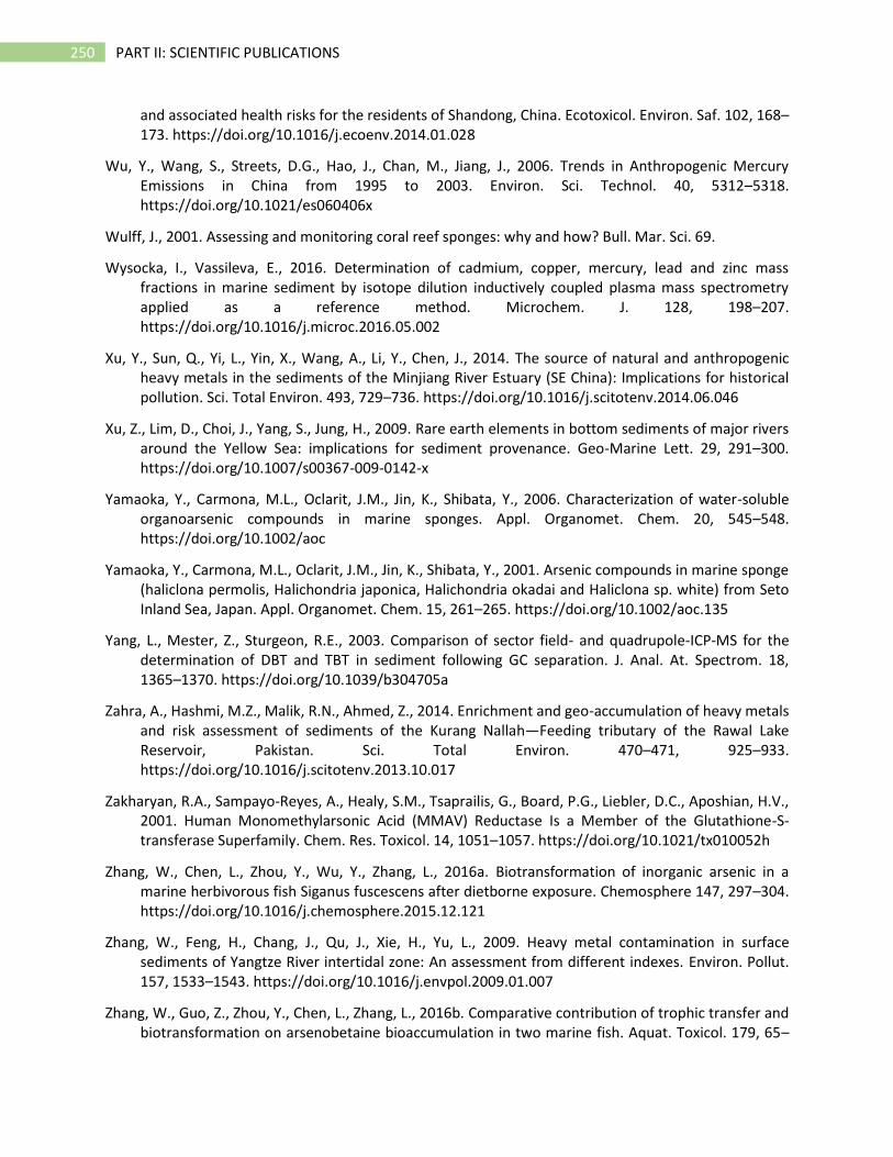
250 PART II: SCIENTIFIC PUBLICATIONS
and associated health risks for the residents of Shandong, China. Ecotoxicol. Environ. Saf. 102, 168–173. https://doi.org/10.1016/j.ecoenv.2014.01.028
Wu, Y., Wang, S., Streets, D.G., Hao, J., Chan, M., Jiang, J., 2006. Trends in Anthropogenic Mercury Emissions in China from 1995 to 2003. Environ. Sci. Technol. 40, 5312–5318. https://doi.org/10.1021/es060406x
Wulff, J., 2001. Assessing and monitoring coral reef sponges: why and how? Bull. Mar. Sci. 69.
Wysocka, I., Vassileva, E., 2016. Determination of cadmium, copper, mercury, lead and zinc mass fractions in marine sediment by isotope dilution inductively coupled plasma mass spectrometry applied as a reference method. Microchem. J. 128, 198–207. https://doi.org/10.1016/j.microc.2016.05.002
Xu, Y., Sun, Q., Yi, L., Yin, X., Wang, A., Li, Y., Chen, J., 2014. The source of natural and anthropogenic heavy metals in the sediments of the Minjiang River Estuary (SE China): Implications for historical pollution. Sci. Total Environ. 493, 729–736. https://doi.org/10.1016/j.scitotenv.2014.06.046
Xu, Z., Lim, D., Choi, J., Yang, S., Jung, H., 2009. Rare earth elements in bottom sediments of major rivers around the Yellow Sea: implications for sediment provenance. Geo-Marine Lett. 29, 291–300. https://doi.org/10.1007/s00367-009-0142-x
Yamaoka, Y., Carmona, M.L., Oclarit, J.M., Jin, K., Shibata, Y., 2006. Characterization of water-soluble organoarsenic compounds in marine sponges. Appl. Organomet. Chem. 20, 545–548. https://doi.org/10.1002/aoc
Yamaoka, Y., Carmona, M.L., Oclarit, J.M., Jin, K., Shibata, Y., 2001. Arsenic compounds in marine sponge (haliclona permolis, Halichondria japonica, Halichondria okadai and Haliclona sp. white) from Seto Inland Sea, Japan. Appl. Organomet. Chem. 15, 261–265. https://doi.org/10.1002/aoc.135
Yang, L., Mester, Z., Sturgeon, R.E., 2003. Comparison of sector field- and quadrupole-ICP-MS for the determination of DBT and TBT in sediment following GC separation. J. Anal. At. Spectrom. 18, 1365–1370. https://doi.org/10.1039/b304705a
Zahra, A., Hashmi, M.Z., Malik, R.N., Ahmed, Z., 2014. Enrichment and geo-accumulation of heavy metals and risk assessment of sediments of the Kurang Nallah—Feeding tributary of the Rawal Lake Reservoir, Pakistan. Sci. Total Environ. 470–471, 925–933. https://doi.org/10.1016/j.scitotenv.2013.10.017
Zakharyan, R.A., Sampayo-Reyes, A., Healy, S.M., Tsaprailis, G., Board, P.G., Liebler, D.C., Aposhian, H.V., 2001. Human Monomethylarsonic Acid (MMAV) Reductase Is a Member of the Glutathione-S-transferase Superfamily. Chem. Res. Toxicol. 14, 1051–1057. https://doi.org/10.1021/tx010052h
Zhang, W., Chen, L., Zhou, Y., Wu, Y., Zhang, L., 2016a. Biotransformation of inorganic arsenic in a marine herbivorous fish Siganus fuscescens after dietborne exposure. Chemosphere 147, 297–304. https://doi.org/10.1016/j.chemosphere.2015.12.121
Zhang, W., Feng, H., Chang, J., Qu, J., Xie, H., Yu, L., 2009. Heavy metal contamination in surface sediments of Yangtze River intertidal zone: An assessment from different indexes. Environ. Pollut. 157, 1533–1543. https://doi.org/10.1016/j.envpol.2009.01.007
Zhang, W., Guo, Z., Zhou, Y., Chen, L., Zhang, L., 2016b. Comparative contribution of trophic transfer and biotransformation on arsenobetaine bioaccumulation in two marine fish. Aquat. Toxicol. 179, 65–
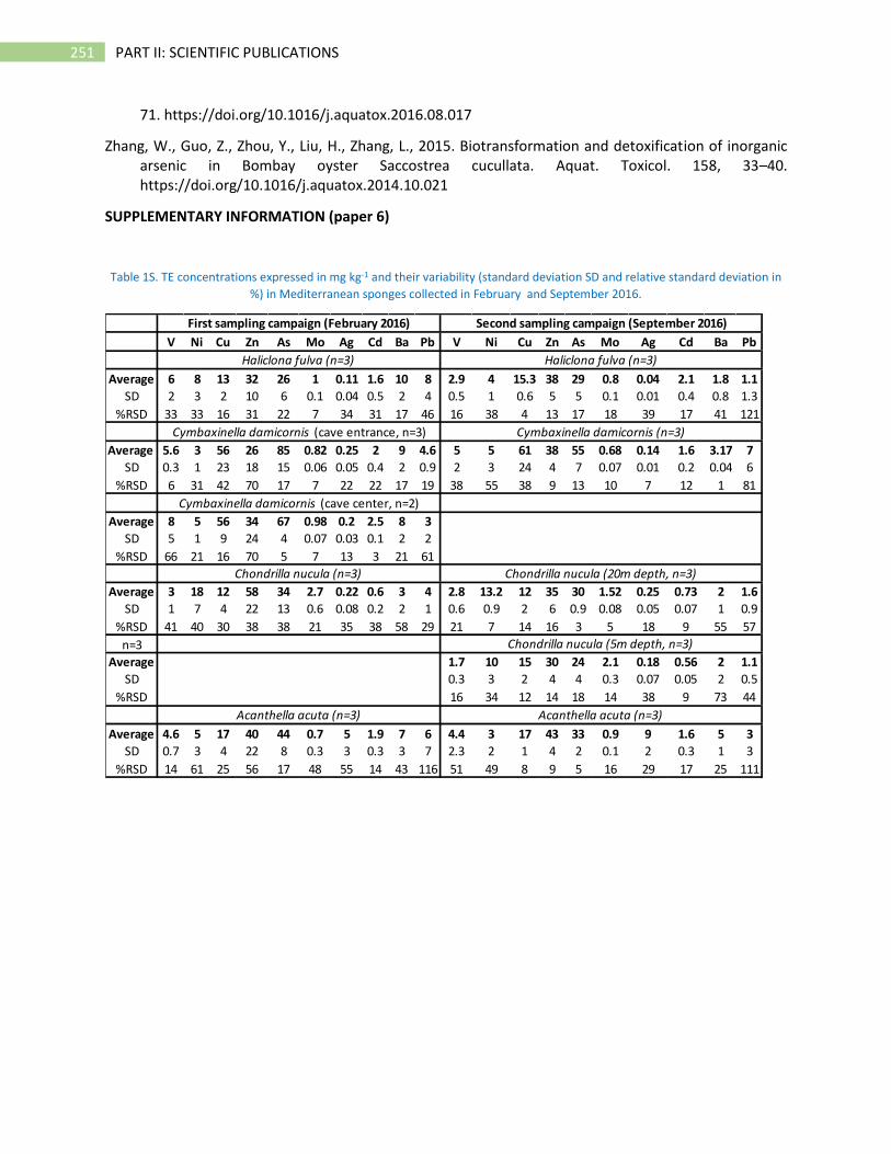
251 PART II: SCIENTIFIC PUBLICATIONS
71. https://doi.org/10.1016/j.aquatox.2016.08.017
Zhang, W., Guo, Z., Zhou, Y., Liu, H., Zhang, L., 2015. Biotransformation and detoxification of inorganic arsenic in Bombay oyster Saccostrea cucullata. Aquat. Toxicol. 158, 33–40. https://doi.org/10.1016/j.aquatox.2014.10.021
SUPPLEMENTARY INFORMATION (paper 6)
Table 1S. TE concentrations expressed in mg kg-1 and their variability (standard deviation SD and relative standard deviation in
%) in Mediterranean sponges collected in February and September 2016.
V Ni Cu Zn As Mo Ag Cd Ba Pb V Ni Cu Zn As Mo Ag Cd Ba Pb
Average 6 8 13 32 26 1 0.11 1.6 10 8 2.9 4 15.3 38 29 0.8 0.04 2.1 1.8 1.1
SD 2 3 2 10 6 0.1 0.04 0.5 2 4 0.5 1 0.6 5 5 0.1 0.01 0.4 0.8 1.3
%RSD 33 33 16 31 22 7 34 31 17 46 16 38 4 13 17 18 39 17 41 121
Average 5.6 3 56 26 85 0.82 0.25 2 9 4.6 5 5 61 38 55 0.68 0.14 1.6 3.17 7
SD 0.3 1 23 18 15 0.06 0.05 0.4 2 0.9 2 3 24 4 7 0.07 0.01 0.2 0.04 6
%RSD 6 31 42 70 17 7 22 22 17 19 38 55 38 9 13 10 7 12 1 81
Average 8 5 56 34 67 0.98 0.2 2.5 8 3
SD 5 1 9 24 4 0.07 0.03 0.1 2 2
%RSD 66 21 16 70 5 7 13 3 21 61
Average 3 18 12 58 34 2.7 0.22 0.6 3 4 2.8 13.2 12 35 30 1.52 0.25 0.73 2 1.6
SD 1 7 4 22 13 0.6 0.08 0.2 2 1 0.6 0.9 2 6 0.9 0.08 0.05 0.07 1 0.9
%RSD 41 40 30 38 38 21 35 38 58 29 21 7 14 16 3 5 18 9 55 57
n=3
Average 1.7 10 15 30 24 2.1 0.18 0.56 2 1.1
SD 0.3 3 2 4 4 0.3 0.07 0.05 2 0.5
%RSD 16 34 12 14 18 14 38 9 73 44
Average 4.6 5 17 40 44 0.7 5 1.9 7 6 4.4 3 17 43 33 0.9 9 1.6 5 3
SD 0.7 3 4 22 8 0.3 3 0.3 3 7 2.3 2 1 4 2 0.1 2 0.3 1 3
%RSD 14 61 25 56 17 48 55 14 43 116 51 49 8 9 5 16 29 17 25 111
Acanthella acuta (n=3)
First sampling campaign (February 2016)
Haliclona fulva (n=3)
Cymbaxinella damicornis (cave entrance, n=3)
Cymbaxinella damicornis (cave center, n=2)
Chondrilla nucula (n=3)
Acanthella acuta (n=3)
Second sampling campaign (September 2016)
Haliclona fulva (n=3)
Cymbaxinella damicornis (n=3)
Chondrilla nucula (5m depth, n=3)
Chondrilla nucula (20m depth, n=3)
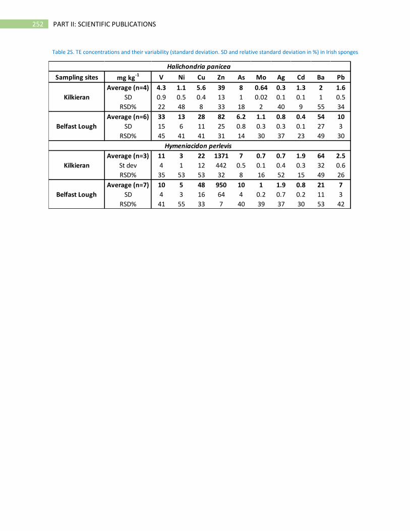
252 PART II: SCIENTIFIC PUBLICATIONS
Table 2S. TE concentrations and their variability (standard deviation. SD and relative standard deviation in %) in Irish sponges
Sampling sites mg kg-1 V Ni Cu Zn As Mo Ag Cd Ba Pb
Average (n=4) 4.3 1.1 5.6 39 8 0.64 0.3 1.3 2 1.6
SD 0.9 0.5 0.4 13 1 0.02 0.1 0.1 1 0.5
RSD% 22 48 8 33 18 2 40 9 55 34
Average (n=6) 33 13 28 82 6.2 1.1 0.8 0.4 54 10
SD 15 6 11 25 0.8 0.3 0.3 0.1 27 3
RSD% 45 41 41 31 14 30 37 23 49 30
Average (n=3) 11 3 22 1371 7 0.7 0.7 1.9 64 2.5
St dev 4 1 12 442 0.5 0.1 0.4 0.3 32 0.6
RSD% 35 53 53 32 8 16 52 15 49 26
Average (n=7) 10 5 48 950 10 1 1.9 0.8 21 7
SD 4 3 16 64 4 0.2 0.7 0.2 11 3
RSD% 41 55 33 7 40 39 37 30 53 42
Halichondria panicea
Hymeniacidon perlevis
Kilkieran
Belfast Lough
Kilkieran
Belfast Lough

253 PART II: SCIENTIFIC PUBLICATIONS
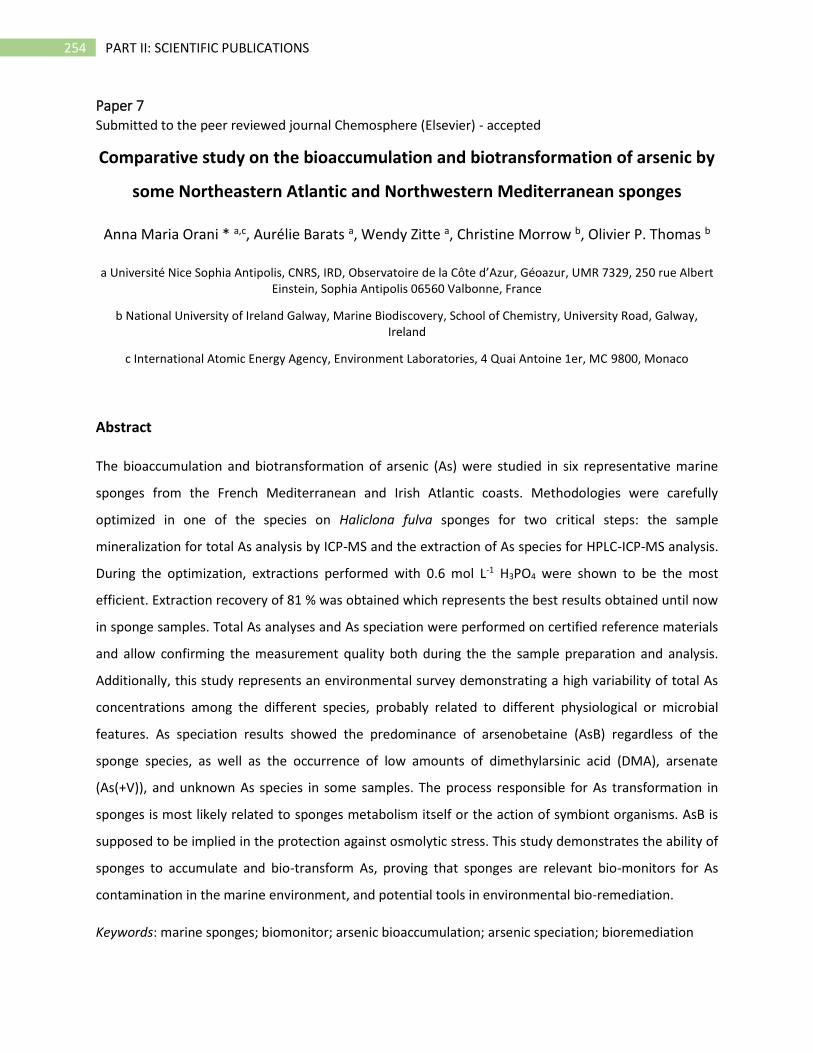
254 PART II: SCIENTIFIC PUBLICATIONS
Paper 7 Submitted to the peer reviewed journal Chemosphere (Elsevier) - accepted
Comparative study on the bioaccumulation and biotransformation of arsenic by
some Northeastern Atlantic and Northwestern Mediterranean sponges
Anna Maria Orani * a,c, Aurélie Barats a, Wendy Zitte a, Christine Morrow b, Olivier P. Thomas b
a Université Nice Sophia Antipolis, CNRS, IRD, Observatoire de la Côte d’Azur, Géoazur, UMR 7329, 250 rue Albert Einstein, Sophia Antipolis 06560 Valbonne, France
b National University of Ireland Galway, Marine Biodiscovery, School of Chemistry, University Road, Galway, Ireland
c International Atomic Energy Agency, Environment Laboratories, 4 Quai Antoine 1er, MC 9800, Monaco
Abstract
The bioaccumulation and biotransformation of arsenic (As) were studied in six representative marine
sponges from the French Mediterranean and Irish Atlantic coasts. Methodologies were carefully
optimized in one of the species on Haliclona fulva sponges for two critical steps: the sample
mineralization for total As analysis by ICP-MS and the extraction of As species for HPLC-ICP-MS analysis.
During the optimization, extractions performed with 0.6 mol L-1 H3PO4 were shown to be the most
efficient. Extraction recovery of 81 % was obtained which represents the best results obtained until now
in sponge samples. Total As analyses and As speciation were performed on certified reference materials
and allow confirming the measurement quality both during the the sample preparation and analysis.
Additionally, this study represents an environmental survey demonstrating a high variability of total As
concentrations among the different species, probably related to different physiological or microbial
features. As speciation results showed the predominance of arsenobetaine (AsB) regardless of the
sponge species, as well as the occurrence of low amounts of dimethylarsinic acid (DMA), arsenate
(As(+V)), and unknown As species in some samples. The process responsible for As transformation in
sponges is most likely related to sponges metabolism itself or the action of symbiont organisms. AsB is
supposed to be implied in the protection against osmolytic stress. This study demonstrates the ability of
sponges to accumulate and bio-transform As, proving that sponges are relevant bio-monitors for As
contamination in the marine environment, and potential tools in environmental bio-remediation.
Keywords: marine sponges; biomonitor; arsenic bioaccumulation; arsenic speciation; bioremediation
255 PART II: SCIENTIFIC PUBLICATIONS
1. Introduction
Arsenic (As) is a ubiquitous element that ranks 20th in abundance in the earth’s crust (1.5–3 mg kg−1).
This metalloid occurs naturally in the environment, and it is also provided by some anthropogenic
activities (Mandal and Suzuki, 2002). As is recognized to be toxic and one of the six most preoccupying
pollutants on earth together with lead, mercury, chromium, some radionuclides and pesticides. The
understanding of As cycle in marine ecosystem remains a challenging task since arsenic often occurs at
very low concentrations (around 1 µg L-1 in seawater) and under one of the most toxic inorganic species
(As(+V)) (Cabon and Cabon, 2000). Within this context, there is a clear need to gain a better
understanding of the As cycle in the marine environment.
The quantification of total As in marine organisms and especially in seafood has been performed in
numerous studies (Phillips, 1990; Kucuksezgin et al., 2014; Wu et al., 2014; Olmedo et al., 2013), but
rarely in marine invertebrates. Among marine invertebrates, sponges are sessile filter feeders, capable
of filtering every day a volume of seawater up to 50 000 times that of their body (Weisz et al., 2008).
They have been recognized as excellent bio-monitors for trace element pollution (Perez et al., 2005;
Cebrian et al., 2007) as they are capable to accumulate trace elements at concentrations higher than
bivalves (Patel et al., 1985; Negri et al., 2006; Padovan et al., 2012). On hard substrata, sponges are one
of the top spatial competitors (Bell, 2008) and have recently been proposed as model organisms to
monitor aquatic contamination, in addition to the already existing and well known “Mussel Watch
Program” (Genta-Jouve et al., 2012). The bioaccumulation of trace elements in sponges was suggested
to differ according to sponge species and the element of interest (Batista et al., 2014; Mayzel et al.,
2014; Cebrian et al., 2007; Patel et al., 1985). Only few studies focused on As bioaccumulation in
sponges (Aly et al., 2013; Araújo et al., 2003; Batista et al., 2014; Denton et al., 2006; Keren et al., 2015;
Keren et al., 2016; Keren et al., 2017; Padovan et al., 2012; Pan et al., 2011; Perez et al., 2005; Schaeffer
et al., 2006; Shiomi et al., 1988; Vaskovsky et al., 1972; Venkateswara Rao et al., 2009; Yamaoka et al.,
2001; Yamaoka et al., 2006). These studies revealed how As concentrations in sponges is variable,
exceeding 100 mg kg-1 in some cases, and usually higher than in other marine organisms (generally < 10
mg kg-1 in fish, algae and shellfish) (Llorente-Mirandes et al., 2010). Sponges seem to accumulate more
As than other marine organisms, which makes them suitable models for biomonitoring studies, as
already proposed by Genta-Jouve et al., 2012. As accumulation was previously demonstrated to be
strongly related to sponge orders or species; for instance higher in demosponges than in calcareous
sponges (Yamaoka et al., 2001).
256 PART II: SCIENTIFIC PUBLICATIONS
The determination of total As concentration is however not sufficient as As toxicity and biological impact
depend directly on its chemical form, i.e. its speciation (Cullen and Reimer, 1989; Hughes, 2002; Sakurai,
2002) . Among arsenic species, inorganic arsenite As(+III) and arsenate As(+V) are the most toxic forms.
These two inorganic forms are carcinogenic and cause damage to the respiratory, cardiovascular,
nervous, and hematopoietic systems, as well as lesions to skin and liver (Pershagen, 1981). The
methylated forms monomethylarsonic acid (MMA) and dimethylarsinic acid (DMA) are less toxic than
the previously mentioned inorganic species, but they are recognized as cancer promoters (Brown et al.,
1997) while arsenobetaine (AsB), the major species in marine animals, arsenocholine (AsC),
trimethylarsine oxide (TMAO) and tetramethylarsonium ion (TMAs) are considered nontoxic (ATSDR,
2007). Other As species, like arsenosugars (AsS), often found in seafood and generally in marine
organisms, have been recognized not to be acutely toxic; nevertheless a chronic toxicity is a possibility
(Andrewes et al., 2004). The quantitation of the different As chemical forms, i.e. arsenic speciation, can
be performed with different analytical techniques(Benramdane et al., 1999; Hsieh et al., 2010; Nearing
et al., 2014 ; Tian et al., 2010). HPLC-ICP-MS represents the most used technique by far (Benramdane et
al., 1999; Nearing et al., 2014) because this hyphenated technique combines a rapid, powerful and
reproducible separation method with a very efficient detector due to its high sensitivity and large linear
dynamic range (Beauchemin, 2008).
In most aquatic organisms, As speciation analysis has already revealed the occurrence of AsB, AsS, DMA
and inorganic species. In freshwater organisms, the inorganic As(+III) species was reported as dominant
for gastropods (Hong et al., 2014), two AsS species for microalgae, DMA for Anguilla japonica and more
often AsB for other fish-species and crustaceans (Miyashita et al., 2009). AsB was suggested to
contribute in a greater proportion of total As in marine organisms than in freshwater ones, which
represents the major difference in As speciation between aquatic organisms (Schaeffer et al., 2006;
Hong et al., 2014). AsB is reported as the most abundant As-species in several organisms, such as
shrimps, bivalves, crabs and fishes (Lai et al., 1999; Schaeffer et al., 2006; Taylor et al., 2012; Caumette
et al., 2012; Hong et al., 2014), whereas some AsS species can also be dominant in clams and mussels
(Grotti et al., 2010; Taylor et al., 2012). The relative proportions of these two major As-compounds (AsB
and AsS) would depend on the position of the organism in the food chain: the percentage of AsB
normally increases through the food web, whereas the AsS fraction decreases (Grotti et al., 2010).
Concerning sponges, the inorganic As(+V) specie was reported as dominant in freshwater sponges from
the Danube River in Hungary (Schaeffer et al., 2006) whereas in Japanese and Philippine marine
sponges, AsS and AsB were found to be dominant, showing interesting variability among the studied
257 PART II: SCIENTIFIC PUBLICATIONS
species (Shiomi et al., 1988; Yamaoka et al., 2001; Yamaoka et al., 2006). Recently, the role of sponge-
associated bacteria in As bioaccumulation was evaluated since bacteria are known as key contributors to
important elemental cycling in sponges, specifically for carbon, nitrogen, sulfur as well as trace elements
(Keren et al., 2015; Keren et al., 2016; Keren et al., 2017). The sponge symbiotic bacterium
Entotheonella sp. was shown to constitute the As-accumulating entity within the holobiont.
Considering the lack of studies on As speciation in marine sponges a deeper knowledge of As speciation
in marine sponges is needed. In this work, a methodology was first developed for total As analyses by
ICP-MS and As speciation by HPLC-ICP-MS in sponges. This approach was then applied to different
sponge species collected in distinct marine environments. This study focused on different sampling sites
located in the French Mediterranean coast, but also in the Irish Atlantic coast. These sites were
characterized by different natural and anthropogenic As inputs offering thus the opportunity to study
possible differences in As bioaccumulation and biotransformation related to the element availability.
2. Materials and methods
2.1. Sampling and target species
The sponge samples analyzed in this study were collected either by SCUBA diving in the French
Mediterranean coast in the Villefranche-sur-Mer Bay, or in the Irish Atlantic coast shore in Greenisland
and in the Killkieran Bay. The French sampling area is densely populated and a well-known tourist
destination, especially in summer time. Greenisland is a large inlet in the Belfast Lough, at the western
end is the city and the port of Belfast, which sits at the mouth of the Lagan River. The lough opens into
the North Channel and connects Belfast to the Irish Sea. Kilkieran Bay is a large, complex inlet in
southern Connemara, County Galway, on west coast of Ireland.
Initial sampling of specimens of the sponge Haliclona fulva was carried out in the Bay of Villefranche
sur Mer (N 43° 41' 59.0'', E 07° 19' 31.5'') on January 2014, in order to optimize the mineralization and
extraction procedures for As analyses. Subsequent sampling was conducted in the Bay of Villefranche
sur Mer on February and September 2016, in Killkieran Bay (N 53° 21’ 22.625’’, O 9° 42’ 17.153”) in
October 2016, and in Greenisland, Carrickfergus (N54°41’24.383”, O 5° 51’ 36.633”) in November 2016.
Sampling locations are shown in Fig. 1A (supplementary information). At least, three specimens of each
sponge species were collected from each sampling site and period. In order to minimize differences due
258 PART II: SCIENTIFIC PUBLICATIONS
to sponge ages, organisms of a similar size were chosen. In the Mediterranean coast, samples were
collected between 5 and 40 m depth, whereas in Ireland, they were collected from intertidal areas.
The following sponge species were collected for 2 sampling dates in the Mediterranean coast:
Acanthella acuta; Cymbaxinellap damicornis; Chondrilla nucula and Haliclona fulva. From Greenisland
and Killkieran Bay, the following species were collected: Halichondria panicea and Hymeniacidon
perlevis (Fig. 2A, supplementary information). These species were selected because of their widespread
occurrence but also for their different morphological characteristics (KeyToNature, 2015):
a) Acanthella acuta (Class: Demospongiae, Order: Axinellida, Family: Dictyonellidae) is a small erect
sponge with rather small oscules.
b) Cymbaxinellap damicornis (Class: Demospongiae, Order: Axinellida, Family: Axinellidae,
pphylocode name), is a rather small, erectly branching sponge with short, compressed branches.
Oscules are small and are located on the apices of the branches, the oscules are surrounded by a
small triangular ‘flap’ of tissue. The genus Axinella is difficult to define on the basis of
morphological characteristic but for the specie analyzed in this study the name Cymbaxinella
damicornis was recently proposed by Gazave et al. (2010) following the phylocode.
c) Chondrilla nucula (Class: Demospongiae, Order: Chondrillida, Family: Chondrillidae) is
amorphous, with globular lobes, or thickly incrusting, up to about 1 cm thick, spreading
horizontally, with pronounced, deeply incised and lacunose, meandering lobes. The color is
dark-brown to walnut-brown.
d) Haliclona fulva (Class: Demospongiae, Order: Haplosclerida, Family: Chalinidae), is a specimen
with irregular and slightly hispid surface. The ectosomal and choanosomal skeletons have a
regular, delicate, unispicular, and isotropic reticulation. Color is dark orange.
e) Halichondria panicea (Class: Demospongiae, Order: Suberitida, Family: Halichondriidae), is
intertidal or shallow-subtidal, thickly encrusting, massive or occasionally branching, and
presents typical volcanoe-shaped oscular chimneys. The surfaces of this sponge are smooth,
consistency firm, texture crumb-of-bread. These sponges are basically light orange-yellow or
pale yellowish green.
f) Hymeniacidon perlevis (Class: Demospongiae, Order: Suberitida, Family: Halichondriidae), is one
of the most common species along the Atlantic coasts of Western Europe. It is orange and has
an irregular surface, often with lower or higher irregular projections. Oscules are inconspicuous.

259 PART II: SCIENTIFIC PUBLICATIONS
Samples were kept frozen at -20°C. The sponge samples were then freeze-dried (Christ MartinTM
AlphaTM 1-2 Ldplus) and ground in an agate mortar in order to obtain a homogeneous powder.
Samples were transferred into PTFE pre-cleaned tubes and kept in a desiccator.
2.2. Sample preparation
All solutions were prepared with doubly deionized water obtained from Millipore water purification
system (Elix & Synergy) (resistivity of 18.2 MΩ cm−1, Total Organic Carbon <5 μg L−1 and microorganisms
<0.1 UFC ml-1). All PTFE and Teflon containers used for sample preparation and/or analysis were pre-
cleaned using a procedure consisting of 24 h bath in 10% HNO3 and careful rinsing with Milli-Q water.
For total As quantification, samples were digested in a closed microwave system (Ethos One, Milestone)
prior to ICP-MS analysis. The digestion program included a 20 min temperature ramp up to 180 °C
followed by 30 min isothermal step (power 2000 W). An aliquot of dried sponge sample was weighted in
Teflon reactors. Chemical reagents were added and the microwave digestion was carried out. The
sample mass and the use of different chemical reagents were optimized within this study. The following
chemical reagents were used: HNO3 (Trace Metal Grade, 67 to 70% w/w, Fisher Chemical), HF (Ultra
Trace Elemental Analysis 47-51% w/w, Optima, Fisher Chemical), HCl (≥30%, for trace analysis, Sigma-
Aldrich) and H2O2 (≥30%, for trace analysis, Sigma-Aldrich). The mineralized solution was then
transferred to PE pre-cleaned tubes and gravimetrically diluted with Milli-Q water, up to a final volume
of 50 mL. All samples were further diluted 15 times in Milli-Q water prior to ICP-MS analysis. At least one
procedural blank and one quality control Certified Reference Materials (CRM) were included in each
digestion run and analyzed with the rest of the samples. The following CRMs were used in this study:
TORT-2 (lobster hepatopancreas, Institute for Environmental Chemistry, National Research Council
Canada, Ottawa, Canada), BCR-627 (tuna fish powder, Institute for Reference Materials and
Measurements, Geel, Belgium) and MESS-2 (estuarine sediment, Institute for Environmental Chemistry,
National Research Council Canada, Ottawa, Canada). These CRM were prepared and analyzed along with
the vent samples as an assessment of analytical accuracy.
For As speciation, the extraction method was optimized using different chemicals and/or proportion:
Milli-Q water, methanol (MeOH, HPLC Plus, ≥99.9%, Sigma-Aldrich) and H3PO4 (≥85 wt. % in H2O, trace
metals basis, Sigma-Aldrich). Extractions were performed the day before analyses and extracts were
kept frozen during the night. Since no sponge CRM is available on the market, the extraction
260 PART II: SCIENTIFIC PUBLICATIONS
performances were evaluated using the certified reference material BCR-627 (certified for As speciation)
and TORT-2. For sponge samples, extractions were performed at least 3 times for each species to
account for intra-specie variability. 10 mL of the selected solvent were added to about 50 mg of dried
sample. The mixture was sonicated for one h. The extracts were then filtered with a single-use syringe
through single-use syringe filters (0.45 µm, Minisart® RC25, Sartorius) and gravimetrically diluted 10
times in Milli-Q water. The extracts were analyzed by HPLC-ICP-MS.
2.3. Sample analyses
A quadrupole ICP-MS (Elan DRCII, Perkin Elmer) was used as detection system for the determination of
total As in sponge samples. ICP-MS operating parameters are summarized in Table 1. 75As isotope may
be interfered in saline matrices by Cl (by 40Ar35Cl+). The most common way to remove these spectral
interferences is using the following correction equation: I(As) = I(m/z=75)-
3.127×I(m/z=77)+2.733×I(m/z=82) where I stands for intensity (Potot et al., 2012; Barats et al., 2014).
This mathematical correction accounts for about possible polyatomic interferences (40Ar35Cl+ or 40Ar37Cl+)
as well as for the occurrence of selenium (77,82Se) in samples. Preparation of standard solutions and
dilution of samples for analysis were carried out in a class 100 clean laboratory. External calibrations
were performed with daily prepared standards obtained by proper dilution of multi-elemental standard
for ICP-MS (ICP-MS standard N°3 Perkin Elmer®, ICP-MS standard N°2 from SCP SCIENCE®) or a mono-
elemental As standard (PlasmaCal, SCP SCIENCE®). An internal standard solution (containing 10 and 1 µg
L-1 of Ge and Tb respectively) was prepared by dilution of mono-elemental standards of Ge and Tb
(PlasmaCal, SCP SCIENCE®). 74Ge was chosen as an internal standard for As analyses to correct
instrumental drifts. All sample analyses were preceded by a minimum of a five-point calibration curve
spanning the entire concentration range of interest. All results were instrument blank corrected to
account for any operational bias. The ongoing instrument performance was monitored by the analysis of
continuing calibration verification standards. Daily analyses of the certified reference natural river water
SLRS-5 or SLRS-6 (National Research Council, Canada) and analyses of the 3 solid CRM (MESS-2, TORT-2
and BCR-627) were carried out to check measurement accuracy and reproducibility of analytical
calculations. Detection limits for 75As averaged 30 ng L-1.
As speciation analysis was performed by HPLC-ICP-MS. Instrumental settings and chromatographic
conditions used throughout this work were described in Table 1. Ion intensities at m/z = 75, 77 and 82
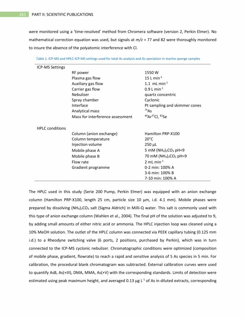
261 PART II: SCIENTIFIC PUBLICATIONS
were monitored using a ‘time-resolved’ method from Chromera software (version 2, Perkin Elmer). No
mathematical correction equation was used, but signals at m/z = 77 and 82 were thoroughly monitored
to insure the absence of the polyatomic interference with Cl.
Table 1. ICP-MS and HPLC-ICP-MS settings used for total As analysis and As speciation in marine sponge samples
ICP-MS Settings
RF power 1550 W
Plasma gas flow 15 L min-1
Auxiliary gas flow 1.1 mL min-1
Carrier gas flow 0.9 L min-1
Nebulizer quartz concentric
Spray chamber Cyclonic
Interface Pt sampling and skimmer cones
Analytical mass 75As
Mass for interference assessment 40Ar37Cl, 82Se
HPLC conditions
Column (anion exchange) Hamilton PRP-X100
Column temperature 20°C
Injection volume 250 µL
Mobile phase A 5 mM (NH4)2CO3 pH=9
Mobile phase B 70 mM (NH4)2CO3 pH=9
Flow rate 2 mL min-1
Gradient programme 0-2 min: 100% A
3-6 min: 100% B
7-10 min: 100% A
The HPLC used in this study (Serie 200 Pump, Perkin Elmer) was equipped with an anion exchange
column (Hamilton PRP-X100, length 25 cm, particle size 10 µm, i.d. 4.1 mm). Mobile phases were
prepared by dissolving (NH4)2CO3 salt (Sigma Aldrich) in Milli-Q water. This salt is commonly used with
this type of anion exchange column (Wahlen et al., 2004). The final pH of the solution was adjusted to 9,
by adding small amounts of either nitric acid or ammonia. The HPLC injection loop was cleaned using a
10% MeOH solution. The outlet of the HPLC column was connected via PEEK capillary tubing (0.125 mm
i.d.) to a Rheodyne switching valve (6 ports, 2 positions, purchased by Perkin), which was in turn
connected to the ICP-MS cyclonic nebulizer. Chromatographic conditions were optimized (composition
of mobile phase, gradient, flowrate) to reach a rapid and sensitive analysis of 5 As species in 5 min. For
calibration, the procedural blank chromatogram was subtracted. External calibration curves were used
to quantify AsB, As(+III), DMA, MMA, As(+V) with the corresponding standards. Limits of detection were
estimated using peak maximum height, and averaged 0.13 µg L-1 of As in diluted extracts, corresponding
262 PART II: SCIENTIFIC PUBLICATIONS
to 0.25 µg g-1 in sponge samples. Arsenic speciation analyses were performed on diluted solutions
obtained after a solid-liquid extraction, optimized in this study, lead on each dried sponge samples. For
quantification in sponge samples and CRM, the chromatograms of the extraction blanks were
systematically subtracted. In case of unknown As species, the calibration curves are similar for all As
species analyzed in this work, as previously demonstrated (Francesconi and Sperling, 2005) and serves
to quantify unknown As species when are detected. This approach was previously used for algae
(Llorente-Mirandes et al., 2010) and in sponge samples (Taylor et al., 2012). Standards used for As
speciation were prepared daily from dilution of As(+III) and As(+V) stocks (1000 mg L-1, Absolute
standard, Inc.) and organic As-mono-species solutions. The latter were prepared from salts of
arsenobetaine (AsB), sodium dimethylarsenite (DMA), disodium methylarsenate (MMA) (Sigma-Aldrich).
Species were identified by their retention times compared with standard compounds. Concentrations
were determined by comparing peak heights to known standards. The CRM BCR-627, certified for AsB
and DMA, was analyzed to check the accuracy of extraction and analytical methods. The TORT-2 was
also analyzed for As speciation and compared with literature data.
Statistical data treatments were carried out using XLSTAT (version 2014.05.5, Addinsoft, Paris,
France). One-way ANOVA tests were performed with a significance level of p<0.05 to estimate the inter-
species variability of As concentrations, between sites (Irish sponges), and between seasons
(Mediterranean sponges).
3. Results and discussion
3.1. Optimization of analytical methodologies
3.1.1. Development of the mineralization method for total As analysis in sponges
Nitric acid is often used to digest different types of marine organisms for trace elements analyses
(shrimps, mussels, gastropods, worm, oysters) (Taylor et al., 2012; Zhang et al., 2015), even for
freshwater sponges (Schaeffer et al., 2006). A two-steps method using HNO3 and then H2O2 was also
reported in aquatic organisms such as algae, fishes, bivalves, crabs, and shrimps (Hong et al., 2014;
Llorente-Mirandes et al., 2010), as well as in sponges and associated bacteria (Keren et al., 2017). In
order to select the best digestion procedure for As determination in marine sponges, an optimization
was carried out on a Haliclona fulva sample. Mineralization protocols were developed on about 100 mg
of dried sponge sample. The different methods and their results are presented in Table 1A
(supplementary information). Protocols without microwaves have been rapidly abandoned because they
resulted in jelly solutions, low As recoveries or results with a poor reproducibility. Acid digestions
263 PART II: SCIENTIFIC PUBLICATIONS
assisted by microwaves without HF usually resulted in slightly lower As recovery than those obtained
with HF (around 20% less). Sample microscope observations revealed undigested spicules in the solution
without HF (Fig. 3A, supplementary information). These protocols conduced to a partial mineralization
of sponge samples. In Antarctic Demospongiae (Sphaerotylus antarcticus, Kirkpatrikia coulmani and
Haliclona sp.) and in the Mediterranean species Petrosia ficiformis, the accumulation of pollutants (Cd,
Pb and Cu) was demonstrated as being lower in the spicules than in the corresponding organic fraction
even if spicules represent about 80% of the biomass (Illuminati et al., 2016). This observation is in full
agreement with our results. Nevertheless, the As amount in Halicona fulva spicules cannot be neglected
because it represents around 20% of the total As. For sponges with siliceous skeletons, the use of HF is
thus recommended. Higher As concentrations were obtained with the use of HNO3/HF or HCl/HNO3/HF
mixtures. Nevertheless, the use of HNO3/HF was preferred to prevent possible interferences onto the
75As isotope coming from HCl. Finally, the chosen sample preparation procedure involving a microwave
digestion has been performed using 5 ml of HNO3 and 2 ml of HF.
The optimized mineralization protocol was then applied to BCR-627 and TORT-2 marine biota CRMs
as well as to MESS-2 sediment CRM. The obtained results for total As were in all cases in good
agreement with the certified values, as shown in Table 2. Further applications of the developed
procedure were performed on about 50 mg of dried sponge.

264 PART II: SCIENTIFIC PUBLICATIONS
Table 2. Total As and As speciation results for three CRMs: BCR-627, TORT-2 and MESS-2. Extracted As concentrations were determined by ICP-MS and AsB concentrations by HPLC-ICP-MS. * and ** represent Indicative values given by *Sunner et al.,
2001 and **Wahlen et al., 2004.
Certified Reference Materials TORT-2 BCR 627 MESS-2
Microwave digested solutions
Total As (mg kg-1) 22 ± 2 (n=6) 5.2 ± 0.5 (n=4) 19.2 ± 1.1 (n=4)
Certified value 21.6 ± 1.8 4.8 ± 0.3 20.7 ± 0.8
Recovery (%) 102 108 92
Extracted solutions
Extracted As (mg kg-1) 23 ± 4 (n=3) 4.6 ± 0.3 (n=6)
Extraction recovery (%) 106 97
As from AsB (mg kg-1) 13 ± 5 (n=4) 4.5 ± 0.5 (n=6)
Certified value 13.8 ± 0.2* 14.3±1.1**
3.9 ± 0.2
As from DMA (mg kg-1) 1.2 ± 0.8 (n=4) 0.1< c <0.3
Certified value 0.97 ± 0.05* 0.84±0.10**
0.15 ± 0.02
As from unknown peak 1.9 ± 0.6 (n=4) -
Speciation recovery (%) 74 98
3.1.2. Development of the extraction method for sponge samples
A very delicate step of the speciation analyses is the chemical extraction of As species as it has to
guarantee the preservation of original chemical forms, avoiding oxidation, reduction or more generally
any conversion in other chemical species. As reported by different authors (Lai et al., 1999; Schaeffer et
al., 2006; Ciardullo et al., 2010; Llorente-Mirandes et al., 2010; Taylor et al., 2012; Zhang et al., 2015),
the most common solid-liquid extraction for As species from biological materials include the use of H2O,
MeOH or a mixture of them, since AsB is the predominant specie in marine animals and it is soluble in
both solvents (Leermakers et al., 2006). A solution made of 2% HNO3 was also used in chemical
extraction for various aquatic organisms (fishes, bivalves, crabs, shrimps) (Hong et al., 2014). H3PO4 was
more often used for As extraction from soils and sediments as it preserves the two redox states of As in
these samples (Ellwood and Maher, 2003). In sponges, extractions were performed either with H2O in
freshwater organisms (revealing low recovery of 30%) (Schaeffer et al., 2006), or with a mixture
H2O/MeOH (Shiomi et al., 1988; Yamaoka et al., 2001; Yamaoka et al., 2006; Keren et al., 2017).
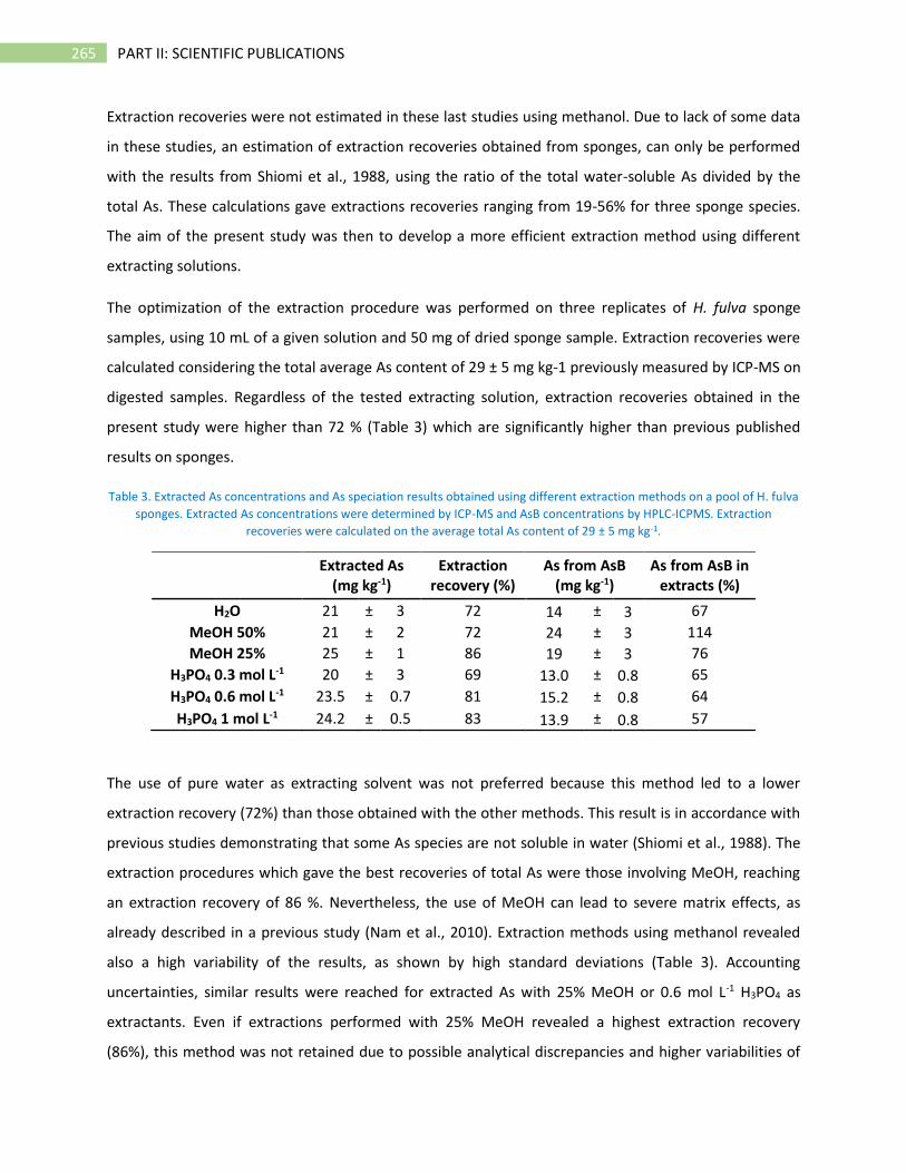
265 PART II: SCIENTIFIC PUBLICATIONS
Extraction recoveries were not estimated in these last studies using methanol. Due to lack of some data
in these studies, an estimation of extraction recoveries obtained from sponges, can only be performed
with the results from Shiomi et al., 1988, using the ratio of the total water-soluble As divided by the
total As. These calculations gave extractions recoveries ranging from 19-56% for three sponge species.
The aim of the present study was then to develop a more efficient extraction method using different
extracting solutions.
The optimization of the extraction procedure was performed on three replicates of H. fulva sponge
samples, using 10 mL of a given solution and 50 mg of dried sponge sample. Extraction recoveries were
calculated considering the total average As content of 29 ± 5 mg kg-1 previously measured by ICP-MS on
digested samples. Regardless of the tested extracting solution, extraction recoveries obtained in the
present study were higher than 72 % (Table 3) which are significantly higher than previous published
results on sponges.
Table 3. Extracted As concentrations and As speciation results obtained using different extraction methods on a pool of H. fulva
sponges. Extracted As concentrations were determined by ICP-MS and AsB concentrations by HPLC-ICPMS. Extraction
recoveries were calculated on the average total As content of 29 ± 5 mg kg-1.
Extracted As
(mg kg-1) Extraction
recovery (%) As from AsB
(mg kg-1) As from AsB in
extracts (%)
H2O 21 ± 3 72 14 ± 3 67
MeOH 50% 21 ± 2 72 24 ± 3 114
MeOH 25% 25 ± 1 86 19 ± 3 76
H3PO4 0.3 mol L-1 20 ± 3 69 13.0 ± 0.8 65
H3PO4 0.6 mol L-1 23.5 ± 0.7 81 15.2 ± 0.8 64
H3PO4 1 mol L-1 24.2 ± 0.5 83 13.9 ± 0.8 57
The use of pure water as extracting solvent was not preferred because this method led to a lower
extraction recovery (72%) than those obtained with the other methods. This result is in accordance with
previous studies demonstrating that some As species are not soluble in water (Shiomi et al., 1988). The
extraction procedures which gave the best recoveries of total As were those involving MeOH, reaching
an extraction recovery of 86 %. Nevertheless, the use of MeOH can lead to severe matrix effects, as
already described in a previous study (Nam et al., 2010). Extraction methods using methanol revealed
also a high variability of the results, as shown by high standard deviations (Table 3). Accounting
uncertainties, similar results were reached for extracted As with 25% MeOH or 0.6 mol L-1 H3PO4 as
extractants. Even if extractions performed with 25% MeOH revealed a highest extraction recovery
(86%), this method was not retained due to possible analytical discrepancies and higher variabilities of
266 PART II: SCIENTIFIC PUBLICATIONS
the results. The 0.6 mol L-1 H3PO4 solutions was selected because it appeared to be the best
compromise: a good extraction recovery 81% (close to the 86% obtained with 25% of MeOH) and a
good reproducibility of the results (RSD=3%). Considering that only a few studies have been published
on As speciation in sponges, the choice of H3PO4 solution was also made in order not to lose the possible
inorganic As species (the most toxic ones) possibly occurring in sponges samples, and to be able to
preserve their chemical forms. The chosen extraction method was therefore applied to the selected
CRMs. The extraction recoveries were found to be quite good, 106 and 97 %, for TORT-2 and BCR 627
respectively (Table 2). These results thus demonstrated the efficiency of the selected extraction
solution.
3.1.3. As speciation analyses
Speciation analyses of the extracts allowed mainly AsB to be quantified whatever the extraction
methods, AsB representing 57-114% of the extracted As (Table 3). The AsB concentration was
overestimated using 50% MeOH as extractant, as shown by the anomalous high proportion of As from
AsB in extracts (114%). As previously demonstrated, AsB concentrations can be overestimated using
MeOH (Nam et al., 2010). Such as for extracted As, As from AsB concentrations revealed similar results
with 25% MeOH or 0.6 mol L-1 H3PO4 as extractants, accounting uncertainties. The difference on
extraction recovery obtained for As from AsB were thus not significant due to the high variability of the
results obtained with 25% MeOH. Finally, the extraction method with 25% MeOH was not retained due
to possible analytical discrepancies and higher variabilities of the results. With the 0.6 mol L-1 H3PO4
solutions, AsB represent 64% of the extracted As with a better precision.
Speciation analyses were performed then on CRMs and conduced to good speciation recoveries: 74%
and 98% for TORT-2 and BCR 627 respectively (Table 2), highlighting the efficiency of speciation
analyses. Measurements on the certified reference material BCR-627 gave a mean value of AsB equal to
4.5 ± 0.5 mg kg-1 (n=6) and the occurrence of DMA just above the detection limit, in agreement with
certified values. In TORT-2, the average AsB value was 13 ± 5 mg kg-1 (n=4), in accordance with
previously reported values (Suner et al., 2001; Wahlen et al., 2004). Two other As species occurred at
low concentrations: DMA at 1.2 ± 0.8 mg kg-1 and another unknown As specie, named A, at 1.9 ± 0.6 mg
kg-1, eluting between DMA and MMA (retention time: tR = 2.5 min). The DMA result is in agreement
with the indicative value. These results on the two CRMs confirm thus the efficiency of speciation
analyses with accurate measurements of AsB.
267 PART II: SCIENTIFIC PUBLICATIONS
3.2. As bioaccumulation in sponges
3.2.1. Variability of As concentrations in sponges
The variability of As content in sponges was estimated within the same specimen (intra-specimen
variability), within the same sponge species (inter-specimen or intra-species variability), between
different sampling sites or seasons, as well between different sponge species (inter-species variability).
The intra-specimen variability was evaluated analyzing at least 3 replicates of each sponge specimen
(Table 2A, supplementary information). Each replicate underwent the whole sample preparation (i.e.
microwave digestion and dilution). The total As content was highly variable within each specimen, with
relative standard deviations (RSD) ranging from 8 to 36%. This result highlights a certain inhomogeneity
which may be related to the low amount of sponge samples weighted for digestion (50 mg).
The inter-specimen (or intra-species) variability was evaluated by determination of total As in different
specimens collected for each sponge species (Table 4). The variability, expressed with RSD, was usually
around 10%, but it reached 38% for C. nucula in Feb. 2016. In Irish sponges inter-specimen variability
was lower than in French samples (Table 4). Different authors reported RSD higher than 30% when
evaluating intra-species variability in total As and other trace elements found in sponge samples (Batista
et al., 2014; Cebrian and Uriz, 2007). A relevant natural variation shall further be considered for these
marine invertebrates.

268 PART II: SCIENTIFIC PUBLICATIONS
Table 4. Summary of As speciation results obtained for different sponges species sampled between February and November 2016 in three sites located in western Europe
Site Date Sponge species
Total As Extracted
As Extraction recovery
(%)
As from AsB
As from DMA
As(+V) Unknown As specie
A
Unknown As specie B
Speciation recovery
(%)
Known As in
sponge (%) (mg kg-1) (mg kg-1) (mg kg-1) (mg kg-1) (mg kg-1) (mg kg-1) (mg kg-1)
Vill
efr
anch
e s
ur
Me
r (F
ran
ce)
Feb. 2016
H. fulva 26± 6 16± 9 59 12± 8 1.7± 0.6 1.4± 0.2 <0.1 1.5± 0.5 106 66
A. acuta 44± 8 28± 1 64 24± 6 3.1± 0.7 1.9± 0.3 <0.1 1.9± 0.4 109 69
C. nucula 34± 13 26± 7 77 24± 9 3± 1.0 1.44± 0.02 <0.1 1.3± 0.1 116 88
C. damicornis
74± 11 36± 8 49 23± 8 3± 1.0 1.6± 0.4 <0.1 1.7± 0.4 79 39
Sep. 2016
H. fulva 29± 5 20± 5 69 16± 2 1.9± 0.1 0.1<c<0.4 <0.1 1.0± 0.1 95 66
A. acuta 33± 2 17± 2 51 16± 4 2.1± 0.1 0.6± 0.2 <0.1 1.4± 0.4 119 61
C. nucula 27± 4 24± 7 87 22± 7 2.3± 0.7 0.1<c<0.3 1.5± 0.4 0.1<c<0.3 104 92
C. damicornis
55± 7 25± 3 46 27± 13 2.7± 1 0.1<c<0.3 <0.1 1.0± 0.2 120 56
Kilk
iera
n B
ay
(Ire
lan
d)
Oct. 2016
H. panicea 7.3± 0.8 6.0± 0.1 83 2.5± 0.2 <0.1 0.1<c<0.3 <0.1 0.89± 0.08 57 47
H. perlevis 6.9± 0.5 7.2± 0.4 105 2.4± 0.3 <0.1 0.1<c<0.3 <0.1 1.1± 0.2 47 49
Gre
en
isla
nd
(No
rth
ern
Ire
lan
d)
Nov. 2016
H. panicea 5.7± 0.5 4.7± 0.4 81 1.7± 0.3 <0.1 0.1<c<0.3 <0.1 0.8± 0.2 52 43
H. perlevis 7.6± 0.3 7± 2 88 3.7± 1.1 <0.1 0.1<c<0.3 <0.1 0.91± 0.03 66 61
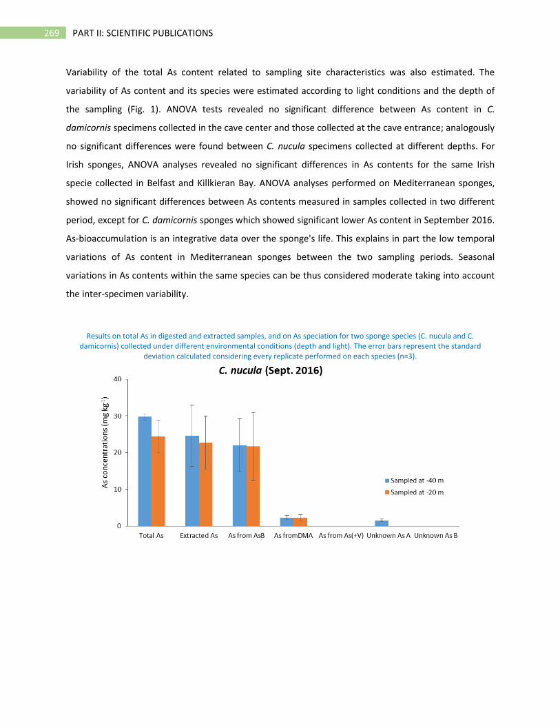
269 PART II: SCIENTIFIC PUBLICATIONS
Variability of the total As content related to sampling site characteristics was also estimated. The
variability of As content and its species were estimated according to light conditions and the depth of
the sampling (Fig. 1). ANOVA tests revealed no significant difference between As content in C.
damicornis specimens collected in the cave center and those collected at the cave entrance; analogously
no significant differences were found between C. nucula specimens collected at different depths. For
Irish sponges, ANOVA analyses revealed no significant differences in As contents for the same Irish
specie collected in Belfast and Killkieran Bay. ANOVA analyses performed on Mediterranean sponges,
showed no significant differences between As contents measured in samples collected in two different
period, except for C. damicornis sponges which showed significant lower As content in September 2016.
As-bioaccumulation is an integrative data over the sponge's life. This explains in part the low temporal
variations of As content in Mediterranean sponges between the two sampling periods. Seasonal
variations in As contents within the same species can be thus considered moderate taking into account
the inter-specimen variability.
Results on total As in digested and extracted samples, and on As speciation for two sponge species (C. nucula and C. damicornis) collected under different environmental conditions (depth and light). The error bars represent the standard
deviation calculated considering every replicate performed on each species (n=3).
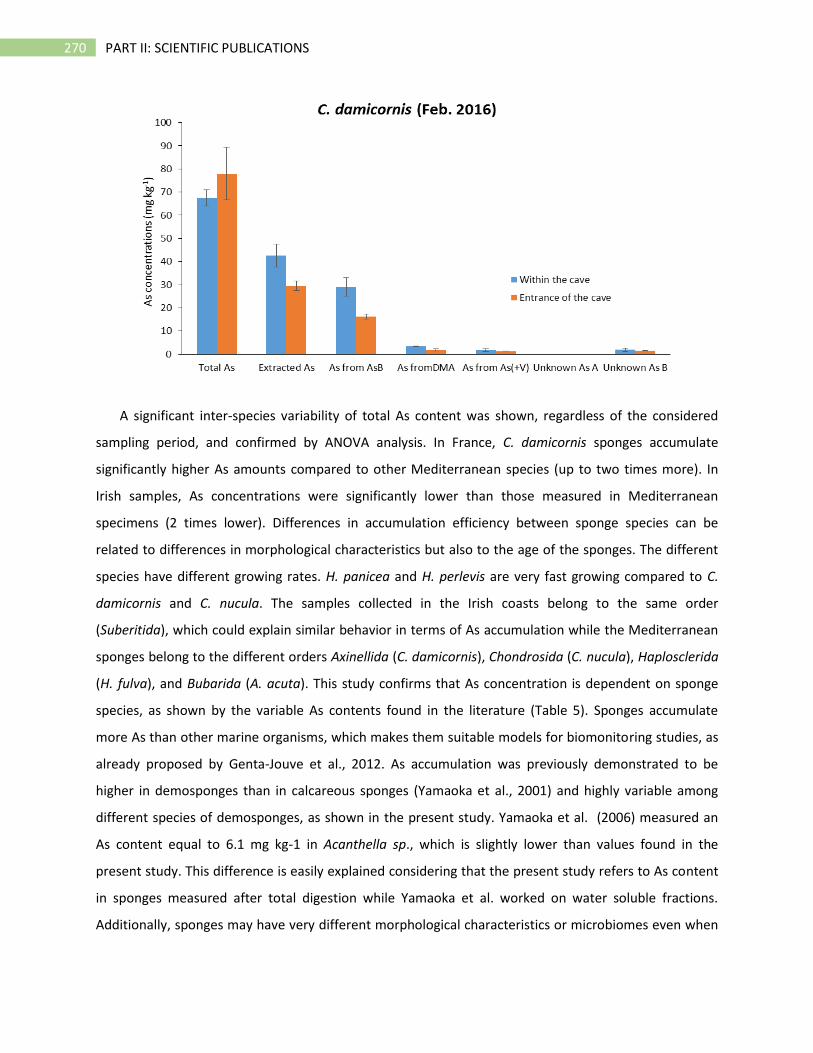
270 PART II: SCIENTIFIC PUBLICATIONS
A significant inter-species variability of total As content was shown, regardless of the considered
sampling period, and confirmed by ANOVA analysis. In France, C. damicornis sponges accumulate
significantly higher As amounts compared to other Mediterranean species (up to two times more). In
Irish samples, As concentrations were significantly lower than those measured in Mediterranean
specimens (2 times lower). Differences in accumulation efficiency between sponge species can be
related to differences in morphological characteristics but also to the age of the sponges. The different
species have different growing rates. H. panicea and H. perlevis are very fast growing compared to C.
damicornis and C. nucula. The samples collected in the Irish coasts belong to the same order
(Suberitida), which could explain similar behavior in terms of As accumulation while the Mediterranean
sponges belong to the different orders Axinellida (C. damicornis), Chondrosida (C. nucula), Haplosclerida
(H. fulva), and Bubarida (A. acuta). This study confirms that As concentration is dependent on sponge
species, as shown by the variable As contents found in the literature (Table 5). Sponges accumulate
more As than other marine organisms, which makes them suitable models for biomonitoring studies, as
already proposed by Genta-Jouve et al., 2012. As accumulation was previously demonstrated to be
higher in demosponges than in calcareous sponges (Yamaoka et al., 2001) and highly variable among
different species of demosponges, as shown in the present study. Yamaoka et al. (2006) measured an
As content equal to 6.1 mg kg-1 in Acanthella sp., which is slightly lower than values found in the
present study. This difference is easily explained considering that the present study refers to As content
in sponges measured after total digestion while Yamaoka et al. worked on water soluble fractions.
Additionally, sponges may have very different morphological characteristics or microbiomes even when
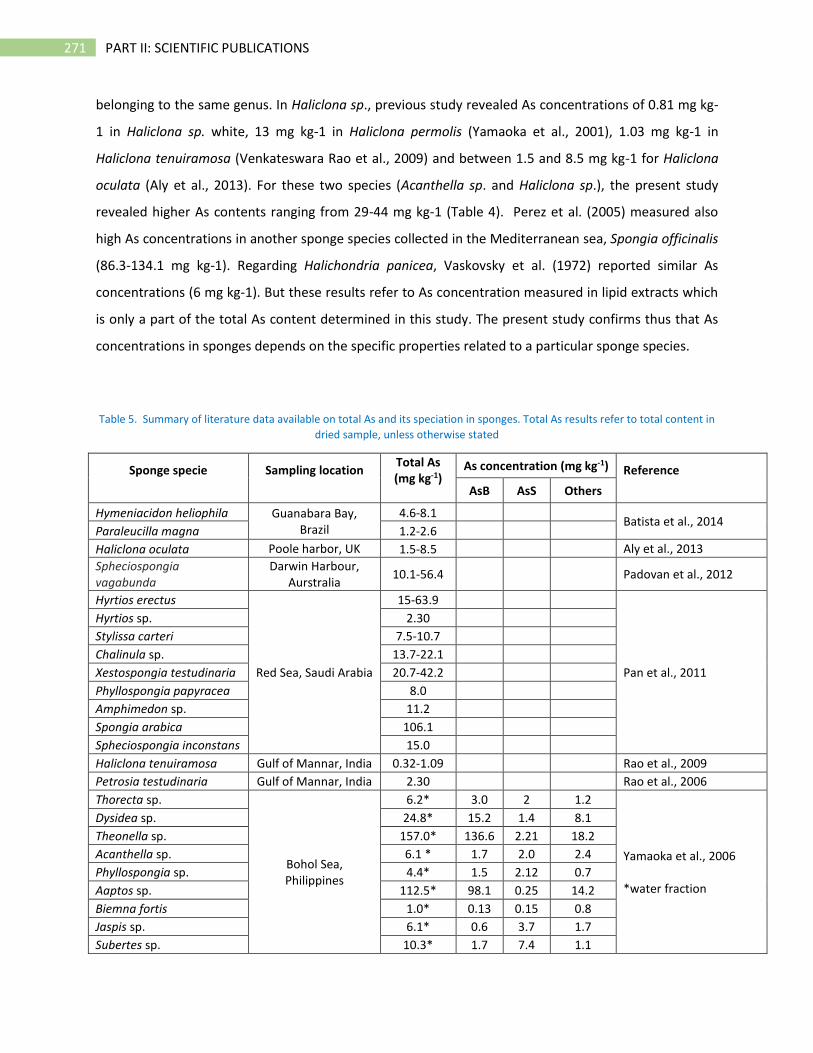
271 PART II: SCIENTIFIC PUBLICATIONS
belonging to the same genus. In Haliclona sp., previous study revealed As concentrations of 0.81 mg kg-
1 in Haliclona sp. white, 13 mg kg-1 in Haliclona permolis (Yamaoka et al., 2001), 1.03 mg kg-1 in
Haliclona tenuiramosa (Venkateswara Rao et al., 2009) and between 1.5 and 8.5 mg kg-1 for Haliclona
oculata (Aly et al., 2013). For these two species (Acanthella sp. and Haliclona sp.), the present study
revealed higher As contents ranging from 29-44 mg kg-1 (Table 4). Perez et al. (2005) measured also
high As concentrations in another sponge species collected in the Mediterranean sea, Spongia officinalis
(86.3-134.1 mg kg-1). Regarding Halichondria panicea, Vaskovsky et al. (1972) reported similar As
concentrations (6 mg kg-1). But these results refer to As concentration measured in lipid extracts which
is only a part of the total As content determined in this study. The present study confirms thus that As
concentrations in sponges depends on the specific properties related to a particular sponge species.
Table 5. Summary of literature data available on total As and its speciation in sponges. Total As results refer to total content in
dried sample, unless otherwise stated
Sponge specie
Sampling location
Total As (mg kg-1)
As concentration (mg kg-1) Reference AsB AsS Others
Hymeniacidon heliophila Guanabara Bay, Brazil
4.6-8.1 Batista et al., 2014
Paraleucilla magna 1.2-2.6
Haliclona oculata Poole harbor, UK 1.5-8.5 Aly et al., 2013
Spheciospongia vagabunda
Darwin Harbour, Aurstralia
10.1-56.4 Padovan et al., 2012
Hyrtios erectus
Red Sea, Saudi Arabia
15-63.9
Pan et al., 2011
Hyrtios sp. 2.30
Stylissa carteri 7.5-10.7
Chalinula sp. 13.7-22.1
Xestospongia testudinaria 20.7-42.2
Phyllospongia papyracea 8.0
Amphimedon sp. 11.2
Spongia arabica 106.1
Spheciospongia inconstans 15.0
Haliclona tenuiramosa Gulf of Mannar, India 0.32-1.09 Rao et al., 2009
Petrosia testudinaria Gulf of Mannar, India 2.30 Rao et al., 2006
Thorecta sp.
Bohol Sea, Philippines
6.2* 3.0 2 1.2
Yamaoka et al., 2006 *water fraction
Dysidea sp. 24.8* 15.2 1.4 8.1
Theonella sp. 157.0* 136.6 2.21 18.2
Acanthella sp. 6.1 * 1.7 2.0 2.4
Phyllospongia sp. 4.4* 1.5 2.12 0.7
Aaptos sp. 112.5* 98.1 0.25 14.2
Biemna fortis 1.0* 0.13 0.15 0.8
Jaspis sp. 6.1* 0.6 3.7 1.7
Subertes sp. 10.3* 1.7 7.4 1.1
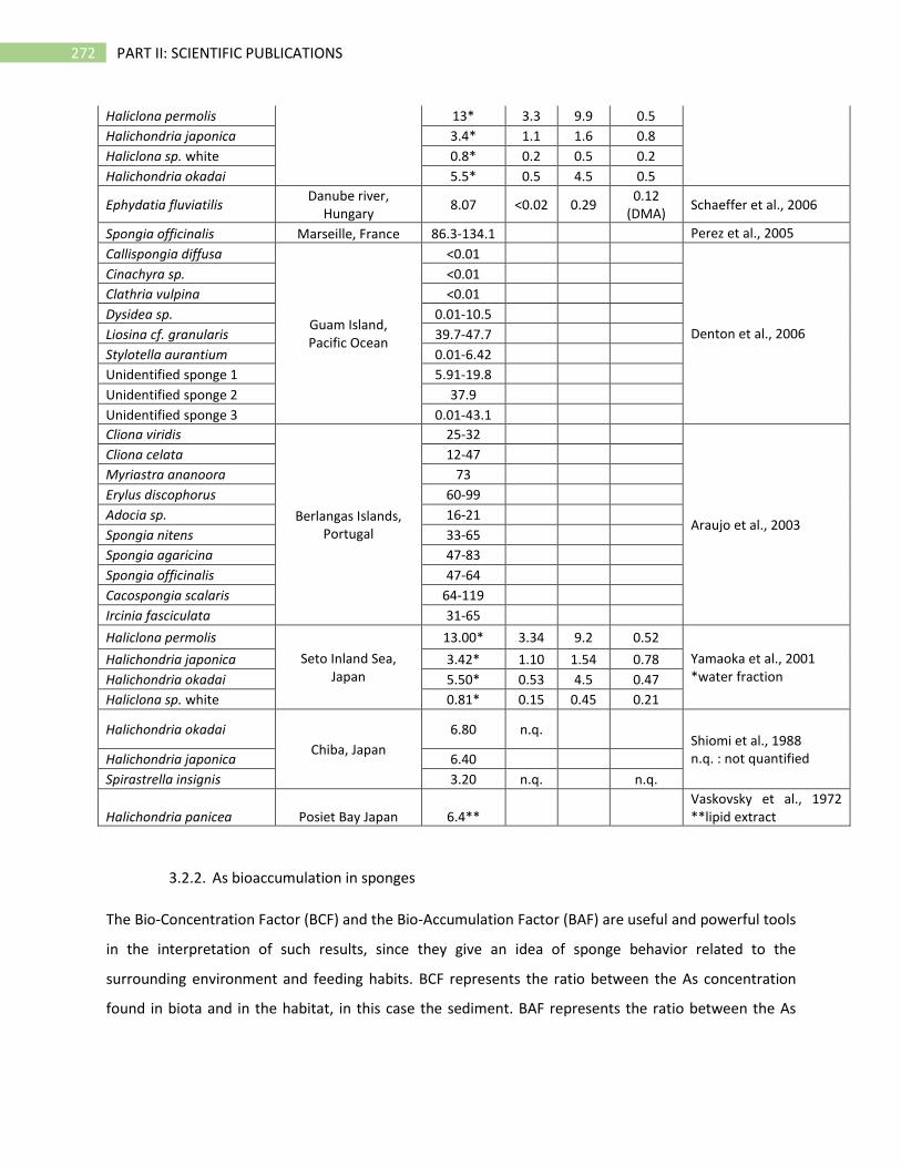
272 PART II: SCIENTIFIC PUBLICATIONS
Haliclona permolis 13* 3.3 9.9 0.5
Halichondria japonica 3.4* 1.1 1.6 0.8
Haliclona sp. white 0.8* 0.2 0.5 0.2
Halichondria okadai 5.5* 0.5 4.5 0.5
Ephydatia fluviatilis Danube river,
Hungary 8.07 <0.02 0.29
0.12 (DMA)
Schaeffer et al., 2006
Spongia officinalis Marseille, France 86.3-134.1 Perez et al., 2005
Callispongia diffusa
Guam Island, Pacific Ocean
<0.01
Denton et al., 2006
Cinachyra sp. <0.01
Clathria vulpina <0.01
Dysidea sp. 0.01-10.5
Liosina cf. granularis 39.7-47.7
Stylotella aurantium 0.01-6.42
Unidentified sponge 1 5.91-19.8
Unidentified sponge 2 37.9
Unidentified sponge 3 0.01-43.1
Cliona viridis
Berlangas Islands, Portugal
25-32
Araujo et al., 2003
Cliona celata 12-47
Myriastra ananoora 73
Erylus discophorus 60-99
Adocia sp. 16-21
Spongia nitens 33-65
Spongia agaricina 47-83
Spongia officinalis 47-64
Cacospongia scalaris 64-119
Ircinia fasciculata 31-65
Haliclona permolis
Seto Inland Sea, Japan
13.00* 3.34 9.2 0.52
Yamaoka et al., 2001 *water fraction
Halichondria japonica 3.42* 1.10 1.54 0.78
Halichondria okadai 5.50* 0.53 4.5 0.47
Haliclona sp. white 0.81* 0.15 0.45 0.21
Halichondria okadai
Chiba, Japan
6.80 n.q. Shiomi et al., 1988 n.q. : not quantified Halichondria japonica 6.40
Spirastrella insignis 3.20 n.q. n.q.
Halichondria panicea Posiet Bay Japan 6.4** Vaskovsky et al., 1972 **lipid extract
3.2.2. As bioaccumulation in sponges
The Bio-Concentration Factor (BCF) and the Bio-Accumulation Factor (BAF) are useful and powerful tools
in the interpretation of such results, since they give an idea of sponge behavior related to the
surrounding environment and feeding habits. BCF represents the ratio between the As concentration
found in biota and in the habitat, in this case the sediment. BAF represents the ratio between the As
273 PART II: SCIENTIFIC PUBLICATIONS
concentration found in biota and in the organism’s diet, in our case seawater, since sponges are filter
feeders (Gobas, 2001).
In this work, sediment collected from the French coast showed a constant As content for both sampling
period: 7 ± 2 mg kg-1 of As (measured on three sediment samples for each sampling period) while
sediment samples collected from Kilkieran Bay and Greenisland show an As content of 7 ± 2 and 2.9 ±
0.3 mg kg-1 respectively. These values are below the limit imposed by the principal environmental
authorities for As in marine sediments (7.24 mg kg-1, US EPA, 2006). Regarding sponges collected in
Ireland, specimens coming from Kilkieran bay showed BCF close to 1, while specimens of H. panicea and
H. perlevis sponges collected in Belfast showed BCF of 2.1 and 3.5 respectively. BCF in Mediterranean
sponges range from 3.6 to 12. Similar values were reported for bivalves (6-19) (Negri et al., 2006) and
were found to be higher than in other sponges (close to 1) (Mayzel et al., 2014). Extremely high As BCF
of 477 was also previously measured in only one sponge species, Theonella swinhoei, which was
explained by the presence of a particular bacterium (Mayzel et al., 2014). It is worth noticing that
Theonella swinhoei is a slow growing and long-lived sponge specie so As concentration may be also
linked to the age of the sponge and thus responsible for the elevated BCF. The fact that most BCF were
higher than 1 (except in Kilkieran Bay) proves that sponges are able to accumulate As at higher
concentrations than their surrounding environment (sediment in our case), which means that there are
additional biological processes involved in As accumulation.
As concentration in seawater used for the calculation of BAF in Mediterranean sponges was determined
in a sample collected in Monaco and measured at the Environment Laboratories of the International
Atomic Energy Agency. The average value found in seawater sample was 1.5 ± 0.2 µg L-1 and it was used
for BAF calculations because of the vicinity of the sampling site. This As content is in agreement with
total As content of 1.3 µg L-1 previously measured in surface seawater from Mediterranean Sea (Cabon
and Cabon, 2000). Mediterranean sponges BAF of As ranged between 15000 and 60000, i.e. in the order
of 4.2 to 4.8 for log BAF. For the calculation of BAF in Irish sponges, the average reference value for As in
seawater was 2.5 µg L-1, as reported by Crompton and Crompton (1989). The BAF obtained were
between 274 and 318 for samples collected in Kilkieran Bay and between 250 and 412 for samples
collected in Greenisland, namely values between 2.4 and 2.6 in logarithmic scale. BAF calculations
revealed thus significant higher values for Mediterranean sponges than Irish ones, but both sufficiently
high to indicate that these organisms are efficient bioaccumulators of As.
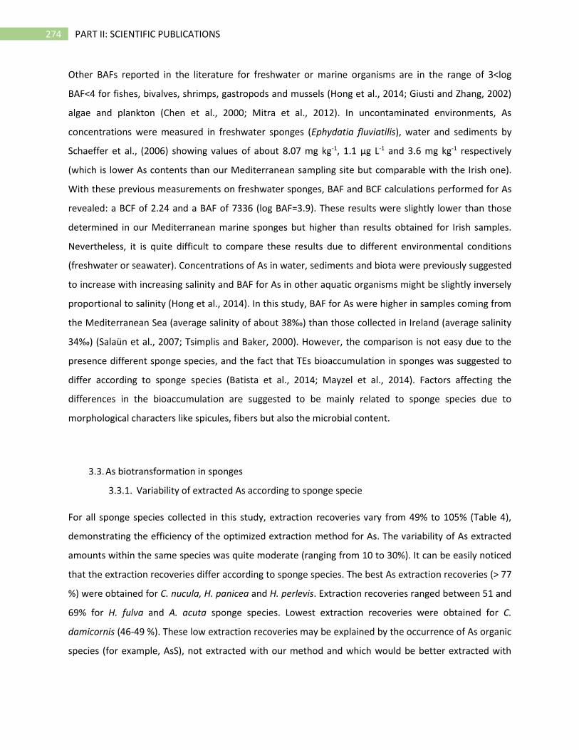
274 PART II: SCIENTIFIC PUBLICATIONS
Other BAFs reported in the literature for freshwater or marine organisms are in the range of 3<log
BAF<4 for fishes, bivalves, shrimps, gastropods and mussels (Hong et al., 2014; Giusti and Zhang, 2002)
algae and plankton (Chen et al., 2000; Mitra et al., 2012). In uncontaminated environments, As
concentrations were measured in freshwater sponges (Ephydatia fluviatilis), water and sediments by
Schaeffer et al., (2006) showing values of about 8.07 mg kg-1, 1.1 µg L-1 and 3.6 mg kg-1 respectively
(which is lower As contents than our Mediterranean sampling site but comparable with the Irish one).
With these previous measurements on freshwater sponges, BAF and BCF calculations performed for As
revealed: a BCF of 2.24 and a BAF of 7336 (log BAF=3.9). These results were slightly lower than those
determined in our Mediterranean marine sponges but higher than results obtained for Irish samples.
Nevertheless, it is quite difficult to compare these results due to different environmental conditions
(freshwater or seawater). Concentrations of As in water, sediments and biota were previously suggested
to increase with increasing salinity and BAF for As in other aquatic organisms might be slightly inversely
proportional to salinity (Hong et al., 2014). In this study, BAF for As were higher in samples coming from
the Mediterranean Sea (average salinity of about 38‰) than those collected in Ireland (average salinity
34‰) (Salaün et al., 2007; Tsimplis and Baker, 2000). However, the comparison is not easy due to the
presence different sponge species, and the fact that TEs bioaccumulation in sponges was suggested to
differ according to sponge species (Batista et al., 2014; Mayzel et al., 2014). Factors affecting the
differences in the bioaccumulation are suggested to be mainly related to sponge species due to
morphological characters like spicules, fibers but also the microbial content.
3.3. As biotransformation in sponges
3.3.1. Variability of extracted As according to sponge specie
For all sponge species collected in this study, extraction recoveries vary from 49% to 105% (Table 4),
demonstrating the efficiency of the optimized extraction method for As. The variability of As extracted
amounts within the same species was quite moderate (ranging from 10 to 30%). It can be easily noticed
that the extraction recoveries differ according to sponge species. The best As extraction recoveries (> 77
%) were obtained for C. nucula, H. panicea and H. perlevis. Extraction recoveries ranged between 51 and
69% for H. fulva and A. acuta sponge species. Lowest extraction recoveries were obtained for C.
damicornis (46-49 %). These low extraction recoveries may be explained by the occurrence of As organic
species (for example, AsS), not extracted with our method and which would be better extracted with
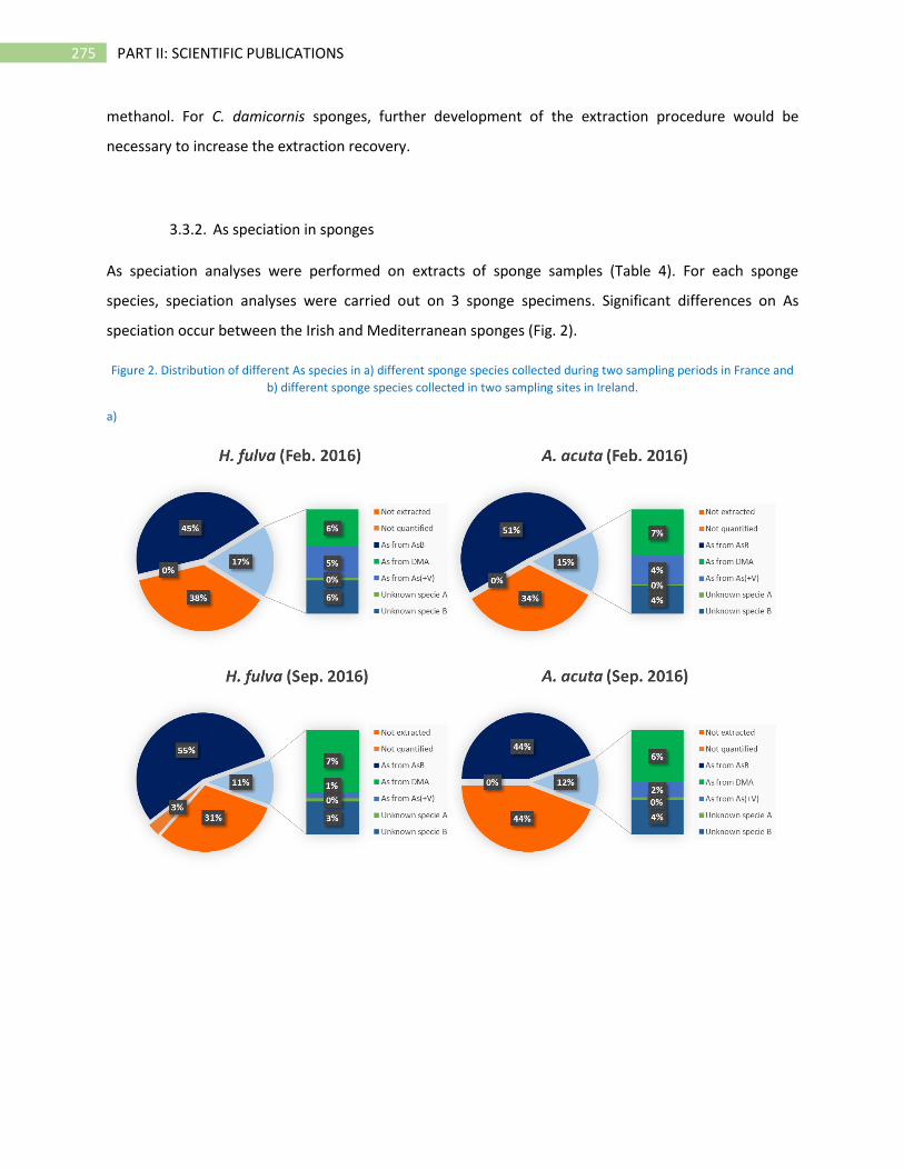
275 PART II: SCIENTIFIC PUBLICATIONS
methanol. For C. damicornis sponges, further development of the extraction procedure would be
necessary to increase the extraction recovery.
3.3.2. As speciation in sponges
As speciation analyses were performed on extracts of sponge samples (Table 4). For each sponge
species, speciation analyses were carried out on 3 sponge specimens. Significant differences on As
speciation occur between the Irish and Mediterranean sponges (Fig. 2).
Figure 2. Distribution of different As species in a) different sponge species collected during two sampling periods in France and
b) different sponge species collected in two sampling sites in Ireland.
a)
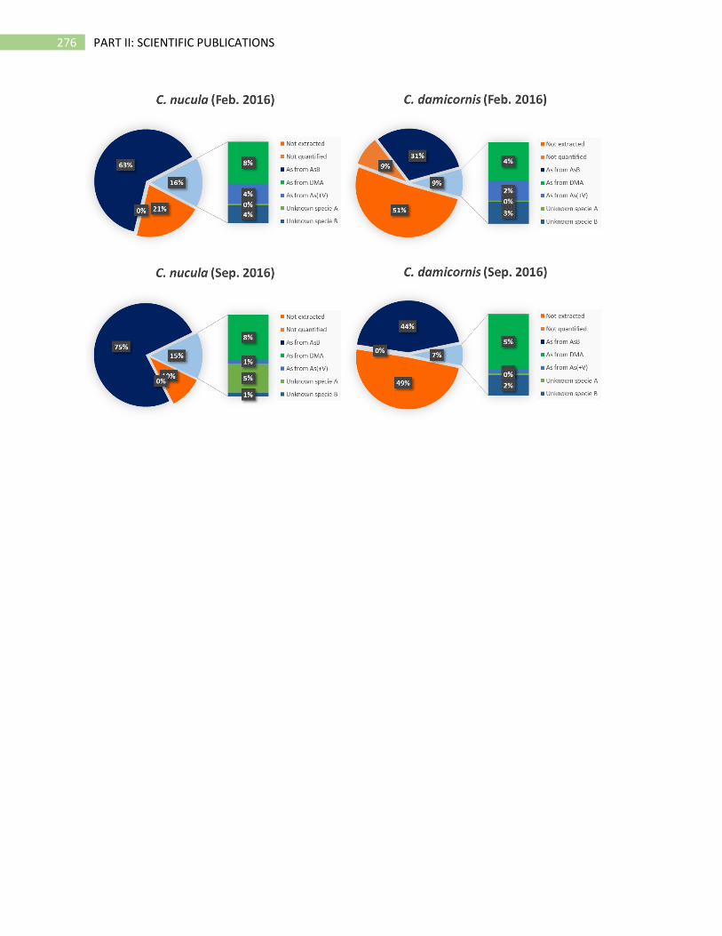
276 PART II: SCIENTIFIC PUBLICATIONS
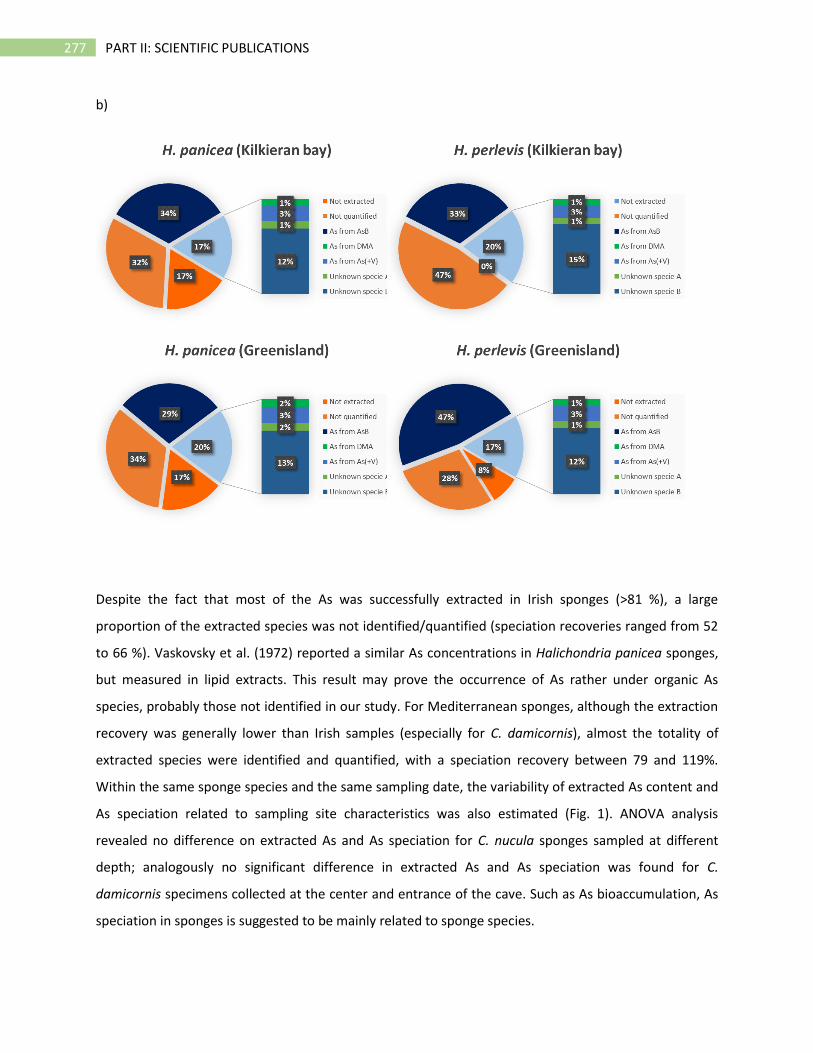
277 PART II: SCIENTIFIC PUBLICATIONS
b)
Despite the fact that most of the As was successfully extracted in Irish sponges (>81 %), a large
proportion of the extracted species was not identified/quantified (speciation recoveries ranged from 52
to 66 %). Vaskovsky et al. (1972) reported a similar As concentrations in Halichondria panicea sponges,
but measured in lipid extracts. This result may prove the occurrence of As rather under organic As
species, probably those not identified in our study. For Mediterranean sponges, although the extraction
recovery was generally lower than Irish samples (especially for C. damicornis), almost the totality of
extracted species were identified and quantified, with a speciation recovery between 79 and 119%.
Within the same sponge species and the same sampling date, the variability of extracted As content and
As speciation related to sampling site characteristics was also estimated (Fig. 1). ANOVA analysis
revealed no difference on extracted As and As speciation for C. nucula sponges sampled at different
depth; analogously no significant difference in extracted As and As speciation was found for C.
damicornis specimens collected at the center and entrance of the cave. Such as As bioaccumulation, As
speciation in sponges is suggested to be mainly related to sponge species.
278 PART II: SCIENTIFIC PUBLICATIONS
As speciation analysis in sponge extracts reveals the large occurrence of AsB (>29% of the total As) and
the presence of different As species at low concentrations: DMA, As(+V) (Fig. 2). Additionally, two
unknown species were found: a first one eluting between DMA and MMA (only for C. nucula in Sep.
2016) and a second one eluting after As(+V). These results on As speciation in marine sponges are
different from those obtained in freshwater sponge Ephydatia fluviatilis in which inorganic species were
found to be dominant: 57 % of As(+V), 20 % of As(+III)), AsS (11%), DMA (4%) and undetected AsB (<1%)
(Schaeffer et al., 2006). In the present study, among minor As species, DMA accounted for about 10% of
extracted As in Mediterranean sponges, (i.e. 4-8% of the total As content) whereas this specie was not
detected in Irish sponges at all. As(+V) was detected in all sponges’ species, but it was possible to
quantify it only for some of the Mediterranean specimens. This species represents about 5-9 % of the
extracted As content (i.e. 1-5 % of the total As content). The unknown As species, named B and eluting
after As(+V) (retention time, tR = 4.5 min), presents a similar As concentration (close to 1 mg kg-1)
regardless of the sponge species, representing between 5% and 15 % of extracted As in Mediterranean
and Irish sponges respectively (i.e. 2 and 15% of the total As). The unknown As specie A, eluting
between DMA and MMA (tR=2.5 min), occurs in A. acuta specimens but only in samples collected in
September 2016, representing 6% of extracted As (i.e. 5% of the total As). Even if AsB is the main As
species in H. fulva, A. acuta and C. nucula sponge species, it occurs in a lesser proportion in C.
damicornis (31-44 %), H. panicea (29-34 %), and H. perlevis (33-47 %) (Fig. 2). Even though C. damicornis
accumulates more As than the other sponge species, this sponge specie does not accumulate more AsB.
This higher As content is thus related to other As species, probably other organic forms not extracted or
not detected with the methodology used in the present study. The AsB predominance in A. acuta (86-
94% of As extracted or 48-55% of total As) is in accordance with the previous results on a sponge of the
same genus (28% of the water soluble extract) (Yamaoka et al., 2006). Two AsS were also reported to
occur in large amounts (22% oxo-AsS-phosphate, 11% oxo-AsS-glycerol, and 39% of unknown As
species). These other As species may coincide with the occurrence of unknown As species found in our
study or other As species not extracted with our method, specifically the As specie B representing 7.5%
of extracted As. In H. fulva, AsB was also the predominant As-species (75-80% of As extracted or 46-55%
of total As), whereas in the same genus (H. permolis), the oxo-AsS-phosphate was identified (61% of the
water soluble extract) (Yamaoka et al., 2001 and 2006). The same authors also reported AsS as
predominant As species in Halichondria sp., and a content of AsB between 9 and 32% whereas AsB were
reported dominant in another study (Shiomi et al., 1988). In the present study, H. panicea sponges from
the same genus contained an AsB which accounts for 34 and 29% of total As, for samples collected in
279 PART II: SCIENTIFIC PUBLICATIONS
Kilkieran bay and Greenisland, respectively. All these results demonstrate that As speciation and the
predominance of AsB or the AsS may not result only from sponge specie or genus characteristics.
Yamaoka et al., (2001 and 2006) suggested that the different proportions of AsS may reflect the
different symbionts living within sponges. This previous hypothesis would support: (1) the change of the
predominant As-species within the same sponge species, and (2) the difference of As-bioaccumulation
and biotransformation within a specific sponge species (C. damicornis, here) comparing to the others.
3.4. Pathways of As bioaccumulation and biotransformation
In surface seawater, As usually occurs under toxic inorganic species, mainly As(+V). Arsenic
speciation analyses in seawater reported in the literature revealed a content of 1 µg L-1 of As(+V) and 0.2
µg L-1 of As(+III) in the Mediterranean sea (Cabon and Cabon, 2000) and from 1.9 to 3 µg L-1 of As(+V)
and As(+III) <LOD in Irish seawater (Salaün et al., 2007). Sponges are efficient filter feeders, strongly
accumulating As (4 < log BAF < 5). Due to As bioaccumulation and biotransformation (converting toxic
inorganic As species in less-toxic organic species) within the sponge tissue, sponges may be a relevant
tool for bioremediation of As-contaminated site, producing possible secondary metabolites of great
interests (pharmaceuticals and bioactive compounds) under stressful environmental conditions (due to
pollution). For instance, a polyarsenic organic compound showing antibacterial and antifungal properties
was recently isolated from sponges (Mancini et al., 2006). The possible application of sponges in the
field of environmental bioremediation has been proposed in previous studies with different applications
(Longo et al., 2010; Santos-Gandelman et al., 2014).
The main occurrence of AsB in osmoconformers such as sponges may be justified in waters
characterized by high salinity because this molecule (as glycine-betaine) may serve to protect against
osmolytic stress (Clowes and Francesconi, 2004; Caumette et al., 2012). Since AsB is also the least toxic
form of arsenic, the production of such a molecule during a protecting process could be useful in the
detoxification of As contaminated waters. Since no AsB occurs in seawater and low contents of inorganic
As measured in sponges, biotransformation is responsible of these changes of As speciation. During their
feeding process, sponges ingest water (where the dominant As-species is As(+V)), and microorganisms
(potentially containing organic As species). Two different pathways may be responsible of the As
bioaccumulation and biotransformation within sponges: (1) a dietary route, through the feeding of
microorganisms (phytoplankton) enriched by organic species; (2) and/or a waterborne route, i.e. a direct
uptake from seawater and biotransformation within sponges.
280 PART II: SCIENTIFIC PUBLICATIONS
Phytoplankton is considered as a major food source for the organisms of higher trophic levels,
such as sponges; this autotrophic organism plays an important role in the distribution and
biotransformation of As species in the marine environment (Rahman et al., 2012). Microorganisms
which constitute the sponge’s food, are known as producers (the first link of the food chain), contain
high concentrations of As. AsB retained first the attention because it is formed by organisms at low
trophic levels and accumulated through the food chain (Edmonds et al., 1993; Edmonds et al., 1997;
Cullen and Reimer, 1989; Francesconi, 2010). Phytoplankton, microalgae, bacteria or cyanobacteria are
able to convert inorganic As into organic species through biological processes (Azizur Rahman et al.,
2012; Wang et al., 2015; Miyashita et al., 2016). For example, in phytoplankton, inorganic arsenic is
incorporated in cells where it is methylated and transformed into AsS via adenosylation steps, possibly
as a detoxification process (Caumette et al., 2012). The direct uptake of AsB-enriched microorganisms by
sponges seems thus to be unlikely because As speciation in producers (algae, phytoplankton) revealed
the main occurrence of AsS and a low content of AsB (Grotti et al., 2010; Llorente-Mirandes et al., 2010).
Another dietary route would be the ingestion of AsS enriched microorganisms and the further
conversion of AsS into AsB with sponge metabolisms or their symbionts organism. The unknown or
undetected As species found in this study may be related to the occurrence of these AsS species.
The occurrence of AsB in sponges may be also related to microorganisms enriched with another
As species, the (arsenoriboside) and ingested by the sponges. . As proposed by Caumette et al. (2012)
for zooplankton, once sponges ingest phytoplankton, AsS may be degraded by associated bacterial
communities, leading to the formation of AsB. The latter was also suggested to be produced within
marine organisms from the transformation of arsenoribosides accumulated from their diet (Foster and
Maher, 2016). Arsonioribosides would be thus another precursor of AsB formation. If the occurrence of
As(+V) in seawater is recognized to be constant along time, the occurrence of micro-organisms is not
continuous and can vary with seasons (e.g. phytoplankton dynamics vs nutrients in seawater). Because
of the main occurrence of AsB within our sponge samples and the seasonal phytoplankton dynamic, the
As biotransformation pathway via a dietary route it is rather unlikely to be the main process.
A waterborne route is the second hypothetic pathway for As bioaccumulation and transformation
in sponges. After direct uptake of As(+V) from seawater, sponges might biotransform this inorganic As
into AsB. Biological processes including methylation steps and conversion into AsB have previously been
proposed for marine fishes (Zhang et al., 2016a; Zhang et al., 2016b) as well as for marine sponges
(Yamaoka et al., 2006). For marine sponges, DMA was also proposed to be converted into AsS and
281 PART II: SCIENTIFIC PUBLICATIONS
further into AsB (Yamaoka et al., 2006). The unknown or undetected As species found in our sponge
samples may account for the occurrence of AsS occuring in different proportions within sponges (34 - 60
%, orange parts in Fig. 2). The As biotransformation within sponges may be directly related to the
sponge metabolism, but could also indirectly occur by the action of symbiotic micro-organisms
(microalgae, bacteria). Symbiotic cyanobacteria can contain high As content and were already
recognized as the source of the AsS in sponges (Yamaoka et al., 2001). Recently, As cycle in a Theonella
swinhoei sponges was demonstrated to be largely driven by symbiotic bacteria (Keren et al., 2017). This
last result suggested rather the main implication of symbiont bacteria for As biotransformation within
sponges; but it is not obvious to confirm this pathway with our results.
4. Conclusions
For the first time, several sponge species from the northwestern Mediterranean, and the northeastern
and western Irish coasts were investigated for their As bioaccumulation and biotransformation.
Methodologies were optimized for As total determination and speciation in these marine organisms.
The total As content was found to be very diverse according to sponge species and sampling sites,
ranging between 6 and 77 mg kg-1. Bioaccumulation and bioconcentration factors revealed the great
capabilities of sponges to accumulate this element with respect to concentration found in surrounding
environment. As speciation showed predominance of AsB in all analyzed samples, in accordance with
previous studies on marine organisms. The pathway for the conversion of As(+V) from seawater into AsB
in sponges is likely to be associated to the sponge metabolism or symbiont organisms. Finally, the
outcomes of this study contribute to a better understanding of the distribution and metabolism of
arsenic compounds in marine sponges.

282 PART II: SCIENTIFIC PUBLICATIONS
References (paper 7)
Aly, W., Williams, I.D., Hudson, M.D., 2013. Metal contamination in water, sediment and biota from a semi-enclosed coastal area. Environ. Monit. Assess. 185, 3879–3895. https://doi.org/10.1007/s10661-012-2837-0
Andrewes, P., Demarini, D.M., Funasaka, K., Wallace, K., Lai, V.W.M., Sun, H., Cullen, W.R., Kitchin, K.T., 2004. Do arsenosugars pose a risk to human health? The comparative toxicities of a trivalent and pentavalent arsenosugar. Environ. Sci. Technol. 38, 4140–4148. https://doi.org/10.1021/es035440f
Araújo, M.F., Conceição, A., Barbosa, T., Lopes, M.T., Humanes, M., 2003. Elemental composition of marine sponges from the Berlengas Natural Park, western Portuguese coast. X-Ray Spectrom. 32, 428–433. https://doi.org/10.1002/xrs.660
ATSDR, 2007. Toxicological Profile for Arsenic, U.S Public Health Service, Agency for Toxic Substances and Disease Registry. https://doi.org/http://dx.doi.org/10.1155/2013/286524
Rahman, M., Hasegawa, H., Peter Lim, R., 2012. Bioaccumulation, biotransformation and trophic transfer of arsenic in the aquatic food chain. Environ. Res. 116, 118–135. https://doi.org/10.1016/j.envres.2012.03.014
Barats, A., Féraud, G., Potot, C., Philippinini, V., Travi, Y., Durrieu, G., Dubar, M., Simler, R., 2014. Naturally dissolved arsenic concentrations in the Alpine/Mediterranean Var River watershed (France). Sci. Total Environ. 473–474, 422–436. https://doi.org/10.1016/J.SCITOTENV.2013.12.007
Batista, D., Muricy, G., Rocha, R.C., Miekeley, N.F., 2014. Marine sponges with contrasting life histories can be complementary biomonitors of heavy metal pollution in coastal ecosystems. Environ. Sci. Pollut. Res. 21, 5785–5794. https://doi.org/10.1007/s11356-014-2530-7
Beauchemin, D., 2008. Inductively coupled plasma mass spectrometry. Anal. Chem. 80, 4455–4486.
Bell, J.J., 2008. The functional roles of marine sponges. Estuar. Coast. Shelf Sci. 79, 341–353. https://doi.org/10.1016/j.ecss.2008.05.002
Benramdane, L., Bressolle, F., Vallon, J.-J., 1999. Arsenic speciation in humans and food products: a review. J. Chromatogr. Sci. 37, 330–44. https://doi.org/10.1093/chromsci/37.9.330
Brown, J.L., Kitchin, K.T., George, M., 1997. Dimethylarsinic acid treatment alters six different rat biochemical parameters: Relevance to arsenic carcinogenesis. Teratog. Carcinog. Mutagen. 17, 71–84. https://doi.org/10.1002/(SICI)1520-6866(1997)17:2<71::AID-TCM3>3.0.CO;2-B
Cabon, J.Y., Cabon, N., 2000. Speciation of major arsenic species in seawater by flow injection hydride generation atomic absorption spectrometry. Fresenius. J. Anal. Chem. 368, 484–9. https://doi.org/10.1007/s002160000526
Caumette, G., Koch, I., Reimer, K.J., 2012. Arsenobetaine formation in plankton: a review of studies at the base of the aquatic food chain. J. Environ. Monit. 14, 2841. https://doi.org/10.1039/c2em30572k
283 PART II: SCIENTIFIC PUBLICATIONS
Cebrian, E., Uriz, M.-J., Turon, X., 2007. Sponges as biomonitors of heavy metals in spatial and temporal surveys in northwestern mediterranean: multispecies comparison. Environ. Toxicol. Chem. 26, 2430–2439. https://doi.org/10.1897/07-292.1
Cebrian, E., Uriz, M.J., 2007. Contrasting effects of heavy metals on sponge cell behavior. Arch. Environ. Contam. Toxicol. 53, 552–558. https://doi.org/10.1007/s00244-006-0257-2
Chen, C.Y., Stemberger, R.S., Klaue, B., Blum, J.D., Pickhardt, P.C., Folt, C.L., 2000. Accumulation of heavy metals in food web components across a gradient of lakes. Limnol. Oceanogr. 45, 1525–1536. https://doi.org/10.4319/lo.2000.45.7.1525
Ciardullo, S., Aureli, F., Raggi, A., Cubadda, F., 2010. Arsenic speciation in freshwater fish: Focus on extraction and mass balance. Talanta 81, 213–221. https://doi.org/10.1016/j.talanta.2009.11.060
Clowes, L.A., Francesconi, K.A., 2004. Uptake and elimination of arsenobetaine by the mussel Mytilus edulis is related to salinity. Comp. Biochem. Physiol. - C Toxicol. Pharmacol. 137, 35–42. https://doi.org/10.1016/j.cca.2003.11.003
Crompton, T.R., Crompton, T.R., 1989. Chapter 8 – Organometallic compounds, in: Analysis of Seawater. pp. 336–359. https://doi.org/10.1016/B978-0-407-01610-1.50011-4
Cullen, W.R., Reimer, K.J., 1989. Arsenic speciation in the environment. Chem. Rev. 89, 713–764. https://doi.org/10.1021/cr00094a002
Denton, G.R.W., Concepcion, L.P., Wood, H.R., Morrison, R.J., 2006. Trace metals in marine organisms from four harbours in Guam. Mar. Pollut. Bull. 52, 1784–1804. https://doi.org/10.1016/j.marpolbul.2006.09.010
Edmonds, J.S., Francesconi, K.A., Stick, R. V, 1993. Arsenic compounds from marine organisms. Nat. Prod. Rep. 10, 421–428.
Edmonds, J.S., Shibata, Y., Francesconi, K. a, Rippingale, R.J., Morita, M., 1997. Arsenic transformations in short marine food chains studied by HPLC-ICP MS. Appl. Organomet. Chem. 11, 281–287. https://doi.org/10.1002/(sici)1099-0739(199704)11:4<281::aid-aoc581>3.3.co;2-j
Ellwood, M.J., Maher, W.A., 2003. Measurement of arsenic species in marine sediments by high-performance liquid chromatography-inductively coupled plasma mass spectrometry. Anal. Chim. Acta 477, 279–291. https://doi.org/10.1016/s0003-2670(02)01414-9
Foster, S., Maher, W., 2016. Arsenobetaine and thio-arsenic species in marine macroalgae and herbivorous animals: Accumulated through trophic transfer or produced in situ? J. Environ. Sci. 49, 131–139. https://doi.org/10.1016/j.jes.2016.06.003
Francesconi, K.A., Sperling, M., 2005. Speciation analysis with HPLC-mass spectrometry: time to take stock. Analyst 130, 998. https://doi.org/10.1039/b504485p
Francesconi, K. a., 2010. Arsenic species in seafood: Origin and human health implications. Pure Appl. Chem. 82, 373–381. https://doi.org/10.1351/PAC-CON-09-07-01
284 PART II: SCIENTIFIC PUBLICATIONS
Gazave, E., Carteron, S., Chenuil, A., Richelle-Maurer, E., Boury-Esnault, N., Borchiellini, C., 2010. Polyphyly of the genus Axinella and of the family Axinellidae (Porifera: Demospongiaep). Mol. Phylogenet. Evol. 57, 35–47. https://doi.org/10.1016/j.ympev.2010.05.028
Genta-Jouve, G., Cachet, N., Oberhänsli, F., Noyer, C., Teyssié, J.L., Thomas, O.P., Lacoue-Labarthe, T., 2012. Comparative bioaccumulation kinetics of trace elements in Mediterranean marine sponges. Chemosphere 89, 340–349. https://doi.org/10.1016/j.chemosphere.2012.04.052
Giusti, L., Zhang, H., 2002. Heavy metals and arsenic in sediments, mussels and marine water from Murano (Venice, Italy). Environ. Geochem. Health 24, 47–65. https://doi.org/10.1023/A:1013945117549
Gobas, F., 2001. Assessing Bioaccumulation Factors of Persistent Organic Pollutants in Aquatic Food-Chains, in: Persistent Organic Pollutants: Environmental Behaviour and Pathways of Human Exposure. pp. 145–165. https://doi.org/10.1007/978-1-4615-1571-5_6
Grotti, M., Lagomarsino, C., Goessler, W., Francesconi, K.A., 2010. Arsenic speciation in marine organisms from Antarctic coastal environments. Environ. Chem. 7, 207–214. https://doi.org/10.1071/EN09131
Hong, S., Khim, J.S., Park, J., Son, H.S., Choi, S.D., Choi, K., Ryu, J., Kim, C.Y., Chang, G.S., Giesy, J.P., 2014. Species- and tissue-specific bioaccumulation of arsenicals in various aquatic organisms from a highly industrialized area in the Pohang City, Korea. Environ. Pollut. 192, 27–35. https://doi.org/10.1016/j.envpol.2014.05.004
Hsieh, M.W., Liu, C.L., Chen, J.H., Jiang, S.J., 2010. Speciation analysis of arsenic and selenium compounds by CE-dynamic reaction cell-ICP-MS. Electrophoresis 31, 2272–2278. https://doi.org/10.1002/elps.200900632
Hughes, M.F., 2002. Arsenic toxicity and potential mechanisms of action. Toxicol. Lett. 133, 1–16. https://doi.org/10.1016/S0378-4274(02)00084-X
Illuminati, S., Annibaldi, A., Truzzi, C., Scarponi, G., 2016. Heavy metal distribution in organic and siliceous marine sponge tissues measured by square wave anodic stripping voltammetry. Mar. Pollut. Bull. 111, 476–482. https://doi.org/10.1016/j.marpolbul.2016.06.098
Keren, R., Lavy, A., Ilan, M., 2016. Increasing the Richness of Culturable Arsenic-Tolerant Bacteria from Theonella swinhoei by Addition of Sponge Skeleton to the Growth Medium. Microb. Ecol. 71, 873–886. https://doi.org/10.1007/s00248-015-0726-0
Keren, R., Lavy, A., Mayzel, B., Ilan, M., 2015. Culturable associated-bacteria of the sponge Theonella swinhoei show tolerance to high arsenic concentrations. Front. Microbiol. 6, 1–11. https://doi.org/10.3389/fmicb.2015.00154
Keren, R., Mayzel, B., Lavy, A., Polishchuk, I., Levy, D., Fakra, S.C., Pokroy, B., Ilan, M., 2017. Sponge-associated bacteria mineralize arsenic and barium on intracellular vesicles. Nat. Commun. 8, 14393. https://doi.org/10.1038/ncomms14393
KeyToNature, 2015. Marine Species Identification Portal [WWW Document]. URL http://species-
285 PART II: SCIENTIFIC PUBLICATIONS
identification.org/index.php (accessed 7.4.17).
Kucuksezgin, F., Gonul, L.T., Tasel, D., 2014. Total and inorganic arsenic levels in some marine organisms from Izmir Bay (Eastern Aegean Sea): A risk assessment. Chemosphere 112, 311–316. https://doi.org/10.1016/j.chemosphere.2014.04.071
Lai, V.W.M., Cullen, W.R., Ray, S., 1999. Arsenic speciation in scallops. Mar. Chem. 66, 81–89. https://doi.org/10.1016/S0304-4203(99)00025-0
Leermakers, M., Baeyens, W., De Gieter, M., Smedts, B., Meert, C., De Bisschop, H.C., Morabito, R., Quevauviller, P., 2006. Toxic arsenic compounds in environmental samples: Speciation and validation. TrAC - Trends Anal. Chem. 25, 1–10. https://doi.org/10.1016/j.trac.2005.06.004
Llorente-Mirandes, T., Ruiz-Chancho, M.J., Barbero, M., Rubio, R., López-Sánchez, J.F., 2010. Measurement of arsenic compounds in littoral zone algae from the Western Mediterranean Sea. Occurrence of arsenobetaine. Chemosphere 81, 867–875. https://doi.org/10.1016/j.chemosphere.2010.08.007
Longo, C., Corriero, G., Licciano, M., Stabili, L., 2010. Bacterial accumulation by the Demospongiae Hymeniacidon perlevis: A tool for the bioremediation of polluted seawater. Mar. Pollut. Bull. 60, 1182–1187. https://doi.org/10.1016/j.marpolbul.2010.03.035
Mancini, I., Guella, G., Frostin, M., Hnawia, E., Laurent, D., Debitus, C., Pietra, F., 2006. On the first polyarsenic organic compound from nature: Arsenicin A from the new caledonian marine sponge Echinochalina bargibanti. Chem. - A Eur. J. 12, 8989–8994. https://doi.org/10.1002/chem.200600783
Mandal, B.K., Suzuki, K.T., 2002. Arsenic round the world: A review. Talanta 58, 201–235. https://doi.org/10.1016/S0039-9140(02)00268-0
Mayzel, B., Aizenberg, J., Ilan, M., 2014. The elemental composition of demospongiae from the Red Sea, Gulf of Aqaba. PLoS One 9. https://doi.org/10.1371/journal.pone.0095775
Mitra, N., Rezvan, Z., Seyed Ahmad, M., Gharaie Mohamad Hosein, M., 2012. Studies of Water Arsenic and Boron Pollutants and Algae Phytoremediation in Three Springs, Iran. Int. J. Ecosyst. 2, 32–37. https://doi.org/10.5923/j.ije.20120203.01
Miyashita, S., Murota, D.C., Kondo, B.K., 2016. Arsenic metabolism in cyanobacteria. Environ. Chem. 13, 577–589.
Miyashita, S., Shimoya, M., Kamidate, Y., Kuroiwa, T., Shikino, O., Fujiwara, S., Francesconi, K.A., Kaise, T., 2009. Rapid determination of arsenic species in freshwater organisms from the arsenic-rich Hayakawa River in Japan using HPLC-ICP-MS. Chemosphere 75, 1065–1073. https://doi.org/10.1016/j.chemosphere.2009.01.029
Nam, S.H., Oh, H.J., Min, H.S., Lee, J.H., 2010. A study on the extraction and quantitation of total arsenic and arsenic species in seafood by HPLC-ICP-MS. Microchem. J. 95, 20–24. https://doi.org/10.1016/j.microc.2009.08.009
286 PART II: SCIENTIFIC PUBLICATIONS
Nearing, M.M., Koch, I., Reimer, K.J., 2014. Complementary arsenic speciation methods: A review. Spectrochim. Acta - Part B At. Spectrosc. 99, 150–162. https://doi.org/10.1016/j.sab.2014.07.001
Negri, A., Burns, K., Boyle, S., Brinkman, D., Webster, N., 2006. Contamination in sediments, bivalves and sponges of McMurdo Sound, Antarctica. Environ. Pollut. 143, 456–467. https://doi.org/10.1016/j.envpol.2005.12.005
Olmedo, P., Pla, A., Hernandez, A.F., Barbier, F., Ayouni, L., Gil, F., 2013. Determination of toxic elements (mercury, cadmium, lead, tin and arsenic) in fish and shellfish samples. Risk assessment for the consumers. Environ. Int. 59, 63–72. https://doi.org/10.1016/j.envint.2013.05.005
Padovan, A., Munksgaard, N., Alvarez, B., McGuinness, K., Parry, D., Gibb, K., 2012. Trace metal concentrations in the tropical sponge Spheciospongia vagabunda at a sewage outfall: Synchrotron X-ray imaging reveals the micron-scale distribution of accumulated metals. Hydrobiologia 687, 275–288. https://doi.org/10.1007/s10750-011-0916-9
Pan, K., Lee, O.O., Qian, P.Y., Wang, W.X., 2011. Sponges and sediments as monitoring tools of metal contamination in the eastern coast of the Red Sea, Saudi Arabia. Mar. Pollut. Bull. 62, 1140–1146. https://doi.org/10.1016/j.marpolbul.2011.02.043
Patel, B., Balani, M., Patel, S., 1985. Sponge “sentinel” of heavy metals. Sci. Total Environ. 41, 143–152.
Perez, T., Longet, D., Schembri, T., Rebouillon, P., Vacelet, J., 2005. Effects of 12 years’ operation of a sewage treatment plant on trace metal occurrence within a Mediterranean commercial sponge (Spongia officinalis, Demospongiae). Mar. Pollut. Bull. 50, 301–309. https://doi.org/10.1016/j.marpolbul.2004.11.001
Phillips, D.J.H., 1990. Arsenic in aquatic organisms: a review, emphasising chemical speciation. Aquat. Toxicol. 16, 151–186.
Potot, C., Féraud, G., Schärer, U., Barats, A., Durrieu, G., Le Poupon, C., Travi, Y., Simler, R., 2012. Groundwater and river baseline quality using major, trace elements, organic carbon and Sr-Pb-O isotopes in a Mediterranean catchment: The case of the Lower Var Valley (south-eastern France). J. Hydrol. 472–473, 126–147. https://doi.org/10.1016/j.jhydrol.2012.09.023
Sakurai, T., 2002. Review: Biological effects of organic arsenic compounds in seafood. Appl. Organomet. Chem. 16, 401–405. https://doi.org/10.1002/aoc.325
Salaün, P., Planer-Friedrich, B., van den Berg, C.M.G., 2007. Inorganic arsenic speciation in water and seawater by anodic stripping voltammetry with a gold microelectrode. Anal. Chim. Acta 585, 312–322. https://doi.org/10.1016/j.aca.2006.12.048
Santos-Gandelman, J.F., Giambiagi-Demarval, M., Muricy, G., Barkay, T., Laport, M.S., 2014. Mercury and methylmercury detoxification potential by sponge-associated bacteria. Antonie van Leeuwenhoek, Int. J. Gen. Mol. Microbiol. 106, 585–590. https://doi.org/10.1007/s10482-014-0224-2
Schaeffer, R., Francesconi, K.A., Kienzl, N., Soeroes, C., Fodor, P., Váradi, L., Raml, R., Goessler, W., Kuehnelt, D., 2006. Arsenic speciation in freshwater organisms from the river Danube in Hungary. Talanta 69, 856–865. https://doi.org/10.1016/j.talanta.2005.11.025
287 PART II: SCIENTIFIC PUBLICATIONS
Shiomi, K., Aoyama, M., Yamanaka, H., Kikuchi, T., 1988. Chemical Forms of Arsenic in Sponges, Sea-Anemones and Sea Hare. Comp. Biochem. Physiol. C-Pharmacology Toxicol. Endocrinol. 90, 361–365.
Suner, M.A., Devesa, V., Munoz, O., Velez, D., Montoro, R., 2001. Application of column switching in high-performance liquid chromatography with on-line thermo-oxidation and detection by HG-AAS and HG-AFS for the analysis of organoarsenical species in seafood samples. J. Anal. At. Spectrom. 16, 390–397. https://doi.org/10.1039/B007518N
Taylor, V.F., Jackson, B.P., Siegfried, M.R., Navratilova, J., Francesconi, K.A., Kirshtein, J., Voytek, M., 2012. Arsenic speciation in food chains from mid-Atlantic hydrothermal vents. Environ. Chem. 9, 130–138. https://doi.org/10.1071/EN11134
Tian, Y., Chen, M.-L., Chen, X.-W., Wang, J.-H., Hirano, Y., Sakamoto, H., Setsu, I., 2010. Arsenic speciation with gradient hydride generation interfacing liquid chromatography and atomic absorption spectrometry. J. Anal. At. Spectrom. 25, 48–54. https://doi.org/10.1039/B913198A
Tsimplis, M.N., Baker, T.F., 2000. Sea level drop in the Mediterranean Sea: An indicator of deep water salinity and temperature changes? Geophys. Res. Lett. 27, 1731–1734. https://doi.org/10.1029/1999GL007004
US EPA, 2006. Marine Sediment Screening Benchmarks, Region III.
Vaskovsky, V.E., Korotchenko, O.D., Kosheleva, L.P., Levin, V.S., 1972. Arsenic in the lipid extracts of marine invertebrates. Comp. Biochem. Physiol. Part B Comp. Biochem. 41, 777–784. https://doi.org/10.1016/0305-0491(72)90090-9
Venkateswara Rao, J., Srikanth, K., Pallela, R., Gnaneshwar Rao, T., 2009. The use of marine sponge, Haliclona tenuiramosa as bioindicator to monitor heavy metal pollution in the coasts of Gulf of Mannar, India. Environ. Monit. Assess. 156, 451–459. https://doi.org/10.1007/s10661-008-0497-x
Wahlen, R., McSheehy, S., Scriver, C., Mester, Z., 2004. Arsenic speciation in marine certified reference materials - Part 2. The quantification of water-soluble arsenic species by high-performance liquid chromatography-inductively coupled plasma mass spectrometry. J. Anal. At. Spectrom. 19, 876–882. https://doi.org/10.1039/b402482f
Wang, Y., Wang, S., Xu, P., Liu, C., Liu, M., Wang, Y., Wang, C., Zhang, C., Ge, Y., 2015. Review of arsenic speciation, toxicity and metabolism in microalgae. Rev. Environ. Sci. Bio/Technology 14, 427–451. https://doi.org/10.1007/s11157-015-9371-9
Weisz, J.B., Lindquist, N., Martens, C.S., 2008. Do associated microbial abundances impact marine demosponge pumping rates and tissue densities? Oecologia 155, 367–376. https://doi.org/10.1007/s00442-007-0910-0
Wu, X., Gao, M., Wang, L., Luo, Y., Bi, R., Li, L., Xie, L., 2014. The arsenic content in marketed seafood and associated health risks for the residents of Shandong, China. Ecotoxicol. Environ. Saf. 102, 168–173. https://doi.org/10.1016/j.ecoenv.2014.01.028
Yamaoka, Y., Carmona, M.L., Oclarit, J.M., Jin, K., Shibata, Y., 2006. Characterization of water-soluble
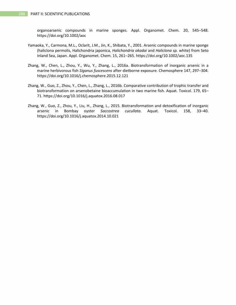
288 PART II: SCIENTIFIC PUBLICATIONS
organoarsenic compounds in marine sponges. Appl. Organomet. Chem. 20, 545–548. https://doi.org/10.1002/aoc
Yamaoka, Y., Carmona, M.L., Oclarit, J.M., Jin, K., Shibata, Y., 2001. Arsenic compounds in marine sponge (haliclona permolis, Halichondria japonica, Halichondria okadai and Haliclona sp. white) from Seto Inland Sea, Japan. Appl. Organomet. Chem. 15, 261–265. https://doi.org/10.1002/aoc.135
Zhang, W., Chen, L., Zhou, Y., Wu, Y., Zhang, L., 2016a. Biotransformation of inorganic arsenic in a marine herbivorous fish Siganus fuscescens after dietborne exposure. Chemosphere 147, 297–304. https://doi.org/10.1016/j.chemosphere.2015.12.121
Zhang, W., Guo, Z., Zhou, Y., Chen, L., Zhang, L., 2016b. Comparative contribution of trophic transfer and biotransformation on arsenobetaine bioaccumulation in two marine fish. Aquat. Toxicol. 179, 65–71. https://doi.org/10.1016/j.aquatox.2016.08.017
Zhang, W., Guo, Z., Zhou, Y., Liu, H., Zhang, L., 2015. Biotransformation and detoxification of inorganic arsenic in Bombay oyster Saccostrea cucullata. Aquat. Toxicol. 158, 33–40. https://doi.org/10.1016/j.aquatox.2014.10.021
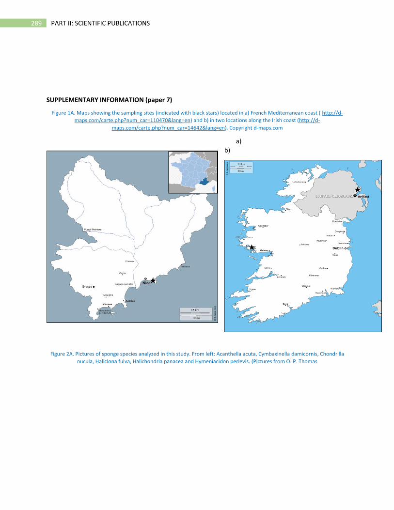
289 PART II: SCIENTIFIC PUBLICATIONS
SUPPLEMENTARY INFORMATION (paper 7)
Figure 1A. Maps showing the sampling sites (indicated with black stars) located in a) French Mediterranean coast ( http://d-
maps.com/carte.php?num_car=110470&lang=en) and b) in two locations along the Irish coast (http://d-
maps.com/carte.php?num_car=14642&lang=en). Copyright d-maps.com
a)
b)
Figure 2A. Pictures of sponge species analyzed in this study. From left: Acanthella acuta, Cymbaxinella damicornis, Chondrilla
nucula, Haliclona fulva, Halichondria panacea and Hymeniacidon perlevis. (Pictures from O. P. Thomas
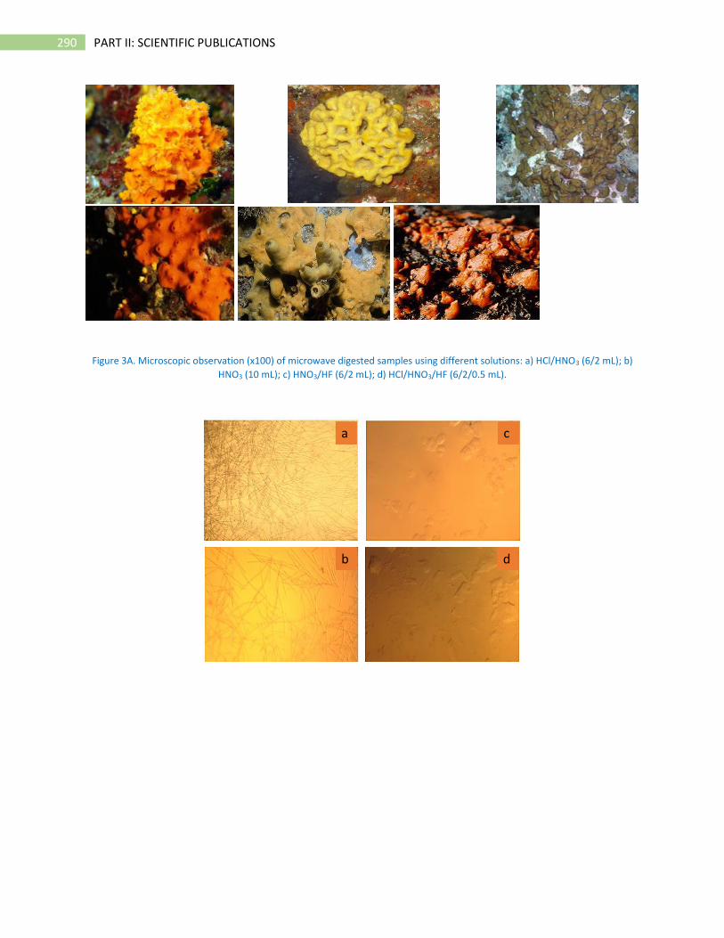
290 PART II: SCIENTIFIC PUBLICATIONS
Figure 3A. Microscopic observation (x100) of microwave digested samples using different solutions: a) HCl/HNO3 (6/2 mL); b)
HNO3 (10 mL); c) HNO3/HF (6/2 mL); d) HCl/HNO3/HF (6/2/0.5 mL).
b
ca
d

291 PART II: SCIENTIFIC PUBLICATIONS
Figure 2S. Chromatograms obtained for the specimen A of each specie analyzed in this study. For C. nucula (CHO S), refers to a
specimen collected at the surface (20 m). Chromatograms were corrected by subtraction of the background baseline (obtained
by the chromatogram of the extracted blank sample).

292 PART II: SCIENTIFIC PUBLICATIONS
Table 1A. Total As results from Haliclona fulva sponge samples (m=100 mg) obtained by different mineralization methods
0
2000
4000
6000
8000
10000
12000
0 2 4 6 8 10
Inte
nsi
ty (
cts)
Time (min)
Mediteranean sponges (Sep. 2016)
HAL A
ACA A
CHO S A
CYM A
-200
800
1800
2800
0 2 4 6 8 10Time (min)
Irish sponges (Oct. and Nov. 2016)
Bel HyP A
Bel HP1 A
HyP A
HP1 A
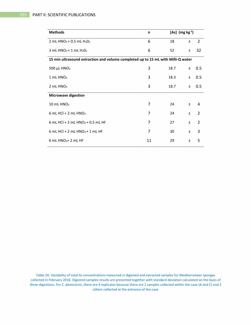
293 PART II: SCIENTIFIC PUBLICATIONS
Methods n [As] (mg kg-1)
2 mL HNO3 + 0.5 mL H202 6 18 ± 2
3 mL HNO3 + 1 mL H202 6 52 ± 32
15 min ultrasound extraction and volume completed up to 15 mL with Milli-Q water
500 µL HNO3 3 18.7 ± 0.5
1 mL HNO3 3 18.3 ± 0.5
2 mL HNO3 3 18.7 ± 0.5
Microwave digestion
10 mL HNO3 7 24 ± 4
6 mL HCl + 2 mL HNO3 7 24 ± 2
6 mL HCl + 2 mL HNO3 + 0.5 mL HF 7 27 ± 2
6 mL HCl + 2 mL HNO3 + 1 mL HF 7 30 ± 3
6 mL HNO3+ 2 mL HF 11 29 ± 5
Table 2A. Variability of total As concentrations measured in digested and extracted samples for Mediterranean sponges
collected in February 2016. Digested samples results are presented together with standard deviation calculated on the basis of
three digestions. For C. damicornis, there are 4 replicates because there are 2 samples collected within the cave (A and C) and 2
others collected at the entrance of the cave
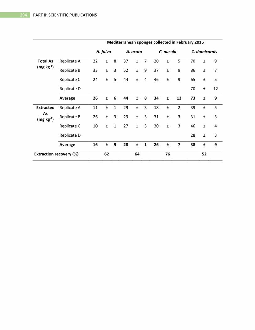
294 PART II: SCIENTIFIC PUBLICATIONS
Mediterranean sponges collected in February 2016
H. fulva A. acuta C. nucula C. damicornis
Total As
(mg kg-1)
Replicate A 22 ± 8 37 ± 7 20 ± 5 70 ± 9
Replicate B 33 ± 3 52 ± 9 37 ± 8 86 ± 7
Replicate C 24 ± 5 44 ± 4 46 ± 9 65 ± 5
Replicate D 70 ± 12
Average 26 ± 6 44 ± 8 34 ± 13 73 ± 9
Extracted
As
(mg kg-1)
Replicate A 11 ± 1 29 ± 3 18 ± 2 39 ± 5
Replicate B 26 ± 3 29 ± 3 31 ± 3 31 ± 3
Replicate C 10 ± 1 27 ± 3 30 ± 3 46 ± 4
Replicate D 28 ± 3
Average 16 ± 9 28 ± 1 26 ± 7 38 ± 9
Extraction recovery (%)
62
64 76 52

295 PART II: SCIENTIFIC PUBLICATIONS

296 PART II: SCIENTIFIC PUBLICATIONS
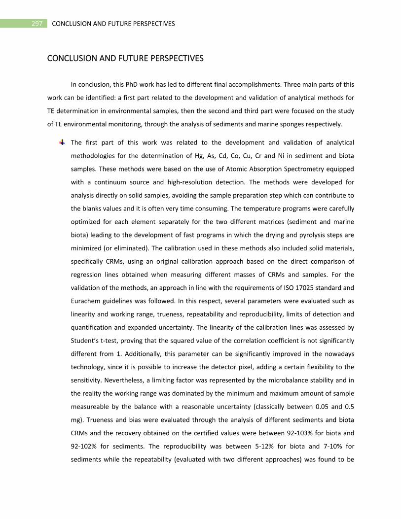
297 CONCLUSION AND FUTURE PERSPECTIVES
CONCLUSION AND FUTURE PERSPECTIVES
In conclusion, this PhD work has led to different final accomplishments. Three main parts of this
work can be identified: a first part related to the development and validation of analytical methods for
TE determination in environmental samples, then the second and third part were focused on the study
of TE environmental monitoring, through the analysis of sediments and marine sponges respectively.
The first part of this work was related to the development and validation of analytical
methodologies for the determination of Hg, As, Cd, Co, Cu, Cr and Ni in sediment and biota
samples. These methods were based on the use of Atomic Absorption Spectrometry equipped
with a continuum source and high-resolution detection. The methods were developed for
analysis directly on solid samples, avoiding the sample preparation step which can contribute to
the blanks values and it is often very time consuming. The temperature programs were carefully
optimized for each element separately for the two different matrices (sediment and marine
biota) leading to the development of fast programs in which the drying and pyrolysis steps are
minimized (or eliminated). The calibration used in these methods also included solid materials,
specifically CRMs, using an original calibration approach based on the direct comparison of
regression lines obtained when measuring different masses of CRMs and samples. For the
validation of the methods, an approach in line with the requirements of ISO 17025 standard and
Eurachem guidelines was followed. In this respect, several parameters were evaluated such as
linearity and working range, trueness, repeatability and reproducibility, limits of detection and
quantification and expanded uncertainty. The linearity of the calibration lines was assessed by
Student’s t-test, proving that the squared value of the correlation coefficient is not significantly
different from 1. Additionally, this parameter can be significantly improved in the nowadays
technology, since it is possible to increase the detector pixel, adding a certain flexibility to the
sensitivity. Nevertheless, a limiting factor was represented by the microbalance stability and in
the reality the working range was dominated by the minimum and maximum amount of sample
measureable by the balance with a reasonable uncertainty (classically between 0.05 and 0.5
mg). Trueness and bias were evaluated through the analysis of different sediments and biota
CRMs and the recovery obtained on the certified values were between 92-103% for biota and
92-102% for sediments. The reproducibility was between 5-12% for biota and 7-10% for
sediments while the repeatability (evaluated with two different approaches) was found to be
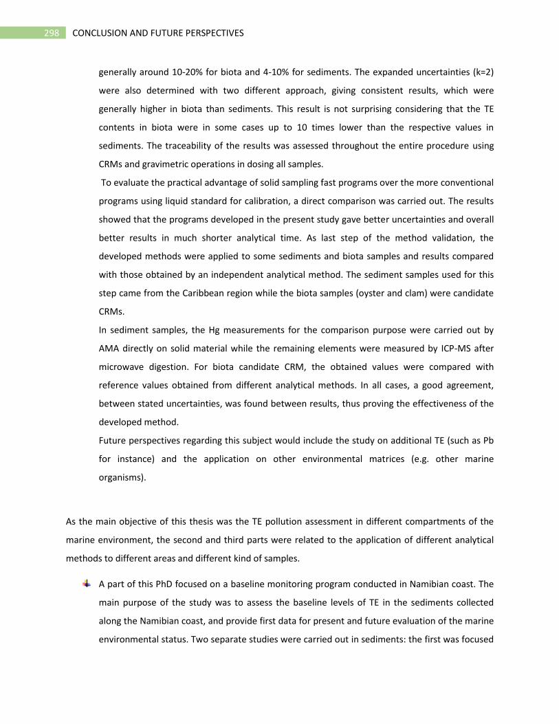
298 CONCLUSION AND FUTURE PERSPECTIVES
generally around 10-20% for biota and 4-10% for sediments. The expanded uncertainties (k=2)
were also determined with two different approach, giving consistent results, which were
generally higher in biota than sediments. This result is not surprising considering that the TE
contents in biota were in some cases up to 10 times lower than the respective values in
sediments. The traceability of the results was assessed throughout the entire procedure using
CRMs and gravimetric operations in dosing all samples.
To evaluate the practical advantage of solid sampling fast programs over the more conventional
programs using liquid standard for calibration, a direct comparison was carried out. The results
showed that the programs developed in the present study gave better uncertainties and overall
better results in much shorter analytical time. As last step of the method validation, the
developed methods were applied to some sediments and biota samples and results compared
with those obtained by an independent analytical method. The sediment samples used for this
step came from the Caribbean region while the biota samples (oyster and clam) were candidate
CRMs.
In sediment samples, the Hg measurements for the comparison purpose were carried out by
AMA directly on solid material while the remaining elements were measured by ICP-MS after
microwave digestion. For biota candidate CRM, the obtained values were compared with
reference values obtained from different analytical methods. In all cases, a good agreement,
between stated uncertainties, was found between results, thus proving the effectiveness of the
developed method.
Future perspectives regarding this subject would include the study on additional TE (such as Pb
for instance) and the application on other environmental matrices (e.g. other marine
organisms).
As the main objective of this thesis was the TE pollution assessment in different compartments of the
marine environment, the second and third parts were related to the application of different analytical
methods to different areas and different kind of samples.
A part of this PhD focused on a baseline monitoring program conducted in Namibian coast. The
main purpose of the study was to assess the baseline levels of TE in the sediments collected
along the Namibian coast, and provide first data for present and future evaluation of the marine
environmental status. Two separate studies were carried out in sediments: the first was focused
299 CONCLUSION AND FUTURE PERSPECTIVES
on a survey on surface sediments collected along the coast and offshore, to have an idea of TE
levels in the area and to identify natural and anthropogenic inputs along the coast; the second
concerned the study of historical trends of TE inputs and levels, by analyzing six core samples
coming from the same area. In both studies, TE mass fractions determined in sediments were
linked to other parameters such as grain size and organic carbon, to better understand the main
features of the sediments of the area. Some parameters such as Enrichment Factors, Geo-
accumulation Index and Pollution load index were used to evaluate possible enrichment in TE
with regards to the natural background levels of the area. Additionally, the determination of Pb
isotope ratios, used as tool to track the pollution source, was of great help and interest for the
evaluation of natural and anthropogenic Pb sources in the Namibian coast. Additionally, to TE,
also Rare Earth Elements were studied, since the area was recently discovered to be potentially
rich in this specific class of elements. The interpretation of the obtained results was rather
challenging as these studies (on surface and core sediments) represent the first literature record
of TE concentrations in the Namibian coastline. The TE results in surface sediments revealed
high enrichment of As, Cd and Sb in several sites while Pb, Cu and Zn inputs were found to be
particularly high only around Walvis Bay, the most industrialized area among the studied sites.
Additionally, the analysis of a sediment core collected in the Walvis Bay harbor revealed that the
highest inputs of these elements occurred after the year 1945. In both studies the data were
further analyzed using Pearson’s correlation and Principal Component Analysis: the purpose was
to identify possible correlations and common sources between metals. The positive correlation
found in both studies for Cu, Pb and Zn (and specifically in Walvis Bay core) confirmed that these
elements had common pattern and possibly common sources in some of the areas. The positive
correlation found for Cd and As (together with P in surface samples) can be explained by the
presence of phosphate mines in the vicinity: both Cd and As are often associated with
phosphate minerals. Apart from the sampling sites around Walvis Bay, and a few close to
Swakopmund, it can be stated that the area is rather not contaminated, as especially shown by
many of the cores analyzed in one of our studies. Elements such as Ni, Cr and Co did not show
enrichment neither in surface sediment nor in the vertical profiles, suggesting that no
anthropogenic inputs influenced their contents. The analysis of TE historical variation in the
cores revealed a significant enrichment of Pb, Zn and Cu almost entirely limited to the surface
samples coming from Walvis Bay harbor. Rare Earth Elements results did not highlight anomalies
ascribable to anthropogenic inputs but nevertheless provided a record of the typical patterns
300 CONCLUSION AND FUTURE PERSPECTIVES
found in the samples, with specific enrichment in Heavy REEs. These studies also represent the
first record of Pb isotopic composition of Namibian sediment thus providing not only the
possibility to verify a potential anthropogenic Pb input but also a record of the natural isotopic
composition of the area. The analysis of results on surface sediments highlighted and confirmed
the anthropogenic origin of Pb around the Walvis Bay area. Additionally, the measurement of Pb
isotope ratios in sediment cores revealed the big variability of the ratios in the first half of the
core collected in the Walvis Bay harbor and a more stable isotopic composition in the deep
samples meaning that after 1945 new Pb sources of anthropogenic origin affected the area. The
Pb isotope ratios trends in the other cores revealed a rather stable pattern with natural isotopic
composition characterized by 208Pb/206Pb and 206Pb/207Pb between 1.988-2.063 and 1.190-1.248
respectively. These studies on TE distribution in surface and core samples from Namibia are of
crucial importance as they provide a first record of natural and anthropogenic inputs in the area.
The importance of this baseline resides on its usefulness in future monitoring programs in the
Namibian coastal area.
Future applications and perspective should include long term monitoring programs to have
better insight on TE availability and source in the region as well as the study of different
matrices such as estuarine and coastal waters and biota.
The other compartment of the marine environment chosen for being studied in this PhD work, regarded
marine organisms, specifically marine sponges. Marine sponges were chosen among marine organisms
because of several characteristics that make them suitable bio-monitor of TE pollution.
The studies performed in this PhD work concerned six sponges’ species collected in different
sites in the Mediterranean and Irish coasts. The main purpose was to evaluate the different
abilities of these species to accumulate and/or transform TE according to sponge species,
sample sites, and seasons. Four sponge’s species were collected in the French Mediterranean
coast (Haliclona fulva, Cymbaxinella damicornis, Chondrilla nucula and Acanthella acuta) and
two species (Halichondria panicea and Hymeniacidon perlevis) were collected in two sites
located in Ireland (Kilkieran Bay and Belfast). Two types of study were performed: the first one
focusing on the TE accumulation in the different sponge species and second one on the specific
accumulation and biotransformation of arsenic.
In the first study, the mass fraction of different TE were determined in at least three replicates
of each sponges specie and the variability of the TE accumulation was determined within the
301 CONCLUSION AND FUTURE PERSPECTIVES
same species as well as between different species. TE accumulation in sponges was
demonstrated significantly different according to sponge species and the target element. C.
damicornis had specific affinity for As and Cu while Ag, Mo and Ni were found in higher
concentrations in A. acuta and Zn in H. perlevis compared to other species. The influence of
sampling sites characteristics (such as sampling depth and exposition to light) and seasons were
evaluated in Mediterranean sponges. The results indicated that sponges can be considered
representative of rather broad area without showing significant variations in TE accumulation;
the same holds true for seasonal variations. Regarding the Irish species the objective was also to
evaluate possible difference related to different TE inputs from different sites. As a matter of
fact higher concentrations of TE were generally found in sponges from Belfast, considered more
polluted area, with some exceptions (Cd and As). A common way to evaluate the extent of TE
accumulation is the calculation of BCF, using the concentrations determined in sediments
collected in the same area. The results found in this PhD work highlighted the great capabilities
of sponges to quantitatively accumulate TE within their tissue since the great majority of BCF
determined in this study were >1, regardless of the sampling site. The highest BCF were
calculated for Ag in A. acuta, (41), for Cu in C. damicornis (18), for Cd in H. panicea and H.
perlevis collected in Kilkieran (21 and 31 respectively). Some elements such as Ba, Ni and V show
rather low BCF in all species, leading to the conclusion that they are probably not involved in
biological processes within the organism.
Lead isotopic ratios were also measured in selected sponges and sediments samples from each
location, to determine whether a Pb pollution occurred and to possibly track the source of Pb.
Even though the Pb concentrations in sediments from all locations were quite low and typical of
non-contaminated areas, the isotopic data revealed a different scenario. Regarding the
Mediterranean samples, the same Pb isotopic composition was found for all analyzed samples.
The absence of linear trend in the three plot graphs and the comparison with literature data
gave confirmation that the unique source is most likely ascribable to natural source. On the
other hand, the analysis of results from Irish samples (sponges and sediments) and comparison
with literature data, showed a Pb source mostly natural for Kilkieran Bay and influenced by
anthropogenic activities in Belfast.
This part of the study on sponges highlights the tangible possibility of their use as biomonitors of
TE pollution in coastal areas as well as their possible application in environmental remediation.
302 CONCLUSION AND FUTURE PERSPECTIVES
Further investigation could include long term temporal survey and the evaluation of
bioaccumulation factors, calculated using the TE concentration in surrounding seawater.
The second study on sponges was specifically focused on the bioaccumulation and
biotransformation of arsenic, one of the most TE accumulated in sponges. A very few studies
have been published on this subject because analytical protocols need to be developed yet. In
this PhD, the analytical method has been optimized including microwave digestion for total As
determination, extraction for As speciation by HPLC-ICP-MS and HPLC chromatographic
conditions. For this purpose, the use of CRM was of crucial importance in all the optimization
steps. The study was carried out on the same sponges analyzed for TE contents and the As
species investigated were: arsenobetaine (AsB), dimethylarsinic acid (DMA), monomethylarsonic
acid (MMA) and the inorganic forms arsenate (As(+V)) and arsenite (As(+III)). The optimization
of mineralization protocol gave as a result the choice of a mixture of HNO3 and HF in microwave
assisted digestion. Several extraction solvents were tested on some sponges’ samples and the
best results were obtained when using a solution of 0.6 M H3PO4. The selected mineralization
and extraction procedures were applied to several specimens of the analyzed species and the
speciation analysis was performed by HPLC-ICP-MS. As already discussed the arsenic
accumulation (and the obtained BCF) was substantially different depending on the considered
specie. C. damicornis was by far the specie which showed the highest affinity for this element.
The speciation analysis results highlighted the predominance of AsB, as already found for
several marine organisms since it is supposed to have a crucial role in protecting organisms from
osmolytic stress in seawater. Lower amounts of DMA were also found in Mediterranean
sponges, while the concentrations in Irish sponges were negligible. The same holds true for
As(+V), equally found in small proportion. Additionally, the presence of two unknown species
here called A and B was also detected in all analyzed species and again in higher content in
Mediterranean sponges compared to Irish sponges. The As biotransformation within sponges
may be related directly to the sponge metabolism, but also indirectly by symbiotic micro-
organisms (microalgae, bacteria). This study suggests that As origins from the transformation of
the inorganic form taken up from seawater into the organic form (or forms) found in sponges’
tissue, due likely to reduction-methylation processes carried out by symbiotic sponge-bacteria.
This study highlights the possible use of sponges for bio-remediation studies, since the toxic
inorganic As species taken up from seawater are transformed in organic species, much less toxic,

303 CONCLUSION AND FUTURE PERSPECTIVES
thanks to intrinsic sponges’ biological processes (or involving symbiotic microorganisms).
Perspectives on this subject should include analytical improvements: extraction procedure,
decrease of detection limits, identification of unknown As species, as well as the study of other
arsenic species such as arsenosugars.

304
305
Résumé
Les éléments traces (ET) se trouvent naturellement dans l’environnement. Ces dernières années, des
apports croissants en ET sont induits par des activités anthropiques, causant des problèmes
environnementaux surtout dans le milieu marin. Certains ET sont toxiques et le besoin de méthodes
fiables pour leur analyse dans des échantillons environnementaux est indéniable. À travers cette thèse,
des méthodes analytiques ont été développées et validées pour l’analyse des ET dans les sédiments et
les organismes marins par spectrométrie d’absorption atomique à source continu, haute résolution et
introduction solide directe (SS-HR-CS-AAS). Des études environnementales basées sur l’utilisation de
cette méthode et d’autres ont été réalisés. Une première étude a été réalisée sur des sédiments (de
surface et carottes) collectés en Namibie. Cette thèse présente une série inédite de concentrations de
base sur la côte namibienne. Une contamination importante en Pb, Cu, Zn et Cd a été démontrée autour
des zones les plus peuplées. Les pollutions au Pb et leurs sources ont été étudiées grâce aux rapports
isotopiques du Pb. Une deuxième étude a été réalisée sur différentes espèces d’éponges marines et des
sédiments collectés en France et en Irlande. Il est montré que les éponges accumulent plus les ET que
les sédiments et de façon différente selon les espèces. Des analyses de spéciation de l’arsenic ont été
réalisées sur les éponges par chromatographie liquide haute performance couplée à un ICP-MS. Les
résultats ont montré une bioaccumulation très importante de ce métalloïde dans les éponges et sa
biotransformation des formes inorganiques en formes organiques beaucoup moins toxiques
Mots-clés : validation de méthode, métaux traces, environnement marin, sédiments, bioaccumulation,
biotransformation
Abstract
Trace elements (TE) naturally occur in the environment but their inputs have been increasing by
anthropogenic activities in the last decades, causing environmental concerns, particularly in coastal
ecosystems. TE are toxic and the need of reliable methods for their determination in environmental
samples is undeniable. The first part of this PhD was focused on the development and full validation of
methods for the analysis of TE in sediments and marine organisms by Solid Sampling High Resolution
Continuum Source Atomic Absorption Spectrometry (SS-HR-CS-AAS). Second, environmental studies
based on these and other methodologies were then performed. A first monitoring survey was
performed on sediments (surface and core samples) collected along the Namibian coast. This thesis
provides the first baseline of TE contents and historical record of pollution in the area. Significant Pb, Cu,
Cd and Zn enrichments were highlighted around the most populated areas, providing a needed baseline
for present and future evaluation of the Namibian marine environment. Pb pollutions and their sources
were also tracked using Pb isotope ratios. A second monitoring survey was performed on different
marine sponges and sediments collected in the French Mediterranean and in the Irish coasts. This work
showed that sponges accumulate more TE than sediments in different extents according to species.
Arsenic speciation analysis was performed in sponges by High Performance Liquid Chromatography
(HPLC) coupled with ICP-MS. This special focus on arsenic highlighted the great bioaccumulation of this
metalloid in sponges and its biotransformation from inorganic forms to less toxic organic forms
Key words: method validation, trace elements, marine environment, sediments, bioaccumulation,
biotransformation

306
Copyright © 2022 FDOKUMEN