
part 1 : the thermodynamics of liquid - CiteSeerX
241
PART 1 : THE THERMODYNAMICS OF LIQUID MIXTURES PART 2 : AN INVESTIGATION INTO THE LOW TEMPERATURE BLEACHING OF A COTTON NON-WOVEN FABRIC USING HYDROGEN PEROXIDE URSULA PENELOPE GOVENDER B. Se. (Hons), University of Natal, Pietermaritzburg THESIS submitted in partial fulfilment of the requirements for the degree of MASTER OF SCIENCE in the Department of Chemistry and Applied Chemistry at the University of Natal, Durban December 1993
-
Upload
khangminh22 -
Category
Documents
-
view
1 -
download
0
Transcript of part 1 : the thermodynamics of liquid - CiteSeerX

PART 1 : THE THERMODYNAMICS OF LIQUID
MIXTURES
PART 2 : AN INVESTIGATION INTO THE LOW
TEMPERATURE BLEACHING OF A
COTTON NON-WOVEN FABRIC
USING HYDROGEN PEROXIDE
URSULA PENELOPE GOVENDER
B. Se. (Hons) , University of Natal, Pietermaritzburg
THESIS
submitted in partial fulfilment of the requirements for the degree of
MASTER OF SCIENCE
in the Department of Chemistry and Applied Chemistry at the
University of Natal, Durban
December 1993

DECLARATION
The experimental work described in this thesis was carried out in the Department of
Chemistry and Applied Chemistry, University of Natal, from March 1992 to December 1993
under the supervision of Professor Trevor Letcher.
These studies represent original work by the author and have not been submitted in any form
to another university. Where use was made of work by others, it has been duly
acknowledged in the text.

ACKNOWLEDGEMENTS
The author wishes to thank :
Professor T.M. Letcher, under whose supervision this research was conducted, for his
guidance and encouragement throughout the course of this study.
Professor Urszula Domanska for rekindling my enthusiasm, for her moral support and her
interest.
Professor M. Sankar for the use of his microcalorimeter and his helpful suggestions.
Ms. Sazi Lutseke for her encouragement and advice.
Mr. George Naidoo of Sybron Chemicals, Mr. Ivan Veerasamy of The Frame Group and
Ms. Wendy Baier for their invaluable assistance with some of the results.
The technical staff of the Chemistry Department at the University of Natal for their
invaluable assistance, most especially Mr. Dave Balson, Mr. Logan Murugas, Ms. Brenda
Joshua and Mr. Roop Singh.
Mr. Allaister Elliot for his helpful discussions and advice.
My friends and colleagues in the department, for their support, help and advice.
The FRD, Johnson & Johnson and Alliance Peroxide for financial assistance.
My family for their interest and support, most especially my sister.
My fiance, Kubaren, for his forbearance, understanding and infinite moral support and for
being a part of my world.
111

ABSTRACT
This thesis is presented in two parts. In part one, the excess molar volumes and the excess
molar enthalpies have been determined for several binary systems at 298.15 K using an LKB
flow microcalorimeter and/or a 2277 Thermal Activity Monitor and an Anton Paar Digital
Densitometer.
The excess molar volumes and excess molar enthalpies, V; and H; , have been determined
for systems involving an alkanol (I-propanol, 2-propanol) mixed with a hydrocarbon (1
hexene, I-heptene, l-octene, I-hexyne, I-heptyne, l-octyne). The results show trends
relating to the degree of unsaturation of the hydrocarbon to the position of the hydroxyl
group on the alkanol.
The excess molar volumes and excess molar enthalpies, V; and H; of {di-n-butylamine +
diethyl ether or dipropyl ether or di-l-methylethyl ether or dibutyl ether or 1,1 dimethylethyl
methyl ether or 1,1 dimethylpropyl methyl ether or tetrahydrofuran or tetrahydropyran or 1,4
dioxane} have been measured over the whole composition range at the temperature 298.15
K in order to investigate di-n-butylamine - ether interactions. The V; values for each of the
systems studied are negative with the exception of the mixtures of (di-n-butylamine + dibutyl
ether or tetrahydrofuran or tetrahydropyran or 1,4 dioxane. The H; results over the whole
mole fraction range are formed endothermically.
iv

Measurements were also made on mixtures involving (a cycloalkane + a pseudo
cycloalkane). The congruency theory was tested for the (cycloalkane + pseudo-cycloalkane)
mixture. The cycloalkane mixtures studied here did not satisfy the null test of the congruency
principle.
In the second part of this thesis the main aim of the investigation was to apply ambient
temperature hydrogen peroxide bleaching techniques to a novel non-woven fabric and to
optimize the treatment conditions for this technique.
Five cold-pad batch bleaching formulas were applied to the non-woven and the sample fabrics
were analyzed for the following properties
a) fluidity (measure of degree of degradation of the cotton fibre as a result of the bleaching
process)
b) wettability (absorbency)
c) whiteness (using instrumental techniques)
d) inherent fibre surface properties (SEM)
A method was elucidated for the cold batch bleaching of the non-woven which produced a
fabric with minimum fibre damage, an acceptable degree of whiteness and excellent
absorbency properties. The treatment parameters of time (Xl), temperature(x2) and hydrogen
peroxide concentration (x3) for this method were optimised using a multiple regression
analysis for three variables and response surface plots.
v

CONTENTS
Acknowledgements
Abstract
PARTl
CHAPTER 1
CONTENTS
THE THERMODYNAMICS OF LIQUID MIXTURES
INTRODUCTION
PAGE
111
IV
xi
1
CHAPTER 2 EXCESS MOLAR FUNCTIONS OF MIXING 3
2.0 Introduction 3
2.1 Excess Molar Volumes of Mixing 4
2.1.1 Measurement of Excess Molar
Volumes 4
2.1.2 Error Analysis for the V~ data 12
2.2 Excess Molar Enthalpies of Mixing 13
2.2.1 Calorimetric Measuring Techniques 14
2.3 Experimental 20
2.3.1 Materials 20
2.3.2. Apparatus Details 22
2.3.2.1 Equipment Description 23
(a) V; measurements 23
(b) H; measurements 30
2.4 Results 41
2.5 Discussion 66
2.5.1 Mixtures of I-alkenes +(I-propanol or 2-propanol) 66
2.5.2 Mixtures of l-alkynes +(I-propanol or 2-propanol) 72
2.5.3 Mixtures of (di-n-butylamine +ethers) 78
vi

CONTENTS
CHAPTER 3 THE PRINCIPLE OF CONGRUENCE
3.1 Introduction
3.2 Short Description of the Application of the
Congruency Principle to Ternary Mixtures
3.3 Experimental
3.3.1 Materials and Apparatus
3.3.2 Preparation of Mixtures
3.4 Results
3.5 Discussions
90
90
91
95
95
95
95
100
CONCLUSIONS and FUTURE WORK
REFERENCES
PART 2 AN INVESTIGATION INTO THE LOW
TEMPERATURE BLEACHING OF A COTTON
NON-WOVEN FABRIC USING HYDROGEN PEROXIDE
103
105
113
CHAPTER 4 INTRODUCTION AND LITERATURE REVIEW
4.1 Introduction
4.2 The Stages in the Production of the
Cotton Patterned Non-Woven Fabric
4.3 Preparation Processes of Cellulosic Fibres
4.4 Hydrogen Peroxide Bleaching
4.4.1 The Role of Chemicals in Hydrogen Peroxide
Bleaching
4.5 Cold Pad Batch Bleaching
vii
114
114
116
117
122
124
127

CONTENTS
CHAPTERS BLEACHING TREATMENTS USED IN THIS WORK
5.1 Introduction
5.2 Bleaching Treatments Investigated in this Work
5.3 Apparatus and Experimental Procedure
5.3.1 Materials
5.3.2 Experimental Methods
133
133
133
138
138
139
CHAPTER 6 EVALUATION OF THE BLEACHED COTTON PATTERNED
NON- WOVEN FABRIC 141
6.1 Introduction 141
6.2 The Degree of Chemical Degradation of the
Cotton Patterned Non-Woven Fabric Samples 143
6.2.1 Introduction 143
6.2.2 Fluidity Test 144
6.2.3 Experimental 145
6.2.4 Results 148
6.2.5 Discussion 150
6.3 Determination of the Wettability of the Bleached
Cotton Patterned Non-Woven Fabric 151
6.3.1 Introduction 151
6.3.2 General Properties of Water towards Cellulose 151
6.3.3 Factors which Determine the Absorbency of
the Cotton Patterned Non-Woven Fabric 152
6.3.4 Experimental 153
6.3.5 Results 154
6.3.6 Discussion 155
6.4 Whiteness of the Bleached Fabric 156
6.4.1 Introduction 156
6.4.2 Experimental 157
viii

CONTENTS
6.4.3 Results
6.4.4 Discussion
6.5 Conclusions
157
159
164
CHAPTER 7 SCANNING ELECTRON MICROSCOPE
INVESTIGATION OF THE
UNBLEACHED AND BLEACHED COTTON PATTERNED NON-
WOVEN FABRIC 165
7.1 Introduction 165
7.2 The Surface Structure of Cotton Patterned Non-Woven Fabric 166
7.3 Experimental 168
7.4 Results 168
7.5 Discussion 177
7.6 Conclusions 180
CHAPTER 8
CHAPTER 9
OPTIMISATION OF THE SINGLE STAGE BLEACHING
PROCESS USING REGRESSION ANALYSIS
8.1 Introduction
8.2 Basic Theory of Regression Analysis
8.3 Experimental
8.4 Results
8.5 Discussion
CONCLUSIONS
181
181
181
184
185
188
193
LIST OF PUBLICATIONS
REFERENCES AND APPENDICES
REFERENCES
ix
194
195
196

CONTENTS
APPENDICES 201
APPENDIX 1.1 201
APPENDIX 1.2 204
APPENDIX 1.3 206
APPENDIX 2.1 208
APPENDIX 2.2 209
APPENDIX 2.3 216
APPENDIX 2.4 219
APPENDIX 2.5 221
x

PART 1
THE THERMODYNAMICS OF LIQUID
MIXTURES
Xl

Chapter 1: Introduction
CHAPTERl
Introduction
Thermodynamics is a useful probe to help better understand molecular interactions in
solution(l). In particular experimental excess functions of liquids mixtures are useful in that
they provide data to test theories of liquid mixtures and provide a guide for the formulation
of new theories(2). For instance, the determination of excess molar enthalpies of aqueous
solutions of hydrocarbons is important in understanding and improving the theories of
hydrophobic interaction and hence increasing the knowledge into the nature of many
biological systems(3). In industry, reliable excess molar enthalpies and excess molar volumes
is all important in the design of chemical plants and reactors(2) •
The material in the first part of this thesis is concerned with determining excess molar
volumes and excess molar enthalpies, V; and H; for binary liquid mixtures, with the aim
of testing various thermodynamic theories. This work has involved the experimental
determination of excess properties for systems concerning molecules not only differing in
shape and size, but also with mixtures where one of the components contains multiple bonds.
V; and H; have been determined for binary systems involving mixtures of (I-alkene or 1
alkyne + an alkanol). The alkanols used were I-propanol, or 2-propanol. These results. (79)
were compared to previously reported excess functions for binary mixtures of a I-alkene, or
l-alkyne with methanol and ethanol, and of an n-alkane with an alkanol, in order to
determine the effect of the double bond on the I-alkene, or the triple bond on the l-alkyne,
on the measured properties.
Excess thermodynamic properties have also been measured for mixtures of {di-n-butylamine
(DBA) + an ether}. The various trends and observations have been compared to work. led· . I· {·b I· (\7,98)preVIOUS y report concernIng systems Invo vIng tn uty amIne (TBA)' ., or acetonitrile
(A~~,64- an ether}. The effect of the n-chain ether, the branched ether and the cyclic ether
molecules on the results was observed.
1

Chapter 1: Introduction
The final set of mixtures investigated in this section involves mixtures of cycloalkanes +
pseudo-cycloalkanes. This set of mixtures presented an opportunity to test the principle of
congruence. (112) The theory of congruence, first proposed by Bronsted and Koefoed, (111) is
used to correlate and predict several thermodynamic properties, such as activity coefficients,
the excess Gibbs free energy of mixing, the excess enthalpy of mixing, and the excess
volume of mixing. The results of the cycloalkanes + pseudo-cycloalkanes mixtures were(126)
compared to the recently reported results for the n-alkane + pseudo-n-alkane mixtures.
2

Chapter 2: Excess Molar Functions••..••
Chapter 2
Excess Molar Functions of Mixing
2.0 INTRODUCTION
By definition(l) the excess molar functions of mixing, X; for a binary mixture is given by
the relation
2.1
where~ is the ideal behaviour of the thermodynamic property X for the mixing process.
Excess functions have been utilized to represent(2) the changes in thermodynamic properties
of mixing from the ideal behaviour i.e. the deviations from ideality.
In this work the excess molar enthalpies, H;, and excess molar volumes, V;, of mixing
were determined for the following binary systems: mixtures of an unsaturated hydrocarbon
[an I-alkene or an I-alkyne] + an alkanol [I-propanol or 2-propanol]; di-n-butylamine
(DBA) + an ether [diethyl ether or dipropyl ether or di-l-methyl ethyl ether (IPE) or dibutyl
ether or 1, I-dimethyl ethyl methyl ether (TBME) or 1, I-dimethylproyl methyl ether (TAME)
or tetrahydrofuran (THF) or tetrahydropyran (THP) or 1,4-dioxane] , over the whole
composition range at the temperature 298.15 K.
The results of (an unsaturated hydrocarbon + an alkanol) binary liquid mixture are
discussed with reference to cited alkane + alkanol work. (3,4) The thermodynamic mixing
properties for the (DBA + an ether) are compared to recently reported H; and V; results
for { acetonitrile (AN) (5,6), or tri-butylamine (TBA) (97,98t + an ether}. The binary
experimental values for {DBA + an ether} are correlated by means of the UNIQUAC and
NRTL models.
3

Chapter 2: Excess Molar Functions.••.•.
2.1 Excess Molar Volumes of Mixing
The volume change on mixing of binary liquid mixtures, V;, at constant pressure is of
interest to a thermochemist because of two reasons:(!)
a) they serve as accuracy indicators for theories of liquid mixtures dealing with
thermodynamic properties, and
b) from a practical point of view, experimentally reliable results are relatively easy to
obtain. (!)
2.1.1 Measurement of Excess Molar Volumes
The excess molar volume, V;, at a concentration of xA of component A is defined as(1)
2.2
where the last term is the ideal molar volume of the mixture. The volume changes for binary
mixtures, V;, can be determined experimentally in one of two ways, namely (i) indirectly
from density ( densitometer or pycnometric) measurements, or (ii) from the more direct
dilatometric methods, ie. by measuring the resultant volume change upon mixing of the two
components.
Both these experimental methods have been extensively reviewed by Battino, (!) Letcher, (8)
Handa and Benson,(9) and by Stokes and Marsh. (10,11,12)
a) Pycnometer
There is a wealth of reference in the literature of a variety of types of pycnometer. (13,14,15)
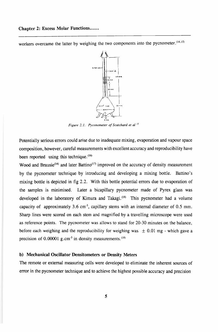
One of the earliest described pycnometer was that of Scatchard, Wood and Mochel(15) and is
illustrated in fig. 2.1. This single arm pycnometer was used to obtain density measurements
with precision of 0.00001 g.cm-3. Basically, this pycnometer has a bulb with a capacity of
11 cm3, a 1 mm internal diameter precision capillary with 11 lines lightly etched around the
stems, and spaced 1 mm apart. (15)
During measurement, the bulb is filled using a hypodermic syringe and cannula and the
composition of the mixtures have to be known with a large degree of accuracy. Many
4
Chapter 2: Excess Molar Functions.•.•..
workers overcame the latter by weighing the two components into the pycnometer. (14,15)
=r_ 60-,,,-'8i-aOmm
1
\J2mm
IFigure 2.1. Pyconometer of Scatchard et al 15
Potentially serious errors could arise due to inadequate mixing, evaporation and vapour space
composition, however, careful measurements with excellent accuracy and reproducibility have
been reported using this technique. (16)
Wood and Brausie(14) and later Battino(l7) improved on the accuracy of density measurement
by the pycnometer technique by introducing and developing a mixing bottle. Battino' s
mixing bottle is depicted in fig 2.2. With this bottle potential errors due to evaporation of
the samples is minimised. Later a bicapillary pycnometer made of Pyrex glass was
developed in the laboratory of Kimura and Takagi. (18) This pycnometer had a volume
capacity of approximately 3.6 cm-3, capillary stems with an internal diameter of 0.5 mm.
Sharp lines were scored on each stem and magnified by a travelling microscope were used
as reference points. The pycnometer was allows to stand for 20-30 minutes on the balance,
before each weighing and the reproducibility for weighing was ± 0.01 mg - which gave a
precision of 0.00001 g.cm-3 in density measurements. (18)
b) Mechanical Oscillator Densitometers or Density Meters
The remote or external measuring cells were developed to eliminate the inherent sources of
error in the pycnometer technique and to achieve the highest possible accuracy and precision
s

Chapter 2: Excess Molar Functions••....
16.5cm
1I ,
CCm)Figure 2.2. Mixing bottle of Battino 17
of the measurement results. (19) The introduction of the remote cells offers a system for liquid
measurement according to the oscillating sample tube method. (20) The density determination
is based, in principle, on measuring the period of oscillation of a vibrating U-shaped sample
tube which is either filled with sample or through which the sample is continuously flowing.
The accuracy of this method is limited to some extent by four control factors: (21) the
calibration procedure, the viscosity of the sample, the pressure of the system and the
temperature control. The density of the sample is related to the resonance frequency of an
electronically excited mechanical oscillator and the period of oscillation of the sample
contained in the oscillator. (21)
The effective mass (M) of the oscillator is composed of its own unknown mass (MJ as well
as the unknown mass of the sample, density p, contained in volume V and is given by
M = Mo - Vp
The resonance frequency is given by
27f'V = (c/M)'h = [c/(Mo + Vp)fh
2.3
2.4
where the mass M is attached to a spring of constant elasticity c, under the condition that the
oscillator performs an undamped oscillation. (9) Rearranging and making p the subject of the
6

Chapter 2: Excess Molar Functions•••.••
formulae
p = -Mo / V + (c/4~V)(1/V2) = A + B-r 2.5
where T = l/v, ie. the period ofoscillation, and A and B are constants characteristic of the
oscillator. Densities are measured relative to a reference material:
2.6
where Po is the density of the reference material and To is its corresponding period of
oscillation.
In this work, a densitometer containing an external measuring cell designed by
Kratky et al (22) and commercially marketed by Anton Paar (Graz. Austria) is used. It
consists of a U-shaped hollow borosilicate glass oscillator or sample tube, mounted in a dual
wall glass cylinder filled with a gas of high thermal conductivity to facilitate a rapid
temperature equilibration of the sample inside the oscillator. B from equation 2.6 is
determined by obtaining T with two calibration measurements with samples of known
densities ie. air and distilled water. The precision obtained in T is 0.000002Hr1• Details
of the Anton Paar vibrating tube densitometer is given in the experimental section - 2.3.2.
Developments by Handa and Benson et azr9) show that in order to obtain a precision of 0.001
cm3•mol-1 in V;, the composition should be precise to five significant figures and density
readings precise to six significant places. Further to this, Battino(7) reported that the
measuring cell temperature must be controlled to ±0.001 K to accurately determine densities
to OO2סס.0 g.cm-3•
c) Direct Measurements - Batch Dilatometers and Continuous Dilution Dilatometers
Highly accurate measurements are obtained by direct measurements using dilatometry, (1,9)
without the need for time consuming procedures such as pycnometer filling, weighing etc.
and errors arising from weight, composition or temperature determination of samples. Direct
dilatometric measurement of V~ gives a much higher ratio of accuracy to effort. (1) A suitable
and simple dilatometer is shown in fig.2.3. (1) The dilatometer is filled with a hypodermic
7

Chapter 2: Excess Molar Functions••••••
syringe. Mixing was achieved by gently rocking the dilatometer to and fro. The excess
molar volume of mixing, V;, is given by the relation: (neglecting small terms allowing for
the effects of the change of pressure on mixing of the volumes of the liquids and of the
mercury)
2.7
where A is the cross sectional area of the capillary and nA and nB are the amounts of
substance of A and of B.
(b)
. -mercury
Figure 2.3 A dilatometer for measurements of volume ofmixing showing (a) before mixing (b) after mixing(l)
8

Chapter 2: Excess Molar Functions••••••
There have been fundamentally two types of dilatometric apparatus designed for the direct
measurement of volume change(9): (i) one composition per loading of the apparatus at a
single temperature or batch dilatometers, and (b) a number of compositions per loading at
a single temperature or continuous dilution dilatometers. (9)
(i) Batch Dilatometry
One of the early examples of a design for a single loading dilatometer was the apparatus by
Keyes and Hildebrand in 1917. (23) As seen in fig.2.4, it consists of a U-tube with mercury
filling the bottom of the vessel in order to separate the two sample components A and B.
Graduated capillaries on the two arms provided the means by which the volumes, before and
after mixing, were determined. The entire mixing vessel was immersed in a thermostatted
bath, and mixing was achieved by rocking the apparatus to and fro. It was reported that
precision of +0.003 cm-3·mot1 in V; could be achieved over the temperature range
280-350 K. (23,7)
Fig 2.4 Keyes and Hildebrand dilatometer3
Duncan, Sheridan and Swinton(25) in their reviews, describe methods and a modified
dilatometer apparatus in which the precision was found to be ± 0.002 cm3·mol-1 or ± 0.5%
9

Ch.apter 2: Excess Molar Functions•••.••
in V;. (24,25)
Errors arising in batch dilatometer include the failure to take into account the a
compressibility correction (a 1 % possible error in V;), corrections due to temperature
fluctuations and the fact that extreme care has to be taken to avoid excessive amounts of
grease on the joints. (26)
The primary disadvantage of the batch dilatometer was the speed of measurement, ie. each
loading of the dilatometer only gave a single V; reading.
(ii) Continuous Dilution Dilatometry
The fundamental disadvantage of the batch dilatometer was eliminated by introduction of the
many compositions per loading dilatometer ie. dilution dilatometry. The original design of
the dilution dilatometer was arguably that by Geffcken, Kruis and Solana.(n) It has the
mixing chamber C initially loaded with pure component A and mercury (as seen in fig. 2.5).
stopcock S leads to reservoir R where pure component B is kept over mercury. The change
in the mercury level upon mixing is read directly from the calibrated and graduated capillary
D. The entire apparatus is kept in a thermostatted vessel. When S is opened, mercury from
C forces some of component B into C via the connecting tube E. S is then closed and mixing
begins. The change in level of mercury in capillary D is read directly. Increments of B are
added in a similar way in order to determine V; as a function of composition at one
temperature. (21)
o E
8 R
Fig 2.5 Dilution dilatometer of Geffcken. Kruis and Solana(27)
10

Chapter 2: Excess Molar Functions....•.
Many workers have modified and adopted Geffcken et al's original design: (29-34)
Stokes et ai(32) modified Geffcken et ai's design by having component B confined in a burette
above which component A is confined in a bulb, both over mercury. The two compartments
are attached to a fine stainless steel tube, and known fractions of component B enter into the
the bulb (containing A) by means of mercury flowing in the opposite direction via a
stopcock. This design facilitates easier loading and usage. (32) Kumaran and McGlashan(33)
designed a tilting dilatometer; this tilting dilatometer is advantageous in that it reduces error
because there are no taps to open and close during a measurement rather- mixing is achieved
by tilting. (33) This design facilitates easier loading and calibration and allows for
measurement of volume changes of any magnitude. Moreover, in the dilatometer designed
by Kumaran and McGlashan, (33) the two liquids are separated by mercury at all stages of a
run instead of only a diffusion boundary in a capillary as in previous dilatometer designs. (32,34)
The dilatometer designed by Kumaran and McGlashan(33) is similar to the one depicted in fig.
2.6 except that capillary C has a larger bore size and it has a calibrated bulb X blown at the
bottom of the calibrated burette A. The presence of the bulb X eliminates the need to
calibrate the mixing cell B. Before the start of the run, bulb B is filled with mercury and
burette A with one of the sample components. After thermal equilibrium and with stopcock
Tt removed, mercury from B is transferred into X thus creating space of known volume in
B. (33) A standard deviation of 0.0007 cm3.mott for V; for this type of dilatometer has been
reported. (33)
There have been two major reported disadvantages for dilution dilatometers. (9) Firstly,
relatively large volumes (50-100 cm3) of highly purified components are required; and
secondly, specifically for the dilatometers described here(32,33,34) , to measure a change in
volume at constant pressure, a correction must be made. That is, a change in the height (Jih)
of the mercury meniscus in the capillary causes a change in the mixing cell pressure equal
to pgJih, where p = density of mercury. Errors in V; of 1-2 % can accrue in this manner.(9)
Tanaka et ai(35) improved on the McGlashan type dilatometer to produce a dilatometer capable
of extremely sensitive precision.
11

Chapter 2: Excess Molar Functions .
,.. ...I\'" /
bulb X
c
Fig 2.6 Similar designed tilting dilatometer of Kumaran and McGlashan 34
2.1.2 Error Analysis for the V~ data obtained from density values used in this work
Appendix 1.1 gives a detailed error analysis. In principle, to obtain a maximum error of
0.002 cm3·mol-1 in V;, the masses must be known to a precision of 0.00001 g, the T values
to 2xl<J6 Hz-1 and the densities to lxl0"5 g.cm-3•
12

Chapter 2: Excess Molar Functions..••..
2.2 Excess Molar Enthalpies of Mixing
All chemical and physical reactions have a net heat evolution which gives basic information
on the mechanism and extent of reaction, a process which often only calorimetry can detect
and measure. (36) For binary liquid mixtures, the excess molar enthalpies of mixing, H;, may
in principle, (37) be defined by the relation
2.8
However, this is not considered a satisfactorily accurate method. It has been reported that
the errors in H; derived in this way are approximately 15 times as large as the error in the
free energies from which it is derived. (2) For this reason the most precise values of H; are
those measured directly by means of a calorimeter.
In principle, the direct measurement of heats of mixing is quite simple. The basic design
involves a cell in which the two liquids are initially separated. (2) All that is required is an
apparatus in which known quantities of two liquids can be brought to a constant temperature,
a thermometer to measure the temperature change when the two liquids are mixed and an
electrical heater in which measured amounts of energy can be dissipated in order to calibrate
the apparatus. (2,38,39) A simple apparatus in which approximate measurements of heats of
mixing may be made is shown in fig 2.7. (2) Measured quantities of two liquids are placed
in the vessels A and B in a thermostat bath. Mixing is brought about by forcing the liquid
from A over into B and the temperature change on mixing is measured by the thermometer
C. The heat capacity of the apparatus is determined for each experiment by passing a
measured current through the heater D of known resistance for a measured time. The
enthalpy of mixing is then given by the relation
2.9
where d T1 is the temperature change on mixing, ~ T2 is the temperature rise on calibration,
13

Chapter 2: Excess Molar Functions••••••
R is the resistance of the heater, I is the current of the heater, and t is the time for which the
current flows. (2)
The isothermal calorimeters used in this work is a commercial LKB 2107-107 flow
microcalorimeter and the Thermometric 2277 Thermal Activity Monitor. The excess molar
enthalpies, H;, were determined for the same binary liquid systems for which the excess
molar volumes are reported.
I) ~cl ~y--~
7:-'/l ~1L \\/' "'~.'.' " / ( 1
-LT:,:! I I: 1
I '
I
IiJ.J.DH
Jf
iI
IlA
lJ
Fig 2. 7 Simple apparatus for measurements ofheats ofmixint
2.2.1 Calorimetric Measuring Techniques
The enthalpies of mixing are measured in calorimeters of which many types have been
described. (40,41,42) The most commonly used methods in calorimetry are the adiabatic and
isothermal methods. In the adiabatic experiments, the two liquids are mixed in an isolated
vessel (Le vacuum jacket) which is thermally insulated from its surrondings. (42) If the excess
14

Chapter 2: Excess Molar Functions .
enthalpy ,H; is positive, there will be a lowering of the temperature on mixing. This drop
in temperature may be nullified .by the simultaneous supply of heat. Such a process is
considered nearly isothermal and any small difference can be corrected for by observing the
temperature change for a calculated supply of electrical energy. (43) If H; is negative, then
the mixture warms on mixing. Such exothermic mixing requires two experiments - one to
measure the temperature rise on mixing and the other to measure the amount of electrical
energy needed to produce such a rise. (43)
The single most important point in the design of any calorimeter for the heats of mixing is
that when the mixture is formed in a vessel in which there is a vapour space(2) there will be
on mixing a change in the composition of the vapour corresponding to the changes in the
partial pressure of the components in the mixture. (2) Corresponding to these changes in
vapour composition there will be evaporation and condensation of small quantities of the
volatile liquids. (1,2,42) When the heat of mixing is small, evaporation or condensation of as
little as 10-2to 10-3 mole of liquid can produce a heat effect as large or larger than that of the
heats of mixing.(44) McGlashan(2) has reported that vapour spaces of up to 0.25 cm3 could
lead to an error in H; of ±100 J. mot1. For this reason much effort has gone into designing
mixing vessels in which vapour spaces are completely eliminated. Accounts in the
literature(45-50) can be found of all kinds of mixing vessel for calorimeters, such as combustion
bomb calorimeters used in the determination of enthalpies of combustion; flame calorimetry
used in the determination of enthalpies for sufficiently volatile substances including gases;
flow calorimeters used in the measurement of enthalpies of reaction between fluids,
microcalorimeters for the measurement of values for IH; I less than 1 kJ between liquids
and "explosion calorimeters" specially designed for the study of reactions between metals at
high temperatures. (1,42) Hirobe's mixing vessel(42) developed in 1914 was arguably the first
mixing vessel which attempted to keep vapour spaces as small as possible. Hirobe's mixing
vessel is shown in fig. 2.8. The liquids are initially separated by mercury, and in contact
with vapour spaces which were kept at a minimum. Mixing comes about by inversion of the
vessel by means of the threads, A shown in the figure.
15

Chapter 2: Excess Molar Functions•.••••
A~
Fig 2.8 Hirobe's mixing vesser42
Modified designs but with more attention focused on the reduction of the effects of vapour
spaces have been developed by later workers. (51,52) One of the major advancements in the
developments of mixing vessels was the one introduced by van der Waals in 1950<53) for his
heats of mixing measurements and is shown if fig. 2.9. It was made of brass and the liquids
were introduced into compartments A and B and isolated by means of a ground in stopper
K. The lid was screwed on against the packing L. Mixing was brought about by
manipulation of nylon threads from outside the calorimeter so as to invert the vessel and
displace K.
:l4mm
Fig 2.9 Van der Wools's mixing vessef3
16

Chapter 2: Excess Molar Functions....••
The mixing vessel of McGlashan and Larkin(54), developed in 1961, is shown in fig. 2.10.
This was one of the first calorimeters suitable for enthalpies of measurement as it eradicates
the errors due to the presence of vapour space and it did not allow for volume changes that
occurred on mixing. (2,54) The vessel consists of two compartments A and B in its upper half,
and a capillary C with bulb D which can be attached to the vessel through the ground glass
joint E and F. A heating element, H, and four thermistors (T1 to T4) distributed over the
surface of the mixing vessel forms part of the Wheatstone bridge assembly. The vessel is
filled completely with and immersed in a bowl of mercury. The mercury is displaced from
the upper compartments by introducing weighed quantities of the mixture through the opening
on A by means of a hypodermic syringe. The loaded vessel with the capillary tube, C, half
fuled with mercury and attached at the ground joint, F is placed in an evacuated enclosure
within a thermostat until temperature is achieved. After temperature equilibration, the liquids
are mixed in the absence of a vapour space by rotation of the apparatus through 180 0, the
direction of rotation being such that the liquid never comes into contact with the greased
joints. The temperature change on mixing is measured by the four thermistors. (54) The
accuracy of the apparatus has been quoted at 0.7 J.moI-l of the maximum value of H;. (37,54)
One of the major disadvantages of this technique and the subsequent designs is that it takes
a long time to get a single measurement and the method cannot be readily automated.
o 1 cmL.U
=-==0sid~ vi~w
Fig 2.10 Adiabatic calorimeter ofMcGlashan and Larkin54
17

Chapter 2: Excess Molar Functions•••••.
For the most precise measurements in which enthalpies of mixing are determined with an
accuracy of +0.05 J.mot1 flow microcalorimetry was developed and advanced. (55,59)
Basically, in flow microcalorimetry, two liquids are injected at a steady known rate into a
mixing vessel, where complete mixing is achieved in the absence of a vapour space. (2) The
excess enthalpy is related to the power output of the heating element and the molar flow rates
of the two components (37) (refer to experimental section for details). The advantage of the
flow microcalorimeter is that it produces rapid, sensitive results; that both endothermic and
exothermic mixing reations can be studied, and that only small quantities (often less than 50
cm3 of each liquid) are needed for each experimental run. (1) No modem flow
microcalorimeter allows any vapour space whatsoever with a resulting precision of 1% or
better being achieved. (60-62) A flow microcalorimeter can be modified to be either adiabatic
or isothermal. (63) The adiabatic condition is achieved when the flow cell and the temperature
sensitive elements are thermally insulated from their surroundings. In the isothermal mode,
the heat of mixing in the reaction vessel is transferred to the heat sink. (63)
A general description of the history of flow microcalorimeter designs as well as the working
principles of flow microcalorimeters (both isothermal and adiabatic) is given by Monk and
Wadso in their review. (64) Amongst the earliest of these designs was that of McGlashan and
Stoeckli. (65) It was reported that this type of instrument gave an error in H; of ±1%.(65)
One major drawback in this instrument was that it required a large sample volume to cover
the whole composition range. Furthermore, heat leaks inherent in the design of the
instrument was not compensated for in the final calculation. (64,65)
A twin conduction calorimeter designed in the laboratory of Monk: and Wadso(64) and later
commercialised by the LKB company (presently taken over by Thermometric) served to
eradicate some of the uncertainties produced by the McGlashan et a(65) type calorimeter.
Basically the apparatus consists of a metal block heat sink, containing a centrally located heat
exchanger unit surrounded by calorimetric units in a twin arrangement. The calorimetric
units comprise two flow reaction cells surrounded by surface thermopiles in contact with
primary heat sinks. The heat sinks are thermally isolated and immersed in a water bath.
Heat evolved or absorbed during the mixing process is thus conducted to or from a heat sink
18

Chapter 2: Excess Molar Functions•..••.
arrangement through the semi-conductor thermopiles. Peristaltic pumps were used to
introduce the liquids into the mixing cell. (64)
Work done by Hsu and Clever(66) on the instrument developed by Monk and Wadso(64)
showed that errors could arise from flow rate variation required to cover the complete mole
fraction composition range. Errors of ±20 J.mot l in H; (66)was reported using the
recommended IUPAC(67) test system (i.e cyclohexane + n-hexane). This error was not
accounted for in H; determinations. This error becomes more substantial and serious in the
dilute mole fraction range where H; is small and the sample liquid flow rates are near their
limits. (66)
Further recent designs of flow microcalorimeters include that of Randzio and
Tomaszkiewicz(1980)(56), Siddiqi and Lucas (1982)(68) and Christensen et al (1981,(45)
1976(46». In all of these designs frictional effects (Le in difficult to mix systems the
principle measurement in the mixing cell is usually regulated via temperature measurements
from thermocouples; their is a small temperature rise due to viscous dissipation in the mixing
and reference arms of the calorimeter- this temperature difference gives rise to errors due
to frictional effects) were simply neglected and have been shown to produce substantial error
if not carefully corrected or designed for. (69)
Raal and Webley(69), in their recent design of a new differential microflow calorimeter
considered the following points as important requirements for the present day
microcalorimeter design: (in addition to the absence of vapour space and careful composition
control)
(a) Carefully designed equilibrators preceding the mixing cell and producing both
components at exactly the set calorimeter temperature at all flow rates
(b) accurate separation of frictional energy from the desired excess enthalpy and
(c) the elimination of heat leaks dependant on fluid flow rates and physical properties.
Accommodating all the above pointers, Raal and Webley(69) designed a differential microflow
19

Chapter 2: Excess Molar Functions...•••
calorimeter capable of producing H; with an accuracy of 0.53 J.mot l• They have reported
results for the (cyclohexane + n-hexane) binary liquid system (the IUPAC recommended test
system)(67) which are in excellent agreement with the data of Marsh and Stokes(7°) and is
superior in precision and accuracy to those of Grolier(57) (Picker type calorimeter), and
McGlashan and Stoeckli. (65)
The most recent developments(7I,72) by workers such as Randzio(56) and his research team are
on instrument capable of measuring H; at high temperatures and pressures as well as
instruments designed to cope with very viscous systems.
2.3 EXPERIMENfAL
2.3.1 Materials
All the liquids used in this work were tested for impurities by GeMS and glc and were kept
in a dry box before use. Some of the liquids were purified according to recommended
methods. (73) A summary of the materials, their suppliers and purities used in this work are
given in Table 2.1.
The alkenes and alkynes were fractionally distilled before use. Glc analysis of the l-alkenes
and l-alkynes showes that the impurity content was less than 0.5 mol percent. The alkanols
were purified repeatedly using previously established methods(74) in the following manner:
they were refluxed over magnesium turnings and iodine for 30 minutes and then distilled
through a 150 mm lagged glass fragment-packed column. The water impurity content in the
alkanols was determined by Karl Fischer titrations to be less than 0.02 mole percent. Glc
analyses indicated a purity of >99.8 mole percent for all the alcohols. The densities of the
of the I-propanol and 2-propanol at 298.15 K was found to be 0.7998 and 0.7815 g'cm-3,
respectively. Di-n-butylamine (DBA) was used without any further purification. The ethers
were distilled before use and dried using 0.4 nm molecular sieves and degassed before
measurement. The ethers were also analyzed for their water contamination before use ans
in all cases the mole fraction of H20 was determined to be < 0.0001. Analysis of the ethers
and the di-n-butylamine done by g.l.c. indicated that the total mole fractions of impurities
was < 0.002 for each of the liquids xcept dipropyl ether and <0.006 for dipropyl ether.
20

Chapter 2: Excess Molar Functions•••••.
Distillation of the dipropyl ether did not improve the purity and the cost of purchasing pure
dipropyl ether was prohibitive. A Varian GCMS and a Hewlett-Packard 5891A gas
chromatograph equipped with a 3393A integrator and a 25m carbowax 20Mc capillary
column was used. All the solvents were kept in a dry-box containing silica-gel and a double
access door.
Table 2.1. Materials used, their suppliers and purities
Compound Supplier Purity (mole %)
I-hexene Aldrich 99.8
I-heptene Aldrich 99.8
l-octene Aldrich 99.5
I-hexyne Aldrich 99.5
I-heptyne Aldrich 99.5
l-octyne Aldrich 99.6
propan-l-ol BDH 99.8
propan-2-o1 BDH 99.7
cyclo-5 Fluka >99
cyclo-6 Polychem 99.0
cyclo-7 Aldrich >99
cyclo-8 Janssen Chimica >99
21
Chapter 2: Excess Molar Functions .
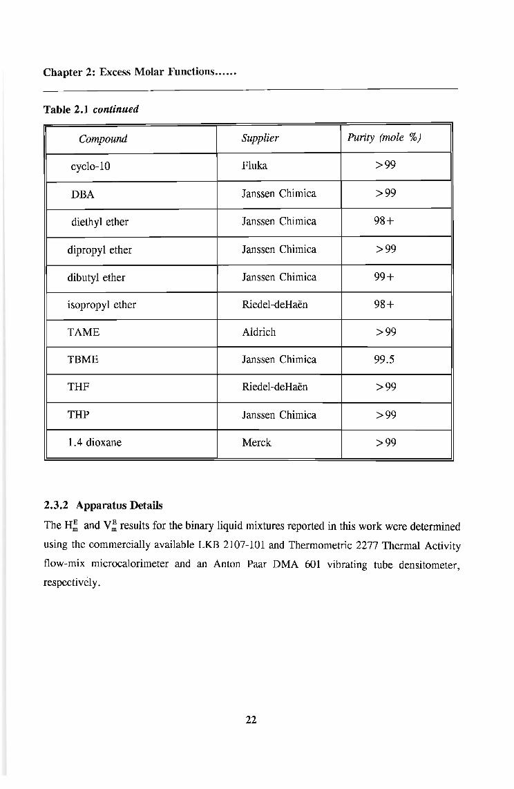
Table 2.1 continued
Compound Supplier Purity (mole %)
cyclo-10 Fluka >99
DBA Janssen Chimica >99
diethyl ether Janssen Chimica 98+
dipropyl ether Janssen Chimica >99
dibutyl ether Janssen Chimica 99+
isopropyl ether Riedel-deHaen 98+
TAME Aldrich >99
TBME Janssen Chimica 99.5
THF Riedel-deHaen >99
THP Janssen Chimica >99
1.4 dioxane Merck >99
2.3.2 Apparatus Details
The H; and V; results for the binary liquid mixtures reported in this work were determined
using the commercially available LKB 2107-101 and Thermometric 2277 Thermal Activity
flow-mix microcalorimeter and an Anton Paar DMA 601 vibrating tube densitometer,
respectively.
22

Chapter 2: Excess Molar Functions••....
2.3.2.1 Equipment Description
a) V~ measurements - Anton Poor DMA 601 vibrating tube densitometer
(i) Principle ofoperation
The laboratory arrangement for the densitometer is shown schematically in fig. 2.11. The
measuring cell is contained in it's own seperate housing and is thermally seperated from the
electronics. The oscillator or sample tube (see fig. 2.12) is made out of borosilicate glass
and is fused into a dual wall glass cylinder. The space between the U-shaped sample tube
and the inner wall of the dual wall is filled with a gas of high thermal conductivity to
facilitate a rapid temperature equilibration of the sample inside the oscillator with the
thermostat liquid which flows through the dual wall cylinder around the sample tube. An
additional shorter capillary tube inside the inner space of the dual wall cylinder is for the
accurate determination of the measuring cell temperature by means of a temperature sensor.
This capillary tube has a wall thickness of about 0.2 mm to assure good heat transfer. In
operation, the sample tube is completely filled with ±0.7 ml of sample substance then
electronically excited and density measurements are determined precisely by measurement
of the period of oscillation of the sample tube. The following relationship exists between the
period, T and the density p :(75)
p = A + B-r 2.10
where A and B are instrument constants that are determined through calibration
measurements with substances of known density.
23

nonac TemperalureConlroller. 11
nc:r~
~~..,N..~nf!s=Q
S'..,
I f't. I I I
-----:3 x Slirrers.B
~~
( ;ranls
H.rri~er
IInll, IJ
lIc:wlrll·l'nc:kud().. A,ll IhC'f ..tumrlt,·r.J
llraunlhrerlll'~I"I -
unit. t:
1-----1---
"'alcr
hal", r.-
......
r:JIl op-
I.' Probe.. -Cnol·ing.. _coil, F
Q::>
'·ertnallenllIealer. (i
--...,
~
-Waler ba.hA
--I '"mp. I I .. rC<"f--I- Period Meler
~~...Q
~·····
fig. 2.11. : Laboratory arrangement.

Chapter 2: Excess Molar Functions .
Fig 2.12 The sample tube or oscillator used for density measurments
25

Chapter 2: Excess Molar Functions .
(ii) Theory ofDensity Measurement
The density determination for liquids is based on the electronic measurement of frequency
or equivalently frequency. (75) The sample is introduced into a device that is capable of
oscillating, and the natural frequency of the oscillating device is influenced by the mass and
therefore the density of the sample. The oscillator is electronically excited to oscillate in an
undamped fashion(20) and the direction of oscillation is perpendicular to a plane through the
inlet and outlet opening of the sample tube. The natural frequency of the oscillating device
is only influenced by that precisely defined volume proportion of the sample that fills the
oscillator up to its nodal points (inlet and outlet points). Thus the relationship between
sample mass and natural frequency of the oscillator can be transferred without error to the
sample density.
If we consider an equivalent system consisting of a hollow body oscillator with the mass M,
which is suspended on a spring with a spring constant c. Its volume, V is assumed to be
filled by a sample of density p .
The natural frequency f of such a system is then given by
f 1 ~2II~~
and therefore the period of oscillation T is given by
1:" = 2 IT ~ M +c p.v
After this expression is squared and simplified by
26
2/.10
211

Chapter 2: Excess Molar Functions••••••
B = 4 lP. Vc
one obtains
2.12
P = A + Ii.T2 where Ii = liB
Therefore, the following applies for the density difference of two samples:
2.13
PI - P2 = B/ (if - ~); and Ii = liB 2.14
Constants A and B contain the spring constants of the oscillator as well as the empty
oscillator's mass and that volume of the sample which participates in the oscillation. These
constants are instrument constants for each individual oscillator and can be determined by
two calibration measurements with samples of known density (e.g. air and deionised water).
An unknown sample density, Px with a period value, Tx is thus determined by the analog
equation:
2.15
where water is the calibrating substance.
A prerequIsIte for measurements of high accuracy is an unquestionable temperature
equilibration after the sample is introduced into the sample tube. (75) A shorter capillary tube
inside the inner space of the dual wall cylinder is for the accurate determination of the
measuring cell temperature by means of a temperature sensor (e.g. a thermistor). The
achievable accuracy depends on the achievable operating temperature. A good external
thermostat with a temperature stability of ±0.01 °C can yield an uncertainty in the density
measurement of approximately ±3 x 10⁻⁶ g. cm-3• (75) For this reason, the temperature
stability was controlled to within 0.001 K in this work. In addition, errors can occur during
27

Chapter 2: Excess Molar Functions•..•..
sample injection into the sample cell when, for example the sample is introduced too fast,
which generates air bubbles which results in a fluctuating and therefore inconsistent T value.
Precautions must be taken during sample introduction to ensure no entrapment of air.
(iii) Temperature Control
A diagrammatic representation of the temperature control system is shown in fig. 2.11. A
uniform temperature throughout the bath was achieved through the use of two variable speed
mechanical stirrers, B. An auxiliary cooling system, C , comprised a 50 litre water bath
cooled by a Grants refrigeration coil, D, was incorporated to assist with the temperature
control of the main water bath. Water from this auxiliary bath was pumped via a Haak
immersion thermostat unit, E, at a rate of 2.8 litre •min-I through a four metre coiled copper
tube, F, (12 mm i.d) placed inside the primary cooling bath. Since the auxiliary bath was
maintained at a temperature of approximately 1 K below the operating temperature, this
arrangement served to assist the main water bath in temperature maintenance. The
thermostat liquid used for both the auxiliary and the main water bath was distilled water
treated with a commercially available corrosion and algae inhibitor.
The thermostat system within the main water bath consisted of a permenant rheostatted
immersion heater, G, delivering up to 4 W, and a 100 W light bulb connected to a Tronac
temperature controller, H. Water from the primary water bath was pumped through the
water jacket by a submersible pump, I, at a rate of 3.4litre· min-I . All rubber tubing to and
from the densitometer was insulated to reduce heat losses. A Hewlett Packard 2801A quartz
thermometer, J, calibrated as discussed in Appendix 1.2 was employed to monitor the
temperature within the main bath. A Paar digital thermometer, linked to a thermocouple,
was used to monitor the temperature in the cell.
(iv) Operation procedure for instrument and actual sample measurement
Before any experimental measurements were made, complete temperature equilibration was
achieved by allowing a warm up time of at least 30 minutes. Prior to each experimental run,
the cell was flushed thoroughly with absolute ethanol (> 99 %) and then acetone. After
flushing, compressed air was blown through the cell. A constant period value, T, for the
28

Chapter 2: Excess Molar Functions•...••
sample tube filled with air (in this case, the value for TA = ± 1.762623) was obtained.
Double distilled pre-boiled water (used as the calibrated standard sample) was then introduced
into the cell by means of a glass syringe, which is equipped with a machined teflon nozzle,
ensuring a leak-proof fit at the sample cell-syringe junction. The injection process was
carried out slowly, enabling the liquid to properly wet the walls of the cell, and thus reducing
the risk of trapping air bubbles in the U-tube. The sample was always filled past its nodal
points and the syringe was left in place, at the inlet nodal point during each measurement.
The outlet nodal point of the cell was sealed with a teflon plug to reduce evaporation.
The solution mixtures were introduced into the sample cell in exactly the same manner as the
distilled water above.
With the cell illumination light off, the photoelectric portion of the excitation system was
automatically activated. Each measuring cycle was allowed to continue until a constant
period value was obtained. Period values for water (reference substance) pure solvents and
air were determined between each solution injection. These values were not only required
for the density calculations, but also permitted a continuous check on both the sample purity
and the densitometer operation. The precision of of T, judged by the repeated measurements
for the same solution at different times, was estimated to be better than 2 x 10⁻⁶ Hz-1•
(v) Preparation ofmixtures
The pure solvents were degassed before sample solutions were made up by immersing the
them in a sonic bath for 20 minutes.
The mixtures were made up in five cm3 flasks fitted with ground glass stoppers. Care was
taken to frrst add the least volatile component to the flask, and that the completed mixture
left a small vapour - just large enough to aid mixing. The mixtures were made up shortly
before injecting into the densitometer, and were given a vigorous shake before injection.
29

Chapter 2: Excess Molar Functions••••••
(b) H~ measurements - LKB 2107 microcalorimeter and the 2277 Thermal Activity
Monitor
(i) Principle ofoperation
The isothermal flow-mix measuring cylinder for the LKB calorimeter used in this work is
shown diagrammatically in fig. 2.13. The mixing vessel, a, has two separate inlets and
comprises a bifilar spiral-wound 24 carat gold tube of 1 mm i.d. and with a volume of 0.5
cm3• The design is such that adequate mixing is achieved with no vapour space. The mixing
vessel is in thermal contact with a pair of matched thermocouples in the thermopiles, B, and
an aluminium heat-sink assembly, C, and with heat sink compound covering all the surfaces
of these items. An exothermic reaction results in heat flow to the heat sink assembly, while
the opposite effect is observed for endothermic reactions. In each case the resultant
temperature difference is detected by the thermopile positioned between the vessel and the
heat sink. The output from the thermopiles is amplified and fed to a digital readout system
and a Perkin-Elmer 561 chart recorder.
The aluminium block heat sink assembly is contained within an insulated housing. A heater
and a temperature sensor are mounted within the main heat sink. The entire arrangement is
contained within an LKB thermostat which comprises a thermostatically controlled air bath.
To maintain the temperatures required for this investigation. Water cooled to 287 K by a
Labcon Thermstat unit, was pumped through at a rate of 500 cm3 • min-I •
The LKB was used in conjunction with an LKB control unit. This incorporates a power
supply capable of providing an adjustable current to the calibration heaters contained within
the insulated mixing vessel assembly, and a facility for heating and monitoring the
temperature of the calorimeter heat sink assembly. This heating facility helps to reduce the
equilibration time of the apparatus during "startup" or when raising the operating temperature
30

Chapter 2: Excess Molar Functions .
A A+B B
~ ~
I
I...........
n
./'--------
A~
A
C
D
Insulated housing
Fig. 2.13 Representation of the LKB microcalorimeter and the exploded view of the flow cell taken from LKB
manual
31

Chapter 2: Excess Molar Functions••....
and was always switched off when measurements with the instrument were made.
Since liquids entering the microcalorimeter are required to be within 0.05 K of the
experimental temperature, they were first routed through an external heat exchanger fitted
into a recess in the bottom of the air bath of the thermostat unit and then through the internal
heat exchangers, D, situated inside the insulated housing containing the mixing vessel
assembly. Samples were introduced using two Jubilee peristaltic pumps, capable of stable
flow rates ranging from 0.03 - 2.0 cm3 ·min-1• Viton tubing, 1.5 mm i.d., and teflon tubing,
1.2 mm i.d were used in the pumps and flow lines respectively. The temperature inside the
microcalorimeter was monitored by a Hewlatt Paclcard 2804 A quartz thermometer and was
found to be constant to within 0.01 K.
The 2277 Thermal Activity Monitor equipped with an external thermostatic water circulator
(Thermometric 2219 Multi-temp II) and a pair of Eldex variable speed piston pumps capable
of stable flow rates ranging from 0.05 to 3 ml·min-1 was used in conjunction with the LKB
microcalorimeter for the (DBA + ether) work. The Viton tubing necessary for the operation
of the peristaltic pumps were not suitable as they were not sufficiently resistant to some of
the solvents, particularly THF and the secondary amine. In addition the LKB
microcalorimeter was considered not sufficiently accurate for precise excess enthalpy
determinations in the 1 to 50 J •mot1 (microwatt) range.
The Thermal Activity Monitor (TAM), utilises the heat flow or heat leakage principle where
heat produced in a thermally defined vessel flows away in an effort to establish thermal
equilibrium with its surroundings (fig.2.14(a». The calorimetric mixing device used in the
TAM (fig. 2. 14(b», has a 24 carat gold flow-mix cell, A, where where two different
liquids can be mixed. The flow mix cell has a small bore T-piece at the base of the
measuring cup where the two incoming flows are mixed. After mixing the reaction takes
place as the mixed flow passes up the spiral, B, around the measuring cup and out to waste.
The measuring cup is sandwiched between a pair of Peltier thermopile heat sensors. These
sensors are in contact with a metal heat sink. The system is designed so that the main path
32

Chapter 2: Excess Molar Functions .
heat sink
thennopile
inlet now tube
metal heat sink
samplEvessel
(a)
(b)
thermopile
inlet now tube
now-mix cell
heat sink
Fig. 2.14 (a) Representation of the heat flow principle used in the TAM and (b) the flow-mix measuring cup in the
TAM taken from TAM manual
33

Chapter 2: Excess Molar Functions....•.
for the flow of heat to or from the measuring cup is through the Peltier elements. The Peltier
elements act as thermoelectric generators capable of responding to temperature gradients of
less than one millionth of a degree celsius. These highly sensitive detectors convert the heat
energy into a voltage signal proportional to the heat flow. Results are presented as a
measure of the thermal energy produced by sample per unit of time.
Results are quantified where known power values are passed through built in precision
resistors. Precision wire wound resistors (C in fig. 2.14(b» are located within each
measuring cup to represent a reaction during electrical calibration. The calibration resistors
is integral with the measuring cup, to simulate as near as possible, the position of the
reaction. This ensures that the output from the detector will be, as near as possible, identical
to the output when the same power is dissipated from the resistor as from the sample.
During calibration, a known current is passed through the appropriate channel heater resistor,
and because the resistor value is known, a specific thermal power gives a calibration level
which may then be used to determine quantitative experimental results. A typical calibration
(A) and experimental (B) recorder output is shown in fig. 2.15.
This entire assembly is located in a stainless steel cylinder. Each cylinder has two measuring
cup assemblies just described; the Peltier elements in each measuring cup are connected in
series but in opposition so that the resultant signal represents the difference in the heat flow
from the two measuring cups. This design allows one measurement cup assembly to be used
for the sample and the other to be used as the blank.
This instrument is suitable for the solvents used in this investigation as ,outside the
calorimeter unit the liquids are in contact with the Teflon (tubes and the tips of the pistons)
and glass only. Inside contacts are the gold tube of the heat exchanger and the mixing cell
and the teflon tubes. Samples were introduced into the cell using two Eltron piston pumps
capable of producing flow rates from 0.5 to 3.0 cm3 • min-l •
The sensitivity and high level of precision of the TAM is largely due to the stability of the
34

Chapter 2: Excess Molar Functions .
infinite heat sink which surrounds the measuring cylinders. This heat sink is formed by a
closed 25 litre thermostatted water bath, maintained to ±2 x 10⁻⁴ QC within the experimental
range. Water is continuously circulated by pumping upwards into a cylindrical stainless steel
tank, where it overflows into a similar but larger outer tank. The pump then re-circulates
the water from the outer tank back into the inner tank. Several interactive controlling
systems work together to maintain the water at a constant temperature. Two thermistors
monitor the water temperature whose signals are fed to an electronic temperature regulator
unit. The 25 litre thermostat is filled with deionised water and a corrosion inhibitor
containing sodium nitrate, sodium metasilicate and benzotriazole.
(iii) Operation procedure and actual sample measurement
For both instruments, an initial equilibration time of at least three days was required. Power
to the equipment was left on continuously for the duration of the experimental
determinations to ensure that thermal equilibrium was maintained in the temperature control
units. The flow lines were filled with water overnight. In the morning absolute ethanol was
pumped through each flow line at a rate of 5 cm3• min-1 for 15 minutes before introduction
of the component liquids.
For the LKB microcalorimeter, the two inlets were separately flushed and primed with the
two degassed sample components. A typical recorder output as a function of time for a
steady state H; measurement is represented in fig.2.16. Section A represents the steady
state baseline obtained without any fluid flowing through the mixing vessel. This was always
recorded before commencing a set of experimental measurements. Since accurate time elapse
values were required for the determination of sample flow rates, the pumps and the stopwatch
were activated simultaneously. Pumping of the samples was continued until a new steady
state was reached, depicted by the baseline deflection, B, in fig. 2.16. Thereafter a
calibration current to the calibration heater was applied in order to nullify this deflection, in
the case of an endothermic reaction restoring the original baseline. In the case of an
35

Chapter 2: Excess Molar Functions•.•...
B
5 lOTime in Minutes
Fig. 2.15 A typical calibration and experimental recorder output for the TAM
exothermic reaction, enough current was applied to reproduce this baseline deflection, B.
In practice, noise and non-uniform flow rates resulting from the peristaltic pumps operating
at low speeds produced regular baseline deflections on the recorder. The current was thus
always adjusted to a point where the spread about the mean value on the deflected baseline
was reproduced about the zero flow-baseline.
Once the original baseline had been regained , both pumps were switched off. The molar
flow rates fz andh were determined by weighing the two component flasks before and after
each experimental run. From these masses and the time elapsed for the experiment, the
molar flow rates were determined. A Mettler AE240 electronic balance, accurate to 0.001
mg was used for the mass determinations.
For the TAM, due to the sensitivity of the instrument and the absence of a control unit
containing an inbuilt current supply, calibration at the individual flow rates was necessary.
Thi~ involved flushing one of the component solvents through both the inlet tubings at a flow
rate similar to that for the actual experimental determination. A known current, I, from an
external power source is simultaneously passed through the inbuilt resistor and because R for
the resistor is known, the expected thermal power ,P, can be obtained from the equation
36
Chapter 2: Excess Molar Functions..•.•.
2.16
and the calorimeter power reading is adjusted accordingly. Both the pumps, the external
power supply were then switched off, the baseline was allowed to return to zero and flow
of the second sample component in one of the lines was initiated for sufficient time to coat
the tubing. Experiments were then carried out according to a method similar to that of the
LKB microcalorimeter with the flow-rates exactly like those used in the calibration.
(iii) Preparation ofMixtures
The sample liquids were prepared in 25 cm3 Quickfit conical flasks fitted with modified B
14 stoppers - which had one 1.8 mm i.d. inlet connected by teflon tubing to the pump. This
design was efficient in reducing evaporation of the component samples hence reducing the
problem of co-existing liquid and gaseous phases. The masses of the effluent collected after
each run were compared to the amounts of pure component consumed, thus serving as a
constant check against liquid leaks in the system. For each new run, a new pumping rate
was set and the process carried out as described.
During some experiments air bubbles were seen in the outlet tube and were disclosed on the
recorder as sudden decreases or increases in the steady state line. These were thought to
originate from gas bubbles present in the sample components. Hence degassing of all
solvents prior to an experimental run was imperative.
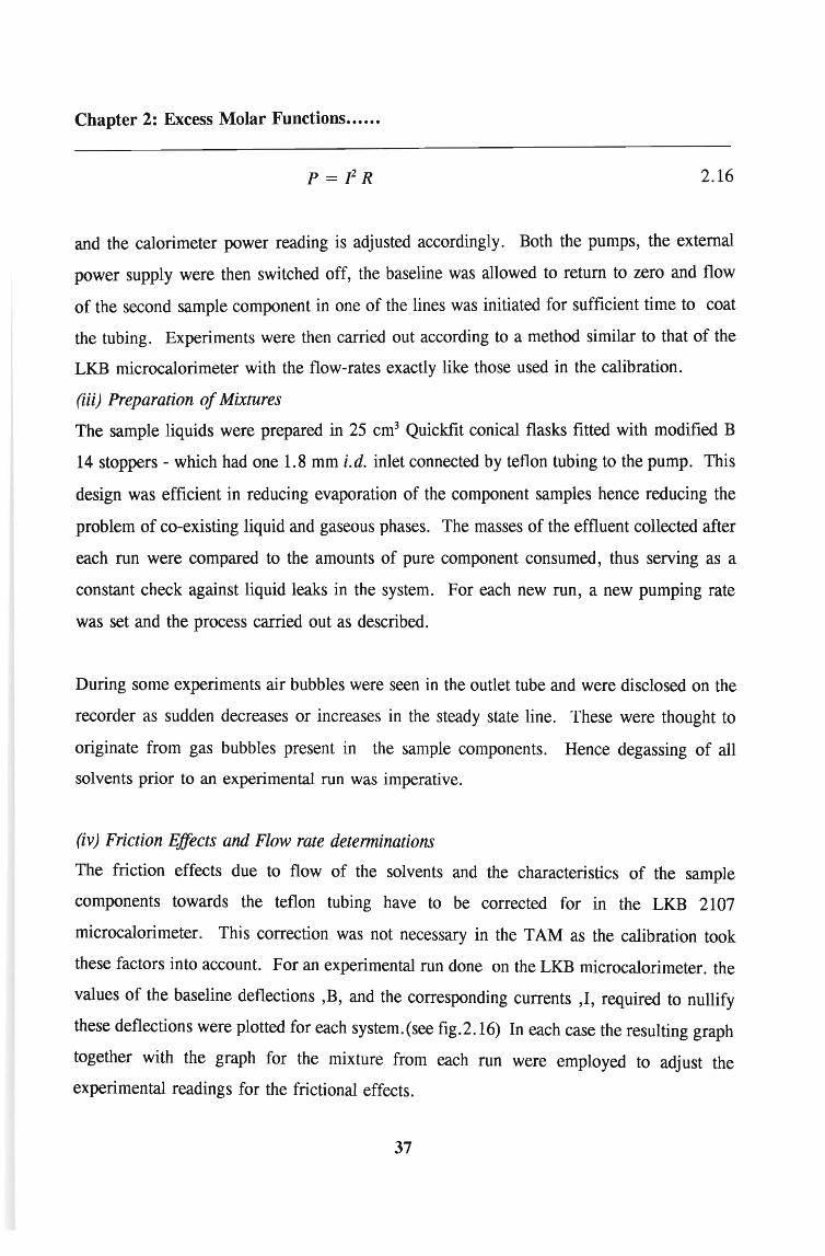
(iv) Friction Effects and Flow rate determinations
The friction effects due to flow of the solvents and the characteristics of the sample
components towards the teflon tubing have to be corrected for in the LKB 2107
microcalorimeter. This correction was not necessary in the TAM as the calibration took
these factors into account. For an experimental run done on the LKB microcalorimeter. the
values of the baseline deflections ,B, and the corresponding currents ,I, required to nullify
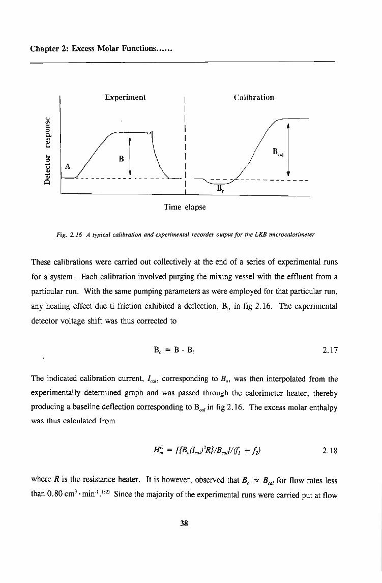
these deflections were plotted for each system. (see fig.2.16) In each case the resulting graph
together with the graph for the mixture from each run were employed to adjust the
experimental readings for the frictional effects.
37
Chapter 2: Excess Molar Functions••••.•
Experiment Calibration
Time elapse
Fig. 2.16 A typical calibration and experimental recorder output for the LKB microcalorimeter
These calibrations were carried out collectively at the end of a series of experimental runs
for a system. Each calibration involved purging the mixing vessel with the effluent from a
particular run. With the same pumping parameters as were employed for that particular run,
any heating effect due ti friction exhibited a deflection, Br, in fig 2.16. The experimental
detector voltage shift was thus corrected to
2.17
The indicated calibration current, l ca1 , corresponding to Bo' was then interpolated from the
experimenta.11y determined graph and was passed through the calorimeter heater, thereby
producing a baseline deflection corresponding to Beal in fig 2.16. The excess molar enthalpy
was thus calculated from
2.18
where R is the resistance heater. It is however, observed that Bo = Beal for flow rates less
than 0.80 cm3• min-l
• (82) Since the majority of the experimental runs were carried put at flow
38

Chapter 2: Excess Molar Functions••••••
rates less than this, the above calibration procedure became unnecessary in many cases and
H; was then determined by
2.19
For exothermic reactions, the steady state deflection, B, was noted and a current, I, was
applied to double this deflection. Heating due to frictional effects would once again produce
a deflection, Bj , and hence equation 2.17 becomes
2.20
The TAM was, however, found to give more precise results for small endothermic and
exothermic reactions and hence for most of the systems discussed in this work it was the
instrument of choice.
(v) Test systems
The excess enthalpies of the nonviscous system (cyclohexane + n-hexane) has recently been
recommended by the IUPAC(67) Commission on Thermodynamics and
Thermochemistry(1970) for checking calorimeter accuracy and data, since results for this
system obtained in five different laboratories with three types of isothermal calorimeters
shows no systematic discrepancies.
39

Chapter 2: Excess Molar Functions...•.•
The recommended equation at 298.15 K is
where Xl is the mole fraction of cyclohexane. Marsh and Stokes(7O) reported very accurate
and precise results using an isothermal batch calorimeter with a standard deviation of 0.09
J •mot l ; Grolier et al(57) obtained data with a Picker flow calorimeter with a standard
deviation of 0.35 J. mol; McGlashan and Stoeckli,(47) and Siddiqi and Lucas(68) used an
isothermal flow calorimeter and obtained a standard deviation of 1.1 J. mol and 0.78 J. mol
respectively. The accuracy and precision for this work was estimated from the data sets
obtained for the (cyclohexane + benzene) system and the standard deviation for these results
and those interpolated from the IUPAC equation is 1.0 J. mot l. This data shows equal and
superior precision to that of McGlashan and Stoeckli.(47)
40
Chapter 2: Excess Molar Functions••••.•
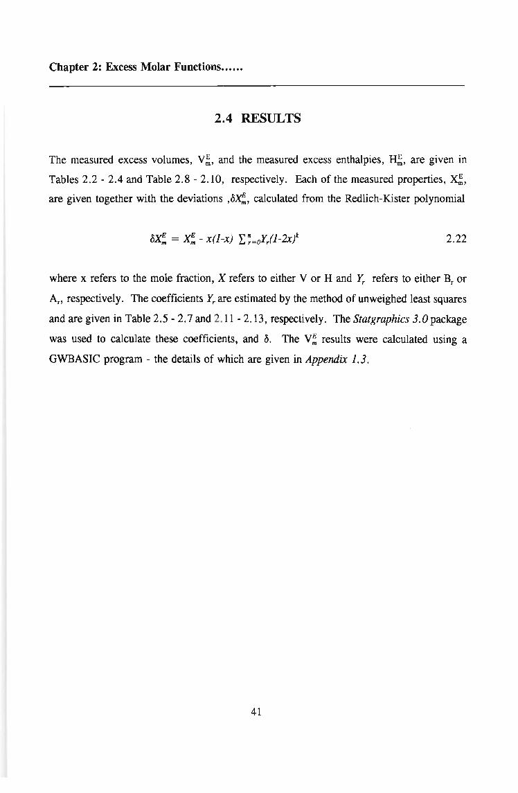
2.4 RESULTS
The measured excess volumes, V;, and the measured excess enthalpies, !I;, are given in
Tables 2.2 - 2.4 and Table 2.8 - 2.10, respectively. Each of the measured properties, X;,
are given together with the deviations ,oX;, calculated from the Redlich-Kister polynomial
2.22
where x refers to the mole fraction, X refers to either V or H and J:. refers to either Br or
An respectively. The coefficients Yr are estimated by the method of unweighed least squares
and are given in Table 2.5 - 2.7 and 2.11- 2.13, respectively. The Statgraphics 3.0 package
was used to calculate these coefficients, and o. The V; results were calculated using a
GWBASIC program - the details of which are given in Appendix 1.3.
41

Chapter 2: Excess Molar Functions..•..•
TABLE 2.2 Excess molar volumes, v;, for binary mixtures of I-hexene, I-heptene and 1-
oct.ene with I-propanol and 2-propanol and the deviations, aY; calculated
from equation.2.22 at the temperature 298.15 K
yE oyE'l()3 yE oyE·l()3 yE oyE'l()3m m m m m m
X X X
cm3'mot1 cm3'mot1 cm3'mot1 cm3'mot1 cm3'mot1 cm3'mot1
xl-C6H12 + (1-x)I-C3H7OH
0.0394 -0.032 1.0 0.3773 -0.038 -5.0 0.8027 0.116 6.0
0.1273 -0.071 10.0 0.4837 0.012 28.0 0.8362 0.112 -2.0
0.1995 -0.081 -15.0 0.5917 0.056 -35.0 0.9100 0.084 -7.0
0.2673 -0.071 4.0 0.7237 0.108 15.0
xl-C7H14 + (1-x)I-C3H7OH
0.0276 -0.001 -7.0 0.4013 0.123 -6.0 0.8314 0.180 4.0
0.0779 0.001 -32.0 0.4706 0.154 -9.0 0.8736 0.151 -5.0
0.1747 0.031 37.0 0.5563 0.189 10.0 0.9276 0.100 -3.0
0.3181 0.084 -9.0 0.6964 0.214 2.0
xl-CgH16 + (l-x)I-C3H7OH
0.0492 0.023 -21.0 0.3195 0.179 -30.0 0.6133 0.270 -6.0
0.0900 0.053 31.0 0.4401 0.230 25.0 0.7134 0.278 -3.0
0.1673 0.100 9.0 0.5232 0.253 20.0 0.8703 0.225 17.0
0.2333 0.137 -15.0
42

Chapter 2: Excess Molar Functions .
Table 2.2. continued
yE oyE·1Q3 yE oyE'1Q3 yE oyE·1Q3m m m m m m
X X X
cm3'moI-1cm3 'moI-1 cm3'moI-1cm3'moI-1 cm3 'moI-1cm3 'moI-1
x1-C6H12 + (1-x)2-C3H7OH
0.0557 0.021 1.0 0.3694 0.276 -28.0 0.7268 0.397 23.0
0.1294 0.061 -27.0 0.4987 0.382 -22.0 0.8254 0.296 -37.0
0.1950 0.115 8.0 0.6039 0.427 18.0 0.8910 0.205 16.0
0.2680 0.185 44.0
x1-~H14 + (l-x)2-C3H7OH
0.0566 0.069 -33.0 0.3505 0.393 -2.0 0.7241 0.492 22.0
0.1031 0.131 19.0 0.4667 0.480 -9.0 0.8704 0.312 2.0
0.1886 0.227 -13.0 0.6027 0.525 -14.0 0.9409 0.160 -20.0
0.2516' 0.299 23.0
x1-CgH16 + (1-xj2-C3H7OH
0.0419 0.074 -1.0 0.3305 0.434 15.0 0.7012 0.529 -14.0
0.0916 O. 3 -1.0 0.4383 0.511 -7.0 0.8534 0.363 36.0
0.1633 0.253 3.0 0.5435 0.555 2.0 0.9401 0.170 -38.0
0.2304 0.332 -10.0
43

Chapter 2: Excess Molar Functions•.••••
TABLE 2.3 Excess molar volumes, V;, for binary mixtures of 1-hexyne, 1-heptyne and 1-
octyne with I-propanol and 2-propanol and the deviations, DV; calculated
from equation 2.22 at the temperature 298.15 K
v E ovE·l(f yE oyE·l(f VE ovE·l(fm m m m m m
X X X
cm3·moI-1 cm3·moI-1 cm3·moI-1 cm3·moI-1 cm3·moI-1 cm3·moI-1
Xl-CJIlO + (1-x)I-C3H7OH
0.0637 -0.054 2.0 0.5097 -0.085 0.0 0.7558 -0.050 1.0
0.1123 -0.083 -3.0 0.6332 -0.073 0.0 0.8260 -0.033 0.0
0.2544 -0.094 3.0 0.7128 -0.060 0.0 0.9009 -0.015 -1.0
0.3968 -0.092 -1.0
xl-C7H12 + (l-x)I-C3H7OH
0.0509 -0.036 -4.0 0.3495 -0.034 -2.0 0.7378 0.059 -1.0
0.0997 -0.047 2.0 0.4721 0.001 1.0 0.8037 0.065 0.0
0.1811 -0.055 2.0 0.5744 0.028 1.0 0.8771 0.060 0.0
0.2497 -0.052 0.0
x1-CgH14 + (1-x)1-C3H7OH
0.0400 -0.013 2.0 0.3277 -0.005 -7.0 0.6815 0.089 -2.0
0.0899 -0.025 0.0 0.4429 0.039 6.0 0.7830 0.096 -2.0
0.1657 -0.026 0.0 0.5386 0.061 1.0 0.8906 0.080 3.0
0.2248 -0.017 2.0
44

Chapter 2: Excess Molar Functions .
TABLE 2.3 continued
yE oyE·1Q3 yE oyE'lQ3 yE oyE·1Q3m m m m m m
X X X
cm3'moI-l cm3'moI-1 cm3'moI-1cm3'moI-l cm3'moI-1cm3'moI-1
X1-CJIlO + (l-x)2-C3H7OH
0.0560 -0.012 -5.0 0.2954 0.102 0.0 0.7737 0.203 9.0
0.0779 -0.010 -5.0 0.3899 0.155 -2.0 0.8970 0.110 -3.0
0.1129 0.117 2.0 0.5284 0.209 -4.0 0.8425 0.151 -4.0
0.2067 0.055 6.0 0.6151 0.226 0.0
x1-~H12 + (1-x)2-C3H7OH
0.0356 0.007 2.0 0.3668 0.188 -7.0 0.7319 0.258 -5.0
0.1008 0.025 -3.0 0.5033 0.262 3.0 0.8506 0.195 0.0
0.1889 0.084 3.0 0.5840 0.282 4.0 0.9205 0.126 3.0
0.2523 0.125 2.0
x1-CgH14 + (1-x)2-C3H7OH
0.0939 0.036 2.0 0.4548 0.266 0.0 0.7899 0.236 0.0
0.1678 0.076 -2.0 0.5555 0.296 -3.0 0.8561 0.174 -3.0
0.2377 0.125 -2.0 0.6969 0.290 3.0 0.9322 0.094 2.0
0.3422 0.205 4.0
45

Chapter 2: Excess Molar Functions•.•..•
TABLE 2.4 Excess molar volumes, V;, for (di-n-butylarnine + an ether) and the
deviations, oV; calculated from equation 2.22 at the temperature 298.15 K
VE VE ·l{)3 VE oVE·l{)3 VE oVE ·l{)3m m m m m m
X X X
cm3·moI-1 cm3·moI-l cm3·moI-1 cm3·moI-l cm3·moI-1 cm3·moI-1
x(C4H9hNH + (l-x)(~Hs)20
0.0250 -0.0554 -4.0 0.2348 -0.2902 4.0 0.5952 -0.3062 -1.6
0.0329 -0.0651 1.2 0.2926 -0.3195 1.5 0.6541 -0.2751 1.1
0.0592 -0.1152 -3.2 0.3371 -0.3367 -2.8 0.6901 -0.2534 1.8
0.0905 -0.1621 -3.3 0.3937 -0.3429 -1.1 0.7492 -0.2142 0.8
0.0931 -0.1651 -2.7 0.4402 -0.3431 -1.3 0.7991 -0.1752 1.0
0.1247 -0.2012 0.6 0.4951 -0.3352 -0.2 0.8057 -0.1686 2.2
0.1603 -0.2338 4.9 0.5395 -0.3254 -1.1 0.9062 -0.0882 -5.4
0.1983 -0.2698 0.5
x(C4H9)2NH + (l-x)(CH3CH2CH2)2)O
0.0706 -0.0023 -1.0 0.4321 -0.1020 -1.8 0.7723 -0.0694 -5.1
0.1193 -0.0398 -2.1 0.4694 -0.1026 -2.3 0.8194 -0.0535 1.5
0.1641 -0.0546 -2.2 0.5058 -0.0992 -0.2 0.8562 -0.0475 -0.7
0.2097 -0.0613 4.9 0.5382 -0.0968 0.1 0.8932 -0.0381 -0.6
0.2768 -0.0798 2.9 0.6028 -0.0866 3.8 0.9389 -0.0208 3.0
0.3319 -0.0912 1.1 0.6722 -0.0802 0.9 0.9602 -0.0182 -1.8
0.3714 -0.1003 -3.4 0.7189 -0.0716 2.1
46
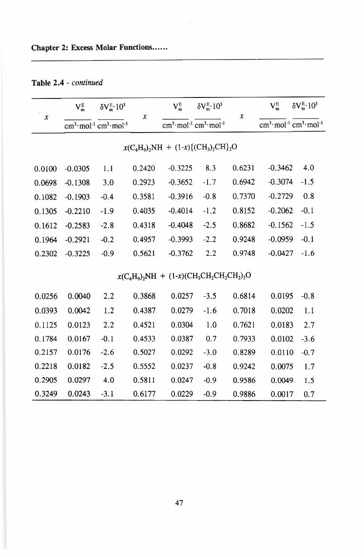
Chapter 2: Excess Molar Functions .
Table 2.4 - continued
yE oyE'l{)3 yE oyE'l{)3 yE oyE·1{)3m m m m m m
X X X
cm3'moI-1 cm3'moI-1 cm3'moI-1 cm3'moI-1 cm3'moI-1 cm3'moI-1
x(C4H9)2NH + (1-x){(CH3)2CH}20
0.0100 -0.0305 1.1 0.2420 -0.3225 8.3 0.6231 -0.3462 4.0
0.0698 -0.1308 3.0 0.2923 -0.3652 -1.7 0.6942 -0.3074 -1.5
0.1082 -0.1903 -0.4 0.3581 -0.3916 -0.8 0.7370 -0.2729 0.8
0.1305 -0.2210 -1.9 0.4035 -0.4014 -1.2 0.8152 -0.2062 -0.1
0.1612 -0.2583 -2.8 0.4318 -0.4048 -2.5 0.8682 -0.1562 -1.5
0.1964 -0.2921 -0.2 0.4957 -0.3993 -2.2 0.9248 -0.0959 -0.1
0.2302 -0.3225 -0.9 0.5621 -0.3762 2.2 0.9748 -0.0427 -1.6
x(C4H9)2NH + (1-x)(CH3CH2CH2CH2)20
0.0256 0.0040 2.2 0.3868 0.0257 -3.5 0.6814 0.0195 -0.8
0.0393 0.0042 1.2 0.4387 0.0279 -1.6 0.7018 0.0202 1.1
0.1125 0.0123 2.2 0.4521 0.0304 1.0 0.7621 0.0183 2.7
0.1784 0.0167 -0.1 0.4533 0.0387 0.7 0.7933 0.0102 -3.6
0.2157 0.0176 -2.6 0.5027 0.0292 -3.0 0.8289 0.0110 -0.7
0.2218 0.0182 -2.5 0.5552 0.0237 -0.8 0.9242 0.0075 1.7
0.2905 0.0297 4.0 0.5811 0.0247 -0.9 0.9586 0.0049 1.5
0.3249 0.0243 -3.1 0.6177 0.0229 -0.9 0.9886 0.0017 0.7
47

Chapter 2: Excess Molar Functions.....•
Table 2.4 - continued
yE oyE·1{)3 yE oyE·1{)3 yE oyE'l{)3m m m m m m
X X X
cm3'moI-1cm3·moI-1 cm3'moI-l cm3'moI-1 cm3·moI-1cm3'moI-1
x(C4H9)2NH + (1-x)CH3C(CH3)20CH3
0.0483 -0.0328 -1.3 0.3925 -0.1359 -0.2 0.6951 -0.1098 -3.6
0.0829 -0.0517 0.4 0.3951 -0.1358 -0.1 0.7129 -0.1029 -0.8
0.1663 -0.0928 -1.5 0.4582 -0.1356 0.6 0.7385 -0.0944 1.4
0.1986 -0.1024 0.2 0.5197 -0.1307 2.2 0.7882 -0.0819 0.2
0.2434 -0.1129 2.3 0.5624 -0.1265 2.2 0.8361 -0.0692 -2.3
0.2552 -0.1156 2.4 0.6291 -0.1211 -2.0 0.8669 -0.0519
0.3055 -0.1318 -4.4 0.6741 -0.1103 0.4 0.9262 -0.0324 -0.1
0.3461 -0.1328 -0.4
x(C4H9)2NH + (1-x)CH3CH2C(CH3)20CH3
0.0209 -0.0092 -3.8 0.3470 -0.0214 2.7 0.7175 -0.0230 2.0
0.0821 -0.0186 -2.2 0.4010 -0.0243 -0.5 0.7687 -0.0232 0.9
0.1152 -0.0202 -0.2 0.4454 -0.0256 -2.0 0.8054 -0.0230 -0.3
0.2005 -0.0233 0.9 0.4931 -0.0263 -2.5 0.8135 -0.0217 0.6
0.2204 -0.0237 0.9 0.5501 -0.0278 -3.6 0.8762 -0.0197 -1.9
0.3016 -0.0235 1.0 0.6260 -0.0233 1.6 0.9288 -0.0139 -2.1
0.3085 -0.0238 0.7 0.6789 -0.0230 2.2
48

Chapter 2: Excess Molar Functions•..•..
Table 2.4 - continued
yE oyE·1Q3 yE oyE·1Q3 yE oyE·1Q3m m m m m m
X X X
cm3·mot1 cm3·mot1 cm3·mot1 cm3·mot1 cm3•mot1 cm3•mot1
x(C4H9)2NH + (I-x) c-(CH2)40
0.0435 0.0215 0.4 0.2953 0.0896 0.0 0.6104 0.0792 -0.6
0.0846 0.0382 -0.2 0.3533 0.0967 2.5 0.6378 0.0764 0.4
0.1080 0.0508 3.7 0.3538 0.0965 2.3 0.7004 0.0673 1.3
0.1150 0.0575 8.0 0.3845 0.0947 -0.5 0.7557 0.0521 -3.9
0.1546 0.0556 -6.5 0.4490 0.0946 0.1 0.8159 0.0491 5.0
0.1568 0.0578 -4.9 0.4786 0.0920 -1.1 0.8842 0.0307 1.5
0.1691 0.0647 -1.4 0.5221 0.0892 -0.6 0.9179 0.0218 0.5
0.2032 0.0706 -3.9 0.5492 0.0861 -1.1 0.9220 0.0156 -4.7
0.2421 0.0862 4.0
x(C4H9)2NH + (1-x)c-(CH0s0
0.0476 0.0310 0.6 0.4468 0.1298 -0.4 0.8260 0.0596 2.2
0.0926 0.0544 0.7 0.4610 0.1285 -1.8 0.8438 0.0379 -13.0
0.1632 0.0842 2.1 0.4884 0.1344 4.5 0.8780 0.0449 6.4
0.2107 0.0932 -3.5 0.5627 0.1253 0.7 0.9245 0.0285 6.4
0.2753 0.1134 1.5 0.6297 0.1147 0.5 0.9482 0.0103 -4.0
0.3262 0.1208 0.2 0.6804 0.1032 0.2 0.9693 0.0133 5.3
0.3675 0.1237 -1.9 0.7122 0.0961 1.6 0.9733 0.0073 0.4
0.4038 0.1274 -1.1 0.7768 0.0725 -2.0 0.9877 0.0014 -1.6
49
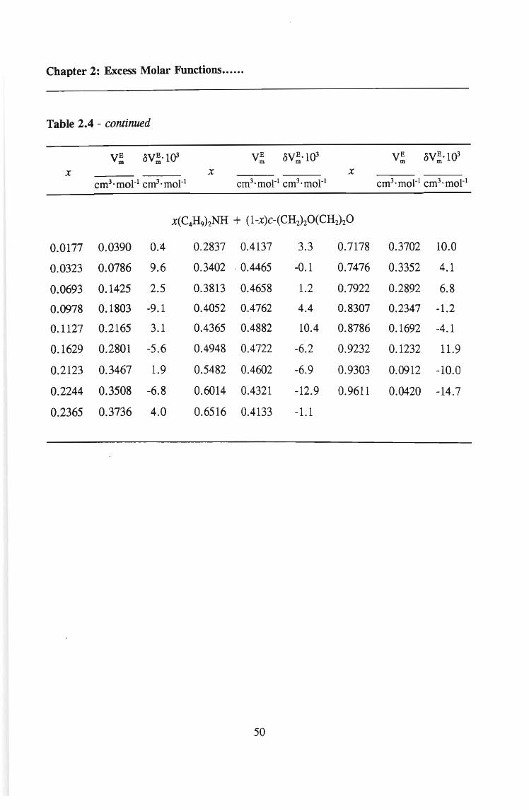
Chapter 2: Excess Molar Functions .
Table 2.4 - continued
VB oVB·1Q3 VE oVE ·1Q3 VE oVB'lQ3m m m m m m
X X X
cm3'moI-l cm3'moI-1 cm3'moI-1cm3'moI-1 cm3'moI-1cm3'moI-1
x(C4H9)2NH + (1-x)c-(CH020 (CH2hO
0.0177 0.0390 O.~ 0.2837 0.4137 3.3 0.7178 0.3702 10.0
0.0323 0.0786 9.6 0.3402 ·0.4465 -0.1 0.7476 0.3352 4.1
0.0693 0.1425 2.5 0.3813 0.4658 1.2 0.7922 0.2892 6.8
0.0978 0.1803 -9.1 0.4052 0.4762 4.4 0.8307 0.2347 -1.2
0.1127 0.2165 3.1 0.4365 0.4882 10.4 0.8786 0.1692 -4.1
0.1629 0.2801 -5.6 0.4948 0.4722 -6.2 0.9232 0.1232 11.9
0.2123 0.3467 1.9 0.5482 0.4602 -6.9 0.9303 0.0912 -10.0
0.2244 0.3508 -6.8 0.6014 0.4321 -12.9 0.9611 0.0420 -14.7
0.2365 0.3736 4.0 0.6516 0.4133 -1.1
50

Chapter 2: Excess Molar Functions••••••
TABLE 2.5. Coefficients Br from equation 2.22 and standard deviations (J'- for { (x1CkH~
or (x1-CkH2k_2) + (l-x)1-CJI70H} at the temperature 298.15 K
Compound
X C6H12 0.068 -1.015 0.126
x C7H 14 0.670 -0.827 0.142
x CgH 16 0.980 -0.538 0.624 -0.633
XC~lO -0.339 -0.122 -0.239 -0.469 0.2
x C7H12 0.030 -0.532 -0.007 -0.282 0.2
x CgH14 0.197 -0.549 0.101 -0.212 0.4
.' b . [~(VE E 2 / 1/2: given y equation (J = JJ m(exp) - Vm(calc» (n - k - 1) .
51

Chapter 2: Excess Molar Functions .
TABLE 2.6. Coefficients Br from equation 2.22 and standard deviations (J'- for { (x1CkH2J
or (x1-CkH2k_2) + (l-X)2-CJI70H} at the temperature 298.15 K
Compound
X CJI12 1.540 -1.239 -0.383 0.378
x C7H14 1.994 -0.922 0.182
x CgH16 2.165 -0.736 0.389
x C6H lO 0.819 -0.644 -0.314 -0.188 0.5
x C7H12 1.031 -0.663 -0.089 -0.247 0.5
x CgH14 1.140 -0.687 0.324 -0.061 0.3
a: given by equation (J = [E(V;(eXP) - V;(calC»2/ (n - k - 1YI2.
52

Chapter 2: Excess Molar Functions•••••.
Table 2.7 Coefficients Br and standard deviations ~ for {x(C4H9)2NH + (l-x)ROR'} at the
temperature 298.15 K by equation 2.22
ROR'
CH3CH2OCH2CH3 -1.3363 -0.4004 -0.1688 -0.2774 0.3
CH3(CH020(CH2)2CH3 -0.3970 -0.0933 0.0407 0.1949 0.3
CH3CH(CH3)OCH(CH3)CH3 -0.0127 -1.5343 -0.3919 0.0096 0.2
CH3(CH2)30(CH2)3CH3 0.1141 0.0521 -0.0377 -0.0664 0.3
CH3C(CH3)2OCH3 0.0029 -0.5489 -0.1275 -0.1052 0.2
CH3CH2C(CH3)2OCH3 -0.0951 0.0119 -0.1452 -0.0525 0.2
c-(CH2)40 0.3666 0.1483 0.0329 -0.2969 0.3
c-(CH2)sO 0.5180 0.0859 -0.0480 0.1532 0.4
c-(CH2)20(CH020 1.9111 0.2517 -0.0616 0.1391 0.7
•. b . [~(VE VE 2 / 1/2: gIven y equation (J = iJ m(exp) - m(cak» (n - k)] .
53

Chapter 2: Excess Molar Functions••••.•
Table 2.8. Excess molar enthalpies,H; for binary mixtures of I-hexene, I-heptene and 1-
octene with I-propanol and 2-propanol and the deviations, 0 H; calculated from equation
2.22 at 298.15 K.
H; oH; H; oH; H; oH;x x x
J·mot1 J·mot1 J·mot1 J·mot1 J·moI-1 J·moI-1
xl-CJI12 + (l-x)I-C3H7OH
0.0518 75.6 0.2 0.3409 428.8 -1.5 0.7014 655.2 -1.4
0.0836 119.2 -0.3 0.4222 510.7 -1.9 0.7489 640.5 4.2
0.1202 168.5 0.0 0.5052 588.2 3.3 0.8016 585.3 -1.2
0.1895 255.6 -0.9 0.5956 639.8 -1.5 0.8722 461.4 -0.8
0.2518 332.3 1.4 0.6636 658.2 -1.1 0.9334 285.7 0.2
0.2944 380.8 1.3
xl-~H14 + (1-x)1-C3H7OH
0.0559 90.2 1.7 0.4533 598.9 2.9 0.7768 664.8 -1.0
0.0928 144.4 -0.6 0.5317 662.8 1.2 0.7932 647.4 0.3
0.1655 252.4 1.1 0.6157 705.8 -1.4 0.8206 611.5 3.8
0.2072 305.2 -3.7 0.6824 713.5 -2.6 0.9007 420.8 -1.8
0.2807 408.1 3.4 0.7352 699.8 0.9 0.9536 228.2 -0.7
0.3746 511.8 -3.5
xl-CgH16 + (i-x) l-C3H7OH
0.0944 169.6 -0.7 0.4798 667.7 0.2 0.7504 730.6 1.6
0.1361 239.9 0.5 0.5387 712.8 0.0 0.8226 640.4 1.0
0.1773 303.8 -0.1 0.6116 749.8 -0.6 0.8612 560.2 1.1
0.2539 414.4 0.3 0.6848 759.0 0.6 0.9033 435.6 -3.7
0.4005 591.0 -0.1 0.7094 750.4 -1.7 0.9568 230.1 1.9
54

Chapter 2: Excess Molar Functions••••••
Table 2.8- continued
H; oH; H; oH; H; oH;x x x
J'moI-l J'moI-l J'moI-l J'motl J'moI-l J'moI-l
x1-C6H12 + (1-x)2-C3H7OH
0.0736 151.4 -0.5 0.3294 636.5 0.7 0.6756 863.5 -4.9
0.1446 308.5 3.7 0.3489 660.9 -3.1 0.7044 859.7 0.5
0.1975 412.8 -0.1 0.4357 763.5 0.1 0.7647 811.7 -3.1
0.2556 521.5 0.9 0.5265 838.2 4.1 0.8335 704.6 -2.8
0.2812 560.4 -3.3 0.5734 862.2 5.1 0.9066 502.2 6.8
x1-C7H14 + (l-x)2-C3H7OH
0.0808 192.4 0.5 0.4455 830.7 3.5 0.7736 833.8 0.1
0.1432 344.8 2.7 0.4677 846.2 1.6 0.8062 786.1 -0.4
0.1814 428.6 -0.7 0.4955 862.0 -1.5 0.8516 690.7 -0.9
0.2526 571.0 -1.6 0.5594 894.7 0.2 0.9055 516.2 -4.5
0.3066 662.7 -1.1 0.6655 904.3 0.0 0.9449 352.6 8.8
0.3304 696.9 -2.0 0.7405 866.7 -0.7
x1-CgH16 + (1-x)2-C3H7OH
0.0736 209.4 3.4 0.3133 726.4 1.3 0.6142 952.5 0.1
0.1144 314.8 0.0 0.3970 831.3 -0.4 0.6926 935.5 0.1
0.1425 382.4 -3.3 0.4574 885.7 -1.2 0.7759 858.4 -0.6
0.1622 433.7 0.5 0.5188 926.9 0.9 0.8326 752.7 -2.10.2429 605.0 -0.4 0.5333 933.7 0.9 0.9059 528.9 2.7
0.2590 635.2 -0.1
55

Chapter 2: Excess Molar Functions•.•..•
Table 2.9 Excess molar enthalpies,H; for binary mixtures of I-hexyne, I-heptyne and 1
octyne with I-propanol and 2-propanol and the deviations, 0 H; calculated from equation
2.22 at 298.15 K.
x x x
X1-CJIlO + (l-x)1-C3H7OH
0.0827 154.6 -4.6 0.3826 658.2 -5.4 0.7359 9 4.4 -1.6
0.1182 225.8 -0.1 0.4458 740.4 -5.1 0.7569 4892.0 -3.8
0.1434 276.3 4.0 0.5463 849.6 1.1 0.8045 851.5 -2.2
0.1545 290.1 -2.5 0.5756 869.2 -1.6 0.8642 745.6 -4.8
0.2016 379.4 2.7 0.6538 914.7 5.5 0.9012 648.7 4.8
0.2513 467.4 5.6 0.6928 921.7 7.5
x1-~H12 + (1-x)1-C3H7OH
0.0652 126.2 -19.5 0.4526 775.2 -2.9 0.7715 916.3 7.2
0.1543 255.8 0.5 0.5032 839.7 0.7 0.7874 898.6 4.7
0.1753 339.6 5.4 0.5658 891.9 -6.0 0.8363 822.4 -2.9
0.2558 470.9 6.1 0.6318 931.2 -5.0 0.8721 741.8 -7.4
0.3668 654.8 1.2 0.7015 941.0 -3.1 0.9502 450.7 2.3
0.4370 760.8 3.5 0.7525 929.2 5.6
x1-CgH 14 + (1-x)1-C3H7OH
0.0887 192.2 10.8 0.4940 850.7 -2.5 0.7553 950.8 0.6
0.1762 359.6 6.0 0.4969 861.2 4.9 0.8302 857.2 -8.2
0.2001 399.4 0.4 0.6214 957.2 2.5 0.8596 800.7 -5.4
0.3283 615.6 -9.1 0.6532 965.0 -1.1 0.9664 789.6 0.0
0.3997 726.3 -7.5 0.6998 976.2 6.3 0.9502 454.2 5.8
0.4091 746.2 -0.8 0.7050 975.8 6.5
56

Chapter 2: Excess Molar Functions•••••.
Table 2.9- continued
x xJ'moI-l J.moI-l
xJ'moI-l J. moI-l
x1-C6H lO + (1-x)2-C3H7OH
0.0637 198.9 -10.7 0.3706 943.8 1.2 0.6578 1127.8 -4.3
0.1457 451.3 -0.3 0.4265 1019.4 -2.4 0.7098 1196.5 -1.6
0.1992 590.8 -1.2 0.5062 1104.2 2.3 0.7538 1047.6 0.4
0.2831 785.9 2.8 0.5997 1140.9 -0.4 0.8685 796.8 12.7
0.3220 864.2 5.0 0.6280 1138.7 -1.6 0.9102 608.9 -9.7
x1-~H12 + (1-x)2-C3H7OH
0.0970 342.9 -0.6 0.4736 1107.6 3.4 0.7084 1119.6 -4.3
0.1200 406.7 -8.6 0.4805 1109.6 -0.7 0.7816 1027.7 3.0
0.2559 768.6 -0.6 0.5802 1160.5 -3.6 0.8025 986.5 4.1
0.3635 972.1 2.7 0.6115 1163.2 -3.7 0.8593 836.0 9.7
0.3833 1007.4 8.5 0.6534 1152.7 -6.0 0.9462 407.7 -11.2
xl-CgH14 + (1-x)2-C3H7OH
0.0749 284.2 -7.0 0.4724 1129.8 3.8 0.7514 1089.7 -1.4
0.1714 594.8 -2.6 0.5017 1158.7 3.2 0.8037 1004.5 7.9
0.2511 798.0 0.5 0.5532 1177.8 -3.1 0.8412 898.2 -1.8
0.3123 926.2 4.8 0.6098 1189.0 0.5 0.8482 885.8 7.0
0.3656 1013.9 4.3 0.6768 1159.0 -7.1 0.9135 610.2 -7.3
57

Chapter 2: Excess Molar Functions•..•••
Table 2.10. Excess molar enthalpies, H;, for (di-n-butylamine + an ether) and the
deviations, oH;, calculated from equation 2.22 at the temPerature 298.15 K.
H; oH; H; oH; H; oH;x x x
J·moI-1 J·moI-1 J·moI-1 J·moI-1 J·moI-1 J·moI-l
x(C4H9)2NH + (1-x)(~H5)20
0.0702 16.50 1.5 0.4123 55.05 2.3 0.6882 37.48 -1.6
0.1006 21.20 0.4 0.4213 56.25 3.3 0.7319 34.65 0.4
0.1510 27.02 -2.4 0.4712 53.14 0.3 0.7528 30.71 -1.0
0.1707 30.58 -1.9 0.5207 51.90 -0.1 0.7895 28.21 -1.1
0.2048 36.69 -0.6 0.5340 59.93 -1.1 0.8132 23.75 -0.3
0.2807 46.20 0.5 0.5887 47.82 -0.1 0.8602 21.25 3.4
0.3478 50.40 -0.1 0.6425 39.65 -3.9 0.9504 7.05 1.1
0.3499 51.05 0.4
X(C4~)2NH + (1-x)(CH3CH2CH~2)O
0.0825 16.42 -1.9 0.3759 65.90 2.0 0.6502 62.17 0.6
0.1187 24.86 -1.0 0.4204 66.14 -0.6 0.7052 55.82 0.4
0.1270 28.56 1.0 0.4501 66.28 -1.7 0.7445 49.13 -0.3
0.1465 33.94 2.5 0.4553 66.67 -1.5 0.7961 42.70 0.8
0.1942 41.18 0.9 0.5427 67.80 -0.4 0.8242 38.42 1.5
0.2862 53.00 -1.4 0.5881 67.50 1.2 0.8550 29.76 -2.9
0.3264 60.04 0.8 0.6433 63.80 1.6 0.8552 28.15 -1.3
0.3588 61.02 -1.4
58

Chapter 2: Excess Molar Functions•••••.
Table 2.10- continued
H; oH; H; oH; ~ o~x x x
J·moI-1 J·moI-1 J·moI-1 J·moI-1 J·moI-l J·moI-l
x(C4H9)2NH + (l-x){ (CH3)2CH}20
0.0952 12.28 1.0 0.4260 29.07 -1.6 0.7089 29.16 -0.1
0.1053 14.25 2.0 0.4399 31.16 0.2 0.7317 27.78 -0.4
0.2502 23.53 0.1 0.5162 32.97 0.9 0.7629 27.69 1.1
0.2872 23.62 -1.8 0.5678 31.83 -0.3 0.7693 27.51 1.4
0.3478 27.82 -0.3 0.5826 32.82 0.7 0.8622 17.29 -1.5
0.3547 27.98 -0.4 0.6341 32.14 0.7 0.9241 9.01 -2.6
0.3578 28.87 0.3
X(C4~)2NH + (1-x)(CH3CH2CH2CH2)20
0.0742 16.98 -0.2 0.3515 68.33 1.2 0.5211 70.45 -1.8
0.0839 20.99 1.6 0.3672 69.02 0.5 0.5960 68.65 1.3
0.1012 21.16 -2.2 0.3769 68.32 -1.0 0.6365 65.09 2.0
0.1220 29.95 1.2 0.3917 70.94 0.5 0.7013 50.92 -3.1
0.1471 32.95 -0.6 0.4202 74.87 2.9 0.7637 43.20 -0.2
0.1535 35.03 0.1 0.4875 76.02 2.9 0.8478 29.55 2.1
0.1622 37.27 0.4 0.4983 71.71 -1.2 0.8624 21.91 -2.6
0.2578 52.57 -2.2 0.5062 71.83 -0.9 0.9176 16.44 2.5
0.3391 64.60 -1.2 0.5099 71.10 -1.5
59

Chapter 2: Excess Molar Functions•••.••
Table 2.10 - continued
H; oH; H; oH; H; oH;x x x
J'moI-1 J'moI-1 J'moI-l J'moI-1 J'moI-l J'mol-1
x(C4H9)2NH + (1-x)CH3C(CH3)20CH3
0.0739 25.59 -2.5 0.4079 82.01 0.7 0.7085 54.25 0.2
0.1122 35.94 2.4 0.4512 88.10 6.3 0.7692 43.20 1.1
0.1805 50.02 -0.7 0.4904 85.53 4.7 0.8274 32.68 2.5
0.2649 66.96 -0.3 0.5580 76.16 0.1 0.8986 22.78 6.8
0.2670 65.65 -2.0 0.5851 75.48 2.3 0.9094 22.37 8.4
0.3097 68.01 -5.7 0.6498 66.70 2.5 0.9985 1.57
0.3988 80.44 -0.5
x(C4H9)2NH + (1-x)CH3CH2C(CH3)20CH3
0.0328 9.11 2.9 0.3855 42.75 -2.3 0.6382 39.70 0.7
0.1226 21.54 0.4 0.4503 42.86 -2.7 0.6643 35.57 -1.5
0.1354 24.87 1.9 0.4764 43.95 -1.5 0.6992 35.37 1.2
0.1887 30.12 0.2 0.5567 44.68 1.2 0.7495 28.96 -0.4
0.2205 33.02 -0.4 0.5867 44.50 2.4 0.7911 24.60 -0.4
0.2568 37.63 0.7 0.5922 44.48 2.7 0.8013 23.08 -0.8
0.3461 41.56 -1.4 0.6148 42.47 2.0 0.8676 13.59 -2.7
60

Chapter 2: Excess Molar Functions .
Table 2.10 - continued
x xJ. maI-t J. maI-t
x
x(C4H9)2NH + (I-x) c-(CH2)40
0.0700 42.38 0.8 0.4132 111.20 0.7 0.7127 67.53 -0.5
0.0952 49.98 -3.7 0.4526 108.90 0.5 0.7628 54.99 -2.0
0.1311 71.04 2.4 0.4871 107.57 2.1 0.8113 47.07 1.3
0.2021 89.84 -0.9 0.5374 98.19 -1.3 0.8545 34.91 -0.6
0.2811 106.71 1.5 0.5802 93.14 -0.1 0.8893 29.20 2.1
0.3297 106.97 -2.6 0.6308 85.38 0.9 0.9352 17.18 1.3
0.3659 111.80 0.9 0.6633 76.15 -2.1
x(C4H9)2NH + (1-x)c-(CH0s0
0.5848 22.16 2.0 0.4227 68.20 0.2 0.6376 47.96 -0.1
0.1082 41.19 1.1 0.4465 66.90 0.1 0.6590 46.05 0.7
0.1515 48.99 -1.4 0.4878 64.92 1.1 0.7328 36.92 1.4
0.2224 62.74 0.5 0.5229 60.75 -0.1 0.7968 26.42 -0.4
0.2806 69.08 1.5 0.5339 58.70 -1.0 0.7992 25.33 -1.2
0.3297 69.19 -0.3 0.6151 49.41 -1.3 0.9016 14.01 1.3
0.3690 68.51 -1.1 0.6176 50.67 0.2 0.9049 11.72 -0.5
61

Chapter 2: Excess Molar Functions•.•.••
Table 2.10 - continued
H; oH; H; oH; H; oH;x x x
J'moI-l J'moI-l J'moI-l J'moI-l J'moI-1 J'moI-l
x(C4H9)2NH + (1-x)c-(CH2)20 (CH2)20
0.0922 275.13 17.3 0.3789 1052.15 5.9 0.5594 846.17 10.6
0.1019 399.43 -0.2 0.4275 1038.99 -1.5 0.6517 754.97 8.3
0.1262 483.89 -11.8 0.4337 1022.17 -15.4 0.7139 659.94 19.6
0.1777 670.46 -12.3 0.4551 1010.50 -13.5 0.7431 581.84 -9.5
0.1932 726.70 -6.4 0.4766 984.04 -21.5 0.7588 571.85 6.5
0.1961 739.80 -2.3 0.5008 965.67 -14.0 0.7951 504.88 -0.3
0.2268 840.25 9.7 0.5412 925.12 -1.5 0.8659 378.45 -2.0
0.2692 840.95 12.4 0.5719 886.59 6.4 0.8746 357.71 -5.7
0.3051 1005.17 16.7 0.5916 845.47 -3.0 0.9234 227.15 -27.1
0.3372 1046.94 22.8
62

Chapter 2: Excess Molar Functions .
TABLE 2.11 Parameters Ar from eqn.2.22 for { (xl-CkH2J or (xl-CkH2k_2) + (l-x)l
C3H70H} at the temperature 298.15 K.
Compound A1 A2 A3
X CJi12 2323 -1575 993 -242
x ~H14 2549 -1636 1057 -362
x CgH16 2737 -1603 1191 -428
XCJilO 3222 511 -242
x C7H12 3342 702 -845
x C gH14 3438 647 -347
63

Chapter 2: Excess Molar Functions••••••
TABLE 2.12 Parameters Ar from eqn.2.22 for { (x1-CkH~ or (x1-CkH2k_2) + (1-x)2
C3H70H} at the temperature 298.15 K
Compound Ao Al A2 A3
X C6H12 3268 -1403 1221 -1178
x C7Hl4 3465 -1200 1360 -1411
x CSHl6 3663 -1169 1451 -1129
x C~IO 4388 1682 -82
x C7Hl2 4503 1254 497
x CSHl4 4617 1488 698
64

Chapter 2: Excess Molar Functions••....
TABLE 2.13 Parameters Ar and standard deviations (J from equation 2.22 for
{x(C4H9)2NH + (l-x)ROR/} at the temperature 298.15 K
ROR'
J·moI-1
CH3CH2OCH2CH3 209.0 56.71 -38.52 1.8
CH3(CH2)20(CHJ2CH3 275.1 0.499 -48.13 1.5
CH3CH(CH3)OCH(CH3)CH3 127.7 -20.52 29.40 1.3
CH3(CH2)30(CH2)3CH3 291.5 40.64 -105.3 1.9
CH3C(CH3)20CH3 321.5 100.5 -104.4 6.8
CH3CH2C(CH3)20CH3 180.7 37.23 -21.84 1.8
c-(CH2)40 416.3 247.7 47.45 1.8
c-(CHJsO 251.3 170.6 44.24 1.1
C-(CHJ20(CHJ20 3922.6 2329.4 -35.69 -2750.1 13.4
a given by eqn. (J = [L (H;(cXP) - lI;(ca1c» 2/ (n-k)]1h where n is the number of experimental
points and k is the order of the polynomial in eqn.2.22
65

Chapter 2: Excess Molar Functions.•••••
2.5 DISCUSSIONS
2.5.1 Mixtures of l-alkenes + (I-propanol or 2-propanol)
It has been reported(76-78) that because the n-alkenes and n-alkynes are soluble in all
proportions with methanol at 298.15 K and in comparison the n-alkanes(78) have only a
limited solubility, that there are specific interactions between the unsaturated hydrocarbon
(double bond of the alkene or triple bond of the alkyne) and the hydroxyl group of the
alkanol. This interaction is representative by an increase in the solubility of the respective
mixtures. For all the (I-alkene + alkanol) mixtures reported, including this work, the
overall magnitude of the volume change is due basically to three effects. The positive effect
due to the dissociation of the alkanol, the positive effect due to the dissociation of the 1
alkene molecules and the negative effect due to the association of the I-alkene with the
alkanol molecule.
The V; results, at 298.15 K, for the (I-alkene + I-propanol or 2-propanol) are reported in
table 2.2 and in fig. 2.17. The V; values for the (I-alkene + I-propanol) become more
positive with an increase in the I-alkene chain length, while the V; results for the (I-alkene
+ 2-propanol) mixtures are all positive for all the I-alkenes investigated in this work. In
particular, the V; curves for the (l-hexene + I-propanol) system is s~ne shaped, being
negative at low x values and positive at high x values (see fig. 2.17). This is probably due
to the contributions being relatively important at high values of x where the dissociation
effect of the alkanol or the alkene is proportionally large. This observation is confirmed by
the results of the (I-heptene or I-octene + I-propanol) mixtures where the volume changes
are largely positive. In addition the V;,max results for the (I-alkenes + 2-propanol) (see
Table 2.I4)are significantly larger than the I-propanol results- this could be due to the steric
effects of the methyl group adjacent to the C-OH bond on the 2-propanol.
66
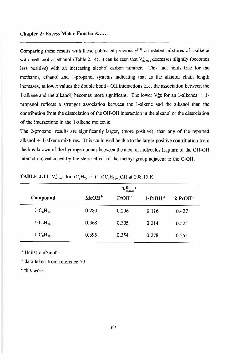
Chapter 2: Excess Molar Functions.•....
Comparing these results with those published previously(79) on related mixtures of I-alkene
with methanol or ethanol, (Table 2.14), it can be seen that V;,max decreases slightly (becomes
less positive) with an increasing alcohol carbon number. This fact holds true for the
methanol, ethanol and I-propanol systems indicating that as the alkanol chain length
increases, at low x values the double bond - OH interactions (Le. the association between the
I-alkene and the alkanol) becomes more significant. The lower V;s for an l-alkenes + 1
propanol reflects a stronger association between the I-alkene and the alkanol than the
contribution from the dissociation of the OH-OH interaction in the alkanol or the dissociation
of the interactions in the I-alkene molecule.
The 2-propanol results are significantly larger, (more positive), than any of the reported
alkanol + I-alkene mixtures. This could well be due to the larger positive contribution from
the breakdown of the hydrogen bonds between the alcohol molecules (rupture of the OH-OH
interaction) enhanced by the steric effect of the methyl group adjacent to the C-OH.
TABLE 2.14 V;,max for xCyH 2y + (l-x)CzH2z+10H at 298.15 K
Compound MeOH b
0.280
0.368
0.395
vE am,max
EtOH b I-PrOBc 2-PrOB c
0.236 0.116 0.427
0.305 0.214 0.525
0.354 0.278 0.555
a Units: cm3·mot1
b data taken from reference 79
C this work
67

Chapter 2: Excess Molar Functions .
0.6.----------6------~
0.5
0.4
~ 0.3,-.:...0E
C')
0.2E0--...--w E>
0.1
-0.1
10.80.60.40.2-0. 2L-__---L-__--L-__----..L ~__~
o
x
Figure 2.17. Excess molar volumes, V; at the temperature 298.15 Kfor 1-propanol + (1), 1-hexene,' or + (2),
1-heptene; or + (3), l-octene andfor 2-propanol + (4), 1-hexene,' or + (5), 1-heptene; or + (6), l-octene
68

Chapter 2: Excess Molar Functions••••••
The ~ values for the I-alkene + I-propanol or 2-propanol are given in Table 2.8 and
plotted in figs. 2.18. The enthalpy changes on mixing are all positive with a maximum at
a composition between 0.6 and 0.7 mole fraction of the I-alkene. This is most likely a
reflection of the breaking of the hydrogen bonds between the alkanol molecules as a result
of the mixing process.
Comparing these results with those published previously on related mixtures of I-alkene with
methanol or ethanol, it can be seen that H;,max increases slightly with increasing alcohol
carbon number. (79) For example H;,max for mixtures of I-hexene with methanol, ethanol and
I-propanol are 570, 620, 660 J·motl, respectively (see Table 2.15)
For each I-alkene, ~,max for mixtures containing 2-propanol are greater than H;,max for
mixtures containing I-propanol. For example, H;,max for I-heptene with 2-propanol and 1
propanol are 910 and 710 J·motl, respectively (Table 2.15). The results for~ {xCyH2y +
(I-x) I-PrOH} and H; {xCyH2y + (I-x) 2-PrOH} show that for each I-alkene the
2-PrOH isomers behave significantly different. In all cases H;{2-PrOH} > H;{1-PrOH} .
This could be due to a weaker interaction of the double bond of the I-alkene with the
secondary alkanol than with the primary alkanol as a result of the steric effect of the methyl
groups in the secondary alkanol which tend to hide the OH group from the double bond
system of the I-alkene. This would have the effect of a smaller negative contribution to the
resulting overall H; and hence a larger positive H;.
For each alkanol, the H;,max value increases slightly with the increasing I-alkene carbon
number. For example, H;,max for mixtures containing methanol with I-hexene, I-heptene and
l-octene are 570, 600 and 630 J. mot l, respectively. This indicates that on increasing carbon
number of the I-alkene, there is a slight positive increase in the enthalpy effect resulting
from the dissociation of the I-alkene molecules. This point is reinforced by the fact that the
self association between I-alkene molecules is relatively weak as judged by the small positive
H;,max for (I-C6H12 + n-C~14)' (I-C7H14 + n-C7H16) and (I-CgH16 + n-C7H16)ofbetween 40
and 55 J·mot l. (80,81) In addition comparison of H;,max literature values(79) for the system (1
hexene + ethanol), 620 J·mol-1with the value of (hexane + ethanol),(77,78) 580 J·moI-1shows
69

Chapter 2: Excess Molar Functions••••••
that in going from a single to a double bond system there is only a very slight effect on the
H; max value. The fact that the H; max results for the (I-alkene + ethanol) mixtures are only, ,
slightly more positive than the H;,max results for the respective (n-alkane + ethanol) and that
the association between the I-alkene and the alkanol is not strong, indicate that dissociation
of the alkanol molecules is the dominant factor in the relatively large positive
H;,max values. This dissociation seems to be enhanced in the 2-propanol possibly due to the
presence of the methyl group next to the alcohol functional group.
TABLE 2.15 H;,max for xCyH2y + (l-x)CzH2z+10H at 298.15 K
~a,mu
Compound MeOH b EtOH b I-PrOHc 2-PrOH c
l-C6H 12 570.0 620.0 658.2 863.5
l-C7H 14 600.0 ·660.0. 713.5 904.3
l-CgH 16 630.0 690.0 759.0 952.5
a Units: J'mot1
b data taken from reference 79
C this work
70

Chapter 2: Excess Molar Functions .
1000r-------------S----i
10.80.60.40.2Oa...----"'------'---__-'-- .....L...-..__~
o
5
4800
200
600..-....,..-
I
0E
J"-"--w E
400I
x
Figure 2.18. Excess molar enthlpies, H: at the temperature 298.15 Kfor 1-propanol + (1), 1-hexene,' or + (2),
1-heptene; or + (3), l-octene andfor 2-propano/ + (4), 1-hexene; or + (5), 1-heptene,' or + (6), l-octene
71

Chapter 2: Excess Molar Functions.••••.
2.5.2 Mixtures of l-alkynes + (I-propanol or 2-propanol)
The results of the volume changes on mixing, V; a 1-alkyne with an alkanol are presented
in Table 2.3 and depicted in fig 2.19. The presence of the triple bond in the mixture seems
to complicate the results somewhat, in that some of the results are negative while some show
a positive excess molar volume. The V~ curves for most of the mixtures reported here , are
sine shaped, being negative at low x values and positive at high x values. This is probably
due to the fact that at low concentrations of the l-alkyne (x) the dissociation of the alkanol
is of less importance than at high values of x where the effect of the breakdown of the
hydrogen bonds between the alkanol is proportionally large. In effect, the V; results of the
(l-alkyne + I-propanol or 2-propanol) system reflects three dominant contributory
interactions: (a) a positive effect of the breakdown of the hydrogen bonds between the alkanol
molecules on mixing, (b) a positive effect of the breakdown of the 7r•••• 7r interactions
between the l-alkyne molecules and (c) a negative effect of the association between an
alkanol and a 1-alkyne molecule. A smaller unpredictable effect due to molecular packing
can also be considered contributory to V;.
Comparing these results to those published previously for a l-alkyne(82) with methanol or
ethanol, it can be seen that V;,max increases slightly with increasing carbon number (Table
2.16). In particular the (l-alkyne + ethanol) system exhibits sine curves for all the l-alkynes
investigated. Furthermore, the V~ for (l-alkyne + ethanol) is less positive than the V; for
(n-alkane + ethanol)(77,78) and (I-alkene + ethanol)(79) systems; this decrease is attributed to
the packing effect induced by the specific interactions of the triple bonds of the 1-alkyne and
the OH group of the alkanol. The results reported here exhibit similar behaviour to the (1
alkyne + methanol or ethanol)<82) systems whereby the V~ values are dependant on the
carbon number of the l-alkyne. These results are, however, significantly more positive than
those for (l-alkyne + methanol or ethanol) indicating that as the chain length of the alkanol
increases so does the V; and V;,max (Table 2.16).
72

Chapter 2: Excess Molar Functions••••••
For each l-alkyne, the V;,max for mixtures containing 2-propanol are greater than V;,max for
mixtures containing I-propanol. For example, V;,max for l-octene with 2-propanol and 1
propanol are +0.065 and +0.282 cm3'mott, respectively. This large difference could be
due to a larger positive contribution arising from the enhanced dissociation of the hydrogen
hydrogen bonds between alkanol molecules.
TABLE 2.16 V;,max for xCyH2y_2 + (l-x)CzH2z+10H at 298.15 K
VE am,max
Compound MeOH b EtOH b I-PrOH c 2-PrOH c
1-C6H lO -0.1350 -0.146 -0.094 -0.012
0.004 0.226
I-C7H12 -0.0334 -0.066 -0.055 0.282
0.050 0.065
l-CgH14 0.0280 -0.014 -0.026 0.296
0.099 0.096
a Units: cm3'moI-1
b data taken from reference 82
C this work
73

Chapter 2: Excess Molar Functions..•..•
0.4~---------------,
56
0.3
0.2.-.-.......:-0E
(')
0.1E0
----"""-.
W E>
0
-0.1
10.80.60.40.2-0. 2~----'------'---_-----L_-_-J...-__--J
o
x
Figure 2.19. Excess molar volumes, V; at the temperature 298.15 K/or 1-propanol + (1), 1-hexyne; or + (2),
1-heptyne; or + (3), l-octyne and/or 2-propanol + (4), 1-hexyne,' or + (5), 1-heptyne; or + (6), l-octyne
74

Chapter 2: Excess Molar Functions•••••.
The H; for a l-alkyne + I-propanol or 2-propanol are all positive with a maximum of about
0.7 mole fraction of l-alkyne and are presented in Table 2.9 and figure 2.20. The large
positive value is most likely a reflection of the breaking of the hydrogen bonds between the
alkanol molecules as a result of the mixing process.
Comparing these results with those reported previously for a l-alkyne with methanol or
ethanol, (82) it can be seen that H;,max increases with increasing carbon number (Table 2.17).
For example H;,max for mixtures of l-hexyne with methanol, ethanol, I-propanol and 2
propanol are 642 , 775, 922 and 1142 J. moll, respectively. The H; results for l-C6HlO or
l-C7H12 or l-C8H14 + ethanol(82) show markedly skew curves with maxima at about 0.7 mole
fraction l-alkyne. The H;,max for these systems are between 150 and 300 J·motlless positive
than the results for (l-alkyne + I-propanol or 2-propanol) reported in this work.
For each l-alkyne, H;,max for mixtures containing I-propanol are less positive than H;,max for
mixtures containing 2-propanol. This is due both to the enhanced dissociation between the
alkanol molecules and the effect of the triple bond of the alkyne.
The self association between alkyne molecules is relatively strong as judged by the positive
H; results reported by Woycicki and Rhensius(83) and by Otsa et al(84) for (l-alkyne + n
alkane) mixtures. Woycicki et a(83) reported H; and H;,max for the mixtures (1-C6HlO
+C6HI4)(592 J·moll) and (I-C7H12 + C7HI6)(567 J·moll). Otsa et al(84) reported H; and H;,max
for the mixtures (I-C7H12 + C7HI6)(557 J·moll) and (I-C8HI4 + C8HI8)(523 J·moll). This
largely endothermic enthalpy contribution could possibly be the major contributory factor to
the H; results reported here.
For each alkanol, the H;,max value increases only slightly with increasing alkyne carbon
number. For example, H;,max for mixtures containing I-propanol with I-hexyne, I-heptyne
and l-octyne are 922, 941, 980 J·molt, respectively.
The effect of the triple bond in the l-alkyne has a major effect on the H;,max value. This can
be seen by comparing H;,max for (l-heptyne + 1-propanol)(945 J·mol-l) to (heptane + 1
propanol) (640 J·motl). (85) This endothermic enthalpy increase when replacing the single
bond with a triple bond is probably due to the combined positive effects of the dissociation
of alkanols (breakdown of H 0 bonding) and the dissociation of 1-alkynes (breakdown
75

Chapter 2: Excess Molar Functions .
of 7r 7r interactions). There is no evidence, from the H; results, to support the presence
of interactions between the 1-alkyne molecules and the alkanols investigated(7r.....H or OH
interactions) .
TABLE 2.17 H;,max for xl-CyH2y_2 + (1-x)C zH2z+ lOH at 298.15 K
HE am,max
Compound
a Units: J'mot l
b data taken from reference 82
C this work
MeOH b
650.0
755.0
682.0
76
EtOH b
770.0
860.0
810.0
922.0
941.0
976.0
2-PrOH c
1142
1163
1189

Chapter 2: Excess Molar Functions .
10.80.60.4
X
0.2O~--_L-__----.J.._-_---l- ---J...-. ~
o
400
200
1400i
3 I6I5 1 I
12002 I
I
I4iII
1000 II
...-.. 800~-0
E....,'-"-- 600w E
J:
Figure 2.20. Excess molar enthalpies, H; at the temperature 298.15 Kfor i-propanol + (1), 1-hexyne; or + (2),
1-heptyne,' or + (3), l-octyne and for 2-propanol + (4), 1-hexyne,' or + (5), 1-heptyne,' or + (6), l-octyne
77

Chapter 2: Excess Molar Functions••.•••
2.5.3 Mixtures of di-n-butylamine(DBA) + ethers
It has been established that secondary amines interact with aromatic substances in the liquid
phase. (86,87) Volume changes on mixing are reported in the literature for (di-n-butylamine +
hexane or heptane or cyclohexane), (87) and for (di-n-butylamine + benzene or chlorobenzene
or nitrobenzene or toluene). (87) V; values of mixtures of (di-n-butylamine + hexane or
chlorobenzene or nitrobenzene)(87) are negative over the whole concentration range. Negative
V; values were observed also for (di-n-butylamine + propan-1-01)(88) at 298.15 K and 313.15
K. V; values have been reported for many binary mixtures containing ethers. Negative V;
values were observed for the mixtures of chloroform(89) or tetrachloromethane(90) with ethers.
Positive V; values were reported for the mixtures of cyclohexane with ethers(91,92) or for {n
alkanes (C6,C8,ClO,C12,C16) + dipropyl ether}(93) or for {an n-alkanes (C6 - C9) +tetrahydrofuran or tetrahydropyran} (94) and for (cyclohexane + tetrahydrofuran) system. (95)
The excess volumes of (a polar substance + a cyclic ether) were observed to be negative,
i.e. (pyridine + tetrahydrofuran)(95) or (thiazole + tetrahydrofuran) (95) or (benzene +
tetrahydrofuran)(95) or (dimethyl sulphoxide + 1,4-dioxane). (96)
The excess volumes V; at the temperature 298.15 K are listed in Table 2.4 and the
experimental data points are presented in figs 2.21 for each of the nine mixtures over the
complete range of the mole fraction x.
Some of V;' s are negative and some are positive but all the mixtures exhibit curves which
are slightly asymmetrical with their minima or maxima at 0.3 < x < 0.5. The V; values
are positive for (di-n-butylamine + dibutyl ether or tetrahydrofuran or tetrahydropyran or
1,4-dioxane). For n-chain ether, the branched ether and for the cyclic ether molecules V;
becomes less negative with increasing molecular weight.
V;s for the systems (di-n-butylamine + an ether) show increased values in the order: di-1
methylethyl ether < diethyl ether < 1, I-dimethylethyl methyl ether < dipropyl ether <
1,1-dimethylpropyl methyl ether < dibutyl ether < tetrahydrofuran < tetrahydropyran <1,4-dioxane.
78

Chapter 2: Excess Molar Functions••••••
The results are similar to those, recently reported(97) for the (tri-n-butylamine + an ether).
The shape of the experimental curves is the same, but the values of V; maximum are lower
{e.g. V~,max for (tri-n-butylamine + 1,4-dioxane) is 0.905 cm3·motl and V;,max for (di-n
butylamine + 1,4-dioxane) is 0.488 cm3·motl}. This is also true for the systems displaying
negative V;, e.g. V;,max for (tri-n-butylamine + di-l-methylethyl ether) is - 0.328 cm3·motl
and for (di-n-butylarnine + di-l-methylethyl ether) it is -0.405 cm3·motl•
Assuming that negative V; values correspond to intermolecular associations, then the V;
results obtained in this work, show for most of the mixtures discussed here some degree of
association between di-n-butylamine and an ether. This can be judged by comparing V;,max
of (di-n-butylamine + an ether) to V;,max of (di-n-butylamine + an n-alkane or a cycloalkane
of comparable carbon number). For example V;,max for (di-n-butylamine + dipropyl ether)
is -0.10 cm3·mol -I and for (di-n-butylamine + n-heptane is 0.06 cm3.mol -1.(87)
Unfortunately these associations are complicated by the effects of molecular packing which
can be significant as can be judged from the V;,max for (di-n-butylamine + heptane) and (di
n-butylamine + cycloalkane) which are 0.06 and 0.56 cm3·mol-1 respectively. (87)
79

Chapter 2: Excess Molar Functions .
0.6 r-----r----r-----r-----,.-----,
9
0.4
..-... 0.2....I
0E
C")
E(J.......,.
---- 0W E~
-0.2
-0.4
10.80.60.40.2-0.6 ----'------.L.---L-__L-._---.J
o
x
Figure 2.21. Excess molar volumes ~ at the temperature 298.15 K as afunction o/x/or [xCrllzIV + (l-x){l,
CHjCH(CH~OCH(CH~CHJ>· 2, CHjCH20CH2CHJ>· 3, CHjC(CH~20CHJ>·4, CHj(CHz)20(CHz)2CHj>·
5,CHjCH2C(CH~20CHJ>.
6, CHlCHz)jO(CHJJjCHJ>· 7, C-(CHzJ40; 8, C-(CHJJ50; 9, C-(CHzJ20(CHJJ20}j.
80

Chapter 2: Excess Molar Functions.•.•.•
H; values have been reported for many binary mixtures containing di-n-butylamine. Negative
H; values, which were symmetrical about mole fraction x = 0.4 were observed for (di-n
butylamine + an alkanol) mixtures(89,90) with minimum value ranging from 3910 J·mot1for
methanol to -2851 J·motl for heptan-1-01 at the temperature 293.15 K. Negative H;s, with
minimum value of -3390 J·motl was reported for (di-n-butylamine + tetrachloromethane)
at the temperature 298.15 K. (89) Endothermic effects were observed for (di-n-butylamine +
n-alkanes) with maximum values of 281 J·mot1(at 303.15 K) and of 1050 J·mot1(at 293.15
K) for n-hexane and n-hexadecane, respectively. Endothermic effects were also observed for
(di-n-butylamine + ethyl acetate or ethyl propionate) with maximum values of 701 J·mot1
and 397 J·mot1 at 298.15 K. (91)
The H; results reported here are tabulated in Table 2.10 and figs 2.22-2.24 show the curves
calculated from eqn. 2.22 and the experimental results for the mixtures discussed in the
section.
Excess enthalpies measured on mixtures of (an amine + an alkanol) show some of the
strongest negative values, found for organic mixtures in the literature. (89,90,93) The reason is
the existence of strong intermolecular interactions between the NH-group of the amine
molecule (A) and the OH-group of the alcohol molecule. In contrast to that, H; for (an
amine + an ester or an ether)(9l) were found to be positive. A measure of the self association
between the molecules of a species (A), can be obtained from H;,max for (A + a
hydrocarbon). Similarly a measure of A-B interactions, can be given by a comparison of
H;,max for (A + a hydrocarbon) and H;,max for (B + a hydrocarbon) with H;,max for (A + B).
If H;,max for (A + B) < < {H;,max for (A + a hydrocarbon) + H;,max for (B + a
hydrocarbon)} then it can be assumed that the species A interact with species B. (94) In this
work H;,max for(di-n-butylamine + an ether) is compared with H;,max for (di-n-butylamine
+ a hydrocarbon) and H;,max for (an ether + a hydrocarbon). The results are given in
Table 2.18. The overall magnitude of H;,max for (di-n-butylamine + an ether) is due to
three effects. The positive effect due to the breakdown of the di-n-butylarnine self
association, the positive effect due to the breakdown of the ether self-association, and the
negative effect of the (di-n-butylamine + an ether) association.
81

Chapter 2: Excess Molar Functions••••••
A comparison of the enthalpies given in Table 2.10 reported in this work indicate a strong
interaction between di-n-butylarnine and an ether, which increases in the following order:
diethy1 ether > dipropy1 ether > dibuty1 ether for the n-chain ethers and di-l-methy1ethy1
ether > 1, I-dimethy1propy1 methyl ether > 1, I-dimethy1ethy1 methyl ether for the branched
ethers and tetrahydropyran > tetrahydrofuran > 1,4 dioxane for the cyclic ethers. In
general the longer the alkyl groups of the ether, the weaker is the interaction with di-n
butylamine. For the branched ethers the inductive effect of the methyl groups in the
branched ethers appears to increase the electron density in the oxygen atom, resulting in an
enhanced self-association effect. The fact that the H;,maxs for (di-n-butylamine +terahydrofuran or 1,4 dioxane) are much more positive than those for (di-n-buty1arnine + an
aliphatic ether) indicates that the effect of the breakdown of the ring ether molecules se1f
assiciation is much stronger due to the large dipole or quadropo1e moment of these ethers. (95)
The excess enthalpies for the mixtures (tri-n-buty1amine + an ether)(98) at the temperature
298.15 K, have been recently reported and the H; values were very much more positive
indicating a dominance of the breakdown of self-association effects.
82

20
nc:r~~.....('D..,N
100 r- -1 I ..~n
~~
80 r- 3 I I0-~• ..,~=Q....0
BOr r~ ~, l ~·0 ···E ·
QC ~~ ---UJE::r: 40 .--
10.80.60.40.2o IL I '"
ox
Figure 2.22 Excess molar enthalpies H; at the temperature 298.15 K as a function a/x/or [x(CP~:JVH
+ (l-x){l, CHjCH20CH2CHJI' 2, CHlCHJJ20(CH:J2CHJI' 3, CHlCHJJjO(CH:JjCHj}l

10.80.60.40.2OIY I I
O. I I JI5l'.
20
ner~'0~
~"'1
1001- - N..3 ~
nX ,,/ ~
801-- /X" " I 1 ~0-~"'1
~cs~
60 ~- / ~ l....0
0~··E 2 ··
2.- ·QC -~
wE
::r: 40
xFigure 2.23 Excess molar enthalpies H~ at the temperature 298.15 K as a function ofx for [x(CPJ}IH
+ (l-x){l, CH3CH(CHJOCH(CHJCH3,' 2, CH3CH2C(CHJ20CH3; 3, CH3C(CHJ20CH3}l

Chapter 2: Excess Molar Functions•.•...
1200 ...--------r-------,-------,----.--------,
10.80.6
2
0.40.2o~------.,;,.------:..--------~--.:~~
ox
200
800
1000
- J0 600E.
--:>---UJE::t
400 -I
Figure 2.24 Excess molar enthalpies H: at the temperature 298.15 K as afunction ofxfor [x(CPJIlH
+ (l-x){l, C-(CH-;)50; 2, c-(CH-;)./); 3, C-(CH-)20(CH-;)20}J
8S

Chapter 2: Excess Molar Functions••.••.
TABLE 2.18 H;,max {x(C4H9)2 NH + (1-x)ROR'} = A together with H;,max {x ROR' +
(I-x) CkH1} = B where CkH1 refers to a hydrocarbon. H;,max {x (C4H9)2 NH + (I-x)
C6Hl4} is 281 J. motl at 303.15 K. (S) All measurements refer to the temperature
298.15 K
ROR' A
J·mol-l J·mot l
CH3CH2OCH2CH3 56 439 c-(CH2)6
CH3(CH2)20(CH2)2CH3 68 305 CH3(CH2)sCH3
CH3CH(CH3)OCH(CH3)CH3 33 240 CH3(CH2)sCH3
CH3(CH2)30(CH2)3CH3 75 93 CH3(CH2)4CH3
CH3C(CH3)20CH3 88 383b CH3(CH2)sCH3
CH3CH2C(CH3)20CH3 45
c-(CH2)40 111 780 CH3(CH2)4CH3
c-(CH2)sO 69 607cc c-(CH2)s
c-(CH2)20(CH2)20 1052 1639 CH3(CH2)sCH3
a data from reference 99
b data from reference 102
c data from reference 100
The experimental results have been correlated using the NRTL equation, (104) the simple
UNIQUAC equation(lOS) and UNIQUAC ASM model. (106) The exact mathematical forms of
the pure components structural parameter r (volume parameter) and q (surface parameter)
have been presented in a paper authored by Domanska et al. (107) The results are shown in
table 2.19, where the binary parameters and absolute arithmetic-mean deviations obtained by
86

Chapter 2: Excess Molar Functions••••••
minimizing the sum of the deviations between the experimental and calculated H; values
using the Marquardt's maximum neighbourhood method for minimization are presented.(108)
The calculations with the UNIQUAC ASM (Kretshmer and Wiebe model of association) were
carried out by the use of the association equilibrium constant for the pure di-n-butylamine:
KA = 0.16 at the temperature 298.15 K, taken from the values of Reimann and Heintz. (88)
The molar enthalpy of formation for the cyclic dimer of di-n-butylamine was taken as hA =
13.2 kJ·mol-1 at the temperature 298.15 K. (109) The enthalpy was assumed to be
independent of temperature and the temperature dependence of the equilibrium constant was
calculated by the van't Hoff relation. The molar volume for di-n-butylamine used was
171.066 cm3·mot1 at the temperature 298.15 K. The molar volumes of ethers were taken
from previously reported work. (98,110)
Figure 2.25 shows the comparison of the experimental and calculated H; values using the
NRTL equation for (di-n-butylamine + tetrahydrofuran) as an example. The results of the
correlation of experimental points with the two parameters NRTL and UNIQUAC equations
are in the same range as the three or four parameters Redlich-Kister equation. For the nine
systems presented in table 2.19, the description of excess molar enthalpy were given by the
NRTL and UNIQUAC models with average standard deviations < a> = 2.3 J·moI-1 and
< a> = 2.7 J·motI (with the exception of 1,4-dioxane), respectively.
The correlation of experimental points in binary mixtures with the results, obtained by means
of the UNIQUAC ASM model are the same as those obtained by simple NRTL and
UNIQUAC models( < a> = 2.8 J·mol-I). The description obtained by means of the
UNIQUAC ASM model with the association constant as the third adjustable parameter is also
in the same range.
87

Chapter 2: Excess Molar Functions••••.•
TABLE 2.19 Correlation of the excess molar enthalpies data for {x(C4H9)2NH + (I-x)
ROR/} by means of the NRTL, UNIQUAC and UNIQUAC ASM equations: values of
parameters and measures of deviations
Ether Parameters Deviations
NRTLa UNIQUAC UNIQUAC NRTL UNIQUAC UNIQUAC
ASM ASM
g12-g11 ~U12 ~U12 q(J'mot1) q(J'motl)b
g12-g22 ~~I dU12 q(cSH;/H;) qCr
J'mol-1
CH3CH2OCH2CH3 171.07 -23.39 -624.89 2.3 2.5 2.6
104.75 87.46 457.50 6.8 7.5 7.9
CH3(CH2)20(CH2)2CH3 127.19 266.54 -732.40 2.2 2.2 2.5
145.60 -175.38 640.13 8.0 7.9 8.2
CH3CH(CH3)OCH(CH3)CH3 630.37 401.54 -615.16 1.5 1.5 1.6
-427.94 -314.80 403.33 9.5 9.6 9.4
CH3(CH2)30(CH2)3CH3 -212.75 -162.49 -504.42 4.1 4.1 4.4
533.19 247.07 281.21 14.1 14.1 15.4
CH3C(CH3)20CH3 -529.45 -92.46 -773.89 4.1 4.3 4.3
1000.95 191.97 774.84 20.0 20.0 20.0
CH3CH2C(CH3)20CH3 -473.96 -137.17 -519.48 1.9 2.0 2.1
747.60 197.01 283.49 10.0 10.2 10.5
c-(CH2)40 -869.45 -153.25 -359.34 1.8 2.9 3.1
1755.30 344.69 187.06 3.8 5.0 5.4
c-(CH2)sO -974.87 -419.27 -199.73 1.1 2.1 2.0
1694.84 627.11 -67.14 4.1 7.9 7.7
c-(CH2)20(CH2)20 2280.62 953.08 833.54 65.0 56.0 55.0
4763.12 731.16 361.82 14.7 13.6 13.5
8: calculated for al2 = 0.3 b: given by eqn. (J = [E(H;(exP) - H;(Calc»2/ (n _ k)]1I2
and C: given by eqn. (Jr = 100 [E(H;(exP) - H;(CalC»2/(H;(exP»2 (n _ k)]I/2.
88

10.80.60.40.2or I I I I '\I
o
20
140,
Cl
, I
=-I
~
I I l'a~..,
120 r-~
~
~~
n
100 1--
~
/'~0S-
.",
..,
BOr I~
- , =-
n
0
....•.0
E
~
QC -, 60
·'C -
·
--··
wE
·
:t:
40'-
xFigure 2.25. Excess enthalpy H;'/or {x(CPsJJtlH + (l-x)c-(CHJP) at
T = 298.15 K. Experimental points are matched by the curve calculated by the NRIL equation.

Chapter 3: The Principle of Congruence .
Chapter 3
The Principle of Congruence
3.1 Introduction
The principle of congruence in its most general form(111) asserts that the configurational
properties of members of a homologous series and of mixtures of members of such a series
at a given temperature and pressure are a function only of the number average chain length.
Thus for an excess property, X;, such as volume or enthalpy, we may write
3.1
The principle has been applied to many binary systemS(112) and to some special cases of
multicomponent mixtures. The simplest kinds of multicomponent systems to which one
might expect to apply are ternary mixtures of members of a homologous series. (113) For such
systems, several possible experimental tests of the principle of congruence suggest
themselves, some of which are outlined as follows(112): (a) null experiments involving mixing
of a binary mixture with its congruent pure homologue and (b) experiments in which a binary
pseudo-n-alkane (A) of integral average chain length n1 is mixed with a number of other n
alkanes (B, C, •.••.) of various chain lengths n2, n3,...... The excess functions for such
experiments would be expected to be the same as those for binary mixtures of pure
component of chain length n1 in the same proportions with the alkanes of chain length (~,
)(112)n3, n4,.·····
The work reported here is an extension of the principle of class (b) above and involves
ternary mixtures obtained by mixing a single component with a equimolar binary mixture.
A novel set of mixtures involving accurately made up pseudo-cycloalkanes has been used to
test the principle which implies that a pseudo-cycloalkane [O.5c-CJl2k + O.5c-CzH2d will
behave like c-CmH2m where m = (k + 1)/2. The V;'s and H;'s values for m = 7 and 8 are
reported in this work over the whole composition range and the results were used to test the
90

Chapter 3: The Principle of Congruence.•....
principle of congruence. The H; values for (pseudo-c-C6H12[O.5c-CsHlO + O.5c-C7HI4l +
c-C6H12) and ([O.6c-CsHlO + O.4c-C1oH20l + c-C7HI4) over the whole composition range are
also reported.
3.2 Short description of the application of the congruency principle to ternary mixtures
First proposed by Bronsted and Koefoed in 1946(111), the principle of congruence asserts that
a mixture of chain molecules from a given homologous series may be characterized by an
index f) and that, at a given temperature and pressure, mixtures with the same index have
the same values for certain of their properties. For n-alkanes,(114) n-alcohols, (11S) perfluoro-n
alkanes, (116) l-alkenes,(117) l-chloroalkenes(118) and methylalkanoates, (119) the index, f) has
usually been identified with n, the average number of carbon atoms per molecule, defmed
by
3.2
where Xi is the mole fraction of the member of the series containing ni carbon atoms.
Mixtures of the same average chain length are said to be congruent. (112)
Various experimental studies have been made of the applicability of this principle to binary
systems. (114-118) The most widely referenced application of the congruency theory for a binary
mixture is that reported by McGlashan(120,12S) for (n-hexane + n-hexadecane). McGlashan(120)
reported an equation in which the principle of congruence was applicable to mixtures which
have asymmetric excess property versus mole fraction curves. (cf. equation 3.3)
A fit to the data for (n-hexane + n-hexadecane) at 20°C gave the following equation for the
excess enthalpy:
H; = (nI - n~2 X1X2 {8.08 - 0.088 [(1 + xI)nI + (1 + x~nJ) 3.4
91

Chapter 3: The Principle of Congruence••••••
In the application of the congruency principle to ternary mixtures for the n-alkanes, the above
system has been extensively examined as a reference for other mixtures. (113,121)
Ternary mixtures may be most simply tested for conformity with the principle of congruence
by considering them as being constituted from two components, one of which is a binary
mixture and the other may be a single component or a binary mixture.. Two kinds of
experimental tests may be used, a null test or a comparative test. Various versions(112) of
these two tests are listed in Table 3.1 where components A., B, C, D, E and F are
homologues. In a null test, components 1 and 2 (from the table) are congruent and should
yield no observable change on mixing for properties such as volume or enthalpy. In a
comparative test, components 1 and 2 are not congruent, and a change observed on mixing
is compared against a binary mixture with which it is congruent. These changes observed
on mixing should be the same if the principle of congruence is valid. (112)
Table 3.1 Summary of the various tests for ternary mixtures.
Component 1 Component 2 Test Type
(A + B), n = Ile C Null Test
(A + B), n = l1c (D + E), n = Ile Null Test
(A + B), n = Ile D (COffiPaffitiV)Le. C D Test
(A + B), n = Ile (D + E), n = np CCOffiPaffitiVji.e. C F Test
Looi et al(113) initiated the application of the congruence principle to ternary mixtures in
which the comparative test [(A + B) + Cl was conducted on a ternary mixture comprising
of a [(O.5C13H28 + O.5CI9H40) + C6H14] mixture. They called the binary mixture (O.5C13
H28
92

Chapter 3: The Principle of Congruence••••••
+ 0.5Cl~) a "pseudo-n-hexadecane". The V; and H; results were compared with that
of system n-hexadecane with n-hexane. The excess volumes are in good agreement with the
results of Diaz Pena et a(122) and also with those of Gomaz-Ibanez and Liuy23) A slightly
poorer correlation was obtained between the excess enthalpies and those of Larkin et af124)
and those interpolated from the data of McGlashan and Morcom, (125)as shown in fig. 3.1.
-------- !-------r--
120 -
~ 80 ~
--....
0.6 0.8
i-j;!
.\ "I.\ i
'. ~
Fig 3.1 Excess enthaJpies. ., (l-x)Cllu + x(O.5C1/f28 + O.5Clfll~ at 298.15K,· -, (l-x)Cllu + XC1Jf34:
results ofLarkin et al: ...., (l-x)CIl14 + xClll34: results ofMcGlashan et al copied from reference 113
In a later paper, Lim and Williamson(l21) reported V; data at 303.15 K on quaternary
mixtures ofpseudo-n-hexadecane + pseudo-n-hexane which were in excellent agreement with
93

Chapter 3: The Principle of Congruence•.••••
the data for pure n-hexane + pure n-hexadecane and the principle of congruence. The
pseudo-n-hexane and the pseudo-n-hexadecane was composed of a binary mixture of
(O.6667CsH12 + O.3333CsH1S) and (O.2CsH1S + O.8C1SH3S), respectively. These workers{12l)
concluded that the excellent agreement between their work and those reported for the pure
n-alkane mixtures confirms the applicability of the principle of congruence to the volumetric
behaviour of mixtures containing a wide range of components of very different chain
lengths. (12l)
This work extends the work done by Letcher et azrZ26) for the (n-alkane + pseudo-n-alkane)
system to include the cycloalkanes. These workers reported studies done on the
application of the congruency null test to a ternary mixture obtained by mixing a pseudo-n
alkane of carbon number m with the n-alkane of carbon number m over the whole
composition range. The excess molar volumes and excess molar enthalpies for
{x(O.5CkH2k+2 + O.5C1H2l+2) + (1-x)CmH 2m+2} where m = (k + 1)/2 were reported to be
within zero to ±O.005 cm3'moI-l and zero to ± 1.1 J'mot1, respectively. (126) The results
show that V; and H; for (an n-alkane of carbon number m + a pseudo-n-alkane of the same
carbon number) are relatively small and can be interpreted as confirmation of the application
of the principle of congruence to homologous mixtures of widely differing chain length. (126)
In this work, a pseudo-cycloalkane of carbon number m was mixed with a cycloalkane of
carbon number m over the whole composition range. The results of this null method was
used to test the principle of congruence.
The experimental V; and H; values for (pseudo-c-CsH16 [O.5C-C~12 + O.5c-ClO
H20l + c
CSHI6) and (pseudo-c-C7H14 [O.5c-CsH16 + O.5c-C6H12l + c-C7H14) and H; values for
(pseudo-c-C6H12 [O.5c-CsHlO + O.5c-C7HI4l + c-C6H12) and ([O.6c-CsH lO+ O.4c-C
lOH20l +
c-C7HI4) are determined and the principle of congruence tested.
94

Chapter 3: The Principle of Congruence••••••
3.3 Experimental
3.3.1 Materials and Apparatus
The cyclopentane was obtained from Fluka (> 99 % GC), the cyclohexane from SARchem
(99 % GC), the cycloheptane from Aldrich (> 99 % GC), the cyclooctane from Janssen
Chemicals (> 99 % GC), and the cyclodecane from Fluka (99 % GC). All the liquids were
analyzed by g.1.c after being fractionally distilled. The V; and H; values were measured
using an Anton Paar DMA 601 vibrating-tube densimeter and the Thermometric 2277
Thermal Activity Monitor, respectively. The methods have been described in Section
2.3.2.1.
3.3.2 Preparation of mixtures
The pseudo-cycloalkane mixtures were made up to within 1 x 10⁻⁴ of x = 0.5, in each case.
The bottles were weighed on a Mettler AT 250 (accurate to ±0.001 mg). The liquids were
degassed just before use by immersing the flask in a sonic bath for 10 to 15 minutes. All
the mixtures were made up in 5 cm3 bottles, and care was taken to keep the vapour space to
a minimum. In all cases the least volatile component was added to the bottle first. The
experimental error in V; is of the order 0.002 cm3·mol-1 and in H; they are of the order 1
J'mol-1 or 1 %.
3.4 Results
The V; results are given in Table 3.2 and the H; results in Table 3.3. Each of the
measured properties are given together with their deviations, 0, calculated from the Redlich
Kister polynomial (eqn. 2.22). The co-efficients Br and Ar are given in Table 3.4.
95

Chapter 3: The Principle of Congruence•..•.•
TABLE 3.2. Excess molar volumes, V;, for x(0.5c-CkH2k + 0.5c-C1H2J + (1 - x)c-CmH2m
where m = (k + 1)/ 2 and the deviations, oV;, calculated from equation (2.22) and Table
3.4 at the temperature 298.15 K
VEm VE
m VEm
x x X
cm3'moI-1 cm3'mol-1 cm3'moI-1 cm3'moI-1
0.2191 -0.00203 0.0020 0.4706 -0.0034 0.002 0.7337 -0.00237 0.002
0.3631 -0.00300 -0.0010 0.6263 -0.00562 -0.002 0.8569 -0.00488 -0.0006
0.0505 -0.00181 -0.003 0.5015 -0.02492 -0.002 0.8135 -0.01438 -0.0004
0.2134 -0.00736 0.003 0.6416 -0.01756 0.002 0.8910 -0.01073 -0.0005
0.3999 -0.02237 -0.0007
96

Chapter 3: The Principle of Congruence••••••
Table 3.3 Excess molar enthalpies, H;, for x(0.5c-CtH2k + 0.5C-C.H2J + (1 - x)c-CmH2m
where m = (k + 1)/ 2 and for x(O.6c-CsHlO + 0.4c-ClOH20) + (1-x)c-~Hl4 and the
deviations, DV;, calculated from equation (2.22) and Table 3.4 at the temperature 298.15 K.
H; oH; H; oH; H; oH;x x x
J'moI-l J'moI-1 J'mol-1 J'moI-1 J'moI-l J'moI-1
x(0.5c-CsHlO + 0.5c-C7H14) + (1-x)c-C6H 12
0.1120 9.2 -0.1 0.5609 21.6 0.6 0.8466 10.8 -0.1
0.1638 12.7 0.1 0.6038 20.2 -0.3 0.8787 8.6 -0.2
0.3524 19.6 -0.1 0.7204 17.5 0.1 0.9045 7.3 0.3
0.5408 20.7 -0.4
x(0.5c-CgH16 + 0.5c-C6H12) +(1-x)c-C7H14
0.0648 0.6 -0.03 0.4833 2.2 0.04 0.7482 1.6 -0.3
0.1526 1.3 -0.04 0.6222 2.2 -0.4 0.8191 1.3 -0.09
0.1807 1.6 0.03 0.6605 2.9 0.5 0.8287 1.5 0.2
0.2708 2.2 -0.02
x(O.5c-C1oH20 + 0.5c-C6H12) +(1-x)C-~gH16
0.1676 4.5 -0.4 0.4881 8.6 0.03 0.8168 5.5 -0.04
0.1984 6.1 0.4 0.5638 8.9 -0.2 0.8758 4.2 -0.2
0.3642 8.6 0.0 0.7796 8.3 0.3
97

Chapter 3: The Principle of Congruence••••••
Table 3.3- continued
.H; oH; H; oH; H; oH;x x x
J·moI-1 J·moI-1 J·moI-1 J·moI-l J·moI-1 J·moI-l
x(O.6c-CsH lO + 0.4c-C lOH2J+ (1-x)c-C7H 14
0.1625 26.3 0.04 0.4306 . 47.8 1.5 0.8395 23.1 -0.3
0.2799 39.2 -0.1 0.5307 44.2 -0.9 0.8712 19.8 0.1
0.3991 44.9 -0.8 0.6805 37.8 0.4
98

Chapter 3: The Principle of Congruence••••••
TABLE 3.4 Coefficients Br and Ar for V; or H; [x(0.5C-4H2k + 0.5c-C1H2J + (1 - x)c
CmH2m where m = (k + 1)/2 and for [x(O.6c-CsHlO + 0.4c-C lOH20) + (1-x)c-C7H1J} at the
temperature 298.15 K by equation (2.22)
Mixture Bo
x(0.5c-CgH16 + 0.5c-C6H12) +(1-x)c-C7H14 -0.0092
x(0.5c-C6H12 + 0.5c-C1oH2J + (l-x)C-C gH 16 -0.0913
x(0.5c-CsHlO + 0.5c-C7H14) + (1-x)c-C6H12 85.2145
x(0.5c-CgH16 + 0.5c-C6H12) +(1-x)c-C7H 14 11.4067
x(0.5c-C1oH20 + 0.5c-C6H12) + (1-x)c-CgH16 35.3082
x(O.6c-CsH lO + 0.4c-C1oH2J+(1-x)c-C7H14 183.5826
99
0.0109
-0.0099
-0.9939
1.3863
7.7945
37.7464
-0.0326
0.0529
5.7348
-3.4867
2.3380
-2.1561

Chapter 3: The Principle of Congruence••.•.•
3.5 DISCUSSION
The V.; and H; results for all the systems investigated are represented
in Figs. 3.2 and 3.3 respectively, where the mole fraction of the pseudo-cycloalkane IS
calculated by using its mean molar mass and regarding it as a single pure substance.
The results show a small positive excess enthalpy and a small negative excess volume of
mixing for all the mixtures. Mixtures containing the c-CSHlO appear to produce the greatest
divergence from the congruence principle. This shows that the effect of adding a -CH2
group to c-CSHlO is not the same as the addition of a -CH2- group to C-CgH16 or c-C1oH20.
In general, the greater the disparity in the carbon number, the greater the divergence from
the congruence principle. The cycloalkane mixtures do not satisfy null test of the congruence
principle as well as the n-alkanes have shown to do.
Future work
In continuation of this congruency work, it is thought that the null method could perhaps be
applied to mixtures containing alkanols, or alkenes, or alkynes.
100

Chapter 3: The Principle of Congruence......
El
-0.005
+
-0.01+
..-..,...I
0E
+C')
E -0.0150.......,--w E +>
-0.02
+
-0.025 +
10.80.60.4
X
0.2
-0.03 l.-------L..__---'--__----'--__....L.....-__
o
Figure 3.2. Excess molar volume V;!or.· (1) {x C-CP16 + (l-x) pseudo-c-CP16 /O.5C-CP12 + O.5c-CuPNlJ and
(2) {x c-CP14 + (l - x) pseudo-c-CP14 /O.5c-CsH16 + O.5c-CP12J)
101

Chapter 3: The Principle of Congruence .
50r----------- --,
4
10.80.6
..LI
0.40.2O~--'-----I.-----L------L. _.l.....__~~
o
40
10
30..-..T"""
I
0E
....,
..........--w E20I
x
Figure 3.3. Exeess molar en/halpies H;/or: (1) {x e-CPI6 + (l - x) pseudo-e-CPl6 [O.5e-CPI2 + O.5e-CuJl:d}
;(2) {x e-C/l14 + (l - x) pseudo-e-C7HI4 [O.5e-C/l16 + O.5e-CPld}; (3) {x e-CPI2 .+ (l - x)pseudo-e-C;1r2
[O.5e-C5HJO + O.5e-CIlIJ) and (4) {x e-Cji/4 + [O.6e-C5HJO + O.4e-CufId}.
102

Conclusions and Future Work
CONCLUSIONS
1.
a) (l-alkenes + 1 or 2-propanol)
For each alkanol, the H;,max and V;,max value increases (becomes more positive) slightly
with increasing 1-alkene carbon number. This indicates that on increasing the carbon number
of the 1-alkene, the dissociation effect of the I-alkene becomes more contributory. In
addition, the I!;,max and V;,max results for the (l-alkenes + 2-propanol) are significantly
larger than the I-propanol results. This could be due to a weaker interaction of the double
bond of the 1-alkene with the secondary alkanol as a result of the steric effects of the methyl
groups in the secondary alkanol which tend to hide the OH group from the double bond
system of the 1-alkene.
(b) (l-alkynes + 1 or 2-propanol)
For each alkanol, the H; and V;, results reflects three dominant contributory interactions:
(i) a positive effect due to the breakdown of the hydrogen bonds between the alkanol
molecules on mixing, (ii) a positive effect due to the breakdown of the 1r•••• 1r interactions
between the I-alkyne molecules and (iii) a negative effect of the association between an
alkanol and a l-alkyne molecule.
For each 1-alkyne, the H; and V; for mixtures containing 2-propanol are greater than H;
and V; for mixtures containing I-propanol. This was attributed to the enhanced dissociation
between the hydrogen-hydrogen bonds of the 2-propanol.
c) Future Work
Further work could be done on mixtures of (a ketone + an alkanol) or (an aldehyde + an
alkanol) to determine the effect of the interaction of the double bond of the carbonyl group
with the alkanol functional group.
103

Conclusions and Future Work
2. (di-n-butylamine + an ether)
The overall magnitude of the H; and V; results presented here are due to three effects: (i)
the positive effect due to the breakdown of the di-n-butylamine self association, (ii) the
positive effect due to the breakdown of the ether self association and (iii) the negative effect
of the (di-n-butylamine + an ether) association.
Further work could be done on (n-butylamine + an ether) to compare it to this work and the
recently reported (tri-n-butylamine or acetonitrile + an ether) results.
In addition, the results presented here have been sent to Dr. A. Heintz of the Physikalisch
Chemisches Institut, Universitat Heidelburg, for correlation with the recently reported
DISQUAC theory.
3. Congruency
The cycloalkane mixtures reported in this work did not satisfy the null test of the congruence
principle. Further null tests could be done on mixtures of (I-alkene + a pseudo-I-alkene)
or (an alkanol + a pseudo-alkanol).
104

References
References
1. M.L. McGlashan, Chemical Thermodynamics, Academic Press Inc., London, 1979.
2. A.G.Williamson, An Introduction to Non-Electrolyte Solutions, Oliver and Boyd, London
1967.
3. J. Sjoqvist and LWadso, FEBS Letters, 14, 254 (1971)
4. G.N. Brown, W.T. Ziegler, J. Chem. Eng. Data, 24, 319 (1979)
5. T.M.Letcher, U. Domanska, J.Chem. Thermo., 25, 1993, (M2918) in press.
6. T.M.Letcher, U. Domanska, J. Chem. Thermo., 25, 1993, (WA002) in press.
7. R.Battino, Chem. Reviews, 71, (1), 5, (1971).
8. T.M.Letcher, ChemSA, 1, 226 (1975).
9. Y.P Handa, G.e Benson, Fluid Phase Equilibria, 3, 185 (1976).
10. R.H Stokes, K.N.Marsh, Ann. Rev. Phys. Chem., 23, 65 (1972).
11. K.N.Marsh, Ann. Rep. R.S.C.,Sect. C, 77, 101 (1980).
12. K.N.Marsh, Ann. Rep. R.S. C. ,Sect. C, 81, 209 (1984).
13. N.Bauer, S.Z. Lewin, Physical Methods ojOrganic chemistry, Voll, Part 1, 131-190,
3rd edition, Weissburger, Interscience, New York, N. Y., 1959
14. S.E. Wood, J.P. Brusie, J. Am. Chem. Soc., 65, 1891 (1953).
15. G. Scatchard, S.E. Wood, J.M. Mochel, J. Am. Chem. Soc., 68, 1957 (1946).
105

References
16. L.Hepler, J. Phys. Chem., 61, 1426 (1957).
17. R. Battino, J. Phys. Chem., 70, 3408 (1966).
18. T. Kimura, S. Takagi, J. Chem. Thermo., 11, 119 (1979).
19. S.J. Ashcroft, D.R. Booker, J.C.R. Turner, J. Chem. Soc. Faraday Trans., 86(1), 145
(1990).
20. H. Leopold, R. Jelinek, G.P.Tilz, Biomedizinische Ttechnik, 22, 231 (1977).
21. H.Leopold, Electronik, 19, 297 (1970).
22. O. Kratky, H. Leopold, H. Stabinger, Z. Angew. Phys., 27,273 (1969).
23. D.B. Keyes, J.H. Hildebrand, J. Am. Chem. Soc., 39, 2126 (1917).
24. J. M. Prausnitz, Molecular Thermodynamics of Fluid Phase Equilibria, Prentice Hall,
New Jersey, 1969.
25. W.A. Duncan, J.P. Sheridan, F.L. Swinton, Trans. Faraday Soc., 62, 1090 (1966).
26. D.J. Stookey, H.M. Sallak, B.D. Smith, J.Chem. Thermo., 5, 741 (1973).
27. W. Geffcken, A. Kruis, L. Solana, Z. Phys. Chem., Abt. B, 35, 317 (1937).
28. A. Desmyter, J.H. van der Waals, Rec. Trav. Chim. Pays-Bas., 77, 53 (1958).
29. H.D. Pflug, G.C. Benson, Can. J. Chem. 46,287 (1968).
30. W.H. Pasfield, J. Phys. Chem., 69,2406 (1965).
31. L.A. Beath, S.P. O'Neill, A.G. Williamson, J.Chem. Thermo., 1,293 (1969).
32. R.H. Stokes, B.J. Levien, K.N. Marsh, J. Chem. Thermo., 2, 43 (1970).
33. M.K. Kumaran, M.L. McGlashan, J. Chem. Thermo., 9, 259 (1977).
106

References
34. G.A. Bottomley, R.L. Scott, J.Chem. Thermo., 6,973 (1974).
35. R. Tanaka, O. Kiyohara, P.J. D'Arcy, G.C. Benson, . Can. I. Chem., 53, 2262 (1975).
36. P.D. Ross, Biochimica et Biophysica Acta, 313, 106 (1973).
37. K.N. Marsh, Chemical Thermodynamics (Specialist Periodical Repons), The Chemical
Society, London, editor: M.L. McGlashan, Vol II, Chapt. 1, (1978).
38. T.M. Letcher, I.W. Bayles, J. Chem. Eng. Data, 16,266 (1971).
39. T.M. Letcher, J.W. Bayles, J. South African Chem. Institute, 25, 53 (1972).
40. M.L.McGLashan, Experimental Thermochemistry, Vol 2, Chapt. 15, editor: H.R.
Skinner, Interscience, London, 1967.
41. F. Becker, Thermochimica Acta, 40, 1 (1980).
42. H.A Skinner, I.M. Sturtevant, S. Sunner, Experimental Thermochemistry, Vo12, Chapt.
9, Interscience, London, 1967.
43. D.A. Armitage, K. W. Morcom, Trans. Faraday Soc., 65, 688 (1969).
44. I.D. Raal, P. Naidoo, Fluid Phase Equilibria., 57, 147 (1990).
45. J.I. Christensen, I.W. Gardner, R.M.Izatt, Rev. Sci. Instrum., 44, 481 (1973).
46. J.J. Christensen, L.D. Hansen, R.M. Izatt, D.J. Eatough, R.M. Hart, Rev. Sci.
Instrum., 52(8), 1226 (1981).
47. I. Wittig, Schmatz, Z. Electrochem., 63, 470 (1959).
48. R.V. Mrazek, H.C. Van Ness, AIChE I ,6, No. 3, 190 (1961).
49. J.J. Christensen, H.D. Johnston, R.M.Izatt, Rev. Sci. Instrum., 39, 1356 (1968).
107

References
50. D.R. Winterhalter, H.C. Van Ness, J. Chem. Eng. Data., 11, 189 (1966).
51. G. Scatchard, L.B. Ticknor, J.R. Goates, E.R. McCartney, J. Am. Chem. Soc., 74,
3721 (1952).
52. R. Thacker, J.S. Rowlinson, Trans. Faraday Soc., 50, 1036 (1956).
53. J.H. van der Waals, J.J. Hermans, Rec. Trav. Chim Pays-Bas., 69,949 (1950).
54. J.A. Larkin, M.L. McGlashan, J. Chem. Soc.(A), 3425 (1961).
55. I. Wadso, Pure & Appl. Chem. 52, 465 (1980).
56. S. Randzio, I. Tomaszkiewicz, J. Phys. Eng. Sci. Instrum., 13, 1292 (1980).
57. J.P.E. Grolier, G.C. Benson, P. Picker, J. Chem. Thermo., 7, 89 (1975).
58. S.J. Gill, Y. Chen, Rev. Sci. Instrum., 43(5), 774 (1972).
59. V.C. Rose, T.S. Storvick, J. Chem. Eng. Data., 11(2), 143 (1966).
60. P. Picker, Can. Res. Dev., 11 (1974).
61. E.B. Naumann, B.A. Buftbam, Mixing in Continuous-Flow Systems, Wiley, New York
1983.
62. J.M. Sturtevant, P.J. Lyons, J. Chem. Thermo., 1, 201 (1969).
63. P. Picker, C. Jolicoeur, J.E. Desnoyers, J. Chem. Thermo., 1, 469 (1969).
64. P. Monk, I. Wadso, Acta Chem. Scanda., 22, 1842 (1968).
65. M.L. McGlashan, H.F. Stoeckli, J.Chem. Thermo., 1,589 (1969).
66. K. Hsu, H.L. Clever, J.Chem. Thermo., 1,435 (1975).
67. IUPAC Commission on Thermodynamics and Thermochemistry, Bull. Thermod.
Thermochem., 13, 507 (1970).
108

References
68. M.A. Siddiqi, K. Lucas, J. Chem. Thermo., 14, 1183 (1982).
69. J.D.Raal, P.A. Webley, AIChE J ,33, No. 4, 604 (1987).
70. K.N. Marsh, R.H. Stokes, J. Chem. Thermo., 1, 223 (1969).
71. J.J. Christensen, R.M. IzaU, Thermochimica Acta, 73, 117 (1984).
72. A. Heintz, R.N. Lichtenhaler, Ber. Bunsenges. Phys. Chem., 83, 853 (1979).
73. D.D. Perrin, D.R. Perrin, W.L.F. Armarego, Purification ofLaboratory Chemicals,
Pergammon Press, Oxford, 1980.
74. B.S. Fumiss, A.T. Hannaford, V. Rogers, P.W.G. Smith, A.R. Tatchell, Vogels
Textbook ofPractical Inorganic Chemistry, Longmans, New York, Fourth edition, 1981
75. R. Battino, J. Phys. Chem., 70, 3408 (1966).
76. R.H. Stokes, C.R. Burfitt, J. Chem. Thermo., 5, 623 (1973).
77. G.N. Brown, W.T. Ziegler, J. Chem. Eng. Data., 24, 319 (1979).
78. V. Ragiani, R. Santi, S. Carra, Lincei-Rend., Sci.Fis. Mat. e Nat., 45,540 (1968).
79. T.M. Letcher, F.E.Z. Schoonbaert, J.D. Mercer-Chalmers, A.K. Prasad, Thermochimica
Acta, 171, 147 (1990).
80. W. Woycicki, J. Chem. Thermo., 7, 703 (1982).
81. S.W Lundberg, J. Chem. Eng. Data., 9, 193 (1964).
82. T.M. Letcher, F.E.Z. Schoonbaert, B. Bean, Fluid Phase Equilibria, 61, 111 (1990).
83. W. Woycicki, P. Rhenius, J. Chem. Thermo., 11, 153 (1979).
84. E. Otsa, L.S. Kudrjawzewa, O.G. Eiseo, Monatsch. Chem., 111, 37 (1960).
109

References
85. V. Regaina, R. Santi, S. Carra, Lincei Rend. Se. Fis. nat.e Nat., 45, 540 (1968).
86. T.M. Letcher, I.W Bayles, J. Chem. Eng. Data., 16,266 (1971).
87. T.M. Letcher, J. Chem. Thermo., 4, 159 (1972).
88. R. Reimann, A. Heintz, J. Solution Chem., 20, 29 (1991).
89. L.A. Beath, S.P. o'Neill, A.G. Williamson, J. Chem. Thermo., 1, 293 (1969).
90. A. Spanedda, L.Lepori, E. Matteoli, Fluid Phase Equilibria, 69, 209 (1991).
91. P. Berti, L. Lepori, E. Matteoli, Fluid Phase Equilibria., 44, 285 (1989).
92. L. Wang, G.C. Benson, B.C.Y. Lu, J. Chem. Thermo., 21, 67 (1989).
93. L. Wang, G.C. Benson, B.C.Y. Lu, J. Chem. Thermo., 21, 147 (1989).
94. M. Pintos, A. Amigo, R.I. Bravo, J. Chem. Thermo., 25, 337 (1993).
95. R. Meyer, G. Guisti, M. Meyer, E. Vincent, Thermochimica Acta, 13, 379 (1975).
96. T. Kumura, S. Takagi, 12th IUPAC Conference on Chemical Thermodynamics,
Snowbird, Utah, USA, 1992, 16-21 August.
97. T.M. Letcher, U. Domanska, J. Chem. Thermo., (1993), submitted for publication.
98. T.M. Letcher, U. Domanska, J. Chem. Thermo., (1993), submitted for publication.
99. J.J. Christensen, R.W. Hanks, R.M. Izatt, Handbook ofHeats ofMixing, Wiley
Interscience, New York, 1982.
100. 1.1. Christensen, R.1. Rowley, R.M. Izatt, Handbook of Heats of Mixing,
Supplementary Volume, Wiley Interscience, New York, 1988.
101. L. Nunez, L. Barral, I. Gomez-Orellana, P.E. Rami! Rio, M.1. Paz-Andrade, J. Chem.
Thermo., 21, 739 (1989).
110

References
102. E. Tusel-Langer, J.M. Garcia Alonso, M.A. Villamanan Glfos, R.N. Lichtenhaler, J.
Soln. Chem., 20, 153 (1991).
103. J.A. Riddick, W.B. Bunger, T.K. Sakano, Organic Solvents. Physical Properties and
Methods of Purification, Wiley Interscience, New York, 1986.
104. H. Renon, J.M. Prausnitz, Chem. Eng. Sci., 22, 299 (1967).
105. D.S Abrams, J.M. Prausnitz, AIChE J., 21, 116 (1975).
106. I.Nagata, Fluid Phase Equilibria, 19, 153 (1985).
107. U. Domanska, K. Domanski, C. Klofutar, S. Paljk, Thermochimica Acta, 164, 227
(1990).
108. D. Marquardt, J. Soc. Appl. Math., 11, 431 (1963).
109. H. Funke, M. Wetzel, A. Heintz, Pure Appl. Chem., 61, 1429 (1989).
110. T.M.Letcher, U. Domanska, J.Chem. Thermo., 25, 1993, (M2918) in press.
111. J.N. Bronsted, J. Koefoed, K. Dan Vidensk. Selsk. Mat-Fys. Medd., 22(17), 1 (1946).
112. S.P. Koh, A.G. Williamson, Chem. Eng. Jnl., 19, 85 (1980).
113. C.K. Looi, C.J. Mayhew, A.G. Williamson, J. Chem. Thermo., 6,117 (1974).
114. S.P. Koh, A.G. Williamson, Chem. Eng. Jnl., 19, 85 (1980).
115. M. Diaz Pena, F. Femandez-Martin, An. R. Soc. Esp. Fis. Quim. Ser. B, 60,9 (1964).
116. E.M. Dantzler, C.M. Knobler, J. Phys. Chem., 73, 1335 (1969).
117. M.W. Pandya, A.G. Williamson, Aust. J. Chem., 24, 465 (1971).
118. B.M. Coursey, E.L. Heric, Can. J. Chem., 49,2631 (1971).
111

References
119. J. Koefoed, Dis,. Faraday. Soc., 15,207 (1953).
120. M.L. McGlashan, Mol. Phys. ,4, 87 (1961).
121. C.B. Lim, A.G. Williamson, J. Chem Thermo., 12, 65 (1980).
122. M. Diaz Pena, J.A.R. Cheda, Anales R. Soc. Esp. Fis. Quim. Ser. R, 71, 262 (1975).
123. J.D. Gomez-Ibanez, C.T. Liu, J. Phys. Chem., 67, 1388 (1963).
124. J.A. Larkin, D.V. Fenby, T.S. Gilman, R.L. Scott, J. Phys. Chem., 70, 1959 (1966).
125. M.L. McGlashan, K.W. Morcom, Trans. Faraday Soc., 57,581 (1961).
126. T.M. Letcher, J. Mercer-Chalmers, R. Battino, J. Chem Thermo., 24, 65 (1992).
112

PART 2
AN INVESTIGATION INTO THE LOW
TEMPERATURE BLEACHING OF A
COTTON NON-WOVEN FABRIC
USING HYDROGEN PEROXIDE
113

Chapter 4: Introduction and literature .
CHAPTER 4
Introduction and literature review
4.1 Introduction
Non-woven cotton fabrics have been defined by EDANA(1) (European Disposables and
Non-woven Association) as " a manufactured sheet web or batt of directionally or randomly
orientated fibres, bonded by friction, and/or cohesion and/or adhesion, excluding paper and
products which are woven, knitted, tufted, stitch - bonded incorporating binding yarns or
filaments, or felted by milling whether additionally needled or not". The non-woven fabric
used in this research is a cellulosic fabric made from using a series of high pressure water
jets which impinge on the greige (raw) fibre webs from above. (2) This process entangles the
web and produces a pattern in the fabric with the following construction: 47 holes/O.Ol m
in the warp and 63 holes/O.01 m in the weft. Greige cotton fibres are used and the resultant
non-woven fabric is bleached and dried to produce a coherent patterned non-woven fabric
(CPNF). Figures 4.1. and 4.2. show a typical unbleached and bleached CPNF,
respectively. These fabrics can also be seen in Appendices 2.1. (a) and (b), respectively.
Figure 4.1. Unbleached coherent patterned non-woven fabric
114

Chapter 4: Introduction and literature .
Figure 4.2. Bleached coherent patterned non-woven fabric
Non-wovens differ from woven fabrics primarily in their manner of construction and the
structural arrangement of the fibres. This difference manifests itself in a lower mechanical
strength property for the non-woven fabric. (3) These differences can be seen in Table 4.1
where the tensile strength properties of the CPNF and a standard woven fabric (60s weft
count and 60s warp count) are given. (5) In the application of any preparation process,
designed for woven fabrics, to non-woven fabrics, it is important to take into account the
inherent differences in the forces holding the fibres of the fabric together and the effect of
the processing chemicals on these forces. In woven fabrics, the very nature of the spinning
and weaving process, Le the extensive intertangling and interweaving of cotton yarns,
produces a fabric of exceptionally strong physical properties (cf. Table 4.1), which can
withstand chemical treatment without integral fibre degradation and damage. In addition
cross linking agents can be utilized in woven fabrics to hold the fibres together. (6) In the
CPNF used in this work, the fibres are held together solely by the interfibre cohesion forces
of the web. (4) The good frictional property of the greige cotton fibre are responsible for these
forces. (4) The tensile property of this type of fabric is substantially lower than that of a
woven fabric and the preparation process should not decrease this any further.
115

Chapter 4: Introduction and literature.••••.
Table 4.1 Comparison of tensile strength values
Fabric
CPNF (unbleached), dry
CPNF (conventionally bleached), dry
bleached woven, dry(5)
Tensile strength (kg/g)
3.0
7.5
34.03
The only preparation process that the CPNF is presently subjected to is bleaching.
Conventional bleaching methods for cellulosic woven fabrics have been utilized to brighten,
remove husks and bleach the CPNF. (l) This conventional bleaching sequence involves a
single stage high temperature, high pressure alkaline peroxide bleach in a kier. No work
has been reported in the literature on the effect of a low temperature bleaching treatment on
the surface or inherent fibre properties of cellulosic CPNF. The study of the effect of these
treatments on the physical and inherent fibre properties of the CPNF forms the basis of this
thesis. The fabric properties which are of interest in this study, are those that appear likely
to undergo change during the combined scouring and bleaching step. The fibre
characteristics chosen for this study were:
a) a Scanning Electrom Microscope (SEM) evaluation of the cotton fibre surface of the
bleached and unbleached CPNF,
b) the degree of degradation of the cotton fibres of the CPNF as a result of the various
bleaching steps Le the fluidity values,
c) the degree of whiteness of the bleached CPNF,
d) the absorbency of the bleached fabric,
116

Chapter 4: Introduction and literature.•.•.•
These criteria are based on the anticipated end uses of the CPNF, such as in medicinal
dressings, as well as on the criteria used by institutions involved in the development of
methods for the evaluation of non-woven fabrics. (1,8)
4.2 The stages in the production of the coherent patterned non-woven fabric (CPNF)
There are three stages in the production for the CPNF used in this research. (4) These stages
are shown in Figure 4.3.
(1) (2) (3)
scutched* raw greige cotton ---------- > fibre web ---------- > unbleached CPNF ---------- > final product CPNF
Figure 4.3 A flow diagram of the processes involved in the manufacture of the coherent patterned non-woven
fabric(4)
where (1) is the cardingt stage
(2) is the entangling and patteming by water jets
(3) is the scouring and bleaching stage
At present the final stage in the CPNF process (bleaching and scouring) is carried out in a
single step alkaline hydrogen peroxide batch process. It serves to clean and remove the
greasiness of the unbleached CPNF.(4) In this treatment, the unbleached CPNF is placed in
a kier, on a rolling spindle, containing an aqueous solution of hydrogen peroxide, sodium
hydroxide, sodium carbonate and a commercially available wetting agent, at a temperature
of 250 °C#. (4,7) One of the primary aims of this investigation was to establish a low
temperature (25-45 QC) combined scouring and bleaching method to replace this high
* mechanically opened, cleaned and formed into a continuous lap
t the disentanglement, cleaning and intermixing of fibres to produce a continuous web suitable for subsequentprocessing.
I This information was obtained from the confidential, restricted data supplied to the author by the companyproducing the CPNF
117

Chapter 4: Introduction and literature .
temperature bleaching process for the CPNF and to optimise this method with respect to the
CPNF property of whiteness and in addition to determine suitable conditions for the
bleaching variables. The variables that were considered important in this work were
hydrogen peroxide concentration, time and temperature. (9) The optimisation investigation
with respect to whiteness is done in chapter 8.
4.3 Preparation processes for cellulosic fibres
Butcher (10) in his review has defined preparation as the cleansing, whitening and stabilising
process for cotton. All preparation processes should produce a fabric that is evenly treated
with excellent absorbency, free of husks, seeds or impurities, whiteness appropriate to the
end use specifications and minimal fibre degradation. (11)
The traditional sequence for preparation and finishing of cotton wovens is shown in Figure.
4.4.
I Oxid. desizing/boiling off
~ Extract. desizing -----fI>I
F" I~""c----.+ d''''''9 -----+ bO"OO9 011-----+ b1eaohOO~---.... DIP
I Cold b""h,,::M h0i--J I~_----. Extract cold bleac~
(+ intensive scour) -------+..DIP .. goods for dyeing or printing
Figure 4.4. Preparation processes for woven fabrics'l7
118
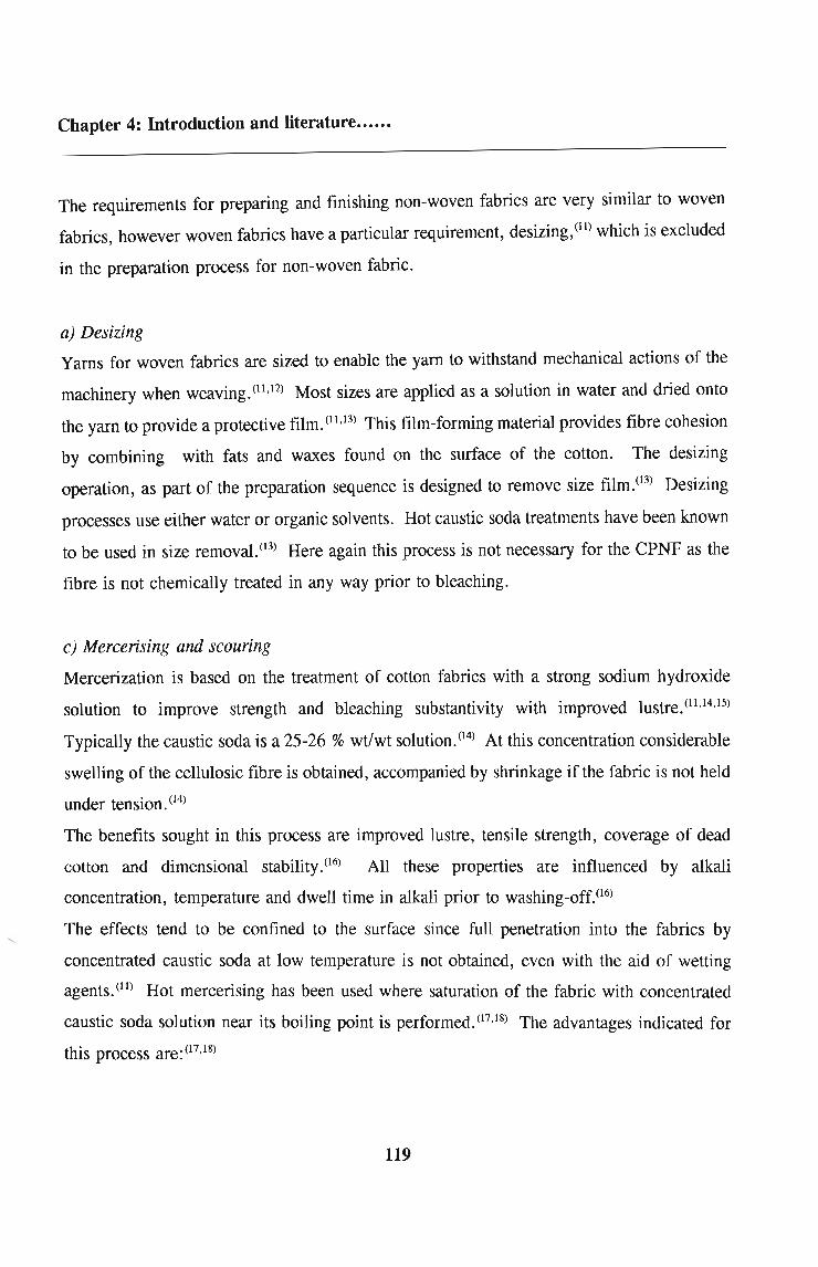
Chapter 4: Introduction and literature .
The requirements for preparing and finishing non-woven fabrics are very similar to woven
fabrics, however woven fabrics have a particular requirement, desizing,(l1) which is excluded
in the preparation process for non-woven fabric.
a) Desizing
Yarns for woven fabrics are sized to enable the yarn to withstand mechanical actions of the
machinery when weaving. (11,12) Most sizes are applied as a solution in water and dried onto
the yarn to provide a protective film. (11,13) This film-forming material provides fibre cohesion
by combining with fats and waxes found on the surface of the cotton. The desizing
operation, as part of the preparation sequence is designed to remove size ftlm.(13) Desizing
processes use either water or organic solvents. Hot caustic soda treatments have been known
to be used in size removal. (13) Here again this process is not necessary for the CPNF as the
fibre is not chemically treated in any way prior to bleaching.
c) Mercerising and scouring
Mercerization is based on the treatment of cotton fabrics with a strong sodium hydroxide
solution to improve strength and bleaching substantivity with improved lustre. (11,14,15)
Typically the caustic soda is a 25-26 % wt/wt solution. (14) At this concentration considerable
swelling of the cellulosic fibre is obtained, accompanied by shrinkage if the fabric is not held
under tension. (14)
The benefits sought in this process are improved lustre, tensile strength, coverage of dead
cotton and dimensional stability. (16) All these properties are influenced by alkali
concentration, temperature and dwell time in alkali prior to washing-off.(16)
The effects tend to be confined to the surface since full penetration into the fabrics by
concentrated caustic soda at low temperature is not obtained, even with the aid of wetting
agents. (11) Hot mercerising has been used where saturation of the fabric with concentrated
caustic soda solution near its boiling point is performed. (17,18) The advantages indicated for
this process are: (17,18)
119

Chapter 4: Introduction and literature.••...
a) increased efficiency and uniformity,
b) improved lustre, tensile strength and dimensional stability since greater fabric stability
is possible,
c) good desizing,
d) better fabric penetration by a hot caustic liquor than with normal mercerisation,
Scouring is applied to the fabric to remove oils, fats, waxes, soluble impurities and
particulate dirt which adheres to the cotton fibres. (11) Natural and other fats and waxes may
be removed prior to dyeing or bleaching by the use of organic solvents, but most preparation
routes use alkali scouring. (11) This may be a single process or be combined with the desizing
or/and bleaching. (11,19) Apart from the fats and waxes, other non-cellulosic constituents can
be removed, particularly nitrogenous matter and pectate. Most importantly cotton seed can
be softened or burst for subsequent removal. Modem scouring practice consists of treatment
with a detergent, with or without the addition of an alkali. (19,20)
Scouring can be carried out in a kier. (20,21) Conventionally the fabric is loaded into the kier
and hot alkaline liquor is circulated for several hours. (20) The process may be carried out at
100 QC, but pressure boiling is also practi.s,ed with temperatures of 120°C being reached. (11)
,. Methods of treatment are described in the literature. (22)
Currently sodium hydroxide is the most generally used reagent. In kier boiling care must
be taken to ensure that air is not entrapped in the fabric since its presence can lead to the
formation of oxycellulose. (11) Provided that there is control of alkali and temperature, good
scouring removal and some fabric whitening can be obtained during this process with little
fibre damage. (11,19,23)
In the non-woven fabric under investigation in this work, the mercerization process is not
considered necessary as the fabric is been subjected to alkali in the combined scouring and
bleaching stage. The CPNF is subjected to a short single stage combined scouring and
bleaching stage.
120

Chapter 4: Introduction and literature.•.•..
d) Bleaching
The three chemicals that can be used for bleaching are sodium hypochlorite, sodium chlorite
and hydrogen peroxide.
i) Hypochlorite
Prior to bleaching with hypochlorite it is essential that the cellulose be cleared of natural
impurities by a thorough scouring. (11) This alone implies complexity in the process with one
or two alkaline boils being required with intermediate washing. These will be followed by
scouring and further washing prior to bleaching. (11,24) Bleaching must be followed by washing
and an antichlor treatment, the latter being performed to remove the products of the
bleaching reaction. The end result is, therefore, a process with high labour content, lengthy
processing time and high water demand. (11,25) In the last decade hypochlorite bleaching has
been replaced very widely by formulations and processes based on hydrogen peroxide,
sodium chlorite or combinations of the two. (26,27)
ii) Sodium chlorite
Sodium chlorite bleaching, in contrast to hypochlorite or hydrogen peroxide bleaching, is
carried out under acidic conditions. (11,25) Under the acid bleaching conditions, a relatively
small amount of natural fats and waxes is removed. (11,22) Chlorite bleaching is also relatively
unaffected by low levels of iron and copper contamination,(lO) however, there are several
disadvantages in chlorite bleaching. (11,25) It is difficult to control chlorine dioxide release and
the products of the bleaching reaction (scheme 4.1) are known to be environmentally
unfriendly.
5CI02 -- + 2H+ -------- > 4CI02 + CI-- + 20H--
Scheme 4.1
121
4.1
4.2

Chapter 4: Introduction and literature .
Also in contrast to hydrogen peroxide bleaching the temperature, pH etc. cannot be selected
to provide very rapid bleaching. (11)
iii) Hydrogen peroxide
Hydrogen peroxide bleaching for cellulosic textiles is carried out under alkaline conditions.
Consequently scouring and bleaching can frequently be combined. (11,27,28) Hydrogen peroxide
is adaptable to a wide range of bleaching conditions: a temperature range from ambient to
250°C and a time range from a few minutes to several hours. (11,27) Cotton oxidised by
hydrogen peroxide is characterised by a high content of ketone groups but a very low
aldehyde and carboxyl content. The ketones formed are inactive carbonyls Le. they cause
no yellowing on ageing. (11) This research is based on the utilization of hydrogen peroxide
as the bleaching agent.
4.4 Hydrogen Peroxide Bleaching
A prime advantage of hydrogen peroxide bleaching is the wide range of conditions over
which it can be used for bleaching cellulosic textiles. (11,27) However, with all bleaching
processes correct process control is essential. (11)
Although considerable progress has been made in the optimisation of bleaching conditions,
the bleaching mechanism is not yet fully understood. (11,24,29) The reason for this is the
heterogeneous nature of the process and the lack of absolute knowledge about the coloured
material that is destroyed. (11) It is well known that hydrogen peroxide can breakdown into
water and oxygen (Scheme 4.2).(24)
4.3
Scheme 4.2
However, it is most unlikely that bleaching can be attributed to such a simple mechanism.
122
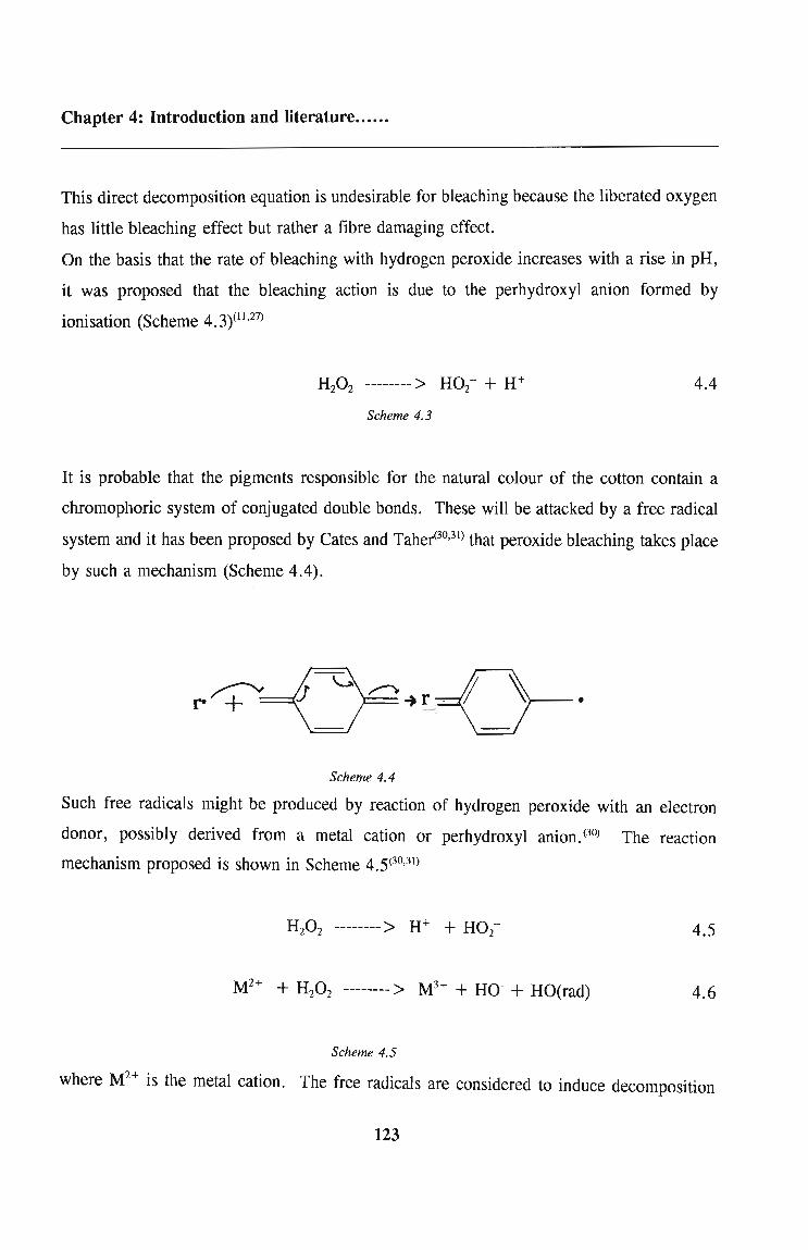
Chapter 4: Introduction and literature .
This direct decomposition equation is undesirable for bleaching because the liberated oxygen
has little bleaching effect but rather a fibre damaging effect.
On the basis that the rate of bleaching with hydrogen peroxide increases with a rise in pH,
it was proposed that the bleaching action is due to the perhydroxyl anion formed by
ionisation (Scheme 4.3)(11,27)
4.4
Scheme 4.3
It is probable that the pigments responsible for the natural colour of the cotton contain a
chromophoric system of conjugated double bonds. These will be attacked by a free radical
system and it has been proposed by Cates and Taher<30,31) that peroxide bleaching takes place
by such a mechanism (Scheme 4.4).
Scheme 4.4
Such free radicals might be produced by reaction of hydrogen peroxide with an electron
donor, possibly derived from a metal cation or perhydroxyl anion. (30) The reaction
mechanism proposed is shown in Scheme 4.5(30,31)
4.5
4.6
Scheme 4.5
where M2+ is the metal cation. The free radicals are considered to induce decomposition
123

Chapter 4: Introduction and literature .
through a chain mechanism. The decomposition within a given time interval is limited by
the level of colour bearing impurities or by inhibiting metal cations. (30) The latter appears
to protect the cellulose from chemical damage by minimising the production of molecular
oxygen in the alkaline medium.(31)
While absolute mechanisms are not yet fully understood, control systems for the
decomposition reaction have been developed,o°,l1) This control is termed stabilisation. (11,24)
Correct process stabilisation conditions control the rate of bleaching and ensure a residual
peroxide content prior to washing off. In this way the required standards of whiteness with
minimum chemical damage are obtained. In effect, for peroxide bleaching four parameters
are to be balanced for efficient and successful bleaching: time, temperature, alkalinity and
hydrogen peroxide concentration. (10,11,19)
In this work time, temperature and hydrogen peroxide concentration are optimised with
respect to a low temperature bleaching process for the CPNF.
4.4.1 The role of chemicals in hydrogen peroxide bleaching
In modern preparation technology, the bleaching process is not only concerned with the
brightening of the fibre by the destruction of the natural colouring matter but it must
frequently make a significant contribution towards preparation for subsequent dyeing, printing
or chemical finishing. (27) The bleaching process may be the only preparation process or more
often it is used in conjunction with other treatments Le scouring or desizing. (27) In this study
a low temperature single stage combined scouring and bleaching process was investigated and
optimised with respect to the CPNF property of whiteness.
Besides the bleaching agent itself, other chemicals are used which have various functions.
These chemicals serve to activate the bleaching agent, (11) stabilise or control the degree of
bleaching agent activation, (9) to give good wetting, surfactant and detergent action in order
to assist in the removal of impurities and to sequester metallic impurities found in the
fibre. (11,25) Extensive research (9,11,25,27,32)has been conducted on the considerations that have
to be given as to the role of each individual chemical used in conjunction with the peroxide
124

Chapter 4: Introduction and literature•...•.
bleaching agent.
a) Alkaline activators
When peroxide bleaching cotton, the alkali added activates the peroxide bleaching and
provides a scouring action. (11) Bleaching processes are most effective when carried out within
the pH range 10.5 to 11. Above this level peroxide bleach liquors are overactivated, giving
excessive wasteful breakdown to oxygen and water. (11,24) If the pH is lower than 10 the
bleaching activity is very low. (11) Alkalinity is normally provided by sodium hydroxide,
sodium carbonate or phosphate. Sodium silicate, when used as a stabiliser, adds to the total
alkalinity. (10)
Sodium hydroxide however, if used alone induces too rapid a decomposition of hydrogen
peroxide (equation 4.3) so that significant amounts of peroxide are lost for bleaching. (11) As
a result stabilisers have to be introduced into the bleaching liquor.
Amides have recently shown(33) to facilitate faster but controlled bleaching action in alkaline
(sodium hydroxide) bleach baths. When the bleach liquor is peroxide based the amides have
shown to inhibit the decomposition reaction of H20 2 and accelerate the formation of the
perhydroxyl ion (equation 4.4). The amides responsible for this increase in the bleaching
activity of peroxide bleach bath include urea, benzamide, formamide and N,N dimethyl
formamide (DMF). (33)
b) Stabilisers
The activity of the peroxide bleaching liquor brought about by addition of alkali is controlled
by the action of stabiliser additives. Stabilisation is described as a process of regulation and
control. The function of these chemicals is to inactivate impurities particularly metallic
impurities, which tend to cause catalytic decomposition of the hydrogen peroxide. (10,11) These
impurities can be introduced into the bleaching system from the fabric, water or the
chemicals used. (11)
The stabilisers first used in bleaching cellulosic fibres were the colloidal sodium silicates. (32)
These are highly effective and have an additional advantage of being comparatively low in
cost. Metasilicate (Na2Si03) and orthosilicates have also been used and these have been
found to wash out more readily than colloidal silicates. (11,34)
125

Chapter 4: Introduction and literature .
The use of sodium silicate requires the provision of good washing off facilities after
bleaching in order to prevent problems caused by residual silicates. (32) Consequently,
although sodium silicate is both effective and economic and is the most widely utilised
stabiliser both in high and low temperature cellulosic bleaching methods, there have been
reviews on the use of alternative chemicals for peroxide stabilisation. (32,35) The commercial
products available are basically organic sequestering agents which are designed to impart a
combined stabilisation, detergency and softening effect.(35,36,37) The organic stabilisers include
polyphosphates, ethylenediamine tetracetic acid (EDTA) and tetrasodium pyrophosphate. (36)
Sodium silicate has been used in most of the low temperature peroxide bleaching treatments
previously reported for cellulosic fibres(IO) and as such this stabiliser was used in all the
bleaching treatments investigated for the CPNF.
c) Wetting agents
Good wetting of material is required to ensure penetration of preparation chemicals and
evenness of treatment. (11) Commercial wetting agents are usually anionic or non-ionic
surfactants or blends of the two. (12) In solution the compounds anionic ionise, with the
surface active component carrying the negative charge (Scheme 4.6, in which R is the long
chain hydrocarbon)
R °S02 °Na -----> R °S02 0- + Na+
Scheme 4.6
4.7
Most commercial products used in the textile preparation processes are ethoxylated fatty
alcohols with the general formula shown below(12)
An important factor affecting the use of wetting agents for the low temperature used batch
bleaching in kiers is the degree to which the bleaching liquor foam.(12) Excessive foam in
kiers can cause cavitation in pumps with resultant poor circulation.(11)
A commercially available wetting agent termed "Foryl B" was used in all the investigations
126

Chapter 4: Introduction and literature .
in this work.
4.5 Cold pad batch bleaching
The process of padding the grey fabric with a strong solution of alkali and hydrogen
peroxide, and storing for several hours, usually overnight, at ambient temperature is called
cold pad batch bleaching. In the last decade, an interest in cold bleaching has increased as
it provides a low energy preparation route. (39,40) Fabric can be impregnated with the bleach
solution in a kier or on open width washers and left batched up overnight. Cold pad batch
bleaching requires: (11)
1. Control of pad liquor concentration and temperature, preferably 25°C
2. Fabric storage without surface drying
3. Washing-off at a minimum of 95°C.
A good wetting agent is essential to ensure good penetration of the grey fabric by the
bleaching liquor, with a detergent auxiliary to aid wax removal and development of good
absorbency. (11)
Numerous recipes (33,35,39,40,41,42)have been described over the years for the single stage low
temperature peroxide scouring and bleaching of cellulosic woven fabrics. Most of these
differ greatly with respect to the treatment time, the range of low temperatures investigated
and additional additives used. Some of the recipes that have been described are outlined
here, with special emphasis on those that have been adapted to the CPNF.
Although the first ever bleaching of cotton with hydrogen peroxide was carried out at a low
temperature as 1928 by Smolens(38), it was not until approximately 15 years ago that it
regained its popularity over the any of the high temperature shock bleach treatments (sodium
chlorite and hypochlorite bleaching etc) because of its energy saving and cost effective
advantages. In particular the single stage combined scouring and bleaching process at
127

Chapter 4: Introduction and literature .
ambient temperature has recently superseded the single stage high temperature treatment.(63)
Dalmas(35) in the early eighties patented a bleaching process for cellulosic fibres done at
60 °C. The invention was a process of bleaching cellulose materials with potassium based
bleach liquors or the products of the reaction between sodium silicate and potassium
hydroxide (equation 4.8).
4.8
Scheme 4.7.
The bleaching liquor employs potassium orthosilicate as the peroxide stabiliser and the
sodium hydroxide as the alkaline medium. Greige cotton fabrics are immersed in a liquor
in a kier at 60°C, allowed to seep for an hour and then rinsed at 60 QC. The bleach liquor
employs a formula of the following composition: potassium orthosilicate, a wetting agent,
50 % hydrogen peroxide and water. These workers have reported that the fabric produced
was soft, absorbent, free of any seeds and husks and of a uniform white. (35)
Wani(39) investigated various bleaching methods including a cold bleaching process as used
by the Ahmedabad Textile Industry Research Association in India (ATIRA) and concluded
that in comparing the cold pad batch process to the conventional high temperature process
a considerable saving in energy, steam and cost is afforded. The cold batch process used by
ATIRA (a) and one of the high temperature treatments (b) is shown in scheme 4.8.
Desize --- > Scour· --- > Wash (hot or cold) --- > Scour --- > Dry (a)
Desize --- > Wash --- > Open kier boilingt --- > 2 hot washes --- > 2 cold washes (b)
Scheme 4.8.
• = 60 °C circulation for 12 h with (50 %) H20 2 0.22 %, sodium hydroxide 0.9 %, ATIRA catalyst 0.3 %, non-
ionic wetting agent 0.22 % ,and
t = 50 % H20 2 1 %, sodium hydroxide 0.3 %, sodium carbonate 0.5 %, SCOUREX 0.3 %, for 4 h at 90 0C.
128

Chapter 4: Introduction and literature•.....
Wani reported that the fabrics produced from the cold pad batch process contain minimum
damage with an acceptable degree of whiteness and absorbency. (39)
Hickman and Andrianjafy(9) evaluated the role of different stabilisers for the hydrogen
peroxide bleaching treatments of cotton woven fabrics. Three organic stabilisers in addition
to sodium silicate were investigated under short and long bleaching times on 100 %
desized but unscoured cotton fabric at a temperature of 95 0 C and the results were compared
to those obtained when sodium silicate was used alone as the peroxide stabiliser. This
temperature was a little high to be termed low temperature, however the results produced are
of importance and can be applied to low temperature bleaching. The bleaching liquor
contained sodium silicate, magnesium sulphate, a wetting agent, caustic soda and hydrogen
peroxide. The bleached samples were analyzed for their whiteness and fluidity properties.
Sodium silicate was shown to be the most effective stabiliser and that the order in which the
organic stabilisers can be ranked depends on the bleaching system itself. (9)
Das and coworkers(40) carried out extensive laboratory studies of the combined scouring and
bleaching cold temperature bleaching processes. In their cold bleaching process , desized
and chemicked· fabrics were bleached at room temperature for time periods ranging from
2 to 24 h. Two bleaching recipes have been described: one containing sodiunm hydroxide,
sodium metasilicate, hydrogen peroxide and a non-ionic wetting agent and the other
containing sodium-metasilicate, tetra sodium pyrophosphate, hydrogen peroxide and the non
ionic wetting agent in the bleaching bath. The wetting agent has been described as a 1: 1
mixture of perchloro-ethylene and the product obtained from the condensation of one mole
of nonyl phenol with 6 - 8 moles of ethylene oxide. These workers reported that for all the
treatments investigated, the fabrics exhibited uniformity in treatment and comparatively lower
damage when compared the traditional high temperature process. (40) The whiteness,
absorbency and fluidity results are all satisfactory for the fabrics bleached by the low
temperature method. (40)
• immersion of the fabric in 2 - 3 gol-! of sodium hypochlorite solution for 1 - 2 h.
129

Chapter 4: Introduction and literature .
Sukumar and Gulrajani(41) assessed a low temperature single stage preparatory process for
cotton wovens wherein five compounds, viz. trisodium phosphate, tetrasodium
pyrophosphate, sodium hexametaphosphate, magnesium sulphate and a sodium salt of
ethylenediamine tetracetic acid (EDTA), were investigated for the activation and stabilization
of the peroxide in the bleach bath. The untreated fabrics were bleached with a solution
containing 4 % scouring agent, 1 % hydrogen peroxide (100 %), 2 % sodium silicate and
2 % activator at room temperature for different time periods (12 - 24 hours). The fabrics
were evaluated for their tensile strength, whiteness, wettability and ash content. These
workers concluded that of the five compounds investigated, only two are suitable for the low
temperature single stage process, viz. tri-sodium phosphate and tetrasodium pyrophosphate. (41)
A mechanism for the activation process for all the activators investigated was reported and
these are shown in equations 4.9 to 4.14.(41) In addition a stabilization mechanism of the
peroxide by sodium silicate was also proposed whereby the silica gel (nSi02) is responsible
for physically trapping the perhydroxyl ions and thus controlling hydrogen peroxide
decomposition.
Na20.nSi02 + mH20 ---> 2NaOH + nSi02 + (m-l)H20 4.14
Scheme 4.9.
130

Chapter 4: Introduction and literature .
Dickenson and Hickman(42) investigated the cold pad bleaching with experiments based on a
central rotatable plan with the following range of conditions: temperature - 20 to 60°C, time
- 7 to 75 hours, sodium persulphate - 0 to 10 g·t l, caustic soda - 1 to 40 g'l-I, hydrogen
peroxide (35 %) - 60 ml'l-I, sodium silicate - 40 g·t l and a commercially available wetting
agent. A recipe based on mixed organic and silicate stabiliser system was also described for
cotton and cotton/polyester blends. These cold processes were compared to the pad steam
processes. Analysis of results showed that the chemical damage increases as the alkalinity
and/or temperature increases and that the use of persulphates can cause an increase in
chemical damage but their influence is substantially less than that of alkali concentration or
temperature. (42) For all the bleached fabrics, a satisfactory final whiteness was obtained over
a wide range of conditions. On comparison with the multistage steam process (conventional
bleaching), it was reported that cold pad bleaching was favourable from both an energy and
cost point of view. (42)
Das et azr33) reported an amide activated bleaching process whereby the amides are
incorporated into the bleaching bath to facilitate faster decomposition of the hydrogen
peroxide. Desized and scoured cotton fabrics were padded through a bleaching bath
containing one of the various amides (urea, benzamide, formamide, N,N-dimethyl
formamide [DMF]), sodium hydroxide 10 g' t l, sodium silicate 15 g'l-I, hydrogen peroxide
20 g'l-I and a wetting agent. The bleaching experiments were carried out at ambient
temperature, 60°C and 90 °C for 8 h. The bleached fabrics were evaluated on the basis of
their final whiteness. At ambient temperature, the rate of peroxide decomposition decreases
in the following sequence: (33)
formamide > DMF > benzamide > urea
Benzamide affords the maximum whiteness with the whiteness value increasing with time and
temperature of bleaching. The benzamide bleaching process is quite useful in cold bleaching
131

Chapter 4: Introduction and literature .
where the time of bleaching can be reduced without impairing the whiteness of the fabric. (33)
Sarma et az<43) recently investigated a combined scouring and bleaching process for chemicked
cotton fabrics. The bleaching bath contained the following activators and/or stabilisers for
peroxide: sodium hydroxide, sodium silicate, potassium persulphate, magnesium sulphate,
a wetting agent. Fabrics were bleached at 25, 35 and 45°C and analyzed with respect to
the physical properties of whiteness, fluidity and absorbency. An optimum treatment for
bleaching was established which produces a fabric of acceptable values of whiteness,
absorbency and fluidity. (43)
Muresan et al(44) reported an alkaline cleaning treatment and conditions for cotton materials.
Experiments were carried out at 25°C on a 100 % cotton textile material in the raw state
in a bleaching bath containing the following chemicals: hydrogen peroxide, sodium
persulphate, sodium silicate and sodium hydroxide. The fabrics were assessed for their
breaking strength, whiteness and hydrophilicity. A multiple regression analysis was used
with four influencing parameters (sodium hydroxide concentration, hydrogen peroxide
concentration, sodium persulphate concentration and time) to optimise the chemical
concentrations and the treatment conditions. The following optimum conditions were
obtained: 20 to 40 g·l-l sodium hydroxide, 60 g. t 1 hydrogen peroxide, 12 g·l-l sodium
persulphate and a treatment time of 5 h.(44) Under these conditions, the whiteness and
hydrophilicity reach maximum values while the breaking strength is low. (44)
Five bleaching treatments based on the methods of Sarma et al,(43)(the most recent literature
procedure obtainable) Muresan et aI, (44) Dickenson et al (42) and Das et al (33)have been used
in this work for the low temperature bleaching of the CPNF. The adaptation of these
methods is discussed in chapter 5.
132

Chapter 5: Bleaching treatments.••..•
Chapter 5
Bleaching treatments used in this work
5.1 Introduction
Numerous recipes have been described over the years for the low temperature bleaching of
cotton woven fabrics. (33,39,40,41,42,43,44) Although most of these recipes differ greatly with
respect to the treatment conditions and the additives used, all served to improve the process
with respect to optimising the bleaching effect while minimising the extent of fibre damage
of the woven cellulosic fabrics.
The treatment conditions employed throughout this investigation were based on those most
recently optimised for the low temperature single stage bleaching process for cotton woven
fabrics. Five combined scouring and bleaching procedures(33,42,43,44) were selected for this
study with the aim of developing a low temperature bleaching process which maximised the
property of whiteness and absorbency. In addition the extent of fibre damage for the CPNF
should be kept minimal. In view of the differences between physical properties of the
woven and non-woven fabrics, (cf Table 4.1) it was considered important to establish
whether the chosen bleaching chemicals and their corresponding treatment conditions resulted
in any CPNF fibre degradation. These effects are discussed in chapters 6 and 7.
This chapter describes the bleaching treatments utilized in this work together with the
materials, laboratory apparatus and chemicals used throughout this study.
5.2 Bleaching treatments investigated in this work
All of the bleaching treatments investigated in this work represent the most recent advances
in low temperature peroxide bleaching research done over the past 10 years for woven
fabrics. As a starting point, the low temperature amide activated bleaching process designed
by Das and coworkers was investigated. (33) In their work amides are incorporated into the
bleaching bath recipe to facilitate faster but controlled decomposition of hydrogen peroxide.
Their formulations are based on the utilization of four amides Le urea, benzamide,
formamide and dimethyl-formamide. Scoured and desized cotton woven fabrics are
133

Chapter 5: Bleaching treatments .
immersed into a bleaching bath containing the bleaching chemicals listed in Table 5.1 and
bleaching was carried out at 25, 60 and 90 °C for the time period ranging from 3.5 to 7 h.
Table 5.1 Bleaching conditions at room temperature for 3.5 to 8 h of Das et a(33).
Chemical Experiment
(g.1-1) 1 2 3 4 5
NaOH 10 10 10 10 10
NazSiz0 3 15 15 15 15 15
HzOz (50 %) 20 20 20 20 20
Emul.Agent 5 5 5 5 5
Urea 30
Benzamide 30
Formamide 30
DMF 30
At 25 °C it was reported that the sequence in the rate of hydrogen peroxide decomposition
is as follows :
formamaide > DMF > benzamide > urea
Benzamide affords the maximum whiteness and in all cases there is practically no loss of
strength of the bleached fabric. Similar trends are observed at the higher temperatures. (33)
Sarma et al(43, 63) reported two papers for the bleaching of woven fabrics at a low temperature
using a persulphate salt as the hydrogen peroxide activator. These workers utilized a
statistical plan similar to the one being used in this investigation. In both their papers they
134

Chapter 5: Bleaching treatments•....•
concluded that the optimum combined scouring and bleaching process for a desized cotton
woven fabric was one carried out at 35°C for a time period of 7 hs.(43) The optimum
bleaching concentrations for the chemicals used in their research is listed in Table 5.2.
This treatment produced a fabric with excellent fabric properties of whiteness, absorbency.
with their fluidity values showing minimum fibre damage. (43)
Table 5.2 Bleaching conditions at 35°C for 7 hs of Sarma et arC).
Chemical % o.w.f....
Sodium Hydroxide 2.5
Sodium Silicate 1.5
K2S2Og 0.4
MgS04 0.32
Scouring Agent 0.9
Hydrogen Peroxide(50%) 1.3
* refers to the percentage weight of fabric and related to g·tI by the equation:
conc. (g'l-I) = (% o.w.f. x 10) / liquor ratio (goods to liquor ratio = 1:5)
More recently, Muresan et al (44)formulated a recipe for bleaching untreated cotton woven
fabrics that involved sodium persulphate as the peroxide activator at room temperature for
a time of 5 h. According to this method the extent of fibre damage incurred during the
single stage scouring and bleaching process is equal to that obtained by the classical
procedure Le alkaline boiling, whitening with hypochlorite ( pt stage) and then with
hydrogen peroxide ( 2nd stage). (44) The concentrations of the bleaching chemicals used by
Muresan et al are listed in Table 5.3.
135
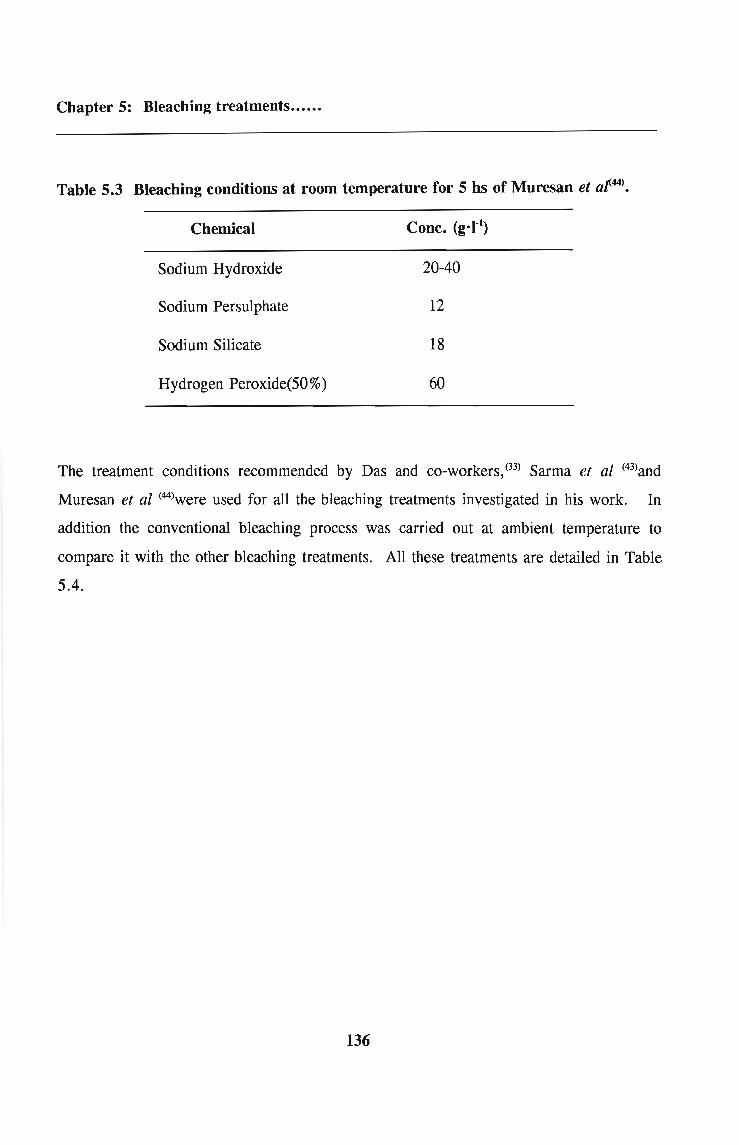
Chapter 5: Bleaching treatments•••.•.
Table 5.3 Bleaching conditions at room temperature for 5 hs of Muresan et af.44).
Chemical
Sodium Hydroxide
Sodium Persulphate
Sodium Silicate
Hydrogen Peroxide(50%)
Conc. (g.r1)
20-40
12
18
60
The treatment conditions recommended by Das and co-workers, (33) Sarma et al (43)and
Muresan et al (44)were used for all the bleaching treatments investigated in his work. In
addition the conventional bleaching process was carried out at ambient temperature to
compare it with the other bleaching treatments. All these treatments are detailed in Table
5.4.
136

Chapter 5: Bleaching treatments•••.••
Table 5.4 Treatment conditions (T) for the various bleaching recipes investigated
Ta Tb Tb T/ TC Tsd
0 1 2 4
Chemical conc. (g • .-1)
NaOH 23 30 30 30 30 30
Na2C03 20
Na2Si20 3 18 18 18 18 18
H20 2 (50 %) 75 65 65 65 65 65
Wetting Agent 10 10 10 10 10 10
NH2CONH2 15
C6HsCONH2 15
HCONH2 15
MgS04 0.5
K2S20 4 0.5
Na2S2OS 12
To, T1 etc. refers to treatment condition 0 and 1 etc., respectively
a conventional bleaching process done at 25°C (normally done at 250°C)
b based on reference 33
C based on reference 43
d based on reference 44
137

Chapter 5: Bleaching treatments.•....
5.3 Apparatus and Experimental procedure
5.3.1 Materials
The CPNF fabric samples used in this investigation has been described in chapter 4 and
shown in appendix 2.1 and were obtained directly from the mill. These samples were not
pretreated in any way prior to bleaching.
Reagent grade chemicals and deionised water was used in all the investigations. The
bleaching chemicals used for each of the investigations together with their suppliers are
listed in Table 5.5
Table 5.5 List of chemicals and their suppliers
Chemical Supplier
NaOH Aldrich
Na2C03 Saarchem
Na2Si20 3 Aldrich
H20 2 (50 %) Alliance Peroxide
Wetting Agent "Foryl D"· Merck
NH2CONH2 Kleber Chemicals
C6HsCONH2 BDH
HCONH2 BDH
MgS04 Saarchem
K2S20 4 Merck
Na2S2Og Aldrich
• Foryl D is the patented name for a commercially available wetting agent.
138

Chapter 5: Bleaching treatments••••••
5.3.2 Experimental methods
All bleaching recipes employed in this work were carried out in a thermally controlled
reaction vessel as shown diagrammatically in Figure 5.1. This setup was carried out so as
to emulate the kier bleaching system as close as possible. The samples were preweighed
prior to being wrapped around the glass tripod, D, and totally immersed in a liquor
containing all the relevant bleaching chemicals except hydrogen peroxide. Temperature
control was achieved by water being pumped from a thermally controlled water bath, C, into
a glass jacket insulating the reaction vessel. The entire assembly was placed on a magnetic
stirrer thus ensuring good mixing and dispersability of the bleaching chemicals. The glass
combination quickfit stopper and tripod, D, was made with two outlets, one for a
thermometer, one to allow the introduction of chemicals and the other to allow the release
of the products of decomposition (oxygen).
All investigations into the bleachirig behaviour of the CPNF were performed as follows: 10
grams of unbleached CPNF was immersed in an alkaline bleach liquor (180 ml deionised
water) containing all the relevant bleaching chemicals except hydrogen peroxide for 30 min
under stirring. A known amount of hydrogen peroxide was added to the bleach liquor and
bleaching was carried out under stirring for a fixed time. The CPNF was then removed from
the liquor and washed with glacial acetic acid, followed by a thorough hot water rinse (80
to 85°C) for five min. to ensure removal of residual chemicals. All the samples were dried
in an oven at 100°C for 60 min.
139

nc:r~
~tD..,~
=[5r
(J'Q...
I~·····
reaction vessel
magnet
cutton wrapped
sti n-a r
~ lilagfldtic
bleaching-~
liquor
~ thermometer
~
.. around glass tripoc D~
bleaching chemicals inI
I
- I
water thermstat I~
water - ----
Thermometer in
Braun
-. Thermostat
unitwater
---- -
out
--_.__.
C --
~...=
Figure 5.1 Diagrammatic representation of the laboratory apparatus used in all the bleaching treatments

Chapter 6: Evaluation of the ••.••.
Chapter 6
Evaluation of the bleached CPNF
6.1 Introduction
In the development of any bleaching process and their corresponding optimisation technique,
it is important to characterise the final fabric as thoroughly as possible.(46) This includes
comparison of the critical fibre properties such as the extent of fibre damage incurred
(fluidity tests, cf. section 6.2)(47), whiteness, (11) absorbency, (11,48) change in the mechanical
properties of the fibre(49), and the complete removal of any impurities found in the cotton, (11)
to the bleached fabric products made by the conventional bleaching process.
In this study the evaluation of effective bleaching for the CPNF, for the five bleaching
treatments described in chapter 5, was performed with respect to the degree of fibre damage
(fluidity), absorbency, and whiteness observations. A scanning electron microscope analysis
was also performed and the results of these are detailed in chapter 7. These results are
compared to those obtained for the high temperature, high pressure bleaching process i. e. the
factory bleached fabric).
The fibre properties of all CPNF samples, both bleached and unbleached, were measured
using standard procedures(50,51,52) (cf. appendix 2.2 and 2.3) and equipment and this
information together with their results are detailed in the following subsections.
The CPNF samples were obtained directly from the mill (see appendix 2.1) and were not
treated chemically in any way prior to bleaching/scouring. Combined scouring and Bleaching
was carried out according to the methods detailed in Table 6.1.
Reagent grade chemicals were used in all the fibre property determinations and deionised
water was used in all appropriate cases. All determinations were carried out at 25 QC and
the bleaching time was kept constant at I hour.
141
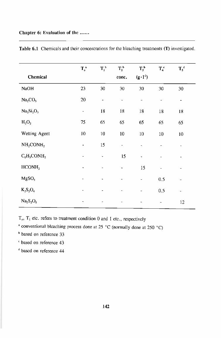
Chapter 6: Evaluation of the •••••.
Table 6.1 Chemicals and their concentrations for the bleaching treatments (T) investigated.
Ta Tb Tb Tb T C T d0 1 2 3 4 s
Chemical conc. (g. r1)
NaOH 23 30 30 30 30 30
Na2C03 20
Na2Si20 3 18 18 18 18 18
H20 2 75 65 65 65 65 65
Wetting Agent 10 10 10 10 10 10
NH2CONH2 15
C6HsCONH2 15
HCONH2 15
MgS04 0.5
K2S20 4 0.5
Na2S2Og 12
To, Tt etc. refers to treatment condition 0 and 1 etc., respectively
a conventional bleaching process done at 25 QC (normally done at 250 QC)
b based on reference 33
C based on reference 43
d based on reference 44
142

Chapter 6: Evaluation of the •.••.•
6.2 The degree of chemical degradation of the CPNF samples (fluidity determinations)
6.2.1 Introduction
In many applications textile fibres require high tensile strength and resistance to chemical
attack. (53) Even slight degradation of cellulose is invariably accompanied by a loss of strength
and/or tendering. (46) The study of degradation mechanisms therefore has important
implications for the production of satisfactory finished fabrics. (53)
From a chemical point of view the complete degradation of cellulose is its conversion into
carbon dioxide and water. (53) Any intermediate stage in this process may be described as
partial degradation and it is these early stages of degradation that has been determined by the
prescribed methods. Quite small changes in chemical composition may profoundly affect
the physical properties of cellulose. (53)
Although many reagents swell cellulose, very few are capable of dissolving it. (53) Much
effort has been put into the search for cellulose solvents and for many years the only known
solvents for cellulose were moderately concentrated acids (70 % sulphuric acid) and
cuprammonium hydroxide. (11) Cuprammonium hydroxide dissolves cellulose without
degradation provided that atmospheric oxygen and light are excluded. (11,42)
Ost in 1911, (54) first suggested that the viscosity of a solution of cellulose in ammoniacal
copper hydroxide can be used as an indication as the average cellulose chain length. This
suggestion was investigated critically by Farrow and Neale in 1924 (55)and finally perfected
by Clibbins and his collaborators at the Shirley Institute. (56,57,58)
It has been reported that cellulose dissolves in cuprammonium hydroxide because a 1: 1
complex is formed between the cuprammonium ion and the 2,3 diol group of the
anhydroglucose chain units. (59) A uncharged square planar complex, as shown in Scheme 6.1
is formed and the formation of this complex involves distortion of the pyranose ring. (53,60)
Scheme 6.1
143

Chapter 6: Evaluation of the .
Kenner et al(61) have shown that cellulose degraded by alkali at temperatures above 170 0 C
results in scission of the glycosidic bonds randomly along the lengths of the fibres and the
newly formed shorter chains can be degraded further.
Under unfavourable conditions the hydrogen peroxide can cause serious oxidative degradation
causing extensive tendering to the fabric. (53) The nature of the degradation is not well
understood. (53) This is due to the strong catalytic influence of metal ions, such as those of
copper and iron, which may be found both in the cellulose and the sodium hydroxide used
for the oxidising liquor. (53) Oxidation by alkaline peroxide has been found to almost certainly
involve peroxy radicals which leads ultimately to chain scission. (53)
6.2.2 Fluidity test
The fluidity method of test is sensitive to the onset of chemical damage before such damage
would become apparent through a loss in tensile strength. (11) The fluidity of cellulose in
cuprammonium is determined in a viscometer as shown in Figure 6.1.
E
c
A
D
Fig 6.1 Viscometer taken from referance 63
144

Chapter 6: Evaluation of the •.....
According to the British Standards test method,(62) the fluidity of a specimen of cotton is the
fluidity of a solution in the standard cuprammonium solvent containing 0.5 g of cotton per
100 ml of solution at 2 °C. In this test a weighed sample of cellulose finely chopped to give
fibres of 1 - 2 mm length is dissolved in standard cuprammonium hydroxide in a standard
viscometer. The viscometer must be filled completely to exclude air and covered to prevent
exposure to light, whilst controlled agitation is given over 16 hours. The viscometer and its
contents are then brought to 20 °C in a thermostatically controlled bath and the rate of flow
through the capillary measured i.e. the time taken for the meniscus to fall from one fixed
mark to another( C to A in the Figure 6.1).(8,62,64) As each viscometer is precalibrated, from
data provided with the instrument, fluidity is then calculated by dividing the viscometer
constant by the time recorded. This gives a direct calculation of fluidity in terms of
Pa-l·s-l (reciprical poise or rhe units).
The principle of the test is that during dissolution, no further breakdown of the cellulose
chain structure will occur. Long chained fabrics i.e with low fibre damage, will provide
a high viscosity solution, hence low fluidity. As a general rule, bleached cotton with a
fluidity above 10 Pa-l·s-t, is regarded as chemically damaged.
6.2.3 Experimental
Unbleached CPNF samples were obtained directly from the mill and bleached according to
the specifications in Table 6.1. Both the bleached and unbleached samples were analyzed
for fluidity using a viscometer of the type shown in Figure 6.2. Samples were selected at
random and sent to Sybron Chemicals (George Naidoo) and The Frame Group (Ivan
Veerasamy) for confirmative analysis. This served as a check for the technique employed
in our laboratory. All the results reported here were within 2 % of those analyzed by Sybron
Chemicals and The Frame Group. The viscometer and the cuprammonium solution were
bought from the Shirley Institute and fluidity determinations were conducted according to the
procedure outlined in the SABS method 115 (revised version, see appendix 2.2)
The fluidity was calculated from the following equations
145

Chapter 6: Evaluation of the .••••.
if t > 200 seconds, F = Cl / t
and
if t < 200 seconds, F = Cl / t - (Kit)
6.1
6.2
where F is the fluidity of the sample, (Pa-l·s-l) t is the time for the solution to flow from
one fixed mark to another (C to A in Figure 6.2), Cl is the viscometer constant and is
supplied with the viscometer certificate (see Figure 6.2) and K is the correction constant for
the viscometer supplied with the viscometer certificate (see Figure 6.2).
146
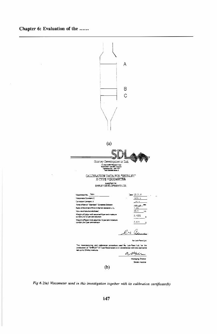
Chapter 6: Evaluation of the •••...
iI
(! A
(a)
BC
~~'01·.-..,ShirleyDevelopmen:s~?.a.a.4.__ l\oe;
-.-IIIA.EllClca~0II1·4eIl1'l"ll"T-=-__ 0
CALIBRATION DATA FOR "SEJRLEY"X-TYPE VISCOMETm
supplied bySH1Rl.EY DEVELOPMENTS LID.
VISCOlTIeleINo. _3_664 _
V~Conslant.C
CorrecIion ConsIaru. K
rmeof lIIlwof"S/lndlrd" G1ve-ineSaIulion.
AItio oflhetimesoftlow in lhelWo--"l,/lt
Volu~otsolution~
WeightofCollon with -.ned IS l*QI1C l"IlClisUnlXlI*nt.fOt"Q.5 perc:.1l1Dlution
WIi9h1of~wilhaam.d IOperQl1CmoiIllnconl8fIt. for 2perc:.nt1Clution
Data: 20.3.91
1931.5
'17 3 5
~-.
1 Q'20.1 c.c.
for laIH'Ianllld.
The mroulK2Uring and calitnton~ ..... .;..~ Lld. for !heproducrion of "SHlRlEY"'X·Type~.in -=---wilh \he Slandards_upby~inIlilul&
~
(b)
Fig 6.2(a) Viscometer used in this investigation together with its calibration certificate(b)
147

Chapter 6: Evaluation of the .
6.2.4 Results
Bleaching was carried out at 25 0 C on ca 109 CPNF samples for a total time of 1 h and the
concentrations of all chemicals as specified in Table 6.1. For each of the samples obtained
from the various bleaching treatments, triplicate fluidity experiments were conducted and the
results are detailed in Table 6.2.
148

Chapter 6: Evaluation of the .
Table 6.2 Fluidity Results
Treatment no. • H 20 2 Activator Fluidity, Pa-1·s·1
Unbleached CPNF 3
Factory bleached CPNF 3
To conventional bleaching 5
5
5
Tt Urea 9
9
8
T2 Benzamide 7
6
6
T3 Formamide 9
10
10
T4 MgS04 and K2S2Og 14
14
15
Ts Na2S2Og 4
4
149

Chapter 6: Evaluation of the ••••••
6.2.5 Discussion
In any bleaching process one of the primary objectives is to ensure preservation of inherent
fibre quality - this property after subsequent processing can never be improved. (6)
Attempts at applying the amide activated bleaching treatments (Tl -T3) to the CPNF (33) were
mildly successful except for the benzamide activated treatment (T2). Relatively high fluidity
results (between 8 - 9 Pa-l·s-l) were obtained for the urea (Tl) and formamide (T3) hydrogen
peroxide bleaching treatments as compared to the fluidity value of the unbleached CPNF
(2.60 Pa-l·s-l). Bleaching with benzamide as the peroxide activator was, however, successful
producing a fabric whose fluidity value ranged from 6 to 6.8 Pa-l.S-l .
Of the bleaching treatments studied, the sodium persulphate peroxide activated bleaching
method (Ts) yielded the best results with fluidity values ranging between 3.65 and
4.15 Pa-l·s-l and these results are comparable to the results of the factory produced bleached
fabric. The double activation treatment with potassium persulphate and magnesium sulphate
(T4) was highly unsuccessful causing extensive damage to the CPNF fibres.
The results of the sodium persulphate activated bleaching treatment (Ts) is superior to the
results obtained by Sarma et al (43)in their similar treatment of cotton woven fabrics
(3.6 - 15.5 Pa-l·s-l). This difference could probably be due to the longer treatment times
studied in their research (7 h).
The finding that sodium persulphate (Ts) produces the smallest amount of fibre damage is in
agreement with the work conducted on woven fabrics. (43,44,66) This activator has been
incorporated in some cold alkaline peroxide bleaching recipes done .(28)
The results obtained here are supported by the scanning electron microscope (SEM) results
discussed in chapter 7 and the sodium persulphate activated bleaching recipe is utilised to
optimise the treatment conditions of time, temperature and hydrogen peroxide concentration
in chapter 8.
150

Chapter 6: Evaluation of the .
6.3 Determination of the wettability of the bleached CPNF
6.3.1 Introduction
The absorbency or wettability of cotton CPNF is its most important fibre property as it is
used as a wound dressing. One of the basic objectives of bleaching research is to ensure
preservation or improvement of this property.
In this work the wettability of all the bleached CPNF fabrics described in Table 6.1 were
determined with the aim of investigating the changes in water absorbency capacity before
and after bleaching.
6.3.2 General properties of water towards cellulose
The affinity of water to cellulose is not difficult to understand. From the chemical formula
(cf scheme 6.2) it can be seen that cellulose possesses an abundance of hydroxyl groups that
need to be solvated. Not all the hydroxyl groups are bound together in the crystalline region
and a proportion of them exist in a sufficiently accessible state on the micellar surfaces in
the fibres to attract water molecules. The moisture relations of cellulose have been
studied(67,68) over many years pioneered by the early work of Urquhart and Williams(67) on
scoured cotton.
On exposing the dry cellulose to a moist atmosphere, water is first absorbed on whatever free
hydroxyl groups are present, and then by groups held together by weak hydrogen bonds.
This imbibed water causes the chain molecules to be pushed apart, exposing more free
hydroxyl groups. (69)
HrO:":""H H 0
oCH20H
-,
o -0"":"" +(:":")'0"00"H H 0 OH H H
o 1-H OH CH20H I H OH
Jx
Scheme 6.2
151

Chapter 6: Evaluation of the ••••••
The cellulose fibres have been reported to absorb water into their interfibrillar spaces where
the liquid is held by capillary action. (70) This type of process depends on physical properties
such fibre surface energy and fibre geometry. (70) The absorbency characteristics of a fibre
are a function OfOl)
a) the volume available to the fluid i.e. the volume available or created in the structure of
the fibre before or during absorption
b) the speed with which the volume takes up fluid and retains it.
Cellulose fibres are extremely absorbent because their natural structure is porous which
provides spaces between where liquids can be held, by capillary action. (71,72) This property
has been enhanced in cellulose processing treatments by the action of swelling agents. (53)
Swelling of cotton may be regarded as the disruption of the fibre solid structure by the
intrusion of the molecules of the swelling agent. (48) When the swelling agent is removed by
washing or other means the cellulose structure contracts again and in all cases forms an
accessible fine structure with increased absorbency properties. (53) In most cases the swelling
agent used for cellulose is aqueous alkali which is incorporated into the preparation process
or applied directly by a process known as mercerisation. (53)
6.3.3 Factors which determine the absorbency of the CPNF
CPNF is made from greige cotton fibres whose structural component is cellulose. Cellulose
in its natural state, has a hydrophobic outermost surface because of wax and other non
cellulosic material found in the cuticle and the primary layer (see fig. 7.3). The removal of
cotton wax from the cotton fibre during scouring and bleaching reduces the hydrophobic
components and increases the wettability of the cotton making it hydrophillic. (48) This
removal of waxes facilitates fibre swelling and hence greater volume available to the sorbing
liquid.
The degree of wettability depends to some extent on the morphology of the CPNF. (48) CPNF
has been reported to possess a fibrillar structure with a helical fibre orientation. (74) The fibre
helix reverses in direction at intervals along the fibre length and these reversal regions co
incides with the convolutions that are seen in the dried, collapsed fibre. A sorbing species
such as water has been reported to open a network of channels or pores by acting as agents
152

Chapter 6: Evaluation of the •.....
for interfibrillar swelling thus increasing the volume available for absorption. (53) In addition
it has been reported(48) that the phenomenon of hydrophillicity is mainly determined by the
competitive effects of spreading amongst the fibers, absorption amongst the fibers and the
influence of surface active agents.
6.3.4 Experimental
Several methods of testing fabric absorbency are available. (15,76,77,78) In practice, tests based
on the timing of a water drop to wet out the fabric, (19) or for a sample of fabric to sink in
water or dye liquor, (52) are frequently used. Well prepared fabrics should show a water
absorbency of less than 5 seconds. (52)
For nonwoven fabrics, the absorbency properties are evaluated according to the EDANA(80)
test method 10.1-72. These methods evaluate the liquid absorptive capacity (commonly
known as absorbency capacity), the liquid absorbency time, and the liquid wicking rate. (80)
In this work the absorbency of the CPNF were evaluated by the method detailed for
absorbent cotton in the British Pharmaceutical Standard Handbook, A226 appendix XX L and
on page 1094, surgical dressings. (52)(see appendix 2.3). In this method, a 1 g sample was
folded four times and allowed to drop lightly on to the surface of water contained in a
beaker. The beaker must be a least 0.012 m in diameter and filled with water to a depth of
0.010 m. The time taken for the sample to sink below the surface of the water is measured
with a stopwatch. This procedure was repeated on two further samples and the average value
was calculated. Distilled water at 20 QC was used as the test liquid.
According to the specifications in the British Pharmaceutical Handboo~51) for absorbent
cotton gauze, the sinking time must not exceed 10 secs.
153

Chapter 6: Evaluation of the ••....
6.3.5 Results
Bleaching was carried out at 25 0 C on ± 109 CPNF samples for a total time of 1 hour and
concentrations of the chemicals according to the specifications in Table 6.1. For each of
the samples obtained from the various bleaching treatments, triplicate absorbency experiments
were conducted and the average results are summarised in Table 6.3.
Table 6.3 Absorbency Results
Treatment no. • H20 2 Activator Absorbency (s)
Unbleached CPNF 8
Factory bleached CPNF 1
To conventional bleaching 3
Tt Urea 4
T2 Benzamide 3
T3 Formamide 2
T4 MgS04 and K2S2Og 36
Ts Na2S2Og 3
• taken from table 6.1
154

Chapter 6: Evaluation of the ••••••
6.3.6 Discussion
The results in Table 6.3 show that for the following bleaching processes, To, T1, T2, T3 and
Ts, the absorbency of the fabrics is not significantly different from that of both the
conventionally bleached and the factory bleached CPNF. The slight improvement in the
absorbency value when comparing these bleached fabrics with the unbleached CPNF could
possibly be due to similar effects produced from the swelling agents present in the bleaching
treatments. Sodium hydroxde and a commercially available wetting agent were used in all
the combined scouring and bleaching treatments as the swelling agent. It has been reported
that the degree of swelling depends on both the reagent used and on the morphology of the
fibre. (6) In all the samples used in this work both these factors are constant and hence it is
found that the degree of swelling should be the same. This is true for all the samples except
for the sample undergoing treatment number 4. The results of all the other treatments except
T4 are in good agreement with the findings of of other workers researching into the
properties of the CPNF.(3,46)
The results in Table 6.3 are also in good agreement with the mechanism that has been
suggested for the absorbency of cotton fabrics. (81) According to this mechanism, for a given
fabric construction, cotton fabrics of the same weight end up with practically identical
properties after laundering and subsequent bleaching processes.
It is clear that although the application of treatment 1, 2 and 4 in Table 6.3 results in a fabric
whose fibres are damaged (see fluidity and SEM results), it does not alter the absorbency
capacity of the fabric in any way. This suggests that the differing peroxide activators in
treatments 1, 2 and 4 have little or no effect on the degree of swelling of the cellulose and
hence on the property of absorption.
It is furthermore clear that, under the treatment conditions 4 in Table 6.1 used in this study,
the bleached CPNF yielded a significantly higher absorbency value. This may be ascribed,
at least in part, to the resistance of these chemicals to the rinsing treatments used in this
work. This in turn could possibly result in these chemicals forming a layer on the fibre
surface hence shielding the available volume on the fibre surface to water impregnation.
155

Chapter 6: Evaluation of the ••...•
6.4. Whiteness of the bleached fabric
6.4.1 Introduction
Whiteness of bleached fabric may be assessed visually or determined instrumentally by a
spectrophotometer. (53) Greisser(82) investigated the correlation between the subjective
evaluation and the objective (instrumental) measurement of the resultant bleached karakul
fabrics and reported that for colour determinations there is excellent agreement between the
visual and instrumental appraisals, but for whiteness determinations instrumental appraisals
provided more consistent and accurate results. This is in keeping with the accepted view by
many workers(24,46) that the instrumental analysis of whiteness of bleached fabrics is the
simplest and most precise property to evaluate the process of bleaching.
All instrumental methods illuminate the sample and measure the amount of light reflected. (46)
The assessment ranges from the measurement of reflectance at a single wavelength to a
complete spectral scan which can be processed to give colour difference or a whiteness
index. Dyer, and Daul(83) have reviewed these whiteness indices, one of which is
recommended in the American Association of Textile Color and Colorists test method 110. (79)
The most widely spectrophotometer is the Beckmann DK-2 spectrophotometer. (5) In this
instrument comparison is made with a magnesium oxide reference. Estimates of the degree
of whiteness are obtained by the index W as reported by Cegarra et a184) :
W = (CF)2 = (lOO - AS)2 6.1
where CF is the difference between the reflectance at 650 and 450 nm called the colouring
factor and AS is the average of reflections at 450, 500, 550, 600 and 650 nm called the
average colour. The higher the value of W the inferior the whiteness.
Another popular instrument, a Hunterlab Multipurpose Reflectometer measures light reflected
at a single wavelength of 457 or 460 nm. (19,46) These wavelengths lie within the blue region
of the spectrum and provide information on both the brightness and yellowness of the sample.
156

Chapter 6: Evaluation of the .
The reflectance on this instrument is always related to an ideal white standard, the
international basis now being magnesium oxide which is taken to have 100 % reflectance. (50)
The reflectance of well bleached samples should be between 80 to 90 %. (24) Extensive
reviews on whiteness and colour measurements are given by Ciba Geigy LTD(86) and
Farbenfabriken Bayer A. G. (87)
More sophisticated and technologically advanced on-line colour spectrophotometers have just
recently been introduced offering an advanced computerized colour and whiteness analysis
system designed to record and report color and whiteness characteristics against
predetermined reference whiteness. (88) These spectrophotometers are rapidly galnlng
popularity for their ease of measurement, their exceptionally high measuring accuracy and
their extensive compatible reference software.
A Datacolor International computer driven spectrophotometer utilizing the Datacolor Uniflash
program was used in this study. (82)
6.4.2 Experimental
The CPNF samples obtained from the bleaching treatments (To to T5)listed in Table 6.1 were
analyzed for their whiteness property by Mr Ivan Veerasamy of The Frame Group. A
Datacolor spectrophotometer programmed with magnesium oxide (100 % reflectance) as the
reference whiteness material was used.
6.4.3 Results
For each of the bleached CPNF samples obtained from the various bleaching treatments listed
in Table 6.1, triplicate whiteness tests was conducted and the results are detailed in Table
6.4.
157

Chapter 6: Evaluation of the ••••.•
Table 6.4 Whiteness Results
Treatment no.*
Unbleached CPNF
Factory bleached CPNF
To
• taken from Table 6.1
conventional bleaching
Urea
Benzamide
Formamide
158
Whiteness (%)
49.67
75.73
67.25
70.10
69.87
73.27
77.34
77.88
80.47
78.27
76.63
68.67
69.87
72.27
65.73
60.54
59.23
79.16
80.21
78.90

Chapter 6: Evaluation of the ..•...
6.4.4 Discussion
Of the five bleaching treatments selected in this investigation, only the use of treatment 4 (T4)
resulted in a bleached CPNF exhibiting poor whiteness. The remainder of the samples
representing the range of bleaching treatment investigated showed equal and superior
whiteness values to that of the factory bleached and conventionally bleached samples.
In particular, treatment 2 and 5 (T2 and Ts) in table 6.4, yielded the best whiteness results
indicating a well bleached sample. It was reported earlier in this work (section 6.2) that the
treatment conditions incorporating urea ,formamide or magnesium sulphate/potassium
persulphate (Tt, T3 and T4, respectively) in the bleaching bath as the peroxide activator
resulted in a highly damaged fibre. From Table 6.4 it can be seen that this damaged fibre
was successfully bleached with an acceptable whiteness value although extensive damage was
caused to the fibres. This indicates that the rate of activation of the hydrogen peroxide was
too rapid resulting in overbleaching and degradation of the cotton fibres.
In view of the preceding discussion, the rates of hydrogen peroxide decomposition were
determined for bleaching treatments Tt to Ts by withdrawing 1 ml aliquots at intervals and
adding 100 ml of 10 % sulphuric acid solution and titrating with standard (0. IN) potassium
permanganate. (24) These results are tabulated in Table 6.5 and plotted against the time of
bleaching (1 h) in Figures 6.1 (a) and (b).
From Figure 6.1. (a) bleaching in the presence of sodium persulphate (Ts) and benzamide
(T2) resulted in a slow and constant rate of decomposition for the time period investigated.
From Figure 6.1. (b) it is evident that the decomposition rate is much faster, indicating that
the activators (Tt, T3 and T4) employed enhance too fast a decomposition of the peroxide.
Thus excessive oxygen is produced accompanied by fibre degradation.
These results are supported by both the fluidity results reported earlier and by the SEM
investigation discussed in chapter 7.
159

Chapter 6: Evaluation of the •••.•.
Table 6.5 The decrease of hydrogen peroxide concentration with an increase in time using
the various bleaching treatments
Time [50 % H 20 2] Time [50 % H 20 2]
minutes g·l-l minutes g·tl
Treatment No. 1 (Ts) •
0.00 6.200 15.00 4.726
2.00 4.862 16.00 4.692
4.00 4.862 20.00 4.692
5.00 4.828 25.00 4.692
6.00 4.828 30.00 4.692
8.00 4.828 40.00 4.624
9.00 4.828 50.00 4.624
10.00 4.726 60.00 4.624
Treatment No. 2 (T2) •
0.00 6.200 20.00 4.624
1.00 4.896 25.00 4.624
3.00 4.760 30.00 4.534
5.00 4.760 35.00 4.534
7.00 4.692 40.00 4.534
10.00 4.624 50.00 4.216
15.00 4.624 60.00 4.216
• taken from Table 6.1
160

Chapter 6: Evaluation of the .
Table 6.5 continued
Time [50 % H 20 2] Time [50 % H 20 2]
minutes g·t l minutes g·tl
Treatment No. 3 (T3)·
0.00 8.800 20.00 5.318
1.00 7.344 25.00 5.008
3.00 7.140 30.00 4.997
5.00 5.832 35.00 4.930
8.00 5.644 40.00 4.260
10.00 5.372 50.00 4.080
15.00 5.348 60.00 3.910
Treatment No. 4 (T l )·
0.00 8.800 20.00 4.930
3.00 6.800 25.00 4.760
6.00 6.460 30.00 4.760
8.00 5.780 35.00 4.760
10.00 5.610 40.00 4.420
12.00 5.440 50.00 3.916
15.00 5.440 60.00 3.230
• taken from Table 6.1
161

Chapter 6: Evaluation of the .
Table 6.5 continued
Time [50 % H20 2] Time [50 % H20 2]
minutes g·t! minutes g·t!
Treatment No. 5 (T4)*
0.00 8.800 25.00 4.624
2.00 6.052 30.00 4.352
5.00 5.780 35.00 4.012
10.00 5.508 40.00 3.740
15.00 5.236 50.00 3.320
20.00 5.100 60.00 3.080
* taken from Table 6.1
162
Chapter 6: Evaluation of t~e_.~~.~••
Treatment No. 1 _ .._- - .6
rA~~~~~F~~~~n~artme=n=t~N~~=2~~~~-~__~--~------_.-
r;
.Cl
,--,5Q)
"0'x0L.. 4Q)Q.
eQ)
3-0>0L..
"0~.c 2 -
?ft0l() 1 --L-...l
60
L--L__. l __.
45 50 55o --l---.-LI_-1----''----->--- L_~ _
o 5 10 15 20 25 30 35 40
time, minutesFigure 6.1 (a) The decrease ofhydrogen peroxide composition plotted against the time ofbleaching in the presence
of (1) Na~208 (1'5) and (2) CP5CONH2 (1'2)
1U
.Ol
,....,Q)"0·xoL-Q)Q.
eQ)
0>oL-
"U~..c'#.ol()~
8
6
2Treatment No. 3
Treatment No. 4
Treatment No. 5 i
-- - --~-' /
oOL----'-5--1J-.0--1~ 20 25 3~ 35 4~~-~~---51~_--60
time. minutesFigure 6.1 (b) The decrease ofhydrogen peroxide composition plotted against the time ofbleaching in the presence
of (3) HCONH2 (1'3) , (4) jlNCONH2 (1'1) and (5)K~208 + MgS04
(1'4)
163

Chapter 6: Evaluation of the ••••••
6.5 Conclusions
1. The sodium persulphate activated bleaching (Ts) and to a lesser extent the benzamide
activated bleaching (T2) method, produced a fabric with minimum fibre damage and hence
low fluidity values.
2. All the bleaching treatments investigated, with the exception of T4 produced a fabric of
acceptable absorbency properties.
3. All the bleaching treatments (To to Ts) investigated in this study except the treatment
incorporating MgS04 and K2S20 g (T4) as the peroxide activator produced a fabric of
acceptable whiteness property.
164

Chapter 7: An investigation .
Chapter 7
Scanning Electron Microscope (SEM) investigation of the unbleached and bleached
Cotton Patterned Non-Woven Fabric
7.1 Introduction
Electron microscopy has been shown(89) to provide valuable information on the essential
elements of the fibre structure of cotton. Research by workers(90) has revealed that cellulose
(the basic structural component of cotton) is organized in the form of relatively course
fibrous structure and that these fibres are further subdivided into microfibrils as shown in
Figures. 7.1. It has been established that the morphology of these fibres are altered
considerably by the differing finishing treatments and their related chemicals. (6)
Fig 7.1. Electron micrograph of the course fibrous structure of cotton
In this work, the surface structures of the CPNF were observed before and after bleaching.
This was done in order to investigate the modifications (if any) to the fibre surfaces of the
final CPNF by the various bleaching treatments.
165

Chapter 7: An investigation ...•••
7.2 The surface strocture of CPNF
Cotton has been regarded as composed of structural units termed fibrils. (49,91,92) These fibres
are essentially a build up of a number of identical units of cellulose and chemical reactions
have been proposed as taking place on the surfaces of these fibrils. (92) An essential aspect
of all chemical finishing processes involving cotton is degree of access of the chemicals to
the fibrillar surfaces. The way in which the fibrillar units are altered during chemical
treatment can exert a profound effect on the fmal properties of the fabric. (6)
Cellulose is the basic structural component of the fibrils and the literature on the physical
structure of these cellulose fibres is extensive. (25,93,94) In recent years, natural cellulose fibre
structures have altered in minor detail as more powerful analytical techniques have been
developed. Essentially, a mature fibre forms a flat ribbon containing approximately thirty
cellulose chains and appear under the electron microscope to be 0.02 to 0.03 J.tm thick and
at least 10 J.tm long. It has been postulated(53) that the fibrils consist of "bundles" of smaller
microfibrils that are approximately 0.004 to 0.006 J.tm in cross section. One of the main
features of the structure of the cotton fibres is the spiral arrangement of the fibrils, which
reverses in direction of rotation periodically along the length of the fibre. This causes the
convolutions observed by many workers(74) and it has been reported that the number of
convolutions varies between 4 and 6 per millimetre.(53,74) It is the~. ~~volutions that play
a large part in determining the mechanical properties of the fabric (e.g. tensile strength,
elasticity etc.) These unique characteristics of cotton fibres are represented lengthwise in fig.
7.2 at a fairly low magnification. In this study these convolutions were observed in all the
fibre and fabric micrographs taken at magnifications of 1000 and lower (see figures 7. to
7.10).
166

Chapter 7: An investigation ••••••
Electron microscopy of the cross-section of the cotton fibres has been extensively
researched. (95,96) It has been established that each fibre consists of three main parts: primary
wall, secondary wall and lumen as shown in fig 7.3). The primary wall consists of a
network of cellulose fibrils covered with an outer layer or cuticle of pectin, protein, mineral
matter and wax. It is the wax that renders the fibre impermeable to water and aqueous
solutions unless a wetting agent is present. The secondary wall constitutes the bulk of a
mature fibre and consists entirely of fibrils of cellulose arranged spirally around the fibre
axis. Thus the cotton fibre consists of an assembly of fibrils in which the cellulose is
accessible to most chemical reagents only at fibrillar surfaces.
Lumen
Primarywall
FatsPectin
Waxes
Fig -7.3. Itkalised morphology ofcotloft jibr~ taJ:m from rpf 6
A cross-section of the CPNF before and after bleaching is shown in fig 7.4 (a) and 7.4 (b).
The CPNF fibres for this micrograph were bleached using the conventional high temperature,
high pressure peroxide bleach method described at the beginning of this study (Table 5.4).
From these figures, it can be seen that the fibres were never stripped of their primary walls
after bleaching because the combined scouring and bleaching process was reasonably mild.
Electron microscopic examination of the bleached CPNF fibres prepared by various methods
was performed in order to examine them for surface changes as compared to the unbleached
cotton fibre.
167

Chapter 7: An investigation ••..•.
(a) (b)
Fig 7.4 Cross section ofthe surface fibres ofthe CPNF (a) before bleaching and (b) after bleaching at 250 QC.
7.3 Experimental
All the micrographs were taken by Mrs Wendy Baier on a Hitachi 5-430 scanning electron
microscope. Instrument operating voltages are recorded on the individual micrographs. The
samples were mounted horizontally on hollowed-out specimen stubs and coated with gold.
7.4 Results
Electron micrographs of fibres from five of the CPNF samples scoured and bleached as
described in chapter 6 and table 6.1 were examined and are shown in figs. 7.5 to 7.9.
Details of the treatments and the results obtained in terms of the bleaching effect and extent
of fibre damage, have been given in Table 6.1. The electron micrographs of untreated
CPNF fibres and fibres of the high temperature, high pressure bleaching process are also
shown in Figures 7.10. and 7.11 , respectively.
168

Chapter 7: An investigation ••••••
(a)
(c)
(b)
(d)
Fig 7.5 SEM micrographs ofbleached CPNF to show surface fibre morphology after application oftreatment 1
in Table 6.1, (a) 45X, (b) 200X, (c) 500X and (d) 1500X
169

Chapter 7: An investigation ••••••
(a)
• 5U
(c)
(b)
(d)
Fig 7.6 SEM micrographs ofbleached CPNF to show surface fibre morphology after application oftreatment 2
in Table 6.1, (a) 45X, (b) 500X, (c) 2000X and (d) 2000X
170

Chapter 7: An investigation ••••••
(a)
(c)
(b)
(d)
Fig 7.7 SEM micrographs 0/ bleached CPNF to show surface fibre morphology after application o/treatment 3
in Table 6.1, (a) 45X, (b) 500X, (c) 1500X and (d) 2000X
171

Chapter 7: An investigation ••••••
(a)
(c)
(b)
(d)
Fig 7.8 SEM micrographs ofbleached CPNF to show surface fibre morphology after application oftreatment 4
in Table 6.1, (a) 42X, (b) 500X, (c) 1000X and (d) 1500X
172
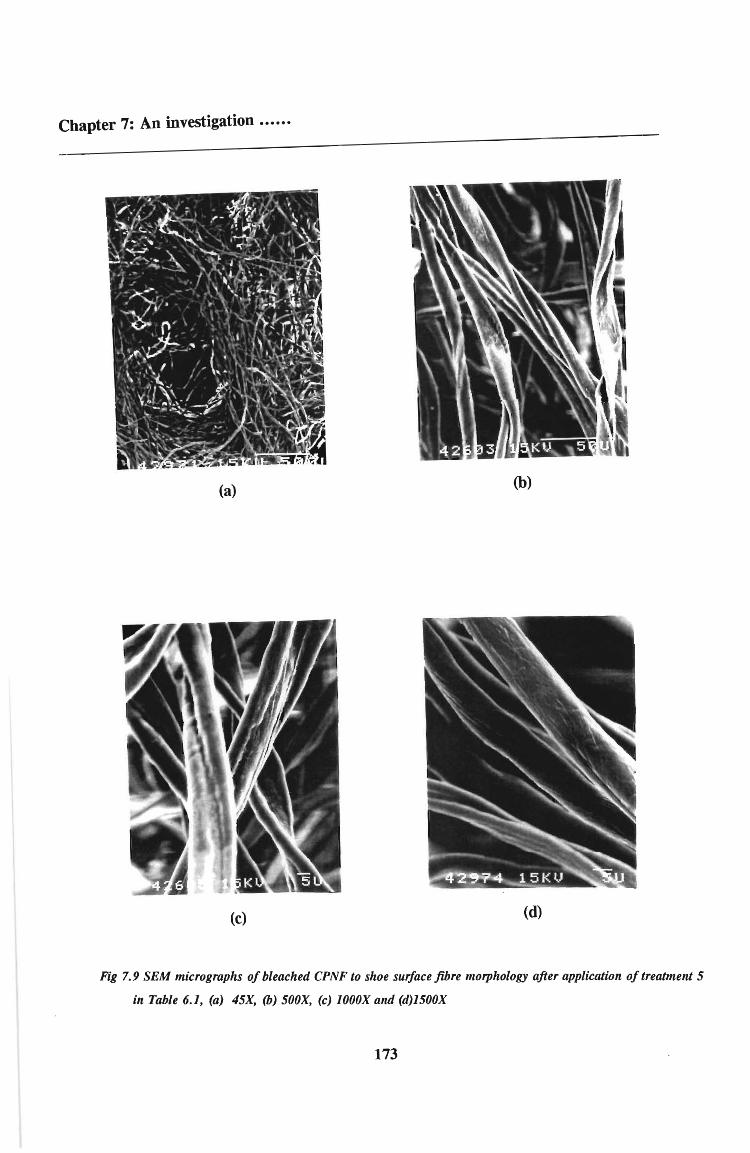
Chapter 7: An investigation ••••••
(a)
(c)
(b)
(d)
Fig 7.9 SEM micrographs ofbleached CPNF to shoe surface fibre morphology after application of treatment 5
in Table 6.1, (a) 45X, (b) 500X, (c) 1000X and (d)1500X
173
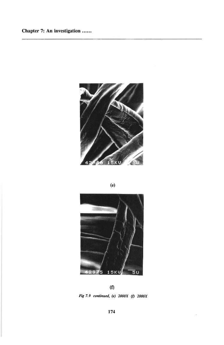
Chapter 7: An investigation ••••••
(e)
(0
Fig 7.9 continued, (e) 2000X (f) 2000X
174

Chapter 7: An investigation ••..•.
(a)
(c)
(b)
(d)
Fig 7.10 SEM micrographs 0/ unbleached CPNF to show surface fibre morphology, (a) 45X, (b) 200X, (c)
1500X and (d) 2000X
175

Chapter 7: An investigation •.•...
(a)
(c)
(b)
(d)
Fig 7.11 SEM micrographs ofbleached CPNF to show surface fibre morphology after high temperature and high
pressure bleaching, (factory bleaced sample), (a) 45X, (b) 500X, (c) 1500X and (d) 2000X
176

Chapter 7: An investigation •••.••
7.5 Discussions
The SEM micrographs obtained in this work confirm the flat ribbonlike structure of cotton
as well as the convolutions observed by other workers. (53,94) These microscopic features are
seen clearly at low magnifications (200X and below). The reversals in the directions of the
twists of the convolutions could also be seen clearly (Figures 7.5. to 7.11.). More detailed
examination of all the samples at higher magnifications (1500 and 2000X), (c) and (d) in
Figures 7.5 to 7.11, showed a wrinkled, rough and corrugated surface. Workers (3) have
shown that it is this property of the greige cotton fibre that is partially responsible for the
success in patterning and forming the CPNF.
Lower magnification micrographs were taken to compare the spatial or geometric
arrangement of the fibres of the webs in the unbleached and bleached samples. It has been
reported(3) that the geometric pattern of unbleached, entangled fabric made with greige
cotton shows a well defined hole that is typical of CPNF. In a successfully produced CPNF,
the water jets will produce this hole. In both the unbleached and bleached fibre samples used
in this work, this characteristic hole is clearly defined (see (a) in Figures 7.5 - 7.11).
Untreated CPNF fibres were generally found to have a well defined, undamaged surface
morphology as shown in Figures 7.10. Some of the bleached fibres, on the other hand,
showed signs of fibre damage and surface contamination which, not surprisingly, was found
to increase with increasing fluidity (see chapter 8) ie. extent of fibre damage of the samples.
The extent of fibre damage was greatest when urea (Tt) was used as the activator for
hydrogen peroxide. As shown in Figure 7.5 the urea in conjunction with the other bleaching
chemicals (Na2Si20 g, NaOH and H200 seems to have attacked the outer surface at intervals
along the length of the fibre. In addition, the hot water washing and neutralization of the
fabric after bleaching failed to remove all of the urea, and crystallites of the chemical can
be seen on the surface.
177

Chapter 7: An investigation ••••••
This fibre damage could possibly be attributed to urea inducing too fast an activation of the
hydrogen peroxide resulting in extensive oxygen being produced(see eqn. 4.3). This
suggestion is collaborated by the work reported by Das et al. (33) Oxygen has been shown to
react with cellulose to produce oxycellulose (according to scheme 7.1), the formation of
which is accompanied by cellulose chain scission and fibre degradation. (6)
oL-c- H
OH/ "'CH:O
CHOH.CH(OH) CH:Ol \/
H-cio
Scheme 7.1.
The fibre produced with formamide (HCONH2) (T3) as the peroxide activator exhibits similar
behaviour along the surface of the fibre as shown in Figures 7.6. Here again the extensive
variations and damage to the surface of the fibre is noted as compared to that of the
unbleached fibre. In particular, from Figure 7.6 (c), a rupture of the fibre surface is
visibly distinguishable. This surface damage could possibly lead to breakage in the fibre and
hence fibre degradation.
The SEM micrographs of the fibres produced with benzamide (T2) as the peroxide activator
is shown in Figures 7.7. Comparison of these micrographs with the unbleached fibres (Figure
7.10) shows that there is no surface damage present after bleaching. In fact, the surface of
bleached fibre is much "cleaner" than that of the unbleached fibre. This is understandable
as the bleaching process serves to remove any impurities present in the raw unbleached
state. (6) These slight impurities are visible in the unbleached fibre and absent in the
benzamide bleached fibre. It is surprising that the benzamide activated bleaching method
178

Chapter 7: An investigation ••••••
should produce differing results to those of the urea and formamide results discussed above.
Das and co-workers(33) in their paper utilise all of the above amides as activators for the cold
peroxide bleaching process of woven fabrics, with a certain degree of success. From this
one can deduce that each of the amides behave in a similar manner during bleaching. Thus
it was expected that the benzamide bleaching (T2) method would produce similar surface and
extent of fibre damage results to the urea (Tt) and formamide (T3) bleaching methods. For
the bleaching of the CPNF this is not the case. Benzamide, in contrast to urea and
formamide, produces a fabric whose fibres exhibit little or no surface degradation or damage.
This behaviour could perhaps be attributed to the structural differences between the amides
resulting in differing activation properties for the hydrogen peroxide.
The SEM micrographs of the bleaching methods adopted by Sarma et al (43) where
magnesium sulphate and potassium persulphate (T4) are the peroxide activators is shown in
Figure 7.8. All of the surfaces of the fibres seem to be penetrated and damaged by the
bleaching chemicals used. In particular the micrograph in Figure 7.8(c) shows a distinct
rupture of the surface of the fibre. However, what is noticeable is that the degree of damage
to the fibre surface in this treatment is not as extensive as that of the urea (Tt) and
formamide (T3) bleaching methods.
The low temperature peroxide bleaching method by Dickenson and Hickman(42) and adapted
to the CPNF (T5) seems to have produced the most successful results with regards to surface
damage to the fibre. The SEM micrographs of these fibres are shown in Figure 7.9.
Analysis of these micrographs shows that the fibres exhibit little or no damage after
bleaching. Comparing these micrograph results with the micrographs of the high
temperature, high pressure conventional bleaching process ( Figure 7.11) shows that there
is little or no discrepancy in surface morphology. This indicates that a peroxide bleached
CPNF with little or no fibre damage can be produced at a low temperature with sodium
persulphate (T5) as the peroxide activator.
It is this method which has been chosen and rigorously optimised for CPNF bleaching in
Chapter 8.
179

Chapter 7: An investigation ..••.•
7.6 Conclusions
The SEM investigation showed very significant differences between the surfaces of the
bleached fibres obtained using the various bleaching processes. The urea (Tt) and formamide
(T3) peroxide activated bleaching treatments produced a fabric with extensive fibre damage
and degradation. The benzamide (T2) activated process, surprisingly, produced a fabric with
little or no damage. The presence of the ring structure in the benzamide and its reactivity
towards peroxide could probably offer an explanation to this behaviour. The potassium
persulphate and magnesium sulphate (T4) peroxide activated bleaching methods also produce
a fabric whose fibres show extensive surface damage.
The SEM study also elucidated a bleaching method with minimum fibre damage. The
sodium persulphate (Ts) activated bleaching process produced a fabric whose fibres undergo
little or no change during bleaching. This method has thus been used to optimise the
bleaching process for the CPNF in the following chapters.
180

Chapter 8: Optimisation of the•.••..
Chapter 8
Optimisation of the single stage bleaching process using regression
analysis
8.1 Introduction
The treatment conditions employed and the results obtained in the previous chapters (6 and
7) suggests that bleaching in the presence of sodium persulphate produced a fabric with
minimum fibre damage. In view of these results, it was considered important to investigate
the influences of certain bleaching variables in a bleaching recipe containing sodium
persulphate as the peroxide activator.
As many workers have shown, (5,9,42,43,98) when investigating aspects of bleaching, a
mathematically designed evaluation is necessary to assess interactions between variables and
the statistical significance of the experimental results. In this study, a technique similar to
the one described by Sarma et aZ43 was employed with the treatment conditions for the
combined scouring and bleaching with hydrogen peroxide were varied according to a
statistical plan for 3 variables. Hydrogen peroxide concentration, bleaching time and
bleaching temperature were chosen as the bleaching variables. Whiteness was chosen as the
criteria for assessing the quality of the bleaching as it was considered the simplest and most
accurate (instrumental analysis) measure to describe the quality of bleaching.
8.2 Basic theory of regression analysis
Regression is the study of the analysis of data aimed at discovering how one or more
variables (called independent variables) affect other variables (called response variables).
For the sake of completeness, the basic equations and their inferences are demonstrated
briefly here, (99,100) but using a computer is the only practical means of performing a multiple
regression analysis on a data set.
For data with an underlying linear pattern i.e. one of the form
y = f30 + f31 X 8.1
181

Chapter 8: Optimisation of the .
a hypothesized straight line is used to explain the behaviour of the variables. For
observations that do not fit this pattern of a straight line, a relationship of the form
y. = (.} + ~ I;l 1(.}·x· + ~ I;l 1(.}·-X? + ~ ~<k(.}ik:X-Xk + c·t tJo iJt=tJtt iJt=tJUt iJt tJ t J 8.2
may be utilized where i = 1, 2, ... ,n ,n is the number of data points and (k+ 1) represents
the number of independant variables. Equation 8.2 is called a regression model and since
k > 1, it is called a multiple quadratic regression model. (99)
The (3i'S, i = 0, 1, ... , k, represent the regression parameters and the c/s, j = 1, 2, ... , n,
the error terms or residualsYOO) The values of the (3/s and c/s are estimated using the
ordinary least squares (G.L.S.) procedure. In multiple regression the Y/s are called the
observations or response variables and xi, x~, .... , xi is said to constitute the design point
corresponding to Yi.(99)
In multiple regression, the residuals are estimated as follows
8.3
where Yi(calC) represents the predicted value of Yi
When there is a good fit to the predicted model, the residuals (cj ) are small. When {3o Le the
constant term in equation 8.2 above, is not equal to zero, a measure of fit is also given by
the equation
8.4
Y = L ?=1 Y/n and R2 is called the multiple regression coefficient. R2 lies between 0 and
1 and the closer this value is to 1 the better the fit of the model. Another parameter R;dj
gives the multiple regression coefficient adjusted for sample size, n. This parameter is
obtained from the following equation
182

Chapter 8: Optimisation of the .
R;dj = 1 - {[Li= 1 (Yohs - Ycalc)2 / n - k - 1)] / [L i= 1 (Yohs - YJ2/ n - I]} 8.5
in which n is the number of data points and k is the number of independent variables. (lOO)
Most computer packages provide all the above statistical values and the simple statistics of
the mean, variance and standard deviation.(lOl) In addition the standard error of the estimate
is obtained from the equation
standard error = s. { L i=l (Xi - X)2 rh 8.6
and is also provided by a statistical computer package. The assumption that the
independent variables are fixed and predetermined by the investigator is made in all multiple
regression correlation procedures. (100)
Equation 8.2 can be represented as a regression or response surface of Y (response variable)
on Xl' X2 ,... , Xn (independent variables) .002) This plotted response surface enables the
response variable, Y, to be optimised as a function of the independent variables. This fitted
surface may attain (a) a maximum, or (b) a minimum, or (c) a saddle point in the region of
interest or (d) it may do none of these thingsYOO) Analysis of the response surface can
therefore provide a method of solving problems of determination of optimum conditions.(44,l02)
In this work, the influence of three independent variables i.e time, temperature and
concentration of hydrogen peroxide, on the response property of whiteness was determined.
Detailed laboratory experiments were performed to investigate the effect of these three
variables on the measured property of whiteness. The whiteness value of the bleached
fabrics was compared to the values obtained for the same fabric prepared using the
conventional high temperature (250°C) high pressure bleach. Response surface diagrams
were drawn and the optimum conditions for the low temperature bleaching with respect to
hydrogen peroxide concentration, time and temperature were obtained.
183

Chapter 8: Optimisation of the..••..
8.3 Experimental
CPNF samples were bleached according to the treatment conditions established earlier (cf
chapter 6 and 7) as the method producing the minimum fibre damage while achieving a good
degree of whiteness and absorbency. For the sake of convenience this method is shown in
Table 8.l.
Values for peroxide concentration, bleaching temperature and time were established
according to a central rotatable plan for three variables. The treatment conditions for the
bleaching process involves a range of hydrogen peroxide concentration, (34 g·l-l to 96 g.-I),
time (2 hours to 6 hours) and temperature(25 °C to 45°C) and is presented in Table 8.2.
Statgraphics
The Statgraphics software is a PC software program integrating a variety of statistical
functions with high resolution colour graphics. In this study Statgraphics was used in the
multiple regression analysis and to plot the response surface diagrams. A computer output
was obtained using the Statgraphics program for multiple regression as shown in appendix
2.4.
Further details of this program can be found in the Statgraphics Users Guide(lOl) manual.
Table 8.1 Treatment conditions for the bleaching recipe chosen to be optimised
Ts
Chemical conc (g·r1)
NaOH 30
Na2Si20 3 18
H20 2 65
Wetting Agent 10
Na2S2Og 12
184

Chapter 8: Optimisation of the•.....
8.4 Results
The results of the response analysis for whiteness are listed in Table 8.2. The regression
coefficients and the multiple correlation coefficient for the bleached CPNF are shown in
Table 8.3.
The surface diagrams for the effects of two variables on the measured property of the
bleached fabrics are shown in Figures 8.1 - 8.3.
The data were analyzed by fitting the variables in a quadratic polynomial of the type
Y = B + ~ B -x - + ~ B --xl + ~ B - -x -x-o LJi=l ~ ~ LJi=l ~~ LJi<j ~J ~ J
where Y is the experimentally measured whiteness response for each experiment and B is the
regression coefficient. From the fitted regression equation 15 possible treatment
combinations were obtained.
185

Chapter 8: Optimisation of the .
Table 8.2 Treatment conditions and whiteness property of prepared fabrics where Xl
refers to hydrogen peroxide concentration, x2 to time, x3 to temperature and Y to the
observed whiteness. The calculated whiteness is dermed as Ycalc.
Expt.No. Xl X2 X3 Y Ycalc
g·rl hrs °C % %
1 65 4 35 80.48 80.36
2 65 2 25 80.77 81.50
3 65 6 25 77.01 75.52
4 96 4 45 79.80 81.30
5 96 4 25 79.49 78.76
6 65 6 45 77.02 77.82
7 96 2 35 80.45 78.22
8 65 4 35 80.28 80.36
9 34 6 35 79.98 78.55
10 34 4 25 77.13 78.56
11 34 4 45 76.70 77.40
12 65 2 45 81.64 80.84
13 34 2 35 81.13 80.43
14 96 6 35 73.24 75.47
15 65 4 35 80.32 80.36
Conventionally prepared fabric - - 77.90 -
186
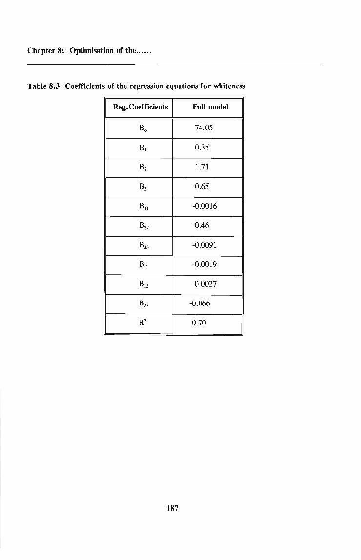
Chapter 8: Optimisation of the .
Table 8.3 Coefficients of the regression equations for whiteness
IReg.Coefficients i Full model I
Bo 74.05
B1 0.35
B2 1.71
B3 -0.65
Bll -0.0016
B22 -0.46
B33 -0.0091
B12 -0.0019
B13 0.0027
B23 -0.066
R2 0.70
187

Chapter 8: Optimisation of the••...•
8.5 Discussion
From Table 8.2, close agreement between the observed and calculated values of the various
parameters shows that the regression equation is applicable in this investigation. The
multiple correlation coefficient (R)(99) is used to ascertain the validity of the regression
equation. R2 was found to be 0.705 and showed fair correlation with respects to the
observed and fitted values.
The regression equation for whiteness has the form
Y = 74.05 + 0.35x1 + 1.71Xz - 0.65x3 - 0.OOI2x'i - 0.46X; - 0.OO91X; - 0.0019xl~ + 0.OO27x1X3 - 0.066Xz~ 8.7
and Y has a positive contribution from two independent variables (Xl and X2)' The largest
positive contribution to whiteness (Le. the regression coefficient for x2, 1.71) is time. This
value suggests that the longer the time of bleaching the higher the degree of whiteness.
However an acceptable degree of whiteness was obtained after 3 hrs.
The regression coefficients for the other major parameters B1 (hydrogen peroxide
concentration) and B3 (temperature) show a small but significant effect on the degree of
whiteness in the ranges investigated in this work (Table 8.2). It is possible that outside the
range, the effect of these parameters might be significant. Other workers(ll,19,27) have found
that this effect becomes significant and contributory at higher temperatures (180°C).
The regression equation (8.7) has been used to plot surface diagrams (Figures 8.1-8.3). The
values used for plotting these figures are the smoothed values (equation 8.7) of the responses
obtained from the 15 data points.
Figure 8.1 shows the effect of three levels of temperature on the whiteness. There is only
a small difference between the whiteness at 25°C (80 %) and 45°C (84 %). This indicates
that bleaching can effectively be carried out at ambient temperature. In addition, the
curvature of both surfaces shows a maximum whiteness (which is of an acceptable
whiteness*) at approximately 3 hrs and 65 g'l-l hydrogen peroxide concentration. This
188

Chapter 8: Optimisation of the .
suggests that in the range investigated, 3 hrs was sufficient for efficient CPNF bleaching.
Figure 8.2 shows the effect of bleaching on the whiteness of the fabrics after 2 hrs (surface
c) and 6 hrs(surface d) of bleaching respectively. At both surfaces, the whiteness increases
as the hydrogen peroxide concentration increases until approximately 65 g'l-l, where the
surface begins to taper off and decrease as the concentration approaches 96 g' t l. This
suggests that a concentration of about 65 g' t l is necessary to obtain a fabric that satisfies the
whiteness controllevel*.
The inference drawn from Figures 8.1 and 8.2 is that 3 hours and 65 g'l-l hydrogen peroxide
concentration is sufficient for the effective bleaching of CPNF and this is supported by the
analysis given in Figure 8.3.
In Figure 8.3, the effect on whiteness obtained using a concentration of hydrogen peroxide
of 34 g' t l and 96 g' t l are shown. Surface e shows that an increase in time has a marginal
increase on the whiteness. For times greater than 3 hrs, the whiteness approaches a constant
value. Surface f exhibits similar behaviour.
8.6 Conclusion
Based on the correlation of the regression equation analysis to the spatial diagrams, a
bleaching formulation consisting of sodium hydroxide (30 g'l-l), sodium silicate (18g'l- I),
sodium persulphate (12g·tl), hydrogen peroxide (65g'l-l)and a wetting agent (10g·tl) at
25°C for 3 hours using a laboratory scale pad-batch kier system provides a potential method
for combined scouring and bleaching of the CPNF.
• The whiteness control level is the value obtained for the conventionally bleached fabric Le. 77.90 %
189

~
~•••c•.......t:3
ee
e3.2
e ....
T7.e
.,.... 8
72
3 ..
,,,.0
a
3
..
8
6
)(l<tJ._, hour.)
ner
i...QC..o
I.......o=o~
~~·····
11..
Ml(hydrog_n p.roMid. oanc.ntr.tion, g/l)
• r.r.r. to 26 C .nd b ~6 C
Fig 8.1 Whiteness response junction; Variables are hydrogen peroxide concentration and time

,Whit.n••• R••pon•• ~uncticn
V.ri.bl••• (H202J and t.mp.ratura
83.2
"4.8
..,2
34
\
//
IU.IS8e
88.15215
28
33
46
41
3"
x2CtaMPereture, C)
n=r~
~~QC..o
i.........Q
=~
~~·····
11..
xl(hydrog.n peroxide concentretion, g/l>
c r.r.r. to ~ houre .nd d to e hour.
Fig 8.2 Whiteness response junction; Variables are hydrogen peroxide concentration and temperature

Whit.n••• R••pon•• Function
V.~t.Di•• • tiMe .nd t.Mp.r.tur.
.-.----------------~
.. 6
<41
37
M3(t••p.r.tur., C)
nt:J"~
~~..,00..0~
• I I
i:f"'t'....0=0,....er~····I
I I I·
r
33
a8
as
e
...................s
.. , : ,:, .
........,.:::......
.....:: ..:....
.............
.............
~
.... , :,.:: .
.::.\: .
..:.\ ....
/
/,/
3\2
e8
,a
93.2
s ....
•••...... c'C •vN .... T1.8
1::J
7<4.8
M2<t.i_, hour.)
• r.r.r. to 3"g/1 end r to 880/1
Fig 8.3 Whiteness response function; Variables are time ana tempera,ure

Chapter 9: Conclusions and Future Work
Chapter 9
Conclusions
Five bleaching treatments for the CPNF were investigated. Based on the results of the
whiteness, fluidity, absorbency and regression analysis, a bleaching formulation consisting
of sodium persulphate (12 g·tI) as the hydrogen peroxide activator, sodium hydroxide
(30 g'l-I) sodium silicate (18 g' t I), hydrogen peroxide (65 g' t I), and a wetting agent at
25 °C for 3 hours using a laboratory scale pad batch Icier system, provides a potential
method for combined scouring and bleaching of the CPNF.
Further work could be done to investigate the conversion of the above process to a
continuous on-flow process. In addition, silicate problems of precipitation on the machinery
in continuous processes need to be accounted for and investigations into an alternate stabiliser
should be done.
193

List of Publications
List of publications
1. T.M. Letcher, I.D. Mercer Chalmers, U.P. Govender, R. Battino, ThermochimicaActa,
224, 39 (1993).
2. T.M. Letcher, I.D. Mercer Chalmers, D.P. Govender, S. Radloff, Thermochimica Acta,
224, 33 (1993).
3. T.M. Letcher, I.D. Mercer Chalmers, U.P. Govender, S. Radloff, Fluid Phase
Equilibria, 79, (1993) accepted for publication.
4. T.M. Letcher, U. Domanska, P. Govender, J. Chem Thermodynamics, 1993, submitted
for publication.
5. T.M. Letcher, U. Domanska, P. Govender, J. Chem Thermodynamics, 1993, submitted
for publication.
6. T.M. Letcher, U.P. Govender, S. N. Lutseke, Textile Research J., 1993, submitted
for publication.
194

REFERENCES AND APPENDICES
195

References
References
1. R. Krcma, Manual of Nonwovens, Textile Trade Press, Smith Publishing Co. Atlanta,
1971, 14.
2. M. Macdonald, Nonwoven Fabric Technology, Noyes Data Corporation, New Jersey,
1971, 140.
3. L. Hunter, The Effect ofCotton Fibre Properties on Processing Peiformance and Fabric
Properties, Symposium for New Technologies for Cotton, 1982, 587.
4. N.S. Lutseke, MSc Thesis, Rhodes University, 1989.
5. M.L. Gulrajani, N. Sukumar, I.S.D. C, 100, 1984, 21.
6. C. Preston, Dyeing Cellulosic Fibres, Dyers Company Publication Trust, England,
Chapter 3: Edited by Ian Holme, 1986, 106.
7. Southern Section of AATCC, Text. Chem. Colorist, 14(1), 1982, 23.
8. Trade literature of Chisso Corporation, Japan.
9. W.S. Hickman, H. Adrianjafy, I.S.D.C, 99, 1983,86.
10. J. V Butcher, Rev. Prog. Coloration, 4, 1973, 90.
11. C. Preston, Dyeing Cellulosic Fibres, Dyers Company Publication Trust, England,
Chapter 2: Edited by Kenneth Dickenson, 1986, 55.
12. J.E. Nettles, Handbook of Chemical Specialities, WHey Interscience Publication, New
York, 1983.
13. B. Smith, J. Rucker, Amer. DyestuffRep., September 1987, 34.
14. N. Mahomed and K.D. Tahir, Textile Horizons, February 1985, 20.
15. L.A. Sitver, Amer. DyestuffRep., July 1980, 24.
16. L.A. Sitver, AATCC National Technical Conference, Book of Papers, 1977, 77.
17. I. Duckworth, K. Rusznak, Proceeding ofthe 10th congress of IFATCC, 1, 1975,343.
18. I. Duckworth, R. Wrennel, I.S.D. C, 93, 1977,407.
19. A. Hebeish, S. EI-Bazza, Amer. DyestuffRep., October 1985, 33.
20. A. Kalinowski, Dyer, 143, 1970, 727.
21. A. Garrett, I.S.D. C, 71, 1955, 830.
22. K.N. Marsh, An Introduction to Textile Bleaching, London, Chapman and Hall, 1946.
23. K. Rowe, Text. Chem. Colorist, 3, 1971, 222.
196

References
24. Anonymous, A Bleachers Handbook, Interox Chemicals.
25. E.R. Trotman, Dyeing and Chemical Technology of Textile Fibres, Charles Griffin and
Company, UK, 6th edition, 1984, Chapter 10.
26. Anonymous, Text. Chem. and Colorist, 3, 1971, 20.
27. H.E. Bille, J.S.D.C, 103, 1987,427.
28. I. Easton, Ciba Review, 3, 1971.
29. H. Naujoks, Textil. Praxis, 24, 1967, 167.
30. C. Taher, A. Cates, Text. Chem. and Colorist, 7, 1975, 220.
31. S. Steinmiller, A. Cates, Text. Chem. and Colorist, 8, 1976, 14.
32. P, Feldmann, B.K. Baston, Amer. Dyestuff Rep., October 1955, 24.
33. T.K. Das, A.K.Mandavawalla, S.K. Datta, Text. Dyer and Printer, February 1983, 2.
34. B. Millsaps, AATCC National Technical Conference, Book of Papers, 1979,72.
35. E.A. Dalmas, U.S Patent No. 4, 337,060,29 June, 1982.
36. R. Soljacic, Tekske, 27, 1978, 27.
37. J, deCensted, P.Essemacker, E. Bouillet, A. Decamps, U.S. Patent No. 4, 363, 699,
14 December, 1982.
38. H.G. Smolens, Amer. DyestuffRep., 41, 1952,24.
39. P.A. Wani, Colourage, March 1982, 11.
40. T.K. Das, A.K.Mandavawalla, S.K. Datta, Text. Dyer and Printer, October 1986, 21.
41. N. SUkumar, N.L. Gulrajani, Textile Res. J., June 1985, 367.
42. K. Dickenson, W.S. Hickman, J. Soc. Dyers Colour., 101, 1985, 283.
43. T.S. Sarma, R.M. Mittal, T. Narisimham, Textile Res. J., December 1989, 748.
44. A. Muresan, R. Batnaru, A. Margu, R. Muresan, Cellul. Chem. Tech., 23, 1989,443.
45. S. Rao, Colourage, September 1988, 20.
46. T.E. Bell, N.J. Stalter, Amer. Dyestuff Rep. , February 18, 1952, 110.
47. W.W. Russell, N.TWoodberry, Industrial and Engineering Chemistry, 12(3), 1940, 151.
48. J.J de Boer, Textile Res. J., October 1980, 624.
49. R. Meredith, Textile Progress, 7, 1975, 37.
50. F.W. Billmeyer Jr., Textbook ofPolymer Science, John Wiley Interscience, 2nd Edition,
New York, 1976.
197

References
51. British Pharmaceutical Test Method No. A226.
52. AATCC Test Method 110.
53. C. Preston, Dyeing Cellulosic Fibres, Dyers Company Publication Trust, England,
Chapter 1: Edited by T.P. Nevell, 1986, 1.
54. H. Ost, Z. Angew. Chem., 24, 1911, 1892.
55. F.D. Farrow, S.M. Neal, J. Text. Inst., 15, 1924, 157T.
56. D.A. Clibbins, A. Little, J. Text. Inst., 27, 1936, 285T.
57. D.A. Clibbins, A. Deake, J. Text. Inst., 19, 1928, 77T.
58. D.A. Clibbins, B.P. Ridge, J. Text. Inst., 19, 1928, 289T.
59. K. Reeves, Advances in Carbohydrate Chem., 6, 1951, 107.
60. T.P Nevell, Rev. Textile Prog., 3, 1951,31.
61. W. Kenner, Cellulose and Cellulose Derivatives, Wiley Interscience, New York, Part
5: Edited by Bikales and Segal, 1971.
62. K. Stamm, Wood and Cellulose Science, Ronald Press Corporation, New York, 1964.
63. B. Finch, H. Roberts, Cellulose Chemistry and its Applications, Chichester, West
Sussex, Ellis Norwood, 1985.
64. S. M. Stark, American Cotton Handbook, Interscience Publishers, 3rd Edition, 1965.
65. C. Earland, D.J. Raven, Experiments in Textile and Fibre Chemistry, Butterworths,
London, 1971.
66. K. Dickenson, Rev. Prog. Coloration, 17, 1987, 1.
67. A. Urquhart, Williams, J. Text. Inst., 15, 1924, 433T.
68. A. Urquhart, Recent Advances in the Chemistry of Cellulose and Starch, Honeyman,
London, 1959.
69. A. Urquhart, B. Howlett, Chem. and Ind., 1951, 82.
70. K. Ott, L. Spurlin, N.!. Grafflin, Cellulose and Cellulose Derivatives, Wiley
Interscience, New York, 2nd Edition, Part 1, 1954.
71. B. Lichstein, Handbook of Fiber Science and Technology, Volume 3. Marcel Dekker
Inc., New York, 1985.
72. L. Rebenfield, Textile Science and Technology, Elsevier Science Publishers, Amsterdam,
1985.
198

References
73. S. Warwicker, G. Wright, J. Appl. Polymer Science, 11, 1967, 659.
74. K.E. Duckett, Suiface Characteristics ofFibers and Textiles, Pan 1, Marcel Dekker Inc,
New York, 1975.
75. E.M. Buras, G.F. Goldthwart, R.M. Kraemer, Textile Res. J., 20, 1950,239.
76. P.R. Lord, Textile Res. J., 44, 1974,516.
77. H. Mark, N.S. Wooding, S.M. Atlas, Chemical Aftenreatment of Textiles, Wiley
Interscience, New York, Chapter 3, 1971.
78. H. Sinner, F. Maczarski, R. Weber, Textile Ind., 134, 1970, 119, 129, 131, 135.
79. AATCC Test Method 79, AATCC Technical Manual, 51, 1975, 165.
80. EDANA recommended Test Method 10, 1-72 Nonwovens Absorbency.
81. S. Warwicker, Shirley Institute Pamphlet No. 93, 1966.
82. R. Greisser, Textilveredlung, 18, No.5, 1983, 157.
83. H. Dyer, R. Daul, Ind. Eng. Chem. Prod. Res. Dev, 20, 1981,222.
84. J. Cegarra, J. Gacen, M. Caro, J.S.D. C, 94, 1978, 88.
85. Anonymous, Amer. Dyestuff Rep. , 76, 1967, 8.
86. Ciba Geigy Review, No. 1, 1973.
87. Bayer Farben Review, Special Edition, No. 3E, 1964.
88. Portable Colour Spectrophotometer, Textile Industries Dyegest SA, March 9, 1993.
89. M.L. Rollins, A.M Cannizzaro, W.R. Goynes, Industrial Analysis of Cotton Cellulose
and Modified Cotton Cellulose, Fiber Science Series, Marcel Dekker, New York, 1972.
90. I.V. Degruy, J.H. Carra, W.R. Goynes, The Fine Structure of Cotton: An Atlas of
Cotton Microscopy, Marcel Dekker Inc. New York, 1973.
91. L.M. Jeffries, Cellule Chem. Tech., 3, 1969,255.
92. A. Tripp, M.L Rollins, Textile Res. J., 21, 1951, 886.
93. M.1. Pope, M.D. Judd, Differential Thermal Analysis- A Guide to the Technique and its
Applications, Heydon, London, 1976.
94. L.A. Morton, F.R. Hearle, Physical Propenies of Textile Fibres, Textile Institute and
Heinemann, London, 1975.
95. B.K. Anderson, lnd. Eng. Chem., 1938.
96. H.T. Duckett, Suiface Characteristics of Fibres and Textiles, Part 1, Marcell Dekker,
199

References
New York, 1975.
97. " Liquid ammonia Treatment of Cellulosic Textiles", Shirley Institute, Manchester.
98. J. Gacen, J. Cegarra, M. Caro, P. Aizpura, l.S.D.e, Nov, 1979,39.
99. A. Sen, M. Srivastava, Regression Analysis - Theory, Methods and Applications,
Springer Verlag, New York Inc., New york, 1990.
100. G.B. Wetherill, Regression Analysis with Applications, Chapman and Hall, 1986.
101. Statgraphics Reference manual for PC.
102. S. Dowdy, S. Wearden, Statistics for Research, Wiley Interscience, 1991.
200

Appendices
Appendix 1.1
Error Analysis
Using the notation in the GWB~SIC computer programme:
where VE
is. the excess molar volume, XA is the mole fraction of A, XB
is the mole fraction
ofB, MA is the molar mass of A, Ma is the molar mass of B, Du is the density of the
mixture, DA is the density of A, and DB is the density of B.
where Bo is the mass of the weighing bottle, BA is the mass of Bo
+ A, and Bn
is the mass
of BA + B.
where C is the densimeter constant (0.542394), Tu is the periodicity value obtained from the
densitometer for the mixture, Tw is the periodicity value for distilled and deionised water, and
Dw is the density of the water.
where TA is the periodicity value obtained for A.
201

Appendices
.where TB is the periodicity value for B.
. where Vl/I is the apparent molar volume, d is the density of the solution, do is the density of
the pure solvent, Cl is the concentration of the solution, and Ml is the molar mass of the
solute.
Calculation of errors
Here ~ represents the error in the quantity, and an example of a typical (average value)
calculation is given.
(aXAlaBo) = -[MA'MB(BB-BA)]/[MB(BA-Bo) + MA(BB-BJF
= - [100.40(1.0)]/[40(1.0) + 100(1.0) + 100(1.0)]2
= -0.20408
(aXAlaBA) = [MA.MB(BB-Bo)]/[MB(BA-Bo) + MA(BB-BJF
= [100.40(1.0)]/[40(1.0) + l00(1.0)f
= 0.20408
(aXAlaBB) = -[MA.MB(BA-Bo)]/[MB(BA-Bo) + MA(BB-BJF
= -[100.40(0.1)]/[40(1.0) + 100(1.0)]2
= -0.20408
Thus, ~A = 0.000004 moles
202

Appendices
(aDu/aiJ = 2iu = 2(1.780000) = 3.56000
(aDu/l1iw) = 2i~ = 2(1.739781) = 3.47956
(ADu)2= (3.56000)2(0.00002)2 + (3.47956)2(0.00002)2
Thus, ~Du = 0.00001 g.cm-3
Similarly, ADA and ADB are equal to 0.00001 g.cm-3
(aVE/axA) = (MA-MB)/Du - MA/DA + MB/DB = 60/0.9 - 100/0.8 + 40/0.8 = -8.33333
(aVE/aDu) = -[XA.MA- (1-XAMB.Du]/(Du)2 = -[0.5(100) - (0.5)40(0.9)]/(0.9J = 39.50617
(aVE/aDA) = -MA/(DA)2.lDA) = -[100/(0.8)2](-0.8) = 125
(aVE/aDB) = -[((1-X.JMB}/(DB)2}(-DB)] = -[0.5.40.(-0.8)]/(0.8)2 = 25
(aV/blado) = [-l000(d-dJ(dJ]/[CJ(do)~ - (MJ.do)/(do)2 = [-1000(0.9-0.8)(0.8)]/[0.05.(0.8)2]
(aVl/>/ad) = 1000/(CJdo) = 1000/(0.05.0.8)
(aV /b/aC 1) = -[lOOO(d-do)Cd/(Cfdo) = [-1000(0.9-,0.8)(0.05)]/[(0.05J(0.8)]
203

Appendices
Appendix 1.2.
Calibration of the IIewlatt-Packard 2804 A Quartz Thermonleter
The Hewlett Packard quartz thermometer was used for all the accurate temperature
.measurements in this work, and was calibrated against a Tinsley platinum resistance
thermometer, which had been previously calibrated by the CSIR-South Africa. The
resistance of the platinum thermometer at any temperature, T, was measured with an FE
Smith difference bridge. This is a modification of a Kelvin double bridge. This and other
Wheatstone bridge type assemblies have been discussed by Hall and Barber. (316) The off
balance current was amplified using a PYE Galvanometer Photocell preamplifier, and was
fed to a PYE Scalamp galvanometer. A 2V emf source was used to drive the circuit.
The heating effects could not be neglected for accurate readings. To a first approximation
the heating effect at different temperatures is constant if the current in the thermometer bulb
is kept constant. This is only true if the conditions of heat transfer between the bulb and its
surroundings remain approximately the same. For this reason calibration was carried out in
an environment closely resembling that in which later measurements would be made. The
calibration of the quartz thermometer was carried out at 5 K intervals over the temperature
range 273 K to 323 K in a thermostatted bath similar to the one described in Chapter 2.
To eliminate any stray emf s it was necessary to take resistance readings of both the platinum
resistance thermometer and of the standard resistance with the current flowing in both
directions in turn; that is four readings, Xl' for each temperature. The resistance, RT , of the
thermometer at the temperature, T, is given to a good approximation by:
B.I
where the first term in equation B.l corresponds to the average of the resistance of the
204

Appendices
standard resistance, R, with the current flowing in both directions, and the second term is
with respect to the platinum resistance thermometer at the temperature, T.
Resistance readings were converted to temperature values using the iterative relationshjp:
T· = [(RT - Ro)/a~] + <3[(T/lOO) - l)](T/lOO)
together with:
• • • • • • • • •• ~g = T· + 0.045(T·/lOO)[(T·/lOO) - 1][(1/630.74) - 1]
B.2
B.3
where a, <3 and ~ are the constants for the platinum resistance thermometer. In this case:
a = 3.9214E-03, <3 = 1.4962 and Ro = 24.95730.
205

Appendices
Appendix 1.3.
GW Basic computer programl to determine excess molar volumes from
density measurements
************
R C BAXTER, RHODES UNIVERSITYB BEAN , RHODES UNIVERSITYJ M-CHALMERS, RHODES UNIVERSITY
CALCULATE AN SWERS
PRODUCE OUTPUT.
:It ,MB,t1;" ,TS,":" ,TB,":",D5,":" ,BA,":." ,TU,"
METSTBDSBATU
REM ************
«XA*MA + XB MS) / P.UNKNOWN) - (CA + CB)
:",MA,":" ,TW,": ",TA,";" ,DW,":" ,BO,":",8B,"
VE
WHERE: P.UNKNOWN IS THE DENSITY OF THE MIXTURECl «XA*MA) / P.A)C2 = «XB*MS) / P.B)
THE FOLLOWING PROGRAM IS WRITTEN IN GWBASIC FOR ANY IBM PC 100%COMPATIBLE WITH IBM PERSONAL COMPUTERS.THIS PROGRAM CALCULATES EXCESS VOLUMES FOR BINARY LIQUID MIXTURESFROM DENSITY ~EASUREMENT, BY THE FOLLOWING SIMPLE RELATIONSHIP:
REM *************************************************************REMREMREMREMREMREMREMREMREMREMREMREMREMREM (AN ANTON PAAR VIBRATING TUBE DENSITOMETER WAS USED IN THIS STUDY)REM
REM ORIGINALLY WRITTEN FOR APPLE BYREM CONVERTED TO GWBASIC FOR IBM BYREM ADAPTED FOR EXP USE BYREMCLSPRINT "THE FOLLOWING PROGRAM CALCULATES EXCESS VOLUMES"PRINTPRINT "INPUT THE FOLLOWING CONSTANTS:"PRINT ,,----------~-------------------"PRINTREM *********************************************************************REM INPUT CONSTANTSREM ********************«************************************************PRINT" (MA AND ME - MOLAR MASSES, T-PERIODS FOR WATER(W), FOR STD(S),"PRINT" AND FOR COMPOUNDS A AND B,"PRINT"DW AND OS - THE DENSITIES OF WATER AND STD RESPECTIVELY,"PRINT"B-MASSES OF SAMPLE CONTAINER (BO), CONTAINER+A(BA) , CONTAINER+B(BB).PRINT"T-PERIOD FOR UNKNOWN(U)"PRINTPRINT" NOTE ;- SEPARATE VALUES BY COMMAS" ; PRINTPRINT" INPUT YOUR VALUES FOR: MA,MB,TW,TS,TA,TB,DW,DS"INPUT MA,MB,TW,TS,TA,TB,DW,DSPRINT: PRINT" INPUT YOUR VALUES FOR: BO,BA,BB,TU"INPUT BO,BA,BB,TUREMREMGOTO 1500REMREMREM **************************************w******************************REMREMREMREM *********************************************************************
CLSLPRINT"THE CONSTANTS ARE :"LPRINT"-------------------"LPRINT""LPRINT"MALPRINT"TWLPRINT"TALPRINT"DWLPRINT"BOLPRINT"BBLPRINT""LPRINT"THE RESULTS ARE :-"LPRINT"------------------"LPRINT""LPRINT"DENSITY OF MIXTURE = ", DULPRINT"---------------------"LPRINT"MOLE FRAC'l'ION OF COMPONENT A = ", XALPRINT"--------------------------------II
102030405060708090100110120130140150160
170180185190200210220230240250260270280290300310320330340350360370380390393394395396397400401402403404420430440450460470480490500510520530540550560570580590
206

Appendices
600 LPRINT"EXCESS VOLUME :: ",VEEN ~·\lE r ENTER> TO SKIP)",' FLNMS1000 INPUT "ENTER OUTPUT DATA F!L l'\4"l •• <
1010 IF FLNMS == "" GOTO 20001020 OPEN "O",#l,FLNMS1030 PRINT#1 , "THE CONSTANTS ARE :::1040 PRINT#l,"-------------------1050 PRINT/1, '"'1060 PRINT#l,"MA :",MA," ME :",MB1070 PRINT#l,"TW :",T\\," TS :",TS1080 PRINT#l,"TA :",TA," TB :",TB1090 PRINT#l,"DW :",DW," OS :",OS1100 PRINT#l,"BO :",BO," BA :",BA1110 PRINT#l,"BB :",BB," TU :",TU1120 PRINT#l,""1130 PRINT#l, "THE RESULTS ARE :-"1140 PRINT#1 , "------------------"1150 PRINT/1,""1160 PRINT#1 , "DENSITY OF MIXTURE == ", DU1170 PRINT#l,"-------------------- 11
1180 PRINTI 1 , "MOLE FAATION OF COMPONENT A == ", XA1190 PRINT#l,"----------------------------- "1200 PRINT/1,"EXCESS VOLUME == ",VE1210 PRINT/l,"--------------- "1220 CLOSE#l1230 GOTO 20001400 REM1410 REM1420 REM1500 REM *****************************************************************~**
1510 REM1520 REM PERFORM CALCULATIONS1530 REM1540 REM1550 REM ********************************************************************1560 REM CALCULATE MOLE FRACTIONS1570 REM *****************~**************************************************
1580 XA == «BA - BO) / MA) / «BA - BO) / MA + (BB - BA) / ME)1590 XB == 1 - XA1600 REM ********************************************************************1610 REM CALCULATE EXCESS VOLUME1620 REM ********************************************************************1630 C == (DW - DS) / (TW A 2 - TS A 2)1640 DU C * (TU A 2 - TW A 2) + DW1650 DA C * (TA A 2 - TW A 2) + OW1660 DB C * (TB A 2 - TW A 2) + DW1670 VE (XA * MA + XB * KB)/DU - XA*MA/DA - XB*KB/DB1680 REM ********************************************************************1690 REM END OF CALCULATIONS1700 REM ********************************************************************1710 REM RETURN TO PRODUCE OUTPUT1720 REM ********************************************************************1730 GOTO 4002000 PRINT2010 INPUT liDO YOU WANT TO USE THE PROGRAM AGAIN ?>"iYN$2020 IF (YN$="YES") OR (YN$=="Y") OR (YN$=="yes") OR (YN$="y") GOTO 2040
·2030 IF (YN$="NO") OR (YN$=="N") OR (YNS=="no") OR (YN$="n") GOTO 22002035 GOTO 20102040 PRINT2050 PRINT "00 YOU WANT TO EMPLOY THE SAME CONSTANTS IN YOUR NEXT CALCULATION?2060 INPUT ">"iYN$2070 IF (YNS=="YES") OR (YNS="Y") OR (YN$="yes") OR (YN$="y") GOTO 3802080 IF (YN$="NO") OR (YNS="N") OR (YNS=="no") OR (YN$="n") GOTO 3602090 GOTO 20502200 END
207

Appendices
Appendix 2.1.
(a)Unbleached CPNF
(b)
Bleached CPNF
208

S A :BlJRBAU OF STANDARDS
Appendices
Appendix 2.2.
SABS Method for Fluidity Determination
STANDARD METHODSSAJ3S Method 115Second Revision
Fluidit of cotton and certain cellulosic man-made fibresin cu rammo~~um solution Modified method
SECTION 1. APPARATUS
1.1 A capillary viscometerl ), x-type
1.2 Bottles2). Transparent polyethylene bottles ofcapacity 35 ± 5 ~ and fitted with an insert of oneof the types shown in Fig. 1.1.3 A camel-hair brush, artists' type1.4 Steel balls. Stainless steel balls, 6 mm diameter.1.5 Funnel. A short-stemmed glass funnel of nominaldiameter 35 mm •1.6 Oven. A drying oven'maintained at 105 ± 5 °C •1.7 Revolving wheel. A wheel capable of being rotatedat 4 r/min . .1.8 Water bath. A glass water bath maintained at20 ± 2°C, of size such as to accommodate the bottle,and provided with a stirrer.1. Sto -watches. Two stop-watches, each of accuracy0,2 s or better).1.10 Balance. A balance having a sensitivity of 0,001 g(or better).
NOTE: In this method reference is made to the latestissues of·BS Handbook 11, and SABS Methods 70, 114, and1027.
l)Calibrated viscometers are obtainable from the ShirleyInstitute, Didsbury, Manchester M20 8RX, United Kingdom.Uncalibrated viscometers can be manufactured locally tothe dimensions prescribed in SABS Method 1027. Thecalibration of these viscometers is also given inSABS Method 1027.
2)Bottles with plug-type inserts that can be modified tothe required shape and to carry the capillary tUbe(s)are obtainable locally.
209

Appendices
SABS Method 115
Cap
I II I11
A Iternat ive plug insert
Fig. 1
210
Modified p lug insert
Po Iyethylene tottle

Appendices
SABS Method 115
SECTION 2. REAGENTS
-2.1 Standard ·cuprammonium solvent3). A solution, 1 t ofwhich contains 15 ± 0,1 g of copper and 200 ± 5 g ofammonia, and W40se nitrous acid content is less than0,5 g.NOTE: It is essential that oxidation of this solvent beavoided by storing it in a blackened stoppered glasscontainer at an ambient temperature of 20 ± 2 °C .
smTION 3. DETERMINATION OF TEE TOTAL VOLUME (Vo)ENCLOSED BY THE POLYErHYLENE BOTTLE
~ Place five stainless steel balls in the bottle. PuSh theinsert into the neck of the bottle and determine the mass.Remove the insert and fill the bottle (still containingthe steel balls) with distilled water at 20 ± 2°C, takingcare to tap out any entrapped air bubbles. Push theinsert fully home into the neck of the bottle so that theexcess of water overflows and, without squeezing thebottle, carefully dry the outside of the bottle withblotting paper or a paper towel. Determine the mass.Record the difference between the initial and final massesof the bottle (containing the five steel balls) as thevolume of liquid it will hold.
SECTION 4. PREPARATION OF TEST SPECIMEN
4.1 ,Desizing. From the test sample cut a portion of massat least 5 g, desize it as described in SABS Method 114,dry it for 2 h in the oven, and condition it in accordancewith SABS Method 70.NOTEa) In the case of fabric, cut it first diagonally intonarrow strips and then into short fragments.b) In the cases of fibres and yarns, cut them into veryshort 1engths •
-----------------~--
3)Instructions for the preparation of the solvent arecontained in Section 5 of BS Handbook 11: 1974, but thesolvent is also available commercially.
211

Appendices
SABS Method 115
4.2 Determination of mass of snecimen required forstandard concentrationd.2.1 Cotton or cellulosic man-made fibres. Calculate,as follows, the mass of specimen needed to produce the.required standard concentration of cellulose in thecuprammonium solvent:
Vo x PM = 100 _ m
where M = numerical value of the mass ofthe desized fibres required, g
Vo = numerical value of the volume of thepolyethylene bottle (see Section 3), cm3
P = standard percentage of cellulose required inthe cuprammonium solution, i.e. 0,5 %in thecase of cotton, and 2 %in the cases of rayonand cellulose acetate
m = assumed moisture content of the test specimen,i.e. 6 %for cotton, or 10 %for rayon andcellulose acetate
ROTE: The mass of acetate fibre required to give a 2 %solution of cellulose may be obtained from the followingmodification of the above formula:
1M = 2Vo [90 x· 142,9 AJ
142,9 -
where' A = acetic acid yield of the desized fibres, i.e.62,5 %, 48,8 %, and 29,4 %in the cases oftriacetate, diacetate, and monoacetaterespectively
212

Appendices
S.AJ3S Me thod 115
4.2.2 Mixtures of cotton and cellulosic man-made fibresa) Calculate, as follows, the mass of the desized and·air-dry mixture needed to produce the standard concentration of cellulose in the cuprammonium solvent:
M_ CmVo- 100
where M = numerical value of the mass of desized and airdry fibres required, g
Cm = numerical value of the concentration of theair-dry mixture calculated in accordance withCb) below, gllOO mt
Vo = numerical value of the volume of thepolyethylene bottle, cm3
b) Calculate the required concentration Cm as follows:
Cm = 11,5 Rc + 0,5
where Cm = the mass of air-dry mixture per 100 mtof solvent, g
Rc = the mass of cotton per gram of air-drymixture, g
NOTE: The above calculation gives a concentration whichequals that which would have been obtained if the components had been separate, the whole of the cotton dissolvedat a concentration of 0,5 %, the whole of the cellulosicman-made fibre dissolved at a concentration of 2 %,and th~two solutions then mixed.
SECTION 5. PROCEDURE
NOTE: It is essential that in all operations thecuprammonium solvent and the solution of cellulose incuprammonium are kept in subdued light and that theambient temperature is between 18 and 22°C during theoutflow of the solution from the viscometer.~ From the desized material (see 4.1) weigh outaccurately a test specimen of the mass, determined inaccordance with 4.2, that will provide a solution ofstandard concentration in the bottle. Using the funneland brush, introduce the weighed specimen into thebottle and add five stainless steel balls.
213

Appendices
SABS Method 115
Half fill the bottle with the cuprammonium solvent andshake it gently until the specimen is thoroughly wetted.Then, using the technique described for the determinationof its volume, completely fill the bottle with the solvent.~ Attach the bottle to the revolving wheel and rotate itfor not less than 15 h and not more than 25 h. Place thebottle with its contents in the water bath, and cool untilits contents reach a temperature of 20 ± 2 °C. Thenremove the bottle from the bath and dry it with blottingpaper or a paper towel.~ By holding the bottle against the light, check that thecontents are free from undissolved cellulose. Then fillwith the test solution the viscometer (clamped in an exactlyvertical position) to above the top circumferential mark, bypouring the solution from the bottle into the open end ofthe viscometer, blocking the outlet as soon as the capillaryis filled. Measure the times, in seconds, required for themeniscus to fall from the top mark to the intermediate mark,and from the top mark to the bottom mark and, by checkingthat the two periods ~re approximately-equal, ensure thatthe capillary has not become partially choked during theoutflow of the liquid.
SECTION 6. CALCULATIONS
6.1 Fluidity of cotton and cellulosic man-made fibres.Calculate the fluidity as follows:
a) If t > 200 5, F = C1/tb) If t ~ 200 s, F = C'I(t - (K/t ) )
where F = cuprammonium fluidity of the cellulosesolution, rhe
*C' = viscometer constantt = total time for the meniscus of the liquid
to travel from the top to the bottomcircumferential mark, s
*K = kinetic energy constant of the viscometer
*In the case of a viscometer supplied with a calibrationcertificate, these constants are supplied by themanufacturer of the viscometer.
214

Appendices
SABS Method 115
6.2 Fluidity of mixtures of cotton and cellulosic manmade fibres. Calculate, as in 6.1, the fluidity of themixture, and then use the following formula to calculate~he cuprammonium fluidity of the cotton component:
Fc = 1,15 Fm - 2,2
where Fc = cuprammonium fluidity of the cottoncomponent, rhe
Fm = cuprammonium fluidi ty of the mixture, rhe
Record the cuprammonium fluidi ty to the nearest wholenumber.NOTE1) Owing to the variety of man-made cellulosic fibresthat may be used and the variation in the percentage of~an-made cellulosic fibres in the blend, the cottonfluidi ty may be in error by 1 or 2 units of cuprammoniumfluidi ty.2) Cuprammonium fluidity is the reciprocal of the dynamicviscosity of a solution of cellulose of prescribedconcentration in a cuprammonium solvent of prescribedcomposition measured under precisely defined conditions.These solutions commo~~y exhibit non-Newtonian flowbehaviour. Cuprammonium fluidity does not, therefore,have absolute physical significance as does the fluidityof a Newtonian liquid and, although it has been expressedin reciprocal poises, it is considered that it should beregarded as an empirical quantity and the results givenin 'units of cu~rammonium fluidi ty' and not in theSI unit Pa-l.s- .
May 1980Approved by the
COUNCIL OF THE SOUTH AFRICAN BUREAU OF STANDARDSCOPYRIGHT RESERVED
sabs ptaISBN 0-626-055164
7 (7p.)
215

Appendices
Appendix 2.3.
British Pharmaceuticals Test Method for AbsorbencyA226 Appendix XX L
Apparatus
A dry, cylindrical I.:opper wire basket, 80 mm high andSO mm in diameter, fabricated from wire of diameter0.4 mm and having a mesh aperture of 15 to 20 mm; thebasket weighs 2.4 to 3.0 g.
1. Sinking time
Method I Weigh the basket to the nearest 10 mg. Takefive samples, each of approximately 1 g, from differentplaces in the material being examined, pack loosely in thebasket and weigh the packed basket to the nearest 10 mg.Huid the basket with its long axis in the horizontalposition and drop it from a height of about 10 mm intowater at 20° contained in a beaker at least 12 cm indiameter and filled to a depth of 10 cm. Measure with astopwatch the time taken by the basket to sink below thesurface of the water. Repeat the procedure on two further.samples and calculate the average value.
Method n Using forceps fold a sample of the material,weighing 1 g, four times (that is, into 16-ply) and smooththe surface. For narrow ribbon gauze, fold as many timesas is necessary to obtain a length not greater than 8 cm.Allow the material to drop lightly on to the surface ofwater at 20° contained in a beaker at least 12 cm indiameter and filled to a depth of 10 cm. Measure with astopwatch the time taken for the sample to sink below thesurface of the water. Repeat the procedure on two furthersamples and calculate the average value. .
2. Water-holding capacity
Mter the sinking time has been recorded in Test 1,Method I remove the basket from the water, allow it todrain for 30 seconds with its long axis in the horizontalposition, transfer it to a tared beaker and weigh to thenearest 10 mg. Calculate the weight of water retained bythe sample. Repeat the procedure on two further samplesand calculate the average value.
§AA .iW·'ter.--,oliibl8iSJi~tartfuuiWI.....s__JJi'"'-'---.:.~·4Ill~liNBUse Method I unless otheDWise directed in themonograph.
Method I
Boil 7 g with 700 ml of wafer for ~n mirll.H~, stirringfrequently, and replace the water lost by evaporation.Decant the liquid into a beaker, sqUC1:ze the residualliquid from the material carefully with a glass rod, mixthe liquids and filter the extract whilst hot. EvaPQrate400 ml and dry the residue to constant weight at 100° to105°.
Method Il
Dry 5 g to constant weight at 105° and determine the lossof weight. Heat slowly with 400 ml of water and boil for Iminute, cool by adding about the same quantity of waferand decant the liquid through a sieve with a nominalmesh aperture of 106 ~, wringing the material by hand
to remove as much of the liquid as possible; return thematerial to the vessel and repeat the washing process withfive 400-ml quantities of water. Place the washed materialand any loose threads or fibres from the sieve in a beaker,cover with a 0.5% solution of diastase and maintain at 70°,or if the mnterial being examined COllluins wool, ~5° to 50°,until free from ·starch. Decant the liquid through thesieve, return any loose fibres or threads retained on thesieve to the bulk material in the vessel, repeat the washingprocess with boiling water and again return any loosefibres or threads retained on the sieve to the bulkmaterial. Dry the material and deti"rmine the loss inweight.
For cotton crepe, cotton stretch, cotton and rubberelastic, heavy colton and rubber elastic and clastic netbandages, and unbleached calico that has not been dyed,
• subtract from the loss in weight 3% of the weight of thefinal dry sample; if the materials have been dyed, subtract1%; with crepe bandage and domene bandage, subtract2%.
Calculate the percentage of water-soluble substanceswith reference to the material dried to constant weight at105°.
-....
frL~~tpJ!J~~!!!!!ijlJJlExtract 5 g with ether in a Soxhlct apparatus for ~ hours,operating the apparatus in such a manner that the rate isat least four extractions per hour. Evaporate the etherextract and dry the residue to constant weight at 100° to105°, unless otherwise specified in the monograph.
Make two 8-ply pads,S cm x 5 cm, of the material beingexamined, place each pad between two pieces of standardundyed bleaclted COtlon laWI and, for each set, sew thethrC1: pieces of material together along one edge to form acomPQsite pad. Carry out Test A and Test B.
Test A
Saturate one of the composite pads with ethanol (70%), layit smoothly in a suitable Bat-bottomed dish, add sufficientethanol (70%) to cover the pad completely, place asmooth, square glass plate, with sides of 5 cm andweighing about 50 g, centrally on top of the pad, presslightly on the glass plate to remove air bubbles and allowto stand at 36° to 38° for 15 minutes. Without removing theglass plate, pour off the ethanol and allow the pad tostand at 36° to 38° for 4 hours. Remove the glass plate,separate the three pieces of cloth forming the compositepad, allow them to dry separately at a temperature notexceeding 60° and examine the two outer pieces 01 undyedcloth for staining. They are virtually unstained.
Test B
Subject the other composite pad to steam at 134° to 138° for3 minutes in an autoclave together with a ~eparate piece ofthe standard undyed bleached cotton lawn. Sepanlte thethree pieces of cloth forming the composite pad andcompare the two outer pieces of cloth with the separate
216

Appendices
Surgical Dressings 1095
seed coat or other impurities. It offersappreciable resistance when pulled and does notshed a significant quantity of dust when shakengently.Fibre identification Complies with tests A, Band D forCOllon, Appendix XX A.
Absorbency,xT.be'sinking rime is not more thin 10 second~,
.~,,~~~~~i.~i,¥5~Od I,:and the water~TWldin~";::~I
'~CfiP'icilfls'Dot Jf:SS than 23.0 g g-., Appendix XX L2. {Acidity or alkalinity To 15 g add 150 ml of water,macerate for 2 hours in a closed vessel, decant the liquid,carefully squeezing out the residual liquid with a glass rodand mix. Reserve 10 ml for the test for Surface-activesubstances and filter the remainder. To 25 ml of thefiltered extract add 0.1 mI of dilute phenolphehalein SOIUlion;to another 25 ml add 0.05 ml of meehyl orange solution.Neither solution shows a pink colour.
Colouring matter Slowly extract 10 g in a narrowpercolator with lehanol (96%) until 50 ml of extract is .obtained. The extract is not more intensely coloured thanrefl?Tetlce SOIUlion Ys or GYh Appendix IV B, Method I, ora solution prepared in the following manner. To 3.0 ml ofblue primal}/ solueion add 7.0 ml of a solution of hydrochloric acid containing 1% w/v of HCI and dilute 0.5 ml ofthe resulting solution to 10 ml with the same solution ofhydrochloric acid. . ,
:".y.r.~,"~' .,\" ....., ~~, . ~....
Ether-soluble subs~an~~st{~~JPq~ethan~0.50%,jr.::~ppend~o~~. ., ;:.. , :~ .. 00' " ..... ,- • ,·i,
Fluorescence When examined under ultra-violet light(365 nm) a layer about 5 mm in thickness displays only aslight brownish-yiolet fluorescence and a few yellowparticles. Not more than a few isolated fibres show anintense blue fluorescence.
Foreign fibres When examined under a microscope, it is .seen to consist almost exclusively of typical co{{on fibres.Only occasional isol~ted foreign fibres may also bepresent.
Neps When 1 g is spread evenly between two colourless,transparent plates, each 10 cm x 10 cm, and examined forneps by transmitted light, it is not more neppy than theEuropean Pharmacop(Eia Seandard for neps.
Surface-active substances Introduce into a 25-mlgraduat~d, ground-glass stoppered cylinder with anexternal diall1eter of 18 [0 22 mm, previously rinsed withsulphuric acid and then with waeer, the portion of theextract reserved in the test for Acidity or alkalinity, shakevigorously 30 times in 10 seconds, allow to stand for 1minute and repeat the shaking. After 5 minutes the heightof froth does not exceed 2 mm above the surface of theliquid.
Water-soluble substances Not more than 0.50%,Appendix XX M. Use 5 g and 500 ml of waeer.Loss on drying When dried ro constant weight at 100° to105°, loses not more than 8.0% of its weight. Use 5 g.
Sulphated ash Not more than 0.40%, Appendix XX S,
Absorbent Cotton and Viscose GauzeAbsorbent Cotton and Viscose Gauze consistsof fabric of plain weave, in which the warpthreads are of cotton and the weft threads areof viscose or of combined cotton and viscoseyarn, or the warp threads are of combinedcotton and viscose yarn and the weft threadsare of cotton or of combined cotton and viscoseyarn. It is bleached to a good white andpurified. It is practically odourless, reasonablyfree from weaving defects and contains notmore than traces of leaf residue, seed coat andother impurities.Fibre identification Complies with the tests for corton andviscose, Appendix XX A.
Content of viscose Not more than 45% when detenninedby Method 3 of British Standard 4407:1975 (Methods oftest. Quantitative analysis of fibre mixtures).Absorbency Sinking time Not more than 10 seconds,Appendix XX L1, Method 1.Acidity or alkalinity To 10 g add 100 ml of WQler,
macerate for 2 hours in a closed vessel, decant'the liquid,carefully squeezing out the residual liquid with a glassrod, mix, reserve 10 ml for the test for Surface-activesubstances and filter the remainder. To 25 ml of thefiltered extract add 0.15 ml of dilule phenolphthaleinsolution; to another 25 ml add 0.05 ml of methyl orangesolution. Neither ,solution shows a pink colour.
Colouring matte'r Slowly extract la g in a percolatorabout 30 mm in diameter with elhanol (96%) until 50 mlof extract is obtained, pour the liquid into a colourless
. .glass cylinder and examine a 20-cm layer against a whitebackground.·A very faiIttyellowish tinge may beobserved, but no bluish or greenish tinge is present.
Threads per 10 cm Type 1: warp, 69 to 77; weft, 53 to61; Type 2: warp, 69 to 77; weft, 41 to 49; Appendix XXCl, Method 1.:. ; ..Weight per unit area Type 1: not less than 14,0 gm-I;Type 2: not less than 13.0 g m-I; Appendix XX Dl,Method III.Ether-soluble ~ub~tanc'~'s Not more than 0.50%,Appendix XX N.
Fluorescence wb~~'~~ned under ultra-violet light(365 nm) a ewo-ply layer may display only a slightbrownish-violet fluorescence and a few yellow particles.
.Not more than a few isolated fibres show an intense bluefluorescence.
Starch and dextrin To the 200 mlof cooled extractreserved in the test for Water-soluble substances add 5 mlof 5M aceeic acid and 0.15 ml of 0.05M iodine. No blueviolet, reddish or brownish colour is produced. '
Surface-active substances Shake vigorously in a cleantest-tube the portion of the aqueous extract reserved inthe test for Acidity or alkalinity and examine after laminutes. Not more than a ring of froth, in contact withthe walls of the tube, remains.
Water-soluble substances Not more than 0.5'0%,Appendix XX M. Reserve 200 ml for the test for Starchand dextrin before filtering the extract.
Loss on drying When dried to constant weight at 100° to
105°, loses not more than 11.0% of its weight. Use 5 g.
217

Appendices
/
~oss on drying When dried to constant weight at 100° to05°, loses not more than 11.0% of its weight. Use 5 g.;ulpbated ash For products containing bright viscose, not;lore than OA5%; for products containing matt viscose,:ot more than 1.2%, Appendix XX S, Method Ill. Use; g.Labelling The lahel on the package ~fnfe~ the type, lhe:ngth and the width.Jnly Absorbem Cotton and Viscose Ribbon Gauze Type22b is usually available in the United Kingdom. In theJbsence of instructions to the contrary in the prescriptionJr order, Absorbeflt Conon aud Viscose Ribbon GauzeType 22b shall be supplied.
Absorbent Cotton and ViscoseWaddingAbsorbent Cotton and Viscose Wadding
. consists of a well-carded blend of AbsorbentCOlton and Absorbent Viscose Wadding inapproximately equal amounts. It is white orslightly yellow and practically odourless. Itcontains not more than traces of leaf residue,pericarp, seed·coat or other impurities. It iscomposed of fibres of average length not lessthan 10 mm. It offers appreciable resistancewhen pulled and does not shed a significantquantity of dust when shaken gently.
The viscose component consists of eitherViscose or Matt Viscose, but not a mixture ofthe two.Fibre identification Complies with the tests for cotton andviscose, Appendix XX A.
Content of conon 40 to 60%, calculated with reference tothe dried material, when determined by the followingmethod.
Cut the wadding in a cross-section to obtain a sampleweighing O.S to 0.7 g, dry it at lOso to 110° and reweigh.Place the sample in a wide-necked flask with a groundglass stopper, add 50 ml of zinc chloride solution,previollsly heated to 40°, stopper [he flask, shakevigorously, allow to stand for 2.5 hours, shaking twiceduring [his period, and filter through sintered glass. Washthe residue, first with zinc chlon'de solution and then withwater until the filtrate is neutral to litmus paper, dry theresidue at 105' to 110° and weigh. Calculate the cottoncontent of the wadding assuming the residue to be cotton.Repeat the operation using a further three samples andcalculate the average result.
Absorbency The sinking rime is not more than 10 seconds,Appendix X:X Ll, Method I, and the water-holdingcapacity is not less than 20.0 g g-I, Appendix XX L2.
·Ether-soluble substances Not more than OA%,Appendix XX N.
Water-soluble substances Not more than 0.6%,Appendix )L"( M.
Loss on drying When dried to constant weight at 100° to
105°, loses not more than 11.0% of its weight. Use 5 g.
SuJphated ash For wadding containing Viscose, not morethan 0.45%; for wadding containing Matt Viscose, notmore than 1.2%, Appendix IX A, Method 11. Use 5 g.
Surgical Dressings IOIJ7
Absorbent Cotton Gauze *Absorbent Gauze
Absorbent Cotton Gauze consists of cottonfabric of plain weave, bleached to a good whiteand purified. It is practically odourless,r~asonably free from weaving defects andcontains not more than traces of leaf n:sidue,pericarp, seed coat or other impurities.
.1Fibre identification The warp and weft threads comply1'.....with tests A, B and D for corton, Appendix XX A.
Absorbency Sinking time, not more than 10 seconds,Appendix XX LI, Method 11.
Acidity or alkalinity To 15.0 g add 150 ml of water, allowto macerate for 2 hours in a closed vessel, decant thesolution, carefully squeezing out the residual liquid with aglass rod, and mix. Reserve 10 ml for the test for Surfaceactive substances and tilter the remainder. To 2S ml of thefiltered aqueous extract add 0.10 ml of dilute phenolphthalein solution; to another 25 m1 add 0.05 m1 of methylorange solution. Neither solution shows a pink colour.
Colouring matter Slowly extract.lO.O, ~ in a narrowpercolator with ethanel (96%) until 50 ml·of extract isobtained. The liquid is not more intensely coloured thanreference solution Y$ or GY6 , Appendix IV B, Method I, ora solution prepared in the following manner. To 3.0 ml ofblue primary solution add 7.0 ml of a solution of hydrochloric acid containing 1% w/v of Hel and dilute 0.5 m1 ofthe resulting solution to 10 ml with the same solution ofhydrochloric acid.
Minimum breaking load Co~piie~ with the ~ppropriaterequirements given in the Table, Appendix XX E,Method IV.
Threads per 10 cm Complies with the appropriaterequirements given in the Table when determined by thefollowing method. Count the number of threads in thewarp and in the weft in a square piece with sides of10 cm, well away from the edges. Make three counts ineach of the warp and the weft, not including the samethreads in the different counts, and calculate the averagecount in each direction.
Weight per unit area Complies with the appropriaterequirement given in the Table· when detennined byweighing a piece 100 cm long using [he full widlh or, forsmaller samples, pieces of not less than 250 cm:, giving atotal surface of not less than 0.5 m 1 and calculating theweight per unit area.
218

· Appendices
Appendix 2.4.
Statgraphics Computer Printout
Cursor at Row:Column:
151
Data EditorFile: STATC1
Maximum Rows: 15Number of Cols: 4
Run
2J456789
101112131415
xl x2 xJ whi teness+--------------~-------------------------------------------------------+
12. 4. 45. 80.778. 2. 25. 77.018. 6. 45. 79.804. 4. 25. 79.49
12. 4. 25. 77.0212. 6. 35. 80.45
8. 4. 35. 80.288. 2. 45. 79.988. 6. 25. 77.13
12. 2. 35. 76.704. 4. 45. 81.644. 6. 35. 81.134. 2. 35. 73.248. 4. 35. 80.32
+----------------------------------------------------------------------+Length 15 15 15 15Typ/wth N/13 N/13 N/13 N/13
Model fitting results for: W.w------------------------------------------------------------------------------
sig.levt-valuecoefficient std. errorIndependent variable------------------------------------------------------------------------------CONSTANT 60.5875 18.530815 3.2696 0.02W.x1 0.765 1.524622 0.5018 0.63W.x2 5.62 3.049244 1.8431 0.12W.x3 0.08975 0.819753 0.1095 0.91(W.X1)*(W.X1) -0.038437 0.067954 -0.5656 0.59(W.x2)*(W.X2) -0.46625 0.271814 -1. 7153 0.14(W.x3)*(W.x3) -0.00015 0.010873 -0.0138 0.98(W.X1)*(W.x2) -0.129375 0.130575 -0.9908 0.36(W.x1)*(W.x3) 0.01 0.026115 0.3829 0.71(W.X2)*(W.x3) -0.00375 0.05223 -0.0718 0.94------------------------------------------------------------------------------R-SQ. (ADJ.) = 0.1741 SE= 2.089206 MAE= 1.000000 DurbWat= 2.88Previously: 0.0000 0.000000 0.000000 0.0015 observations fitted, forecast(s) computed for 0 missing val. of dep. var.
219

Appendices
Analysis of Variance for the Full Regression------------------------------------------------------------------------------Source Sum of Squares OF Mean Square F-Ratio P-val------------------------------------------------------------------------------ModelError
52.161821.8239
95
5.795754.36478
1.32785 .39
------------------------------------------------------------------------------Total (Corr.)
R-squared = 0.705025R-squared (Adj. for d.f.)
73.9857
0.174071
14
stnd. error of est.Ourbin-Watson statistic
2.0892.886
Regression results for W.w
ObservationNumber
123456789
101112131415
ObservedValues
80.480080.770077.010079.800079.490077.020080.450080.280079.980077.130076.700081.640081.130073.240080.3200
220
FittedValues
80.360081.502575.5150si. 295078.757577.817578.222580.360078.550078.560077.397580.842580.432575.467580.3600

Appendices
Appendix 2.5.
Published PapersThermochimica Acta, 224 (1993) 39-42Elsevier Science Publishers RV., Amsterdam
Excess molar enthalpies and excess molar volumes ofmixtures of cycloalkanes and pseudo-cycloalkanes
39
T.M. Letcher a,*, J.D. Mercer-Chalmers a, V.P. Govender a and R. Battino b
a Department of Chemistry and Applied Chemistry, University of Natal, Durban(South Africa)b Department of Chemistry, Wright State University, Dayton, OH (USA)
(Received 13 January 1993; accepted 17 February 1993)
Abstract
Excess molar enthalpies and volumes were measured at atmospheric pressure and at298.15 K for three-component systems. A pseudo-cycloalkane of carbon number m wasmixed with a cycloalkane of carbon number m over the whole composition range. Thevalues of m ranged from 6 to 8. The results were used to test the principle of congruence.
INTRODUCTION
In an earlier investigation [1], we tested the principle of congruence on amixture of alkanes and pseudo-alkanes, by means of a novel null method.In this work, a novel set of mixtures involving accurately made uppseudo-cycloalkanes has been used to test the principle which implies that apseudo-cycloalkane [O.5c-Ck H2k + O.5c-C,H2,] will behave like c-Cm H2m
where m = (k + 1)/2. This paper reports H~ and V~ values for (pseudo-cCgH16 [O.5c-C6H 12 + O.5-c-ClOH 20] + C-CgH16), and (pseudo-c-C7H 14 [O.5cCgH16 + O.5c-C6H 12] + C-~H14) and Hr;;.. values for (pseudo-c-C6H 12
[O.5c-CsH lO + O.5c-~H14] + c-C6H I2) and ([O.6c-CsH lO + 0.4c-ClOH20] +C-~H14).
EXPERIMENTAL
The cyclopentane was obtained from Fluka (>99% GC), the cyclohexane from SARchem (990/0 GC), the cycloheptane from Aldrich (>990/0GC), the cyclooctane from Janssen Chemicals (>99% GC), and the
221

Appendices
40 T.M. Letcher et al./Thermochim. Acta 224 (1993) 39-42
cyclodecane from Fluka (>99% GC). The pseudo-cycloalkanes were madeup as previously described [1]. The H~ values were measured using an LKB2277 (Bioactivity Monitor) microflow calorimeter, and the V~ values weremeasured using an Anton Paar DMA 601 vibrating-tube densimeter. Themethods have been previously described [2,3].
RESULTS
The H~ results are given in Table 1, together with the deviations d,where
n
d = H~/J mol- 1- x(l- x) L A r(1- 2xY
r=O
The V~ values are given in Table 2, together with the deviations d', wheren
d' = V~/cm3 mol- 1- x(1 - x) L B r (1- 2xY
r=O
The experimental error in H~ is of the order of 1 J mol- l or 10/0, and in
TABLE 1
Excess molar enthalpies Hr;;,. for x(0.5c-CkHzk + 0.5c-CHz,) + (1 - x)c-CmHzm wherem = (k + 1)/2 and for x(0.6c-CsH lO + O.4c-C IOHzo ) + (1 - x )C-GH
I4at 298.15 K
x x x
x(0.5c-CsH IO + 0.5c-C7H 14) + (1 - x)c-C6H
1Z
0.1120 9.2 -0.1 0.5609 21.60.1638 12.7 0.1 0.6038 20.20.3524 19.6 -0.1 0.7204 17.50.5408 20.7 -0.4
x(0.5c-CgH I6 + 0.5c-C6H 1z) + (1 - x )C-GHI4
0.0648 0.6 0.03 0.4833 2.20.1526 1.3 -0.04 0.6222 2.20.1807 1.6 0.03 0.6605 2.90.2708 2.2 -0.02
0.6-0.3
0.1
0.04-0.4
0.5
0.8466 10.80.8787 8.60.9045 7.3
0.7482 1.60.8191 1.30.8287 1.5
-0.1-0.2
0.3
-0.3-0.09
0.2
x(0.5c-C IOHzo + 0.5c-C6H 1z) + (1 - x )C-CgH 16
0.1676 4.5 -0.4 0.4881 8.60.1984 6.1 0.4 0.5638 8.90.3642 8.6 0.0 0.7796 8.3
x(0.6c-CsH IO + O.4c-C lOHzo ) + (1 - x )C-GH14
0.1625 26.3 0.04 0.4306 47.80.2799 39.2 -0.1 0.5307 44.20.3991 44.9 -0.8 0.6805 37.8
222
0.03 0.8168 5.5 -0.04-0.2 0.8758 4.2 -0.2
0.3
1.5 0.8395 23.1 -0.3-0.9 0.8712 19.8 0.1
0.4

Appendices
T.M. Letcher et al./Thermochim. Acta 224 (1993) 39-42 41
TABLE 2
Excess molar volumes V; for x(0.5c-Ck H2k + 0.5c-C/H2/ ) + (1 - x)c-Cm H2m wherem = (k + l)/2 at 298.15 K
x V~/ Ll x V~/ Ll x V~/ Llcm3 mo)-l cm3 mo)-1 cm3 mo)-l
x(0.5c-CsH I6 + 0.5c-C6H I2) + (1 - X)C-~HI4
0.2191 -0.00203 0.0020 0.4706 -0.00034 0.002 0.7337 -0.00237 0.0020.3631 -0.00300 -0.001 0.6263 -0.00562 -0.002 0.8569 -0.00488 -0.0006
x(0.5c-C6H I2 + 0.5c-C lOH20) + (1 - x)C-CSH I60.0505 -0.00181 -0.003 0.5015 -0.02492 -0.002 0.8135 -0.01438 -0.00040.2134 -0.00736 0.003 0.6416 -0.01756 0.002 0.8910 -0.01073 -0.00050.3999 -0.02237 -0.0007
TABLE 3
Coefficients A r and Br for H; or V; [x(0.5c-Ck H2k + 0.5c-C/H2/ ) + (1 - x)c-Cm H2m ] wherem = (k + l)/2 and [x (0. 6c-CsH lO + 004c-C lOH 20) + (1 - X)C-~HI4]
Mixture
x(0.5c-CsH lO + 0.5c-C7H I4) + (1 - x )c-C6H I2x(0.5c-CsH I6 + 0.5c-C6H 12) + (1 - x )C-~HI4x(0.5c-C IOH20 + 0.5c-C6H I2) + (1 - x)C-CSH I6x(0.6c-CsH IO + 004c-C lOH 20) + (1 - x )C-~HI4
x(0.5c-CsH I6 ) + 0.5c-C6H I2) + (1 - x )C-~HI4x(0.5c-C6H I2 + 0.5c-C IOH 20) + (1 - x )C-CSH I6
Ao Al A2
85.2145 -0.9939 5.734811.4067 1.3863 -30486735.3082 7.7945 2.3380
183.5826 37.7464 -2.1561
Bo B) B2
-0.0092 0.0109 -0.0326-0.0913 -0.0099 0.0529
V; they are of the order of 0.002 cm3 mol-I, and in x it is estimated to beless than 1 x 10⁻⁴
• The coefficie~tsA r and Br are given in Table 3.
DISCUSSION
Our results show a small positive excess enthalpy and a small negativeexcess volume of mixing for all the mixtures. Mixtures containing thec-CSH lO appear to produce the greatest divergence from the congruenceprinciple. This shows that the effect of adding a -CH2- group to c-CSH
lOis
not the same as the addition of a -CH2- group to C-CgH 16 or c-CIQH20
• Ingeneral, the greater the disparity in the carbon number the greater thedivergence from the congruence principle. The cycloalkane mixtures do notsatisfy the congruence principle as well as the n-alkane mixtures do.
223

Appendices
42
ACKNOWLEDGEMENTS
T.M. Letcher et al./Thermochim. Acta 224 (1993) 39-42
The authors thank FRD (South Africa) for financial assistance, andProfessor M. Sankar, of the University of Durban Westville, for his helpand the use of his microcalorimeter.
REFERENCES
1 T.M. Letcher, J.D. Mercer-Chalmers, RA.J. Bean and R. Battino, J. Chem. Thermodyn.,29 (1992) 1229.
2 J. Suurkiusk and I. Wadso, Chem. SCf., 20 (1982) 155.3 T.M. Letcher and R.e. Baxter, J. Chem. Thermodyn., 19 (1987) 321.
224

Appendices
Thermochimica Acta, 224 (1993) 33-38Elsevier Science Publishers B.Y., Amsterdam
Excess molar enthalpies and excess molar volumes ofbinary mixtures of 1-alkenes with 1-propanol and 2-propanol
33
T.M. Letcher a,*, J. Mercer-Chalmers a, U.P. Govender a and S. Radloff b
a Department of Chemistry, University of NataL, Durban (South Africa)b Department of MathematicaL Statistics, Rhodes University, Grahamstown (South Africa)
(Received 14 January 1993; accepted 15 February 1993)
Abstract
Molar excess enthalpies H; and molar excess volumes V; have been determined usinga Thermometric flow calorimeter and a Paar DMA 601 density meter, respectively. Themeasurements were made over the whole composition range for mixtures of 1-hexene,1-heptene and l-octene with I-propanol and 2-propanol at 298.15 K. The results werecompared with H; and V; values for binary mixtures of a 1-alkene with methanol andethanol, and of an n-alkane with an alkanol, in order to determine the effect of the double
. bond in the 1-alkene on the measured properties.
INTRODUCTION
In a previous paper [1] the molar exc ss enthalpies H~ and molar excessvolumes V~ at 298.15 K for binary mi tures of a I-alkene with methanoland ethanol were reported and discuss d. In this work, the above H~ andV~ measurements were extended to in lude the alkanols, I-propanol and2-propanol. The results are discusse in terms of specific interactionsbetween the double bond in the 1-alk ne and the hydroxyl group in thealkanol and the hydrogen bonds in the alkanol.
EXPERIMENTAL
1-Hexene, 1-heptene and l-octen were supplied by the AldrichChemical Co., and distilled before use. Analysis by GLC showed that totalimpurities were less than 0.2 mololo fo 1-hexene and 1-heptene and lessthan 0.5 mol. 010 for l-octene.
The propanols, supplied by Aldric Chemical Company, were driedrepeatedly using the method of Lund and Bjerrum [2]. The alcohols wereanalysed for water content before mixing using a Karl-Fischer titration
* Corresponding author.
0040-6031/93/$06.00 © 1993 - Elsevier Science Publishers B.Y. All rights reserved
225

Appendices
34 T.M. Letcher et al./Thermochim. Acta 224 (1993) 33-38
TABLE 1
Excess enthalpy Hr;;, data in J mol-I for binary mixtures of 1-hexene, 1-heptene and l-octenewith I-propanol and 2-propanol at 298.15 K
x Hr;;, ~' X Hr;;, ~' X Hr;;, ~'
xC6H I2 + (1 - x )CH3CH2CH2OH0.0518 75.6 0.2 0.3409 428.8 -1.5 0.7014 655.2 -1.40.0836 119.2 -0.3 0.4222 510.7 -1.9 0.7489 640.5 4.20.1202 168.5 0.0 0.5052 588.2 3.3 0.8016 585.3 -1.20.1895 255.6 -0.9 0.5956 639.8 -1.5 0.8722 461.4 -0.80.2518 332.3 1.4 0.6636 658.2 -1.1 0.9334 285.7 0.20.2944 380.8 1.3
X~HI4 + (1 - x )CH3CH2CH2OH0.0559 90.2 1.7 0.4533 598.9 2.9 0.7768 664.8 -1.00.0928 144.4 -0.6 0.5317 662.8 1.2 0.7932 647.4 0.30.1655 252.4 1.1 0.6157 705.8 -1.4 0.8206 611.5 3.80.2072 305.2 -3.7 0.6824 713.5 -2.6 0.9007 420.8 -1.80.2807 408.1 3.4 0.7352 699.8 0.9 0.9536 228.2 -0.70.3746 511.8 -3.5
XCSH I6 + (1 - x)CH3CH2OH2OH0.0944 169.6 -0.7 0.4798 667.7 0.2 0.7504 730.6 1.60.1361 239.9 0.5 0.5387 712.8 0.0 0.8226 640.4 1.00.1773 303.8 -0.1 0.6116 749.8 -0.6 0.8612 560.2 1.10.2539 414.4 0.3 0.6848 759.0 0.6 0.9033 435.6 -3.70.4005 591.0 -0.1 0.7094 750.4 -1.7 0.9568 230.1 1.9
xC6H 12 + (1 - x)CH3CH(OH)CH3
0.0736 151.4 -0.5 0.3294 636.5 0.7 0.6756 863.5 -4.90.1446 308.5 3.7 0.3489 660.9 -3.1 0.7044 859.7 0.50.1975 412.8 -0.1 0.4357 763.5 0.1 0.7647 811.7 -3.10.2556 521.5 0.9 0.5265 838.2 4.1 0.8335 704.6 -2.80.2812 560.4 -3.3 0.5734 862.2 5.1 0.9066 502.2 6.8
X~HI4 + (1 - x )CH3CH(OH)CH3
0.0808 192.4 0.5 0.4455 830.7 3.5 0.7736 833.8 0.10.1432 344.8 2.7 0.4677 846.2 1.6 0.8062 786.1 -0.40.1814 428.0 -0.7 0.4955 862.0 -1.5 0.8516 690.7 -0.90.2526 571.0 -1.6 0.5594 894.7 0.2 0.9055 516.2 -4.50.3066 662.7 -1.1 0.6655 904.3 0.0 0.9449 352.6 8.80.3304 696.9 -2.0 0.7405 866.7 -0.7
XCSH I6 + (1- x)CH3CH(OH)CH3
0.0736 209.4 3.4 0.3133 726.4 1.3 0.6142 952.5 0.10.1144 314.8 0.0 0.3970 831.3 -0.4 0.6926 935.5 0.10.1425 382.4 -3.3 0.4574 885.7 -1.2 0.7759 858.4 -0.60.1622 433.7 0.5 0.5188 926.9 0.9 0.8326 752.7 -2.10.2429 605.0 -0.4 0.5333 933.7 0.9 0.9059 528.9 2.70.2590 635.2 -0.1
226

Appendices
T.M. Letcher et al./Thermochim. Acta 224 (1993) 33-38 35
procedure. The water content was always found to be <0.02 mol. 0/0. Thedensities of the 1-hexene, 1-heptene, l-octene, I-propanol and 2-propanolwere found to be 0.6684, 0.6926, 0.7107, 0.7998 and 0.7815 g cm-\respectively.
RESULTS
Results for H~ and V~ are given in Tables 1 and 2, respectively, togetherwith the corresponding deviations ;i' and ;i". The deviations were
TABLE 2
Excess volume V;, data in cm3 mol- 1 for binary mixtures of 1-hexene, 1-heptene andl-octene with 1-propanol and 2-propanol at 298.15 K
x V;, !:i." X 104 X V;, !:i." X 104 X V;, !:i." X 104
xC6H 1Z + (1 - x )CH3CHzCHzOH0.0394 -0.032 1 0.3773 -0.038 -5 0.8027 0.116 60.1273 -0.071 10 0.4837 0.012 28 0.8362 0.112 -20.1995 -0.081 -15 0.5917 0.056 -35 0.9100 0.084 -70.2673 -0.071 4 0.7237 0.108 15
X~H14 + (1 - x)CH3CHzCHzOH0.0276 -0.001 -7 0.4013 0.123 -6 0.8314 0.180 40.0779 0.001 -32 0.4706 0.154 -9 0.8736 0.151 -50.1747 0.031 37 0.5563 0.189 10 0.9276 0.100 -30.3181 0.084 -9 0.6964 0.214 2
XCSH l6 + (1 - x)CH3CHzCHzOH0.0492 0.023 -21 0.3195 0.179 -30 0.6133 0.270 -60.0900 0.053 31 0.4401 0.230 25 0.7134 0.278 -30.1673 0.100 9 0.5232 0.253 20 0.8703 0.225 170.2333 0.137 -15
xC6H 1Z + (1 - x)CH3CH(OH)CH3
0.0557 0.021 1 0.3694 0.276 -28 0.7268 0.397 230.1294 0.061 -27 0.4987 0.382 -22 0.8254 0.296 -370.1950 0.115 8 0.6039 0.427 18 0.8910 0.205 160.2680 0.185 44
X~HI4 + (1- x)CH3CH(OH)CH3
0.0566 0.069 -33 0.3505 0.393 -2 0.7241 0.492 220.1031 0.131 19 0.4667 0.480 -9 0.8704 0.312 20.1886 0.227 -13 0.6027 0.525 -14 0.9409 0.160 -200.2516 0.299 23
XCSH l6 + (1 - x)CH3CH(OH)CH3
0.0419 0.074 -1 0.3305 0.434 15 0.7012 0.529 -140.0916 0.153 -1 0.4383 0.511 -7 0.8534 0.363 360.1633 0.253 3 0.5435 0.555 2 0.9401 0.170 -380.2304 0.332 -10
227

Appendices
36 T.M. Letcher et al./Thermochim. Acta 224 (1993) 33-38
TABLE 3
Values at 298.15 K of coefficients A r in J mol-I for eqn. (1)
Mixture
x1-C6H 12 + (1 - x)CH3CH2CH20Hx1-~HI4+ (1- x)CH3CH2CH20Hx1-CsH 16 + (1 - x)CH3CH2CH20Hx1-C6H 12 + (1 - x)CH3CH(OH)CH3
x1-~HI4 + (1- x)CH3CH(OH)CH3
x1-CsH 16 + (1 - x)CH3CH(OH)CH3
A r
A o AI A 2 A 3
2323 -1575 993 -2422549 -1636 1057 -3622737 -1603 1191 -4283268 -1403 1221 -11783465 -1200 1360 -14113663 -1169 1451 -1129
calculated from the smoothing equation
r=3
~ = X~ - x(l - x) L X r(1- 2xYr=O
(1)
where ~ may be either ~' or ~", X~ may be either H~ or V~ and X r may beeither A ror Bn respectively. The coefficients A rand Br are given in Tables 3and 4.
DISCUSSION
The H~ values for I-alkene + I-propanol or 2-propanol are all positivewith a maximum at a composition between 0.6 and 0.7 mole fraction ofI-alkene. This is most likely a reflection of the breaking of the hydrogenbonds between the alkanol molecules as a result of the mixing process.
TABLE 4
Values at 298.15 K of coefficients Br in cm3 mol-I for eqn. (1)
Mixture
x1-C6H 12 + (1 - X )CH3CH2CH20Hx1-~HI4+ (1- x)CH3CH2CH20Hx1-CsH 16 + (1 - x)CH3CH2CH20Hx1-C6H 12 + (1 - x)CH3CH(OH)x1-~HI4+ (1- x)CH3CH(OH)CH3
x1-CsH 16 + (1 - x)CH3CH(OH)CH3
Br
Bo B I B2
0.068 -1.015 0.1260.670 -0.827 0.1420.980 -0.538 0.6241.540 -1.239 -0.3831.994 -0.922 0.1822.165 -0.736 0.389
228
-0.6330.378

Appendices
T.M. Letcher et al./Thermochim. Acta 224 (1993) 33-38 37
Comparing these results with those published previously [1] on relatedmixtures of I-alkene with methanol or ethanol, it can be seen thatH;(maximum) increases slightly with increasing alcohol carbon number.For example H;(maximum) for mixtures of I-hexene with methanol,ethanol and I-propanol are 570, 620 and 660 J mol-\ respectively.
For each I-alkene, H;(maximum) for mixtures containing 2-propanolare greater than H;(maximum) for mixtures containing I-propanol. Forexample, H;(maximum) for I-heptene with 2-propanol and I-propanol are920 and 710 J mol-\ respectively.
For each alkanol, the H;(maximum) value increases slightly withincreasing I-alkene carbon number. For example, H;(maximum) formixtures containing methanol with I-hexene, I-heptene and l-octene are570, 590 and 630 J mol-\ respectively.
The double bond in the I-alkene has only a slight effect on theH;(maximum) value. This can be seen by comparing H;(maximum) forI-hexene + ethanol (620 J mol-I) with the value for hexane + ethanol(580 J mol-I) from the literature [3].
The magnitude of the partial molar excess enthalpies at infinite dilutiongives some clue to the process taking place on mixing. For each mixture(x]I-Cy H2y + x2CzH2z+10H), Hf{(x2= 0) > H~(xI = 0), indicating a higherendothermic enthalpy for the complete dissociation of the alkanolmolecules (x 2 = 0) than for the dissociation of I-alkene molecules and theassociation of a I-alkene with an alkanol molecule (x I = 0). The partialmolar excess enthalpies at infinite dilution HF(x j = 0) were calculated bythe method described by Letcher and Jerman [4] and are given in Table 5.
The volume changes on mixing a I-alkene with an alkanol are largelypositive which again reflects the dissociation effect of the alkanol. This isreinforced by the magnitude of the parital molar excess volumes of thealkanols at infinite dilution, Vf{(x2= 0) which are longer than V~(xI = 0).These values are given in Table 5.
TABLE 5
Values of the partial molar excess properties H~(Xl = 0), H!f(X2 = 0), V~(Xl = 0) andVi(x2= 0)
Mixture H~(x I = 0)/ Hi(x2= 0)/ V~(x I = 0)/ V2(X 2= 0)/J mol- 1 J mol-I cm) mol-I cm) mol-I
x1-C6H 12 + (1- x)CH)CH2CH70Hx1-~H14+ (1- x)CH)CH2CH20Hx1-CsH 16 + (1- x)CH)CH2CH20Hx1-C6H 12 + (1 - x)CH)CH(OH)CH)x1-~HI4+ (1- x)CH)CH(OH)CH)x1-CsH 16 + (1 - x)CH)CH(OH)CH)
149916081897190822142816
229
513356045959707074367412
-0.82-0.02
0.43-0.30
1.251.82
1.211.642.783.543.103.29

Appendices
38
ACKNOWLEDGEMENT
T.M. Letcher et al./Thermochim. Acta 224 (1993) 33-38
The authors thank the FRD (South Africa) for financial aid.
REFERENCES
1 T.M. Letcher, F.E.Z. Schoonbaert, J.D. Mercer-Chalmers and A.K. Prasad, Thermochim. Acta, 171 (1990) 147.
2 B.S. Furniss, A.T Hannaford, V. Rogers, P.W.G. Smith and A.R. Tatchell, Vogel'sTextbook of Practical Organic Chemistry, Longmans, New York, 4th edn., p. 269.
3 H.K. deQ. Jones and B.c.y. Lu, J. Chem. Eng. Data, 11 (1966) 488.4 TM. Letcher and P.T Jerman, J. South African Chem. Inst., 29 (1976) 55.
230