Basic Thermodynamics: Software Solutions – Part I
218
-
Upload
khangminh22 -
Category
Documents
-
view
0 -
download
0
Transcript of Basic Thermodynamics: Software Solutions – Part I
2
Dr. M. Thirumaleshwar
Basic Thermodynamics: Software Solutions – Part I (Software used, Units, Pressure, Temp, Pure substances)
Download free eBooks at bookboon.com

3
Basic Thermodynamics: Software Solutions – Part I1st edition© 2014 Dr. M. Thirumaleshwar & bookboon.comISBN 978-87-403-0672-9
Download free eBooks at bookboon.com
Basic Thermodynamics: Software Solutions Part I
4
Contents
Contents
Dedication 8
Message by Rev.Fr. Joseph Lobo, Director, SJEC, Mangalore, India 9
Preface 10
About the Author 13
About the Software used 15
To the Student 16
1 Introduction To The Software Used 181.1 Introduction: 181.2 About the software: 191.3 ‘Free’ Software: 45
Download free eBooks at bookboon.com
Click on the ad to read more
GET THERE FASTER
Oliver Wyman is a leading global management consulting firm that combines
deep industry knowledge with specialized expertise in strategy, operations, risk
management, organizational transformation, and leadership development. With
offices in 50+ cities across 25 countries, Oliver Wyman works with the CEOs and
executive teams of Global 1000 companies.
An equal opportunity employer.
Some people know precisely where they want to go. Others seek the adventure of discovering uncharted territory. Whatever you want your professional journey to be, you’ll find what you’re looking for at Oliver Wyman.
Discover the world of Oliver Wyman at oliverwyman.com/careers
DISCOVEROUR WORLD

Basic Thermodynamics: Software Solutions Part I
5
Contents
1.4 Summary: 641.5 References: 65
2 SI units, Unit conversion, Pressure, Temperature etc. 662.1 Introduction: 662.2 International System of Units (SI): 662.3 Conversion of Units: 742.4 Examples of Unit conversion: 772.5 Examples of Pressure calculations with Manometers: 802.6 Examples of Temperature calculations with Thermocouples: 932.7 Constant volume gas thermometer: 1032.8 Resistance Thermometer Detectors (RTD): 1062.9 Summary: 1152.10 References: 116
3 Properties Of Pure Substances 1173.1 Introduction: 1173.2 Property diagrams for Water: 1183.3 Property Diagrams from Software: 1263.4 Property values and Tables: 140
Download free eBooks at bookboon.com
Click on the ad to read moreClick on the ad to read more
Basic Thermodynamics: Software Solutions Part I
6
Contents
3.5 Example Problems: 1813.6 Determination of ‘quality’ (or dryness fraction) of wet steam: 2073.7 Conclusion: 2163.8 References: 2163.9 Exercise Problems: 216
4 Work, Heat and I Law of Thermodynamics applied to Closed systems Part II4.1 Formulas used: Part II4.2 Now, let us work out a few problems with EES: Part II4.3 Now, let us solve a few problems with TEST: Part II4.4 References: Part II
5 I Law of Thermodynamics applied to Flow Processes Part II5.1 Formulas used: Part II5.2 Problems solved with EES: Part II5.3 Problems solved with The Expert System for Thermodynamics (TEST): Part II5.4 References: Part II
Download free eBooks at bookboon.com
Click on the ad to read moreClick on the ad to read moreClick on the ad to read more
81,000 kmIn the past four years we have drilled
That’s more than twice around the world.
What will you be?
Who are we?We are the world’s leading oilfield services company. Working globally—often in remote and challenging locations—we invent, design, engineer, manufacture, apply, and maintain technology to help customers find and produce oil and gas safely.
Who are we looking for?We offer countless opportunities in the following domains:n Engineering, Research, and Operationsn Geoscience and Petrotechnicaln Commercial and Business
If you are a self-motivated graduate looking for a dynamic career, apply to join our team.
careers.slb.com
Basic Thermodynamics: Software Solutions Part I
7
Contents
6 II Law of Thermodynamics Part III6.1 Formulas used Part III6.2 Problems (EES) Part III6.3 Problems (TEST) Part III6.4 References Part III
7 Entropy Part III7.1 Formulas used Part III7.2 Problems Part III7.3 References Part III
8 Availability and Irreversibility Part IV8.1 Formulas used Part IV8.2 Problems Part IV8.3 References Part IV
9 Real and Ideal gases, and Gas mixtures Part IV9.1 Formulas used Part IV9.2 Problems Part IV9.3 References Part IV
Download free eBooks at bookboon.com
Click on the ad to read moreClick on the ad to read moreClick on the ad to read moreClick on the ad to read more
Hellmann’s is one of Unilever’s oldest brands having been popular for over 100 years. If you too share a passion for discovery and innovation we will give you the tools and opportunities to provide you with a challenging career. Are you a great scientist who would like to be at the forefront of scientific innovations and developments? Then you will enjoy a career within Unilever Research & Development. For challenging job opportunities, please visit www.unilever.com/rdjobs.
Could you think of 101 new thingsto do with eggs and oil?

Basic Thermodynamics: Software Solutions Part I
8
Dedication
DedicationThis work is lovingly dedicated at the lotus feet of
Bhagavan Sri Sathya Sai Baba
“There is only one religion, the religion of Love.There is only one caste, the caste of Humanity.
There is only one language, the language of the Heart.There is only one God, He is Omnipresent.”
“Help Ever, Hurt Never!”
…Bhagavan Sri Sathya Sai Baba
Download free eBooks at bookboon.com

Basic Thermodynamics: Software Solutions Part I
9
Message by Rev.Fr. Joseph Lobo
Message by Rev.Fr. Joseph LoboDirector, St. Joseph Engineering College, Vamanjoor, Mangalore – 575 028 India
I am honoured to write this message to the E-book written by Dr Thirumaleshwar Muliya. My acquaintance with Dr Muliya is of a short time while he was visiting our college as a visiting faculty to the department of Mechanical Engineering. I admire his simplicity, great humane approach and a deep passion for teaching. As a senior Professor of Mechanical Engineering, a Principal and as the Senior Scientific Officer heading Cryogenics Dept. at Bhabha Atomic Research Centre, Trombay, Mumbai and Centre for Advanced Technology, Indore, he comes across as a man with intellectual calibre, rich competence and a wealth of experience. As a teacher, he has keenly seen the challenges and the problems that are faced by hundreds of students studying Engineering.
Dr Muliya is a great teacher who has integrated both knowledge and experience in his teaching. He has authored many books with a noble purpose for helping the students to acquire the right knowledge. His recent book entitled “Software Solutions to Problems in Basic Thermodynamics” is here before you. This book is written keeping in mind the syllabus of Visvesvaraya Technological University and helping the students to find the right solutions to the problems that are described in each subject.
I congratulate him for his hard work and a very thoughtful initiative taken in accomplishing this wonderful work. This book is made available to all for free as a generous gift publishing as an E-book by bookboon.com. St Joseph Engineering College is very proud of Dr Muliya, of all his outstanding achievements and incalculable contributions that he has made to the society in the field of Science and Technology. May this book be a source of joy to him and a source of learning to every reader across the world.
Fr Joseph J. Lobo Director – St Joseph Engineering College Date: 21.03.2014
Download free eBooks at bookboon.com
Basic Thermodynamics: Software Solutions Part I
10
Preface
Preface“Thermodynamics” is an important subject in engineering studies and has applications in almost all fields of engineering. As such, it is included as a ‘core subject’ in the engineering syllabi of many Universities.
In engineering colleges, generally, the subject of Thermodynamics is taught over two semesters:
a) In the first half, ‘Basic Thermodynamics’ is taught. This covers the topics of Units, Pressure, Temperature, Properties of Pure substances, Zeroth Law, Heat and Work, First Law of Thermodynamics for a closed system and for flow processes, Second Law of Thermodynamics, Heat engines, Refrigerators and Heat Pumps, Entropy, Availability and Irreversibility, Real and Ideal gases and Gas mixtures etc.
b) In the second half, ‘Applied Thermodynamics’ is dealt with. Here, the topics studied are: Thermodynamic relations, Vapour power cycles, Gas power cycles, Refrigeration cycles, Psychrometrics, Reactive Systems and Compressible fluid flow.
Thermodynamics is also considered as an abstract subject by students since many of the concepts introduced are unfamiliar to them. Therefore, the subject is better learnt by solving a large number of problems.
This book contains solutions to problems in Basic Thermodynamics, as per the syllabus of B.E. courses in Visweswaraya Technological University (VTU), Karnataka, India (and other Universities as well).
Solutions to Problems in Applied Thermodynamics will be presented in a subsequent book.
In this book, problems are solved using three popular software, viz. “Mathcad”, “Engineering Equation Solver (EES)” and “The Expert System on Thermodynamics (TEST)”.
Comments are included generously in the codes so that the logic behind the solutions is clear. An introductory chapter gives a brief overview of the software used.
Download free eBooks at bookboon.com
Basic Thermodynamics: Software Solutions Part I
11
Preface
Advantages of using computer software to solve problems are many:
1) It helps in solving the problems fast and accurately 2) Parametric analysis (what – if analysis) and graphical visualization is done very easily. This
helps in an in-depth analysis of the problem. 3) Once a particular type of problem is solved, it can be used as a template and solving similar
problems later becomes extremely easy. 4) In addition, one can plot the data, curve fit, write functions for various properties or
calculations and re-use them. 5) These possibilities create interest, curiosity and wonder in the minds of students and
enthuse them to know more and work more.
This book is an expanded version of the teaching notes of the author, who has taught this subject over the past many years to Engineering students.
S.I. Units are used throughout this book. Wide variety of worked examples presented in the book should be useful for those appearing for University, AMIE and Engineering Services examinations.
This particular book may be used in conjunction with any of the standard Text Books on Engineering Thermodynamics.
The book is presented in four Parts:
Part-1 contains the following:
Chapter 1. Introduction to the Software usedChapter 2. S.I. Units, Unit conversion, Pressure, Temperature etc.Chapter 3. Properties of Pure substances
Part-2 contains problems on following topics:
Chapter 4. Work, Heat and I Law of Thermodynamics applied to Closed SystemsChapter 5. I Law of Thermodynamics applied to Flow processes
Part-3 contains problems on following topics:
Chapter 6. II Law of ThermodynamicsChapter 7. Entropy
Download free eBooks at bookboon.com
Basic Thermodynamics: Software Solutions Part I
12
Preface
Part-4 contains problems on following topics:
Chapter 8. Availability and IrreversibilityChapter 9. Real and Ideal gases and Gas Mixtures
Acknowledgements: Firstly, I would like to thank all my students, who have been an inspiration to me and without whose active involvement, this work would not have been possible.
I am grateful to Rev. Fr. Valerian D’Souza, former Director of St. Joseph Engineering College (SJEC), Mangalore, for his love, deep concern and support in all my academic pursuits.
Sincere thanks are due to Rev. Fr. Joseph Lobo, Director, SJEC, for his kindness, regard and words of encouragement, and for providing a very congenial and academic atmosphere in the college. He has, very graciously, given a Message to this book to bless my effort.
I would also like to thank Dr. Joseph Gonsalves, Principal, SJEC, for giving me all the facilities and unstinted support in my academic activities.
Also, I should express my appreciation to Dr. Thirumaleshwara Bhat, Head, Dept. of Mechanical Engineering, SJEC, and other colleagues in Department, for their cooperation and encouragement in this venture.
I should mention my special thanks to Bookboon.com for publishing this book on the Internet. Ms. Sophie and her editorial staff have been most helpful.
Finally, the author would like to express his sincere thanks and appreciation to his wife, Kala, who has given continuous support and encouragement, and made many silent sacrifices during the period of writing this book, so that this book becomes a reality.
M. ThirumaleshwarMarch 2014
Download free eBooks at bookboon.com
Basic Thermodynamics: Software Solutions Part I
13
About the Author
About the AuthorDr. M. Thirumaleshwar graduated in Mechanical Engineering from Karnataka Regional Engineering College, Surathkal, Karnataka, India, in the year 1965. He obtained M.Sc (cryogenis) from University of Southampton, U.K. and Ph.D. (cryogenics) from Indian Institute of Science, Bangalore, India.
He is a Fellow of Institution of Engineers (India), Life Member, Indian Society for Technical Education, and a Foundation Fellow of Indian Cryogenics Council.
He has worked in India and abroad on large projects in the areas involving heat transfer, fluid flow, vacuum system design, cryo-pumping etc.
He worked as Head of Cryogenics Dept. in Bhabha Atomic Research Centre (BARC), Bombay and Centre for Advanced Technology (CAT), Indore, from 1966 to 1992.
He worked as Guest Collaborator with Superconducting Super Collider Laboratory of Universities Research Association, in Dallas, USA from 1990 to 1993.
Download free eBooks at bookboon.com
Click on the ad to read moreClick on the ad to read moreClick on the ad to read moreClick on the ad to read moreClick on the ad to read more
© Deloitte & Touche LLP and affiliated entities.
360°thinking.
Discover the truth at www.deloitte.ca/careers
© Deloitte & Touche LLP and affiliated entities.
360°thinking.
Discover the truth at www.deloitte.ca/careers
© Deloitte & Touche LLP and affiliated entities.
360°thinking.
Discover the truth at www.deloitte.ca/careers © Deloitte & Touche LLP and affiliated entities.
360°thinking.
Discover the truth at www.deloitte.ca/careers
Basic Thermodynamics: Software Solutions Part I
14
About the Author
He also worked at the Institute of Cryogenics, Southampton, U.K. as a Visiting Research Fellow from 1993 to 1994.
He was Head of the Dept. of Mechanical Engineering, Fr. Conceicao Rodrigues Institute of Technology, Vashi, Navi Mumbai, India for eight years.
He also worked as Head of Dept. of Mechanical Engineering and Civil Engineering, and then as Principal, Vivekananda College of Engineering and Technology, Puttur (D.K.), India.
He was Professor and coordinator of Post-graduate program in the Dept. of Mechanical Engineering in St. Joseph Engineering College, Vamanjoor, Mangalore, India.
A book entitled “Fundamentals of Heat and Mass Transfer” authored by him and published by M/s Pearson Education, India (2006) has been adopted as a Text book for third year engineering students by the Visweswaraya Technological University (V.T.U.), Belgaum, India.
He has recently authored a free e-book entitled “Software Solutions to Problems on Heat Transfer” wherein problems are solved using 4 software viz. Mathcad, EES, FEHT and EXCEL. This book, containing about 2750 pages, is presented in 9 parts and all the 9 parts can be downloaded for free from www.bookboon.com.
He has also written and published three booklets entitled as follows:
1. Towards Excellence… How to Study (A Guide book to Students)2. Towards Excellence… How to teach (A guide book to Teachers)3. Towards Excellence… Seminars, GD’s and Personal Interviews
(A guide book to Professional and Management students)
Dr. M. Thirumaleshwar has attended several National and International conferences and has more than 50 publications to his credit.
Download free eBooks at bookboon.com

Basic Thermodynamics: Software Solutions Part I
15
About the Software used
About the Software usedFollowing three software are used while solving problems in this book:
1. Mathcad 2001 (Ref: www.ptc.com)2. Engineering Equation Solver (EES) (Ref: www.fchart.com), and3. The Expert System for Thermodynamics (TEST) (Ref: www.thermofluids.net)
Trial versions of the first two software and detailed Instruction Manuals may be down-loaded from the websites indicated.
TEST is a very versatile and popular Java based software for solving Thermodynamics problems and can be accessed freely on the website indicated. Initially, free registration is required.
Chapter 1 gives an introduction to these software as well as some free software available for water/steam properties, humidity calculations and Unit conversions.
Download free eBooks at bookboon.com
Click on the ad to read moreClick on the ad to read moreClick on the ad to read moreClick on the ad to read moreClick on the ad to read moreClick on the ad to read more

Basic Thermodynamics: Software Solutions Part I
16
To the Student
To the StudentDear Student:
Thermodynamics is an important core subject useful in many branches of engineering.
When the subject ‘Basic Thermodynamics’ is first introduced, students often feel that it is an abstract subject, since the terms such as ‘work’, ‘heat’ ‘energy’ etc seem to appear with new meanings; also, terms such as ‘entropy’, ‘enthalpy’, ‘exergy’ etc are rather unfamiliar! In addition, the teacher talks of the Carnot cycle as an Ideal cycle, but says that ‘it is not a practical cycle’! Immediately the student asks himself: ‘then, why am I studying this?’. Well, importance of these topics are appreciated by students only when they are exposed to ‘Applied Thermodynamics’ where topics such as Gas power cycles used in I.C. Engines and Turbines, Vapour power cycles used in Power plants, Refrigeration cycles etc are taught.
Best way to learn such an abstract subject is to work out a large number of problems, particularly of practical applications.
This book contains solutions to problems on ‘Basic Thermodynamics’ using three popular software, viz. Mathcad, Engineering Equation Solver (EES), and The Expert System for Thermodynamics (TEST). Trial versions of Mathcad, and EES can be downloaded from the websites indicated. TEST can be accessed directly from the website www.thermofluids.net after an initial, free registration.
Problems in this book are chosen from the University question papers and standard Thermodynamics Text books.
Use of Software in solving problems has many advantages:
1. It helps in logical thinking2. Problems are solved quickly and accurately3. Parametric solutions (or ‘what-if ’ solutions) are obtained easily4. Solutions can be presented in tabular or graphical form, very easily and quickly5. Once a particular type of problem is solved, solving a similar problem with different data
input becomes very easy6. Ease of getting solutions to problems in tabular or graphical form creates further interest
and curiosity on the subject and encourages students to be creative and work further7. In Thermodynamics, traditionally, one has to interpolate property values from Tables, and
this is a very tedious process while solving problems. Use of suitable software allows one to get accurate property values with minimum effort.
Download free eBooks at bookboon.com
Basic Thermodynamics: Software Solutions Part I
17
To the Student
How to use this Book?
You need not worry if you don’t know about these software. Since each problem is solved systematically step by step, and is well commented, just reading through the solution will make the logic of the solution clear to you. That is the most important thing in solving the problems. Then, you must work out the problem yourself, by hand or using the software. Of course, use of software has the above-mentioned advantages. Simply reading the book won’t do. Have your favorite Text book nearby, in case you need to refer to it for any formulas or clarifications. There is no other ‘easy method’. As they say, ‘Success is 1% inspiration plus 99% perspiration!’
Lastly, I hope that you too will enjoy as much as I did in solving these problems. Good Luck!
Author
Download free eBooks at bookboon.com
Click on the ad to read moreClick on the ad to read moreClick on the ad to read moreClick on the ad to read moreClick on the ad to read moreClick on the ad to read moreClick on the ad to read more
������������� ����������������������������������������������� �� ���������������������������
������ ������ ������������������������������ ����������������������!���"���������������
�����#$%����&'())%�*+����������,����������-
.��������������������������������� ��
���������� ���������������� ������������� ���������������������������� �����������
The Wakethe only emission we want to leave behind
Basic Thermodynamics: Software Solutions Part I
18
Introduction To The Software Used
1 Introduction To The Software Used
Learning objectives:
1. In this chapter, a brief overview is given about three very useful commercial, technical software, viz. Mathcad, EES and TEST, particularly useful to solve problems in Thermodynamics.
2. This chapter is not intended as a tutorial on these software. However, since many examples have been worked out, it is expected that the reader will get sufficient working knowledge on use of these software.
3. In addition, four ‘free’ software are described, with worked examples. Out of these, two programs viz. SteamTab of ChemicaLogic and SteamTable of Figener S/A are for finding out properties of Steam/Water and the ‘Humidity Calculator’ program of Vaisala, Finland is for psychrometric calculations. Also, a very useful program for Units conversion viz. ‘UConeer’ from Katmar Software is explained. They are handy, little programs, though with some limitations.
1.1 Introduction:
‘Thermodynamics’ deals with heat, work and their interactions. Traditionally, Thermodynamics course requires considerable amount of problem solving, since the subject is studied better by applying the theory to practical problems. Study of Thermodynamics also involves referring to tables and charts to find out the thermodynamic and other properties of various working substances such as water/steam, air, refrigerants, fuels etc. Interpolation in tables and charts is always a tedious work and is a source of error. With the advent of high speed personal computers, and with the availability of good thermodynamic and technical computing software, calculations and problem solving in Thermodynamics has become easy, fast and straight-forward. However, it must be clearly appreciated that there is no substitute for ‘thorough understanding’ of the theory on the part of the student; computers are only tools to be used efficiently, and cannot replace the originality, thinking, analysis and intuition associated with human brain.
In this book, problems in Thermodynamics are solved using three popular software, viz. Mathcad, Engineering Equation Solver (EES), and The Expert System for Thermodynamics (TEST). We also introduce four ‘free’ software, viz. ‘SteamTab Companion’ (from M/s ChemicaLogic Corporation) and ‘SteamTable’ (from M/s Figener S/A) to determine the properties of Steam/Water, ‘Humidity calculator’ from Vysala Oyj (Finland) for psychrometric calculations, and ‘Uconeer’, a very popular Units conversion program from Katmar Software.
Download free eBooks at bookboon.com
Basic Thermodynamics: Software Solutions Part I
19
Introduction To The Software Used
In this Chapter, we shall give an introduction to these software. It is not intended to give a tutorial on these software; but, only the salient features immediately required for the purpose of solving problems in the present context, will be explained. These software, have much higher capabilities than explained here, and for a detailed information on any of them, the reader must refer to the respective instruction manual or specialized publications on that particular software.
1.2 About the software:
1.2.1 Mathcad:
What is Mathcad?
Mathcad, supplied by M/s Parametric Technology Corporation, USA, is a very powerful and popular problem solving tool for students of Science and engineering. It turns the computer screen in to a ‘live Maths note pad’, and has a ‘free form interface’, i.e. you can add equations, text and graphs in a single document. One great advantage of Mathcad is that equations are entered in ‘real Math’ notation (i.e. as you would enter in a note pad by hand) and not in a single line, complicated manner as in programming languages such as FORTRAN. This makes it very easy to see if there is any mistake committed while entering the equation. There are built-in functions and formulae and there is facility for user-defined functions too. Unlimited vectors and matrices, ability to solve problems numerically and symbolically , root finding, quick and very easy 2-D and 3-D graphics, ‘click selecting’ of greek and other symbols from palettes are some other high-lights. All this is done without any programming, but, just with a few clicks in Windows.
Symbols in Mathcad worksheet:
Mathcad uses usual math notations. +, -, * and / have usual meaning: addition, subtraction, multiplication and division. One advantage in Mathcad is that you can assign a value to a variable and use that variable subsequently throughout your worksheet. Symbol for assignment is:= i.e. a colon combined with ‘equal’ sign.
Consider the following example. Let variables A, B and C be assigned values of 3, 5 and 7 respectively. Then, the product A .B. C is obtained by simply typing A.B.C = , i.e. result is obtained by typing the desired mathematical operation, followed by = (i.e. equals sign of maths). Some typical calculations using A, B and C are shown below:
A 3 B 5 C 7 ....assigning values to variables A, B and C
A B C 105 ....multiplication
2 A 8 B 4 C 18 ....multiplication, addition and subtraction
Download free eBooks at bookboon.com

Basic Thermodynamics: Software Solutions Part I
20
Introduction To The Software Used
A B
C2.143 ....division
B24 A C 59 ....exponentiation
A3B3C322.249 ...taking square root
expA
B C1.089 ....using ‘built-in’ exponential function
Note that typing the equals sign (‘ = ’) after typing the mathematical operation, gives the final result immediately and accurately.
‘What-if ’ analysis in Mathcad:
If a phenomenon depends on any variables, estimating the effect of varying one variable on the phenomenon, while rest of the variables are held constant, is known as ‘what-if ’ analysis. Such an analysis is carried out very easily in Mathcad.
Consider, for example, the heat flow by conduction through a rod.
Download free eBooks at bookboon.com
Click on the ad to read moreClick on the ad to read moreClick on the ad to read moreClick on the ad to read moreClick on the ad to read moreClick on the ad to read moreClick on the ad to read moreClick on the ad to read more
CAREERKICKSTARTAn app to keep you in the know
Whether you’re a graduate, school leaver or student, it’s a difficult time to start your career. So here at RBS, we’re providing a helping hand with our new Facebook app. Bringing together the most relevant and useful careers information, we’ve created a one-stop shop designed to help you get on the career ladder – whatever your level of education, degree subject or work experience.
And it’s not just finance-focused either. That’s because it’s not about us. It’s about you. So download the app and you’ll get everything you need to know to kickstart your career.
So what are you waiting for?
Click here to get started.
Basic Thermodynamics: Software Solutions Part I
21
Introduction To The Software Used
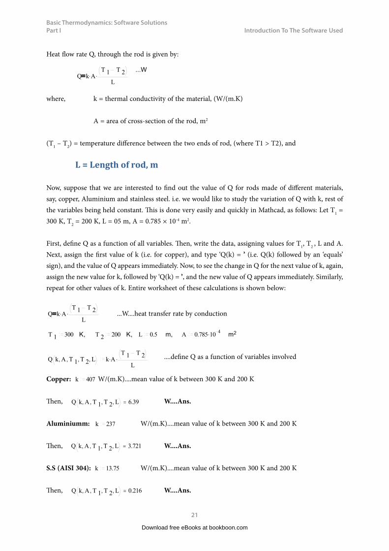
Heat flow rate Q, through the rod is given by:
Q k A.T 1 T 2
L.
...W
where, k = thermal conductivity of the material, (W/(m.K)
A = area of cross-section of the rod, m2
(T1 – T2) = temperature difference between the two ends of rod, (where T1 > T2), and
L = Length of rod, m
Now, suppose that we are interested to find out the value of Q for rods made of different materials, say, copper, Aluminium and stainless steel. i.e. we would like to study the variation of Q with k, rest of the variables being held constant. This is done very easily and quickly in Mathcad, as follows: Let T1 = 300 K, T2 = 200 K, L = 05 m, A = 0.785 × 10⁻⁴ m2.
First, define Q as a function of all variables. Then, write the data, assigning values for T1, T2 , L and A. Next, assign the first value of k (i.e. for copper), and type ‘Q(k) = ’ (i.e. Q(k) followed by an ‘equals’ sign), and the value of Q appears immediately. Now, to see the change in Q for the next value of k, again, assign the new value for k, followed by ‘Q(k) = ’, and the new value of Q appears immediately. Similarly, repeat for other values of k. Entire worksheet of these calculations is shown below:
Q k AT 1 T 2
L ...W....heat transfer rate by conduction
T 1 300 K, T 2 200 K, L 0.5 m, A 0.785 104
m2
Q k A T 1 T 2 L k AT 1 T 2
L
....define Q as a function of variables involved
Copper: k 407 W/(m.K)....mean value of k between 300 K and 200 K
Then, Q k A T 1 T 2 L 6.39 W....Ans.
Aluminiumm: k 237 W/(m.K)....mean value of k between 300 K and 200 K
Then, Q k A T 1 T 2 L 3.721 W....Ans.
S.S (AISI 304): k 13.75 W/(m.K)....mean value of k between 300 K and 200 K
Then, Q k A T 1 T 2 L 0.216 W....Ans.
Download free eBooks at bookboon.com
Basic Thermodynamics: Software Solutions Part I
22
Introduction To The Software Used
In a similar manner, by individually changing other values viz. area of cross-section (A), end temperatures (T1, T2) and length (L), effect on the heat transfer rate (Q) can be studied.
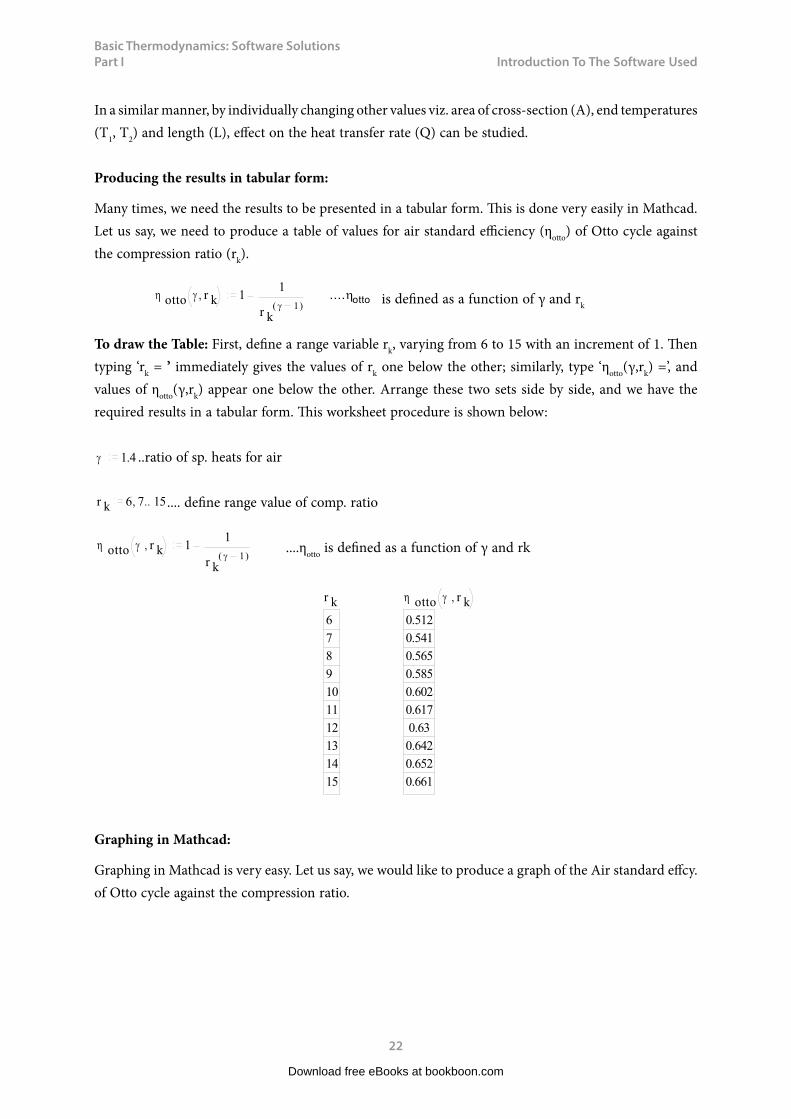
Producing the results in tabular form:
Many times, we need the results to be presented in a tabular form. This is done very easily in Mathcad. Let us say, we need to produce a table of values for air standard efficiency (ηotto) of Otto cycle against the compression ratio (rk).
otto r k 11
r k1( )
.... otto is defined as a function of γ and rk
To draw the Table: First, define a range variable rk, varying from 6 to 15 with an increment of 1. Then typing ‘rk = ’ immediately gives the values of rk one below the other; similarly, type ‘ηotto(γ,rk) =’, and values of ηotto(γ,rk) appear one below the other. Arrange these two sets side by side, and we have the required results in a tabular form. This worksheet procedure is shown below:
1.4 ..ratio of sp. heats for air
r k 6 7 15.... define range value of comp. ratio
otto r k 11
r k1( )
....ηotto is defined as a function of γ and rk
r k
6
7
8
9
10
11
12
13
14
15
otto r k
0.512
0.541
0.565
0.585
0.602
0.617
0.63
0.642
0.652
0.661
Graphing in Mathcad:
Graphing in Mathcad is very easy. Let us say, we would like to produce a graph of the Air standard effcy. of Otto cycle against the compression ratio.
Download free eBooks at bookboon.com
Basic Thermodynamics: Software Solutions Part I
23
Introduction To The Software Used
We have:
otto r k 11
r k1( )
.... otto is defined as a function of γ and rk
First step is to define a ‘range variable’ rk, varying from say, 6 to 15, in increments of 1. In Mathcad, it is written in the form:
r k 6 7 15 .... define range value of comp. ratio
Then click on the graphing palette, and select the x-y graph. A graphing area appears with two ‘place holders’, one on the x-axis and the other on the y-axis. Fill in the x-axis place holder with rk. On the y-axis place holder, fill in ηotto(γ,rk). Click any where outside the graph and immediately the graph appears. Further, there are simple mouse-click commands for giving titles for the graph, x-axis and y-axis, and also for showing grid lines and legend. Logarithmic scaling also can be applied by simple mouse click commands. Entire worksheet is shown below:
Download free eBooks at bookboon.com
Click on the ad to read moreClick on the ad to read moreClick on the ad to read moreClick on the ad to read moreClick on the ad to read moreClick on the ad to read moreClick on the ad to read moreClick on the ad to read moreClick on the ad to read more
Basic Thermodynamics: Software Solutions Part I
24
Introduction To The Software Used
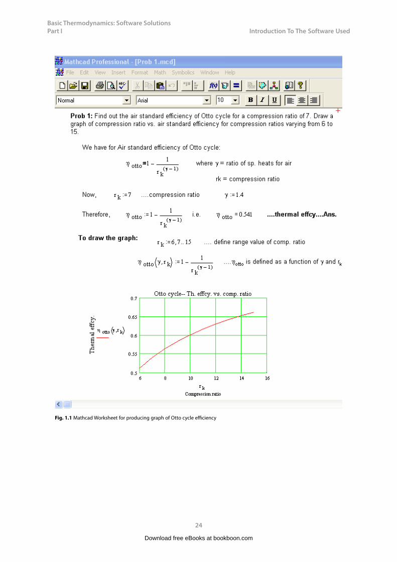
Fig. 1.1 Mathcad Worksheet for producing graph of Otto cycle efficiency
Download free eBooks at bookboon.com
Basic Thermodynamics: Software Solutions Part I
25
Introduction To The Software Used
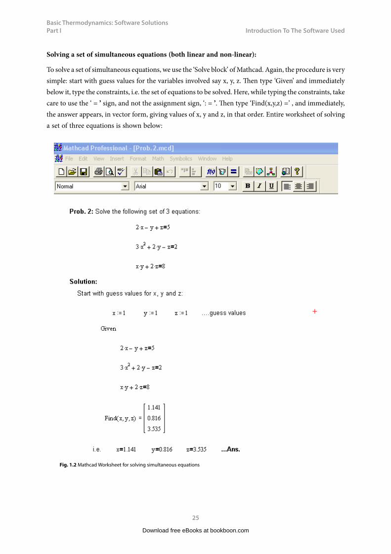
Solving a set of simultaneous equations (both linear and non-linear):
To solve a set of simultaneous equations, we use the ‘Solve block’ of Mathcad. Again, the procedure is very simple: start with guess values for the variables involved say x, y, z. Then type ‘Given’ and immediately below it, type the constraints, i.e. the set of equations to be solved. Here, while typing the constraints, take care to use the ‘ = ’ sign, and not the assignment sign, ‘: = ’. Then type ‘Find(x,y,z) =’ , and immediately, the answer appears, in vector form, giving values of x, y and z, in that order. Entire worksheet of solving a set of three equations is shown below:
Fig. 1.2 Mathcad Worksheet for solving simultaneous equations
Download free eBooks at bookboon.com

Basic Thermodynamics: Software Solutions Part I
26
Introduction To The Software Used
Mathcad has several other capabilities such as: differentiation, integration, matrices, symbolic calculations etc. There is also programming capability in Mathcad with the usual constructs such as if–then–else, do-loops etc. Thus, with its very wide mathematical and graphing functionality, coupled with programming capability and the convenience of Windows platform, Mathcad is a very powerful and versatile tool for engineering and scientific calculations.
Note: It is pertinent to make one note here. Mathcad does not contain built-in functions for thermodynamic properties of working substances such as steam/water, air, refrigerants, fuels etc; one has to buy separately add-in programs supplied by third parties.
1.2.2 Engineering Equation Solver (EES):
What is EES?
EES, supplied by M/s F-Chart Software, USA, is basically an equation solver, which gives numerical solutions of a set of linear or non-linear algebraic or differential equations. EES also provides built-in functions for thermodynamic and transport properties of many fluids such as water/steam, dry and moist air, refrigerants, cryogenic fluids, fuels and others. User written data and functions can also be added to the library. Parametric study can easily be conducted to provide optimum design solutions. There is good graphing capability and publication quality graphs of different types can easily be generated. Combined with this is the programming capability, as in other computer languages such as ‘Fortran’ or ‘C’, making EES a powerful tool to solve problems in Thermodynamics.
Download free eBooks at bookboon.com
Click on the ad to read moreClick on the ad to read moreClick on the ad to read moreClick on the ad to read moreClick on the ad to read moreClick on the ad to read moreClick on the ad to read moreClick on the ad to read moreClick on the ad to read moreClick on the ad to read more
AXA Global Graduate Program
Find out more and apply
Basic Thermodynamics: Software Solutions Part I
27
Introduction To The Software Used
Equations Window of EES:
As you start EES, equations window appears. Here, you enter your equations. Formatting rules are as follows (Ref: F-chart.com):
1. Upper and lower case letters are not distinguished. EES will (optionally) change the ease of all variables to match the manner in which they first appear.
2. Blank lines and spaces may be entered as desired since they are ignored. 3. Comments must be enclosed within braces { } or within quote marks “ ”. Comments may
span as many lines as needed. Comments within braces may be nested in which case only the outermost set of { } are recognized. Comments within quotes will also be displayed in the Formatted Equations window.
4. Variable names must start with a letter and consist of any keyboard characters except ( ) ‘ | * / + – ^ { }: “ or ;. Array variables are identified with square braces around the array index or indices, e.g., X[5,3]. String variables are identified with a $ as the last character in the variable name. The maximum length of a variable name is 30 characters.
5. Multiple equations may be entered on one line if they are separated by a semi-colon (;). The maximum line length is 255 characters.
6. The caret symbol ^ or ** is used to indicate raising to a power. 7. The order in which the equations are entered does not matter. 8. The position of knowns and unknowns in the equation does not matter.
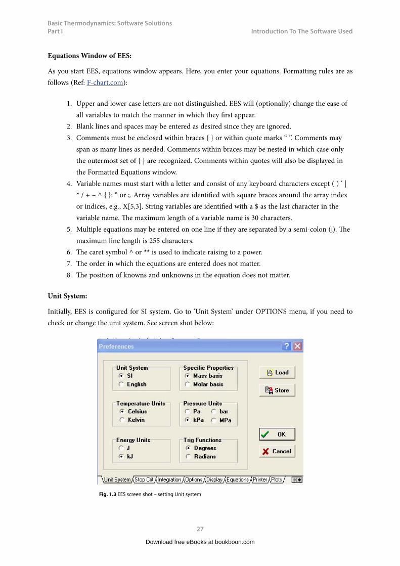
Unit System:
Initially, EES is configured for SI system. Go to ‘Unit System’ under OPTIONS menu, if you need to check or change the unit system. See screen shot below:
Fig. 1.3 EES screen shot – setting Unit system
Download free eBooks at bookboon.com
Basic Thermodynamics: Software Solutions Part I
28
Introduction To The Software Used
Also, go to ‘Variable Info’ under OPTIONS menu and set the units of all variables; this makes sure that all units are consistent and avoids unnecessary error messages popping up.
Formatted equations Window:
In this window, you can see the equations entered in the equations window, in a formatted manner. This is useful to quickly check if you have entered the equations properly.
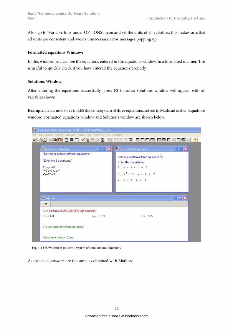
Solutions Window:
After entering the equations successfully, press F2 to solve; solutions window will appear with all variables shown.
Example: Let us now solve in EES the same system of three equations, solved in Mathcad earlier. Equations window, Formatted equations window and Solutions window are shown below:
Fig. 1.4 EES Worksheet to solve a system of simultaneous equations
As expected, answers are the same as obtained with Mathcad.
Download free eBooks at bookboon.com
Basic Thermodynamics: Software Solutions Part I
29
Introduction To The Software Used
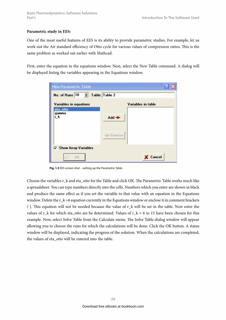
Parametric study in EES:
One of the most useful features of EES is its ability to provide parametric studies. For example, let us work out the Air standard efficiency of Otto cycle for various values of compression ratios. This is the same problem as worked out earlier with Mathcad.
First, enter the equation in the equations window. Next, select the New Table command. A dialog will be displayed listing the variables appearing in the Equations window.
Fig. 1.5 EES screen shot – setting up the Parametric Table
Choose the variables r_k and eta_otto for the Table and click OK. The Parametric Table works much like a spreadsheet. You can type numbers directly into the cells. Numbers which you enter are shown in black and produce the same effect as if you set the variable to that value with an equation in the Equations window. Delete the r_k =6 equation currently in the Equations window or enclose it in comment brackets { }. This equation will not be needed because the value of r_k will be set in the table. Now enter the values of r_k for which eta_otto are be determined. Values of r_k = 6 to 15 have been chosen for this example. Now, select Solve Table from the Calculate menu. The Solve Table dialog window will appear allowing you to choose the runs for which the calculations will be done. Click the OK button. A status window will be displayed, indicating the progress of the solution. When the calculations are completed, the values of eta_otto will be entered into the table.
Download free eBooks at bookboon.com
Basic Thermodynamics: Software Solutions Part I
30
Introduction To The Software Used
Fig. 1.6 EES Worksheet – calculations in Parametric Table
Graphing in EES:
Select New Plot Window from the Plot menu. The New Plot Window dialog window shown below will appear. Choose r_k to be the x-axis by clicking on r_k in the x-axis list. Click on eta_otto in the y-axis list. Select the scale limits for r_k and eta_otto, if required. Grid lines make the plot easier to read. Click on the Grid Lines control for both the x and y axes. When you click the OK button, the plot will be constructed and the plot window will appear. In the screen shot shown below, all the tree windows (i.e. Equation, Parametric Table and the Plot windows) are arranged side by side:
Download free eBooks at bookboon.com
Click on the ad to read moreClick on the ad to read moreClick on the ad to read moreClick on the ad to read moreClick on the ad to read moreClick on the ad to read moreClick on the ad to read moreClick on the ad to read moreClick on the ad to read moreClick on the ad to read moreClick on the ad to read more
Designed for high-achieving graduates across all disciplines, London Business School’s Masters in Management provides specific and tangible foundations for a successful career in business.
This 12-month, full-time programme is a business qualification with impact. In 2010, our MiM employment rate was 95% within 3 months of graduation*; the majority of graduates choosing to work in consulting or financial services.
As well as a renowned qualification from a world-class business school, you also gain access to the School’s network of more than 34,000 global alumni – a community that offers support and opportunities throughout your career.
For more information visit www.london.edu/mm, email [email protected] or give us a call on +44 (0)20 7000 7573.
Masters in Management
The next step for top-performing graduates
* Figures taken from London Business School’s Masters in Management 2010 employment report
Basic Thermodynamics: Software Solutions Part I
31
Introduction To The Software Used
Fig. 1.7 EES graph – screen shot
Once created, there are a variety of ways in which the appearance of the plot can be changed. Refer to the EES manual for further study. Help can also be obtained at any time by pressing F1.
Fluid property functions in EES: As mentioned earlier, EES has built-in functions for thermodynamic and properties of a variety of fluids, making it very convenient to solve problems in Thermodynamics.
As an example, let us find out the isentropic work produced in a turbine when steam expands from 30 bar, 350 C to 10 kPa. Also, find out the quality of exit steam.
Procedure is as follows: We know that isentropic turbine work = (h1 – h2) per kg of steam, where h1 = enthalpy at inlet to the turbine, and h2 = enthalpy at exit. In EES, open the Equations window. Enter the given data:
Download free eBooks at bookboon.com
Basic Thermodynamics: Software Solutions Part I
32
Introduction To The Software Used
Fig. 1.8 EES Worksheet to find Isentropic work of Turbine
Now, to get enthalpies of steam/water we have to use the built-in functions of EES. Before doing so, it is important to confirm that the unit settings are alright. So, under OPTIONS menu, click on ‘unit system’ and check that units are set OK, as shown earlier.
Download free eBooks at bookboon.com
Click on the ad to read moreClick on the ad to read moreClick on the ad to read moreClick on the ad to read moreClick on the ad to read moreClick on the ad to read moreClick on the ad to read moreClick on the ad to read moreClick on the ad to read moreClick on the ad to read moreClick on the ad to read moreClick on the ad to read more
Get Internationally Connected at the University of Surrey MA Intercultural Communication with International BusinessMA Communication and International Marketing
MA Intercultural Communication with International Business
Provides you with a critical understanding of communication in contemporary socio-cultural contexts by combining linguistic, cultural/media studies and international business and will prepare you for a wide range of careers.
MA Communication and International Marketing
Equips you with a detailed understanding of communication in contemporary international marketing contexts to enable you to address the market needs of the international business environment.
For further information contact:T: +44 (0)1483 681681E: [email protected]/downloads

Basic Thermodynamics: Software Solutions Part I
33
Introduction To The Software Used
Now, go to ‘Function Info’ in OPTIONS menu: Select ‘Fluid properties’ button. On the RHS, names of several fluids appear. Select Steam_NBS. On the LHS, select the property required viz. Enthalpy. To get enthalpy, you have to input any two independent properties. You can choose the independent properties, using the selection arrows at the bottom of screen. We have chosen P and T for state 1, since the same are given as data. Format for entering the function is also shown at the bottom line, in Ex: (see the screen shot below).
Fig. 1.9 EES – Function Info window
Now, paste the format on the equations window, taking care to enter the same notations for P and T used earlier. For state 2 at the exit of the turbine, input the pressure and entropy; the pressure at exit of turbine, P2, is given as 10 kPa and we know that s2 = s1 for isentropic expansion in turbine. To determine quality at state 2, input pressure P2 and enthalpy h2.
Download free eBooks at bookboon.com
Basic Thermodynamics: Software Solutions Part I
34
Introduction To The Software Used
Go to ‘Variable Info’ under OPTIONS menu and set the units of all variables to make sure that all units are consistent and no unnecessary error messages pop up. Screen shot is shown below:
Fig. 1.10 EES – Variable Info window to set Units
Now, press F2 to calculate. Solutions window will appear, where we read the isentropic turbine work as 979.7 kJ/kg and the ‘quality’ at exit of turbine, x2 as 0.8124. See the screen shot below:
Fig. 1.11 EES Solution Window-- Isentropic work of Turbine
Thus, we see that EES is a very versatile software. It is easy to learn, has an intuitive interface, and is particularly suited to solve problems in Thermodynamics because of its built-in functions for a large number of substances. EES is developed by Prof. Klein and his colleagues who teach Thermodynamics and Heat Transfer at Wisconsin University, USA.
Download free eBooks at bookboon.com
Basic Thermodynamics: Software Solutions Part I
35
Introduction To The Software Used
1.2.3 The Expert System for Thermodynamics (TEST):
What is TEST?
TEST is a web based learning tool for Thermodynamics. It is not a ‘commercial’ software, in its strict sense. Educational version of TEST is freely made available to Educators by the author of TEST, Prof. Subrata Bhattacharjee. ‘Mirroring’ is also encouraged to ensure that every one has access to the same, updated version.
TEST, according to its author, Prof. Subrata Bhattacharjee of San Diego State University, USA, is “…a visual environment to solve thermo problems, pursue what-if scenarios, perform numerical experiments, and engage in a life-long learning experience… It is a visual platform where a user can look up traditional charts and tables, explore hundreds of thermodynamic systems through Flash animations, browse online solutions to problems”. Calculations in TEST are done by…Daemons – smart thermodynamic calculators customized for specific classes of problems”. A TEST solution is visual in nature, but can be saved and recreated later.
Download free eBooks at bookboon.com
Click on the ad to read moreClick on the ad to read moreClick on the ad to read moreClick on the ad to read moreClick on the ad to read moreClick on the ad to read moreClick on the ad to read moreClick on the ad to read moreClick on the ad to read moreClick on the ad to read moreClick on the ad to read moreClick on the ad to read moreClick on the ad to read more
STEP INTO A WORLD OF OPPORTUNITYwww.ecco.com/[email protected]

Basic Thermodynamics: Software Solutions Part I
36
Introduction To The Software Used
‘Daemons’ (i.e. TEST calculators) can be used to evaluate thermodynamic properties, define complete states, analyze thermodynamic systems such as: IC engines, gas turbines, steam power plants, refrigeration, air-conditioning, combustion, etc., and perform what-if analysis, produce solution report, plot thermodynamic charts, and create solution macros called TEST-codes, which can be saved for later use. TEST has a rich database of working substances – solids, liquids, gases, gas mixtures, phase-change fluids, moist air etc. One can also create a custom solid, liquid, or gas. There are more than forty refrigerants in the TEST database. TEST also has hundreds of animations of systems and old fashioned thermodynamic tables and charts are also provided. There is an I/O panel, wherein one can perform numerical calculations in an ‘Excel-like’ environment. Refer to the exhaustive tutorial of TEST (Ref: www.thermofluids.net) for complete instructions on using TEST.
While TEST is great as a visual solution to problems in thermodynamics, another aspect to be remembered is that the equations, formulas and steps involved in calculations are hidden ‘behind the scene’. Therefore TEST is very much useful as a visual tool for quick calculations and verification of designs. To produce ‘publication quality’ graphs, it is recommended that the graph data produced in TEST are transferred to some other software such as Excel (or any other) for further processing.
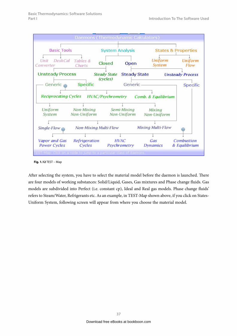
Systematic approach to solve thermodynamic problems:
Fig. 1.12 shows the TEST – Map i.e. classification of daemons for solving different types of thermodynamic problems. Essentially, there are 3 types of daemons: Basic, State and System daemons. See the sub-classification under each type of daemon. Note that under “Basic’ daemons, there is a very good Units conversion program, a desk calculator and conventional thermodynamic property tables. Click on the appropriate daemon to bring it to surface. “…The core of the daemon is its robust state calculator, which bundles the relevant state variables (p, T, v, u, h, s, etc.) into a single graphical interface called a state. You can enter the known state variables in any desired units and calculate the state fully or partially by the click of a button. The daemon checks for redundancy in inputs, determines phase composition, and plots simple thermodynamic diagrams (such as the T-s diagram, psychrometric plot etc.)”.
Download free eBooks at bookboon.com
Basic Thermodynamics: Software Solutions Part I
37
Introduction To The Software Used
Fig. 1.12 TEST – Map
After selecting the system, you have to select the material model before the daemon is launched. There are four models of working substances: Solid/Liquid, Gases, Gas mixtures and Phase change fluids. Gas models are subdivided into Perfect (i.e. constant cp), Ideal and Real gas models. Phase change fluids’ refers to Steam/Water, Refrigerants etc. As an example, in TEST-Map shown above, if you click on States-Uniform System, following screen will appear from where you choose the material model.
Download free eBooks at bookboon.com

Basic Thermodynamics: Software Solutions Part I
38
Introduction To The Software Used
Download free eBooks at bookboon.com
Click on the ad to read moreClick on the ad to read moreClick on the ad to read moreClick on the ad to read moreClick on the ad to read moreClick on the ad to read moreClick on the ad to read moreClick on the ad to read moreClick on the ad to read moreClick on the ad to read moreClick on the ad to read moreClick on the ad to read moreClick on the ad to read moreClick on the ad to read more
Basic Thermodynamics: Software Solutions Part I
39
Introduction To The Software Used
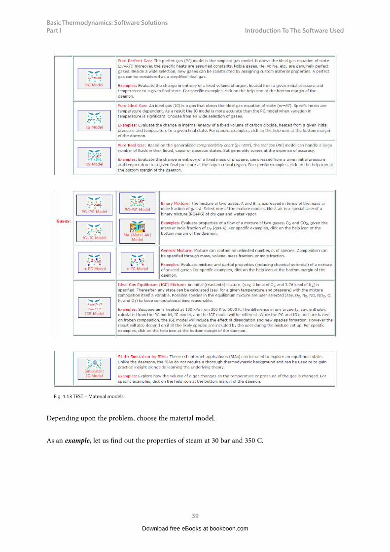
Fig. 1.13 TEST – Material models
Depending upon the problem, choose the material model.
As an example, let us find out the properties of steam at 30 bar and 350 C.
Download free eBooks at bookboon.com
Basic Thermodynamics: Software Solutions Part I
40
Introduction To The Software Used
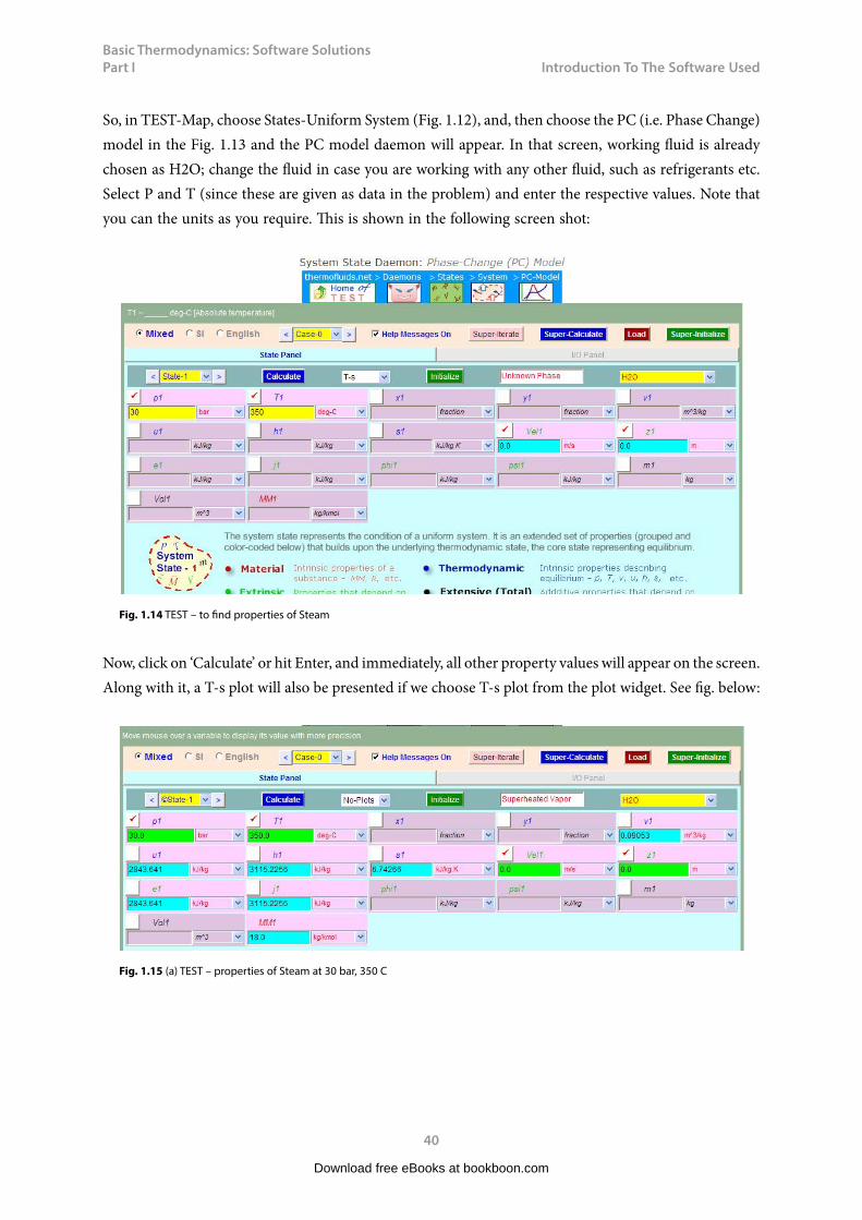
So, in TEST-Map, choose States-Uniform System (Fig. 1.12), and, then choose the PC (i.e. Phase Change) model in the Fig. 1.13 and the PC model daemon will appear. In that screen, working fluid is already chosen as H2O; change the fluid in case you are working with any other fluid, such as refrigerants etc. Select P and T (since these are given as data in the problem) and enter the respective values. Note that you can the units as you require. This is shown in the following screen shot:
Fig. 1.14 TEST – to find properties of Steam
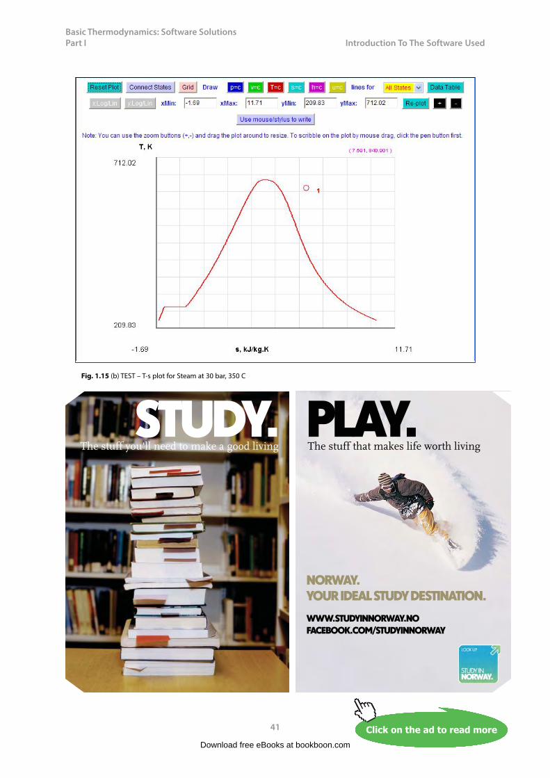
Now, click on ‘Calculate’ or hit Enter, and immediately, all other property values will appear on the screen. Along with it, a T-s plot will also be presented if we choose T-s plot from the plot widget. See fig. below:
Fig. 1.15 (a) TEST – properties of Steam at 30 bar, 350 C
Download free eBooks at bookboon.com
Basic Thermodynamics: Software Solutions Part I
41
Introduction To The Software Used
Fig. 1.15 (b) TEST – T-s plot for Steam at 30 bar, 350 C
Download free eBooks at bookboon.com
Click on the ad to read moreClick on the ad to read moreClick on the ad to read moreClick on the ad to read moreClick on the ad to read moreClick on the ad to read moreClick on the ad to read moreClick on the ad to read moreClick on the ad to read moreClick on the ad to read moreClick on the ad to read moreClick on the ad to read moreClick on the ad to read moreClick on the ad to read moreClick on the ad to read more
STUDY. PLAY.The stuff you'll need to make a good living The stuff that makes life worth living
NORWAY. YOUR IDEAL STUDY DESTINATION.
WWW.STUDYINNORWAY.NOFACEBOOK.COM/STUDYINNORWAY
Basic Thermodynamics: Software Solutions Part I
42
Introduction To The Software Used
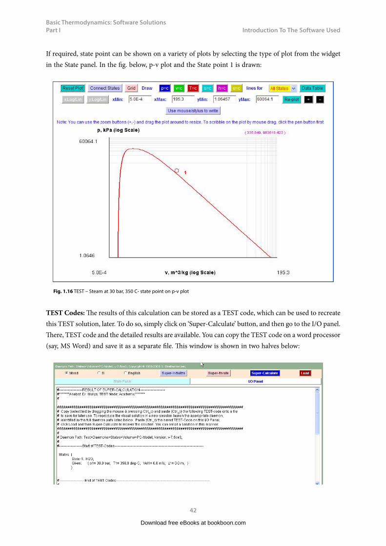
If required, state point can be shown on a variety of plots by selecting the type of plot from the widget in the State panel. In the fig. below, p-v plot and the State point 1 is drawn:
Fig. 1.16 TEST – Steam at 30 bar, 350 C- state point on p-v plot
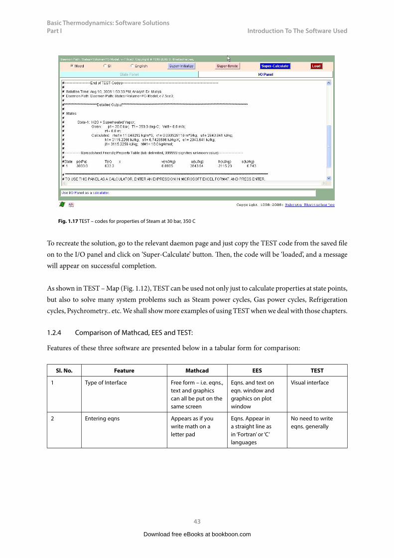
TEST Codes: The results of this calculation can be stored as a TEST code, which can be used to recreate this TEST solution, later. To do so, simply click on ‘Super-Calculate’ button, and then go to the I/O panel. There, TEST code and the detailed results are available. You can copy the TEST code on a word processor (say, MS Word) and save it as a separate file. This window is shown in two halves below:
Download free eBooks at bookboon.com
Basic Thermodynamics: Software Solutions Part I
43
Introduction To The Software Used
Fig. 1.17 TEST – codes for properties of Steam at 30 bar, 350 C
To recreate the solution, go to the relevant daemon page and just copy the TEST code from the saved file on to the I/O panel and click on ‘Super-Calculate’ button. Then, the code will be ‘loaded’, and a message will appear on successful completion.
As shown in TEST – Map (Fig. 1.12), TEST can be used not only just to calculate properties at state points, but also to solve many system problems such as Steam power cycles, Gas power cycles, Refrigeration cycles, Psychrometry.. etc. We shall show more examples of using TEST when we deal with those chapters.
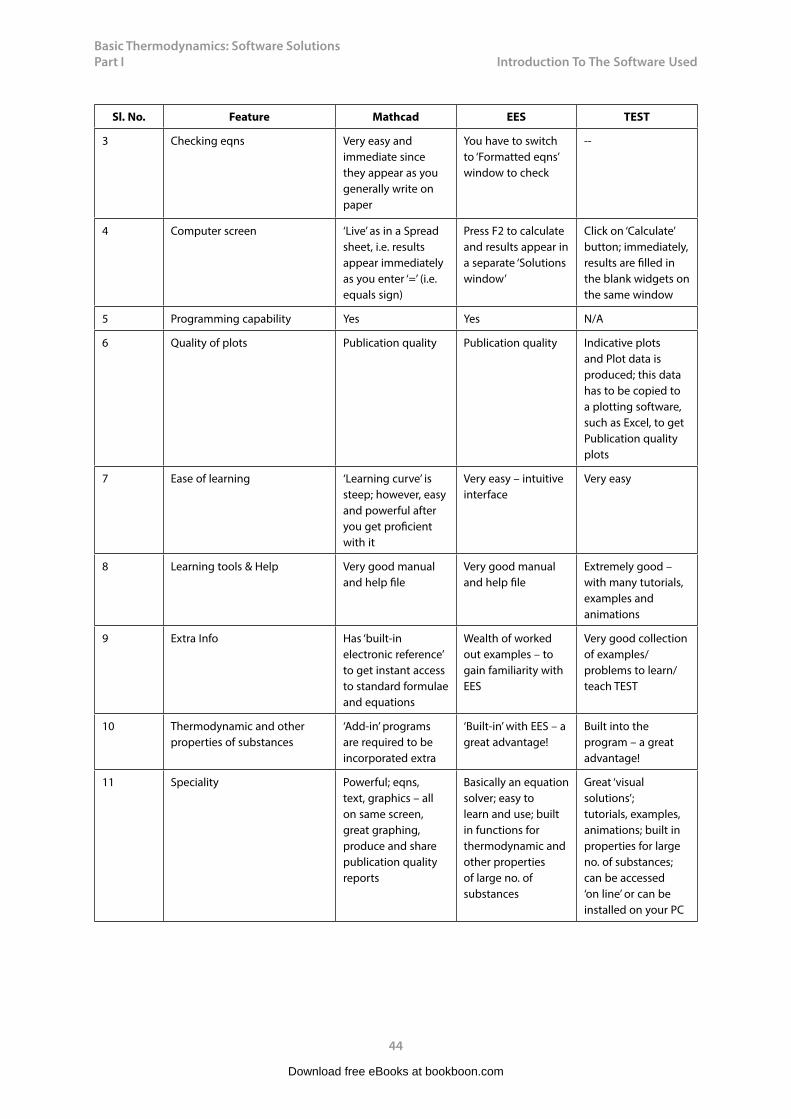
1.2.4 Comparison of Mathcad, EES and TEST:
Features of these three software are presented below in a tabular form for comparison:
Sl. No. Feature Mathcad EES TEST
1 Type of Interface Free form – i.e. eqns., text and graphics can all be put on the same screen
Eqns. and text on eqn. window and graphics on plot window
Visual interface
2 Entering eqns Appears as if you write math on a letter pad
Eqns. Appear in a straight line as in ‘Fortran’ or ‘C’ languages
No need to write eqns. generally
Download free eBooks at bookboon.com
Basic Thermodynamics: Software Solutions Part I
44
Introduction To The Software Used
Sl. No. Feature Mathcad EES TEST
3 Checking eqns Very easy and immediate since they appear as you generally write on paper
You have to switch to ‘Formatted eqns’ window to check
--
4 Computer screen ‘Live’ as in a Spread sheet, i.e. results appear immediately as you enter ‘=’ (i.e. equals sign)
Press F2 to calculate and results appear in a separate ‘Solutions window’
Click on ‘Calculate’ button; immediately, results are filled in the blank widgets on the same window
5 Programming capability Yes Yes N/A
6 Quality of plots Publication quality Publication quality Indicative plots and Plot data is produced; this data has to be copied to a plotting software, such as Excel, to get Publication quality plots
7 Ease of learning ‘Learning curve’ is steep; however, easy and powerful after you get proficient with it
Very easy – intuitive interface
Very easy
8 Learning tools & Help Very good manual and help file
Very good manual and help file
Extremely good – with many tutorials, examples and animations
9 Extra Info Has ‘built-in electronic reference’ to get instant access to standard formulae and equations
Wealth of worked out examples – to gain familiarity with EES
Very good collection of examples/problems to learn/teach TEST
10 Thermodynamic and other properties of substances
‘Add-in’ programs are required to be incorporated extra
‘Built-in’ with EES – a great advantage!
Built into the program – a great advantage!
11 Speciality Powerful; eqns, text, graphics – all on same screen, great graphing, produce and share publication quality reports
Basically an equation solver; easy to learn and use; built in functions for thermodynamic and other properties of large no. of substances
Great ‘visual solutions’; tutorials, examples, animations; built in properties for large no. of substances; can be accessed ‘on line’ or can be installed on your PC
Download free eBooks at bookboon.com

Basic Thermodynamics: Software Solutions Part I
45
Introduction To The Software Used
Sl. No. Feature Mathcad EES TEST
12 Suitability Quite powerful technical software; but, needs add – in programs to solve some types of thermodynamics problems
Especially suitable to solve thermodynamics problems since property functions are built in
Specially developed to solve thermodynamics problems
13 Speed (…depends on computer confign. of course)
Fast Fast Java applets may take a little time to load on Internet; Fast if TEST is installed on your PC
14 Website ptc.com Fchart.com Thermofluids.net
Table 1.1 Comparison of Mathcad, EES and TEST5
1.3 ‘Free’ Software:
There are many ‘free’ software available in the Internet, made available by well known companies or some well meaning individuals. Generally, such software are not very versatile and are meant to do some specific job; but, they may do that job very well indeed, some times, even better than commercially available software!
Download free eBooks at bookboon.com
Click on the ad to read moreClick on the ad to read moreClick on the ad to read moreClick on the ad to read moreClick on the ad to read moreClick on the ad to read moreClick on the ad to read moreClick on the ad to read moreClick on the ad to read moreClick on the ad to read moreClick on the ad to read moreClick on the ad to read moreClick on the ad to read moreClick on the ad to read moreClick on the ad to read moreClick on the ad to read more
Technical training on WHAT you need, WHEN you need it
At IDC Technologies we can tailor our technical and engineering training workshops to suit your needs. We have extensive
experience in training technical and engineering staff and have trained people in organisations such as General Motors, Shell, Siemens, BHP and Honeywell to name a few.Our onsite training is cost effective, convenient and completely customisable to the technical and engineering areas you want covered. Our workshops are all comprehensive hands-on learning experiences with ample time given to practical sessions and demonstrations. We communicate well to ensure that workshop content and timing match the knowledge, skills, and abilities of the participants.
We run onsite training all year round and hold the workshops on your premises or a venue of your choice for your convenience.
Phone: +61 8 9321 1702Email: [email protected] Website: www.idc-online.com
INDUSTRIALDATA COMMS
AUTOMATION & PROCESS CONTROL
ELECTRONICS
ELECTRICAL POWER
MECHANICAL ENGINEERING
OIL & GASENGINEERING
For a no obligation proposal, contact us today at [email protected] or visit our website for more information: www.idc-online.com/onsite/
Basic Thermodynamics: Software Solutions Part I
46
Introduction To The Software Used
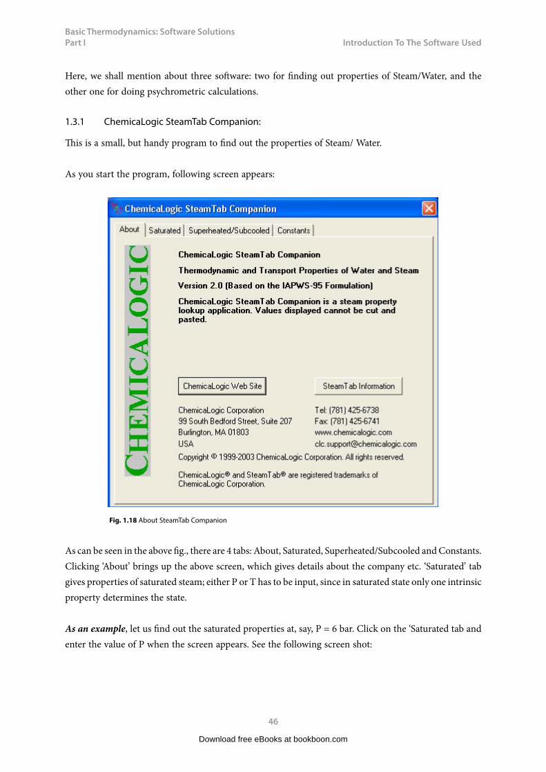
Here, we shall mention about three software: two for finding out properties of Steam/Water, and the other one for doing psychrometric calculations.
1.3.1 ChemicaLogic SteamTab Companion:
This is a small, but handy program to find out the properties of Steam/ Water.
As you start the program, following screen appears:
Fig. 1.18 About SteamTab Companion
As can be seen in the above fig., there are 4 tabs: About, Saturated, Superheated/Subcooled and Constants. Clicking ‘About’ brings up the above screen, which gives details about the company etc. ‘Saturated’ tab gives properties of saturated steam; either P or T has to be input, since in saturated state only one intrinsic property determines the state.
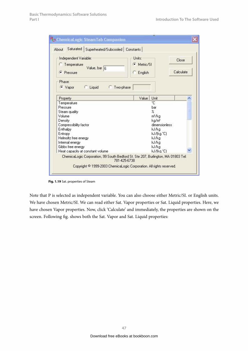
As an example, let us find out the saturated properties at, say, P = 6 bar. Click on the ‘Saturated tab and enter the value of P when the screen appears. See the following screen shot:
Download free eBooks at bookboon.com
Basic Thermodynamics: Software Solutions Part I
47
Introduction To The Software Used
Fig. 1.19 Sat. properties of Steam
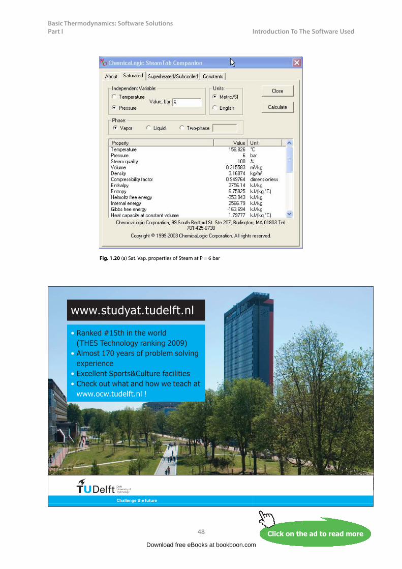
Note that P is selected as independent variable. You can also choose either Metric/SI. or English units. We have chosen Metric/SI. We can read either Sat. Vapor properties or Sat. Liquid properties. Here, we have chosen Vapor properties. Now, click ‘Calculate’ and immediately, the properties are shown on the screen. Following fig. shows both the Sat. Vapor and Sat. Liquid properties:
Download free eBooks at bookboon.com
Basic Thermodynamics: Software Solutions Part I
48
Introduction To The Software Used
Fig. 1.20 (a) Sat. Vap. properties of Steam at P = 6 bar
Download free eBooks at bookboon.com
Click on the ad to read moreClick on the ad to read moreClick on the ad to read moreClick on the ad to read moreClick on the ad to read moreClick on the ad to read moreClick on the ad to read moreClick on the ad to read moreClick on the ad to read moreClick on the ad to read moreClick on the ad to read moreClick on the ad to read moreClick on the ad to read moreClick on the ad to read moreClick on the ad to read moreClick on the ad to read moreClick on the ad to read more
���������� ����� ��������� �������������������������������� �!�" ��#������"��$�%��&��!�"��'����� �(%����������(������ ��%�� ")*+� +���$����� ��"��*������+ ���� ����������� ������ �� ���,���, +��$ ,���-
���," +�� , +��$ ,��
Basic Thermodynamics: Software Solutions Part I
49
Introduction To The Software Used
Fig. 1.20 (b) Sat. Liq. properties of Steam at P = 6 bar
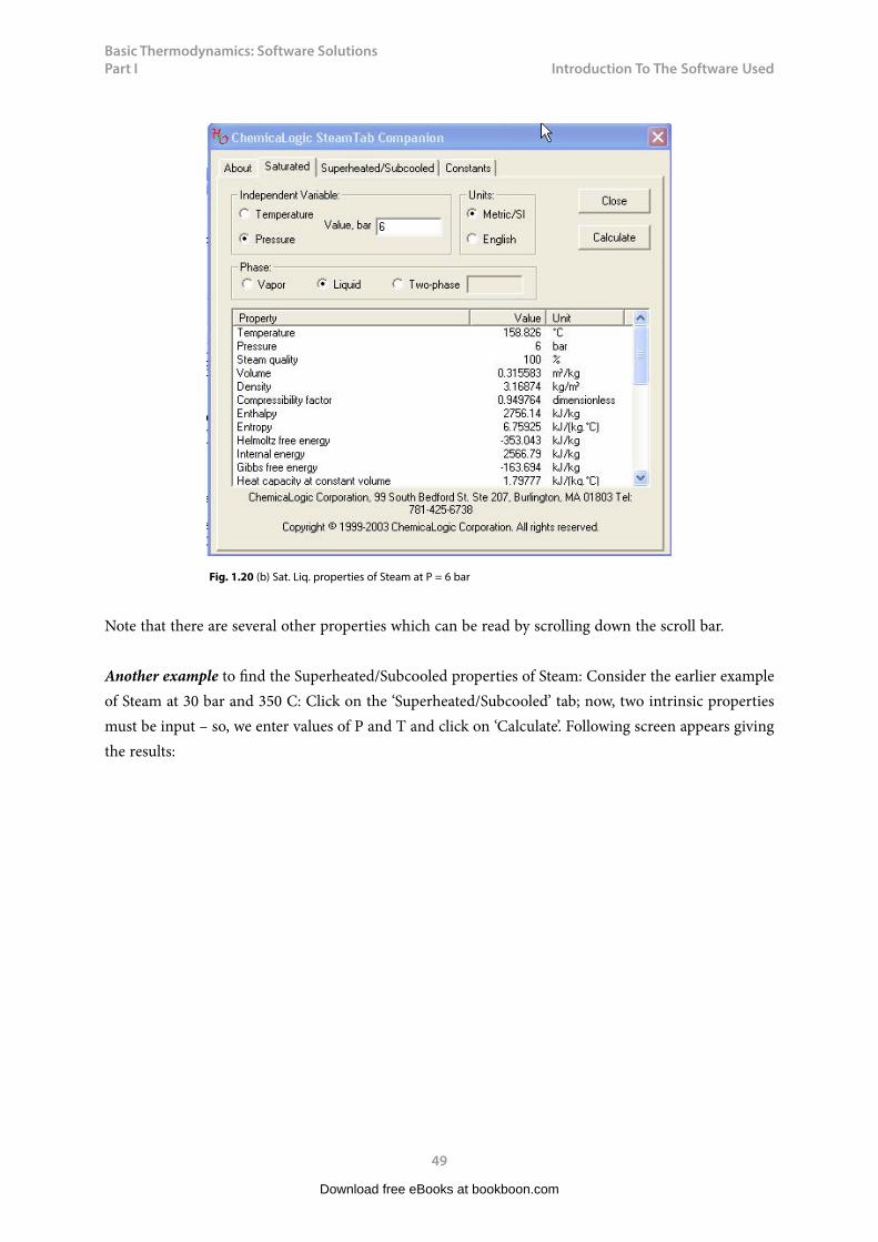
Note that there are several other properties which can be read by scrolling down the scroll bar.
Another example to find the Superheated/Subcooled properties of Steam: Consider the earlier example of Steam at 30 bar and 350 C: Click on the ‘Superheated/Subcooled’ tab; now, two intrinsic properties must be input – so, we enter values of P and T and click on ‘Calculate’. Following screen appears giving the results:
Download free eBooks at bookboon.com
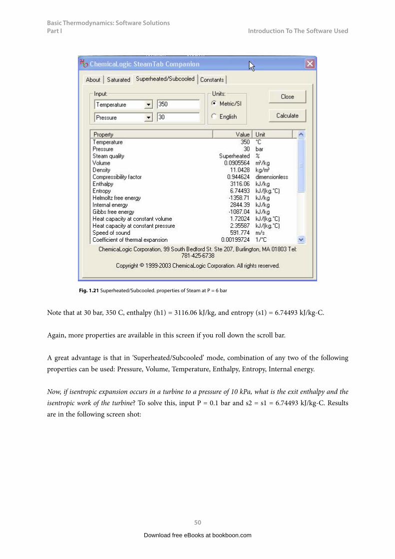
Basic Thermodynamics: Software Solutions Part I
50
Introduction To The Software Used
Fig. 1.21 Superheated/Subcooled. properties of Steam at P = 6 bar
Note that at 30 bar, 350 C, enthalpy (h1) = 3116.06 kJ/kg, and entropy (s1) = 6.74493 kJ/kg-C.
Again, more properties are available in this screen if you roll down the scroll bar.
A great advantage is that in ‘Superheated/Subcooled’ mode, combination of any two of the following properties can be used: Pressure, Volume, Temperature, Enthalpy, Entropy, Internal energy.
Now, if isentropic expansion occurs in a turbine to a pressure of 10 kPa, what is the exit enthalpy and the isentropic work of the turbine? To solve this, input P = 0.1 bar and s2 = s1 = 6.74493 kJ/kg-C. Results are in the following screen shot:
Download free eBooks at bookboon.com
Basic Thermodynamics: Software Solutions Part I
51
Introduction To The Software Used
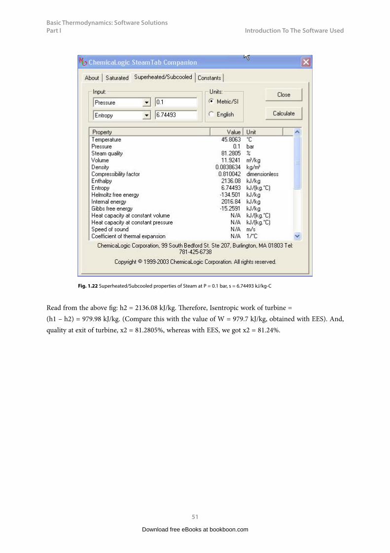
Fig. 1.22 Superheated/Subcooled properties of Steam at P = 0.1 bar, s = 6.74493 kJ/kg-C
Read from the above fig: h2 = 2136.08 kJ/kg. Therefore, Isentropic work of turbine = (h1 – h2) = 979.98 kJ/kg. (Compare this with the value of W = 979.7 kJ/kg, obtained with EES). And, quality at exit of turbine, x2 = 81.2805%, whereas with EES, we got x2 = 81.24%.
Download free eBooks at bookboon.com

Basic Thermodynamics: Software Solutions Part I
52
Introduction To The Software Used
Clicking on ‘Constants’ tab brings up the screen giving values of some constants pertaining to Steam/Water:
Fig. 1.23 Constants for Steam/Water
Two disadvantages of this software are:
1) there is no ‘copy and paste’ facility, i.e. you can not copy and paste these values into another file, and
2) there is no ‘log’ facility, i.e. each time you make a new calculation, results of earlier calculations are lost since they are not stored in a log file.
Still, this software is quite useful since it permits input of any two properties to get a large number of remaining properties.
1.3.2 SteamTable from M/s Figener S/A:
This is also a very handy, little program to find out properties of Steam/Water. In addition, it gives (T-s), (T-h) and (h-s) or Mollier charts for steam, and the state point calculated is also plotted in those charts. Further, a log facility is also provided, so that you can see the record of calculations done by you in one sitting.
Download free eBooks at bookboon.com

Basic Thermodynamics: Software Solutions Part I
53
Introduction To The Software Used
As you open the program, following screen appears:
Fig. 1.24 SteamTable – opening screen
Download free eBooks at bookboon.com
Click on the ad to read moreClick on the ad to read moreClick on the ad to read moreClick on the ad to read moreClick on the ad to read moreClick on the ad to read moreClick on the ad to read moreClick on the ad to read moreClick on the ad to read moreClick on the ad to read moreClick on the ad to read moreClick on the ad to read moreClick on the ad to read moreClick on the ad to read moreClick on the ad to read moreClick on the ad to read moreClick on the ad to read moreClick on the ad to read more
Basic Thermodynamics: Software Solutions Part I
54
Introduction To The Software Used
As can be seen, four tabs: ‘About’ (i.e. above screen), ‘Steam table (complete range)’, ‘Saturation zone’ and ‘Diagrams’.
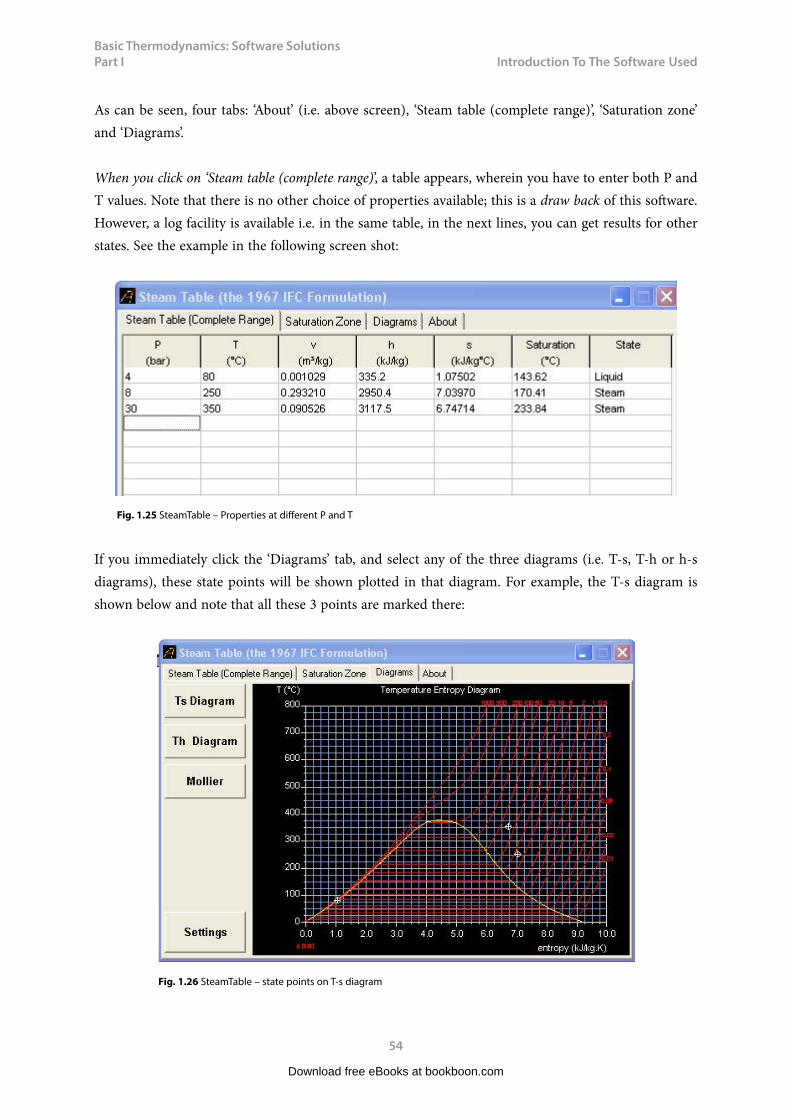
When you click on ‘Steam table (complete range)’, a table appears, wherein you have to enter both P and T values. Note that there is no other choice of properties available; this is a draw back of this software. However, a log facility is available i.e. in the same table, in the next lines, you can get results for other states. See the example in the following screen shot:
Fig. 1.25 SteamTable – Properties at different P and T
If you immediately click the ‘Diagrams’ tab, and select any of the three diagrams (i.e. T-s, T-h or h-s diagrams), these state points will be shown plotted in that diagram. For example, the T-s diagram is shown below and note that all these 3 points are marked there:
Fig. 1.26 SteamTable – state points on T-s diagram
Download free eBooks at bookboon.com
Basic Thermodynamics: Software Solutions Part I
55
Introduction To The Software Used
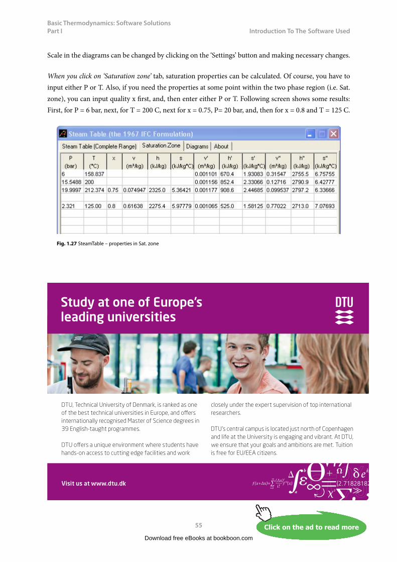
Scale in the diagrams can be changed by clicking on the ‘Settings’ button and making necessary changes.
When you click on ‘Saturation zone’ tab, saturation properties can be calculated. Of course, you have to input either P or T. Also, if you need the properties at some point within the two phase region (i.e. Sat. zone), you can input quality x first, and, then enter either P or T. Following screen shows some results: First, for P = 6 bar, next, for T = 200 C, next for x = 0.75, P= 20 bar, and, then for x = 0.8 and T = 125 C.
Fig. 1.27 SteamTable – properties in Sat. zone
Download free eBooks at bookboon.com
Click on the ad to read moreClick on the ad to read moreClick on the ad to read moreClick on the ad to read moreClick on the ad to read moreClick on the ad to read moreClick on the ad to read moreClick on the ad to read moreClick on the ad to read moreClick on the ad to read moreClick on the ad to read moreClick on the ad to read moreClick on the ad to read moreClick on the ad to read moreClick on the ad to read moreClick on the ad to read moreClick on the ad to read moreClick on the ad to read moreClick on the ad to read more
DTU, Technical University of Denmark, is ranked as one of the best technical universities in Europe, and offers internationally recognised Master of Science degrees in 39 English-taught programmes.
DTU offers a unique environment where students have hands-on access to cutting edge facilities and work
closely under the expert supervision of top international researchers.
DTU’s central campus is located just north of Copenhagen and life at the University is engaging and vibrant. At DTU, we ensure that your goals and ambitions are met. Tuition is free for EU/EEA citizens.
Visit us at www.dtu.dk
Study at one of Europe’s leading universities
Basic Thermodynamics: Software Solutions Part I
56
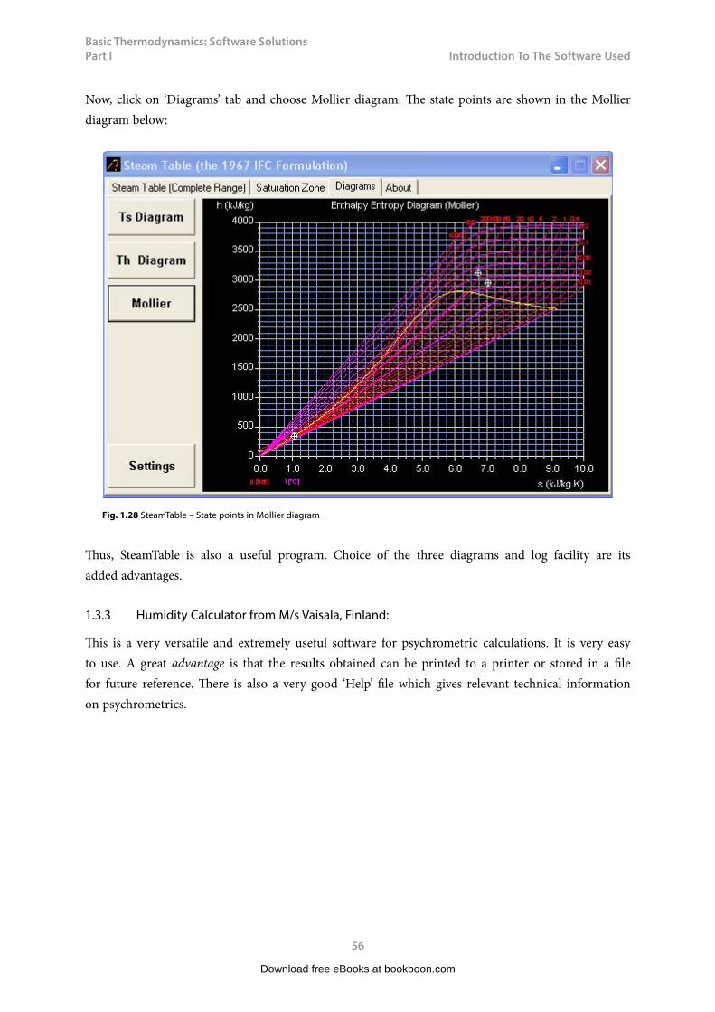
Introduction To The Software Used
Now, click on ‘Diagrams’ tab and choose Mollier diagram. The state points are shown in the Mollier diagram below:
Fig. 1.28 SteamTable – State points in Mollier diagram
Thus, SteamTable is also a useful program. Choice of the three diagrams and log facility are its added advantages.
1.3.3 Humidity Calculator from M/s Vaisala, Finland:
This is a very versatile and extremely useful software for psychrometric calculations. It is very easy to use. A great advantage is that the results obtained can be printed to a printer or stored in a file for future reference. There is also a very good ‘Help’ file which gives relevant technical information on psychrometrics.
Download free eBooks at bookboon.com

Basic Thermodynamics: Software Solutions Part I
57
Introduction To The Software Used
Following is the extract from the details supplied in the ‘help’ file:
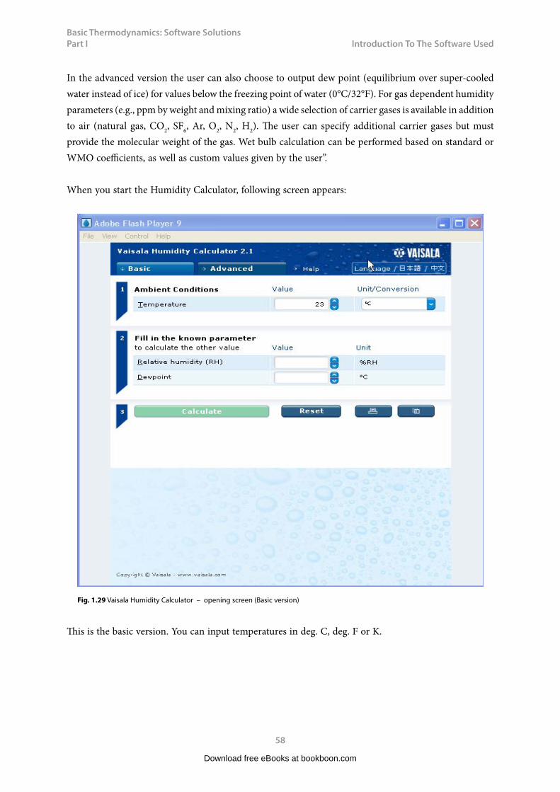
“Vaisala Humidity calculator is a software tool that provides an easy way for solving humidity conversions from one humidity parameter to another. It can also be used to calculate the effect of changing ambient conditions. Vaisala Humidity Calculator includes both a basic version and an advanced version which are shown on the user interface as separate sheets. The basic version provides calculations between relative humidity and dew point when one of these parameters and temperature are known. Note that below the freezing point of water (0°C/32°F), frost point values are provided by convention, although the word dew point is commonly used to express both dew point and frost point. The advanced version of Vaisala Humidity Calculator includes calculation of:
• relative humidity • dewpoint / frostpoint • parts per million. • absolute humidity • mixing ratio • water content • vapor pressure • wet bulb temperature
Download free eBooks at bookboon.com
Click on the ad to read moreClick on the ad to read moreClick on the ad to read moreClick on the ad to read moreClick on the ad to read moreClick on the ad to read moreClick on the ad to read moreClick on the ad to read moreClick on the ad to read moreClick on the ad to read moreClick on the ad to read moreClick on the ad to read moreClick on the ad to read moreClick on the ad to read moreClick on the ad to read moreClick on the ad to read moreClick on the ad to read moreClick on the ad to read moreClick on the ad to read moreClick on the ad to read more
Increase your impact with MSM Executive Education
For more information, visit www.msm.nl or contact us at +31 43 38 70 808
or via [email protected] the globally networked management school
For more information, visit www.msm.nl or contact us at +31 43 38 70 808 or via [email protected]
For almost 60 years Maastricht School of Management has been enhancing the management capacity
of professionals and organizations around the world through state-of-the-art management education.
Our broad range of Open Enrollment Executive Programs offers you a unique interactive, stimulating and
multicultural learning experience.
Be prepared for tomorrow’s management challenges and apply today.
Executive Education-170x115-B2.indd 1 18-08-11 15:13
Basic Thermodynamics: Software Solutions Part I
58
Introduction To The Software Used
In the advanced version the user can also choose to output dew point (equilibrium over super-cooled water instead of ice) for values below the freezing point of water (0°C/32°F). For gas dependent humidity parameters (e.g., ppm by weight and mixing ratio) a wide selection of carrier gases is available in addition to air (natural gas, CO2, SF6, Ar, O2, N2, H2). The user can specify additional carrier gases but must provide the molecular weight of the gas. Wet bulb calculation can be performed based on standard or WMO coefficients, as well as custom values given by the user”.
When you start the Humidity Calculator, following screen appears:
Fig. 1.29 Vaisala Humidity Calculator – opening screen (Basic version)
This is the basic version. You can input temperatures in deg. C, deg. F or K.
Download free eBooks at bookboon.com
Basic Thermodynamics: Software Solutions Part I
59
Introduction To The Software Used
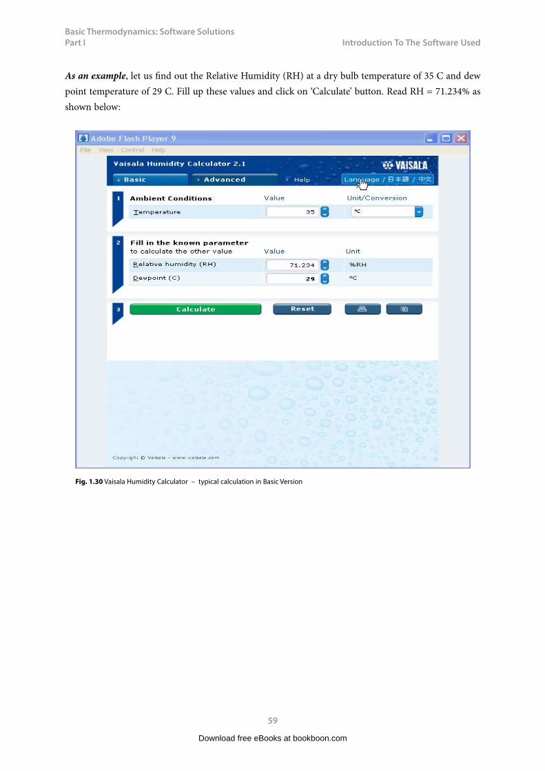
As an example, let us find out the Relative Humidity (RH) at a dry bulb temperature of 35 C and dew point temperature of 29 C. Fill up these values and click on ‘Calculate’ button. Read RH = 71.234% as shown below:
Fig. 1.30 Vaisala Humidity Calculator – typical calculation in Basic Version
Download free eBooks at bookboon.com
Basic Thermodynamics: Software Solutions Part I
60
Introduction To The Software Used
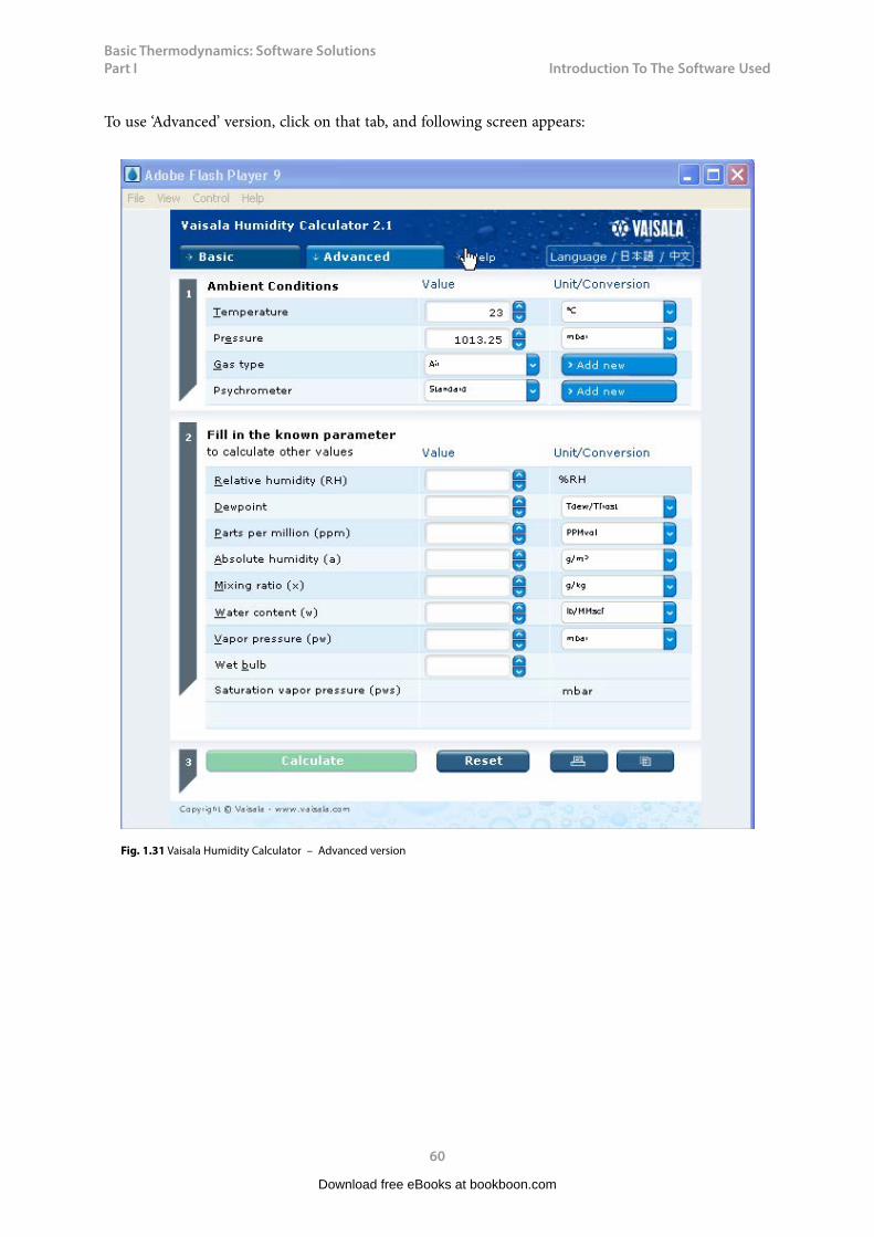
To use ‘Advanced’ version, click on that tab, and following screen appears:
Fig. 1.31 Vaisala Humidity Calculator – Advanced version
Download free eBooks at bookboon.com
Basic Thermodynamics: Software Solutions Part I
61
Introduction To The Software Used
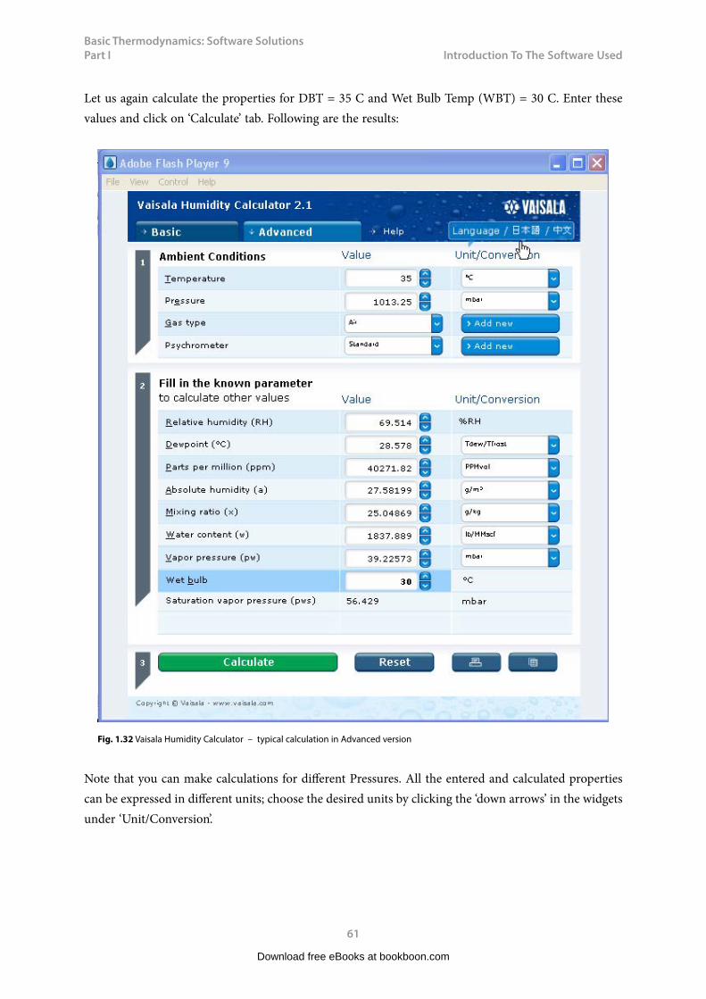
Let us again calculate the properties for DBT = 35 C and Wet Bulb Temp (WBT) = 30 C. Enter these values and click on ‘Calculate’ tab. Following are the results:
Fig. 1.32 Vaisala Humidity Calculator – typical calculation in Advanced version
Note that you can make calculations for different Pressures. All the entered and calculated properties can be expressed in different units; choose the desired units by clicking the ‘down arrows’ in the widgets under ‘Unit/Conversion’.
Download free eBooks at bookboon.com

Basic Thermodynamics: Software Solutions Part I
62
Introduction To The Software Used
‘Reset’ button will reset the values, so that you are ready for next calculation. Next to ‘Reset’ button is the Print button using which you can print the results; and next to Print button is the Copy button. Click on Copy button and then paste the results to MS Word and save as shown below:
Ambient Conditions Value Unit/Conversion
Temperature 35 °C
Pressure 1013.25 mbar
Gas type Air
Psychrometer Standard
Relative humidity (RH) 69.514 %RH
Dewpoint (°C) 28.578 Tdew/Tfrost
Parts per million (ppm) 40271.82 PPMvol
Absolute humidity (a) 27.58199 g/m³
Mixing ratio (x) 25.04869 g/kg
Water content (w) 1837.889 lb/MMscf
Vapor pressure (pw) 39.22573 mbar
Wet bulb 30 °C
Saturation vapor pressure (pws) 56.429 mbar
Download free eBooks at bookboon.com
Click on the ad to read moreClick on the ad to read moreClick on the ad to read moreClick on the ad to read moreClick on the ad to read moreClick on the ad to read moreClick on the ad to read moreClick on the ad to read moreClick on the ad to read moreClick on the ad to read moreClick on the ad to read moreClick on the ad to read moreClick on the ad to read moreClick on the ad to read moreClick on the ad to read moreClick on the ad to read moreClick on the ad to read moreClick on the ad to read moreClick on the ad to read moreClick on the ad to read moreClick on the ad to read more
EXPERIENCE THE POWER OF FULL ENGAGEMENT…
RUN FASTER. RUN LONGER.. RUN EASIER…
READ MORE & PRE-ORDER TODAY WWW.GAITEYE.COM
Challenge the way we run
1349906_A6_4+0.indd 1 22-08-2014 12:56:57
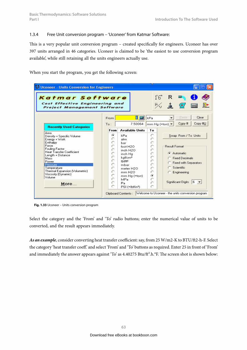
Basic Thermodynamics: Software Solutions Part I
63
Introduction To The Software Used
1.3.4 Free Unit conversion program – ‘Uconeer’ from Katmar Software:
This is a very popular unit conversion program – created specifically for engineers. Uconeer has over 397 units arranged in 46 categories. Uconeer is claimed to be ‘the easiest to use conversion program available’, while still retaining all the units engineers actually use.
When you start the program, you get the following screen:
Fig. 1.33 Uconeer – Units conversion program
Select the category and the ‘From’ and ‘To’ radio buttons; enter the numerical value of units to be converted, and the result appears immediately.
As an example, consider converting heat transfer coefficient: say, from 25 W/m2-K to BTU/ft2-h-F. Select the category ‘heat transfer coeff.’ and select ‘From’ and ‘To’ buttons as required. Enter 25 in front of ‘From’ and immediately the answer appears against ‘To’ as 4.40275 Btu/ft².h.°F. The screen shot is shown below:
Download free eBooks at bookboon.com

Basic Thermodynamics: Software Solutions Part I
64
Introduction To The Software Used
Fig. 1.34 Uconeer – Units conversion for heat transfer coefficient
There is also facility to copy to clip board and choose the result formats and significant digits. There is a very good ‘Help’ file, Gas and Liquid Volume/Mass Flow converters, Gas constant converter and Hardness converter. However, there is one ‘disadvantage’, which does not affect the results anyway: regular popping up of advertisements regarding the products or services provided by the company, as shown in the above screen shot.
1.4 Summary:
In this chapter, a brief overview was given about three very useful commercial, technical software, viz. Mathcad, EES and TEST, particularly useful to solve problems in Thermodynamics. This chapter is not intended as a tutorial on these software. However, since some examples have been worked out, it is expected that the reader will get sufficient working knowledge on use of these software. As we proceed, more problems will be worked out; all the examples will be thoroughly commented, and the reader should not have any difficulty in understanding the solutions, even if he does not use these software.
In addition, four ‘free’ software are described, with worked examples. Out of these, two programs are for finding out properties of Steam/Water and one program for psychrometric calculations, and another program for Units conversion.
Download free eBooks at bookboon.com

Basic Thermodynamics: Software Solutions Part I
65
Introduction To The Software Used
1.5 References:
1. Y.A.Cengel and M.A.Boles. Thermodynamics – An Engineering Approach. 4th ed. New Delhi: Tata McGraw-Hill, 2003
2. http://physics.nist.gov/cuu/Units/index.html3. www.ptc.com4. www.fchart.com5. www.thermofluids.net6. www.chemicalogic.com7. www.figener.com.br8. www.vaisala.com9. www.katmarsoftware.com
Download free eBooks at bookboon.com
Click on the ad to read moreClick on the ad to read moreClick on the ad to read moreClick on the ad to read moreClick on the ad to read moreClick on the ad to read moreClick on the ad to read moreClick on the ad to read moreClick on the ad to read moreClick on the ad to read moreClick on the ad to read moreClick on the ad to read moreClick on the ad to read moreClick on the ad to read moreClick on the ad to read moreClick on the ad to read moreClick on the ad to read moreClick on the ad to read moreClick on the ad to read moreClick on the ad to read moreClick on the ad to read moreClick on the ad to read more
GET THERE FASTER
Oliver Wyman is a leading global management consulting firm that combines
deep industry knowledge with specialized expertise in strategy, operations, risk
management, organizational transformation, and leadership development. With
offices in 50+ cities across 25 countries, Oliver Wyman works with the CEOs and
executive teams of Global 1000 companies.
An equal opportunity employer.
Some people know precisely where they want to go. Others seek the adventure of discovering uncharted territory. Whatever you want your professional journey to be, you’ll find what you’re looking for at Oliver Wyman.
Discover the world of Oliver Wyman at oliverwyman.com/careers
DISCOVEROUR WORLD
Basic Thermodynamics: Software Solutions Part I
66
SI Unitss, Unit Conversions, Pressures, Temperature etc.
2 SI Units, Unit Conversion, Pressure, Temperature etc.
Learning objectives:
1. In this chapter, we first describe the International System of Units (i.e. SI Units). Authentic information from National Institute of Standards and Technology (NIST), USA, formerly (National Bureau of Standards – NBS – USA) is compiled.
2. Unit conversion examples are demonstrated with Uconeer and the Unit converter of TEST software.
3. Then, we discuss about the pressure measurement with manometers and work out some examples using Mathcad as well as EES. One example on ‘curve fitting’ with EES is also explained.
4. Temperature measurement with Thermocouples is explained next. Details regarding different types of thermocouples are given. Problems are worked out using both Mathcad and EES.
5. Next, constant volume gas thermometer is described and a problem is worked out using EES.
6. Finally, RTD’s and Pt resistance thermometer are explained; a versatile, free software viz. PRTCalc to make calculations in connection with Pt-100 is introduced and a problem is worked out in Mathcad and verified with PRTCalc.
7. Finally, Temperature vs Resistance characteristics for Pt-100 thermometer are drawn in Mathcad.
2.1 Introduction:
In this chapter, we shall, first describe International System of Units (SI), its proper usage, Unit conversion from one system of units to another and, then work out problems on measurement of pressure with manometers, and measurement of temperature with thermocouples.
2.2 International System of Units (SI):
SI Units are now almost universally adopted in scientific work. National Institute of Standards and Technology (NIST), USA, formerly (National Bureau of Standards – NBS – USA) has brought out authoritative information on SI Units and guide lines for the correct usage of SI Units. An extract of that information is given below:
Download free eBooks at bookboon.com

Basic Thermodynamics: Software Solutions Part I
67
SI Unitss, Unit Conversions, Pressures, Temperature etc.
There are seven base units in SI:
Table 2.1. SI base units
SI base unit
Base quantity Name Symbol
length meter m
mass kilogram kg
time second s
electric current ampere A
thermodynamic temperature kelvin K
amount of substance mole mol
luminous intensity candela cd
Download free eBooks at bookboon.com
Click on the ad to read moreClick on the ad to read moreClick on the ad to read moreClick on the ad to read moreClick on the ad to read moreClick on the ad to read moreClick on the ad to read moreClick on the ad to read moreClick on the ad to read moreClick on the ad to read moreClick on the ad to read moreClick on the ad to read moreClick on the ad to read moreClick on the ad to read moreClick on the ad to read moreClick on the ad to read moreClick on the ad to read moreClick on the ad to read moreClick on the ad to read moreClick on the ad to read moreClick on the ad to read moreClick on the ad to read moreClick on the ad to read more
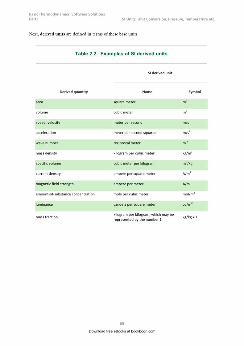
Basic Thermodynamics: Software Solutions Part I
68
SI Unitss, Unit Conversions, Pressures, Temperature etc.
Next, derived units are defined in terms of these base units:
Download free eBooks at bookboon.com
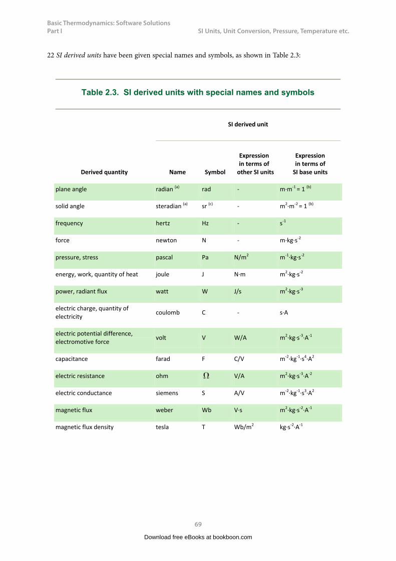
Basic Thermodynamics: Software Solutions Part I
69
SI Unitss, Unit Conversions, Pressures, Temperature etc.
22 SI derived units have been given special names and symbols, as shown in Table 2.3:
Download free eBooks at bookboon.com

Basic Thermodynamics: Software Solutions Part I
70
SI Unitss, Unit Conversions, Pressures, Temperature etc.
Download free eBooks at bookboon.com
Click on the ad to read moreClick on the ad to read moreClick on the ad to read moreClick on the ad to read moreClick on the ad to read moreClick on the ad to read moreClick on the ad to read moreClick on the ad to read moreClick on the ad to read moreClick on the ad to read moreClick on the ad to read moreClick on the ad to read moreClick on the ad to read moreClick on the ad to read moreClick on the ad to read moreClick on the ad to read moreClick on the ad to read moreClick on the ad to read moreClick on the ad to read moreClick on the ad to read moreClick on the ad to read moreClick on the ad to read moreClick on the ad to read moreClick on the ad to read more
81,000 kmIn the past four years we have drilled
That’s more than twice around the world.
What will you be?
Who are we?We are the world’s leading oilfield services company. Working globally—often in remote and challenging locations—we invent, design, engineer, manufacture, apply, and maintain technology to help customers find and produce oil and gas safely.
Who are we looking for?We offer countless opportunities in the following domains:n Engineering, Research, and Operationsn Geoscience and Petrotechnicaln Commercial and Business
If you are a self-motivated graduate looking for a dynamic career, apply to join our team.
careers.slb.com

Basic Thermodynamics: Software Solutions Part I
71
SI Unitss, Unit Conversions, Pressures, Temperature etc.
The special names and symbols of the 22 SI derived units with special names and symbols given in Table 2.3 may themselves be included in the names and symbols of other SI derived units, as shown in Table 2.4:
Download free eBooks at bookboon.com
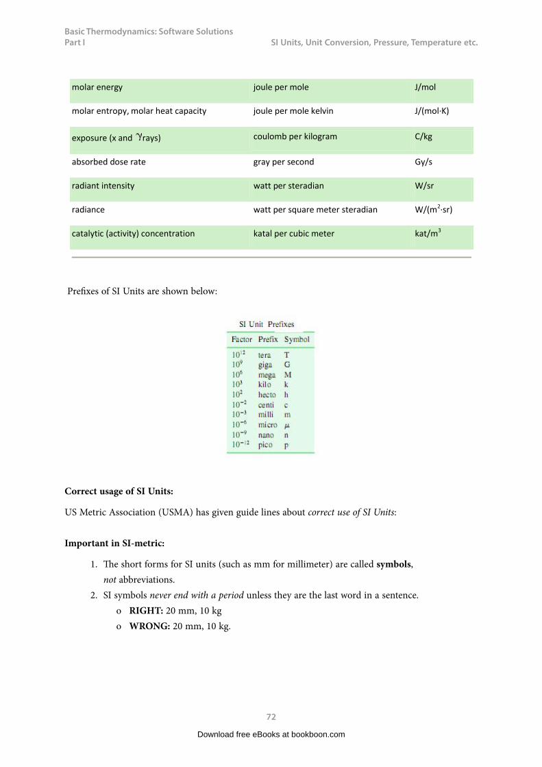
Basic Thermodynamics: Software Solutions Part I
72
SI Unitss, Unit Conversions, Pressures, Temperature etc.
Prefixes of SI Units are shown below:
Correct usage of SI Units:
US Metric Association (USMA) has given guide lines about correct use of SI Units:
Important in SI-metric:
1. The short forms for SI units (such as mm for millimeter) are called symbols, not abbreviations.
2. SI symbols never end with a period unless they are the last word in a sentence. ο RIGHT: 20 mm, 10 kg ο WRONG: 20 mm, 10 kg.
Download free eBooks at bookboon.com

Basic Thermodynamics: Software Solutions Part I
73
SI Unitss, Unit Conversions, Pressures, Temperature etc.
3. SI symbols should be preceded by digits and a space must separate the digits from the symbol. ο RIGHT: It was 300 mm wide. The millimeter width was given. ο WRONG: It was 300mm wide. The mm width was given.
4. Symbols always are written in the singular form (even when more than one is meant). ο RIGHT: 1 mm, 500 mm, 1 kg, 36 kg ο WRONG: 500 mms, 36 kgs ο BUT: It is correct to pluralize written-out metric unit names: 25 kilograms, 250 milliliters
5. The symbol for a compound unit that is a quotient of two units is indicated by a solidus or by a negative exponent.
ο RIGHT: km/h or km·h-1 (for kilometers per hour) ο WRONG: kmph or kph (do not use p as a symbol for “per”.) ο BUT: It is correct to say or write “kilometers per hour”.
6. The meaning of an SI symbol can be changed if you substitute a capital letter for a lower case letter.
ο RIGHT: mm (for millimeter, which means 1/1000 of a meter) ο WRONG: MM or Mm (M is the prefix for mega, which means one million; a
megameter is a million meters)
Download free eBooks at bookboon.com
Click on the ad to read moreClick on the ad to read moreClick on the ad to read moreClick on the ad to read moreClick on the ad to read moreClick on the ad to read moreClick on the ad to read moreClick on the ad to read moreClick on the ad to read moreClick on the ad to read moreClick on the ad to read moreClick on the ad to read moreClick on the ad to read moreClick on the ad to read moreClick on the ad to read moreClick on the ad to read moreClick on the ad to read moreClick on the ad to read moreClick on the ad to read moreClick on the ad to read moreClick on the ad to read moreClick on the ad to read moreClick on the ad to read moreClick on the ad to read moreClick on the ad to read more
Hellmann’s is one of Unilever’s oldest brands having been popular for over 100 years. If you too share a passion for discovery and innovation we will give you the tools and opportunities to provide you with a challenging career. Are you a great scientist who would like to be at the forefront of scientific innovations and developments? Then you will enjoy a career within Unilever Research & Development. For challenging job opportunities, please visit www.unilever.com/rdjobs.
Could you think of 101 new thingsto do with eggs and oil?
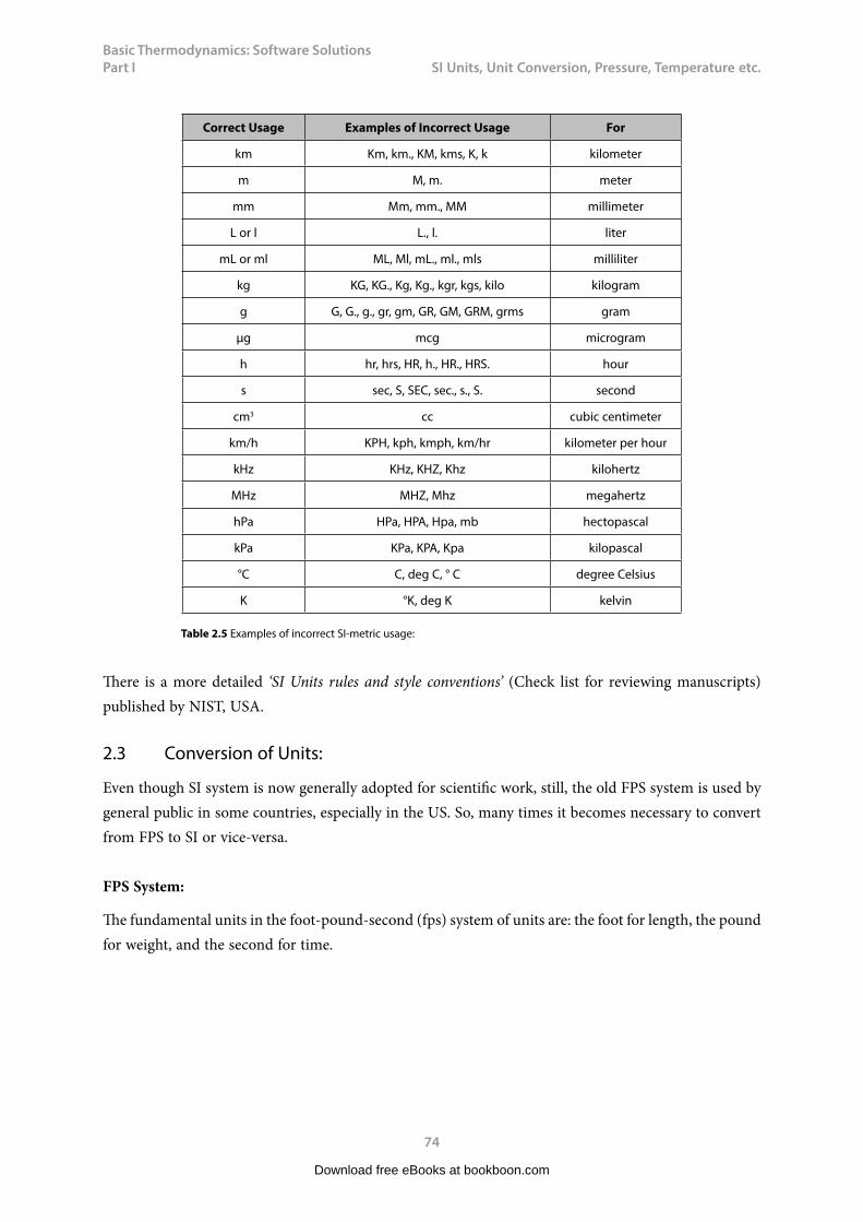
Basic Thermodynamics: Software Solutions Part I
74
SI Unitss, Unit Conversions, Pressures, Temperature etc.
Correct Usage Examples of Incorrect Usage For
km Km, km., KM, kms, K, k kilometer
m M, m. meter
mm Mm, mm., MM millimeter
L or l L., l. liter
mL or ml ML, Ml, mL., ml., mls milliliter
kg KG, KG., Kg, Kg., kgr, kgs, kilo kilogram
g G, G., g., gr, gm, GR, GM, GRM, grms gram
µg mcg microgram
h hr, hrs, HR, h., HR., HRS. hour
s sec, S, SEC, sec., s., S. second
cm3 cc cubic centimeter
km/h KPH, kph, kmph, km/hr kilometer per hour
kHz KHz, KHZ, Khz kilohertz
MHz MHZ, Mhz megahertz
hPa HPa, HPA, Hpa, mb hectopascal
kPa KPa, KPA, Kpa kilopascal
°C C, deg C, ° C degree Celsius
K °K, deg K kelvin
Table 2.5 Examples of incorrect SI-metric usage:
There is a more detailed ‘SI Units rules and style conventions’ (Check list for reviewing manuscripts) published by NIST, USA.
2.3 Conversion of Units:
Even though SI system is now generally adopted for scientific work, still, the old FPS system is used by general public in some countries, especially in the US. So, many times it becomes necessary to convert from FPS to SI or vice-versa.
FPS System:
The fundamental units in the foot-pound-second (fps) system of units are: the foot for length, the pound for weight, and the second for time.
Download free eBooks at bookboon.com
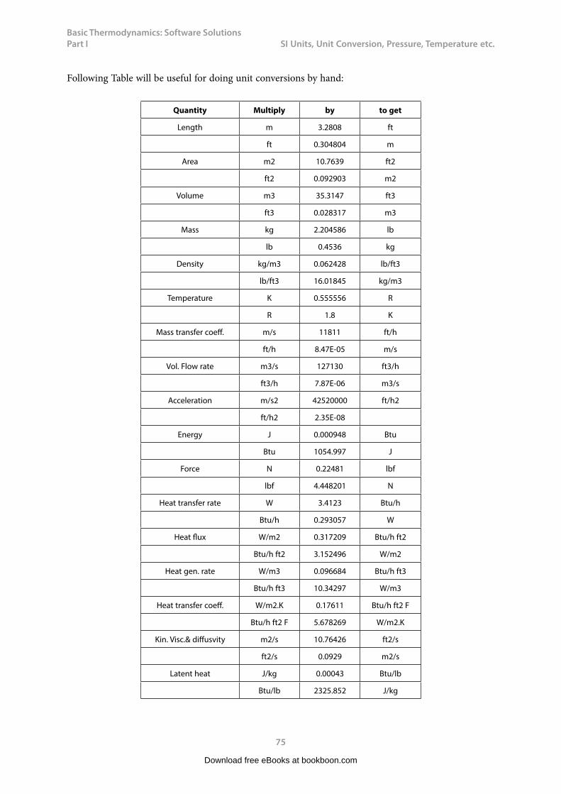
Basic Thermodynamics: Software Solutions Part I
75
SI Unitss, Unit Conversions, Pressures, Temperature etc.
Following Table will be useful for doing unit conversions by hand:
Quantity Multiply by to get
Length m 3.2808 ft
ft 0.304804 m
Area m2 10.7639 ft2
ft2 0.092903 m2
Volume m3 35.3147 ft3
ft3 0.028317 m3
Mass kg 2.204586 lb
lb 0.4536 kg
Density kg/m3 0.062428 lb/ft3
lb/ft3 16.01845 kg/m3
Temperature K 0.555556 R
R 1.8 K
Mass transfer coeff. m/s 11811 ft/h
ft/h 8.47E-05 m/s
Vol. Flow rate m3/s 127130 ft3/h
ft3/h 7.87E-06 m3/s
Acceleration m/s2 42520000 ft/h2
ft/h2 2.35E-08
Energy J 0.000948 Btu
Btu 1054.997 J
Force N 0.22481 lbf
lbf 4.448201 N
Heat transfer rate W 3.4123 Btu/h
Btu/h 0.293057 W
Heat flux W/m2 0.317209 Btu/h ft2
Btu/h ft2 3.152496 W/m2
Heat gen. rate W/m3 0.096684 Btu/h ft3
Btu/h ft3 10.34297 W/m3
Heat transfer coeff. W/m2.K 0.17611 Btu/h ft2 F
Btu/h ft2 F 5.678269 W/m2.K
Kin. Visc.& diffusvity m2/s 10.76426 ft2/s
ft2/s 0.0929 m2/s
Latent heat J/kg 0.00043 Btu/lb
Btu/lb 2325.852 J/kg
Download free eBooks at bookboon.com
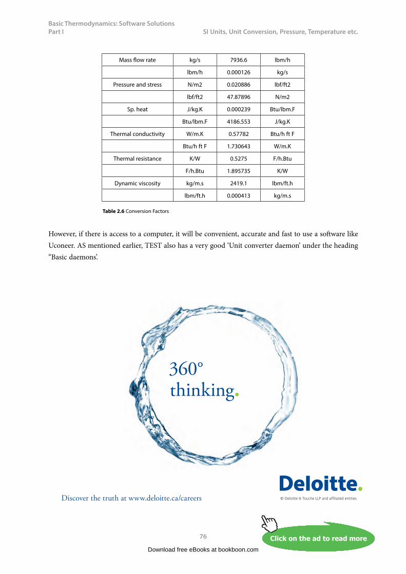
Basic Thermodynamics: Software Solutions Part I
76
SI Unitss, Unit Conversions, Pressures, Temperature etc.
Mass flow rate kg/s 7936.6 lbm/h
lbm/h 0.000126 kg/s
Pressure and stress N/m2 0.020886 lbf/ft2
lbf/ft2 47.87896 N/m2
Sp. heat J/kg.K 0.000239 Btu/lbm.F
Btu/lbm.F 4186.553 J/kg.K
Thermal conductivity W/m.K 0.57782 Btu/h ft F
Btu/h ft F 1.730643 W/m.K
Thermal resistance K/W 0.5275 F/h.Btu
F/h.Btu 1.895735 K/W
Dynamic viscosity kg/m.s 2419.1 lbm/ft.h
lbm/ft.h 0.000413 kg/m.s
Table 2.6 Conversion Factors
However, if there is access to a computer, it will be convenient, accurate and fast to use a software like Uconeer. AS mentioned earlier, TEST also has a very good ‘Unit converter daemon’ under the heading “Basic daemons’.
Download free eBooks at bookboon.com
Click on the ad to read moreClick on the ad to read moreClick on the ad to read moreClick on the ad to read moreClick on the ad to read moreClick on the ad to read moreClick on the ad to read moreClick on the ad to read moreClick on the ad to read moreClick on the ad to read moreClick on the ad to read moreClick on the ad to read moreClick on the ad to read moreClick on the ad to read moreClick on the ad to read moreClick on the ad to read moreClick on the ad to read moreClick on the ad to read moreClick on the ad to read moreClick on the ad to read moreClick on the ad to read moreClick on the ad to read moreClick on the ad to read moreClick on the ad to read moreClick on the ad to read moreClick on the ad to read more
© Deloitte & Touche LLP and affiliated entities.
360°thinking.
Discover the truth at www.deloitte.ca/careers
© Deloitte & Touche LLP and affiliated entities.
360°thinking.
Discover the truth at www.deloitte.ca/careers
© Deloitte & Touche LLP and affiliated entities.
360°thinking.
Discover the truth at www.deloitte.ca/careers © Deloitte & Touche LLP and affiliated entities.
360°thinking.
Discover the truth at www.deloitte.ca/careers
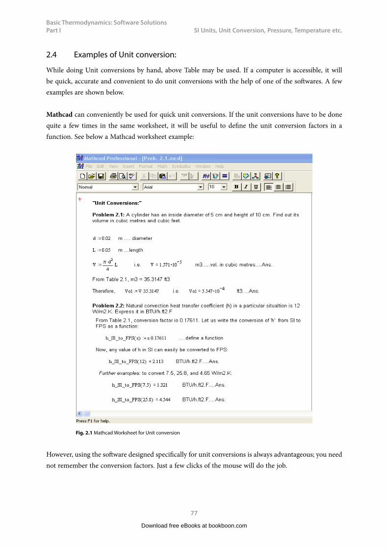
Basic Thermodynamics: Software Solutions Part I
77
SI Unitss, Unit Conversions, Pressures, Temperature etc.
2.4 Examples of Unit conversion:
While doing Unit conversions by hand, above Table may be used. If a computer is accessible, it will be quick, accurate and convenient to do unit conversions with the help of one of the softwares. A few examples are shown below.
Mathcad can conveniently be used for quick unit conversions. If the unit conversions have to be done quite a few times in the same worksheet, it will be useful to define the unit conversion factors in a function. See below a Mathcad worksheet example:
Fig. 2.1 Mathcad Worksheet for Unit conversion
However, using the software designed specifically for unit conversions is always advantageous; you need not remember the conversion factors. Just a few clicks of the mouse will do the job.
Download free eBooks at bookboon.com
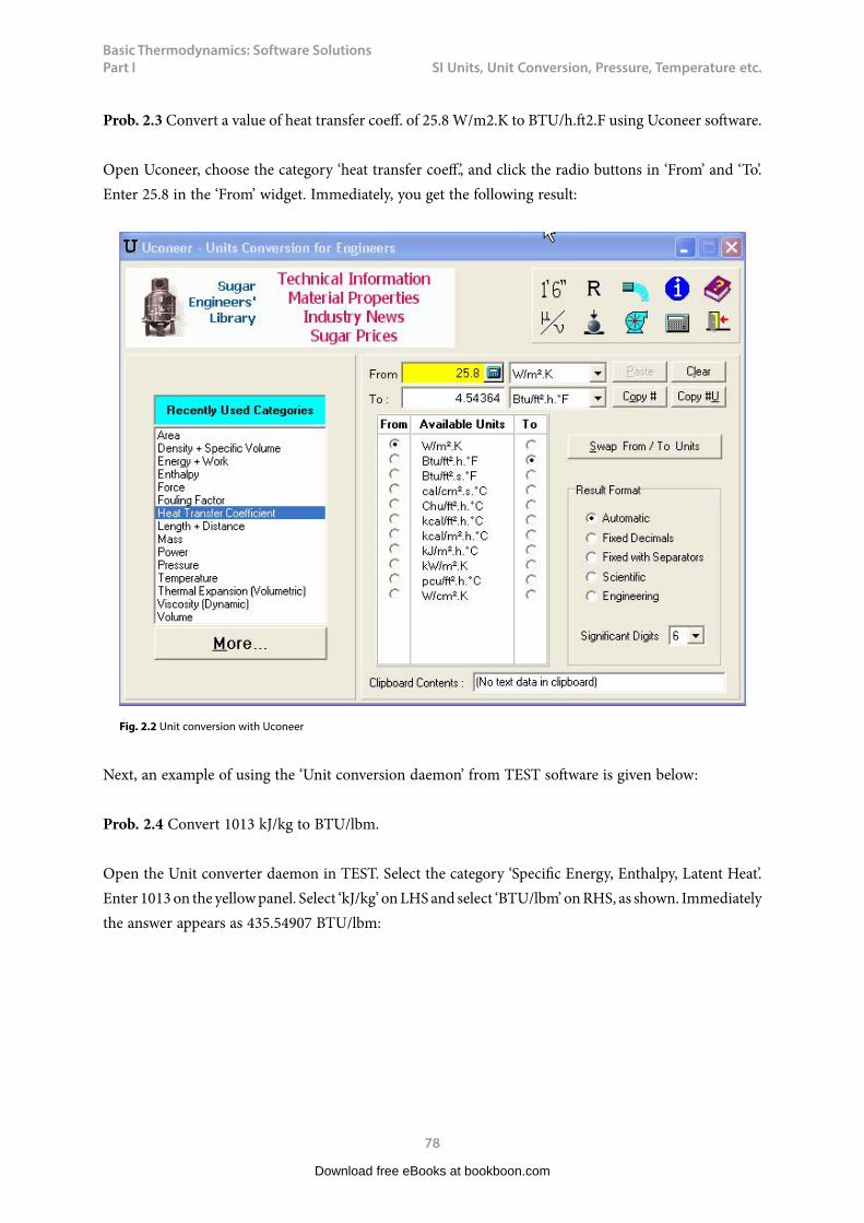
Basic Thermodynamics: Software Solutions Part I
78
SI Unitss, Unit Conversions, Pressures, Temperature etc.
Prob. 2.3 Convert a value of heat transfer coeff. of 25.8 W/m2.K to BTU/h.ft2.F using Uconeer software.
Open Uconeer, choose the category ‘heat transfer coeff.’, and click the radio buttons in ‘From’ and ‘To’. Enter 25.8 in the ‘From’ widget. Immediately, you get the following result:
Fig. 2.2 Unit conversion with Uconeer
Next, an example of using the ‘Unit conversion daemon’ from TEST software is given below:
Prob. 2.4 Convert 1013 kJ/kg to BTU/lbm.
Open the Unit converter daemon in TEST. Select the category ‘Specific Energy, Enthalpy, Latent Heat’. Enter 1013 on the yellow panel. Select ‘kJ/kg’ on LHS and select ‘BTU/lbm’ on RHS, as shown. Immediately the answer appears as 435.54907 BTU/lbm:
Download free eBooks at bookboon.com

Basic Thermodynamics: Software Solutions Part I
79
SI Unitss, Unit Conversions, Pressures, Temperature etc.
Fig. 2.3 Unit conversion in TEST software
Download free eBooks at bookboon.com
Click on the ad to read moreClick on the ad to read moreClick on the ad to read moreClick on the ad to read moreClick on the ad to read moreClick on the ad to read moreClick on the ad to read moreClick on the ad to read moreClick on the ad to read moreClick on the ad to read moreClick on the ad to read moreClick on the ad to read moreClick on the ad to read moreClick on the ad to read moreClick on the ad to read moreClick on the ad to read moreClick on the ad to read moreClick on the ad to read moreClick on the ad to read moreClick on the ad to read moreClick on the ad to read moreClick on the ad to read moreClick on the ad to read moreClick on the ad to read moreClick on the ad to read moreClick on the ad to read moreClick on the ad to read more
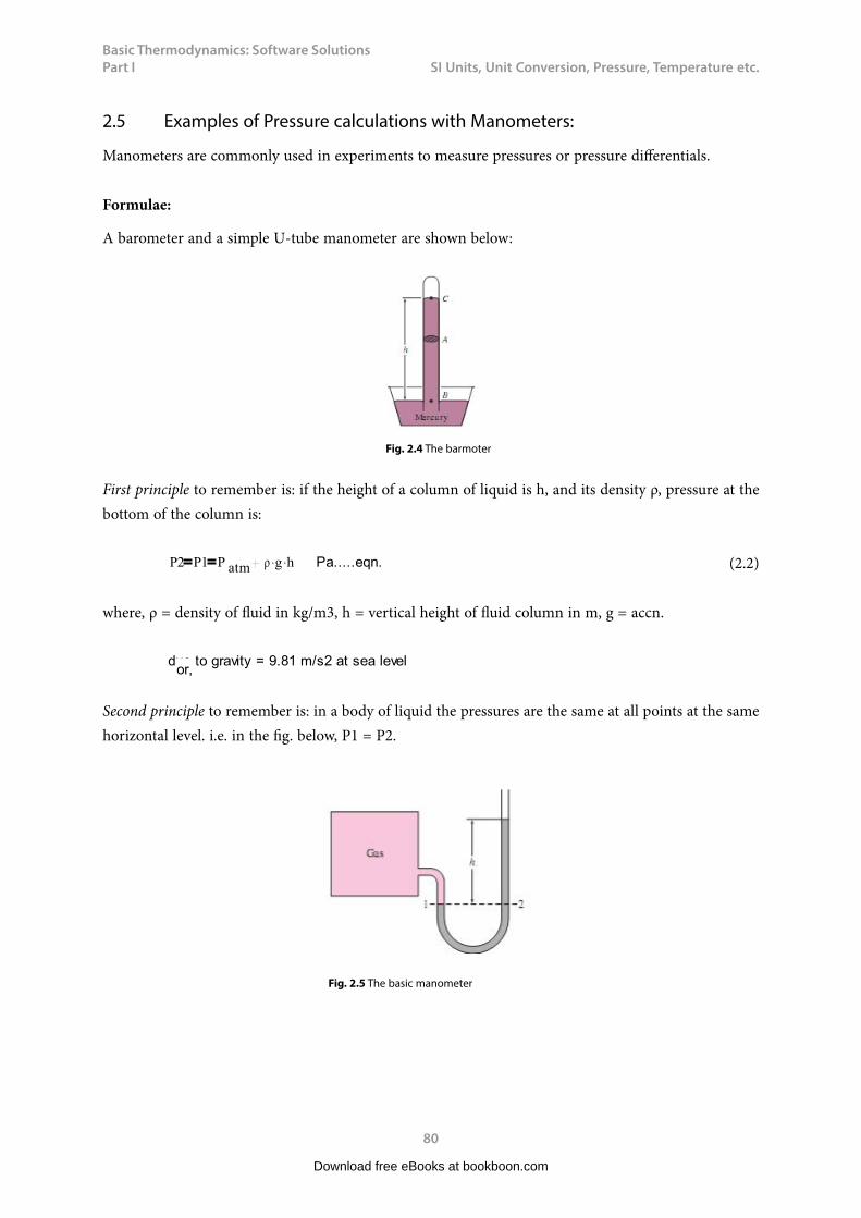
Basic Thermodynamics: Software Solutions Part I
80
SI Unitss, Unit Conversions, Pressures, Temperature etc.
2.5 Examples of Pressure calculations with Manometers:
Manometers are commonly used in experiments to measure pressures or pressure differentials.
Formulae:
A barometer and a simple U-tube manometer are shown below:
Fig. 2.4 The barmoter
First principle to remember is: if the height of a column of liquid is h, and its density ρ, pressure at the bottom of the column is:
P2 P1 P atm g h Pa.....eqn. (2.2)
where, ρ = density of fluid in kg/m3, h = vertical height of fluid column in m, g = accn.
due to gravity = 9.81 m/s2 at sea levelor,
Second principle to remember is: in a body of liquid the pressures are the same at all points at the same horizontal level. i.e. in the fig. below, P1 = P2.
Fig. 2.5 The basic manometer
Download free eBooks at bookboon.com
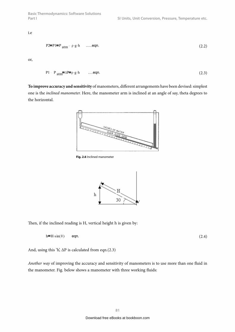
Basic Thermodynamics: Software Solutions Part I
81
SI Unitss, Unit Conversions, Pressures, Temperature etc.
i.e
P2 P1 P atm g h .....eqn. (2.2)
or,
P1 P atm P g h ....eqn. (2.3)
To improve accuracy and sensitivity of manometers, different arrangements have been devised: simplest one is the inclined manometer. Here, the manometer arm is inclined at an angle of say, theta degrees to the horizontal.
Fig. 2.6 Inclined manometer
Then, if the inclined reading is H, vertical height h is given by:
h H sin( ) eqn. (2.4)
And, using this ‘h’, ΔP is calculated from eqn.(2.3)
Another way of improving the accuracy and sensitivity of manometers is to use more than one fluid in the manometer. Fig. below shows a manometer with three working fluids:
Download free eBooks at bookboon.com
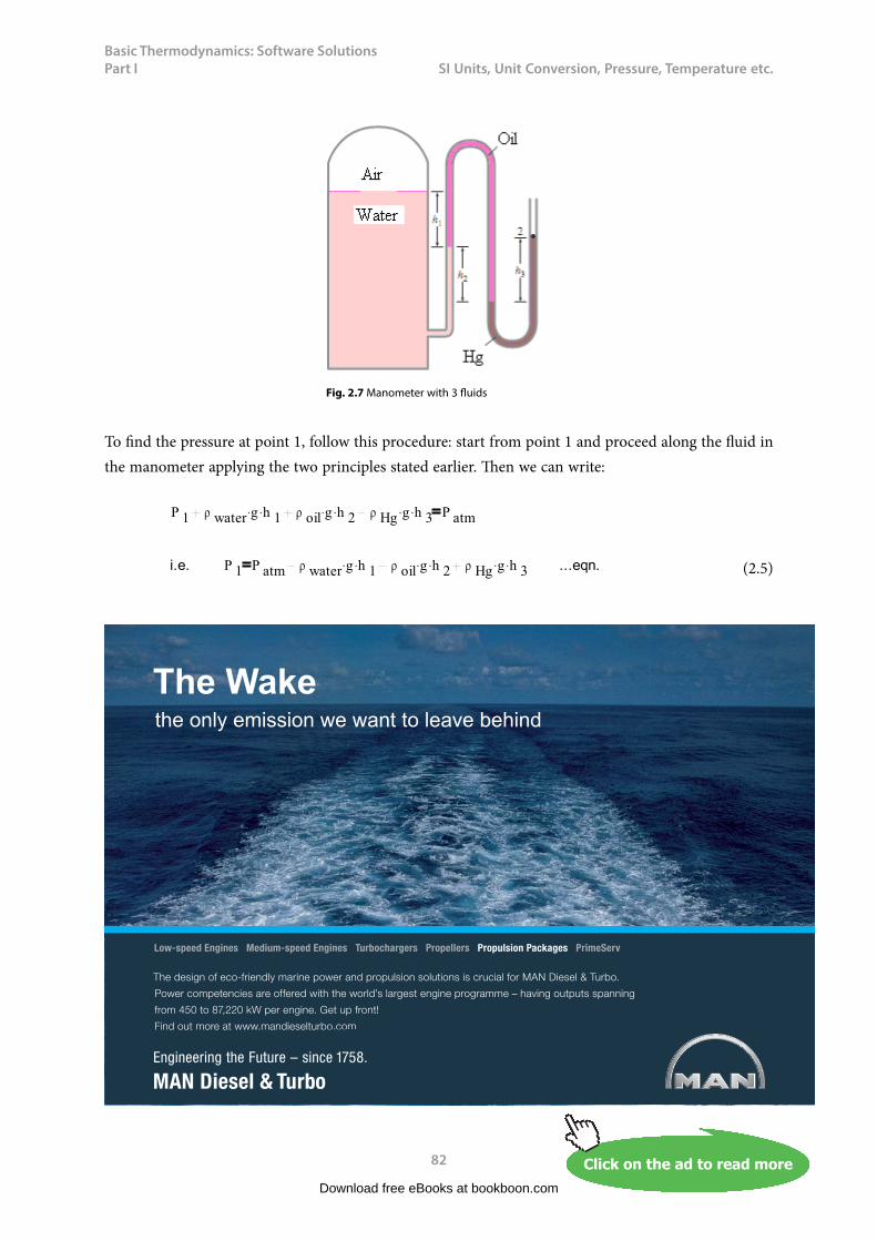
Basic Thermodynamics: Software Solutions Part I
82
SI Unitss, Unit Conversions, Pressures, Temperature etc.
Fig. 2.7 Manometer with 3 fluids
To find the pressure at point 1, follow this procedure: start from point 1 and proceed along the fluid in the manometer applying the two principles stated earlier. Then we can write:
P 1 water g h 1 oil g h 2 Hg g h 3 P atm
i.e. P 1 P atm water g h 1 oil g h 2 Hg g h 3 ...eqn. (2.5)
Download free eBooks at bookboon.com
Click on the ad to read moreClick on the ad to read moreClick on the ad to read moreClick on the ad to read moreClick on the ad to read moreClick on the ad to read moreClick on the ad to read moreClick on the ad to read moreClick on the ad to read moreClick on the ad to read moreClick on the ad to read moreClick on the ad to read moreClick on the ad to read moreClick on the ad to read moreClick on the ad to read moreClick on the ad to read moreClick on the ad to read moreClick on the ad to read moreClick on the ad to read moreClick on the ad to read moreClick on the ad to read moreClick on the ad to read moreClick on the ad to read moreClick on the ad to read moreClick on the ad to read moreClick on the ad to read moreClick on the ad to read moreClick on the ad to read more
������������� ����������������������������������������������� �� ���������������������������
������ ������ ������������������������������ ����������������������!���"���������������
�����#$%����&'())%�*+����������,����������-
.��������������������������������� ��
���������� ���������������� ������������� ���������������������������� �����������
The Wakethe only emission we want to leave behind
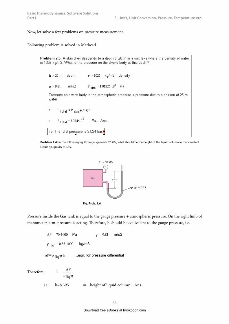
Basic Thermodynamics: Software Solutions Part I
83
SI Unitss, Unit Conversions, Pressures, Temperature etc.
Now, let solve a few problems on pressure measurement.
Following problem is solved in Mathcad.
Problem 2.6: In the following fig. if the gauge reads 70 kPa, what should be the height of the liquid column in manometer? Liquid sp. gravity = 0.85.
Fig. Prob. 2.6
Pressure inside the Gas tank is equal to the gauge pressure + atmospheric pressure. On the right limb of manometer, atm. pressure is acting. Therefore, h should be equivalent to the gauge pressure, i.e.
P 70 1000 Pa g 9.81 m/s2
liq 0.85 1000 kg/m3
P liq g h ...eqn. for pressure differential
Therefore, hP
liq g
i.e. h=8.395 m....height of liquid column....Ans.
Download free eBooks at bookboon.com
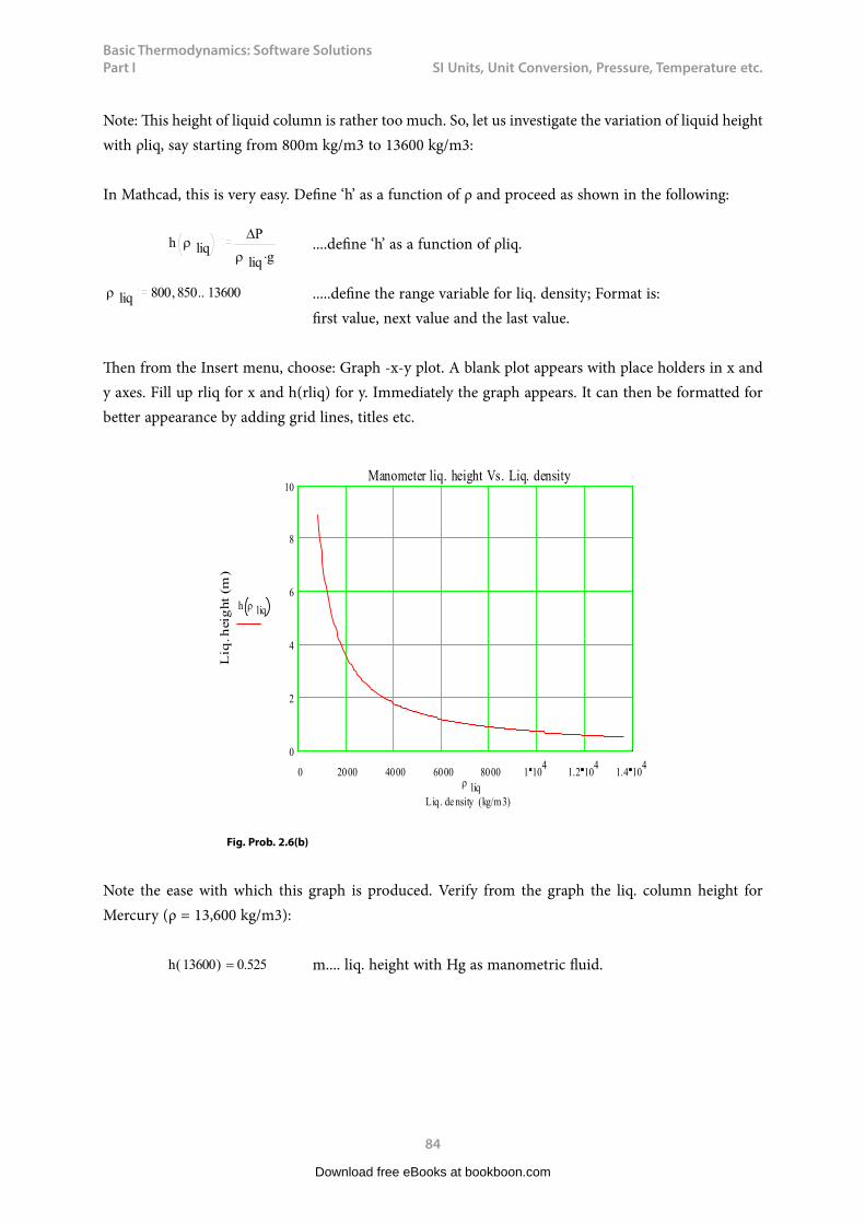
Basic Thermodynamics: Software Solutions Part I
84
SI Unitss, Unit Conversions, Pressures, Temperature etc.
Note: This height of liquid column is rather too much. So, let us investigate the variation of liquid height with ρliq, say starting from 800m kg/m3 to 13600 kg/m3:
In Mathcad, this is very easy. Define ‘h’ as a function of ρ and proceed as shown in the following:
h liqP
liq g ....define ‘h’ as a function of ρliq.
liq 800 850 13600 .....define the range variable for liq. density; Format is: first value, next value and the last value.
Then from the Insert menu, choose: Graph -x-y plot. A blank plot appears with place holders in x and y axes. Fill up rliq for x and h(rliq) for y. Immediately the graph appears. It can then be formatted for better appearance by adding grid lines, titles etc.
Fig. Prob. 2.6(b)
Note the ease with which this graph is produced. Verify from the graph the liq. column height for Mercury (ρ = 13,600 kg/m3):
h 13600( ) 0.525 m.... liq. height with Hg as manometric fluid.
Download free eBooks at bookboon.com
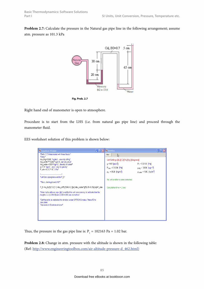
Basic Thermodynamics: Software Solutions Part I
85
SI Unitss, Unit Conversions, Pressures, Temperature etc.
Problem 2.7: Calculate the pressure in the Natural gas pipe line in the following arrangement; assume atm. pressure as 101.3 kPa
Fig. Prob. 2.7
Right hand end of manometer is open to atmosphere.
Procedure is to start from the LHS (i.e. from natural gas pipe line) and proceed through the manometer fluid.
EES worksheet solution of this problem is shown below:
Thus, the pressure in the gas pipe line is: P1 = 102163 Pa = 1.02 bar.
Problem 2.8: Change in atm. pressure with the altitude is shown in the following table: (Ref: http://www.engineeringtoolbox.com/air-altitude-pressure-d_462.html)
Download free eBooks at bookboon.com
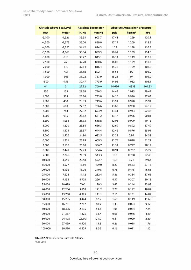
Basic Thermodynamics: Software Solutions Part I
86
SI Unitss, Unit Conversions, Pressures, Temperature etc.
Altitude Above Sea Level Absolute Barometer Absolute Atmospheric Pressure
feet meter in. Hg mm Hg psia kg/cm2 kPa
-5,000 -1,526 35.58 903.7 17.48 1.229 120.5
-4,500 -1,373 35.00 889.0 17.19 1.209 118.5
-4,000 -1,220 34.42 874.3 16.9 1.188 116.5
-3,500 -1,068 33.84 859.5 16.62 1.169 114.6
-3,000 -915 33.27 845.1 16.34 1.149 112.7
-2,500 -763 32.70 830.6 16.06 1.129 110.7
-2,000 -610 32.14 816.4 15.78 1.109 108.8
-1,500 -458 31.58 802.1 15.51 1.091 106.9
-1,000 -305 31.02 787.9 15.23 1.071 105.0
-500 -153 30.47 773.9 14.96 1.052 103.1
01) 0 29.92 760.0 14.696 1.0333 101.33
500 153 29.38 746.3 14.43 1.015 99.49
1,000 305 28.86 733.0 14.16 0.996 97.63
1,500 458 28.33 719.6 13.91 0.978 95.91
2,000 610 27.82 706.6 13.66 0.960 94.19
2,500 763 27.32 693.9 13.41 0.943 92.46
3,000 915 26.82 681.2 13.17 0.926 90.81
3,500 1,068 26.33 668.8 12.93 0.909 89.15
4,000 1,220 25.84 656.3 12.69 0.892 87.49
4,500 1,373 25.37 644.4 12.46 0.876 85.91
5,000 1,526 24.90 632.5 12.23 0.86 84.33
6,000 1,831 23.99 609.3 11.78 0.828 81.22
7,000 2,136 23.10 586.7 11.34 0.797 78.19
8,000 2,441 22.23 564.6 10.91 0.767 75.22
9,000 2,746 21.39 543.3 10.5 0.738 72.40
10,000 3,050 20.58 522.7 10.1 0.71 69.64
15,000 4,577 16.89 429.0 8.29 0.583 57.16
20,000 6,102 13.76 349.5 6.76 0.475 46.61
25,000 7,628 11.12 282.4 5.46 0.384 37.65
30,000 9,153 8.903 226.1 4.37 0.307 30.13
35,000 10,679 7.06 179.3 3.47 0.244 23.93
40,000 12,204 5.558 141.2 2.73 0.192 18.82
45,000 13,730 4.375 111.1 2.15 0.151 14.82
50,000 15,255 3.444 87.5 1.69 0.119 11.65
55,000 16,781 2.712 68.9 1.33 0.094 9.17
60,000 18,306 2.135 54.2 1.05 0.074 7.24
70,000 21,357 1.325 33.7 0.65 0.046 4.49
80,000 24,408 0.8273 21.0 0.41 0.029 2.80
90,000 27,459 0.520 13.2 0.26 0.018 1.76
100,000 30,510 0.329 8.36 0.16 0.011 1.12
Table 2.7 Atmospheric pressure with Altitude 1) Sea Level
Download free eBooks at bookboon.com

Basic Thermodynamics: Software Solutions Part I
87
SI Unitss, Unit Conversions, Pressures, Temperature etc.
Find out the atm. pressure in kPa at an altitude of 10000 m.
Let us work out this problem in EES. First, we prepare a ‘look up table’ in EES with altitude (m) in column 1 and pressure (kPa) in column 2; then, plot the pressure against altitude, and then get the curve fit equation and then use it to calculate the pressure at 10000 m altitude in the equations window.
Since ‘curve fit’ is an important requirement in many problems, let us show the details: After starting EES, go to ‘Tables’ menu, select ‘New look up table’, select two columns and 30 rows, and fill up the altitude values in metres in the column 1, and pressure values in kPa in column 2. Look up table is shown below:
Download free eBooks at bookboon.com
Click on the ad to read moreClick on the ad to read moreClick on the ad to read moreClick on the ad to read moreClick on the ad to read moreClick on the ad to read moreClick on the ad to read moreClick on the ad to read moreClick on the ad to read moreClick on the ad to read moreClick on the ad to read moreClick on the ad to read moreClick on the ad to read moreClick on the ad to read moreClick on the ad to read moreClick on the ad to read moreClick on the ad to read moreClick on the ad to read moreClick on the ad to read moreClick on the ad to read moreClick on the ad to read moreClick on the ad to read moreClick on the ad to read moreClick on the ad to read moreClick on the ad to read moreClick on the ad to read moreClick on the ad to read moreClick on the ad to read moreClick on the ad to read more
CAREERKICKSTARTAn app to keep you in the know
Whether you’re a graduate, school leaver or student, it’s a difficult time to start your career. So here at RBS, we’re providing a helping hand with our new Facebook app. Bringing together the most relevant and useful careers information, we’ve created a one-stop shop designed to help you get on the career ladder – whatever your level of education, degree subject or work experience.
And it’s not just finance-focused either. That’s because it’s not about us. It’s about you. So download the app and you’ll get everything you need to know to kickstart your career.
So what are you waiting for?
Click here to get started.
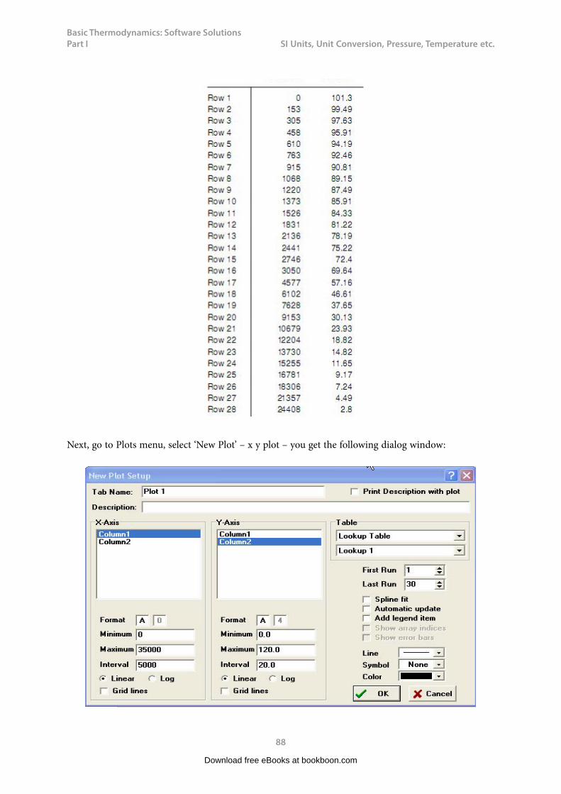
Basic Thermodynamics: Software Solutions Part I
88
SI Unitss, Unit Conversions, Pressures, Temperature etc.
Next, go to Plots menu, select ‘New Plot’ – x y plot – you get the following dialog window:
Download free eBooks at bookboon.com
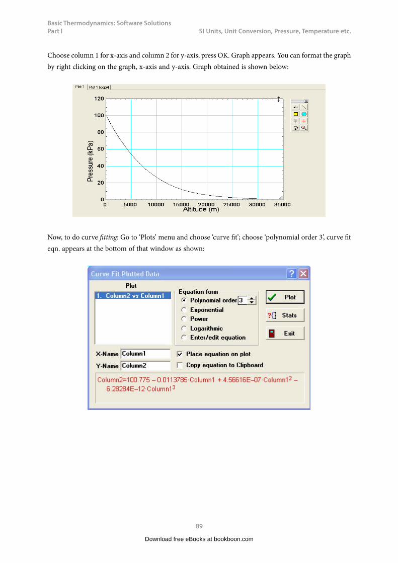
Basic Thermodynamics: Software Solutions Part I
89
SI Unitss, Unit Conversions, Pressures, Temperature etc.
Choose column 1 for x-axis and column 2 for y-axis; press OK. Graph appears. You can format the graph by right clicking on the graph, x-axis and y-axis. Graph obtained is shown below:
Now, to do curve fitting: Go to ‘Plots’ menu and choose ‘curve fit’; choose ‘polynomial order 3’, curve fit eqn. appears at the bottom of that window as shown:
Download free eBooks at bookboon.com

Basic Thermodynamics: Software Solutions Part I
90
SI Unitss, Unit Conversions, Pressures, Temperature etc.
Statistics regarding the plot (to find how good is the curve fit) can be obtained by clicking on ‘Stats’:
Download free eBooks at bookboon.com
Click on the ad to read moreClick on the ad to read moreClick on the ad to read moreClick on the ad to read moreClick on the ad to read moreClick on the ad to read moreClick on the ad to read moreClick on the ad to read moreClick on the ad to read moreClick on the ad to read moreClick on the ad to read moreClick on the ad to read moreClick on the ad to read moreClick on the ad to read moreClick on the ad to read moreClick on the ad to read moreClick on the ad to read moreClick on the ad to read moreClick on the ad to read moreClick on the ad to read moreClick on the ad to read moreClick on the ad to read moreClick on the ad to read moreClick on the ad to read moreClick on the ad to read moreClick on the ad to read moreClick on the ad to read moreClick on the ad to read moreClick on the ad to read moreClick on the ad to read more
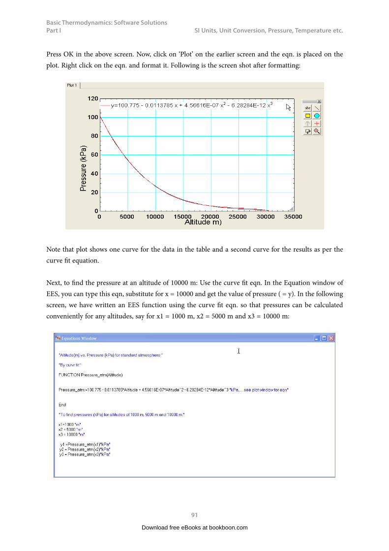
Basic Thermodynamics: Software Solutions Part I
91
SI Unitss, Unit Conversions, Pressures, Temperature etc.
Press OK in the above screen. Now, click on ‘Plot’ on the earlier screen and the eqn. is placed on the plot. Right click on the eqn. and format it. Following is the screen shot after formatting:
Note that plot shows one curve for the data in the table and a second curve for the results as per the curve fit equation.
Next, to find the pressure at an altitude of 10000 m: Use the curve fit eqn. In the Equation window of EES, you can type this eqn, substitute for x = 10000 and get the value of pressure ( = y). In the following screen, we have written an EES function using the curve fit eqn. so that pressures can be calculated conveniently for any altitudes, say for x1 = 1000 m, x2 = 5000 m and x3 = 10000 m:
Download free eBooks at bookboon.com
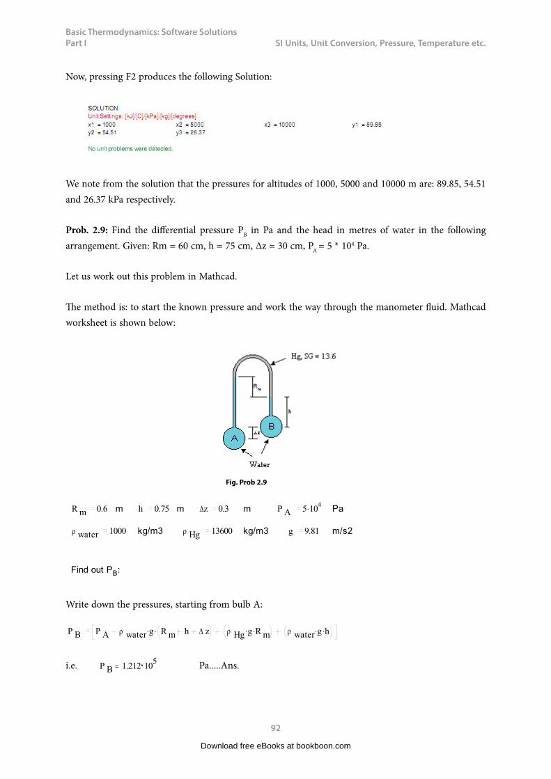
Basic Thermodynamics: Software Solutions Part I
92
SI Unitss, Unit Conversions, Pressures, Temperature etc.
Now, pressing F2 produces the following Solution:
We note from the solution that the pressures for altitudes of 1000, 5000 and 10000 m are: 89.85, 54.51 and 26.37 kPa respectively.
Prob. 2.9: Find the differential pressure PB in Pa and the head in metres of water in the following arrangement. Given: Rm = 60 cm, h = 75 cm, Δz = 30 cm, PA = 5 * 104 Pa.
Let us work out this problem in Mathcad.
The method is: to start the known pressure and work the way through the manometer fluid. Mathcad worksheet is shown below:
Fig. Prob 2.9
Rm 0.6 m h 0.75 m z 0.3 m P A 5 104
Pa
water 1000 kg/m3 Hg 13600 kg/m3 g 9.81 m/s2
Find out PB:
Write down the pressures, starting from bulb A:
P B P A water g Rm h z Hg g Rm water g h
i.e. P B 1.212 105 Pa.....Ans.
Download free eBooks at bookboon.com

Basic Thermodynamics: Software Solutions Part I
93
SI Unitss, Unit Conversions, Pressures, Temperature etc.
To find the head in metres of water:
P B water g head
i.e. headP B
water g
i.e. head=12.357 m of water....Ans.
2.6 Examples of Temperature calculations with Thermocouples:
Thermocouple works on the basis of ‘Seebeck effect’ discovered by Thomas Johann Seebeck in 1821: i.e. when a junction formed out of two dis-similar metals/alloys is kept at a temperature different from the other ends, an emf is generated between those ends as shown below:
Download free eBooks at bookboon.com
Click on the ad to read moreClick on the ad to read moreClick on the ad to read moreClick on the ad to read moreClick on the ad to read moreClick on the ad to read moreClick on the ad to read moreClick on the ad to read moreClick on the ad to read moreClick on the ad to read moreClick on the ad to read moreClick on the ad to read moreClick on the ad to read moreClick on the ad to read moreClick on the ad to read moreClick on the ad to read moreClick on the ad to read moreClick on the ad to read moreClick on the ad to read moreClick on the ad to read moreClick on the ad to read moreClick on the ad to read moreClick on the ad to read moreClick on the ad to read moreClick on the ad to read moreClick on the ad to read moreClick on the ad to read moreClick on the ad to read moreClick on the ad to read moreClick on the ad to read moreClick on the ad to read more
AXA Global Graduate Program
Find out more and apply
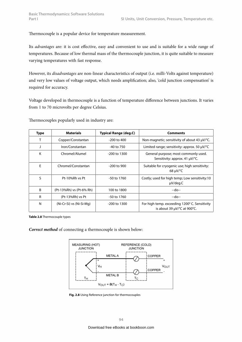
Basic Thermodynamics: Software Solutions Part I
94
SI Unitss, Unit Conversions, Pressures, Temperature etc.
Thermocouple is a popular device for temperature measurement.
Its advantages are: it is cost effective, easy and convenient to use and is suitable for a wide range of temperatures. Because of low thermal mass of the thermocouple junction, it is quite suitable to measure varying temperatures with fast response.
However, its disadvantages are non-linear characteristics of output (i.e. milli-Volts against temperature) and very low values of voltage output, which needs amplification; also, ‘cold junction compensation’ is required for accuracy.
Voltage developed in thermocouple is a function of temperature difference between junctions. It varies from 1 to 70 microvolts per degree Celsius.
Thermocouples popularly used in industry are:
Type Materials Typical Range (deg.C) Comments
T Copper/Constantan -200 to 400 Non-magnetic; sensitivity of about 43 µV/°C.
J Iron/Constantan -40 to 750 Limited range; sensitivity: approx. 50 µV/°C
K Chromel/Alumel -200 to 1300 General purpose; most commonly used. Sensitivity: approx. 41 µV/°C.
E Chromel/Constantan -200 to 900 Suitable for cryogenic use; high sensitivity: 68 µV/°C
S Pt-10%Rh vs Pt -50 to 1760 Costly; used for high temp; Low sensitivity:10 μV/deg.C
B (Pt-13%Rh) vs (Pt-6% Rh) 100 to 1800 --do--
R (Pt-13%Rh) vs Pt -50 to 1760 --do--
N (Ni-Cr-Si) vs (Ni-Si-Mg) -200 to 1300 For high temp. exceeding 12000 C. Sensitivity is about 39 µV/°C at 900°C.
Table 2.8 Thermocouple types
Correct method of connecting a thermocouple is shown below:
Fig. 2.8 Using Reference junction for thermocouples
Download free eBooks at bookboon.com
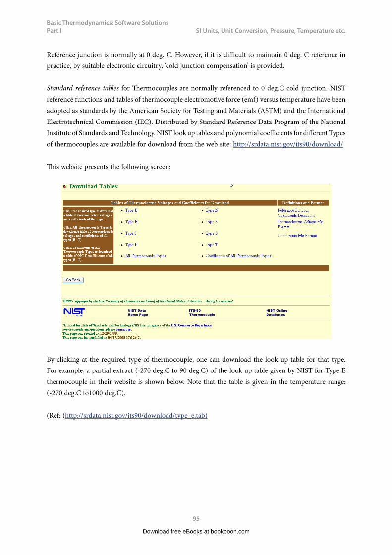
Basic Thermodynamics: Software Solutions Part I
95
SI Unitss, Unit Conversions, Pressures, Temperature etc.
Reference junction is normally at 0 deg. C. However, if it is difficult to maintain 0 deg. C reference in practice, by suitable electronic circuitry, ‘cold junction compensation’ is provided.
Standard reference tables for Thermocouples are normally referenced to 0 deg.C cold junction. NIST reference functions and tables of thermocouple electromotive force (emf) versus temperature have been adopted as standards by the American Society for Testing and Materials (ASTM) and the International Electrotechnical Commission (IEC). Distributed by Standard Reference Data Program of the National Institute of Standards and Technology. NIST look up tables and polynomial coefficients for different Types of thermocouples are available for download from the web site: http://srdata.nist.gov/its90/download/
This website presents the following screen:
By clicking at the required type of thermocouple, one can download the look up table for that type. For example, a partial extract (-270 deg.C to 90 deg.C) of the look up table given by NIST for Type E thermocouple in their website is shown below. Note that the table is given in the temperature range: (-270 deg.C to1000 deg.C).
(Ref: (http://srdata.nist.gov/its90/download/type_e.tab)
Download free eBooks at bookboon.com
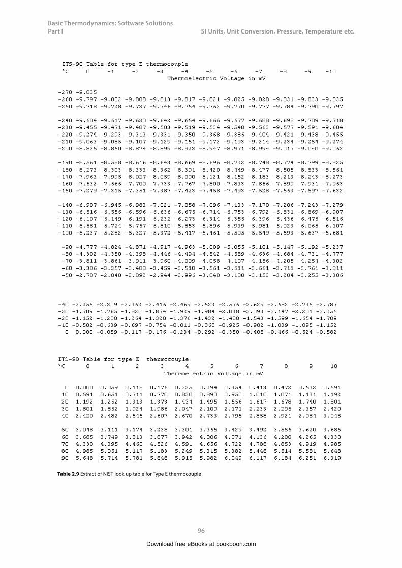
Basic Thermodynamics: Software Solutions Part I
96
SI Unitss, Unit Conversions, Pressures, Temperature etc.
Table 2.9 Extract of NIST look up table for Type E thermocouple
Download free eBooks at bookboon.com
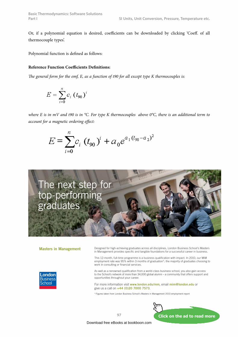
Basic Thermodynamics: Software Solutions Part I
97
SI Unitss, Unit Conversions, Pressures, Temperature etc.
Or, if a polynomial equation is desired, coefficients can be downloaded by clicking ‘Coeff. of all thermocouple types’.
Polynomial function is defined as follows:
Reference Function Coefficients Definitions:
The general form for the emf, E, as a function of t90 for all except type K thermocouples is:
where E is in mV and t90 is in °C. For type K thermocouples above 0°C, there is an additional term to account for a magnetic ordering effect:
Download free eBooks at bookboon.com
Click on the ad to read moreClick on the ad to read moreClick on the ad to read moreClick on the ad to read moreClick on the ad to read moreClick on the ad to read moreClick on the ad to read moreClick on the ad to read moreClick on the ad to read moreClick on the ad to read moreClick on the ad to read moreClick on the ad to read moreClick on the ad to read moreClick on the ad to read moreClick on the ad to read moreClick on the ad to read moreClick on the ad to read moreClick on the ad to read moreClick on the ad to read moreClick on the ad to read moreClick on the ad to read moreClick on the ad to read moreClick on the ad to read moreClick on the ad to read moreClick on the ad to read moreClick on the ad to read moreClick on the ad to read moreClick on the ad to read moreClick on the ad to read moreClick on the ad to read moreClick on the ad to read moreClick on the ad to read more
Designed for high-achieving graduates across all disciplines, London Business School’s Masters in Management provides specific and tangible foundations for a successful career in business.
This 12-month, full-time programme is a business qualification with impact. In 2010, our MiM employment rate was 95% within 3 months of graduation*; the majority of graduates choosing to work in consulting or financial services.
As well as a renowned qualification from a world-class business school, you also gain access to the School’s network of more than 34,000 global alumni – a community that offers support and opportunities throughout your career.
For more information visit www.london.edu/mm, email [email protected] or give us a call on +44 (0)20 7000 7573.
Masters in Management
The next step for top-performing graduates
* Figures taken from London Business School’s Masters in Management 2010 employment report

Basic Thermodynamics: Software Solutions Part I
98
SI Unitss, Unit Conversions, Pressures, Temperature etc.
where e is the natural logarithm constant, E is in mV, and t90 is in °C. The constants a0, a1, and a2 have the values:
a0 = 0.118597600000x100
a1 = – 0.118343200000x10⁻³
a2 = 0.126968600000x10³
As an example, coefficients for E type thermocouple are downloaded and shown below: Note that polynomial coefficients for E type are given for two temperature ranges, i.e. from -170 to 0 deg.C and 0 to 1000 deg.C:
************************************* This section contains coefficients for type E thermocouples for* the two subranges of temperature listed below. The coefficients * are in units of °C and mV and are listed in the order of constant * term up to the highest order. The equation is of the form * E = sum(i=0 to n) c_i t^i.** TemperatureRange (°C)* -270.000 to 0.000* 0.000 to 1000.000************************************name: reference function on ITS-90type: Etemperature units: °Cemf units: mVrange: -270.000, 0.000, 130.000000000000E+000.586655087080E-010.454109771240E-04-0.779980486860E-06-0.258001608430E-07-0.594525830570E-09-0.932140586670E-11-0.102876055340E-12-0.803701236210E-15-0.439794973910E-17-0.164147763550E-19-0.396736195160E-22-0.558273287210E-25-0.346578420130E-28range: 0.000, 1000.000, 100.000000000000E+000.586655087100E-010.450322755820E-040.289084072120E-07-0.330568966520E-090.650244032700E-12-0.191974955040E-15-0.125366004970E-170.214892175690E-20-0.143880417820E-230.359608994810E-27
Download free eBooks at bookboon.com
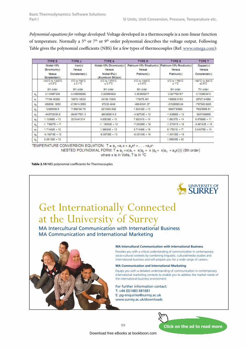
Basic Thermodynamics: Software Solutions Part I
99
SI Unitss, Unit Conversions, Pressures, Temperature etc.
Polynomial equations for voltage developed: Voltage developed in a thermocouple is a non-linear function of temperature. Normally a 5th or 7th or 9th order polynomial describes the voltage output. Following Table gives the polynomial coefficients (NBS) for a few types of thermocouples (Ref: www.omega.com):
Table 2.10 NBS polynomial coefficients for Thermocouples
Download free eBooks at bookboon.com
Click on the ad to read moreClick on the ad to read moreClick on the ad to read moreClick on the ad to read moreClick on the ad to read moreClick on the ad to read moreClick on the ad to read moreClick on the ad to read moreClick on the ad to read moreClick on the ad to read moreClick on the ad to read moreClick on the ad to read moreClick on the ad to read moreClick on the ad to read moreClick on the ad to read moreClick on the ad to read moreClick on the ad to read moreClick on the ad to read moreClick on the ad to read moreClick on the ad to read moreClick on the ad to read moreClick on the ad to read moreClick on the ad to read moreClick on the ad to read moreClick on the ad to read moreClick on the ad to read moreClick on the ad to read moreClick on the ad to read moreClick on the ad to read moreClick on the ad to read moreClick on the ad to read moreClick on the ad to read moreClick on the ad to read more
Get Internationally Connected at the University of Surrey MA Intercultural Communication with International BusinessMA Communication and International Marketing
MA Intercultural Communication with International Business
Provides you with a critical understanding of communication in contemporary socio-cultural contexts by combining linguistic, cultural/media studies and international business and will prepare you for a wide range of careers.
MA Communication and International Marketing
Equips you with a detailed understanding of communication in contemporary international marketing contexts to enable you to address the market needs of the international business environment.
For further information contact:T: +44 (0)1483 681681E: [email protected]/downloads
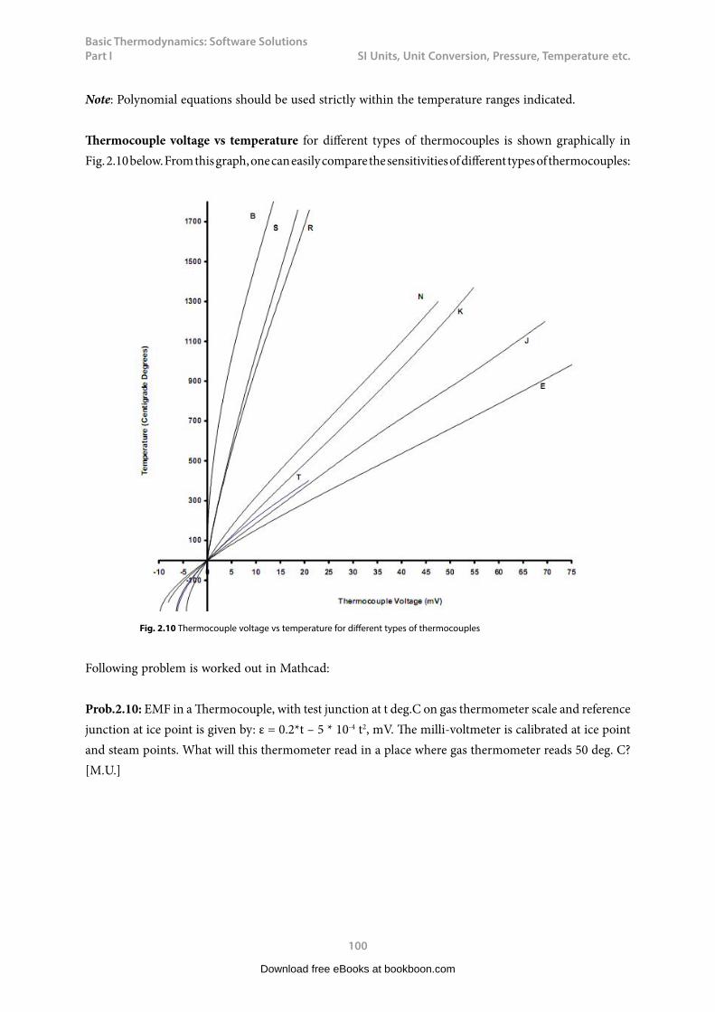
Basic Thermodynamics: Software Solutions Part I
100
SI Unitss, Unit Conversions, Pressures, Temperature etc.
Note: Polynomial equations should be used strictly within the temperature ranges indicated.
Thermocouple voltage vs temperature for different types of thermocouples is shown graphically in Fig. 2.10 below. From this graph, one can easily compare the sensitivities of different types of thermocouples:
Fig. 2.10 Thermocouple voltage vs temperature for different types of thermocouples
Following problem is worked out in Mathcad:
Prob.2.10: EMF in a Thermocouple, with test junction at t deg.C on gas thermometer scale and reference junction at ice point is given by: ε = 0.2*t – 5 * 10-4 t2, mV. The milli-voltmeter is calibrated at ice point and steam points. What will this thermometer read in a place where gas thermometer reads 50 deg. C? [M.U.]
Download free eBooks at bookboon.com
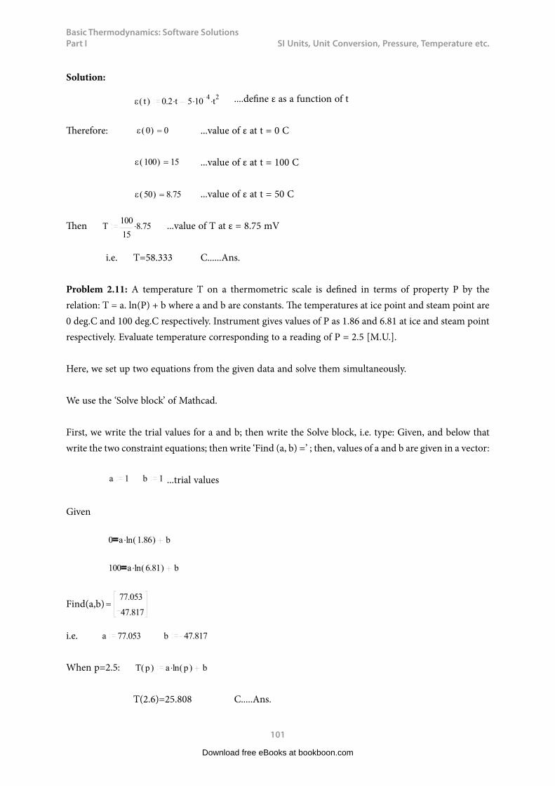
Basic Thermodynamics: Software Solutions Part I
101
SI Unitss, Unit Conversions, Pressures, Temperature etc.
Solution:
t( ) 0.2 t 5 104t2 ....define ε as a function of t
Therefore: 0( ) 0 ...value of ε at t = 0 C
100( ) 15 ...value of ε at t = 100 C
50( ) 8.75 ...value of ε at t = 50 C
Then T100
158.75 ...value of T at ε = 8.75 mV
i.e. T=58.333 C......Ans.
Problem 2.11: A temperature T on a thermometric scale is defined in terms of property P by the relation: T = a. ln(P) + b where a and b are constants. The temperatures at ice point and steam point are 0 deg.C and 100 deg.C respectively. Instrument gives values of P as 1.86 and 6.81 at ice and steam point respectively. Evaluate temperature corresponding to a reading of P = 2.5 [M.U.].
Here, we set up two equations from the given data and solve them simultaneously.
We use the ‘Solve block’ of Mathcad.
First, we write the trial values for a and b; then write the Solve block, i.e. type: Given, and below that write the two constraint equations; then write ‘Find (a, b) =’ ; then, values of a and b are given in a vector:
a 1 b 1 ...trial values
Given
0 a ln 1.86( ) b
100 a ln 6.81( ) b
Find(a,b)77.053
47.817
i.e. a 77.053 b 47.817
When p=2.5: T p( ) a ln p( ) b
T(2.6)=25.808 C.....Ans.
Download free eBooks at bookboon.com

Basic Thermodynamics: Software Solutions Part I
102
SI Unitss, Unit Conversions, Pressures, Temperature etc.
Problem 2.12: The readings tA and tB of two Celsius thermometers A and B agree at the Ice point (0 deg.C) and Steam point (100 deg.C), but elsewhere are related by the equation: tA = l + m* tA + n* tB
2, where l, m and n are constants. When both the thermometers are immersed in a well stirred oil bath, A registers 51 deg.C, while B registers 50 deg.C. Determine the reading on B when A reads 25 deg.C [M.U.]
This problem is now solved in EES:
First, enter the constraints in the ‘Equation window’. See the comments against each line in the screen shot below. Next press F2 and the solution appears in the ‘Solutions window’.
We get the solution as: tB = 24.26 deg.C when tA = 25 deg.C
Problem 2.13: Fahrenheit and Centigrade thermometers are both immersed in a fluid. Fahrenheit reading is numerically twice that of the Centigrade reading. What is the temperature of the fluid expressed on degree Rankine and Kelvin?
This problem is also easily solved in EES. See the screen prints of ‘Equation window’ and ‘Solution window’ below. Read the comments against each eqn. in the Eqns. Window.
Download free eBooks at bookboon.com
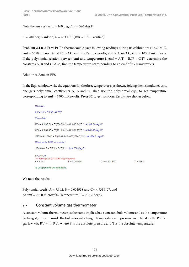
Basic Thermodynamics: Software Solutions Part I
103
SI Unitss, Unit Conversions, Pressures, Temperature etc.
Note the answers as: x = 160 deg.C, y = 320 deg.F;
R = 780 deg. Rankine; K = 433.1 K; (R/K = 1.8 …verified).
Problem 2.14: A Pt vs Pt-Rh thermocouple gave following readings during its calibration: at 630.74 C, emf = 5550 microvolts; at 961.93 C, emf = 9150 microvolts, and at 1064.3 C, emf = 10335 microvolts. If the polynomial relation between emf and temperature is emf = A.T + B.T2 + C.T3, determine the constants A, B and C. Also, find the temperature corresponding to an emf of 7300 microvolts.
Solution is done in EES.
In the Eqn. window, write the equations for the three temperatures as shown. Solving them simultaneously, one gets polynomial coefficients A, B and C. Then use the polynomial eqn. to get temperature corresponding to emf = 7300 microvolts. Press F2 to get solution. Results are shown below:
We note the results:
Polynomial coeffs: A = 7.142, B = 0.002938 and C=-4.931E-07, andAt emf = 7300 microvolts, Temperature T = 796.2 deg.C
2.7 Constant volume gas thermometer:
A constant volume thermometer, as the name implies, has a constant bulb volume and as the temperature is changed, pressure inside the bulb also will change. Temperature and pressure are related by the Perfect gas law, viz. P.V = m. R .T where P is the absolute pressure and T is the absolute temperature.
Download free eBooks at bookboon.com

Basic Thermodynamics: Software Solutions Part I
104
SI Unitss, Unit Conversions, Pressures, Temperature etc.
A schematic diagram of a constant volume thermometer is shown below:
Fig. 2.11 Constant volume gas thermometer
Volume is maintained constant by maintaining the level at the mark as shown in Fig. above, by moving the reservoir up or down.
Download free eBooks at bookboon.com
Click on the ad to read moreClick on the ad to read moreClick on the ad to read moreClick on the ad to read moreClick on the ad to read moreClick on the ad to read moreClick on the ad to read moreClick on the ad to read moreClick on the ad to read moreClick on the ad to read moreClick on the ad to read moreClick on the ad to read moreClick on the ad to read moreClick on the ad to read moreClick on the ad to read moreClick on the ad to read moreClick on the ad to read moreClick on the ad to read moreClick on the ad to read moreClick on the ad to read moreClick on the ad to read moreClick on the ad to read moreClick on the ad to read moreClick on the ad to read moreClick on the ad to read moreClick on the ad to read moreClick on the ad to read moreClick on the ad to read moreClick on the ad to read moreClick on the ad to read moreClick on the ad to read moreClick on the ad to read moreClick on the ad to read moreClick on the ad to read more
STEP INTO A WORLD OF OPPORTUNITYwww.ecco.com/[email protected]
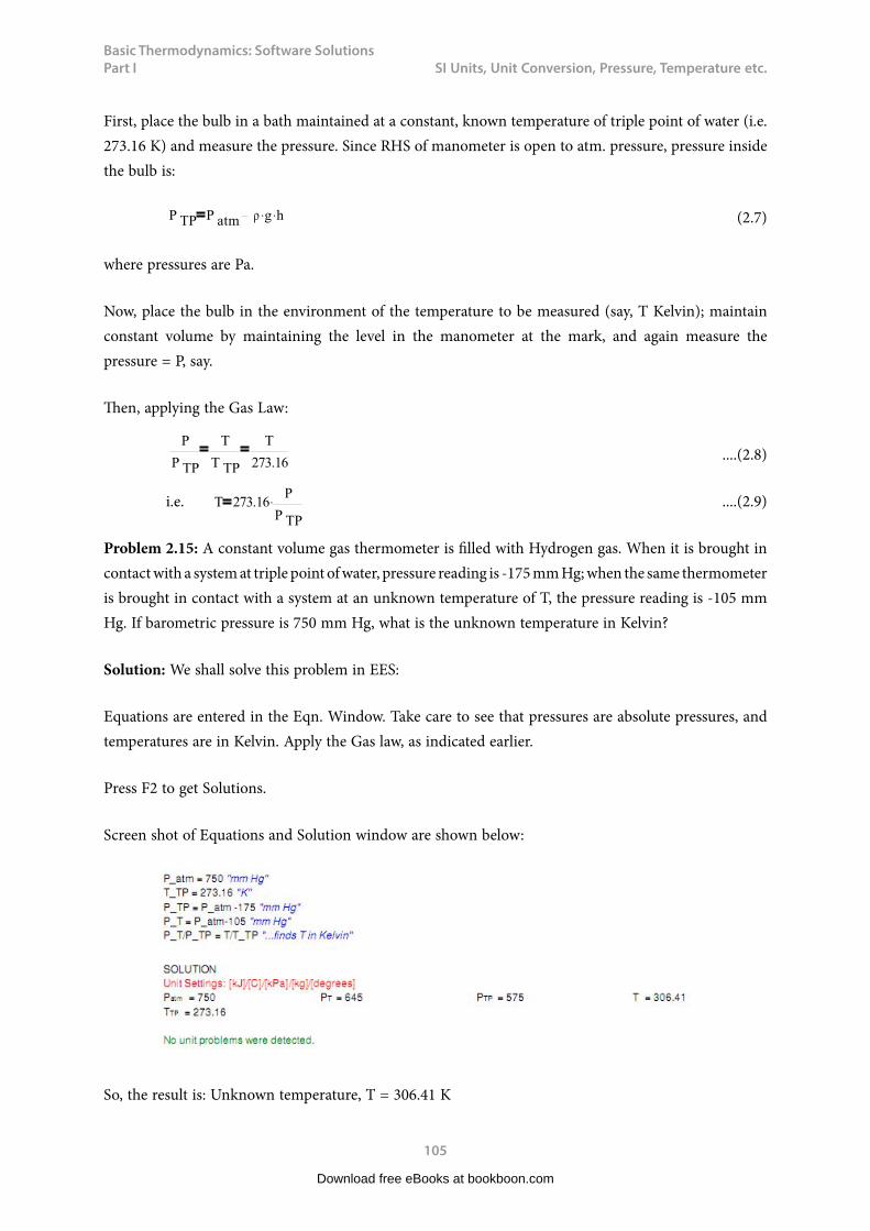
Basic Thermodynamics: Software Solutions Part I
105
SI Unitss, Unit Conversions, Pressures, Temperature etc.
First, place the bulb in a bath maintained at a constant, known temperature of triple point of water (i.e. 273.16 K) and measure the pressure. Since RHS of manometer is open to atm. pressure, pressure inside the bulb is:
P TP P atm g h (2.7)
where pressures are Pa.
Now, place the bulb in the environment of the temperature to be measured (say, T Kelvin); maintain constant volume by maintaining the level in the manometer at the mark, and again measure the pressure = P, say.
Then, applying the Gas Law:
P
P TP
T
T TP
T
273.16 ....(2.8)
i.e. T 273.16P
P TP
....(2.9)
Problem 2.15: A constant volume gas thermometer is filled with Hydrogen gas. When it is brought in contact with a system at triple point of water, pressure reading is -175 mm Hg; when the same thermometer is brought in contact with a system at an unknown temperature of T, the pressure reading is -105 mm Hg. If barometric pressure is 750 mm Hg, what is the unknown temperature in Kelvin?
Solution: We shall solve this problem in EES:
Equations are entered in the Eqn. Window. Take care to see that pressures are absolute pressures, and temperatures are in Kelvin. Apply the Gas law, as indicated earlier.
Press F2 to get Solutions.
Screen shot of Equations and Solution window are shown below:
So, the result is: Unknown temperature, T = 306.41 K
Download free eBooks at bookboon.com

Basic Thermodynamics: Software Solutions Part I
106
SI Unitss, Unit Conversions, Pressures, Temperature etc.
2.8 Resistance Thermometer Detectors (RTD):
RTD’s work on the principle that electrical resistances of many metals such as Platinum, Copper, Aluminium, Lead, Indium, Gold and Silver change with temperature.
Generally, Platinum is used because of its advantages:
i. it has a wide range and non-reactive upto high temperatures of around 850 deg. C, ii. it has good accuracyiii. it has good interchangeabilityiv. it has long term stabilityv. it can be drawn into wiresvi. it is not too soft vii. it gives reproducible results, andviii. it is not affected by corrosion and oxidation
Disadvantages of Pt are:
i. expensiveii. influenced by lead wire resistanceiii. slow thermal response, andiv. low resistance to shock and vibration
Pure Pt (99.99%) is used, since impurities in the resistor will affect the electrical resistance. Pt-resistance thermometers are known as PRT. According to the IEC and DIN Standards, temperature coefficient of the resistance wire must be 0.0038500C-1 (i.e. mean resistance change referred to the nominal resistance at zero deg.C) and it should have a resistance of 100 ohms at 0 deg.C; so, it is known as PT-100. Its resistance changes approximately 0.4 ohms/degree C. Following graph shows the variation of resistance with temperature:
Fig. 2.12 Resistance – Temperature characteristics of Pt-100
Download free eBooks at bookboon.com
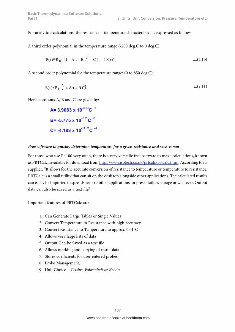
Basic Thermodynamics: Software Solutions Part I
107
SI Unitss, Unit Conversions, Pressures, Temperature etc.
For analytical calculations, the resistance – temperature characteristics is expressed as follows:
A third order polynomial in the temperature range (-200 deg.C to 0 deg.C):
R t( ) R 0 1 A t B t2
C t 100( ) t3 ....(2.10)
A second order polynomial for the temperature range: (0 to 850 deg.C):
...(2.11)
Here, constants A, B and C are given by:
Free software to quickly determine temperature for a given resistance and vice-versa:
For those who use Pt 100 very often, there is a very versatile free software to make calculations, known as PRTCalc., available for download from http://www.isotech.co.uk/prtcalc/prtcalc.html. According to its supplier: “It allows for the accurate conversion of resistance to temperature or temperature to resistance. PRTCalc is a small utility that can sit on the desk top alongside other applications. The calculated results can easily be imported to spreadsheets or other applications for presentation, storage or whatever. Output data can also be saved as a text file”.
Important features of PRTCalc are:
1. Can Generate Large Tables or Single Values 2. Convert Temperature to Resistance with high accuracy3. Convert Resistance to Temperature to approx. 0.01°C4. Allows very large lists of data 5. Output Can be Saved as a text file 6. Allows marking and copying of result data 7. Stores coefficients for user entered probes 8. Probe Management. 9. Unit Choice – Celsius, Fahrenheit or Kelvin
Download free eBooks at bookboon.com
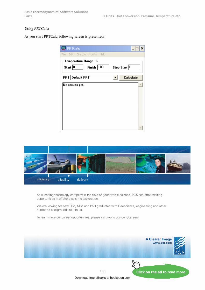
Basic Thermodynamics: Software Solutions Part I
108
SI Unitss, Unit Conversions, Pressures, Temperature etc.
Using PRTCalc:
As you start PRTCalc, following screen is presented:
Download free eBooks at bookboon.com
Click on the ad to read moreClick on the ad to read moreClick on the ad to read moreClick on the ad to read moreClick on the ad to read moreClick on the ad to read moreClick on the ad to read moreClick on the ad to read moreClick on the ad to read moreClick on the ad to read moreClick on the ad to read moreClick on the ad to read moreClick on the ad to read moreClick on the ad to read moreClick on the ad to read moreClick on the ad to read moreClick on the ad to read moreClick on the ad to read moreClick on the ad to read moreClick on the ad to read moreClick on the ad to read moreClick on the ad to read moreClick on the ad to read moreClick on the ad to read moreClick on the ad to read moreClick on the ad to read moreClick on the ad to read moreClick on the ad to read moreClick on the ad to read moreClick on the ad to read moreClick on the ad to read moreClick on the ad to read moreClick on the ad to read moreClick on the ad to read moreClick on the ad to read more
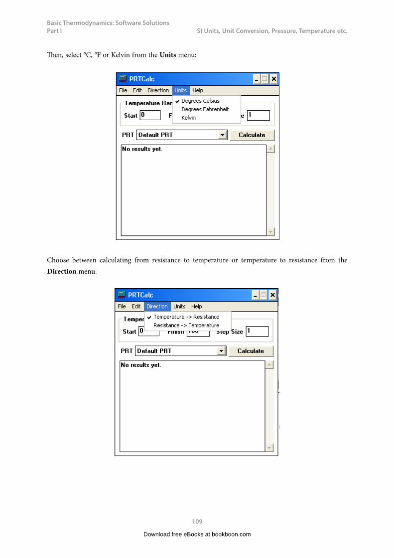
Basic Thermodynamics: Software Solutions Part I
109
SI Unitss, Unit Conversions, Pressures, Temperature etc.
Then, select °C, °F or Kelvin from the Units menu:
Choose between calculating from resistance to temperature or temperature to resistance from the Direction menu:
Download free eBooks at bookboon.com

Basic Thermodynamics: Software Solutions Part I
110
SI Unitss, Unit Conversions, Pressures, Temperature etc.
Press ‘Calculate’ and the table of Temp vs Resistance appears as shown:
Use the Edit menu to copy data to the clipboard; the data can then be pasted into a spreadsheet to produce a graph. As an example, values of resistances are calculated in the temperature range -180 deg.C to 820 deg.C and the table produced is copied to Excel; then, the Temperature vs Resistance chart is produced in Excel, and is shown below:
Download free eBooks at bookboon.com

Basic Thermodynamics: Software Solutions Part I
111
SI Unitss, Unit Conversions, Pressures, Temperature etc.
If you wish to calculate a single value only, say the value of resistance at 55 deg.C, then, leave the Finish box empty, and click on ‘Calculate’; you read the resistance as 121.321 ohms.:
Note: You can run multiple copies of PRTCalc simultaneously to see the effects of different coefficients or for multiple thermometers.
Download free eBooks at bookboon.com
Click on the ad to read moreClick on the ad to read moreClick on the ad to read moreClick on the ad to read moreClick on the ad to read moreClick on the ad to read moreClick on the ad to read moreClick on the ad to read moreClick on the ad to read moreClick on the ad to read moreClick on the ad to read moreClick on the ad to read moreClick on the ad to read moreClick on the ad to read moreClick on the ad to read moreClick on the ad to read moreClick on the ad to read moreClick on the ad to read moreClick on the ad to read moreClick on the ad to read moreClick on the ad to read moreClick on the ad to read moreClick on the ad to read moreClick on the ad to read moreClick on the ad to read moreClick on the ad to read moreClick on the ad to read moreClick on the ad to read moreClick on the ad to read moreClick on the ad to read moreClick on the ad to read moreClick on the ad to read moreClick on the ad to read moreClick on the ad to read moreClick on the ad to read moreClick on the ad to read more
STUDY. PLAY.The stuff you'll need to make a good living The stuff that makes life worth living
NORWAY. YOUR IDEAL STUDY DESTINATION.
WWW.STUDYINNORWAY.NOFACEBOOK.COM/STUDYINNORWAY
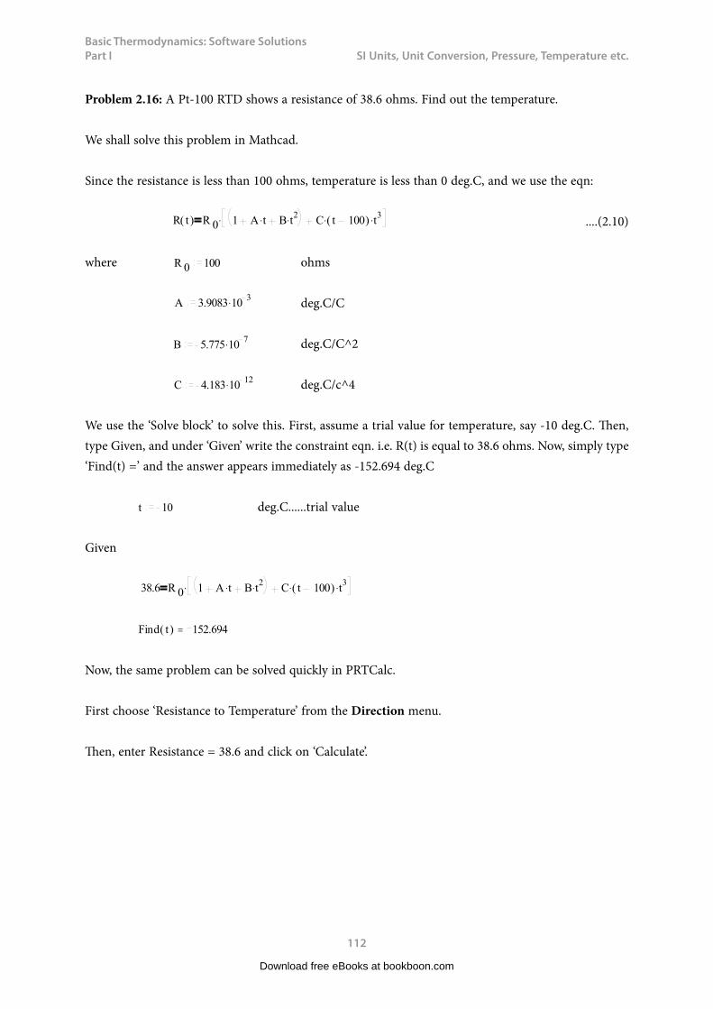
Basic Thermodynamics: Software Solutions Part I
112
SI Unitss, Unit Conversions, Pressures, Temperature etc.
Problem 2.16: A Pt-100 RTD shows a resistance of 38.6 ohms. Find out the temperature.
We shall solve this problem in Mathcad.
Since the resistance is less than 100 ohms, temperature is less than 0 deg.C, and we use the eqn:
R t( ) R 0 1 A t B t2
C t 100( ) t3 ....(2.10)
where R 0 100 ohms
A 3.9083 103 deg.C/C
B 5.775 107 deg.C/C^2
C 4.183 1012 deg.C/c^4
We use the ‘Solve block’ to solve this. First, assume a trial value for temperature, say -10 deg.C. Then, type Given, and under ‘Given’ write the constraint eqn. i.e. R(t) is equal to 38.6 ohms. Now, simply type ‘Find(t) =’ and the answer appears immediately as -152.694 deg.C
t 10 deg.C......trial value
Given
38.6 R 0 1 A t B t2
C t 100( ) t3
Find t( ) 152.694
Now, the same problem can be solved quickly in PRTCalc.
First choose ‘Resistance to Temperature’ from the Direction menu.
Then, enter Resistance = 38.6 and click on ‘Calculate’.
Download free eBooks at bookboon.com
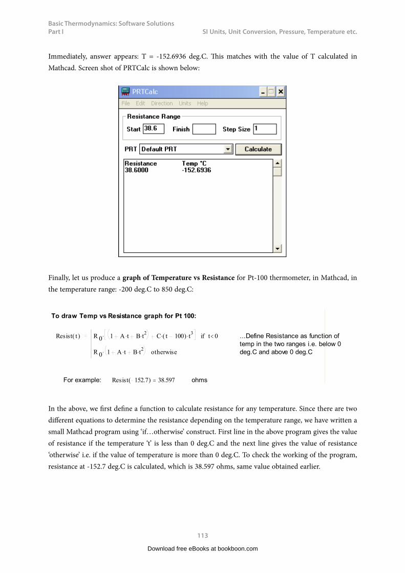
Basic Thermodynamics: Software Solutions Part I
113
SI Unitss, Unit Conversions, Pressures, Temperature etc.
Immediately, answer appears: T = -152.6936 deg.C. This matches with the value of T calculated in Mathcad. Screen shot of PRTCalc is shown below:
Finally, let us produce a graph of Temperature vs Resistance for Pt-100 thermometer, in Mathcad, in the temperature range: -200 deg.C to 850 deg.C:
To draw Temp vs Resistance graph for Pt 100:
Resist t( ) R 0 1 A t B t2
C t 100( ) t3
t 0if
R 0 1 A t B t2otherwise
...Define Resistance as function of
temp in the two ranges i.e. below 0
deg.C and above 0 deg.C
For example: Resist 152.7( ) 38.597 ohms
In the above, we first define a function to calculate resistance for any temperature. Since there are two different equations to determine the resistance depending on the temperature range, we have written a small Mathcad program using ‘if…otherwise’ construct. First line in the above program gives the value of resistance if the temperature ‘t’ is less than 0 deg.C and the next line gives the value of resistance ‘otherwise’ i.e. if the value of temperature is more than 0 deg.C. To check the working of the program, resistance at -152.7 deg.C is calculated, which is 38.597 ohms, same value obtained earlier.
Download free eBooks at bookboon.com

Basic Thermodynamics: Software Solutions Part I
114
SI Unitss, Unit Conversions, Pressures, Temperature etc.
Next, to draw the graph, first define a range variable ‘t’ to vary from -200 deg.C to 850 deg.C with an increment of 5 deg.C. Then, from the ‘Insert’ menu in Mathcad, click ‘graph-x-y plot’ and a blank plot appears with one ‘place holder’ on the x-axis and another ‘place holde’r on the y-axis. On the x-axis place holder type ‘t’ and on the y-axis place holder type ‘Resist(t)’ and the graph appears immediately. To format the graph for grid lines, titles, axis limits etc, double click on the graph and the formatting menu table appears where the choices can be selected. The Mathcad worksheet with graph is shown below:
t 200 195 850 ...define a range variable t from -200 C to 850 C with an increment of 5 deg.C
Download free eBooks at bookboon.com
Click on the ad to read moreClick on the ad to read moreClick on the ad to read moreClick on the ad to read moreClick on the ad to read moreClick on the ad to read moreClick on the ad to read moreClick on the ad to read moreClick on the ad to read moreClick on the ad to read moreClick on the ad to read moreClick on the ad to read moreClick on the ad to read moreClick on the ad to read moreClick on the ad to read moreClick on the ad to read moreClick on the ad to read moreClick on the ad to read moreClick on the ad to read moreClick on the ad to read moreClick on the ad to read moreClick on the ad to read moreClick on the ad to read moreClick on the ad to read moreClick on the ad to read moreClick on the ad to read moreClick on the ad to read moreClick on the ad to read moreClick on the ad to read moreClick on the ad to read moreClick on the ad to read moreClick on the ad to read moreClick on the ad to read moreClick on the ad to read moreClick on the ad to read moreClick on the ad to read moreClick on the ad to read more
Technical training on WHAT you need, WHEN you need it
At IDC Technologies we can tailor our technical and engineering training workshops to suit your needs. We have extensive
experience in training technical and engineering staff and have trained people in organisations such as General Motors, Shell, Siemens, BHP and Honeywell to name a few.Our onsite training is cost effective, convenient and completely customisable to the technical and engineering areas you want covered. Our workshops are all comprehensive hands-on learning experiences with ample time given to practical sessions and demonstrations. We communicate well to ensure that workshop content and timing match the knowledge, skills, and abilities of the participants.
We run onsite training all year round and hold the workshops on your premises or a venue of your choice for your convenience.
Phone: +61 8 9321 1702Email: [email protected] Website: www.idc-online.com
INDUSTRIALDATA COMMS
AUTOMATION & PROCESS CONTROL
ELECTRONICS
ELECTRICAL POWER
MECHANICAL ENGINEERING
OIL & GASENGINEERING
For a no obligation proposal, contact us today at [email protected] or visit our website for more information: www.idc-online.com/onsite/
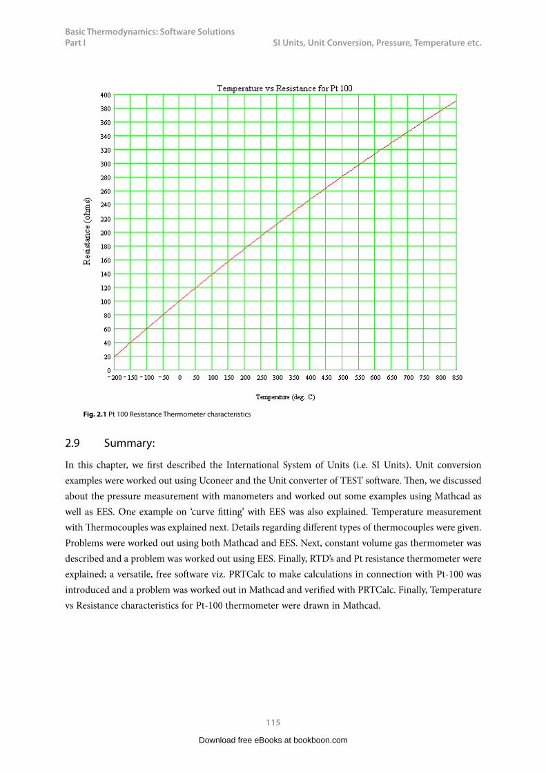
Basic Thermodynamics: Software Solutions Part I
115
SI Unitss, Unit Conversions, Pressures, Temperature etc.
Fig. 2.1 Pt 100 Resistance Thermometer characteristics
2.9 Summary:
In this chapter, we first described the International System of Units (i.e. SI Units). Unit conversion examples were worked out using Uconeer and the Unit converter of TEST software. Then, we discussed about the pressure measurement with manometers and worked out some examples using Mathcad as well as EES. One example on ‘curve fitting’ with EES was also explained. Temperature measurement with Thermocouples was explained next. Details regarding different types of thermocouples were given. Problems were worked out using both Mathcad and EES. Next, constant volume gas thermometer was described and a problem was worked out using EES. Finally, RTD’s and Pt resistance thermometer were explained; a versatile, free software viz. PRTCalc to make calculations in connection with Pt-100 was introduced and a problem was worked out in Mathcad and verified with PRTCalc. Finally, Temperature vs Resistance characteristics for Pt-100 thermometer were drawn in Mathcad.
Download free eBooks at bookboon.com

Basic Thermodynamics: Software Solutions Part I
116
SI Unitss, Unit Conversions, Pressures, Temperature etc.
2.10 References:
1. Y.A. Cengel and M.A. Boles. Thermodynamics – An Engineering Approach. 4th ed. New Delhi: Tata McGraw-Hill, 2003
2. I. Granet and M. Bluestein. Thermodynamics and Heat Power. 6th ed. Delhi: Pearson Education Asia, 2001
3. C.P.Arora. Thermodynamics. New Delhi: Tata McGraw-Hill, 19984. http://srdata.nist.gov/its90/main/5. www.efunda.com6. http://www.minco.com/tools/sensorcalc/7. www.temperatures.com8. www.omega.com9. www.peaksensors.com
10. www.dataforth.com11. www.picotech.com12. www.maxim-ic.com13. http://www.isotech.co.uk/prtcalc/prtcalc.html
Download free eBooks at bookboon.com
Basic Thermodynamics: Software Solutions Part I
117
Properties f Pure Substances
3 Properties Of Pure SubstancesLearning objectives:
1. In this chapter, we study about ‘pure substances’ i.e. substances which have a fixed chemical composition throughout.
2. Various property diagrams are explained, with particular reference to water. 3. Use of EES, TEST and many ‘free’ and online software to determine properties and plot
property diagrams for different substances is demonstrated. 4. Methods of finding out property values and generating property tables are also shown using
different software. 5. Determination of dryness fraction (or quality) of steam with ‘throttling calorimeter’ as well
as ‘separating and throttling calorimeter’ is explained.
3.1 Introduction:
A substance may exist in solid, liquid or gaseous state, and a ‘pure substance’ , by definition, is homogeneous and has the same chemical composition in all the states. For example, water has the same chemical composition whether it exists as ice (i.e. solid), or liquid water or steam (i.e. gaseous state). Sometimes, a mixture of gases, such as air is also treated as pure substance as far as it does not change phase. (When air changes phase, it has different compositions in gaseous and liquid phases).
In engineering, we frequently use water, air and refrigerants as important working substances. Water/steam is used in boilers, turbines and power plants. Air is used in Internal combustion engines and in numerous other applications. Many different types of refrigerants are in use in refrigeration and air-conditioning applications.
We shall study the properties of simple, compressible systems (i.e. systems where surface effects, magnetic effects and electrical effects are insignificant), where changes in pressure (P), volume (v) and temperature (T) are important. While studying the properties of pure substances, it is worthwhile to remember the ‘State principle’, which states as follows: ‘For a simple, compressible substance specifying the values of any two independent, intensive properties will fix the values of all of the others’. Here, the term ‘independent’ is important. Thus, for example, pressure (P) and temperature (T) are two independent properties for liquid water or gaseous steam, and given P and T fix the state for liquid water or gaseous steam. But, when the water is boiling, P and T are dependent on each other; so, one more independent property such as ‘quality’ is to be specified to fix the state.
We shall present our discussion mainly for water, but in general, the principles are valid for other fluids too.
Download free eBooks at bookboon.com
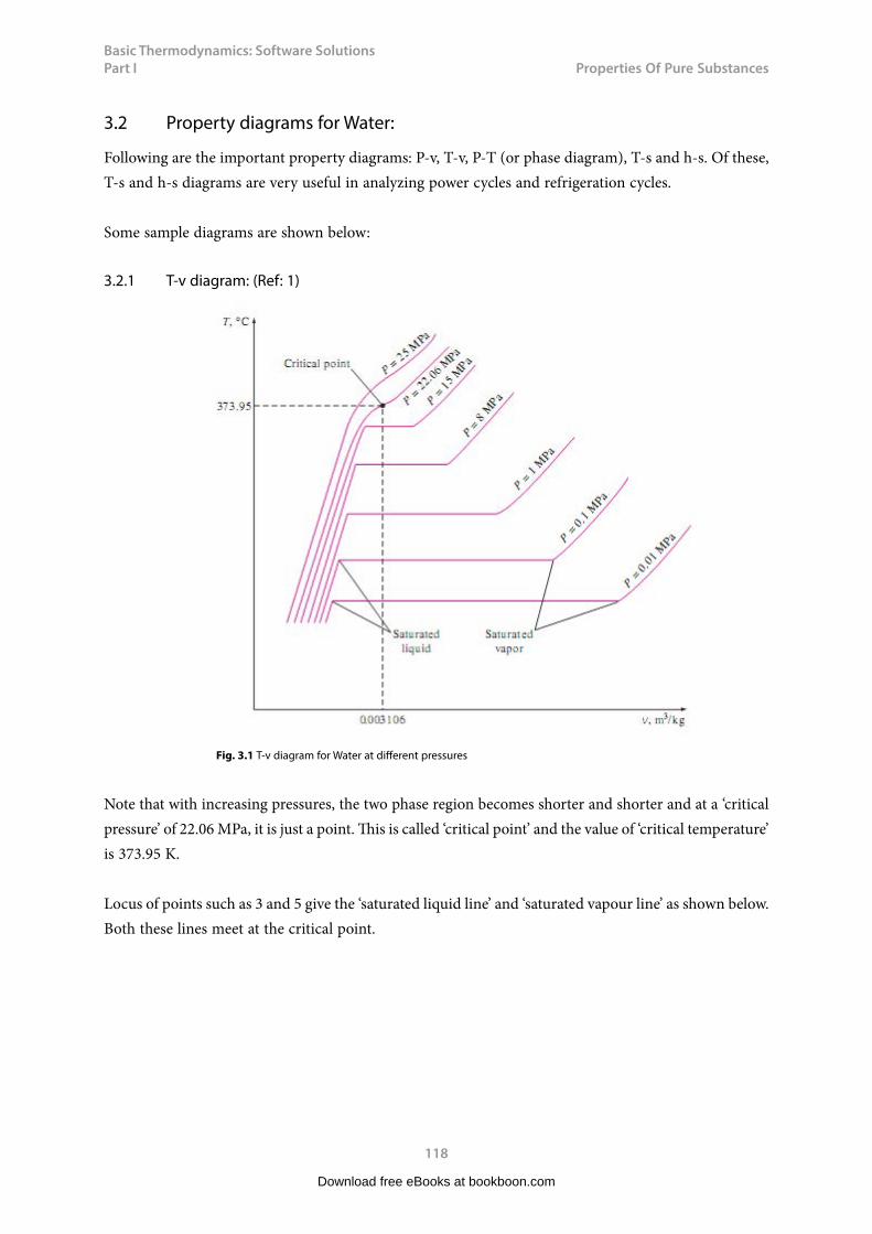
Basic Thermodynamics: Software Solutions Part I
118
Properties f Pure Substances
3.2 Property diagrams for Water:
Following are the important property diagrams: P-v, T-v, P-T (or phase diagram), T-s and h-s. Of these, T-s and h-s diagrams are very useful in analyzing power cycles and refrigeration cycles.
Some sample diagrams are shown below:
3.2.1 T-v diagram: (Ref: 1)
Fig. 3.1 T-v diagram for Water at different pressures
Note that with increasing pressures, the two phase region becomes shorter and shorter and at a ‘critical pressure’ of 22.06 MPa, it is just a point. This is called ‘critical point’ and the value of ‘critical temperature’ is 373.95 K.
Locus of points such as 3 and 5 give the ‘saturated liquid line’ and ‘saturated vapour line’ as shown below. Both these lines meet at the critical point.
Download free eBooks at bookboon.com

Basic Thermodynamics: Software Solutions Part I
119
Properties f Pure Substances
3.2.2 P-v diagram: (Ref: 1)
Note the various regions and the nature of constant temperature lines in the following P-v diagram.
Fig. 3.2 P-v diagram for Pure substance
It is a specialty with water that as it freezes, the volume increases, whereas for most of other substances, volume decreases as temperature decreases.
If the solid region is also included, P-v diagram for water (which expands on freezing) will appear as follows:
Fig. 3.3 P-v diagram for water (which expands on freezing)
Download free eBooks at bookboon.com
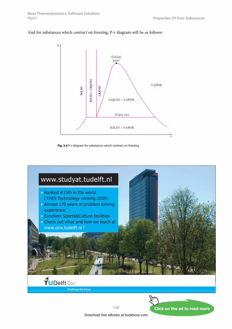
Basic Thermodynamics: Software Solutions Part I
120
Properties f Pure Substances
And for substances which contract on freezing, P-v diagram will be as follows:
Fig. 3.4 P-v diagram for substances which contract on freezing
Download free eBooks at bookboon.com
Click on the ad to read moreClick on the ad to read moreClick on the ad to read moreClick on the ad to read moreClick on the ad to read moreClick on the ad to read moreClick on the ad to read moreClick on the ad to read moreClick on the ad to read moreClick on the ad to read moreClick on the ad to read moreClick on the ad to read moreClick on the ad to read moreClick on the ad to read moreClick on the ad to read moreClick on the ad to read moreClick on the ad to read moreClick on the ad to read moreClick on the ad to read moreClick on the ad to read moreClick on the ad to read moreClick on the ad to read moreClick on the ad to read moreClick on the ad to read moreClick on the ad to read moreClick on the ad to read moreClick on the ad to read moreClick on the ad to read moreClick on the ad to read moreClick on the ad to read moreClick on the ad to read moreClick on the ad to read moreClick on the ad to read moreClick on the ad to read moreClick on the ad to read moreClick on the ad to read moreClick on the ad to read moreClick on the ad to read more
���������� ����� ��������� �������������������������������� �!�" ��#������"��$�%��&��!�"��'����� �(%����������(������ ��%�� ")*+� +���$����� ��"��*������+ ���� ����������� ������ �� ���,���, +��$ ,���-
���," +�� , +��$ ,��
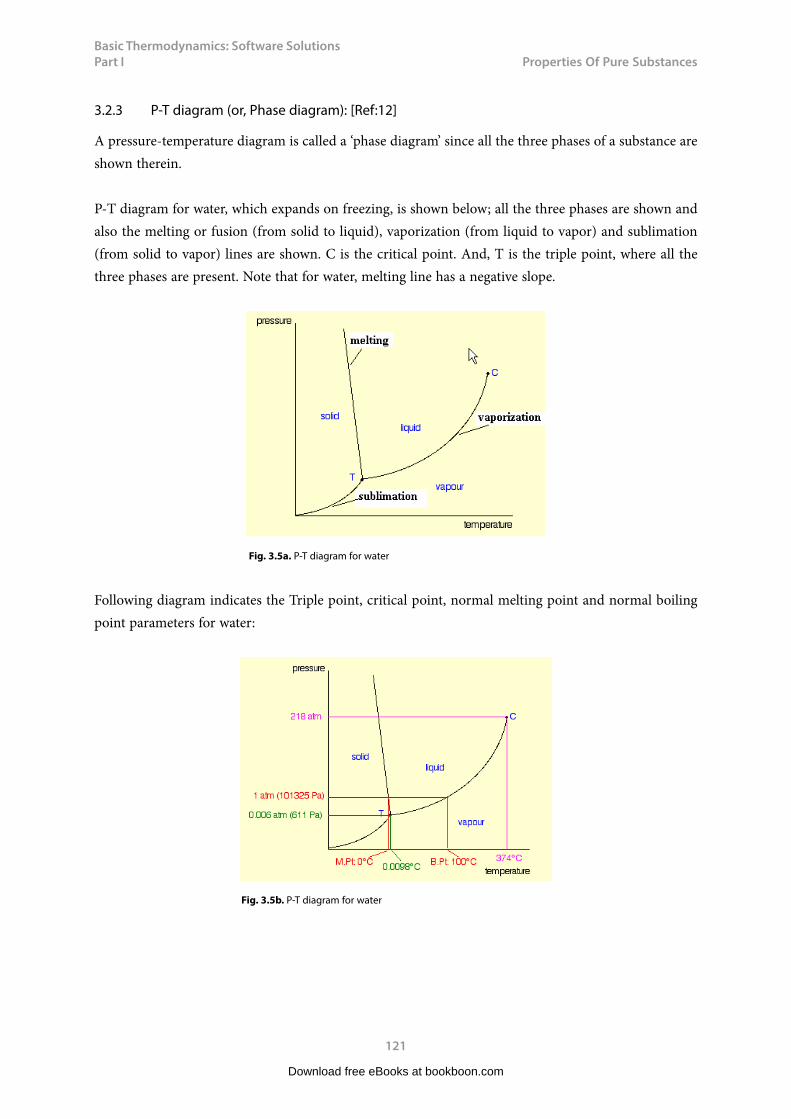
Basic Thermodynamics: Software Solutions Part I
121
Properties f Pure Substances
3.2.3 P-T diagram (or, Phase diagram): [Ref:12]
A pressure-temperature diagram is called a ‘phase diagram’ since all the three phases of a substance are shown therein.
P-T diagram for water, which expands on freezing, is shown below; all the three phases are shown and also the melting or fusion (from solid to liquid), vaporization (from liquid to vapor) and sublimation (from solid to vapor) lines are shown. C is the critical point. And, T is the triple point, where all the three phases are present. Note that for water, melting line has a negative slope.
Fig. 3.5a. P-T diagram for water
Following diagram indicates the Triple point, critical point, normal melting point and normal boiling point parameters for water:
Fig. 3.5b. P-T diagram for water
Download free eBooks at bookboon.com

Basic Thermodynamics: Software Solutions Part I
122
Properties f Pure Substances
Note that for water, as a consequence of negative slope of the melting line, freezing temperature decreases with an increase in pressure; also, at a temperature below the Triple point, as the pressure is increased vertically along the constant temperature line, vapor will first become a solid and then liquid! At a temperature above the critical temperature, it is impossible to condense a vapor into liquid by increasing the pressure.
For a substance other than water, i.e. which contracts on freezing, the phase diagram will look as follows:
Fig. 3.6 P-T diagram for a substance which contracts on freezing
Download free eBooks at bookboon.com
Click on the ad to read moreClick on the ad to read moreClick on the ad to read moreClick on the ad to read moreClick on the ad to read moreClick on the ad to read moreClick on the ad to read moreClick on the ad to read moreClick on the ad to read moreClick on the ad to read moreClick on the ad to read moreClick on the ad to read moreClick on the ad to read moreClick on the ad to read moreClick on the ad to read moreClick on the ad to read moreClick on the ad to read moreClick on the ad to read moreClick on the ad to read moreClick on the ad to read moreClick on the ad to read moreClick on the ad to read moreClick on the ad to read moreClick on the ad to read moreClick on the ad to read moreClick on the ad to read moreClick on the ad to read moreClick on the ad to read moreClick on the ad to read moreClick on the ad to read moreClick on the ad to read moreClick on the ad to read moreClick on the ad to read moreClick on the ad to read moreClick on the ad to read moreClick on the ad to read moreClick on the ad to read moreClick on the ad to read moreClick on the ad to read more
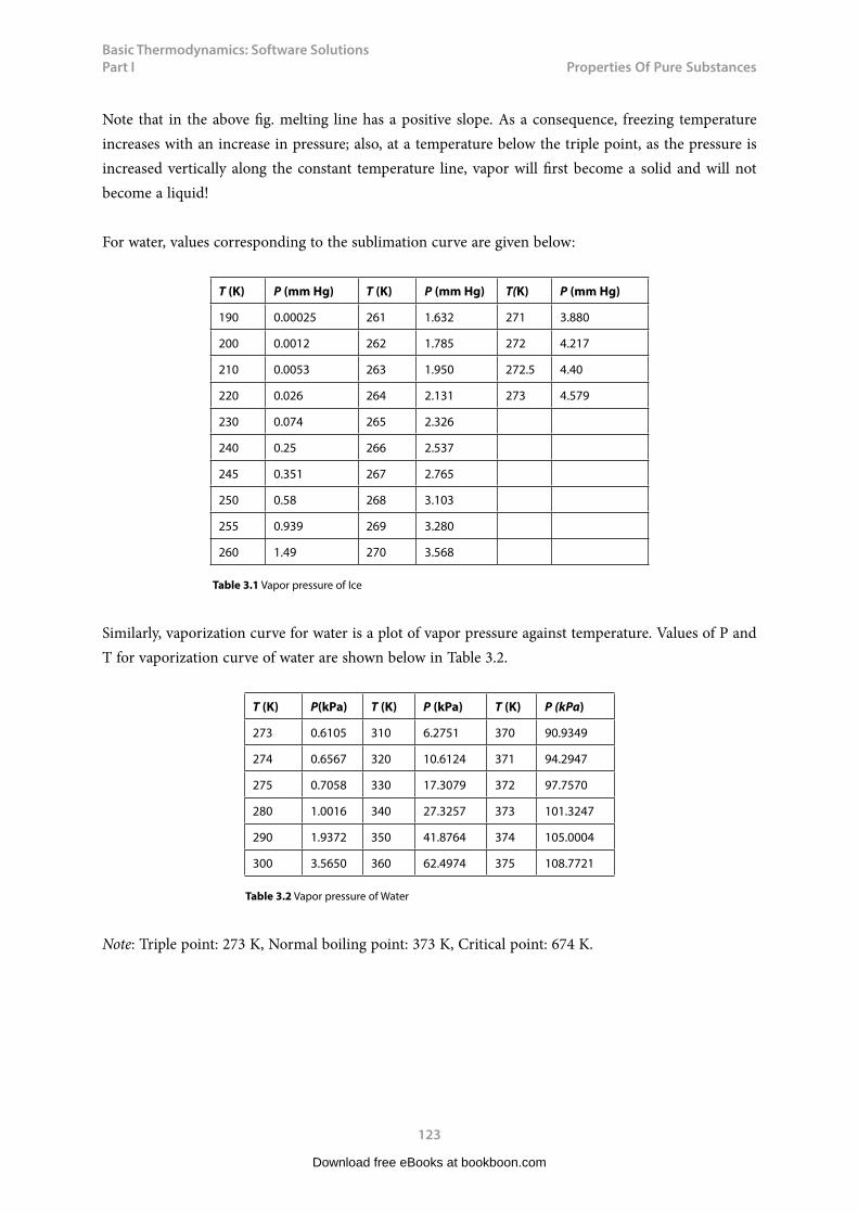
Basic Thermodynamics: Software Solutions Part I
123
Properties f Pure Substances
Note that in the above fig. melting line has a positive slope. As a consequence, freezing temperature increases with an increase in pressure; also, at a temperature below the triple point, as the pressure is increased vertically along the constant temperature line, vapor will first become a solid and will not become a liquid!
For water, values corresponding to the sublimation curve are given below:
T (K) P (mm Hg) T (K) P (mm Hg) T(K) P (mm Hg)
190 0.00025 261 1.632 271 3.880
200 0.0012 262 1.785 272 4.217
210 0.0053 263 1.950 272.5 4.40
220 0.026 264 2.131 273 4.579
230 0.074 265 2.326
240 0.25 266 2.537
245 0.351 267 2.765
250 0.58 268 3.103
255 0.939 269 3.280
260 1.49 270 3.568
Table 3.1 Vapor pressure of Ice
Similarly, vaporization curve for water is a plot of vapor pressure against temperature. Values of P and T for vaporization curve of water are shown below in Table 3.2.
T (K) P(kPa) T (K) P (kPa) T (K) P (kPa)
273 0.6105 310 6.2751 370 90.9349
274 0.6567 320 10.6124 371 94.2947
275 0.7058 330 17.3079 372 97.7570
280 1.0016 340 27.3257 373 101.3247
290 1.9372 350 41.8764 374 105.0004
300 3.5650 360 62.4974 375 108.7721
Table 3.2 Vapor pressure of Water
Note: Triple point: 273 K, Normal boiling point: 373 K, Critical point: 674 K.
Download free eBooks at bookboon.com
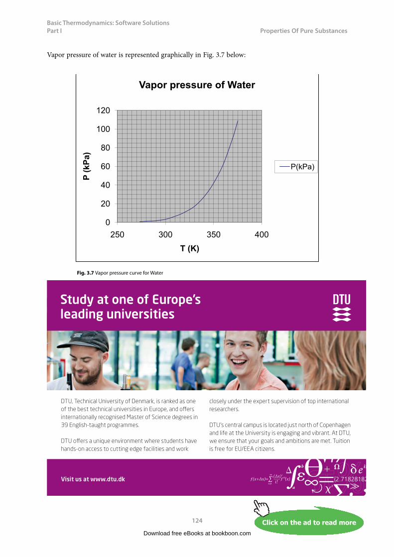
Basic Thermodynamics: Software Solutions Part I
124
Properties f Pure Substances
Vapor pressure of water is represented graphically in Fig. 3.7 below:
0
20
40
60
80
100
120
250 300 350 400
P (k
Pa)
T (K)
Vapor pressure of Water
P(kPa)
Fig. 3.7 Vapor pressure curve for Water
Download free eBooks at bookboon.com
Click on the ad to read moreClick on the ad to read moreClick on the ad to read moreClick on the ad to read moreClick on the ad to read moreClick on the ad to read moreClick on the ad to read moreClick on the ad to read moreClick on the ad to read moreClick on the ad to read moreClick on the ad to read moreClick on the ad to read moreClick on the ad to read moreClick on the ad to read moreClick on the ad to read moreClick on the ad to read moreClick on the ad to read moreClick on the ad to read moreClick on the ad to read moreClick on the ad to read moreClick on the ad to read moreClick on the ad to read moreClick on the ad to read moreClick on the ad to read moreClick on the ad to read moreClick on the ad to read moreClick on the ad to read moreClick on the ad to read moreClick on the ad to read moreClick on the ad to read moreClick on the ad to read moreClick on the ad to read moreClick on the ad to read moreClick on the ad to read moreClick on the ad to read moreClick on the ad to read moreClick on the ad to read moreClick on the ad to read moreClick on the ad to read moreClick on the ad to read more
DTU, Technical University of Denmark, is ranked as one of the best technical universities in Europe, and offers internationally recognised Master of Science degrees in 39 English-taught programmes.
DTU offers a unique environment where students have hands-on access to cutting edge facilities and work
closely under the expert supervision of top international researchers.
DTU’s central campus is located just north of Copenhagen and life at the University is engaging and vibrant. At DTU, we ensure that your goals and ambitions are met. Tuition is free for EU/EEA citizens.
Visit us at www.dtu.dk
Study at one of Europe’s leading universities
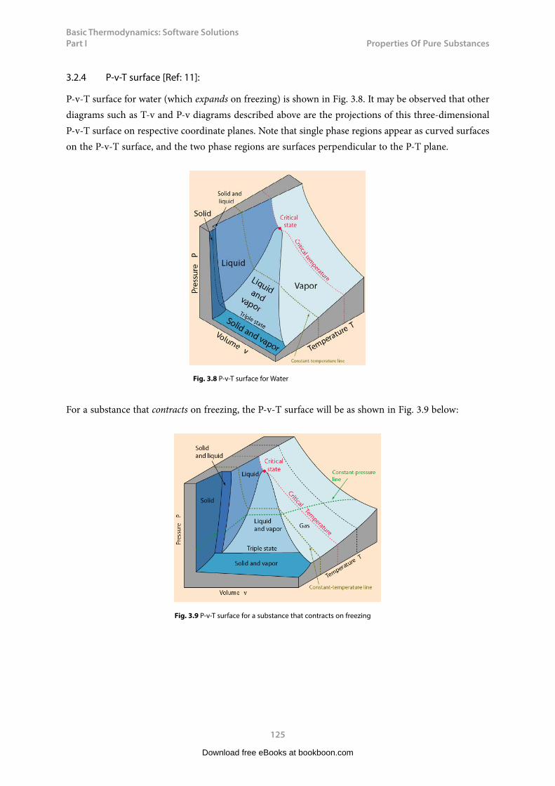
Basic Thermodynamics: Software Solutions Part I
125
Properties f Pure Substances
3.2.4 P-v-T surface [Ref: 11]:
P-v-T surface for water (which expands on freezing) is shown in Fig. 3.8. It may be observed that other diagrams such as T-v and P-v diagrams described above are the projections of this three-dimensional P-v-T surface on respective coordinate planes. Note that single phase regions appear as curved surfaces on the P-v-T surface, and the two phase regions are surfaces perpendicular to the P-T plane.
Fig. 3.8 P-v-T surface for Water
For a substance that contracts on freezing, the P-v-T surface will be as shown in Fig. 3.9 below:
Fig. 3.9 P-v-T surface for a substance that contracts on freezing
Download free eBooks at bookboon.com
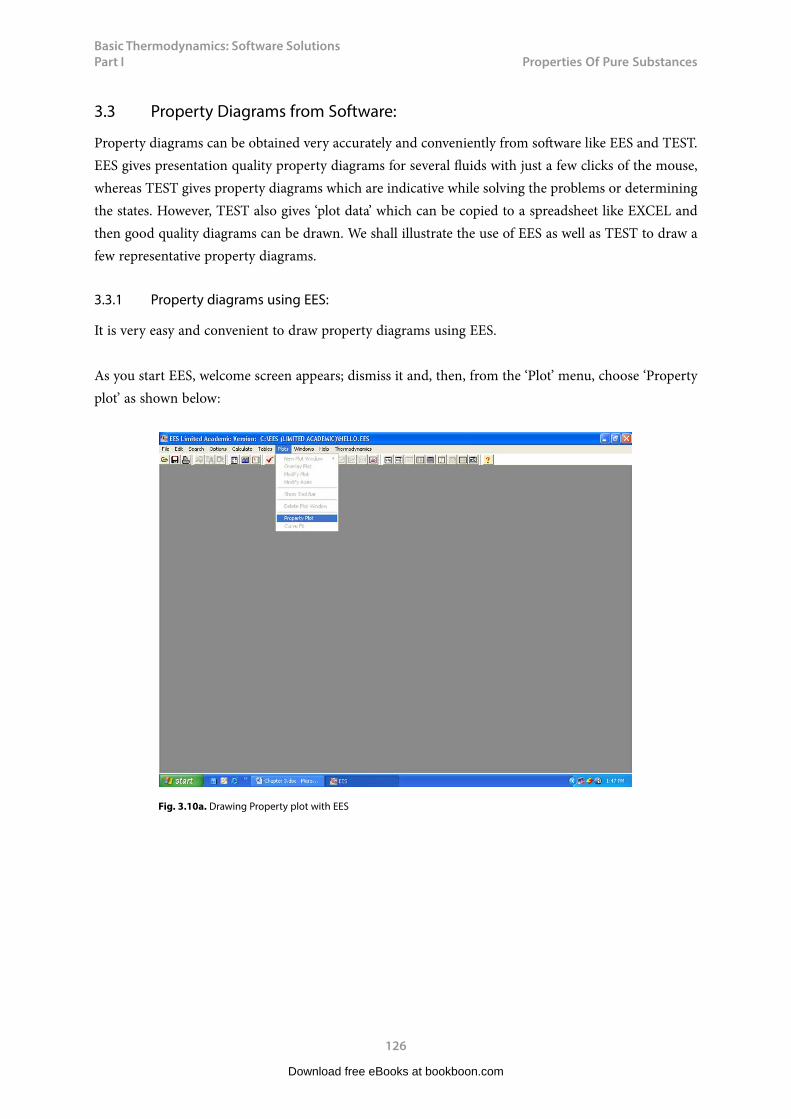
Basic Thermodynamics: Software Solutions Part I
126
Properties f Pure Substances
3.3 Property Diagrams from Software:
Property diagrams can be obtained very accurately and conveniently from software like EES and TEST. EES gives presentation quality property diagrams for several fluids with just a few clicks of the mouse, whereas TEST gives property diagrams which are indicative while solving the problems or determining the states. However, TEST also gives ‘plot data’ which can be copied to a spreadsheet like EXCEL and then good quality diagrams can be drawn. We shall illustrate the use of EES as well as TEST to draw a few representative property diagrams.
3.3.1 Property diagrams using EES:
It is very easy and convenient to draw property diagrams using EES.
As you start EES, welcome screen appears; dismiss it and, then, from the ‘Plot’ menu, choose ‘Property plot’ as shown below:
Fig. 3.10a. Drawing Property plot with EES
Download free eBooks at bookboon.com

Basic Thermodynamics: Software Solutions Part I
127
Properties f Pure Substances
Then, the ‘Property plot information’ window appears. Here, you choose the fluid (Steam_NBS), Type of plot (say, T-v plot), and constant pressure, entropy and quality lines, as shown below in Fig. 3.10 b.
Fig. 3.10b. Drawing Property plot with EES
Download free eBooks at bookboon.com
Click on the ad to read moreClick on the ad to read moreClick on the ad to read moreClick on the ad to read moreClick on the ad to read moreClick on the ad to read moreClick on the ad to read moreClick on the ad to read moreClick on the ad to read moreClick on the ad to read moreClick on the ad to read moreClick on the ad to read moreClick on the ad to read moreClick on the ad to read moreClick on the ad to read moreClick on the ad to read moreClick on the ad to read moreClick on the ad to read moreClick on the ad to read moreClick on the ad to read moreClick on the ad to read moreClick on the ad to read moreClick on the ad to read moreClick on the ad to read moreClick on the ad to read moreClick on the ad to read moreClick on the ad to read moreClick on the ad to read moreClick on the ad to read moreClick on the ad to read moreClick on the ad to read moreClick on the ad to read moreClick on the ad to read moreClick on the ad to read moreClick on the ad to read moreClick on the ad to read moreClick on the ad to read moreClick on the ad to read moreClick on the ad to read moreClick on the ad to read moreClick on the ad to read more
Increase your impact with MSM Executive Education
For more information, visit www.msm.nl or contact us at +31 43 38 70 808
or via [email protected] the globally networked management school
For more information, visit www.msm.nl or contact us at +31 43 38 70 808 or via [email protected]
For almost 60 years Maastricht School of Management has been enhancing the management capacity
of professionals and organizations around the world through state-of-the-art management education.
Our broad range of Open Enrollment Executive Programs offers you a unique interactive, stimulating and
multicultural learning experience.
Be prepared for tomorrow’s management challenges and apply today.
Executive Education-170x115-B2.indd 1 18-08-11 15:13
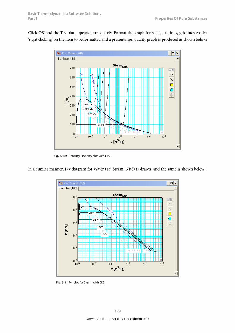
Basic Thermodynamics: Software Solutions Part I
128
Properties f Pure Substances
Click OK and the T-v plot appears immediately. Format the graph for scale, captions, gridlines etc. by ‘right clicking’ on the item to be formatted and a presentation quality graph is produced as shown below:
Fig. 3.10c. Drawing Property plot with EES
In a similar manner, P-v diagram for Water (i.e. Steam_NBS) is drawn, and the same is shown below:
Fig. 3.11 P-v plot for Steam with EES
Download free eBooks at bookboon.com
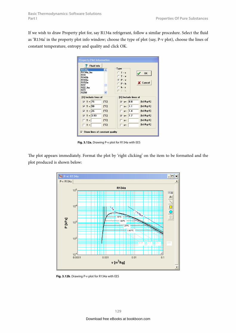
Basic Thermodynamics: Software Solutions Part I
129
Properties f Pure Substances
If we wish to draw Property plot for, say R134a refrigerant, follow a similar procedure. Select the fluid as ‘R134a’ in the property plot info window; choose the type of plot (say, P-v plot), choose the lines of constant temperature, entropy and quality and click OK.
Fig. 3.12a. Drawing P-v plot for R134a with EES
The plot appears immediately. Format the plot by ‘right clicking’ on the item to be formatted and the plot produced is shown below:
Fig. 3.12b. Drawing P-v plot for R134a with EES
Download free eBooks at bookboon.com
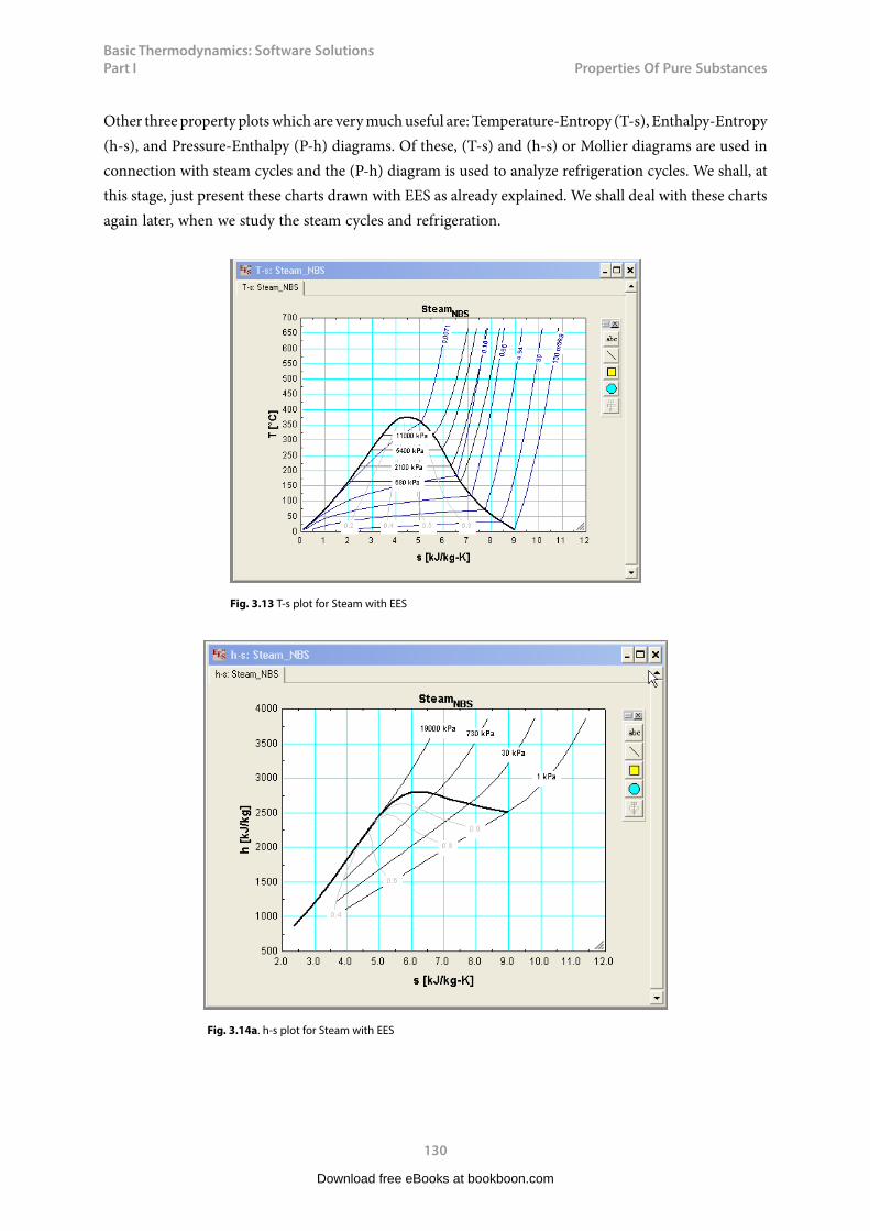
Basic Thermodynamics: Software Solutions Part I
130
Properties f Pure Substances
Other three property plots which are very much useful are: Temperature-Entropy (T-s), Enthalpy-Entropy (h-s), and Pressure-Enthalpy (P-h) diagrams. Of these, (T-s) and (h-s) or Mollier diagrams are used in connection with steam cycles and the (P-h) diagram is used to analyze refrigeration cycles. We shall, at this stage, just present these charts drawn with EES as already explained. We shall deal with these charts again later, when we study the steam cycles and refrigeration.
Fig. 3.13 T-s plot for Steam with EES
Fig. 3.14a. h-s plot for Steam with EES
Download free eBooks at bookboon.com
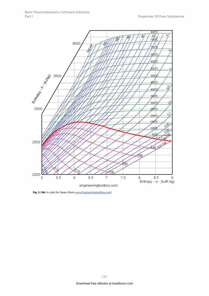
Basic Thermodynamics: Software Solutions Part I
131
Properties f Pure Substances
Fig. 3.14b. h-s plot for Steam (from www.Engineeringtoolbox.com)
Download free eBooks at bookboon.com

Basic Thermodynamics: Software Solutions Part I
132
Properties f Pure Substances
Fig. 3.15a. P-h plot for R12 with EES
Download free eBooks at bookboon.com
Click on the ad to read moreClick on the ad to read moreClick on the ad to read moreClick on the ad to read moreClick on the ad to read moreClick on the ad to read moreClick on the ad to read moreClick on the ad to read moreClick on the ad to read moreClick on the ad to read moreClick on the ad to read moreClick on the ad to read moreClick on the ad to read moreClick on the ad to read moreClick on the ad to read moreClick on the ad to read moreClick on the ad to read moreClick on the ad to read moreClick on the ad to read moreClick on the ad to read moreClick on the ad to read moreClick on the ad to read moreClick on the ad to read moreClick on the ad to read moreClick on the ad to read moreClick on the ad to read moreClick on the ad to read moreClick on the ad to read moreClick on the ad to read moreClick on the ad to read moreClick on the ad to read moreClick on the ad to read moreClick on the ad to read moreClick on the ad to read moreClick on the ad to read moreClick on the ad to read moreClick on the ad to read moreClick on the ad to read moreClick on the ad to read moreClick on the ad to read moreClick on the ad to read moreClick on the ad to read more
EXPERIENCE THE POWER OF FULL ENGAGEMENT…
RUN FASTER. RUN LONGER.. RUN EASIER…
READ MORE & PRE-ORDER TODAY WWW.GAITEYE.COM
Challenge the way we run
1349906_A6_4+0.indd 1 22-08-2014 12:56:57
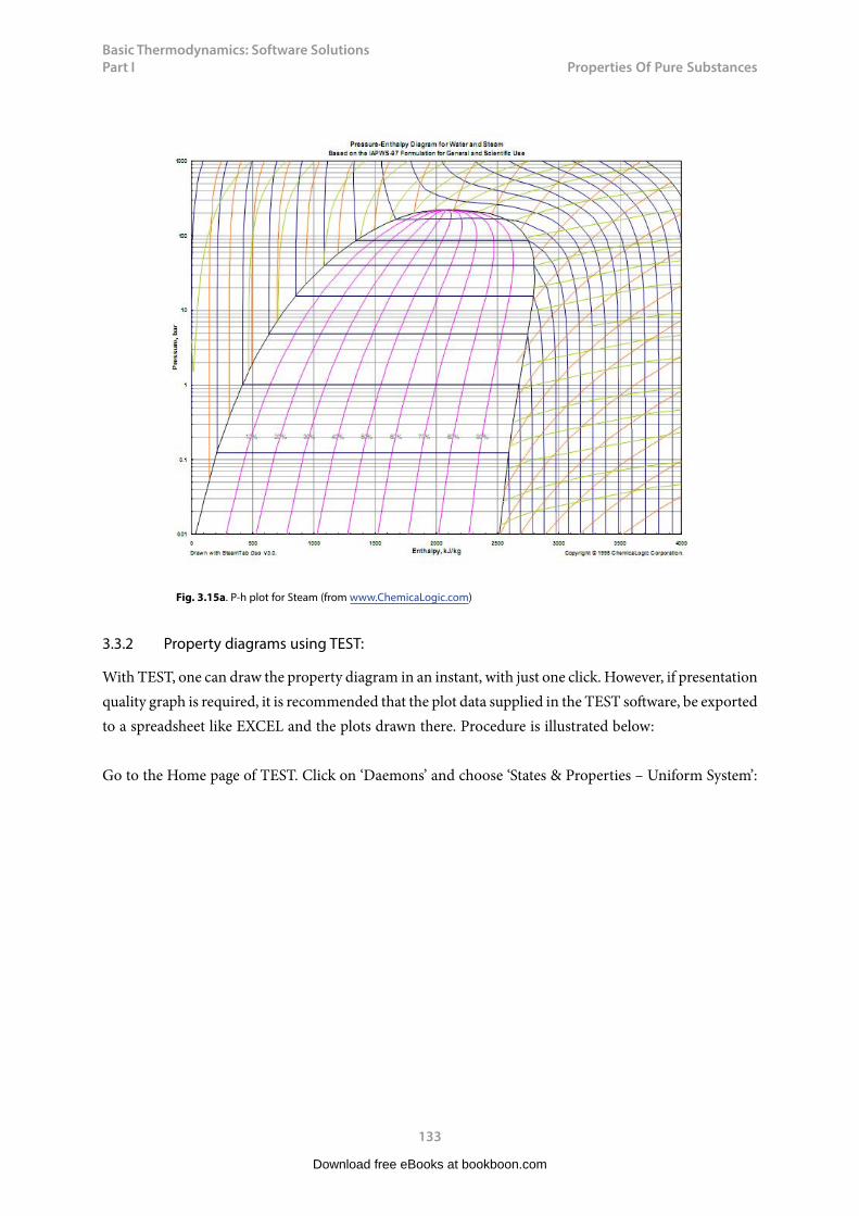
Basic Thermodynamics: Software Solutions Part I
133
Properties f Pure Substances
Fig. 3.15a. P-h plot for Steam (from www.ChemicaLogic.com)
3.3.2 Property diagrams using TEST:
With TEST, one can draw the property diagram in an instant, with just one click. However, if presentation quality graph is required, it is recommended that the plot data supplied in the TEST software, be exported to a spreadsheet like EXCEL and the plots drawn there. Procedure is illustrated below:
Go to the Home page of TEST. Click on ‘Daemons’ and choose ‘States & Properties – Uniform System’:
Download free eBooks at bookboon.com
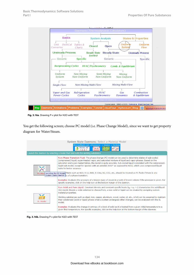
Basic Thermodynamics: Software Solutions Part I
134
Properties f Pure Substances
Fig. 3.16a. Drawing P-v plot for H2O with TEST
You get the following screen; choose PC model (i.e. Phase Change Model), since we want to get property diagram for Water/Steam.
Fig. 3.16b. Drawing P-v plot for H2O with TEST
Download free eBooks at bookboon.com
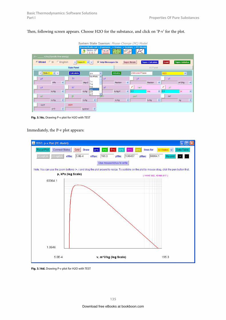
Basic Thermodynamics: Software Solutions Part I
135
Properties f Pure Substances
Then, following screen appears. Choose H2O for the substance, and click on ‘P-v’ for the plot.
Fig. 3.16c. Drawing P-v plot for H2O with TEST
Immediately, the P-v plot appears:
Fig. 3.16d. Drawing P-v plot for H2O with TEST
Download free eBooks at bookboon.com
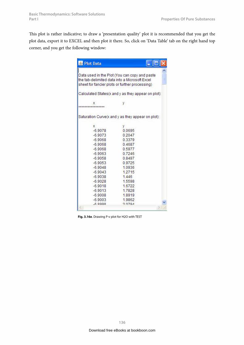
Basic Thermodynamics: Software Solutions Part I
136
Properties f Pure Substances
This plot is rather indicative; to draw a ‘presentation quality’ plot it is recommended that you get the plot data, export it to EXCEL and then plot it there. So, click on ‘Data Table’ tab on the right hand top corner, and you get the following window:
Fig. 3.16e. Drawing P-v plot for H2O with TEST
Download free eBooks at bookboon.com
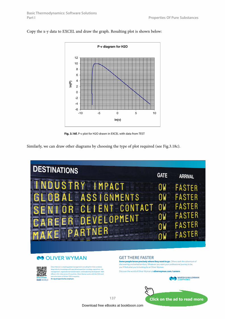
Basic Thermodynamics: Software Solutions Part I
137
Properties f Pure Substances
Copy the x-y data to EXCEL and draw the graph. Resulting plot is shown below:
Fig. 3.16f. P-v plot for H2O drawn in EXCEL with data from TEST
Similarly, we can draw other diagrams by choosing the type of plot required (see Fig.3.18c).
Download free eBooks at bookboon.com
Click on the ad to read moreClick on the ad to read moreClick on the ad to read moreClick on the ad to read moreClick on the ad to read moreClick on the ad to read moreClick on the ad to read moreClick on the ad to read moreClick on the ad to read moreClick on the ad to read moreClick on the ad to read moreClick on the ad to read moreClick on the ad to read moreClick on the ad to read moreClick on the ad to read moreClick on the ad to read moreClick on the ad to read moreClick on the ad to read moreClick on the ad to read moreClick on the ad to read moreClick on the ad to read moreClick on the ad to read moreClick on the ad to read moreClick on the ad to read moreClick on the ad to read moreClick on the ad to read moreClick on the ad to read moreClick on the ad to read moreClick on the ad to read moreClick on the ad to read moreClick on the ad to read moreClick on the ad to read moreClick on the ad to read moreClick on the ad to read moreClick on the ad to read moreClick on the ad to read moreClick on the ad to read moreClick on the ad to read moreClick on the ad to read moreClick on the ad to read moreClick on the ad to read moreClick on the ad to read moreClick on the ad to read more
GET THERE FASTER
Oliver Wyman is a leading global management consulting firm that combines
deep industry knowledge with specialized expertise in strategy, operations, risk
management, organizational transformation, and leadership development. With
offices in 50+ cities across 25 countries, Oliver Wyman works with the CEOs and
executive teams of Global 1000 companies.
An equal opportunity employer.
Some people know precisely where they want to go. Others seek the adventure of discovering uncharted territory. Whatever you want your professional journey to be, you’ll find what you’re looking for at Oliver Wyman.
Discover the world of Oliver Wyman at oliverwyman.com/careers
DISCOVEROUR WORLD
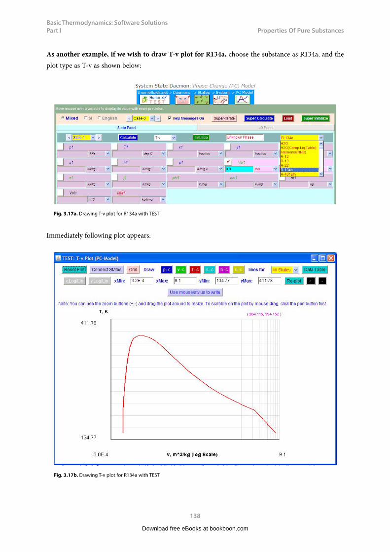
Basic Thermodynamics: Software Solutions Part I
138
Properties f Pure Substances
As another example, if we wish to draw T-v plot for R134a, choose the substance as R134a, and the plot type as T-v as shown below:
Fig. 3.17a. Drawing T-v plot for R134a with TEST
Immediately following plot appears:
Fig. 3.17b. Drawing T-v plot for R134a with TEST
Download free eBooks at bookboon.com
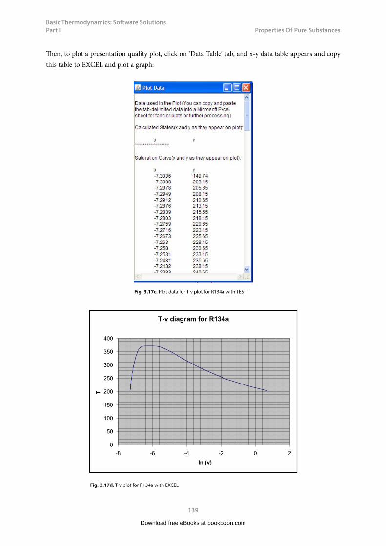
Basic Thermodynamics: Software Solutions Part I
139
Properties f Pure Substances
Then, to plot a presentation quality plot, click on ‘Data Table’ tab, and x-y data table appears and copy this table to EXCEL and plot a graph:
Fig. 3.17c. Plot data for T-v plot for R134a with TEST
0
50
100
150
200
250
300
350
400
-8 -6 -4 -2 0 2
T
ln (v)
T-v diagram for R134a
Fig. 3.17d. T-v plot for R134a with EXCEL
Download free eBooks at bookboon.com

Basic Thermodynamics: Software Solutions Part I
140
Properties f Pure Substances
3.4 Property values and Tables:
Many times, it is difficult to read accurately from the Property plots, particularly if the scale is logarithmic. We may need property values at a given state; or, we may need a table of property values at a set of points. P, v and T are measurable properties and other properties tabulated are internal energy (u), enthalpy (h) and entropy (s). Generally these properties are calculated from the measured properties by means of complicated state equations. For example, for steam, different formulae are applicable depending upon the region in which the state lies. (see figure 3.18 below).
International Association for Properties of Water and Steam (IAPWS_97) defines the properties of Steam in 5 regions:
• region 1 for the liquid state from low to high pressures, • region 2 for the vapor and ideal gas state, • region 3 for the thermodynamic state around the critical point, • region 4 for the saturation curve (vapor-liquid equilibrium), • region 5 for high temperatures above 1073.15 K (800 °C) and pressures up to 10 MPa (100 bar).
Download free eBooks at bookboon.com
Click on the ad to read moreClick on the ad to read moreClick on the ad to read moreClick on the ad to read moreClick on the ad to read moreClick on the ad to read moreClick on the ad to read moreClick on the ad to read moreClick on the ad to read moreClick on the ad to read moreClick on the ad to read moreClick on the ad to read moreClick on the ad to read moreClick on the ad to read moreClick on the ad to read moreClick on the ad to read moreClick on the ad to read moreClick on the ad to read moreClick on the ad to read moreClick on the ad to read moreClick on the ad to read moreClick on the ad to read moreClick on the ad to read moreClick on the ad to read moreClick on the ad to read moreClick on the ad to read moreClick on the ad to read moreClick on the ad to read moreClick on the ad to read moreClick on the ad to read moreClick on the ad to read moreClick on the ad to read moreClick on the ad to read moreClick on the ad to read moreClick on the ad to read moreClick on the ad to read moreClick on the ad to read moreClick on the ad to read moreClick on the ad to read moreClick on the ad to read moreClick on the ad to read moreClick on the ad to read moreClick on the ad to read moreClick on the ad to read more
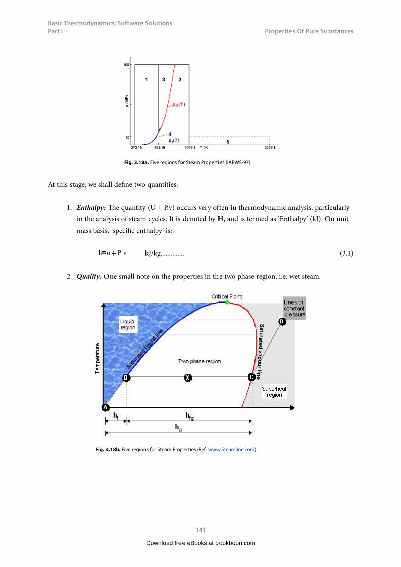
Basic Thermodynamics: Software Solutions Part I
141
Properties f Pure Substances
Fig. 3.18a. Five regions for Steam Properties (IAPWS-97)
At this stage, we shall define two quantities:
1. Enthalpy: The quantity (U + P.v) occurs very often in thermodynamic analysis, particularly in the analysis of steam cycles. It is denoted by H, and is termed as ‘Enthalpy’ (kJ). On unit mass basis, ‘specific enthalpy’ is:
h u P v kJ/kg.............. (3.1)
2. Quality: One small note on the properties in the two phase region, i.e. wet steam.
Fig. 3.18b. Five regions for Steam Properties (Ref: www.Steamline.com)
Download free eBooks at bookboon.com
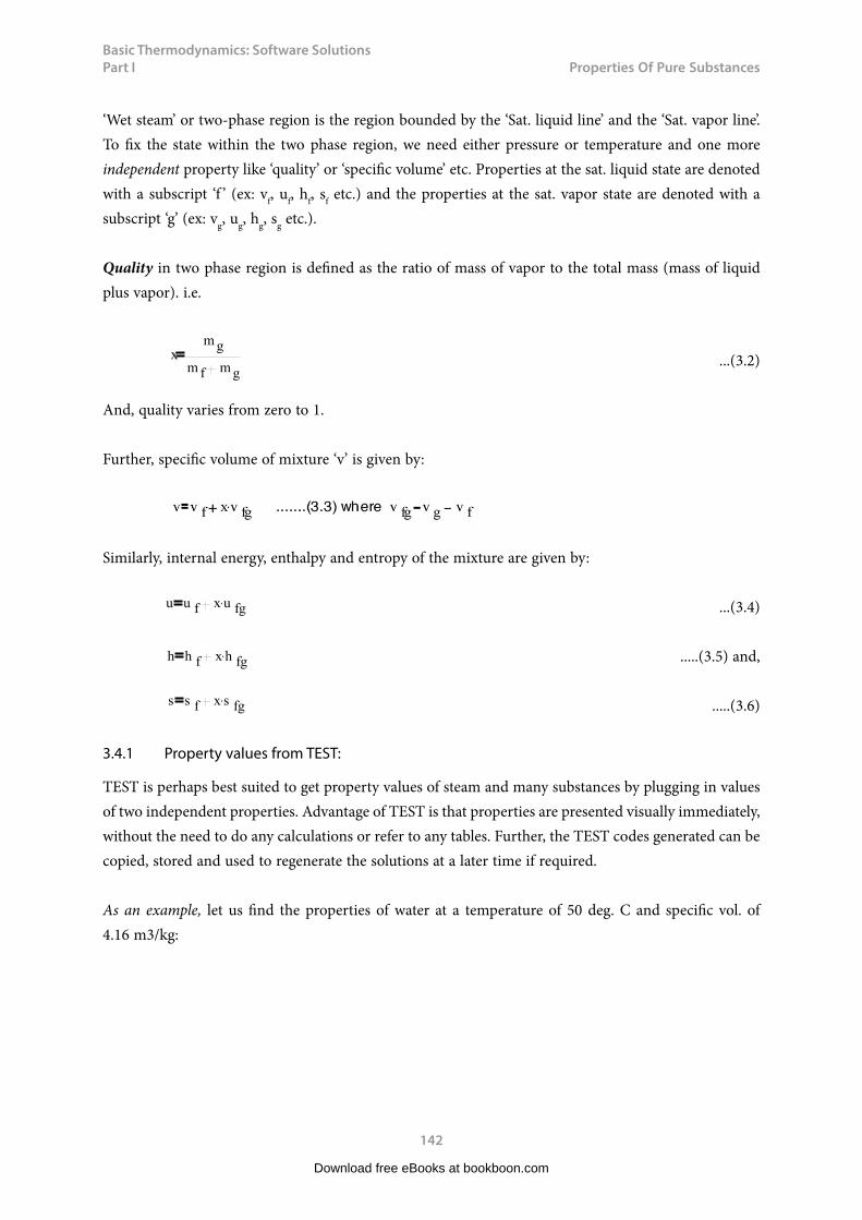
Basic Thermodynamics: Software Solutions Part I
142
Properties f Pure Substances
‘Wet steam’ or two-phase region is the region bounded by the ‘Sat. liquid line’ and the ‘Sat. vapor line’. To fix the state within the two phase region, we need either pressure or temperature and one more independent property like ‘quality’ or ‘specific volume’ etc. Properties at the sat. liquid state are denoted with a subscript ‘f ’ (ex: vf, uf, hf, sf etc.) and the properties at the sat. vapor state are denoted with a subscript ‘g’ (ex: vg, ug, hg, sg etc.).
Quality in two phase region is defined as the ratio of mass of vapor to the total mass (mass of liquid plus vapor). i.e.
xm g
m f m g
...............(3.2) ...(3.2)
And, quality varies from zero to 1.
Further, specific volume of mixture ‘v’ is given by:
Similarly, internal energy, enthalpy and entropy of the mixture are given by:
u u f x u fg ...(3.4)
h h f x h fg .....(3.5) and,
s s f x s fg .....(3.6)
3.4.1 Property values from TEST:
TEST is perhaps best suited to get property values of steam and many substances by plugging in values of two independent properties. Advantage of TEST is that properties are presented visually immediately, without the need to do any calculations or refer to any tables. Further, the TEST codes generated can be copied, stored and used to regenerate the solutions at a later time if required.
As an example, let us find the properties of water at a temperature of 50 deg. C and specific vol. of 4.16 m3/kg:
Download free eBooks at bookboon.com

Basic Thermodynamics: Software Solutions Part I
143
Properties f Pure Substances
Open TEST, Click Map > Uniform system > Phase Change model. (See Figs. 3.18a and 3.18b.). Following screen appears. H2O is automatically selected as the substance. State required is called as State 1. Select T1 and v1 and plug in the values given, as shown below:
Fig. 3.19a. Finding property values for H2O with TEST
Download free eBooks at bookboon.com
Click on the ad to read moreClick on the ad to read moreClick on the ad to read moreClick on the ad to read moreClick on the ad to read moreClick on the ad to read moreClick on the ad to read moreClick on the ad to read moreClick on the ad to read moreClick on the ad to read moreClick on the ad to read moreClick on the ad to read moreClick on the ad to read moreClick on the ad to read moreClick on the ad to read moreClick on the ad to read moreClick on the ad to read moreClick on the ad to read moreClick on the ad to read moreClick on the ad to read moreClick on the ad to read moreClick on the ad to read moreClick on the ad to read moreClick on the ad to read moreClick on the ad to read moreClick on the ad to read moreClick on the ad to read moreClick on the ad to read moreClick on the ad to read moreClick on the ad to read moreClick on the ad to read moreClick on the ad to read moreClick on the ad to read moreClick on the ad to read moreClick on the ad to read moreClick on the ad to read moreClick on the ad to read moreClick on the ad to read moreClick on the ad to read moreClick on the ad to read moreClick on the ad to read moreClick on the ad to read moreClick on the ad to read moreClick on the ad to read moreClick on the ad to read more
81,000 kmIn the past four years we have drilled
That’s more than twice around the world.
What will you be?
Who are we?We are the world’s leading oilfield services company. Working globally—often in remote and challenging locations—we invent, design, engineer, manufacture, apply, and maintain technology to help customers find and produce oil and gas safely.
Who are we looking for?We offer countless opportunities in the following domains:n Engineering, Research, and Operationsn Geoscience and Petrotechnicaln Commercial and Business
If you are a self-motivated graduate looking for a dynamic career, apply to join our team.
careers.slb.com
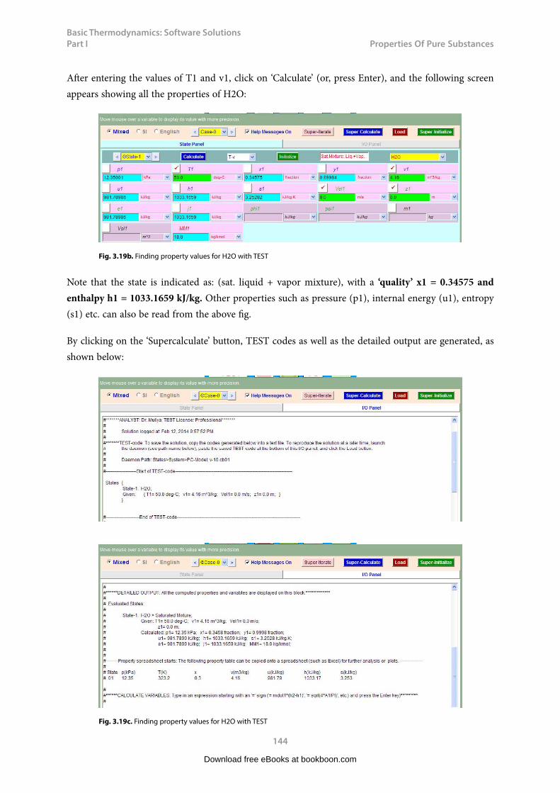
Basic Thermodynamics: Software Solutions Part I
144
Properties f Pure Substances
After entering the values of T1 and v1, click on ‘Calculate’ (or, press Enter), and the following screen appears showing all the properties of H2O:
Fig. 3.19b. Finding property values for H2O with TEST
Note that the state is indicated as: (sat. liquid + vapor mixture), with a ‘quality’ x1 = 0.34575 and enthalpy h1 = 1033.1659 kJ/kg. Other properties such as pressure (p1), internal energy (u1), entropy (s1) etc. can also be read from the above fig.
By clicking on the ‘Supercalculate’ button, TEST codes as well as the detailed output are generated, as shown below:
Fig. 3.19c. Finding property values for H2O with TEST
Download free eBooks at bookboon.com
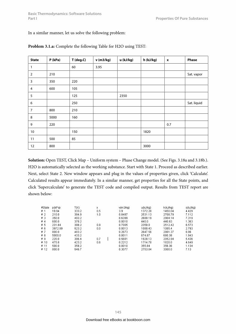
Basic Thermodynamics: Software Solutions Part I
145
Properties f Pure Substances
In a similar manner, let us solve the following problem:
Problem 3.1.a: Complete the following Table for H2O using TEST:
State P (kPa) T (deg.C) v (m3/kg) u (kJ/kg) h (kJ/kg) x Phase
1 60 3.95
2 210 Sat. vapor
3 350 220
4 600 105
5 125 2350
6 250 Sat. liquid
7 800 210
8 5000 160
9 220 0.7
10 150 1820
11 500 85
12 800 3000
Solution: Open TEST, Click Map – Uniform system – Phase Change model. (See Figs. 3.18a and 3.18b.). H2O is automatically selected as the working substance. Start with State 1. Proceed as described earlier. Next, select State 2. New window appears and plug in the values of properties given, click ‘Calculate’. Calculated results appear immediately. In a similar manner, get properties for all the State points, and click ‘Supercalculate’ to generate the TEST code and compiled output. Results from TEST report are shown below:
Download free eBooks at bookboon.com
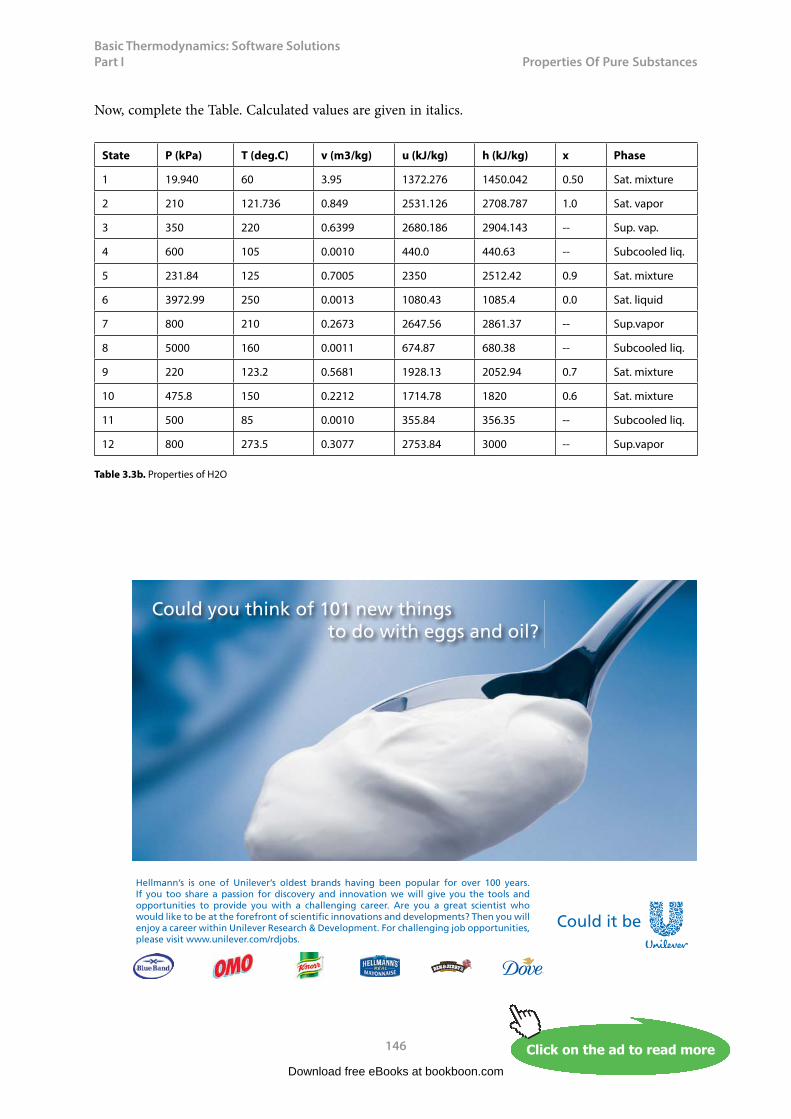
Basic Thermodynamics: Software Solutions Part I
146
Properties f Pure Substances
Now, complete the Table. Calculated values are given in italics.
State P (kPa) T (deg.C) v (m3/kg) u (kJ/kg) h (kJ/kg) x Phase
1 19.940 60 3.95 1372.276 1450.042 0.50 Sat. mixture
2 210 121.736 0.849 2531.126 2708.787 1.0 Sat. vapor
3 350 220 0.6399 2680.186 2904.143 -- Sup. vap.
4 600 105 0.0010 440.0 440.63 -- Subcooled liq.
5 231.84 125 0.7005 2350 2512.42 0.9 Sat. mixture
6 3972.99 250 0.0013 1080.43 1085.4 0.0 Sat. liquid
7 800 210 0.2673 2647.56 2861.37 -- Sup.vapor
8 5000 160 0.0011 674.87 680.38 -- Subcooled liq.
9 220 123.2 0.5681 1928.13 2052.94 0.7 Sat. mixture
10 475.8 150 0.2212 1714.78 1820 0.6 Sat. mixture
11 500 85 0.0010 355.84 356.35 -- Subcooled liq.
12 800 273.5 0.3077 2753.84 3000 -- Sup.vapor
Table 3.3b. Properties of H2O
Download free eBooks at bookboon.com
Click on the ad to read moreClick on the ad to read moreClick on the ad to read moreClick on the ad to read moreClick on the ad to read moreClick on the ad to read moreClick on the ad to read moreClick on the ad to read moreClick on the ad to read moreClick on the ad to read moreClick on the ad to read moreClick on the ad to read moreClick on the ad to read moreClick on the ad to read moreClick on the ad to read moreClick on the ad to read moreClick on the ad to read moreClick on the ad to read moreClick on the ad to read moreClick on the ad to read moreClick on the ad to read moreClick on the ad to read moreClick on the ad to read moreClick on the ad to read moreClick on the ad to read moreClick on the ad to read moreClick on the ad to read moreClick on the ad to read moreClick on the ad to read moreClick on the ad to read moreClick on the ad to read moreClick on the ad to read moreClick on the ad to read moreClick on the ad to read moreClick on the ad to read moreClick on the ad to read moreClick on the ad to read moreClick on the ad to read moreClick on the ad to read moreClick on the ad to read moreClick on the ad to read moreClick on the ad to read moreClick on the ad to read moreClick on the ad to read moreClick on the ad to read moreClick on the ad to read more
Hellmann’s is one of Unilever’s oldest brands having been popular for over 100 years. If you too share a passion for discovery and innovation we will give you the tools and opportunities to provide you with a challenging career. Are you a great scientist who would like to be at the forefront of scientific innovations and developments? Then you will enjoy a career within Unilever Research & Development. For challenging job opportunities, please visit www.unilever.com/rdjobs.
Could you think of 101 new thingsto do with eggs and oil?
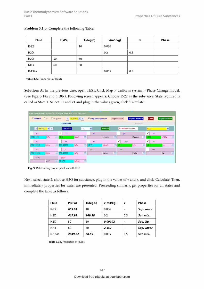
Basic Thermodynamics: Software Solutions Part I
147
Properties f Pure Substances
Problem 3.1.b: Complete the following Table:
Fluid P(kPa) T(deg.C) v(m3/kg) x Phase
R-22 10 0.036
H2O 0.2 0.5
H2O 50 60
NH3 60 30
R-134a 0.005 0.5
Table 3.3c. Properties of Fluids
Solution: As in the previous case, open TEST, Click Map > Uniform system > Phase Change model. (See Figs. 3.18a and 3.18b.). Following screen appears. Choose R-22 as the substance. State required is called as State 1. Select T1 and v1 and plug in the values given, click ‘Calculate’:
Fig. 3.19d. Finding property values with TEST
Next, select state 2, choose H2O for substance, plug in the values of v and x, and click ‘Calculate’. Then, immediately properties for water are presented. Proceeding similarly, get properties for all states and complete the table as follows:
Fluid P(kPa) T(deg.C) v(m3/kg) x Phase
R-22 659.61 10 0.036 - Sup. vapor
H2O 467.99 149.38 0.2 0.5 Sat. mix.
H2O 50 60 0.00102 - Sub. Liq.
NH3 60 30 2.452 - Sup. vapor
R-134a 2049.62 68.59 0.005 0.5 Sat. mix.
Table 3.3d. Properties of Fluids
Download free eBooks at bookboon.com
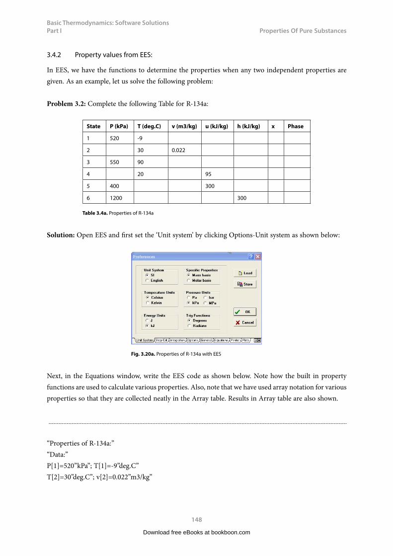
Basic Thermodynamics: Software Solutions Part I
148
Properties f Pure Substances
3.4.2 Property values from EES:
In EES, we have the functions to determine the properties when any two independent properties are given. As an example, let us solve the following problem:
Problem 3.2: Complete the following Table for R-134a:
State P (kPa) T (deg.C) v (m3/kg) u (kJ/kg) h (kJ/kg) x Phase
1 520 -9
2 30 0.022
3 550 90
4 20 95
5 400 300
6 1200 300
Table 3.4a. Properties of R-134a
Solution: Open EES and first set the ‘Unit system’ by clicking Options-Unit system as shown below:
Fig. 3.20a. Properties of R-134a with EES
Next, in the Equations window, write the EES code as shown below. Note how the built in property functions are used to calculate various properties. Also, note that we have used array notation for various properties so that they are collected neatly in the Array table. Results in Array table are also shown.
“Properties of R-134a:”“Data:”P[1]=520”kPa”; T[1]=-9”deg.C”T[2]=30”deg.C”; v[2]=0.022”m3/kg”
Download free eBooks at bookboon.com

Basic Thermodynamics: Software Solutions Part I
149
Properties f Pure Substances
P[3]=550”kPa”; T[3]=90”deg.C”T[4]=20”deg.C”; u[4]=95”kJ/kg”P[5]=400”kPa”;u[5]=300”kJ/kg”P[6]=1200”kPa”; h[6]=300”kJ/kg”
“Calculate properties for State 1:”v[1]=VOLUME(R134a,T=T[1],P=P[1]) “calculates sp. volume”u[1]=INTENERGY(R134a,T=T[1],P=P[1]) “calclulates int. energy”h[1]=ENTHALPY(R134a,T=T[1],P=P[1]) “calculates sp. enthalpy”x[1]=QUALITY(R134a,h=h[1],P=P[1]) “calculates quality (dryness fraction)”
“Calculate properties for State 2:”P[2]=PRESSURE(R134a,T=T[2],v=v[2]) “calculates pressure”u[2]=INTENERGY(R134a,T=T[2],v=v[2]) “calculates int. energy”h[2]=ENTHALPY(R134a,T=T[2],v=v[2]) “calculates sp. enthalpy”x[2]=QUALITY(R134a,h=h[2],P=P[2]) “calculates quality (dryness fraction)”
“Calculate properties for State 3:”v[3]=VOLUME(R134a,T=T[3],P=P[3]) “calculates sp. volume”u[3]=INTENERGY(R134a,T=T[3],v=v[3]) “calculates int. energy”h[3]=ENTHALPY(R134a,T=T[3],v=v[3]) “calculates sp. enthalpy”x[3]=QUALITY(R134a,h=h[3],P=P[3]) “calculates quality (dryness fraction)”
«Calculate properties for State 4:»P[4]=PRESSURE(R134a,T=T[4],u=u[4]) «calculates pressure»v[4]=VOLUME(R134a,T=T[4],u=u[4]) «calculates sp. volume»h[4]=ENTHALPY(R134a,T=T[4],v=v[4]) “calculates sp. enthalpy”x[4]=QUALITY(R134a,h=h[4],P=P[4]) “calculates quality (dryness fraction)”
“Calculate properties for State 5:”v[5]=VOLUME(R134a,P=P[5],u=u[5]) “calculates sp. volume”T[5]=TEMPERATURE(R134a,u=u[5],P=P[5]) “calculates temperature”h[5]=ENTHALPY(R134a,T=T[5],v=v[5]) “calculates enthalpy”x[5]=QUALITY(R134a,h=h[5],P=P[5]) “calculates quality (dryness fraction)”
“Calculate properties for State 6:”v[6]=VOLUME(R134a,P=P[6],h=h[6]) “calculates sp. volume”T[6]=TEMPERATURE(R134a,h=h[6],P=P[6]) “calculates temperature”u[6]=INTENERGY(R134a,T=T[6],v=v[6]) “calculates int. energy”x[6]=QUALITY(R134a,h=h[6],P=P[6]) “calculates quality (dryness fraction)”
Download free eBooks at bookboon.com

Basic Thermodynamics: Software Solutions Part I
150
Properties f Pure Substances
Fig. 3.20b. Array Table
Download free eBooks at bookboon.com
Click on the ad to read moreClick on the ad to read moreClick on the ad to read moreClick on the ad to read moreClick on the ad to read moreClick on the ad to read moreClick on the ad to read moreClick on the ad to read moreClick on the ad to read moreClick on the ad to read moreClick on the ad to read moreClick on the ad to read moreClick on the ad to read moreClick on the ad to read moreClick on the ad to read moreClick on the ad to read moreClick on the ad to read moreClick on the ad to read moreClick on the ad to read moreClick on the ad to read moreClick on the ad to read moreClick on the ad to read moreClick on the ad to read moreClick on the ad to read moreClick on the ad to read moreClick on the ad to read moreClick on the ad to read moreClick on the ad to read moreClick on the ad to read moreClick on the ad to read moreClick on the ad to read moreClick on the ad to read moreClick on the ad to read moreClick on the ad to read moreClick on the ad to read moreClick on the ad to read moreClick on the ad to read moreClick on the ad to read moreClick on the ad to read moreClick on the ad to read moreClick on the ad to read moreClick on the ad to read moreClick on the ad to read moreClick on the ad to read moreClick on the ad to read moreClick on the ad to read moreClick on the ad to read more
© Deloitte & Touche LLP and affiliated entities.
360°thinking.
Discover the truth at www.deloitte.ca/careers
© Deloitte & Touche LLP and affiliated entities.
360°thinking.
Discover the truth at www.deloitte.ca/careers
© Deloitte & Touche LLP and affiliated entities.
360°thinking.
Discover the truth at www.deloitte.ca/careers © Deloitte & Touche LLP and affiliated entities.
360°thinking.
Discover the truth at www.deloitte.ca/careers
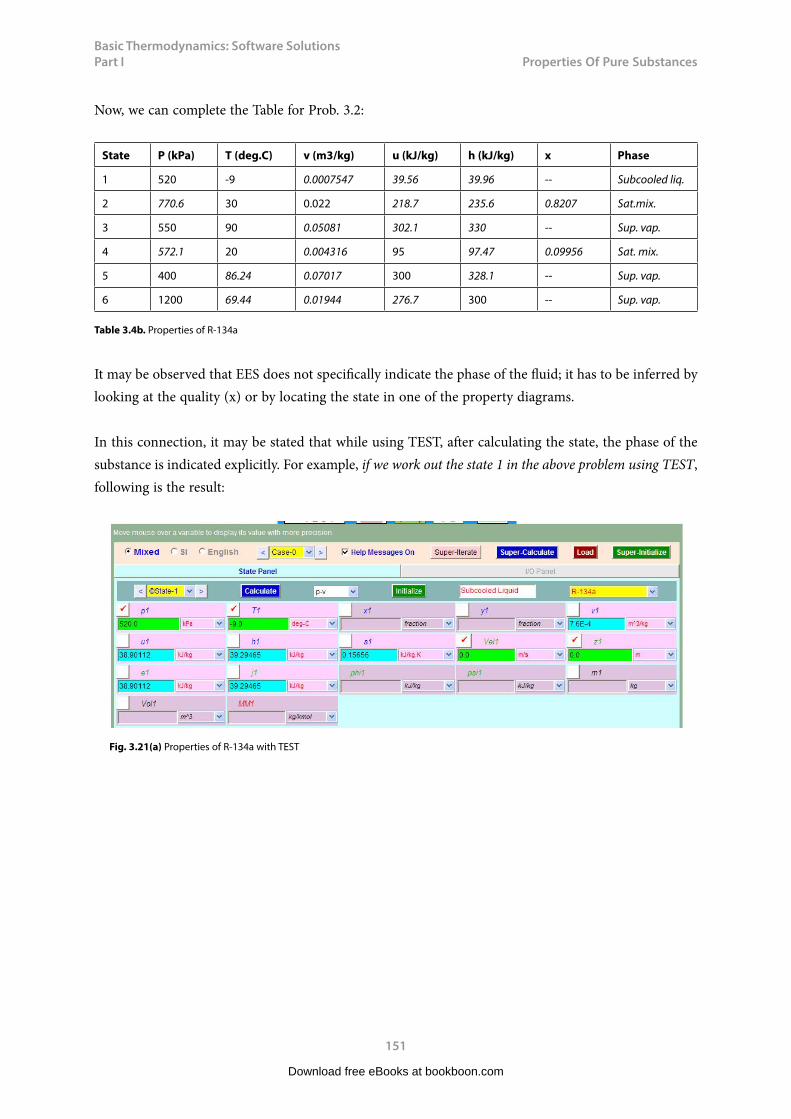
Basic Thermodynamics: Software Solutions Part I
151
Properties f Pure Substances
Now, we can complete the Table for Prob. 3.2:
State P (kPa) T (deg.C) v (m3/kg) u (kJ/kg) h (kJ/kg) x Phase
1 520 -9 0.0007547 39.56 39.96 -- Subcooled liq.
2 770.6 30 0.022 218.7 235.6 0.8207 Sat.mix.
3 550 90 0.05081 302.1 330 -- Sup. vap.
4 572.1 20 0.004316 95 97.47 0.09956 Sat. mix.
5 400 86.24 0.07017 300 328.1 -- Sup. vap.
6 1200 69.44 0.01944 276.7 300 -- Sup. vap.
Table 3.4b. Properties of R-134a
It may be observed that EES does not specifically indicate the phase of the fluid; it has to be inferred by looking at the quality (x) or by locating the state in one of the property diagrams.
In this connection, it may be stated that while using TEST, after calculating the state, the phase of the substance is indicated explicitly. For example, if we work out the state 1 in the above problem using TEST, following is the result:
Fig. 3.21(a) Properties of R-134a with TEST
Download free eBooks at bookboon.com
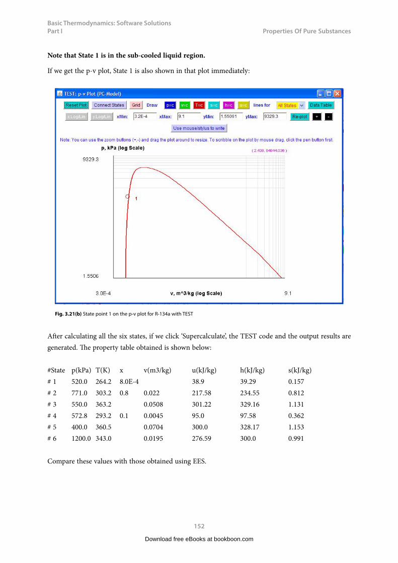
Basic Thermodynamics: Software Solutions Part I
152
Properties f Pure Substances
Note that State 1 is in the sub-cooled liquid region.
If we get the p-v plot, State 1 is also shown in that plot immediately:
Fig. 3.21(b) State point 1 on the p-v plot for R-134a with TEST
After calculating all the six states, if we click ‘Supercalculate’, the TEST code and the output results are generated. The property table obtained is shown below:
#State p(kPa) T(K) x v(m3/kg) u(kJ/kg) h(kJ/kg) s(kJ/kg)# 1 520.0 264.2 8.0E-4 38.9 39.29 0.157# 2 771.0 303.2 0.8 0.022 217.58 234.55 0.812# 3 550.0 363.2 0.0508 301.22 329.16 1.131# 4 572.8 293.2 0.1 0.0045 95.0 97.58 0.362# 5 400.0 360.5 0.0704 300.0 328.17 1.153# 6 1200.0 343.0 0.0195 276.59 300.0 0.991
Compare these values with those obtained using EES.
Download free eBooks at bookboon.com
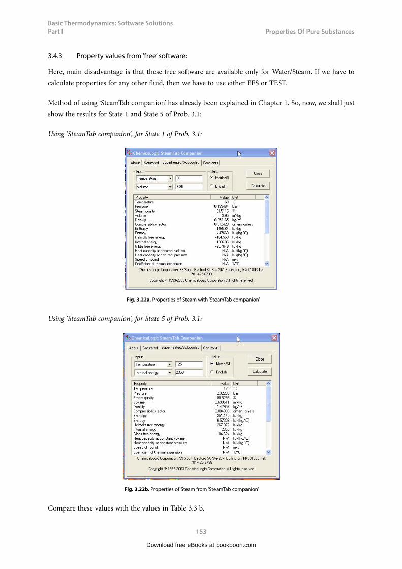
Basic Thermodynamics: Software Solutions Part I
153
Properties f Pure Substances
3.4.3 Property values from ‘free’ software:
Here, main disadvantage is that these free software are available only for Water/Steam. If we have to calculate properties for any other fluid, then we have to use either EES or TEST.
Method of using ‘SteamTab companion’ has already been explained in Chapter 1. So, now, we shall just show the results for State 1 and State 5 of Prob. 3.1:
Using ‘SteamTab companion’, for State 1 of Prob. 3.1:
Fig. 3.22a. Properties of Steam with ‘SteamTab companion’
Using ‘SteamTab companion’, for State 5 of Prob. 3.1:
Fig. 3.22b. Properties of Steam from ‘SteamTab companion’
Compare these values with the values in Table 3.3 b.
Download free eBooks at bookboon.com

Basic Thermodynamics: Software Solutions Part I
154
Properties f Pure Substances
3.4.4 Property values from ‘online software’:
3.4.4.1 From NIST Website:
Property values can be calculated online for many fluids. Most popular and versatile online software is from NIST, which can give all types of data and graphs for a huge number of fluids. Go to: http://webbook.nist.gov/chemistry/fluid/. Following window appears:
Download free eBooks at bookboon.com
Click on the ad to read moreClick on the ad to read moreClick on the ad to read moreClick on the ad to read moreClick on the ad to read moreClick on the ad to read moreClick on the ad to read moreClick on the ad to read moreClick on the ad to read moreClick on the ad to read moreClick on the ad to read moreClick on the ad to read moreClick on the ad to read moreClick on the ad to read moreClick on the ad to read moreClick on the ad to read moreClick on the ad to read moreClick on the ad to read moreClick on the ad to read moreClick on the ad to read moreClick on the ad to read moreClick on the ad to read moreClick on the ad to read moreClick on the ad to read moreClick on the ad to read moreClick on the ad to read moreClick on the ad to read moreClick on the ad to read moreClick on the ad to read moreClick on the ad to read moreClick on the ad to read moreClick on the ad to read moreClick on the ad to read moreClick on the ad to read moreClick on the ad to read moreClick on the ad to read moreClick on the ad to read moreClick on the ad to read moreClick on the ad to read moreClick on the ad to read moreClick on the ad to read moreClick on the ad to read moreClick on the ad to read moreClick on the ad to read moreClick on the ad to read moreClick on the ad to read moreClick on the ad to read moreClick on the ad to read more
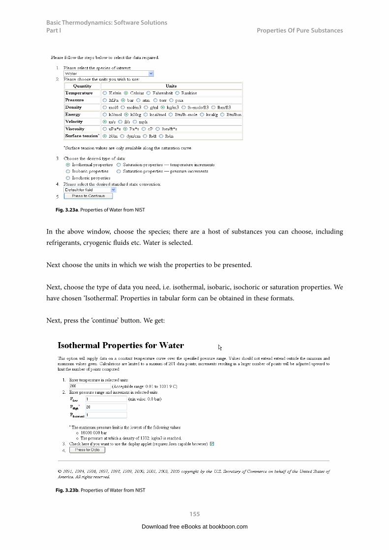
Basic Thermodynamics: Software Solutions Part I
155
Properties f Pure Substances
Fig. 3.23a. Properties of Water from NIST
In the above window, choose the species; there are a host of substances you can choose, including refrigerants, cryogenic fluids etc. Water is selected.
Next choose the units in which we wish the properties to be presented.
Next, choose the type of data you need, i.e. isothermal, isobaric, isochoric or saturation properties. We have chosen ‘Isothermal’. Properties in tabular form can be obtained in these formats.
Next, press the ‘continue’ button. We get:
Fig. 3.23b. Properties of Water from NIST
Download free eBooks at bookboon.com
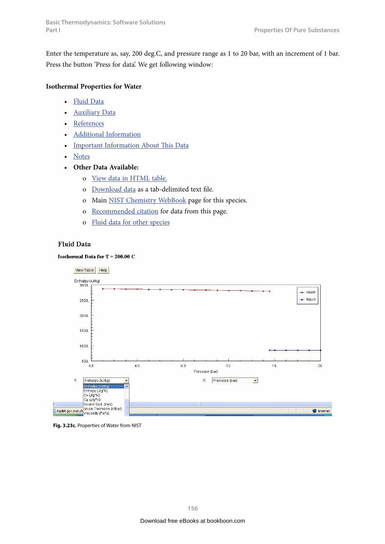
Basic Thermodynamics: Software Solutions Part I
156
Properties f Pure Substances
Enter the temperature as, say, 200 deg.C, and pressure range as 1 to 20 bar, with an increment of 1 bar. Press the button ‘Press for data’. We get following window:
Isothermal Properties for Water
• Fluid Data • Auxiliary Data • References • Additional Information • Important Information About This Data • Notes • Other Data Available:
ο View data in HTML table. ο Download data as a tab-delimited text file. ο Main NIST Chemistry WebBook page for this species. ο Recommended citation for data from this page. ο Fluid data for other species
Fig. 3.23c. Properties of Water from NIST
Download free eBooks at bookboon.com
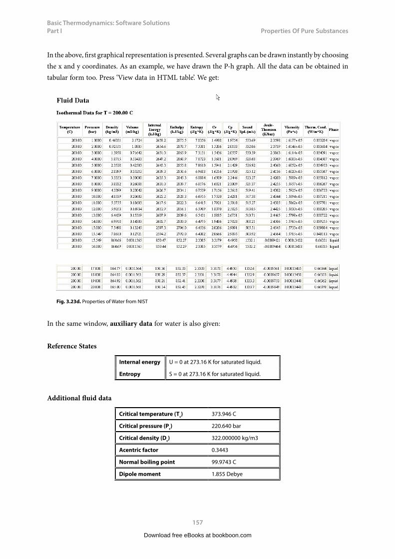
Basic Thermodynamics: Software Solutions Part I
157
Properties f Pure Substances
In the above, first graphical representation is presented. Several graphs can be drawn instantly by choosing the x and y coordinates. As an example, we have drawn the P-h graph. All the data can be obtained in tabular form too. Press ‘View data in HTML table’. We get:
Fig. 3.23d. Properties of Water from NIST
In the same window, auxiliary data for water is also given:
Reference States
Internal energy U = 0 at 273.16 K for saturated liquid.
Entropy S = 0 at 273.16 K for saturated liquid.
Additional fluid data
Critical temperature (Tc) 373.946 C
Critical pressure (Pc) 220.640 bar
Critical density (Dc) 322.000000 kg/m3
Acentric factor 0.3443
Normal boiling point 99.9743 C
Dipole moment 1.855 Debye
Download free eBooks at bookboon.com
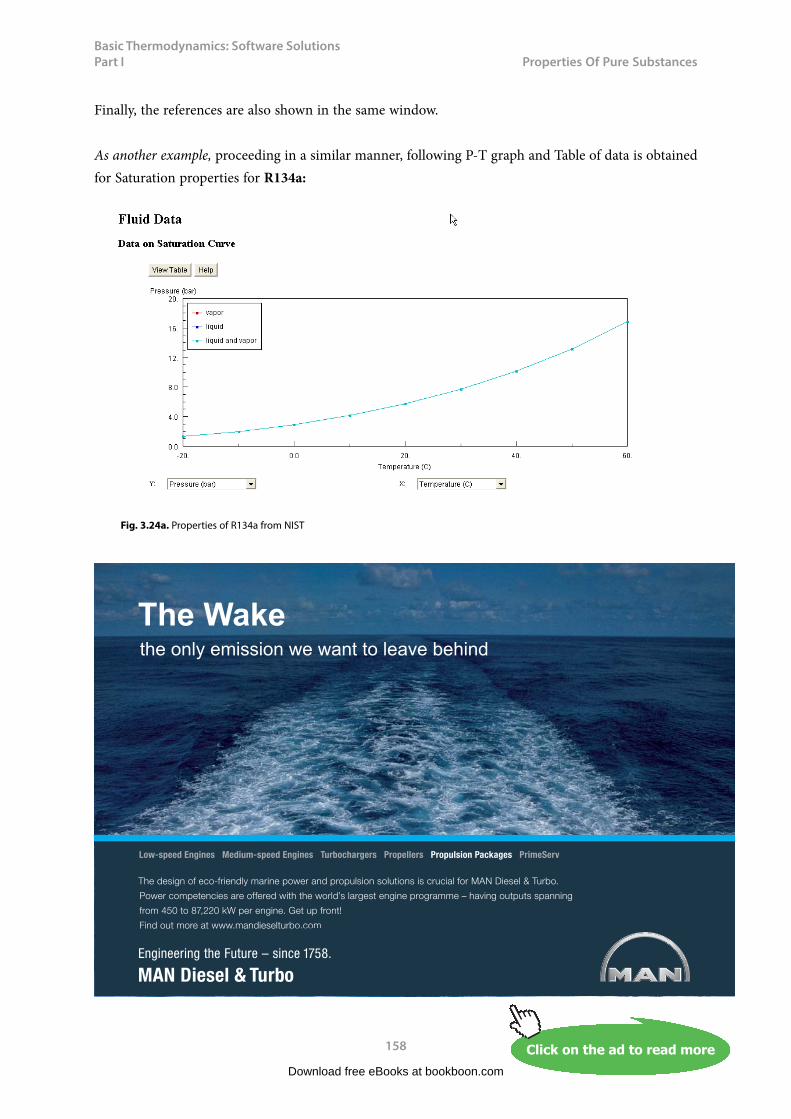
Basic Thermodynamics: Software Solutions Part I
158
Properties f Pure Substances
Finally, the references are also shown in the same window.
As another example, proceeding in a similar manner, following P-T graph and Table of data is obtained for Saturation properties for R134a:
Fig. 3.24a. Properties of R134a from NIST
Download free eBooks at bookboon.com
Click on the ad to read moreClick on the ad to read moreClick on the ad to read moreClick on the ad to read moreClick on the ad to read moreClick on the ad to read moreClick on the ad to read moreClick on the ad to read moreClick on the ad to read moreClick on the ad to read moreClick on the ad to read moreClick on the ad to read moreClick on the ad to read moreClick on the ad to read moreClick on the ad to read moreClick on the ad to read moreClick on the ad to read moreClick on the ad to read moreClick on the ad to read moreClick on the ad to read moreClick on the ad to read moreClick on the ad to read moreClick on the ad to read moreClick on the ad to read moreClick on the ad to read moreClick on the ad to read moreClick on the ad to read moreClick on the ad to read moreClick on the ad to read moreClick on the ad to read moreClick on the ad to read moreClick on the ad to read moreClick on the ad to read moreClick on the ad to read moreClick on the ad to read moreClick on the ad to read moreClick on the ad to read moreClick on the ad to read moreClick on the ad to read moreClick on the ad to read moreClick on the ad to read moreClick on the ad to read moreClick on the ad to read moreClick on the ad to read moreClick on the ad to read moreClick on the ad to read moreClick on the ad to read moreClick on the ad to read moreClick on the ad to read more
������������� ����������������������������������������������� �� ���������������������������
������ ������ ������������������������������ ����������������������!���"���������������
�����#$%����&'())%�*+����������,����������-
.��������������������������������� ��
���������� ���������������� ������������� ���������������������������� �����������
The Wakethe only emission we want to leave behind
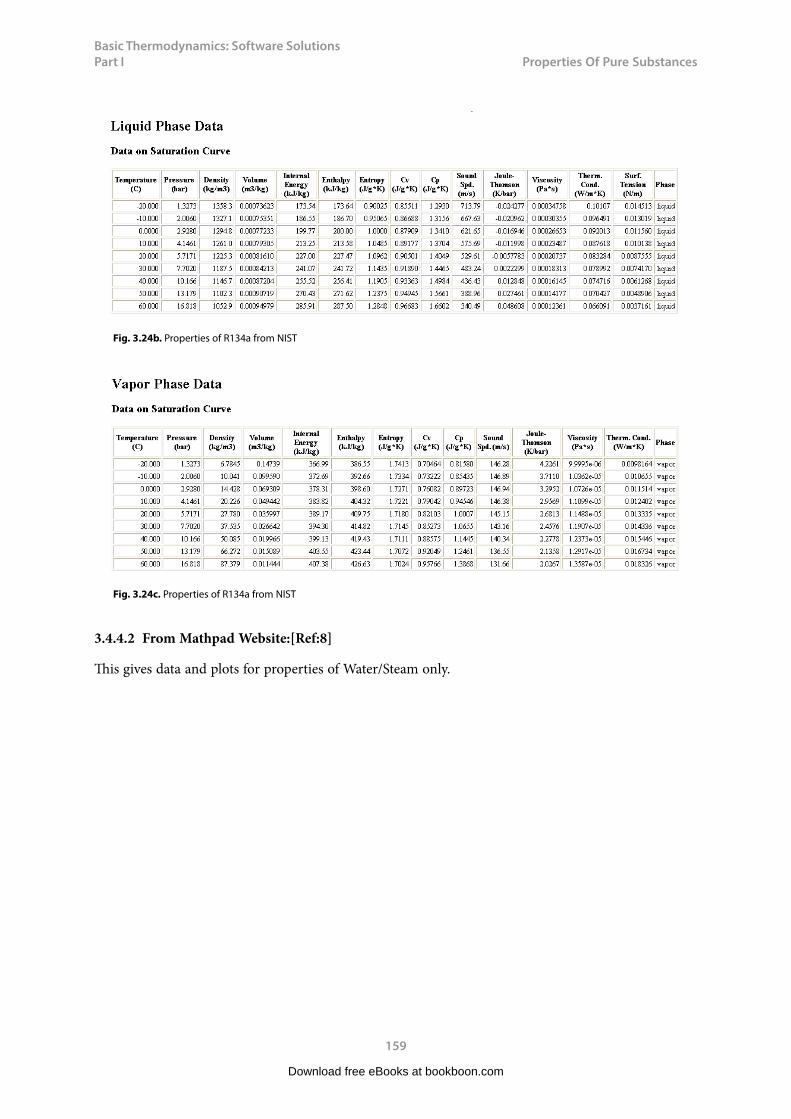
Basic Thermodynamics: Software Solutions Part I
159
Properties f Pure Substances
Fig. 3.24b. Properties of R134a from NIST
Fig. 3.24c. Properties of R134a from NIST
3.4.4.2 From Mathpad Website:[Ref:8]
This gives data and plots for properties of Water/Steam only.
Download free eBooks at bookboon.com
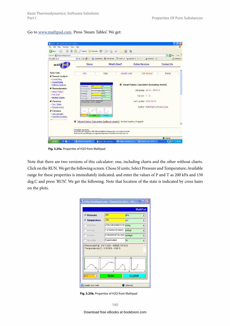
Basic Thermodynamics: Software Solutions Part I
160
Properties f Pure Substances
Go to www.mathpad.com. Press ‘Steam Tables’. We get:
Fig. 3.25a. Properties of H2O from Mathpad
Note that there are two versions of this calculator: one, including charts and the other without charts. Click on the RUN. We get the following screen. Chose SI units. Select Pressure and Temperature; Available range for these properties is immediately indicated, and enter the values of P and T as 200 kPa and 150 deg.C and press ‘RUN’. We get the following. Note that location of the state is indicated by cross hairs on the plots.
Fig. 3.25b. Properties of H2O from Mathpad
Download free eBooks at bookboon.com

Basic Thermodynamics: Software Solutions Part I
161
Properties f Pure Substances
If you click on the ‘Steam Tables calculator (without charts)’, you get the following screen:
Fig. 3.25c. Properties of H2O from Mathpad
Download free eBooks at bookboon.com
Click on the ad to read moreClick on the ad to read moreClick on the ad to read moreClick on the ad to read moreClick on the ad to read moreClick on the ad to read moreClick on the ad to read moreClick on the ad to read moreClick on the ad to read moreClick on the ad to read moreClick on the ad to read moreClick on the ad to read moreClick on the ad to read moreClick on the ad to read moreClick on the ad to read moreClick on the ad to read moreClick on the ad to read moreClick on the ad to read moreClick on the ad to read moreClick on the ad to read moreClick on the ad to read moreClick on the ad to read moreClick on the ad to read moreClick on the ad to read moreClick on the ad to read moreClick on the ad to read moreClick on the ad to read moreClick on the ad to read moreClick on the ad to read moreClick on the ad to read moreClick on the ad to read moreClick on the ad to read moreClick on the ad to read moreClick on the ad to read moreClick on the ad to read moreClick on the ad to read moreClick on the ad to read moreClick on the ad to read moreClick on the ad to read moreClick on the ad to read moreClick on the ad to read moreClick on the ad to read moreClick on the ad to read moreClick on the ad to read moreClick on the ad to read moreClick on the ad to read moreClick on the ad to read moreClick on the ad to read moreClick on the ad to read moreClick on the ad to read more
CAREERKICKSTARTAn app to keep you in the know
Whether you’re a graduate, school leaver or student, it’s a difficult time to start your career. So here at RBS, we’re providing a helping hand with our new Facebook app. Bringing together the most relevant and useful careers information, we’ve created a one-stop shop designed to help you get on the career ladder – whatever your level of education, degree subject or work experience.
And it’s not just finance-focused either. That’s because it’s not about us. It’s about you. So download the app and you’ll get everything you need to know to kickstart your career.
So what are you waiting for?
Click here to get started.
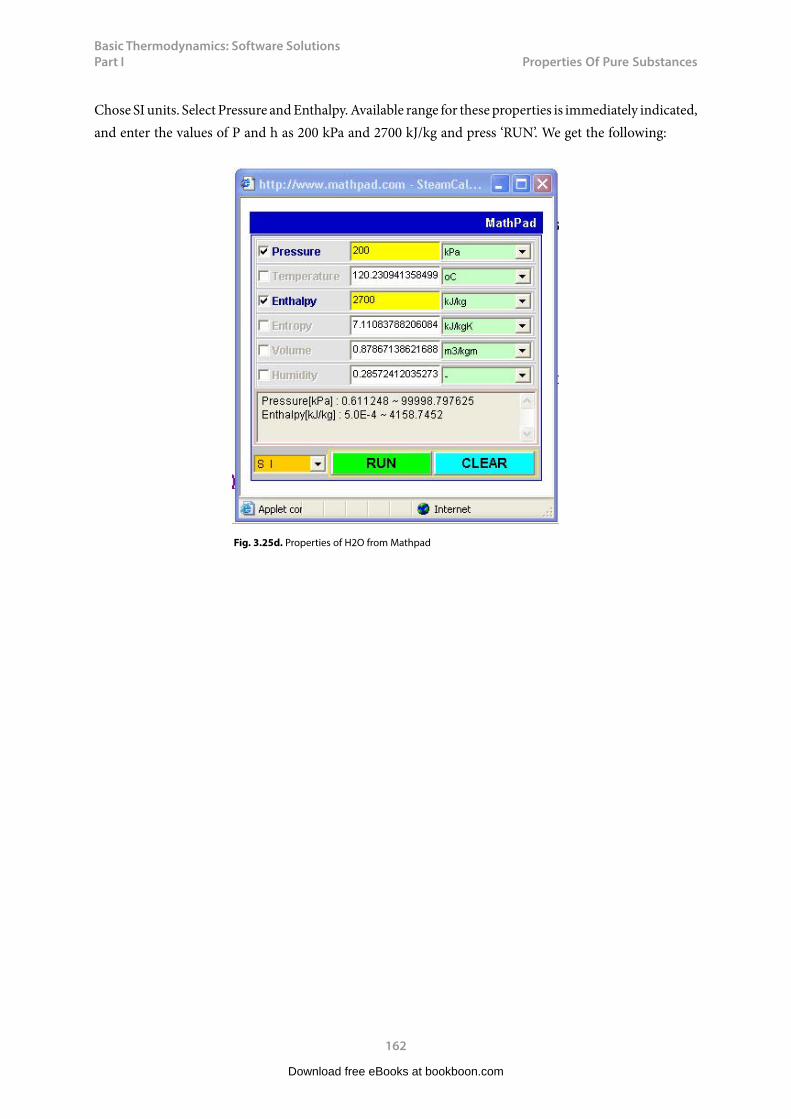
Basic Thermodynamics: Software Solutions Part I
162
Properties f Pure Substances
Chose SI units. Select Pressure and Enthalpy. Available range for these properties is immediately indicated, and enter the values of P and h as 200 kPa and 2700 kJ/kg and press ‘RUN’. We get the following:
Fig. 3.25d. Properties of H2O from Mathpad
Download free eBooks at bookboon.com

Basic Thermodynamics: Software Solutions Part I
163
Properties f Pure Substances
3.4.4.3 From Moscow Power Engg. Institute (MPEI) Website [Ref: 13]:
Properties of Water/Steam are presented in a comprehensive manner in this Website. Data are calculated in a Mathcad calculation server. As you open the website, following screen is presented, with several possible choices.
Fig. 3.26. Properties of H2O from MPEI
Download free eBooks at bookboon.com

Basic Thermodynamics: Software Solutions Part I
164
Properties f Pure Substances
As an example of its use, let us calculate the properties of sat. water and steam with chart as a function of temperature (t). Click on the appropriate button on the page as shown and enter 50 deg.C for t; following results and plots appear:
Download free eBooks at bookboon.com
Click on the ad to read moreClick on the ad to read moreClick on the ad to read moreClick on the ad to read moreClick on the ad to read moreClick on the ad to read moreClick on the ad to read moreClick on the ad to read moreClick on the ad to read moreClick on the ad to read moreClick on the ad to read moreClick on the ad to read moreClick on the ad to read moreClick on the ad to read moreClick on the ad to read moreClick on the ad to read moreClick on the ad to read moreClick on the ad to read moreClick on the ad to read moreClick on the ad to read moreClick on the ad to read moreClick on the ad to read moreClick on the ad to read moreClick on the ad to read moreClick on the ad to read moreClick on the ad to read moreClick on the ad to read moreClick on the ad to read moreClick on the ad to read moreClick on the ad to read moreClick on the ad to read moreClick on the ad to read moreClick on the ad to read moreClick on the ad to read moreClick on the ad to read moreClick on the ad to read moreClick on the ad to read moreClick on the ad to read moreClick on the ad to read moreClick on the ad to read moreClick on the ad to read moreClick on the ad to read moreClick on the ad to read moreClick on the ad to read moreClick on the ad to read moreClick on the ad to read moreClick on the ad to read moreClick on the ad to read moreClick on the ad to read moreClick on the ad to read moreClick on the ad to read more
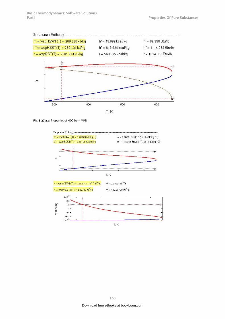
Basic Thermodynamics: Software Solutions Part I
165
Properties f Pure Substances
Fig. 3.27 a,b. Properties of H2O from MPEI
Download free eBooks at bookboon.com
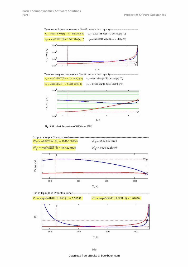
Basic Thermodynamics: Software Solutions Part I
166
Properties f Pure Substances
Fig. 3.27 c,d,e,f. Properties of H2O from MPEI
Download free eBooks at bookboon.com

Basic Thermodynamics: Software Solutions Part I
167
Properties f Pure Substances
Fig. 3.27 g,h,i. Properties of H2O from MPEI
Download free eBooks at bookboon.com
Click on the ad to read moreClick on the ad to read moreClick on the ad to read moreClick on the ad to read moreClick on the ad to read moreClick on the ad to read moreClick on the ad to read moreClick on the ad to read moreClick on the ad to read moreClick on the ad to read moreClick on the ad to read moreClick on the ad to read moreClick on the ad to read moreClick on the ad to read moreClick on the ad to read moreClick on the ad to read moreClick on the ad to read moreClick on the ad to read moreClick on the ad to read moreClick on the ad to read moreClick on the ad to read moreClick on the ad to read moreClick on the ad to read moreClick on the ad to read moreClick on the ad to read moreClick on the ad to read moreClick on the ad to read moreClick on the ad to read moreClick on the ad to read moreClick on the ad to read moreClick on the ad to read moreClick on the ad to read moreClick on the ad to read moreClick on the ad to read moreClick on the ad to read moreClick on the ad to read moreClick on the ad to read moreClick on the ad to read moreClick on the ad to read moreClick on the ad to read moreClick on the ad to read moreClick on the ad to read moreClick on the ad to read moreClick on the ad to read moreClick on the ad to read moreClick on the ad to read moreClick on the ad to read moreClick on the ad to read moreClick on the ad to read moreClick on the ad to read moreClick on the ad to read moreClick on the ad to read more
AXA Global Graduate Program
Find out more and apply
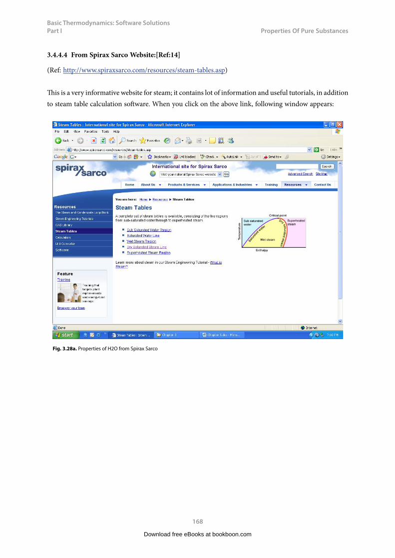
Basic Thermodynamics: Software Solutions Part I
168
Properties f Pure Substances
3.4.4.4 From Spirax Sarco Website:[Ref:14]
(Ref: http://www.spiraxsarco.com/resources/steam-tables.asp)
This is a very informative website for steam; it contains lot of information and useful tutorials, in addition to steam table calculation software. When you click on the above link, following window appears:
Fig. 3.28a. Properties of H2O from Spirax Sarco
Download free eBooks at bookboon.com
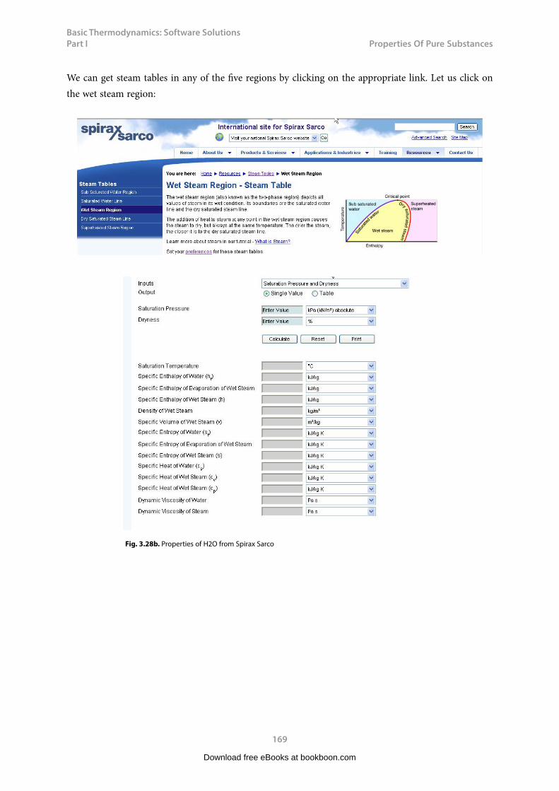
Basic Thermodynamics: Software Solutions Part I
169
Properties f Pure Substances
We can get steam tables in any of the five regions by clicking on the appropriate link. Let us click on the wet steam region:
Fig. 3.28b. Properties of H2O from Spirax Sarco
Download free eBooks at bookboon.com

Basic Thermodynamics: Software Solutions Part I
170
Properties f Pure Substances
Note that you can get output for a single point (state) or you can generate a table for a set of states. Let us get property at a single point. Input can be pressure and quality (dryness) or other combinations which can be chosen from the widget. For now, enter Psat = 200 kPa and dryness = 80%. Press ‘Calculate’. You get:
Fig. 3.28c. Properties of H2O from Spirax Sarco
3.4.5 Property Tables:
Many times, values of properties are required in a tabular form for reference. Tables can be obtained in the given range immediately from some of these software.
3.4.5.1 Property table from NIST:
This has already been explained under article 3.4.4. Advantage of NIST website is that you can get property table and several types of plots not only for Water but also for a very large number of fluids. So, it is a very useful site and should always be kept in mind while looking for properties of substances.
Download free eBooks at bookboon.com

Basic Thermodynamics: Software Solutions Part I
171
Properties f Pure Substances
3.4.5.2 Property table from Spirax Sarco:
Click on http://www.spiraxsarco.com/resources/steam-tables.asp). Then click on Superheated region. Select the Inputs as Superheated temperature and pressure, and Outputs as Table:
Fig. 3.29a.Properties of H2O from Spirax Sarco
Download free eBooks at bookboon.com
Click on the ad to read moreClick on the ad to read moreClick on the ad to read moreClick on the ad to read moreClick on the ad to read moreClick on the ad to read moreClick on the ad to read moreClick on the ad to read moreClick on the ad to read moreClick on the ad to read moreClick on the ad to read moreClick on the ad to read moreClick on the ad to read moreClick on the ad to read moreClick on the ad to read moreClick on the ad to read moreClick on the ad to read moreClick on the ad to read moreClick on the ad to read moreClick on the ad to read moreClick on the ad to read moreClick on the ad to read moreClick on the ad to read moreClick on the ad to read moreClick on the ad to read moreClick on the ad to read moreClick on the ad to read moreClick on the ad to read moreClick on the ad to read moreClick on the ad to read moreClick on the ad to read moreClick on the ad to read moreClick on the ad to read moreClick on the ad to read moreClick on the ad to read moreClick on the ad to read moreClick on the ad to read moreClick on the ad to read moreClick on the ad to read moreClick on the ad to read moreClick on the ad to read moreClick on the ad to read moreClick on the ad to read moreClick on the ad to read moreClick on the ad to read moreClick on the ad to read moreClick on the ad to read moreClick on the ad to read moreClick on the ad to read moreClick on the ad to read moreClick on the ad to read moreClick on the ad to read moreClick on the ad to read more
Designed for high-achieving graduates across all disciplines, London Business School’s Masters in Management provides specific and tangible foundations for a successful career in business.
This 12-month, full-time programme is a business qualification with impact. In 2010, our MiM employment rate was 95% within 3 months of graduation*; the majority of graduates choosing to work in consulting or financial services.
As well as a renowned qualification from a world-class business school, you also gain access to the School’s network of more than 34,000 global alumni – a community that offers support and opportunities throughout your career.
For more information visit www.london.edu/mm, email [email protected] or give us a call on +44 (0)20 7000 7573.
Masters in Management
The next step for top-performing graduates
* Figures taken from London Business School’s Masters in Management 2010 employment report
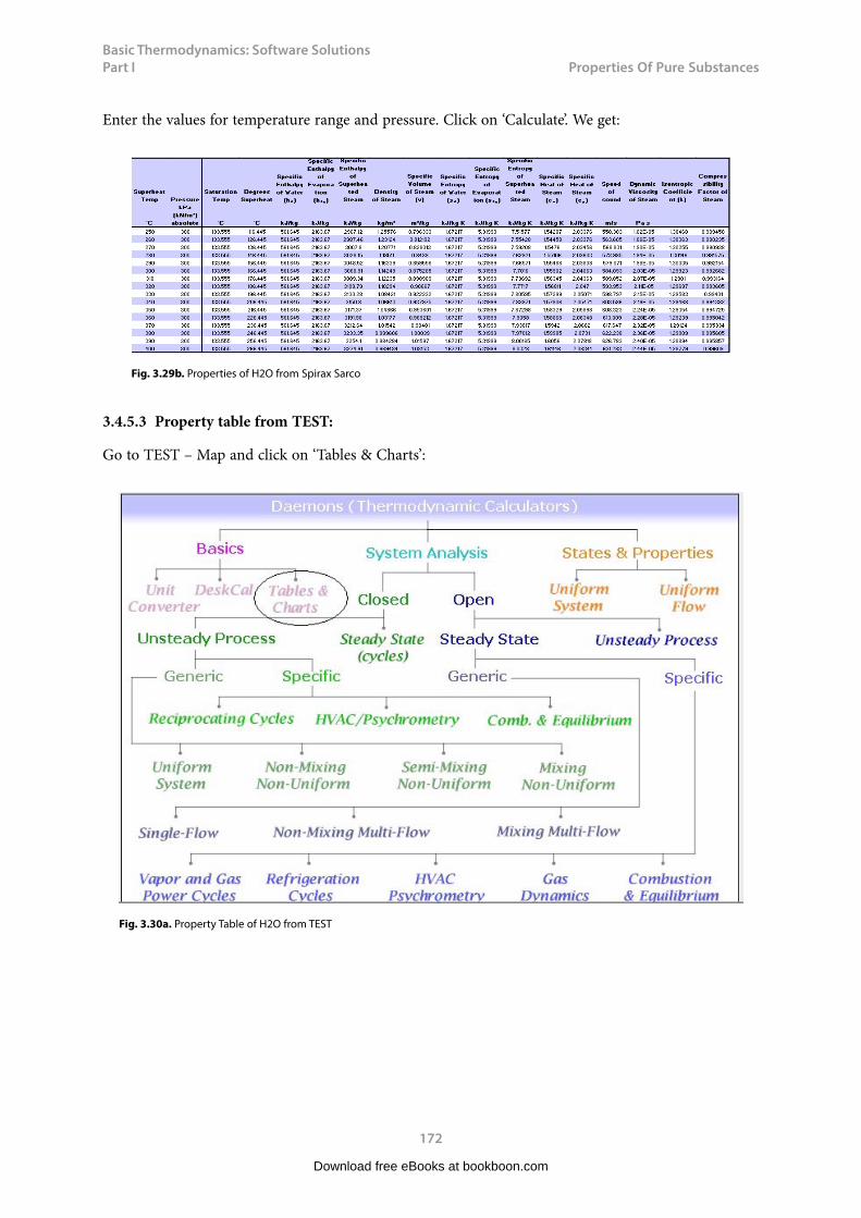
Basic Thermodynamics: Software Solutions Part I
172
Properties f Pure Substances
Enter the values for temperature range and pressure. Click on ‘Calculate’. We get:
Fig. 3.29b. Properties of H2O from Spirax Sarco
3.4.5.3 Property table from TEST:
Go to TEST – Map and click on ‘Tables & Charts’:
Fig. 3.30a. Property Table of H2O from TEST
Download free eBooks at bookboon.com

Basic Thermodynamics: Software Solutions Part I
173
Properties f Pure Substances
We get:
Download free eBooks at bookboon.com

Basic Thermodynamics: Software Solutions Part I
174
Properties f Pure Substances
Fig. 3.30b. Property Table of H2O from TEST
Download free eBooks at bookboon.com
Click on the ad to read moreClick on the ad to read moreClick on the ad to read moreClick on the ad to read moreClick on the ad to read moreClick on the ad to read moreClick on the ad to read moreClick on the ad to read moreClick on the ad to read moreClick on the ad to read moreClick on the ad to read moreClick on the ad to read moreClick on the ad to read moreClick on the ad to read moreClick on the ad to read moreClick on the ad to read moreClick on the ad to read moreClick on the ad to read moreClick on the ad to read moreClick on the ad to read moreClick on the ad to read moreClick on the ad to read moreClick on the ad to read moreClick on the ad to read moreClick on the ad to read moreClick on the ad to read moreClick on the ad to read moreClick on the ad to read moreClick on the ad to read moreClick on the ad to read moreClick on the ad to read moreClick on the ad to read moreClick on the ad to read moreClick on the ad to read moreClick on the ad to read moreClick on the ad to read moreClick on the ad to read moreClick on the ad to read moreClick on the ad to read moreClick on the ad to read moreClick on the ad to read moreClick on the ad to read moreClick on the ad to read moreClick on the ad to read moreClick on the ad to read moreClick on the ad to read moreClick on the ad to read moreClick on the ad to read moreClick on the ad to read moreClick on the ad to read moreClick on the ad to read moreClick on the ad to read moreClick on the ad to read moreClick on the ad to read more
Get Internationally Connected at the University of Surrey MA Intercultural Communication with International BusinessMA Communication and International Marketing
MA Intercultural Communication with International Business
Provides you with a critical understanding of communication in contemporary socio-cultural contexts by combining linguistic, cultural/media studies and international business and will prepare you for a wide range of careers.
MA Communication and International Marketing
Equips you with a detailed understanding of communication in contemporary international marketing contexts to enable you to address the market needs of the international business environment.
For further information contact:T: +44 (0)1483 681681E: [email protected]/downloads
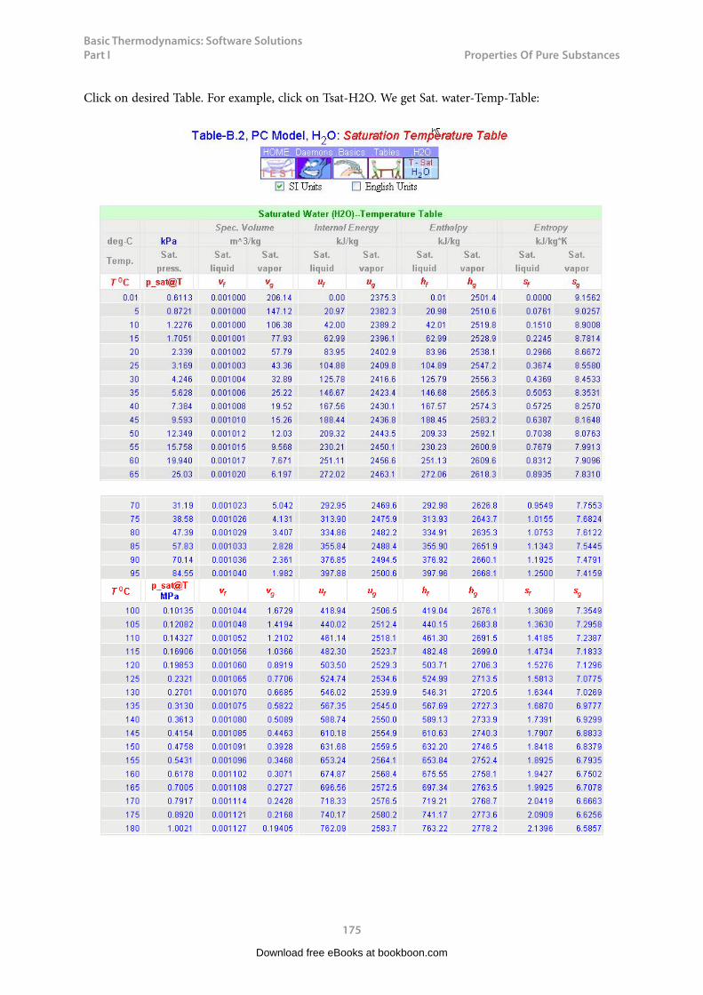
Basic Thermodynamics: Software Solutions Part I
175
Properties f Pure Substances
Click on desired Table. For example, click on Tsat-H2O. We get Sat. water-Temp-Table:
Download free eBooks at bookboon.com
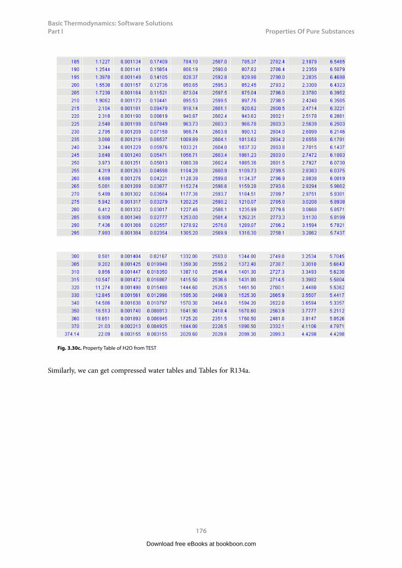
Basic Thermodynamics: Software Solutions Part I
176
Properties f Pure Substances
Fig. 3.30c. Property Table of H2O from TEST
Similarly, we can get compressed water tables and Tables for R134a.
Download free eBooks at bookboon.com

Basic Thermodynamics: Software Solutions Part I
177
Properties f Pure Substances
3.4.5.4 Property table from free software WSProps:
This software is from www.Sourceforge.net. As you start WSProps, go to File-New and following window appears:
Fig. 3.31a. Property Table of H2O from WSProps
Download free eBooks at bookboon.com
Click on the ad to read moreClick on the ad to read moreClick on the ad to read moreClick on the ad to read moreClick on the ad to read moreClick on the ad to read moreClick on the ad to read moreClick on the ad to read moreClick on the ad to read moreClick on the ad to read moreClick on the ad to read moreClick on the ad to read moreClick on the ad to read moreClick on the ad to read moreClick on the ad to read moreClick on the ad to read moreClick on the ad to read moreClick on the ad to read moreClick on the ad to read moreClick on the ad to read moreClick on the ad to read moreClick on the ad to read moreClick on the ad to read moreClick on the ad to read moreClick on the ad to read moreClick on the ad to read moreClick on the ad to read moreClick on the ad to read moreClick on the ad to read moreClick on the ad to read moreClick on the ad to read moreClick on the ad to read moreClick on the ad to read moreClick on the ad to read moreClick on the ad to read moreClick on the ad to read moreClick on the ad to read moreClick on the ad to read moreClick on the ad to read moreClick on the ad to read moreClick on the ad to read moreClick on the ad to read moreClick on the ad to read moreClick on the ad to read moreClick on the ad to read moreClick on the ad to read moreClick on the ad to read moreClick on the ad to read moreClick on the ad to read moreClick on the ad to read moreClick on the ad to read moreClick on the ad to read moreClick on the ad to read moreClick on the ad to read moreClick on the ad to read more
STEP INTO A WORLD OF OPPORTUNITYwww.ecco.com/[email protected]
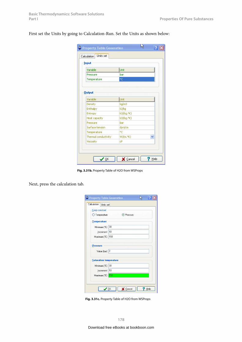
Basic Thermodynamics: Software Solutions Part I
178
Properties f Pure Substances
First set the Units by going to Calculation-Run. Set the Units as shown below:
Fig. 3.31b. Property Table of H2O from WSProps
Next, press the calculation tab.
Fig. 3.31c. Property Table of H2O from WSProps
Download free eBooks at bookboon.com
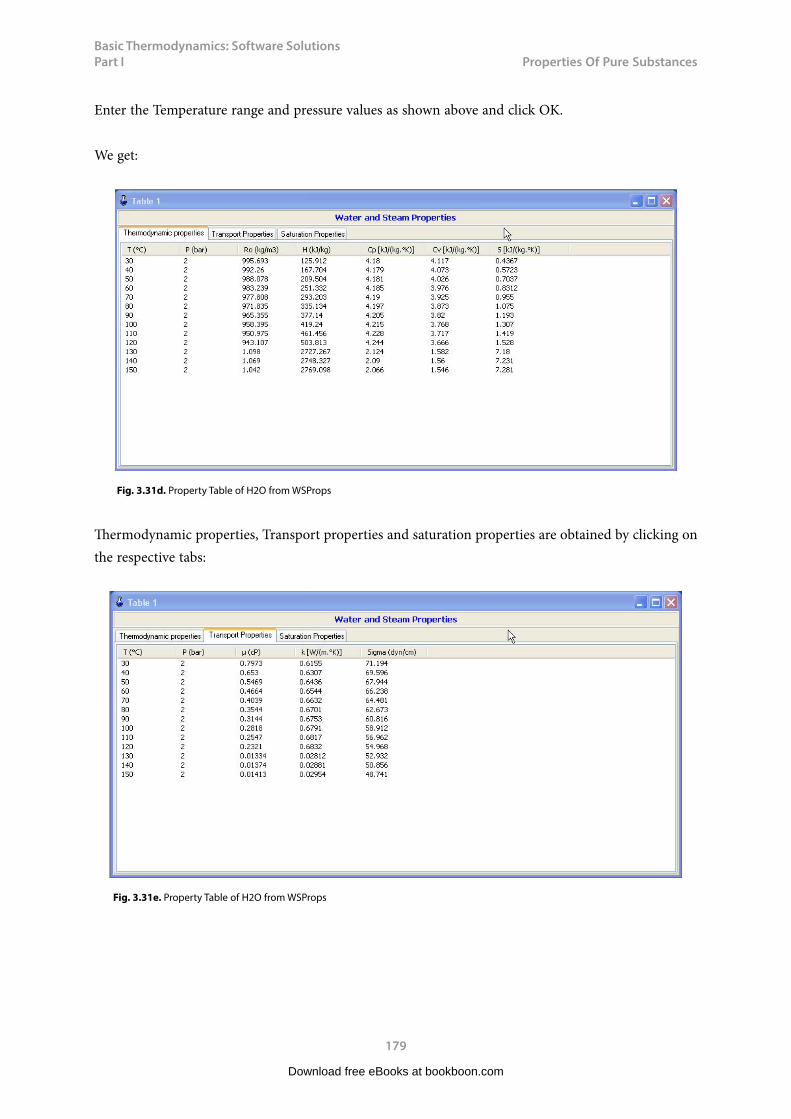
Basic Thermodynamics: Software Solutions Part I
179
Properties f Pure Substances
Enter the Temperature range and pressure values as shown above and click OK.
We get:
Fig. 3.31d. Property Table of H2O from WSProps
Thermodynamic properties, Transport properties and saturation properties are obtained by clicking on the respective tabs:
Fig. 3.31e. Property Table of H2O from WSProps
Download free eBooks at bookboon.com
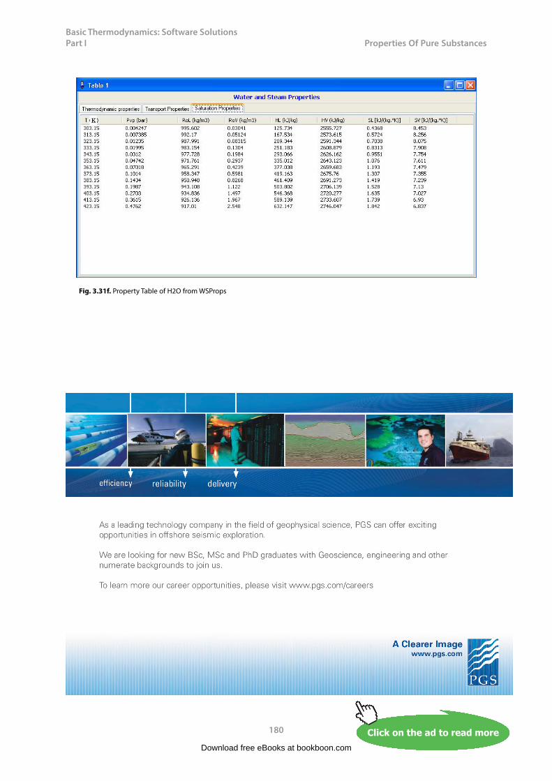
Basic Thermodynamics: Software Solutions Part I
180
Properties f Pure Substances
Fig. 3.31f. Property Table of H2O from WSProps
Download free eBooks at bookboon.com
Click on the ad to read moreClick on the ad to read moreClick on the ad to read moreClick on the ad to read moreClick on the ad to read moreClick on the ad to read moreClick on the ad to read moreClick on the ad to read moreClick on the ad to read moreClick on the ad to read moreClick on the ad to read moreClick on the ad to read moreClick on the ad to read moreClick on the ad to read moreClick on the ad to read moreClick on the ad to read moreClick on the ad to read moreClick on the ad to read moreClick on the ad to read moreClick on the ad to read moreClick on the ad to read moreClick on the ad to read moreClick on the ad to read moreClick on the ad to read moreClick on the ad to read moreClick on the ad to read moreClick on the ad to read moreClick on the ad to read moreClick on the ad to read moreClick on the ad to read moreClick on the ad to read moreClick on the ad to read moreClick on the ad to read moreClick on the ad to read moreClick on the ad to read moreClick on the ad to read moreClick on the ad to read moreClick on the ad to read moreClick on the ad to read moreClick on the ad to read moreClick on the ad to read moreClick on the ad to read moreClick on the ad to read moreClick on the ad to read moreClick on the ad to read moreClick on the ad to read moreClick on the ad to read moreClick on the ad to read moreClick on the ad to read moreClick on the ad to read moreClick on the ad to read moreClick on the ad to read moreClick on the ad to read moreClick on the ad to read moreClick on the ad to read moreClick on the ad to read more
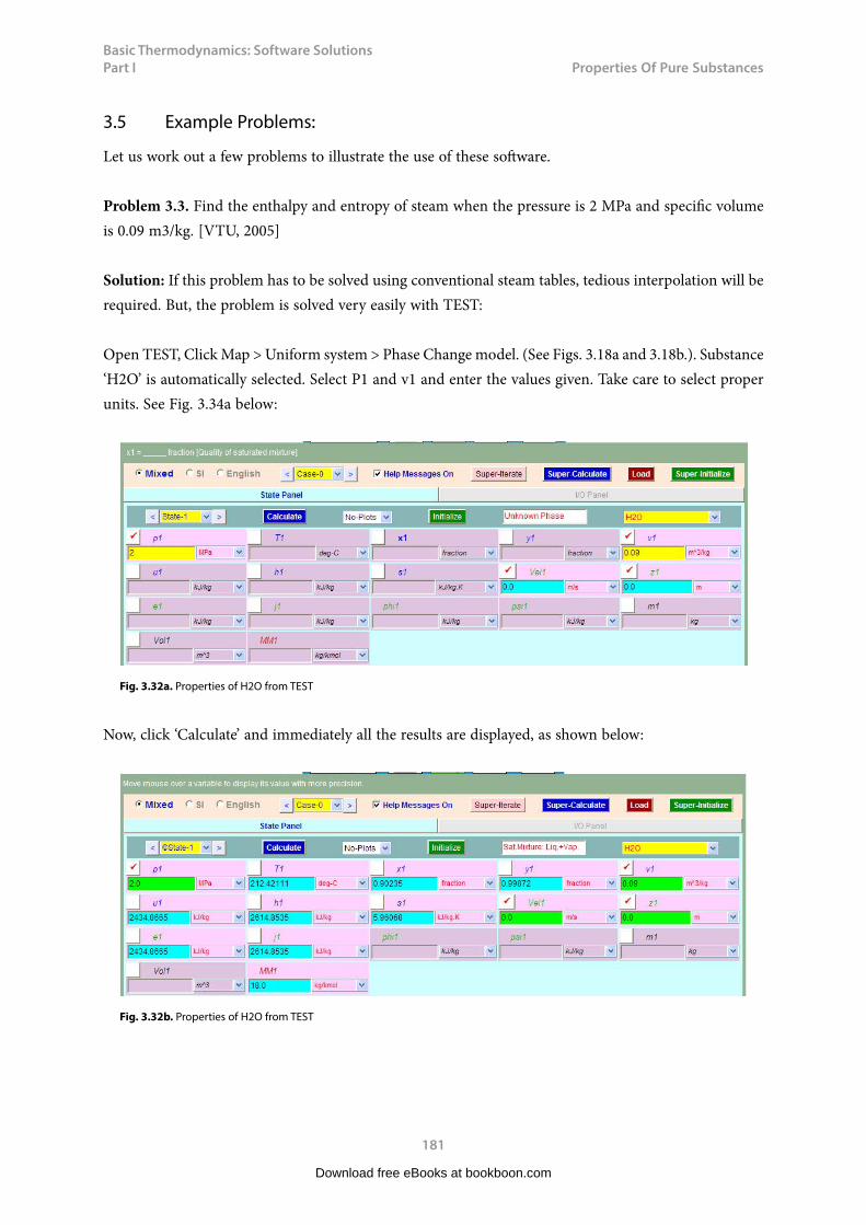
Basic Thermodynamics: Software Solutions Part I
181
Properties f Pure Substances
3.5 Example Problems:
Let us work out a few problems to illustrate the use of these software.
Problem 3.3. Find the enthalpy and entropy of steam when the pressure is 2 MPa and specific volume is 0.09 m3/kg. [VTU, 2005]
Solution: If this problem has to be solved using conventional steam tables, tedious interpolation will be required. But, the problem is solved very easily with TEST:
Open TEST, Click Map > Uniform system > Phase Change model. (See Figs. 3.18a and 3.18b.). Substance ‘H2O’ is automatically selected. Select P1 and v1 and enter the values given. Take care to select proper units. See Fig. 3.34a below:
Fig. 3.32a. Properties of H2O from TEST
Now, click ‘Calculate’ and immediately all the results are displayed, as shown below:
Fig. 3.32b. Properties of H2O from TEST
Download free eBooks at bookboon.com
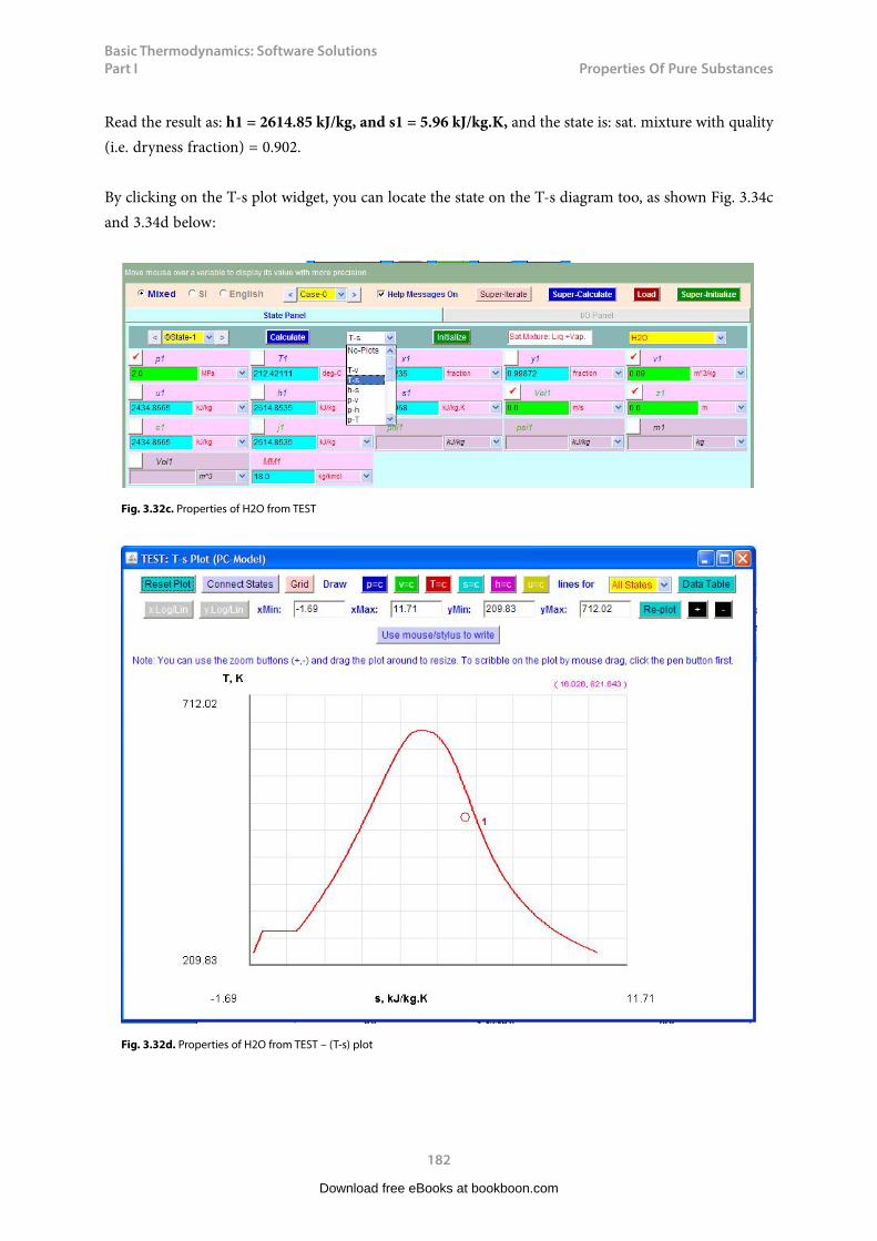
Basic Thermodynamics: Software Solutions Part I
182
Properties f Pure Substances
Read the result as: h1 = 2614.85 kJ/kg, and s1 = 5.96 kJ/kg.K, and the state is: sat. mixture with quality (i.e. dryness fraction) = 0.902.
By clicking on the T-s plot widget, you can locate the state on the T-s diagram too, as shown Fig. 3.34c and 3.34d below:
Fig. 3.32c. Properties of H2O from TEST
Fig. 3.32d. Properties of H2O from TEST – (T-s) plot
Download free eBooks at bookboon.com
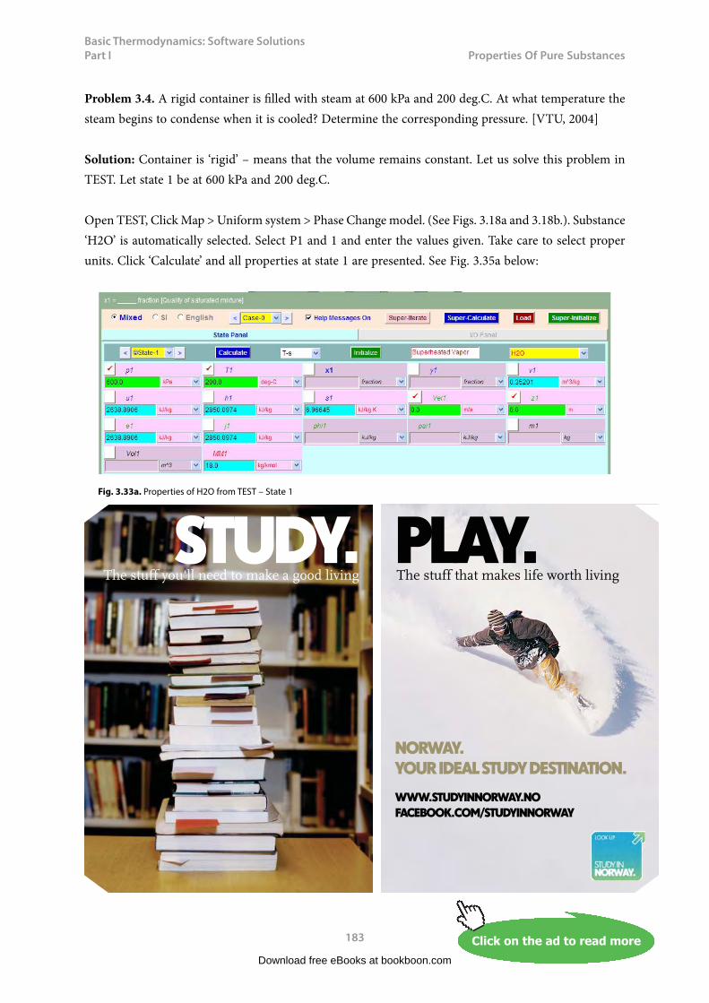
Basic Thermodynamics: Software Solutions Part I
183
Properties f Pure Substances
Problem 3.4. A rigid container is filled with steam at 600 kPa and 200 deg.C. At what temperature the steam begins to condense when it is cooled? Determine the corresponding pressure. [VTU, 2004]
Solution: Container is ‘rigid’ – means that the volume remains constant. Let us solve this problem in TEST. Let state 1 be at 600 kPa and 200 deg.C.
Open TEST, Click Map > Uniform system > Phase Change model. (See Figs. 3.18a and 3.18b.). Substance ‘H2O’ is automatically selected. Select P1 and 1 and enter the values given. Take care to select proper units. Click ‘Calculate’ and all properties at state 1 are presented. See Fig. 3.35a below:
Fig. 3.33a. Properties of H2O from TEST – State 1
Download free eBooks at bookboon.com
Click on the ad to read moreClick on the ad to read moreClick on the ad to read moreClick on the ad to read moreClick on the ad to read moreClick on the ad to read moreClick on the ad to read moreClick on the ad to read moreClick on the ad to read moreClick on the ad to read moreClick on the ad to read moreClick on the ad to read moreClick on the ad to read moreClick on the ad to read moreClick on the ad to read moreClick on the ad to read moreClick on the ad to read moreClick on the ad to read moreClick on the ad to read moreClick on the ad to read moreClick on the ad to read moreClick on the ad to read moreClick on the ad to read moreClick on the ad to read moreClick on the ad to read moreClick on the ad to read moreClick on the ad to read moreClick on the ad to read moreClick on the ad to read moreClick on the ad to read moreClick on the ad to read moreClick on the ad to read moreClick on the ad to read moreClick on the ad to read moreClick on the ad to read moreClick on the ad to read moreClick on the ad to read moreClick on the ad to read moreClick on the ad to read moreClick on the ad to read moreClick on the ad to read moreClick on the ad to read moreClick on the ad to read moreClick on the ad to read moreClick on the ad to read moreClick on the ad to read moreClick on the ad to read moreClick on the ad to read moreClick on the ad to read moreClick on the ad to read moreClick on the ad to read moreClick on the ad to read moreClick on the ad to read moreClick on the ad to read moreClick on the ad to read moreClick on the ad to read moreClick on the ad to read more
STUDY. PLAY.The stuff you'll need to make a good living The stuff that makes life worth living
NORWAY. YOUR IDEAL STUDY DESTINATION.
WWW.STUDYINNORWAY.NOFACEBOOK.COM/STUDYINNORWAY
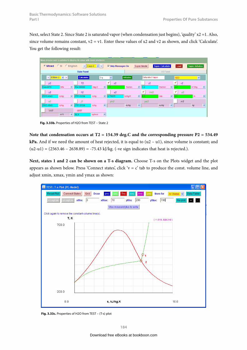
Basic Thermodynamics: Software Solutions Part I
184
Properties f Pure Substances
Next, select State 2. Since State 2 is saturated vapor (when condensation just begins), ‘quality’ x2 =1. Also, since volume remains constant, v2 = v1. Enter these values of x2 and v2 as shown, and click ‘Calculate’. You get the following result:
Fig. 3.33b. Properties of H2O from TEST – State 2
Note that condensation occurs at T2 = 154.39 deg.C and the corresponding pressure P2 = 534.49 kPa. And if we need the amount of heat rejected, it is equal to (u2 – u1), since volume is constant; and (u2-u1) = (2563.46 – 2638.89) = -75.43 kJ/kg. (-ve sign indicates that heat is rejected.).
Next, states 1 and 2 can be shown on a T-s diagram. Choose T-s on the Plots widget and the plot appears as shown below. Press ‘Connect states’, click ‘v = c’ tab to produce the const. volume line, and adjust xmin, xmax, ymin and ymax as shown:
Fig. 3.33c. Properties of H2O from TEST – (T-s) plot
Download free eBooks at bookboon.com
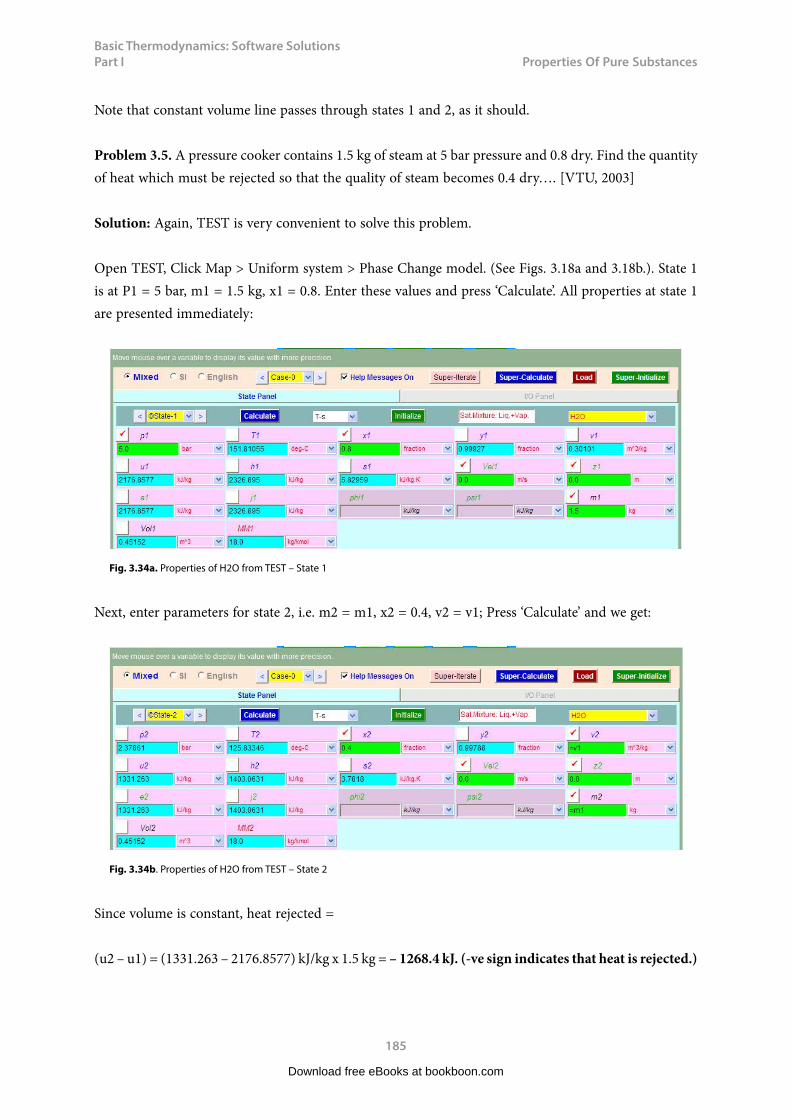
Basic Thermodynamics: Software Solutions Part I
185
Properties f Pure Substances
Note that constant volume line passes through states 1 and 2, as it should.
Problem 3.5. A pressure cooker contains 1.5 kg of steam at 5 bar pressure and 0.8 dry. Find the quantity of heat which must be rejected so that the quality of steam becomes 0.4 dry…. [VTU, 2003]
Solution: Again, TEST is very convenient to solve this problem.
Open TEST, Click Map > Uniform system > Phase Change model. (See Figs. 3.18a and 3.18b.). State 1 is at P1 = 5 bar, m1 = 1.5 kg, x1 = 0.8. Enter these values and press ‘Calculate’. All properties at state 1 are presented immediately:
Fig. 3.34a. Properties of H2O from TEST – State 1
Next, enter parameters for state 2, i.e. m2 = m1, x2 = 0.4, v2 = v1; Press ‘Calculate’ and we get:
Fig. 3.34b. Properties of H2O from TEST – State 2
Since volume is constant, heat rejected =
(u2 – u1) = (1331.263 – 2176.8577) kJ/kg x 1.5 kg = – 1268.4 kJ. (-ve sign indicates that heat is rejected.)
Download free eBooks at bookboon.com
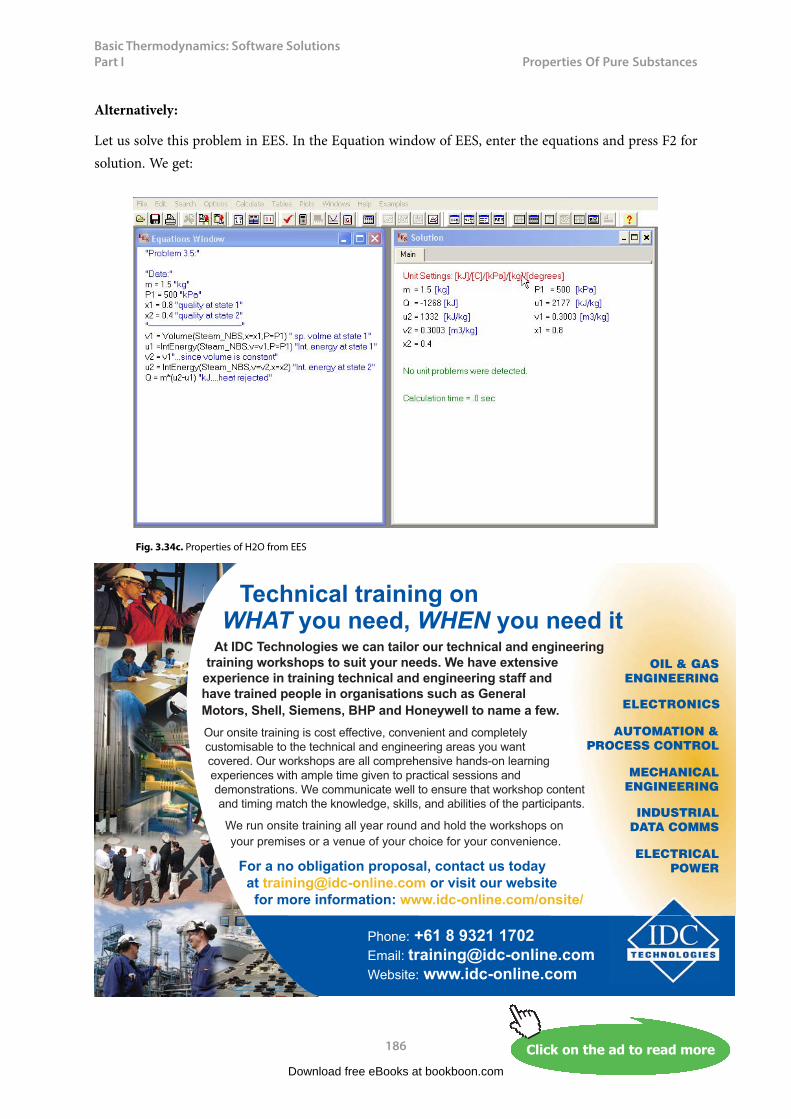
Basic Thermodynamics: Software Solutions Part I
186
Properties f Pure Substances
Alternatively:
Let us solve this problem in EES. In the Equation window of EES, enter the equations and press F2 for solution. We get:
Fig. 3.34c. Properties of H2O from EES
Download free eBooks at bookboon.com
Click on the ad to read moreClick on the ad to read moreClick on the ad to read moreClick on the ad to read moreClick on the ad to read moreClick on the ad to read moreClick on the ad to read moreClick on the ad to read moreClick on the ad to read moreClick on the ad to read moreClick on the ad to read moreClick on the ad to read moreClick on the ad to read moreClick on the ad to read moreClick on the ad to read moreClick on the ad to read moreClick on the ad to read moreClick on the ad to read moreClick on the ad to read moreClick on the ad to read moreClick on the ad to read moreClick on the ad to read moreClick on the ad to read moreClick on the ad to read moreClick on the ad to read moreClick on the ad to read moreClick on the ad to read moreClick on the ad to read moreClick on the ad to read moreClick on the ad to read moreClick on the ad to read moreClick on the ad to read moreClick on the ad to read moreClick on the ad to read moreClick on the ad to read moreClick on the ad to read moreClick on the ad to read moreClick on the ad to read moreClick on the ad to read moreClick on the ad to read moreClick on the ad to read moreClick on the ad to read moreClick on the ad to read moreClick on the ad to read moreClick on the ad to read moreClick on the ad to read moreClick on the ad to read moreClick on the ad to read moreClick on the ad to read moreClick on the ad to read moreClick on the ad to read moreClick on the ad to read moreClick on the ad to read moreClick on the ad to read moreClick on the ad to read moreClick on the ad to read moreClick on the ad to read moreClick on the ad to read more
Technical training on WHAT you need, WHEN you need it
At IDC Technologies we can tailor our technical and engineering training workshops to suit your needs. We have extensive
experience in training technical and engineering staff and have trained people in organisations such as General Motors, Shell, Siemens, BHP and Honeywell to name a few.Our onsite training is cost effective, convenient and completely customisable to the technical and engineering areas you want covered. Our workshops are all comprehensive hands-on learning experiences with ample time given to practical sessions and demonstrations. We communicate well to ensure that workshop content and timing match the knowledge, skills, and abilities of the participants.
We run onsite training all year round and hold the workshops on your premises or a venue of your choice for your convenience.
Phone: +61 8 9321 1702Email: [email protected] Website: www.idc-online.com
INDUSTRIALDATA COMMS
AUTOMATION & PROCESS CONTROL
ELECTRONICS
ELECTRICAL POWER
MECHANICAL ENGINEERING
OIL & GASENGINEERING
For a no obligation proposal, contact us today at [email protected] or visit our website for more information: www.idc-online.com/onsite/

Basic Thermodynamics: Software Solutions Part I
187
Properties f Pure Substances
Problem 3.6: A rigid vessel contains 1 kg of wet steam at a pressure of 0.15 MPa. When the mixture is heated, the state passes through the critical point. Determine:
i. the volume of the vesselii. mass of liquid and vapor initially in the vesseliii. temperature of the mixture when the pressure has risen to 3 MPa, andiv. the heat transfer required to produce the final state (iii)….[VTU, 2004]
Solution:
Note two points:
i. Since 1 kg of wet steam passes through the critical point in a closed vessel, it is clear that the volume must be equal to critical volume = 0.003155 m3/kg.
ii. Specific volume of wet steam is given by:
Therefore, for a constant volume process, we can write, approximately:
...(3.8)
Where x1, x2 are the dryness fraction values at state 1 and state 2 respectively.
First let us solve this problem with TEST:
Download free eBooks at bookboon.com
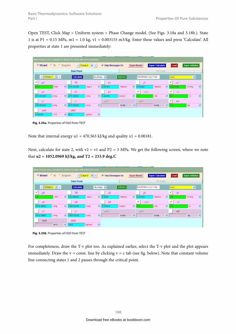
Basic Thermodynamics: Software Solutions Part I
188
Properties f Pure Substances
Open TEST, Click Map > Uniform system > Phase Change model. (See Figs. 3.18a and 3.18b.). State 1 is at P1 = 0.15 MPa, m1 = 1.0 kg, v1 = 0.003155 m3/kg. Enter these values and press ‘Calculate’. All properties at state 1 are presented immediately:
Fig. 3.35a. Properties of H2O from TEST
Note that internal energy u1 = 470.563 kJ/kg and quality x1 = 0.00181.
Next, calculate for state 2, with v2 = v1 and P2 = 3 MPa. We get the following screen, where we note that u2 = 1052.0969 kJ/kg, and T2 = 233.9 deg.C
Fig. 3.35b. Properties of H2O from TEST
For completeness, draw the T-v plot too. As explained earlier, select the T-v plot and the plot appears immediately. Draw the v = const. line by clicking v = c tab (see fig. below). Note that constant volume line connecting states 1 and 2 passes through the critical point.
Download free eBooks at bookboon.com
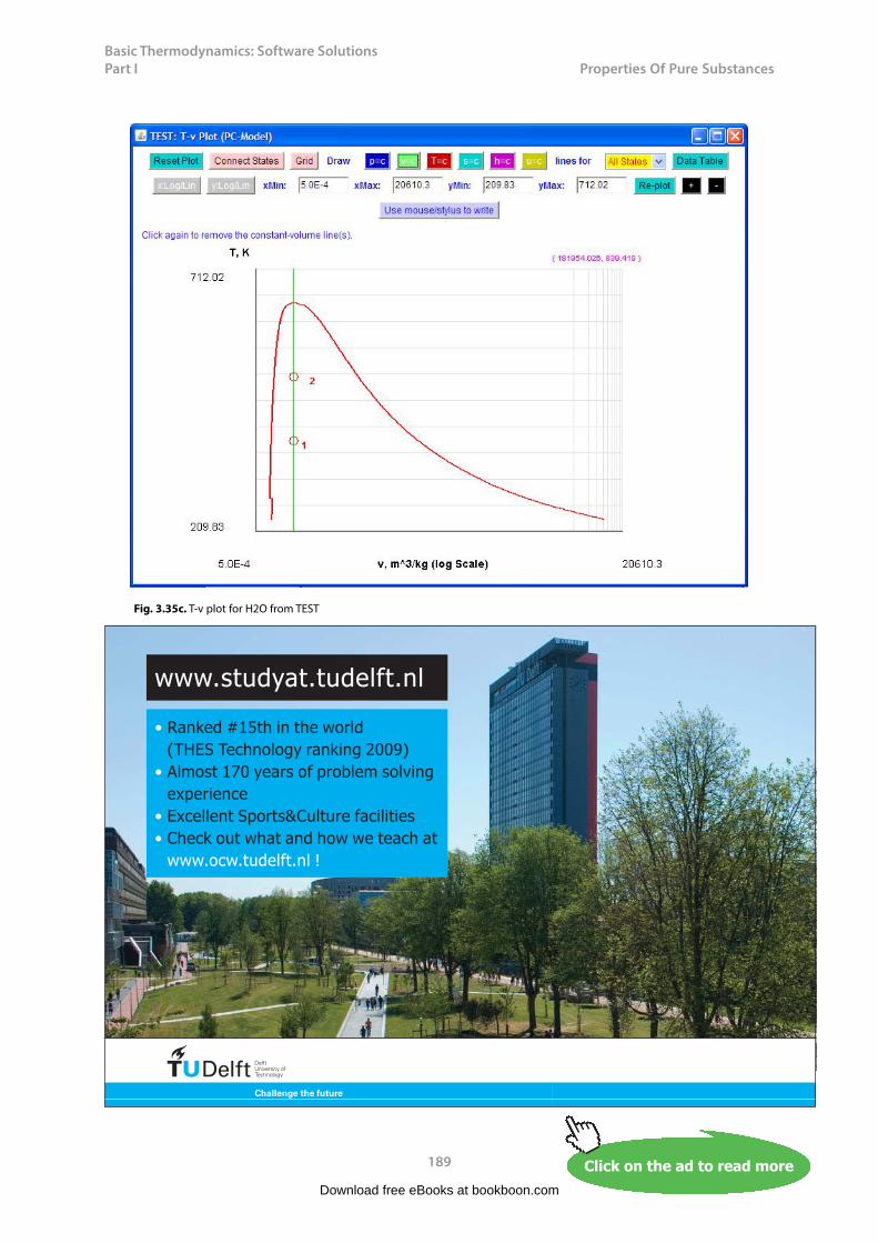
Basic Thermodynamics: Software Solutions Part I
189
Properties f Pure Substances
Fig. 3.35c. T-v plot for H2O from TEST
Download free eBooks at bookboon.com
Click on the ad to read moreClick on the ad to read moreClick on the ad to read moreClick on the ad to read moreClick on the ad to read moreClick on the ad to read moreClick on the ad to read moreClick on the ad to read moreClick on the ad to read moreClick on the ad to read moreClick on the ad to read moreClick on the ad to read moreClick on the ad to read moreClick on the ad to read moreClick on the ad to read moreClick on the ad to read moreClick on the ad to read moreClick on the ad to read moreClick on the ad to read moreClick on the ad to read moreClick on the ad to read moreClick on the ad to read moreClick on the ad to read moreClick on the ad to read moreClick on the ad to read moreClick on the ad to read moreClick on the ad to read moreClick on the ad to read moreClick on the ad to read moreClick on the ad to read moreClick on the ad to read moreClick on the ad to read moreClick on the ad to read moreClick on the ad to read moreClick on the ad to read moreClick on the ad to read moreClick on the ad to read moreClick on the ad to read moreClick on the ad to read moreClick on the ad to read moreClick on the ad to read moreClick on the ad to read moreClick on the ad to read moreClick on the ad to read moreClick on the ad to read moreClick on the ad to read moreClick on the ad to read moreClick on the ad to read moreClick on the ad to read moreClick on the ad to read moreClick on the ad to read moreClick on the ad to read moreClick on the ad to read moreClick on the ad to read moreClick on the ad to read moreClick on the ad to read moreClick on the ad to read moreClick on the ad to read moreClick on the ad to read more
���������� ����� ��������� �������������������������������� �!�" ��#������"��$�%��&��!�"��'����� �(%����������(������ ��%�� ")*+� +���$����� ��"��*������+ ���� ����������� ������ �� ���,���, +��$ ,���-
���," +�� , +��$ ,��
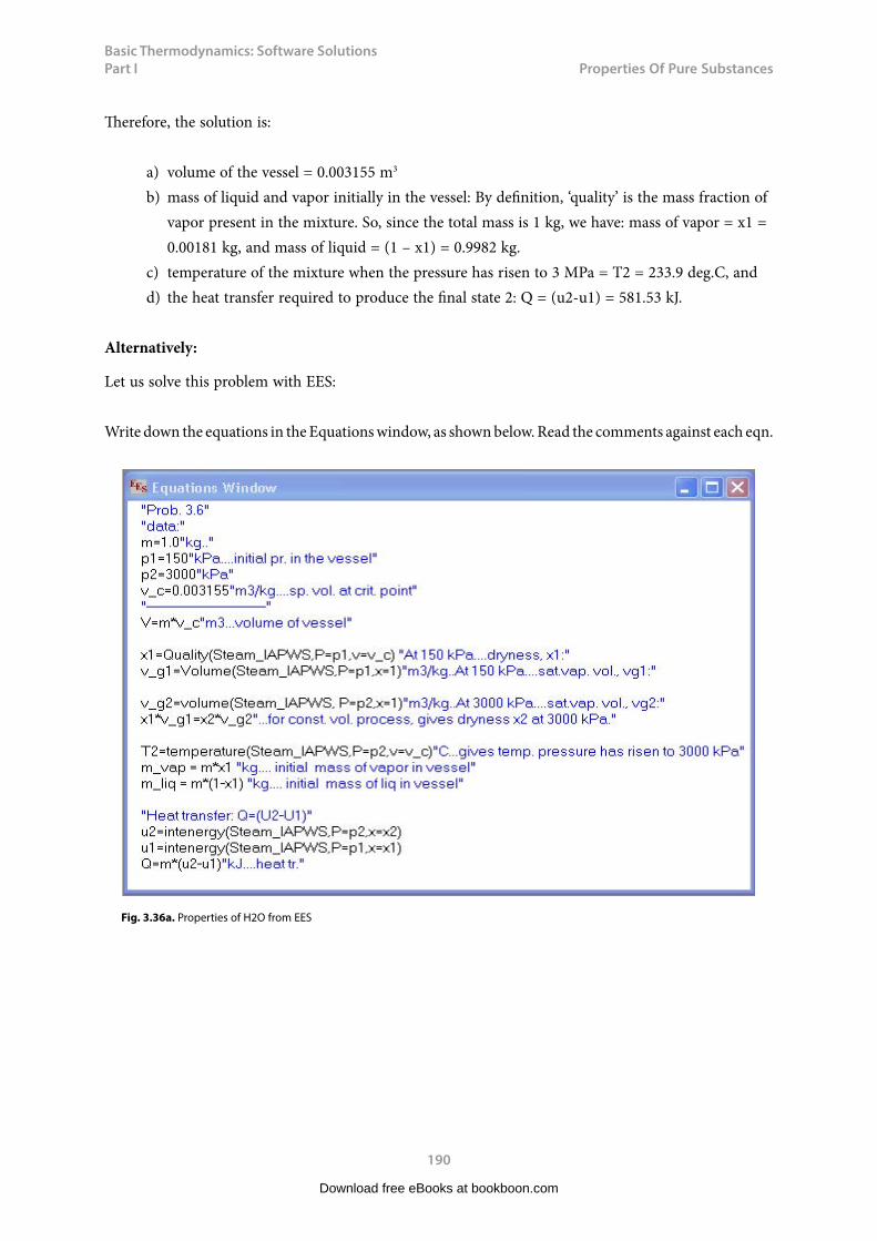
Basic Thermodynamics: Software Solutions Part I
190
Properties f Pure Substances
Therefore, the solution is:
a) volume of the vessel = 0.003155 m3
b) mass of liquid and vapor initially in the vessel: By definition, ‘quality’ is the mass fraction of vapor present in the mixture. So, since the total mass is 1 kg, we have: mass of vapor = x1 = 0.00181 kg, and mass of liquid = (1 – x1) = 0.9982 kg.
c) temperature of the mixture when the pressure has risen to 3 MPa = T2 = 233.9 deg.C, andd) the heat transfer required to produce the final state 2: Q = (u2-u1) = 581.53 kJ.
Alternatively:
Let us solve this problem with EES:
Write down the equations in the Equations window, as shown below. Read the comments against each eqn.
Fig. 3.36a. Properties of H2O from EES
Download free eBooks at bookboon.com
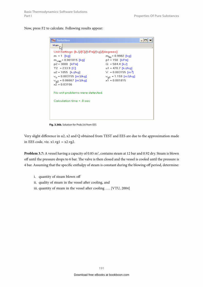
Basic Thermodynamics: Software Solutions Part I
191
Properties f Pure Substances
Now, press F2 to calculate. Following results appear:
Fig. 3.36b. Solution for Prob.3.6 from EES
Very slight difference in u2, x2 and Q obtained from TEST and EES are due to the approximation made in EES code, viz. x1.vg1 = x2.vg2.
Problem 3.7: A vessel having a capacity of 0.85 m3, contains steam at 12 bar and 0.92 dry. Steam is blown off until the pressure drops to 6 bar. The valve is then closed and the vessel is cooled until the pressure is 4 bar. Assuming that the specific enthalpy of steam is constant during the blowing off period, determine:
i. quantity of steam blown offii. quality of steam in the vessel after cooling, andiii. quantity of steam in the vessel after cooling …. [VTU, 2004]
Download free eBooks at bookboon.com

Basic Thermodynamics: Software Solutions Part I
192
Properties f Pure Substances
Solution:
Since the problem involves finding out the states, TEST is most convenient to use.
Open TEST, Click Map > Uniform system > Phase Change model. (See Figs. 3.18a and 3.18b.). State 1 is at P1 = 12 bar, Vol1 = 0.85 m3, x1 = 0.92. Enter these values and press ‘Calculate’. All properties at state 1 are presented immediately:
Fig. 3.37a. Properties of H2O with TEST – state 1
Download free eBooks at bookboon.com
Click on the ad to read moreClick on the ad to read moreClick on the ad to read moreClick on the ad to read moreClick on the ad to read moreClick on the ad to read moreClick on the ad to read moreClick on the ad to read moreClick on the ad to read moreClick on the ad to read moreClick on the ad to read moreClick on the ad to read moreClick on the ad to read moreClick on the ad to read moreClick on the ad to read moreClick on the ad to read moreClick on the ad to read moreClick on the ad to read moreClick on the ad to read moreClick on the ad to read moreClick on the ad to read moreClick on the ad to read moreClick on the ad to read moreClick on the ad to read moreClick on the ad to read moreClick on the ad to read moreClick on the ad to read moreClick on the ad to read moreClick on the ad to read moreClick on the ad to read moreClick on the ad to read moreClick on the ad to read moreClick on the ad to read moreClick on the ad to read moreClick on the ad to read moreClick on the ad to read moreClick on the ad to read moreClick on the ad to read moreClick on the ad to read moreClick on the ad to read moreClick on the ad to read moreClick on the ad to read moreClick on the ad to read moreClick on the ad to read moreClick on the ad to read moreClick on the ad to read moreClick on the ad to read moreClick on the ad to read moreClick on the ad to read moreClick on the ad to read moreClick on the ad to read moreClick on the ad to read moreClick on the ad to read moreClick on the ad to read moreClick on the ad to read moreClick on the ad to read moreClick on the ad to read moreClick on the ad to read moreClick on the ad to read moreClick on the ad to read more
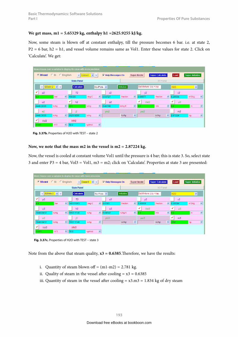
Basic Thermodynamics: Software Solutions Part I
193
Properties f Pure Substances
We get mass, m1 = 5.65329 kg, enthalpy h1 =2625.9255 kJ/kg.
Now, some steam is blown off at constant enthalpy, till the pressure becomes 6 bar. i.e. at state 2, P2 = 6 bar, h2 = h1, and vessel volume remains same as Vol1. Enter these values for state 2. Click on ‘Calculate’. We get:
Fig. 3.37b. Properties of H2O with TEST – state 2
Now, we note that the mass m2 in the vessel is m2 = 2.87224 kg.
Now, the vessel is cooled at constant volume Vol1 until the pressure is 4 bar; this is state 3. So, select state 3 and enter P3 = 4 bar, Vol3 = Vol1, m3 = m2; click on ‘Calculate’. Properties at state 3 are presented:
Fig. 3.37c. Properties of H2O with TEST – state 3
Note from the above that steam quality, x3 = 0.6385.Therefore, we have the results:
i. Quantity of steam blown off = (m1-m2) = 2.781 kg.ii. Quality of steam in the vessel after cooling = x3 = 0.6385iii. Quantity of steam in the vessel after cooling = x3.m3 = 1.834 kg of dry steam
Download free eBooks at bookboon.com
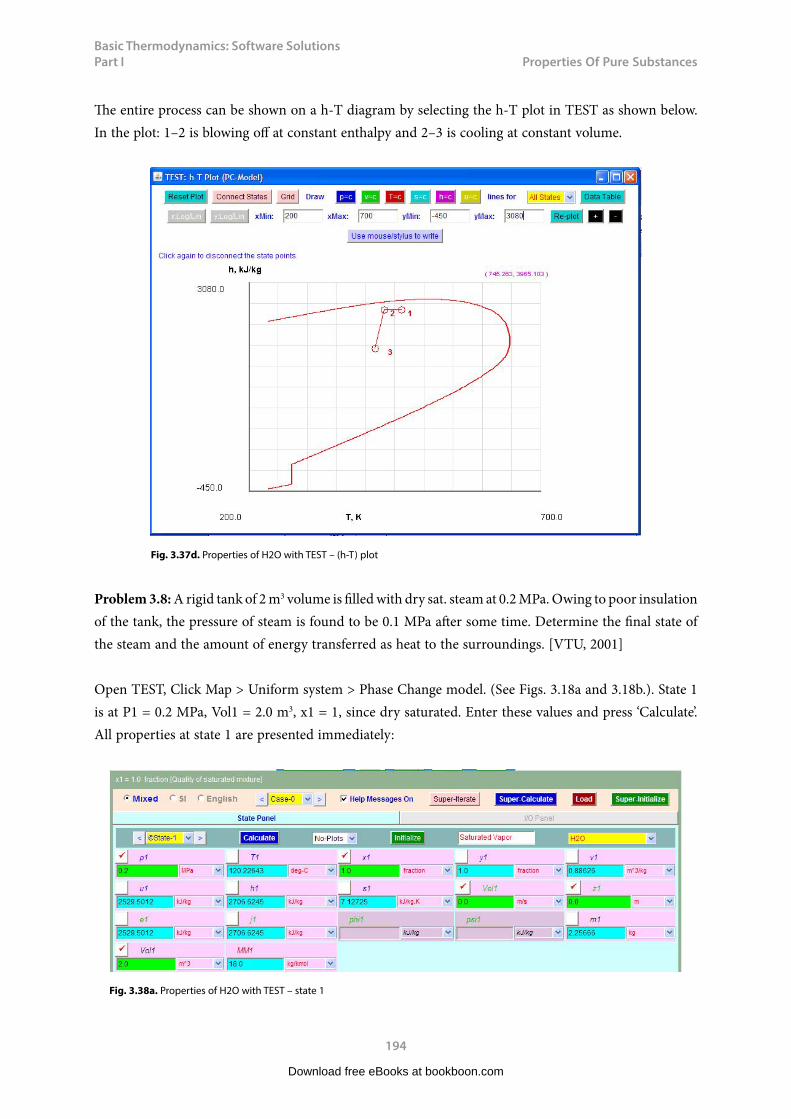
Basic Thermodynamics: Software Solutions Part I
194
Properties f Pure Substances
The entire process can be shown on a h-T diagram by selecting the h-T plot in TEST as shown below. In the plot: 1–2 is blowing off at constant enthalpy and 2–3 is cooling at constant volume.
Fig. 3.37d. Properties of H2O with TEST – (h-T) plot
Problem 3.8: A rigid tank of 2 m3 volume is filled with dry sat. steam at 0.2 MPa. Owing to poor insulation of the tank, the pressure of steam is found to be 0.1 MPa after some time. Determine the final state of the steam and the amount of energy transferred as heat to the surroundings. [VTU, 2001]
Open TEST, Click Map > Uniform system > Phase Change model. (See Figs. 3.18a and 3.18b.). State 1 is at P1 = 0.2 MPa, Vol1 = 2.0 m3, x1 = 1, since dry saturated. Enter these values and press ‘Calculate’. All properties at state 1 are presented immediately:
Fig. 3.38a. Properties of H2O with TEST – state 1
Download free eBooks at bookboon.com

Basic Thermodynamics: Software Solutions Part I
195
Properties f Pure Substances
Note that mass of steam, m1 = 2.25666 kg, and internal energy of steam, u1 = 2529.5012 kJ/kg.
Now, select state 2, and enter the known conditions, i.e. Vol2 = Vol1, m2 = m1 and P2 = 0.1 MPa. Click on ‘Calculate’. We get:
Fig. 3.38b. Properties of H2O with TEST – state 2
We read: u2 = 1509.4971 kJ/kg. and quality, x2 = 0.52288. Energy transferred to surroundings = m.(u2 – u1) = -2.25666 kg x 1020 kJ/kg = -2301.79 kJ. (-ve sign indicates that heat is rejected.)
Download free eBooks at bookboon.com
Click on the ad to read moreClick on the ad to read moreClick on the ad to read moreClick on the ad to read moreClick on the ad to read moreClick on the ad to read moreClick on the ad to read moreClick on the ad to read moreClick on the ad to read moreClick on the ad to read moreClick on the ad to read moreClick on the ad to read moreClick on the ad to read moreClick on the ad to read moreClick on the ad to read moreClick on the ad to read moreClick on the ad to read moreClick on the ad to read moreClick on the ad to read moreClick on the ad to read moreClick on the ad to read moreClick on the ad to read moreClick on the ad to read moreClick on the ad to read moreClick on the ad to read moreClick on the ad to read moreClick on the ad to read moreClick on the ad to read moreClick on the ad to read moreClick on the ad to read moreClick on the ad to read moreClick on the ad to read moreClick on the ad to read moreClick on the ad to read moreClick on the ad to read moreClick on the ad to read moreClick on the ad to read moreClick on the ad to read moreClick on the ad to read moreClick on the ad to read moreClick on the ad to read moreClick on the ad to read moreClick on the ad to read moreClick on the ad to read moreClick on the ad to read moreClick on the ad to read moreClick on the ad to read moreClick on the ad to read moreClick on the ad to read moreClick on the ad to read moreClick on the ad to read moreClick on the ad to read moreClick on the ad to read moreClick on the ad to read moreClick on the ad to read moreClick on the ad to read moreClick on the ad to read moreClick on the ad to read moreClick on the ad to read moreClick on the ad to read moreClick on the ad to read more
DTU, Technical University of Denmark, is ranked as one of the best technical universities in Europe, and offers internationally recognised Master of Science degrees in 39 English-taught programmes.
DTU offers a unique environment where students have hands-on access to cutting edge facilities and work
closely under the expert supervision of top international researchers.
DTU’s central campus is located just north of Copenhagen and life at the University is engaging and vibrant. At DTU, we ensure that your goals and ambitions are met. Tuition is free for EU/EEA citizens.
Visit us at www.dtu.dk
Study at one of Europe’s leading universities
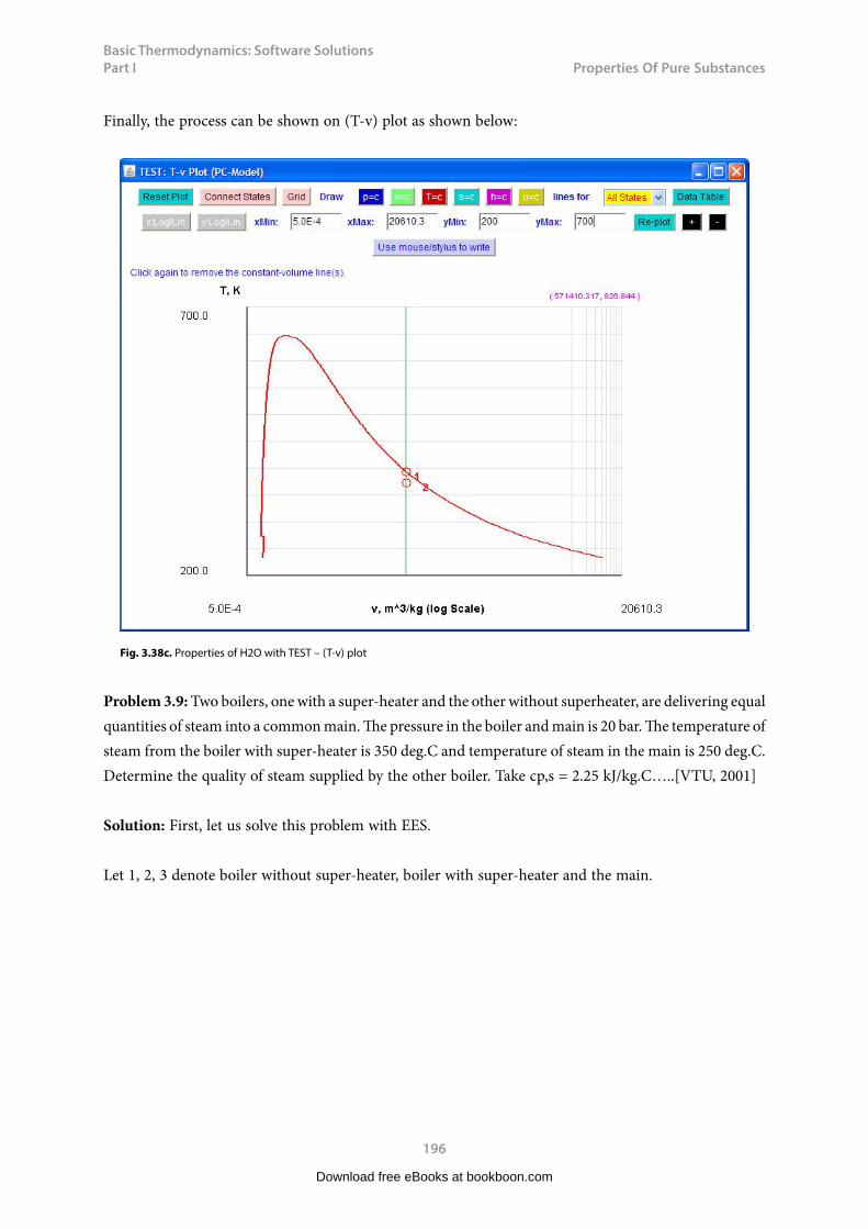
Basic Thermodynamics: Software Solutions Part I
196
Properties f Pure Substances
Finally, the process can be shown on (T-v) plot as shown below:
Fig. 3.38c. Properties of H2O with TEST – (T-v) plot
Problem 3.9: Two boilers, one with a super-heater and the other without superheater, are delivering equal quantities of steam into a common main. The pressure in the boiler and main is 20 bar. The temperature of steam from the boiler with super-heater is 350 deg.C and temperature of steam in the main is 250 deg.C. Determine the quality of steam supplied by the other boiler. Take cp,s = 2.25 kJ/kg.C…..[VTU, 2001]
Solution: First, let us solve this problem with EES.
Let 1, 2, 3 denote boiler without super-heater, boiler with super-heater and the main.
Download free eBooks at bookboon.com
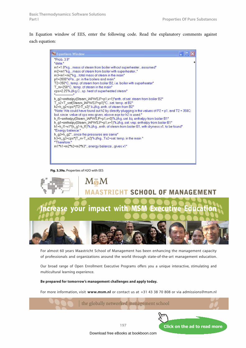
Basic Thermodynamics: Software Solutions Part I
197
Properties f Pure Substances
In Equation window of EES, enter the following code. Read the explanatory comments against each equation:
Fig. 3.39a. Properties of H2O with EES
Download free eBooks at bookboon.com
Click on the ad to read moreClick on the ad to read moreClick on the ad to read moreClick on the ad to read moreClick on the ad to read moreClick on the ad to read moreClick on the ad to read moreClick on the ad to read moreClick on the ad to read moreClick on the ad to read moreClick on the ad to read moreClick on the ad to read moreClick on the ad to read moreClick on the ad to read moreClick on the ad to read moreClick on the ad to read moreClick on the ad to read moreClick on the ad to read moreClick on the ad to read moreClick on the ad to read moreClick on the ad to read moreClick on the ad to read moreClick on the ad to read moreClick on the ad to read moreClick on the ad to read moreClick on the ad to read moreClick on the ad to read moreClick on the ad to read moreClick on the ad to read moreClick on the ad to read moreClick on the ad to read moreClick on the ad to read moreClick on the ad to read moreClick on the ad to read moreClick on the ad to read moreClick on the ad to read moreClick on the ad to read moreClick on the ad to read moreClick on the ad to read moreClick on the ad to read moreClick on the ad to read moreClick on the ad to read moreClick on the ad to read moreClick on the ad to read moreClick on the ad to read moreClick on the ad to read moreClick on the ad to read moreClick on the ad to read moreClick on the ad to read moreClick on the ad to read moreClick on the ad to read moreClick on the ad to read moreClick on the ad to read moreClick on the ad to read moreClick on the ad to read moreClick on the ad to read moreClick on the ad to read moreClick on the ad to read moreClick on the ad to read moreClick on the ad to read moreClick on the ad to read moreClick on the ad to read more
Increase your impact with MSM Executive Education
For more information, visit www.msm.nl or contact us at +31 43 38 70 808
or via [email protected] the globally networked management school
For more information, visit www.msm.nl or contact us at +31 43 38 70 808 or via [email protected]
For almost 60 years Maastricht School of Management has been enhancing the management capacity
of professionals and organizations around the world through state-of-the-art management education.
Our broad range of Open Enrollment Executive Programs offers you a unique interactive, stimulating and
multicultural learning experience.
Be prepared for tomorrow’s management challenges and apply today.
Executive Education-170x115-B2.indd 1 18-08-11 15:13
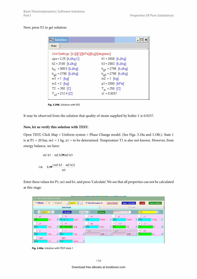
Basic Thermodynamics: Software Solutions Part I
198
Properties f Pure Substances
Now, press F2 to get solution:
Fig. 3.39b. Solution with EES
It may be observed from the solution that quality of steam supplied by boiler-1 is 0.9257.
Now, let us verify this solution with TEST:
Open TEST, Click Map > Uniform system > Phase Change model. (See Figs. 3.18a and 3.18b.). State 1 is at P1 = 20 bar, m1 = 1 kg, x1 = to be determined. Temperature T1 is also not known. However, from energy balance, we have:
m1 h1 m2 h2 m3 h3
i.e. h1m3 h3 m2 h2( )
m1
Enter these values for P1, m1 and h1, and press ‘Calculate’. We see that all properties can not be calculated at this stage:
Fig. 3.40a. Solution with TEST-state 1
Download free eBooks at bookboon.com

Basic Thermodynamics: Software Solutions Part I
199
Properties f Pure Substances
However, we proceed to states 2 and 3 and ‘Supercalculate’ and TEST will refer back to state 1 and calculate properties at state 1 at that stage.
For state 2, we have: P2 = 20 bar, T2 = 350 C, m2 = m1. Enter these values and click on ‘Calculate’. We get:
Fig. 3.40b. Solution with TEST-state 2
Next, for state 3 (i.e. Steam main), P3 = P1, T3 = 250 C, m3 = (m1 + m2). Enter these values and press ‘Calculate’. We get:
Fig. 3.40c. Solution with TEST-state 3
Download free eBooks at bookboon.com

Basic Thermodynamics: Software Solutions Part I
200
Properties f Pure Substances
Now, click ‘Supercalculate’:Go to state 1 and following screen appears for state1:
Fig. 3.40d. Solution with TEST-state 1
It may be seen that quality of steam supplied by the boiler with no super-heater is: x1 = 0.93043.
‘Supercalculate’ also generates TEST code which can be copied to a MS Word file and used to regenerate the results at a later date if required, and also a property table. The property table from the TEST report is reproduced below:
Fig. 3.40e. Solution with TEST- property table
Problem 3.10: Temperature of feed water entering a boiler is 50 deg.C and the pressure of steam in the boiler is 13 bar. How much heat will be required to produce one kg of steam if the steam produced is:
i. 0.97 dryii. Dry saturatediii. Superheated with 40 deg.C of superheat
Take cp for superheated steam as 2.1 kJ/kg.C and cp of water as 4.187 kJ/kg.C …[VTU, 2000]
Download free eBooks at bookboon.com

Basic Thermodynamics: Software Solutions Part I
201
Properties f Pure Substances
Solution: First, let us solve this problem with Mathcad. In Mathcad, there are no built-in properties for steam. So, we will get the steam properties from ‘SteamTab companion’ and use them in Mathcad for further calculations. Mathcad worksheet is shown below:
Let h1 = enthalpy of feed water at 50 C and 13 bar,
h2 = enthalpy of 0.97 dry steam
h3 = enthalpy of dry sat. steam
h4 = enthalpy of superheated steam with 40 deg. C superheat
Download free eBooks at bookboon.com
Click on the ad to read moreClick on the ad to read moreClick on the ad to read moreClick on the ad to read moreClick on the ad to read moreClick on the ad to read moreClick on the ad to read moreClick on the ad to read moreClick on the ad to read moreClick on the ad to read moreClick on the ad to read moreClick on the ad to read moreClick on the ad to read moreClick on the ad to read moreClick on the ad to read moreClick on the ad to read moreClick on the ad to read moreClick on the ad to read moreClick on the ad to read moreClick on the ad to read moreClick on the ad to read moreClick on the ad to read moreClick on the ad to read moreClick on the ad to read moreClick on the ad to read moreClick on the ad to read moreClick on the ad to read moreClick on the ad to read moreClick on the ad to read moreClick on the ad to read moreClick on the ad to read moreClick on the ad to read moreClick on the ad to read moreClick on the ad to read moreClick on the ad to read moreClick on the ad to read moreClick on the ad to read moreClick on the ad to read moreClick on the ad to read moreClick on the ad to read moreClick on the ad to read moreClick on the ad to read moreClick on the ad to read moreClick on the ad to read moreClick on the ad to read moreClick on the ad to read moreClick on the ad to read moreClick on the ad to read moreClick on the ad to read moreClick on the ad to read moreClick on the ad to read moreClick on the ad to read moreClick on the ad to read moreClick on the ad to read moreClick on the ad to read moreClick on the ad to read moreClick on the ad to read moreClick on the ad to read moreClick on the ad to read moreClick on the ad to read moreClick on the ad to read moreClick on the ad to read moreClick on the ad to read more
EXPERIENCE THE POWER OF FULL ENGAGEMENT…
RUN FASTER. RUN LONGER.. RUN EASIER…
READ MORE & PRE-ORDER TODAY WWW.GAITEYE.COM
Challenge the way we run
1349906_A6_4+0.indd 1 22-08-2014 12:56:57
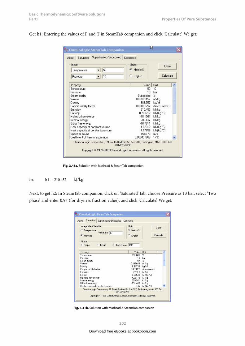
Basic Thermodynamics: Software Solutions Part I
202
Properties f Pure Substances
Get h1: Entering the values of P and T in SteamTab companion and click ‘Calculate’. We get:
Fig. 3.41a. Solution with Mathcad & SteamTab companion
i.e. h1 210.452 kJ/kg
Next, to get h2: In SteamTab companion, click on ‘Saturated’ tab; choose Pressure as 13 bar, select ‘Two phase’ and enter 0.97 (for dryness fraction value), and click ‘Calculate’. We get:
Fig. 3.41b. Solution with Mathcad & SteamTab companion
Download free eBooks at bookboon.com
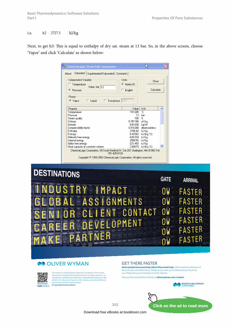
Basic Thermodynamics: Software Solutions Part I
203
Properties f Pure Substances
i.e. h2 2727.3 kJ/kg
Next, to get h3: This is equal to enthalpy of dry sat. steam at 13 bar. So, in the above screen, choose ‘Vapor’ and click ‘Calculate’ as shown below:
Fig. 3.41c. Solution with Mathcad & SteamTab companion
Download free eBooks at bookboon.com
Click on the ad to read moreClick on the ad to read moreClick on the ad to read moreClick on the ad to read moreClick on the ad to read moreClick on the ad to read moreClick on the ad to read moreClick on the ad to read moreClick on the ad to read moreClick on the ad to read moreClick on the ad to read moreClick on the ad to read moreClick on the ad to read moreClick on the ad to read moreClick on the ad to read moreClick on the ad to read moreClick on the ad to read moreClick on the ad to read moreClick on the ad to read moreClick on the ad to read moreClick on the ad to read moreClick on the ad to read moreClick on the ad to read moreClick on the ad to read moreClick on the ad to read moreClick on the ad to read moreClick on the ad to read moreClick on the ad to read moreClick on the ad to read moreClick on the ad to read moreClick on the ad to read moreClick on the ad to read moreClick on the ad to read moreClick on the ad to read moreClick on the ad to read moreClick on the ad to read moreClick on the ad to read moreClick on the ad to read moreClick on the ad to read moreClick on the ad to read moreClick on the ad to read moreClick on the ad to read moreClick on the ad to read moreClick on the ad to read moreClick on the ad to read moreClick on the ad to read moreClick on the ad to read moreClick on the ad to read moreClick on the ad to read moreClick on the ad to read moreClick on the ad to read moreClick on the ad to read moreClick on the ad to read moreClick on the ad to read moreClick on the ad to read moreClick on the ad to read moreClick on the ad to read moreClick on the ad to read moreClick on the ad to read moreClick on the ad to read moreClick on the ad to read moreClick on the ad to read moreClick on the ad to read moreClick on the ad to read more
GET THERE FASTER
Oliver Wyman is a leading global management consulting firm that combines
deep industry knowledge with specialized expertise in strategy, operations, risk
management, organizational transformation, and leadership development. With
offices in 50+ cities across 25 countries, Oliver Wyman works with the CEOs and
executive teams of Global 1000 companies.
An equal opportunity employer.
Some people know precisely where they want to go. Others seek the adventure of discovering uncharted territory. Whatever you want your professional journey to be, you’ll find what you’re looking for at Oliver Wyman.
Discover the world of Oliver Wyman at oliverwyman.com/careers
DISCOVEROUR WORLD
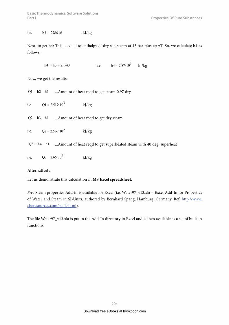
Basic Thermodynamics: Software Solutions Part I
204
Properties f Pure Substances
i.e. h3 2786.46 kJ/kg
Next, to get h4: This is equal to enthalpy of dry sat. steam at 13 bar plus cp.ΔT. So, we calculate h4 as follows:
h4 h3 2.1 40 i.e. h4 2.87 103 kJ/kg
Now, we get the results:
Q1 h2 h1 ...Amount of heat reqd to get steam 0.97 dry
i.e. Q1 2.517 103 kJ/kg
Q2 h3 h1 ...Amount of heat reqd to get dry steam
i.e. Q2 2.576 103 kJ/kg
Q3 h4 h1 ...Amount of heat reqd to get superheated steam with 40 deg. superheat
i.e. Q3 2.66 103 kJ/kg
Alternatively:
Let us demonstrate this calculation in MS Excel spreadsheet.
Free Steam properties Add-in is available for Excel (i.e. Water97_v13.xla – Excel Add-In for Properties of Water and Steam in SI-Units, authored by Bernhard Spang, Hamburg, Germany, Ref: http://www.cheresources.com/staff.shtml).
The file Water97_v13.xla is put in the Add-In directory in Excel and is then available as a set of built-in functions.
Download free eBooks at bookboon.com
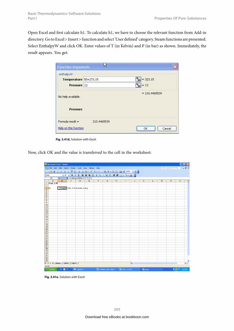
Basic Thermodynamics: Software Solutions Part I
205
Properties f Pure Substances
Open Excel and first calculate h1. To calculate h1, we have to choose the relevant function from Add-in directory. Go to Excel > Insert > function and select ‘User defined’ category. Steam functions are presented. Select EnthalpyW and click OK. Enter values of T (in Kelvin) and P (in bar) as shown. Immediately, the result appears. You get:
Fig. 3.41d. Solution with Excel
Now, click OK and the value is transferred to the cell in the worksheet:
Fig. 3.41e. Solution with Excel
Download free eBooks at bookboon.com
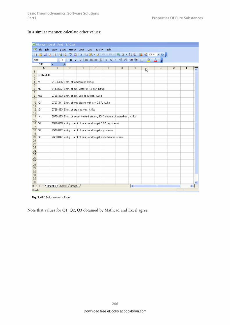
Basic Thermodynamics: Software Solutions Part I
206
Properties f Pure Substances
In a similar manner, calculate other values:
Fig. 3.41f. Solution with Excel
Note that values for Q1, Q2, Q3 obtained by Mathcad and Excel agree.
Download free eBooks at bookboon.com
Basic Thermodynamics: Software Solutions Part I
207
Properties f Pure Substances
3.6 Determination of ‘quality’ (or dryness fraction) of wet steam:
3.6.1 Throttling calorimeter:
Here, wet steam from the steam mains(state 1) is throttled in a throttling valve in such a way that the final state 2 is in the super-heated region. Throttling is a constant enthalpy process. In state 1, P and T are interdependent; so, P1 is measured. In state 2, both P2 and T2 are measured. See fig. 3.44a and 3.44b. Then, h2 can easily be calculated (or found out from steam tables). Since h1 = h2, we can write:
h 1 h f1 x1 h fg1
i.e. h 1 h f1 x1 h g1 h f1 .....(3.9)
and, x1
h 1 h f1
h g1 h f1 ......(3.10)
Knowing P1, sat. liq. enthalpy hf1 and sat. vap. enthalpy hg1 are easily determined and thus the quality of steam in the mains, x1 is determined.
Download free eBooks at bookboon.com
Click on the ad to read moreClick on the ad to read moreClick on the ad to read moreClick on the ad to read moreClick on the ad to read moreClick on the ad to read moreClick on the ad to read moreClick on the ad to read moreClick on the ad to read moreClick on the ad to read moreClick on the ad to read moreClick on the ad to read moreClick on the ad to read moreClick on the ad to read moreClick on the ad to read moreClick on the ad to read moreClick on the ad to read moreClick on the ad to read moreClick on the ad to read moreClick on the ad to read moreClick on the ad to read moreClick on the ad to read moreClick on the ad to read moreClick on the ad to read moreClick on the ad to read moreClick on the ad to read moreClick on the ad to read moreClick on the ad to read moreClick on the ad to read moreClick on the ad to read moreClick on the ad to read moreClick on the ad to read moreClick on the ad to read moreClick on the ad to read moreClick on the ad to read moreClick on the ad to read moreClick on the ad to read moreClick on the ad to read moreClick on the ad to read moreClick on the ad to read moreClick on the ad to read moreClick on the ad to read moreClick on the ad to read moreClick on the ad to read moreClick on the ad to read moreClick on the ad to read moreClick on the ad to read moreClick on the ad to read moreClick on the ad to read moreClick on the ad to read moreClick on the ad to read moreClick on the ad to read moreClick on the ad to read moreClick on the ad to read moreClick on the ad to read moreClick on the ad to read moreClick on the ad to read moreClick on the ad to read moreClick on the ad to read moreClick on the ad to read moreClick on the ad to read moreClick on the ad to read moreClick on the ad to read moreClick on the ad to read moreClick on the ad to read more
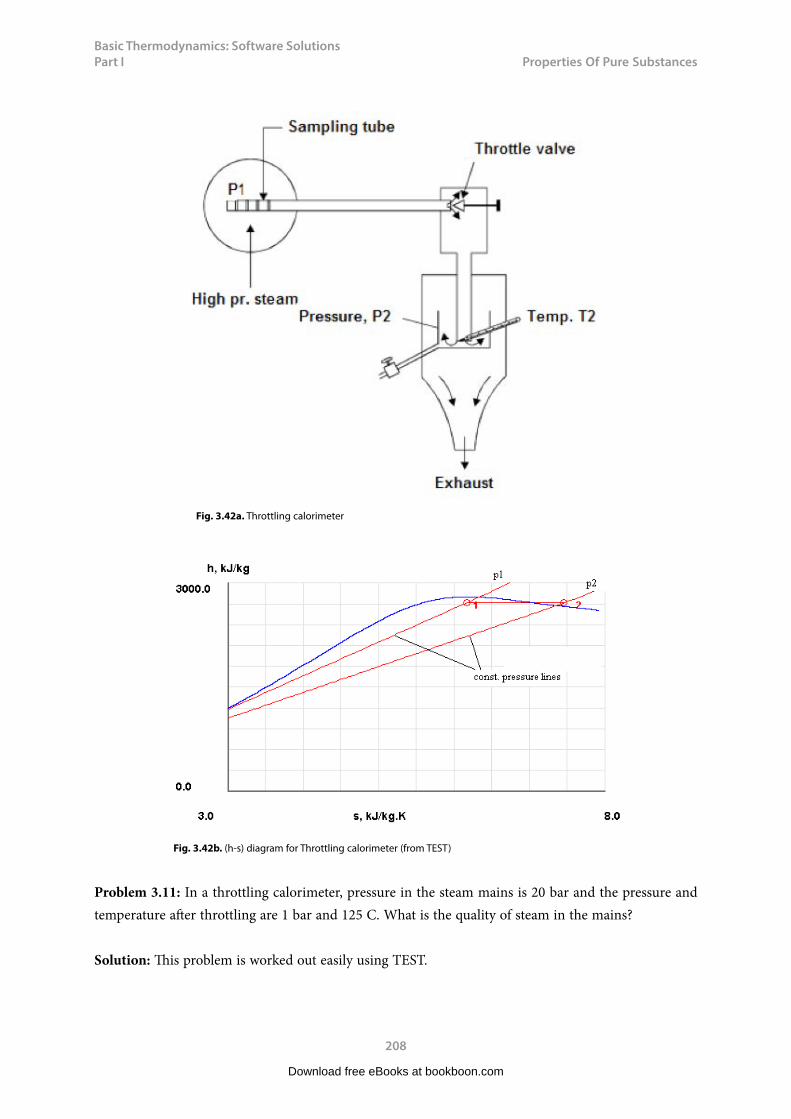
Basic Thermodynamics: Software Solutions Part I
208
Properties f Pure Substances
Fig. 3.42a. Throttling calorimeter
Fig. 3.42b. (h-s) diagram for Throttling calorimeter (from TEST)
Problem 3.11: In a throttling calorimeter, pressure in the steam mains is 20 bar and the pressure and temperature after throttling are 1 bar and 125 C. What is the quality of steam in the mains?
Solution: This problem is worked out easily using TEST.
Download free eBooks at bookboon.com

Basic Thermodynamics: Software Solutions Part I
209
Properties f Pure Substances
Go to TEST > Map > Uniform system > Phase Change model. (See Figs. 3.18a and 3.18b.). State 1 is at P1 = 20 bar, x1 = to be determined. Temperature T1 is also not known. However, we know h1 = h2, where h2 will be determined later. So, enter the value of P1 and for h1 enter h1 = h2. Click ‘Calculate’. We see that all properties can not be calculated at this stage. We get:
Fig. 3.43a. Throttling calorimeter – properties at state 1 (from TEST)
Download free eBooks at bookboon.com
Click on the ad to read moreClick on the ad to read moreClick on the ad to read moreClick on the ad to read moreClick on the ad to read moreClick on the ad to read moreClick on the ad to read moreClick on the ad to read moreClick on the ad to read moreClick on the ad to read moreClick on the ad to read moreClick on the ad to read moreClick on the ad to read moreClick on the ad to read moreClick on the ad to read moreClick on the ad to read moreClick on the ad to read moreClick on the ad to read moreClick on the ad to read moreClick on the ad to read moreClick on the ad to read moreClick on the ad to read moreClick on the ad to read moreClick on the ad to read moreClick on the ad to read moreClick on the ad to read moreClick on the ad to read moreClick on the ad to read moreClick on the ad to read moreClick on the ad to read moreClick on the ad to read moreClick on the ad to read moreClick on the ad to read moreClick on the ad to read moreClick on the ad to read moreClick on the ad to read moreClick on the ad to read moreClick on the ad to read moreClick on the ad to read moreClick on the ad to read moreClick on the ad to read moreClick on the ad to read moreClick on the ad to read moreClick on the ad to read moreClick on the ad to read moreClick on the ad to read moreClick on the ad to read moreClick on the ad to read moreClick on the ad to read moreClick on the ad to read moreClick on the ad to read moreClick on the ad to read moreClick on the ad to read moreClick on the ad to read moreClick on the ad to read moreClick on the ad to read moreClick on the ad to read moreClick on the ad to read moreClick on the ad to read moreClick on the ad to read moreClick on the ad to read moreClick on the ad to read moreClick on the ad to read moreClick on the ad to read moreClick on the ad to read moreClick on the ad to read more
81,000 kmIn the past four years we have drilled
That’s more than twice around the world.
What will you be?
Who are we?We are the world’s leading oilfield services company. Working globally—often in remote and challenging locations—we invent, design, engineer, manufacture, apply, and maintain technology to help customers find and produce oil and gas safely.
Who are we looking for?We offer countless opportunities in the following domains:n Engineering, Research, and Operationsn Geoscience and Petrotechnicaln Commercial and Business
If you are a self-motivated graduate looking for a dynamic career, apply to join our team.
careers.slb.com
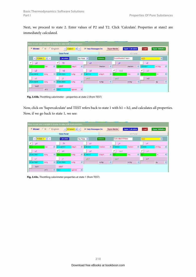
Basic Thermodynamics: Software Solutions Part I
210
Properties f Pure Substances
Next, we proceed to state 2. Enter values of P2 and T2. Click ‘Calculate’. Properties at state2 are immediately calculated.
Fig. 3.43b. Throttling calorimeter – properties at state 2 (from TEST)
Now, click on ‘Supercalculate’ and TEST refers back to state 1 with h1 = h2, and calculates all properties. Now, if we go back to state 1, we see:
Fig. 3.43c. Throttling calorimeter properties at state 1 (from TEST)
Download free eBooks at bookboon.com
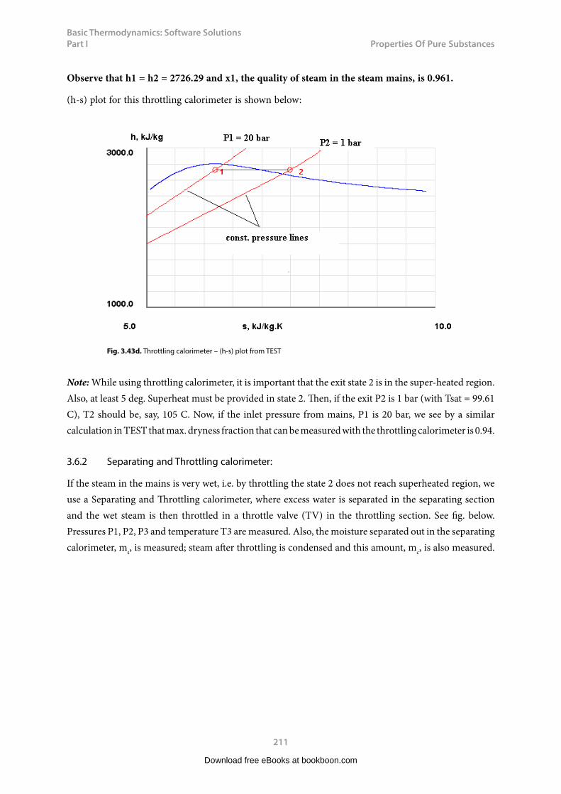
Basic Thermodynamics: Software Solutions Part I
211
Properties f Pure Substances
Observe that h1 = h2 = 2726.29 and x1, the quality of steam in the steam mains, is 0.961.
(h-s) plot for this throttling calorimeter is shown below:
Fig. 3.43d. Throttling calorimeter – (h-s) plot from TEST
Note: While using throttling calorimeter, it is important that the exit state 2 is in the super-heated region. Also, at least 5 deg. Superheat must be provided in state 2. Then, if the exit P2 is 1 bar (with Tsat = 99.61 C), T2 should be, say, 105 C. Now, if the inlet pressure from mains, P1 is 20 bar, we see by a similar calculation in TEST that max. dryness fraction that can be measured with the throttling calorimeter is 0.94.
3.6.2 Separating and Throttling calorimeter:
If the steam in the mains is very wet, i.e. by throttling the state 2 does not reach superheated region, we use a Separating and Throttling calorimeter, where excess water is separated in the separating section and the wet steam is then throttled in a throttle valve (TV) in the throttling section. See fig. below. Pressures P1, P2, P3 and temperature T3 are measured. Also, the moisture separated out in the separating calorimeter, ms, is measured; steam after throttling is condensed and this amount, mc, is also measured.
Download free eBooks at bookboon.com

Basic Thermodynamics: Software Solutions Part I
212
Properties f Pure Substances
P2 is approximately equal to P1, since the pressure drop in the separator is generally quite small.
Fig. 3.44a. Separating and Throttling calorimeter
Download free eBooks at bookboon.com
Click on the ad to read moreClick on the ad to read moreClick on the ad to read moreClick on the ad to read moreClick on the ad to read moreClick on the ad to read moreClick on the ad to read moreClick on the ad to read moreClick on the ad to read moreClick on the ad to read moreClick on the ad to read moreClick on the ad to read moreClick on the ad to read moreClick on the ad to read moreClick on the ad to read moreClick on the ad to read moreClick on the ad to read moreClick on the ad to read moreClick on the ad to read moreClick on the ad to read moreClick on the ad to read moreClick on the ad to read moreClick on the ad to read moreClick on the ad to read moreClick on the ad to read moreClick on the ad to read moreClick on the ad to read moreClick on the ad to read moreClick on the ad to read moreClick on the ad to read moreClick on the ad to read moreClick on the ad to read moreClick on the ad to read moreClick on the ad to read moreClick on the ad to read moreClick on the ad to read moreClick on the ad to read moreClick on the ad to read moreClick on the ad to read moreClick on the ad to read moreClick on the ad to read moreClick on the ad to read moreClick on the ad to read moreClick on the ad to read moreClick on the ad to read moreClick on the ad to read moreClick on the ad to read moreClick on the ad to read moreClick on the ad to read moreClick on the ad to read moreClick on the ad to read moreClick on the ad to read moreClick on the ad to read moreClick on the ad to read moreClick on the ad to read moreClick on the ad to read moreClick on the ad to read moreClick on the ad to read moreClick on the ad to read moreClick on the ad to read moreClick on the ad to read moreClick on the ad to read moreClick on the ad to read moreClick on the ad to read moreClick on the ad to read moreClick on the ad to read moreClick on the ad to read more
Hellmann’s is one of Unilever’s oldest brands having been popular for over 100 years. If you too share a passion for discovery and innovation we will give you the tools and opportunities to provide you with a challenging career. Are you a great scientist who would like to be at the forefront of scientific innovations and developments? Then you will enjoy a career within Unilever Research & Development. For challenging job opportunities, please visit www.unilever.com/rdjobs.
Could you think of 101 new thingsto do with eggs and oil?
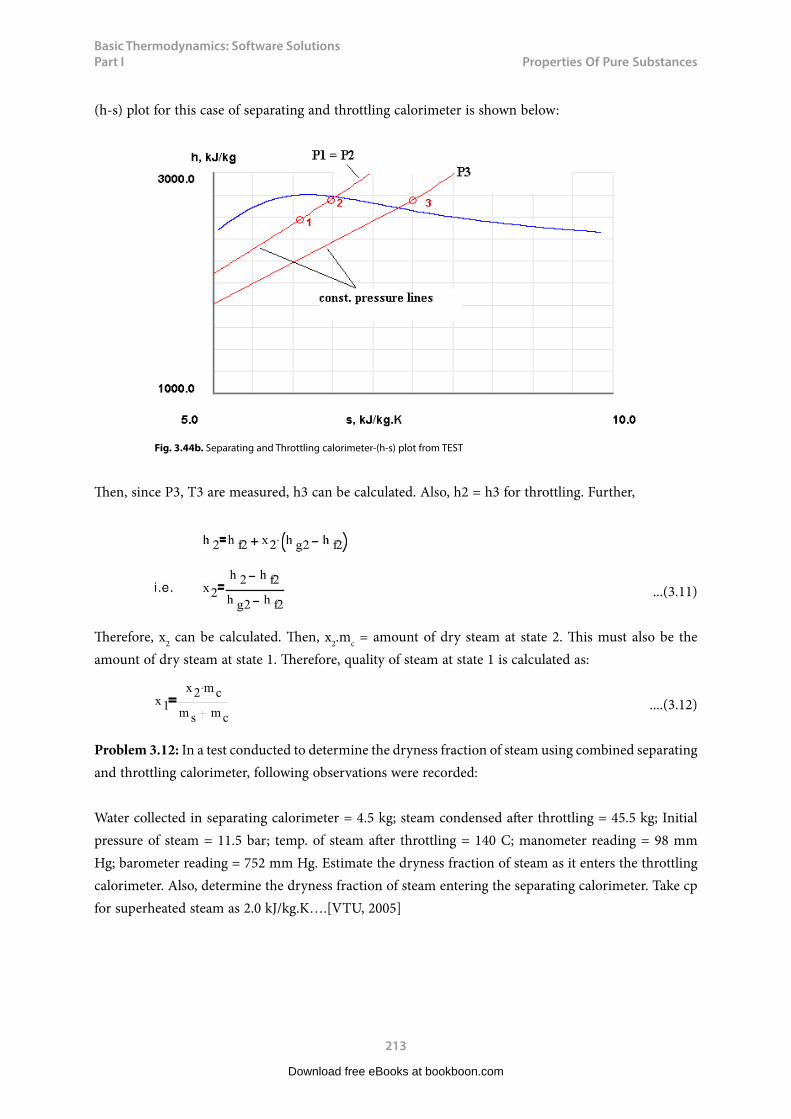
Basic Thermodynamics: Software Solutions Part I
213
Properties f Pure Substances
(h-s) plot for this case of separating and throttling calorimeter is shown below:
Fig. 3.44b. Separating and Throttling calorimeter-(h-s) plot from TEST
Then, since P3, T3 are measured, h3 can be calculated. Also, h2 = h3 for throttling. Further,
...(3.11)
Therefore, x2 can be calculated. Then, x2.mc = amount of dry steam at state 2. This must also be the amount of dry steam at state 1. Therefore, quality of steam at state 1 is calculated as:
x1
x2 mc
ms mc ....(3.12)
Problem 3.12: In a test conducted to determine the dryness fraction of steam using combined separating and throttling calorimeter, following observations were recorded:
Water collected in separating calorimeter = 4.5 kg; steam condensed after throttling = 45.5 kg; Initial pressure of steam = 11.5 bar; temp. of steam after throttling = 140 C; manometer reading = 98 mm Hg; barometer reading = 752 mm Hg. Estimate the dryness fraction of steam as it enters the throttling calorimeter. Also, determine the dryness fraction of steam entering the separating calorimeter. Take cp for superheated steam as 2.0 kJ/kg.K….[VTU, 2005]
Download free eBooks at bookboon.com
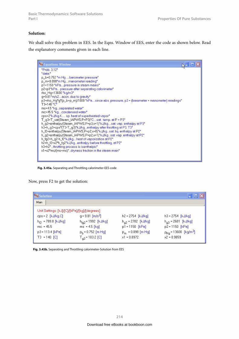
Basic Thermodynamics: Software Solutions Part I
214
Properties f Pure Substances
Solution:
We shall solve this problem in EES. In the Eqns. Window of EES, enter the code as shown below. Read the explanatory comments given in each line.
Fig. 3.45a. Separating and Throttling calorimeter-EES code
Now, press F2 to get the solution:
Fig. 3.45b. Separating and Throttling calorimeter-Solution from EES
Download free eBooks at bookboon.com
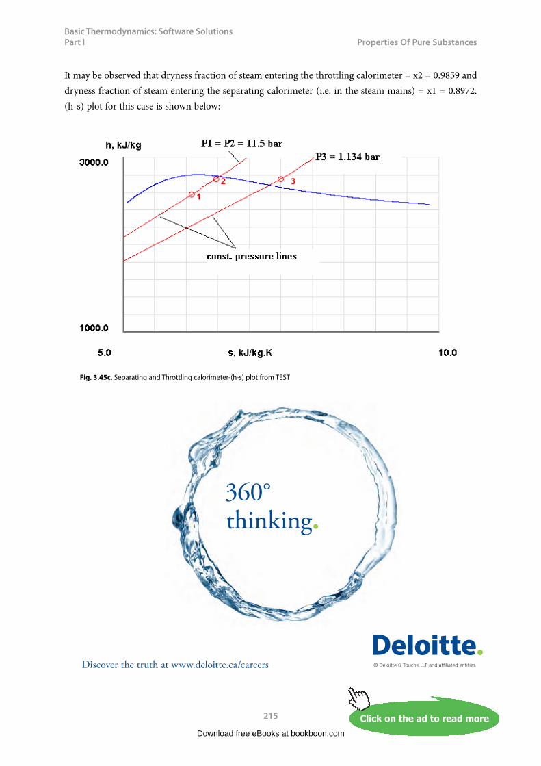
Basic Thermodynamics: Software Solutions Part I
215
Properties f Pure Substances
It may be observed that dryness fraction of steam entering the throttling calorimeter = x2 = 0.9859 and dryness fraction of steam entering the separating calorimeter (i.e. in the steam mains) = x1 = 0.8972. (h-s) plot for this case is shown below:
Fig. 3.45c. Separating and Throttling calorimeter-(h-s) plot from TEST
Download free eBooks at bookboon.com
Click on the ad to read moreClick on the ad to read moreClick on the ad to read moreClick on the ad to read moreClick on the ad to read moreClick on the ad to read moreClick on the ad to read moreClick on the ad to read moreClick on the ad to read moreClick on the ad to read moreClick on the ad to read moreClick on the ad to read moreClick on the ad to read moreClick on the ad to read moreClick on the ad to read moreClick on the ad to read moreClick on the ad to read moreClick on the ad to read moreClick on the ad to read moreClick on the ad to read moreClick on the ad to read moreClick on the ad to read moreClick on the ad to read moreClick on the ad to read moreClick on the ad to read moreClick on the ad to read moreClick on the ad to read moreClick on the ad to read moreClick on the ad to read moreClick on the ad to read moreClick on the ad to read moreClick on the ad to read moreClick on the ad to read moreClick on the ad to read moreClick on the ad to read moreClick on the ad to read moreClick on the ad to read moreClick on the ad to read moreClick on the ad to read moreClick on the ad to read moreClick on the ad to read moreClick on the ad to read moreClick on the ad to read moreClick on the ad to read moreClick on the ad to read moreClick on the ad to read moreClick on the ad to read moreClick on the ad to read moreClick on the ad to read moreClick on the ad to read moreClick on the ad to read moreClick on the ad to read moreClick on the ad to read moreClick on the ad to read moreClick on the ad to read moreClick on the ad to read moreClick on the ad to read moreClick on the ad to read moreClick on the ad to read moreClick on the ad to read moreClick on the ad to read moreClick on the ad to read moreClick on the ad to read moreClick on the ad to read moreClick on the ad to read moreClick on the ad to read moreClick on the ad to read moreClick on the ad to read more
© Deloitte & Touche LLP and affiliated entities.
360°thinking.
Discover the truth at www.deloitte.ca/careers
© Deloitte & Touche LLP and affiliated entities.
360°thinking.
Discover the truth at www.deloitte.ca/careers
© Deloitte & Touche LLP and affiliated entities.
360°thinking.
Discover the truth at www.deloitte.ca/careers © Deloitte & Touche LLP and affiliated entities.
360°thinking.
Discover the truth at www.deloitte.ca/careers
Basic Thermodynamics: Software Solutions Part I
216
Properties f Pure Substances
3.7 Conclusion:
In this chapter, we studied about pure fluids. Various property diagrams were explained, with particular reference to water. Use of software to plot property diagrams for different substances was demonstrated. Methods of finding out property values and generating property tables were also shown using different software. Determination of dryness fraction (or quality) of steam with ‘throttling calorimeter’ as well as ‘separating and throttling calorimeter’ was explained.
3.8 References:
1. Y.A. Cengel and M.A. Boles. Thermodynamics – An Engineering Approach. 4th ed. New Delhi: Tata McGraw-Hill, 2003
2. Sonntag et. al. Fundamentals of Thermodynamics. 5th ed. Singapore: John Wiley & Sons, 1999
3. http://www.engineering.uiowa.edu/fluidslab/referenc/physprop.html4. http://webbook.nist.gov/chemistry/fluid/5. http://properties.nist.gov/6. http://www.cheresources.com/iapwsif97.shtml (For prop. of Water/Steam & Excel Add-in)7. http://www.x-eng.com/Download_XSteam.htm (For prop. of Water/Steam & Excel Add-in)8. http://www.mathpad.com/index.html (Free Applet for Steam properties)9. http://www.science.uwaterloo.ca/~cchieh/cact/c123/phasesdgm.html
10. http://www.eng.usf.edu/~campbell/ThermoI/Proptut/tut1.html11. http://hyperphysics.phy-astr.gsu.edu/Hbase/thermo/pvtexp.html#c112. http://www.chemguide.co.uk/physical/phaseeqia/phasediags.html#top13. http://twt.mpei.ac.ru/ochkov/WSPHB/Engindex.html(IAPWS-IF97-Moscow
Power Engg. Institute- Mathcad server)14. http://www.spiraxsarco.com/resources/steam-tables.asp15. www.spreadsheetworld.com ((for free Excel Add-In: XLThermalFluids which gives values of
P, v, T, s, u, h and x for 37 common fuids)
3.9 Exercise Problems:
1. A 200-m3 rigid tank is filled with saturated liquid-vapor mixture of water at 125°C. If 25% of the mass is liquid and the 75% of the mass is vapor, find out the total mass in the tank.
2. Water is boiled at 300 kPa pressure in a pressure cooker. The cooker initially contains 2.5 kg of water. Once boiling started, it is observed that half of the water in the cooker evaporated in 20 minutes. If the heat loss from the cooker is negligible, find the average rate of energy transfer to the cooker.
3. A 0.25-m3 rigid tank contains 8.5 kg of water (in any phase or phases) at 500 kPa. Find the temperature in the tank.
4. A rigid tank contains 0.7 kg of steam at 9 MPa and 300°C. What is the volume of the tank?
Download free eBooks at bookboon.com
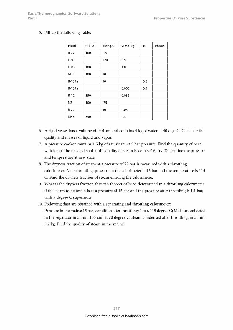
Basic Thermodynamics: Software Solutions Part I
217
Properties f Pure Substances
5. Fill up the following Table:
Fluid P(kPa) T(deg.C) v(m3/kg) x Phase
R-22 100 -25
H2O 120 0.5
H2O 100 1.8
NH3 100 20
R-134a 50 0.8
R-134a 0.005 0.5
R-12 350 0.036
N2 100 -75
R-22 50 0.05
NH3 550 0.31
6. A rigid vessel has a volume of 0.01 m3 and contains 4 kg of water at 40 deg. C. Calculate the quality and masses of liquid and vapor.
7. A pressure cooker contains 1.5 kg of sat. steam at 5 bar pressure. Find the quantity of heat which must be rejected so that the quality of steam becomes 0.6 dry. Determine the pressure and temperature at new state.
8. The dryness fraction of steam at a pressure of 22 bar is measured with a throttling calorimeter. After throttling, pressure in the calorimeter is 13 bar and the temperature is 115 C. Find the dryness fraction of steam entering the calorimeter.
9. What is the dryness fraction that can theoretically be determined in a throttling calorimeter if the steam to be tested is at a pressure of 15 bar and the pressure after throttling is 1.1 bar, with 5 degree C superheat?
10. Following data are obtained with a separating and throttling calorimeter:Pressure in the mains: 15 bar; condition after throttling: 1 bar, 115 degree C; Moisture collected in the separator in 5 min: 155 cm3 at 70 degree C; steam condensed after throttling, in 5 min: 3.2 kg. Find the quality of steam in the mains.
Download free eBooks at bookboon.com

To see Part II, download: Basic Thermodynamics: Software Solutions – Part II
Download free eBooks at bookboon.com