Abstract- This paper presents a technique for parameter estima-tion of uncertain nonlinear systems based on the computation of an accurate and robust derivative using higher order sliding modes. The proposed scheme does not involve any observer design or numerical differentiation. The novelty of the method is to facilitate the determination of system parameters via calculat-ing accurate derivatives of the measured system input-outputs. To validate the technique, simulations have been performed for an uncertain nonlinear Three Tank System. The convergence in this approach is shown to be faster than existing techniques by an order of magnitude even in the presence of measurement noise. The presented parameter estimation scheme is relatively simple and can be employed for the controller design, fault di-agnosis leading to reconfigurable control of nonlinear systems. Index Terms- higher order sliding modes, parameter estimation, uncertain nonlinear systems, robust exact differentiator.

I. INTRODUCTION The behavior of real-life systems is represented by complex and highly nonlinear models. The model response is deter-mined by the certain constants referred to as plant or model parameters. These parameters may be measured or deter-mined using laws of physics, material properties etc. For most of the systems information about such parameters is not directly available and these parameters have to be deduced by observing the systems response to certain inputs. If these parameters do not change with time and the system is linear and stable, their values can be determined easily. For the ap-plications where these unknown parameters change with time, or changes in operating conditions or aging of equip-ment, render the simple parameter estimation techniques inef-fective. This becomes more difficult especially for the case of nonlinear systems. These complexities are further enhanced by coupled interactions between control elements and the elements of plant to be controlled. Parameter uncertainties arise due to imperfect knowledge of the physical parameter values, un-modeled system dynamics or parameter variations during operation. Examples of physical parameters include stiffness and damping coefficients in mechanical systems, aero-dynamical coefficients in flying objects, flow or dis-charge coefficients of valves/pipes in process industry, capa-citors and inductors in electric circuits etc. Model based parameter estimation methods for linear and nonlinear systems have been widely studied by the research-ers [1], [5]–[7], [18] – [20], [22]. Most of these parameter estimation schemes provide means of updating system para-meters online in real time for robust control, controller recon-figuration or effective fault diagnosis and isolation [5], [11], 1. Postgraduate students at Center for Advance Studies in Engineering

(CASE) Islamabad Pakistan; (e-mail: iqbal@case.edu.pk). 2. Dr. A. I. Bhatti is Professor at Muhammad Ali Jinnah University (MAJU)

Islamabad Pakistan; (e-mail: aib@jinnah.edu.pk). 3. Postgraduate students at Muhammad Ali Jinnah University (MAJU) Isla-

mabad Pakistan; (e-mail: sayubi@gmail.com,).

[12]. The nonlinear parameter estimation techniques do not require linearization of system equations and can account for the uncertainties in the estimated parameters, but most of these are difficult to implement online because of their com-plexities. Join et al [5], Flies and Sira-Ramirez [12] used al-gebraic estimation scheme for the parameter estimation of uncertain nonlinear three tank system. A novel concept of sliding mode control with the capability of controlling a non-linear system in the presence of uncertainties associated with parameters and modeling errors has been proposed by Alwi and Edwards [11]. An observer is designed as an online filter to compute an estimate of state vector using limited mea-surements of some states of a commercial aircraft. A variable structure filter and smooth variable structure filter in conjunc-tion with sliding mode control to estimate non-measurable states for the tracking controller were described in Habibi et al [10]. Khiar et al [21] has developed two estimators based on unknown input observers, a high gain and 2-order sliding mode observers. The performance of both observers is com-pared for a gasoline engine, sliding mode observer based estimators performs better than high gain observer. Higher order sliding modes (HOSM) are currently finding useful applications and have been developed actively by the researchers in the control and diagnosis community. Standard sliding modes provide finite time convergence and robustness with respect to internal and external disturbances. For this, the relative degree of the constraint has to be ‘one’ which leads to the possibility of chattering effect. Higher order slid-ing modes remove the chattering phenomena while preserv-ing the main properties of standard sliding modes. Arbitrary order sliding controllers with finite time convergence have been demonstrated in [6], [7], [9], [13], [16], [17] and [23]. The real-time implementation of the arbitrary-order control-lers needs robust estimation of higher order derivatives of inputs and outputs. This is achieved by the recently presented arbitrary-order robust exact differentiators with finite-time convergence [2]-[4], [14] and [17]. It has been proved that lth order differentiator allows real time robust exact differentia-tion up to lth order, provided that the next (l+1)th derivative is bounded. The performance of these differentiators is asymptotically optimal in the presence of small Lebesgue-measureable input noises. The main difficulty in real-time differentiation is due to diffe-rentiation sensitivity to input noises. The high gain differen-tiators in [8], [13], [15] provide an exact derivative provided their gains tend to infinity which also leads to higher sensitiv-ity to small high-frequency noises. Another drawback of the high-gain differentiators is their peaking effect, i.e., the max-imal output values during the transient grows infinitely when gains tend to infinity. Join et al [ [5] has determined estima-tion of time derivative of an analytic function using the trun-cated series of Taylor expansion. This leads to a system of linear equation giving the estimated values of derivatives.

Parameter Estimation of Nonlinear Systems using Higher Order Sliding Modes

M. Iqbal1, A. I. Bhatti2 Member IEEE, S. Iqbal3, I. H. Kazmi3

CONFIDENTIAL. Limited circulation. For review only.

Preprint submitted to 7th International Conference on Control and Automation.Received May 23, 2009.

This derivative estimation technique does not require the precise statistical knowledge of the process or measurement noise as is required in the case of Extended Kalman Filters. This technique involves higher order time polynomial ap-proximation, the iterative integration process to low pass fil-ter high-frequency perturbation or noise, which is computa-tionally time consuming and also can have numerical issues in online implementation, in the mentioned numeric tech-nique the derivative approximations become invalid which needs periodic resetting the calculations [12]. HOSM observ-er has been used to estimate simultaneously throttle discharge coefficient, indicated torque parameter and load torque of a gasoline engine by Butt and Bhatti [1]. The exact derivatives have been calculated by successive implementation of robust exact first-order differentiator with finite-time convergence. This differentiator is based on 2-sliding mode and is proved to feature the best possible asymptotically converging deriva-tive provided the second time derivative of the base signal is bounded [2], [3], [7], [14]. As per the author’s best knowledge, the proposed HOSM differentiator based technique is used perhaps for the first time for parameters estimation of nonlinear systems. This paper presents a generic framework for the robust estimation of uncertain parameters in nonlinear systems using robust exact differentiator. The presented framework does not need the development of an observer or numeric differentiator and no precise knowledge of statistical properties of the nonlinear system is required. The remaining of the paper is organized as follows: In Section II generalized problem formulation for the estimation of unknown uncertain parameters of nonlinear systems is briefly described. It also contains description of HOSM robust exact differentiator being used for the estima-tion of time derivatives. An example of nonlinear uncertain Three Tank System for parameter estimation is discussed in Section III. Section IV presents the simulation results. Sec-tion V contains the concluding remarks.

II. PROBLEM FORMULATION

Consider a system of the form : �̇� = 𝑓(𝑥, 𝑝, 𝑡) + g(𝑥, 𝑡) 𝛷(𝑢) 𝑦 = ℎ(𝑥, 𝑡) (1) where, 𝑥 ∈ ℝ is a measureable state vector, 𝑢 ∈ ℝ is a control input vector, g(𝑥, 𝑡) is a known nonlinear function with g(𝑥, 𝑡) ≠ 0. 𝑝 ∈ ℝ is the unknown/uncertain parame-ter vector in parameter space 𝑃 {𝑝 ∈ [𝑝 , 𝑝 ], 𝑖 =1,2, ⋯ , 𝑞}. 𝑦 ∈ ℝ . 𝛷(𝑢) can be a nonlinear continuous function. 𝑓(𝑥, 𝑝, 𝑡) is a smooth nonlinear function, and func-tions 𝑓, 𝛷 satisfy the following assumptions [24]: Assumption 1: 𝑓(𝑥, 𝑝, 𝑡) = αT(𝑝)𝜉(𝑥, 𝑡) 𝛼 = 𝛼 , 𝛼 , ⋯ , 𝛼 (2) 𝜉 = [𝜁 , 𝜁 , ⋯ , 𝜁 ] where 𝜁 = 𝜉 (𝑥, 𝑡) are known nonlinear functions and li-nearly independent. 𝛼 = 𝛼 (𝑝) are the combinations of 𝑝; q denotes the dimension of 𝛼. Assumption 2: 𝑢 𝛷(𝑢) ≥ ℎ𝑢 (3)

where ℎ is a positive and non-zero constant. 𝛷(𝑢) is a mea-surable and 𝛷(0) = 0. As the bounds of 𝑝 are given, the bounds of 𝛼(𝑝) can also be obtained and the following assumption can be introduced. Assumption 3: 𝛼 ∈ [𝛼 , 𝛼 ] ∀ 𝑝 ∈ 𝑃 (4) Suppose 𝛼 is the uncertain parameter vector of the estimator and 𝛼 is a time varying parameter vector which is calculated in terms uncertain parameter and its bounds: 𝛼 (𝑡) = 𝛼 if 𝛼 < 𝛼 𝛼 (𝑡) if 𝛼 ≤ 𝛼 ≤𝛼 if 𝛼 > 𝛼 𝛼 (5)

In the following paragraphs, we will omit the elements of some functions for simplicity. A. Observability & Identifiability of Nonlinear System Identifiability is the possibility to identify the parameters of a control system from its input-output map. The identifiability property, a prerequisite for parameter estimation guarantees that the model parameters can be determined uniquely from measured data. The identifiability property is well characte-rized and algorithms for ordinary differential equation exist. In literature different methods are used to test the observabili-ty of nonlinear systems, the differential geometry and alge-braic approach. Rank test condition is being used for both the approaches, where observability of a system is determined by calculating the dimension of the space spanned by gradients of the Lie-derivatives of its output functions. For this, one has to find the rank of the following Jacobian matrix [25]:

O =

⎣⎢⎢⎢⎢⎢⎢⎢⎢⎡ ⋯⋮ ⋱ ⋮⋯⋮ ⋱ ⋮⋯⋮ ⋱ ⋮⋮ ⎦⎥⎥

⎥⎥⎥⎥⎥⎥⎤

If this Jacobian matrix is a full rank (Rank (O) = n), then system is algebraically observable. The problem of parameter identifiability can be treated as special case of observability problem by considering parameters as state variables with time derivative zero i.e., �̇� = 0, so the observability rank test can used to determine parameter identifiability. For nonlinear system (1) with assumption �̇� = 0, 𝑥 and 𝑝 are considered as the same type of variables. Without initial conditions for x, the non-observable variables can be both in 𝑥 and in 𝑝. Sup-pose that we are given a full set of initial conditions on 𝑥 𝑖. 𝑒. , 𝑥(0) = 𝑥 . Then the problem of observability of the 𝑥 variables disappears [25], what is left is exactly the problem of identifiability for the parameters, the set of para-meters that realizes a given input-output map, at least locally. This can be determined by the rank test using differential geometry and algebraic approaches. For analytical system (1) the rank test amounts to calculating the rank of the following Jacobean for 𝑖 = 1,2, ⋯ , 𝑝, 𝑗 = 1,2, ⋯ , 𝑞 and 𝑘 =1,2, ⋯ , 𝑛 − 1:

CONFIDENTIAL. Limited circulation. For review only.

Preprint submitted to 7th International Conference on Control and Automation.Received May 23, 2009.

𝐽 = 𝐿 ℎ (6)

If the rank of this matrix is n, then the system (1) is identifia-ble. If not, the non-identifiable parameters can be found by removing associated columns in this matrix as described in [25]. B. Estimation of HOSM Based Robust Derivatives: The sliding mode control (SMC) methods are developed to design a stable system with high rate of convergence to the desired state and low sensitivity to plant parameter variations. The sliding mode control is based on keeping exactly a prop-erly chosen constraint by means of high frequency control switching. The biggest advantage of SMC is its insensitivity to variation in system parameters, external disturbances and modeling errors. The main idea of higher order sliding modes is to act on higher order derivatives of sliding variables as compared to the 1st order derivative in standard sliding mode technique. This gives all the advantages of standard sliding modes with additional advantage leading to removal of chat-tering effect. The r-sliding mode is determined by 𝜎 = �̇� =�̈� ⋯ = 𝜎 = 0, which form an r-dimensional condition on state of the dynamic system. The sliding order is a measure of the smoothness of the sliding variable in the vicinity of the sliding mode in general any r-sliding controller that keep 𝜎 =0, needs. �̇� = �̈� ⋯ = 𝜎 to be made available [13], [17]. Sliding mode techniques are known to be robust with a straight forward design formulation and thus provide a robust solution to parameter estimation, control and fault diagnosis. A robust exact differentiator developed by [7], [14], [17], as a part of the arbitrary order sliding mode controllers, with fi-nite-time convergence has been adapted for the purpose of parameter estimation and is presented here for completeness of proposed scheme. Consider an input signal 𝑓(𝑡) a function defined on [0, ∞), consisting of a bounded Lebesgue-measureable noise with unknown features and unknown base signal 𝑓 (𝑡) with nth derivative having a known Lipschitz constant 𝐿 > 0 resulting from a real time noisy measurement [3], [14]. The unknown sampling noise 𝑓(𝑡) − 𝑓 (𝑡) is assumed to be bounded. as-sume that the associated differential inclusion discussed in [14] exist as a solution to (1), which causes boundedness of �̈�, allowing the implementation of 1st order robust differentia-tor with finite time convergence. The task is to find real es-timates of 𝑓 , �̇� using only values of 𝑓(t) and number L. The estimates are to be exact in the absence of noise, when 𝑓(𝑡) = 𝑓 (𝑡). Let the noises be absent. Introduce an auxiliary dynamic system �̇� = 𝑢, 𝜎(𝑡, 𝑧 ) = 𝑧 − 𝑓(𝑡). The task is to make 𝜎 and �̇� vanish in finite time by means of continuous control using only measurements of 𝜎 i.e. to establish a 2-sliding mode. The modified version of the super-twisting controller is applied, producing the close-loop system. �̇� = −𝜆 |𝑧 − 𝑓(𝑡)| / 𝑠𝑖𝑔𝑛 𝑧 − 𝑓(𝑡) +𝑧 , �̇� = −𝜆 𝑠𝑖𝑔𝑛 (𝑧 − 𝑓). Here 𝜆 > 𝐿 and 𝜆 is chosen sufficiently large with respect to 𝜆 . The 2-sliding mode 𝜎 = 𝑧 − 𝑓(𝑡) = 0, �̇� = 𝜆 |𝜎| / 𝑠𝑖𝑔𝑛 𝜎 + 𝑧 − �̇� = 𝑧 − �̇� = 0 is established in fi-nite time. Thus in the presence of noise 𝑧 and 𝑧 are consi-dered as estimates 𝑓 and �̇� respectively.

Thus, with recursive iterations, the 𝑛th order differentiator [3] has the form �̇� = 𝑣 , 𝑣 = −𝜆 |𝑧 − 𝑓(𝑡)| /( )𝑠𝑖𝑔𝑛 𝑧 − 𝑓(𝑡) +𝑧 , �̇� = 𝑣 , 𝑣 = −𝜆 |𝑧 − 𝑣 | / 𝑠𝑖𝑔𝑛 (𝑧 − 𝑣 )+𝑧 , ⋯ �̇� = 𝑣 , 𝑣 = −𝜆 |𝑧 − 𝑣 | / 𝑠𝑖𝑔𝑛 (𝑧 − 𝑣 )+𝑧 , 𝑧 = −𝜆 𝑠𝑖𝑔𝑛 (𝑧 − 𝑣 ), (7) Where 𝜆 > 0 are chosen sufficiently large in the reverse order. Note that it contains actually all the lower-order diffe-rentiators and each recursive step requires tuning one para-meter only. Parameters 𝜆 tuned for 𝐶 = 1, the parameters are easily recalculated for any value of 𝐶 by 𝜆 =𝜆 𝐶 /( ). The values of Lipschitz Constant 𝐶 can be computed by taking into account the maximum frequency component and maximum amplitude of the function f(t). C. Estimation of Uncertain Nonlinear System Parameters: The nth order robust exact differentiator is utilized to estimate the derivatives of input and outputs using the measured sys-tem data. The technique used for the estimation of parameters exploits the main features of the higher order sliding modes. Assume that the unknown parameters 𝛼 = 𝛼 , 𝛼 , ⋯ , 𝛼 satisfy some natural identifiability conditions (6), then for 𝑗 = 1, ⋯ , 𝑞: 𝛼 = ϒ (t, 𝐿 ℎ, 𝐿 ℎ ⋯ , 𝐿 ℎ, u, u̇ ⋯ , u( )) (8) where ϒ is a nonlinear function of its arguments. An accu-rate estimate [α ] of α is obtained by replacing the deriva-tives of control input and output variables in equation (8) with their estimates obtained by the robust exact differentia-tor estimator (7): [α ] = ϒ (t, 𝐿 ℎ, 𝐿 ℎ , ⋯ , 𝐿 ℎ , u, [u̇] , ⋯ , [u ] ) (9) This gives a relationship for the estimates of the parameters in terms of input, output and their derivatives. The required derivatives are obtained through estimation of higher order sliding modes (HOSM) based robust exact derivative tech-nique discussed below.

III. EXAMPLE: THREE TANK SYSTEM DESCRIPTION . The three tank system represents a typical process system in process industry, fuel management system of airplanes in aircrafts and flight vehicles. Parameters like viscosity coeffi-cients are uncertain [5], [12] because of change in liquid cha-racteristics, aging effects and change operating environments.

Figure. 1. The Three-Tank System

CONFIDENTIAL. Limited circulation. For review only.

Preprint submitted to 7th International Conference on Control and Automation.Received May 23, 2009.

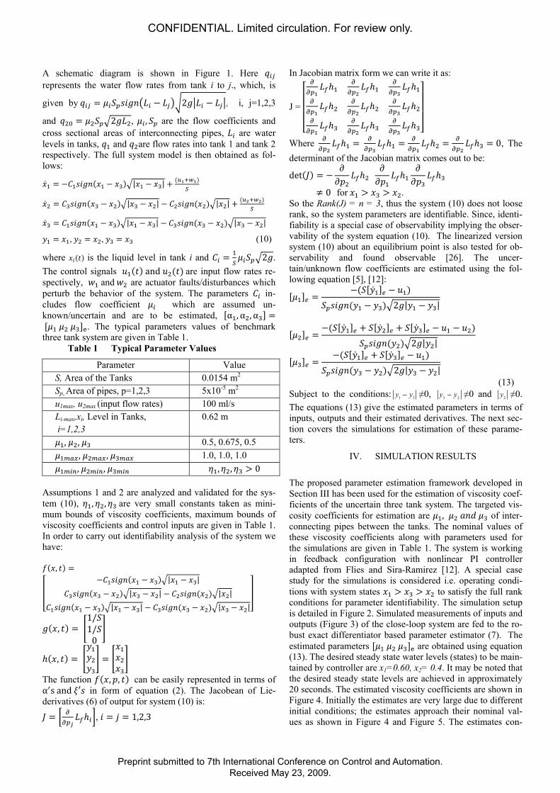
A schematic diagram is shown in Figure 1. Here 𝑞 represents the water flow rates from tank i to j., which, is

given by 𝑞 = 𝜇 𝑆 𝑠𝑖𝑔𝑛 𝐿 − 𝐿 2𝑔 𝐿 − 𝐿 , i, j=1,2,3

and 𝑞 = 𝜇 𝑆 2𝑔𝐿 , 𝜇 , 𝑆 are the flow coefficients and cross sectional areas of interconnecting pipes, 𝐿 are water levels in tanks, 𝑞 and 𝑞 are flow rates into tank 1 and tank 2 respectively. The full system model is then obtained as fol-lows: �̇� = −𝐶 𝑠𝑖𝑔𝑛(𝑥 − 𝑥 ) |𝑥 − 𝑥 | + ( ) �̇� = 𝐶 𝑠𝑖𝑔𝑛(𝑥 − 𝑥 ) |𝑥 − 𝑥 | − 𝐶 𝑠𝑖𝑔𝑛(𝑥 ) |𝑥 | + ( ) �̇� = 𝐶 𝑠𝑖𝑔𝑛(𝑥 − 𝑥 ) |𝑥 − 𝑥 | − 𝐶 𝑠𝑖𝑔𝑛(𝑥 − 𝑥 ) |𝑥 − 𝑥 | 𝑦 = 𝑥 , 𝑦 = 𝑥 , 𝑦 = 𝑥 (10)

where 𝑥 (𝑡) is the liquid level in tank i and 𝐶 = 𝜇 𝑆 2𝑔. The control signals 𝑢 (𝑡) and 𝑢 (𝑡) are input flow rates re-spectively, 𝑤 and 𝑤 are actuator faults/disturbances which perturb the behavior of the system. The parameters 𝐶 in-cludes flow coefficient 𝜇 which are assumed un-known/uncertain and are to be estimated, [α , α , α ] = [𝜇 𝜇 𝜇 ] . The typical parameters values of benchmark three tank system are given in Table 1.

Table 1 Typical Parameter Values

Parameter Value S, Area of the Tanks 0.0154 m2 Sp, Area of pipes, p=1,2,3 5x10-5 m2 u1max, u2max (input flow rates) 100 ml/s Li-max,xi, Level in Tanks, i=1,2,3

0.62 m 𝜇 , 𝜇 , 𝜇 0.5, 0.675, 0.5 𝜇 , 𝜇 , 𝜇 1.0, 1.0, 1.0 𝜇 , 𝜇 , 𝜇 𝜂 , 𝜂 , 𝜂 > 0 Assumptions 1 and 2 are analyzed and validated for the sys-tem (10), 𝜂 , 𝜂 , 𝜂 are very small constants taken as mini-mum bounds of viscosity coefficients, maximum bounds of viscosity coefficients and control inputs are given in Table 1. In order to carry out identifiability analysis of the system we have: 𝑓(𝑥, 𝑡) = −𝐶 𝑠𝑖𝑔𝑛(𝑥 − 𝑥 ) |𝑥 − 𝑥 |𝐶 𝑠𝑖𝑔𝑛(𝑥 − 𝑥 ) |𝑥 − 𝑥 | − 𝐶 𝑠𝑖𝑔𝑛(𝑥 ) |𝑥 |𝐶 𝑠𝑖𝑔𝑛(𝑥 − 𝑥 ) |𝑥 − 𝑥 | − 𝐶 𝑠𝑖𝑔𝑛(𝑥 − 𝑥 ) |𝑥 − 𝑥 |

𝑔(𝑥, 𝑡) = 1/𝑆1/𝑆0

ℎ(𝑥, 𝑡) = 𝑦𝑦𝑦 = 𝑥𝑥𝑥

The function 𝑓(𝑥, 𝑝, 𝑡) can be easily represented in terms of α s and 𝜉′𝑠 in form of equation (2). The Jacobean of Lie-derivatives (6) of output for system (10) is: 𝐽 = 𝐿 ℎ , 𝑖 = 𝑗 = 1,2,3

In Jacobian matrix form we can write it as:

J = ⎣⎢⎢⎢⎡ 𝐿 ℎ 𝐿 ℎ 𝐿 ℎ𝐿 ℎ 𝐿 ℎ 𝐿 ℎ𝐿 ℎ 𝐿 ℎ 𝐿 ℎ ⎦⎥⎥

⎥⎤

Where 𝐿 ℎ = 𝐿 ℎ = 𝐿 ℎ = 𝐿 ℎ = 0, The determinant of the Jacobian matrix comes out to be: det(𝐽) = − 𝜕𝜕𝑝 𝐿 ℎ 𝜕𝜕𝑝 𝐿 ℎ 𝜕𝜕𝑝 𝐿 ℎ ≠ 0 for 𝑥 > 𝑥 > 𝑥 . So the Rank(J) = n = 3, thus the system (10) does not loose rank, so the system parameters are identifiable. Since, identi-fiability is a special case of observability implying the obser-vability of the system equation (10). The linearized version system (10) about an equilibrium point is also tested for ob-servability and found observable [26]. The uncer-tain/unknown flow coefficients are estimated using the fol-lowing equation [5], [12]: [𝜇 ] = −(𝑆[�̇� ] − 𝑢 )𝑆 𝑠𝑖𝑔𝑛(𝑦 − 𝑦 ) 2𝑔|𝑦 − 𝑦 | [𝜇 ] = −(𝑆[�̇� ] + 𝑆[�̇� ] + 𝑆[�̇� ] − 𝑢 − 𝑢 )𝑆 𝑠𝑖𝑔𝑛(𝑦 ) 2𝑔|𝑦 |

[𝜇 ] = −(𝑆[�̇� ] + 𝑆[�̇� ] − 𝑢 )𝑆 𝑠𝑖𝑔𝑛(𝑦 − 𝑦 ) 2𝑔|𝑦 − 𝑦 | (13)

Subject to the conditions: 1 3y y− ≠0, 3 2y y− ≠0 and 2y ≠0. The equations (13) give the estimated parameters in terms of inputs, outputs and their estimated derivatives. The next sec-tion covers the simulations for estimation of these parame-ters.

IV. SIMULATION RESULTS

The proposed parameter estimation framework developed in Section III has been used for the estimation of viscosity coef-ficients of the uncertain three tank system. The targeted vis-cosity coefficients for estimation are 𝜇 , 𝜇 𝑎𝑛𝑑 𝜇 of inter-connecting pipes between the tanks. The nominal values of these viscosity coefficients along with parameters used for the simulations are given in Table 1. The system is working in feedback configuration with nonlinear PI controller adapted from Flies and Sira-Ramirez [12]. A special case study for the simulations is considered i.e. operating condi-tions with system states 𝑥 > 𝑥 > 𝑥 to satisfy the full rank conditions for parameter identifiability. The simulation setup is detailed in Figure 2. Simulated measurements of inputs and outputs (Figure 3) of the close-loop system are fed to the ro-bust exact differentiator based parameter estimator (7). The estimated parameters [𝜇 𝜇 𝜇 ] are obtained using equation (13). The desired steady state water levels (states) to be main-tained by controller are x1=0.60, x2= 0.4. It may be noted that the desired steady state levels are achieved in approximately 20 seconds. The estimated viscosity coefficients are shown in Figure 4. Initially the estimates are very large due to different initial conditions; the estimates approach their nominal val-ues as shown in Figure 4 and Figure 5. The estimates con-

CONFIDENTIAL. Limited circulation. For review only.

Preprint submitted to 7th International Conference on Control and Automation.Received May 23, 2009.

verge asymptotically to their nominal values. The conver-gence time is about one second, which is reasonably fast con-sidering the slow dynamics of the three tank system which shorter than the estimate times of the order of 100 seconds as compared with algebraic techniques of Join et al [5] and Flies and Sira-Ramirez [12]. The convergence time is also faster by orders of magnitude as compared with Sensitivity-Model-Based Adaptive Filters by C. Bhon [27]. Figure 6 shows the estimated values of viscosity coefficients in the presence of noise with zero mean and variance of 0.01. The results shows the estimates are reasonably good in the presence of noise. However the convergence time has increased, still it is very good as compared to the overall system response and above quoted reference. The convergence in this approach is shown to be accurate and faster than existing techniques by an order of magnitude even in the presence of noise. Figure 7 shows the estimation error of of viscosity coefficients against their nominal values. The estimation errors are small to a third decimal place, which is < 1% of nominal values and are with-in acceptable limits. An analysis of Figure 3 and Figure 4 shows that the convergence of estimated parameters to their nominal values in less than 2.4 sec indicates the proposed scheme is global in nature and does not depend on a particu-lar set point.

V. CONCLUSIONS A general framework for parameter estimation of dynamic systems using robust exact differentiator is presented. Unlike numerical derivatives the differentiation method used is not

prone to measurement noises and other arithmetic issues. The estimation method based on efficient robust exact differentia-tor is validated by the online estimation of viscosity coefficients of an industry standard benchmark: three tank system. The estimated parameter approaches to their nominal

Figure 3. Plant output history with state feedback PI Controller

0 5 10 15 20 25 30 35 40 45 500

0.20.40.60.8

1Outputs of the Plant

0 5 10 15 20 25 30 35 40 45 500

0.2

0.4

0.6

0 5 10 15 20 25 30 35 40 45 500

0.02

0.04

0.06

Time (Sec)

Y1

Y2

Y3

Figure 2. Schematic diagram of parameter estimation

Figure 5. Estimates of viscosity coefficients in steady state

0 5 10 15 20 25 30 35 40 45 500.450.470.490.510.530.55

Flow or Viscosity Coefficient Estimates

0 5 10 15 20 25 30 35 40 45 500.6

0.64

0.68

0 5 10 15 20 25 30 35 40 45 500.450.470.490.510.530.55

Time (Sec)

μ3

μ2

μ1

Figure 4. Estimates of viscosity coefficients during initial phase

0 0.5 1 1.5 2 2.5 3 3.5 4 4.5 5

-40

-20

0

Flow or Viscosity Coefficient Estimates

0 0.5 1 1.5 2 2.5 3 3.5 4 4.5 5

-100

-50

0

0 0.5 1 1.5 2 2.5 3 3.5 4 4.5 5-150

-100

-50

0

Time (Sec)

μ3

μ2

μ1

Figure 6. Estimates of viscosity coefficients during steady state in the presence of noise with variance 0.01

0 5 10 15 20 25 30 35 40 45 50-0.5

0

0.5

1

0 5 10 15 20 25 30 35 40 45 50-0.5

0

0.5

1

0 5 10 15 20 25 30 35 40 45 50-0.5

0

0.5

1

Time (Sec)

μ3

μ2

μ1

CONFIDENTIAL. Limited circulation. For review only.

Preprint submitted to 7th International Conference on Control and Automation.Received May 23, 2009.

values asymptotically. The performance is estimator is also very good in the presence of noise. The convergence of esti-mated parameters to their nominal values is shown to be bet-ter than the existing numeric techniques by an order of mag-nitude. The parameter estimation based on higher order sliding mode technique is exact and insensitive to high frequency noise. The estimated parameters can be effectively employed in systems modeling, controller design and fault diagnostics. The concept of arbitrary order differentiator can be used to increase the number of parameters estimated using a single nonlinear dynamical equation.

ACKNOWLEDGMENT

This work was partially supported by Higher Education Commission (HEC) of Pakistan. The authors are also thank-ful to the research fellows at Control and Signal Processing Research (CASPR) group, M. A. Jinnah University, Islama-bad for their useful help and suggestions.

REFERENCES

[1] Q. R. Butt, A. I. Bhatti, “Estimation of Gasoline Engine Parameters using Higher Order Sliding Mode”, IEEE Transaction on Industrial Electronics, Vol. 55, No. 11, November 2008.

[2] A. Levant, “Higher-order sliding modes, differentiation and output feedback control”, International Journal of Control, Vol. 76, 2003

[3] A. Levant, “Robust Exact Differentiation via Sliding Mode Tech-nique”, Automatica, Vol. 34, No. 3, 1998.

[4] A. Levant, “Lecture on High-Order Sliding-Modes at the VSS Tutorial Workshop”, 17th IFAC World Congress, Seoul, July 6, 2008.

[5] C. Join, H. Sira-Ramirez . M. Flies, “Control of an uncertain Three-Tank system via online parameter identification and fault detection”, IFAC, 2005.

[6] L. Fridman, A. Loukianov, A. Soto-Cota, “Higher Order Sliding Mode Controllers and Differentiators for a Synchronous Generator with Exci-tor Dynamics”, IFAC 2005.

[7] M. Smaoui, X. Brun, D. Thonassat, “A Robust Differentiator Control-ler Design for an Electropneumatic System”, Proceedings of 44th CDC and ECC, Seville, Spain, December 12-15 2005.

[8] A. Dabroom, H. K. Khalil, “Numerical Differentiation Using High-Gain Observers”, Proceeding of the 36th Conference on Decision & Control, California, USA, December 1997.

[9] M. K. Khan, S. K. Spurgeon, P. F. Puleston, “Robust Speed Control of an Automotive Engine using Second Order Sliding Modes”, European Control Conference (ECC), Porto Portugal, September 2001.

[10] S. Habibi, R. Bouton, Y. Chinniah, “Estimation using a New Variable Structure Filter”, Proceedings of American Control Conference, An-chorage AK, May 8-10, 2002.

[11] H. Alwi, C. Edwards, “Fault Detection and Fault Tolerant Sliding Mode Control of a Civil Aircraft Using a Sliding-Mode-Based Scheme”, IEEE Transactions on Control Systems Technology”, Vol. 16, May 2008

[12] M. Flies, H. Sira-Ramirez, “Control via State Estimations of some Nonlinear Systems”, Proceedings Symp. Nonlinear Control Systems (NOLCOS), Stuttgart, 2004

[13] Arie Levant, “Principles of 2-Sliding Mode design”, Automatica, Vo-lume 43, Issue 4, April 2007

[14] A. Levant, “Exact Differentiation of Signals with Unbounded Higher Derivatives”, Proc. of the 45th IEEE Conference on Decision and Control, San-Diego, California, December 14-17, 2006

[15] Y. Chitour, “Time-Varying High-Gain Observers for Numerical Diffe-rentiation”, IEEE Transactions on Automatic Control, Vol. 47, No. 9, September 2002

[16] A. Levant, “Homogeneity approach to high-order sliding mode de-sign”, Automatica, Vol. 41, 2005

[17] A. Levant, Y. Povlov, “Generalized Homogeneous Quasi Controllers”, International Journal of Robust and Nonlinear Control, 18 (4-5), Spe-cial issue: Advances in Higher Order Sliding Mode Control, 2007

[18] T. Floquet, J.A. Twiddle and S.K. Spurgeon “Parameter estimation via second order sliding modes with application to thermal modeling in a high speed rotating machine” IEEE International Conference on Indus-trial Technology, Mumbai, India 15-17 December 2006.

[19] H. Shraim, Bouchra Ananou, L Fridman, H, Noura, Mustapha, “Sliding Mode Observer for estimation of vehicle Parameters, Forces and States of the centre of gravity”, 45th IEEE Conference on Decision & Control, December 2006

[20] G. Rizzoni, S. Drakunov, Y. Wang, “Online Estimation of Indicated Torque in IC engines Via Sliding Mode Observor”, American Controll Conference, June 1995

[21] D. Khiar, J. Lauber, T. Flouqat, T. M. Guerrra, “An Observer for the Instantaneous Torque Estimation of an IC Engine”, IEEE 2005.

[22] I. Haskara, L. Mianzo, “Real-time Cylinder pressure and Indicated Torque estimation via a second order sliding modes”, Proceedings of American Control Conference, Arlington, VA June 25-27, 2001.

[23] J. K. Pieper, R. Mehrotra, “Air/Fuel Ratio Control Using Sliding Mode Methods”, American Control Conference, California, June 1999

[24] Z. Ke-qin, Z. Kai-yu, S. U. Hong-ye, C. Jian, G. Hong, “ Sliding Mode Identifier for parameter uncertain nonlinear dynamic systems with non-linear input”, Journal of Zhejiang University SCIENCE V. 3, No. 4, P.426-430 Sep. - Oct. 2002.

[25] M. Anguelova, “ Observability and Identifiability of nonlinear systems with applications in biology”, PhD Thesis, Department of Mathemati-cal Sciences, Chalmers University of Technology and Göteborg Uni-versity, Göteborg, Sweden, 2007.

[26] M. Iqbal, Q. R. Butt, A. I. Bhatti, "Linear Model Based Diagnostic Framework of Three Tank System", WSEAS Conference SYSTEMS, WSEAS, CSCC, Crete island, Greece, July 2007, WSEAS Conference SYSTEMS, WSEAS, CSCC, Crete island, Greece, July 2007

[27] C. Bhon, “Recursive Parameter Estimation for Nonlinear Continuous-Time Systems through Sensitivity-Model-Based Adaptive Filters”, PhD dissertation, Department of Electrical Engineering and Informa-tion Sciences, Ruhr-University Bochum, 2000.

Figure 7. Estimation error of viscosity coefficient as compared with their nominal values of 0.5, 0.675 and 0.5 respectively. The estimation error is less than 1% of the nominal values

5 10 15 20 25 30 35 40 45 50-5

0

5x 10-3

5 10 15 20 25 30 35 40 45 50

-5

0

5

x 10-3

5 10 15 20 25 30 35 40 45 50-5

0

5x 10-3

CONFIDENTIAL. Limited circulation. For review only.

Preprint submitted to 7th International Conference on Control and Automation.Received May 23, 2009.